0

Alma Mater Studiorum – Università di Bologna

DOTTORATO DI RICERCA IN

SCIENZE DELLA TERRA DELLA VITA E DELL’AMBIENTE

Ciclo 32°

Settore Concorsuale: 05/A1 BOTANICA

Settore Scientifico Disciplinare: BIO/01 BOTANICA GENERALE

PLANTS DEALING WITH HEAVY METALS:

BIOINDICATION POTENTIAL, PHYSIOLOGICAL RESPONSES

AND STRESS ASSESSMENT TECHNIQUES

Presentata da: Mirko Salinitro

Coordinatore Dottorato Supervisore

Prof. Giulio Viola Prof.ssa Annalisa Tassoni

Esame finale anno 2020

1

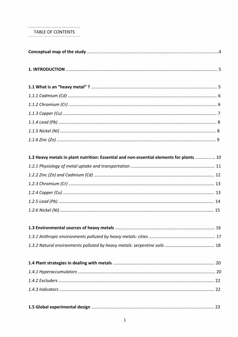
Conceptual map of the study ………………………………………………………………………………………………………..4

1. INTRODUCTION ……………………………………………………………………………………………………………………….. 5

1.1 What is an “heavy metal” ? ........................................................................................................ 5

1.1.1 Cadmium (Cd) ……………………………………………………………………………………………………………………… 6

1.1.2 Chromium (Cr) …………………………………………………………………………………………………………………….. 6

1.1.3 Copper (Cu) …………………………………………………………………………………………………………………………. 7

1.1.4 Lead (Pb) …………………………………………………………………………………………………………………………….. 8

1.1.5 Nickel (Ni) …………………………………………………………………………………………………………………………… 8

1.1.6 Zinc (Zn) ……………………………………………………………………………………………………………………………… 9

1.2 Heavy metals in plant nutrition: Essential and non-essential elements for plants ……………… 10

1.2.1 Physiology of metal uptake and transportation …………………………………………………………………. 11

1.2.2 Zinc (Zn) and Cadmium (Cd) ………………………………………………………………………………………………. 12

1.2.3 Chromium (Cr) …………………………………………………………………………………………………………………… 13

1.2.4 Copper (Cu) ……………………………………………………………………………………………………………………….. 13

1.2.5 Lead (Pb) …………………………………………………………………………………………………………………………… 14

1.2.6 Nickel (Ni) …………………………………………………………………………………………………………………………. 15

1.3 Environmental sources of heavy metals ……..………………………………………………………………………. 16

1.3.1 Anthropic environments polluted by heavy metals: cities …………………………………………………… 17

1.3.2 Natural environments polluted by heavy metals: serpentine soils ……………………………………… 18

1.4 Plant strategies in dealing with metals ……………………………………………………………………………….. 20

1.4.1 Hyperaccumulators ……………………………………………………………………………………………………………. 20

1.4.2 Excluders …………………………………………………………………………………………………………………………… 22

1.4.3 Indicators ………………………………………………………………………………………………………………………….. 22

1.5 Global experimental design ………………………………………………………………………………………………… 23

TABLE OF CONTENTS

2

1.5.1 Selection of plant species …………………………………………………………………………………………………… 23

1.5.2 Poligonum aviculare L. ………………………………………………………………………………………………………. 24

1.5.3 Senecio vulgaris L. ……………………………………………………………………………………………………………… 25

1.5.4 Cardamine hirsuta L. …………………………………………………………………………………………………………. 25

1.5.5 Poa annua L. ……………………………………………………………………………………………………………………… 26

1.5.6 Stellaria media L. Vill. ………………………………………………………………………………………………………… 26

1.5.7 Selection of sampling stations …………………………………………………………………………………………… 27

1.5.8 Pot cultivation of urban plants ………………………………………………………………………………………….. 30

1.5.9 Seed collection and conservation ………………………………………………………………………………………. 30

1.5.10 Conceptual map of applied methods .....…………………………………………………………………………… 31

1.6 References …………………………………………………………………………………………………………………………… 33

CHAPTERS …………………………………………………………………………………………………………………………..……… 42

2. Heavy metals bioindication potential of the common weeds Senecio vulgaris L., Polygonum

aviculare L. and Poa annua L. ……………………………………………………………………………………………………. 42

2.1 Introduction …………………………………………………………………………………………………………………………. 43

2.2 Materials and methods ………………………………………………………………………………………………….…..… 45

2.3 Results …………………………………………………………………………………………………………………………...……. 51

2.4 Discussion ………………………………………………………………………………………………………………………….…. 56

2.5 Conclusions ………………………………………………………………………………………………………………….…….... 59

2.6 References ……………………………………………………………………………………………………………………………. 60

3. PH variation influences Ni and Zn uptake in different populations of Stellaria media L. Vill.

Grown in hydroponics ……………………………………………………………………………………………………………….. 66

3.1 Introduction …………………………………………………………………………………………………………………………. 66

3.2 Materials and methods ………………………………………………………………………………………………………… 68

3.3 Results …………………………………………………………………………………………………………………………….……. 62

3.4 Discussion ………………………………………………………………………………………………………………………….…..77

3.5 Conclusions ……………………………………………………………………………………………………………………….…. 80

3.6 References ……………………………………………………………………………………………………………………………. 80

3

4. Antioxidant compounds (polyphenols and flavonoids) chlorophylls and biomass as tools for

the evaluations of HMs stress …………………………………………………………………………………………………… 84

4.1 Introduction …………………………………………………………………………………………………………………………. 85

4.2 Materials and methods ………………………………………………………………………………………………………… 88

4.3 Results ………………………………………………………………………………………………………………………………..… 94

4.4 Discussion ……………………………………………………………………………………………………………………….…. 104

4.5 Conclusions ………………………………………………………………………………………………………………………... 110

4.6 References ………………………………………………………………………………………………………………………….. 111

5. Hormesis: when heavy metals become beneficial, the case of cadmium tested on three annual

weeds ……………………………………………………………………………………………………………………………………... 119

5.1 Introduction ……………………………………………………………………………………………………………………….. 119

5.2 Materials and methods ………………………………………………………………………………………………………. 122

5.3 Results ………………………………………………………………………………………………………………………………… 127

5.4 Discussion ………………………………………………………………………………………………………………………….. 134

5.5 Conclusions ………………………………………………………………………………………………………………………... 138

5.6 References …………………………………………………………………………………………………………………………. 139

6. Final conclusions and future perspectives …………………………………………………………………………… 142

Acknowledgments …………………………………………………………………………………………………………………… 145

4

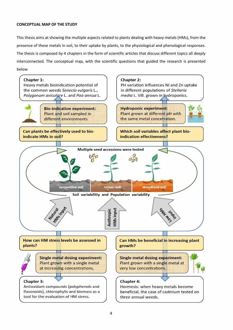
CONCEPTUAL MAP OF THE STUDY

This thesis aims at showing the multiple aspects related to plants dealing with heavy metals (HMs), from the

presence of these metals in soil, to their uptake by plants, to the physiological and phenological responses.

The thesis is composed by 4 chapters in the form of scientific articles that discuss different topics all deeply

interconnected. The conceptual map, with the scientific questions that guided the research is presented

below.

5

1. INTRODUCTION

Since the beginning of the industrialization era, the impact of man on the biosphere has been so

important that it has become necessary to indicate as anthroposphere the sphere of man’s

settlement and activity. This term can be applied to any part of the biosphere that has been deeply

changed under the influence of technical civilization (Kabata-Pendias, 2011). The always growing

changes caused by human activities, are becoming more and more impactful on all planet

ecosystems.

One of the global issues connected to human activities is the release of heavy metals (HMs) in the

air, water and soil. Several processes are responsible for HM pollution, among which the most

important are: combustion of oil and carbon, mining and smelting activities, use of chemical

fertilizers and sludge in agriculture.

In recent years, the overwhelming amount of studies related to HMs contributed to a better

understanding of the biogeochemical processes that control trace element cycling and their

permanence in the environment. This knowledge will be at the basis of our future possibility to

manage and reduce trace elements release in the environment, and a prerequisite for a sustainable

land use. This is a fundamental objective to achieve, since the concentration of most HMs in plants

(i.e. food crops), is often positively correlated with the abundance of these elements in soils. It is

therefore our priority the maintenance of soil productivity and safety, avoiding the spreading of

anthropogenic pollutants along the food chain (Kabata-Pendias, 2011).

1.1. What is an “heavy metal” ?

The term “heavy metal” refers to metallic elements with a density greater than 5 g/cm³ (Nies, 1999).

HMs usually behave like cations when they are free ions in water solutions. They have an ionic

diameter between 138 to 160 picometers, are mostly divalent elements (Mn2+, Ni2+, Cu2+, Zn2+, etc)

and are quite reactive (Weast, 1984). Most HMs are transition elements with incompletely filled d

orbitals, this characteristic makes them redox-active and able to form complexes with organic

ligands (Nies, 1999). In general, in the literature, the term “heavy metal” has always been used with

a negative meaning connected with environmental pollution, biological hazard and toxicity. Heavy

metals are also called “trace elements”, and this definition, having a more neutral meaning,

indicates their low concentration (< 0.1%) in biological tissues, since they are mostly micronutrient

for all living organisms. The term trace elements only relates to ions abundance and also includes

6

elements having various chemical properties (Kabata-Pendias, 2011). Regardless of the term used,

a list of HMs of great environmental concern has been summarized by Kabata-Pendias (2011) and

among them are worthy of being cited: As, Be, Cd, Cr, Cu, Hg, Ni, Pb, Se, Tl, V, Zn.

In the present thesis, six of them have been studied and a brief description of each element is

provided below.

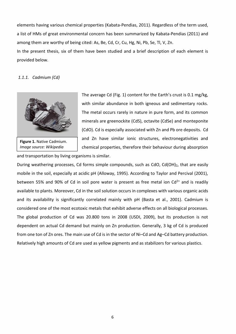
1.1.1. Cadmium (Cd)

The average Cd (Fig. 1) content for the Earth’s crust is 0.1 mg/kg,

with similar abundance in both igneous and sedimentary rocks.

The metal occurs rarely in nature in pure form, and its common

minerals are greenockite (CdS), octavite (CdSe) and monteponite

(CdO). Cd is especially associated with Zn and Pb ore deposits. Cd

and Zn have similar ionic structures, electronegativities and

chemical properties, therefore their behaviour during absorption

and transportation by living organisms is similar.

During weathering processes, Cd forms simple compounds, such as CdO, Cd(OH)2, that are easily

mobile in the soil, especially at acidic pH (Alloway, 1995). According to Taylor and Percival (2001),

between 55% and 90% of Cd in soil pore water is present as free metal ion Cd2+ and is readily

available to plants. Moreover, Cd in the soil solution occurs in complexes with various organic acids

and its availability is significantly correlated mainly with pH (Basta et al., 2001). Cadmium is

considered one of the most ecotoxic metals that exhibit adverse effects on all biological processes.

The global production of Cd was 20.800 tons in 2008 (USDI, 2009), but its production is not

dependent on actual Cd demand but mainly on Zn production. Generally, 3 kg of Cd is produced

from one ton of Zn ores. The main use of Cd is in the sector of Ni–Cd and Ag–Cd battery production.

Relatively high amounts of Cd are used as yellow pigments and as stabilizers for various plastics.

Figure 1. Native Cadmium. Image source: Wikipedia

7

1.1.2. Chromium (Cr)

The abundance of Cr (Fig. 2) in the Earth’s upper crust is on

averages 100 mg/kg, while in ultramafic rocks its content can be

over 3000 mg/kg. Cr-rich minerals are likely to be associated with

pyroxenes, amphibolites and micas in intrusive rocks.

The geochemistry of Cr is complex because of its easy conversion

from +3 to +6 oxidation state, with the second much more toxic

than the first (Bartlett and Kimble, 1976; Bartlett, 1997). Since Cr3+ is slightly mobile only in very

acidic media, its compounds are considered to be very stable in soils. On the other hand, Cr6+ is very

unstable in soils and is easily mobilized in both acid and alkaline soils. Global production of Cr in

2008 was reported at 21.5 million tons (USDI, 2009).

The major proportion of Cr is used for stainless steel and chromate plating. In the chemical industry,

Cr (both +3 and +6) is used primarily in pigments, metal galvanizing and as wood preservatives. The

main source of Cr pollution are considered to be the dyeing and leather tanning process wastes that

are discharged directly into waste streams. Thus, chromite ore processing residue is of the greatest

environmental risk in some regions.

1.1.3. Copper (Cu)

Copper (Fig. 3) occurs in the Earth’s crust at concentrations

between 25 and 75 mg/kg, it is particularly abundant in

mafic igneous rocks and in argillaceous sediments. Copper

reveals a strong affinity for sulphur, hence its principal

minerals are chalcopyrite (CuFeS2), bornite (Cu5FeS4),

chalcocite (Cu2S) and covellite (CuS)(Kabata-Pendias, 2011).

World Cu production was 15.7 million tons in 2008 (USDI,

2009). Due to its versatile properties, Cu has a wide range of

applications, such as in the production of various conductor

materials, it is added in fertilizers, pesticides and animal fodder.

Generally, Cu is accumulated in the upper layer of soils due to its tendency to be adsorbed by organic

matter (Logan et al., 1997). Cu is a rather immobile element in soils; the only process that

Figure 2. Native Chromium. Image source: Wikipedia

Figure 3. Native Copper. Image source: Wikipedia

8

significantly contributes to increase soil Cu availability, is desorption due to the mineralization of

organic matter.

1.1.4. Lead (Pb)

The average Pb content is the Earth’s crust is estimated as 15

mg/kg. Its terrestrial abundance indicates a tendency for a

concentration in the acid series of igneous rocks and

argillaceous sediments. In the environment, two kinds of Pb are

known: primary and secondary. Primary Pb is of a geogenic

origin and was incorporated into minerals at the time of their

formation, while secondary Pb is of a radiogenic origin from the

decay of U and Th. The most common Pb mineral (Fig. 4) is

galena (PbS). The global production of Pb in 2008 was 3.8 million

tons (USDI, 2009) which was obtained mainly from galena deposits. However, in the United States,

above 90% of all Pb was produced from secondary sources, like Pb scraps from spent lead-acid

batteries.

The largest worldwide use of Pb is in fact for lead-acid batteries and, until 1990s, as an additive in

petrol in most developed countries. Lead is the least mobile respect to other trace metals in soils,

because it easily forms insoluble precipitates or is strongly bound to clay minerals (Vega et al., 2007).

In soils, primary Pb is mostly localized in surface layers given its affinity to organic matter, but also

as consequence of its deposition form atmospheric particles (Blum et al., 1997).

1.1.5. Nickel (Ni)

In the Earth’s crust, the mean Ni (Fig. 5) abundance has

been estimated around 20 mg/kg, whereas in the

ultramafic rocks Ni ranges from 1400 to 2000 mg/kg.

In rocks, Ni occurs primarily as sulphides and arsenides

and is associated with several Fe minerals. After

weathering, most Ni precipitates with Fe and Mn oxides,

and becomes included in goethite, limonite, serpentinite,

as well as in other Fe minerals. Organic matter exhibits a strong ability to absorb Ni, thus it is highly

Figure 5. Nickel ores after smelting. Image source: Wikipedia

Figure 4. Galena mineral (PbS). Image source: Wikipedia

9

concentrated in coal and oil. For this reason, a significant proportion of Ni emissions in the

environment are from fossil fuel combustion. Global Ni production was estimated to be 1.6 million

tons in 2008 (USDI, 2009). The 68% of this metal is used for stainless steels. It is also widely used for

magnetic components and electrical equipment. Its compounds are utilized as dyes, in ceramic and

glass manufactures, and in batteries containing Ni–Cd compounds (Reck et al., 2008).

1.1.6. Zinc (Zn)

Average Zn (Fig. 6) content of the Earth’s crust is estimated at

70 mg/kg, Zn is quite uniformly distributed in magmatic rocks,

whereas in sedimentary rocks it is likely to be concentrated in

argillaceous sediments.

This element is very mobile during weathering processes and

its compounds are readily precipitated by reactions with

carbonates. Global production of Zn in 2008 was 11.3 million

tons (USDI, 2009). The principal Zn ores are sphalerite,

wurzite and smithsonite, all containing about 50% of Zn. Zinc

ores often contain other trace metals, such as Pb, Cu, Ag and Cd.

Zinc is used in many industrial productions, mainly as corrosion protector of steel. It is an important

component of various alloys and is widely used as catalyst in different chemical production (e.g.

rubber vulcanization, pigments, and plastic). It is also used in batteries, pipes, and electronic devices.

Agricultural fertilization is known to increase Zn contents of surface soils since the deficiency of this

element is quite common (Huang and Jin, 2008). In natural environments, Zn leaching is

counterbalanced by its atmospheric input that, in last years, exceeded its output due to the

significant contribution of anthropic emissions.

Figure 6. Zinc ores after smelting. Image source: Wikipedia

10

1.2. Heavy metals in plant nutrition: essential and non-essential elements for plants

Plants are autotrophic organisms in which nutritive processes

are based on the conversion of inorganic carbon (CO2) to

organic compounds through photosynthesis combined with the

uptake of other essential nutrients. Some of these nutrients are

necessary for the plant survival at high concentration, while

others only at low concentration, and are therefore defined

respectively “macronutrients” and “micronutrients” (Fig. 7).

Macronutrients (C, H, O, N, P, K, S, Ca, Mg) represent the main

constituent elements of proteins and DNA, besides covering

also a fundamental structural role. (Manahan, 2000; Clemens,

2001). Micronutrients instead are mostly structural

components of some enzymes and act as enzymatic activators

or regulators (Clemens, 2001). At present, 17 micronutrients

(Al, B, Br, Cl, Co, Cu, F, Fe, I, Mn, Mo, Ni, Rb, Si, Ti, V, Zn) are

known to be essential for plants; some are proved to be

necessary for few species only, and others are known to have stimulating effects on plant growth,

but their functions are not yet recognized (Kabata-Pendias, 2011). When micronutrients are present

at higher concentrations than necessary, they can easily cause toxicity, conversely when their

concentration is too low, plants show deficiency symptoms (Clemens, 2001). In addition to these

elements, plants are able to absorb a great variety of other “non-essential” elements (e.g. Cd, Cr,

Pb) present in soils. Plants’ average concentration of the metals object of study in the present thesis

are summarized in Table 1.

Element Essentiality Deficiency limit

(ppm)

Average concentration

(ppm)

Toxicity limit (ppm)

Cd no no 0.03–5 > 5–30

Cr no no 1-30 > 10–30

Cu yes < 2-5 5-25 > 20-100

Table 1. Plants’ average concentration of heavy metals found in plants. Only the six elements studied in the present thesis are shown. Deficiency and toxicity limits are reported when possible. All values are expressed in ppm on plant FW basis. Adapted from: Kabata-Pendias (2011).

Figure 7. Label of a commercial fertilizer with micronutrients. Image source: Amazon

11

Ni yes < 0.05 5-100 > 50-100

Pb no no 0.5-10 > 30-300

Zn yes < 10-20 20-400 > 200-400

The chemical composition of plants therefore reflects the elemental composition of the growing

media (e.g. soil). The extent to which this relationship exists, however, is highly variable and is

governed by many different factors (see chapter 3). For example Cr, Pb are slightly soluble and

strongly absorbed by soil particles, similarly Cu is mainly bound to organic matter, therefore they

are not easily taken up by plants. Ni, Cd, Zn are mobile in soil and readily taken up by plants (Kabata-

Pendias, 2011).

Since this study is focused on the effects of six HMs (Cu, Zn, Ni, Cd, Pb, Cr), a summarised description

of their specific uptake mechanisms and functions in plant cells is reported below.

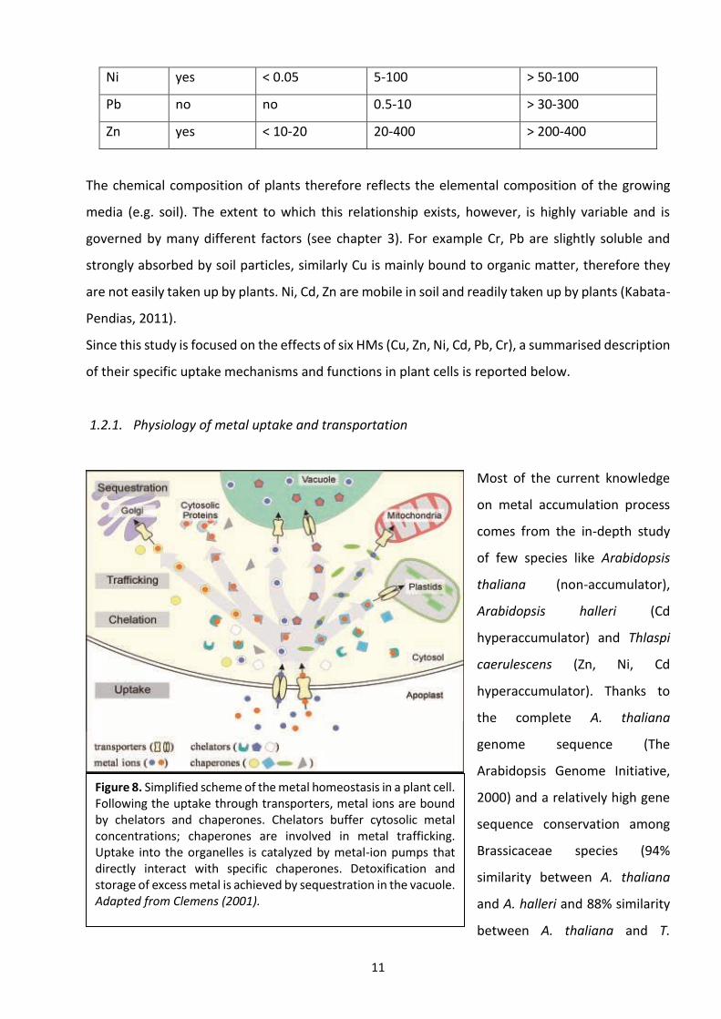
1.2.1. Physiology of metal uptake and transportation

Most of the current knowledge

on metal accumulation process

comes from the in-depth study

of few species like Arabidopsis

thaliana (non-accumulator),

Arabidopsis halleri (Cd

hyperaccumulator) and Thlaspi

caerulescens (Zn, Ni, Cd

hyperaccumulator). Thanks to

the complete A. thaliana

genome sequence (The

Arabidopsis Genome Initiative,

2000) and a relatively high gene

sequence conservation among

Brassicaceae species (94%

similarity between A. thaliana

and A. halleri and 88% similarity

between A. thaliana and T.

Figure 8. Simplified scheme of the metal homeostasis in a plant cell. Following the uptake through transporters, metal ions are bound by chelators and chaperones. Chelators buffer cytosolic metal concentrations; chaperones are involved in metal trafficking. Uptake into the organelles is catalyzed by metal-ion pumps that directly interact with specific chaperones. Detoxification and storage of excess metal is achieved by sequestration in the vacuole. Adapted from Clemens (2001).

12

caerulescens), many gene comparisons have been made to better understand those involved in

metal homeostasis and accumulation (Talke et al., 2006; van de Mortel et al., 2006). These candidate

genes are mostly involved in metal transport, metal chelation and metal-induced oxidative stress

response. Despite the overwhelming amount of studies, connections between metals and specific

transporters seem hard to find (Fig. 8). One of the reasons is probably the low specificity of some

mechanisms involved in metal transportation and chelation, thus allowing some species to tolerate

and accumulate several metals simultaneously (Van der Ent et al., 2017b). To make the situation

furtherly complicated the mechanisms of metal uptake are also influenced by soil metal

concentration. Morel (1997), described that at low cation concentrations (both HMs and nutrients)

of the soil solution (<0.5 μM), active absorption predominates, whereas at higher concentrations

(>0.1 mM) the absorption is dominated by passive (diffusion) processes.

1.2.2. Zinc (Zn) and Cadmium (Cd)

Zn and Cd have high chemical affinity and many studies (e.g. Lu et al., 2010, Meyer and Verbruggen,

2012) demonstrated that the uptake of these two ions follows the same biological pathway. Zn is

an important micronutrient for plants while for Cd, with the exception of the recently described Cd-

carbonic anhydrase of marine diatoms (Lane & Morel, 2000), no biological functions are known

(Kabata-Pendias, 2011; Van der Ent et al., 2017b).

Prior to uptake, these metals are actively mobilized from the soil by acidification or by chelating

secretion from roots (Clemens et al., 2002). Nicotianamine (NA) is a common chelator excreted by

plants that binds metals including Zn, Fe and Cd. After mobilization, divalent metal transporters of

the ZIP family (Zrt-Irt-like Protein) present on the root surface, pump the metal inside the cells. It is

still not clear if Cd uptake is determined by specific or via Zn-Fe transport mechanisms, but these

are likely to be partially overlapped in most non specialized species (Meyer and Verbruggen, 2012).

Once in the roots these metals are often complexed with NA; for example the complex Zn-NA

provides Zn with a high symplastic mobility towards the xylem (Deinlein et al., 2012; Cornu et al.,

2015). The Zn and Cd present in root tissues is then actively loaded into the xylem by the HMA4

proteins (ATPase pumps), as observed in A. halleri (Talke et al., 2006; Courbot et al., 2007;

Hanikenne et al., 2008). It is supposed that HMA4 also acts as a physiological regulator: while it

depletes the metal pool from roots, it triggers a Zn-deficiency response resulting in high expression

of several ZIP genes (Hanikenne et al., 2008). Once in the xylem, metals are transported to the

shoots thanks to the evapo-transpiration negative pressure. In this compartment, Zn is mainly

13

bound to organic acids such as malate and citrate (Lu et al., 2013; Cornu et al., 2015). Eventually,

the metal reaches the leaves and it is suggested that HMA4 and ZIP transporters again play an

important role in unloading and distributing metallic ions to shoot tissues (Krämer et al., 2007;

Hanikenne and Nouet, 2011). The metal is then stored in the vacuole, and this function is most likely

ensured by MTP1 (Metal Tolerance Protein 1) as suggested for A. halleri and T. caerulescens (Dräger

et al., 2004; Talke et al., 2006; Shahzad et al., 2010) event tough the role of this protein has to be

further confirmed.

1.2.3. Chromium (Cr)

Cr can be absorbed both as Cr +3 or Cr +6, and no specific mechanism for its uptake is up to date

known. This metal is generally uptaken by other non-specific carriers together with other essential

elements and water (Shanker et al., 2005). Members of the Brassicaceae family that are sulphur-

loving plants, have been found to accumulate high Cr amounts (Zayed et al., 1998), thereby

suggesting that Cr is translocated in the plants via S uptake mechanism, such as sulphate carriers

(Barceló and Poschenrieder, 1997). Due to chemical similarity between these two elements, the

presence of high S in the growing medium reduces the uptake of Cr in the plants as both compete

for the same transport channel (Skeffington et al., 1976; Singh et al., 2013). Cr interacts positively

with plant Fe nutrition (Bonet et al., 1991). In fact, it has been observed that Fe-loving plants, such

as spinach (Spinacia oleracea) and turnip (Brassica rapa subsp. rapa), are the most effective in

translocating Cr to aerial tissues compared to lettuce (Lactuca sativa) and cabbage (Brassica

oleracea var. capitata) that do not accumulate Fe and are thus less effective in Cr translocation (Cary

et al., 1977). Cr is generally accumulated in the roots, which in can accumulate 100-fold higher Cr

than the shoots (Zayed et al., 1998). The poor translocation of this element to the aerial parts of the

plant is probably due to formation of insoluble Cr compounds inside the roots vacuole.

1.2.4. Copper (Cu)

Cu is a micronutrient for plants but, despite its essentiality, it becomes extremely toxic at levels

slightly above the plant needs. Cu uptake and homeostasis is therefore strictly regulated by specific

transporters located in the plasma membrane (Kampfenkel et al., 1995). Eukaryotic cells utilize

copper transporter (CTR family) proteins to transport Cu2+ ions into the cytosol (Penarrubia et al.,

2010). The CTR-like transporters in plants are called COPT (Copper Transporter) (Kampfenkel et al.,

14

1995). Until recently, the only functionally characterized COPT transporter was COPT1 (Sancenon et

al., 2004) which was involved in Cu transport, but was never detected in roots. Conversely, the

production of COPT5 has been detected throughout the plant (except in pollen), with clearly

elevated values in roots, confirming its function in Cu uptake from soil (Jaquinod et al., 2007; Garcia-

Molina et al., 2011). Inside the plants Cu ions are complexed with phytochelatins and

metallothioneins (Maitani et al., 1996). These proteins constitute one of the cytosolic Cu storage

and contribute to copper detoxification in plant cells (Hamer et al., 1985). The importance of

metallothioneins was demonstrated by Murphy and Taiz (1995), in an experiment of

metallothionein induction by Cu treatment, on different Arabidopsis ecotypes. During the transport

of Cu in the xylem and phloem, nicotianamine has been demonstrated to act as main chelator (von

Wirén et al., 1999), its physiological role has been mainly studied in a NA-deficient tomato mutant,

which exhibits severe growth limitation and intercostal chlorosis due to the lack of Cu (Pich and

Scholz, 1996). Vacuolar sequestration of Cu is poorly documented, mainly because Cu is immediately

utilized in protein production. This thesis, in supported by the presence of a Cu fast recycling

mechanisms, for instance during leaf senescence when Cu is re-mobilized to other plant growing

parts in order to minimize the loss of valuable nutrients (Himelblau and Amasino, 2000).

1.2.5. Lead (Pb)

No biological function is known to date for Pb. This metal, which is toxic even at low concentration,

is usually poorly available to plants and immobilized in soil in non-soluble forms. It is therefore

unlikely that transporters with specificities for this metal cation exist. Instead, this non-essential

metal is able to enter cells through cation transporters with a broad substrate specificity. For

example, it is well documented that iron-deficiency leads to an enhanced uptake of other metal ions

including Pb (Cohen et al., 1998). The pathways of Pb uptake have been poorly investigated and only

few studies are available on this topic. Arazi et al. (1999) investigated a transporter (NtCBP4) in

transgenic tobacco plants that demonstrated to have high specificity for Pb. This transporter is

involved in metal uptake across the root plasma membranes. Transegenic plants that overexpressed

NtCBP4, have higher Pb accumulation both in roots and shoots, and show Pb toxicity when

compared to the wild types. Once in the plant, Pb is probably bound to phytochelatins and then

transported towards shoots (Clemens, 2001). Storage of Pb in the vacuole was found to be

correlated with high levels of histidine in cells, suggesting a role of this amino acid in Pb chelation.

15

However, the histidine response during vacuolar metal uptake has been found for several other

metal ions suggesting a low specificity of this mechanisms (Krämer et al., 1996).

1.2.6. Nickel (Ni)

In A. thaliana, the mechanisms involved in Ni homeostasis are strongly linked to Fe homeostasis

(Schaaf et al., 2006; Morrissey et al., 2009; Nishida et al., 2011), so that the metal transporter IRT1

(ZIP family) required for the Fe uptake from the soil was also shown to be involved in Ni uptake (Vert

et al., 2002; Nishida et al., 2012). Interestingly, the over-expression of IRT1 in the roots of N.

caerulescens (now T. caerulescens) is also correlated with Ni hyperaccumulation in the same plant

accession located in Monte Prinzera, an Italian serpentine site with soil/rocks characterized by high

Ni concentrations (Halimaa et al., 2014).

Once in the roots, Ni requires metal chelators (citrate and malate) that are able to stabilize this

metal at different pH allowing its transport to the aerial parts of the plant (Callahan et al., 2006;

Sarret et al., 2013). The load in the xylematic flow of Ni-citrate and Ni-malate is probably carried out

by the MATE transporter protein family (Multidrug And Toxic compound Extrusion). Those

transporters are more expressed in the hyperaccumulator N. caerulescens than in the related non-

accumulator A. thaliana (van de Mortel et al., 2006). Again, nicotianamine has a strong affinity for

Ni over a wide pH range and is proposed to bind Ni in more neutral compartments such as cytoplasm

or phloem (Callahan et al., 2006; Rellan-Alvarez et al., 2008; Alvarez-Fernandez et al., 2014). When

Ni reaches the leaves, several evidences indicate that ferroportin (FPN) and iron-regulated (IREG)

transporters play an essential role in the sequestration of Ni in vacuoles. It was in fact demonstrated

that an over-expression of AtIREG2 in transgenic Arabidopsis plants significantly increases Ni

tolerance and accumulation (Schaaf et al., 2006; Merlot et al., 2014).

16

1.3. Environmental sources of heavy metals

One of the most dramatic aspects that man will be facing in the immediate future is the pollution of

soil determined by the growing release of HMs.

These elements are naturally present in the environment, but in the last decades the exponential

growth of human activities responsible for the production of these pollutants, arouse concerns due

to the potential risk of widespread contamination of soils (Fusco et al., 2005).

HM soil pollution is particularly severe around large urban areas as a result of vehicular traffic,

where high concentration of typical anthropogenic metals like Zn, Cu and Pb, can be detected in soil

and dust (Li et al., 2003).

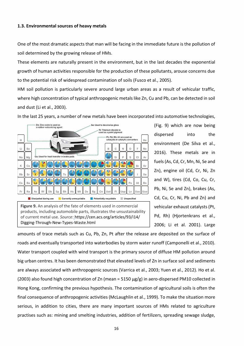
In the last 25 years, a number of new metals have been incorporated into automotive technologies,

(Fig. 9) which are now being

dispersed into the

environment (De Silva et al.,

2016). These metals are in

fuels (As, Cd, Cr, Mn, Ni, Se and

Zn), engine oil (Cd, Cr, Ni, Zn

and W), tires (Cd, Co, Cu, Cr,

Pb, Ni, Se and Zn), brakes (As,

Cd, Cu, Cr, Ni, Pb and Zn) and

vehicular exhaust catalysts (Pt,

Pd, Rh) (Hjortenkrans et al.,

2006; Li et al. 2001). Large

amounts of trace metals such as Cu, Pb, Zn, Pt after the release are deposited on the surface of

roads and eventually transported into waterbodies by storm water runoff (Camponelli et al., 2010).

Water transport coupled with wind transport is the primary source of diffuse HM pollution around

big urban centres. It has been demonstrated that elevated levels of Zn in surface soil and sediments

are always associated with anthropogenic sources (Varrica et al., 2003; Yuen et al., 2012). Ho et al.

(2003) also found high concentration of Zn (mean = 5150 μg/g) in aero-dispersed PM10 collected in

Hong Kong, confirming the previous hypothesis. The contamination of agricultural soils is often the

final consequence of anthropogenic activities (McLaughlin et al., 1999). To make the situation more

serious, in addition to cities, there are many important sources of HMs related to agriculture

practises such as: mining and smelting industries, addition of fertilizers, spreading sewage sludge,

Figure 9. An analysis of the fate of elements used in commercial products, including automobile parts, illustrates the unsustainability of current metal use. Source: https://cen.acs.org/articles/93/i14/ Digging-Through-New-Types-Waste.html

17

use of pesticides (Singh, 2001). Soil contamination is not only a social and sanitary issue, but is also

an economic concern since it implies elevated monetary costs related to the decreased agricultural

productivity and to the eventual remediation (Bini, 2010).

1.3.1. Anthropic environments polluted by heavy metals: cities

In cities, heavy metals may originate from various types of sources, nonetheless vehicular emissions

are considered one of the main sources of HM contamination, especially Pb (Duong and Lee, 2011,

WSDE, 2011). This metal is present in gasoline

and many other vehicle parts including

batteries, wheel balancing weights and metallic

paints. Pb emissions from gasoline combustion

reached their peak in the early 1970s and then

started to declined, especially after the EU ban

of leaded gasoline in 2000 (UNEP, 2015).

Although leaded gasoline was phased out

decades ago, Pb concentrations in road dust

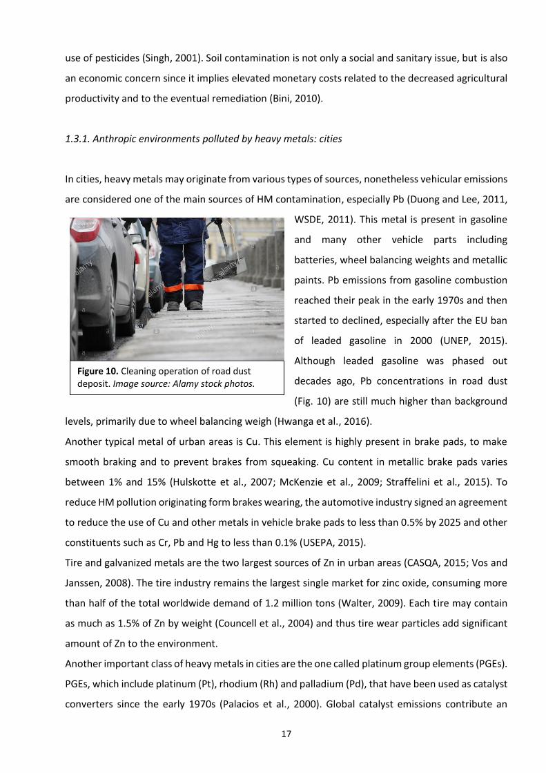
(Fig. 10) are still much higher than background

levels, primarily due to wheel balancing weigh (Hwanga et al., 2016).

Another typical metal of urban areas is Cu. This element is highly present in brake pads, to make

smooth braking and to prevent brakes from squeaking. Cu content in metallic brake pads varies

between 1% and 15% (Hulskotte et al., 2007; McKenzie et al., 2009; Straffelini et al., 2015). To

reduce HM pollution originating form brakes wearing, the automotive industry signed an agreement

to reduce the use of Cu and other metals in vehicle brake pads to less than 0.5% by 2025 and other

constituents such as Cr, Pb and Hg to less than 0.1% (USEPA, 2015).

Tire and galvanized metals are the two largest sources of Zn in urban areas (CASQA, 2015; Vos and

Janssen, 2008). The tire industry remains the largest single market for zinc oxide, consuming more

than half of the total worldwide demand of 1.2 million tons (Walter, 2009). Each tire may contain

as much as 1.5% of Zn by weight (Councell et al., 2004) and thus tire wear particles add significant

amount of Zn to the environment.

Another important class of heavy metals in cities are the one called platinum group elements (PGEs).

PGEs, which include platinum (Pt), rhodium (Rh) and palladium (Pd), that have been used as catalyst

converters since the early 1970s (Palacios et al., 2000). Global catalyst emissions contribute an

Figure 10. Cleaning operation of road dust deposit. Image source: Alamy stock photos.

18

estimated dispersion of 6 tons of Pt annually (Rauch et al., 2005). Despite adverse effects have never

been observed on the environment, PGEs in road dust are up to three orders of magnitude higher

than in background soil. For example, concentrations of 2000 ng/g Pt, 1000 ng/g Pd, and 100 ng/g

Rh have been detected in Shieffield (UK) road dust (Jackson et al., 2007).

1.3.2. Natural environments polluted by heavy metals: serpentine soils

HMs are released in the environment also

trough natural processes, like the

weathering of metal enriched rocks as in the

case of serpentine soils. Serpentine soils

(Fig. 11) occupy a very small part of the land

surface of the earth, less than 1% according

to Brooks (1987), but are highly valuable

areas renowned for their particular

vegetation and ore extraction. Serpentine

soils derive by the weathering of ultramafic

rocks that contain serpentinite mineral (Oze et al., 2004; McGahan et al., 2008). Serpentinite

weathering originates soils characterized by altered chemical and physical properties that reduce

plant productivity and induce stress and toxicity to non-adapted species (Jenny, 1980). Several

factors are thought to be responsible of this low productivity, such as a low Ca:Mg ratio, caused by

the high amounts of Mg released from the parent material, and abundant HMs (in particular Ni, Cr,

Co). In addition, these soils often have low macronutrient (N, P, K) concentrations because of their

paucity in the rock and the presence of scarce vegetation (Alexander et al., 2007).

Mafic and ultramafic ones are richer in Cr and Ni (up to 3400 mg/kg of Cr and 3600 mg/kg of Ni) if

compared to average concentrations of Cr and Ni in normal rocks (about 84 and 34 mg/kg, of Cr and

Ni respectively) (McGrath, 1995).

Because of their particular pedogenesis, serpentine soils often host a specialized flora, therefore

these areas have been identified as hotspost of suitable species for phytomining, phytoremediation

and phytostabilization of HMs (Bini et al., 2017).

Serpentine rocks and soils are particularly abundant in the ophiolite belts and are typically found

within regions of the Circum-Pacific margin and Mediterranean sea (Oze et al., 2004). Pedogenesis

of serpentine soils results to be different among locations, because of the wide distribution of

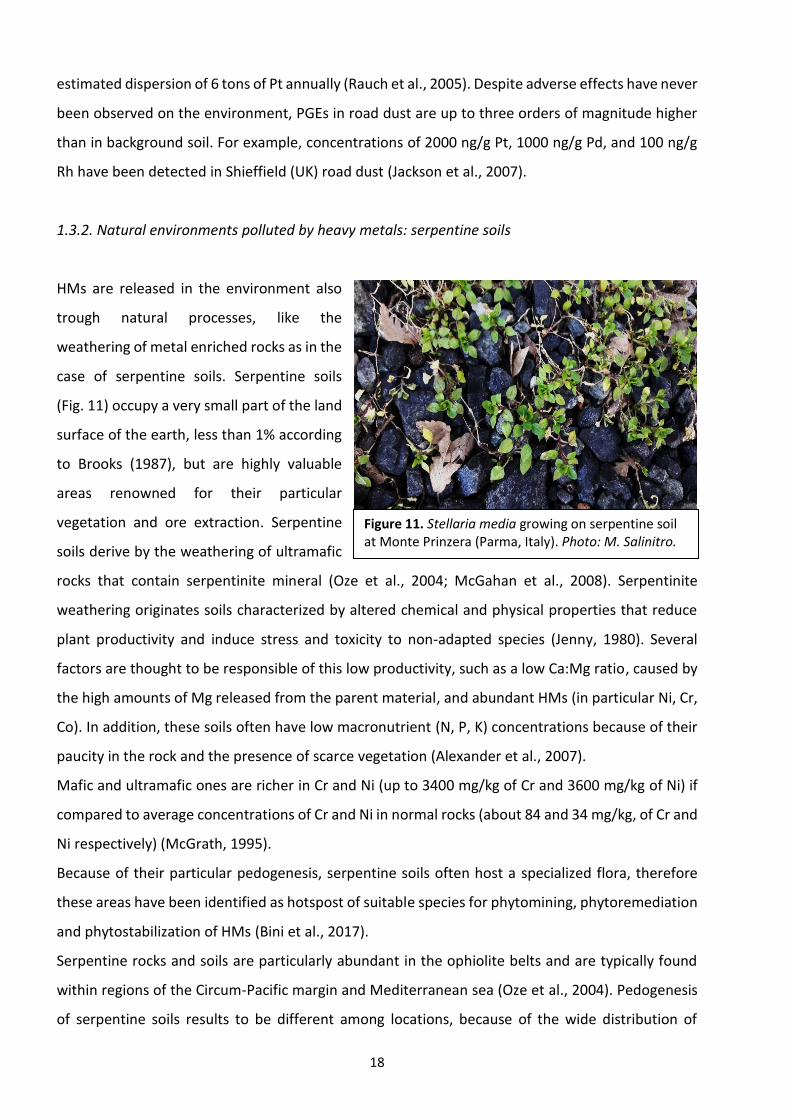
Figure 11. Stellaria media growing on serpentine soil at Monte Prinzera (Parma, Italy). Photo: M. Salinitro.

19

ultramafic substrates in different climate, topography and biota (Lee et al., 2004; Hseu, 2006).

Nonetheless, the release of Cr and Ni into ecosystems during serpentine mineral weathering is a

common trait of serpentine pedogenesis. These processes are source of non-anthropogenic metal

contamination, however, if compared with HMs of anthropogenic origin, those of lithogenic-derived

ones are less mobile in soil and hardly available in the soil solution (Becquer et al., 2003; Garnier et

al., 2006).

1.4. Plant strategies in dealing with metals

When plants end up growing in metal

contaminated soil, they cannot prevent

metal uptake due to their concomitant

absorption together with other essential

nutrients. However, plant are able to

tolerate/accumulate these toxic ions

present at various amounts in their leaves

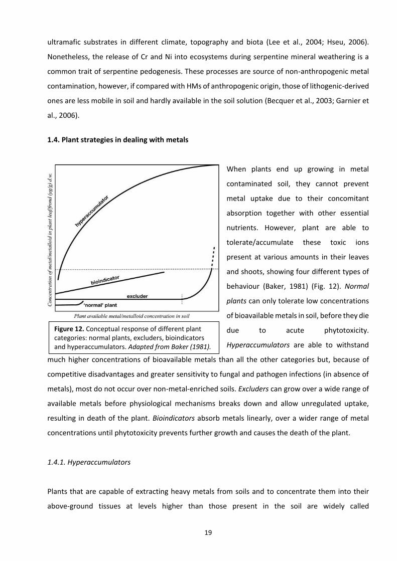
and shoots, showing four different types of

behaviour (Baker, 1981) (Fig. 12). Normal

plants can only tolerate low concentrations

of bioavailable metals in soil, before they die

due to acute phytotoxicity.

Hyperaccumulators are able to withstand

much higher concentrations of bioavailable metals than all the other categories but, because of

competitive disadvantages and greater sensitivity to fungal and pathogen infections (in absence of

metals), most do not occur over non-metal-enriched soils. Excluders can grow over a wide range of

available metals before physiological mechanisms breaks down and allow unregulated uptake,

resulting in death of the plant. Bioindicators absorb metals linearly, over a wider range of metal

concentrations until phytotoxicity prevents further growth and causes the death of the plant.

1.4.1. Hyperaccumulators

Plants that are capable of extracting heavy metals from soils and to concentrate them into their

above-ground tissues at levels higher than those present in the soil are widely called

Figure 12. Conceptual response of different plant categories: normal plants, excluders, bioindicators and hyperaccumulators. Adapted from Baker (1981).

20

hyperaccumulators (Mganga et al., 2011; Baker, 1981). Hyperaccumulators can be further divided

in ‘obligate’ and ‘facultative’ hyperaccumulators. The obligate hyperaccumulator species are

endemic to some type of metalliferous soil and always exhibit metal uptake. Facultative

hyperaccumulators, on the other hand, are species in which some populations exhibit

hyperaccumulation and some other not (Pollard et al., 2014). It has been proposed (Proctor, 1993;

Horger et al., 2013) that plants showing this behaviour have an advantage in the protection against

pathogens and herbivores because of their toxicity.

To define a plant as hyperaccumulator several authors (i.e. Baker and Brooks, 1989; Broadley et al.,

2007; Krämer, 2010) proposed metal thresholds based on unusual metal concentrations that were

sensibly above the average in some species. Normal concentration ranges in plants have been

tabulated for major, minor and trace elements in many reviews (i.e. Raskin and Ensley, 2000) and a

recent discussion regarding appropriate criteria for defining hyperaccumulation thresholds of many

elements can be found in van der Ent et al. (2013) (Table 2).

However, nominal thresholds should be applied sensibly and not as absolute cut-off and other

factors should be considered when accounting a hyperaccumulator. According to van der Ent et al.

(2013) metals have to be present with 2–3 orders of magnitude higher in plant leaves than in than

in the soil (for normal soils) and at least one order of magnitude greater for metalliferous soils.

Plants have to be cultivated in natural soil, in order to reproduce natural growth conditions or

possibly collected in their natural habitat. In fact, is known that in hydroponics condition or

artificially spiked soil, high concentration of metals can be reached even by non-accumulator plants.

Moreover, when regarding to a hyperaccumulator, a bioconcentration factor >1 (but often >50), a

shoot to-root metal concentration quotient >1 and extreme metal tolerance, must be present

(Baker and Whiting, 2002). If adopting the previous criteria, about 500 plant taxa have been cited in

the literature as hyperaccumulators of one or more elements (As, Cd, Co, Cu, Mn, Ni, Pb, Se, Tl, Zn).

Element Normal leaves concentration (ppm) Hyperaccumulation threshold (ppm)

Zn 20 - 400 >3000

Cu 5 - 25 >300

Cd 0.03 - 5 >100

Ni 5 - 100 >1000

Pb 0.05 - 10 >1000

Cr 1 - 30 >300

Table 2. Reference metal concentrations for normal and hyperaccumulating plants. Adapted from van der Ent et al. (2013).

21

These numbers are subject to change and may increase with

further exploration and analysis. Nonetheless, many doubts

remain about records regarding Pb, Cu and Cr. For example, Pb

root uptake is severely restricted root cell membrane while and

Cu levels in plant tissues are strictly regulated specific

transporters and chelators even in enriched soils. It is therefore

possible that many records are a consequence of the accidental

contamination of the samples due to soil dust, as demonstrated

for most of the Cu hyperaccumulator by Faucon et al. (2007).

Conversely, hyperaccumulation for Ni, Zn, Cd have been

confirmed experimentally beyond any doubt in a range of plant

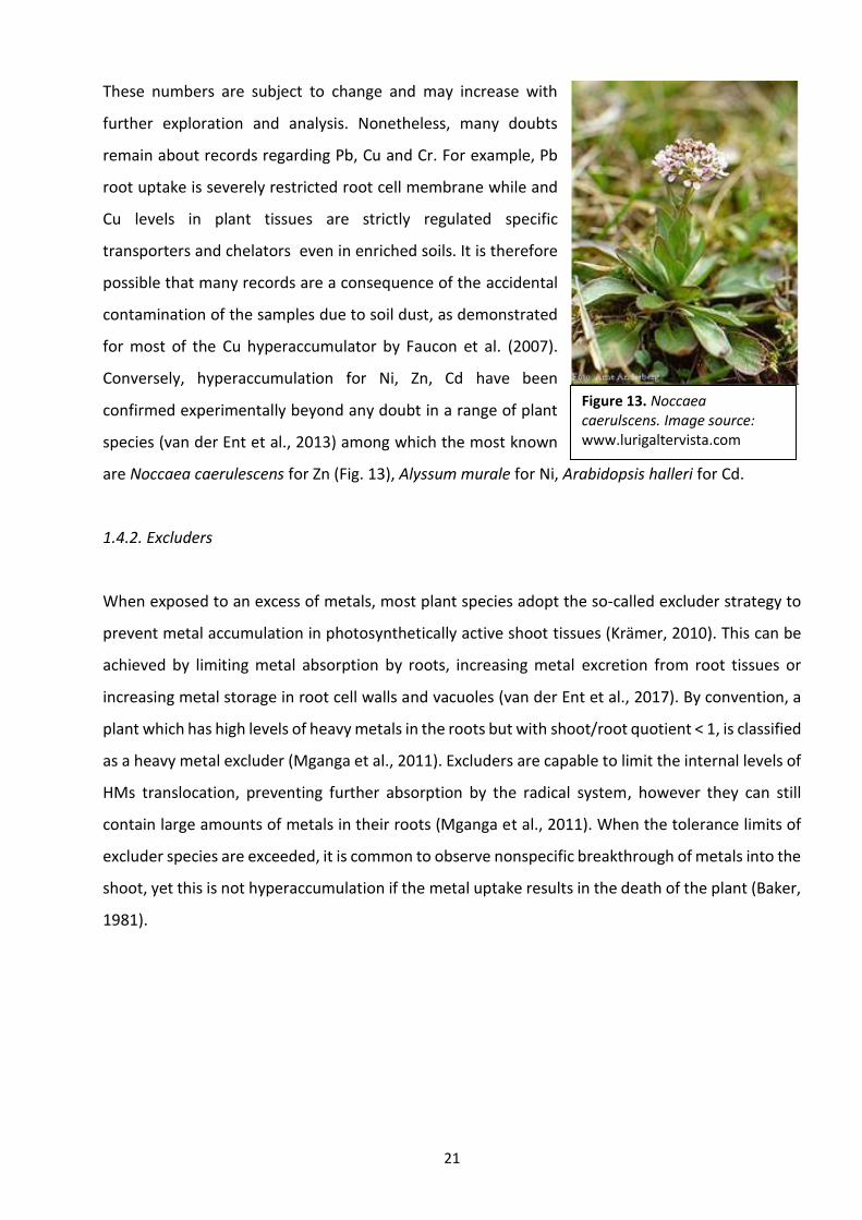
species (van der Ent et al., 2013) among which the most known

are Noccaea caerulescens for Zn (Fig. 13), Alyssum murale for Ni, Arabidopsis halleri for Cd.

1.4.2. Excluders

When exposed to an excess of metals, most plant species adopt the so-called excluder strategy to

prevent metal accumulation in photosynthetically active shoot tissues (Krämer, 2010). This can be

achieved by limiting metal absorption by roots, increasing metal excretion from root tissues or

increasing metal storage in root cell walls and vacuoles (van der Ent et al., 2017). By convention, a

plant which has high levels of heavy metals in the roots but with shoot/root quotient < 1, is classified

as a heavy metal excluder (Mganga et al., 2011). Excluders are capable to limit the internal levels of

HMs translocation, preventing further absorption by the radical system, however they can still

contain large amounts of metals in their roots (Mganga et al., 2011). When the tolerance limits of

excluder species are exceeded, it is common to observe nonspecific breakthrough of metals into the

shoot, yet this is not hyperaccumulation if the metal uptake results in the death of the plant (Baker,

1981).

Figure 13. Noccaea caerulscens. Image source: www.lurigaltervista.com

22

1.4.3. Indicators

Indicators (Fig. 14) are those plants in which the metal

concentration inside their above-ground tissues is directly

proportional to the external concentration of the soil

(Baker and Walker, 1990). These species are generally

characterized by slow and reduced biomass production

and a linear significant soil/plant correlation. However,

exposed to continued uptake of heavy metals, these plant

species are possible pollutant indicators and are also useful

in soil phytostabilization (Mganga et al., 2011).

1.5. Global experimental design

The aim of this section is to give an overview of the criteria used in the selection of plant species,

sampling locations, and on seed collection and sample processing methods. The goal is to provide

an overall view of the entire sampling design that cross-links all the experiments presented in this

thesis.

Following, in each chapter, the methods related to the described specific study will be discussed in

detail.

1.5.1. Selection of plant species

During the present research, a total of five plant species were studied, with the aim of investigating

different aspects all related to HMs uptake by plants. The plants species were selected on the basis

of the following features:

- Herbaceous

- Cosmopolite

- Present in a wide variety of environments

- Annual life cycle

- Fast-growing

- Several generations per year

- High production of seeds

Figure 14. The dandelion (Taraxacum officinale) has been discovered to be a good indicator of HMs in soil. Photo: Mirko Salinitro.

23

- High viability of seeds

- Easy to grow

- Small size

The use of herbaceous annual plants is certainly convenient because most of these species can

complete their life cycle (from germination to fruiting) in less than two months. Therefore, lab

experiments can be carried out in a reasonable amount of time, observing the plant at all its

phenological stages. Cosmopolite plants can be found in worldwide making it possible to extend in

the future applied methodologies to other areas. Moreover, the presence of these plants in several

environments makes them common, easy to find and to identify. These plants are generally resistant

and adaptable to a wide range of conditions, so that it is possible to find their populations adapted

to polluted areas (like urban environments), agroecosystems, woodland areas and ultramafic

outcrops. The high production and viability of seeds make the germination stage easier in lab

experiments, in addition seeds of ruderal plants can keep high germination rates for years even

without specific conservation protocols. Finally, the choice of species characterized by small size

and easy to grow, makes their cultivation possible in restricted spaces and artificial conditions as in

the case of hydroponics, one of the most common methods of lab plant cultivation.

After a screening of several urban species, all possessing the above mentioned characteristics, five

species were chosen belonging to five different botanical families (Table 3).

Species Botanical family Common name Studied in chapter Fig.

Polygonum aviculare L. Polygonaceae common knotgrass 1, 3 15

Senecio vulgaris L. Asteraceae groundsel 1, 3 16

Cardamine hirsuta L. Brassicaceae hairy bittercress 4 17

Poa annua L. Poaceae annual bluegrass 1, 4 18

Stellaria media (L.) Vill. Caryophyllaceae chickweed 2, 4 19

Table 3. List of plant species used for the experiments. For each species is reported the chapter of the present thesis, in which it was used.

24

1.5.2. Polygonum aviculare L.

The name Polygonum is derived from a

Greek word meaning “many knees”,

because of the conspicuous enlarged

nodes of the plant, while aviculare

means “related to birds” as these

animals feed on this plant seeds.

P. aviculare (Fig. 15) is an annual herb

with semi-erect stems that may grow up

to 40 cm long. The leaves are hairless,

elliptical with short stalks, 25 to 35 mm

long and 10 to 15 mm wide. The

flowering period is summer to autumn,

the plant produce small green-white

flowers inserted in the leaf axils. The fruit is a dark brown, three-edged nut. The root is a deep

taproot with few ramifications.

1.5.3. Senecio vulgaris L.

The name Senecio means “old man”, in

reference to the plant becoming grey and hairy

when fruiting, while vulgaris means “common”

as the plant grows in many habitats. S. vulgaris

(Fig. 16) is an erect herbaceous annual plant

growing up 45 cm tall. Leaves are sessile, lobed,

around 61 mm long and 25 mm wide, smaller

towards the top of the plant. Leaves are

sparsely covered with soft, smooth, fine hairs.

Yellow inflorescences appear at the top of plant

in spring, carried by several small branches. The

seeds are achenes with a pappus of about 1 cm,

useful for wind dissemination. The root system consists of a shallow, well branched taproot.

Figure 16. Senecio vulgaris L. from the ultramafic station of Mount Prinzera, Parma. Photo: Mirko Salinitro

Figure 15. Polygonum aviculare L. from the urban station

of Porta Garibaldi in Milan city centre. Photo: M. Salinitro.

25

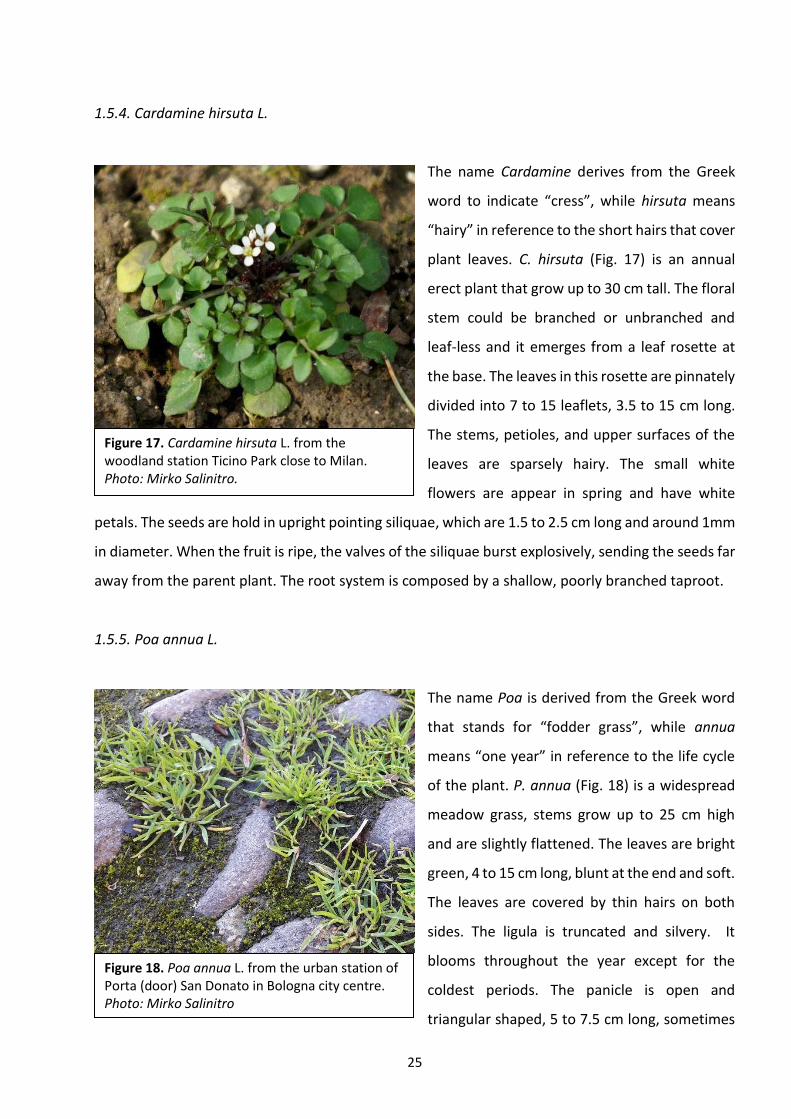
1.5.4. Cardamine hirsuta L.

The name Cardamine derives from the Greek

word to indicate “cress”, while hirsuta means

“hairy” in reference to the short hairs that cover

plant leaves. C. hirsuta (Fig. 17) is an annual

erect plant that grow up to 30 cm tall. The floral

stem could be branched or unbranched and

leaf-less and it emerges from a leaf rosette at

the base. The leaves in this rosette are pinnately

divided into 7 to 15 leaflets, 3.5 to 15 cm long.

The stems, petioles, and upper surfaces of the

leaves are sparsely hairy. The small white

flowers are appear in spring and have white

petals. The seeds are hold in upright pointing siliquae, which are 1.5 to 2.5 cm long and around 1mm

in diameter. When the fruit is ripe, the valves of the siliquae burst explosively, sending the seeds far

away from the parent plant. The root system is composed by a shallow, poorly branched taproot.

1.5.5. Poa annua L.

The name Poa is derived from the Greek word

that stands for “fodder grass”, while annua

means “one year” in reference to the life cycle

of the plant. P. annua (Fig. 18) is a widespread

meadow grass, stems grow up to 25 cm high

and are slightly flattened. The leaves are bright

green, 4 to 15 cm long, blunt at the end and soft.

The leaves are covered by thin hairs on both

sides. The ligula is truncated and silvery. It

blooms throughout the year except for the

coldest periods. The panicle is open and

triangular shaped, 5 to 7.5 cm long, sometimes

Figure 18. Poa annua L. from the urban station of Porta (door) San Donato in Bologna city centre. Photo: Mirko Salinitro

Figure 17. Cardamine hirsuta L. from the woodland station Ticino Park close to Milan. Photo: Mirko Salinitro.

26

they is tinged purple. The seeds are small brown caryopsis. The root system is composed by thin,

shallow, collated roots.

1.5.6. Stellaria media (L.) Vill.

The name Stellaria is derived from a Latin word

meaning “star”, which is a reference to the

shape of its flowers; media is derived from Latin

and means, “intermediate” because of its mid-

size. S. media is annual plant, with weak and

generally creeping stems that could reach a

length up to 40 cm. The plant germinates in

autumn, then forms large mats of foliage during

winter. The leaves are oval and opposite, 20 to

25 mm long and 10 to 15 mm wide. Lower

leaves have stalks while the upper ones are sessile. Blooming season starts in early spring, flowers

are white and small with 5 deeply lobed petals. The whole plant is sparsely hairy, especially on leaf

stalks and flower calix. The fruit consists of an oval capsule with inside several flattened, brown,

kidney-shaped seeds, 0.8 to 1.3 mm big. The root system is composed by thin roots that also emerge

from the nodes of the creeping branches.

Figure 19. Stellaria media (L.) Vill from the woodland station of Park Talon close to Bologna. Photo: Mirko Salinitro.

27

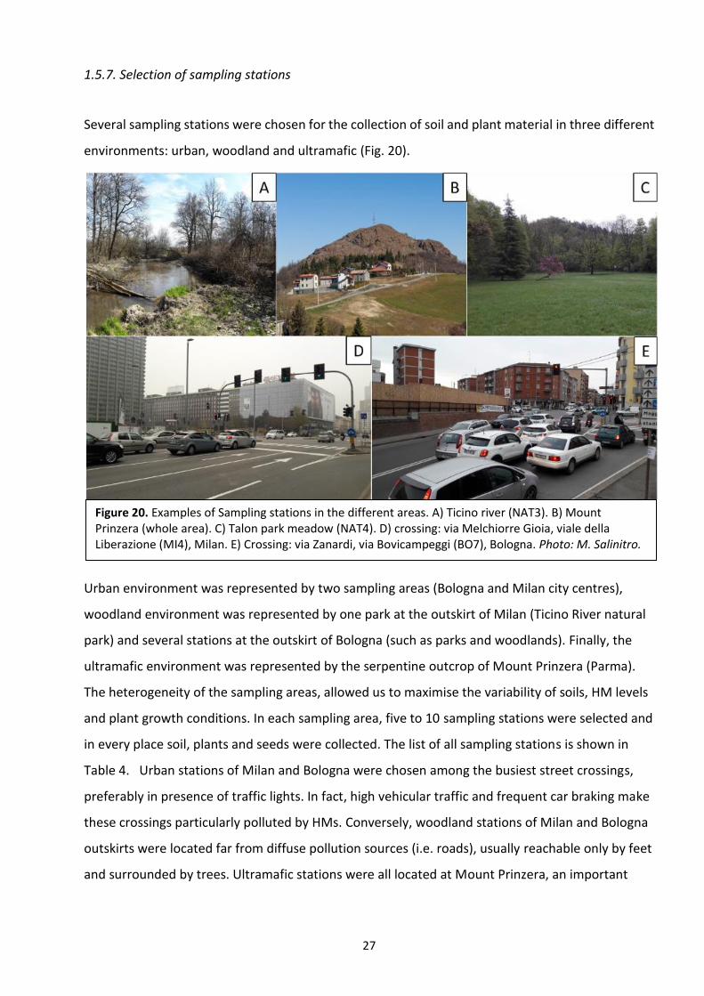
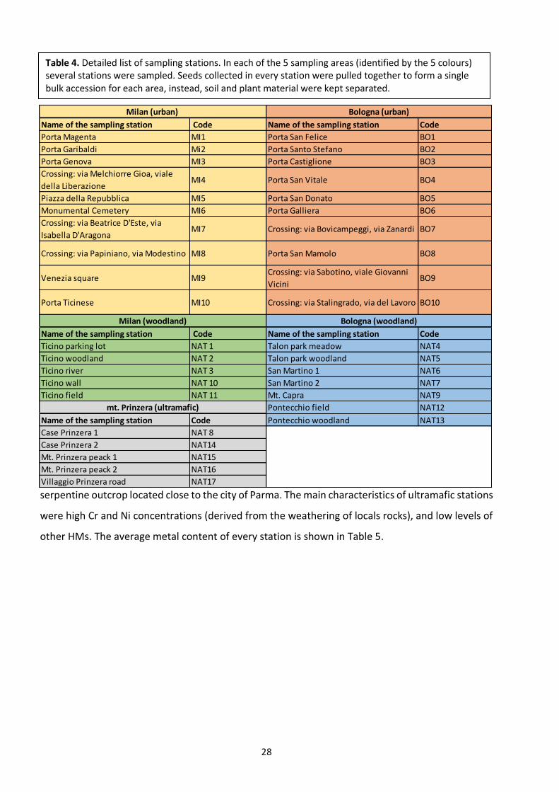
1.5.7. Selection of sampling stations

Several sampling stations were chosen for the collection of soil and plant material in three different

environments: urban, woodland and ultramafic (Fig. 20).

Urban environment was represented by two sampling areas (Bologna and Milan city centres),

woodland environment was represented by one park at the outskirt of Milan (Ticino River natural

park) and several stations at the outskirt of Bologna (such as parks and woodlands). Finally, the

ultramafic environment was represented by the serpentine outcrop of Mount Prinzera (Parma).

The heterogeneity of the sampling areas, allowed us to maximise the variability of soils, HM levels

and plant growth conditions. In each sampling area, five to 10 sampling stations were selected and

in every place soil, plants and seeds were collected. The list of all sampling stations is shown in

Table 4. Urban stations of Milan and Bologna were chosen among the busiest street crossings,

preferably in presence of traffic lights. In fact, high vehicular traffic and frequent car braking make

these crossings particularly polluted by HMs. Conversely, woodland stations of Milan and Bologna

outskirts were located far from diffuse pollution sources (i.e. roads), usually reachable only by feet

and surrounded by trees. Ultramafic stations were all located at Mount Prinzera, an important

Figure 20. Examples of Sampling stations in the different areas. A) Ticino river (NAT3). B) Mount Prinzera (whole area). C) Talon park meadow (NAT4). D) crossing: via Melchiorre Gioia, viale della Liberazione (MI4), Milan. E) Crossing: via Zanardi, via Bovicampeggi (BO7), Bologna. Photo: M. Salinitro.

28

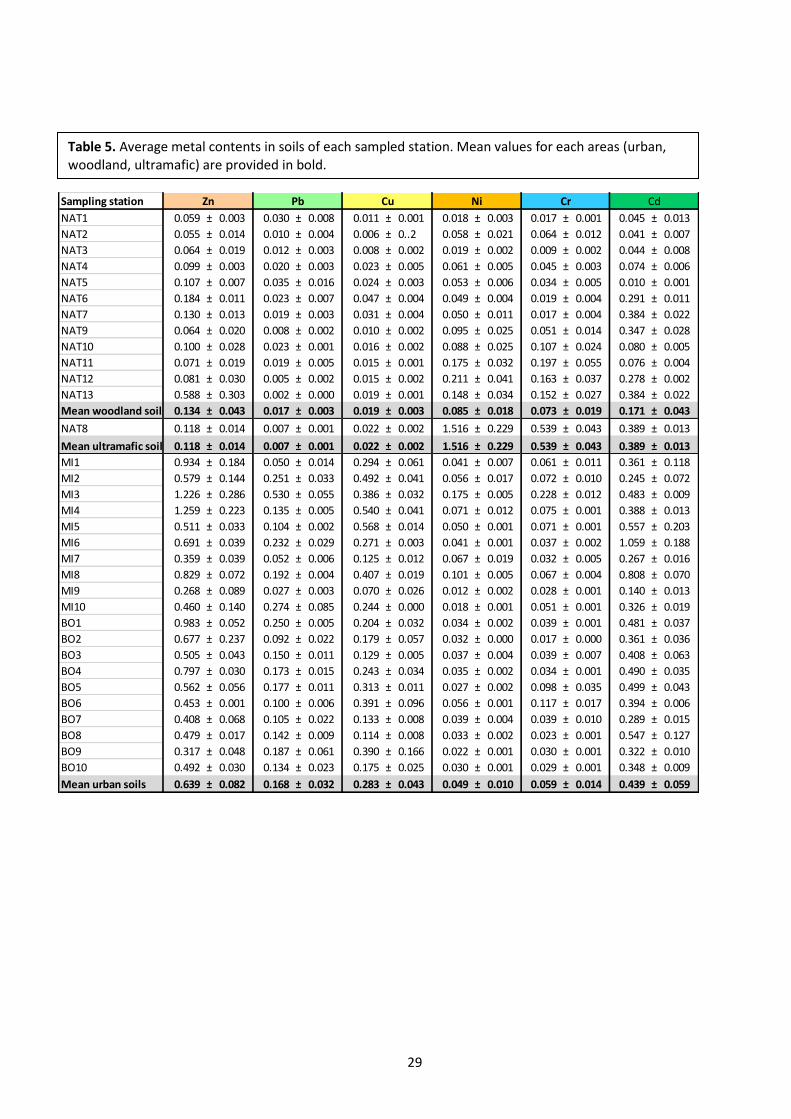
serpentine outcrop located close to the city of Parma. The main characteristics of ultramafic stations

were high Cr and Ni concentrations (derived from the weathering of locals rocks), and low levels of

other HMs. The average metal content of every station is shown in Table 5.

Table 4. Detailed list of sampling stations. In each of the 5 sampling areas (identified by the 5 colours) several stations were sampled. Seeds collected in every station were pulled together to form a single bulk accession for each area, instead, soil and plant material were kept separated.

Name of the sampling station Code Name of the sampling station Code

Porta Magenta MI1 Porta San Felice BO1

Porta Garibaldi Mi2 Porta Santo Stefano BO2

Porta Genova MI3 Porta Castiglione BO3

Crossing: via Melchiorre Gioa, viale

della LiberazioneMI4 Porta San Vitale BO4

Piazza della Repubblica MI5 Porta San Donato BO5

Monumental Cemetery MI6 Porta Galliera BO6

Crossing: via Beatrice D'Este, via

Isabella D'AragonaMI7 Crossing: via Bovicampeggi, via Zanardi BO7

Crossing: via Papiniano, via Modestino MI8 Porta San Mamolo BO8

Venezia square MI9Crossing: via Sabotino, viale Giovanni

ViciniBO9

Porta Ticinese MI10 Crossing: via Stalingrado, via del Lavoro BO10

Name of the sampling station Code Name of the sampling station Code

Ticino parking lot NAT 1 Talon park meadow NAT4

Ticino woodland NAT 2 Talon park woodland NAT5

Ticino river NAT 3 San Martino 1 NAT6

Ticino wall NAT 10 San Martino 2 NAT7

Ticino field NAT 11 Mt. Capra NAT9

Pontecchio field NAT12

Name of the sampling station Code Pontecchio woodland NAT13

Case Prinzera 1 NAT 8

Case Prinzera 2 NAT14

Mt. Prinzera peack 1 NAT15

Mt. Prinzera peack 2 NAT16

Villaggio Prinzera road NAT17

mt. Prinzera (ultramafic)

Milan (urban) Bologna (urban)

Milan (woodland) Bologna (woodland)

29

Table 5. Average metal contents in soils of each sampled station. Mean values for each areas (urban, woodland, ultramafic) are provided in bold.

Sampling station

NAT1 0.059 ± 0.003 0.030 ± 0.008 0.011 ± 0.001 0.018 ± 0.003 0.017 ± 0.001 0.045 ± 0.013

NAT2 0.055 ± 0.014 0.010 ± 0.004 0.006 ± 0..2 0.058 ± 0.021 0.064 ± 0.012 0.041 ± 0.007

NAT3 0.064 ± 0.019 0.012 ± 0.003 0.008 ± 0.002 0.019 ± 0.002 0.009 ± 0.002 0.044 ± 0.008

NAT4 0.099 ± 0.003 0.020 ± 0.003 0.023 ± 0.005 0.061 ± 0.005 0.045 ± 0.003 0.074 ± 0.006

NAT5 0.107 ± 0.007 0.035 ± 0.016 0.024 ± 0.003 0.053 ± 0.006 0.034 ± 0.005 0.010 ± 0.001

NAT6 0.184 ± 0.011 0.023 ± 0.007 0.047 ± 0.004 0.049 ± 0.004 0.019 ± 0.004 0.291 ± 0.011

NAT7 0.130 ± 0.013 0.019 ± 0.003 0.031 ± 0.004 0.050 ± 0.011 0.017 ± 0.004 0.384 ± 0.022

NAT9 0.064 ± 0.020 0.008 ± 0.002 0.010 ± 0.002 0.095 ± 0.025 0.051 ± 0.014 0.347 ± 0.028

NAT10 0.100 ± 0.028 0.023 ± 0.001 0.016 ± 0.002 0.088 ± 0.025 0.107 ± 0.024 0.080 ± 0.005

NAT11 0.071 ± 0.019 0.019 ± 0.005 0.015 ± 0.001 0.175 ± 0.032 0.197 ± 0.055 0.076 ± 0.004

NAT12 0.081 ± 0.030 0.005 ± 0.002 0.015 ± 0.002 0.211 ± 0.041 0.163 ± 0.037 0.278 ± 0.002

NAT13 0.588 ± 0.303 0.002 ± 0.000 0.019 ± 0.001 0.148 ± 0.034 0.152 ± 0.027 0.384 ± 0.022

Mean woodland soils 0.134 ± 0.043 0.017 ± 0.003 0.019 ± 0.003 0.085 ± 0.018 0.073 ± 0.019 0.171 ± 0.043

NAT8 0.118 ± 0.014 0.007 ± 0.001 0.022 ± 0.002 1.516 ± 0.229 0.539 ± 0.043 0.389 ± 0.013

Mean ultramafic soils 0.118 ± 0.014 0.007 ± 0.001 0.022 ± 0.002 1.516 ± 0.229 0.539 ± 0.043 0.389 ± 0.013

MI1 0.934 ± 0.184 0.050 ± 0.014 0.294 ± 0.061 0.041 ± 0.007 0.061 ± 0.011 0.361 ± 0.118

MI2 0.579 ± 0.144 0.251 ± 0.033 0.492 ± 0.041 0.056 ± 0.017 0.072 ± 0.010 0.245 ± 0.072

MI3 1.226 ± 0.286 0.530 ± 0.055 0.386 ± 0.032 0.175 ± 0.005 0.228 ± 0.012 0.483 ± 0.009

MI4 1.259 ± 0.223 0.135 ± 0.005 0.540 ± 0.041 0.071 ± 0.012 0.075 ± 0.001 0.388 ± 0.013

MI5 0.511 ± 0.033 0.104 ± 0.002 0.568 ± 0.014 0.050 ± 0.001 0.071 ± 0.001 0.557 ± 0.203

MI6 0.691 ± 0.039 0.232 ± 0.029 0.271 ± 0.003 0.041 ± 0.001 0.037 ± 0.002 1.059 ± 0.188

MI7 0.359 ± 0.039 0.052 ± 0.006 0.125 ± 0.012 0.067 ± 0.019 0.032 ± 0.005 0.267 ± 0.016

MI8 0.829 ± 0.072 0.192 ± 0.004 0.407 ± 0.019 0.101 ± 0.005 0.067 ± 0.004 0.808 ± 0.070

MI9 0.268 ± 0.089 0.027 ± 0.003 0.070 ± 0.026 0.012 ± 0.002 0.028 ± 0.001 0.140 ± 0.013

MI10 0.460 ± 0.140 0.274 ± 0.085 0.244 ± 0.000 0.018 ± 0.001 0.051 ± 0.001 0.326 ± 0.019

BO1 0.983 ± 0.052 0.250 ± 0.005 0.204 ± 0.032 0.034 ± 0.002 0.039 ± 0.001 0.481 ± 0.037

BO2 0.677 ± 0.237 0.092 ± 0.022 0.179 ± 0.057 0.032 ± 0.000 0.017 ± 0.000 0.361 ± 0.036

BO3 0.505 ± 0.043 0.150 ± 0.011 0.129 ± 0.005 0.037 ± 0.004 0.039 ± 0.007 0.408 ± 0.063

BO4 0.797 ± 0.030 0.173 ± 0.015 0.243 ± 0.034 0.035 ± 0.002 0.034 ± 0.001 0.490 ± 0.035

BO5 0.562 ± 0.056 0.177 ± 0.011 0.313 ± 0.011 0.027 ± 0.002 0.098 ± 0.035 0.499 ± 0.043

BO6 0.453 ± 0.001 0.100 ± 0.006 0.391 ± 0.096 0.056 ± 0.001 0.117 ± 0.017 0.394 ± 0.006

BO7 0.408 ± 0.068 0.105 ± 0.022 0.133 ± 0.008 0.039 ± 0.004 0.039 ± 0.010 0.289 ± 0.015

BO8 0.479 ± 0.017 0.142 ± 0.009 0.114 ± 0.008 0.033 ± 0.002 0.023 ± 0.001 0.547 ± 0.127

BO9 0.317 ± 0.048 0.187 ± 0.061 0.390 ± 0.166 0.022 ± 0.001 0.030 ± 0.001 0.322 ± 0.010

BO10 0.492 ± 0.030 0.134 ± 0.023 0.175 ± 0.025 0.030 ± 0.001 0.029 ± 0.001 0.348 ± 0.009

Mean urban soils 0.639 ± 0.082 0.168 ± 0.032 0.283 ± 0.043 0.049 ± 0.010 0.059 ± 0.014 0.439 ± 0.059

CdZn Pb Cu Ni Cr

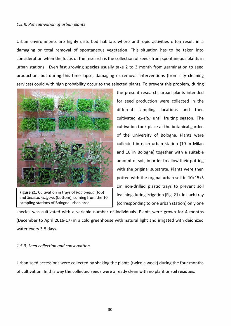
30

1.5.8. Pot cultivation of urban plants

Urban environments are highly disturbed habitats where anthropic activities often result in a

damaging or total removal of spontaneous vegetation. This situation has to be taken into

consideration when the focus of the research is the collection of seeds from spontaneous plants in

urban stations. Even fast growing species usually take 2 to 3 month from germination to seed

production, but during this time lapse, damaging or removal interventions (from city cleaning

services) could with high probability occur to the selected plants. To prevent this problem, during

the present research, urban plants intended

for seed production were collected in the

different sampling locations and then

cultivated ex-situ until fruiting season. The

cultivation took place at the botanical garden

of the University of Bologna. Plants were

collected in each urban station (10 in Milan

and 10 in Bologna) together with a suitable

amount of soil, in order to allow their potting

with the original substrate. Plants were then

potted with the orginal urban soil in 10x15x5

cm non-drilled plastic trays to prevent soil

leaching during irrigation (Fig. 21). In each tray

(corresponding to one urban station) only one

species was cultivated with a variable number of individuals. Plants were grown for 4 months

(December to April 2016-17) in a cold greenhouse with natural light and irrigated with deionized

water every 3-5 days.

1.5.9. Seed collection and conservation

Urban seed accessions were collected by shaking the plants (twice a week) during the four months

of cultivation. In this way the collected seeds were already clean with no plant or soil residues.

Figure 21. Cultivation in trays of Poa annua (top) and Senecio vulgaris (bottom), coming from the 10 sampling stations of Bologna urban area.

31

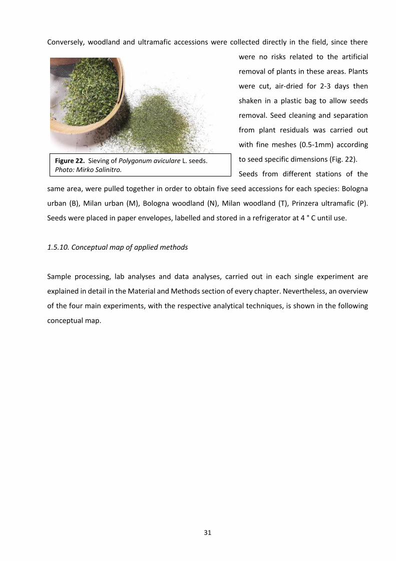
Conversely, woodland and ultramafic accessions were collected directly in the field, since there

were no risks related to the artificial

removal of plants in these areas. Plants

were cut, air-dried for 2-3 days then

shaken in a plastic bag to allow seeds

removal. Seed cleaning and separation

from plant residuals was carried out

with fine meshes (0.5-1mm) according

to seed specific dimensions (Fig. 22).

Seeds from different stations of the

same area, were pulled together in order to obtain five seed accessions for each species: Bologna

urban (B), Milan urban (M), Bologna woodland (N), Milan woodland (T), Prinzera ultramafic (P).

Seeds were placed in paper envelopes, labelled and stored in a refrigerator at 4 ° C until use.

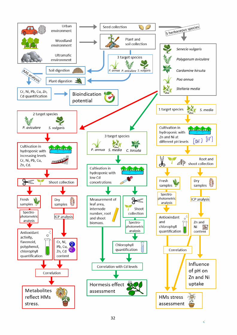
1.5.10. Conceptual map of applied methods

Sample processing, lab analyses and data analyses, carried out in each single experiment are

explained in detail in the Material and Methods section of every chapter. Nevertheless, an overview

of the four main experiments, with the respective analytical techniques, is shown in the following

conceptual map.

Figure 22. Sieving of Polygonum aviculare L. seeds. Photo: Mirko Salinitro.

32

33

1.6 References

Alexander EB, Coleman RG, Keeler-Wolf T, Harrison SP (2007). Serpentine geoecology of western North America. Oxford University Press, New York, USA.

Alloway BJ (1995). Heavy Metals in Soils, 2nd edition, Blackie Academic and Professional,

Chapman and Hall, London, UK.

Alvarez-Fernandez A, Diaz-Benito P, Abadia A, Lopez- Millan AF, Abadia J (2014). Metal species involved in long distance metal transport in plants. Frontiers in Plant Science, 5: 105.

Arazi T, Sunkar R, Kaplan B, Fromm H (1990). A tobacco plasma membrane calmodulin-binding transporter confers Ni2+ tolerance and Pb2+ hypersensitivity in transgenic plants. The Plant Journal, 20: 171–182.

Baker AJM (1981). Accumulators and excluders: strategies in the response of plants to heavy metals. Journal of Plant Nutrition, 3: 643–665.

Baker AJM, Brooks RR (1989). Terrestrial higher plants which hyperaccumulate metallic elements: a review of their distribution, ecology and phytochemistry. Biorecovery, 1: 81–126.

Baker AJM, Walker PL (1990). Ecophysiology of metal uptake by tolerant plants. In: Shaw AJ (ed.), Heavy Metal Tolerance in Plants: Evolutionary Aspects, CRC Press, Boca Raton, USA, pp. 155–177.

Baker AJM, Whiting SN (2002). In search of the Holy Grail: a further step in understanding metal hyperacumulation. New Phytologist, 155: 1–7.

Barceló J, Poschenrieder CH (1997). Chromium in plants. In: Canali S, Tittarelli F, Sequi P (eds.), Chromium: environmental issues. Franco Angeli, Milano, Italy, pp. 101–130.

Bartlett RJ (1997). The chromium scene, In: Canali S, Tittarelli F, Sequi P (eds.), Chromium Environmental Issues. Franco Angeli, Rome, pp. 304

Bartlett RJ, Kimble JM (1976). Behavior of chromium in soils. I. Trivalent forms. II. Hexavalent Forms. Journal of Environmental Quality, 5: 379–383.

Basta NT, Gradwohl R, Snethen KL, Schroder JL (2001). Chemical mobilization of lead, zinc and cadmium in smelter contaminated soils treated with exceptional quality biosolids. Journal of Environmental Quality, 30: 1222–1230.

Becquer T, Quantin C, Sicot M, Boudot JP (2003). Chromium availability in ultramafic soils from New Caledonia. Science of the Total Environment, 301: 251–261.

Bini C (2010). From soil contamination to land restoration. Nova Science Publishers Inc., New York, USA.

Bini C, Maleci L, Wahsha M (2017). Potentially toxic elements in serpentine soils and plants from Tuscany (Central Italy). A proxy for soil remediation. Catena 148: 60–66.

34

Blum WEH, Brandstetter A, Wenzel WW (1997). Trace element distribution in soils as affected by land use, In: Adriano DC, Chen ZS, Yang SS, Iskadar IK (eds.) Biogeochemistry of Trace Metals, Science Reviews, Northwood, United Kingdom pp. 466.

Bonet A, Poschenrieder C, Barceló J (1991). Chromium (III)-iron interaction in Fe-deficient and Fe-sufficient bean plants. 1. Growth and nutrient content. Journal of Plant Nutrition, 14: 403–414.

Proctor J (1993). The vegetation of ultramafic (serpentine) soils. Ed. Intercept Ltd, Andover, Hampshire, England pp. 408

Broadley MR, White PJ, Hammond JP, Zelko I, Lux A (2007). Zinc in plants. New Phytologist, 173(4): 677–702.

Brooks RR (1987). Serpentine and its vegetation. Dioscorides Press, Portland, USA.

Callahan DL, Baker AJM, Kolev SD, Wedd AG (2006). Metal ion ligands in hyperaccumulating plants. Journal of Biological Inorganic Chemistry, 11: 2–12.

Camponelli KM, Lev SM, Snodgrass JW, Landa ER, Casey RE (2010). Chemical fractionation of Cu and Zn in stormwater, roadway dust and stormwater pond sediments. Environmental Pollution, 158: 2143–2149.

Cary EE, Allaway WH, Olson OE (1977). Control of chromium concentrations in food plants. 1. Absorption and translocation of chromium by plants. Journal of Agricultural and Food Chemistry, 25: 300–304.

CASQA (2015). Zinc sources in California urban runoff. Menlo Park, CA: Technical Memo, California Stormwater Quality Association. https://www.casqa.org/

Clemens S (2001). Molecular mechanisms of plant metal tolerance and homeostasis. Planta, 212(4): 475–486.

Clemens S, Palmgren MG, Krämer U (2002). A long way ahead: understanding and engineering plant metal accumulation. Trends in Plant Science, 7: 309–315

Cohen CK, Fox TC, Garvin DF, Kochian LV (1998). The role of iron-deficiency stress responses in stimulating heavy metal transport in plants. Plant Physiology, 116: 1063–1072.

Cornu J, Deinlein U, Horeth S, Braun M, Schmidt H, Weber M, Persson DP, Husted S, Schjoerring JK, Clemens S (2015). Contrasting effects of nicotianamine synthase knockdown on zinc and nickel tolerance and accumulation in the zinc/cadmium hyperaccumulator Arabidopsis halleri. New Phytologist, 206: 738–750.

Councell TB, Duckenfield KU, Landa ER, Callender E (2004). Tire-wear particles as a source of zinc to the environment. Environmental Science and Technology, 38: 4206–4214.

Courbot M, Willems G, Motte P, Arvidsson S, Roosens N, Saumitou-Laprade P, Verbruggen N (2007). A major QTL for Cd tolerance in Arabidopsis halleri co-localizes with HMA4, a gene encoding a heavy metal ATPase. Plant Physiology, 144: 1052–1065

35

De Silva S, Ball AS, Huynh T, Reichman SM (2016). Metal accumulation in roadside soil in Melbourne, Australia: effect of road age, traffic density and vehicular speed. Environmental Pollution 208: 102–109.

Deinlein U, Weber M, Schmidt H, Rensch S, Trampczynska A, Hansen TH, Husted S, Schjoerring JK, Talke IN, Krämer U, Clemens S (2012). Elevated nicotianamine levels in Arabidopsis halleri roots play a key role in zinc hyperaccumulation. Plant Cell, 24: 708–723.

Dräger DB, Desbrosses-Fonrouge AG, Krach C, Chardonnens AN, Meyer RC, Saumitou-Laprade P, Krämer U (2004). Two genes encoding Arabidopsis halleri MTP1 metal transport proteins co-segregate with zinc tolerance and account for high MTP1 transcript levels. The Plant Journal, 39: 425–439

Duong TTT, Lee BK (2011). Determining contamination level of heavy metals in road dust from busy traffic areas with different characteristics. Journal of Environmental Management 92: 554–562.

Faucon MP, Shutcha MN, Meerts P (2007). Revisiting copper and cobalt concentrations in supposed hyperaccumulators from South Africa: influence of washing and metal concentrations in soil. Plant and Soil, 301: 29–36.

Fusco N, Micheletto L, Dal Corso G, Borgato L, Furini A (2005). Identification of cadmium regulated genes by cDNA-AFLP in the heavy metal accumulator Brassica juncea L. Journal of Experimental Botany, 56(421): 3017–3027.

Garcia-Molina A, Andrés-Colàs N, Perea-Garcia A, Del Valle-Tascon S, Penarrubia L, Puig S (2011). The intracellular Arabidopsis COPT5 transport protein is required for photosynthetic electron transport under severe copper deficiency. The Plant Journal, 65: 848–860.

Garnier J, Quaitin C, Martins ES, Becquer T (2006). Solid speciation and availability of chromium in ultramafic soils from Niquelandia, Brazil. Journal of Geochemical Exploration, 88: 206–209.

Halimaa P, Lin YF, Ahonen VH, Blande D, Clemens S, Gyenesei A, Haikio E, Karenälmpi SO, Laiho A, Aarts MG, Pursiheimo JP, Schat H, Schmidt H, Tuomainen MH, Tervahauta AI (2014). Gene expression differences between Noccaea caerulescens ecotypes help to identify candidate genes for metal phytoremediation. Environmental Science & Technology, 48: 3344–3353.

Hamer DH, Thiele DJ, Lemontt JE (1985). Function and auto regulation of yeast copper thionein. Science, 228: 685–690.

Hanikenne M, Nouet C (2011). Metal hyperaccumulation and hypertolerance: a model for plant evolutionary genomics. Current Opinion in Plant Biology, 14: 252–259.

Hanikenne M, Talke IN, Haydon MJ, Lanz C, Nolte A, Motte P, Kroymann J, Weigel D, Krämer U (2008). Evolution of metal hyperaccumulation required cisregulatory changes and triplication of HMA4. Nature, 453: 391–395.

Himelblau E, Amasino RM (2000). Delivering copper within plant cells. Current Opinion in Plant Biology, 3: 205–210.

36

Hjortenkrans DST, Bergback B, Haggerud A (2006). New metal emission patterns in road traffic environments. Environmental Monitoring and Assessment, 117: 85–98.

Ho KF, Lee SC, Chan CK, Jimmy CY, Chow JC, Yao XH (2003). Characterization of chemical species in PM2.5 and PM10 aerosols in Hong Kong. Atmospheric Environment, 37: 31–39.

Horger AC, Fones HN, Preston GM (2013). The current status of the elemental defense hypothesis in relation to pathogens. Frontiers in Plant Science, 4: 395.

Hseu ZY (2006). Concentration and distribution of chromium and nickel fractions along a serpentinitic toposequence. Soil Science, 171: 341–353.

Huang SW, Jin JY (2008). Status of heavy metals in agricultural soils as affected by different patterns of land use. Environmental Monitoring and Assessment, 339: 317–327.

Hulskotte JH, van der Gon HA, Visschedijk AJ, Schaap M (2007). Brake wear from vehicles as an important source of diffuse copper pollution. Water Science and Technology, 56: 223–231.

Hwanga HM, Fialaa MJ, Parkb D, Wadec TL (2016). Review of pollutants in urban road dust and stormwater runoff: part 1. Heavy metals released from vehicles. International Journal of Urban Sciences, 20(3): 334–360.

Jackson MT, Sampson J, Prichard HM (2007). Platinum and palladium variations through the urban environment: Evidence from 11 sample types from Sheffield, UK.Science of The Total Environment 385 (1-3):117-131

Jaquinod M, Villiers F, Kieffer-Jaquinod S, Hugouvieux V, Bruley C, Garin J, Bourguignon J (2007). A proteomics dissection of Arabidopsis thaliana vacuoles isolated from cell culture. Molecular and Cellular Proteomics, 6: 394–412

Jenny H (1980). The soil resource: origin and behavior. Springer-Verlag, New York.

Kabata-Pendias A (2011). Trace Elements in Soils and Plants. 4th edition. CRC Press/Taylor & Francis Group, Boca Raton, FL, USA.

Kampfenkel K, Kushnir S, Babiychuk E, Inze D, Van MM (1995). Molecular characterization of a putative Arabidopsis thaliana copper transporter and its yeast homologue. Journal of Biological Chemistry, 270: 28479–28486.

Krämer U (2010). Metal hyperaccumulation in plants. Annual Reviews of Plant Biology, 61(1): 517–534.

Krämer U, Cotter-Howells JD, Charnock JM, Baker AJM, Smith AC (1996). Free histidine as a metal chelator in plants that accumulate nickel. Nature, 379: 635–638.

Krämer U, Talke IN, Hanikenne M (2007). Transition metal transport. FEBS Letters, 581: 2263–2272.

Lane TW, Morel FM (2000). A biological function for cadmium in marine diatoms. Proceedings of the National Academy of Sciences of the United States of America, 97: 4627-4631.

37

Lee BD, Graham RC, Laurent TE, Amrhein C (2004). Pedogenesis in a wetland meadow and surrounding pensertinic landslide terrain, northern California, USA. Geoderma, 118: 303–320.

Li X, Poon CS, Liu PS (2001). Heavy metal contamination of urban soils and street dusts in Hong Kong. Applied Geochemistry, 16: 1361–1368.

Li Y, Hu Y, Li X, Xiao D (2003). A review on road ecology. Chinese Journal of Applied Ecology. 14: 447–452.

Logan EM, Pulford ID, Cook GT, Mackenzie AB (1997). Complexation of Cu2+ and Pb2+ by peat and humic acid. Eurasian Journal of Soil Science, 48: 685–696.

Lu L, Tian S, Zhang J, Yang X, Labavitch JM, Webb SM, Latimer M, Brown PH (2013). Efficient xylem transport and phloem remobilization of Zn in the hyperaccumulator plant species Sedum alfredii. New Phytologist, 198: 721–731.

Maitani T, Kubota H, Sato K, Yamada T (1996). The composition of metals bound to class III metallothionein (phytochelatin and its desglycyl peptide) induced by various metals in root cultures of Rubia tinctorum. Plant Physiology, 110: 1145–1150.

Manahan SE (2000). Environmental Chemistry, CRC Press LLC, Boca Raton, FL, USA.

McGahan DG, Southard RJ, Claassen V (2008). Tectonic inclusions in serpentinite landscapes contribute plant nutrient calcium. Soil Science Society of America Journal, 72:838–847.

McGrath SP (1995). Chromium and nickel. In: B.J. Alloway (ed.) Heavy Metals in Soils. 2nd edition. Blackie Academic and Professional, London, UK.

McKenzie ER, Money JE, Green PG, Young TM (2009). Metals associated with stormwater: relevant brake and tire samples. Science of the Total Environment, 407: 5855–5860.

McLaughlin MJ, Parker DR, Clarke JM (1999). Metals and micronutrients: food safety issues. Field Crops Research, 60: 143–163.

Merlot S, Hannibal L, Martins S, Martinelli L, Amir H, Lebrun M, Thomine S (2014). The metal transporter PgIREG1 from the hyperaccumulator Psychotria gabriellae is a candidate gene for nickel tolerance and accumulation. Journal of Experimental Botany, 65: 1551–1564.

Meyer CL, Verbruggen N (2012). The use of the model species Arabidopsis halleri towards phytoextraction of cadmium polluted soils. Nature Biotechnology, 30: 9–14.

Mganga N, Manoko MLK, Rulangaranga ZK (2011). Classification of plants according to their heavy metal content around north Mara gold mine, Tanzania: implication for phytoremediation. Tanzania Journal of Science, 37: 109–119.

Morel JL (1997) Bioavailability of trace elements to terrestrial plants, in Soil Ecotoxicology, Tarradellas J, Bitton G, Rossel D, eds., CRC Press, Boca Raton, FL, pp. 141,

38

Lu L, Tian S, Zhang M, Zhang J, Yang X, Jiang H. (2010) The role of Ca pathway in Cd uptake and translocation by the hyperaccumulator Sedum alfredii. Journal of hazardous materials 183(1-3): 22-28 Morrissey J, Baxter IR, Lee J, Li L, Lahner B, Grotz N, Kaplan J, Salt DE, Guerinot ML (2009). The ferroportin metal efflux proteins function in iron and cobalt homeostasis in Arabidopsis. The Plant Cell, 21: 3326–3338.

Murphy A, Taiz L (1995). Comparison of metallothionein gene expression and non-protein thiols in ten Arabidopsis ecotypes: correlation with copper tolerance. Plant Physiology, 109: 945–954.

Nies DH (1999). Microbial heavy-metal resistance. Applied Microbiology and Biotechnology, 51(6): 730–750.

Nishida S, Aisu A, Mizuno T (2012). Induction of IRT1 by the nickel-induced iron-deficient response in Arabidopsis. Plant Signaling & Behavior, 7: 329–331.

Nishida S, Tsuzuki C, Kato A, Aisu A, Yoshida J, Mizuno T (2011). AtIRT1, the primary iron uptake transporter in the root, mediates excess nickel accumulation in Arabidopsis thaliana. Plant and Cell Physiology, 52: 1433–1442.

Oze C, Fendorf S, Bird DK, Coleman RG (2004). Chromium geochemistry of serpentine soils. International Geology Review, 46: 97–126.

Palacios MA, Gomez M, Moldovan M, Morrison G, Rauch S, McLeod C, Torrens JM (2000). Platinum-group elements: quantification in collected exhaust fumes and studies of catalysts surfaces. Science of the Total Environment, 257: 1–15.

Penarrubia L, Andrés-Colàs N, Moreno J, Puig S (2010). Regulation of copper transport in Arabidopsis thaliana: a biochemical oscillator? Journal of Biological Inorganic Chemistry, 15: 29–36.

Pich A, ScholzI G (1996). Translocation of copper and other micronutrients in tomato plants (Lycopersicon esculentum Mill.): nicotianamine-stimulated copper transport in the xylem. Journal of Experimental Botany, 47: 41–47.

Pollard AJ, Reeves RD, Baker AJM (2014). Facultative hyperaccumulation of heavy metals and metalloids. Plant Science, 218: 8–17.

Raskin I, Ensley BD (2000). Phytoremediation of toxic metals: using plants to clean up the environment. Wiley, New York, USA.

Rauch S, Hemond HF, Barbante C, Owari M, Morrison GM, Peucker-Ehrenbrink B, Wass U (2005). Importance of automobile exhaust catalyst emissions for the deposition of platinum, palladium, and rhodium in the northern hemisphere. Environmental Science and Technology, 39: 8156–8162.

Reck BK, Müller DB, Rostkowski K, Graedel TE (2008). Anthropogenic nickel cycle: insights into use, trade, and recycling. Environmental Science & Technology, 42: 3394–3400.

39

Rellan-Alvarez R, Abadia J, Alvarez-Fernandez A (2008). Formation of metal-nicotianamine complexes as affected by pH, ligand exchange with citrate and metal exchange. A study by electrospray ionization time-of-flight mass spectrometry. Rapid Communications in Mass Spectrometry, 22: 1553–1562.

Sancenon V, Puig S, Mateu-Andres I, Dorcey E, Thiele DJ, Penarrubia L (2004). The Arabidopsis copper transporter COPT1 functions in root elongation and pollen development. Journal of Biological Chemistry, 279: 15348–15355.

Sarret G, Smits E, Michel HC, Isaure MP, Zhao FJ, Tappero R (2013). Use of synchrotron-based techniques to elucidate metal uptake and metabolism in plants. In: Sparks DL (ed.), Advances in agronomy, vol 119. Elsevier Academic, San Diego, USA.

Schaaf G, Honsbein A, Meda AR, Kirchner S, Wipf D, von Wiren N (2006). AtIREG2 encodes a tonoplast transport protein involved in iron-dependent nickel detoxification in Arabidopsis thaliana roots. Journal of Biological Chemistry, 281: 25532–25540.

Shahzad Z, Gosti F, Frerot H, Lacombe E, Roosens N, Saumitou-Laprade P, Berthomieu P (2010). The five AhMTP1 zinc transporters undergo different evolutionary fates towards adaptive evolution to zinc tolerance in Arabidopsis halleri. PLoS Genetics, 6(4): e1000911.

Shanker AK, Cervantes C, Loza-Tavera H, Avudainayagam S (2005). Chromium toxicity in plants. Environment International, 31: 739–753.

Singh B (2001). Heavy metals in soils: sources, chemical reactions and forms. In: D. Smith, S. Fityus and M. Allman (eds.), Geotechnics: Proceedings of the 2nd Australia and New Zealand Conference on Environmental Geotechnics, Newcastle, NSW, Australia, 28-30 November 2001

Singh HP, Mahajan P, Kaur S, Batish DR, Kohli RH (2013). Chromium toxicity and tolerance in plants. Environmental Chemistry Letters, 11(3): 229–254.

Skeffington RA, Shewry PR, Peterson PJ (1976). Chromium uptake and transport in barley seedlings (Hordeum vulgare L.). Planta, 132: 209–214.

Straffelini G, Ciudin R, Ciotti A, Gialanella S (2015). Present knowledge and perspectives on the role of copper in brake materials and related environmental issues: a critical assessment. Environmental Pollution, 207: 211–219.

Talke IN, Hanikenne M, Krämer U (2006). Zinc dependent global transcriptional control, transcriptional deregulation, and higher gene copy number for genes in metal homeostasis of the hyperaccumulator Arabidopsis halleri. Plant Physiology, 142: 148–167.

Taylor MD, Percival HJ (2001). Cadmium in soil solutions from a transect of soils away from a fertilizer bin. Environmental Pollution, 113: 35–40.

The Arabidopsis Genome Initiative (2000). Analysis of the genome sequence of the flowering plant Arabidopsis thaliana. Nature 408: 796–815.

40

UNEP (2015). Leaded petrol phase-out: Global status as at January 2015. Nairobi: Partnership for Clean Fuels and Vehicles, United Nations Environment Programme. https://www.unenvironment.org

USDI (2009). Mineral Commodity Summary. United States Geological Survey, Reston, VA. https://www.usgs.gov/

USEPA (2015). Copper-free brake initiative. Washington, DC: National Pollutant Discharge Elimination System, United States Environmental Protection Agency. https://www.epa.gov/

van de Mortel JE, Almar Villanueva L, Schat H, Kwekkeboom J, Coughlan S, Moerland PD, Ver Loren van Themaat E, Koornneef M, Aarts MG (2006). Large expression differences in genes for iron and zinc homeostasis, stress response and lignin biosynthesis distinguish Arabidopsis thaliana and the related metal hyperaccumulator Thlaspi caerulescens. Plant Physiology, 142: 1127–1147.

van der Ent A, Baker AJM, Reeves RD, Pollard AJ, Schat H (2013). Hyperaccumulators of metal and metalloid trace elements: facts and fiction. Plant and Soil 362: 319–334.

van der Ent A, Baker AJM, Echevarria G, Morel JL (2017). Agromining: farming for metal. Extracting unconventional resources using plants. Springer International Publishing. Reston, VA, USA.

Varrica D, Dongarra G, Sabatino G, Monna F (2003). Inorganic geochemistry of roadway dust from the metropolitan area of Palermo, Italy. Environmental Geology, 44: 222–230.

Vega FA, Covelo EF, Vazques JJ, Abdrade L (2007). Influence of mineral and organic components on copper, lead and zinc sorption by acid soils. Journal of Environmental Science and Health, Part A: Toxic/Hazardous Substances and Environmental Engineering, 42: 2167–2173.

Vert G, Grotz N, Dedaldechamp F, Gaymard F, Guerinot ML, Briat JF, Curie C (2002). IRT1, an Arabidopsis transporter essential for iron uptake from the soil and for plant growth. The Plant Cell, 14: 1223–1233.

Von Wirén N, Klair S, Bansal S, Briat JF, Khodr H, Shioiri T, Leigh RA, Hider RC (1999). Nicotianamine chelates both Fe III and Fe II. Implications for metal transport in plants. Plant Physiology, 119: 1107–1114.

Vos JH, Janssen MPM (2008). EU-wide control measures to reduce pollution from water framework directive relevant substances. Copper and Zinc in the Netherlands. National Institute for Public Health and the Environment (RIVM Report 607633002). Amsterdam, Netherland.

Walter J (2009). Zinc about it. Tire Technology International, March. 18. https://www.tiretechnologyinternational.com/online-magazines/in-this-issue-march-2018.html

Weast RC (1984). Handbook of Chemistry and Physics, CRC Press, Boca Raton, FL, USA.

WSDE (2011). Control of toxic chemicals in puget sound: Phase 3: Primary sources of selected toxic chemicals and quantities released in the puget sound basin (Publication No. 11-03-024). Olympia, WA, USA: Washington State Department of Ecology. https://ecology.wa.gov

41

Yuen JQ, Olin PH, Lim HS, Benner SG, Sutherland RA, Ziegler AD (2012). Accumulation of potentially toxic elements in road deposited sediments in residential and light industrial neighborhoods of Singapore. Journal of Environmental Management, 101: 151–163.

Zayed A, Lytle CM, Qian JH, Terry N (1998). Chromium accumulation, translocation and chemical speciation in vegetable crops. Planta, 206: 293–299.

42

RESEARCH CHAPTERS

2. Heavy metals bioindication potential of the common weeds Senecio vulgaris L., Polygonum

aviculare L. and Poa annua L.

Article status

Published: Salinitro Ma, Tassoni Aa, Casolari Sb, de Laurentiis Fb, Zappi Ab, Melucci Db. Heavy Metals

Bioindication Potential of the Common Weeds Senecio vulgaris L., Polygonum aviculare L. and Poa

annua L. Molecules 2019, 24, 2813

a Department of Biological Geological and Environmental Sciences, University of Bologna, Via Irnerio

42, 40126 Bologna, Italy

b Department of Chemistry “G. Ciamician”, University of Bologna, Via Selmi 2, 40126 Bologna, Italy

Author Contributions

Mirko Salinitro collected the samples, analysed the data, wrote the manuscript and coordinated the

study. Dora Melucci analysed the data and contributed to write the manuscript. Sonia Casolari and

Francesco de Laurentiis performed the AAS analyses. Annalisa Tassoni coordinated the study and

revised the manuscript. Alessandro Zappi analysed the data.

List of abbreviations

AAS = Atomic Absorption Spectroscopy

BAF = Bio-accumulation factor

BAF_BM = Bio-accumulation Factor calculated on bioavailable metal in soil

BAF_TM = Bio-accumulation Factor calculated on total metal in soil

BM = Bioavailable soil metal concentration

HMs = Heavy metals

IM = Inorganic matter

LOO-CV = leave-one-out cross-validation

LoD = Limit of detection

OM = Organic matter

PM = Plant metal concentration

TM = Total soil metal concentration

43

2.1. Introduction

The fast urbanization and industrialization in the last decades have resulted in increasing contents

of trace metals in the environment (Wang et al., 2014; Ahmad et al., 2016; Charlerworth et al.,

2011). These elements are not degradable, therefore they could accumulate in soil and become

potentially hazardous to terrestrial and aquatic ecosystems, and thus to human and animal life

(Melucci et al., 2018; Tchounwou et al., 2012). HMs are naturally present in the environment as a

result of either natural processes or human activities (He et al., 2005; Li et al., 2009). In natural

ecosystems, HMs come from ultramafic rocks and ore minerals and, during weathering that leads

to soil formation, could be released in the environment (Szyczewski et al., 2009). On the other hand,

anthropogenic sources (i.e. vehicular traffic, mining activities and refining processes) are nowadays

the main responsible for HMs pollution (Kabata-Pendias and Mukherjee, 2007; Norgate et al., 2007).

Urban areas are recognized to be the major sources for contaminants (Markert et al., 2011;

Wiseman et al., 2013), and traffic is the primary source of HMs that accumulate in roadside soils

(Zereini et al., 2007) and street dust (Lough et al., 2005). HMs are produced by vehicles tailpipe

emissions, as well as from the wear and tear of mechanical components such as brakes, tires and

catalytic converters (Zereini et al., 2007; Zereini et al., 2012).

In recent years, it has been shown that HMs levels in soil and vegetation have increased considerably

due to traffic pollution, and the problem rises as daily traffic increases (Onder and Dursun, 2006).

This diffuse source of pollution in areas where people live and food is produced, poses a serious

threat to human health. In fact, these pollutants can enter plants directly via foliar absorption or

taken up from the soil through the root system (Jozic et al., 2009) and undergo processes of bio-

magnification (Locatelli and Melucci, 2012; Locatelli and Melucci, 2013). Despite the high toxicity of

HMs for plants, when these elements are present in soil at low concentrations plants continue to

grow healthy even while accumulating these metals. The ability of plants to accumulate HMs into

their tissues may therefore be used to monitor soil pollution (Malizia et al., 2012).

Biomonitoring techniques using indicator plants (bioindication) are becoming common methods to

detect toxic levels of HMs in the environments. Mosses and lichens, for example, are known to be

the most sensitive indicators of atmospheric pollution (Jenkis, 1987; Jiang et al., 2018), thus they

are broadly used in urban environment. Unfortunately, because of the absence of roots and their

restricted presence on hard substrate, they are not suitable for soil monitoring. Many authors agree

that herbaceous plants could be effective biomonitoring tools, and some common species like the

dandelion (Taraxacum officinale Weber), nettle (Urtica dioica L.) and broadleaf plantain (Plantago

44

major L.) have already been successfully used (Malizia et al., 2012; Galal and Shehata, 2015; Rule,

1994; Fröhlichová et al., 2018). Not all plants are suitable as indicators; some basic characteristic of

a good bioindicator were listed by Wittig, (1993). An indicator plant should: i) accumulate one or

several selected elements; ii) have low sensitivity to the accumulated elements; iii) have wide

distribution in various environments; iv) show a correlation between metal accumulation and input

into the ecosystem.

Even when using the right plant, bioindication properties could be affected by other factors like soil

properties complexation of HMs, oxidation state (Szyczewski et al., 2009; Lin and Zhang, 1990) and

phenologic phase of the plants (Keane et al., 2001). Seasonality plays an important role in

determining HMs concentration in plant tissues. Despite some species grow all year long, it has been

demonstrated that Cu, Fe, Mn, Pb and Zn contents in dandelion leaves collected in autumn, were

higher compared to those collected at the same sites in spring (Keane et al., 2001). Similar results

were reported for alfalfa (Medicago sativa L.) with regard to Mo content (Karlsson, 1961). Soil

properties, like cationic exchange capacity, clay content, pH, organic matter content, are likely to

change HMs availability to plants (Kashem and Singh, 2001; Antoniadis et al., 2008). For example,

Dai et al. (2004) estimated that extractable Cd, Pb and Zn in contaminated soils were positively

correlated with organic matter contents due to the consequent pH decrease. Moreover, low pH is

optimal for metal availability since solubility has been shown to increase with decreasing pH (Ghosh

and Singh, 2005; Nanda and Abraham, 2013). Given the high variability of soils, bioindication could

not be considered a technique able to precisely measure trace metal in soil, but rather a way to

estimate them and their interaction with plants in some specific conditions. Therefore, it is of vital

importance to assess indication properties of a species on several soils that differ for their HMs

content and physical properties.

The aim of our study was to test the ruderal species Senecio vulgaris L., Polygonum aviculare L. and

Poa annua L., as possible candidates for the biomonitoring Cu, Zn, Cd, Cr, Ni and Pb in multiple

environments. Furthermore, we aimed at assessing how different type of soils can affect the

predictive potential of these species.

45

2.2. Materials and Methods

2.2.1. Samples collection

For this study, three common weed species that had the basic characteristic to be good biondicators

according to Wittig (1993) were selected. All the three species are ruderal plants, which makes them

common in all anthropic habitats, and in particular:

1) Senecio vulgaris L. (groundsel) is an annual plant of the Asteraceae family. Originally with an

Eurasiatic distribution, today it has become sub-cosmopolitan worldwide. The species is common in

all habitats among which disturbed areas like road margins, arable fields and gardens. It preferably

grows on clay soil rich in nitrogen and organic matter.

2) Poa annua L. (annual bluegrass) is an annual plant of the Poaceae family. Originally with an

Eurasiatic distribution, today widely naturalized in the temperate areas of the globe. It’s a pioneer

species that grows in trampled areas, gardens and roads margins, on nitrogen-rich soils.

3) Polygonum aviculare L. (common knotgrass) is an annual plant of the Polygonaceae family. The

species is cosmopolitan and, because of its high variability, it is adaptable to several habitats growing

on all soil types and being resistant to trampling. It is widespread in urban areas, arable fields, but

also woodland margins.

To maximize the metal content in the tissues, plants were harvested close to the end of their life

cycle, therefore during the fruiting season (April-May 2017 for P. annua and S. vulgaris, October

2017 for P. aviculare). Only the aerial parts of the plants were sampled. After collection, plants

where thoroughly washed with deionized water, then oven dried at 50° C until constant weight.

Dried samples were powdered with an Ultraturrax IKA® A11 basic (Staufen, Germany), then stored

at room temperature until analysis. In order to have high heterogeneity of soil conditions, the three

herbaceous species were harvested in 8 stations belonging to three different habitats (Fig. 1). Five

stations were from the urban environments of Bologna and Milan city centers (BO7, BO8, MI3, MI4,

MI9), two stations were from woodland environment (Ticino Park Loc. Besate, (MI) Talon Park,

Casalecchio (BO), respectively NAT1, NAT5) and one was an ultramafic station from Mount Prinzera

(Parma, Italy) (NAT8)

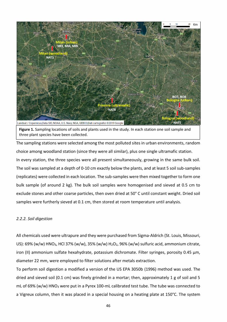
46

The sampling stations were selected among the most polluted sites in urban environments, random

choice among woodland station (since they were all similar), plus one single ultramafic station.

In every station, the three species were all present simultaneously, growing in the same bulk soil.

The soil was sampled at a depth of 0-10 cm exactly below the plants, and at least 5 soil sub-samples

(replicates) were collected in each location. The sub-samples were then mixed together to form one

bulk sample (of around 2 kg). The bulk soil samples were homogenised and sieved at 0.5 cm to

exclude stones and other coarse particles, then oven dried at 50° C until constant weight. Dried soil

samples were furtherly sieved at 0.1 cm, then stored at room temperature until analysis.

2.2.2. Soil digestion

All chemicals used were ultrapure and they were purchased from Sigma-Aldrich (St. Louis, Missouri,

US): 69% (w/w) HNO3, HCl 37% (w/w), 35% (w/w) H2O2, 96% (w/w) sulfuric acid, ammonium citrate,

iron (II) ammonium sulfate hexahydrate, potassium dichromate. Filter syringes, porosity 0.45 µm,

diameter 22 mm, were employed to filter solutions after metals extraction.

To perform soil digestion a modified a version of the US EPA 3050b (1996) method was used. The

dried and sieved soil (0.1 cm) was finely grinded in a mortar; then, approximately 1 g of soil and 5

mL of 69% (w/w) HNO3 were put in a Pyrex 100-mL calibrated test tube. The tube was connected to

a Vigreux column, then it was placed in a special housing on a heating plate at 150°C. The system

Figure 1. Sampling locations of soils and plants used in the study. In each station one soil sample and three plant species have been collected.

47

was left in reflux mode for 30 min. Subsequently, the tube was cooled in an ice-bath, then 5 mL of

35% (w/w) H2O2 were added, and the addition of H2O2 drops continued until the solution in the tube

stopped boiling. Then, 10 mL of 37% (w/w) HCl were introduced, and another reflux step was applied

for 15 min. Once digestion was completed, the solution was cooled down and filtered. Finally, the

liquid phase was transferred into a 50 mL flask and brought to the final volume with 0.5 M HNO3.

The total concentration of metals in soils (TM) was measured in µg/g (briefly indicated as ppm).

Blank digestions (without soil) were carried out using the same reagents as described above.

2.2.3. Plant digestions

Acid digestion on plant shoots was carried using a modified protocol adapted from Huang and

Schulte (1985). An aliquot of plant powdered shoots, between 0.05 and 0.1 g, was placed in a 10-

mL glass tube and 2 mL of 69% (w/w) HNO3 were added. A pre-digestion phase was obtained by

leaving the tubes at room temperature for 24 hours; then the tubes were first placed on a hot plate

at 75°C for 1 h and subsequently the temperature was risen to 125°C for another 1 h. During the

digestion the tubes were left open without any reflux system.

In the 2-hours digestion the volume of acid reduced to about 1 mL; then it was transferred in a 10-

mL flask and brought to the final volume with MilliQ water to obtain a digestate with about 6-7%

(w/w) HNO3. Generally, even though no plant residues were visible, they were filtered by 0.45 µm

filters. The concentration of metals in plants (PM) was measured in µg/g (briefly indicated as ppm).

Blank digestions (without plants) were carried out using the same reagents as described above.

2.2.4. Extraction of bioavailable metal fraction from soil

The dried and sieved soil (0.1 cm) was finely grinded in a mortar, then sieved with a 0.5 mm mesh.

5 g of sieved soil was then transferred to an extraction bottle in which 5 mL of 2% (w/v) ammonium

citrate solution were added. The obtained mixture was shaken on an end-over-end tube roller mixer

at 30 rpm for 1 h at 20°C. The extracts were immediately separated by decantation for few minutes,

followed by centrifugation for 10 min at about 3000 x g. The supernatant was recovered and the

liquid was stored in a polyethylene container at 4°C until analysis. The concentration of bioavailable

metals in soil (MeCitr) was measured in µg/g (ppm). Blank extractions (without soil) was carried out

using the same reagents as described above (Quevauviller, 2002).

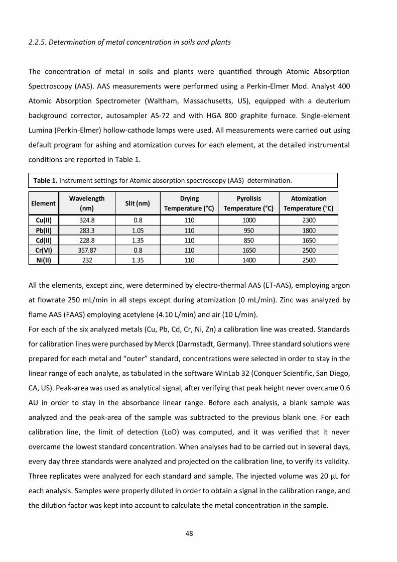
48

2.2.5. Determination of metal concentration in soils and plants

The concentration of metal in soils and plants were quantified through Atomic Absorption

Spectroscopy (AAS). AAS measurements were performed using a Perkin-Elmer Mod. Analyst 400

Atomic Absorption Spectrometer (Waltham, Massachusetts, US), equipped with a deuterium

background corrector, autosampler AS-72 and with HGA 800 graphite furnace. Single-element

Lumina (Perkin-Elmer) hollow-cathode lamps were used. All measurements were carried out using

default program for ashing and atomization curves for each element, at the detailed instrumental

conditions are reported in Table 1.

All the elements, except zinc, were determined by electro-thermal AAS (ET-AAS), employing argon

at flowrate 250 mL/min in all steps except during atomization (0 mL/min). Zinc was analyzed by

flame AAS (FAAS) employing acetylene (4.10 L/min) and air (10 L/min).

For each of the six analyzed metals (Cu, Pb, Cd, Cr, Ni, Zn) a calibration line was created. Standards

for calibration lines were purchased by Merck (Darmstadt, Germany). Three standard solutions were

prepared for each metal and “outer” standard, concentrations were selected in order to stay in the

linear range of each analyte, as tabulated in the software WinLab 32 (Conquer Scientific, San Diego,

CA, US). Peak-area was used as analytical signal, after verifying that peak height never overcame 0.6

AU in order to stay in the absorbance linear range. Before each analysis, a blank sample was

analyzed and the peak-area of the sample was subtracted to the previous blank one. For each

calibration line, the limit of detection (LoD) was computed, and it was verified that it never

overcame the lowest standard concentration. When analyses had to be carried out in several days,

every day three standards were analyzed and projected on the calibration line, to verify its validity.

Three replicates were analyzed for each standard and sample. The injected volume was 20 μL for

each analysis. Samples were properly diluted in order to obtain a signal in the calibration range, and

the dilution factor was kept into account to calculate the metal concentration in the sample.

Table 1. Instrument settings for Atomic absorption spectroscopy (AAS) determination.

ElementWavelength

(nm)Slit (nm)

Drying

Temperature (°C)

Pyrolisis

Temperature (°C)

Atomization

Temperature (°C)

Cu(II) 324.8 0.8 110 1000 2300

Pb(II) 283.3 1.05 110 950 1800

Cd(II) 228.8 1.35 110 850 1650

Cr(VI) 357.87 0.8 110 1650 2500

Ni(II) 232 1.35 110 1400 2500

49

In order to analyze Cd, Cr, Ni and Pb by AAS, some matrix modifiers were necessary. In particular

Mg(NO3)2 (Perkin Elmer, Waltham, Massachusetts, US) for Cd and Cr, PdCl2 (Fluka, Honeywell,

Morris Planes, NJ, USA) for Cd, and NH4H2PO4 (Sigma Aldrich, St. Louis, Missouri, US) for Pb. 20

μL/mL of a solution containing all of the modifiers were added to each sample, final concentrations:

200 mg/L for Mg(NO3)2, 2.3 mg/L for PdCl2, 4 mg/L for NH4H2PO4. It was also verified that the

presence of an unnecessary modifiers did not influence the measurements of other metals (as Cu

and Zn, which did not require any modifier).

2.2.6. Determination of organic matter and granulometry of soil

The percentage of organic matter in soils (OM) was determined by two experimental methods:

titration and Loss on Ignition. The percentage of inorganic matter (IM) was calculated as 100% - OM

%.

To measure OM, the titration was carried out following the method of Walkley and Black (1934). 0.5

g of soil, 10 mL of potassium dichromate 0.167 M and 20 mL of 96% (w/w) sulfuric acid were placed

in a 500 mL conical flask, slowly percolating along the internal walls of the flask, not to overheat the

mixture. The flask was covered with watch glass and left to rest for 30 min. Then the reaction was

interrupted by adding 200 mL of distilled water, previously cooled in the refrigerator. A few drops

of ferroin (redox indicator) were added, and titration was carried out with a solution of iron (II)

ammonium sulfate hexahydrate 0.5 M until the color changed. At the same time, a blank test was

performed with 10 mL of dichromate, 20 mL of sulfuric acid and 200 mL of distilled water. The

following expression was used for the calculation of organic carbon (C) expressed in g/kg.

𝐶 = 3.9 ∙(𝐵−𝐴)

𝑀𝑆𝑜𝑖𝑙∙ MFe

where: B = volume of the solution of iron (II) ammonium sulfate hexahydrate used in the titration

of the blank test, expressed in mL; A = volume of the solution of iron (II) ammonium sulfate

hexahydrate used in the titration of the sample solution, expressed in mL; MFe = effective molarity

of the solution of iron (II) ammonium sulfate hexahydrate; MSoil = mass of the soil sample,

expressed in grams. To transform g/kg of organic carbon into the corresponding organic substance

content, a conversion factor is applied: % OM_titr = % OM_titr x 1.724.

To validate OM content found by titration, we compared the results with the one found by Loss on

Ignition method (official method for the determination of OM) as explained in Storer (1984). The

two methods were comparable and gave similar results, therefore the titration method results were

validated and used for statistical elaborations.

50

Granulometry of the samples was assessed by sieving samples with gradually smaller mashes and

weighting the fraction held into each mesh. Four classes of granulometry were defined: particles >

0.5 mm (coarse), particles between 0.5 and 0.25 mm (medium), particles between 0.25 mm and 63

µm (fine) particles < 63 µm (ultra fine).

2.2.7. Data analysis

The matrix containing all collected data was composed by 86 observation (objects) and 43 variables.

We used chemometrics to extract useful information from our dataset and in particular to create

and validate models. Chemometrics was applied both in univariate mode (analysis of correlation,

creation of linear regression) and in multivariate mode (Principal Components Analysis, PCA) (Miller

and Miller, 2010; Brereton, 2007). To create linear models, the Multiple Linear Regression tool

(MLR) was applied. In order to validate MLR models, besides considering the model p-values

(ANOVA test), which should be close to the null value, the same data used to create the model were

projected onto it, both in calibration mode (blue dots in response plots in results section) and by

leave-one-out cross-validation (LOO-CV) (red dots in response plots in results section). Projection in

calibration mode means that, once created the model, data are projected into it as they are. LOO-

CV, on the other side, creates as many models as the number of samples, leaving each time one

sample out from the model creation and projecting it onto such model. In this way, each sample is

treated as if it was an external data used to validate the regression performance of the overall

model. Both in calibration and in LOO-CV, response values of each sample are recalculated by

projection. Then, two further response lines are computed (blue for calibration mode, red for LOO-

CV), in which the independent variables are the known (experimental) response and the dependent

variables are the recalculated values that appear in the response plot. The predictive model

performances are evaluated by the parameters of these lines. In a perfect case, the recalculated

responses would be exactly equal to the known ones, thus the response lines would be the bisector

of the response plot, with slope=1, offset=0 and R2=1. Model performances are considered

acceptable if the response line parameters are close to these ideal values. A further parameter of

the response lines is root-mean-squared-error (RMSE), which is a sort of sum of distances between

the known responses and the recalculated ones, therefore, it should be close to zero. The potential

suitability of a species as bio-indicator of one or more metals was validated in two steps. Firstly, we

tested the correlation between bioaccumulation factor calculated on TM and Bioaccumulation

factor calculated on BM, if that correlation was good (between 0.7 and 1), we tested the correlation

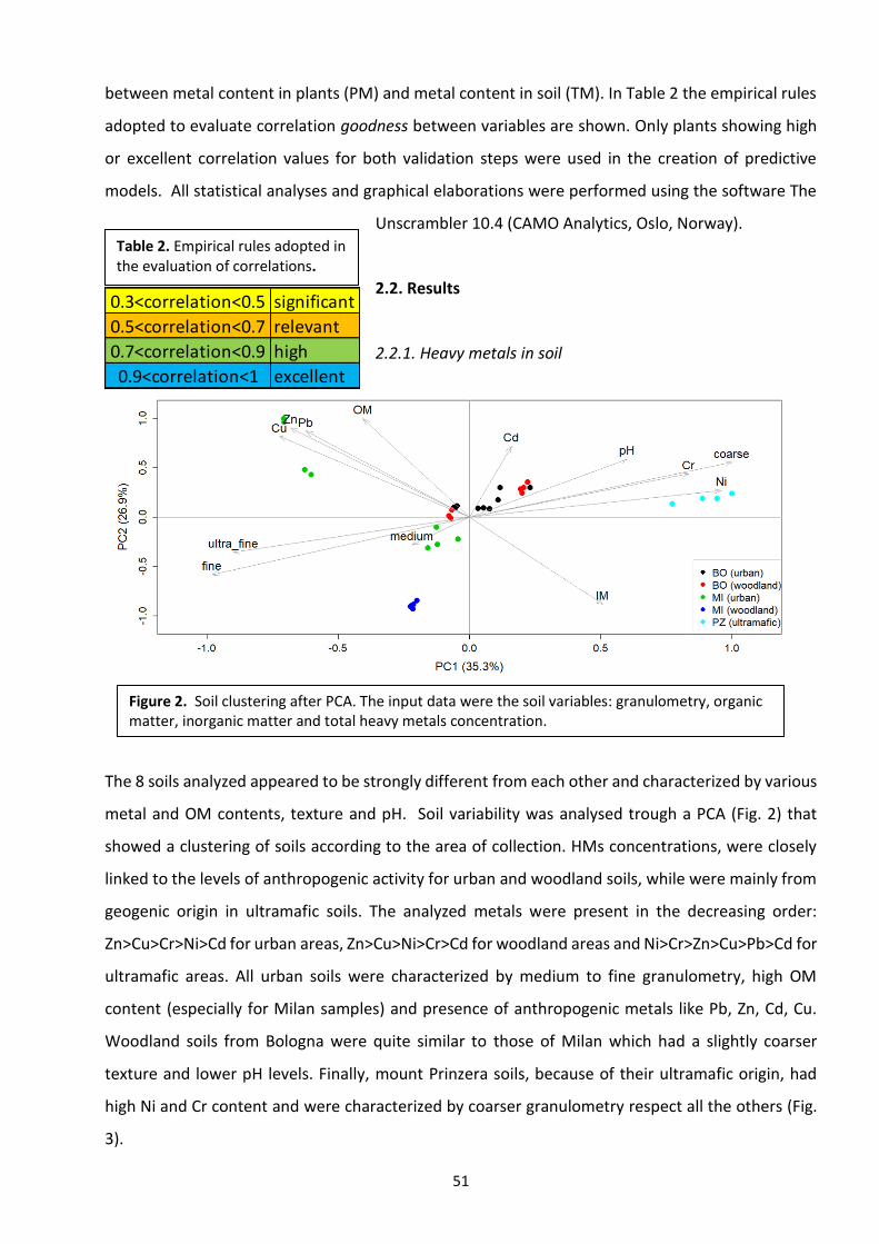
51

between metal content in plants (PM) and metal content in soil (TM). In Table 2 the empirical rules

adopted to evaluate correlation goodness between variables are shown. Only plants showing high

or excellent correlation values for both validation steps were used in the creation of predictive

models. All statistical analyses and graphical elaborations were performed using the software The

Unscrambler 10.4 (CAMO Analytics, Oslo, Norway).

2.2. Results

2.2.1. Heavy metals in soil

The 8 soils analyzed appeared to be strongly different from each other and characterized by various

metal and OM contents, texture and pH. Soil variability was analysed trough a PCA (Fig. 2) that

showed a clustering of soils according to the area of collection. HMs concentrations, were closely

linked to the levels of anthropogenic activity for urban and woodland soils, while were mainly from

geogenic origin in ultramafic soils. The analyzed metals were present in the decreasing order:

Zn>Cu>Cr>Ni>Cd for urban areas, Zn>Cu>Ni>Cr>Cd for woodland areas and Ni>Cr>Zn>Cu>Pb>Cd for

ultramafic areas. All urban soils were characterized by medium to fine granulometry, high OM

content (especially for Milan samples) and presence of anthropogenic metals like Pb, Zn, Cd, Cu.

Woodland soils from Bologna were quite similar to those of Milan which had a slightly coarser

texture and lower pH levels. Finally, mount Prinzera soils, because of their ultramafic origin, had

high Ni and Cr content and were characterized by coarser granulometry respect all the others (Fig.

3).

0.3<correlation<0.5 significant

0.5<correlation<0.7 relevant

0.7<correlation<0.9 high

0.9<correlation<1 excellent

Table 2. Empirical rules adopted in the evaluation of correlations.

Figure 2. Soil clustering after PCA. The input data were the soil variables: granulometry, organic matter, inorganic matter and total heavy metals concentration.

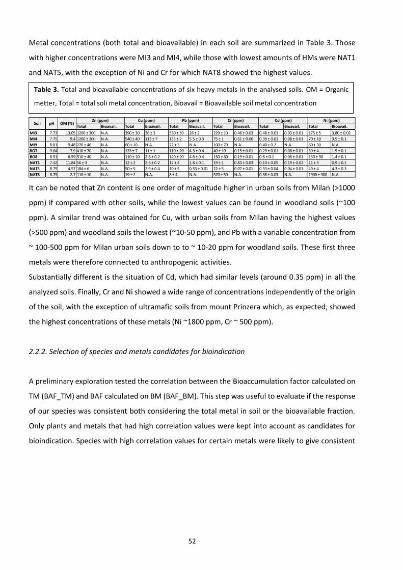
52

Metal concentrations (both total and bioavailable) in each soil are summarized in Table 3. Those

with higher concentrations were MI3 and MI4, while those with lowest amounts of HMs were NAT1

and NAT5, with the exception of Ni and Cr for which NAT8 showed the highest values.

It can be noted that Zn content is one order of magnitude higher in urban soils from Milan (>1000

ppm) if compared with other soils, while the lowest values can be found in woodland soils (~100

ppm). A similar trend was obtained for Cu, with urban soils from Milan having the highest values

(>500 ppm) and woodland soils the lowest (~10-50 ppm), and Pb with a variable concentration from

~ 100-500 ppm for Milan urban soils down to to ~ 10-20 ppm for woodland soils. These first three

metals were therefore connected to anthropogenic activities.

Substantially different is the situation of Cd, which had similar levels (around 0.35 ppm) in all the

analyzed soils. Finally, Cr and Ni showed a wide range of concentrations independently of the origin

of the soil, with the exception of ultramafic soils from mount Prinzera which, as expected, showed

the highest concentrations of these metals (Ni ~1800 ppm, Cr ~ 500 ppm).

2.2.2. Selection of species and metals candidates for bioindication

A preliminary exploration tested the correlation between the Bioaccumulation factor calculated on

TM (BAF_TM) and BAF calculated on BM (BAF_BM). This step was useful to evaluate if the response

of our species was consistent both considering the total metal in soil or the bioavailable fraction.

Only plants and metals that had high correlation values were kept into account as candidates for

bioindication. Species with high correlation values for certain metals were likely to give consistent

Total Bioavail. Total Bioavail. Total Bioavail. Total Bioavail. Total Bioavail. Total Bioavail.

MI3 7.73 13.05 1200 ± 300 N.A. 390 ± 30 36 ± 3 530 ± 50 28 ± 2 229 ± 10 0.48 ± 0.03 0.48 ± 0.01 0.03 ± 0.01 175 ± 5 3.80 ± 0.02

MI4 7.75 9.4 1200 ± 200 N.A. 540 ± 40 113 ± 7 135 ± 2 5.5 ± 0.3 75 ± 1 0.61 ± 0.06 0.39 ± 0.01 0.08 ± 0.01 70 ± 10 3.5 ± 0.1

MI9 8.81 9.48 270 ± 40 N.A. 60 ± 10 N.A. 22 ± 3 N.A. 100 ± 70 N.A. 0.40 ± 0.2 N.A. 60 ± 30 N.A.

BO7 9.04 7.9 410 ± 70 N.A. 133 ± 7 11 ± 1 110 ± 20 4.3 ± 0.4 40 ± 10 0.15 ± 0.01 0.29 ± 0.01 0.08 ± 0.01 39 ± 4 1.5 ± 0.1

BO8 8.91 6.59 510 ± 40 N.A. 110 ± 10 2.6 ± 0.2 120 ± 20 4.6 ± 0.4 150 ± 60 0.19 ± 0.01 0.6 ± 0.1 0.06 ± 0.01 130 ± 90 1.4 ± 0.1

NAT1 7.42 11.84 56 ± 3 N.A. 12 ± 2 2.6 ± 0.2 12 ± 4 2.8 ± 0.1 19 ± 1 0.83 ± 0.03 0.10 ± 0.05 0.19 ± 0.02 11 ± 3 0.9 ± 0.1

NAT5 8.79 4.57 184 ± 6 N.A. 50 ± 5 3.9 ± 0.4 19 ± 5 0.53 ± 0.01 22 ± 5 0.07 ± 0.01 0.33 ± 0.04 0.04 ± 0.01 49 ± 4 4.3 ± 0.3

NAT8 8.79 2.7 110 ± 10 N.A. 19 ± 2 N.A. 8 ± 4 N.A. 570 ± 50 N.A. 0.38 ± 0.03 N.A. 1900 ± 300 N.A.

Soil pH OM (%)Ni (ppm)Zn (ppm) Cu (ppm) Pb (ppm) Cr (ppm) Cd (ppm)

Table 3. Total and bioavailable concentrations of six heavy metals in the analysed soils. OM = Organic

metter, Total = total soli metal concentration, Bioavail = Bioavailable soil metal concentration

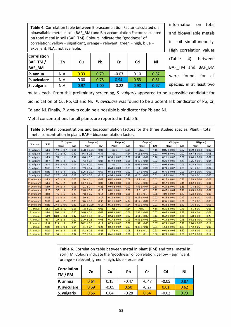
53

information on total

and bioavailable metals

in soil simultaneously.

High correlation values

(Table 4) between

BAF_TM and BAF_BM

were found, for all

species, in at least two

metals each. From this preliminary screening, S. vulgaris appeared to be a possible candidate for

bioindication of Cu, Pb, Cd and Ni. P. aviculare was found to be a potential bioindicator of Pb, Cr,

Cd and Ni. Finally, P. annua could be a possible bioindicator for Pb and Ni.

Metal concentrations for all plants are reported in Table 5.

Table 6. Correlation table between metal in plant (PM) and total metal in soil (TM. Colours indicate the “goodness” of correlation: yellow = significant, orange = relevant, green = high, blue = excellent.

Correlation

TM / PMZn Cu Pb Cr Cd Ni

P. annua 0.64 0.15 -0.47 -0.47 -0.05 0.87

P. aviculare 0.59 -0.05 0.50 -0.27 0.61 0.62

S. vulgaris 0.56 0.04 -0.28 0.54 -0.02 0.73

Table 5. Metal concentrations and bioaccumulation factors for the three studied species. Plant = total metal concentration in plant, BAF = bioaccumulation factor.

BAF BAF BAF BAF BAF BAF

S. vulgaris Mi3 17.9 ± 0.7 0.01 0.78 ± 0.05 0.02 N.D. N.D. 0.05 ± 0.01 0.02 0.39 ± 0.03 0.02

S. vulgaris Mi4 471 ± 40 0.32 9.8 ± 0.9 0.39 N.D. 0.16 ± 0.01 0.02 0.05 ± 0.01 0.02 0.67 ± 0.03 0.03

S. vulgaris Mi9 70 ± 1 0.39 8.6 ± 0.5 0.28 0.36 ± 0.02 0.09 0.51 ± 0.01 0.16 0.21 ± 0.02 0.01 0.64 ± 0.03 0.02

S. vulgaris Bo7 99 ± 4 0.17 7.3 ± 0.5 0.07 0.77 ± 0.02 0.01 0.49 ± 0.02 0.02 0.21 ± 0.01 2.49 1.25 ± 0.01 0.04

S. vulgaris Bo8 5.4 ± 0.5 0.01 0.08 ± 0.01 0.01 N.D. 0.02 ± 0.01 0.02 0.06 ± 0.01 0.09 0.25 ± 0.02 0.02

S. vulgaris Nat8 17 ± 1 0.16 2.9 ± 0.2 0.16 0.48 ± 0.03 0.03 1.14 ± 0.07 0.03 0.73 ± 0.02 1.86 5.1 ± 0.3 0.02

S. vulgaris Nat1 54 ± 4 1.02 8.26 ± 0.03 0.69 0.42 ± 0.03 0.02 0.7 ± 0.01 0.05 0.76 ± 0.03 0.01 3.07 ± 0.06 0.06

S. vulgaris Nat5 22.7 ± 0.6 0.13 5.7 ± 0.2 0.14 4.96 ± 0.03 0.31 0.16 ± 0.01 0.01 14.6 ± 0.4 0.02 2.4 ± 0.1 0.06

P. aviculare Mi3 47 ± 3 0.03 14 ± 1 0.04 0.82 ± 0.03 0.02 1.7 ± 0.1 0.01 0.17 ± 0.01 0.36 1.93 ± 0.08 0.01

P. aviculare Mi4 56 ± 2 0.04 13.7 ± 0.7 0.03 1.03 ± 0.08 0.01 1.58 ± 0.08 0.02 0.17 ± 0.01 0.44 0.62 ± 0.01 0.01

P. aviculare Mi9 30 ± 3 0.16 21 ± 1 0.22 0.63 ± 0.05 0.02 3.52 ± 0.07 0.13 0.24 ± 0.01 1.86 1.8 ± 0.2 0.15

P. aviculare Bo7 57 ± 3 0.13 19.8 ± 0.2 0.15 0.81 ± 0.01 0.01 2.5 ± 0.2 0.12 0.47 ± 0.04 5.48 0.65 ± 0.03 0.02

P. aviculare Bo8 46 ± 5 0.20 7.8 ± 0.7 0.14 1.02 ± 0.08 0.01 1.3 ± 0.1 0.08 4.04 ± 0.07 1.72 1.23 ± 0.05 0.02

P. aviculare Nat8 32 ± 2 0.31 39 ± 1 2.17 0.12 ± 0.01 0.01 0.22 ± 0.03 0.02 0.16 ± 0.01 0.42 2.2 ± 0.2 0.02

P. aviculare Nat1 40 ± 2 0.75 3.6 ± 0.1 0.30 0.11 ± 0.02 N.D. 0.17 ± 0.01 0.01 0.35 ± 0.01 5.01 1.2 ± 0.1 0.06

P. aviculare Nat5 27.4 ± 0.6 0.29 3.15 ± 0.09 0.14 0.13 ± 0.01 N.D. 0.12 ± 0.01 0.01 0.33 ± 0.02 1.43 1.6 ± 0.2 0.03

P. annua Mi3 220 ± 10 0.15 1.8 ± 0.01 0.01 N.D. N.D. 0.35 ± 0.01 0.71 4.1 ± 0.3 0.03

P. annua Mi4 108 ± 8 0.20 14.0 ± 0.6 0.07 0.08 ± 0.01 0.01 2.33 ± 0.01 0.07 0.46 ± 0.04 1.92 5.8 ± 0.4 0.07

P. annua Mi9 84.0 ± 0.4 0.47 14.2 ± 0.1 0.15 0.54 ± 0.02 0.02 4.14 ± 0.05 0.14 0.42 ± 0.02 3.31 6.8 ± 0.6 0.20

P. annua Bo7 29 ± 2 0.10 11.0 ± 0.8 0.08 0.17 ± 0.03 0.01 0.45 ± 0.02 0.01 0.13 ± 0.01 0.48 0.82 ± 0.01 0.06

P. annua Bo8 119 ± 9 0.26 20.2 ± 0.3 0.19 0.25 ± 0.02 0.01 1.52 ± 0.06 0.07 0.23 ± 0.02 0.48 2.00 ± 0.07 0.14

P. annua Nat8 4.0 ± 0.4 0.04 4.1 ± 0.4 0.23 0.54 ± 0.02 0.03 0.38 ± 0.01 0.01 1.53 ± 0.01 3.89 17.2 ± 0.2 0.02

P. annua Nat1 98 ± 5 1.85 5.2 ± 0.3 0.43 1.7 ± 0.1 0.08 3.1 ± 0.1 0.21 0.61 ± 0.06 8.57 3.5 ± 0.3 0.19

P. annua Nat5 34 ± 1 0.37 7.7 ± 0.7 0.33 0.41 ± 0.03 0.01 1.6 ± 0.1 0.06 0.23 ± 0.01 1.01 6.27 ± 0.03 0.17

<LoD

<LoD

<LoD

<LoD <LoD

<LoD

Species SoilPlant PlantPlantPlantPlant

Cr (ppm) Cd (ppm) Ni (ppm)

Plant

Zn (ppm) Cu (ppm) Pb (ppm)

Table 4. Correlation table between Bio-accumulation Factor calculated on bioavailable metal in soil (BAF_BM) and Bio-accumulation Factor calculated on total metal in soil (BAF_TM). Colours indicate the “goodness” of correlation: yellow = significant, orange = relevant, green = high, blue = excellent. N.A., not available.

Correlation

BAF_TM /

BAF_BM

Zn Cu Pb Cr Cd Ni

P. annua N.A. 0.33 0.79 -0.03 0.10 0.87

P. aviculare N.A. 0.00 0.78 0.94 0.83 0.81

S. vulgaris N.A. 0.97 1.00 -0.22 0.98 0.97

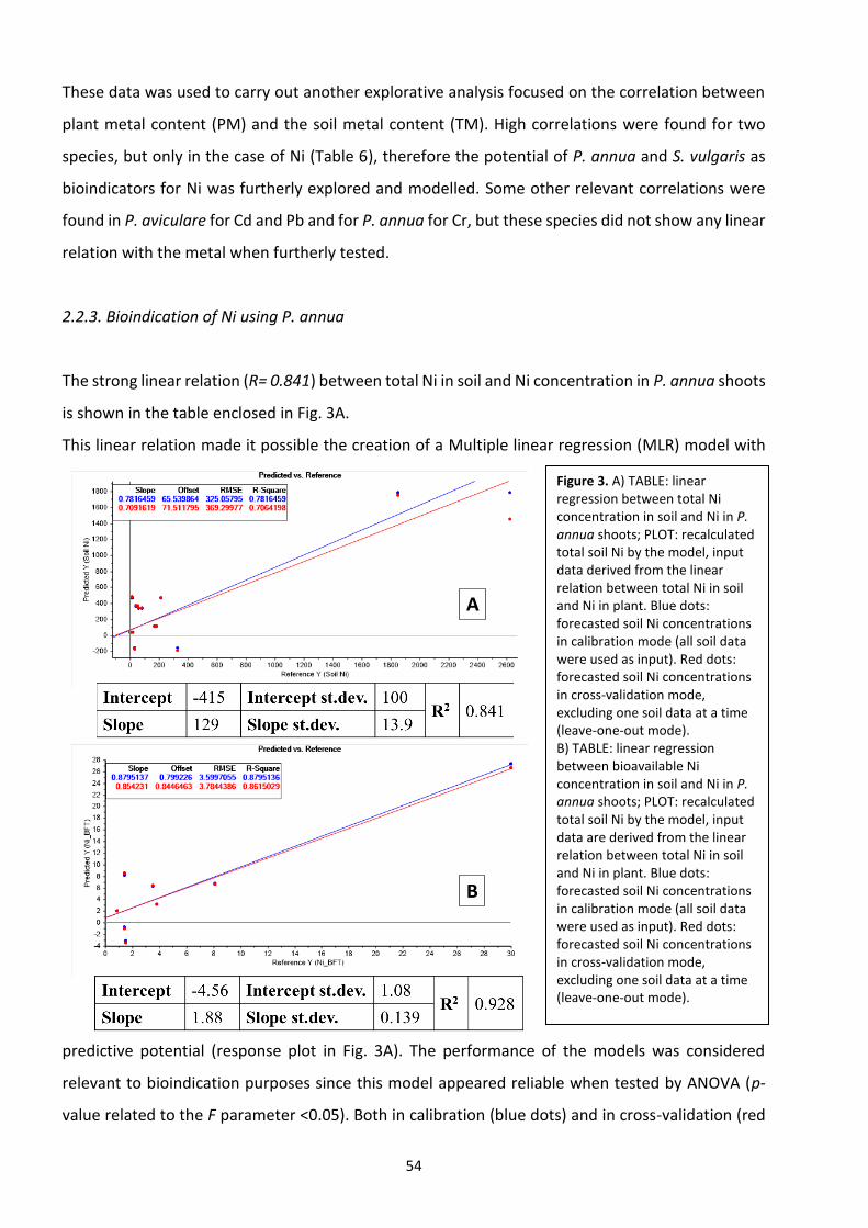
54

These data was used to carry out another explorative analysis focused on the correlation between

plant metal content (PM) and the soil metal content (TM). High correlations were found for two

species, but only in the case of Ni (Table 6), therefore the potential of P. annua and S. vulgaris as

bioindicators for Ni was furtherly explored and modelled. Some other relevant correlations were

found in P. aviculare for Cd and Pb and for P. annua for Cr, but these species did not show any linear

relation with the metal when furtherly tested.

2.2.3. Bioindication of Ni using P. annua

The strong linear relation (R= 0.841) between total Ni in soil and Ni concentration in P. annua shoots

is shown in the table enclosed in Fig. 3A.

This linear relation made it possible the creation of a Multiple linear regression (MLR) model with

predictive potential (response plot in Fig. 3A). The performance of the models was considered

relevant to bioindication purposes since this model appeared reliable when tested by ANOVA (p-

value related to the F parameter <0.05). Both in calibration (blue dots) and in cross-validation (red

A

B

Figure 3. A) TABLE: linear regression between total Ni concentration in soil and Ni in P. annua shoots; PLOT: recalculated total soil Ni by the model, input data derived from the linear relation between total Ni in soil and Ni in plant. Blue dots: forecasted soil Ni concentrations in calibration mode (all soil data were used as input). Red dots: forecasted soil Ni concentrations in cross-validation mode, excluding one soil data at a time (leave-one-out mode). B) TABLE: linear regression between bioavailable Ni concentration in soil and Ni in P. annua shoots; PLOT: recalculated total soil Ni by the model, input data are derived from the linear relation between total Ni in soil and Ni in plant. Blue dots: forecasted soil Ni concentrations in calibration mode (all soil data were used as input). Red dots: forecasted soil Ni concentrations in cross-validation mode, excluding one soil data at a time (leave-one-out mode).

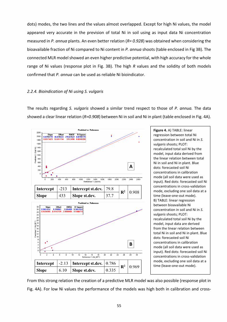
55

dots) modes, the two lines and the values almost overlapped. Except for high Ni values, the model

appeared very accurate in the prevision of total Ni in soil using as input data Ni concentration

measured in P. annua plants. An even better relation (R= 0.928) was obtained when considering the

bioavailable fraction of Ni compared to Ni content in P. annua shoots (table enclosed in Fig 3B). The

connected MLR model showed an even higher predictive potential, with high accuracy for the whole

range of Ni values (response plot in Fig. 3B). The high R values and the solidity of both models

confirmed that P. annua can be used as reliable Ni bioindicator.

2.2.4. Bioindication of Ni using S. vulgaris

The results regarding S. vulgaris showed a similar trend respect to those of P. annua. The data

showed a clear linear relation (R=0.908) between Ni in soil and Ni in plant (table enclosed in Fig. 4A).

From this strong relation the creation of a predictive MLR model was also possible (response plot in

Fig. 4A). For low Ni values the performance of the models was high both in calibration and cross-

A

B

Figure 4. A) TABLE: linear regression between total Ni concentration in soil and Ni in S. vulgaris shoots; PLOT: recalculated total soil Ni by the model, input data derived from the linear relation between total Ni in soil and Ni in plant. Blue dots: forecasted soil Ni concentrations in calibration mode (all soil data were used as input). Red dots: forecasted soil Ni concentrations in cross-validation mode, excluding one soil data at a time (leave-one-out mode). B) TABLE: linear regression between bioavailable Ni concentration in soil and Ni in S. vulgaris shoots; PLOT: recalculated total soil Ni by the model, input data are derived from the linear relation between total Ni in soil and Ni in plant. Blue dots: forecasted soil Ni concentrations in calibration mode (all soil data were used as input). Red dots: forecasted soil Ni concentrations in cross-validation mode, excluding one soil data at a time (leave-one-out mode).

56

validation mode. While for high Ni values, results obtained in cross-validation were slightly different

from the calibrations ones. The model appeared reliable when tested by ANOVA (p-value related to

the F parameter <0.05) therefore significant for bioindication purposes. An even better linear

relation (R= 0.969) was obtained when considering the bioavailable Ni pool in soil compared to P.

annua Ni content (table enclosed in Fig 4B). The connected MLR model showed therefore an even

higher predictive potential (response plot in Fig. 4B) respect to the one calculated on total Ni

content. In this case, for all Ni concentrations the performance of the model was similar, with the

data forecasted in cross-validation (red dots) almost overlapped to the ones calculated in calibration

(blu dots). This high similarity of the two sets gave strength to the model that can be considered as

highly reliable for available Ni prevision in soil.

2.3. Discussion

Polluted urban soils from Milan and Bologna, despite some peculiarities connected to parent

materials that contributed to their pedogenesis, were characterized by similar amounts and types

of HMs. All urban surfaces, in fact, receive deposits that mainly come from anthropic activities, like

vehicle emissions, industrial discharges, domestic heating and material weathering (Gibson and

Farmer, 1986; Kelly et al., 1996).

Street dust and top roadside soils in urban areas are typical sinks of HMs from atmospheric

deposition and water runoff. Key HMs in these zones are: Pb from gasoline additives, Cu, Zn and Cd

from car components, tire abrasion, lubricants and industrial emissions (Markus and McBratney,

1996; Wilcke et al., 1998). MI3 and MI4 (Table 4) resulted the most polluted soils as they were

collected in very busy street crossing. This relation underlined the important role of vehicular traffic

in contributing to soil pollution.

Woodland soils were collected in natural areas not influenced by anthropic activities and trace

elements detected in such soils were those originally present in parent materials. However, a small

contribution form diffuse sources of HMs pollution, like vehicles emission, cannot be excluded for

these samples as well. It has been reported, in fact, that fine particulate such as that coming from

tires and brakes abrasion may fall far away from source location (Hulskotte et al., 2007). Finally, in

ultramafic soil, collected far from anthropic source of pollution, the level of anthropic HMs (Zn, Cu,

Pb, Cd) was low, demonstrating the naturalness of this environment, but, given the ultramafic rock

origin on which pedogeneseis took place, the soil was highly enriched in Ni and Cr (Kierczak et al.,

2007).

57

The marked heterogeneity of sampled soils was the main obstacle to the calculation of plant-soil

linear relations in the absorption of metals. The investigated soils showed a wide range of properties

(like different texture, pH, OM content, etc.) that deeply affected the bioavailability of metal to

plants (Kabata-Pendias, 2011; Yang and Ye, 2009). Morover, it is widely known that trace elements

are not taken up by plants in a way directly proportional to their concentrations in soil (Curlik et al.,

2016). The uptake of these elements by plants is selective: essential nutrients (like Zn, Cu and Mn)

are actively uptaken and show a more linear relation to soil concentration if compared to non-

essential nutrients (Kabata-Pendias, 2011; Smillie, 2015). This active absorption of micronutrients

eventually results in a greater translocation and concentration in plant shoots, but also in a higher

toxicity if compared to non-essential nutrients (Ralph and Burchett, 1998).

In agreement with these uptake mechanisms, the species investigated in the present research

showed higher correlations between plant metal content and soil metal content for Zn and Ni

(micronutrients) than for non-essential ones such as Cd (Table 6). Despite correlation coefficient for

Zn where around 0.6 for all species (Table 6), no linear relations were found for this metal in all

selected plant species. On the other hand, P. annua (R= 0.87) and S. vulgaris (R= 0.73) showed a

linear relation between the amount of uptaken Ni and present in soil as similarly found also for

Taraxacum officinale (Fröhlichová et al., 2018).

Another possible reason for the lack of linear relations between metal content in soils and plants is

probably due to the poor translocation capacity of these elements from root to shoot. Other studies

in fact demonstrated that when non-essential metals are present at high concentration in soil, most

herbaceous plants tend to use exclusion strategies to prevent the uptake of these toxic elements

(Weis et al., 2004; Weis and Weis, 2004). This phenomenon was observed for Cd in Halophyla ovalis

(Ralph and Burchett, 1998) and for Pb (Sharma and Dubey, 2005). Species unable to prevent root

absorption, instead limit the translocation to shoots keeping the majority of toxic elements stored

in roots (Stoltz and Greger, 2002).

In the present study roots were not collected, so data about metal concentration in below ground

organs were not available, but a previously published extensive literature demonstrated that soil

HMs concentration better correlate to root metal concentration respect to shoot levels (Llagostera

et al., 2011; Phillips et al., 2015). However, shoots are the most used parts for bioindication

purposes, due to their visibility and easiness of collection. For this reason, the use of plants with

limited translocation capacity of HMs in above ground parts, has low practical use (Llagostera et al.,

2011).

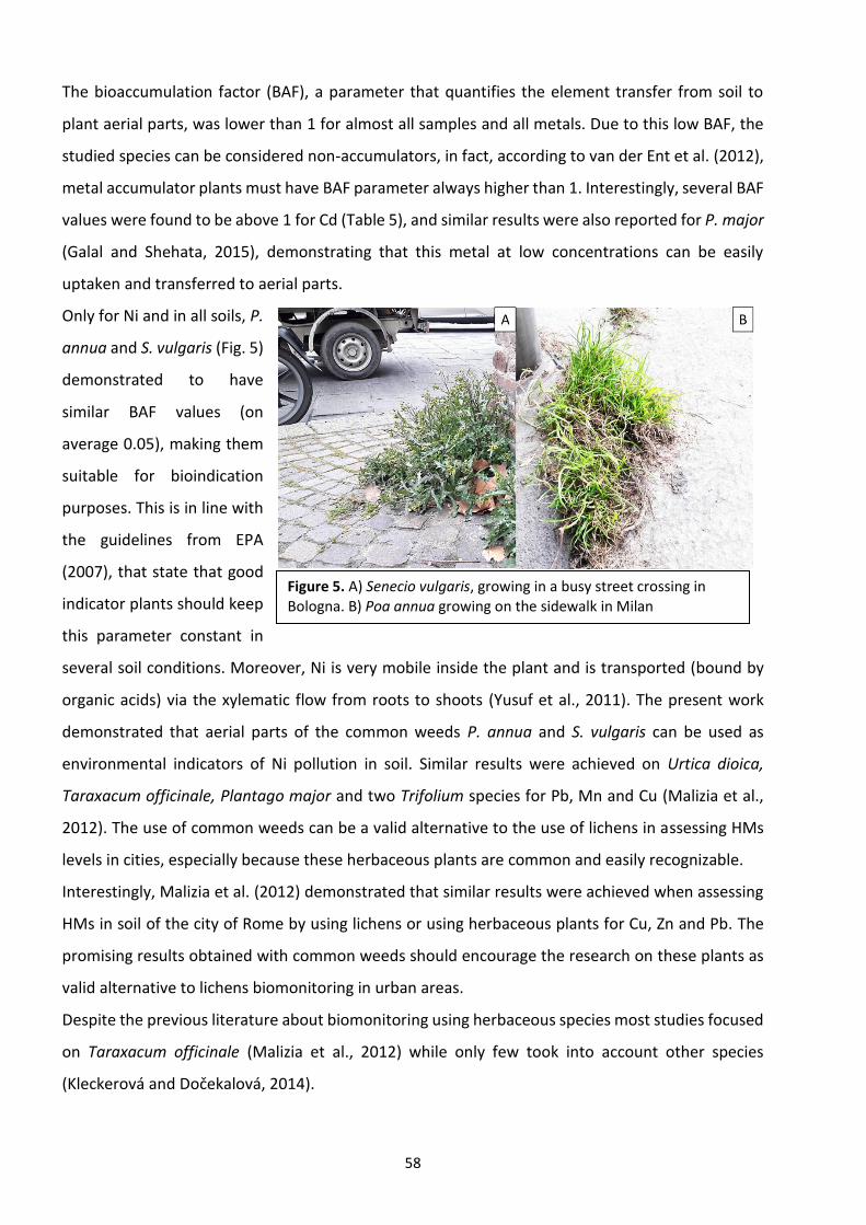
58

The bioaccumulation factor (BAF), a parameter that quantifies the element transfer from soil to

plant aerial parts, was lower than 1 for almost all samples and all metals. Due to this low BAF, the

studied species can be considered non-accumulators, in fact, according to van der Ent et al. (2012),

metal accumulator plants must have BAF parameter always higher than 1. Interestingly, several BAF

values were found to be above 1 for Cd (Table 5), and similar results were also reported for P. major

(Galal and Shehata, 2015), demonstrating that this metal at low concentrations can be easily

uptaken and transferred to aerial parts.

Only for Ni and in all soils, P.

annua and S. vulgaris (Fig. 5)

demonstrated to have

similar BAF values (on

average 0.05), making them

suitable for bioindication

purposes. This is in line with

the guidelines from EPA

(2007), that state that good

indicator plants should keep

this parameter constant in

several soil conditions. Moreover, Ni is very mobile inside the plant and is transported (bound by

organic acids) via the xylematic flow from roots to shoots (Yusuf et al., 2011). The present work

demonstrated that aerial parts of the common weeds P. annua and S. vulgaris can be used as

environmental indicators of Ni pollution in soil. Similar results were achieved on Urtica dioica,

Taraxacum officinale, Plantago major and two Trifolium species for Pb, Mn and Cu (Malizia et al.,

2012). The use of common weeds can be a valid alternative to the use of lichens in assessing HMs

levels in cities, especially because these herbaceous plants are common and easily recognizable.

Interestingly, Malizia et al. (2012) demonstrated that similar results were achieved when assessing

HMs in soil of the city of Rome by using lichens or using herbaceous plants for Cu, Zn and Pb. The

promising results obtained with common weeds should encourage the research on these plants as

valid alternative to lichens biomonitoring in urban areas.

Despite the previous literature about biomonitoring using herbaceous species most studies focused

on Taraxacum officinale (Malizia et al., 2012) while only few took into account other species

(Kleckerová and Dočekalová, 2014).

Figure 5. A) Senecio vulgaris, growing in a busy street crossing in Bologna. B) Poa annua growing on the sidewalk in Milan

59

The results of the present study highlighted the possibility to find new species suitable for

bioindication of metal pollution in anthropic environments. The importance of having several

bioindicator species in each environment has been underlined by Phillips et al. (2015) who

suggested a multi-species approach to bioindication in order to obtain more precise results. Finally,

it was demonstrated the possibility to create predictive models when strong linear relations are

present between the amount of Ni in the soil and in the plant. This chemometric approach was not

aimed at the replacement of collection and analysis of samples but, instead, at further validating

the results achieved by traditional field samplings and lab analysis.

2.4 Conclusions

The present results about the possible use of S. vulgaris, P. aviculare and P. annua, as HMs

bioindicators, showed that metal concentrations in soils and plants mostly do not correlate under

natural growth conditions. Despite metals found in soils are always present in plants, their

concentration in above ground organs is deeply influenced by soil properties and plant translocation

capacity. None of the studied species was suitable to be a good biondicator for Zn, Cu, Pb, Cr, and

Cd; moreover, P. aviculare was found to be inefficient even as Ni indicator. On the contrary, the

present work demonstrated the feasibility to use P. annua and S. vulgaris as bioindicators of Ni

concentration in soil. The two species were reliable indicators both of total and bioavailable Ni

fractions. In fact, the metal analytical data achieved in soil and plant aerial parts of these two species

allowed us to develop good chemometric models, which were able to forecast with great accuracy

Ni concentration in soil staring from the amount of Ni in plants.

60

2.5. References Ahmad SS, Reshi ZA, Shah MA, Rashid I, Ara R, Andrabi SMA (2016). Heavy metal accumulation in

the leaves of Potamogeton natans and Ceratophyllum demersum in a Himalayan RAMSAR site:

management implications. Wetlands Ecology and Management, 24, 469-475.

Antoniadis V, Robinson JS, Alloway BJ (2008). Effects of short-term pH fluctuations on cadmium,

nickel, lead, and zinc availability to ryegrass in a sewage sludge-amended field. Chemosphere, 71,

759-764.

Brereton RG (2007). Applied Chemometrics for Scientists, Wiley, Hoboken, NJ, USA.

Charlesworth S, De Miguel E, Ordóñez A (2011). A review of the distribution of particulate trace

elements in urban terrestrial environments and its application to considerations of risk.

Environmental Geochemistry and Health, 33(2), 103–123.

Curlık J, Kolesar M, Durza O, Hiller E (2016). Dandelion (Taraxacum officinale) and agrimony

(Agrimonia eupatoria) as indicators of geogenic contamination of flysch soils in Eastern Slovakia.

Archives of Environmental Contamination and Toxicology, 70, 475–486.

Dai J, Becquer T, Rouiller JH, Reversat G, Reversat FB, Lavelle P (2004). Influence of heavy metals on

C and N mineralization and microbial biomass in Zn-, Pb-, Cu-, and Cd-contaminated soils. Applied

Soil Ecology, 25, 99-109.

EPA (1996). Acid digestion of sediments, sludges, and soils. METHOD 3050B Revision 2 December

1996. U.S Environmental Protection Agency. Washington D.C., USA. https://www.epa.gov/

EPA (2007). Framework for Metal Risk Assessment. U.S Environmental Protection Agency. Office of

the Science Advisor, Washington D.C., USA. https://www.epa.gov/

Fröhlichová A, Száková J, Najmanová J, Tlustoš P (2018). An assessment of the risk of element

contamination of urban and industrial areas using Taraxacum sect. Ruderalia as a bioindicator.

Environmental Monitoring and Assessment, 190, 150

Galal TM, Shehata HS. (2015). Bioaccumulation and translocation of heavy metals by Plantago major

L. grown in contaminated soils under the effect of traffic pollution. Ecological Indicators, 48, 244–

251.

61

Ghosh M, Singh SP (2005). A review on phytoremediation of heavy metals and utilization of its by-

products. Applied Ecology and Environmental Research, 3, 1–18.

Gibson MJ, Farmer JG (1986). Multi-step chemical extraction of heavy metals from urban soils.

Environmental Pollution, 11, 117-135.

He ZL, Yang XE, Stoffella PJ (2005). Trace elements in agroecosystems and impacts on the

environment. Journal of Trace Elements in Medicine and Biology, 19, 125–140.

Huang CY, Schulte EE (1985). Digestion of plant tissue for analysis by ICP emission spectroscopy.

Communications in Soil Science and Plant Analysis, 16, 943–958.

Hulskotte JH, van der Gon HA, Visschedijk AJ, Schaap M (2007). Brake wear from vehicles as an

important source of diffuse copper pollution. Water Science and Technology, 56, 223–231.

Jenkis DA (1987). Trace elements in saxicolous lichens, In: Pollutant Transport and Fate in

Ecosystems, Coughtrey PJ, Martin MH, Unsworth MH (Eds.), Blackwell Science, Oxford, UK, pp. 249

Jiang Y, Fan M, Hu R, Zhao J, Wu J (2018). Mosses are better than leaves of vascular plants in

monitoring atmospheric heavy metal pollution in urban areas. International Journal of

Environmental Research and Public Health, 15(6), 1105

Jozic M, Peer T, Turk R (2009). The impact of the tunnel exhausts in terms of heavy metals to the

surrounding ecosystem. Environmental Monitoring and Assessment, 150, 261–271.

Kabata-Pendias A (2011). Trace elements in soils and plants, 4th ed, Taylor & Francis Group, Milton

Park, UK.

Kabata-Pendias A, Mukherjee AB (2007). Trace Elements from Soil to Human. Springer, Berlin,

Heidelberg.

Karlsson N (1961). On molybdenum in Swedish soil and vegetation and some related questions,

Statens Lantbrkem, Kontrollanst. Stockholm (SW).

Kashem MA, Singh BR (2001). Metal availability in contaminated soils: I. Effects of flooding and

organic matter on changes in Eh, pH and solubility of Cd, Ni and Zn. Nutrient Cycling in

Agroecosystems, 61, 247-255.

62

Keane B, Collier M, Shann JR, Rogstad SH (2001). Metal content of dandelion (Taraxacum officinale)

leaves in relation to soil contamination and airborne particulate matter. Science of the Total

Environment, 281, 63–78.

Kelly J, Thornton I, Simpson PR (1996). Urban geochemistry: a study of influence of anthropogenic

activity on heavy metal content of soils in traditionally industrial and non-industrial areas of Britain.

Applied Geochemistry 11, 363–370

Kierczak J, Neel C, Bril H, Puziewicz J (2007) Effect of mineralogy and pedoclimatic variations on Ni

and Cr distribution in serpentine soils under temperate climate. Geoderma, 142:165– 177.

Kleckerová A, Dočekalová H (2014). Dandelion plants as a biomonitor of urban area contamination

by heavy metals. International Journal of Environmental Research, 8(1), 157-164.

Li J, Lu Y, Yin W, Gan H, Zhang C, Deng X, Deng X, Lian J (2009). Distribution of heavy metals in

agricultural soils near a petrochemical complex in Guangz-hou, China. Environmental Monitoring

and Assessment, 153, 365–375.

Lin YX, Zhang XM (1990). Accumulation of heavy metals and the variation of amino acids and protein

in Eichhornia crassipes (Mart.) Solms in the Dianchi Lake. Oceanolology and Limnology Sinica 21,

179–184.

Llagostera I, Pérez M, Romero J (2011). Trace metal content in the seagrass Cymodocea nodosa:

differential accumulation in plant organs. Aquatic Botany, 95, 124–128.

Locatelli C, Melucci D (2012). Voltammetric determination of ultra-trace total mercury and toxic

metals in meals. Food Chemistry, 30, 460-466.

Locatelli C, Melucci D (2013). Voltammetric method for ultra-trace determination of total mercury

and toxic metals in vegetables. Comparison with spectroscopy. Central European Journal of

Chemistry, 11(5), 790-800.

Lough G, Schauer JJ, Park JS, Shafer MM, Deminter JT, Weinstein J (2005). Emissions of metals

associated with motor vehicle roadways. Environmental Science and Technology, 39, 826–836.

Malizia D, Giuliano A, Ortaggi G, Masotti A (2012). Common plants as alternative analytical tools to

monitor heavy metals in soil. Chemistry Central Journal, 6(Suppl 2):S6.

63

Markert B, Wunschmann S, Franzle S, Graciana Figuereido AM, Ribeirao A, Wang M (2011).

Bioindication of atmospheric trace metals-with special reference to megacities. Environmental

Pollution, 159, 1991–1995.

Markus JA, McBratney AB (1996). An urban soil study: heavy metals in Glebe, Australia. Australian

Journal of Soil Research 34, 453–465.

Melucci D, Locatelli M, Locatelli C, Zappi A, De Laurentiis F, Carradori S, Campestre C, Leporini L,

Zengin G, Picot CMN, Menghini L, Mahomoodally MF (2018). A comparative assessment of biological

effects and chemical profile of Italian Asphodeline lutea extracts. Molecules, 23, 461-474.

Miller JN, Miller JC (2010). Statistics and Chemometrics for Analytical Chemistry, Pearson Education,

London, UK.

Nanda S, Abraham A (2013). Remediation of heavy metal contaminated soil. African Journal of

Biotechnology, 12(21), 3099–3109.

Norgate TE, Jahanshahi S, Rankin WJ (2007). Assessing the environmental impact of metal

production processes. Journal of Cleaner Production, 15, 838–848.

Onder S, Dursun S (2006). Air borne heavy metal pollution of Cedrus libani (A. Rich) in the city centre

of Konya (Turkey). Atmospheric Environment, 40, 1122–1133.

Phillips DP, Human LRD, Adams JB (2015). Wetland plants as indicators of heavy metal

contamination. Marine Pollution Bulletin, 92, 227–232.

Quevauviller P (2002). Operationally-defined extraction procedures for soil and sediment analysis.

Part 3: New CRMs for trace-element extractable contents. Trends in Analytical Chemistry, 21(11),

774-785.

Ralph PJ, Burchett MD (1998). Photosynthetic responses of Halophila ovalis to heavy metals stress.

Environmental Pollution, 103, 91–101.

Rule JH (1994). Use of small plants as trace elements phytomonitors, with emphasis on the common

dandelion, Taraxacum officinale, In: Biogeochemistry of Trace Elements, Adriano DC, Chen ZS, Yang

SS, Iskandar I K (Eds.), Science Reviews, Wales, UK, pp. 627.

Sharma P, Dubey RS (2005). Lead toxicity in plants. Brazilian Journal of Plant Physiology, 17, 35–52.

64

Smillie C (2015). Salicornia spp. as a biomonitor of Cu and Zn in salt marsh sediments. Ecological

Indicators, 56, 70-77.

Stoltz E, Greger M (2002). Accumulation properties of As, Cd, Cu, Pb and Zn by four wetland plant

species growing on submerged mine tailings. Environmental and Experimental Botany, 47, 271–280.

Storer DA (1984). A simple high sample volume ashing procedure for determining soil organic

matter. Communications in Soil Science and Plant Analysis, 15, 759-772.

Szyczewski P, Siepak J, Niedzielski P, Sobczyński T (2009). Research on heavy metals in Poland. Polish

Journal of Environmental Studies, 5, 755–768.

Tchounwou PB, Yedjou CG, Patlolla AK, Sutton DJ (2012). Heavy metal toxicity and the environment.

In: Molecular, Clinical and Environmental Toxicology, Luch A (Ed.), Springer Basel, Switzerland, pp.

133–164.

van der Ent A, Baker AJM, Reeves RD, Pollard AJ, Schat H (2012). Hyperaccumulators of metal and

metalloid trace elements: facts and fiction. Plant and Soil, 362, 319-334.

Walkley A, Black A (1934). An examination of the Degtjareff method for determining soil organic

matter, and a proposed modification of the chromic acid titration method. Soil Science, 37, 29–38.

Wang Z, Yao L, Liu G, Liu W (2014). Heavy metals in water, sediments and submerged macrophytes

in ponds around the Dianchi Lake, China. Ecotoxology Environmental Safety, 107, 200–206.

Weis JS, Glover T, Weis P (2004). Interactions of metals affect their distribution in tissues of

Phragmites australis. Environmental Pollution, 131, 409–415.

Weis JS, Weis P (2004). Metal uptake, transport and release by wetland plants: implications for

phytoremediation and restoration. Environment International, 30, 685–700.

Wilcke W, Muller S, Kanchanakool N, Zech W (1998). Urban soil contamination in Bangkok: heavy

metal and aluminium portioning in topsoils. Geoderma, 86, 211–228.

Wiseman CLS, Zereini F, Puttmann W (2013). Traffic-related trace element fate and uptake by plants

cultivated in roadside soils in Toronto, Canada. Science of the Total Environment, 442, 86–95.

65

Wittig R (1993). General aspects of biomonitoring heavy metals by plants, In: Plants as Biomonitors,

Market B (Ed.), VCH, Weinheim, Germany. pp. 485.

Yang J, Ye Z (2009). Metal accumulation and tolerance in wetland plants. Frontiers of Biology in

China, 4(3), 282–288.

Yusuf M, Fariduddin Q, Hayat S, Ahmad A (2011). Nickel: an overview of uptake, essentiality and

toxicity in plants. Bulletin of Environmental Contamination and Toxicology, 86, 1–17.

Zereini F, Alsenz H, Wiseman CLS, Puttmann W, Reimer E, Schleyer R, Bieber E, Wallasch M (2012).

Platinum group elements (Pt, Pd, Rh) in airborne particulate matter in rural vs. urban areas of

Germany: concentrations and spatial patterns of distribution. Science of the Total Environment, 416,

261–268.

Zereini F, Wiseman CLS, Puttmann W (2007). Changes in palladium, platinum, and rhodium

concentrations, and their spatial distribution in soils along a major highway in Germany from 1994

to 2004. Environmental Science and Technology, 41, 451–456.

66

3. PH variation influences Ni and Zn uptake in different populations of Stellaria media L. Vill.

grown in hydroponics

Article status

Published: Salinitro Ma, Tognacchini Ac, van der Ent Ab, Tassoni Aa. Stress responses and nickel and

zinc accumulation in different accessions of Stellaria media (L.) Vill. in response to solution pH

variation in hydroponic culture. Plant Physiology and Biochemistry, 2020. doi:

https://doi.org/10.1016/j.plaphy.2020.01.012

a Department of Biological, Geological and Environmental Science, University of Bologna, Via

Irnerio 42, 40126, Italy

b Centre for Mined Land Rehabilitation, Sustainable Minerals Institute, Sir James Foots Building

(47A), The University of Queensland, Brisbane QLD 4072, Australia

c University of Natural Resources and Life Sciences, Department of Forest and Soil Sciences,

Institute of Soil Research, Konrad-Lorenz-Straße 24, 3430 Tulln, Vienna, Austria

Authors contribution

Mirko Salinitro performed the experiment, carried out the analyses and wrote the manuscript,

Antony van der Ent, coordinated the study, Alice Tognacchini perfomed the ICP-MS analyses,

Annalisa Tassoni, revised the manuscript.

List of abbreviations:

AA: ascorbic acid,

ABTS: 2,2'-azino-bis(3-etilbenzotiazolin-6-sulfonic) acid,

CAT: catechin,

GA: gallic acid,

HMs: heavy metals

3.1. Introduction

The correlation between metal availability and soil parameters has been intensively studied over

the last decades, to better understand which were the main parameters that influence metals

activity in soil, hence uptake and toxicity for plants (Kukier et al., 2004; Pérez-Esteban et al., 2012;

67

Pérez-Esteban et al., 2014; Zia et al., 2018). A significant number of studies have shown that soil pH

and dissolved organic carbon (DOC) strongly influence metal concentrations and speciation in soil

solutions, although the specific effects vary between different metals (Kunhikrishnan et al., 2017;

Schneider et al., 2016). Other studies have considered the influence of total organic matter content,

with Fe-Mn oxides and pH as major factors for metal availability in soil solution (Pérez-Esteban et

al., 2012; Pérez-Esteban et al., 2014; Zeng et al., 2011). Ni and Zn are typically strongly correlated

to soil solution pH and are weakly influenced by other factors (Bhogal et al., 1993; Kukier et al.,

2004; Zia et al., 2018). It has been demonstrated that soluble organic carbon did not affect Zn

concentrations in soil solution because of the lower affinity of Zn for organic compounds (Wong et

al., 2007), while for Ni, soil characteristic (like clay content and cationic exchange capacity) (CEC))

and pH have significant effect on metal availability (Zia et al., 2018). Nonetheless, most authors

agree that pH is the major factor in influencing metal availability and uptake (Kukier et al., 2004;

Park et al., 2011; Walker et al., 2004). For Zn a negative correlation between pH and soluble Zn (at

low pH more solubility) has been observed in many studies and conclusion on this metal appear

consistent in the literature (Pérez-Esteban et al., 2014; Zeng et al., 2011; Zia et al., 2018).

The situation is very different for Ni. A study on the effect of different soil pH on Ni concentrations

of the hyperaccumulators Alyssum murale and Alyssum corsicum, concluded that an increase in soil

pH was associated with an increase in shoot Ni concentration (Li et al., 2003). Those results were in

contrast with other data demonstrating that the increase of soil pH caused a decrease of Ni

concentrations in various non-accumulator species (Kukier and Chaney, 2004; L'Huillier and

Edighoffer, 1996) and in the hyperaccumulators Berkheya coddii and Alyssum bertolonii (Robinson

et al., 1999; Robinson et al., 1997). Moreover, contrasting results were found by (Kukier et al., 2004)

studying A. corsicum and A. murale in different Ni-contaminated soils. Additionally, it has been

recently stressed that the bioavailability of metals varies with plant species as a result of rhizosphere

mechanisms such as root acidification or alkalinisation (Chaignon et al., 2002; Hinsinger and

Courchesne, 2008). For instance, a study found that the availability of Zn was higher than expected

in tobacco plants due to roots-induced pH decrease (Loosemore et al., 2004).

Despite many studies have been carried out on soil evaluating the synergic influence of many

factors, very limited research (i.e Kumar et al., 2012) has been done in hydroponic, to investigate

how a single factor (i.e. pH) could influence the availability and the subsequent uptake of a certain

metal in plants.

If evaluating the effect of a single factor can be difficult in a complex system like the soil, it is

conversely possible in hydroponic conditions in which the nutrient solution parameters can be

68

singularly manipulated. Moreover, roots acidification or alkalinisation is effectively counterbalanced

in hydroponics, making these root processes uninfluential. Following this approach, the aim of the

present study was to evaluate the effect of pH on the uptake and toxicity of Ni and Zn, on the non-

accumulator plant Stellaria media grown in hydroponics. Moreover, the plant content of

chlorophylls, polyphenols, flavonoids and the antioxidant activity were analysed in order to

correlate them with Ni and Zn accumulation and metal stress effects in S. media.

3.2. Material and Methods

3.2.1. Selected species

Stellaria media (L.) Vill. (Caryophyllaceae) is an annual herbaceous plant native to Europe and widely

naturalized in all continents. It commonly grows in disturbed habitats, such as road margins, crop

fields and bare soils deposits. Five different accessions of Stellaria media were collected in the year

2017 in five different locations. For each location, seeds were taken in several stations to sample

the whole genetic variability of each place. Two accessions were respectively from the urban

environment of Milan and Bologna (Italy), two accessions were from woodland stations located at

the outskirt of Milan and Bologna, one accession was from ultramafic soils naturally enriched of Ni

and Cr and located at mount Prinzera (Parma, Italy) (see detailed table at page 28). Urban stations

were characterized by high and polymetallic pollution of soils, woodland station were conversely

characterized by low heavy metal (HMs) levels, ultramafic station were characterized by high levels

of Cr and Ni only. Seed collections was carried out at the end of the vegetative season of the plants

(late April). Plants were cut and air-dried, then shook to allow the release of seed. Seeds were sieved

to remove plant particles, air-dried for 1 week, than stored in plastic tubes at room temperature

until sowing. For the germination, seeds were soaked overnight in tap water, then placed on a

substrate composed by perlite, vermiculite and quartz sand in a ratio of 1:1:1. Seeds were watered

with tap water and kept in the dark at 20°C for 2-3 days until germination. Seedlings were then

transferred in a growth cabinet with 12-12 hour light-dark at 25°C degrees for 1 week, before

transplanting them into the hydroponic system.

3.2.2. Hydroponic culture system

69

The hydroponic system was composed of 4 separate tanks (25 L each) filled with Vega Classic

nutrient solution (Canna, Brisbane QLD, Australia) diluted 1:250, containing: 16.3 mM N, 1.2 mM P,

5.7 mM K, 4.4 mM Ca, 1.3 mM Mg, 1.1 mM S, 14 μM Fe-DTPA (diethylenetriamine penta acetic acid

ferric complex), 26 μM B, 0.6 μM Cu, 10.2 μM Mn, 0.8 μM Mo, 4.3 μM Zn.

The nutrient solution was spiked with Zn(NO3)2·6H20 or Ni(NO3)2·6H2O to obtain a concentration of

0.55 mM and 0.10 mM respectively (Table 1).

pH Zn (mM) Ni (mM)

5.0 0 (Control) 0 (Control)

5.0 0.55 0.10

5.5 n.d. 0.10

6.0 0.55 0.10

6.5 0.55 0.10

7.0 0.55 no growth

Table 1. Different pH treatments with Ni and Zn in hydroponics. N.d., not determined.

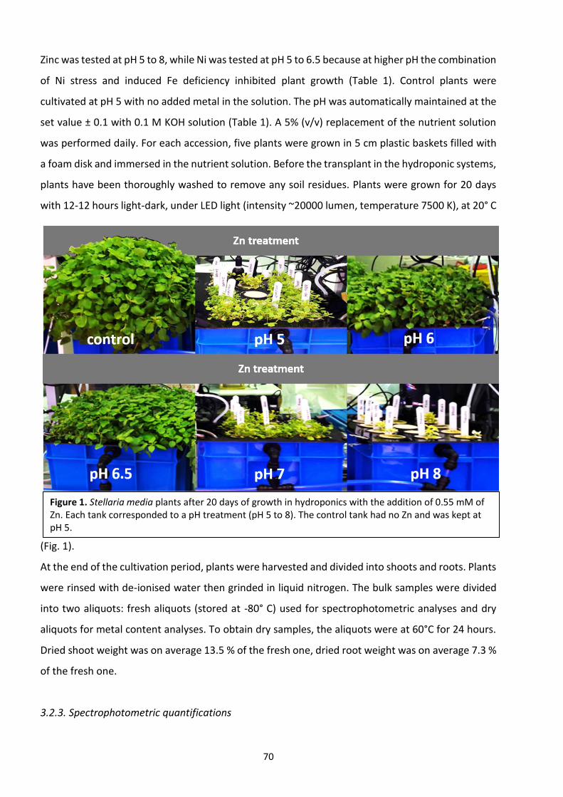
70

Zinc was tested at pH 5 to 8, while Ni was tested at pH 5 to 6.5 because at higher pH the combination

of Ni stress and induced Fe deficiency inhibited plant growth (Table 1). Control plants were

cultivated at pH 5 with no added metal in the solution. The pH was automatically maintained at the

set value ± 0.1 with 0.1 M KOH solution (Table 1). A 5% (v/v) replacement of the nutrient solution

was performed daily. For each accession, five plants were grown in 5 cm plastic baskets filled with

a foam disk and immersed in the nutrient solution. Before the transplant in the hydroponic systems,

plants have been thoroughly washed to remove any soil residues. Plants were grown for 20 days

with 12-12 hours light-dark, under LED light (intensity ~20000 lumen, temperature 7500 K), at 20° C

(Fig. 1).

At the end of the cultivation period, plants were harvested and divided into shoots and roots. Plants

were rinsed with de-ionised water then grinded in liquid nitrogen. The bulk samples were divided

into two aliquots: fresh aliquots (stored at -80° C) used for spectrophotometric analyses and dry

aliquots for metal content analyses. To obtain dry samples, the aliquots were at 60°C for 24 hours.

Dried shoot weight was on average 13.5 % of the fresh one, dried root weight was on average 7.3 %

of the fresh one.

3.2.3. Spectrophotometric quantifications

Figure 1. Stellaria media plants after 20 days of growth in hydroponics with the addition of 0.55 mM of Zn. Each tank corresponded to a pH treatment (pH 5 to 8). The control tank had no Zn and was kept at pH 5.

71

For spectrophotometric analyses, 0.1 g of freshly grinded plant samples were extracted with 1 mL

of 95% (v/v) methanol and shaken overnight at room temperature. The supernatant was then

recovered after centrifugation at 15,300 x g for 5 minutes at room temperature and used in the

total polyphenols, total flavonoids and antioxidant activity quantification reactions.

Total polyphenols colorimetric quantification was performed through Folin-Ciocalteu assay (Ferri et

al., 2013; Singleton et al., 1999). The results were expressed as mg of gallic acid equivalents per g of

fresh weight (mg GA eq/gFW) by means of a dose-response calibration curve (between 0 and 15 µg

of gallic acid).

Total flavonoids colorimetric quantification assay was performed as in Zhishen et al. (1999). The

results were expressed as mg of catechin equivalents per g of fresh weight (mg CAT eq/gFW) by

means of a dose-response calibration curve (between 2 and 14 µg of catechin).

The antioxidant activity quantification was performed through ABTS (2,2'-azino-bis(3-

etilbenzotiazolin-6-sulfonic) acid) reagent decolorimetric assay (Ferri et al., 2013; Re et al., 1999)

and the results were expressed as grams of ascorbic acid (AA) equivalents per g of fresh weight (mg

AA eq/gFW) by means of a dose-response calibration curve (between 0 and 2 µg of AA).

For the determination of photosynthetic pigments, a modified method from Radwan et al. (2007)

and Metzner et al. (1965) as used. 0.1 g of freshly grinded plants, were extracted with 1.5 mL of 85%

(v/v) acetone and mixed 2 times for 30 seconds, the samples were then centrifuged at 4°C, 665 x g

for 5 minutes and the supernatant recovered. Plant powder resulted completely bleached at the

end of the extraction.

The supernatant was analysed at three different wavelengths (663, 644 and 452.5 nm) and the

obtained absorbance values were processed to give the pigment concentrations in mg/gFW with

the following equations:

chlorophyll a = 10.3 x Abs663 – 0.98 x Abs644,

chlorophyll b = 19.7 x Abs644 – 3.87 x Abs663,

carotenoids = 4.2 x Abs452.5 – [(0.0264 x chl-a) + (0.426 x chl-b)]

All the spectrophotometric analyses were performed with a Cary 60 UV-Vis spectrophotometer

(Agilent Technologies, Santa Clara, CA, USA).

3.2.4. Nickel and zinc quantification

For the quantification of metals, grinded roots and shoots were oven dried at 80°C until constant

weight. Samples were pre-digested at room temperature with 2 mL 70% (v/v) HNO3 for 1 day, then

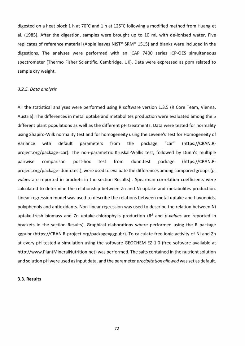
72

digested on a heat block 1 h at 70°C and 1 h at 125°C following a modified method from Huang et

al. (1985). After the digestion, samples were brought up to 10 mL with de-ionised water. Five

replicates of reference material (Apple leaves NIST® SRM® 1515) and blanks were included in the

digestions. The analyses were performed with an iCAP 7400 series ICP-OES simultaneous

spectrometer (Thermo Fisher Scientific, Cambridge, UK). Data were expressed as ppm related to

sample dry weight.

3.2.5. Data analysis

All the statistical analyses were performed using R software version 1.3.5 (R Core Team, Vienna,

Austria). The differences in metal uptake and metabolites production were evaluated among the 5

different plant populations as well as the different pH treatments. Data were tested for normality

using Shapiro-Wilk normality test and for homogeneity using the Levene's Test for Homogeneity of

Variance with default parameters from the package “car” (https://CRAN.R-

project.org/package=car). The non-parametric Kruskal-Wallis test, followed by Dunn’s multiple

pairwise comparison post-hoc test from dunn.test package (https://CRAN.R-

project.org/package=dunn.test), were used to evaluate the differences among compared groups (p-

values are reported in brackets in the section Results) . Spearman correlation coefficients were

calculated to determine the relationship between Zn and Ni uptake and metabolites production.

Linear regression model was used to describe the relations between metal uptake and flavonoids,

polyphenols and antioxidants. Non-linear regression was used to describe the relation between Ni

uptake-fresh biomass and Zn uptake-chlorophylls production (R2 and p-values are reported in

brackets in the section Results). Graphical elaborations where performed using the R package

ggpubr (https://CRAN.R-project.org/package=ggpubr). To calculate free ionic activity of Ni and Zn

at every pH tested a simulation using the software GEOCHEM-EZ 1.0 (free software available at

http://www.PlantMineralNutrition.net) was performed. The salts contained in the nutrient solution

and solution pH were used as input data, and the parameter precipitation allowed was set as default.

3.3. Results

73

3.3.1. Population variability

Population variability was mainly observed in control plants and in treatments were Zn and Ni

toxicity resulted low (Fig. 2). The smallest plants were those coming from ultramafic and Bologna

urban accessions with an average shoot weight of 7.7 gFW and 6.4 gFW, respectively.

The Milan urban accession showed an intermediate shoot weight with an average of 15.1 gFW, while

Milan and Bologna woodland accessions displayed a higher average shoot weight of 22.8 gFW.

These differences disappeared when Zn and Ni concentrations in plants tissue were higher and toxic

effects buffered population variability (Figs. 3A, B).

3.3.2. PH influence on Ni and Zn uptake

An overall different biomass production (at all tested pH) was noticed between plants grown with

Ni and plants grown with Zn (Fig. 3). For the first, the average weight of treated plants was 0.11 gFW

Figure 2. Different plant populations of Stellaria media L. Vill. after 1 week of hydroponic growth in control conditions (no metal and pH 5.0). A) Bologna woodland; B) Milan woodland; C) Milan urban; D) Bologna urban; E) ultramafic.

Figure 3. Shoot biomass variability in Stellaria media plants from five different populations, after hydroponic culture at different pH. Plants treated with Ni (A) and with Zn (B) at different pH. B, Bologna urban; M, Milan urban; N, Bologna woodland; P, ultramafic; T, Milan woodland. Highlighted with grey circles the ultramafic and Bologna urban accessions, which always showed the smallest size plants in low stress conditions.

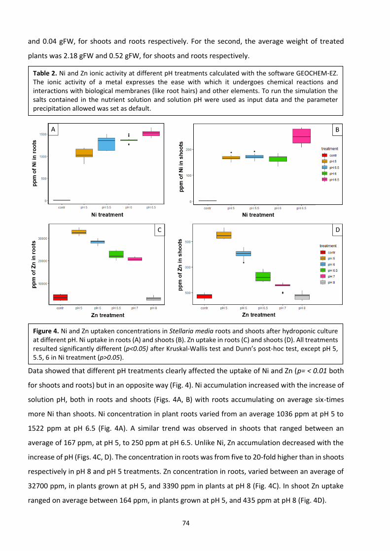
74

and 0.04 gFW, for shoots and roots respectively. For the second, the average weight of treated

plants was 2.18 gFW and 0.52 gFW, for shoots and roots respectively.

Data showed that different pH treatments clearly affected the uptake of Ni and Zn (p= < 0.01 both

for shoots and roots) but in an opposite way (Fig. 4). Ni accumulation increased with the increase of

solution pH, both in roots and shoots (Figs. 4A, B) with roots accumulating on average six-times

more Ni than shoots. Ni concentration in plant roots varied from an average 1036 ppm at pH 5 to

1522 ppm at pH 6.5 (Fig. 4A). A similar trend was observed in shoots that ranged between an

average of 167 ppm, at pH 5, to 250 ppm at pH 6.5. Unlike Ni, Zn accumulation decreased with the

increase of pH (Figs. 4C, D). The concentration in roots was from five to 20-fold higher than in shoots

respectively in pH 8 and pH 5 treatments. Zn concentration in roots, varied between an average of

32700 ppm, in plants grown at pH 5, and 3390 ppm in plants at pH 8 (Fig. 4C). In shoot Zn uptake

ranged on average between 164 ppm, in plants grown at pH 5, and 435 ppm at pH 8 (Fig. 4D).

Figure 4. Ni and Zn uptaken concentrations in Stellaria media roots and shoots after hydroponic culture at different pH. Ni uptake in roots (A) and shoots (B). Zn uptake in roots (C) and shoots (D). All treatments resulted significantly different (p<0.05) after Kruskal-Wallis test and Dunn’s post-hoc test, except pH 5, 5.5, 6 in Ni treatment (p>0.05).

Table 2. Ni and Zn ionic activity at different pH treatments calculated with the software GEOCHEM-EZ. The ionic activity of a metal expresses the ease with which it undergoes chemical reactions and interactions with biological membranes (like root hairs) and other elements. To run the simulation the salts contained in the nutrient solution and solution pH were used as input data and the parameter precipitation allowed was set as default.

75

Ion activity of Ni did not show significant changes among pH treatments, but only a slight decrease

at the increase of pH, conversely Zn activity decreased at higher pH treatment (Table 2).

The translocation of both Ni and Zn from roots to shoots was affected by their availability. The

translocation of Ni from roots to shoots was around 25 % in control plants, where Ni levels were

very low, whereas in all the other treatments the translocation was around 12% to increase up to

16% at pH 6.5 (R2 = 0.604, p<0.01) (Fig. 5A). When Zn levels were low (i.e. in control treatment) or

its availability was low (i.e. in the pH 8 treatment) plant transferred up to the 15% of Zn from roots

to shoots. Conversely, with the increase of Zn availability, the translocation decreased around 3%

and went slightly up at 5% at pH 5 (R2 = 0.913, p<0.01) (Fig. 5B).

Ionic activity in Zn treatment Precipitates µg/L

pH Zn Fe PO4- ZnPO4 FeOH- FePO4

8 3.904 × 10-7 3.198 × 10-21 9.213 x 10-9 4.672 0.192 -

7 2.221 × 10-6 3.190 × 10-18 6.752 x 10-9 1.104 0.187 -

6.5 7.006 v 10-6 3.311 × 10-17 1.202 x 10-10 1.079 0.183 -

6 2.642 v 10-5 2.395 × 10-16 1.653 x 10-11 0.990 0.185 -

5 2.584 × 10-4 1.533 × 10-14 2.590 x 10-13 - - 0.090

Ionic activity in Ni treatment Precipitates µg/L

pH Ni Fe PO4- ZnPO4 FeOH- FePO4

6.5 3.337 × 10-5 2.339 × 10-17 1.668 × 10-10 - - 0.093

6 3.517 × 10-5 1.788 × 10-16 2.252 × 10-11 - - 0.093

5.5 3.590 × 10-5 1.595 × 10-15 2.520 × 10-12 - - 0.093

5 3.654 v 10-5 1.535 × 10-14 2.616 × 10-13 - - 0.093

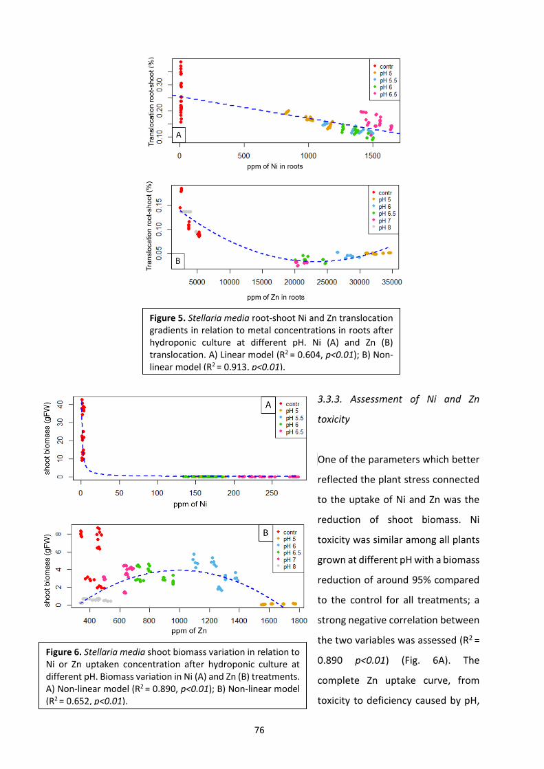
76

3.3.3. Assessment of Ni and Zn

toxicity

One of the parameters which better

reflected the plant stress connected

to the uptake of Ni and Zn was the

reduction of shoot biomass. Ni

toxicity was similar among all plants

grown at different pH with a biomass

reduction of around 95% compared

to the control for all treatments; a

strong negative correlation between

the two variables was assessed (R2 =

0.890 p<0.01) (Fig. 6A). The

complete Zn uptake curve, from

toxicity to deficiency caused by pH,

Figure 5. Stellaria media root-shoot Ni and Zn translocation gradients in relation to metal concentrations in roots after hydroponic culture at different pH. Ni (A) and Zn (B) translocation. A) Linear model (R2 = 0.604, p<0.01); B) Non-linear model (R2 = 0.913, p<0.01).

Figure 6. Stellaria media shoot biomass variation in relation to Ni or Zn uptaken concentration after hydroponic culture at different pH. Biomass variation in Ni (A) and Zn (B) treatments. A) Non-linear model (R2 = 0.890, p<0.01); B) Non-linear model (R2 = 0.652, p<0.01).

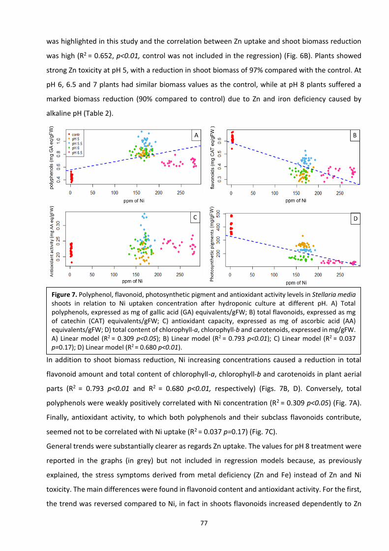
77

was highlighted in this study and the correlation between Zn uptake and shoot biomass reduction

was high (R2 = 0.652, p<0.01, control was not included in the regression) (Fig. 6B). Plants showed

strong Zn toxicity at pH 5, with a reduction in shoot biomass of 97% compared with the control. At

pH 6, 6.5 and 7 plants had similar biomass values as the control, while at pH 8 plants suffered a

marked biomass reduction (90% compared to control) due to Zn and iron deficiency caused by

alkaline pH (Table 2).

In addition to shoot biomass reduction, Ni increasing concentrations caused a reduction in total

flavonoid amount and total content of chlorophyll-a, chlorophyll-b and carotenoids in plant aerial

parts (R2 = 0.793 p<0.01 and R2 = 0.680 p<0.01, respectively) (Figs. 7B, D). Conversely, total

polyphenols were weakly positively correlated with Ni concentration (R2 = 0.309 p<0.05) (Fig. 7A).

Finally, antioxidant activity, to which both polyphenols and their subclass flavonoids contribute,

seemed not to be correlated with Ni uptake (R2 = 0.037 p=0.17) (Fig. 7C).

General trends were substantially clearer as regards Zn uptake. The values for pH 8 treatment were

reported in the graphs (in grey) but not included in regression models because, as previously

explained, the stress symptoms derived from metal deficiency (Zn and Fe) instead of Zn and Ni

toxicity. The main differences were found in flavonoid content and antioxidant activity. For the first,

the trend was reversed compared to Ni, in fact in shoots flavonoids increased dependently to Zn

Figure 7. Polyphenol, flavonoid, photosynthetic pigment and antioxidant activity levels in Stellaria media shoots in relation to Ni uptaken concentration after hydroponic culture at different pH. A) Total polyphenols, expressed as mg of gallic acid (GA) equivalents/gFW; B) total flavonoids, expressed as mg of catechin (CAT) equivalents/gFW; C) antioxidant capacity, expressed as mg of ascorbic acid (AA) equivalents/gFW; D) total content of chlorophyll-a, chlorophyll-b and carotenoids, expressed in mg/gFW. A) Linear model (R2 = 0.309 p<0.05); B) Linear model (R2 = 0.793 p<0.01); C) Linear model (R2 = 0.037 p=0.17); D) Linear model (R2 = 0.680 p<0.01).

78

concentration (R2 = 0.852 p<0.01) (Fig. 8B). Moreover, as similarly reported for Ni, total polyphenols

concentration was positively correlated with the increase of Zn (R2 = 0.728 p<0.01) (Fig. 8A). Because

both polyphenols and flavonoids may contribute to antioxidant activity, this parameter also showed

a clear positive relation with Zn concentration (R2 = 0.751 p<0.01) (Fig. 8C). Photosynthetic pigments

content slightly increased in treatments at pH 6 and 6.5 compared to the control, then sharply

decreased at pH 5 (R2 = 0.476 p=<0.05).

3.4. Discussion

The aim of our research was to study the interactions between Zn and Ni uptake and the variable

pH on a non-accumulator plant (Stellaria media) in hydroponic culture. This approach allowed us to

observe changes in Zn and Ni uptake, with no interference due to soil characteristic like cationic

exchange capacity, organic carbon content or root acidification processes. The lack of buffer factors

in the experiment made clearer the effects caused by pH, but, on the other side, made plants more

vulnerable to Ni and Zn toxicity. All plants in the Ni treatments suffered chlorosis due to Ni toxicity,

while in the Zn treatment at pH 8 the plants suffered Zn and Fe deficiency (Table 2). In general, the

deleterious effects of Ni were more marked than Zn ones, partly because the intrinsic higher toxicity

Figure 8. Polyphenol, flavonoid, photosynthetic pigment and antioxidant activity levels in Stellaria media shoots in relation to Zn uptaken concentration after hydroponic culture at different pH. A) Total polyphenols expressed as mg of gallic acid (GA) equivalents/gFW; B) total flavonoids expressed as mg of catechin (CAT) equivalents/gFW; C) antioxidant capacity expressed as mg of ascorbic acid (AA) equivalents/gFW; D) total content of chlorophyll-a, chlorophyll-b and carotenoids expressed in mg/gFW. A) Linear model (R2 = 0.728 p<0.01); B) Linear model (R2 = 0.852 p<0.01); C) Linear model (R2 = 0.751 p<0.01); D) Non-linear model (R2 = 0.476 p=<0.05).

79

of Ni (Kabata-Pendias, 2010) and partly because higher translocation occurred from roots to shoots

(Fig. 5A, B).

The present experimental design moreover, aimed at the assessment of possible variations among

the tested five different S. media plant populations. The hypothesis that different populations

coming from different habitats, could have developed different abilities in metal tolerance, has been

already confirmed by several studies (Bickham et al., 2000; Collier et al., 2010; Keane et al., 2005),

that took into consideration populations growing on standard and mine soils. Our data did not

confirm such hypothesis and all populations appeared homogeneous for Zn and Ni uptake (p=0.92

for Ni, and p=0.91 for Zn) and for flavonoid, polyphenol and photosynthetic pigment productions.

Therefore, it appears that differences in Ni and Zn concentrations and availability between urban,

woodland and ultramafic soils were not enough marked to allow diversification among populations.

Despite that, population indeed differed for their size, in fact plants coming from contaminated

environments, such as urban and ultramafic accessions, were smaller then woodland accessions

(Figs. 2, 3A, 3B). It was observed that, at the increase of pH there was a correspondent increase in

Ni uptake both in roots and shoots of S. media (Fig. 4). The conceptual model of such response is

known as biotic ligand model (Di Toro et al., 2001). When metal ionic activity is kept constant, an

increase in pH may cause higher binding of metal cations by biotic ligands (biological membrane and

transporter proteins) because of the deprotonation of transporters (Lòpez et al., 2000). Our results

showed that Ni activity can be considered almost constant at all pH tested (Table 2), and this ideal

situation could happen only in total absence of other factors able to bind or release Ni ions from the

solution. Similar results were never achieved in pot experiments. In fact the only few studies carried

out on non-accumulator plants like crop plants (Kukier and Chaney, 2004; L'Huillier and Edighoffer,

1996; Sanders et al., 1986) reported opposite trends.

The uptake of Ni may vary according to the type media (i.e. soil, perlite, hydroponic, etc.) in which

the plant is grown. In fact, studies conducted on oats (Weng et al., 2003) found that Ni concentration

in shoots increased with the increase of pH, analogously to our results (Fig. 4A).

As stated in several previous studies (Pérez-Esteban et al., 2014; Zeng et al., 2011; Zia et al., 2018),

soil pH is the main variable affecting bioavailability and uptake of Zn. This study is consistent with

the literature since a strong negative correlation in Zn uptake at the increase of pH was observed

(Fig. 4). This behaviour, can be explained by the chemical forms that Zn assumes at different pH

(Kukier et al., 2004). Solution pH influences the speciation of Zn: at pH values below 7.7, Zn2+

predominates and plants can easily absorb it, but above pH 7.7, ZnOH+ is the main species and is

not bioavailable anymore (Kiekens, 1995; Reddy et al., 1995). Moreover, as confirmed by the

80

GEOCHEM-EZ simulation (Table 2), free Zn activity decreased with increasing pH values, coupled

with Zn precipitation at the high pH treatments.

Unlike Ni, the behaviour of Zn in hydroponics closely simulates the one in soil, as soluble Zn is mainly

present as inorganic species, mostly as the free cation (94–98%) in soil solution. Moreover, few

interactions with soil and organic matter may occur (Meers et al., 2006; Pérez-Esteban et al., 2014;

Weng et al., 2002).

Zn and Ni toxicity, induced by differential uptake among pH treatments, influenced several plant

parameters, first of all the amount of biomass. As expected Zn and Ni toxicity caused a reduction of

biomass and chlorosis, as widely stated in the literature (Jayakumar et al., 2007; Weng et al., 2003)

(Fig. 6, 7D, 8D). Beside these effects, the production of secondary metabolites (like flavonoids and

polyphenols) connected with the decrease of oxidative stress, was investigated. Interestingly the

correlation between the production of these compounds and metal uptake was strong both for Ni

(R2 = 0.309, R2 = 0.793, for flavonoids and polyphenols respectively) and Zn (R2 = 0.852, R2 = 0.728,

for flavonoids and polyphenols respectively) (Fig. 7A, 7B, 8A, 8B). In Ni treatments data were

grouped in two main clusters: control and pH treatments. All treated plants exhibited acute Ni

toxicity, therefore the production of polyphenols and flavonoids and photosynthetic pigments was

quite similar for all pH treatments and strongly different from control (Fig. 7). Flavonoids (a

subfamily of polyphenols) were negatively correlated with Ni uptake, despite most of studies

(Chalker-Scott, 1999; Winkel-Shirley, 2002) reported opposite trends, but total polyphenols were

positively correlated. As a result, no correlation was detected for antioxidant capacity (Fig. 7C). This

negative trend was probably caused by the high toxicity of Ni which suppressed the production of

flavonoids as found by Jayakumar et al. (2007), Similarly, a decrease in polyphenols in the treatment

at pH 6.5 was detected, despite the overall growing trend, a similar situation was reported in maize

plants by (Kisa et al., 2016). The lower toxicity of Zn instead, allowed us to observe a gradual

production of antioxidant which steadily increased from control treatment to high Zn stress (pH 5

treatment), with no signs of inhibition by the excessive toxicity. Polyphenols, flavonoids and total

antioxidant capacity were all increasing at the increase of metal concentration acting clearly against

the subsequent oxidative stress (Chalker-Scott, 1999; Jayakumar et al., 2007; Kisa et al., 2016; Kumar

et al., 2012; Winkel-Shirley, 2002). Conversely, photosynthetic pigments content was negatively

affected by Zn uptake which caused chlorosis (Fig. 8D).

81

3.5. Conclusions

This study showed that the variable pH is positively correlated with Ni uptake in hydroponic culture,

while an opposite trend was detected in similar studies carried out on soil. Conversely, Zn uptake

negatively correlated with pH and results found in soil and hydroponic are consistent. As

consequence data pointed out that in soils, many other factors (such as organic matter and clay

content) play an important role in controlling Ni solubility and uptake, while Zn is chiefly controlled

by pH. Stellaria media plants had high Ni and Zn uptake and showed several toxicity symptoms and

this study demonstrated that production of antioxidant substances (like polyphenols) is

proportional with Zn and Ni concentration in shoots, while on the contrary biomass production and

chlorophyll contents were supressed. Finally, our results demonstrated the suitability of using

hydroponic systems to study single variables affecting metal uptake. These simplified systems can

effectively avoid interference with many other substrate variables that cannot be excluded when

experiments are performed using soil. Taking into consideration the relations between pH and the

uptake of different metals, can be a starting key to maximize the success of biomonitoring

campaigns and phytoremediation interventions in metal polluted sites.

3.6. References

Bhogal NS, Sakal R, Singh AP, Sinha RB (1993). Micronutrient status in acquic ustifluvents and

udifluvents as related to certain soil properties. Journal of the Indian Society of Soil Science, 41, 75-

78.

Bickham JW, Sandhu S, Hebert PDN, Chikhi L, Athwal R. (2000). Effects of chemical contaminants an

genetic diversity in natural populations: implications for biomonitoring and ecotoxicology. Mutation

Research-Reviews in Mutation Research, 463, 33-51.

Chaignon V, Bedin F, Hinsinger P. (2002). Copper bioavailability and rhizosphere pH changes as

affected by nitrogen supply for tomato and oilseed rape cropped on an acidic and a calcareous soil.

Plant and Soil, 243, 219-228.

Chalker-Scott L. (1999). Environmental significance of anthocyanins in plant stress responses.

Photochemistry and Photobiology 70, 1-9.

Collier MH, Keane B, Rogstad SH (2010). Productivity differences between dandelion (Taraxacum

officinale; Asteraceae) clones from pollution impacted versus non-impacted soils. Plant and Soil,

329, 173-183.

82

Di Toro DM, Allen HE, Bergman HL, Meyer JS, Paquin PR, Santore RC (2001). Biotic ligand model of

the acute toxicity of metals. 1. Technical basis. Environmental Toxicology and Chemistry, 20, 2383-

2396.

Ferri M, Gianotti A, Tassoni A (2013). Optimisation of assay conditions for the determination of

antioxidant capacity and polyphenols in cereal food components. Journal of Food Composition and

Analysis, 30, 94-101.

Hinsinger P, Courchesne F. 2008. Biogeochemistry of metals and metalloids at the soil–root

interface. In: Biophysic- Chemical Processes of Heavy Metals and Metalloids in Soil Environments.

Violante A, Huang PM, Gadd GM (Eds.), Hoboken, USA: John Wiley & Sons, pp. 267-311.

Huang CY, Schulte EE (1985). Digestion of plant tissue for analysis by ICP emission spectroscopy.

Communications in Soil Science and Plant Analysis, 16, 943-958.

Jayakumar K, Jaleel C, Vijayarengan P (2007). Changes in growth, biochemical constituents, and

antioxidant potentials in radish (Raphanus sativus L.) under cobalt stress. Turkish Journal of Biology,

31, 127-136.

Kabata-Pendias A (2010). Trace Elements in Soils and Plants. Boca Raton, FL, USA: Taylor & Francis

Group.

Keane B, Collier MH, Rogstad SH (2005). Pollution and genetic structure of North American

populations of the common dandelion (Taraxacum officinale). Environmental Monitoring and

Assessment, 105, 341-357.

Kiekens L (1995). Zinc. In:. Heavy Metals in Soils, Alloway BJ (Ed), London, UK: Blackie Academic and

Professional, 284-305.

Kisa D, Elmastas M, Ozturk L, Kayir O (2016). Responses of the phenolic compounds of Zea mays

under heavy metal stress. Applied Biological Chemistry, 59, 813-820.

Kukier U, Chaney RL (2004). In situ remediation of nickel phytotoxicity for different plant species.

Journal of Plant Nutrition, 27, 465-495.

Kukier U, Peters CA, Chaney RL, Angle JS, Roseberg RJ (2004). The effect of pH on metal accumulation

in two Alyssum species. Journal of Environmental Quality, 33, 2090-2102.

Kumar A, Prasad MNV, Sytar O (2012). Lead toxicity, defense strategies and associated indicative

biomarkers in Talinum triangulare grown hydroponically. Chemosphere, 89, 1056-1065.

Kunhikrishnan A, Choppala G, Seshadri B, Wijesekara H, Bolan NS, Mbene K, Kim WI (2017). Impact

of wastewater derived dissolved organic carbon on reduction, mobility, and bioavailability of As(V)

and Cr(VI) in contaminated soils. Journal of Environmental Management, 186, 183-191.

L'Huillier L, Edighoffer S (1996). Extractability of nickel and its concentration in cultivated plants in

Ni rich ultramafic soils of New Caledonia. Plant and Soil, 186, 255-264.

83

Li YM, Chaney RL, Brewer EP, Angle JS, Nelkin J (2003). Phytoextraction of nickel and cobalt by

hyperaccumulator Alyssum species grown on nickel-contaminated soils. Environmental Science &

Technology, 37, 1463-1468.

Loosemore N, Straczek A, Hinsinger P, Jaillard B (2004). Zinc mobilisation from a contaminated soil

by three genotypes of tobacco as affected by soil and rhizosphere pH. Plant and Soil 260, 19-32.

Lòpez A, Làzaro N, Priego JM, Marques AM (2000). Effect of pH on the biosorption of nickel and

other heavy metals by Pseudomonas fluorescens 4F39. Journal of Industrial Microbiology &

Biotechnology, 24, 146-151.

Meers E, Unamuno VR, Du Laing G, Vangronsveld J, Vanbroekhoven K, Samson R, Diels L, Geebelen

W, Ruttens A, Vandegehuchte M, Tack FMG (2006). Zn in the soil solution of unpolluted and polluted

soils as affected by soil characteristics. Geoderma, 136, 107-119.

Metzner H, Rau H, Senger H (1965). Untersuchungen zur Synchronisierbakeit einzelner

Pigmentmangel-Mutanten von Chlorella. Planta, 186-194.

Park JH, Lamb D, Paneerselvam P, Choppala G, Bolan N, Chung JW (2011). Role of organic

amendments on enhanced bioremediation of heavy metal(loid) contaminated soils. Journal of

Hazardous Materials, 185, 549-574.

Pérez-Esteban J, Escolastico C, Masaguer A, Moliner A (2012). Effects of sheep and horse manure

and pine bark amendments on metal distribution and chemical properties of contaminated mine

soils. European Journal of Soil Science, 63, 733-742.

Pérez-Esteban J, Escolastico C, Masaguer A, Vargas C, Moliner A (2014). Soluble organic carbon and

pH of organic amendments affect metal mobility and chemical speciation in mine soils.

Chemosphere, 103, 164-171.

Radwan DEM, Fayez KA, Mahmoud SY, Hamad A, Lu G (2007). Physiological and metabolic changes

of Cucurbita pepo leaves in response to zucchini yellow mosaic virus (ZYMV) infection and salicylic

acid treatments. Plant Physiology and Biochemistry, 45, 480-489.

Re R, Pellegrini N, Proteggente A, Pannala A, Yang M, Rice-Evans C (1999). Antioxidant activity

applying an improved ABTS radical cation decolorization assay. Free Radical Biology and Medicine,

26, 1231-1237.

Reddy KJ, Wang L, Gloss SP (1995). Solubility and mobility of copper, zinc and lead in acidic

environments. Plant and Soil 171, 53-58.

Robinson BH, Brooks RR, Clothier BE (1999). Soil amendments affecting nickel and cobalt uptake by

Berkheya coddii: potential use for phytomining and phytoremediation. Annals of Botany, 84, 689-

694.

84

Robinson BH, Chiarucci A, Brooks RR, Petit D, Kirkman JH, Gregg PEH, DeDominicis V (1997). The

nickel hyperaccumulator plant Alyssum bertolonii as a potential agent for phytoremediation and

phytomining of nickel. Journal of Geochemical Exploration, 59, 75-86.

Sanders JR, Mcgrath SP, Adams TM (1986). Zinc, copper and nickel concentrations in ryegrass grown

on sewage sludge-contaminated soils of different pH. Journal of the Science of Food and Agriculture,

37, 961-968.

Schneider AR, Ponthieu M, Cances B, Conreux A, Morvan X, Gommeaux M, Marin B, Benedetti MF

(2016). Influence of dissolved organic matter and manganese oxides on metal speciation in soil

solution: a modelling approach. Environmental Pollution, 213, 618-627.

Singleton VL, Orthofer R, Lamuela-Raventos RM (1999). Analysis of total phenols and other

oxidation substrates and antioxidants by means of Folin-Ciocalteu reagent. Methods in Enzymology,

299, 152-178.

Walker DJ, Clemente R, Bernal MP (2004). Contrasting effects of manure and compost on soil pH,

heavy metal availability and growth of Chenopodium album L. in a soil contaminated by pyritic mine

waste. Chemosphere, 57, 215-224.

Weng LP, Lexmond TM, Wolthoorn A, Temminghoff EJM, Van Riemsdijk WH (2003). Phytotoxicity

and bioavailability of nickel: chemical speciation and bioaccumulation. Environmental Toxicology

and Chemistry, 22, 2180-2187.

Weng LP, Temminghoff EJM, Lofts S, Tipping E, Van Riemsdijk WH (2002). Complexation with

dissolved organic matter and solubility control of heavy metals in a sandy soil. Environmental

Science & Technology, 36, 4804-4810.

Winkel-Shirley B (2002). Biosynthesis of flavonoids and effects of stress. Current Opinion in Plant

Biology, 5, 218-223.

Wong JWC, Li KL, Zhou LX, Selvam A (2007). The sorption of Cd and Zn by different soils in the

presence of dissolved organic matter from sludge. Geoderma, 137, 310-317.

Zeng FR, Ali S, Zhang HT, Ouyang YB, Qiu BY, Wu FB, Zhang GP (2011). The influence of pH and

organic matter content in paddy soil on heavy metal availability and their uptake by rice plants.

Environmental Pollution, 159, 84-91.

Zhishen J, Mengcheng T, Janming W (1999). The determination of flavonoid in mulberry and their

scavenging effects on superoxide radicals. Food Chemistry, 64, 555-559.

Zia A, van den Berg L, Ahmad MN, Riaz M, Zia D, Ashmore M (2018). Controls on accumulation and

soil solution partitioning of heavy metals across upland sites in United Kingdom (UK). Journal of

Environmental Management, 222, 260-267.

85

4. Antioxidant compounds (polyphenols and flavonoids) chlorophylls and biomass as tools for

the evaluations of heavy metal stress

Article status

In preparation: Salinitro Ma, Casolari Sb, Zappi Ab, Melucci Db, Tognacchini Ac, Tassoni Aa. Antioxidant

compounds (polyphenols and flavonoids) chlorophylls and biomass as tools for the evaluations of

heavy metal stress.

a Department of Biological Geological and Environmental Sciences, University of Bologna, Via Irnerio

42, 40126 Bologna, Italy

b Department of Chemistry “G. Ciamician”, University of Bologna, Via Selmi 2, 40126 Bologna, Italy

c University of Natural Resources and Life Sciences, Department of Forest and Soil Sciences,

Institute of Soil Research, Konrad-Lorenz-Straße 24, 3430 Tulln, Vienna, Austria

Author Contributions

Mirko Salinitro cultivated the plants, analysed the samples, elaborated the data, wrote the

manuscript and coordinated the study. Sonia Casolari and Alice togancchini performed the AAS and

ICP-MS analyses. Dora Melucci and Alessandro Zappi contributed to analyse the data Annalisa

Tassoni coordinated the study and revised the manuscript.

List of abbreviations:

AA: ascorbic acid,

ABTS: 2,2'-azino-bis(3-etilbenzotiazolin-6-sulfonic) acid,

CAT: catechin,

GA: gallic acid,

HMs: heavy metals

ROS: Reactive oxygen species

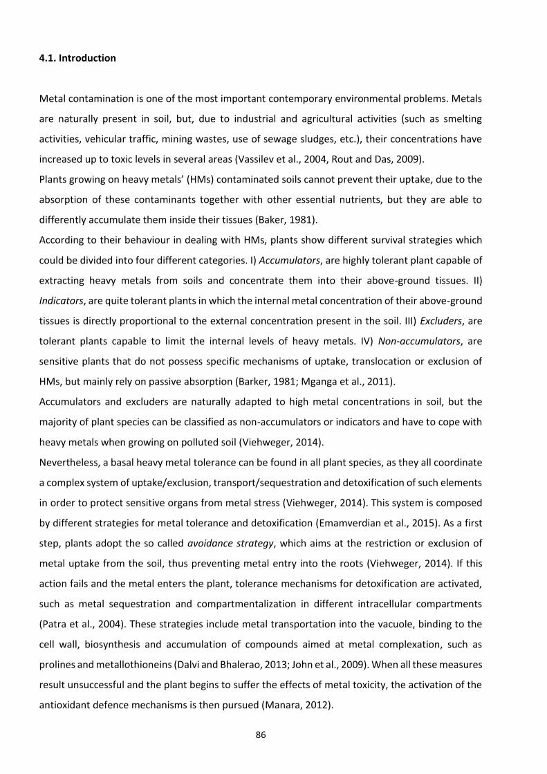
86

4.1. Introduction

Metal contamination is one of the most important contemporary environmental problems. Metals

are naturally present in soil, but, due to industrial and agricultural activities (such as smelting

activities, vehicular traffic, mining wastes, use of sewage sludges, etc.), their concentrations have

increased up to toxic levels in several areas (Vassilev et al., 2004, Rout and Das, 2009).

Plants growing on heavy metals’ (HMs) contaminated soils cannot prevent their uptake, due to the

absorption of these contaminants together with other essential nutrients, but they are able to

differently accumulate them inside their tissues (Baker, 1981).

According to their behaviour in dealing with HMs, plants show different survival strategies which

could be divided into four different categories. I) Accumulators, are highly tolerant plant capable of

extracting heavy metals from soils and concentrate them into their above-ground tissues. II)

Indicators, are quite tolerant plants in which the internal metal concentration of their above-ground

tissues is directly proportional to the external concentration present in the soil. III) Excluders, are

tolerant plants capable to limit the internal levels of heavy metals. IV) Non-accumulators, are

sensitive plants that do not possess specific mechanisms of uptake, translocation or exclusion of

HMs, but mainly rely on passive absorption (Barker, 1981; Mganga et al., 2011).

Accumulators and excluders are naturally adapted to high metal concentrations in soil, but the

majority of plant species can be classified as non-accumulators or indicators and have to cope with

heavy metals when growing on polluted soil (Viehweger, 2014).

Nevertheless, a basal heavy metal tolerance can be found in all plant species, as they all coordinate

a complex system of uptake/exclusion, transport/sequestration and detoxification of such elements

in order to protect sensitive organs from metal stress (Viehweger, 2014). This system is composed

by different strategies for metal tolerance and detoxification (Emamverdian et al., 2015). As a first

step, plants adopt the so called avoidance strategy, which aims at the restriction or exclusion of

metal uptake from the soil, thus preventing metal entry into the roots (Viehweger, 2014). If this

action fails and the metal enters the plant, tolerance mechanisms for detoxification are activated,

such as metal sequestration and compartmentalization in different intracellular compartments

(Patra et al., 2004). These strategies include metal transportation into the vacuole, binding to the

cell wall, biosynthesis and accumulation of compounds aimed at metal complexation, such as

prolines and metallothioneins (Dalvi and Bhalerao, 2013; John et al., 2009). When all these measures

result unsuccessful and the plant begins to suffer the effects of metal toxicity, the activation of the

antioxidant defence mechanisms is then pursued (Manara, 2012).

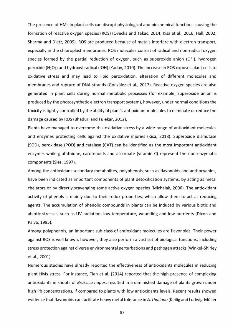
87

The presence of HMs in plant cells can disrupt physiological and biochemical functions causing the

formation of reactive oxygen species (ROS) (Ovecka and Takac, 2014; Kisa et al., 2016; Hall, 2002;

Sharma and Dietz, 2009). ROS are produced because of metals interfere with electron transport,

especially in the chloroplast membranes. ROS molecules consist of radical and non-radical oxygen

species formed by the partial reduction of oxygen, such as superoxide anion (O2−), hydrogen

peroxide (H2O2) and hydroxyl radical (·OH) (Yadav, 2010). The increase in ROS exposes plant cells to

oxidative stress and may lead to lipid peroxidation, alteration of different molecules and

membranes and rupture of DNA strands (González et al., 2017). Reactive oxygen species are also

generated in plant cells during normal metabolic processes (for example; superoxide anion is

produced by the photosynthetic electron transport system), however, under normal conditions the

toxicity is tightly controlled by the ability of plant´s antioxidant molecules to eliminate or reduce the

damage caused by ROS (Bhaduri and Fulekar, 2012).

Plants have managed to overcome this oxidative stress by a wide range of antioxidant molecules

and enzymes protecting cells against the oxidative injuries (Kisa, 2018). Superoxide dismutase

(SOD), peroxidase (POD) and catalase (CAT) can be identified as the most important antioxidant

enzymes while glutathione, carotenoids and ascorbate (vitamin C) represent the non-enzymatic

components (Sies, 1997).

Among the antioxidant secondary metabolites, polyphenols, such as flavonoids and anthocyanins,

have been indicated as important components of plant detoxification systems, by acting as metal

chelators or by directly scavenging some active oxygen species (Michalak, 2006). The antioxidant

activity of phenols is mainly due to their redox properties, which allow them to act as reducing

agents. The accumulation of phenolic compounds in plants can be induced by various biotic and

abiotic stresses, such as UV radiation, low temperature, wounding and low nutrients (Dixon and

Paiva, 1995).

Among polyphenols, an important sub-class of antioxidant molecules are flavonoids. Their power

against ROS is well known, however, they also perform a vast set of biological functions, including

stress protection against diverse environmental perturbations and pathogen attacks (Winkel-Shirley

et al., 2001).

Numerous studies have already reported the effectiveness of antioxidants molecules in reducing

plant HMs stress. For instance, Tian et al. (2014) reported that the high presence of complexing

antioxidants in shoots of Brassica napus, resulted in a diminished damage of plants grown under

high Pb concentrations, if compared to plants with low antioxidants levels. Recent results showed

evidence that flavonoids can facilitate heavy metal tolerance in A. thaliana (Keilig and Ludwig-Müller

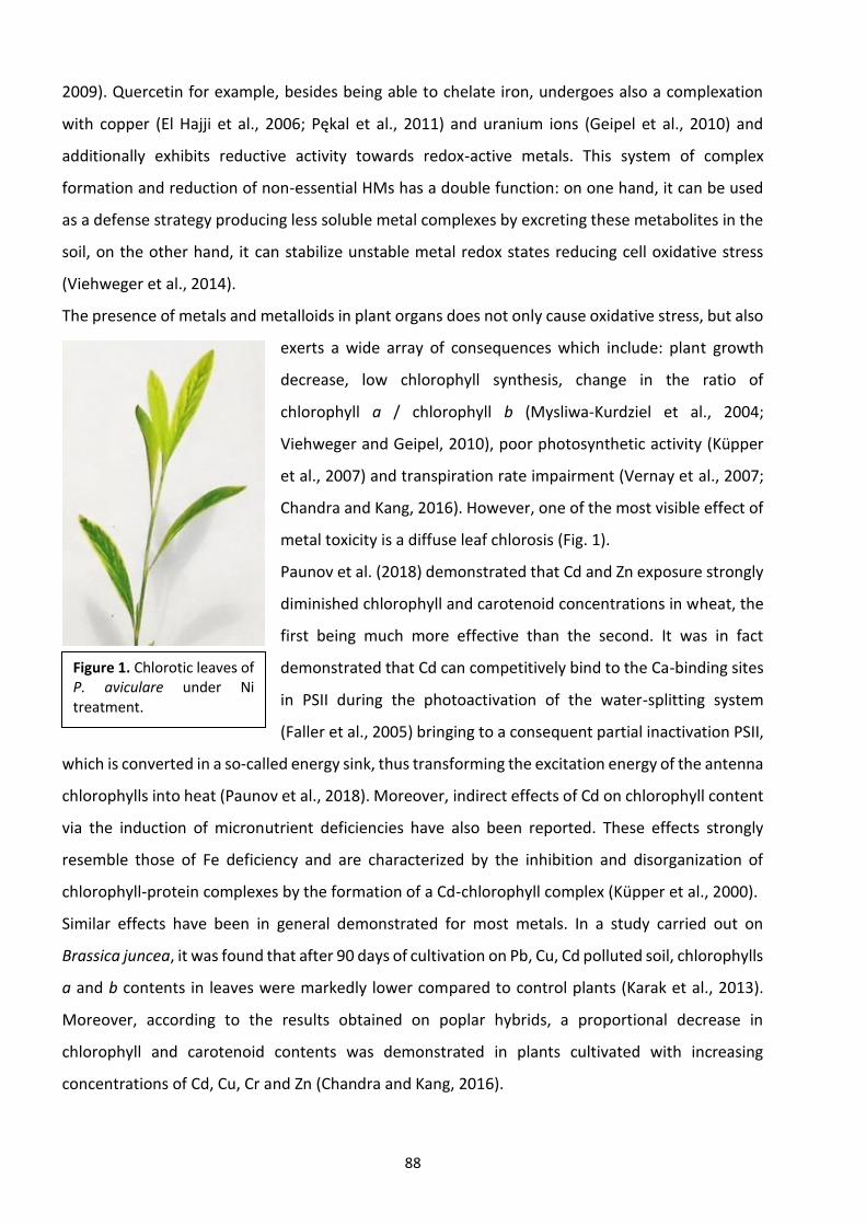
88

2009). Quercetin for example, besides being able to chelate iron, undergoes also a complexation

with copper (El Hajji et al., 2006; Pękal et al., 2011) and uranium ions (Geipel et al., 2010) and

additionally exhibits reductive activity towards redox-active metals. This system of complex

formation and reduction of non-essential HMs has a double function: on one hand, it can be used

as a defense strategy producing less soluble metal complexes by excreting these metabolites in the

soil, on the other hand, it can stabilize unstable metal redox states reducing cell oxidative stress

(Viehweger et al., 2014).

The presence of metals and metalloids in plant organs does not only cause oxidative stress, but also

exerts a wide array of consequences which include: plant growth

decrease, low chlorophyll synthesis, change in the ratio of

chlorophyll a / chlorophyll b (Mysliwa-Kurdziel et al., 2004;

Viehweger and Geipel, 2010), poor photosynthetic activity (Küpper

et al., 2007) and transpiration rate impairment (Vernay et al., 2007;

Chandra and Kang, 2016). However, one of the most visible effect of

metal toxicity is a diffuse leaf chlorosis (Fig. 1).

Paunov et al. (2018) demonstrated that Cd and Zn exposure strongly

diminished chlorophyll and carotenoid concentrations in wheat, the

first being much more effective than the second. It was in fact

demonstrated that Cd can competitively bind to the Ca-binding sites

in PSII during the photoactivation of the water-splitting system

(Faller et al., 2005) bringing to a consequent partial inactivation PSII,

which is converted in a so-called energy sink, thus transforming the excitation energy of the antenna

chlorophylls into heat (Paunov et al., 2018). Moreover, indirect effects of Cd on chlorophyll content

via the induction of micronutrient deficiencies have also been reported. These effects strongly

resemble those of Fe deficiency and are characterized by the inhibition and disorganization of

chlorophyll-protein complexes by the formation of a Cd-chlorophyll complex (Küpper et al., 2000).

Similar effects have been in general demonstrated for most metals. In a study carried out on

Brassica juncea, it was found that after 90 days of cultivation on Pb, Cu, Cd polluted soil, chlorophylls

a and b contents in leaves were markedly lower compared to control plants (Karak et al., 2013).

Moreover, according to the results obtained on poplar hybrids, a proportional decrease in

chlorophyll and carotenoid contents was demonstrated in plants cultivated with increasing

concentrations of Cd, Cu, Cr and Zn (Chandra and Kang, 2016).

Figure 1. Chlorotic leaves of P. aviculare under Ni treatment.

89

Despite the high correlation between heavy metal stress, antioxidant response and photosynthetic

pigments content, some authors argued that the overall effects of most abiotic stress were often

dependent on the plant species, genotype and other plant characteristics (Le Gall et al., 2015).

Nonetheless, photosynthetic pigments reduction caused by HMs was frequently used to determine

plant stress level (Aggarwal et al., 2012). In order to widen the knowledge on the various parameter

used to evaluate HM stress, the aim of the present study was investigate the differences in

physiological responses to increasing concentrations of six HMs (Cd, Cr, Cu, Ni, Pb, Zn), with

particular attention to antioxidant activity, polyphenol and flavonoid production, photosynthetic

pigments content and biomass production. The plants used were P. aviculare and S. vulgaris, each

of them represented by in five different populations, grown in hydroponic culture. The relations

between HMs uptake, antioxidant metabolites production and photosynthetic pigments content,

was then tested as reliable HM stress biomarkers.

4.3. Materials and Methods

4.3.1. Species selection

In this study, two annual weeds have been selected: Polygonum aviculare (Fig. 2) and Senecio

vulgaris (Fig. 3), because of their widespread presence in numerous environments, from disturbed

one to almost pristine. These two species are tolerant to

HM pollution, fast growing and produce abundant seeds

with high viability, for the previous reasons were perfect

candidates for our research.

P. aviculare is an annual plant belonging to the

Polygonaceae family, is a cosmopolitan species, growing

in several disturbed habitats and in particular in

frequently trampled areas. It germinates in spring and it

continuously flowers during the hot season to finally

produce seeds in autumn. The stems are creeping and grow up to 45-50 cm long, it has dark-green

oval leaves and small whitish flowers growing at the axil of each, followed by small triangular nuts.

Figure 2. Polygonum aviculare (L.). Photo: Mirko Salinitro

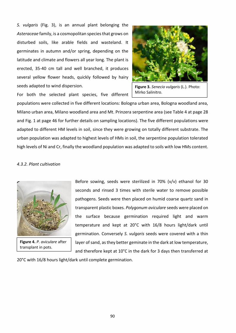
90

S. vulgaris (Fig. 3), is an annual plant belonging the

Asteraceae family, is a cosmopolitan species that grows on

disturbed soils, like arable fields and wasteland. It

germinates in autumn and/or spring, depending on the

latitude and climate and flowers all year long. The plant is

erected, 35-40 cm tall and well branched, it produces

several yellow flower heads, quickly followed by hairy

seeds adapted to wind dispersion.

For both the selected plant species, five different

populations were collected in five different locations: Bologna urban area, Bologna woodland area,

Milano urban area, Milano woodland area and Mt. Prinzera serpentine area (see Table 4 at page 28

and Fig. 1 at page 46 for further details on sampling locations). The five different populations were

adapted to different HM levels in soil, since they were growing on totally different substrate. The

urban population was adapted to highest levels of HMs in soil, the serpentine population tolerated

high levels of Ni and Cr, finally the woodland population was adapted to soils with low HMs content.

4.3.2. Plant cultivation

Before sowing, seeds were sterilized in 70% (v/v) ethanol for 30

seconds and rinsed 3 times with sterile water to remove possible

pathogens. Seeds were then placed on humid coarse quartz sand in

transparent plastic boxes. Polygonum aviculare seeds were placed on

the surface because germination required light and warm

temperature and kept at 20°C with 16/8 hours light/dark until

germination. Conversely S. vulgaris seeds were covered with a thin

layer of sand, as they better geminate in the dark at low temperature,

and therefore kept at 10°C in the dark for 3 days then transferred at

20°C with 16/8 hours light/dark until complete germination.

Figure 3. Senecio vulgaris (L.). Photo: Mirko Salinitro.

Figure 4. P. aviculare after transplant in pots.

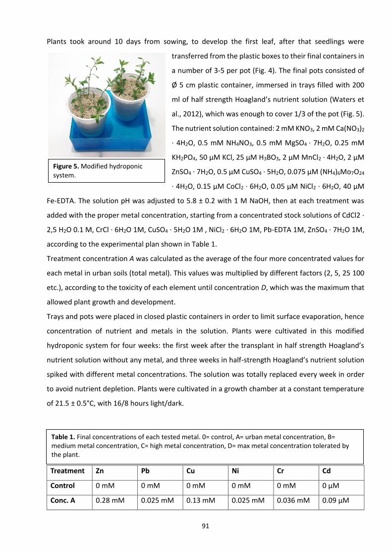
91

Plants took around 10 days from sowing, to develop the first leaf, after that seedlings were

transferred from the plastic boxes to their final containers in

a number of 3-5 per pot (Fig. 4). The final pots consisted of

Ø 5 cm plastic container, immersed in trays filled with 200

ml of half strength Hoagland’s nutrient solution (Waters et

al., 2012), which was enough to cover 1/3 of the pot (Fig. 5).

The nutrient solution contained: 2 mM KNO3, 2 mM Ca(NO3)2

· 4H2O, 0.5 mM NH4NO3, 0.5 mM MgSO4 · 7H2O, 0.25 mM

KH2PO4, 50 µM KCl, 25 µM H3BO3, 2 µM MnCl2 · 4H2O, 2 µM

ZnSO4 · 7H2O, 0.5 µM CuSO4 · 5H2O, 0.075 µM (NH4)6Mo7O24

· 4H2O, 0.15 µM CoCl2 · 6H2O, 0.05 µM NiCl2 · 6H2O, 40 µM

Fe-EDTA. The solution pH was adjusted to 5.8 ± 0.2 with 1 M NaOH, then at each treatment was

added with the proper metal concentration, starting from a concentrated stock solutions of CdCl2 ·

2,5 H2O 0.1 M, CrCl · 6H2O 1M, CuSO4 · 5H2O 1M , NiCl2 · 6H2O 1M, Pb-EDTA 1M, ZnSO4 · 7H2O 1M,

according to the experimental plan shown in Table 1.

Treatment concentration A was calculated as the average of the four more concentrated values for

each metal in urban soils (total metal). This values was multiplied by different factors (2, 5, 25 100

etc.), according to the toxicity of each element until concentration D, which was the maximum that

allowed plant growth and development.

Trays and pots were placed in closed plastic containers in order to limit surface evaporation, hence

concentration of nutrient and metals in the solution. Plants were cultivated in this modified

hydroponic system for four weeks: the first week after the transplant in half strength Hoagland’s

nutrient solution without any metal, and three weeks in half-strength Hoagland’s nutrient solution

spiked with different metal concentrations. The solution was totally replaced every week in order

to avoid nutrient depletion. Plants were cultivated in a growth chamber at a constant temperature

of 21.5 ± 0.5°C, with 16/8 hours light/dark.

Treatment Zn Pb Cu Ni Cr Cd

Control 0 mM 0 mM 0 mM 0 mM 0 mM 0 μM

Conc. A 0.28 mM 0.025 mM 0.13 mM 0.025 mM 0.036 mM 0.09 μM

Figure 5. Modified hydroponic system.

Table 1. Final concentrations of each tested metal. 0= control, A= urban metal concentration, B= medium metal concentration, C= high metal concentration, D= max metal concentration tolerated by the plant.

92

Conc. B 0.56 mM 0.25 mM 0.26 mM 0.12 mM 0.18 mM 9.46 μM

Conc. C 1.11mM 1.25 mM 0.66 mM 0.25 mM 0.36 mM 47.29 μM

Conc. D 2.78 mM 2.50 mM 1.32 mM 0.62 mM 0.89 mM 94.59μM

4.3.3. Sample collection and preparation

At the end of the fourth week of culture, only plant shoots were harvested. They were rinsed with

deionized water, then dried up with paper towels before weighting (fresh weight). Once weighted,

fresh samples were grinded in liquid nitrogen to obtain a homogeneous powder. The bulk powders

were then stored at -80°C for further analysis.

4.3.4. Metal quantifications

For the quantification of metals, 0.5 gFW of grinded shoots were oven dried at 80°C 24 hours until

constant weight. About 0.1-0.2 gDW of samples were pre-digested at room temperature with 2 mL

70% (v/v) HNO3 for 1 day, then digested on a heat block 1 h at 70°C and 1 h at 125°C following a

modified method from Huang and Schulte, (1985). After the digestion, samples were taken up to 10

mL with deionised water. Five replicates of reference material (Apple leaves NIST® SRM® 1515) and

blanks (only nitric acid) were included in the digestions. Metal concentration analysis were

performed with ICP-MS Elan 9000 DRCe, (Perkin Elmer, Waltham, Massachusetts, USA). Data were

expressed as ppm related to sample dry weight.

4.3.5. Spectrophotometrical analysis

Total flavonoids quantification assay was performed as explained in Zhishen et al. (1999) and Ferri

et al. (2013). This spectrophotometric analysis is based on the progressive colouration (orange) of

AlCr3 and NaNO2 in presence of increasing concentration of flavonoids in alkaline environment. The

same methanolic extracts obtained for antioxidant activity were used for total flavonoid

quantification. The supernatant was then recovered after centrifugation at 12000 rmp for 5

minutes. The calibration curve was made with growing concentration of (+)catechin hydrate (CAT)

from 2 to 14 μg/mL) and as blank control deionised water was used. An appropriate volume of

sample was put in 1.5 mL tubes, 400 μL of deionized water were added then 30 μL of NaNO2 5%

(w/v). The solution were mixed and after 5 minutes 30 μL of AlCl3 10% (w/v) were added. The

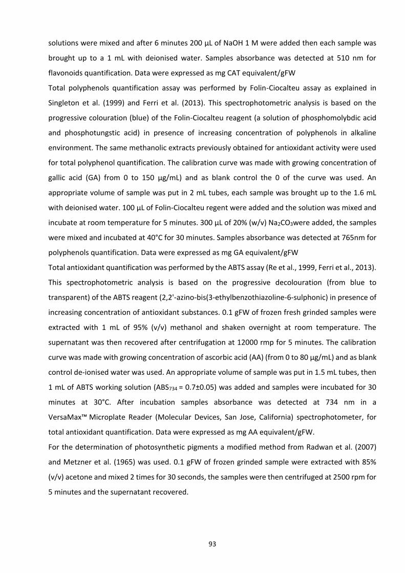
93

solutions were mixed and after 6 minutes 200 μL of NaOH 1 M were added then each sample was

brought up to a 1 mL with deionised water. Samples absorbance was detected at 510 nm for

flavonoids quantification. Data were expressed as mg CAT equivalent/gFW

Total polyphenols quantification assay was performed by Folin-Ciocalteu assay as explained in

Singleton et al. (1999) and Ferri et al. (2013). This spectrophotometric analysis is based on the

progressive colouration (blue) of the Folin-Ciocalteu reagent (a solution of phosphomolybdic acid

and phosphotungstic acid) in presence of increasing concentration of polyphenols in alkaline

environment. The same methanolic extracts previously obtained for antioxidant activity were used

for total polyphenol quantification. The calibration curve was made with growing concentration of

gallic acid (GA) from 0 to 150 μg/mL) and as blank control the 0 of the curve was used. An

appropriate volume of sample was put in 2 mL tubes, each sample was brought up to the 1.6 mL

with deionised water. 100 μL of Folin-Ciocalteu regent were added and the solution was mixed and

incubate at room temperature for 5 minutes. 300 μL of 20% (w/v) Na2CO3were added, the samples

were mixed and incubated at 40°C for 30 minutes. Samples absorbance was detected at 765nm for

polyphenols quantification. Data were expressed as mg GA equivalent/gFW

Total antioxidant quantification was performed by the ABTS assay (Re et al., 1999, Ferri et al., 2013).

This spectrophotometric analysis is based on the progressive decolouration (from blue to

transparent) of the ABTS reagent (2,2'-azino-bis(3-ethylbenzothiazoline-6-sulphonic) in presence of

increasing concentration of antioxidant substances. 0.1 gFW of frozen fresh grinded samples were

extracted with 1 mL of 95% (v/v) methanol and shaken overnight at room temperature. The

supernatant was then recovered after centrifugation at 12000 rmp for 5 minutes. The calibration

curve was made with growing concentration of ascorbic acid (AA) (from 0 to 80 μg/mL) and as blank

control de-ionised water was used. An appropriate volume of sample was put in 1.5 mL tubes, then

1 mL of ABTS working solution (ABS734 = 0.7±0.05) was added and samples were incubated for 30

minutes at 30°C. After incubation samples absorbance was detected at 734 nm in a

VersaMax™ Microplate Reader (Molecular Devices, San Jose, California) spectrophotometer, for

total antioxidant quantification. Data were expressed as mg AA equivalent/gFW.

For the determination of photosynthetic pigments a modified method from Radwan et al. (2007)

and Metzner et al. (1965) was used. 0.1 gFW of frozen grinded sample were extracted with 85%

(v/v) acetone and mixed 2 times for 30 seconds, the samples were then centrifuged at 2500 rpm for

5 minutes and the supernatant recovered.

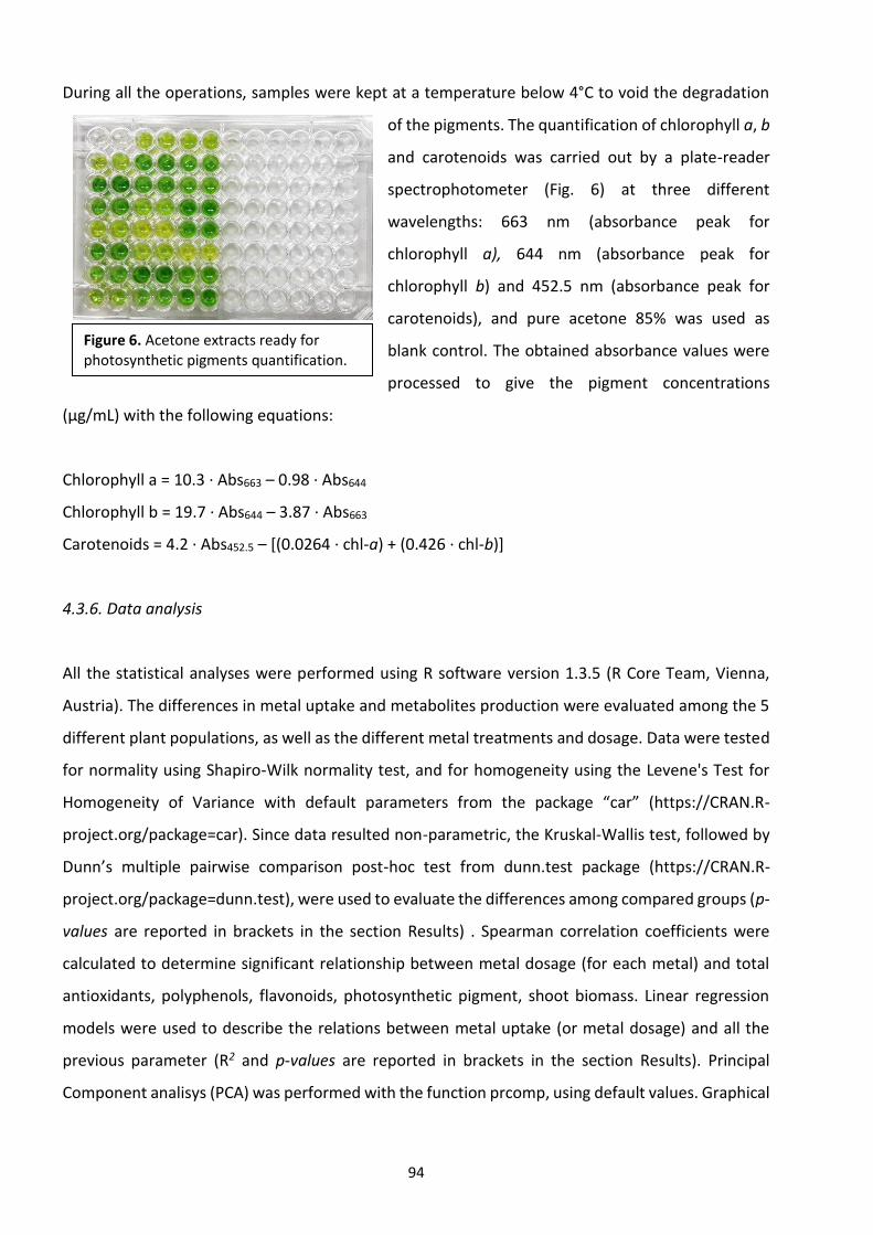
94

During all the operations, samples were kept at a temperature below 4°C to void the degradation

of the pigments. The quantification of chlorophyll a, b

and carotenoids was carried out by a plate-reader

spectrophotometer (Fig. 6) at three different

wavelengths: 663 nm (absorbance peak for

chlorophyll a), 644 nm (absorbance peak for

chlorophyll b) and 452.5 nm (absorbance peak for

carotenoids), and pure acetone 85% was used as

blank control. The obtained absorbance values were

processed to give the pigment concentrations

(μg/mL) with the following equations:

Chlorophyll a = 10.3 · Abs663 – 0.98 · Abs644

Chlorophyll b = 19.7 · Abs644 – 3.87 · Abs663

Carotenoids = 4.2 · Abs452.5 – [(0.0264 · chl-a) + (0.426 · chl-b)]

4.3.6. Data analysis

All the statistical analyses were performed using R software version 1.3.5 (R Core Team, Vienna,

Austria). The differences in metal uptake and metabolites production were evaluated among the 5

different plant populations, as well as the different metal treatments and dosage. Data were tested

for normality using Shapiro-Wilk normality test, and for homogeneity using the Levene's Test for

Homogeneity of Variance with default parameters from the package “car” (https://CRAN.R-

project.org/package=car). Since data resulted non-parametric, the Kruskal-Wallis test, followed by

Dunn’s multiple pairwise comparison post-hoc test from dunn.test package (https://CRAN.R-

project.org/package=dunn.test), were used to evaluate the differences among compared groups (p-

values are reported in brackets in the section Results) . Spearman correlation coefficients were

calculated to determine significant relationship between metal dosage (for each metal) and total

antioxidants, polyphenols, flavonoids, photosynthetic pigment, shoot biomass. Linear regression

models were used to describe the relations between metal uptake (or metal dosage) and all the

previous parameter (R2 and p-values are reported in brackets in the section Results). Principal

Component analisys (PCA) was performed with the function prcomp, using default values. Graphical

Figure 6. Acetone extracts ready for photosynthetic pigments quantification.

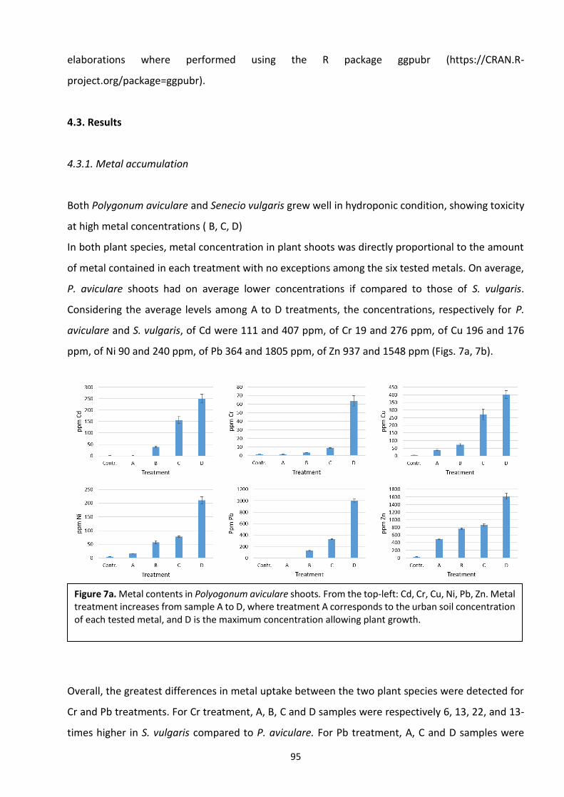
95

elaborations where performed using the R package ggpubr (https://CRAN.R-

project.org/package=ggpubr).

4.3. Results

4.3.1. Metal accumulation

Both Polygonum aviculare and Senecio vulgaris grew well in hydroponic condition, showing toxicity

at high metal concentrations ( B, C, D)

In both plant species, metal concentration in plant shoots was directly proportional to the amount

of metal contained in each treatment with no exceptions among the six tested metals. On average,

P. aviculare shoots had on average lower concentrations if compared to those of S. vulgaris.

Considering the average levels among A to D treatments, the concentrations, respectively for P.

aviculare and S. vulgaris, of Cd were 111 and 407 ppm, of Cr 19 and 276 ppm, of Cu 196 and 176

ppm, of Ni 90 and 240 ppm, of Pb 364 and 1805 ppm, of Zn 937 and 1548 ppm (Figs. 7a, 7b).

Overall, the greatest differences in metal uptake between the two plant species were detected for

Cr and Pb treatments. For Cr treatment, A, B, C and D samples were respectively 6, 13, 22, and 13-

times higher in S. vulgaris compared to P. aviculare. For Pb treatment, A, C and D samples were

Figure 7a. Metal contents in Polyogonum aviculare shoots. From the top-left: Cd, Cr, Cu, Ni, Pb, Zn. Metal treatment increases from sample A to D, where treatment A corresponds to the urban soil concentration of each tested metal, and D is the maximum concentration allowing plant growth.

96

respectively 6, 7 and 5-times higher in S. vulgaris compared to P. aviculare. The only metal which

was similarly absorbed by both species was Cu, whose concentrations were slightly lower in all

samples in S. vulgaris shoots compared to P. aviculare ones (Figs. 7a, 7b). S. vulgaris resulted to be

above the hyperaccumulation threshold set for Pb (>1000 ppm; Van der Ent et al., 2013), in the

treatments C and D with respectively 2401 and 4580 ppm of metal accumulated in plant shoots.

Also for Cd the set hyperaccumulation threshold (> 100 ppm; Van der Ent et al., 2013) was overtaken

in treatments B, C and D (226, 630 and 765 ppm respectively) for S. vulgaris and C, D for P. aviculare

(156 and 250 ppm).

The different metals were differentially transferred from soils to shoots according to the type of

species and metal. This parameter is called bioaccumulation factor (BAF) and is calculated as the

ratio between metal concentration in soil (in this case in the hydroponic solution) and the metal

concentration in plant shoots. BAFs for P. aviculare and for S. vulgaris were reported in Tables 2a

and 2b. Overall, BAFs for all metals were higher for S. vulgaris, in accordance with the general higher

metal content detected, if compared to P. aviculare. The only exception was Cu, where the uptake

and transfer efficiencies in S. vulgaris were slightly lower than in P. aviculare. With the exception of

A, B, C Cr treatments and A treatment for Pb in P. aviculare, all BAFs were > 1, showing that the two

studied species were able to concentrate metals in their aerial parts when cultivated in hydroponic.

The most easily transferred metals were Cd, followed by Zn and Ni with maximum BAFs respectively

of 416, 57, 34 in S. vulgaris and of 222, 27, 13 in P. aviculare (Tables 2a, 2b). From the present data,

it can be clearly noticed that for Cd, Zn and Ni, at the increase of the metal concentration in the

Figure 7b. Metal contents in Senecio vulgaris shoots. From the top-left: Cd, Cr, Cu, Ni, Pb, Zn. Metal treatment increases from A to D samples, where treatment A corresponds to the urban soil concentration of each tested metal, and D is the maximum concentration allowing plant growth.

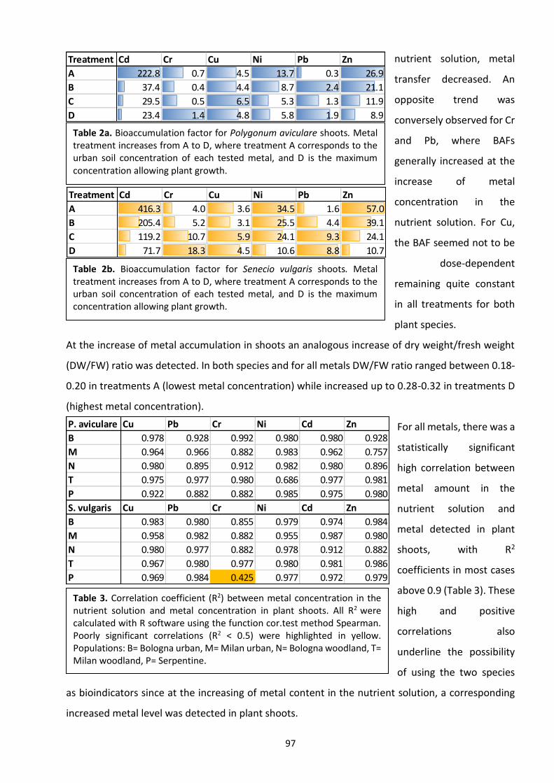
97

nutrient solution, metal

transfer decreased. An

opposite trend was

conversely observed for Cr

and Pb, where BAFs

generally increased at the

increase of metal

concentration in the

nutrient solution. For Cu,

the BAF seemed not to be

dose-dependent

remaining quite constant

in all treatments for both

plant species.

At the increase of metal accumulation in shoots an analogous increase of dry weight/fresh weight

(DW/FW) ratio was detected. In both species and for all metals DW/FW ratio ranged between 0.18-

0.20 in treatments A (lowest metal concentration) while increased up to 0.28-0.32 in treatments D

(highest metal concentration).

For all metals, there was a

statistically significant

high correlation between

metal amount in the

nutrient solution and

metal detected in plant

shoots, with R2

coefficients in most cases

above 0.9 (Table 3). These

high and positive

correlations also

underline the possibility

of using the two species

as bioindicators since at the increasing of metal content in the nutrient solution, a corresponding

increased metal level was detected in plant shoots.

Treatment Cd Cr Cu Ni Pb Zn

A 222.8 0.7 4.5 13.7 0.3 26.9

B 37.4 0.4 4.4 8.7 2.4 21.1

C 29.5 0.5 6.5 5.3 1.3 11.9

D 23.4 1.4 4.8 5.8 1.9 8.9

Treatment Cd Cr Cu Ni Pb Zn

A 416.3 4.0 3.6 34.5 1.6 57.0

B 205.4 5.2 3.1 25.5 4.4 39.1

C 119.2 10.7 5.9 24.1 9.3 24.1

D 71.7 18.3 4.5 10.6 8.8 10.7

Table 2a. Bioaccumulation factor for Polygonum aviculare shoots. Metal treatment increases from A to D, where treatment A corresponds to the urban soil concentration of each tested metal, and D is the maximum concentration allowing plant growth.

Table 2b. Bioaccumulation factor for Senecio vulgaris shoots. Metal treatment increases from A to D, where treatment A corresponds to the urban soil concentration of each tested metal, and D is the maximum concentration allowing plant growth.

Table 3. Correlation coefficient (R2) between metal concentration in the nutrient solution and metal concentration in plant shoots. All R2 were calculated with R software using the function cor.test method Spearman. Poorly significant correlations (R2 < 0.5) were highlighted in yellow. Populations: B= Bologna urban, M= Milan urban, N= Bologna woodland, T= Milan woodland, P= Serpentine.

P. aviculare Cu Pb Cr Ni Cd Zn

B 0.978 0.928 0.992 0.980 0.980 0.928

M 0.964 0.966 0.882 0.983 0.962 0.757

N 0.980 0.895 0.912 0.982 0.980 0.896

T 0.975 0.977 0.980 0.686 0.977 0.981

P 0.922 0.882 0.882 0.985 0.975 0.980

S. vulgaris Cu Pb Cr Ni Cd Zn

B 0.983 0.980 0.855 0.979 0.974 0.984

M 0.958 0.982 0.882 0.955 0.987 0.980

N 0.980 0.977 0.882 0.978 0.912 0.882

T 0.967 0.980 0.977 0.980 0.981 0.986

P 0.969 0.984 0.425 0.977 0.972 0.979

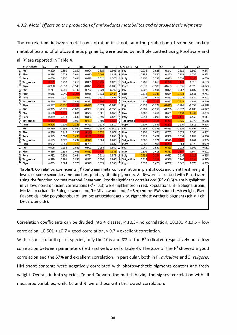
98

4.3.2. Metal effects on the production of antioxidants metabolites and photosynthetic pigments

The correlations between metal concentration in shoots and the production of some secondary

metabolites and of photosynthetic pigments, were tested by multiple cor.test using R software and

all R2 are reported in Table 4.

Correlation coefficients can be divided into 4 classes: < ±0.3= no correlation, ±0.301 < ±0.5 = low

correlation, ±0.501 < ±0.7 = good correlation, > 0.7 = excellent correlation.

With respect to both plant species, only the 10% and 8% of the R2 indicated respectively no or low

correlation between parameters (red and yellow cells Table 4). The 25% of the R2 showed a good

correlation and the 57% and excellent correlation. In particular, both in P. aviculare and S. vulgaris,

HM shoot contents were negatively correlated with photosynthetic pigments content and fresh

weight. Overall, in both species, Zn and Cu were the metals having the highest correlation with all

measured variables, while Cd and Ni were those with the lowest correlation.

Table 4. Correlation coefficients (R2) between metal concentration in plant shoots and plant fresh weight, levels of some secondary metabolites, photosynthetic pigments. All R2 were calculated with R software using the function cor.test method Spearman. Poorly significant correlations (R2 < 0.5) were highlighted in yellow, non-significant correlations (R2 < 0.3) were highlighted in red. Populations: B= Bologna urban, M= Milan urban, N= Bologna woodland, T= Milan woodland, P= Serpentine. FW: shoot fresh weight, Flav: flavonoids, Poly: polyphenols, Tot_antiox: antioxidant activity, Pigm: photosynthetic pigments (chl a + chl b+ carotenoids).

Cu Pb Cr Ni Cd Zn Cu Pb Cr Ni Cd Zn

FW -0.890 -0.859 -0.850 -0.904 -0.835 -0.901 FW -0.976 -0.928 -0.841 -0.683 -0.920 -0.877

Flav 0.786 0.923 0.691 0.950 0.446 0.823 Flav 0.836 0.570 0.890 0.584 0.749 0.723

Poly 0.638 0.770 0.881 0.678 0.632 0.575 Poly 0.709 0.739 0.896 0.628 0.166 0.600

Tot_antiox 0.281 0.752 0.615 0.836 0.235 0.825 Tot_antiox 0.768 0.868 0.298 0.143 0.710 0.683

Pigm -0.908 -0.852 -0.540 -0.871 -0.117 -0.830 Pigm -0.839 -0.509 -0.600 -0.576 -0.720 -0.873

FW -0.714 -0.858 -0.740 -0.787 -0.829 -0.742 FW -0.807 -0.904 -0.874 -0.587 -0.807 -0.711

Flav 0.936 0.940 0.205 0.915 0.733 0.484 Flav 0.612 0.342 0.664 0.414 0.531 0.761

Poly 0.646 0.919 0.365 0.632 0.821 0.695 Poly 0.708 0.952 0.862 0.928 0.864 0.891

Tot_antiox 0.599 0.880 0.898 0.925 0.146 0.270 Tot_antiox 0.928 0.270 0.877 0.329 0.881 0.746

Pigm -0.587 -0.456 -0.289 -0.476 -0.623 -0.683 Pigm -0.859 -0.729 -0.410 -0.906 -0.758 -0.898

FW -0.935 -0.875 -0.805 -0.967 -0.965 -0.755 FW -0.867 -0.955 -0.786 -0.872 -0.883 -0.877

Flav 0.608 0.114 0.801 0.564 0.501 0.853 Flav 0.667 0.663 0.655 0.478 0.442 0.863

Poly 0.879 0.813 0.836 0.866 0.856 0.828 Poly 0.643 0.890 0.569 0.131 0.560 0.611

Tot_antiox 0.122 0.238 0.503 0.499 0.660 0.657 Tot_antiox 0.216 0.131 0.211 0.325 0.770 0.578

Pigm -0.408 -0.501 -0.328 -0.733 -0.823 -0.512 Pigm -0.807 -0.582 -0.270 -0.870 -0.518 -0.824

FW -0.910 -0.893 -0.844 -0.656 -0.895 -0.916 FW -0.883 -0.958 -0.893 -0.926 -0.897 -0.741

Flav 0.946 0.849 0.956 0.170 0.472 0.677 Flav 0.905 0.676 0.765 0.653 0.585 0.862

Poly 0.585 0.662 0.493 0.162 0.116 0.856 Poly 0.838 0.671 0.959 0.514 0.848 0.956

Tot_antiox 0.695 0.877 0.692 0.370 0.684 0.696 Tot_antiox 0.967 0.924 0.576 0.182 0.661 0.985

Pigm -0.902 -0.941 -0.410 -0.765 -0.931 -0.697 Pigm -0.948 -0.903 -0.257 -0.863 -0.125 -0.929

FW -0.908 -0.853 -0.885 -0.931 -0.894 -0.846 FW -0.945 -0.935 -0.416 -0.913 -0.905 -0.911

Flav 0.816 0.859 0.669 0.487 0.126 0.343 Flav 0.806 0.613 0.337 0.197 0.634 0.602

Poly 0.922 0.901 0.644 0.724 0.611 0.878 Poly 0.333 0.294 0.692 0.616 0.119 0.868

Tot_antiox 0.929 0.891 0.836 0.822 0.650 0.960 Tot_antiox 0.614 0.223 0.566 0.940 0.256 0.975

Pigm -0.893 -0.824 -0.579 -0.940 -0.935 -0.959 Pigm -0.937 -0.620 -0.707 -0.842 -0.778 -0.963

po

pu

lati

on

M

po

pu

lati

on

M

P. aviculare S. vulgaris

po

pu

lati

on

B

po

pu

lati

on

B

po

pu

lati

on

N

po

pu

lati

on

N

po

pu

lati

on

T

po

pu

lati

on

T

po

pu

lati

on

P

po

pu

lati

on

P

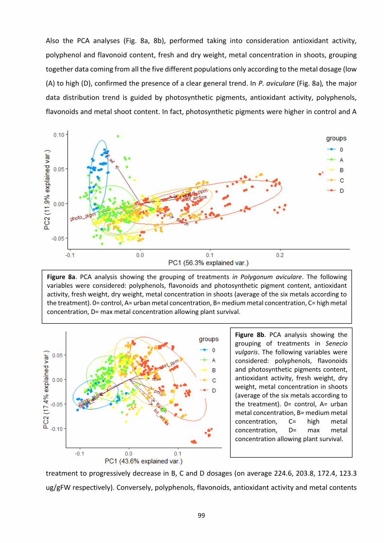
99

Also the PCA analyses (Fig. 8a, 8b), performed taking into consideration antioxidant activity,

polyphenol and flavonoid content, fresh and dry weight, metal concentration in shoots, grouping

together data coming from all the five different populations only according to the metal dosage (low

(A) to high (D), confirmed the presence of a clear general trend. In P. aviculare (Fig. 8a), the major

data distribution trend is guided by photosynthetic pigments, antioxidant activity, polyphenols,

flavonoids and metal shoot content. In fact, photosynthetic pigments were higher in control and A

treatment to progressively decrease in B, C and D dosages (on average 224.6, 203.8, 172.4, 123.3

ug/gFW respectively). Conversely, polyphenols, flavonoids, antioxidant activity and metal contents

Figure 8a. PCA analysis showing the grouping of treatments in Polygonum aviculare. The following variables were considered: polyphenols, flavonoids and photosynthetic pigment content, antioxidant activity, fresh weight, dry weight, metal concentration in shoots (average of the six metals according to the treatment). 0= control, A= urban metal concentration, B= medium metal concentration, C= high metal concentration, D= max metal concentration allowing plant survival.

Figure 8b. PCA analysis showing the grouping of treatments in Senecio vulgaris. The following variables were considered: polyphenols, flavonoids and photosynthetic pigments content, antioxidant activity, fresh weight, dry weight, metal concentration in shoots (average of the six metals according to the treatment). 0= control, A= urban metal concentration, B= medium metal concentration, C= high metal concentration, D= max metal concentration allowing plant survival.

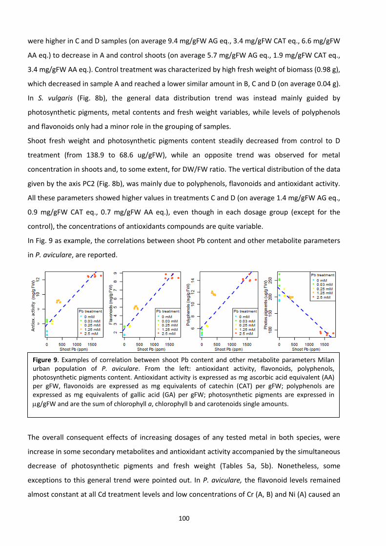
100

were higher in C and D samples (on average 9.4 mg/gFW AG eq., 3.4 mg/gFW CAT eq., 6.6 mg/gFW

AA eq.) to decrease in A and control shoots (on average 5.7 mg/gFW AG eq., 1.9 mg/gFW CAT eq.,

3.4 mg/gFW AA eq.). Control treatment was characterized by high fresh weight of biomass (0.98 g),

which decreased in sample A and reached a lower similar amount in B, C and D (on average 0.04 g).

In S. vulgaris (Fig. 8b), the general data distribution trend was instead mainly guided by

photosynthetic pigments, metal contents and fresh weight variables, while levels of polyphenols

and flavonoids only had a minor role in the grouping of samples.

Shoot fresh weight and photosynthetic pigments content steadily decreased from control to D

treatment (from 138.9 to 68.6 ug/gFW), while an opposite trend was observed for metal

concentration in shoots and, to some extent, for DW/FW ratio. The vertical distribution of the data

given by the axis PC2 (Fig. 8b), was mainly due to polyphenols, flavonoids and antioxidant activity.

All these parameters showed higher values in treatments C and D (on average 1.4 mg/gFW AG eq.,

0.9 mg/gFW CAT eq., 0.7 mg/gFW AA eq.), even though in each dosage group (except for the

control), the concentrations of antioxidants compounds are quite variable.

In Fig. 9 as example, the correlations between shoot Pb content and other metabolite parameters

in P. aviculare, are reported.

The overall consequent effects of increasing dosages of any tested metal in both species, were

increase in some secondary metabolites and antioxidant activity accompanied by the simultaneous

decrease of photosynthetic pigments and fresh weight (Tables 5a, 5b). Nonetheless, some

exceptions to this general trend were pointed out. In P. aviculare, the flavonoid levels remained

almost constant at all Cd treatment levels and low concentrations of Cr (A, B) and Ni (A) caused an

Figure 9. Examples of correlation between shoot Pb content and other metabolite parameters Milan urban population of P. aviculare. From the left: antioxidant activity, flavonoids, polyphenols, photosynthetic pigments content. Antioxidant activity is expressed as mg ascorbic acid equivalent (AA) per gFW, flavonoids are expressed as mg equivalents of catechin (CAT) per gFW; polyphenols are expressed as mg equivalents of gallic acid (GA) per gFW; photosynthetic pigments are expressed in

g/gFW and are the sum of chlorophyll a, chlorophyll b and carotenoids single amounts.

101

increase of photosynthetic pigments. In S. vulgaris, polyphenols only increased at the highest

dosage of any metal, remaining almost constant between control, A and B treatments;

photosynthetic pigments slightly increased respect to the control, at low levels (concentration A) of

Cd, Cr, Ni and Pb, to decrease again at higher dosages of the same metals. Data in Tables 5a and 5b

also indicate which metals were most toxic for the two plant species. Acute toxicity can be observed

in a plant, when a dramatic decrease in plant biomass and photosynthetic pigments is accompanied

by an opposite sharp increase in secondary metabolites. P. aviculare was in general less sensitive to

HMs than S. vulgaris since it showed acute toxicity only in few cases and in particular under Cu, Pb,

Zn treatments at dosage D (Table 5a, data highlighted in yellow). Instead, in S. vulgaris acute toxicity

was detected in a higher number of treatments: Cd (sample D), Cu (D), Ni (D), Pb (C, D) and Zn (C,

D) (Table 5b, data highlighted in yellow).

Table 5a. Average levels of all populations, of fresh weight (gFW), flavonoids (mg CAT eq/gFW), polyphenols (mg GA eq/gFW), antioxidant activity (mg AA eq/gFW) and photosynthetic pigments

(g/gFW) in P. aviculare. Highlighted in yellow the concentrations that gave acute toxic effects.

Table 5b. Average levels of all populations, of fresh weight (gFW), flavonoids (mg CAT eq/gFW), polyphenols (mg GA eq/gFW), antioxidant activity (mg AA eq/gFW) and photosynthetic pigments

(g/gFW) in S. vulgaris. Highlighted in yellow the treatments that gave acute toxic effects.

Treatment FW Flav Poly Antiox. act Pigm

control 0.84 0.33 1.06 0.38 118.76

Cd_A 0.55 0.50 0.98 0.55 154.16

Cd_B 0.23 0.44 0.95 0.57 110.92

Cd_C 0.14 0.67 1.48 0.51 112.11

Cd_D 0.09 0.91 1.35 0.54 68.15

control 0.61 1.00 1.00 0.67 136.03

Cr_A 0.39 0.51 0.98 0.50 160.42

Cr_B 0.25 0.70 1.07 0.57 148.75

Cr_C 0.08 0.85 1.16 0.68 136.07

Cr_D 0.06 1.17 1.61 0.82 119.30

control 0.84 0.67 1.07 0.56 131.46

Cu_A 0.08 0.84 1.02 0.62 127.11

Cu_B 0.05 0.79 1.03 0.68 121.84

Cu_C 0.03 0.76 1.22 0.71 96.95

Cu_D 0.01 1.36 1.41 0.96 56.75

control 0.99 0.34 1.10 0.49 133.73

Ni_A 0.70 0.64 1.02 0.52 143.57

Ni_B 0.60 0.50 1.10 0.46 94.66

Ni_C 0.42 0.59 1.19 0.52 64.43

Ni_D 0.16 0.90 1.50 0.80 50.32

control 0.97 0.42 1.01 0.56 149.65

Pb_A 0.38 0.50 1.02 0.48 156.15

Pb_B 0.07 0.54 1.08 0.47 146.16

Pb_C 0.02 0.84 1.40 0.55 70.09

Pb_D 0.01 0.97 1.63 0.66 70.35

control 1.06 0.76 0.79 0.53 164.13

Zn_A 0.50 0.43 0.99 0.44 129.98

Zn_B 0.56 0.59 1.16 0.59 99.95

Zn_C 0.23 1.03 1.53 0.84 69.08

Zn_D 0.07 1.49 1.90 1.15 53.04

Treatment FW Flav Poly Antiox. Act Pigm

control 1.20 1.93 4.97 4.80 235.93

Cd_A 0.38 2.63 4.90 3.62 218.76

Cd_B 0.12 2.36 5.15 3.50 208.24

Cd_C 0.05 2.40 5.66 3.04 164.76

Cd_D 0.02 2.42 7.13 4.33 139.44

control 1.20 1.79 5.09 4.76 201.27

Cr_A 0.55 2.00 5.68 2.54 234.96

Cr_B 0.08 2.02 6.23 3.01 228.11

Cr_C 0.02 2.31 7.80 3.76 221.52

Cr_D 0.02 3.59 9.61 6.70 186.23

control 1.11 1.58 5.55 4.23 200.36

Cu_A 0.02 1.94 5.51 3.37 192.90

Cu_B 0.00 2.33 6.06 3.08 202.67

Cu_C 0.00 2.76 9.24 7.36 146.66

Cu_D 0.00 4.18 10.78 8.70 77.21

control 0.96 1.41 6.51 3.27 217.48

Ni_A 0.26 2.03 5.08 4.17 238.42

Ni_B 0.04 2.76 5.82 5.21 199.18

Ni_C 0.02 3.22 7.16 5.36 184.36

Ni_D 0.01 3.75 8.82 7.75 133.82

control 0.79 1.58 6.13 2.00 236.42

Pb_A 0.31 2.66 5.89 4.29 230.77

Pb_B 0.08 2.81 6.48 4.63 217.52

Pb_C 0.01 3.61 9.23 6.93 177.98

Pb_D 0.01 5.01 11.25 9.04 122.67

control 0.65 2.53 6.54 0.56 240.42

Zn_A 0.11 1.66 6.92 4.15 236.65

Zn_B 0.11 2.11 7.29 4.43 167.21

Zn_C 0.03 2.26 9.04 5.59 139.14

Zn_D 0.01 4.65 15.57 10.39 77.80

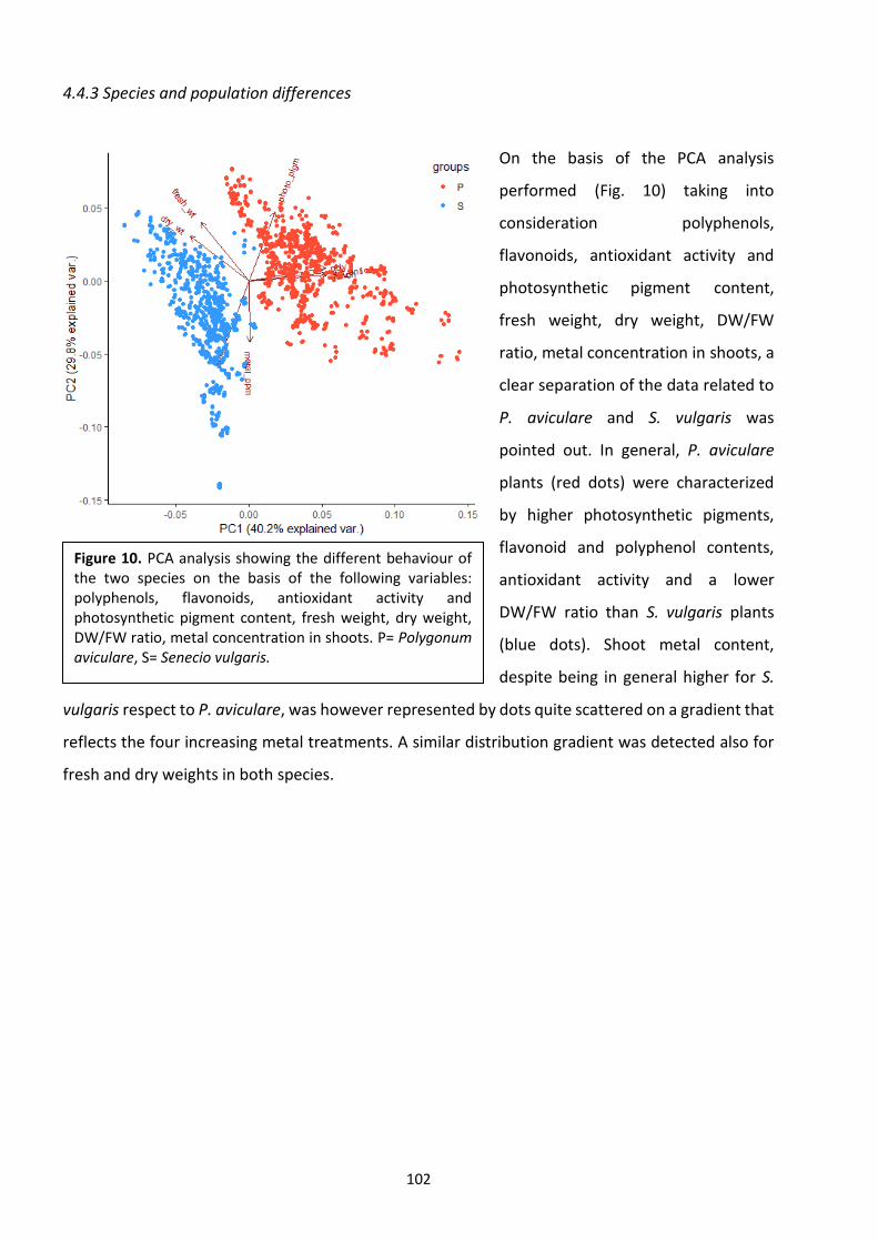
102

4.4.3 Species and population differences

On the basis of the PCA analysis

performed (Fig. 10) taking into

consideration polyphenols,

flavonoids, antioxidant activity and

photosynthetic pigment content,

fresh weight, dry weight, DW/FW

ratio, metal concentration in shoots, a

clear separation of the data related to

P. aviculare and S. vulgaris was

pointed out. In general, P. aviculare

plants (red dots) were characterized

by higher photosynthetic pigments,

flavonoid and polyphenol contents,

antioxidant activity and a lower

DW/FW ratio than S. vulgaris plants

(blue dots). Shoot metal content,

despite being in general higher for S.

vulgaris respect to P. aviculare, was however represented by dots quite scattered on a gradient that

reflects the four increasing metal treatments. A similar distribution gradient was detected also for

fresh and dry weights in both species.

Figure 10. PCA analysis showing the different behaviour of the two species on the basis of the following variables: polyphenols, flavonoids, antioxidant activity and photosynthetic pigment content, fresh weight, dry weight, DW/FW ratio, metal concentration in shoots. P= Polygonum aviculare, S= Senecio vulgaris.

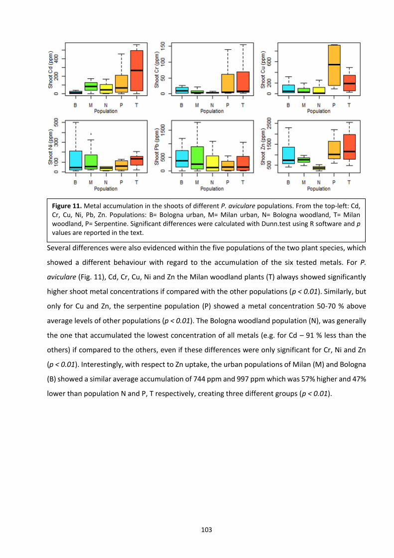
103

Several differences were also evidenced within the five populations of the two plant species, which

showed a different behaviour with regard to the accumulation of the six tested metals. For P.

aviculare (Fig. 11), Cd, Cr, Cu, Ni and Zn the Milan woodland plants (T) always showed significantly

higher shoot metal concentrations if compared with the other populations (p < 0.01). Similarly, but

only for Cu and Zn, the serpentine population (P) showed a metal concentration 50-70 % above

average levels of other populations (p < 0.01). The Bologna woodland population (N), was generally

the one that accumulated the lowest concentration of all metals (e.g. for Cd – 91 % less than the

others) if compared to the others, even if these differences were only significant for Cr, Ni and Zn

(p < 0.01). Interestingly, with respect to Zn uptake, the urban populations of Milan (M) and Bologna

(B) showed a similar average accumulation of 744 ppm and 997 ppm which was 57% higher and 47%

lower than population N and P, T respectively, creating three different groups (p < 0.01).

Figure 11. Metal accumulation in the shoots of different P. aviculare populations. From the top-left: Cd, Cr, Cu, Ni, Pb, Zn. Populations: B= Bologna urban, M= Milan urban, N= Bologna woodland, T= Milan woodland, P= Serpentine. Significant differences were calculated with Dunn.test using R software and p values are reported in the text.

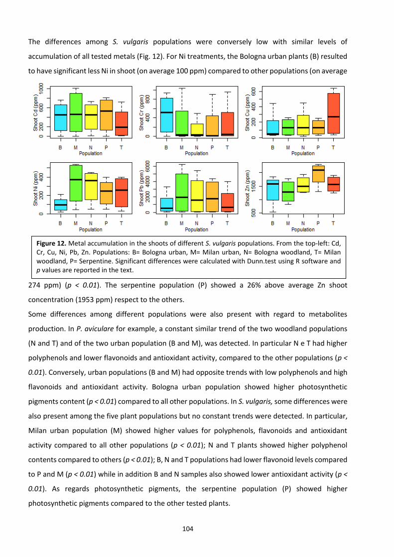
104

The differences among S. vulgaris populations were conversely low with similar levels of

accumulation of all tested metals (Fig. 12). For Ni treatments, the Bologna urban plants (B) resulted

to have significant less Ni in shoot (on average 100 ppm) compared to other populations (on average

274 ppm) (p < 0.01). The serpentine population (P) showed a 26% above average Zn shoot

concentration (1953 ppm) respect to the others.

Some differences among different populations were also present with regard to metabolites

production. In P. aviculare for example, a constant similar trend of the two woodland populations

(N and T) and of the two urban population (B and M), was detected. In particular N e T had higher

polyphenols and lower flavonoids and antioxidant activity, compared to the other populations (p <

0.01). Conversely, urban populations (B and M) had opposite trends with low polyphenols and high

flavonoids and antioxidant activity. Bologna urban population showed higher photosynthetic

pigments content (p < 0.01) compared to all other populations. In S. vulgaris, some differences were

also present among the five plant populations but no constant trends were detected. In particular,

Milan urban population (M) showed higher values for polyphenols, flavonoids and antioxidant

activity compared to all other populations (p < 0.01); N and T plants showed higher polyphenol

contents compared to others (p < 0.01); B, N and T populations had lower flavonoid levels compared

to P and M (p < 0.01) while in addition B and N samples also showed lower antioxidant activity (p <

0.01). As regards photosynthetic pigments, the serpentine population (P) showed higher

photosynthetic pigments compared to the other tested plants.

Figure 12. Metal accumulation in the shoots of different S. vulgaris populations. From the top-left: Cd, Cr, Cu, Ni, Pb, Zn. Populations: B= Bologna urban, M= Milan urban, N= Bologna woodland, T= Milan woodland, P= Serpentine. Significant differences were calculated with Dunn.test using R software and p values are reported in the text.

105

No differences were reported for shoot biomass of all populations under the same treatment

conditions (p > 0.05), that happened both for P. aviculare and S. vulgaris.

4.4. Discussion

Five populations (2 urban, 2 woodland and 1 serpentine) of two common weeds, P. aviculare and S.

vulgaris, were cultivated in hydroponic, with increasing doses of 6 selected HMs, (Cd, Cr, Cu, Ni, Pb,

Zn) (Table 1). All the plants grew well at low metal concetration (A), while started to show toxicity

simptoms at concentration B, C and D.

The present data demonstrated that, in both P. aviculare and S. vulgaris, the concentration of all

the six tested metals was proportional to the treatment dosage in hydroponic culture conditions

(Figs. 7a, 7b). Because of this proportional absorption, the studied species can be considered good

candidates as indicator plants, even though the metal uptake efficiency of the two species was

significantly different. P. aviculare was more efficient, when compared to S. vulgaris, in preventing

the absorption of metals going toward an excluder behavior especially in the presence of Cd and Pb.

In fact, all metals appeared to be more concentrated in S. vulgaris shoots respect to P. aviculare,

from - 60% in the case of Zn to - 93 % in the case of Cd. The only exception was Cu, which was

instead absorbed in similar amounts (176 ppm in S. vulgaris and 195 ppm in P. aviculare) in both

species. It was in fact previously demonstrated in Arabidopsis thaliana, that Cu requirement is

strictly regulated by plants, so to prevent uncontrolled uptake from the substrate (Kampfenkel et

al., 1995; Penarrubia et al., 2010) leading to hypothesise a similar mechanism of exclusion also for

P. aviculare and S. vulgaris.

For some metals at high dosages, the hyper-accumulation thresholds fixed by Van der Ent et al.

(2013) on the basis of a global database of hyperaccumulator plants, were largely exceeded. That

has happened for Cd (threshold of > 100 ppm) and Pb (threshold of > 1000 ppm), with some S.

vulgaris shoot samples being above 500 ppm for Cd and 5000 ppm for Pb and some P. aviculare

shoot samples being above 250 ppm for Cd (Fig. 7a, 7b). Nonetheless the previous data, the two

selected plant species cannot be considered hyper-accumulators as, in the present experiments

they were not cultivated on soil, but in hydroponics, which is one the essential requirements to

evaluate the hyper-accumulation capacity of a species (Van der Ent et al., 2013). Furthermore, the

hyper-accumulation threshold was exceeded only for highest metal doses in the nutrient culture

solution. These conditions may have caused, an uncontrolled breakthrough of metal due to a

generalized physiological disruption of plant cells (Baker, 1981), consequently leading to high levels

106

of HMs in plant tissues. Hence, it was concluded that the tested species did not show a hyper-

accumulation mechanisms, but the high Cd and Pb concentrations reached in some samples, were

dose-dependent as a consequence of plant cells disruption phenomenon.

All metals in both species (except for Cr in P. aviculare) had a shoot bio-accumulation factor (BAF) >

1, demonstrating the ability of these plants to concentrate metallic ions within the aerial parts in

hydroponic conditions (Tables 2a, 2b). This situation is usually not present when plants are grown

on soil, where metals are usually less available due to the interactions with soil particles and pH. In

fact, similar ruderal species like Plantago major and Taraxacum officinale collected on roadside soils

enriched in several trace metals, showed BAFs <1 for most elements (Galal and Shehata, 2015;

Kleckerová and Dočekalová, 2014). P. aviculare itself, when grown on natural soils, was not capable

of concentrating HMs in its shoots (Chapter 2 of the present thesis and Salinitro et al., 2019) on the

contrary to what detected in hydroponic conditions (Tables 2a, 2b).

In both plant species, BAFs decreased with the increase of Cd, Ni and Zn concentrations in the

solution (Table 2a, 2b), demonstrating a controlled absorption mechanism for these elements,

aimed at limiting their uptake at toxic concentrations. The trend was different for Cr and Pb, which

levels showed a possible passive uptake through the root membrane as already shown for some

non-essential elements, among which Cr, by Shanker et al. (2005) who confirmed the absence of

specific Cr transporter. In fact, at Cr and Pb increasing doses in the nutrient solutions, higher BAFs

were also observed in both species (Tables 2a, 2b). Cu BAFs remained almost constant at all

treatment concentrations (with the exception of C samples for both species), again confirming the

strict regulation of the uptake of this metal (Tables 2a, 2b).

The two species, beside being different in the HMs absorption capacity, with P. aviculare

accumulating less metals than S. vulgaris, were also quite different in their reaction toward HM-

caused stress as shown by results related to the levels of some plant metabolites (Fig. 10). Although

P. aviculare plants had a more limited HM uptake, they seemed to be more equipped in the

activation of the antioxidant system, producing more polyphenols, flavonoids, and having a higher

antioxidant activity (with respect to shoot gFW), when compared to S. vulgaris (Fig. 10, Tables 5a,

5b). Secondary metabolites, such as polyphenols and flavonoids, show in fact a well documented

antioxidant activity and play an important role in mitigating metal stress toxic effects (such as ROS

production), along with superoxide dismutase (SOD), peroxidase (POD) and catalase (CAT) enzymes

and with phytochelatins (Rice-Evans and Miller, 1996; Sies, 1997; Michalak, 2006)

The differential absorption of all tested metals in P. aviculare populations (Fig. 11) was not easily

explainable on the basis of the metal levels to which plants were adapted to in their original habitat

107

which were previously reported in table 5 at page 29, and in Salinitro et al. (2019). P. aviculare B

and M urban populations absorbed more Ni, Pb and Zn than other populations, while the serpentine

(S) and Milan woodland (T) populations showed higher levels of Cr, Cd, Cu and Zn.

On one hand, the similar behavior of the two urban populations (that showed higher uptake rate of

very common metals in urban environment such as Pb and Zn, could be explained by a major

tolerance capacity of the plants toward these elements, probably caused by a pre-adaptation to

environmental characteristics. On the other hand, it seemed difficult to explain the similar uptake

behavior of the serpentine (P) (adapted to high Ni and Cr levels) and the Milan woodland (T) (not

adapted to metals) population, which was in contrast with the other woodland population (N) being

the one accumulating the lowest amount of all tested elements (Fig. 11). Similar results were

previously reported for Paspalum distichum and Cynodon dactylon, the populations of which, when

growing on mine tailings, have evolved a greater metal tolerance compared to those growing on

unpolluted soils (Shu et al., 2002).

In S. vulgaris, the metal uptake differences among populations tended to disappear, with the

exception of Ni, in which population B accumulated - 60 % compared to the other accessions and

Zn, in which population P accumulated 26% more than the others. These results could not be

explained with the pre-adaptation model, unlike P. aviculare were urban and woodland population

behaved consistently (Figs. 11, 12).

When analysing the differences among the five different P. aviculare populations with regards to

the production of some plant metabolites (such as polyphenols and flavonoids) having antioxidant

activity, they also reflected a similar trend based on the environment of origin. For example, the

two urban B and M populations behaved similarly having a high content of polyphenols, flavonoids

and antioxidant activity levels on the opposite of the two woodland populations (T and N) which

showed low levels. Similarly to what has been detected for HM uptake, S. vulgaris has no fixed

population groups that could reflect the plant pre-adaptation to environmental metal stress levels.

A possible hypothesis could be the fact that S. vulgaris needs more time than P. aviculare to

differentiate ecotypes because of its wind-dispersion strategy. In facts, long distance dispersion

favour genetic mixing, maintaining low differences among populations, as demonstrated for several

tropical species (Hamrick et al., 1993).

The effect of increasing concentrations of metals on inducing the production of some plant

metabolites (Table 4), seemed in agreement with patterns already reported in the literature for

other species: a general increase in antioxidant activity and antioxidant molecules (such as

flavonoids and polyphenols) and a decrease of photosynthetic pigments content and of shoot

108

biomass (i.e Michalak, 2006; Martins and Mourato, 2006; Viehweger, 2014). In particular, Lavid et

al. (2001), demonstrated that increasing Cd accumulation in Nymphaea alba leaves, was

accompanied by increasing polyphenols and peroxidase activity levels. Polyphenols in fact, can act

as scavengers of HMs thanks to their capacity to form insoluble complexes with divalent and

trivalent cations, reducing their cellular concentrations (Lavid et al., 2001). Vajpayee et al., (2000)

also reported severe toxic effects of Cr on N. alba with regards to photosynthetic pigments. This

plant in fact, when exposed to 200 uM Cr for twelve days showed a decrease in Chl a of about

81.3% and Chl b of 61.4%.

There are also evidences that flavonoids can play a role in Al toxicity resistance in Zea mais (Kidd et

al., 2001), despite no data were specifically reported regerding flavonoids in relation with the six

metal tested in the present study.

The present research demonstrated that 82% of the metal treatments showed a good or excellent

correlation between the amount of polyphenols and flavonoids, antioxidant capacity and the metal

concentration in plant shoots, confirming that in most cases the metal stress level and the amount

of secondary metabolites showing antioxidant activity were strictly connected.

The production of different types of polyphenols, flavonoids and of other antioxidant molecules, is

rather ubiquitous in plants when subjected to different abiotic or biotic stress, among which HMs,

drought, UV radiation, pathogens, etc (Dixon and Paiva, 1995). Consequently, information like metal

concentration or type of stressor cannot be inferred just looking at antioxidants concentrations in

plant tissues. Another issue is the widespread lack of linearity of these metal-metabolite relations

that are represented in many cases by logarithmic or exponential dose-response curves (Fig. 13a,

13b). In the case of a logarithmic curve, the plant immediately reacts to low concentrations of HM,

producing high contents of antioxidant molecules, to soon reach a plateau after which increasing

HM concentrations do not stimulate further antioxidants production (Fig. 13a). In the case of an

exponential curve, the plant do not react to a wide range of HM concentrations up to a specific HM

level which triggers the sharp production of antioxidant metabolites starts (Fig. 13b).

The high variability of antioxidant responses in plants, leads to the need to integrate the data

regarding the amounts secondary metabolites with several other markers, in order to obtain a

complete and reliable evaluation of the plant stress. These may include, among many other, shoot

and root biomass, photosynthetic pigments content and antioxidant activity.

For instance, several literature papers reported that HMs strongly affect photosynthetic processes,

causing both a reduction of photosynthetic pigments amount and plant growth (Küpper et al., 1998;

Chandra and Kang, 2016; Bidar et al., 2007; Zornoza et al., 2002) and of antioxidant capacity (Rout

109

and Das, 2003). For instance, it has been demonstrated that Plantago major (Kosobrukhov et al.,

2004) and Brassica napus (Tian et al., 2014; Bilal Shakoor et al., 2014) plants grown with high Pb

concentrations, showed a reduced production of photosynthetic pigments and a lower biomass

compared to control treatments. Similarly, the antioxidant activity of tomato plants, treated with

increasing concentrations of Cd, Cu and Pb, was directly proportional to the level of metal treatment

(Kisa, 2018).

In the present study, by integrating the data regarding polyphenols and flavonoids content,

antioxidant activity, photosynthetic pigments content and shoot biomass (Tables 5a, 5b), it was

possible to understand which metals were the most toxic for the two studied species. The drastic

reduction of photosynthetic pigments and shoot biomass and the simultaneous sharp increase in

the production of antioxidant compounds were considered biomarkers of HM acute stress

conditions. This situation occurred more frequently in S. vulgaris compared to P. aviculare, the

second being therefore considered more resistant to HM stress than the first one. The metals that

induced the highest toxicity effects in P. aviculare were Cu, Pb and Zn, especially at their maximum

tested concentrations (table 5a). In S. vulgaris, metal toxicity was recorded for high and medium

concentrations of Cd, Ni, Cu, Pb and Zn (table 5b). It can be hypothesised that the greater sensitivity

to HMs detected in S. vulgaris respect to P. aviculare, could be due to several factors, such as the

higher metal uptake capacity and the lower production of detected antioxidant metabolites of S.

vulgaris leading to a reduced protection capacity against HM-induced oxidative stress.

The acute toxicity responses observed in this study for some metal treatments like Cu and Zn, seems

to be in line with other studies which reported these elements as extremely toxic, with effects

comparable to those exerted by Pb and Hg (Zenk, 1996). Nonetheless, the most toxic element even

at very low concentrations resulted to be Cd, as also shown by Jagodin et al. (1995) who reported a

Cd toxicity in plants 2 to 20-fold higher than that of other HMs.

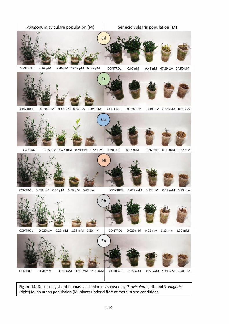
110

Figure 14. Decreasing shoot biomass and chlorosis showed by P. aviculare (left) and S. vulgaris (right) Milan urban population (M) plants under different metal stress conditions.

111

4.5. Conclusions

The present study demonstrated that P. aviculare and S. vulgaris had a linear uptake of Cd, Cr, Cu,

Ni, Pb and Zn, when cultivated in hydroponic conditions in the presence of increasing metal

concentrations (Fig. 14). Because of this behaviour, the two studied species can be suitable as metal

indicators in the several environments since their widespread presence. For the highest Cd and Pb

treatments, the commonly set hyper-accumulation threshold was largely exceeded nonetheless in

these condition the two studied species showed severe toxicity symptoms, therefore highlighting

their incapability to hyper-accumulate metals. P. aviculare demonstrated to be more tolerant than

S. vulgaris to high HMs levels in the solutions suggesting its possible use in for phytostabilization

purposes. Differences in HMs accumulation and in some metabolites production were detected

among the five P. aviculare populations, being instead absent among S. vulgaris populations. These

results showed that some species, that have low mobility (i.e. with seeds dispersed by gravity) can

develop urban ecotypes adapted to polluted soils.

Our study demonstrated that flavonoids, polyphenols, antioxidant activity, photosynthetic pigment

production and shoot biomass, were mostly correlated with metal content in plant shoots and

therefore can be effectively used as a marker of HM stress in plants. Nonetheless, the amount of

secondary metabolites produced by plants in response to HMs is wider, and the inclusion of

antioxidant enzymes (SOD, POD, CAT), phytochelatins and metallothioneins in plant stress

evaluation can furtherly improve the results. The mere quantification of antioxidant metabolites,

cannot give information about the type of metal that caused the oxidative stress, neither the

concentration of the stressors. In fact, high dosage of poorly toxic metal give similar effects of low

doses of highly toxic metals.

Because of the limits discussed above, the integration of biological parameters can be an effective

way to evaluate metal stress and toxicity in plants, only when coupled with the quantification of

trace elements in plant tissues.

112

4.6. References

Aggarwal A, Sharma I, Tripati BN, Munjal AK, Baunthiyal M, Sharma V (2012). Metal toxicity and

photosynthesis. In: Itoh S, Mohanty P, Guruprasad KN. Photosynthesis: overviews on recent

progress & future perspectives. 1st edition, IK International Publishing House Pvt. Ltd, New Delhi,

India, pp. 229-236.

Baker AJM (1981). Accumulators and excluders: strategies in the response of plants to heavy metals.

Journal of Plant Nutrition, 3:643–665.

Bhaduri AM, Fulekar MH. (2012). Antioxidant enzyme responses of plants to heavy metal stress.

Reviews in Environmental Science and Bio/Technology, 11(1):55-69.

Bidar G, Garcon G, Pruvot C, Dewaele D, Cazier F, Douay F, Shirali P (2007). Behavior of Trifolium

repens and Lolium perenne growing in a heavy metal contaminated field: plant metal concentration

and phytotoxicity. Environmental Pollution, 147:546-553.

Bilal Shakoor M, Ali S, Hameed A, Farid M, Hussain S, Yasmeen T, Najeeb U, Aslam Bharwana S,

Hasan Abbasi G (2014). Citric acid improves lead (Pb) phytoextraction in Brassica napus L. by

mitigating Pb-induced morphological and biochemical damages. Ecotoxicology and Environmental

Safety, 109:38–47.

Chandra R, Kang H (2016). Mixed heavy metal stress on photosynthesis, transpiration rate, and

chlorophyll content in poplar hybrids, Forest Science and Technology, 12:(2)55-61.

Clemens S (2001). Molecular mechanisms of plant metal tolerance and homeostasis. Planta,

212(4):475-486.

Dalvi AA, Bhalerao SA (2013). Response of plants towards heavy metal toxicity: an overview of

avoidance, tolerance and uptake mechanism. Annual Plant Science, 2:362–368.

Dixon RA, Paiva NL (1995). Stress-induced phenylpropanoid metabolism. The Plant Cell, 7(7):1085–

1097.

113

El Hajji H, Nkhili E, Tomao V, Dangles O (2006). Interactions of quercetin with iron and copper ions:

complexation and autoxidation. Free Radical Research, 40:303–320.

Emamverdian A, Ding Y, Mokhberdoran F, Xie Y (2015). Heavy metal stress and some mechanisms

of plant defense response. Scientific World Journal, 2015: 756120.

Faller P, Kienzler K, Krieger-Liszkay A (2005). Mechanism of Cd2+ toxicity: Cd2+ inhibits

photoactivation of photosystem II by competitive binding to the essential Ca2+ site. Biochimica et

Biophysica Acta, 1706:158–164.

Ferri M, Gianotti A, Tassoni A (2013). Optimisation of assay conditions for the determination of

antioxidant capacity and polyphenols in cereal food components. Journal of Food Composition and

Analysis, 30(2):94-101.

Galal TM, Shehata HS (2015) Bioaccumulation and translocation of heavy metals by Plantago major

L. grown in contaminated soils under the effect of traffic pollution. Ecological Indicators, 48:244–

251.

Geipel G, Drewitz S, Viehweger K (2010). Detection of uranium(IV) by LIPAS in biologic relevant

samples. In: Bernhard G, Foerstendorf H, Richter A, Viehweger K. Annual Report 2010, Institute of

Radiochemistry. Helmholtz-Zentrum Dresden-Rossendorf e.V, Dresden, Germany, pp. 108

González A, Gil-Díaz MM, Pinilla P, Lobo MC (2017). Impact of Cr and Zn on growth, biochemical and

physiological parameters, and metal accumulation by wheat and barley plants. Water Air Soil

Pollution, 228:419.

Hall JL (2002). Cellular mechanisms for heavy metal detoxification and tolerance. Journal of

Experimental Botany, 53(366):1-11.

Hamrick JL, Murawski DA, Nason JD (1993). The influence of seed dispersal mechanisms on the

genetic structure of tropical tree populations. Vegetatio, 107/108:281-297.

114

Huang CY, Schulte EE (1985). Digestion of plant tissue for analysis by ICP emission spectroscopy.

Communications in Soil Science and Plant Analysis 1:943-958.

Jagodin B, Govorina V, Vinogradova S, Zamaraev A, Chapovskaja G (1995). Cadmium and lead

accumulation in some agricultural crops, grown in podzolic soils. Izvestija TSHA, 2:85–99.

John R, Ahmad P, Gadgil K, S. Sharma S (2009). Heavy metal toxicity: effect on plant growth,

biochemical parameters and metal accumulation by Brassica juncea L. International Journal of Plant

Production, 3:65–76.

Kampfenkel K, Kushnir S, Babiychuk E, Inze D, Van MM (1995). Molecular characterization of a

putative Arabidopsis thaliana copper transporter and its yeast homologue. Journal of Biological

Chemistry, 270: 28479–28486.

Karak T, Bhattacharyya P, Kumar-Paul R, Das DK (2013). Metal accumulation, biochemical response

and yield of Indian mustard grown in soil amended with rural roadside pond sediment.

Ecotoxicology and Environmental Safety, 92: 161–173.

Keilig K, Ludwig-Müller J (2009). Effect of flavonoids on heavy metal tolerance in Arabidopsis

thaliana seedlings. Botanical Studies, 50:311–318.

Kidd PS, Llugany M, Poschenrieder C, Gunsé B, Barceló J (2001). The role of root exudates in

aluminium resistance and silicon-induced amelioration of aluminium toxicity in three variety of

maize (Zea mays L.). Journal of Experimental Botany, 52:1339-1352.

Kisa D, Elmastaş M, Öztürk L, Kayır Ö (2016). Responses of the phenolic compounds of Zea mays

under heavy metal stress. Applied Biological Chemistry, 59:813–820.

Kisa D (2018). The responses of antioxidant aystem against the heavy metal-induced atress in

tomato. Journal of Natural and Applied Sciences, 22(1):1-6.

Kleckerová A, Dočekalová H (2014). Dandelion plants as a biomonitor of urban area contamination

by heavy metals. International Journal of Environmental Research, 8(1):157-164.

115

Kosobrukhov A, Knyazeva I, Mudrik V (2004). Plantago major plants responses to increase content

of lead in soil: growth and photosynthesis. Plant Growth Regulation, 42: 145–151.

Küpper H, Küpper F, Spiller M (1998). In situ detection of heavy metal substituted chlorophylls in

water plants. Photosynthesis Research, 58(2):123–133.

Küpper H, Lombi E, Zhao FJ, McGrath SP (2000). Cellular compartmentation of cadmium and zinc in

relation to other elements in the hyper-accumulator Arabidopsis halleri. Planta, 212:75–84.

Küpper H, Parameswaran A, Leitenmaier B, Trtilek M, Setlik I (2007). Cadmium induced inhibition of

photosynthesis and long-term acclimation to cadmium stress in the hyperaccumulator Thlaspi

caerulescens. New Phytologist, 175:655–674.

Lavid N, Schwartz A, Yarden O, Tel-Or A (2001). The involvement of polyphenols and peroxidase

activities in heavy metal accumulation by epidermal glands of waterlily (Nymphaeaceae). Planta,

212:323-331.

Le Gall H, Philippe F, Domon JM, Gillet F, Pelloux J, Rayon C (2015). Cell wall metabolism in response

to abiotic stress. Plants, 4:112-166.

Manara A (2012). Plant responses to heavy metal toxicity. In: Furini A. (Ed.), Plants and Heavy

Metals. Springer, Dordrecht, Netherlands, pp. 27–53.

Martins LL, Mourato MM (2006). Effect of excess copper on tomato plants: growth parameters,

enzyme activities, chlorophyll, and mineral content. Journal of Plant Nutrition, 29:2179–2198.

Metzner H, Rau H, Senger H (1965). Untersuchungen zur Synchronisierbakeit einzelner

Pigmentmangel-Mutanten von Chlorella. Planta, 65:186-194.

Mganga N, Manoko MLK, Rulangaranga ZK (2011). Classification of plants according to their heavy

metal content around North Mara gold mine, Tanzania: implication for phytoremediation. Tanzania

Journal of Science, 37(1):109-119.

116

Michalak A (2006). Phenolic compounds and their antioxidant activity in plants growing under heavy

metal stress. Polish Journal of Environmental Studies, 15(4):523-530.

Mysliwa-Kurdziel B, Prasad MNV, Strzalka K (2004). Heavy Metal Stress in Plants: from biomolecules

to ecosystems. Ed. Springer, Berlin, Heidelberg, pp. 127

Ovecka M, Takac T (2014). Managing heavy metal toxicity stress in plants: biological and

biotechnological tools. Biotechnology Advances, 32:73–86.

Patra M, Bhowmik N, Bandopadhyay B, Sharma A (2004). Comparison of mercury, lead and arsenic

with respect to genotoxic effects on plant systems and the development of genetic tolerance.

Environmental Experimental Botany, 52:199–223.

Paunov M, Koleva L, Vassilev A, Vangronsveld J, GoltsevInt V (2018). Effects of different metals on

photosynthesis: cadmium and zinc affect chlorophyll fluorescence in Durum wheat. Journal of

Molecular Science, 19:787.

Pękal A, Biesaga M, Pyrzynska K (2011).Interaction of quercetin with copper ions: complexation,

oxidation and reactivity towards radicals. BioMetals 24(1): 41-49

Penarrubia L, Andrés-Colàs N, Moreno J, Puig S (2010). Regulation of copper transport in Arabidopsis

thaliana: a biochemical oscillator? Journal of Biological Inorganic Chemistry, 15: 29–36.

Radwan DEM, Fayez KA, Mahmoud SY, Hamad A, Lu G (2007). Physiological and metabolic changes

of Cucurbita pepo leaves in response to zucchini yellow mosaic virus (ZYMV) infection and salicylic

acid treatments. Plant Physiology and Biochemistry 45:480-489.

Re R, Pellegrini N, Proteggente A, Pannala A, Yang M, Rice-Evans C (1999). Antioxidant activity

applying an improved ABTS radical cation decolorization assay. Free Radical Biology and Medicine,

26(9-10):1231-1237.

117

Rice-Evans CA, Miller NJ (1996). Antioxidant activities of flavonoids as bioactive components of food.

Biochemical Society Transaction, 24:790-795.

Rout GR, Das P (2003). Effect of metal toxicity on plant growth and metabolism: I. Zinc. Agronomie,

23:3-11.

Rout GR, Das P (2009). Effect of metal toxicity on plant growth and metabolism: I. Zinc. In: Lichtfouse

E, Navarrete M, Debaeke P, Véronique S, Alberola C. (Eds.) Sustainable Agriculture. Springer,

Dordrecht, The Netherlands, pp. 873–884.

Salinitro M, Tassoni A, Casolari S, de Laurentiis F, Zappi A, Melucci D (2019). Heavy metals

bioindication potential of the common weeds Senecio vulgaris L., Polygonum aviculare L. and Poa

annua L. Molecules, 24(15):2813.

Shanker AK, Cervantes C, Loza-Tavera H, Avudainayagam S. (2005). Chromium toxicity in plants.

Environmental International, 31: 739–753.

Sharma SS, Dietz KJ (2009). The relationship between metal toxicity and cellular redox imbalance.

Trends in Plant Science, 14:43–50.

Shu WS, Ye SZ, Lan CY, Zhang ZQ, Wong MH (2002). Lead, zinc and copper accumulation and

tolerance in populations of Paspalum distichum and Cynodon dactylon. Environmental Pollution,

120:445–453.

Sies H (1997). Oxidative stress: oxidants and antioxidants. Experimental Physiology, 82(2):291-295.

Singleton VL, Orthofer R, Lamuela-Raventos RM (1999). Analysis of total phenols and other

oxidation substrates and antioxidants by means of Folin-Ciocalteu reagent. Methods in Enzymology

299:152-178.

Tian T, Ali B, Qin Y, Malik Z, Gill RA, Ali S, Zhou W (2014). Alleviation of lead toxicity by 5-

aminolevulinic acid is related to elevated growth, photosynthesis, and suppressed ultrastructural

damages in oilseed rape. BioMed Research International, 2014:1–11.

118

Vajpayee LP, Tripathi RD, Rai UN, Ali MB, Singh SN (2000). Chromium (VI) accumulation reduces

chlorophyll biosynthesis, nitrate reductase activity and protein content in Nymphaea alba.

Chemosphere, 41:1075-1082.

Van der Ent A, Baker AJM, Reeves RD, Pollard AJ, Schat H (2013). Hyperaccumulators of metal and

metalloid trace elements: facts and fiction. Plant and Soil, 362:319–334.

Vassilev A, Schwitzguébel JP, Thewys T, van der Leli D, Vangronsveld J (2004). The use of plants for

remediation of metal-contaminated soils. Scientific World Journal, 4:9–34.

Vernay P, Gauthier-Moussard C, Hitmi A (2007). Interaction of bioaccumulation of heavy metal

chromium with water relation, mineral nutrition and photosynthesis in developed leaves of Lolium

perenne L. Chemosphere, 68:1563–1575.

Viehweger K, Geipel G (2010). Uranium accumulation and tolerance in Arabidopsis halleri under

native versus hydroponic conditions. Environmental and Experimental Botany, 69:39–46.

Viehweger K (2014). How plants cope with heavy metals. Botanical Studies, 55:1–12.

Waters MT, Bussell JD, Jost R (2012). Arabidopsis hydroponics and shoot branching assay.

Bioprotocol 2(19):1-9.

Winkel-Shirley B (2001). Flavonoid biosynthesis. A colorful model for genetics, biochemistry, cell

biology, and biotechnology. Plant Physiology, 126(2):485-493.

Yadav SK (2010). Heavy metals toxicity in plants: an overview on the role of glutathione and

phytochelatins in heavy metal stress tolerance of plants. South African Journal of Botany, 76(2):167-

179.

Zenk MH (1996). Heavy metal detoxification in higher plants: a review. Gene, 179:21-30.

119

Zhishen J, Mengcheng T, Jianming W. (1999). The determination of flavonoid contents in mulberry

and their scavenging effects on superoxide radicals. Food Chemistry 64(4):555-559.

Zornoza P, Vázquez S, Esteban E, Fernández-Pascual M, Carpena R (2002). Cadmium-stress in

nodulated white lupin: strategies to avoid toxicity. Plant Physiology and Biochemistry, 40(12):1003-

1009

120

5. Hormesis: when heavy metals become beneficial, the case of cadmium tested on three annual

weeds

Article status

In preparation: Salinitro Ma, Guardigli Ga, Tassoni Aa. Hormesis: when heavy metals become

beneficial, the case of cadmium tested on three annual weeds.

a Department of Biological Geological and Environmental Sciences, University of Bologna, Via Irnerio

42, 40126 Bologna, Italy

Author Contributions

Mirko Salinitro, analysed the data, contributed to write the manuscript and coordinated the study.

Giorgia Guardigli, cultivated the plant, collected the data and contributed to write the manuscript.

Annalisa Tassoni coordinated the study and revised the manuscript.

List of abbreviations

ROS = Reactive oxygen species

HMs = Heavy metals

5.1. Introduction

The term hormesis appeared for the first time in the scientific literature in 1943, when Southam and

Ehrlich (1943) tested the effect of the extracts of the red cedar tree on the growth of a large number

of fungal species. Since then, there has been an increasing attention to the topic and publications

about hormesis have kept growing in the last years (Calabrese, 2015b).

The term hormesis describes a biphasic dose-response relationship characterized by opposite

effects caused by low and high doses of the same substance (Calabrese & Blain, 2009; Calabrese,

2015a, 2015b). These substances include organic compounds (i.e. weed-killers), biological

molecules (i.e. polyphenols), physical stressors (i.e. radiations) and chemicals (i.e. heavy metals)

(Kendig et al., 2010). Hormesis effect includes both positive and negative responses, because the

fundamental requirement of this phenomenon is to display reversal response between low and high

substance doses, regardless to its beneficial or harmful effects on the studied organism (Calabrese

et al., 2009).

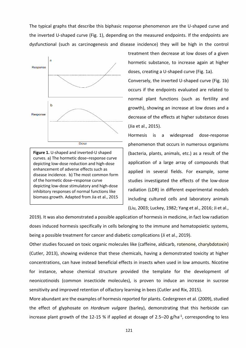
121

The typical graphs that describe this biphasic response phenomenon are the U-shaped curve and

the inverted U-shaped curve (Fig. 1), depending on the measured endpoints. If the endpoints are

dysfunctional (such as carcinogenesis and disease incidence) they will be high in the control

treatment then decrease at low doses of a given

hormetic substance, to increase again at higher

doses, creating a U-shaped curve (Fig. 1a).

Conversely, the inverted U-shaped curve (Fig. 1b)

occurs if the endpoints evaluated are related to

normal plant functions (such as fertility and

growth), showing an increase at low doses and a

decrease of the effects at higher substance doses

(Jia et al., 2015).

Hormesis is a widespread dose-response

phenomenon that occurs in numerous organisms

(bacteria, plants, animals, etc.) as a result of the

application of a large array of compounds that

applied in several fields. For example, some

studies investigated the effects of the low-dose

radiation (LDR) in different experimental models

including cultured cells and laboratory animals

(Liu, 2003; Luckey, 1982; Yang et al., 2016; Ji et al.,

2019). It was also demonstrated a possible application of hormesis in medicine, in fact low radiation

doses induced hormesis specifically in cells belonging to the immune and hematopoietic systems,

being a possible treatment for cancer and diabetic complications (Ji et al., 2019).

Other studies focused on toxic organic molecules like (caffeine, aldicarb, rotenone, charybdotoxin)

(Cutler, 2013), showing evidence that these chemicals, having a demonstrated toxicity at higher

concentrations, can have instead beneficial effects in insects when used in low amounts. Nicotine

for instance, whose chemical structure provided the template for the development of

neonicotinoids (common insecticide molecules), is proven to induce an increase in sucrose

sensitivity and improved retention of olfactory learning in bees (Cutler and Rix, 2015).

More abundant are the examples of hormesis reported for plants. Cedergreen et al. (2009), studied

the effect of glyphosate on Hordeum vulgare (barley), demonstrating that this herbicide can

increase plant growth of the 12-15 % if applied at dosage of 2.5–20 g/ha-1, corresponding to less

Figure 1. U-shaped and inverted-U shaped curves. a) The hormetic dose–response curve depicting low-dose reduction and high-dose enhancement of adverse effects such as disease incidence. b) The most common form of the hormetic dose–response curve depicting low-dose stimulatory and high-dose inhibitory responses of normal functions like biomass growth. Adapted from Jia et al., 2015

122

than 1% of the rate suggested to kill weeds. Another study has investigated the hormesis effect

induced by the herbicide metamitron on Chenopodium album, showing that hormetic doses of this

weed-killer, stimulated seed yield of the 45% above untreated plants. This study gives important

insight to understand the evolution of herbicide resistance in weeds (Belz, 2018).

Hormesis effects, have also been widely reported as a reaction to low concentration of heavy metals

(HMs) (i.e. Agathokleous et al., 2019; Seth et al., 2007; Hajiboland et al., 2013). In a recent study,

the dose-response effect of Lanthanum, a rare earth element that has numerous applications in

modern industries, was evaluated in a large number of plant taxa. It was observed that, the

maximum biological response to low La doses was at 56 μM, at which concentration La affected

numerous biological processes in plants like: biomass amount, cell growth rate, chlorophyll content,

peroxidase activity, flavonoids content and many other (Agathokleous et al., 2019).

In general it is assumed that hormesis is an adaptive response to stress, possibly triggered by an

initial disruption of homeostasis followed by a compensatory process aimed at the re-establishment

of the previous status (Calabrese, 2015a). These responses are often over-compensatory and occur

thanks to several mechanisms still unclear, that differ depending on the biological system studied

and the type of stress applied.

When focusing specifically on the hormesis effect induced in plants by heavy metals, three main

action mechanisms could be distinguished (Poschenrieder et al., 2013):

- Substrate interactions: the ionic interactions between different chemicals present in the soil

can affect nutrient absorption in a positive or negative way.

- Metal-induced activation of specific defense reactions, such as translation of metal tolerance

genes.

- Metal-induce general defense reactions, triggered by the generation of reactive oxygen

species (ROS) as consequence of the metal-induced oxidative stress, leading to the activation

of the antioxidant response determining the final hormesis stimulation effect.

Since, the main mechanisms of hormesis are still largely unknown, it is important to figure out how

widespread this phenomenon is among plants and which substances can cause it. For this reason

we chose common weeds as model species, since these plants can be easily found in places (i.e.

urban environments) characterized by HMs pollution, including Cd. This metal, in fact has been

widely studied for its acute toxicity but also for its capacity to stimulate hormetic response in several

organisms. The aim of this study is therefore to assess the presence of hormesis effect in three

herbaceous species (Poa annua, Stellaria media, Cardamine hirsuta) caused by the exposure to

micro-doses of Cd.

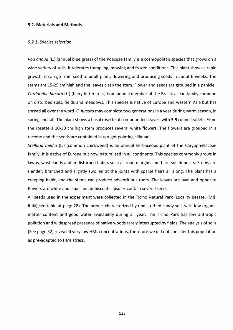
123

5.2. Materials and Methods

5.2.1. Species selection

Poa annua (L.) (annual blue grass) of the Poaceae family is a cosmopolitan species that grows on a

wide variety of soils. It tolerates trampling, mowing and frozen conditions. This plant shows a rapid

growth, it can go from seed to adult plant, flowering and producing seeds in about 6 weeks. The

stems are 15-25 cm high and the leaves clasp the stem. Flower and seeds are grouped in a panicle.

Cardamine hirsuta (L.) (hairy bittercress) is an annual member of the Brassicaceae family common

on disturbed soils, fields and meadows. This species is native of Europe and western Asia but has

spread all over the word. C. hirsuta may complete two generations in a year during warm season, in

spring and fall. The plant shows a basal rosette of compounded leaves, with 3-9 round leaflets. From

the rosette a 10-30 cm high stem produces several white flowers. The flowers are grouped in a

raceme and the seeds are contained in upright pointing siliquae.

Stellaria media (L.) (common chickweed) is an annual herbaceous plant of the Caryophyllaceae

family. It is native of Europe but now naturalized in all continents. This species commonly grows in

lawns, wastelands and in disturbed habits such as road margins and bare soil deposits. Stems are

slender, branched and slightly swollen at the joints with sparse hairs all along. The plant has a

creeping habit, and the stems can produce adventitious roots. The leaves are oval and opposite

flowers are white and small and dehiscent capsules contain several seeds.

All seeds used in the experiment were collected in the Ticino Natural Park (Locality Besate, (MI),

Italy)(see table at page 28). The area is characterized by undisturbed sandy soil, with low organic

matter content and good water availability during all year. The Ticino Park has low anthropic

pollution and widespread presence of native woods rarely interrupted by fields. The analysis of soils

(See page 52) revealed very low HMs concentrations, therefore we did not consider this population

as pre-adapted to HMs stress.

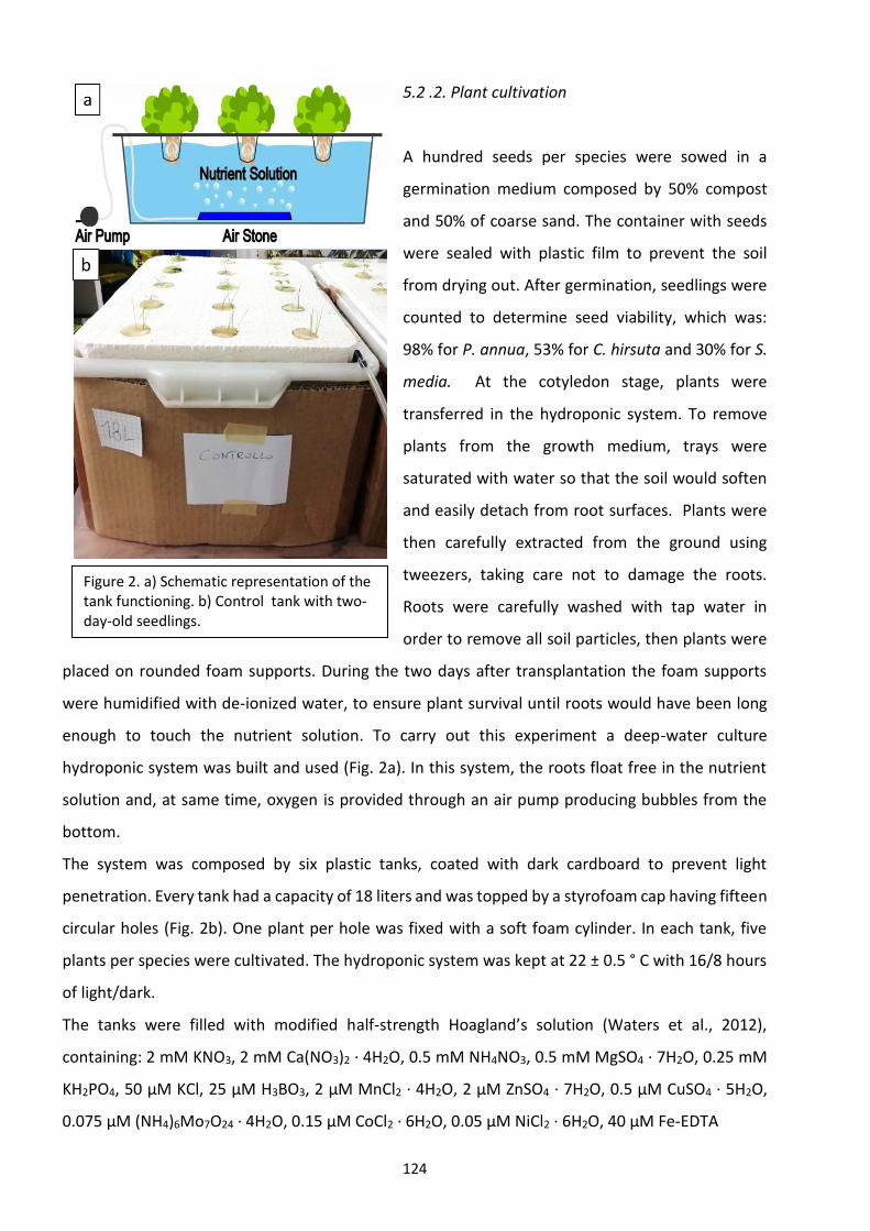
124

5.2 .2. Plant cultivation

A hundred seeds per species were sowed in a

germination medium composed by 50% compost

and 50% of coarse sand. The container with seeds

were sealed with plastic film to prevent the soil

from drying out. After germination, seedlings were

counted to determine seed viability, which was:

98% for P. annua, 53% for C. hirsuta and 30% for S.

media. At the cotyledon stage, plants were

transferred in the hydroponic system. To remove

plants from the growth medium, trays were

saturated with water so that the soil would soften

and easily detach from root surfaces. Plants were

then carefully extracted from the ground using

tweezers, taking care not to damage the roots.

Roots were carefully washed with tap water in

order to remove all soil particles, then plants were

placed on rounded foam supports. During the two days after transplantation the foam supports

were humidified with de-ionized water, to ensure plant survival until roots would have been long

enough to touch the nutrient solution. To carry out this experiment a deep-water culture

hydroponic system was built and used (Fig. 2a). In this system, the roots float free in the nutrient

solution and, at same time, oxygen is provided through an air pump producing bubbles from the

bottom.

The system was composed by six plastic tanks, coated with dark cardboard to prevent light

penetration. Every tank had a capacity of 18 liters and was topped by a styrofoam cap having fifteen

circular holes (Fig. 2b). One plant per hole was fixed with a soft foam cylinder. In each tank, five

plants per species were cultivated. The hydroponic system was kept at 22 ± 0.5 ° C with 16/8 hours

of light/dark.

The tanks were filled with modified half-strength Hoagland’s solution (Waters et al., 2012),

containing: 2 mM KNO3, 2 mM Ca(NO3)2 · 4H2O, 0.5 mM NH4NO3, 0.5 mM MgSO4 · 7H2O, 0.25 mM

KH2PO4, 50 µM KCl, 25 µM H3BO3, 2 µM MnCl2 · 4H2O, 2 µM ZnSO4 · 7H2O, 0.5 µM CuSO4 · 5H2O,

0.075 µM (NH4)6Mo7O24 · 4H2O, 0.15 µM CoCl2 · 6H2O, 0.05 µM NiCl2 · 6H2O, 40 µM Fe-EDTA

Figure 2. a) Schematic representation of the tank functioning. b) Control tank with two-day-old seedlings.

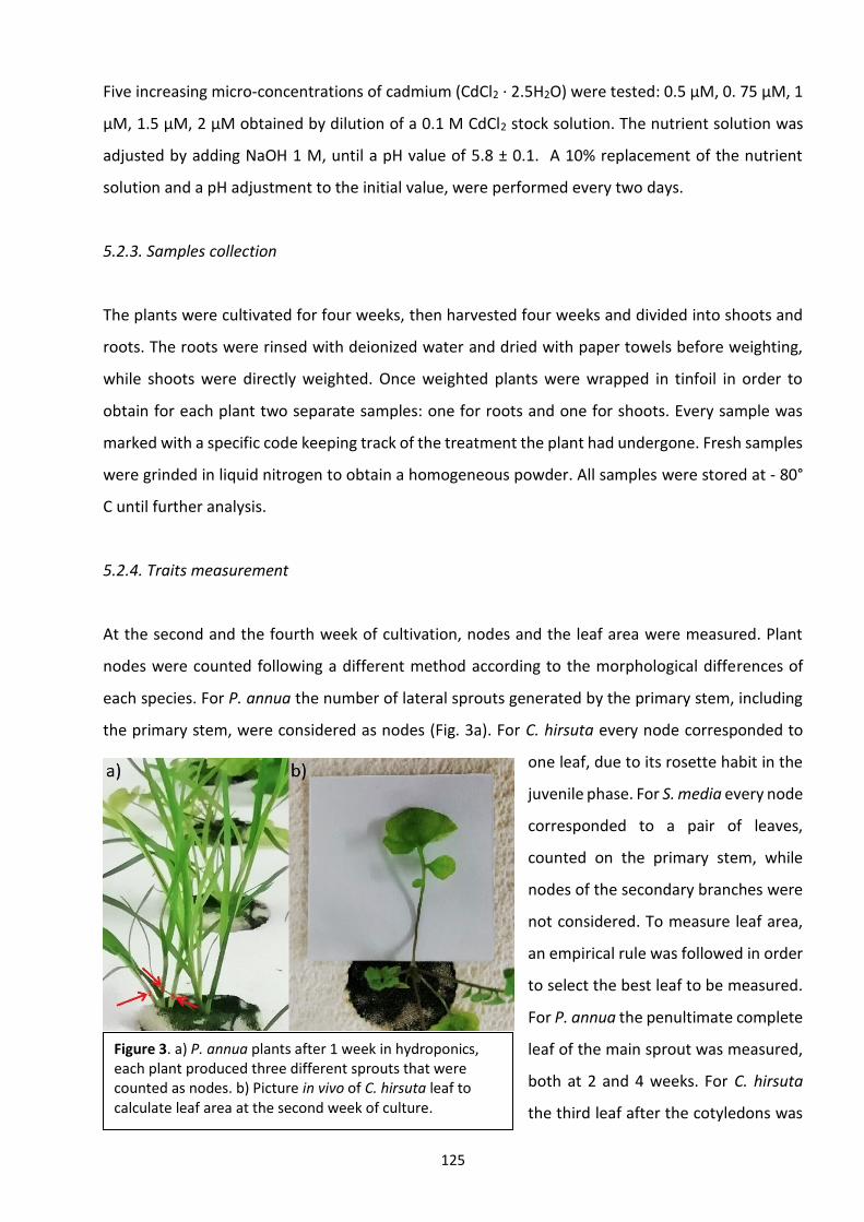
125

Five increasing micro-concentrations of cadmium (CdCl2 · 2.5H2O) were tested: 0.5 µM, 0. 75 µM, 1

µM, 1.5 µM, 2 µM obtained by dilution of a 0.1 M CdCl2 stock solution. The nutrient solution was

adjusted by adding NaOH 1 M, until a pH value of 5.8 ± 0.1. A 10% replacement of the nutrient

solution and a pH adjustment to the initial value, were performed every two days.

5.2.3. Samples collection

The plants were cultivated for four weeks, then harvested four weeks and divided into shoots and

roots. The roots were rinsed with deionized water and dried with paper towels before weighting,

while shoots were directly weighted. Once weighted plants were wrapped in tinfoil in order to

obtain for each plant two separate samples: one for roots and one for shoots. Every sample was

marked with a specific code keeping track of the treatment the plant had undergone. Fresh samples

were grinded in liquid nitrogen to obtain a homogeneous powder. All samples were stored at - 80°

C until further analysis.

5.2.4. Traits measurement

At the second and the fourth week of cultivation, nodes and the leaf area were measured. Plant

nodes were counted following a different method according to the morphological differences of

each species. For P. annua the number of lateral sprouts generated by the primary stem, including

the primary stem, were considered as nodes (Fig. 3a). For C. hirsuta every node corresponded to

one leaf, due to its rosette habit in the

juvenile phase. For S. media every node

corresponded to a pair of leaves,

counted on the primary stem, while

nodes of the secondary branches were

not considered. To measure leaf area,

an empirical rule was followed in order

to select the best leaf to be measured.

For P. annua the penultimate complete

leaf of the main sprout was measured,

both at 2 and 4 weeks. For C. hirsuta

the third leaf after the cotyledons was

Figure 3. a) P. annua plants after 1 week in hydroponics, each plant produced three different sprouts that were counted as nodes. b) Picture in vivo of C. hirsuta leaf to calculate leaf area at the second week of culture.

126

considered at the second week, while and the largest and most developed leaf in the whole plant

was taken into account at the fourth week. In S. media the third pair of leaves were analyzed at the

second week, and the eighth pair of leaves after the cotyledons, at the fourth week.

To precisely calculate the leaf area, leaves pictures were taken using as a background cardboard

square of known size (5 x 5 cm or 15 x 15 cm), the leaf was spread as much as possible on the

cardboard in order to avoid measurement biases due to leaf wrinkles. Leaf’s stalks were included in

the pictures and considered in the calculation, the camera was vertically placed on the cardboard in

order to maintain the same proportions between leaf and cardboard in the picture. At the end of

the second week this procedure was performed in vivo, without removing the leaves from the plants

(Fig. 3b), to prevent plant damages or hindering its growth.

To calculate leaf area, every picture

was cut using Adobe® Photoshop

software at the dimension of the

cardboard square, setting the size of

the image at 5 x 5 cm or 15 x 15 cm.

After that, using the software ImageJ

(https://imagej.net), all pictures were

transformed to binary (only black and

white pixels) to obtain a black leaf

shape on a white background area

(Fig. 4). After binary transformation,

white and black pixels were counted using the tool Analyze>Measure available in the software

toolbar. Leaf area was then calculated using the following proportion:

Black pixels : Total pixels = Leaf area : Square area

Leaf area (cm2) = (Black pixels) x (Square area)

Total pixels

At the end of the cultivation period (week 4) fresh weight (FW), dry weight (DW) and amount of

photosynthetic pigments were also measured. For the determination of dry weight, approximately

0.3-0.5 gFW aliquots of roots and shoots bulk powders were oven-dried at 60°C for 24 hours and

weighted.

Figure 4. Original leaf pictures (top) and binary version (bottom) used to count pixel. a) C. hirsuta. b) P. annua. c) S. media.

127

To quantify photosynthetic pigments, a modified method from Radwan et al. (2007) and Metzner

et al. (1965) was used. 0.1 gFW of shoots grinded powders were extracted with 1.5 mL of 85% (v/v)

acetone and mixed 2 times for 30 seconds, the samples were then centrifuged at 4°C, 2500 rpm for

5 minutes and the supernatant recovered. The supernatant was analyzed at three different

wavelengths (663, 644 and 452.5 nm) and the obtained absorbance values were processed to give

the pigment concentrations in mg/gFW with the following equations:

chlorophyll a = 10.3 x Abs663 – 0.98 x Abs644

chlorophyll b = 19.7 x Abs644 – 3.87 x Abs663

carotenoids = 4.2 x Abs452.5 – [(0.0264 x chl-a) + (0.426 x chl-b)]

All the spectrophotometric analyses were performed with a VersaMax™ Microplate Reader

(Molecular Devices, San Jose, California) spectrophotometer. A 96-wells plate was used to load

samples on the instrument and for each sample 200 µL of acetone extract were placed in every well.

5.2.5. Data analysis

All the statistical analyses were performed using Rstudio software version 3.6.1. The differences in

plant growth were evaluated among the three different species as well as among the different

cadmium treatments. For each species a dataset with 18 variables (columns) and 30 observations

(rows) was produced. Data were tested for normality using the Shapiro-Wilk normality test (data

are normal if p>0.05), and for homogeneity using Levene’s Test for Homogeneity of Variance (data

are homogeneous if p>0.05) with default parameters from the package Car (https://CRAN.R-

project.org/package=car). The Analysis of Variance ANOVA, followed by Tukey HSD test was used

performed for all parametric samples group in order to detect significant differences between the

analyzed groups (p value <0.05). While for the non-parametric data the Kruskal-Wallis test followed

by Dunn’s post-hoc test were used. Non-linear models were used to describe the trend of plant

growth according to the different cadmium treatments. Principal Component analisys (PCA) was

performed with the function prcomp, using default values. Graphical elaborations where performed

using the R package ggpubr (https://CRAN.R-project.org/package=ggpubr).

128

5.3. Results

5.3.1. Poa annua

Overall, this species

showed an hormetic

response to central Cd

treatments (0.75 μM, 1

μM), with an increase in

fresh and dry biomass of

roots and shoots. This

effects were not detected

in control plants and high

Cd dosages. The PCA

analysis (Fig. 5) that took

into account traits

measured at 4 weeks,

chlorophyll content, FW,

DW and DW/FW, showed

a clear separation of the treatments in two main groups: control and Cd 2 μM treated plants were

very similar, in contrast with all the other Cd treated plants who showed mostly an increase in whole

plant biomass. The variables that mainly allowed such a clear separation were shoots and roots

fresh weight, and the number of nodes. These parameters were those mostly affected by different

Cd treatments.

Figure 5. PCA showing the grouping of P. annua samples according to the

treatment. The variables used in the PCA were: photosynthetic pigments (Chl a, Chl b, Carotenoids), shoot DW, FW and DW/FW, root DW, FW and DW/FW, nodes number, leaf area. Treatments: Contr= 0 µM Cd, T00005= 0.5 µM Cd, T000075= 0.75 µM Cd, T0001= 1 µM Cd, T00015= 1.5 µM Cd, T0002= 2 µM Cd.

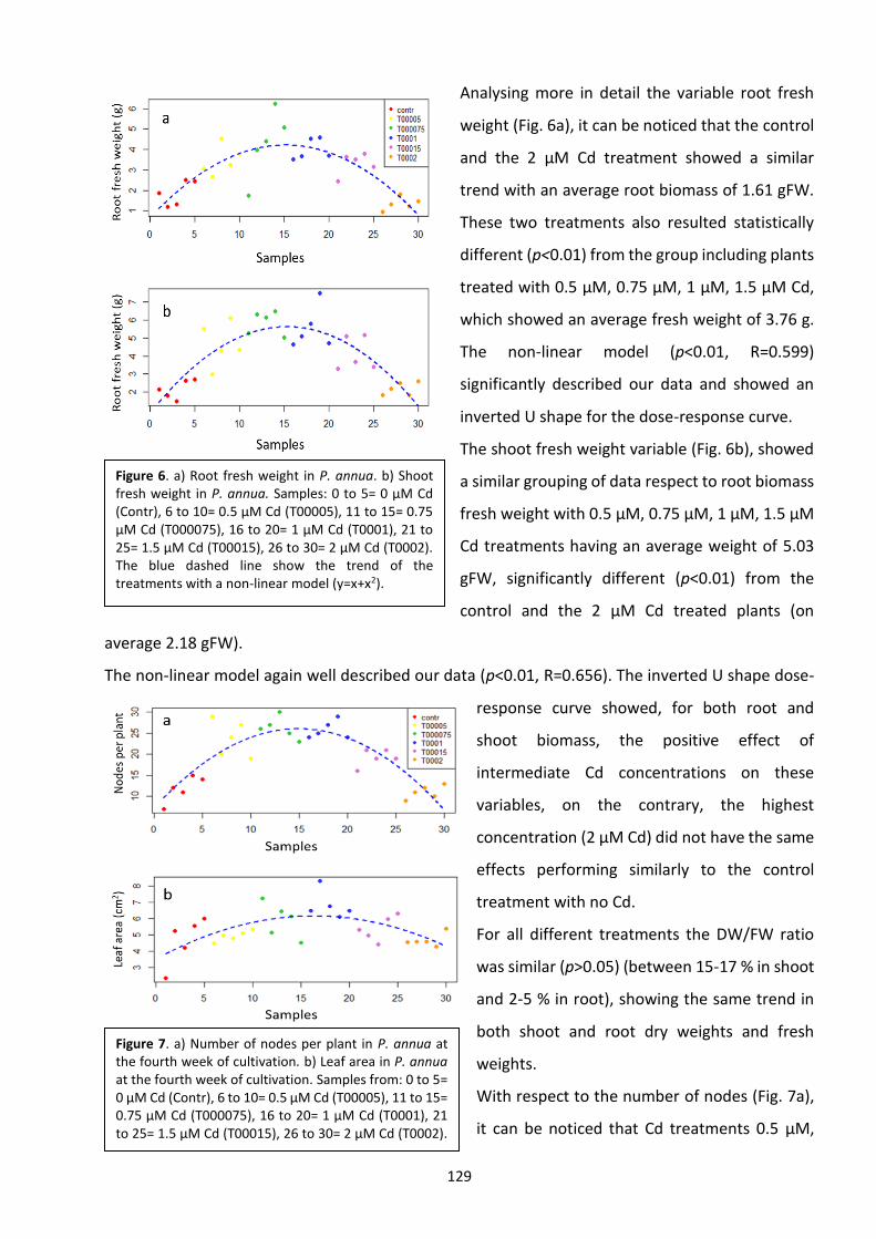
129

Analysing more in detail the variable root fresh

weight (Fig. 6a), it can be noticed that the control

and the 2 μM Cd treatment showed a similar

trend with an average root biomass of 1.61 gFW.

These two treatments also resulted statistically

different (p<0.01) from the group including plants

treated with 0.5 μM, 0.75 μM, 1 μM, 1.5 μM Cd,

which showed an average fresh weight of 3.76 g.

The non-linear model (p<0.01, R=0.599)

significantly described our data and showed an

inverted U shape for the dose-response curve.

The shoot fresh weight variable (Fig. 6b), showed

a similar grouping of data respect to root biomass

fresh weight with 0.5 μM, 0.75 μM, 1 μM, 1.5 μM

Cd treatments having an average weight of 5.03

gFW, significantly different (p<0.01) from the

control and the 2 μM Cd treated plants (on

average 2.18 gFW).

The non-linear model again well described our data (p<0.01, R=0.656). The inverted U shape dose-

response curve showed, for both root and

shoot biomass, the positive effect of

intermediate Cd concentrations on these

variables, on the contrary, the highest

concentration (2 µM Cd) did not have the same

effects performing similarly to the control

treatment with no Cd.

For all different treatments the DW/FW ratio

was similar (p>0.05) (between 15-17 % in shoot

and 2-5 % in root), showing the same trend in

both shoot and root dry weights and fresh

weights.

With respect to the number of nodes (Fig. 7a),

it can be noticed that Cd treatments 0.5 μM,

Figure 6. a) Root fresh weight in P. annua. b) Shoot fresh weight in P. annua. Samples: 0 to 5= 0 µM Cd (Contr), 6 to 10= 0.5 µM Cd (T00005), 11 to 15= 0.75 µM Cd (T000075), 16 to 20= 1 µM Cd (T0001), 21 to 25= 1.5 µM Cd (T00015), 26 to 30= 2 µM Cd (T0002). The blue dashed line show the trend of the treatments with a non-linear model (y=x+x2).

Figure 7. a) Number of nodes per plant in P. annua at the fourth week of cultivation. b) Leaf area in P. annua at the fourth week of cultivation. Samples from: 0 to 5= 0 µM Cd (Contr), 6 to 10= 0.5 µM Cd (T00005), 11 to 15= 0.75 µM Cd (T000075), 16 to 20= 1 µM Cd (T0001), 21 to 25= 1.5 µM Cd (T00015), 26 to 30= 2 µM Cd (T0002). The blue dashed line describe the trend of the

𝑦 = 𝑥 + 𝑥2

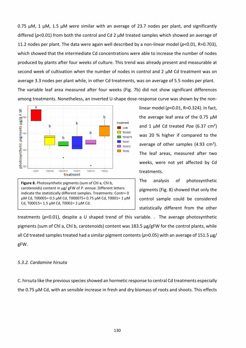
130

0.75 μM, 1 μM, 1.5 μM were similar with an average of 23.7 nodes per plant, and significantly

differed (p<0.01) from both the control and Cd 2 μM treated samples which showed an average of

11.2 nodes per plant. The data were again well described by a non-linear model (p<0.01, R=0.703),

which showed that the intermediate Cd concentrations were able to increase the number of nodes

produced by plants after four weeks of culture. This trend was already present and measurable at

second week of cultivation when the number of nodes in control and 2 μM Cd treatment was on

average 3.3 nodes per plant while, in other Cd treatments, was on average of 5.5 nodes per plant.

The variable leaf area measured after four weeks (Fig. 7b) did not show significant differences

among treatments. Nonetheless, an inverted U-shape dose-response curve was shown by the non-

linear model (p<0.01, R=0.324). In fact,

the average leaf area of the 0.75 μM

and 1 μM Cd treated Poa (6.37 cm2)

was 20 % higher if compared to the

average of other samples (4.93 cm2).

The leaf areas, measured after two

weeks, were not yet affected by Cd

treatments.

The analysis of photosynthetic

pigments (Fig. 8) showed that only the

control sample could be considered

statistically different from the other

treatments (p<0.01), despite a U shaped trend of this variable. . The average photosynthetic

pigments (sum of Chl a, Chl b, carotenoids) content was 183.5 µg/gFW for the control plants, while

all Cd treated samples treated had a similar pigment contents (p>0.05) with an average of 151.5 µg/

gFW.

5.3.2. Cardamine hirsuta

C. hirsuta like the previous species showed an hormetic response to central Cd treatments especially

the 0.75 μM Cd, with an sensible increase in fresh and dry biomass of roots and shoots. This effects

Figure 8. Photosynthetic pigments (sum of Chl a, Chl b, carotenoids) content in µg/ gFW of P. annua. Different letters indicate the statistically different samples. Treatments: Contr= 0 µM Cd, T00005= 0.5 µM Cd, T000075= 0.75 µM Cd, T0001= 1 µM Cd, T00015= 1.5 µM Cd, T0002= 2 µM Cd.

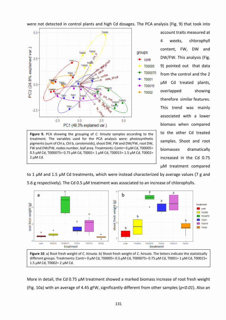
131

were not detected in control plants and high Cd dosages. The PCA analysis (Fig. 9) that took into

account traits measured at

4 weeks, chlorophyll

content, FW, DW and

DW/FW. This analysis (Fig.

9) pointed out that data

from the control and the 2

μM Cd treated plants,

overlapped showing

therefore similar features.

This trend was mainly

associated with a lower

biomass when compared

to the other Cd treated

samples. Shoot and root

biomasses dramatically

increased in the Cd 0.75

μM treatment compared

to 1 μM and 1.5 μM Cd treatments, which were instead characterized by average values (7 g and

5.6 g respectively). The Cd 0.5 μM treatment was associated to an increase of chlorophylls.

More in detail, the Cd 0.75 μM treatment showed a marked biomass increase of root fresh weight

(Fig. 10a) with an average of 4.45 gFW, significantly different from other samples (p<0.01). Also an

Figure 9. PCA showing the grouping of C. hirsuta samples according to the treatment. The variables used for the PCA analysis were: photosynthetic pigments (sum of Chl a, Chl b, carotenoids), shoot DW, FW and DW/FW, root DW, FW and DW/FW, nodes number, leaf area. Treatments: Contr= 0 µM Cd, T00005= 0.5 µM Cd, T000075= 0.75 µM Cd, T0001= 1 µM Cd, T00015= 1.5 µM Cd, T0002= 2 µM Cd.

Figure 10. a) Root fresh weight of C. hirsuta. b) Shoot fresh weight of C. hirsuta. The letters indicate the statistically different groups. Treatments: Contr= 0 µM Cd, T00005= 0.5 µM Cd, T000075= 0.75 µM Cd, T0001= 1 µM Cd, T00015= 1.5 µM Cd, T0002= 2 µM Cd.

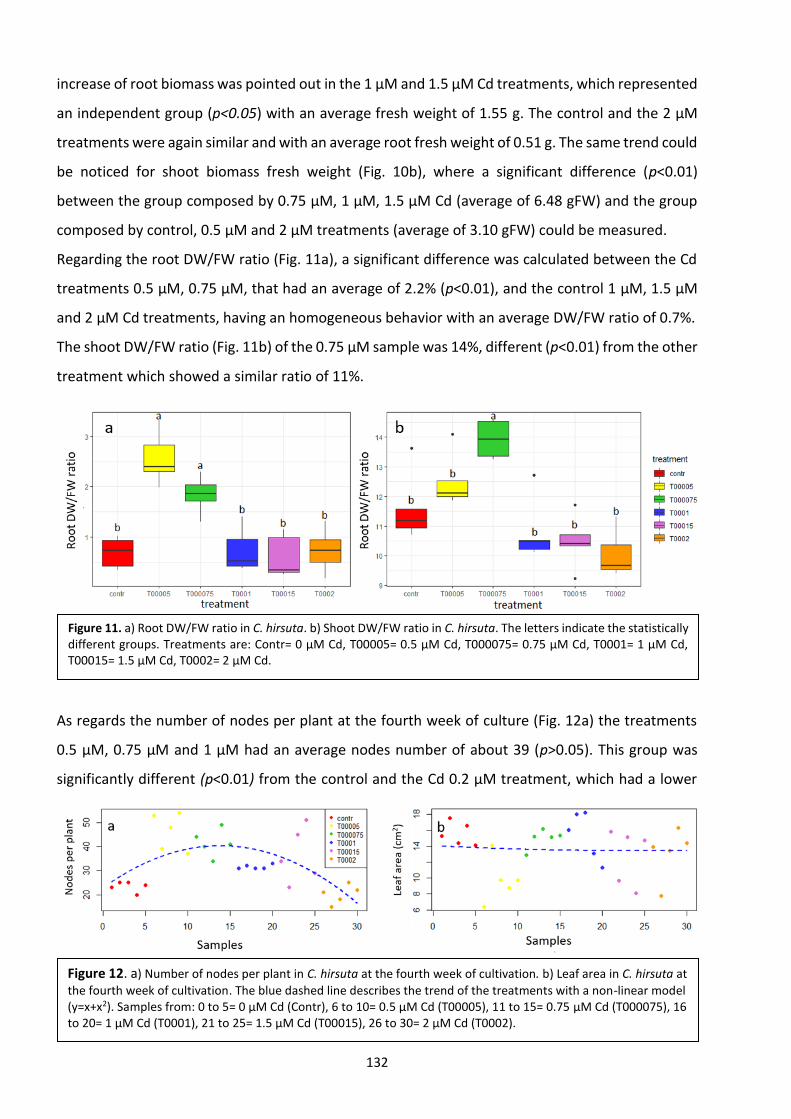
132

increase of root biomass was pointed out in the 1 μM and 1.5 μM Cd treatments, which represented

an independent group (p<0.05) with an average fresh weight of 1.55 g. The control and the 2 μM

treatments were again similar and with an average root fresh weight of 0.51 g. The same trend could

be noticed for shoot biomass fresh weight (Fig. 10b), where a significant difference (p<0.01)

between the group composed by 0.75 μM, 1 μM, 1.5 μM Cd (average of 6.48 gFW) and the group

composed by control, 0.5 μM and 2 μM treatments (average of 3.10 gFW) could be measured.

Regarding the root DW/FW ratio (Fig. 11a), a significant difference was calculated between the Cd

treatments 0.5 μM, 0.75 μM, that had an average of 2.2% (p<0.01), and the control 1 μM, 1.5 μM

and 2 μM Cd treatments, having an homogeneous behavior with an average DW/FW ratio of 0.7%.

The shoot DW/FW ratio (Fig. 11b) of the 0.75 μM sample was 14%, different (p<0.01) from the other

treatment which showed a similar ratio of 11%.

As regards the number of nodes per plant at the fourth week of culture (Fig. 12a) the treatments

0.5 µM, 0.75 µM and 1 µM had an average nodes number of about 39 (p>0.05). This group was

significantly different (p<0.01) from the control and the Cd 0.2 µM treatment, which had a lower

Figure 12. a) Number of nodes per plant in C. hirsuta at the fourth week of cultivation. b) Leaf area in C. hirsuta at

the fourth week of cultivation. The blue dashed line describes the trend of the treatments with a non-linear model (y=x+x2). Samples from: 0 to 5= 0 µM Cd (Contr), 6 to 10= 0.5 µM Cd (T00005), 11 to 15= 0.75 µM Cd (T000075), 16 to 20= 1 µM Cd (T0001), 21 to 25= 1.5 µM Cd (T00015), 26 to 30= 2 µM Cd (T0002).

Figure 11. a) Root DW/FW ratio in C. hirsuta. b) Shoot DW/FW ratio in C. hirsuta. The letters indicate the statistically different groups. Treatments are: Contr= 0 µM Cd, T00005= 0.5 µM Cd, T000075= 0.75 µM Cd, T0001= 1 µM Cd, T00015= 1.5 µM Cd, T0002= 2 µM Cd.

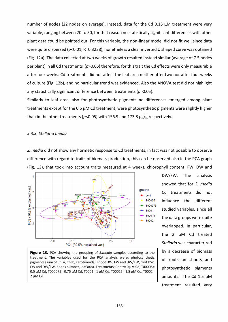
133

number of nodes (22 nodes on average). Instead, data for the Cd 0.15 µM treatment were very

variable, ranging between 20 to 50, for that reason no statistically significant differences with other

plant data could be pointed out. For this variable, the non-linear model did not fit well since data

were quite dispersed (p<0.01, R=0.3238), nonetheless a clear inverted U shaped curve was obtained

(Fig. 12a). The data collected at two weeks of growth resulted instead similar (average of 7.5 nodes

per plant) in all Cd treatments (p>0.05) therefore, for this trait the Cd effects were only measurable

after four weeks. Cd treatments did not affect the leaf area neither after two nor after four weeks

of culture (Fig. 12b), and no particular trend was evidenced. Also the ANOVA test did not highlight

any statistically significant difference between treatments (p>0.05).

Similarly to leaf area, also for photosynthetic pigments no differences emerged among plant

treatments except for the 0.5 µM Cd treatment, were photosynthetic pigments were slightly higher

than in the other treatments (p<0.05) with 156.9 and 173.8 µg/g respectively.

5.3.3. Stellaria media

S. media did not show any hormetic response to Cd treatments, in fact was not possible to observe

difference with regard to traits of biomass production, this can be observed also in the PCA graph

(Fig. 13), that took into account traits measured at 4 weeks, chlorophyll content, FW, DW and

DW/FW. The analysis

showed that for S. media

Cd treatments did not

influence the different

studied variables, since all

the data groups were quite

overlapped. In particular,

the 2 µM Cd treated

Stellaria was characterized

by a decrease of biomass

of roots an shoots and

photosynthetic pigments

amounts. The Cd 1.5 µM

treatment resulted very

Figure 13. PCA showing the grouping of S.media samples according to the

treatment. The variables used for the PCA analysis were: photosynthetic pigments (sum of Chl a, Chl b, carotenoids), shoot DW, FW and DW/FW, root DW, FW and DW/FW, nodes number, leaf area. Treatments: Contr= 0 µM Cd, T00005= 0.5 µM Cd, T000075= 0.75 µM Cd, T0001= 1 µM Cd, T00015= 1.5 µM Cd, T0002= 2 µM Cd.

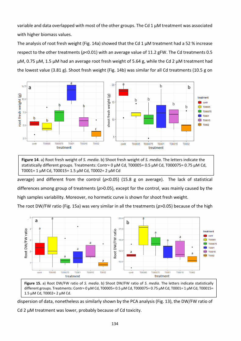
134

variable and data overlapped with most of the other groups. The Cd 1 µM treatment was associated

with higher biomass values.

The analysis of root fresh weight (Fig. 14a) showed that the Cd 1 µM treatment had a 52 % increase

respect to the other treatments (p<0.01) with an average value of 11.2 gFW. The Cd treatments 0.5

µM, 0.75 µM, 1.5 µM had an average root fresh weight of 5.64 g, while the Cd 2 µM treatment had

the lowest value (3.81 g). Shoot fresh weight (Fig. 14b) was similar for all Cd treatments (10.5 g on

average) and different from the control (p<0.05) (15.8 g on average). The lack of statistical

differences among group of treatments (p>0.05), except for the control, was mainly caused by the

high samples variability. Moreover, no hormetic curve is shown for shoot fresh weight.

The root DW/FW ratio (Fig. 15a) was very similar in all the treatments (p>0.05) because of the high

dispersion of data, nonetheless as similarly shown by the PCA analysis (Fig. 13), the DW/FW ratio of

Cd 2 µM treatment was lower, probably because of Cd toxicity.

Figure 15. a) Root DW/FW ratio of S. media. b) Shoot DW/FW ratio of S. media. The letters indicate statistically different groups. Treatments: Contr= 0 µM Cd, T00005= 0.5 µM Cd, T000075= 0.75 µM Cd, T0001= 1 µM Cd, T00015= 1.5 µM Cd, T0002= 2 µM Cd.

Figure 14. a) Root fresh weight of S. media. b) Shoot fresh weight of S. media. The letters indicate the statistically different groups. Treatments: Contr= 0 µM Cd, T00005= 0.5 µM Cd, T000075= 0.75 µM Cd, T0001= 1 µM Cd, T00015= 1.5 µM Cd, T0002= 2 µM Cd

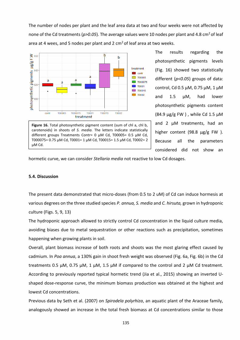
135

The number of nodes per plant and the leaf area data at two and four weeks were not affected by

none of the Cd treatments (p>0.05). The average values were 10 nodes per plant and 4.8 cm2 of leaf

area at 4 wees, and 5 nodes per plant and 2 cm2 of leaf area at two weeks.

The results regarding the

photosynthetic pigments levels

(Fig. 16) showed two statistically

different (p<0.05) groups of data:

control, Cd 0.5 µM, 0.75 µM, 1 µM

and 1.5 µM, had lower

photosynthetic pigments content

(84.9 µg/g FW ) , while Cd 1.5 µM

and 2 µM treatments, had an

higher content (98.8 µg/g FW ).

Because all the parameters

considered did not show an

hormetic curve, we can consider Stellaria media not reactive to low Cd dosages.

5.4. Discussion

The present data demonstrated that micro-doses (from 0.5 to 2 uM) of Cd can induce hormesis at

various degrees on the three studied species P. annua, S. media and C. hirsuta, grown in hydroponic

culture (Figs. 5, 9, 13)

The hydroponic approach allowed to strictly control Cd concentration in the liquid culture media,

avoiding biases due to metal sequestration or other reactions such as precipitation, sometimes

happening when growing plants in soil.

Overall, plant biomass increase of both roots and shoots was the most glaring effect caused by

cadmium. In Poa annua, a 130% gain in shoot fresh weight was observed (Fig. 6a, Fig. 6b) in the Cd

treatments 0.5 μM, 0.75 μM, 1 μM, 1.5 μM if compared to the control and 2 μM Cd treatment.

According to previously reported typical hormetic trend (Jia et al., 2015) showing an inverted U-

shaped dose-response curve, the minimum biomass production was obtained at the highest and

lowest Cd concentrations.

Previous data by Seth et al. (2007) on Spirodela polyrhiza, an aquatic plant of the Araceae family,

analogously showed an increase in the total fresh biomass at Cd concentrations similar to those

Figure 16. Total photosynthetic pigment content (sum of chl a, chl b, carotenoids) in shoots of S. media. The letters indicate statistically different groups Treatments Contr= 0 µM Cd, T00005= 0.5 µM Cd, T000075= 0.75 µM Cd, T0001= 1 µM Cd, T00015= 1.5 µM Cd, T0002= 2 µM Cd.

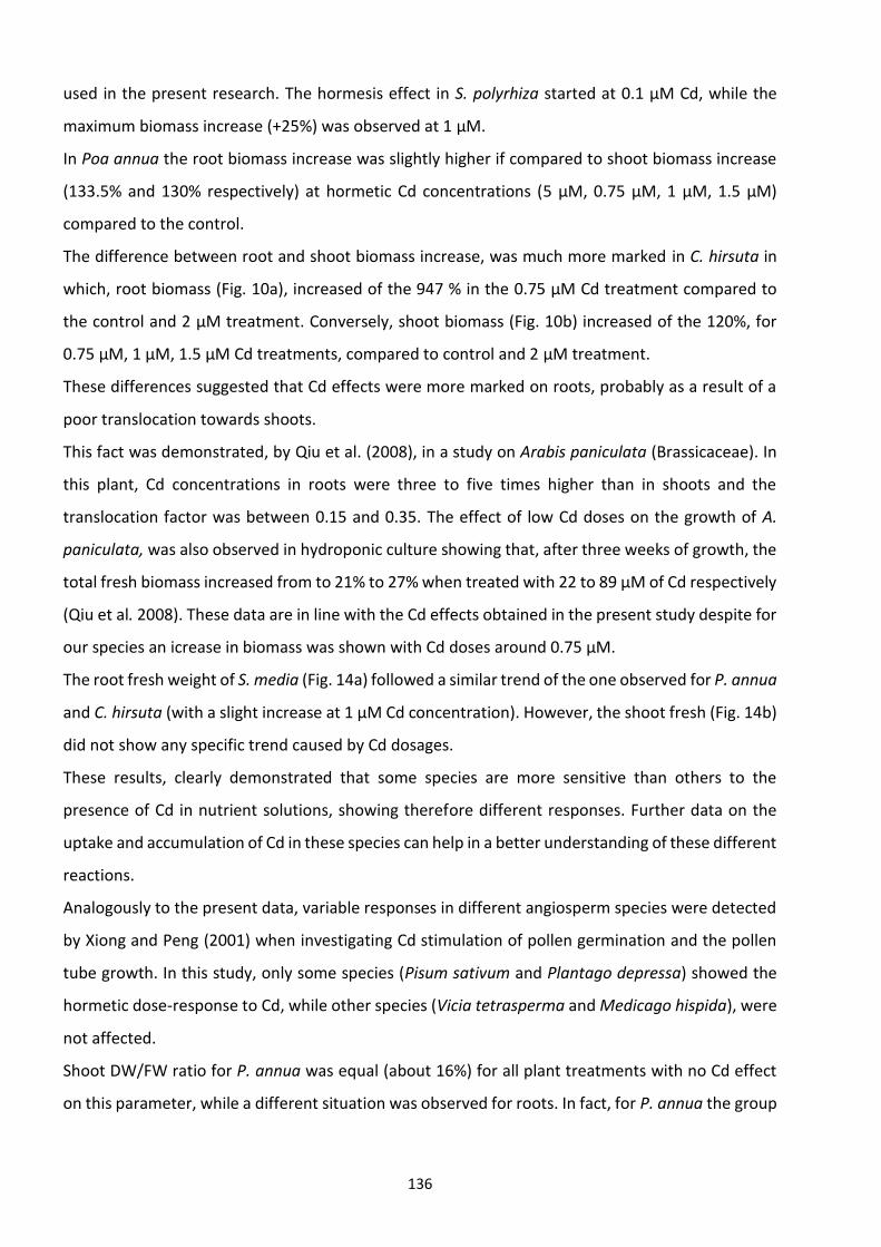
136

used in the present research. The hormesis effect in S. polyrhiza started at 0.1 μM Cd, while the

maximum biomass increase (+25%) was observed at 1 μM.

In Poa annua the root biomass increase was slightly higher if compared to shoot biomass increase

(133.5% and 130% respectively) at hormetic Cd concentrations (5 μM, 0.75 μM, 1 μM, 1.5 μM)

compared to the control.

The difference between root and shoot biomass increase, was much more marked in C. hirsuta in

which, root biomass (Fig. 10a), increased of the 947 % in the 0.75 μM Cd treatment compared to

the control and 2 μM treatment. Conversely, shoot biomass (Fig. 10b) increased of the 120%, for

0.75 μM, 1 μM, 1.5 μM Cd treatments, compared to control and 2 μM treatment.

These differences suggested that Cd effects were more marked on roots, probably as a result of a

poor translocation towards shoots.

This fact was demonstrated, by Qiu et al. (2008), in a study on Arabis paniculata (Brassicaceae). In

this plant, Cd concentrations in roots were three to five times higher than in shoots and the

translocation factor was between 0.15 and 0.35. The effect of low Cd doses on the growth of A.

paniculata, was also observed in hydroponic culture showing that, after three weeks of growth, the

total fresh biomass increased from to 21% to 27% when treated with 22 to 89 µM of Cd respectively

(Qiu et al. 2008). These data are in line with the Cd effects obtained in the present study despite for

our species an icrease in biomass was shown with Cd doses around 0.75 µM.

The root fresh weight of S. media (Fig. 14a) followed a similar trend of the one observed for P. annua

and C. hirsuta (with a slight increase at 1 μM Cd concentration). However, the shoot fresh (Fig. 14b)

did not show any specific trend caused by Cd dosages.

These results, clearly demonstrated that some species are more sensitive than others to the

presence of Cd in nutrient solutions, showing therefore different responses. Further data on the

uptake and accumulation of Cd in these species can help in a better understanding of these different

reactions.

Analogously to the present data, variable responses in different angiosperm species were detected

by Xiong and Peng (2001) when investigating Cd stimulation of pollen germination and the pollen

tube growth. In this study, only some species (Pisum sativum and Plantago depressa) showed the

hormetic dose-response to Cd, while other species (Vicia tetrasperma and Medicago hispida), were

not affected.

Shoot DW/FW ratio for P. annua was equal (about 16%) for all plant treatments with no Cd effect

on this parameter, while a different situation was observed for roots. In fact, for P. annua the group

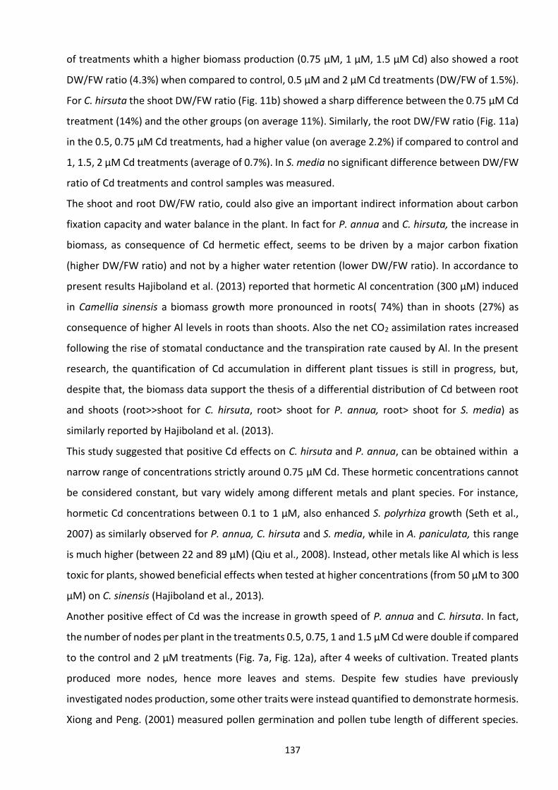
137

of treatments whith a higher biomass production (0.75 μM, 1 μM, 1.5 μM Cd) also showed a root

DW/FW ratio (4.3%) when compared to control, 0.5 μM and 2 μM Cd treatments (DW/FW of 1.5%).

For C. hirsuta the shoot DW/FW ratio (Fig. 11b) showed a sharp difference between the 0.75 μM Cd

treatment (14%) and the other groups (on average 11%). Similarly, the root DW/FW ratio (Fig. 11a)

in the 0.5, 0.75 μM Cd treatments, had a higher value (on average 2.2%) if compared to control and

1, 1.5, 2 μM Cd treatments (average of 0.7%). In S. media no significant difference between DW/FW

ratio of Cd treatments and control samples was measured.

The shoot and root DW/FW ratio, could also give an important indirect information about carbon

fixation capacity and water balance in the plant. In fact for P. annua and C. hirsuta, the increase in

biomass, as consequence of Cd hermetic effect, seems to be driven by a major carbon fixation

(higher DW/FW ratio) and not by a higher water retention (lower DW/FW ratio). In accordance to

present results Hajiboland et al. (2013) reported that hormetic Al concentration (300 µM) induced

in Camellia sinensis a biomass growth more pronounced in roots( 74%) than in shoots (27%) as

consequence of higher Al levels in roots than shoots. Also the net CO2 assimilation rates increased

following the rise of stomatal conductance and the transpiration rate caused by Al. In the present

research, the quantification of Cd accumulation in different plant tissues is still in progress, but,

despite that, the biomass data support the thesis of a differential distribution of Cd between root

and shoots (root>>shoot for C. hirsuta, root> shoot for P. annua, root> shoot for S. media) as

similarly reported by Hajiboland et al. (2013).

This study suggested that positive Cd effects on C. hirsuta and P. annua, can be obtained within a

narrow range of concentrations strictly around 0.75 μM Cd. These hormetic concentrations cannot

be considered constant, but vary widely among different metals and plant species. For instance,

hormetic Cd concentrations between 0.1 to 1 μM, also enhanced S. polyrhiza growth (Seth et al.,

2007) as similarly observed for P. annua, C. hirsuta and S. media, while in A. paniculata, this range

is much higher (between 22 and 89 µM) (Qiu et al., 2008). Instead, other metals like Al which is less

toxic for plants, showed beneficial effects when tested at higher concentrations (from 50 μM to 300

μM) on C. sinensis (Hajiboland et al., 2013).

Another positive effect of Cd was the increase in growth speed of P. annua and C. hirsuta. In fact,

the number of nodes per plant in the treatments 0.5, 0.75, 1 and 1.5 μM Cd were double if compared

to the control and 2 μM treatments (Fig. 7a, Fig. 12a), after 4 weeks of cultivation. Treated plants

produced more nodes, hence more leaves and stems. Despite few studies have previously

investigated nodes production, some other traits were instead quantified to demonstrate hormesis.

Xiong and Peng. (2001) measured pollen germination and pollen tube length of different species.

138

They observed that, at concentrations of 0.0001 μg/ml and 1.58 μg/ml Cd, Pisum sativum and

Plantago depressa pollen germination and pollen tube length increased respectively of 2-9% and

10-80%. Durenne et al. (2018) observed that root elongation stimulatory effect in Brassica napus

was induced by increasing Cd treatments between 5 to 15 μM.

In the present study, Cd did not affect the photosynthetic pigments content of C. hirsuta and S.

media, but had a negative effect on the production of chlorophylls a, b and carotenoids in P. annua

(Fig. 8). We speculated that, despite the better performance in P. annua biomass production of Cd

treated samples, photosynthetic pigments content decrease was caused by Cd toxicity. This effect

was also detected in Spirodela polyrrhiza (Seth et al., 2007), where a reduction in photosynthetic

pigments after 0.5 µM Cd treatment, was detected. Similary, Muszyńska et al. (2019) reported a chl

a and b decrease of about 13-14% in the shoots of a non-metallicolous population of Silene vulgaris,

cultivated for four weeks in the presence of 33 µM Pb. The reduction in photosynthetic pigments

was detected only in P. annua, which is a metal-sensitive plant, while C. hirsuta (as many other

Brassicaceae species) is to some extent tolerant to HMs. For Stellaria media, the effect of Cd did not

negatively impact photosynthetic pigments content but instead was more reflected on shoot

biomass (Fig. 14b). Nonetheless, even in the presence of a damage, the hormesis effect can still be

observed. In fact, hormesis is the consequence of an over-compensatory response, which does not

necessary recover completely all plant damages. This concept was also stated by Calabrese (2015a),

who asserted that the plant response to a damage in one part may influence the growth of other

sections. This means that, even if the plant fails in restoring a specific damage (i.e. plant

photosynthetic pigments), the action undertaken could benefit other plant functions (Calabrese,

2015a).

The processes at the basis of this phenomenon are multiple, but in the case of HMs the dominant

hypothesis involves the activation of the antioxidant system. Some scientists speculated that the

low oxidative stress caused by HMs, can trigger hormesis. In fact, the production of ROS and the

consequent production of antioxidant-related metabolites in a low-stress regime, could cause the

over-compensatory effect (Poschenrieder et al., 2013; Hajiboland et al., 2013; Seth et al., 2007). In

support of this hypothesis, a study conducted by Lin et al. (2007) on Triticum aestivum cultivated in

presence of low Cd levels, showed stimulated plant growth but also reduced level of oxygen-derived

free radicals in plant cells mainly due to an hyper-efficiency of the ROS scavenging system. In this

study the enhanced activity of antioxidants enzymes was mainly detected for superoxide dismutase

(SOD), catalase (CAT,), guaiacol peroxidase (GPX), ascorbate peroxidase (APX) and glutathione

reductase (GR).

139

5.5. Conclusion

Cadmium is one of the most hazardous and ubiquitous soil and water contaminants generated

mainly by human activities, nonetheless, if present at low concentrations, can have stimulatory

effects on plant growth. In the present study on three weeds species grown in hydroponic culture,

Cd concentrations between 0.5 to 1.5 µM were the most effective and in particular the 0.75 µM

treatment showed the highest impact on plant growth.

The multi-species test carried out in the present study, demonstrated that hormesis effect is not

only dose-dependent but also species-dependent. In fact, hormesis features were significantly

evident only in two species (P. annua and C. hirsuta) out of three, since for S. media no significant

changes of the measured parameters were observed. Therefore, hormetic reactions can be

considered species-specific and could vary in intensity according to the species and metal used.

In standard growth conditions of light and temperature, low Cd concentrations led to an increase of

biomass production and growth speed (calculated as number of nodes), showing at least for P.

annua and C. hirsuta, the classical hormesis dose-response feature, for most of the investigated

variables, and represented by an inverted U-shaped curve (Fig. 17).

Several practical applications could be foreseen for the hormesis effect from medicine to cell culture

to food production, without neglecting the possible adverse effects of this metal. For this reasons

further studies are definitely necessary to better unfold the mechanism of this complex

phenomenon.

Figure 17. P. annua after four weeks of culture in hydroponic system at different low Cd concentrations.

Plants treated with 0.75 to 1.5 M showed a clear hormesis stimulatory effect. The red line represents the U-shaped curve that described the function shoot biomass in P. annua.

140

5.6. References

Agathokleous E, Kitao M, Calabrese EJ (2019). Hormetic dose responses induced by lanthanum in

plants. Environmental Pollution 244:332-341.

Belz RG (2018). Herbicide hormesis can act as a driver of resistance evolution in weeds-PSII-target

site resistance in Chenopodium album L. as a case study. Pest Management Science. 74(12):2874-

2883.

Calabrese EJ, Blain RB (2009). Hormesis and plant biology. Environmental Pollution 157:42-48.

Calabrese EJ (2015a). Hormesis: principles and applications. Homeopathy 104, 69-82.

Calabrese EJ (2015b). Hormesis within a mechanistic context. Homeopathy 104, 90-96.

Cedergreen N, Felby C, Porter JR, Streibig JC. (2009). Chemical stress can increase crop yield. Field

Crops Research 114:54–57.

Cutler GC, Rix RR (2015). Can poisons stimulate bees? Appreciating the potential of hormesis in bee–

pesticide research. Pest Management Science 71(10):1368-1370.

Cutler GC (2013). Insects, insecticides and hormesis: evidence and considerations for study. Dose-

Response 11:154-177.

Durenne B, Druart P, Blondel A, Fauconnier ML (2018). How cadmium affects the fitness and the

glucosinolate content of oilseed rape plantlets. Environmental and Experimental Botany 155:185–

194.

Hajiboland R, Rad SB, Barceló J, Poschenrieder C (2013). Mechanisms of aluminum-induced growth

stimulation in tea (Camellia sinensis). Journal of Plant Nutrition and Soil Science, 176:616-625.

Ji K, Wang Y, Du L, Xu C, Liu Y, He N, Wang J, Liu Q (2019). Research progress on the biological effects

of low-dose radiation in China. Dose-Response 17(1):1559325819833488

141

Jia L, Liu Z, Wei Chen W, Ye Y, Yu S, He X (2015). Hormesis effects induced by cadmium on growth

and photosynthetic performance in a hyperaccumulator, Lonicera japonica Thunb. Journal of Plant

Growth Regulation, 34:13-21.

Kendig EL, Le HH, Belcher SM (2010). Defining hormesis: evaluation of a complex concentration

response phenomenon. International Journal of Toxicology 29(3):235-246.

Lin R, Wang X, Luo Y, Du W, Guo H, Yin D (2007). Effects of soil cadmium on growth, oxidative stress

and antioxidant system in wheat seedlings (Triticum aestivum L.). Chemosphere, 69:89-98.

Liu SZ (2003). On radiation hormesis expressed in the immune system. Toxicology 33(3-4):431-441.

Luckey TD (1982). Physiological benefits from low levels of ionizing radiation. Health Physics

43(6):771-789.

Metzner H, Rau H, Senger H (1965). Untersuchungen zur Synchronisierbakeit einzelner

Pigmentmangel-Mutanten von Chlorella. Planta, 65:186-194.

Muszyńska E, Labudda M, Kamińska I, Górecka M, Bederska-Błaszczyk M (2019). Evaluation of heavy

metal-induced responses in Silene vulgaris ecotypes. Protoplasma, 256:1279-1297.

Poschenrieder C, Cabot C, Martos S, Gallego B, Barceló J (2013). Do toxic ions induce hormesis in

plants? Plant Science 212:15-25.

Qiu RL, Zhao X, Tang YT, Yu FM, Hu PJ (2008). Antioxidative response to Cd in a newly discovered

cadmium hyperaccumulator, Arabis paniculata F. Chemosphere, 74:6-12.

Radwan DEM, Fayez KA, Mahmoud SY, Hamad A, Lu G (2007).Physiological and metabolic changes

of Cucurbita pepo leaves in response to zucchini yellow mosaic virus (ZYMV) infection and salicylic

acid treatments. Plant Physiology and Biochemistry, 45:480-489.

142

Seth CS, Chaturvedi PK, Misra V (2007). Toxic effect of arsenate and cadmium alone and in

combination on giant duckweed (Spirodela polyrrhiza L.) in response to its accumulation.

Environmental Toxicology 22(6):539-549.

Southam CM, Ehrlich J. (1943). Effects of extracts of western red cedar heartwood on certain wood-

decaying fungi in culture. Phytopathology, 33: 517-524.

Waters MT, Bussell JD, Jost R (2012). Arabidopsis hydroponics and shoot branching assay.

Bioprotocols 2(19): 1-9.

Xiong ZT, Peng YH (2001). Response of pollen germination and tube growth to cadmium with special

reference to low concentration exposure. Ecotoxicology and Environmental Safety, 48:51-55.

Yang G, Li W, Jiang H, Liang X, Zhao Y, Yu D, Zhou L, Wang G, Tian H, Han F, Cai L, Cui J. (2016). Low-

dose radiation may be a novel approach to enhance the effectiveness of cancer therapeutics.

International Journal of Cancer 139(10):2157-2168.

143

6. Final conclusions and future perspectives

The conceptual map below shows the former scientific question that guided each studied and the

main conclusions we drew after the analysis of our results.

144

Within the present thesis, several aspects related to plants dealing with HMs demonstrated to be

deeply interconnected. The four articles/chapters took into consideration only common weeds (S.

vulgaris, P. aviculare, P. annua, C. hirsuta, S. media), capable of growing in a wide range of

environments, from the most disturbed, like cities, to the least contaminated, like woodlands.

In the first chapter, our results showed that concentration of the six studied metals in soils seems

in general not correlated with that in the shoots when plants are grown under natural conditions,

with the only exception of Ni in Poa annua and S. vulgaris. This fact highlighted how soil properties

and plant translocation capacity, are essential in determining the final shoot metal concentration,

even more than the total metal concentration present in the soil.

Among the different factors influencing metal uptake from substrate to plant, pH seemed to be

one of the most important. In the second chapter, by means of an hydroponic approach, S. media

plants were subjected to variable pH values, keeping the concentration of Zn and Ni constant in

the growing solution. The experiment results confirmed the primary importance of this parameter

in determining the concentration of these two metals in S. media shoot and root tissues. In fact,

pH was positively correlated with Ni uptake in hydroponic culture, conversely, Zn uptake was

negatively correlated with pH. Results led to conclude that this variable must be taken into

account during bioindication studies in order to avoid biases caused by a reduced or enlarged pool

of available metals in the soil. When Zn and Ni were highly available to the plant, S. media also

presented several toxicity symptoms and a correlated increased production of antioxidant

substances (like flavonoids and polyphenols), which was proportional with Zn and Ni

concentrations in shoots. On the contrary, biomass production and photosynthetic pigment

content were supressed by increasing concentrations of metals. These correlations were the main

subject of study in the third chapter, that aimed at verifying the possibility to evaluate and

quantify HM-related stress and toxicity in plants using antioxidant metabolites, photosynthetic

pigments and biomass as reliable markers. For this purpose P. aviculare and S. vulgaris were used

as model species.

The study results demonstrated that these two species showed a linear uptake of Cd, Cr, Cu, Ni, Pb

and Zn, when cultivated in hydroponic conditions in the presence of increasing metal

concentrations, for this reason they can be considered indicator species, despite their behaviour

on natural soil is strongly affected physical an chemical parameters. Morover, P. aviculare

demonstrated to be more tolerant than S. vulgaris to high HMs levels suggesting its possible use

for phytostabilization of HM polluted lands. In this study five different populations (2 urban, 2

woodland, 1 serpentine) for each species were tested, the differential HM accumulation and the

145

production of some antioxidant metabolites and of photosynthetic pigments among these

populations, demonstrated (especially for P. aviculare) that some urban ecotypes seemed to show

a better pre-adaptation to urban polluted soils.

Nonetheless, the main results of the third chapter demonstrated that antioxidant activity, flavonoid,

polyphenol, photosynthetic pigment production and plant biomass were mostly correlated with the

metal contents in plant shoots. In conclusion, these parameters could effectively be used as markers

of HM stress in the tested plant species.

On the other hand, it has to be taken into account that oxidative stress caused by heavy metals is

quite generic, and that the only presence of antioxidant metabolites cannot give information neither

about the type of metal that caused the stress nor regarding the concentration of the stressor. In

fact, a high dosage of poorly toxic metals may give similar effects than low doses of highly toxic

metals.

Despite the deleterious effect that HMs produce on plants, (chlorosis, reduction in biomass,

oxidative stress, etc.,) when present at very low concentrations in the growing medium, they could

also exert beneficial effects. Some of them are in fact micronutrient for plants like Cu, Zn and Ni

thus essential for the development of these organisms. Some other are non-essential nutrients,

nevertheless, if present at low concentration the can enhance plant growth, by causing the so-called

hormesis effect. In the fourth chapter, we demonstrated that Cd micro-doses (between 0.5 to 1.5

µM) were able to induce hormesis in P. annua and C. hirsuta cultivated in hydroponic conditions.

Results demonstrated that hormesis effect was not only dose-dependent but also species-

dependent. In fact, hormesis features were significantly evident in P. annua and C. hirsuta, but

absent in S. media under the same growth conditions.

In general, low Cd concentrations led to an increase of biomass production and growth speed,

showing, at least for P. annua and C. hirsuta, the classical hormesis dose-response feature

represented by an inverted U-shaped curve. Several practical applications could be foreseen for this

effect, from plant cell culture to increased plant production.

All the investigations carried out in this thesis contributed a little to the advancement of the state

of knowledge related to plant dealing with HMs, but mostly demonstrated how complex and

interweaved are the relations in the system soil-plant, with regard to which heavy metals are only

a little component of the environment. The awareness of the infinite amount of relations and

equilibriums that plants have developed with all the environmental features surrounding them (Fig.

1) must be the driving force for future studies aimed at furtherly unfolding this mysterious world.

146

Acknowledgements

I would like to thank my supervisor, Prof. Annlisa Tassoni, for the practical and financial support of

my work, helping me to get the best results possible and valorise them in the proper way. I am also

grateful for the patient job she has done in revising the whole thesis. I also want to thank the other

members of my research groups, Doc. Maura Ferri and Doc. Stefania Monari for their practical

support in the lab, helping me with finding things and teaching me the analysis protocols.

Figure 1. An artistic installation by Michael Pederson in Sydney, who delights in creating humorous and thoughtful signs to highlight hidden elements of urban landscape like plants, in this picture a dandelion. Image source : https://www.thisiscolossal.com/2015/10/sydney-street-signs/

147

A special thanks goes to the people I met at the University of Queensland, during my period abroad,

especially to Antony van der Ent and Alice Tognacchini, for their precious help in the lab and the

useful suggestion they gave me to develop my studies. I also brought home from that experience

an invaluable amount of knowledge that will always be useful for my future studies.

I would like to express my gratitude to all the thesis students that surrounded my during this three

years of PhD and all the colleagues of the dept. of Analytical Chemistry G. Ciamician (Doc. Sonia

Casolari, Doc. Alessandro Zappi, Prof. Dora Melucci, Doc. Francesco de Laurentiis) for their precious

help in carrying out my lab analysis.

Last but not the least, I would like to thank my parents, that have always been proud of me, for the

objectives I reached, my girlfriend Martina who supported and born me during my thesis writing

and all my friends that distracted me with other activities, keeping my mind sane.