Disegno e Metodi dell'Ingegneria Industriale e Scienze ...
169
Alma Mater Studiorum – Università di Bologna DOTTORATO DI RICERCA IN Disegno e Metodi dell’Ingegneria Industriale e Scienze Aerospaziali Ciclo XXVI Settore Concorsuale di afferenza: 09/A1 Ingegneria Aeronautica, Aerospaziale e Navale Settore Scientifico disciplinare: ING-IND/05 Impianti e Sistemi Aerospaziali AN INTEGRATED TRANSMISSION-MEDIA NOISE CALIBRATION SOFTWARE FOR DEEP-SPACE RADIO SCIENCE EXPERIMENTS Presentata da: Gilles Mariotti Coordinatore Dottorato Relatore Prof. Vincenzo Parenti Castelli Prof. Paolo Tortora Esame finale anno 2014
-
Upload
khangminh22 -
Category
Documents
-
view
0 -
download
0
Transcript of Disegno e Metodi dell'Ingegneria Industriale e Scienze ...

Alma Mater Studiorum – Università di Bologna
DOTTORATO DI RICERCA IN
Disegno e Metodi dell’Ingegneria Industriale e Scienze Aerospaziali
Ciclo XXVI
Settore Concorsuale di afferenza: 09/A1 Ingegneria Aeronautica, Aerospaziale e Navale Settore Scientifico disciplinare: ING-IND/05 Impianti e Sistemi Aerospaziali
AN INTEGRATED TRANSMISSION-MEDIA NOISE CALIBRATION
SOFTWARE FOR DEEP-SPACE RADIO SCIENCE EXPERIMENTS
Presentata da: Gilles Mariotti Coordinatore Dottorato Relatore Prof. Vincenzo Parenti Castelli Prof. Paolo Tortora
Esame finale anno 2014

An Integrated Transmission-Media Noise Calibration Software For Deep-Space Radio Science Experiments
Gilles Mariotti
2
Note: This thesis is constantly updated in order to correct for typos and other inaccuracies. Please contact the author ([email protected]) for the latest version.

An Integrated Transmission-Media Noise Calibration Software For Deep-Space Radio Science Experiments
Gilles Mariotti
3
TABLE OF CONTENTS 1 SOMMARIO ............................................................................................. 15
2 INTRODUCTION ...................................................................................... 17
3 TRANSMISSION MEDIA .......................................................................... 19
Impact on error budgets ................................................................................................. 19 3.1 Dispersive noise sources ................................................................................................ 20 3.2
3.2.1 Coronal and Interplanetary Plasma ..............................................................................23
3.2.2 Earth Ionosphere ........................................................................................................... 25
Earth Troposphere ......................................................................................................... 26 3.33.3.1 Mapping Functions ....................................................................................................... 27
4 CALIBRATION TECHNIQUES .................................................................. 29
Solar Plasma ................................................................................................................... 29 4.14.1.1 Multifrequency link ...................................................................................................... 29
4.1.1.1 Limitations to applicability ........................................................................................ 30
4.1.1.2 Results of the application on Cassini SCE1 data ........................................................ 31
4.1.2 Single Uplink Incomplete Link .................................................................................... 34
4.1.2.1 Thin Screen Hypothesis .............................................................................................. 35
4.1.2.2 Wiener Filter .............................................................................................................. 39
4.1.3 Dual Uplink Incomplete Link ....................................................................................... 47
4.1.3.1 Estimation of Post-Newtonian parameter γ ............................................................... 51
4.1.3.2 First application to Doppler data from the Juno mission .......................................... 54
Ionosphere ...................................................................................................................... 55 4.2 Troposphere .................................................................................................................... 55 4.3
4.3.1 Overview of Available Tropospheric Path Delay Calibrations ..................................... 55
4.3.2 GNSS-based Estimation ................................................................................................ 57
4.3.2.1 Overview ...................................................................................................................... 57
4.3.2.2 GPS Signals ............................................................................................................. 58
4.3.2.3 Observables ............................................................................................................ 60
4.3.2.4 Pseudoranges ........................................................................................................... 61
4.3.2.5 Estimation paradigms ............................................................................................ 63
4.3.2.5.1 Point positioning .................................................................................................. 63
4.3.2.5.2 Relative positioning .............................................................................................. 65
4.3.2.5.3 Precise Point Positioning (PPP) ........................................................................... 67
4.3.2.6 International GNSS Service (IGS) ......................................................................... 68
4.3.2.7 Code Architecture .................................................................................................... 71
4.3.2.8 Overview and Background ...................................................................................... 71
4.3.2.9 Pre-Processing ......................................................................................................... 72
4.3.2.9.1 EPOCH_TIME ...................................................................................................... 72
4.3.2.9.2 SATEPHM ............................................................................................................ 73
4.3.2.9.3 RNXNAVDATA/RELDLY .................................................................................... 73
4.3.2.9.4 SATCORR ............................................................................................................. 75
4.3.2.9.5 SITEDATA ............................................................................................................ 77
4.3.2.9.6 SITECORR ............................................................................................................ 77
4.3.2.9.7 RNXDATA ............................................................................................................ 81
4.3.2.9.8 ECLIPSE ............................................................................................................... 81

An Integrated Transmission-Media Noise Calibration Software For Deep-Space Radio Science Experiments
Gilles Mariotti
4
4.3.2.9.9 PCVCORR ............................................................................................................ 82
4.3.2.9.10 WINDUP ............................................................................................................ 84
4.3.2.9.11 METEORNX ....................................................................................................... 85
4.3.2.9.12 ESAMODEL ....................................................................................................... 85
4.3.2.9.13 TROPODATA ..................................................................................................... 86
4.3.2.9.14 IONODLY ........................................................................................................... 86
4.3.2.9.14.1 Ionofree Linear Combination ......................................................................... 89
4.3.2.9.15 RNXPREPROC .................................................................................................. 90
4.3.2.9.16 DCBCORR .......................................................................................................... 90
4.3.2.9.17 SITECLOCK ....................................................................................................... 92
4.3.2.9.18 SITESYNC .......................................................................................................... 94
4.3.2.9.19 DDFORM ........................................................................................................... 94
4.3.2.9.20 SLIPDETECT ..................................................................................................... 95
4.3.2.9.21 SATSYNC/SATPOS_RETRO_SYNC .................................................................. 97
4.3.2.10 Processing ............................................................................................................. 99
4.3.2.10.1 AMBSOLV .......................................................................................................... 99
4.3.2.10.2 FILTER_STAGE .............................................................................................. 100
4.3.2.10.2.1 Ambiguity Fixing ............................................................................................ 103
4.3.2.10.2.2 Weight Matrix of Correlated Observables..................................................... 104
4.3.2.10.2.3 State Constrains ............................................................................................. 106
4.3.2.10.2.4 FILTER_STAGE pseudo-code ...................................................................... 107
4.3.2.11 Post-Processing ....................................................................................................108
4.3.2.11.1 PLOT_TOOL ......................................................................................................108
4.3.2.11.2 CSP_CREATOR ................................................................................................. 109
4.3.2.11.3 TDM_CREATOR ............................................................................................... 110
4.3.2.12 Validation .............................................................................................................. 111
4.3.2.12.1 Comparisons with Gipsy-Oasis II / IGS TropoSNX .......................................... 111
4.3.2.12.2 Case 1. Goldstone (IGS station GOL2) .............................................................. 111
4.3.2.12.3 Case 2. Cebreros ................................................................................................ 113
4.3.2.12.4 Test against an HATPRO microwave radiometer ............................................ 115
4.3.2.12.5 Flight Dynamics ................................................................................................ 119
4.3.2.12.5.1 Test Case 1: Planck tracked from Cebreros .................................................... 120
4.3.2.12.5.2 Test Case 2: Planck tracked from New Norcia .............................................. 121
4.3.2.12.5.3 Test Case 3: Venus Express tracked from Cebreros ...................................... 123
4.3.2.12.5.4 Conclusions .................................................................................................... 124
4.3.3 Microwave Radiometers .............................................................................................. 125
4.3.3.1 Radiometry Basics ..................................................................................................... 125
4.3.3.1.1 Thermal radiation ............................................................................................... 125
4.3.3.1.2 Brightness and related radiometric quantities................................................... 125
4.3.3.1.3 Black-body and Grey-body radiators ................................................................. 126
4.3.3.1.3.1 Black Body ........................................................................................................ 126
4.3.3.1.3.2 Grey Body ......................................................................................................... 128
4.3.3.1.3.3 Measuring radiometric temperatures ............................................................. 128
4.3.3.1.4 Theory of radiative transfer ................................................................................ 130
4.3.3.1.4.1 Extinction ......................................................................................................... 130
4.3.3.1.4.2 Emission .......................................................................................................... 131
4.3.3.1.4.3 Equation of transfer and its formal solution ................................................... 131

An Integrated Transmission-Media Noise Calibration Software For Deep-Space Radio Science Experiments
Gilles Mariotti
5
4.3.3.1.4.4 Apparent temperature of an absorbing and scattering medium .................... 131
4.3.3.1.5 Microwave interaction with atmosphere constituents ....................................... 133
4.3.3.1.5.1 Standard Atmosphere ...................................................................................... 133
4.3.3.1.5.2 Absorption and emission by atmospheric gases ............................................. 134
4.3.3.1.6 Techniques for passive microwave sensing of the atmosphere ......................... 137
4.3.3.1.6.1 The inverse problem......................................................................................... 137
4.3.3.1.6.2 Temperature profile retrieval .......................................................................... 138
4.3.3.1.6.3 Integrated water vapour (IWV) and liquid water path (LWP) retrieval ......... 139
4.3.3.1.6.4 Path delay estimation ...................................................................................... 140
4.3.3.1.6.5 Attenuation Retrieval....................................................................................... 140
4.3.3.1.6.6 Statistical regression retrieval algorithms ...................................................... 141
4.3.3.2 Radiometer Systems .............................................................................................. 142
4.3.3.2.1 Noise characterization ........................................................................................ 142
4.3.3.3 Operations ............................................................................................................. 144
4.3.3.3.1 Accuracy and calibrations ................................................................................... 144
4.3.3.3.2 Precision ............................................................................................................. 146
4.3.3.3.2.1 Dicke radiometer ............................................................................................. 149
4.3.3.3.2.2 Noise-adding radiometer ................................................................................ 150
4.3.3.3.3 Radiometer data files processing ....................................................................... 151
5 INTEGRATED CALIBRATION SOFTWARE ............................................ 153
Multifrequency Link ..................................................................................................... 155 5.15.1.1 Input ............................................................................................................................ 155
5.1.2 Output .......................................................................................................................... 155
Tropospheric noise calibration ..................................................................................... 156 5.25.2.1 Calibrations Priority List ............................................................................................. 156
5.2.2 Input ............................................................................................................................ 157
5.2.3 Output .......................................................................................................................... 157
Ionospheric Noise Calibration ...................................................................................... 158 5.35.3.1 Input ............................................................................................................................ 158
5.3.2 Output .......................................................................................................................... 158
5.3.3 Ionospheric Path Delay Scaling Routine .................................................................... 158
5.3.4 Calibrations Priority List ............................................................................................. 158
Observables Quality Check ........................................................................................... 159 5.45.4.1 Input ............................................................................................................................ 159
5.4.2 Output .......................................................................................................................... 159
6 CONCLUSIONS ...................................................................................... 161
7 BIBLIOGRAPHY .................................................................................... 163

An Integrated Transmission-Media Noise Calibration Software For Deep-Space Radio Science Experiments
Gilles Mariotti
6
An Integrated Transmission-Media Noise Calibration Software For Deep-Space Radio Science Experiments
Gilles Mariotti
7
TABLE OF FIGURES Figure 3.1 Cassini Range-Rate (Doppler) error budget evolution in time .......................................................... 20
Figure 3.2 Solar corona interaction with deep-space radio link ........................................................................... 24
Figure 3.3 Plasma noise model superimposed over ADEV values of Cassini two-way Doppler residuals. The poor compliance between model and data at larger SEP’s is due to the influence of other noise sources. ....... 25
Figure 4.1 Impact parameter versus time during SCE1 ......................................................................................... 31
Figure 4.2 SEP angle versus time during SCE1 ..................................................................................................... 32
Figure 4.3 Allan Deviation for the three bands during SCE1 ................................................................................ 32
Figure 4.4 Allan Standard Deviation of the plasma calibrated link (purple) during SCE1 ................................. 33
Figure 4.5 ASDEV vs. integration time, DOY 161/2002 ....................................................................................... 34
Figure 4.6 Thin screen hypothesis.......................................................................................................................... 35
Figure 4.7 Thin screen for low SEP angles ............................................................................................................. 36
Figure 4.8 Thin screen for great SEP angles .......................................................................................................... 37
Figure 4.9 Uplink plasma noise computed by incomplete and multifrequency links ......................................... 37
Figure 4.10 Post-fit residuals for multifrequency link (blue) and incomplete link (red) observables ...............38
Figure 4.11 ADEV for Doppler residuals DOY 161/2002 ......................................................................................38
Figure 4.12 Allan standard deviation for the incomplete link during SCE1 ........................................................ 39
Figure 4.13 Link geometry ..................................................................................................................................... 41
Figure 4.14 Time domain filter function for L=4AU, β =145° .............................................................................. 42
Figure 4.15 Frequency domain filter function for L=4AU, β =145° ...................................................................... 43
Figure 4.16 Relative spectral error ......................................................................................................................... 43
Figure 4.17 Time domain Wiener Filter DOY 160/2002....................................................................................... 44
Figure 4.18 Plasma screen equivalent filter ........................................................................................................... 44
Figure 4.19 Uplink plasma contribution computed by Wiener filter for Cassini SCE1 Doppler data DOY 160/2002 ................................................................................................................................................................. 45
Figure 4.20 Comparison between plasma screen yU (blue) and wiener yU (red). The second plot shows in blue a low-pass filtered plasma screen yU ...................................................................................................................... 45
Figure 4.21 ADEV of Doppler residuals for the two incomplete link calibrations. Notice the advantage at low integration times for the Wiener filter scheme ...................................................................................................... 46
Figure 4.22 ADEV during SCE1, Wiener is shown in dark green, Ka/Ka residuals are shown for comparison 46
Figure 4.23 Coefficients of the uplink (red line) and downlink (blue line) plasma variance as a function of χ. The optimal Dual Uplink Incomplete (purple dot) minimizes the sum of the two plasma contributions to the variance. The formulation proposed in 1993 (red dot) cancels entirely the uplink signal but the total coefficient (black curve) is not at a minimum. ...................................................................................................... 49
Figure 4.24 Comparison of the Allan standard deviation at 1000 s integration time of the Doppler residuals for the 1993 (red) and optimized (black) Dual Uplink Dual Down- link calibration schemes. Plasma free residuals (magenta) obtained using the full Multifrequency calibration are shown for reference. ................... 50
Figure 4.25 Allan standard deviation at 1000 s for the raw X/X and Ka/Ka links and the calibrated Cassini’s SCE1 Doppler residuals. .......................................................................................................................................... 51
Figure 4.26 Doppler residuals of an ODP passthrough using observables calibrated by the dual uplink incomplete algorithm. ............................................................................................................................................. 52
Figure 4.27 ODP Doppler residuals of ODP passthrough using raw X/X observables. ...................................... 53
Figure 4.28 Expected (black) and observed (red) γ bias. ...................................................................................... 54
Figure 4.29 ADEV@1000s of Juno GRT Doppler residuals ................................................................................. 55
Figure 4.30 Example of GPS satellites in view at a given time from a site on Earth ........................................... 58
Figure 4.31 GPS signals .......................................................................................................................................... 60
Figure 4.32 Pseudorange biases ............................................................................................................................. 62
Figure 4.33 Example of a network centered around Zimmerwald, CH ............................................................... 67
Figure 4.34 Corrections to pseudoranges needed by PPP and DGNSS with short baselines [41] ..................... 68
Figure 4.35 Visual example of a GPS orbit in ECEF coordinates ......................................................................... 73
Figure 4.36 GPS orbital parameters ....................................................................................................................... 74
Figure 4.37 GPS Block-IIR yaw attitude model ..................................................................................................... 76

An Integrated Transmission-Media Noise Calibration Software For Deep-Space Radio Science Experiments
Gilles Mariotti
8
Figure 4.38 Points of interest of a GNSS receiver site: MM, ARP, APC [85] ....................................................... 77
Figure 4.39 Evolution of pole (polhody) and mean pole coordinates (courtesy JPL) ........................................ 80
Figure 4.40 Cylindrical shadow model ..................................................................................................................82
Figure 4.41 PCO and PCV for a receiver antenna [86] ..........................................................................................83
Figure 4.42 PCVs for GPS and GLONASS satellites as a function of Nadir angle (courtesy Technische Universität München) .............................................................................................................................................83
Figure 4.43 Layout of dipole orientation to compute the phase wind-up effect................................................. 84
Figure 4.44 Ionospheric Point ............................................................................................................................... 88
Figure 4.45 Example of carrier-phase cycle clip (from Navipedia) ...................................................................... 96
Figure 4.46 Example of wide-lane ambiguity resolution using Melbourne-Wübbena combination applied to double-difference data .......................................................................................................................................... 100
Figure 4.47 PLOT_TOOL output: the upper left window shows the ZWD estimate for the rover station (Goldstone in the example) compared to Saastamoinen and the relative TROPO-SINEX file, the two widows on the right show pre-fit (upper, note phase ambiguities up to about 106 meters) and post-fit residuals (lower), respectively. The lower left plot is the residuals distribution with the best fitting Gaussian distribution superimposed. ................................................................................................................................... 108
Figure 4.48 Zenith Path Delay estimates from UniBO GNSS S/W, TROPO-SINEX IGS products, and GIPSY-OASIS II S/W .......................................................................................................................................................... 111
Figure 4.49 ZPD difference between UniBO GNSS S/W and TROPO-SINEX data. Standard Deviation and Mean are reported in the legend. Notably the difference never exceeds 2 cm, with the exception of a single outlier. .....................................................................................................................................................................112
Figure 4.50 TROPO-SINEX product versus GIPSY-OASIS II estimate. Note the lower noise and the 7-mm offset between the two datasets. ............................................................................................................................113
Figure 4.51 Zenith Path Delay for Cebreros estimated by UniBO S/W and GIPSY-OASIS II .......................... 114
Figure 4.52 ZPD difference for CEBR between Unio S/W estimate and GIPSY-OASIS II ................................ 115
Figure 4.53 ZWD estimates for ESOC site, July 2013 ......................................................................................... 116
Figure 4.54 UniBO and GIPSY ZWD estimates difference wrt HATPRO. GIPSY performed almost 2 times better. ...................................................................................................................................................................... 117
Figure 4.55 One-way range-rate tropospheric contribution computed from HATPRO ZWD data (Blue) and UniBO GNSS S/W (Black) for ESOC site. ............................................................................................................ 118
Figure 4.56 PSD of the difference in range-rate contribution with respect to HATPRO data. ......................... 119
Figure 4.57 Expected and actual Doppler residuals RMS improvement. Note that the expected improvement is below the AMFIN noise floor of 0.02 mm/s .....................................................................................................121
Figure 4.58 Expected and actual Doppler residuals noise improvement .......................................................... 122
Figure 4.59 Detail of the Doppler residuals calibrated by Saastamoinen (above) and UniBO GNSS S/W (below). Note that the GNSS-based calibration removes the fringes at low-elevation (red circles) by a more accurate correction of the path delay ................................................................................................................... 123
Figure 4.60 Planck radiation law curves showing brightness as function of frequency and temperature ...... 127
Figure 4.61 Radiometric temperatures from scene to receiver ........................................................................... 130
Figure 4.62 Line spectrum and line broadening ................................................................................................. 135
Figure 4.63 Opacity due to oxygen, water vapour and liquid water in non-precipitating clouds below 100 GHz ................................................................................................................................................................................ 137
Figure 4.64 Antenna - transmission - receiver system ........................................................................................ 144
Figure 4.65 External Absolute calibration linear regression .............................................................................. 145
Figure 4.66 Total-Power radiometer with superheterodyne receiver. The signal voltage and spectrum of each stage are shown. .................................................................................................................................................... 147
Figure 4.67 Dicke-switch radiometer block diagram .......................................................................................... 149
Figure 4.68 Noise-adding radiometer block diagram .......................................................................................... 151
Figure 5.1 OD process workflow ........................................................................................................................... 153
Figure 5.2 Architecture of the integrated pre-processing software for radiometric data ................................. 154
Figure 5.3 Multifrequency Link Block .................................................................................................................. 155
Figure 5.4 Wet Tropospheric delay calibration block ......................................................................................... 156
Figure 5.5 Hydrostatic tropospheric path delay calibration block ..................................................................... 156
Figure 5.6 Ionospheric path delay calibration block ........................................................................................... 158
An Integrated Transmission-Media Noise Calibration Software For Deep-Space Radio Science Experiments
Gilles Mariotti
9
LIST OF TABLES
Table 3.1 Doppler error budget for Cassini and Rosetta missions developed for ASTRA [7] study ................... 19
Table 4.1 Coefficients of plasma contents and the non-dispersive contribution for each observable ................ 50
Table 4.2 GPS signals specifications ...................................................................................................................... 59
Table 4.3 IGS products precision and latency ....................................................................................................... 69
Table 4.4 RINEX files naming standard ................................................................................................................ 70
Table 4.5 Synoptic table of the main subroutines ................................................................................................. 71
Table 4.6 GPS broadcast orbital parameters ......................................................................................................... 74
Table 4.7 Doodson Numbers for the 11 main partial tides .................................................................................... 79
Table 4.8 DCB corrections for code observables according to receiver type ....................................................... 91
Table 4.9 Least-squares adjustment model ........................................................................................................... 93
Table 4.10 Algorithm for cycle-slip detection using the Melbourne- Wübbena observable ............................... 97
Table 4.11 Satellite light-time solution algorithm ................................................................................................ 98
Table 4.12 FILTER_STAGE algorithm ................................................................................................................ 107
Table 4.13 Example of a "CSP card" file ............................................................................................................... 109
Table 4.14 Example of a TDM tropospheric delay record. .................................................................................. 110
Table 4.15 Comparison between OD residuals obtained with Saastamoinen and GNSS-based tropospheric corrections for Planck tracked from Cebreros ..................................................................................................... 120
Table 4.16 Comparison between OD residuals obtained with Saastamoinen and GNSS-based tropospheric corrections for Planck tracked from New Norcia .................................................................................................121
Table 4.17 Example of an IWV retrieval algorithm creation ............................................................................... 142
Table 4.18 Example of the content of a *.PD file .................................................................................................. 151

An Integrated Transmission-Media Noise Calibration Software For Deep-Space Radio Science Experiments
Gilles Mariotti
10

An Integrated Transmission-Media Noise Calibration Software For Deep-Space Radio Science Experiments
Gilles Mariotti
11
LIST OF ACRONIMS A/S Anti-Spoofing
ADEV Allan Standard Deviation
AGC Automatic Gain Control
AMC Advanced Media Calibration
AMFIN Advanced Modular Facility for Interplanetary Navigation
ARP Antenna Reference Point
ASI Agenzia Spaziale Italiana
AU Astronomical Unit
AWVR Advanced Water Vapor Radiometer
C/A Coarse/Acquisition
CCSDS Consultative Committee for Space Data Systems
CSP Command Statement Processor
DCB Differential Code Bias
DGNSS Differential GNSS
DMD Media Calibration Subsystem
DOY Day Of Year
DSA Deep Space Antenna
DSN Deep Space Network
DSS Deep Space Station
ECEF Earth-Centered Earth-Fixed
ECMWF European Centre for Medium-Range Weather Forecasts
EOP Earth Orientation Parameters
ESA European Space Agency
ESOC European Space Operations Centre
ESTRACK ESA Tracking Network
FTP File Transfer Protocol
GIM Global Ionosphere Map
GMF Global Mapping Function
GNSS Global Navigation Satellite System
GPS Global Positioning System
GRT General Relativity Theory/Test
GWE Gravitational Waves Experiment
HATPRO Humidity And Temperature PROfiler
I/O Input/Output
IERS International Earth Rotation and Reference Systems Service
IF Intermediate Frequency
IFMS Intermediate Frequency and Modem System

An Integrated Transmission-Media Noise Calibration Software For Deep-Space Radio Science Experiments
Gilles Mariotti
12
IGS International GNSS Service
IP Ionospheric Point
ISA International Standard Atmosphere
ITRF International Terrestrial Reference Frame
IWV Integrated Water Vapor
JPL Jet Propulsion Laboratory
LAMBDA Least-squares AMBiguity Decorrelation Adjustment
LBLRTM Line-By-Line Radiative Transfer Model
LEO Low Earth Orbit
LoS Line of Sight
LWC/LWP Liquid Water Content/Path
MIT Massachusetts Institute of Technology
MLAMBDA Modified LAMBDA
MM Monument Marker
MOPS Minimum Operational Performance Standard
MORE Mercury Orbiter Radio science Experiment
MPM Millimeter–wave Propagation Model
MWR MicroWave Radiometer
NASA National Aeronautics and Space Administration
NAVSTAR NAVigation Satellite Timing And Ranging
NEU North-East-Up
NRTK Network Real-Time Kinematic
OCS Operation Control System
OD Orbit Determination
ODP Orbit Determination Program
OWLT One-Way Light-Time
PCO Phase-Center Offset
PCV Phase-Center Variations
PD Path Delay
PLL Phase-Lock Loop
PPN Parameterized Post-Newtonian
PPP Precise Point Positioning
PRN Pseudo-Random Noise
PSD Power Spectral Density
RADAR RAdio Detection And Ranging
RF Radio Frequency
RHCP Right-Handed Circular Polarization
RMS Root Mean Square
RPG Radiometer Physics GmbH
RSR Radio Science Receiver
An Integrated Transmission-Media Noise Calibration Software For Deep-Space Radio Science Experiments
Gilles Mariotti
13
RSS Root Sum Squared
RTK Real-Time Kinematic
RTLT Round-Trip Light-Time
S/C Spacecraft
S/N Signal to Noise
S/W Software
SCE1 Solar Conjunction Experiment 1
SEP Sun-Earth-Probe
SHD Slant Hydrostatic Delay
SNR Signal-to-Noise Ratio
SPD Slant Path Delay
SPE Sun-Probe-Earth
STD Slant Tropospheric Delay
SWD Slant Wet Delay
TDM Tracking Data Message
TEC Total Electron Content
TSAC Tracking System Analytical Calibration
UniBO University of Bologna
UTC Universal Time Coordinated
VEX Venus Express
VLBI Very Long Baseline Interferometry
VMF1 Vienna Mapping Function 1
VTEC Vertical TEC
WAAS Wide-Area Augmentation System
ZHD Zenith Hydrostatic Delay
ZPD Zenith Path Delay
ZWD Zenith Wet Delay
∆DOR Delta-Differential One-way Range

An Integrated Transmission-Media Noise Calibration Software For Deep-Space Radio Science Experiments
Gilles Mariotti
14

An Integrated Transmission-Media Noise Calibration Software For Deep-Space Radio Science Experiments
Gilles Mariotti
15
1 SOMMARIO
Alla base di ogni esperimento scientifico condotto tramite sonde interplanetarie c’è la stima dello stato (posizione e velocità) dello spacecraft (S/C), che permette di pianificare ed effettuare le manovre necessarie alla navigazione. Questo processo di posizionamento è noto come determinazione orbitale e avviene tramite una stima ai minimi quadrati basata su dati radiometrici, trasmessi dallo spacecraft e ricevuti dalle stazioni di tracking sulla Terra. Queste due grandezze ci permettono di ricostruire rispettivamente la distanza stazione-S/C (Range) e la componente radiale della velocità della sonda (Range-Rate). Tramite il medesimo procedimento è possibile non solo effettuare la navigazione nello spazio profondo, ma anche stimare grandezze relative a fenomeni fisici che influenzano la traiettoria e i segnali radio dei satelliti (es: il campo gravitazionale di un pianeta su cui la sonda sta effettuando un fly-by). In questo modo la determinazione orbitale permette di condurre esperimenti di radio scienza. L’accuratezza della stima è dettata innanzitutto dalla qualità delle osservabili misurate durante il tracking. Effetti parassiti che influenzano queste osservabili radiometriche (ritardi di fase per il Range e Doppler shift per il Range-Rate) ma non sono generati dai fenomeni fisici di interesse vanno identificati come sorgenti di rumore nelle osservazioni e, se possibile, rimossi o mitigati. Per ogni esperimento di radio scienza viene definito un error budget in cui tutte le sorgenti di rumore sono caratterizzate in termini statistici (media e deviazione standard, effetti sistematici o random, forma dello spettro in frequenza, tempo di autocorrelazione, etc…) e sommate, in modo da ottenere il livello di accuratezza totale ottenibile nella stima dei parametri richiesti. Nello specifico, le sorgenti di interesse in questa trattazione sono quelle introdotte dalla rifrazione dell’ambiente spaziale in cui avviene la propagazione dei segnali radio delle sonde. Un segnale radio deep-space attraverserà tre distinti ambienti di propagazione rifrattivi: • la troposfera terrestre • la ionosfera terrestre • il plasma contenuto nella corona solare e nel vento solare.
Ognuno di questi mezzi di trasmissione presenta un proprio indice di rifrazione dovuto all’interazione tra le particelle costituenti e le onde elettromagnetiche del link radio. In base alla natura di questa rifrazione diversi approcci di calibrazione sono stati sviluppati e utilizzati nelle operazioni. Il lavoro di dottorato qui descritto è incentrato sullo sviluppo e ingegnerizzazione di tecniche di calibrazione dei rumori dovuti ai mezzi di trasmissione agenti sui dati radiometri di sonde interplanetarie.

An Integrated Transmission-Media Noise Calibration Software For Deep-Space Radio Science Experiments
Gilles Mariotti
16
Nello specifico, l’obiettivo finale del lavoro è la creazione di un sistema di calibrazione integrato ed automatizzato, che sia in grado di fornire ai team di navigazione e radio scienza dati radiometrici immuni dai rumori dovuti agli ambienti di propagazione, fungendo da stadio di pre-processing nel workflow della determinazione orbitale. L’applicazione è in grado di selezionare ed applicare il migliore algoritmo di calibrazione disponibile in base ai dati radiometrici ed ancillari fornitegli. Le tecniche specifiche per la calibrazione di ciascun rumore di rifrazione sono:
• Plasma solare link a multifrequenza (3 bande) link incompleti a singolo uplink link incompleto a doppio uplink
• Ionosfera link a multifrequenza stima basata su dati GNSS mappe GIM modello di Klobuchar
• Troposfera misure di radiometri a microonde stima basata su dati GNSS modelli basati su misure meteo sulla stazione modelli statistici stagionali
Un codice integrato ed automatico per la calibrazione dei dati radiometri rappresenta una novità nel campo della determinazione orbitale, sebbene sia ESA che NASA prevedano già delle procedura standard per la calibrazione dei dati radiometrici. Il software qui presentato è pensato per essere pienamente compatibile in I/O con questi standard, e con lo standard inter-agenzia TDM per la distribuzione dei dati radiometri delle sonde deep-space. Il s/w descritto è in fase di sviluppo presso il Laboratorio di Radio Scienza ed Esplorazione Planetaria di Forlì, all’interno di una collaborazione tra l’università di Bologna, Roma “La Sapienza” ed il politecnico di Pisa, sotto contratto ASI (Agenzia Spaziale Italiana).

An Integrated Transmission-Media Noise Calibration Software For Deep-Space Radio Science Experiments
Gilles Mariotti
17
2 INTRODUCTION
Navigation of spacecraft orbiting in interplanetary space is carried out by analyzing the radio waves that are transmitted to and received from the space vehicles. Deep-space applications operate on S, X and, in the recent years, on Ka frequency bands. By measuring the light-time and the Doppler shift of the signals, it is possible to fix the position of a deep-space probe in the solar system. Deep-space radio links usually operate in a phase-coherent two-way mode: a carrier is transmitted from Earth to the probe, the onboard RF system scales its frequency by a turn-around ratio α and then retransmits it to the ground station. Thanks to this implementation, the time standard of the link is generated by the ultra-stable oscillator (USO, usually a hydrogen maser) on the ground, bypassing the onboard USO completely. The orbit determination of deep-space spacecraft mainly consists of a least-squares filtering of radiometric data retrieved by the Earth-S/C radio link: the precision of the reconstructed orbit is then completely dependent on the quality of these radiometric data. The observables usually adopted in the filter are:
• RF wave light-time (Range observable, it represents the radial distance between the ground station and the space vehicle)
• Doppler shift affecting the carrier frequency (Range-Rate observable, i.e. the radial component of the S/C velocity with respect to Earth)
• Delta-Differential One-Way Ranging (∆DOR or DDOR) data (interferometry technique that produces the angular location of a target spacecraft relative to a reference direction in the sky, usually a quasar) [1].
A number of errors in the Doppler and range observations limit the accuracy to which spacecraft orbit can be reconstructed [2]. We can divide these effects in several categories:
• tracking equipment (e.g. clock instabilities, instrumental delays, antenna noise)
• propagation media refraction affecting the signals
• model and numerical errors in the filter software. Every deep-space mission has a so-called error budget that reports all of the effects that deteriorate observables quality and their magnitude: this helps to pinpoint the final expected accuracy of the determined orbit and also identifies which error sources have the most prominent effect on the mission. Effects of error sources are described by their phase delay when dealing with range observables, and by their Allan Standard Deviation (ADEV) for Doppler data. The ADEV [3] is a figure of merit that describes the frequency stability of Doppler residuals generated by the filter, and can be seen as a modified standard deviation that can also report information on the noise level of a signal at different integration times. Every ADEV value reported then must indicate also the integration time τ they refer to. The various error sources can be neglected or reduced by employing appropriate mitigation and calibration techniques.

An Integrated Transmission-Media Noise Calibration Software For Deep-Space Radio Science Experiments
Gilles Mariotti
18
Radio Science (that is the investigation on characteristic properties of the atmosphere, ionosphere, and planetary rings of planets and satellites, gravitational fields and ephemerides of planets, solar plasma and magnetic fields activities, and general relativity) is also based on the orbit determination process [4]. The present work describes the efforts in creating a pre-processing software to be run prior to the main orbit determination stage in order to calibrate the radiometric data from the effects of propagation media. The propagation media affecting deep-space signals are namely:
• Interplanetary and coronal Solar Plasma
• Earth ionosphere
• Earth troposphere.
Depending on the nature of the refraction introduced by each propagation noise source, different calibration techniques can be applied. The code described in this thesis is capable of identifying and applying the best available calibration to the radiometric data that are being processed. A completely autonomous conditioning software capable of removing all of the noise sources represents a novelty in orbit determination: NASA’s Deep Space Network (DSN) relies on several standards (AMC [5] and TSAC [6]) for tropospheric noise removal used by the Deep Space Station Media Calibration Subsystem (DMD), but there is no such thing as an integrated software that can autonomously calibrate all propagation noises at once. The European ESTRACK network has no automatic calibration capability other than tropospheric noise calibration based on surface weather measurements. This software is currently under development by the Radio Science and Planetary Exploration Lab in Forlì, under a contract issued by the Italia Space Agency (ASI). The thesis outline is the following:
• Chapter 3 reports a background on propagation media noises affecting deep-space carriers
• Chapter 4 describes the various calibration techniques available for these refraction noises and their implementation in the pre-processing software
• Finally a general overview of the code architecture is given in Chapter 5
• Conclusions in Chapter 6.

An Integrated Transmission-Media Noise Calibration Software For Deep-Space Radio Science Experiments
Gilles Mariotti
19
3 TRANSMISSION MEDIA
Impact on error budgets 3.1
Transmission media noises are, for most of the deep-space missions, the major contributors to observables error budgets [6][7]. As shown by Table 3.1, the ADEV introduced on the Doppler residuals by troposphere and plasma noises are the bulk of the total noise level for the Cassini and Rosetta orbit determination.
Table 3.1 Doppler error budget for Cassini and Rosetta missions developed for ASTRA [7] study
Error budgets can also vary in time since some errors depend on the geometry of the problem (the Sun-Earth-Probe angle SEP) and the season, as shown in Figure 3.1.

An Integrated Transmission-Media Noise Calibration Software For Deep-Space Radio Science Experiments
Gilles Mariotti
20
Figure 3.1 Cassini Range-Rate (Doppler) error budget evolution in time
From these two examples it is immediately apparent that mitigation or rejection of media noises is a priority in deep-space navigation and radio science experiments.
Dispersive noise sources 3.2
Dispersive propagation media introduce a refraction on RF carries that varies in magnitude according to the frequency of the carriers themselves. The dispersion effect is caused by the charged particles in the propagation media, so the refraction is given by the ratio between the own frequency of the electrons in the medium and the frequency of the crossing RF wave. Of the three media reported in Chapter 1, the solar plasma and the Earth’s ionosphere consist of electrically charged particles, ejected by the Sun. For a dispersive medium, the refraction index can be represented by this approximated expression: 2
2 1
−=ωωPn
(3.1)
where ω is the signal angular velocity and ωp is the plasma angular velocity, and this approximation is valid when the RF wave satisfies the condition ω >> ωp. Given the signal phase velocity
dt
dr
n
cV ==φ
(3.2)
The following expression holds:

An Integrated Transmission-Media Noise Calibration Software For Deep-Space Radio Science Experiments
Gilles Mariotti
21
c
drndt
=
(3.3)
Considering now a two-way phase coherent link like the ones established by Deep Space Network [2], we can define the signals that are transmitted and received by both the ground station and the probe, starting from the uplink signal originated from the ground station1 [9]: ( )tfV UGT 2cos π (3.4)
Signals received on-board will be shifted in phase by the propagation delay TU induced by the refraction of plasma that the RF wave crosses in the uplink leg:
∫ ∫ ∫ −=
−≅
−==l U
UU
l l
PPU f
I
c
A
c
ldr
cdr
cdrn
cT
2
22
21
11
11
1
ωω
ωω
(3.5)
where lU is the uplink path length, IU represents the uplink plasma TEC (total electron content) and A is a constant given by the ratio ℎ 8 ∙ ⁄ . The resulting received sinusoidal signal is: ( ) ( )[ ]USRSRSR TtfVtfV −= U 2cos 2cos ππ (3.6)
which is then transponded back to Earth with the proper coherence mode turn-around ratio α (neglecting a possible transponder phase offset): ( )[ ]UUST TtfV − 2cos πα (3.7)
Traveling back to ground station in the downlink leg, the radio wave will cross another plasma zone with its own electron content ID that creates another propagation delay, TD.
22U
DDD f
I
c
A
c
lT
α−=
(3.8)
So the signal received by the ground station is: ( )[ ]DUUGR TTtfV −− 2cos πα (3.9)
We are now able to calculate the total path delay, and the relative frequency shift, induced by both uplink and downlink plasma contents. Assuming the path length l as the average of the uplink and downlink path lengths we have the phase and the frequency received by the ground station:
1 Subscript letters stand for: ground station (G), spacecraft (S), transmitted (T), received (R), uplink (U), downlink (D).

An Integrated Transmission-Media Noise Calibration Software For Deep-Space Radio Science Experiments
Gilles Mariotti
22
++−==
++−=
222
222
21
)(
21
)(
2 2)(
U
D
U
UU
GRGR
U
D
U
UUGR
f
I
c
A
f
I
c
A
c
lf
dt
tdtf
f
I
c
A
f
I
c
A
c
ltft
ααθ
π
απαθ
&&&
(3.10)
The normalized Doppler shift resulting from the second expression of Eq. (3.10) is:
222
2
U
D
U
U
U
UGR
f
I
c
A
f
I
c
A
c
l
f
ffy
ααα &&&
++−=−=
(3.11)
We can integrate in time the Doppler shift term − , to obtain the electrical length (that is the Range observable itself):
2222222U
D
U
UND
t
DUt t
UU f
P
f
PldtI
f
AdtI
f
Adtll
αα++∆=++−=∆ ∫∫ ∫ &&&
(3.12)
We have an equation with three unknowns: a so-called non-dispersive observable and two constants related to the plasma electron content. In a similar fashion, the normalized Doppler shift: ( )
dt
ld
cy
∆= 1 (3.13)
consists of three contributions, one proportional to the range rate, that is the needed value, and two introduced by the plasma encountered by the signal during the transmission.
2222 ααD
UNDUU
ND
yyy
f
N
f
Myy ++=++=
(3.14)
This demonstration explains the progressive adoption of higher and higher carrier frequencies in deep-space communication: the dispersive effect scales with the frequency squared. In general, RF signals crossing electrically-charged zones suffer from these modifications:
• group and phase delays
• dispersion (frequency-dependent delays and spatial separation of rays)
• Faraday rotation of the polarization plane
• absorption
• amplitude scintillation
• spectral broadening The first two effects are directly visible in the observables values, while amplitude scintillation poses a threat on the phase locking of the signal, because it introduces both

An Integrated Transmission-Media Noise Calibration Software For Deep-Space Radio Science Experiments
Gilles Mariotti
23
constructive and destructive interferences that disrupt the signal phasor, to levels where the ground receiver PLL can't track the carrier anymore [10]. Scintillation is modeled with an exponential/polynomial approximation that defines a scintillation index [11].
3.2.1 Coronal and Interplanetary Plasma
The Sun ejects charged particles that form the solar corona region and the solar wind. Plasma noise in radiometric observables shows a heavy dependency upon the link geometry, especially the distance from the Sun a (impact parameter) and the SEP (Sun-Earth-Probe) angle α, that defines the magnitude of the solar wind velocity component normal to the signal path (See Figure 3.2). The PSD of solar wind phase delay is given by the model [12]:
( ) ( )( ) ( )∫ ∫
−∞
+=
l
n dxdqxV
fq
xV
xckfS
2033.08
34
0
2
22
2 ππφ (3.15)
where x is the coordinate along the signal line of sight l, f is the frequency of the computed PSD component, k the free-space wavenumber, cn is the structure constant of the refractive index along x, and V(x) is the solar wind velocity component normal to the line of sight vector at position x. It has to be noted that PSD and ADEV of plasma noise are related by a proportionality factor. Figure 3.2 depicts the geometry of a deep-space radio link which signals crosses the corona region.

An Integrated Transmission-Media Noise Calibration Software For Deep-Space Radio Science Experiments
Gilles Mariotti
24
Figure 3.2 Solar corona interaction with deep-space radio link
The variations of plasma contribution to the error budget in Figure 3.1 is then explained by model (3.15), that defines a direct dependence of this noise source on the SEP angle (SPE angle for probes orbiting around inner planets), as shown also in Figure 3.3.

An Integrated Transmission-Media Noise Calibration Software For Deep-Space Radio Science Experiments
Gilles Mariotti
25
Figure 3.3 Plasma noise model superimposed over ADEV values of Cassini two-way Doppler residuals. The poor compliance between model and data at larger SEP’s is due to the influence of other noise
sources.
A coarse approximation of the dependence of plasma ADEV upon SEP is given by: ( )[ ] 65 sin),( −∝ SEPSEPy τσ (3.16)
Since plasma noise is driven mainly by the electronic density in the medium, the spectral behavior of this noise source is the one of a fully-developed Kolmogorov turbulence: this means that Eq. (3.15) can be expressed in the form [13]:
Plasma phase delay PSD ( )( )
61
32
38
)( −
−
−
∝
∝
∝
ττσ
φ
y
y ffS
ffS
(3.17) Plasma Doppler PSD
ADEV of Plasma Doppler
The TEC value for the solar corona can be modeled using the Baumbach-Allen model [14] (where r is the distance from the Sun expressed in solar radii): ( ) 3-
2
5
6
8
16
8
cm 1044.31055.11099.2
rrrrnTEC e
⋅+⋅+⋅== (3.18)
3.2.2 Earth Ionosphere
The ionosphere is the portion of Earth’s atmosphere involved in the interaction between atmospheric constituents and the solar wind.

An Integrated Transmission-Media Noise Calibration Software For Deep-Space Radio Science Experiments
Gilles Mariotti
26
This interaction generates an electrically charged (ionized) layer that spans in altitude from 50 to about 1000 km. The ionospheric path delay presents a diurnal effect due to the local solar radiation received. At the same time, there is a seasonal effect, since the local winter hemisphere is tipped away from the Sun, thus receiving less solar radiation. Different geographic regions of the Earth's surface (polar, auroral zones, mid-latitudes and equatorial regions) are also not equal with respect to the solar radiation they receive. Moreover, the activity of the Sun follows the eleven-year sunspot cycle. During solar maxima, the star is more active and emits more radiation. Active solar phenomena such as solar flares are more frequent around solar maxima. Solar flares are associated with a release of charged particles into the solar wind. When the latter reach the Earth, it interacts with the Earth's geomagnetic field and causes some modifications to the ionosphere. Ionospheric effects on radiometric observables have much less importance in X- and Ka- band applications since their magnitude is much lower than the influence of solar wind (due to the significant disproportion between their respective electron contents). The multifrequency techniques use for solar plasma noise calibration, presented in Section 4.1, apply also to this noise source, due to their dispersive nature.
Earth Troposphere 3.3
A wave transmitted to and from a S/C suffers from a path delay due to the troposphere non-unit refractive index n. This refractive index is introduced by neutral particles so this effect does not scale with the incident carrier frequency. It is possible to link the refractivity N to the values of temperature T, dry pressure p and partial water vapor pressure e: ( )
23216 110
T
ek
T
ek
T
pknN ++=−= − (3.19)
The k coefficients have been estimated by several studies throughout the years[15][16]. This relation is usually split into a dry (Nd) and a wet (Nw) component since the first factor of the sum is not dependent upon water vapour, contrary to the others. At last, the path delay will be the integral of the refractivity along the line-of-sight path of the radio wave:
∫∫
++==LoS
NN
LoSdr
T
ek
T
ek
T
pkNdrSTD
wd
44344212321 (3.20)
Although the slant path delay (STD or SPD) on the direction of the probe is needed, the zenith columnar delay (ZTD/ZPD) is much easier to compute using models and measurements from both meteo stations and radiosondes. These two quantities are related by means of a mapping function that depends on the elevation angle ε of the probe. The simplest mapping function csc(ε) assumes a planar Earth surface and a horizontally stratified atmosphere, while more recent, complex and

An Integrated Transmission-Media Noise Calibration Software For Deep-Space Radio Science Experiments
Gilles Mariotti
27
accurate mapping functions make also use of meteorological and site-specific parameters (Section 3.3.1 and [7][8][9]). Since the refractivity can be split into two components (wet and dry/hydrostatic), also the path delay is usually handled as two separate contributions:
• ZHD: zenith hydrostatic delay, that is introduced by molecules in hydrostatic equilibrium like oxygen and nitrogen
• ZWD: zenith wet delay, related to the water vapor content of the troposphere. The ZHD is the major contribution to the delay, since it is typically around 2.1-2.2 meters, but it has a very steady behavior that allows for an effective modelization of its fluctuations. On the contrary, ZWD is much less relevant in the absolute sense (it hardly surpasses 25 cm) but is extremely unstable due to the natural turbulence and inhomogeneous concentration of the water vapor in the atmosphere. For radiometric applications using Doppler observables, it can also become the major contribution to the error budget in some parts of the year [7][20]. The tropospheric path delay can be modeled with a random walk process for the wet component (that translates into a white noise in the Doppler observable y Eq. (3.13)) and with a Kolmogorov turbulence for the dry part (the dry spectrum however contains a clear diurnal component plus higher harmonics) [5]. The mean ADEV contributions to the error budget for Cassini tracking from the Goldstone DSN site, during years 2001-2003, were:
• wet part: σy(103 s) = 7·10-15 s/s
• dry part: σy(103 s) = 8·10-16 s/s
3.3.1 Mapping Functions
As reported in the previous section, the slant delay on the line of sight for a station-spacecraft link is related to the zenithal value relative to the ground station by means of a mapping function dependent on satellite’s elevation ε. = ∙ ! " = # ∙ !"
(3.21)
Many mapping functions of increasing complexity have been defined through the years. The simplest (flat Earth) is the trigonometric function $ % = &'() % (3.22)
that neglects Earth’s curvature, but can still be used operatively for high elevation angles. Marini first and then Herring proposed a more satisfactory approach, based on a theoretically infinite fractional expansion dependent not only on the elevation, but also on meteorological measurements:

An Integrated Transmission-Media Noise Calibration Software For Deep-Space Radio Science Experiments
Gilles Mariotti
28
* + =1 + 1 + .1 + …sin + + sin + + .sin + + …
(3.23)
Coefficients a, b, c have to be determined and they are function of the meteorological parameters: P, surface pressure, T surface temperature and e water vapor pressure (eventually derived from relative humidity index HR). This approach is used as a base by many other mapping functions in use today that are distinguished by their values of the above coefficients. It has to be noted that some mapping functions are not based upon the Marini approach. The most used mapping functions are:
• Chao [21]
• Niell [22]
• Saastamoinen (used with its model for the ZTD) [23]
• Black [24]
• Ifadis [25]
• Vienna VMF1 [18]
• Global Mapping Function GMF [19]
among which the Niell one is arguably the most utilized (it is also the default setting for both ODP and AMFIN, that are the orbit determination programs used by JPL and ESA, respectively). The Niell wet and dry mapping functions consider a, b, c coefficients as variable throughout the year, and the variation is described by: 3 4,67 = 3 489:; −3 4:8<=>?@?9 cos C2 67 − 67E365.25JKL M , (3.24)
where 3 = , ., represents the mapping function coefficient (reported in [22]) and 67E the maximum winter day, which is set to 28 for the northern hemisphere and 211 for the southern one.
In the recent years, the development of VMF1 and GMF mapping function showed several improvements with respect to the Niell mapping function. Detailed discussion on mapping functions are covered by Estefan and Sovers [17] and in the ASTRA study [20].

An Integrated Transmission-Media Noise Calibration Software For Deep-Space Radio Science Experiments
Gilles Mariotti
29
4 CALIBRATION TECHNIQUES
Solar Plasma 4.1
4.1.1 Multifrequency link
The removal of noise generated by the charged particles media described in Section 3.2 is achieved exploiting its dispersion effect on the signals. The modifications on path delay and Doppler shift induced by these noise sources have different magnitudes on observables extracted from carriers at different frequencies, but they are originated by a single plasma content and a single non-dispersive contribution. This permits to create a determined set of linearly independent equations, using multiple transmission bands at once, where the three aforementioned unknowns are the same in every relation, but their effect is differently scaled by carrier frequencies. Since there are three unknowns to be computed, the same number of observables (or frequency bands) must be available on-board to achieve a complete removal. Assuming a radio link such as the one present on the Cassini probe, that features the X/X, X/Ka and Ka/Ka phase coherent bands, a 3-by-3 equation set can be written starting from Eq. (3.12) and (3.14) and applying them to each band.
Writing N = 3 O , NP = Q O and indicating the uplink frequency ratio between X and Ka
bands with β, the system becomes2:
(4.1)
It can be seen that this system is determined, and its inversion yields the needed results:
(4.2)
2 In the Doppler shift case, but range has an identical formalization
yX /X = yND + yU + yD
α x/x2
yX /Ka = yND + yU + yD
α x/ka2
yKa/Ka = yND + yU
β 2 + y D
β 2α 2ka/ka
yD = yXX − yXKa
α XX−2 −α XKa
−2 ≅ 0.67(yXX − yXK )
yU =yXK − yKK − yD ⋅ α XK
−2 − β −2αKK−2( )
1− β −2 ≅ −1.05yKK +1.1⋅10−3yXX +1.05yXK
yND = yKK − β −2 yU +αKK−2 ⋅ yD
pl( ) ≅ yKK + 1
13yXX + 1
35yXK

An Integrated Transmission-Media Noise Calibration Software For Deep-Space Radio Science Experiments
Gilles Mariotti
30
The coefficients reported are derived by the values of α and β used in the Cassini case, and their magnitudes bear important consequences for the accuracy and stability requirements of each link. If we suppose that each measured quantity y' is affected by a stochastic, incoherent error ε, the non-dispersive observable will be:
(4.3)
One can note that while the Ka/Ka error appears with a unit coefficient, the measurements errors of the other two bands are scaled by 1/13 and 1/35: this means that (as expected) the major contribution to the non-dispersive observable is determined by the band operating at highest frequency, that is less affected by the degradation due to the dispersive medium. This implies that the requirements of the on-board and ground radio system could be designed with two different specification tiers: a standard level for X/X and X/Ka electronics and a more demanding one for the Ka/Ka link. However, it must be noted that this considerations apply only to noise sources that are non-coherent among the three links, and not to noises that affect every band in the same way (like mechanical deformations in antennas or clock instabilities).
4.1.1.1 Limitations to applicability
The application of this calibration technique is limited by mainly two effects due to plasma, among the ones reported in Section 3.2, that take place when the impact parameter of the signal drops below a certain minimum threshold. 1. Magnetic corrections to the refractive index
At distances from the Sun shorter than 2-3 solar radii, the solar magnetic field magnitude grows rapidly, and the refractive index of the plasma becomes dependent upon a magnetic contribution along with the default electric one. This results in a refractive index that is no longer the one presented in Section 3.2, but is
modified by the amount3 Ω SO , thus invalidating the mathematical formalization of plasma-related contribution to observables at the basis of the multifrequency link. 2. Spatial separation of the paths traveled by rays at different frequencies
The flow originating from the Sun can be considered homogeneous only if located further than 4 solar radii, at least. At shorter distances, plasma density gradients in the corona become non negligible and generate a dispersive deflection δ in the wave path direction. At a certain impact parameter b, a wave with frequency f is deflected by the amount:
(4.4)
3 Ω is the electron cyclotron angular frequency
yND ≅ y 'KK + εKK + 1
13y 'XX + εXX( ) + 1
35y 'XK + εXK( )
δ (b, f ) = e2
2πme f 2 cmdmB1+ dm
2,1
2
Rs
b
dm
m∑

An Integrated Transmission-Media Noise Calibration Software For Deep-Space Radio Science Experiments
Gilles Mariotti
31
where B is the Euler's beta function, RS is the Sun radius, e and me are charge and mass of the electron, and cm and dm are respectively the numerators and exponents of the Baumbach-Allen solar plasma electron density model Eq. (3.18). This deflection causes the three waves to cross different plasma zones, generating nine distinct values of ynd, yU and yD in three equations. Solving the multifrequency link system for data originated in these configurations would bear unreliable observables, so it is advisable to discard data when the impact parameter is shorter than 4-5 RS. Other effects (e.g. diffraction) also become significant [26].
4.1.1.2 Results of the application on Cassini SCE1 data
The multifrequency link scheme was used for the first time on the data originated by the Cassini solar conjunction experiment in and 2002, and a dramatic improvement in signal stability was achieved [27][10][26][27]. As the experiment name suggests, the spacecraft was located at superior conjunction with respect to the Sun and the Earth, that is the worst case scenario in terms of plasma noise, since both SEP and impact parameter assume values where the signal degradation due to this noise source is at its maximum. Figures below show these two parameters during the 2002 SCE1 time window, which spans from DOY 160 to DOY 185 (June 9th to July 4th)4.
Figure 4.1 Impact parameter versus time during SCE1
4 Observation data was gathered during the days highlighted in the plots, and days 169-172 are missing due to a failure in the ground station Ka transmitter.

An Integrated Transmission-Media Noise Calibration Software For Deep-Space Radio Science Experiments
Gilles Mariotti
32
Figure 4.2 SEP angle versus time during SCE1
In this configuration the three bands show a highly variable stability, and Allan deviation value rapidly increases towards conjunction: its value at DOY 173 (the day when SEP and impact parameter were at minimum) is nearly two orders of magnitude worse than the one at the first day, DOY 160.
Figure 4.3 Allan Deviation for the three bands during SCE1
It can be seen that link accuracy is strongly dependent upon the geometric configuration, since plasma is the major noise affecting the data. The multifrequency link is capable of yielding results that don't show such a behavior: as it can be seen from Figure 4.4, the Allan Deviation at 1000s integration time provided by the calibration is constantly (except DOY 173, for the reasons addressed in the previous

An Integrated Transmission-Media Noise Calibration Software For Deep-Space Radio Science Experiments
Gilles Mariotti
33
paragraph) on the 1-2∙10-14 level, that is about 100 times lower than the mean X/X value and 5-10 times lower than the Ka/Ka one.
Figure 4.4 Allan Standard Deviation of the plasma calibrated link (purple) during SCE1
This error levels are substantially equal to those registered at solar opposition during Cassini's GWE experiments (Figure 3.3), in the most benign scenario for plasma noise, and prove the effectiveness of the calibration. The non-dispersive observable stability can be expected to be substantially constant for a broad range of solar elongation angles. Furthermore, the residual uncalibrated plasma contribution can be expected to be at orders of magnitude of about 10-16, far below the current accuracy specification threshold for deep space missions and can be de facto considered as completely removed. At these values plasma noise can be neglected in comparison of the wet troposphere delay and the antenna mechanical noise, that become the dominant noise sources, with typical Allan deviations in the 10-14 timescale. The major benefit coming from calibration occurs at DOY 168, where the non-dispersive Allan standard deviation is one order of magnitude below the Ka/Ka stability. This is due to the fact that both elongation angle and impact parameter in that day were at values at which the plasma degradation is significant, but application of the multifrequency link is still possible. The same case does not apply to DOY 173, when impact parameter was shorter than the recommended distances from the Sun reported in 4.1.1.1, thus preventing the correct calibration. The effectiveness of the multifrequency calibration is also shown by PSD and ADEV(τ)
plots: while raw observables residuals show the typical TUV W⁄ slope of a Kolmogorov turbulence (Section 3.2.1), the calibrated Doppler observable shows the ADEV slope of a white noise in frequency.

An Integrated Transmission-Media Noise Calibration Software For Deep-Space Radio Science Experiments
Gilles Mariotti
34
Figure 4.5 ASDEV vs. integration time, DOY 161/2002
The same goes for the power spectrum of the Doppler shift residuals: X/X follows a power
law similar to the Kolmogorov turbulence (U X⁄ ), while the non-dispersive shift residuals shows a near-white distribution. The multifrequency link proves to be an extremely powerful tool for noise calibration and its application will be essential to meet the requirements for the radio links of future missions like BepiColombo. Thanks to this calibration scheme the plasma noise is no longer the principal noise source in the error budget since its contribution to observables stability is lowered by two orders of magnitude.
4.1.2 Single Uplink Incomplete Link
When a full triple link is not available in the ground-spacecraft RF chain, and only two bands are used, it is still possible to calibrate a certain amount of plasma noise from the observables. Without the third frequency band observable, the equation set reported in (4.1) is reduced to an underdetermined system of two equations in three unknowns. An often applied scheme consists of a single uplink carrier that is then transponded with two downlink phase-coherent carriers: in this configuration we have only the first two equations of (4.1).

An Integrated Transmission-Media Noise Calibration Software For Deep-Space Radio Science Experiments
Gilles Mariotti
35
(4.5)
It is clear that only one unknown, yD, can be directly calculated.
(4.6)
In order to retrieve the other two elements and complete the calibration it is necessary to make an assumption on the magnitude of the uplink plasma content. The simplest method is based on the hypothesis that the whole plasma zone is concentrated in a single layer located in the point where the line of sight is closest to the Sun. A more accurate calibration uses a statistical method to compute the uplink plasma from the downlink through an optimal Wiener filter. Once the uplink plasma has been calculated, the non-dispersive observable can be simply given by inverting either the first or the second equation.
(4.7)
4.1.2.1 Thin Screen Hypothesis
A very simple method used to estimate the uplink plasma content yU is based upon the assumption that plasma is not spread throughout the whole signal path, but lies on a thin layer that originates from the Sun and crosses the probe line of sight orthogonally. This implies that a radio wave crosses exactly the same plasma electronic content in both legs, therefore yD and yU are equal, albeit shifted by the time that the signal takes to depart from the screen during uplink and reach it back during the downlink.
Figure 4.6 Thin screen hypothesis
yX /X = yND + yU + yD
α x/x2
yX /Ka = yND + yU + yD
α x /ka2
yD = yX /X − yX /Ka
α X /X−2 −α X /Ka
−2
yND = yX /X − yU − yD
α x/x2
yND = yX /Ka − yU − yD
α x/ka2

An Integrated Transmission-Media Noise Calibration Software For Deep-Space Radio Science Experiments
Gilles Mariotti
36
The amount of the shift depends upon the relative geometry of the bodies, specifically on the SEP angle. If the SEP angle is below 90°, the plasma layer lies on the direction of the impact parameter, as in Figure 4.7:
Figure 4.7 Thin screen for low SEP angles
The time delay between the two plasma contributions is
(4.8)
This model is effective for data relative to probes at superior conjunction (where the delay can also be further simplified by neglecting the cosine of SEP), while it gives inaccurate results when the elongation angle increases. For angles larger than 90°, this model does not hold, and the plasma screen position must be placed directly on the Earth surface, that becomes the point in the line of sight that is closest to the Sun.
yU (t) = yD t − RTLT − 2AU
ccos(SEP)

An Integrated Transmission-Media Noise Calibration Software For Deep-Space Radio Science Experiments
Gilles Mariotti
37
Figure 4.8 Thin screen for great SEP angles
The delay in this case is simply the RTLT of the signal, since the screen is located exactly at the ground station. (4.9)
Regardless of which of these two cases applies, the incomplete link scheme is unable to determine the very first segment of the uplink plasma shift (as there is no corresponding downlink signal to be used to infer information on the uplink plasma noise). Hence that portion of radiometric data will not be calibrated for the uplink plasma contribution, and must be discarded.
Figure 4.9 Uplink plasma noise computed by incomplete and multifrequency links
yU (t) = yD t − RTLT( )

An Integrated Transmission-Media Noise Calibration Software For Deep-Space Radio Science Experiments
Gilles Mariotti
38
Figure 4.10 Post-fit residuals for multifrequency link (blue) and incomplete link (red) observables
The calibration becomes effective at high integration times, where the Allan standard deviation of residuals starts to drop significantly below the X/X and X/Ka levels (example for DOY 161 in Figure 4.11). It can be said that this calibration technique injects high-frequency noise into observables so no improvement over X/X observable alone can be achieved for short integration times.
Figure 4.11 ADEV for Doppler residuals DOY 161/2002

An Integrated Transmission-Media Noise Calibration Software For Deep-Space Radio Science Experiments
Gilles Mariotti
39
The Incomplete link calibration shows the same limitations of the triple one: at DOY 173 it shows no improvement in stability from the X/X link alone. In general, during the entire experiment window the calibration showed an improvement in Allan Deviation values of about one order of magnitude from the X/X link, while remaining another order of magnitude above the full calibration accuracy. The Incomplete link is unable to completely eliminate the dependency of the Allan Deviation upon the Solar elongation angle, and is heavily outperformed by the multifrequency link during the days closest to solar conjunction.
Figure 4.12 Allan standard deviation for the incomplete link during SCE1
Since the plasma screen assumption becomes less representative of the real link when the elongation angle increases, this incomplete link is not adequate to calibrate data coming from spacecraft far from solar conjunction. The statistical approach of the Wiener filter should overcome this limitation and ensure more satisfying accuracies at wider SEP’s.
4.1.2.2 Wiener Filter
As reported above, the thin plasma screen approximation performs well only in a restricted set of geometries. A more general approach, based upon much weaker assumptions [14], is to determine statistically the uplink plasma using the correlation function of electron content distributions between two points in space at different distances from the Sun, starting from the downlink plasma time series, already computed analytically.

An Integrated Transmission-Media Noise Calibration Software For Deep-Space Radio Science Experiments
Gilles Mariotti
40
We can assume the uplink plasma distribution present along the line of sight, PD(t)5, contains also the uplink distribution PU(t), modulated by two functions that describe the correlations of "fast" and "slow" plasma turbulence fluctuations6. The electron contents of two points r and r' (with the Sun as reference), at different times t and t', are correlated with this function: (4.10)
where = YUZ is the long scale, time-independent correlation function that depends upon
the coordinate Y = V | + ′|, and R is the local correlation function related to ^ = ′ − and T = ′ − . The autocorrelation and cross-correlation spectra between PD and PU depend upon the function Cne. Since in this case we need only the electron content along a straight line (the line of sight), with abscissa s going from 0 (Earth) to L (S/C), we can write7:
1. The downlink plasma autocorrelation spectrum SD, that is the correlation of electronic contents encountered by:
• a photon located at s at time t-s, arriving at the ground station at time t
• a photon at point s', arriving at the ground station at time t+τ
2. The uplink-downlink plasma cross-correlation spectrum SUD, correlation of the electronic contents crossed by:
• a photon at point s', arriving at the ground station at time t+τ
• an uplink photon that arrives back to Earth at time t, since it departed at instant t-2L and so is located at s by the time t-2L+s
(4.11)
With a coordinate substitution, we introduce again a slow scale coordinate η=(s+s')/2 and a fast scale coordinate ξ= s' - s, that allow to rewrite the functions g and R, along with the spectra as:
5 Since d> = > ⁄ , thanks to convolution properties, all of the processes applied to PU and PD can be applied to yU and yD in the same way. 6 Slow fluctuations occur upon scales comparable with the AU, while fast fluctuations occur at the plasma waves phase velocity, at local scales about three orders of magnitude shorter than the AU. 7 Here we use times and distances as interchangeable, with L that is both the OWLT and the range of the spacecraft.
Cne(r ,r ',t, t ') = ne r , t( ) ⋅ne r ',t '( ) ≅ g(ρ) ⋅ R ζ ,τ( )
SD ω( ) = A2 e−iωτ dτ−∞
∞
∫ ds Cnes,s ',t − s, t + τ − s '( )
0
L
∫0
L
∫ ds '
SUD ω( ) = A2 e−iωτ
−∞
∞
∫ dτ ds Cnes, s ',t − 2L + s, t + τ − s '( )
0
L
∫0
L
∫ ds '

An Integrated Transmission-Media Noise Calibration Software For Deep-Space Radio Science Experiments
Gilles Mariotti
41
(4.12)
the integration bounds in ξ have been extended to infinity thanks to the fact that R is significantly different from 0 only in a little range of ξ values near 0. g becomes a function of η since the distance ρ can be retrieved using Carnot theorem for every LoS point η.
Figure 4.13 Link geometry
Assuming the time interval AU/c as unity we have:
(4.13)
The classical Wiener-Kolmogorov theory provides a linear estimator h(t) that is capable, through the convolution (4.14)
to compute the function a(), that is an optimal estimate of the uplink plasma content PU(t) with respect to the mean square error e2
(4.15)
The construction of the convolution kernel h(t) is conducted in the frequency domain, using the non-causal formalization of the classical Wiener filter theory.
SD ω( ) = A2 e−iωτ dτ−∞
∞
∫ g(η)dη R ξ,τ − ξ( ) −∞
∞
∫0
L
∫ dξ
SUD ω( ) = A2 e−iωτ dτ−∞
∞
∫ g(η)dη R ξ,τ + 2(L −η)( )−∞
∞
∫0
L
∫ dξ
ρ η( ) = 1+η2 + 2η cos(β )
12
g η( ) = ρ−4 η( ) = 1+η2 + 2η cos(β ) −2
PU (t) = PD (t)∗ h(t)
e2 = PU (t) − PU (t) 2

An Integrated Transmission-Media Noise Calibration Software For Deep-Space Radio Science Experiments
Gilles Mariotti
42
(4.16)
where gn is the function g normalized by its integral along the line of sight:
(4.17)
In the time domain, the inverse Fourier transform of the filter function gives its impulse response8:
(4.18)
Assuming as example L=4AU, β=145° we have these filter functions:
Figure 4.14 Time domain filter function for L=4AU, β =145°
8 δ represents the Dirac Delta function
H ω( ) = F h(t)[ ] =SUD ω( )SD ω( ) = gn η( )
0
L
∫ e−2iω L−η( )dη
gn η( ) =g η( )
g η( )0
L
∫ dη
h(t) = gn η( )0
L
∫ δ t − 2 L −η( ) dη

An Integrated Transmission-Media Noise Calibration Software For Deep-Space Radio Science Experiments
Gilles Mariotti
43
Figure 4.15 Frequency domain filter function for L=4AU, β =145°
Since the mean square error of the Wiener filter in the frequency domain is defined as:
(4.19)
we can plot the relative filter spectral error:
Figure 4.16 Relative spectral error
As for the plasma screen incomplete link, the Wiener filter calibration becomes effective at longer integration scales, since its spectral error decreases towards lower frequencies. For DOY 160, time domain filter assumes this shape:
e2 = SD ω( )−∞
∞
∫ 1− H ω( ) 2
dω

An Integrated Transmission-Media Noise Calibration Software For Deep-Space Radio Science Experiments
Gilles Mariotti
44
Figure 4.17 Time domain Wiener Filter DOY 160/2002
For comparison, the time shift used in the thin screen approximation yields the same result given by the convolution of PD with a Kronecker delta placed at the delay instant.
Figure 4.18 Plasma screen equivalent filter
The plasma content computed by the filter brings information only in the lower bands of the spectrum, and appears as a smoothed mean trend:

An Integrated Transmission-Media Noise Calibration Software For Deep-Space Radio Science Experiments
Gilles Mariotti
45
Figure 4.19 Uplink plasma contribution computed by Wiener filter for Cassini SCE1 Doppler data DOY
160/2002
We can compare this data with the uplink plasma contribution calculated using the screen approximation, and we can see that at these low SEP values, the Wiener filter uplink plasma estimate is substantially a low-pass filtering of the results of the screen method.
Figure 4.20 Comparison between plasma screen yU (blue) and wiener yU (red). The second plot shows in
blue a low-pass filtered plasma screen yU
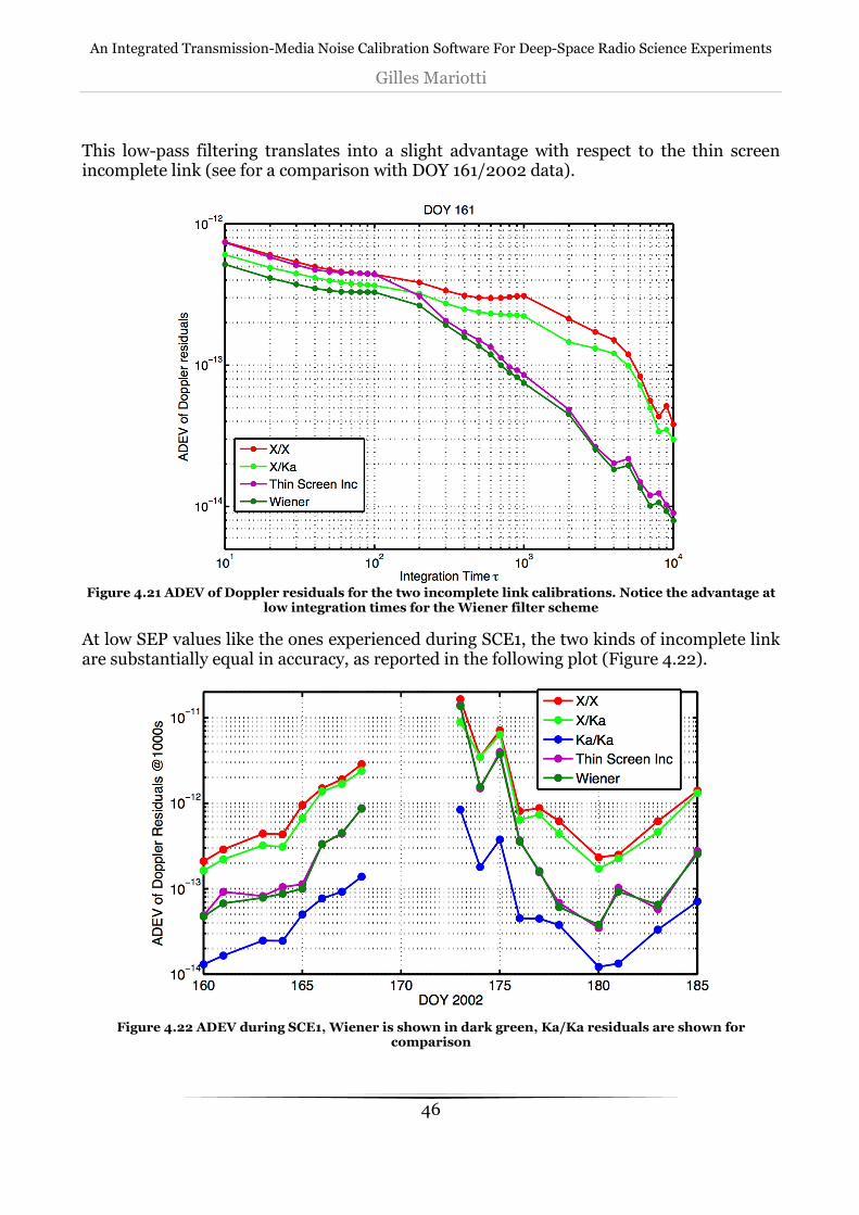
An Integrated Transmission-Media Noise Calibration Software For Deep-Space Radio Science Experiments
Gilles Mariotti
46
This low-pass filtering translates into a slight advantage with respect to the thin screen incomplete link (see for a comparison with DOY 161/2002 data).
Figure 4.21 ADEV of Doppler residuals for the two incomplete link calibrations. Notice the advantage at
low integration times for the Wiener filter scheme
At low SEP values like the ones experienced during SCE1, the two kinds of incomplete link are substantially equal in accuracy, as reported in the following plot (Figure 4.22).
Figure 4.22 ADEV during SCE1, Wiener is shown in dark green, Ka/Ka residuals are shown for
comparison

An Integrated Transmission-Media Noise Calibration Software For Deep-Space Radio Science Experiments
Gilles Mariotti
47
A test to compare the calibration performance of the two incomplete link types have been carried out using X/X and X/Ka data gathered during GWE1 and various gravity flybys, in addition to the SCE1 data shown, to cover the whole range of possible SEP angles. The expected behavior of the two calibrations consist in a similar performance at low SEP angles, and an increasing advantage of the Wiener filter as the SEP angle increases. The results seem to be consistent with the expectations, although the small number of suitable passes from the gravity flybys data does not represent a truly meaningful statistical basis, in particular in the range of mid-SEP angles. At opposition a drop in accuracy is expected for the Wiener filter, due to its formulation [14] that is inferred from several assumptions that do not hold at the largest elongation angles: in detail, in this configuration the Earth and spacecraft speeds must be taken into account. An optimal Wiener filter for opposition has been presented [14], but the difference between the two filters is negligible and computationally-wise the normal filter can be used even at position.
4.1.3 Dual Uplink Incomplete Link
The incomplete link described in the previous paragraphs is applied to data originated by a radio system with a single uplink carrier and two downlink carriers, which is a typical link configuration for deep space probes. In presence of a radio scheme that consists of two completely separate uplink/downlink bands, such as the one for NASA's Juno mission, the 3-by-3 set Eq. (4.1) is reduced in a different fashion than in Eq. (4.7). Since there is no cross-band observable, only the X/X and Ka/Ka equations are available.
(4.20)
Once again it is not possible to isolate all of the unknowns, but one can eliminate one of the two plasma contributions to create a new parameter y* that is close as possible to the true non-dispersive observable yND. The first conceived version of the technique[14] eliminates the uplink plasma contribution:
(4.21)
However, a more statistically-optimized version of the combination has been defined during the development of the calibration software described in this work [30]. Given the observable model from Eq. (4.20), a linear combination of X/X and Ka/Ka observables with coefficients χ and ψ:
yX /X = yND + yU + yD
α x/x2
yKa/Ka = yND + yU
β 2 + y D
β 2α 2ka/ka
y* = β 2yKK − yXX
β 2 −1= yND +
α −2KK −α XX
−2( )β 2 −1
yD

An Integrated Transmission-Media Noise Calibration Software For Deep-Space Radio Science Experiments
Gilles Mariotti
48
N∗ = c ⋅ Nee + f ⋅ Ngg (4.22)
is also a linear combination of ynd, yU and yD: ( ) ( ) ( ) DxxkkUND yyyy ψαχαβψχβψχ 2222* −−−− +++++= (4.23)
As we can neglect the cross-correlation among the three contributions (in particular the two plasma components are correlated only at a certain delay [7]), the variance associated with this observable is:
( ) ( ) ( ) 22222222222* DxxkkUND σψαχαβσψχβσψχσ −−−− +++++= (4.24)
This identity can be further simplified by imposing that ynd should be carried without modifications into y* (thus requiring c + f = 1), and using the hypothesis that the two plasma contributions have the same noise level: hP ≃ h = h<= . With these assumptions, the previous equation becomes a function of conly: ( )[ ] ( )[ ] 2222222222 1 1 plXXXXKKND σαχααβχβσσ* −−−−− +−++−+= (4.25)
The optimization of the linear combination of the X/X and Ka/Ka observables consists in the minimization of the coefficient of h<= , through an appropriate value of c, computed
from the minimum condition: ( )[ ] ( )[ ] 0 1 1
2 22222 2 =+−++− −−−−−XXXXKK αχααβχβ
d
d
χ (4.26)

An Integrated Transmission-Media Noise Calibration Software For Deep-Space Radio Science Experiments
Gilles Mariotti
49
Figure 4.23 Coefficients of the uplink (red line) and downlink (blue line) plasma variance as a function
of χ. The optimal Dual Uplink Incomplete (purple dot) minimizes the sum of the two plasma contributions to the variance. The formulation proposed in 1993 (red dot) cancels entirely the uplink
signal but the total coefficient (black curve) is not at a minimum.
The final values of and are then obtained: ( ) ( )
( ) ( ) ( )
( ) ( )( ) ( ) ( )422244
22244
422244
4222
1121
111
1121
11
−−−−−−
−−−−−
−−−−−−
−−−−
+++−++−+
=−=
+++−++−+
−=
xxxxkkkk
xxkkkk
xxxxkkkk
xxxxkk
αααβαβααβαβχψ
αααβαβαααβχ
(4.27)
Using Cassini’s values, we have c ≃ 1.0552 and f ≃ –0.0552, while the legacy formulation presented in Bertotti et al. 1993 [14] uses c ≃ 1.0457 and f ≃ –0.0457: Figure 4.23 shows the comparison between the coefficients of h<= for the two algorithms.
To test the effectiveness of this theoretical statement, both dual uplink calibration schemes were applied to Cassini’s SCE data. The optimum link has achieved a 10% average reduction of the ADEV of the Doppler residuals at 1000 s integration time, with a peak of 30% for a few passes. This result is shown in Figure 4.24.

An Integrated Transmission-Media Noise Calibration Software For Deep-Space Radio Science Experiments
Gilles Mariotti
50
Figure 4.24 Comparison of the Allan standard deviation at 1000 s integration time of the Doppler
residuals for the 1993 (red) and optimized (black) Dual Uplink Dual Down- link calibration schemes. Plasma free residuals (magenta) obtained using the full Multifrequency calibration are shown for
reference.
It is clear that the residual plasma contribution to y* is very modest, and it can be concluded that the Dual Uplink Incomplete calibration brings down the total plasma noise standard deviation by about 75% when compared to the one affecting the raw Ka/Ka observable (assuming yD and yU having the same noise level, we have: √0.0019 - 0.0129 √0.0437 - 0.0502 0.2372⁄ ).
Table 4.1 Coefficients of plasma contents and the non-dispersive contribution for each observable
ynd yU yD
yxx 1 1 0.7244
yxk 1 1 0.0502
ykk 1 0.0437 0.0502
ynd Eq. (4.2) 1 0 0
y* (legacy) 1 0 0.0194
y* (optimal) 1 –0.0091 0.0129
A much more interesting result comes from the comparison of the stability of the residuals, that highlights the actual gap in calibration performance between the full Multifrequency link and the Dual Uplink incomplete scheme. The plot of the Allan standard deviation at 1000s integration time (Figure 4.25) of y* generated by the Dual Uplink Incomplete technique and ynd obtained by the full triple link

An Integrated Transmission-Media Noise Calibration Software For Deep-Space Radio Science Experiments
Gilles Mariotti
51
Eq. (4.2) shows an excellent level of phase stability for the simpler plasma calibration scheme: the Allan standard deviation is consistently below 3·10–14 s/s, and the degradation in stability during the days closer to the solar conjunction (that occurred on DOY 172/2002), is smaller than the Ka/Ka one. Particular attention must be dedicated to the DOY 173 residuals: when fed with this data set, the Dual Uplink incomplete calibration routine performed better than the full multifrequency link one, which is supposed to provide a complete removal of dispersive noises. A plausible explanation of the unexpected result on DOY 173 could reside in the omission of X/Ka link: Cassini’s on-board transponder, due to severe amplitude scintillation at X band, loses lock on the uplink signal and its phasor cannot be precisely reconstructed. The resulting fluctuations in the instantaneous phase are then multiplied by the geratio (roughly 4.5 times) resulting in high noise levels for the X/Ka link.
Figure 4.25 Allan standard deviation at 1000 s for the raw X/X and Ka/Ka links and the calibrated
Cassini’s SCE1 Doppler residuals.
Moving towards larger SEP angles, where the plasma noise effect weakens, the difference between the calibration performance of the two algorithms (that ranges between 20% and 80%) should narrow: this allows relaxing the requirements on the design of the on-board RF chain, at least for missions that do not envisage critical operations at low SEP angles. Analyzing once again the ADEV(τ) slope, we have that the residual calibrated by the Dual Uplink Incomplete link show a white-noise behavior for tracking passes that comply with the limitations reported in Section 4.1.1.1.
4.1.3.1 Estimation of Post-Newtonian parameter γ
Cassini’s multifrequency Doppler observables acquired during SCE1 in 2002 allowed to obtain a significant reduction of the uncertainty of the parametrized post Newtonian (PPN)

An Integrated Transmission-Media Noise Calibration Software For Deep-Space Radio Science Experiments
Gilles Mariotti
52
relativity parameter γ, describing how the space-time curvature induced by a gravitational mass is responsible of deflections and delays experienced by an RF wave. The solution γ= 1 + (2.1 ± 2.3)·10–5 obtained [27] reduced the formal uncertainty with respect to previous experiments, thanks to the multifrequency link and water vapor radiometer-based Earth troposphere calibrations. The very same analysis approach is replicated here with the only difference of using Doppler data that were calibrated using the dual uplink incomplete algorithm, both to further quantify the loss of accuracy of this calibration scheme and to assess its impact for scientific applications, in addition to the analysis of the post-fit residuals discussed in the previous section. To this aim, ODP was used to generate Cassini’s orbital solution and to estimate the parameters of interest using a set-up identical to the legacy one, that is using the same estimated and consider parameters to keep both results as homogeneous and comparable as possible. The new OD results using the incomplete calibration show that the estimation of γ is severely biased away from the unity value predicted by general relativity, γ= 1 + (–12.5 ± 2.6)·10–5. While the formal uncertainty is very close to the one achieved using the plasma-free observables, the estimated value of 0.999875 is about 5 standard deviations off from the nominal solution, showing a bias due to the plasma noise that the dual uplink calibration was unable to absorb.
Figure 4.26 Doppler residuals of an ODP passthrough using observables calibrated by the dual uplink
incomplete algorithm.
Figure 4.26 shows the average of the dual uplink-calibrated residuals for each tracking pass obtained by using the legacy orbital solution as a priori value for a passthrough analysis (meaning that no iteration on the estimated parameters was carried out). The mean of residuals moves away from zero when approaching superior conjunction, in a very similar manner to the raw X/X uncalibrated observables, shown for comparison in Figure 4.27.

An Integrated Transmission-Media Noise Calibration Software For Deep-Space Radio Science Experiments
Gilles Mariotti
53
Figure 4.27 ODP Doppler residuals of ODP passthrough using raw X/X observables.
Note that this behavior of the Doppler residuals shows up only when no estimation iterations are performed, while a full orbit determination run (with estimation iterations) returns good zero-mean Doppler residuals, showing that the bias is transferred from the residuals to the estimated parameters, γ in particular. The estimation of γ is severely affected by solar plasma because both physical effects produce a deflection of the ray path, so that the residual dispersive noise left by the Dual Uplink Incomplete calibration is recognized by the filter as a gravitational bending. As these deflections have opposite sign [26], the resulting estimated value of is lower than 1 or, in other words, the bias is negative. Moreover, the bias should grow when using lower carrier frequencies. This statement is confirmed by a model for the bias generated combining the Baumbach-Allen model for the electron density of the solar corona Eq. (3.18) with the formulation of the gravitational delay used within ODP [31]: ( )
−++++=
1221
12212
ln12
rrr
rrr
clgr
γδ (4.28)
where µ is the gravitational parameter of the Sun, r1 and r2 the position vectors of the Earth and the S/C, and r12 the vector of the ray path. The coronal model has been used to estimate the path delay due to plasma δlpl, and then Eq. (4.28) has been inverted to find γ using δlpl + δlgr instead of δlgr on the left-hand side. This gives us a qualitative trend that we expect the ODP results to follow and, actually, the filter behaves accordingly: the estimates generated using these observables are γ= 1 + (–8.81 ± 0.94)·10–3 for the raw X/X link and
γ= 1 + (–3.23 ± 0.2)·10–3 for the raw Ka/Ka link (Figure 4.28).

An Integrated Transmission-Media Noise Calibration Software For Deep-Space Radio Science Experiments
Gilles Mariotti
54
Figure 4.28 Expected (black) and observed (red) γ bias.
Although the results obtained using the Dual Uplink Incomplete calibration scheme are not promising for highly demanding radio science experiments, an attempt was made to combine the best of each calibration in a mixed data set from Cassini’s 2002 SCE1. The combined observables were formed starting from the original multifrequency link calibrated data and replacing in it the Dual Uplink observables for DOY 173 only, because of the peculiar ASDEV levels shown in Figure 4.25. The rationale for this choice is that DOY 173 is the most important tracking pass in the data set, from the γ estimation point of view, since this parameter becomes more observable approaching conjunction (the gravitational influence on y is inversely proportional to the impact parameter [32]). With this mixed data set input, our best estimation result is γ= 1 + (3.48 ± 2.17)·10–5, with a 5% reduction of the formal estimation error, with respect to the reference result.
4.1.3.2 First application to Doppler data from the Juno mission
During summer of 2012 a solar conjunction experiment was planned for the Juno spacecraft, called Juno GRT (General Relativity Test). Doppler data generated by the GRT experiment were the first chance for testing the Dual Uplink incomplete link with genuine Juno X/X+Ka/Ka data. The conclusions from previous section are not encouraging about the accuracy for PPN parameters estimation, but still these data are important for running calibration tests and readiness tests for both pre-processing and OD software prior to the Jovian phase of the mission.

An Integrated Transmission-Media Noise Calibration Software For Deep-Space Radio Science Experiments
Gilles Mariotti
55
Figure 4.29 ADEV@1000s of Juno GRT Doppler residuals
The GRT residuals are in line with the behavior expected from the simulation with Cassini data: the ADEV@1000s ratio between dual uplink-calibrated residuals and raw Ka/Ka residuals is still in the 20-80% interval as in the Cassini case.
Ionosphere 4.2
Due to its dispersive behavior, ionospheric noises in radiometric observables are removed by the same multifrequency algorithms described in Section 4.1. When a multifrequency calibration is not available, or only incomplete scheme are usable due to radio system constraints (lack of three two-way bands), the ionospheric path delay and Doppler signals can be modelled to some extent by the Klobuchar model and by using the so called Global Ionosphere Maps (GIM). Both these techniques are discussed in Section 4.3.2.9.14. Ionospheric path delay can also be estimated by GNSS analysis software: JPL provides ionospheric calibrations within CSP cards under the TSAC specification.
Troposphere 4.3
4.3.1 Overview of Available Tropospheric Path Delay Calibrations
Removal of tropospheric wet and dry path delays can be achieved through different calibration techniques, with various degrees of effectiveness and cost. In increasing order of complexity they are:
1. Statistical/blind models 2. Models based on surface meteo data 3. GNSS-based estimation 4. Microwave radiometers retrieval
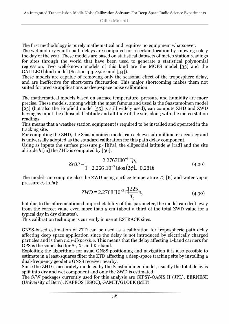
An Integrated Transmission-Media Noise Calibration Software For Deep-Space Radio Science Experiments
Gilles Mariotti
56
The first methodology is purely mathematical and requires no equipment whatsoever. The wet and dry zenith path delays are computed for a certain location by knowing solely the day of the year. These models are based on statistical datasets of meteo station readings for sites through the world that have been used to generate a statistical polynomial regression. Two well-known models of this kind are the MOPS model [33] and the GALILEO blind model (Section 4.3.2.9.12 and [34]). These models are capable of removing only the seasonal effect of the troposphere delay, and are ineffective for short-term fluctuation. This major shortcoming makes them not suited for precise applications as deep-space noise calibration. The mathematical models based on surface temperature, pressure and humidity are more precise. These models, among which the most famous and used is the Saastamoinen model [23] (but also the Hopfield model [35] is still widely used), can compute ZHD and ZWD having as input the ellipsoidal latitude and altitude of the site, along with the meteo station readings. This means that a weather station equipment is required to be installed and operated in the tracking site. For computing the ZHD, the Saastamoinen model can achieve sub-millimeter accuracy and is universally adopted as the standard calibration for this path delay component. Using as inputs the surface pressure p0 [hPa], the ellipsoidal latitude φ [rad] and the site altitude h [m] the ZHD is computed by [36]:
( ) h
pZHD
⋅−⋅⋅−⋅⋅= −
−
28.02 cos10266.21
102767.23
03
ϕ (4.29)
The model can compute also the ZWD using surface temperature T0 [K] and water vapor pressure e0 [hPa]:
00
3 1225102768.2 e
TZWD ⋅⋅= −
(4.30)
but due to the aforementioned unpredictability of this parameter, the model can drift away from the correct value even more than 5 cm (about a third of the total ZWD value for a typical day in dry climates). This calibration technique is currently in use at ESTRACK sites. GNSS-based estimation of ZTD can be used as a calibration for tropospheric path delay affecting deep space application since the delay is not introduced by electrically charged particles and is then non-dispersive. This means that the delay affecting L-band carriers for GPS is the same also for S-, X- and Ka-band. Exploiting the algorithms for usual GNSS positioning and navigation it is also possible to estimate in a least-squares filter the ZTD affecting a deep-space tracking site by installing a dual-frequency geodetic GNSS receiver nearby. Since the ZHD is accurately modeled by the Saastamoinen model, usually the total delay is split into dry and wet component and only the ZWD is estimated. The S/W packages currently used for this analysis are GIPSY-OASIS II (JPL), BERNESE (University of Bern), NAPEOS (ESOC), GAMIT/GLOBK (MIT).

An Integrated Transmission-Media Noise Calibration Software For Deep-Space Radio Science Experiments
Gilles Mariotti
57
JPL currently provides GNSS-based tropospheric path delay calibration for DSN sites under the AMC [37] and TSAC [17][6] standards. This calibration technique provides sub-cm accuracy for the zenith path delay removal in range observables and a range-rate calibration accuracy of tens of µm/s. A complete discussion on the implementation of a GNSS-based tropospheric calibration S/W is reported in Section 4.3.2. The most effective calibration available for tropospheric path delay involves the installation at the tracking site of a microwave radiometer. Microwave radiometers are instruments that can retrieve a large number of atmospheric quantities by measuring the brightness temperature of the sky. The integrated water vapour content, that can be converted to ZWD by a simple scale factor, is one of them. This calibration can completely reject tropospheric delay for range and range-rate observables (down to the mm and µm/s levels [20]). Due to the applicability limitations of the retrieval algorithms used to convert brightness temperatures, the instrument becomes unreliable when precipitating clouds and rain are present on its line of sight (in general, when the Rayleigh scattering model is not applicable and the Mie scattering comes into play). Since GNSS is instead an all-weather technique, it is advisable to deploy the needed equipment for both calibrations at a tracking site to exploit their synergy. Radiometry basics and MWR operations are covered in Section 4.3.3.
4.3.2 GNSS-based Estimation
This section describes the mathematical models and the code implementation of a GNSS-based estimation software for the tropospheric path delay. This calibration method relies on the non-dispersive nature of the tropospheric path delay, that doesn’t scale with the carrier frequency. This means that the delay affecting a GNSS receiver operating on the L-band is the same on S-, X- and Ka-band. Thanks to the IGS worldwide network of GNSS receivers that provides precise orbits for GPS and GLONASS satellites, an accurate estimation of the delay is possible by installing a receiver in the deep-space site and then processing the data using GNSS analysis software [38]. This makes GNSS-based estimation a very cost-effective solution for tropospheric noise rejection in radiometric observables, and is one of the techniques currently in use for rejecting this type of noise source at JPL [37].
4.3.2.1 Overview
The core objective of a Global Navigation Satellite System (GNSS) is to provide precise position and velocity information to users on (or near) Earth using satellites of known positions broadcasting signals marked with their own time standard. The first operating GNSS constellation was the American NAVSTAR GPS system, which development started in 1973 and it’s still the major player in the GNSS field, while other newer systems are being developed and deployed: the Russian GLONASS (the constellation is being completed, the minimum global coverage was achieved in 2013), China’s Beidou/COMPASS and the European GALILEO.

An Integrated Transmission-Media Noise Calibration Software For Deep-Space Radio Science Experiments
Gilles Mariotti
58
This documents and the software it describes are focused on GPS, but most of the theoretical background covered is common to any GNSS system. NAVSTAR GPS is divided into three segments: Space, Control, User [39]. The space segment consists of a constellation of 32 MEO satellites distributed on 6 nearly-circular orbits at 55° inclination and 11h 58’ orbital period (half a sidereal day). This layout has been selected in order to ensure visibility of at least 4 satellites above 15 degrees elevation from any point on Earth, at any time. This condition is achieved by the nominal constellation of 24 satellites, but other 8 satellites have been added to provide redundant measurements and improve availability and reliability. Satellites provide a platform for radio transceivers, atomic clocks, computers and various ancillary equipment used to operate the system (among others, two 7 m2 solar panels for power supply and a propulsion system for orbit adjustments and stability control). Several generations of satellites have been created: the first satellites were called Block I and have been discontinued. Currently several variants of Block II space vehicles are orbiting: Block IIA, Block IIR, Block IIR-M, Block IIF. The modernization roadmap for the system envisages the launch of Block IIIA satellites starting in 2014.
Figure 4.30 Example of GPS satellites in view at a given time from a site on Earth
(black dots are visible satellites)
The control segment comprises the Operational Control System (OCS) which consists of a master control station (located at Falcon AFB, Colorado), worldwide monitor stations and ground control stations. They main tasks of this segment are: satellite tracking for orbit and clock determination, time synchronization, upload of the navigation message to the satellites.
4.3.2.2 GPS Signals
All signals transmitted by a GPS satellite are derived from the fundamental frequency f0 of the satellite oscillator.

An Integrated Transmission-Media Noise Calibration Software For Deep-Space Radio Science Experiments
Gilles Mariotti
59
Table 4.2 GPS signals specifications
f0 = 10.23 MHz
L1 L2
Multiplier 154 f0 120 f0
Frequency 1575.42 MHz 1227.60 MHz
Wavelength 19.03 cm 24.42 cm
The two sinusoidal carrier frequencies L1 and L2 are right-hand circular polarized and modulated (biphase modulation) with two pseudorandom codes and with the navigation message to transmit information such as the readings of the satellite clocks, the orbital parameters, etc (Figure 4.31). The navigation message contains information of the satellite health status, its orbit and various correction data (e.g. ionosphere corrections)[40]. The two pseudorandom noise (PRN) codes are generated by hardware devices called tapped feedback shift registers, and are used to transmit the satellite clock readings. Each bit is referred to as chip.
• The C/A-code (Coarse/Acquisition) has a frequency f0/10 (length 1023 chips) and is repeated every millisecond: this means that two consecutive chips are less than 1 microsecond apart, resulting in a chip length of about 300 meters.
• The P-code (Precision) has frequency f0 and originates from the combination of two series of bits, resulting in 2.3547·1014 bits repeated every 266.4 days. The total code length is partitioned into 37 unique one-week segments and each segment is assigned to a satellite defining its PRN number. The chip length is about 30 meters. This code can be encrypted using the A/S (Anti-Spoofing) mode, that converts the P-code into Y-code, decrypted only by a secret conversion algorithm based on an encryption key called W-code.
The range precision of a code observable is usually 10% of the chip length.

An Integrated Transmission-Media Noise Calibration Software For Deep-Space Radio Science Experiments
Gilles Mariotti
60
Figure 4.31 GPS signals
4.3.2.3 Observables
Ranging using GNSS satellites is based on two observables:
• One-way transmission time of signals from satellite to receiver
• Carrier phase angle At each reception of a code signal, the transmission time ∆p is computed by subtracting the receiver time of reception tR to the emitter clock reading tS contained in the code [39]: ( ) ( )SS
RRS
RSR tttt
ct δδρ −−−=−==∆ (4.31)
Both time tags suffer from the clock bias introduced by their respective oscillators. For quartz oscillators used in low-end receiver, this contribution can reach the microsecond level, that translates into a staggering 300 km ranging error. The estimation of the receiver clock delay is then essential in order to achieve an admissible accuracy in the estimated position. This is why the visibility of at least 4 satellites must be ensured at any given time (4 range values, against 4 estimated parameters: 3 position components and 1 clock bias). The satellite clock is very stable in comparison (Cesium and Rubidium atomic standards) and its delay can be modeled by a polynomial which coefficients are transmitted in the navigation message. Finally, the range ρ is computed by multiplying the light time by the speed of light c. The other way to compute the range between receiver and satellite is to observe the beat phase between the reconstructed (received) carrier and the reference carrier in the receiver PLL.
Bc
f RScarrier
SR +
−−≅Φ δδρ (4.32)

An Integrated Transmission-Media Noise Calibration Software For Deep-Space Radio Science Experiments
Gilles Mariotti
61
This observable is more precise than the code but suffers from an ambiguity component that is due to the fact that the initial integer number of cycles between satellite and receiver is unknown at the time of first acquisition. This ambiguity B remains the same as long as the lock on the carrier is maintained. The phase then can give very accurate information on the variation of the range relative to an unknown initial position. The beat phase is expressed in phase cycles and must be multiplied by the carrier wavelength of the relative band i (λi=c/fLi) to yield the range Li=λi · Φi. Signals Doppler shift can also be used as a source of data, to retrieve the satellite radial velocity, but will not be covered in this discussion. A receiver can theoretically generate up to 5 different range values from any satellite in view on the two frequencies:
• C/A: C1
• P (military): P1, P2
• Carrier Phase: L1, L2 “Synthetic” P-code measurements are available to civil users thanks to several techniques developed through the years by receiver manufactures to overcome A/S (e.g. cross-correlation and Z-tracking [39]). The modernization program for the GPS will provide three new civil codes to receive: L2C, L5 (I+Q), L1C. Since L5 is transmitted on a new carrier, also the new L5 phase is observable.
4.3.2.4 Pseudoranges
Clock delays are not the only noise components that spoil the accuracy of code and phase observables: several other phenomena of various natures introduce unwanted delays in the signal light time and phase shifts in the carriers. The distance retrieved by the receiver then is not the actual range but rather a pseudorange9, that must be corrected in order to improve the positioning accuracy.
9 Note: in common GPS jargon, “pseudorange” is often use to indicate solely code measurements, so is not uncommon to talk about “phase and pseudorange observables”

An Integrated Transmission-Media Noise Calibration Software For Deep-Space Radio Science Experiments
Gilles Mariotti
62
Figure 4.32 Pseudorange biases
Figure 4.32 shows the main noise components that turn the geometric range into the received pseudorange. By indicating the code pseudorange (between satellite j and receiver A) with P and the carrier-phase pseudorange with L we have that: ( )
( ) Lj
AjAAX
jA
jA
jA
jA
jArelA
jjA
jA
PAXjA
jA
jA
jA
jArelA
jjA
jA
BwMKITdtdtcL
MKITdtdtcP
ελδδρ
εδδρ
+++++++++−+=
+++++++−+=
,,
,, (4.33)
where:
• ρAj geometrical distance between receiver A and satellite i
• c speed of light
• dtA receiver clock offset
• dtj satellite clock offset
• δjrel,A relativistic error
• TAj tropospheric path delay
• IAj ionospheric path delay, frequency dependent
• KAj hardware biases
• MAj multipath effect
• δjx,A displacement error due to phase center offset (PCO), phase center variations
(PCV), antenna reference point eccentricity, solid Earth tides, polar motion.
• wAj phase windup of the RHCP wave due to spacecraft attitude
• BAj carrier phase ambiguity (a different value on each band)
• ε measurement noise (1% of chip length for code, 0.01 cycles for carrier phase).

An Integrated Transmission-Media Noise Calibration Software For Deep-Space Radio Science Experiments
Gilles Mariotti
63
Each component must be cancelled in order to achieve the desired level of accuracy, and different methodologies are used depending on the specific noise source. In general pseudorange noises can be completely or partially removed by using:
• models
• linear combinations of observables from the same satellite
• combinations of observables from different satellite-receiver pairs (differential approach)
• estimation of the parameter Depending on the user application a different solution can be used for a specific delay component, since signals that are considered as noise for pure positioning and navigation, for other types of surveys are the very signal of interest to be extrapolated from the pseudorange. For instance, the ionosphere delay is cancelled by the Klobuchar model or using an appropriate combination of L1 and L2 pseudoranges for positioning, while it can be estimated as a parameter by users interested in sounding Earth ionosphere. For the application here described, the signal of interest is the tropospheric path delay (the wet component in particular).
4.3.2.5 Estimation paradigms
The two main approaches that can be used for positioning and surveying using GNSS systems are the point positioning and the relative (or differential) positioning. Both techniques can be used in post-processing and in real-time applications, with different levels of achievable precision.
4.3.2.5.1 Point positioning
The point positioning approach is conceptually the easiest. It uses the pseudorange data provided by a GNSS receiver in order to compute its position and clock error. The estimation step itself is a least-squares filter that computes the coordinates errors with respect to an initial position, used to linearize the geometric range from satellite to
receiver. The geometric range Yqr is given by: ( ) ( ) ( )222
)( Aj
Aj
Ajj
A ZZYYXXt −+−+−=ρ (4.34)
and can be linearized around a position XA0 using a Taylor series expansion of Eq. (4.34): ( ) ( ) ( )
AjA
jAA
e
jA
Aj
A
e
jA
Aj
A
e
jA
Aj
Aj
Aj
Ajj
AjA
jA
XdedZZZ
dYYY
dXXX
ZZYYXX
jZA
jYA
jXA
ˆ00
0
0
0
0
0
2
0
2
0
2
00
+=−−−−−−
+−+−+−=∆−=
ρρρρ
ρρρ
434214342143421
(4.35)

An Integrated Transmission-Media Noise Calibration Software For Deep-Space Radio Science Experiments
Gilles Mariotti
64
This linear relation is used to build the linear system relating pseudoranges to position components dXA=dXA, dYA, dZA and clock δA. Assuming that satellites i, j, k, w are in view from receiver A the observation equations for code are:
−−−−
=
−−−−
A
A
A
A
wZA
wYA
wXA
kZA
kYA
kXA
jZA
jYA
jXA
iZA
iYA
iXA
wA
wA
kA
kA
jA
jA
iA
iA
dt
dZ
dY
dX
ceee
ceee
ceee
ceee
P
P
P
P
0
0
0
0
ρρρρ
(4.36)
It has to be noted that at a certain epoch t, the system is invertible since 4 satellites are always in view, and any additional satellite provides redundancy to improve the estimation accuracy. Since is always possible to build a determined set, every epoch can be processed separately, therefore movement of the receiver is permitted (kinematic positioning). For carrier-phase observables this does not apply due to phase ambiguities that add a new parameter for each satellite in view:
−−−−
=
−−−−
kA
wA
jA
iA
A
A
A
A
wZA
wYA
wXA
kZA
kYA
kXA
jZA
jYA
jXA
iZA
iYA
iXA
wA
wA
kA
kA
jA
jA
iA
iA
B
B
B
B
dtdZ
dY
dX
ceee
ceee
ceee
ceee
L
L
L
L
λλ
λλ
ρρρρ
000
000
000
000
0
0
0
0
(4.37)
With any number of visible satellites, this set in underdetermined for a single epoch. This means that carrier-phase positioning requires a static initialization for real-time kinematic applications. Furthermore, phase ambiguities must be estimated as float numbers, not integers, due to the hardware biases. These adjustment models are implying that the satellite clocks have been corrected using the navigation message polynomials and are neglecting completely all of the error sources in Eq. 4.33 and Figure 4.32, that will then corrupt the position, clock and ambiguity estimations. Path delays due to transmission media in particular (ionosphere and troposphere) can cause errors of tens of meters in the position and in general each error component must be addressed to reach cm-level accuracy. To achieve this accuracy, even the satellites orbital

An Integrated Transmission-Media Noise Calibration Software For Deep-Space Radio Science Experiments
Gilles Mariotti
65
elements and clocks provided in the navigation message are not adequate and more precise information must be used (see Section 4.3.2.5.3).
4.3.2.5.2 Relative positioning
Most part of the errors affecting pseudoranges can be addressed by differencing observables generated by two receivers. If the receivers are close enough to each other (in other words, the baseline is short), most of the error contributions cancel out, especially the ones due to transmission media refraction. In general, one of the receivers is considered as a reference (also called master) station, which position is well known, and then the other receiver (the rover) position is estimated as relative to the reference position. The observation vector used in the estimation process is not the pseudorange between satellite j and receiver A anymore, but rather a series of differences among pseudoranges received by both stations.
• Single differences: pseudoranges received by stations A and B from satellite j are differenced. The resulting difference will be unaffected by satellite-related errors, e.g. the satellite clock bias, the satellite hardware bias.
• Double differences: the single-difference pseudorange relative to satellite j is subtracted from the single-differenced pseudorange relative to satellite i. All of the station-related error sources cancel out: receiver clock bias, receiver hardware bias. If the baseline between stations is shorter than a few tens of kilometers also transmission media delays (ionospheric and tropospheric) get rejected. Since both hardware delays are canceled, the double-differenced phase ambiguities can be fixed as integers during the least-squares filtering stage.
The differential GNSS algorithm based on double differences has been and still is the most accurate surveying and navigation technique available, but is being challenged by the rise of PPP techniques (Section 4.3.2.5.3). Depending on the application, several implementations of this paradigm have been conceived: e.g. RTK, NRTK. In the tropospheric delay estimation code here described, the double-difference approach is implemented, but using a longer baseline so that the tropospheric signal is not cancelled from the observable. This means that also the ionosphere delay is not rejected and must be removed by other means (i.e. ionofree linear combination of L1 and L2). There are several ways to compose double-differences, with respect to what satellites to pick. For tropospheric delay estimation, this strategy is used: at a certain epoch, the satellite with highest elevation upon the rover station is chosen as reference satellite and all the other satellites in view are differenced to its pseudorange. Assuming as master the station A and B as the rover, and satellite j as reference, the double differenced observables for each satellite i will be: ( ) ( )
( ) ( )jB
jA
iB
iA
ijAB
jB
jA
iB
iA
ijAB
LLLLL
PPPPP
−−−=∆∇
−−−=∆∇ (4.38)
while the adjustment models for this technique will be:

An Integrated Transmission-Media Noise Calibration Software For Deep-Space Radio Science Experiments
Gilles Mariotti
66
• Code
=
∆∇−∆∇∆∇−∆∇∆∇−∆∇
B
B
B
wjZB
wjYB
wjXB
kjZB
kjYB
kjXB
ijZB
ijYB
ijXB
wjAB
wjAB
kjAB
kjAB
ijAB
ijAB
dZ
dY
dX
eee
eee
eee
P
P
P
0
0
0
ρρρ
(4.39)
• Carrier Phase
∆∇
∆∇
∆∇
=
∆∇−∆∇∆∇−∆∇∆∇−∆∇
wjA
kjA
ijA
B
B
B
wjZB
wjYB
wjXB
kjZB
kjYB
kjXB
ijZB
ijYB
ijXB
wjAB
wjAB
kjAB
kjAB
ijAB
ijAB
B
B
B
dZdY
dX
eee
eee
eee
L
L
L
00
00
00
0
0
0
λλ
λ
ρρρ
(4.40)
Once again the geometric range has been linearized around positions XA0 and XB0. We can consider the master station as well-positioned (XA0=XA), then the double differenced linear unity vectors are computed by: ( ) ( )
( )
( )
( ) B
e
jB
iB
ijAB
jB
iB
ijAB
jB
jB
jA
jA
iB
iB
iA
iA
jB
jA
iB
iA
ijAB
XdeeijB
ˆˆ
ˆ
0
0
0
0
00
0
0
43421−+∆∇=
=∆−∆+∆∇=
=∆−+
∆−−∆−−
∆−=
=−−−=∆∇
==
ρρρρ
ρρρρρρρρ
ρρρρρ
(4.41)
A network of reference stations can be used to add redundancy and degrees of freedom to the estimation. Several network configurations can be chosen: for ZWD estimation usually a network of master stations centered in the rover is created, with the number of available baselines equal to the number of master stations.

An Integrated Transmission-Media Noise Calibration Software For Deep-Space Radio Science Experiments
Gilles Mariotti
67
Figure 4.33 Example of a network centered around Zimmerwald, CH
Since the parameter of interest is not the position of the rover, but its zenith wet delay, the reference stations should also have ZWD information available along with their precise position (Section 4.3.2.9.13).
4.3.2.5.3 Precise Point Positioning (PPP)
Precise Point positioning, or PPP, is a single point positioning technique that can achieve the same precision levels of differential GNSS without the need to use reference stations. The improved accuracy is achieved by using precise orbit and satellite clock data provided by the IGS (International GNSS Service, Section 4.3.2.6), that are computed using a worldwide network of reference stations. The user can achieve the accuracy of DGNSS approaches without the need of a close-by reference station. The PPP algorithm uses as input code and phase observations from a dual-frequency receiver, and precise satellite orbits and clocks. The observations coming from all the satellites are processed together in a filter that solves for the receiver coordinates, the receiver clock, the zenith tropospheric delay and the phase ambiguities. All of the error sources reported in Section 4.3.2.4 are removed using a dedicated model or algorithm [38]. The PPP technique offers significant benefits compared to differential precise positioning:
• PPP involves only a single GPS receiver and, therefore, no reference stations are needed in the vicinity of the user.
• PPP can be regarded as a global position approach because its position solutions referred to a global reference frame. As a result, PPP provides much greater positioning consistency than the differential approach in which position solutions are relative to the local base station or stations.
• PPP can support other applications beyond positioning. For example, as PPP technique estimates receiver clock and tropospheric effect parameters in addition to

An Integrated Transmission-Media Noise Calibration Software For Deep-Space Radio Science Experiments
Gilles Mariotti
68
position coordinate parameter, it provides another way for precise time transfer and troposphere estimation using a single GPS receiver.
However, PPP presents several shortcomings: • A long convergence time, this is a drawback for real-time applications. • Integer ambiguity resolution is not possible due to hardware biases (cf. Section
4.3.2.5.1). • Difficult pre-processing and screening of data (cycle-slips, outliers) • A large number of error components must be corrected, see Figure 4.34)
Figure 4.34 Corrections to pseudoranges needed by PPP and DGNSS with short baselines [41]
Due to the long baselines used in this ZWD estimation software, several of this corrections must be applied even if working in a double-difference paradigm.
4.3.2.6 International GNSS Service (IGS)
The International GNSS Service (IGS) is a voluntary federation of more than 200 worldwide agencies that pool resources and permanent GPS & GLONASS station data to generate precise GPS & GLONASS products. Currently the IGS includes two GNSS’s and intends to incorporate future constellations. The foundation of IGS is a global network of over 350 permanent, continuously operating, geodetic-quality GPS and GLONASS tracking sites. The station data are archived at three Global Data Centers and six Regional Data Centers. 10 Analysis Centers (ESOC is one of them) regularly process the data and contribute

An Integrated Transmission-Media Noise Calibration Software For Deep-Space Radio Science Experiments
Gilles Mariotti
69
products to the Analysis Center coordinator, who produces the official IGS combined products. The classic products are:
• Precise satellites orbits and clocks with different levels of accuracy and latency • Earth Rotation Parameters • Precise coordinates of the stations in the network.
Table 4.3 IGS products precision and latency
ULTRA-RAPID RAPID FINAL
Orbit RMS 3-5 cm 2.5 cm 2.5 cm
Clock RMS 150 ps (4.5 cm) 75 ps (2.25 cm) 75 ps (2.25 cm)
Latency 6 hours 17-41 hours 12-18 days
Other “augmentation” products are available, i.e. :
• Worldwide grid of ionospheric TEC • Tropospheric path delay for several stations in the network • LEO satellites orbits
All products are consistent with the ITRF reference frame realization and offer an absolute positioning. Each product is distributed using a dedicated standard file format10:
• RINEX (Table 4.4): RINEX observations (*.yyo, *.yyd and other): receivers data METEO-RINEX (*.yym): weather station data RINEX navigation (*.yyn): broadcast navigation message from constellation CLOCK-RINEX (*.yyc or *.clk): clock offset for satellites and receivers
• SINEX: estimated stations locations • SP3: GPS and GLONASS S/C orbits • IONEX: worldwide TEC grid • TROPO-SINEX: stations tropospheric path delay and horizontal gradients • ANTEX: calibrations for antenna phase center offsets and variations
The ZWD estimation program reported makes use of IGS products for its analysis, featuring automated download and read routines for all the main IGS file formats.
10 http://igscb.jpl.nasa.gov/components/formats.html
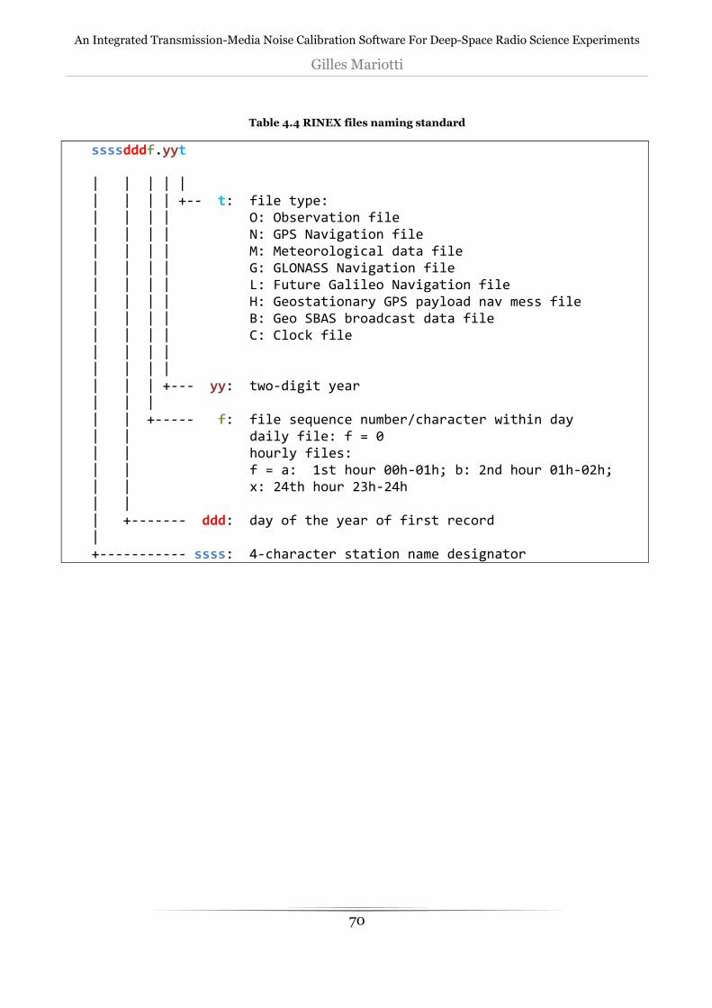
An Integrated Transmission-Media Noise Calibration Software For Deep-Space Radio Science Experiments
Gilles Mariotti
70
Table 4.4 RINEX files naming standard
ssssdddf.yyt | | | | | | | | | +-- t: file type: | | | | O: Observation file | | | | N: GPS Navigation file | | | | M: Meteorological data file | | | | G: GLONASS Navigation file | | | | L: Future Galileo Navigation file | | | | H: Geostationary GPS payload nav mess file | | | | B: Geo SBAS broadcast data file | | | | C: Clock file | | | | | | | | | | | +--- yy: two-digit year | | | | | +----- f: file sequence number/character within day | | daily file: f = 0 | | hourly files: | | f = a: 1st hour 00h-01h; b: 2nd hour 01h-02h; | | x: 24th hour 23h-24h | | | +------- ddd: day of the year of first record | +----------- ssss: 4-character station name designator
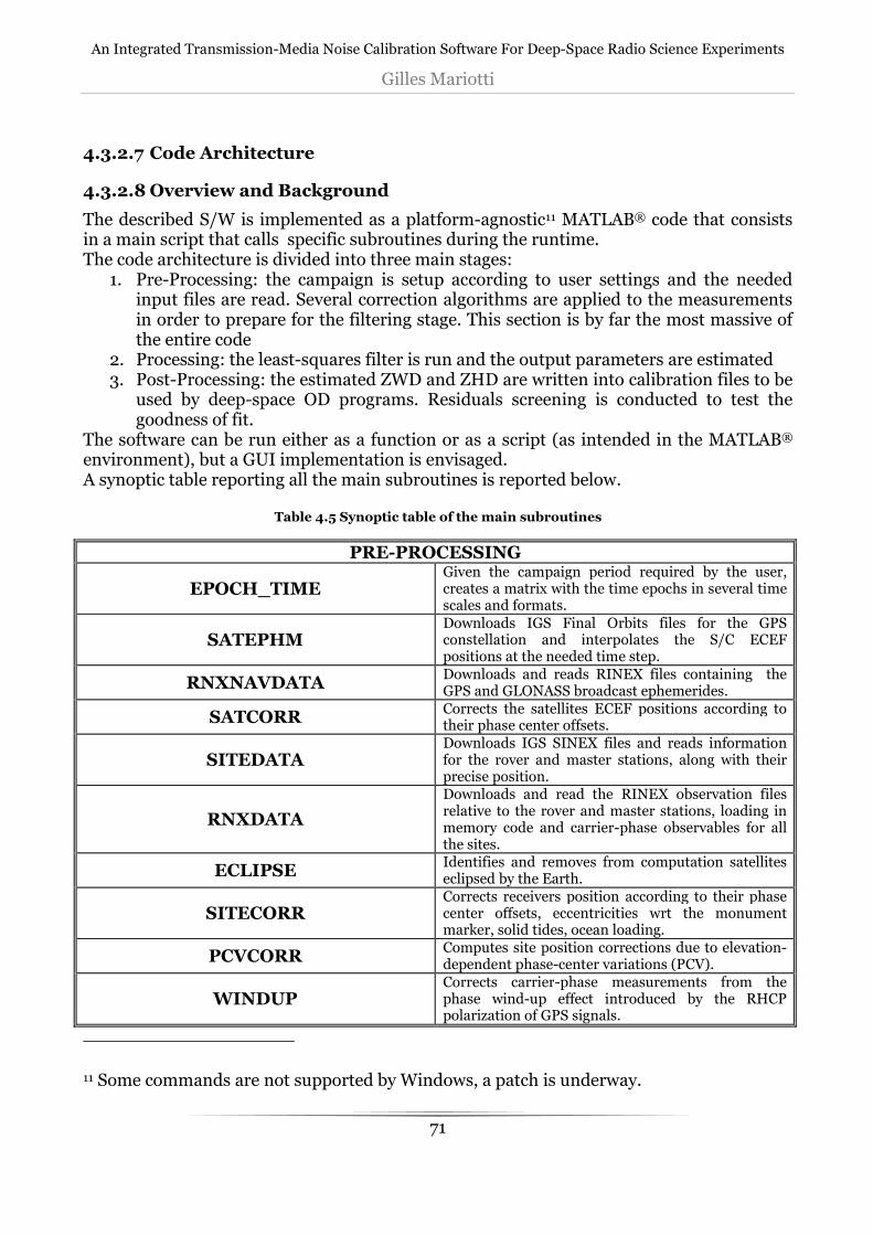
An Integrated Transmission-Media Noise Calibration Software For Deep-Space Radio Science Experiments
Gilles Mariotti
71
4.3.2.7 Code Architecture
4.3.2.8 Overview and Background
The described S/W is implemented as a platform-agnostic11 MATLAB® code that consists in a main script that calls specific subroutines during the runtime. The code architecture is divided into three main stages:
1. Pre-Processing: the campaign is setup according to user settings and the needed input files are read. Several correction algorithms are applied to the measurements in order to prepare for the filtering stage. This section is by far the most massive of the entire code
2. Processing: the least-squares filter is run and the output parameters are estimated 3. Post-Processing: the estimated ZWD and ZHD are written into calibration files to be
used by deep-space OD programs. Residuals screening is conducted to test the goodness of fit.
The software can be run either as a function or as a script (as intended in the MATLAB®
environment), but a GUI implementation is envisaged. A synoptic table reporting all the main subroutines is reported below.
Table 4.5 Synoptic table of the main subroutines
PRE-PROCESSING
EPOCH_TIME Given the campaign period required by the user, creates a matrix with the time epochs in several time scales and formats.
SATEPHM Downloads IGS Final Orbits files for the GPS constellation and interpolates the S/C ECEF positions at the needed time step.
RNXNAVDATA Downloads and reads RINEX files containing the GPS and GLONASS broadcast ephemerides.
SATCORR Corrects the satellites ECEF positions according to their phase center offsets.
SITEDATA Downloads IGS SINEX files and reads information for the rover and master stations, along with their precise position.
RNXDATA
Downloads and read the RINEX observation files relative to the rover and master stations, loading in memory code and carrier-phase observables for all the sites.
ECLIPSE Identifies and removes from computation satellites eclipsed by the Earth.
SITECORR Corrects receivers position according to their phase center offsets, eccentricities wrt the monument marker, solid tides, ocean loading.
PCVCORR Computes site position corrections due to elevation-dependent phase-center variations (PCV).
WINDUP Corrects carrier-phase measurements from the phase wind-up effect introduced by the RHCP polarization of GPS signals.
11 Some commands are not supported by Windows, a patch is underway.
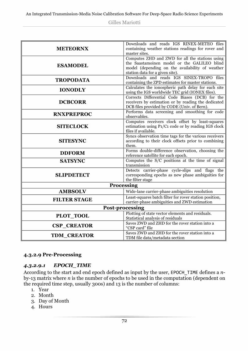
An Integrated Transmission-Media Noise Calibration Software For Deep-Space Radio Science Experiments
Gilles Mariotti
72
METEORNX Downloads and reads IGS RINEX-METEO files containing weather stations readings for rover and master sites.
ESAMODEL
Computes ZHD and ZWD for all the stations using the Saastamoinen model or the GALILEO blind model (depending on the availability of weather station data for a given site).
TROPODATA Downloads and reads IGS SINEX-TROPO files containing the ZPD estimates for master stations.
IONODLY Calculates the ionospheric path delay for each site using the IGS worldwide TEC grid (IONEX files).
DCBCORR Corrects Differential Code Biases (DCB) for the receivers by estimation or by reading the dedicated DCB files provided by CODE (Univ. of Bern).
RNXPREPROC Performs data screening and smoothing for code observables.
SITECLOCK Computes receivers clock offset by least-squares estimation using P1/C1 code or by reading IGS clock files if available.
SITESYNC Syncs observation time tags for the various receivers according to their clock offsets prior to combining them.
DDFORM Forms double-difference observation, choosing the reference satellite for each epoch.
SATSYNC Computes the S/C positions at the time of signal transmission
SLIPDETECT Detects carrier-phase cycle-slips and flags the corresponding epochs as new phase ambiguities for the filter stage
Processing
AMBSOLV Wide-lane carrier-phase ambiguities resolution
FILTER STAGE Least-squares batch filter for rover station position, carrier-phase ambiguities and ZWD estimation
Post-processing
PLOT_TOOL Plotting of state vector elements and residuals. Statistical analysis of residuals
CSP_CREATOR Saves ZWD and ZHD for the rover station into a “CSP card” file
TDM_CREATOR Saves ZWD and ZHD for the rover station into a TDM file data/metadata section
4.3.2.9 Pre-Processing
4.3.2.9.1 EPOCH_TIME
According to the start and end epoch defined as input by the user, EPOCH_TIME defines a n-by-13 matrix where n is the number of epochs to be used in the computation (dependent on the required time step, usually 300s) and 13 is the number of columns:
1. Year 2. Month 3. Day of Month 4. Hours

An Integrated Transmission-Media Noise Calibration Software For Deep-Space Radio Science Experiments
Gilles Mariotti
73
5. Minutes 6. Seconds 7. Day Of Year (DOY) 8. GPS Week12 9. Day of current GPS week (numeral) 10. Seconds from start of week 11. Julian Date (with decimals) 12. Total seconds from start epoch 13. Seconds of current day
4.3.2.9.2 SATEPHM
Precise GPS and GLONASS orbits in the ECEF (Earth Centered Earth Fixed) frame of reference are provided by IGS ( Section 4.3.2.6) using the SP3 file format. SATEPHM reads the SP3 final orbits file for each day needed in the campaign and stores positions and clocks values into the workspace. SP3 data are provided with a 15-minute time step so an interpolation could be needed to meet the user-required time step. The interpolation is performed using an 18-node centered Neville polynomial fit [42], providing interpolation precision at the mm level. For the first and last epochs of the day, SP3’s for the previous and following days are downloaded in order to maintain the symmetric interpolation, if available. Otherwise, a non-symmetric interpolation is performed.
Figure 4.35 Visual example of a GPS orbit in ECEF coordinates
4.3.2.9.3 RNXNAVDATA/RELDLY
GPS broadcast ephemerides contained in the navigation message (Section 4.3.2.2) are used to compute the correction for the relativistic error affecting the pseudoranges. The relativistic orbit perturbation consists of two separated effects: the Shapiro effect, acting on the signals themselves, and the Sagnac effect, a relativistic clock drift due to orbit eccentricity [43]. Thus, the correction to the Shapiro effect is applied to phase and code
12 Number of weeks passed since 00:00:00 UTC on Sunday, 6th January 1980

An Integrated Transmission-Media Noise Calibration Software For Deep-Space Radio Science Experiments
Gilles Mariotti
74
observables, while the clock drift correction is applied to the satellite clock offset (or again to observables by multiplying it by the speed of light c). The Shapiro effect can be represented by the Holdridge model [44]:
−+++
=∆j
iij
jii
j
rel c ρρρρρρµρ ln
22
, (4.42)
where ρj and ρi are the geocentric positions of satellite j and station i, respectively, while ρj
i is their mutual distance. On the other hand, the Sagnac relativistic clock drift depends on the GNSS orbital parameters [43]:
.sin22
constEeac
trel +=∆ µ (4.43)
Where µ is the Earth’s gravitational constant; a, e and E are the orbit’s semimajor axis, eccentricity and eccentric anomaly, respectively. An alternative representation of this relation, expressed in terms of satellite position and velocity, is also widely used [38]. Finally, the constant term in the sum cannot be decoupled from the clock offset dtj
itself (Section 4.3.2.4). These parameters are broadcast by GPS space vehicles within the navigation message, that is also stored by IGS servers in a daily RINEX file named brdcddd0.yyn: this file is a merge of the individual site navigation files into one, non-redundant file that can be utilized by users instead of the many individual navigation files.
Table 4.6 GPS broadcast orbital parameters
Mo Mean anomaly at reference time ∆n Mean motion difference from computed value e Eccentricity
a Square root of the semi-major axis
Figure 4.36 GPS orbital parameters
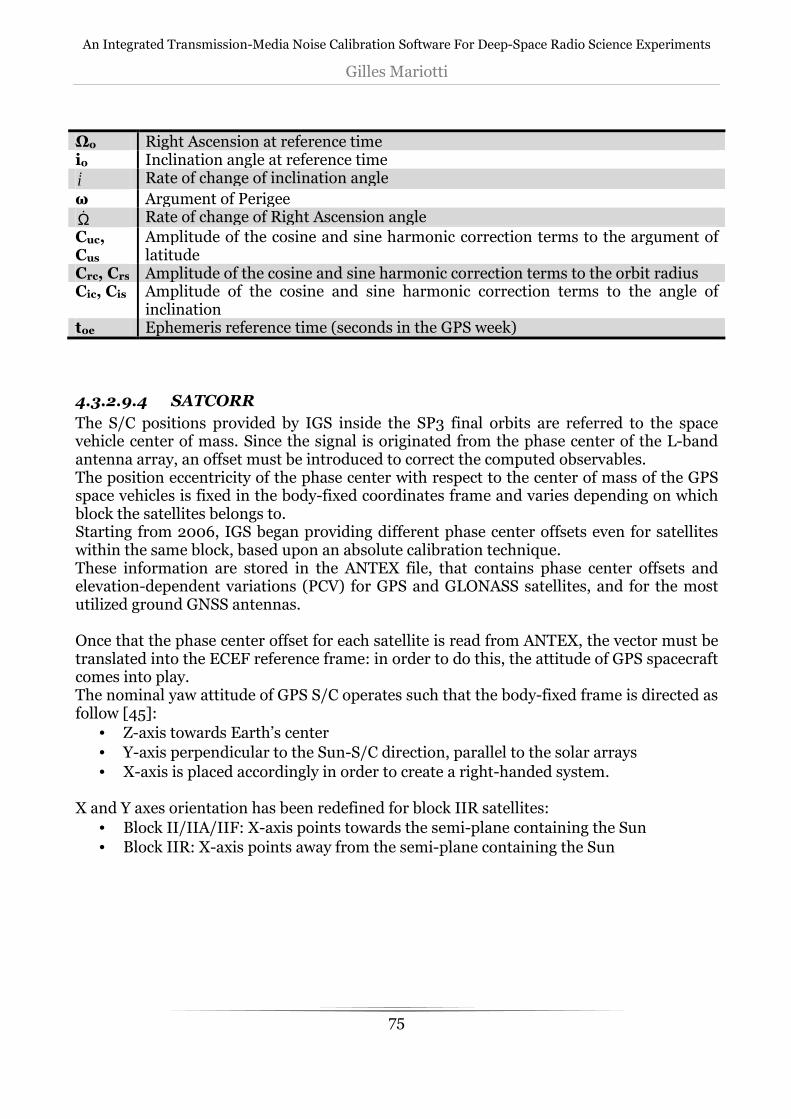
An Integrated Transmission-Media Noise Calibration Software For Deep-Space Radio Science Experiments
Gilles Mariotti
75
Ωo Right Ascension at reference time io Inclination angle at reference time
i& Rate of change of inclination angle
ω Argument of Perigee
Ω& Rate of change of Right Ascension angle
Cuc, Cus
Amplitude of the cosine and sine harmonic correction terms to the argument of latitude
Crc, Crs Amplitude of the cosine and sine harmonic correction terms to the orbit radius Cic, Cis Amplitude of the cosine and sine harmonic correction terms to the angle of
inclination toe Ephemeris reference time (seconds in the GPS week)
4.3.2.9.4 SATCORR
The S/C positions provided by IGS inside the SP3 final orbits are referred to the space vehicle center of mass. Since the signal is originated from the phase center of the L-band antenna array, an offset must be introduced to correct the computed observables. The position eccentricity of the phase center with respect to the center of mass of the GPS space vehicles is fixed in the body-fixed coordinates frame and varies depending on which block the satellites belongs to. Starting from 2006, IGS began providing different phase center offsets even for satellites within the same block, based upon an absolute calibration technique. These information are stored in the ANTEX file, that contains phase center offsets and elevation-dependent variations (PCV) for GPS and GLONASS satellites, and for the most utilized ground GNSS antennas. Once that the phase center offset for each satellite is read from ANTEX, the vector must be translated into the ECEF reference frame: in order to do this, the attitude of GPS spacecraft comes into play. The nominal yaw attitude of GPS S/C operates such that the body-fixed frame is directed as follow [45]:
• Z-axis towards Earth’s center
• Y-axis perpendicular to the Sun-S/C direction, parallel to the solar arrays
• X-axis is placed accordingly in order to create a right-handed system. X and Y axes orientation has been redefined for block IIR satellites:
• Block II/IIA/IIF: X-axis points towards the semi-plane containing the Sun
• Block IIR: X-axis points away from the semi-plane containing the Sun

An Integrated Transmission-Media Noise Calibration Software For Deep-Space Radio Science Experiments
Gilles Mariotti
76
Hence, the unit vectors relating the body-fixed frame to the ECEF frame can be computed only after knowing the exact Sun position in the ECEF frame: to this extent, SATCORR makes use of NAIF SPICE kernels provided by JPL [46]. Once that the position Xsun is known, the ∆Xsat=∆xsat, ∆ysat, ∆zsat read from ANTEX is converted into ECEF coordinates by:
satzsatzsatxECEFsat zeyexeX ∆⋅+∆⋅+∆⋅=∆ ˆˆˆ (4.44)
where the unit vectors describing the change of coordinates system are:
×=
∆×∆×±=
−=
zyx
sunsatz
sunsatz
y
sat
satz
eee
Xe
Xee
X
Xe
ˆˆˆ
ˆ
ˆˆ
ˆ
,
(4.45)
with ECEF
satECEFsun
sunsat XXX −=∆ (4.46)
To be noted that the relation for t must be given a sign according to the model of the
satellite that is being corrected: negative for Block-II/IIA/IIF, positive for Block-IIR. Finally, the corrected ECEF position for each space vehicle will be: ECEF
satECEFsatsat XXX ∆+=*
(4.47)
Figure 4.37 GPS Block-IIR yaw attitude model

An Integrated Transmission-Media Noise Calibration Software For Deep-Space Radio Science Experiments
Gilles Mariotti
77
With this correction, the S/C positions are now referred to the antenna array phase center.
4.3.2.9.5 SITEDATA
SITEDATA downloads and reads the SINEX files containing precise geocentric positions for sites that are part of the IGS worldwide network. These positions are produced by combining global solutions computed by the IGS analysis centers. The described code uses IGS network stations as master stations for the differential computation, so the information provided by the SINEX files are used to fix the XA values seen in Section 4.3.2.5.2.
4.3.2.9.6 SITECORR
SINEX files contain additional information for the sites, among which there are antenna phase center offsets (redundant with ANTEX data) and antenna eccentricities, i.e. the distance from the Monument Marker (MM) of a site, to which the position is referred, to the Antenna Reference Point (ARP), as seen in Figure 4.38:
PCOs and eccentricities for receivers are usually provided in geocentric Cartesian coordinates X,Y,Z or in topocentric North, East, Up N,E,U. In the second case, translation to geocentric must be computed [47].
Figure 4.38 Points of interest of a GNSS receiver site: MM, ARP, APC [85]

An Integrated Transmission-Media Noise Calibration Software For Deep-Space Radio Science Experiments
Gilles Mariotti
78
SITECORR is also in charge of correcting for several other displacement effects acting on the position of the receiver: solid tides, ocean loading, polar motion. Solid Earth tides are the displacement effects acting upon the shape of the geoid due to the gravitational pull of the Moon and, to a lesser extent, of the Sun. Tidal displacement can be expressed as a spherical harmonics expansion in which the component of order and degree mxn depends upon the Love and Shida numbers hmn and lmn. The major contributions to the tidal displacement are given by degrees 2nd and 3rd , computed by [48]:
• m=n=2 ( ) ( ) ( )[ ]
⋅−⋅+
−⋅=∆ ∑
= ⊕
⊕ XXXXXXlXX
XhX
RX jjj
j
jj
jsolid
ˆ ˆˆˆ ˆˆ32
1ˆˆ3 ˆ 2
2
2
3
23
4
2,
µ
µ (4.48)
• m=n=3 ( ) ( )
( ) ( )[ ]⋅−
−⋅+
+
⋅−⋅=∆ ∑= ⊕
⊕
XXXXXXl
XXXXXhX
RX
jECEFjj
jjj
j
jsolid
ˆ ˆˆˆ 2
3ˆˆ2
15
ˆˆ2
3ˆˆ2
5ˆ
2
3
3
3
3
24
5
3,
µ
µ
(4.49)
where:
• µj = gravitational parameter for the Moon (j = 2) or the Sun (j = 3),
• µ⊕ = gravitational parameter for the Earth,
• Xj = Moon or Sun ECEF position,
• R⊕ = Earth’s equatorial radius,
• X = ground station ECEF position,
• h2 = nominal degree 2 Love number,
• l2 = nominal degree 2 Shida number. A Fortran routine provided by Dennis Milbert13 and based on IERS official software packages is compiled as a MATLAB® MEX function and runs within SITECORR. Also the well-known oceanic tides cause a displacement in the site position, by exerting a pressure onto the shores of emerged lands. For tracking sites near or along coastlines the Oceanic Tide Loading (OTL) effects can cause a displacement up to the cm level in magnitude, while inland stations are affected only by a few millimeters. The main model used by IERS conventions is the FES2004 [49].
13 http://home.comcast.net/~dmilbert/softs/solid.htm

An Integrated Transmission-Media Noise Calibration Software For Deep-Space Radio Science Experiments
Gilles Mariotti
79
The tidal displacement consists of several constituents: diurnal, semi-diurnal and long-period, and each of these have one in-phase and one out-of-phase contribution that are described by the Doodson numbers [50]. The displacement is given by IERS conventions [48] in topocentric U,-E,-N coordinates by: ( )( )∑
=
−+=∆11
1
cosk
ckkkckkNEUOTL utAfX ϕχ (4.50)
where k is the index describing each of the 11 main tides, c cycles through the three coordinates, Ack and φck are a site-dependent amplitude and phase angle of the k-th partial tide. These site-dependent coefficients are distributed by Chalmers University14 using the dedicated .BLQ file format. The described code uses the global FES2004.blq file provided by University of Bern for the Bernese GNSS software [51].
Table 4.7 Doodson Numbers for the 11 main partial tides
Tide f u M2 1.0004 - 0.0373 cos (N) + 0.0002 cos (2N) -2.14° sin (N) S2 1.0 0.0 N2 see M2 see M2
K2 1.0241 + 0.2863 cos (N) + 0.0083 cos (2N) - 0.0015 cos (3N)
-17.74° sin (N) + 0.68° sin (2N) - 0.04° sin (3N)
K1 1.0060 + 0.1150 cos (N) - 0.0088 cos (2N) + 0.0006 cos (3N)
-8.86° sin (N) + 0.68° sin (2N) - 0.07° sin (3N)
O1 1.0089 + 0.1871 cos (N) - 0.0147 cos (2N) +0.0014 cos (3N)
10.80° sin (N) -1.34° sin (2N) +0.19° sin (3N)
P1 1.0 0.0 Q1 see O1 see O1
Mf 1.0429 + 0.4135 cos (N) - 0.0040 cos (2N) -23.74° sin (N) +2.68° sin (2N) - 0.38° sin (3N)
Mm 1.0000 - 0.1300 cos (N) + 0.0013 cos (2N) 0.0 Ssa 1.0 0.0 The values of fk and uk are the scale factor and the phase offset for each partial tide, and are a function of the lunar node N (Sun contribution is negligible) [50]: I)-0.05295(D-1900)-(Y 32818.19157.259 −=N [deg] (4.51)
where:
• Y : year
14 http://holt.oso.chalmers.se/loading/index.html

An Integrated Transmission-Media Noise Calibration Software For Deep-Space Radio Science Experiments
Gilles Mariotti
80
• D : day of year
• I = int[(Y-1901)/4]. The astronomical argument χk(t) is computed for each tidal component by the official IERS routine ARG2.f15, which source code has been integrated into SITECORR. The last displacement effect corrected by the routine is the tide caused by rotational deformation due to polar motion, that can reach up to a couple of centimeters [48]. The position of the Earth’s mean rotation pole has a secular variation xp, yp, with respect to the ECEF reference frame.
Figure 4.39 Evolution of pole (polhody) and mean pole coordinates (courtesy JPL)
The variation in the Earth’s centrifugal potential due to this motion is described by the difference between the instantaneous position and the running averages px and py− that
describe the mean pole:
( ) [arcsec] 2
1
pp
pp
yym
xxm
−−=
−=
.
(4.52)
The m3 coefficient describing the fractional variation in the rotation rate is neglected due to its small influence.
15 ftp://tai.bipm.org/iers/conv2010/chapter7/

An Integrated Transmission-Media Noise Calibration Software For Deep-Space Radio Science Experiments
Gilles Mariotti
81
Using these differences the displacement of a site on the Earth due to polar displacement is given (in local NEU coordinates) by: ( )[ ]
( )[ ]( )[ ]
[mm]
)sin( )cos( 2 sin33
)cos( )sin( cos 9
)sin( )cos( 2 cos 9
21
21
21
λλθλλθλλθ
mm
mm
mm
U
E
N
X NEU
+−−−+−
=∆∆∆
=∆ (4.53)
where:
• θ: distance from pole (complementary angle to ellipsoidal latitude)
• λ: ellipsoidal longitude The polar position is distributed by IERS and several other associations (e.g. IGS) within the Earth Orientation Parameters (EOP) file16 [52].
4.3.2.9.7 RNXDATA
RNXDATA is the routine in charge of opening and reading observations recorded by GNSS receivers. Each manufacturer uses a proprietary format for its receivers, but a standard interchange file has been defined: the Receiver-INdependent EXchange format (RINEX, see Section 4.3.2.6). The routine automatically downloads observation files for IGS stations from IGS ftp repositories and is capable of reading both version 2.xx and version 3 RINEX files. For non-IGS sites, the code looks for user-provided RINEX’s within a dedicated directory. The code is capable of distinguish the four GNSS constellations (GPS, GLONASS, Beidou, Galileo). For GPS, the output contains (if provided by the file):
• antenna model
• receiver model
• site approximate position
• site marker name (four-digit callsign)
• antenna eccentricity wrt monument marker (see Figure 4.38)
• antenna PCO (see Figure 4.38)
• code pseudoranges in meters: C1, P1 (depending on receiver model, see 4.3.2.9.16), P2
• carrier-phase pseudoranges in cycles: L1, L2
• a matrix containing 1’s and 0’s indicating which satellites are in view from the site at a given observation epoch.
4.3.2.9.8 ECLIPSE
GPS yaw attitude control law is programmed in a way that causes the solar arrays of each spacecraft to face the Sun in every circumstance. Given the GPS orbital planes, satellites happen to be eclipsed by the Earth in a portion of their orbit twice per year, for about seven weeks [53]. While shadowed by the Earth, the satellite attitude control system is driven solely by the noise of the Sun sensors, issuing unpredictable commands to the reaction wheels.
16 http://www.iers.org/nn_10398/IERS/EN/Science/EarthRotation/EOP.html

An Integrated Transmission-Media Noise Calibration Software For Deep-Space Radio Science Experiments
Gilles Mariotti
82
Depending on the satellite Block model, different behaviors have been observed [54][45], but it can be said that the yaw attitude of GPS satellites is essentially random during eclipse periods and for up to 30 minutes past exiting from shadow. Furthermore, the non-gravitational force due to solar radiation pressure vanishes, and given the difficulty in modeling this type of force, the orbit determination precision is degraded. As a consequence, the orbit determination during eclipse periods may be considerably degraded and the removal of satellites under such conditions can improve the high-precision positioning results.
In order to assess which (if any) satellites are in a shadow condition, a simple model considering the Earth’s shadow as a cylinder can be used (although a more detailed eclipse model [55] [36], considering also penumbra sections, is used by ECLIPSE). A satellite with a given Φ angle from the Sun at the geocenter is in eclipse if both these inequalities apply at once:
( )
( )
<−⋅
<⋅⋅
=
⊕RX
XX
XX
ECEFsat
ECEFsun
ECEFsat
ECEFsun
ECEFsat
φ
φ
2cos1
0cos
(4.54)
4.3.2.9.9 PCVCORR
In Section 4.3.2.9.6 the PCO of an antenna with respect to its ARP is described. Every antenna however is affected also by an anisotropy in the position of the phase center, that changes depending on the direction of the signal wave front, during both reception (ground site) or transmission (satellites). These elevation and azimuth dependent displacements are called PCV’s (Phase Center Variations), and are different for each antenna model (even for each antenna-radome combination) [56].
Figure 4.40 Cylindrical shadow model
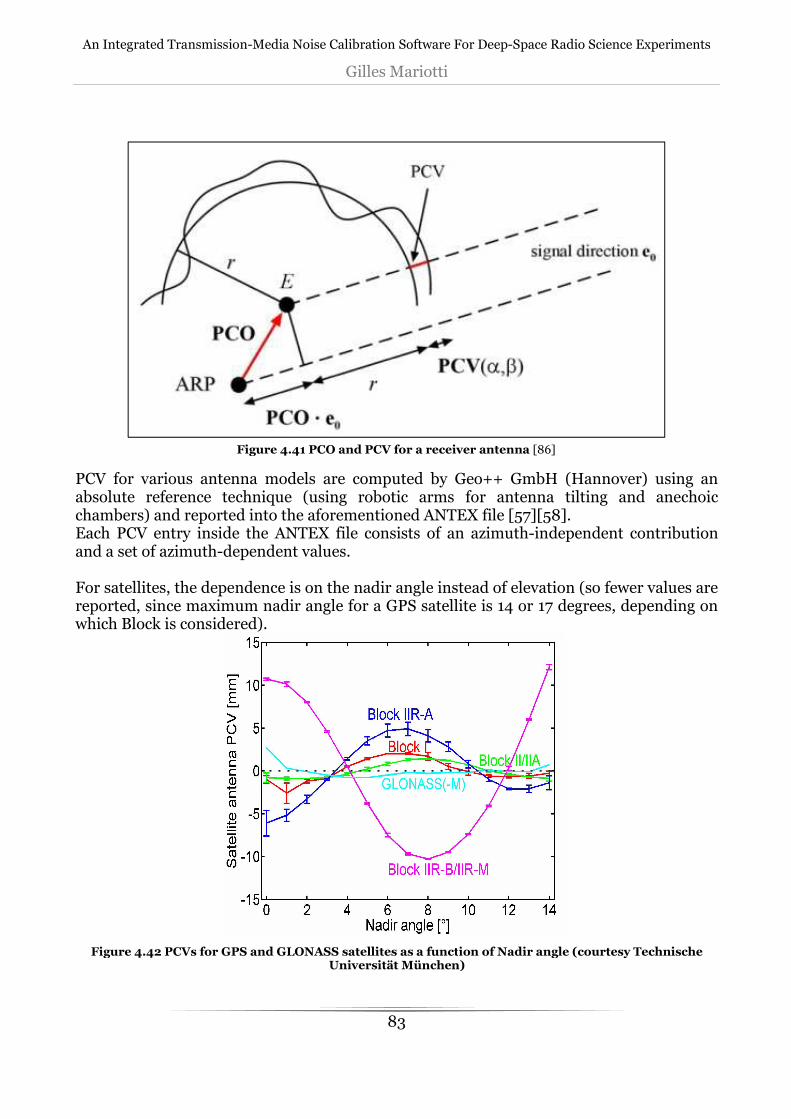
An Integrated Transmission-Media Noise Calibration Software For Deep-Space Radio Science Experiments
Gilles Mariotti
83
PCV for various antenna models are computed by Geo++ GmbH (Hannover) using an absolute reference technique (using robotic arms for antenna tilting and anechoic chambers) and reported into the aforementioned ANTEX file [57][58]. Each PCV entry inside the ANTEX file consists of an azimuth-independent contribution and a set of azimuth-dependent values. For satellites, the dependence is on the nadir angle instead of elevation (so fewer values are reported, since maximum nadir angle for a GPS satellite is 14 or 17 degrees, depending on which Block is considered).
Figure 4.42 PCVs for GPS and GLONASS satellites as a function of Nadir angle (courtesy Technische Universität München)
Figure 4.41 PCO and PCV for a receiver antenna [86]

An Integrated Transmission-Media Noise Calibration Software For Deep-Space Radio Science Experiments
Gilles Mariotti
84
Once read from the ANTEX file, PCV corrections for both receiver and satellite antennas are applied to code and phase observables for each satellite-receiver pair.
4.3.2.9.10 WINDUP
Due to the Right-Hand Circular Polarization (RHCP) of GPS signals, an error is introduced into the carrier-phase measurements due to satellite yaw rotation. Given the necessity for the spacecraft to point the solar arrays towards the Sun, the effective dipole of the antenna array spins around the yaw axis, thus adding or subtracting (depending on the spin direction) a fractional number of wavelengths (phase cycles) to the carrier. This effect is called phase wind-up can reach up to 4 cm in double-difference observations with very long baselines [38]. It goes without saying that code measurements are not affected. The wind-up effect is the sum of an integer number N of cycles and a fractional part: δϕπ +=∆Φ N2 (4.55)
The integer part can be neglected since it adds directly into the ambiguity parameter for that satellite/receiver pair, estimated later, so only the fractional part δφ is considered.
In order to compute the correction to this effect, the effective dipole vectors for both the transmitting and receiving antenna, along with the line of sight vector, must be computed.
Figure 4.43 Layout of dipole orientation to compute the phase wind-up effect

An Integrated Transmission-Media Noise Calibration Software For Deep-Space Radio Science Experiments
Gilles Mariotti
85
If we call Kvthe receiver antenna effective dipole, Kv′the satellite’s effective dipole and ρ the line of sight unit vector, we have that the wind-up correction is computed by [59]:
( )[ ]
( )( ) 'ˆˆˆˆˆ'ˆ'ˆ
ˆˆˆˆˆˆˆ
'
'arccos'ˆ
yxxd
yxxd
dd
ddddsign
×−⋅−=
×+⋅−=
⋅⋅⋅×⋅=∆
ρρρ
ρρρ
ρϕ
(4.56)
The effective dipoles in Eq. (4.56) are computed starting from the local body axes wx′,Nx′ for the satellite, while for the receiving antenna wx,Nx, the local topocentric northward and eastward directions, respectively (the directions are chosen so that the y component of the effective crossed dipole is delayed in phase by 90° with respect to x).
4.3.2.9.11 METEORNX
As mentioned in Section 4.3.1, the two components of tropospheric path delay are split and only the ZWD is estimated by the filter. The ZHD is computed either by the GALILEO Blind model or the Saastamoinen by subroutine ESAMODEL (Section 4.3.2.9.12), depending on the availability of weather station data for master and rover sites. These data are provided once again by IGS for a selected number of stations using the METEO version of the RINEX standard (*.yym) . METEORNX checks the availability of the file in the IGS ftp repositories, downloads them and stores the information into the workspace.
4.3.2.9.12 ESAMODEL
The well-behaved nature of the path delay hydrostatic component allows a precise estimation of its value by a simple model based on ground meteorological measurements. ESAMODEL utilizes the Saastamoinen model reported in Eq. (4.29) for the ZHD and also computes the first guess for the rover ZWD using Eq. (4.30). The namesake of the subroutine comes from the alternative model available and selectable by the user when invoking the function. This path delay model [34], based on numerical weather models and the ECMWF ERA 15 dataset, has been generated in the GALILEO framework in order to replace the MOPS model used by the GPS WAAS system (Wide Area Augmentation System) [33]. In this model, called TropGrid, the ZHD is calculated once again with Eq. (4.29), while the ZWD is computed by:
[m] 1
10 036
+= −
λe
g
R
T
kZWD
m
d
M
(4.57)
with:
• k3 : refraction coefficient from Eq. (3.19), set at 370100 ± 1200 [K2 hPa-1]
• Rd : dry air gas constant, 287.054 [J Kg-1 K-1]
• gm : weighted mean gravity acceleration [m s-2], denominator of Eq. (4.29)

An Integrated Transmission-Media Noise Calibration Software For Deep-Space Radio Science Experiments
Gilles Mariotti
86
• λ : water vapor pressure decrease factor
• TM : mean temperature [K]
( )
+−≅= ∫∫
∞∞
m
dT
hh
M g
RTdh
T
edh
T
eT
11 : 02
00λβ
(4.58)
• βT : air temperature lapse rate [K m-1]. If surface meteorological data are not available for a certain site, the values needed by the TropoGrid equations (4.29) and (4.57) are provided by the Galileo Blind Model. Using this statistical model, we can compute any atmospheric quantity Xi = (p, TM, e, λ) by describing it with a seasonal and a diurnal component: ( ) ( )
( ) ( ) ( ) ( )[ ]
−⋅−=
−⋅−=
DbHHDbDXHHDX
aDaaDX
iiii
iiii
32
321
24
2cos,
25.365
2cos
π
π
,
(4.59)
• i : index indicating which atmospheric quantity is calculated
• D : day of year
• HH: hour of day; coefficients provided by model weather maps:
• a1i : annual average of the parameter
• a2i : seasonal fluctuation of the parameter
• a3i : day of minimum value of the parameter
• b2i : daily fluctuation, calculated by linear interpolation between the average values of daily fluctuations during nearest months to day D
• b3i : hour of the day at which the minimum value occurs, by linear interpolation between the average values of daily fluctuations during nearest months to day D.
4.3.2.9.13 TROPODATA
As reported in Section 4.3.2.5.2, this ZWD estimation code uses IGS sites as master stations, considering the precise ZWD information for these reference sites as available. The needed data are once again downloaded from IGS ftp servers, stored in TROPO-SINEX files. This subroutine reads and imports into the workspace the path delay information contained in the file. By standard, the minimum information contained in a TROPO-SINEX file is the total Zenith path delay (ZPD) for a site and its standard deviation. The ZWD is then computed using the site ZHD provided by ESAMODEL: ZWD=ZPD-ZHD.
4.3.2.9.14 IONODLY
The ionospheric delay is one of the major noise contribution to pseudoranges for L-band ranging systems like GNSS constellations (Section 4.3.2.4). Its effect can reach 2-3 meters at zenith and up to 50 meters for low-elevation measurements.
An Integrated Transmission-Media Noise Calibration Software For Deep-Space Radio Science Experiments
Gilles Mariotti
87
It has a frequency-dependent (dispersive) behavior and causes at once a phase delay and a group advance [39]: ( )
( )32,
32,
3.401
3.401
−
−
++=
+−=
fOf
nn
fOf
nn
egrion
ephion
(4.60)
• ne : electron density along propagation path. By integrating ne along the geometric signal path s0 we obtain the Total Electron Content (TEC) of the column of atmosphere crossed by the signal, and we can convert the refractive indexes of the medium into phase and group delays:
22
221
1
22
221
1
0
3.40, 3.40
3.40, 3.40
LP
LP
L
L
L
L
e
f
TECI
f
TECI
f
TECI
f
TECI
dsnTEC
+=+=
−=−=
= ∫
(4.61)
A basic removal of ionospheric effects (about 50% of the delay) can be done on single-frequency observations thanks to the Klobuchar model [60], given the user approximate geodetic latitude φ and longitude λ, elevation ε and azimuth α angles with respect to the observed satellite and the Klobuchar coefficients broadcast by the navigation message [40]. For a more accurate removal of this delay source, the user can exploit a global TEC map called GIM (Global Ionosphere Map), computed by CODE (Center for Orbit Determination in Europe, Bern). These GIMs are distributed daily using the IONEX file standard and contain a 73-by-73-by-13 space-time grid with a 2.5° resolution in latitude, 5° resolution in longitude and a 2-h time span. TEC values contained in the file are given at a standard altitude that is the mean ionosphere height. By interpolating this grid it is possible to compute the VTEC (Vertical TEC) for any site on Earth at a given time. The slant value of TEC must then be retrieved by applying a mapping function (similarly to the tropospheric case). Both the interpolation of the VTEC maps and the mapping function computation must be conducted with respect to the so-called Ionospheric Point (IP). If we collapse the whole ionosphere (spread on an altitude range between 50 and 1000 km) into a single thin layer placed at about 300-500 km, the IP represents the point where the RF beam instantaneously crosses the ionospheric layer, and is affected by the whole ionospheric delay at once [39].

An Integrated Transmission-Media Noise Calibration Software For Deep-Space Radio Science Experiments
Gilles Mariotti
88
Figure 4.44 Ionospheric Point
The mapping function can be as simple as sec(zip), using the zenith angle computed at the ionospheric point, but IONODLY implements instead the geometric and ellipsoidal mapping functions described by Xu [61]. IP zenith angle can be obtained simply by:
( )
++
=⊕
⊕ zhR
hRz
mip sinasin 0 (4.62)
while, for interpolation of IONEX maps, the latitude and longitude of IP must be computed [60]:
( )( )
( )ipip
ip
ϕαψλλ
αψϕϕε
ψ
cos
cos
cos
022.011.0
0137.0
+=
+=
−+
=
(4.63)
Note: ψ is expressed in semicircles (and the elevation value used to calculate it must be provided in semicircles too). Once that the IP coordinates are available, the VTEC value is retrieved by picking the four nearest nodes in the IONEX grid, and performing a bivariate interpolation based on the spherical distance of each grid node from the IP, weighted by 1.5 [36]. The interpolation in time is conducted with a 10-point polynomial.

An Integrated Transmission-Media Noise Calibration Software For Deep-Space Radio Science Experiments
Gilles Mariotti
89
Also the second order contribution ( 3−∝ f , mm-level in pseudorange) of ionospheric delay
can be computed thanks to the Bassiri and Hajj model [62].
4.3.2.9.14.1 Ionofree Linear Combination
The model just reported for computing the ionospheric delay is used when some degree of calibration is needed for uncombined code and phase data, like DCB estimation or satellite light-time solution. During the processing stage of the code, the ionospheric delay is more precisely removed (1st-degree effect is removed completely, but 2nd order remains) by combining the carrier-phase observables L1 and L2 into a third observable LC (often called L3).
( ) ( )
1.546- 546.2
212 1 322
21
22
22
21
21
≅≅
−−
−=+==
βα
βα Lff
fL
ff
fLLLLC
LL
L
LL
L
.
(4.64)
The same combination is also available for code measurements (PC, P3). Starting from Equations (4.33) and (4.61) one can see that this combination erases the ionospheric contribution:
( ) ( ) ( ) ( ) 0122
21
22
21
22
22
21
21
222
21
22
122
21
21 =
−−
−=
−−
−= L
L
L
LL
L
LL
LL
LL
LL
LL
LLC I
f
f
ff
f
ff
fI
ff
fI
ff
fI
.
(4.65)
A major drawback of this combination is posed by the ambiguity term (Section 4.3.2.10.1), because it cannot be expressed in the form λLC·BLC, and its estimation (and cycle-slip detection) becomes more difficult due to the very small (virtual) wavelength of the new observable LC, that is then referred to also as narrow-lane:
cmff
c
LLNLLC 7.10
21
=+
== λλ.
(4.66)
The resulting ambiguity term is:
( ) ( ) ( )( )221122
21
2222
21
22
1122
21
21
LLLLLL
LLLL
LLL
LL
LLC BfBf
ff
cB
ff
fB
ff
fB +
−=
−−
−= λλ (4.67)
given the so-called wide-lane ambiguity (Section 4.3.2.10.1):
21 LLWL BBB −= (4.68)
we have that the ionofree ambiguity term is a linear combination of two integer values [51]:
( )( ) ( ) NLB
LLCWLLL
LLLLL
LLLC BB
ff
fcBfBf
ff
cB 12
221
222112
221
λ−−
=+−
= (4.69)
The BL1 term is at the same manner called narrow-lane ambiguity.

An Integrated Transmission-Media Noise Calibration Software For Deep-Space Radio Science Experiments
Gilles Mariotti
90
Eq. (4.69) allows the code to deal separately with the two ambiguity terms: the wide-lane ambiguity is estimated before the filter using the Melbourne-Wübbena combination (Sections 4.3.2.9.20, 4.3.2.10.1)[63], while the narrow-lane term is estimated by the least-squares filter.
4.3.2.9.15 RNXPREPROC
Code measurements are very noisy compared to carrier-phase ones (Section 4.3.2.4): the ratio between measurement noises for code and carrier phase is about 100 times. Several technique have been introduced to smooth the code data in order to suppress the noise to a certain extent. Code smoothing is performed by means of a Hatch Filter [39][64]: at a given time tag t the smoothed code for a certain satellite is computed by correcting the original measurement P(t) using the trend of the carrier-phase data L on the same frequency. ( ) ( )[ ])1()()( 1)()( −−+−+= tLtLtPwtPwtP pPsmooth (4.70)
where wP is the width of the smoothing window (usually set to 0.8), that acts as a relative weight for the original code and the smoothed code. For initialization at t=1, wP is set to 1. The subroutine performs also integrity checks on the RINEX file, detecting and removing spot data (single observations isolated in time) and unpaired observations (code values present at a given time without the relative phase measurement, and vice versa).
4.3.2.9.16 DCBCORR
Instrumental biases are present in C1, P1, P2 observables. These delays are not accessible and cause errors when using combinations of code measurements, and are called Differential Code Biases (DCB). The two major effects considered are:
• KP1-P2=KP1 – KP2
• KP1-C1= KP1 – KC1 By convention, IGS precise satellite clock corrections have to be consistent to the P1 and P2 observables. This implies that each clock correction contains the ionosphere-free linear combination of (unknown) KP1 and KP2 biases: 2.546 KP1 − 1.546 KP2. The same applies to broadcast ephemerides. DCB correction comes into play whenever code measurements are used in combination to IGS products and with each other. In the described S/W, DCB correction is mandated by the operations performed in AMBSOLV (Section 4.3.2.10.1), that uses the Melbourne-Wübbena combination, and SITECLOCK (Section 4.3.2.9.17) where the site clock offset is estimated using code measurements. The tracking data retrieved from C1/X2 and C1/P2 receiver classes (see Section 4.3.2.3 for A/S-overcoming techniques) must be corrected in order to achieve full consistency with P1/P2 data, or precise satellite clock information.
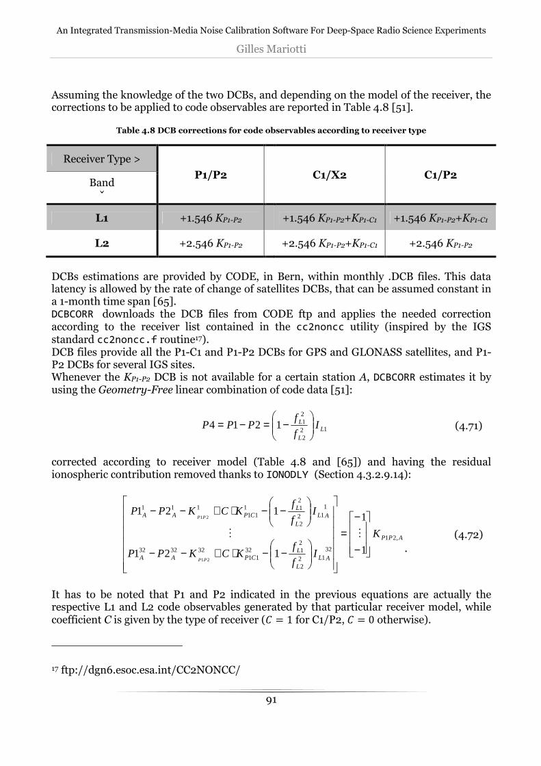
An Integrated Transmission-Media Noise Calibration Software For Deep-Space Radio Science Experiments
Gilles Mariotti
91
Assuming the knowledge of the two DCBs, and depending on the model of the receiver, the corrections to be applied to code observables are reported in Table 4.8 [51].
Table 4.8 DCB corrections for code observables according to receiver type
Receiver Type >
P1/P2 C1/X2 C1/P2 Band
ˇ
L1 +1.546 KP1-P2 +1.546 KP1-P2+KP1-C1 +1.546 KP1-P2+KP1-C1
L2 +2.546 KP1-P2 +2.546 KP1-P2+KP1-C1 +2.546 KP1-P2
DCBs estimations are provided by CODE, in Bern, within monthly .DCB files. This data latency is allowed by the rate of change of satellites DCBs, that can be assumed constant in a 1-month time span [65]. DCBCORR downloads the DCB files from CODE ftp and applies the needed correction according to the receiver list contained in the cc2noncc utility (inspired by the IGS standard cc2noncc.f routine17). DCB files provide all the P1-C1 and P1-P2 DCBs for GPS and GLONASS satellites, and P1-P2 DCBs for several IGS sites. Whenever the KP1-P2 DCB is not available for a certain station A, DCBCORR estimates it by using the Geometry-Free linear combination of code data [51]:
122
21 1214 L
L
L If
fPPP
−=−= (4.71)
corrected according to receiver model (Table 4.8 and [65]) and having the residual ionospheric contribution removed thanks to IONODLY (Section 4.3.2.9.14):
APP
AL
L
LCPAA
AL
L
LCPAA
K
If
fKCKPP
If
fKCKPP
PP
PP
,21
3212
2
2132
11323232
112
2
211
11111
1
1
121
121
21
21
−
−=
−−⋅+−−
−−⋅+−−
MM
.
(4.72)
It has to be noted that P1 and P2 indicated in the previous equations are actually the respective L1 and L2 code observables generated by that particular receiver model, while coefficient C is given by the type of receiver (y = 1 for C1/P2, y = 0 otherwise).
17 ftp://dgn6.esoc.esa.int/CC2NONCC/

An Integrated Transmission-Media Noise Calibration Software For Deep-Space Radio Science Experiments
Gilles Mariotti
92
4.3.2.9.17 SITECLOCK
Receiver clock offset is the second most massive contribution to the pseudorange after geometric range itself. It can reach up to 300 km for low-end oscillators and is usually on the meter level for geodetic-grade GNSS receivers. Although both satellites and receivers clock offsets are canceled within double difference observables, the knowledge of this quantity (with a 1-µsec precision) is required in order to synchronize the time tags of the different receivers prior to the double difference combination (see Section 4.3.2.9.18). Once again, clock offsets for a large number of IGS stations have been estimated by the analysis centers and are publicly available to download (RINEX-CLOCK files, see Section 4.3.2.6). For stations not covered by the IGS RINEX-CLOCK files, the clock offset is estimated using a least-squares filter run on ionofree code observables PC (Section 4.3.2.9.14.1). Recalling the point position system Eq. (4.36), we can compile for each epoch t (for in-view satellites i, .., w) the equation set:
43421
M
M
444444 3444444 21L
L
L
L
M
M
444444 3444444 21
M
M
δ
AW t
−=
−−−−
−−−−
)(
)(
)1(
0
0
0
0
0
0
0
0
0
0
0
0,
0,
ndt
tdt
dtdZ
dY
dX
c
eee
eee
TcdtPC
TcdtPC
A
A
A
A
A
A
wZA
wYA
wXA
iZA
iYA
iXA
t
wA
wA
wArel
wwA
iA
iA
iArel
iiA
ρδ
ρδ
(4.73)
Since the clock offset is not constant in time, each At must be zero-padded in order to account for all clock offset value in the state vector. The system is initialized with the a-priori state X0 which is used also to linearize the
geometric distanceYq> . Note that the distance must be considered at the time of transmission of the signal, so the light-time solution for the satellite must be computed (Section 4.3.2.9.21). The a-priori clock offset in X0 can be set to 0. We can then create the total equation set by concatenating the vectors and matrices relative to every epoch from first to n-th:

An Integrated Transmission-Media Noise Calibration Software For Deep-Space Radio Science Experiments
Gilles Mariotti
93
δAWδ
A
A
A
W
W
W
n
1
n
1
1 )3()3( 1 xxx nnmm ++=→
=
321
M
321
M (4.74)
If the condition number of matrix A is a cause for concern, the speed of light c can be replaced by 1, and the clock offset can be estimated as a distance (c·dtA). We then introduce the weight matrix P:
=
)(
)(
)1(
0
0
nw
tw
w
k
w
i
O
O
P (4.75)
The weight for each satellite in view at a given epoch depends on the elevation of satellite i over the site A and is given by: [ ] [ ])(tan)()( 2212 tttw i
APCii εσσ ⋅== −−
(4.76)
where σPC is the a-priori noise of the P-code ionofree combination (1 meter: 0.3 meters of nominal P-code precision multiplied by 3 due to the combination of uncorrelated measurement noises). The ordering of the diagonal in matrix P is:
1. weight for each in-view satellites at epoch (a Pt matrix if we follow the notation) 2. cycle through epochs.
Now we can compute the normal matrices and solve for δ using a least squares algorithm [61][59][38]:
Table 4.9 Least-squares adjustment model
OBSERVATION MODEL AXW =
NORMAL MATRICES PWAb
PAANT
T
==
COFACTOR MATRIX 1NQ −=
STATE VECTOR CORRECTION b Qδ =
NEW STATE VECTOR δXX 0 +=

An Integrated Transmission-Media Noise Calibration Software For Deep-Space Radio Science Experiments
Gilles Mariotti
94
RESIDUALS AXWV −=
VARIANCE OF UNIT WEIGHT )3(
20 +−
=nm
PVV T
σ
A-POSTERIORI COVARIANCE OF STATE Q 20σ
The solution is then reiterated by replacing the state vector X0=X, re-computing W and b, and the cofactor matrix z = hEz. Convergence is reached when hE = 1 (within a certain tolerance). The computation of δ is performed using the Cholesky decomposition [42].
4.3.2.9.18 SITESYNC
When combining measurements provided by different receivers, the time tags of the various observations must be synchronized in order to operate with homogenous data. Given the true GPS time of signal receipt tr, the receiver will tag that observation with an epoch t’r = tr + dtA. This translates into a pseudorange error δsync that is driven by the satellite radial velocity as seen from the site A:
AiA
isyncA dtρδ &−=, (4.77)
Given the maximum reachable radial velocity of 900 m/s, having the clock offset of the receiver known with a precision of 1 µsec causes the magnitude of this pseudorange error to drop below 1 mm [51][36]. The correction (4.77) is applied to all observables for each station in the chosen network.
4.3.2.9.19 DDFORM
DDFORM performs the double-difference operation onto the observation vectors (Section 4.3.2.5.2). The reference satellite is chosen at any epoch as the one with highest elevation above the rover station. However, the reference satellite doesn’t change as soon as another satellite becomes the highest in the sky, but only when the previous reference sets below an user-defined threshold. This helps maintaining the same reference satellite for a longer interval. The reference satellite is the same for all baselines: if a satellite for a certain rover-master baseline is chosen as reference but is not in view for another baseline, that satellite is discarded and the reference status is given to the next highest in view, and so on. The double–difference observables are marked with ∇∆ and are computed as specified in Eq. (4.38):
• Single differences: pseudoranges received by stations A and B from satellite j are differenced.

An Integrated Transmission-Media Noise Calibration Software For Deep-Space Radio Science Experiments
Gilles Mariotti
95
( )( )j
BjA
jAB
jB
jA
jAB
LLL
PPP
−=∆
−=∆ (4.78)
• Double differences: the single-difference pseudorange relative to satellite j is subtracted from the single-differenced pseudorange relative to satellite i.
( ) ( )
( ) ( )jB
jA
iB
iA
ijAB
jB
jA
iB
iA
ijAB
LLLLL
PPPPP
−−−=∆∇
−−−=∆∇ (4.38)
Among the possible satellite combinations that can be used to construct double-differenced observation vectors, the ijl scheme reported in [36] has been chosen.
4.3.2.9.20 SLIPDETECT
Following a loss-of-lock, on resumption of tracking to the satellite, the accurate fractional part of the carrier phase can be measured again, while the integer part B (Eq. (4.32)) will no longer provide the correction to the fractional phase measurement that yields the true satellite-receiver range, because the receiver has lost count of the integer cycles traveled by the satellite during the blind period. So the integer phase becomes unknown again, as at the beginning of tracking. When screening the carrier-phase observable, one can see a characteristic “jump” in the data after a loss-of-lock and re-acquisition of the signal. This jump is referred to as cycle slip. Cycle-slip detection and repair plays a major role in precise carrier-phase data processing since undetected cycle slips can severely bias the observables (e.g. a 5λ cycle slip introduces an error of about 1 meter in the computation).

An Integrated Transmission-Media Noise Calibration Software For Deep-Space Radio Science Experiments
Gilles Mariotti
96
Figure 4.45 Example of carrier-phase cycle clip (from Navipedia)
In the present S/W the cycle slip detection is conducted on the double-difference observables. The detected cycle-slip are not repaired (i.e. the observable is not corrected with the computed slip amount), but instead a flag is activated, telling the filter to add and initialize a different phase ambiguity parameter in the state vector (Section 4.3.2.10.2). Cycle-slip detection is performed by running two tests:
1. Triple-difference observables 2. Melbourne-Wübbena combination of double-difference observables.
Test 1. consists in comparing the time-derivative of double-difference carrier-phase data (triple-difference data): )()1()(δ tLCtLCtLC ij
ABijAB
ijAB ∆∇−+∆∇=∆∇ (4.79)
with triple-difference computed observables. A certain epoch t is flagged as cycle slip if the triple-difference residuals are outside the 1-cycle threshold. Since all the major errors are either corrected by models or canceled by the double differences, we have:
( ) ][ 1 δδ1
δ cycleTLC ijAB
ijAB
c
ijAB >∆∇+∆∇−∆∇ ρ
λ (4.80)

An Integrated Transmission-Media Noise Calibration Software For Deep-Space Radio Science Experiments
Gilles Mariotti
97
The troposphere term is computed using the values generated by TROPODATA or ESAMODEL, while the geometric range is the output of the light-time solution in SATSYNC (Section 4.3.2.9.21). The jump due to the different phase ambiguity terms between two epochs with different reference satellites is disregarded. Test 2. relies on the Melbourne-Wübbena combination, that is a particular code-phase combination that is immune to geometric range, troposphere, ionosphere, and clock drifts [63][66][51], so basically only the ambiguity term remains: ( ) ( )
WLWLLL
ijABL
ijABL
LL
ijABL
ijABLij
AB Bff
PfPf
ff
LfLfMW λ=
+∆∇+∆∇
−−
∆∇−∆∇=∆∇
21
21
21
21 2121
.
(4.81)
This new observable is also called wide-lane because of its virtual wavelength λWL=86 cm. The combination can be computed for both undifferenced and (single-,double-,triple-) differenced data. The cycle-slips detection on MW observables is performed by comparing the value at epoch t to the recursive mean computed using previous epochs. Once again the jump due to reference satellite change is disregarded.
Table 4.10 Algorithm for cycle-slip detection using the Melbourne- Wübbena observable
1. cycle trough epochs 2. isolate epoch period (t0,…,tn) with same reference satellite j
3. cycling through baselines AB, and satellites i, compute ∇∆3|q>r at epochs (t0,…,tn) just retrieved.
4. cycling k=(t0,…,tn), compute recursive mean and variance of MW data:
5. mark epoch k as cycle-slip if
where K is a user-defined threshold (usually 3.5) and m(0) is initialized at λWL/2. 6. reset m(k) and s2(k) within a same reference-satellite period if a cycle slip is
encountered.
( ) ( )
( ) ( ) [ ]k
kmkMWks
k
kks
k
kMWkm
k
kkm
ijAB
ijAB
2
22 )()()1(
1
)()1(
1
−∆∇+−−=
∆∇+−−=
(4.82)
( )1)1()( 2 −⋅≥−−∆∇ ksKkmkMW ijAB
(4.83)
At the end of the routine, a certain data point is marked as cycle slip if any of the two tests (or both) has detected a phase jump.
4.3.2.9.21 SATSYNC/SATPOS_RETRO_SYNC
GNSS space vehicles orbit at roughly 20.2oo km [39], resulting in a signal light-time of about 67 µsec (not counting propagation delays): this means that between the times of

An Integrated Transmission-Media Noise Calibration Software For Deep-Space Radio Science Experiments
Gilles Mariotti
98
signal emission and reception, the spacecraft has traveled a distance of about 200-300 meters. During GNSS surveys then the satellite position at signal transmission time must be
computed in order to retrieve the correct geometric range Yq> . In order to perform this operation (called light-time solution), the code pseudorange is used within a recursive procedure for the computation of signal travel time τ. Recalling Eq. (4.31) we have that the signal travel time is:
( ) ( )iSAR
SR
iA dttdtttt
c−−−=−== ρτ (4.84)
We can define a first guess for Yq> using the code pseudorange corrected for propagation
effects: Yq> ≅ `yq> − q>. The recursive algorithm uses successive calculations of dtA obtained by comparing the signal travel time retrieved from the pseudorange with the one computed with the current satellite position. The steps are reported in Table 4.11:
Table 4.11 Satellite light-time solution algorithm
1. signal travel time from observables
2. geometric range
3. receiver clock offset estimate (note: dti is corrected for the Sagnac Effect, Eq.
(4.43))
4. corrected signal travel time
5. signal transmission time
6. Interpolation of satellite position at signal transmission time Xi(ti) 7. Correction of satellite position due to Earth rotation (S⊕ Earth spin rate)
c
TPC iA
iA −=0τ (4.85)
( ) ( ) ( )222
Ai
Ai
Aii
A ZZYYXX −+−+−=ρ (4.34)
reli
iA
A tdtc
dt ∆++−= ρτ 0 (4.86)
( )reli
A tdtdt ∆−−−= 0ττ (4.87)
τ−= tt i (4.88)

An Integrated Transmission-Media Noise Calibration Software For Deep-Space Radio Science Experiments
Gilles Mariotti
99
8. Replace Xi(t) with Xi(ti) and repeat steps 2-7
9. Convergence is reached when Kq − Kq,<9>@p< 0.1 µsec
( ) ( ) ( )( ) ( ) ( )( ) ( )
sin cos
sin cos
iiiicorr
iiiiiicorr
iiiiiicorr
tZtZ
tXtYtY
tYtXtX
=
Ω−Ω=
Ω+Ω=
=Ω ⊕τω
(4.89)
The final receiver clock offset estimate used here is discarded after the computation. The procedure is repeated for every satellite-station couple for which a code observable is available at a given epoch. It has to be noted that this algorithm is not performed just once in the pre-processing stage: rather it is run within the least-squares filter subroutines every time that a new estimate for the receiver position XA is computed.
4.3.2.10 Processing
4.3.2.10.1 AMBSOLV
The last step before the main filtering process is the estimation of the wide-lane ambiguity term. Recalling the definition of the ionofree combination in Section 4.3.2.9.14.1, Eq. (4.69) showed that it is not possible to express the carrier-phase ambiguity for this virtual observable with a single integer value λLC·BLC, but rather with a combination of two integer values:
( )( ) ( ) NLLCWL
LL
LLLLL
LL
LC BBff
fcBfBf
ff
cB λ−
−=+
−=
22
21
222112
221
(4.69)
As already mentioned, the value BL1 is called narrow-lane ambiguity due to the very short wavelength λLC, while it is possible to determine the term BWL= BL1 - BL2 in an easier fashion. This term is called wide-lane ambiguity because is the same ambiguity term generated when using wide-lane combinations like:
1. the wide-lane combination itself
2. the Melbourne-Wübbena combination Eq. (4.81)
The present S/W uses the Melbourne-Wübbena combination thanks to its outstanding immunity to all of the major error effects.
21
21 215
LL
LL
ff
LfLfL
−−
= (4.90)

An Integrated Transmission-Media Noise Calibration Software For Deep-Space Radio Science Experiments
Gilles Mariotti
100
Starting from Eq. (4.81) we can show that the relative ambiguity term is: ( ) ( )
4342143421 WLB
LL
WL
LLLL
LLLLLLMW BB
ff
c
ff
BfBfB 21
2121
222111 −−
=−−
=
λ
λλ
(4.91)
The previous relation shows the origin for the wide-lane name: the virtual wavelength associated to this combination is 86 cm. The large wavelength comes in handy for both cycle-slips detection and ambiguity resolution, since it creates a large “space” between two possible values that the ambiguity term can assume, making it easier to estimate the correct value starting from the observable, even in presence of a larger measurement noise due to the combination of phase and code observables. The double-difference wide-lane ambiguity is computed by approximating to the nearest
integer the mean value of ∇∆3|q>r in each sequence epoch with the same reference satellite.
4.3.2.10.2 FILTER_STAGE
The most important stage of a GNSS survey is the final least-squares adjustment. The filter implemented in this code is a batch filter that processes measurements relative to all of the epochs at once (non-sequential approach).
Figure 4.46 Example of wide-lane ambiguity resolution using Melbourne-Wübbena combination applied to double-difference data

An Integrated Transmission-Media Noise Calibration Software For Deep-Space Radio Science Experiments
Gilles Mariotti
101
The filter provides the final estimation of the corrected ECEF position and ZWD for the rover station, along with the narrow-lane ambiguities. The adjustment algorithm is the one already reported in Table 4.9:
Table 4.9 Least-squares adjustment model
OBSERVATION MODEL AXW =
NORMAL MATRICES PWAb
PAANT
T
==
COFACTOR MATRIX 1NQ −=
STATE VECTOR CORRECTION b Qδ =
NEW STATE VECTOR δXX 0 +=
RESIDUALS AXWV −=
VARIANCE OF UNIT WEIGHT )3(
20 +−
=nm
PVV T
σ
A-POSTERIORI COVARIANCE OF STATE Q 20σ
The state vector consists of the 3 static rover position components, the ZWD for the rover station for every epoch, and all of the narrow-lane ambiguities:
∆∇
∆∇
=++
wz
DBNL
ij
ABNL
B
B
B
B
B
xrn
B
B
nZWD
ZWD
Z
Y
X
M
M
)(
)1(
1)3(X
(4.92)
The state vector has dimensions: (3+n+r) x 1 where n is the number of epochs available and r is the total number of double-difference observations that accounts for every available permutation of baselines, reference satellites, in-view satellites, and passes.

An Integrated Transmission-Media Noise Calibration Software For Deep-Space Radio Science Experiments
Gilles Mariotti
102
To clarify: consider that at epoch t these satellites are in view: i, k, w, and satellite j is reference. B is the rover station and baselines AB, CB, DB are available. This means that 9 ionofree carrier-phase measurements are available at epoch t and, consequently, 9 ambiguity values are added to the state vector. At epoch t+1, satellite z rises and becomes in-view for the baseline CB. This means that now
we have 10 measurements available, but only the new ambiguity term ∇∆r that is added into the state vector. At epoch t+2, the reference satellite changes, but the satellites in view are the same. We still have 10 measurements for epoch t+2, and 10 new ambiguity parameters in the state vector. Twelve sidereal hours later, the same satellite configuration is in view of the stations [39]: this time the ambiguities are reset and added as new parameters since a new signal acquisition has been performed. Finally, the ambiguity parameters relative to data that was detected as cycle-slips are split into two or more separate parameters, forcing the filter to estimate a different ambiguity value for data before and after the cycle-slip event. Using this policy, the state vector is compiled at the beginning of the computation and remains the same throughout the process. The state vector is initialized with the a-priori rover position provided by SITEDATA or RNXDATA, the zenith wet delay for the rover station computed by ESAMODEL, and to 0 for the ambiguities. A note on the static rover position: since the corrections to the rover position reported in Section 4.3.2.9.6 cause the position XB to become variable in time instead that static, we split the position into the reference monument marker position that is the one to be estimated, and the correction ∆XB(t) that is added to the static position during the computation of the geometric range [36]. The observation vector is compiled using double-differenced ionofree carrier-phase data, corrected for: tropospheric delay, wide-lane ambiguities, geometric range (light-time resolved). All other effects are considered as corrected thanks to the preprocessing subroutines reported in Chapter 4.3.2.9. Given j the reference satellite at epoch t, B the rover station and A, C, D the masters, for that epoch we can build the reduced observations vector Wt (also called pre-fit residuals) and the design matrix At:
( )
( )
∆∇−∆∇−
−∆∇−∆∇−∆∇
∆∇−∆∇−
−∆∇−∆∇−∆∇
=
wj
DBNLLCwj
DBWLLL
LwjDB
wjDB
wjDB
ij
ABNLLCij
ABWLLL
LijAB
ijAB
ijAB
t
BBff
fcTLC
BBff
fcTLC
λρ
λρ
22
21
20
22
21
20
M
MW
(4.93)

An Integrated Transmission-Media Noise Calibration Software For Deep-Space Radio Science Experiments
Gilles Mariotti
103
The double-difference geometric range is given by Eq. (4.41), accounting also for the signal travel time (Section 4.3.2.9.21) and the corrections from SITECORR (Section 4.3.2.9.6), while the tropospheric contribution is: (4.97) ( ) ( )
( ) ( )[ ]( ) ( )[ ]( ) ( )[ ]
BijBB
ijBA
ijAA
ijA
Bj
BBj
BAjAA
jA
BiBB
iBA
iAA
iA
jB
jA
iB
iA
ijAB
ZWDmwZHDmhZWDmwZHDmh
ZWDmwZHDmhZWDmwZHDmh
ZWDmwZHDmhZWDmwZHDmh
TTTTT
∆+∆−∆+∆=
=+−+−
++−+=
=−−−=∆∇
(4.94)
where mh and mw are the hydrostatic and wet mapping functions, respectively. The mapping functions available in the code are: Chao [21], Niell [17], VMF1 [18]. The design matrix At contains double-difference unit vectors of the linearized positions, rover wet mapping functions, and the wavelength of the ionofree combination:
∆−
∆−
=
0
0
00)(0
0)(0
M
M
L
MMMM
MMMM
LL
LCwjB
wjZB
wjYB
wjXB
LCijB
ijZB
ijYB
ijXB
tmweee
tmweee
λ
λ
tA (4.95)
Once that At and Wt are compiled for every epoch, they are stacked as in Eq. (4.74), resulting in A and W. During every iteration, outliers are detected assuming a normal distribution for the standardized residuals
T1 AQAPV
V'⋅⋅−
= − 20σ
(4.96)
A data point u is and outlier if: ( )V'V' σKu >)( (4.97)
where K is an user-defined threshold, usually set to 3.5.
4.3.2.10.2.1 Ambiguity Fixing
At this stage, the ambiguities are estimated as float values. In order to fix them to their original integer nature, the LAMBDA method is used. The LAMBDA Method was introduced by P.J.G. Teunissen in 1993 [67], and stands for Least-squares AMBiguity Decorrelation Adjustment. When using the LAMBDA method, the integer least squares ambiguity estimates are computed in two steps. First the ambiguities are decorrelated, by means of the Z-transformation. Then the integer minimization problem is solved by a discrete search over an ellipsoidal region, the ambiguity search ellipsoid [68].

An Integrated Transmission-Media Noise Calibration Software For Deep-Space Radio Science Experiments
Gilles Mariotti
104
We can call b the partition of the state vector in Eq. (4.92) that doesn’t contain the phase ambiguities, and a the sub-vector that consists of the ambiguities. After the least-squares adjustment, we have the float estimates for a and b, and we can also partition the resulting cofactor matrix Q:
=
=
aTba
bab
QQQ
a
bX (4.98)
The LAMBDA method operates then on a and Qa in order to decorrelate the ambiguity terms and fix them to integer values. The output is given by an integer ambiguity vector and the new cofactor matrixz. Once we have the fixed ambiguities, we need to adjust the non-ambiguity part of the state accordingly, by: ( )
Tba
1ababb
1aba
QQQQQ
aaQQbb−
−
−=
−−=ˆ
ˆˆ (4.99)
the resulting state vector is the new estimate with fixed integer ambiguities.
=
a
bX
ˆ
ˆ (4.100)
In the code, the LAMBDA stage is performed by means of the MLAMBDA (Modified LAMBDA) routine, a computational-optimized MATLAB® implementation of the method [69].
4.3.2.10.2.2 Weight Matrix of Correlated Observables
Since we are dealing with double-difference observables, the weight matrix P cannot be filled considering the observables as uncorrelated, as in Eq. (4.75). The weight matrix is constructed starting from the a-priori covariance for each zero-difference uncombined carrier-phase observable: [ ])(tan)( 22
2/1
2tzt i
ALiA ⋅= σσ (4.101)
where z is the zenith angle (complementary angle to elevation) of the satellite i over station A. The nominal standard deviation σ for phase observables is 3 mm for L1 and 4 mm for L2. We can compile a matrix Σ with all the a-priori noises associated to available undifferenced uncombined carrier-phase observables:

An Integrated Transmission-Media Noise Calibration Software For Deep-Space Radio Science Experiments
Gilles Mariotti
105
=
2
0
0
1
1
1
1
1
1
1
L
kCL
jCL
kAL
jAL
kBL
iBL
jBL
σ
σσ
σσ
σσ
OM
LL
M
O
M
LLO
M
Σ (4.102)
The values on the diagonal are ordered in this fashion:
1. L1 measurements from reference satellite j to rover station B 2. L1 measurements of in-view satellites i through k over rover B 3. reference and in-view satellites over master station A 4. reference and in-view satellites over master station C 5. reference and in-view satellites over other masters 6. repeat 1-5 with L2 measurements
It is time now to correlate the phase noises, by means of a functional matrix F that describes the operations of ionofree combination and double-differencing. Given that the vector Wt is sorted according to the baseline (AB, CB, DB, …), the functional matrix is compiled as follow (using index x to cycle through baselines):
MMM
LL
C
A
x ↓
= L2L1L1L1
L2L1L1L1
FBFCFAFB
FBFCFAFB
F (4.103)
where the sub-matrices are defined as: [ ] [ ]
[ ] [ ]
[ ]
==≠
⋅⋅−=⋅⋅−==
⋅⋅−=⋅⋅−=
− ),n(n),(nXX
Xxif
),n(n),(nX),n(n),(nX
Xxif
,nt)(n),(n,nt)(n),(n
xxx
xxxxxx
xxxx
12
2
2
1
11
11
zeroszerosFF
IonesFIonesF
IonesFBIonesFB
LL1
LL1
LL1
ββαα
ββαα
(4.104)

An Integrated Transmission-Media Noise Calibration Software For Deep-Space Radio Science Experiments
Gilles Mariotti
106
where nx is the number of inview satellites (not including reference) for baseline BX, while nt is the number of in-view satellites for all baselines at that epoch (not including reference), respectively. α and β are the coefficients of the ionofree combination Eq. (4.64). The final weight matrix for all epochs is then given: ( )
( )
( )
⋅⋅
⋅⋅
⋅⋅
=
=
−
=
−=
−
nt
t
t
1
2
11
1
0
0
0
0
T
T
T
FΣF
FΣF
FΣF
PO
(4.105)
4.3.2.10.2.3 State Constrains
Zenith Wet Delay can be considered as a random walk process [36]. In a sequential adjustment, like the Kalman filter, an estimated parameter is modeled as a random walk (or a Gauss-Markov process in general) by tuning accordingly the transition matrix and the process noise matrix (or state cofactor matrix) [36][61]. In the non-sequential least-squares adjustment proposed here, this behavior is introduced using constrains to the state vector. We recall from [51] that a constraint to the state vector can be expressed as a virtual observation:
=
hP
PX
H
A
h
W , (4.106)
The matrix H and vector h are compiled depending on which type of constraint is introduced: absolute, relative, zero-mean. In this case, a relative constraint is introduced, imposing that the ZWD at a given epoch is equal to the value at the previous epoch within a certain covariance that is set according to
the process noise QZWD of the random walk, (usually 8·10-5 or 10-4 /√ [36]): t , 0)1()( ∀=+− tZWDtZWD BB (4.107)
so we have:
)1 ,1( ,
11
11
11
−=
−
−−
= nzeroshHOO
(4.108)
H has dimension (n-1)-by-(n-1) since the constraint cannot be imposed for last epoch n, while the dispersion matrix of the constraint Ph is:

An Integrated Transmission-Media Noise Calibration Software For Deep-Space Radio Science Experiments
Gilles Mariotti
107
( ) )1,1(
12 −−⋅∆⋅=−
nntQZWD IPh (4.109)
where ∆t is the time step between epochs, in seconds. We have now a constrained least-squares adjustment that is performed on the new normal matrices
hPHPWAb'
HPHPAAN'
hTT
hTT
+=
+=
.
(4.110)
We can also add an a-priori constraint on the state vector using a matrix PX0:
hPHPWAb'
PHPHPAAN'
hTT
X0hTT
+=
++=
.
(4.111)
The a-priori covariance of the state is used to penalize the distance of an estimated parameter from 0, and is usually set to:
cycles 10P
cm 25P
m 4P
,
),(
),(
)3,3(
10amb
ZWD
pos
1
1
1
==
=
⋅⋅
⋅=
−
−
−
rrIP
nnIP
IP
amb
ZWD
pos
X0P (4.112)
where we recall that n is the number of epochs and r is the total number of phase ambiguities.
4.3.2.10.2.4 FILTER_STAGE pseudo-code
The adjustment process is performed as follows:
Table 4.12 FILTER_STAGE algorithm
1. define number of epochs n and number of different ambiguities r 2. add number of cycle slip detected to r 3. initialize state Xo and covariance matrices 4. cycle through epochs (t=1, .., n)
a. add ∆XB(t) to a-priori rover position b. define weight matrix for current epoch Pt c. cycle through master stations/baselines (M=A, C, D, …)
I. cycle through in-view satellites (i)
A. retrieve ∇∆y>r (t)
B. compute ∇∆YE>r ()and >r() (Section 4.3.2.9.21)
C. compute ∇∆E>r () and ∆>r() D. retrieve ∇∆,>r
(t) from AMBSOLV results (Section 4.3.2.10.1)
E. add reduced observable to Wt according to Eq. (4.93)

An Integrated Transmission-Media Noise Calibration Software For Deep-Space Radio Science Experiments
Gilles Mariotti
108
F. add >r()⋯ −∆>r ⋯ ⋯ to At as in Eq. (4.95)
5. concatenate Pt, Wt, At to build P, A, W 6. compute constraints H, h, Ph 7. build normal matrices Eq. (4.111) 8. estimate X (Table 4.9) 9. perform integer ambiguity fixing using LAMBDA 10. Test for outliers with Eq. (4.97) and remove them, iterate 5-9
11. Replace Xo with X, re-weight cofactor matrix Q using Q 20σ
12. iterate 4-9 until 1 20 ≅σ
4.3.2.11 Post-Processing
Once that the ZWD and position estimates are computed, the solution is statistically tested and the results are written in the needed output format.
4.3.2.11.1 PLOT_TOOL
PLOT_TOOL generates the final plot for the result of the analysis and prints it to screen. A check on the kurtosis of the residuals (4.96) is performed to ensure that it represents a normal distribution: the kurtosis of a normal distribution is equal to 3 so if the computed kurtosis drifts away from this value too much an alarm flag is raised.
Figure 4.47 PLOT_TOOL output: the upper left window shows the ZWD estimate for the rover station (Goldstone in the example) compared to Saastamoinen and the relative TROPO-SINEX file, the two
widows on the right show pre-fit (upper, note phase ambiguities up to about 106 meters) and post-fit

An Integrated Transmission-Media Noise Calibration Software For Deep-Space Radio Science Experiments
Gilles Mariotti
109
residuals (lower), respectively. The lower left plot is the residuals distribution with the best fitting Gaussian distribution superimposed.
4.3.2.11.2 CSP_CREATOR
CSP cards are the standard format used by JPL/ODP[31] and AMFIN[70] orbit determination programs to load and apply various edits to radiometric data: tropospheric path delay calibration is one of these edits. Once that the ZHD and ZWD for the rover station are computed, their values are converted into the Normalized Power Series used to store this information into CSP cards [17]:
12
)(0
−−−=
=∑=
AB
AtX
XCtZWDn
k
kk
(4.113)
where Ck is the k-th coefficient of the series and X is a normalized time variable that is -1 at the beginning of a validity period for the polynomial and 1 at the end. A and B are the times of start and end of the validity period. Only values A and B and coefficients Ck are written into the file. CSP cards containing TSAC calibrations (the standard used by JPL for GNSS-based calibrations) report polynomials valid over 6-hour intervals. The maximum degree n is chosen by CSP_CREATOR in order to maintain the standard deviation of the difference between the output polynomial and the original time series below 1 mm. Another mode available is called piecewise-linear and is intended for writing the exact estimated time series without interpolation, but still respecting CSP cards specifications. In order to do this, the validity period is set equal to the epoch step of the final estimate, and only degree-0 and -1 coefficients are created (constant value + linear). The resulting output is a piecewise representation of the ZHD/ZWD without loss of information.
Table 4.13 Example of a "CSP card" file
# ADJUST(ALL)BY NRMPOW( 2.1106, -0.0021, 0.0022, 0.0014) MODEL (DRY NUPART)FROM(2012/05/20,00:00:00)TO(2012/05/20,06:00:00)DSN(83). # ADJUST(ALL)BY NRMPOW( 0.0659, -0.0012, 0.0240, -0.0223) MODEL (WET NUPART)FROM(2012/05/20,00:00:00)TO(2012/05/20,06:00:00)DSN(83). Table 4.13 shows an example of a CSP card entry:
• The ADJUST() command tells the code to apply this correct to all data types (range, Doppler, VLBI)
• the numbers in NRPOW() are the coefficients of the series
• MODEL() tells which delay is being calibrated (ZHD or ZWD)
• FROM() and TO() are the validity boundaries of the polynomial
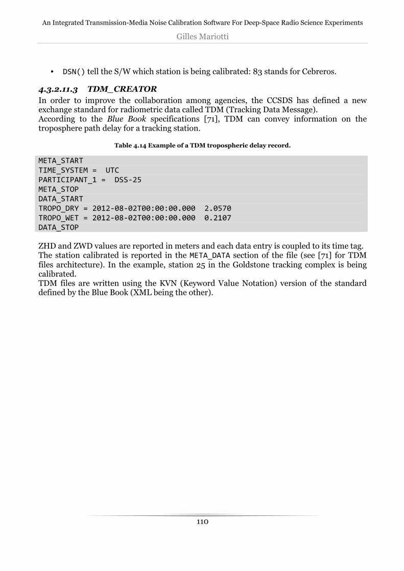
An Integrated Transmission-Media Noise Calibration Software For Deep-Space Radio Science Experiments
Gilles Mariotti
110
• DSN() tell the S/W which station is being calibrated: 83 stands for Cebreros.
4.3.2.11.3 TDM_CREATOR
In order to improve the collaboration among agencies, the CCSDS has defined a new exchange standard for radiometric data called TDM (Tracking Data Message). According to the Blue Book specifications [71], TDM can convey information on the troposphere path delay for a tracking station.
Table 4.14 Example of a TDM tropospheric delay record.
META_START TIME_SYSTEM = UTC PARTICIPANT_1 = DSS-25 META_STOP DATA_START TROPO_DRY = 2012-08-02T00:00:00.000 2.0570 TROPO_WET = 2012-08-02T00:00:00.000 0.2107 DATA_STOP ZHD and ZWD values are reported in meters and each data entry is coupled to its time tag. The station calibrated is reported in the META_DATA section of the file (see [71] for TDM files architecture). In the example, station 25 in the Goldstone tracking complex is being calibrated. TDM files are written using the KVN (Keyword Value Notation) version of the standard defined by the Blue Book (XML being the other).
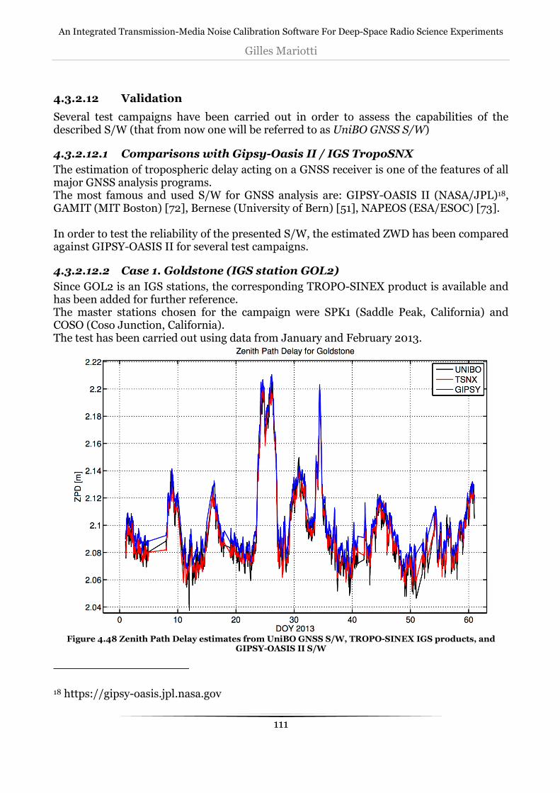
An Integrated Transmission-Media Noise Calibration Software For Deep-Space Radio Science Experiments
Gilles Mariotti
111
4.3.2.12 Validation
Several test campaigns have been carried out in order to assess the capabilities of the described S/W (that from now one will be referred to as UniBO GNSS S/W)
4.3.2.12.1 Comparisons with Gipsy-Oasis II / IGS TropoSNX
The estimation of tropospheric delay acting on a GNSS receiver is one of the features of all major GNSS analysis programs. The most famous and used S/W for GNSS analysis are: GIPSY-OASIS II (NASA/JPL)18, GAMIT (MIT Boston) [72], Bernese (University of Bern) [51], NAPEOS (ESA/ESOC) [73]. In order to test the reliability of the presented S/W, the estimated ZWD has been compared against GIPSY-OASIS II for several test campaigns.
4.3.2.12.2 Case 1. Goldstone (IGS station GOL2)
Since GOL2 is an IGS stations, the corresponding TROPO-SINEX product is available and has been added for further reference. The master stations chosen for the campaign were SPK1 (Saddle Peak, California) and COSO (Coso Junction, California). The test has been carried out using data from January and February 2013.
Figure 4.48 Zenith Path Delay estimates from UniBO GNSS S/W, TROPO-SINEX IGS products, and
GIPSY-OASIS II S/W
18 https://gipsy-oasis.jpl.nasa.gov

An Integrated Transmission-Media Noise Calibration Software For Deep-Space Radio Science Experiments
Gilles Mariotti
112
The test can be considered as passed since the ZPD difference between the tested S/W and TROPO-SINEX data was compatible with the difference among the two benchmark datasets (TSNX versus GIPSY). The difference between UniBO S/W and TROPO-SINEX has a standard deviation of 5 mm, while the TSNX-GIPSY difference has a 4-mm standard deviation, but a slight offset is present.
Figure 4.49 ZPD difference between UniBO GNSS S/W and TROPO-SINEX data. Standard Deviation and
Mean are reported in the legend. Notably the difference never exceeds 2 cm, with the exception of a single outlier.
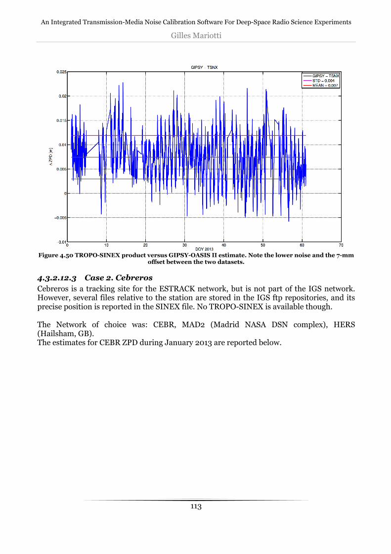
An Integrated Transmission-Media Noise Calibration Software For Deep-Space Radio Science Experiments
Gilles Mariotti
113
Figure 4.50 TROPO-SINEX product versus GIPSY-OASIS II estimate. Note the lower noise and the 7-mm
offset between the two datasets.
4.3.2.12.3 Case 2. Cebreros
Cebreros is a tracking site for the ESTRACK network, but is not part of the IGS network. However, several files relative to the station are stored in the IGS ftp repositories, and its precise position is reported in the SINEX file. No TROPO-SINEX is available though. The Network of choice was: CEBR, MAD2 (Madrid NASA DSN complex), HERS (Hailsham, GB). The estimates for CEBR ZPD during January 2013 are reported below.

An Integrated Transmission-Media Noise Calibration Software For Deep-Space Radio Science Experiments
Gilles Mariotti
114
Figure 4.51 Zenith Path Delay for Cebreros estimated by UniBO S/W and GIPSY-OASIS II
The difference between UniBO and GIPSY-OASIS II for CEBR data has a 7-mm standard deviation with a 4-mm offset.

An Integrated Transmission-Media Noise Calibration Software For Deep-Space Radio Science Experiments
Gilles Mariotti
115
Figure 4.52 ZPD difference for CEBR between Unio S/W estimate and GIPSY-OASIS II
4.3.2.12.4 Test against an HATPRO microwave radiometer
An HATPRO microwave radiometer [74] has been installed during Summer 2013 at ESOC premises, for testing and characterization purposes prior to the planned installation at the Cebreros ESTRACK site. The simultaneous availability of a Septentrio GNSS geodetic receiver on the very same roof allowed for a very precise comparison campaign between the ZWD retrieved by the instrument and the GNSS-based estimates. The comparison campaign has been carried out by comparing four datasets: Saastamoinen model, UniBO GNSS S/W, GIPSY-OASIS II, HATPRO.

An Integrated Transmission-Media Noise Calibration Software For Deep-Space Radio Science Experiments
Gilles Mariotti
116
Figure 4.53 ZWD estimates for ESOC site, July 2013
The UniBO S/W showed a difference with respect to HATPRO results (that we can consider as the benchmark) with a 1-cm standard deviation ,while GIPSY-OASIS estimates marked a 6-mm standard deviation. Although the GIPSY result was almost two times better, the UniBO-HATPRO difference is remarkably small and the test can be deemed as passed. As expected, Saastamoinen performed worse with a 22-mm standard deviation. Differencing the two GNSS-based estimates reveals a 4-mm offset between the two with 9 millimeters of standard deviation.

An Integrated Transmission-Media Noise Calibration Software For Deep-Space Radio Science Experiments
Gilles Mariotti
117
Figure 4.54 UniBO and GIPSY ZWD estimates difference wrt HATPRO. GIPSY performed almost 2 times
better.
The comparison with the radiometer is very interesting also in terms of the time derivative of the ZWD, that plays a role when dealing with deep-space tracking using Doppler data. The one-way range-rate contribution of troposphere’s wet component computed by HATPRO and UNIBO GNSS S/W is shown below:

An Integrated Transmission-Media Noise Calibration Software For Deep-Space Radio Science Experiments
Gilles Mariotti
118
Figure 4.55 One-way range-rate tropospheric contribution computed from HATPRO ZWD data (Blue)
and UniBO GNSS S/W (Black) for ESOC site.
It has to be noted that during deep-space operations the tropospheric range-rate component is much higher, due to the S/C elevation (up to 4 times due to the mapping function) and the two-way transmission. However, even at zenith the difference between the two calibrations is significant. A direct comparison between range-rate contributions of GNSS-based calibrations with respect to the HATPRO benchmark is not so useful, since GNSS-based techniques are not capable of retrieving the ZWD with a sufficient precision for high-frequency components. By reviewing the PSD of the difference with respect to HATPRO for the various estimation sources, we notice that they begin to drift apart from each other only for very-low frequency components (3-6 hours).

An Integrated Transmission-Media Noise Calibration Software For Deep-Space Radio Science Experiments
Gilles Mariotti
119
Figure 4.56 PSD of the difference in range-rate contribution with respect to HATPRO data.
It is safe to say then that GNSS-based calibration is as ineffective as the Saastamoinen for the high-frequency part of the data spectrum, and a microwave-radiometer calibration is mandatory for precise deep-space and radio-science operations.
4.3.2.12.5 Flight Dynamics
A further test for the S/W capabilities has been carried out in collaboration with ESOC Flight Dynamics Division, that is in charge of ESA probes navigation. The CSP cards generated by the UniBO S/W have been used to calibrate Range and Doppler radiometric data for the Planck and VEX spacecraft, in order to assess the impact of the GNSS-based calibration on the orbit determination process. Tracking passes are chosen so that the interplanetary plasma contribution to the error budget is negligible and the tropospheric noise is dominant: Planck operates on Lagrange L2 point that is permanently shielded by the Earth from the solar wind, while VEX passes are chosen during an inferior conjunction phase.
1. Planck, tracked from Cebreros. The tracking period is 14 days, from 2013/01/22 to 2013/02/04.
2. Planck, tracked from New Norcia. The tracking period is 14 days, from 2012/05/31 to 2012/06/13.
3. Venus Express, tracked from Cebreros. The tracking period is 14 days, from 2012/05/31 to 2012/06/13, centred around the inferior solar conjunction happening on 6th June 2013.
For each of the test cases, the orbit determination is run with two different calibration models for the tropospheric delay: the Saastamoinen and the GNSS UniBO estimates, and the residuals of the final fit are compared in terms of RMS.

An Integrated Transmission-Media Noise Calibration Software For Deep-Space Radio Science Experiments
Gilles Mariotti
120
4.3.2.12.5.1 Test Case 1: Planck tracked from Cebreros
The results of the two orbit determinations in terms of residuals statistics are presented in Table 4.15. The range-rate residuals seem to indicate little or no variation in the RMS when including GNSS-based correction, while the range shows slightly worse residuals (+3.5%). This trend however is not confirmed for all passes and does not seem to have statistical relevance. The maximum position difference between the two determined orbits during the reconstructed arc is 102 m, which is insignificant compared with the formal uncertainties of the reconstructed orbit.
Table 4.15 Comparison between OD residuals obtained with Saastamoinen and GNSS-based tropospheric corrections for Planck tracked from Cebreros
Saastamoinen GPS Data
pass RMS
doppler (mm/s)
RMS range (m)
RMS doppler (mm/s)
RMS range (m)
% doppler % range
1 0,04447 0,26746 0,04452 0,27380 0,11 2,37
2 0,03899 0,25531 0,03904 0,28222 0,13 10,54
3 0,02010 0,20762 0,02006 0,21434 -0,22 3,23
4 0,03236 0,38090 0,03238 0,36880 0,06 -3,18
5 0,02344 0,27352 0,02348 0,26570 0,20 -2,86
6 0,07163 0,22852 0,07174 0,23174 0,16 1,41
7 0,03988 0,03986 -0,06
8 0,01973 0,39593 0,01968 0,42494 -0,21 7,33
9 0,01872 0,22559 0,01871 0,25575 -0,06 13,37
10 0,01347 0,25155 0,01337 0,27023 -0,70 7,43
11 0,13395 0,39076 0,13293 0,43901 -0,77 12,35
12 0,03929 0,24959 0,03929 0,25646 -0,02 2,75
13 0,06422 0,24054 0,06427 0,24177 0,07 0,51
14 0,01172 0,01229 4,89
TOTAL 0,05114 0,27985 0,05098 0,28970 -0,31 3,52
It is worth noting that on many passes the Doppler noise RMS is in the order of 0.02 mm/s or lower, which can be considered very close to the intrinsic limitations of the current modeling in the AMFIN software (numerical noise due to truncation in time and position is negligible for this scenario). Also, no tracking data were acquired at low elevation, where the differences in the zenith tropospheric delay are magnified by the effect of the mapping function.

An Integrated Transmission-Media Noise Calibration Software For Deep-Space Radio Science Experiments
Gilles Mariotti
121
Figure 4.57 Expected and actual Doppler residuals RMS improvement. Note that the expected
improvement is below the AMFIN noise floor of 0.02 mm/s
4.3.2.12.5.2 Test Case 2: Planck tracked from New Norcia
The comparison for the residuals statistics derived from the two orbit determinations are presented in Table 4.16 for Planck spacecraft tracked from New Norcia. In this case the variations due to the new tropospheric calibrations are relevant in most individual passes, as well as on the overall figures. The Doppler noise shows reductions that can be important in some of the passes and a small overall reduction of about 1.5%. It is worth noting that the overall Doppler noise RMS here is much larger (about 3 times) than in the previous scenario. Also in this case numerical noise due to truncation is negligible. The largest effect however can be seen on the range observable, with individual variations of up to 100% and an overall reduction of 29%. The range variations are mostly affecting the bias rather than the noise level and may reveal the presence of some systematic source of error. The difference in position between the determined orbits is significant, with a maximum of 2.32 km at the beginning of the observation arc. The most affected component is the one in North-South direction, as expected when tracking with radiometric line-of-sight observables only. The 1-σ uncertainties in the same direction are 587 m formal, 1.51 km consider, at the center of the observation arc.
Table 4.16 Comparison between OD residuals obtained with Saastamoinen and GNSS-based tropospheric corrections for Planck tracked from New Norcia
Saastamoinen GPS Data
pass RMS doppler (mm/s)
RMS range (m)
RMS doppler (mm/s)
RMS range (m)
% doppler % range
1 0,07254 0,47261 0,05706 0,46128 -21,34 -2,40
2 0,03414 0,24277 0,03234 0,42365 -5,28 74,51
3 0,05345 0,39286 0,05100 0,33647 -4,59 -14,35

An Integrated Transmission-Media Noise Calibration Software For Deep-Space Radio Science Experiments
Gilles Mariotti
122
4 0,05299 0,35141 0,05000 0,25967 -5,65 -26,11
5 0,06076 0,53240 0,06121 0,44586 0,74 -16,25
6 0,10857 0,34195 0,09225 0,28987 -15,03 -15,23
7 0,21210 1,30715 0,21164 0,66012 -0,22 -49,50
8 0,05637 0,48538 0,04872 0,98262 -13,56 102,44
9 0,05521 0,61485 0,05481 0,26519 -0,71 -56,87
10 0,22503 1,21182 0,22042 0,45271 -2,05 -62,64
11 0,27983 2,10662 0,27610 1,18866 -1,33 -43,58
12 0,08251 0,86887 0,08074 0,62302 -2,15 -28,29
13 0,28462 0,89760 0,28654 0,91915 0,68 2,40
14 0,08049 0,73506 0,08052 0,73378 0,03 -0,17
TOTAL 0,15186 0,90096 0,14962 0,63934 -1,47 -29,04
However, Doppler observations down to 6.5 degrees are present in the tracking data, and they can provide further information about the improvements achievable with GNSS-based calibrations, since the corrections are magnified by the mapping function. An additional comparison between ODs has been made including the additional data. As expected, the variations in Doppler residuals now are much more pronounced, with reductions up to 37%. The overall reduction is only 0.4%, due to the high relative weight of the very noisy passes on 9th-10th of June, but the tendency to an improvement in Doppler residuals can be confirmed also over time spans longer than a single pass (-7% over the first 9 days). The variations in Doppler have an important impact on the orbit, and this is the reason of even larger (individual) variations visible in range residuals, even if the set of range observables is the same as in the previous OD comparison.
Figure 4.58 Expected and actual Doppler residuals noise improvement

An Integrated Transmission-Media Noise Calibration Software For Deep-Space Radio Science Experiments
Gilles Mariotti
123
4.3.2.12.5.3 Test Case 3: Venus Express tracked from Cebreros
The last test case considered is Venus Express tracked from Cebreros around the inferior solar conjunction, where the expected noise level is at the minimum, being the most favourable geometric configuration for this mission to avoid solar plasma effects. Also in this case, no clear conclusion can be drawn by looking at the results, despite the fact that the elevation goes down to 10 degrees in all passes. While the range seems to show a consistent tendency to slightly lower errors in the GNSS-based case, the Doppler noise variations are more erratic and on average slightly worse. The variations in the range biases are up to nearly 4 m at the beginning of the arc, and mainly depend on the difference in the orbits. It is worth noting that for many passes the Doppler noise level is very low, close to the limitations of the AMFIN system (the expected maximum numerical error caused by time truncation is in the order of 0.013 mm/s in the selected geometric configuration). The maximum position difference between the two orbits is about 37 m during the reconstructed arc, which is insignificant compared with the orbit uncertainties.
Figure 4.59 Detail of the Doppler residuals calibrated by Saastamoinen (above) and UniBO GNSS S/W (below). Note that the GNSS-based calibration removes the fringes at low-
elevation (red circles) by a more accurate correction of the path delay

An Integrated Transmission-Media Noise Calibration Software For Deep-Space Radio Science Experiments
Gilles Mariotti
124
4.3.2.12.5.4 Conclusions
In at least one scenario, Planck satellite tracked from New Norcia, the effect of GNSS-based calibration on the residuals statistics and the orbit determination was significant, showing an improvement on both range and Doppler residuals, and a difference in position comparable with the orbit uncertainty. On the other two scenarios considered, Venus Express and Planck tracked from Cebreros, the results were less meaningful and no clear conclusion could be derived. It must be remarked that the scope of this analysis was necessarily limited in terms of time availability and resources and a more systematic approach, with more tests run always in the same conditions would be necessary for a deeper investigation of the subject.

An Integrated Transmission-Media Noise Calibration Software For Deep-Space Radio Science Experiments
Gilles Mariotti
125
4.3.3 Microwave Radiometers
This section covers the basics of microwave radiometers operations, starting from a theoretical background and discussing several design archetypes for this type of instrument [75]. Finally the tropospheric path delay retrieval is described.
4.3.3.1 Radiometry Basics
4.3.3.1.1 Thermal radiation
All substances with a finite temperature radiate electromagnetic energy, due to collisions occurring among its atoms. These collisions cause electrons to shift between different energy levels, with a resulting electromagnetic emission. Each transition spawns a wave at its own frequency (given by Bohr’s equation), resulting in a line spectrum. The energy transition mechanism is also triggered by an incident wave, provided that the frequency satisfies Bohr’s equation: this means that the absorption and emission spectra of a body are identical. The probability that a collision will occur is dictated by the density of atoms and their kinetic energy: since the kinetic energy of atoms inside a substance is described by temperature, it follows that the intensity of radiation increases with the body temperature. The spectrum associated with molecules is more complex than with single atoms, since also vibrational and rotational transitions take place. As the substance becomes more and more complex, allowing more interactions between particles, the emission spectrum broadens, until it becomes a continuum. Radiometry is a field of science and engineering related to the measurement of the
electromagnetic radiation just described, allowing the remote sensing on an object.
Remote sensing is either active or passive depending on how the instruments interacts
with the observed scene. If the instruments transmits a carrier and then receives the
reflection generated by the scene, we have active radiometry, e.g. a RADAR system. On the
other hand, if the instrument is only receiving the naturally-emitted radiation of the scene,
we have a passive radiometer.
4.3.3.1.2 Brightness and related radiometric quantities
Consider a transmitting antenna placed at distance R (distant enough for the far-field approximation to be valid) from a receiving antenna. The power intercepted by the receiving antenna will be proportional to the power density St of the transmitter and the receiver effective area Ar: ` = ? = *? (4.114)
If we treat the transmitting antenna, that has an effective aperture At as a point source with a directional distribution *?(θ, φ) equal to its radiation intensity (power density per unit solid angle), we can define a quantity representing the radiated power per unit solid angle, per unit area as = *?? [|UVU]. (4.115)

An Integrated Transmission-Media Noise Calibration Software For Deep-Space Radio Science Experiments
Gilles Mariotti
126
This quantity is known as the brightness (or radiance, or intensity) of the source, with dimensions. If we note that the solid angle subtended by the transmitting antenna is ? = ? ⁄ , then we have that the received power is: ` = ? . (4.116)
The brightness can also vary throughout the spectrum, so the spectral brightness Bf (f) is
defined, as the brightness per unit bandwidth df.
We extend these results to the differential level, also dropping the necessity for the receiver
to be on the direction of maximum directivity of the source (by introducing its radiation
pattern), finding that:
K` , 4 = , , 4*; , 4KK. (4.117)
The total radiated power P is computed by the double integral on 4π for the solid angle (resulting in the spectral power Pf) and then by integrating on the bandwidth (f, f+∆f) of interest. Furthermore, a ½ factor should be introduced if the radiation is unpolarized (like atmospheric emission), since only half of the incident power is absorbed by the antenna.
4.3.3.1.3 Black-body and Grey-body radiators
4.3.3.1.3.1 Black Body
A black body is an ideal object that absorbs all of the incident energy it receives, at all
frequencies, without reflection. This makes the black body a perfect absorber and also a
perfect emitter: since the black body is by definition in thermodynamic equilibrium, its
temperature is not changing, so all of the absorbed power must be emitted, as stated by
Kirchhoff’s law.
A black body then radiates at least as much energy as any other body at the same
temperature T.
The spectral brightness over a frequency f of a black body at a certain temperature T is
defined by Planck’s radiation law:
= 2ℎX C 1 ⁄ − 1M, (4.118)
where h is Planck’s constant, k is Boltzmann’s constant and c the speed of light.
The law can also be express in terms of wavelength λ as
= 2ℎ¡ C 1¢ ⁄ − 1M. (4.119)
The only two variables of this equation are frequency (wavelength) and temperature, as
shown in Figure 4.60.
The exact values of frequency at which the brightness curve peaks can be retrieved by the
Wien displacement law as function of temperature.

An Integrated Transmission-Media Noise Calibration Software For Deep-Space Radio Science Experiments
Gilles Mariotti
127
Figure 4.60 Planck radiation law curves showing brightness as function of frequency and temperature
Planck’s law can be used to infer various useful results. • Stefan-Boltzmann law: since a black body radiates on the whole spectrum, its total
brightness is given by integrating Planck’s law on (0,∞): B = 2ℎ ¤ ¥ X ⁄ − 1¦ = hZ§
E . (4.120)
Where σ is the Stefan-Boltzmann constant.
This results tells us that the brightness of a black body is dependent upon the fourth
power of its physical temperature. Note that this relation is not valid for Bf or Bλ.
• Rayleigh-Jeans approximation: in a large part of the microwave region, the
condition ℎ ¨⁄ ≪ 1 holds, thus allowing the approximation ex-1≈x.
Then:
= 2¨ = 2¨ . (4.121)
This law is simpler than Planck’s formulation but deviates less than 3% from its value for frequencies up to 1012 Hz.
We can use the Rayleigh-Jeans identity in order to get information on the power radiated by a black body: we remember that the total emitted power is the triple integral

An Integrated Transmission-Media Noise Calibration Software For Deep-Space Radio Science Experiments
Gilles Mariotti
128
` = 12 ¤ ª(, 4)*;(, 4)KKZ«¬∆ , (4.122)
and if the detected power is limited to a bandwidth narrow enough for Bf to be considered constant over ∆f , the integral becomes:
` = ¨∆ ®°± ª*;(, 4)KZ«²³³³³´³³³³µ®¯= ¨∆.
(4.123)
There is a direct correspondence between the power radiated over a certain bandwidth by a black body and its temperature. This allows to use the two quantities interchangeably.
4.3.3.1.3.2 Grey Body
Although this is an ideal case, the formulation used for real objects (often called grey bodies) can be brought back to this identity, making it of extreme importance for microwave remote sensing. If a grey object has a spectral brightness Bf(θ,φ), we can define an equivalent radiometric temperature TB(θ,φ) that makes the Rayleigh-Jeans approximation still valid , 4 = 2¨ , 4. (4.124)
This radiometric temperature is not physical, and is usually referred to as the Brightness Temperature of the object. So a grey body with a physical temperature T emits the same radiance as a black body at a temperature equal to its brightness temperature, that is always lower than T. That is like saying that a real object has an emissivity e lower than 1, given: , 4 = , 4 = , 4 , 0 ≤ ≤ 1. (4.125)
Emissivity is then the ratio of the radiance actually emitted by the object to the one that it would emit if it were a black body (higher by definition). Brightness temperature is the fundamental quantity on which the whole remote sensing field is based. By measuring the brightness temperature of a scene, information on its physical states can be inferred, e.g. temperature profiles and humidity levels can be retrieved by measuring the brightness temperature of the downwelling radiation of the sky.
4.3.3.1.3.3 Measuring radiometric temperatures
In practical applications, the power incident on the observing antenna is not only the one due to the emission of the target, but is a combination of several contributions originating from different sources. In the case of atmospheric profiles retrieval, the radiometer

An Integrated Transmission-Media Noise Calibration Software For Deep-Space Radio Science Experiments
Gilles Mariotti
129
antenna will receive not only the radiation of the atmospheric gases and liquid water, but also extra-terrestrial emission, the self-emitted radiation of the terrain, the reflection of the atmospheric radiation due to terrain, and even the self-emission of the antenna itself. This composite radiometric temperature will be called apparent temperature TAP. This quantity is not equal to TB, and careful considerations must be made in order to define whether or not TAP is a good representation of TB in each operational scenario. However, neither TAP is the temperature seen by the receiver. To explain this concept, as far as what the receiver sees, we can swap the antenna with a matched resistor. Resistors deliver a noise power Pn proportional to their temperature TA, following the same law governing black bodies: ; = ¨q∆. (4.126)
The antenna itself however receives a power that is function of the apparent temperature of the observed scene:
` = 12∆ª2¨ q·(, 4)*;(, 4)KZ« . (4.127)
By equating Pn=P we find that
q = ®°±ªq· , 4*; , 4KZ«= ∬ q· , 4*; , 4KZ« ∬ *; , 4KZ«
. (4.128)
This means that the effective temperature seen by the receiver is the antenna radiometric temperature TA, that is equal to the scene’s apparent temperature integrated over the 4π solid angle, weighted by the antenna pattern, normalized by the pattern solid angle Ωp. Furthermore, this formulation is valid for an ideal case in which the antenna is lossless (it has no self-emission) and has no minor lobes: for a real antenna, the radiometric temperature reaching the receiver is q¹ = º=º» + º= 1 − º»¼ + 1 − º=E. (4.129)
The real antenna radiometric temperature consists of the main beam contribution »
(that is the actual apparent temperature of the scene), disrupted by parasite temperatures
due to side lobes »¼and antenna self-emission (proportional to its physical temperature
T0).
Figure 4.61 shows a wrap-up of the various stages from scene’s brightness temperature to
the antenna radiometric temperature seen by the receiver.

An Integrated Transmission-Media Noise Calibration Software For Deep-Space Radio Science Experiments
Gilles Mariotti
130
Figure 4.61 Radiometric temperatures from scene to receiver »can be retrieved by inverting the equation for q¹, since the main beam and radiation
efficiency are possible to calculate while T0 can be monitored by a thermocouple.
» = C 1º=ºMq¹ − C1 − ºº M »¼ − C1 − º=º=º M E. (4.130)
»¼ can vary on a wide range of values. For an upward-pointing radiometer however, this
quantity is constant and its contribution to the antenna temperature is lower than 10 K for
well-designed antenna patterns (ηM>0.97).
4.3.3.1.4 Theory of radiative transfer
As we just saw, the apparent temperature TAP is the fundamental observable in remote sensing. In order to derive expressions for the TAP of different scenes, one must understand the mechanisms that regulate the interaction between radiation and matter: extinction and emission.
4.3.3.1.4.1 Extinction
Let us consider a small cylindrical volume of cross-section dA, thickness dr and density ρ. An incident brightness B(r) upon the lower face of the cylinder will lose a value dB at the other end r+dr due to extinction caused by the medium, dependent on its power attenuation coefficient ke (or extinction coefficient, [nepers m-1]): K9½? = ¨9 K. (4.131)
Extinction can take place due to absorption (radiated energy is transformed in other types of energy, i.e. heat) and/or scattering (the energy is deviated on directions that are not the direction of propagation). Hence, the attenuation coefficient can be split into two contributions: ¨9 = ¨:+¨p. (4.132)

An Integrated Transmission-Media Noise Calibration Software For Deep-Space Radio Science Experiments
Gilles Mariotti
131
4.3.3.1.4.2 Emission
The cylinder will also emit brightness in direction r. The amount depends on the thermal emission and the scattering source functions: K98 = (¨:¾: + ¨p¾p)K. (4.133)
It has to be noted that the emission mechanisms depends also on attenuation coefficients.
Ja is also called absorption source function due to the thermodynamic equilibrium
condition: all of the power absorbed must be emitted.
If we define the ratio = ¨p ¨9⁄ as the single-scattering albedo, we can rewrite the
emission equation as
K98 = ¨9 ¾K, (4.134)
where J is the effective total source function, and is equal to ¾ ≜ 1 − ¾: = ¾p. 4.3.3.1.4.3 Equation of transfer and its formal solution
Using emission and extinction laws, the total brightness variation generated by the body can be computed as K = + K − = K98 − K9½? = ¨9 ¾ − K. (4.135)
Introducing the optical depth KT = ¨9K we can derive a differential equation for
brightness along the propagation direction, known as the equation of transfer:
KKT + = ¾. (4.136)
In order to solve the equation, the optical thickness is defined, as the integral of the optical depth along a range between two points r1 and r2 on the propagation path: T V, = ¤ ¨9KÀ
± . (4.137)
Using this quantity we then proceed to solve the equation that yields: = 0UÁ E, +¤ ¨9 ′¾ ′
E UÁ Â,K¹. (4.138)
The above solution states that the brightness B(r) at any point r is given by two terms: • The first term represents the reduction of magnitude of the initial brightness B(0)
due to extinction by the medium between 0 and r. • The integral represents emission and scattering by the material, described by the
sum of infinitesimal differential emitted brightnesses ke(r’)J(r’), reduced in magnitude by the extinction factor.
4.3.3.1.4.4 Apparent temperature of an absorbing and scattering medium
We remember that the Rayleigh-Jeans approximation gives the brightness in terms of radiometric temperature:
An Integrated Transmission-Media Noise Calibration Software For Deep-Space Radio Science Experiments
Gilles Mariotti
132
() = 2¨ q·()∆. (4.139)
This relation allows to use the equation of transfer to describe variations of TAP . Thanks to Kirchhoff’s law we can use the same approach to describe source functions:
absorption ¾: = 2¨ ∆
scattering ¾p(Ã) = 2¨ ¼(Ã)∆. total
¾ Ã = J 1 − + ¼ ÃL 2¨ ∆
(4.140)
One can note that the absorption source function depends on the physical temperature of the body, while the scattering source is defined in terms of the scattered radiometric temperature, parameter created in order to rewrite Js (that is the solid angle integral of the brightness weighted by a phase function ψ describing the amount of radiation scattered from an arbitrary direction ri into the propagation direction r) using a Rayleigh-Jeans-like formulation: ¼(Ã) = 14ªf(Ã, Ã>)q·(Ã>)K>Z« . (4.141)
This description of source functions is used to derive the radiative transfer solution for the apparent temperature of an observed scene: q· Ã = q· 0UÁ E, +¤ ¨9 ′J 1 − + ¼ ÃL
E UÁÂ,K¹. (4.142)
Scattering introduces quite a complication, since the solution at every point depends on interactions at every other point. Under clear sky conditions however, earth’s atmosphere is free from scattering in the microwave region. Below 10 GHz, scattering effects can be neglected also for most weather conditions involving non-precipitating liquid water. In general, when precipitating clouds and liquid water are present, the scattering is not negligible and depends on the density and the drop-size distribution of water droplets, that are responsible of volume scattering. Assuming the atmosphere as a scatter-free medium, the last result can be greatly simplified since a<<1, resulting in: q· = q· 0UÁ E, +¤ ¨: ¹
E UÁ Â,K¹, (4.143)
where the optical thickness is now function only of the absorption coefficient
An Integrated Transmission-Media Noise Calibration Software For Deep-Space Radio Science Experiments
Gilles Mariotti
133
T(¹, ) = ¤ ¨:K¹ . (4.144)
The scatter-free assumption is not a trivial one since isn’t always fit to describe the atmosphere, and must be handled carefully in order to retrieve meaningful measurements from the radiometer.
4.3.3.1.5 Microwave interaction with atmosphere constituents
As seen thanks to the last result of previous chapter, the radiometric temperature of the atmosphere depends on its temperature and absorption coefficient profiles as function of height. This means that radiometry is a useful technique to exploit for atmospheric observation, by inverting the apparent temperature relation. In general, the atmosphere is transparent (even in presence of cloud or mild rainfalls) in the 1-15 GHz region, while the absorption maxima of oxygen (50-70 window and 118.7 GHz) and water vapour (22.2 and 183.3 GHz) can be used to retrieve temperature and water vapour height profiles.
4.3.3.1.5.1 Standard Atmosphere
The Standard Atmosphere is a generalized model of the vertical structure of the earth’s atmosphere and provides temperature, pressure and density profiles representing the average conditions at middle latitudes [76]. Several revisions of the standard atmosphere have been released over the years. For microwave remote sensing, the most interesting part is the lower layer of the atmosphere, since the bulk of the total gases mass is contained there (and also radiometers cannot observe the atmosphere beyond a few kilometres, due to air opacity) .
• Temperature profile Temperature steadily drops in the first 11 kilometres of atmosphere (troposphere), with a constant lapse rate a=-6.5 K/km, starting from a mean surface temperature of 288.15 K. Above the troposphere, a layer reaching 20 km presents a constant temperature (tropopause). Above the tropopause, an inversion of the temperature profile causes the temperature to raise up to the stratopause.
Ä = Å 0 − Ä0 ≤ Ä ≤ 11¨ 1111 ≤ Ä ≤ 20¨ 11 + Ä − 2020 ≤ Ä ≤ 32¨ (4.145)
• Density profile
The density of dry air decreases exponentially with altitude:
Y Ä = 1.225U ÆÀ⁄ J1 + 0.3 sin Ä Ç⁄ L J¨ X⁄ L (4.146)
H2=7.3 km is the density scale height.
• Pressure profile

An Integrated Transmission-Media Noise Calibration Software For Deep-Space Radio Science Experiments
Gilles Mariotti
134
Pressure can be retrieved from density and temperature using the ideal gas law
` = 2.87Y (4.147)
or in alternative with and exponential fit using a scale height H3=7.7 km and a surface pressure of 1013.25 mbar:
` Ä = EU ÆÈ⁄ J.L. (4.148)
• Water-Vapour Density profile
The average surface value for water-vapour density, for middle latitudes, is ρ0=7.72 g/m3 . The profile is expressed with a decreasing exponential with scale height H4 typically chosen between 2 and 2.5 km:
Y Ä = YEU ÆÉ⁄ J/XL. (4.149)
The total mass of water vapour contained in a vertical column of unit section is 3 = ¤ Y ÄKÄ =§
E YEÇZ J/L. (4.150)
4.3.3.1.5.2 Absorption and emission by atmospheric gases
As discussed in chapter 4.3.3.1.1, the absorption and emission spectra of all matter depend on the energy states of atoms and molecules that it contains. Isolated, undisturbed and stationary molecular systems present a spectrum that consists of sharp, well defined frequency lines corresponding to different quantized energy levels (line spectrum). In reality, molecules are in constant motion, interacting and colliding with one another and with other material objects: these disturbances cause the energy levels to vary in width, resulting in a broadening of the frequency lines. This type is the most important among the various sources of line broadening and it’s known as pressure broadening.
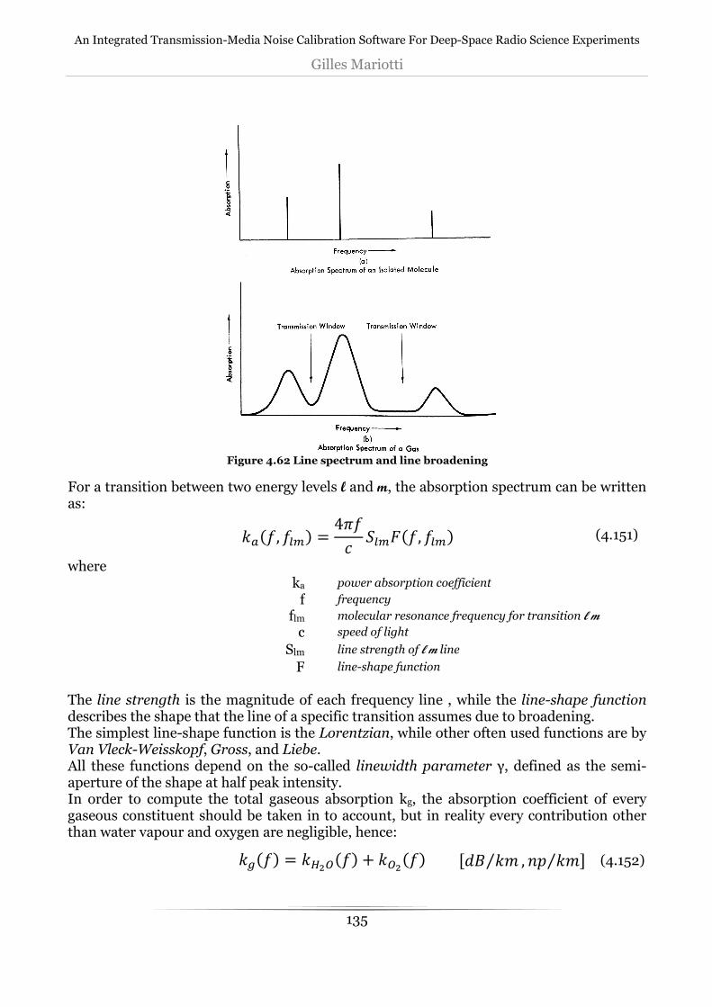
An Integrated Transmission-Media Noise Calibration Software For Deep-Space Radio Science Experiments
Gilles Mariotti
135
Figure 4.62 Line spectrum and line broadening
For a transition between two energy levels l and m, the absorption spectrum can be written as: ¨:(, =8) = 4 =8*(, =8) (4.151)
where ka power absorption coefficient
f frequency
flm molecular resonance frequency for transition l m
c speed of light
Slm line strength of l m line
F line-shape function
The line strength is the magnitude of each frequency line , while the line-shape function describes the shape that the line of a specific transition assumes due to broadening. The simplest line-shape function is the Lorentzian, while other often used functions are by Van Vleck-Weisskopf, Gross, and Liebe. All these functions depend on the so-called linewidth parameter γ, defined as the semi-aperture of the shape at half peak intensity. In order to compute the total gaseous absorption kg, the absorption coefficient of every gaseous constituent should be taken in to account, but in reality every contribution other than water vapour and oxygen are negligible, hence: ¨Ê() = ¨ÆÀË() + ¨ËÀ() [K ¨⁄ , Ì ¨⁄ ] (4.152)

An Integrated Transmission-Media Noise Calibration Software For Deep-Space Radio Science Experiments
Gilles Mariotti
136
Absorption due to oxygen and water vapour can be computed using several models that depend on pressure , temperature and water-vapour density. Nowadays, the most used by the microwave propagation community are the MPM by Liebe [77], the Rosenkranz model [78] and also the LBLRTM by Clough [79]. Using these models, it is observed that:
• Water vapour has two strong rotational absorption lines at 22.235 and 183.31 GHz • Oxygen presents a large number of absorption lines spread out over the 50-70-GHz
range, blended together in a single absorption band due to pressure broadening (the 60-GHz oxygen complex), together with an additional line at 118.75 GHz.
Once again, this formulation is adequate only when describing a scatter-free medium: precipitating clouds and other hydrometers cause extinction also by scattering, that is usually coped with using statistical approaches based on density, shape and size distributions. The typical formulation used is the Lorenz-Mie equations. For non-precipitating clouds the Rayleigh approximation is introduced: using this approximation scattering is neglected, and the liquid water absorption depends only on the total liquid amount and not on the drop-size distribution. The absorption coefficient is then generalized into: ¨:(Ä) = ¨Ê(Ä) + ¨¢=@Íp(Ä) + ¨<9¢(Ä) (4.153)
Since atmosphere is not a homogeneous and planar medium, the integral of the absorption coefficient along the line of sight is of interest (especially for air- and spaceborne radiometry). Given a zenith angle θ in which the instrument is pointing (assuming a scatter-free atmosphere and that θ<70° so refraction can be ignored) we have the opacity (see optical depth in section 4.3.3.1.4.3) of the atmosphere: TÎ = sec ¤ ¨Ê(Ä)KÄ = TE sec §
E , [K, Ì] (4.154)
and also the total atmospheric loss factor Î = ÁÐ ÑÒÓÎ [K, Ì]. (4.155)
The reciprocal of the loss factor is called transmissivity: ÔÎ = 1 ÎO = UÁÐ ÑÒÓÎ JK, ÌL. (4.156)

An Integrated Transmission-Media Noise Calibration Software For Deep-Space Radio Science Experiments
Gilles Mariotti
137
Thanks to these definitions we have then the total sky radiometric temperature, that is the sum of the downwelling emission of the non-scattering atmosphere and the brightness temperature of extra-terrestrial sources, namely our galaxy and the cosmic radiation. ¼eÕ() = PÖ() + (˼ + q)UÁÐ ÑÒÓÎ , (4.157)
where
PÖ sec ¤ ¨: Šŧ
EUÁ E, ÑÒÓÎKĹ,
T 0, Ĺ × ¨: ÄKĹE ,
˼ 2.7Ø,
qÙÙ..Ú5ÛÇÄ.
(4.158)
Also point sources not included in this discussion (like the sun) should be considered. A
stationary sun without flares and sunspots has an almost constant brightness temperature
of 6000 K in the 10-30 GHz region.
4.3.3.1.6 Techniques for passive microwave sensing of the atmosphere
4.3.3.1.6.1 The inverse problem
The calculation of the brightness temperature of the atmosphere relative to certain meteorological conditions is called direct or forward problem.
Figure 4.63 Opacity due to oxygen, water vapour and liquid water in non-precipitating clouds below 100 GHz
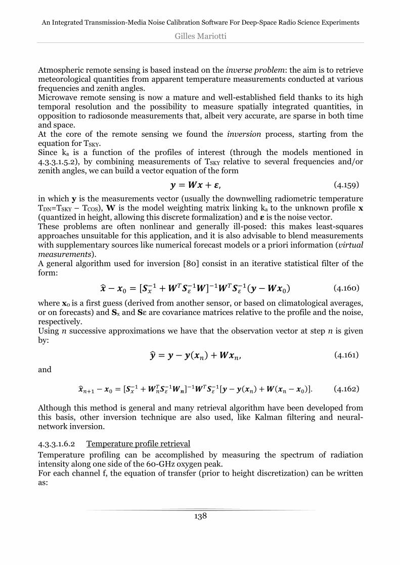
An Integrated Transmission-Media Noise Calibration Software For Deep-Space Radio Science Experiments
Gilles Mariotti
138
Atmospheric remote sensing is based instead on the inverse problem: the aim is to retrieve meteorological quantities from apparent temperature measurements conducted at various frequencies and zenith angles. Microwave remote sensing is now a mature and well-established field thanks to its high temporal resolution and the possibility to measure spatially integrated quantities, in opposition to radiosonde measurements that, albeit very accurate, are sparse in both time and space. At the core of the remote sensing we found the inversion process, starting from the equation for TSKY. Since ka is a function of the profiles of interest (through the models mentioned in 4.3.3.1.5.2), by combining measurements of TSKY relative to several frequencies and/or zenith angles, we can build a vector equation of the form Ü = ÝÞ + %, (4.159)
in which y is the measurements vector (usually the downwelling radiometric temperature TDN=TSKY – TCOS), W is the model weighting matrix linking ka to the unknown profile x (quantized in height, allowing this discrete formalization) and ε is the noise vector. These problems are often nonlinear and generally ill-posed: this makes least-squares approaches unsuitable for this application, and it is also advisable to blend measurements with supplementary sources like numerical forecast models or a priori information (virtual measurements). A general algorithm used for inversion [80] consist in an iterative statistical filter of the form: Þ − ÞE = [ß½UV +ÝßàUVÝ]UVÝßàUV(Ü −ÝÞE) (4.160)
where x0 is a first guess (derived from another sensor, or based on climatological averages, or on forecasts) and Sx and Sε are covariance matrices relative to the profile and the noise, respectively. Using n successive approximations we have that the observation vector at step n is given by: Ü = Ü − Ü(Þ;) +ÝÞ;, (4.161)
and Þ;¬V − ÞE = [ß½UV +Ý;ßàUVÝá]UVÝßàUV[Ü − Ü(Þ;) +Ý(Þ; − ÞE)]. (4.162)
Although this method is general and many retrieval algorithm have been developed from this basis, other inversion technique are also used, like Kalman filtering and neural-network inversion.
4.3.3.1.6.2 Temperature profile retrieval
Temperature profiling can be accomplished by measuring the spectrum of radiation intensity along one side of the 60-GHz oxygen peak. For each channel f, the equation of transfer (prior to height discretization) can be written as:

An Integrated Transmission-Media Noise Calibration Software For Deep-Space Radio Science Experiments
Gilles Mariotti
139
PÖ(, ) = ¤ |(, , Ä)(Ä)KħE
|(, , Ä) = −âÔÎ(0, ÄâÄ = ¨: ÄUÁ E, ÑÒÓ Î sec . (4.163)
Using oxygen to retrieve temperature finds its reason in the fact that close to 60 GHz, absorption is dominated by k02, that is strongly dependent upon oxygen partial pressure, that is a portion of the total dry pressure P(z) with a constant mixing ratio (21%). That is to say that the weighting matrix W depends only on the pressure height profile (frequency and zenith angle aside). Using the hydrostatic equation and the equation of state, T and P can be related: in this way T(z) is retrieved after retrieving T(P) by the inversion. K` = K ln` = −3 KÄ
| , , ` = −âÔÎ p, `â ln` = âÔÎ 0, ÄâÄ ∙ âÄâ ln` PÖ , = ¤ | , , ` `K ln`äå ·æ
U§
(4.164)
Geopotential height can also be computed:
Ä· = − 3¤ `K ln`äå ·äå ·æ . (4.165)
4.3.3.1.6.3 Integrated water vapour (IWV) and liquid water path (LWP) retrieval
Ground-based passive microwave radiometry is by far the most accurate method for determining water vapour and liquid water content of the atmosphere, and it has been in use for more than 35 years. ρv(z) can be inferred from TDN inversion like T(z), by an adequate selection of the instrument channels:
• TDN should be very sensitive to ρv(z), and not to other profiles
• The weighting function Wρ should have height profiles sufficiently different to minimize redundancy.
These criteria can be met by selecting frequencies lying on peaks and shoulders of the 22.235- and 183.31-GHz water vapour absorption lines. Since the 22.235-GHz line is weaker and varies very slowly with height, it is not always adequate for water vapour retrieval, especially in dry climates: for this reason, the 183.31-GHz is used. In this band, absorption is dominated by water vapour: ka≈kh2o. Due to its strength however, this channel can be easily saturated. A standard approach to water vapour profiling is the use of dual-frequency (nowadays multi-frequency) measurements, since the total opacity of a column of unitary cross-section can be approximated to the sum [75]

An Integrated Transmission-Media Noise Calibration Software For Deep-Space Radio Science Experiments
Gilles Mariotti
140
T = TÊ+¨ ∙ ç|è + ¨= ∙ |` (4.166)
where τg is the opacity due to dry gases, that can be known thanks to vertical profiles of P and T. By using accurate absorption models to compute kv and kl (that in this formulation indicate the absorption coefficients divided by the density of water vapour and liquid water, respectively), only IWV and LWP are unknown, and can be retrieved by performing a brightness temperature measurement on two separate frequencies f1 and f2, resulting in two opacity readings τ1 and τ2. τg is subtracted from τ1 and τ2 and then the 2-by-2 equation set is inverted: ç|è = ¨=TV − ¨=VT¨V¨= − ¨¨=V ,JL
|` = ¨VT − ¨TV¨V¨= − ¨¨=V JL. (4.167)
Using a multi-frequency approach, the two unknowns are retrieved by means of least squares or other linear regression algorithms.
4.3.3.1.6.4 Path delay estimation
Path delay can be retrieved from measurements of temperature, pressure and water vapour profiles, using a least squares inversion from radiometric temperatures or by exploiting its relation with the IWV: é|6 = 10UWê C¨ + ¨X8M ç|è, (4.168)
where RW is the specific gas constant for water vapour and Tm is the weighted mean atmospheric temperature [81]:
8 = × éêUVKħE× éêUVKħE, (4.169)
with ZW compressibility of air. Another relation between IVW and ZWD is given by [36]: ë = é|6/ç|è = 0.102 + 1708.08/ (4.170)
where TM is the mean atmosphere temperature in K: = 54.7 + 0.77 ∙ E (4.171)
Other conversion formulas are available [82].
4.3.3.1.6.5 Attenuation Retrieval

An Integrated Transmission-Media Noise Calibration Software For Deep-Space Radio Science Experiments
Gilles Mariotti
141
Atmospheric attenuation is described by the extinction coefficient ke that, considering the atmosphere as a scatter-free medium, is equal to the total absorption coefficient kg. So the opacity described in Section 4.3.3.1.5.2 is the total attenuation of a column of air. The method to retrieve the atmospheric opacity is the tipping curve method, described in Section 4.3.3.3.1. This method makes use of the mean radiating temperature of the atmosphere, introduced in the same section. In an operating scenario, Tmr has its own retrieval algorithm, usually based on a linear or quadratic regression of surface meteorological measurements.
4.3.3.1.6.6 Statistical regression retrieval algorithms
The most used retrieval algorithm is a simple statistical regression of brightness temperatures and weather station data. Starting from a database of weather measurements (usually radiosonde-derived) and corresponding brightness temperatures from the instrument, it is possible to define a fitting polynomial, and its coefficients can be used for later brightness temperatures measurements in order to retrieve the needed quantities (IWV, ZWD, Attenuation, etc.). These coefficients are site-specific. For the radiometer at DSS-25 (Goldstone), this retrieval algorithm used by JPL is [5]: ) 4.31(3062.0) 8.23(6899.0) 2.22(1364.0849.0 GHzTGHzTGHzTZWD BBB −⋅+⋅−−= (4.172)
where the three TB values are the outputs of the three receiver channels of the instrument. Another example of how a statistical retrieval is built is given by Radiometer Physics GmbH: given a radiosonde database for a site, half of the mesurements are used to “train” the retrieval, thus producing the fit coefficients. The other half of the database is used to test the fitting accuracy of the retrieval.

An Integrated Transmission-Media Noise Calibration Software For Deep-Space Radio Science Experiments
Gilles Mariotti
142
Table 4.17 Example of an IWV retrieval algorithm creation
10k radiosonde profiles
TR
AIN
ING
Compute REAL IWV from half of the profiles ∫∝h
real dhHRIWV
Simulate instrument TBs using the Radiative Transfer Model
Half of the profiles are used to create the fit
...21 210 +++= BBSIM TaTaaIWV
FIT
Compute REAL IWV for the other half of the database
TE
ST
Simulate IWV for the second half using RTM + FIT
COMPARE REAL AND SIMULATED IWV
4.3.3.2 Radiometer Systems
Radiometers are highly sensitive receivers designed to measure thermal electromagnetic emission by material media. The core function of the instrument is to measure the radiometric antenna temperature TA’ from a received power PA’=kTA’B, (with B bandwidth). However, strictly speaking, the instrument provides an estimate of TA’, since its output voltage Vout is merely an average of a noise-like signal. It is then of extreme importance to characterize the radiometer in terms of accuracy, resolution ∆T and transfer function.
4.3.3.2.1 Noise characterization
The instrument components themselves will add noise to the input signal. A complete characterization of the magnitude and nature of these noises must be carried out in order to operate a radiometer. Two figures of merit are usually adopted to describe the noise performance of a radiometer:
• Noise figure F It measures the SNR degradation due to noise addiction by a two-port device between its input and output ports
* = Q>;Q@? . (4.173)
A device with gain G, receiving a power Psi with a thermal noise Pni=kT0B will add a noise ∆Pno to the output Pso, and these relations hold:

An Integrated Transmission-Media Noise Calibration Software For Deep-Space Radio Science Experiments
Gilles Mariotti
143
* = p> ;p ;> = 1Û Û¨E + ∆ ;¨E = 1 + ∆ ;Û¨E
; = *Û¨E
(4.174)
A noisy device with a noise figure F operating at temperature T0 behaves like an ideal noise-free device at temperature FT0. Describing a device noise performance using F, also the operating temperature has to be specified. To avoid confusion, F is usually standardized to T0=290K.
• Effective noise temperature TE It is an alternative description of noise performance, that depends only on device parameters. The effective noise temperature TE is the temperature of a thermal resistor that, if placed at the input of an equivalent noise-free device, would produce the same noise power ∆Pno of the noisy device. If the actual noise temperature at input is TI (since Pni=kTIB) then the total input noise of the equivalent noise-free device is TI+TE, and so the output will be:
; = Û( ;> + ì) = Û¨(í+ì). (4.175)
The two parameters are connected since they are related through temperature T0
ì = * − 1E, (4.176)
however F has been used more commonly to describe conventional receivers, whereas effective temperature is preferred for low-noise systems. If the device of interest is an attenuator, so it has a loss factor L instead of a gain, its equivalent noise temperature will be ì = − 1· , (4.177)
where TP is its physical temperature. For a superheterodyne receiver, the effective noise temperature is relative to the whole chain of stages forming the device (RF amplifier, mixer, preamp, IF amplifier), but is practically equal to the one of the first stage, the RF amplifier. Using these notions we can derive the total-system equivalent input noise power PSYS, referred to the antenna terminals. This power consists of the power delivered by the antenna PA’ and the equivalent input noise power of the combination of transmission line and the receiver P’REC. Neglecting side lobes, we can recall the antenna temperature relation found in section 4.3.3.1.3.3: q¹ = ¨q¹ = ¨º=q + 1 − º=<, (4.178)
while the transmission-line and receiver power is
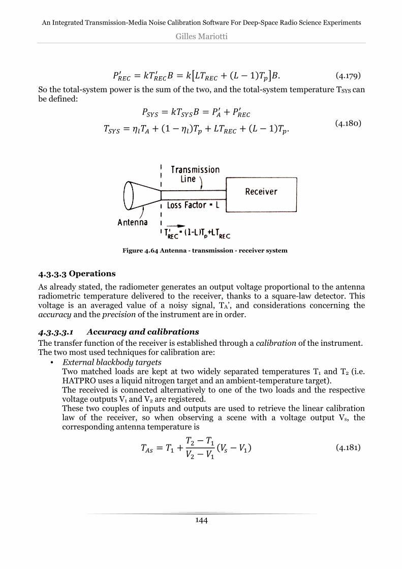
An Integrated Transmission-Media Noise Calibration Software For Deep-Space Radio Science Experiments
Gilles Mariotti
144
ì¹ = ¨ì¹ = ¨ì + ( − 1)<. (4.179)
So the total-system power is the sum of the two, and the total-system temperature TSYS can be defined: ¼Õ¼ = ¨¼Õ¼ = q¹ + ì¹ ¼Õ¼ = º=q + 1 − º=< + ì + − 1<. (4.180)
4.3.3.3 Operations
As already stated, the radiometer generates an output voltage proportional to the antenna radiometric temperature delivered to the receiver, thanks to a square-law detector. This voltage is an averaged value of a noisy signal, TA’, and considerations concerning the accuracy and the precision of the instrument are in order.
4.3.3.3.1 Accuracy and calibrations
The transfer function of the receiver is established through a calibration of the instrument. The two most used techniques for calibration are:
• External blackbody targets Two matched loads are kept at two widely separated temperatures T1 and T2 (i.e. HATPRO uses a liquid nitrogen target and an ambient-temperature target). The received is connected alternatively to one of the two loads and the respective voltage outputs V1 and V2 are registered. These two couples of inputs and outputs are used to retrieve the linear calibration law of the receiver, so when observing a scene with a voltage output Vs, the corresponding antenna temperature is
qp = V + − Vè − èV èp − èV (4.181)
Figure 4.64 Antenna - transmission - receiver system

An Integrated Transmission-Media Noise Calibration Software For Deep-Space Radio Science Experiments
Gilles Mariotti
145
Targets are frequently built to have high emissivity, with a surface of high thermal conductivity covered by a thin layer of very absorbent material, and embedded in a thermal insulator. For the linear regression to be a good fit of the receiver transfer function, the reference temperatures should be close to the temperatures of the typical scenes the instrument is going to observe, but this is not always possible since the typical temperatures of the clear sky in the 20-45-GHz and 70-150-GHz windows span between 10 and 50 K, thus an operational deployment of target at such temperatures can prove difficult.
• Tipping curve In low transmission conditions, when reference targets at adequate temperatures are not feasible, the tipping-curve calibration can give higher degrees of accuracy. In this method, an elevation scan is conducted, measuring brightness temperatures at different zenith angles θ. Radiometric temperatures can be converted to opacity values τθ through the definition of the (almost angular-independent) mean radiating temperature Tm (refer to the proof for section 4.3.3.1.6.3):
8 = × (Ä)¨:(Ä)UÁ(E,KħE× ¨: ÄUÁ E,KħE
. (4.182)
The apparent temperature of the scene can be rewritten as:
q· ¢pUÁî - 8 ∙ J1 UÁîL, (4.183)
hence: TÎ ln C 8 ¢p
8 q· M. (4.184)
Opacity is then a function of the air mass ratio a:
T2 T1
V1
V2
V
T
è èV V
Figure 4.65 External Absolute calibration linear regression

An Integrated Transmission-Media Noise Calibration Software For Deep-Space Radio Science Experiments
Gilles Mariotti
146
() = TÎTE = sec , T[()] = ()TE + .. (4.185)
If the system is in calibration, the plot of opacity with respect to air mass should pass through the origin: if this doesn’t happen a single parameter in the radiometer equation is adjusted until it does [83][84].
4.3.3.3.2 Precision
The radiometric sensitivity (or resolution) ∆T is the smallest change in TA’ that can be detected by the radiometer output. In order to define analytically the resolution a simple block scheme for a radiometer is described below: The receiver stage is usually a single-sideband receiver that consists of an RF amplifier that ‘’filters’’ the input by amplifying the frequency components contained in the operative bandwidth B. The signal is then translated into IF and further amplified.

An Integrated Transmission-Media Noise Calibration Software For Deep-Space Radio Science Experiments
Gilles Mariotti
147
Recalling section 4.3.3.2.1 the total input noise power and noise temperature are: ¼Õ¼ = ¨¼Õ¼ = q¹ + ì¹ ¼Õ¼ = º=q + (1 − º=)< + ì + ( − 1)<. (4.186)
So the average output power for the IF amplifier will be: íï = Û¨¼Õ¼, (4.187)
and since the input power consists of thermal noise, the instantaneous IF voltage can be described by a Gaussian probability distribution with zero mean and standard deviation σ, and its envelope is said to be Rayleigh distributed:
Ì è9 = ðè9h UñòÀ óÀ⁄ è9 ≥ 00è9 ≤ 0. (4.188)
Figure 4.66 Total-Power radiometer with superheterodyne receiver. The signal voltage and spectrum of each stage are shown.

An Integrated Transmission-Media Noise Calibration Software For Deep-Space Radio Science Experiments
Gilles Mariotti
148
Assuming that the IF power is developed across a 1-ohm transistor, it can be shown that íï = è9»»»» = 2h. (4.189)
The detector stage is assumed to be a square-law detector with a power-sensitivity constant Cd, and its averaged output will be èÍ»»» = yÍè9»»»» = 2yÍh = yÍ íï = yÍÛ¨¼Õ¼. (4.190)
The probability distribution can be propagated into the IF output voltage Ì è9Kè9 = Ì èÍKèÍ → Ì èÍ = 1èÍ»»»Uñö ñö»»»»⁄ , (4.191)
while the variance is hÍ = èÍ»»»» − è»Í ≅ è»Í. (4.192)
This means that the signal outputted by the detector has a coefficient of variation of 1: hÍè»Í = 1. (4.193)
This uncertainty level is way too high to be acceptable, so a low-pass filter is added after the detector to cancel high-frequency fluctuations in the detected voltage. This is equivalent to say that Vd is averaged over some time interval τ. The output voltage of the low-pass filter consists of a DC and an AC component: è@? = è»@? + è:¢ . (4.194)
Integrating a random signal of bandwidth B over a time τ leads to a reduction of its variance by a factor Bτ: h@?è»@? = hÍè»Í 1T → h@?è»@? = 1√T. (4.195)
The filter than significantly reduces the uncertainty of the output signal. Since we know that the dc output voltage and the system average input power Psys are related by the system gain factor GS (where glf is the gain of the filter): è»@? = Ûpptp = =yÍÛ¨¼Õ¼, (4.196)
We can relate the output voltage uncertainty to the radiometric temperature uncertainty: ∆ptpptp = 1√T, (4.197)
That leads to the formulation for the resolution of a total-power radiometer: ∆íPìq ≅ ∆ptp = ptp√T = q¹ + ì√T . (4.198)
It has to be noted that this formulation describes the ideal case, where no gain fluctuations are present in the receiver.

An Integrated Transmission-Media Noise Calibration Software For Deep-Space Radio Science Experiments
Gilles Mariotti
149
For a material radiometer, the resolution is dominated by gain fluctuations ∆Gs: ∆ ≅ ptp÷ 1√T + C∆ÛpÛp M. (4.199)
The fluctuations can be neglected only if is at least 4 orders of magnitude smaller than the gain itself: such a stability is very difficult to achieve, so several techniques have been conceived to overcome this issue, e.g. Dicke-switch radiometers, noise-adding radiometers, automatic gain control (AGC).
4.3.3.3.2.1 Dicke radiometer
Numerous studies aimed to characterize the nature of system-gain fluctuations showed that the most of the fluctuations lies in the part of the spectrum below 1 Hz, and above 1 kHz fluctuations disappear altogether. This means that the system gain can be considered as constant over time intervals shorter than a few tens of milliseconds. Under this assumption, the Dicke radiometer operates by continuously switching between the antenna and a reference load for a period between 1 and 20 msec. Half of the switch cycle will have the antenna connected, and the other half will be with the load connected, but the instantaneous system-gain value will be identical throughout the entire cycle.
The detected dc voltage for each half-cycle will be: è»Í Q = yÍÛ¨ q¹ + ìè»Í ø* = yÍÛ¨ ìï + ì. (4.200)
Figure 4.67 Dicke-switch radiometer block diagram

An Integrated Transmission-Media Noise Calibration Software For Deep-Space Radio Science Experiments
Gilles Mariotti
150
A synchronous demodulator is placed downstream of the detector, giving as output è»pt; = 12 [è»Í(Q) − è»Í(ø*)] = 12yÍÛ¨(q¹ − ìï), (4.201)
that is then low-pass filtered into Vout: è»@? = 12=yÍÛ¨(q¹ − ìï) = 12Ûp(q¹ − ìï). (4.202)
We can now derive the resolution for a Dicke radiometer, from the quadratic sum of the three noise contributions, namely the antenna, the reference load and the system-gain fluctuations (assumed to be independent from each other): ∆ = ù2(q¹ + ì)T²³³³´³³³µ∆úûü
+ 2 (ìï + ì)T²³³³³´³³³³µ∆ýòþ+ C∆ÛpÛp M (q¹ − ìï)²³³³³³´³³³³³µ .∆
(4.203)
Using real radiometer parameters in this equation, it is immediately apparent that the Dicke switch significantly reduces the radiometric temperature uncertainty with respect to a total-power radiometer. A further improvement in accuracy can be provided by a balanced Dicke switch, in which TA’=TREF: in this case the resolution reduces to ∆ = 2q¹ + ì√T = 2∆íPìq . (4.204)
Several balancing techniques are used to achieve this result, e.g. reference-channel control, antenna-channel noise injection, pulsed noise injection, gain modulation, etc. At last, it has to be noted that the switch itself contributes to the noise figure of the instrument by adding up to 75 K to the receiver noise temperature.
4.3.3.3.2.2 Noise-adding radiometer
This concept is aimed at removing the gain fluctuations effect upon the radiometric sensitivity without using a Dicke switch. In this configuration, a square-wave noise is coupled into the receiver input from a noise diode (with noise temperature TN) driven by a constant-rate square-wave generator, and the detector output is synchronously demodulated outputting a voltage ratio Y (that is the ratio between the average output voltage of the half-cycles in which the noise diode is ON and OFF):
7» =è»Ëïï
è»ËÖ − è»Ëïï
=q¹+ ì
Ö. (4.205)

An Integrated Transmission-Media Noise Calibration Software For Deep-Space Radio Science Experiments
Gilles Mariotti
151
This signal is then low-pass filtered as usual.
We have then that the output voltage is independent of system-gain variations, while the resolution can be proven to be: ∆ = 2q¹ + ì√T ¥1 + q¹ + ìÖ ¦ = 2∆íPìq C1 + ptpÖ M. (4.206)
This quantity is slightly higher than the one achieved by the Dicke radiometer, but the absence of an input switch is an attractive feature for those applications (like star-tracking or astronomic research) that cope with very cold targets.
4.3.3.3.3 Radiometer data files processing
The AWVR radiometers in use at DSN [5] provide brightness temperatures and other raw data using *.OB files. A dedicated division at JPL processes these files using ad hoc retrieval algorithms and produce *.PD files, containing the hydrostatic and wet path delays retrieved for the site.
Table 4.18 Example of the content of a *.PD file
# Path delay data file # Header lines start with "#" # Data lines start with "P" # # Fields in "P" lines are: # Time in sec since 0000 UT of 1/1/1970 # az in deg. # el in deg. # wet pdzen in cm # dry pdzen in cm # cloud liq. in microns
Figure 4.68 Noise-adding radiometer block diagram

An Integrated Transmission-Media Noise Calibration Software For Deep-Space Radio Science Experiments
Gilles Mariotti
152
# alg_id # cloud_flag # wvr_flag # mtp_flag # surf_flag # wind_flag # pd_flag # # # time az el wetdly drydly cloud alg f f f f f f P 1007262360 -106.284 0163.203 0009.593 0206.842 000060 001 1 0 0 0 0 0 P 1007262384 -106.235 0163.125 0009.638 0206.842 000061 001 1 0 0 0 0 0 P 1007262408 -106.183 0163.046 0009.608 0206.847 000063 001 1 0 0 0 0 0 P 1007262432 -106.130 0162.969 0009.633 0206.847 000065 001 1 0 0 0 0 0 P 1007262456 -106.081 0162.890 0009.580 0206.851 000065 001 1 0 0 0 0 0 The software under development and described in this thesis is capable of processing the PD files and use their data for path delay calibration. It is also capable of detecting bad radiometer data and discard the information, and assigning calibration priority to the path delays retrieved by GNSS processing. Bad radiometers data can be introduced by several operational conditions:
• Sun contamination (radiation of the Sun is inside the beam of the instrument) • Ground contamination (the instrument is pointing too low so ground radiative
emission is caught in the antenna beam) • High liquid water content in the observed sky (the non-scattering sky assumption
and also the Rayleigh scattering model are not suited anymore to describe the radiative transfer taking place)
• Strong wind The last two points are the probable cause of several unreliable radiometer measurements used to calibrate Cassini flybys data for Enceladus and Dione in the mid-200019. The PD file format contains specific flags that report information on both liquid water content and wind speed that can be used to assess delay data quality.
19 Steve Keihm - personal communication

An Integrated Transmission-Media Noise Calibration Software For Deep-Space Radio Science Experiments
Gilles Mariotti
153
5 INTEGRATED CALIBRATION SOFTWARE
All of the calibration techniques described in Chapter 1 are implemented as subroutines in an all-around integrated calibration software for radiometric observables. This code is intended as a pre-processing stage to be run on Range and Doppler data in order to remove the propagation media noises from the orbit determination process, that enhancing the accuracy achievable by deep-space probes navigation and radio science experiments, in the framework of inter-agency collaboration for data analysis and experiments.
Figure 5.1 OD process workflow
The software architecture is split into several modules, that roughly resemble the various sections of Chapter 4. The top level is the main layer of the code, that deals with input and output files, and is reported in Figure 5.2. The standard input file formats for the pre-processing S/W are:
• radiometric tracking observables: TDM format
• open-loo radiometric tracking observables: RSR binary format
• microwave radiometer path delay measurements: .PD files
• GNSS-related files described in Section 4.3.2 while the output files are:
• calibrated tracking observables with additional tropospheric fields: TDM
• a quality file reporting a-priori weights for TDM data and general information on data quality and calibration used.

An Integrated Transmission-Media Noise Calibration Software For Deep-Space Radio Science Experiments
Gilles Mariotti
154
Fig
ur
e 5
.2 A
rc
hite
ctu
re
of th
e in
teg
ra
ted
pr
e-p
ro
ce
ssin
g s
oftw
ar
e fo
r r
ad
iom
etr
ic d
ata

An Integrated Transmission-Media Noise Calibration Software For Deep-Space Radio Science Experiments
Gilles Mariotti
155
The program is capable of automatically selecting the best calibration algorithms available according to the provided data, and producing output TDM file containing tracking data free (completely or as much as possible) from propagation and refraction noise contributions.
Multifrequency Link 5.1
The multifrequency algorithm is responsible for removing the non-dispersive noises from either Doppler or range data, using a linear combination of data coming from different bands (Section 4.1).
Figure 5.3 Multifrequency Link Block
The software can run various calibration schemes with respect to the number of bands available.
5.1.1 Input
Doppler or range observables transmitted using various bands available on the S/C, read from a TDM file or RSR open loop files (pre-processed by a numerical PLL).
5.1.2 Output
A single “synthetic” observable (referred to an user-defined band, typically X/X) that is (to some extent, depending on the input) free from dispersive noises.

An Integrated Transmission-Media Noise Calibration Software For Deep-Space Radio Science Experiments
Gilles Mariotti
156
Tropospheric noise calibration 5.2
Figure 5.4 Wet Tropospheric delay calibration block
Figure 5.5 Hydrostatic tropospheric path delay calibration block
5.2.1 Calibrations Priority List
According to the features of the various troposphere calibration schemes reported in Section 4.3.1, and their accuracies, a priority system can be defined to choose which method is to prefer.

An Integrated Transmission-Media Noise Calibration Software For Deep-Space Radio Science Experiments
Gilles Mariotti
157
The hydrostatic amount of the delay can be modeled with good accuracy by the Saastamoinen model, so this source is to be preferred against the blind model if meteo-station data are available. If the tracking station is covered by JPL TSAC files, this information is the same of the Saastamoinen model for the hydrostatic component. DRY PATH DELAY PRIORITY
a) TSAC / SAASTAMOINEN (whichever is available)
b) ESA GALILEO Blind Model
MWRs are at present the best source of calibration for the wet path delay, but their values are not reliable if clouds or rain are present during the pass, so the GNSS program output have the highest (on average) “all-weather” accuracy. Since the wet path delay field of TSACs is compiled using GIPSY (the GNSS software used by JPL) , this calibration card shares the same level of accuracy. Saastamoinen and blind models are the least accurate methods (as explained in the relative sections above) so they should be used only as backup. WET PATH DELAY PRIORITY
a) MWR (if reliable)
b) GNSS / TSAC (if available)
c) SAASTAMOINEN Model (if meteo data are available)
d) ESA GALILEO Blind Model
5.2.2 Input
Meteo station readings, station coordinates, date.
5.2.3 Output
Zenithal wet and dry path delays.

An Integrated Transmission-Media Noise Calibration Software For Deep-Space Radio Science Experiments
Gilles Mariotti
158
Ionospheric Noise Calibration 5.3
Figure 5.6 Ionospheric path delay calibration block
5.3.1 Input
Station coordinates, S/C elevation and azimuth.
5.3.2 Output
Ionospheric path delay.
5.3.3 Ionospheric Path Delay Scaling Routine
If the ionosphere PD is calculated, its amount is valid only for a specific carrier frequency, due to its dispersive nature, and this frequency varies with respect to the source of the calibration. GNSS retrieves delays on the L1 and L2 GPS bands, while JPL’s TSAC files are referred to a standard S-band frequency. A specific routine homogenizes the various ionosphere information, scaling the values so that the output TDM is compiled with data at the same reference band regardless of calibration method used. A further scaling to the actual observables uplink and downlink frequencies must be carried out inside the orbit determination program, since it is not possible to accomplish this task during the pre-processing stage if ramped uplinks are in use (uplink frequency values are dependent upon the RTLT calculated with the light-time solution).
5.3.4 Calibrations Priority List
For ionosphere calibration the best accuracy is achieved by the multifrequency link plasma calibration, so the ionosphere block should be bypassed if the full triple link (or the dual uplink incomplete link) is available (Section 4.2). Otherwise, the GNSS calibration is to be preferred.

An Integrated Transmission-Media Noise Calibration Software For Deep-Space Radio Science Experiments
Gilles Mariotti
159
IONOSPHERIC PATH DELAY PRIORITY a) MULTIFREQUENCY LINK (bypass ionospheric calibration)
b) GNSS SOFTWARE / TSAC
c) GIMs
d) KLOBUCHAR MODEL
Observables Quality Check 5.4
Since the orbit determination routine uses a weighted sum of squares as cost function, a precise way to define a weight for each data point should be implemented. This task can be accomplished by using the SNR of each record, mixed with a weighting system that takes in account weather conditions on the site (e.g. the wind that can cause a vibration on the antenna, affecting the observables), or any other parameter that is capable of evaluating the reliability of the antenna at a given time. This information could also be provided by some kind of statistical analysis on the signals, such as polynomial fittings, chi-square tests etc. One could also notice that the SNR information alone is not capable of detecting the origin of the disturbance on the observable: this implies the risk of confusing actual scientific information with uncalibrated noise. This weighting policy is currently TBD and a deeper test campaign is required to pinpoint the most useful parameters. The output of this routine can be written in a separate “quality file” or inside the ancillary data section of the final TDM document.
5.4.1 Input
SNR values relative to the tracking data, other inputs TBD.
5.4.2 Output
A quality file containing a weighting coefficient for every observable record.


An Integrated Transmission-Media Noise Calibration Software For Deep-Space Radio Science Experiments
Gilles Mariotti
161
6 CONCLUSIONS
This thesis has described the implementation of a calibration, format-translation and data conditioning software for radiometric tracking data of deep-space spacecraft. All of the available propagation-media noise rejection techniques available as features in the code have been covered in their mathematical formulations, performance and software implementations. Some techniques are retrieved from literature and current state of the art, while other algorithms (like the optimal Dual Uplink incomplete link) have been conceived ex novo. All of the three typical deep-space refractive environments (solar plasma, ionosphere, troposphere) are dealt with by employing specific subroutines. Specific attention has been reserved to the GNSS-based tropospheric path delay calibration subroutine, since it is the most bulky module of the software suite, in terms of both the sheer number of lines of code, and development time (albeit GNSS-based estimation is not the most effective calibration available for tropospheric noises). The software is currently in its final stage of development and once completed will serve as a pre-processing stage for orbit determination codes, especially the new Orbit 14 OD software under development by University of Pisa, a partner in the Italian Space Agency (ASI) tender that acts as the framework in which the development is taking place. Calibration of transmission-media noise sources in radiometric observables proved to be an essential operation to be performed of radiometric data in order to meet the more and more demanding error budget requirements of modern deep-space missions: the ambitious 20-cm two-way range accuracy for the MORE experiment will be impossible to achieve without a complete removal of each noise source reported in this work (along with all the other errors unrelated to the topics here discussed). A completely autonomous and all-around propagation-media calibration software is a novelty in orbit determination, although standalone codes are currently employed by ESA and NASA. The described S/W is planned to be compatible with the current standards for tropospheric noise calibration used by both these agencies like the AMC, TSAC and ESA IFMS weather data, and it natively works with the Tracking Data Message file format (TDM) adopted by CCSDS as standard aimed to promote and simplify inter-agency collaboration.

An Integrated Transmission-Media Noise Calibration Software For Deep-Space Radio Science Experiments
Gilles Mariotti
162

An Integrated Transmission-Media Noise Calibration Software For Deep-Space Radio Science Experiments
Gilles Mariotti
163
7 BIBLIOGRAPHY
[1] P. W. Kinman, “210 - Delta Differential One-way Ranging,” in 810-005, Rev. E DSMS Telecommunications Link Design Handbook, 2004, pp. 1–25.
[2] C. L. Thornton and J. S. Border, “Radiometric Tracking Techniques for Deep-Space Navigation,” in MONOGRAPH 1 DEEP–SPACE COMMUNICATIONS AND NAVIGATION SERIES, 2000, pp. 1–94.
[3] J. A. Barnes, A. R. Chi, L. S. Cutler, D. J. Healey, D. B. Leeson, T. E. McGunigal, J. A. Mullen, W. L. Smith, R. L. Sydnor, R. F. C. Vessot, and G. M. R. Winkler, “Characterization of Frequency Stability,” IEEE Trans. Instrum. Meas., vol. IM–20, no. 2, pp. 105–120, May 1971.
[4] S. W. Asmar and N. A. Renzetti, “The Deep Space Network as an Instrument for Radio Science Research,” in JPL Publication 80-93, 1993.
[5] S. J. Keihm, A. Tanner, and H. Rosenberger, “Measurements and Calibration of Tropospheric Delay at Goldstone from the Cassini Media,” Interplanet. Netw. Prog. Rep., vol. 42, no. 158, pp. 1–17, 2004.
[6] P. H. Richter, “303 - Media Calibration,” in DSMS Telecommunications Link Design Handbook, 2000, p. 15.
[7] S. W. Asmar, J. W. Armstrong, L. Iess, and P. Tortora, “Spacecraft Doppler tracking: Noise budget and accuracy achievable in precision radio science observations,” Radio Sci., vol. 40, no. 2, Apr. 2005.
[8] L. Iess, F. Budnik, C. Colamarino, A. Corbelli, M. Di Benedetto, V. Fabbri, A. Graziani, R. Hunt, N. James, M. Lanucara, R. Maddè, M. Marabucci, G. Mariotti, M. Mercolino, P. Racioppa, L. Simone, P. Tortora, M. Westcott, and M. Zannoni, “ASTRA: Interdisciplinary Study on Enhancement of the End-To-End Accuracy for Spacecraft Tracking Techniques,” in 63rd International Astronautical Congress, 2012.
[9] L. Iess, Palmerini, and P. Tortora, “Error Analysis for BepiColombo Radio Science Experiment,” 2002.
[10] P. Tortora, L. Iess, and J. E. Ekelund, “Accurate Navigation of Deep Space Probes using Multifrequency Links: the Cassini Breakthrough during Solar Conjunction Experiments,” in IAF abstracts 34th COSPAR Scientific Assembly, 2002, vol. 1, p. 675.
[11] C. Ho, “106, Rev. A - Solar Corona and Solar Wind Effects,” in DSMS Telecommunications Link Design Handbook, 2005, pp. 1–17.

An Integrated Transmission-Media Noise Calibration Software For Deep-Space Radio Science Experiments
Gilles Mariotti
164
[12] J. W. Armstrong, R. Woo, and F. B. Estabrook, “Interplanetary phase scintillation and the search for very low frequency gravitational radiation,” Astrophys. J., vol. 230, pp. 570–574, Jun. 1979.
[13] J. W. Armstrong, R. Woo, and F. B. Estabrook, “Interplanetary phase scintillation and the search for very low frequency gravitational radiation,” Astrophys. J., vol. 230, no. 230, p. 570, Jun. 1979.
[14] B. Bertotti, G. Comoretto, and L. Iess, “Doppler tracking of spacecraft with multi-frequency links,” Astron. Astrophys., no. 269, pp. 13–25, 1993.
[15] G. D. Thayer, “An improved equation for the radio refractive index of air,” Radio Sci., vol. 9, no. 10, pp. 803–807, Oct. 1974.
[16] J. M. Rüeger, “Refractive Index Formulae for Radio Waves Refractive Index Formulae for Radio Waves,” pp. 1–13, 2002.
[17] J. A. Estefan and O. J. Sovers, “A comparative survey of current and proposed tropospheric refraction-delay models for DSN radio metric data calibration,” Jet Propuls. Lab Rep., vol. 1, no. October, 1994.
[18] J. Boehm and H. Schuh, “Vienna mapping functions in VLBI analyses,” Geophys. Res. Lett., vol. 31, no. 1, pp. 2–5, 2004.
[19] J. Boehm, A. Niell, P. Tregoning, and H. Schuh, “Global Mapping Function (GMF): A new empirical mapping function based on numerical weather model data,” Geophys. Res. Lett., vol. 33, no. 7, pp. 3–6, 2006.
[20] “ESA ITT AO/1-6221/09/F/MOS: ASTRA.”
[21] C. C. Chao, “New tropospheric range corrections with seasonal adjustment,” JPL Tech. Rep. 32-1526 Vol. VI, vol. 77, no. 4, p. 67, 1971.
[22] A. E. Niell, “Global mapping functions for the atmosphere delay at radio wavelengths,” J. Geophys. Res., vol. 101, no. B2, p. 3227, 1996.
[23] J. Saastamoinen, “Atmospheric correction for the troposphere and stratosphere in radio ranging of satellites, in the use of artificial Satellites for geodesy,” Geophys. Monogr. 15, vol. 16, pp. 247–251, 1972.
[24] H. D. Black, “An easily implemented algorithm for the tropospheric range correction,” J. Geophys. Res., vol. 83, no. B4, p. 1825, 1978.
[25] I. Ifadis, “The Atmospheric Delay of Radio Waves: Modelling the Elevation Dependence on a Global Scale - Technical Report no. 38L,” Goterborg, 1986.
An Integrated Transmission-Media Noise Calibration Software For Deep-Space Radio Science Experiments
Gilles Mariotti
165
[26] B. Bertotti and G. Giampieri, “Solar Coronal Plasma in Doppler Measurements,” Sol. Phys., vol. 178, no. 1, pp. 85–107, 1998.
[27] B. Bertotti, L. Iess, and P. Tortora, “A test of general relativity using radio links with the Cassini spacecraft.,” Nature, vol. 425, no. 6956, pp. 374–6, Sep. 2003.
[28] P. Tortora, L. Iess, and J. Bordi, “Precise Cassini Navigation During Solar Conjunctions Through Multifrequency Plasma Calibrations,” J. Guid. Control Dyn., vol. 27, no. 2, pp. 251–257, 2004.
[29] P. Tortora, L. Less, and R. G. Herrera, “The cassini multifrequency link performance during 2002 solar conjunction,” 2003 IEEE Aerosp. Conf. Proc. (Cat. No.03TH8652), vol. 3, pp. 3_1465–3_1473, 2003.
[30] G. Mariotti and P. Tortora, “Experimental validation of a dual uplink multifrequency dispersive noise calibration scheme for Deep Space tracking,” Radio Sci., vol. 48, no. 2, pp. 111–117, Mar. 2013.
[31] T. D. Moyer, Formulation for Observed and Computed Values of Deep Space Network Data Types for Navigation. Hoboken, NJ, USA: John Wiley & Sons, Inc., 2003.
[32] L. Iess, G. Giampieri, J. D. Anderson, and B. Bertotti, “Doppler measurement of the solar gravitational deflection,” Class. Quantum Gravity, vol. 16, no. 5, pp. 1487–1502, May 1999.
[33] MOPS, “Minimum Operational Performance Standards for Global Positioning System/Wide Area Augmentation System Airborne Equipment,” United States, 1998.
[34] E. Krueger, T. Schueler, G. Hein, A. Martellucci, and G. Blarzino, “Galileo tropospheric correction approaches developed within GSTB-V1,” in Proc. of GNSS 2004 - European Navigation Conference, 17-19 May, 2004.
[35] H. S. Hopfield, “Tropospheric Effect on Electromagnetically Measured Range: Prediction from Surface Weather Data,” Radio Sci., vol. 6, no. 3, pp. 357–367, Mar. 1971.
[36] T. Schüler, On ground-based GPS tropospheric delay estimation. München: Univ. der Bundeswehr, 2001, p. 374.
[37] Y. Bar-Sever and C. Jacobs, “Atmospheric media calibration for the deep space network,” Proc. IEEE, vol. 95, no. 11, pp. 2180–2192, 2007.
[38] J. Kouba, “A Guide to using international GNSS Service ( IGS ) Products,” Geod. Surv. Div. Nat. Resour. Canada Ottawa, vol. 6, p. 34, 2009.

An Integrated Transmission-Media Noise Calibration Software For Deep-Space Radio Science Experiments
Gilles Mariotti
166
[39] B. Hofmann-Wellenhof, H. Lichtenegger, and J. Collins, Global positioning system : theory and practice / B. Hofmann-Wellenhof, H. Lichtenegger, J. Collins. Springer,, 2001.
[40] US DoD, “GPS SPS Signal Specification,” 1995.
[41] C. Rizos, V. Janssen, C. Roberts, and T. Grinter, “Precise Point Positioning : Is the Era of Differential GNSS Positioning Drawing to an End ? Precise Point Positioning : Is the Era of Differential GNSS Positioning Drawing to an End ?,” in FIG Working Week 2012, 2012, no. May, pp. 1–17.
[42] W. H. Press, S. A. Teukolsky, W. T. Vetterling, and B. P. Flannery, Numerical recipes in C (2nd ed.): the art of scientific computing, vol. 29, no. 4. Cambridge University Press, 1992, p. 501.
[43] N. Ashby and James J. Spilker, “Introduction to Relativistic Effects on the Global Positioning System,” Glob. Position. Syst. Theory Appl., vol. 1, pp. 4–17, 1996.
[44] D. B. Holdridge, “An alternate expression for light time using general relativity.,” JLP Sp. Progr. Summ., vol. III, no. 37–48, pp. 2–4, 1967.
[45] J. Kouba, “A simplified yaw-attitude model for eclipsing GPS satellites,” GPS Solut., vol. 13, no. 1, pp. 1–12, Mar. 2008.
[46] C. H. Acton, “Ancillary data services of NASA’s navigation and Ancillary Information Facility,” Planet. Space Sci., vol. 44, no. 1 SPEC. ISS., pp. 65–70, 1996.
[47] G. Seeber, Satellite Geodesy: Foundations, Methods & Applications., 2nd ed. New York, 1993, p. 531.
[48] G. Petit and B. Luzum, “IERS conventions (2010),” 2010.
[49] F. Lyard, F. Lefevre, T. Letellier, and O. Francis, “Modelling the global ocean tides: modern insights from FES2004,” Ocean Dyn., vol. 56, no. 5–6, pp. 394–415, Sep. 2006.
[50] A. T. Doodson, “The Analysis of Tidal Observations,” Philos. Trans. R. Soc. A Math. Phys. Eng. Sci., vol. 227, no. 647–658, pp. 223–279, Jan. 1928.
[51] M. Dach, R. Hugentobler, U. Fridez, P. and Meindl, “Bernese GPS Software Manual Version 5.0.” Astronomical Institute, University of Bern, Bern, p. 612, 2007.
[52] P. K. Seidelmann, “1980 IAU Theory of Nutation: The final report of the IAU Working Group on Nutation,” Celest. Mech., vol. 27, no. 1, pp. 79–106, May 1982.

An Integrated Transmission-Media Noise Calibration Software For Deep-Space Radio Science Experiments
Gilles Mariotti
167
[53] J. M. J. Z. and M. H.-P. J. Sanz Subirana, “Satellite Eclipses,” 2011. [Online]. Available: http://www.navipedia.net/index.php/Satellite_Eclipses.
[54] Y. E. Bar-Sever, “A new model for GPS yaw attitude,” J. Geod., vol. 70, no. 11, pp. 714–723, Nov. 1996.
[55] P. D. Lane, “The cambridge encyclopedia of astronomy,” The Physics Teacher, vol. 18, no. 1. p. 70, 1980.
[56] A. I. EL-Hattab, “Influence of GPS antenna phase center variation on precise positioning,” NRIAG J. Astron. Geophys., Nov. 2013.
[57] G. Wübbena, F. Menge, M. Schmitz, G. Seeber, and C. Völksen, “A New Approach for Field Calibration of Absolute Antenna Phase Center Variations,” in ION GPS-96, 1996.
[58] G. Wübbena and M. Schmitz, “Absolute GNSS antenna calibration with a robot: repeatability of phase variations, calibration of GLONASS and determination of carrier-to-noise pattern,” Proc. IGS …, 2006.
[59] A. Leick, Gps Satellite Survey, 3rd ed. New York: Wiley, 1994, p. 464.
[60] J. Klobuchar, “Ionospheric Time-Delay Algorithm for Single-Frequency GPS Users,” IEEE Trans. Aerosp. Electron. Syst., vol. AES-23, no. 3, pp. 325–331, May 1987.
[61] G. Xu, GPS: Theory, Algorithms and Applications, 2nd ed. Berlin, Heidelberg: Springer Berlin Heidelberg, 2007, p. 340.
[62] S. Bassiri and G. Hajj, “Higher-Order Ionospheric Effects on the GPS Observables and Means of Modeling Them,” Manuscripta Geod., vol. 18, pp. 280–289, 1993.
[63] G. Blewitt, “Carrier phase ambiguity resolution for the Global Positioning System applied to geodetic baselines up to 2000 km,” J. Geophys. Res. Solid Earth (1978 …, vol. 94, no. B8, pp. 10,187–10,203, 1989.
[64] B. Park, K. Sohn, and C. Kee, “Optimal Hatch Filter with an Adaptive Smoothing Window Width,” J. Navig., vol. 61, no. 03, Jun. 2008.
[65] S. Schaer, “Differential Code Biases (DCB) in GNSS Analysis,” in IGS Analysis Center Workshop, 2008.
[66] W. G. Melbourne, “The case for ranging in GPS-based geodetic systems,” in Proc. 1st Int. Symp. on Precise Positioning with GPS, Rockville, Maryland (1985), 1985, pp. 373–386.

An Integrated Transmission-Media Noise Calibration Software For Deep-Space Radio Science Experiments
Gilles Mariotti
168
[67] P. Teunissen, “Least-squares estimation of the integer GPS ambiguities,” Invit. Lect. Sect. IV theory …, no. August, 1993.
[68] P. Joosten, “The LAMBDA-Method : Matlab Implementation,” Matlab Toolbox Manual, …, no. March 2001, pp. 1–15, 2001.
[69] X.-W. Chang, X. Yang, and T. Zhou, “MLAMBDA: a modified LAMBDA method for integer least-squares estimation,” J. Geod., vol. 79, no. 9, pp. 552–565, Nov. 2005.
[70] ESA/ESOC Flight Dynamics Division, “AMFIN Algorithms,” 2000.
[71] “CCSDS 503.0-B-1: TRACKING DATA MESSAGE Recommendation for Space Data System Standards,” no. September 2010. .
[72] T. A. Herring, R. W. King, and S. C. Mcclusky, “GAMIT Reference Manual - GPS Analysis at MIT,” no. October 2010. pp. 1–171, 2010.
[73] ESA, “DOPS-SYS-TN-0100-OPS-GN NAPEOS Mathematical Models and Algorithms,” 2009.
[74] Radiometer Physics GmbH, “RPG-MWD-STD-TM Technical Instrument Manual,” Bonn, DE, 2011.
[75] F. T. Ulaby, R. K. Moore, and A. K. Fung, “Microwave remote sensing: Active and passive. Volume 1 - Microwave remote sensing fundamentals and radiometry,” Microw. Remote Sens. Act. Passiv., vol. 1, no. 1, p. 456, 1981.
[76] M. Cavcar, “The International Standard Atmosphere (ISA),” 2000.
[77] H. J. Liebe and D. H. Layton, Millimeter-Wave Properties of the Atmosphere: Laboratory Studies and Propagation Modeling. NITA Report 87-224, U.S. Dept. of Commerce, Netional Telecommunication Science, 1987, p. 80.
[78] P. W. Rosenkranz, “Absorption of Microwaves by Atmospheric Gases,” in Atmospheric Remote Sensing by Microwave Radiometry, A. Janssen, Ed. New York: Wiley & Sons, Inc., 1993, pp. 37–90.
[79] D. D. Turner, B. M. Lesht, S. A. Clough, J. C. Liljegren, H. E. Revercomb, and D. C. Tobin, “Dry Bias and Variability in Vaisala RS80-H Radiosondes: The ARM Experience,” J. Atmos. Ocean. Technol., vol. 20, no. 1, pp. 117–132, Jan. 2003.
[80] C. D. Rodgers, “Retrieval of atmospheric temperature and composition from remote measurements of thermal radiation,” Rev. Geophys., vol. 14, no. 4, p. 609, 1976.
[81] V. B. Mendes, G. Prates, L. Santos, and R. B. Langley, “An Evaluation of the Accuracy of Models for the Determination of the Weighted Mean Temperature of the

An Integrated Transmission-Media Noise Calibration Software For Deep-Space Radio Science Experiments
Gilles Mariotti
169
Atmosphere,” in National Technical Meeting of The Institute of Navigation, 2000, pp. 433–438.
[82] T. R. Emardson and H. J. P. Derks, “On the relation between the wet delay and the integrated precipitable water vapour in the European atmosphere,” Meteorol. Appl., vol. 7, no. 1, pp. 61–68, Mar. 2000.
[83] E. R. Westwater, S. Crewell, and C. Matzler, “A review of surface-based microwave and millimeter-wave radiometric remote sensing of the troposphere,” Radio Sci. Bull., vol. 310, pp. 59–80, 2004.
[84] E. R. Westwater, “Analysis and improvement of tipping calibration for ground-based microwave radiometers,” IEEE Trans. Geosci. Remote Sens., vol. 38, no. 3, pp. 1260–1276, May 2000.
[85] J. Sanz Subirana, J. M. J. Zornoza, and M. Hernández-Pajares, “Antenna Phase Center,”2011.[Online]. Available:http://www.navipedia.net/index.php/Satellite_Antenna_Phase_Centre.
[86] P. Kuhlmann and H. Zeimetz, “Validation of the Laboratory Calibration of Geodetic Antennas based on GPS Measurements,” in FIG Congress Sidney 2010, 2010.