LECTURE NOTES ON DIGITAL SIGNAL PROCESSING III B ...

GVPW DIGITAL SIGNAL PROCESSING

LECTURE NOTES

ON

DIGITAL SIGNAL PROCESSING

III B.TECH II SEMESTER (JNTUK – R 13)

FACULTY : B.V.S.RENUKA DEVI (Asst.Prof) / Dr. K. SRINIVASA RAO (Assoc. Prof)

DEPARTMENT OF ELECTRONICS AND COMMUNICATIONS ENGINEERING

GVP COLLEGE OF ENGINEERING FOR WOMEN

MADHURAWADA, VISAKHAPATNAM-48


UNIT I – INTRODUCTION

Syllabus

Introduction to Digital Signal Processing: Discrete time signals & sequences, linear shift invariant systems,

stability, and causality. Linear constant coefficient difference equations. Frequency domain representation of

discrete time signals and systems.

Introduction

Signal

A signal is any physical quantity that carries information, and that varies with time, space, or any other

independent variable or variables. Mathematically, a signal is defined as a function of one or more independent

variables.

1 – Dimensional signals mostly have time as the independent variable. For example,

Eg., S1 (t) = 20 t2

2 – Dimensional signals have two independent variables. For example, image is a 2 – D signal whose

independent variables are the two spatial coordinates (x,y)

Eg., S2 (t) = 3x + 2xy + 10y2

Video is a 3 – dimensional signal whose independent variables are the two spatial coordinates, (x,y) and time

(t).

Similarly, a 3 – D picture is also a 3 – D signal whose independent variables are the three spatial coordinates

(x,y,z).

Signals S1 (t) and S2 (t) belong to a class that are precisely defined by specifying the functional dependence on

the independent variables.

Natural signals like speech signal, ECG, EEG, images, videos, etc. belong to the class which cannot be

described functionally by mathematical expressions.

System

A system is a physical device that performs an operation on a signal. For example, natural signals are generated

by a system that responds to a stimulus or force.

For eg., speech signals are generated by forcing air through the vocal cords. Here, the vocal cord and the vocal

tract constitute the system (also called the vocal cavity). The air is the stimulus.

The stimulus along with the system is called a signal source.

An electronic filter is also a system. Here, the system performs an operation on the signal, which has the effect

of reducing the noise and interference from the desired information – bearing signal.

When the signal is passed through a system, the signal is said to have been processed.

Processing

The operation performed on the signal by the system is called Signal Processing. The system is characterized

by the type of operation that it performs on the signal. For example, if the operation is linear, the system is

called linear system, and so on.


Digital Signal Processing

Digital Signal Processing of signals may consist of a number of mathematical operations as specified by a

software program, in which case, the program represents an implementation of the system in software.

Alternatively, digital processing of signals may also be performed by digital hardware (logic circuits). So, a

digital system can be implemented as a combination of digital hardware and software, each of which performs

its own set of specified operations.

Basic elements of a Digital Signal Processing System

Most of the signals encountered in real world are analog in nature .i.e., the signal value and the independent

variable take on values in a continuous range. Such signals may be processed directly by appropriate analog

systems, in which case, the processing is called analog signal processing. Here, both the input and output

signals are in analog form.

These analog signals can also be processed digitally, in which case, there is a need for an interface between the

analog signal and the Digital Signal Processor. This interface is called the Analog – to – Digital Converter

(ADC), whose output is a digital signal that is appropriate as an input to the digital processor.

In applications such as speech communications, that require the digital output of the digital signal processor to

be given to the user in analog form, another interface from digital domain to analog domain is required. This

interface is called the Digital – to – Analog Converter (DAC).

In applications like radar signal processing, the information extracted from the radar signal, such as the position

of the aircraft and its speed are required in digital format. So, there is no need for a DAC in this case.

Block Diagram Representation of Digital Signal Processing

Advantages of Digital Signal Processing over Analog Signal Processing

1. A digital programmable system allows flexibility in reconfiguring the digital signal processing

operations simply by changing the program.

Reconfiguration of an analog system usually implies a redesign of the hardware followed by testing and

verification.

2. Tolerances in analog circuit components and power supply make it extremely difficult to control the

accuracy of analog signal processor.

A digital signal processor provides better control of accuracy requirements in terms of word length,

floating – point versus fixed – point arithmetic, and similar factors.

3. Digital signals are easily stored on magnetic tapes and disks without deterioration or loss of signal

fidelity beyond that introduced in A/D conversion. So the signals become transportable and can be

processed offline.

4. Digital signal processing is cheaper than its analog counterpart.

5. Digital circuits are amenable for full integration. This is not possible for analog circuits because

inductances of respectable value (μH or mH) require large space to generate flux.

6. The same digital signal processor can be used to perform two operations by time multiplexing, since

digital signals are defined only at finite number of time instants.

analog input signal

Analog - to -Digital

Converter (ADC)

Digital Signal

Processor (DSP)

Digital - to -Analog

Converter (DAC)

Analog output signal


7. Different parts of digital signal processor can work at different sampling rates.

8. It is very difficult to perform precise mathematical operations on signals in analog form but these

operations can be routinely implemented on a digital computer using software.

9. Several filters need several boards in analog signal processing, whereas in digital signal processing,

same DSP processor is used for many filters.

Disadvantages of Digital Signal Processing over Analog Signal Processing

1. Digital signal processors have increased complexity.

2. Signals having extremely wide bandwidths require fast – sampling – rate ADCs. Hence the frequency

range of operation of DSPs is limited by the speed of ADC.

3. In analog signal processor, passive elements are used, which dissipate very less power.

In digital signal processor, active elements like transistors are used, which dissipate more power.

The above are some of the advantages and disadvantages of digital signal processing over analog signal

processing.

Discrete – time signals

A discrete time signal is a function of an independent variable that is an integer, and is represented by x [ n ] ,

where n represents the sample number (and not the time at which the sample occurs).

A discrete time signal is not defined at instants between two successive samples, or in other words, for non –

integer values of n. (But, it is not zero, if n is not an integer).

Discrete time signal representation

The different representations of a discrete time signal are

1. Graphical Representation

2. Functional representation

𝑥[𝑛] = {1, 𝑓𝑜𝑟 𝑛 = 1, 2 3

4, 𝑓𝑜𝑟 𝑛 = 20, 𝑒𝑙𝑠𝑒𝑤ℎ𝑒𝑟𝑒

3. Tabular representation

N - - - - - - -2 -1 0 1 2 3 4 5 - - - - - -

x [ n ] - - - - - - 0 0 1 1 4 1 0 0 - - - - - -

-4 -3 -2 -1 0 1 2 3 4-3

-2

-1

0

1

2

3

4

sample number n

DT s

ignal

x[n]

Graphical Representation


4. Sequence representation

x [ n ] = { - , -, -. -, - , 0, 0, 1, 4, 1, 0, 0, - , - , - , - }

the above is a representation of a two – sided infinite duration sequence, and the symbol indicates the time

origin (n = 0).

If the sequence is zero for n < 0, it can be represented as

x [ n ] = { 1, 4, 1, 2, - , - , - , - }

Here the leftmost point in the sequence is assumed to be the time origin, and so the symbol is optional in this

case.

A finite duration sequence can be represented as

x[ n ] = { 3, -1, -2, 5, 0, 4, -1}

This is referred to as a 7 – point sequence.

Elementary discrete time sequences

These are the basic sequences that appear often, and play an important role. Any arbitrary sequence can be

represented in terms of these elementary sequences.

1. Unit – Sample sequence It is denoted by δ [ n ]. It is defined as

𝛿[𝑛] = {1, 𝑓𝑜𝑟 𝑛 = 00, 𝑓𝑜𝑟 𝑛 ≠ 0

It is also referred as discrete time impulse.

It is mathematically much less complicated than the continuous impulse δ (t), which is zero everywhere

except at t = 0. At t = 0, it is defined in terms of its area (unit area), but not by its absolute value.

It is graphically represented as

2. Unit step sequence

It is denoted by u [ n ] and defined as

𝑢[𝑛] = {1, 𝑓𝑜𝑟 𝑛 ≥ 00, 𝑓𝑜𝑟 𝑛 < 0



3. Unit ramp sequence

It is denoted by Ur [ n ], and is defined as

𝑢𝑟[𝑛] = {𝑛, 𝑓𝑜𝑟 𝑛 ≥ 00, 𝑓𝑜𝑟 𝑛 < 0


4. Exponential sequence

It is defined as

𝑥[𝑛] = 𝑎𝑛 𝑓𝑜𝑟 𝑎𝑙𝑙 𝑛

a. If a is real, x[n] is a real exponential.

a > 1

a < 1


-1 < a < 0

a < -1

b. If a is complex valued, then a can be expressed as a = rejθ, so that x[n] can be represented as

𝑥[𝑛] = 𝑟𝑛𝑒𝑗𝑛𝜃

= 𝑟𝑛[cos 𝑛𝜃 + 𝑗 sin 𝑛𝜃] So, x [ n ] is represented graphically by plotting the real part and imaginary parts separately as functions of n,

which are

𝑥𝑅[𝑛] = 𝑟𝑛 cos 𝑛𝜃

𝑥𝐼[𝑛] = 𝑟𝑛 sin 𝑛𝜃

If r < 1, the above two functions are damped cosine and sine functions, whose amplitude is a decaying

exponential.


If r = 1, then both the functions have fixed amplitude of unity.

If r > 1, then they are cosine and sine functions respectively, with exponentially growing amplitudes.

Alternatively, x [ n ] can be represented by the amplitude and phase functions:

Amplitude function, 𝐴[𝑛] = |𝑥[𝑛]| = 𝑟𝑛

Phase function, ∅[𝑛] = ∠𝑥[𝑛] = 𝑛𝜃

For example, for r < 1, the amplitude function would be

And the phase function would be

Although the phase function ∅[𝑛] = 𝑛𝜃 is a linear function of n, it is defined only over an interval of 2π (since

it is an angle).i.e., over an interval –π<θ<π or 0<θ<2π.


So we subtract multiples of 2π from ∅[𝑛] before plotting .i.e., we plot ∅[𝑛] modulo 2π instead of ∅[𝑛]. This

results in a piecewise linear graph for the phase function, instead of a linear graph.

Classification of Discrete – Time Sequences:

1. Energy Signals and Power Signals

The energy of a signal x[n] is defined as

𝐸 = ∑ |𝑥[𝑛]|2

∞

𝑛=−∞

If this energy is finite, i.e., 0 < E < ∞, then x[n] is called an Energy Signal.

For signals having infinite energy, the average power can be calculated, which is defined as

𝑃𝑎𝑣 = lim𝑁→∞

1

2𝑁 + 1∑ |𝑥[𝑛]|2

𝑁

𝑛=−𝑁

𝑜𝑟, 𝑃𝑎𝑣 = lim𝑁→∞

1

2𝑁 + 1𝐸𝑁 , 𝑤ℎ𝑒𝑟𝑒

EN = signal energy of x[n] over the finite interval –N < n < N, .i.e.,

𝐸 = lim𝑁→∞

𝐸𝑁

• For signals with finite energy .i.e., for Energy Signals, E is finite, thus resulting in zero average power.

So, for energy signals, Pav =0.

• Signals with infinite energy may have finite or infinite average power. If the average power is finite and

nonzero, such signals are called Power Signals.

• Signals with finite power have infinite energy.

• If both energy, E as well as average power, Pav of a signal are infinite, then the signal is neither an

energy signal nor a power signal.

• Periodic signals have infinite energy. Their average power is equal to its average power over one period.

• A signal cannot both be an energy signal and a power signal.

• All practical signals are energy signals.

2. Periodic and aperiodic signals

A signal x[n] is periodic with period N if and only if

𝑥[𝑛 + 𝑁] = 𝑥[𝑛] ∀ 𝑛

The smallest N for which the above relation holds is called the fundamental period.

If no finite value of N satisfies the above relation, the signal is said to be aperiodic or non – periodic.

The sum of M periodic Discrete – time sequences with periods N1, N2, …, NM, is always periodic with

period N where

𝑁 = 𝐿𝐶𝑀(𝑁1, 𝑁2, … , 𝑁𝑀)

3. Even and Odd Signals

A real – valued discrete – time signal is called an Even Signal if it is identical with its reflection about

the origin .i.e., it must be symmetrical about the vertical axis.

𝑥[𝑛] = 𝑥[−𝑛] ∀𝑛


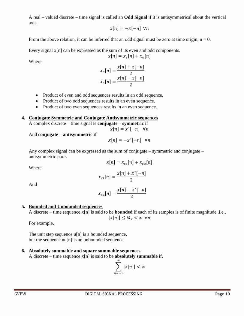
A real – valued discrete – time signal is called an Odd Signal if it is antisymmetrical about the vertical

axis.

𝑥[𝑛] = −𝑥[−𝑛] ∀𝑛

From the above relation, it can be inferred that an odd signal must be zero at time origin, n = 0.

Every signal x[n] can be expressed as the sum of its even and odd components.

𝑥[𝑛] = 𝑥𝑒[𝑛] + 𝑥𝑜[𝑛] Where

𝑥𝑒[𝑛] =𝑥[𝑛] + 𝑥[−𝑛]

2

𝑥𝑜[𝑛] =𝑥[𝑛] − 𝑥[−𝑛]

2

• Product of even and odd sequences results in an odd sequence.

• Product of two odd sequences results in an even sequence.

• Product of two even sequences results in an even sequence.

4. Conjugate Symmetric and Conjugate Antisymmetric sequences

A complex discrete – time signal is conjugate – symmetric if

𝑥[𝑛] = 𝑥∗[−𝑛] ∀𝑛

And conjugate – antisymmetric if

𝑥[𝑛] = −𝑥∗[−𝑛] ∀𝑛

Any complex signal can be expressed as the sum of conjugate – symmetric and conjugate –

antisymmetric parts

𝑥[𝑛] = 𝑥𝑐𝑠[𝑛] + 𝑥𝑐𝑎[𝑛] Where

𝑥𝑐𝑠[𝑛] =𝑥[𝑛] + 𝑥∗[−𝑛]

2

And

𝑥𝑐𝑎[𝑛] =𝑥[𝑛] − 𝑥∗[−𝑛]

2

5. Bounded and Unbounded sequences

A discrete – time sequence x[n] is said to be bounded if each of its samples is of finite magnitude .i.e., |𝑥[𝑛]| ≤ 𝑀𝑥 < ∞ ∀𝑛

For example,

The unit step sequence u[n] is a bounded sequence,

but the sequence nu[n] is an unbounded sequence.

6. Absolutely summable and square summable sequences

A discrete – time sequence x[n] is said to be absolutely summable if,

∑ |𝑥[𝑛]|

∞

𝑛=−∞

< ∞


And it is said to be square summable if

∑ |𝑥[𝑛]|2

∞

𝑛=−∞

< ∞ (𝑬𝒏𝒆𝒓𝒈𝒚 𝑺𝒊𝒈𝒏𝒂𝒍)

Discrete – Time Systems

A system accepts an input such as voltage, displacement, etc. and produces an output in response to this input.

A system can be viewed as a process that results in transforming input signals into output signals.

A discrete – time system can be represented as

𝑥[𝑛] → 𝑦[𝑛] 𝑜𝑟, 𝑦[𝑛] = 𝑇 {𝑥[𝑛]}

Discrete – Time System Properties

1. Linearity

A system is said to be linear if it satisfies superposition principle, which in turn is a combination of

additivity and homogeneity.

Additivity implies that

If the response of the DT system to x1[n] is y1[n], and the response to x2[n] is y2[n], then

the response of the system to {x1[n]+x2[n]} must be {y1[n]+y2[n]}.

Homogeneity implies that

if the response of a DT system to x[n] is y[n], then the response of the system to ax[n] must be ay[n],

where a is a constant.

Thus, for a DT system,

If

𝑥[𝑛] → 𝑦[𝑛] 𝑥1[𝑛] → 𝑦1[𝑛]

𝑎𝑛𝑑, 𝑥2[𝑛] → 𝑦2[𝑛] Then according to additivity principle

𝑥1[𝑛] + 𝑥2[𝑛] → 𝑦1[𝑛] + 𝑦2[𝑛] And according to homogeneity principle

𝑎𝑥[𝑛] → 𝑎𝑦[𝑛] (𝑎 = 𝑐𝑜𝑛𝑠𝑡𝑎𝑛𝑡)

• If a = 0, then the above relation implies that a zero input must result in a zero output.

Combining the above two principle to get superposition principle, we obtain

A system is Linear if it satisfies the following relation

𝑎𝑥1[𝑛] + 𝑏𝑥2[𝑛] → 𝑎𝑦1[𝑛] + 𝑏𝑦2[𝑛] (𝑎, 𝑏 = 𝑐𝑜𝑛𝑠𝑡𝑎𝑛𝑡𝑠)

Discrete - Time Input Signal, x[n]

Discrete - Time System

Discrete - Time Output signal, y[n]


2. Time – Variant and Time – Invariant Systems

A system is time – invariant if its characteristics and behavior are fixed over time .i.e., a time – shift in

input signal causes an identical time – shift in output signal.

𝑖𝑓 𝑥[𝑛] → 𝑦[𝑛] 𝑡ℎ𝑒𝑛, 𝑥[𝑛 − 𝑛0] → 𝑦[𝑛 − 𝑛0] ∀ 𝑛0

If the above the relation is not satisfied, then the system is time – variant.

3. Causal and Non – causal Systems

A system is causal or non – anticipatory or physically realizable, if the output at any time n0 depends

only on present and past inputs (n < n0), but not on future inputs.

In other words, if the inputs are equal upto some time n0, the corresponding outputs must also be equal

upto that time n0, for a causal system.

4. Stable and unstable systems

A stable system is one in which, a bounded input results in a response that does not diverge. Then the

system is said to be BIBO stable.

For a system, if the input is bounded .i.e,

𝑖𝑓 |𝑥[𝑛]| ≤ 𝑀𝑥 < ∞ ∀𝑛

And if the corresponding output is also bounded .i.e., |𝑦[𝑛]| ≤ 𝑀𝑦 < ∞ ∀𝑛

Then the system is said to be BIBO stable.

5. Memory and memoryless systems

A system is said to possess memory, or is called a dynamic system, if its output depends on past or

future values of the input.

If the output of the system depends only on the present input, the system is said to be memoryless.

6. Invertible systems

A system is said to be invertible if by observing the output, we can determine its input. i.e., we can

construct an inverse system that when cascaded with the given system, yields an output equal to the

original input.

A system can have inverse if distinct inputs lead to distinct outputs.

7. Passive and lossless systems

A system is said to be passive if the output y[n] has at most the same energy as the input.

∑ |𝑥[𝑛]|2

∞

𝑛=−∞

≤ ∑ |𝑦[𝑛]|2

∞

𝑛=−∞

< ∞

If the energy of the output is equal to the energy of the input, then the system is said to be lossless.

Properties of Unit Impulse Sequence

Multiplication property

When a sequence x[n] is multiplied by a unit impulse located at k i.e., δ[n-k], picks out a single value/sample of

x[n] at the location of the impulse i.e., x[k].

𝑥[𝑛]𝛿[𝑛 − 𝑘] = 𝑥[𝑘]𝛿[𝑛 − 𝑘] = 𝑖𝑚𝑝𝑢𝑙𝑠𝑒 𝑤𝑖𝑡ℎ 𝑠𝑡𝑟𝑒𝑛𝑔𝑡ℎ 𝑥[𝑘]𝑙𝑜𝑐𝑎𝑡𝑒𝑑 𝑎𝑡 𝑛 = 𝑘


Sifting property

The impulse function δ[n-k] “sifts” through the function x[n] and pulls out the value x[k]

∑ 𝑥[𝑛]𝛿[𝑛 − 𝑘]

∞

𝑛=−∞

= 𝑥[𝑘]

Signal decomposition

Any arbitrary sequence x[n] can be expressed as a weighted sum of shifted impulses.

𝑥[𝑛] = ∑ 𝑥[𝑘]

∞

𝑘=−∞

𝛿[𝑛 − 𝑘]

Impulse response

Impulse response of a discrete – time system is defined as the output/response of the system to unit impulse

input and is represented by h[n].

If for a system,

𝑥[𝑛] → 𝑦[𝑛] Then,

𝛿[𝑛] → ℎ[𝑛] If the DT system satisfies the property of time – invariance, then,

𝛿[𝑛 − 𝑘] → ℎ[𝑛 − 𝑘] In addition to being time – invariant, if the system also satisfies linearity (homogeneity and additivity), then,

Homogeneity:

𝑥[𝑘]𝛿[𝑛 − 𝑘] → 𝑥[𝑘]ℎ[𝑛 − 𝑘]

Additivity:

∑ 𝛿[𝑛 − 𝑘]

∞

𝑘=−∞

→ ∑ ℎ[𝑛 − 𝑘]

∞

𝑘=−∞

Combining the above two properties, a Linear Time – Invariant (LTI) System can be described by the input –

output relation by

∑ 𝑥[𝑘]𝛿[𝑛 − 𝑘]

∞

𝑘=−∞

→ ∑ 𝑥[𝑘]ℎ[𝑛 − 𝑘]

∞

𝑘=−∞

The Left hand side is the input x[n] expressed as a weighted sum of shifted impulses (from signal

decomposition property of impulse function). So, the right hand side must be the output y[n] of the DT system

in response to input x[n].

Discrete - Time unit impulse, δ[n]

Discrete - Time System

impulse response, h[n]


Thus the output of a Linear Time – Invariant (LTI) system can be expressed as

𝑦[𝑛] = ∑ 𝑥[𝑘]ℎ[𝑛 − 𝑘]

∞

𝑘=−∞

𝑜𝑟, 𝑦[𝑛] = 𝑥[𝑛] ∗ ℎ[𝑛]

The above relation is called Convolution Sum.

So, the impulse response h[n] of an LTI DT system completely characterizes the system .i.e., a knowledge of

h[n] is sufficient to obtain the response of an LTI system to any arbitrary input x[n].

Properties of Convolution Sum

1. Commutative Property

𝑥[𝑛] ∗ ℎ[𝑛] = ℎ[𝑛] ∗ 𝑥[𝑛]

x[n] x[n] * h[n] ≡ h[n] h[n] * x[n]

2. Associative Property

𝑥[𝑛] ∗ {ℎ1[𝑛] ∗ ℎ2[𝑛]} = {𝑥[𝑛] ∗ ℎ1[𝑛]} ∗ ℎ2[𝑛]

x[n] y[n] ≡ x[n] y[n]

From this property it can be inferred that, a cascade combination of LTI systems can be replaced by a

single system whose impulse response is the convolution of the individual impulse responses.

3. Distributive Property

𝑥[𝑛] ∗ {ℎ1[𝑛] + ℎ2[𝑛]} = {𝑥[𝑛] ∗ ℎ1[𝑛]} + {𝑥[𝑛] ∗ ℎ2[𝑛]}

x[n] y[n] ≡ x[n] y[n]

From this property, it can be inferred that, a parallel combination of LTI systems can be replaced by a

single system whose impulse response is the sum of individual responses.

input, x[n]LTI System,

h[n]output,

y[n] = x[n] * h[n]

h[n] x[n]

h1[n] h2[n] h1[n]*h2[n]

h1[n]

h2[n]

h1[n] + h2[n]


Relation between LTI system properties and impulse response

Memory

For an LTI system to be memoryless, the impulse response must be zero for nonzero sample positions.

ℎ[𝑛] = 0 𝑓𝑜𝑟 𝑛 ≠ 0

ℎ[𝑛] = 𝑘 𝛿 [𝑛] 𝑤ℎ𝑒𝑟𝑒 𝑘 = 𝑐𝑜𝑛𝑠𝑡𝑎𝑛𝑡

Causality

For an LTI system to be causal, its impulse response must be zero for negative time instants.

ℎ[𝑛] = 0 𝑓𝑜𝑟 𝑛 < 0

So, for a causal LTI system the output (from the convolution sum equation) can be expressed as

𝑦[𝑛] = ∑ ℎ[𝑘]𝑥[𝑛 − 𝑘]

∞

𝑘=0

𝑜𝑟, 𝑦[𝑛] = ∑ 𝑥[𝑘]ℎ[𝑛 − 𝑘]

𝑛

𝑘=−∞

Stability

An LTI system is BIBO stable if its impulse response is absolutely summable.

∑ |ℎ[𝑘]|

∞

𝑘=−∞

< ∞

Invertibility

An LTI system with impulse response h[n] is invertible if we can design another LTI system with

impulse response hI[n] such that

ℎ[𝑛] ∗ ℎ𝐼[𝑛] = 𝛿 [𝑛]

LTI systems characterized by Linear Constant – Coefficient Difference Equations (LCCDE)

In general, any LTI system with input x[n] and output y[n] can be described by an LCCDE as follows

∑ 𝑎𝑘𝑦[𝑛 − 𝑘]

𝑁

𝑘=0

= ∑ 𝑏𝑘𝑥[𝑛 − 𝑘]

𝑀

𝑘=0

, 𝑎0 ≡ 1

𝑜𝑟, 𝑦[𝑛] = − ∑ 𝑎𝑘𝑦[𝑛 − 𝑘]

𝑁

𝑘=1

+ ∑ 𝑏𝑙𝑥[𝑛 − 𝑙]

𝑀

𝑙=0


Where N is called the order of the difference equation/ system.

This equation expresses the output of an LTI system at time n in terms of present and past inputs and

past outputs.

Solution of LCCDE (Direct Solution – Solution in time domain)

Given an LCCDE, the goal is to determine the output y[n], n> 0 given a specific input x[n], n > 0, and a

set of initial conditions.

The total solution of the LCCDE is assumed to be the sum of two parts:

Homogeneous/complementary solution, yH[n] and

Particular solution, yP[n]

Homogeneous Solution

The homogeneous difference equation is obtained by substituting input x[n]=0 in the LCCDE.

∑ 𝑎𝑘𝑦[𝑛 − 𝑘]

𝑁

𝑘=0

= 0 − − − − − −𝐸𝑞. 1

The solution to this homogeneous equation is assumed to be in the form of an exponential .i.e.,

𝑦ℎ[𝑛] = 𝜆𝑛 − − − − − −𝐸𝑞. 2

Substituting Eq. 2 in Eq. 1, we obtain

∑ 𝑎𝑘𝜆𝑛−𝑘

𝑁

𝑘=0

= 0 , 𝑎0 = 1

Expanding this equation

𝜆𝑛−𝑁(𝜆𝑁 + 𝑎1𝜆𝑁−1 + 𝑎2𝜆𝑁−2 + ⋯ ⋯ + 𝑎𝑁−1𝜆 + 𝑎𝑁) = 0

The polynomial in the parenthesis is called the characteristic polynomial of the system.

The characteristic equation is given by

𝜆𝑁 + 𝑎1𝜆𝑁−1 + 𝑎2𝜆𝑁−2 + ⋯ ⋯ + 𝑎𝑁−1𝜆 + 𝑎𝑁 = 0

Its solution has N roots denoted by λ1, λ2, …, λN, which can be real or complex.

Complex valued roots occur as complex conjugate pairs.

If some roots are identical, then we have multiple order roots.


If all roots are distinct, then the general solution is given by

𝑦𝐻[𝑛] = 𝐶1𝜆1𝑛 + 𝐶2𝜆2

𝑛 + ⋯ ⋯ + 𝐶𝑁𝜆𝑁𝑛

C1, C2, … , CN are weighting coefficients.

For multiple order roots, if λ1 repeats m times, then the solution is given by

𝑦𝐻[𝑛] = 𝐶1𝜆1𝑛 + 𝐶2𝑛𝜆1

𝑛 + 𝐶3𝑛2𝜆1𝑛

⋯ ⋯ + 𝐶𝑚𝑛𝑚−1𝜆1𝑛

+ 𝐶𝑚+1𝜆2𝑛 + 𝐶𝑚+2𝜆3

𝑛 + ⋯ 𝐶𝑁𝜆𝑁𝑛

Particular solution

The particular solution must satisfy the LCCDE for the specific input signal x[n], n > 0 .

We assume a form for yP[n] that depends on the form of the input x[n] as follows

Input, x[n] Particular solution, yP[n]

Constant, A Constant, K

A Mn KMn

AnM K0nM + K1n

M-1+…+KM

AnnM An(K0nM+K1n

M-1+…+KM)

A cos ω0n K1 cos ω0n + K2 sin ω0n

A sin ω0n

If the particular solution, yP [n] has the same form as the homogeneous solution yH [n], we multiply

yP[n] with n or n2 or n3 so that it is different from yH[n].

Total solution y[n] = yH[n]+yP[n]

The total solution will contain {Ci}s from the homogeneous solution. They are determined by

substituting the given initial conditions in the total solution.

Frequency domain representation of discrete time signals

The concept of frequency is closely related to a specific type of periodic motion called harmonic oscillation,

which is described by sinusoidal functions. The CT and DT sinusoidal signals are characterized by the

following properties:

1. A continuous time sinusoid x(t) = cos (2πfat) is periodic for any value of fa.

But for DT sinusoid x[n]=cos(2πfdn) to be periodic with period N (an integer), we require

cos(2𝜋𝑓𝑑𝑛) = cos[2𝜋𝑓𝑑(𝑛 + 𝑁)] = cos (2𝜋𝑓𝑑𝑛 + 2𝜋𝑓𝑑𝑁)

This is possible only if

2𝜋𝑓𝑑𝑁 = 2𝜋𝑘 (𝑘 𝑖𝑠 𝑎𝑛 𝑖𝑛𝑡𝑒𝑔𝑒𝑟)


Or

𝑓𝑑 =𝑘

𝑁

i.e., the discrete frequency fd must be a rational number (ratio of two integers).

Similarly, a discrete time exponential ejωn is periodic only if 𝜔

2𝜋= 𝑓𝑑 = 𝑟𝑎𝑡𝑖𝑜𝑛𝑎𝑙 𝑛𝑢𝑚𝑏𝑒𝑟.

The period is the denominator after 𝜔

2𝜋 is simplified such that in

𝜔

2𝜋=

𝑘

𝑁, k and N are relatively prime.

2. A CT sinusoidal signal x(t) = cos(Ωt) has a unique waveform for every value of Ω, 0 < Ω < ∞.

Increasing Ω results in a sinusoidal signal of ever – increasing frequency.

But, for a DT sinusoidal signal cos (ωn), considering two frequencies separated by an integer multiple of

2π, (ω and ω + 2πm, m is an integer), we have

cos[(𝜔 ± 2𝜋𝑚)𝑛] = cos (𝜔𝑛 ± 2𝜋𝑚𝑛)

Since m and n are both integers

cos(𝜔𝑛 ± 2𝜋𝑚𝑛) = cos (𝜔𝑛)

So, a DT sinusoidal sequence has unique waveform only for the values of ω over a range of 2π. The

range −𝜋 ≤ 𝜔 ≤ 𝜋 defines the fundamental range of frequencies or principal range.

3. The highest rate of oscillation in a DT sinusoidal sequence is attained when ω=π or ω= - π . the rate of

oscillation increases continually as ω increases from 0 to π, then decreases as ω increases from π to 2π.

So low – frequency DT sine waves have ω near 0 or any even multiple of π, while the high – frequency

sine waves have ω near + π or other odd multiples of π.

Frequency domain representation of discrete time systems

The frequency response function completely characterizes a linear time invariant system in the frequency

domain. Since, most signals can be expressed in Fourier domain as a weighted sum of harmonically related

exponentials, the response of an LTI system to this class of signals can be easily determined.

The response of any relaxed LTI system to an arbitrary input signal x[n] is given by the convolution sum

𝑦[𝑛] = ∑ ℎ[𝑘]𝑥[𝑛 − 𝑘]

∞

𝑘=−∞

Here, the system is characterized in the time domain by its impulse response h[n]. to develop a frequency

domain characterization of the system, we excite the system with the complex exponential

𝑥[𝑛] = 𝐴𝑒𝑗𝜔𝑛 , −∞ < 𝑛 < ∞

Where A is the amplitude and ω is any arbitrary frequency confined to the frequency interval [ - π, π ]. By

substituting this in the above convolution sum, we obtain the response as


𝑦[𝑛] = ∑ ℎ[𝑘][𝐴𝑒𝑗𝜔(𝑛−𝑘)]

∞

𝑘=−∞

= 𝐴 [ ∑ ℎ(𝑘)𝑒−𝑗𝜔𝑘

∞

𝑘=−∞

] 𝑒𝑗𝜔𝑛

Here, the term inside the brackets is a function of frequency ω. It is the Fourier Transform of the impulse

response h[n], and is denoted by

𝐻(𝜔) = ∑ ℎ(𝑘)𝑒−𝑗𝜔𝑘

∞

𝑘=−∞

And 𝑦[𝑛] = 𝐴𝐻(𝜔) 𝑒𝑗𝜔𝑛

Since the output differs from the input only by a constant multiplicative factor, the exponential input signal is

called the eigen function of the system, and the multiplicative factor is called the eigenvalue of the system.

H(ω) is a complex valued function of the frequency variable ω.

LECTURE NOTES ON DIGITAL SIGNAL PROCESSING III B ...

Documents

Transcript of LECTURE NOTES ON DIGITAL SIGNAL PROCESSING III B ...