NNT : 2016SACLS272

THÈSE DE DOCTORAT DE

L’UNIVERSITÉ PARIS-SACLAY

PRÉPARÉE À

L’UNIVERSITÉ PARIS-SUD

AU SEIN DU LABORATOIRE AIMÉ COTTON,

EN COLLABORATION AVEC L’ORGANISATION EUROPÉENNE POUR LA

RECHERCHE NUCLÉAIRE (CERN)

ÉCOLE DOCTORALE N° 572

Ondes et Matières

Spécialité de doctorat : Physique quantique

Par

Mme Pauline Yzombard

Laser cooling and manipulation of antimatter in the AEgIS experiment

Thèse présentée et soutenue à Orsay le 24 novembre 2016

Composition du Jury :

Dr. Lunney David Directeur de recherche au Centre de Sciences Président

Nucléaires et de Sciences de la Matière, CNRS, France

Dr. Ulmer Stefan Initiative researcher at the Ulmer Initiative Research Unit, RIKEN, Japan Rapporteur

Dr. Karr Jean-Philippe Maitre de conférence à l’Université d'Evry - Val d'Essonne, France Rapporteur

Dr. Madsen Niels Senior lecturer at the Swansea University, UK. Examinateur

Dr. Crivelli Paolo Senior scientist at Laboratory of Positron & Positronium Physics Examinateur

- Switzerland

Dr. Comparat Daniel Directeur de recherche au laboratoire Aimé Cotton, CNRS, France Directeur de thèse

Dr. Doser Michael Senior research physicist at CERN, Switzerland Invité

Laser cooling and manipulation of Antimatter

in the AEgIS experiment

Pauline Yzombard

Laboratoire Aimé Cotton, Campus d'Orsay, 91405 Orsay cedex, France

Acknowledgments -

Remerciements

Faisant l'inventaire de toutes les personnes qui m'ont accompagnées lorsde cette aventure et que j'aimerais tant remercier, j'ai pris la pleine mesurema chance de vous avoir tout autour ! Commençons par mon cher directeurde thèse, Daniel, qui a eu la patience de répondre à ma dizaine d'e-mails an-goissés quotidiens. J'aime à penser que nous avons accompli un beau travailensemble. Un grand merci à Michael et à toute l'équipe cernoise d'AEgIS,qui m'ont acceuillie sans condition: thanks a lot Stefan, thanks to you thecryogenics has no more secrets for me, grazie Seba per tutte le pause per iltè che abbiamo preso fuori ! How can I thank the AEgIS people withoutmentioning Ingrid, my dearest tea-breaker, Ine, BenJ, Ola, Lisa, Laura andLillian, the famous positron dream-team crew. Grazie mille alla squadra lasere positroni italiana: Ruggero, Zeudi-cara, Gemma, Daniel K ! A little winkto Ingmari, Olga, Sameed, Giancarlo, Nicola and Angela. Thanks to youguys, I spent three amazing years working with you in such a "challenging"(thank you Lillian) experiment, that made me become a better physicist anda better person I believe. As Seba likes saying: "what did you do today ?Well, I've saved the world and xed my apparatus...".

En parlant de sauver le monde, je remercie absolument mes parents quim'ont toujours soutenue jusque dans mes choix les plus saugrenus (étudierl'antimatière en Suisse ? Bien sûr ma chérie, fonce !). Et que dire de mongrand-frère et de sa constante présence ! Merci Julien pour toutes ces soiréesjeux ensemble, relâcher la pression et poser le cerveau pour une heure oudeux sur un jeu vidéo, ça fait un tel bien ! Moi aussi je suis ère d'être tasoeur !

Enn, un grand merci à tous mes amis, de tous bords. Les "supops", bellebande de physiciens/ingénieurs en devenir il y a trois ans, nous voici tousgrands et face au choix existentiel de se trouver un "vrai" boulot, un autre

i

boulot, ici ou ailleurs ! Merci ma Louise, nos échanges acharnés d'e-mails ontété une vraie bouée d'air, bisous à BenJ et son dèle soutien pour l'anti-c∗,bisous à voisine Aurélie, Sandra, binôme Delphine, Margaux, binôme So-phie, Cyrille, Sean&Aurore, Jerem et Clem', Marie-Aude, nos retrouvaillessont toujours aussi belles ! J'en prote pour embrasser aussi les amis du Sud,si bien nommés, Cynthi-puce et Seb, les années ne nous ont pas éloignées,loin de là! Et les nouveaux amis: Chloé& Stephan, Lucas & Céline, Simon,Marissa & Mat, merci pour ces soirées jeux, escapes games, et apéro cagoles !

As proper experimental physicists, we did try once to count the num-ber of dierent "`thank you" we learned in contact to the people of CERN,Seba and I. I think this is the proper time to repeat the experiment, withoutgoogle-translate! Thanks, grazie, tuk (?!), danke schön, aligato, obrigado,spasiba, gracias, choukrane, xie-xie, merci pour tout !

Pauline

ii

Contents

1 A Ph.D thesis in the AEgIS collaboration - about lasers andantimatter 2

I Positronium physics and experiments 5

2 Positronium: an exotic atom 72.1 Positronium: an hydrogenoid atom . . . . . . . . . . . . . . . 72.2 Positronium lifetimes: radiation process versus annihilation

process . . . . . . . . . . . . . . . . . . . . . . . . . . . . . . . 10

3 Positronium production in AEgIS 153.1 Positronium production . . . . . . . . . . . . . . . . . . . . . 153.2 The positron system of AEgIS - setup description . . . . . . . 17

3.2.1 The source and moderator . . . . . . . . . . . . . . . . 173.2.2 The rst Surko trap . . . . . . . . . . . . . . . . . . . 183.2.3 The accumulator . . . . . . . . . . . . . . . . . . . . . 193.2.4 The transfer line and the buncher. . . . . . . . . . . . . 203.2.5 The test chamber . . . . . . . . . . . . . . . . . . . . . 223.2.6 Ps detections . . . . . . . . . . . . . . . . . . . . . . . 23

4 Positronium laser excitation 264.1 Ps laser excitations - latest results . . . . . . . . . . . . . . . . 264.2 Ps laser excitations - main interests for AEgIS experiment . . 274.3 The laser system in AEgIS - setup description . . . . . . . . . 30

5 Experimental results of Ps laser excitation 375.1 The Ps n=3 laser excitation measurements . . . . . . . . . . . 38

5.1.1 The signal diagnostics . . . . . . . . . . . . . . . . . 385.1.2 The measurements settings . . . . . . . . . . . . . . . 405.1.3 Results . . . . . . . . . . . . . . . . . . . . . . . . . . . 41

iii

5.1.4 A quick analysis of the n=3 excitation signal obtained 425.2 A Doppler scan of the Ps cloud spectral line . . . . . . . . . . 445.3 The saturation regime - verication measurements . . . . . . . 465.4 Rydberg Ps excitation . . . . . . . . . . . . . . . . . . . . . . 475.5 Summary of the experimental results and short prospect . . . 48

6 Simulations analysis 506.1 The case of high saturation photoionization regime - a simple

solution . . . . . . . . . . . . . . . . . . . . . . . . . . . . . . 526.2 High photoionization regime: studies of the Doppler Scan and

UV saturation measurements . . . . . . . . . . . . . . . . . . 536.2.1 The geometrical coecient η . . . . . . . . . . . . . . . 546.2.2 The photoionization probability . . . . . . . . . . . . . 55

6.3 The n=3 laser at resonance and at saturation - study of thephotoionization saturation . . . . . . . . . . . . . . . . . . . . 56

II A possible positronium laser cooling ? Theoreticaland simulations studies 58

7 Ps Doppler laser cooling - theory 617.1 Laser cooling of an open two-level system . . . . . . . . . . . . 62

7.1.1 The rate equations . . . . . . . . . . . . . . . . . . . . 647.1.2 The excitation rate formula . . . . . . . . . . . . . . . 647.1.3 The steady-state regime for short interaction time . . . 657.1.4 For long interaction times . . . . . . . . . . . . . . . . 66

7.2 The scattering rate . . . . . . . . . . . . . . . . . . . . . . . . 687.3 Toward the force resulting of the laser-atom interaction . . . 68

7.3.1 A possible laser broadening of for the narrow-line tran-sition of the Positronium ? . . . . . . . . . . . . . . . . 71

7.4 The Ps laser cooling, which formalism ? . . . . . . . . . . . . . 72

8 Positronium laser cooling - simulations 748.1 The simulation C++ code - the optical pumping code . . . . . 76

8.1.1 The input les . . . . . . . . . . . . . . . . . . . . . . . 768.1.2 The outputs . . . . . . . . . . . . . . . . . . . . . . . . 78

8.2 Doppler laser cooling of Ps - Some simulation results . . . . . 798.2.1 In the absence of magnetic eld . . . . . . . . . . . . . 818.2.2 In the presence of a magnetic eld . . . . . . . . . . . 928.2.3 What is the eect of a 1D laser cooling on the velocities

of the other directions. . . . . . . . . . . . . . . . . . . 98

iv

8.2.4 What is the eect on the Ps positions of the 1D coolingalong the z axis ? . . . . . . . . . . . . . . . . . . . . 98

8.3 Conclusion and prospective . . . . . . . . . . . . . . . . . . . 100

9 The Orsay laser system for the Doppler laser cooling of Ps 1049.1 Description of the current system . . . . . . . . . . . . . . . . 104

9.1.1 The red-laser beam . . . . . . . . . . . . . . . . . . . . 1099.1.2 The 243-nm beam . . . . . . . . . . . . . . . . . . . . . 109

9.2 Stretching the UV pulse . . . . . . . . . . . . . . . . . . . . . 1119.2.1 The ber setup . . . . . . . . . . . . . . . . . . . . . . 1129.2.2 Loss cavity using beam splitter . . . . . . . . . . . . . 1169.2.3 The loss cavity setup using polarization cube . . . . . . 1189.2.4 Current situation of the Orsay laser . . . . . . . . . . . 122

10 Another way to focus of the Ps cloud? The dipolar forceinteraction 12310.1 The dipolar force interaction principle . . . . . . . . . . . . . . 12310.2 The dipolar force on a single atom . . . . . . . . . . . . . . . . 12910.3 Some results . . . . . . . . . . . . . . . . . . . . . . . . . . . . 13010.4 The dipolar force's eect on the Gaussian distributions of Ps

cloud . . . . . . . . . . . . . . . . . . . . . . . . . . . . . . . . 133

11 Short summary of the Ps studies and prospective 139

III Antiprotons manipulations and cooling studies 141

12 The AEgIS main apparatus - the traps description and plasmabehaviors 14412.1 The choice of Penning-Malmberg traps . . . . . . . . . . . . . 145

12.1.1 The ideal Penning trap . . . . . . . . . . . . . . . . . . 14512.1.2 The cylindrical-shape Penning trap alternative . . . . . 14612.1.3 The Penning-Malmberg trap . . . . . . . . . . . . . . . 14812.1.4 The AEgIS apparatus . . . . . . . . . . . . . . . . . . 149

12.2 The 4.5 T Penning-Malmberg trap - the catching system . . . 15012.3 The 1 T Penning-Malmberg trap . . . . . . . . . . . . . . . . 151

13 The 2014 and 2015 beamtimes - some results about the cool-ing and compression of the p plasma 15413.1 Electron cooling and rotating walls techniques . . . . . . . . . 15613.2 The diagnostics . . . . . . . . . . . . . . . . . . . . . . . . . . 15713.3 Results on p plasma compression . . . . . . . . . . . . . . . . 159

v

13.3.1 Procedure 0: loading and cooling of electrons - Study:RW applied on electron plasma only. . . . . . . . . . . 159

13.3.2 Procedure 1: catching and cooling of antiprotons -Study: centrifugal separation vs heating plasmas byRW drive. . . . . . . . . . . . . . . . . . . . . . . . . . 161

13.3.3 Procedure 2: a second faster RW applied once the an-tiprotons are cooled. . . . . . . . . . . . . . . . . . . . 165

13.3.4 Procedure 3: a third RW stage, with a reduced numberof electrons . . . . . . . . . . . . . . . . . . . . . . . . 168

13.3.5 Procedure 4: toward a fourth RW stage and highercompressions of e− and p . . . . . . . . . . . . . . . . 170

13.4 Summary . . . . . . . . . . . . . . . . . . . . . . . . . . . . . 171

14 Toward a sympathetic cooling of antiprotons - the laser cool-ing of molecular anions 17314.1 A possible laser cooling of anions to sympathetically cool an-

tiprotons in AEgIS . . . . . . . . . . . . . . . . . . . . . . . . 17614.2 The C−

2 molecule . . . . . . . . . . . . . . . . . . . . . . . . . 17714.3 The rst scheme: Doppler cooling over X ↔ B transition . . . 179

14.3.1 The 3D optical molasses . . . . . . . . . . . . . . . . . 17914.3.2 In a Paul trap . . . . . . . . . . . . . . . . . . . . . . . 182

14.4 The second scheme: Sisyphus cooling over X ↔ A transition . 18414.4.1 The simplest scheme with 3 lasers . . . . . . . . . . . . 18714.4.2 With repumping lasers on the vibrational state X(v=1)188

14.5 Conclusion . . . . . . . . . . . . . . . . . . . . . . . . . . . . . 189

15 Conclusion and perspective 191

A Hydrogenoid atoms: scaling relations between Hydrogen andPositronium atom 193A.1 General description . . . . . . . . . . . . . . . . . . . . . . . . 193

A.1.1 The positronium model . . . . . . . . . . . . . . . . . . 195A.2 The time independent Schrödinger equation . . . . . . . . . . 195

A.2.1 For a reduced particle µ . . . . . . . . . . . . . . . . . 195A.2.2 The 1D-Schrodinger equation . . . . . . . . . . . . . . 197A.2.3 Scaling relation between Ps and H atoms . . . . . . . . 198

A.3 Scaling relations - prospective . . . . . . . . . . . . . . . . . . 199

B Photoionization probability for a 3-level system 200B.1 An exact solution . . . . . . . . . . . . . . . . . . . . . . . . . 200B.2 The high saturation hypothesis to simplify the formula . . . . 201

vi

B.3 Approximations formula - determination of the validity con-ditions . . . . . . . . . . . . . . . . . . . . . . . . . . . . . . . 201

B.4 Verication of the approximation's validity made for our mea-surements analysis . . . . . . . . . . . . . . . . . . . . . . . . 202

B.5 The geometrical factor η approximation . . . . . . . . . . . . . 205

C Derivation of the internal energies of an hydrogenoid atom 209C.1 Q.E.D correction . . . . . . . . . . . . . . . . . . . . . . . . . 209C.2 Zeeman eect . . . . . . . . . . . . . . . . . . . . . . . . . . . 211C.3 Stark and Motional Stark eects . . . . . . . . . . . . . . . . . 211C.4 The dipole strength of an optical transition . . . . . . . . . . . 213

D Laser cooling on a broad-transition - the radiation pressureforce 214

D.0.1 The low saturation regime - s ≪ 1 . . . . . . . . . . . 216

1

Chapter 1

A Ph.D thesis in the AEgIS

collaboration - about lasers and

antimatter

Since its prediction by Dirac at the beginning of the past century and itsrst experimental discovery in 1933 by Anderson [1], antimatter has gener-ated great interest and triggered multiple studies, among which experimentaltests on the QED theory [2], the Charge, Parity and Time Reversal (CPT)theorem or the Weak Equivalence Principle (WEP). The WEP states thatany body in a gravitational eld experiences the same acceleration, indepen-dent of its own composition. Several experiments have been carried out andhave veried the WEP at 10−13 accuracy for ordinary matter [3]. But thequestion is still open for antimatter. Some experiments [4, 5] and theoret-ical discussions such as [6] infer that the WEP should hold for antimatter.However, this statement relies on theoretical assumptions and indirect ar-guments, and some attempts to model a quantum gravity theory tend topredict a possible violation of the WEP for antimatter [7]. That's why fur-ther tests of the WEP are still required. In order to try to answer the debate,one promising possibility is to perform a direct measurement of the eect ofgravity on antimatter.

As the unique source of low energy antiprotons in the world, the An-tiproton Decelerator (AD) facility at CERN has provided bunches of tensof millions cold antiprotons (5.3 MeV p) for more than a decade. In 2002,the rst cold antihydrogen atoms were produced [8, 9]. Since then, a trap-ping technique has been developed to catch small numbers of H for severalminutes [10]. These advances have opened paths for systematic studies ofantimatter properties, such as atomic spectroscopy [11] or gravity tests [12].

2

Like the GBAR experiment [13] or the recent ALPHA-g project [14], theAEgIS collaboration [15] - Antihydrogen Experiment: Gravity, Interferome-try, Spectroscopy - wants to investigate the eect of gravity on antimatter.More specically, AEgIS aims to measure the deection of a cold antihydro-gen beam under Earth's gravitational eld in order to perform a direct testof the WEP.

The AEgIS collaboration plans to form antihydrogen atoms using a charge-exchange process between trapped antiprotons and a Rydberg0 excited positro-nium (Ps∗) cloud:

Ps∗ + p→ (e+ + p)∗ + e− = H∗ + e− (1.1)

The creation of antihydrogen via Ps charge-exchange has already beenrealized by the ATRAP collaboration [16] in 2004. In their system, the ex-citation of Ps toward a Rydberg state was performed using Rydberg cesiumatoms Cs∗. The Cs∗ excited by laser collide with the e+ cloud, and form Psatoms into Rydberg states. Contrary to the double charge exchange processesused by ATRAP, AEgIS rather plans to directly laser excite the positroniumcloud, in order to be able to control the Rydberg states of the Ps atoms.

I started my mission in AEgIS as a master student of the laboratoire AiméCotton, for studying the feasibility of laser cooling the positronium, in orderto enhance the antihydrogen formation via charge exchange. I continued thisproject within my Ph.D project, where it was decided that I would workfull-time at CERN in order to supervise the laser systems, and would takean active part in the daily experimental life of AEgIS.

Following the objectives I had to address during this Ph.D, this thesis isdivided in three parts:

Part I deals with the experimental results we obtained on the positron-ium atom. This rst part opens with physics properties and denitionof the Ps atom, in Chap. 2. Then, the rst observation of the laserexcitation of the Ps n=3 level, plus the demonstration of an ecienttwo-photon excitation path to reach the Ps Rydberg states are shownin Chap. 5. The description of the experimental setups used -positronsystem (Chap. 3) and laser system (Chap. 4)- as well as simulationsto analyze our results are also presented (Chap. 6).

0A Rydberg atom is an excited atom with one or more electrons that have a very highprincipal quantum number (n). In this work, we will consider that the electronic leveln ≥ 15 is a Rydberg state.

3

Part II is dedicated to theoretical studies and simulations of possiblelaser cooling of Ps. Doppler laser cooling is considered in Chap. 8,and some theory discussions about the feasibility of such a cooling arementioned in Chap. 7. In order to perform the rst experimental trials,an appropriate laser system needs to be developed. The Chap 9 dealswith the technical challenges to be tackled and the possible solutions wehave considered to improve the dye-laser system I installed at CERN,that presents suitable wavelengths for Doppler cooling. Finally, anotherlaser manipulation of the Ps cloud is studied, using the Dipolar force(Chap. 10). A small summary of the studies and experimental workperformed on the Ps atom is given in Chap. 11 and opens the path tothe third part on antiproton physics.

Part III is devoted to the work I took part regarding the manipulationsof antiprotons. The trapping system of AEgIS, where the catching,cooling and compression of antiproton plasma take place, is reviewedin Chap. 12. Some results of the beam-time of 2014 and 2015 aregiven in Chap. 13. Good compression is reachable with our trappingsystem which leads to a better stability of the conned p plasma andthus to better antihydrogen formation. However, cold antiprotons (∼100 mK) are still required to enhance drastically the charge exchangecross section [15, 17] and form a cold beam of antihydrogen, crucial forprecise gravity test. That's why nally, the idea of using laser cooledmolecular anions to sympathetically cool the antiprotons is discussedin Chap. 14, where the theoretical studies and simulations are shown.The conclusion and prospective of this Ph.D work are discussed inChap. 15

From these studies and experimental work, we published three articles[18, 19, 20]. Chapters 14, 5 and 3 respectively deal with the details of thesepublications.

4

Part I

Positronium physics and

experiments

5

The positronium (Ps) is a purely leptonic hydrogenoid atom formed by anelectron (e−) and its antiparticle, a positron (e+) bound together with a bind-ing energy of 6.8 eV. It is the lightest atom known, and it was experimentallydiscovered in 1951 by Deutsch [21].

As said in the introduction, Ps atom plays a major role in the AEgISexperiment since we plan to use Rydberg exited positronium to create anti-hydrogen, via a charge-exchange process with trapped antiprotons:

Ps∗ + p → (e+ + p)∗ + e−

Ps∗ + p → H∗ + e−(1.2)

The study of the Ps formation (emission cone, creation rate, temperature[22], etc.) as well as its spectroscopic properties [23, 24] is not only crucial forthe success of the AEgIS collaboration, but also of great interests for manyphysics studies, like QED tests [2, 25]. Indeed, the purely leptonic propertyof the positronium atom removes the corrections due to the nucleus (noquarks involved) and allows a direct measurement of the QED corrections.Positronium atoms are also an important tool for applied research, notablyin porous condensed matter [26].

In the following chapters, we will rst present a quick review of the Psphysics theory (chap.2), before describing the AEgIS experimental setup forPs formation (chap.3) and Ps laser excitation (chap.4). We will then presentsome of the latest results we obtained (chap.5), and discuss in the secondpart of this thesis, a possible laser cooling of Ps (Chap. 7).

6

Chapter 2

Positronium: an exotic atom

As Positronium binds a matter particle and its antimatter counterpart,this metastable atom has some interesting properties, and a short lifetime.Ps has two ground-states, corresponding to dierent congurations of spinsorientations of the electron and positron. The singlet state, with a total spinequal to zero, is called para-positronium (p-Ps). It has a short lifetime of125 ps in vacuum and annihilates in 2γ emission. The triplet state or ortho-positronium (o-Ps) corresponds to a total spin number equal to 1 and has alonger lifetime of 142 ns in vacuum. It annihilates in 3γ emission.

2.1 Positronium: an hydrogenoid atom

As positronium is an hydrogen-like atom, its physics is very well-knownand can be easily scaled from the Hydrogen physics. Indeed, in the reduced-mass framework, the reduced masses of a Hydrogen and a Ps are given by:

µ(H) = me (2.1)

µ(Ps) = 2×me (2.2)

µ(Ps) = 2× µ(H) (2.3)

where me is the mass of an electron (or of a positron).

Resulting from the factor 2 between the reduced masses of the two systems,one can easily derive4 the following relations:

Bohr radiusa(Ps)0 = 2× a(H)

0 (2.4)4A more detailed study is given in the Appendix A.

7

Hartree energy

E(Ps)Ha =

1

2E

(H)Ha (2.5)

Internal energy

E(Ps)n =

1

2E(H)

n (2.6)

Wave function

ψ(Ps)(E(Ps)n,l,m, r, θ, ϕ) =

1

2√2ψ(H)(2E

(H)n,l,m,

1

2r, θ, ϕ) (2.7)

electric dipoled(Ps)n1,n2

= 2× d(H)n1,n2

(2.8)

where the dipole electric (matrix element) is given by:

d(µ)n1,n2 = ⟨ψ(µ)

n1 | qe r | ψ(µ)n2 ⟩

=∫ψ(µ)(E

(µ)n1,l1,m1, r, θ, ϕ)× (qe r)× ψ(µ)(E

(µ)n2,l2,m2, r, θ, ϕ) r

2 dr dθ dϕ

(2.9)

spontaneous rate between | n, l,m⟩ and | n′, l′,m′⟩ states.

Γ(Ps) =1

2Γ(H) (2.10)

For instance, the last relation (2.10) can be derived using the proportion-ality relation Γ ∝ d2E3, where E is the energy dierence between thetwo states | n, l,m⟩ and | n′, l′,m′⟩.

These scaling relations make it possible to quickly calculate the internalenergy structures of Ps, in zero eld (cf. Fig 2.1). For example, the internalenergy of the transition between the triplet ground state of Ps and its rsttriplet excited state (n=2,l=1) is characterized by a wavelength of 243.1nm ; that is the double of the well-known wavelength of the Lyman alphatransition for Hydrogen (λLymanα = 121.6 nm). This assessment opens somegreat possibilities concerning the laser excitation studies, since the currenttechnologies provide more easily intense beams in the range of 243 nm thanin the UV-C range.

8

Figure 2.1: Ps and H internal energies sketches - scaling relations illustratedhere. Note that no ne nor hyperne structures are drawn. The spontaneousemission of the n=2 triplet (P) state is indicated by Γp

An important remark is that this scaling approach is only valid for theelectrostatic interaction. When considering the ne - hyperne structures ofH and Ps, the sub-level splitting diers not only in scale but also in generalstructure. For the hydrogen atom, the spin-orbit coupling dominates andgives the ne structure, whereas the spin(µe−)-spin(µp) interaction is muchsmaller and provides the hyperne splitting. For positronium, the large mag-netic moment of the positron (µe+ = µe− = 657µp) leads to a bigger spin-spininteraction, comparable to the spin-orbit interaction. In addition, as men-tioned in [27], "the electron-positron annihilation mechanism, acting virtu-ally, causes spin-dependent ne-structure shifts of the same order as thosecaused by magnetic spin-spin and spin-orbit interactions."

In Fig 2.2, a comparison of the n=1 and n=2 hyperne structures ofhydrogen and positronium is presented. For Ps, the distinction between neand hyperne structures is not as well dened as for the hydrogen.

9

Figure 2.2: Zoom on the ground and rst excited states' hyperne structures,for hydrogen and positronium atoms. The scaling considerations only workfor the electrostatic interaction framework ; once the spin-orbit and spin-spin interactions are taken into account, the unique nature of Ps leads to adierent internal structure than for hydrogen. Figure taken from [27], energylevel dierences are given in MHz.

2.2 Positronium lifetimes: radiation process ver-

sus annihilation process

In this section, we want to explore the Ps lifetimes, for ground and excitedstates. Indeed, the positronium is a meta-stable atom, of whose ground statesannihilate in 0.125 ns (p-Ps) or 142 ns (o-Ps) in vacuum. The p-Ps annihilatesin 2 γ, whereas the o-Ps tends to annihilate in a 3γ process.

By laser excitation, the lifetime of Ps can be drastically increased. In Table2.1 are given some of the relevant radiation lifetimes (spontaneous lifetimes)and annihilation times for Ps ground states, rst and second excited statesand Rydberg states. It is worth noting that the radiative lifetime scales withn3. Ps internal states are noted as: n 2s+1ℓ, where n is the principal quantumnumber, s= se++se− the total spin, and ℓ the orbital momentum.

10

states annihilation lifetime radiation lifetime

11S 0.125 ps -

13S 142 ns -

21S 1 ns 243.1 ms

21P 3.3 ms 3.19 ns

23S 1.1µs 243.1 ms

23P ≥ 100 µs 3.19 ns

31S - 3.36 ns

31P 400 µs 10.54 ns

31D > 400 µs -

33S 3.7 µs -

33P 11 ms 10.54 ns (toward 13S) and 30.92 ns (toward 23S)

33D > 11 ms 30.92 ns (toward 23P)

(n ≥ 3)1S ∝n3

α3∝n3

α3

(n ≥ 3)3S ∝n3

α4∝n3

α3

Table 2.1: lifetimes of Ps, considering annihilation and radiation processes[27, 28]

The annihilation rst order rates for ℓ=0 (S states) states are given by[27]:

Γ2γ(n1S) ∼ fRYD

α3

n3= 1

τS,2γ

Γ3γ(n3S) ∼ fRYD

α4

n3= 1

τS,3γ

(2.11)

Where α is the ne-structure constant, and fRYD such as h fRYD = h cR∞,where R∞ is the Rydberg constant.

And the rst order annihilation rates for ℓ=1 states (P states) are pro-portional to:

11

Γ2γ(n1P ) ∼ fRYD

α5

n3= 1

τP,2γ

Γ3γ(n3P ) ∼ fRY D

α6

n3ln(α) = 1

τP,3γ

(2.12)

In a semi-classical approach ([28]), the radiative mean-lifetimes for a givenstate with the nal state unspecied (for ℓ >0) can be approximated thanksto the correspondence principle, that gives the following proportionality re-lation:

Γspont(n, ℓ) ∼ 2π fRYDα3

n3(l(l + 1)) (2.13)

We would like to comment on these equations. As shown in equations(2.12) and (2.13) for P states, the radiative process appears to be faster (inα−3) than the annihilation process (in α−5). This observation works evenbetter for higher ℓ states, since the overlap of positron and electron wave-functions decreases when ℓ increases. That leads to a lower probability forhaving both e+ and e− in the same orbit, and consequently the annihilationtime should increase with ℓ.

That's why in general, excited Ps are more likely to deexcite than toannihilate as it is illustrated in Fig 2.3. Referring to the Table 2.1, thereader can note that this behavior is under some particular exceptions. Forinstance, the 23S state is more likely to rst annihilate than to decay towardthe ground states, since the radiation transition is not allowed (ℓ = 1).The 23S state is considered in that case as "meta-stable" with a lifetime 1.1µs.

For further details regarding the annihilation process, the reader couldrefer to [27], chap 2.3. Concerning the Ps deexcitation, the reader couldconsult [28, 29]. A summary of the lifetimes and annihilation times for then=1, n=2 and n=3 of the Ps atom is summarized in Fig. 2.4.

12

Figure 2.3: Radiative lifetime of Ps states, as a function of the principalquantum number n. Graph taken from [13], Fig.9. For excited Ps states(n>2), the radiation process over all the sub-levels (over all ℓ) dominatesthe annihilation, and Ps will rst deexcite before annihilating in the groundstate.

13

Figure 2.4: Zoom on the internal n=1, n=2 and n=3 levels of the Ps atom.The radiative and annihilation lifetimes of the states, as well as the wave-lengths of the transition are indicated.

14

Chapter 3

Positronium production in AEgIS

Since the AEgIS experiment aims to create antihydrogen via charge-exchangebetween a Rydberg0 excited Ps* and an antiproton, one of the major eortsof our collaboration was to build a dedicated positron system to form Ps,excite and study it.Here, we will present rst the basics of the Ps production, and then wewill give a quick review of the positron system, its main characteristics andchallenges. For a more detailed description, the reader could refer to [20].

3.1 Positronium production

In metal and semi-conductors, the density of free electrons is too highfor any Ps formation in bulks, the implanted positrons just annihilate aftera short diusion path inside the medium. Insulator, in the contrary, has alow enough electron density to form Ps. In particular, when implanting intosilica bulks, a conversion eciency up to 72% has been demonstrated [30].

In order to form Ps in AEgIS, a bunch of positrons is implanted on asilica-based target, with a kinetic energy in the range of few keV (see Fig.3.1).Such targets are synthesized, using a Silicon wafer electro-chemically etchedin order to form nano-channels (of about 5 - 15nm diameters) inside. Thesurface of these nano-channels is oxidized to form a thin layer of silica.

In silicon, positrons have a quite long diusion length before annihilation(few hundreds of nm). That allows the e+ to release energy and diuse towardthe silica layers where Ps can be formed and emitted into the nano-channels.

0We remind that a Rydberg atom is an excited atom with one or more electrons thathave a very high principal quantum number (n).

15

Figure 3.1: Positronium formation: a) Sketch of a silica-based target (trans-verse cross-section). The incoming e+ is implanted in the Silicon wafer,diuses and reaches the Silica layer where Ps is created. Ps then reachesthe surface after several collisions with the nano-channels' walls. b) top viewimages of some silica-based targets used in AEgIS - These pictures are ob-tained by scanning electron microscope (SEM) technique, that reveals thenano-channels structure.Pictures taken from [31]

The converted Ps atoms collide with the nano-channel's walls and loss en-ergy, some of them annihilate during the process. In our samples, up to 50%of the implanted positrons are converted to o-Ps that can reach the surfaceand be emitted into the vacuum. By varying the implantation energy, onechanges the depth impact of the e+ into the target, and consequently, theeciency of the thermalization of the Ps by collision with the nano-channels'walls.

In order to form eciently o-Ps into vacuum, the positron cloud has to beimplanted at keV energy range into the nano-channel silica target convertor.We need then to be able to bunch the e+ cloud at the suitable energy, and inthe mean time, being able to both focus spatially (full width tens of maximum<5 mm) and temporally (FWHM<10 ns) the positrons on the target. Thefollowing section 3.2 gives a quick overview of the positron system conceivedto provide positron bunches optimized for the o-Ps production with our targetconvertors.

16

3.2 The positron system of AEgIS - setup de-

scription

To produce positrons, the AEgIS experiment uses a 22Na radioactivesource1, that emits β+ radiation with a half-life of 2.6 years. In March 2012,AEgIS bought a 22Na 21mCi β+ radioactive source. Since the radioactivesource eciency decreased down to 11mCi in 2015, a new 50mCi e+ sourcewas ordered and installed in June 2016, that provides about 4 times morepositrons. We will start here to rst give a quick description of each dier-ent part of the so-called positron system of AEgIS, from the source to thevacuum test chamber (see the schematic in g 3.2), before getting into thepositronium production.

3.2.1 The source and moderator

As the radioactive source emits positrons at high energy, with a broadenergy spectrum, a moderator is used to slow down fast positrons at the exitof the source, with an eciency of a few percent. The moderator consists ofa thin solid lm of Neon deposited directly on the surface of the source andits holder. For growing it, a Ne gas is injected into the source chamber, andfreezes on the source holder, set at 7 K via a closed Liquid Helium (LHe)cooling circuit.

Figure 3.2: Sketch of the AEgIS positrons system. [20]

1Another way to produce e+ is to bombard high energy electrons on a dense target,that can be converted in a pair of (e− - e+).

17

3.2.2 The rst Surko trap

Continuously emitted positrons are rst stacked into a Surko-like trap,then into a second trap, called the "accumulator", which typically enable toreach up to 108 positrons in a bunch. Named after C.M.Surko and coworkerswho rst invented this type of trap [32, 33], a Surko trap is a Penning-Malmberg trap using a buer gas to cool down the positrons. Dierentstages composed a Surko trap, each stage has a lower electrode potentialthan the previous one, as well as a lower buer gas pressure. Our Surko traphas 3 stacking stages (see g 3.3). As positrons come into the trap in therst stage, they loose energy through inelastic collisions with gas moleculesand get colder. This rst cooling has to be ecient, that's why the buergas pressure is quite high (≃ 10−4 mbar), as a consequence, the lifetime ofpositrons is shortened to few hundreds of milliseconds. Cooler positrons thenfall into a second deeper stage, they can't escape back, and get colder. Thenthey fall into a third lower potential well, and get stack.

Figure 3.3: Principle of a Surko trap: continuously emitted e+ enter by theinlet electrode, collide with buer gas, get cooled and nally accumulate inthe last stage, where rotating wall (RW) compression is applied to them.

In the AEgIS system in 2015, with the 11mCi source, the Surko trapprovides a pulse of around 3. ×104 e+, every 0.15 s. The magnetic radialconnement is done with a 0.07 T magnetic eld, and the three stages areshaped with 6 electrodes. A rotating wall2 (RW) drive to compress thepositron plasma is applied on the last stage. The buer gas is a mixtureof N2 gas (up to 10−4 mbar, injected into the whole trap to rst cool fast

18

positrons), and CO2 gas (which is injected only in the third stage directlythrough the sectorized electrode, in order to compensate the heating fromthe RW).

3.2.3 The accumulator

The so-called accumulator trap is also a Penning-Malmberg trap, usingonly CO2 gas to compensate the heating from RW and thus to compresspositrons. In comparison to the rst Surko trap, the accumulator has alower gas pressure (6 × 10−8 mbar), with a connement magnetic eld of0.1 T. Consequently, the e+ lifetime is of the order of minutes, rather thanmilliseconds for the Surko trap. 21 electrodes shape a harmonic potentialwell,improving the storage time of e+ and thus a better cooling process (adi-abatic decay of e+ into deeper regions of the trap) than for a stairs-likepotential. RW is applied on the middle electrode. By raising up and downthe inlet electrode (see Fig.3.4), this second trap can be lled several times,stacking e+ pulses from the rst Surko trap every 0.15 s. The maximumstorage time is around 9 min. In normal working conditions with the 11mCisource (year 2015), 1000 pulses are stacked in the accumulator to reach up to7×107 e+ in less than 3 min. Then, the potential well is reshaped to a linearslope in order to dump the e+ plasma, with an ejecting energy that can beadjusted between 50 eV and 500 eV. In order to be eciently transferred tothe "main" apparatus, the positrons need to be accelerated up to 300eV, toavoid to be back-reected by the 4.5T magnetic eld of the Penning trap. Wenote that raising a potential to give them an acceleration of 50eV to 500eVleads to a typical temporal spread of the cloud of about 15 - 20 ns. Openingthe accumulator trap, without accelerating the positrons would lead to a e+

cloud of only few eV energy, with a big energy spread. This is not desir-able for a good transport, compression and acceleration, that is necessary toimplant focused positrons with the proper energy in the target converter ofthe test chamber. . To work in the test chamber (Fig. 3.6, the e+ plasmais dumped with 100 eV energy from the accumulator (see g 3.4) into the"buncher", the accelerating electrodes (see section below). In this context,the term "positron plasma" will refer to a compressed cloud of positrons,with a typical number in the range of 106 − 108 positrons.

2The RW technique is also called Radial Compression Using Rotating Electric elds.This consists of applying a rotating electric eld in order to couple it with the plasmato inject angular momentum. "These elds produce a torque on the plasma, therebycompressing the plasma radially in a non-destructive manner" [34] Chap. 4.5.

19

Figure 3.4: Accumulator: principle of the dumping process. Positrons areaccumulated up to 108 e+ in the center of an harmonically-shaped trap, wherea RW compression is applied (left gure). In order to dump, the electrodes'potential is raised to form a linear slope to bunch the e+ plasma, with anadjustable kicking energy of few tens of eV (right gure). Figure taken from[35]

3.2.4 The transfer line and the buncher.

As seen previously, the AEgIS experiment aims to produceH via a charge-exchange process between a Rydberg excited Ps and a trapped p (see Eq.1.2). For a matter of space, the experimental zone is organized in dierentoors or layers, see Fig.3.5. On the rst oor, the p are delivered from theAD thanks to several focusing and bending magnets. We will name thispart the AD-6 arm. The two main Penning-Malmberg traps (referred as 4.5Tesla and 1 Tesla traps) are settled in the prolongation of the incoming p line.

20

Figure 3.5: Sketch of the AEgIS zone, in front view. In the rst oor, theAD arm provides antiprotons that are trapped into the main apparatus (rstin the 4.5 Tesla trap and then into the 1 Tesla trap). On the second oor,the positron system is installed. A transfer line has been built to transporte+ from the accumulator traps into the main traps.

On top of the AD arm, the positrons system (source and traps) is set-up. A dedicated transfer line to inject e+ from the second oor accumulatortrap to the 4.5 T trap has been developed (see Fig.3.5). At the exit of theaccumulator, the positrons move in a bunch of ∼ 20 ns and ∼ 20 cm spread(FWHM). They are then magnetically transported by the use of 7 solenoids.Some small correction coils have been installed too.

In order to study more easily the e+ and Ps physics, a test chamberat room temperature has been built on the second oor. For some of theintended physics studies, like spectroscopy measurements, the region of thetest chamber has to be as magnetic-eld-free as possible. For other studies,a magnetically induced quenching between o-Ps and p-Ps would be needed.Thus, the chamber has been designed to implant positrons in a target heldin a magnetic eld tunable from less than 2 Gauss up to 300 Gauss.

In order to inject the e+ inside this test chamber, 28 electrodes generatethe nal electrostatic transport, as shown in Fig.3.6(no more magnetic eldguiding). A special device has been conceived to reshape the temporal spreadof the e+ beam, and to give an adequate implantation energy [20]. It is calledthe "buncher" (see Fig. 3.2), and is made of the 25 last transferring electrodesof 1.6 cm each, for a total length of 40 cm.

21

The rst electrode is made of µ-metal, that acts as a magnetic eld ter-minator to reduce the eld from 85 G (the transport magnetic eld valueimmediately before the injection in the electrostatic system) to 2 G within5 mm. The µ-metal electrode, set at -800 V, the second electrode (-2100 V)and the following 25 electrodes of the buncher form two lenses focusing thepositrons into the middle of the buncher itself.With its 40 cm long, this system is long enough to contain the whole positronpulse which. Indeed, at the buncher entrance, the e+ pulse width is estimatedto be about 20 cm [20]. When the positron pulse is arrived, a parabolic po-tential is raised between the rst and the last electrode in order to compressthe pulse in time (from 20 - 30 ns to about 7 ns) and space (few mm, depend-ing for instance of the electro-magnetic conditions inside the test chamber).It also allows to accelerate the e+ bunch, from an energy of 100 eV to therequired implantation energy, typically 3.5 keV (up to 7 keV).

Figure 3.6: Transfer line (Buncher) and the test chamber sketch. Figuretaken from [35]

3.2.5 The test chamber

The nal stage of the e+ system is the aforementioned test chamber, wherethe e+ beam is implanted with a kinetic energy of few keV into a nano-channeled silica target (See Fig. 3.6). An "actuator" holder, consisting of amovable mount with several slots on it, that makes possible the installation

22

of 5 target samples the same time. This system gives the possibility to testdierent targets by moving the actuator position, without having to breakthe chamber's vacuum for changing from one target to another one. Forcentering the incoming beam, one of the 5 slots of the actuator is left emptyto let the e+ beam pass through it, and annihilate on a micro-channel plate(MCP) with phosphor screen, that is placed just behind the target holder. APbWO4 detector is set-up as close as possible on the top of the target (∼ 4cm) in order to maximize the annihilation counts registered. This crystalis a fast detector able to quickly acquire annihilation gammas ; for a singlephoton, the answer of this PbWO4 gives a signal with a FWHM less than 4ns.

These detectors provide both a spatial diagnostic to measure the e+ beamsize (MCP) and an annihilation detection to monitor the amount of e+ hit-ting the target area (PbWO4). It is estimated that 30 -40 % of positronsreleased from the accumulator hit the sample in a spot of < 4 mm FWTM3 .The others are lost mainly because of the small entrance of the Buncher, thatis at the switching point from magnetic to electrostatics transport. Indeed,the e+ beam expands when passing from magnetic to electrostatic conne-ment, causing losses. The incoming e+ are eciently converted into partiallythermalized o-Ps ; up to ∼ 35% of the 3.3 keV e+ are converted into o-Ps.The calibration of the eciency of conversion of the targets used in AEgIShas been realized in a previous work by the Trento group, led by SebastianoMariazzi and Roberto Brusa [22] by integrating the o-Ps signal.

3.2.6 Ps detections

A widely used method to probe positron behavior in diverse media and de-tect positronium formation is the positron annihilation lifetime spectroscopy(PALS) technique. Based on the principle that positrons or positroniumatoms will annihilate through interaction with electrons in materials, the re-leased annihilation gamma rays are detected. The positrons are continuouslyemitted by a radioactive source and implanted in the target with a preciselydened timing, using electrical choppers. This is the start signal.

The detection of the gamma rays resulting from the annihilation withthe material gives the stop signal. By integrating many signals, the lifetimespectrum of positrons is obtained. The Ps formation can be detected sinceo-Ps usually has a much longer lifetime than positrons, therefore the gammarays coming from their annihilation hit the detector after the prompt peakcoming from e+ annihilation.

3Full width at tenth maximum

23

Figure 3.7: Typical SSPALS[36] spectra measurements in AEgIS. The graycurve shows the e+ prompt peak annihilation on the MCP (no Ps formation).The black curve shows the signal of the e+ implantation on a silica-based tar-get and the Ps formation. After the prompt peak of e+, a long tail is recordedcorresponding to the annihilation of o-Ps in vacuum, with an expected life-time of 142 ns. In the top right window image of the gure, a zoom of thelong tail annihilation signal is tted by a decreasing exponential and givesa τ ∼ 140 ns. The long lifetime tail signal is evidence of Ps formation andemission in vacuum. Each curve is an average of 10 SSPALS signals. Figuretaken from [20].

An alternative way to measure Ps formation, used in AEgIS, is the single-shot positron annihilation lifetime spectroscopy (SSPALS) technique [36]. Incontrary to the PALS, this technique consists in implanting simultaneouslymany e+. Fast detectors are required in order not to saturate the signal bythe numerous annihilation gamma rays obtained in one implantation shot.In this process, the long lifetime spectrum of Ps can be measured in onebunch of positrons. Fig 3.7 shows typical signals of e+ implantation and Psformation inside the test chamber of AEgIS.

24

An example of the calibration of the eciency of a typical positron-positronium target converter we use is shown in Fig. 3.8. This works comesfrom previous studies of the positron crew in AEgIS [22]. We estimate thataround 35 % of positrons implanted with an energy of 3.3 keV are formed aso-Ps. Then, using a Ps diusion model, we can estimate that from 3× 107

e+, 4 × 106 o-Ps are emitted into vacuum [22], meaning an eciency of about13%. An example of the calibration of the eciency of a typical positron-positronium target converter we use is shown in Fig. 3.8. This works comesfrom previous studies of the positron crew in AEgIS [22]. We estimate thataround 35 % of positrons implanted with an energy of 3.3 keV are formedas o-Ps. Then, using a Ps diusion model, we can estimate that from 3×107 e+, 4 × 106 o-Ps are emitted into vacuum [22], meaning an eciency ofabout 13%.

Figure 3.8: The fraction F3γ(E) of implanted positrons forming o-Ps thatannihilate in a 3γ process is shown as a function of the implantation energyE of the positrons. This works has been realized in [22], for three dierenttemperatures of the target convertor. For 3.3keV, the converted fraction isabout 35 %.

25

Chapter 4

Positronium laser excitation

4.1 Ps laser excitations - latest results

Since its discovery in 1951, the study of positronium physics - and inparticular the spectroscopy - has become a great tool to perform tests onbound-states QED theory, since Ps is free of hadronic eects that disturbQED calculations.

The rst laser excited state of Ps has been observed by S. Chu and A.P. Mills, Jr. [37] in 1982, via a two-photon absorption technique to performthe 13S → 23S optical transition. Following this work, in 1990, K P Ziock,C.D. Dermer and coworkers developed a UV pulsed laser system to saturatethe transition 13S → 23P (λ0 = 243 nm) [38] and produce a large fraction ofexcited Ps. They also rst demonstrated in 1990 the Rydberg excitation ofPs, using a two-photon process via 13S → 23P → n=Rydberg states [39].

In 2012, A.P. Mills and coworkers exploited the same optical path toproduce Rydberg positronium [40] with an overall eciency of 25 %. Morerecently, the Cassidy's group worked on developing a technique to selectPs* Rydberg states via the Stark eect [41], that leads to the possibility ofmanipulating long-lifetime Ps*, using the huge electric-dipole momentum ofRydberg states to control their motion. This technique is of great interestto create a beam of long-lifetime Ps, to perform free-fall gravity test on Ps[42]. In the last chapter (chap.II) of this part, we will also present anothertechnique we believe could lead to a great control of Ps motion and lifetime,thanks to Doppler laser cooling.

26

4.2 Ps laser excitations - main interests for AEgIS

experiment

As seen in Chap.1, in order to form a cold beam of antihydrogen, AEgISplans to use the charge-exchange process between an antiproton and a Ryd-berg positronium, following the reaction:

Ps∗ + p→ H∗ + e− (4.1)

There are mainly three benets in using this technique rather than thestandard mixing process in nested traps4 :

In the AEgIS charge-exchange scheme, the Ps cloud is generated viaconversion of a pulsed e+ plasma implanted on a Silica-based target.Consequently, the H formation is pulsed, which is primordial for a timeof ight measurement as planned in AEgIS.

This method forms H with a narrow and well-dened n-state distribu-tion, in comparison to the mixing process [43]. Indeed, the created Hhas a similar binding energy than the internal energy of the Ps* impliedin the reaction [17].

Besides, colder antihydrogen atoms are expected to be formed viacharge-exchange than via mixing formation. In the mixing process,the two plasmas of p and e+ merge and consequently get some heatduring the process. Unlike in the charge exchange formation, wherethe p plasma can be merely held at rest. Since the formed H momen-tum is dominated by the p one, this reaction potentially leads to formcold H, with an antiproton plasma kept at 100mK. For further details,the reader could refer to [44], chap 2.3.

In order to increase the formation rate of antihydrogen by charge exchange,the positronium cloud is excited to Rydberg states. The Ps geometrical crosssection scales as σPs,n = a20 n

4 for an excited Ps, where n is the principalquantum number.

Although a quantum calculation is necessary to obtain the collisional crosssection when the positronium is in a low-n state, for a high-n state of positro-nium, a classical trajectories Monte Carlo approach can be used [15, 17]. This

4This process consists of a 3-body recombination, between two positrons and an an-tiproton. The two plasmas are trapped into a nested trap (M-shape trap). During theantihydrogen formation, the inner-potential walls of the trap are lowered in order to letthe two plasmas interact.

27

collision model leads to the following conclusion: the rate of H produced viacharge exchange with a Ps* scales with the collisional cross section σC . Thiscross section is proportional to the Ps geometrical one (σPs) and also dependson the relative velocity between antiprotons and positronium (see [15] chap4.).

The AEgIS proposal plans on using 100mK conned antiprotons to formeciently antihydrogen. However, as explained in more details in Part III,the caught antiproton are cooled (via electron and adiabatic cooling) downto few tens of Kelvin. Briey, the antiprotons delivered by the AD facilityhave an energy of 5.3 MeV, that is slowed down to few 10 keV after pas-sage through thin degrader foils (tens of µm). Our apparatus allows us tocatch the fraction of p at 9 keV, and we use the so-called "electron cooling"technique (see Chap. 13.1) to cool them far below few eV. The e− coolingthat consists of sympathetically cooling the antiprotons with the electronsthat have thermalized by synchrotron radiation with the environment. Thislimits the minimum temperature reachable to be close to the room tempera-ture (at the Helium liquid temperature, 4.2 K). That explains why we haveinvestigated techniques to obtain cooler p plasmas.

Assuming that the antiprotons are cooled down to 100mK, the cross sec-tion of the charge exchange process reaction increases when the relative ve-

locity kv =vPsCM

ve+of the center of mass velocity of the Ps and the positron

orbits decreases, as shown in Fig. 4.1.

28

Figure 4.1: Charge-exchange cross section σ divided by n4Ps, as a functionof kv, the ratio of the positronium center of mass's velocity and the orbitvelocity of the positron. For kv ≤ 1, the cross section increases drastically.Calculations performed in [17].

We will deal with the particular issue of cooling antiprotons in Chap. 14.

As mentioned previously, the cross section of the reaction of charge ex-change scales in n4, where n is the rst quantum number of the Ps internalstate, translating then the excitation level of the Ps [17]. AEgIS aims toexcite Ps around n=15 to n=20, in order to drastically improve the H for-mation rate. A higher excitation would lead to an even better enhancementof the antihydrogen production rate, but it is not feasible in the AEgIS ap-

29

paratus. Indeed for n≥ 20, Ps∗ is ionized due to the huge motional Starkeect in a 1 T magnetic eld. More information about this limiting processcan be found in [45].

Another benet to the Rydberg excitation is that the Ps lifetime is dras-tically prolonged, as seen in the section 2.2. In the 1 T trap's productionregion, the distance between the target convertor to produce Ps and the ptrapped plasma is about 2 cm (see Fig. 4.2). The excitation of the Ps cloudtoward Rydberg states allow them to y by this 2 cm distance without self-annihilating and then reach the antiproton region where the charge-exchangeprocess can occur to form antihydrogen.

4.3 The laser system in AEgIS - setup descrip-

tion

We will now describe the dedicated AEgIS laser system for excitation toRydberg states, before presenting some experimental results of laser excita-tions inside the test chamber.

30

Figure 4.2: Schematics of the inside of the 1 T trap. Top: the p plasma istrapped on axis, whereas the positrons are loaded by cyclotron excitationmotion into the o-axis trap. The production Silica-based target is placedo-axis, at about 2 cm distance from the on-axis p trap. Bottom: the Hproduction is triggered by the implantation of the pulsed positron plasmainto the target. A Ps cloud is created, laser excited to Rydberg states andtravels to the p plasma to form H* via charge-exchange Ps∗ + p← e− + H∗.

In order to reach Rydberg states for Ps in presence of 1 T magnetic eld, adedicated broadband laser system has been conceived and built by the Milano

31

group of our collaboration (INFN, Milano University) [46]. The maintenanceof this laser system to perform Ps excitation inside the test chamber has beenpart of my work at CERN.

As mentioned previsouly, the production of Rydberg positronium has beenrst demonstrated by Ziock and coworkers in 1990 [39], using a two photonexcitation process, via the optical path 13S ← 23S ← n Rydberg. This tech-nique has been also exploited in 2012 by Cassidy and Mills [40] that excited25 % of the produced Ps toward Rydberg states.

The Milano group of AEgIS has preferred designing and building a lasersystem to reach Rydberg levels using the n=3 level as the intermediate step,as illustrated in Fig. 4.3. The excitation from n=3 to Rydberg states wasexpected to be more ecient and to require less laser intensity than fromn=2 level [45], which is interesting when laser excitation has to be done in acryogenic environment as in the AEgIS apparatus. Conceiving such a lasersystem at VUV wavelength with broad lines represented by itself a challeng-ing project, regarding the laser technologies. This was another motivationfor our collaboration to choose this optical path for the two photon excitation.

Moreover, exciting Ps toward n=3 level hadn't been performed so far ;and for instance, the excited Ps(n=3) can decay toward the n=2 metastablestate (the S triplet state) with a branching ratio of ≈ 13% [46, 47]. Beingable to obtain a long-living Ps beam in a single dened state is a key ingre-dient for interferometry and gravity measurements, since the precision of theinterferometry measurement scales in T2, where T is the time of interaction[48]. For example, the group of Cassidy plans to realize a gravity interferom-eter using Rydberg states [42]. Producing a beam of Ps in the metastablen=2 state could open ways to Ps gravity measurements too.

32

Figure 4.3: Internal Ps energy scheme with the Milano laser system tran-sitions. The purpose of this laser system is to perform Rydberg excitationin 1 T magnetic eld and cryogenic environment. It has been developed tohave a broad spectral linewidth of σrms= 2 π 48 GHz (spectral bandwidthmeasured FWHM = 110 GHz = 2

√2 ln(2)σrms).

The main laser pump in the AEgIS apparatus is a Q-Switched Nd:YAGlaser from Eskpla that provides three wavelengths: 1064 nm (100 mJ), 532 nm(150 mJ) and 266 nm (15 mJ). A fourth exit delivers a pulse of 1064 nm + 532nm (150mJ). The repetition rate is 10Hz, for a pulse length t1064nm = 6− 8ns ; depending on the supply settings of the ash-lamp which pumps theNd:YAG crystal. Fig.4.4 shows the two dierent optical lines that generatethe required 205 nm and ∼1700 nm beams. Here is given a short description:

The UV (205nm) line: n=1 ↔ n=3 transitionIn order to generate the 205nm beam, a non linear BBO (Barium bo-rate) crystal is used to sum two incoming beams of 266nm and 894nm.This crystal is named frequency "sum" crystal in our apparatus. Al-though the 266 nm is directly provided by the Nd:YAG pump, the 894

33

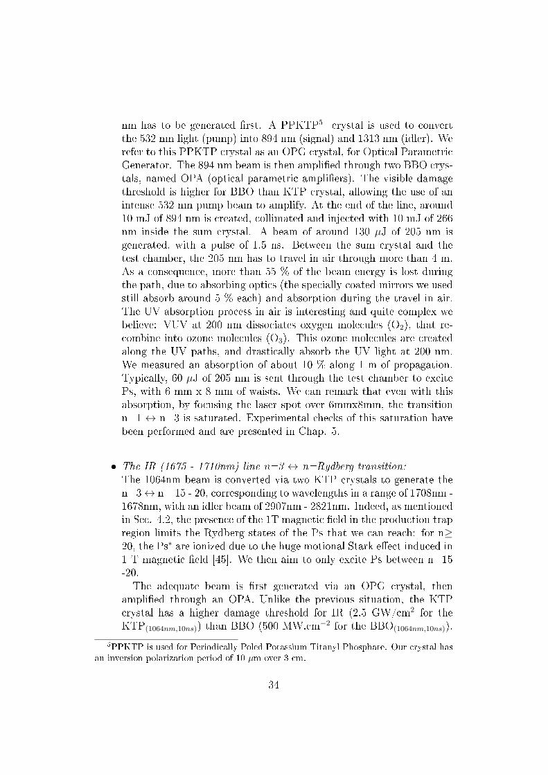
nm has to be generated rst. A PPKTP5 crystal is used to convertthe 532 nm light (pump) into 894 nm (signal) and 1313 nm (idler). Werefer to this PPKTP crystal as an OPG crystal, for Optical ParametricGenerator. The 894 nm beam is then amplied through two BBO crys-tals, named OPA (optical parametric ampliers). The visible damagethreshold is higher for BBO than KTP crystal, allowing the use of anintense 532 nm pump beam to amplify. At the end of the line, around10 mJ of 894 nm is created, collimated and injected with 10 mJ of 266nm inside the sum crystal. A beam of around 130 µJ of 205 nm isgenerated, with a pulse of 1.5 ns. Between the sum crystal and thetest chamber, the 205 nm has to travel in air through more than 4 m.As a consequence, more than 55 % of the beam energy is lost duringthe path, due to absorbing optics (the specially coated mirrors we usedstill absorb around 5 % each) and absorption during the travel in air.The UV absorption process in air is interesting and quite complex webelieve: VUV at 200 nm dissociates oxygen molecules (O2), that re-combine into ozone molecules (O3). This ozone molecules are createdalong the UV paths, and drastically absorb the UV light at 200 nm.We measured an absorption of about 10 % along 1 m of propagation.Typically, 60 µJ of 205 nm is sent through the test chamber to excitePs, with 6 mm x 8 mm of waists. We can remark that even with thisabsorption, by focusing the laser spot over 6mmx8mm, the transitionn=1 ↔ n=3 is saturated. Experimental checks of this saturation havebeen performed and are presented in Chap. 5.

The IR (1675 - 1710nm) line n=3 ↔ n=Rydberg transition:The 1064nm beam is converted via two KTP crystals to generate then=3↔ n= 15 - 20, corresponding to wavelengths in a range of 1708nm -1678nm, with an idler beam of 2907nm - 2821nm. Indeed, as mentionedin Sec. 4.2, the presence of the 1T magnetic eld in the production trapregion limits the Rydberg states of the Ps that we can reach: for n≥20, the Ps∗ are ionized due to the huge motional Stark eect induced in1 T magnetic eld [45]. We then aim to only excite Ps between n=15-20.The adequate beam is rst generated via an OPG crystal, then

amplied through an OPA. Unlike the previous situation, the KTPcrystal has a higher damage threshold for IR (2.5 GW/cm2 for theKTP(1064nm,10ns)) than BBO (500 MW.cm−2 for the BBO(1064nm,10ns)).

5PPKTP is used for Periodically Poled Potassium Titanyl Phosphate. Our crystal hasan inversion polarization period of 10 µm over 3 cm.

34

After the OPA stage, up to 4 mJ at 1675nm -1710nm can be reached.The tuning of the wavelength is done by monitoring the temperatureof the OPG crystal. This 4 mJ has to be compared to the saturationenergy of these transitions n=20 is typically around 250 µJ.cm−2, fora full-mixing of the manifolds in 1 T magnetic eld. More details aregiven in [46], Chap. 3.3.

Figure 4.4: Schematic of Milano laser apparatus with the dierent opticalline to generate the 205 and 1650 - 1700nm beams. Schematic taken from[49].

As the laser system is implemented directly in the experimental zone, andnot in a separated laser chamber with temperature control and white-roomstandards, this system needs to be frequently readjusted. Besides, the ash-lamp characteristics change on a month-scale, leading to a dierent pumpingof the Nd:YAG crystal and thus, to dierent emission parameters for thepump beams (changes in energy, beam size and beam divergence). The spotsizes and beam divergence are crucial for this system in order to optimize thenon linear processes, without burning the crystals. A couple of telescopes isjudiciously set along the dierent generation lines to adapt the beam char-

35

acteristics to the nominal required values.

Usually, the time-scale for a measurement of Ps laser excitation is a coupleof weeks. The laser system is realigned from scratch before we start themeasurements. This typically takes few days. However, the calibration andoptimization of the lasers are daily checked before starting the data taking:spatial alignment, wavelengths, spot sizes, power delivered, etc.

36

Chapter 5

Experimental results of Ps laser

excitation

In this chapter, I will present the latest results of Ps excitation we per-formed in AEgIS. These are the rst observation of the n=3 excited stateof Ps, and the demonstration of an ecient Rydberg excitation path usingthe n=3 level as the intermediate state. These measurements have been per-formed in the vacuum test chamber (see Fig. 5.1) between April and June2015, and are the collective results of

the positron system's crew - mainly constituted at that time bySebastiano Mariazzi, the expert responsible for the positron system atCERN, by Roberto Brusa and Giancarlo Nebia leaders respectively ofthe Trento and Padova groups, by Benjamin Rienacker, Ph.D studentof the CERN group, and by the technical students Ola K. Forslund,Lisa Marx, Laura Resch and Ine B. Larsen,

and the laser group - namely Ruggero Caravita, Ph.D student ofthe INFN Genova group, Fiodor Serrentino and Marco Prevedelli, alsofrom the Genova group, Zeudi Mazotta, Ph.D student of the INFNMilano lab and her supervisor Simone Cialdi, Daniel Comparat and Ifrom the laboratoire Aime Cotton, CNRS.

A PRA article has been published [19]. As for the measurements them-selves, where I worked on optimizing and aligning the laser system with thepositron system, I took an active part in the redaction of this collaborationarticle and several corrections and exchanges with the editors and referees.

To be able to laser excite the Ps cloud, one main requirement was to syn-chronize the e+ implantation in the target (that gives the starting time of the

37

Ps formation) with the laser pulses, in order to overlap spatially and tempo-rally the Ps and laser beams. The synchronization was done via a customeld-programmable gate array (FPGA) based synchronization device, givinga time resolution of 2 ns and a jitter of less than 600 ps. The time delay be-tween the prompt positron annihilation peak and the laser pulses was set to16 ns as an optimal value. This delay was determined after several measure-ments for dierent timings around a theoretical value, given by the expectedescape time of Ps from the target. This expected value was calculated thanksto a Monte Carlo code developed by Zeudi Mazzotta, that derives the propa-gation of the Ps cloud for a isotropic emission, taken into account the initialtemperature of the Ps and its initial size. The geometry of the test chamberis implemented as well as the detector positions and eciency given by thesolid angles of detection. This code gives the laser excitation eciency of Psas function of the spatial and temporal localizations of the laser in regardof the Ps cloud, and provides us the theoretical optimum time and positionto send the lasers inside the test chamber and enhance the excitation signaldetected.

5.1 The Ps n=3 laser excitation measurements

Our rst goal was to perform the n=1↔ n=3 excitation. As we have seenpreviously, until then, only the rst excited state n = 2 and the Rydberg levelsn = 10 - 31 Ps have been experimentally observed [38, 37, 40, 41].

5.1.1 The signal diagnostics

Two methods of diagnostics have been used to measure the excitationsignal:

The magnetic quenching-based measurement.In presence of a magnetic eld the 33P sub-states with m = 0, ± 1(excluding 33P1,m=0

6 ) are mixed with the 31P sub-states, and candecay toward the 11S state, subsequently annihilating with a lifetimeof 125 ps into two γ rays [46].

In a SSPALS signal (as in Fig. 3.7), this phenomenon results in aquick rise of annihilation counts just after the laser excitation, then in

6We note the internal state of Ps, with the hyperne structure splitting | n, l, s, j,m⟩as: n2s+1ℓj,m, where n is the main quantum number, l the orbital momentum, s the totalspin, j = l + s the total angular momentum, and m its projection over the quantizationaxis. We use the associated letters to dene the value of l as: l = 0⇔ ℓ=S, l = 1⇔ ℓ=P,l = 2⇔ ℓ=D, etc.

38

a decrease of the annihilation counts coming from the long lifetime o-Psremaining, that forms the long tail of the signal. Since we laser excitereally close in time after to the prompt e+ peak signal, the small risedue to Ps quenching is lost in the prompt peak counts; thus the signalobserved is simply the decrease in annihilation counts for the long tail.

The photoionization. The 1064nm beam is used to photoionize the Ps33P excited states. As for the quenching process, this technique resultsin a decrease of the o-Ps population since the photoionization dissoci-ates the positronium atoms, the free positrons are quickly acceleratedin few ns toward the last negative electrode of our set-up, where theyannihilate.

As a diagnostic, we dene the fraction S(%) of quenched or ionized o-Psatoms as the dierence of areas of the SSPALS spectra with and withoutlasers, normalized to area without laser. For this rst measurement, theareas are taken in the region between 250 ns and 450 ns from the promptpeak:

S =(foff − fon)

foff(5.1)

where foff is the area dened by the SSPALS signal, without laser, andfon the one, with laser shot. The integration time window for the S fractionof n=3 excited Ps is indicated in the Fig. 5.2 b) that delimits the areas fonand foff between the two vertical lines. This time window has been arbitrarychosen to correspond to the o-Ps emission signal into vacuum (exponentialdecrease of the number of o-Ps, with a lifetime of 142 ns in vacuum, trans-lated by a 3-γ emission), before the arrival of the fast Ps atoms on the wallsof the test chamber, that enhances the annihilate rate recorded in the SS-PALS curves.

Note that all SSPALS curves are normalized to 1, regarding the max-imum prompt peak value. This normalization is done to limit variationsof the experimental conditions from one measurement set to another. In-deed, the measurements presented here have been recorded over weeks time,but the stability of the positron system is of order of hours. The modera-tor eciency decreases of a 7% per hour during the rst 7 hours and thenaround 7% per day in normal conditions. Typically during the measurementsrecords, we grew a new moderator twice a day to keep a good eciency ofpositrons production and accumulations. The normalization makes signif-icant the comparison between SSPALS curves registered from one day to

39

another with dierent moderators states that lead to dierent numbers ofpositrons, since both the positron prompt peak and the number of Ps pro-duced are proportional to the number of implanted positrons.

For the rst measurements performed to excite and detect the n=3 state,the S parameter denition is independent of the chosen time window. Indeed,the excitation toward n=3 and photoionization of the Ps cloud is translatedby the immediate dissociation of the excited o-Ps. The increase of annihi-lation counts caused by the photoionization of the addressed o-Ps is lost inthe e+ prompt peak annihilation signal. The signal measured in the long-tailpart of the SSPALS curves is then only due to annihilation in vacuum of theo-Ps, in both case of lasers ON or OFF. That's why the S parameter that isa ratio of two integrals dened by the exponential decay of o-Ps in vacuumis independent of the time windows chosen for those measurements.

As a matter of test, we double-checked the S values obtained for a dierenttime window (from 230ns to 450ns instead of 250ns to 450ns), and the valuescalculated were matching each other within the error-bar range as shown inFig. 5.5, in the section 5.2. Indeed, the S parameter is dened as a relativechange of the areas below the SSPALS spectra with laser on (fon) and o(foff ). If the time window is changed, the area fon and foff are dierent buttheir normalized dierence should stay constant.

5.1.2 The measurements settings

Our excitation measurements have been performed in the test chamber atroom temperature. The implanted e+ energy was 3.3keV, with a beam sizeof FWTM7 < 4 mm. The magnetic eld was set at 250 G, and the electriceld experienced by the formed o-Ps was 600V/cm, generated by the lasttransfer electrode.

For the rst measurement, the excitation laser was set at theoretical res-onance (λL= 205.05 nm), with an energy of 60µJ measured in front of thetest chamber viewport, and a spot size of 6mm × 8mm (FWHM). The testchamber viewport is made in fused silica, with a measured transmission ef-ciency of around 90% for the 205nm. In g.5.1 is presented the schematicof the vacuum test chamber: the incoming laser beams are shot through theviewport, perpendicularly to the positrons beam (Z axis), and excite the Psemitted from the target, in the transverse direction (Y direction). The laserwas aligned as close as possible from the target production region, in order

7Full width at tenth maximum

40

Figure 5.1: test chamber schematic. The e+ comes from -z direction to beimplanted on the target, where Ps are emitted in a supposedly isotropic cone.Laser beams are sent in the y axis through the viewport as close as possibleto the target to excite the exiting Ps .

to cover geometrically all the o-Ps exiting the converter. The Ps cloud issupposed to have the same exiting beam radius than the e+ implanted beam.In order to protect the nano-porous silica-based target from any damage dueto the laser radiation, a small mechanical shadow has been installed on thetarget holder to mask the target to prevent that any laser light hits directlythe target. Specially, we want to avoid any formation of paramagnetic centersinto the target, induced by the UV light, as studied in [50]

5.1.3 Results

In Fig.5.2 are presented our experimental results. In the left im-age (5.2 a) is shown a typical signal obtained for the quenching measurementtype. A signal Squenching = 3.6 ± 1.2 % has been recorded for the magneticquenching measurements, for an average of 11 single SSPALS shots.

We then wanted to conrm the n=3 excitation using a second intense laser

41

Figure 5.2: Ps laser excitation to n=3 state. The black arrow indicates thetime when the laser is sent. Fig a). Quenching result: S ≈ 3.6 %. average of11 single shots. Fig. b). Photoionization result: a signal of S ≈ 15.5 % hasbeen measured, for an average of 15 single shots. The S parameter valueshave been calculated for a time window between 250ns and 450ns.

beam to photoionize the excited o-Ps. For this purpose, the 1064nm beamwas used with a high energy (50 mJ) and a big spot (FWHM ≈ 12mm), syn-chronized and aligned in order to cover the UV beam in the target region.This measurement gives at resonance a signal Sphotoionization = 15.5 ± 1.1 %,for an average of 15 single SSPALS shots (see Fig. 5.2 b) ).

5.1.4 A quick analysis of the n=3 excitation signal ob-tained

In order to predict the excitation laser eciency, a C++ code was usedto perform the numerical diagonalization of the full interaction Hamiltonianin electric and magnetic elds and to calculate the generalized Einstein'scoecients [46]. These coecients were fed into a rate equation solver tocalculate the transition probabilities, as a function of the laser excitation in-tensity, bandwidth and electro-magnetic elds environment. This code wasrst written in a Mathematica program by Fabio Villa, before being improvedby Ruggero Caravita that translated the code into a faster version in C++.During my master thesis studies, I spent a great part of my time working

42

on this code and the theory behind: the matter-light interaction, for an hy-drogenic atom in electro-magnetic elds, with all the energetic correctionsapplied (QED, Zeeman, Stark, Quadratic Stark eects). For more informa-tion about the calculations performed by this code, the reader could refer to[46, 51].

For a theoretical point of view, at resonance and with perfect temporaland geometrical overlaps between Ps cloud and lasers, one should expect100 % excitation+ionization eciency in the high saturation regime. Thephotoionization measurement has been performed in high saturation regimefor the 1064nm laser beam, and consequently any n=3 excited Ps is quasi-instantaneously disassociated.

Considering the magnetic and electrical elds of the experiment, our sim-ulation code gives a theoretical value for the quenching eciency fquenched= 17 %, and an excitation+ionization eciency of fphotoionized = 93 % withperfect temporal and geometrical overlaps between Ps cloud and lasers.

Figure 5.3: Ps laser excitation in the test chamber: schematics of the spatialand spectral distributions of the lasers and Ps cloud. Fig. a) indicates thedirections of propagation of the lasers (along +y) and the Ps cloud (toward+z), with the geometrical overlap η, both in top and front views inside thetest chamber. Fig. b) shows the two spectral distributions of the lasers andthe transition line, broadened by the Doppler eect.

43

In our experimental setup, sketched in Fig. 5.3, one of the main limi-tations for reaching a higher excitation signal is due to the laser spectralwidth, that covers partially the Doppler prole of Ps emitted from a room-temperature target and limit the velocity range of atoms at resonance. Asecond limitation is the limited geometrical overlap of the laser spot on thePs cloud. With the 3.3keV e+ implantation energy, the mean velocity of par-tially thermalized o-Ps is expected to be of the order of 105 m.s−1, giving aDoppler broadening kσv ≈ 2π × 470 GHz, with k= 2π

λLthe wavevector norm,

when the laser bandwidth is measured to be σL = 2π (48GHz).

Further analysis is developed in the Chap. 6. Nevertheless, a quick lookon the results obtained shows that the ratio between purely quenched signaland quenching+photoionization signal remains in the same order for theo-retical predictions and measured values. For a number of n=3 excited atomsNexcited = 15.5% of the total produced Ps, the expected quenched fraction isthen Stheo,quenching= Nexcited × fquenched = 15.5%× 17% = 2.6 %, that is inreasonable agreement with the experimental value measured Squenching=3.6± 1.2 %.

5.2 A Doppler scan of the Ps cloud spectral

line

We then performed a scan in frequency of the 205nm exciting beam, fora photoionization 1064nm beam constant at 50 mJ. We kept the UV energyconstant at 60µJ, with the same FWHM = 6mm × 8mm spot size. Fig. 5.4shows the fraction of excited Ps, for dierent detunings of the UV laser (δ =ω0 − ωL, where ω0 is the transition frequency, and ωL the laser frequency).Doing so gives the linewidth of the 13S - 33P Ps transition, with a Dopplerbroadening of the line measured to be about σDoppler = 470 GHz.

44

Figure 5.4: The linewidth of the 13S↔ 33P transition, obtained by scanningthe frequency of the UV laser, for a constant energy of 56 µJ. The photoion-ization laser was set 50mJ, in the high saturation regime. Each point is thengiven by 15 SSPALS shots and the continuous curve is the result of a tprocess described in Chap.6.

Fitting a Gaussian to the resulting points gives the central value of the3P excitation line at 205.05 ± 0.02 nm. The value predicted by theory is205.0474 nm [46]. The simulations performed to analyze the data are de-scribed in the following chapter 6.

Finally, in order to double check the independence of the time-windowchosen to analyze our SSPALS signals, we performed a second data extractionof the S(%) parameter, using as a time window t=230ns to 450ns, instead of250ns to 450ns. The results are presented in Fig. 5.5, and shows that the Sparameters calculated with the new time window (in red) are consistent withthe value calculated with the time window 200ns width (black points).

45

Figure 5.5: To demonstrate that the signal S(%) is independent of the timewindow we selected, we present here the linewidth of the 13S ↔ 33P transi-tion, with the data points analyzed for a time window 250 ns to 450 ns (blackpoints), and for a second time window from 230 ns to 450 ns (red points).The S(%) values calculated for the two dierent time windows are within theerror bars, and thus consistent each other.

5.3 The saturation regime - verication mea-

surements

In order to verify if the previous laser settings actually saturate the tran-sition, we performed several measurements for dierent laser intensities, forboth the 205nm (at photoionization beam intensity xed 50mJ) and for the1064nm (at UV beam intensity xed 60µJ). The results are presented inFig. 5.6. The 1S-3P transition appears only slightly saturated, while the3P-continuum is strongly saturated, meaning that any n=3 atom is disso-ciated (photoionized) as soon as they get excited. These considerations arediscussed in more details in the following chapter Chap.6 of the data analysisand in appendix B.

46

Figure 5.6: Saturation measurements: S parameter as a function of a). UV205nm energy (IR energy = 50 mJ) and b). IR 1064nm energy (UV energy =60 µJ). Arrows mark the laser energies used for the measurements presentedin Fig. 5.2. The continuous lines are ts of the 3 levels rate equation model-see Chap.6

5.4 Rydberg Ps excitation

Once the n=3 excitation performed and characterized, we demonstratedfor the rst time the Ps excitation toward Rydberg states via the 33P inter-mediate state. These measurements were performed using the 205 nm beamat resonance, with 60 µJ, and varying the wavelength of the dedicated IR1675 nm-1720 nm laser for addressing the n= 3 ↔ n Rydberg.

In case of Rydberg excitation, long lifetime Ps* can reach the walls of thevacuum chamber where they annihilate. The most distant walls of the testchamber seen by Ps are between 4 and 6 cm away from the production target,as illustrated in Fig. 5.1. For a Ps cloud produced at a mean velocity of 105

m.s−1, these distances correspond to a journey time of 400 - 600 ns beforePs* annihilation. Consequently, the SSPALS spectra signal of Ps* excitationis a decrease of annihilation immediately after the laser shot and an increaseat later times when Ps* annihilate on the walls, as shown in the Fig. 5.7 a).

We then varied the λIR from 1715 nm to 1685 nm, and scanned the dif-ferent Rydberg states resonant transition from n = 15 to n ≈ 18, as plottedin Fig. 5.7 b). Because of the presence of magnetic and electric elds thatbroaden and mix the lines, the dierent Rydberg states start to be hardlydistinguishable for n > 16. A theoretical spectrum plotted in Fig. 5.7b) was

47

obtained with our code of the full-Hamiltonian diagonalization in externalelds. For these measurement scans, the S parameter has been dened on anarbitrary time window between 350 ns and 600 ns, and gives another indirectproof of the ecient laser excitation of the n = 3 states.Note that because of the combination of both the annihilation phenomenain vacuum and in the inner walls of the test chamber at the long times, theratio of the integrals of the SSPALS curves is dependent of the time windowchosen. Consequently in this case, the S parameter only gives a qualitativediagnostics of the excitation toward Rydberg.

Figure 5.7: Fig a) Rydberg excitation SSPALS signal, for λIR = 1709 nm,corresponding to the transition n=3↔ n=15. 205 nm beam is set at reso-nance. Fig. b) Scan of the Rydberg transitions: the dierent S parametersdata are plot as a function of the IR wavelength in the range n = 15 - 18,compared with a theoretical linear spectrum. The electro-magnetic eld con-ditions are 600V/cm and 250G, implying a mixing of the lines. For n≥ 16 itbecomes dicult to distinguish from the dierent Rydberg states.

5.5 Summary of the experimental results and

short prospect

In this chapter, the recent measurements of the laser excitation of Ps havebeen presented, showing the rst observation of the n=3 laser excited Ps aswell as the Rydberg n=15-16 Ps levels reached via the n=3 level as the in-termediate step. These results have been obtained in the test chamber, atroom temperature and for 250 G and 600 V/cm environment and with animplantation energy of 3.3 keV for the e+ bunch. A next step for AEgIS is to

48

perform the same laser excitations in the cryogenic and high magnetic eldenvironment of main apparatus, that is planned for the beamtime of 2016.

In addition to this, the measurements carried out into the test chamberstill continue to be performed in parallel of the work in the main traps. Aclear signal of the n=2 metastable Ps, via spontaneous decay from the n=3excited state is under study, as well as the transverse Doppler prole of theemitted o-Ps for dierent energies of positron implantation. The charac-terization of the transverse energy of the Ps cloud, via the Doppler prolemeasurements are of importance to obtain information about the o-Ps emis-sion. We want to know if the emission can be directional or if o-Ps are emittedwithout any privileged direction (2π steradian emission). This informationwill be primordial to rene the estimation calculations of the number of o-Ps∗ that will be able to reach the antiproton plasma in the production trap.Moreover, the demonstration of the ecient production of a meta-stable Psbeam (the 23S) will open paths for a physics studies on long-livng Ps, thatis also interesting for us and more widely for the scientic community. Forinstance, this could help the realization of the Ps interferometry to performa gravity test (see [13]).

Further experiments are foreseen be to tested in the next months andyears, like the Doppler cooling of Ps. We will discuss the feasibility and theinterest in Chap. 8.

49

Chapter 6

Simulations analysis

To analyze these results, I improved a simple 3-level rate equation modelrst developed by Daniel Comparat. The absorption, stimulated and spon-taneous emissions, and ionization are taken into account in order to calculatethe population evolution of the 3 states: N0 is the population of the groundstate (13S), N1 is the intermediate state (33S) one and N2 gives the number ofphotoionized atoms, or for our model, the population of a "continuum state".In Fig 6.1 is presented a scheme of our model with the dierent interestingparameters.

Figure 6.1: Schematic of the 3 level system used to model the photoionizationrate and thus the expected signal to be measured.

50

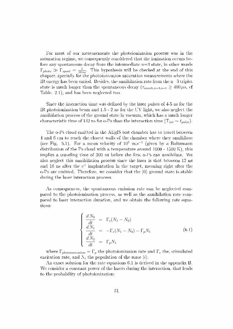
For most of our measurements the photoionization process was in thesaturation regime, we consequently considered that the ionization occurs be-fore any spontaneous decay from the intermediate n=3 state, in other wordsΓphoto ≫ Γspont =

110ns

. This hypothesis will be checked at the end of thischapter, specially for the photoionization saturation measurements where theIR energy has been varied. Besides, the annihilation rate from the n=3 tripletstate is much longer than the spontaneous decay (τannih,n=3,s=1 ≥ 400µs, cfTable. 2.1), and has been neglected too.

Since the interaction time was dened by the laser pulses of 4-5 ns for theIR photoionization beam and 1.5 - 2 ns for the UV light, we also neglect theannihilation process of the ground state in vacuum, which has a much longercharacteristic time of 142 ns for o-Ps than the interaction time (Tint ∼ tpulse).

The o-Ps cloud emitted in the AEgIS test chamber has to travel between4 and 6 cm to reach the closest walls of the chamber where they annihilate(see Fig. 5.1). For a mean velocity of 105 m.s−1 (given by a Boltzmanndistribution of the Ps cloud with a temperature around 1000 - 1500 K), thisimplies a traveling time of 300 ns before the rst o-Ps can annihilate. Wealso neglect this annihilation process since the laser is shot between 12 nsand 16 ns after the e+ implantation in the target, meaning right after theo-Ps are emitted. Therefore, we consider that the |0⟩ ground state is stableduring the laser interaction process.

As consequences, the spontaneous emission rate can be neglected com-pared to the photoionization process, as well as the annihilation rate com-pared to laser interaction duration, and we obtain the following rate equa-tions:

dN0

dt= Γe(N1 −N0)

dN1

dt= −Γe(N1 −N0)− ΓpN1

dN2

dt= ΓpN1

(6.1)

where Γphotoionization = Γp the photoionization rate and Γe the, stimulatedexcitation rate, and Ni the population of the state |i⟩.

An exact solution for the rate equations 6.1 is derived in the appendix B.We consider a constant power of the lasers during the interaction, that leadsto the probability of photoionization:

51

Pphoto(Tint) =N2(T )

N

= (1−1

2√

4Γ2e + Γ2

p

exp(−1

2(2Γe + Γp +

√4Γ2

e + Γ2p)Tint)

×(2Γe + Γp +√

4Γe + Γp) exp(√4Γe + Γp Tint)

+(2Γe + Γp −√

4Γe + Γp))(6.2)

With Tint the interaction time of the laser excitation+photoionization.This result can be simplied under some conditions that are discussed in

the appendix B. Anyhow, we would like now to introduce an intuitive so-lution in case of the high saturation regime for the photoionization process.We will then verify its compatibility with our conditions.

6.1 The case of high saturation photoionization

regime - a simple solution

Our experimental settings give a photoionization rate of:

Γp = σphoto,n=3,theo

IIR

h νIR= σphoto,n=3,theo ×

EIR

tpulse,IR πw2IR

×λIR

h c

= 3.48× 10−17 cm2 ×50mJ

4ns π( 8mm

2√

2 ln(2))2×

1064nm

h c

= 6.42× 109 s−1

(6.3)Where EIR and tpulse,IR are respectively the energy and the pulse dura-

tion of the IR photoionization beam, with a wavelength λIR = 1064 nm), andσphoto,n=3,theo is the theoretical value of the photoionization cross section fromthe n=3 triplet state of Ps, taken from [46, 45]. The IR beam is consideredto be top-hat shaped, with wIR is the radius. The interaction time Tint islimited by the laser pulse, so Tint = tpulse,IR

For an interaction time of 4 ns corresponding to the IR photoionizationFWHM pulse time, we obtain a ratio Γp× Tint ≈ 25 ≫ 1, corresponding tothe high saturation regime case.

52

If the photoionization time t = 1/Γp is much faster than the interaction timeTint, we can consider that the change in population toward the continuumstate occurs instantaneous compared to the total time of excitation Tint, i.e.∀ t ≤ Tint, N1(t) ≈ 0. This statement could be physically understood as thefollowing: once a Ps gets excited toward the n=3 state, it is immediatelyphotoionized. Thus, the rst rate equation is simplied in:

dN0

dt= −ΓeN0

By integrating over the total interaction time Tint, we obtain the groundstate population N0(Tint)=Ntot exp(−Γe Tint). Since we considered a closedsystem, the number of photoionized atoms after T is:

N2 = Ntot −N0 −N1 ≈ Ntot(1− exp(−Γe Tint)) (6.4)

We then approximate the probability of photoionization after a time Tint

with:

Pphoto,approx(Tint) ≈ 1− exp(−Γe Tint) (6.5)

Eq. 6.5 means that the probability to photoionize the Ps cloud is onlygiven by the excitation rate toward the n=3 state and the excitation time in-teraction. This is derived under the hypothesis of a strong saturation regimefor the photoionization laser.

The validity conditions for a good agreement of this approximation withthe exact solution of N2 are discussed in the appendix B. It is shown thatwe can consider that the simple solution (Eq.6.5) can be applied for anymeasurement done with the photoionization laser at saturation energies wehad.

6.2 High photoionization regime: studies of the

Doppler Scan and UV saturation measure-

ments

In this section, in order to extract the transverse temperature of the Pscloud, we want to t the Doppler scan measurements. Fitting the UV satura-tion measurements will allow us to extract the value of the dipole strength ofthe transition. In both cases, the photoionization was set to be in the strongsaturation regime, meaning that the Eq. 6.5 can be used. To determine the

53

photoionization probability Pphoto,approx(Tint), we then need to determine theexcitation rate formula.

In the appendix B, the excitation rate Γe is derived considering that theexcitation laser which performs the 13S ↔ 33P transition (∼ 110 GHz) ismuch larger than the natural linewidth of the transition (∼ 0.1 GHz) andthe hyperne splitting (< 4 GHz for the 33P, see Fig. 2.4). This leads to:

Γe(δ,Ω, σL) =Ω(r)2π

2

1√2πσ2

L

exp(−δ2

2σ2L

) (6.6)

where Ω(r) is the Rabi frequency of the laser-matter coupling such as|~Ω(r)| = |dEL(r)|, where d is the electrical dipole strength of the transition(matrix elemet) and EL the laser amplitude (electric wave). We also deneσL the rms value of the laser bandwidth, and δ0 = ω0−ωL the laser detuningcompared to the transition energy ~ω0 for an atom at rest. For an atom ata velocity v, the detuning δ is then taken to be δ = δ0 − kL.v

6.2.1 The geometrical coecient η

In general, the probability of photoionization Pphoto,approx = 1−exp(−Γe Tint)depends on the spatial distribution of the laser I(r), since Γe the excitationrate toward n=3 state is a function of the Rabi frequency Ω(r) of the light-matter interaction.In case of a low saturation regime for the n=1 ↔ n=3 transition, the pho-toionization probability can be approximated byPphoto,approx(Ω(r)) ∼ Γe(Ω(r))Tint.

Therefore, the total photoionization probability Pphoto,approx,tot is the re-sult of the 3D integral of the excitation rate times the spatial distributionof the Ps cloud. It is shown in Appendix B Sec. B.5 that the probability ofphotoionization Pphoto,approx,tot = Pphoto,approx(Ω0)× η, where η is a geometri-cal factor of overlap between the lasers and Ps cloud distributions and Ω0 isthe peak value of the Rabi frequency.

In the Appendix. B, Eq. B.22, η has been derived to be:

ηtheo =σ2r,L

σ2r,Ps + σ2

r,L

(6.7)

54

Where σr,L and σr,Ps are respectively the rms values of the spatial Gaus-sian distributions of the laser and the Ps cloud, both taken in the interactionplane x, z (plane transverse to the lasers' propagation direction). The sit-uation is illustrated in Fig. 5.3 a), with the notations given.

For simplication, we use the approximated probability of photoionizationPphoto,approx,tot = Pphoto,approx(Ω0)× η, not only for the weak saturation case,but also for generic saturation regimes. In a sens, the eciency reductiondue to the spatial variation of the laser intensity in the tails is taken intoaccount in the global geometrical coecient η.

We then introduce a coecient η ≤ 1 that contains all the spatial depen-dencies of the problem (See Fig. 5.3 a) ):

The spatial overlap between the laser beams and the Ps cloud.

The excitation eciency's spatial dependance (Γe(r)) that comes fromthe spatial variation of the laser intensity I(r).

6.2.2 The photoionization probability

In order to t the Doppler scan measurements, we want to nd an expres-sion of the photoionization probability that takes into account the Ps velocityand the laser detuning. Both lasers to perform the n=1↔ n=3 and the n =3→ continuum transitions are at saturation. Since the photoionization laseris powerful enough to imply a strong saturation the transition to the con-tinuum, the photoionization probability can be approximated by Eq. (6.5).This equation provides an approximation of the photoionization probability,for a given velocity v of the Ps atom and for a given laser detuning δ of the205nm beam.

We assume that the Ps velocity distribution is a Gaussian distribution,with a mean temperature T(K). The integrated photoionization probabilityover the Ps velocity spectrum is thus given by:

P (t, δ) = η

∫ +∞

−∞Pphoto,approx(t, δ, v)

√1

2πσ2v

e− v2

2σ2v dv (6.8)

where σv =√kBT/m is the standard deviation of the velocity along the

laser propagation axis, for a Ps cloud at a temperature T.

55

The formula 6.8 was used to t the data in Fig.5.4 and Fig.5.6 a). Wefound a Rabi frequency Ωfit ≈ 5.5×1010 s−1 ±1.1 1010 s−1 that gives a dipolestrength of dfit = 1.76± 0.59 Debye, in good agreement with the theoreticalvalue of 1.65 Debye, derived from the equation:

d ≈

√Γs 3h 4πϵ0

λ3064π4

(6.9)

Since the lineshape of Fig.5.4 is almost entirely dominated by the ther-mal distribution of the Ps, the t also gives information about the Ps cloud'stransverse temperature. We obtained a standard deviation of o-Ps velocity inthe transverse direction σv ≈ 105 m/s, or a temperature T = 1300± 200K.

From the t, the geometrical overlap coecient η has been determined tobe ηfit = 80 %. The implanted e+ cloud has a full width tens of maximum

(FWTM) of 4 mm × 5 mm, meaning a variance value of σint =FWTM

2√

2Log[2].

We assume the Ps cloud is emitted out of the target surface with the sameinitial size than the e+ cloud spread, and that it propagates with a meanvelocity of σv = 105m.s−1.

The laser interaction happens with a delay of tdelay=16 ns. The spa-tial spread of the Ps cloud at the time of the laser interaction is then

σr,Ps =√σ2init,x + t2delay × σ2

v ×√σ2init,z + t2delay × σ2

v . We found a variance

of the Ps cloud σr,Ps = 2.7 mm. Finally, for a laser waist of 6 mm × 8 mm,we found a theoretical ηtheo = 62%, in good agreement with the t value of80%, regarding the accuracy of the measurements.

6.3 The n=3 laser at resonance and at satura-

tion - study of the photoionization satura-

tion

In this last section, we want to analyze the photoionization saturationmeasurements we did (see Sec. 5.3 and Fig. 5.6 b) ). For this, we set theUV laser at resonance (δ=0) and saturation (EUV = 56µJ), that xes thecoupling eciency, i.e. Ω that we previously t to be Ωfit = 5.37× 109 s−1.We thus obtain:

56

Γe(δ = 0,Ωfit) = 6.04 109 s−1 (6.10)

Since we want to analyze the photoionization probability at resonance,for various photoionization energies, we use the probability formula given inEq.6.2. This formula is valid under the condition Γp ≫ Γspont, its validity ischecked in the next paragraph.

The t curve is plotted in the Fig. 5.6.b). For a high saturation energy ofEIR=60 mJ, the photoionization rate parameter is tted to be Γp,fit(60mJ)= 5 109 s−1. This value allows us to extract a photoionization cross sectionvalue:

σphoto,fit = Γp,fit ×h c× tint × π w2

λ0EIR

= 3.1× 10−17 cm2 (6.11)

That is in a good agreement with the theoretical one σphoto = 3.48×10−17

cm−1.

Validity of the hypothesis

With the t cross section's value we obtained, we can now check the valid-ity of our hypothesis. For deriving the Eq.6.2 that gives the photoionizationprobability for various energies of the UV and IR lasers, we did the approx-imation: Γp ≫ Γspont. This inequality remains valid for the low IR energy

measurements we did, with: Γp(5.6mJ) ≈ 5×108 ≫ Γspont =1

10ns= 1×108.

For the measurement performed at the lowest IR photoionization energy of2.9 mJ, the photoionization rate is still higher than the spontaneous decay(Γp(2.9mJ) ≈ 2.5 × 108 ≈ 2.5 × Γspont), we consider this case to be at thelimit of validity of our model, and should not be taken into account for ttingthe curve Fig. 5.6.

57

Part II

A possible positronium laser

cooling ? Theoretical and

simulations studies

58

In the AEgIS scheme (cf Fig. 6.2 a)), two main parameters can drasticallyincrease the charge exchange formation eciency:

The p plasma temperature. As shown in the AEgIS proposal ([15]), coldantiproton plasma is required to have an ecient charge transfer withthe weakly-bound positron from the Ps*. In the chapter 14, I explainin more details the strategy we started to develop to sympathetic cooltrapped antiprotons, using laser cooled molecular anions. One of thebig issue to perform laser cooling of molecules is to nd a closed cycleof absorptions/emissions of photons. A promising candidate seems tobe the C−

2 molecule, and I present later some simulation results forthe dierent laser cooling schemes that are encouraging. In the AEgISproposal, we aim to cool the p plasma down to ≈ 100 mK.

The overlapping of the trapped p plasma and the Ps cloud. In thecurrent geometry of our apparatus, Ps beam is formed at a distance 2cm from the antiproton plasma region, most of the created Ps atomsdon't reach the p plasma, as shown in Fig. 6.2 a).

Figure 6.2: The AEgIS H formation schematic: in gray, the emission coneof Ps cloud sketched. Fig a) shows a wide emission. Most of the formed Psatoms don't reach the antiproton plasma and are consequently lost for thecharge exchange process. Fig b) shows a more collimated Ps cloud thanks tosome laser interaction.

During my thesis, I investigated several laser-matter interaction schemesin order to try to collimate the Ps atoms before Rydberg excitation, as shownin Fig. 6.2. the collimation of the Ps cloud would signicantly increase the

59

solid angle of overlaps between p and Ps∗.

To do so, I studied the possibility:

to use a Doppler laser cooling to reduce the transverse velocity of thePs cloud and focus the Ps emission. I develop the basics theory inChap. 7 and present some simulations results in 8. The Chap. 9, thecurrent status of the laser setup to perform the rst laser cooling trialis described.

to use the dipolar force of a highly detuned and intense laser to act asa focusing lens on the Ps cloud and collimate it. This will be seen inChap. 10.

60

Chapter 7

Ps Doppler laser cooling - theory

It is common to model the Doppler laser cooling by a two-level atomicsystem in interaction with a monochromatic laser acting on a broad-linetransition. This simple model works particularly well for alkaline atoms, likefor sodium atoms, on which the rst optical molasses has been performed in1985 by S. Chu and coworkers at the Bell Labs. Or, for instance, for rubid-ium on which the rst BEC was observed [52]. The limits of validity of sucha theory imply that the transition linewidth has to be greater than the recoilenergy of a single absorbed photon and than the laser bandwidth.

The case of the positronium diers for two main reasons:

The really small mass of the Ps atom (mPs = 2×me− ≪ mH) implies ahuge recoil energy for each photon absorbed. For the transition n=1↔

n=2, the energy recoil of the 243 nm photon (Er =~2 k2L2mPs

) is 200 times

more important than the natural linewidth equivalent energy ~Γspont.The Doppler cooling on the rst transition of the Ps is then a case of anarrow-line transition cooling, and the model of a broad-line transitionhas to be carefully checked and adapted.

Ideally, to address a maximum of emitted Ps, the huge Doppler broad-ening would have to be covered by the spectrally broad exciting lasers,and consequently, the approximation of the monochromatic laser is nomore valid. For a Ps cloud at 1000 K, the Doppler broadening is about400 GHz wide, much larger than the spontaneous rate Γspont = 1/142ns =7× 106 s−1, meaning a spontaneous frequency of about 1 MHz.

For all these reasons, the study of the Doppler cooling of the Ps atom hasto be performed with care. The possibility of a Ps laser cooling has been rst

61

studied by [53]. Later in 2000 - 2002, the group of K. Wada, M. Kajita andcoworkers [54, 55] experimentally proceeded to the rst trials. Even if theexperiment was not successful, theoretical and simulations studies have beenperformed to model the cooling eciency over the rst transition n=1 ↔n=2 (with a typo of a factor 2π in their paper). A recent work [56] proposeda combine scheme to reach the BEC, taken into account thermalization withthe nano-channels of the target convertor, and Ps-Ps scattering process inaddition of the Doppler laser cooling.

During my thesis, I studied the possibility to laser cool the Ps atom on thetransition 13S1 ↔ 23P2. The theoretical particularities of such laser coolingare discussed in the following sections. In Sec. 7.1. I remind briey the 2-level system model in order to derive the rate equations and dene properlythe parameters of interests for a Doppler cooling, as the scattering rate 7.2.In a second time in Sec. 7.3, I deal with the force resulting from the laser-matter interaction. Here, a distinction between broad-line and narrow-linetransitions has to be done. In the last Sec. 7.4, I briey conclude this theorysection for the Ps case. The explanations derived here lead to the simulationsresults I present in Chap. 8.

7.1 Laser cooling of an open two-level system

Here is considered a two-level system atom coupled with an externalelectro-magnetic eld, as illustrated in the Fig. 7.1. We study this usualmodel with two renements:

the 2-level system is considered to be open, in order to be able tosimulate the annihilation and photoionization processes

the laser is not considered monochromatic, but has a large spectralbandwidth σL ≫ Γs

The excitation rate between the two states is noted Γe, and we introducethe rates Γ1 and Γ2 that are the decay rates from the level |1⟩ and |2⟩ towardall the other energies levels but the two considered states |1⟩ and |2⟩. Forinstance, for the laser cooling of the o-Ps over the rst transition, |1⟩ would

be the ground state and Γ1 the annihilation rate Γ1 =1

142ns.

We want here to remind the well-known results of the populations evolu-tion in a quasi steady-state regime, as well as the important denitions suchas the saturation parameter, saturation intensity or photon scattering rate.

62

Figure 7.1: The opened 2-level system scheme. Γ1 and Γ2 are the leak ratesfrom the levels |1⟩ and |2⟩ to all the other levels. In case of the Ps, Γ1 can beassociated to the annihilation rate, that would mimic the annihilation towarda ctive "dead" level |0⟩

We dene the density matrix ρ that gives both information about thepopulation and coherence of the system:

ρ =

(ρ11 ρ12ρ21 ρ22

)(7.1)

such as ρii = Ni is the population of the level |i⟩, and ρ12 = ρ∗21 the co-herence between the two levels.

The coupling with the laser is given by the Rabi frequency Ω =dEL exp(iψL)

~,

where d is the electric dipole strength of the transition, EL the amplitude ofthe laser wave and ψL the phase of the laser.

We introduce Γtot that is the decoherence relaxation rate of the coupling.It takes into account the contributions from the spontaneous emission (cou-pling with the vacuum states of the electro-magnetic eld), from the opticalrelaxations toward other levels (Γ1 and Γ2) and the decoherence induced bythe rms laser bandwidth (σL): Γtot = Γs + σL + Γ1 + Γ2.

63

7.1.1 The rate equations

Since we want to model the cooling of the Ps atoms with a large Dopplerbroadening, the laser bandwidth σL has to be in the order of the hundreds of

GHz, much larger than the natural linewidth of the transition (1

3.2ns= 0.3

MHz). That leads us to study the case of a fast decoherence of the coupling,

that is similar to assume:d ρ12

dt= 0.

In the semi-classical framework, the dynamic of the incoherent laser-matter interaction can thus be modeled using the framework of the rateequations [57]:

dρ11

dt= (Γs + Γe) ρ22 − (Γe + Γ1) ρ11

dρ22

dt= −(Γs + Γ2 + Γe) ρ22 + Γe ρ11

(7.2)

where Γe is the excitation rate, that gives the laser coupling eciency.

7.1.2 The excitation rate formula

In order to calculate the dynamics of the laser interaction, it is then pri-mordial to derive the excitation rate.

The excitation rate is proportional to the convolution of the laser spectrum

IL(ω) and the Lorentzian natural bandwidth (Ls =Γs

2π

1

(ω − ω0)2 − Γ2s

), as

explained in Appendix B of [58]8

Γe =π d2

~2ϵ0 cIL(ω)⊗ Ls(ω) (7.3)

If we consider a Lorentzian laser spectrum, the excitation rate can beanalytically calculated:

Γe =

Ω2

2δ20 + Γ2

tot/4×

Γs

2(7.4)

8I corrected a missing factor ~2

64

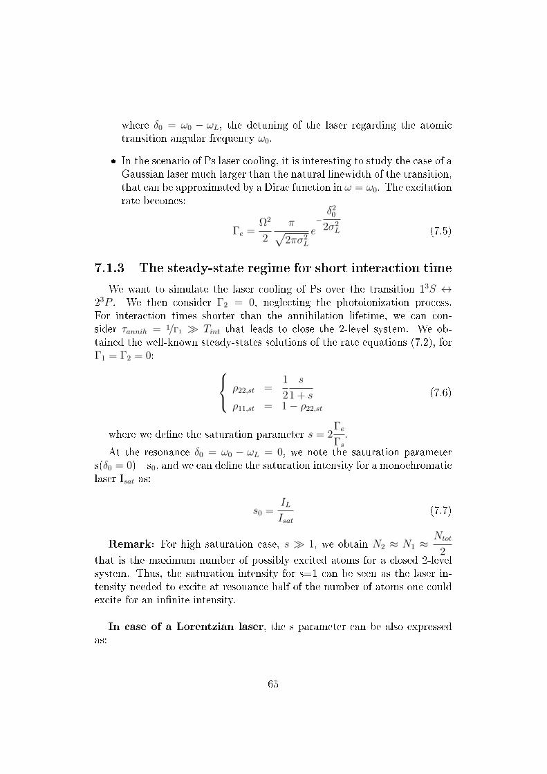
where δ0 = ω0 − ωL, the detuning of the laser regarding the atomictransition angular frequency ω0.

In the scenario of Ps laser cooling, it is interesting to study the case of aGaussian laser much larger than the natural linewidth of the transition,that can be approximated by a Dirac function in ω = ω0. The excitationrate becomes:

Γe =Ω2

2

π√2πσ2

L

e−δ202σ2

L (7.5)

7.1.3 The steady-state regime for short interaction time

We want to simulate the laser cooling of Ps over the transition 13S ↔23P . We then consider Γ2 = 0, neglecting the photoionization process.For interaction times shorter than the annihilation lifetime, we can con-sider τannih = 1/Γ1 ≫ Tint that leads to close the 2-level system. We ob-tained the well-known steady-states solutions of the rate equations (7.2), forΓ1 = Γ2 = 0: ρ22,st =

1

2

s

1 + sρ11,st = 1− ρ22,st

(7.6)

where we dene the saturation parameter s = 2Γe

Γs

.

At the resonance δ0 = ω0 − ωL = 0, we note the saturation parameters(δ0 = 0) =s0, and we can dene the saturation intensity for a monochromaticlaser Isat as:

s0 =IL

Isat(7.7)

Remark: For high saturation case, s ≫ 1, we obtain N2 ≈ N1 ≈Ntot

2that is the maximum number of possibly excited atoms for a closed 2-levelsystem. Thus, the saturation intensity for s=1 can be seen as the laser in-tensity needed to excite at resonance half of the number of atoms one couldexcite for an innite intensity.

In case of a Lorentzian laser, the s parameter can be also expressedas:

65

s(δ0) =2|Ω|2

Γ2tot + 4δ20

Γtot

Γs

s0 = s(0) =2|Ω|2

ΓtotΓs

(7.8)

For a monochromatic Lorentzian laser then: s0 =2Ω2

Γ2s

Using the expression of the dipole seen in Eq (6.9), we obtained the well-known expression:

Isat =1

6~ c (

2π

λ0)3Γs

2π(7.9)

For the Ps atom, the saturation intensity of the transition n=1 ↔ n=2excited by a monochromatic laser is then Isat = 0.45 W.cm−2.

For a non-monochromatic laser as the case studied here, the saturationintensity depends on the laser bandwidth and is dened by:

Isat,L = Isat ×Γtot

Γs

(7.10)

For a laser bandwidth of σL = 2π 100 GHz and Γtot = σL + Γs ≈ σL, weobtain a saturation intensity of Isat,L = 910 W.cm−2.

7.1.4 For long interaction times

Because we want to be able to perform an ecient laser cooling on Ps,longer interaction times should be studied as well, typically of the order ofthe Ps lifetime. The approximation consisting in neglecting the annihilationdecay rate is no more valid for times Tint ∼ τannih. The laser interactionbetween two levels with nite lifetime is treated in details in [59]. Chap. 2.4.where the population evolution over times is given. No more steady-statescan be reached, since for innite time all the atoms would have ee out ofthe open system.

For our simulations, we decided to treat the annihilation of Ps over timeas the decay toward a ctive third level "dead". The simplest way to modelthis situation is then to consider a closed 3-level system, where the n=1 o-Psground state is modeled as a meta-stable state, and the "dead" ctive level

66

is the ground state, named |0⟩. We keep Γ2 = 0, Γ1 is then the decay ratefrom the ground state |1⟩ to the dead level |0⟩. The rate equations become:

dρ22

dt= −(Γs + Γe) ρ22 + Γe ρ11

dρ11

dt= (Γs + Γe) ρ22 − (Γe + Γ1) ρ11

dρ00

dt= Γ1 ρ11

(7.11)

In the case of the laser excitation of Ps, the annihilation lifetime of theground state |1⟩ is much longer than the lifetime of the excited state |2⟩:τannih = 142ns≫ 1/Γs = 3.2ns.

As a consequence, the evolution of the dead level |0⟩ is much slower thanthe evolution of the ground |1⟩ and excited |2⟩ states. Over the characteristicevolution step t that denes the typical time for the level |1⟩ and |2⟩ tochange, the population of the dead level can be considered constant. Wedene the interaction time Tint = N × t, where N would be the numberof absorptions and emissions of photon that lead to a population changes inρ11 and ρ22.

Thus, quasi-steady states can be calculated between Tint and Tint +t,

and leads toρ11,stt

∣∣∣∣∣Tint

= 0 andρ22,stt

∣∣∣∣∣Tint

= 0:ρ22,st =

1

2

s

1 + s(1− ρ00)

ρ11,st =1

2

s+ 2

s+ 1(1− ρ00)

ρ00 = exp(−Γ1 ρ11,st Tint)

(7.12)

For short interaction time Tint ≪ τannih =1

Γ1

, ρ00 ≈ 0, that leads back

the usual steady-state solutions for a closed 2-level system seen previously(Eq. 7.6).

This derivation conrms that we can use the usual formula of the sat-uration parameter s and the saturation uence Isat when we study the Pslaser excitation, even for a long excitation time. For instance, this is of greatinterest to determine the good parameters to choose to simulate the lasercooling, as the laser power, detuning and bandwidth.

67

7.2 The scattering rate

At the end, the rate equations formalism allows to calculate the popu-lation evolution of an atomic system in interaction with a laser. In orderto model the cooling eect of this interaction, the interesting parameter toexpress is the photon scattering rate.

Γscat = Γs ρ22Γscat = Γe × (ρ11,st − ρ22,st)

(7.13)

The expression of the excitation rate Γe depends on the model of the laserspectrum chosen, as seen previously in Sec. 7.1.2.

This scattering rate gives the cooling eciency of the interaction. In orderto determine the cooling process on an atom in motion, we can calculate overtime the changes in impulsion due to photon absorbed (~ kL) and scattered9,based on the rate equations.

We used this principle to simulate a possible laser cooling on the Ps, thatwe will discuss on the following chapter 8.

7.3 Toward the force resulting of the laser-

atom interaction

In order to nd the adapted parameters for the cooling simulations, it wasuseful to determine the force resulting of the laser interaction with the atomin motion. Taking into account the velocity v of the atom in the previousformula is rather simple if we replace the laser frequency ωL by the one seen bythe atom ωL−kL.v. The detuning becomes thus δ0 = ω0−ωL → δ = δ0−k.v

and for a Lorentzian laser, s(v) =2Ω2

4(δ0 − kL.v)2 + Γ2tot

Γtot

Γs

.

To model the laser interaction resulting force, a distinction has to be donebetween broad-line transition and the narrow-line transition:

9The spontaneous emission is not isotropic and depends if deexcitation goes toward aσ± or a π transmission For a π transition (m = 0), the spontaneous emission's densityof probability is ρπ(θ) = sin2(θ) ; whereas for σ± transition (|m| = 1), the density of

probability of emission is ρσ± =1 + cos(θ)2

2. Here, θ is the co-latitude θ ∈ [0, π] in the

spherical coordinates. More details are given in my master thesis [51], Append. C.

68

In the following, we call an optical transition "broad" when the recoilenergy due to the absorption or emission of a photon is much smaller thanthe natural linewidth of the transition (~Γs ≫Erecoil). In this situation, theBrownian motion formalism can be applied to derive the average force feltby the atom in interaction with a classical electromagnetic laser wave [60].This force is called the radiation pressure force, and can be seen as a frictionforce of coecient α, such as F = −αv for the low velocities and low sat-uration regime. Physically, this force can be understood as the pressure ofthe photons applied on the atom. The laser cooling over a broad-line tran-sition leads to a velocity distribution evolution that decreases exponentiallyv(t) = v0 exp(−αt).

As seen in the introduction of this chapter, this case models most ofthe laser cooling processes, mainly over alkali atoms. In Fig. 7.2, a) isshown a typical radiative force generated by two counter-propagating lasersin interaction with an atom in motion ; the capture range and force strengthare determined by the laser detuning, intensity and bandwidth. More detailsare given in Appendix D. The minimum temperature reachable with theDoppler cooling over a broad-line transition is given by the Doppler energy:

Tmin =EDoppler

kB=

~Γs

kB(7.14)

69

Figure 7.2: Illustration of the force resulting from the laser-matter interactionand the scattering rate, for respectively the two transitions cases. a) In caseof a broad-line transition (~Γs ≫ Erecoil), the averaged radiative force canbe derived. The force strength and capture range are determined by thelaser intensity, detuning and bandwidth. Here, the force is obtained for twocounter-propagating lasers, with a power PL= 5000 W, a rms bandwidth

σL= 100 GHz, and a detuning δ = ±k0 v0

2, where k0 =

2 π

λ0is the wavevector

of the transition and v0 =

√kB T

mPs

is the mean velocity of the Ps cloud at the

temperature T=1000 K. b) Case of a narrow-line transition (Erecoil ≥ ~Γs):The resulting scattering rate of 2 counter-propagating monochromatic lasersis plotted. The optimum photon scattering power (equivalent to the coolingeciency) can be derived and is obtained for a detuning of δ = −3ωr, whereωr is the angular frequency of of the photon energy recoil such as Erecoil =~ωr. Figure taken from [60], where the complete derivation of this force canbe found.

In the case of the light positronium atom, the transition over the tripletstates n=1 ↔ n=2 belongs to a narrow-line transition case, where therecoil energy for a 243 nm photon is Erecoil ≈ 200 × ~Γs. From this situa-tion, the force resulting of the laser interaction is more complex to derive.

As shown in [60] the velocity distribution evolves in1

v−β, where β is a pos-

itive damping coecient. This is a much smoother evolution than in the

70

case of the broad-line transition, where the velocity distribution exponen-tially evolves (for s≪ 1, m a = F ∼ αv) as seen previously.

The coecient β can be calculated and is found to be β = 2|δ|

ωrecoil

, where

Erecoil = ~ωrecoil. In order to dene a normalizable kinetic energy, the laserdetuning must be chosen δ > 3

2ωrecoil. Numerical simulations of the force

of two counter-propagating monochromatic lasers give an optimum coolingeciency for σL ≈ ωrecoil and δ ≈ 3ωrecoil [60]. As illustrated in Fig. 7.2 b),where the scattering power of the force is plotted, this detuning is a goodcompromise between the velocity capture range of the lasers and the rangeof atoms in "dark".

The minimum temperature reachable with the Doppler cooling over anarrow-line transition is given by the recoil energy:

Tmin =Erecoil

kB=

(~ kL)2

2 kBm(7.15)

For the Ps over the transition n=1 ↔ n=2, we found Tmin=0. 15 K.

7.3.1 A possible laser broadening of for the narrow-linetransition of the Positronium ?

In some cases, the laser intensity is powerful enough to broaden conse-quently the transition line, and a situation of a broad transition can be re-covered. For intense "monochromatic"' lasers, the linewidth of the transitionis not more characterized by Γs but by an eective term

Γs,eff = Γs

√1 + I/Isat,L = Γs

√1 + (

2Ω2

Γ3s

)× Γtot (7.16)

For a non-monochromatic laser, the broadening of the transition is given

by: Γs,eff,L=Γs

√1 +

I

Isat,L.

Consequently, if the broadening of the line is large enough to fulll thecondition of validity of the Brownian motion approach:

~Γs,eff ≫ Er(≥ ~Γs) or (nonmonochromatic) ~Γs,eff,L ≫ Er(≥ ~Γs)

(7.17)then, the friction force model can be applied. For the laser cooling on Ps

we want to attempt, the characteristic values are given in Table 7.1.

71

Γs ωr Γs,eff Γs,eff,L

1

τlifetime

~k2L

2mPs

Γs

√1 + I/Isat Γs

√1 + I/Isat,L

0,3 GHz 19 GHz 52 GHz 3 GHz

Table 7.1: This table summarizes some interesting parameters to determine ifthe laser cooling of Ps can be approximated by the cooling over a broad-line,enlarged by intense laser. We took a laser power P = 5000 W, equivalent of500 µJ over 100 ns, and σL = 100 GHz. It appears that for our large andintense laser, the condition Eq. 7.17 is not fullled, and the approach of thefriction force formalism can't be strictly applied.

Since we want to perform a Doppler cooling with broadband lasers, thecondition ωr ≤ Γs,eff,L to recover a situation of broad-line transition is notfullled. The Brownian motion approach and the radiation pressure forcecan't be use for a good modeling of the Ps cooling.

Nevertheless, the radiation pressure force gives a good empirical explana-tion of the eect of laser interaction on the atom in general. That's why ina preliminary approach, we decided to use the well-known expression of theradiation pressure force to determine some rough estimations of the param-eters of interest to maximize the laser cooling eciency, namely: the laserpower, detuning and spectral bandwidth. The radiation pressure force fortwo counter-propagating lasers in low saturation is given by:

⟨Frad⟩ = ~kLΓs

2(

s1

s1 + 1−

s2

s2 + 1) (7.18)

where s1 and s2 are the saturation parameters of the two counter-propagatinglasers. This force expression was used to the plot the Fig. 7.2 a).

7.4 The Ps laser cooling, which formalism ?

In this chapter, we have seen that the laser cooling of Ps diers from theusual Doppler laser cooling. Although the rate equations formalism is stillvalid, the annihilation process needs to be taken into account. This mod-ies the well-known steady-state solutions for a closed two-level system ininteraction with a non-monochromatic laser. The table 7.1 summarizes some

72

characteristics lifetimes of the Ps atom.

We have also reminded that the radiation pressure force model is onlyvalid for broad-line transition (when ~Γs ≫ Erecoil), and leads to exponentialchanges in the velocity distribution. In the contrary, for narrow-line transi-tion as for the Ps case, the eect of the laser interaction on the atom is morecomplex to derive, and appears to be smoother with velocity changes in |v|−β.

Nevertheless, the laser cooling of positronium can be properly simulatedwithin the rate equations formalism: the eect of the Doppler cooling onthe atoms can be derived by calculating the changes in impulsion due toabsorbed and scattered photons over time using the rate equations. We usedthis formalism to numerically simulate Ps laser cooling on a C++ code andI propose to discuss about our simulation results in the next chapter 8.

73

Chapter 8

Positronium laser cooling -

simulations

As we have seen previously, the positronium is a metastable atom witha short lifetime in vacuum of 142 ns for the ground state o-Ps. One of thegreatest challenges is then to be able to eciently cool o-Ps in few tens ofnanoseconds. The typical Doppler laser cooling times for alkali atoms ratherscale in the order of tens of microseconds. However, the positronium is thelightest atom possible. The energy recoil of one emitted photon is conse-quently much more important than for usual atoms, with a mass at least ofthe order of the proton mass. This statement implies that every scatteredphoton removes a large amount of energy from the Ps atom, and a conse-quent laser cooling on o-Ps should be feasible in scales on tens of ns, overthe transition n=1 ↔ n=2.

The 23P Ps states have a decay time of 3.19 ns, and a much longer an-nihilation lifetime (> 100 µs), see Table. 2.1. The annihilation for the n=2level can easily be neglected in comparison to its decay time. Without mag-netic eld, the transition wavelength λ0 between 13S↔ 23P is at 243.01 nm,leading to a recoil velocity of v = 1500 m.s−1 that can be translated inkinetic energy by EK= 1/2mPsv2=kB 0.15 K. Potentially, only few cy-cles of absorption/spontaneous emissions are needed to change consequentlythe Ps velocities: an initial temperature of the Ps cloud of 1000 K (Boltz-mann distribution) means a velocity spread of 90 km/s. In a rst simplecalculation, the huge energy recoil removed for each spontaneous scattered

photons implies that only80× 105

1500= 60 cooling cycles, in an interaction time

of tint = 60× 3.2 ns × 2 ≈ 380 ns, would lead to the drastically decrease ofthe 1D temperature of the Ps cloud, down to the Doppler limit.

74

Besides, for a 100 GHz broadband laser, the saturation intensity is 5800W/cm2, meaning an energy of 580 µJ for a pulse of 100 ns and a waist of

about 8 mm (for a Gaussian laser IL =2PL

π w2). These values are quite realistic

to obtain, if generated with pulsed lasers. Since the rst quick derivations ofa Doppler laser cooling tend to indicate its feasibility, we started to study itin more details.

Figure 8.1: Ps n=1, n=2 hyperne structures, with the transition strengthsindicated on the arrows and the annihilation time in parenthesis. The pinkdouble arrow indicates the cooling transition chosen.

I simulated laser cooling of Ps for dierent situations: in one-dimension(1D) and three-dimension (3D), in free space and for a 1 T magnetic envi-ronment. Before presenting the results, I would like rst to explain brieythe C++ code used, as well as the Ps internal levels structures that we hadto model for the simulations at 0 T and 1 T environment, see Fig. 8.1.

75

8.1 The simulation C++ code - the optical pump-

ing code

The C++ program developed by Daniel Comparat is called the "opticalpumping code" in the following. It uses the rate equations for spontaneous,absorption and stimulated emissions. It derives laser excitation and motionunder external forces (scattering + dipolar + magnetic + electric + gravity)and take into account N-body Colomb's interactions and Lorentz forces, incase of charged particles. The momentum recoil is also implemented. I usedthis code to simulate not only the Ps laser cooling, but also the possible lasercooling of the molecular anion C−

2 in traps. I present our studies on thismatter in the Part III Chap. 14.

The algorithm and details of calculations can be found on the appendixof [57]. Here, I simply present the main results of our study on Ps atoms.

During the simulations, I mainly worked on debugging the code and Iimplemented some modications concerning the initial thermalization of theatom cloud, as well as the non isotropic spontaneous emission, see App. Cof my master thesis [51]. I also generated the Ps atoms input les for both 0T and 1 T cases.

8.1.1 The input les

The code reads two types of input les:

a "levels le" that expresses the dierent internal energy states of theparticle considered.

A state is dened by its quantum numbers, including the projection oftotal angular momentum along the magnetic axis M, and an arbitrarynumber to name the level. To identify a state, the code also needs itsenergy at zero electrical-magnetic eld. In order to calculate the energyshift due to the presence of an electric or a magnetic eld, the "levelsle" also gives coecients to compute the linear and quadratic changesin energy.

In case of Ps, we had to implement dierent types of internal states:

The usual quantum states, identied in the basis |n, l, s, j,m⟩.

76

For instance, the o-Ps ground states 13S1 are then n=1, s=1, l=0,m=0,±1.

The "dead levels" to model the annihilation of Ps. These ctivelevels have been created to model the annihilation as a sponta-neous decay toward quantum states. In Sec. 7.1.4, this principlehas been treated for the simple case of the opened 2-level systemon which we close the losses due to the annihilation by adding active third level "dead".

The "continuum levels" to simulate a possible photoionization. Inorder to mimic the continuum, we decided to also create ctivestates dened at the energy of photoionization. The atoms thatreach this kind of level can't be re-emitted (no spontaneous orstimulated emission).

a "lines le" provides the information about the transitions betweenthe dierent internal levels. For transition between two usual quanti-ed states (or between a usual state and a dead level), the strengthof the transition is given by the electrical dipole squared, in Debye2.For transition between a quantied state and a "continuum" state, thestrength is given by the cross section of photoionization11, in cm2.

In order to simulate the Doppler laser cooling on Ps, my work was rst togenerate such input les. Because we wanted to investigate the cooling onlyover the transition n=1 ↔ n=2, I focused on the creation of the level lesfor the 4 states of the n=1 level and the 16 states of the n=2 level, and theassociated lines les, for both cases of no magnetic eld and a 1 T eld.

To do so, I wrote a Mathematica code based on the work of the formerAEgIS Ph.D student Fabio Villa [46].

By performing the diagonalization of the full-Hamiltonian of the system,this code calculates the internal energies of an hydrogenoid atom, with theQED corrections, Zeeman and Stark eects, as well as the dipole strengthsfor each transitions, with or without magnetic elds. More details can befound in the Appen. C.

In addition to these two input les, the code reads a global parameterle, where dierent variables can be dened, such as the type of particles,

11The derivation of the photoionization cross section of the n=2 Ps was made thanks toa Mathematica code provided by Fabio Villa ([46]) and Fabrizio Castelli (from the Milano-INFN group of AEgIS), based on the Gordon formula ([61, 62]) that I adapted.

77

the initial temperature of the particles clouds (Boltzmann distribution), itsdimensions, positions in regard of the lasers, its initial velocities, and theelectro-magnetic environment that can simulate trapping.

In this le are also dened the lasers properties: number of lasers, alongone, two or the three dimensions of space, the direction, the type of spectraldistribution (Lorentzian or Gaussian), the laser frequencies, power, waists,bandwidths and polarization. This parameter le allows the user of the codeto easily play on the parameters of the simulations.

8.1.2 The outputs

For each particle, the internal state (the population of the internal energystates) and the external state (position, velocity, kinetic energy) are the out-put of the code.

Although well dened for a Boltzmann distribution of the atoms velocities,the meaning of the notion of temperature is not really conserved during thePs laser cooling. However we dene T1D,i the "ctive" temperature alongthe axis i, for a mesoscopic number of N≥ 1 particles as:

1

N

∑j≤N

1

2×m× (vi − vi,j)2 =

1

2× kB T1D,i (8.1)

where vi,j is the velocity along the axis i of the particle j, m its mass, vi

is the averaged velocity vi =1

N

∑j≤N vi,jalong the direction i.The 3D tem-

perature is then dened as the rms value of the 1D temperatures of the three

directions of space T3D =

√1

3

∑i∈x,y,z T

21D,i.

The output les can provide information of each single particle, but alsostatistics of the cloud: averaged temperature over 1 axis or the 3 axis (3Dmean temperature), averaged velocities, kinetic and potential energies, aver-age positions and the corresponding standard deviations.

These statistics are calculated over 50% of the particles within the coreof the cloud; meaning we removed the 25% of the most extreme particles onboth sides of the mean velocity. This selection has been done to remove anyparticle with weird orbit or extreme velocities.This is specially useful for thestudies of trapped particles, like for our work on the C−

2 molecules, presentedin the Chap. 14.

78

In the following simulation results for Ps, we will present the 3D tempera-ture T3D,50% and 1D T1D,50% that are the average temperature calculated over50% of the most centered particles. To simplify the notations we will writeTnD,50% = TnD. Because the Doppler broadening of the Ps cloud is huge,the laser cooling will aect only a fraction of the Ps atoms. As mentionedpreviously, the denition of temperature is not really conserved during thePs laser cooling. By selecting the 50% atoms in the core of the distribution,we emphasize the laser interaction eects on the atoms selected.

8.2 Doppler laser cooling of Ps - Some simu-

lation results

During my thesis, I spent time to optimize the laser cooling eciency,both in free eld condition and for a 1 T eld. The quantication axis as-sociated to the magnetic eld has been set along the z axis. In AEgIS, thetarget convertor in the test chamber is typically at room temperature. Theenergy implantation of the positrons determined the depth into the nano-channels in which the Ps are formed. Once bound, the Ps collides with thenano-channels' walls to reach the surface and the Ps cloud tends to partially-thermalize with the target. The implantation energy and the temperatureof the target convertor are then of importance to control the temperatureof the emitted Ps cloud. We can mention that in AEgIS, for a target atroom temperature, the "slow" fraction of Ps is emitted for a mean tempera-ture around 1000 K, depending of the energy implantation of the incomingpositrons [63, 31]. The "slow" Ps atoms are partially-thermalized via phononemission during the collisions with the nano-channels of the target. Besides,preliminary studies have been carried out on targets cooled down at cryo-genic temperature and show that the slow fraction of Ps can reach coolertemperatures of few hundreds of Kelvin.

In our simulations, the Ps cloud can expend in all the direction of space.This situation is an approximation of the real situation of Ps creation inAEgIS, where the Ps are emitted from the target convertor with a privilegeddirection among the +z axis, and can't propagate along -z where the targetstops them.

The initial conditions of the Ps cloud and laser spots are illustrated inFig. 8.2: the laser spots are centered in the position of space (0,0,0), andthe Ps cloud is set at the position (0,0,-2mm), meaning we model the target

79

Figure 8.2: Illustration of the simulations initials conditions of the Ps cloud(positions and velocity distributions) and the laser beams, in free eld envi-ronment. a) shows the spacial positions of the Ps cloud and laser beams, incase of a 1D laser cooling. b) shows the initial velocity distribution of the Pscloud. To model the cone of Ps emitted with a privileged direction toward+z, an initial velocity kick has been added to the random velocity of eachparticle, given by its Maxwellian velocity distribution at a temperature T.

convertor to be placed at -2 mm along the z axis.To model the cone of emitted Ps that has a privileged propagation direc-

tion toward +z, an initial velocity kick on the z direction is added to theinitial random 3D velocity of each particle. This velocity kick vT is chosento be the equivalent velocity of the xed initial temperature T of the cloud,

meaning vT =

√kB T

mPs

, see Fig. 8.2 b).

note that in all our simulations, we consider that the Ps atoms are all emit-ted at the same time (t=0). We model the space distribution as a Gaussian,but the time distribution is a Dirac function. This approximation doesn'tshow the reality of the Ps emission in AEgIS: the positron cloud implementedin the nano-channel target has a temporal spread of few ns. Its temporalwidth is reduced via the buncher device (see Chap. 3). The emission of o-Pslasts some ns, the fast Ps atoms are emitted within the rst ns after thee+ implantation (no many collisions with the nano-channels), but the slowfraction of the Ps are emitted later, after having partially thermalized withthe walls of the target.

80

Anyhow, since we want to laser cool only the slow fraction of the emittedPs, we send the laser beams after a delayed time, long enough for all thePs atoms to be formed and emitted. If the laser spots are big enough, theycover all the slow positronium atoms. In this case, we can model the laserinteraction with the whole Ps cloud, as if the Ps atoms would have beengenerated instantaneously.

Typically, the laser cooling was simulated for a cloud of 400 particles ininteraction with 2 or 6 counter-propagating lasers, modeling 1D or 3D opticalmolasses. For the initialization of the simulations, the velocity and positionof each particle are randomly chosen along the Gaussian distributions set by:

the temperature T that denes the Maxwellian velocity density distri-

bution p(v)=

(m

2 kB T

)3/2

exp(−m v2

2 kB T)

the 3D rms value σr,Ps of the Gaussian spatial distribution n(r) =

1

(2πσ2r,Ps)

3/2e−

r2

2σ2r,Ps

The initial spatial cloud of the Ps has usually been set at σr,Ps = 3 mm,and the lasers waists at 7 mm.

8.2.1 In the absence of magnetic eld

In this section, are presented some results of the simulations of the Dopplerlaser cooling of Ps in the absence of magnetic eld. More than proving thepossibility of such cooling in relatively short interaction times, which hasalready been done in the literature [53], these simulations were importantto determine the optimum parameters for the lasers, in order to prepare anexperimental trial in AEgIS.

We rst present a typical result of 1D Doppler cooling, obtained for thetwo counter-propagating lasers detuned at -2.5 cm−1(∼ 75 GHz), meaninga wavelength at resonance at 243.036 nm (over a transition at 243.021 nmin absence of magnetic eld), with a power of 5000 W each, and a spectralbandwidth of 50 GHz. In other words, the Ps atoms at resonance with thelaser have a velocity around 18 200 m.s−1 ± 12 150m.s−1.

Experimentally, to be able to diagnose the cooling eect on the Ps cloud,one solution is to probe the velocity distribution of the cloud with a second

81

narrow-band laser that will be referred as the "probe" laser. The probinghas to be done at dierent times during the cooling process to diagnose theevolution of the Ps velocities during the laser interaction. For each probingtime, a frequency scan of the probe laser has to be done to reconstruct theDoppler prole of the transition in an histogram of the Ps velocities. That'swhy the histogram of velocities of Ps appears to be a good diagnostics of thecooling.

In Fig. 8.3 are presented several histograms of the Ps velocities afterdierent times of the laser interaction, with a simulated initial cloud of 2000particles. The t=0 ns histogram gives the velocity distributions of the cloudat its initial temperature of 1000 K. Then, the cloud is probed at 20 ns and 50ns. The velocity range at resonance with the cooling laser is slowly depleted,and the number of Ps in zero-velocity range increases, demonstrating thenthe cooling eect.

82

Figure 8.3: Velocity distributions of the Ps cloud, probed over time during 1Dlaser interaction. During the laser cooling, the velocity range addressed bylasers is depopulated, and the number of Ps atoms at low velocity increases.

In order to obtain the optimized results, dierent scans of the coolingparameters have been run: the laser power, bandwidth and detuning. Forinstance, the detuning determines the central velocity at resonance vres ≈18 200 m.s−1 for a Ps atom, given by the formula:

ω0 − ωL − k.v = 0

vres =ω0 − ωL

k

vres =2π c 100× δ[cm−1]

k

(8.2)

The laser bandwidth σL determines the window of velocities vres aroundvres that are still at resonance with the laser. Then, varying the laser band-width σL changes the width of the velocity range vres. The expression of

83

vres is obtained from Eq. (8.2):

(ω0 − ωL) = kvresωL = 2π σL = kvres

vres =2π 109σL[GHz]

k

(8.3)

From the laser power, the Rabi frequency (|Ω| =dEL

~) is derived, which

determines the speed or eciency of the cooling; with d the electric dipoleof the transition and EL the wave amplitude of the laser.

In the gures 8.4, 8.5, 8.6, the histograms of the evolution of the velocitydistribution are presented for dierent values of the laser power (PL), laserdetuning δ and laser bandwidth σL. The Ps cloud has been generated at1000 K, for 2000 particles. The Doppler broadening of the cloud is thereforeabout 360 GHz.

For the laser power scan given in Fig. 8.4, the laser powers of 1000 W,5000 W and 10 000 W correspond to respectively to a moderate satura-tion regime (s0=2.8), high-saturation regime (s0=14) and strong-saturationregime (s0=28). This saturation parameter has been calculated using theexpression of the Eq. (7.7); the laser intensity IL has been derived for a laserwaist of 7 mm and the saturation intensity for σL = 50 GHz is Isat,L = 456W.cm−2.

We can note from histograms t=50 ns and t=75 ns, that the case of10 000 W shows two peaks into the zero-velocity ranges, whereas the 5000W histograms show a single peak. Although the central peak of the 5000W histogram appears higher than one of the two peaks of the 10 000 Whistogram, the sum of the two peaks of the 10 000 W histogram actually givea higher number of Ps in the velocity-range, than for the 5000 W case. Thus,in case of highly saturated transition (PL=10 000 W), the number of cooledPs seems to be higher.

However, for the case PL = 10 000 W, the presence of these two peaks inthe low-velocity range seems to indicate that the Ps cloud couldn't reach atemperature as cold as in the case of the mid-saturation regime (5000 W),where just a single peak in the low-velocity range appears. This can probablybe explained by the broadening of the transition line due to the high laserintensity.

84

Finally we can note that for a power of PL=1000 W, the cooling appearsto be slow and not complete in 75 ns. For a fast and ecient cooling, PL ≥5000 W seems a good value.

Figure 8.4: Scan of the laser power PL. The detuning δ and the spectralbandwidth σL have been xed at δ = −2.5cm−1 ∼ 75 GHz and σL=50 GHz.a) PL = 1000 W, b) PL = 5000 W, c) PL = 10 000 W.

The scan of the laser linewidth is given in Fig. 8.5. As for the histogramsin Fig. 8.4, the lasers are detuned 2.5 cm−1 = 75 GHz. 12

The scan performed in the Fig. 8.5 gives the cooling behavior for dier-ent linewidths of the laser: σL = 50 GHz means an excitation window ofvres = 12 150 m.s−1 around vres, σL = 100 GHz ↔ vres = 24 300 m.s−1

and σL = 200 GHz ↔ vres = 48 600 m.s−1. In the histograms for σL = 50GHz and σL = 100 GHz, the depletion of the atoms around vres is clearlyvisible after 75 ns of cooling ; whereas for the broader laser bandwidth case(200 GHz), the velocities at resonance for the two counter-propagating lasersoverlap. In this case, even if the number of Ps atoms in the low-velocitieswindow increases, there is no clear hole formation around vres.

12the unity of the frequency detuning δ is given in cm−1 with δ[cm−1] =ω0 − ωL

100× 2π c.

85

We can note that for T= 1000 K, the Doppler broadening is about 360GHz, whereas the laser is detuned to be resonant at a frequency at centeredaround 75 GHz. The capture range of the laser, given by σL, varying here forthe scan. The common setting for a Doppler cooling over a broad-transition

is usually to choose δ ≈ Γdoppler =kL v0

2π. However, as seen previously in

Chap. 7 the case of the Ps is special because of the huge photon recoil gen-erated on such a light atom. That's why the bandwidth needs to be adjustedin order to avoid any heating on the slow atoms. Indeed, if the lasers are toolarge and not enough detuned, the atom in motion will also be at resonancewith the laser propagating in the same direction, compensating the coolingeect of the counter-propagating laser. This limits the minimum tempera-ture reachable during the laser cooling.

From the simulations, it seems that the case Fig. 8.5 b) where σL = 100

GHz ≈1

3

kL v0

2πis a good compromise for a relatively fast cooling with a good

capture range around the detuned frequency 75 GHz, and without heatingthe slow atoms. The case σL = 200 GHz addresses faster Ps atoms, but theminimum temperature reachable might be higher.

86

Figure 8.5: Scan of the laser linewidth σL. The detuning δ and the power PL

have been xed at 75 GHz and 5000 W. a) σL = 50 GHz, b) σL= 100 GHz,c) σL = 200 GHz.

From the laser power scan of Fig. 8.4, we can note that increasing thelaser power to reach the strong saturated regime (PL=10 000 W) leads toa similar cooling eect than when the laser bandwidth is increased from 50GHz to 100 GHz (Fig. 8.5). This illustrates the broadening of the line dueto the intense laser that over-saturate the transition (s0(10 000 W)= 4.5).

The last scan - presented in Fig. 8.6 - is performed over the laser detuningδ. The capture range v =12 150 m.s−1 is xed by the laser bandwidth at50 GHz - see Eq. (8.3). The rst column a) is for a detuning δ = 75 GHz,corresponding to a central velocity at resonance of vres = 18 200 m.s−1. Thecentral peak increases over time, showing that the number of cooled Ps grows.

The second column b), the detuning is set at δ = 120 GHz (∼ 4 cm−1)corresponding to a central velocity at resonance of vres = 29 140 m.s−1. Thedepletion of the atoms with their velocities at resonance is clearly movedtoward higher velocity. The number of cooled atoms increases and severalcentral peaks in the histogram are formed: the low velocity atoms are spreadalong a larger range (four central peaks). Indeed, the atoms within the lowvelocities ranges around 5000 m.s−1 are not at resonance with the laser (dark

87

zone) and thus not cooled as in the previous case a).

Finally in c), the cooling interaction sets for δ = 180 GHz (∼ 6 cm−1)↔ vres = 43 700 m.s−1 is presented in the last column. We can see the up-rising of two peaks at around 25 000 m.s−1, meaning that the detuning istoo strong, and the atoms are only slowed down to around the range of 25000 m.s−1, but cannot be cooled down to lower velocity (out of resonance).Indeed, the atoms at lower velocities are in the "dark" zone of the photonscattering rate (cooling eciency low is no photon scattered), as illustratedin Fig. 7.2 b).

Figure 8.6: Scan of the detuning δ. The power PL and the laser linewidthσL are xed at 5000 W and 50 GHz. a) δ=75 GHz, b) δ= 120 GHz, c) δ=180 GHz

The detuning then needs to be adjusted to nd a compromise betweenaddressing the fast atoms (δ ≈ ΓDoppler ≈ 10 cm−1 ∼ 300 GHz) for an e-cient and fast cooling, but also having an eect on the slow Ps to reach evenlower temperature (δ ≈ 75 GHz). In order to keep the atoms at resonancewith the laser during the whole cooling process, both the detuning and thebandwidth should be smoothly decreased. A possible solution might be toperform a temporal sweep of the laser detuning: starting from a high detun-ing to cool the fast atoms, the frequency at resonance and the laser power

88

are adapted during the cooling interaction to aect the slower Ps atoms aswell. A sweep in the laser linewidth would also increase the cooling eciency.

At the end, thanks to these parameters scans, the optimum values forthe lasers detuning, power and bandwidth can be roughly determined, fordierent initial parameters of the Ps cloud (temperature and size). The choiceof the laser parameters requires to answer to some compromises. First, thelasers have to excite fast atoms (being highly detuned and broad spectrally)without heating the moderately slow atoms (narrower bandwidth) or havingthe slow atoms in a dark zone (not too much detuned). Because the Dopplereect on the Ps atom is so important - a broadening of 360 GHz for a cloud at1000 K - the frequency sweep could appear to be a good solution. However,in practice the sweep of the bandwidth and the frequency over a such widerange of frequencies could be hard to implement.

Besides, a second compromise has to be found regarding the laser inten-sity. Because the atoms of Ps are so light, they escape quickly from the laserinteraction area. This speaks in favor of generating big laser spots to havetime to perform the cooling, and as a consequence, for a xed laser power,this will lead to less intense lasers. But at the opposite, the Ps annihilation (τlifetimePs under interaction = 2× 142 ns) process has to be tackled, and requiresan ecient cooling, so intense lasers. This consideration adds complexityto the cooling experimental setup and choice of the parameters: large laserspots are required versus intense lasers needed for a fast cooling.

3D cooling and eect on the Ps cloud temperature ?

Once the scans of the laser parameters performed for the velocity distri-butions, I looked into the temperature evolution of the Ps cloud. The coolingwas simulated either in 1D case (2 counter-propagating laser along z) or 3Dconguration (6 lasers). The temperatures T1D and T3D used here have beendened previously in Sec. 8.1.2, in order to characterize the eciency of thelaser cooling on the core of the excited atoms. As the initial temperature ofthe Ps cloud is an important parameter for the cooling eciency, I mainlystudied 3 cases:

The partially-thermalized situation: where the slow o-Ps atoms havea typical temperature of 1000 K, emitted from a target converter atroom temperature.

The cryostat situation: the target is attached to a cryostat, and theinitial temperature of the o-Ps cloud is set at 100 K.

89

And an intermediate case, where the initial temperature of the cloudis set at 500 K.

The simulations presented here in Fig. 8.7 are the results of the optimiza-tion of the laser cooling parameters, obtained by some scans of the values.

In the results presented in Fig. 8.7, the blue solid curves represent the tem-perature evolutions, both for the 1D (rst column) and 3D (second column)laser cooling situations with dierent initial temperatures ; the populationevolution over time is plotted in red dots, the decrease is due to annihilationin vacuum. The dashed-dotted green line represents the fraction of the Psatoms that escape from the laser interaction region (referred as "NumbersPs out from the interaction area" in Fig. 8.7). In other words, this is thepercentage of the atoms that leave the laser waist region and are lost for thecooling process, compared to the initial number of atoms generated in thecloud. This region is simply dened as the volume dened by the laser waistsin the three directions of space.

In these simulations, the power of each laser has been set at 5000 W, thatappears to be a good compromise between a high ecient laser cooling and apower reachable experimentally (5000W over 100 ns is 500µJ). The detuningand laser bandwidth has been adapted for each initial temperature using theformula of Eq. (8.2) and Eq. (8.3).

Starting from an initial temperature of 1000 K, the Ps cloud can be cooledin 100 ns down to around 500 K (see Fig. 8.7, rst row). However, we cannote that the laser cooling of fast Ps appears to be limited: at such highkinetic energy, fast Ps atoms escape from the laser interaction space in tensof ns and are lost for the cooling (green dashed curves).

In Fig. 8.7, the second row starts with a Ps cloud at Tinitial = 500 K andreaches about 150 K for the 1D case, and above 200 K for the 3D case in 100ns. The third simulation starts with a Ps cloud at Tinitial = 100 K and leadsto a nal temperature of few Kelvin after hundred ns, and we note that lessand less atoms escape from the interaction laser area.

90

Figure 8.7: Simulations results of Doppler 1D and 3D laser cooling in a freeeld environment. The temperatures evolution (T1D,y and T3D) of a cloudof 400 Ps are given for a laser interaction of 100 ns, with dierent initialtemperature. Row 1). The initial temperature is set at 1000 K, the laserdetuning is 300 GHz (∼ 10 cm−1), and the laser bandwidth rms value is 500GHz. Row 2). The initial temperature is set at 500 K, the laser detuningis 190 GHz (∼ -6.33 cm−1), and the laser bandwidth rms value is 200 GHz.Row 3). The initial temperature is set at 100 K, the laser detuning is at 84GHz (∼ -2.8 cm−1), and the laser bandwidth rms value is 100 GHz. For allthe simulations, the power of each lasers was set at 5000 W.91

A frequency sweep ?

Starting from an initial temperature of 1000 K, a sweep in laser frequencywould be needed to be able to cool further down the Ps. As seen in Sec.8.2.1, the laser needs to be strongly detuned to excite fast atoms, but in thatcase the slower Ps are not addressed by the cooling lasers. We could con-sider the three previous simulations in a row to roughly model a frequencysweep of the cooling lasers. If we only consider the Ps lost by annihilation,we can see that after an interaction time of 300 ns, about 30 % of the initialPs haven't yet annihilated and are cooled down to few kelvins, in both 1Dand 3D cases. Indeed, the laser interaction tends to extend the Ps cloud'slifetime: at the strongly saturated steady state regime, 50% of the Ps arein the n=2 level with an innite lifetime (τannih,n=2 > 100µs). The overalllifetime is then 2 × τannihi,n=1 = 286 ns, instead of the 142 ns lifetime invacuum for ground-state o-Ps without laser excitation. However, since thefast Ps atoms tend to escape from the laser area, the number of Ps atomsin initial conditions of the following simulations (Ti= 500 K and Ti= 100 K)have to be readjusted in order to consider these simulations as the result ofa smooth sweep of the laser parameters.

From these simulations, we can see that in the rst 100 ns, the Ps cloudbe cooled from 1000 K to 500 K; then adjusting the laser for a further coolingfor an additional 100 ns, the temperature could decreased to 100 K. A laststep of cooling with adapted parameters would decrease the temperature tofew K, for an additional 100 ns.

8.2.2 In the presence of a magnetic eld

In this section, I studied the particular case of the laser cooling for Psformed in the AEgIS apparatus, meaning for a xed value of the magneticeld at 1 T, and for a cryogenic environment of a few K. The Fig. 8.8 presentsa schematic of the situation modeled here: the Ps are emitted in a preferen-tial propagation direction along the -y axis, and the magnetic eld is along+z.

The presence of the magnetic eld couples the 21P and 23P,m=0,± 1states, except for the 23P0,m=0. In a 1T magnetic eld, the Zeeman mixingbetween the singlet ground state 11S0, m=0 and the triplet ground state 13S1,m=0 has also to be taken into account, and induces the fast annihilation ofthe triplet13 m=0.

92

Figure 8.8: a) Scheme of the antihydrogen formation in AEgIS. b) and c)Illustration of the simulations initial conditions of the Ps cloud (positionsand velocity distributions) and the laser beams, in case of a 1T magneticenvironment. b) shows the spacial positions of the Ps cloud and laser beams,in case of a 1D laser cooling along the z axis. c) shows the initial velocity dis-tribution of the Ps cloud. To model the cone of Ps emitted with a privilegeddirection toward -y, an initial velocity kick has been added to the randomvelocity of each particle, given by its Maxwellian velocity distribution at atemperature T.

In case of an optical pumping on the 13S1 ↔ 23P transition with a linearlaser polarization, mixed states can be excited and consequently decayed intothe p-Ps ground state 11S where they instantaneously annihilate. This is thequenching process, already mentioned in Sec. 5.1. To perform a laser cool-

ing, several photon absorption/emission cycles (∼105m.s−1

1500 m.s−1∼ 70) have to

occur in order to substantial remove energy . For each photon absorbed, theexcited Ps has a certain probability to quench and annihilate, depending ofthe magnetic eld. Any laser cooling cycling on mixed triplet-singlet stateswill allow the Ps to deexcite toward the singlet ground state, with a lifetime

13The Zeeman eect leads to a mixing between the two ground states with m=0. In theperturbed new basis for a magnetic eld of 1T, the eigen states that express the mixingare: |1⟩ = 0.99 |n = 1, l = 0, s = 0, j = 0,m = 0⟩+ 0.13 |n = 1, l = 0, s = 1, j = 1,m = 0⟩and |3⟩ = 0.12 |n = 1, l = 0, s = 0, j = 0,m = 0⟩ + 0.99 |n = 1, l = 0, s = 1, j =1,m = 0⟩. The lifetime of the mainly-triplet ground state |3⟩ is given by τannihil =

1

0.9921

142ns+ 0.132

1

0.125 ps

= 7ns, whereas the mainly-singlet state |1⟩ becomes 127 ps.

The triplet ground states with m=±1 stay pure states.

93

in the 1 T eld of 127 ps. Therefore the laser cooling will lead to the anni-hilation of the Ps cloud in few tens of ns.

To reproduce at best this situation of the antihydrogen formation in theAEgIS setup (see 8.8 a), the simulation initial parameters of the Ps cloudand laser beams have been modied, as illustrated in Fig. 8.8 b) and c): foreach single particle, an initial velocity kick is added on the y component asvy,0= - v0, and the Ps initial position is set at (0, +2 mm, 0), meaning atarget convertor located 2 mm distance from the laser beam centers (0,0,0).

1D cooling with linear laser polarizations

In a rst stage, to verify the theoretical enhancement of the Ps annihila-tion, I simulated the 1D laser cooling on the z axis, with a linear polarizationof the lasers, for a cloud of 600 Ps initially at 100 K. The Fig. 8.9 showsboth the 1D mean temperature (blue curve) and the number of Ps (dashedred curve) evolution over time. Although the laser cooling still works, only15 % of the Ps are still there after a laser interaction of 100 ns. This hasto be put into perspective with the case of no laser interaction, where aftera ight in vacuum of 100 ns, 50 % of the o-Ps atoms remains. Thus, forlasers propagating along the quantication axis (magnetic eld direction),with linear polarizations, the laser interaction results in both cooling the Pscloud and enhancing the Ps annihilation.

94

Figure 8.9: 1D laser cooling of a Ps cloud, in presence of a 1T magnetic eld.The blue curve presents the temperature evolution over time, the dashed redcurve shows the population evolution. After a laser interaction of 100 ns, lessthan 15% of the Ps remains.

Control of the laser polarization to limit the annihilation decay

When studying in details the Zeeman mixing of the Ps states, it appearsthat some triplet states are not mixed with singlet states, as for instancethe level 23P2, m=±2 that remains purely triplet. Indeed, the Zeeman eectcouples only states with the same conguration of the total quantum mo-mentum projection over the quantum axis m, as mentioned in the AppendixC.

If the photon absorptions and emission cycles only occur on optical transi-tions between pure triplet states, the laser cooling could be realized withoutenhancing the annihilation rate.

95

Figure 8.10: The σ+-excitation cycling scheme. The magnetic eld is alongthe z axis, as the two-counter propagating lasers direction. The laser polar-izations are chosen to only allow the σ+ transitions leading to a laser coolingthat cycles only over the pure states |13S1,m = 1⟩ ↔ |23P2,m = 2⟩ thatdon't mix even in presence of magnetic eld - this is the optical pumpingprocess.

Thanks to the Pauli selection rules13, the laser cooling over the transition13S1, m=1↔

σ+

23P2,m=2 (or 13S1, m=-1↔σ−23P2,m=-2) appears to be a closed

cycle between only pure states. The principle of this cooling scheme is illus-trated in the Fig. 8.10.

I then simulated the 1D laser cooling following the σ+ excitation cyclingscheme, by selecting the polarization of the lasers as indicated in Fig. 8.10.The result is shown in Fig. 8.11: after 100 ns of cooling, about 50% of the Psremains, compared to the 15% remaining atoms for a laser cooling without

13We remind here that if the propagating wavevector kL is aligned with the quanti-cation axis of the atom (parallel to the magnetic eld), then the laser polarization canbe associated to the transition polarization: a right circular polarized laser - propagatingalong the quantication axis - will induce a σ+ transition (m = mexcited−mground = +1),whereas a left circular polarized beam will lead to a σ− transition (m = −1). A linearlaser polarization along the quantication axis will π excite the atom (m = 0) As aconsequence, the laser polarization can lead to a selection of the excited states, accordingto the Pauli selections rules

96

polarization control. We can conclude that forcing the excitation over σ+transitions, in order to cycle over only pure states limits the decay towardsinglet ground states and makes possible the 1D laser cooling of Ps in pres-ence of magnetic eld.

Figure 8.11: 1D laser cooling of a Ps cloud, in presence of a 1T magnetic eld,cycling on only pure states. The polarization of the 2 counter-propagatinglasers has been chosen to only excite σ+ transitions. The blue curve presentsthe temperature evolution over time, the dashed red curve shows the pop-ulation evolution. After a laser interaction of 100 ns, about 50% of the Psare still alive. This optical excitation scheme limits the decay toward singletground states and makes possible the 1D laser cooling of Ps in presence ofmagnetic eld.

However, we can state that the remaining number of Ps in the case of theσ+ excitations cycling scheme is still lower than for the 1D laser cooling inabsence of magnetic eld, as seen in Sec. 8.2.1. This is explained by theinitialization of the internal states of the Ps cloud generated for the simula-tions. I consider that the Ps formed by the target convertor and emitted invacuum are distributed over the pure triplet states, m=-1,1, and the mixedstate |2⟩ m=0 that has the longer lifetime (τ|2⟩ = 7 ns). We consider that

97

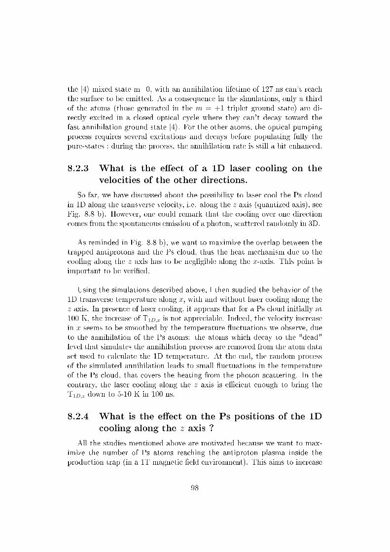
the |4⟩ mixed state m=0, with an annihilation lifetime of 127 ns can't reachthe surface to be emitted. As a consequence in the simulations, only a thirdof the atoms (those generated in the m = +1 triplet ground state) are di-rectly excited in a closed optical cycle where they can't decay toward thefast annihilation ground state |4⟩. For the other atoms, the optical pumpingprocess requires several excitations and decays before populating fully thepure-states ; during the process, the annihilation rate is still a bit enhanced.

8.2.3 What is the eect of a 1D laser cooling on thevelocities of the other directions.

So far, we have discussed about the possibility to laser cool the Ps cloudin 1D along the transverse velocity, i.e. along the z axis (quantized axis), seeFig. 8.8 b). However, one could remark that the cooling over one directioncomes from the spontaneous emission of a photon, scattered randomly in 3D.

As reminded in Fig. 8.8 b), we want to maximize the overlap between thetrapped antiprotons and the Ps cloud, thus the heat mechanism due to thecooling along the z axis has to be negligible along the x-axis. This point isimportant to be veried.

Using the simulations described above, I then studied the behavior of the1D transverse temperature along x, with and without laser cooling along thez axis. In presence of laser cooling, it appears that for a Ps cloud initially at100 K, the increase of T1D,x is not appreciable. Indeed, the velocity increasein x seems to be smoothed by the temperature uctuations we observe, dueto the annihilation of the Ps atoms: the atoms which decay to the "dead"level that simulates the annihilation process are removed from the atom dataset used to calculate the 1D temperature. At the end, the random processof the simulated annihilation leads to small uctuations in the temperatureof the Ps cloud, that covers the heating from the photon scattering. In thecontrary, the laser cooling along the z axis is ecient enough to bring theT1D,z down to 5-10 K in 100 ns.

8.2.4 What is the eect on the Ps positions of the 1Dcooling along the z axis ?

All the studies mentioned above are motivated because we want to max-imize the number of Ps atoms reaching the antiproton plasma inside theproduction trap (in a 1T magnetic eld environment). This aims to increase

98

the eciency of the formation of antihydrogen via charge-exchange process.The idea of laser cooling the transverse temperature along the z-axis is thento increase the solid angle of the Ps cloud with the antiprotons.

In this last section, I looked into the eect of the 1D laser cooling on thePs positions. More specically, I aimed to specied the number of Ps atomsthat stay "focused" in a cloud of less then 5 mm size during their traveltoward the antiprotons (propagation along the y axis, see Fig. 8.8 b)). Icounted then the numbers of Ps inside | x, z |< 5 mm with and without lasercooling, and probed for dierent times. The results are presented in Fig.8.12. I chose a size of 5 mm that would correspond to a typical length of theantiproton plasma, in the z direction (axial connement).

Figure 8.12: Table which gives the number of Ps atoms that stay inside acloud of | x, z |< 5 mm size, with or without laser interaction. The uppertable presents the number of Ps for the transverse z direction, where the 1Dcooling is applied. The lower table gives the number of Ps for the other trans-verse direction x. In these simulations, a cloud of 2000 Ps is emitted towardthe antiproton plasma at a temperature of 100 K, along the y propagationaxis. The annihilation of the o-Ps in vacuum is taken into account.

99

In the tables of Fig. 8.12, we can see that the number of Ps inside | x |< 5mm doesn't change much during the cooling over the z direction, in compar-ison to the case without laser. This is a conrmation that the heating dueto the scattered photon is negligible, as mentioned in Sec. 8.2.3 just above.

However, in the cooled direction z, it appears that only a factor 2 in thenumber of Ps that stayed inside | z |< 5 mm can be won. This limited im-provement is mostly due to the annihilation process: the laser cooling takestime, in the order of the o-Ps lifetime (142 ns). During the laser cooling, mostof the Ps annihilate and don't reach the antiproton plasma. This problemwas initially thought to be resolved by exciting the o-Ps toward the Rydbergstates n=15-20, that is impossible during the laser cooling.

If we only consider the impact of the collimation of the 1D laser coolingon the Ps cloud, this analysis seems to indicate that the 1D cooling over thez-axis is not preferable compared to the solution of a direct excitation of thePs cloud to Rydberg state.

8.3 Conclusion and prospective

We have seen in this chapter that laser cooling of Ps should be realizablefor reasonable short interaction times, and for both 0 T and 1 T magneticeld environments. For instance, if we consider a Ps cloud with an initialtemperature of 1000 K, an ecient cooling would be given by lasers set at5000 W, detuned around 300 GHz (∼ 10 cm−1) for a bandwidth of 200 GHz; in 100 ns the 1D and 3D temperatures can be expected to have decreasedaround 500 K.

The presence of magnetic eld limits the possibility of a 3D laser cool-ing because of the Zeeman mixing of singlet and triplet states. Indeed, theselection of pure-states cycles we just presented is only possible for lasersaligned with the magnetic axis direction. Thus, the laser cooling of Ps inpresence of magnetic eld appears to be feasible only in 1D, and parallel tothe B eld. We can remark the laser cooling scheme in 1T is not ecientin 3D. Indeed, the lasers need to be parallel to the quantication axis to beable to only excite on the pure states (σ± transitions), in order to avoid toenhance the annihilation of the cloud by exciting mixed triplet-singlet states.

A proof of principle of this laser cooling will be important for us, that'swhy I spent a great part of my thesis to develop a laser system that could

100

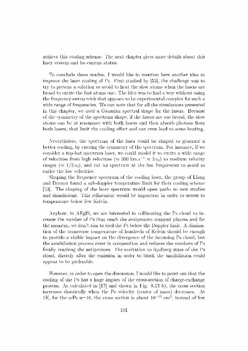
achieve this cooling scheme. The next chapter gives more details about thislaser system and its current status.

To conclude these studies, I would like to mention here another idea toimprove the laser cooling of Ps. First studied by [53], the challenge was totry to present a solution to avoid to heat the slow atoms when the lasers arebroad to excite the fast atoms one. The idea was to nd a way without usingthe frequency sweep trick that appears to be experimental complex for such awide range of frequencies. We can note that for all the simulations presentedin this chapter, we used a Gaussian spectral shape for the lasers. Becauseof the symmetry of the spectrum shape, if the lasers are too broad, the slowatoms can be at resonance with both lasers and then absorb photons fromboth lasers, that limit the cooling eect and can even lead to some heating.

Nevertheless, the spectrum of the laser could be shaped to generate abetter cooling, by cutting the symmetry of the spectrum. For instance, if weconsider a top-hat spectrum laser, we could model it to excite a wide rangeof velocities from high velocities (≈ 300 km.s−1 ≈ 3 v0) to medium velocityranges (≈ 1/2 v0), and cut its spectrum at the low frequencies to avoid toexcite the low velocities.

Shaping the frequency spectrum of the cooling laser, the group of Liangand Dermer found a sub-doppler temperature limit for their cooling scheme[53]. The shaping of the laser spectrum would open paths to new studiesand simulations. This renement would be important in order to access totemperature below few Kelvin.

Anyhow, in AEgIS, we are interested in collimating the Ps cloud to in-crease the number of Ps that reach the antiprotons trapped plasma and forthe moment, we don't aim to cool the Ps below the Doppler limit. A diminu-tion of the transverse temperature of hundreds of Kelvin should be enoughto provide a visible impact on the divergence of the incoming Ps cloud, butthe annihilation process enter in competition and reduces the numbers of Psnally reaching the antiprotons. The excitation to Rydberg state of the Pscloud, directly after the emission in order to block the annihilation couldappear to be preferable.

However, in order to open the discussion, I would like to point out that thecooling of the Ps has a huge impact of the cross-section of charge-exchangeprocess. As calculated in [17] and shown in Fig. 8.13 b), the cross sectionincreases drastically when the Ps velocity (center of mass) decreases. At1K, for the o-Ps n=16, the cross section is about 10−13 cm2, instead of few

101

10−15 cm2 for 100 K (pink arrows) ! This will be in favor of performing thelaser cooling of Ps along the y direction (reduction of the Ps center of massvelocivty), as illustrated in Fig. 8.13 a). In this schematic, the pink arrowsindicate the two counter-propagating lasers that perform the 1D laser cool-ing at 1T along z. One idea could be to slightly tilt the laser directions (redarrows) to couple the cooling to z and y, and reduce the CM velocity of theo-Ps. .

102

Figure 8.13: a) A drawing presenting the 1D laser cooling situation insidethe production trap (1T eld). The center of mass (CM) velocity of theo-Ps vCM,Ps and the positron velocity ve+ are represented. The pink arrowsindicate the two z counter-propagating lasers performing the cooling ; thered ones are a suggestion to couple the cooling of the transverse z directionwith the direction of propagation y, in order to reduce the Ps CM velocity.b) The cross-section of the charge exchange process, for dierent n-statesof the o-Ps, is plotted in function of the relative velocity of the CM andthe positron orbital velocity, for B=0 T and B= 1 T. For the o-Ps(n=16),

the corresponding ratiovCM,Ps

ve+is indicated by the pink arrows, for several

equivalent temperatures T =mPs × v2CM,Ps

kBof 1000 K, 100 K, 10 K and 1 K.

The cross-section increases when the velocity of the CM decreases.

This would require more developed studies to quantify any potential gain:in one hand, the laser cooling down to 1K of Ps atom increases by a fact 100the cross section of the charge-exchange process. In the other hand, duringthe laser cooling, the annihilation of the o-Ps decreases the number of Psreaching the antiprotons to few percents (in 300 ns). The quenching eectshould obviously not be forgotten too. The question remains opened to ndthe best compromise of the two situations.

103

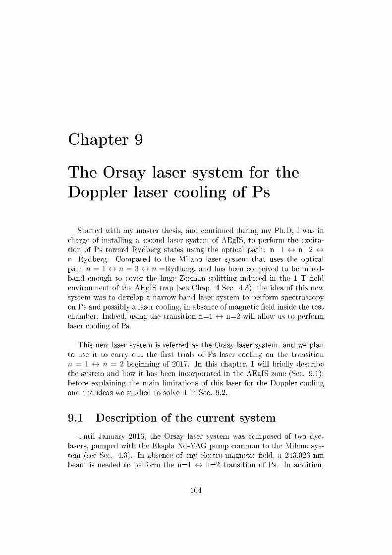
Chapter 9

The Orsay laser system for the

Doppler laser cooling of Ps

Started with my master thesis, and continued during my Ph.D, I was incharge of installing a second laser system of AEgIS, to perform the excita-tion of Ps toward Rydberg states using the optical path: n=1 ↔ n=2 ↔n=Rydberg. Compared to the Milano laser system that uses the opticalpath n = 1 ↔ n = 3 ↔ n =Rydberg, and has been conceived to be broad-band enough to cover the huge Zeeman splitting induced in the 1 T eldenvironment of the AEgIS trap (see Chap. 4 Sec. 4.3), the idea of this newsystem was to develop a narrow-band laser system to perform spectroscopyon Ps and possibly a laser cooling, in absence of magnetic eld inside the testchamber. Indeed, using the transition n=1 ↔ n=2 will allow us to performlaser cooling of Ps.

This new laser system is referred as the Orsay-laser system, and we planto use it to carry out the rst trials of Ps laser cooling on the transitionn = 1 ↔ n = 2 beginning of 2017. In this chapter, I will briey describethe system and how it has been incorporated in the AEgIS zone (Sec. 9.1);before explaining the main limitations of this laser for the Doppler coolingand the ideas we studied to solve it in Sec. 9.2.

9.1 Description of the current system

Until January 2016, the Orsay laser system was composed of two dye-lasers, pumped with the Ekspla Nd-YAG pump common to the Milano sys-tem (see Sec. 4.3). In absence of any electro-magnetic eld, a 243.023 nmbeam is needed to perform the n=1 ↔ n=2 transition of Ps. In addition,

104

we also have developed a tunable red laser with wavelengths from 736 nm to745 nm to excite Ps from the rst excited state n=2 to Rydberg (n= 15 -20), and then Rydberg spectroscopy in absence of magnetic eld in the testchamber.

Because of the restrictive space of the AEgIS zone, the second laser systemhas to be added in a second oor, above the Milano-laser table. The Fig. 9.1shows a scheme of the so-called laser hut in AEgIS, that is a 4 meter squaredspace, placed in the back of the trap magnets, and delimited by two blackcurtains. When working on the lasers, the curtains are closed and preventthe access of the back of our zone. Part of my work was to supervise theinstallation of this second oor and a removable walking platform that allowsthe laser user to work at 2-m height. I also spent time to comply the quite re-strictive safety requirements of CERN to get the authorization to work withclass 4 lasers on two oors (with periscopes to connect the two laser systems).

Working on the laser systems in AEgIS is complex mainly because of thereally conned space and the necessity to work at height on a platform thatisn't specially recommended for lasers works. Besides, the vibrations due toother workers in the zone make the optimization of the laser quite challenging- our laser systems are not isolated in a laser hut apart from the experimen-tal zone, as it is the case for the other experiments in the AD hall. No airtemperature control is present in the AEgIS laser hut, that is also criticalfor the stability of the systems. Finally, because the access to the back ofour experimental zone can only be done by crossing the laser hut or climbingover the two vessels of the trap magnets, the works on the lasers have to bestrictly planned in order not to disturb the other workers.

105

Figure 9.1: Scheme of the AEgIS laser hut. The two laser-systems are dividedin two oors. The Milano system is on the rst oor, and the Orsay-lasersystem is placed above, at 2 m altitude. In order to work on the second table,a removable platform has been built to allow the laser user to stand up atthe proper height.

Since February 2016, a new Nd-YAG pump from the CNI company hasbeen ordered by my laboratory and installed in the upper laser table, as in-dicated in Fig. 9.1. More powerful than the Ekspla one, it delivers 250 mJof 532 nm, in an 8-ns pulse (top-hat), and this allows the two laser systemsto be independently pumped and used in parallel.

The Orsay-laser system is based on dye-laser technologies. Fig. 9.2 a)shows the principle of our dye-laser cavity. The dye powder is diluted intosome solvents (ethanol and methanol) and circulates into a transparent cell,and plays the role of the active medium of the laser. Despite the inconvenientof using ammable toxic products14, using dye-laser has some benets:

14During my thesis, I took care of the safety issues regarding the chemicals used inAEgIS. Dye-powders are registered as toxic, and diluted in ethanol, ammable. Assur-

106

As the active medium of the laser, an excited (pumped) dye typicallyuoresces over a large spectrum, with a bandwidth of about 20-30 nm.By introducing a grating into the laser cavity, this huge uorescencespectrum is diracted over a large cone of angles. The edge mirrorof the cavity reects a fraction of the wavelengths diracted by thegrating, and thus selects only one wavelength that circulates into thecavity and generates the laser beam. The dye-laser can be tuned overthe width of the uorescence spectrum (about 20-30 nm) by adjustingthe angle of reection of the edge mirror that selects the wavelengthmatching the laser cavity.

This kind of laser setup tends to generate quite narrow-band lasers.When the uorescence spot covers N lines of grating, the bandwidth

ν of the laser at a central frequency ν is given by:νν≈

1

N. In

our case, we use a 1 cm long grating with 2400 lines/mm, meaninga selection in frequency of the uorescence spectrum of the excited

dye medium of F =ν486nm

ν≈ 4. 10−5. In other words, the laser

bandwidth is then δν = ν × F ≈ 25 GHz.

ing the safety of the uses of such products at CERN, as well as the storage and stock-management were part of my work.

107

Figure 9.2: Dye laser cavity - schematic and picture. a) the schematic of thecavity of a dye-laser. The grating allows to generate a narrow-band laser,and adjusting the angle of reexion of the edge mirror allows to select thewavelength. b) Picture of the home-made dye laser cavity, that was used toproduce the red laser for the transition n=2 ↔ n = Rydberg.

The Fig. 9.3 a) shows a schematic of the Orsay table, where the two dye-lasers were rst installed and pumped by the Ekspla NdYAG source untilbeginning of 2016 - Fig. b): the second laser has been removed to free somespace, and the CNI YAG pumped has been installed. The BBO crystals areused to generate the third harmonic of the YAG (355 nm) and to doublethe 486 nm generated by the Continuum dye-laser, and produce the 243 nmbeam.

108

9.1.1 The red-laser beam

To generate the 740-nm beam, we use the oxazyn-dye diluted in ethanol,pumped with the second harmonic of YAG (532 nm). This laser is a home-made dye laser, from the Laboratoire Aimé Cotton that hadn't been usedfor years, and I had to reinstall it from scratch, piece by piece at CERN.The Fig. 9.2 is a picture of the cavity of this home-made dye laser. We cansee the cell where the dye is circulating, the edge-mirror (the exit mirror ishidden), the anamorphic prisms that expend the uorescence spot to coverall the grating surface. With about 40 mJ of 532 nm, about 3 mJ of red beamcould be produced. This laser is installed on an aluminum plate in order tobe able to easily remove and reinstall it. It has been removed beginning of2016 to free space.

9.1.2 The 243-nm beam

In order to generate the 243-nm UV beam, we rst generate a 486-nm laserfrom a Coumarin-dye laser, pumped by the third harmonic of the pump YAG(355-nm beam). Then, the 486-nm light is frequency-doubled using a nonlinear BBO crystal of 5 mm × 5 mm × 5 mm size. The dye-laser setup usedhere is an industrial Continuum laser ND4600. With 35 mJ of pump 355 nm,up to 2.5 mJ of blue light (486 nm) is produced, and converted up to 600 µJof 243 nm. Because its intrinsic nature of dye laser (multi-modes), the UVenergy uctuates shot by shot by about 15%.

The 243-nm beam to laser cool Ps atoms?

As explained in the previous chapters 7 and 8, we want to perform lasercooling of Ps using the 243-nm beam. The simulations tend to indicate thatthe UV pulse needs to last some tens of ns. Unfortunately, the two NdYAGpumps we own in AEgIS, based on Q-switched technologies, provide respec-tively laser pulses for the 1064 nm of 5-6 ns for the Ekspla source, and 8 nspulses for the CNI pump.

The Ekspla pump provides quasi Gaussian pulses. The non linear processfor the second harmonic generation (SHG) acts on the temporal Gaussian

pulse by shortening the generated pulse as: tSHG=tpump

2. Then, the 243-nm

beam pumped by the Ekspla pump leads to a pulse of about 2 ns (FWHM).Whereas the CNI laser delivers top-hat spectral pulses. The SHG pulse from

109

Figure 9.3: Schemes of the Orsay table, for the two dierent periods of time.a) until beginning of 2016, the Orsay-system was composed of two dye-lasers,that generated the wavelengths for performing the Ps Rydberg excitationusing the transitions n=1 ↔

243nmn=2 ↔

∼740nmn=Rydberg. b) Since February

2016, a new NdYAG pump from the CNI company has been installed, andthe home-made red dye laser has been removed to free some space.

a top-hat spectral prole keep the same pulse width. Thus, the CNI laserleads to a 243 nm beam of rather 8 ns (FWHM). This is still too short tosee any measurable laser cooling eect on Ps. The UV pulse needs then tobe lengthened. That's why the red dye-laser has been removed to be able tocarry-out some trials to stretch the UV pulse. I will explain now dierentideas we studied to lengthen the 243-nm laser.

9.2 Stretching the UV pulse

We rst studied the possibility to buy a commercial laser that wouldmatch the requirements of generating a long pulse (≥ 100 ns), high powerand tunable bandwidth at 243 nm. We found that the commercial solutionbased on the Alexandrite (Cr3+:BeAl2O4) crystal from LightAge companywas very promising. Its main characteristics are:

Tunable outputs:

720-735 nm, can be extended to 720-800 nm, for the fundamentalharmonic.

higher harmonics possibly tunable too: 360-400 nm, 240-270 nm,190-200 nm

A long pulse duration: the nominal Q-switched pulse duration is 100ns and can varied from below 30 ns to 200 ns.

An adjustable spectral bandwidth. The spectral linewidth is <30 MHzfor the fundamental and can be modied from Fourier-Transform lim-ited pulse to very large bandwidth (>100 GHz) based on dierent CWlaser seeders inside the cavity.

Nice stability of the laser frequency: output wavelength stability of<300 MHz/day. Frequency chirp corrected to be less than 50 MHz.

And nally, good energy generated. We can expect a pulse of an energygreater or equal to 1 mJ for the 243-265 nm beam.

This laser will match perfectly the requirements for an ecient laser cool-ing of the Ps cloud, for the "modest" sum of ≈ 200 ke.

Among the other possible choices we looked for, we could mention:

Using the Cr:LiSAF based laser as developed in [64]. But this wouldlead to intense laser development with no guarantee to reach a largelaser power.

111

Using a long (>100 ns) pump (like the Hawk-HP from quantronix lasersor the Mesa-355-40M from Continuum company or the Evolution 527nm from Coherent Inc) to pump the Orsay laser system to producethe 243 nm. This may lead to some issues during the pumping of thedye (thermal eect). Furthermore the dye uorescence is a non linearprocess and needs intense pump to be ecient. This technique couldalso be limited because of a weak laser power generated.

Considering a continuous-wave (cw) pulse-amplied laser, such as theone developed in the ASACUSA experiment at CERN [65]. In a similarway, the injection seeded pulsed (Ti:Sa) lasers produce 729 nm beamthat can then be tripled to form 243 nm. In a very recent publicationstudying the cooling of Positronium for Bose-Einstein Condensation(BEC) [56], they suggested such a complex laser with frequency triplingwith an injection seeded pulsed Ti:Sa, and a sophisticated spectralmodication by Electro-Optics Modulator. Here again this would leadto a non-negligible laser development for us.

In absence of any funding, we tried to nd cheap solutions. The obviousone would be to lengthen the pulse generated by the dye-laser system (Orsaysystem) currently installed in AEgIS. We studied mainly two setups:

dividing physically the mother pulse into several secondary pulses.Each secondary pulse travels dierent paths, with the length adaptedto cause additional temporal delay. At the end, the secondary pulsesare recombined with their time delays into a single nal pulse. To doso, we studied the possibility of using bers.

entering the mother pulse into a loss-cavity. One of the mirror of thecavity has a low transmission percentage (typically 10 to 40 % trans-mission), for each turn into the cavity, a secondary pulse is emitted.We studied mainly two setups for this loss-cavity, also called stretchingcavity in literature [66].

9.2.1 The ber setup

The concept of this ber setup is illustrated in Fig. 9.4 a). First, we had tocontact and discuss with companies to determine which kind of ber divideris technically realizable for UV beam, in order to minimize the losses duringthe injection. I investigated dierent combinations to divide the pulse intoN secondary pulses. Fig. 9.4 b) shows the ber divider we used in AEgIS tocarry out the rst trials - this divider is not UV-resistant, and can't be use

112

as a long-term solution.

Figure 9.4: The bers solution to stretch the UV pulse. a) the schematic ofthe principle is drawn here. The mother pulse is divided into 3 secondarypulses. Each sister-pulse travels into one of the 3 paths with dierent lengths(d1 < d2 < d3), leading to dierent time delays for each path. The UV beamis absorbed by the fused-silica solarization resistant bers with an attenuationfactor of 0.3dB/m. This implies that the secondary pulses are more and moreattenuated as they propagate in longer lengths of ber. b) the picture of aber divider 1 toward 3 that we have in AEgIS, not adapted for UV. Thecoupling is not optimized for this device, and the losses are about 50 % forvisible light. Since these dividers haven't been conceived to be UV-resistantand minimize the UV absorption, the losses for the 243nm were considerable:only few percents of the incoming pulse exited at the end of each secondaryber. We used two of these dividers to obtain the results shown in Fig. 9.5a).

The Fig. 9.6 gives a table of three dierent congurations studied, withthe combined pulse results: shape, temporal stretching and nal total en-ergy. The losses come from two sources: the geometrical overlap betweenthe mother ber with a big core (600 µJ for the simulations) toward the Nsecondary bers of varying core size, and the attenuation during the pulsepropagation into the bers. Indeed, the UV beam at 243 nm is absorbedby the fused-silica solarization resistant bers with an attenuation factor of0.3dB/m. The eect is not negligible, specially for the long delayed secondarypulses that propagate along a great path into the ber. This attenuation ex-plains the progressive decreases of the intensity of secondary pulses.

113

According to the simulations, it appears that the division of 1 pulse into5 secondary pulses is a good compromise to optimize the areas overlaps ofthe bers. For the mother ber of a core of 600µm, the division into 5 bersof 200 µm is technically realizable, and will induce geometrical losses of only30 %.

For an initial pulse at 243 nm of I0 = 600 µJ and a pulse of FWHM = 8ns, we obtain a combined pulse of 260 µJ in 90 ns duration, meaning a powerof 2900 W or an intensity of 5800 W/cm2 ≈ Isat,L,100GHz for a waist radiusof 4 mm. This conguration seems adequate for the cooling purpose.

However, we are here limited by the ber technology. We contacted sev-eral companies to ask the possibilities of conceiving such dividers, that couldhold the 600 µJ of UV pulsed beam without melting. We are still in discus-sion with the IDIL French company to solve the melting issue. Using the twobers dividers we had at CERN (shown in Fig. 9.4 b) ), in 2015, we did a rsttest to lengthen the pulse, as presented in Fig. 9.5. At that time, the laserpump used was the NdYAG Ekspla pump, with an initial pulse duration ofabout 6-8 ns, that produced an UV pulse of about 2 ns. The ber lengths of3 m, 5 m and 10 m to delay the secondary pulses were not adapted to delaythe pulses in order to make them overlap. The refractive index of the bercore for the UV is about nfiber=1.45, the propagation of the light over 1 m

leads then to a time delay of: t = 1 m1.45

c≈ 5 ns for the pulse.

With the new CNI NdYAG pump, the 243 nm beam has a pulse lengthof about 8 ns, the delays induce by 3 m, 5 m and 10 m are respectively 15ns, 25 ns and 50 ns. In the Fig. 9.5 a), the secondary pulses are separatedin time since their mother pulse was 2 ns (FHWM) and the bers too longfor such short pulses; whereas the sisters pulses coming from the 8 ns motherpulse generated by the CNI pump should overlap using the same bers (3 m,5 m and 10 m).

114

Figure 9.6: Fiber divider solutions: Simulations results for 3 dierent con-gurations. The initial UV pulse has a FHWM of 8 ns. The solution usingthe dividers 1 ↔ 5 seems to be a good conguration, where the geometricaloverlap is maximized and the initial pulse of 8 ns is lengthened to about 90ns with only 60 % total losses. These losses are due both to the attenuationinto the bers and the geometrical overlaps of the mother ber's core withthe secondary bers' core. For an initial pulse of I0 = 600 µm, we obtain acombined pulse of 260 µJ in 90 ns duration, meaning a power of 2900 W oran intensity of 5800 W/cm2 ≈ Isat,L,100GHz for a radius waist of 4 mm.

Figure 9.5: Test on the bers solution to lengthen the UV pulse. The initialpulse duration is about 2 ns. a) The secondary pulses recorded on an oscillo-scope card Agilent 1 GHz. b) the simulation expected result for the lengthsof the bers (3 m, 5 m and 10 m). The bers lengths have to be adapted tooverlap the pulses, and new ber dividers 1↔3 or 1↔5 have to be purchasedsince the ones used that are not UV resistant. The simulations are madeconsidering that the coupling from the mother ber into the 3 sister bers isthe same for each sister ber. The attenuation of the peaks in the simulationis only due to the absorption into the bers. However, the experimental re-sult in a) shows experimentally that the coupling is not equal for each sisterber, that's why the second pulse is higher then the rst one.

9.2.2 Loss cavity using beam splitter

In parallel to the bers solution, we studied then the loss cavity setup,also referred as the "stretching cavity". In Fig. 9.7 is presented the typicalschematic of a such cavity.15

15We only studied squared-shape cavity instead of triangle-shape or other kind of setups(see [66]) since we want to limit the reectivity losses of the commercial UV mirrors thatare typically optimized for a 45 reexion.

116

Figure 9.7: Schematic of the loss cavity setup. The incoming beam I0 entersinto the loss cavity through the beam splitter. Partially reected (R %) andtransmitted (T%), the inner-cavity beam undergoes N turns before leavingcompletely the cavity. At each turn n ≤ N , a secondary pulse is emitted. Thenal pulse formula is given by Iout(t) = RI0(t)+

∑0≤n≤N T

2Rn I0(t0−nt).By adjusting the length of the cavity, we can adjust the delay t betweeneach secondary pulse emitted.

The optimization of this setup was then to determine the proper ratio re-ectivity over transmission (R/T) to generate secondary pulses of the sameorder of magnitude. Fig. 9.8 shows dierent congurations for the trans-mission and reection parameters of the beam splitter. For all the dierentcongurations, the number of secondary pulses with similar intensity appearsto be limited. There is a simple reason for this: in order to have a great num-ber of secondary pulses, most of the energy of the mother pulse has to enterinto the cavity, implying R small. But then, after the rst turn, the rst sec-ondary pulse emitted will be highly intense since T = 1 − R is high. Then,most of the energy has left the cavity after just one turn. Coecient such asR ≈ 35 % seems to be a good compromise and the mother pulse of FWHM=8ns can be stretched up to 50 ns.

117

Figure 9.8: Simulations results for the loss cavity setup, varying the reex-ion/transmission ratio. In blue is plotted the mother pulse, of FWHM =8 ns, in orange is the stretched beam, made of the secondary pulses. Agood compromise for having similar intensity secondary pulses seems to beR≈ 35%. In this case, the pulse can be lengthened to 50 ns.

At the end, if we consider that we want to produce only secondary pulseswith comparable intensity, the number of secondary pulses that can be emit-ted from the stretching cavity appears to be limited. Indeed, the nalstretched pulse has to be intense to excite the transition n=1↔ n=2 over allits duration, otherwise the stretching will be ineective. The solution R=35% (shown in Fig. 9.8, mid column, seems a good compromise.

However, even if the stretching capacity of this loss cavity setup appearsto be smaller than for the bers solution, this system has the great benet oflimiting the energy losses. For UV excimer mirror at 99.9 % reectivity, theenergies losses are negligible after few turns into the cavity compared to the0.3dB/m of the ber attenuation (see Sec. 9.2.1). Besides, according to theprevious simulations of laser cooling (See Chap. 8), generating a UV pulseof 50 ns should be enough to see an eect on slow positronium atoms. Thistechnique seems promising then.

9.2.3 The loss cavity setup using polarization cube

For studying the last stretching solution, I supervised the work of anunder-graduated student Grace Kerber, from the Boston students exchangeprogram. Grace studies at the Gustavus Adolphus College, in Minnesota,

118

USA, and she worked in AEgIS for 4 months between March to June 2016.

With Grace, we then looked for an idea to improve the loss-cavity setupand nd a solution to increase the number of secondary pulses with compara-ble intensity. We thought of using polarization cube instead of a simple beamsplitter. The scheme of principle is presented in Fig. 9.9. The polarizationcube transmits horizontal polarized light, and reects vertical polarization.By projecting the inner-cavity pulses into a combination of vertical and hor-izontal polarization, we can select the among of light transmitted at eachturn. A waveplate λ/2 can be used to polarize the light into a combinationof vertical (a%) and horizontal (b %=1- a%) polarization.

Figure 9.9: The loss-cavity setup, using a polarization cube. In order toenter the cavity, the rst mirror (M1) is barely missed. A waveplate λ/2 isplaced into the cavity to select the percentage of light vertically polarizeda (that will be reected in the cavity) and the percentage b of horizontallypolarized light (that will be transmitted). The exiting pulse is then given bythe formula: Iout(t) =

∑Nn≥0 Iin(t− nt)× b an =

∑n≥0 In(t).

In order to enter into the cavity, the rst mirror (M1) has to be barelymissed, and the light enters the cavity with a small angle. This angle willlead to the displacement of the pulse's after each turn, until the beam gets

119

out of the mirrors. This will limit the numbers of pulses we can possiblyhave inside the cavity.

Grace wrote a code in Matlab to simulate this setup, and tried to nd thebest setting parameters to maximize the number of secondary pulses. In Fig.9.10 is presented some of the results. a) shows the paths of three rays thatdelimit the incoming UV pulse. In order to represent the laser beam, witha possible divergence, she chose to plot three dierent optical rays: the redand black lines determine the edge of the beam (contours), and the green lineis the central ray. This trick allows to illustrate the divergence of the beamand the possible issues after several turns into the cavity. The beam enterswith a slight angle (mirror slightly missed to let enter the mother pulse),the edge rays are tilt from the central path (case of a non collimated beam),and for each reexion on the 45 mirrors of the cavity, they accumulate abigger angle with respect to the normal of the mirrors. As a consequence,the direction of reexion for the central ray and the edges rays diers a lotafter a few turns inside the cavity. This creates dierent spot locations atthe Ps target region for the each secondary pulse, as shown in Fig 9.10 a).

120

Figure 9.10: Some simulations result performed by Grace Kerber, for a=92%, b=1-a=8%, a cavity length of 3.2 m and an initial pulse of FWHM = 4ns. a) shows the paths of three rays that delimit the incoming UV pulse -the red and black lines determine the edge of the beam, and the green lineis the central path. This illustrates the eect of divergence on the beamafter several turns into the cavity. The secondary pulse spots are spatiallyseparated at the Ps target region. b) presents the exiting pulse Iout(t) =∑In(t). The secondary pulses In don't overlap temporally in purpose, to

extend even more the exiting pulse.

The Fig. 9.10 b) plot presents the exiting pulse Iout, where the secondarypulses (I0, I1, I2, etc.) don't temporally overlap in purpose.

In order to increase even more the laser interaction time, we thought itcould be interesting to perform some tests with temporally separated pulses.Indeed, the typical cooling cycle over n= 1 ↔ n=2 transition of Ps is about2× τspont = 6.4 ns. If the laser excitation is made of several pulses of FWHM≈ 8 ns spaced of few ns as shown in Fig. 9.10 b), this temporal spacingwill give the time for the excited atom to decay toward ground state, beforegetting excited by the following pulse. The cooling eciency shouldn't betoo much disturbed. The optical pumping code (c++ code) used for thesimulations in Chap. 8 should be adapted a bit, before being able to makethe simulations with a temporal laser pulse made of several separated pulses.

One of the main limitations of this setup still remains the possible numberof turns we can expect to reach, entering with a small angle into the cavity.Some tricks can be played introducing a correcting converging lens. Grace

121

also implemented in her code the possibility to add one convergence lensinside the cavity to try to correct the divergence of the beam. The rstresults seem to indicate that the focal length of the lens should be of theorder of the cavity length to be able to compensate the divergence at eachturn. The best position to place the lens seems to be right before the rstmirror M1. Anyhow, the preliminary simulation results of Grace indicatethat it will be dicult to generate more than 4 turns, for standard opticssizes (1 inch diameter). Besides, the fact that all the secondary pulses don'tspatial overlap neither could be a big limitation of this scheme. Furtherstudies are needed to be able to select one or the other stretching solution.

9.2.4 Current situation of the Orsay laser

For now, the optimization of the Orsay system with the new source is go-ing on, as well as the implementation of new safety requirements due to theinstallation of a second class 4 laser pump in the zone. Specially, this newsource has to be interlocked with the existing synchronization system usedfor the Milano system. Moreover, the non linear crystal used to produce thesecond harmonic of the 1064 nm YAG has to be replaced because of somedamage at the delivery, that is slowing down the laser work in the zone. Wealso ordered a bigger BBO crystal to generate even more the third harmonicof the YAG to pump the Coumarin laser dye. We hope to be able to generateup to 800 µJ of 243nm with an optimized system.

Olga Khalidova is a new post-doc of AEgIS who started in March 2016.Together we continue testing the dierent stretching solutions, to be readyfor the beginning of 2017. We have ordered both the beam splitter and aUV polarization cube to try to set-up the cavity loss solution in the followingmonths.

122

Chapter 10

Another way to focus of the Ps

cloud? The dipolar force

interaction

During my Ph.D, I also studied the possibility to collimate the Ps beamusing the dipolar force. A strongly detuned and intense laser creates a localpotential well that either attracts or repulses the atoms in interaction withit, depending of the detuning sign.

The dipolar force can lead to the deceleration of the particles in interac-tion with the created well. In 2010, Barker's group produced a stationarymolecular beam thanks to the interaction with an optical lattice [67] usingthe dipolar interaction. Our idea was to investigate the possibility to use thedipolar force to focus the Ps cloud, using the attraction/repulsion propertyof this interaction.

In the following chapter, I will briey present the dipolar force eect onthe phase-space of the atom, and I will give some simulation results, beforediscussing the possibility of a practical realization. It is beyond the purposeof this chapter to deal with the theory to derive the dipolar force; for instance,the reader could refer to [68] for more detail.

10.1 The dipolar force interaction principle

The dipolar force derives from the laser dipolar potential Udip such as:

F = −∇Udip(r) (10.1)

Where the dipolar potential can be expressed - for a strong detuning and

123

low saturation - as Udip(r) = ±~Ω(r)2

4δ∝I(r)

δ, with δ = ωL−ω0 the detuning

of the transition and r the position of the particle inside the laser spot. More

generally, the dipolar potential can be derived as Udip =~ δ2

ln(1 + s(r))

(See [68]), where the s parameter refers to the saturation parameter denedprevisouly in Eq. (7.7).

It appears that the more intense the laser is, the deeper the potential wellis, allowing to capture fast atoms. However, the laser also need to be stronglydetuned in order to avoid to absorb and scatter any photon.

In Fig. 10.1, a simple scheme of the dressed atom picture illustrates thedipolar force eects of a blue detuned laser between a transition |f⟩ ↔ |e⟩ ofan atom. The dipolar force acting on the atom over the transition |f⟩ ↔ |e⟩depends on the sign of the detuning. During the interaction, the states |f⟩(lower level) and |e⟩ (upper level) are mixed, and form new states |+⟩ and|−⟩ that are usually called the dressed atom states. A red-detuned intenselaser creates a potential well that attracts the atoms (low-eld seeker) inthe |−⟩ state, and a blue-detuned laser tends to expel the atoms (high-eldseeker) in the |−⟩ state. The dipolar force has the opposite eect on the |+⟩state. If strongly detuned, we can identify |f⟩ ≈ |−⟩ and |e⟩ ≈ |+⟩.

124

Figure 10.1: The dipolar force's eect over the transition |f⟩ ↔ |e⟩ is illus-trated in the dressed-atom picture, for a blue detuned laser. Both the atomand the laser eld are quantized. The states |f⟩ and |e⟩ are mixed and formthe coupled states |+⟩ and |−⟩, usually called the dressed-atom states. Insidethe laser spot, the atoms either see an attractive potential (|+⟩ ≈

|δ|≫1|e⟩) or

a repulsive one (|−⟩ ≈|δ|≫1

|f⟩). Illustration taken from [68]

As mentioned previously, our idea here is to use the dipolar force to focusthe Ps cloud, using the attraction/repulsion property of this interaction. InFig. 10.2 is sketched the interaction scheme (top gure) and the dipolar forceeect on the atoms in phase-space picture (bottom gure). The dipolar eectis illustrated within the harmonic approximation (see below).

In the Fig. 10.2 top-gure, the Ps cloud is emitted at a time t0, freelytravels during a time t10, before interacting with the laser during a time t21.After the laser interaction, the Ps cloud continues its free-ight during a timet32. In the case of an attractive force, the laser interaction induces a rotationof the position and velocity distribution in the phase-space of the atoms, asshown in Fig. 10.2 bottom gure. By precisely tuning the interaction time,we can play on the rotation eects, and then the atom cloud can be focusedin a certain point of space after the interaction and a free ight.

The studies I performed aimed to determine the ideal interaction time tofocus the Ps cloud, depending on parameters such as its initial temperature

125

Figure 10.2: The dipolar force focusing principle. In the top image, thePs cloud is emitted (a), where it travels during a time t10free from anyinteraction, before interacting (b) with the laser, for a time21. Leaving theinteraction region (c), the Ps cloud continues its free-ight during a time t32until reaching the target point (d), where we want to focus the Ps atoms.The laser interaction with a strongly detuned and intense laser creates apotential well felt by the atoms, that induces a rotation on the phase-spacedistribution of the atoms, as illustrated in the bottom gure. The phase-space distribution of the Ps cloud is shown for the dierent positions (a),(b), (c) and (d), before and after the interaction. We consider here thedipolar force within the harmonic approximation.

126

and size.

In order to be able to use the dipolar force with the laser system alreadyavailable at CERN, I only studied one scheme using the NdYAG wavelength1064 nm that is the most powerful laser we have. Using a highly intenselaser is mandatory to create a deep potential well and increase the capturerange on the atoms in interaction. Moreover, as illustrated in Fig. 10.3, theYAG laser pump appears to be ideally detuned to interact on the transitionn = 2↔ n = 3 of the Ps (corresponding wavelength λ32= 1312nm).

Beforehand, the Ps cloud would required to be excited to the n=3 state, inorder to make the dipolar force attractive on the transition n = 2↔ n = 3.In our simple model, we neglect the spontaneous decays from the n=3 states,compared to the time of interaction. The spontaneous decays from the Ps

n=3 are: Γs,3↔2 =1

30.92nsand Γs,3↔1 =

1

10ns. So, in a rst approach, for

small interaction times of 2 or 3 ns, this approximation can still be applied.

In our scheme, if a Ps excited in n=3 absorbs a photon to go to n=2 anddeexcites toward the ground state, it will be lost for the dipolar interactionon the transition n = 3 ↔ n = 2. The laser needs then to be far fromresonance. In other words, the scattering rate has to be negligible:

Γscatt =Γs Udip

~ δ

Γscatt =Ω2 Γs

4 δ2

(10.2)

Thus, to be neglected, we need Γscatt ∼I

δ2≪

1

tinteraction, meaning the

dipolar force is strong for δ ≫ Γs,Ω. That's why the 1064 nm laser ap-pears to be suitable for our purposes: intense and strongly detuned fromthe transition. For our YAG pulsed laser of 350 mJ, 15 ns and waists of

w=√5mm× 0.1mm, we derive a scattering rate of: Γscatt =

1

2.7µs16.

16To derive the scattering rate, the Rabi frequency of the interaction needs to be cal-

culated. From the theoretical spontaneous decay Γs,2↔3 =1

30.92ns, we can derive the

dipole strength of the transition n=2 ↔ n=3: d23 =

√~Γs,2↔3 3π ϵ0

k30≈ 15 Debye. Then,

for a YAG pulse laser of 350 mJ, over 15 ns and a waist of w=√5mm× 0.1mm, we obtain

127

Figure 10.3: Schemes of principle to use the dipolar force on Ps atom: a)First, the Ps atom has to be in the n=3 excited state. b) Once the atoms arein n=3, they will experience a blue-detuned dipolar force (attractive force)on the transition n = 3↔ n = 2.

Typically in the following, we consider interaction times of the order of

2 ns or 3 ns, thus Γinteraction =1

tinteraction≈

1

2ns= 0.5 GHz≫ Γscat =

1

2.7µs.

For the simulations, I consider that the Ps cloud is emitted toward the xdirection, and the laser is shined along the y axis (focusing of the z compo-nent). The laser interaction will aect the Ps cloud position and velocity onthe transverse x, 0, z plane, as illustrated in Fig. 10.2.

the Rabi frequency value:

Ω =d23 EL

~=

d23

√2 IL

ϵ0 c

~≈ 7× 1013 s−1 (10.3)

Using Eq. (10.2), this leads to the scattering rate: Γscatt =1

2.7µs

128

10.2 The dipolar force on a single atom

In case of the dipolar force, the laser-matter interaction's impact on theclassical position and velocity of the atom can be easily pictured by the phase-

space vector Z(t) =(z(t)vz(t)

), where z(t) is the particle position, and vz(t)

its velocity along the z axis. The atom propagating in a free-ight during atime tprop is given by the matrix:

Mfree =

(1 tprop0 1

)(10.4)

The laser-matter interaction with the dipolar force during a time tint leadsto a rotation in the phase-space distribution of the atom and its phase-spacevector is multiplied by the matrix:

Mint. dip. =

cos(ωtrap tint)sin(ωtrap tint)

ωtrap

−ωtrap × sin(ωtrap tint) cos(ωtrap tint)

(10.5)

Where ωtrap is the angular frequency of the dipolar trap.

We consider here that the laser is stationary (I(t) constant), and we modelwithin the harmonic well approximation: the cold atoms oscillate in the cen-ter of the dipolar well, the Gaussian laser eect can be approximated by:

exp(−r2

2σ2L

) = 1−r2

2σ2L

. In other words, the atoms in interaction feel an har-

monic potential with the angular frequency ωtrap and experience a rotationof their phase-space distributions - see Fig. 10.2.

In a harmonic trap, the particle oscillates at a dened frequency of ωtrap:

ωtrap = 2π1

π wL

√Udip

mPs

(10.6)

where wL is the laser waist

In the matrix formalism, it is easy to calculate the classical path of severalparticles in interaction with a laser. The total interaction matrix, resultingof a free-ight of the atom during a time t10, followed by the laser interactionduring t21 and nishing by a free ight until the target region, during t32 isthen:

129

Mtot =Mfree,t32 ×Mint,t21 ×Mfree,t10 (10.7)

The classical path evolution of an atom is then derived by:

Z(t) =

(z(t)vz(t)

)=Mtot Z0 (10.8)

I wrote a Mathematica code to solve and plot the path of several particles, fordierent interaction times. The dipolar trap parameters (depth and angularfrequency) are also derived in the code.

10.3 Some results

The main limitation of this focusing principle comes from the laser inten-sity needed to induce a deep enough potential well to catch Ps at few tensof Kelvin. The maximum temperature captured by the trap is dened by:

Tmax =Udip

kB= ~ δ ln

1 +I/Isat

1 + 4δ2

Γ2s

× 1

2 kB(10.9)

We dene the mean velocity of the Ps cloud by, v0 =

√kB T

mPs

where T

is the initial temperature of the Ps cloud. Here we can give some typicalvalues reachable with our system: for a laser intensity of 3 GW/cm2, mean-ing a pulse laser of 450mJ over 10 ns, focused on asymmetric waist wL =√5 mm× 0.2mm, the maximum temperature of capture for the Ps is about

30 K corresponding to a mean velocity caught of v0,trapped=15 km.s−1. Theoscillation frequency of the rotation in the potential well is then ωtrap ≈ 2π 4.7MHz.

As reminded in Fig. 10.4 a), we want here to determine the optimumtimes of free-ights and laser interaction that the Ps cloud should experienceto be more focused when reaching the trapped antiproton region - locatedat about 3 cm from the Ps cloud's formation. To do so in the simulations,the rst free-ight time t10 can be tuned, as well as the interaction timet21. Since the antiproton target region is xed at a 2 cm distance from thePs convertor target, the last free-ight time t32 is xed by the other two times.

130

In the simulations, I rst modeled the Ps beam evolution over time bytracing the paths of 15 atoms that illustrate some typical atoms trajectoriesof the global cloud. These atoms are generated for 3 dierent positions inspace, with 5 dierent initial velocities. Fig. 10.4 b) shows the initial raysthat model the Ps cloud, for a temperature of 30 K. The Ps cloud size isconsidered to be initially 2 mm wide, thus I only take into account 3 extremepositions generated at 0 mm, -1 mm x,z, 0 mm, 0 mm and 0 mm,+1 mm. For each point, ve dierent paths are plotted with ve dierentvelocities that dene the limits of the Ps cone of emission: v = v0ex± 2 v0ez,v = v0ex ± v0ez and v = v0 ex.

Figure 10.4: The initial conditions for the Ps focusing, using the dipolar force.a) is a reminder of the AEgIS schematic for the antihydrogen production. Be-tween the Ps converter target and the antiproton trap, the Positronium cloudhas to travel about 2 cm distance. b) shows the 15 initial paths that denethe Ps cloud in the Mathematica code. Initially, the Ps cloud is supposedto be 2 mm wide along the z axis, with an initial temperature T. The tem-perature gives the mean velocity v0 that xes the emission cone, given twoextreme atoms' paths with the initial velocity v = v0ex±2 v0ez. We considerthat the atoms are emitted at the same time (no spread in x). .

The simulation purpose was then to determine a set of entangled param-eters:

For a xed temperature of the atoms, the ideal interaction time isdetermined to focus their path in the antiproton trapped region, asillustrated in Fig. 10.5 a). The new NdYAG laser we have at CERNhas a pulse time of about 15 ns. In order to select an interaction time

131

smaller than this value, we can for instance squeeze the laser dimensionsto reduce the crossing time. The interaction time is dened to be theminimal value between the laser pulse time (tpulse,laser = 15 ns) and the

Ps atoms crossing time (tcross =wx

v0).

But squeezing the laser spot also modies the trap depth and then themaximal temperature of capture. Thus, faster Ps atoms would feel thedipolar trapping force and the interaction time has to be adapted tofocus them at the antiproton position.

In Fig. 10.5 are presented some typical results. In order to initializethe atom paths, as shown in Fig. 10.4 b), the initial velocity v0 has been

taken to correspond to a ctive temperature T = 30 K, v0 =

√kB T

mP s≈ 15

km.s−1. These 30 K correspond to the maximum capture depth of the dipo-lar trap generated by a laser energy of 350 mJ, over 15 ns and for a waist ofwL =

√wx × wz=

√0.1mm× 5mm. I considered the laser interaction was

delimited by its waist sizes wx and wz (the eect of the tails are not takeninto account into this simple simulation). This value of 30 K is an arbitrarytemperature, chosen to be in the order of the lowest temperatures that thethermalized o-Ps emitted in vacuum can reach, for the target we use (withnano-channels of 6 - 8 nm size) and in the case where the target is cooled tocryogenic temperatures.

During a free-ight over a distance of 3 cm - corresponding to an over-estimation of the distance to reach the trapped antiproton area - the Ps cloudexpends to 12 cm ; as shown by the red dashed paths in the simulations. Wedene the Ps cloud extremities by the two extreme atom paths, that givesthe nal size in the p target.

In the column 1, a scan of the interaction time t21 = tint is presented. Thedistance between the positronium target convertor and the laser is xed andcorresponds to the free-ight distance x10= 2 mm. The interaction time iscrucial to be able to focus the atoms in the target region. If the Ps cloud isfocused on 1.1 cm in the target region for the (b) situation, the (c) situationgives a focusing of about 2 cm whereas the interaction time only diers of0.5 ns.

In the column 2 are shown the results of a scan of the free-ight distancex10 for a xed interaction time of tint=4 ns. The distance of free ight before

132

laser interaction is also important: a variation of 1 mm in position drasticallychanges the focusing result. Besides, for a too long free-ight before the laserinteraction (see (e) and (f) cases), the Ps cloud extends too much and thelaser spot doesn't overlap it completely anymore. In the simulations, thisis visible on the Ps trajectory at the edges of the cloud that don't interactwith the laser and are not deected (the eect of the laser tails is not takeninto account since we consider only a harmonic potential well of interaction,approximation valid at the center of the laser spot) .

For these basic simulations, the best parameters seem to be for the b)situation with tint = 4.5 ns and x10= 2 mm. Under this laser interaction, thePs cloud's size is focused down to 1.1 cm in the antiproton target region.

In Fig. 10.5, the graph a) appears to be a good conguration to con-centrate the Ps beam on the antiproton region in a spot of 1.1 cm spread ;whereas without laser interaction, the Ps cloud would have expended to 12cm after the 3 cm of free- ight (red dashed line).

These results are encouraging, but the capture range of the dipolar trapis too small for the Ps actually produced in the test chamber of AEgIS: onlya small fraction of the Ps emitted could feel the rotating eect of the dipolarforce. Besides, this simulation only takes into account the paths of someatoms with xed initial position and velocity, and doesn't take into accountthe spread distribution of the Ps cloud, in both velocity and position. Torene more, I also studied the inuence of the dipolar force on the Gaussiandistributions of the emitted Ps cloud.

10.4 The dipolar force's eect on the Gaussian

distributions of Ps cloud

So far, we have only considered point sources: each path represents onePs atom, and we simulated the path of 15 atoms that roughly delimit thePs emission cone's extremities. But the Ps cloud can also be modeled as aspread source.

The emitted Ps cloud can be associated to the random variable Z(t), suchas at the emission time t=0, Z(t=0)=Z0 follows a 2D normal distributionN (µ0,Σ0) with:

133

Figure 10.5: Scan results of the interaction parameters (time t21=tint) anddistance x10). The simulations are done for a Ps cloud initially at 30 K andover 2 mm spread (along z). The 1 column shows results for a xed positionof the laser (x10 = 2 mm), and a varied interaction time. The 2 columngives results of the scan of the laser position x10, for a xed interaction time(4 ns). The antiproton target is located at 3 cm far from the Ps emissiontarget. Without laser interaction, the Ps cloud would have expended to 12cm after the 3 cm of free-ight (red dashed line). In all the graphs, the Psatoms paths in interaction with the dipolar force are in pink, and the laserposition is given by the black line. We can remark that in f), the extreme Pstrajectories are not deected by the laser: the free-ight propagation during3 mm lets the Ps cloud extend too much, and the extreme Ps atoms are outof the laser spot. The laser spot's size in x is represented by a black line.

µ0 =

(00

)Σ0 =

(σ2Z0

00 σVz,0

) (10.10)

In the case of the point-source model, we have seen in Eq. (10.8) that Z(t)follows an ane transformation Z(t)=MtotZ0. For the spread-source case,the Z(t) random variable then also undergoes this ane transfor-mation. This is valid in the harmonic hypothesis where all the atoms feela constant eld. In other words, we consider here that the Ps atoms arein the center of the laser spot, and that the laser spot is bigger than the Pscloud. In this case, the spread-source Z(t) of all the atoms follows the normaldistribution:

N (Mtot µ0,Mtot Σ0tMtot) (10.11)

We nally obtained the variance Σ = Mtot Σ0tMtot expression of the Ps

cloud that has experienced a rst free-ight during t10 time, then a dipo-lar interaction during t21 and nally a second free-ight of t32 to reach theantiproton target:

σ2x = σ2

x,0 × cos(ωtrap t21)− ωtrap t32 sin(ωtrap t21)2+

σV 2z,0(t10 + t32) cos(ωtrap t21) + (

1

ωtrap

− t32 × ωT ) sin(ωtrap t21)2

(10.12)

σ2Vz

= σ2z,O ω

2trap × sin(ωtrap t21)

2 + σ2Vz,0× cos((ωtrap t21)− t10 ωtrap sin(ωtrap t21)2

(10.13)The dipolar force implies rotation in the phase-space of the position and

velocity distribution spreads ; the rms value σz and thus the spatial size ofthe Ps cloud are alternatively focused or defocused, as shown in Fig. 10.6, a).

Optimum traveling and interaction times can be found to focus the spa-tial distribution in the antiproton target area. In Fig. 10.6 b) and c) are

plotted the ratioσz

σz,0of the spatial distribution of a Ps cloud initially at 30

K, as a function of the interaction time t21. Without any laser interaction,

135

the free propagation for a ight of 3 cm leads to a spread of the Ps cloudof σz = 15 × σz,0. In b) The Ps cloud rst travels x10=2 mm before thelaser interaction ; the antiproton target area is located at 3 cm distance fromthe Ps emission initial region (along the x axis). With a dipolar interactionof 2.5 ns, the spatial distribution is focused to reach a nal variance valueσz = 10× σz,0 at the p region.In c) The Ps cloud propagates longer before the dipolar interaction (x10= 5mm), and the nal squeezing of the Ps cloud in the target region becomesσz = 5× σz,0 for an interaction time of 2 ns.

136

Figure 10.6: The evolution of the variance of the spatial distribution of the Pscloud, depending of the rst free-ight distance z10 and the interaction time

t21=tint. The notations are given in Fig. 10.2. Fig. a) presents the ratioσz

σz,0,

for the case where the dipolar interaction is only considered. No free-ightcontribution is taken into account (t10 = t32 = 0), the variance σz is thusplotted just after the Ps emission (x10 =x32=0). This illustrates the rotation

eect of the dipolar force on the space-phase distribution of the cloud:σz

σz,0varies sinusoidally as a function of the interaction time. Whereas, in Figb) and c), the variance of the Ps cloud's spatial distribution is measuredat the antiproton target. In these two graphs, both the traveling distancebefore the interaction z12 and the interaction time tint are chosen to focusthe Ps cloud at the antiproton target, located at 3 cm distance from thePs emission source. Optimum interaction times can be found to focus thespatial distribution in the antiproton target area.

Theses results conrm the simulations performed in Sec. 10.3, which con-sider only the ballistic paths of few atoms. For cold atoms, the dipolar trapacts like a focusing lens on the Ps cloud, for chosen traveling and interactiontimes.

However, in the present state, the dipolar focusing technique seems notto be adapted for the AEgIS purposes ; mainly because of the small capturerange. Indeed, as shown in the simulations Fig. 10.6, in order to have agood focusing eect, the Ps cloud needs rst to extend a bit before the laserinteraction: a better focusing is reached for a rst free-journey of z10= 5 mm

137

than for z10= 2 mm. As a consequence, the laser spot needs to be big enoughto cover the Ps cloud and a huge power would be needed to have a stronglaser intensity to keep a good capture range.

Unfortunately, the depth trap is limited by the reachable laser intensity,and the capture range doesn't exceed few tens of Kelvins. Technical solutionscould be studied to increase the capture range of the dipolar interaction: forinstance, the potential depth could be enhanced using a cavity to build a moreintense laser. Further studies and laser developments would be required toadapt the dipolar focusing force to our purposes.

138

Chapter 11

Short summary of the Ps studies

and prospective

In the parts I and II, I presented the studies I have done on the positron-ium physics and the experimental works. In 2015 in the test chamber setup,we obtained the rst laser excitation results for AEgIS, that was a milestonetoward the formation of antihydrogen by charge exchange. The excitationof Ps atom to Rydberg states is now planned to be performed during thebeam-time of 2016. This will be a crucial step toward the formation of anti-hydrogen via charge-exchange for us.

In parallel to this, the possibility of Doppler laser cooling the Ps atomsseems promising in theory and has to be tested. The experimental solutionto built an adequate laser is under development. We aim to conceive a UVpulse, lengthened to 50 ns - 80 ns, with a minimum power of 300 µJ - 500µJ. Currently, both the beam splitter R=35%/ T=65% and the polarizationcube have been ordered. Once delivered, Olga and I would like to performthe rst trials to align the loss cavity. We think that the biggest problem willbe the stability of the cavity shot by shot, and hope that we will be able tomatch the cavity to produce at least 4 secondary pulses. Moreover, we havejust ordered two ber dividers 1↔ 5 from the IDIL company. They have beenlooking for technical solutions to avoid to burn the divider when injecting500 µJ to 1 mJ of UV light. The ber solution will have the advantage toprovide a stable stretching system. This will be a rst setup to demonstratethe laser cooling, inside the test chamber in the absence of magnetic eld,where no strict control of the polarization is required.

Moreover, we have to tackle the problem of the narrow bandwidth of the243 nm generated from the dye-laser technique. The laser bandwidth is de-

139

ned by the inner-cavity grating that limits the spectral width. We may con-sider to change our setup and use solid crystals to generate the 243nm, usingoptical parametric generator (OPG)/ optical parametric amplier techniquesas it is the case in the Milano laser system of AEgIS. Anyway, a commer-cial solution would be to buy a solid-state laser based on Alexandrite, thatcould provide a long pulse at 243 nm of 200 ns, with a tunable bandwidthfrom 50 GHz to 1 THz. This would be the ideal - and expensive - solu-tion. If performed, the Ps laser cooling would have a great impact on theH formation eciency, by focusing the solid angle of the Ps cloud and im-proving the overlap between trapped antiprotons and the incoming Ps atoms.

As mentioned in the introduction of the Part.II, another way to enhancethe charge exchange process is to cool the antiproton plasma. In the AEgISproposal, a 100 mK antiproton plasma is required to perform the gravity testwithin a precision of 1%. In the next Part III, I will present the works onantiprotons I took part in order to try to fulll this condition.

140

Part III

Antiprotons manipulations and

cooling studies

141

As the unique source of cold antiprotons in the world, the AntiprotonDecelerator (AD) facility at CERN delivered bunches of 3. 107 antiprotonssince 2001. The cycling rate of the AD is a p bunch every ∼ 120 s, providedat an energy of 5.3 MeV.

During the beam-time period, the p beam time is divided in slices of 8hours, sent to the 5 experiments currently settled in the hall: AEgIS [15],Alpha [69], Asacusa [70], Atrap [71], and Base [72]. The 5 experiments sharetheir working-time in 3 periods or shifts: the morning shift, from 7 am to 3pm, the afternoon shift from 3 pm to 11 pm, and the night shift to completethe day from 11 pm to 7 am. A weekly rotation of the attributed shifts isdone. Typically an experiment has 3 weeks of antiprotons beams, and one-two weeks o to work during these periods.

Most of the experimental setups use degrader foils (thin foils, generallyin aluminum or silicon) to decelerate antiprotons down to around few keVthat is a suitable energy for trapping. This process leads to the loss of most(99%) of the antiprotons. An upgrade of the AD ring is currently under con-struction to slow further down the antiproton bunches to 100 keV. This newring is called ELENA[73] for Extra Low ENergy Antiproton ring, and wouldbe able to provide antiproton to all experiments at the same time, cancelingthe need for the 8 hours shifts division. The rst commissioning of ELENAis planned for end of the 2016 beam time. The new Gbar[13] experiment -approved in 2012 - should start its commissioning in the AD hall at the endof 2016 and take beam during the 2017 beam time from the ELENA facility.

Approved in 2008, AEgIS experiment has started to be installed in 2010and took its rst beam-time in 2012. In the rst chapter of this last part(Chap. 12), I would like to give a quick overview of the AEgIS main ap-paratus and the non-neutral plasma trapping scheme used in AEgIS. Formore details, the reader could report to the thesis of Daniel Krasnicky [74],currently post-doc in the collaboration, who worked during its Ph.D on thecommissioning of the two traps.

In the chapter 13, I will present some of the results of antiproton plasmamanipulations and cooling we obtained during the 2015 beam-time. Duringthis period of my Ph.D, my time was mainly dedicated to the p shifts.

The idea of sympathetically cool antiproton plasma with laser cooledatomic anions has been studied for years by the group of Alban Kellerbauerof the Heidelberg university [75], in AEgIS. During my thesis, I took an ac-

142

tively part in the studies to rather use cold molecular anions than atomicanions. The study of dierent possible laser schemes to cool the molecularanion C−

2 will be presented in the chapter 14.

143

Chapter 12

The AEgIS main apparatus - the

traps description and plasma

behaviors

The AEgIS apparatus is illustrated in Fig. 12.1. In the AD experimentalzone, it is composed of the positron system, traps system, the data acqui-sitions (DAQ) and detectors systems (not indicated in Fig. 12.1), and thelasers systems (not indicated in Fig. 12.1). The description of the positronsystem is given in the rst part of this thesis, Chap. 3, and the descrip-tions of the laser systems can be found in Sec. 4.3 and Chap. 9. Here, wewill focus on the short review of the two Penning-Malmberg traps, referredas 4.5 T and 1 T traps (main traps) that form the core of the trapping system.

144

Figure 12.1: Schematic of the AEgIS apparatus. The AD arm provides an-tiprotons that are trapped into the main apparatus composed of two Penning-Malmberg traps at 4.5 T and 1 T. On the second oor, the positron system isinstalled. A transfer line has been built to transport e+ from the accumulatortraps into the main traps, where the antihydrogen formation is planned tooccur in the 1 T trap's production region.

12.1 The choice of Penning-Malmberg traps

As for the other experiments in the AD Hall, AEgIS has chosen to usethe so-called linear Penning traps in order to catch and manipulate the an-tiprotons from the AD facility. In this section, I would like to remind quicklysome properties of this type of trap, and the possibility of plasma manipu-lations and compressions that a Penning trap oers ; before presenting morespecically the AEgIS apparatus.

12.1.1 The ideal Penning trap

A Penning trap is composed of a superposition of a static electric potentialthat ensures the axial connement, and of a homogeneous magnetic eld thatconnes radially the charged particles. The ideal electrostatic potential of aPenning trap is quadratic:

145

Ψ(x, y, z) =V0

2D(z2 −

x2

2−y2

2) (12.1)

where V0 and D are the constant of the traps: V0 is the potential dif-ference between the ring electrode and the end-cap electrodes, and D is thecharacteristic size of the trap.

In order to conceive an ideal harmonic eld, the electrodes have to be hy-perbolic shaped, as illustrated in Fig. 12.2 a). This experimental trap setupis mainly limited by the purity of the eld-lines: since the charged particlesneed to be loaded into the trap, usually a hole is made in the center of oneof the end-caps that perturbs the eld lines and thus the trap stability. Be-sides, machining electrodes following hyperbolic curves is rather dicult toobtained, and default in curvature would induce perturbations too.

12.1.2 The cylindrical-shape Penning trap alternative

For these practical reasons, the open-ended cylindrical-type Penning trapsgeometry are widely used as an alternative setup in ion trap physics. Fig.12.2 b) presents the concept idea: any cylindrically symmetric electrodestructure that creates a saddle point also generates a harmonic potentialof the form of Eq. (12.1) in a small region around its center. Adding cor-rection electrodes to reach the ideal electrostatic eld has been studied indetail, as in [76] where a total of 7 electrodes compensate the trap's eld toreach a perfect quadratic-like eld.

146

Figure 12.2: Dierent Penning trap designs: a) the ideal Penning trap ge-ometry - hyperbolic shape b) The open-ended cylindrical Penning trap. Themagnetic eld axis is along the cylindrical electrodes. Pictures taken from[74]

In a Penning trap, the dynamics of a plasma diers from the motionof non-interacting particles. We consider here the plasma dynamics for

λDebye =

√ϵ0 kB Tplasma

n∗ e2<sizeplasma, where n∗ is the plasma density. A cloud

of particles presents the collective behavior of a plasma for a low temperatureand a high density. Some derivations on the plasma dynamics are given in[74]. In short, the plasma rotates around the magnetic axis at the rotation

frequency ωr =ωc

2±√ω2c

4−ω2p

2, where ωc =

q B

mis the cyclotron frequency

and ωp =q2 n0

ϵ0mis the plasma frequency, proportional to the plasma density

n0.

The rotation of the plasma is caused by the cross eld product E × B. Theradial component of the electric eld comes both from trap's radial electriceld components and the space charge of the plasma that creates an electriceld. This rotation drift pushes inward the particles, due to the generatedLorentz force q v × B, and thus compensate the combined repulsion eect(space charge, default of the trap, etc), and makes the trap stable.

147

Remark: In the following, we use the "plasma" word to refer to "non-neutral plasma", composed only of particles of the same sign of charge. Inplasma physics in general, a plasma is usually dened by the property ofquasi-neutrality, which does not hold in our case. By "plasma", I indicateeither cloud of positrons, electrons or antiprotons or even both species to-gether that do exhibit collective phenomena similar to neutral plasma, butdo have substantial space-charge, which is the main dierence compared toneutral plasma.

12.1.3 The Penning-Malmberg trap

An alternative trap is to generate a square-like potential rather than aharmonic trap. Fig.12.3 shows a schematic of a typical Malmberg trap, thatis a easier-to-build version of the Penning trap. This trap is composed of aset of concentric cylindrical electrodes which form a at potential well. Usu-ally, the central electrode is grounded and designed to be longer than theend-caps electrodes where the trapping voltage is applied.

The particle motion in a Malmberg trap diers from a pure Penning trap(harmonic well), since the particle doesn't feel any electric eld in most of itstravels (in the center of the trap) except at the edges, close to the end-capregions. Thus, the particles undergo cyclotron oscillation in the magneticeld and bounce back and forth between the end-caps. Only in the end-capregions, the particles feel the drift rotation E ×B from the external electriceld.

However, we can note that due to the radial electric eld of the non-neutralplasma (generated by the space-charge eect), the particles out of axis rotateeven though there is no radial trap eld in the middle of the trap. This isthe main dierence between single particle and many particle behavior: thenon-neutral plasma with homogeneous density rotates at a dened frequency(collective behavior).

148

Figure 12.3: Penning-Malmberg trap. a) schematic of the linear Penning-Malmberg trap: two ends caps ensure the axis connement. b), c) and d):the loading procedures. The end caps V1 plays the role of the door for thecharge particles to enter. For the loading, the V1 electrode is grounded tolet enter the particles (b), while the end-caps electrode V2 is set at Vc=9kVfor catching the antiprotons. Once entered (c), the V1 electrode is raised toVc (d). Once caught, the electrons cooling procedure can start.

12.1.4 The AEgIS apparatus

AEgIS has chosen to use the so-called Multi-Ring Trap geometry, thatis a cylindrical Penning-Malmberg trap composed of many short cylindricalelectrodes of the same length. One of the advantages of a multi-ring trapis that the length of the harmonic region can be tuned or its spatial posi-tion can be moved along the axis by just changing the voltages applied to

149

trap's electrodes [74], and then shift the position of the plasma inside un-der certain conditions of trap stability (usually, we proceed of an adiabatictransfer to reshape the trap). We also can use this trap is a non-harmonictrap conguration (Malmberg-type) that gives more freedom for the plasmamanipulations.

12.2 The 4.5 T Penning-Malmberg trap - the

catching system

As shown in Fig. 3.5, the Penning-Malmberg trap referred as the 4.5 Ttrap is the rst system that is responsible for catching the antiprotons comingfrom the AD arm17.

The 4.5 T catching system consists of a 1 m long stack of cylindricalelectrodes with inner electrode radius of r0 = 15 mm. The Fig. 12.4 is adrawing of the catching system, where three types of electrodes are mounted:

the standard gold-plated aluminum low voltage (±200 V) electrodes,with dierent lengths of 13.5 mm, 30 mm and 40 mm. They constitutethe core of the parts called "antiproton trap", "positron trap" and"transfer region" in the global trap. See Fig. 12.4 for the notations.

the divided electrodes (gold-plated aluminum) for rotating wall com-pression, split azimuthally into 4 equivalent sectors 13.5 mm long each.They are placed in the "antiproton trap" and "positron trap".

the high voltage electro-polished Titanium electrodes, that can sus-tained up to -20 kV at maximum for the p catching, and up to +1 kVfor positron catching. They are used as the end-caps of the trap. InFig. 12.4, they are marked as HV1, HV2 and HV3.

17The capture range of these traps in the order of few keV, but the AD delivers bunchesof 5.3 MeV p. Before catching, the incoming antiprotons are rst slowed down passingthrough thin aluminum foils of ≈ 150 µm, that are called degrader foils.

150

Figure 12.4: 4.5 T trap design, with the dierent trap regions indicated.Drawing taken from [74]

The role of this rst trap is multiple:

the catching of antiproton bunches, compression (via the rotating walltechnique), stacking and cooling. Typical potentials applied to the trapfor a loading procedure are illustrated in Fig. 12.3 b).

the catching of positrons, accumulation and compression.

the transfer to the 1 T trapping system.

Started during the beam-time of 2014 and continued during the beam-timeof 2015, we mostly characterized the 4.5 T catching system. For instance,systematic studies have been carried out to determine procedures and pa-rameters to cool and compress at best the antiproton plasma. I will presentsome of our recent results in the chapter 13

12.3 The 1 T Penning-Malmberg trap

The 1 T trapping system has been conceived to match both:

the exigence of having a low magnetic environment to avoid as muchas possible the Zeeman mixing of the dierent energy levels of theH∗, produced in Rydberg states. The idea of the AEgIS proposal isto perform Stark acceleration of the antihydrogen atoms, and a goodcontrol of the energy levels is needed to accelerate the H toward thetrap exit.

the necessity of having a high enough magnetic eld to be able to trapand manipulate antiproton and positron plasmas.

151

The 1 T trapping system is complex since it has to comply with a lot ofrequirements. Fig. 12.5 is a schematic of the dierent parts of the 1 T traps.

Figure 12.5: 1 Tesla trap schematic, with the dierent trap regions indicated.Drawing taken from [74]

First, since the plasma radius depends on the connement of magneticeld, the transfer from 4.5 T trapping environment to 1 T will induce a dras-

tic increase of the plasma radius such as r1T = r4.5T ×√

4.5T

1≈ 2.1× r4.5T .

This plasma expansion is not really desirable for an ecient transfer with-out lossing antiprotons during the process . However, the needs of havinga moderate catching magnetic eld in order to limit the Zeeman splittingeects on H didn't let much choice. That's why a so-called "Large radiustrap", with large radius electrodes (r=22 mm), was designed to catch andrecompress the antiprotons coming from the 4.5 T trap. Then, the "ON-axis" trap (r=5 mm) is made for stacking and cooling the antiprotons beforebeing loaded to the "production trap" region. The "OFF-axis" (r=5 mm)trap has been conceived to accumulate positron plasma, loaded by diocotronmotion. From there, the positrons are accelerated to be implanted into thepositronium target converter, placed at about 2 cm away from the antiprotonplasma trapped into the production area.

Note that the electrodes of the ON-axis trap have a grid in the top, inorder to let pass through the Ps∗ from the Ps target converter placed above.The transparency of the grid is estimated to be 50 %. Because of the grid,the stability of the plasma conned inside the ON-axis trap is perturbed. Weaim to have a plasma as compressed as possible before the transfer towardthe ON-axis trap, in order to limit the disturbance of the grid.

More details about all the procedures of trapping and loading can be

152

found in [74]. In the next chapter, I will present some typical procedures ofantiprotons catching, cooling and compressions we performed in the 4.5 Ttrap, during the beam-times of 2014 and 2015.

153

Chapter 13

The 2014 and 2015 beamtimes -

some results about the cooling

and compression of the p plasma

During the beam-times of 2014 and 2015, AEgIS spent a great among oftime characterizing the trap behaviors to obtain the coolest and most com-pressed plasma of antiprotons reachable in our apparatus. An article is underprocess that would analyze deeply the physics behind our last results. It isout of the context of this chapter to enter into the details of the dynamicsof the plasma and its modes, or to review the detailed physics theory behindthe rotating walls and electrons cooling techniques. This chapter is more tofocus on the results obtained.

The INFN Genova group, led by Gemma Testera, is responsible for thetrap operation. In addition to the installation and maintenance of the traps,part of their mission is to optimize the catching procedure of antiprotons butalso to develop manipulation protocols on electron, positron and antiprotonplasmas, to compress and cool the plasmas to prepare the antihydrogen pro-duction.

During the beam-time periods, all the laboratories of the collaborationhave to take their share in providing participants for the runs, called "shiftoperators". Although the Genova group settles down the main physics ob-jectives for a session of shifts, the shift operator takes an active part in thedata acquisition and decisions about further measurements to carry on in theshifts.

During the beam-times 2014 and 2015, I dedicated a major part of my

154

time participating in the trap missions as a "shift operator". Part of the timewas dedicated to the trap calibrations:

catching eciency of antiprotons - depending on the degrader foils.In AEgIS, dierent degrader foils can be placed on path of the ADbunch to adjust the reduction of energy on the antiprotons. We foundthe optimum for a combination of 40 µm (thickness from the tunabledegrader) + the other degrader systems (≈ 100µm).

sympathetic cooling eciency - depending on the electron plasma loaded(number of electrons, compression and overlap of the two plasmas).Typically, we load about 108 e−, and reduce the antiproton energy in30 - 50 s of about 55% - 65 % of the caught p.

transfer eciency - depending on the compression and cooling, detec-tors calibrations (MCP), etc. Typically, a total eciency of 10 - 15 %of the total among of caught antiprotons from the AD bunch can betransferred and trapped into the ON-axis trap inside (1 T region), aftercooling and compression.

In the following, the second point will be mainly discussed. In addition tothis task, I was involved in the series of measurements to optimize the com-pression and cooling of the antiproton plasma in the 4.5 T Penning-Malmbergtrap. Reaching a compressed plasma is crucial for an ecient transfer fromthe 4.5 T catching trap to the production trap in the 1 T trap (see Chap. 12),since the plasma blows up during its travel from a high magnetic eld to alower one. It is also of the rst important to compress the antiproton plasmato re-catch the antiprotons in the center of the ON-axis trap with a smallradius. Indeed, the grids pierced in the ON-axis electrodes disturb the sym-metry of the trap. Then, in order limit the disturbance on the connementeciency, the antiprotons should be compressed to be far from the defaultof the trap (the grids). Some of the best results obtained are presented here.

Section 13.1 provides some denitions of the techniques we used to com-press and cool the antiproton plasma. A quick review of the experimentalsetup and diagnostics we used is given in section 13.2. In Sec. 13.3, the bestprocedures and the results obtained are presented.

155

13.1 Electron cooling and rotating walls tech-

niques

As mentioned before in Chap.12, the results of compression presentedhere rely on the so-called Rotating Wall (RW) technique, that compressesnon-neutral plasmas in a Penning-trap. Since this process generates heat,a cooling mechanism needs to be present in the trap. The electrode has tobe at least sectorized into 4 sectors to apply the rotating electric eld. Therotating eld injects an angular momentum to the plasma (production of atorque on the plasma), and thereby compresses the plasma radially. Moredetails can be found in [34, 74]

Originally, the rotating wall technique operates only at the frequencies ofthe plasma radial modes. In 2005, Danielson and Surko used a 5 T Penning-Malmberg trap and demonstrated a new regime of rotating wall process calledthe "strong drive" regime [77] that "permits a novel high-density regime" tobe reached, where the RW frequency corresponds to the rotation frequencyof the plasma.

It is worth noticing that the RW technique is really ecient for electronsand positrons. Indeed, the cooling mechanism required to maintain the sta-bility of the plasma during the RW process comes directly from the particlesthemselves that are cooled by cyclotron radiation in a high magnetic eldPenning-Malmberg trap (See. Chap. 14). Applying RW drive on antiprotonsdirectly seems less ecient, because the particles are heavier than electrons.In 2008, the experiment ASACUSA has performed direct RW on p plasma,and the speed and eciency of compression appear to be relatively low [78]:a time of 200s was needed to compress roughly 40% of the caught antipro-tons. They don't seem to indicate the cooling mechanism that ensures thestability of the antiproton plasma during the RW drive. One explanationcould be that some electrons remain in the trap after the removal of the e−

plasma, too few to be easily detected but still playing a role of cooler.

An indirect compression of the antiprotons can be achieved, as rst pre-sented by the collaboration Alpha [79] in 2008. The electrons and antiprotonsare conned in the same trap, and the compression of antiprotons is drivenby the electron plasma on which the RW is applied. The results presentedbelow use this indirect technique.

156

13.2 The diagnostics

During the 2014 and 2015 beamtimes, we carried out several systematicmeasurements to test procedures that implement various numbers of rotatingwalls (RW) stages on electrons, for dierent numbers of the e− in the trap.We aimed to determine the best procedure that provides a good compromisebetween reaching a high cooling rate on the antiprotons caught and obtaininga good compression of the plasma, in relatively short times.

The procedures tested and presented here were carried out in the 4.5 Ttrap, in the so-called P trap (dened in Sec. 12.2, Fig. 12.4). In order toimage the radial prole of the plasma (electron, antiproton or positron), weused the MCP coupled to a phosphor screen and a CCD located after the"on-axis" trap at the end of the 1 T trap (dened in Sec. 12.3, Fig. 12.5),far from the location where the procedures took place. The plasma blows upduring its ight from the 4.5 T to the 1 T region (radius 2.1 times bigger),the sizes of the plasma have then to be rescaled during the analysis process.Because of a slight misalignment between the 4.5 T and 1 T electrodes, theimages of the MCP presented in this chapter appear to be partially cut.

The Fig. 13.1 illustrates the setup used here. In order to obtain thenumber of electrons/positrons, a Faraday cup is used in the left of the Ptrap. Several external scintillators placed all around the P trap estimatethe number of antiprotons released from the trap, by comparing with MonteCarlo simulations.

157

Figure 13.1: Schematic of the experimental setup. The antiprotons andelectrons are conned in the P trap of the 4.5 T apparatus. The plasmaimaging is realized by dropping the particles to the right through the 1 Ttraps (large radius trap and on-axis trap with smaller radius) toward anMCP coupled to a phosphor screen and a CCD camera. To measure theelectron number, the e− are pulsed to the Faraday cup on the left hand-sideof the P trap. External scintillators located all around the P trap estimatethe number of antiprotons released, thanks to comparison to Monte Carlosimulations.

During the procedures of cooling and compression of antiprotons, we usu-ally get rid of the electrons by applying series of short 80 ns pulses on oneof the endcap. By opening the trap for a short time, we allow the electrons

(that move

√mp

me−= 42 times faster than the antiprotons) to leave the trap.

More than 90% of the antiprotons stay inside the trap during this process.The electrons can be sent either toward the Faraday cup to be counted (leftside of the P trap), or toward the 1 T MCP on the right side. Again, eitherthe number of antiprotons is measured (dump recorded by the scintillators)or the radial prole is recorded (dump toward the 1 T MCP).

Remark : Because we can't distinguish the signal coming from an an-tiproton or from an electron in the MCP detector, we can't measure in asingle run the two radial proles of the electron and antiproton plasmas. Wehave to repeat twice the procedure to obtain both information. This requiresa high repeatability of each run, and then stable trap conditions. This is ob-tained by a stable loading condition of the electrons (density varying of 2%at most) and a fast and reliable "real-time" electronics system that controlsthe traps. A 10 MHz clocked homemade FPGA system drives the potentials

158

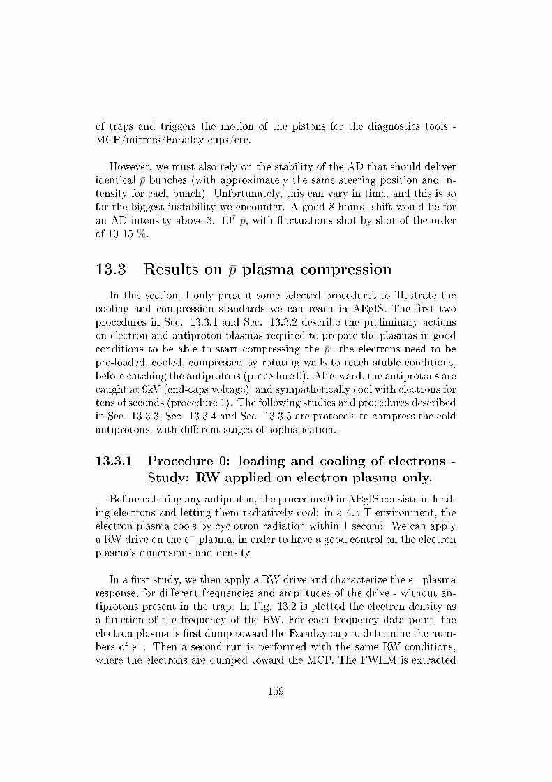
of traps and triggers the motion of the pistons for the diagnostics tools -MCP/mirrors/Faraday cups/etc.

However, we must also rely on the stability of the AD that should deliveridentical p bunches (with approximately the same steering position and in-tensity for each bunch). Unfortunately, this can vary in time, and this is sofar the biggest instability we encounter. A good 8 hours- shift would be foran AD intensity above 3. 107 p, with uctuations shot by shot of the orderof 10-15 %.

13.3 Results on p plasma compression

In this section, I only present some selected procedures to illustrate thecooling and compression standards we can reach in AEgIS. The rst twoprocedures in Sec. 13.3.1 and Sec. 13.3.2 describe the preliminary actionson electron and antiproton plasmas required to prepare the plasmas in goodconditions to be able to start compressing the p: the electrons need to bepre-loaded, cooled, compressed by rotating walls to reach stable conditions,before catching the antiprotons (procedure 0). Afterward, the antiprotons arecaught at 9kV (end-caps voltage), and sympathetically cool with electrons fortens of seconds (procedure 1). The following studies and procedures describedin Sec. 13.3.3, Sec. 13.3.4 and Sec. 13.3.5 are protocols to compress the coldantiprotons, with dierent stages of sophistication.

13.3.1 Procedure 0: loading and cooling of electrons -Study: RW applied on electron plasma only.

Before catching any antiproton, the procedure 0 in AEgIS consists in load-ing electrons and letting them radiatively cool: in a 4.5 T environment, theelectron plasma cools by cyclotron radiation within 1 second. We can applya RW drive on the e− plasma, in order to have a good control on the electronplasma's dimensions and density.

In a rst study, we then apply a RW drive and characterize the e− plasmaresponse, for dierent frequencies and amplitudes of the drive - without an-tiprotons present in the trap. In Fig. 13.2 is plotted the electron density asa function of the frequency of the RW. For each frequency data point, theelectron plasma is rst dump toward the Faraday cup to determine the num-bers of e−. Then a second run is performed with the same RW conditions,where the electrons are dumped toward the MCP. The FWHM is extracted

159

from the radial prole measured, and the density is then calculated fromthese two measurements. From Fig. 13.2, we can note that we don't reachthe strong-drive regime (indicated in dashed blue curve) where the plasmafrequency follows the frequency of the RW (see Sec. 13.1). Anyhow, for slowfrequencies applied, the compression of the electrons follows a linear regime.

When the RW is switched on directly with a high frequency (above 3MHz), we have noted that the tails of the plasma are not driven and notcompressed. It seems that if the dierence between the plasma rotationfrequency itself and the RW frequency is too high, the electrons far from thecenter of the plasma don't follow the RW drive. This tends to explain thebreak in compression for a frequency above 3 MHz, in Fig. 13.2. In additionto this, the RW implies heating (losses) is quite important for high amplitudeof the RW drive (fast compression).

Figure 13.2: RW compression of electrons: scan of the response of the electronplasma under rotating wall drive, varying the frequency of the RW applied,for a xed amplitude. The blue curve represents the strong drive regime.The red crosses are the density of the electron plasma achieved for dierentRW frequency.

Remark: The nal size (compression) of the plasma is determined by

160

the frequency of the RW, whereas the speed of the RW drive is given by theamplitude (voltage applied). We did note that if we switch on the RW drivetoo fast (too high amplitude), the outer electrons seem not to be draggedand not compressed.

13.3.2 Procedure 1: catching and cooling of antiprotons- Study: centrifugal separation vs heating plas-mas by RW drive.

In AEgIS, the starting point for any antiproton trapping and manipula-tion procedures begins with a pre-loading of electrons before the antiprotonarrival. The antiprotons are caught at 9kV (end-caps voltage), and sympa-thetically cooled by the electron plasma. In the following, I call these twosteps (loading electrons + catching antiprotons and cooling) the procedure1. We studied two settings to maximize the fraction of antiprotons cooledby electrons.

without any RW drive applied on electrons neither before the catchingof p nor during the sympathetic cooling the process.

with RW drive active on electrons during all the procedure.

The motivation was to obtain as much as possible antiprotons, cooled andcompressed before being transferred the production trap (ON-axis trap), andwe had to determine which conguration was the most interesting for thispurpose.

The procedure 1 begins with the loading of electrons ten seconds beforethe antiproton bunch arrival. The number of electrons loaded by our electrongun in the trap is typically 4 - 6.5 × 108. As seen in Sec. 13.3.1, the elec-trons are caught in the P trap (see Fig. 13.1), and thermalize by cyclotronradiation.

The antiprotons are caught in the 4.5 T trap, with the end-caps voltage setat 9kV. We typically conne about 1 - 1.3% of the antiproton bunch from theAD, corresponding roughly to 3. 105 antiprotons. The overlap between theantiproton and the electron plasmas determines the fraction of antiprotonssympathetically cooled. The number of electrons loaded determines alsothe time needed for cooling. Typically, for 4 - 6.5 × 108 electrons, all theantiprotons that overlap with the e− cloud are cooled within a cooling timeof 40 s or 50 s: their axial energy, initially mostly of the order of keV, hasdecreased below 150 eV. The fraction of the remaining hot antiprotons is

161

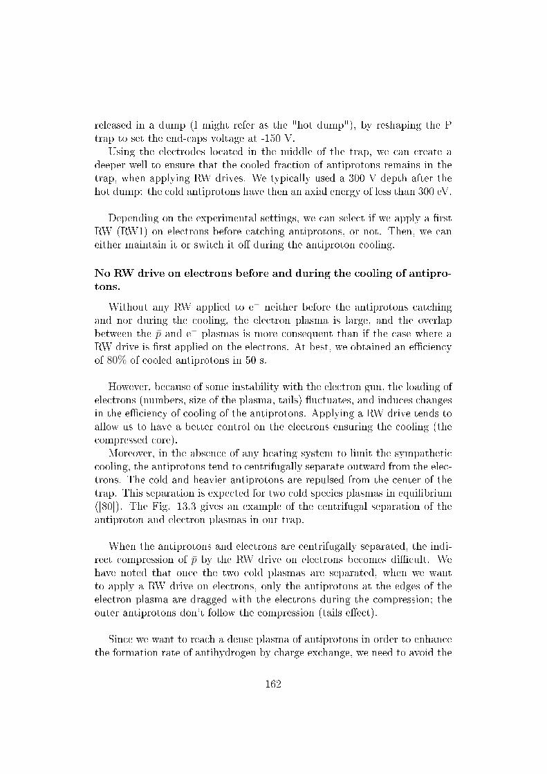
released in a dump (I might refer as the "hot dump"), by reshaping the Ptrap to set the end-caps voltage at -150 V.

Using the electrodes located in the middle of the trap, we can create adeeper well to ensure that the cooled fraction of antiprotons remains in thetrap, when applying RW drives. We typically used a 300 V depth after thehot dump: the cold antiprotons have then an axial energy of less than 300 eV.

Depending on the experimental settings, we can select if we apply a rstRW (RW1) on electrons before catching antiprotons, or not. Then, we caneither maintain it or switch it o during the antiproton cooling.

No RW drive on electrons before and during the cooling of antipro-tons.

Without any RW applied to e− neither before the antiprotons catchingand nor during the cooling, the electron plasma is large, and the overlapbetween the p and e− plasmas is more consequent than if the case where aRW drive is rst applied on the electrons. At best, we obtained an eciencyof 80% of cooled antiprotons in 50 s.

However, because of some instability with the electron gun, the loading ofelectrons (numbers, size of the plasma, tails) uctuates, and induces changesin the eciency of cooling of the antiprotons. Applying a RW drive tends toallow us to have a better control on the electrons ensuring the cooling (thecompressed core).

Moreover, in the absence of any heating system to limit the sympatheticcooling, the antiprotons tend to centrifugally separate outward from the elec-trons. The cold and heavier antiprotons are repulsed from the center of thetrap. This separation is expected for two cold species plasmas in equilibrium([80]). The Fig. 13.3 gives an example of the centrifugal separation of theantiproton and electron plasmas in our trap.

When the antiprotons and electrons are centrifugally separated, the indi-rect compression of p by the RW drive on electrons becomes dicult. Wehave noted that once the two cold plasmas are separated, when we wantto apply a RW drive on electrons, only the antiprotons at the edges of theelectron plasma are dragged with the electrons during the compression; theouter antiprotons don't follow the compression (tails eect).

Since we want to reach a dense plasma of antiprotons in order to enhancethe formation rate of antihydrogen by charge exchange, we need to avoid the

162

centrifugal separation of cold antiprotons and electrons.

With a RW drive active before and during the cooling process

As seen in Sec. 13.3.1, a rst RW can be applied to the electron plasmato compress it before the antiprotons arrive, in order to have a good controlon the shape and density of the e− plasma. It can be kept active once theantiprotons are caught to provide heats on both the p and e− plasmas, toavoid the centrifugal separation.

Indeed, it is important to note that if we kept the rst RW active duringthe sympathetic cooling of the antiprotons, this RW drive does not inducecompression on the antiprotons. Indeed, the electrons are typically loaded10s before the antiprotons arrival. The rst RW is applied just after theloading, and is then active for a long enough time to let the electron plasmareach its equilibrium and be compressed at the maximal density imposed bythe frequency of the RW1. Once the antiprotons are caught, the RW1 doesn'timply compression on electrons anymore and thus there is no indirectly com-pression on antiprotons. This RW1 only generates heat to both plasmas andblocks the centrifugal separation during the cooling stage.

In AEgIS, we use the RW drive to apply a constant heating onthe plasmas and thereby avoid the centrifugal separation.The usual fraction of antiprotons caught that gets cooled by electrons in 50sis 55% up to 65%, depending on the RW1 frequency and amplitude chosen.We usually choose 0.3 MHz and 0.2 V for the rst RW stage, and obtainabout 60-62 % cooling eciency, meaning that we obtained 2. 105 cold an-tiprotons trapped into our system.

In our apparatus, the RW drive has to be active to prevent the centrifugalseparation. In order to illustrate the importance of keeping the heating of theRW drive active during all the antiproton manipulation procedures, the Fig.13.3 gives an example of the images, of both the antiproton and the electronplasmas, when the RW drive has been switched o one second before dumpingthe plasma toward the MCP. This leads to centrifugal separation.

163

Figure 13.3: An example of the images of the antiproton (left image) and theelectron plasmas (right image) on the MCP, in case of centrifugal separation.To obtain these images, the RW drive that was active during the coolingprocess is stopped 1 s before the electrons are rst dumped, followed by theantiprotons after a delay of 250µs.

However, in order to have a wide plasma and a large overlap betweenantiprotons and electrons, and thereby to a better cooling ratio, one couldthink about applying a RW drive on the electrons at a lower frequency than0.3 MHz. Indeed, the nal density of the electron plasma is determined bythe frequency of the RW drive. A frequency <0.3 MHz would lead to a widerplasma and a bigger overlap between antiprotons and electrons. However,during our scans, we noted that if we used a lower frequency (<0.3 MHz),we observed a "boiling-o" eect on the antiprotons caught. The externalscintillators counts, recording the annihilation of antiprotons, increase duringthe cooling procedure when the RW drive is active for low frequencies. Theselosses appeared to be radial losses of the antiprotons. A RW frequency lowerthan 0.3 MHz seems to induce some coupling with the radial modes of thep plasma and provoke losses. That's why, we typically used 0.3 MHz as theRW frequency for the rst RW drive in all our procedures.

We can note in Fig. 13.3 in the electrons image (right image) that the twotraps are misaligned: electrodes in the 1 T trap obliterate the plasma fromthe 4.5 T trap projected onto the MCP ("tiger-eyes" phenomenon), we see animage "cut". However, for the antiprotons (right image), the deformation ofthe image observed comes from an additional phenomenon. The deformation

164

is due to E×B drift: during their ight from the 4.5 T trap toward the MCP,the antiprotons (much slower than the electrons) have time to interact withtheir own charge image of the (cutting) electrode. Since they travel closeto this electrode (misalignment of the 4.5 T and 1 T axis), they actuallyfeel their charge image and a change in the connement E eld comparedto the center position of the trap (gradient), that cause a shift and also adeformation of the ring.

13.3.3 Procedure 2: a second faster RW applied oncethe antiprotons are cooled.

The second procedure we tested on antiprotons was developed to compressthe antiprotons, after the electron cooling. A second RW drive (RW2) isapplied just after the dump of the hot antiprotons.

As the procedure 1, this procedure starts with the compression of electronswith a slow frequency and amplitude (default value 0.3 MHz and 0.2 V). Thisrst RW is kept active during the whole cooling process for 40 s or 50 s, oncethe antiprotons are caught. After the hot dump has been released, we applya second RW stage (RW2) at a higher frequency to start compressing bothplasmas. The antiprotons are dragged with the RW drive on electrons. Fig.13.4 shows several images of the antiproton plasma obtained for dierentfrequencies of the second stage of the RW, and for about 6.5× 108 electronsloaded. The second column shows the reconstruction analysis tool, to com-pensate the tiger-eyes eect observed on the MCP due to misalignment ofthe 4.5 T and on-axis 1 T traps.

During these scans, we varied the number of electrons loaded into thetrap. We observed that the maximum compression achieved depends on thedensity of the e−: a lower number of electrons appears to allow a strongercompression, for the same RW frequency and amplitude values. This phe-nomenon is illustrated in Fig. 13.5. In the rst row, the compressed imagesof the antiproton plasma is shown for dierent frequencies of the second RWstage, with 6.5× 108 electrons loaded in the trap (case 1). In the second line,the number of loaded electrons is reduced to 4× 108 (case 2).

For all the compressions scans presented in Fig. 13.5, the rst RW stagewas applied for 50 s (cooling time) at a frequency of 0.8 MHz and an ampli-tude of 0.2 V. The second RW stage was applied for 20 s.

Besides, it is worth noticing that the number of cooled antiprotons we

165

Figure 13.4: Example of MCP images of the antiproton plasma, for dierentfrequencies of the second RW stage. An increase of the frequency of the RWenhances the compression of the plasma. The rst column gives in false-color the images of the MCP without analysis treatment, whereas the secondcolumn shows a reconstruction t of the cut plasma to obtain a value forthe radii of interest. The black circles delimit the plasma FHWM and theintensity of the signal at about 3 sigma above the background. We applied aradial symmetry to determine the prole of the plasma. The green and redcircles delimit the electrodes inner diameter of the 4.5 T and 1 T traps thatare misaligned.

measured for the case 2 where 4 × 108 e− are loaded in the trap seem to beroughly in the order of the number of the cold p obtained with the largernumber of electrons 6.5 × 108 (case 1). Indeed, in the second case, about55-60 % of the caught antiprotons are sympathetically cooled, whereas forthe case 1, with a larger number of electrons, the cold fraction is about 60 -65 %. The uctuations of the AD facility, shot by shot, makes it dicult tocarry out a precise comparison for the two loading electron cases, and we willneed to accumulate more data on this procedure. However, it seems that thenumber of antiprotons for the case 2 is only slightly lower than for the case1, whereas the compression of the antiproton plasma, for the same frequencyand amplitude of the RW drive appears to be much bigger for the case 2 thanthe case 1 (see Fig. 13.5). This would imply that for the same frequencyof the RW2, a better compression on the antiprotons can be achieved if thenumber of loaded electrons is lower.

In the Fig. 13.5, we only present results for two typical numbers of elec-trons (6.5 × 108 and 4× 108 e−). However, we did continue to decrease thenumber of electrons loaded before the antiprotons catching, and carried onthe frequency scan. The nal compression on p appeared to be even betterfor lower number of electrons, for the same frequency of the second RW ap-plied.

Anyhow, the choice of the ideal number of electrons to be loaded is not thateasy. A compromise has to be done between the nal compression achievedon antiproton plasma (low number of electrons in the trap) and the fractionof cooled p obtained (high number of electrons). Indeed, if the number ofelectrons rst loaded is too small, the compression at the rst stage of theRW will lead to a small compressed e− plasma. Then, the overlap betweenthe electron plasma and antiprotons caught that get sympathetically cooledwill decrease. Moreover, the time needed to cool the antiprotons has to bealso considered: by reducing the number of electrons, the cooling time isextended (less collisions), and we aim to have relatively fast procedures touse as much as possible the antiproton bunches from the AD, deliver every≈ 120 s.

167

Figure 13.5: MCP images of the antiproton plasma - scan of the second RWstage frequency, for two electron loading conditions: the rst row presents theresults of compression on antiproton plasma, with 6.5 × 108 electrons loadedinto the trap (case 1), for three dierent RW2 frequencies. The second rowgives the image of the antiprotons for the same three RW frequencies, withan initial cloud of 4 × 108 electrons (case 2). The maximum compressionachieved seems to be reachable for a reduced number of electrons, and this,only for a slight trade-o in the number of cold and compressed antiprotons- see discussion above.

At the end of these scans, we decided that a good compromise was to load4. 108 electrons into the trap before the antiproton catching.

13.3.4 Procedure 3: a third RW stage, with a reducednumber of electrons

After the conclusion of the previous scans, we came up with the idea ofapplying the compression RW stages, with a reduced number of electrons,

168

after the cooling process. The idea is then to keep a large number of elec-trons for the phase of cooling (before the release of the hot dump) in orderto have a big overlap between antiprotons caught and electrons to quicklycool a maximum of p. Then, since we have seen that a better compressionis achieved with a lower number of electrons, we remove a fraction of themand start the RW compression.

In other words: the third procedure presented here consists of followingthe standard loading and compression of electrons before the antiprotonsarrival, and keeping it active during 40 s of cooling (rst RW stage). Wetypically load 4× 108 electrons into the trap, in order to reach a fraction of55-60 % cold antiprotons. Then, the remaining fraction of hot antiprotonsis dumped by reshaping the trap (procedure 1). A second stage of RW isapplied during 20 s or 40 s (RW2) to start the compression of the electrons(procedure 2). The innovation of this third procedure resides in removingone fth of the electrons in fast kicked. During the process, more than 90%

of the antiprotons (

√mp

me−= 42 times slower) stay in the reshaped trap. A

third RW stage is applied afterward, with a higher frequency or amplitude,during 20 s or 40 s and a further compression in achieved on the antiprotons.

Fig. 13.6 shows the FWHM of the antiproton plasma radial prole as afunction of the third RW frequency. As the image of the plasma is obtainedin a 1 T magnetic eld region and the procedure is developed into the 4.5T trap, a correction on the size of the plasma has been applied (factor 2.1smaller in the higher magnetic eld region).

169

Figure 13.6: Results of the third RW stage applied on a reduced electronplasma: the FWHM of the antiproton plasma's radial prole in the 4.5 T isplotted as a function of the third RW frequency.

For the results plotted here, the two rst RW frequencies were set at 0.3MHz, for 0.1 V, and for a number of 4. 108 electrons. Our best compressionresults are obtained for a third RW frequency above 2 MHz with 0.5 V anda compression during 20 s, where the FWHM is below 0.4 mm, for typically2 105 antiprotons.

Some antiprotons losses are observable during the third RW process, whenthe frequency applied higher than 4 MHz, probably due to an excessive heat-ing of the plasma.

13.3.5 Procedure 4: toward a fourth RW stage andhigher compressions of e− and p

Finally, we implemented a procedure that adds a fourth RW stage, on evenmore reduced electron plasma compared to the procedure 3. After the thirdRW compression, a second fast removal of electrons is performed whereasthe trap is reshaped to be smaller. Even if a full scan of this procedurehasn't been carried out because of some vacuum issues and lack of time, thistechnique looks promising. In Fig. 13.7 is gives one of the best compression

170

results we obtained for a fourth RW frequency of 2 MHz, with 0.5 V appliedduring 20 s of compression. The radial prole of the antiproton plasma ispresented in two cases: without any compression stage (blue dots) and withthe four RW drives applied to the plasma (procedure 4). The size correction(from 1 T to 4.5 T envrionment) has been applied to the data. The FWHMradius is found to be 170µm.

Figure 13.7: Radial prole of the antiproton plasma without compression(blue dots) and with (red dots) the procedure 4 where four RW stages areapplied.

We can note the hole in the radial prole of the compressed antiprotons(red dotted curve) in Fig. 13.7, that results from a partial centrifugal sepa-ration of the electron and antiproton plasma.

13.4 Summary

Typically, from a good AD bunch (intensity 3. 107 p), we are able tocatch 3. 105 antiprotons into our trap at 4.5 T and 9 kV end-caps voltage.Then, within 150 s, up to 2. 105 antiprotons are sympathetically cooled byelectrons. Thanks to several stages of RW on electrons, the antiprotons aredriven to a highly compressed plasma: from the procedures we developed,

171

we are able to reach p plasma of radius below 0.4 mm, into a 10 cm longtrap, with a 4.5 T magnetic eld connement.

During the last beamtimes, we rather focused on improving the compres-sion procedures, since a high density of the antiproton plasma is requiredfor an ecient transfer toward the production region trap, at 1 T. However,we could easily increase the number of caught antiprotons by improving ourtrap control electronics in order to extend the end-cap voltage from 9kV to12kV (no hardware limitation). This could increase drastically the numberof antiprotons in our trap. Moreover, each step of the procedures describedabove could be optimized further more to enhance the number of p cooledand compressed.

Because of some vacuum issues during the beamtime of 2015 and conse-quent bad lifetime of the antiprotons in the trap, the full characterizationof the procedures hasn't been carried out, and more systematic measure-ments for procedure 4 need to be done. The behavior of the tails of boththe electrons and antiproton plasmas needs to be fully characterized for theprocedures 3 and 4, as well as the possible losses when the RW applied istoo fast or too strong. Typically, we load 4. 108 electrons into the trapbefore catching antiprotons, and apply a slow RW of 0.3 MHz and 0.2 Vfor few tens of second. This rst compression on electrons leads to an over-lap of the two plasmas that results in a cooling eciency of 55-65 % forthe sympathetic cooling: about 2. 105 antiprotons are cooled after beingcaught. This rotating wall is usually kept active in order to produce someheat on both plasmas to avoid centrifugal separation, during the 40 -50 s ofthe cooling process. Then, several stages of RW can be applied. We observedthat reducing the number of electrons allow for better compression of the an-tiproton plasma, for a xed RW frequency. We developed further proceduresthat alternatively use RW stages and electron removals. Final compressionof the p plasma, down to 400 µm (FWHM of the radial prole) were achieved.

These nice preliminary results indicate that our trap system provideshighly repeatable conditions and great compression results, necessary for anecient production of antihydrogen. As mentioned in the description of theON-axis trap in Sec. 12.3, where the production of antihydrogen is plannedto occur, the presence of grid in the top of the electrodes perturbs the sta-bility of the antiproton connement. In order to limit this eect, the plasmaneeds to be compressed in the center of the trap, far from the grid default.

172

Chapter 14

Toward a sympathetic cooling of

antiprotons - the laser cooling of

molecular anions

As mentioned previously in the introduction of the Part II, a key elementto increase the antihydrogen formation via charge-exchange is to use a coldantiproton plasma, since the cross section of the reaction depends on therelative velocity between the antiproton, the center of mass of the Ps andthe orbital velocity of the positron [15]. Moreover, AEgIS aims to form a coldbeam of 100 mK antihydrogen atoms. The temperature of the antihydrogenatoms depends mainly of the temperature of the antiprotons in the charge-exchange process. Several techniques can be use to cool ion plasma in aPenning trap, among them are:

The buer gas cooling [81]. This consists of the exchange of energybetween the trapped ions and the particles of a low-pressure gas thatundergo elastic collisions. This gas is usually chosen to be light andinert, as for instance the He gas. This technique works for cyclotronand axial but not for the magnetron motion ; the temperature limitis the apparatus temperature. This technique is for instance used inAEgIS for the positron system in the Surko and Accumulator traps(See Chap. 3)

The resistive cooling [81]. For this technique, a resistor is connectedbetween the two end-caps electrodes. The ions moving in the trapinduce a charge image in the electrodes. This charge image follows themotions of center of mass of the ions, and then leads to a movementof electric charges through the resistor system that dissipates energy.

173

This energy comes from the motional energy of the ions in the axialdirection. This technique leads to an exponential decrease of the axialmotion of the center of mass of the ions, down to the temperature ofthe apparatus.

The radiative cooling [81]. This technique is based on the fact thatcharged particles radiate when they don't undergo a constant motion.For non-relativistic energies, in magnetic elds, this phenomenon isgenerally called synchroton radiation, and this leads to the thermaliza-tion of the particles with the environment. This specially works well forlight charged particles (electron/positron) since the radiation rate γradis inversely proportional to the cube of the mass. The radiation rate

for the cyclotron motion (radial) is derived in [74]: γrad =q4B2

3π, ϵ0 c3m3.

For electron (or positron), the thermalization time tth =1

γradis then

2.6 s in a 1 T environment, and about 0.13 s in a 4.5 T environment.However, for antiprotons 1800 times heavier than electrons, the ther-malization time is too long to be considered, in comparison for instanceto the stability of the trap (heating process).

The electron cooling. Sympathetic cooling of ions can be performedusing electrons cooled by cylcotron radiation. For cations, this tech-nique can use the so-called nested Penning traps, as rst performed byD. Hall and G. Gabrielse in 1996 [82]. This consists of an M shapedtrap: the electrons are loaded and cooled in the central part of the M.The positive ions are conned in the inverted part of the potential well,on both sides of the central region, where they can interact with theelectrons and get cooled. Applying this technique to antiprotons hasthe great advantage that the electrons and p can be caught in the sametrapping well. Usually, the electrons are pre-loaded to be cooled beforethe antiprotons arrival and improve the cooling eciency. In AEgiS,from the centrifugal separation we measured during standard catch-ing/cooling procedure, we estimate the cold fraction of the antiprotonstrapped and cooled in the 4.5 T apparatus to be around 80 K whenthe RW drive is kept active. In Chap. 13, the procedures presented tocompress the antiproton plasma use electron cooling to rst cool an-tiprotons but also to compensate the heating coming from the rotatingwall drive.

The adiabatic cooling [74]. This consists of opening the trap's wallsslowly. By this action, the ions cool down due to the volumetric expan-

174

sion. To stay adiabatic, the changes of the electric and magnetic eldsof the trap has to be slower than the time-scale of the ions motions andslower than the collisions time. Under these conditions, the ion cloudstays at equilibrium and can be described by a Maxwell-Boltzmanndistribution. In this technique, the antiprotons density decreases.

The evaporative cooling, that consists of elastic collisions that scatterhigh energy particles out of the conning trap, decreasing then the tem-perature of the remaining particles. In 2010, the Alpha collaborationperformed an evaporative cooling on antiprotons [83], to reach with theremaining p a cooled plasma of about 9 K.

Direct laser cooling. The rst demonstrations of laser cooling on trappedions have been performed in 1978 [84, 85], on Ba+ and Mg2+ ions. Thetheoretical analysis of laser cooling for both free and trapped atomscan be found in [86]. In this chapter, I will more specically deal withthe possibility of a laser cooling on the molecular anion C−

2 , that iseven more tricky for several reasons I discuss later in Sec. 14.1. Thedirect laser cooling requires that the charged particle has at least twointernal bound states ; e.g. this technique is then irrelevant for coolingantiprotons.

The sympathetic cooling using another (laser cooled) species.Demonstrated in 1980 [87] on isotopes of Mg+ ions, the sympatheticcooling by directly laser-cooled species on a simultaneously trappedsecond species can be powerful. The trap stability has to be care-fully checked for both trapped species, for the ions to reach a commonequilibrium temperature. For instance, the Gbar experiment plans tosympathetic cool a single antihydrogen ion H+ with laser cooled Be+

ions [88]. The use of a third species with an intermediate mass as thehydrogen-deuterium ion HD+ has been considered to play the role of abuer species to increase the sympathetic cooling eciency. I studiedthe possibility to sympathetic cool the antiproton plasma with anions(see Sec. 14.1). This chapter is specially dedicated to the study of thecooling of the molecular anion C−

2 .

More details for all the techniques mentioned above could be found forinstance in [34, 81] where most of the trap techniques, plasma manipulations,cooling and detections are reviewed. In the thesis of D. Krasnicky [74], re-sults of the radiative, adiabatic and resistive cooling techniques can be foundfor the AEgIS apparatus.

175

14.1 A possible laser cooling of anions to sym-

pathetically cool antiprotons in AEgIS

In the AEgIS proposal [15], a temperature of 100 mK is assumed to e-ciently form a cold beam of antihydrogen atoms to perform gravity tests. Toreach such a cold plasma, a possibility is to use cold anions to sympatheti-cally cool the antiprotons. Indeed, most of the standard cooling techniques Ireviewed above lead to a nal temperature close to the ambient temperatureof the apparatus. Even if AEgIS setup is cooled at cryogenics liquid heliumtemperature (4.2 K), the antiproton plasma, cooled by electrons, is far abovethe 100 mK foreseen for the gravity measurement.

That's why the laser cooling of anions is under study in AEgIS. The choiceof atomic anions is limited, since the excess electron is only weakly boundby quantum-mechanical correlation eects. As a result, only a few atomicanions are known to exhibit electric-dipole transitions between bound states:Os−, La− and Ce− [89, 90, 91]. The group of A. Kellerbauer has studied thespectroscopy of atomic anions, as Os− [92] and La− [93] to nd the propercandidate, and a laser cooling scheme is under development for La−.

For molecules, the situation is quite dierent because their electric dipolecan bind an extra electron, and even di-anions have been found to exist [94].

That's why a parallel study plans to use molecular anions instead of atomicanions, since the number of potential suitable candidates for a laser coolingseems larger. One major problem for applying laser cooling to molecules isto nd a closed cycle of transitions, in order to avoid to populate dark statesthat would stop the cooling process. Although it has already been success-fully performed for neutral diatomic molecules [95], it has never been doneso far for anions. Some challenges of the laser-cooling molecular ions havebeen described in [96]. For direct laser cooling of diatomic molecules, a keyingredient is a good branching ratio, i.e. Franck-Condon factor, between vi-brational levels in order to close the absorption/emission cycle of the coolingscheme with only few levels involved.

In this chapter, I will deal more specically with one molecule selectedduring our reviewing of the possible candidates: the C−

2 anion. It presents awell known spectroscopy as well as good Franck Condon coecients to closewith a few lasers the transition X ↔ B (see Fig. 14.1 were the green arrowsindicate the cooling scheme), repumping the vibrational ground states up tov"=4. This implies that Doppler laser cooling could be possibly considered,

176

the details of the cooling scheme and some results are presented in Sec. 14.3.

Besides, I studied a scheme to apply a Sisyphus cooling on the transitionX↔ A, in a Penning-like trap with a gradient of magnetic potential for theC−

2 molecule, and I develop this idea in the Sec. 14.4 - see Fig. 14.1 with thetransition indicated by the red arrows.

The results presented here are published in Ref. [18].

14.2 The C−2 molecule

In order to nd a proper cooling scheme, it seems appropriate to selecta molecule with good FC factor. However, the choice of the most suitablecandidate is not obvious since a compromise has to be found between us-ing fast electronic transitions and choosing extremely good FC factors. Alist of possible candidates is given in our article [18]. This necessary pre-liminary research has been performed mainly by D. Comparat. I focusedmy studies on the C−

2 anion physics and simulations, presented here. Thismolecule presents the great advantage that its spectroscopy is very well-known. The C−

2 molecule exhibits a B2Σu(v′ = 0) ↔X2Σg(v

′′ = 0) systemand a A2Π1/2,u(v

′ = 0)↔ X2Σg(v′′ = 0) system with 72% and 96 % branch-

ing ratio, respectively. As an homonuclear molecule, C−2 doesn't present a

decay channel through B2Σ →A2Π, as heteronuclear molecule does, that isalso a great benet. Finally, this anion has the notable advantage of notpresenting any hyperne structure.

177

Figure 14.1: C−2 level structure. Electronic and vibrational levels, as well

as the optical transitions potential laser cooling are drawn, in the absenceof magnetic eld. The green arrows show the Doppler cooling scheme onthe X↔ B transition, with a possible photodetachment (dashed green line).The red arrows point out the transitions that could be used for a Sisyphuscooling on the X↔ A transition. The widths of the arrows are proportionalto the transition strengths given by the Franck Cordon coecients. Besides,the two fundamental electronics levels of the neutral molecule the C2 arepresented: the X 1Σ+

g and a3Πu states.

In Fig. 14.1 is presented the electronic and vibrational levels of C−2 . Its

three electronic levels are shown: the ground state X2Σg (in black), and thetwo excited states A2Πu (in red) and B2Σu (in green). The green arrowspresent the Doppler scheme studied on the X↔ B transition, that I developin Sec. 14.3 ; the red arrows show the transitions over X↔ A to try to per-form a Sisyphus-type laser cooling - see Sec. 14.4.To illustrate the possibility

178

of a photodetachment of the electron, two fundamental electronics levels ofthe neutral molecule the C2 are presented too: the X 1Σ+

g and a3Πu states.

14.3 The rst scheme: Doppler cooling over X

↔ B transition

The rst cooling scheme I studied was a Doppler cooling on the transitionX(v=0)↔ B(v'=0). For a 3D laser cooling, 6 counter-propagating lasersare set on the X(v′′ = 0, N ′′ = 2) ↔ B(v′ = 0, N ′ = 0) transition and 2repumping counter-propagating lasers are needed on the X(v′′ = 0, N ′′ =0)↔B(v′ = 0, N ′ = 0). Besides, because of a FC factor of only 72% betweenthe X(v=0) and B(v'=0) states, an optical repumping is needed to closethe cooling circuit. 8 counter-propagating (on the direction ± z) repumperlasers have been considered to pump the higher vibrational ground states X(v=1,2,3 and 4). The widths of the green arrows in Fig. 14.1 indicatethe weight of the FC factors and the transitions involved in the coolingscheme. The dotted green arrow illustrated the possibility of a two-photonabsorption and a photoionization of C−

2 , that has been taken into account inour simulations.

14.3.1 The 3D optical molasses

We rst studied the possibility of cooling C−2 without external eld to cap-

ture the particles. When looking for a possible cooling scheme for ions, it iscommon to conne them with external elds before applying any laser cool-ing. That's why at rst glance, this study may appear like a simple exercisein style. However, we considered interesting to investigate the possibility ofremoving the strong external trapping eld, in the same spirit of what it wasrealized for the rst laser cooling of neutral molecules (YO [97] and SrF [95]),which was performed in a magnetic optical trap (MOT). Besides, removingthe external trapping eld would allow to get rid of the micro motion thatperturbs the cooling in Paul and Penning traps: for instance, the group ofCh. Schneider, T. Schaetz and coworkers [98] succeeded in cooling Ba+ cloudby dipolar force in 2010.

Before considering an optical molasses for ions, it is worth noting thatan anionic beam can be brought close to standstill very easily by an electriceld [99] unlike for neutral molecules which are dicult to produce at lowvelocity, despite the development of techniques such as velocity ltering or

179

buer gas cooling (see detailed list in [100]).

If we consider a typical beam of C−2 is produced with a current of 1 nA

and emitted at 1000 eV with an energy dispersion of 1 eV [101], then a 1000volt potential electrode can decelerate such a beam. Moreover, due to theenergy dispersion of the beam, the stability of this voltage power supply isnot critical. Typically 1/100000 of the anions (i.e. 0.01 pA current) will bedecelerated inside the box to below an energy of 0.01 mV. This correspondsroughly to 0.1 K, which is within the capture range of molasses cooling.

We rst studied the possibility of laser cooling in free space: we simulatea 3D molasses cooling on a cloud of 150 particles at an initial temperature of80 mK, with a spherical Gaussian distribution (σrms = 4 mm). All the lasersare CW lasers, with a power of 0.5 W, a 2 cm waist and a red detuning of 10MHz from the transition. The laser parameters values have been determinedand optimized after a scan of each dierent parameters around theoreticalvalues, in order to obtain .

Indeed, it is worth noticing that the X(v=0,N=2)↔ B(v'=0,N'=0) tran-sition corresponds to the usual Doppler cooling over a broad-line case:

Erecoil =~2 k2L2mC−

2

=

~2(

2π

541nm

)2

2× 2× 12 a.u.= 1.9 10−29 J

~Γs = 1.38 10−27 J ≫ Erecoil

(14.1)

where a.u. is the atomic mass. In this case, the radiation pressure force canbe used to roughly determined the cooling strength of the interaction, asfunction of the laser power, detuning and bandwidth - see Append. D.

In Fig. 14.2(a) is presented the evolution of the kinetic energy of the cloudover time (black), that corresponds to the T3D,50% dened in Chap. 8. Wecan note a rst increase in temperature at 1 ms. This is explained due to theconversion of the Coulomb potential (repulsions) energy into kinetic energy:for the initialization parameters of the particles, we have arbitrary chosen adensity of the cloud that leads to a Coulomb repulsion force stronger thanthe connement force of the trap. That's why, at the rst instants of thesimulations, the charged particle cloud extends, that is translated by the in-crease of the kinetic energy. Then, a fast cooling down to 1 mK is observed,even if most of the molecules escape from the laser waist interaction area(dashed red curves). The molecules that leave the laser interaction zone are

180

lost for the cooling process, I refer to them as "losses".

During the optimization of the cooling parameters, we observed that thenal temperature and losses depend on the initial density (dened by the σrms

of the Gaussian distribution of the cloud) because of space charge eects thatcounter the cooling. In these rst simulations, we didn't attempt trappingin a MOT conguration (Optical Molasses trapping). Indeed, the Zeemaneect of B(v′ = 0, N ′ = 0) is weak (quadratic behavior [102]), and realizing aMOT would require a magnetic-eld gradient that produces a Lorentz forcestronger than the laser trapping one.

Figure 14.2: Doppler laser cooling results, cycled on the X↔B transition ofthe C−

2 molecule. (a): the 3D molasses cooling. Result of the 3D laser coolingsimulation of an initial bunch of 150 anions at 80 mK. The red dashed curvegives the population losses, corresponding to molecules which escape from thelaser interaction area. The kinetic energy evolution (in temperature unit) ofthe remaining particles is plotted in black. (b): The Doppler cooling in a Paultrap. In black, evolution of the temperature initially at 5K in a Paul trap.The red dashed curve gives the population losses, through photo-ionizationor decays into high vibrational ground states that are non repumped (v > 4).

This 3D free-cooling appears to work for diluted cloud of particles (to limitthe Coulomb interaction and fast expansion of the cloud that escapes fromthe laser interaction area), and for initial temperatures below the hundredsof mK.

181

14.3.2 In a Paul trap

We then simulated the Doppler cooling over the transition X↔ B in aPaul trap. For simplicity, we only considered the motion in a harmonicpseudo-potential well V (r) = 1/2 m ωr(x

2 + y2) + 1/2 m ω2z . That consists

of averaging the RF micro-motion, as done in [103].

We considered here 5 K as an initial temperature for the C−2 cloud. This

could correspond to a pre-cooling, using for instance a buer gas (Helium).The lasers are set with a 600 MHz red detuning, and a spectral laser band-width of σL=35 MHz, values coming from an optimization scan of each pa-rameter to nd the best laser cooling eciency. We also set the repump-ing lasers for the dierent vibrational levels of the ground state X up toX(v′′ = 4), as shown in Fig. 14.1(a). But since the particles are trapped,the repumping lasers are only along the +z direction, and we use only 4repumpers.

In Fig. 14.2(b), the simulations result is presented where a cooling downto 60 mK is achieved within 50 ms. The photo-detachment process has beentaken into account. Because the photo-detachment cross-section of C−

2 for theB-state is unknown, we used the order of magnitude of the photo-detachmentcross section of C2, σph,C2 ∼ 10−17 cm2 [104] as a typical value.

For a laser intensity of I = 0.16 W/cm2, the photo-detachment rate forthe B-state is then Iσph/hν = 4.3 s−1. For our simulation parameters thatdene the excitation rate (X ↔ B), within 50 ms of interaction, only 3 % ofthe molecules are lost by photo-detachment (X → B → Continuum).

In addition to the photo-detachment losses, we considered that the moleculesdecaying into the high vibrational ground states X(v>4) are lost for the cool-ing process (dark states). The total losses' evolution over time is shown inFig. 14.2(b) in the red dotted curve.

The Doppler cooling in the Paul trap gives promising results (a temper-ature of less than 100 mK can be reached within 50 ms), with 12 lasers toclose the cooling cycle (2 cooling laser on the transition | X,v” = 0,j"=3/2⟩ ↔ | B,v'=0,j'=1/2⟩ along ± z, 2 repumping laser on | X,v” = 0,j"=1/2 ⟩↔ | B,v'=0,j'=1/2⟩ on ± z, and 1 laser along + z for each transition | X,v"=1,2,3,4, j=1/2,3/2⟩ ↔| B,v'=0,j'=1/2⟩).

. Even if we need 12 lasers are required here, we believe that this sketchcould be experimentally implemented, using for instance ber laser technol-ogy.

182

We note that for these simulations, the trap is loaded using an initial (nonthermalized) Gaussian velocity distribution. The evolution of this non equi-librium system leads to the high frequency velocity variations and thus tothe instantaneous temperature uctuations visible in Fig.14.2(b), due to theoscillations of the particles in the trap. Indeed, when a particle oscillates intoa trap, the kinetic energy is exchanged into potential energy, then back to ki-netic energy. At the beginning of the simulations, each particle of the cloud israndomly attributed an initial velocity v picked from a Maxwell-Boltzmann

distribution at T0 (p(v) =

(m

2π kB T0

)3/2

exp(−mv2

2 kB T0) d3v). The contribu-

tion of every particle that oscillate in the trap with dierent maximal kineticenergy, leads to the uctuations of the global temperature at each time t,

Tinstantaneous = ⟨Tinst,i⟩i∈x,y,z =

√1

3

∑i∈x,y,z T

2inst,i, with Tinst,t dened be-

low.

In order to try to reduce the instantaneous temperature uctuations inour simulations, I started to investigate a way to force the thermalizationof the cloud of particles in motion inside the trap, before we start the lasercooling.

An idea proposed by Berendsen and coworkers [105] is to couple themolecules to an external bath to force the thermal equilibrium. Couplingthe particles to a thermostat makes the instantaneous temperature of thecloud converge toward T0 (enhanced thermalization). To do so, their algo-rithm proposes to apply a correcting factor λ to the velocity of each particleof the cloud, at every time evolution step t. The λ factor models thecoupling to an external bath at T0.

For a given time t, we determine the factor λ(t) to apply to the velocityof each atom at the time t + t. The velocity at t + t is modied by∀ i ∈ x, y, z, vi(t+t) = λ(t)vi(t), where λ(t) is determined by [105]:

λ(t) =

(1 + α

[Tinst,i

T0− 1

])(14.2)

with α the coupling strength of the particle cloud to the thermostat; andTinst,i the "instantaneous equivalent temperature" along the i axis for the

entire cloud of the N particles, such as Tinst,i =2

kB

1

N

∑j≤N

1

2×m×(vi−vi,j)2

(see Eq (8.1) ).

183

The strength of the coupling α determines the time required to reach theequilibrium. This parameter has to be carefully tuned, to nd a compromisebetween a fast thermalization process and smooth changes in the velocitydistribution to avoid any numerical artifact error. Typically, Berendsen andcoworkers considered a coupling time τ = αt = 0.4 ps, where t is evolu-tion time step taken for the calculations of the dynamics evolutions. I haveupdated the optical pumping C++ code to implement this enhanced ther-malization, before we start the laser cooling. The full study of this algorithmhasn't been yet carried out for our C−

2 simulations, but its eectiveness seemsto be mostly linked to the strength of the coupling. Besides, since the lasercooling wipes out the thermal equilibrium, the instantaneous uctuationsthe global cloud temperature, due to the motion of particles with dierentvelocities, continues to be present during the cooling process. Since the lasercooling of a diluted C−

2 cloud in trap would probably lead experimentally toa non thermal equilibrium condition, we consider that forcing the thermal-ization in our simulations was not crucial for our purposes.

14.4 The second scheme: Sisyphus cooling over

X ↔ A transition

A solution to avoid the losses of C−2 through photo-detachment or decays

into high vibrational levels of the ground-state is to cool through the A-state.This cooling has very similar characteristics (linewidth, wavelength) to thoseof La− [91] but with a lighter particle and no photo-detachment in the case ofC−

2 . The cooling over the transition X↔A is slow τspont,A(v′=0) ≈ 50µs ([106])compared to the usual lifetime of the transitions used in the laser cooling ofthe Alkali atoms. This corresponds to a Doppler cooling over a narrow-line

case: Erecoil =~2 k2L2mC−

2

= 1.8 10−30J∼ ~Γs = 2.1 10−30 J. The particularities

of this kind of transition have been seen for the Ps atom cooling case (SeeChap. 7).

Anyhow, the cooling scheme considered in this third simulation is new.It consists of performing a Sisyphus-type laser cooling [57], on the X ↔ Atransition. We call "Sisyphus" cooling any cooling scheme that makes a par-ticle climb again and again a potential hill. During the process, the particlelosses energy. The trick is then to nd a way to place back the particle atthe beginning of the potential hill, just after its has reached the top of the

184

hill, without gaining back the same among of energy lost.

In the scheme we developed, the particles are trapped into a modiedPenning trap, where the magnetic eld has a gradient from 0.2 T to 2 T - seeFig. 14.3 a). This gradient creates the potential hill needed for the Sisyphuscooling process, indicated in Fig. 14.3 b). Due to the axial motion inducedby the electric trapping potential (300 µs oscillation time in the simulation),particles move between the high (2 T) and low (0.2 T) magnetic elds atboth ends of their axial range.

185

Figure 14.3: Detail of the Sisyphus cooling principle. a) Schematic of thetrapping potentials. The trap considered here is a Penning-like trap, with aharmonic electric potential to conne the axial motion (upper graph). Theconnement of the radial motion is insured by a magnetic eld varying from0.2 T to 2 T, in ∼ 1.5 cm long. This magnetic gradient eld creates theSisyphus potential hill. b). A zoom on the X ↔ A energies: |X1⟩=X(v′′ =0, N ′′ = 0) and |X2⟩=X(v′′ = 0, N ′′ = 2) |A⟩=A(v′ = 0, N ′ = 1, J ′ = 1/2).From the magnetic eld gradient, the corresponding Zeeman eect on theC−

2 internal level states is represented. Laser excitations and spontaneousdecays are illustrated with red solid line and red dashed line respectively.The dierent steps of the cooling cycle are indicated by the green numbersin parenthesis - see description in the text.

The sisyphus cooling cycle is explained in Fig. 14.3 b), with the dierentsteps of the cycle indicated by the green numbers in parenthesis. A usefulcooling cycle can be described by the following steps: a given particle ini-

186

tially in the ground state |X1⟩,M1 = −1

2in position 1 oscillates in the trap,

climbs the potential hill before getting excited in position 2 toward |A⟩ state

(position 3). There, the particle is spontaneously emitted to the |X1,M =1

2,

in position 4. The particle oscillates and climbs the potential hill and getsexcited in position 5 to the state A (position 6). There, the particle sponta-neously decays to position 1. The cooling cycle is closed.

The repumper laser on the transition |X2⟩ ↔ |A⟩ in position 7, excitesthe atoms that spontaneously decay from the position 3 and 5 of the coolingcycle in the |X2⟩ states, in order to allow the deexcitation toward |X1⟩ andcontinue the cooling process.

The energy gaps between the |X1⟩,M1 = −1

2and |X1⟩,M1 =

1

2states, due

to the Zeeman splitting, leads to a huge among of energy removed for eachuseful cooling cycle. More than 1 K is removed for each closed absorption-emission cycle, as the molecule continuously climbs the magnetic potentialhill.

14.4.1 The simplest scheme with 3 lasers

Here, we studied the evolution of the axial temperature, set initially at 60K for a cloud of 200 anions. For our low density plasma there is no couplingbetween radial and axial motions. The radial shape of the plasma followsthe inhomogeneous magnetic eld, thus the plasma is more compressed inthe 2T eld region, and has a larger radius in the 0.2 T region.

For the rst simulations, two cooling lasers for the transitions |X1⟩ ↔ |A⟩are detuned at2.5351 µm and 2.5358 µm to be respectively resonant at 0.2T and 2 T, along the X(v′′ = 0, N ′′ = 0,M ′′ = −1/2)0.2T ↔ A(v′ = 0, N ′ =1, J ′ = 1/2)0.2T and X(v′′ = 0, N ′′ = 0,M ′′ = 1/2)2T ↔ A(v′ = 0, N ′ =1, J ′ = 1/2)2T transitions. The laser power is set at 0.05 W for a 1 mmwaist, and a spectral bandwidth of 100 MHz.In order to reduce the number of lasers, the repumping of the losses in theX(v′′ = 0, N ′′ = 2) states is performed (|X2⟩ ↔ |A⟩ transition) with only onesingle broadband (σL =6000 MHz, PL=0.05 W) laser which addresses all theZeeman-split sub-levels, resonant at 0.2 T. The transitions pumped by laserare indicated in Fig. 14.3 b).

187

Figure 14.4: Sisyphus cooling results. The black curves correspond to theevolution of the axial temperature of the cloud, the red dashed curves in-dicate the number of C−

2 lost during the cooling process. Sisyphus coolingperformed in an inhomogeneous Penning trap and cooled on the X↔A tran-sition, without (a) or with (b) repumping the X(v′′ = 1) state. The initialtemperatures of the cloud are respectively 60 K and 100 K.

The simulation result is presented in Fig.14.4(a). In tens of ms, the axialtemperature is cooled down from 60 K to few K. The lost population indicatedin dashed red reached 60 %. This is mainly due to the spontaneous decay toX(v′′ = 1).

14.4.2 With repumping lasers on the vibrational stateX(v=1)

We then studied the same cooling scheme, repumping the X(v′′ = 1)states. In Fig. 14.4(b) is presented an alternative simulation where thedecays in the vibrational X(v′′ = 1) states are repumped by two lasers at4.574 µm and 4.593 µm. These lasers address the X(v′′ = 1, N ′′ = 0) ↔A(v′ = 0, N ′ = 1, J ′ = 1/2) and X(v′′ = 1, N ′′ = 2) ↔ A(v′ = 0, N ′ = 1, J ′ =1/2) to be both resonant at 0.2 T, with a spectral bandwidth of 6 GHz anda power of 0.1 W.

Although this simulation requires 2 more lasers, it has the clear advantageof cooling a greater part of the molecules, since less than 0.5% of anions fallin the X(v′′ = 2) black levels within 80 ms. This has to be compared with

188

the rst case without repumpers, where 60% of the C−2 decay into the black

states X(v′′ = 1) within 20 ms. These are encouraging results seem they tendto indicate that a powerful cooling could be realized on molecular anions,without populating dark states too fast.

As for the Doppler cooling in the Paul trap, we load the trap using aninitially non thermalized Gaussian velocity distribution. The evolution ofthis system toward the equilibrium leads to the instantaneous temperatureuctuations observed in the results in Fig.14.4.

14.5 Conclusion

In this chapter, I have presented three possible deceleration and laser cool-ing schemes for anionic molecules, either in free space or trapped, by usingDoppler or Sisyphus cooling. The Sisyphus cooling scheme proposed here onthe transition X ↔ A has the great benet of getting rid of the problem ofphoto-detachment.

Finally, among these three cooling schemes studied, the Sisyphus coolingappears to be the most promising for the AEgIS apparatus. The project Bo-realis, led by Sebastian Gerber, within the AEgIS collaboration has started in2015 to commission and develop the test-setup at CERN. The experimentalconstruction of the C−

2 source has started in the summer 2016, as well as themass spectrometer. Since the rst studies published in 2015, we have consid-ered other cooling schemes to cool the C−

2 molecules, such as a possible laserevaporative cooling, on the transition X ↔ A: this will consists of excitingthe hottest particles by Doppler selection, then photoionizing the selectedanions. A foreseen problem is that the hot electrons removed will probablystay trapped in the Penning trap where the C−

2 are conned, heating up thecold remaining particles.

We have also tried to nd out technical solutions to build a trap comply-ing with the Sisyphus cooling scheme. In addition to the diculties to buildwith permanent magnets a stable Penning-like trap with a strong gradientof eld, it seems that collective eects of the plasma will aect the motioninside the Sisyphus trap if the gradient of magnetic eld is too steep ([107]).An idea will be then to build a standard Penning trap, and locally create apotential hill generated by dipolar force (strong detuned laser). The depthof a dipolar well will be quite limited, and the amount of energy lost at everycooling cycle will be smaller (≈ 1 mK) than for the potential hill created byZeeman splitting as presented in Sec. 14.4. However, with many oscillations

189

in the trap, this cooling alternative could be ecient. This is one of the manysolutions currently studied by the group of S. Gerber in AEgIS, in which D.Comparat and I still take an active part.

We could note that if successful, the production of a cold C−2 plasma

would be more suitable for the AEgIS purposes than the La− cold plasma.Indeed, the small mass ratio between C−

2 atoms and p seems to be promisingfor an ecient sympathetic cooling of the antiprotons, as studied in [88], ifcompared with the La− mass dierence with the antiproton.

190

Chapter 15

Conclusion and perspective

During these three years of my Ph.D, we obtained signicant results thatpaved the way for the antihydrogen formation in AEgIS. As for instance therst Ps laser excitation to the n=3 level [19], used as an intermediate state toreach the Rydberg states n=15 - 17. These measurements were performed inthe test chamber, in low electro-magnetic eld environment (600 V/cm and200 G). The next step is then to carry out the laser excitation of Ps insidethe 1 T magnetic eld environment of the main apparatus. This is one ofthe big objectives for the beam times of 2016 and 2017.

During the previous beam times of 2014 and 2015, we have developedreliable and ecient procedures to manipulate the electron and antiprotonplasmas. On average, about 1% of the antiprotons provided by the AD ringare caught, and between 55% to 65% are cooled sympathetically by electrons; meaning that for a typical run, we have 2× 105 cold antiprotons. Compres-sion procedures, using several rotating walls stages have been tested, leadingto a maximal radial compression of the plasma down to 200 µm (radius ofthe FWHM) for the best results inside the 4.5 T magnetic eld trap. A goodcompression is mandatory to be able to transfer the p plasma toward theproduction trap inside the 1 T magnet. Besides, a compressed antiprotonplasma is required to enhance he stability of connement of the productiontrap (whose electrodes have grids on the top to let pass through the Ps∗

cloud), and then increase the production rate of the antihydrogen atoms.

In parallel to the experimental results obtained, I worked on future projectsto enhance the antihydrogen formation:

The sympathetic cooling of the antiproton plasma, using laser cooledmolecular anions. The theoretical studies to determine the most suit-able candidate and the best laser cooling schemes have been carried out

191

[18]. It appears that the C−2 molecule is a good candidate, with its spec-

troscopy well-known and good Franck Cordon coecients For instance,I found that a 100 K C−

2 cloud can potentially be cooled down to fewKelvin in tens of ms, using a Sisyphus-type laser cooling scheme, on thetransition X↔ A, where very few molecules are lost into dark states.The simulations results are promising, and the experimental setup isunder development at CERN. The C−

2 source should be operationalwithin the end of 2016.

The direct laser cooling of Ps. The studies of both Doppler cooling andDipolar focusing have been performed, and the simulations indicatethat a 243 nm pulse of 50 ns long would already have a signicantimpact on the velocities distribution of the Ps cloud. However, buildingthe suitable laser system still requires more work. The laser systembased on dye-laser that I have installed at CERN generates a UV pulseof 4-8 ns, depending on the NdYAG pump used. A few ideas havebeen studied to stretch the UV pulse up to 50 ns, limiting the lossof energy during the process. But this needs now to be implemented,and some solutions still need to be found to ensure the stability of thelaser, and the detuning of the spectral bandwidth. In addition to thedevelopment of the laser itself, the test chamber needs to be modiedto prepare the cooling (two counter-propagating lasers are required)and install diagnostics.

These works represent some of the future improvements of the AEgISapparatus, to prepare the gravity measurements in the best conditions.

192

Appendix A

Hydrogenoid atoms: scaling

relations between Hydrogen and

Positronium atom

The hydrogen atom is a simple two-body problem system, and its physicsin quantum mechanics is analytically well-known. The Ps atom, as the boundstate of an electron and an antiproton is also a two-body system, and itsphysics can be deduced from the hydrogen atom up to a certain point. Thisappendix is dedicated to derive some scaling relations between the hydrogenand the positronium atoms. The reader may refer to the ref [108], in whosespirit this annex was written.

A.1 General description

A hydrogenic atom consists of two charged particles (of respective massm1 and m2), in Coulomb potential interaction.

In the Galilean laboratory frame, the total energy of the system is givenby:

Htot =p212m1

+p222m2

+ Vinteraction =p212m1

+p222m2

+q2

|r1 − r2|(A.1)

Where: q2 = e2/4πϵ0; r1 =−−−→OM1, r2 =

−−−→OM2 are the respective positions of

the two particles in the laboratory frame (O is the center of this frame, M1

and M2 the positions of the real particles), and p1, p2 their momentum.

193

If the system of our two particles is isolated, we generally solve the problemintroducing two ctitious particles: the center of mass (CM) particle andthe reduced particle. The CM particle has the total mass of the system,MCM = m1 + m2, and its motion (RCM , PCM) is given by the classicalmotion equation. We denote G the point position of the CM particle.

RCM =−→OG =

m1r1 +m2r2

m1 +m2

⇒ PCM = p1 + p2

It is then more practical to resolve the Schrödinger equation motion for the

reduced particle into the center of mass frame, which is Galilean ( ¨RCM = 0).In this frame, we consider only the relative motion of (real orreduced) particles with respect to the position of the center ofmass particle (point G). For the real particles M1 and M2 we have thenthe following relations:

r′i =−−→GM i =

−→GO +

−−→OM i = −RCM + ri

p′i = mi

−→r′i = mi(−

˙RCM + ˙ri) = −mi

˙RCM + pi

Then, we obtain the following relations:

r′1 − r′2 = r1 − r2We introduce then a vector r as r = r′1 − r′2 = r1 − r2, and introduce

the notion of the reduced particle that is dened by the position vector r.Reciprocally, in the CM frame, the real particle motion can be expressedthanks to the motion of the reduced particles:

r′1 = −m2

m1 +m2

r

r′2 =m1

m1 +m2

r

and: p′1 = m1

˙r′1 = m1 (−

m2

m1 +m2

) ˙r = −µ ˙r = −p

p′2 = m2˙r′2 = m2 (

m1

m1 +m2

) ˙r = µ ˙r = p

The reduced particle has then a mass of µ =m1m2

m1 +m2

, and its motion

vector is r, p in the CM frame.

194

Now, we want to derive the total energy of the system (cf.(A.1)) in theCM frame. For that, we inject the following relation for a real particle i:

pi = p′i +mi˙RCM into the following sum:

p212m1

+p222m2

=p′212m1

+p′222m2

+m2

1R2CM

2m1

+m2

2R2CM

2m2

+m1

˙RCM .p′1m1

+m2

˙RCM .p′2m2

=p′1=−p′2

(m2 +m1)

2m1m2

p2 +(m1 +m2)

2R2

CM + 0

⇒p212m1

+p222m2

=p2

2µ+

P 2CM

2MCM

A.1.1 The positronium model

In this annexe, we focus on the Positronium atom, which is made of anelectron coupled with its antiparticle, a positron. This atom is the lightestleptonic atom possible: the masses of the two particles are the same, m1 =m2 = me = 9.109 10−31 kg. Thus, we have the following reduced system: M

(Ps)CM = 2me

µ(Ps) =me

2We note that the reduced mass of the Hydrogen is

µ(H) = me = 2 µ(Ps) (A.2)

Here we want to scale some usual parameters from the Hydro-gen's ones, such as the internal energy, the Bohr radius, and the photo-ionization cross section.

A.2 The time independent Schrödinger equa-

tion

A.2.1 For a reduced particle µ

We derive here the time independent Schrödinger equation in the re-duced/center of mass particles' frame, by identifying the classical total energy

195

H of the Eq. (A.1) with the Hamiltonian operator of our global system. Thisis possible because all the transformation done are linear operations.

Thus, we obtain the following equation:

Htotψtot = Eψtot

⇔

(p2

2µ+

P 2CM

2MCM

+q2

r)ψtot = Eψtot

⇔

(−~2∇2

r

2µ−

~2∇2RCM

2MCM

+q2

r)ψtot = Eψtot

(A.3)

Where ψtot is the eigenstate of the total system. Then, since we are placedin the CM frame, we can separate the eigen function of the total system intothe product of the two partial wave functions describing the reduced particleand the CM particle:

ψtot = ψ(µ)ψ(CM)

The only operator acting on the wavefunction of the CM particle, in the

sub-system of the CM is −~2∇2

RCM

2MCM

. Thus, ψ(CM) has the following solution

form:ψ(CM) = exp(−ik.RCM) (A.4)

Where the wavevector k such as E = ~c k.

In the following, we simply refer to the wavefunction of the reduced par-ticle by ψ(µ) = ψ. And nally, without any interaction with an externaleld, for the reduced particle for any hydrogenic atom, the time independentSchrödinger equation can be expressed as:

(−~2

2µ∇2

r −e2

4πϵ0r

)ψ(r) = Eψ(r) (A.5)

It is well known ([109]) that the solutions are:

ψ(r) = ψn,l,m(r, θ, ϕ) = Rn,l(r)Yl,m(θ, ϕ)

We denote ψn,l,m the eigenstates for the bound states, and by extensionψk,l,m becomes the solutions for the continuum.

196

We usually denote the Hartree Energy as the following quantity:

E(µ)Ha =

µ e4

(4πϵ0~)2(A.6)

Thus, the internal energy for a state ψn of a hydrogenic atom is given by:

E(µ)n =

E(µ)Ha

2n2

Thus, because of the1

2factor between the reduced mass of the Ps and

that of the H, the non-relativistic energy of Ps can be expressed by:

E(Ps)n =

1

2E(H)

n (A.7)

In other words, the whole well-known non-relativistic internal structureof the Hydrogen can be transposed to the Ps atom, by dividing each energyby 2 (See Fig. 2.1).

In a same way, we dene the Bohr radius as:

a(µ)0 =

4πϵ0~2

µ e2

Thus, we obtain the following scaling for the Ps Bohr radius:

a(Ps)0 = 2 a

(H)0 (A.8)

A.2.2 The 1D-Schrodinger equation

From the previous 3 dimensional equation A.5, the 1D-Schrödinger equa-tion only depending on r can be derived ([61, 59]):

∂2

∂r2(r Rl(r))−

l(l + 1)

r2r Rl(r)−

2µ

~2e2

4πϵ0 rr Ul(r) = −

2µ

~2r Rl(r) (A.9)

The solution of the equation (A.9) is well-known. The reader could referto [109] or [61], and the normalized radial function can be expressed as:

197

R(µ)n,l (r) =

(2

n a(µ)0

)3/2 [(n− l − 1)!

2n (n+ l)!

]1/2e−Z r/(na

(µ)0 )

(2Z r

n a(µ)0

)l

L2l+1n−l−1

(2Z r

n a(µ)0

)(A.10)

This expression is helpful to study the scaling relation between the hydro-gen and the positronium atom.

A.2.3 Scaling relation between Ps and H atoms

From the solutions given in Eq. (A.10) of the Eq. (A.9), we can derivethe scaling relation between the Ps and the hydrogen wavefunctions:

R(Ps)n,l (r) =

(2

n a(Ps)0

)3/2 [(n− l − 1)!

2n (n+ l)!

]1/2e−Z r/(na

(Ps)0 )

(2Z r

n a(Ps)0

)l

L2l+1n−l−1

(2Z r

na(Ps)0

)

=

(2

n 2× a(H)0

)3/2 [(n− l − 1)!

2n (n+ l)!

]1/2e−Z r/(n 2×a

(H)0 )

(2Z r

n 2× a(H)0

)l

L2l+1n−l−1

(2Z r

n 2×a(µ)0

)=

1

23/2 ×R(H)

n,l (1

2r)

(A.11)Since ψ(µ)

n,l,m(r,R) = R(µ)n,l (r, E) × Yl,m, we nally obtained the following

relation scale for the wavefunctions of Ps and Hydrogen atoms:

ψ(Ps)n,l (r, En) =

1

2√2× ψ(H)

n,l (1

2× r, 2× En) (A.12)

From this relation scale can be derived more complex relations, as forinstance the electric dipole scaling relation between two states |1⟩ and |2⟩:

d(µ)|1⟩,|2⟩ = ⟨2|d1,2|1⟩ (A.13)

This leads then to:

198

d(Ps)|1⟩,|2⟩ = ⟨ψ(Ps)

2 (r)|qe r|ψ(Ps2 )⟩

=∫r2 dr dθ sin(ϕ)dϕψ

(Ps)2 (r)× qe r × ψ(Ps

2 )(r)

= qe1

2√22 ×

∫r2 dr dθ sin(ϕ)dϕψ

(H)2 (

1

2r)× qe r × ψ(H

2 )(1

2r)

= qe1

2√22 ×

∫23 r′2 dr′ dθ sin(ϕ)dϕψ

(H)2 (r′)× qe 2 r′ × ψ(H)

2 (r′)

= qe24

23∫r′2 dr′ dθ sin(ϕ)dϕψ

(H)2 (r′)× qe r′ × ψ(H

2 )(r′)

= 2d(H)|1⟩,|2⟩

(A.14)

d(Ps)|1⟩,|2⟩ = 2d

(H)|1⟩,|2⟩ (A.15)

A.3 Scaling relations - prospective

In this Appendix are given some of the most useful scaling relations be-tween Ps and Hydrogen. This approach is powerful since it helps to predictand derive the Ps atomic physics properties of the Coulomb interaction (noQED and hyperne structure energy correction). For instance, the internalenergy for the state n for a positronium atom is half the internal energy ofthe corresponding level for the hydrogen atom (E(Ps)

n = E(H)n ), the lifetime of

an excited state n of Ps is twice the spontaneous time of the correspondinglevel for the hydrogen: τ (Ps)

n=2 = 3.2 ns = 2×τ (H)n=2 = 2×1.6 ns. Moreover, from

these scaling considerations, the photoionization cross section value can benumerically calculated [62], as well as the branching ratio between two states.

These relations were used for many simulation works on Ps I carried outduring my thesis.

199

Appendix B

Photoionization probability for a

3-level system

Here, we want to derive an exact solution of the number of atoms photoion-ized, from the simple 3-level system described in Part.I Sec.6. The notationcan be found in the Fig. 6.1. The ground state population is noted N0, theexcited state one N1 and the "continuum" ctive level is N2. This modelis considered for a high photoionization regime, meaning that the sponta-neous decay has been neglected in comparison to the photoionization process(Γspont ≪ Γphoto,Γe).

dN0

dt= Γe(N1 −N0)

dN1

dt= −Γe(N1 −N0)− ΓphotoN1

dN2

dt= ΓphotoN1

(B.1)

where Γphoto = Γp the photoionization rate and Γe the, stimulated excitationrate.

B.1 An exact solution

The Eq. B.1 are linear equations, that can be easily solved when diag-

onalizing the matrix M such asd

dt

N0

N1

N2

= M

N0

N1

N2

. This leads to the

solutions:

200

N2(T ) = N(1−1

2Bexp(−

1

2(A+B)T )(A+B) exp(B T ) + (A−B))

(B.2)where I considered the initial conditions N1(t=0)= N and N2(t=0)=0. We

note A = (2Γe + Γp) and B =√ = (

√4Γ2

e + Γ2p).

B.2 The high saturation hypothesis to simplify

the formula

Since we worked in the high saturation regime for the photoionizationlaser, we can consider than ΓpT≫ 1. That implies (A-B)≪ (A+B) exp(BT).We then approximate N2 with:

N2(T ) ≈ N(1−A+B

2Bexp(−

(A−B)

2T )) (B.3)

We introduce the factor α:

α =Γe

Γp

(B.4)

We can rewrite the factors:

A+B = 2Γe + Γp +√4Γ2

e + Γ2p = Γp(1 + 2α +

√1 + 4α2)

A−B = Γp(1 + 2α−√1 + 4α2)

And nally, for a ratio Γp× T≫ 1, the photoionization probability for anexcitation time T is :

Pphoto(T ) =N2(T )

N

Pphoto(T ) ≈ 1−1 + 2α +

√1 + 4α2

2√1 + 4α2

exp(Γp T (√

1 + 4α2)− 1 + 2α))

(B.5)

B.3 Approximations formula - determination

of the validity conditions

We want now to determine in which conditions the probability of pho-toionization can be approximated by:

201

Pphoto(T ) ≈ 1− exp(−Γe T ) (B.6)

as it has been done in the section (Part I Sec.6) analyzing the measure-ments results in the core of this thesis. These approximation conditions are

dened by studying the value of the characteristic product1

Γp × T.

For this, in Fig. B.1 we plotted in Mathematica the 3 dierent formulafound for the photoionization probability:

the Eq. (B.2): is the exact solution of the rate equations. The only ap-proximation: the spontaneous decay has been neglected in comparisonto the photoionization process - curve in blue

the Eq. (B.5): gives an approximated solution, under the condition1

Γp × T≫ 1 - curve in red

the Eq. (B.6): is an intuitive solution derived from the 3-level system

in case of high saturation regime, (1

Γp × T≫ 1) - curve in green.

In Fig. B.1 are presented three sets of plots, for1

Γp × T= 5,

1

Γp × T= 10

and1

Γp × T= 20, as a function of α. We can note that for Γp × T = 20,

the three formula correctly match for any α, meaning for any excitation rateΓe(Ω, δ) = α × Γp. We conclude that for Γp× T ≥ 20, the approximatedformula for the photoionization probability given in Eq. (B.6) is valid.

B.4 Verication of the approximation's validity

made for our measurements analysis

We want here to justify the validity of the approximations we made in thechapter Chap. 6 , where we considered the simple intuitive solution (in Sec.6.1) to model the photoionization probability.

In order to verify in which regime we were for our measurements, we rsthave to express both Γp and Γe rates. To determine the stimulated excitationrate, we consider that the UV laser performing the transition n=1 ↔ n=3

202

Figure B.1: Photoionization probabilities plots, for the 3 dierent formula:in dashed blue, the exact solution derived from the rate equation model Eq.(B.2) ; in red, the approximated solution Eq. (B.5), and in green, the simplesolution intuited for the high saturation regime Eq. (B.6). a) Γp×T = 2, b)Γp×T = 10, c) Γp×T = 20. Results are discussed in the text.

is a Gaussian with a spectral bandwidth (110 GHz) much larger than thenatural bandwidth of the 33P excited level (tlifetime ≈ 10 ns) or the hyper-ne splitting (3 GHz). Then, the Lorentzian spectral distribution of the n=3level can be approximated by a Dirac function centered on the wavelengthλ0: Lω=δ(ω0).Since the excitation rate Γe can be seen as the convolution of the laser irra-diance spectrum (Iω) and natural linewidth of the transition, with a normal-ization term ([58]. Appendix.B).

Γe(δ,Ω, γL) = [Lω

⊗Iω](ω0 − kL.v)×

π |d|2

~2 ϵ0c(B.7)

The convolution is then simplied by the Dirac function and gives:

Γe(δ,Ω, γL) =Ω(r)2π

2

1√2πγ2L

exp(−δ

2γ2L) (B.8)

with Ω(r) =|EL d|~

is the Rabi frequency norm of the laser-matter cou-

pling, and σL the rms value of the laser bandwidth.

We calculated the value of photoionization rate Γp using the theoreticalvalue of the photoionization cross section for the n=3 level σphoto= 3.48 10−17

cm2 [46], that leads to:

Γp = σphotoI

hν= 5.6× 109 s−1 (B.9)

203

The laser intensity I is calculated for 60 mJ of 1064 nm, with a radiuswaist of 4 mm.

Here, we can verify the rst approximation we made: the spontaneousdecays has been neglected since we considered the photoionization processto be much faster to occur, i.e. we considered Γp ≫ Γspont. This hypothesisis thus valid since the lifetime of the 33P level is about 10 ns. This leads toa spontaneous rate Γspont =

110ns

= 0.1 109 s−1 ≪ Γp = 5.5 109 s−1.

Besides, for an interaction time of 4ns, corresponding to the IR pulse

time(FWHM), we nd a parameter αcrit ≈1

20≈ 0.05 ≪ 1. In other terms,

with our experimental settings, we have a factor Γp × T =5.5 109 × 4 ns =22. As we have seen in the previous section, this regime corresponds to theFig. B.1 c). In this case, the probability of photoionization can be perfectlyapproximated by the simple formula Eq. (B.6).

In particular, for our measurements settings, the excitation rate Γe canbe calculated considering the laser energy and detuning:

Γe = function(Ω(r), δ) = function(Ω, δ) (B.10)

We here neglect the r dependence of the Rabi frequency to only considerits peak value Ω = Ω(0), and introduce instead a total spatial eciencyfactor η. This approximation is discussed in the following section B.5. Thetransition electrical dipole strength d can be calculated theoretically using:

d =

√Γspont 3h 4πϵ0

λ3

64π4≈ 1.65 Debye (B.11)

Leading to:

|Ω| =dEL

~=

d

√2 IL

ϵ0 c

~= 5.24 1010 s−1 (B.12)

The excitation rate for a laser at resonance (δ = 0) and 110 GHz (FWHM)

large is then Γe = 5.75 109. This gives a ratio α =Γe

Γp

=5.75

5.51≈ 1.1 .

According to the Fig. B.1 c), when we are the case ΓpT= 20, the threecurves perfectly match for this α value. We have justied here our use of the

204

simple solution for the photoionization probability in Part.I Sec.6, in case ofhigh saturation regime for the photoionization process:

Pphoto(T,Γe) = 1− exp(−Γe T )

B.5 The geometrical factor η approximation

In the previous calculations and analysis, we decided to use a total ge-ometrical factor η to take into account the lasers and Ps cloud overlap aswell as the spatial dependence of the eciency of the laser-matter coupling.Here, we discuss the validity of this approach.

In general, the excitation process and thus the photoionization probabilitydepend on the spatial variation of the laser intensity I(r), that denes thecoupling strength or the Rabi frequency Ω(r) such as:

Ω(r) =dEL

~=d

~×

√2 I(r)

ϵ0 c(B.13)

Where the laser intensity prole I(r) is taken to be Gaussian, with avariance σr,L. The spatial dependance of the Rabi frequency can be writtenas:

Ω(r)2 = Ω(0)2 × e−x2 + y2

2σ2r,L (B.14)

where, x,y,z are the spacial coordinates in the test chamber, as indicatedin Fig. 5.1. The z axis is the direction of the incoming e+ pulses that areimplanted in the target area. The x,y plane is the parallel plane to thetarget converter where the lasers are shined, so x, y is the transverse planeto the e+ and Ps clouds propagation.

We want now to demonstrate that it is possible to remove this spatialdependance of the photoionization probability by introducing a global ge-ometrical factor η, in case of a low saturation regime on the n=1 ↔ n=3transition, and a high saturation of the photoionization process.

In this case, for a spatial localization r in the laser spot, and a velocity v ofPs, and for the laser set at the resonance, the probability of photoionizationis given by:

205

Pphoto,approx = 1− exp(Γe Tint)≈ Γe × Tint

Pphoto,approx(r, δ0,v) ≈Ω(r)2√2πσr,L

e−(δ0 − kL.v)

2

2σ2r,L × Tint = Pphoto,r,v(r, δ0,v)

(B.15)The probability of photoionization for a xed r integrated over the Ps

cloud velocity distribution is then:

Pphoto,r(r, δ0) =

∫ +∞

−∞Pphoto,r,v(r, δ0,v)× pv dv (B.16)

where pv is the velocity distribution of the Ps, dened by a Boltzmann dis-tribution of a cloud at a temperature T:

pv =1

2π σ2T

e−v2

2σ2T with σT =

√kBT

mPs

(B.17)

We obtained:

Pphoto,r(r, δ0) =∫ +∞−∞ Pphoto,r,v × pv dv

=∫ +∞−∞ Tint × Γe(δ0 − kL.v)× pv dv

=∫ +∞−∞ Tint × Ω(r)2

1√2πσr,L

e−(δ0 − kL.v)

2

2σ2r,L ×

1

2π σ2T

e−v2

2σ2T dv

(B.18)For a xed r, the probability of photoionization integrated over the Ps

velocity distribution is thus the convolution of two Gaussians and leads to:

Pphoto,r(r, δ0) = TintΩ(r)2

2π

1√2π(σ2

r,L + k2Lσ2T )e−

δ202(σ2

r,L + k2Lσ2T )

(B.19)Finally, the total probability of photoionization Pphoto integrated over

space is given by the 3D integral of Pphoto,r times the spatial distribution

of the Ps cloud n(r) =1

(2πσ2r,Ps)

3/2e−

r2

2σ2r,Ps . This is an approximation since

we consider an isotropic 4π emission, without any preferential direction.

206

Pphoto =

∫d3r Pphoto,r(δ0,Ω(r))× n(r)

= Tint

∫dx dy

Ω(x, y)2

2

∫ ∞

0

dz π1√

2π(σ2r,L + k2Lσ

2T )e−

δ202(σ2

r,L + k2Lσ2T )

×1

(2πσ2r,Ps)

3/2e−x2 + y2 + z2

2σ2r,Ps

= TintΩ(0)2

2π

1√2π(σ2

r,L + k2Lσ2T )e−

δ202(σ2

r,L + k2Lσ2T )

×∫d2r

e−x2 + y2

2σr,L ×∫ ∞

0

dz1

(2πσ2r,Ps)

3/2e−x2 + y2 + z2

2σ2r,Ps

(B.20)

We identify the factor TintΩ(0)2

2π

1√2π(σ2

r,L + k2Lσ2T )e−

δ202(σ2

r,L + k2Lσ2T ) =

Pphoto,r=0(Ω(0), δ0) to be the probability of photoionization at r=0, calculatedin Eq. B.19. Then:

Pphoto = Pphoto,r=0(Ω(0), δ0)×

√2πσ2

r,Ps

(2πσ2r,Ps)

3/2×∫dx dy e

−x2 + y2

2σ2r,L × e

−x2 + y2

2σ2r,Ps

= Pphoto,r=0(Ω(0), δ0)×1

2πσ2r,Ps

× (2πσr,L2σ

2r,Ps

σ2r,L + σ2

r,Ps

)

Pphoto = Pphoto,r=0(Ω(0), δ0)×σ2r,L

σ2r,L + σ2

r,Ps

(B.21)At the end, the total probability of photoionization, integrated over spatial

and velocity distributions can be written as:

Pphoto = Pphoto,r=0(Ω0, δ0)× η (B.22)

207

where η is a geometrical factor of overlaps

η =σ2r,L

σ2r,L + σ2

r,Ps

(B.23)

Pphoto,r=0 is the probability of photoionization for a constant Rabi fre-quency taken at the peak value Ω0 = Ω(0), and a detuning δ0 = ω0 − ωL,integrated over the Ps velocity distribution.

This derivation is valid for a weak saturation of the n=1↔ n=3 transitionand in high photoionization regime. To simplify the equations and analysis ofthe data, we decided to keep this approximation for the moderate saturation(EUV = 56µJ) regime we had during the measurements of the n=3 andRydberg measurements we performed. The t results are in good agreementwith the theoretical values expected, we then decided that a higher renementof the model would have been beyond the scope of our measurements analysis.

208

Appendix C

Derivation of the internal energies

of an hydrogenoid atom

In this annex, I would like to briey give the formula used in the Mathe-matica code to calculate the internal energies of the Ps, under the presenceof external electric and magnetic elds. These calculations are based on thework of Fabio Villa [46]. In addition to the energies of the internal state, thecode gives the dipole strengths of the transitions, and the excitation rate fora given transition of the Ps in interaction with a laser. We are under thesemi-classical approach, where the atom is quantied but not the laser eld.

The analytic formula that give the energetic corrections are generally givenin the Clebsh-Gordan and 3J-6J symbols notations [110].

C.1 Q.E.D correction

The quantum electrodynamics (Q.E.D) correction Q.E.D is the shift inenergy due to the electromagnetic interaction between the nucleus and theelectrons or positrons. This leads to the ne structure of an atom withoutany external magnetic eld. We only considered the Q.E.D correction in

α2 order, where α is the ne structure constant. α =e2

4πϵ0 ~ c, with e the

electrical charge.For a given state |n, l, s, j,m⟩ of the Ps, where n is the principal quantum

number, l the total orbital momentum, s the spin of the electron or positronand j = l+ s, with m its projection on the quantication axis (the magneticaxis), the QED correction can be expressed as [109]:

209

EQED(n, l, s, j,m) =Eha e α

2

4n3× (

11

8n−

4

2l + 1)+

Eha e α2

4n3×

2

l(2l + 1)(l + 1)( δj,l+1

l(3l + 4)

2l + 3− δj,l − δj,l−1

(l + 1)(3l − 1)

2l − 1)

(C.1)

This correction has to be applied on the level energy:

En =EHa(µ)

2n2(C.2)

where EHa(µ) is the Hatree energy EHa(µ) =µ× e4

(4πϵ0~)2.

Without any external eld, the Ps energy ne structure can be derivedusing:

E[n, l, s, j,m] = En +EQED (C.3)

The derivation of the Ps level input le for the C++ code - inabsence of magnetic eld

As mentioned in Chap.8, Sec. 8.1.1, I used the formula (C.3) to calculatethe energies of the sub-levels of the state n=1 and n=2 and then, I generatethe levels le as input for the C++ code. I took the zero-energy referenceto be the ground state 13S1 energy. For instance, another possibility couldhave been to consider the continuum limit as the zero-energy reference.

The annihilation levels have been added with a negative arbitrary energy.The only relevant parameters for the annihilation levels are their quantumstates (to allow the spontaneous decay from any ground state, following theselection rules) and the strength of the transition itself (given by the annihi-

lation rate Γannih =1

τannih).

The "continuum" levels have been set at the energetic limit that denesthe continuum (i.e at the energy +En=1,l=0,s=1,j=1).

210

C.2 Zeeman eect

In the presence of a magnetic eld, the Zeeman eect induces energy shifts.We note the magnetic dipoles for the total angular momentum L = r × pand the spin of the electron and positron of the Ps as

µL,e± = ±e

2me

Le± and µS,e± = ±e

2me

Se± (C.4)

Under a magnetic eld B=Buz , the Zeeman eect can be expressed as:

HZeeman = −(µL,e+ + µL,e− + µS,e+ + µS,e−).B =2µBB

~(Sz

e− − Sze+) (C.5)

where µB is the Bohr magneton such that µB=e~2me

.

We can remark that for Ps, the Zeeman eect only couples sub-levels ofsame spin congurations. Indeed, the center of mass of the Ps (composedby an electron and its antiparticle of same mass, the positron) is at thecenter of the system, implying Le+=Le−. Thus, the angular orbital momentacompensate each other. Only the eect of the magnetic eld on the spinslead to an energetic correction between two sub-levels |n1, l1, s1, j1,m1⟩ and|n1, l2, s2, j2,m2⟩:

EZeeman = ⟨n1, l2, s2, j2,m2|HZeeman|n1, l1, s1, j1,m1⟩

= 2µBB ×−((−1)s1+s2 − 1)

2× δn1,n2δl1,l2δm1,m2 × Cj1,m1

s1,0,l1,m1 × Cj2,m2s2,0,l2,m2

(C.6)

where (Cc,γa,α,b,β) are the Clebsh-Gordan coecients (See. [110], chap. 8).

For more details about the formula shown here. See e.g. [46], Chap 3.2

C.3 Stark and Motional Stark eects

If we want to perform laser cooling on Ps in the AEgIS apparatus, thepresence of the huge magnetic eld of 1 T has to be taken into account.Because the Ps is so light, its center of mass velocity vCM is importantenough to induce a signicant electric eld Einduced = vCM .B that can't beneglected. The Motional Stark eect has to be modeled, even if no importantexternal electric eld should be present in the AEgIS environment.

211

HMotional Stark = delectrical.Einduced = −e r.(vCM ∧ B) (C.7)

The Wigner-Ecart theorem gives the action of an irreducible tensor on astate |n, l, s, j,m⟩. Because we want to study the eect of a eld perpendic-ular to the quantization axis (the magnetic eld), it is interesting to rotatethe basis x,y,z, where z is the magnetic axis toward the new basis ([111],Chap. 2.):

u−1, u0, u+1 = (ux − i uy√

2), uz, (

ux + i uy)√2 (C.8)

In this basis, an external eld F is separated in a component parallel tothe magnetic axis Z, and in two elements perpendicular to it. The Starkeect of the eld F is then expressed as :

EStark = ⟨n2, l2, s2, j2,m2|HMS|n1, l1, s1, j1,m1⟩ = e (2a0) (δl1,l2−1 + δl1, l2 + 1)

×(−1)s1+m2+1+l2 Rn2,l2n1,l1

l2 s1 j2j1 1 l1

(l1 1 l20 0 0

)×

1∑q=−1

(Eq ×(

j2 1 j1−m2 q m1

))

(C.9)where a0 is the Bohr radius of the Hydrogen (two times smaller than theone of the Ps) and Rn2,l2

n1,l1 is the matrix element of radial function such as

Rn2,l2n1,l1 =

∫ inf

0Rn1,l1 × Rn2,l2 × rr2dr . We note Rn,l the radial function of the

wavefunction of the Ps |n, l, s, j,m⟩=|Ψn,l,s,j,m⟩ .

In the case of the Motional Stark eect, we note that the non-zero com-ponents are along u+ and u− and than the maximum energy shift is obtainedfor:

E(+1)induced,max = −E(−1)

induced,max =|vCM |.|B|√

2(C.10)

The derivation of the Ps level input le for the C++ code - inpresence of magnetic eld

In case of the 1 T eld we wanted to simulate, I generated the levels leinput of the Ps using the formula:

E[n, l, s, j,m] = En +EQED + EZeeman + EMotionalStark (C.11)

212

C.4 The dipole strength of an optical transition

Without electric and magnetic elds, the dipole strength of a transition be-tween two states |1⟩0=|n10, l10, s10, j10,m10⟩ and |2⟩0=|n20, l20, s20, j20,m20⟩is given by ([46], Chap.3.):

delectrical,0 = ⟨n20, ℓ20, s20, j20,m20| − er|n10, ℓ10, s10, j10,m10⟩ = 0 ⟨j|d|i⟩0(C.12)

d0 = e 2a0 × δs10,s20(δℓ10,ℓ20+1 + δℓ10,ℓ20−1)×Rn20,ℓ20n10,ℓ10

× (−1)j10+s10+ℓ10+1+m20−m10

×√2j10 + 1

√2ℓ20 + 1× Cj20,m0

j10,m10,1,(m20−m10)× C l1,0

ℓ20,0,1,0×l20 s10 j20j10 1 l10

(C.13)

In case of magnetic eld, the eigen states of the total Hamiltonian areexpressed in the perturbed basis |n, l, s, j,m⟩=|i⟩. The presence of amagnetic eld induces Zeeman mixing of the states.

The electric or magnetic eld induces a perturbation that aects the dipolevalue too. The dipole strength d0 of the non-perturbed states are known(Eq. C.13). Then, in order to derive the new perturbed dipole strengthd, we expressed the perturbed states into the non-perturbed states basis|n0, l0, s0, j0,m0⟩=|i⟩0. To do so, we performed the numerical diagonal-ization of the full-Hamiltonian, and obtained the coecients ai,i0 of basisexchanges:

|n1, l1, s1, j1,m1⟩ = |i⟩ =∑i0

ai,i0|i >0 (C.14)

Leading to:d = ⟨j|d|i⟩ =

∑i0

∑j0

ai,i0a∗j,j0⟨j0|d|i0⟩︸ ︷︷ ︸

known

(C.15)

The derivation of the Ps lines input le for the C++ code

The dipole strengths formulas, derived in presence (see Eq. (C.15) ) or ab-sence of magnetic elds (see Eq. (C.13) ) were used to generate the "lines" in-put le, of the C++ code Optical Pumping, described in Chap. (see Chap.8,Sec. 8.1).

213

Appendix D

Laser cooling on a

broad-transition - the radiation

pressure force

We want here to quickly remind some well-known results about the lasercooling over a broad transition ~Γs ≫ Erecoil, in order to compare withthe Ps case. I studied the possibility of performing the laser cooling of Psover the transition n=1 ↔ n=2 in Chap. 7 and the hypothesis of the usualDoppler cooling over a broad-transition have to be checked carefully. In thisappendix, I review quickly the derivation of the radiation pressure force, anduses it in rst approximation to determine, with a Mathematica code, someparameters for the Ps cooling.

In this case, the absorption and emission of a photon leads to a smallperturbation on the velocity of the atom, and the Brownian motion formalismcan be applied to derive an averaged force from the laser-matter interaction.Due to random walk, the momentum coming from spontaneous emission isaverage zero, and consequently, we dene the radiation pressure force to be:

⟨Frad⟩ = −~Γscat∇ψL (D.1)

Where ∇ψL is the gradient of phase the laser. For a plane-wave, we nd:

⟨Frad⟩ = −~Γscat kL = ~kL Γs ρ22,st (D.2)

For two counter-propagating lasers in a low saturation regime, the totalforce resulting is the sum of the two radiation pressure forces ([60]. Chap.2).

214

⟨Frad,tot⟩ = ⟨Frad,1⟩+ ⟨Frad,2⟩

= ~kLΓs

2(

s1

s1 + 1−

s2

s2 + 1)

= kLΓs

2

(

(Ω2/2)× (Γtot/Γs)

(δ0 − kL.v)2 + (Γ2tot/4) + (Ω2/2)× (Γtot/Γs)

) −

((Ω2/2)× (Γtot/Γs)

(δ0 + kL.v)2 + (Γ2tot/4) + (Ω2/2)× (Γtot/Γs)

)

(D.3)

where s1 and s2 are the saturation parameter of each laser, depending onthe detuning δ = δ0 ± kL.v. Γtot is the coherence rate, taking into all thedecoherence contributions, such as Γtot = Γs + σL + Γ1 + Γ2 + γcol. Thedenition of the rates are given in the Chap. 7.1 Fig. 7.1.

Figure D.1: Case of a broad-line transition: The radiation pressure forcefor two counter-propagating lasers - optimization of the cooling parameters.The normalized radiation pressure force is plotted for dierent power and

bandwidth values, for a xed detuning δ =ΓDoppler

2=k v0

2. In abscissa is

the velocity of the Ps atom, between −1.5 v0, 1.5 v0, where v0 =

√kB T

mPs

.

The Ps cloud temperature is xed at T= 1000 K. a) PL=5000 W (EL= 500µJ, tpulse,L = 100 ns) and σL = 100 GHz. b) PL=5000 W (EL= 500 µJ,tpulse,L = 100 ns) and σL = 500 GHz. c) PL= 10 000 W (EL= 500 µJ,tpulse,L = 50 ns), and σL = 100 GHz. Increasing the laser bandwidth impliesa decrease of the radiation pressure force intensity but a longer capture range.

As mentioned in the introduction of this appendix, in a rst approxima-

215

tion to model laser cooling on the Ps atom, we decided to use the radiationpressure force expression, that gives an empirical approach of the laser eecton the atom. Plotting this total force in a simple Mathematica code, allowedus to determine a rough estimate of the optimum parameters for a possibleDoppler cooling of Ps.

Some results are shown in Fig. D.1. We can see that increasing thelaser bandwidth implies a decrease of the radiation pressure force intensity

but a longer capture range. I xed δ ≈ΓDoppler

2=

kL × v02

that presents

a good compromise between addressing the maximum of atoms and havingan intense force, that is determined by the tangent of the force in the zero

velocity range. We remind that v0 is the mean velocity given by v0 =

√kB T

mPs

Remark: to compensate the huge Doppler broadening of the Ps cloud, itwould be ideal to have a laser as large as the broadening to excite all the Ps.Unfortunately, a large bandwidth of the laser implies a decrease in the forceintensity, as shown in Fig. D.1 b). For a Ps cloud at 1000 K, the Doppler

broadening is in the order of kL ×

√kB T

2me

≈ 2THz. For these simulations,

we nd that a laser power of 5000 W, for a bandwidth of 100 GHz seems togenerate a decent cooling force, with a good capture range.

These preliminary studies given in this appendix were as a starting pointfor the simulations studies of the Doppler laser cooling of Ps, reported inChap.8

D.0.1 The low saturation regime - s ≪ 1

For low saturation regime, the radiation pressure force of N≥ 2 counter-propagating lasers is the sum of the dierent lasers contributions18 , and canbe written as:

18Since the cooling time scales with 1/s0, it could be interesting to increase thesaturation. But for generic saturation parameter values, the derivation of the totalforce becomes more complex and we can't sum the forces of each laser. In practice, theoptimum value for the saturation parameter tends to be s ≈ 1, when the stimulatedand spontaneous emissions are in the same order. On average, an excited atom willdecay through the spontaneous process once over 2 cycles, that is a good compromise forecient cooling (spontaneous decay preferred, meaning s ≪ 1) and a fast cooling time(meaning transition strongly saturated).

216

F ≈ ~ k2L s02δΓs

δ2 + Γ2s/4× v

F ≈ −αv(D.5)

where we note the friction coecient α(δ,Ω) = ~ k2L s0(δ,Ω)2δΓs

δ2 + Γ2s/4. We

note that s0 is the saturation parameter, for an atom at rest, that can beexpressed in case of a Lorentzian laser as:

s0 =2|Ω|2

Γ2tot + 4(δ)2

Γtot

Γs

(D.6)

We nally derive a simple expression for the radiation pressure force torst-order of the atom velocity, that can be seen as a friction force. Wenote that α is positive for a negative detuning δ. As a consequence, the Psvelocity distribution experiences an exponential decay under the laser-lightinteraction:

ma = mdv

dt= F = −α v

v = v0 exp(−αt)(D.7)

The maximum friction coecient αmax is obtained for a detuning δ =Γs

2:

αmax = 2 s0(δ =Γs

2)× ~ k2L

αmax = 2~ k2LΩ2

Γ2s

(D.8)

The strength of the total force is illustrated by the slope of the forceplotted in Fig. D.1 (the steeper the slope is, the stronger the force is). Theminimum temperature reachable with the Doppler cooling over a broad-linetransition is given by the so-call Doppler limit:

In order to model the total radiation pressure force, it is usual to consider the atom issaturated by the 6 incoming lasers, and derive the saturation answer of the system. Moreinformation can be found in [112] that provides the following formula for the force for Nplane-wave lasers interaction:

F(v) =∑j≤N

~kj

Γs

2

Ij/Isat

1 + 4(δ−kj.v/Γs)2 +NIj

Isat

(D.4)

217

Tmin =~Γs

kB(D.9)

Hypothesis validity?

In this last part, I remind the hypothesis behind the derivation of the ra-diation pressure force. The averaged radiation pressure force comes from theBrownian motion approach. The validity limit is then ~Γs ≫ Erecoil, thatis not the case for the Ps atom for a monochromatic laser, as discussed inChap. 7. We can translate this hypothesis by the following: any consequenteect of the radiation pressure force on the atom velocity is the result ofmany repeated absorption-spontaneous cycles. For one cycle of absorptionand photon scattered, the change in velocity is considered to be a small per-turbation that lets the radiation pressure force constant over a single cycle.

Besides, as explained in [60] lesson 2, in order to be able to apply theBrownian motion formalism, the atom velocities have to be small enough

compared to the interval of resonant velocities for the laser δvres =Γs

kL. This

condition comes from the competition between:

the cooling process that is characterized by the friction coecient αdened below

and the warming up due to the random walk, that is translated by thediusion coecient in momentum Dp ≈ ~2 k2L Γs s0 (formula valid forthe low saturation regime s0 ≪ 1).

218

Bibliography

[1] Carl D. Anderson. The positive electron. Phys. Rev., 43:491494, Mar1933.

[2] Savely G. Karshenboim. Precision physics of simple atoms: QEDtests, nuclear structure and fundamental constants. Physics Reports,422(1 - 2):1 63, 2005.

[3] E.G. Adelberger, J.H. Gundlach, B.R. Heckel, S. Hoedl, and S. Schlam-minger. Torsion balance experiments: A low-energy frontier of particlephysics. Progress in Particle and Nuclear Physics, 62(1):102 134,2009.

[4] Sandip Pakvasa, Walter A. Simmons, and Thomas J. Weiler. Test ofequivalence principle for neutrinos and antineutrinos. Phys. Rev. D,39:17611763, Mar 1989.

[5] A Apostolakis, E Aslanides, G Backenstoss, P Bargassa, O Behnke,A Benelli, V Bertin, F Blanc, P Bloch, P Carlson, M Carroll, E Cawley,G Chardin, M.B Chertok, M Danielsson, M Dejardin, J Derre, A Ealet,C Eleftheriadis, L Faravel, W Fetscher, M Fidecaro, A Filipcic, D Fran-cis, J Fry, E Gabathuler, R Gamet, H.-J Gerber, A Go, A Haselden, P.JHayman, F Henry-Couannier, R.W Hollander, K Jon-And, P.-R Ket-tle, P Kokkas, R Kreuger, R Le Gac, F Leimgruber, I Mandic, N Man-thos, G Marel, M Mikuz, J Miller, F Montanet, A Muller, T Nakada,B Pagels, I Papadopoulos, P Pavlopoulos, G Polivka, R Rickenbach,B.L Roberts, T Ruf, L Sakeliou, M Schäfer, L.A Schaller, T Schi-etinger, A Schopper, L Tauscher, C Thibault, F Touchard, C Toura-manis, C.W.E Van Eijk, S Vlachos, P Weber, O Wigger, M Wolter,D Zavrtanik, D Zimmerman, John Ellis, N.E Mavromatos, and D.VNanopoulos. Tests of the equivalence principle with neutral kaons.Physics Letters B, 452(3 4):425 433, 1999.

219

[6] Michael Martin Nieto and T. Goldman. The arguments against anti-gravity and the gravitational acceleration of antimatter. Physics Re-ports, 205(5):221 281, 1991.

[7] J. Ponce de Leon. Extra symmetry in the eld equations in 5-D withspatial spherical symmetry. Class. Quant. Grav., 23:30433052, 2006.

[8] M. Amoretti et al. Production and detection of cold antihydrogenatoms. Nat Lett, 419:456459, 2002.

[9] G. Gabrielse, N. S. Bowden, P. Oxley, A. Speck, C. H. Storry, J. N. Tan,M. Wessels, D. Grzonka, W. Oelert, G. Schepers, T. Sefzick, J. Walz,H. Pittner, T. W. Hänsch, and E. A. Hessels. Driven production ofcold antihydrogen and the rst measured distribution of antihydrogenstates. Phys. Rev. Lett., 89:233401, Nov 2002.

[10] G. B. Andresen et al. Trapped antihydrogen. Nature, 468:673 676, Oct2010.

[11] B.X.R. Alves and al. Alpha collaboration. Observation of the 1s-2stransition in trapped antihydrogen. Nature, 2016.

[12] C. Amole, al. Alpha collaboration, and A.E. Charman. Descriptionand rst application of a new technique to measure the gravitationalmass of antihydrogen. Nature Communication, 4:1785, 2013.

[13] G. Dufour, D. B. Cassidy, P. Crivelli, P. Debu, A. Lambrecht, V. V.Nesvizhevsky, S. Reynaud, A. Yu. Voronin, and T. E. Wall. Prospectsfor studies of the free fall and gravitational quantum states of antimat-ter. Advances in High Energy Physics, 2015, 2015.

[14] The ALPHA Collaboration and A. E. Charman. Description and rstapplication of a new technique to measure the gravitational mass ofantihydrogen. Nature Comm., 4:1785, March 2013.

[15] G. Dobrychev et al. Proposal for the AEGIS experiment at the CERNAntiproton Decelerator (Antimatter Experiment: Gravity, Interferom-etry, Spectroscopy). 2007.

[16] C. H. Storry, A. Speck, D. Le Sage, N. Guise, G. Gabrielse, D. Grzonka,W. Oelert, G. Schepers, T. Sefzick, H. Pittner, M. Herrmann, J. Walz,T. W. Hänsch, D. Comeau, and E. A. Hessels. First laser-controlledantihydrogen production. Phys. Rev. Lett., 93:263401, Dec 2004.

220

[17] D. Krasnicky, R. Caravita, C. Canali, and G. Testera. Cross sectionfor rydberg antihydrogen production via charge exchange between ry-dberg positroniums and antiprotons in a magnetic eld. Phys. Rev. A,94:022714, Aug 2016.

[18] Pauline Yzombard, Mehdi Hamamda, Sebastian Gerber, MichaelDoser, and Daniel Comparat. Laser cooling of molecular anions. Phys.Rev. Lett., 114:213001, May 2015.

[19] S. Aghion, C. Amsler, A. Ariga, T. Ariga, G. Bonomi, P. Bräu-nig, J. Bremer, R. S. Brusa, L. Cabaret, M. Caccia, R. Caravita,F. Castelli, G. Cerchiari, K. Chlouba, S. Cialdi, D. Comparat, G. Con-solati, A. Demetrio, L. Di Noto, M. Doser, A. Dudarev, A. Eredi-tato, C. Evans, R. Ferragut, J. Fesel, A. Fontana, O. K. Forslund,S. Gerber, M. Giammarchi, A. Gligorova, S. Gninenko, F. Guatieri,S. Haider, H. Holmestad, T. Huse, I. L. Jernelv, E. Jordan, A. Keller-bauer, M. Kimura, T. Koettig, D. Krasnicky, V. Lagomarsino, P. Lan-sonneur, P. Lebrun, S. Lehner, J. Liberadzka, C. Malbrunot, S. Mari-azzi, L. Marx, V. Matveev, Z. Mazzotta, G. Nebbia, P. Nedelec,M. Oberthaler, N. Pacico, D. Pagano, L. Penasa, V. Petracek, C. Pis-tillo, F. Prelz, M. Prevedelli, L. Ravelli, L. Resch, B. Rienäcker, O. M.Røhne, A. Rotondi, M. Sacerdoti, H. Sandaker, R. Santoro, P. Scam-poli, L. Smestad, F. Sorrentino, M. Spacek, J. Storey, I. M. Strojek,G. Testera, I. Tietje, S. Vamosi, E. Widmann, P. Yzombard, J. Zmeskal,and N. Zurlo. Laser excitation of the n = 3 level of positronium forantihydrogen production. Phys. Rev. A, 94:012507, Jul 2016.

[20] S. Aghion, C. Amsler, A. Ariga, T. Ariga, A.S. Belov, G. Bonomi,P. Braunig, J. Bremer, R.S. Brusa, L. Cabaret, M. Caccia, R. Car-avita, F. Castelli, G. Cerchiari, K. Chlouba, S. Cialdi, D. Comparat,G. Consolati, A. Demetrio, L. Di Noto, M. Doser, A. Dudarev, A. Ered-itato, C. Evans, J. Fesel, A. Fontana, O.K. Forslund, S. Gerber,M. Giammarchi, A. Gligorova, S. Gninenko, F. Guatieri, S. Haider,H. Holmestad, T. Huse, I.L. Jernelv, E. Jordan, T. Kaltenbacher,A. Kellerbauer, M. Kimura, T. Koetting, D. Krasnicky, V. Lago-marsino, P. Lebrun, P. Lansonneur, S. Lehner, J. Liberadzka, C. Mal-brunot, S. Mariazzi, L. Marx, V. Matveev, Z. Mazzotta, G. Nebbia,P. Nedelec, M. Oberthaler, N. Pacico, D. Pagano, L. Penasa, V. Pe-tracek, C. Pistillo, F. Prelz, M. Prevedelli, L. Ravelli, B. Rienäcker,O.M. RÃhne, S. Rosenberger, A. Rotondi, M. Sacerdoti, H. Sandaker,R. Santoro, P. Scampoli, F. Sorrentino, M. Spacek, J. Storey, I.M.Strojek, G. Testera, I. Tietje, S. Vamosi, E. Widmann, P. Yzombard,

221

S. Zavatarelli, and J. Zmeskal. Positron bunching and electrostatictransport system for the production and emission of dense positroniumclouds into vacuum. Nuclear Instruments and Methods in Physics Re-search Section B: Beam Interactions with Materials and Atoms, 362:86 92, 2015.

[21] Martin Deutsch. Evidence for the formation of positronium in gases.Phys. Rev., 82:455456, May 1951.

[22] Sebastiano Mariazzi, Paolo Bettotti, and Roberto S. Brusa. Positron-ium cooling and emission in vacuum from nanochannels at cryogenictemperature. Phys. Rev. Lett., 104:243401, Jun 2010.

[23] A. C. L. Jones, T. H. Hisakado, H. J. Goldman, H. W. K. Tom, A. P.Mills, and D. B. Cassidy. Doppler-corrected balmer spectroscopy ofrydberg positronium. Phys. Rev. A, 90:012503, Jul 2014.

[24] T. E. Wall, D. B. Cassidy, and S. D. Hogan. Single-color two-photon spectroscopy of rydberg states in electric elds. Phys. Rev.A, 90:053430, Nov 2014.

[25] Savely G. Karshenboim. Precision study of positronium: Testingbound state qed theory. International Journal of Modern Physics A,19(23):38793896, 2004.

[26] Andrzej Czarnecki. Positronium and polyelectrons. Nuclear Physics A,827(1 4):541c 543c, 2009. PANIC08Proceedings of the 18th Particlesand Nuclei International Conference.

[27] S Berko and H N Pendleton. Positronium. Annual Review of Nuclearand Particle Science, 30(1):543581, 1980.

[28] Hermann Marxer and Larry Spruch. Semiclassical estimation of theradiative mean lifetimes of hydrogenlike states. Phys. Rev. A, 43:12681274, Feb 1991.

[29] M W Horbatsch, M Horbatsch, and E A Hessels. A universal formulafor the accurate calculation of hydrogenic lifetimes. Journal of PhysicsB: Atomic, Molecular and Optical Physics, 38(11):1765, 2005.

[30] S. Van Petegem, C. Dauwe, T. Van Hoecke, J. De Baerdemaeker,and D. Segers. Diusion length of positrons and positronium inves-tigated using a positron beam with longitudinal geometry. Phys. Rev.B, 70:115410, Sep 2004.

222

[31] S. Mariazzi, P. Bettotti, S. Larcheri, L. Toniutti, and R. S. Brusa. Highpositronium yield and emission into the vacuum from oxidized tunablenanochannels in silicon. Phys. Rev. B, 81:235418, Jun 2010.

[32] T. J. Murphy and C. M. Surko. Positron trapping in an electrostaticwell by inelastic collisions with nitrogen molecules. Phys. Rev. A,46:56965705, Nov 1992.

[33] J. R. Danielson, D. H. E. Dubin, R. G. Greaves, and C. M. Surko.Plasma and trap-based techniques for science with positrons. Rev.Mod. Phys., 87:247306, Mar 2015.

[34] N Madsen RC Thompson, M Knoop. Physics with trapped charedparticles, lectures from the les houches winter school. Imperial CollegePress., 2014.

[35] Ine Larsen Jernelv. Master Thesis - Optimising Positron-PositroniumConversion in Preparation of Positronium Laser Excitation. NorwegianUniversity of Science and Technology., 2015.

[36] D. B. Cassidy, S. H. M. Deng, H. K. M. Tanaka, and A. P. Mills.Single shot positron annihilation lifetime spectroscopy. Applied PhysicsLetters, 88(19), 2006.

[37] Steven Chu and Allen P. Mills. Excitation of the positronium 13s1 →23s1 two-photon transition. Phys. Rev. Lett., 48:13331337, May 1982.

[38] K P Ziock, C D Dermer, R H Howell, F Magnotta, and K M Jones.Optical saturation of the 1 3 s-2 3 p transition in positronium. J. Phys.B: At., Mol. Opt. Phys., 23(2):329, 1990.

[39] K. P. Ziock, R. H. Howell, F. Magnotta, R. A. Failor, and K. M. Jones.First observation of resonant excitation of high n states in positronium.Phys. Rev. Lett., 64:23662369, May 1990.

[40] D. B. Cassidy, T. H. Hisakado, H. W. K. Tom, and A. P. Mills. Ecientproduction of rydberg positronium. Phys. Rev. Lett., 108:043401, Jan2012.

[41] T. E. Wall, A. M. Alonso, B. S. Cooper, A. Deller, S. D. Hogan, andD. B. Cassidy. Selective production of rydberg-stark states of positro-nium. Phys. Rev. Lett., 114:173001, Apr 2015.

223

[42] D. B. Cassidy and S. D. Hogan. Atom control and gravity measure-ments using rydberg positronium. International Journal of ModernPhysics: Conference Series, 30:1460259, 2014.

[43] M. L. Wall, C. S. Norton, and F. Robicheaux. Two-stage rydbergcharge exchange in a strong magnetic eld. Phys. Rev. A, 72:052702,Nov 2005.

[44] W A Bertsche, E Butler, M Charlton, and N Madsen. Physics withantihydrogen. Journal of Physics B: Atomic, Molecular and OpticalPhysics, 48(23):232001, 2015.

[45] F. Castelli, I. Boscolo, S. Cialdi, M. G. Giammarchi, and D. Comparat.Phys. Rev. A, 78:052512, Nov 2008.

[46] F. Villa. Laser system for positronium excitation to Rydberg levels forAegis experiment. Laser system for positronium excitation to Rydberglevels for Aegis experiment, PhD thesis, Milano, 2011.

[47] K C Harvey. Slow metastable atomic hydrogen beam by optical pump-ing. J. Appl. Phys., 53(5):33833386, 1982.

[48] M. K. Oberthaler. Anti-matter wave interferometry with positronium.Nuclear Instruments and Methods in Physics Research B, 192:129134,May 2002.

[49] R. Caravita. Laser apparatus for exciting Positronium in AEGISPositronium spectroscopy experiment. Master thesis, University ofMilano-Italy, 2012.

[50] D. B. Cassidy, K. T. Yokoyama, S. H. M. Deng, D. L. Griscom,H. Miyadera, H. W. K. Tom, C. M. Varma, and A. P. Mills. Positron-ium as a probe of transient paramagnetic centers in a-sio2. Phys. Rev.B, 75:085415, Feb 2007.

[51] Pauline Yzombard. Master Thesis - rapport de stage : refroidissementlaser de l'antimatiere. Institut d'Optique Graduate School, UniverteParis XI, 2013.

[52] M. H. Anderson, J. R. Ensher, M. R. Matthews, C. E. Wieman, andE. A. Cornell. Observation of bose-einstein condensation in a diluteatomic vapor. Science, 269(5221):198201, 1995.

[53] Edison P. Liang and Charles D. Dermer. Laser cooling of positronium.Optics Communications, 65(6):419 424, 1988.

224

[54] H Iijima, T Asonuma, T Hirose, M Irako, T Kumita, M Kajita, K Mat-suzawa, and K Wada. Laser cooling system of ortho-positronium. Nucl.Instru. Meth. Phys. Res. A, 455:104 108, 2000.

[55] T. Kumita, T. Hirose, M. Irako, K. Kadoya, B. Matsumoto, K. Wada,N.N. Mondal, H. Yabu, K. Kobayashi, and M. Kajita. Study on lasercooling of ortho-positronium. Nucl. Instru. Meth. Phys. Res. B, 192:171175, 2002.

[56] K Shu, X Fan, T Yamazaki, T Namba, S Asai, K Yoshioka, andM Kuwata-Gonokami. Study on cooling of positronium for bose ein-stein condensation. J. Phys. B, 49(10):104001, 2016.

[57] Daniel Comparat. Molecular cooling via sisyphus processes. Phys. Rev.A, 89:043410, Apr 2014.

[58] Daniel Comparat. Molecular cooling via sisyphus processes. Phys. Rev.A, 89:043410, Apr 2014.

[59] Gilbert Grynberg Alain Aspect, Claude Fabre. Optique Quantique:lasers. Ecole Polytechnique, 2006.

[60] Jean Dalibard. Une breve histoire des atomes froids, Lessons at theCollege de France. College de France, 2015.

[61] H. A. Bethe and E. E. Salpeter. Quantum Mechanics of One- andTwo-Electron Atoms. 1977.

[62] J. J. Yeh and I. Lindau. Atomic Subshell Photoionization Cross Sec-tions and Asymmetry Parameters: 1 ≤= Z ≤= 103. Atomic Data andNuclear Data Tables, 32:1, 1985.

[63] S. Mariazzi, A. Salemi, and R. S. Brusa. Positronium cooling intonanopores and nanochannels by phonon scattering. Phys. Rev. B,78:085428, Aug 2008.

[64] Margaret K. Brown. Long-pulse broadband 243-nm source based on acr:lisaf laser operating at 972 nm, 1999.

[65] Hori, M., Soter, A., and Dax, A. Development of narrowband lasers forspectroscopy of antiprotonic atoms. EPJ Web of Conferences, 66:05006,2014.

225

[66] Rajeev Khare and Paritosh K. Shukla. Temporal Stretching of LaserPulses, Coherence and Ultrashort Pulse Laser Emission. Number ISBN978-953-307-242-5. InTech, 2010.

[67] A I Bishop, L Wang, and P F Barker. Creating cold stationary molec-ular gases by optical stark deceleration. New Journal of Physics,12(7):073028, 2010.

[68] Daniel Comparat. Atoms Photons interaction, Master lessons. Univer-sity of Paris XI, 2012.

[69] Jerey S Hangst and Paul Bowe. ALPHA Proposal. Technical ReportCERN-SPSC-2005-006. SPSC-P-325, CERN, Geneva, Jan 2005.

[70] Ryugo Hayano and Eberhard Widmann. Atomic Spectroscopy AndCollisions Using Slow Antiprotons (ASACUSA). Technical Re-port CERN-SPSC-2005-002. SPSC-97-19-ADD-2, CERN, Geneva, Jan2005. revised version submitted on 2005-01-11 03:56:36.

[71] G Gabrielse, T Roach, and J K Estrada. Proposal presented to theSPSLC: The production and study of cold antihydrogen. TechnicalReport CERN-SPSC-97-8. SPSC-P-306, CERN, Geneva, 1997.

[72] S Ulmer, Y Yamazaki, C Smorra, K Blaum, K Franke, Y Matsuda,H Nagahama, W Quint, J Walz, A Mooser, and G Schneider. TechnicalDesign Report BASE. Technical Report CERN-SPSC-2013-002. SPSC-TDR-002, CERN, Geneva, Jan 2013.

[73] H Herr. A small deceleration ring for extra low energy antiprotons(ELENA). Ettore Majorana Int. Sci. Ser., Phys. Sci., 17(CERN-PSCC-82-3. PSCC-P-52-Add-1):633642. 14 p, 1982.

[74] Daniel Krasnicky. PhD. Thesis: Antiproton Capture and Cooling forProduction of Cold Antihydrogen. Number ISBN 978-953-307-242-5.Universta di Genova, 2013.

[75] A. Kellerbauer, A. Fischer, and U. Warring. Measurement of the zee-man eect in an atomic anion: Prospects for laser cooling of os−. Phys.Rev. A, 89:043430, Apr 2014.

[76] H. Raimbault-Hartmann, D. Beck, G. Bollen, M. König, H.-J. Kluge,E. Schark, J. Stein, S. Schwarz, and J. Szerypo. A cylindrical Penningtrap for capture, mass selective cooling, and bunching of radioactiveion beams. Nuclear Instruments and Methods in Physics Research B,126:378382, 1997.

226

[77] J. R. Danielson and C. M. Surko. Torque-balanced high-density steadystates of single-component plasmas. Phys. Rev. Lett., 94:035001, Jan2005.

[78] N. Kuroda, H. A. Torii, M. Shibata, Y. Nagata, D. Barna, M. Hori,D. Horváth, A. Mohri, J. Eades, K. Komaki, and Y. Yamazaki. Radialcompression of an antiproton cloud for production of intense antiprotonbeams. Phys. Rev. Lett., 100:203402, May 2008.

[79] G. B. Andresen, W. Bertsche, P. D. Bowe, C. C. Bray, E. Butler, C. L.Cesar, S. Chapman, M. Charlton, J. Fajans, M. C. Fujiwara, R. Fu-nakoshi, D. R. Gill, J. S. Hangst, W. N. Hardy, R. S. Hayano, M. E.Hayden, R. Hydomako, M. J. Jenkins, L. V. Jørgensen, L. Kurchani-nov, R. Lambo, N. Madsen, P. Nolan, K. Olchanski, A. Olin, A. Povilus,P. Pusa, F. Robicheaux, E. Sarid, S. Seif El Nasr, D. M. Silveira, J. W.Storey, R. I. Thompson, D. P. van der Werf, J. S. Wurtele, and Y. Ya-mazaki. Compression of antiproton clouds for antihydrogen trapping.Phys. Rev. Lett., 100:203401, May 2008.

[80] T. M. O'Neil. Centrifugal separation of a multispecies pure ion plasma.Physics of Fluids, 24(8):14471451, 1981.

[81] F. G. Major, V. N. Gheorghe, and G. Werth. Charged Particle Trap:Physics and Techniques of Charged Particle Field Connement, vol-ume 37. Springer Berlin Heidelberg, 2005.

[82] D. S. Hall and G. Gabrielse. Electron cooling of protons in a nestedpenning trap. Phys. Rev. Lett., 77:19621965, Sep 1996.

[83] G. B. Andresen, M. D. Ashkezari, M. Baquero-Ruiz, W. Bertsche, P. D.Bowe, E. Butler, C. L. Cesar, S. Chapman, M. Charlton, J. Fajans,T. Friesen, M. C. Fujiwara, D. R. Gill, J. S. Hangst, W. N. Hardy,R. S. Hayano, M. E. Hayden, A. Humphries, R. Hydomako, S. Jon-sell, L. Kurchaninov, R. Lambo, N. Madsen, S. Menary, P. Nolan,K. Olchanski, A. Olin, A. Povilus, P. Pusa, F. Robicheaux, E. Sarid,D. M. Silveira, C. So, J. W. Storey, R. I. Thompson, D. P. van der Werf,D. Wilding, J. S. Wurtele, and Y. Yamazaki. Evaporative cooling ofantiprotons to cryogenic temperatures. Phys. Rev. Lett., 105:013003,Jul 2010.

[84] W. Neuhauser, M. Hohenstatt, P. Toschek, and H. Dehmelt. Optical-sideband cooling of visible atom cloud conned in parabolic well. Phys.Rev. Lett., 41:233236, Jul 1978.

227

[85] D. J. Wineland, R. E. Drullinger, and F. L. Walls. Radiation-pressurecooling of bound resonant absorbers. Phys. Rev. Lett., 40:16391642,Jun 1978.

[86] D. J. Wineland and Wayne M. Itano. Laser cooling of atoms. Phys.Rev. A, 20:15211540, Oct 1979.

[87] R. E. Drullinger, D. J. Wineland, and J. C. Bergquist. High-resolutionoptical spectra of laser cooled ions. Applied physics, 22(4):365368,1980.

[88] L. Hilico, J.-P. Karr, A. Douillet, P. Indelicato, S. Wolf, and F. SchmidtKaler. Cooling antihydrogen ions for the free-fall experiment GBAR.ArXiv e-prints, February 2014.

[89] L Pan and D.R. Beck. Candidates for laser cooling of atomic anions:L− versus Os−. Phys. Rev. A, 82(1):14501, 2010.

[90] C. W. Walter, N. D. Gibson, Y.-G. Li, D. J. Matyas, R. M. Alton,S. E. Lou, R. L. Field, III, D. Hanstorp, L. Pan, and D. R. Beck.Experimental and theoretical study of bound and quasibound states ofCe−. Phys. Rev. A, 84(3):032514, September 2011.

[91] C. W. Walter, N. D. Gibson, D. J. Matyas, C. Crocker, K. A. Dungan,B. R. Matola, and J. Rohlén. Candidate for Laser Cooling of a NegativeIon: Observations of Bound-Bound Transitions in La−. Physical ReviewLetters, 113(6):063001, August 2014.

[92] Alban Kellerbauer and Stephan Fritzsche. High-resolution optical spec-troscopy of os− with a view to laser cooling of atomic anions. Journalof Physics: Conference Series, 388(1):012023, 2012.

[93] E. Jordan, G. Cerchiari, S. Fritzsche, and A. Kellerbauer. High-resolution spectroscopy on the laser-cooling candidate la−. Phys. Rev.Lett., 115:113001, Sep 2015.

[94] Stephen N Schauer, Peter Williams, and R N Compton. Productionof small doubly charged negative carbon cluster ions by sputtering.Physical review letters, 65(5):625, 1990.

[95] E. S. Shuman, J. F. Barry, and D. DeMille. Laser cooling of a diatomicmolecule. Nature, 467:820823, 2010.

228

[96] J.H.V. Nguyen, C.R. Viteri, E.G. Hohenstein, C.D. Sherrill,K.R. Brown, and B Odom. Challenges of laser-cooling molecular ions.New Journal of Physics, 13(6):63023, 2011.

[97] Matthew T. Hummon, Mark Yeo, Benjamin K. Stuhl, Alejandra L.Collopy, Yong Xia, and Jun Ye. 2d magneto-optical trapping of di-atomic molecules. Phys. Rev. Lett., 110:143001, Apr 2013.

[98] T. Huber Ch. Schneider, M. Enderlein and T. Schaetz. Optical trappingof an ion. Nat. Phot., 4:772, 2010.

[99] V Rudnev and A Gonzalez Urena. Discharge source coupled to a decel-eration unit for anion beam generation: Application to H2− photode-tachment. Review of Scientic Instruments, 84(12):, 2013.

[100] D Comparat. Molecular cooling via Sisyphus processes. Phys. Rev. A,89(4):43410, 2014.

[101] U Hefter, Roy D Mead, P A Schulz, and W C Lineberger. Ultrahigh-resolution study of autodetachment in C−

2 . Phys. Rev. A, 28(3):14291439, September 1983.

[102] M. R. Tarbutt. Magneto-optical trapping forces for atoms andmolecules with complex level structures. New Journal of Physics,17(1):015007, January 2015.

[103] C. B. Zhang, D. Oenberg, B. Roth, M. A. Wilson, and S. Schiller.Molecular-dynamics simulations of cold single-species and multispeciesion ensembles in a linear paul trap. Phys. Rev. A, 76:012719, Jul 2007.

[104] S.S. Kumar, D Hauser, R Jindra, T Best, S Roucka, W.D. Geppert, T.J.Millar, and R Wester. Photodetachment as a Destruction Mechanismfor CN−and C3N− Anions in Circumstellar Envelopes. AstrophysicalJournal, 776:25, 2013.

[105] H. J. C. Berendsen, J. P. M. Postma, W. F. van Gunsteren, A. DiNola,and J. R. Haak. Molecular dynamics with coupling to an external bath.The Journal of Chemical Physics, 81(8):36843690, 1984.

[106] Rosmus Pavel and Werner Hans−Joachim. Multireference −ci cal-culations of radiative transition probabilities in c−2 . The Journal ofChemical Physics, 80(10):50855088, 1984.

229

[107] K. Gombero, J. Fajans, J. Wurtele, A. Friedman, D. P. Grote, R. H.Cohen, and J.-L. Vay. Simulation studies of non-neutral plasma equilib-ria in an electrostatic trap with a magnetic mirror. Physics of Plasmas,14(5), 2007.

[108] P Lambropoulos L.B.Madsen. Scaling of hydrogenic atoms and ionsinteracting with lasers eld: Positronium in a laser eld. PRA, 59:6,1999.

[109] Claude Cohen-Tannoudji Bernard Diu Franck Laloe. Tome I, QuantumMechanics. Wiley 1st edition, 1991.

[110] D.A. Varshalovich; A.N. Moskalev; V.K. Khersoniskii. Qmoment theoryof angular momentum. World Scientic, 1988.

[111] Paul Huillery. Few and Many-body Physics in cold Rydberg Gases. PhDthesis, Universite Paris-Sud, Laboratoire Aime Cotton, Universita diStudi di Pisa, dipartimento di Fisica E.Fermo, 2013.

[112] P. D. Lett, W. D. Phillips, S. L. Rolston, C. E. Tanner, R. N. Watts,and C. I. Westbrook. Optical molasses. J. Opt. Soc. Am. B, 6(11):20842107, Nov 1989.

230

Court résumé de la thèse :

Refroidissement laser et manipulation d’antimatière, au sein de l’expérience

AEgIS

Par : Pauline Yzombard

Novembre 2016

Université Paris-Sud, Paris XI, Paris-Saclay

Laboratoire Aimé Cotton (Orsay, France)

CERN (Meyrin, Switzerland)

Cette thèse s’est déroulée en collaboration avec le laboratoire Aimé Cotton et l’expérience AEgIS :

Antihydrogen experiment : gravity, interferometry, spectroscopy) du CERN (Suisse). Cette

collaboration qui rassemble les compétences diverses de plus de 15 laboratoires à travers l’Europe, a

pour objectif final de mesurer la déflection d’un faisceau froid d’antihydrogènes soumis au champ

gravitationnel terrestre.

A cette fin, plusieurs étapes importantes doivent être réalisées pour préparer tous les ingrédients

pour cette mesure de précision inédite. Durant les trois années écoulées à travailler dans AEgIS, j’ai

pu prendre part à plusieurs de ces réalisations, et également participer à la conception et l’étude de

futures améliorations. Ce bref résumé se propose de donner un aperçu des différentes

problématiques en jeu et de quelques résultats obtenus. Cette thèse traite des sujets tels que

l’excitation par laser d’atomes de positronium, de plusieurs schémas de refroidissements par lasers

envisagés pour améliorer la formation d’antihydrogène ou encore de manipulations de plasma

d’antiprotons.

1. L’antimatière et le Décélérateur d’antiprotons au CERN

L’antimatière dont l’existence a été prédite par Dirac au début du 20ième siècle, et pour la première

fois observée en 1933 by Anderson [Anderson], est par définition le symétrique de la matière par

rapport aux charges électriques. Si les antiélectrons, appelés positrons (e+) sont produits sur Terre

naturellement par radiation β+, les seules sources naturelles d’antiprotons () observées proviennent

des raies cosmiques. C’est pourquoi au pays des accélérateurs de particules, le CERN, a été construit

l’unique source d’antiprotons froids à ce jour : un faisceau de protons accéléré par le Synchrotron à

protons (PS) est bombardé contre une cible métallique. Les énergies libérées sont telles qu’une

collision sur un million produit une paire de protons-antiprotons. Les antiprotons ainsi formés sont

trop énergétiques et les trajectoires trop désordonnées pour que le faisceau de puisse être utilisé

directement. Les antiprotons produits sont ainsi injectés dans le Décélérateur d’Antiproton (AD), qui

collimate et refroidit les jusqu’à réduire leur énergie à 5.3 MeV avant de les distribuer aux cinq

expériences présentes dans le hall de l’AD.

AEgIS [aegis] est l’une de ces expériences, et comme ses voisines, piège les antiprotons utilisant des

pièges de Penning-Malmberg (piège de Penning linéaire) à haut champ magnétique (1 T et 4.5 T), en

environnement cryogénique (≈4 K). Malgré les grandes capacités de confinement de tels pièges, seuls

les antiprotons ayant une énergie autour de 100keV sont attrapés, et AEgIS utilise de fines feuilles de

métal pour réduire la puissance du faisceau d’antiprotons entrant. Environ 1% des antiprotons

fournis par l’AD sont capturés et refroidis dans nos pièges, soit environ 2-3 105 par cycle du

décélérateur (≈ 2 minutes)

2. L’antihydrogène dans AEgIS

AEgIS prévoit donc de pratiquer la première mesure directe de l’effet de la gravité sur un faisceau

d’antihydrogène froid (). L’antihydrogène est le plus simple atome d’antimatière réalisable,

puisqu’il lie un antiproton avec un positron.

AEgIS prévoit d’utiliser la technique d’échange de charges entre un plasma d’antiprotons plasma et

des atomes de positronium excités par laser dans leurs états de Rydberg pour créer un faisceau

d’antihydrogène.

𝑃𝑠∗ + → 𝐻∗ + 𝑒− 𝐸𝑞(1)

Un positronium (Ps) est un atome exotique qui lie un électron à son antiparticule, le positron. Cette

combinaison instable entre matière et antimatière peut se former dans un état de spin singlet (s=0),

le positronium alors formé est appelé para-positronium (p-Ps) et a un temps de vie extrêmement

court (125 ps). L’état de spin triplet (s=1) donne lieu à un atome d’ortho-positronium (o-Ps), de

temps de vie plus long (142ns) ; c’est cet état métastable que nous considérons dans AEgIS.

Dans AEgIS, nous voulons utiliser des atomes de Ps excités vers des états de hautes énergies, dits de

Rydberg. L’intérêt de l’excitation par laser est double :

- augmenter la section efficace du Ps pour accroître le taux de formation d’antihydrogènes par

échange de charges. En effet, la section efficace de collision qui détermine l’efficacité de la

recombinaison des antiprotons avec les Ps, augmente avec la section efficace des particules en jeu.

La section efficace du Ps croit quadratiquement avec le niveau d’excitation n : σPs α n².

-augmenter le temps de vie du nuage de Ps. En effet, les o-Ps formés dans leur niveau fondamental

ont un temps de vie de 142 ns dans le vide, un temps trop court pour que le nuage de Ps puisse

traverser les 2 cm nécessaire pour atteindre le plasma des antiprotons piégés.

3. Excitation laser du Ps

AEgIS possède deux systèmes lasers pour exciter le positronium jusqu’à ses niveaux de Rydberg. Un

premier système génère un pulse d’UV à 205 nm pour exciter la transition n=1 <-> n=3, puis un

second pulse d’infra-rouge autour de 1700 nm réalise la transition n=3 <-> n=15-18 (Rydberg). Ce

système, basé sur des cristaux non-linéaires, est pompé à partir d’une source laser NdYAG. Il a été

conçu par le groupe de Milan (INFN) d’AEgIS, pour générer des pulses lasers larges spectralement

(largeur spectrale σrms ≈ 110 GHz) afin de couvrir l’important élargissement spectrale induit par effet

Zeeman à 1 T. En effet, ce système a pour but d’exciter les atomes de Ps jusqu’à leur état de Rydberg

pour préparer la formation des antihydrogènes, et cela doit se faire à l’intérieur du piège de Penning

à 1 T.

Le second système laser, installé par D. Comparat et moi-même au CERN, excite quant à lui les

transitions n=1 <-> n=2 et n=2 <-> n=Rydberg du Ps, en générant des pulses à 243 nm et 730 nm. Ces

longueurs d’ondes sont obtenues en pompant des lasers à colorant, par une même source laser

NdYAG. Ce second système a été pensé lui pour être fin spectralement afin de pouvoir pratiquer une

spectroscopie des états de Rydberg du Ps en champ nul. En effet, une chambre de test à température

ambiante est installée dans AEgIS et permet de produire des Ps dans un environnement

électromagnétique faible.

Lors de ma thèse, nous avons obtenus les premiers résultats de production de Ps dans la chambre de

test (Voir. [Ps1]) et ainsi pu tester le premier système laser pour exciter les positronium. Nous avons

ainsi obtenu les premiers résultats d’excitation par laser du Ps dans son niveau n=3, et prouvé que

l’excitation jusqu’au niveau de Rydberg utilisant le niveau n=3 comme intermédiaire était efficace.

Ces résultats ont été également publiés dans [Ps2].

Fig. 1 : Résultats expérimentaux d’excitation du Ps dans le niveau excité n=3. Mesures du signal

d’annihilation des positrons et positronium, au court du temps. Le pic d’annihilation visible à partir

de 150 ns correspond à l’implantation des positrons dans le cible nano-poreuse pour former les

positroniums. La queue du signal correspond à l’annihilation des o-Ps émis dans le vide, qui ont un

temps de vie de 142 ns.

Deux techniques de détection ont été utilisé pour prouver l’excitation laser : a). La technique dite du

« Quenching » : en présence d’un champ magnétique, les niveaux excités triplets du Ps sont

mélangés par effet Zeeman avec les niveaux singlets. Ceci autorise la désexcitation vers le niveau

fondamental du p-Ps, de très court temps de vie (125 ps). Les atomes excités par laser vers le niveau

n=3 ont ainsi une probabilité de se désexciter vers le fondamental p-Ps et s’annihiler

immédiatement. Le résultat sur le signal est une diminution des comptes d’annihilation sur les temps

longs (queue du signal), ce qu’on observe sur la courbe rouge (laser envoyé) par rapport à la courbe

rouge (pas de laser). b) la technique de photoionisation, qui consiste à envoyer un laser intense pour

dissocier les Ps excités dans le niveau n=3. Comme la technique précédente, ceci se traduit par une

diminution des comptes d’annihilation des Ps dans le temps (courbe rouge) par rapport au cas sans

laser (courbe bleue). Les flèches noires indiquent le temps où les lasers pulsés excitateurs ont été

envoyé.

Ces bons résultats sont les premiers pas vers la formation de l’antihydrogène via échange de charges,

comme prévu dans AEgIS. Les beamtimes de 2016 et 2017 doivent maintenant confirmer que nous

sommes capables d’exciter le Ps dans des états de Rydberg contrôlés en champ magnétique élevé, et

ainsi pratiquer les premiers essais pour former l’antihydrogène.

4. L’étude d’un possible refroidissement laser

Par la configuration même du système de piégeage d’AEgIS, le taux de formation d’antihydrogène

par échanges de charges apparait comme insuffisant. En effet, comme illustré dans la figure 2, la

cible permettant la création des Ps se trouve à 2 cm, le recouvrement entre le nuage de Ps et le

plasma d’antiprotons confinés est faible. Ainsi, même si les atomes de Ps seront sont excités vers

des niveaux à hautes énergies autour de n = 15 – 20, afin d’augmenter drastiquement la section

efficace de collision, le taux de formation d’antihydrogènes reste faible.

Une des idées que j’ai étudiées pendant ma thèse afin de palier à ce problème de recouvrement, est

la possibilité d’un refroidissement laser des positronium. La Fig. 2, b) montre le principe : si un

refroidissement laser est pratiqué sur les vitesses transverses des atomes de Ps, le nuage sera

focalisé et un plus grand nombre de Ps atteindra les antiprotons.

Fig. 2 : a) Schéma de la formation des antihydrogènes dans AEgIS, dans l’enceinte du piège à 1 T. Les

antiprotons sont confinés au centre du piège, les atomes de positronium sont formés hors axe, à 2

cm de distance. b) un refroidissement laser appliqué sur les vitesses transverses à la propagation du

nuage de Ps vers les antiprotons conduit à une focalisation des Ps sur le plasma de , et à un meilleur

recouvrement donc à une meilleure production d’antihydrogène.

Le refroidissement Doppler

J’ai étudié la possibilité d’un refroidissement laser sur la transition 1S <-> 3P de l’ortho-positronium,

transition déjà envisagé dans des travaux antérieurs [Pscool1] ou plus récemment dans [Pscool2].

Le refroidissement du Ps est spécial et nécessite d’être réalisé dans un temps assez court,

comparable au temps de vie moyen des Ps, de 142 ns. Les temps typiques de refroidissement

Doppler des atomes alcalins sont de plusieurs ms.

Pour autant, le Ps est l’atome le plus léger qu’il soit (2 fois la masse de l’électron !), ce qui conduit à

une énergie de recul conséquente. Tout photon absorbé ou émit sur la transition n=1 <-> n=2 conduit

à une variation de la vitesse de l’atome de 1500 m/s. Face à une si forte énergie de recul, la

modélisation de la force moyenne de refroidissement devient subtile. Nous avons eu recours aux

équations de taux pour calculer l’évolution temporel d’un nuage de Ps, soumis à des lasers

excitateurs. Le code C++, écrit par Daniel Comparat, que j’ai aidé à améliorer, calcule l’évolution des

états internes et externes de chaque particule. Ce code étudie l’excitation laser et le mouvement de

N particules, sous l’effet de forces extérieures (diffusion, force dipolaire, champ magnétique et

électrique, gravité), et prend en compte l’interaction Coulombienne à N corps et la force de Lorentz

en cas de particules chargés. Le moment de recul est aussi implémenté. Une description complète du

code peut être trouvée dans l’article [Comparat1].r

Quelques résultats : En Fig. 3, sont donnés l’évolution de la température d’un ensemble

mésoscopique (200 Ps) sans champ magnétique, soumis à un refroidissement laser 1D (deux lasers

contra-propageant) ou 3D (6 lasers contra-propageant deux à deux).

Fig. 3. Résultat d’un refroidissement Doppler appliqué à un ensemble de 200 Ps, en l’absence de

champ magnétique. La température initiale des Ps, suivant une distribution de Boltzmann, est

choisie à 1000 K (première ligne), 500 K (deuxième ligne), et 100 K (troisième ligne). L’évolution de la

température est donnée en bleu, la courbe en vert pointillée donne le pourcentage d’atomes

quittant la zone d’interaction laser. L’annihilation des Ps est prise en compte et la courbe en tiret

rouge présente l’évolution du nombre de Ps dans le temps.

Après 100 ns d’interaction laser, un refroidissement conséquent de la température moyenne des

atomes est visible, en 1D et 3D.

Une étude similaire a été faite dans le cas de la présence d’un fort champ magnétique. L’effet

Zeeman conduisant aux mélanges d’états triplets et singlets du Ps donnent lieu à des subtilités pour

éviter d’augmenter l’annihilation des Ps. Pour autant, un refroidissement 1D semble envisageable, si

effectué le long de l’axe de quantification qui correspond à l’axe magnétique. La prochaine étape est

maintenant de procéder aux premiers tests expérimentaux. Les développements lasers nécessaires

pour construire le système laser adapté (long pulse, énergétique à 243 nm) sont aussi discutés dans

ma thèse.

5. Refroidissement et compression du plasma d’antiprotons

Dans AEgIS, nous utilisons deux séries de pièges de Penning-Malmberg à 4.5 T et 1 T pour confiner les

plasmas d’antiprotons, électrons et positrons. De fines feuilles d’aluminium (dites « degraders ») sont

placées à l’entrée du premier piège à 4.5 T afin de décélérer le faisceau d’antiprotons à 5 MeV et

piégés les antiparticules restant à quelques keV. Typiquement, nous piégeons les antiprotons

traversant les degraders, en appliquant une tension de 9kV aux électrodes dites « end-caps » qui

servent à former les murs du puits de potentiel axial. Pour chaque paquet d’antiprotons délivrés par

l’AD, nous capturons environs 1 % des particules, soit 3 105 .

Pour former des antihydrogènes, nous devons refroidir les antiprotons (diminuer leur énergie

cinétique et donc potentielle de piégeage). Grâce à la technique dite « de refroidissement par

électrons », nous sommes capables de refroidir environs 2 105 antiprotons en dessous de la centaine

d’électrons voltes.

Cette technique consiste à utiliser un bain d’électrons froids qui va servir d’espèce tampon

(« buffer ») pour refroidir les antiprotons par collisions : on appelle ce procédé un refroidissement

sympathique. Les électrons sont refroidis grâce au rayonnement cyclotron, dans un champ de 4.5 T,

les électrons thermalisent avec leur environnement en environs 1 s.

Tous nos pièges sont à des températures cryogéniques : les aimants supraconducteurs utilisés pour

générer les forts champs magnétiques de 1 T et 4.5 T sont refroidis aux températures de l’hélium

liquide – 4.2 K. Ainsi, en une seconde environs, un bain de 108 électrons sont refroidis à quelques

dizaines de Kelvin, et confinés dans le même piège que le plasma d’antiprotons, permet de refroidir

sympathiquement les .

Pendant les périodes de faisceaux de 2014 et 2015, j’ai travaillé à l’optimisation des procédures pour

capturer, refroidir et compression les antiprotons. Grâce à la technique dite du « rotating walls »,

appliquée au plasma d’électrons, nous sommes en mesure de compresser le plasma des e-. Les

antiprotons mélangés aux électrons peuvent suivre cette compression dans certaines conditions et

être compresser à leur tour. Les détails de nos plus prometteurs résultats sont discutés dans ma

thèse.

6. Le refroidissement par laser d’anions moléculaires -l’étude du cas du C2-

L’idée de cette dernière étude était de trouver une solution pour refroidir les antiprotons en dessous

du Kelvin. Nous avons ainsi étudié la possibilité d’utiliser des ions négatifs, au préalable refroidit par

laser, pour effectuer un refroidissement sympathique du plasma d’antiprotons.

Le groupe d’Alban Kellerbauer à Heidelberg, membre de la collaboration AEgIS, étudie depuis des

années la possibilité de refroidir des anions atomiques : après l’étude de la spectroscopie de l’Os- et

La-, le candidat qui pourrait prétendre à un refroidissement laser semble être le La-. Actuellement,

leur groupe développe l’expérience pour les premiers essais, en piège de Paul.

Durant ma thèse, j’ai étudié la possibilité d’utiliser des anions moléculaires. Bien que le

refroidissement laser ait été réalisé pour les molécules neutres, aucun refroidissement laser n’a

jamais été montré pour les anions, atomiques ou moléculaires. Ce projet est ambitieux, mais

présente l’avantage d’avoir plus de candidats à étudier parmi les molécules ! Nous avons sélectionné

l’anion C2-, dont la spectroscopie est connue (grand avantage !) et propose de bons coefficients de

Franck-Condon. Ces coefficients donnent le couplage entre les différents états internes de la

molécule, et nous appelons « bons coefficients » des coefficients qui indiquent une nette préférence

pour la particule de se désexciter vers un seul état. Ceci est très important afin de trouver un cycle de

refroidissement qui nécessite qu’un nombre restreint de niveaux internes. Si la particule se désexcite

vers des niveaux non excités par laser, les niveaux dits « noirs » accumulent des particules jusqu’à ce

que le processus de refroidissement s’arrête, faute de particules restantes à exciter.

Fig. 4 présente la structure des niveaux internes de C2-, ainsi que les niveaux X et A de la molécule C2

(pour montrer le risque de photoionisation). Les flèches vertes et rouges indiquent les transitions

optiques sur lesquelles nous avons étudié la possibilité d’un refroidissement Doppler ou d’un

refroidissement de type Sisyphe.

Fig. 4. Structure des énergies internes de l’anion C2- et de la molécule C2. Les flèches indiquent les

transitions optiques étudiées pour un refroidissement Doppler (flèches vertes), sur la transition

XB, ou un refroidissement Sisyphe (flèches rouges) sur la transition XA.

De cette étude théorique, nous avons publié un article [PRL_C2Minus]. Par exemple, nous avons

étudié la possibilité d’un refroidissement de type Sisyphe sur la transition XA. L’idée est de générer

un piège de Penning adapté avec un gradient de champ pour générer la colline de potentiel. L’effet

Zeeman sépare les états X |m=±1/2 > (levée de dégénérescence), dont les énergies suivent (au

premier ordre) linéairement le gradient du champ B. Les particules piégés oscillent, et ressentent

cette colline de potentiel, et perdent de l’énergie à chaque fois qu’elles « montent ». Par des lasers

astucieusement placés, on ramène les particules « en bas de la colline », comme le fameux mythe

Sisyphe. Plus de détails sont donnés dans [PRL_C2Minus], ainsi que dans la thèse. La Fig.5 présente

deux résultats de simulations du refroidissement Sisyphe. La température axiale d’un nuage de 200

C2- est tracé en fonction du temps, lors de l’interaction laser. En quelques dizaines de ms, l’effet du

refroidissement se fait ressentir, et la température décroit jusqu’à quelques Kelvin. La Fig. 5, a)

présente une simulation sans lasers « repompeurs » qui excitent les états « sombres » (X, v’’=1), dans

lesquels les particules peuvent se désexciter, alors que la Fig. 5) b) utilise deux lasers repompeurs,

afin de pouvoir continuer le refroidissement plus longtemps, en limitant les états « sombres ».

Fig. 5. Résultats de simulation du refroidissement Sisyphe, d’un nuage de 200 C2-. Fig. a) n’utilise pas

de lasers repompeurs, et b) présente des lasers repompeurs sur la transition X v’’=1 A.

Ces simulations sont prometteuses, et nous ont permis de commencer à développer un système

expérimental au CERN. Le Projet Borealis, au sein d’AEgIS, conduit par Sebastian Gerber, a pour but

de développer une source de C2-, et de tester différents schémas de refroidissement laser de ces

anions, avant de l’implémenter dans AEgIS dans le futur.

7. Perspective

Cette thèse au sein de l’expérience AEgIS m’a permis d’être à l’interface de plusieurs domaines

d’études : le développement d’un système laser et les simulations de physique atomique se sont

alliés au travail quotidien pour maintenir l’expérience en état de fonctionnement (cryogénie,

entretien du vide). J’ai pu prendre une part active dans l’acquisition de données lors des « shifts »

d’antiprotons, et approfondir ma connaissance sur la physique des plasmas.

Cette thèse se divise en trois parties, présentant dans un premier temps mon travail expérimental

effectué sur la physique des Positronium, dont l’excitation du niveau n=3 a été la plus grande

avancée de notre travail. La deuxième partie présente plus mon travail théorique et de simulations,

pour prévoir et développer un système laser adapté pour le refroidissement des atomes de

positronium, et ainsi, améliorer le rendement de formation des antihydrogènes dans AEgIS.

Enfin, la troisième partie est consacrée à mon travail relatif aux antiprotons : la participation aux

shifts, et l’optimisation de notre système de piégeage, pour compresser et refroidir par électrons les

antiprotons. Mais aussi, l’étude d’un possible refroidissement sympathique des antiprotons, utilisant

les anions moléculaires C2-, au préalable refroidit par laser, a fait partie de mes sujets d’étude.

Bibliographie

[aegis] AEgIS proposal G. Drobychev et al, 2007 CERN-SPSC-2007017,

http://cdsweb.cern.ch/record/1037532

[Anderson] Anderson, Carl D. (1933). "The Positive Electron". Physical Review. 43 (6): 491–494.

Bibcode:1933PhRv...43..491A. doi:10.1103/PhysRev.43.491.

[PS1] Positron bunching electrostatic transport system for the production emission of

dense positronium clouds into vacuum, S. Aghion, and al - AEgIS Collaboration, Nuclear

Instruments Methods in Physics Research Section B: Beam Interactions with Materials Atoms 362,

86-92, Published in November 2015

Doi : 10.1016/j.nimb.2015.08.097

[Ps2] Laser excitation of the n=3 level of positronium for antihydrogen production, Aghion, S.

Amsler, and al - AEgIS Collaboration, Phys. Rev. A. 94 012507, Published in July 2016

Doi: 10.1103/PhysRevA.94.012507

[Pscool1] Edison P. Liang and Charles D. Dermer. Laser cooling of positronium. Optics Communications, 65(6):419 _ 424, 1988.

[Pscool2] K Shu, X Fan, T Yamazaki, T Namba, S Asai, K Yoshioka, and M Kuwata-Gonokami. Study on cooling of positronium for bose Einstein condensation. J. Phys. B, 49(10):104001, 2016. [Comparat1] Molecular cooling via Sisyphus processes, Comparat, Daniel, Phys. Rev. A 89 043410

(2014) - doi = 10.1103/PhysRevA.89.043410

[PRL_C2Minus] Laser Cooling of Molecular Anions, P. Yzombard, M. Hamamda S. Gerber, M.

Doser, Michael D. Comparat Phys. Rev. Lett. 114 213001, ( 2015)

Title : Laser cooling and manipulation of Antimatter in the AEgIS experiment

Keywords : laser cooling, positronium, anti-gravity, antihydrogen

My Ph.D project took place within the AEgIS collaboration, one of the antimatter experiments at the CERN. The final goal of the

experiment is to perform a gravity test on a cold antihydrogen () beam. AEgIS proposes to create such a cold beam based on a charge exchange reaction between excited Rydberg Positronium (Ps) and cold trapped antiprotons: 𝑷𝒔∗ + → 𝑯∗ + 𝒆−.

Studying the Ps physics is crucial for the experiment, and requires adapted laser systems. During this Ph.D, my primary undertaking was the responsibility for the laser systems in AEgIS. To excite Ps atom up to its Rydberg states (≃ 𝟐𝟎) in the presence of a high magnetic field (1T), two broadband pulsed lasers have been developed. We realized the first laser excitation of the Ps into the n=3 level, and demonstrated an efficient optical path to reach the Rydberg state n=16-17. These results, obtained in the vacuum test chamber and in the absence of strong magnetic field, reach a milestone toward the formation of antihydrogen in AEgIS, and the immediate next step for us is to excite Ps atoms inside our 1 T trapping apparatus, where the formation of antihydrogen will take place.

However, even once this next step will be successful, the production rate of antihydrogen atoms will nevertheless be very low, and their temperature much higher than could be wished. During my Ph.D, I have installed further excitation lasers, foreseen to perform fine spectroscopy on Ps atoms and that excite optical transitions suitable for a possible Doppler cooling.

I have carried out theoretical studies and simulations to determine the proper characteristics required for a cooling laser system. The transverse laser cooling of the Ps beam will enhance the overlap between the trapped antiprotons plasma and the Ps beam during the charge-exchange process, and therefore drastically improve the production rate of antihydrogen. The control of the compression and cooling of the antiproton plasma is also crucial for the antihydrogen formation. During the beamtimes of 2014 and 2015, I participated in the characterization and optimization our catching and manipulation procedures to reach highly compressed antiproton plasma, in repeatable conditions. Another project in AEgIS I took part aims to improve the formation rate of ultracold antihydrogen, by studying the possibility of a sympathetically cooling of the antiprotons using a laser-cooled anion plasma. I investigated some laser cooling schemes on the C2

- molecular anions, and the simulations are promising. I actively contribute to the commissioning of the test apparatus at CERN to carry on the trials of laser cooling on the C2

- species. If successful, this result will not only be the first cooling of anions by laser, but will open the way to a highly efficient production of ultracold antihydrogen atoms.

Titre : manipulation et refroidissement laser de l’antimatière, au sein de l’expérience AEgIS

Mots clés : refroidissement laser, positronium, anti-gravité, antihydrogène

Ma thèse s’est déroulée dans le cadre de la collaboration AEgIS, une des expériences étudiant l’antimatière au CERN. L’objectif final est de mesurer

l’effet de la gravité sur un faisceau froid d’antihydrogène (). AEgIS se propose de créer les froids par échange de charges entre un atome de Positronium (Ps) excité (état de Rydberg) et un antiproton piégé: 𝑃𝑠∗ +

→ 𝐻∗ + 𝑒−.

L’étude de la physique du Ps est cruciale pour AEgIS, et demande des systèmes lasers adaptés. Pendant ma thèse, ma première tâche a été de veiller au bon fonctionnement des systèmes lasers de l’expérience. Afin d’exciter le positronium jusqu’à ses états de Rydberg (≃ 𝟐𝟎) en présence d’un fort champ magnétique (1 T), deux lasers pulsés spectralement larges ont été spécialement conçu. Nous avons réalisé la première excitation par laser du Ps dans son niveau n=3, et prouvé une excitation efficace du nuage de Ps vers les niveaux de Rydberg n=16-17. Ces mesures, réalisées dans la chambre à vide de test d’AEgIS, à température ambiance et pour un faible champ magnétique environnant, sont la première étape vers la formation d’antihydrogène. Le prochain objectif est de répéter ces résultats dans l’enceinte du piège à 1 T, où les antihydrogènes seront formés. Pour autant, malgré l’excitation Rydberg des Ps pour accroître la section efficace de collision, la production d’antihydrogène restera faible,

et la température des H formés sera trop élevée pour toute mesure de gravité. Pendant ma thèse, j’ai installé au CERN un autre système laser prévu pour pratiquer une spectroscopie précise des niveaux de Rydberg du Ps. Ce système excite des transitions optiques qui pourraient convenir à un refroidissement Doppler : la transition 𝒏 = 𝟏 ↔ 𝒏 = 𝟐.

J’ai étudié la possibilité d’un tel refroidissement, en procédant à des simulations poussées pour déterminer les caractéristiques d’un système laser adapté La focalisation du nuage de Ps grâce au refroidissement des vitesses transverses devrait accroitre le recouvrement des positroniums avec les antiprotons piégés, et ainsi

augmenter grandement la production d’H.

Le contrôle du refroidissement et de la compression du plasma d’antiprotons est aussi essentiel pour la formation des antihydrogènes. Pendant les temps de faisceaux d’antiprotons de 2014 et 2015, j’ai contribué à la caractérisation et l’optimisation des procédures pour attraper et manipuler les antiprotons, afin d’atteindre des plasmas très denses, et ce, de façon reproductible.

Enfin, j’ai participé activement à l’élaboration d’autre projet à l’étude AEgIS, qui vise aussi à augmenter la production d’antihydrogène : le projet d’un refroidissement sympathique des antiprotons, en utilisant un plasma d’anions refroidis par laser. J’ai étudié la possibilité de refroidir l’ion moléculaire C2

-, et les résultats de simulations sont encourageants. Nous sommes actuellement en train de développer au CERN le système expérimental qui nous permettra de faire les premiers tests de refroidissement sur le C2

-. Si couronné de succès, ce projet ne sera pas seulement le premier résultat de refroidissement par laser d’anions, mais ouvrira aussi les portes à une production efficace d’antihydrogènes froids.

Université Paris-Saclay

Espace Technologique / Immeuble Discovery

Route de l’Orme aux Merisiers RD 128 / 91190 Saint-Aubin, France