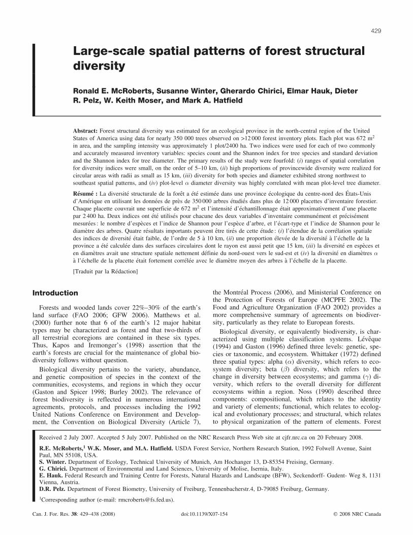
Large-scale spatial patterns of forest structuraldiversity

Ronald E. McRoberts, Susanne Winter, Gherardo Chirici, Elmar Hauk, DieterR. Pelz, W. Keith Moser, and Mark A. Hatfield

Abstract: Forest structural diversity was estimated for an ecological province in the north-central region of the UnitedStates of America using data for nearly 350 000 trees observed on >12 000 forest inventory plots. Each plot was 672 m2

in area, and the sampling intensity was approximately 1 plot/2400 ha. Two indices were used for each of two commonlyand accurately measured inventory variables: species count and the Shannon index for tree species and standard deviationand the Shannon index for tree diameter. The primary results of the study were fourfold: (i) ranges of spatial correlationfor diversity indices were small, on the order of 5–10 km, (ii) high proportions of provincewide diversity were realized forcircular areas with radii as small as 15 km, (iii) diversity for both species and diameter exhibited strong northwest tosoutheast spatial patterns, and (iv) plot-level � diameter diversity was highly correlated with mean plot-level tree diameter.

Resume : La diversite structurale de la foret a ete estimee dans une province ecologique du centre-nord des Etats-Unisd’Amerique en utilisant les donnees de pres de 350 000 arbres etudies dans plus de 12 000 placettes d’inventaire forestier.Chaque placette couvrait une superficie de 672 m2 et l’intensite d’echantillonnage etait approximativement d’une placettepar 2 400 ha. Deux indices ont ete utilises pour chacune des deux variables d’inventaire communement et precisementmesurees : le nombre d’especes et l’indice de Shannon pour l’espece d’arbre, et l’ecart-type et l’indice de Shannon pour lediametre des arbres. Quatre resultats importants peuvent etre tires de cette etude : (i) l’etendue de la correlation spatialedes indices de diversite etait faible, de l’ordre de 5 a 10 km, (ii) une proportion elevee de la diversite a l’echelle de laprovince a ete calculee dans des surfaces circulaires dont le rayon est aussi petit que 15 km, (iii) la diversite en especes eten diametres avait une structure spatiale nettement definie du nord-ouest vers le sud-est et (iv) la diversite en diametres �

a l’echelle de la placette etait fortement correlee avec le diametre moyen des arbres a l’echelle de la placette.

[Traduit par la Redaction]

Introduction

Forests and wooded lands cover 22%–30% of the earth’sland surface (FAO 2006; GFW 2006). Matthews et al.(2000) further note that 6 of the earth’s 12 major habitattypes may be characterized as forest and that two-thirds ofall terrestrial ecoregions are contained in these six types.Thus, Kapos and Iremonger’s (1998) assertion that theearth’s forests are crucial for the maintenance of global bio-diversity follows without question.

Biological diversity pertains to the variety, abundance,and genetic composition of species in the context of thecommunities, ecosystems, and regions in which they occur(Gaston and Spicer 1998; Burley 2002). The relevance offorest biodiversity is reflected in numerous internationalagreements, protocols, and processes including the 1992United Nations Conference on Environment and Develop-ment, the Convention on Biological Diversity (Article 7),

the Montreal Process (2006), and Ministerial Conference onthe Protection of Forests of Europe (MCPFE 2002). TheFood and Agriculture Organization (FAO 2002) provides amore comprehensive summary of agreements on biodiver-sity, particularly as they relate to European forests.

Biological diversity, or equivalently biodiversity, is char-acterized using multiple classification systems. Leveque(1994) and Gaston (1996) defined three levels: genetic, spe-cies or taxonomic, and ecosystem. Whittaker (1972) definedthree spatial types: alpha (�) diversity, which refers to eco-system diversity; beta (�) diversity, which refers to thechange in diversity between ecosystems; and gamma (�) di-versity, which refers to the overall diversity for differentecosystems within a region. Noss (1990) described threecomponents: compositional, which relates to the identityand variety of elements; functional, which relates to ecolog-ical and evolutionary processes; and structural, which relatesto physical organization of the pattern of elements. Forest

Received 2 July 2007. Accepted 5 July 2007. Published on the NRC Research Press Web site at cjfr.nrc.ca on 20 February 2008.

R.E. McRoberts,1 W.K. Moser, and M.A. Hatfield. USDA Forest Service, Northern Research Station, 1992 Folwell Avenue, SaintPaul, MN 55108, USA.S. Winter. Department of Ecology, Technical University of Munich, Am Hochanger 13, D-85354 Freising, Germany.G. Chirici. Department of Environmental and Land Sciences, University of Molise, Isernia, Italy.E. Hauk. Federal Research and Training Centre for Forests, Natural Hazards and Landscape (BFW), Seckendorff- Gudent- Weg 8, 1131Vienna, Austria.D.R. Pelz. Department of Forest Biometry, University of Freiburg, Tennenbacherstr.4, D-79085 Freiburg, Germany.

1Corresponding author (e-mail: rmcroberts@fs.fed.us).

429

Can. J. For. Res. 38: 429–438 (2008) doi:10.1139/X07-154 # 2008 NRC Canada

structural diversity is further characterized with respect tothree components: tree species diversity, tree size diversity,and spatial diversity (Pommerening 2002; Varga et al. 2005).

Forest structural biodiversity assessments have been madeusing data for a variety of variables including tree size, foli-age height, coarse woody debris, and charred wood (Varga etal. 2005). Smith et al. (1997) argued that tree size variablesare logical for assessing structural diversity because silvicul-tural management objectives focused on increasing biodiver-sity are generally defined in terms of tree sizes and densities.Staudhammer and LeMay (2001) noted that tree size datapermit assessment of tree-size diversity; Buongiorno et al.(1994) noted that tree size data are easily and objectively ac-quired by most forest inventories; and Buongiorno et al.(1994) and Kant (2002) noted that tree size data permits esti-mation of the economic consequences of diversity targets.

For large-area biodiversity assessments, the national forestinventories (NFIs) of North America, Europe, and elsewhereprovide the most comprehensive, readily available, and geo-graphically extensive tree species and size data. Representa-tives of 27 European countries and the United States ofAmerica (USA) participating in COST (Cooperation in theField of Science and Technology) Action E43, ‘‘Harmoni-zation of the National Forest Inventories of Europe’’ (COST2006), investigated the ecological relevance and technicalfeasibility of 41 inventory variables associated with aspectsof forest biodiversity. For the 22 countries providing data,tree species, diameter at breast height (DBH), and heightare among the tree-level variables deemed the most ecologi-cally relevant and technically feasible and for which data aremost frequently acquired. However, for some NFIs, speciesis recorded only for broader species categories. In addition,although DBH is measured by the NFIs of all 22 countries,the lower DBH limit for which measurements are obtainedvaries in Europe with the 12 cm Swiss limit being the great-est. Further, height measurements are often obtained foronly a subsample of trees with heights for remaining treespredicted from statistical models.

In ecology, organisms in close spatial proximity may beexpected to be more similar than those at greater distances(Fortin 1999). Thus, forest structural diversity assessmentsalso frequently include a spatial component (Pommerening2002; Varga et al. 2005). Most studies of the spatial compo-nent of forest structural diversity have focused on the simi-larity of within-stand or small-area patterns (e.g.,Kuuluvainen et al. 1996; Pommerening 2002). Because for-est stands, by definition, have at least moderate levels of ho-mogeneity, within-stand structural diversity should be lessthan diversity for spatial extents that encompass multiplestands. Reports of investigations of the structure of forest bi-odiversity at scales larger than stands are rare. Among thefew, Nekola and White (1999) investigated the decrease inspecies similarity with increasing distance for spruce–fir inboreal forests from Alaska, USA, to Newfoundland, Canada,and for Appalachian montane spruce–fir in the eastern USA.They reported proportional decreases in similarity of 0.16 inthe northern regions and 0.42 in the Appalachian regionwith every 1000 km increase in distance. In addition to therarity of large-scale spatial diversity investigations, relation-ships between forest structural diversity and spatial scalehave not been rigorously investigated.

Analyses of forest structural diversity have relied on notonly a variety of variables but also a variety of indices basedon those variables. Because diversity assesses variability bydefinition, indices based on the distributions of tree attrib-utes are both intuitive and logical. For categorical variablessuch as tree species, indices based on simple counts or pro-portions are reasonable, although accommodation for rare orclustered species may be necessary. For continuous variablessuch as DBH, indices based on distributions are reasonable(Neumann and Starlinger 2001).

The Society of American Foresters (SAF 1991) notes that‘‘because the definition of biological diversity is expansive,progress in conservation efforts is most often accomplishedwhen discussions focus on specific components of biologicaldiversity.’’ With this admonition in mind, this study ad-dressed only the three components of structural diversity:species diversity, tree size diversity, and spatial diversity; inparticular, the objectives focused on the large-scale spatialpatterns of tree species and size diversity. In addition, thestudy was intended as a preliminary evaluation of the ana-lytical techniques proposed by COST Action E43 (COST2006) except that the analysis would use NFI data from theUSA where harmonization of data collection has alreadybeen accomplished. Therefore, as a means of facilitatingcomparisons of results from this study with results of COSTAction E43 studies and studies in other global regions, onlycommon, accurately measured, inventory variables wereconsidered; for this study, the variables were tree speciesand DBH. Although the vertical component of structural di-versity is also important, not all NFIs measure height on alltrees. In addition, height is a tree-level variable for whichaccurate data are difficult to obtain, particularly in closedcanopy, deciduous forests. Finally, Neumann and Starlinger(2001) found strong correlation between DBH variation anddiversity measures for other variables.

The overall objectives of the study were to use NFI datato estimate and depict large-scale patterns of forest structuraldiversity and to conduct preliminary investigations of theanalytical techniques proposed by COST Action E43(COST 2006). The specific objectives of the study werefourfold: (i) to estimate � and � diversity for an ecologicalprovince, (ii) to estimate the range of spatial correlation forindices of biodiversity, (iii) to investigate the relationshipbetween diversity and spatial scale, and (iv) to constructmaps depicting spatial distributions of values of biodiversityindices. The objectives did not include investigations ofcausal factors such as management or fragmentation thatcontribute to and affect patterns of structural diversity.

Data

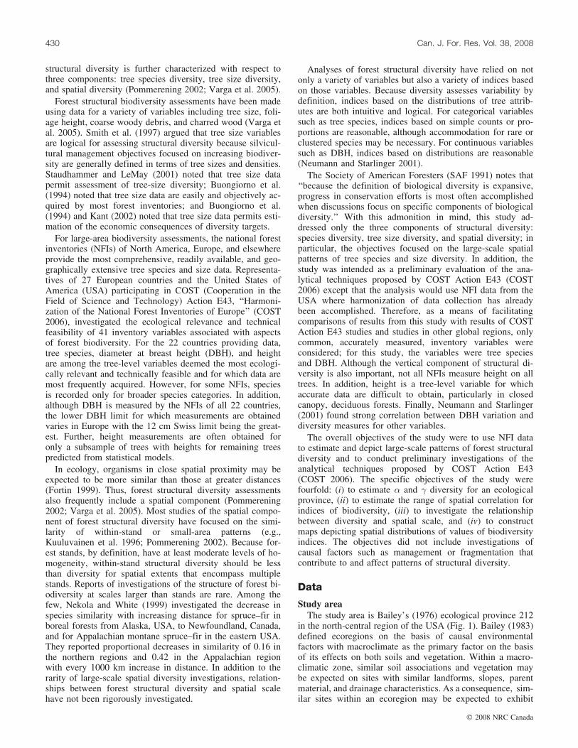
Study areaThe study area is Bailey’s (1976) ecological province 212

in the north-central region of the USA (Fig. 1). Bailey (1983)defined ecoregions on the basis of causal environmentalfactors with macroclimate as the primary factor on the basisof its effects on both soils and vegetation. Within a macro-climatic zone, similar soil associations and vegetation maybe expected on sites with similar landforms, slopes, parentmaterial, and drainage characteristics. As a consequence, sim-ilar sites within an ecoregion may be expected to exhibit

430 Can. J. For. Res. Vol. 38, 2008

# 2008 NRC Canada

similar vegetation, whereas similar sites in different ecore-gions may exhibit dissimilar vegetation. Within ecoregions,ecological divisions are further distinguished on the basisof climax vegetation (e.g., prairie and forest), and withinecological divisions, provinces are distinguished on the ba-sis of climax vegetation dominating upland areas of theprovinces. Thus, a greater degree of spatial similarity inforest structural diversity may be expected within ecologi-cal provinces than between ecological provinces.

Ecological province 212 extends approximately 700 kmnorth to south and approximately 775 km east to west. Theprovince covers 381 500 km2; for comparison purposes, thecountry of Germany covers approximately 357 000 km2.Most of the province has low relief with rolling hills, lakes,poorly drained depressions, and glacial features. Elevationsabove sea level are mostly in the range of 175–550 m withminimum elevations of approximately 175 m near the GreatLakes and maximum elevations of 700 m in small isolatedareas (Geology.com 2007). Mean annual precipitation rangesfrom 56 cm in the northwest to 85 cm near the easternshores of the Great Lakes in the southeast (NOAA 1974).Mean minimum winter temperature ranges from –20 8C inthe northwest to –9 8C in the southeast, and mean maximumsummer temperature ranges from 25 8C in the northwest, to21 8C along the Great Lakes on the northern boundary ofthe province, and to 28 8C in the southeast. The provincelies between boreal and broadleaf deciduous forest zonesand is, therefore, transitional with mixed stands of pine,spruce, cedar, birch, and maple. Soils vary greatly and in-clude peat, muck, marl, clay, silt, sand, gravel, and bouldersin various combinations.

Forest inventory dataThe Forest Inventory and Analysis (FIA) program of the

USDA Forest Service conducts the NFI of the USA. The FIAprogram has established field plot centers in permanent loca-tions across the USA using a sampling design that is assumed toproduce a random, equal probability sample (Bechtold and Pat-terson 2005; McRoberts et al. 2005). The sampling design isbased on the tessellation of the USA into 2400 ha (6000 acre)hexagons and features a permanent plot at a randomly se-lected location within each hexagon. The resulting plot arrayhas been divided into five nonoverlapping, interpenetratingpanels, and measurement of all plots in one panel is com-pleted before measurement of plots in the next panel is initi-ated. Panels in the study area are selected on a 5 yearrotating basis. Over a complete measurement cycle, the sam-pling intensity is approximately 1 plot/2400 ha, and the meandistance between plots is approximately 5 km. In general,locations of forested or previously forested plots are deter-mined using global positioning system receivers, whereaslocations of nonforested plots are determined using aerialimagery and digitization methods. Each plot consists offour 7.31 m (24 ft) radius circular subplots for a total areaof 672 m2. The subplots are configured as a central subplotand three peripheral subplots with centers located at36.58 m (120 ft) and azimuths of 08, 1208, and 2408 fromthe center of the central subplot. The FIA program restrictsobservations and measurements on these plots to trees withDBH ‡ 12.5 cm (5 in.). This DBH limit is comparablewith the 12 cm common lower DBH limit for European

NFIs. Tree species is determined by visually inspectingthe bark and leaves, and DBH is measured by wrapping a di-ameter tape around the tree at a height of 1.37 m (4.5 ft).

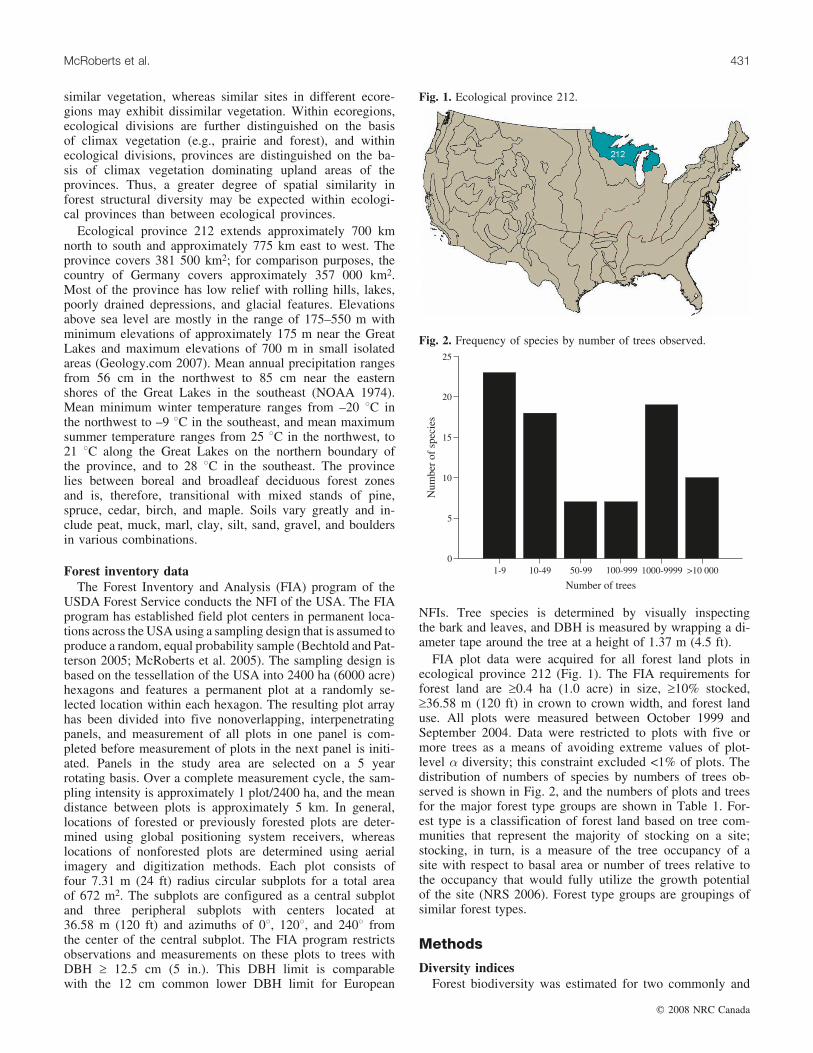
FIA plot data were acquired for all forest land plots inecological province 212 (Fig. 1). The FIA requirements forforest land are ‡0.4 ha (1.0 acre) in size, ‡10% stocked,‡36.58 m (120 ft) in crown to crown width, and forest landuse. All plots were measured between October 1999 andSeptember 2004. Data were restricted to plots with five ormore trees as a means of avoiding extreme values of plot-level � diversity; this constraint excluded <1% of plots. Thedistribution of numbers of species by numbers of trees ob-served is shown in Fig. 2, and the numbers of plots and treesfor the major forest type groups are shown in Table 1. For-est type is a classification of forest land based on tree com-munities that represent the majority of stocking on a site;stocking, in turn, is a measure of the tree occupancy of asite with respect to basal area or number of trees relative tothe occupancy that would fully utilize the growth potentialof the site (NRS 2006). Forest type groups are groupings ofsimilar forest types.

Methods

Diversity indicesForest biodiversity was estimated for two commonly and

Fig. 1. Ecological province 212.

10-49 1000-9999

Number of trees

0

5

10

15

20

25

Num

ber

ofsp

ecie

s

1-9 100-999 >10 00050-99

Fig. 2. Frequency of species by number of trees observed.

McRoberts et al. 431

# 2008 NRC Canada

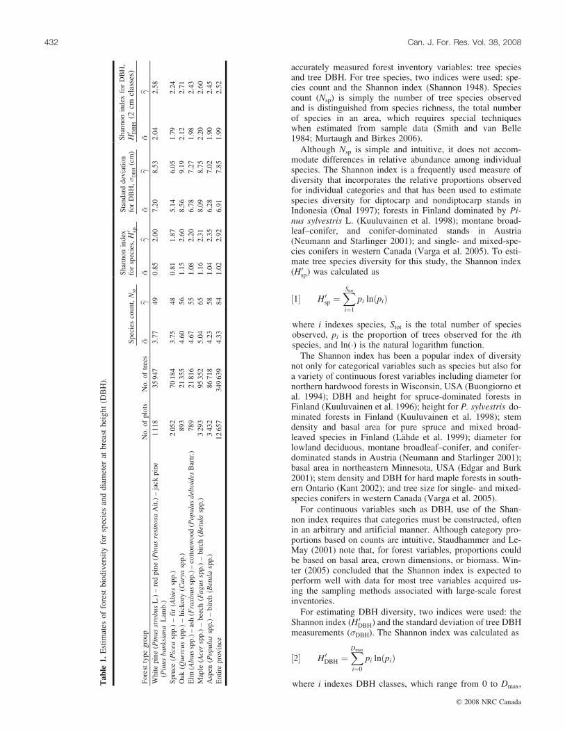
accurately measured forest inventory variables: tree speciesand tree DBH. For tree species, two indices were used: spe-cies count and the Shannon index (Shannon 1948). Speciescount (Nsp) is simply the number of tree species observedand is distinguished from species richness, the total numberof species in an area, which requires special techniqueswhen estimated from sample data (Smith and van Belle1984; Murtaugh and Birkes 2006).

Although Nsp is simple and intuitive, it does not accom-modate differences in relative abundance among individualspecies. The Shannon index is a frequently used measure ofdiversity that incorporates the relative proportions observedfor individual categories and that has been used to estimatespecies diversity for diptocarp and nondiptocarp stands inIndonesia (Onal 1997); forests in Finland dominated by Pi-nus sylvestris L. (Kuuluvainen et al. 1998); montane broad-leaf–conifer, and conifer-dominated stands in Austria(Neumann and Starlinger 2001); and single- and mixed-spe-cies conifers in western Canada (Varga et al. 2005). To esti-mate tree species diversity for this study, the Shannon index(H 0

sp) was calculated as

½1� H 0sp ¼

XStoti¼1

pi lnðpiÞ

where i indexes species, Stot is the total number of speciesobserved, pi is the proportion of trees observed for the ithspecies, and ln(�) is the natural logarithm function.

The Shannon index has been a popular index of diversitynot only for categorical variables such as species but also fora variety of continuous forest variables including diameter fornorthern hardwood forests in Wisconsin, USA (Buongiorno etal. 1994); DBH and height for spruce-dominated forests inFinland (Kuuluvainen et al. 1996); height for P. sylvestris do-minated forests in Finland (Kuuluvainen et al. 1998); stemdensity and basal area for pure spruce and mixed broad-leaved species in Finland (Lahde et al. 1999); diameter forlowland deciduous, montane broadleaf–conifer, and conifer-dominated stands in Austria (Neumann and Starlinger 2001);basal area in northeastern Minnesota, USA (Edgar and Burk2001); stem density and DBH for hard maple forests in south-ern Ontario (Kant 2002); and tree size for single- and mixed-species conifers in western Canada (Varga et al. 2005).

For continuous variables such as DBH, use of the Shan-non index requires that categories must be constructed, oftenin an arbitrary and artificial manner. Although category pro-portions based on counts are intuitive, Staudhammer and Le-May (2001) note that, for forest variables, proportions couldbe based on basal area, crown dimensions, or biomass. Win-ter (2005) concluded that the Shannon index is expected toperform well with data for most tree variables acquired us-ing the sampling methods associated with large-scale forestinventories.

For estimating DBH diversity, two indices were used: theShannon index (H 0

DBH) and the standard deviation of tree DBHmeasurements (�DBH). The Shannon index was calculated as

½2� H 0DBH ¼

XDmax

i¼0

pi lnðpiÞ

where i indexes DBH classes, which range from 0 to Dmax,Tab

le1.

Est

imat

esof

fore

stbi

odiv

ersi

tyfo

rsp

ecie

san

ddi

amet

erat

brea

sthe

ight

(DB

H).

Spec

ies

coun

t,N

sp

Shan

non

inde

xfo

rsp

ecie

s,H

0 sp

Stan

dard

devi

atio

nfo

rD

BH

,�

DB

H(c

m)

Shan

non

inde

xfo

rD

BH

,H

0 DBH

(2cm

clas

ses)

Fore

stty

pegr

oup

No.

ofpl

ots

No.

oftr

ees

� �b �

� �b �

� �b �

� �b �

Whi

tepi

ne(P

inus

stro

bus

L.)

–re

dpi

ne(P

inus

resi

nosa

Ait.

)–

jack

pine

(Pin

usba

nksi

ana

Lam

b.)

111

835

947

3.77

490.

852.

007.

208.

532.

042.

58

Spru

ce(P

icea

spp.

)–

fir

(Abi

essp

p.)

205

270

184

3.75

480.

811.

875.

146.

051.

792.

24O

ak(Q

uerc

ussp

p.)

–hi

ckor

y(C

arya

spp.

)89

321

355

4.60

561.

152.

608.

569.

192.

122.

71E

lm(A

lnus

spp.

)–as

h(F

raxi

nus

spp.

)–co

ttonw

ood

(Pop

ulus

delt

oide

sB

artr

.)78

921

816

4.67

551.

082.

206.

787.

271.

982.

43M

aple

(Ace

rsp

p.)

–be

ech

(Fag

ussp

p.)

–bi

rch

(Bet

ula

spp.

)3

293

9535

25.

0465

1.16

2.31

8.09

8.75

2.20

2.60

Asp

en(P

opul

ussp

p.)

–bi

rch

(Bet

ula

spp.

)3

432

8671

84.

2358

1.04

2.35

6.28

7.02

1.90

2.45

Ent

ire

prov

ince

1265

734

963

94.

3384

1.02

2.92

6.91

7.85

1.99

2.52

432 Can. J. For. Res. Vol. 38, 2008

# 2008 NRC Canada

pi is the proportion of trees in the ith DBH class, and ln(�) isagain the natural logarithm function. For this study, DBHclasses of 1, 2, and 5 cm widths were considered. The sec-ond index, �DBH, was calculated as

½3� �DBH ¼

ffiffiffiffiffiffiffiffiffiffiffiffiffiffiffiffiffiffiffiffiffiffiffiffiffiffiffiffiffiffiffiffiffiffiffiffiffiffiffiffiXni¼1

ðDBHi � DBHÞ2

n� 1

vuuuut

where DBHi is measured DBH for the ith tree, DBH ismean DBH for the area for which diversity is estimated,and n is the number of trees. The advantages of standard de-viation are threefold: it is easy to calculate and interpret; itmay be calculated by plot for each inventory method thatyields stem density; and temporal changes can be easily de-tected. Minimum values for standard deviations are realizedwhen all diameter observations are similar, whereas maxi-mum values are realized when one-half the observations areat the lower extreme and one-half are at the upper extreme.Finally, COST Action E43 has selected the standard devia-tion of distributions of tree DBH measurements as an indexof horizontal structural biodiversity (COST 2006).

Spatial analysesWhittaker (1972), Lahde et al. (1999), and Neumann and

Starlinger (2001) all calculated � diversity using sample plotdata. Similarly, for this study, � diversities for Nsp, H 0

sp, �DBH,and H 0

DBH were calculated for each inventory plot, and themean � diversity for each index over all plots was attrib-uted to the entire province. Within the province, � diver-sity for Nsp was simply Stot, whereas � diversities for H 0

sp,�DBH, and H 0

DBH were calculated using data for all trees ob-served for all plots. Mean � diversities and � diversitiesfor the most common forest type groups within the prov-ince were estimated using the same four indices.

Spatial aspects of biodiversity were investigated usingthree methods. Firstly, for each of the four indices, an em-pirical spatial semivariogram for � diversity was constructedas

½4� b�ðhÞ ¼ 1

2kNðhÞkXNðhÞ

ð�i � �jÞ2

where N(h) denotes a set of plots whose Euclidean separa-tion distance in geographical space is within a neighborhoodof h (Cressie 1993), kNðhÞk is the number of pairs of plotsin N(h), and �i and �j are the values of � diversity for theith and jth plots in N(h) for each of Nsp, H 0

sp, �DBH, andH 0

DBH. Although it is customary to use the Greek letter �for semivariance on the left side of eq. 4, the Greek letter �is used here to avoid confusion with � diversity. Assumingnegligible semivariance for h � 0, an empirical correlogrammay be constructed from the semivariogram as

½5� b�ðhÞ ¼ 1�b�ðhÞb�max

where b�max is the maximum observed value of b�ðhÞ for theinterval 0 £ h £ 250 km. Restriction to this interval is a re-sult of small kNðhÞk for h > 250 km. The intent with the

use of spatial correlograms was to estimate the geographicdistances at which � diversity is no longer spatially corre-lated.

The second spatial investigation focused on estimating therelationships between diversity and spatial area. For eachplot location, diversity using each index was calculated us-ing all plot data in n-plot neighborhoods where n rangedfrom n = 1 to n = 100. Neighborhoods were defined withrespect to numbers of plots rather than distances as a resultof the random component in the FIA sampling design. Be-cause distances between nearest plot locations vary ran-domly, the numbers of plots within a given distance ofspecific locations also varies. Thus, because the probabilityof observing infrequently occurring events (such as rare spe-cies or very large trees) is correlated with the number ofplots observed, diversity estimates based on fewer plotscould be biased downward relative to estimates based onmore plots. The distances between each plot location andthe locations of the n plots in its n-plot neighborhood werecalculated, and the maximum of the n distances was definedas the neighborhood radius. For each value of n, the ratio ofthe mean diversity over all plots and the � diversity for theprovince was graphed against the mean neighborhood ra-dius. The intent of this investigation was to estimate therate at which diversity increases with spatial scale.

The third spatial investigation focused on constructingprovince-level maps of � diversity and diversity for areasof increasing size. Estimation points were selected at the in-tersections of a 5 km � 5 km grid that formed the frame-work for the maps. For each estimation point, � diversitywas estimated as the inverse distance-weighted mean of the� diversities for the five FIA plots nearest to the point ingeographical space. Although the selection of five as thenumber of nearest plots is arbitrary, five is regarded as thesmallest number that accurately reflected the diversity inclose proximity to the grid point. In addition, for values ofn ranging from n = 5 to n = 100, diversity was estimatedusing data for all plots within n-plot neighborhoods and wasattributed to the estimation point location. The intent of thisinvestigation was to depict visually the spatial distribution offorest structural diversity.

Results

Species and DBH data were acquired for 348 189 trees on12 367 plots. Although 84 species were observed, 12 speciesaccounted for 75% of the trees, 19 species accounted for90% of the trees, 30 species accounted for 99% of the trees,and 23 species were represented by fewer than 10 trees each(Fig. 2). The most frequently observed species were quakingaspen (Populus tremuloides Michx.), sugar maple (Acer sac-charum Marsh.), northern white cedar (Thuja occidentalisL.), and red maple (Acer rubrum L.), each of which ac-counted for more than 10% of the total number of trees ob-served. Of the 84 species observed, 78 are considered nativeto the ecoprovince. Of the six species not considered native,three conifers are of European origin, two conifers are na-tive to the western USA, and one deciduous species is nativeto the eastern USA.

Magurran (1988) notes that, for diversity analyses, plotsizes should be compatible with the size of the organism

McRoberts et al. 433

# 2008 NRC Canada

under investigation and recommends a large number ofsmall plots rather than a small number of large plots. Forthis study, observations were available for >12 000 plots ofsize 672 m2 with a mean of >28 trees/plot. Although no rig-

orous test was conducted, the plot and sample sizes weredeemed adequate. Nevertheless, different plot and samplesizes may produce different results. However, on the basisof the national consistency of the FIA plot configurationand sampling intensity, comparable studies could be con-ducted anywhere in the USA.

DiversityAs expected, mean � diversity was less than � diversity

for all four indices (Table 1). Because plot-level values ofH 0

DBH were so highly correlated (0.80 £ b� = £ 0.94) amongthe 1, 2, and 5 cm DBH classes, only results for the 2 cmclass are reported. Ratios of mean � diversity to � diversitywere 0.05 for Nsp, 0.35 for H 0

sp, 0.88 for �DBH, and 0.79 forH 0

DBH. The small ratio for Nsp can be attributed to the rela-tively large number of species with only a few observations.However, even if all species with <100 observations wereignored, the ratio for Nsp would still be only 0.12. The latterresult and the small ratio for H 0

sp suggest nonuniformity inthe distribution of at least some species throughout the prov-ince.

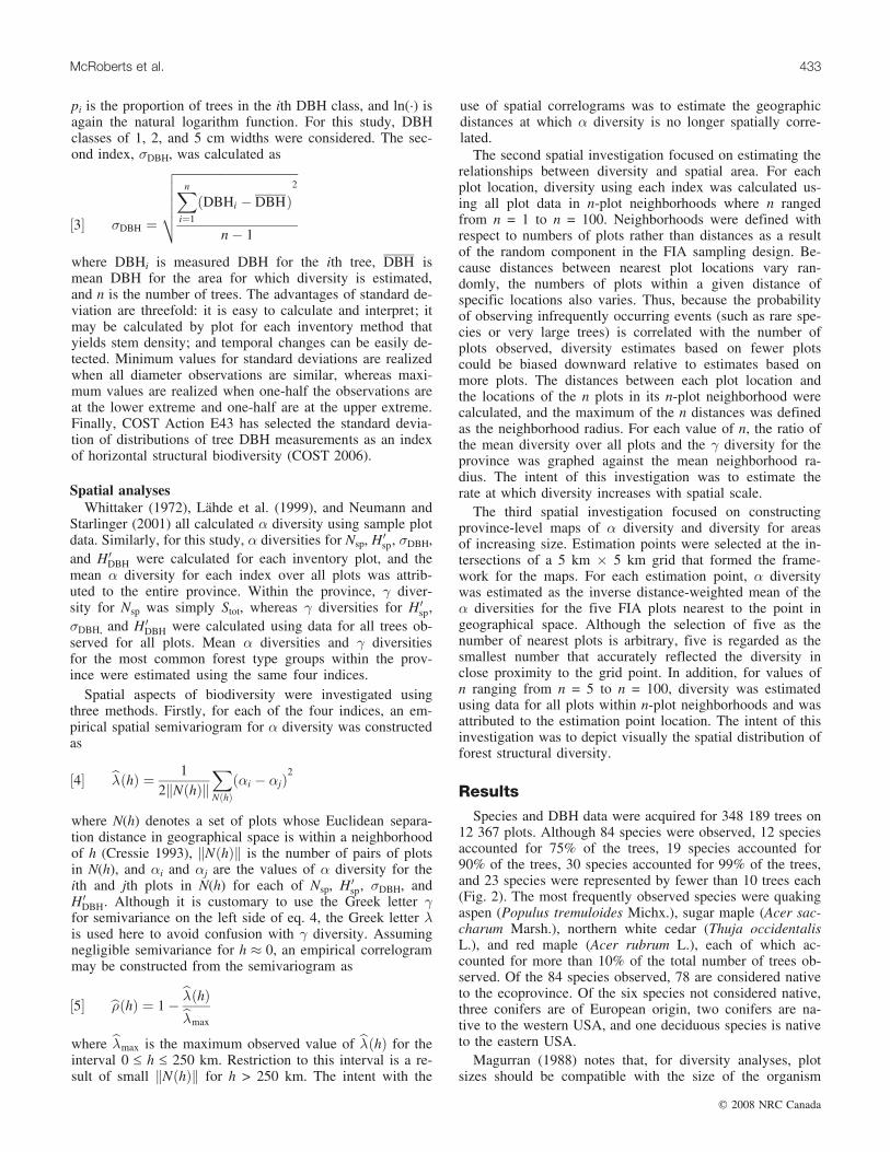
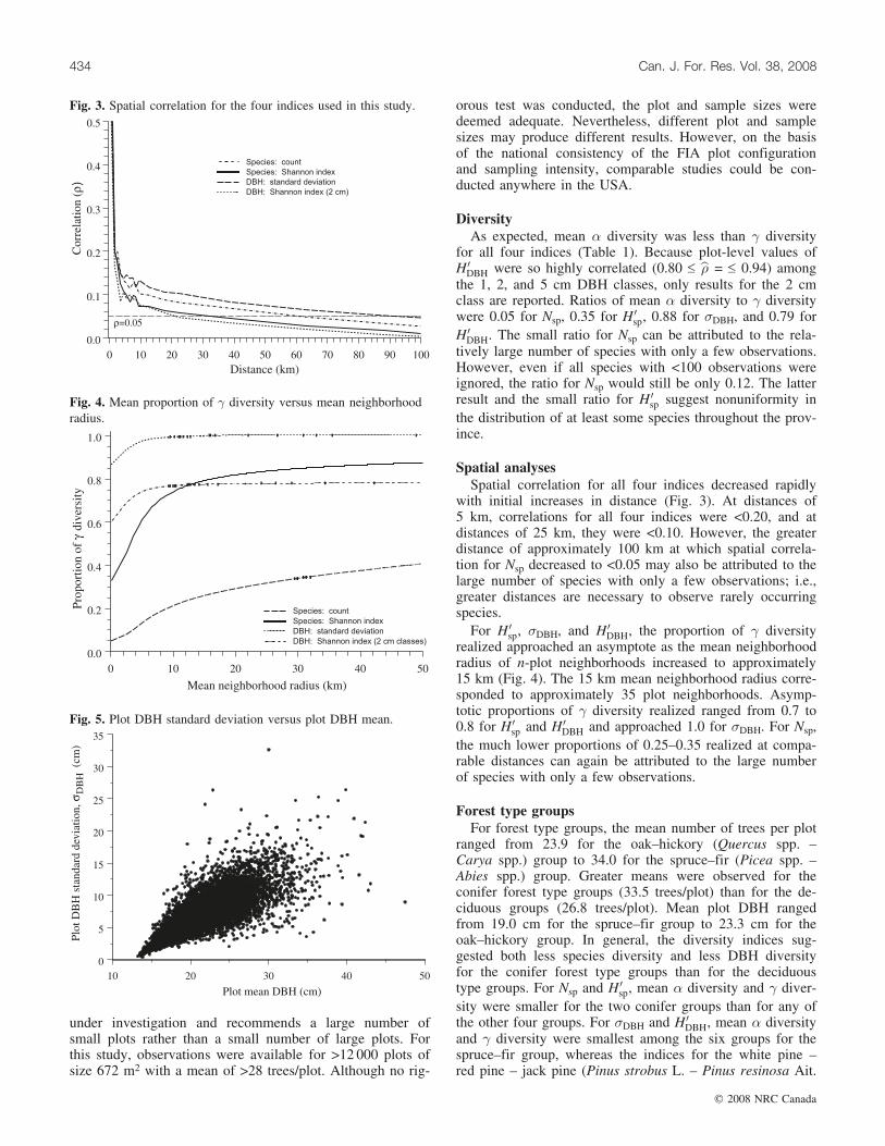
Spatial analysesSpatial correlation for all four indices decreased rapidly

with initial increases in distance (Fig. 3). At distances of5 km, correlations for all four indices were <0.20, and atdistances of 25 km, they were <0.10. However, the greaterdistance of approximately 100 km at which spatial correla-tion for Nsp decreased to <0.05 may also be attributed to thelarge number of species with only a few observations; i.e.,greater distances are necessary to observe rarely occurringspecies.

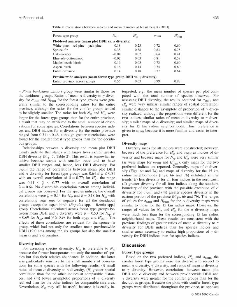
For H 0sp, �DBH, and H 0

DBH, the proportion of � diversityrealized approached an asymptote as the mean neighborhoodradius of n-plot neighborhoods increased to approximately15 km (Fig. 4). The 15 km mean neighborhood radius corre-sponded to approximately 35 plot neighborhoods. Asymp-totic proportions of � diversity realized ranged from 0.7 to0.8 for H 0

sp and H 0DBH and approached 1.0 for �DBH. For Nsp,

the much lower proportions of 0.25–0.35 realized at compa-rable distances can again be attributed to the large numberof species with only a few observations.

Forest type groupsFor forest type groups, the mean number of trees per plot

ranged from 23.9 for the oak–hickory (Quercus spp. –Carya spp.) group to 34.0 for the spruce–fir (Picea spp. –Abies spp.) group. Greater means were observed for theconifer forest type groups (33.5 trees/plot) than for the de-ciduous groups (26.8 trees/plot). Mean plot DBH rangedfrom 19.0 cm for the spruce–fir group to 23.3 cm for theoak–hickory group. In general, the diversity indices sug-gested both less species diversity and less DBH diversityfor the conifer forest type groups than for the deciduoustype groups. For Nsp and H 0

sp, mean � diversity and � diver-sity were smaller for the two conifer groups than for any ofthe other four groups. For �DBH and H 0

DBH, mean � diversityand � diversity were smallest among the six groups for thespruce–fir group, whereas the indices for the white pine –red pine – jack pine (Pinus strobus L. – Pinus resinosa Ait.

0 10 20 30 40 50 60 70 80 90 100Distance (km)

0.0

0.1

0.2

0.3

0.4

0.5

Cor

rela

tion

(ρ)

Species: count

Species: Shannon index

DBH: standard deviation

DBH: Shannon index (2 cm)

ρ=0.05

Fig. 3. Spatial correlation for the four indices used in this study.

0 10 20 30 40 50

Mean neighborhood radius (km)

0.0

0.2

0.4

0.6

0.8

1.0

Species: count

Species: Shannon index

DBH: standard deviation

DBH: Shannon index (2 cm classes)

Prop

ortio

nof

γdi

vers

ity

Fig. 4. Mean proportion of � diversity versus mean neighborhoodradius.

10 20 30 40 50

Plot mean DBH (cm)

0

5

10

15

20

25

30

35

Plot

DB

H s

tand

ard

devi

atio

n,(c

m)

σ DB

H

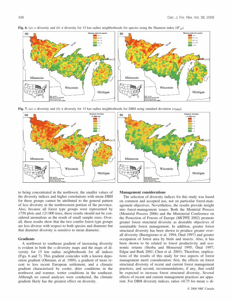
Fig. 5. Plot DBH standard deviation versus plot DBH mean.

434 Can. J. For. Res. Vol. 38, 2008

# 2008 NRC Canada

– Pinus banksiana Lamb.) group were similar to those forthe deciduous groups. Ratios of mean � diversity to � diver-sity for �DBH and H 0

DBH for the forest type groups were gen-erally similar to the corresponding ratios for the entireprovince, although the ratios for the conifer groups tendedto be slightly smaller. The ratios for both Nsp and H 0

sp werelarger for the forest type groups than for the entire province,a result that may be attributed to the small number of obser-vations for some species. Correlations between species indi-ces and DBH indices for � diversity for the entire provinceranged from 0.31 to 0.46, although greater correlations werefound for the conifer forest type groups than for the decidu-ous groups.

Relationships between � diversity and mean plot DBHclearly indicate that stands with larger trees exhibit greaterDBH diversity (Fig. 5; Table 2). This result is somewhat in-tuitive because stands with smaller trees tend to havesmaller DBH ranges and, hence, less DBH diversity. For�DBH, the range of correlations between mean plot DBHand � diversity for forest type groups was 0.64 £ b� £ 0.81with an overall correlation of b� ¼ 0:77; for H 0

sp, the rangewas 0.41 £ b� £ 0.77 with an overall correlation ofb� ¼ 0:64. No discernible correlation pattern among individ-ual groups was observed. For the species indices, the overallcorrelations were b� = 0.14 for Nsp and b� = 0.18 for H 0

sp withcorrelations near zero or negative for all the deciduousgroups except the aspen–birch (Populus spp. – Betula spp.)group. Correlations calculated across forest type groups be-tween mean DBH and � diversity were � ¼ 0:53 for Nsp, b�= 0.69 for H 0

sp, and b� ‡ 0.98 for both �DBH and H 0DBH. The

effects of these correlations are evident for the spruce–firgroup, which had not only the smallest mean provincewideDBH (19.0 cm) among the six groups but also the smallestmean � and � diversities.

Diversity indicesFor assessing species diversity, H 0

sp is preferable to Nspbecause the former incorporates not only the number of spe-cies but also their relative abundance. In addition, the latterwas particularly sensitive to the small numbers of observa-tions for some species with the following results: (i) smallratios of mean � diversity to � diversity, (ii) greater spatialcorrelation than for the other indices at comparable distan-ces, and (iii) lower asymptotic proportions of � diversityrealized than for the other indices for comparable size area.Nevertheless, Nsp may still be useful because it is easily in-

terpreted, e.g., the mean number of species per plot com-pared with the total number of species observed. Forassessing DBH diversity, the results obtained for �DBH, andH 0

sp were very similar: similar ranges of spatial correlation;similar distances to the asymptote of proportion of � diver-sity realized, although the proportions were different for thetwo indices; similar ratios of mean � diversity to � diver-sity; similar maps of � diversity; and similar maps of diver-sity for 15 km radius neighborhoods. Thus, preference isgiven to �DBH because it is more familiar and easier to inter-pret.

Diversity mapsDiversity maps for all indices were constructed; however,

because of the preference for H 0sp and �DBH as indices of di-

versity and because maps for Nsp and H 0sp were very similar

(as were maps for �DBH and H 0DBH), only maps for the two

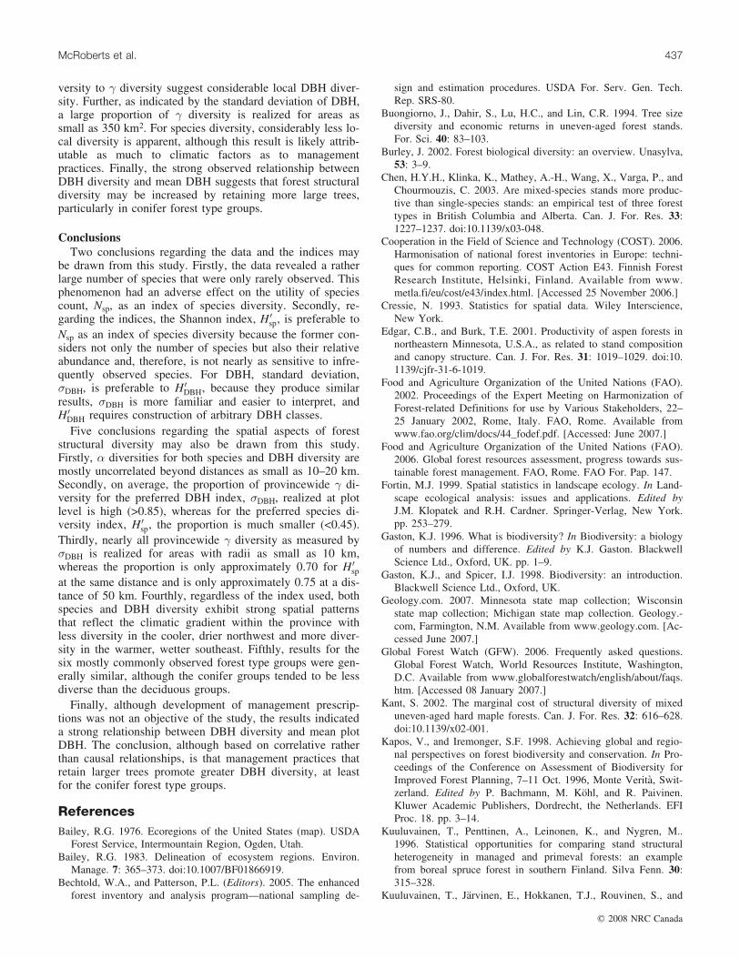
preferred indices are reported. Generally, maps of � diver-sity (Figs. 6a and 7a) and maps of diversity for the 15 kmradius neighborhoods (Figs. 6b and 7b) exhibited similartrends: (i) less diversity for all four indices in the northwest;(ii) greater diversity for all four indices along the southernboundary of the province with the possible exception of �diversity for �DBH; and (iii) greater species diversity in theeastern portion of the province (Figs. 6b and 7b). The rangesof values for �DBH and H 0

DBH for the � diversity maps weresimilar to those for the 15 km radius maps. However, theranges of values for Nsp and H 0

sp for the � diversity mapswere much less than for the corresponding 15 km radiusneighborhood maps. These results are consistent with theprevious findings of greater ratios of mean � diversity to �diversity for DBH indices than for species indices andsmaller areas necessary to realize high proportions of � di-versity for DBH indices than for species indices.

Discussion

Forest type groupsBased on the two preferred indices, H 0

sp and �DBH, theconifer forest type groups were less diverse with respect tomean � diversity, � diversity, and ratios of mean � diversityto � diversity. However, correlations between mean plotDBH and � diversity and between provincewide DBH and� diversity were greater for the conifer groups than for thedeciduous groups. Because the plots with conifer forest typegroups were distributed throughout the province, as opposed

Table 2. Correlations between indices and mean diameter at breast height (DBH).

Forest type group Nsp H 0sp �DBH H 0

DBH

Plot-level analyses (mean plot DBH vs. � diversity)White pine – red pine – jack pine 0.18 0.23 0.72 0.60Spruce–fir 0.38 0.38 0.83 0.75Oak–hickory –0.04 0.02 0.64 0.41Elm–ash–cottonwood –0.02 0.03 0.81 0.58Maple–beech–birch –0.16 0.03 0.73 0.60Aspen–birch 0.16 –0.14 0.74 0.60Entire province 0.14 0.18 0.77 0.64

Provincewide analyses (mean forest type group DBH vs. � diversity)Entire province across groups 0.55 0.63 0.99 0.98

McRoberts et al. 435

# 2008 NRC Canada

to being concentrated in the northwest, the smaller values ofthe diversity indices and higher correlations with mean DBHfor these groups cannot be attributed to the general patternof less diversity in the northwestern portion of the province.Also, because all forest type groups were represented by‡750 plots and ‡21 000 trees, these results should not be con-sidered anomalous as the result of small sample sizes. Over-all, these results show that the two conifer forest type groupsare less diverse with respect to both species and diameter butthat diameter diversity is sensitive to mean diameter.

GradientsA northwest to southeast gradient of increasing diversity

is evident in both the �-diversity maps and the maps of di-versity for 15 km radius neighborhoods for all indices(Figs. 6 and 7). This gradient coincides with a known depo-sition gradient (Ohmann, et al. 1989), a gradient of more re-cent to less recent European settlement, and a climaticgradient characterized by cooler, drier conditions in thenorthwest and warmer, wetter conditions in the southeast.Although no causal analyses were conducted, the climaticgradient likely has the greatest effect on diversity.

Management considerationsThe selection of diversity indices for this study was based

on common and accepted use, not on particular forest-man-agement objectives. Nevertheless, the results provide insightinto forest-management issues. Both the Montreal Process(Montreal Process 2006) and the Ministerial Conference onthe Protection of Forests of Europe (MCPFE 2002) promotegreater forest structural diversity as desirable objectives ofsustainable forest management. In addition, greater foreststructural diversity has been shown to produce greater over-all diversity (Buongiorno et al. 1994; Onal 1997) and greateroccupation of forest area by birds and insects. Also, it hasbeen shown to be related to forest productivity and eco-nomic returns (Sterba and Monserud 1995; Onal 1997;Edgar and Burk 2001; Chen et al. 2003). Therefore, implica-tions of the results of this study for two aspects of forestmanagement merit consideration: first, the effects on foreststructural diversity of recent and current forest managementpractices, and second, recommendations, if any, that couldbe expected to increase forest structural diversity. Severaleffects of recent and current management practices are appa-rent. For DBH diversity indices, ratios >0.75 for mean � di-

Fig. 6. (a) � diversity and (b) a diversity for 15 km radius neighborhoods for species using the Shannon index (H 0sp).

Fig. 7. (a) � diversity and (b) a diversity for 15 km radius neighborhoods for DBH using standard deviation (�DBH).

436 Can. J. For. Res. Vol. 38, 2008

# 2008 NRC Canada

versity to � diversity suggest considerable local DBH diver-sity. Further, as indicated by the standard deviation of DBH,a large proportion of � diversity is realized for areas assmall as 350 km2. For species diversity, considerably less lo-cal diversity is apparent, although this result is likely attrib-utable as much to climatic factors as to managementpractices. Finally, the strong observed relationship betweenDBH diversity and mean DBH suggests that forest structuraldiversity may be increased by retaining more large trees,particularly in conifer forest type groups.

ConclusionsTwo conclusions regarding the data and the indices may

be drawn from this study. Firstly, the data revealed a ratherlarge number of species that were only rarely observed. Thisphenomenon had an adverse effect on the utility of speciescount, Nsp, as an index of species diversity. Secondly, re-garding the indices, the Shannon index, H 0

sp, is preferable toNsp as an index of species diversity because the former con-siders not only the number of species but also their relativeabundance and, therefore, is not nearly as sensitive to infre-quently observed species. For DBH, standard deviation,�DBH, is preferable to H 0

DBH, because they produce similarresults, �DBH is more familiar and easier to interpret, andH 0

DBH requires construction of arbitrary DBH classes.Five conclusions regarding the spatial aspects of forest

structural diversity may also be drawn from this study.Firstly, � diversities for both species and DBH diversity aremostly uncorrelated beyond distances as small as 10–20 km.Secondly, on average, the proportion of provincewide � di-versity for the preferred DBH index, �DBH, realized at plotlevel is high (>0.85), whereas for the preferred species di-versity index, H 0

sp, the proportion is much smaller (<0.45).Thirdly, nearly all provincewide � diversity as measured by�DBH is realized for areas with radii as small as 10 km,whereas the proportion is only approximately 0.70 for H 0

sp

at the same distance and is only approximately 0.75 at a dis-tance of 50 km. Fourthly, regardless of the index used, bothspecies and DBH diversity exhibit strong spatial patternsthat reflect the climatic gradient within the province withless diversity in the cooler, drier northwest and more diver-sity in the warmer, wetter southeast. Fifthly, results for thesix mostly commonly observed forest type groups were gen-erally similar, although the conifer groups tended to be lessdiverse than the deciduous groups.

Finally, although development of management prescrip-tions was not an objective of the study, the results indicateda strong relationship between DBH diversity and mean plotDBH. The conclusion, although based on correlative ratherthan causal relationships, is that management practices thatretain larger trees promote greater DBH diversity, at leastfor the conifer forest type groups.

ReferencesBailey, R.G. 1976. Ecoregions of the United States (map). USDA

Forest Service, Intermountain Region, Ogden, Utah.Bailey, R.G. 1983. Delineation of ecosystem regions. Environ.

Manage. 7: 365–373. doi:10.1007/BF01866919.Bechtold, W.A., and Patterson, P.L. (Editors). 2005. The enhanced

forest inventory and analysis program—national sampling de-

sign and estimation procedures. USDA For. Serv. Gen. Tech.Rep. SRS-80.

Buongiorno, J., Dahir, S., Lu, H.C., and Lin, C.R. 1994. Tree sizediversity and economic returns in uneven-aged forest stands.For. Sci. 40: 83–103.

Burley, J. 2002. Forest biological diversity: an overview. Unasylva,53: 3–9.

Chen, H.Y.H., Klinka, K., Mathey, A.-H., Wang, X., Varga, P., andChourmouzis, C. 2003. Are mixed-species stands more produc-tive than single-species stands: an empirical test of three foresttypes in British Columbia and Alberta. Can. J. For. Res. 33:1227–1237. doi:10.1139/x03-048.

Cooperation in the Field of Science and Technology (COST). 2006.Harmonisation of national forest inventories in Europe: techni-ques for common reporting. COST Action E43. Finnish ForestResearch Institute, Helsinki, Finland. Available from www.metla.fi/eu/cost/e43/index.html. [Accessed 25 November 2006.]

Cressie, N. 1993. Statistics for spatial data. Wiley Interscience,New York.

Edgar, C.B., and Burk, T.E. 2001. Productivity of aspen forests innortheastern Minnesota, U.S.A., as related to stand compositionand canopy structure. Can. J. For. Res. 31: 1019–1029. doi:10.1139/cjfr-31-6-1019.

Food and Agriculture Organization of the United Nations (FAO).2002. Proceedings of the Expert Meeting on Harmonization ofForest-related Definitions for use by Various Stakeholders, 22–25 January 2002, Rome, Italy. FAO, Rome. Available fromwww.fao.org/clim/docs/44_fodef.pdf. [Accessed: June 2007.]

Food and Agriculture Organization of the United Nations (FAO).2006. Global forest resources assessment, progress towards sus-tainable forest management. FAO, Rome. FAO For. Pap. 147.

Fortin, M.J. 1999. Spatial statistics in landscape ecology. In Land-scape ecological analysis: issues and applications. Edited byJ.M. Klopatek and R.H. Cardner. Springer-Verlag, New York.pp. 253–279.

Gaston, K.J. 1996. What is biodiversity? In Biodiversity: a biologyof numbers and difference. Edited by K.J. Gaston. BlackwellScience Ltd., Oxford, UK. pp. 1–9.

Gaston, K.J., and Spicer, I.J. 1998. Biodiversity: an introduction.Blackwell Science Ltd., Oxford, UK.

Geology.com. 2007. Minnesota state map collection; Wisconsinstate map collection; Michigan state map collection. Geology.-com, Farmington, N.M. Available from www.geology.com. [Ac-cessed June 2007.]

Global Forest Watch (GFW). 2006. Frequently asked questions.Global Forest Watch, World Resources Institute, Washington,D.C. Available from www.globalforestwatch/english/about/faqs.htm. [Accessed 08 January 2007.]

Kant, S. 2002. The marginal cost of structural diversity of mixeduneven-aged hard maple forests. Can. J. For. Res. 32: 616–628.doi:10.1139/x02-001.

Kapos, V., and Iremonger, S.F. 1998. Achieving global and regio-nal perspectives on forest biodiversity and conservation. In Pro-ceedings of the Conference on Assessment of Biodiversity forImproved Forest Planning, 7–11 Oct. 1996, Monte Verita, Swit-zerland. Edited by P. Bachmann, M. Kohl, and R. Paivinen.Kluwer Academic Publishers, Dordrecht, the Netherlands. EFIProc. 18. pp. 3–14.

Kuuluvainen, T., Penttinen, A., Leinonen, K., and Nygren, M..1996. Statistical opportunities for comparing stand structuralheterogeneity in managed and primeval forests: an examplefrom boreal spruce forest in southern Finland. Silva Fenn. 30:315–328.

Kuuluvainen, T., Jarvinen, E., Hokkanen, T.J., Rouvinen, S., and

McRoberts et al. 437

# 2008 NRC Canada

Heikkinen, K. 1998. Structural heterogeneity and spatial auto-correlation in a natural Pinus sylvestris dominated forest. Eco-graphy, 21: 159–174. doi:10.1111/j.1600-0587.1998.tb00670.x.

Lahde, E., Laiho, O., Norokorpi, Y., and Saksa, T. 1999. Standstructure as the basis of diversity index. For. Ecol. Manage.115: 213–220. doi:10.1016/S0378-1127(98)00400-9.

Leveque, C. 1994. Environnement et diversite du vivant. CollectionExplora. Pocket Sciences/Cite des sciences, Paris.

Magurran, A.E. 1988. Ecological diversity and its measurement.Princeton University Press, Princeton, N.J.

Matthews, E., Payne, R., Rohweder, M., and Siobahn, M. 2000. Pi-lot analysis of global ecosystems: forest ecosystems. World Re-sources Institute, Washington, D.C.

McRoberts, R.E., Bechtold, W.A., Patterson, P.L., Scott, C.T., andReams, G.A. 2005. The enhanced forest inventory and analysisprogram of the USDA Forest Service: historical perspective andannouncement of statistical documentation. J. For. 103: 304–308.

Ministerial Conference on the Protection of Forests in Europe(MCPFE). 2002. Improved pan-European indicators for sustain-able forest management. MCPFE Liaison Unit, Vienna. Avail-able from www.mcpfe.org. [Accessed December 2006.]

Montreal Process. 2006. Criteria and indicators for the conservationand sustainable management of temperate and boreal forests.Montreal Process Liaison Office, International Forestry Coop-eration Office, Forestry Agency, Japanese Ministry of Agricul-ture, Forestry and Fisheries, Tokyo, Japan. Available fromwww.mpci.org/rep-pub/1995/santiago_e.html. [Accessed Decem-ber 2006.]

Murtaugh, P.A., and Birkes, D.S. 2006. An empirical method forinferring species richness from samples. Environmetrics, 17:129–138. doi:10.1002/env.755.

National Oceanic and Atmospheric Administration (NOAA). 1974.Climates of the states. Vols. 1 and 2. Water Information Center,Inc., Port Washington, N.Y.

Nekola, J.C., and White, P.S. 1999. The distance decay of similar-ity in biogeography and ecology. J. Biogeogr. 26: 867–878.doi:10.1046/j.1365-2699.1999.00305.x.

Neumann, M., and Starlinger, F. 2001. The significance of differentindices for stand structure and diversity in forests. For. Ecol.Manage. 145: 91–106. doi:10.1016/S0378-1127(00)00577-6.

Noss, R.F. 1990. Indicators for monitoring biodiversity: a hierarch-ical approach. Conserv. Biol. 4: 355–364. doi:10.1111/j.1523-1739.1990.tb00309.x.

Ohmann, L.F., Grigal, D.F., and Brovold, S. 1989. Characterizationof 171 study plots across a Lakes States acidic deposition gradi-ent. USDA For. Serv. North Central Exp. Stn. Resour. Bull. NC-110.

Onal, H. 1997. Trade-off between structural diversity and economicobjectives in forest management. Am. J. Agric. Econ. 79: 1001–1012. doi:10.2307/1244439.

Pommerening, A. 2002. Approaches to quantifying forest structure.Forestry, 75: 305–324. doi:10.1093/forestry/75.3.305.

Shannon, C.E. 1948. A mathematical theory of communication.Bell Syst. Tech. J. 27: 379–423, 623–656.

Smith, D.M., Larson, B.C., Kelty, M.J., Mark, P., and Ashton, S.1997. The practice of silviculture: applied forest ecology. 9thed. John Wiley & Sons, New York.

Smith, E.P., and van Belle, G. 1984. Nonparametric estimation ofspecies richness. Biometrics, 40: 119–129. doi:10.2307/2530750.

Society of American Foresters (SAF). 1991. Biological diversity inforest ecosystems: a position of the Society of American Fores-ters. Society of American Foresters, Bethesda, Md. SAF Publ.91-03. ISBN O-939970-45-7. www.safnet.org/policyandpress/psst/Biologicaldiversity.cfm. [Accessed December 2006.]

Staudhammer, C.L., and LeMay, V.M. 2001. Introduction and eva-luation of possible indices of stand structural diversity. Can. J.For. Res. 31: 1105–1115. doi:10.1139/cjfr-31-7-1105.

Sterba, H., and Monserud, R.A. 1995. Potential volume yield formixed-species Douglas-fir stands in the northern Rocky Moun-tains. For. Sci. 41: 531–545.

USDA Forest Service Northern Research Station (NRS). 2006. For-est inventory and analysis national core field guide. Vol. I. Fieldcollection procedures for phase 2 plots. USDA Forest Service,Northern Research Station, Missoula, Mont.

Varga, P., Chen, H.Y.H., and Klinka, K. 2005. Tree-size diversitybetween single- and mixed-species stands in three forest typesin western Canada. Can. J. For. Res. 35: 593–601. doi:10.1139/x04-193.

Whittaker, R.H. 1972. Evolution and measurement of species diver-sity. Taxon, 21: 213–251. doi:10.2307/1218190.

Winter, S. 2005. Ermittlung von Struktur-Indikatoren zur Abschat-zung des Einflusses forslicher Bewirtschaftung auf die Biozoo-nosen von Tiefland-Buchenwaldern. Dissertation, TechnicalUniversity of Dresden, Dresden, Germany. Publ. 322 S.

438 Can. J. For. Res. Vol. 38, 2008

# 2008 NRC Canada