Equilibrium patterns of genetic diversity shuffled by migration ...
133
HAL Id: tel-02277731 https://tel.archives-ouvertes.fr/tel-02277731v2 Submitted on 15 Jun 2020 HAL is a multi-disciplinary open access archive for the deposit and dissemination of sci- entific research documents, whether they are pub- lished or not. The documents may come from teaching and research institutions in France or abroad, or from public or private research centers. L’archive ouverte pluridisciplinaire HAL, est destinée au dépôt et à la diffusion de documents scientifiques de niveau recherche, publiés ou non, émanant des établissements d’enseignement et de recherche français ou étrangers, des laboratoires publics ou privés. Equilibrium patterns of genetic diversity shuffled by migration and recombination Veronica Miro Pina To cite this version: Veronica Miro Pina. Equilibrium patterns of genetic diversity shuffled by migration and recombination. Statistics [math.ST]. Sorbonne Université, 2018. English. NNT : 2018SORUS253. tel-02277731v2
-
Upload
khangminh22 -
Category
Documents
-
view
3 -
download
0
Transcript of Equilibrium patterns of genetic diversity shuffled by migration ...
HAL Id: tel-02277731https://tel.archives-ouvertes.fr/tel-02277731v2
Submitted on 15 Jun 2020
HAL is a multi-disciplinary open accessarchive for the deposit and dissemination of sci-entific research documents, whether they are pub-lished or not. The documents may come fromteaching and research institutions in France orabroad, or from public or private research centers.
L’archive ouverte pluridisciplinaire HAL, estdestinée au dépôt et à la diffusion de documentsscientifiques de niveau recherche, publiés ou non,émanant des établissements d’enseignement et derecherche français ou étrangers, des laboratoirespublics ou privés.
Equilibrium patterns of genetic diversity shuffled bymigration and recombination
Veronica Miro Pina
To cite this version:Veronica Miro Pina. Equilibrium patterns of genetic diversity shuffled by migration and recombination.Statistics [math.ST]. Sorbonne Université, 2018. English. NNT : 2018SORUS253. tel-02277731v2
Sorbonne Université
École doctorale de sciences mathématiques de Paris centreLaboratoire de Probabilités, Statistique et Modélisation
Thèse de doctoratDiscipline : Mathématiques
présentée par
Verónica Miró Pina
Equilibrium patterns of genetic diversity shuffled bymigration and recombination
dirigée par Amaury Lambert et Emmanuel Schertzer
Présentée et soutenue publiquement le 7 septembre 2018
Devant le jury composé de :
M. Bastien Fernandez Directeur de recherches CNRS ExaminateurM. Amaury Lambert Professeur Sorbonne Université DirecteurM. Emmanuel Schertzer Maître de conférences Sorbonne Université DirecteurM. Viet Chi Tran Maître de conférences Univ Lille ExaminateurMme Amandine Véber Chargée de recherches CNRS RapporteuseMme Aleksandra Walczak Directrice de recherches CNRS ExaminatriceM. Carsten Wiuf Professeur University of Copenhagen Rapporteur

2
Sorbonne Université - LPSMCampus Pierre et Marie CurieCase courrier 1584 place Jussieu75 252 Paris Cedex 05
Sorbonne UniversitéÉcole doctorale de sciencesmathématiques de Paris centreBoîte courrier 2904 place Jussieu75 252 Paris Cedex 05

Remerciements
Je voulais tout d’abord remercier chaleureusement mes rapporteurs, Amandine Véber etCarsten Wiuf et les membres de mon jury, Bastien Fernandez, Viet Chi Tran et AleksandraWalczak d’avoir consacré du temps et de l’énergie à l’évaluation de cette thèse.
Merci à mes deux directeurs de thèse pour leur encadrement exceptionnel. Merci dem’avoir laissé autant de liberté, de m’avoir permis de prendre le temps de choisir monchemin, de me tromper, de changer de direction, tout en me guidant et en étant toujourslà quand j’en avais besoin. Merci pour votre patience. Et surtout merci de m’avoir permisde découvrir deux personnes extraordinaires. Merci Emmanuel pour ta créativité sans fin,tes idées incroyables. Merci de m’avoir poussé à faire toujours mieux. Merci pour toutesles fois où tu es venu me demander si j’avais besoin d’aide. Merci de m’avoir supporté dansles périodes difficiles et d’avoir fait semblant d’être serein quand j’étais stréssée. Mercipour ton optimisme qui a essayé de compenser mon pessimisme. Merci à Amaury pourtes conseils avisés, sur le plan scientifique mais aussi sur le plan personnel. Merci dem’avoir aidé à reprendre confiance en moi et de m’avoir rappelé à plein d’occasions quele plus important dans la recherche c’est de prendre du plaisir. Merci pour toutes lesconversations passionnantes sur tout et n’importe quoi. Merci de faire toujours attentionà l’ambiance dans l’équipe et à ce que chacun trouve sa place. Je suis très contente queFélix puisse prendre la relève et j’espère qu’il saura profiter encore plus que moi de cebinome d’encadrants de choc. Et surtout, j’espère que nous aurons l’occasion de travaillerensemble tous les trois dans le futur.
Je voudrais aussi remercier tous ceux et celles qui ont contribué à ma formation avantla thèse. Tout d’abord, le Lycée Francais de Murcia, dans lequel j’ai passé 15 annéesmerveilleuses. Merci, non seulement aux professeurs, mais aussi à tout le personnel, desCPE aux surveillantes, de m’avoir supporté et de m’avoir aidé à grandir. Porque el liceo,es el liceo ! Et merci à Mme Gohin, M. Prost et M. Etienne de m’avoir donné le goûtde la science et de m’avoir encouragé à continuer mes études en France. Merci à FaroukBoucekkine, qui m’a fait voir la beauté des mathématiques et qui a été un grand soutienpendant les périodes de doute en prepa. Merci aussi à un autre professeur de prépa, qui ajuré un jour que jamais je ne rentrerai à l’ENS et jamais je ne ferai de thèse. Vous m’avez
3
4
dit que c’était impossible donc je l’ai fait. Merci à l’ENS de m’avoir offert 4 années deliberté, 4 années où j’ai pu profiter de cours passionnants, découvrir le monde merveilleuxde la Recherche et être entourée de personnes exceptionnelles. Merci aussi à Luis Almeidaet au reste de l’équipe enseignante du M2 math-bio de Jussieu pour leur patience quandj’étais une petite biologiste perdue dans le monde des mathématiciens. Enfin, je voulaisremercier la Danse, de m’avoir inculqué très jeune la discipline dont j’ai eu besoin plustard et d’avoir été là pour me permettre de m’évader.
Je voudrais remercier l’équipe SMILE de m’avoir accompagné dans cette aventure etm’avoir permis de travailler dans la meilleure ambiance possible. Merci d’avoir partagé descafés, des gâteaux, des repas à l’AURA, des mots sur le tableau mais aussi des apéros surla terrasse, des voyages au ski, des randonnées sans eau, des raclettes, des escape game,des manifs, de la musique stochastique, des fonctions test et des uniformes, des descentesde l’infini avec de la poussière, du coloriage et du découpage de chromosomes... MerciMarc, Fanny, Miraine, Francois Bienvenu, Jean-Jil, Félix, Élise, Florence, Marguerite,Kader, Thomas, Pascal, Julie, Francois Blanquart, Guillaume, Luca, Cécile, Airam, Todd,Odile, Tristan, Salma, Mélanie, Charles, Sophie, Eliott et tous les autres smileurs qui sontpassés par l’équipe. Merci aussi aux collègues de l’èquipe Modélisation aléatoire du vivantet aux organisateurs et membres assidus du Groupe de Travail des Thésards du LPSMen particulier Yann Chiffaudel, Michel Pain, Paul Melotti, Clément Cosco. Merci aussià tous les gens avec qui j’ai passé de bons moments lors des conférences et écoles dété:Raphael, Paul, Delphin, Sebastian and Sebastian, Sandra, Philippe, Joseba... GraciasAdrián González Casanova pour ser mi mejor amigo de conferencias y gracias también aArno Siri-Jégousse por haber confiado en mi y haberme dado la oportunidad de continuaresta aventura del otro lado del charco.
Je voulais aussi remercier les amis qui m’ont accompagné dans cette aventure. Mercià Mariane d’être toujours la voix de la sagesse. Merci pour cette capacité que tu as à mefaire retrouver le chemin de la raison et merci pour ton soutien indefectible. Merci aussià Spin, Totoro et bb8 (mais pas à Cyrille, sinon il va être jaloux d’avoir moins de motsque toi). Merci à Antoine Petit d’être la personne sur qui je peux toujours compter et quime connait mieux que je ne me connais moi même. Merci d’être toujours la pour me fairevoir la part des choses et m’empêcher de me prendre trop aux sérieux. Merci de m’avoiraccueilli au retour de Princeton et d’être venu à mon secours à chaque fois que j’en aieu besoin. Merci aussi à Laura pour les réunions du Club des Ppetits. Merci Olivier dem’avoir soutenu quand j’avais cassé ma thèse. Merci Emilie, Corentin et Claire, pour toutesles soirées à Alésia. Merci à Nath et JackieJack, mes colocs pendant la première annéede thèse avec qui j’ai partagé beaucoup de pates au pesto, des soirées et de conversationsphilosophiques. Merci aussi à Julia et Mathieu qui font partie de la famille de Villejuif.Merci Anne, Valentine et Justine, mes stars de la K-Pop, pour les safaris antropologiques
5
et les soirées films niais. Merci Clément et tes poissons ponctuels, pour les conseils aviséspour survivre dans le monde des probas. Merci à Judith, Noémie et Aurore, la teampompom toujours. Merci aussi à Xavier, Raph, Alexis et Mathieu, Laure et Jaime, et tousles autres amis de l’ENS. Merci Lola pour les soirées salsa et les débats politiques toujourspassionants. Obrigada David, muchas gracias por confiar siempre en mi y por los mensajesde ánimo.
Y gracias al Pisi por ser como una familia. Gracias Ana y Alba por haberme dejadodescubriros. Gracias por haberme acompañado en este viaje, por haber hecho que losmomentos difíciles lo fueran algo menos. Gracias Ana, por ser un ejemplo de que quienla sigue la consigue. Y por todos los momentos divertidos y asburdos. Gracias Alba poracompañarme en la misión de hermana mayor, por nuestros debates, por ser tan distintaa mi y ayudarme a ver las cosas desde otro punto de vista. Creo que hemos aprendidomucho la una de la otra. Por los viajes, por nuestras cenas, por las noches interminablesy absurdas, por nuestras locuras: gracias grinchitas ! Y gracias a todos los habitantestemporales del pisi (Giorgio, Gloria, Mari...) por tantos momentos especiales.
También quería darle las gracias a esas personas que me han apoyado desde la distancia.Gracias a mis amigas de siempre (en ese “amigas” se reconocerá también algún que otroamigo). Algunas lleváis 24 años aguantandome, otras algo menos, hemos vivido tantascosas juntas, hemos tenido nuestros enfados y nuestras peleas, como hermanas que somos.Pero la unión que seguimos teniendo después de 9 años viviendo en ciudades y paísesdistintos es el tesoro más grande que tengo. Gracias vuestros whatsapps, vuestros audiosinfinitos y vuestros mensajes por instagram, sin los cuales la redacción de esta tésis seme hubiese hecho interminable. Ojalá nunca se acaben los aperitivazos de nochebuena,los amigos invisibles, los entierros de la sardina, las noches de verano... Que sigamosapoyándonos siempre desde la distancia. Y que estoy muy orgullosa de teneros comoamigas.
Muchas gracias a toda la pandilla de Lopa, por haber hecho que los veranos siempresean especiales (y no solo por la rareza anual de Rafa). Por hacer que los cursos siempreempezaran con las pilas cargadas de migas, barbacoas, bocadillos tropicales y helados dela jijonenca (y sin ningún kilo de menos). Porque podré viajar lejos, conocer un millón desitios nuevos, pero siempre querré volver a la llana, y el verano no será verano sin ir enbici por las salinas. Gracias a mis amigos frikis, mis medulpis, por estar desde siempre yentendernos como nadie.
Por último, quería dar las gracias a mi familia, por haberme apoyado siempre y haberestado tan presentes desde la distancia. Gracias a mi tía Mari Angeles y a mis primasAitana y Alba, sin las cuales habría perdido aún más aviones de los que ya perdí. Graciaspor estar siempre ahí. Gracias al gen Pina por haberme dado una familia tan absurda
6
y divertida. Gracias a mi abuela Cari y a mis tíos Ricardo y Antonio, por habermeacompañado tantas veces desde el otro lado del teléfono del laboratorio a casa y por haberconfiado en mi siempre. Gracias a mi hermana pequeña que a veces es mi hermana mayor,a la que no ha dudado en echarme la bronca cuando me lo merecía para que nunca tirarala toalla. Confía en ti pequeña, que vas a llegar muy lejos. Gracias a mi otra hermana, mipolo opuesto, la que me hace reir, la que me recuerda que nunca hay que tomarse las cosasdemasiado en serio, que hay que dejarse fluir, la responsable de que diga tantas tonterías.Gracias por ser tan inútil, pero ser mi inútil. Gracias a mis perris por ser tan bebuchis.Y gracias a mis padres por confiar en mi, por haberme dejado elegir mi camino con totallibertad, caerme, levantarme y hacerme fuerte. Vuestro apoyo y vuestro consejo nunca mehan faltado y no dudasteis en hacer 2000 km de la noche a la mañana para salvarme enel momento más difícil de estos 9 años. Y sin eso, probablemente hoy no estaría dondeestoy. Gracias por estar siempre al otro lado del teléfono, cuando necesito desahogarmeo reirme. Gracias por haberme enseñado a esforzarme y a luchar, pero sobre todo porhaberme enseñado a ser la persona que soy hoy.
Contents
Introduction 51 A brief history of population genetics . . . . . . . . . . . . . . . . . . . . . . 7
1.1 Darwin’s legacy and the study of natural selection . . . . . . . . . . 71.2 Mendel and the birth of genetics . . . . . . . . . . . . . . . . . . . . 81.3 The birth of population genetics . . . . . . . . . . . . . . . . . . . . 9
2 Classical models in population genetics . . . . . . . . . . . . . . . . . . . . . 102.1 The Wright-Fisher model . . . . . . . . . . . . . . . . . . . . . . . . 102.2 The Moran model . . . . . . . . . . . . . . . . . . . . . . . . . . . . 132.3 The Kingman coalescent . . . . . . . . . . . . . . . . . . . . . . . . . 15
3 Multi-locus models and Recombination . . . . . . . . . . . . . . . . . . . . . 173.1 Why are they important? . . . . . . . . . . . . . . . . . . . . . . . . 173.2 Two-locus models . . . . . . . . . . . . . . . . . . . . . . . . . . . . . 203.3 The case of n loci . . . . . . . . . . . . . . . . . . . . . . . . . . . . . 233.4 The Ancestral Recombination Graph and the partitioning process . . 243.5 Applications: linkage disequilibrium, haplotype blocks and inference 27
4 Geographic structure and speciation . . . . . . . . . . . . . . . . . . . . . . 294.1 Geographic structure and genetic differentiation . . . . . . . . . . . . 294.2 The biological species concept and reproductive barriers . . . . . . . 304.3 Geography and speciation . . . . . . . . . . . . . . . . . . . . . . . . 334.4 Fitness landscapes . . . . . . . . . . . . . . . . . . . . . . . . . . . . 34
I Chromosome Painting 371 Introduction . . . . . . . . . . . . . . . . . . . . . . . . . . . . . . . . . . . . 37
1.1 Motivation: a Moran model with recombination . . . . . . . . . . . . 371.2 The R-partitioning process . . . . . . . . . . . . . . . . . . . . . . . 401.3 Approximation of the stationary distribution of the ARG . . . . . . 421.4 Characterization of the leftmost block of the R-partitioning process . 441.5 Biological relevance . . . . . . . . . . . . . . . . . . . . . . . . . . . . 451.6 Outline . . . . . . . . . . . . . . . . . . . . . . . . . . . . . . . . . . 47
2 The R-partitioning process . . . . . . . . . . . . . . . . . . . . . . . . . . . . 47
7
8 CONTENTS
2.1 Some preliminary definitions . . . . . . . . . . . . . . . . . . . . . . 472.2 Definition of the R-partitioning process . . . . . . . . . . . . . . . . 48
3 Stationary measure for the R-partitioning process . . . . . . . . . . . . . . . 514 Proof of Theorem 1.3 . . . . . . . . . . . . . . . . . . . . . . . . . . . . . . . 565 Proof of Theorem 1.4 . . . . . . . . . . . . . . . . . . . . . . . . . . . . . . 68
II Deriving the expected number of detected haplotype junctions in hybridpopulations 891 Introduction . . . . . . . . . . . . . . . . . . . . . . . . . . . . . . . . . . . . 912 The expected number of detected junctions . . . . . . . . . . . . . . . . . . 923 Individual Based Simulations . . . . . . . . . . . . . . . . . . . . . . . . . . 94
IIIHow does geographical distance translate into genetic distance? 971 Introduction . . . . . . . . . . . . . . . . . . . . . . . . . . . . . . . . . . . . 97
1.1 Genetic distances in structured populations. Speciation . . . . . . . 971.2 Population divergence and fitness landscapes . . . . . . . . . . . . . 981.3 An individual based model (IBM) . . . . . . . . . . . . . . . . . . . . 991.4 Slow mutation–migration and large population - long chromosome
regime. . . . . . . . . . . . . . . . . . . . . . . . . . . . . . . . . . . 1001.5 Consequences of our result . . . . . . . . . . . . . . . . . . . . . . . . 1021.6 Discussion and open problems . . . . . . . . . . . . . . . . . . . . . . 1041.7 Outline . . . . . . . . . . . . . . . . . . . . . . . . . . . . . . . . . . 104
2 Approximation by a population based model . . . . . . . . . . . . . . . . . . 1053 Large population - long chromosome limit . . . . . . . . . . . . . . . . . . . 109
3.1 The genetic partition measure . . . . . . . . . . . . . . . . . . . . . . 1103.2 Some notation . . . . . . . . . . . . . . . . . . . . . . . . . . . . . . 1113.3 Convergence of the genetic partition probability measure . . . . . . 112
4 Proof of Theorem 3.1 . . . . . . . . . . . . . . . . . . . . . . . . . . . . . . . 1134.1 Main steps of the proof . . . . . . . . . . . . . . . . . . . . . . . . . 1144.2 Proof of Proposition 4.3 . . . . . . . . . . . . . . . . . . . . . . . . . 1184.3 Tightness: Proof of Proposition 4.4 . . . . . . . . . . . . . . . . . . . 122
5 Proof of Theorem 1.1 and more . . . . . . . . . . . . . . . . . . . . . . . . . 1246 An example: a population with a geographic bottleneck . . . . . . . . . . . 127
Introduction
Population genetics is the field that studies how different factors influence genetic vari-ability within and between populations. It is also devoted to the study of ancestry rela-tionships between genes by the means of “genealogical trees”. As we shall see, these twoquestions are related.
In most organisms, genetic information is carried by molecules of deoxyribonucleicacid (DNA), which is a chain of nucleotides that can be formed of one of four bases:cytosine (C), guanine (G), adenine (A) or thymine (T). Individuals may carry one orseveral DNA molecules or chromosomes. In haploid species each individual carries onecopy of each chromosome, whereas in diploid species, each individual carries two copiesof each chromosome. For example, humans have 23 pairs of chromosomes. The DNAsequence of an individual is inherited from its parents and constitutes its genotype. Thephenotype of an individual is the set of all its observable characteristics or traits and isencoded by its genotype. A gene is a portion of DNA that codes for a given protein. Genes,but also regulatory sequences and other non-coding sequences determine the phenotype ofan individual. We will often use the term locus to refer to a region of the chromosome,without specifying if it is a gene, a portion of a gene, a regulatory sequence, a singlebase... An allele is a version of a locus. Genetic variability is the fact that individuals havedifferent genotypes i.e. carry different alleles. As we shall see, the linear arrangement ofthe different loci in a chromosome has an important effect in the way they are transmittedfrom one generation to another, and therefore in genetic variability.
As already mentioned, we are going to study how different factors influence geneticvariability within and between populations. Among these “evolutionary forces” are:
— Mutations, that are changes in the DNA sequence of an individual that occur ran-domly. Mutation creates new alleles and is the ultimate source of genetic variability.
— Genetic recombination is the mechanism by which an individual can inherit achromosome that is a mosaic of two parental chromosomes. Genes that are close toone another often share the same evolutionary history and are in linkage disequilib-rium (i.e. the frequency of association of their different alleles is higher or lower than
9
10 INTRODUCTION
what would be expected if loci were independent). Recombination breaks up linkagedisequilibrium.
— Population structure, which, from a geneticist’s point of view, is the fact that thereare mating restrictions. For example, in a geographically structured population,individuals are more likely to reproduce with individuals that live close to them,which promotes genetic differentiation.
— Migration, that allows gene flow between individuals from different areas and weak-ens population structure.
— Natural selection, that is the fact that some individuals are better adapted to theenvironment, so they have more chances to survive and produce offspring.
— Competition between individuals for resources (and other biological interactionssuch as predation, parasitism, etc...).
— Demographic variation: the size of a population has an important effect on geneticvariability: the smaller the population size, the more likely it is that two randomlychosen individuals have a recent common ancestor.
During my PhD I have studied the effect of three of these forces: recombination, popula-tion structure and migration. I have used two different models to study how recombinationand migration shuffle genetic diversity.
In the first model, recombination is the only evolutionary force and we look at its effecton the chromosome of a randomly sampled individual. We consider a model in which,at time 0 each individual has her unique chromosome painted in a distinct color. By theblending effect of recombination, the genomes of descending individuals look like mosaicsof colors, where each segment of the same color is called an identical-by-descent (IBD)segment. The goal of my first project was to characterize this mosaic at equilibrium. Forexample, if the leftmost locus is red, we have been able to characterize the distribution ofthe amount of red in the mosaic and of the positions of the red segments. The results ofthis project are presented in Chapter I and in an article to be submitted .
In Chapter II, I present an application of the results of Chapter I, in which we usedthe distribution of IBD block lengths to study hybrid populations.
In the second project, I have studied the effects of geographic structure, migration, mu-tation and recombination in the genetic composition of a metapopulation. The metapop-ulation is modelled as a graph where vertices correspond to subpopulations and edgesare associated to migration rates. The idea behind this project was to study speciation:when two subpopulations accumulate enough genetic differences they may become separatespecies. We have been able to characterize the distribution of the genetic distances between
1. A BRIEF HISTORY OF POPULATION GENETICS 11
subpopulations in a low mutation - low migration regime, depending on the geographicstructure, and to show that some geographic configurations can promote speciation. Theresults of this project are presented in Chapter III and in an article that is under revisionfor Stochastic Processes and their Applications [?].
1 A brief history of population genetics
Mathematical models have played an important role in the study of genetic variationsince the 1930s. John B.S. Haldane, Ronald A. Fisher and Sewall Wright are consideredas the “founding fathers” of population genetics. They developed the first models describ-ing the evolution of the genetic composition of a population, opening the way for thedevelopment of a fruitful branch of mathematics devoted to the study of refinements andgeneralizations of their models. In this section, we explain the historical context in whichpopulation genetics emerged.
1.1 Darwin’s legacy and the study of natural selection
By the end of the 19th century, the concept of evolution was largely accepted by thescientific community, but the mechanisms of evolution and the supports of heredity re-mained controversial. In fact Charles Darwin had published his book On the origin ofspecies in 1859, suggesting that populations evolve over the course of generations througha process of natural selection. His theory was based on three concepts: variation betweenindividuals, adaptation to the environment and heredity of traits. But he did not proposea mechanism for species formation and his theory on inheritance, pangenesis, did not meetany success [?].
Among Darwin’s successors one of the most famous was his half-cousin Francis Galton,who was the first to develop a statistical theory of heredity. He was particularly interestedin describing variation in human populations and identifying which human abilities werehereditary. In 1877, in an article called Typical laws of inheritance, Galton described how,when crossing peas that produce large seeds, the offspring produce seeds whose size iscloser to the population mean. Galton called this phenomenon “reversion” (although laterhe changed the name into regression). He made similar observations in human heightand published the results in an article Regression toward mediocrity in hereditary stature.Galton would interpret this as meaning that the small variation by which natural selectionwas supposed to act according to Darwin could not work because small changes would beneutralized by regression toward the mean. In other words, evolution had to proceed viadiscontinuous steps [?].
Galton is considered as one of the founders of modern statistics and introduced impor-tant concepts and tools such as correlation studies, linear regression, standard deviationand the Gaussian law of error. On the other hand he is also considered as the founder
12 INTRODUCTION
of eugenics: he believed that the human species could help direct its future by selectivelybreeding individuals who have “desired” traits. This ideology had terrible consequences onEuropean and American politics in the first half of the 19th century, but this goes beyondthe aims of this introduction.
Galton is also the founder of the “biometric” school, which was devoted to the mathe-matical description of the effects of natural selection. Galton’s work was continued by hisstudent Karl Pearson, who also made major contributions to the field of statistics (cor-relation coefficient, hypothesis testing, p-value, χ2 test, principal component analysis...).Pearson and his colleague Raphael Weldon expanded statistical reasoning to the study ofinheritance and natural and sexual selection. Unlike Galton, Pearson and Weldon devel-oped a continuous theory of evolution in which natural selection was supposed to act bygradual variation. As we will see, this gave rise to an intense debate between biometriciansand geneticists.
1.2 Mendel and the birth of genetics
The history of genetics begins in 1865, with the work of Gregor Mendel. His breedingexperiments on peas allowed him to show that the patterns of inheritance obey simplestatistical rules, with some traits being dominant and others recessive [?]. But his workwas not given any attention by the scientific community. There is evidence that Darwinwas aware of Mendel’s results, but without the concept of mutation, his laws seemed toimply that traits remain fixed. This could be the reason why Darwin did not pay muchattention to his work. In 1900, De Vries, Correns and von Tschermak rediscovered Mendel’slaws. In addition, De Vries introduced the concept of mutation, after observing some rarebut brutal changes from one generation to the next. In 1906 William Bateson introducedthe term “genetics” to describe the study of inheritance. The term “gene” was introducedthree years later by Wilhelm Johannsen to describe the units of hereditary information.
Chromosomes had been observed under the microscope by W. Fleming at the end ofthe 19th century, but it was not until the 1900s that Theodor Bovery linked chromosomesand heredity. Walter Sutton was the first to suggest that chromosomes constitute thephysical basis of the Mendelian law of heredity [?]. Thomas H. Morgan and his colleaguesdemonstrated the chromosomal theory experimentally. They introduced the idea that agene corresponds to a specific region in the chromosome. They proposed the idea thatgenetic linkage was related to the distance between genes in a chromosome and suggesteda process of crossing over to explain recombination [?].
However it took several decades to discover the molecular basis of heredity and, atthe time Wright, Fisher and Haldane wrote their theories, the role of DNA had not beenestablished yet. In fact it was not until the 1940s that the experiments by Oswald Avery andhis colleagues, together with the work of Alfred Hershey and Martha Chase on bacterialphages, allowed to identify DNA as the hereditary material. In 1944, Erwin Chargaff
1. A BRIEF HISTORY OF POPULATION GENETICS 13
noted that the nucleotide composition of DNA varied across species, but the proportionof A was always the same as the proportion of T and the proportion of G was equal tothe proportion of C. This realization, together with some important X-ray cristallographywork by Rosalind Franklin and Maurice Wilkins, allowed James Watson and Francis Crickto discover the double helix structure of DNA in 1953. Some years later, they establishedthe central dogma of molecular biology, which explains the flow of genetic information,from DNA to proteins (via RNA) and which allowed to establish that phenotypic variationarises from changes in the DNA sequence [?, ?].
1.3 The birth of population genetics
At the beginning of the 20th century there was an intense debate between “Mendelians”(Bateson, De Vries ...) and “Darwinians” (Pearson, Weldon, ...). Part of the controversywas about the mechanisms of evolution: while the biometricians claimed that speciesevolve through the action of natural selection (that acts via small, gradual changes), thegeneticists believed that discontinuous, brutal changes (mutations) were responsible forevolutionary change and did not believe in natural selection [?]. But there was also adisagreement on methodology. While Pearson and Weldon wanted to make predictions,Bateson and the geneticists were more focused on describing the mechanisms of heredity.Pearson criticized the biologists for not being able to use mathematical techniques, statingthat “before we can accept any cause of a progressive change as a factor we must have notonly shown its plausibility but if possible have demonstrated its quantitative ability”. Forthe geneticists, the work of the biometricians was “almost metaphysical speculation as tothe causes of heredity”.
The Mendelian and the biometrician models were eventually reconciled with the de-velopment of population genetics, thanks to the work of Fisher, Haldane and Wright.Fisher, who belonged to the same school as Galton and Pearson and who made majorcontributions in the field of statistics, e.g. the Monte Carlo method and the maximumlikelihood estimation, is the man who allowed to conciliate the two different points of viewon methodology. For Fisher, values obtained in experiments were no longer considered forwhat they were but as representations of a set of possibilities with probabilities attached.Because experimental results fluctuate, they have to be analyzed by probabilistic meth-ods. This methodology at hand, Fisher and Haldane developed stochastic models thatassumed Mendelian inheritance and where the combined effect of mutation and selectionproduced genetic variation and evolutionary change. Haldane applied statistical analysisto the study of real examples of natural selection such as the peppered moth. While Fisherand Haldane studied large populations, Wright was more interested in studying geneticdrift, which is the phenomenon according to which, in a finite population, gene frequen-cies can evolve by the randomness of births and deaths. One of his major contributionsis the shifting-balance theory to explain species formation by population subdivision (see
14 INTRODUCTION
4.4). The theoretical work of these three authors was a critical step towards developing aunified theory of evolution. The models they developed and their extensions are still usednowadays and presented in the next section.
2 Classical models in population genetics
2.1 The Wright-Fisher model
This model was developed by Fisher (1930) and Wright (1931). The hypothesis of themodel are the following:
— The population size, N , is constant.
— Individuals are haploid (i.e. each individual carries a single copy of each gene).
— Mating is random.
— The population is panmictic i.e. all individuals are potential partners and there areno mating restrictions.
— Generations are non-overlapping, i.e. all individuals reproduce and die at the sametime.
Definition 2.1. In the neutral Wright-Fisher model, the individuals from generation t+ 1
choose their unique parent uniformly (and independently) at random from generation t.
Consider a single gene with two alleles a and A. If, at generation t there are k indi-viduals carrying allele A, we denote by XN
t the proportion of individuals of type A in thepopulation. If XN
t = k/N , NXNt+1 follows a binomial distribution of parameters N and
k/N . (XNt )t∈N is a Markov chain, valued in 0, 1/N, . . . , 1 and that has two absorbing
states, 0 and 1. We say that an allele is fixed when its frequency reaches 1 (otherwise wesay that it is extinct). Let us call τN the absorption time time, i.e.
τN = mint,XNt = 0 or XN
t = 1.
In this model, all individuals of generation 0 have the same probability of being the commonancestor of all the individuals of generation τN , so we have
P(XNτN
= 1|XN0 =
i
N) =
i
N.
In words, the probability of fixation of a neutral allele is its initial frequency.
This model is neutral, in the sense that all individuals have the same probability ofbeing parents of an individual in the next generation, independently of their genotype.Variation in allele frequency is only due to random sampling. This phenomenon is calledgenetic drift.
2. CLASSICAL MODELS IN POPULATION GENETICS 15
We can also consider the case where natural selection confers an advantage to theindividuals that carry allele A with respect to those carrying allele a. In the Wright-Fishermodel with selection, when an individual from generation t+1 chooses her parent in such away that each individual of type A from generation t has a probability (1+s)/(N(1+sXt))
of being chosen and each individual of type a a probability 1/(N(1 + sXNt )). Then, given
XNt , the number of individuals carrying allele A at generation t + 1 follows a binomial
distribution with parameters N and (1+s)XNt
(1+sXNt )
. The ratio between the mean number ofoffspring of an individual of type A and of an individual of type a is given by s, whichis called the relative fitness. The concept of fitness was introduced by Haldane, and itrepresents the marginal ability to survive and reproduce in a given environment.
When the population size is large, the changes in the genetic frequencies from onegeneration to another are small, so it is quite natural to approximate (XN
t )t∈N by a diffusionprocess. This concept already appeared in an article by William Feller in 1951 [?]. As XN
t+1
follows a binomial distribution, using Taylor expansions, we have
E(XNt+1 −XN
t |XNt = x) = sx(1− x) + o(s)
E((XNt+1 −XN
t )2|XNt = x) =
1
Nx(1− x) + o(s). (1)
It can be shown that, if we consider the series of Markov processes (XNbNtc, N ∈ N), where
XN is the frequency of allele A in a Wright-Fisher model with fitness rate s ≡ sN , thatscales with the population size in such a way that
NsN −→N→∞
s (2)
and if ∀N ∈ N, XN0 = x0, then
Proposition 2.2. For all T > 0, (XNbNtc)N∈N converges in distribution in the Skorokhod
topology D([0, T ],R) to the solution of:dXt = sXt(1−Xt)dt+
√Xt(1−Xt)dBt,
X0 = x0,(3)
where B is a standard Brownian motion.
See for example [?] (Theorem 2.2, Chapter 10) for a proof of this result.
Remark 2.3. To obtain the diffusion approximation we had to renormalize time (i.e. toconsider XN
bNtc instead of XNt . We say that in the Wright-Fisher diffusion time is measured
in units of N generations.
Remark 2.4. In the stochastic differential equation (3), the drift term corresponds tonatural selection while the diffusion term corresponds to genetic drift.

16 INTRODUCTION
Figure 1 – The Wright-Fisher diffusion. The curves represent the frequency of allele Aas a function of time. In the left-hand side s = 0 and in the right-hand side s = 2. Wesimulated 4 trajectories, with X0 = 0.5 and stopped the simulations when absorption wasreached.
From (1) one can see that the mean variation in allelic frequency from one generationto another only depends on the selection coefficient s while the variance of (XN
t+1 − XNt )
depends on the inverse of the population size. Hypothesis 2 guarantees that there is abalance between natural selection and genetic drift. But small populations are more sensitiveto genetic drift. If NsN → 0, the magnitude of genetic drift can overwhelm the effectof selection resulting in non adaptive evolution (i.e. fixation of alleles is totally randomand does not depend on the fitness value). On the contrary, when the population size islarge and NsN → ∞, the Wright-Fisher model converges to a deterministic model i.e.(XNbNtc, N ∈ N) converges to the solution of
X ′(t) = sX(t)(1−X(t)).
The Wright-Fisher diffusion was used for example by Motoo Kimura [?] to compute thetime to fixation of an allele. For the sake of simplicity, we will only present this result forthe neutral case (i.e. when s = 0). Let (Xt, t ≥ 0) solution of (3) and Q its infinitesimalgenerator. Let
τ = mint,Xt = 0 or Xt = 1
For x ∈ [0, 1], define g(x) = E(τ |X0 = x). It is not hard to prove that
Qg(x) = −1 and g(0) = 0. (4)
By solving this differential equation, it can be shown that
g(x) = −2(x log(x) + (1− x) log(1− x)). (5)
2. CLASSICAL MODELS IN POPULATION GENETICS 17
In addition, as a corollary of Proposition 2.2, it can be shown that
limN→∞
E(τN ) = E(τ),
see [?], Corollary 2.4, Chapter 10, for a proof of this result. Consider a population ofsize N 1 where all individuals carry allele a, except one mutant of type A. We haveXN
0 = 1/N 1. Taking into account the fact that time is measured in units of Ngenerations, replacing into (5), we get
E(τN ) ' 2
N×N = 2.
Kimura and Ohta [?] showed that, when the process is conditioned to the fixation of A(which happens with probability 1/N), then
E(τN |XτN = 1) ' 2× 1
1/N= 2N.
In words, the time it takes for a neutral allele to be fixed in the population is of the orderof the population size.
Remark 2.5. To model a population of N diploid individuals, where each individual carriestwo copies of each chromosome, one can consider a Wright-Fisher model with populationsize 2N .
2.2 The Moran model
This model was proposed by Patrick A.P. Moran in 1958. It is a continuous timeanalogous to the Wright-Fisher model. The hypothesis are the same as in the Wright-Fisher model except that the generations are overlapping.
Definition 2.6. In the neutral Moran model, each individual reproduces at rate 1. Sheproduces an offspring, which is a copy of herself, that replaces a randomly chosen individualin the population (who dies simultaneously).
Again, consider a single gene with two alleles, A and a. Let Y Nt the fraction of the
population carrying allele A at time t. The reproduction events between individuals ofthe same type do not change the genetic composition of the population, so we have thefollowing transition rates for (Y N
t )i
N→ i+ 1
Nat rate N
i
N(1− i
N)
i
N→ i− 1
Nat rate N
i
N(1− i
N).
(6)
Remark 2.7. In the Moran model, the total reproduction rate is N , but it takes at least N

18 INTRODUCTION
reproduction events to replace the whole population. So one time unit corresponds to onegeneration in the Wright-Fisher model.
It is also possible to add selection into this model. Assume allele A is favoured bynatural selection and its relative fitness is s > 0. Then we assume that individuals of typeA reproduce at rate 1 + 2s instead of 1. Then the transition rates become
i
N→ i+ 1
Nat rate (1 + 2s)N
i
N(1− i
N)
i
N→ i− 1
Nat rate N
i
N(1− i
N)
(7)
Time is accelerated by N/2 and we let QN be the infinitesimal generator of the process(Y NNt/2; t ≥ 0). We have
QNf
(i
N
)= (1 + 2s)
N
2N
i
N(1− i
N)
(f
(i+ 1
N
)− f
(i
N
))+N
2N
i
N(1− i
N)
(f
(i− 1
N
)− f
(i
N
))
Again, assume that in the Moran model with population size N , the fitness rate is sN ,such that NsN −→
N→∞s. For every function f that is at least twice differentiable in [0, 1],
using Taylor expansions, we have:
QNf(x) = (1 + 2sN )N2
2x(1− x)
(1
Nf ′(x) +
1
2N2f ′′(x) + o(1/N2)
)+N2
2x(1− x)
(−1
Nf ′(x) +
1
2N2f ′′(x) + o(1/N2)
)−→Qf(x) f ′(x)sx(1− x) +
1
2f ′′(x)x(1− x)
which is the generator of the diffusion process that corresponds to the solution of (3). Asin the case of the Wright-Fisher model, it can be proved properly that, if Y N = x0, forT > 0, the sequence of processes (Y N )N≥1 converges in distribution, in the Skorokhodtopology D([0, T ],R) to the solution of (3).
Remark 2.8. In the Wright-Fisher model we had to accelerate time by a factor N to obtainthe convergence to the Wright-Fisher diffusion. In the Moran model we had to acceleratetime by N/2. From a biological point of view, this means that differences in the breedingstructure of a population can lead to differences in the timescale of changes in the population(see [?], Chapter 3).
2. CLASSICAL MODELS IN POPULATION GENETICS 19
2.3 The Kingman coalescent
Another important line of research in population genetics consists in tracing backwardsin time the ancestry of a population. Instead of looking at how the genetic composition ofthe population evolves, we look at how individuals are related to one another, i.e. for eachpair of individuals, we want to know how many generation ago lived their last commonancestor. The Kingman coalescent was introduced by John F.C. Kingman in 1982 [?]to describe the genealogy of a panmictic population, of constant size, made of haploidindividuals, where mating is uniformly random.
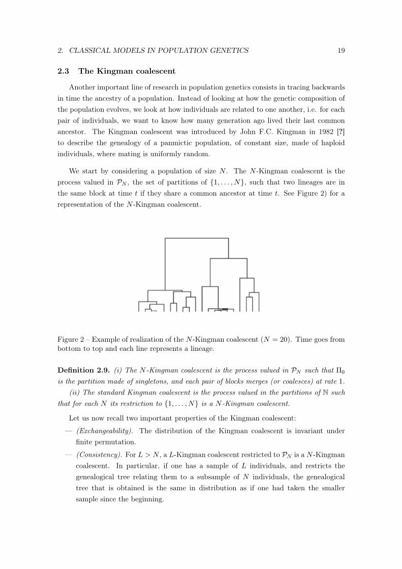
We start by considering a population of size N . The N -Kingman coalescent is theprocess valued in PN , the set of partitions of 1, . . . , N, such that two lineages are inthe same block at time t if they share a common ancestor at time t. See Figure 2) for arepresentation of the N -Kingman coalescent.
Figure 2 – Example of realization of the N -Kingman coalescent (N = 20). Time goes frombottom to top and each line represents a lineage.
Definition 2.9. (i) The N -Kingman coalescent is the process valued in PN such that Π0
is the partition made of singletons, and each pair of blocks merges (or coalesces) at rate 1.(ii) The standard Kingman coalescent is the process valued in the partitions of N such
that for each N its restriction to 1, . . . , N is a N -Kingman coalescent.
Let us now recall two important properties of the Kingman coalescent:
— (Exchangeability). The distribution of the Kingman coalescent is invariant underfinite permutation.
— (Consistency). For L > N , a L-Kingman coalescent restricted to PN is a N -Kingmancoalescent. In particular, if one has a sample of L individuals, and restricts thegenealogical tree relating them to a subsample of N individuals, the genealogicaltree that is obtained is the same in distribution as if one had taken the smallersample since the beginning.
20 INTRODUCTION
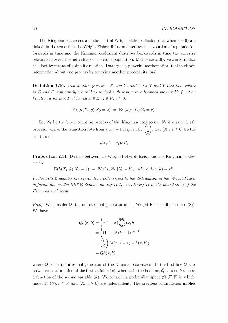
The Kingman coalescent and the neutral Wright-Fisher diffusion (i.e. when s = 0) arelinked, in the sense that the Wright-Fisher diffusion describes the evolution of a populationforwards in time and the Kingman coalescent describes backwards in time the ancestryrelations between the individuals of the same population. Mathematically, we can formalizethis fact by means of a duality relation. Duality is a powerful mathematical tool to obtaininformation about one process by studying another process, its dual.
Definition 2.10. Two Markov processes X and Y , with laws X and Y that take valuesin E and F respectively are said to be dual with respect to a bounded measurable functionfunction h on E × F if for all x ∈ E, y ∈ F , t ≥ 0,
EX (h(Xt, y)|X0 = x) = EY(h(x, Yt)|Y0 = y).
Let Nt be the block counting process of the Kingman coalescent. Nt is a pure death
process, where, the transition rate from i to i− 1 is given by(i
2
). Let (Xt; t ≥ 0) be the
solution of √xt(1− xt)dBt.
Proposition 2.11 (Duality between the Wright-Fisher diffusion and the Kingman coales-cent).
E(h(Xt, k)|X0 = x) = E(h(x,Nt)|N0 = k), where h(x, k) = xk.
In the LHS E denotes the expectation with respect to the distribution of the Wright-Fisherdiffusion and in the RHS E denotes the expectation with respect to the distribution of theKingman coalescent.
Proof. We consider Q, the infinitesimal generator of the Wright-Fisher diffusion (see (8)).We have
Qh(x, k) =1
2x(1− x)
∂2h
∂x2(x, k)
=1
2(1− x)k(k − 1)xk−1
=
(n
2
)(h(x, k − 1)− h(x, k))
= Qh(x, k),
where Q is the infinitesimal generator of the Kingman coalescent. In the first line Q actson h seen as a function of the first variable (x), whereas in the last line, Q acts on h seen asa function of the second variable (k). We consider a probability space (Ω,F ,P) in which,under P, (Nt, t ≥ 0) and (Xt; t ≥ 0) are independent. The previous computation implies
3. MULTI-LOCUS MODELS AND RECOMBINATION 21
that
d
dsE(h(Xs, Nt−s)) = E
(Qh(Xs, Nt−s)− Qh(Xs, Yt−s)
)= 0,
and the conclusion follows by integrating between 0 and t.
Now consider the Moran model for finite population of size N and the N -Kingmancoalescent.
Proposition 2.12 (Duality between the Moran and the N -Kingman coalescent). For
i ≥ k, define HN (i, k) =
(i
k
)/
(N
k
)E(HN (NXN
Nt/2, k)|X0 = x) = E(HN (Nx,Nt)|N0 = k).
where in the LHS, E denotes the expectation with respect to the distribution of the Moranmodel and in the RHS, E denotes the expectation with respect to the distribution of theN -Kingman coalescent (backwards in time).
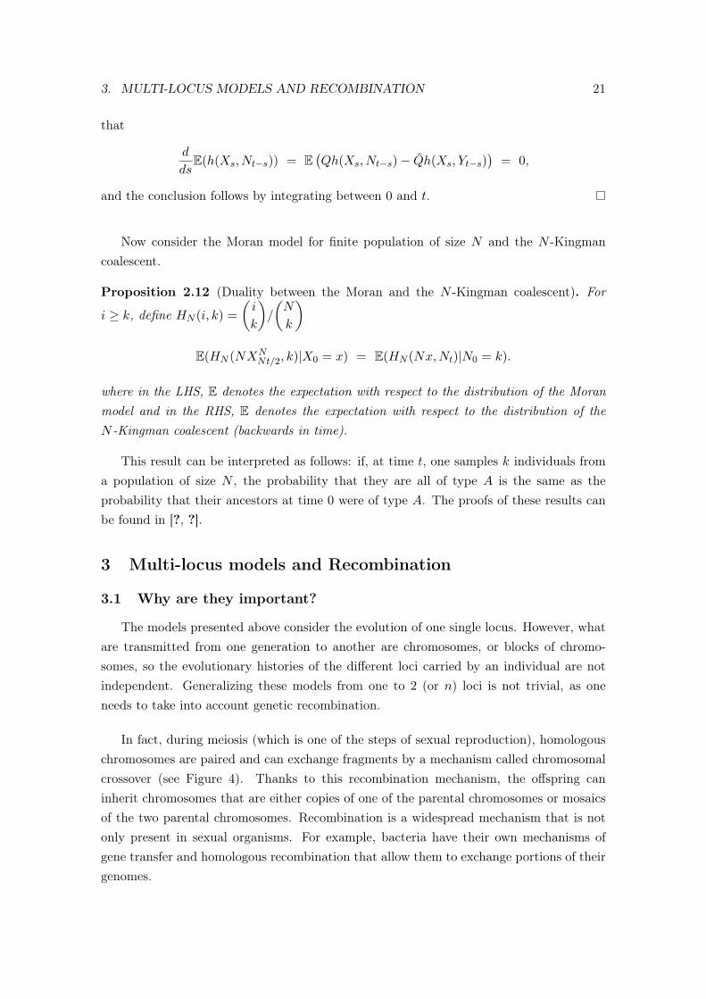
This result can be interpreted as follows: if, at time t, one samples k individuals froma population of size N , the probability that they are all of type A is the same as theprobability that their ancestors at time 0 were of type A. The proofs of these results canbe found in [?, ?].
3 Multi-locus models and Recombination
3.1 Why are they important?
The models presented above consider the evolution of one single locus. However, whatare transmitted from one generation to another are chromosomes, or blocks of chromo-somes, so the evolutionary histories of the different loci carried by an individual are notindependent. Generalizing these models from one to 2 (or n) loci is not trivial, as oneneeds to take into account genetic recombination.
In fact, during meiosis (which is one of the steps of sexual reproduction), homologouschromosomes are paired and can exchange fragments by a mechanism called chromosomalcrossover (see Figure 4). Thanks to this recombination mechanism, the offspring caninherit chromosomes that are either copies of one of the parental chromosomes or mosaicsof the two parental chromosomes. Recombination is a widespread mechanism that is notonly present in sexual organisms. For example, bacteria have their own mechanisms ofgene transfer and homologous recombination that allow them to exchange portions of theirgenomes.
22 INTRODUCTION
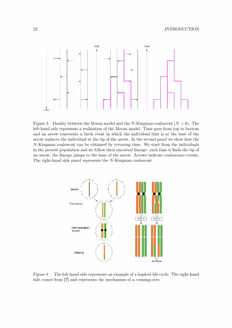
Figure 3 – Duality between the Moran model and the N -Kingman coalescent (N = 6). Theleft-hand side represents a realization of the Moran model. Time goes from top to bottomand an arrow represents a birth event in which the individual that is at the base of thearrow replaces the individual at the tip of the arrow. In the second panel we show how theN -Kingman coalescent can be obtained by reversing time. We start from the individualsin the present population and we follow their ancestral lineage: each time it finds the tip ofan arrow, the lineage jumps to the base of the arrow. Arrows indicate coalescence events.The right-hand side panel represents the N -Kingman coalescent.
Figure 4 – The left-hand side represents an example of a haploid life cycle. The right-handside comes from [?] and represents the mechanism of a crossing-over.
3. MULTI-LOCUS MODELS AND RECOMBINATION 23
All these mechanisms are complex and costly. Trying to explain how the recombinationmechanisms emerged and why they are maintained has been an important line of researchin evolutionary biology [?, ?, ?, ?, ?]. If asked why sex and recombination are suchwidespread mechanisms, most biologists would say that it increases genetic variabilityand hence allows evolution to proceed faster. However, recombination does not allow toproduce new alleles, so the link between genetic variance and recombination is not clear.In addition, recombination can break up favorable associations between alleles that havebeen accumulated by selection (this is known as the “recombination load”).
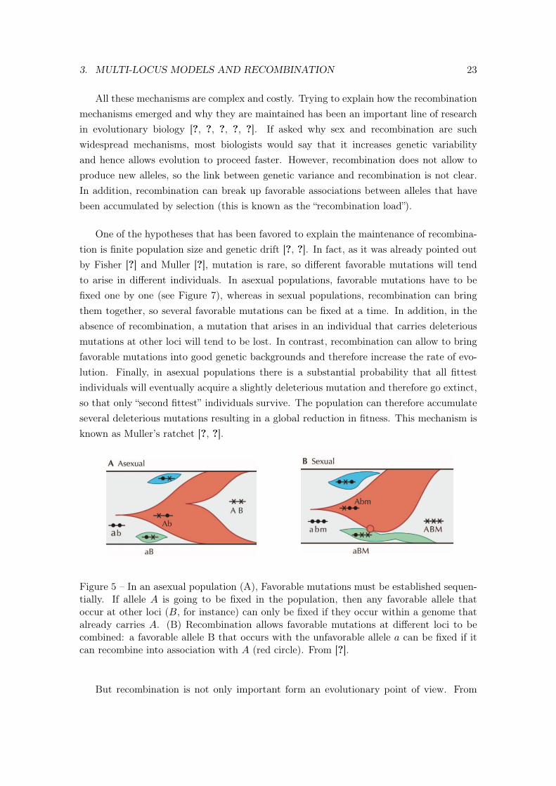
One of the hypotheses that has been favored to explain the maintenance of recombina-tion is finite population size and genetic drift [?, ?]. In fact, as it was already pointed outby Fisher [?] and Muller [?], mutation is rare, so different favorable mutations will tendto arise in different individuals. In asexual populations, favorable mutations have to befixed one by one (see Figure 7), whereas in sexual populations, recombination can bringthem together, so several favorable mutations can be fixed at a time. In addition, in theabsence of recombination, a mutation that arises in an individual that carries deleteriousmutations at other loci will tend to be lost. In contrast, recombination can allow to bringfavorable mutations into good genetic backgrounds and therefore increase the rate of evo-lution. Finally, in asexual populations there is a substantial probability that all fittestindividuals will eventually acquire a slightly deleterious mutation and therefore go extinct,so that only “second fittest” individuals survive. The population can therefore accumulateseveral deleterious mutations resulting in a global reduction in fitness. This mechanism isknown as Muller’s ratchet [?, ?].
Figure 5 – In an asexual population (A), Favorable mutations must be established sequen-tially. If allele A is going to be fixed in the population, then any favorable allele thatoccur at other loci (B, for instance) can only be fixed if they occur within a genome thatalready carries A. (B) Recombination allows favorable mutations at different loci to becombined: a favorable allele B that occurs with the unfavorable allele a can be fixed if itcan recombine into association with A (red circle). From [?].
But recombination is not only important form an evolutionary point of view. From
24 INTRODUCTION
a modeler’s point of view, models that take into account recombination are complex butcan be very powerful. In fact, nowadays with the advent of new generation sequencingtechniques it has become usual to have access to whole genomes. Considering that locihave evolved independently results in an important loss of statistical power and can leadto incorrect inferences. Multi-locus models that take into account linkage disequilibriumhave become of particular interest to analyse data. As we shall see in Section 3.5, analysingrecombination patterns can be useful for the detection of selection [?], to study recent de-mography [?], in candidate gene studies [?] or to analyse data from experimental evolution[?]. In Chapter II we use recombination patterns to study hybrid populations.
3.2 Two-locus models
In this section we are going to define a multi-locus version of the Wright-Fisher and theMoran model described in 2.1 and 2.2. We will start by considering the case of two loci.Locus 1 has two alleles, A1 and A2, and locus 2 has two alleles B1 and B2. The populationsize is N , the recombination rate between the two loci is ρN and all the alleles are neutral,so s = 0 for any genotype. We denote by
XN11 the frequency of genotype A1B1
XN12 the frequency of genotype A1B2
XN21 the frequency of genotype A2B1
XN22 the frequency of genotype A2B2
Recall, that, at each time t we have
XN11(t) +XN
12(t) +XN21(t) +XN
22(t) = 1.
Finally, we denote by XN the vector (XN11, X
N12, X
N21, X
N22)T .
Definition 3.1. In the Wright-Fisher model with recombination, each individual from gen-eration t+1 chooses two parents uniformly (and independently) at random from generationt. With probability 1−ρN , she inherits the alleles at both loci from one of the parents (cho-sen at random). With probability ρN , she inherits allele at locus 1 from one parent (chosenat random) and allele at locus 2 from the other parent.
Fix i, j ∈ 1, 2. Considering the different ways an individual AiBj can be formed, we
3. MULTI-LOCUS MODELS AND RECOMBINATION 25
have
E(XNij (t+ 1)−XN
ij )(t) | XN (t) = (xii, xij , xji, xjj)T )
= (1− ρN )xij + ρN (x2ij + xiixjj + xiixij + xijxjj)− xij
= ρN (xiixjj − xijxji).
In addition, conditional on XN (t) = (xii, xij , xji, xjj), XN (t + 1) follows a multinomialdistribution of parameters N and (xii, xij , xji, xjj), which gives
Var(XNij (t+ 1) | XN (t) = (xii, xij , xji, xjj)
T ) =1
Nxij(1− xij)
∀(i′, j′) 6= (i, j), Cov(XNij (t+ 1), XN
i′j′(t+ 1)| XN (t) = (xii, xij , xji, xjj)T ) = − 1
Nxijxi′j′
Assume that XN0 = x0 and
NρN −→N→∞
ρ.
Proposition 3.2. For any T > 0, (XNbNtc)N∈N converges in distribution (in the Skorokhod
topology D([0, T ],R4) to the solution ofdXt =ρ(−1, 1, 1,−1)TD(X(t))dt+ σ(X(t))dBt,
X0 = x0.(8)
where B is a standard Brownian motion in R4. and
D(X) = X1X4 −X2X3,
and σ(X)σ(X)T = M(X) where
∀i, j ∈ 1, 2, 3, 4, i 6= j, M(X)i,i = Xi(1−Xi)
M(X)i,j = −XiXj .
We let the reader refer to [?] for a formal proof or to [?] for a modern exposition of thisresult.
Remark 3.3. D is called the “linkage disequilibrium”. In fact, if XN1− is the total frequency
of allele A1 (XN1− = XN
11 + XN12) and XN
−1 is the total frequency of allele B1 (XN−1 =
XN11 +XN
21), we have
D(XN ) = XN11 − (XN
11 +XN12)(XN
11 +XN21)
= XN11 −XN
1−XN−1.
26 INTRODUCTION
Linkage disequilibrium is a measure of the non-random association between alleles A1 andB1. From (8), we have
D(XN (t)) −→t→∞
0,
but the rate of convergence depends on ρ. Therefore, in a neutral setting, linkage disequi-librium should decrease with time and with distance in the chromosome. However patternsof linkage disequilibrium can be affected by many factors such as population subdivision,demographic bottlenecks or natural selection (see [?] or Section 3.5).
Similarly, we can define a Moran model with recombination in the following way
Definition 3.4. In the Moran model with recombination each individual reproduces at rate1. She chooses a random partner in the population.
- With probability 1− ρN , the chromosome of the offspring is a copy of one of the twoparents (chosen at random).
- With probability ρN , there is a crossing over between these two loci. The offspringcopies the allele at one locus from one parent and the allele at the other locus fromthe other parent.
Define e11 = (1, 0, 0, 0)T , e12 = (0, 1, 0, 0)T , e21 = (0, 0, 1, 0)T , e22 = (0, 0, 0, 1)T .Again, we accelerate time by N/2 and we assume that
N
2ρN −→
N→∞ρ.
Let QN be the infinitesimal generator of the Markov process (XN (Nt/2); t ≥ 0). For anyfunction f at least twice differentiable, if x = (xij))i,j∈1,2,
QNf(x) =N2
2(1− ρN )
∑i,j∈1,2
∑k,p∈1,2
xijxkp
(f(x+
1
Neij −
1
Nekp)− f(x)
)
+ ρNN2
2
∑i,j∈1,2
∑k,p∈1,2
xijxkp
(f(x+
1
Neip −
1
Nekj)− f(x)
)
−→N→∞
ρ∑
i,j∈1,2
∑k 6=i,p 6=j
(xipxjk − xijxkp)∂f
∂xij(x)
+1
2
∑(i,j),(k,p)∈1,2
xij(1i=k,j=p − xkp)∂2f
∂xij∂xkp(x).
where the last equality is obtained by means of Taylor expansions (as in the one-locusMoran model). The last line corresponds to the generator of the diffusion process definedin (8). As in the case of the simple Moran model, it can be shown that the sequence(Y N , N ≥ 1) is tight in D([0, T ],R4)) converges in distribution, in the Skorokhod topologyD([0, T ],R) to the solution of (8).
3. MULTI-LOCUS MODELS AND RECOMBINATION 27
3.3 The case of n loci
These two models can be extended to the case of n loci. In this work, we will onlyconsider single crossing over recombination which means that at each reproduction event, ifrecombination takes place, the chromosome of each parent is partitioned into two segments.The offspring inherits the genetic material to the right of the cutpoint from one parentand the genetic material from the left of the cutpoint from the other parent. The positionof the cut point is uniformly distributed in the chromosome, so the probability that thecrossing over occurs between two given loci depends on the distance between these two locion the chromosome.
The n loci are identified to their positions in a chromosome, which are given by z =
(z1, . . . , zn) ∈ [0, 1] such that z1 = 0 < z2 < . . . < zn = 1.
Definition 3.5. In the Wright-Fisher model with recombination, each individual from gen-eration t+1 chooses two parents uniformly (and independently) at random from generationt.
- With probability 1 − ρN there is no recombination and she inherits all the loci fromone of the parents (chosen uniformly at random).
- For i ∈ 2, . . . , n, with probability ρN (zi−zi−1) the offspring inherits loci z1, . . . , zi−1
from one parent and zi, . . . , zn from the other one.
Definition 3.6. In the Moran model with recombination each individual reproduces at rate1 and chooses a random partner
- With probability 1 − ρN there is no recombination and the offspring inherits all theloci from one of the parents (chosen at random).
- For i ∈ 2, . . . , n, with probability ρN (zi−zi−1) the offspring inherits loci z1, . . . , zi−1
from one parent and zi, . . . , zn from the other one.
The offspring replaces a randomly chosen individual in the population, who simultaneouslydies.
As in the case of two loci, when time is rescaled by N and the recombination rate scaleswith the population size in such a way that ρ = limN→∞ ρNN the Wright-Fisher modelwith recombination has a diffusive limit. For the Moran model with recombination thisdiffusive limit arises when time is rescaled by N/2 and ρ = limN→∞ ρNN/2.
We follow closely [?] and we assume that each locus i has k possible alleles i1, . . . , ik.The set of al possible genotypes is E =
∏ni=1i1, . . . , ik. For each e ∈ E, we denote by xe
the frequency of genotype e in the population. Let S be the set of non-empty subsets of1, . . . , n. For S ∈ S, we denote by xSe , the marginal frequency of the alleles e into S. In
28 INTRODUCTION
particular, for ` ∈ 1, . . . , n, we denote by x≤le (resp. x>le ) the marginal frequency of thealleles e into 1, . . . , ` (resp. `+ 1, . . . , n
x≤le =∑
j∈E, j|E≤`=e
xj , x≤le =∑
j∈E, j|E>`=e
xj
where E≤` =∏i≤`i1, . . . , ik and E>` =
∏i>`i1, . . . , ik. The generator of the Wright-
Fisher diffusion for n recombining loci with k alleles per loci is given by
L =∑e∈E
n−1∑`=1
ρ(z`+1 − z`)(x≤le − x≤le )∂
∂xe+∑j∈E
xe(1e=k − xj)∂2
∂xe∂xj
. (9)
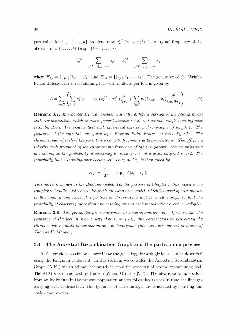
Remark 3.7. In Chapter III, we consider a slightly different version of the Moran modelwith recombination, which is more general because we do not assume single crossing-overrecombination. We assume that each individual carries a chromosome of length 1. Thepositions of the cutpoints are given by a Poisson Point Process of intensity λdx. Thechromosomes of each of the parents are cut into fragments at these positions . The offspringinherits each fragment of the chromosome from one of the two parents, chosen uniformlyat random, so the probability of observing a crossing-over at a given cutpoint is 1/2. Theprobability that a crossing-over occurs between zi and zj is then given by
ri,j =1
2(1− exp(−λ|zi − zj |).
This model is known as the Haldane model. For the purpose of Chapter I, this model is toocomplex to handle, and we use the single crossing-over model, which is a good approximationof this one, if one looks at a portion of chromosome that is small enough so that theprobability of observing more than one crossing over at each reproduction event is negligible.
Remark 3.8. The parameter ρN corresponds to a recombination rate. If we rescale thepositions of the loci in such a way that zi = ρNzi, this corresponds to measuring thechromosome in units of recombination, or “morgans” (this unit was named in honor ofThomas H. Morgan).
3.4 The Ancestral Recombination Graph and the partitioning process
In the previous section we showed how the genealogy for a single locus can be describedusing the Kingman coalescent. In this section, we consider the Ancestral RecombinationGraph (ARG) which follows backwards in time the ancestry of several recombining loci.The ARG was introduced by Hudson [?] and Griffiths [?, ?]. The idea is to sample n locifrom an individual in the present population and to follow backwards in time the lineagescarrying each of these loci. The dynamics of these lineages are controlled by splitting andcoalescence events.
3. MULTI-LOCUS MODELS AND RECOMBINATION 29
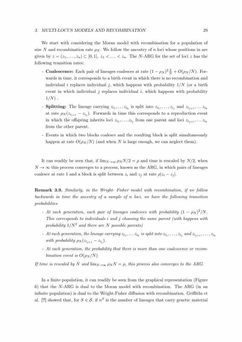
We start with considering the Moran model with recombination for a population ofsize N and recombination rate ρN . We follow the ancestry of n loci whose positions in aregiven by z = (z1, . . . , zn) ⊂ [0, 1], z1 < . . . < zn. The N -ARG for the set of loci z has thefollowing transition rates:
- Coalescence: Each pair of lineages coalesces at rate (1− ρN )2 2N +O(ρN/N). For-
wards in time, it corresponds to a birth event in which there is no recombination andindividual i replaces individual j, which happens with probability 1/N (or a birthevent in which individual j replaces individual i, which happens with probability1/N) .
- Splitting: The lineage carrying zi1 , . . . zik is split into zi1 , . . . , zij and zij+1 , . . . zikat rate ρN (zij+1 − zij ). Forwards in time this corresponds to a reproduction eventin which the offspring inherits loci zi1 , . . . .zij from one parent and loci zij+1 , . . . zikfrom the other parent.
- Events in which two blocks coalesce and the resulting block is split simultaneouslyhappen at rate O(ρN/N) (and when N is large enough, we can neglect them).
It can readily be seen that, if limN→∞ ρNN/2 = ρ and time is rescaled by N/2, whenN →∞ this process converges to a process, known as the ARG, in which pairs of lineagescoalesce at rate 1 and a block is split between zi and zj at rate ρ|zi − zj |.
Remark 3.9. Similarly, in the Wright- Fisher model with recombination, if we followbackwards in time the ancestry of a sample of n loci, we have the following transitionprobabilities
- At each generation, each pair of lineages coalesces with probability (1 − ρN )2/N .This corresponds to individuals i and j choosing the same parent (with happens withprobability 1/N2 and there are N possible parents)
- At each generation, the lineage carrying zi1 , . . . zik is split into zi1 , . . . , zij and zij+1 , . . . , zikwith probability ρN (zij+1 − zij ).
- At each generation, the probability that there is more than one coalescence or recom-bination event is O(ρN/N)
If time is rescaled by N and limN→∞ ρNN = ρ, this process also converges to the ARG.
In a finite population, it can readily be seen from the graphical representation (Figure6) that the N -ARG is dual to the Moran model with recombination. The ARG (in aninfinite population) is dual to the Wright-Fisher diffusion with recombination. Griffiths etal. [?] showed that, for S ∈ S, if nS is the number of lineages that carry genetic material
30 INTRODUCTION
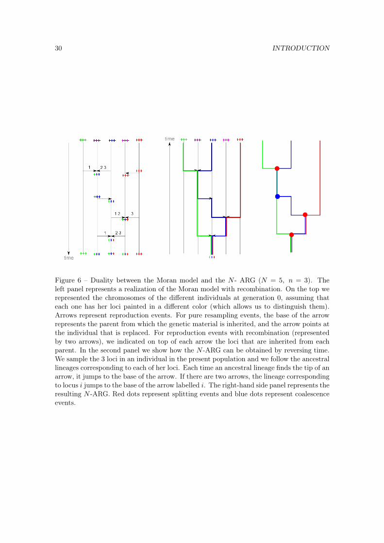
Figure 6 – Duality between the Moran model and the N - ARG (N = 5, n = 3). Theleft panel represents a realization of the Moran model with recombination. On the top werepresented the chromosomes of the different individuals at generation 0, assuming thateach one has her loci painted in a different color (which allows us to distinguish them).Arrows represent reproduction events. For pure resampling events, the base of the arrowrepresents the parent from which the genetic material is inherited, and the arrow points atthe individual that is replaced. For reproduction events with recombination (representedby two arrows), we indicated on top of each arrow the loci that are inherited from eachparent. In the second panel we show how the N -ARG can be obtained by reversing time.We sample the 3 loci in an individual in the present population and we follow the ancestrallineages corresponding to each of her loci. Each time an ancestral lineage finds the tip of anarrow, it jumps to the base of the arrow. If there are two arrows, the lineage correspondingto locus i jumps to the base of the arrow labelled i. The right-hand side panel represents theresulting N -ARG. Red dots represent splitting events and blue dots represent coalescenceevents.
3. MULTI-LOCUS MODELS AND RECOMBINATION 31
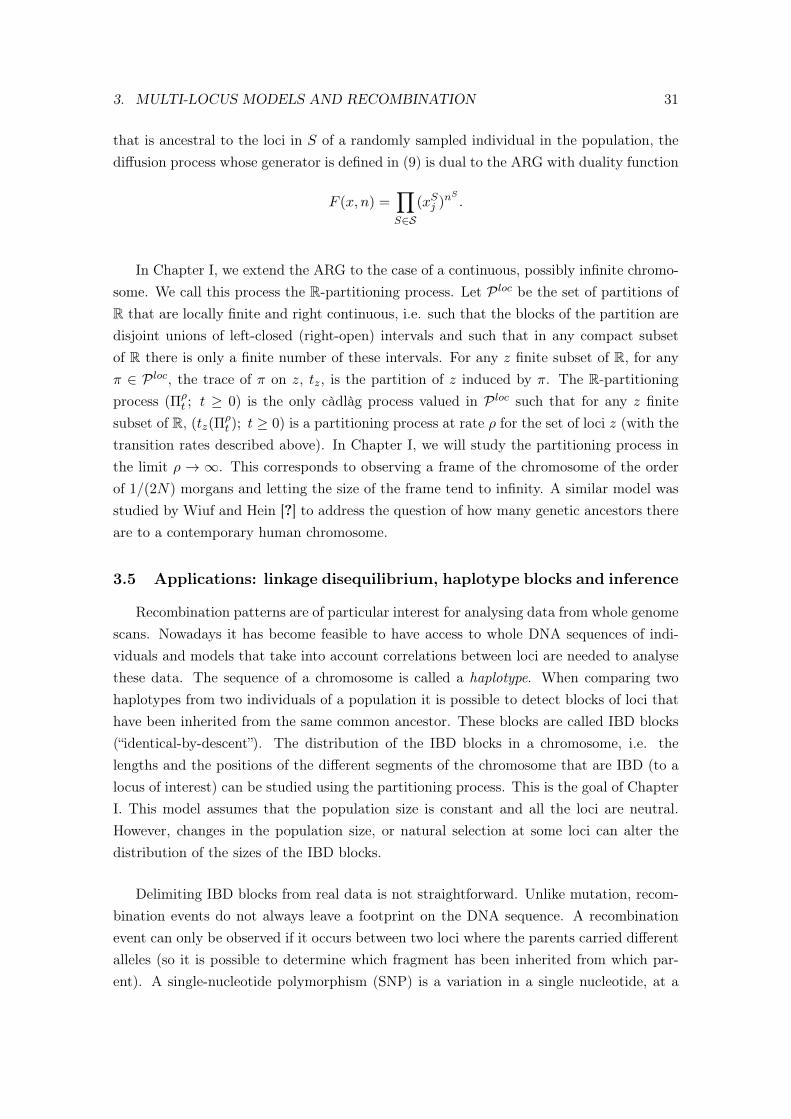
that is ancestral to the loci in S of a randomly sampled individual in the population, thediffusion process whose generator is defined in (9) is dual to the ARG with duality function
F (x, n) =∏S∈S
(xSj )nS.
In Chapter I, we extend the ARG to the case of a continuous, possibly infinite chromo-some. We call this process the R-partitioning process. Let P loc be the set of partitions ofR that are locally finite and right continuous, i.e. such that the blocks of the partition aredisjoint unions of left-closed (right-open) intervals and such that in any compact subsetof R there is only a finite number of these intervals. For any z finite subset of R, for anyπ ∈ P loc, the trace of π on z, tz, is the partition of z induced by π. The R-partitioningprocess (Πρ
t ; t ≥ 0) is the only càdlàg process valued in P loc such that for any z finitesubset of R, (tz(Π
ρt ); t ≥ 0) is a partitioning process at rate ρ for the set of loci z (with the
transition rates described above). In Chapter I, we will study the partitioning process inthe limit ρ → ∞. This corresponds to observing a frame of the chromosome of the orderof 1/(2N) morgans and letting the size of the frame tend to infinity. A similar model wasstudied by Wiuf and Hein [?] to address the question of how many genetic ancestors thereare to a contemporary human chromosome.
3.5 Applications: linkage disequilibrium, haplotype blocks and inference
Recombination patterns are of particular interest for analysing data from whole genomescans. Nowadays it has become feasible to have access to whole DNA sequences of indi-viduals and models that take into account correlations between loci are needed to analysethese data. The sequence of a chromosome is called a haplotype. When comparing twohaplotypes from two individuals of a population it is possible to detect blocks of loci thathave been inherited from the same common ancestor. These blocks are called IBD blocks(“identical-by-descent”). The distribution of the IBD blocks in a chromosome, i.e. thelengths and the positions of the different segments of the chromosome that are IBD (to alocus of interest) can be studied using the partitioning process. This is the goal of ChapterI. This model assumes that the population size is constant and all the loci are neutral.However, changes in the population size, or natural selection at some loci can alter thedistribution of the sizes of the IBD blocks.
Delimiting IBD blocks from real data is not straightforward. Unlike mutation, recom-bination events do not always leave a footprint on the DNA sequence. A recombinationevent can only be observed if it occurs between two loci where the parents carried differentalleles (so it is possible to determine which fragment has been inherited from which par-ent). A single-nucleotide polymorphism (SNP) is a variation in a single nucleotide, at a
32 INTRODUCTION
specific locus. The higher the density of SNPs the most accurately we can infer IBD blocks(see Chapter II). Different methods have been developed to infer IBD blocks. Algorithmssuch as fastIBD [?] or IBD_Haplo [?] identify long haplotype segments that are shared be-tween two individuals by a combination of likelihood methods and Hidden Markov Models(HMM).
The distribution of IBD block lengths can be used to infer the recent demographichistory of populations. Classical methods use mutation patterns to infer past demographicvariation (see e.g. [?] for a review on this topic). But mutation rates are usually too lowto be used to detect fast demographic changes. Ralph and Coop [?] and Ringbauer et al.[?] used IBD blocks to infer recent migration patterns in European human populations.
Recombination patterns can also be used to detect loci under selection. The ideabehind these methods is that loci that are under selection tend to be fixed rapidly ina population. During a selective sweep, loci that are close to the locus under selectiontend to be hitchhiked (i.e. the alleles that are in the same haplotype where the beneficialmutation arose also tend to be fixed, because recombination does not have time to breakup the linkage). Therefore alleles that are under positive selection tend to be locatedwithin long IBD blocks. Some examples of these type of methods are Extended HaplotypeHomozygosity [?] or Runs of Homozygosity [?].
Janzen et al. [?] used the IBD block length distribution to infer the time since admixturein hybrid populations. The idea is that by comparing the genotypes of the hybrids to thoseof the ancestral populations, one can infer which haplotype blocks have been inherited fromeach of the ancestral populations. As the blocks are split by recombination, their size tendto decrease with time (until fixation is reached), so the sizes of the blocks are informativeabout the admixture time. But the quality of the inference depends on the density and thepositions of the SNPs (or markers) that segregate between the two ancestral populations.In [?] the authors had assumed that the markers were regularly spaced and derived aformula to infer the admixture time from the number of junctions between blocks. InChapter II I present some work in collaboration with Thijs Janzen in which I derived aformula to infer the admixture time using markers that are randomly distributed acrossthe genome.
Recombination patterns can also be useful to analyse data from experimental evolution.For example, in the experiment by Teotonio et al. [?], individuals from different subpopu-lations of C. elegans have been crossed for several generations. By sequencing the offspringand comparing their haplotypes to those of the ancestral individuals, it is possible to inferwhich haplotype blocks have been inherited from each of the ancestral subpopulations.One of the motivations behind I is to derive a neutral model of the IBD-block distributionto analyse this type of experiment.
4. GEOGRAPHIC STRUCTURE AND SPECIATION 33
4 Geographic structure and speciation
In On the origin of species, Darwin called species formation the “mystery of mysteries”.He was perplexed by the clustering of individuals into discrete species and the absence of“transitional forms”. When listing the drawbacks of his theory he wrote: “Why is not allnature in confusion instead of the species being, as we see them, well defined?”.
It is not surprising that since then, the process of speciation has received an enormousamount of attention from evolutionary biologists. The speciation process is complex anddifficult to understand from a theoretical point of view because there are many factorscontrolling the dynamics of speciation (mutation, geographic structure, migration, recom-bination, natural selection, sexual selection...). Chapter III is devoted to the study of aparticular model of speciation that can be used to understand how the geographic structureof a population can promote species formation. In this section we will give some biologicalbackground and review some important models of speciation that will allow us to justifysome of the hypotheses made in that chapter.
4.1 Geographic structure and genetic differentiation
Geographic structure is one of the main drivers of within species genetic variability:if the geographical range is larger than the typical dispersal rate of its individuals, aspecies can be structured into different local subpopulations with limited contact. On thecontrary, migration allows the different subpopulations (or demes) to exchange genes andhas an homogenising effect.
One of the first models that was proposed to explain how the geographic structurepromotes genetic variability was Wright’s stepping stone model [?], which was later im-proved by Kimura [?]. In this model, a population is divided into several demes which canexchange migrants with their nearest neighbours in Z or Z2. Wright proposed a statisticaltheory on how population differentiation should vary as a function of the migration ratesbetween demes, which was called “Isolation by distance”.
Malécot studied the case of a population in continuous space where individual dispersalis assumed to be normally distributed [?] . He proposed a formula for the probability Pthat two individuals sampled at distance r on the real line have the same allele at a givenlocus
P (r)
P (0)= exp(−r
√(2µ)/σ),
where µ is the mutation rate and σ is the dispersal coefficient (i.e. the standard deviationof the dispersal distribution). This formula is known as Malécot’s formula and can beextended to R2 or R3.
34 INTRODUCTION
Samuel Karlin analysed how migration patterns can influence genetic variability in ametapopulation [?]. A metapopulation is a population that is formed by several demesconnected by migration. The geographic structure of a metapopulation can be modelled bya graph in which the vertices represent the subpopulations. Two vertices are connected ifthe corresponding demes can exchange migrants and each edge is associated to a migrationrate. Using a deterministic model, Karlin studied which geographic configurations promotegenetic variability and speciation: for example he showed that, in the presence of selection,some geographic structures can promote speciation. This is for example the case of ametapopulation graph that is clustered, in the sense that it is formed from the union ofseveral (almost) complete graphs connected by a limited number of edges. In Chapter III,we showed, using a stochastic model, that, even if the absence of selection, a clusteredgeographic structure promotes genetic differentiation which can lead to speciation.
4.2 The biological species concept and reproductive barriers
It is difficult and beyond the scope of this thesis to give a universal definition of aspecies. For sexual organisms, one of the most commonly used definitions was given byMayr in 1942 [?]:
“Species are groups of actually or potentially interbreeding natural populations, which arereproductively isolated from other such groups.”
This defines the biological species concept. A more general definition of this concept, basedon evolutionary considerations, was given by de Queiroz in 1998 [?]:
“Species are separately evolving metapopulation lineages ; they form an independent genepool and reproductive community that evolves together.”
But there are many other ways to define a species. For example:
- A phenotypic species is a morphologically distinguishable group of individuals.
- A phylogenetic species is a monophyletic group of individuals i.e. a group that consistsof all the descendants of a common ancestor.
- An ecological species is a group of individuals that occupy the same niche, i.e. thatare adapted to a particular set of resources in the environment.
Although all these definitions do not always lead to the same classification, they all havesome advantages and are used in different contexts ([?]). In this work we are going toconsider sexual organisms and adopt the biological species concept, which is one of themost commonly used in evolutionary biology.
The biological species concept focuses on the capacity of individuals to interbreed,which means that they can mate and produce viable and fertile offspring. Speciation can
4. GEOGRAPHIC STRUCTURE AND SPECIATION 35
be seen as the emergence of mechanisms that prevent individuals from different groups tointerbreed. These mechanisms are called reproductive barriers. Among these mechanismswe can distinguish between:
- Prezygotic barriers, that are mechanisms that prevent fertilization. They includeecological mechanisms and habitat or behavioural differences that prevent mating.For example the American toad and the Fowler’s toad are closely related species thatlive in the same areas of North America but that are unable to reproduce becausetheir mating season is different [?]. They also include anatomical differences andgametic incompatibility. For example, in the Drosophila genus, the differences in theshape of the genital organs prevent mating between individuals from different species[?].
- Postzygotic barriers, that are mechanisms that prevent the development of hybrids.They include embryo inviability, sterility and reduced fitness of hybrids. Mules, thatare hybrids between a donkey and a horse, are a classic example of hybrid sterility.
These mechanisms are controlled genetically and different models have been proposedto study how these barriers emerge and are maintained.
• The Dobzhansky-Muller model
This model was proposed independently by Dobzhansky [?] and Muller [?]. It involvestwo loci in diploid individuals.
The model assumes that, in an ancestral population, all individuals carry the samegenotype AABB. The population is split into two subpopulations and gene flow is in-terrupted (for example, by a geographic barrier). In the first one, a mutation is fixed inthe first locus and the genotype of the population becomes aaBB. In the second one,a mutation is fixed in the second locus and the the genotype of the population becomesAAbb. Fixation is possible because AABb and AaBB heterozygotes are viable and theirfitness is similar to the fitness of the homozygotes. In a cross between two parents fromdifferent subpopulations, the genotype of the offspring would be aAbB. If these hybridsare non viable, a postzygotic reproductive barrier has emerged.
In this model, speciation may be adaptive or not. a and b can be neutral or each onemay confer a selective advantage in the environment where it emerges. In the second case,fixation should be faster.
Different biological mechanisms have been proposed for these Dobzhansky-Muller in-compatibilities. For example, they can involve a maternal and a paternal gene, bothinvolved in reproduction. One can code for a sperm protein and the other one for an eggprotein, that interact during fertilization. The proteins produced from the derived alleles

36 INTRODUCTION
a and b may lack matching, which prevents fertilization (see e.g. [?] for some example inmarine invertebrates). It has also been proposed that Dobzhansky-Muller incompatibilitiescan arise by gene duplication. Initially both loci (A and B) code for the same trait but onemay lose its function. If each locus loses its function in one sub-population, hybrids willlack this trait and may not be viable. Also, this kind of incompatibilities can be causedby negative epistatic interactions. Epistatic interactions arise when the effect of a genedepends on the genetic context in which it acts.
However, very few examples of real Dobzhansky-Muller incompatibilities, involvingonly two loci have been found in nature and are well characterized. One occurs betweentwo closely related species of fish, the platyfish, X. maculatus and the swordtail X. helleri(see e.g. [?, ?, ?]). The first one has spots on the dorsal fin whereas the second one lacksspots. The spots are produced by a X -linked gene which expression is controlled by asecond locus. While the platyfish has both genes, the swordtail lacks both. Hybrids, whichhave the spot producing gene but not the repressor, have large spots which develop intotumors. Therefore the fitness of the hybrids is reduced.
• The Nei model
Another model for the evolution of reproductive isolation was developed by Nei andhis collaborators [?]. It is a one-locus multi-allelic model of post-zygotic incompatibility.A locus A which is involved in hybrid sterility or inviability has a series of different alleles(Ai)i≥1. Homozygotes AiAi and heterozygotes AiAi+1 and AiAi−1 are viable and have thesame fitness. But heterozygotes AiAi+2 and AiAi−2 are lethal or sterile.
In their model, the different alleles are neutral, in the sense that all viable individualshave the same fitness. The model assumes that in an ancestral population allele Ai isfixed. The population is split into two subpopulations. By genetic drift, allele Ai+1 can befixed in one subpopulation and allele Ai−1 in the other one. The genotype of the hybridsis Ai+1Ai−1, so they not viable and a reproductive barrier is built.
Models of incompatibilities involving a large number of loci
Some multi-locus generalizations of these models have been studied. Orr [?] andGavrilets and Gravner [?] studied how the probability of reproductive isolation dependson the number of substitutions between two sub-populations. Assume that the ancestralgenotype is abcde which is replaced in one subpopulation by AbcdE and by aBcde in thesecond one. The allele E can be incompatible with alleles a and B. More generally, the kth
substitution can be incompatible with k − 1 alleles. If each new derived allele has a prob-ability p of being incompatible with each locus, the expected number of incompatibilitiesbetween two populations differing at k loci was pk2
2 . They predicted a “snowballing effect”:if the number of substitutions increases linearly with time, the number of incompatibilities,increases faster than linearly with time (and therefore the probability that two individuals

4. GEOGRAPHIC STRUCTURE AND SPECIATION 37
are able to interbreed decreases faster than linearly with time). He also concluded thatspeciation should occur more easily if many loci are involved in reproductive barriers: ina multi-locus systems there are more possible combinations of loci that can give rise toincompatibilities than in a classical two locus model.
The model we use in Chapter III is a simplified version of this model, proposed byYamaguchi and Iwasa in [?]. We will consider a set of ` incompatibility controlling loci.The genetic distance between two individuals is defined as the number of these loci thatdiffer between the two. Inspired by this “snowballing effect”, we will assume that thereis a threshold of speciation s and reproductive incompatibility emerges when the geneticdistance becomes higher than the threshold. One of the advantages of this type of approachis that it takes into account the fact that speciation takes time, and two populations thatare not completely isolated can produce hybrids. Many examples of hybridization betweenlineages that had been thought to be separate species have been found in nature, forexample in cichlid fishes [?, ?], warblers [?], fruit flies [?], butterflies [?, ?] and sculpins [?].Chapter II is devoted to the study of hybrid populations. The idea is to use recombinationpatterns to infer the time since admixture.
4.3 Geography and speciation
As we have seen, geographic structure promotes genetic differentiation between sub-populations. The accumulation of genetic differences between populations may give rise toreproductive incompatibilities and therefore to the formation of new species. Geographicstructure can play a crucial role in speciation and models of speciation have been classifieddepending on the geographical setting.
- Sympatric speciation is the emergence of two or more species from a single ancestralpopulation, in the same geographic location, without any spatial isolation. One of themost studied examples of sympatric speciation is that of the clichids, a very diversifiedfamily that lives in the Rift Valley lakes. The plausibility and generality of sympatricspeciation has been a source of controversy amongst evolutionary biologists. In the2000s Gavrilets [?, ?] derived general conditions for sympatric speciation. It requiresdisruptive selection, which occurs when extreme phenotypes have a fitness advantageover more intermediate phenotypes, and assortative mating, which means that matingbetween individuals with similar genotypes is promoted.
- Allopatric speciation is the formation of new species from subpopulations which aregeographically isolated. In the absence of gene flow, each subpopulation accumulatesmutations independently, which promotes the emergence of reproductive barriers.Local adaptation can accelerate the divergence between the different subpopulations.
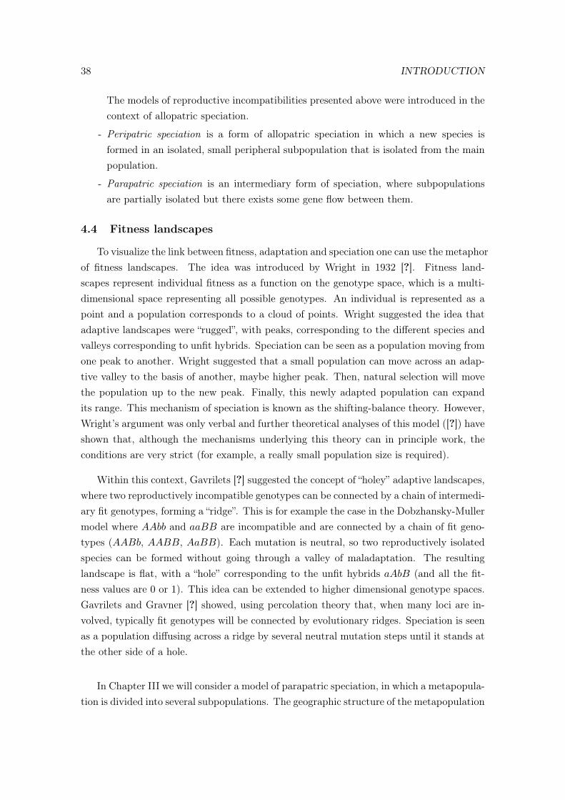
38 INTRODUCTION
The models of reproductive incompatibilities presented above were introduced in thecontext of allopatric speciation.
- Peripatric speciation is a form of allopatric speciation in which a new species isformed in an isolated, small peripheral subpopulation that is isolated from the mainpopulation.
- Parapatric speciation is an intermediary form of speciation, where subpopulationsare partially isolated but there exists some gene flow between them.
4.4 Fitness landscapes
To visualize the link between fitness, adaptation and speciation one can use the metaphorof fitness landscapes. The idea was introduced by Wright in 1932 [?]. Fitness land-scapes represent individual fitness as a function on the genotype space, which is a multi-dimensional space representing all possible genotypes. An individual is represented as apoint and a population corresponds to a cloud of points. Wright suggested the idea thatadaptive landscapes were “rugged”, with peaks, corresponding to the different species andvalleys corresponding to unfit hybrids. Speciation can be seen as a population moving fromone peak to another. Wright suggested that a small population can move across an adap-tive valley to the basis of another, maybe higher peak. Then, natural selection will movethe population up to the new peak. Finally, this newly adapted population can expandits range. This mechanism of speciation is known as the shifting-balance theory. However,Wright’s argument was only verbal and further theoretical analyses of this model ([?]) haveshown that, although the mechanisms underlying this theory can in principle work, theconditions are very strict (for example, a really small population size is required).
Within this context, Gavrilets [?] suggested the concept of “holey” adaptive landscapes,where two reproductively incompatible genotypes can be connected by a chain of intermedi-ary fit genotypes, forming a “ridge”. This is for example the case in the Dobzhansky-Mullermodel where AAbb and aaBB are incompatible and are connected by a chain of fit geno-types (AABb, AABB, AaBB). Each mutation is neutral, so two reproductively isolatedspecies can be formed without going through a valley of maladaptation. The resultinglandscape is flat, with a “hole” corresponding to the unfit hybrids aAbB (and all the fit-ness values are 0 or 1). This idea can be extended to higher dimensional genotype spaces.Gavrilets and Gravner [?] showed, using percolation theory that, when many loci are in-volved, typically fit genotypes will be connected by evolutionary ridges. Speciation is seenas a population diffusing across a ridge by several neutral mutation steps until it stands atthe other side of a hole.
In Chapter III we will consider a model of parapatric speciation, in which a metapopula-tion is divided into several subpopulations. The geographic structure of the metapopulation
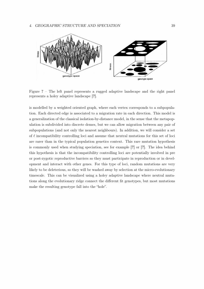
4. GEOGRAPHIC STRUCTURE AND SPECIATION 39
Figure 7 – The left panel represents a rugged adaptive landscape and the right panelrepresents a holey adaptive landscape [?].
is modelled by a weighted oriented graph, where each vertex corresponds to a subpopula-tion. Each directed edge is associated to a migration rate in each direction. This model isa generalization of the classical isolation-by-distance model, in the sense that the metapop-ulation is subdivided into discrete demes, but we can allow migration between any pair ofsubpopulations (and not only the nearest neighbours). In addition, we will consider a setof ` incompatibility controlling loci and assume that neutral mutations for this set of lociare rarer than in the typical population genetics context. This rare mutation hypothesisis commonly used when studying speciation, see for example [?] or [?]. The idea behindthis hypothesis is that the incompatibility controlling loci are potentially involved in preor post-zygotic reproductive barriers so they must participate in reproduction or in devel-opment and interact with other genes. For this type of loci, random mutations are verylikely to be deleterious, so they will be washed away by selection at the micro-evolutionarytimescale. This can be visualized using a holey adaptive landscape where neutral muta-tions along the evolutionary ridge connect the different fit genotypes, but most mutationsmake the resulting genotype fall into the “hole”.

40 INTRODUCTION

Chapter I
Chromosome Painting
Abstract
We consider a Moran model with recombination in a haploid population of size N . Ateach birth event, with probability 1 − ρN the offspring copies one parent’s chromosome,and with probability ρN she inherits a chromosome that is a mosaic of both parentalchromosomes. We assume that at time 0 each individual has her chromosome painted in adifferent color and we study the color partition of the chromosome that is asymptoticallyfixed in a large population, when we look at a portion of the chromosome such thatρ := limN→∞
ρNN2 → ∞. To do so, we follow backwards in time the ancestry of the
chromosome of a randomly sampled individual. This yields a Markov process valued inthe color partitions of the half-line, that was introduced by [?], in which blocks can mergeand split, called the partitioning process. Its stationary distribution is closely related tothe fixed chromosome in our Moran model with recombination. We are able to provide anapproximation of this stationary distribution when ρ 1 and an error bound. This allowsus to show that the distribution of the (renormalised) length of the leftmost block of thepartition (i.e. the region of the chromosome that carries the same color as 0) converges toan exponential distribution. In addition, the geometry of this block can be described interms of a Poisson point process with an explicit intensity measure.
1 Introduction
1.1 Motivation: a Moran model with recombination
Genetic recombination is the mechanism by which, in species that reproduce sexually,an individual can inherit a chromosome that is a mosaic of two parental chromosomes.Many classical population genetics models ignore recombination and only focus on a singlelocus, i.e. a location on the chromosome with a unique evolutionary history. In thissetting, many analytical results are known. For example the time to fixation (i.e. the first
41
42 CHAPITRE 1
time at which all individuals carry the same allele) or the fixation probabilities (see forexample [?]). However, understanding the joint evolution of different loci is well known tobe mathematically challenging, as one needs to take into account non-trivial correlationsbetween loci along the chromosome. For instance, loci that are close to one another aredifficult to recombine, so they often inherit their genetic material from the same parentand as a consequence, often share a similar evolutionary history. On the contrary, loci thatare far from one another will tend to have different, but not independent, evolutionaryhistories.
To visualize the questions that will be addressed in this work, let us imagine that inthe ancestral population, each individual carries a single continuous chromosome paintedin a distinct color. By the blending effect of recombination, after a few generations, thechromosome of each individual looks like a mosaic of colors, each color corresponding tothe genetic material inherited from a single ancestral individual. Some natural questionsarise: How does the mosaic of colors that is fixed in the population look like? How manycolors are there? If the leftmost locus is red (i.e. is inherited from the individual with redchromosome in the ancestral population), what is the amount of red in the mosaic andwhere are the red loci located? These questions are interesting from a biological pointof view: for example, the number of colors in the mosaic corresponds to the number ofancestors that have contributed to an extant chromosome. Loci that are of the same color(i.e., that have been inherited from the same individual in the ancestral population) arecalled identical-by-descent (IBD).
It is known that changes in the population size or natural selection can alter the sizesof the IBD segments: for example genes that are under selection tend to be located withinlarge IBD segments. This prediction can guide the detection of genes that are underselection (see for example the methods developed by [?] or [?]). The aim of this articleis to characterize the distribution of the IBD blocks along a chromosome in the absenceof selection or demography. Our results may then be used as predictions under the nullhypothesis, that can serve as a standard to which compare real data, e.g., to infer selectionor demography.
Also, our results may be relevant to the analysis of data obtained in experimental evo-lution. For example, in the experiment carried out by Teotónio et al. [?], the authorsintercrossed individuals from 16 different subpopulations of the worm C. elegans and letthe population evolve for several generations at controlled population size. Then, eachindividual is genotyped, each of its variants is mapped to one of the 16 ancestor subpopu-lations, so as to get a represention of each DNA sequence of each individual as a partitionof the sequence into 16 colors. Again, our model (or an extension to our model accomo-dating for the finite number of colors), might be used as a null model whose predictionscan be compared to these real color mosaics.
Sampling the chromosome, seen as a continuous, single-ended strand modelled by the

1. INTRODUCTION 43
positive half-line, of an individual in the present population and tracing backwards in timethe ancestry of every locus yields a process valued in the partitions of R+, called the R-partitioning process. Here, x ≥ 0 and y ≥ 0 belong to the same block of the R-partitioningprocess at time t if the loci at positions x and y on the sampled chromosome shared thesame ancestor t units of time ago.
The R-partitioning process is the continuum analog of the celebrated Ancestral Re-combination Graph [?, ?, ?]. Before giving a formal description of this object, we start byshowing how it arises naturally from a multi-locus Moran model. The population size is Nand each haploid individual carries a single linear chromosome of length R. At time 0, eachindividual has her (unique) chromosome painted in a distinct color (see Figure 1.1). Eachindividual reproduces at rate 1, and upon reproduction, the individual chooses a randompartner in the population. Let ρN ∈ (0, 1),
— With probability 1 − ρNR, the offspring copies one parent’s chromosome (chosenuniformly at random).
— With probability ρNR, a recombination event occurs. We assume single-crossoverrecombination which means that each parental chromosome is cut into two fragments.The position of the cutpoint (i.e. the crossover) is uniformly distributed along thechromosome (see Figure 1.1). The offspring copies the genetic material to the left ofthis point from one parent and the genetic material to the right of this point fromthe other parent.
The offspring then replaces a randomly chosen individual in the population. Because ofrecombination, at time t each chromosome is a mosaic of colors, each color correspondingto the genetic material inherited from one individual in the founding generation. (In otherwords, loci sharing the same color are IBD.)
Figure I.1 – Moran model model with recombination.
Let us now consider z = (z0, z1, . . . , zn) ∈ [0, R] corresponding to the locations of n+ 1
loci along the chromosome (with z0 < z1 < . . . < zn). Forward in time, the evolution of thegenetic composition of the population can be described in terms of a (n+ 1)-locus Moran
44 CHAPITRE 1
model with recombination as described in [?, ?]. Backward in time, the genealogy of thoseloci (sampled from the same individual) is described in terms of the discrete partitioningprocess, introduced by [?], which traces the history of the n + 1 loci under consideration(see Figure 1.1). More precisely, the discrete partitioning process (associated to z) is aMarkov process valued in the partitions of z = z0, z1, . . . , zn such that zi and zj are inthe same block at time t if and only if they inherit their respective genetic material fromthe same individual t units of time ago. (In other words, zi and zj are IBD if we look tunits of time in the past). In a population of size N , it can be seen that the dynamics ofthe discrete partitioning process are controlled by the following transitions.
— Each pair of blocks coalesces at rate 2/N +O(ρN/N).
— Each block b = zi1 , . . . , zik is fragmented into zi1 , . . . , zij and zij+1 , . . . , zik atrate ρN (zij+1 − zij ).
— Simultaneous splitting and coalescence events happen at rate O(ρN/N).
The interesting scaling for this process is when time is accelerated by N/2 and therecombination probability scales with N in such a way that
limN→∞
ρNN/2 = ρ, (I.1)
for some ρ > 0. It can readily be seen that the discrete partitioning process in a populationof size N converges in distribution (in the Skorokhod topology) to a process (Γρ,zt ; t ≥ 0),which is the Markov process with the following transition rates:
— Each pair of blocks coalesces at rate 1.
— Each block b = zi1 , . . . , zik is fragmented into zi1 , . . . , zij and zij+1 , . . . , zik atrate ρ(zij+1 − zij ).
In the literature, Γρ,z is also referred to as the Ancestral Recombination Graph (ARG)[?, ?, ?] associated to z (with recombination rate ρ). The following scaling property caneasily be deduced from the description of the transition rates. We assume that at time0 all loci are sampled in the same individual, i.e. we consider the ARG started from thecoarsest partition. Then
∀R > 0, ΓR,z = Γ1,Rz in distribution. (I.2)
In the following, we are going to consider a high recombination regime, i.e. that ρ is large.This relation states that this is equivalent to considering that the distances between lociof interest are large.
1.2 The R-partitioning process
As the goal of this article is to characterize the distribution of the IBD blocks in acontinuous chromosome in an infinite population, we extend the ARG (Γρ,zt ; t ≥ 0) to the

1. INTRODUCTION 45
Figure I.2 – Duality between the Moran model and the discrete partitioning process (N =5, n = 3). The left panel represents a realization of the Moran model with recombination.On the top we represented the chromosomes of the different individuals at generation0, assuming that each one is painted in a different color. Arrows represent reproductionevents. For reproduction events without recombination, the base of the arrow represents theparent from which the genetic material is inherited, and the arrow points at the individualthat is replaced. For reproduction events with recombination (represented by two arrows),we indicate on top of each arrow the loci that are inherited from each parent. In thesecond panel we show how the discrete partitioning process can be obtained by revertingtime. We sample the 3 loci in an individual in the present population and we follow theancestral lineages corresponding to each of her loci. Each time an ancestral lineage findsthe tip of an arrow, it jumps to the base of the arrow. If there are two arrows, the lineagecorresponding to locus i jumps to the base of the arrow labelled i.
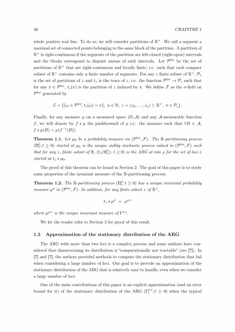
46 CHAPITRE 1
whole positive real line. To do so, we will consider partitions of R+. We call a segment amaximal set of connected points belonging to the same block of the partition. A partition ofR+ is right-continuous if the segments of the partition are left-closed (right-open) intervalsand the blocks correspond to disjoint unions of such intervals. Let P loc be the set ofpartitions of R+ that are right-continuous and locally finite, i.e. such that each compactsubset of R+ contains only a finite number of segments. For any z finite subset of R+, Pzis the set of partitions of z and tz is the trace of z, i.e. the function P loc → Pz such thatfor any π ∈ P loc, tz(π) is the partition of z induced by π. We define F as the σ-field onP loc generated by
C = ω ∈ P loc, tz(ω) = π, n ∈ N, z = (z0, . . . , zn) ⊂ R+, π ∈ Pz.
Finally, for any measure µ on a measured space (Ω,A) and any A-measurable functionf , we will denote by f ? µ the pushforward of µ i.e. the measure such that ∀B ∈ A,f ? µ(B) = µ(f−1(B)).
Theorem 1.1. Let µ0 be a probability measure on (P loc,F). The R-partitioning process(Πρ
t ; t ≥ 0) started at µ0 is the unique càdlàg stochastic process valued in (P loc,F) suchthat for any z, finite subset of R, (tz(Π
ρt ); t ≥ 0) is the ARG at rate ρ for the set of loci z
started at tz ? µ0.
The proof of this theorem can be found in Section 2. The goal of this paper is to studysome properties of the invariant measure of the R-partitioning process.
Theorem 1.2. The R-partitioning process (Πρt ; t ≥ 0) has a unique invariant probability
measure µρ in (P loc,F). In addition, for any finite subset z of R+,
tz ? µρ = µρ,z
where µρ,z is the unique invariant measure of Γρ,z.
We let the reader refer to Section 3 for proof of this result.
1.3 Approximation of the stationary distribution of the ARG
The ARG with more than two loci is a complex process and some authors have con-sidered that characterizing its distribution is “computationally not tractable” (see [?]). In[?] and [?], the authors provided methods to compute the stationary distribution that failwhen considering a large number of loci. Our goal is to provide an approximation of thestationary distribution of the ARG that is relatively easy to handle, even when we considera large number of loci.
One of the main contributions of this paper is an explicit approximation (and an errorbound for it) of the stationary distribution of the ARG (Γρ,zt ; t ≥ 0) when the typical
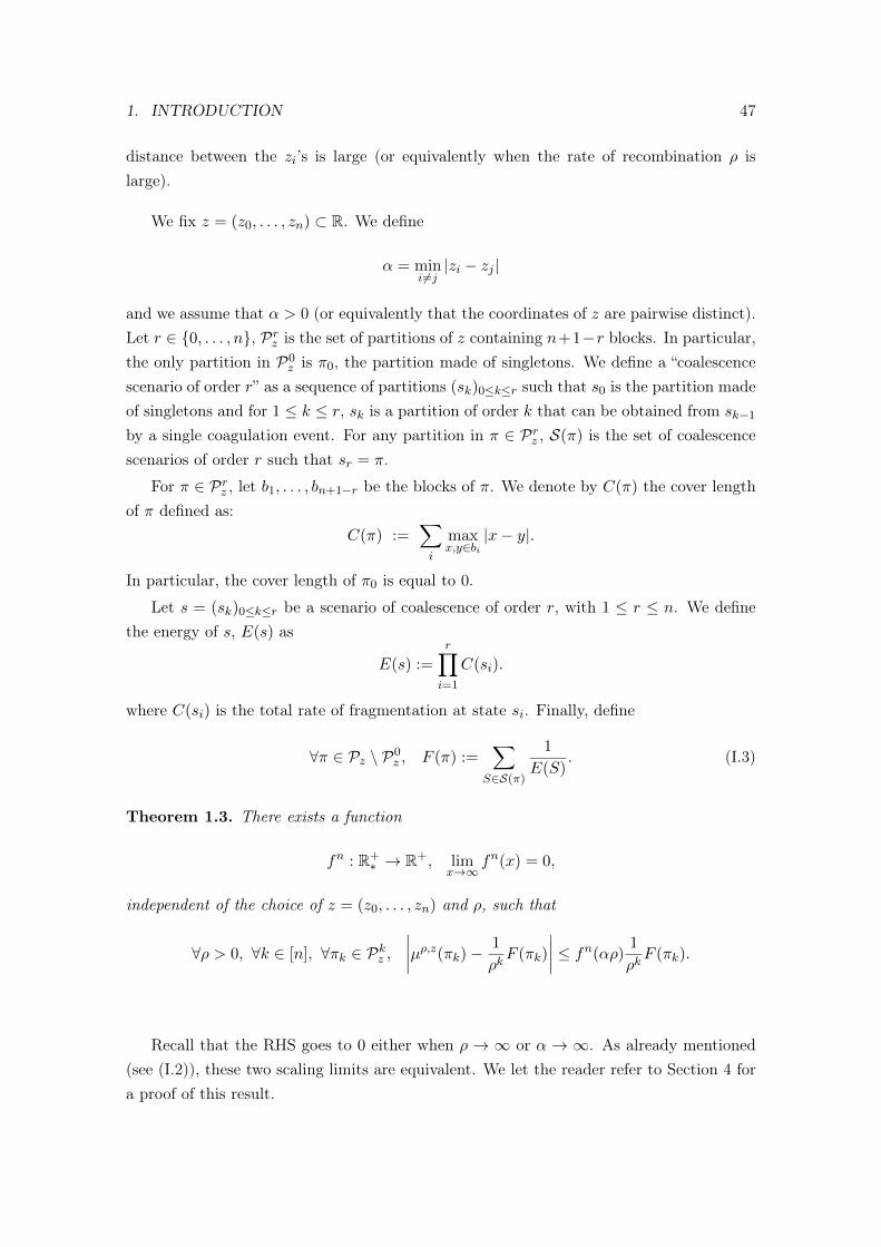
1. INTRODUCTION 47
distance between the zi’s is large (or equivalently when the rate of recombination ρ islarge).
We fix z = (z0, . . . , zn) ⊂ R. We define
α = mini 6=j|zi − zj |
and we assume that α > 0 (or equivalently that the coordinates of z are pairwise distinct).Let r ∈ 0, . . . , n, Prz is the set of partitions of z containing n+1−r blocks. In particular,the only partition in P0
z is π0, the partition made of singletons. We define a “coalescencescenario of order r” as a sequence of partitions (sk)0≤k≤r such that s0 is the partition madeof singletons and for 1 ≤ k ≤ r, sk is a partition of order k that can be obtained from sk−1
by a single coagulation event. For any partition in π ∈ Prz , S(π) is the set of coalescencescenarios of order r such that sr = π.
For π ∈ Prz , let b1, . . . , bn+1−r be the blocks of π. We denote by C(π) the cover lengthof π defined as:
C(π) :=∑i
maxx,y∈bi
|x− y|.
In particular, the cover length of π0 is equal to 0.
Let s = (sk)0≤k≤r be a scenario of coalescence of order r, with 1 ≤ r ≤ n. We definethe energy of s, E(s) as
E(s) :=r∏i=1
C(si).
where C(si) is the total rate of fragmentation at state si. Finally, define
∀π ∈ Pz \ P0z , F (π) :=
∑S∈S(π)
1
E(S). (I.3)
Theorem 1.3. There exists a function
fn : R+∗ → R+, lim
x→∞fn(x) = 0,
independent of the choice of z = (z0, . . . , zn) and ρ, such that
∀ρ > 0, ∀k ∈ [n], ∀πk ∈ Pkz ,∣∣∣∣µρ,z(πk)− 1
ρkF (πk)
∣∣∣∣ ≤ fn(αρ)1
ρkF (πk).
Recall that the RHS goes to 0 either when ρ → ∞ or α → ∞. As already mentioned(see (I.2)), these two scaling limits are equivalent. We let the reader refer to Section 4 fora proof of this result.
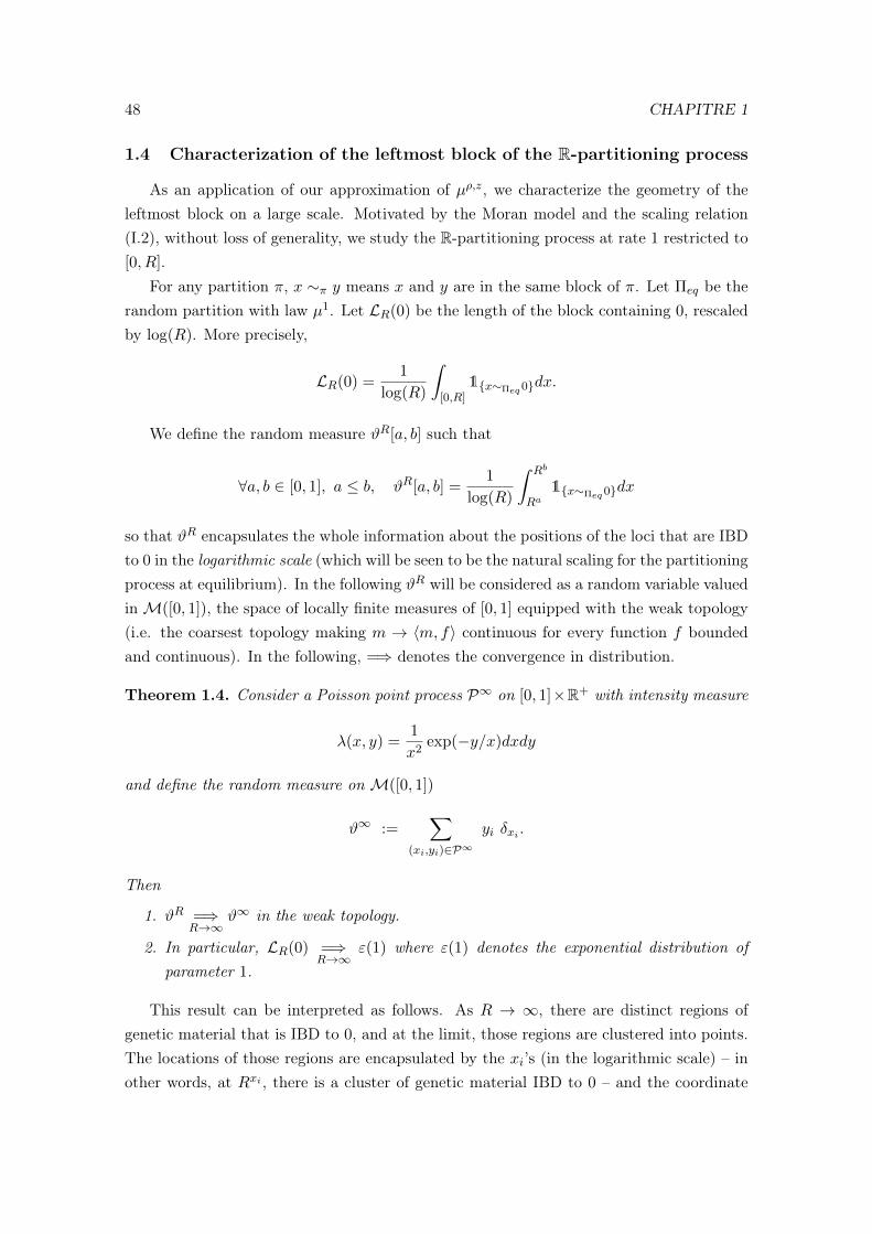
48 CHAPITRE 1
1.4 Characterization of the leftmost block of the R-partitioning process
As an application of our approximation of µρ,z, we characterize the geometry of theleftmost block on a large scale. Motivated by the Moran model and the scaling relation(I.2), without loss of generality, we study the R-partitioning process at rate 1 restricted to[0, R].
For any partition π, x ∼π y means x and y are in the same block of π. Let Πeq be therandom partition with law µ1. Let LR(0) be the length of the block containing 0, rescaledby log(R). More precisely,
LR(0) =1
log(R)
∫[0,R]
1x∼Πeq0dx.
We define the random measure ϑR[a, b] such that
∀a, b ∈ [0, 1], a ≤ b, ϑR[a, b] =1
log(R)
∫ Rb
Ra1x∼Πeq0dx
so that ϑR encapsulates the whole information about the positions of the loci that are IBDto 0 in the logarithmic scale (which will be seen to be the natural scaling for the partitioningprocess at equilibrium). In the following ϑR will be considered as a random variable valuedinM([0, 1]), the space of locally finite measures of [0, 1] equipped with the weak topology(i.e. the coarsest topology making m → 〈m, f〉 continuous for every function f boundedand continuous). In the following, =⇒ denotes the convergence in distribution.
Theorem 1.4. Consider a Poisson point process P∞ on [0, 1]×R+ with intensity measure
λ(x, y) =1
x2exp(−y/x)dxdy
and define the random measure onM([0, 1])
ϑ∞ :=∑
(xi,yi)∈P∞yi δxi .
Then
1. ϑR =⇒R→∞
ϑ∞ in the weak topology.
2. In particular, LR(0) =⇒R→∞
ε(1) where ε(1) denotes the exponential distribution ofparameter 1.
This result can be interpreted as follows. As R → ∞, there are distinct regions ofgenetic material that is IBD to 0, and at the limit, those regions are clustered into points.The locations of those regions are encapsulated by the xi’s (in the logarithmic scale) – inother words, at Rxi , there is a cluster of genetic material IBD to 0 – and the coordinate

1. INTRODUCTION 49
yi corresponds the amount of genetic material that is IBD to 0 present in this cluster (seeFigure 1.4). Note that the positions of the segments (in the logarithmic scale) are givenby the Poisson process of intensity (1/x)dx, which is known as “the scale invariant PoissonProcess” (see for example [?]).
We performed some numerical simulations of the partitioning process to illustrate thesecond part of Theorem 1.4. Figure 1.4 shows how the length of the cluster covering 0 isexponentially distributed.
Figure I.3 – Distribution of the length of the leftmost block (R = 5000). Theblue histogram represents the empirical distribution, that was obtained by simulating thepartitioning process, for a chromosome of length R = 5000. The number of replicates is10000. The red curve is the probability density function of an exponential distribution ofparameter 1. We compared the empirical distribution to an exponential distribution usinga Kolmogorov-Smirnov test, which was positive, with a p-value of 10−4.
1.5 Biological relevance
Recall that a “morgan” is a unit used to measure genetic distance. The distance betweentwo loci is 1 morgan if the average number of crossovers is 1 per reproduction event. Inother words, in a population of size N , if we consider the discrete partitioning process atrate 1, two loci zi and zj are at distance 2
N |zi − zj | morgans.We studied the R-partitioning process at rate 1 restricted to [0, R], which should corre-
spond to a portion (or frame) of the chromosome that is of size R/N morgans (and smallenough so that the single crossing-over approximation is valid). Then, we first let the pop-ulation size N tend to infinity (in order to get the partitioning process from the underlying
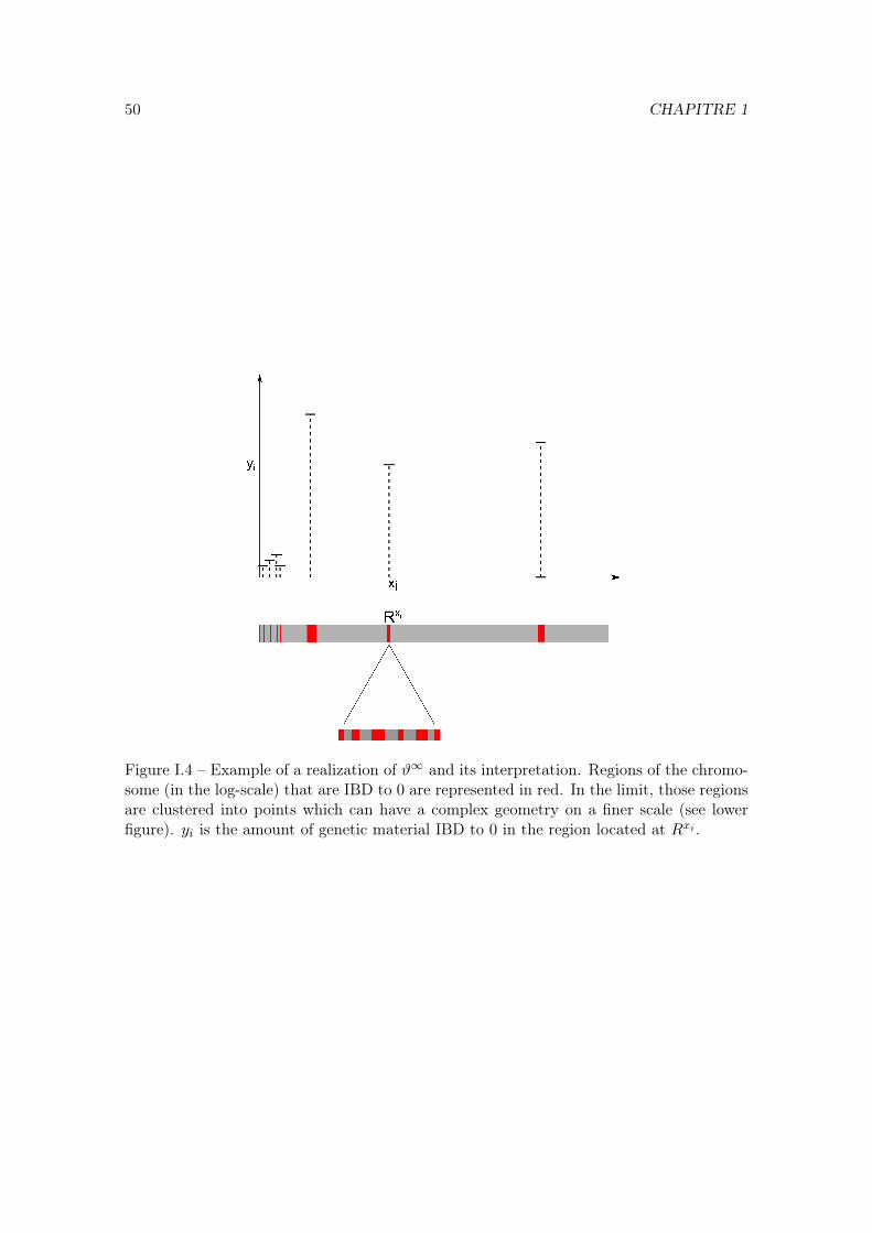
50 CHAPITRE 1
Figure I.4 – Example of a realization of ϑ∞ and its interpretation. Regions of the chromo-some (in the log-scale) that are IBD to 0 are represented in red. In the limit, those regionsare clustered into points which can have a complex geometry on a finer scale (see lowerfigure). yi is the amount of genetic material IBD to 0 in the region located at Rxi .
2. THE R-PARTITIONING PROCESS 51
finite population model), and then the size of the frame go to ∞ (in the R-partitioningprocess). Note that since we take successive limits (first N → ∞ and then R → ∞), thisgives no clue on how the population size and the size of the observation frame should scalewith one another to ensure that the approximation is correct.
[?] used the same hypothesis. They explained that this approximation should be validin human populations, where for example, the size of chromosome 1 is 2.93 morgans andthe effective population size is N = 20000. If one looks at a frame of this chromosome oflength 1 morgan (1/3 of the chromosome), then R = 20000.
1.6 Outline
This paper is organized as follows. In Section 2 we propose a construction of the R-partitioning process and we prove Theorem 1.1. In Section 3 we show the existence anduniqueness of a stationary distribution for this process (Theorem 1.2). Finally, Sections 4and 5 are devoted to the proofs of Theorems 1.3 and 1.4 respectively.
2 The R-partitioning process
2.1 Some preliminary definitions
We start by recalling some definitions that are useful for the rest of the paper and byclarifying some notation. In the following, we consider partitions of R+ or of subsets ofR+. We call a segment a maximal set of adjacent points belonging to the same block ofthe partition. For E = R+ or E ⊂ R+, we say that a partition ω of E is locally finite iffor any compact subset K of E such that K ∩ E 6= ∅, tK∩E(ω) contains a finite numberof segments. We say that a partition is right continuous if the segments of the partitionare left-closed (right-open) intervals (and the blocks correspond to disjoint unions of suchintervals). Note that for a partition that is right continuous, infinite sequences of smallintervals can only accumulate to the left of a point. For a < b ∈ R+, we denote by P loc[a,b]
(resp. P loc) the set of the partitions of [a, b] (resp. R+) that are right continuous and finite(resp. right continuous and locally finite). We define the σ-field F on P loc generated by
C = ω ∈ P loc, tz(ω) = π, n ∈ N, z = (z0, . . . , zn) ⊂ R+, π ∈ Pz.
We also need to define a distance d on P loc. To do so, we start by identifying eachpartition in P loc to a function from R+ to itself. More precisely, we define a map φ :
P loc → D(R+,R+) such that, for π ∈ P loc, φ(π) is constructed as follows. For each blockB of π and for each x ∈ B, we set φ(π)(x) := min(B). Note that φ is injective and∀x ∈ R+, φ(π)(x) ≤ x. Also, as π ∈ P loc, φ is càdlàg and has a finite number of jumps in
52 CHAPITRE 1
any compact set of R+. Now, for any π1, π2 ∈ P loc, define
d(π1, π2) :=
∫ +∞
0|φ(π1)(x)− φ(π2)(x)| exp(−x)dx.
It can easily be checked that d defines a distance on P loc. For T > 0, we will denoteby D([0, T ],P loc) the Skorokhod space associated to (P loc, d) equipped with the standardSkorokhod topology. For each partition π ∈ P loc we define a natural ordering on its blocks.We denote by b0, b1, . . . , bi, . . . the blocks of π indexed in such a way that min(b0) <
min(b1) < . . .
The space P loc is separable under d. Indeed, for n ∈ N∗, let Sn be the set of partitionsin π ∈ P loc such that in π|[0,n[ each block is a finite union of segments whose endpointsare in [0, n[∩Q and [n,+∞[ is included in a block of π. S = ∪nSn is countable and usingstandard methods, it can be shown that given π ∈ P loc and ε > 0, there exists a partitionπ′ ∈ S such that d(π, π′) < ε. The space P loc is not complete but we define its completionP loc.
In the following, we will also consider partitions of Q+. We define P locQ as the set oflocally finite partitions of Q+ that are right continuous (in the sense that if Q+ 3 xn ↓ x ∈Q+ then xn is in the same segment as x for n large enough) and FQ the σ-field generatedby
CQ = ω ∈ PQ, tz(ω) = π, n ∈ N, z = (z0, . . . , zn) ⊂ Q+, π ∈ Pz.
2.2 Definition of the R-partitioning process
We start by defining ARG for a finite set of loci [?, ?, ?]. Note that here we only considerthe case of single-crossover recombination. We consider a finite set of loci, whose positionsin the chromosome are given by z ⊂ R+, z = z0, . . . , zn (with z0 < z1 < . . . < zn). Letρ > 0. Let (Γρ,zt ; t ≥ 0) be the Markov process on (Pz,Fz), with the following transitionrates:
— Coagulation: Consider π1 ∈ Pz and a and b two blocks of π1. Let c = a ∪ b andπ2, the partition obtained by coalescing the blocks a and b into c and letting all theother blocks unchanged. A transition from π1 to π2 occurs at rate:
q(π1, π2) = 1.
— Fragmentation: Now take π1 ∈ Pz and a a block of π1 containing k elementszi1 , . . . , zik such that zi1 < . . . < zik . Let j < k. Let b = zi1 , . . . , zij and c =
zij+1 , . . . , zik and π2, the partition obtained by fragmenting a into b and c. A
2. THE R-PARTITIONING PROCESS 53
transition from π1 to π2 occurs at rate:
q(π1, π2) = ρ(zij+1 − zij ).
— All these events are independent and all other events have rate 0.
This process is called the ARG at recombination rate ρ, for the set of particles (or loci)z. It is easily seen that Γρ,zt has a finite state-space and is irreducible. We call µρ,z itsunique invariant probability measure, that will be characterized in Section 4.
We now want to define a process on (P loc,F), called the R-partitioning process so thatfor any z finite subset of R+, the trace on z is distributed as the ARG Γρ,z.
We set Πρ,L0 = π0, π0 ∈ P loc[0,L[. We assume that the blocks of this partition are indexed
with the natural order defined on the previous section. The partitioning process on P loc[0,L[
is generated by a sequence of independent Poisson point processes as follows:
— For all i, j ∈ N, Y i,j is a Poisson point process of intensity 1. For t ∈ Y i,j , at timet− there is a coagulation event: blocks bi and bj are replaced by bi ∪ bj . If i or jdoes not correspond to the index of any block, nothing happens.
— For all i ∈ N, Xi is a Poisson point process on R+ × [0, L[ with intensity ρ dt⊗ dx.The atoms of Xi correspond to fragmentation events. For (t, x) ∈ Xi, if at timet−, Πρ,L
t− = π, if bi is a block of π and x ∈ ] min(bi), sup(bi)[, bi is fragmented into twoblocks bi,− and bi,+ such that bi,− = bi∩[0, x[ and bi,+ = bi∩[x, L]. Then Πρ,L
t is equalto the partition obtained by replacing bi by bi,− and bi,+. If x /∈ ] min(bi), sup(bi)[,nothing happens.
After each event, blocks are relabelled in such a way that they remain ordered, in the sensespecified above. Recall that, with this construction, the partitions that are formed arealways right continuous. Also the number of blocks of Πρ|[0,L[ is stochastically dominatedby a birth-death process which jumps from n to n + 1 at rate ρLn and from n to n − 1
at rate n(n − 1)/2 with initial condition the number pf blocks in π0, which is known toremain locally bounded (and even to have +∞ as entrance boundary, see [?]). There isthe same stochastic domination between the two processes for the numbers of jump eventson any fixed time interval. This shows that the number of blocks in Πρ
t |[0,L[ is a.s. locallybounded and since the number of segments jumps at most by +1 at each event, the numberof segments is also a.s. locally bounded. So a.s. for all t, Πρ,L
t ∈ P loc[0,L[.
Finally, we define the partitioning process in R, as the projective limit of (Πρ,Lt ; t ≥
0)L∈R+ as L → ∞. In fact, by construction, ∀L′ > L, ∀t ≥ 0, Πρ,L′
t |[0,L[ = Πρ,Lt , where
Πρ,L′ |[0,L[ is the natural restriction of Πρ,L′
t to [0, L[.
Proposition 2.1. The R-partitioning process, (Πρt ; t ≥ 0) with initial measure π0 is the
54 CHAPITRE 1
unique càdlàg stochastic process valued in (P loc,F) such that
∀L ≥ 0, (Πρt ∩ [0, L]; t ≥ 0) = (Πρ,L
t ; t ≥ 0)
with Π0 = π0. Further for any finite subset z in R+, tz(Πρ) is distributed as Γρ,z, the ARGwith initial condition tz(π0).
Proof. We need to check that, for any T > 0, (Πρt ; 0 ≤ t ≤ T ) ∈ D([0, T ],P loc) almost
surely. To do so, we need to prove that with probability 1, for every t ∈ [0, T ], for everyε > 0, one can find s > 0 such that d(Πρ
t ,Πρt+s) < ε. Fix ε > 0 and pick L > 0 such that
2 exp(−L)(L+1) < ε. From the Poissonian construction, for any T > 0, the process Πρ|[0,L[
has a finite number of jumps in [0, T ], which happen at times t1, . . . , tn. We choose s > 0
such that |t− s| < mini |ti+1 − ti|. Then Πt|[0,L[ = Πt+s|[0,L[. As φ(Πρt |[0,L[) = φ(Πρ
t )|[0,L[,for any x ∈ [0, L[, φ(Πρ
t )(x) = φ(Πρt+s)(x), so
d(Πρt ,Π
ρt+s) = 0 +
∫ +∞
L|φ(Πρ
t )(x)− φ(Πρt+s)(x)|e−xdx
≤∫ +∞
L2x exp(−x)dx = 2 exp(−L)(L+ 1) < ε,
and similarly for left-hand limits. So (Πρt ; 0 ≤ t ≤ T ) ∈ D([0, T ],P loc). The fact that
tz(Πρ) is distributed as Γρ,z, the ARG with initial condition tz(π0) can be readily seen
from the definition.
In addition, the following proposition can easily be deduced. Note that the secondequality is just a trivial consequence of the first one.
Proposition 2.2 (Consistency). For all z and y, finite subsets of R+ such that y ⊂ z,
Γρ,y = Γρ,z|y,
where Γρ,z|y denotes the restriction of Γρ,z to Py, and
µρ,y = ty ? µρ,z.
We now turn to the proof of the main result of this section, i.e. Theorem 1.1.
Proof of Theorem 1.1. Let (Πt; t ≥ 0) be a càdlàg process in (P loc,F) such that for any z,finite subset of R,
(tz(Πt); t ≥ 0)d= (Γρ,zt ; t ≥ 0)
d= (tz(Π
ρt ); t ≥ 0).

3. STATIONARY MEASURE FOR THE R-PARTITIONING PROCESS 55
We denote by zii∈N an enumeration of the rational numbers and for all n ∈ N, we definezn := z0, . . . zn. For every n > 1, we have
tzn(Πρ) = tQ(Πρ)|zn and tzn(Π) = tQ(Π)|zn ,
so we have(tQ(Πρ
t ); t ≥ 0)d= (tQ(Πt); t ≥ 0).
In particular
∀(t1, . . . , tn) ⊂ R+ (tQ(Πρt1
), . . . , tQ(Πρtn))
d= (tQ(Πt1), . . . , tQ(Πtn)). (I.4)
Similarly as done p.49, the number of blocks of and number of events undergone by(tz(Πt); t ∈ [0, T ]) are stochastically dominated, uniformly in z ⊂ Q ∩ [0, L], by thoseof a birth-death process which jumps from n to n + 1 at rate ρLn and from n to n − 1
at rate n(n− 1)/2 with initial condition the number of blocks in Π0. This shows that a.s.for all t ≥ 0, tQ(Πt) ∈ P locQ (and of course tQ(Πρ
t ) ∈ P locQ ). Since the partitions in P loc
(resp. P locQ ) are right-continuous and since Q is dense in R, for every π ∈ P locQ there existsa unique π ∈ P loc such that tQ(π) = π. In other words, the projection map
tQ : (P loc,F)→ (P locQ ,FQ)
is bijective. With a little bit of extra work, one can show that t−1Q is measurable so, from
(I.4),∀(t1, . . . , tn) ⊂ R+, (Πρ
t1, . . . ,Πρ
tn)d= (Πt1 , . . . ,Πtn).
This implies that ∀T > 0, (Πt; 0 ≤ t ≤ T )d= (Πρ
t ; 0 ≤ t ≤ T ), in the Skorokhodtopology D([0, T ], P loc) (see [?], Theorem 16.6). So (Πρ
t ; t ≥ 0) is the unique processin D([0, T ], P loc) such that for any z, finite subset of R, (tz(Π
ρt ); t ≥ 0) is distributed as
(Γρ,zt ; t ≥ 0). As P loc ⊂ P loc, the theorem is proved.
3 Stationary measure for the R-partitioning process
The goal of this section is to prove Theorem 1.2. The idea of the proof is to considerthe stationary measure of the partitioning process on finite sets of rational numbers. UsingKolmogorov’s extension theorem we define its unique projective limit in P locQ . Then, usingcontinuity arguments, we prove that there is a unique extension of this measure to thepartitions of R. Let us now go into more details. We decompose the proof into severallemmas.
Lemma 3.1. A measure ν is invariant for (Πρt ; t ≥ 0) iff for any finite subset z of R+,
ν t−1z is invariant for (tz(Π
ρt ); t ≥ 0).
56 CHAPITRE 1
Proof. We obviously only prove the “if” part. We consider a probability measure ν and foreach finite z ⊂ R+, we define νz := ν t−1
z . We assume that for any subset z ∈ R, νz isinvariant for (tz(Π
ρt )). We assume that Πρ
0 = π0 is distributed according to ν. We want toprove that
∀B ∈ F , ∀t ∈ R+, P(Πρt ∈ B) = P(Πρ
0 ∈ B).
As F is the σ-field generated by C, and C is closed under finite intersection, we only needto prove that for any z finite subset of R+,
∀π ∈ Pz, ∀t ∈ R+, P(tz(Πρt ) = π) = P(tz(Π
ρ0) = π).
As νz is invariant for tz(Πρ),
∀π ∈ Pz, P(tz(Πρt ) = π) = P(tz(Π
ρ0) = π) = νz(π),
which completes the proof of Lemma 3.1.
Lemma 3.2. There exists a unique probability measure µρ on (PQ,FQ) charging rightcontinuous partitions such that, for every finite z ⊂ Q+,
tz ? µρ = µρ,z.
Furthermore, µρ only charges locally finite partitions of Q+ and for every x ∈ Q+,
µρ(x is the extremity of a segment) = 0.
Proof. From Proposition 2.2, the family (µρ,z; z ⊂ Q+) is consistent in the sense that fortwo finite subsets z ⊂ z′ then
tz ? µρ,z′ = µρ,z.
By an application of the Kolmogorov extension theorem, there exists a unique measure µρ
defined on (PQ,FQ) such that for every finite subset z in Q we have
tz ? µρ = µρ,z.
(To see how one can apply Kolmogorov theorem in the context of consistent random par-titions, we refer the reader to [?], Proposition 2.1.)
We now need to prove that µρ only charges locally finite partitions of Q+. To do so,we follow closely [?]. We fix a, b ∈ N, a < b. We want to prove that, if π is a partition ofQ distributed as µρ, then S[a,b], the number of segments in π|[a,b]∩Q is finite almost surely.
3. STATIONARY MEASURE FOR THE R-PARTITIONING PROCESS 57
To do so, we define
∀n ∈ N∗, εn := 2−n,
Xin := 1((a+(i−1)εn)6∼(a+iεn))
zin := (a+ (i− 1)εn, a+ εn) ∈ R2.
In words, Xin = 1 if (i − 1)εn and iεn belong to different segments. Let us compute theexpectation of S[a,b]. Using the monotone convergence theorem we have
E(S[a,b]) = 1 + E( limn→∞
b2n(b−a)c∑i=1
Xin) = 1 + limn→∞
b2n(b−a)c∑i=1
E(Xin)
= 1 + limn→∞
b2n(b−a)c∑i=1
µρ,zin(a+ (i− 1)εn, a+ iεn).
The ARG at rate ρ for the set of loci zin has only two types of transitions: coagulation atrate 1 and fragmentation at rate ρεn, so
µρ,zin(a+ (i− 1)εn, a+ iεn) =ρεn
1 + ρεn
which gives
E(S[a,b]) = 1 + limn→∞
b2n(b−a)c∑i=1
ρ2−n
1 + ρεn= 1 + ρ(b− a).
Then S[a,b] is finite almost surely, which implies that µρ only charges locally finite partitionsof Q.
For the last statement let x ∈ Q+. By the previous argument,
µρ(x is the extremity of a segment) = limε↓0
µρ(x− ε 6∼ x+ ε) = 0,
which completes the proof.
Lemma 3.3. There exists a unique measure µρ on (P loc,F) such that
tQ ? µρ = µρ,
where µρ is the measure defined in Lemma 3.2.
Proof. Let P locQ the set of locally finite partitions of Q such that for all x ∈ Q+, x is notan extremity of a segment of π. Note that here we do not assume that the partitions of Qare right continuous. From the previous Lemma, µρ(P locQ ) = 1. Similarly, let P loc be the
58 CHAPITRE 1
set of elements π of P loc such that for all x ∈ Q+, x is not an extremity of a segment ofπ. Since Q is dense in R, it is easy to see that for every π ∈ P locQ there exists a uniqueπ ∈ P loc such that tQ(π) = π. In other words, the projection map
tQ : (P loc,F)→ (P locQ ,FQ)
is bijective. (Note that the condition that there are no rational extremities for the latterstatement to hold, can be understood with the following counterexample. Let π be thepartition of Q+ consisting of the two blocks [0, 1] ∩Q and ]1,+∞) ∩Q. Then there is noright-continuous partition π ∈ P loc such that tQ(π) = π.) With a little bit of extra work,one can show that t−1
Q is measurable. As already mentioned in the proof of Theorem 1.1,the projection map
tQ : (P loc,F)→ (P locQ ,FQ)
is bijective and measurable, so the measure µρ defined by
µρ = t−1Q ?
[µρ(· ∩ P locQ )
]has mass 1 and satisfies
tQ ? µρ = µρ.
To prove uniqueness, let µ on (P loc,F) such that tQ ? µ = µρ. Because µρ only chargesP locQ ,
tQ ? µ = µρ(· ∩ P locQ ).
Because µ only charges right continuous partitions, µ only charges P loc (i.e., elementswith no rational extrmities). Taking the pushforward of the two members of the previousequality by t−1
Q , we get
µ(· ∩ P loc) = t−1Q ? (tQ ? µ) = t−1
Q ?[µρ(· ∩ P locQ )
]= µρ.
Since µ only charges P loc, µ = µρ.
Proof of Theorem 1.2. We have proved that there exists a unique probability measure µρ
on (P loc,F) such that, for any finite subset z of Q+, tz ? µρ is invariant for (tz(Πρt ); t ≥ 0)
(by combining Lemmas 3.2 and 3.3). Using Lemma 3.1, we still need to prove that thesame property holds for any finite subset z ⊂ R+. This will be shown by a continuityargument.
We fix ρ > 0. We denote by Pρ the law of the process (Πρt ; t ≥ 0), with initial condition
Πρ0 with law µρ. We also fix z = (z1, . . . , zn) ⊂ R+. For each z∗ = (z∗1 , . . . , z
∗n) ⊂ Q+, we
define a function g∗ : Pz∗ → Pz such that, if π is a partition of z∗, g∗(π) is the partitionof z such that for every i, j ∈ [n], zi ∼g∗(π) zj iff z∗i ∼π z∗j . For every t > 0, we define the
3. STATIONARY MEASURE FOR THE R-PARTITIONING PROCESS 59
eventA(z∗, t) = ∀s ∈ [0, t], tz(Π
ρs) = g∗(tz∗(Π
ρs)).
We want to prove that for every t > 0 and for Fz-measurable bounded function f onPz,
Eρ(f(tz(Πρt ))) = Eρ(f(tz(Π
ρ0)).
As µρ is a measure on P loc, for every ε > 0 one can find z∗ = (z∗1 , . . . , z∗n) ⊂ Q+ such that
Pρ(A(z∗, t))||f ||∞ < ε/2 and |Eρ(f(g∗(tz∗(Πρ0)), A(z∗, t))| < ε/2.
Then
Eρ(f(tz(Πρt ))) = Eρ(f(tz(Π
ρt )), A(z∗, t)) + Eρ(f(tz(Π
ρt )), A(z∗, t))
= Eρ(f(g∗(tz∗(Πρt )), A(z∗, t)) + Eρ(f(tz(Π
ρt )), A(z∗, t)).
As z∗ ⊂ Q+, µρ t−1z∗ is invariant for tz∗(Π
ρt )),
Eρ(f(g∗(tz∗(Πρt )), A(z∗, t)) = Eρ(f(g∗(tz∗(Π
ρ0)))− Eρ(f(g∗(tz∗(Π
ρ0)), A(z∗, t)).
Then,
|Eρ(f(tz(Πρt )))− Eρ(f(g∗(tz∗(Π
ρ0)))| ≤ Pρ(A(z∗, t))||f ||∞
+|Eρ(f(g∗(tz∗(Πρ0)), A(z∗, t))|
so|Eρ(f(tz(Π
ρt )))− Eρ(f(tz(Π
ρ0))| < ε,
and the conclusion follows by letting ε→ 0.
To conclude this section, we state an important property of µρ.
Proposition 3.4 (Scaling). Fix ρ > 0. For every λ ∈> 0, define hλ : R → R such that∀x ∈ R, hλ(x) = λx. Then
hλ ? µρ = µλρ
Similarly, for any z ⊂ R,hλ ? µ
ρ,z = µλρ,z
Proof. This proposition can easily be deduced from the definition of the ARG and thescaling (I.2) and the construction of the R-partitioning process given in the previous section.
Without loss of generality, in Section 5, we will consider the partitioning process withrecombination rate ρ = 1.
60 CHAPITRE 1
4 Proof of Theorem 1.3
Theorem 1.3, provides an approximation of the stationary measure of the discretepartitioning process when ρ → ∞ or α → ∞, i.e. when recombination is much morefrequent than coalescence. This approximation of µρ,z is easy to handle, and that will beused in the proof of Theorem 1.4. We start by clarifying some notation that were alreadydefined in the introduction and by introducing some new notation. In the following, we fixz = (z0, . . . , zn) a finite subset of R, and we define
α = mini 6=j|zi − zj |
and we assume that α > 0 (or equivalently that the coordinates of z are pairwise distinct).
Definition 4.1. We consider the ARG ρ for the set of loci z, Γρ,z. We say that a partitionπ ∈ Pz is of order r if it can be obtained from the finest partition (π0 := z0, . . . , zn)by r successive coagulation events. We denote by Pkz the subset of Pz containing all thepartitions of order k.
For example, for i, j, k, l ∈ 0, . . . , n:
— π0 = z0, . . . , zn is the only partition of order 0.
— z0, . . . , zi, zj, . . . , zn is of order 1.
— z0, . . . , zi, zj , zk, . . . , zn is of order 2.
— z0, . . . , zi, zj, zk, zl, . . . , zn is also of order 2.
— z0, z1, . . . , zn is the only partition of order n.
Note that as the number of blocks decreases by 1 at each coalescence event, in a partitionof order k, there are always n + 1 − k blocks, so this definition is equivalent to the onegiven in the Introduction.
Definition 4.2. Let (sk)0≤k≤r be a sequence of r elements of Pz. The sequence (sk) iscalled a “(coalescence) scenario of order r” if:
— s0 is the finest partition.
— For 1 ≤ k ≤ r, sk is a partition of order k that can be obtained from sk−1 by a singlecoagulation event.
If π is a partition of order r, we denote by S(π) the set of coalescence scenarios of orderr, such that sr = π.
For example, the partition z0, . . . , zi, zj , zk, . . . , zn can be obtained from the
4. PROOF OF THEOREM 1.3 61
finest partition with three different scenarios:
zizjzk . . . → zi, zjzk . . . → zi, zj , zk
zizjzk . . . → zi, zkzj . . . → zi, zj , zk
zizjzk . . . → zk, zjzi . . . → zi, zj , zk . . .
For π ∈ Pz, let b1, b2, . . . , bk, . . . be the blocks of π. We denote by C(π) the cover lengthof π defined as:
C(π) :=∑i
maxx,y∈bi
|x− y|.
In particular, the cover length of π0 is equal to 0.
If π1 and π2 are two partitions in Pz, we define θ(π1, π2) as the transition rate fromπ1 to π2 in the finite partitioning process Γ1,z with recombination rate ρ = 1 (and we setθ(π1, π2) = 0 if the transition is not possible). By definition, in the ARG Γρ,z (with recom-bination rate ρ), the transition rate from π1 to π2 is θ(π1, π2) if the transition correspondsto a coagulation event and ρθ(π1, π2) if it is a fragmentation. It can readily be seen that,
∀π ∈ Prz ,∑
ω∈Pr−1z
θ(π, ω) = C(π).
In words, when ρ = 1, the total fragmentation rate corresponds to the cover length. Forgeneral values of ρ, the fragmentation rate is the cover length multiplied by ρ.
Also, the total coalescence rate from a partition of order k only depends on n and k(and not in the values of z0, . . . , zn and ρ) and is given by
∑ω∈Pr+1
z
θ(π, ω) = γk :=(n− k)(n− k + 1)
2,
where γk corresponds to the number of pairs of blocks in a partition of order k.
Definition 4.3. Let s = (sk)0≤k≤r be a scenario of coalescence of order r, with 1 ≤ r ≤ n.We define the energy of s, E(s) as:
E(s) :=
r∏i=1
C(si) =
r∏i=1
∑π∈Pi−1
z
θ(si, π).
In words, the energy of a scenario corresponds to the product of the successive coverlengths at each step.
Now we can state the main result of this section, that gives an approximation of µρ,z,when ρ or α is large. The idea behind this theorem is that, when ρ 1 or α 1,fragmentation events occur much more often than coalescence events. This implies that
62 CHAPITRE 1
the partition made of singletons is the most likely configuration and the probability of apartition decreases with its order. Define
∀z ⊂ R+, ∀π ∈ Pz \ π0, F (π) :=∑
S∈S(π)
1
E(S). (I.5)
We recall the statement of Theorem 1.3.
Theorem. There exists a function
fn : R+∗ → R+, lim
x→∞fn(x) = 0,
independent of the choice of z = (z0, . . . , zn) and ρ, such that
∀ρ > 0, ∀k ∈ [n], ∀πk ∈ Pkz ,∣∣∣∣µρ,z(πk)− 1
ρkF (πk)
∣∣∣∣ ≤ fn(αρ)1
ρkF (πk).
Before proving Theorem 1.3 we need to prove some technical results. But to give thereader some intuition on this result, we will start by giving a brief sketch of the proof.Until further notice, we are going to fix ρ > 0, k ∈ [n], π ∈ Pkz a partition of order k ≥ 1.We will start by defining some notation.
- t+0 = inft > 0, Γρ,zt 6= π0.
- Tπ = inft > 0, Γρ,zt = π, T0 = inft > t+0 , Γρ,zt = π0.
- Pπ (resp P0) denotes the law of Γρ,z conditioned on the initial condition Γρ,z0 = π
(resp Γρ,z0 = π0).
Recall that the variables defined above depend on z and ρ, but for the sake of clarity thisdependency is not made explicit.
The idea behind the proof of Theorem 1.3 is to use excursion theory and a well knownextension of Blackwell’s renewal theorem [?] that states that
µρ,z(π) =E0(Y π
1 )
E0(∆0), (I.6)
where ∆0 is the time between two renewals at π0 and Y π1 is the time spent in π during an
excursion out of π0. (More precise definitions of these variables will be given in the proofof Theorem 1.3).
As we consider that α 1 or ρ 1, fragmentation occurs much more often thancoalescence so π0 is the most likely configuration and Γρ,z spends most of the time at π0.Then E0(∆0) can be approximated by the expectation of the holding time at π0 which is1/γ0. Also, in this regime, most excursions out of π0 will only visit π at most one time, so
4. PROOF OF THEOREM 1.3 63
E0(Y π1 ) can be approximated by
P0(Tπ < T0)1
ρC(π),
where P0(Tπ < T0) is the probability that π is reached during the excursion out of π0 and1
ρC(π) is approximately the expectation of the holding time at π when ρC(π) γk (i.e.when recombination occurs much more often than coalescence).
The core of the proof is to compute P0(Tπ < T0). (This will be done in Corollary4.6.)To do so, we will consider Γρ,z, the embedded chain of the ARG Γρ,z, conditioned onthe initial condition Γρ,z0 = π0. We call a “direct path” a trajectory that goes from π0 to πin only k coalescence steps (without recombination events). Indirect paths are trajectoriesthat are longer and that contain at least a recombination event. As we consider a highrecombination regime, where coalescence occurs much more often than recombination,direct paths will be much more likely that indirect paths. (This will be formalized inLemma 4.5.) So we can approximate P0(Tπ < T0) by the sum of the probabilities of thedirect paths. Then the conclusion will follow by realizing that a direct path corresponds to ascenario of coalescence and showing that P0(Tπ < T0) can be approximated by C(π)
ρk−1γ0F (π).
(This will be formalized in Corollary 4.6.) Finally, replacing in (I.6), we find that µρ,z(π)
can be approximated by F (π)ρk
.
Before turning to the formal proof of Theorem 1.3, we start by proving some technicalresults. We consider Γρ,z, the embedded chain of the ARG Γρ,z. Let P0 denote the law ofΓρ,z conditioned on Γρ,z0 = π0 and ∀π′ ∈ Pz, Pπ′ denotes the law of Γρ,z conditioned onΓρ,z0 = π′. We will consider paths that go from π0 to π. A path is defined as follows.
Definition 4.4. For j ∈ N∗, π′, π′′ ∈ Pz, we define:
G(j, π′ → π′′) = (π(0) = π′, π(1), . . . , π(j−1), π(j) = π′′),
π(1), . . . , π(j−1) ∈ Pz \ π′, π′′ such that
θ(π(i), π(i+1)) > 0 ∀i ∈ 0, · · · , j − 1.
In words, G(j, π′ → π′′) contains every possible path (admissible for the partitioning pro-cess) that connects π′ to π′′ in j steps.
We are going to consider paths p that go from π0 to π, which have at least k steps (asπ is of order k).
- p is a direct path if p ∈ G(k, π0 → π), i.e., p can only be composed of coalescenceevents.
- p is an indirect path if p ∈ G(k + N, π0 → π), N ∈ N∗. Indirect paths containat least one recombination event. Note that the parity of the process implies thatG(k + 2N + 1, π0 → π) is empty.
64 CHAPITRE 1
Lemma 4.5. Fix N ∈ N∗ and a path p in G(k + 2N, π0 → π). There exists a pathp ∈ G(k, π0 → π) such that
P0(p)
P0(p)≤
((1 + γ1
ρα)k
αρ
)N.
Proof of Lemma 4.5. We fix N ∈ N∗ and we start with proving that
∀p ∈ G(k + 2N, π0 → π), ∃ p ∈ G(k + 2(N − 1), π0 → π),
P0(p)
P0(p)≤
(1 + γ1
ρα)k
αρ. (I.7)
We consider a path p ∈ G(k + 2N, π0 → π) such that
p = (π0, π1, . . . , πj , πj−1, πi1 , πi2 , . . . , π).
where the indices of the π, π’s coincide with the order of the partition (for instance, in thetransition πj → πj−1, the order of the partition decreases by one unit, which correspondsto a fragmentation event). We do not specify the order of πi1 , πi2 , . . . As N ≥ 1 there is atleast one recombination event (πj → πj−1). The path p can be decomposed into p1 and p2
such that:
p1 ∈ G((j − 1) + 2, π0 → πj−1), p1 = (π0, π1, . . . , πj−1, πj , πj−1)
p2 ∈ G(k + 2N − (j − 1)− 2, πj−1 → π), p2 = (πj−1, πi1 , πi2 , . . . , π).
In words, we decompose p into two paths, p1 that goes from π0 until the first recombinationevent and p2 that contains the rest of the path.
The idea now is to find a direct path
p1 ∈ G(j − 1, π0 → πj−1), p1 = (π0, π1, . . . , πj−1)
such that
P0(p1)
P0(p1)≤ 1
αρ
(1 +
γ1
ρα
)j−1
≤ 1
αρ
(1 +
γ1
ρα
)k.
To do so, consider the fragmentation event that occurs between step j and step j+1 in p(when transitioning from πj to πj−1). πj contains n+1−j blocks and let (b1, . . . bn−j , b
∗) bethe blocks of πj such that b∗ is the block of πj that is fragmented during this fragmentationevent and za < zb the two elements of b∗ such that b∗ is fragmented between za and zb (i.e.such that b∗ is fragmented into b∗a and b∗b where za is the rightmost element in b∗a and zb
4. PROOF OF THEOREM 1.3 65
the leftmost element in b∗b). We have
C(πj) = C(πj−1) + zb − za. (I.8)
Let i∗ ≤ j be the first step of p such that za and zb are in the same block, i.e
i∗ = mini∈[j]i, za ∼πi zb.
We will construct a direct path p1 = (π0, · · · , πj−1) in such a way that
∀ 1 ≤ i < i∗, C(πi) ≤ C(πi)
if i∗ < j − 1, ∀ i∗ < i ≤ j, C(πi−1) ≤ C(πi), (I.9)
(Note that the terminal value of p1 coincides with the terminal value of p1 and its length isj−1 instead of j+1).) See Figure 4 for a concrete example. In words, we skip step i∗, andrearrange the path in such a way that p1 is admissible, ends at πj−1 and the inequalities(I.9) are satisfied along the way. Formally, the path p1 is constructed as follows :
— If i∗ < j−1, for i ∈ i∗+1, . . . , j−1, let (bi1, . . . bin−i, b
i∗) be the blocks of πi, where bi∗
is the one that contains za and zb. The blocks of πi−1 are (bi1, . . . , bin−i, b
in−i+1, b
in−i+2)
such that:
- if z ∈ bi∗ and z ≤ za, z ∈ bin−i+1.
- if z ∈ bi∗ and z ≥ zb, z ∈ bin−i+2.
If i∗ = j − 1 we skip the present step in the construction of p.
— If in πi∗−1, za is the rightmost element in its block and zb the leftmost element in itsblock, then we define (π1, . . . , πi∗−1) = (π1, . . . , πi∗−1). With this construction πi∗
can be obtained from πi∗−1 by a coalescence event, so the path p is admissible forΓρ,z.
— Else, (π1, . . . , πi∗−1) are constructed from (π1, . . . , πi∗−1) in the following way. Letus denote by ba and bb the blocks of πi∗−1 that contain za and zb respectively. For1 ≤ i ≤ i∗ − 1,
- If the coalescence event between πi−1 and πi involves two blocks bc and bd suchthat in πi∗−1, bc, bd ⊂ ba (resp. bc, bd ⊂ bb) and if bc contains an element thatis smaller than za and bd contains an element is larger than zb, then in thecoalescence step between πi−1 and πi, bc (resp. bd) coalesces with the blockcontaining za (resp. zb). (And nothing happens to bd - resp. bc).
- Otherwise the same coalescence event occurs between πi−1 and πi and betweenπi−1 and πi.
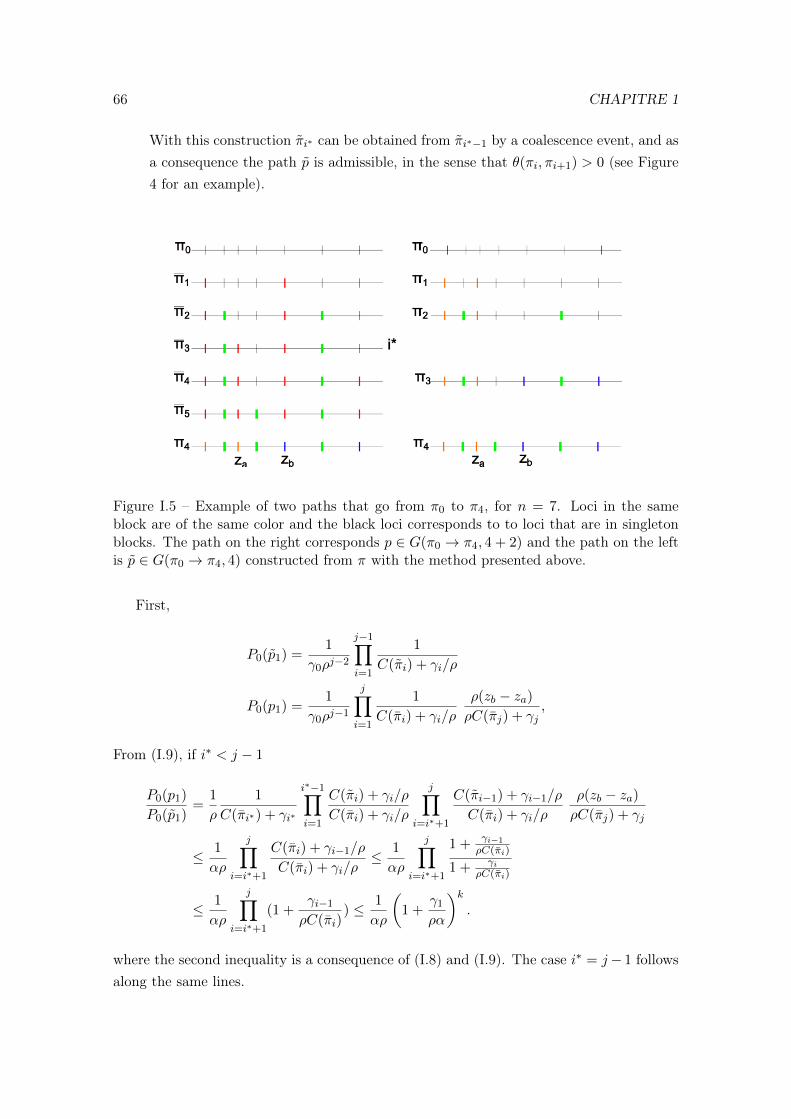
66 CHAPITRE 1
With this construction πi∗ can be obtained from πi∗−1 by a coalescence event, and asa consequence the path p is admissible, in the sense that θ(πi, πi+1) > 0 (see Figure4 for an example).
Figure I.5 – Example of two paths that go from π0 to π4, for n = 7. Loci in the sameblock are of the same color and the black loci corresponds to to loci that are in singletonblocks. The path on the right corresponds p ∈ G(π0 → π4, 4 + 2) and the path on the leftis p ∈ G(π0 → π4, 4) constructed from π with the method presented above.
First,
P0(p1) =1
γ0ρj−2
j−1∏i=1
1
C(πi) + γi/ρ
P0(p1) =1
γ0ρj−1
j∏i=1
1
C(πi) + γi/ρ
ρ(zb − za)ρC(πj) + γj
,
From (I.9), if i∗ < j − 1
P0(p1)
P0(p1)=
1
ρ
1
C(πi∗) + γi∗
i∗−1∏i=1
C(πi) + γi/ρ
C(πi) + γi/ρ
j∏i=i∗+1
C(πi−1) + γi−1/ρ
C(πi) + γi/ρ
ρ(zb − za)ρC(πj) + γj
≤ 1
αρ
j∏i=i∗+1
C(πi) + γi−1/ρ
C(πi) + γi/ρ≤ 1
αρ
j∏i=i∗+1
1 + γi−1
ρC(πi)
1 + γiρC(πi)
≤ 1
αρ
j∏i=i∗+1
(1 +γi−1
ρC(πi)) ≤ 1
αρ
(1 +
γ1
ρα
)k.
where the second inequality is a consequence of (I.8) and (I.9). The case i∗ = j− 1 followsalong the same lines.
4. PROOF OF THEOREM 1.3 67
Let us define
p ∈ G(k + 2, π0 → π), p = (π0, π1, . . . , πj−1, πi1 , πi2 . . . , π).
Since
P0(p) = P0(p1) Pπj−1(p2), P0(p) = P0(p1) Pπj−1(p2)
we have
P0(p)
P0(p)=P0(p1)
P0(p1)≤
(1 + γ1
ρα
)k(αρ)
,
which completes the proof of (I.7). Lemma 4.5 then follows by a simple induction on Nusing (I.7).
Corollary 4.6. There exists a function
un : R+∗ → R+, lim
x→∞un(x) = 0,
independent of the choice of z, π and ρ, such that∣∣∣∣P0(Tπ < T0) − C(π)
ρk−1γ0F (π)
∣∣∣∣ ≤ un(αR)C(π)
ρk−1γ0F (π).
Proof. We have
P0(Tπ < T0) =∑N≥k
∑p∈G(N,π0→π)
P0(p).
As π is of order k, a path from π0 to π has at least k steps. In addition, as the order ofthe partition can only increase or decrease by 1 at each step, a path from π0 to π can onlyhave k + 2N steps, with N ≥ 0, so
P0(Tπ < T0) =∑
p∈G(k,π0→π)
P0(p) +∑N≥1
∑p∈G(k+2N,π0→π)
P0(p). (I.10)
We start by considering the first term in the right hand side. We consider a path p
such that
p ∈ G(k, π0 → π), p = (π0, π1, . . . , π).
68 CHAPITRE 1
We have:
P0(p) =1
γ0
k−1∏i=1
1
ρC(πi) + γi.
Recall that
F (π) =∑
s∈S(π)
k∏i=1
1
C(si).
Further, paths that have k steps are only composed of coalescence events, and thereforeG(k, π0 → π) = S(π). It follows that
∑p∈G(k,π0→π)
P0(p)− C(π)
ρk−1γ0F (π) =
1
ρk−1γ0
∑s∈S(π)
(k−1∏i=1
1
C(si) + γi/ρ−k−1∏i=1
1
C(si)
)
and using the fact that γi ≤ γ0,
∑s∈S(π)
∣∣∣∣∣k−1∏i=1
1
C(si) + γi/ρ−k−1∏i=1
1
C(si)
∣∣∣∣∣ =∑
s∈S(π)
k−1∏i=1
1
C(si)
(1−
k−1∏i=1
1
1 + γi/(ρC(si))
)
≤∑
s∈S(π)
k−1∏i=1
1
C(si)
(1−
(1
1 + γ0/(ρα)
)k−1)
≤ C(π)F (π)
(1− 1
(1 + γ0/(ρα))k−1
)so ∣∣∣∣∣∣
∑p∈G(k,π0→π)
P0(p)− C(π)
ρk−1γ0F (π)
∣∣∣∣∣∣ ≤ C(π)
ρk−1γ0F (π)
(1− 1
(1 + γ0/(ρα))k−1
). (I.11)
To prove Proposition 4.6, we still need to consider the second term in the right handside of (I.10). Using Lemma 4.5, we have∑
N≥1
∑p∈G(k+2N,π0→π)
P0(p)
≤∑
p∈G(k,π0→π)
P0(p)
∑N≥1
|G(k + 2N, π0 → π)|
((1 + γ1
ρα)k
αρ
)N . (I.12)
To compute |G(k + 2N, π0 → π)|, let us recall that, at each step in a path:
— If it corresponds to a coalescence event from a partition of order j there are γjpossibilities, and ∀j ∈ 0, . . . , n γj ≤ n(n+ 1).
— If it corresponds to a fragmentation event, there are at most (n + 1) blocks in the
4. PROOF OF THEOREM 1.3 69
partition and each one contains at most (n+ 1) elements, so that each block can befragmented in n different ways.
From there, it can easily be seen that
|G(k + 2N, π0 → π)| ≤ (n(n+ 1))k+2N .
Combining this with (I.12), we have:∑N≥1
∑p∈G(k+2N,π0→π)
P0(p)
≤
∑p∈G(k,π0→π)
P0(p)
(n(n+ 1))k∑N≥1
(n2(n+ 1)2(1 + γ1
ρα)k
αρ
)N,
which combined with (I.10) and (I.11), gives:∣∣∣∣P0(Tπ < T0)− C(π)
ρk−1γ0F (π)
∣∣∣∣ ≤ C(π)
ρk−1γ0F (π)un,k(αρ)
where un,k is a function independent of z and ρ and vanishing at∞. The conclusion followsby setting un(αρ) = maxk∈[n](u
n,k(αρ)).
Before stating the last technical result that is needed in the proof of Theorem 1.3, weneed to introduce some notation:
- t+π = inft > 0, Γρ,zt 6= π
- Tπ = inft > t+π , Γρ,zt = π, T0 = inft > t+π , Γρ,zt = π0.
Lemma 4.7. For any n ∈ N, there exist two functions gn and hn such that
limx→∞
gn(x) = 0, limx→∞
hn(x) = 1
independent on the choice of z, π and ρ such that
(i) E0(T0 − t+0 ) ≤ gn(αρ)
(ii) ∀k > 0, ∀π ∈ Pkz , Pπ(T0 < Tπ) ≥ hn(αρ).
Proof. We fix ρ > 0, n ∈ N, z = (z0, . . . , zn), k ∈ [n], π ∈ Pkz .
The idea of the proof is to consider the stochastic process (Xρ,zt ; t ≥ 0) valued in
0, . . . , n and such that ∀t ≥ 0, Xρ,zt is the order of the partition Γρ,zt . This process is not
Markovian, but it can easily be compared to a Markov process (W ρ,zt , t ≥ 0) in such a way
that the excursions out of 0 of W ρ,z are longer than those of Xρ,z.
70 CHAPITRE 1
More precisely, let W ρ,z be the birth-death process in 0, · · · , n where all the deathrates are equal to ρα and the birth rate at state k is γk (note that γn = 0).
With these transition rates, for any πk ∈ Pkz , the total coalescence rate from πk for theprocess Γρ,zt is the same as the birth rate from k for W ρ,z
t . On the other hand, the totalfragmentation rate for Γρ,zt when Γρ,zt = πk is equal to ρC(πk) and is always higher thanthe death rate at k for W ρ,z
t . We can find a coupling between W ρ,z and Xρ,z such that theholding times at 0 of the two process are the same (as the birth rate in 0 for W ρ,z is thesame as the coagulation rate from 0 for Γρ,z). In addition, during an excursion out of 0,the holding time at k > 0 for Xρ,z is shorter than the holding time at k for W ρ,z and theembedded chain of Xρ,z jumps more easily to the right than the embedded chain of W ρ,z.
Let us denote by E0 the probability with respect to the distribution ofW ρ,z, conditionalto W ρ,z
0 = 0, and define
t+0 = inft > 0,W ρ,z 6= 0
T0 = inft > t+0 , Wρ,zt = 0.
By construction, we have
E0(T0 − t+0 ) ≤ E0(T0 − t+0 ).
Finally, E0(T0 − t+0 ) only depends on ρα and n and it can be checked that
E0(T0 − t+0 ) −→αρ→∞
0
so (i) is verified.
(ii) can be handled by similar methods. Namely, let W ρ,z denote the embedded chainof W ρ,z
Pπ(T0 < Tπ) ≥ P(W ρ,z0 = k, W ρ,z
1 = k − 1, . . . , W ρ,zk = 0)
=
k∏i=1
ρα
ρα+ γi≥
n∏i=1
ρα
ρα+ γi−→ρα→∞
1
where the first inequality is obtained by the same argument as in (i). This completes theproof of Lemma 4.7.
We are now ready to prove the main results of this section.
Proof of Theorem 1.3. We will consider excursions of (Γρ,zt ) out of π0. Let us consider(Ji)i∈N the renewal times at π0 i.e. the successive jump times of (Γρ,zt ) such that Γρ,zJi = π0
4. PROOF OF THEOREM 1.3 71
(and Γρ,zJi− 6= π0). For i ∈ N∗, let us define
∆i0 := Ji − Ji−1
the time between two renewals at π0. The (∆i0)i∈N are independent and identically dis-
tributed random variables. Also, for i ∈ N∗, consider
Y πi :=
∫ Ji
Ji−1
1Γρ,zt =πdt,
which corresponds to the time spent by Γρ,z in π during the ith excursion out of π0. Bystandard excursion theory, the Y π
i ’s are independent and identically distributed randomvariables.
From the ergodic theorem we have
µρ,z(π) = limT→∞
1
T
∫ T
01Γρ,zs =πds a.s.
= limn→∞
1
Jn
n∑k=1
∫ Jn
Jn−1
1Γρ,zs =πds a.s..
Since the excursions are independent from one another, using Blackwell’s renewal theorem[?], and the law of large numbers,
limn→∞
n
Jn=
1
E0(∆10)
and limn→∞
1
n
n∑k=1
∫ Jn
Jn−1
1Γρ,zs =πds = E0(Y π1 ) a.s.,
which easily gives
µρ,z(π) =E0(Y π
1 )
E0(∆10).
LetH0 be the holding time at π0 andH the holding time at π. H0 follows an exponentialdistribution of parameter γ0. H follows an exponential distribution of parameter (C(π) +
γk). By standard excursion theory,
E(Y π1 ) = P0(Tπ < T0)
∑k≥1
kE(H)Pπ(Tπ < T0)k−1Pπ(T0 < Tπ)
= P0(Tπ < T0)1
(ρC(π) + γk)
1
Pπ(T0 < Tπ),
and
E(∆10) = E(H0) + E0(T0 − t+0 ) where E(H0) =
1
γ0.
72 CHAPITRE 1
Combining this with Corollary 4.6, we have∣∣∣∣ µρ,z(π) − C(π)F (π)
γ0ρk−1
1
(ρC(π) + γk)
1
Pπ(T0 < Tπ)
1
1/γ0 + E0(T0 − t+0 )
∣∣∣∣≤ un(αρ)
C(π)F (π)
γ0ρk−1
1
(ρC(π) + γk)
1
Pπ(T0 < Tπ)
1
1/γ0 + E0(T0 − t+0 )
≤ un(αρ)F (π)
ρk1
1 + γkρC(π)
1
Pπ(T0 < Tπ)
1
1 + E0(T0 − t+0 )γ0
so ∣∣∣∣ µρ,z(π) − F (π)
ρk
∣∣∣∣≤ un(αρ)
F (π)
ρk1
1 + γkρC(π)
1
Pπ(T0 < Tπ)
1
1 + E0(T0 − t+0 )γ0
+
∣∣∣∣ C(π)F (π)
γ0ρk−1
1
(ρC(π) + γk)
1
Pπ(T0 < Tπ)
1
1/γ0 + E0(T0 − t+0 )− F (π)
ρk
∣∣∣∣≤ F (π)
ρk
(un(αρ)
1
Pπ(T0 < Tπ)
1
1 + E0(T0 − t+0 )γ0
+
∣∣∣∣∣ 1 − 1
1 + γkρC(π)
1
Pπ(T0 < Tπ)
1
1 + E0(T0 − t+0 )γ0
∣∣∣∣∣)
and using Lemma 4.7 (and the fact that ρC(π) ≥ ρα), the term between parentheses canneeded??be bounded by fn(αρ), where fn is independent on the choice of z and ρ and is such that
limx→+∞
fn(x) = 0,
which completes the proof of Theorem 1.3.
5 Proof of Theorem 1.4
Thanks to Proposition 3.4 (scaling), in this section we will assume without loss ofgenerality that ρ = 1 and consider the R-partitioning process restricted to [0, R]. Thestrategy of the proof is based on the following lemma. (Note that the second point willallow us to rephrase the convergence of ϑR in the weak topology in terms of a momentproblem).
Lemma 5.1. (i) For every k-tuple of disjoint intervals [ai, bi]ki=1 in [0, 1] and anyk-tuple of integers niki=1
E
(k∏i=1
ϑ∞([ai, bi])ni
)=
k∏i=1
ni! bni−1i (bi − ai).
5. PROOF OF THEOREM 1.4 73
(ii) Let νRR≥0 be a sequence of random variables inM([0, 1]) that have no atoms andsuch that and for every k-tuple of disjoint intervals [ai, bi]ki=1 in [0, 1] and anyk-tuple of integers niki=1
limR→∞
E
(k∏i=1
νR([ai, bi])ni
)=
k∏i=1
ni! bni−1i (bi − ai).
Then νR =⇒R→∞
ϑ∞ in the weak topology.
Proof of Lemma 5.1. We start by proving (i). We fix k = 1. We fix a, b ∈ [0, 1], a ≤ b andwe compute M , the moment generating function of ϑ∞([a, b]).
M(t) = E(exp(tϑ∞[a, b]))
= E(exp(t∑
(xi,yi)∈P∞, xi∈[a,b]
yi)).
M(t) is the Laplace functional of P∞ for f(x, y) = −ty, so it is well known that:
M(t) = exp
(−∫
[a,b]×R+
(1− ety)λ(x, y)dxdy
)
= exp
(−∫
[a,b]
dx
x
∫R+
(1− ety) 1
xe−y/xdy
)
= exp
(∫ b
a
tx
1− txdx
x
)= exp
(log
(1− ta1− tb
))=
1− ta1− tb
.
Note that when a = 0, M(t) is the moment generating function of an exponential distri-bution of parameter 1/b and M (n)(0) = n!bn. When a 6= 0, we use a Taylor expansion ofM(t):
1− ta1− tb
= (1− ta)∞∑n=0
(tb)n
=
∞∑n=0
(tb)n −∞∑n=1
abn−1tn
= 1 +
∞∑n=1
n! bn−1(b− a)
n!tn,
so M (n)(0) = n!bn−1(b− a) for n ≥ 1, which implies (i). To prove this result for k > 1, weuse the fact that P∞ is a Poisson point process so that, for any k-tuple of disjoint intervals
74 CHAPITRE 1
B1, . . . Bk, ϑ∞(B1), . . . , ϑ∞(Bk) are mutually independent.
We now turn to the proof of (ii). Let νRR≥0 be a sequence of random variables inM([0, 1]). Note that for every x ∈ [0, 1], ϑ∞ does not charge x almost surely. From [?](Theorem 16.16 page 316), it follows that proving
νR =⇒R→∞
ϑ∞ in the weak topology
boils down to proving that ∀n ∈ N, for any k-tuple of intervals B1, . . . , Bk
(νR(B1), . . . , νR(Bk)) =⇒R→∞
(ϑ∞(B1), . . . , ϑ∞(Bk)). (I.13)
To prove (I.13), we use a method of moments. We will apply an extension of Carleman’scondition for multi-dimensional random variables [?, ?].
Fix n, k ∈ N and for a given k-tuple of disjoint intervals [ai, bi]ki=1, define
Mkn =
k∑i=1
E(ϑ∞([ai, bi])n), C =
∞∑n=1
(Mkn)−
12n .
The condition states that, if C = ∞ (for any choice of k and [ai, bi]ki=1 that are notnecessarily disjoint), proving (I.13) is equivalent to proving that for k ∈ N, n1, . . . , nk ∈ Nk
E
(k∏i=1
νR([ai, bi])ni
)−→R→∞
E
(k∏i=1
ϑ∞([ai, bi])ni
). (I.14)
From (i), we have
Mkn =
k∑i=1
n! bn−1i (bi − ai) ≤ kn!
and since
∞∑n=1
1
(kn!)1
2n
≥ 1
k
∞∑k=1
1
(n!)1
2n
≥ 1
k
∞∑k=1
1
n12
=∞
we get C = ∞ and we can apply the extension of Carleman’s condition. We use the factthat
∀a ≤ b ≤ c, νR[a, c] = νR[a, b] + νR[b, c] and ϑ∞[a, c] = ϑ∞[a, b] + ϑ∞[b, c]
so that (I.14) reduces to the case where the intervals [ai, bi]ki=1 are pairwise disjoint. This
5. PROOF OF THEOREM 1.4 75
completes the proof of Lemma 5.1.
Since ϑR is absolutely continuous with respect to the Lebesgue measure,
∀a ≤ b ≤ c, ϑR[a, c] = ϑR[a, b] + ϑR[b, c],
so, from Lemma 5.1, the proof of Theorem 1.4 boils down to proving that for every k-tupleof disjoint intervals [ai, bi]ki=1 in [0, 1] and any k-tuple of integers niki=1
limR→∞
E
(k∏i=1
ϑR([ai, bi])ni
)=
k∏i=1
ni! bni−1i (bi − ai). (I.15)
The rest of this section will be dedicated to the proof of this asymptotical relation.We start by fixing k ∈ N, n1, . . . nk ∈ Nk, n = n1 + . . . + nk and [ai, bi]ki=1 a k-tuple ofdisjoint intervals. Without loss of generality we assume a1 < b1 < a2 . . . < ak < bk. Forany z = (z0, z1, . . . , zn) ⊂ R+ we define c(z) as the coarsest partition of z.
We start by rewriting the right hand side of the equation (I.14):
E
(k∏i=1
ϑR([ai, bi])ni
)
=1
log(R)nEµ1
(∫[Ra1 ,Rb1 ]n1×...×[Rak ,Rbk ]nk
10∼z1∼...∼zndz1 . . . dzn
)
=1
log(R)n
∫[Ra1 ,Rb1 ]n1×...×[Rak ,Rbk ]nk
µz,1(c(z))dz1 . . . dzn (I.16)
where Eµ1 denotes the expectation with respect to µ1, z0 = 0 and µz,1 is defined as theinvariant measure of the partitioning process for the set of loci z = (z0, · · · , zn) with arecombination rate equal to 1.
Let us now give some intuition for the rest of the section. Let VR be the volume of theintegration domain above. We have
E
(k∏i=1
ϑR([ai, bi])ni
)=
VRlog(R)n
EZ(µ(z0,Z),1(z0, Z)
),
where EZ denotes the expectation with respect to Z = (Z1, . . . , Zn) distributed as auniform random variable on [Ra1 , Rb1 ]n1 × . . . × [Rak , Rbk ]nk and where we recall thatµz,1 = tz ? µ. When R 1, for a “typical” configuration Z, the distances between thezi’s will be of order R. As ρ = 1, the fragmentation rates correspond to the distancesbetween the zi’s and are of order R 1, whereas the coalescence rate is always 1 foreach pair of blocks. In this situation, fragmentation events occur much more often than

76 CHAPITRE 1
coalescence events, which is the framework of Theorem 1.3. The main idea behind (I.15)is to approximate the integrand using this theorem.
Let us now go into the details of the proof. We decompose the proof into four steps.In the following [ai, bi]ni=1 will denote a set of disjoint intervals listed in increasing order.
Step 1. Define
CRβ := z1, . . . , zn ∈ ⊗ni=1[Rai−1, Rbi−1]ni : s.t. if z0 := 0
∀i 6= j ∈ 0, . . . , n, |zi − zj | ≥ β
(Note that in the rest of the proof, we will always set z0 = 0.) The aim of this step is toprove the following proposition.
Proposition 5.2.
∀β > 0, limR→∞
1
log(R)n
∫CRβ
F (c(z))dz1 . . . dzn =
k∏i=1
ni! bni−1i (bi − ai), (I.17)
where, as defined in Section 4,
F (c(z)) =∑
s∈S(c(z))
1
E(s),
and where E(s) is the product of the successive cover lengths along the coalescence scenarios.
To see why this Proposition is useful for the proof of (I.15), we let the reader refer toSteps 2 and 3.
In the following we fix β ≥ 1, and we assume that R is large enough so that ∀i ∈[k], Rbi−1 > βR−1. Let Σn be the set of permutations of [n]. For σ ∈ Σn define
CRβ,σ := z1, . . . , zn ∈ CRβ , zσ(1) < . . . . < zσ(n).
Recall that, as the intervals [ai, bi]ni=1 are disjoint, the zi’s belonging to [aj , bj ] are alwayssmaller than those belonging to [aj+1, bj+1]. This means that there are only n1! . . . nk!
permutations for which CRβ,σ is non empty. Using the symmetry between the zi’s belongingto the same interval, we have∫
CRβ
F (c(z)) dz1 . . . dzn =∑σ∈Σn
∫CRβ,σ
F (c(z)) dz1 . . . dzn
= n1! . . . nk!
∫CRβ,Id
F (c(z)) dz1 . . . dzn,
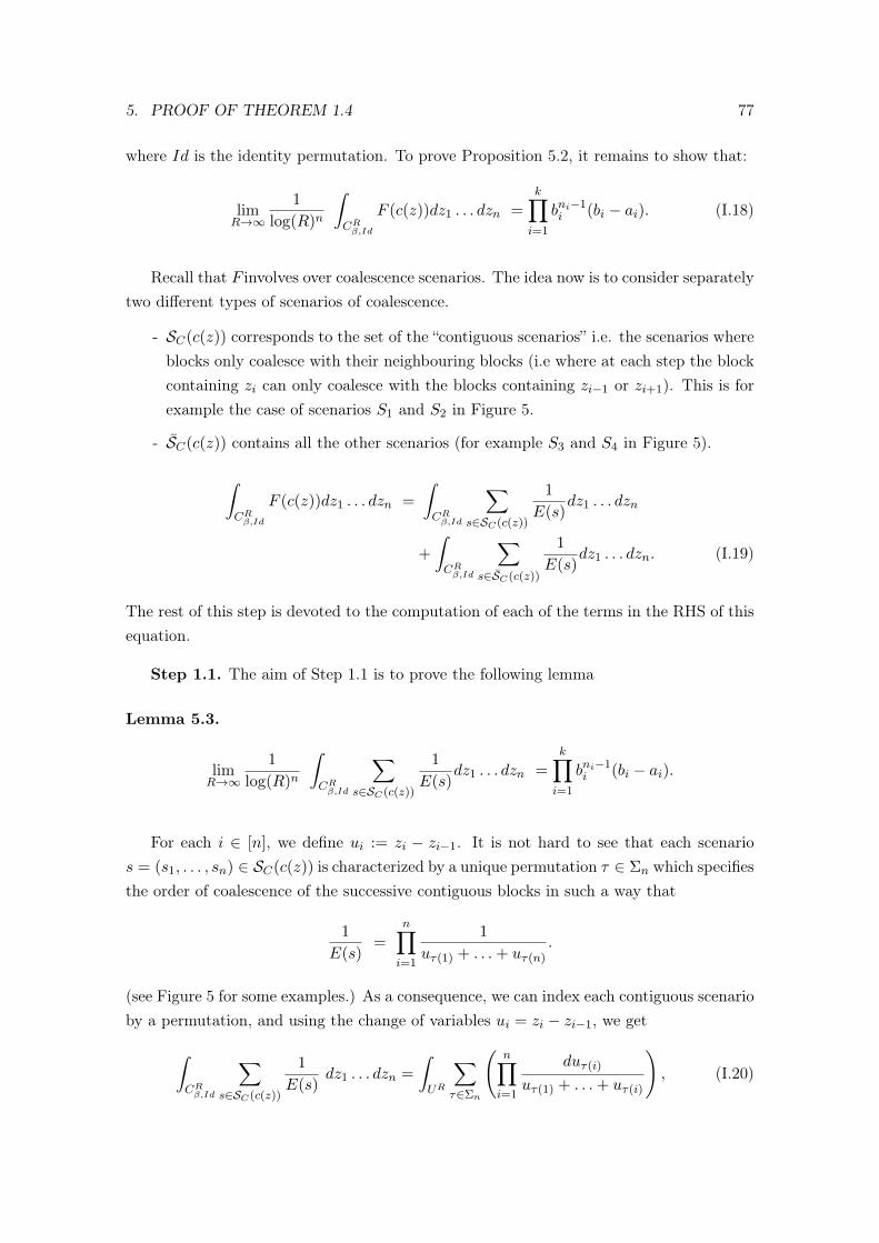
5. PROOF OF THEOREM 1.4 77
where Id is the identity permutation. To prove Proposition 5.2, it remains to show that:
limR→∞
1
log(R)n
∫CRβ,Id
F (c(z))dz1 . . . dzn =k∏i=1
bni−1i (bi − ai). (I.18)
Recall that F involves over coalescence scenarios. The idea now is to consider separatelytwo different types of scenarios of coalescence.
- SC(c(z)) corresponds to the set of the “contiguous scenarios” i.e. the scenarios whereblocks only coalesce with their neighbouring blocks (i.e where at each step the blockcontaining zi can only coalesce with the blocks containing zi−1 or zi+1). This is forexample the case of scenarios S1 and S2 in Figure 5.
- SC(c(z)) contains all the other scenarios (for example S3 and S4 in Figure 5).
∫CRβ,Id
F (c(z))dz1 . . . dzn =
∫CRβ,Id
∑s∈SC(c(z))
1
E(s)dz1 . . . dzn
+
∫CRβ,Id
∑s∈SC(c(z))
1
E(s)dz1 . . . dzn. (I.19)
The rest of this step is devoted to the computation of each of the terms in the RHS of thisequation.
Step 1.1. The aim of Step 1.1 is to prove the following lemma
Lemma 5.3.
limR→∞
1
log(R)n
∫CRβ,Id
∑s∈SC(c(z))
1
E(s)dz1 . . . dzn =
k∏i=1
bni−1i (bi − ai).
For each i ∈ [n], we define ui := zi − zi−1. It is not hard to see that each scenarios = (s1, . . . , sn) ∈ SC(c(z)) is characterized by a unique permutation τ ∈ Σn which specifiesthe order of coalescence of the successive contiguous blocks in such a way that
1
E(s)=
n∏i=1
1
uτ(1) + . . .+ uτ(n).
(see Figure 5 for some examples.) As a consequence, we can index each contiguous scenarioby a permutation, and using the change of variables ui = zi − zi−1, we get
∫CRβ,Id
∑s∈SC(c(z))
1
E(s)dz1 . . . dzn =
∫UR
∑τ∈Σn
(n∏i=1
duτ(i)
uτ(1) + . . .+ uτ(i)
), (I.20)
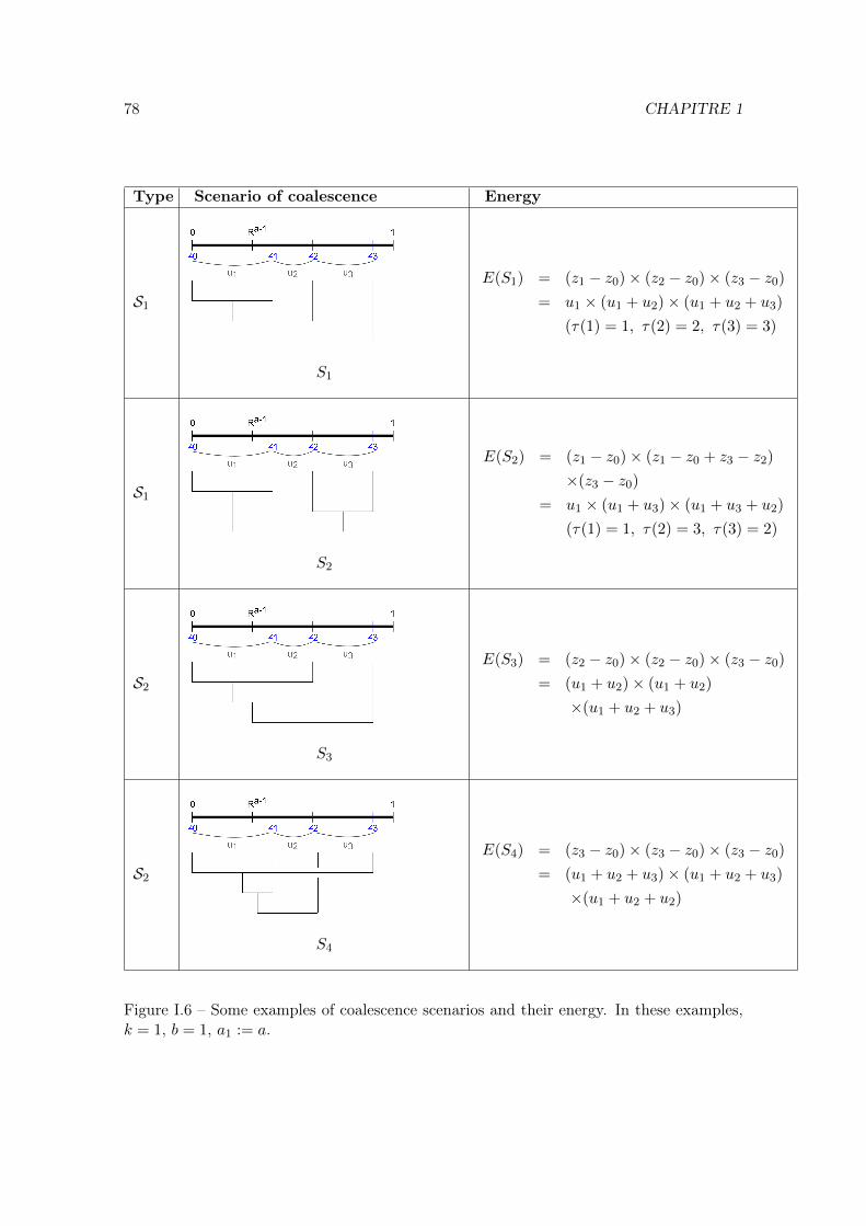
78 CHAPITRE 1
Type Scenario of coalescence Energy
S1
S1
E(S1) = (z1 − z0)× (z2 − z0)× (z3 − z0)
= u1 × (u1 + u2)× (u1 + u2 + u3)
(τ(1) = 1, τ(2) = 2, τ(3) = 3)
S1
S2
E(S2) = (z1 − z0)× (z1 − z0 + z3 − z2)
×(z3 − z0)
= u1 × (u1 + u3)× (u1 + u3 + u2)
(τ(1) = 1, τ(2) = 3, τ(3) = 2)
S2
S3
E(S3) = (z2 − z0)× (z2 − z0)× (z3 − z0)
= (u1 + u2)× (u1 + u2)
×(u1 + u2 + u3)
S2
S4
E(S4) = (z3 − z0)× (z3 − z0)× (z3 − z0)
= (u1 + u2 + u3)× (u1 + u2 + u3)
×(u1 + u2 + u2)
Figure I.6 – Some examples of coalescence scenarios and their energy. In these examples,k = 1, b = 1, a1 := a.

5. PROOF OF THEOREM 1.4 79
where UR is defined as follows. First, let us define (see also Figure I.7)
wR(1) := max(βR−1, Ra1−1)
WR(1) := Rb1−1
∀2 ≤ i ≤ k,wR(i) := Rai−1 −Rbi−1−1
WR(i) := Rbi−1 −Rai−1−1
∀1 ≤ i ≤ k, LR(i) := Rbi−1 −Rai−1.
Finally, we set n0 := 0. Under the assumption that R is large enough so that ∀i ∈[k], Rbi−1 > βR−1
UR := u1, . . . , un ∈ ⊗ki=1
([wR(i),WR(i)]× [βR−1, LR(i)]ni−1
):
∀i ∈ [k],
ni∑j=ni−1+2
uj ≤ LR(i) andn1+...+ni∑
j=1
uj ≤ Rbi−1
In fact, by definition of CRβ,Id, ∀j ∈ [n], βR−1 ≤ uj = zj − zj−1. In addition, the LR(i)’scorrespond to the lengths of the different intervals [Rai−1, Rbi−1], so when zj and zj−1 be-long to the same interval, uj = zj−zj−1 ≤ LR(i) (See Figure I.7). The wR(i)’s correspondto the distance between two contiguous intervals and the WR(i)’s to the maximal distancebetween two points of contiguous intervals. So, when zj and zj−1 belong to different in-tervals then uj = zj − zj−1 ∈ [wR(i),WR(i)] (See Figure I.7). Finally, the last inequalitiescome from the fact that for j ∈ ni−1 + 1, . . . , ni, the zi’s belong to the same interval[ai, bi], so the sum of their distances cannot exceed the length of the interval. In addition,the distance between z0 and zni cannot exceed Rbi−1.
Figure I.7 – The set UR.
To compute the RHS of (I.20), we start by proving the following Lemma.
80 CHAPITRE 1
Lemma 5.4. For any τ ∈ Σn, κ > 1, define
KR,κτ = u1, . . . , un ∈ UR, ∀i ∈ [n], uτ(i) > κ
i−1∑j=1
uτ(j)
KR,κτ = UR \KR,κ
τ
We have
(i) ∀κ > 1, limR→∞
1
log(R)n
∑τ∈Σn
∫KR,κτ
(n∏i=1
duτ(i)
uτ(1) + . . .+ uτ(i)
)= 0
(ii) limκ→∞
limR→∞
1
log(R)n
∑τ∈Σn
∫KR,κτ
(n∏i=1
duτ(i)
uτ(1) + . . .+ uτ(i)
)=
k∏i=1
bni−1i (bi − ai).
Remark 5.5. The proof of Lemma 5.4 is rather cumbersome, but the idea behind the proofis simple. In a nutshell, the idea is that, depending on the positions of the loci (the zi’s),one scenario is much more likely than the others. More precisely, for any configurationz ∈ CRβ,Id, there exists a scenario Smin ∈ SC(c(z)) associated to permutation τmin ∈ Σn
such thatuτmin(1) ≤ uτmin(2) ≤ . . . ≤ uτmin(n).
By coalescing the ui’s in the increasing order, the successive cover lengths are minimised.
Proof. We start by proving (i). We fix τ ∈ Σn, κ > 1. We make the following change ofvariables. Let us define Ψτ such that for 1 ≤ i ≤ n, (Ψτ (u1, . . . , un))τ(i) = uτ(1)+. . .+uτ(i).We have ∫
UR
(n∏i=1
duτ(i)
uτ(1) + . . .+ uτ(i)
)=
∫v∈Ψτ (UR)
dv1 . . . dvnv1 . . . vn
. (I.21)
In particular, as
∀i ∈ [n], uτ(i) ≤ κi−1∑j=1
uτ(j) ⇔ ∀i ∈ [n], vτ(i) ≤ (1 + κ)vτ(i−1),
we have ∫KR,κτ
(n∏i=1
duτ(i)
uτ(1) + . . .+ uτ(i)
)=
∫V R,κτ
dv1 . . . dvnv1 . . . vn
whereV R,κτ = v ∈ Ψτ (UR),∃i ∈ [n], vτ(i) ≤ (1 + κ)vτ(i−1).
For every i ∈ [n], we define
V R,κτ (i) = v ∈ Ψτ (UR), vτ(i) ≤ (1 + κ)vτ(i−1).
5. PROOF OF THEOREM 1.4 81
We have
V R,κτ =
n⋃i=1
V R,κτ (i).
We fix τ ∈ Σn and i ∈ [n]. The vτ(j)’s are the successive cover lengths at each step of thescenario S associated to τ , so it can readily be seen that
∀j ∈ [n], vj ∈ [R−1, 1] and vτ(1) < . . . < vτ(n),
which implies that
V R,κτ (i) ⊂ v ∈ [R−1, 1]n, vτ(i−1) < vτ(i) < (1 + κ)vτ(i−1),
so ∫V R,κτ (i)
dvτ(1) . . . dvτ(n)
vτ(1) . . . vτ(n)≤(∫ 1
R−1
dv
v
)n−2 ∫ 1
R−1
dvτ(i−1)
vτ(i−1)
∫ (1+κ)vτ(i−1)
vτ(i−1)
dvτ(i)
vτ(i)
= log(R)n−2
∫ 1
R−1
dvτ(i−1)
vτ(i−1)log(1 + κ)
= log(R)n−1 log(1 + κ),
which completes the proof of (i).
We now turn to the proof of (ii). We decompose the proof into four steps.
Step a. Define
XR := ⊗ki=1
([wR(i),WR(i)]× [βR−1, LR(i)]ni−1
).
Then
1
log(R)n
∫XR
(n∏i=1
duiui
)=
1
log(R)n
k∏i=1
∫ WR(i)
wR(i)
du
u
(∫ LR(i)
βR−1
du
u
)ni−1
=1
log(R)n
k∏i=1
log
(WR(i)
wR(i)
)log
(LR(i)
βR−1
)ni−1
−→R→∞
k∏i=1
(bi − ai)bni−1i . (I.22)
Step b. Next, for every κ > 1 and for every τ ∈ Σn, we define
XRτ := u1, . . . , un ∈ XR : uτ(1) ≤ . . . ≤ uτ(n),
Aκτ := u1, . . . , un,∀i ∈ [n], uτ(i) > κ
i−1∑j=1
uτ(j).
82 CHAPITRE 1
XR,κτ := XR ∩Aκτ .
By reasoning along the same lines as in the proof of (i), one can show that
limR→∞
1
log(R)n
∣∣∣∣∣∫XRτ
(n∏i=1
duτ(i)
uτ(i)
)−∫XR,κτ
(n∏i=1
duτ(i)
uτ(i)
)∣∣∣∣∣ = 0.
From Step 1, we get that for every κ > 1
limR→∞
1
log(R)n
∑τ∈Σn
∫XR,κτ
(n∏i=1
duτ(i)
uτ(i)
)=
k∏i=1
(bi − ai)bni−1i (I.23)
Step c. We aim of this step is to prove that for every τ ∈ Σn,
limR→∞
1
log(R)n
∫KR,κτ
(n∏i=1
duτ(i)
uτ(i)
)= lim
R→∞
1
log(R)n
∫XR,κτ
(n∏i=1
duτ(i)
uτ(i)
)(I.24)
From the definition of KR,κτ , we have
KR,κτ = XR,κ
τ ∩ (KR1 ∩KR
2 )
where
KR1 := u1, . . . , un, ∀i ∈ [k],
ni∑j=ni−1+2
uj ≤ LR(i) ,
KR2 := u1, . . . , un, ∀i ∈ [k]
n1+...+ni∑j=1
uj ≤ Rbi−1 .
If
limR→∞
1
log(R)n
∣∣∣∣∣∫XR,κτ ∩KR
1
(n∏i=1
duτ(i)
uτ(i)
)−∫XR,κτ
(n∏i=1
duτ(i)
uτ(i)
)∣∣∣∣∣ = 0 (I.25)
and
limR→∞
1
log(R)n
∣∣∣∣∣∫XR,κτ ∩KR
2
(n∏i=1
duτ(i)
uτ(i)
)−∫XR,κτ
(n∏i=1
duτ(i)
uτ(i)
)∣∣∣∣∣ = 0, (I.26)
then
limR→∞
1
log(R)n
∣∣∣∣∣∫KR,κτ
(n∏i=1
duτ(i)
uτ(i)
)−∫XR,κτ
(n∏i=1
duτ(i)
uτ(i)
)∣∣∣∣∣ = 0. (I.27)
We will only prove (I.25), as (I.26) can be proved along the same lines. To do so, we
5. PROOF OF THEOREM 1.4 83
define
Y R,κτ :=u1, . . . , un ∈ ⊗ki=1
[wR(i),WR(i)]×
[βR−1,
LR(i)
1 + 1κ
]ni−1 ,
uτ(1) ≤ . . . ≤ uτ(n).
so that Y R,κτ ⊂ XR
τ . By similar computations as those used in the proof of (i), it can beshown that
limR→∞
1
log(R)n
∫XRτ \Y
R,κτ
n∏i=1
duτ(i)
uτ(i)= 0,
so
limR→∞
1
log(R)n
∣∣∣∣∣∫XR,κτ
n∏i=1
duτ(i)
uτ(i)−∫Y R,κτ ∩Aκτ
n∏i=1
duτ(i)
uτ(i)
∣∣∣∣∣ = 0, (I.28)
and
limR→∞
1
log(R)n
∣∣∣∣∣∫XR,κτ ∩KR
1
n∏i=1
duτ(i)
uτ(i)−∫Y R,κτ ∩Aκτ∩KR
1
n∏i=1
duτ(i)
uτ(i)
∣∣∣∣∣ = 0 (I.29)
Let us show thatY R,κτ ∩Aκτ ∩KR
1 = Y R,κτ ∩Aκτ ,
i.e. that
∀(u1, . . . , un) ∈ Y R,κτ ∩Aκτ , ∀i ∈ [k],
ni∑j=ni−1+2
uj ≤ LR(i).
We fix i ∈ [k] and we define
mi := j ∈ ni−1 + 2, . . . , ni, τ−1(j) = maxτ−1(ni−1 + 2), . . . , τ−1(ni)
As
uτ(mi) > κ
mi−1∑j=1
uτ(j),
thenni∑
j=ni−1+2
uj ≤mi∑j=1
uτ(j) =
(1 +
1
κ
)uτ(mi) ≤
(1 +
1
κ
)LR(i)
1 + 1κ
= LR(i).
Since Y R,κτ ∩ Aκτ ∩ KR
1 = Y R,κτ ∩ Aκτ , combining (I.28) and (I.29), (I.25) is proved.
Equation (I.26) can be proved along the same lines, so (I.27) is verified.
Step d. Finally, for any τ ∈ Σn, for any u1, . . . , un ∈ KR,κτ , we have
∀i ∈ [n], uτ(i) ≤ uτ(1) + . . .+ uτ(i−1) + uτ(i) ≤(
1 +1
κ
)uτ(i),
84 CHAPITRE 1
which implies that
∑τ∈Σn
∫KR,κτ
(n∏i=1
duτ(i)
uτ(i)
)≤∑τ∈Σn
∫KR,κτ
(n∏i=1
duτ(i)
uτ(1) + . . .+ uτ(i)
)
and ∑τ∈Σn
∫KR,κτ
(n∏i=1
duτ(i)
uτ(1) + . . .+ uτ(i)
)≤ 1
(1 + 1κ)n
∑τ∈Σn
∫KR,κτ
(n∏i=1
duτ(i)
uτ(i)
)
This, combined with Step b (see (I.23)) and Step c (see (I.24))
k∏i=1
(bi − ai)bni−1i ≤ lim
R→∞
1
log(R)n
∑τ∈Σn
∫KR,κτ
(n∏i=1
duτ(i)
uτ(1) + . . .+ uτ(i)
)
≤∏ki=1(bi − ai)bni−1
i
(1 + 1κ)n
,
and the conclusion follows by taking κ→∞.
Proof of Lemma 5.3. From (I.20), we have
limR→∞
1
log(R)n
∫CRβ,Id
∑s∈SC(c(z))
1
E(s)dz1 . . . dzn
= limR→∞
1
log(R)n
∑τ∈Σk
∫UR
n∏i=1
duτ(i)
uτ(1) + . . .+ uτ(i)
= limR→∞
1
log(R)n
∑τ∈Σk
(∫KR,κτ
n∏i=1
duτ(i)
uτ(1) + . . .+ uτ(i)+
∫KR,κτ
n∏i=1
duτ(i)
uτ(1) + . . .+ uτ(i)
).
Using Lemma 5.4 and taking κ→∞ in the RHS, we have
limR→∞
1
log(R)n
∫CRβ,Id
∑s∈SC(c(z))
1
E(s)dz1 . . . dzn =
k∏i=1
bni−1i (bi − ai). (I.30)
Step 1.2. The aim of this step is to compute the second term in the RHS of (I.19).
Lemma 5.6.limR→∞
1
log(R)n
∫CRβ,Id
∑S∈SC(c(z))
1
E(S)dz1 . . . dzn = 0.
Proof. We fix z = z0, z1, . . . , zn ∈ CRβ,Id. We start by considering scenarios where blocksonly coalesce with neighbouring blocks, except for one step. In other words, we start by
5. PROOF OF THEOREM 1.4 85
considering scenarios in S ′C(c(z)), the set of scenarios that contain one single coalescenceevent between two non-neighbouring blocks. For example, S3 in Figure 5 is in S ′C(c(z)).We consider S′ = (s′0, s
′1, . . . , s
′n) ∈ S ′C(c(z)), a scenario of coalescence in which step j > 1,
is the only coalescence event between two non neighbouring blocks. The idea is to compareS′ with a scenario S ∈ SC(c(z)) and use this scenario to show that
limR→∞
1
log(R)n
∫CRβ,Id
1
E(S′)dz1 . . . dzn = 0. (I.31)
As already argued each scenario in SC(c(z)) is associated to a permutation τ such that,at each step i, the cover length increases by uτ(i). The scenario S and the correspondingpermutation τ are constructed as follows (and we let the reader refer to Figure I.8 for anexample, where subfigures (i), . . . , (iv) correspond to each step in the following construc-tion).
(i) For 0 ≤ i < j, we set si = s′i. Before step j, there are only coalescence events betweenneighbouring blocks in S′. τ(1), . . . , τ(j − 1) are constructed in such a way that
∀1 ≤ i < j, C(si) = C(s′i) =
i∑k=1
uτ(k).
(ii) At step j, in scenario S′ there is a coalescence event between two non neighbouringblocks, which means that there exists i1 < i2 < . . . < i` such that C(s′j) = C(s′j−1)+
ui1 + . . . + ui` . sj is the partition of order j such that C(sj) = C(sj−1) + ui1 . Weset τ(j) := i1. We have
C(sj) =i∑
k=1
uτ(k) ≤ C(s′j).
(iii) For j < i ≤ j + `− 1, τ(i) := ii−j , i.e., we add successively ui2 , . . . , ui` . We have
∀j < i ≤ j + `− 1, C(si) ≤ C(s′i).
(iv) For j + ` ≤ i ≤ j, the si’s are constructed as follows. Let ur1 , . . . , urp be the ui’sthat have not been added yet to the cover length of S′ (i.e. the ui’s that are not inuτ(1), . . . , uτ(j+`)), indexed in such a way that in S′, ur1 coalesces before ur2 etc. . .. Then we set uτ(j+`+i) = uri . In other words, the uri ’s are added to the coverlength in S in the same order as they are added in S′ (see Figure I.8).
With this construction, we have
1
E(S)=
n∏i=1
1
uτ(1) + . . .+ uτ(i)
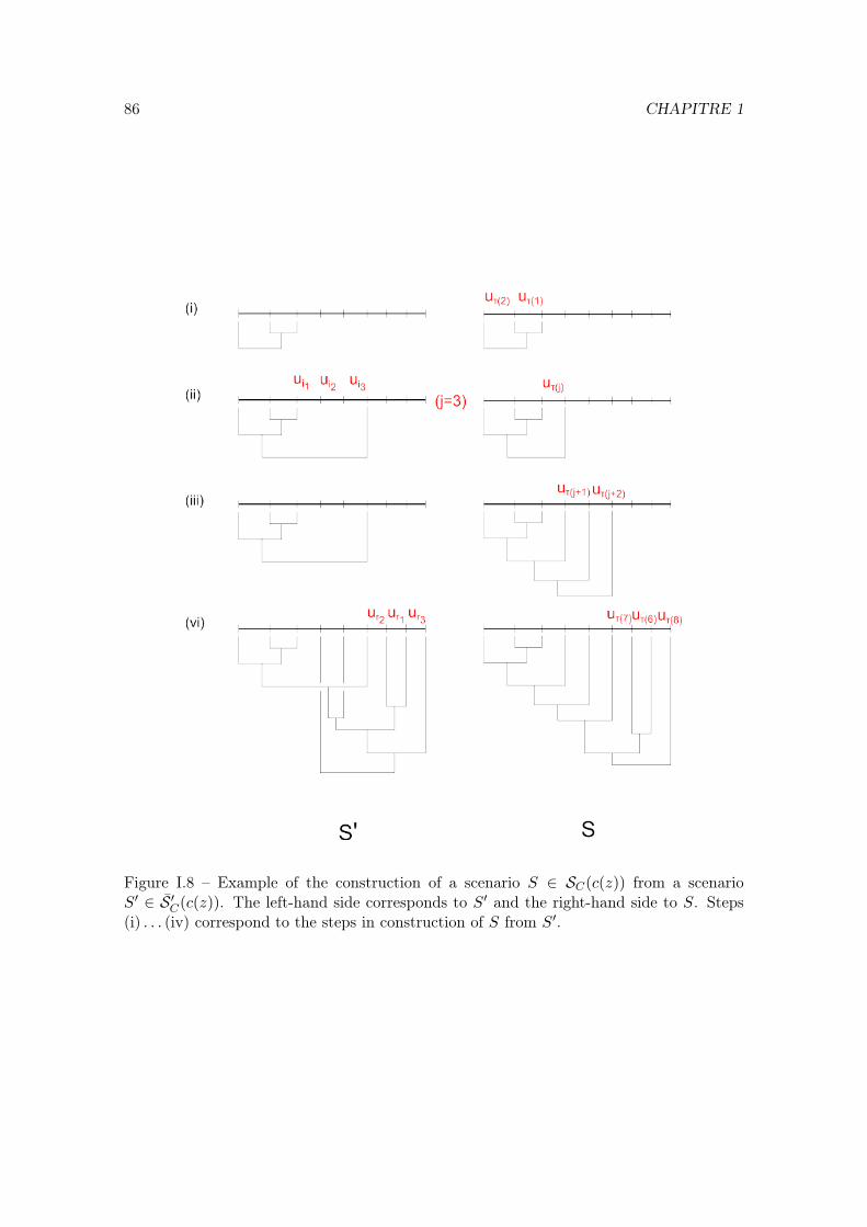
86 CHAPITRE 1
Figure I.8 – Example of the construction of a scenario S ∈ SC(c(z)) from a scenarioS′ ∈ S ′C(c(z)). The left-hand side corresponds to S′ and the right-hand side to S. Steps(i) . . . (iv) correspond to the steps in construction of S from S′.
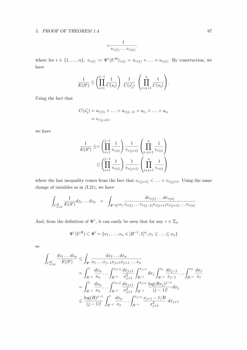
5. PROOF OF THEOREM 1.4 87
=1
vτ(1) . . . vτ(n).
where for i ∈ 1, . . . , n, vτ(i) := Ψτ (UR)τ(i) = uτ(1) + . . . + uτ(i). By construction, wehave
1
E(S′)≤
(j−1∏i=1
1
C(si)
)1
C(s′j)
n∏i=j+1
1
C(si)
.
Using the fact that
C(s′j) = uτ(1) + . . .+ uτ(j−1) + ui1 + . . .+ ui`
= vτ(j+`),
we have
1
E(S′)≤=
(j−1∏i=1
1
vτ(i)
)1
vτ(j+`)
n∏i=j+1
1
vτ(i)
≤
(j−1∏i=1
1
vτ(i)
)1
vτ(j+1)
n∏i=j+1
1
vτ(i)
where the last inequality comes from the fact that vτ(j+1) < . . . < vτ(j)+l. Using the samechange of variables as in (I.21), we have∫
CRβ,Id
1
E(S′)dz1 . . . dzn =
∫Ψτ (UR)
dvτ(1) . . . dvτ(n)
vτ(1) . . . vτ(j−1)vτ(j+1)vτ(j+1) . . . vτ(n)
And, from the definition of Ψτ , it can easily be seen that for any τ ∈ Σn
Ψτ (UR) ⊂ Ψ′ = x1, . . . , xn ∈ [R−1, 1]n, x1 ≤ . . . ≤ xn
so ∫CRβ,Id
dz1 . . . dznE(S′)
≤∫
Ψ′
dx1 . . . dxnx1 . . . xj−1xj+1xj+1 . . . xn
=
∫ 1
R−1
dxnxn
. . .
∫ xj+2
R−1
dxj+1
x2j+1
∫ xj+1
R−1
dxj
∫ xj
R−1
dxj−1
xj−1. . .
∫ x2
R−1
dx1
x1
=
∫ 1
R−1
dxnxn
. . .
∫ xj+2
R−1
dxj+1
x2j+1
∫ xj+1
R−1
log(Rxj)j−1
(j − 1)!dxj
≤ log(R)j−1
(j − 1)!
∫ 1
R−1
dxnxn
. . .
∫ xj+2
R−1
xj+1 − 1/R
x2j+1
dxj+1
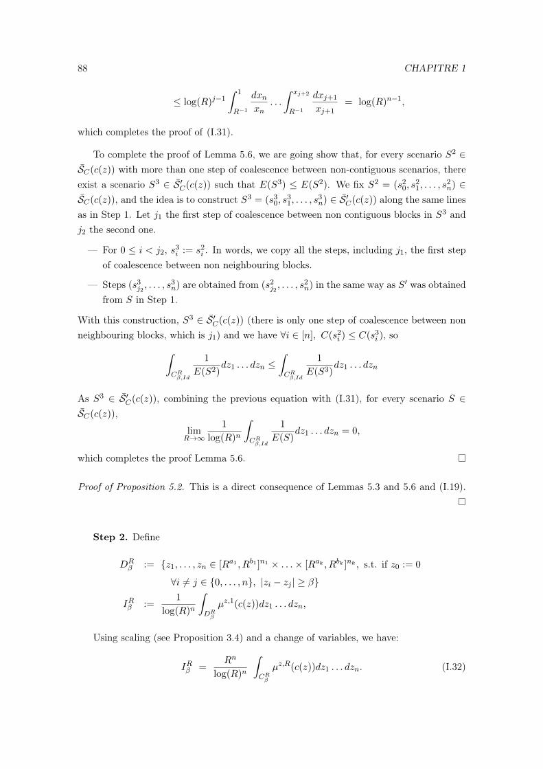
88 CHAPITRE 1
≤ log(R)j−1
∫ 1
R−1
dxnxn
. . .
∫ xj+2
R−1
dxj+1
xj+1= log(R)n−1,
which completes the proof of (I.31).
To complete the proof of Lemma 5.6, we are going show that, for every scenario S2 ∈SC(c(z)) with more than one step of coalescence between non-contiguous scenarios, thereexist a scenario S3 ∈ S ′C(c(z)) such that E(S3) ≤ E(S2). We fix S2 = (s2
0, s21, . . . , s
2n) ∈
SC(c(z)), and the idea is to construct S3 = (s30, s
31, . . . , s
3n) ∈ S ′C(c(z)) along the same lines
as in Step 1. Let j1 the first step of coalescence between non contiguous blocks in S3 andj2 the second one.
— For 0 ≤ i < j2, s3i := s2
i . In words, we copy all the steps, including j1, the first stepof coalescence between non neighbouring blocks.
— Steps (s3j2, . . . , s3
n) are obtained from (s2j2, . . . , s2
n) in the same way as S′ was obtainedfrom S in Step 1.
With this construction, S3 ∈ S ′C(c(z)) (there is only one step of coalescence between nonneighbouring blocks, which is j1) and we have ∀i ∈ [n], C(s2
i ) ≤ C(s3i ), so∫
CRβ,Id
1
E(S2)dz1 . . . dzn ≤
∫CRβ,Id
1
E(S3)dz1 . . . dzn
As S3 ∈ S ′C(c(z)), combining the previous equation with (I.31), for every scenario S ∈SC(c(z)),
limR→∞
1
log(R)n
∫CRβ,Id
1
E(S)dz1 . . . dzn = 0,
which completes the proof Lemma 5.6.
Proof of Proposition 5.2. This is a direct consequence of Lemmas 5.3 and 5.6 and (I.19).
Step 2. Define
DRβ := z1, . . . , zn ∈ [Ra1 , Rb1 ]n1 × . . .× [Rak , Rbk ]nk , s.t. if z0 := 0
∀i 6= j ∈ 0, . . . , n, |zi − zj | ≥ β
IRβ :=1
log(R)n
∫DRβ
µz,1(c(z))dz1 . . . dzn,
Using scaling (see Proposition 3.4) and a change of variables, we have:
IRβ =Rn
log(R)n
∫CRβ
µz,R(c(z))dz1 . . . dzn. (I.32)
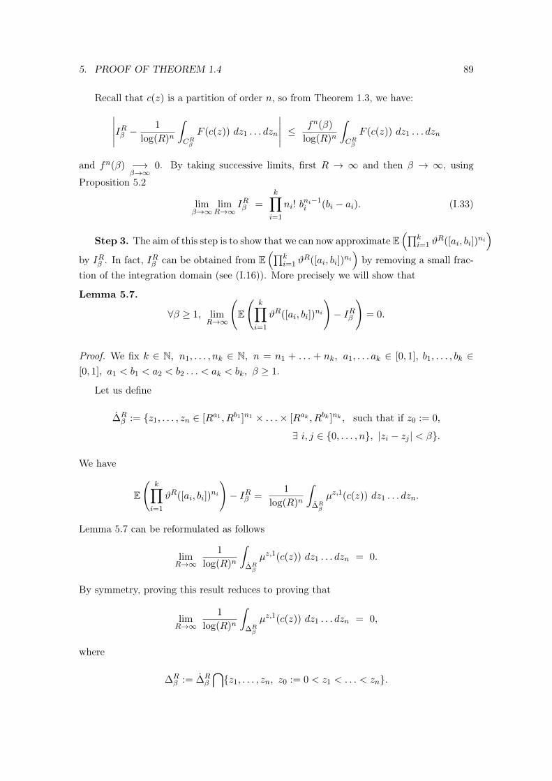
5. PROOF OF THEOREM 1.4 89
Recall that c(z) is a partition of order n, so from Theorem 1.3, we have:∣∣∣∣∣IRβ − 1
log(R)n
∫CRβ
F (c(z)) dz1 . . . dzn
∣∣∣∣∣ ≤ fn(β)
log(R)n
∫CRβ
F (c(z)) dz1 . . . dzn
and fn(β) −→β→∞
0. By taking successive limits, first R → ∞ and then β → ∞, using
Proposition 5.2
limβ→∞
limR→∞
IRβ =k∏i=1
ni! bni−1i (bi − ai). (I.33)
Step 3. The aim of this step is to show that we can now approximate E(∏k
i=1 ϑR([ai, bi])
ni)
by IRβ . In fact, IRβ can be obtained from E(∏k
i=1 ϑR([ai, bi])
ni)by removing a small frac-
tion of the integration domain (see (I.16)). More precisely we will show that
Lemma 5.7.
∀β ≥ 1, limR→∞
(E
(k∏i=1
ϑR([ai, bi])ni
)− IRβ
)= 0.
Proof. We fix k ∈ N, n1, . . . , nk ∈ N, n = n1 + . . . + nk, a1, . . . ak ∈ [0, 1], b1, . . . , bk ∈[0, 1], a1 < b1 < a2 < b2 . . . < ak < bk, β ≥ 1.
Let us define
∆Rβ := z1, . . . , zn ∈ [Ra1 , Rb1 ]n1 × . . .× [Rak , Rbk ]nk , such that if z0 := 0,
∃ i, j ∈ 0, . . . , n, |zi − zj | < β.
We have
E
(k∏i=1
ϑR([ai, bi])ni
)− IRβ =
1
log(R)n
∫∆Rβ
µz,1(c(z)) dz1 . . . dzn.
Lemma 5.7 can be reformulated as follows
limR→∞
1
log(R)n
∫∆Rβ
µz,1(c(z)) dz1 . . . dzn = 0.
By symmetry, proving this result reduces to proving that
limR→∞
1
log(R)n
∫∆Rβ
µz,1(c(z)) dz1 . . . dzn = 0,
where
∆Rβ := ∆R
β
⋂z1, . . . , zn, z0 := 0 < z1 < . . . < zn.
90 CHAPITRE 1
Let S be the set of all subsets of [n] containing at most n − 1 elements. For S ∈ S,define
∆Rβ,S = ∆R
β
⋂z1, . . . , zn : ∀i ∈ S, |zi − zi−1| ≥ β, ∀i /∈ S, |zi − zi−1| < β.
in such a way that∆Rβ =
⋃S∈S
∆Rβ,S .
It follows that ∫∆Rβ
µz,1(c(z)) dz1 . . . dzn =∑S∈S
∫∆Rβ,S
µz,1(c(z)) dz1 . . . dzn
≤∑S∈S
∫∆Rβ,S
µz,1(πS) dz1 . . . dzn
where ∀S ∈ S, πS = π ∈ Pz, ∀i, j ∈ S, zi ∼π zj (and where the inequality follows fromthe fact that c(z) ∈ πS). We define zS := zi, i ∈ S. Proposition 2.2 gives:
µz,1(πS) = µzS ,1(c(zS)).
Define
∆Rβ,S := (zi)i∈S : ∃ (zj)j∈1,...,n\S , (z1, . . . , zn) ∈ ∆R
β,S.
We let the reader convince herself that, for any S ∈ S there exists m1, . . . ,mk ∈ N, m1 +
. . .+mk = |S|, such that ∆Rβ,S can be rewritten as
∆Rβ,S = z1, . . . z|S| ∈ [Ra1−1, Rb1−1]m1 × . . .× [Rak−1, Rbk−1]mk :
z0 := 0 ≤ z1 ≤ . . . ≤ z|S| and ∀ i, j ∈ S, i 6= j, |zi − zj | > β.
This allows us to rewrite the previous inequality as∫∆Rβ
µz,1(c(z)) dz1 . . . dzn ≤∑S∈S
∫∆Rβ,S
µzS ,1(c(zS))dz1 . . . dzi . . .︸ ︷︷ ︸
i∈S
. . . dzj . . .︸ ︷︷ ︸j 6∈S
=∑S∈S
∫∆Rβ,S
µzS ,1(c(z))dz1 . . . dz|S|
∏j /∈S
∫ zj−1+β
zj−1
dzj
= βn−|S|
∑S∈S
∫∆Rβ,S
µzS ,1(c(z))dz1 . . . dz|S| (I.34)
5. PROOF OF THEOREM 1.4 91
where z = (z0, . . . , z|S|) and z0 = 0. From (I.33), we have
limR→∞
1
log(R)|S|
∫∆Rβ,S
µzS ,1(c(z))dz1 . . . dz|S| =
∏i∈[k], mi 6=0
bmi−1i (bi − ai).
As |S| < n,
limR→∞
1
log(R)n
∑S∈S
∫∆Rβ,S
µzS ,1(c(z))dz1 . . . dz|S| = 0,
which combined with (I.34) concludes the proof of the Lemma 5.7.
Step 4. Conclusion. Combining (I.33) and with Lemma 5.7 (Step 3), we have provedthat for every k-tuple of disjoint intervals [ai, bi]ki=1 and any k-tuple of integers niki=1
limR→∞
E
(k∏i=1
ϑR([ai, bi])ni
)=
k∏i=1
ni! bni−1i (bi − ai).
So, using Lemma 5.1, ϑR converges to ϑ∞ in distribution in the weak topology. In partic-ular, we have
LR(0) = ϑR[0, 1] +1
log(R)
∫[0,1]
1x∼π0dx
and1
log(R)
∫[0,1]
1x∼π0dx ≤1
log(R)−→R→∞
0
so, using equation (I.14), we have
∀n ∈ N, limR→∞
E(LR(0)n) = limR→∞
E(ϑR[0, 1]n) = n!
which are the moments of the exponential distribution of parameter 1. As in the proof ofLemma 5.1, using Carleman’s condition (for k = 1), this implies that LR(0) converges indistribution to an exponential distribution of parameter 1.

92 CHAPITRE 1
Chapter II
Deriving the expected number ofdetected haplotype junctions inhybrid populations
In this chapter, I present some work in progress, in collaboration with Thijs Janzen,from Carl von Ossietzky University (Oldenburg, Germany). It aims at using the AncestralRecombination Graph to study hybridization.
The idea is to consider a hybrid population that emerged from a single hybridiza-tion event between two ancestral populations P and Q. We assume that, at time 0, theproportion of individuals from population P is p and the proportion of individuals frompopulation Q is q = 1− p. The evolution of the hybrid population can be modelled usinga Wright-Fisher model with recombination, which is an analogous in discrete time to theMoran model with recombination used in Chapter I. Instead of assuming that, at time 0
each individual has her chromosome painted in a distinct color, we assume that there areonly two colors, corresponding to each of the ancestral populations. By the blending effectof recombination, the chromosomes of the hybrids are mosaics of these two colors. Forinstance, in Figure II.1, the blue color indicates that the individual carrying the displayedchromosome inherited this portion of the chromosome from the blue ancestral subpopula-tion.
Inferring which fragments of the chromosome have been inherited from each ancestralsubpopulation from genomic data is not straightforward. As the two ancestral populationsare supposed to be closely related species, their genomes are quite similar. Therefore,one needs to use molecular markers: a marker is a locus that segregates between the twoancestral populations, i.e. such that each of the ancestral populations carries a differentallele at this locus. If two consecutive markers carry different allelles (i.e. each one carriesthe allele associated to one of the subpopulations) we say that we observe a “junction”.
93
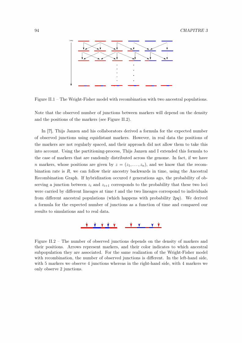
94 CHAPITRE 3
Figure II.1 – The Wright-Fisher model with recombination with two ancestral populations.
Note that the observed number of junctions between markers will depend on the densityand the positions of the markers (see Figure II.2).
In [?], Thijs Janzen and his collaborators derived a formula for the expected numberof observed junctions using equidistant markers. However, in real data the positions ofthe markers are not regularly spaced, and their approach did not allow them to take thisinto account. Using the partitioning-process, Thijs Janzen and I extended this formula tothe case of markers that are randomly distributed across the genome. In fact, if we haven markers, whose positions are given by z = (z1, . . . , zn), and we know that the recom-bination rate is R, we can follow their ancestry backwards in time, using the AncestralRecombination Graph. If hybridization occured t generations ago, the probability of ob-serving a junction between zi and zi+1 corresponds to the probability that these two lociwere carried by different lineages at time t and the two lineages correspond to individualsfrom different ancestral populations (which happens with probability 2pq). We deriveda formula for the expected number of junctions as a function of time and compared ourresults to simulations and to real data.
Figure II.2 – The number of observed junctions depends on the density of markers andtheir positions. Arrows represent markers, and their color indicates to which ancestralsubpopulation they are associated. For the same realization of the Wright-Fisher modelwith recombination, the number of observed junctions is different. In the left-hand side,with 5 markers we observe 4 junctions whereas in the right-hand side, with 4 markers weonly observe 2 junctions.

1. INTRODUCTION 95
1 Introduction
The traditional view where species or lineages accumulate incompatibilities over timeand become reproductively isolated from each other has led to insight into the processesgenerating and maintaining biodiversity [?]. This view has proven to be misleading how-ever, and it has become apparent that lineages do not necessarily only branch, but thatlineages can also come back together [?]. In plants, it has been known for quite sometime that hybridization between lineages can lead to not only viable offspring, but can alsopotentially lead to the formation of new lineages, and ultimately, species [?]. It has longbeen debated whether this process could also happen in animals, but over the past fewyears numerous examples have appeared, including, but not limited to, butterflies [?, ?],cichlid fishes [?, ?], warblers [?], fruit flies [?] and sculpins [?].
Understanding the time-line of these hybridization events is paramount in obtaining afull understanding of the process and its impact. Often, hybridization processes occur fast,on a timescale that is too rapid to accumulate enough mutations. Instead, recombinationprocesses are sufficiently rapid so as to leave a footprint in genomes undergoing hybridiza-tion. After admixture of two lineages, contiguous genomic blocks within the genome arebroken down by recombination over time. The delineations between these blocks weretermed “junctions” by Fisher [?, ?], and inheritance of these junctions is similar to thatof point-mutations. Further work on the theory of junctions has shown how junctionsaccumulate over time for sib-sib mating [?], self-fertilization [?], alternate parent-offspringmating [?, ?], a randomly mating population [?], and for sub-structured populations [?, ?].
So far, applying the theory of junctions has shown to be difficult, as it requires extensivegenotyping of the admixed lineage, but also of the parental lineages. With the currentdecrease in genotyping costs [?], such analyses are currently coming well within reach,and frameworks are currently being developed that assist in inferring local ancestry, givenmolecular data of parental and admixed lineages (in order to identify the markers of the twopopulations). Nevertheless, molecular data always provide an imperfect picture of ancestryalong the genome, and inferring the number of junctions along a genome remains limited bythe number of diagnostic markers available. Currently, the theory of junctions does not takeinto account the effect of a limited number of genetic markers, and previous analyses takinginto account the effect of a limited number of markers have had to resort to simulations[?, ?]. Janzen et al. [?] provided an analytical description of the effect of using evenlyspaced genetic markers, and they find that predictions taking into account this marker effectdiffer substantially from more naive predictions not taking this marker effect into account.Molecular markers are rarely evenly spaced, and it is therefore warranted to extend thecurrent theory of junctions by including the effect of non-evenly spaced molecular markerson inferring the number of junctions in a genome, and inference of subsequent properties,such as the time since admixture. Here we present a new description of the expected
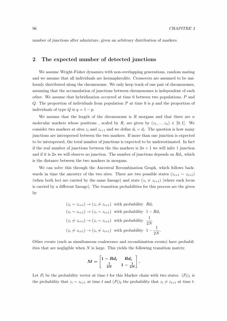
96 CHAPITRE 3
number of junctions after admixture, given an arbitrary distribution of markers.
2 The expected number of detected junctions
We assume Wright-Fisher dynamics with non-overlapping generations, random matingand we assume that all individuals are hermaphrodite. Crossovers are assumed to be uni-formly distributed along the chromosome. We only keep track of one pair of chromosomes,assuming that the accumulation of junctions between chromosomes is independent of eachother. We assume that hybridization occurred at time 0 between two populations, P andQ. The proportion of individuals from population P at time 0 is p and the proportion ofindividuals of type Q is q = 1− p.
We assume that the length of the chromosome is R morgans and that there are nmolecular markers whose positions , scaled by R, are given by (z1, . . . zn) ∈ [0, 1]. Weconsider two markers at sites zi and zi+1 and we define di = di. The question is how manyjunctions are interspersed between the two markers. If more than one junction is expectedto be interspersed, the total number of junctions is expected to be underestimated. In factif the real number of junctions between the tho markers is 2n+ 1 we will infer 1 junctionand if it is 2n we will observe no junction. The number of junctions depends on Rdi, whichis the distance between the two markers in morgans.
We can solve this through the Ancestral Recombination Graph, which follows back-wards in time the ancestry of the two sites. There are two possible states (zi+1 ∼ zi+1)
(when both loci are carried by the same lineage) and state (zi 6∼ zi+1) (where each locusis carried by a different lineage). The transition probabilities for this process are the givenby
(zi ∼ zi+1)→ (zi 6∼ zi+1) with probability Rdi
(zi ∼ zi+1)→ (zi ∼ zi+1) with probability 1−Rdi
(zi 6∼ zi+1)→ (zi ∼ zi+1) with probability1
2N
(zi 6∼ zi+1)→ (zi 6∼ zi+1) with probability 1− 1
2N.
Other events (such as simultaneous coalescence and recombination events) have probabil-ities that are negligible when N is large. This yields the following transition matrix:
M =
[1 − Rdi Rdi
12N
1 − 12N
].
Let Pt be the probability vector at time t for this Markov chain with two states. (Pt)1 isthe probability that zi ∼ zi+1 at time t and (Pt)2 the probability that zi 6∼ zi+1 at time t.
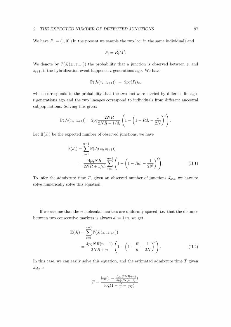
2. THE EXPECTED NUMBER OF DETECTED JUNCTIONS 97
We have P0 = (1, 0) (In the present we sample the two loci in the same individual) and
Pt = P0Mt.
We denote by P(Jt(zi, zi+1)) the probability that a junction is observed between zi andzi+1, if the hybridization event happened t generations ago. We have
P(Jt(zi, zi+1)) = 2pq(Pt)2,
which corresponds to the probability that the two loci were carried by different lineagest generations ago and the two lineages correspond to individuals from different ancestralsubpopulations. Solving this gives:
P(Jt(zi, zi+1)) = 2pq2NR
2NR+ 1/di
(1−
(1−Rdi −
1
2N
)t).
Let E(Jt) be the expected number of observed junctions, we have
E(Jt) =n−1∑i=1
P(Jt(zi, zi+1))
=4pqNR
2NR+ 1/di
n−1∑i=1
(1−
(1−Rdi −
1
2N
)t). (II.1)
To infer the admixture time T , given an observed number of junctions Jobs, we have tosolve numerically solve this equation.
If we assume that the n molecular markers are uniformly spaced, i.e. that the distancebetween two consecutive markers is always d := 1/n, we get
E(Jt) =
n−1∑i=1
P(Jt(zi, zi+1))
=4pqNR(n− 1)
2NR+ n
(1−
(1− R
n− 1
2N
)t). (II.2)
In this case, we can easily solve this equation, and the estimated admixture time T givenJobs is
T =log(1− Jobs(2NR+n)
4pqRN(n−1) )
log(1− Rn −
12N )
.
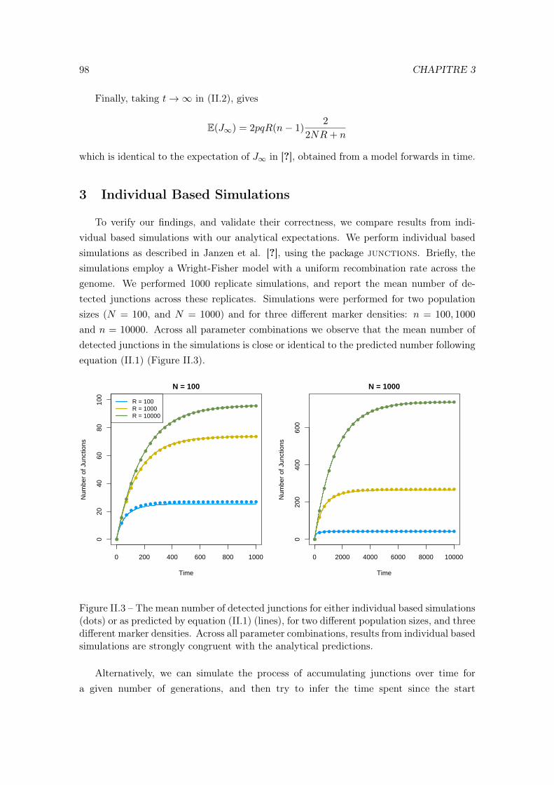
98 CHAPITRE 3
Finally, taking t→∞ in (II.2), gives
E(J∞) = 2pqR(n− 1)2
2NR+ n
which is identical to the expectation of J∞ in [?], obtained from a model forwards in time.
3 Individual Based Simulations
To verify our findings, and validate their correctness, we compare results from indi-vidual based simulations with our analytical expectations. We perform individual basedsimulations as described in Janzen et al. [?], using the package junctions. Briefly, thesimulations employ a Wright-Fisher model with a uniform recombination rate across thegenome. We performed 1000 replicate simulations, and report the mean number of de-tected junctions across these replicates. Simulations were performed for two populationsizes (N = 100, and N = 1000) and for three different marker densities: n = 100, 1000
and n = 10000. Across all parameter combinations we observe that the mean number ofdetected junctions in the simulations is close or identical to the predicted number followingequation (II.1) (Figure II.3).
0 200 400 600 800 1000
020
4060
8010
0
N = 100
Time
Num
ber
of J
unct
ions
R = 100R = 1000R = 10000
0 2000 4000 6000 8000 10000
020
040
060
0
N = 1000
Time
Num
ber
of J
unct
ions
Figure II.3 – The mean number of detected junctions for either individual based simulations(dots) or as predicted by equation (II.1) (lines), for two different population sizes, and threedifferent marker densities. Across all parameter combinations, results from individual basedsimulations are strongly congruent with the analytical predictions.
Alternatively, we can simulate the process of accumulating junctions over time fora given number of generations, and then try to infer the time spent since the start
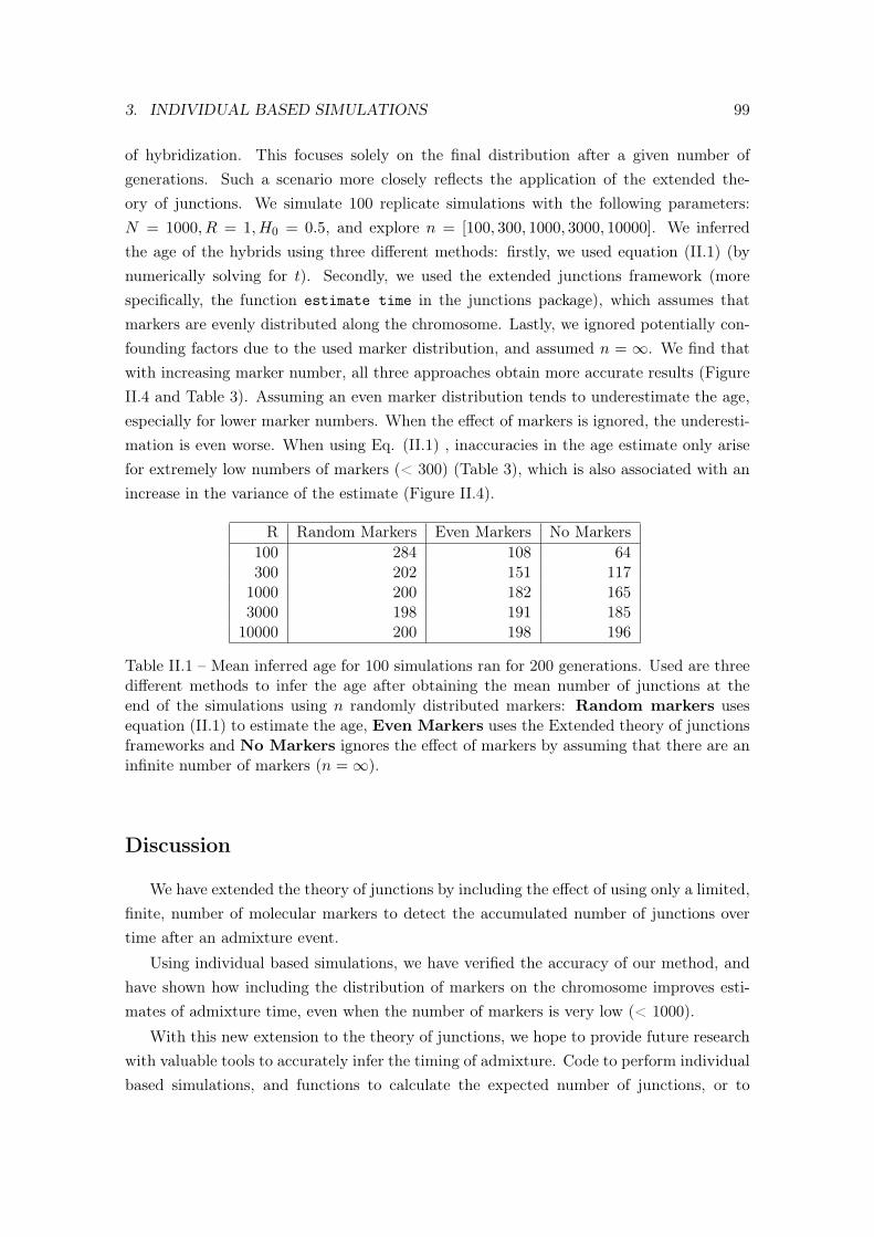
3. INDIVIDUAL BASED SIMULATIONS 99
of hybridization. This focuses solely on the final distribution after a given number ofgenerations. Such a scenario more closely reflects the application of the extended the-ory of junctions. We simulate 100 replicate simulations with the following parameters:N = 1000, R = 1, H0 = 0.5, and explore n = [100, 300, 1000, 3000, 10000]. We inferredthe age of the hybrids using three different methods: firstly, we used equation (II.1) (bynumerically solving for t). Secondly, we used the extended junctions framework (morespecifically, the function estimate time in the junctions package), which assumes thatmarkers are evenly distributed along the chromosome. Lastly, we ignored potentially con-founding factors due to the used marker distribution, and assumed n = ∞. We find thatwith increasing marker number, all three approaches obtain more accurate results (FigureII.4 and Table 3). Assuming an even marker distribution tends to underestimate the age,especially for lower marker numbers. When the effect of markers is ignored, the underesti-mation is even worse. When using Eq. (II.1) , inaccuracies in the age estimate only arisefor extremely low numbers of markers (< 300) (Table 3), which is also associated with anincrease in the variance of the estimate (Figure II.4).
R Random Markers Even Markers No Markers100 284 108 64300 202 151 1171000 200 182 1653000 198 191 18510000 200 198 196
Table II.1 – Mean inferred age for 100 simulations ran for 200 generations. Used are threedifferent methods to infer the age after obtaining the mean number of junctions at theend of the simulations using n randomly distributed markers: Random markers usesequation (II.1) to estimate the age, Even Markers uses the Extended theory of junctionsframeworks and No Markers ignores the effect of markers by assuming that there are aninfinite number of markers (n =∞).
Discussion
We have extended the theory of junctions by including the effect of using only a limited,finite, number of molecular markers to detect the accumulated number of junctions overtime after an admixture event.
Using individual based simulations, we have verified the accuracy of our method, andhave shown how including the distribution of markers on the chromosome improves esti-mates of admixture time, even when the number of markers is very low (< 1000).
With this new extension to the theory of junctions, we hope to provide future researchwith valuable tools to accurately infer the timing of admixture. Code to perform individualbased simulations, and functions to calculate the expected number of junctions, or to
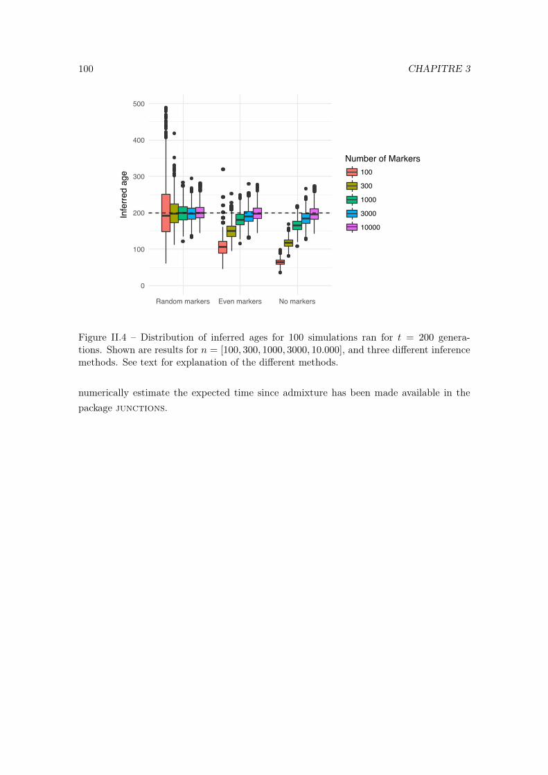
100 CHAPITRE 3
0
100
200
300
400
500
Random markers Even markers No markers
Infe
rre
d a
ge
Number of Markers
100
300
1000
3000
10000
Figure II.4 – Distribution of inferred ages for 100 simulations ran for t = 200 genera-tions. Shown are results for n = [100, 300, 1000, 3000, 10.000], and three different inferencemethods. See text for explanation of the different methods.
numerically estimate the expected time since admixture has been made available in thepackage junctions.
Chapter III
How does geographical distancetranslate into genetic distance?
Joint work with Emmanuel Schertzer. Currentlyin revision in Stochastic Processes and their Ap-plications [?].
Abstract
Geographic structure can affect patterns of genetic differentiation and speciation rates.In this article, we investigate the dynamics of genetic distances in a geographically struc-tured metapopulation. We model the metapopulation as a weighted directed graph, withd vertices corresponding to d subpopulations that evolve according to an individual basedmodel. The dynamics of the genetic distances is then controlled by two types of transitions-mutation and migration events. We show that, under a rare mutation - rare migrationregime, intra subpopulation diversity can be neglected and our model can be approximatedby a population based model. We show that under a large population - long chromosomelimit, the genetic distance between two subpopulations converges to a deterministic quan-tity that can asymptotically be expressed in terms of the hitting time between two randomwalks in the metapopulation graph. Our result shows that the genetic distance betweentwo subpopulations does not only depend on the direct migration rates between them buton the whole metapopulation structure.
1 Introduction
1.1 Genetic distances in structured populations. Speciation
In most species, the geographical range is much larger than the typical dispersal dis-tance of its individuals. A species is usually structured into several local subpopulations
101
102 CHAPITRE 2
with limited genetic contact. Because migration only connects neighbouring populations,more often than not, populations can only exchange genes indirectly, by reproducing withone or several intermediary populations. As a consequence, the geographical structuretends to buffer the homogenising effect of migration, and as such, it is considered to beone of the main drivers for the persistence of genetic variability within species (see [?] or[?]).
The aim of this article is to present some analytical results on the genetic compositionof a species emerging from a given geographical structure. The main motivation behind thiswork is to study speciation. When two populations accumulate enough genetic differences,they may become reproductively isolated, and therefore considered as different species. Asthe geographic structure of a species is one of the main drivers for the genetic differentiationbetween subpopulations, this work should shed light on which are the geographic conditionsunder which new species can emerge.
Several authors have studied parapatric speciation, i.e. speciation in the presence ofgene flow between subpopulations, for example [?, ?, ?] and [?, ?]. In their models, someloci on the chromosome are responsible for reproductive isolation. These loci may be in-volved in incompatibilities at any level of biological organisation (molecular, physiological,behavioural etc) and either prevent mating (pre-zygotic incompatibilities) or prevent thedevelopment of hybrids (post-zygotic incompatibilities). The number of segregating lociincreases through the accumulation of mutations, and decreases after each migration event(creating the opportunity for some gene exchange between the migrants and the host pop-ulation). When the number of segregating loci between two individuals reaches a certainthreshold, they become reproductively incompatible. For example, Yamaguci and Iwasa[?, ?] studied the case of a metapopulation containing two homogeneous subpopulations.The authors studied how the genetic distance, defined as the number of loci differing be-tween the two subpopulations, evolves through time, using a continuous-time model. Whenconsidering metapopulations with more than two subpopulations, this kind of dynamicsmay translate into complex patterns of speciation. One particularly intriguing exampleis the case of ring species [?, ?], where two neighbouring subpopulations are too differentto be able to reproduce with one another but can exchange genes indirectly, by repro-ducing with a series of intermediate subpopulations that form a geographic “ring”. Howthese patterns emerge and are maintained is still poorly understood, and we hope that ouranalytical result might shed some new light on the subject.
1.2 Population divergence and fitness landscapes
To study speciation by accumulation of genetic differences, we model the evolution ofsome loci on the chromosome, that are potentially involved in reproductive incompati-bilities. To visualise these evolutionary dynamics, Wright [?] suggested the metaphor ofadaptive landscapes. Adaptive landscapes represent individual fitness as a function defined
1. INTRODUCTION 103
on the genotype space, which is a multi-dimensional space representing all possible geno-types. Wright emphasised the idea of ‘rugged’ adaptive landscapes, with peaks of fitnessrepresenting species and valleys representing unfit hybrids. Speciation, seen as a popula-tion moving from one peak to another, implies a temporary reduction in fitness, which isnot very likely to occur in large populations, where genetic drift is not important enoughto counterbalance the effect of selection (see [?] for a more detailed discussion). However,Gavrilets [?] suggested the idea of ‘holey’ adaptive landscapes, where local fitness maximacan be partitioned into connected sets (called evolutionary ridges). Speciation is thereforeseen as a population diffusing across a ridge, by neutral mutation steps, until it stands atthe other side of a hole. Theoretical models, such as [?], have shown, using percolationtheory, that in high-dimensional genotype spaces, fit genotypes are typically connected byevolutionary ridges.
Our model (see Section 1.3) is built in this framework. In fact we will assume that,in large populations, deleterious mutations are washed away by selection at the micro-evolutionary timescale and describe the evolutionary dynamics for our set of incompatibilitycontrolling loci as neutral (any genotype on the evolutionary ridge can be accessed by singlemutation neutral steps). This is the idea behind the description of our model in Section1.3.
Further, we consider that the evolutionary dynamics along the ridge are slow (as randommutations are very likely to be deleterious, mutations along the evolutionary ridge areassumed to be rarer than in the typical population genetics framework), which is why westudy our model in a low mutation - low migration regime (see Section 1.4 for more details).This assumption is commonly made when studying speciation, for example in [?] or [?].
1.3 An individual based model (IBM)
We model the metapopulation as a weighted directed graph with d vertices, correspond-ing to the different subpopulations. Each directed edge (i, j) is equipped with a migrationrate in each direction. (In particular, if two subpopulations are not connected, we assumethat the migration rates are equal to 0.) We assume the existence of two scaling parame-ters, γ and ε, that will converge to 0 successively (first γ → 0 and then ε→ 0, see Section1.4 for more details).
Each subpopulation consists of nεi individuals, i ∈ E := 1, · · · , d. Each individualcarries a single chromosome of length 1, which contains lε loci of interest (that are involvedin reproductive incompatibilities). We assume that the vector of positions for those loci –denoted by Lε = x1, · · · , xlε – is obtained by throwing lε uniform random variables on[0, 1]. (The positions are chosen randomly at time 0, but are the same for all individualsand do not change through time).
Conditioned on Lε, each subpopulation then evolves according to an haploid neutralMoran model with recombination.
104 CHAPITRE 2
— Each individual x reproduces at constant rate 1 and chooses a random partner y(y 6= x). Upon reproduction, their offspring replaces a randomly chosen individualin the population.
— The new individual inherits a chromosome which is a mixture of the parental chro-mosomes. Both parental chromosomes are cut into fragments in the following way:we assume a Poisson Point Process of intensity λ on [0, 1]. Two loci belong to thesame fragment iff there is no atom of the Poisson Point Process between them. Foreach fragment, the offspring inherits the fragment of one of the two parents chosenrandomly.
To our Moran model we add two other types of events:
— Mutation occurs at rate bγ,ε per individual, per locus according to an infinite allelemodel.
— Migration from subpopulation i to subpopulation j occurs at rate mγij . At each
migration event, one individual migrates from subpopulation i to j, and replacesone individual chosen uniformly at random in the resident population. (We set∀i ∈ E, mγ
i,i = 0.)
We define the genetic distance between two individuals x and y as:
δγ,ε(x, y) =1
lε# k ∈ 1, · · · , lε : x and y differ at locus k .
Consider two subpopulations i and j and let i1, · · · , inεi the individuals in popula-tion i and j1, · · · , jnεj the individuals in population j. The genetic distance betweensubpopulations i and j is defined as follows:
dε,γ(i, j) =
1
nεi
∑x∈i1,··· ,inε
i
miny∈j1,··· ,jnε
jδγ,ε(x, y)
∨ 1
nεj
∑y∈j1,··· ,jnε
j
minx∈i1,··· ,inε
iδγ,ε(x, y)
.(III.1)
This corresponds to the so-called modified Haussdorff distance between subpopulations, asintroduced by [?]. (This distance has the advantage of averaging over the individuals ineach subpopulation, so introducing a single mutant or migrant would produce a smoothvariation in the genetic distances.)
1.4 Slow mutation–migration and large population - long chromosomeregime.
In this section, we start by describing in more details the slow mutation–migrationregime alluded in Sections 1.2 and 1.3.
It is well known that in the absence of mutation and migration, the neutral Moranmodel describing the dynamics at the local level reaches fixation in finite time: the average
1. INTRODUCTION 105
time to fixation for a single locus is of the order of the size of the subpopulation [?, ?] (Inour multi-locus model, it will also depend on the number of loci and on the recombinationrate λ.) Heuristically, if we assume a low mutation - low migration regime, i.e. that
∀i, j ∈ E, 1
bγ,εnεi,
1
mγi,j
nεj , lε 1, (III.2)
the average time between two migration events (1/mγi,j), and the average time between
two successive mutations at a given locus (1/(bγ,εnεj)) are much larger than the averagetime to fixation. This ensures that the fixation process is fast compared to the time-scaleof mutation and migration, and, as a result, when looking at a randomly chosen locus,subpopulations are homogeneous except for short periods of time right after a migrationevent or a mutation event. This suggests that if we accelerate time properly, we can neglectintra-subpopulation diversity and approximate our model by a population based model.
Inspired by these heuristics, we are going to take a low mutation - low migrationregime, by making the mutation and migration rates depend on the scaling parameter γin the following way:
mγi,j = γMi,j where Mi,j ≥ 0 is a constant
bγ,ε = γε b∞ where b∞ > 0 is a constant.
In a second time, we will make another approximation: we will consider a large pop-ulation - long chromosome limit. In fact, our second scaling parameter ε, corresponds tothe inverse of a typical subpopulation size. The parameters of the model depend on ε inthe following way (corresponding to the second inequality in (III.2):
nεi = [Ni/ε] where Ni > 0 remains constant as ε→ 0
lε →∞ as ε→ 0
In this article, we are going to take the limits successively: first γ → 0 and then ε→ 0,in order to be consistent with the informal inequality (III.2). We are now ready to statethe main result of this paper.
Theorem 1.1. For each pair of subpopulations i, j ∈ E, let Si and Sj be two independentrandom walks on E starting respectively from i and j and whose transition rate from k top is equal to Mkp := Mpk/Nk, where Nk denotes the (renormalised) population at site k.Finally, define Dt(i, j) as
∀t ≥ 0, Dt(i, j) = 1 −∫ t
0e−2b∞sP(τij ∈ ds) − e−2b∞tP (τij > t) ,
where τij = inft ≥ 0 : Si(t) = Sj(t).
106 CHAPITRE 2
If at time 0 the metapopulation is homogeneous (i.e. all the individuals in all subpopu-lations share the same genotype) then
limε→0
limγ→0
(dγ,εt/(γε)(i, j), t ≥ 0) = (Dt(i, j), t ≥ 0) in the sense of finite dimensional
distributions (f.d.d.).
In particular,limt→∞
Dt(i, j) = 1− E(e−2b∞τij ).
This result can be seen as a law of large numbers over the chromosome. Although theloci are linked (through recombination) and they do not fix independently, when consider-ing a large number of them, they become decorrelated, regardless of the value of λ. (Notethat the limiting process does not depend on λ.) The model behaves as if infinitely manyloci evolved independently according to a Moran model with inhomogeneous reproductionrates (see Remark 2.4). The expression of the genetic distances has then a natural ge-nealogical interpretation. Si and Sj can be interpreted as the ancestral lineages startingfrom i and j, and our genetic distance is related to the probability that those lines meetbefore experiencing a mutation (or in other words, that i and j are Identical By Descent(IBD)).
Remark 1.2. In Theorem 1.1, we considered a rather restrictive initial condition. InSection 5, we give a stronger version of this theorem, which works for a larger range ofinitial conditions, but that requires to introduce several notations.
1.5 Consequences of our result
One interesting consequence of our result is that the genetic distance does not coincidewith the classical graph distance, but instead it depends on all possible paths between i andj in the graph, and all the migration rates (and not only the shortest path and the directmigration ratesMij andMji), i.e., it does not only depend on the direct gene flow betweeni and j but on the whole metapopulation structure. In particular, this suggests thatadding new subpopulations to the graph (which would correspond to colonisation of newdemes), removing any edge (which could correspond to the emergence of a geographical orreproductive barrier between two subpopulations), or changing any migration rate (whichcould correspond to modifying the habitat structure, for example) can potentially modifythe whole genetic structure of the population.
One striking illustration of the previous discussion is presented in Section 6, where weconsider an example where a geographic bottleneck is dramatically amplified in our newmetric. See Figure 1.5 and Theorem 6.1 for a more precise statement. If we consider, as
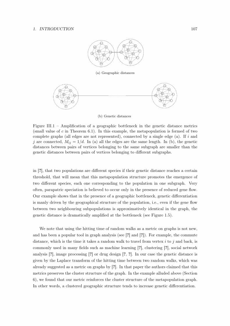
1. INTRODUCTION 107
(a) Geographic distances
(b) Genetic distances
Figure III.1 – Amplification of a geographic bottleneck in the genetic distance metrics(small value of c in Theorem 6.1). In this example, the metapopulation is formed of twocomplete graphs (all edges are not represented), connected by a single edge (a). If i andj are connected, Mij = 1/d. In (a) all the edges are the same length. In (b), the geneticdistances between pairs of vertices belonging to the same subgraph are smaller than thegenetic distances between pairs of vertices belonging to different subgraphs.
in [?], that two populations are different species if their genetic distance reaches a certainthreshold, that will mean that this metapopulation structure promotes the emergence oftwo different species, each one corresponding to the population in one subgraph. Veryoften, parapatric speciation is believed to occur only in the presence of reduced gene flow.Our example shows that in the presence of a geographic bottleneck, genetic differentiationis manly driven by the geographical structure of the population, i.e., even if the gene flowbetween two neighbouring subpopulations is approximatively identical in the graph, thegenetic distance is dramatically amplified at the bottleneck (see Figure 1.5).
We note that using the hitting time of random walks as a metric on graphs is not new,and has been a popular tool in graph analysis (see [?] and [?]). For example, the commutedistance, which is the time it takes a random walk to travel from vertex i to j and back, iscommonly used in many fields such as machine learning [?], clustering [?], social networkanalysis [?], image processing [?] or drug design [?, ?]. In our case the genetic distance isgiven by the Laplace transform of the hitting time between two random walks, which wasalready suggested as a metric on graphs by [?]. In that paper the authors claimed that thismetrics preserves the cluster structure of the graph. In the example alluded above (Section6), we found that our metric reinforces the cluster structure of the metapopulation graph.In other words, a clustered geographic structure tends to increase genetic differentiation.
108 CHAPITRE 2
1.6 Discussion and open problems
As already mentioned above, the main result is obtained by: (i) proving that, in alow mutation - low migration regime (i.e., when γ → 0), subpopulations are monomorphicmost of the time and our individual based model converges to a population based model,(ii) showing that, under a large population - long chromosome limit (i.e. taking ε → 0),the genetic distances between subpopulations (for the population based model) convergeto a deterministic process (defined in Theorem 1.1). Taking these two limits successivelygives no clue on how the parameters should be compared to ensure the approximation tobe correct. It would be interesting to take the limits simultaneously but it is technicallychallenging (for example we would need to characterise the time to fixation for l loci thatdo not fix independently, which is not easy).
As discussed in the previous paragraph, we can only show our results under some ratherdrastic constraints: subpopulations are asymptotically monomorphic. More generally, webelieve that Theorem 1.1 should hold under relaxed assumptions, namely when the intra-subpopulation genetic diversity is low compared to the inter-subpopulation diversity (seeFigure III.2 for an example, where γ = 2e−6 and ε = 5e−3 ). Technically, this wouldcorrespond to the condition that at a typical locus (i.e, a locus chosen uniformly at random)each subpopulations is monomorphic at that site with high probability (which is in essence(III.2)). Of course, proving such a result would be much more challenging, but wouldpresumably correspond to a more realistic situation.
1.7 Outline
In Section 2, we show that in the rare mutation-rare migration regime (i.e. when γ → 0
whereas ε remains constant), the individual based model (IBM) described above convergesto a population based model (PBM) (see Theorem 2.2). This PBM is a generalization ofthe model proposed by Yamaguchi and Iwasa [?, ?] in three ways. First, it is an extensionof their model from two to an arbitrary number of subpopulations, which is not trivial froma mathematical point of view. Second, in [?, ?], the authors only assumed that the migrantalleles are fixed independently at every locus. Too make the model more realistic, we tookinto account genetic linkage, which introduces a non-trivial spatial correlation between loci(along the chromosome). Finally, we suppose that the loci are distributed randomly alongthe chromosome (and not in a regular fashion). Section 2 is interesting on its own since itprovides a theoretical justification of the model proposed in [?, ?].
In Section 3 and 4, we study the PBM in the large population - long chromosome limit(i.e. when ε → 0). We properly introduce the main tool used to study the populationbased model – the genetic partition probability measure – and show an ergodic theoremrelated to this process (see Theorem 3.1).
Finally, in Section 5 we prove our main result (Theorem 5.1 which is an extension of
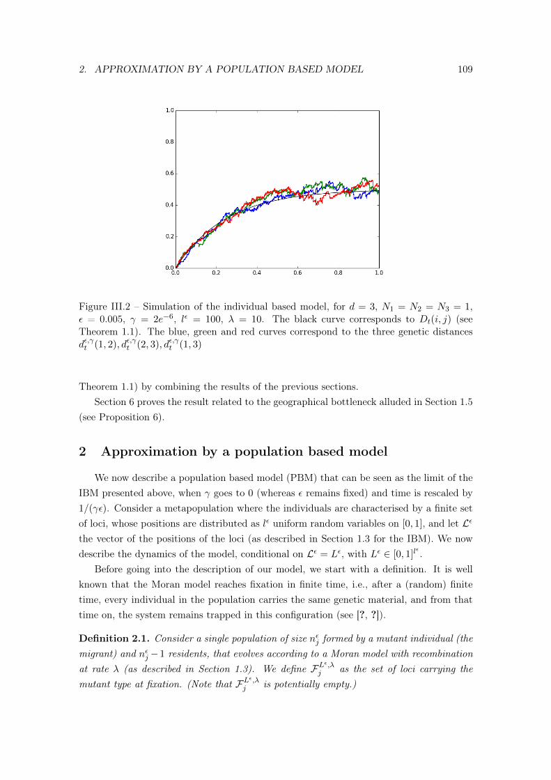
2. APPROXIMATION BY A POPULATION BASED MODEL 109
Figure III.2 – Simulation of the individual based model, for d = 3, N1 = N2 = N3 = 1,ε = 0.005, γ = 2e−6, lε = 100, λ = 10. The black curve corresponds to Dt(i, j) (seeTheorem 1.1). The blue, green and red curves correspond to the three genetic distancesdε,γt (1, 2), dε,γt (2, 3), dε,γt (1, 3)
Theorem 1.1) by combining the results of the previous sections.Section 6 proves the result related to the geographical bottleneck alluded in Section 1.5
(see Proposition 6).
2 Approximation by a population based model
We now describe a population based model (PBM) that can be seen as the limit of theIBM presented above, when γ goes to 0 (whereas ε remains fixed) and time is rescaled by1/(γε). Consider a metapopulation where the individuals are characterised by a finite setof loci, whose positions are distributed as lε uniform random variables on [0, 1], and let Lε
the vector of the positions of the loci (as described in Section 1.3 for the IBM). We nowdescribe the dynamics of the model, conditional on Lε = Lε, with Lε ∈ [0, 1]l
ε .Before going into the description of our model, we start with a definition. It is well
known that the Moran model reaches fixation in finite time, i.e., after a (random) finitetime, every individual in the population carries the same genetic material, and from thattime on, the system remains trapped in this configuration (see [?, ?]).
Definition 2.1. Consider a single population of size nεj formed by a mutant individual (themigrant) and nεj−1 residents, that evolves according to a Moran model with recombinationat rate λ (as described in Section 1.3). We define FL
ε,λj as the set of loci carrying the
mutant type at fixation. (Note that FLε,λ
j is potentially empty.)
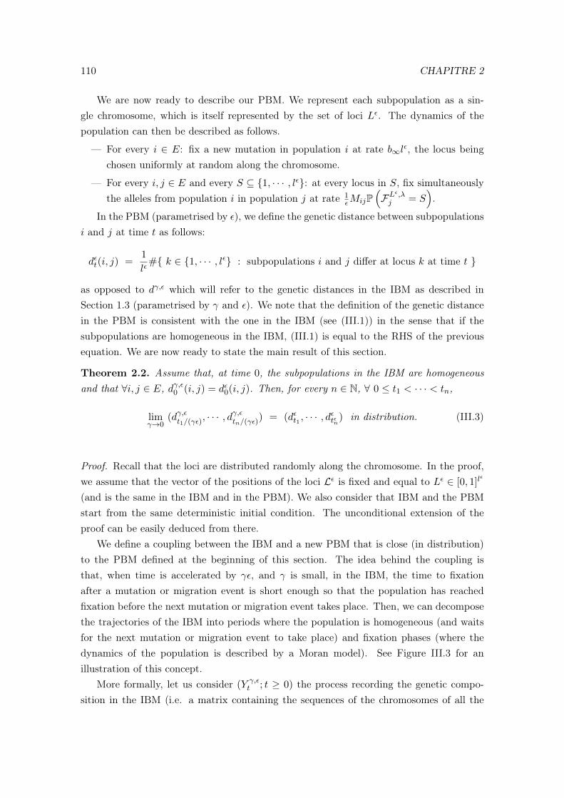
110 CHAPITRE 2
We are now ready to describe our PBM. We represent each subpopulation as a sin-gle chromosome, which is itself represented by the set of loci Lε. The dynamics of thepopulation can then be described as follows.
— For every i ∈ E: fix a new mutation in population i at rate b∞lε, the locus beingchosen uniformly at random along the chromosome.
— For every i, j ∈ E and every S ⊆ 1, · · · , lε: at every locus in S, fix simultaneouslythe alleles from population i in population j at rate 1
εMijP(FL
ε,λj = S
).
In the PBM (parametrised by ε), we define the genetic distance between subpopulationsi and j at time t as follows:
dεt(i, j) =1
lε# k ∈ 1, · · · , lε : subpopulations i and j differ at locus k at time t
as opposed to dγ,ε which will refer to the genetic distances in the IBM as described inSection 1.3 (parametrised by γ and ε). We note that the definition of the genetic distancein the PBM is consistent with the one in the IBM (see (III.1)) in the sense that if thesubpopulations are homogeneous in the IBM, (III.1) is equal to the RHS of the previousequation. We are now ready to state the main result of this section.
Theorem 2.2. Assume that, at time 0, the subpopulations in the IBM are homogeneousand that ∀i, j ∈ E, dγ,ε0 (i, j) = dε0(i, j). Then, for every n ∈ N, ∀ 0 ≤ t1 < · · · < tn,
limγ→0
(dγ,εt1/(γε), · · · , dγ,εtn/(γε)
) = (dεt1 , · · · , dεtεn
) in distribution. (III.3)
Proof. Recall that the loci are distributed randomly along the chromosome. In the proof,we assume that the vector of the positions of the loci Lε is fixed and equal to Lε ∈ [0, 1]l
ε
(and is the same in the IBM and in the PBM). We also consider that IBM and the PBMstart from the same deterministic initial condition. The unconditional extension of theproof can be easily deduced from there.
We define a coupling between the IBM and a new PBM that is close (in distribution)to the PBM defined at the beginning of this section. The idea behind the coupling isthat, when time is accelerated by γε, and γ is small, in the IBM, the time to fixationafter a mutation or migration event is short enough so that the population has reachedfixation before the next mutation or migration event takes place. Then, we can decomposethe trajectories of the IBM into periods where the population is homogeneous (and waitsfor the next mutation or migration event to take place) and fixation phases (where thedynamics of the population is described by a Moran model). See Figure III.3 for anillustration of this concept.
More formally, let us consider (Y γ,εt ; t ≥ 0) the process recording the genetic compo-
sition in the IBM (i.e. a matrix containing the sequences of the chromosomes of all the
2. APPROXIMATION BY A POPULATION BASED MODEL 111
Figure III.3 – The curve represents the genetic distance between two subpopulations forthe IBM. The vertical lines represent the decomposition of the trajectories. The fixationphases are represented in red. Simulation with 3 subpopulations, with 100 individuals oneach, carrying 100 loci, with γ = 0.0001, ∀i, j,Mi,j = 1, b∞ = 1, λ = 5.
individuals in the metapopulation) after rescaling time by γε so that
1. For i ∈ E, mutation events on the subpopulation i occurs according to a PoissonPoint Process (PPP) with intensity measure b∞lεnεidt.
2. For i, j ∈ E, migration events from i to j can be described in terms of a PPP withintensity measure Mi,j/εdt.
Define Eγ,ε the event that every time a subpopulation is affected by a mutation or amigration event on the interval [0, T ], the subpopulation is genetically homogeneous whenthe event occurs (as in Figure III.3). In other words, there is no overlap between mutationand migration fixation periods. The time to fixation in our (multi-locus) Moran modelonly depends on the number of individuals and the number of loci, so in our model it onlydepends on ε (but not on γ). As a consequence, P (Eγ,ε)→ 1 as γ → 0.
Next, let us consider T γ,εt as the Lebesgue measure of
0 ≤ s ≤ t : ∀i ∈ E pop. i is homogeneous.
In words, (T γ,εt ; t ≥ 0) is the random clock which is obtained by skipping the fixation periodafter a migration or mutation event (i.e. by skipping the red intervals in Figure III.3). Byarguing as in the previous paragraph, as γ → 0, it is not hard to see that (T γ,εt ; t ≥ 0)
converges to the identity in the Skorohod topology on [0, T ] for every T ≥ 0.
112 CHAPITRE 2
Let us now consider
Zγ,εt = Y γ,ε
(T γ,ε)−1t
, where (T γ,ε)−1t = infs ≥ 0 : T γ,εs ≥ t.
By construction, this process defines a PBM in the sense that at every time t, any subpop-ulation is composed by genetically homogeneous individuals. Further, since (T γ,εt ; t ≥ 0)
converges to the identity and mutation and migration events occur at Poisson times, thefinite dimensional distributions of Zγ,ε are a good approximations of the ones for the IBM.
Let us now show that Zγ,ε (constructed from the IBM) is close in distribution tothe PBM defined at the begining of this section. Conditioned on the event Eγ,ε (whoseprobability goes to 1) and on the PPP’s described in 1 and 2 above, the PBM Zγ,ε can bedescribed as follows. Define p∆t,i to be the probability for a mutant allele (at a given locusof a given individual) to fix in a population of size nεi , conditioned on the fixation time tobe smaller than ∆t. Then the distribution of the conditioned PBM Zγ,εt can be generatedas follows.
(a) At every mutation time t in subpopulation i ∈ E, choose a locus k uniformly atrandom and fix the mutation instantaneously with probability p∆t
γε,i, where ∆t is the
time between t and the next mutation or migration event (in our new time scale).We note that if the mutation does not fix, then Zγ,ε is not affected by the mutationevent, and as a consequence “effective mutation” events in Zγ,ε are obtained from themutation events in the IBM after thinning each time with their respective probabilityp∆tγε,i.
(b) At every migration event t on subpopulation j, fix a random set S where S is chosenaccording to FL
ε,λ,∆t/γεj , where ∆t is defined as in the previous point, and where
FLε,λ,s
j is the random variable FLε,λ
j conditioned on the fixation to occur in a timesmaller smaller than s.
Since fixation occurs in finite time almost surely, and the distribution of the fixation timeonly depends on ε, we have
FLε,λ,∆t/εγ
j =⇒γ→0FL
ε,λj , and lim
γ→0p∆t/εγ,i =
1
nεj
where the RHS of the second limit is the probability of fixation of a mutant allele in theabsence of conditioning.
Putting all the previous observations together, one can easily show that the geneticdistance in Zγ,ε converges (in the finite dimensional distributions sense) to the ones of the
3. LARGE POPULATION - LONG CHROMOSOME LIMIT 113
PBM. In particular, we recover the mutation rate on subpopulation i in the PBM
b∞lεnεi︸ ︷︷ ︸
rate of mutation in the IBM
× 1
nεi︸︷︷︸proba of fixation
= b∞lε,
which corresponds to the limiting “effective mutation rate” in the PBM Zγ,ε (see (a) above)as γ → 0. This completes the proof of Theorem 2.2.
We note that Theorem 2.2 could be extended to the case where the subpopulations arenot homogeneous in the IBM at time t = 0. Indeed, arguing as in the proof of Proposition2.2, if we start with some non-homogeneous initial condition, then each island reachesfixation before experiencing any mutation or mutation event with very high probability.In order to get an effcient coupling between the IBM and the PBM, we simply choose theinitial condition of the PBM as the state of IBM after this initial fixation period.
Remark 2.3. Choose a locus k ∈ 1, · · · , lε. We let the reader convince herself thatin the PBM the genetic composition at a given locus k follows the following Moran-typedynamics:
(mutation) “Individual” i takes on a new type (or allele) at rate b∞.
(reproduction) “Individual” j inherits its type from “individual” i at rate (1/ε)MijP(k ∈ FL
ε,λj
).
Further, in a neutral one-locus Moran model, the probability of fixation of a singleallele in a resident population of size nεj is equal to its initial frequency, which in ourcase is 1/nεj. Thus
1
εMijP
(k ∈ FL
ε,λj
)=
1
εMij/n
εj .
This dynamics is not dependent on the position of the locus under consideration.
Remark 2.4. Our model can be seen as a multi-locus Moran model with inhomogeneousreproduction rates. The main difficulty in analysing this model stems from the fact thatthere exists a non trivial correlation between loci. This correlation is induced by the fact thatfixation of migrant alleles can occur simultaneously at several loci during a given migrationevent. In turn, the set of fixed alleles during a given migration event is determined by thelocal Moran dynamics described in the Introduction.
3 Large population - long chromosome limit
In this Section, we study the PBM described in the Section 2, in the large population- long chromosome limit. In particular, we study the dynamics of the genetics distancesand we state Theorem 3.1, that together with Theorem 2.2 implies the main result of thisarticle, namely Theorem 5.1, that is a stronger version of Theorem 1.1 (see Section 5).
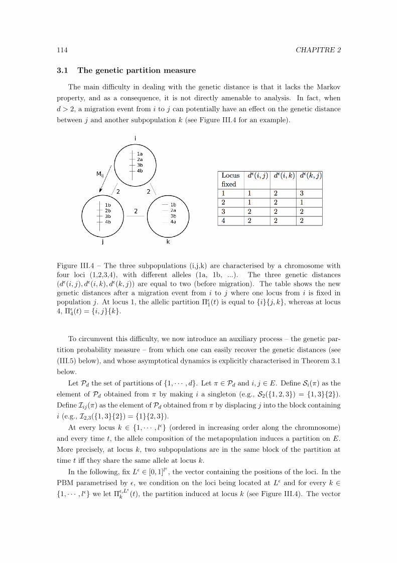
114 CHAPITRE 2
3.1 The genetic partition measure
The main difficulty in dealing with the genetic distance is that it lacks the Markovproperty, and as a consequence, it is not directly amenable to analysis. In fact, whend > 2, a migration event from i to j can potentially have an effect on the genetic distancebetween j and another subpopulation k (see Figure III.4 for an example).
Figure III.4 – The three subpopulations (i,j,k) are characterised by a chromosome withfour loci (1,2,3,4), with different alleles (1a, 1b, ...). The three genetic distances(dε(i, j), dε(i, k), dε(k, j)) are equal to two (before migration). The table shows the newgenetic distances after a migration event from i to j where one locus from i is fixed inpopulation j. At locus 1, the allelic partition Πε
1(t) is equal to ij, k, whereas at locus4, Πε
4(t) = i, jk.
To circumvent this difficulty, we now introduce an auxiliary process – the genetic par-tition probability measure – from which one can easily recover the genetic distances (see(III.5) below), and whose asymptotical dynamics is explicitly characterised in Theorem 3.1below.
Let Pd the set of partitions of 1, · · · , d. Let π ∈ Pd and i, j ∈ E. Define Si(π) as theelement of Pd obtained from π by making i a singleton (e.g., S2(1, 2, 3) = 1, 32).Define Iij(π) as the element of Pd obtained from π by displacing j into the block containingi (e.g., I2,3(1, 32) = 12, 3).
At every locus k ∈ 1, · · · , lε (ordered in increasing order along the chromnosome)and every time t, the allele composition of the metapopulation induces a partition on E.More precisely, at locus k, two subpopulations are in the same block of the partition attime t iff they share the same allele at locus k.
In the following, fix Lε ∈ [0, 1]lε , the vector containing the positions of the loci. In the
PBM parametrised by ε, we condition on the loci being located at Lε and for every k ∈1, · · · , lε we let Πε,Lε
k (t), the partition induced at locus k (see Figure III.4). The vector
3. LARGE POPULATION - LONG CHROMOSOME LIMIT 115
Πε,Lε(t) =(
Πε,Lε
k (t); k ∈ 1, · · · , lε)describes the genetic composition of the population
at time t. According to the description of our dynamics, Πε,Lε(t) is a Markov chain withthe following transition rates:
— (mutation) For every Π ∈ (Pd)lε , i ∈ E, k ∈ 1, · · · , lε, define Ski to be the operator
on (Pd)lε such that ∀ Π ∈ (Pd)l
ε
Ski (Π) =
Πj ∀j 6= k
Si(Πj) j = k.
The transition rate of the process from state Π to Ski (Π) is given by b∞.
— (migration from i to j) For every i, j ∈ E, S ⊂ 1, · · · , lε, define ISij the operatoron (Pd)l
ε such that ∀ Π ∈ (Pd)lε
ISij(Π) =
Πk ∀k /∈ S
Iij(Πk) ∀k ∈ S.
The transition rate of the process from Π to ISij(Π) is given by Mij
ε P(FL
ε,λj = S
).
To summarise, for every test function h, the generator of Πε,Lε can be written as
Gε,Lεh(Π) =1
ε
d∑i,j=1
Mij
∑S⊂1,··· ,lε
P(FLε,λ
j = S) [h(ISij(Π))− h(Π)] +
b∞
d∑i=1
lε∑k=1
(h(Ski (Π))− h(Π)
). (III.4)
3.2 Some notation
Let Md denote the space of signed finite measures on Pd. Since Pd is finite, we canidentify elements ofMd as vectors of RBelld , where Belld is the Bell number, which countsthe number of elements in Pd (the number of partitions of d elements). In particular, if πis a partition of E, and µ ∈Md, then µ(π) will correspond to the measure of the singletonπ, or equivalently, to the “πth coordinate” of the vector µ. We define the inner product< ·, · > as
< ·, · >: Md ×Md → R
m, v →∑π∈Pd
m(π)v(π).
For every function f : Pd → Pd, we define the operator ∗ s.t for every m ∈ Md, for everyπ ∈ Pd, f ∗ m(π) = m(f−1(π)). In words, f ∗ m is the push-forward measure of m by
116 CHAPITRE 2
f . Further, we will also consider square matrices indexed by elements in Pd. For such amatrix K and an element m ∈Md, we define Km(π) :=
∑π′∈Pd K(π, π′)m(π′).
Define
X : (Pd)lε → M(Pd)
Π → 1
lε
∑k≤lε
δΠk ,
i.e., X(Π) is the empirical measure associated to the “sample” Π1, · · · ,Πlε . In the following,we define
ξε,Lε
t := X(Πε,Lε(t))
will be referred to as the (empirical) genetic partition probability measure of the population,conditional on the lε loci to be located at Lε. We also define
ξεt ≡ ξε,Lε
t = X(Πε,Lε(t)) where Lε ∼ U([0, 1]lε)
will be referred to as the (empirical) genetic partition probability measure of the population.
The genetic distance between i and j at time t can then be expressed in terms of ξεt asfollows:
dεt(i, j) = 1− ξεt (π ∈ Pd : i ∼π j)). (III.5)
In the following, we identify the process (ξεt , t ≥ 0) to a process in the set of the càdlàgfunctions from R+ to RBelld , equipped with the standard Skorokhod topology.
3.3 Convergence of the genetic partition probability measure
Following Remark 2.3, for every k ∈ 1, · · · , lε, the process (Πε,Lε
k (t); t ≥ 0) – thepartition at locus k – obeys the following dynamics:
1. (reproduction event) j is merged in the block containing i at rate Mij1εnεj
.
2. (mutation) Individual i takes on a new type at rate b∞.
The generator associated to the allelic partition at locus k is then given by
Gεg(π) =
d∑i,j=1
Mij1
εnεj( g(Iij(π))− g(π) ) + b∞
d∑i=1
( g(Si(π))− g(π) ) . (III.6)
Recall that the expression of the generator associated to the allelic partition at a givenlocus k is independent on the position of locus k and on λ. Also recall that εnεi → Ni, and
4. PROOF OF THEOREM 3.1 117
thus
Gεg(π)→ Gg(π) :=d∑
i,j=1
Mji ( g(Iij(π))− g(π) ) + b∞
d∑i=1
( g(Si(π))− g(π) ) as ε→ 0.
(III.7)Direct computations yield that tG, the transpose of the matrix G satisfies
∀m ∈Md,tGm =
d∑i,j=1
Mji(Iij ∗m−m) + b∞
d∑i=1
(Si ∗m−m) . (III.8)
In the light of (III.7), the following theorem can be interpreted as an ergodic theorem.We show that the (dynamical) empirical measure constructed from the allelic partitionsalong the chromosome converges to the probability measure of a single locus. Although inthe IBM the different loci are linked and do not fix independently (as already mentioned inRemark 2.4), as the number of loci tends to infinity, they become decorrelated. In the largepopulation - long chromosome limit, the following result indicates that the model behavesas if infinitely many loci evolved independently according to the (one-locus) Moran modelwith generator G provided in (III.7).
In the following “ =⇒′′ indicates the convergence in distribution. Also, we identify(ξεt ; t ≥ 0) to a function from R+ to RBelld ; and convergence in the weak topology meansthat for every T > 0, the process (ξεt ; t ∈ [0, T ]) converges in the Skorohod topologyD([0, T ],RBelld).
Theorem 3.1 (Ergodic theorem along the chromosome). Assume that ξε0 is deterministicand there exists a probability measure P 0 ∈Md such that the following convergence holds:
ξε0 −→ε→0
P 0. (III.9)
Then(ξεt ; t ≥ 0) =⇒
ε→0(Pt; t ≥ 0) in the weak topology,
where P solves the forward Kolmogorov equation associated to the aforementioned Moranmodel, i.e.,
d
dsPs = tGPs
with initial condition P0 = P 0 and where tG denotes the transpose of G (see (III.8)).
4 Proof of Theorem 3.1
The idea behind the proof is to condition on Lε = Lε, and then decompose the Markovprocess (< ξε,Lεt , v >; t ≥ 0) into a drift part and a Martingale part. We show that thedrift part converges to the solution of the Kolmogorov equation alluded in Theorem 3.1
118 CHAPITRE 2
and that the Martingale part vanishes when ε→ 0. The main steps of the computation areoutlined in the next subsection. We leave technical details (tightness and second momentcomputations) until the end of the section.
4.1 Main steps of the proof
Fix Lε ∈ [0, 1]lε . Recall the definition ofGε,Lε , the generator of the process (Πε,Lε(t); t ≥
0), given in (III.4). Let f : R → R be a Borel bounded function and let v ∈ Md. Leth(Π) = f(〈X(Π), v〉). Then, it is straightforward to see from (III.4) that
Gε,Lεh(Π) =1
ε
d∑i,j=1
Mij Eλ,Lε,j(f(⟨X(ISij(Π)), v
⟩)− f(〈X(Π), v〉)
)+ b∞l
εd∑i=1
Elε(f(⟨X(SKi (Π)), v
⟩)− f(〈X(Π), v〉)
), (III.10)
where in the first line Eλ,Lε,j is the expected value taken with respect to the randomvariable S, distributed as FL
ε,λj as defined in Definition 2.1. In the second line, Elε is the
expected value is taken with respect to K, distributed as a uniform random variable on1, · · · , lε.
Lemma 4.1. Let v ∈Md, Lε ∈ [0, 1]lε , g(Π) := 〈X(Π), v〉. Then Gε,Lεg(Π) =
⟨tGεX(Π), v
⟩where tGε is the transpose of Gε – the generator of the allelic partition at a single locus asdefined in (III.6) – i.e.,
∀m ∈Md,tGεm =
d∑i,j=1
Mij1
εnεi(Iij ∗m−m) + b∞
d∑i=1
(Si ∗m−m) . (III.11)
Proof. We define the two following signed measures:
∂SijX(Π) = X(ISij(Π)) − X(Π), ∂Ki X(Π) = X(SKi (Π)) − X(Π). (III.12)
In words, ∂SijX(Π) is the change in the genetic partition measure X(Π) if we merge j inthe block of i at every locus in S, and ∂Ki X(Π) is the change in X(Π) if we single outelement i at locus K. Using those notations, for our particular choice of g, (III.10) writes
Gε,Lεg(Π) =1
ε
d∑i,j=1
Mij Eλ,Lε,j(⟨∂SijX(Π), v
⟩)+ b∞l
εd∑i=1
Elε(⟨∂Ki X(Π), v
⟩).
We now show that for every v ∈Md,
Eλ,Lε,j(⟨∂SijX(Π), v
⟩)=
1
nεj〈Iij ∗X(Π)−X(Π), v〉 ,
4. PROOF OF THEOREM 3.1 119
Elε(⟨∂Ki X(Π)
⟩)=
1
lε〈Si ∗X(Π)−X(Π), v〉 . (III.13)
We only prove the first identity. The second one can be shown along the same lines. Again,we let Πk be the kth coordinate of Π. By definition, the vector ISij(Π) is only modified atthe coordinates belonging to S, and thus
⟨∂SijX(Π), v
⟩=
∑π∈Pd
v(π)
lε(|k ≤ lε : (ISij(Π))k = π| − |k ≤ lε : Πk = π|
)=
∑π∈Pd
v(π)
lε(|k ∈ S : ISij(Πk) = π| − |k ∈ S : Πk = π|
).(III.14)
Secondly, for every j ∈ E,
Eλ,Lε,j(|k ∈ S : Πk = π|) = Eλ,Lε,j(∑k∈S
1Πk=π) =∑k≤lε
1Πk=πEλ,Lε,j(1k∈S).
As S is distributed as FLε,λ
j , we can use the fact that P(k ∈ FL
ε,λj
)= Mij
1nεj
(see Remark2.3), and then
Eλ,Lε,j(|k ∈ S : Πk = π|) =1
nεj|k ≤ lε, Πk = π| = lε
nεjX(Π)(π). (III.15)
Furthermore, by applying (III.15) for every π′ ∈ I−1ij (π) and then taking the sum over
every such partitions, we get
Eλ,Lε,j(|k ∈ S : Iij(Πk) = π| =lε
nεjX(Π)(I−1
ij (π)) =lε
nεjIij ∗X(Π)(π).
This completes the proof of (III.13). From this result, we deduce that
Gε,Lεg(Π) =1
ε
d∑i,j=1
Mij1
nεj(Iij ∗X(Π)−X(Π)) + b∞
d∑i=1
(Si ∗X(Π)−X(Π)) .
This completes the proof of Lemma 4.1.
For every Lε ∈ [0, 1]lε , for every v ∈Md, define
M ε,Lε,vt :=
⟨ξε,L
ε
t , v⟩−∫ t
0
⟨tGεξε,L
ε
s , v⟩ds, Bε,Lε,L
ε,v
t :=
∫ t
0
⟨tGεξε,L
ε
s , v⟩ds.
Since⟨ξε,L
ε
t , v⟩is bounded, the previous result implies thatM ε,Lε,v is a martingale with re-
spect to (FLεt )t≥0, the filtration generated by (Πε,Lε(t); t ≥ 0). Further, the semi-martingale
120 CHAPITRE 2⟨ξε,L
ε
t , v⟩admits the following decomposition:
⟨ξε,L
ε
t , v⟩
= M ε,Lε,vt + Bε,Lε,v
t .
Lemma 4.2. For every v ∈Md, for every Lε ∈ [0, 1]lε,
⟨M ε,Lε,v
⟩t
=
∫ t
0mε,Lε,v(Πε,Lε(s))ds
with
mε,Lε,v(Π) =1
ε
d∑i,j=1
Mij Eλ,Lε,j(⟨∂SijX(Π), v
⟩2)
+ b∞lε
d∑i=1
Elε(⟨∂Ki X(Π), v
⟩2).
Proof. Let h(Π) = 〈X(Π), v〉2. Then, by (III.10)
Gε,Lεh(Π) =1
ε
d∑i,j=1
MijEλ,Lε,j(⟨X(ISij(Π), v)
⟩2 − 〈X(Π), v〉2)
+ b∞lε
d∑i=1
Elε(⟨X(SKi (Π)), v
⟩2 − 〈X(Π), v〉2).
Since
⟨X(ISij(Π)), v
⟩2 − 〈X(Π), v〉2 =⟨X(ISij(Π))−X(Π), v
⟩2+ 2
⟨X(ISij(Π))−X(Π), v
⟩〈X(Π), v〉⟨
X(Ski (Π)), v⟩2− 〈X(Π), v〉2 =
⟨X(Ski (Π))−X(Π), v
⟩2+ 2
⟨X(Ski (Π))−X(Π), v
⟩〈X(Π), v〉 ,
the previous identities yield
Gε,Lεh(Π) = 2Gε,Lεg(Π) 〈X(Π), v〉 +
1
ε
d∑i,j=1
MijEλ,Lε,j(⟨∂SijX(Π), v
⟩2)
+ b∞lε
d∑i=1
Elε(⟨∂Ki X(Π), v
⟩2),
where g(Π) = 〈X(Π), v〉. As a consequence
⟨X(Πε,Lε(t)), v
⟩2 − 2
∫ t
0Gε,Lεg(Πε,Lε(s))
⟨X(Πε,Lε(s)), v
⟩ds
−∫ t
0
1
ε
d∑i,j=1
MijEλ,Lε,j(⟨∂SijX(Πε,Lε(s)), v
⟩2)ds−
∫ t
0b∞l
εd∑i=1
Elε(⟨∂Ki X(Πε,Lε(s)), v
⟩2)ds

4. PROOF OF THEOREM 3.1 121
is a martingale. Further using Itô’s formula, the process
⟨X(Πε,Lε(t)), v
⟩2 − 2
∫ t
0Gε,Lεg(Πε,Lε(s))
⟨X(Πε,Lε(s)), v
⟩ds −
⟨M ε,Lε,v
⟩t
is also a martingale. Combining the two previous results completes the proof of Lemma4.2.
Proposition 4.3.limε→0
E( supΠ∈(Pd)lε
mε,Lε,v(Π)) = 0,
where the expected value is taken with respect to the random variable Lε.
Proposition 4.4. Let T > 0. The family of random variables (ξε; ε > 0) is tight in theweak topology D([0, T ],RBelld).
We postpone the proof of Propositions 4.3 and 4.4 until Sections 4.2 and 4.3 respectively.
Proof of Theorem 3.1 based on Proposition 4.3 and 4.4. Since (ξε; ε > 0) is tight, we canalways extract a subsequence converging in distribution (for the weak topology) to a lim-iting random measure process ξ. We will now show that ξ can only be the solution of theKolmogorov equation alluded in Theorem 3.1. From (III.11), for every probability measurem on Pd, for every v ∈Md,
∣∣ ⟨tGεm, v⟩ ∣∣ ≤ (2d∑
i,j=1
Mij1
εnεi+ 2b∞d)||v||∞, (III.16)
where ||v||∞ := maxπ∈PN v(π). Since as ε → 0, nεiε → Ni, the term between parenthe-ses also converges, and thus the RHS is uniformly bounded in ε. Finally, the boundedconvergence theorem implies that for every v ∈Md,
E(〈ξt, v〉 −
∫ t
0
⟨tGξs, v
⟩ds
)2
= limε→0
E
((〈ξεt , v〉 −
∫ t
0
⟨tGεξεs, v
⟩ds
)2),
where we used the fact that tGεm → tGm for every m ∈ Md (where G is defined as inTheorem 3.1). On the other hand, since
E(〈ξεt , v〉 −
∫ t
0
⟨tGεξεs, v
⟩ds
)2
= E
(E
((⟨ξε,L
ε
t , v⟩−∫ t
0
⟨tGεξε,L
ε
s , v⟩ds
)2
| Lε))
= E(E(⟨M ε,Lε,v⟩
t| Lε))
= E(E(
∫ t
0mε,Lε,v(Πε,Lε(s))ds | Lε))
≤ t E( supπ∈(Pd)lε
mε,Lε,v(Π)).

122 CHAPITRE 2
Lemma 4.2 and Proposition 4.3 imply that
E(〈ξt, v〉 −
∫ t
0
⟨tGξs, v
⟩ds
)2
= 0,
which ends the proof of Theorem 3.1.
Remark 4.5 (Magnitude of the stochastic fluctuations). Lemma 4.1 and the proof Propo-sition 4.3 entail that:
∀v ∈Md, E(⟨M ε,Lε,v⟩
t) ≤ ε log(1/ε)C +
1
lεC ′
where C is a constant. This suggests that the order of magnitude of the fluctuations shouldbe of the order of max(
√ε log(1/ε),
√(1/lε)).
In [?], the authors proposed a diffusion approximation (only for the case of two sub-populations). Their approximation is based on the simplifying hypothesis that loci are fixedindependently on each other – the number of fixed loci (after each migration event) followsa binomial distribution–, and the hypothesis that the number of loci l is s.t. l >> 1
ε . Theyfound that the magnitude of the stochastic fluctuations was
√ε.
In summary, the previous heuristics suggest that taking into account correlations be-tween loci increases the magnitude of the stochastic fluctuations.
4.2 Proof of Proposition 4.3
Our first step in proving Proposition 4.3 is to prove the following result.
Lemma 4.6. ∀ i, j ∈ E, ∀λ > 0,
limε→0
1
(lε)2εE
(Eλ,Lε,j(
lε∑k=1
lε∑k′=1
1k∈S1k′∈S | Lε)
)= 0.
Before turning to the proof of this result, we recall the definition of the ancestralrecombination graph (ARG) (see also [?], [?], [?]) for the case of two loci. Fix Lε =
`1, · · · `lε the positions of the loci in the chromosome, λ the recombination rate, andchoose two loci k and k′ among the lε loci. In order to compute the probability that forboth loci the allele from the migrant is fixed in the host population – P(k, k′ ∈ FL
ε,λj ) – we
follow backwards in time the genealogy of the corresponding alleles carried by a referenceindividual in the present population, assuming that a migration event occurred in the past(sufficiently many generations ago, so that we can assume fixation).
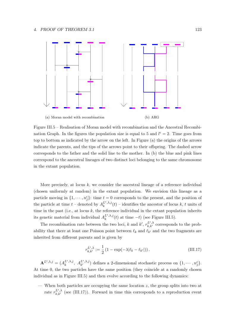
4. PROOF OF THEOREM 3.1 123
(a) Moran model with recombination (b) ARG
Figure III.5 – Realisation of Moran model with recombination and the Ancestral Recombi-nation Graph. In the figures the population size is equal to 5 and lε = 2. Time goes fromtop to bottom as indicated by the arrow on the left. In Figure (a) the origins of the arrowsindicate the parents, and the tips of the arrows point to their offspring. The dashed arrowcorresponds to the father and the solid line to the mother. In (b) the blue and pink linescorrespond to the ancestral lineages of two distinct loci belonging to the same chromosomein the extant population.
More precisely, at locus k, we consider the ancestral lineage of a reference individual(chosen uniformly at random) in the extant population. We envision this lineage as aparticle moving in 1, · · · , nεj: time t = 0 corresponds to the present, and the position ofthe particle at time t – denoted by AL
ε,λ,jk (t) – identifies the ancestor of locus k, t units of
time in the past (i.e., at locus k, the reference individual in the extant population inheritsits genetic material from individual AL
ε,λ,jk (t) at time −t) (see Figure III.5).
The recombination rate between the two loci, k and k′, rLε,λ
k,k′ corresponds to the prob-ability that there at least one Poisson point between `k and `k′ and the two fragments areinherited from different parents and is given by
rLε,λ
k,k′ :=1
2(1− exp(−λ|`k − `k′ |)) . (III.17)
ALε,λ,j = (ALε,λ,j
k , ALε,λ,j
k′ ) defines a 2-dimensional stochastic process on 1, · · · , nεj.At time 0, the two particles have the same position (they coincide at a randomly chosenindividual as in Figure III.5) and then evolve according to the following dynamics:
— When both particles are occupying the same location z, the group splits into two atrate rL
ε,λk,k′ (see (III.17)). Forward in time this corresponds to a reproduction event
124 CHAPITRE 2
where z is replaced by the offspring of x and y. Each individual x reproduces atrate 1 (chooses a random partner y), and with probability 1/nεj his offspring replacesindividual z. There are nεj possible choices for x. Following (III.17), the probabilitythat both loci are inherited from different parents is rL
ε,λk,k′ , so the rate of fragmentation
for loci k, k′ is given by nεj .1nεj. rL
ε,λk,k′ .
— When the two particles are occupying different positions, they jump to the sameposition at rate 2/nεj . Forwards in time, this corresponds to a reproduction eventwhere the individual located at AL
ε,λ,jk (resp. AL
ε,λ,jk′ ) replaces the one at AL
ε,λ,jk′
(resp. ALε,λ,j
k ), and the offspring inherits the allele at locus k′ (resp. k) from thisparent. A reproduction event where the individual located at AL
ε,λ,jk (resp. AL
ε,λ,jk′ )
replaces the one at ALε,λ,j
k′ (resp. ALε,λ,j
k ) occurs at rate 2/nεj (as the individual atAL
ε,λ,jk –resp. AL
ε,λ,jk′ – can be the mother or the father); and the probability that
the offspring inherits the locus k′ (resp. k) from this parent is 1/2. The total rate ofcoalescence is 2 . 2
nεj. 1
2 .
Since we assume that the migration event occurred far back in the past, the followingduality relation holds:
P(k, k′ ∈ FLε,λ
j ) = limt→∞
P(AL
ε,λ,jk (t) = AL
ε,λ,jk′ (t) = 1
). (III.18)
In other words, assuming that the migrant is labelled 1, the set on the RHS correspondsto the set of loci inheriting their genetic material from the migrant.
Proof of Lemma 4.6. Define (Y Lε,λ,j(t) := 1AL
ε,λ,jk (s)=AL
ε,λ,j
k′ (s); s ≥ 0). It is easy to see
from the previous description of the dynamics that Y is a Markov chain on 0, 1 with thefollowing transition rates:
q1,0 = rLε,λ
k,k′ , q0,1 =2
nεj
and further
— conditional on Y Lε,λ,j(t) = 1, the two lineages (ALε,λ,j
k (t), ALε,λ,j
k′ (t)) occupy a com-mon position that is distributed as a uniform random variable on 1, · · · , nεj.
— conditional on Y Lε,λ,j(t) = 0, (ALε,λ,j
k (t), ALε,λ,j
k′ (t)) are distinct and are distributedas a two uniformly sampled random variables (without replacement) on 1, · · · , nεj.
We have:P(AL
ε,λ,jk (t) = AL
ε,λ,jk′ (t) = 1) = P
(Y Lε,λ,j(t) = 1
) 1
nεj.
Furthermore, it is straightforward to show that
limt→∞
P(Y Lε,λ,j(t) = 1
)=
2
nεj
1
rLε,λ
k,k′ + 2nεj
.
4. PROOF OF THEOREM 3.1 125
From (III.18), we get that,
Eλ,Lε,j(∑
k,k′∈1,··· ,lε
1k∈S1k′∈S) = limt→∞
∑k,k′∈1,··· ,lε
P(ALε,λ,j
k (t) = ALε,λ,j
k′ (t) = 1)
=2
(nεj)2
∑k,k′∈1,··· ,lε
112(1− e−λ|`k−`k′ |) + 2
nεj
.
One can then easily check that, ∃ α > 0 such that, for every Lε = `1, · · · `lε,
Eλ,Lε,j(∑
k,k′∈1,··· ,lε
1k∈S1k′∈S) ≤ 2
(nεj)2
∑k,k′∈1,··· ,lε
1
α|`k − `k′ |+ 2nεj
. (III.19)
Thus,
E
(Eλ,Lε,j(
lε∑k=1
lε∑k′=1
1k∈S1k′∈S | Lε)
)≤ 2
(nεj)2
∫[0,1]lε
dx1, · · · dxlε∑
k,k′∈1,··· ,lε
1
α|xk − xk′ |+ 2nεj
≤ 2
(nεj)2
∑k,k′∈1,··· ,lε
∫[0,1]2
dxkdxk′
α|xk − xk′ |+ 2nεj
.
In addition, using the fact that nεj = [Nj/ε],
1
(lε)2εE
(Eλ,Lε,j(
lε∑k=1
lε∑k′=1
1k∈S1k′∈S | Lε)
)
≤ 2ε
(Nj − ε)2
∫[0,1]2
dtds
α|t− s|+ 2ε/Nj
=4ε
(Nj − ε)2
∫ 1
0ds
∫ s
o
dt
α|t− s|+ 2ε/Nj
=4ε
α(Nj − ε)2
∫ 1
0log
(αNj
2εs+ 1
)ds
=4ε
α(Nj − ε)2
((1 +
2ε
αNj) log
(αNj
2ε+ 1
)− 1
)−→ε→0
0.
We are now ready to prove Proposition 4.3.
Proof of Proposition 4.3. Using the definition given in Lemma 4.2,
mε,Lε,v(Π) =1
ε
d∑i,j=1
Mij Eλ,Lε,j(⟨∂SijX(Π), v
⟩2)
+ b∞lε
d∑i=1
Elε(⟨∂Ki X(Π), v
⟩2).
To bound the second term in the RHS, we note that, by definition, Ski (Π) and Π only
126 CHAPITRE 2
differ in one component, so from the definition of ∂Ki X(Π) (see (III.12)), it is not hard tosee that ⟨
∂Ki X(Π), v⟩2 ≤ 4
(lε)2||v||2∞.
It follows that,
b∞lε Elε(
⟨∂Ki X(Π), v
⟩2) ≤ 4b∞
lε||v||2∞. (III.20)
Since lε →∞ as ε→ 0, this term converges and can be bounded from above, uniformly inΠ and ε ∈ (0, 1). Note that this bound does not depend on the choice of Lε.
For the second term on the RHS, we simply note that expanding 1εEλ,Lε,j
(⟨∂SijX(Π), v
⟩2)
(see (III.14)), yields a sum of four terms that can be upper bounded by
||v||2∞(lε)2ε
Eλ,Lε,j(|k ∈ S, Πk ∈ p1| |k ∈ S, Πk ∈ p2|),
where p1 and p2 are alternatively replaced by π, I−1ij (π) with π ∈ Pd. Finally, ∀Lε ∈
[0, 1]lε ,
Eλ,Lε,j(|k ∈ S, Πk ∈ p1| |k ∈ S, Πk ∈ p2|)(lε)2ε
=1
(lε)2εEλ,Lε,j(
lε∑k=1
1Πk∈p11k∈S
lε∑k′=1
1Πk′∈p21k′∈S)
=1
(lε)2ε
lε∑k=1
lε∑k′=1
1Πk∈p11Πk′∈p2Eλ,Lε,j(1k∈S1k′∈S)
≤ 1
(lε)2εEλ,Lε,j(
lε∑k=1
lε∑k′=1
1k∈S1k′∈S)
(III.21)
randomising the positions of the loci and using Lemma 4.6 the term on the RHS alsoconverges and can also be bounded from above, which completes the proof.
4.3 Tightness: Proof of Proposition 4.4
We follow closely [?]. It is sufficient to prove that for every v ∈ Md, the projectedprocess (〈ξε, v〉 ; ε > 0) is tight. To this end, we use Aldous criterium (see [?]). In thefollowing, we define
M ε,vt := 〈ξεt , v〉 −
∫ t
0
⟨tGεξεs, v
⟩ds, Bε,v
t :=
∫ t
0
⟨tGεξεs, v
⟩ds.
4. PROOF OF THEOREM 3.1 127
We first note thatsupt∈[0,T ]
| 〈ξεt , v〉 | ≤ ||v||∞,
which implies that that for every deterministic t ∈ [0, T ], the sequence of random variables(〈ξεt , v〉 ; ε > 0) is tight. Thus, the first part of Aldous criterium is sastified. Next, let δ > 0,and take two stopping times τ ε and σε with respect to (F εt )t≥0 the filtration generated by(Πε,Lε
t , t ≥ 0), such that 0 ≤ τ ε ≤ σε ≤ τ ε + δ ≤ T . Since 〈ξεt , v〉 = M ε,vt + Bε,v
t , it isenough to show that the quantities
E (|M ε,vσε −M
ε,vτε |) and E (|Bε,v
σε − Bε,vτε |)
are bounded from above by two functions in δ (uniformly in the choice of τ ε, σε and ε)going to 0 as δ go to 0. The rest of the proof is dedicated to proving those two inequalities.We start with the martingale part. First,
E (|M ε,vσε −M
ε,vτε |)
2 ≤ E(
(M ε,vσε −M
ε,vτε )
2)
Recall that ∀Lε ∈ [0, 1]lε , M ε,Lε,v is a martingale. Thus, M ε,v is a martingale with respect
to (Gεt )t≥0 = (F εt )t≥0 ∨ σ(Lε), where (F εt )t≥0 is the filtration generated by (Πε,Lεt ). As
(F εt )t≥0 ⊂ (Gεt )t≥0, τ ε and σε are also stopping times for the filtration (Gεt )t≥0, so that
E (|M ε,vσε −M
ε,vτε |)
2 ≤ E(E((M ε,Lε,vσε −M ε,Lε,v
τε
)2| Lε)
)≤ E
(E(⟨M ε,Lε,v⟩
σε−⟨M ε,Lε,v⟩
τε| Lε
))= E
(∫ τε
σεmε,Lε,v(Πε(s))ds
).
where mε,Lε,v(Π) was defined in Lemma 4.2 and where the second line follows from thefact that τ ε and σε are stopping times for the filtration (Gεt )t≥0. If there exists C1 suchthat
supLε∈[0,1]lε
supΠ∈(Pd)lε
mε,Lε,v(Π) ≤ C1, (III.22)
then,E (|M ε,v
σε −Mε,vτε |) ≤
√C1
√δ,
thus showing the desired inequality for the martingale part M ε,v. To prove (III.22), werecall the definition of mε,Lε,v(Π),
mε,Lε,v(Π) =1
ε
d∑i,j=1
Mij Eλ,Lε,j(⟨∂SijX(Π), v
⟩2)
+ b∞lε
d∑i=1
Elε(⟨∂Ki X(Π), v
⟩2).
128 CHAPITRE 2
The second term in the RHS can be bounded as in the proof of Proposition 4.3 (see (III.20)).For the first term in the RHS, we use the bound given by (III.21). We only need to prove
that 1(lε)2ε
Eλ,Lε,j(lε∑k=1
lε∑k′=1
1k∈S1k′∈S) is bounded. Using (III.19),
1
(lε)2εEλ,Lε,j(
lε∑k=1
lε∑k′=1
1k∈S1k′∈S) ≤ 1
(lε)2ε
(lε)2
nεj−→ε→0
Nj ,
so (III.22) is proved.
We now turn to the drift part. First, for every Lε ∈ [0, 1]lε ,
∣∣∣Bε,Lε,vσε − Bε,Lε,v
τε
∣∣∣ ≤ ∫ σε
τε|⟨tGεX(Πε,Lε(s)), v
⟩|ds.
We already showed in (III.16), that the integrand on the RHS is uniformly bounded in ε.Thus, there exists C2 such that, for every Lε ∈ [0, 1]l
ε :∣∣∣Bε,Lε,vσε − Bε,Lε,v
τε
∣∣∣ ≤ δC2.
So,
E (|Bε,vσε − Bε,v
τε |) = E(E(
(|Bε,Lε,vσε − Bε,Lε,v
τε |) | Lε))≤ δC2.
which is the desired inequality. This completes the proof of Proposition 4.4.
Remark 4.7. Notice that the tightness (and the convergence) does not depend on therecombination rate. However, for small values of λ, or if Lε is such that the positionsof the loci are all very close to each other, correlations between loci are very high. Thismeans that, when a migration event takes place, either no locus will be fixed (with highprobability), or almost all loci from the migrant will be fixed. Therefore, if we let λ → 0,the process of the genetics distances converges to a process that increases continuously (dueto mutation) and has negative jumps (due to migration events). See Figure III.6 for anumerical simulation.
5 Proof of Theorem 1.1 and more
In this section we state and prove a stronger version of Theorem 1.1 (see Theorem 5.1below). As in Theorem 1.1, we consider, for each pair of subpopulations i, j ∈ E, Si andSj , two independent random walks on E starting respectively from i and j and whosetransition rate from k to p is equal to Mkp := Mpk/Nk.
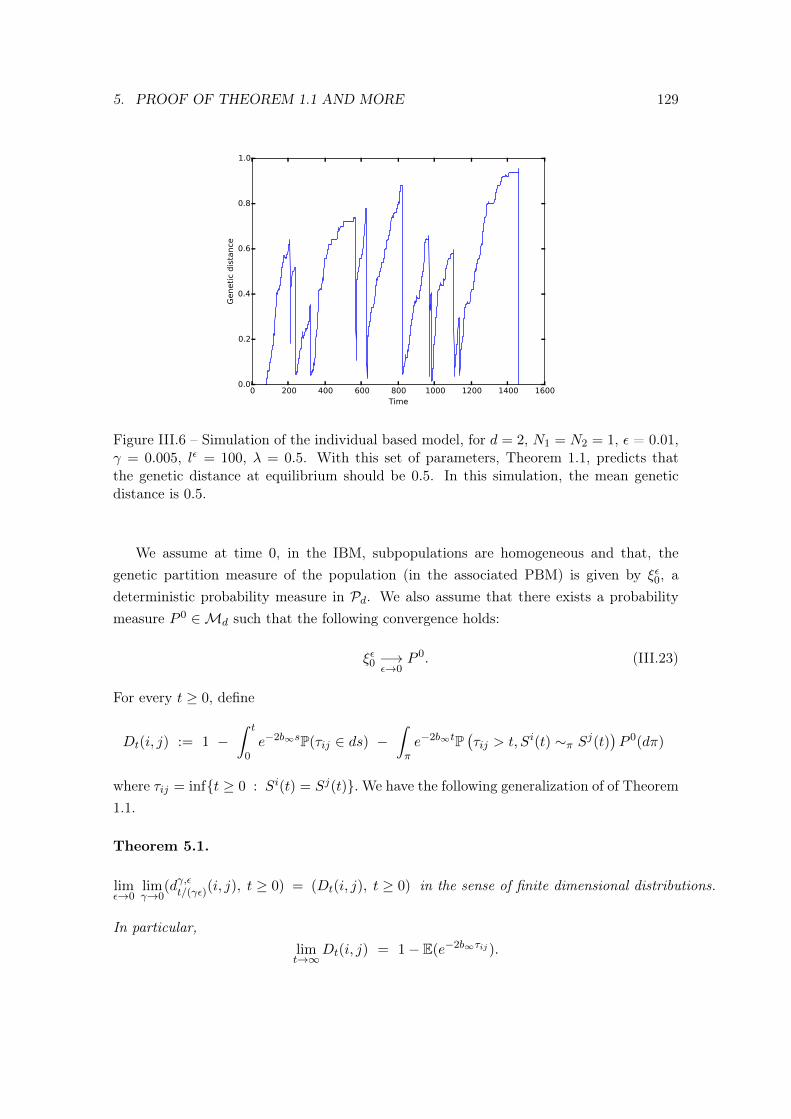
5. PROOF OF THEOREM 1.1 AND MORE 129
0 200 400 600 800 1000 1200 1400 1600Time
0.0
0.2
0.4
0.6
0.8
1.0
Geneti
c dis
tance
Figure III.6 – Simulation of the individual based model, for d = 2, N1 = N2 = 1, ε = 0.01,γ = 0.005, lε = 100, λ = 0.5. With this set of parameters, Theorem 1.1, predicts thatthe genetic distance at equilibrium should be 0.5. In this simulation, the mean geneticdistance is 0.5.
We assume at time 0, in the IBM, subpopulations are homogeneous and that, thegenetic partition measure of the population (in the associated PBM) is given by ξε0, adeterministic probability measure in Pd. We also assume that there exists a probabilitymeasure P 0 ∈Md such that the following convergence holds:
ξε0 −→ε→0
P 0. (III.23)
For every t ≥ 0, define
Dt(i, j) := 1 −∫ t
0e−2b∞sP(τij ∈ ds) −
∫πe−2b∞tP
(τij > t, Si(t) ∼π Sj(t)
)P 0(dπ)
where τij = inft ≥ 0 : Si(t) = Sj(t).We have the following generalization of of Theorem1.1.
Theorem 5.1.
limε→0
limγ→0
(dγ,εt/(γε)(i, j), t ≥ 0) = (Dt(i, j), t ≥ 0) in the sense of finite dimensional distributions.
In particular,limt→∞
Dt(i, j) = 1− E(e−2b∞τij ).
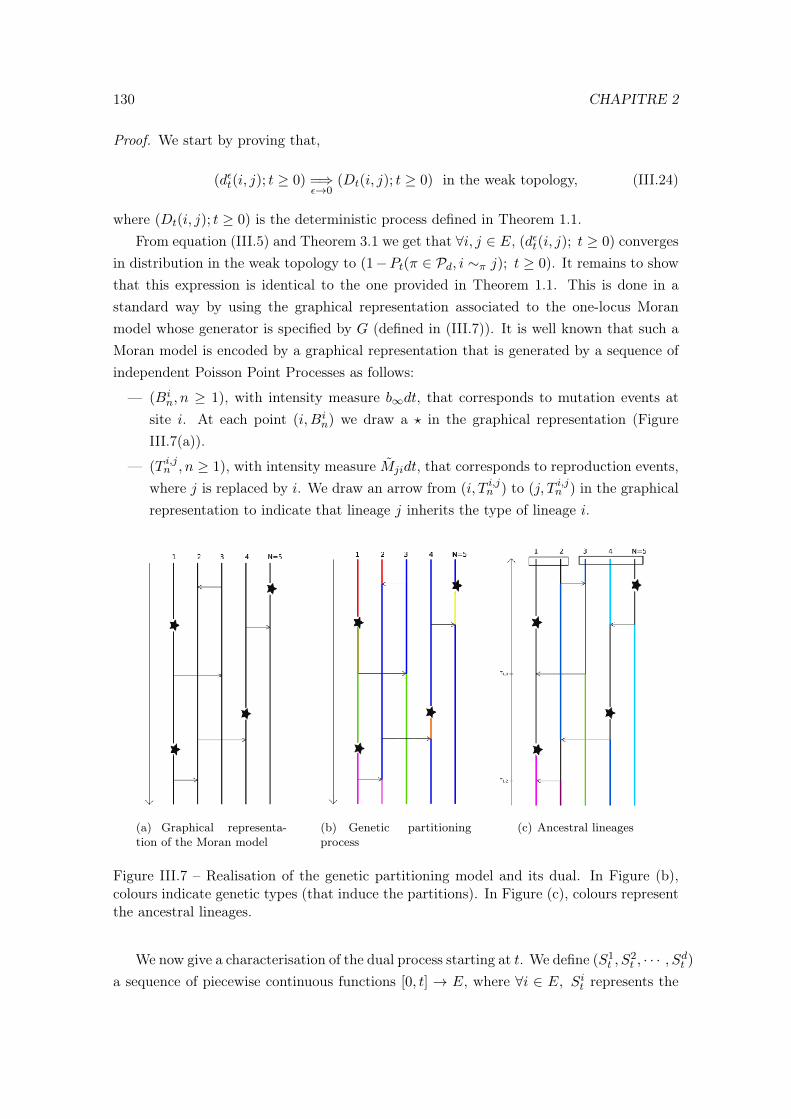
130 CHAPITRE 2
Proof. We start by proving that,
(dεt(i, j); t ≥ 0) =⇒ε→0
(Dt(i, j); t ≥ 0) in the weak topology, (III.24)
where (Dt(i, j); t ≥ 0) is the deterministic process defined in Theorem 1.1.From equation (III.5) and Theorem 3.1 we get that ∀i, j ∈ E, (dεt(i, j); t ≥ 0) converges
in distribution in the weak topology to (1−Pt(π ∈ Pd, i ∼π j); t ≥ 0). It remains to showthat this expression is identical to the one provided in Theorem 1.1. This is done in astandard way by using the graphical representation associated to the one-locus Moranmodel whose generator is specified by G (defined in (III.7)). It is well known that such aMoran model is encoded by a graphical representation that is generated by a sequence ofindependent Poisson Point Processes as follows:
— (Bin, n ≥ 1), with intensity measure b∞dt, that corresponds to mutation events at
site i. At each point (i, Bin) we draw a ? in the graphical representation (Figure
III.7(a)).
— (T i,jn , n ≥ 1), with intensity measure Mjidt, that corresponds to reproduction events,where j is replaced by i. We draw an arrow from (i, T i,jn ) to (j, T i,jn ) in the graphicalrepresentation to indicate that lineage j inherits the type of lineage i.
(a) Graphical representa-tion of the Moran model
(b) Genetic partitioningprocess
(c) Ancestral lineages
Figure III.7 – Realisation of the genetic partitioning model and its dual. In Figure (b),colours indicate genetic types (that induce the partitions). In Figure (c), colours representthe ancestral lineages.
We now give a characterisation of the dual process starting at t. We define (S1t , S
2t , · · · , Sdt )
a sequence of piecewise continuous functions [0, t] → E, where ∀i ∈ E, Sit represents the
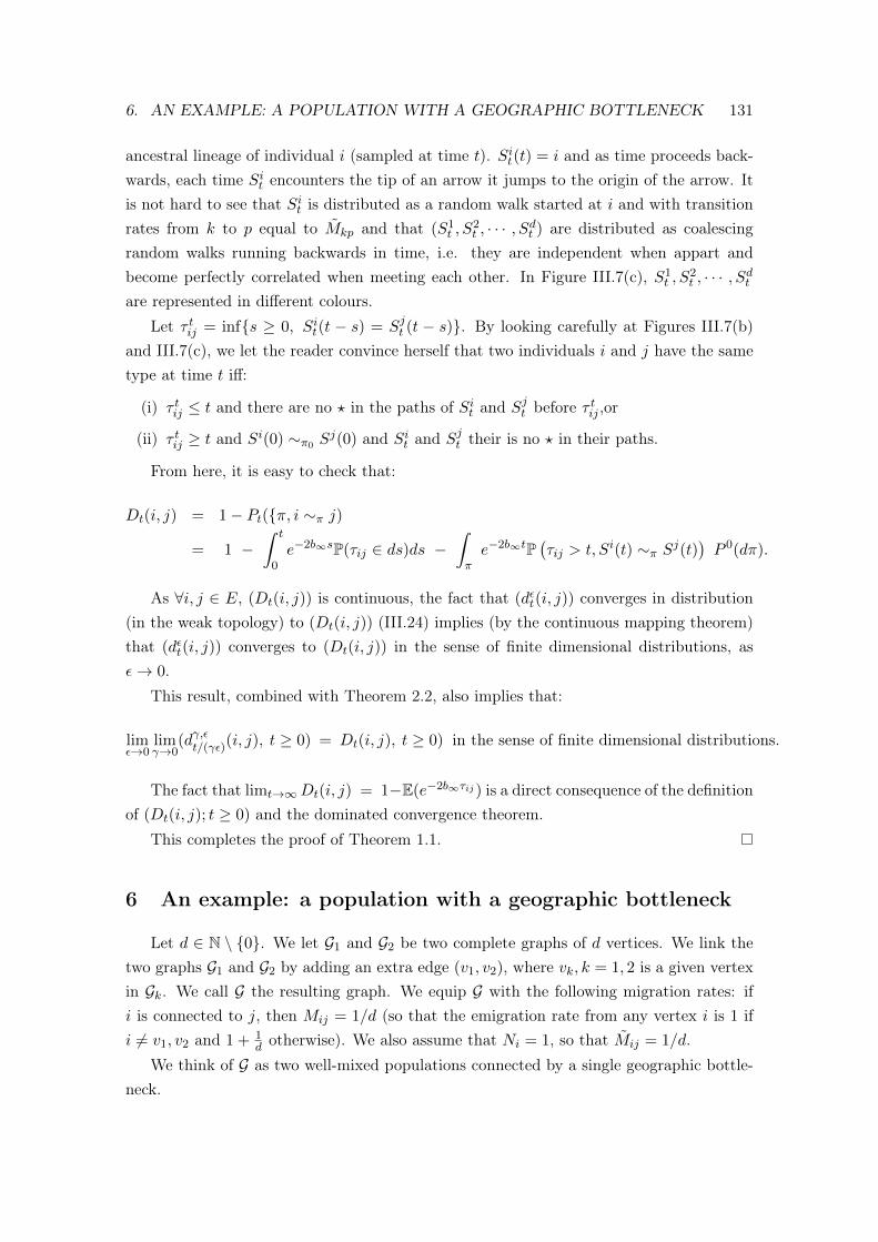
6. AN EXAMPLE: A POPULATION WITH A GEOGRAPHIC BOTTLENECK 131
ancestral lineage of individual i (sampled at time t). Sit(t) = i and as time proceeds back-wards, each time Sit encounters the tip of an arrow it jumps to the origin of the arrow. Itis not hard to see that Sit is distributed as a random walk started at i and with transitionrates from k to p equal to Mkp and that (S1
t , S2t , · · · , Sdt ) are distributed as coalescing
random walks running backwards in time, i.e. they are independent when appart andbecome perfectly correlated when meeting each other. In Figure III.7(c), S1
t , S2t , · · · , Sdt
are represented in different colours.Let τ tij = infs ≥ 0, Sit(t − s) = Sjt (t − s). By looking carefully at Figures III.7(b)
and III.7(c), we let the reader convince herself that two individuals i and j have the sametype at time t iff:
(i) τ tij ≤ t and there are no ? in the paths of Sit and Sjt before τ tij ,or
(ii) τ tij ≥ t and Si(0) ∼π0 Sj(0) and Sit and S
jt their is no ? in their paths.
From here, it is easy to check that:
Dt(i, j) = 1− Pt(π, i ∼π j)
= 1 −∫ t
0e−2b∞sP(τij ∈ ds)ds −
∫πe−2b∞tP
(τij > t, Si(t) ∼π Sj(t)
)P 0(dπ).
As ∀i, j ∈ E, (Dt(i, j)) is continuous, the fact that (dεt(i, j)) converges in distribution(in the weak topology) to (Dt(i, j)) (III.24) implies (by the continuous mapping theorem)that (dεt(i, j)) converges to (Dt(i, j)) in the sense of finite dimensional distributions, asε→ 0.
This result, combined with Theorem 2.2, also implies that:
limε→0
limγ→0
(dγ,εt/(γε)(i, j), t ≥ 0) = Dt(i, j), t ≥ 0) in the sense of finite dimensional distributions.
The fact that limt→∞Dt(i, j) = 1−E(e−2b∞τij ) is a direct consequence of the definitionof (Dt(i, j); t ≥ 0) and the dominated convergence theorem.
This completes the proof of Theorem 1.1.
6 An example: a population with a geographic bottleneck
Let d ∈ N \ 0. We let G1 and G2 be two complete graphs of d vertices. We link thetwo graphs G1 and G2 by adding an extra edge (v1, v2), where vk, k = 1, 2 is a given vertexin Gk. We call G the resulting graph. We equip G with the following migration rates: ifi is connected to j, then Mij = 1/d (so that the emigration rate from any vertex i is 1 ifi 6= v1, v2 and 1 + 1
d otherwise). We also assume that Ni = 1, so that Mij = 1/d.We think of G as two well-mixed populations connected by a single geographic bottle-
neck.
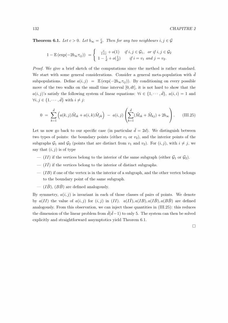
132 CHAPITRE 2
Theorem 6.1. Let c > 0. Let b∞ = cd . Then for any two neighbours i, j ∈ G
1− E (exp(−2b∞τij)) =
c
1+c + o(1) if i, j ∈ G1, or if i, j ∈ G2
1− 1d + o(1
d) if i = v1 and j = v2.
Proof. We give a brief sketch of the computations since the method is rather standard.We start with some general considerations. Consider a general meta-population with d
subpopulations. Define a(i, j) = E (exp(−2b∞τij)). By conditioning on every possiblemove of the two walks on the small time interval [0, dt], it is not hard to show that thea(i, j)’s satisfy the following system of linear equations: ∀i ∈ 1, · · · , d, a(i, i) = 1 and∀i, j ∈ 1, · · · , d with i 6= j:
0 =d∑
k=1
(a(k, j)Mik + a(i, k)Mjk
)− a(i, j)
d∑k=1
(Mik + Mkj) + 2b∞
. (III.25)
Let us now go back to our specific case (in particular d = 2d). We distinguish betweentwo types of points: the boundary points (either v1 or v2), and the interior points of thesubgraphs G1 and G2 (points that are distinct from v1 and v2). For (i, j), with i 6= j, wesay that (i, j) is of type
— (II) if the vertices belong to the interior of the same subgraph (either G1 or G2).
— (II) if the vertices belong to the interior of distinct subgraphs.
— (IB) if one of the vertex is in the interior of a subgraph, and the other vertex belongsto the boundary point of the same subgraph.
— (IB), (BB) are defined analogously.
By symmetry, a(i, j) is invariant in each of those classes of pairs of points. We denoteby a(II) the value of a(i, j) for (i, j) in (II). a(II), a(IB), a(IB), a(BB) are definedanalogously. From this observation, we can inject those quantities in (III.25): this reducesthe dimension of the linear problem from d(d−1) to only 5. The system can then be solvedexplicitly and straightforward assymptotics yield Theorem 6.1.