Studies in Non-equilibrium Statistical Physics:
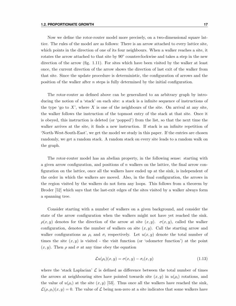
152
— Studies in Non-equilibrium Statistical Physics: Pattern Formation and Absorbing Phase Transitions A Thesis Submitted to Tata Institute of Fundamental Research, Mumbai, India for the degree of Doctor of Philosophy in Physics By Rahul Dandekar Department of Theoretical Physics Tata Institute of Fundamental Research Mumbai - 400 005, India October 2014 Final version Submitted in July, 2015
-
Upload
khangminh22 -
Category
Documents
-
view
2 -
download
0
Transcript of Studies in Non-equilibrium Statistical Physics:
—
Studies in Non-equilibrium Statistical Physics:
Pattern Formation and Absorbing Phase Transitions
A Thesis
Submitted to
Tata Institute of Fundamental Research, Mumbai, India
for the degree of
Doctor of Philosophy
in
Physics
By
Rahul Dandekar
Department of Theoretical Physics
Tata Institute of Fundamental Research
Mumbai - 400 005, India
October 2014
Final version Submitted in July, 2015


Declaration
This thesis is a presentation of my original research work. Wherever contribu-
tions of others are involved, every effort is made to indicate this clearly, with
due reference to the literature, and acknowledgement of collaborative research
and discussions.
The work was done under the guidance of Professor Deepak Dhar, at the Tata
Institute of Fundamental Research, Mumbai.
(Rahul Dandekar)
In my capacity as the supervisor of the candidate’s thesis, I certify that the
above statements are true to the best of my knowledge.
(Deepak Dhar)

Acknowledgements
I owe a huge debt to my supervisor, Prof. Deepak Dhar, for his guidance and unlimited
wisdom, and also for his patience in dealing with my spells of losing and gaining interest in
various topics, and his belief that someday I will learn the fine art of academic writing. I
hope that he holds this belief even after reading this thesis.
Among my seniors, Kabir has provided me with both a role model and an outlet for frus-
tration, although in the latter case the reverse is probably truer. I learnt a lot of worldly
wisdom from Sasi. Tridib will always be associated with memories of my initial years
and the malpuvas at Mohd. Ali Road. Other officemates, both past and present, are too
numerous to name, but the DTP experience would have been utterly desolate without them.
Nikhil, Geet and Sambuddha made life in the office and outside far more bearable.
Oh, yes, Geet wants a separate sentence all to himself. Nikhil (in a double role), Ravitej,
Gourab, Aditi and Garima had the thankless job of being my closest friends, but they per-
sisted through it for all six years. And all of the other batchmates shared with us not only
classes and assignments but the whole winding wavering thread of PhD life.
And whether or not I needed someone to talk to, Anisha and Achal have been there,
enriching my life through diverse yet lush conversation. Sonal, Parul and Surat have been
able sparring partners, yet curiously supportive and understanding. I also thank Colaba
girls for not bothering me too much and letting me concentrate on my research.
And all this and more would have been impossible without daily, hourly support of my
parents, who never pushed me to pursue something I didn’t find exciting. I can never repay
the debts I owe them.


Collaborators
This thesis is based on work done under the supervision of Prof. Deepak Dhar.
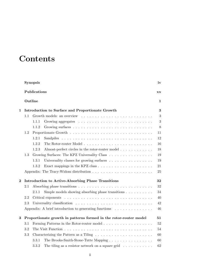
Contents
Synopsis iv
Publications xx
Outline 1
1 Introduction to Surface and Proportionate Growth 3
1.1 Growth models: an overview . . . . . . . . . . . . . . . . . . . . . . . . . . 3
1.1.1 Growing aggregates . . . . . . . . . . . . . . . . . . . . . . . . . . . 3
1.1.2 Growing surfaces . . . . . . . . . . . . . . . . . . . . . . . . . . . . . 8
1.2 Proportionate Growth . . . . . . . . . . . . . . . . . . . . . . . . . . . . . . 11
1.2.1 Sandpiles . . . . . . . . . . . . . . . . . . . . . . . . . . . . . . . . . 12
1.2.2 The Rotor-router Model . . . . . . . . . . . . . . . . . . . . . . . . . 16
1.2.3 Almost-perfect circles in the rotor-router model . . . . . . . . . . . . 18
1.3 Growing Surfaces: The KPZ Universality Class . . . . . . . . . . . . . . . . 19
1.3.1 Universality classes for growing surfaces . . . . . . . . . . . . . . . . 19
1.3.2 Exact mappings in the KPZ class . . . . . . . . . . . . . . . . . . . . 21
Appendix: The Tracy-Widom distribution . . . . . . . . . . . . . . . . . . . . . . 25
2 Introduction to Active-Absorbing Phase Transitions 32
2.1 Absorbing phase transitions . . . . . . . . . . . . . . . . . . . . . . . . . . . 32
2.1.1 Simple models showing absorbing phase transitions . . . . . . . . . . 34
2.2 Critical exponents . . . . . . . . . . . . . . . . . . . . . . . . . . . . . . . . 40
2.3 Universality classification . . . . . . . . . . . . . . . . . . . . . . . . . . . . 42
Appendix: A brief introduction to generating functions . . . . . . . . . . . . . . 46
3 Proportionate growth in patterns formed in the rotor-router model 51
3.1 Forming Patterns in the Rotor-router model . . . . . . . . . . . . . . . . . . 52
3.2 The Visit Function . . . . . . . . . . . . . . . . . . . . . . . . . . . . . . . . 54
3.3 Characterizing the Pattern as a Tiling . . . . . . . . . . . . . . . . . . . . . 60
3.3.1 The Brooks-Smith-Stone-Tutte Mapping . . . . . . . . . . . . . . . . 60
3.3.2 The tiling as a resistor network on a square grid . . . . . . . . . . . 62
ii
CONTENTS iii
3.3.3 Determining the visit function . . . . . . . . . . . . . . . . . . . . . 64
3.4 Other starting backgrounds . . . . . . . . . . . . . . . . . . . . . . . . . . . 65
3.4.1 Type II . . . . . . . . . . . . . . . . . . . . . . . . . . . . . . . . . . 65
3.4.2 Type III . . . . . . . . . . . . . . . . . . . . . . . . . . . . . . . . . . 66
3.4.3 Type IV . . . . . . . . . . . . . . . . . . . . . . . . . . . . . . . . . . 67
3.5 Bounded Fluctuations and Quasiperiodicity . . . . . . . . . . . . . . . . . . 69
3.6 Summary and concluding remarks . . . . . . . . . . . . . . . . . . . . . . . 73
Appendix: Derivation on eqn. (3.9) from matching of boundary conditions . . . 74
4 Rotor-router Patterns on Noisy Backgrounds 76
4.1 Recurrent and Transient Backgrounds . . . . . . . . . . . . . . . . . . . . . 77
4.1.1 Recurrence and Transience . . . . . . . . . . . . . . . . . . . . . . . 77
4.1.2 Notation and Protocol . . . . . . . . . . . . . . . . . . . . . . . . . . 79
4.2 From Approximate to Exact Visit function . . . . . . . . . . . . . . . . . . 79
4.2.1 Point perturbations . . . . . . . . . . . . . . . . . . . . . . . . . . . 82
4.3 Case I . . . . . . . . . . . . . . . . . . . . . . . . . . . . . . . . . . . . . . . 85
4.3.1 The rules for drawing defect lines . . . . . . . . . . . . . . . . . . . . 85
4.3.2 The exact visit function and Tracy-Widom fluctuations . . . . . . . 87
4.3.3 Lines of constant visit function . . . . . . . . . . . . . . . . . . . . . 89
4.4 Case II . . . . . . . . . . . . . . . . . . . . . . . . . . . . . . . . . . . . . . . 90
4.4.1 Rules for drawing defect lines . . . . . . . . . . . . . . . . . . . . . . 91
4.4.2 Lines of constant visit function . . . . . . . . . . . . . . . . . . . . . 93
4.4.3 Transition from recurrence to transience . . . . . . . . . . . . . . . . 94
4.5 Conclusions . . . . . . . . . . . . . . . . . . . . . . . . . . . . . . . . . . . . 97
5 A Class of Active-Absorbing Phase Transitions 100
5.1 Definition of the model . . . . . . . . . . . . . . . . . . . . . . . . . . . . . . 101
5.2 Phase Space Picture . . . . . . . . . . . . . . . . . . . . . . . . . . . . . . . 102
5.3 Counting steady-state configurations using generating functions . . . . . . . 105
5.4 Activity and Transience fields . . . . . . . . . . . . . . . . . . . . . . . . . . 108
5.4.1 Activity field . . . . . . . . . . . . . . . . . . . . . . . . . . . . . . . 109
5.4.2 Transience field . . . . . . . . . . . . . . . . . . . . . . . . . . . . . . 109
5.5 A Mapping to a Gas of Defects . . . . . . . . . . . . . . . . . . . . . . . . . 111
5.6 Non-equilibrium exponents of the Conserved Lattice Gas . . . . . . . . . . . 112
5.6.1 Steady-state exponents . . . . . . . . . . . . . . . . . . . . . . . . . 112
5.6.2 Random initial conditions . . . . . . . . . . . . . . . . . . . . . . . . 114
5.7 Summary and Concluding Remarks . . . . . . . . . . . . . . . . . . . . . . . 117
Appendix I: Counting the Absorbing Configurations . . . . . . . . . . . . . . . . 118
Appendix II: Counting the isolated active 1s . . . . . . . . . . . . . . . . . . . . . 120
6 Summary and Concluding Remarks 124
Synopsis
1. Introduction
In recent years, non-equilibrium phenomena have been the focus of studies in statisti-
cal mechanics. The discovery of nontrivial exactly soluble models has been important in
developing a deeper understanding of several nonequilibrium phenomena. Properties such
as universality of critical exponents have been found to hold true even for nonequilibrium
phase transitions. In this synopsis, I describe my studies on two model systems that benefit
from the simplicity of the models which makes them amenable to exact analysis, and yet
display behaviour shared by more complicated models.
Growing patterns in which the internal structure grows proportionately with the pat-
tern are said to exhibit proportionate growth. Such growth is seen in young animals, for
instance, where the internal organs grow as the body grows. A simple far-from-equilibrium
model which has been found to show proportionate growth is the sandpile model, where
the patterns were created by dropping sand on the origin of a 2D lattice and letting the
configuration stabilise [1] [2]. These studies are reviewed in [3]. The structure of some such
patterns was characterized and was found to be described by discrete analytic functions on
graphs, where the graph depends on the pattern being studied.
The first topic we describe is proportionately growing patterns in another model, called
the rotor-router model. The rotor-router model shows self-organised criticality in its steady
state, like the sandpile model. It has also been of interest to computer scientists as a deran-
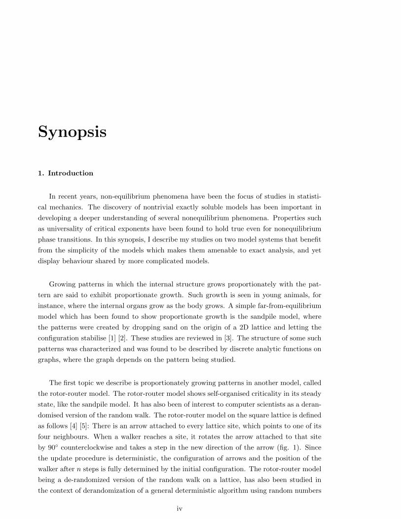
domised version of the random walk. The rotor-router model on the square lattice is defined
as follows [4] [5]: There is an arrow attached to every lattice site, which points to one of its
four neighbours. When a walker reaches a site, it rotates the arrow attached to that site
by 90 counterclockwise and takes a step in the new direction of the arrow (fig. 1). Since
the update procedure is deterministic, the configuration of arrows and the position of the
walker after n steps is fully determined by the initial configuration. The rotor-router model
being a de-randomized version of the random walk on a lattice, has also been studied in
the context of derandomization of a general deterministic algorithm using random numbers
iv
v
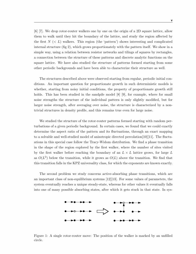
[6] [7]. We drop rotor-router walkers one by one on the origin of a 2D square lattice, allow
them to walk until they hit the boundary of the lattice, and study the region affected by
the first N (< L) walkers. This region (the ‘pattern’) shows interesting and complicated
internal structure (fig 2), which grows proportionately with the pattern itself. We show in a
simple way, using a relation between resistor networks and tilings of squares by rectangles,
a connection between the structure of these patterns and discrete analytic functions on the
square lattice. We have also studied the structure of patterns formed starting from some
other periodic backgrounds and have been able to characterize their structure as well.
The structures described above were observed starting from regular, periodic initial con-
ditions. An important question for proportionate growth in such deterministic models is
whether, starting from noisy initial conditions, the property of proportionate growth still
holds. This has been studied in the sandpile model [8] [9], for example, where for small
noise strengths the structure of the individual pattern is only slightly modified, but for
larger noise strength, after averaging over noise, the structure is characterized by a non-
trivial structures in density profile, and this remains true even for large noise.
We studied the structure of the rotor-router patterns formed starting with random per-
turbations of a given periodic background. In certain cases, we found that we could exactly
determine the aspect ratio of the pattern and its fluctuations, through an exact mapping
to a solvable and well-studied model of anisotropic directed percolation[10][11]. The fluctu-
ations in this special case follow the Tracy-Widom distribution. We find a phase transition
in the shape of the region explored by the first walker, where the number of sites visited
by the first walker before reaching the boundary of an L × L lattice grows, for large L
as O(L3) below the transition, while it grows as O(L) above the transition. We find that
this transition falls in the KPZ universality class, for which the exponents are known exactly.
The second problem we study concerns active-absorbing phase transitions, which are
an important class of non-equilibrium systems [12][13]. For some values of parameters, the
system eventually reaches a unique steady-state, whereas for other values it eventually falls
into one of many possible absorbing states, after which it gets stuck in that state. In sys-
Figure 1: A single rotor-router move: The position of the walker is marked by an unfilledcircle.
vi SYNOPSIS
Figure 2: Pattern formed by depositing rotor-router walkers at the origin of a square lattice,starting from an initial configuration of all arrows pointing East, after 1600 walkers. Notethat the second picture is scaled by a factor 4 compared to the first. Colour code: darkblue - →, light blue - ↑, yellow - ←, red - ↓
tems characterized by stochastic rules which allow for growth or dissipation of activity in
a region depending on the local neighbourhood, and for diffusion to surrounding regions,
such transitions are expected to fall in the universality class of Directed Percolation, as
conjectured by Grassberger and Jannsen in the early 1980s [14].
We were interested in systems where the number of particles is conserved. In such cases,
due to the additional conservation law, the Grassberger-Janssen conjecture is not expected
to hold. However, the numerical analysis of the transition in such models has resulted in
conflicting results [27], and it would be helpful to have nontrivial exactly solvable models
as a testing ground for such analyses. There have been few exactly solvable models with
a complex phase space structure which show active-absorbing transitions with a conserved
number of particles. Aside from two models created by de Oliviera and da Silva in [15], solv-
able conserved-particle-number models which show an absorbing phase transition generally
have the same exponents as the simplest such example, which is the Conserved Lattice Gas
[16].
We constructed, following [15], a class of exactly solvable models, all of which display
an active-absorbing transition in one dimension. We found that the steady-state can be ex-
actly determined, and we calculated the (static) critical exponents of the transition, using
the generating function technique. Our analysis showed that the order parameter exponent
β = n for the nth model in the class. This shows emphatically that these models do not
belong to the Directed Percolation universality class, and in fact each model in the class,
for n > 1, defines a separate universality class for active-absorbing phase transitions in 1D.
2. Pattern Formation in the Rotor-Router Model
vii
In this section we describe the study of proportionately growing patterns for the rotor-
router model starting from periodic backgrounds. The characterization here turns out to
be simpler than in the case of the sandpile model, related to the fact that here one only
deals with piece-wise linear functions instead of piece-wise quadratic functions.
We form patterns in the rotor-router model by putting walkers one by one at the origin
and letting them walk till they leave from the edge of the lattice. A new walker is introduced
at the origin when the previous walker has left. We study the configuration of arrows when
the N -th walker has just left the system. In this section, we mainly consider the case where
the initial configuration is such that all arrows are parallel, pointing due East (→). Clearly,
the first walker put at the origin would move along the positive y-axis, rotating the arrows
it encounters to point North. The second walker rotates the arrow at the origin to point
West, and then walks North along the vertical line x = −1. After a large number of walkers
have left the lattice, the pattern of arrows left behind is a complex one made of triangular
and dart-like patches (fig 2).
To characterize the structure of the pattern, we determined the sizes of the different
patches in the pattern, using as input the observed arrangement of these elements in the
pattern. For this, we use the Brooks-Smith-Stone-Tutte (BSST) mapping ([17]) which al-
lows one to find the sizes of all the squares in a square tiling using only information about
their geometric arrangement in the tiling. Each tiling corresponds to a resistor network
with horizontal lines in the tiling as the nodes in the network. The function V where
V (X) is the height in the tiling of the node X measured from the base can be shown to
be harmonic on this graph, ∇2V = 0, where ∇2 is the discrete Laplacian on the square grid.
We consider the pattern in fig. 2. Rescaling the pattern formed when the number of
walkers N → ∞, to have diameter D′ = 1 and centred at the origin, the rescaled pattern
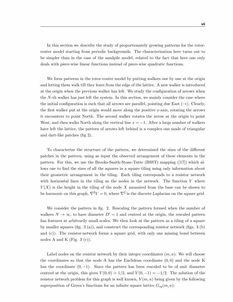
has features at arbitrarily small scales. We then look at the pattern as a tiling of a square
by smaller squares (fig. 3 (a)), and construct the corresponding resistor network (figs. 3 (b)
and (c)). The resistor-network forms a square grid, with only one missing bond between
nodes A and K (Fig. 3 (c)).
Label nodes on the resistor network by their integer coordinates (m,n). We will choose
the coordinates so that the node A has the Euclidean coordinate (0, 0) and the node K
has the coordinate (0,−1). Since the pattern has been rescaled to be of unit diameter
centred at the origin, this gives V (0, 0) = 1/2, and V (0,−1) = −1/2. The solution of the
resistor network problem for this graph is well known, V (m,n) being given by the following
superposition of Green’s functions for an infinite square lattice Gsq(m,n):
viii SYNOPSIS
(a) (b)
(c)
Figure 3: (a) The pattern as a square tiling. The first few levels of the correspondingnetwork are shown. (b) Part of the resistor network corresponding to the tiling above. Theedges illustrated part (a) are in black with arrows indicating the direction of the current.Note that some nodes (for example (1,0) and (1,1)) correspond to horizontal segments whichlie at the same height, but have not been grouped together as a single segment. (c) Thegraph in part (b) shown as a part of the complete resistor network for the tiling in (a). Thecomplete resistor network has the form of a square lattice.
V (m,n) = 2(Gsq(m,n+ 1)−Gsq(m,n)) (1)
where [18]
Gsq(m,n) =
∫ π
−π
dk1
2π
∫ π
−π
dk2
2π
1− cos(k1m+ k2n)
2− cos k1 − cos k2(2)
From this solution we get the sizes of various elements in the pattern. For exam-
ple, the size of the big squares at the four corners of Fig. 3 (a) is given by the dif-
ference in the vertical co-ordinates of lines A and B. From Fig. 3 (c) this is equal to
V (A) − V (B) = V (0, 0) − V (1, 0). Using the values V (1, 0) = 2π − 1/2 and V (0, 0) = 1/2,
the size of these largest squares in the pattern relative to the size of the pattern is 1− 2π .
The visit function VN (x, y) on the original square lattice is defined as the number of
times the site (x, y) visited by N walkers before they exit the lattice. In each of the tri-
ix
angular or dart-shaped regions in fig 2, VN (x, y) can be proved to be a piecewise linear
function mx+ny+ cm,n, with m and n integers. An important construction is a one-to-one
correspondence between regions across which the form of VN (x, y) does not change, and
squares in the tiling picture of the pattern. This allows one to use eqn. 1 to determine the
visit function everywhere in the pattern.
(a)
0 50 100 150 200 250 3000
50
100
150
200
250
300
(b)
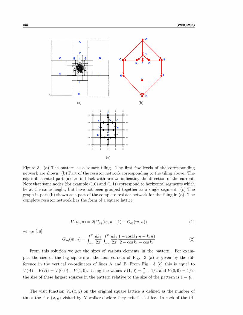
Figure 4: Pattern formed the initial backgrounds generated by tiling the lattice with the2x2 unit cell given in (a) is shown in (b) after 700 walkers put at the origin have left thelattice. Colour code: dark blue - →, light blue - ↑, yellow - ←, red - ↓.
(a)
0 50 100 150 200 250 3000
50
100
150
200
250
300
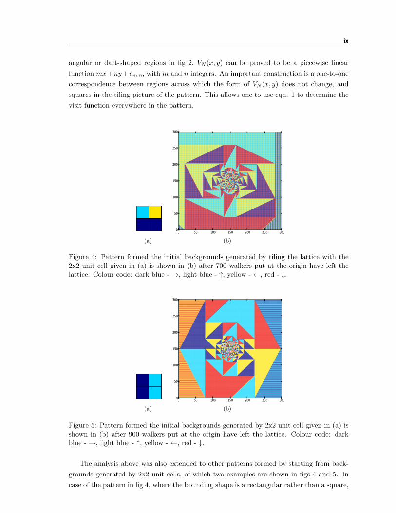
(b)
Figure 5: Pattern formed the initial backgrounds generated by 2x2 unit cell given in (a) isshown in (b) after 900 walkers put at the origin have left the lattice. Colour code: darkblue - →, light blue - ↑, yellow - ←, red - ↓.
The analysis above was also extended to other patterns formed by starting from back-
grounds generated by 2x2 unit cells, of which two examples are shown in figs 4 and 5. In
case of the pattern in fig 4, where the bounding shape is a rectangular rather than a square,
x SYNOPSIS
the aspect ratio of the pattern can also be calculated from the above analysis.
(a)
(b)
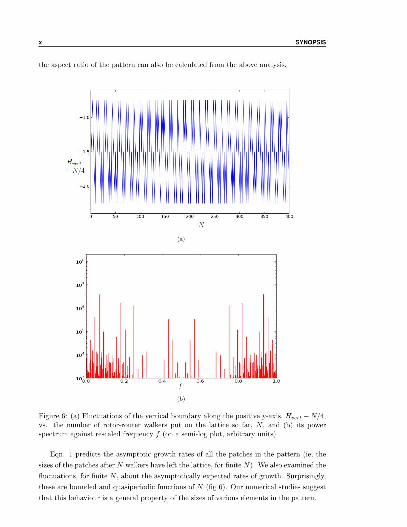
Figure 6: (a) Fluctuations of the vertical boundary along the positive y-axis, Hvert −N/4,vs. the number of rotor-router walkers put on the lattice so far, N , and (b) its powerspectrum against rescaled frequency f (on a semi-log plot, arbitrary units)
Eqn. 1 predicts the asymptotic growth rates of all the patches in the pattern (ie, the
sizes of the patches after N walkers have left the lattice, for finite N). We also examined the
fluctuations, for finite N , about the asymptotically expected rates of growth. Surprisingly,
these are bounded and quasiperiodic functions of N (fig 6). Our numerical studies suggest
that this behaviour is a general property of the sizes of various elements in the pattern.
xi
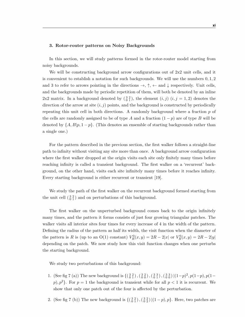
3. Rotor-router patterns on Noisy Backgrounds
In this section, we will study patterns formed in the rotor-router model starting from
noisy backgrounds.
We will be constructing background arrow configurations out of 2x2 unit cells, and it
is convenient to establish a notation for such backgrounds. We will use the numbers 0, 1, 2
and 3 to refer to arrows pointing in the directions →, ↑, ← and ↓ respectively. Unit cells,
and the backgrounds made by periodic repetition of them, will both be denoted by an inline
2x2 matrix. In a background denoted by ( 3 20 1 ), the element (i, j) (i, j = 1, 2) denotes the
direction of the arrow at site (i, j) points, and the background is constructed by periodically
repeating this unit cell in both directions. A randomly background where a fraction p of
the cells are randomly assigned to be of type A and a fraction (1− p) are of type B will be
denoted by A,B|p, 1− p. (This denotes an ensemble of starting backgrounds rather than
a single one.)
For the pattern described in the previous section, the first walker follows a straight-line
path to infinity without visiting any site more than once. A background arrow configuration
where the first walker dropped at the origin visits each site only finitely many times before
reaching infinity is called a transient background. The first walker on a ‘recurrent’ back-
ground, on the other hand, visits each site infinitely many times before it reaches infinity.
Every starting background is either recurrent or transient [19].
We study the path of the first walker on the recurrent background formed starting from
the unit cell ( 3 20 1 ) and on perturbations of this background.
The first walker on the unperturbed background comes back to the origin infinitely
many times, and the pattern it forms consists of just four growing triangular patches. The
walker visits all interior sites four times for every increase of 4 in the width of the pattern.
Defining the radius of the pattern as half its width, the visit function when the diameter of
the pattern is R is (up to an O(1) constant) V 0R(x, y) = 2R − 2|x| or V 0
R(x, y) = 2R − 2|y|depending on the patch. We now study how this visit function changes when one perturbs
the starting background.
We study two perturbations of this background:
1. (See fig 7 (a)) The new background is ( 3 20 1 ) , ( 3 2
0 0 ) , ( 3 30 1 ) , ( 3 3
0 0 ) |(1−p)2, p(1−p), p(1−p), p2. For p = 1 the background is transient while for all p < 1 it is recurrent. We
show that only one patch out of the four is affected by the perturbation.
2. (See fig 7 (b)) The new background is ( 3 20 1 ) , ( 3 2
0 2 ) |(1− p), p. Here, two patches are
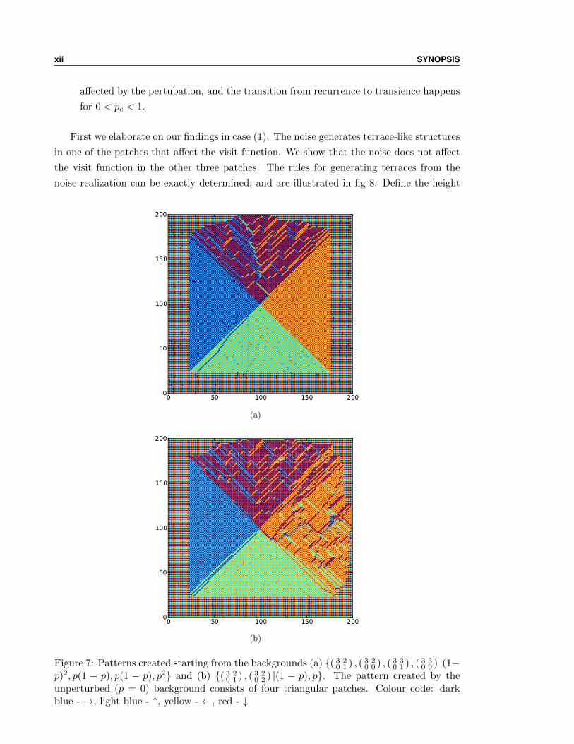
xii SYNOPSIS
affected by the pertubation, and the transition from recurrence to transience happens
for 0 < pc < 1.
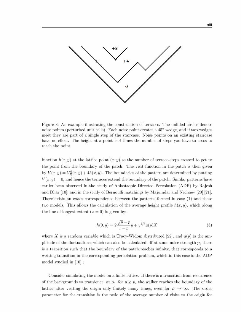
First we elaborate on our findings in case (1). The noise generates terrace-like structures
in one of the patches that affect the visit function. We show that the noise does not affect
the visit function in the other three patches. The rules for generating terraces from the
noise realization can be exactly determined, and are illustrated in fig 8. Define the height
(a)
(b)
Figure 7: Patterns created starting from the backgrounds (a) ( 3 20 1 ) , ( 3 2
0 0 ) , ( 3 30 1 ) , ( 3 3
0 0 ) |(1−p)2, p(1 − p), p(1 − p), p2 and (b) ( 3 2
0 1 ) , ( 3 20 2 ) |(1 − p), p. The pattern created by the
unperturbed (p = 0) background consists of four triangular patches. Colour code: darkblue - →, light blue - ↑, yellow - ←, red - ↓
xiii
Figure 8: An example illustrating the construction of terraces. The unfilled circles denotenoise points (perturbed unit cells). Each noise point creates a 45 wedge, and if two wedgesmeet they are part of a single step of the staircase. Noise points on an existing staircasehave no effect. The height at a point is 4 times the number of steps you have to cross toreach the point.
function h(x, y) at the lattice point (x, y) as the number of terrace-steps crossed to get to
the point from the boundary of the patch. The visit function in the patch is then given
by V (x, y) = V 0R(x, y) + 4h(x, y). The boundaries of the pattern are determined by putting
V (x, y) = 0, and hence the terraces extend the boundary of the patch. Similar patterns have
earlier been observed in the study of Anisotropic Directed Percolation (ADP) by Rajesh
and Dhar [10], and in the study of Bernoulli matchings by Majumdar and Nechaev [20] [21].
There exists an exact correspondence between the patterns formed in case (1) and these
two models. This allows the calculation of the average height profile h(x, y), which along
the line of longest extent (x = 0) is given by:
h(0, y) = 2
√p− p
1− py + y1/3a(p)X (3)
where X is a random variable which is Tracy-Widom distributed [22], and a(p) is the am-
plitude of the fluctuations, which can also be calculated. If at some noise strength pc there
is a transition such that the boundary of the patch reaches infinity, that corresponds to a
wetting transition in the corresponding percolation problem, which in this case is the ADP
model studied in [10] .
Consider simulating the model on a finite lattice. If there is a transition from recurrence
of the backgrounds to transience, at pc, for p ≥ pc the walker reaches the boundary of the
lattice after visiting the origin only finitely many times, even for L → ∞. The order
parameter for the transition is the ratio of the average number of visits to the origin for
xiv SYNOPSIS
a given noise strength, to the lattice size L: v(p) = limL→∞ v(p, L)/L. v(p) = 0 in the
transient phase. From the result for h(x, y) we derive the exact formula
v(p) = 1− 2
√p− p
1− p(4)
The background is thus recurrent for all p < 1, while the p = 1 case is transient. From
eqn. (3), the fluctuations in the order parameter would scale as L1/3, obeying KPZ scaling
[23], and the numerics are consistent with this prediction.
For the second background, shown in fig 7 (b), two patches are affected by the noise,
and we cannot determine the height function h(x, y) exactly. In this case it is observed
from simulations that the transition happens at pc ≈ 0.6, and for p > pc the background
is transient. As p is increased to pc, the shape of the visited region becomes increasingly
anisotropic, and its longest elongation is along the line x = y.
In this case the terraces in both patches invade each other, and a region around the 45
line x = y reaches a state where they have equal density. It can be proved that the rules
for generating staircases of both types, call them types A and B, are exactly symmetrical.
The height function falls when crossing staircases of type A and rises when crossing those
of type B. Hence there is an h → −h symmetry for the fluctuations of the height along
the line x = y, superimposed on a uniform decrease as one gets farther from the origin.
Fluctuations in h(x, x) are hence expected to fall into the Edwards-Wilkinson [24] rather
than into the KPZ class, and scale as x1/4 rather than the x1/3 in eqn 3. Since this is
the direction of greatest extent of the pattern, the fluctuations in v(p) also go as L1/4, a
prediction verified by numerical simulations.
4. An exactly solved class of active-absorbing phase transitions
There has recently been a lot of interest in models showing an active-absorbing phase
transition, especially in systems with a conserved number of particles [27][16][25][26]. The
simplest example of such a transition occurs in the so-called Conserved Lattice Gas (CLG),
which is defined by the transitions 110 → 101, 011 → 101, where both occurring at rate
unity, and 1 denotes an occupied site and 0 denotes an empty site. Active (or moveable)
particles are ones with one vacant neighbour and one occupied neighbour. In this model
[28], if one starts with density < 1/2, all particles eventually move away from each other
and all activity ceases. The system is said to have entered an absorbing state. There are
infinitely many absorbing states at a given density < 1/2, in the thermodynamic limit. For
a density > 1/2, the system eventually enters a steady-state, where the density of active
particles ρa ∼ (ρ− 1/2) near the transition point. The activity density near the transition
density ρc defines the exponent β through the relation ρa ∼ (ρ− ρc)β. For the CLG, β = 1.
xv
We develop a class of such models related to the Conserved Lattice Gas for which, in
addition to having a steady-state that can be exactly determined, have the interesting prop-
erty that the order parameter exponent β for the transition is > 1. In most equilibrium
and non-equilibrium systems, including Directed Percolation, one finds that β < 1, in all
dimensions where the transition exists. This shows that these models are not in the same
universality class as Directed Percolation. In fact, the models for each n fall into a different
universality class.
Our models are generalizations of a model proposed by da Silva and de Oliveira [15],
which has β = 2, to construct a class of lattice-gas models with assisted hopping and finite-
range interactions, for which the steady-state, and the value of β can be determined exactly
to be n, where n can be made to take any integral value, depending on the model. The
models are defined on a line of L sites with N particles, and at most one particle can occupy
one site. A configuration is denoted by a binary string 0m11n10m2 . . . , where 1m denotes a
cluster of m particles and 0n denotes cluster of n empty sites. The model with range n is
defined by the following set of transition rules:
1m+10kΓ1(i,k)→ 1m0i10k−i, (5)
0k1m+1 Γ1(i,k)→ 0k−i10i1m, (6)
1m0i10i′1m
′ Γ2(i,i+i′)→ 1m+10i+i′1m
′, (7)
1m0i10i′1m
′ Γ2(i′,i+i′)→ 1m0i+i′1m
′+1, (8)
where Γ1(i, k) = 0 for i > n, and we assume that Γ(1, k) 6= 0 for all k. Γ2(i, k) = 0 if k > n.
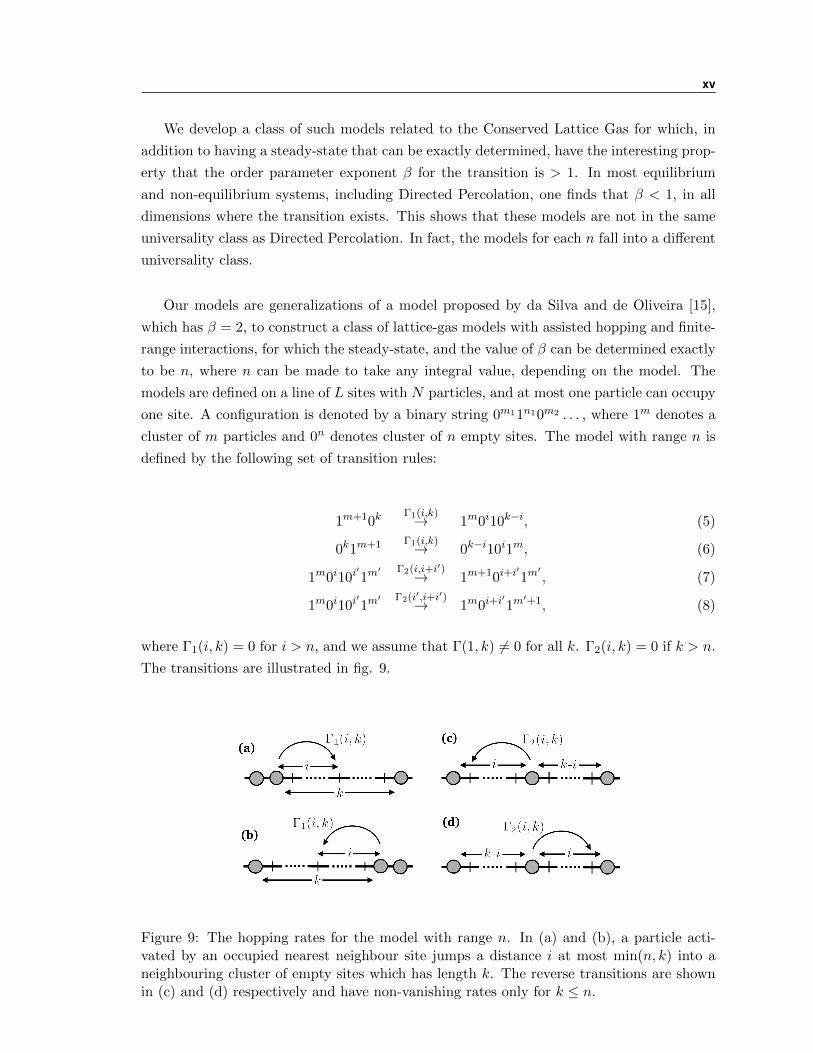
The transitions are illustrated in fig. 9.
Figure 9: The hopping rates for the model with range n. In (a) and (b), a particle acti-vated by an occupied nearest neighbour site jumps a distance i at most min(n, k) into aneighbouring cluster of empty sites which has length k. The reverse transitions are shownin (c) and (d) respectively and have non-vanishing rates only for k ≤ n.
xvi SYNOPSIS
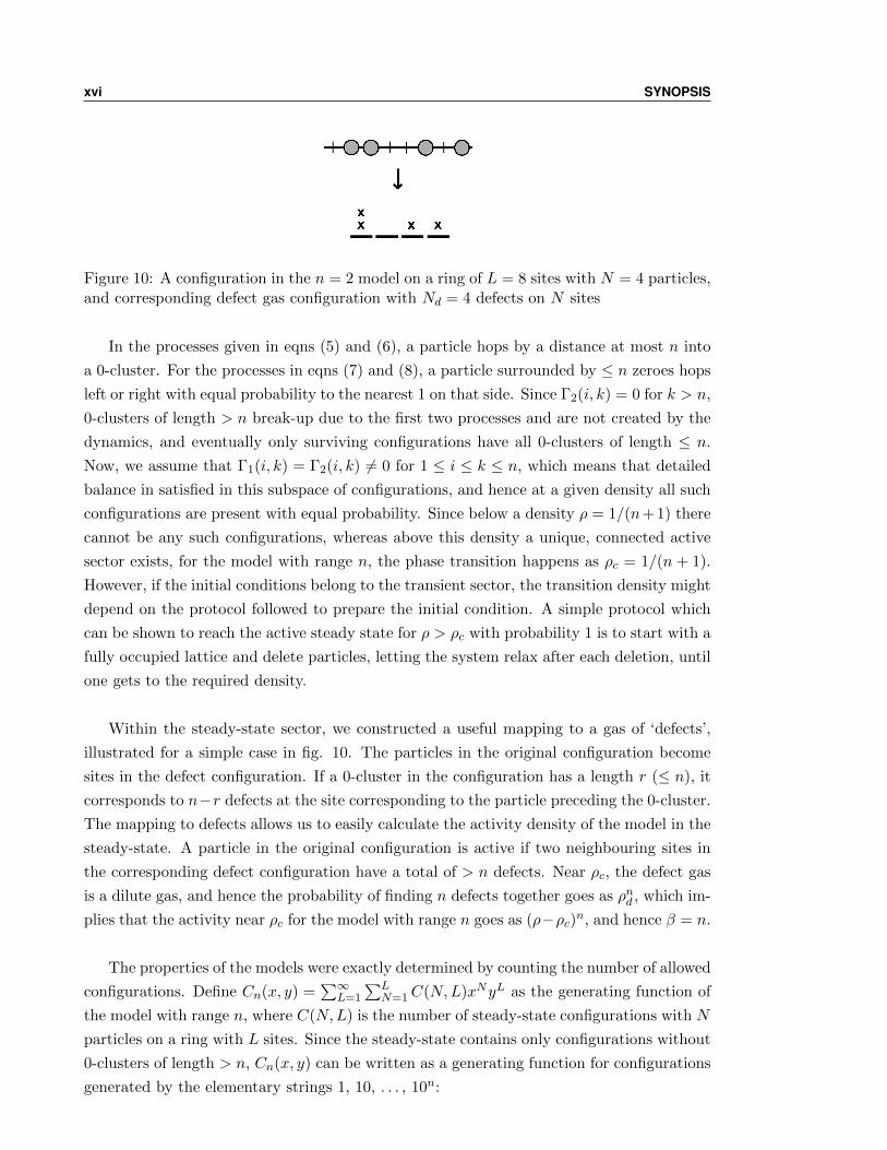
Figure 10: A configuration in the n = 2 model on a ring of L = 8 sites with N = 4 particles,and corresponding defect gas configuration with Nd = 4 defects on N sites
In the processes given in eqns (5) and (6), a particle hops by a distance at most n into
a 0-cluster. For the processes in eqns (7) and (8), a particle surrounded by ≤ n zeroes hops
left or right with equal probability to the nearest 1 on that side. Since Γ2(i, k) = 0 for k > n,
0-clusters of length > n break-up due to the first two processes and are not created by the
dynamics, and eventually only surviving configurations have all 0-clusters of length ≤ n.
Now, we assume that Γ1(i, k) = Γ2(i, k) 6= 0 for 1 ≤ i ≤ k ≤ n, which means that detailed
balance in satisfied in this subspace of configurations, and hence at a given density all such
configurations are present with equal probability. Since below a density ρ = 1/(n+ 1) there
cannot be any such configurations, whereas above this density a unique, connected active
sector exists, for the model with range n, the phase transition happens as ρc = 1/(n + 1).
However, if the initial conditions belong to the transient sector, the transition density might
depend on the protocol followed to prepare the initial condition. A simple protocol which
can be shown to reach the active steady state for ρ > ρc with probability 1 is to start with a
fully occupied lattice and delete particles, letting the system relax after each deletion, until
one gets to the required density.
Within the steady-state sector, we constructed a useful mapping to a gas of ‘defects’,
illustrated for a simple case in fig. 10. The particles in the original configuration become
sites in the defect configuration. If a 0-cluster in the configuration has a length r (≤ n), it
corresponds to n−r defects at the site corresponding to the particle preceding the 0-cluster.
The mapping to defects allows us to easily calculate the activity density of the model in the
steady-state. A particle in the original configuration is active if two neighbouring sites in
the corresponding defect configuration have a total of > n defects. Near ρc, the defect gas
is a dilute gas, and hence the probability of finding n defects together goes as ρnd , which im-
plies that the activity near ρc for the model with range n goes as (ρ−ρc)n, and hence β = n.
The properties of the models were exactly determined by counting the number of allowed
configurations. Define Cn(x, y) =∑∞
L=1
∑LN=1C(N,L)xNyL as the generating function of
the model with range n, where C(N,L) is the number of steady-state configurations with N
particles on a ring with L sites. Since the steady-state contains only configurations without
0-clusters of length > n, Cn(x, y) can be written as a generating function for configurations
generated by the elementary strings 1, 10, . . . , 10n:
xvii
Cn(x, y) =
(1− xy1− yn+1
1− y
)−1
− 1 (9)
The activity density ρa can be determined, by a similar counting procedure, as a para-
metric function of the density ρ throughout the active phase. Near ρ = ρc, one can then
show that β = n for the model n.
These models have a ‘ladder’ of transient configurations, which do not form part of the
steady-state sector, and once left are never visited again. These are, for the model with
hopping range n, all configurations with at least one 0-cluster of length > n. The number
of these 0-clusters decreases monotonically in time. However, we introduce a field h which
takes the evolution back up the transient ‘ladder’, by adding the following transitions to
definition of the model:
1m+10kh← 1m010k−1 for k > n and m ≥1 (10)
This field h is closely related to the concept of a field which couples to the activity,
which for the CLG (the n = 1 model) has been studied earlier using a mean-field analysis
[13]. We find that with our construction of the field, the steady-state properties can be
determined, and the corresponding generating function C(x, y, h) is a simple function. The
exponent δ, defined by ρa|ρ=ρc ∼ h1/δ, can be calculated to be δ = 2/n for the model with
range n. Thus, we were able to calculate the three independent stationary exponents of the
models β, ν and δ exactly.
Bibliography
[1] D. Dhar, T. Sadhu and S. Chandra, EPL, 85 48002
[2] T. Sadhu and D. Dhar, Physical Review E, 85 021107 (2012)
[3] D. Dhar and T. Sadhu, J. Stat. Mech. P11006 (2013); arXiv:1310.1359.
[4] V. B. Priezzhev, D. Dhar, A. Dhar and S. Krishnamurthy, Physical Review Letters,
77 5079 (1996)
[5] A. M. Povolotsky, V. B. Priezzhev, and R. R. Scherbakov, Physical Review E, 58 5449
(1998)
[6] J. Propp, Chaos, 20 037110 (2010)
[7] A. E. Holroyd, L. Levine, K. Meszaros, Y. Peres, J. Propp and D. B. Wilson, Progress
in Probability, 60 331 (2008); arXiv:0801.330
[8] T. Sadhu and D. Dhar, Journal of Statistical Physics, 138 815 (2010)
[9] T. Sadhu and D. Dhar, Journal of Statistical Mechanics: Theory and Experiment,
P03001 (2011)
[10] R. Rajesh and D. Dhar, Phys. Rev. Lett. 81 1646 (1998).
[11] S. N. Majumdar, arXiv: 0701193.
[12] G. Grinstein and M. A. Munoz, in Fourth Granada Lectures in Computational Physics,
edited by P. L. Garrido and J. Marro, Lecture Notes in Physics Vol. 493 (Springer,
Berlin, 1997), p. 223.
[13] S. Lubeck, Int. J. Mod. Phys. B 18, 3977 (2004).
[14] H. K. Janssen, Z. Phys. B 42 151 (1981);
P. Grassberger, Z. Phys. B, 47, 365 (1982).
[15] E. F. da Silva, and M. J. de Oliveira, J. Phys. A: Math. Gen. 41, 385004 (2008).
[16] M. Rossi, R. Pastor-Satorras, and A. Vespignani, Phys. Rev. Lett. 85, 1803 (2000).
xviii
BIBLIOGRAPHY xix
[17] R. L. Brooks, C. A. B. Smith, A. H. Stone and W. T. Tutte, Duke Mathematical
Journal 7 312.
[18] F. Spitzer, Principles of Random Walk, pp. 124, 148-51, (Van Nostrand, Princeton,
1964);
[19] A. E. Holroyd and J. Propp, Contemporary Mathematics, 520 105 (2010);
arXiv:0904.4507
[20] S. N. Majumdar, and S. Nechaev, Phys. Rev. E, 72, 020901 (2005).
[21] S. N. Majumdar, K. Mallick, and S. Nechaev, Phys. Rev. E, 77, 011110 (2008).
[22] C. A. Tracy, and H. Widom (1994), Comm. Math. Phys., 159, 151 (1994)
[23] M. Kardar, G. Parisi, and Y.C. Zhang, Phys. Rev. Lett., 56, 889 (1986).
[24] S. F. Edwards and D. R. Wilkinson, Proceedings of the Royal Society of London. A.
Mathematical and Physical Sciences 381, 17 (1982).
[25] A. Vespignani, R. Dickman, M. A. Munoz, S. Zapperi, Phys. Rev. E 62, 4564 (2000).
[26] R. Dickman, M. A. Munoz, A. Vespignani, S. Zapperi, Braz. J. Phys. 30, 27 (2000).
[27] M. Basu, U. Basu, S. Bondyopadhyay, P. K. Mohanty, and H. Hinrichsen, Phys. Rev.
Lett. 109, 015702 (2012).
[28] M. J. de Oliveira, Phys. Rev. E 71, 016112 (2005).
Publications
• R. Dandekar and D. Dhar,
Proportionate growth in patterns formed in the rotor-router model, Journal of Sta-
tistical Mechanics: Theory and Experiment, P11030 (2014)
arxiv:1312.6888
• R. Dandekar,
Proportionately growing patterns on noisy backgrounds and KPZ scaling,
in preparation
• R. Dandekar and D. Dhar,
A class of exactly solved assisted-hopping models of active-inactive state transition
on a line,
EPL (Europhysics Letters), 104 26003 (2013)
Other Publications
• R. Dandekar,
Comment on ‘Self-organized cooperative criticality in coupled complex systems’, EPL
(Europhysics Letters), 107 10001 (2014).
xx
Outline
This thesis is organised as follows:
Chapters 1 and 2 form the introductory part of the thesis. In Chapter 1, we will review
previous studies of the growth of surfaces and aggregates of particles, with an emphasis
on Kardar-Parisi-Zhang (KPZ) and Edwards-Wilkinson (EW) surfaces, and on aggregates
formed by starting from a seed in deterministic particle models. We place these particular
models in the context of general growth models, then describe proportionate growth in the
rotor-router aggregation and sandpile models. We also describe in detail growth models in
the KPZ universality class and recently discovered exact mappings between these models,
which allow one to determine the full distribution of the fluctuations in the growing surfaces.
In chapter 2, we review the phenomenon of absorbing phase transitions, in systems
with and without a conserved number of particles. Absorbing states are states which the
dynamics can lead to but cannot escape from. Absorbing (or active-absorbing) phase tran-
sitions are transitions in which, as an external parameter is tuned, the long-time limit of
the system changes from an active fluctuating steady-state to an absorbing state where
no further change occurs. These transitions are governed by static and dynamical critical
exponents which obey well-known scaling relations. We will also discuss the phenomena of
universality, wherein transitions in many diverse systems nevertheless show the same critical
exponents near the transition. The classification of universality classes of absorbing phase
transitions, especially those in systems with a conserved number of particles, has been a
topic of particular interest in the recent literature.
In chapter 3, we study the growing patterns formed in the rotor-router model by adding
N walkers at the center of an L×L two-dimensional square lattice, starting with a periodic
background of arrows, and relaxing to a stable configuration. The pattern is made of a
large number of triangular and quadrilateral regions, where in each region all arrows point
in the same direction. We show that the pattern formed by arrows which have been rotated
at least one full circle, may be described in terms of a tiling of the plane by squares of
different sizes. The sizes of these squares, and the size of the pattern, grow linearly with N ,
for 1 N < 2L. We use the Brooks-Smith-Stone-Tutte theorem relating tilings of squares
1
2 OUTLINE
by smaller squares to resistor networks, to determine the exact relative sizes of these tiles.
The scaling limit of the number of visits φ(ξ, η) as a function of the scaled position (ξ, η)
is also determined. We also present numerical evidence that the deviations of the sizes of
different squares in the tiling from the asymptotic linear growth law are always O(1), and
are quasiperiodic functions of N .
In chapter 4, we will consider the patterns formed by rotor-router walkers on back-
grounds which are not perfectly periodic, but are perturbations of periodic backgrounds
with the arrow directions changed at some randomly chosen sites. We see that this noise
creates ‘defect lines’ in some of the patches, which also affect the shapes of the patch bound-
aries. We study perturbations on particular starting backgrounds, and how the presence of
the noise affects the shapes of the patches in the pattern and how these properties vary as
the noise strength p is varied.
In chapter 5, we present the construction and analysis of a class of assisted-hopping
models which show an active-absorbing phase transitions in one dimension. The models
are a generalization of the Conserved Lattice Gas (CLG) model defined in Chapter 1. The
steady state for all the models in the class can be exactly determined and various quantities
calculated easily with the help of generating functions. We show that, for the model where
the particles have a hopping range n, for n = 1, 2, 3, . . . , the critical exponent β = n. The
model with n = 2 was first defined by da Silva and de Oliviera. The models with n > 2 are
new universality classes for active-absorbing phase transitions.

Chapter 1
Introduction to Surface and
Proportionate Growth
In this chapter, we will review previous studies of the growth of surfaces and aggregates of
particles, with an emphasis on Kardar-Parisi-Zhang (KPZ) and Edwards-Wilkinson (EW)
surfaces, and on aggregates formed by starting from a seed in deterministic particle models.
However, we first place these particular models in the context of general growth models in
section I. In section II, we describe the rotor-router aggregation and sandpile models for
proportionate growth. In section III, we describe growth models in the KPZ universality
class and recently discovered exact mappings between these models, and describe how these
allow us to determine the full distribution of the fluctuations in the growing surfaces.
1.1 Growth models: an overview
In this section we describe known models of stochastically growing aggregates and their
surfaces. This allows us to introduce a formalism for analysing growing aggregates, and
their surfaces, formed in a deterministic cellular automaton model in Chapters 3 and 4.
We first describe various models for growth of an aggregate from a seed. Then we will
move on to studying the surfaces of these growing aggregates, which gives us an opportunity
to introduce models of growth starting from flat surface as well. Good reviews are in Viscek’s
book [1] and the review by Herrmann [2]. Note that we do not consider reaction-diffusion
or hydrodynamic pattern formation models here, see [3] for a review.
1.1.1 Growing aggregates
The Eden Model
One of the simplest models of the growth of a random aggregate, starting from a single
seed, was proposed by Eden in 1961 [4]. In this model, a cluster grows starting from an
3
4 1. INTRODUCTION TO SURFACE AND PROPORTIONATE GROWTH
(a) (b)
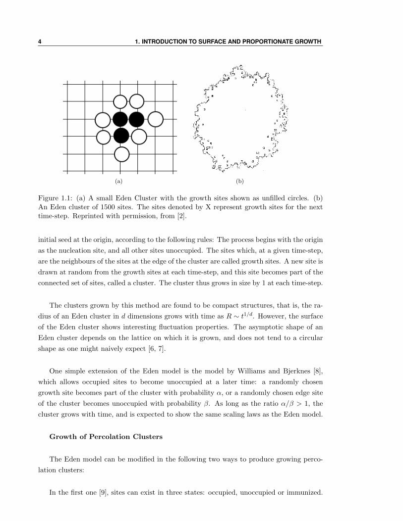
Figure 1.1: (a) A small Eden Cluster with the growth sites shown as unfilled circles. (b)An Eden cluster of 1500 sites. The sites denoted by X represent growth sites for the nexttime-step. Reprinted with permission, from [2].
initial seed at the origin, according to the following rules: The process begins with the origin
as the nucleation site, and all other sites unoccupied. The sites which, at a given time-step,
are the neighbours of the sites at the edge of the cluster are called growth sites. A new site is
drawn at random from the growth sites at each time-step, and this site becomes part of the
connected set of sites, called a cluster. The cluster thus grows in size by 1 at each time-step.
The clusters grown by this method are found to be compact structures, that is, the ra-
dius of an Eden cluster in d dimensions grows with time as R ∼ t1/d. However, the surface
of the Eden cluster shows interesting fluctuation properties. The asymptotic shape of an
Eden cluster depends on the lattice on which it is grown, and does not tend to a circular
shape as one might naively expect [6, 7].
One simple extension of the Eden model is the model by Williams and Bjerknes [8],
which allows occupied sites to become unoccupied at a later time: a randomly chosen
growth site becomes part of the cluster with probability α, or a randomly chosen edge site
of the cluster becomes unoccupied with probability β. As long as the ratio α/β > 1, the
cluster grows with time, and is expected to show the same scaling laws as the Eden model.
Growth of Percolation Clusters
The Eden model can be modified in the following two ways to produce growing perco-
lation clusters:
In the first one [9], sites can exist in three states: occupied, unoccupied or immunized.
1.1. GROWTH MODELS: AN OVERVIEW 5
One modifies the Eden rule to the rule that an unoccupied non-immunized neighbouring
site of the cluster might become occupied with probability p, or become ‘immunized’ with
probability (1 − p). Immunized sites can not be occupied at any later time. For p < pc,
where pc is the percolation threshold on the particular lattice, the cluster grows until it
reaches a finite size for which there are no more growth sites on the boundary. For p > pc,
with a non-zero probability the growth produces an infinite cluster. The fully grown clusters
are created with the same probabilities as site percolation clusters; however, while growing
they do not have the same surface structure as percolation clusters.
The second extension, Invasion Percolation [10], was defined by Wilkinson as a growth
model that generates critical percolation clusters without the need for fine-tuning of a pa-
rameter. One assigns a random number we to each edge e on the lattice, called its weight.
we is chosen from a uniform distribution [0, 1]. At each new time-step, instead of choosing
a random site on the boundary to add to the cluster, one chooses the boundary edge of the
lowest weight. One then adds the neighbour along the edge to the cluster. (Sometimes the
lowest weight boundary edge already has both its end sites in the cluster, in which case it
is simply removed from the list of boundary edges.)
From bond percolation, we know that if edges on a lattice are randomly occupied with
probability p > pc, then an infinite cluster results. Thus it is reasonable that even at large
times, the invasion cluster will not get to a stage where edges with weights p > pc are
being added to the cluster (not considering initial transients). In fact, a theorem due to
Haggstrom, Peres and Schonmann [11] says that if ηi is the weight of the edge added at the
i-th time-step, the maximum of the sequence ηi tends to pc as i→∞. The bulk properties
of the growing cluster, for example the fractal dimension, are the same as those of the span-
ning cluster in the percolation problem at pc. Thus invasion percolation finds the critical
value on its own, and generates a critical cluster. Thus it can be considered an example of
self-organized criticality.
Diffusion-Limited Aggregation
Diffusion-Limited Aggregation was introduced by Witten and Sander in 1981 [12] to
model the formation of soot particles in air by aggregation. Since then the model has been
applied to various other phenomena, such as viscous fingering, spinodal decomposition, and
several other applications.
The model is defined as follows: we start with a seed at the origin. A particle starts
diffusing from a point in an arbitrary direction far away from the origin, and diffuses until
it either escapes to infinity (in computer simulations a cutoff is imposed) or reaches a site
next to the seed, at which point it sticks there. Then a new particle is released from an
6 1. INTRODUCTION TO SURFACE AND PROPORTIONATE GROWTH
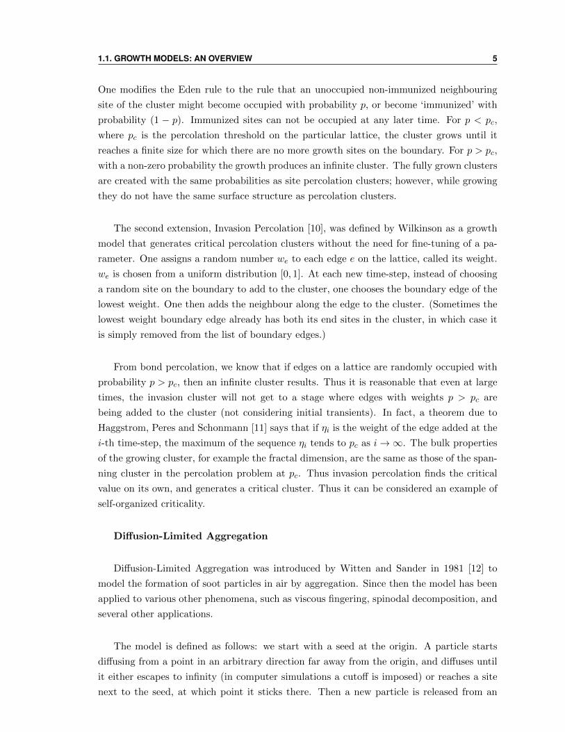
Figure 1.2: A Diffusion-Limited Aggregation cluster in the continuum. Picture taken frommagnin.plil.net/spip.php?article102
arbitrary direction far away from the origin and starts diffusing, again either diffusing to
infinity or sticking to the growing cluster. This process can be performed in the contin-
uum, or on a lattice (in which case the particles perform random walks). The cluster has
a tree-like shape, as shown in fig 1.2, and the properties of the cluster depend on the type
of lattice used. The DLA clusters are fractals, unlike the Eden clusters: in the continuum,
the mass of a cluster varies with its radius as Ra, with a ≈ 1.715 < 2 which implies that
the cluster is not space-filling. While on a square lattice in 2d, the exponent is asq ≈ 1.5 [13].
The tree-like shape of the cluster may be viewed as the result of the instability of a
circularly growing cluster to perturbations of its surface: bumps on the surface expose more
surface area and hence grow faster than the surroundings, while growth in the valleys is
slower. Since the particles are finite-sized, they themselves provide the perturbations neces-
sary to destabilize circular growth. The outer ‘branches’ of the tree-like structures formed
due to this instability grow faster than the inner branches, as few particles reach the inner
branches without getting stuck on the way [14].
The basic DLA model can be modified by introducing a probability for sticking: at
every encounter with the cluster, a particle sticks with probability p ≤ 1. For p 1 and
for small sizes of the cluster, a particle has a chance to explore the entire boundary of the
cluster before settling at some site on the boundary. Thus, all sites are on the boundary
are equiprobable sites for growth, and the cluster is approximately an Eden cluster of that
size. However, once the cluster becomes large enough, for any finite p, the particle can only
explore a finite neighbourhood of the site of its initial attempt at sticking, before getting
1.1. GROWTH MODELS: AN OVERVIEW 7
stuck. Thus the asymptotic cluster is still a DLA cluster. In the limit p→ 0, the aggrega-
tion becomes truly reaction-Limited, and one recovers the Eden model.
Cluster-cluster aggregation
Instead of aggregating models where particles attach to a single growing cluster, one
can define models where two diffusing clusters of sizes m and n stick to each other and
form a cluster of size m + n when they meet, with rates k(m,n) depending on the sizes
of the two clusters [22]. Simulations, and exact solutions of a few integrable kernels show
the existence of a gelation transition, such that after a given time an infinite cluster forms,
although all particles might not be part of the cluster. The order and the exponents of the
cluster depend on the exact form of k(m,n). For more details on cluster-cluster aggregation
see [23] and Viscek’s book [1].
Internal Diffusion-Limit Aggregation
(a) (b)
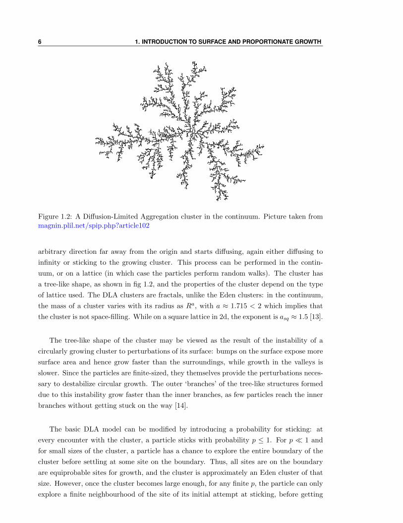
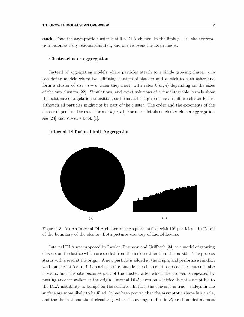
Figure 1.3: (a) An Internal DLA cluster on the square lattice, with 106 particles. (b) Detailof the boundary of the cluster. Both pictures courtesy of Lionel Levine.
Internal DLA was proposed by Lawler, Bramson and Griffeath [34] as a model of growing
clusters on the lattice which are seeded from the inside rather than the outside. The process
starts with a seed at the origin. A new particle is added at the origin, and performs a random
walk on the lattice until it reaches a site outside the cluster. It stops at the first such site
it visits, and this site becomes part of the cluster, after which the process is repeated by
putting another walker at the origin. Internal DLA, even on a lattice, is not susceptible to
the DLA instability to bumps on the surfaces. In fact, the converse is true - valleys in the
surface are more likely to be filled. It has been proved that the asymptotic shape is a circle,
and the fluctuations about circularity when the average radius is R, are bounded at most
8 1. INTRODUCTION TO SURFACE AND PROPORTIONATE GROWTH
by log (R) [35].
1.1.2 Growing surfaces
In this subsection we describe the growth of surfaces of growing aggregates. As explained
later, growing surfaces usually fall into one of two universality classes. Here, using vari-
ous models, we motivate the important quantities to be studied and show that they have
universal properties.
Eden Surfaces
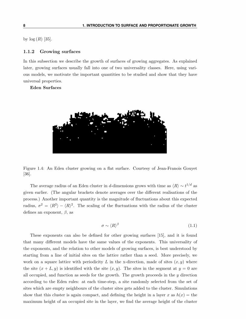
Figure 1.4: An Eden cluster growing on a flat surface. Courtesy of Jean-Franois Gouyet[36].
The average radius of an Eden cluster in d-dimensions grows with time as 〈R〉 ∼ t1/d as
given earlier. (The angular brackets denote averages over the different realisations of the
process.) Another important quantity is the magnitude of fluctuations about this expected
radius, σ2 = 〈R2〉 − 〈R〉2. The scaling of the fluctuations with the radius of the cluster
defines an exponent, β, as
σ ∼ 〈R〉β (1.1)
These exponents can also be defined for other growing surfaces [15], and it is found
that many different models have the same values of the exponents. This universality of
the exponents, and the relation to other models of growing surfaces, is best understood by
starting from a line of initial sites on the lattice rather than a seed. More precisely, we
work on a square lattice with periodicity L in the x-direction, made of sites (x, y) where
the site (x + L, y) is identified with the site (x, y). The sites in the segment at y = 0 are
all occupied, and function as seeds for the growth. The growth proceeds in the y direction
according to the Eden rules: at each time-step, a site randomly selected from the set of
sites which are empty neighbours of the cluster sites gets added to the cluster. Simulations
show that this cluster is again compact, and defining the height in a layer x as h(x) = the
maximum height of an occupied site in the layer, we find the average height of the cluster
1.1. GROWTH MODELS: AN OVERVIEW 9
〈h〉 ∼ t/L. Similarly to radial cluster growth, we can define the variance σ2 = 〈h2〉 − 〈h〉2.
There exists a crossover time scale,
τ ∼ Lz (1.2)
such that σ grows as
σ ∼ 〈h〉β for t Lz (1.3)
while for t Lz it saturates at the value
σ ∼ Lα (1.4)
These equations define three exponents, β, α and z. One writes an asymptotic scaling
form for σ as
σ ∼ Lαf(〈h〉Lz
) (1.5)
where f(x) is called a scaling function. To agree with eqns. (1.3) and (1.4), we need that
f(x) ∼ xβ as x → 0 and f(x) → 1 as x → ∞. This gives a scaling relation between the
exponents
β = α/z (1.6)
In d = 2, numerical simulations show that for Eden growth on a flat surface, α ≈ 0.5
and β ≈ 0.33 [5].
Since the growth of the surface is translation-invariant in the direction x, and since the
only macroscopic length scale in the problem is L, we expect that the correlation function
C(x) = 〈(h(x′ + x)− h(x′))2〉 (1.7)
varies as a power-law, C(x) ∼ x2α. The exponent α is called the Hurst exponent, and
in this case it is the same as the exponent α defined from the average height fluctuations.
The exponents of the Eden growth from a line in 1+1 dimensions can be predicted from
the analysis of the KPZ equation, see section III. For now, we describe two other models of
surface growth - one which falls in the same universality class (has the same values for the
exponents α and z) as Eden growth from a line, and another which does not.
Ballistic Deposition
This and the next model fall under the category of deposition-evaporation models, where
particles are deposited onto a growing surface, or evaporated from it. For both the models,
we discuss only the cases where there is no evaporation from the surface.
10 1. INTRODUCTION TO SURFACE AND PROPORTIONATE GROWTH
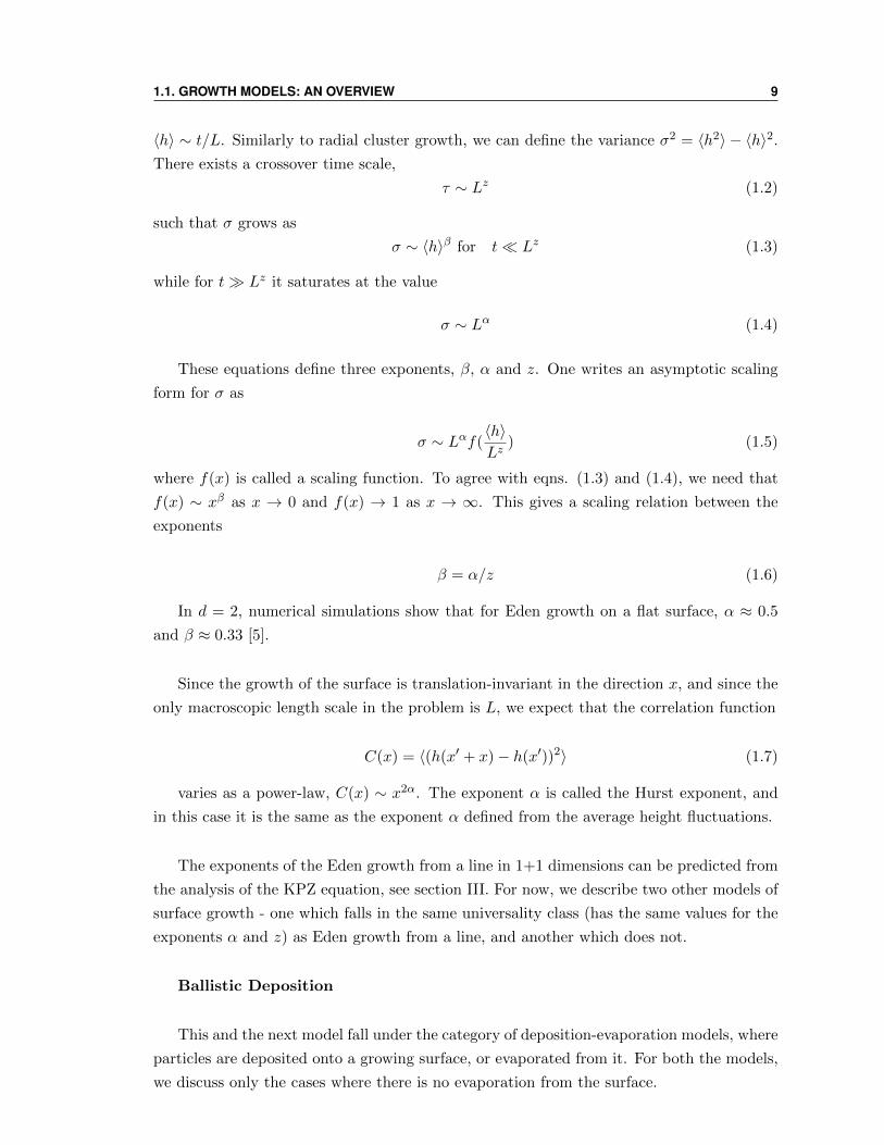
Figure 1.5: A ballistic deposition cluster growing on a flat surface. Courtesy of Jean-FranoisGouyet [36].
In ballistic deposition [19], particles are dropped normally onto a surface, and travel
ballistically downwards until they reach a cell adjacent to a cell already in the cluster, and
stick there. The position of the dropping particles over the direction along the surface is
chosen uniformly randomly. Thus the new growth occurs uniformly over the exposed neigh-
bours of the growing cluster. (The empty sites in the bulk cannot be occupied later.)
An Eden cluster, on the other hand, chooses a new site over the unoccupied neighbours
of the cluster, whether in the bulk or on the surface. However, since both Eden and ballistic
deposition clusters are compact (observed in simulations), for large cluster sizes if we rescale
time, the growth of both surfaces should proceed in approximately the same way. This ex-
pectation is confirmed by simulations, the exponents β and z for the ballistic deposition
models are the same as those for the Eden model. Both models fall in the KPZ universality
class.
Random Deposition with surface diffusion
If particles are dropped uniformly over a substrate and stick to the topmost particle in
the layer they are dropped in, we have the random deposition model. The cluster is then is
simply a collection of independently growing stacks, and the height of each stack and the
variance of h over the sample grow as t and t1/2 respectively.
In random deposition with surface diffusion, a particle which drops onto the topmost
particle in a layer does not stick there - instead, it diffuses to a neighbouring site if the height
at the neighbouring site is lower than that at the current site, continuing this process for
a fixed number of time-steps, at the end of which it sticks to the site it has ended up on.
Thus the different stacks do not grow independently, and although the average height still
grows as t, the variance is much reduced from the random deposition case. Edwards and
Wilkinson in 1982 [17] derived an evolution equation for the coarse-grained h(x) for this
1.2. PROPORTIONATE GROWTH 11
model, (see section III for details) which gives
σ ∼ L1/2f(〈h〉L2
) (1.8)
The scaling relation β = α/z gives β = 1/4.
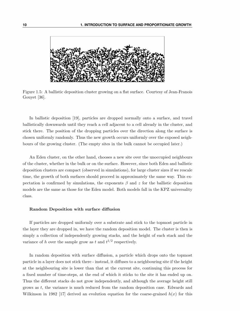
The Polynuclear Growth model
Another interesting model of a growing surface is the Polynuclear growth, or PNG,
model [20, 21]. The polynuclear growth model is defined in one-dimension and continuous
time. It concerns the growth of a one-dimensional interface, growing without overhangs -
thus one that can be characterised by a function h(x, t), which is the height of the interface
at position x and time t. The function h(x) in the PNG model is an integer valued function
with discontinuous jumps of ±1 (see fig 1.6). We call these jumps as kinks (when the
increase going in the +x direction is +1) or antikinks (when it is −1). The dynamics of
the interface is best described in terms of these kinks and antikinks in h(x). Kink-antikink
pairs are nucleated at rate unity per unit length. (The blue part of h(x) in the figure.
Once nucleated, the kinks move towards the right and the antikinks move towards the left,
both at unit velocity. Kinks and antikinks annihilate upon meeting. (See fig. 1.6). The
fluctuations of the height in this model scale in with the same exponents as the Eden and
Ballistic Deposition models discussed above.
Figure 1.6: The evolution of h(x) in the PNG model. The pair of discontinuities in bluehave just been generated, and will move in opposite directions.
1.2 Proportionate Growth
In section I, we observed that the aggregation models defined there did not show any in-
ternal structure, showing growth and change only at the boundaries. In this section, we
study deterministic aggregation models, with particle input at the origin, which show in-
ternal structure which grows at the same rate as the pattern itself. Such growth is termed
‘proportionate growth’.
12 1. INTRODUCTION TO SURFACE AND PROPORTIONATE GROWTH
Approximately proportionately growing patterns are found in biology: as baby animals
grow from birth to adulthood, the different parts of the body grow roughly proportionately
to each other. While proportionate growth is quite typical in the animal kingdom, examples
of proportionate growth outside biology are hard to find. In this section, we discuss growing
patterns formed in the abelian sandpile model (ASM) which show proportionate growth.
Here, the patterns are formed by depositing particles one by one at the origin of a finite
square lattice and letting the configuration relax using the ASM relaxation rules, until it
becomes stable. We then define the rotor-router model, a model of a derandomized random
walker on a lattice, and use the model to define a derandomized version of the IDLA, which
shows interesting internal structure, and proportionate growth.
1.2.1 Sandpiles
The abelian sandpile model [25, 26] is defined on a 2D L×L square lattice as follows: parti-
cles are dropped randomly on the sites of the lattice. If, after a particle has been dropped on
a site, the height of the site (ie, the number of particles on the site) exceeds 3, one particle
from the site is sent to each of its nearest neighbours, thus reducing the height of the site
by 4 and increasing the height at each neighbour by 1. This is known as a ‘toppling’. In the
process, some other heights might exceed 3, and those sites are toppled, and so on. When
a boundary site of the lattice is toppled, the number of particles on the lattice decreases
by one. (When a corner site topples, it decreases by two.) This is known as an avalanche,
and it stops once all heights are less than 4. Then the next particle is dropped on the
lattice. This model is thus a model with deterministic toppling rules, but random drive,
and boundary dissipation. In the steady-state, it shows no intrinsic length scale, except the
lattice size L. This means that the height-height correlation function decays as a power
law, and the probability distributions for avalanche size and duration also decay as power
laws. The sandpile system is said to exhibit self-organized criticality. For more details on
the sandpile model see [27].
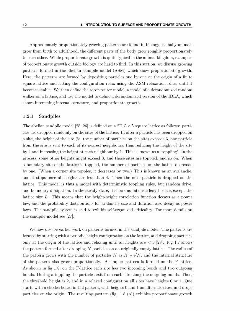
We now discuss earlier work on patterns formed in the sandpile model. The patterns are
formed by starting with a periodic height configuration on the lattice, and dropping particles
only at the origin of the lattice and relaxing until all heights are < 3 [28]. Fig 1.7 shows
the pattern formed after dropping N particles on an originally empty lattice. The radius of
the pattern grows with the number of particles N as R ∼√N , and the internal structure
of the pattern also grows proportionally. A simpler pattern is formed on the F-lattice.
As shown in fig 1.8, on the F-lattice each site has two incoming bonds and two outgoing
bonds. During a toppling the particles exit from each site along the outgoing bonds. Thus,
the threshold height is 2, and in a relaxed configuration all sites have heights 0 or 1. One
starts with a checkerboard initial pattern, with heights 0 and 1 on alternate sites, and drops
particles on the origin. The resulting pattern (fig. 1.8 (b)) exhibits proportionate growth
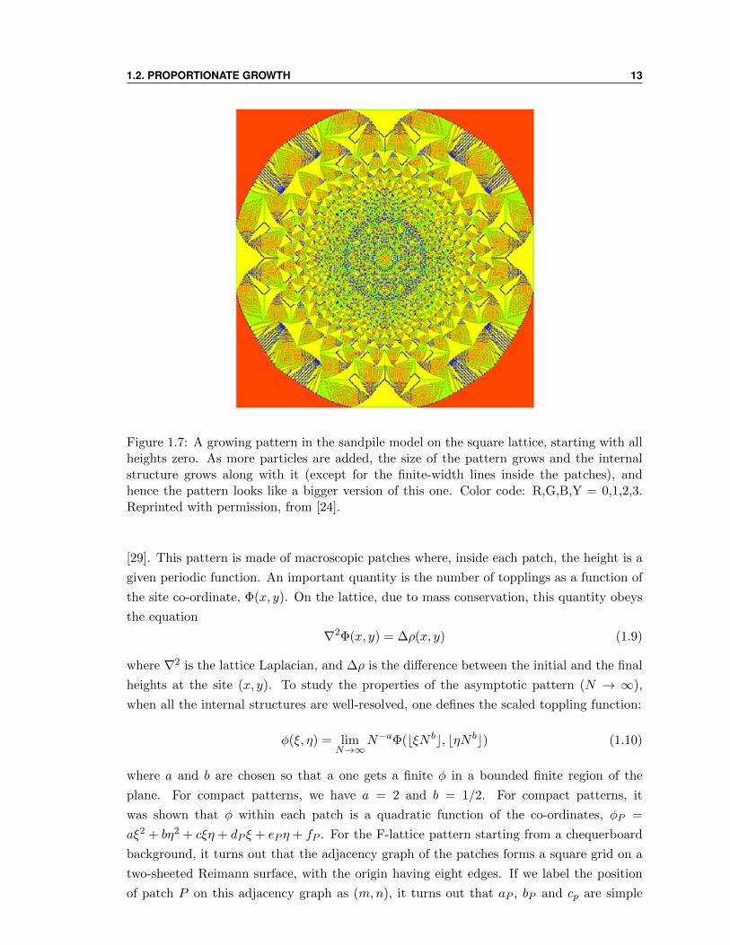
1.2. PROPORTIONATE GROWTH 13
Figure 1.7: A growing pattern in the sandpile model on the square lattice, starting with allheights zero. As more particles are added, the size of the pattern grows and the internalstructure grows along with it (except for the finite-width lines inside the patches), andhence the pattern looks like a bigger version of this one. Color code: R,G,B,Y = 0,1,2,3.Reprinted with permission, from [24].
[29]. This pattern is made of macroscopic patches where, inside each patch, the height is a
given periodic function. An important quantity is the number of topplings as a function of
the site co-ordinate, Φ(x, y). On the lattice, due to mass conservation, this quantity obeys
the equation
∇2Φ(x, y) = ∆ρ(x, y) (1.9)
where ∇2 is the lattice Laplacian, and ∆ρ is the difference between the initial and the final
heights at the site (x, y). To study the properties of the asymptotic pattern (N → ∞),
when all the internal structures are well-resolved, one defines the scaled toppling function:
φ(ξ, η) = limN→∞
N−aΦ(bξN bc, bηN bc) (1.10)
where a and b are chosen so that a one gets a finite φ in a bounded finite region of the
plane. For compact patterns, we have a = 2 and b = 1/2. For compact patterns, it
was shown that φ within each patch is a quadratic function of the co-ordinates, φP =
aξ2 + bη2 + cξη + dP ξ + eP η + fP . For the F-lattice pattern starting from a chequerboard
background, it turns out that the adjacency graph of the patches forms a square grid on a
two-sheeted Reimann surface, with the origin having eight edges. If we label the position
of patch P on this adjacency graph as (m,n), it turns out that aP , bP and cp are simple
14 1. INTRODUCTION TO SURFACE AND PROPORTIONATE GROWTH
functions of m and n (for details see [29]). Now, using the fact that φ is continuous across
patch boundaries, it was shown that the matching condition can be put in the form
∇2dm,n = 0 (1.11)
∇2em,n = 0 (1.12)
where the Laplacian ∇2 is taken on either the odd sublattice or the even sublattice of the
square grid. These equations were solved in [29] to derive the form of the asymptotic top-
pling function for all the patches, which allowed them to evaluate the relative sizes of the
various patches in the pattern. The structure of the patterns has an intriguing connection
with discrete analytic functions on the graph [39].
Figure 1.8: (a) The structure of the F-lattice. (b) A growing pattern in the sandpile modelon the F-lattice lattice, starting with a chequerboard pattern of 0s and 1s. Color code: Red= 0, White = 1. Reprinted with permission, from [29].
Thus, the toppling function for the pattern was calculated by solving the Laplace equa-
tion on the adjacency graph of the patches. For several other patterns studied, including
linearly growing ones, it turns out that one part of the toppling function inside each patch
encodes the co-ordinates of the patch on the adjacency graph, and the coefficients of the
other part obey a Laplace equation on the adjacency graph [30, 37]. For many patterns, we
show in Chapter 3 that this relationship follows naturally, and most easily, from the fact
that the patterns can be seen as tilings of squares by smaller squares.
There is also an interesting connection between some sandpile patterns and Apollonian
circle packing, which was discovered by Levine, Pedgen and Smart [40]. Another object in
the sandpile model known to exhibit interesting structure is the identity configuration. For
details, see [32] and [33].
1.2. PROPORTIONATE GROWTH 15
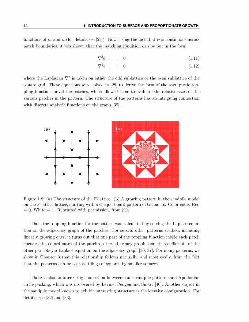
Note that the sandpile model is a deterministic model, but natural systems almost cer-
tainly have some element of noise. Sadhu and Dhar also studied the effects of various
kinds of noise on the growth of the patterns [31]. They found, firstly, that adding a slight
non-deterministic element to the dynamics of the model, such that in a small fraction of top-
plings particles are not transferred equally to the nearest neighbours, destroys the internal
structure of the pattern after a short while. It has also been found that adding dissipation,
in the form that in a small fraction of topplings all the particles at the site are lost, not
only destroys the pattern but slows down the growth to a logarithmic rate [38].
Figure 1.9: The sandpile pattern on an F-lattice starting with a chequerboard configuration,where a fraction p of 1s are changed to 0s. (a) p = 0.01, (b) p = 0.1. Color code: Red = 0,White = 1. Reprinted with permission, from [24].
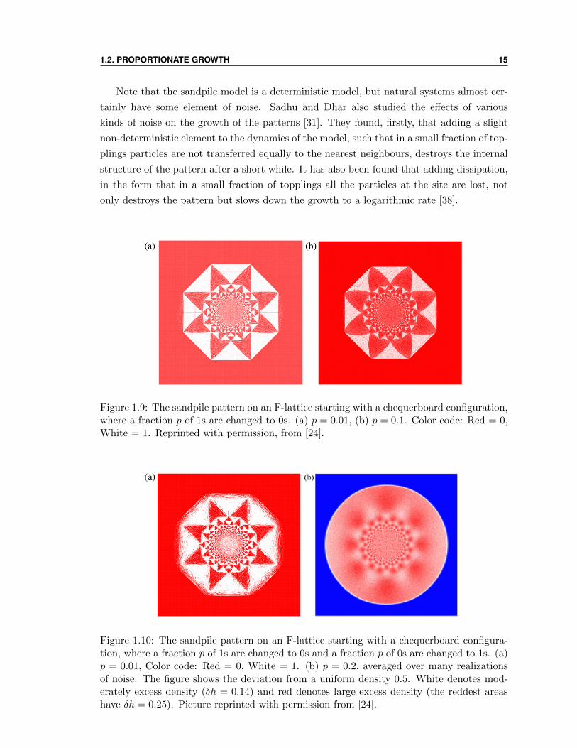
Figure 1.10: The sandpile pattern on an F-lattice starting with a chequerboard configura-tion, where a fraction p of 1s are changed to 0s and a fraction p of 0s are changed to 1s. (a)p = 0.01, Color code: Red = 0, White = 1. (b) p = 0.2, averaged over many realizationsof noise. The figure shows the deviation from a uniform density 0.5. White denotes mod-erately excess density (δh = 0.14) and red denotes large excess density (the reddest areashave δh = 0.25). Picture reprinted with permission from [24].
16 1. INTRODUCTION TO SURFACE AND PROPORTIONATE GROWTH
The most interesting results for sandpile patterns with noise are obtained when the
initial sand configuration on the lattice is made non-periodic, but keeping the toppling
rules deterministic. On the F-lattice, instead of starting with a checkerboard pattern of 1s
and 0s, one can randomly change a fraction p of the 1s to 0s. One then gets the pattern
shown in fig 1.9 (a), where, interestingly, although internal noisy structures develop inside
the patches, the patches are still well-resolved for small noise, and the boundaries between
them are still sharply defined. On the other hand, if one changes a fraction p of the 0s to 1s
as well, the boundaries between the patches turn fuzzy even for small noise (fig 1.10 (a)),
and for large p it is hard to see any remaining structure in the pattern. However, averaging
over several realizations of the disorder, one gets a picture like fig 1.10 (b), which shows
a very weak density inhomogeneity for all p, corresponding roughly to the positions of the
patches in the original pattern.
1.2.2 The Rotor-router Model
The rotor-router model is a simple model of a deterministic walk, in which the walker locally
modifies the medium it moves in, affecting its subsequent motion when it returns to the
same site. The model was originally introduced in the context of self-organized criticality,
and called the Eulerian Walker model [41, 42, 43]. The name comes from the fact that on a
finite undirected graph, the walk eventually settles into an Euler cycle, in which each edge
of the graph is visited exactly once in each direction.
The topic of deterministic walks on a lattice has a long history within physics and math-
ematics, being first proposed by Chris Langton as ‘Langton’s ants’ as a particular cellular
automaton [44]. The kinetic theory properties of such walks and the relation to random
walks on a lattice became an object of study in the following decades [45, 46, 47]. Within
the mathematics community, Jim Propp independently proposed the same model as the
Eulerian Walker, as a derandomized version of the random walk, naming it the rotor-router
model [48]. Reviews of earlier work on the rotor-router model may be found in [50] and
[51]. An introductory discussion of derandomization techniques in computer science may
be found in [54].
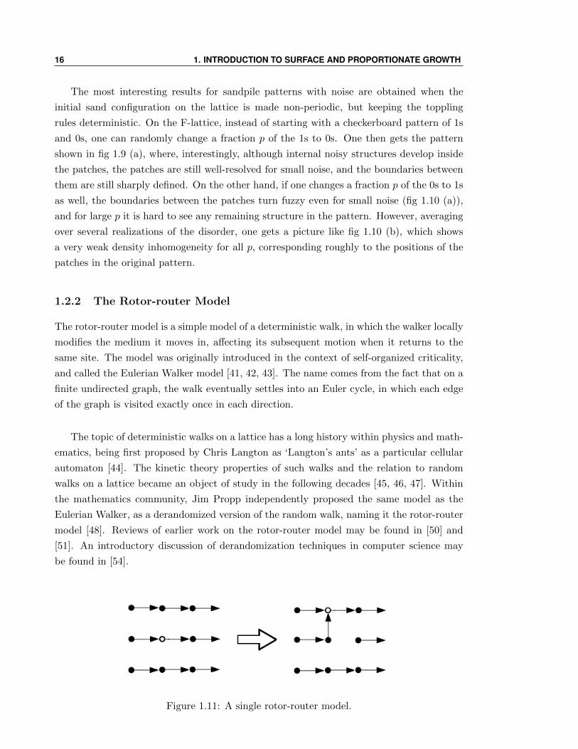
Figure 1.11: A single rotor-router model.
1.2. PROPORTIONATE GROWTH 17
Now we define the rotor-router model more precisely, on a two-dimensional square lat-
tice. The rules of the model are as follows: There is an arrow attached to every lattice site,
which points in the direction of one of its four neighbours. When a walker reaches a site, it
rotates the arrow attached to that site by 90 counterclockwise and takes a step in the new
direction of the arrow (fig. 1.11). For sites which have been visited by the walker at least
once, the current direction of the arrow shows the direction of last exit of the walker from
that site. Since the update procedure is deterministic, the configuration of arrows and the
position of the walker after n steps is fully determined by the initial configuration.
The rotor-router as defined above can be generalized to an arbitrary graph by intro-
ducing the notion of a ‘stack’ on each site: a stack is a infinite sequence of instructions of
the type ‘go to X’, where X is one of the neighbours of the site. On arrival at any site,
the walker follows the instruction of the topmost entry of the stack at that site. Once it
is obeyed, this instruction is deleted (or ‘popped’) from the list, so that the next time the
walker arrives at the site, it finds a new instruction. If stack is an infinite repetition of
‘North-West-South-East’, we get the model we study in this paper. If the entries are chosen
randomly, we get a random stack. A random stack on every site leads to a random walk on
the graph.
The rotor-router model has an abelian property, in the following sense: starting with
a given arrow configuration, and positions of n walkers on the lattice, the final arrow con-
figuration on the lattice, once all the walkers have ended up at the sink, is independent of
the order in which the walkers are moved. Also, in the final configuration, the arrows in
the region visited by the walkers do not form any loops. This follows from a theorem by
Broder [52] which says that the last-exit edges of the sites visited by a walker always form
a spanning tree.
Consider starting with a number of walkers on a given background, and consider the
state of the arrow configuration when the walkers might not have yet reached the sink.
ρ(x, y) denotes for the direction of the arrow at site (x, y). σ(x, y), called the walker
configuration, denotes the number of walkers on site (x, y). Call the starting arrow and
walker configurations as ρi and σi respectively. Let u(x, y) denote the total number of
times the site (x, y) is visited - the visit function (or ‘odometer function’) at the point
(x, y). Then ρ and σ at any time obey the equation
Lu(ρi)(x, y) = σ(x, y)− σi(x, y) (1.13)
where the ‘stack Laplacian’ L is defined as difference between the total number of times
the arrows at neighbouring sites have pointed towards site (x, y) in u(ρi) rotations, and
the value of u(ρi) at the site (x, y) [53]. Thus once all the walkers have reached the sink,
L(ρ, ρi)(x, y) = 0. The value of L being non-zero at a site indicates that some walkers have
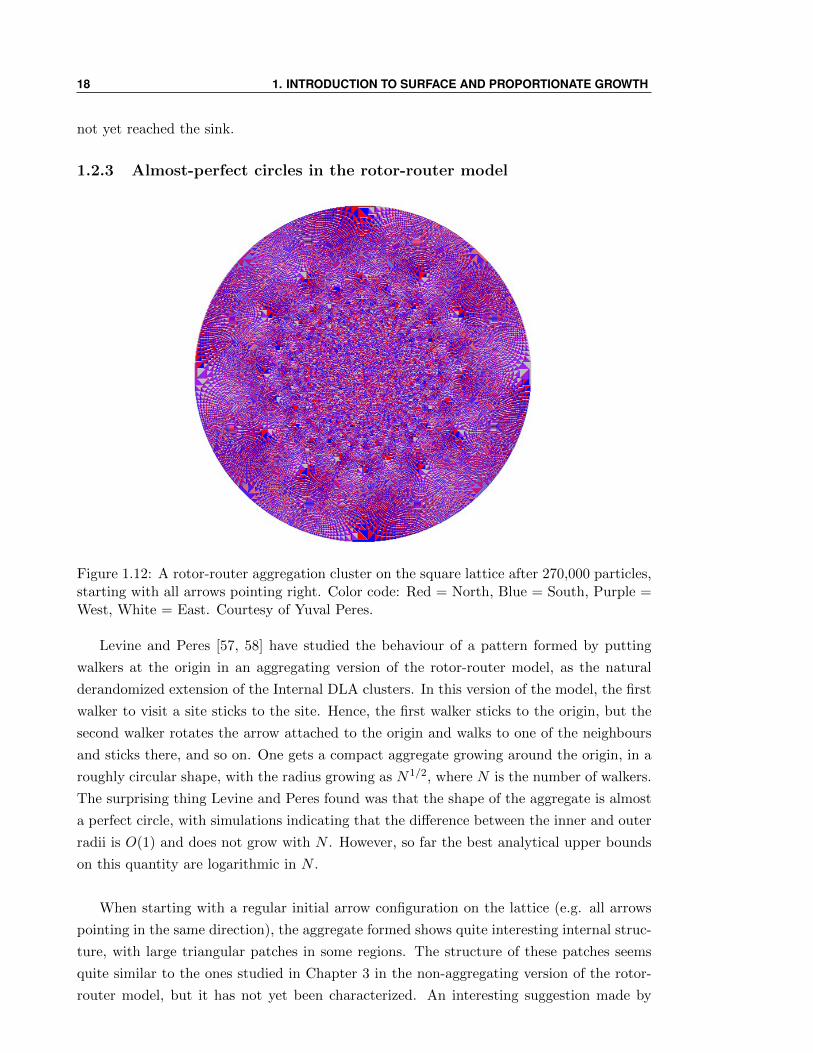
18 1. INTRODUCTION TO SURFACE AND PROPORTIONATE GROWTH
not yet reached the sink.
1.2.3 Almost-perfect circles in the rotor-router model
Figure 1.12: A rotor-router aggregation cluster on the square lattice after 270,000 particles,starting with all arrows pointing right. Color code: Red = North, Blue = South, Purple =West, White = East. Courtesy of Yuval Peres.
Levine and Peres [57, 58] have studied the behaviour of a pattern formed by putting
walkers at the origin in an aggregating version of the rotor-router model, as the natural
derandomized extension of the Internal DLA clusters. In this version of the model, the first
walker to visit a site sticks to the site. Hence, the first walker sticks to the origin, but the
second walker rotates the arrow attached to the origin and walks to one of the neighbours
and sticks there, and so on. One gets a compact aggregate growing around the origin, in a
roughly circular shape, with the radius growing as N1/2, where N is the number of walkers.
The surprising thing Levine and Peres found was that the shape of the aggregate is almost
a perfect circle, with simulations indicating that the difference between the inner and outer
radii is O(1) and does not grow with N . However, so far the best analytical upper bounds
on this quantity are logarithmic in N .
When starting with a regular initial arrow configuration on the lattice (e.g. all arrows
pointing in the same direction), the aggregate formed shows quite interesting internal struc-
ture, with large triangular patches in some regions. The structure of these patches seems
quite similar to the ones studied in Chapter 3 in the non-aggregating version of the rotor-
router model, but it has not yet been characterized. An interesting suggestion made by
1.3. GROWING SURFACES: THE KPZ UNIVERSALITY CLASS 19
Matt Cook is that this pattern is extremely similar to a Moire patterns created on the unit
circle in the complex plane [59].
1.3 Growing Surfaces: The KPZ Universality Class
In section 1.1 we discussed many different growing surfaces. Remarkably, in many of these
models, the exponents α and β have similar values. In this section we discuss the two
main universality classes of growing rough surfaces. Then we discuss a more remarkable
form of universality that has been discovered in the past thirty years in various superficially
unconnected models in statistical physics. It is a universality manifest not just in the scaling
properties of certain variables, but in their probability distributions as well. We present
a few exact mappings between such models which are relevant to this thesis, first from a
model of subsequence matching to the asymmetric exclusion process, and then from the
ASEP to growing surfaces.
1.3.1 Universality classes for growing surfaces
To study the dynamics of non-equilibrium systems, one often integrates out the microscopic
degrees of freedom to get a Langevin equation for a coarse-grained field, which represents
the mesoscopic degrees of freedom. In fact, one can usually write down the Langevin equa-
tion using only the symmetries of the microscopic dynamics, and keeping all terms allowed
by these symmetries. One then determines which terms are relevant or irrelevant in a renor-
malization sense. The values of the parameters in the coarse-grained description depend,
of course, on the parameters in the microscopic dynamics.
To study growing surfaces, the relevant mesoscopic field is a coarse-grained height func-
tion h(x, t), without overhangs, defined on continuous space and time. (Note that if the
model has overhangs, it has to be shown that their existence is irrelevant after the coarse-
graining.) For many models, such as the Eden model, one can argue that overhangs are
irrelevant for the mesoscopic dynamics. We restrict the Langevin equation for h(x, t) to
obey the following constraints ([61]):
(i) There is translation invariance along the growth direction, that is, the dynamics of
growth does not depend on the heights.
(ii) In the plane perpendicular to the growth direction, we have translation, inversion
and rotation symmetries.
(iii) The equation is first order in time.
(iv) The randomness in the growth dynamics is local in space and time.
These symmetries dictate that the only surviving terms in the Langevin equation are of
the form (∇ah)c where the product ac is even, or products of such terms. The most general
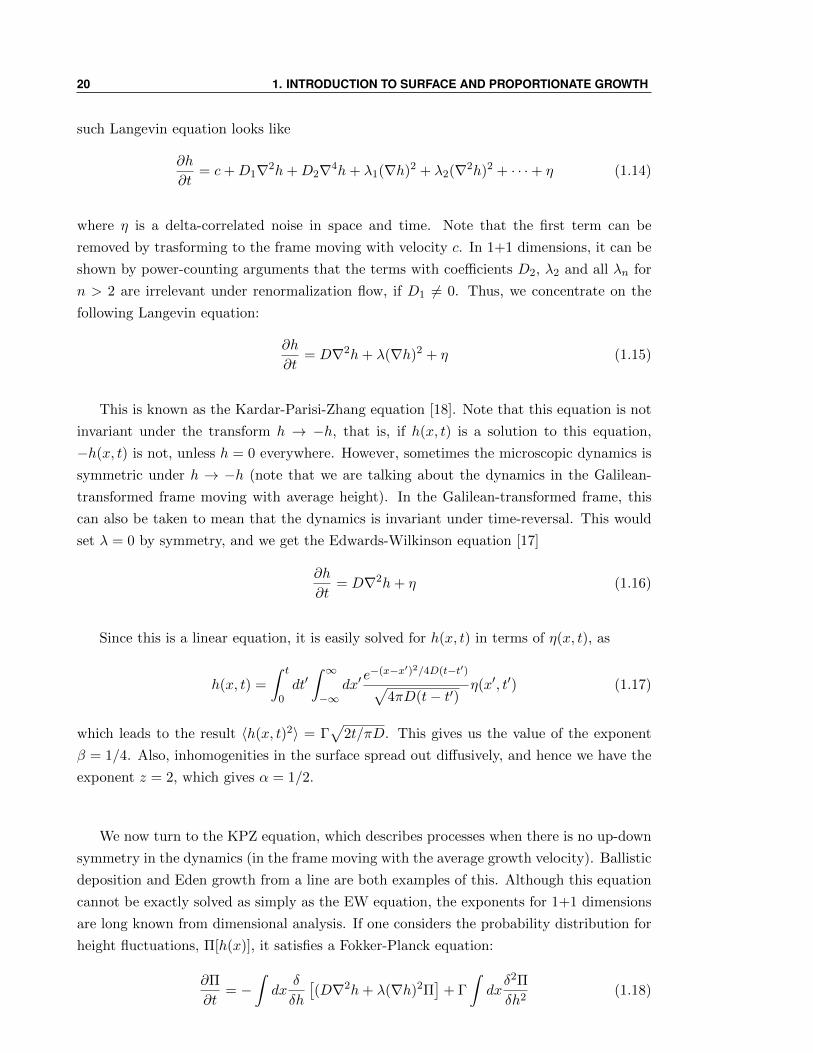
20 1. INTRODUCTION TO SURFACE AND PROPORTIONATE GROWTH
such Langevin equation looks like
∂h
∂t= c+D1∇2h+D2∇4h+ λ1(∇h)2 + λ2(∇2h)2 + · · ·+ η (1.14)
where η is a delta-correlated noise in space and time. Note that the first term can be
removed by trasforming to the frame moving with velocity c. In 1+1 dimensions, it can be
shown by power-counting arguments that the terms with coefficients D2, λ2 and all λn for
n > 2 are irrelevant under renormalization flow, if D1 6= 0. Thus, we concentrate on the
following Langevin equation:
∂h
∂t= D∇2h+ λ(∇h)2 + η (1.15)
This is known as the Kardar-Parisi-Zhang equation [18]. Note that this equation is not
invariant under the transform h → −h, that is, if h(x, t) is a solution to this equation,
−h(x, t) is not, unless h = 0 everywhere. However, sometimes the microscopic dynamics is
symmetric under h → −h (note that we are talking about the dynamics in the Galilean-
transformed frame moving with average height). In the Galilean-transformed frame, this
can also be taken to mean that the dynamics is invariant under time-reversal. This would
set λ = 0 by symmetry, and we get the Edwards-Wilkinson equation [17]
∂h
∂t= D∇2h+ η (1.16)
Since this is a linear equation, it is easily solved for h(x, t) in terms of η(x, t), as
h(x, t) =
∫ t
0dt′∫ ∞−∞
dx′e−(x−x′)2/4D(t−t′)√
4πD(t− t′)η(x′, t′) (1.17)
which leads to the result 〈h(x, t)2〉 = Γ√
2t/πD. This gives us the value of the exponent
β = 1/4. Also, inhomogenities in the surface spread out diffusively, and hence we have the
exponent z = 2, which gives α = 1/2.
We now turn to the KPZ equation, which describes processes when there is no up-down
symmetry in the dynamics (in the frame moving with the average growth velocity). Ballistic
deposition and Eden growth from a line are both examples of this. Although this equation
cannot be exactly solved as simply as the EW equation, the exponents for 1+1 dimensions
are long known from dimensional analysis. If one considers the probability distribution for
height fluctuations, Π[h(x)], it satisfies a Fokker-Planck equation:
∂Π
∂t= −
∫dx
δ
δh
[(D∇2h+ λ(∇h)2Π
]+ Γ
∫dxδ2Π
δh2(1.18)
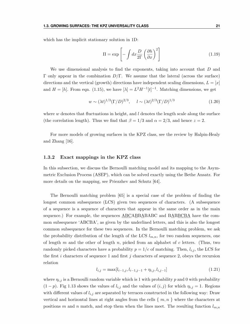
1.3. GROWING SURFACES: THE KPZ UNIVERSALITY CLASS 21
which has the implicit stationary solution in 1D:
Π = exp
[−∫dx
D
2Γ
(∂h
∂x
)2]
(1.19)
We use dimensional analysis to find the exponents, taking into account that D and
Γ only appear in the combination D/Γ. We assume that the lateral (across the surface)
directions and the vertical (growth) directions have independent scaling dimensions, L = [x]
and H = [h]. From eqn. (1.15), we have [λ] = L2H−1[t]−1. Matching dimensions, we get
w ∼ (λt)1/3(Γ/D)2/3, l ∼ (λt)2/3(Γ/D)1/3 (1.20)
where w denotes that fluctuations in height, and l denotes the length scale along the surface
(the correlation length). Thus we find that β = 1/3 and α = 2/3, and hence z = 2.
For more models of growing surfaces in the KPZ class, see the review by Halpin-Healy
and Zhang [16].
1.3.2 Exact mappings in the KPZ class
In this subsection, we discuss the Bernoulli matching model and its mapping to the Asym-
metric Exclusion Process (ASEP), which can be solved exactly using the Bethe Ansatz. For
more details on the mapping, see Priezzhev and Schutz [64].
The Bernoulli matching problem [65] is a special case of the problem of finding the
longest common subsequence (LCS) given two sequences of characters. (A subsequence
of a sequence is a sequence of characters that appear in the same order as in the main
sequence.) For example, the sequences ABCABBABABC and BABBCBA have the com-
mon subsequence ‘ABCBA’, as given by the underlined letters, and this is also the longest
common subsequence for these two sequences. In the Bernoulli matching problem, we ask
the probability distribution of the length of the LCS lm,n, for two random sequences, one
of length m and the other of length n, picked from an alphabet of c letters. (Thus, two
randomly picked characters have a probability p = 1/c of matching. Then, li,j , the LCS for
the first i characters of sequence 1 and first j characters of sequence 2, obeys the recursion
relation
li,j = max[li−1,j , li−1,j−1 + ηi,j , li,j−1] (1.21)
where ηi,j is a Bernoulli random variable which is 1 with probability p and 0 with probability
(1− p). Fig 1.13 shows the values of li,j and the values of (i, j) for which ηi,j = 1. Regions
with different values of li,j are separated by terraces constructed in the following way: Draw
vertical and horizontal lines at right angles from the cells m,n where the characters at
positions m and n match, and stop them when the lines meet. The resulting function lm,n
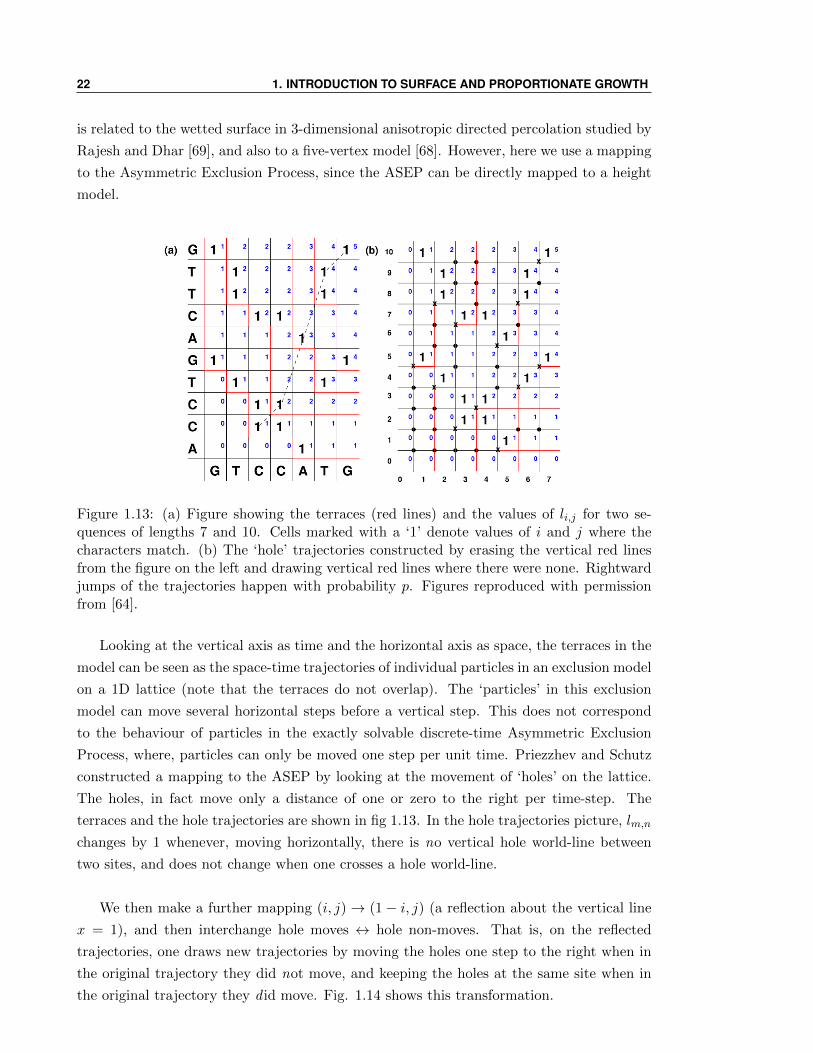
22 1. INTRODUCTION TO SURFACE AND PROPORTIONATE GROWTH
is related to the wetted surface in 3-dimensional anisotropic directed percolation studied by
Rajesh and Dhar [69], and also to a five-vertex model [68]. However, here we use a mapping
to the Asymmetric Exclusion Process, since the ASEP can be directly mapped to a height
model.
Figure 1.13: (a) Figure showing the terraces (red lines) and the values of li,j for two se-quences of lengths 7 and 10. Cells marked with a ‘1’ denote values of i and j where thecharacters match. (b) The ‘hole’ trajectories constructed by erasing the vertical red linesfrom the figure on the left and drawing vertical red lines where there were none. Rightwardjumps of the trajectories happen with probability p. Figures reproduced with permissionfrom [64].
Looking at the vertical axis as time and the horizontal axis as space, the terraces in the
model can be seen as the space-time trajectories of individual particles in an exclusion model
on a 1D lattice (note that the terraces do not overlap). The ‘particles’ in this exclusion
model can move several horizontal steps before a vertical step. This does not correspond
to the behaviour of particles in the exactly solvable discrete-time Asymmetric Exclusion
Process, where, particles can only be moved one step per unit time. Priezzhev and Schutz
constructed a mapping to the ASEP by looking at the movement of ‘holes’ on the lattice.
The holes, in fact move only a distance of one or zero to the right per time-step. The
terraces and the hole trajectories are shown in fig 1.13. In the hole trajectories picture, lm,n
changes by 1 whenever, moving horizontally, there is no vertical hole world-line between
two sites, and does not change when one crosses a hole world-line.
We then make a further mapping (i, j)→ (1− i, j) (a reflection about the vertical line
x = 1), and then interchange hole moves ↔ hole non-moves. That is, on the reflected
trajectories, one draws new trajectories by moving the holes one step to the right when in
the original trajectory they did not move, and keeping the holes at the same site when in
the original trajectory they d id move. Fig. 1.14 shows this transformation.
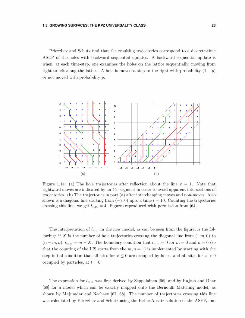
1.3. GROWING SURFACES: THE KPZ UNIVERSALITY CLASS 23
Priezzhev and Schutz find that the resulting trajectories correspond to a discrete-time
ASEP of the holes with backward sequential updates. A backward sequential update is
when, at each time-step, one examines the holes on the lattice sequentially, moving from
right to left along the lattice. A hole is moved a step to the right with probability (1− p)or not moved with probability p.
(a) (b)
Figure 1.14: (a) The hole trajectories after reflection about the line x = 1. Note thatrightward moves are indicated by an 45 segment in order to avoid apparent intersections oftrajectories. (b) The trajectories in part (a) after interchanging moves and non-moves. Alsoshown is a diagonal line starting from (−7, 0) upto a time t = 10. Counting the trajectoriescrossing this line, we get l7,10 = 4. Figures reproduced with permission from [64].
The interpretation of lm,n in the new model, as can be seen from the figure, is the fol-
lowing: if X is the number of hole trajectories crossing the diagonal line from (−m, 0) to
(n−m,n), lm,n = m−X. The boundary condition that lm,n = 0 for m = 0 and n = 0 (so
that the counting of the LIS starts from the m,n = 1) is implemented by starting with the
step initial condition that all sites for x ≤ 0 are occupied by holes, and all sites for x > 0
occupied by particles, at t = 0.
The expression for lm,n was first derived by Seppalainen [66], and by Rajesh and Dhar
[69] for a model which can be exactly mapped onto the Bernoulli Matching model, as
shown by Majumdar and Nechaev [67, 68]. The number of trajectories crossing this line
was calculated by Priezzhev and Schutz using the Bethe Ansatz solution of the ASEP, and
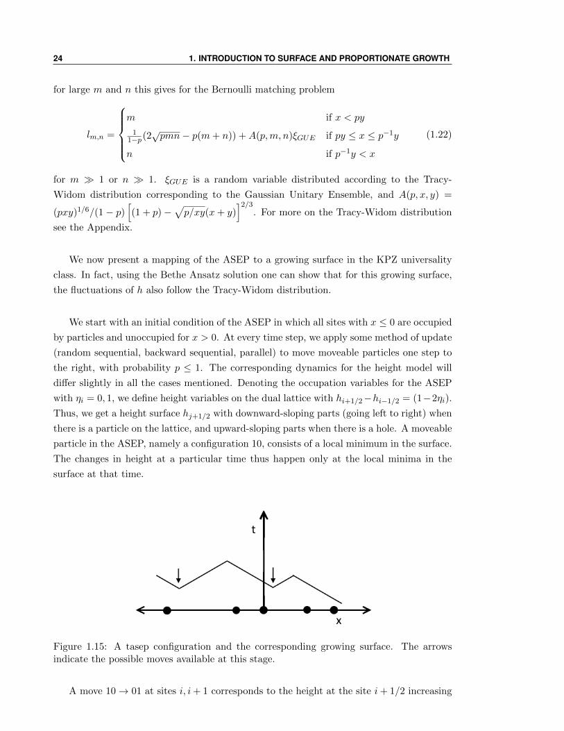
24 1. INTRODUCTION TO SURFACE AND PROPORTIONATE GROWTH
for large m and n this gives for the Bernoulli matching problem
lm,n =
m if x < py
11−p(2
√pmn− p(m+ n)) +A(p,m, n)ξGUE if py ≤ x ≤ p−1y
n if p−1y < x
(1.22)
for m 1 or n 1. ξGUE is a random variable distributed according to the Tracy-
Widom distribution corresponding to the Gaussian Unitary Ensemble, and A(p, x, y) =
(pxy)1/6/(1− p)[(1 + p)−
√p/xy(x+ y)
]2/3. For more on the Tracy-Widom distribution
see the Appendix.
We now present a mapping of the ASEP to a growing surface in the KPZ universality
class. In fact, using the Bethe Ansatz solution one can show that for this growing surface,
the fluctuations of h also follow the Tracy-Widom distribution.
We start with an initial condition of the ASEP in which all sites with x ≤ 0 are occupied
by particles and unoccupied for x > 0. At every time step, we apply some method of update
(random sequential, backward sequential, parallel) to move moveable particles one step to
the right, with probability p ≤ 1. The corresponding dynamics for the height model will
differ slightly in all the cases mentioned. Denoting the occupation variables for the ASEP
with ηi = 0, 1, we define height variables on the dual lattice with hi+1/2−hi−1/2 = (1−2ηi).
Thus, we get a height surface hj+1/2 with downward-sloping parts (going left to right) when
there is a particle on the lattice, and upward-sloping parts when there is a hole. A moveable
particle in the ASEP, namely a configuration 10, consists of a local minimum in the surface.
The changes in height at a particular time thus happen only at the local minima in the
surface at that time.
Figure 1.15: A tasep configuration and the corresponding growing surface. The arrowsindicate the possible moves available at this stage.
A move 10→ 01 at sites i, i+ 1 corresponds to the height at the site i+ 1/2 increasing
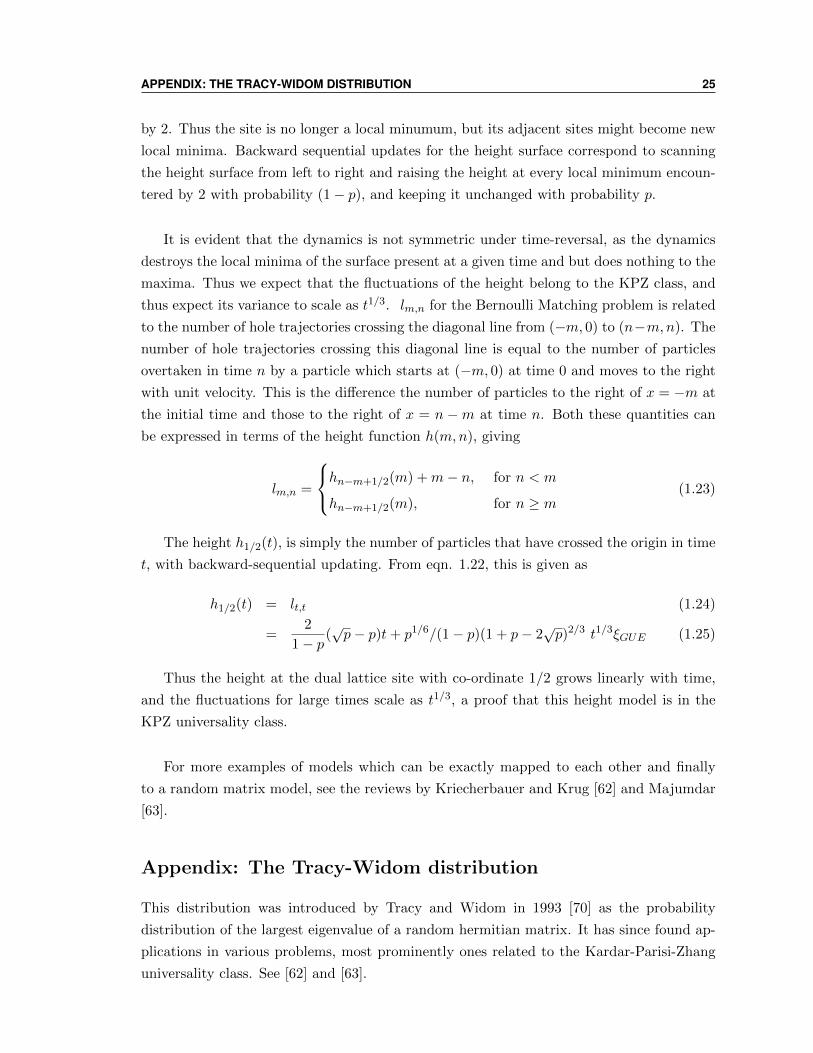
APPENDIX: THE TRACY-WIDOM DISTRIBUTION 25
by 2. Thus the site is no longer a local minumum, but its adjacent sites might become new
local minima. Backward sequential updates for the height surface correspond to scanning
the height surface from left to right and raising the height at every local minimum encoun-
tered by 2 with probability (1− p), and keeping it unchanged with probability p.
It is evident that the dynamics is not symmetric under time-reversal, as the dynamics
destroys the local minima of the surface present at a given time and but does nothing to the
maxima. Thus we expect that the fluctuations of the height belong to the KPZ class, and
thus expect its variance to scale as t1/3. lm,n for the Bernoulli Matching problem is related
to the number of hole trajectories crossing the diagonal line from (−m, 0) to (n−m,n). The
number of hole trajectories crossing this diagonal line is equal to the number of particles
overtaken in time n by a particle which starts at (−m, 0) at time 0 and moves to the right
with unit velocity. This is the difference the number of particles to the right of x = −m at
the initial time and those to the right of x = n −m at time n. Both these quantities can
be expressed in terms of the height function h(m,n), giving
lm,n =
hn−m+1/2(m) +m− n, for n < m
hn−m+1/2(m), for n ≥ m(1.23)
The height h1/2(t), is simply the number of particles that have crossed the origin in time
t, with backward-sequential updating. From eqn. 1.22, this is given as
h1/2(t) = lt,t (1.24)
=2
1− p(√p− p)t+ p1/6/(1− p)(1 + p− 2
√p)2/3 t1/3ξGUE (1.25)
Thus the height at the dual lattice site with co-ordinate 1/2 grows linearly with time,
and the fluctuations for large times scale as t1/3, a proof that this height model is in the
KPZ universality class.
For more examples of models which can be exactly mapped to each other and finally
to a random matrix model, see the reviews by Kriecherbauer and Krug [62] and Majumdar
[63].
Appendix: The Tracy-Widom distribution
This distribution was introduced by Tracy and Widom in 1993 [70] as the probability
distribution of the largest eigenvalue of a random hermitian matrix. It has since found ap-
plications in various problems, most prominently ones related to the Kardar-Parisi-Zhang
universality class. See [62] and [63].
26 1. INTRODUCTION TO SURFACE AND PROPORTIONATE GROWTH
Figure 1.16: The probability density for the largest eigenvalue, for Gaussian Orthogonal(β = 1), Gaussian Unitary (β = 2) and Gaussian Symplectic (β = 4) Ensembles.
The cumulative distribution function of the Tracy-Widom distribution is given by the
formula
F2(s) = exp
(−∫ ∞s
(x− s)q2(x)dx
)(1.26)
where q(s) is the solution of the type II Painleve equation
q′′(s) = sq(s) + 2q(s)3 (1.27)
which satisfies the boundary condition q(s) ∼ Ai(s) as s → ∞, where Ai(s) is the Airy
function. One can numerically evaluate
〈s〉 = −1.2065335746 . . . , 〈s2〉 − 〈s〉2 = 1.6077810346 . . . (1.28)
and other higher moments. Similar cumulative distributions F1(s) and F4(s), related to
F2, can be defined for the distributions of the largest eigenvalues of random symmetric and
quaternionic matrices respectively.
Although the exact form of the distribution can be evaluated numerically (plotted in fig
1.16), the behaviour of the tails can be determined via a simple scaling argument for the
ASEP (refer to [61] for details). As given earlier the number of particles crossing the origin
in time t, in a TASEP with backward-sequential updates, is given as
N(t) = a(p)t+ b(p)t1/3ξGUE (1.29)
where a(p) and b(p) are p-dependent functions. We set p = 1/2, and approximate the
probabilities for N very large and very small. N(t) = 0 corresponds to the situation in
which none of the particles move in time t. This means that the first particle does not move
at all times 1, 2, . . . , t, giving us a probability P (N(t) = 0) = 2−t. To get N = 0 involves
APPENDIX: THE TRACY-WIDOM DISTRIBUTION 27
setting ξGUEsim− t2/3, giving
PGUE(ξ) ∼ exp (−c−|ξ|3/2) for ξ → −∞ (1.30)
Similarly, not set N(t) = t, the maximum number of walkers which can be moved past the
origin in time t. The probability of this is (since, at each time step, all particles after the
origin must be moved one more step to the right)
1
2× 1
22× · · · × 1
2(t− 1)× 1
2t=
1
2t(t+1)/2(1.31)
Note that setting N(t) = t involves setting ξGUE ∼ t2/3, thus giving
PGUE(ξ) ∼ exp (−c+ξ3) for ξ →∞ (1.32)
The values of the constants c+ and c− can de determined by an analysis of the random
matrices based on, for example, a mapping to a logarithmically interacting gas on a line, to
be c+ = 1/12 and c− = 4/3.
Bibliography
[1] T. Viscek, Fractal growth phenomena Vol. 4. (World scientific, Singapore) (1989).
[2] H. J. Hermann, Phys. Rep. 136 153 (1986).
[3] M. C. Cross and P. C. Hohenberg, Rev. Mod. Phys. 65 851 (1993).
[4] M. Eden, Proc. Fourth Berkeley Symp. on Mathematical Statistics and Probability,
ed. F. Neyman (Univ. of Claif. Press, Berkeley) Vol. IV, p. 223 (1961).
[5] D. E. Wolf and J. Kertesz, J. Phys. A 23 L257 (1987) (exponents in d=2,3,4).
[6] D. Dhar, Phys. Rev. Lett., 54 2058 (1985).
[7] M.T. Batchelor and B.I. Henry, Phys. Lett. A, 157 229 (1991).
[8] T. Williams and R. Bjerknes, Nature 236 19 (1972).
[9] Z. Alexandrowicz, Phys. Lett. 80A 284 (1980)
A. Bunde, H. J. Hermann, A. Margolina and H. E. Stanley, Phys. Rev. Lett. 55 653
(1985).
[10] R. Chandler, J. Koplik, K. Lerman and J. F. Willemsen, J. Fluid. Mech. 119 246
(1982)
D. Wilkinson and J. F. Willemsen, J. Phys. A 16 3365 (1983)
B. Nickel and D. Wilkinson, Phys. Rev. Lett. 51 71 (1983).
[11] O.Haggstrom, Y.Peres and R.H.Schonmann: Perplexing Problems in Probability.
Festschrift in honor of Harry Kesten. M. Bramson, R. Durrett, ed. (Birkhauser, 1999),
pp. 69-90
[12] T. A. Witten and L. M. Sander, Phys. Rev. Lett. 47 1400, 1981.
[13] P. Meakin, Phys. Rev. Lett. 51 1119 (1983) (dla exponents).
[14] J. W. Lyklema, C. Evertsz and L. Pietronero, Europhys. Lett. 2 77 (1986).
[15] F. Family, Physica A, 168 561 (1990) (defines exponents for growing surfaces).
[16] T. Halpin-Healy and Y-C Zhang, Phys. Rep. 254 215 (1995).
28
BIBLIOGRAPHY 29
[17] S. F. Edwards and D. R. Wilkinson, Proc. Roy. Soc. Lond. A. Math. Phys. Sci. 381
17 (1982).
[18] K. Kardar, G. Parisi, and Y.Z. Zhang, Phys. Rev. Lett. 56 889 (1986).
[19] M. J. Vold, J. Coll. Sci., 14 168 (1959).
[20] M. Prahofer and H. Spohn, Phys. Rev. Lett 84 4882 (2000)
M. Prahofer and H. Spohn, J. Stat. Phys. 108 1071 (2002)
[21] K. Johansson, Comm. Math. Phys. 242 277 (2003)
[22] M. Kolb, R. Botet and R. Jullien, 51 1123 (1983)
[23] F. Leyvraz, J. Phys. A 18 321 (1985)
[24] T. Sadhu and D. Dhar, J. Stat. Mech. P11006 (2013).
[25] P. Bak, C. Tang and K. Wiesenfeld, Phys. Rev. Lett. 59 381 1987.
[26] D. Dhar, Phys. Rev. Lett. 64 1613 (1990).
[27] D. Dhar, Physica A 369 29 (2006).
[28] S. Ostojic, Physica A 318 187 (2003).
[29] D. Dhar, T. Sadhu and S. Chandra, Europhys. Lett. 85 48002 (2009).
[30] T. Sadhu and D. Dhar, J. Stat. Phys. 138 815 (2010).
[31] T. Sadhu and D. Dhar, J. Stat. Mech. P03001 (2011).
[32] M. Creutz, Comput. Phys. 5 198 (1991).
[33] S. Caracciolo, G. Paoletti and A. Sportiello, J. Phys. A: Math. Theor. 41 495003 (2008).
[34] G. F. Lawler, M. Bramson and D. Griffeath, Ann. Probab. 20 2117 (1992).
[35] L. Levine and Y. Peres, J. d’Analyse Math. 111 151 (2010).
[36] J.-F. Gouyet, Physique et structures fractales, Elsevier Masson, 1992.
[37] T. Sadhu and D. Dhar, Phys. Rev. E 85 021107 (2012).
[38] R. Dandekar, Pattern formation in diusive sandpiles, 2011 Proc. Conf. Dynamics of
Phase Transformations (Bangalore) www.jncasr.ac.in/dpt/abstract poster.pdf
[39] L. Lovasz, Dicrete Analytic Functions: An Exposition, http://www.cs.elte.hu/ lo-
vasz/analytic.pdf
[40] L. Levine, W. Pegden and C. K. Smart arXiv:1208.4839 (2012).
30 BIBLIOGRAPHY
[41] V. B. Priezzhev, D. Dhar, A. Dhar and S. Krishnamurthy, Phys. Rev. Lett., 77 5079
(1996).
[42] R. R. Scherbakov, Vl. V. Papoyan, and A. M. Povolotsky, Phys. Rev. E, 55 3686
(1997).
[43] A. M. Povolotsky, V. B. Priezzhev, and R. R. Scherbakov, Phys. Rev. E, 58 5449
(1998).
[44] C. G. Langton, Physica D, 22 120 (1986)
https://en.wikipedia.org/wiki/Langton‘s ant
[45] Th. W. Ruijgrok and E. G. D. Cohen, Phys. Lett. A 133 415 (1988)
[46] L.A. Bunimovich, S. E. Troubetzkoy, J. Stat. Phys., 67 289 (1992)
[47] H. Freund and P. Grassberger, Physica A, 190 218 (1992)
[48] J. Propp, Chaos, 20 037110 (2010).
[49] A. E. Holroyd and J. Propp, Contemporary Mathematics, 520 105 (2010)
arXiv:0904.4507
[50] A. E. Holroyd, L. Levine, K. Meszaros, Y. Peres, J. Propp and D. B. Wilson, Progress
in Probability, 60 331 (2008). arXiv:0801.330
[51] L. Levine, The rotor-router model, Harvard University Senior Thesis (2002).
arXiv:0409407
[52] A. Z. Broder, Generating random spanning trees, Foundations of Computer Science
442 (1989).
[53] T. Friedrich and L. Levine, Fast simulation of large-scale growth models, Random
Structures & Algorithms 42 185 (2013)
[54] S. P. Vadhan, Pseudorandomness, preprint available from
http://people.seas.harvard.edu/ salil/pseudorandomness/.
[55] L. Florescu, S. Ganguly, L. Levine and Y. Peres, arXiv:1301.3521
[56] M. Kleber, The Mathematical Intelligencer, 27 55 (2005).
[57] L. Levine and Y. Peres, Indiana Univ. Math. J., 57 431 (2008). arXiv:0503251.
[58] L. Levine and Y. Peres, Potential Analysis, 30 1 (2009), arXiv:0704.0688.
[59] Matt Cook, http://paradise.caltech.edu/cook/Warehouse/ForPropp/
[60] R. Kapri and D. Dhar, Phys. Rev. E, 80 051118 (2009).
BIBLIOGRAPHY 31
[61] P. L. Krapivsky, S. Redner, and E. Ben-Naim, A kinetic view of statistical physics
(Cambridge University Press, Cambridge) (2010)
[62] T. Kriecherbauer and J. Krug, J. Phys. A: Math. Theo. 43 403001 (2010),
arXiv:0803.2796 (2008).
[63] S. N. Majumdar, Les Houches lecture notes, 2006, arxiv:0701193.
[64] V. B. Priezzhev and G. M. Schutz, J. Stat. Mech. P09007 (2008).
[65] J. Boutet de Monvel, Eur. Phys. J. B 7, 293 (1999); Phys. Rev. E 62, 204 (2000).
[66] T. Seppalainen, Ann. Appl. Probab. 7, no. 4, 886 (1997).
[67] S.N. Majumdar and S. Nechaev, Phys. Rev. E 72, 020901(R) (2005).
[68] S.N. Majumdar, K. Mallick and S. Nechaev, arXiv:0710.1030v1 [cond-mat.stat-mech]
(2007).
[69] R.Rajesh and D.Dhar, Phys.Rev. Lett. 81, 1646 (1998).
[70] C.A. Tracy and H. Widom, Commun. Math. Phys. 159, 151 (1994); 177, 727(1996).
Chapter 2
Introduction to Active-Absorbing
Phase Transitions
In this chapter, we will review the phenomenon of absorbing phase transtions, in systems
with and without a conserved number of particles. Absorbing states are states which the
dynamics can lead to but cannot escape from. In Absorbing (or active-absorbing) phase
transitions, as an external parameter is tuned, the long-time limit of the system changes
from an active fluctuating steady-state to an absorbing state where no further changes occur.
Some useful reviews are the lecture notes by Grinstein and Munoz [1], the review articles
by Hinrichsen [2] and Lubeck [3] (the latter focuses on the study of scaling relations and
scaling functions), and the recent book by Henkel, Hinrichsen and Lubeck [4]. These tran-
sitions are characterized by static and dynamical critical exponents which obey well-known
scaling relations. We will also discuss the phenomena of universality, wherein transitions
in many diverse systems nevertheless show the same critical exponents near the transition.
The classification of universality classes of absorbing phase transitions, especially those in
systems with a conserved number of particles, has been a topic of particular interest in the
recent literature [5, 6, 7, 8].
2.1 Absorbing phase transitions
Absorbing states are configurations of the system in which no further transitions are pos-
sible. In the following we give some, admittedly idealized, models of real systems which
exhibit transitions between an absorbing phase and a fluctuating active phase.
(i) An epidemic disease spreading through the population might die out if the infection
rate is low, that is, infected individuals at a particular time do not infect anyone else before
they die or recover. A simple model for this is an that an infected person infects everyone
he or she comes in contact with a given probability p and recovers from the disease at a unit
rate. Once the disease dies out it cannot regenerate, and hence this is an absorbing state.
32
2.1. ABSORBING PHASE TRANSITIONS 33
Whether the disease dies out or proliferates depends on the mean number of other people
a single infected personal infects before dying or recovering, which depends on p. As p is
varied, there is transition between eventual dying out and a phase where there are always
some infected individuals in the population [9, 10, 11]. More realistic models of epidemics
have been proposed, among them the Generalized Epidemic Process, which is a model where
individuals infected earlier have a different susceptibility to the disease the next time round
(for example, they might become immune after a given number of infections). Similar to
the epidemic models are models of forest fires where the state where the fire dies out is
absorbing [12].
(ii) The Ziff-Gulari-Barshad (ZGB) model [13] for the catalytic oxidation of carbon
monoxide (CO) to carbon dioxide (CO2) on a substrate, is defined as follows: Consider the
substrate to be a 2D lattice. A CO atom gets adsorbed to an empty site on the surface at a
rate y. The two atoms of an O2 molecule get adsorbed to an adjacent pair of empty sites at
a rate 1− y. The difference between the two rates represents the different concentrations of
the gases in the air above the substrate, and is a tunable parameter. If a CO molecule and
an O atom find themselves on adjacent sites, they merge to form a CO2 molecule and desorb
from the surface. This model has two absorbing states - one (for low y) where the entire
lattice is filled with O atoms, and one (for high y) where it is entirely filled with CO atoms .
Note that this is because both these species cannot desorb on their own. Simulations show
correspondingly that there are two transitions and three phases in this model - an active
phase sandwiched between the two absorbing phases mentioned above. The transition for
low y which is continuous and the one for high y which is first-order [13, 14].
(iii) Water injected at one end of a porous medium percolates under the influence of
an external force, and either stops percolating at some point or continues percolating down
‘forever’, depending on the porosity of the medium. If one (in modelling this system) forbids
flow of water against gravity, then whether the pores at some level are occupied by water
depends on the state of the previous level. The downward direction can be seen as the time
axis, and hence the state of the a pore (wetted or not) can be said to depend on the state
of its neighbours at the ‘previous time-step’. As one varies the porosity of the medium, it
changes the probability of neighbouring pores being connected by downward channels, and
one gets a transition from an absorbing state where after a certain time (or level, going
downward)in the long-time limit (same as long-distance in the downward direction in the
porous material) there is no water in the pores, to a state where there is always a finite
density of wet pores arbitrarily downwards. Note that here only also assumes that the struc-
ture of the pores does not changes as one moves down, so that it also remains same in ‘time’.
One observes from the above examples that the ‘activity’, whether it is the presence of
a diseased individual or desorption from the surface or presence of a wetted pore, does not
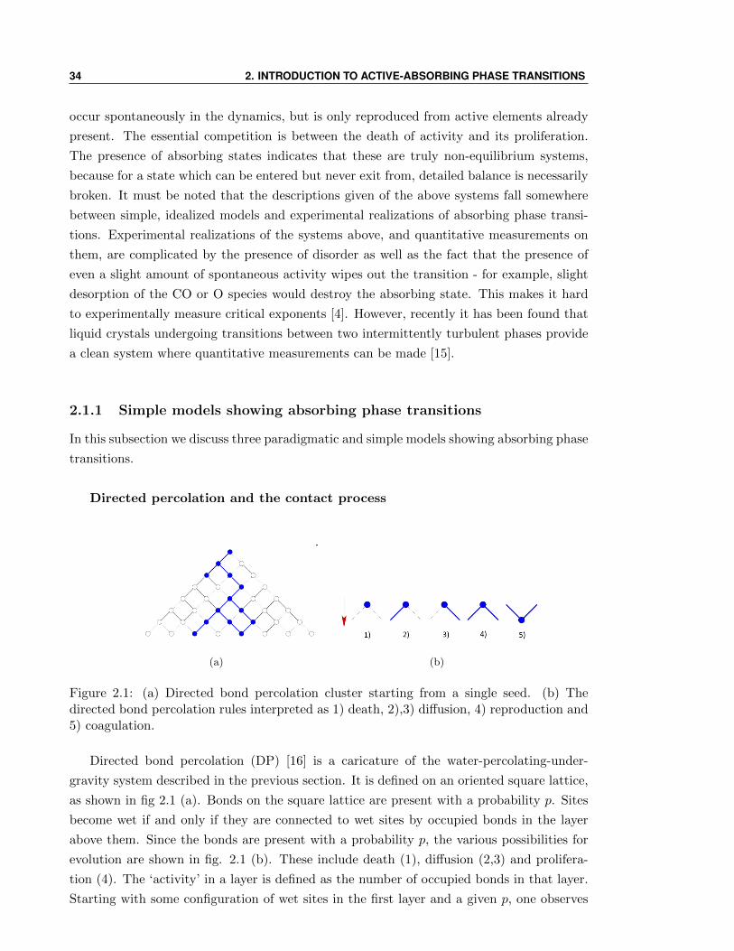
34 2. INTRODUCTION TO ACTIVE-ABSORBING PHASE TRANSITIONS
occur spontaneously in the dynamics, but is only reproduced from active elements already
present. The essential competition is between the death of activity and its proliferation.
The presence of absorbing states indicates that these are truly non-equilibrium systems,
because for a state which can be entered but never exit from, detailed balance is necessarily
broken. It must be noted that the descriptions given of the above systems fall somewhere
between simple, idealized models and experimental realizations of absorbing phase transi-
tions. Experimental realizations of the systems above, and quantitative measurements on
them, are complicated by the presence of disorder as well as the fact that the presence of
even a slight amount of spontaneous activity wipes out the transition - for example, slight
desorption of the CO or O species would destroy the absorbing state. This makes it hard
to experimentally measure critical exponents [4]. However, recently it has been found that
liquid crystals undergoing transitions between two intermittently turbulent phases provide
a clean system where quantitative measurements can be made [15].
2.1.1 Simple models showing absorbing phase transitions
In this subsection we discuss three paradigmatic and simple models showing absorbing phase
transitions.
Directed percolation and the contact process
(a) (b)
Figure 2.1: (a) Directed bond percolation cluster starting from a single seed. (b) Thedirected bond percolation rules interpreted as 1) death, 2),3) diffusion, 4) reproduction and5) coagulation.
Directed bond percolation (DP) [16] is a caricature of the water-percolating-under-
gravity system described in the previous section. It is defined on an oriented square lattice,
as shown in fig 2.1 (a). Bonds on the square lattice are present with a probability p. Sites
become wet if and only if they are connected to wet sites by occupied bonds in the layer
above them. Since the bonds are present with a probability p, the various possibilities for
evolution are shown in fig. 2.1 (b). These include death (1), diffusion (2,3) and prolifera-
tion (4). The ‘activity’ in a layer is defined as the number of occupied bonds in that layer.
Starting with some configuration of wet sites in the first layer and a given p, one observes
2.1. ABSORBING PHASE TRANSITIONS 35
whether the activity dies out or survives in the long-time limit. This model has not been
solved analytically, but numerical studies show that for a 2D square lattice, the transition
point pc = 0.644700185(5) [17]. The universal properties of the model such as the critical
exponents (in an expansion around the higher critical dimension) and the structure of the
phase diagram can be determined by field theoretic analysis. Reviews of the field theory
approach to DP are [18, 19, 20, 2]. [1] discusses renormalization starting from a Langevin
equation. We will not discuss the field theory approach in this thesis.
The ‘contact process’ is a continuous-time version of the directed bond percolation
model, and is defined by the following rules [21, 22, 23]: sites on a d-dimensional lattice
can be occupied or empty. Empty sites which have an occupied nearest neighbouring site
can get occupied at rate λ, and occupied sites become unoccupied at rate 1. This is also a
simple model for the spread of epidemics discussed in the previous subsection.
For the contact process in the mean field approximation, it is easy to see that the transi-
tion between proliferation and death happens at λ = 1/2d for a cubic lattice in d dimensions.
Close to the critical point, the density of infected individuals in the steady state grows as
(λ − 1) , giving the critical exponent value β = 1. MFT also gives ν‖ = 1 and ν⊥ = 1/2
([23]). (See section 2.2 for the definitions of these exponents.) In 1D, the transition point
is however λ = 3.29785(8) [24]. This model falls in the same universality class as directed
percolation (as do many other models, see section 2.3).
Infinitely many absorbing states: pair contact process
All the models discussed so far have only a single absorbing state on the absorbing
side of the transition. (The ZGB model had two, but they were associated with different
transitions.) Some models of catalysis, in particular models where two species can co-exist
without desorption, like the examples given below, have an exponentially large number of
absorbing states.
A simple model of this kind is Jensen’s ‘pair contact process’ [27]. The process is similar
to the contact process, except that isolated occupied sites can no longer proliferate or die.
If there is a pair of occupied nearest-neighbour sites, however, they can infect one of the
vacant neighbours around them at random at rate λ. A pair of such sites can also become
unoccupied, at rate 1. For low λ . 0.08 occupied pairs of sites eventually die out, leaving a
configuration with only isolated particles - that is, occupied sites with no occupied nearest
neighbours - which cannot move or evaporate from the surface. Every configuration with
only isolated occupied sites is thus an absorbing state. The number of such configurations
grows exponentially with the volume of the system.
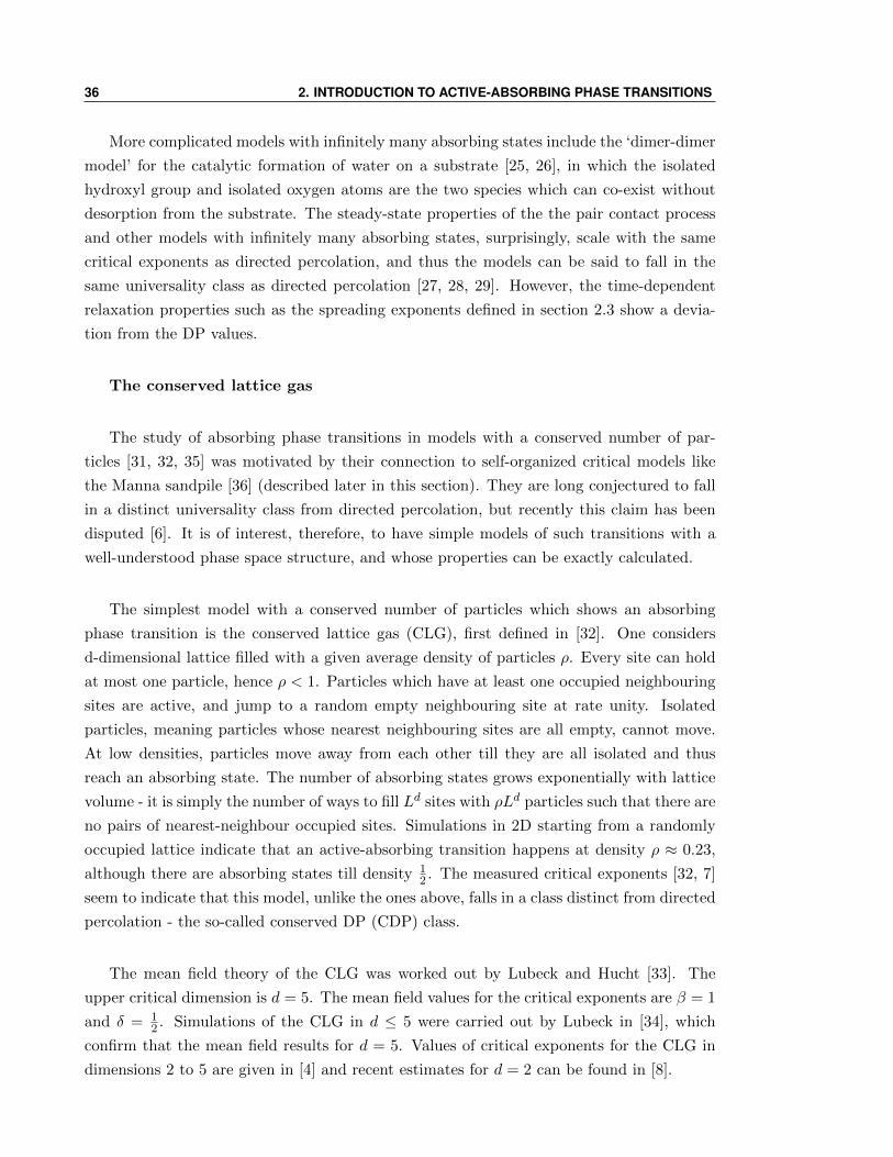
36 2. INTRODUCTION TO ACTIVE-ABSORBING PHASE TRANSITIONS
More complicated models with infinitely many absorbing states include the ‘dimer-dimer
model’ for the catalytic formation of water on a substrate [25, 26], in which the isolated
hydroxyl group and isolated oxygen atoms are the two species which can co-exist without
desorption from the substrate. The steady-state properties of the the pair contact process
and other models with infinitely many absorbing states, surprisingly, scale with the same
critical exponents as directed percolation, and thus the models can be said to fall in the
same universality class as directed percolation [27, 28, 29]. However, the time-dependent
relaxation properties such as the spreading exponents defined in section 2.3 show a devia-
tion from the DP values.
The conserved lattice gas
The study of absorbing phase transitions in models with a conserved number of par-
ticles [31, 32, 35] was motivated by their connection to self-organized critical models like
the Manna sandpile [36] (described later in this section). They are long conjectured to fall
in a distinct universality class from directed percolation, but recently this claim has been
disputed [6]. It is of interest, therefore, to have simple models of such transitions with a
well-understood phase space structure, and whose properties can be exactly calculated.
The simplest model with a conserved number of particles which shows an absorbing
phase transition is the conserved lattice gas (CLG), first defined in [32]. One considers
d-dimensional lattice filled with a given average density of particles ρ. Every site can hold
at most one particle, hence ρ < 1. Particles which have at least one occupied neighbouring
sites are active, and jump to a random empty neighbouring site at rate unity. Isolated
particles, meaning particles whose nearest neighbouring sites are all empty, cannot move.
At low densities, particles move away from each other till they are all isolated and thus
reach an absorbing state. The number of absorbing states grows exponentially with lattice
volume - it is simply the number of ways to fill Ld sites with ρLd particles such that there are
no pairs of nearest-neighbour occupied sites. Simulations in 2D starting from a randomly
occupied lattice indicate that an active-absorbing transition happens at density ρ ≈ 0.23,
although there are absorbing states till density 12 . The measured critical exponents [32, 7]
seem to indicate that this model, unlike the ones above, falls in a class distinct from directed
percolation - the so-called conserved DP (CDP) class.
The mean field theory of the CLG was worked out by Lubeck and Hucht [33]. The
upper critical dimension is d = 5. The mean field values for the critical exponents are β = 1
and δ = 12 . Simulations of the CLG in d ≤ 5 were carried out by Lubeck in [34], which
confirm that the mean field results for d = 5. Values of critical exponents for the CLG in
dimensions 2 to 5 are given in [4] and recent estimates for d = 2 can be found in [8].
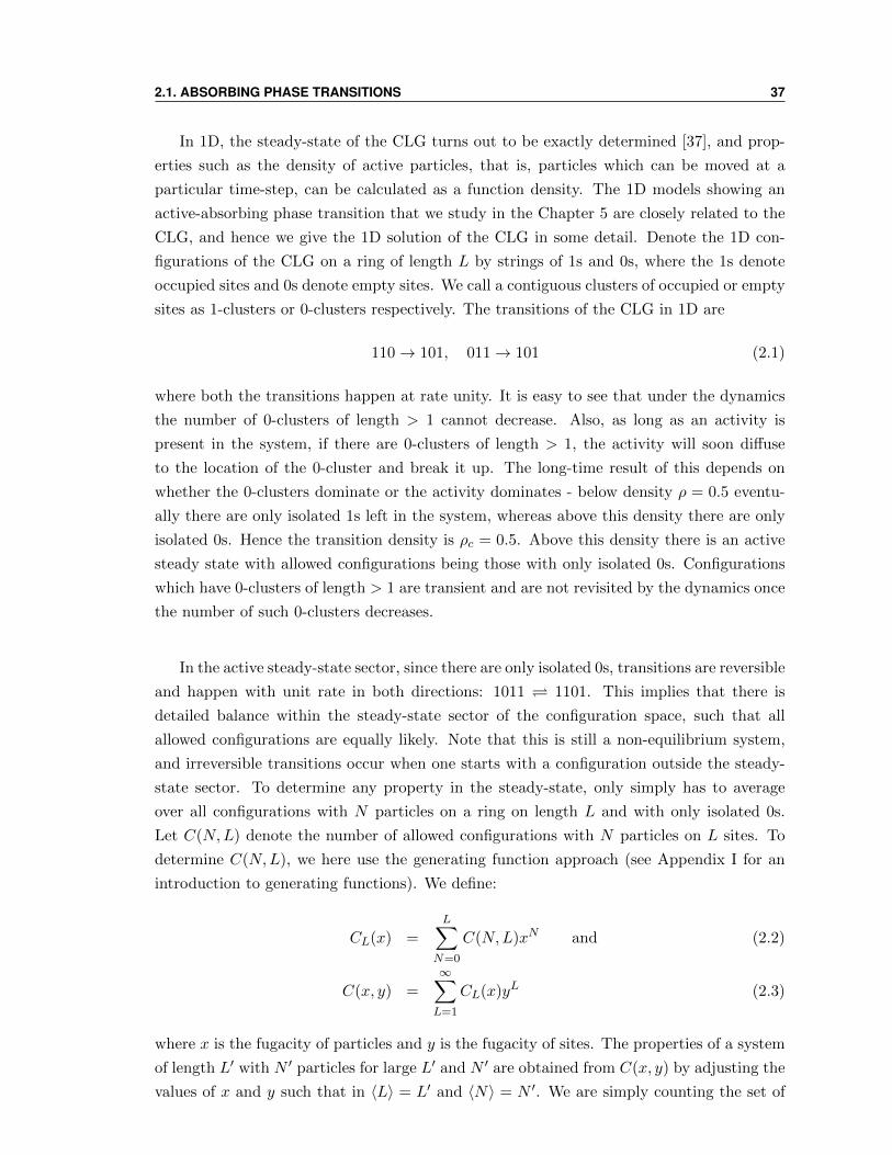
2.1. ABSORBING PHASE TRANSITIONS 37
In 1D, the steady-state of the CLG turns out to be exactly determined [37], and prop-
erties such as the density of active particles, that is, particles which can be moved at a
particular time-step, can be calculated as a function density. The 1D models showing an
active-absorbing phase transition that we study in the Chapter 5 are closely related to the
CLG, and hence we give the 1D solution of the CLG in some detail. Denote the 1D con-
figurations of the CLG on a ring of length L by strings of 1s and 0s, where the 1s denote
occupied sites and 0s denote empty sites. We call a contiguous clusters of occupied or empty
sites as 1-clusters or 0-clusters respectively. The transitions of the CLG in 1D are
110→ 101, 011→ 101 (2.1)
where both the transitions happen at rate unity. It is easy to see that under the dynamics
the number of 0-clusters of length > 1 cannot decrease. Also, as long as an activity is
present in the system, if there are 0-clusters of length > 1, the activity will soon diffuse
to the location of the 0-cluster and break it up. The long-time result of this depends on
whether the 0-clusters dominate or the activity dominates - below density ρ = 0.5 eventu-
ally there are only isolated 1s left in the system, whereas above this density there are only
isolated 0s. Hence the transition density is ρc = 0.5. Above this density there is an active
steady state with allowed configurations being those with only isolated 0s. Configurations
which have 0-clusters of length > 1 are transient and are not revisited by the dynamics once
the number of such 0-clusters decreases.
In the active steady-state sector, since there are only isolated 0s, transitions are reversible
and happen with unit rate in both directions: 1011 1101. This implies that there is
detailed balance within the steady-state sector of the configuration space, such that all
allowed configurations are equally likely. Note that this is still a non-equilibrium system,
and irreversible transitions occur when one starts with a configuration outside the steady-
state sector. To determine any property in the steady-state, only simply has to average
over all configurations with N particles on a ring on length L and with only isolated 0s.
Let C(N,L) denote the number of allowed configurations with N particles on L sites. To
determine C(N,L), we here use the generating function approach (see Appendix I for an
introduction to generating functions). We define:
CL(x) =L∑
N=0
C(N,L)xN and (2.2)
C(x, y) =
∞∑L=1
CL(x)yL (2.3)
where x is the fugacity of particles and y is the fugacity of sites. The properties of a system
of length L′ with N ′ particles for large L′ and N ′ are obtained from C(x, y) by adjusting the
values of x and y such that in 〈L〉 = L′ and 〈N〉 = N ′. We are simply counting the set of
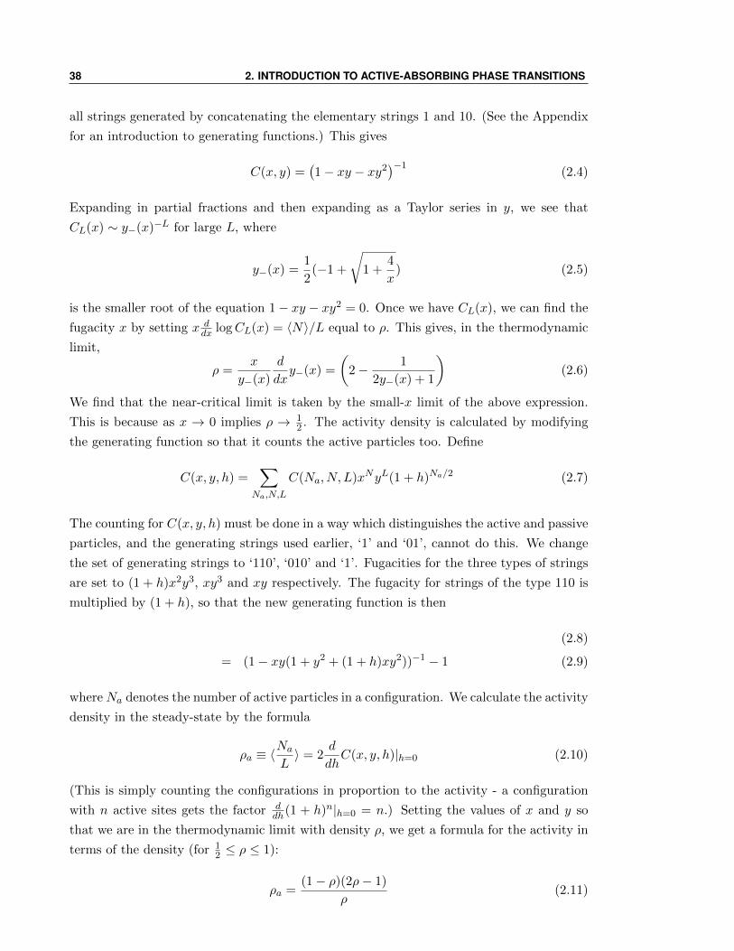
38 2. INTRODUCTION TO ACTIVE-ABSORBING PHASE TRANSITIONS
all strings generated by concatenating the elementary strings 1 and 10. (See the Appendix
for an introduction to generating functions.) This gives
C(x, y) =(1− xy − xy2
)−1(2.4)
Expanding in partial fractions and then expanding as a Taylor series in y, we see that
CL(x) ∼ y−(x)−L for large L, where
y−(x) =1
2(−1 +
√1 +
4
x) (2.5)
is the smaller root of the equation 1− xy − xy2 = 0. Once we have CL(x), we can find the
fugacity x by setting x ddx logCL(x) = 〈N〉/L equal to ρ. This gives, in the thermodynamic
limit,
ρ =x
y−(x)
d
dxy−(x) =
(2− 1
2y−(x) + 1
)(2.6)
We find that the near-critical limit is taken by the small-x limit of the above expression.
This is because as x → 0 implies ρ → 12 . The activity density is calculated by modifying
the generating function so that it counts the active particles too. Define
C(x, y, h) =∑
Na,N,L
C(Na, N, L)xNyL(1 + h)Na/2 (2.7)
The counting for C(x, y, h) must be done in a way which distinguishes the active and passive
particles, and the generating strings used earlier, ‘1’ and ‘01’, cannot do this. We change
the set of generating strings to ‘110’, ‘010’ and ‘1’. Fugacities for the three types of strings
are set to (1 + h)x2y3, xy3 and xy respectively. The fugacity for strings of the type 110 is
multiplied by (1 + h), so that the new generating function is then
(2.8)
= (1− xy(1 + y2 + (1 + h)xy2))−1 − 1 (2.9)
where Na denotes the number of active particles in a configuration. We calculate the activity
density in the steady-state by the formula
ρa ≡ 〈Na
L〉 = 2
d
dhC(x, y, h)|h=0 (2.10)
(This is simply counting the configurations in proportion to the activity - a configuration
with n active sites gets the factor ddh(1 + h)n|h=0 = n.) Setting the values of x and y so
that we are in the thermodynamic limit with density ρ, we get a formula for the activity in
terms of the density (for 12 ≤ ρ ≤ 1):
ρa =(1− ρ)(2ρ− 1)
ρ(2.11)
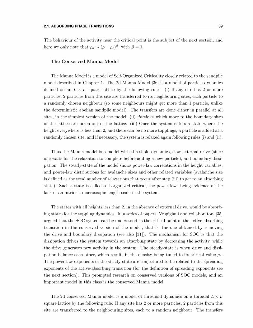
2.1. ABSORBING PHASE TRANSITIONS 39
The behaviour of the activity near the critical point is the subject of the next section, and
here we only note that ρa ∼ (ρ− ρc)β, with β = 1.
The Conserved Manna Model
The Manna Model is a model of Self-Organized Criticality closely related to the sandpile
model described in Chapter 1. The 2d Manna Model [36] is a model of particle dynamics
defined on an L × L square lattice by the following rules: (i) If any site has 2 or more
particles, 2 particles from this site are transferred to its neighbouring sites, each particle to
a randomly chosen neighbour (so some neighbours might get more than 1 particle, unlike
the deterministic abelian sandpile model). The transfers are done either in parallel at all
sites, in the simplest version of the model. (ii) Particles which move to the boundary sites
of the lattice are taken out of the lattice. (iii) Once the system enters a state where the
height everywhere is less than 2, and there can be no more topplings, a particle is added at a
randomly chosen site, and if necessary, the system is relaxed again following rules (i) and (ii).
Thus the Manna model is a model with threshold dynamics, slow external drive (since
one waits for the relaxation to complete before adding a new particle), and boundary dissi-
pation. The steady-state of the model shows power-law correlations in the height variables,
and power-law distributions for avalanche sizes and other related variables (avalanche size
is defined as the total number of relaxations that occur after step (iii) to get to an absorbing
state). Such a state is called self-organized critical, the power laws being evidence of the
lack of an intrinsic macroscopic length scale in the system.
The states with all heights less than 2, in the absence of external drive, would be absorb-
ing states for the toppling dynamics. In a series of papers, Vespigiani and collaborators [35]
argued that the SOC system can be understood as the critical point of the active-absorbing
transition in the conserved version of the model, that is, the one obtained by removing
the drive and boundary dissipation (see also [31]). The mechanism for SOC is that the
dissipation drives the system towards an absorbing state by decreasing the activity, while
the drive generates new activity in the system. The steady-state is when drive and dissi-
pation balance each other, which results in the density being tuned to its critical value ρc.
The power-law exponents of the steady-state are conjectured to be related to the spreading
exponents of the active-absorbing transition (for the definition of spreading exponents see
the next section). This prompted research on conserved versions of SOC models, and an
important model in this class is the conserved Manna model.
The 2d conserved Manna model is a model of threshold dynamics on a toroidal L × Lsquare lattice by the following rule: If any site has 2 or more particles, 2 particles from this
site are transferred to the neighbouring sites, each to a random neighbour. The transfers
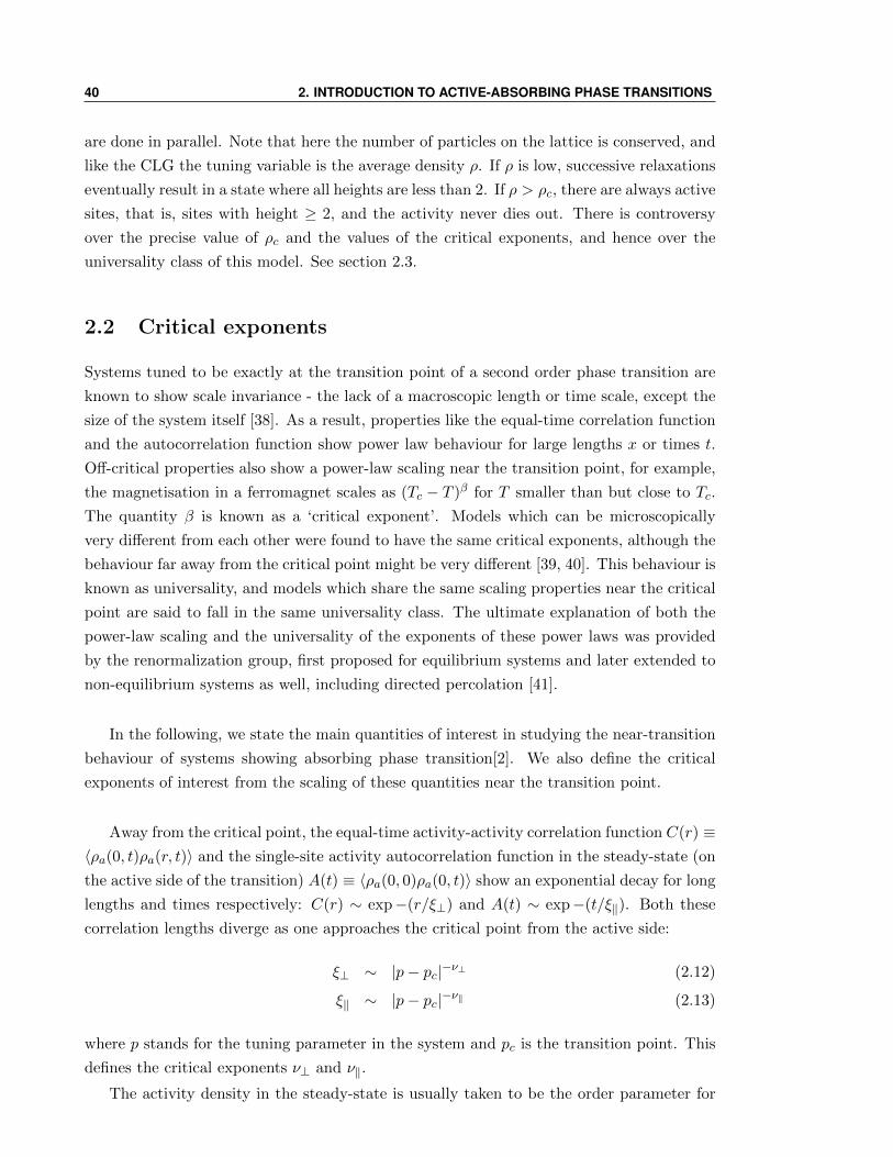
40 2. INTRODUCTION TO ACTIVE-ABSORBING PHASE TRANSITIONS
are done in parallel. Note that here the number of particles on the lattice is conserved, and
like the CLG the tuning variable is the average density ρ. If ρ is low, successive relaxations
eventually result in a state where all heights are less than 2. If ρ > ρc, there are always active
sites, that is, sites with height ≥ 2, and the activity never dies out. There is controversy
over the precise value of ρc and the values of the critical exponents, and hence over the
universality class of this model. See section 2.3.
2.2 Critical exponents
Systems tuned to be exactly at the transition point of a second order phase transition are
known to show scale invariance - the lack of a macroscopic length or time scale, except the
size of the system itself [38]. As a result, properties like the equal-time correlation function
and the autocorrelation function show power law behaviour for large lengths x or times t.
Off-critical properties also show a power-law scaling near the transition point, for example,
the magnetisation in a ferromagnet scales as (Tc − T )β for T smaller than but close to Tc.
The quantity β is known as a ‘critical exponent’. Models which can be microscopically
very different from each other were found to have the same critical exponents, although the
behaviour far away from the critical point might be very different [39, 40]. This behaviour is
known as universality, and models which share the same scaling properties near the critical
point are said to fall in the same universality class. The ultimate explanation of both the
power-law scaling and the universality of the exponents of these power laws was provided
by the renormalization group, first proposed for equilibrium systems and later extended to
non-equilibrium systems as well, including directed percolation [41].
In the following, we state the main quantities of interest in studying the near-transition
behaviour of systems showing absorbing phase transition[2]. We also define the critical
exponents of interest from the scaling of these quantities near the transition point.
Away from the critical point, the equal-time activity-activity correlation function C(r) ≡〈ρa(0, t)ρa(r, t)〉 and the single-site activity autocorrelation function in the steady-state (on
the active side of the transition) A(t) ≡ 〈ρa(0, 0)ρa(0, t)〉 show an exponential decay for long
lengths and times respectively: C(r) ∼ exp−(r/ξ⊥) and A(t) ∼ exp−(t/ξ‖). Both these
correlation lengths diverge as one approaches the critical point from the active side:
ξ⊥ ∼ |p− pc|−ν⊥ (2.12)
ξ‖ ∼ |p− pc|−ν‖ (2.13)
where p stands for the tuning parameter in the system and pc is the transition point. This
defines the critical exponents ν⊥ and ν‖.
The activity density in the steady-state is usually taken to be the order parameter for
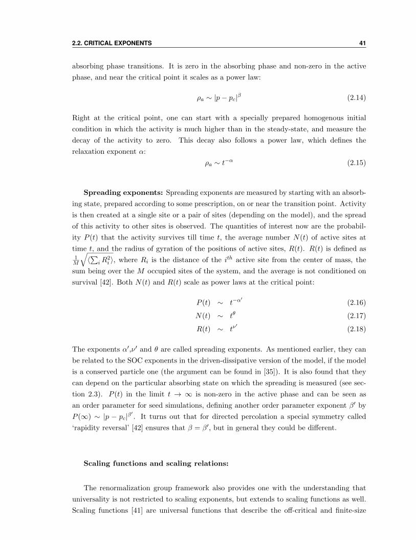
2.2. CRITICAL EXPONENTS 41
absorbing phase transitions. It is zero in the absorbing phase and non-zero in the active
phase, and near the critical point it scales as a power law:
ρa ∼ |p− pc|β (2.14)
Right at the critical point, one can start with a specially prepared homogenous initial
condition in which the activity is much higher than in the steady-state, and measure the
decay of the activity to zero. This decay also follows a power law, which defines the
relaxation exponent α:
ρa ∼ t−α (2.15)
Spreading exponents: Spreading exponents are measured by starting with an absorb-
ing state, prepared according to some prescription, on or near the transition point. Activity
is then created at a single site or a pair of sites (depending on the model), and the spread
of this activity to other sites is observed. The quantities of interest now are the probabil-
ity P (t) that the activity survives till time t, the average number N(t) of active sites at
time t, and the radius of gyration of the positions of active sites, R(t). R(t) is defined as1M
√〈∑
iR2i 〉, where Ri is the distance of the ith active site from the center of mass, the
sum being over the M occupied sites of the system, and the average is not conditioned on
survival [42]. Both N(t) and R(t) scale as power laws at the critical point:
P (t) ∼ t−α′
(2.16)
N(t) ∼ tθ (2.17)
R(t) ∼ tν′
(2.18)
The exponents α′,ν ′ and θ are called spreading exponents. As mentioned earlier, they can
be related to the SOC exponents in the driven-dissipative version of the model, if the model
is a conserved particle one (the argument can be found in [35]). It is also found that they
can depend on the particular absorbing state on which the spreading is measured (see sec-
tion 2.3). P (t) in the limit t → ∞ is non-zero in the active phase and can be seen as
an order parameter for seed simulations, defining another order parameter exponent β′ by
P (∞) ∼ |p − pc|β′. It turns out that for directed percolation a special symmetry called
‘rapidity reversal’ [42] ensures that β = β′, but in general they could be different.
Scaling functions and scaling relations:
The renormalization group framework also provides one with the understanding that
universality is not restricted to scaling exponents, but extends to scaling functions as well.
Scaling functions [41] are universal functions that describe the off-critical and finite-size
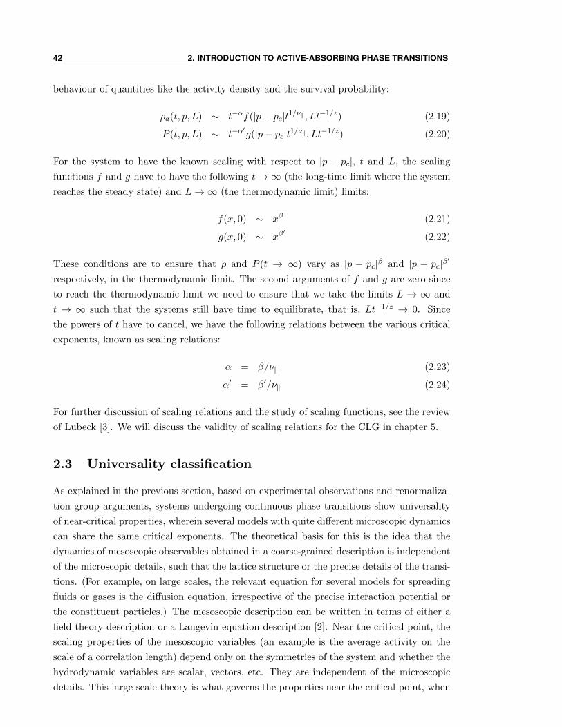
42 2. INTRODUCTION TO ACTIVE-ABSORBING PHASE TRANSITIONS
behaviour of quantities like the activity density and the survival probability:
ρa(t, p, L) ∼ t−αf(|p− pc|t1/ν‖ , Lt−1/z) (2.19)
P (t, p, L) ∼ t−α′g(|p− pc|t1/ν‖ , Lt−1/z) (2.20)
For the system to have the known scaling with respect to |p − pc|, t and L, the scaling
functions f and g have to have the following t→∞ (the long-time limit where the system
reaches the steady state) and L→∞ (the thermodynamic limit) limits:
f(x, 0) ∼ xβ (2.21)
g(x, 0) ∼ xβ′
(2.22)
These conditions are to ensure that ρ and P (t → ∞) vary as |p − pc|β and |p − pc|β′
respectively, in the thermodynamic limit. The second arguments of f and g are zero since
to reach the thermodynamic limit we need to ensure that we take the limits L → ∞ and
t → ∞ such that the systems still have time to equilibrate, that is, Lt−1/z → 0. Since
the powers of t have to cancel, we have the following relations between the various critical
exponents, known as scaling relations:
α = β/ν‖ (2.23)
α′ = β′/ν‖ (2.24)
For further discussion of scaling relations and the study of scaling functions, see the review
of Lubeck [3]. We will discuss the validity of scaling relations for the CLG in chapter 5.
2.3 Universality classification
As explained in the previous section, based on experimental observations and renormaliza-
tion group arguments, systems undergoing continuous phase transitions show universality
of near-critical properties, wherein several models with quite different microscopic dynamics
can share the same critical exponents. The theoretical basis for this is the idea that the
dynamics of mesoscopic observables obtained in a coarse-grained description is independent
of the microscopic details, such that the lattice structure or the precise details of the transi-
tions. (For example, on large scales, the relevant equation for several models for spreading
fluids or gases is the diffusion equation, irrespective of the precise interaction potential or
the constituent particles.) The mesoscopic description can be written in terms of either a
field theory description or a Langevin equation description [2]. Near the critical point, the
scaling properties of the mesoscopic variables (an example is the average activity on the
scale of a correlation length) depend only on the symmetries of the system and whether the
hydrodynamic variables are scalar, vectors, etc. They are independent of the microscopic
details. This large-scale theory is what governs the properties near the critical point, when
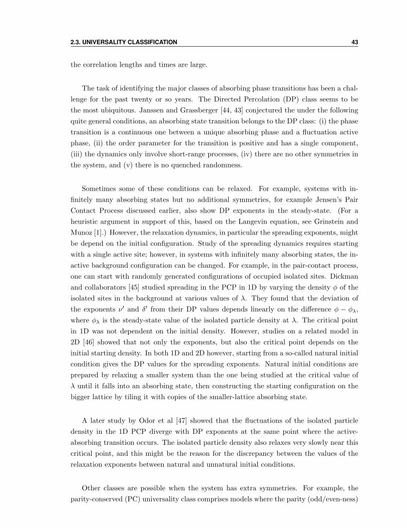
2.3. UNIVERSALITY CLASSIFICATION 43
the correlation lengths and times are large.
The task of identifying the major classes of absorbing phase transitions has been a chal-
lenge for the past twenty or so years. The Directed Percolation (DP) class seems to be
the most ubiquitous. Janssen and Grassberger [44, 43] conjectured the under the following
quite general conditions, an absorbing state transition belongs to the DP class: (i) the phase
transition is a continuous one between a unique absorbing phase and a fluctuation active
phase, (ii) the order parameter for the transition is positive and has a single component,
(iii) the dynamics only involve short-range processes, (iv) there are no other symmetries in
the system, and (v) there is no quenched randomness.
Sometimes some of these conditions can be relaxed. For example, systems with in-
finitely many absorbing states but no additional symmetries, for example Jensen’s Pair
Contact Process discussed earlier, also show DP exponents in the steady-state. (For a
heuristic argument in support of this, based on the Langevin equation, see Grinstein and
Munoz [1].) However, the relaxation dynamics, in particular the spreading exponents, might
be depend on the initial configuration. Study of the spreading dynamics requires starting
with a single active site; however, in systems with infinitely many absorbing states, the in-
active background configuration can be changed. For example, in the pair-contact process,
one can start with randomly generated configurations of occupied isolated sites. Dickman
and collaborators [45] studied spreading in the PCP in 1D by varying the density φ of the
isolated sites in the background at various values of λ. They found that the deviation of
the exponents ν ′ and δ′ from their DP values depends linearly on the difference φ − φλ,
where φλ is the steady-state value of the isolated particle density at λ. The critical point
in 1D was not dependent on the initial density. However, studies on a related model in
2D [46] showed that not only the exponents, but also the critical point depends on the
initial starting density. In both 1D and 2D however, starting from a so-called natural initial
condition gives the DP values for the spreading exponents. Natural initial conditions are
prepared by relaxing a smaller system than the one being studied at the critical value of
λ until it falls into an absorbing state, then constructing the starting configuration on the
bigger lattice by tiling it with copies of the smaller-lattice absorbing state.
A later study by Odor et al [47] showed that the fluctuations of the isolated particle
density in the 1D PCP diverge with DP exponents at the same point where the active-
absorbing transition occurs. The isolated particle density also relaxes very slowly near this
critical point, and this might be the reason for the discrepancy between the values of the
relaxation exponents between natural and unnatural initial conditions.
Other classes are possible when the system has extra symmetries. For example, the
parity-conserved (PC) universality class comprises models where the parity (odd/even-ness)
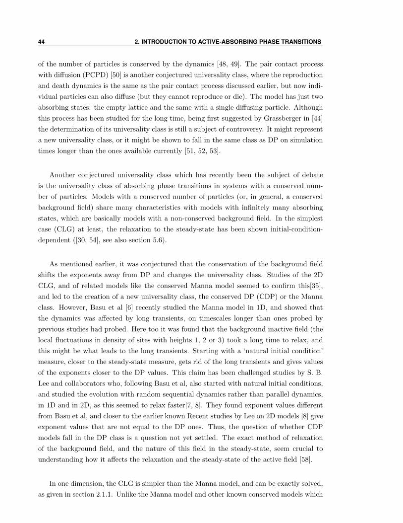
44 2. INTRODUCTION TO ACTIVE-ABSORBING PHASE TRANSITIONS
of the number of particles is conserved by the dynamics [48, 49]. The pair contact process
with diffusion (PCPD) [50] is another conjectured universality class, where the reproduction
and death dynamics is the same as the pair contact process discussed earlier, but now indi-
vidual particles can also diffuse (but they cannot reproduce or die). The model has just two
absorbing states: the empty lattice and the same with a single diffusing particle. Although
this process has been studied for the long time, being first suggested by Grassberger in [44]
the determination of its universality class is still a subject of controversy. It might represent
a new universality class, or it might be shown to fall in the same class as DP on simulation
times longer than the ones available currently [51, 52, 53].
Another conjectured universality class which has recently been the subject of debate
is the universality class of absorbing phase transitions in systems with a conserved num-
ber of particles. Models with a conserved number of particles (or, in general, a conserved
background field) share many characteristics with models with infinitely many absorbing
states, which are basically models with a non-conserved background field. In the simplest
case (CLG) at least, the relaxation to the steady-state has been shown initial-condition-
dependent ([30, 54], see also section 5.6).
As mentioned earlier, it was conjectured that the conservation of the background field
shifts the exponents away from DP and changes the universality class. Studies of the 2D
CLG, and of related models like the conserved Manna model seemed to confirm this[35],
and led to the creation of a new universality class, the conserved DP (CDP) or the Manna
class. However, Basu et al [6] recently studied the Manna model in 1D, and showed that
the dynamics was affected by long transients, on timescales longer than ones probed by
previous studies had probed. Here too it was found that the background inactive field (the
local fluctuations in density of sites with heights 1, 2 or 3) took a long time to relax, and
this might be what leads to the long transients. Starting with a ‘natural initial condition’
measure, closer to the steady-state measure, gets rid of the long transients and gives values
of the exponents closer to the DP values. This claim has been challenged studies by S. B.
Lee and collaborators who, following Basu et al, also started with natural initial conditions,
and studied the evolution with random sequential dynamics rather than parallel dynamics,
in 1D and in 2D, as this seemed to relax faster[7, 8]. They found exponent values different
from Basu et al, and closer to the earlier known Recent studies by Lee on 2D models [8] give
exponent values that are not equal to the DP ones. Thus, the question of whether CDP
models fall in the DP class is a question not yet settled. The exact method of relaxation
of the background field, and the nature of this field in the steady-state, seem crucial to
understanding how it affects the relaxation and the steady-state of the active field [58].
In one dimension, the CLG is simpler than the Manna model, and can be exactly solved,
as given in section 2.1.1. Unlike the Manna model and other known conserved models which
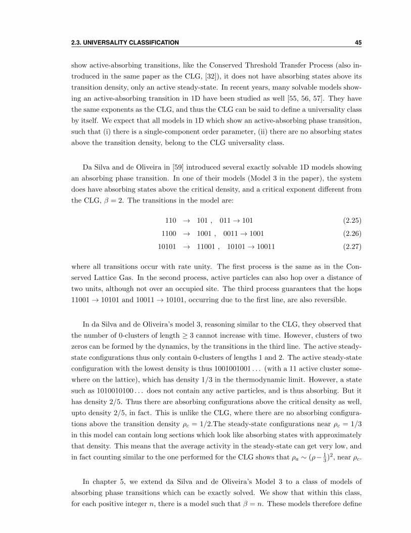
2.3. UNIVERSALITY CLASSIFICATION 45
show active-absorbing transitions, like the Conserved Threshold Transfer Process (also in-
troduced in the same paper as the CLG, [32]), it does not have absorbing states above its
transition density, only an active steady-state. In recent years, many solvable models show-
ing an active-absorbing transition in 1D have been studied as well [55, 56, 57]. They have
the same exponents as the CLG, and thus the CLG can be said to define a universality class
by itself. We expect that all models in 1D which show an active-absorbing phase transition,
such that (i) there is a single-component order parameter, (ii) there are no absorbing states
above the transition density, belong to the CLG universality class.
Da Silva and de Oliveira in [59] introduced several exactly solvable 1D models showing
an absorbing phase transition. In one of their models (Model 3 in the paper), the system
does have absorbing states above the critical density, and a critical exponent different from
the CLG, β = 2. The transitions in the model are:
110 → 101 , 011→ 101 (2.25)
1100 → 1001 , 0011→ 1001 (2.26)
10101 → 11001 , 10101→ 10011 (2.27)
where all transitions occur with rate unity. The first process is the same as in the Con-
served Lattice Gas. In the second process, active particles can also hop over a distance of
two units, although not over an occupied site. The third process guarantees that the hops
11001→ 10101 and 10011→ 10101, occurring due to the first line, are also reversible.
In da Silva and de Oliveira’s model 3, reasoning similar to the CLG, they observed that
the number of 0-clusters of length ≥ 3 cannot increase with time. However, clusters of two
zeros can be formed by the dynamics, by the transitions in the third line. The active steady-
state configurations thus only contain 0-clusters of lengths 1 and 2. The active steady-state
configuration with the lowest density is thus 1001001001 . . . (with a 11 active cluster some-
where on the lattice), which has density 1/3 in the thermodynamic limit. However, a state
such as 1010010100 . . . does not contain any active particles, and is thus absorbing. But it
has density 2/5. Thus there are absorbing configurations above the critical density as well,
upto density 2/5, in fact. This is unlike the CLG, where there are no absorbing configura-
tions above the transition density ρc = 1/2.The steady-state configurations near ρc = 1/3
in this model can contain long sections which look like absorbing states with approximately
that density. This means that the average activity in the steady-state can get very low, and
in fact counting similar to the one performed for the CLG shows that ρa ∼ (ρ− 13)2, near ρc.
In chapter 5, we extend da Silva and de Oliveira’s Model 3 to a class of models of
absorbing phase transitions which can be exactly solved. We show that within this class,
for each positive integer n, there is a model such that β = n. These models therefore define
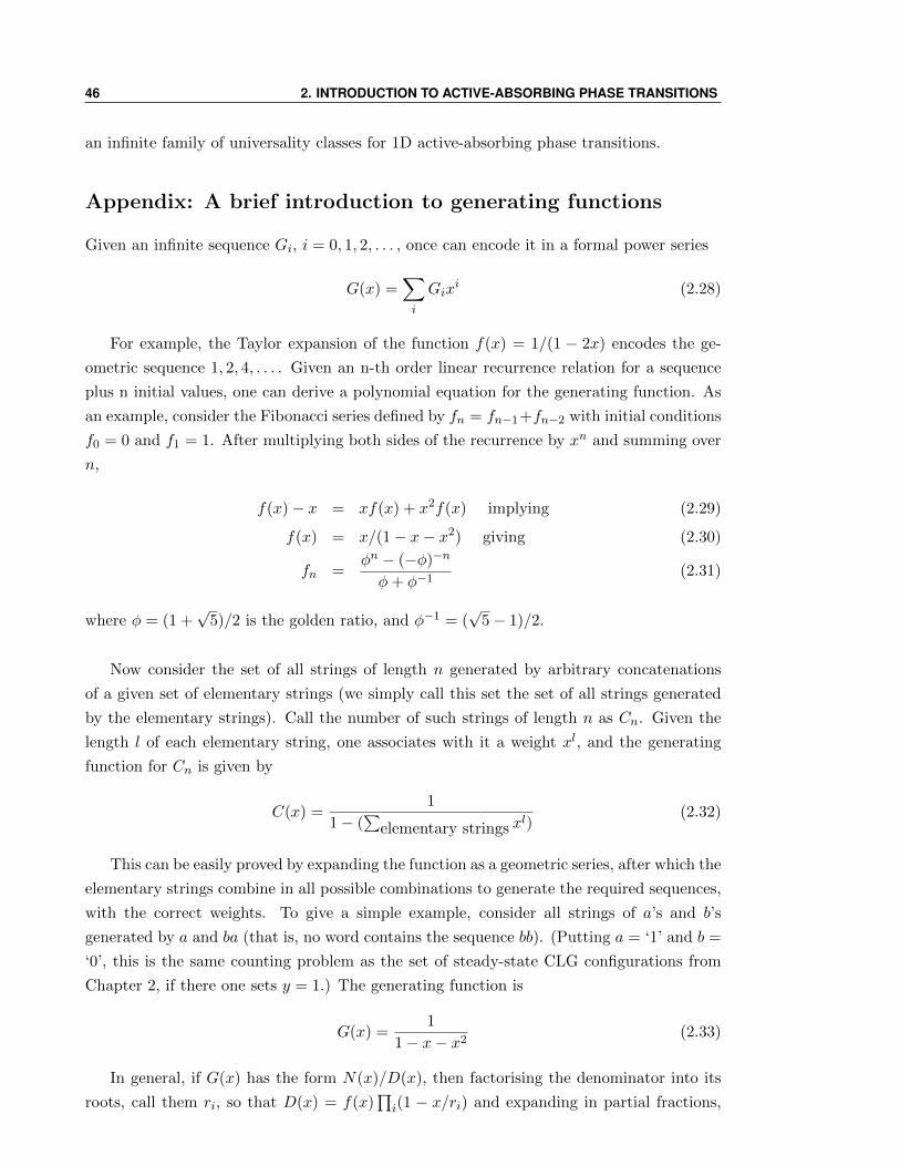
46 2. INTRODUCTION TO ACTIVE-ABSORBING PHASE TRANSITIONS
an infinite family of universality classes for 1D active-absorbing phase transitions.
Appendix: A brief introduction to generating functions
Given an infinite sequence Gi, i = 0, 1, 2, . . . , once can encode it in a formal power series
G(x) =∑i
Gixi (2.28)
For example, the Taylor expansion of the function f(x) = 1/(1 − 2x) encodes the ge-
ometric sequence 1, 2, 4, . . . . Given an n-th order linear recurrence relation for a sequence
plus n initial values, one can derive a polynomial equation for the generating function. As
an example, consider the Fibonacci series defined by fn = fn−1+fn−2 with initial conditions
f0 = 0 and f1 = 1. After multiplying both sides of the recurrence by xn and summing over
n,
f(x)− x = xf(x) + x2f(x) implying (2.29)
f(x) = x/(1− x− x2) giving (2.30)
fn =φn − (−φ)−n
φ+ φ−1(2.31)
where φ = (1 +√
5)/2 is the golden ratio, and φ−1 = (√
5− 1)/2.
Now consider the set of all strings of length n generated by arbitrary concatenations
of a given set of elementary strings (we simply call this set the set of all strings generated
by the elementary strings). Call the number of such strings of length n as Cn. Given the
length l of each elementary string, one associates with it a weight xl, and the generating
function for Cn is given by
C(x) =1
1− (∑
elementary strings xl)
(2.32)
This can be easily proved by expanding the function as a geometric series, after which the
elementary strings combine in all possible combinations to generate the required sequences,
with the correct weights. To give a simple example, consider all strings of a’s and b’s
generated by a and ba (that is, no word contains the sequence bb). (Putting a = ‘1’ and b =
‘0’, this is the same counting problem as the set of steady-state CLG configurations from
Chapter 2, if there one sets y = 1.) The generating function is
G(x) =1
1− x− x2(2.33)
In general, if G(x) has the form N(x)/D(x), then factorising the denominator into its
roots, call them ri, so that D(x) = f(x)∏i(1 − x/ri) and expanding in partial fractions,
APPENDIX: A BRIEF INTRODUCTION TO GENERATING FUNCTIONS 47
one arrives at the general form
Gn =∑i
cir−ni (2.34)
The constants ci can be determined from the initial conditions.
The same counting can also be done using a transfer matrix approach as follows: Every
linear recursion relation can be converted to a transfer matrix between (Gn,. . . ,Gn−m) and
(Gn+1,. . . ,Cn−m+1). If the length of the longest elementary string is m means that the
recurrent relation is an m-th order recurrence. The corresponding transfer matrix is then
an m×m matrix. By raising the transfer matrix to the L-th power, one obtains the number
of allowed strings of length L as a sum of L-th powers of the transfer matrix eigenvalues:
Gn =∑
i ciλLi , where λi are the roots of the transfer matrix. Since the values of Gn are
the same in both approaches, we get λi = r−1i , relating the transfer matrix and generating
function approaches.
Bibliography
[1] G. Grinstein and M. A. Munoz, in Fourth Granada Lectures in Computational Physics,
edited by P. L. Garrido and J. Marro, Lecture Notes in Physics Vol. 493 (Springer,
Berlin, 1997), p. 223.
[2] H. Hinrichsen, Advances in Physics 49, 815 (2000).
[3] S. Lubeck, Int. J. Mod. Phys. B 18, 3977 (2004).
[4] M. Henkel, H. Hinrichsen, and S. Lbeck, Non-Equilibrium Phase Transitions: Vol. 1:
Absorbing Phase Transitions, (Springer, Berlin) (2009).
[5] G. Odor, Rev. Mod. Phys., 76, 663 (2004).
[6] M. Basu, U. Basu, S. Bondyopadhyay, P. K. Mohanty, and H. Hinrichsen, Phys. Rev.
Lett. 109, 015702 (2012).
[7] S. B. Lee, Phys. Rev. E 89, 060101(R) (2014).
[8] S. B. Lee, Phys. Rev. E 89, 062133 (2014).
[9] J. L. Cardy, J. Phys. A 16, L709 (1983).
[10] J. L. Cardy and P. Grassberger, J. Phys. A 18, L267 (1985).
[11] H. K. Janssen, Z. Phys. B 58, 311 (1985).
[12] K. Chen, P. Bak and M. H. Jensen, Phys. Lett. A 149, 207 (1990).
[13] R. M. Ziff, E. Gulari and Y. Barshad, Phys. Rev. Lett 56, 2553 (1986).
[14] P. Meakin and D. J. Scalapino, J. Chem. Phys. 87, 731 (1987).
[15] K. A. Takeuchi, M. Kuroda, H. Chat, and M. Sano, Phys. Rev. E 80, 051116 (2009),
K. A. Takeuchi, M. Kuroda, H. Chat, and M. Sano, Phys. Rev. Lett. 99, 234503 (2007);
103, 089901 (2009).
[16] S. R. Broadbent and J. M. Hammersley, Proc. Camb. Philos. Soc. 53, 629 (1957).
[17] I. Jensen, J. Phys. A 37, 6899 (2004).
48
BIBLIOGRAPHY 49
[18] V. N. Gribov, Sov. Phys. JETP 26 414 (1968).
[19] H. D. I. Abarbanel et al., Phys. Rep. 21C, 120 (1975).
[20] J. L. Cardy amd R. L. Sugar, J. Phys. A 13, L423 (1980).
[21] T. E. Harris, Ann. Prob. 2, 969 (1974).
[22] T. M. Liggett, Interacting Particle Systems (Springer-Verlag, N.Y.), (1985).
[23] J. Marro and R. Dickman, Nonequilibrium Phase Transitions and Critical Phenomena
(Cambridge University Press, Cambridge) (1997).
[24] R. Dickman and J. K. da Silva, Phys. Rev. E 58, 4266 (1998).
[25] E. V. Albano, J. Phys. A 25, 2557 (1992).
[26] A. Maltz and E. V. Albano, Surf. Sci. 277, 414 (1992).
[27] I. Jensen, Phys. Rev. Lett. 70, 1465 (1993)
[28] I. Jensen and R. Dickman, Phys. Rev. E, 48 1710 (1993).
[29] I. Jensen, Int. J. Mod. Phys. B 8, 3299 (1994)
[30] S. B. Lee, and S.-G. Lee, Phys. Rev. E. 78, 040103(R) (2008).
[31] G. Grinstein, in Scale Invariance, Interfaces and Non-Equilibrium Dynamics, edited
by A. McKane et al., NATO Advanced Study Institute, Series B: Physics Vol. 344
(Plenum, New York, 1995).
[32] M. Rossi, R. Pastor-Satorras, and A. Vespignani, Phys. Rev. Lett. 85, 1803 (2000).
[33] S. Lubeck and A Hucht, J. Phys. A: Math. Gen. 34 L577 (2001).
[34] S. Lubeck, Phys. Rev. E 64, 016123 (2001).
[35] A. Vespignani, R. Dickman, M. A. Munoz, S. Zapperi, Phys. Rev. E 62, 4564 (2000).
R. Dickman, M. A. Munoz, A. Vespignani, S. Zapperi, Braz. J. Phys. 30, 27 (2000).
[36] S. S. Manna, J. Phys. A 24, L363 (1991).
[37] M. J. de Oliveira, Phys. Rev. E 71, 016112 (2005).
[38] J. Cardy, Scaling and renormalization in statistical physics, Cambridge University Press
(Cambridge) (1996).
[39] L. P. Kadanoff, Physics 2 263 (1966),
B. Widom, Physica 73 107 (1974).
[40] K. G. Wilson and J. Kogut, Phys. Rep., 12 75 (1974).
50 BIBLIOGRAPHY
[41] C. Domb and M. S. Green eds., Phase Transitions and Critical Phenomena, Vol 6
(Academic, London) (1976).
[42] P. Grassberger and A. de la Torre, Ann. Phys. (N.Y.) 122, 373 (1979).
[43] H. K. Janssen, Z. Phys. B 42, 151 (1981).
[44] P. Grassberger, Z. Phys. B 47, 365 (1982).
[45] J. F. F. Mendes, R. Dickman, M. Henkel and M. C. Marques, J. Phys. A: Math. Gen.
27 3019 (1994),
I. Jensen and R. Dickman, Phys. Rev. E 48 1710 (1993).
[46] R. Dickman, Phys. Rev. E 53, 2223 (1996).
[47] G. Odor, J. F. Mendes, M. A. Santos and M. C. Marques, Phys. Rev E, 58 7020 (1998).
[48] H. Takayasu, and A. Y. Tretyakov, Phys. Rev. Lett. 68, 3060 (1992).
[49] J. Cardy, and U. C. Tauber, Phys. Rev. Lett. 77, 4780 (1996).
[50] M. J. Howard and U. C. Tauber, J. Phys. A 30, 7721 (1997).
[51] E. Carlon, M. Henkel, and U. Schollwock, Phys. Rev. E 63, 036101 (2001).
[52] J. Kockelkoren, and H. Chate, Phys. Rev. Lett. 90, 125701 (2003).
[53] H. Hinrichsen, Physica A 361, 457 (2006).
[54] S. Bondyopadhyay, Phys. Rev. E. 88, 062125 (2013).
[55] K. Jain, Phys. Rev. E 72, 017105 (2005).
[56] U. Basu, and P. K. Mohanty, Phys. Rev. E 79, 041143 (2009).
[57] A. Gabel, P. L. Krapivsky and S. Redner, Phys. Rev. Lett. 105 210603 (2010).
[58] S. D. da Cunha, L. R. da Silva, G. M. Viswanathan and R. Dickman, arXiv:1405.1134.
[59] E. F. da Silva, and M. J. de Oliveira, J. Phys. A: Math. Gen. 41, 385004 (2008).
Chapter 3
Proportionate growth in patterns
formed in the rotor-router model
In this chapter, we will study the growing patterns formed in the rotor-router model by
adding N walkers at the center of an L × L two-dimensional square lattice, starting with
a periodic background of arrows, and relaxing to a stable configuration. (See 3.1.) The
pattern is made of a large number of triangular and quadrilateral regions, where in each
region all arrows point in the same direction. We show that the pattern formed by arrows
which have been rotated at least one full circle, may be described in terms of a tiling of the
plane by squares of different sizes. The sizes of these squares, and the size of the pattern,
grow linearly with N , for 1 N < 2L. We use the Brooks-Smith-Stone-Tutte theorem
relating tilings of squares by smaller squares to resistor networks, to determine the exact
relative sizes of these tiles. The scaling limit of the number of visits φ(ξ, η) as a function of
the scaled position (ξ, η) is also determined. We also present numerical evidence that the
deviations of the sizes of different squares in the tiling from the asymptotic linear growth
law are always O(1), and are quasiperiodic functions of N .
The outline of this chapter is as follows: In section 3.1, we state our protocol for creating
patterns in the rotor-router model. In section 3.2, we study the pattern obtained from the
initial configuration with all arrows parallel. We define the asymptotic pattern, and the
scaling limit of the visit function for the pattern. In section 3.3, using the Brooks-Smith-
Stone-Tutte (BSST) theorem, we construct the resistor network corresponding to the tiling
seen in the pattern and determine the sizes of the tiles. We obtain an exact characterization
of the asymptotic pattern, and determine the relative sizes of different elements. Thus we
also determine the visit function for the pattern in the large N limit. In section 3.4, we
extend the analysis to some other patterns obtained starting from different periodic initial
configurations. In section 3.5, we give evidence that the deviations in the diameter and sizes
of various elements in the pattern from simple linear dependence on N are bounded and
show quasiperiodicity. Section 3.6 contains a summary of our results, and some concluding
51
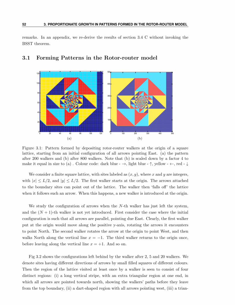
52 3. PROPORTIONATE GROWTH IN PATTERNS FORMED IN THE ROTOR-ROUTER MODEL
remarks. In an appendix, we re-derive the results of section 3.4 C without invoking the
BSST theorem.
3.1 Forming Patterns in the Rotor-router model
0 20 40 60 80 100 1200
20
40
60
80
100
120
(a)
0 100 200 300 400 5000
100
200
300
400
500
(b)
Figure 3.1: Pattern formed by depositing rotor-router walkers at the origin of a squarelattice, starting from an initial configuration of all arrows pointing East. (a) the patternafter 200 walkers and (b) after 800 walkers. Note that (b) is scaled down by a factor 4 tomake it equal in size to (a) . Colour code: dark blue - →, light blue - ↑, yellow - ←, red - ↓
We consider a finite square lattice, with sites labeled as (x, y), where x and y are integers,
with |x| ≤ L/2, and |y| ≤ L/2. The first walker starts at the origin. The arrows attached
to the boundary sites can point out of the lattice. The walker then ‘falls off’ the lattice
when it follows such an arrow. When this happens, a new walker is introduced at the origin.
We study the configuration of arrows when the N -th walker has just left the system,
and the (N + 1)-th walker is not yet introduced. First consider the case where the initial
configuration is such that all arrows are parallel, pointing due East. Clearly, the first walker
put at the origin would move along the positive y-axis, rotating the arrows it encounters
to point North. The second walker rotates the arrow at the origin to point West, and then
walks North along the vertical line x = −1. The third walker returns to the origin once,
before leaving along the vertical line x = +1. And so on.
Fig 3.2 shows the configurations left behind by the walker after 2, 5 and 20 walkers. We
denote sites having different directions of arrows by small filled squares of different colours.
Then the region of the lattice visited at least once by a walker is seen to consist of four
distinct regions: (i) a long vertical stripe, with an extra triangular region at one end, in
which all arrows are pointed towards north, showing the walkers’ paths before they leave
from the top boundary, (ii) a dart-shaped region with all arrows pointing west, (iii) a trian-
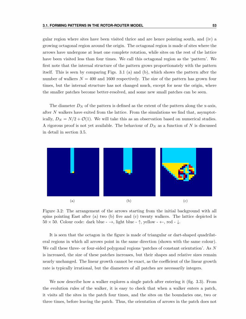
3.1. FORMING PATTERNS IN THE ROTOR-ROUTER MODEL 53
gular region where sites have been visited thrice and are hence pointing south, and (iv) a
growing octagonal region around the origin. The octagonal region is made of sites where the
arrows have undergone at least one complete rotation, while sites on the rest of the lattice
have been visited less than four times. We call this octagonal region as the ‘pattern’. We
first note that the internal structure of the pattern grows proportionately with the pattern
itself. This is seen by comparing Figs. 3.1 (a) and (b), which shows the pattern after the
number of walkers N = 400 and 1600 respectively. The size of the pattern has grown four
times, but the internal structure has not changed much, except for near the origin, where
the smaller patches become better-resolved, and some new small patches can be seen.
The diameter DN of the pattern is defined as the extent of the pattern along the x-axis,
after N walkers have exited from the lattice. From the simulations we find that, asymptot-
ically, DN = N/2 +O(1). We will take this as an observation based on numerical studies.
A rigorous proof is not yet available. The behaviour of DN as a function of N is discussed
in detail in section 3.5.
(a) (b) (c)
Figure 3.2: The arrangement of the arrows starting from the initial background with allspins pointing East after (a) two (b) five and (c) twenty walkers. The lattice depicted is50× 50. Colour code: dark blue - →, light blue - ↑, yellow - ←, red - ↓.
It is seen that the octagon in the figure is made of triangular or dart-shaped quadrilat-
eral regions in which all arrows point in the same direction (shown with the same colour).
We call these three- or four-sided polygonal regions ‘patches of constant orientation’. As N
is increased, the size of these patches increases, but their shapes and relative sizes remain
nearly unchanged. The linear growth cannot be exact, as the coefficient of the linear growth
rate is typically irrational, but the diameters of all patches are necessarily integers.
We now describe how a walker explores a single patch after entering it (fig. 3.3). From
the evolution rules of the walker, it is easy to check that when a walker enters a patch,
it visits all the sites in the patch four times, and the sites on the boundaries one, two or
three times, before leaving the patch. Thus, the orientation of arrows in the patch does not
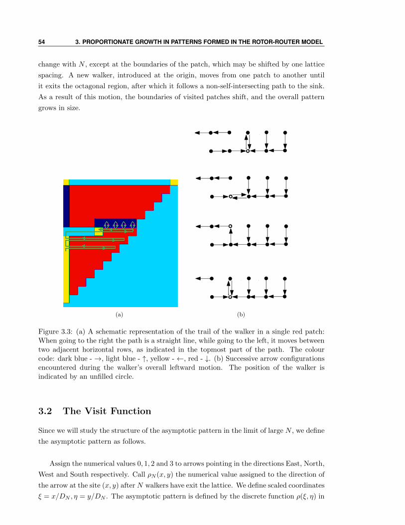
54 3. PROPORTIONATE GROWTH IN PATTERNS FORMED IN THE ROTOR-ROUTER MODEL
change with N , except at the boundaries of the patch, which may be shifted by one lattice
spacing. A new walker, introduced at the origin, moves from one patch to another until
it exits the octagonal region, after which it follows a non-self-intersecting path to the sink.
As a result of this motion, the boundaries of visited patches shift, and the overall pattern
grows in size.
(a) (b)
Figure 3.3: (a) A schematic representation of the trail of the walker in a single red patch:When going to the right the path is a straight line, while going to the left, it moves betweentwo adjacent horizontal rows, as indicated in the topmost part of the path. The colourcode: dark blue - →, light blue - ↑, yellow - ←, red - ↓. (b) Successive arrow configurationsencountered during the walker’s overall leftward motion. The position of the walker isindicated by an unfilled circle.
3.2 The Visit Function
Since we will study the structure of the asymptotic pattern in the limit of large N , we define
the asymptotic pattern as follows.
Assign the numerical values 0, 1, 2 and 3 to arrows pointing in the directions East, North,
West and South respectively. Call ρN (x, y) the numerical value assigned to the direction of
the arrow at the site (x, y) after N walkers have exit the lattice. We define scaled coordinates
ξ = x/DN , η = y/DN . The asymptotic pattern is defined by the discrete function ρ(ξ, η) in
3.2. THE VISIT FUNCTION 55
the unit square centered at the origin, given by the limit
ρ(ξ, η) = limN→∞
ρN (bDNξc, bDNηc) (3.1)
The function ρ(ξ, η) is a piece-wise-constant integer function of its (real) arguments,
and gives the orientation of the arrow at point (ξ, η) in the scaled pattern. We will defer a
formal proof of the existence of this limit to future studies. For the sandpile patterns, the
existence of the asymptotic pattern has been proved for the initially empty background by
Pegden and Smart in [2].
With our normalization convention and the observation that DN = N/2 + O(1), and
using the fact that the pattern is symmetric about the y-axis, the left and right boundaries
of the scaled pattern are at |ξ| = 1/2. From the observation that the pattern is in the shape
of an octagon, and has equal extent in horizontal and vertical directions, we infer that the
upper and lower boundaries of the scaled pattern lie along the lines |η| = 1/2.
From fig 3.1, it can be seen that the outer patches are bigger and hence are well-formed
even for small N , while one has to increase N in order to distinguish patches with smaller
diameters. The asymptotic pattern as defined above has well-resolved triangular or dart-
shaped patches at all levels, with sharp boundaries. The boundaries between well-resolved
patches seem to be of width at most 2 in the original unscaled units. (This may be checked
by zooming into fig. 3.1 in the electronic file of this thesis.)
The exact characterization of the sandpile patterns was given in terms of the toppling
function ΦN (x, y) which gives the number of topplings at any lattice point (x, y), when N
particles are added at the origin and the configuration is relaxed. For the rotor-router model,
the corresponding function, which we also denote ΦN (x, y) is the so-called visit function,
which counts the total number of full rotations undergone by the arrow attached to the site
(x, y) due to the first N walkers. The region where ΦN is non-zero is just the octagonal
region which we have earlier defined as our pattern. Define the scaled visit function φ(ξ, η)
by
φ(ξ, η) = limN→∞
ΦN (bDNξc, bDNηc)DN
(3.2)
Note that the total number of visits to the site (x, y) is given by 4ΦN (x, y) + ρN (x, y).
Now we argue that ΦN in every patch is the sum of a linear function of x and y and a
periodic part, with the periodicity same as that of the initial background. (For examples
of patterns on backgrounds where the unit cell is 2× 2, see section V, and figs. 10, 11 and
13.) Let us take a patch of constant orientation, where the basis vectors of the periodic
arrow configuration within the patch are e1 and e2. Define ∆jΦ(~R) for j = 1, 2 as the finite
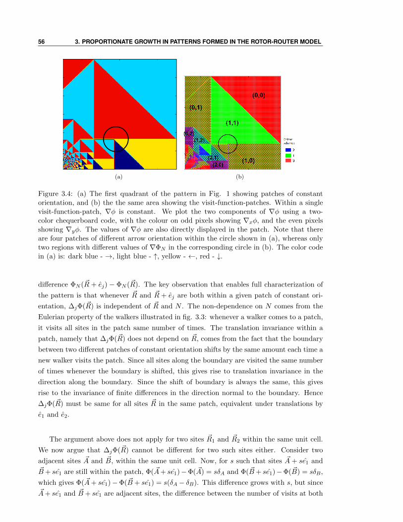
56 3. PROPORTIONATE GROWTH IN PATTERNS FORMED IN THE ROTOR-ROUTER MODEL
(a) (b)
Figure 3.4: (a) The first quadrant of the pattern in Fig. 1 showing patches of constantorientation, and (b) the the same area showing the visit-function-patches. Within a singlevisit-function-patch, ∇φ is constant. We plot the two components of ∇φ using a two-color chequerboard code, with the colour on odd pixels showing ∇xφ, and the even pixelsshowing ∇yφ. The values of ∇φ are also directly displayed in the patch. Note that thereare four patches of different arrow orientation within the circle shown in (a), whereas onlytwo regions with different values of ∇ΦN in the corresponding circle in (b). The color codein (a) is: dark blue - →, light blue - ↑, yellow - ←, red - ↓.
difference ΦN (~R + ej) − ΦN (~R). The key observation that enables full characterization of
the pattern is that whenever ~R and ~R + ej are both within a given patch of constant ori-
entation, ∆jΦ(~R) is independent of ~R and N . The non-dependence on N comes from the
Eulerian property of the walkers illustrated in fig. 3.3: whenever a walker comes to a patch,
it visits all sites in the patch same number of times. The translation invariance within a
patch, namely that ∆jΦ(~R) does not depend on ~R, comes from the fact that the boundary
between two different patches of constant orientation shifts by the same amount each time a
new walker visits the patch. Since all sites along the boundary are visited the same number
of times whenever the boundary is shifted, this gives rise to translation invariance in the
direction along the boundary. Since the shift of boundary is always the same, this gives
rise to the invariance of finite differences in the direction normal to the boundary. Hence
∆jΦ(~R) must be same for all sites ~R in the same patch, equivalent under translations by
e1 and e2.
The argument above does not apply for two sites ~R1 and ~R2 within the same unit cell.
We now argue that ∆jΦ(~R) cannot be different for two such sites either. Consider two
adjacent sites ~A and ~B, within the same unit cell. Now, for s such that sites ~A + se1 and
~B+ se1 are still within the patch, Φ( ~A+ se1)−Φ( ~A) = sδA and Φ( ~B+ se1)−Φ( ~B) = sδB,
which gives Φ( ~A+ se1)−Φ( ~B + se1) = s(δA − δB). This difference grows with s, but since
~A+ se1 and ~B + se1 are adjacent sites, the difference between the number of visits at both
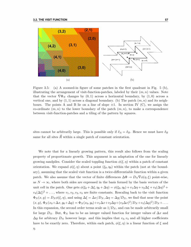
3.2. THE VISIT FUNCTION 57
(a) (b)
Figure 3.5: (a) A zoomed-in figure of some patches in the first quadrant in Fig. 5 (b),illustrating the arrangement of visit-function-patches, labeled by their (m,n) values. Notethat the vector ∇ΦN changes by (0, 1) across a horizontal boundary, by (1, 0) across avertical one, and by (1, 1) across a diagonal boundary. (b) The patch (m,n) and its neigh-bours. The points A and B lie on a line of slope ±1. In section IV (C), we assign theco-ordinate (m,n) to the lower boundary of the patch (m,n), to make a correspondencebetween visit-function-patches and a tiling of the pattern by squares.
sites cannot be arbitrarily large. This is possible only if δA = δB. Hence we must have δR
same for all sites ~R within a single patch of constant orientation.
We note that for a linearly growing pattern, this result also follows from the scaling
property of proportionate growth. This argument is an adaptation of the one for linearly
growing sandpiles. Consider the scaled toppling function φ(ξ, η) within a patch of constant
orientation. We expand φ(ξ, η) about a point (ξ0, η0) within the patch (not at the bound-
ary), assuming that the scaled visit function is a twice-differentiable function within a given
patch. We also assume that the vector of finite differences ∆Φ → DN∇φ(η, ξ) point-wise,
as N → ∞, where both sides are expressed in the basis formed by the basis vectors of the
unit cell in the patch. One gets φ(ξ0 + ∆ξ, η0 + ∆η) = φ(ξ0, η0) + v1∆η+ v2∆ξ+ v3(∆η)2 +
v4(∆ξ)2 + . . . , where v1, v2, v3, v4 are finite constants. Rescaling back to the visit function
ΦN (x, y) = DNφ(ξ, η), and using ∆ξ = ∆x/DN ,∆η = ∆y/DN , we find that near the point
(x, y), ΦN (x0+∆x, y0+∆y) = ΦN (x0, y0)+v1∆x+v2∆y+(v3∆x)2/DN+v4(∆y)2/DN+. . . .
In this expansion, the second order terms scale as 1/DN , and can be made arbitrarily small
for large DN . But, ΦN has to be an integer valued function for integer values of ∆x and
∆y for arbitrary DN however large. and this implies that v3, v4 and all higher coefficients
have to be exactly zero. Therefore, within each patch, φ(ξ, η) is a linear function of ξ and
η.
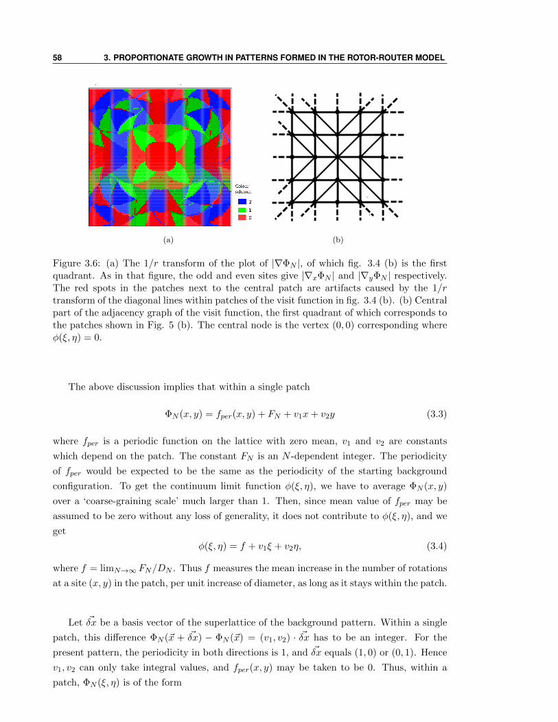
58 3. PROPORTIONATE GROWTH IN PATTERNS FORMED IN THE ROTOR-ROUTER MODEL
(a) (b)
Figure 3.6: (a) The 1/r transform of the plot of |∇ΦN |, of which fig. 3.4 (b) is the firstquadrant. As in that figure, the odd and even sites give |∇xΦN | and |∇yΦN | respectively.The red spots in the patches next to the central patch are artifacts caused by the 1/rtransform of the diagonal lines within patches of the visit function in fig. 3.4 (b). (b) Centralpart of the adjacency graph of the visit function, the first quadrant of which corresponds tothe patches shown in Fig. 5 (b). The central node is the vertex (0, 0) corresponding whereφ(ξ, η) = 0.
The above discussion implies that within a single patch
ΦN (x, y) = fper(x, y) + FN + v1x+ v2y (3.3)
where fper is a periodic function on the lattice with zero mean, v1 and v2 are constants
which depend on the patch. The constant FN is an N -dependent integer. The periodicity
of fper would be expected to be the same as the periodicity of the starting background
configuration. To get the continuum limit function φ(ξ, η), we have to average ΦN (x, y)
over a ‘coarse-graining scale’ much larger than 1. Then, since mean value of fper may be
assumed to be zero without any loss of generality, it does not contribute to φ(ξ, η), and we
get
φ(ξ, η) = f + v1ξ + v2η, (3.4)
where f = limN→∞ FN/DN . Thus f measures the mean increase in the number of rotations
at a site (x, y) in the patch, per unit increase of diameter, as long as it stays within the patch.
Let ~δx be a basis vector of the superlattice of the background pattern. Within a single
patch, this difference ΦN (~x + ~δx) − ΦN (~x) = (v1, v2) · ~δx has to be an integer. For the
present pattern, the periodicity in both directions is 1, and ~δx equals (1, 0) or (0, 1). Hence
v1, v2 can only take integral values, and fper(x, y) may be taken to be 0. Thus, within a
patch, ΦN (ξ, η) is of the form
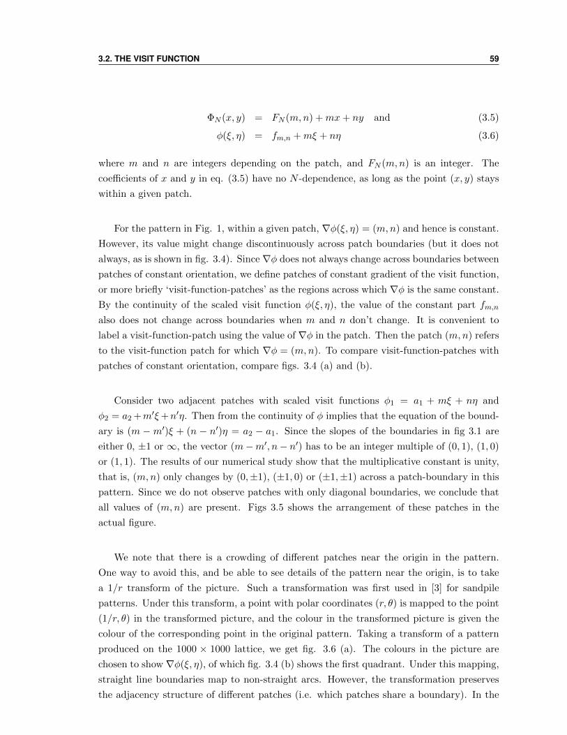
3.2. THE VISIT FUNCTION 59
ΦN (x, y) = FN (m,n) +mx+ ny and (3.5)
φ(ξ, η) = fm,n +mξ + nη (3.6)
where m and n are integers depending on the patch, and FN (m,n) is an integer. The
coefficients of x and y in eq. (3.5) have no N -dependence, as long as the point (x, y) stays
within a given patch.
For the pattern in Fig. 1, within a given patch, ∇φ(ξ, η) = (m,n) and hence is constant.
However, its value might change discontinuously across patch boundaries (but it does not
always, as is shown in fig. 3.4). Since ∇φ does not always change across boundaries between
patches of constant orientation, we define patches of constant gradient of the visit function,
or more briefly ‘visit-function-patches’ as the regions across which ∇φ is the same constant.
By the continuity of the scaled visit function φ(ξ, η), the value of the constant part fm,n
also does not change across boundaries when m and n don’t change. It is convenient to
label a visit-function-patch using the value of ∇φ in the patch. Then the patch (m,n) refers
to the visit-function patch for which ∇φ = (m,n). To compare visit-function-patches with
patches of constant orientation, compare figs. 3.4 (a) and (b).
Consider two adjacent patches with scaled visit functions φ1 = a1 + mξ + nη and
φ2 = a2 +m′ξ+n′η. Then from the continuity of φ implies that the equation of the bound-
ary is (m −m′)ξ + (n − n′)η = a2 − a1. Since the slopes of the boundaries in fig 3.1 are
either 0, ±1 or ∞, the vector (m−m′, n− n′) has to be an integer multiple of (0, 1), (1, 0)
or (1, 1). The results of our numerical study show that the multiplicative constant is unity,
that is, (m,n) only changes by (0,±1), (±1, 0) or (±1,±1) across a patch-boundary in this
pattern. Since we do not observe patches with only diagonal boundaries, we conclude that
all values of (m,n) are present. Figs 3.5 shows the arrangement of these patches in the
actual figure.
We note that there is a crowding of different patches near the origin in the pattern.
One way to avoid this, and be able to see details of the pattern near the origin, is to take
a 1/r transform of the picture. Such a transformation was first used in [3] for sandpile
patterns. Under this transform, a point with polar coordinates (r, θ) is mapped to the point
(1/r, θ) in the transformed picture, and the colour in the transformed picture is given the
colour of the corresponding point in the original pattern. Taking a transform of a pattern
produced on the 1000 × 1000 lattice, we get fig. 3.6 (a). The colours in the picture are
chosen to show ∇φ(ξ, η), of which fig. 3.4 (b) shows the first quadrant. Under this mapping,
straight line boundaries map to non-straight arcs. However, the transformation preserves
the adjacency structure of different patches (i.e. which patches share a boundary). In the
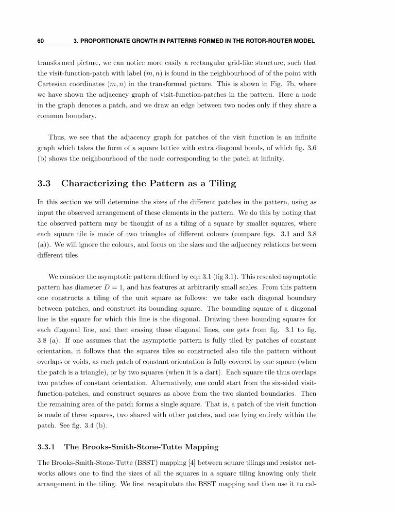
60 3. PROPORTIONATE GROWTH IN PATTERNS FORMED IN THE ROTOR-ROUTER MODEL
transformed picture, we can notice more easily a rectangular grid-like structure, such that
the visit-function-patch with label (m,n) is found in the neighbourhood of of the point with
Cartesian coordinates (m,n) in the transformed picture. This is shown in Fig. 7b, where
we have shown the adjacency graph of visit-function-patches in the pattern. Here a node
in the graph denotes a patch, and we draw an edge between two nodes only if they share a
common boundary.
Thus, we see that the adjacency graph for patches of the visit function is an infinite
graph which takes the form of a square lattice with extra diagonal bonds, of which fig. 3.6
(b) shows the neighbourhood of the node corresponding to the patch at infinity.
3.3 Characterizing the Pattern as a Tiling
In this section we will determine the sizes of the different patches in the pattern, using as
input the observed arrangement of these elements in the pattern. We do this by noting that
the observed pattern may be thought of as a tiling of a square by smaller squares, where
each square tile is made of two triangles of different colours (compare figs. 3.1 and 3.8
(a)). We will ignore the colours, and focus on the sizes and the adjacency relations between
different tiles.
We consider the asymptotic pattern defined by eqn 3.1 (fig 3.1). This rescaled asymptotic
pattern has diameter D = 1, and has features at arbitrarily small scales. From this pattern
one constructs a tiling of the unit square as follows: we take each diagonal boundary
between patches, and construct its bounding square. The bounding square of a diagonal
line is the square for which this line is the diagonal. Drawing these bounding squares for
each diagonal line, and then erasing these diagonal lines, one gets from fig. 3.1 to fig.
3.8 (a). If one assumes that the asymptotic pattern is fully tiled by patches of constant
orientation, it follows that the squares tiles so constructed also tile the pattern without
overlaps or voids, as each patch of constant orientation is fully covered by one square (when
the patch is a triangle), or by two squares (when it is a dart). Each square tile thus overlaps
two patches of constant orientation. Alternatively, one could start from the six-sided visit-
function-patches, and construct squares as above from the two slanted boundaries. Then
the remaining area of the patch forms a single square. That is, a patch of the visit function
is made of three squares, two shared with other patches, and one lying entirely within the
patch. See fig. 3.4 (b).
3.3.1 The Brooks-Smith-Stone-Tutte Mapping
The Brooks-Smith-Stone-Tutte (BSST) mapping [4] between square tilings and resistor net-
works allows one to find the sizes of all the squares in a square tiling knowing only their
arrangement in the tiling. We first recapitulate the BSST mapping and then use it to cal-
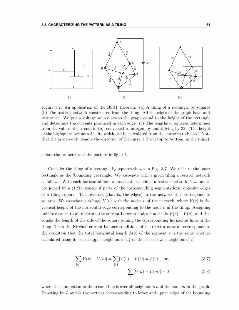
3.3. CHARACTERIZING THE PATTERN AS A TILING 61
(a) (b) (c)
Figure 3.7: An application of the BSST theorem. (a) A tiling of a rectangle by squares(b) The resistor network constructed from the tiling. All the edges of the graph have unitresistance. We put a voltage source across the graph equal to the height of the rectangleand determine the currents produced in each edge. (c) The lengths of squares determinedfrom the values of currents in (b), converted to integers by multiplying by 32. (The heightof the big square becomes 32. Its width can be calculated from the currents to be 33.) Notethat the arrows only denote the direction of the current (from top to bottom, in the tiling).
culate the properties of the pattern in fig. 3.1.
Consider the tiling of a rectangle by squares shown in Fig. 3.7. We refer to the outer
rectangle as the ‘bounding’ rectangle. We associate with a given tiling a resistor network
as follows: With each horizontal line, we associate a node of a resistor network. Two nodes
are joined by a (1 Ω) resistor if parts of the corresponding segments form opposite edges
of a tiling square. The resistors (that is, the edges) in the network thus correspond to
squares. We associate a voltage V (v) with the nodes v of the network, where V (v) is the
vertical height of the horizontal edge corresponding to the node v in the tiling. Assigning
unit resistance to all resistors, the current between nodes v and u is V (v)− V (u), and this
equals the length of the side of the square joining the corresponding horizontal lines in the
tiling. Then the Kirchoff current balance conditions of the resistor network corresponds to
the condition that the total horizontal length L(v) of the segment v is the same whether
calculated using its set of upper neighbours u or the set of lower neighbours `
∑u
[V (u)− V (v)] =∑`
[V (v)− V (`)] = L(v) or, (3.7)
∑n
[V (n)− V (m)] = 0 (3.8)
where the summation in the second line is over all neighbours n of the node m in the graph.
Denoting by L and U the vertices corresponding to lower and upper edges of the bounding
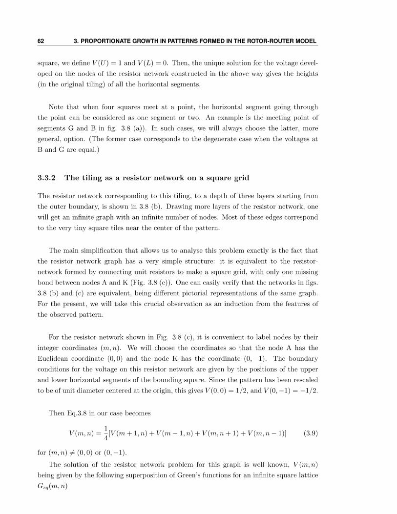
62 3. PROPORTIONATE GROWTH IN PATTERNS FORMED IN THE ROTOR-ROUTER MODEL
square, we define V (U) = 1 and V (L) = 0. Then, the unique solution for the voltage devel-
oped on the nodes of the resistor network constructed in the above way gives the heights
(in the original tiling) of all the horizontal segments.
Note that when four squares meet at a point, the horizontal segment going through
the point can be considered as one segment or two. An example is the meeting point of
segments G and B in fig. 3.8 (a)). In such cases, we will always choose the latter, more
general, option. (The former case corresponds to the degenerate case when the voltages at
B and G are equal.)
3.3.2 The tiling as a resistor network on a square grid
The resistor network corresponding to this tiling, to a depth of three layers starting from
the outer boundary, is shown in 3.8 (b). Drawing more layers of the resistor network, one
will get an infinite graph with an infinite number of nodes. Most of these edges correspond
to the very tiny square tiles near the center of the pattern.
The main simplification that allows us to analyse this problem exactly is the fact that
the resistor network graph has a very simple structure: it is equivalent to the resistor-
network formed by connecting unit resistors to make a square grid, with only one missing
bond between nodes A and K (Fig. 3.8 (c)). One can easily verify that the networks in figs.
3.8 (b) and (c) are equivalent, being different pictorial representations of the same graph.
For the present, we will take this crucial observation as an induction from the features of
the observed pattern.
For the resistor network shown in Fig. 3.8 (c), it is convenient to label nodes by their
integer coordinates (m,n). We will choose the coordinates so that the node A has the
Euclidean coordinate (0, 0) and the node K has the coordinate (0,−1). The boundary
conditions for the voltage on this resistor network are given by the positions of the upper
and lower horizontal segments of the bounding square. Since the pattern has been rescaled
to be of unit diameter centered at the origin, this gives V (0, 0) = 1/2, and V (0,−1) = −1/2.
Then Eq.3.8 in our case becomes
V (m,n) =1
4[V (m+ 1, n) + V (m− 1, n) + V (m,n+ 1) + V (m,n− 1)] (3.9)
for (m,n) 6= (0, 0) or (0,−1).
The solution of the resistor network problem for this graph is well known, V (m,n)
being given by the following superposition of Green’s functions for an infinite square lattice
Gsq(m,n)
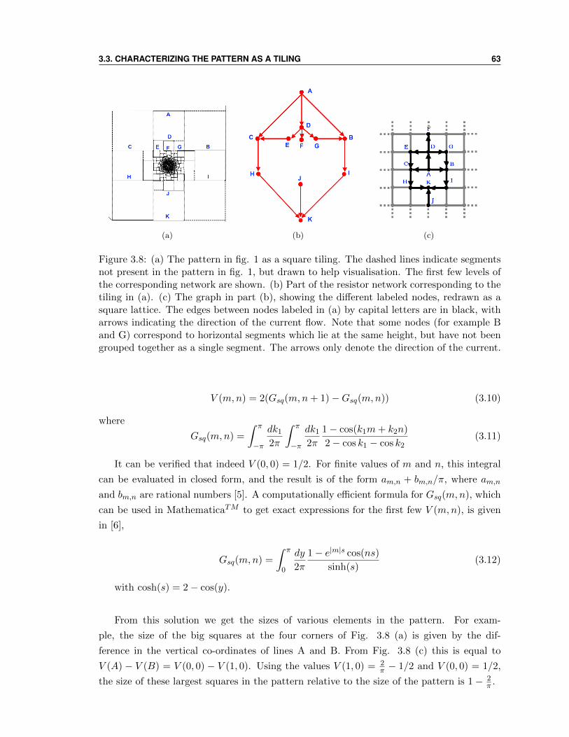
3.3. CHARACTERIZING THE PATTERN AS A TILING 63
(a) (b) (c)
Figure 3.8: (a) The pattern in fig. 1 as a square tiling. The dashed lines indicate segmentsnot present in the pattern in fig. 1, but drawn to help visualisation. The first few levels ofthe corresponding network are shown. (b) Part of the resistor network corresponding to thetiling in (a). (c) The graph in part (b), showing the different labeled nodes, redrawn as asquare lattice. The edges between nodes labeled in (a) by capital letters are in black, witharrows indicating the direction of the current flow. Note that some nodes (for example Band G) correspond to horizontal segments which lie at the same height, but have not beengrouped together as a single segment. The arrows only denote the direction of the current.
V (m,n) = 2(Gsq(m,n+ 1)−Gsq(m,n)) (3.10)
where
Gsq(m,n) =
∫ π
−π
dk1
2π
∫ π
−π
dk1
2π
1− cos(k1m+ k2n)
2− cos k1 − cos k2(3.11)
It can be verified that indeed V (0, 0) = 1/2. For finite values of m and n, this integral
can be evaluated in closed form, and the result is of the form am,n + bm,n/π, where am,n
and bm,n are rational numbers [5]. A computationally efficient formula for Gsq(m,n), which
can be used in MathematicaTM to get exact expressions for the first few V (m,n), is given
in [6],
Gsq(m,n) =
∫ π
0
dy
2π
1− e|m|s cos(ns)
sinh(s)(3.12)
with cosh(s) = 2− cos(y).
From this solution we get the sizes of various elements in the pattern. For exam-
ple, the size of the big squares at the four corners of Fig. 3.8 (a) is given by the dif-
ference in the vertical co-ordinates of lines A and B. From Fig. 3.8 (c) this is equal to
V (A) − V (B) = V (0, 0) − V (1, 0). Using the values V (1, 0) = 2π − 1/2 and V (0, 0) = 1/2,
the size of these largest squares in the pattern relative to the size of the pattern is 1− 2π .
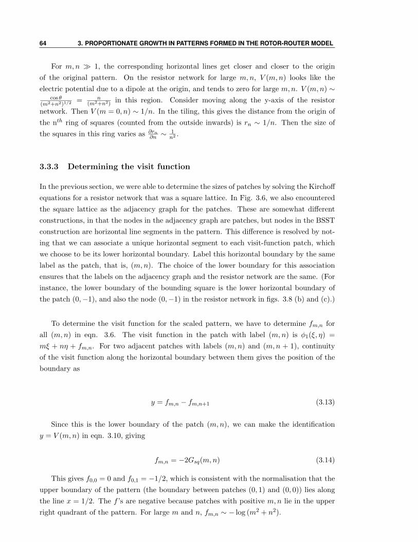
64 3. PROPORTIONATE GROWTH IN PATTERNS FORMED IN THE ROTOR-ROUTER MODEL
For m,n 1, the corresponding horizontal lines get closer and closer to the origin
of the original pattern. On the resistor network for large m,n, V (m,n) looks like the
electric potential due to a dipole at the origin, and tends to zero for large m,n. V (m,n) ∼cos θ
(m2+n2)1/2= n
(m2+n2)in this region. Consider moving along the y-axis of the resistor
network. Then V (m = 0, n) ∼ 1/n. In the tiling, this gives the distance from the origin of
the nth ring of squares (counted from the outside inwards) is rn ∼ 1/n. Then the size of
the squares in this ring varies as ∂rn∂n ∼
1n2 .
3.3.3 Determining the visit function
In the previous section, we were able to determine the sizes of patches by solving the Kirchoff
equations for a resistor network that was a square lattice. In Fig. 3.6, we also encountered
the square lattice as the adjacency graph for the patches. These are somewhat different
constructions, in that the nodes in the adjacency graph are patches, but nodes in the BSST
construction are horizontal line segments in the pattern. This difference is resolved by not-
ing that we can associate a unique horizontal segment to each visit-function patch, which
we choose to be its lower horizontal boundary. Label this horizontal boundary by the same
label as the patch, that is, (m,n). The choice of the lower boundary for this association
ensures that the labels on the adjacency graph and the resistor network are the same. (For
instance, the lower boundary of the bounding square is the lower horizontal boundary of
the patch (0,−1), and also the node (0,−1) in the resistor network in figs. 3.8 (b) and (c).)
To determine the visit function for the scaled pattern, we have to determine fm,n for
all (m,n) in eqn. 3.6. The visit function in the patch with label (m,n) is φ1(ξ, η) =
mξ + nη + fm,n. For two adjacent patches with labels (m,n) and (m,n + 1), continuity
of the visit function along the horizontal boundary between them gives the position of the
boundary as
y = fm,n − fm,n+1 (3.13)
Since this is the lower boundary of the patch (m,n), we can make the identification
y = V (m,n) in eqn. 3.10, giving
fm,n = −2Gsq(m,n) (3.14)
This gives f0,0 = 0 and f0,1 = −1/2, which is consistent with the normalisation that the
upper boundary of the pattern (the boundary between patches (0, 1) and (0, 0)) lies along
the line x = 1/2. The f ’s are negative because patches with positive m,n lie in the upper
right quadrant of the pattern. For large m and n, fm,n ∼ − log (m2 + n2).
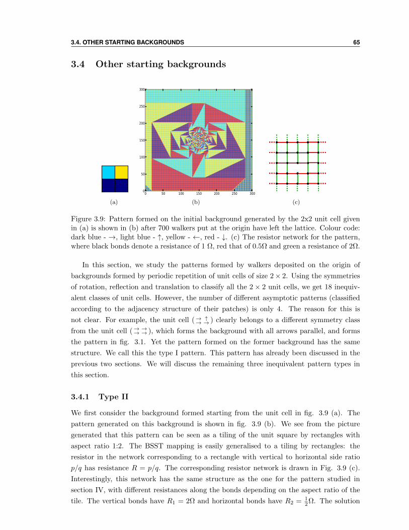
3.4. OTHER STARTING BACKGROUNDS 65
3.4 Other starting backgrounds
(a)
0 50 100 150 200 250 3000
50
100
150
200
250
300
(b) (c)
Figure 3.9: Pattern formed on the initial background generated by the 2x2 unit cell givenin (a) is shown in (b) after 700 walkers put at the origin have left the lattice. Colour code:dark blue - →, light blue - ↑, yellow - ←, red - ↓. (c) The resistor network for the pattern,where black bonds denote a resistance of 1 Ω, red that of 0.5Ω and green a resistance of 2Ω.
In this section, we study the patterns formed by walkers deposited on the origin of
backgrounds formed by periodic repetition of unit cells of size 2× 2. Using the symmetries
of rotation, reflection and translation to classify all the 2× 2 unit cells, we get 18 inequiv-
alent classes of unit cells. However, the number of different asymptotic patterns (classified
according to the adjacency structure of their patches) is only 4. The reason for this is
not clear. For example, the unit cell (→ ↑→ → ) clearly belongs to a different symmetry class
from the unit cell (→ →→ → ), which forms the background with all arrows parallel, and forms
the pattern in fig. 3.1. Yet the pattern formed on the former background has the same
structure. We call this the type I pattern. This pattern has already been discussed in the
previous two sections. We will discuss the remaining three inequivalent pattern types in
this section.
3.4.1 Type II
We first consider the background formed starting from the unit cell in fig. 3.9 (a). The
pattern generated on this background is shown in fig. 3.9 (b). We see from the picture
generated that this pattern can be seen as a tiling of the unit square by rectangles with
aspect ratio 1:2. The BSST mapping is easily generalised to a tiling by rectangles: the
resistor in the network corresponding to a rectangle with vertical to horizontal side ratio
p/q has resistance R = p/q. The corresponding resistor network is drawn in Fig. 3.9 (c).
Interestingly, this network has the same structure as the one for the pattern studied in
section IV, with different resistances along the bonds depending on the aspect ratio of the
tile. The vertical bonds have R1 = 2Ω and horizontal bonds have R2 = 12Ω. The solution
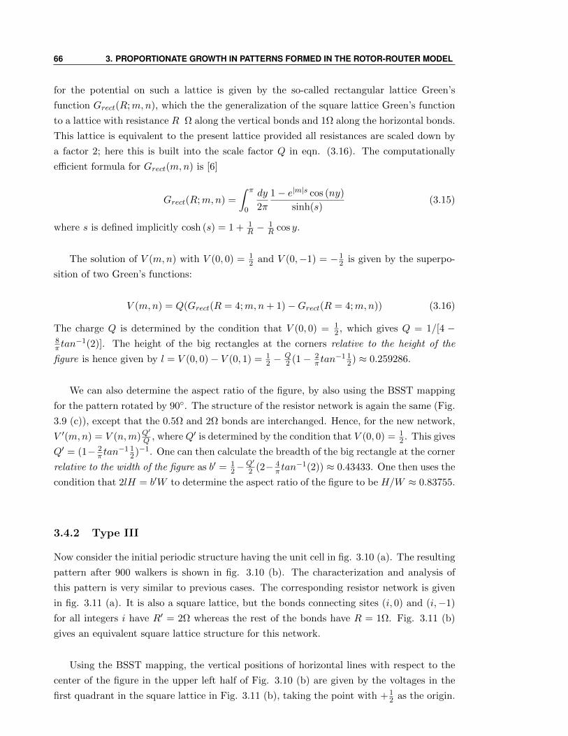
66 3. PROPORTIONATE GROWTH IN PATTERNS FORMED IN THE ROTOR-ROUTER MODEL
for the potential on such a lattice is given by the so-called rectangular lattice Green’s
function Grect(R;m,n), which the the generalization of the square lattice Green’s function
to a lattice with resistance R Ω along the vertical bonds and 1Ω along the horizontal bonds.
This lattice is equivalent to the present lattice provided all resistances are scaled down by
a factor 2; here this is built into the scale factor Q in eqn. (3.16). The computationally
efficient formula for Grect(m,n) is [6]
Grect(R;m,n) =
∫ π
0
dy
2π
1− e|m|s cos (ny)
sinh(s)(3.15)
where s is defined implicitly cosh (s) = 1 + 1R −
1R cos y.
The solution of V (m,n) with V (0, 0) = 12 and V (0,−1) = −1
2 is given by the superpo-
sition of two Green’s functions:
V (m,n) = Q(Grect(R = 4;m,n+ 1)−Grect(R = 4;m,n)) (3.16)
The charge Q is determined by the condition that V (0, 0) = 12 , which gives Q = 1/[4 −
8π tan
−1(2)]. The height of the big rectangles at the corners relative to the height of the
figure is hence given by l = V (0, 0)− V (0, 1) = 12 −
Q2 (1− 2
π tan−1 1
2) ≈ 0.259286.
We can also determine the aspect ratio of the figure, by also using the BSST mapping
for the pattern rotated by 90. The structure of the resistor network is again the same (Fig.
3.9 (c)), except that the 0.5Ω and 2Ω bonds are interchanged. Hence, for the new network,
V ′(m,n) = V (n,m)Q′
Q , where Q′ is determined by the condition that V (0, 0) = 12 . This gives
Q′ = (1− 2π tan
−1 12)−1. One can then calculate the breadth of the big rectangle at the corner
relative to the width of the figure as b′ = 12−
Q′
2 (2− 4π tan
−1(2)) ≈ 0.43433. One then uses the
condition that 2lH = b′W to determine the aspect ratio of the figure to be H/W ≈ 0.83755.
3.4.2 Type III
Now consider the initial periodic structure having the unit cell in fig. 3.10 (a). The resulting
pattern after 900 walkers is shown in fig. 3.10 (b). The characterization and analysis of
this pattern is very similar to previous cases. The corresponding resistor network is given
in fig. 3.11 (a). It is also a square lattice, but the bonds connecting sites (i, 0) and (i,−1)
for all integers i have R′ = 2Ω whereas the rest of the bonds have R = 1Ω. Fig. 3.11 (b)
gives an equivalent square lattice structure for this network.
Using the BSST mapping, the vertical positions of horizontal lines with respect to the
center of the figure in the upper left half of Fig. 3.10 (b) are given by the voltages in the
first quadrant in the square lattice in Fig. 3.11 (b), taking the point with +12 as the origin.
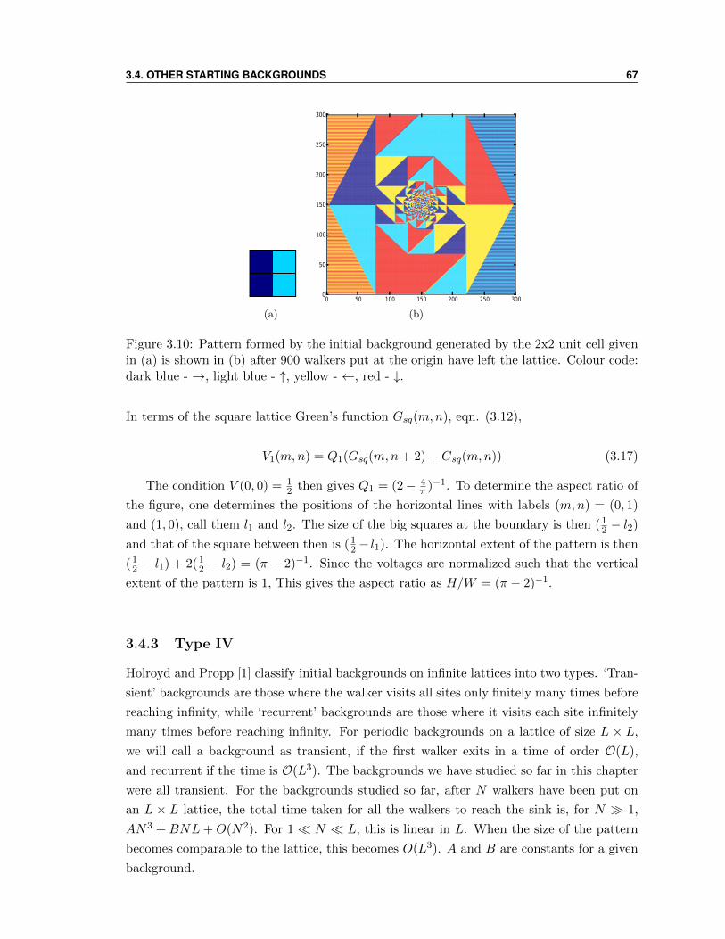
3.4. OTHER STARTING BACKGROUNDS 67
(a)
0 50 100 150 200 250 3000
50
100
150
200
250
300
(b)
Figure 3.10: Pattern formed by the initial background generated by the 2x2 unit cell givenin (a) is shown in (b) after 900 walkers put at the origin have left the lattice. Colour code:dark blue - →, light blue - ↑, yellow - ←, red - ↓.
In terms of the square lattice Green’s function Gsq(m,n), eqn. (3.12),
V1(m,n) = Q1(Gsq(m,n+ 2)−Gsq(m,n)) (3.17)
The condition V (0, 0) = 12 then gives Q1 = (2− 4
π )−1. To determine the aspect ratio of
the figure, one determines the positions of the horizontal lines with labels (m,n) = (0, 1)
and (1, 0), call them l1 and l2. The size of the big squares at the boundary is then (12 − l2)
and that of the square between then is (12 − l1). The horizontal extent of the pattern is then
(12 − l1) + 2(1
2 − l2) = (π − 2)−1. Since the voltages are normalized such that the vertical
extent of the pattern is 1, This gives the aspect ratio as H/W = (π − 2)−1.
3.4.3 Type IV
Holroyd and Propp [1] classify initial backgrounds on infinite lattices into two types. ‘Tran-
sient’ backgrounds are those where the walker visits all sites only finitely many times before
reaching infinity, while ‘recurrent’ backgrounds are those where it visits each site infinitely
many times before reaching infinity. For periodic backgrounds on a lattice of size L × L,
we will call a background as transient, if the first walker exits in a time of order O(L),
and recurrent if the time is O(L3). The backgrounds we have studied so far in this chapter
were all transient. For the backgrounds studied so far, after N walkers have been put on
an L × L lattice, the total time taken for all the walkers to reach the sink is, for N 1,
AN3 + BNL + O(N2). For 1 N L, this is linear in L. When the size of the pattern
becomes comparable to the lattice, this becomes O(L3). A and B are constants for a given
background.
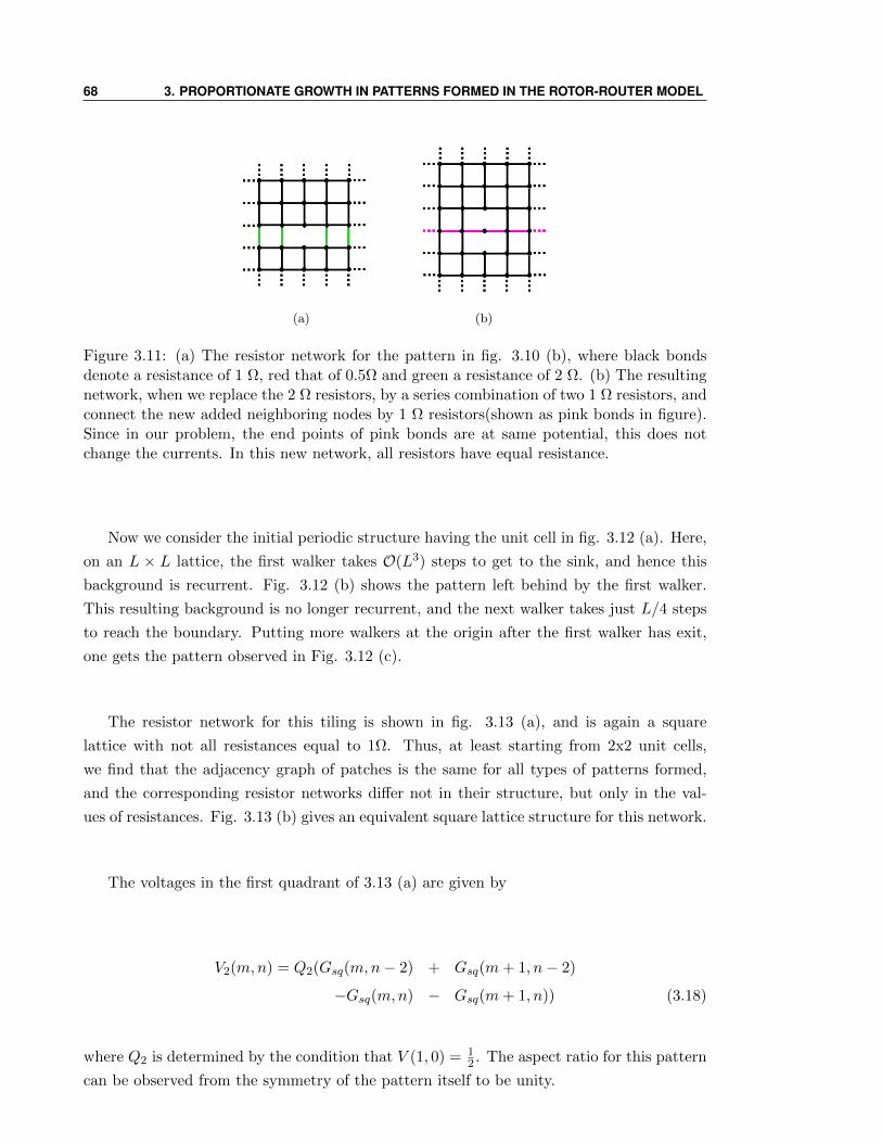
68 3. PROPORTIONATE GROWTH IN PATTERNS FORMED IN THE ROTOR-ROUTER MODEL
(a) (b)
Figure 3.11: (a) The resistor network for the pattern in fig. 3.10 (b), where black bondsdenote a resistance of 1 Ω, red that of 0.5Ω and green a resistance of 2 Ω. (b) The resultingnetwork, when we replace the 2 Ω resistors, by a series combination of two 1 Ω resistors, andconnect the new added neighboring nodes by 1 Ω resistors(shown as pink bonds in figure).Since in our problem, the end points of pink bonds are at same potential, this does notchange the currents. In this new network, all resistors have equal resistance.
Now we consider the initial periodic structure having the unit cell in fig. 3.12 (a). Here,
on an L × L lattice, the first walker takes O(L3) steps to get to the sink, and hence this
background is recurrent. Fig. 3.12 (b) shows the pattern left behind by the first walker.
This resulting background is no longer recurrent, and the next walker takes just L/4 steps
to reach the boundary. Putting more walkers at the origin after the first walker has exit,
one gets the pattern observed in Fig. 3.12 (c).
The resistor network for this tiling is shown in fig. 3.13 (a), and is again a square
lattice with not all resistances equal to 1Ω. Thus, at least starting from 2x2 unit cells,
we find that the adjacency graph of patches is the same for all types of patterns formed,
and the corresponding resistor networks differ not in their structure, but only in the val-
ues of resistances. Fig. 3.13 (b) gives an equivalent square lattice structure for this network.
The voltages in the first quadrant of 3.13 (a) are given by
V2(m,n) = Q2(Gsq(m,n− 2) + Gsq(m+ 1, n− 2)
−Gsq(m,n) − Gsq(m+ 1, n)) (3.18)
where Q2 is determined by the condition that V (1, 0) = 12 . The aspect ratio for this pattern
can be observed from the symmetry of the pattern itself to be unity.
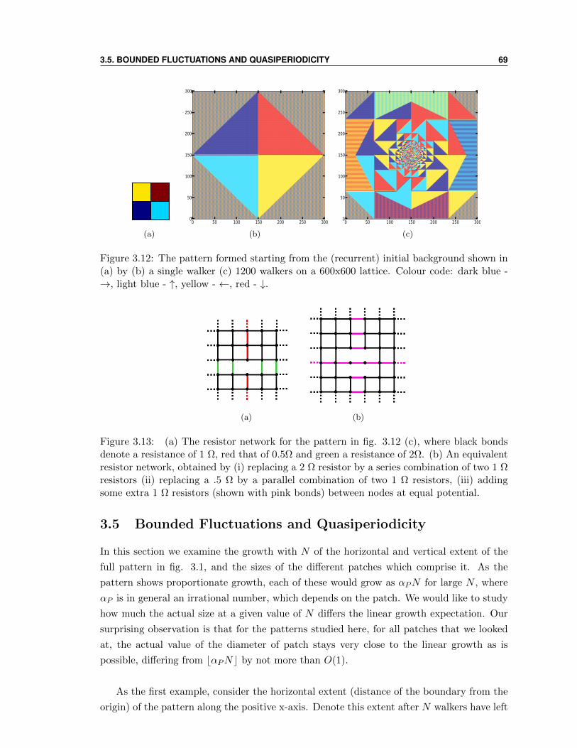
3.5. BOUNDED FLUCTUATIONS AND QUASIPERIODICITY 69
(a)
0 50 100 150 200 250 3000
50
100
150
200
250
300
(b)
0 50 100 150 200 250 3000
50
100
150
200
250
300
(c)
Figure 3.12: The pattern formed starting from the (recurrent) initial background shown in(a) by (b) a single walker (c) 1200 walkers on a 600x600 lattice. Colour code: dark blue -→, light blue - ↑, yellow - ←, red - ↓.
(a) (b)
Figure 3.13: (a) The resistor network for the pattern in fig. 3.12 (c), where black bondsdenote a resistance of 1 Ω, red that of 0.5Ω and green a resistance of 2Ω. (b) An equivalentresistor network, obtained by (i) replacing a 2 Ω resistor by a series combination of two 1 Ωresistors (ii) replacing a .5 Ω by a parallel combination of two 1 Ω resistors, (iii) addingsome extra 1 Ω resistors (shown with pink bonds) between nodes at equal potential.
3.5 Bounded Fluctuations and Quasiperiodicity
In this section we examine the growth with N of the horizontal and vertical extent of the
full pattern in fig. 3.1, and the sizes of the different patches which comprise it. As the
pattern shows proportionate growth, each of these would grow as αPN for large N , where
αP is in general an irrational number, which depends on the patch. We would like to study
how much the actual size at a given value of N differs the linear growth expectation. Our
surprising observation is that for the patterns studied here, for all patches that we looked
at, the actual value of the diameter of patch stays very close to the linear growth as is
possible, differing from bαPNc by not more than O(1).
As the first example, consider the horizontal extent (distance of the boundary from the
origin) of the pattern along the positive x-axis. Denote this extent after N walkers have left
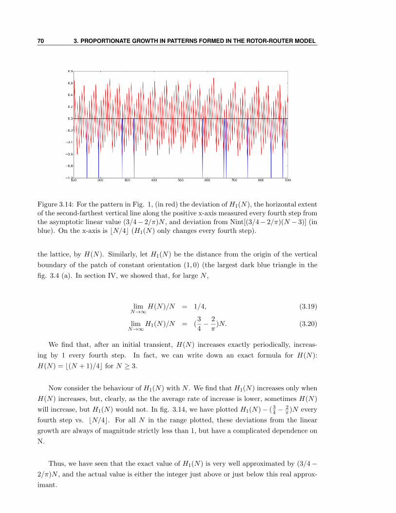
70 3. PROPORTIONATE GROWTH IN PATTERNS FORMED IN THE ROTOR-ROUTER MODEL
Figure 3.14: For the pattern in Fig. 1, (in red) the deviation of H1(N), the horizontal extentof the second-farthest vertical line along the positive x-axis measured every fourth step fromthe asymptotic linear value (3/4− 2/π)N , and deviation from Nint[(3/4− 2/π)(N − 3)] (inblue). On the x-axis is bN/4c (H1(N) only changes every fourth step).
the lattice, by H(N). Similarly, let H1(N) be the distance from the origin of the vertical
boundary of the patch of constant orientation (1, 0) (the largest dark blue triangle in the
fig. 3.4 (a). In section IV, we showed that, for large N ,
limN→∞
H(N)/N = 1/4, (3.19)
limN→∞
H1(N)/N = (3
4− 2
π)N. (3.20)
We find that, after an initial transient, H(N) increases exactly periodically, increas-
ing by 1 every fourth step. In fact, we can write down an exact formula for H(N):
H(N) = b(N + 1)/4c for N ≥ 3.
Now consider the behaviour of H1(N) with N . We find that H1(N) increases only when
H(N) increases, but, clearly, as the the average rate of increase is lower, sometimes H(N)
will increase, but H1(N) would not. In fig. 3.14, we have plotted H1(N)− (34 −
2π )N every
fourth step vs. bN/4c. For all N in the range plotted, these deviations from the linear
growth are always of magnitude strictly less than 1, but have a complicated dependence on
N.
Thus, we have seen that the exact value of H1(N) is very well approximated by (3/4−2/π)N , and the actual value is either the integer just above or just below this real approx-
imant.
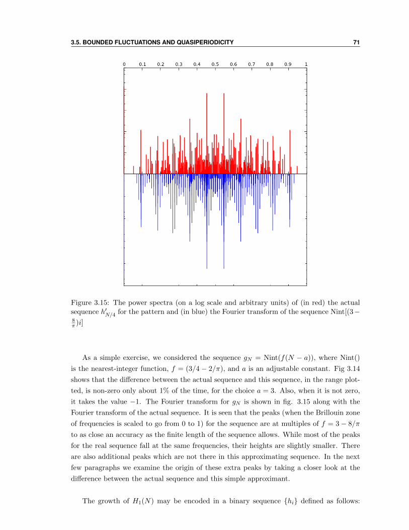
3.5. BOUNDED FLUCTUATIONS AND QUASIPERIODICITY 71
Figure 3.15: The power spectra (on a log scale and arbitrary units) of (in red) the actualsequence h′N/4 for the pattern and (in blue) the Fourier transform of the sequence Nint[(3−8π )i]
As a simple exercise, we considered the sequence gN = Nint(f(N − a)), where Nint()
is the nearest-integer function, f = (3/4− 2/π), and a is an adjustable constant. Fig 3.14
shows that the difference between the actual sequence and this sequence, in the range plot-
ted, is non-zero only about 1% of the time, for the choice a = 3. Also, when it is not zero,
it takes the value −1. The Fourier transform for gN is shown in fig. 3.15 along with the
Fourier transform of the actual sequence. It is seen that the peaks (when the Brillouin zone
of frequencies is scaled to go from 0 to 1) for the sequence are at multiples of f = 3− 8/π
to as close an accuracy as the finite length of the sequence allows. While most of the peaks
for the real sequence fall at the same frequencies, their heights are slightly smaller. There
are also additional peaks which are not there in this approximating sequence. In the next
few paragraphs we examine the origin of these extra peaks by taking a closer look at the
difference between the actual sequence and this simple approximant.
The growth of H1(N) may be encoded in a binary sequence hi defined as follows:
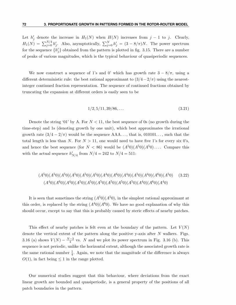
72 3. PROPORTIONATE GROWTH IN PATTERNS FORMED IN THE ROTOR-ROUTER MODEL
Let h′j denote the increase in H1(N) when H(N) increases from j − 1 to j. Clearly,
H1(N) =∑N/4
j=0 h′j . Also, asymptotically,
∑Nj=0 h
′j = (3 − 8/π)N . The power spectrum
for the sequence h′j obtained from the pattern is plotted in fig. 3.15. There are a number
of peaks of various magnitudes, which is the typical behaviour of quasiperiodic sequences.
We now construct a sequence of 1’s and 0’ which has growth rate 3 − 8/π, using a
different deterministic rule: the best rational approximant to (3/4−2/π) using the nearest-
integer continued fraction representation. The sequence of continued fractions obtained by
truncating the expansion at different orders is easily seen to be
1/2, 5/11, 39/86, . . . (3.21)
Denote the string ‘01’ by A. For N < 11, the best sequence of 0s (no growth during the
time-step) and 1s (denoting growth by one unit), which best approximates the irrational
growth rate (3/4− 2/π) would be the sequence AAA. . . , that is, 010101. . . , such that the
total length is less than N . For N > 11, one would need to have five 1’s for every six 0’s,
and hence the best sequence (for N < 86) would be (A50)(A50)(A50) . . . . Compare this
with the actual sequence h′N/4 from N/4 = 242 to N/4 = 511:
(A50)(A50)(A50)(A50)(A50)(A50)(A40)(A60)(A40)(A50)(A40)(A60)(A50) (3.22)
(A40)(A60)(A40)(A50)(A50)(A50)(A50)(A50)(A50)(A40)(A60)(A40)
It is seen that sometimes the string (A50)(A50), in the simplest rational approximant at
this order, is replaced by the string (A40)(A60). We have no good explanation of why this
should occur, except to say that this is probably caused by steric effects of nearby patches.
This effect of nearby patches is felt even at the boundary of the pattern. Let V (N)
denote the vertical extent of the pattern along the positive y-axis after N walkers. Figs.
3.16 (a) shows V (N) − N−34 vs. N and we plot its power spectrum in Fig. 3.16 (b). This
sequence is not periodic, unlike the horizontal extent, although the associated growth rate is
the same rational number 14 . Again, we note that the magnitude of the difference is always
O(1), in fact being ≤ 1 in the range plotted.
Our numerical studies suggest that this behaviour, where deviations from the exact
linear growth are bounded and quasiperiodic, is a general property of the positions of all
patch boundaries in the pattern.
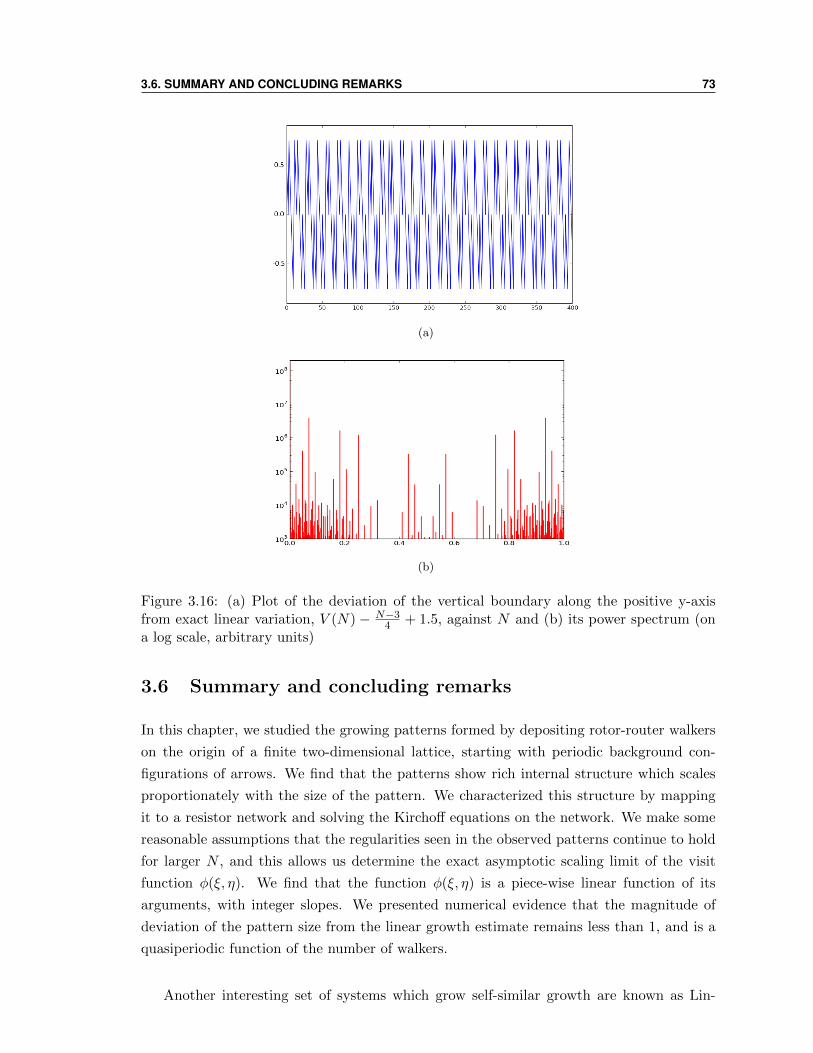
3.6. SUMMARY AND CONCLUDING REMARKS 73
(a)
(b)
Figure 3.16: (a) Plot of the deviation of the vertical boundary along the positive y-axisfrom exact linear variation, V (N)− N−3
4 + 1.5, against N and (b) its power spectrum (ona log scale, arbitrary units)
3.6 Summary and concluding remarks
In this chapter, we studied the growing patterns formed by depositing rotor-router walkers
on the origin of a finite two-dimensional lattice, starting with periodic background con-
figurations of arrows. We find that the patterns show rich internal structure which scales
proportionately with the size of the pattern. We characterized this structure by mapping
it to a resistor network and solving the Kirchoff equations on the network. We make some
reasonable assumptions that the regularities seen in the observed patterns continue to hold
for larger N , and this allows us determine the exact asymptotic scaling limit of the visit
function φ(ξ, η). We find that the function φ(ξ, η) is a piece-wise linear function of its
arguments, with integer slopes. We presented numerical evidence that the magnitude of
deviation of the pattern size from the linear growth estimate remains less than 1, and is a
quasiperiodic function of the number of walkers.
Another interesting set of systems which grow self-similar growth are known as Lin-
74 3. PROPORTIONATE GROWTH IN PATTERNS FORMED IN THE ROTOR-ROUTER MODEL
dermayer or (L-) systems [7], which are defined by a set of objects, and iterative rules
to generate larger systems made of these objects, from smaller ones. Interestingly, one-
dimensional L-systems can generate sequences generated from the continued fraction ex-
pansions of algebraic numbers, like the ones studied in section 3.5. (Note, however, that the
irrationals which characterize the growth of the patterns in chapter 3 depend on π, which
is not an algebraic number.) Perhaps an L-system construction in 2D can be constructed
to approximate the growth of rotor-router patterns.
Appendix: Derivation on eqn. (3.9) from matching of bound-
ary conditions
Consider the arrangement of six-sided visit-function-patches shown in Fig. 3.5 (b). We note
that the point A lies on the boundary of patches labeled (m,n) and (m− 1, n). Continuity
of φ across the boundary implies that
φ(A) = fm−1,n + (m− 1) ξA + n ηA = fm,n +m ξA + nηA, (3.23)
where A ≡ (ξA, ηA). Thus
ξA = fm−1,n − fm,n. (3.24)
Similar arguments give
ηA = fm,n − fm,n+1, (3.25)
ξB = fm,n − fm+1,n, (3.26)
ηB = fm,n−1 − fm,n.
Now, we note that the line AB was a boundary of a patch of constant orientation, and has
a slope that can only take one of the values 0,±1,∞. In this case, it must be 1. Hence we
get
fm+1,n + fm−1,n + fm,n−1 + fm,n+1 − 4fm,n = 0 (3.27)
which is the Eq. (3.9), obtained earlier using the BSST theorem.
Bibliography
[1] A. E. Holroyd and J. Propp, Rotor Walks and Markov Chains, Contemporary Mathe-
matics, 520 105 (2010) arXiv:0904.4507
[2] W. Pegden and C. K. Smart. Convergence of the Abelian sandpile, Duke Mathematical
Journal 162 627 (2013)
[3] S. Ostojic, Physica A 318 187 (2003).
[4] R. L. Brooks, C. A. B. Smith, A. H. Stone and W. T. Tutte, The Dissection of Rect-
angles into Squares, Duke Mathematical Journal 7 312 (1940).
[5] F. Spitzer, Principles of Random Walk, pp. 124, 148-51, (Van Nostrand, Princeton,
1964);
[6] J. Cserti, Application of the lattice Green’s function for calculating the resistance of an
infinite networks of resistors, Am. J. Phys., 68 896 (2000).
[7] Aristid Lindenmayer, Mathematical models for cellular interaction in development, J.
Theoret. Biology, 18 280 (1968)
https://en.wikipedia.org/wiki/L-system
75
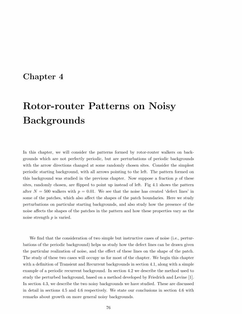
Chapter 4
Rotor-router Patterns on Noisy
Backgrounds
In this chapter, we will consider the patterns formed by rotor-router walkers on back-
grounds which are not perfectly periodic, but are perturbations of periodic backgrounds
with the arrow directions changed at some randomly chosen sites. Consider the simplest
periodic starting background, with all arrows pointing to the left. The pattern formed on
this background was studied in the previous chapter. Now suppose a fraction p of these
sites, randomly chosen, are flipped to point up instead of left. Fig 4.1 shows the pattern
after N = 500 walkers with p = 0.01. We see that the noise has created ‘defect lines’ in
some of the patches, which also affect the shapes of the patch boundaries. Here we study
perturbations on particular starting backgrounds, and also study how the presence of the
noise affects the shapes of the patches in the pattern and how these properties vary as the
noise strength p is varied.
We find that the consideration of two simple but instructive cases of noise (i.e., pertur-
bations of the periodic background) helps us study how the defect lines can be drawn given
the particular realization of noise, and the effect of these lines on the shape of the patch.
The study of these two cases will occupy us for most of the chapter. We begin this chapter
with a definition of Transient and Recurrent backgrounds in section 4.1, along with a simple
example of a periodic recurrent background. In section 4.2 we describe the method used to
study the perturbed background, based on a method developed by Friedrich and Levine [1].
In section 4.3, we describe the two noisy backgrounds we have studied. These are discussed
in detail in sections 4.5 and 4.6 respectively. We state our conclusions in section 4.6 with
remarks about growth on more general noisy backgrounds.
76
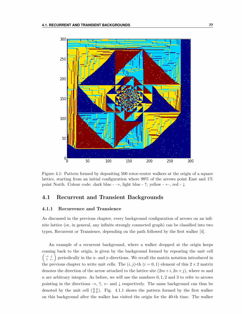
4.1. RECURRENT AND TRANSIENT BACKGROUNDS 77
Figure 4.1: Pattern formed by depositing 500 rotor-router walkers at the origin of a squarelattice, starting from an initial configuration where 99% of the arrows point East and 1%point North. Colour code: dark blue - →, light blue - ↑, yellow - ←, red - ↓
4.1 Recurrent and Transient Backgrounds
4.1.1 Recurrence and Transience
As discussed in the previous chapter, every background configuration of arrows on an infi-
nite lattice (or, in general, any infinite strongly connected graph) can be classified into two
types, Recurrent or Transience, depending on the path followed by the first walker [4].
An example of a recurrent background, where a walker dropped at the origin keeps
coming back to the origin, is given by the background formed by repeating the unit cell(→ ↓↑ ←
)periodically in the x- and y-directions. We recall the matrix notation introduced in
the previous chapter to write unit cells. The (i, j)-th (i = 0, 1) element of this 2× 2 matrix
denotes the direction of the arrow attached to the lattice site (2m+ i, 2n+ j), where m and
n are arbitrary integers. As before, we will use the numbers 0, 1, 2 and 3 to refer to arrows
pointing in the directions →, ↑, ← and ↓ respectively. The same background can thus be
denoted by the unit cell ( 0 30 2 ). Fig. 4.1.1 shows the pattern formed by the first walker
on this background after the walker has visited the origin for the 40-th time. The walker
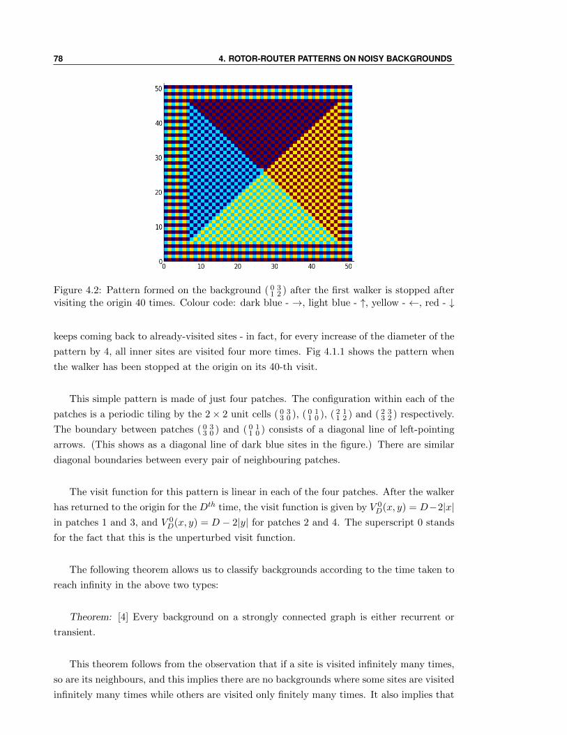
78 4. ROTOR-ROUTER PATTERNS ON NOISY BACKGROUNDS
Figure 4.2: Pattern formed on the background ( 0 31 2 ) after the first walker is stopped after
visiting the origin 40 times. Colour code: dark blue - →, light blue - ↑, yellow - ←, red - ↓
keeps coming back to already-visited sites - in fact, for every increase of the diameter of the
pattern by 4, all inner sites are visited four more times. Fig 4.1.1 shows the pattern when
the walker has been stopped at the origin on its 40-th visit.
This simple pattern is made of just four patches. The configuration within each of the
patches is a periodic tiling by the 2× 2 unit cells ( 0 33 0 ), ( 0 1
1 0 ), ( 2 11 2 ) and ( 2 3
3 2 ) respectively.
The boundary between patches ( 0 33 0 ) and ( 0 1
1 0 ) consists of a diagonal line of left-pointing
arrows. (This shows as a diagonal line of dark blue sites in the figure.) There are similar
diagonal boundaries between every pair of neighbouring patches.
The visit function for this pattern is linear in each of the four patches. After the walker
has returned to the origin for the Dth time, the visit function is given by V 0D(x, y) = D−2|x|
in patches 1 and 3, and V 0D(x, y) = D − 2|y| for patches 2 and 4. The superscript 0 stands
for the fact that this is the unperturbed visit function.
The following theorem allows us to classify backgrounds according to the time taken to
reach infinity in the above two types:
Theorem: [4] Every background on a strongly connected graph is either recurrent or
transient.
This theorem follows from the observation that if a site is visited infinitely many times,
so are its neighbours, and this implies there are no backgrounds where some sites are visited
infinitely many times while others are visited only finitely many times. It also implies that
4.2. FROM APPROXIMATE TO EXACT VISIT FUNCTION 79
the recurrence or transience of a background is independent of the choice of the site that
the first walker is dropped on.
Given a periodic background, we study the effect on the pattern as the arrow directions
at randomly chosen sites are flipped. If one starts with a recurrent background, and flips a
certain fraction of sites, when this fraction is large the background might become transient.
Such cases, where there is a transition from recurrence to transience at a certain fraction
p, turn out to be the most interesting cases, and we focus on them in this chapter. It could
also happen that the background retains its transience/recurrence even as we vary p from
0 to 1.
4.1.2 Notation and Protocol
We will be constructing background arrow configurations out of 2×2 unit cells. Unit cells,
and the backgrounds made by periodic repetition of them, will both be specified by a 2x2
matrix.
We extend the notation to random backgrounds as follows: A,B|p, 1 − p denotes an
ensemble of starting backgrounds where each unit cell on the lattice is of type A with prob-
ability p or of type B with probability (1 − p). Thus, a background ( 2 30 1 ),( 1 0
0 1 ) |0.8, 0.2denotes the ensemble of backgrounds in which, for a typical background in the ensemble,
about 80% of the unit cells are ( 2 30 1 ) and 20% are ( 1 0
0 1 ).
The protocol for constructing patterns, given a background, is as follows: starting with
a given background specification, say A,B|p, 1− p we generate a random starting back-
ground on an L × L lattice. For transient backgrounds, we then drop N walkers at the
center of the lattice, and wait till they have all exit the lattice, and study the resulting
pattern. For recurrent backgrounds, we study the pattern after stopping the walk at a
specified stopping time, usually the 4N -th time the walker visits the origin.
Defining the final configuration of arrows that have undergone at least one full rotation
as ‘the pattern’, we now have an ensemble of patterns for a given starting background
specification (ie, for given A, B and p). We will focus on calculating the averages of various
properties taken over this ensemble.
4.2 From Approximate to Exact Visit function
Given a starting random background, we need a method for calculating the resulting pat-
terns that allows for analytical treatment. Our aim is to determine the final visit function
once the walker has returned to the origin for the 4N -th time. We will start with an ap-
proximate guess for final visit function - our guess will be the visit function for the periodic
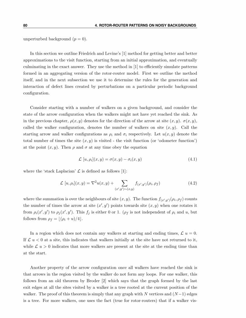
80 4. ROTOR-ROUTER PATTERNS ON NOISY BACKGROUNDS
unperturbed background (p = 0).
In this section we outline Friedrich and Levine’s [1] method for getting better and better
approximations to the visit function, starting from an initial approximation, and eventually
culminating in the exact answer. They use the method in [1] to efficiently simulate patterns
formed in an aggregating version of the rotor-router model. First we outline the method
itself, and in the next subsection we use it to determine the rules for the generation and
interaction of defect lines created by perturbations on a particular periodic background
configuration.
Consider starting with a number of walkers on a given background, and consider the
state of the arrow configuration when the walkers might not have yet reached the sink. As
in the previous chapter, ρ(x, y) denotes for the direction of the arrow at site (x, y). σ(x, y),
called the walker configuration, denotes the number of walkers on site (x, y). Call the
starting arrow and walker configurations as ρi and σi respectively. Let u(x, y) denote the
total number of times the site (x, y) is visited - the visit function (or ‘odometer function’)
at the point (x, y). Then ρ and σ at any time obey the equation
L [u, ρi](x, y) = σ(x, y)− σi(x, y) (4.1)
where the ‘stack Laplacian’ L is defined as follows [1]:
L [u, ρi](x, y) = ∇2u(x, y) +∑
(x′,y′)∼(x,y)
f(x′,y′)(ρi, ρf ) (4.2)
where the summation is over the neighbours of site (x, y). The function f(x′,y′)(ρi, ρf ) counts
the number of times the arrow at site (x′, y′) points towards site (x, y) when one rotates it
from ρi(x′, y′) to ρj(x
′, y′). This fj is either 0 or 1. (ρf is not independent of ρi and u, but
follows from ρf = b(ρi + u)/4c.
In a region which does not contain any walkers at starting and ending times, L u = 0.
If L u < 0 at a site, this indicates that walkers initially at the site have not returned to it,
while L u > 0 indicates that more walkers are present at the site at the ending time than
at the start.
Another property of the arrow configuration once all walkers have reached the sink is
that arrows in the region visited by the walker do not form any loops. For one walker, this
follows from an old theorem by Broder [2] which says that the graph formed by the last
exit edges at all the sites visited by a walker is a tree rooted at the current position of the
walker. The proof of this theorem is simply that any graph with N vertices and (N−1) edges
is a tree. For more walkers, one uses the fact (true for rotor-routers) that if a walker vis-

4.2. FROM APPROXIMATE TO EXACT VISIT FUNCTION 81
its a site which is part of a loop, the loop is finally broken after a certain number of steps [3].
If a loop, or ‘cycle’, exists in an arrow configuration, we can define an operation called
‘reverse cycle popping’, where all the arrows which form the cycle are rotated 90 clockwise
(that is, reverse of the anti-clockwise direction in which they are moved by the walkers).
This destroys the original loop, but might create new loops. It is useful to extend the
definition of reverse cycle popping to a set of arrows which do not form a loop as simply
doing nothing to the arrow configuration. Friedrich and Levine show that the procedure of
reverse cycle-popping a set of sites commutes with the operation of starting a walker at a
site and letting it walk until it reaches the sink. That is, reverse-popping the loop before
starting the walk will result in the same final configuration once the walker has reached the
sink as performing the reverse-popping after the walker has reached the sink - if the loop
still exists, that is. (If the walker visits any site on the loop, the final configuration will not
contain that loop, and reverse-cycle popping will do nothing.)
The Friedrich-Levine procedure finds the exact solution of the equation 4.1, given the
following information:
(i) Initial arrow and chip configurations, ρi and σi;
(ii) The final condition is that all chips have ended up at the sink;
(iii) An initial guess for the visit function, u0(x, y).
The steps of the procedure are as follows:
1. Evaluate the initial guess for the final arrow configuration, ρ0 = b(ρi + u0)/4c
2. Evaluate L [u0, ρi](x, y) at all sites. This gives a σ0(x, y), an initial guess for the final
chip configurations. Sites at which σ0 > 0 are said of be hills of height σ0, and sites
at which σ0 < 0 are called holes of depth |σ0|.
3. Place walkers at each hill site equal in number to the height of the hill, and let them
walk until they reach the holes. When a walker reaches a hole, the height of the hole
decreases by 1.
4. Once all these hills have been moved to the holes, scan the lattice for any loops in
the part of the lattice where u0 is non-zero, and reverse-cycle-pop them. Rescan and
repeat until no more loops are left.
At the end of the this procedure, one gets an updated guess for u(x, y), because u(x, y)
changes every time a cycle containing the point (x, y) is reverse-popped or when an extra
walker visits (x, y), according to the following rules:
• Extra walkers - extra walkers walking from hills to holes add to u on the sites along
the path followed by the walker, in the usual way.
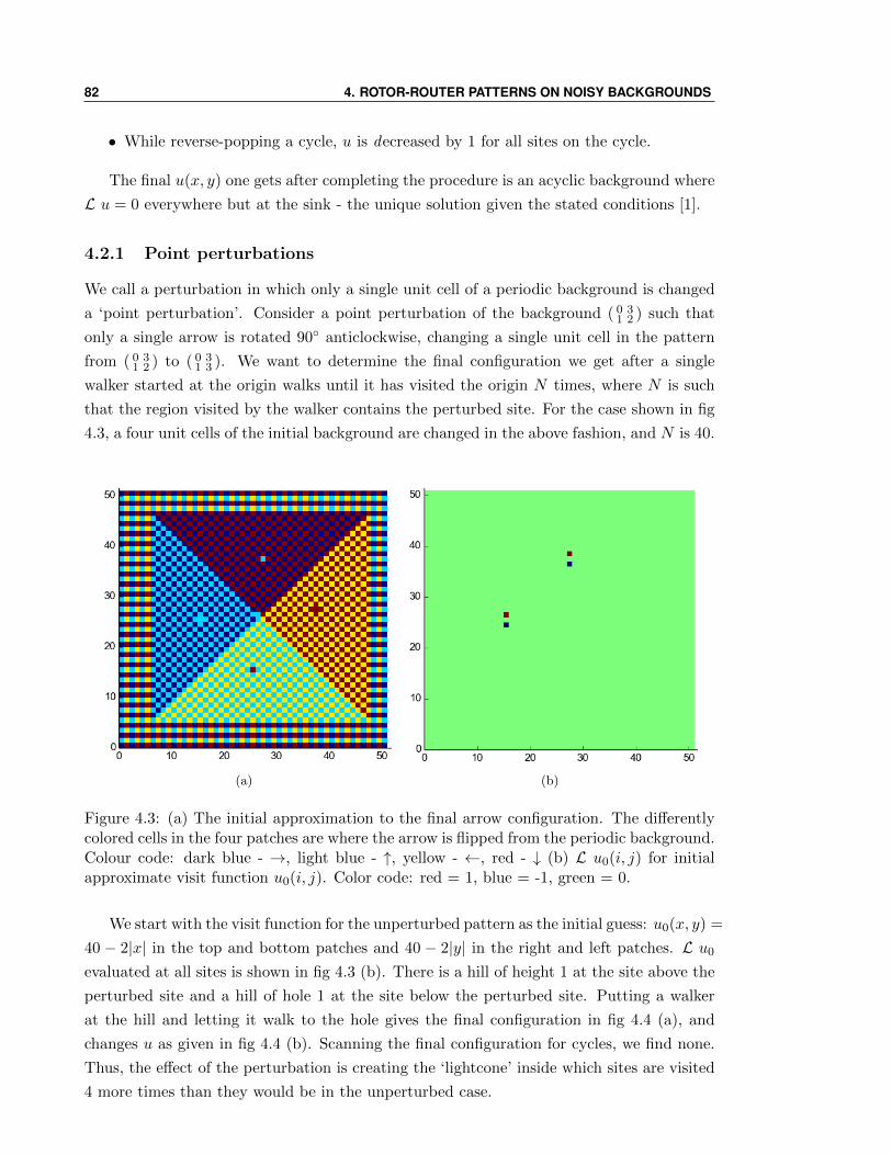
82 4. ROTOR-ROUTER PATTERNS ON NOISY BACKGROUNDS
• While reverse-popping a cycle, u is decreased by 1 for all sites on the cycle.
The final u(x, y) one gets after completing the procedure is an acyclic background where
L u = 0 everywhere but at the sink - the unique solution given the stated conditions [1].
4.2.1 Point perturbations
We call a perturbation in which only a single unit cell of a periodic background is changed
a ‘point perturbation’. Consider a point perturbation of the background ( 0 31 2 ) such that
only a single arrow is rotated 90 anticlockwise, changing a single unit cell in the pattern
from ( 0 31 2 ) to ( 0 3
1 3 ). We want to determine the final configuration we get after a single
walker started at the origin walks until it has visited the origin N times, where N is such
that the region visited by the walker contains the perturbed site. For the case shown in fig
4.3, a four unit cells of the initial background are changed in the above fashion, and N is 40.
(a) (b)
Figure 4.3: (a) The initial approximation to the final arrow configuration. The differentlycolored cells in the four patches are where the arrow is flipped from the periodic background.Colour code: dark blue - →, light blue - ↑, yellow - ←, red - ↓ (b) L u0(i, j) for initialapproximate visit function u0(i, j). Color code: red = 1, blue = -1, green = 0.
We start with the visit function for the unperturbed pattern as the initial guess: u0(x, y) =
40 − 2|x| in the top and bottom patches and 40 − 2|y| in the right and left patches. L u0
evaluated at all sites is shown in fig 4.3 (b). There is a hill of height 1 at the site above the
perturbed site and a hill of hole 1 at the site below the perturbed site. Putting a walker
at the hill and letting it walk to the hole gives the final configuration in fig 4.4 (a), and
changes u as given in fig 4.4 (b). Scanning the final configuration for cycles, we find none.
Thus, the effect of the perturbation is creating the ‘lightcone’ inside which sites are visited
4 more times than they would be in the unperturbed case.
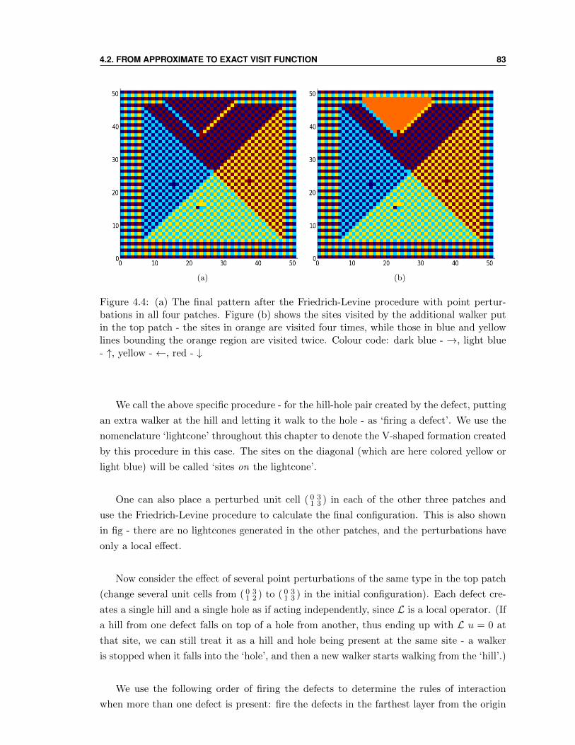
4.2. FROM APPROXIMATE TO EXACT VISIT FUNCTION 83
(a) (b)
Figure 4.4: (a) The final pattern after the Friedrich-Levine procedure with point pertur-bations in all four patches. Figure (b) shows the sites visited by the additional walker putin the top patch - the sites in orange are visited four times, while those in blue and yellowlines bounding the orange region are visited twice. Colour code: dark blue - →, light blue- ↑, yellow - ←, red - ↓
We call the above specific procedure - for the hill-hole pair created by the defect, putting
an extra walker at the hill and letting it walk to the hole - as ‘firing a defect’. We use the
nomenclature ‘lightcone’ throughout this chapter to denote the V-shaped formation created
by this procedure in this case. The sites on the diagonal (which are here colored yellow or
light blue) will be called ‘sites on the lightcone’.
One can also place a perturbed unit cell ( 0 31 3 ) in each of the other three patches and
use the Friedrich-Levine procedure to calculate the final configuration. This is also shown
in fig - there are no lightcones generated in the other patches, and the perturbations have
only a local effect.
Now consider the effect of several point perturbations of the same type in the top patch
(change several unit cells from ( 0 31 2 ) to ( 0 3
1 3 ) in the initial configuration). Each defect cre-
ates a single hill and a single hole as if acting independently, since L is a local operator. (If
a hill from one defect falls on top of a hole from another, thus ending up with L u = 0 at
that site, we can still treat it as a hill and hole being present at the same site - a walker
is stopped when it falls into the ‘hole’, and then a new walker starts walking from the ‘hill’.)
We use the following order of firing the defects to determine the rules of interaction
when more than one defect is present: fire the defects in the farthest layer from the origin
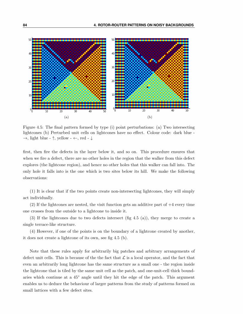
84 4. ROTOR-ROUTER PATTERNS ON NOISY BACKGROUNDS
(a) (b)
Figure 4.5: The final pattern formed by type (i) point perturbations: (a) Two intersectinglightcones (b) Perturbed unit cells on lightcones have no effect. Colour code: dark blue -→, light blue - ↑, yellow - ←, red - ↓
first, then fire the defects in the layer below it, and so on. This procedure ensures that
when we fire a defect, there are no other holes in the region that the walker from this defect
explores (the lightcone region), and hence no other holes that this walker can fall into. The
only hole it falls into is the one which is two sites below its hill. We make the following
observations:
(1) It is clear that if the two points create non-intersecting lightcones, they will simply
act individually.
(2) If the lightcones are nested, the visit function gets an additive part of +4 every time
one crosses from the outside to a lightcone to inside it.
(3) If the lightcones due to two defects intersect (fig 4.5 (a)), they merge to create a
single terrace-like structure.
(4) However, if one of the points is on the boundary of a lightcone created by another,
it does not create a lightcone of its own, see fig 4.5 (b).
Note that these rules apply for arbitrarily big patches and arbitrary arrangements of
defect unit cells. This is because of the the fact that L is a local operator, and the fact that
even an arbitrarily long lightcone has the same structure as a small one - the region inside
the lightcone that is tiled by the same unit cell as the patch, and one-unit-cell thick bound-
aries which continue at a 45 angle until they hit the edge of the patch. This argument
enables us to deduce the behaviour of larger patterns from the study of patterns formed on
small lattices with a few defect sites.
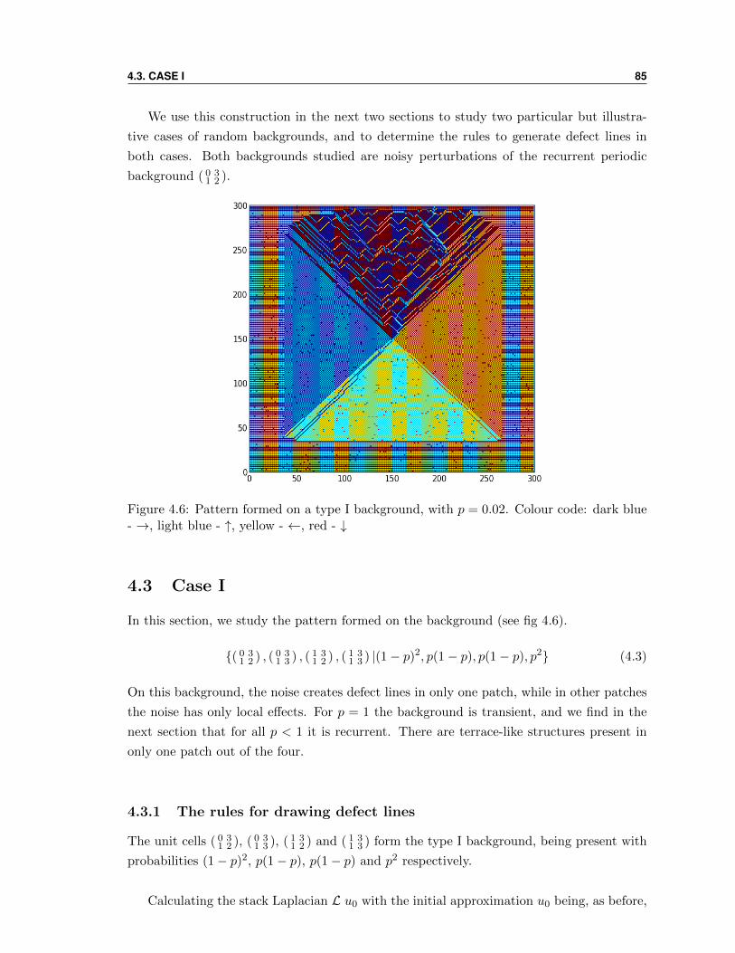
4.3. CASE I 85
We use this construction in the next two sections to study two particular but illustra-
tive cases of random backgrounds, and to determine the rules to generate defect lines in
both cases. Both backgrounds studied are noisy perturbations of the recurrent periodic
background ( 0 31 2 ).
Figure 4.6: Pattern formed on a type I background, with p = 0.02. Colour code: dark blue- →, light blue - ↑, yellow - ←, red - ↓
4.3 Case I
In this section, we study the pattern formed on the background (see fig 4.6).
( 0 31 2 ) , ( 0 3
1 3 ) , ( 1 31 2 ) , ( 1 3
1 3 ) |(1− p)2, p(1− p), p(1− p), p2 (4.3)
On this background, the noise creates defect lines in only one patch, while in other patches
the noise has only local effects. For p = 1 the background is transient, and we find in the
next section that for all p < 1 it is recurrent. There are terrace-like structures present in
only one patch out of the four.
4.3.1 The rules for drawing defect lines
The unit cells ( 0 31 2 ), ( 0 3
1 3 ), ( 1 31 2 ) and ( 1 3
1 3 ) form the type I background, being present with
probabilities (1− p)2, p(1− p), p(1− p) and p2 respectively.
Calculating the stack Laplacian L u0 with the initial approximation u0 being, as before,
86 4. ROTOR-ROUTER PATTERNS ON NOISY BACKGROUNDS
the visit function for the unperturbed patch, we find that the ( 1 31 2 ) unit cells act identically
to the ( 0 31 3 ) ones, both producing hill-hole pairs that, when fired, generate lightcones in the
patch, except the lightcones have vertices at sites where x and y are both odd, in one case,
and at sites where x and y are both even, in the other. It turns out that the lightcones
of the second kind of firing (due to the perturbation ( 1 31 2 )) interact with the lightcones of
the first kind (due to ( 0 31 3 ), studied in the previous section) according to the rules given
in the previous section, without distinguishing which kind of unit cell created the defect line.
Thus the rules for drawing defect lines given the positions of the perturbed unit cells are:
(i) Start two defect lines at right angles to each other at each noise point.
(ii) If two defect lines meet, they do not continue beyond that point. This results in a
terrace-like structure.
(iii) Noise points which fall on existing defect lines do not create any new defect lines.
We give a heuristic explanation for rule (iii). The defect lines which form the two arms
of a lightcone have the same arrow structure, locally, as the patches on either side of the
current patch. That is, the defect line on the right side of a lightcone is made of the same
unit cells which tile the patch to the right. We know that L is a local operator, and that in
both these patches the perturbation has only a local effect and does not generate lightcones.
Thus we can expect that a perturbation on such a defect line would also have only a local
effect, and not generate lightcones either. As shown earlier, this expectation is verified by
explicit studies of small systems.
Denote the unperturbed visit function by V0(x, y), and the visit function for a partic-
ular noise realisation by V (x, y). We define a height function h(x, y) in the top patch by
4h(x, y) = V (x, y) − V0(x, y) = V (x, y) − (D − 2y). The value of h at a point (x, y) which
does not lie on a defect line is given by the number of terraces crossed in order to get to the
region from the origin (or from the boundary of the patch). If (x, y) lies on a defect line,
h(x, y) is h′ − 12 , where h′ is the value of h for the region inside the defect line. Once we
draw the defect lines according to the above rules, we can determine h(x, y) for all points
inside the patch, and this determines V (x, y).
Note that the periodicity of the patches and the equivalence proved in the previous
section allow us to use calculations of the final state on small-sized patches, as was done in
the figures above, to generalise to large patches and arbitrary levels of noise (as long as the
background stays recurrent).
4.3. CASE I 87
4.3.2 The exact visit function and Tracy-Widom fluctuations
In chapter 1 we described the Bernoulli matching problem, and mapped it to a height
model in which the height increases in integer steps as one crosses terraces with vertical and
horizontal boundaries, situated in the first quadrant of the xy-plane. The height increases
monotonically in both x- and y-directions. Here we only recall the basic rules for generating
height terraces in the Bernoulli matching problem. We are given two random sequences of
characters of length i and j and asked to find the longest increasing subsequence (LCS)
: (a) Consider first quadrant of the square lattice. If the x-th character from sequence 1
is the same as the y-th character from sequence 2, draw two lines, one horizontal and one
vertical, starting from point (x, y). (b) Merge these lines to form terraces when they meet.
(c) Points on existing defect lines have no effect. (d) The length of the LCS of the first m
characters of the first word and the first n characters of the second word, l(m,n) obeys the
rules: l(0, 0) = 0, and l(m,n) increases by 1 each time you climb a terrace. As noted in
Chapter 1, we have that for large x and y,
hBM =
x if x < py
11−p(2
√pxy − p(x+ y)) +A(p, x, y) ξGUE if py ≤ x ≤ p−1y
y if p−1y < x
(4.4)
where ξGUE is a random variable distributed according to the Tracy-Widom distribu-
tion corresponding to the Gaussian Unitary Ensemble, and A(p, x, y) = (pxy)1/6/(1 −
p)[(1 + p)−
√p/xy(x+ y)
]2/3.
Comparing the rules given in the previous subsection for the perturbations of type (i)
and for Bernoulli matchings, we see that if one changes co-ordinates from (x, y) for Bernoulli
matchings to (x+ y, x− y) for the rotor-router patch, h(x, y) = hBM (x+ y, x− y) for the
same realization of noise. Note that this correspondence holds for all values of p. (So
long as the rotor background is recurrent, which as we show below it is for p < 1). Given
the one-to-one correspondence between the two problems, we immediately conclude that
h(x, y) = hBM (x+ y, y− x). In particular, along the y-axis, the visit function goes like (for
large y 1)
V (y) = V (0)− 2y + 4 + hBM (y, y) (4.5)
where V (0) is the mean number of visits to the origin. Note that since h(x, y) ≥ 0, the
boundary of the affected patch is extended outwards. We perform simulations on finite
lattices with absorbing boundaries, where the walker exits the lattice when the boundary of
the affected patch touches the boundary of the lattice. The longest extent of the boundary
is, on average, along the y-axis. Working on an L×L lattice and setting V (L/2) = 0, from
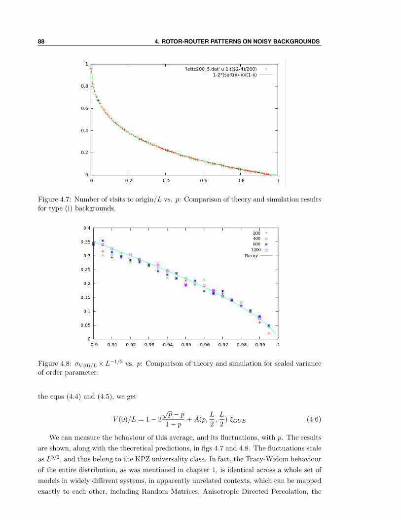
88 4. ROTOR-ROUTER PATTERNS ON NOISY BACKGROUNDS
Figure 4.7: Number of visits to origin/L vs. p: Comparison of theory and simulation resultsfor type (i) backgrounds.
Figure 4.8: σV (0)/L×L−1/3 vs. p: Comparison of theory and simulation for scaled varianceof order parameter.
the eqns (4.4) and (4.5), we get
V (0)/L = 1− 2
√p− p
1− p+A(p,
L
2,L
2) ξGUE (4.6)
We can measure the behaviour of this average, and its fluctuations, with p. The results
are shown, along with the theoretical predictions, in figs 4.7 and 4.8. The fluctuations scale
as L3/2, and thus belong to the KPZ universality class. In fact, the Tracy-Widom behaviour
of the entire distribution, as was mentioned in chapter 1, is identical across a whole set of
models in widely different systems, in apparently unrelated contexts, which can be mapped
exactly to each other, including Random Matrices, Anisotropic Directed Percolation, the
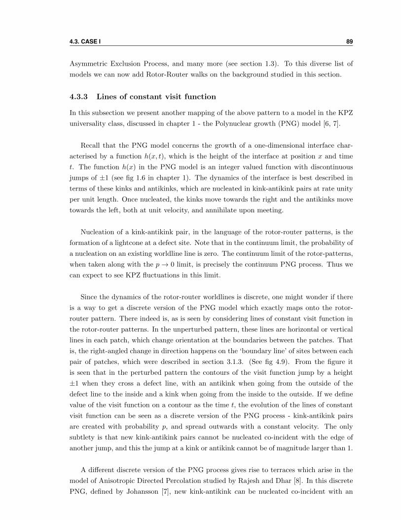
4.3. CASE I 89
Asymmetric Exclusion Process, and many more (see section 1.3). To this diverse list of
models we can now add Rotor-Router walks on the background studied in this section.
4.3.3 Lines of constant visit function
In this subsection we present another mapping of the above pattern to a model in the KPZ
universality class, discussed in chapter 1 - the Polynuclear growth (PNG) model [6, 7].
Recall that the PNG model concerns the growth of a one-dimensional interface char-
acterised by a function h(x, t), which is the height of the interface at position x and time
t. The function h(x) in the PNG model is an integer valued function with discontinuous
jumps of ±1 (see fig 1.6 in chapter 1). The dynamics of the interface is best described in
terms of these kinks and antikinks, which are nucleated in kink-antikink pairs at rate unity
per unit length. Once nucleated, the kinks move towards the right and the antikinks move
towards the left, both at unit velocity, and annihilate upon meeting.
Nucleation of a kink-antikink pair, in the language of the rotor-router patterns, is the
formation of a lightcone at a defect site. Note that in the continuum limit, the probability of
a nucleation on an existing worldline line is zero. The continuum limit of the rotor-patterns,
when taken along with the p→ 0 limit, is precisely the continuum PNG process. Thus we
can expect to see KPZ fluctuations in this limit.
Since the dynamics of the rotor-router worldlines is discrete, one might wonder if there
is a way to get a discrete version of the PNG model which exactly maps onto the rotor-
router pattern. There indeed is, as is seen by considering lines of constant visit function in
the rotor-router patterns. In the unperturbed pattern, these lines are horizontal or vertical
lines in each patch, which change orientation at the boundaries between the patches. That
is, the right-angled change in direction happens on the ‘boundary line’ of sites between each
pair of patches, which were described in section 3.1.3. (See fig 4.9). From the figure it
is seen that in the perturbed pattern the contours of the visit function jump by a height
±1 when they cross a defect line, with an antikink when going from the outside of the
defect line to the inside and a kink when going from the inside to the outside. If we define
value of the visit function on a contour as the time t, the evolution of the lines of constant
visit function can be seen as a discrete version of the PNG process - kink-antikink pairs
are created with probability p, and spread outwards with a constant velocity. The only
subtlety is that new kink-antikink pairs cannot be nucleated co-incident with the edge of
another jump, and this the jump at a kink or antikink cannot be of magnitude larger than 1.
A different discrete version of the PNG process gives rise to terraces which arise in the
model of Anisotropic Directed Percolation studied by Rajesh and Dhar [8]. In this discrete
PNG, defined by Johansson [7], new kink-antikink can be nucleated co-incident with an
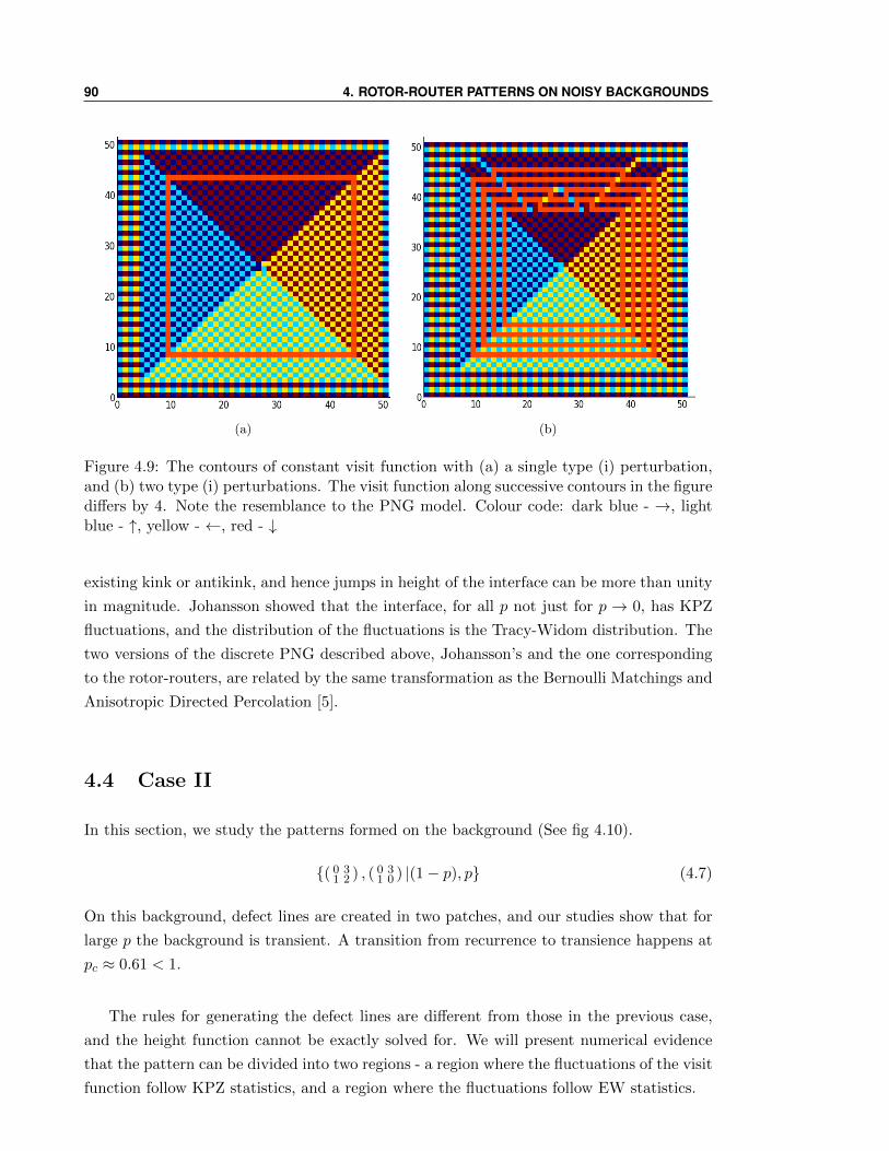
90 4. ROTOR-ROUTER PATTERNS ON NOISY BACKGROUNDS
(a) (b)
Figure 4.9: The contours of constant visit function with (a) a single type (i) perturbation,and (b) two type (i) perturbations. The visit function along successive contours in the figurediffers by 4. Note the resemblance to the PNG model. Colour code: dark blue - →, lightblue - ↑, yellow - ←, red - ↓
existing kink or antikink, and hence jumps in height of the interface can be more than unity
in magnitude. Johansson showed that the interface, for all p not just for p → 0, has KPZ
fluctuations, and the distribution of the fluctuations is the Tracy-Widom distribution. The
two versions of the discrete PNG described above, Johansson’s and the one corresponding
to the rotor-routers, are related by the same transformation as the Bernoulli Matchings and
Anisotropic Directed Percolation [5].
4.4 Case II
In this section, we study the patterns formed on the background (See fig 4.10).
( 0 31 2 ) , ( 0 3
1 0 ) |(1− p), p (4.7)
On this background, defect lines are created in two patches, and our studies show that for
large p the background is transient. A transition from recurrence to transience happens at
pc ≈ 0.61 < 1.
The rules for generating the defect lines are different from those in the previous case,
and the height function cannot be exactly solved for. We will present numerical evidence
that the pattern can be divided into two regions - a region where the fluctuations of the visit
function follow KPZ statistics, and a region where the fluctuations follow EW statistics.
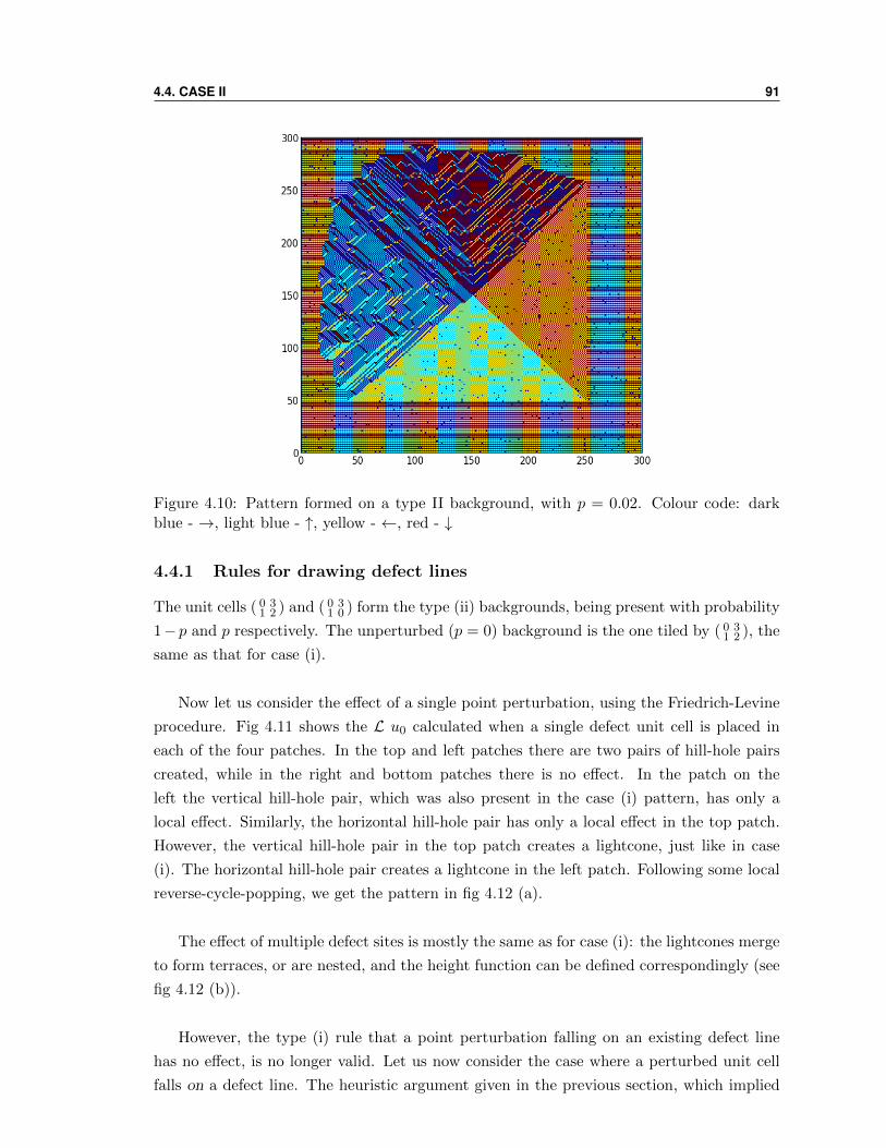
4.4. CASE II 91
Figure 4.10: Pattern formed on a type II background, with p = 0.02. Colour code: darkblue - →, light blue - ↑, yellow - ←, red - ↓
4.4.1 Rules for drawing defect lines
The unit cells ( 0 31 2 ) and ( 0 3
1 0 ) form the type (ii) backgrounds, being present with probability
1− p and p respectively. The unperturbed (p = 0) background is the one tiled by ( 0 31 2 ), the
same as that for case (i).
Now let us consider the effect of a single point perturbation, using the Friedrich-Levine
procedure. Fig 4.11 shows the L u0 calculated when a single defect unit cell is placed in
each of the four patches. In the top and left patches there are two pairs of hill-hole pairs
created, while in the right and bottom patches there is no effect. In the patch on the
left the vertical hill-hole pair, which was also present in the case (i) pattern, has only a
local effect. Similarly, the horizontal hill-hole pair has only a local effect in the top patch.
However, the vertical hill-hole pair in the top patch creates a lightcone, just like in case
(i). The horizontal hill-hole pair creates a lightcone in the left patch. Following some local
reverse-cycle-popping, we get the pattern in fig 4.12 (a).
The effect of multiple defect sites is mostly the same as for case (i): the lightcones merge
to form terraces, or are nested, and the height function can be defined correspondingly (see
fig 4.12 (b)).
However, the type (i) rule that a point perturbation falling on an existing defect line
has no effect, is no longer valid. Let us now consider the case where a perturbed unit cell
falls on a defect line. The heuristic argument given in the previous section, which implied
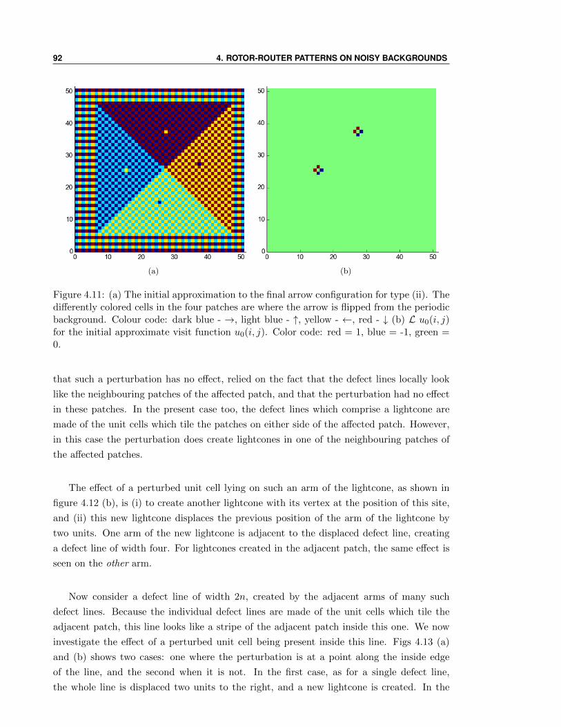
92 4. ROTOR-ROUTER PATTERNS ON NOISY BACKGROUNDS
(a) (b)
Figure 4.11: (a) The initial approximation to the final arrow configuration for type (ii). Thedifferently colored cells in the four patches are where the arrow is flipped from the periodicbackground. Colour code: dark blue - →, light blue - ↑, yellow - ←, red - ↓ (b) L u0(i, j)for the initial approximate visit function u0(i, j). Color code: red = 1, blue = -1, green =0.
that such a perturbation has no effect, relied on the fact that the defect lines locally look
like the neighbouring patches of the affected patch, and that the perturbation had no effect
in these patches. In the present case too, the defect lines which comprise a lightcone are
made of the unit cells which tile the patches on either side of the affected patch. However,
in this case the perturbation does create lightcones in one of the neighbouring patches of
the affected patches.
The effect of a perturbed unit cell lying on such an arm of the lightcone, as shown in
figure 4.12 (b), is (i) to create another lightcone with its vertex at the position of this site,
and (ii) this new lightcone displaces the previous position of the arm of the lightcone by
two units. One arm of the new lightcone is adjacent to the displaced defect line, creating
a defect line of width four. For lightcones created in the adjacent patch, the same effect is
seen on the other arm.
Now consider a defect line of width 2n, created by the adjacent arms of many such
defect lines. Because the individual defect lines are made of the unit cells which tile the
adjacent patch, this line looks like a stripe of the adjacent patch inside this one. We now
investigate the effect of a perturbed unit cell being present inside this line. Figs 4.13 (a)
and (b) shows two cases: one where the perturbation is at a point along the inside edge
of the line, and the second when it is not. In the first case, as for a single defect line,
the whole line is displaced two units to the right, and a new lightcone is created. In the
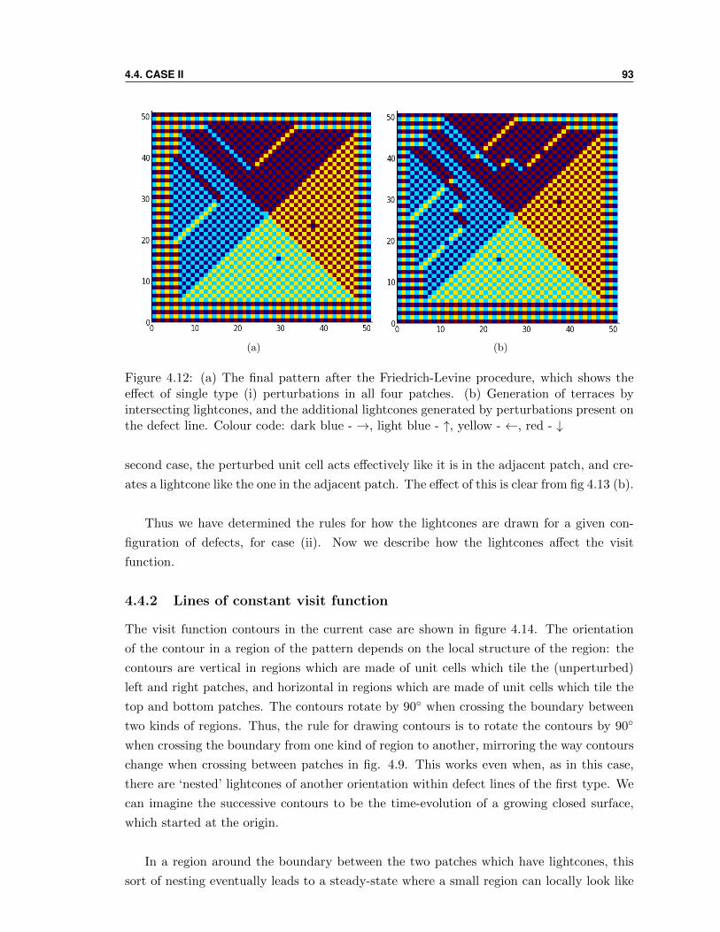
4.4. CASE II 93
(a) (b)
Figure 4.12: (a) The final pattern after the Friedrich-Levine procedure, which shows theeffect of single type (i) perturbations in all four patches. (b) Generation of terraces byintersecting lightcones, and the additional lightcones generated by perturbations present onthe defect line. Colour code: dark blue - →, light blue - ↑, yellow - ←, red - ↓
second case, the perturbed unit cell acts effectively like it is in the adjacent patch, and cre-
ates a lightcone like the one in the adjacent patch. The effect of this is clear from fig 4.13 (b).
Thus we have determined the rules for how the lightcones are drawn for a given con-
figuration of defects, for case (ii). Now we describe how the lightcones affect the visit
function.
4.4.2 Lines of constant visit function
The visit function contours in the current case are shown in figure 4.14. The orientation
of the contour in a region of the pattern depends on the local structure of the region: the
contours are vertical in regions which are made of unit cells which tile the (unperturbed)
left and right patches, and horizontal in regions which are made of unit cells which tile the
top and bottom patches. The contours rotate by 90 when crossing the boundary between
two kinds of regions. Thus, the rule for drawing contours is to rotate the contours by 90
when crossing the boundary from one kind of region to another, mirroring the way contours
change when crossing between patches in fig. 4.9. This works even when, as in this case,
there are ‘nested’ lightcones of another orientation within defect lines of the first type. We
can imagine the successive contours to be the time-evolution of a growing closed surface,
which started at the origin.
In a region around the boundary between the two patches which have lightcones, this
sort of nesting eventually leads to a steady-state where a small region can locally look like
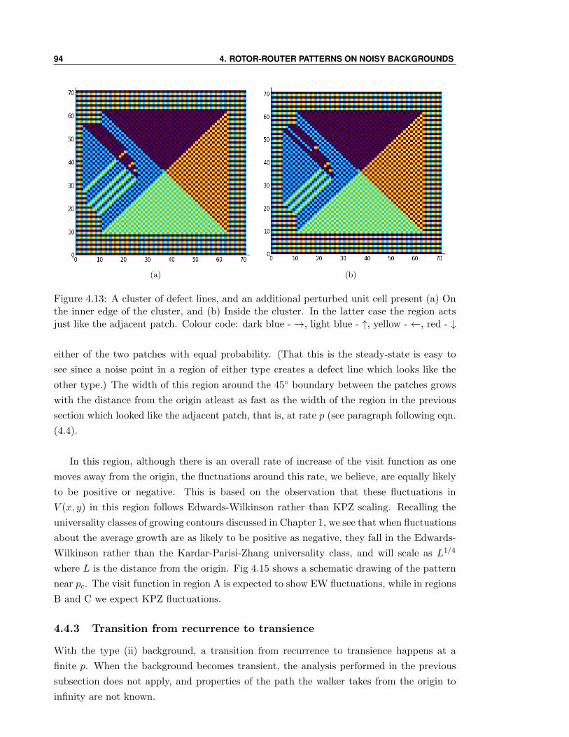
94 4. ROTOR-ROUTER PATTERNS ON NOISY BACKGROUNDS
(a) (b)
Figure 4.13: A cluster of defect lines, and an additional perturbed unit cell present (a) Onthe inner edge of the cluster, and (b) Inside the cluster. In the latter case the region actsjust like the adjacent patch. Colour code: dark blue - →, light blue - ↑, yellow - ←, red - ↓
either of the two patches with equal probability. (That this is the steady-state is easy to
see since a noise point in a region of either type creates a defect line which looks like the
other type.) The width of this region around the 45 boundary between the patches grows
with the distance from the origin atleast as fast as the width of the region in the previous
section which looked like the adjacent patch, that is, at rate p (see paragraph following eqn.
(4.4).
In this region, although there is an overall rate of increase of the visit function as one
moves away from the origin, the fluctuations around this rate, we believe, are equally likely
to be positive or negative. This is based on the observation that these fluctuations in
V (x, y) in this region follows Edwards-Wilkinson rather than KPZ scaling. Recalling the
universality classes of growing contours discussed in Chapter 1, we see that when fluctuations
about the average growth are as likely to be positive as negative, they fall in the Edwards-
Wilkinson rather than the Kardar-Parisi-Zhang universality class, and will scale as L1/4
where L is the distance from the origin. Fig 4.15 shows a schematic drawing of the pattern
near pc. The visit function in region A is expected to show EW fluctuations, while in regions
B and C we expect KPZ fluctuations.
4.4.3 Transition from recurrence to transience
With the type (ii) background, a transition from recurrence to transience happens at a
finite p. When the background becomes transient, the analysis performed in the previous
subsection does not apply, and properties of the path the walker takes from the origin to
infinity are not known.
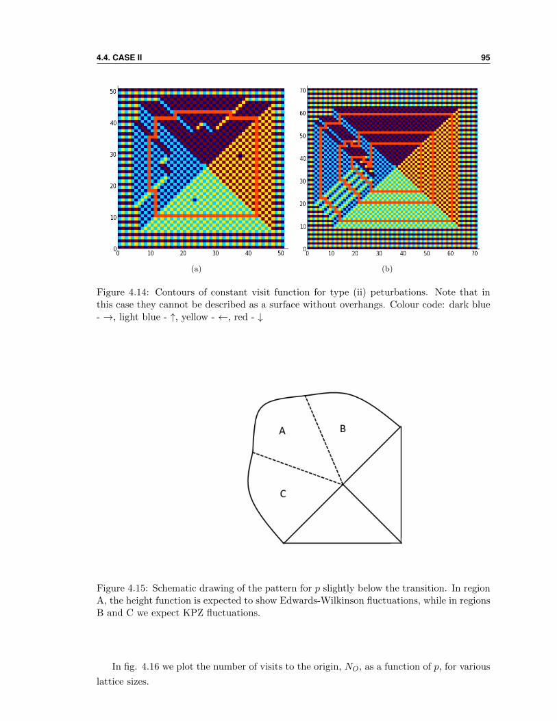
4.4. CASE II 95
(a) (b)
Figure 4.14: Contours of constant visit function for type (ii) peturbations. Note that inthis case they cannot be described as a surface without overhangs. Colour code: dark blue- →, light blue - ↑, yellow - ←, red - ↓
Figure 4.15: Schematic drawing of the pattern for p slightly below the transition. In regionA, the height function is expected to show Edwards-Wilkinson fluctuations, while in regionsB and C we expect KPZ fluctuations.
In fig. 4.16 we plot the number of visits to the origin, NO, as a function of p, for various
lattice sizes.
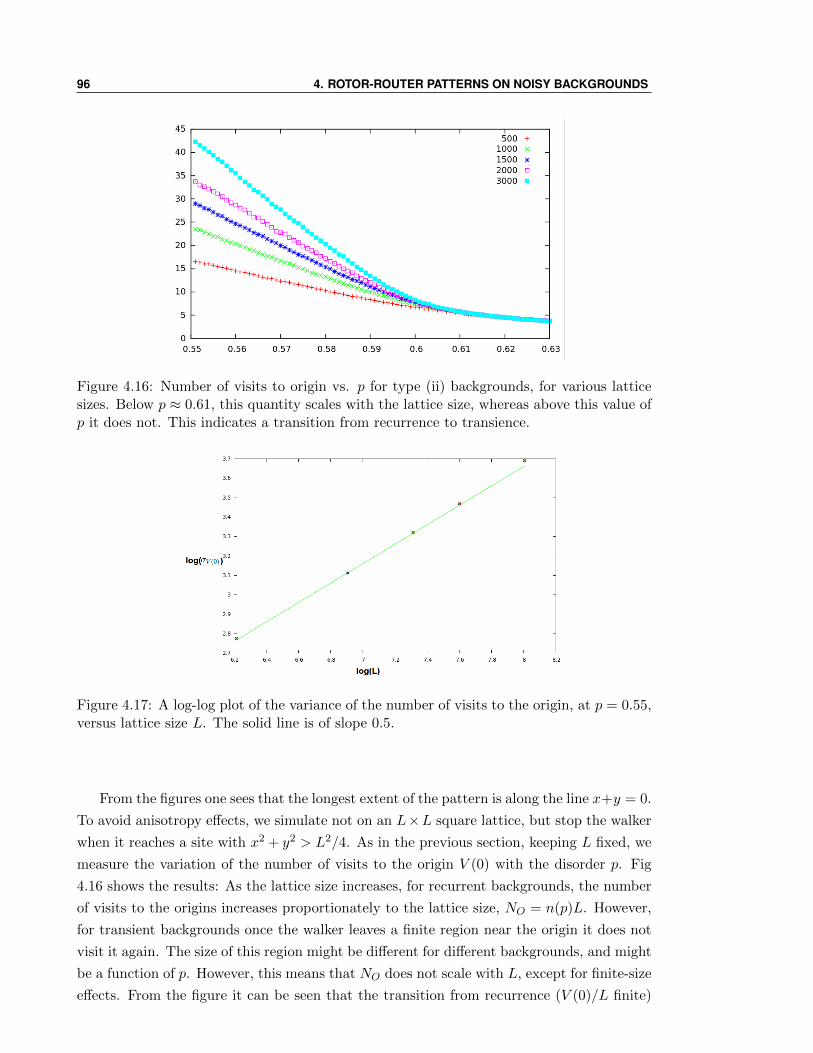
96 4. ROTOR-ROUTER PATTERNS ON NOISY BACKGROUNDS
Figure 4.16: Number of visits to origin vs. p for type (ii) backgrounds, for various latticesizes. Below p ≈ 0.61, this quantity scales with the lattice size, whereas above this value ofp it does not. This indicates a transition from recurrence to transience.
Figure 4.17: A log-log plot of the variance of the number of visits to the origin, at p = 0.55,versus lattice size L. The solid line is of slope 0.5.
From the figures one sees that the longest extent of the pattern is along the line x+y = 0.
To avoid anisotropy effects, we simulate not on an L×L square lattice, but stop the walker
when it reaches a site with x2 + y2 > L2/4. As in the previous section, keeping L fixed, we
measure the variation of the number of visits to the origin V (0) with the disorder p. Fig
4.16 shows the results: As the lattice size increases, for recurrent backgrounds, the number
of visits to the origins increases proportionately to the lattice size, NO = n(p)L. However,
for transient backgrounds once the walker leaves a finite region near the origin it does not
visit it again. The size of this region might be different for different backgrounds, and might
be a function of p. However, this means that NO does not scale with L, except for finite-size
effects. From the figure it can be seen that the transition from recurrence (V (0)/L finite)
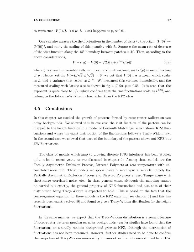
4.5. CONCLUSIONS 97
to transience (V (0)/L→ 0 as L→∞) happens at pc ≈ 0.61.
One can also measure the the fluctuations in the number of visits to the origin, 〈V (0)2〉−〈V (0)〉2, and study the scaling of this quantity with L. Suppose the mean rate of decrease
of the visit function along the 45 boundary between patches is M . Then, according to the
above considerations,
V (−x, y) = V (0)−√
2My + y1/4B(p)ξ (4.8)
where ξ is a random variable with zero mean and unit variance, and B(y) is some function
of p. Hence, setting V (−L/√
2, L/√
2) = 0, we get that V (0) has a mean which scales
as L, and a variance that scales as L1/4. We measured this variance numerically, and the
measured scaling with lattice size is shown in fig 4.17 for p = 0.55. It is seen that the
exponent is quite close to 1/2, which confirms that the rms fluctuations scale as L0.25, and
belong to the Edwards-Wilkinson class rather than the KPZ class.
4.5 Conclusions
In this chapter we studied the growth of patterns formed by rotor-router walkers on two
noisy backgrounds. We showed that in one case the visit function of the pattern can be
mapped to the height function in a model of Bernoulli Matchings, which shows KPZ fluc-
tuations and where the exact distribution of the fluctuations follows a Tracy-Widom law.
In the second case we showed that part of the boundary of the pattern shows not KPZ but
EW fluctuations.
The class of models which map to growing discrete PNG interfaces has been studied
quite a lot in recent years, as was discussed in chapter 1. Among these models are the
Totally Asymmetric Exclusion Process, Directed Polymers at zero temperature with un-
correlated noise, etc. These models are special cases of more general models, namely the
Partially Asymmetric Exclusion Process and Directed Polymers at zero Temperature with
short-range correlated noise, etc. In these general cases, although the mapping cannot
be carried out exactly, the general property of KPZ fluctuations and also that of their
distribution being Tracy-Widom is expected to hold. This is based on the fact that the
coarse-grained equation for these models is the KPZ equation (see chapter 1) and this has
recently been exactly solved [9] and found to give a Tracy-Widom distribution for the height
fluctuations.
In the same manner, we expect that the Tracy-Widom distribution is a generic feature
of rotor-router patterns growing on noisy backgrounds - earlier studies have found that the
fluctuations on a totally random background grow as KPZ, although the distribution of
fluctuations has not been measured. However, further studies need to be done to confirm
the conjecture of Tracy-Widom universality in cases other than the ones studied here. EW

98 4. ROTOR-ROUTER PATTERNS ON NOISY BACKGROUNDS
fluctuations also seem to play a part in some cases. The existence of other backgrounds
showing both KPZ and EW fluctuations in different regions is an open question.
Bibliography
[1] T. Friedrich and L. Levine, Fast simulation of large-scale growth models, Random
Structures & Algorithms 42 185 (2013)
arxiv:1006.1003
[2] A. Z. Broder, Generating random spanning trees, Foundations of Computer Science
442 (1989).
[3] A. M. Povolotsky, V. B. Priezzhev, and R. R. Scherbakov, Phys. Rev. E, 58 5449
(1998).
[4] A. E. Holroyd, and J. Propp, Algorithmic probability and combinatorics, 520 105
(2010)
[5] S. N. Majumdar and S. Nechaev, Phys. Rev. E 72 020901 (2005)
[6] M. Prahofer and H. Spohn, Phys. Rev. Lett 84 4882 (2000)
M. Prahofer and H. Spohn, J. Stat. Phys. 108 1071 (2002)
[7] K. Johansson, Comm. Math. Phys. 242 277 (2003)
[8] R. Rajesh and D. Dhar, Phys. Rev. Lett. 81 1646 (1998)
[9] T. Sasamoto and H. Spohn, J. Stat. Mech. P11013 (2010)
99
Chapter 5
A Class of Active-Absorbing Phase
Transitions
In this chapter, we present the construction and analysis of a class of assisted-hopping mod-
els which show an active-absorbing phase transitions in one dimension. The models are a
generalization of the Conserved Lattice Gas (CLG) model defined in the introduction. The
steady state for all the models in the class can be exactly determined and various quantities
calculated easily with the help of generating functions. We show that, for the model where
the particles have a hopping range n, for n = 1, 2, 3, . . . , the critical exponent β = n. The
model with n = 2 was defined by da Silva and de Oliviera in [1]. The models with n > 2
define previously unknown universality classes for active-absorbing phase transitions.
Models with β > 1 are not typical in equilibrium or non-equilibrium problems. An
important issue here is the correct identification of the order parameter. In the percolation
problem, the fractional number of sites in the backbone [2], the bulk conductance in a ran-
dom resistor network [3] or the rigidity modulus in a random spring network [4] could be
considered as possible order parameters, but these are known to vanish with different powers
than the fractional number of sites in the infinite cluster near the critical point. In the Bose
glass-superfluid transition, the superfluid density at zero temperature grows more slowly
than the density of the fluid which is the tuning parameter [5]. For the active-absorbing
phase transitions we are interested in, this issue is presumably not so contentious, as there
is a natural choice of order parameter, viz. the mean density of activity, which is the choice
we use in this chapter to define β.
The plan of this chapter is as follows: In section 5.1 we define the generalized model. In
section 5.2 we discuss structure of the configuration space for the models. In sections 5.3 and
5.4 we use the technique of generating functions to determined several properties and critical
exponents of the models, with and without an external field conjugate to the activity. In
section 5.5 we present a mapping to a gas of defects with height restriction, which makes it
100
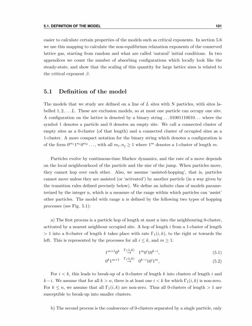
5.1. DEFINITION OF THE MODEL 101
easier to calculate certain properties of the models such as critical exponents. In section 5.6
we use this mapping to calculate the non-equilibrium relaxation exponents of the conserved
lattice gas, starting from random and what are called ‘natural’ initial conditions. In two
appendices we count the number of absorbing configurations which locally look like the
steady-state, and show that the scaling of this quantity for large lattice sizes is related to
the critical exponent β.
5.1 Definition of the model
The models that we study are defined on a line of L sites with N particles, with sites la-
belled 1, 2, . . . L. These are exclusion models, so at most one particle can occupy one site.
A configuration on the lattice is denoted by a binary string . . . 01001110010. . . where the
symbol 1 denotes a particle and 0 denotes an empty site. We call a connected cluster of
empty sites as a 0-cluster (of that length) and a connected cluster of occupied sites as a
1-cluster. A more compact notation for the binary string which denotes a configuration is
of the form 0m11n10m2 . . . , with all mi, nj ≥ 1 where 1m denotes a 1-cluster of length m.
Particles evolve by continuous-time Markov dynamics, and the rate of a move depends
on the local neighbourhood of the particle and the size of the jump. When particles move,
they cannot hop over each other. Also, we assume ‘assisted-hopping’, that is, particles
cannot move unless they are assisted (or ‘activated’) by another particle (in a way given by
the transition rules defined precisely below). We define an infinite class of models parame-
terized by the integer n, which is a measure of the range within which particles can ‘assist’
other particles. The model with range n is defined by the following two types of hopping
processes (see Fig. 5.1):
a) The first process is a particle hop of length at most n into the neighbouring 0-cluster,
activated by a nearest neighbour occupied site. A hop of length i from a 1-cluster of length
> 1 into a 0-cluster of length k takes place with rate Γ1(i, k), to the right or towards the
left. This is represented by the processes for all i ≤ k, and m ≥ 1:
1m+10kΓ1(i,k)→ 1m0i10k−i, (5.1)
0k1m+1 Γ1(i,k)→ 0k−i10i1m, (5.2)
For i < k, this leads to break-up of a 0-cluster of length k into clusters of length i and
k− i. We assume that for all k > n, there is at least one i < k for which Γ1(i, k) is non-zero.
For k ≤ n, we assume that all Γ1(i, k) are non-zero. Thus all 0-clusters of length > 1 are
susceptible to break-up into smaller clusters.
b) The second process is the coalescence of 0-clusters separated by a single particle, only
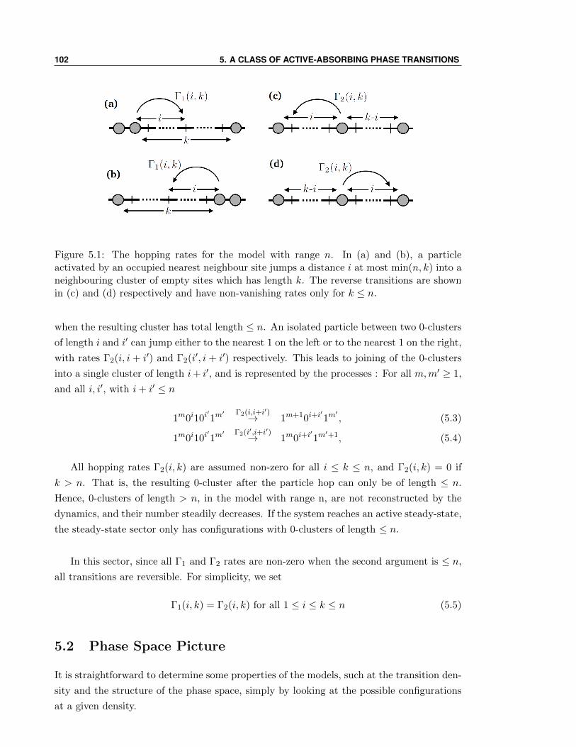
102 5. A CLASS OF ACTIVE-ABSORBING PHASE TRANSITIONS
Figure 5.1: The hopping rates for the model with range n. In (a) and (b), a particleactivated by an occupied nearest neighbour site jumps a distance i at most min(n, k) into aneighbouring cluster of empty sites which has length k. The reverse transitions are shownin (c) and (d) respectively and have non-vanishing rates only for k ≤ n.
when the resulting cluster has total length ≤ n. An isolated particle between two 0-clusters
of length i and i′ can jump either to the nearest 1 on the left or to the nearest 1 on the right,
with rates Γ2(i, i + i′) and Γ2(i′, i + i′) respectively. This leads to joining of the 0-clusters
into a single cluster of length i+ i′, and is represented by the processes : For all m,m′ ≥ 1,
and all i, i′, with i+ i′ ≤ n
1m0i10i′1m
′ Γ2(i,i+i′)→ 1m+10i+i′1m
′, (5.3)
1m0i10i′1m
′ Γ2(i′,i+i′)→ 1m0i+i′1m
′+1, (5.4)
All hopping rates Γ2(i, k) are assumed non-zero for all i ≤ k ≤ n, and Γ2(i, k) = 0 if
k > n. That is, the resulting 0-cluster after the particle hop can only be of length ≤ n.
Hence, 0-clusters of length > n, in the model with range n, are not reconstructed by the
dynamics, and their number steadily decreases. If the system reaches an active steady-state,
the steady-state sector only has configurations with 0-clusters of length ≤ n.
In this sector, since all Γ1 and Γ2 rates are non-zero when the second argument is ≤ n,
all transitions are reversible. For simplicity, we set
Γ1(i, k) = Γ2(i, k) for all 1 ≤ i ≤ k ≤ n (5.5)
5.2 Phase Space Picture
It is straightforward to determine some properties of the models, such at the transition den-
sity and the structure of the phase space, simply by looking at the possible configurations
at a given density.
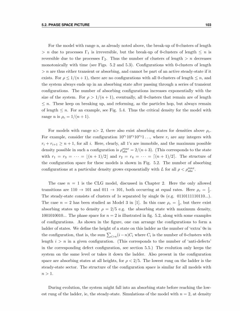
5.2. PHASE SPACE PICTURE 103
For the model with range n, as already noted above, the break-up of 0-clusters of length
> n due to processes Γ1 is irreversible, but the break-up of 0-clusters of length ≤ n is
reversible due to the processes Γ2. Thus the number of clusters of length > n decreases
monotonically with time (see Figs. 5.2 and 5.3). Configurations with 0-clusters of length
> n are thus either transient or absorbing, and cannot be part of an active steady-state if it
exists. For ρ ≤ 1/(n+ 1), there are no configurations with all 0-clusters of length ≤ n, and
the system always ends up in an absorbing state after passing through a series of transient
configurations. The number of absorbing configurations increases exponentially with the
size of the system. For ρ > 1/(n + 1), eventually, all 0-clusters that remain are of length
≤ n. These keep on breaking up, and reforming, as the particles hop, but always remain
of length ≤ n. For an example, see Fig. 5.4. Thus the critical density for the model with
range n is ρc = 1/(n+ 1).
For models with range n> 2, there also exist absorbing states for densities above ρc.
For example, consider the configuration 10r110r210r31 . . ., where ri are any integers with
ri + ri+1 ≥ n + 1, for all i. Here, clearly, all 1’s are immobile, and the maximum possible
density possible in such a configuration is ρmaxabs = 2/(n+ 3). (This corresponds to the state
with r1 = r3 = · · · = b(n + 1)/2c and r2 = r4 = · · · = d(n + 1)/2e. The structure of
the configuration space for these models is shown in Fig. 5.2. The number of absorbing
configurations at a particular density grows exponentially with L for all ρ < ρmaxabs .
The case n = 1 is the CLG model, discussed in Chapter 2. Here the only allowed
transitions are 110 → 101 and 011 → 101, both occurring at equal rates. Here ρc = 12 .
The steady-state consists of clusters of 1s separated by single 0s (e.g. 0110111110110...).
The case n = 2 has been studied as Model 3 in [1]. In this case ρc = 13 , but there exist
absorbing states up to density ρ = 2/5 e.g. the absorbing state with maximum density,
1001010010... The phase space for n = 2 is illustrated in fig. 5.2, along with some examples
of configurations. As shown in the figure, one can arrange the configurations to form a
ladder of states. We define the height of a state on this ladder as the number of ‘extra’ 0s in
the configuration, that is, the sum∑
i>n(i−n)Ci where Ci is the number of 0-clusters with
length i > n in a given configuration. (This corresponds to the number of ‘anti-defects’
in the corresponding defect configuration, see section 5.5.) The evolution only keeps the
system on the same level or takes it down the ladder. Also present in the configuration
space are absorbing states at all heights, for ρ < 2/5. The lowest rung on the ladder is the
steady-state sector. The structure of the configuration space is similar for all models with
n > 1.
During evolution, the system might fall into an absorbing state before reaching the low-
est rung of the ladder, ie, the steady-state. Simulations of the model with n = 2, at density
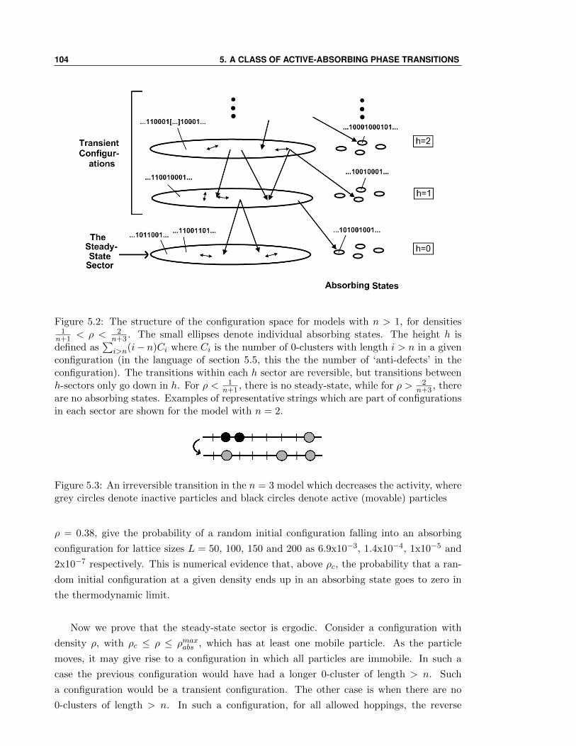
104 5. A CLASS OF ACTIVE-ABSORBING PHASE TRANSITIONS
Figure 5.2: The structure of the configuration space for models with n > 1, for densities1
n+1 < ρ < 2n+3 . The small ellipses denote individual absorbing states. The height h is
defined as∑
i>n(i− n)Ci where Ci is the number of 0-clusters with length i > n in a givenconfiguration (in the language of section 5.5, this the the number of ‘anti-defects’ in theconfiguration). The transitions within each h sector are reversible, but transitions betweenh-sectors only go down in h. For ρ < 1
n+1 , there is no steady-state, while for ρ > 2n+3 , there
are no absorbing states. Examples of representative strings which are part of configurationsin each sector are shown for the model with n = 2.
Figure 5.3: An irreversible transition in the n = 3 model which decreases the activity, wheregrey circles denote inactive particles and black circles denote active (movable) particles
ρ = 0.38, give the probability of a random initial configuration falling into an absorbing
configuration for lattice sizes L = 50, 100, 150 and 200 as 6.9x10⁻³, 1.4x10⁻⁴, 1x10⁻⁵ and
2x10⁻⁷ respectively. This is numerical evidence that, above ρc, the probability that a ran-
dom initial configuration at a given density ends up in an absorbing state goes to zero in
the thermodynamic limit.
Now we prove that the steady-state sector is ergodic. Consider a configuration with
density ρ, with ρc ≤ ρ ≤ ρmaxabs , which has at least one mobile particle. As the particle
moves, it may give rise to a configuration in which all particles are immobile. In such a
case the previous configuration would have had a longer 0-cluster of length > n. Such
a configuration would be a transient configuration. The other case is when there are no
0-clusters of length > n. In such a configuration, for all allowed hoppings, the reverse
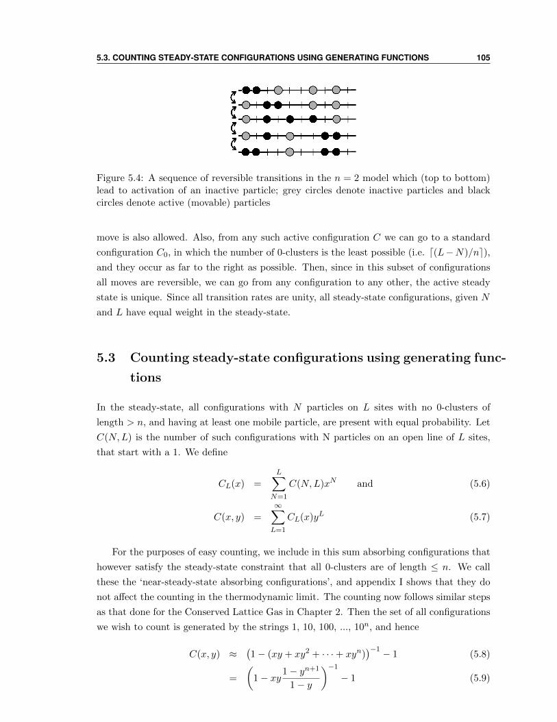
5.3. COUNTING STEADY-STATE CONFIGURATIONS USING GENERATING FUNCTIONS 105
Figure 5.4: A sequence of reversible transitions in the n = 2 model which (top to bottom)lead to activation of an inactive particle; grey circles denote inactive particles and blackcircles denote active (movable) particles
move is also allowed. Also, from any such active configuration C we can go to a standard
configuration C0, in which the number of 0-clusters is the least possible (i.e. d(L−N)/ne),and they occur as far to the right as possible. Then, since in this subset of configurations
all moves are reversible, we can go from any configuration to any other, the active steady
state is unique. Since all transition rates are unity, all steady-state configurations, given N
and L have equal weight in the steady-state.
5.3 Counting steady-state configurations using generating func-
tions
In the steady-state, all configurations with N particles on L sites with no 0-clusters of
length > n, and having at least one mobile particle, are present with equal probability. Let
C(N,L) is the number of such configurations with N particles on an open line of L sites,
that start with a 1. We define
CL(x) =
L∑N=1
C(N,L)xN and (5.6)
C(x, y) =
∞∑L=1
CL(x)yL (5.7)
For the purposes of easy counting, we include in this sum absorbing configurations that
however satisfy the steady-state constraint that all 0-clusters are of length ≤ n. We call
these the ‘near-steady-state absorbing configurations’, and appendix I shows that they do
not affect the counting in the thermodynamic limit. The counting now follows similar steps
as that done for the Conserved Lattice Gas in Chapter 2. Then the set of all configurations
we wish to count is generated by the strings 1, 10, 100, ..., 10n, and hence
C(x, y) ≈(1− (xy + xy2 + · · ·+ xyn)
)−1 − 1 (5.8)
=
(1− xy1− yn+1
1− y
)−1
− 1 (5.9)
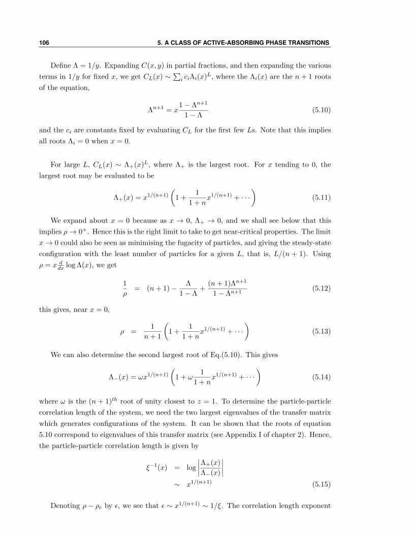
106 5. A CLASS OF ACTIVE-ABSORBING PHASE TRANSITIONS
Define Λ = 1/y. Expanding C(x, y) in partial fractions, and then expanding the various
terms in 1/y for fixed x, we get CL(x) ∼∑
i ciΛi(x)L, where the Λi(x) are the n+ 1 roots
of the equation,
Λn+1 = x1− Λn+1
1− Λ(5.10)
and the ci are constants fixed by evaluating CL for the first few Ls. Note that this implies
all roots Λi = 0 when x = 0.
For large L, CL(x) ∼ Λ+(x)L, where Λ+ is the largest root. For x tending to 0, the
largest root may be evaluated to be
Λ+(x) = x1/(n+1)
(1 +
1
1 + nx1/(n+1) + · · ·
)(5.11)
We expand about x = 0 because as x → 0, Λ+ → 0, and we shall see below that this
implies ρ→ 0+. Hence this is the right limit to take to get near-critical properties. The limit
x→ 0 could also be seen as minimising the fugacity of particles, and giving the steady-state
configuration with the least number of particles for a given L, that is, L/(n + 1). Using
ρ = x ddx log Λ(x), we get
1
ρ= (n+ 1)− Λ
1− Λ+
(n+ 1)Λn+1
1− Λn+1(5.12)
this gives, near x = 0,
ρ =1
n+ 1
(1 +
1
1 + nx1/(n+1) + · · ·
)(5.13)
We can also determine the second largest root of Eq.(5.10). This gives
Λ−(x) = ωx1/(n+1)
(1 + ω
1
1 + nx1/(n+1) + · · ·
)(5.14)
where ω is the (n + 1)th root of unity closest to z = 1. To determine the particle-particle
correlation length of the system, we need the two largest eigenvalues of the transfer matrix
which generates configurations of the system. It can be shown that the roots of equation
5.10 correspond to eigenvalues of this transfer matrix (see Appendix I of chapter 2). Hence,
the particle-particle correlation length is given by
ξ−1(x) = log
∣∣∣∣Λ+(x)
Λ−(x)
∣∣∣∣∼ x1/(n+1) (5.15)
Denoting ρ− ρc by ε, we see that ε ∼ x1/(n+1) ∼ 1/ξ. The correlation length exponent
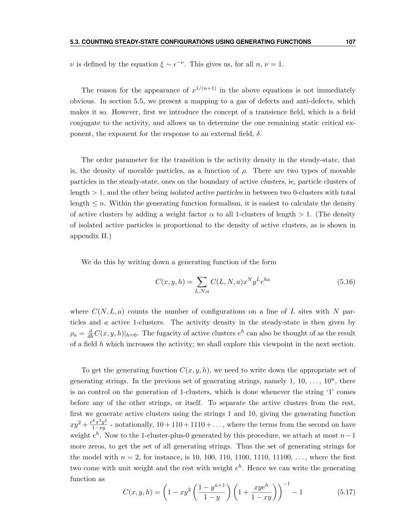
5.3. COUNTING STEADY-STATE CONFIGURATIONS USING GENERATING FUNCTIONS 107
ν is defined by the equation ξ ∼ ε−ν . This gives us, for all n, ν = 1.
The reason for the appearance of x1/(n+1) in the above equations is not immediately
obvious. In section 5.5, we present a mapping to a gas of defects and anti-defects, which
makes it so. However, first we introduce the concept of a transience field, which is a field
conjugate to the activity, and allows us to determine the one remaining static critical ex-
ponent, the exponent for the response to an external field, δ.
The order parameter for the transition is the activity density in the steady-state, that
is, the density of movable particles, as a function of ρ. There are two types of movable
particles in the steady-state, ones on the boundary of active clusters, ie, particle clusters of
length > 1, and the other being isolated active particles in between two 0-clusters with total
length ≤ n. Within the generating function formalism, it is easiest to calculate the density
of active clusters by adding a weight factor α to all 1-clusters of length > 1. (The density
of isolated active particles is proportional to the density of active clusters, as is shown in
appendix II.)
We do this by writing down a generating function of the form
C(x, y, h) =∑L,N,a
C(L,N, a)xNyLeha (5.16)
where C(N,L, a) counts the number of configurations on a line of L sites with N par-
ticles and a active 1-clusters. The activity density in the steady-state is then given by
ρa = ddhC(x, y, h)|h=0. The fugacity of active clusters eh can also be thought of as the result
of a field h which increases the activity; we shall explore this viewpoint in the next section.
To get the generating function C(x, y, h), we need to write down the appropriate set of
generating strings. In the previous set of generating strings, namely 1, 10, . . . , 10n, there
is no control on the generation of 1-clusters, which is done whenever the string ‘1’ comes
before any of the other strings, or itself. To separate the active clusters from the rest,
first we generate active clusters using the strings 1 and 10, giving the generating function
xy2 + ehx2y3
1−xy - notationally, 10 + 110 + 1110 + . . . , where the terms from the second on have
weight eh. Now to the 1-cluster-plus-0 generated by this procedure, we attach at most n−1
more zeros, to get the set of all generating strings. Thus the set of generating strings for
the model with n = 2, for instance, is 10, 100, 110, 1100, 1110, 11100, . . . , where the first
two come with unit weight and the rest with weight eh. Hence we can write the generating
function as
C(x, y, h) =
(1− xy2
(1− yn+1
1− y
)(1 +
xyeh
1− xy
))−1
− 1 (5.17)
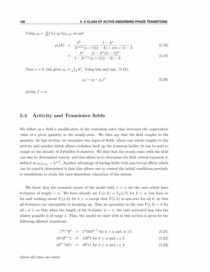
108 5. A CLASS OF ACTIVE-ABSORBING PHASE TRANSITIONS
Using ρa = ddhC(x, y, h)|h=0, we get
ρa(Λ) =x2
Λn+2
1− Λn
(n+ 1)(1− Λ) + x(n+ 1)− Λ(5.18)
=Λn
1− Λn+1
(1− Λn)(1− Λ)2
(n+ 1)(1− Λ)− Λ(5.19)
Near x = 0, this gives ρa ≈ 1n+1Λn. Using this and eqn. (5.12),
ρa ∼ (ρ− ρc)n (5.20)
giving β = n.
5.4 Activity and Transience fields
We define as a field a modification of the transition rates that increases the expectation
value of a given quantity in the steady-state. We then say that the field couples to the
quantity. In this section, we introduce two types of fields, where one which couples to the
activity and another which allows evolution back up the transient ladder (it can be said to
couple to the density of forbidden 0-clusters). We find that the steady-state with the field
can also be determined exactly, and this allows us to determine the field critical exponent δ,
defined as ρa|ρ=ρc ∼ h1/δ. Another advantage of having fields with non-trivial effects which
can be exactly determined is that this allows one to control the initial conditions precisely
in simulations to study the time-dependent relaxation of the system.
We know that the transient states of the model with β = n are the ones which have
0-clusters of length > n. We have already set Γ1(i, k) = Γ2(i, k) for k ≤ n, but have so
far said nothing about Γ1(i, k) for k > n except that Γ(1, k) is non-zero for all k, so that
all 0-clusters are susceptible to breaking up. Now we specialise to the case Γ(i, k) = 0 for
all i 6= 1, so that when the length of the 0-cluster is > n, the only activated hop into the
cluster possible is of range 1. Thus, the model we start with in this section is given by the
following allowed transitions
1m+10k → 1m010k−1 for k > n and m ≥1 (5.21)
10i10k−i1 110k1 for k ≤ n and i ≤ k (5.22)
10k−i10i1 10k11 for k ≤ n and i ≤ k (5.23)
where all rates are unity.
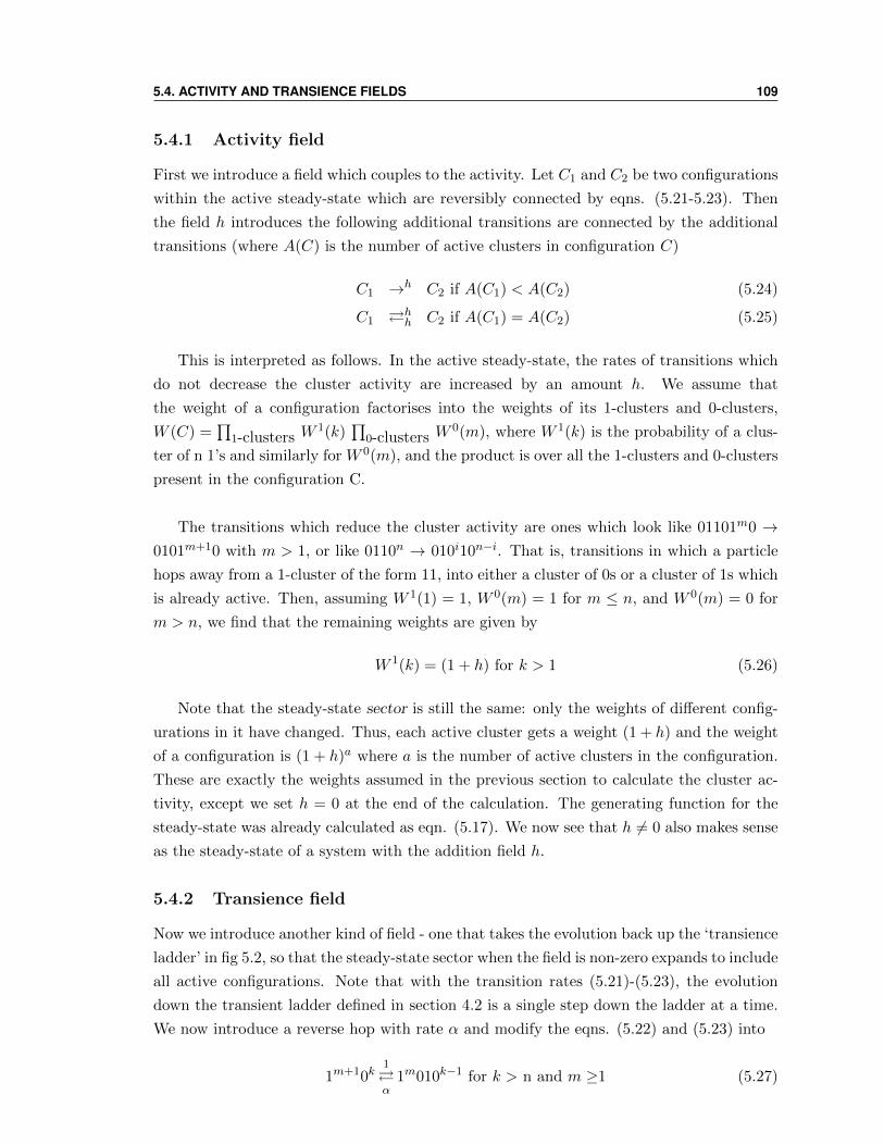
5.4. ACTIVITY AND TRANSIENCE FIELDS 109
5.4.1 Activity field
First we introduce a field which couples to the activity. Let C1 and C2 be two configurations
within the active steady-state which are reversibly connected by eqns. (5.21-5.23). Then
the field h introduces the following additional transitions are connected by the additional
transitions (where A(C) is the number of active clusters in configuration C)
C1 →h C2 if A(C1) < A(C2) (5.24)
C1 hh C2 if A(C1) = A(C2) (5.25)
This is interpreted as follows. In the active steady-state, the rates of transitions which
do not decrease the cluster activity are increased by an amount h. We assume that
the weight of a configuration factorises into the weights of its 1-clusters and 0-clusters,
W (C) =∏
1-clusters W1(k)
∏0-clusters W
0(m), where W 1(k) is the probability of a clus-
ter of n 1’s and similarly for W 0(m), and the product is over all the 1-clusters and 0-clusters
present in the configuration C.
The transitions which reduce the cluster activity are ones which look like 01101m0 →0101m+10 with m > 1, or like 0110n → 010i10n−i. That is, transitions in which a particle
hops away from a 1-cluster of the form 11, into either a cluster of 0s or a cluster of 1s which
is already active. Then, assuming W 1(1) = 1, W 0(m) = 1 for m ≤ n, and W 0(m) = 0 for
m > n, we find that the remaining weights are given by
W 1(k) = (1 + h) for k > 1 (5.26)
Note that the steady-state sector is still the same: only the weights of different config-
urations in it have changed. Thus, each active cluster gets a weight (1 + h) and the weight
of a configuration is (1 + h)a where a is the number of active clusters in the configuration.
These are exactly the weights assumed in the previous section to calculate the cluster ac-
tivity, except we set h = 0 at the end of the calculation. The generating function for the
steady-state was already calculated as eqn. (5.17). We now see that h 6= 0 also makes sense
as the steady-state of a system with the addition field h.
5.4.2 Transience field
Now we introduce another kind of field - one that takes the evolution back up the ‘transience
ladder’ in fig 5.2, so that the steady-state sector when the field is non-zero expands to include
all active configurations. Note that with the transition rates (5.21)-(5.23), the evolution
down the transient ladder defined in section 4.2 is a single step down the ladder at a time.
We now introduce a reverse hop with rate α and modify the eqns. (5.22) and (5.23) into
1m+10k1α
1m010k−1 for k > n and m ≥1 (5.27)
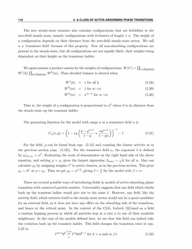
110 5. A CLASS OF ACTIVE-ABSORBING PHASE TRANSITIONS
The new steady-state measure also contains configurations that are forbidden in the
zero-field steady-state, namely configurations with 0-clusters of length > n. The weight of
a configuration depends on their distance from the zero-field steady-state sector. We call
α a ‘transience field’ because of this property. Now all non-absorbing configurations are
present in the steady-state, but all configurations are not equally likely, their weights being
dependent on their height on the transience ladder.
We again assume a product ansatz for the weights of configurations: W (C) =∏
1-clustersW 1(k)
∏0-clusters W
0(m). Then detailed balance is obeyed when
W 1(k) = 1 for all k (5.28)
W 0(m) = 1 for m <n (5.29)
W 0(m) = αm−n for m >n (5.30)
That is, the weight of a configuration is proportional to αd where d is its distance from
the steady-state up the transient ladder.
The generating function for the model with range n in a transience field α is
Cα(x, y) =
(1− xy
(y − yn+1
1− y+αyn+1
1− yα
))−1
− 1 (5.31)
For the field, ρ can be found from eqn. (5.12) and counting the cluster activity as in
the previous section (eqn. (5.19)). For the transience field α, the exponent δ is defined
by ρa|ρ=ρc ∼ αδ. Evaluating the roots of denominator on the right hand side of the above
equation, and setting ρ = ρc gives the largest eigenvalue Λmax ∼√α for all n. One can
calculate ρa by assigning weights eh to active clusters, as in the previous section. This gives
ρa ∼ Λn at ρ = ρc. Thus we get ρa ∼ αn/2, giving δ = n2 for the model with β = n.
There are several possible ways of introducing fields in models of active-absorbing phase
transition with conserved particle number. Universality suggests that any field which climbs
back up the transient ladder would give rise to the same δ. However, any field, like the
activity field, which restricts itself to the steady-state sector would not be a good candidate
for an external field, as it does not have any effect on the absorbing side of the transition,
and hence at the critical point. In the context of the CLG, Lubeck ([6])used as a field
a random hopping process in which all particles hop at a rate a to one of their available
neighbours. In the case of the models defined here, we see that this field can indeed take
the evolution back up the transient ladder. This field changes the transition rates in eqn.
5.27 to
1m+10k1+aa
1m010k−1 for k > n and m ≥1 (5.32)
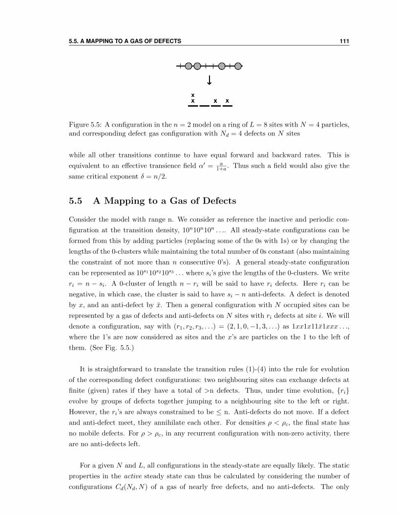
5.5. A MAPPING TO A GAS OF DEFECTS 111
Figure 5.5: A configuration in the n = 2 model on a ring of L = 8 sites with N = 4 particles,and corresponding defect gas configuration with Nd = 4 defects on N sites
while all other transitions continue to have equal forward and backward rates. This is
equivalent to an effective transience field α′ = a1+a . Thus such a field would also give the
same critical exponent δ = n/2.
5.5 A Mapping to a Gas of Defects
Consider the model with range n. We consider as reference the inactive and periodic con-
figuration at the transition density, 10n10n10n . . .. All steady-state configurations can be
formed from this by adding particles (replacing some of the 0s with 1s) or by changing the
lengths of the 0-clusters while maintaining the total number of 0s constant (also maintaining
the constraint of not more than n consecutive 0’s). A general steady-state configuration
can be represented as 10s110s210s3 . . . where si’s give the lengths of the 0-clusters. We write
ri = n − si. A 0-cluster of length n − ri will be said to have ri defects. Here ri can be
negative, in which case, the cluster is said to have si − n anti-defects. A defect is denoted
by x, and an anti-defect by x. Then a general configuration with N occupied sites can be
represented by a gas of defects and anti-defects on N sites with ri defects at site i. We will
denote a configuration, say with (r1, r2, r3, . . .) = (2, 1, 0,−1, 3, . . .) as 1xx1x11x1xxx . . .,
where the 1’s are now considered as sites and the x’s are particles on the 1 to the left of
them. (See Fig. 5.5.)
It is straightforward to translate the transition rules (1)-(4) into the rule for evolution
of the corresponding defect configurations: two neighbouring sites can exchange defects at
finite (given) rates if they have a total of >n defects. Thus, under time evolution, rievolve by groups of defects together jumping to a neighbouring site to the left or right.
However, the ri’s are always constrained to be ≤ n. Anti-defects do not move. If a defect
and anti-defect meet, they annihilate each other. For densities ρ < ρc, the final state has
no mobile defects. For ρ > ρc, in any recurrent configuration with non-zero activity, there
are no anti-defects left.
For a given N and L, all configurations in the steady-state are equally likely. The static
properties in the active steady state can thus be calculated by considering the number of
configurations Cd(Nd, N) of a gas of nearly free defects, and no anti-defects. The only
112 5. A CLASS OF ACTIVE-ABSORBING PHASE TRANSITIONS
constraint is that no site can have more than n defects. Adding one particle is equivalent
to adding (n + 1) defects. These defects unbind, and at low densities, form a nearly ideal
gas. The fugacity associated with one defect is x1/(n+1), and forms a natural variable to
describe properties of this gas.
Since all allowed configurations with a fixed number Nd = (n+1)N−L defects on N sites
are equally likely, we can define the generating function Cd(w, z) =∑
Nd=0,N=1Cd(Nd, N)wNdzN .
It can be verified that Cd(w, z) = C(x = zwn, y = 1/w).
In terms of defects, the activity is the probability that two neighbouring sites have a total
of ≥ n, but strictly less than 2n defects. (If two neighbouring sites have 2n defects then the
original configuration is 111, and hence the middle particle cannot move.) This probability
can be calculated to give (using the fact that in the thermodynamic limit w = 1/y = Λ+)
ρa = ρΛn(n+ 1)− (n+ 2)Λ− Λn + 2Λn+1
(1− Λn+1)2(5.33)
Near the transition, since the gas of defects is nearly ideal, the probability of two neigh-
bouring sites having a total of ≥ n defects varies as n-th power of density of defects, hence
as εn. As the exponent β by the variation of the mean activity as a function of (ρ − ρc),ρ ∼ (ρ− ρc)β, this immediately gives us that β = n.
5.6 Non-equilibrium exponents of the Conserved Lattice Gas
In this section we take the first step towards a description of the non-equilibrium dynamics
of the models defined by equations (5.1)-(5.4), by analysing the evolution of the conserved
lattice gas (our model with n = 1) starting from various initial conditions and deriving the
non-equilibrium exponents θ and z defined in Chapter 2. The dynamics of the CLG has
been studied earlier, and the analysis is non-trivial and the dynamical exponents seem to
be initial-condition dependent. The non-equilibrium evolution of the CLG starting from
random initial conditions was studied numerically by Lee and Lee in [7] and [8] through
a finite-size-scaling analysis, and the study of the evolution from certain initial conditions
closer to the steady-state was done by Bondyopadhyay [9], who found a different set of
exponents. We explain this discrepancy by showing the existence of two scaling regimes,
based on the initial conditions, with different consistent sets of exponents.
5.6.1 Steady-state exponents
Active-absorbing transitions, as mentioned in Chapter 2, are characterized by four steady-
state exponents, defined by the scaling of the following quantities near the critical point, in
5.6. NON-EQUILIBRIUM EXPONENTS OF THE CONSERVED LATTICE GAS 113
the steady-state:
ρa ∼ (ρ− ρc)β (5.34)
ρa|ρ=ρc ∼ hδ (5.35)
C(r, ρ) ∼ f(r1/ν⊥(ρ− ρc)) (5.36)
C(t, ρ) ∼ f(t−ν‖(ρ− ρc)) (5.37)
where C(r, ρ) is the equal-time density-density correlation function, and C(t, ρ) is the auto-
correlation function for the density. We have already derived that for the CLG, β = ν⊥ = 1
and δ = 1/2. We now determine the behaviour of the autocorrelation function of the density.
We work close to the critical point ρ = 1/2, in the low-activity limit. Denote the density
indicator variable at the site i by νi. The mapping to defects defined in the previous section
maps the CLG to a symmetric exclusion process on N sites. Here we provide a slightly
different mapping to an exclusion process on L sites, on the dual lattice. Denoting the
occupation variable on the dual lattice site between sites i and i+ 1 on the original lattice
by bi+ 12, the mapping is given by bi+ 1
2= νiνi+1. We shall denote dual sites with b = 0
by an empty circle, , and those with b = 1 by a filled circle, •. The CLG configuration
101101011101 on the set of sites 0,1,2,. . . ,10,11 then corresponds to the dual lattice configu-
ration ••• on the sites 12 ,11
2 ,. . . , 912 101
2 . Note that any two • s are separated by
an even number of s. The transition 1101→ 1011 translates to a two-site hop • → •.
We want to consider the density autocorrelation function 〈νi(0)νi(t)〉. This is equal to
the probability P (νi(t) = 1|νi(0) = 1) × P (νi(0) = 1). Consider the transition (after two
hops) 101011 → 110101, or in dual language, • → • . Note that the parity of
the sites 2 to 5 flipped from 0 to 1 or vice versa in this transition. The parity of site i thus
stays the same after a time t if there have been an even number of hops i − 12 to i + 1
2 in
that time (hops the other way are counted as negative). P (νi(t) = 1|νi(0) = 1) is simply
equal to the probability that there have been an even number of flips from 1 to 0 or back,
and is equal to the probability that there have been even number of hops across the bond
on the dual lattice which corresponds to this site, in time t. The process on the dual lattice
is an undirected exclusion process with a finite-range of hopping. It is known that, for a
symmetric exclusion process with finite-range hops, the probability that there are a total
of m hoppings across a given bond, in time t, is given for large times by [10]
P (m, t) ≈ N exp
(− m2
A(ρd)√t
)(5.38)
where A(ρd) is a function of the density of the particles and N denotes the normalization
constant. For low densities ρd 1, A(ρd) ≈ Cρd where C is a constant that depends on the
model. This can be seen by taking the continuum limit for low density, where we imagine
114 5. A CLASS OF ACTIVE-ABSORBING PHASE TRANSITIONS
the particles to be point particles in a continuum. Then the particles perform independent
random walks with a diffusion constant which depends on the model, with the exclusion
interaction corresponding only to an exchange of particle labels when two random walkers
cross. The number of walkers on the right of the origin which end up on the left after time
t can then be shown be to a Poisson random variable with paramter λ = ρ√Dt/π [11], and
the same for the walkers on the left of the origin which end up on the right. The difference
between these Poisson distributions then gives eqn. (5.38) with A(ρd) ≈ 2ρ√D/π for small
ρ.
The sum over allm can be expressed in terms of Jacobi theta functions as N ϑ(0; i a(ρd, t)),
where a(ρd, t) = 1/A(ρd)√t. Setting this sum to 1 gives N = (ϑ(0; i a(ρd, t)))
−1. The differ-
ence between the even and odd sums is ϑ(12 ; i a(ρd, t)). Expanding these in MathematicaTM
for small a(ρd, t) (large times), we get the final answer
P (νi(t) = 1|νi(0) = 1) ≈ 1
2+ exp (−A(ρd)
√t) (5.39)
Thus the connected part of the correlation function, for large times, has a stretched
exponential form exp−(√t/τ) where τ ∼ ρ−2
d ∼ (ρ− ρc)−2. Hence the exponent ν‖ defined
according to eqn. (5.37) is 2.
However, in this case the density autocorrelation function is a special observable - it
depends only on the particles hopping across a bond on the dual lattice. A more general
observable, for example the activity autocorrelation function, depends also on the auto-
correlation of the density in the dual lattice exclusion process. (The activity, for low ρ,
is simply the number of 11s, which is the number of particles on the dual lattice.) For
large times, since the density diffuses, this goes as 1/√t. Thus the activity autocorrelation
function for the CLG has a 1/√t that dominates the stretched exponential contribution. A
stretched exponential behaviour of the autocorrelation function, which also occurs through
a mapping to an exclusion process, has earlier been observed, in some sectors of the phase
space, in a model with infinitely many conservations laws [12].
The behaviour of the activity autocorrelation for short times (1 t ρ−2) also goes as
t−1/2, since this is proportional to the probability that a particle on the dual lattice comes
back to its initial position. (For t ρ−2, the particles do not interact.) This behaviour
was observed in simulations in [9].
5.6.2 Random initial conditions
We consider starting from a high-activity set of initial conditions at a given density, on a
finite ring of size L. One can then assume the following finite-size scaling ansatz for the
5.6. NON-EQUILIBRIUM EXPONENTS OF THE CONSERVED LATTICE GAS 115
long-time decay of the activity with time, near ρc:
ρa = t−θf(t1/ν‖(ρ− ρc), tL−z) (5.40)
where we have put hats on the exponents to denote that these exponents might be initial-
condition dependent, and might not be equal to their steady-state counterparts. The equa-
tion above can be taken as the definition of θ, z and ν‖. We assume that the scaling function
obeys the limits f(z, 0) ∼ zν‖θfor z 1 and f(0, y) ∼ yθ for y 1. This gives that for
large times, the activity saturates at
ρa|ρ=ρc ∼ L−zθ and (5.41)
ρa ∼ (ρ− ρc)ν‖θ for L→∞ (5.42)
If we assume that the system reaches the steady-state at the end of this scaling regime,
we get the scaling relation ν‖θ = β. Lee and Lee also make the observation that, if one
stays a finite number of particles about the critical density L/2, then for large L, in the
steady-state only a finite number of active sites survives. That is, ρa|t→∞ = 2/L in the
steady-state. From eqn. (5.41), this leads to the scaling relation zθ = 1. Note that the
violation of these scaling relations would signal that the system does not reach the steady-
state at the end of the scaling regime for eqn. (5.40).
Violation of the second scaling relation was precisely what Lee and Lee ([7, 8]) observed,
when starting with random initial conditions (a Bernoulli process on each site with param-
eter ρ, and constrained so that the total number of particles is ρL). They found, by fitting
the data to the scaling eqn. (5.40)
θ = 1/4 , ν‖ = 4 and z = 2 (5.43)
It is seen that zθ = 1/2. Also, z = z but is not equal to ν‖/ν⊥, which is another signal
that the steady-state exponents do not matter in this regime of decay. In [8], Lee and Lee
re-examined the data for the saturation values of the activity density, and found that at
the end of the scaling regime, ρa|sat ∼ L−1/2. Thus, the data seem to indicate the existence
of a consistent scaling regime with the above exponents, but the system does not reach the
steady-state at the end of this regime.
The CLG starting from random initial condition can, in the defect picture, be mapped
to an A-B annihilation process. Recall that for the CLG on a line of length L with N
particles, the corresponding defect configuration is on a line of N sites. Each 1 becomes a
site on the line, and if it is followed by a 0-cluster of length n, the corresponding site has
1 − n defects on it (−m defects = m anti-defects). There can be at most one defect on a
site, but any number of anti-defects. In the defect configuration, defects can diffuse around,
116 5. A CLASS OF ACTIVE-ABSORBING PHASE TRANSITIONS
anti-defects are stationary, and defects and anti-defects annihilate each other. The steady-
state contains no anti-defects, and the dynamics in the steady-state thus maps exactly to a
symmetric exclusion process. Starting from random initial conditions, however, would map
on to an A-B annihilation process with B stationary [13]. The activity is equal to twice the
number of particle clusters in the defect configuration.
The A-B annihilation process in one dimension is known to separate, after a short tran-
sient, into domains consisting only of particles of a single type. The exponents for the
dynamical evolution of the A-B annihilation process have been derived in the thermody-
namic limit by Bramson and Lebowitz [14]. We use the simpler domain picture, originally
due to Leyvraz and Redner [13], to explain the exponents observed by Lee and Lee and
explain the existence of a scaling regime. Since the A defects are mobile and diffuse around,
if they meet any anti-defects they annihilate. Consider starting with equal densities of de-
fects and anti-defects, which corresponds to starting with random initial conditions in the
CLG at ρ = 1/2. In a time t, the A-defects have almost surely visited every site within a
length√Dt. The domain picture of A-B annihilation says that in d ≤ 2 dimensions, the
system separates into domains of excess A or excess B particles. Since the initial conditions
were created by a poisson process, the number of excess defects or anti-defects in a length
∼ t1/2 is ∼ t1/4. Thus the number of defects surviving up to time t in a system of length L
is ∼ t1/4 × L/t1/2 = t−1/4L. Since each domain of length t1/2 contains only t1/4 particles,
the particles are well-separated and there would be almost no defect clusters of length > 1.
Hence the activity would be proportional to the number of defects, and hence ρa ∼ t−1/4
for t L2.
Once t is of O(L2), the diffusing defects have explored large parts of the system, and
hence there would be very few anti-defects left. The number of surviving defects at this
time-scale is simply ∼ t1/4 × t1/2/t1/2 = t1/4 ∼ L1/2, and hence ρa ∼ L−1/2 at the end of
the scaling regime.
Now consider starting with a density slightly above the critical density. In this case, the
number of excess defects in a length l is ∼ l(ρ − ρc). The A-B annihilation regime stops
only when the domain length becomes large enough so that most domains have an excess of
defects over anti-defects. This happens when l(ρ− ρc) ∼ l1/2, and hence the scaling regime
is valid till a time t ∼ l2 ∼ (ρ− ρc)−4. Thus the scaling form of A-B annihilation should be
ρa = t−1/4f(tL−2, t(ρ− ρc)4) with (5.44)
ρsata |ρ=ρc ∼ L−1/2 (5.45)
which is consistent with Lee and Lee’s results.
5.7. SUMMARY AND CONCLUDING REMARKS 117
Note that, however, at the end of this regime the activity, although proportional to
(ρ − ρc), is still higher than its equilibrium value, because although some regions have
equilibrated, regions at the edges of domains have not equilibrated with regions near their
centre, and hence there are more isolated particles and less defect-clusters of larger length.
There follows another regime of equilibration, only after which the system reaches the
steady-state. This regime of equilibration can be viewed as coarsening in the dual lattice
exclusion process. There is no clear separation of scales between the two regimes, however,
and if one starts with a state sufficiently close to the steady-state sector, one might not
see the t−1/4 decay. Bondyopadhyay [9] studied the evolution starting from this kind of
initial condition. If one assumes the existence of a single regime starting from this initial
condition, after which the system is in the steady-state, the exponents found will obey the
scaling relations ν‖θ = β and zν⊥ = ν‖ where the exponents β, ν⊥ and ν‖ are the steady-
state exponents determined in this chapter. Bondyopadhyay’s values are indeed consistent
with these scaling relations.
5.7 Summary and Concluding Remarks
In summary, we have studied a class of non-equilibrium models of assisted hoppings in one
dimension, characterized by a range parameter n, for all positive integer values of n, gener-
alizing the model studied by da Silva and de Oliveira [1]. We determined the steady-state
measure exactly and showed that the critical exponents have the values β = n and ν = 1
for these models. For n ≥ 3, these define previously unknown universality classes of active-
absorbing phase transitions.
It is straightforward to extend our discussion to models with asymmetrical hoppings,
where particles can hop only to the right (say), on a ring. For concreteness we set all non-
zero rates to 1. Then, one can check that in the active state, all recurrent configurations
occur with equal probability. There is a net mean current in the active steady state, which
is proportional to mean activity, and thus also varies as |ρ− ρc|β, with β = n. Thus we see
that adding a directionality to these models does not change the critical exponent β.
If one considers the decay of activity with time starting from a randomly prepared state
outside the steady-state sector, then this process can be expressed as the annihilation dy-
namics of defects and anti-defects, where the anti-defects do not move, but are eventually
annihilated by invading defects. Thus the activity at the critical density, where one starts
with an equal number of defects and anti-defects, would decay as t−12z where z is the dynam-
ical exponent in the steady-state. This has been observed in the CLG (which is the model
with range 1) [7] where it has also been explained in terms of a mapping to a two-species
annihilation process [16].
118 5. A CLASS OF ACTIVE-ABSORBING PHASE TRANSITIONS
The exponent of the initial power-law relaxation of the activity at the critical density
has, in a number of models, been observed to be different for relaxation from a random
initial condition and for relaxation within the steady-state sector [7]. In the class of models
defined here, one can characterize the structure of transient and steady state configurations
in some detail, which might be useful in elucidating the origin of this dependence on the
initial conditions. We plan to explore this in the future.
Appendix I: Counting the Absorbing Configurations
The most interesting absorbing configurations above ρc are ones which obey the steady-state
condition of having no 0-clusters of length >n, and these are the ones which are included in
the generating function for the active steady-state. They can be converted into steady-state
configurations by adding a single active particle. We now wish to show that they don’t af-
fect the counting in the thermodynamic limit.
Thus, here we show how to count the number of such ‘near-steady-state’ (NSS) absorb-
ing configurations. The structure of these configurations is closely related to the structure
of the configurations in the active steady-state, and also sheds light on the origin of the
exponent β = n.
The condition that a configuration is absorbing is that it must consist of isolated 1s
such that if the neighbouring 0-clusters to the left and right of a particle have length nr and
nl respectively, then nr + nl > n. Consider the model with range 2: this means that the
“near-steady-state” absorbing configurations consist of 1s with the neighbourhoods ‘0100’,
‘0010’ and ‘00100’. All such configurations are generated by the strings ‘100’ and ‘10100’,
and thus
A(x, y) =1
1− xy3 − x2y5− 1 (5.46)
where the term xy3 corresponds to the string 100 and the term x2y5 to the string 10100.
The number of NSS absorbing configurations grows as λa(x)L at fugacity x, where λa
is the largest solution of λ5a = x2 + xλ2
a. Here we will confine ourselves to studying the
behaviour near ρc and show that the number of NSS absorbing states is negligible in the
thermodynamic limit near ρc.
Near x = 0, λa(x) = x1/3(1 + 13x
1/3 − 79x
2/3 + ...). Now let λ+(x) be the exponential of
the entropy per site for the active steady-state. Near x = 0, λ+ = x1/3(1+ 13x
1/3+ 13x
2/3+...).
Thus, λ+ − λa ≈ 49λ
3+.
First we show that near the critical point, the average length between active particles
APPENDIX I: COUNTING THE ABSORBING CONFIGURATIONS 119
can be found from eqn. (5.46). For the model with n = 2, the background is not static
- active particles can become inactive until they are activated by a passing active parti-
cle (fig. 4.4). Active particles are separated by inactive strings, where most of the extra
N −L/3 potentially active particles in the system reside as part of inactive strings, making
the activity ∼ (ρ− ρc)2. The inactive strings between the active particles are generated by
the elementary strings ‘100’ and ‘10100’, and hence their generating function is also given
by eqn. (5.46).
Asymptotically, the generating function of inactive configurations between two active
particles in the system is given by A(x, y) ≈ C1−λa(x)y , where C is a constant. The average
length between two active particles is hence given by the average length of an inactive
configuration is
〈L〉 =y
A(x, y)
d
dyA(x, y) (5.47)
≈ λay
1− λay(5.48)
Since we want to find the average length between two active particles in the infinite
system, we put y = 1/λ+, and using that λ+ − λa ≈ 49λ
3+, we get that near ρc,
〈L〉 ≈ λ2+ =
1
(ρ− ρc)2(5.49)
which is to be expected since the density of active particles for the model with range 2 goes
like (ρ− ρc)2. For general n, since ρa ∼ (ρ− ρc)n, we expect that
〈L〉 ∼ 1
(ρ− ρc)n≈ λay
1− λay(5.50)
Assume λ+ − λa ∼ λa+. We can then carry out the above reasoning in reverse and obtain
that for the model with range n, a = n+ 1. That is,
λ+ − λa ∼ λn+1+ (5.51)
The total number of active configurations in a system of length L at a certain fugacity
of particles is given by λL+ and the number of near-steady-state absorbing configurations
by λLa . Thus, near the critical point, the number of active configurations is exponentially
larger than the number of near-steady-state absorbing configurations for given N and L.
Notice that this result depends solely on the dependence of the activity on (ρ− ρc).
120 5. A CLASS OF ACTIVE-ABSORBING PHASE TRANSITIONS
Appendix II: Counting the isolated active 1s
In this appendix we prove that the activity of isolated 1s in the model with range n scales
near the critical point in the same way as the cluster activity, namely as (ρ− ρc)n.
We consider the model with range n on a ring with L sites and N particles. The parti-
tion function Z(N,L) = Cr(N,L) where Cr(N,L) is the number of configurations on the
ring with no clusters of more than n zeroes. (We leave out the subscript n for simplicity in
notation.) We also denote the number of configurations on the ring with a particle present
at a particular site (say site 0) as C1r (N,L).
Because of translation invariance, C1r (N,L) = N
LCr(N,L) = ρCr(N,L). Also, on either
side of the particle at site zero there can be either a 1 or a 0. That means C1r (N,L) =
C(N − 1, L− 1), where C(N,L) is the number of configurations of N particles on a line of
length L with free boundary conditions. C(N,L) is given implicity in terms of the generat-
ing function in eqn (5.9).
For the calculation of the number of active isolated 1s, we restrict to the model with
range 2 for concreteness, but the same calculations can easily be carried out for higher n as
well. What we want to calculate is the probability that a particular site contains an active
isolated 1, that is,
ρ10101 =C10101r (N,L)
Cr(N,L)(5.52)
where C10101r (N,L) is the number of configurations containing the string 10101 at sites
[1,5]. (In Model 3 for instance we will need to calculate C101001r (N,L).) It is seen that
C10101r (N,L) = C(N − 3, L− 5). We need to calculate ρ10101 = C(N−3,L−5)
ρC(N−1,L−1) .
We first find an expression for C(N,L) from eqn. (5.9). The notation [yn]C(y) denotes
the coefficient of the nth term in the series expansion of C(y) about y = 0. What we need
to find is
C(N,L) = [yL][xN ]1
1− (y + y2)( xy1−xy )
(5.53)
= [yL](y + y2 + y3)N (5.54)
= [yL−3N ](1 + y−1 + y−2)N (5.55)
= [z3N−L](1 + z + z2)N (5.56)
= [za](1 + z + z2)N (5.57)
=1
2πi
∮z−(a+1)(1 + z + z2)N (5.58)
=1
2πi
∮e−NS(z) (5.59)
APPENDIX II: COUNTING THE ISOLATED ACTIVE 1s 121
where we have defined a = 3N − L, which obeys a = (ρ − ρc)L. S(z) ≡ a+1N log z −
N log (1 + z + z2). The contour in the integral is the unit circle.
Evaluating the integral by the saddle point method, assuming 1 a N would give
us the correct powers of a and N , multiplied by constants which might have a weaker
dependence on a and N . Since we want the leading dependence of ρ on a/L, the saddle
point method is sufficient for our purposes. The equation to be solved for the saddle-point
is
d
dzS(z) = 0 (5.60)
where S(z) = −a+ 1
Nlog z + log (1 + z + z2) (5.61)
The saddle point which gives the dominant contribution is at z = a/N −a2/N2+ higher
order terms. Then asymptotically
C(N,L) = A(a
N)−a(1 + 8
a
N)N (1 + · · · ) (5.62)
where A is only weakly dependent on a/N .
Since ρ10101 is given by C(N−3,L−5)ρC(N−1,L−1) , where we see that a = 3N−L−2 in the denominator
and a = 3N − L − 4 in the numerator. Hence, remembering that N = L/3 + a/3, to first
order in a/L we get
ρ10101 ∼ (a/L)2 (5.63)
∼ (ρ− ρc)2 (5.64)
Thus confirming that β = 2 for the model with range 2.
Similar saddle-point evaluations can be done for the longer-range models too. The
equation for the saddle-point of the n-range model is a+1N (1 + z + · · · + zn) = z (where
a = N − (n+ 1)L). This has one solution which goes as a/L+ · · · , while all the other solu-
tions are of the form constant +O(a/L). Thus the former solution dominates for a/L << 1,
and C(N,L) ∼ (a/L)a. Then ρ10···010···01 where the number of 0s on both sides of the central
1 sum to n is given by (a/L)n, giving β = n.
For the model with range 2, there is a closed-form evaluation for C(N,L) in eqn. (5.57),
122 5. A CLASS OF ACTIVE-ABSORBING PHASE TRANSITIONS
given by the Gegenbauer polynomials defined by [17]
(1− 2xt+ t2)−α =∞∑n=0
C(α)n (x)tn (5.65)
where C(α)n (x) =
Γ(2α)
Γ(2α− n)n!2F1
(− n, 2α+ n;α+
1
2;1− x
2
)(5.66)
evaluated at x = −12 .
The cluster activities can also be evaluated by this method. For example, in the 2-range
model, ρclus = C110r /C1
r = C1011/C1r + C10011/C1
r , where in the numerator is second 1 is
taken to be at site zero. The dominant contribution comes from the C10011r term, which
goes as (ρ− ρc)2, while the first term goes as (ρ− ρc)3.
Bibliography
[1] E. F. da Silva and M. J. de Oliveira, J. Phys. A: Math. Gen. 41, 385004 (2008).
[2] D. Stauffer and A Aharony, Introduction to percolation theory, CRC press (1994).
[3] B. Derrida, D. Stauffer, H. J. Hermann, and J. J. Vannimenus. Phys.(Paris) Lett. 1983
44 L913 (1984)
[4] S. Feng and P. N. Sen, Phys. Rev. Lett. 52, 216 (1984).
[5] M. P. A. Fisher, P. B. Weichman, G. Grinstein and D. S. Fisher, Phys. Rev. B 40 546
(1989)
[6] S. Lubeck and A .Hucht, J. Phys. A: Math. Gen. 35 4853 (2002).
[7] S. B. Lee and S.-G. Lee, Phys. Rev. E. 78, 040103(R) (2008).
[8] S.-G. Lee and S. B. Lee, Complex, Part I, LNICST 4, 841 (2009).
[9] S. Bondyopadhyay, Phys. Rev. E. 88, 062125 (2013).
[10] S.N. Majumdar and M. Barma, Physica (Amsterdam) 177A, 366 (1991)
[11] P. L. Krapivsky, S. Redner, and E. Ben-Naim, A kinetic view of statistical physics,
Cambridge University Press, 2010.
[12] M. Barma and D. Dhar, Phys. Rev. Lett. 73, 2135 (1993)
[13] F. Leyvraz and S. Redner, Phys. Rev. Lett., 66, 2168 (1991)
[14] M. Bramson and J. L. Lebowitz, J. Stat. Phys. 65, 941 (1991)
[15] F. Leyvraz and S. Redner, Phys. Rev. A 46, 3132 (1992)
[16] K. Jain, Phys. Rev. E 72, 017105 (2005).
[17] E. W. Weisstein, “Gegenbauer Polynomial”, MathWorld – A Wolfram Web Resource.
http://mathworld.wolfram.com/GegenbauerPolynomial.html
123
Chapter 6
Summary and Concluding Remarks
In this thesis, we studied the patterns formed by rotor-router walkers on periodic and ran-
dom backgrounds, and defined and solved for the steady-state properties of a new class of
active-absorbing phase transitions.
First, we studied the growing patterns formed by depositing rotor-router walkers on the
origin of a finite two-dimensional lattice, starting with periodic background configurations of
arrows. We find that the patterns show rich internal structure which scales proportionately
with the size of the pattern. We characterized this structure by mapping it to a resistor
network and solving the Kirchoff equations on the network. We make some reasonable
assumptions that the regularities seen in the observed patterns continue to hold for larger
N , and this allows us determine the exact asymptotic scaling limit of the visit function
φ(ξ, η). We find that the function φ(ξ, η) is a piece-wise linear function of its arguments,
with integer slopes. We presented numerical evidence that the magnitude of deviation of
the pattern size from the linear growth estimate remains less than 1, and is a quasiperiodic
function of the number of walkers.
It would be interesting to explore other patterns where the basic tiles are not squares, for
which there is no equivalent of the Brooks-Smith-Stone-Tutte theorem. Also, the quasiperi-
odicity of the deviations in the diameters of patches from linear dependence on N in these
rotor-router patterns and the reason these deviations are as small as possible (the deviation
never exceeds 1 in magnitude) remains to be understood. It would certainly be desirable
to have a more rigorous derivation of the presumably exact results presented in this thesis.
Then, in chapter 4 we studied the growth of patterns formed by rotor-router walkers on
two noisy backgrounds. We showed that in one case the visit function of the pattern can
be mapped to the height function in a model of Bernoulli Matchings, which shows KPZ
fluctuations and where the exact distribution of the fluctuations follows a Tracy-Widom
law. In the second case we argued that part of the boundary of the pattern shows not KPZ
124
125
but EW fluctuations.
The class of models which map to growing discrete PNG interfaces has been studied
quite a lot in recent years, as was discussed in chapter 1. Among these models are the
Totally Asymmetric Exclusion Process, Directed Polymers at zero temperature with un-
correlated noise, etc. These models are special cases of more general models, namely the
Partially Asymmetric Exclusion Process and Directed Polymers at zero Temperature with
short-range correlated noise, etc. In these general cases, although the mapping cannot
be carried out exactly, the general property of KPZ fluctuations and also that of their
distribution being Tracy-Widom is expected to hold. This is based on the fact that the
coarse-grained equation for these models is the KPZ equation (see chapter 1) and this has
recently been exactly solved and found to give a Tracy-Widom distribution for the height
fluctuations.
In the same manner, we expect that the Tracy-Widom distribution is a generic feature
of rotor-router patterns growing on noisy backgrounds - earlier studies have found that the
fluctuations on a totally random background grow as KPZ, although the distribution of
fluctuations has not been measured. However, further studies need to be done to confirm
the conjecture of Tracy-Widom universality in cases other than the ones studied here. EW
fluctuations also seem to play a part in some cases - the class of patterns where one observes
EW scaling, and the crossover between KPZ and EW within the pattern in such cases, are
interesting questions we plan to explore in the future
In chapter 5, we studied a class of non-equilibrium models of assisted hoppings in one
dimension, characterized by a range parameter n, for all positive integer values of n, gen-
eralizing the model studied by da Silva and de Oliveira. We determined the steady-state
measure exactly and showed that the critical exponents have the values β = n and ν = 1
for these models. For n ≥ 3, these define previously unknown universality classes of active-
absorbing phase transitions.
It is straightforward to extend our discussion to models with asymmetrical hoppings,
where particles can hop only to the right (say), on a ring. For concreteness we set all non-
zero rates to 1. Then, one can check that in the active state, all recurrent configurations
occur with equal probability. There is a net mean current in the active steady state, which
is proportional to mean activity, and thus also varies as |ρ− ρc|β, with β = n. Thus we see
that adding a directionality to these models does not change the critical exponent β.
If one considers the decay of activity with time starting from a randomly prepared state
outside the steady-state sector, then this process can be expressed as the annihilation dy-
namics of defects and anti-defects, where the anti-defects do not move, but are eventually
126 6. SUMMARY AND CONCLUDING REMARKS
annihilated by invading defects. Thus the activity at the critical density, where one starts
with an equal number of defects and anti-defects, would decay as t−12z where z is the dy-
namical exponent in the steady-state. This has been observed in the CLG (which is the
model with range 1) where it has also been explained in terms of a mapping to a two-species
annihilation process.
The exponent of the initial power-law relaxation of the activity at the critical density
has, in a number of models, been observed to be different for relaxation from a random
initial condition and for relaxation within the steady-state sector. In the class of models
defined here, one can characterize the structure of transient and steady state configurations
in some detail, which might be useful in elucidating the origin of this dependence on the
initial conditions. We plan to explore this further in future.