EFFICIENT COMBINATION OF NEURAL AND SYMBOLIC LEARNING

FOR RELATIONAL DATA

by

Navdeep Kaur

APPROVED BY SUPERVISORY COMMITTEE:

Sriraam Natarajan, Chair

Gopal Gupta

Nicholas Ruozzi

Gautam Kunapuli

Kristian Kersting

Copyright c© 2020

Navdeep Kaur

All rights reserved

To my Master

EFFICIENT COMBINATION OF NEURAL AND SYMBOLIC LEARNING

FOR RELATIONAL DATA

by

NAVDEEP KAUR, BTech, MTech, MS

DISSERTATION

Presented to the Faculty of

The University of Texas at Dallas

in Partial Fulfillment

of the Requirements

for the Degree of

DOCTOR OF PHILOSOPHY IN

COMPUTER SCIENCE

THE UNIVERSITY OF TEXAS AT DALLAS

December 2020

ACKNOWLEDGMENTS

I would extend my gratitude to my PhD advisor, Dr. Sriraam Natarajan, for having my back

especially in this last year amid the entire pandemic. Although I decided to pursue a futuristic

topic in my PhD dissertation, still you always ensured that I followed my research interests and my

PhD met its successful end. I am thankful to you for your continuous support.

I offer my sincerest thanks to Dr. Gautam Kunapuli who has selflessly helped me during the entire

time he was a part of the StARLinG lab. I am indebted to you for spending hours and hours of your

valuable time teaching research to me. I grew immensely as a researcher under your mentorship.

Behind every successful woman is a father who believed in the power of her dreams. I wish to

thank my father for being the wind beneath my wings; I hope I have made you proud. Further, I

am immensely thankful to my mother for providing me the strength and motivation that I needed

to keep going during the lowest phases of my PhD through hours-long phone calls. I am thankful

to my sister for her constant love and care and my brother for being my “ATM” during the times

I went broke as a graduate student. I would also like to acknowledge my extended family: my

bother-in-law, my sister-in-law for always being there for me; and especially my niece and my

nephew for teaching me the meaning of love all over again.

My gratitude list would not be complete without thanking my peers at StARLinG lab, especially

Phillip Odom and Mayukh Das who helped me so much during my initial days in the lab when

I was still finding my feet. You both have taught me an important lesson of a lifetime: to come

forward and help others when they are struggling with their research. Finally, I wish to extend my

love to Nandini and Srijita for being such good friends.

I would like to acknowledge the support of AFOSR award FA9550-18-1-0462 for generously fund-

ing my research. Any opinions, findings and conclusion or recommendations are those of the

authors and do not necessarily reflect the view of the US government or AFOSR.

November 2020

v

EFFICIENT COMBINATION OF NEURAL AND SYMBOLIC LEARNING

FOR RELATIONAL DATA

Navdeep Kaur, PhDThe University of Texas at Dallas, 2020

Supervising Professor: Sriraam Natarajan, Chair

Much has been achieved in AI but to realize its true potential, it is imperative that the AI sys-

tem should be able to learn generalizable and actionable higher-level knowledge from lowest level

percepts. Inspired by this goal, neuro-symbolic systems have been developed for the past four

decades. These systems encompass the complementary strengths of fast adaptive learning of neural

networks from low-level input signals and the deliberative, generalizable models of the symbolic

systems. The advent of deep networks has accelerated the development of these neuro-symbolic

systems. While successful, there are several open problems to be addressed in these systems, a

few of which we tackle in this dissertation. These include: (i) several primitive neural network ar-

chitectures have not been well studied in the symbolic context; (ii) lack of generic neuro-symbolic

architectures that are do not make distributional assumptions; (iii) generalization abilities of many

such systems are limited. The objective of this dissertation is to develop novel neuro-symbolic

models that (i) induce symbolic reasoning capabilities to fundamental yet unexplored neural net-

work architectures, and (ii) provide unique solutions to the generalization issues that occur during

neuro-symbolic integration.

More specifically, we consider one of the primitive models, Restricted Boltzmann Machines, that

was originally employed for pre-training the deep neural networks and propose two unique solu-

tions to lift them for relational model. For the first solution, we employ relational random walks to

vi

generate relational features for Boltzmann machines. We train the Boltzmann machines by passing

these resulting features through a novel transformation layer. For the second solution, we employ

the mechanism of functional gradient boosting to learn the structure and the parameters of the

lifted Restricted Boltzmann Machines simultaneously. Next, most of the neuro-symbolic models

designed till date have focused on incorporating neural capabilities in specific models, resulting in

lack of a general relational neural network architecture. To overcome this, we develop a generic

neuro-symbolic architecture that exploits the concept of relational parameter tying and combining

rules to incorporate the first-order logic rules into the hidden layers of the proposed architecture.

One of the prevalent neuro-symbolic models called knowledge graph embedding models encode

the symbols as learnable vectors in Euclidean space and lose an important characteristic of gener-

alizability to newer symbols while doing so. We propose two unique solutions to circumvent this

problem by exploiting the text description of entities in addition to the knowledge graph triples in

both the models. In our first model, we train both the text and knowledge graph data in genera-

tive setting, while in the second model, we posit the two data sources in adversarial setting. Our

broad results across these several directions demonstrate the efficacy and efficiency of the proposed

approaches on benchmarks and novel data sets.

In summary, this dissertation takes one of the first steps towards realizing the grand vision of the

neuro-symbolic integration by proposing novel models that allow for symbolic reasoning capabil-

ities inside neural networks.

vii

TABLE OF CONTENTS

ACKNOWLEDGMENTS . . . . . . . . . . . . . . . . . . . . . . . . . . . . . . . . . . . . v

ABSTRACT . . . . . . . . . . . . . . . . . . . . . . . . . . . . . . . . . . . . . . . . . . . vi

LIST OF FIGURES . . . . . . . . . . . . . . . . . . . . . . . . . . . . . . . . . . . . . . . xii

LIST OF TABLES . . . . . . . . . . . . . . . . . . . . . . . . . . . . . . . . . . . . . . . xv

CHAPTER 1 INTRODUCTION . . . . . . . . . . . . . . . . . . . . . . . . . . . . . . . 1

1.1 Neuro-Symbolic Systems . . . . . . . . . . . . . . . . . . . . . . . . . . . . . . . 3

1.2 Aim of the dissertation . . . . . . . . . . . . . . . . . . . . . . . . . . . . . . . . 5

1.3 Dissertation Statement . . . . . . . . . . . . . . . . . . . . . . . . . . . . . . . . 7

1.4 Dissertation Contributions . . . . . . . . . . . . . . . . . . . . . . . . . . . . . . 7

1.5 Dissertation Outline . . . . . . . . . . . . . . . . . . . . . . . . . . . . . . . . . . 7

CHAPTER 2 TECHNICAL BACKGROUND . . . . . . . . . . . . . . . . . . . . . . . . 10

2.1 Restricted Boltzmann Machines . . . . . . . . . . . . . . . . . . . . . . . . . . . 10

2.2 Relational Random Walks . . . . . . . . . . . . . . . . . . . . . . . . . . . . . . 12

2.3 Functional Gradient Boosting . . . . . . . . . . . . . . . . . . . . . . . . . . . . . 13

2.4 Generative Knowledge Graph Embeddings . . . . . . . . . . . . . . . . . . . . . . 15

2.5 Latent Dirichlet Allocation . . . . . . . . . . . . . . . . . . . . . . . . . . . . . . 17

2.6 Generative Adversarial Networks . . . . . . . . . . . . . . . . . . . . . . . . . . . 19

PART I NEURAL STATISTICAL RELATIONAL LEARNING MODELS . . . . . . . . . 20

CHAPTER 3 RELATIONAL RESTRICTED BOLTZMANN MACHINES . . . . . . . . . 21

3.1 Introduction . . . . . . . . . . . . . . . . . . . . . . . . . . . . . . . . . . . . . . 21

3.2 Related Work . . . . . . . . . . . . . . . . . . . . . . . . . . . . . . . . . . . . . 23

3.2.1 Statistical Relational Learning Models . . . . . . . . . . . . . . . . . . . . 23

3.2.2 Structure Learning Approaches . . . . . . . . . . . . . . . . . . . . . . . 24

3.2.3 Propositionalization Approaches . . . . . . . . . . . . . . . . . . . . . . . 24

3.3 Why study Relational Boltzmann Machines ? . . . . . . . . . . . . . . . . . . . . 25

3.4 Relational Restricted Boltzmann Machines: The Proposed Approach . . . . . . . . 26

3.4.1 Step 1: Relational data representation . . . . . . . . . . . . . . . . . . . . 27

3.4.2 Step 2: Relational transformation layer . . . . . . . . . . . . . . . . . . . 28

viii

3.4.3 Step 3: Learning Relational RBMs . . . . . . . . . . . . . . . . . . . . . . 30

3.4.4 Relation to Statistical Relational Learning Models . . . . . . . . . . . . . 31

3.5 Experiments . . . . . . . . . . . . . . . . . . . . . . . . . . . . . . . . . . . . . . 34

3.5.1 Data Sets . . . . . . . . . . . . . . . . . . . . . . . . . . . . . . . . . . . 37

3.5.2 Results . . . . . . . . . . . . . . . . . . . . . . . . . . . . . . . . . . . . 38

3.6 Conclusion . . . . . . . . . . . . . . . . . . . . . . . . . . . . . . . . . . . . . . 41

CHAPTER 4 BOOSTING RELATIONAL RESTRICTED BOLTZMANN MACHINES . . 42

4.1 Introduction . . . . . . . . . . . . . . . . . . . . . . . . . . . . . . . . . . . . . . 42

4.2 Related Work . . . . . . . . . . . . . . . . . . . . . . . . . . . . . . . . . . . . . 44

4.2.1 Relational Functional Gradient Boosting based models . . . . . . . . . . . 44

4.2.2 Neuro-Symbolic models . . . . . . . . . . . . . . . . . . . . . . . . . . . 45

4.3 Boosting of Lifted RBMs . . . . . . . . . . . . . . . . . . . . . . . . . . . . . . . 46

4.3.1 Functional Gradient Boosting of Lifted RBMs . . . . . . . . . . . . . . . 50

4.3.2 Representation of Functional Gradients for LRBMs . . . . . . . . . . . . . 53

4.3.3 Learning Relational Regression Trees . . . . . . . . . . . . . . . . . . . . 54

4.3.4 LRBM-Boost Algorithm . . . . . . . . . . . . . . . . . . . . . . . . . . . 55

4.4 Experimental Section . . . . . . . . . . . . . . . . . . . . . . . . . . . . . . . . . 56

4.4.1 Experimental setup . . . . . . . . . . . . . . . . . . . . . . . . . . . . . . 57

4.4.2 Comparison of LRBM-Boost to other neuro-symbolic models . . . . . . . 57

4.4.3 Comparison of LRBM-Boost to other relational gradient-boosting models 59

4.4.4 Effectiveness of boosting relational ensembles . . . . . . . . . . . . . . . 60

4.4.5 Interpretability of LRBM-Boost . . . . . . . . . . . . . . . . . . . . . . 61

4.4.6 Inference in a Lifted RBM . . . . . . . . . . . . . . . . . . . . . . . . . . 64

4.5 Conclusion . . . . . . . . . . . . . . . . . . . . . . . . . . . . . . . . . . . . . . 67

CHAPTER 5 NEURAL NETWORKS WITH RELATIONAL PARAMETER TYING . . . 68

5.1 Introduction . . . . . . . . . . . . . . . . . . . . . . . . . . . . . . . . . . . . . . 68

5.2 Related Work . . . . . . . . . . . . . . . . . . . . . . . . . . . . . . . . . . . . . 70

5.2.1 Lifted Relational Neural Networks . . . . . . . . . . . . . . . . . . . . . . 70

5.2.2 Relational Random Walks . . . . . . . . . . . . . . . . . . . . . . . . . . 71

ix

5.2.3 Tensor Based Models . . . . . . . . . . . . . . . . . . . . . . . . . . . . . 72

5.2.4 Other Models . . . . . . . . . . . . . . . . . . . . . . . . . . . . . . . . 72

5.3 Neural Networks with Relational Parameter Tying: The proposed approach . . . . 72

5.3.1 Generating Lifted Random Walks . . . . . . . . . . . . . . . . . . . . . . 74

5.3.2 Network Instantiation . . . . . . . . . . . . . . . . . . . . . . . . . . . . . 76

5.4 Experiments . . . . . . . . . . . . . . . . . . . . . . . . . . . . . . . . . . . . . . 80

5.4.1 Data Sets . . . . . . . . . . . . . . . . . . . . . . . . . . . . . . . . . . . 81

5.4.2 Baselines and Experimental Details . . . . . . . . . . . . . . . . . . . . . 82

5.4.3 Results . . . . . . . . . . . . . . . . . . . . . . . . . . . . . . . . . . . . 84

5.5 Relation with Convolutional Neural Network . . . . . . . . . . . . . . . . . . . . 88

5.6 Conclusion . . . . . . . . . . . . . . . . . . . . . . . . . . . . . . . . . . . . . . 88

PART II KNOWLEDGE GRAPH EMBEDDING MODELS . . . . . . . . . . . . . . . . 89

CHAPTER 6 TOPIC AUGMENTED KNOWLEDGE GRAPH EMBEDDINGS . . . . . . 90

6.1 Introduction . . . . . . . . . . . . . . . . . . . . . . . . . . . . . . . . . . . . . . 90

6.2 Related Work . . . . . . . . . . . . . . . . . . . . . . . . . . . . . . . . . . . . . 93

6.2.1 Knowledge graph embeddings models . . . . . . . . . . . . . . . . . . . . 94

6.2.2 Text-aware Knowledge graph embeddings models . . . . . . . . . . . . . 95

6.2.3 Gaussian Embeddings in Knowledge graphs . . . . . . . . . . . . . . . . . 97

6.2.4 LDA based models . . . . . . . . . . . . . . . . . . . . . . . . . . . . . . 98

6.3 Topic Augmented Knowledge Graph Embeddings: the proposed TAKE approach . 99

6.3.1 Problem Formulation . . . . . . . . . . . . . . . . . . . . . . . . . . . . . 99

6.3.2 Learning the model parameters . . . . . . . . . . . . . . . . . . . . . . . . 104

6.3.3 TAKE Algorithm . . . . . . . . . . . . . . . . . . . . . . . . . . . . . . . 112

6.4 Experiments . . . . . . . . . . . . . . . . . . . . . . . . . . . . . . . . . . . . . . 114

6.4.1 Knowledge Graph Completion . . . . . . . . . . . . . . . . . . . . . . . . 115

6.4.2 Entity Classification . . . . . . . . . . . . . . . . . . . . . . . . . . . . . 117

6.4.3 Interpretability of the proposed model . . . . . . . . . . . . . . . . . . . . 119

6.4.4 Effect on sparsely occurring entities . . . . . . . . . . . . . . . . . . . . . 120

6.5 Conclusion . . . . . . . . . . . . . . . . . . . . . . . . . . . . . . . . . . . . . . 122

x

CHAPTER 7 TEXT AUGMENTED ADVERSARIAL KNOWLEDGE GRAPH EMBED-DINGS . . . . . . . . . . . . . . . . . . . . . . . . . . . . . . . . . . . . . . . . . . . 123

7.1 Introduction . . . . . . . . . . . . . . . . . . . . . . . . . . . . . . . . . . . . . . 123

7.2 Related Work . . . . . . . . . . . . . . . . . . . . . . . . . . . . . . . . . . . . . 125

7.3 Adversarial Approach to learning KB embedding model . . . . . . . . . . . . . . 126

7.3.1 The Generator Design . . . . . . . . . . . . . . . . . . . . . . . . . . . . 127

7.3.2 The Discriminator Design . . . . . . . . . . . . . . . . . . . . . . . . . . 130

7.4 The proposed algorithm . . . . . . . . . . . . . . . . . . . . . . . . . . . . . . . . 131

CHAPTER 8 CONCLUSION . . . . . . . . . . . . . . . . . . . . . . . . . . . . . . . . 134

8.1 Future Directions . . . . . . . . . . . . . . . . . . . . . . . . . . . . . . . . . . . 134

8.1.1 Knowledge Graph Alignment . . . . . . . . . . . . . . . . . . . . . . . . 134

8.2 Closing Remarks . . . . . . . . . . . . . . . . . . . . . . . . . . . . . . . . . . . 142

REFERENCES . . . . . . . . . . . . . . . . . . . . . . . . . . . . . . . . . . . . . . . . . 144

BIOGRAPHICAL SKETCH . . . . . . . . . . . . . . . . . . . . . . . . . . . . . . . . . . 158

CURRICULUM VITAE

xi

LIST OF FIGURES

2.1 Discriminative Restrictive Boltzmann Machines . . . . . . . . . . . . . . . . . . . . . 11

2.2 Relational random walks on variablized relational graph. The background file con-tains the schema of the dataset which is represented as a graph. After performingconstrained random walks on it, we convert each random walk into a first order logicclause. We use −1 to denote the inverse of a relation which is considered a uniquerelation in itself. . . . . . . . . . . . . . . . . . . . . . . . . . . . . . . . . . . . . . 12

2.3 Functional Gradient Boosting, where the loss function is mean squared error. . . . . . 14

2.4 The generative process of triples T in a given knowledge graph K = {E ,R, T }.The embeddings h and t are generated by the zero-mean spherical Gaussian priorN (0, λ−1e I), the relation r is generated by the zero-mean spherical Gaussian priorN (0, λ−1r I) and triple (h, r, t) is generated by the probability 0.5∗(

(softmax1(score

(h, r, t)) ∗ softmax2(score(h, r, t)))

. . . . . . . . . . . . . . . . . . . . . . . . . 17

3.1 Lifted random walks are converted into feature vectors by explicitly grounding everyrandom walk for every training example. Nodes and edges of the graph in (a) representtypes and predicates, and underscore ( Pr) represents the inverted predicates. Therandom walks counts (b) are then used as feature values for learning a discriminativeRBM (DRBM). An example of random walk represented as clause is (c). . . . . . . . 28

3.2 Weights learned by Alchemy and RRBMs for a clause vs. size of the domain. . . . . . 33

3.3 The number of RRBM features grows exponentially with maximum path length ofrandom walks. We set λ = 6 to balance tractability with performance. . . . . . . . . . 36

3.4 (Q1): Results show that RRBMs generally outperform baseline MLN and decision-tree (Tree-C) models. . . . . . . . . . . . . . . . . . . . . . . . . . . . . . . . . . . . 39

3.5 (Q2) Results show better or comparable performance of RRBM-C and RRBM-CE to MLN-Boost, which all use counts. . . . . . . . . . . . . . . . . . . . . . . . . . . . . . . . 39

3.6 (Q2) Results show better or comparable performance of RRBM-E and RRBM-CE toRDN-Boost, which all use existentials. . . . . . . . . . . . . . . . . . . . . . . . . . . 40

3.7 (Q4) Results show better or comparable performance of our random-walk-based fea-ture generation approach (RRBM) compared to propositionalization (BCP-RBM). . . . . . 40

4.1 An example of a lifted RBM. The atomic predicates each have a corresponding nodein the visible layer (fi). Atomic predicates can be used to create richer features asconjunctions, which are represented as hidden nodes (hj); the connections between thevisible and hidden layers are sparse and only exist when the predicate correspondingto fi appears in the compound feature hj . The output layer is a one-hot vectorizationof a multi-class label y, and has one node for each class yk. The connections betweenthe hidden and output layers are dense and allow all features to contribute to reasoningover all the classes. . . . . . . . . . . . . . . . . . . . . . . . . . . . . . . . . . . . . 48

xii

4.2 Weights in a lifted RBM. . . . . . . . . . . . . . . . . . . . . . . . . . . . . . . . . . 52

4.3 A general relational regression tree for lifted RBMs when learning a target predicatet(x). Each path from root to leaf is a compound feature (also a logical clause Clauser)that enters the RBM as a hidden node hr. The leaf node contains the weights θr ={dr, cr,W r, U r

0 , Ur1} of all edges introduced into the lifted RBM when this hidden

node/discovered feature is introduced into the RBM structure. . . . . . . . . . . . . . 53

4.4 Comparing LRNN, RRBM-C, MLN-Boost and LRBM-Boost on AUC-ROC. . . . . . . . . . 58

4.5 Comparing LRNN, RRBM-C, MLN-Boost and LRBM-Boost on AUC-PR. . . . . . . . . . . 59

4.6 An example of combined lifted tree learned from ensemble of trees. To construct thistree, we compute the regression value of each training example by traversing throughall the boosted trees. A single large tree is overfit to this (modified) training set togenerate a single tree. . . . . . . . . . . . . . . . . . . . . . . . . . . . . . . . . . . . 62

4.7 Lifted RBM obtained from the combined tree in Figure 4.6. Each path along the treein that figure represents the corresponding hidden node of LRBM. . . . . . . . . . . . 62

4.8 Ensemble of trees learned during training of LRBM-Boost. The ensemble of trees isgenerated in SPORTS domain where predicate P, T, Z represent plays(sports, team),teamplaysagainstteam(team, team) and athleteplaysforteam(athlete, team)respectively and target R represents teamplayssport(team, sports). . . . . . . . . 63

4.9 Demonstration of the conversion of two lifted trees in Figure 4.8 to LRBM. We createone hidden node for each path in each regression tree. . . . . . . . . . . . . . . . . . . 63

4.10 LRBM inference for Example 1. . . . . . . . . . . . . . . . . . . . . . . . . . . . . . 64

5.1 The relational neural network is unrolled in three stages, ensuring that the output isa function of facts through two hidden layers: the combining rules layer (with liftedrandom walks) and the grounding layer (with instantiated random walks). Weights aretied between the input and grounding layers based on which fact/feature ultimatelycontributes to which rule in the combining rules layer. . . . . . . . . . . . . . . . . . 76

5.2 Example: unrolling the network with relational parameter tying. . . . . . . . . . . . . 79

6.1 An example of entity descriptions in Freebase . . . . . . . . . . . . . . . . . . . . . . 91

6.2 The proposed TAKE approach. Both the entities h and t in the triple (h, r, t) are drawnfrom the distribution N (θ, λ−1e ) and the relation r is drawn from N (0, λ−1r ), whereasthe probability of triple (h, r, t) being true, P(yh,r,t = 1) is drawn from Equation6.14 where P(1) and P(0) refers to the true part and three false terms in the equationrespectively. . . . . . . . . . . . . . . . . . . . . . . . . . . . . . . . . . . . . . . . . 99

6.3 Interpretability in Knowledge Graph embeddings on FB15K dataset. we randomlypick 10 entities from dataset and we represent each entity as mixture of top-two topics,and we further pick two most probable words in each topic. . . . . . . . . . . . . . . . 119

xiii

6.4 Table displays top two topics learnt along each of first 10 dimensions of 100-dimensionalFB15K entity. . . . . . . . . . . . . . . . . . . . . . . . . . . . . . . . . . . . . . . . 120

6.5 The effect of proposed model on sparsely occurring entities’ embeddings. The Y-axisplots average of offset=(e−θ)ᵀ(e−θ) value of each embedding while the X-axis plotsthe number of times an embedding occurs in the KG. . . . . . . . . . . . . . . . . . . 121

8.1 A Finite State Transducer. Operation a : b represent that the finite state transducerwould read input character a ∈ x and outputs character b ∈ y. . . . . . . . . . . . . . 137

8.2 Knowledge graph alignment by string-edit distance in embedding space. . . . . . . . . 139

xiv

LIST OF TABLES

4.1 Comparison of LRBM-Boost and RDN-Boost. . . . . . . . . . . . . . . . . . . . . . . . 60

4.2 Comparison of (a) an ensemble of trees learned by LRBM-Boost, (b) an explainableLifted RBM constructed from the ensemble of trees learned by LRBM-Boost and (c)learning a single, large, relational probability tree (LRBM-NoBoost). . . . . . . . . . 61

5.1 Data sets used in our experiments to answer Q1–Q3. The last column shows thenumber of sampled groundings of random walks per example for NNRPT. . . . . . . . . 81

5.2 Comparison of different learning algorithms based on AUC-ROC and AUC-PR. NNRPTis comparable or better than standard SRL methods across all data sets. . . . . . . . . . 84

5.3 Comparison of NNRPT with propositionalization-based approaches. NNRPT is signifi-cantly better on a majority of data sets. . . . . . . . . . . . . . . . . . . . . . . . . . . 85

5.4 Comparison of NNRPT and LRNN on AUC-ROC and AUC-PR on different data sets.Both the models were provided expert hand-crafted rules from Sourek et al., (Soureket al., 2018). NNRPT is capable of employing rules to improve performance in somedata sets. . . . . . . . . . . . . . . . . . . . . . . . . . . . . . . . . . . . . . . . . . . 86

5.5 Comparsion of LRNN and NNRPT using relational random walk features. Across all thedomains NNRPT could better exploit the power of relational random walks. . . . . . . . 86

5.6 Comparison of NNRPT and LRNN on AUC-ROC and AUC-PR on different data sets.Both the models were provided clauses learnt by PROGOL, (Muggleton, 1995). NNRPTis capable of employing rules to improve performance in some data sets. . . . . . . . . 87

6.1 Data sets used in our experiments on TAKE model (Xie et al., 2016) . . . . . . . . . . 115

6.2 Mean Rank and Hits@10 (entity prediction) for models tested on FB15K dataset . . . 116

6.3 Mean Rank and Hits@1 (relation prediction) for models tested on FB15K dataset . . . 117

6.4 The MAP Results for entity classification in FB15K and FB20K datasets . . . . . . . . 118

xv

CHAPTER 1

INTRODUCTION

Developing AI agents that can mimic the human cognitive system has been a long cherished goal

of AI. In order to realize this goal, such an agent must act in the presence of real-world data which

is inherently relational as it captures the interactions between objects in domain through specific

relations. This necessitates the need for learning methods that can faithfully learn from relational

data without the requirement of representing it first as fixed-length feature vectors as is typically

needed by standard machine learning models (Cristianini and Shawe-Taylor, 2000; Quinlan, 1993).

Fueled by this, the field of Inductive Logic Programming (ILP, (Lavrac and Dzeroski, 1993)) was

born. Given the background knowledge about the given domain and the positive and negative

examples of the task to be learned, ILP models learn a set of first-order logic rules that entail

all the positive examples and none of the negative examples. One of the major strength of the

ILP models is that they possess symbolic reasoning capabilities as their representation employs

first-order logical rules that can perform deductive reasoning to answer queries.

Though compelling, one of the major drawback of the ILP models is their inability to deal with

noise and uncertainty intrinsic to relational data. To overcome this limitation, the field of Statistical

Relational Learning (SRL, (Getoor and Taskar, 2007; De Raedt et al., 2016)) emerged as a powerful

machine learning paradigm that can exploit the rich structure present among the objects while

handling the uncertainty in the data. In these models, the complex interaction between objects

is typically modeled by first-order logic clauses while the uncertainty in them is quantified by

annotating these clauses with either probability distributions (Raedt et al., 2007; Natarajan et al.,

2012), or weights (Richardson and Domingos, 2006; Khot et al., 2011; Ramanan et al., 2018).

These models range from directed models (Getoor et al., 2001; Jaeger, 1997; Kersting and Raedt,

2007) to bi-directed models (Richardson and Domingos, 2006; Taskar, 2002), and sampling-based

approaches (Kameya and Sato, 2011; Poole, 1993). Though expressive, scalability has been a

major issue in full model learning i.e. when the rules and the parameters are learned from data.

1

Over the past decade, deep learning (Goodfellow et al., 2016; Bengio, 2009) has deservedly

attracted significant attention in major research fields such as speech recognition (Hinton et al.,

2012), computer vision (Krizhevsky et al., 2012; He et al., 2016), natural language processing

(Sutskever et al., 2014) and reinforcement learning (Silver et al., 2017; Mnih et al., 2015). The

success of deep learning can be attributed to multiple factors: the automated feature engineering

performed by the hidden layers of a given model where each successive layer is learning com-

binations of features of its preceding layer resulting in improved performance; the accessibility

of large datasets that are needed to train the deep models as function approximators; and finally

the availability of advanced hardware architectures like GPUs and HPCs that can parallelize the

execution and thus facilitate the training of deep models.

We now briefly compare the strengths and the weakness of the neural/deep models and the

symbolic models (ILP/SRL models) along six dimensions. First, the majority of the deep models

proposed till date operate at the signal level where their input is in the form of pixels, speech

signals, text characters whereas ILP/SRL models function at symbolic level where the models suc-

cinctly represent probabilistic dependencies among the attributes of different related objects. Sec-

ond, while it is hard to understand the meaning of the parameters in the hidden layers of the deep

models, the first-order logic rules learnt in ILP models are interpretable. For instance, first-order

clause: bornInCity(A, B)∧cityInCountry(B, C)⇒ bornInCountry(A, C) can be interpreted as

every person A who is born in city B, which is further located in country C, is born in country C.

Third, deep learning models are data-hungry and require millions of training examples to train

efficiently. The major reason for this is that deep models generally have a large number of param-

eters in their hidden layers which require sufficient number of examples in order to move them

into regions corresponding to the optimal solutions. On the other hand, symbolic methods can

effectively leverage domain knowledge as both search bias and as inductive bias. This can make

them potentially learn with fewer examples compared to the deep models (Evans and Grefenstette,

2018). As a flip-side of the above feature, the neural network models are scalable and can train

2

with massive datasets without difficulty. The scalability to train on domains with large data has

been major bottleneck of ILP/SRL systems. The structure learning methods followed by these

models learn locally by greedily adding one literal at a time to the partially-built clause; infer the

coverage of this new clause and finally select the literal with the best coverage to be added the

clause. This process of performing inference at the inner loop of learning slows down the learning

of probabilistic graphical models.

Fifth, the performance of neural networks deteriorate when the test data is significantly larger

than the train data (Evans and Grefenstette, 2018) while the efficiency of symbolic models is un-

affected by the size of test data because they learn lifted clauses which endow them with gener-

alization ability to reason over any number of new objects introduced at test time. Finally, the

deep models are efficient. This claim is bolstered by the fact that they have yielded state-of-the-art

results in all the major application domains: (a) recommender systems (Zhang et al., 2019), (b)

question-answering systems (Xiong et al., 2017), (c) games (Mnih et al., 2015) to name a few

whereas symbolic models are still to prove their efficiency at the same level of success.

1.1 Neuro-Symbolic Systems

Both the symbolic and the neural network models have complimentary strengths and weakness.

Consequently, it is natural to design systems that bridge the gap between the symbolic and neural

models such that the resulting models have the best of both the worlds. This field of integrating the

symbolic reasoning and the neural network models is called neuro-symbolic systems (Raedt et al.,

2020; Garcez et al., 2002) and is the theme of this dissertation. Neuro-symbolic integration has

been longstanding goal of AI where an ideal model would operate analogous to human cognitive

system. One important goal of such neuro-symbolic systems is that the neural network component

will function at the perceptron level analogous to human eyes when they view a scene before them

while the symbolic component would act analogous to human mind/cognition performing higher-

level logical reasoning in order to explain the viewed scene (Besold et al., 2017).

3

While successful, primitive deep models were limited in their application to relational data.

This led to significant growth in neuro-symbolic models specifically designed for relation data.

Neuro-symbolic models proposed in the past decade can be divided into two major sub-categories:

• the first set of models brought symbols into a form (i.e. flat-feature vectors) that was readily

acceptable to neural networks. The key idea here is that the objects and relations present in

given relational data are represented as learnable vectors (called knowledge graph embeddings

or simply embeddings) in a k-dimensional Euclidean space (Bordes et al., 2013; Lin et al.,

2015; Ma et al., 2017; Trouillon et al., 2016; Yang et al., 2015). The plausibility of a relation

between objects is expressed as a scoring function, which is obtained by different types of

algebraic operations among relations and the objects. The major appeal of this sub-field is

scalability, as one can learn embedding over millions or billions of facts present in a given

knowledge graph.

• Very recently, there has been another set of models that consider already existing ILP/SRL

models and bring neural networks into them by introducing a differentiable counterpart of

symbolic operations existing in classical logic models. Unlike knowledge graph embed-

dings, these models operate more at the symbolic level. For instance, DeepProblog (Man-

haeve et al., 2018) learns the probability distribution of a predicate by employing a neu-

ral network while leaving the rest of the standard ProbLog model (Raedt et al., 2007) un-

changed. Similarly, Neural Markov Logic Networks (MLN) (Marra and Kuzelka, 2019)

learns the potential function of standard MLN (Richardson and Domingos, 2006) by utiliz-

ing the neural networks. RelNN (Kazemi and Poole, 2018) stacks multiple layers of standard

RLR (Kazemi et al., 2014) model in order to learn latent properties of the target object.

• Another model in this category is Neural Theorem Prover (NTP) (Rocktaschel and Riedel,

2017) that performs inference in first-order logic clauses by standard backward-chaining

procedure except that soft unification between the goal and the head of a given clause is

4

performed in embedding space. In order to make ILP models robust to noise and uncertainty,

recently ∂ILP (Evans and Grefenstette, 2018) proposed differentiable version of ILP model

that could deduce a fact by performing forward chaining on definite clauses. We call these

subset of neuro-symbolic models as neural SRL models in this dissertation.

1.2 Aim of the dissertation

Motivated by the successes of neuro-symbolic integration, we aim to develop novel models that

complement the existing research by lifting the relatively unexplored neural models, or by design-

ing a generic neuro-symbolic architecture, or by proposing the solutions to the problems that have

emerged as a side-effect of introducing neural networks into symbolic models.

This thesis is spread across the two sub-fields of neuro-symbolic systems discussed in the

previous section. The first half of the thesis focuses on proposing novel neural SRL models. In our

proposed models, instead of using a neural network as a differentiable component inside an existing

standard SRL model, as done in DeepProbLog (Manhaeve et al., 2018), Neural MLN (Marra and

Kuzelka, 2019) or NTP (Rocktaschel and Riedel, 2017), we take the inverse approach. We built

upon an existing neural network model, namely Restricted Boltzmann Machines (Rumelhart and

McClelland, 1987; Larochelle and Bengio, 2008) and propose two novel models: RRBM and

LRBM-Boost, to instill relational capabilities into the model through first-order logic rules. The

motivation to study Boltzmann Machines in relational context arises from the fact that they were

employed as a pre-training model in each layer of one of the primitive deep models: Deep Belief

Networks (Bengio et al., 2006; Hinton and Osindero, 2006). Lifting a model existing at one layer

of deep architectures may eventually lead us towards achieving the final goal of designing stacked

architecture inside neuro-symbolic systems.

Further, we propose a general neuro-symbolic architecture, that we call NNRPT, which is

inspired from two concepts in standard SRL. Firstly, all the instances of a given logical rule share

the same parameters, a concept known as parameter tying. Also, a logical variable can have varying

5

number of parents (known as multiple-parents problem) in its ground network (Natarajan et al.,

2008). Such models can be described by independently considering the probability of each logical

variable conditioned on each parent variable. These conditional probabilities can then be combined

by combining rules. We propose a neuro-symbolic model that exploits relational parameter tying

and combining rules to incorporate the first-order logic rules into the hidden layers of the proposed

architecture. The parameters of the model are trained by employing backpropagation technique. As

shown in our experimental evaluations, the three neural SRL models proposed in this dissertation

are efficient, generalizable to newer objects encountered at test time, and can perform complex

reasoning inside the neural architecture.

The second half of the dissertation concentrates on sub-field of knowledge graph embedding

models and proposes two novel solutions to one of the fundamental problem faced by embedding

models: generalizability of embeddings. Most of the knowledge graph embedding models perform

learning on the ground atoms, making them unsuitable to reason over new objects encountered at

the test time. We propose two unique solutions to tackle the problem of generalizability in knowl-

edge graph embeddings: TAKE and TAAKE. In both the models, we utilize the supplementary

text information available alongside the knowledge graphs (KG). In TAKE model, we exploit topic

modeling to extract the hidden topic information about entities from the text which serve as embed-

dings for newer entities encountered in the knowledge graphs. We also utilize the interpretability

of topic models to assign a human-readable topic to each dimension of a given embedding.

Conversely, TAAKE model employs the text information and the knowledge graph data as two

adversaries against each other such that the sub-modules handling two type of data are satisfy-

ing the opposite constraints. The goal of the text based sub-module is to bring the text and the KG

embeddings closer to each other whereas the goal of KG based sub-module to drive the KG embed-

dings away from the text embeddings. The competition would generate high-quality embeddings.

Collectively, all the proposed models in this thesis is our effort towards tighter integration of

the symbolic and the deep models in order to harness the strengths of both of them resulting

in neuro-symbolic models that are effective, scalable, and have complex-reasoning abilities.

6

1.3 Dissertation Statement

This dissertation aims at developing novel neuro-symbolic models that lift the neural networks

to relational domains in order to induce symbolic reasoning capabilities in them and further

solve the specific problems that are encountered during the neuro-symbolic integration.

1.4 Dissertation Contributions

I. Proposing novel architectures in neural SRL sub-field where the goal is to:

(i) lift a primitive neural network: Restricted Boltzmann Machines, to relational domains.

(ii) propose a neuro-symbolic model that does not make any distributional assumptions.

(iii) to retain the symbolic reasoning capability in proposed neural architectures.

(iv) take a first-step towards structure learning of neuro-symbolic systems.

II. Solve the problems encountered in knowledge graph embeddings sub-field including:

(i) proposing efficient solutions to the generalizability issue encountered in embeddings.

(ii) endowing the embeddings with interpretability along each dimension.

1.5 Dissertation Outline

As discussed previously, this dissertation has been divided into two high-level parts. Part I outlines

our approaches proposed in neural SRL sub-field. Part II describes our approaches to unresolved

challenges in knowledge graph embedding sub-field.

Chapter 2 presents the necessary technical background which lays the foundation for under-

standing all the models proposed in this dissertation. We first introduce the Restricted Boltzmann

Machines. This is followed by the introduction of relational random walks and concept of func-

tional gradient boosting. These mechanisms are utilized to lift the Restricted Boltzmann Machines.

7

Next, we introduce the concept of generative knowledge graph embeddings, latent Dirichlet alloca-

tion and generative adversarial networks - the three concepts that lay the groundwork for proposing

two unique solutions to generalizability in knowledge graph embeddings.

Part I

Chapter 3 details our first proposed approach, RRBM, for learning Boltzmann machine clas-

sifiers from relational data. We use lifted random walks to generate features for predicates that

are then used to construct the observed features in the RBM in a manner similar to Markov Logic

Networks. We empirically evaluate our proposed model on six relational domains to show that the

proposed model is comparable or better than the state-of-the-art probabilistic relational learning.

Chapter 4 presents our second solution to lifting Boltzmann machines by employing gradient-

boosted approach to learn the structure and the parameters of the Relational Restricted Boltzmann

Machines simultaneously (LRBM-Boost). Here, we learn a set of weak relational regression trees

whose paths from root to leaf represents the model structure and the leafs of the tree represent the

model parameters. These trees are compiled into lifted Restricted Boltzmann Machines where the

paths along tree form the hidden layers of the resultant model and the leafs of the trees represent

the connection of the model resulting in an explainable model.

Chapter 5 proposes a generic neural network architecture, NNRPT, for relational data. We learn

relational random-walk-based features to capture local structural interactions in the relational data.

These relational features form the template network architecture for all the examples, which is

further unrolled for each example by exploiting parameter tying of the network weights, where

instances of the same example share parameters.

8

Part II

Chapter 6 develops a novel solution to the issue of generalizability of knowledge graph embed-

dings and proposes a model, TAKE, that exploits two sources of data: knowledge graphs triples

and the text description of entities and considers the generative modeling of both the sources to

learn the knowledge graph embeddings. The topics learnt from the text act as substitute for em-

beddings when newer data is encountered at the test time. As another contribution, we employ text

topics to interpret the significance of each embedding dimension.

Chapter 7 posits first of its kind solution (TAAKE) to the generalizability of embeddings by

positioning the text and knowledge graph data in adversarial setting. The two sources of data form

two independent sub-modules competing against each other. Text-based module aims at driving

the text embedding and the knowledge graph embeddings of entities closer to each other while

the knowledge graph based module intends to drive the text based embeddings away from the

knowledge graph embeddings. We hypothesize that the competition to stay ahead of the other

module could result in superior embeddings.

Chapter 8 presents our concluding remarks and introduces open problems (Kaur et al., 2020a)

that remain to be addressed in order to achieve tighter neuro-symbolic integration.

9

CHAPTER 2

TECHNICAL BACKGROUND

In this chapter, we present the necessary technical background for the dissertation. We begin by

introducing Restricted Boltzmann Machines in Section 2.1. Next, we outline the two mechanisms

that were employed by us to lift them to relational domains. Specifically, we introduce relational

random walks in Section 2.2 and relational functional gradient boosting in Section 2.3. Then, we

introduce generative knowledge graph embeddings in Section 2.4 and LDA model in Section 2.5

which was exploited to learn generative knowledge graph embeddings in the presence of text in

Chapter 6. Finally, we introduce the generative adversarial networks (GAN) in Section 2.6 which

is the foundation upon which our proposed model of learning from multi-modal data in adversarial

setting is built in Chapter 7.

2.1 Restricted Boltzmann Machines

In Chapters 3 and 4, we introduce two novel neuro-symbolic models that combine the rich struc-

tural information present in relational data with a specific connectionist model, namely Restricted

Boltzmann machines (RBM, (Rumelhart and McClelland, 1987)). We introduce them here.

Restricted Boltzmann Machines are stochastic neural networks that consists of two layers: layer

of visible units and another layer of hidden units. The restriction imposed on the model is that the

nodes within the same layer are not connected and they only interact with the nodes in the other

layer. Although RBMs proposed originally are generative, we consider Discriminative Restricted

Boltzmann Machines proposed in Larochelle and Bengio (2008) in this dissertation. This is due

to the fact that many relational tasks such as entity resolution, link prediction etc are naturally

discriminative. Mathematically, RBMs use a Bernoulli input layer (visible layer, x), a Bernoulli

hidden layer (h) and a softmax output layer y. The joint configuration (y, x, h) of the model has

the following energy function:

E(y,x,h) = −hᵀWx− bᵀx− cᵀh− dᵀy − hᵀUy, (2.1)

10

Figure 2.1: Discriminative Restrictive Boltzmann Machines

where W are the weights connecting visible and the hidden layers, U are the weights connecting

hidden and output layers and b, c, d are, respectively, the biases of the visible, hidden and the output

layers of the model. In a multi-class setting, if there are C classes to be predicted then yl =(1Ci=l

)represents the one-hot vectorization of the target class l. The joint probability of RBM is defined

as p(y, x,h) = 1Ze−E(y,x,h) where Z is the normalization constant defined as Z =

∑y,x,h e

−E(y,x,h).

Though computing p(y, x,h) is intractable, the conditional version p(y|x) can be computed exactly

as follows:

p(y|x) =exp

(dl +

∑j ζ(cj + Ujl +

∑kWjkxk)

)∑

l∗∈{1,2,..C}

exp(dl∗ +

∑j ζ(cj + Ujl∗ +

∑kWjkxk)

) , (2.2)

where ζ(a) = log(1 + ea), the softplus function.

Next, we explain relational random walks in detail. We leverage them for structure learning in

Relational Restricted Boltzmann Machines (RRBM) in Chapter 3 and Neural Network with

Relational Parameter Tying (NNRPT) models in Chapter 5.

11

Figure 2.2: Relational random walks on variablized relational graph. The background file containsthe schema of the dataset which is represented as a graph. After performing constrained randomwalks on it, we convert each random walk into a first order logic clause. We use −1 to denote theinverse of a relation which is considered a unique relation in itself.

2.2 Relational Random Walks

We assume the graphical representation of the schema of relational data, where nodes represent

the object type or variables (e.g. person, venue or course) and an edge represents relation between

two object types (see Figure 2.2). A relational random walk on a lifted graph will comprise of

randomly following a path along the sequence of edges of the graph (Lao and Cohen, 2010):

Type0Relation1−−−−−→ Type1

Relation2−−−−−→ Type2 . . .Relationt−−−−−→ Typet

In this dissertation, we constrain our random walks by two ways: (i) we set the maximum length

of random walks to be a predefined parameter t (ii) we constrain the end of each random walk

to coincide with the object types of the target Target(Type0, Typet) under consideration. Conse-

quently, we obtain Horn clauses by representing each random walk as body of clause and target

under consideration to be the head of the clause. For instance, the Type0Relation1−−−−−→ Type1

Relation2−−−−−→

12

Type2Relation3−−−−−→ Type3 will be converted into the clause:

Relation1(Type0, T ype1) ∧ Relation2(Type1, T ype2)∧

Relation3(Type2, T ype3)⇒ Target(Type0, T ype3)

The resulting first-order logic clauses obtained from relational random walks form the observed

layer of our proposed neural SRL models. The advantages of leveraging relational random walks

for neural network learning are:

(a) Random walks, in general, are a faster mechanism for performing structure learning in rela-

tional domains than, say, an ILP learner (Quinlan, 1990; Lavrac and Dzeroski, 1993). In ILP

learner, each potential clause is scored in order to finally obtain the clauses that offer best

coverage of the examples in a given domain. Though effective, the scoring of clauses serve

as a bottleneck in these models. On the other hand, random walks are faster as they do not

involve scoring of clauses.

(b) We acquire a large number of random walks on relational data to perform structure learning;

even though vast majority of random walks might not be highly predictive, some random

walks will capture meaningful structure present in the data that would endow the model the

power to discriminate between positive and negative examples. The argument is similar to

classical ensemble methods where a large number of weak classifiers form a strong classifier.

This hypothesis is further validated by our experimental evaluation in Sections 3.5 and 5.4.

Hence, structure learning by performing random walks is both efficient and effective. We now

introduce relational functional gradient boosting. This mechanism is employed while boosting

relational RBM model in Chapter 4.

2.3 Functional Gradient Boosting

Functional gradient boosting (FGB), introduced by Friedman 2001 in 2001, has emerged as a state-

of-the-art ensemble method. Functional gradient boosting aims to learn a model f(·) by optimizing

13

Figure 2.3: Functional Gradient Boosting, where the loss function is mean squared error.

a loss function L[f ] by emulating gradient descent. At iteration m, however, instead of explicitly

computing the gradient ∂L[fm−1](xi, yi), FGB approximates the gradient using a weak regression

tree 1, ∆m.

For a probabilistic model, the loss function is replaced by a (log-) likelihood function (L[ψ]),

which is described in terms of a potential function ψ(·), which FGB aims to learn. FGB begins

with an initial potential ψ0; intuitively, ψ0 represents the prior of the probability distribution of

target atom. This initial potential can be any function: a constant, a prior probability distribution

or any function that incorporates background knowledge available prior to learning.

At iteration m, FGB approximates the true gradient by a functional gradient ∆m. That is,

gradient boosting will attempt to identify an approximate gradient ∆m that corrects the errors of

1A weak base estimator is any model that is “simple” and underfits (hence, weak). From machine-learning stand-point, such weak learners are high bias, low variance and easy to learn. Shallow decision trees are a popular choicefor weak base estimators for ensemble learning, owing to their algorithmic efficiency and interpretability.

14

the current potential, ψm−1. This ensures that the new potential ψm = ψm−1 + ∆m continues to

improve. Like most boosting algorithms, FGB learns ∆m as a weak regression tree, and ensembles

several such weak trees to learn a final potential function (see Figure 2.3). Thus, the final model is

a sum of regression trees ψm = ψ0 + ∆1 + . . .+ ∆m (Figure 2.3). In relational models, regression

trees are replaced by relational regression trees (RRTs, (Blockeel and De Raedt, 1998)). The past

models including Natarajan et al. (2011), Khot et al. (2011), Natarajan et al. (2012), Yang et

al. (2016), Natarajan et al. (2017), Ramanan et al. (2018), Das et al. (2020) - have utilized this

technique in order to learn efficient relational models.

We now proceed to providing the necessary background required to understand the proposed

models in part II of the dissertation on knowledge graph embeddings. We begin by introducing two

concepts: generative knowledge graph embeddings (Section 2.4) and Latent Dirichlet Allocation

(Section 2.5) both of which will be utilized to learn the proposed multi-modal knowledge graph

embeddings model in Chapter 6.

2.4 Generative Knowledge Graph Embeddings

A standard knowledge graph is represented as K = (E ,R, T ) consisting of set E of entities, setR

of relations and set T = {(h, r, t)}|T |n=1 of knowledge graph triples. Further, h ∈ RK , t ∈ RK and

r ∈ RK representK-dimensional embedding of head, tail and relation respectively of a given triple

(h, r, t) in KG. Additionally, we use symbol e ∈ RK to denote both head and tail embedding. Our

generative model is inspired by the Bayesian matrix factorization proposed in Salakhutdinov and

Mnih (2007). As a first step, the prior probability of an entity e ∈ E (which could represent either

head h or tail t) is drawn from zero-mean spherical Gaussian prior with variance σ2e :

P(E | σ2

e

)=

|E|∏i=1

N(ei | 0, σ2

eI)

(2.3)

15

Similarly, the prior probability of a relation r is drawn from zero-mean spherical Gaussian prior

with the variance σ2r :

P(R | σ2

r

)=

|R|∏p=1

N(rp | 0, σ2

rI)

(2.4)

The likelihood over all the triples T in KB K is defined as:

P(T | E , R

)=

|T |∏n=1

P(yhn,rn,tn = 1 | hn, rn, tn) (2.5)

In the above expression, the log-probability that a given triple (h, r, t) is true, i.e. P(yh,r,t =

1 | h, r, t), is defined as the product of two softmax functions which are generated by corrupting

either the head or the tail of the triple in their respective denominators and mathematically defined

by following expression (Lacroix et al., 2018):

P(yh,r,t = 1 | h, r, t) =(softmax1(score(h, r, t)) ∗ softmax2(score(h, r, t))

)(2.6)

=

(exp

(score(h, r, t)

)∑t∈E exp

(score(h, r, t)

) ∗ exp(

score(h, r, t))∑

h∈E exp(

score(h, r, t))) (2.7)

where (h, r, t) (or (h, r, t)) is the corrupt (false) triple in the knowledge graph generated by cor-

rupting the tail entity t (or head entity h). Although one could potentially consider several existing

models (Bordes et al., 2013; Lin et al., 2015; Trouillon et al., 2016) to score the relation triples

(h, r, t) in knowledge graph K, we employ the DistMult (Salehi et al., 2018; Yang et al., 2015)

model in Chapter 6. This allows us to define the scoring function of a triple as:

score(h, r, t) =K∑l=1

hlrltl (2.8)

where hl represents the embedding’s value along the l-th dimension. Consequently, the log of the

posterior distribution over the entities and relations’ embeddings given the triples T is given as:

log P(E , R | T , σ2

r , σ2e

)= log P

(T | E , R

)+ log P

(E | σ2

e

)+ log P

(R | σ2

r

)(2.9)

=

|T |∑n=1

log P(y = 1 | hn, rn, tn

)− λe

2

|E|∑i=1

(eᵀi ei)− λr

2

|R|∑j=1

(rᵀjrj

)+ C (2.10)

16

Figure 2.4: The generative process of triples T in a given knowledge graph K = {E ,R, T }.The embeddings h and t are generated by the zero-mean spherical Gaussian prior N (0, λ−1e I), therelation r is generated by the zero-mean spherical Gaussian prior N (0, λ−1r I) and triple (h, r, t) isgenerated by the probability 0.5 ∗ (

(softmax1(score (h, r, t)) ∗ softmax2(score(h, r, t))

)where C represents the constant terms that do not depend on the model parameters, λe = 1/σ2

e and

λr = 1/σ2r . Now, the generative process of knowledge graph triples can be described as follows

(see Figure 2.4):

1. For each entity e, draw its corresponding embedding e ∼ N(0, λ−1e I

).

2. For each relation r, draw its corresponding embedding r ∼ N(0, λ−1r I

).

3. Draw a triple (h, r, t) according to probability P(yh,r,t = 1 | h, r, t) in Equation (2.7).

Next, we discuss the latent Dirichlet allocation model which is utilized in Chapter 6 to learn a

generative model over text description of knowledge graph entities.

2.5 Latent Dirichlet Allocation

In text mining literature (Feldman and Sanger, 2006; Blei and Lafferty, 2009), a topic is defined

as probability distribution over fixed set of vocabulary words. The goal of topic modeling (Blei

et al., 2003; Blei and Lafferty, 2005; Hofmann, 1999) is to automatically uncover the underlying

topics (or themes) being discussed in a given document by analyzing the original text. Once the

17

topics are discovered, topic modeling can act as a powerful technique for clustering documents that

have similar topics, exploring how different topics are connected and how they trend over time, for

performing document classification and information retrieval (Blei and Lafferty, 2009). Though

various models have been developed for discovering the topics of a document, the most seminal

work for topic modeling has been Latent Dirichlet Allocation (LDA, (Blei et al., 2003)). LDA is

a hierarchical, Bayesian model which posits that each document can be generated as a mixture of

topics and each topic, in turn, is characterized by distribution over words present in the vocabulary.

In order to capture the topics in a document, LDA is formulated as a hidden variable model such

that the words in the document represent the visible data; the topic distribution of a given document

and the topic of each word in a document are learnt as the hidden variable of the model.

Let D = {di}Mi=1 be the set of documents under consideration and each document di be repre-

sented as set di = (wij)Nii=1 of Ni words. Further, assume that K be the number of topics present

in any document and V be the size of the vocabulary of words. Note that when we formulate our

new model in Chapter 6, the number of hidden topics K that each document has is same as the

dimensionality K that knowledge graph embeddings in Section 2.4 can exhibit. Let θ ∈ RK be

the topic distribution of a given document and β ∈ RK×V be the word distribution of each of the

K topics. Finally, index i, j, k represent i-th document, j-th word and k-th topic. An LDA model

generates a document by the following generative process:

1. For each document di:

(a) draw a vector of topic distribution θi ∼ Dir(~α)

(b) for each word wij in document:

i. draw the topic assignment of j-th word in di as zij ∼Mult(θi), zij ∈ {1, 2, . . . K}

ii. draw a word wij ∼Mult(βzij), wij ∈ {1, 2, . . . V }

Here zij is a hidden variable that represents the topic of j-th word in i-th document, Dir(~α)

is Dirichlet distribution with parameter ~α, which is K-dimensional positive vector and Mult(θi)

18

is multinomial distribution with parameter θi. The central problem in LDA model is to infer the

posterior distribution of the hidden variables i.e. {θ, z} given a text document d. However, the

exact solution of this problem is intractable (Blei et al., 2003); thus, the model relies on variational

EM algorithm to learn variational parameters corresponding to document-topics distribution θ and

the topic of each word z.

We now describe generative adversarial networks (GAN, (Goodfellow et al., 2014)) which was

the first model to pose the given datasets in adversarial setting. This forms the basis for Chapter 7.

2.6 Generative Adversarial Networks

Generative Adversarial Networks (GANs, (Goodfellow et al., 2014)) are one of the most influen-

tial generative model put forward by deep learning community. In this model, two sub-models -

namely generator G and discriminator D are playing minimax game against each other. The goal

of generator is to generate noisy data z ∼ pz(z) that is as real as the true distribution x ∼ pdata(x)

while the opposing goal of discriminator is to learn to discern between the noisy and true distribu-

tion. The mutual competition between both the models drive them to optimize the opposing goals

simultaneously until the generator becomes capable of generating the true data distribution at the

global optimum, which is the end goal of GANs. The aim of discriminator D is to optimize the

following objective function:

maxD(Ex∼pdata(x)[logD(x)] + Ez∼pz(z)[log(1−D(G(z)))]

)(2.11)

While the opposing goal of the generator is to minimize the following objective function:

minG(Ez∼pz(z)[log(1−D(G(z)))]

)(2.12)

In the original work, both G and D were represented and trained as multi-layer perceptron models.

One of major drawback of standard GANs is they exhibit training instability, which is amelio-

rated by works like Wassertein GAN (Arjovsky et al., 2017; Gulrajani et al., 2017) that propose a

novel optimization functions for training GANs. We develop a new model in Chapter 7 which is

motivated by this concept of positioning two models as adversaries against each other.

19

PART I

NEURAL STATISTICAL RELATIONAL LEARNING MODELS

20

CHAPTER 3

RELATIONAL RESTRICTED BOLTZMANN MACHINES

In this chapter, we present our first proposed approach (Kaur et al., 2017) for learning Boltzmann

machines from relational data (RRBM) and show that our method of constructing RBM is compa-

rable or better than the state-of-the-art probabilistic relational learning approaches.

3.1 Introduction

Restricted Boltzmann machines (RBMs, (Rumelhart and McClelland, 1987; Lecun et al., 2006))

are popular models for learning probability distributions due to their expressive power. Conse-

quently, they have been applied to various tasks such as collaborative filtering (Salakhutdinov et al.,

2007), motion capture (Taylor et al., 2007) and video sequences (Sutskever and Hinton, 2007).

Similarly, there has been significant research on the theory of RBMs: approximating log-likelihood

gradient by contrastive divergence (CD) (Hinton, 2002), persistent CD (Tieleman, 2008), parallel

tempering (Desjardins et al., 2010), extending them to handle real-valued variables and developing

discriminative versions of these RBMs.

While these models are powerful, they make the standard assumption of using flat feature vec-

tors to represent the problem. On the other hand, general Statistical Relational Learning (SRL

(Getoor and Taskar, 2007; De Raedt et al., 2016)) methods use richer symbolic features during

learning; however, they have not been fully exploited in deep-learning methods. Learning SRL

models is computationally intensive (Natarajan et al., 2016) however, particularly model structure

(qualitative relationships). This is due to the fact that structure learning requires searching over ob-

jects, their attributes, and attributes of related objects. Hence, the state-of-the-art learning method

for SRL models learns a series of weak relational rules that are combined during prediction.

Another limitation is that these method leads to rules that are dependent on each other making

them uninterpretable, since weak rules cannot always model rich relationships that exist in the

21

domain. For instance, a weak rule could say something like: “a professor is popular if he teaches

a course”. When learning discriminatively, this rule could have been true if some professors teach

at least one course, while at least one not so popular popular professor did not teach a course in the

current data set. Our first contribution is to use a set of interpretable rules based on the successful

Path Ranking Algorithm (PRA, (Lao and Cohen, 2010)).

Our second contribution is to employ these relational rules in learning RBMs. Recently, Hu

et al. (Hu et al., 2016), employed logical rules to enhance the representation of neural networks.

There has also been work on lifting neural networks to relational settings (Blockeel and Uwents,

2004; DiMaio and Shavlik, 2004; Sourek et al., 2018). While specific methodologies differ, at

a higher-level all these methods employ relational and logic rules as features of neural networks

and train them on relational data. In this spirit, we propose a methodology for lifting RBMs to

relational data. While previous methods on lifting relational networks employed logical constraints

or templates, we use relational random walks to construct relational rules, which are then used as

features in an RBM. Specifically, we consider random walks constructed by the PRA approach

of Lao and Cohen (2010) to develop features that can be trained using RBMs. We consider the

formalism of discriminative RBMs as our base classifier and use these relational walks with them.

We propose two approaches to instantiating RBM features: (1) similar to the approach of

Markov Logic Networks (MLNs, (Domingos and Lowd, 2009)) and Relational Logistic Regres-

sion (RLR, (Kazemi et al., 2014)), we instantiate features with counts of the number of times a

random walk is satisfied for every training example; and (2) similar to Relational Dependency

Networks (RDNs, (Natarajan et al., 2012)), we instantiate features with existentials (1 if ∃ at least

one instantiation of the path in the data, otherwise 0). Given these features, we train a discrimina-

tive RBM with the following assumptions: the input layer is multinomial (to capture counts and

existentials), the hidden layer is sigmoidal, and the output layer is Bernoulli.

To summarize, we make the following contributions: (1) we combine the powerful formal-

ism of RBMs with the representation ability of relational logic; (2) we develop a relational RBM

22

(RRBM) that does not fully propositionalize the data; (3) we show the connection between our

proposed neuro-symbolic method and standard SRL approaches such as RDNs, MLNs and RLR,

and (4) we demonstrate the effectiveness of this novel approach by empirically comparing against

state-of-the-art methods that also learn from relational data.

The rest of the chapter is organized as follows: Section 3.2 presents the past research closely

related with our work, Section 3.3 describes the significance of studying the relational counterpart

of RBMs. Section 3.4 present our RRBM approach and algorithm in detail, and explore its connec-

tions to some well-known probabilistic relational models. Section 3.5 presents the experimental

results on standard relational data sets. Finally, the last section concludes the paper by outlining

future research directions.

3.2 Related Work

Our related work touches in general on standard Statistical Relational Learning models and specif-

ically focuses on structure learning approaches in SRL, followed by propositionalization based

models, and finally Restricted Boltzmann machines.

3.2.1 Statistical Relational Learning Models

Markov Logic Networks (Domingos and Lowd, 2009) are relational undirected models, where

first-order logic formulas correspond to cliques of a Markov network, and formula weights corre-

spond to the clique potentials. An MLN can be instantiated as a Markov network with a node for

each ground predicate (atom) and a clique for each ground formula. All groundings of the same

formula are assigned the same weight leading to the following joint probability distribution over

all atoms: P (X=x) = 1Z

exp (∑

iwini(x)), where ni(x) is the number of times the i-th formula

is satisfied by possible world x, and Z is a normalization constant. Intuitively, a possible world

where formula fi is true one more time than a different possible world is ewi times as probable,

all other things being equal. While typical MLN learning methods can learn the full joint model

23

of all the relations (predicates) in the domain, we focus on discriminative learning of MLNs in the

next subsection where the goal is to learn a conditional distribution of one relation given all the

other relations. One discriminative model that explicitly models the conditional distribution of one

relation given the others is relational logistic regression (RLR) (Kazemi et al., 2014). RLR extends

logistic regression to relational settings to handle varying population sizes of the feature space for

different examples. An interesting observation is that RLR can be considered as an aggregator

when there are multiple values for the same set of features.

3.2.2 Structure Learning Approaches

Many structure learning approaches for Statistical Relational Learning (SRL), including MLNs,

use graph representations. For example, Learning via Hypergraph Lifting (LHL) (Kok and Domin-

gos, 2009) builds a hypergraph over ground atoms; LHL then clusters the atoms to create a “lifted”

hypergraph, and traverses this graph to obtain rules. Specifically, they use depth-first traversal to

create the paths in this “lifted” hypergraph to create potential clauses by using the conjunction of

predicates from the path as the body of the clause.

Learning with Structural Motifs (LSM) (Kok and Domingos, 2010) performs random walks

over the graph to cluster nodes and performs depth-first traversal to generate potential clauses. We

use random walks over a lifted graph to generate all possible clauses, and then use a non-linear

combination (through the hidden layer) of ground clauses, as opposed to linear combination in

MLNs. Our hypothesis space includes the clauses generated by both these approaches without the

additional complexity of clustering the nodes.

3.2.3 Propositionalization Approaches

To learn powerful deep models on relational data, propositionalization is used to convert ground

atoms into a fixed-length feature vector. For instance, kFoil (Landwehr et al., 2010) uses a dy-

namic approach to learn clauses to propositionalize relational examples for SVMs. Each clause is

24

converted into a Boolean feature that is 1, if an example satisfies the clause body and each clause

is scored based on the improvement of the SVM learned using the clause features. Alternately, the

Path Ranking Algorithm (PRA) (Lao and Cohen, 2010), which has been used to perform knowl-

edge base completion, creates features for a pair of entities by generating random walks from a

graph. We use a similar approach to perform random walks on the lifted relational graph to learn

the structure of our relational model.

3.3 Why study Relational Boltzmann Machines ?

The motivation to study Boltzmann Machines in relational context is two folds, inspired by two

different perspectives (Fischer and Igel, 2012):

(a) they can be viewed as undirected graphical models, particularly as Markov random fields

(MRF, (Pearl, 1988)). When considered as MRFs, Boltmann machines have two set of vari-

ables: the visible variables as in the case of standard MRF, but in addition, it also includes

hidden variables.

(b) Boltzmann machines can be viewed through the lens of feed-forward neural networks where

they are interpreted as stochastic neural networks with one hidden layer of non-linear pro-

cessing units.

We would now consider each perspective in detail here. Markov Logic Networks, one of the

most popular SRL model, is defined as a set of weighted first order logic clauses. When instan-

tiated, the resulting clauses represent a MRF whose each feature is represented by one possible

grounding of first order logic formula. As discussed previously, Boltzmann machines are also

MRFs with latent variables as additional component present in the graph. This motivates the need

of relational Boltzmann machines that would, potentially, perform as efficiently as MLNs. This

is based on the intuition that both the models have originated from MRF. Furthermore, relational

Boltzmann machines would also leverage the hidden features of MRFs, that would enable it to

25

capture complex latent features present in relational data. These latent data are not easily captured

only by visible features as in the case of MLNs.

We now consider an alternative view of Boltzmann machines as feed-forward neural network to

help us better understand the need of lifting them. Among the first few models that were employed

to prove that deep neural networks can be trained without getting stuck in the local optima were

Deep Belief Networks (Bengio et al., 2006; Hinton and Osindero, 2006). The idea was to perform

greedy layer-wise training of the DBN by considering one layer at a time keeping the parameters of

all other layers fixed. It was mathematically proven that training each layer of DBN is equivalent

to optimizing the parameters of Boltzmann machines at each layer. This motivates us to learn

relational Boltzmann machines as they can serve as the starting point to further lift the complex,

deep models to relational domains. The advantage of learning such relational deep architectures is

that, like standard deep architectures, the hidden layer of the resulting deep neuro-symbolic models

will capture the higher order abstractions present in the relational data.

3.4 Relational Restricted Boltzmann Machines: The Proposed Approach

Reconsider MLNs, arguably one of the leading relational approaches unifying logic and probabil-

ity. The use of relational formulas as features within a log-linear model allows the exploitation of

“deep” knowledge. Nevertheless, this is still a shallow architecture as there are no “hierarchical”

formulas defined from lower levels. The hierarchical stacking of layers, however, is the essence

of deep learning and, as we demonstrate in this work, critical for relational data, even more than

for propositional data. This is due to one of the key features of relational modeling: predictions of

the model may depend on the number of individuals, that is, the population size. Sometimes this

dependence is desirable, and in other cases, model weights may need to change. In either case,

it is important to understand how predictions change with population size when modeling or even

learning the relational model (Kazemi et al., 2014).

26

We now introduce Relational RBMs (RRBM), relational classifier that can learn hierarchical

relational features through its hidden layer and model non-linear decision boundaries. The idea is

to use lifted random walks to generate relational features for predicates that are then counted (or

used as existentials) to become RBM features. Of course, more than one RBM could be trained,

stacking them on top of each other. For the sake of simplicity, we focus on a single layer; however,

our approach is easily extended to multiple layers. Our learning task can be defined as follows:

Given: Relational data, D; Target Predicate, T .

Learn: Relational Restricted Boltzmann Machine (RRBM) in a discriminative fashion.

We are given data, D = {(xi, yi)`i=1}, where each training example is a vector, xi ∈ Rm with a

multi-class label, yi ∈ {1, . . . , C}. The training labels are represented by a one-hot vectorization:

yi ∈ {0, 1}C with yki = 1 if yi = k and zero otherwise. For instance, in a three-class problem,

if yi = 2, then yi = [0, 1, 0]. The goal is to train a classifier by maximizing the log-likelihood,

L =∑`

i=1 log p(yi | xi). In this work, we employ discriminative RBMs, for which we make

some key modeling assumptions:

1. input layers (relational features) are modeled using a multinomial distribution, for counts or

existentials;

2. the output layer (target predicate) is modeled using a Bernoulli distribution

3. hidden layers are continuous, with a range in [0, 1].

3.4.1 Step 1: Relational data representation

We use a lifted-graph representation to model relational data, D. Each type corresponds to a node

in the graph and the predicate r(t1, t2) is represented by a directed edge from the node t1 to t2

in the graph. For N -ary predicates, say r(t1, ..., tn), we introduce a special compound value type

27

Figure 3.1: Lifted random walks are converted into feature vectors by explicitly grounding everyrandom walk for every training example. Nodes and edges of the graph in (a) represent types andpredicates, and underscore ( Pr) represents the inverted predicates. The random walks counts (b)are then used as feature values for learning a discriminative RBM (DRBM). An example of randomwalk represented as clause is (c).

(CVT)1, rCVT, for each n-ary predicate. For each argument tk, an edge erk is added between the

nodes rCVT and tk. Similarly for unary predicates, r(t) we create a binary predicate isa(t, r).

3.4.2 Step 2: Relational transformation layer

Now, we generate the input feature vector xi from a relational example, T(a1j, a2j). Inspired by

the Path Ranking Algorithm (Lao and Cohen, 2010), we use random walks on our lifted relational

graph to encode the local relational structure for each example. We generate m unique random

walks connecting the argument types for the target predicate to define the m dimensions of x.

Specifically, starting from the node for the first argument’s type, we repeatedly perform random

walks till we reach the node for the second argument. For further details of relational random walk

generation process, refer to Section 2.2. Since random walks also correspond to the set of candidate

clauses considered by structure-learning approaches for MLNs (Kok and Domingos, 2009, 2010),

this transformation function can be viewed as structure of our relational model.

1wiki.freebase.com/wiki/Compound Value Type

28

A key feature of an RBM trained on standard i.i.d. data is that the feature set x is defined

in advance and is finite. With relational data, this set can potentially be infinite, and feature size

can vary with each training instance. For instance, if the random walk is a paper written by a

professor− student combination, not all professor− student combinations will have the

same number of feature values. This is commonly referred as multiple-parent problem (Natarajan

et al., 2008). To alleviate this problem, SRL methods consider one of two approaches – aggregators

or combining rules. Aggregators combine multiple values to a single value, while combining

rules combine multiple probability distributions into one. While these solutions are reasonable for

traditional probabilistic models that estimate distributions, they are not computationally feasible

for the current task.

Our approach to the multiple-parent problem is to consider existential semantics: if there ex-

ists at least one instance of the random walk that is satisfied for an example, the feature value

corresponding to that random walk is set to 1 (otherwise, to 0). This approach was also recently

(and independently of our work) used by Wang and Cohen (2016) for ranking via matrix factoriza-

tion. This leads to our first model: RRBM-Existentials, or RRBM-E, where E denotes the existential

semantics used to construct the RRBM. One limitation of RRBM-E is that it does not differentiate

between a professor− student combination that has only one paper and another that has 10

papers, that is, it does not take into account how often a relationship is true in the data. Inspired

by MLNs, we also consider counts of the random walks as feature values, a model we denote

RRBM-Counts or RRBM-C (Figure 3.1). For example, if a professor− student combination has

written 10 papers, the feature value corresponding to this random walk for that combination is 10.

To summarize, we define two transformation functions, xj = g(a1j, a2j)

• ge(a1j, a2j, p) = 1, if ∃ a grounding of the pth random walk connecting object a1j to object

a2j, otherwise 0 (RRBM-E);

• gc(a1j, a2j, p) = #groundings of pth random walk connecting object a1j to a2j (RRBM-C).

29

For example, consider that the walk takes(S, C) ∧ taughtBy(C, P) is used to generate a feature

for advisedBy(s1, p1). The function gc: |{C | takes(s1, C) ∧ taughtBy(C, p1)}| would generate

the required count feature. On the other hand, with the function, ge, this feature would be set to 1,

if ∃C, takes(s1, C) ∧ taughtBy(C, p1).

These transformation functions also allow us to relate our approach to other well-known rela-

tional models. For instance, gc uses counts similar to MLNs, while ge uses existential semantics

similar to RDNs (Natarajan et al., 2012). Using features from ge to learn weights for a logistic

regression model would lead to an RLR model, while using features from gc would correspond to

learning an MLN (as we show later). One could also imagine using RLR as an aggregator from

these random walks, but this is beyond the scope of our work. While counts are more informative

and connect to existing SRL formalisms such as MLNs, exact counting is computationally expen-

sive in relational domains. This can be mitigated by using approximate counting approaches, such

as in Das et al. (2016) that leverages the power of graph databases. Our empirical evaluation did

not require count approximations; we defer integration of approximate counting to future research.

3.4.3 Step 3: Learning Relational RBMs

The output of the relational transformation layer is fed into multilayered discriminative RBM

(DRBM) to learn a regularized, non-linear, weighted combination of features. The relational trans-

formation layer stacked on top of the DRBM forms the Relational RBM model. Due to non-

linearity, we are able to learn a much more expressive model than traditional MLNs and RLRs.

Recall that the DRBM as defined by Larochelle and Bengio (2008) consists of n hidden units,

h, and the joint probability is modeled as p(y,x,h) ∝ e−E(y,x,h), where the energy function is

parameterized Θ ≡ (W,b, c,d,U):

E(y,x,h) = −hTWx− bTx− cTh− dTy − hTUy. (3.1)

30

As with most generative models, computing the joint probability p(y,x) is intractable, but the

conditional distribution P (y|x) can be computed exactly (Salakhutdinov et al., 2007) as

p(y|x) =edy+

∑nj=1 ζ(cj+Ujy+

∑mf=1 Wjfxf )∑C

k=1 edk+

∑nj=1 ζ(cj+Ujk+

∑mf=1 Wjfxf )

. (3.2)

In Equation 3.2, ζ(z) = log(1+ez), the softplus function, and the index f sums over all the features

xf of example x. During learning, the log-likelihood function is maximized to compute the DRBM

parameters Θ. The gradient of the conditional probability (Equation 3.2) can be computed as:

∂

∂θlog p(yi|xi) =

n∑j=1

σ (oyj(xi))∂oyj(xi)

∂θ+

C∑k=1

n∑j=1

σ (okj(xi)) p(k|xi)∂okj(xi)

∂θ. (3.3)

In Equation 3.3, oyj(xi) = cj + Ujy +∑m

f=1 Wjfxif , where x refers to random-walk features for

every training example. As mentioned earlier, we assume that input features are modeled using a

multinomial distribution. To consider counts as multinomials, we use an upper bound on counts:

2 max(count(xji )) for every feature; bounds are the same for both train and test sets to avoid

overfitting. In other words, the bound is simply twice the max feature count over all the examples

of the training set. We can choose the scaling factor through cross-validation, but value 2 seems to

be a reasonable scale in our experiments. For the test examples, we can use the random walks to

generate the features and the RBM layers to generate predictions from these features.

RRBM Algorithm: The complete approach to learn Relational RBMs is shown in Algorithm 1.

In Step 1, we generate type-restricted random walks using PRA. These random walks (rw) are

used to construct the feature matrix. For each example, we obtain exact counts for each random

walk, which becomes the corresponding feature value for that example (Step 7). A DRBM can be

trained on the features (Step 12) as explained in Section 3.4.3.

3.4.4 Relation to Statistical Relational Learning Models

The random walks can be interpreted as logical clauses (that are used to generate features) and

the DRBM input feature weights b in Equation 3.1 can be interpreted as clause weights (wp).

31

Algorithm 1 LearnRRBM(T, G, P): Relational Restricted Boltzmann MachinesInput: T(t1, t2): target predicate, G: lifted graph over types, m: number of features

1: . Generate m random walks between t1 and t22: rw := PerformRandomWalks(G, t1, t2, m)3: for 0 ≤ j < l do . Iterate over all training examples4: . Generate features for T(a1j, a2j)5: for 0 ≤ p < m do . Iterate over all the paths6: . pth feature computed from the arguments of xj7: xj[p] := gc(a1j, a2j, rw[p])8: end for9: end for

10: x := {xj} . Input matrix11: . Learn DRBM from the features and examples12: Θ := LearnDRBM(x, y)13: return RRBM(Θ, rw)

This interpretation highlights connections between our approach and Markov logic networks. In-

tuitively, the relational transformation layer captures the structure of MLNs and the RBM layer

captures the weights of the MLNs. More concretely, exp(bTx) in Equation 3.1 can be viewed as

exp(∑

pwpnp(x)) in the probability distribution for MLNs. To verify this intuition, we compare

the weights learned for clauses in MLNs to weights learned by RRBM-C. We generated a synthetic

data set for a university domain with varying number of objects (professors and students). We

picked a subset of professor− student pairs to have an advisedBy relationship and add com-

mon papers or common courses based on the following two clauses:

1. author(A, P) ∧ author(B, P)→ advisedBy(A, B)

2. teach(A, C) ∧ registered(B, C)→ advisedBy(A, B)

The first clause states that if a professor A co-authors a paper P with the student B, then A

advises B. The second states that if a student B registers for a course C taught by professor A

then A advises B. Figure 3.2 shows the weights learned by discriminative and generative weight

learning in Alchemy and RRBM for these two clauses as a function of the number of objects in

32

(a) Co-author clause (b) Course clause

Figure 3.2: Weights learned by Alchemy and RRBMs for a clause vs. size of the domain.

the domain. Recall that in MLNs, the weight of a rule captures the confidence in that rule — the

higher the number of instances satisfying a rule, the higher is the weight of the rule. As a result, the

weight of the rule learned by Alchemy also increases in Figure 3.2. We observe a similar behavior

with the weight learned for this feature in our RRBM formulation as well. While the exact values

differ due to difference in the model formulation, this illustrates clearly that the intuitions of the

model parameters from standard SRL models are still applicable.

In contrast to standard SRL models, RRBMs are not a shallow architecture. This can be better

understood by looking at the rows of the weights W in the energy function (Equation 3.1): they

act as additional filter features, combining different clause counts. That is, E(y,x,h) looks at how

well the usage profile of a clause aligns with different filters associated with rowsWj·. These filters

are shared across different clauses, but different clauses will make comparisons with different

filters by controlling clause-dependent biases Ujy in the σ terms. Notice also, that two similar

clauses could share some filters in W , that is, both could simultaneously have large positive values

of Ujy for some rows Wj·. This can be viewed as a form of statistical predicate invention as it

discovers new concepts and is akin to (discriminative) second-order MLNs (Kok and Domingos,

2007). In contrast to second-order MLNs, however, no second-order rules are required as input

33

to discover new concepts. While MLNs can learn arbitrary N -ary target predicates, due to the

definition of random walks in the original work, we are restricted to learning binary relations.

3.5 Experiments

To compare RRBM approaches to state-of-the-art algorithms, we consider RRBM-E, RRBM-C and

RRBM-CE. The last approach, RRBM-CE combines features from both existential and count RRBMs

(i.e., union of count and existential features). Our experiments answers the following questions:

Q1: How do RRBM-E and RRBM-C compare to baseline MLNs and Decision Trees?

Q2: How do RRBM-E and RRBM-C compare to the state-of-the-art SRL approaches?

Q3: How do RRBM-E, RRBM-C, and RRBM-CE generalize across all domains?

Q4: How do random-walk generated features compare to propositionalization?

To answer Q1, we compare RRBMs to Learning with Structural Motifs (LSM) (Kok and Domin-

gos, 2010). Specifically, we perform structure learning with LSM followed by weight learning with

Alchemy (Kok et al., 2010) and denote this as MLN. We would also like to answer the question:

how crucial is it to use a RBM, and not some other ML algorithm? We use decision trees (Quinlan,

1993) as a proof-of-concept for demonstrating that a good probabilistic model when combined

with our random walk features can potentially yield better results than naive combination of ML

algorithm with features. We denote the decision tree model as Tree-C. For LSM, we used the

parameters recommended by Kok and Domingos (2010). However, we set the maximum path

length of random walks of LSM structure learning to 6 to be consistent with the maximum path

length used in RRBM. We used both discriminative and generative weight-learning for Alchemy

and present the best-performing result.

To answer Q2, we compare RRBM-C to MLN-Boost (Khot et al., 2011), and RRBM-E to RDN-

Boost (Natarajan et al., 2012) both of which are SRL models that learn the structure and param-

eters simultaneously. For MLN-Boost and RDN-Boost, we used default settings and 20 gradient

34

steps for all data sets. For RRBM, since path-constrained random walks (Lao and Cohen, 2010)

are performed on binary predicates, we convert unary and ternary predicates into binary predi-

cates. For example, predicates such as teach(a1, a2, a3) are converted to three binary predicates:

teachArg1(id, a1), teachArg2(id, a2), teachArg3(id, a3) where id is the unique identifier for

a predicate. As another example, unary predicates such as student(s1) are converted to binary

predicates of the form isa(s1, student). To ensure fairness, we used binary predicates as inputs

to all the methods considered here. We also allow inverse relations in random walks, that is, we

consider a relation and its inverse to be distinct relations. For one-to-one and one-to-many rela-

tions, this sometimes leads to uninteresting random walks of the form relation→ relation−1

→ relation. In order to avoid this situation, we add additional sanity constraints on walks that

prevent relations and their inverses from immediately following one another and avoid loops.

To answer Q4, we compare our method with Bottom Clause Propositionalization (Franca et al.,

2014) (BCP-RBM), which generates one bottom clause for each example and considers each atom

in the body of the bottom clause to be a unique feature. We utilize Progol (Muggleton, 1995) to

generate bottom clauses by using its default configuration but setting variable depth = 1 to handle

large data sets. Contrary to the original work (Franca et al., 2014) that uses a neural network, we

use RBM as the learning model, as our goal is to demonstrate the usefulness of random walks to

generate features.

In our experiments, we subsample training examples at 2 : 1 ratio of negatives to positives. The

number of RBM hidden nodes are set to 60% of visible nodes, the learning rate, η = 0.05 and the

number of epochs to 5. These hyperparameters have been optimized by line search.

A Note On Hyperparameter Selection: An important hyperparameter for RRBMs is the maxi-

mum path length of random walks, which influences the number of RRBM features. Figure 3.3

shows that the number of features generated grows exponentially with maximum path length. We

restricted the maximum path length of random walks to λ = 6 in order to strike a balance between

tractability and performance; λ = 6 demonstrated consistently good performance across a vari-

35

Figure 3.3: The number of RRBM features grows exponentially with maximum path length ofrandom walks. We set λ = 6 to balance tractability with performance.

ety of data sets, while keeping the feature size tractable. As mentioned above, other benchmark

methods such as LSM were also restricted to maximum random walk length of 6 for fairness.

Hyperparameter selection is an open issue in both relational learning as well as deep learning;

in the latter, careful tuning of hyperparameters and architectures such as regularization constants

and number of layers is critical. Recent work on automated hyperparameter selection can also

be used with RRBMs, if a more systematic approach to hyperparameter selection for RRBMs is

desired, especially in practical settings. Bergstra and Bengio (2012) demonstrated that random

search is more efficient for hyperparameter optimization than grid search or manual tuning. This

approach can be used to select optimal η and λ jointly. Snoek et al (2012) recently used Bayesian

optimization for automated hyperparameter tuning. While this approach was shown to be highly

effective across diverse machine learning formalisms including for support vector machines (Cris-

tianini and Shawe-Taylor, 2000), Latent Dirichlet Allocation (Blei et al., 2003) and convolutional

neural networks (Goodfellow et al., 2016), it requires powerful computational capabilities and

parallel processing to be feasible in practical settings.

36

3.5.1 Data Sets

We used several benchmark data sets to evaluate the performance of our algorithms. We compare

several approaches using conditional log-likelihood (CLL), area under ROC curve (AUC-ROC),

and area under precision-recall curve (AUC-PR). Measuring PR performance on skewed relational

data sets yields a more conservative view of learning performance (Davis and Goadrich, 2006). As

a result, we use this metric to report statistical significant improvements at p = 0.05. We employ

5-fold cross validation across all data sets.

UW-CSE: The UW-CSE data set (Richardson and Domingos, 2006) is a standard benchmark that

consists of predicates and relations such as professor, student, publication, hasPosition

and taughtBy etc. The data set contains information from five different areas of computer science

about professors, students and courses, and the task is to predict the advisedBy relationship be-

tween a professor and a student. For MLNs, we present results from generative weight learning as

it performed better than discriminative weight learning.

Mutagenesis: The MUTAGENESIS data set2 has two entities: atom and molecule, and consists of

predicates that describe attributes of atoms and molecules, as well as the types of relationships that

exist between atom and molecule. The target predicate is moleatm(aid, mid), to predict whether a

molecule contains a particular atom. For MLN, we present results from generative weight learning

as it had better results than discriminative learning.

Cora Entity Resolution is a citation matching data set (Poon and Domingos, 2007); in the citation-

matching problem, a “group” is a set of citations that refer to the same publication. Here, a large

fraction of publications belong to non-trivial groups, that is, groups that have more than one ci-

tation; the largest group contains as many as 54 citations, which makes this a challenging prob-

lem. It contains the predicates such as Author, Title, Venue, HasWordAuthor, HasWordTitle,

SameAuthor and the target predicate is SameVenue. Alchemy did not complete running after 36

2cs.sfu.ca/∼oschulte/BayesBase/input

37

hours and therefore we report results from Khot et al. (2011).

IMDB: This data set was first created by Mihalkova and Mooney (2007) and contains nine predi-

cates: gender, genre, movie, samegender, samegenre, samemovie, sameperson, workedunder,

actor and director; we predict the workedUnder as target relation. Since actor and director

are unary predicates, we converted them to one binary predicate isa(person, designation)

where designation can take two values - actor and director. For MLNs, we report the gen-

erative weight learning results here.

Yeast: contains millions of facts (Lao and Cohen, 2010) from papers published between 1950 and

2012 on the yeast organism Saccharomyces cerevisiae. It includes predicates like gene, journal,

author, title, chem, etc. The target predicate is cites, that is, we predict the citation link be-

tween papers. As in the original paper, we need to prevent models from using information obtained

later than the publication date. While calculating features for a citation link, we only considered

facts that were earlier than a publication date. Since we cannot enforce this constraint in LSM, we

do not report Alchemy results for Yeast.

Sports: NELL (Carlson et al., 2010) is an online3 Never-Ending Learning system that extracts in-

formation from online text data, and converts this into a probabilistic knowledge base. We consider

NELL data from the sports domain consisting of information about players and teams. The task

is to predict whether a team plays a particular sport or not. Alchemy did not complete its run after

36 hours, thus we do not report its result for this data set.

3.5.2 Results

Q1: Figure 3.4 compares our approaches to baseline MLNs and decision trees to answer Q1.

RRBM-E and RRBM-C have significant improvement over Tree-C on UW-CSE and Yeast data sets,

with comparable performance on the other four. Across all data sets (except Cora) and all metrics,

RRBM-E and RRBM-C beat the baseline MLN approach. Thus, we can answer Q1 affirmatively:

3rtw.ml.cmu.edu/rtw/

38

Figure 3.4: (Q1): Results show that RRBMs generally outperform baseline MLN and decision-tree(Tree-C) models.

Figure 3.5: (Q2) Results show better or comparable performance of RRBM-C and RRBM-CE to MLN-Boost, which all use counts.

RRBM models outperform baseline approaches in most cases.

Q2: We compare RRBM-C to MLN-Boost (count-based models) and RRBM-E to RDN-Boost (ex-

istential -based models) in Figures 3.5 and 3.6. Compared to MLN-Boost on CLL, RRBM-C has a

statistically significant improvement or is comparable on all data sets. RRBM-E is comparable to

RDN-Boost on all the data sets with statistical significant CLL improvement on Cora. We also see

significant AUC-ROC improvement of RRBM-C on Cora and RRBM-E on IMDB. Thus, we confirm

that RRBM-E and RRBM-C are better or comparable to the current best structure learning methods.

39

Figure 3.6: (Q2) Results show better or comparable performance of RRBM-E and RRBM-CE toRDN-Boost, which all use existentials.

Figure 3.7: (Q4) Results show better or comparable performance of our random-walk-based fea-ture generation approach (RRBM) compared to propositionalization (BCP-RBM).

Q3: Broadly, the results show that RRBM approaches generalize well across different data sets.

The results also indicate that RRBM-CE generally improves upon RRBM-C and has comparable per-

formance to RRBM-E. This shows that existential features are sufficient or better at modeling. This

is also seen in the boosting approaches, where RDN-Boost (existential semantics), generally out-

performs MLN-Boost (count semantics).

Q4: Since BCP-RBM only generates existential features, we compare BCP-RBM with RRBM-E to

answer Q4. Figure 3.7 shows that RRBM-E has statistically significantly better performance than

BCP-RBM on three data sets on CLL. Further, RRBM-E demonstrates significantly better performance

40

than BCP-RBM on four data sets: Cora, Mutagenesis, IMDB and Sports - both on AUC-ROC and

AUC-PR. This allows us to state positively that random-walk features yield better or comparable

performance than propositionalization. For IMDB, BCP-RBM generated identical bottom clauses for

all positive examples, resulting in an extreme case of just a single positive example to be fed into

RBM. This results in a huge skew (distinctly observable in AUC-PR of IMDB for BCP-RBM).

3.6 Conclusion

Relational data and knowledge graphs are useful in many tasks, but feeding them to deep learners

is a challenge. To address this problem, we have presented a combination of deep and symbolic

learning, which gives rise to a powerful deep architecture for relational classification tasks, called

Relational Restricted Boltzmann Machines. In contrast to propositional approaches that use deep

learning features as inputs to log-linear models (e.g. (Deng, 2015)), we proposed and explored

a paradigm connecting relational features as inputs to deep learning. While statistical relational

models depend much more on the discriminative quality of the clauses that are fed as input, Re-

lational RBMs can learn useful hierarchical relational features through its hidden layer and model

non-linear decision boundaries. The benefits were illustrated on several SRL benchmark data sets,

where RRBMs outperformed state-of-the-art structure learning approaches—showing the tight in-

tegration of deep learning and symbolic learning models.

41

CHAPTER 4

BOOSTING RELATIONAL RESTRICTED BOLTZMANN MACHINES

Relational Restricted Boltzmann Machine (RRBM) approach discussed in the previous chapter

employs a rule learner (for structure learning) and a weight learner (for parameter learning) se-

quentially. In this chapter, we develop a novel gradient-boosted approach for learning Relational

RBM (LRBM-Boost) (Kaur et al., 2020b) that performs both tasks simultaneously.

4.1 Introduction

Restricted Boltzmann Machines (RBMs) (Rumelhart and McClelland, 1987) have emerged as one

of the most popular probabilistic learning methods. Coupled with advances in theory of learning

RBMs: contrastive divergence (CD, (Hinton, 2002)), persistent CD (Tieleman, 2008), and parallel

tempering (Desjardins et al., 2010) to name a few, their applicability has been extended to a variety

of tasks (Taylor et al., 2007). While successful, most of these models have been used with a flat

feature representation (vectors, matrices, tensors) and not necessarily in the context of relational

data. In problems where data is relational, these approaches typically flatten the data by either

propositionalizing them or constructing embeddings that allowed them to employ standard RBMs.

This results in the loss of “natural” interpretability that is inherent to relational representations, as

well as a possible decline in performance due to imperfect propositionalization/embedding.

Consequently, there has been recent interest in developing neural models that directly operate

on relational data. Specifically, significant research has been conducted on developing graph con-

volutional neural networks (Schlichtkrull et al., 2018) that model graph data (a restricted form of

relational data). Most traditional truly relational/logical learning methods (De Raedt et al., 2016;

Getoor and Taskar, 2007) are capable of learning with data of significantly greater complexity,

including hypergraphs. Such representations have also been recently adapted to learning neural

models (Pham et al., 2017; Kazemi and Poole, 2018; Sourek et al., 2018). One recent approach in

42

this direction is our Relational RBMs (Kaur et al., 2017) discussed in the previous chapter, where

relational random walks were learned over data (effectively, randomized compound relational fea-

tures) and then employed as input layer to an RBM.

While reasonably successful, this method still propositionalized relational features by con-

structing two forms of data aggregates: counts and existentials, which results in loss of valuable

information. Motivated by this limitation, we propose a full, Lifted Restricted Boltzmann Ma-

chines (LRBM), where the inherent representation is relational. Additionally, the LRBM can be

learned without significant feature engineering, that is, a key component of our approach is discov-

ering the structure of lifted RBMs. We propose a gradient-boosting approach for learning both

the structure and parameters of LRBMs simultaneously. The resulting hidden nodes are newly

discovered features, represented as conjunctions of logical predicates.

These hidden layers are learned using the machinery of functional-gradient boosting (Fried-

man, 2001) on relational data. The idea is to learn a sequence of relational regression trees (RRTs)

and then transform them to an LRBM by identifying appropriate transformations. There are a few

salient features of our approach: (1) in addition to being well-studied and widely used (Natarajan

et al., 2011; Khot et al., 2011; Natarajan et al., 2012; Gutmann and Kersting, 2006), RRTs can be

parallelized and adapted easily to new, real-world domains; (2) our approach can handle hybrid

data easily, which is an issue for many logical learners; (3) perhaps most important, our approach

is explainable, unlike other neural models. This is due to the fact that the hidden layers of the

LRBM are simple conjunctions (paths in a tree), and can be easily interpreted as opposed to com-

plex embeddings1. Finally, (4) due to the nature of our learning method, we learn sparser LRBMs

compared to employing random walks.

1Embedding approaches transform data from the input space to a feature space. A familiar example of this isPrincipal Components Analysis, which transforms input features to compound features via linear combination; the newfeatures are no longer naturally interpretable. This is also the case with deep learning, which diminish interpretabilityby chaining increasingly complex feature combinations across successive layers (for example, autoencoders).

43

We make a few key contributions in this work: (1) as far as we are aware, this is the first

principled approach to learning truly lifted RBMs from relational data; (2) our representation en-

sures that the resulting RBM is interpretable and explainable (due to the hidden layer being simple

conjunctions of logical predicates). We present (3) a gradient-boosting algorithm for simultane-

ously learning the structure and parameters of LRBMs as well as (4) a transformation process

to construct a sparse LRBM from an ensemble of relational regression trees produced by gradi-

ent boosting. Finally, (5) our empirical evaluation clearly demonstrates three aspects: efficacy,

efficiency and explainability of our approach compared to the state-of-the-art on several data sets.

The rest of the chapter is organized as follows - we review the related work in Section 4.2

followed by our proposed model in Section 4.3. We then present our empirical evaluations in

Section 4.4 before concluding the chapter in Section 4.5.

4.2 Related Work

We categorize our related work into two groups: past functional gradient boosting models and the

neuro-symbolic systems proposed so far. Each of them is discussed below.

4.2.1 Relational Functional Gradient Boosting based models

Since our proposed model relies on the mechanism of relational Functional Gradient Boosting,

we review the past models that have utilized this technique in order to learn efficient models. The

most popular among them are Relational Dependency Networks (Natarajan et al., 2012), Relational

Logistic Regression (Ramanan et al., 2018), discriminative training of undirected models (Khot

et al., 2011), temporal models (Yang et al., 2016) and learning relational policies (Natarajan et al.,

2011). Inspired by the success of these methods, we propose to learn the hidden layer of an LRBM

using functional gradient boosting.

44

4.2.2 Neuro-Symbolic models

Because LRBM model is a neural model deveoped for relational data, we review the recent neuro-

symbolic models here. Among them, relational embeddings (Nickel et al., 2011; Bordes et al.,

2013; Socher et al., 2013; Yang et al., 2015; Nickel et al., 2016; Trouillon et al., 2016) have gained

popularity recently. A common theme among current approaches is to learn a vector representation,

that is, an embedding for each relation and each entity present in the knowledge base. Most

of these approaches also assume binary relations, which is a rather restrictive assumption that

cannot capture the richness of real-world relational domains. Further, million of parameters (of

embeddings) are needed to be learned to train these model. Finally, and possibly most concerning:

many embedding approaches cannot easily generalize to new data, and the entire set of embeddings

has to be relearned with new data, or for every new task.

Approaches closest to our proposed work are what we called as neural SRL models in Chap-

ter 1 (Kazemi and Poole, 2018; Sourek et al., 2018; Franca et al., 2014; DiMaio and Shavlik,

2004; Lodhi, 2013); these approaches also represent the structure of a neural network as first-order

clauses as we do. The key difference however, is that in all these models, clauses have already

been obtained either from an expert or an independent ILP system. That is to say, domain rules

that make up its structure and the resulting neural network architectures are manually specified,

and these approaches typically only perform parameter learning.

Recently, relational neural networks have been proposed for vision tasks (Santoro et al., 2017;

Sung et al., 2018; Hu et al., 2018). While promising, these networks have fixed, manually-specified

structures and the nature of the relations captured between objects is also not interpretable or ex-

plainable. In contrast, our model learns the structure and parameters of neural network simultane-

ously. One common theme among all these models is that they learn latent features of relational

data in their hidden layers, but our model, being still in its nascent stage, cannot do so yet.

A few approaches for learning neural network on graphs exist. Graph convolutional networks

(Niepert et al., 2016) enable graph data to be trained directly on convolutional networks. Another

45

set of popular approaches (Scarselli et al., 2009) train a recurrent neural network on each node of

the graph by accepting the input from neighboring nodes until a fixed point is reached. The work

of Schlichtkrull et al. (2018) extends this by learning embeddings for entities and relations in the

relational graph.

Recently, Pham et al. (2017) proposed a neural network architecture where connections in the

different nodes of network are encoded according to given graph structure. RBMs have also been

considered in the context of relational data. For instance, two tensor based models (Huang et al.,

2015; Li et al., 2014) proposed to lift RBMs by incorporating a four-order tensor into their architec-

ture that captures interaction between quartet consisting of two objects, relation existing between

them and hidden layer. Finally, our previous approach (Chapter 3) learns relational random walks

and uses the counts of the groundings as observed layer of an RBM.

4.3 Boosting of Lifted RBMs

In our proposed model, scalars are denoted in lower-case (y, w), vectors in bold face (y, w), and

matrices in upper case (Y , W ). uᵀv denotes the dot product between u and v.

Recall that our goal is to learn a truly lifted RBM. Consequently, both the hidden and observed

layers of the RBM should be lifted (parameterized as against propositional RBMs). This is to

say that, the observed layers are the predicates (logical relations describing interactions) in the

domain, while the hidden layer consists of conjunctions of predicates (logical rules) learned from

data. Instead of a complete network, connections exist only between predicates and hidden nodes

that are present in the conjunction. We illustrate RBM lifting with the following example.

Example. Consider a movie domain that contains the entity types (variables) Person(P), Movie(M)

and Genre(G). Predicates in this domain describe relationships between the various entities, such

as DirectedBy(M, P), ActedIn(P, M), InGenre(M, G) and entity resolution predicates such as

SamePerson(P1, P2) and SameGenre(G1, G2). These predicates are the atomic domain features,

46

fi. The task is to predict the nature of the collaboration between two persons P1 and P2; this task

can be represented via the target predicate:

Collaborated(P1, P2) =

0, P1, P2 never collaborated,

1, P1 worked under P2,

2, P2 worked under P1,

3, P1, P2 collaborated at the same level.

To perform this 4-class classification task, we can construct more complex lifted features through

conjunctions of the atomic domain features. For example, consider the following lifted feature, h1:DirectedBy(M1, P1) ∧ InGenre(M1, G1)∧

ActedIn(P2, M2) ∧ InGenre(M2, G2)∧

¬ SameGenre(G1, G2)

⇒ ( Collab(P1, P2) = 0 ). (h1)

This lifted feature is a compound domain rule (essentially a typical conjunction in logic models)

made up of several atomic domain features that describes one possible classification condition of

the target predicate. Specifically, the lifted feature h1 expresses the situation where two persons P1

and P2 are unlikely to have collaborated if they work in different genres. Every such compound do-

main rule becomes lifted feature with a corresponding hidden node. In this example, we introduce

two others:

DirBy(M1, P1) ∧ ActedIn(P3, M1) ∧ SamePer(P3, P2)⇒ ( Collab(P1, P2) = 1 ) , (h2)

ActedIn(P1, M) ∧ ActedIn(P2, M)⇒ ( Collab(P1, P2) = 3 ). (h3)

The key intuition is that these rules, or lifted features, capture the latent structure of the domain

and are a critical component of lifting RBMs. The layers of lifted RBM are as follows (Figure 4.1):

• Visible layer, atomic domain predicates: We create a visible node vi for each lifted atomic

domain predicate fi. Thus, we can express any possible structure that can be enumerated

as conjunction of these atomic features. In Figure 4.1, the visible layer consists of the five

atomic predicates introduced above, f1, . . . , f5.

47

Figure 4.1: An example of a lifted RBM. The atomic predicates each have a corresponding nodein the visible layer (fi). Atomic predicates can be used to create richer features as conjunctions,which are represented as hidden nodes (hj); the connections between the visible and hidden layersare sparse and only exist when the predicate corresponding to fi appears in the compound featurehj . The output layer is a one-hot vectorization of a multi-class label y, and has one node for eachclass yk. The connections between the hidden and output layers are dense and allow all features tocontribute to reasoning over all the classes.

• Hidden layer, compound domain rule: Each of the compound features can be represented

as a node in the hidden layer, hi. In this manner, the lifted RBM is able to construct and

use complex structural rules to reason over the domain. This is similar to classical neural

networks, propositional RBMs and deep learning, where the hidden layer neurons represent

rich and complex feature combinations.

The key difference from existing architectures is that the connections between the visible

and hidden layers are not dense; rather, they are extremely sparse and depend only on the

atomic predicates that appear in the corresponding lifted compound features. In Figure 4.1,

the hidden node h1 is connected to the atomic predicate nodes f1, f2, f3 and f5, while the

hidden node h3 is connected to only the atomic predicate node f2. This allows the lifted RBM

to represent the domain structure in a compact manner. Furthermore, such “compression”

48

can enable acceleration of weight learning as unnecessary edges are not introduced into the

model structure.

• Output layer, one-hot vectorization: As mentioned above, the lifted RBM formulation can

easily handle multi-class classification. In this example, the target predicate can take 4 val-

ues as it corresponds to a 4-class classification problem. This can be modelled with four

output nodes y1, . . . , y4 through one-hot vectorization of the labels. Note that the connec-

tions between the hidden and output layers are dense. This is to ensure that all features can

contribute to the classification of all the labels.

Furthermore, this enables the lifted RBM to reason with uncertainty. For example, consider

the compound domain feature h1, which describes a condition for two persons to have never

collaborated. By ensuring that the hidden-to-output connections are dense, we allow for the

contribution of this rule to the final prediction to be soft rather than hard. This is similar to

how Markov logic networks learn different rule weights to quantify the relative importance

of the domain rules/lifted features. In a similar manner, the lifted RBM allows for reason-

ing under uncertainty by learning the network weights to reflect the relative significance of

various features to different labels.

Our task now is to learn such lifted RBMs. Specifically, we propose to learn the structure

(compound features as hidden nodes) as well as the parameters (weights on all the edges and

biases within the nodes). This is a key novelty as our approach uses gradient boosting to learn

sparser LRBMs, unlike the fully connected propositional ones. To learn an LRBM, we need to

(1) formulate the (lifted) potential definitions, (2) derive the functional gradients, (3) transform the

gradients to explainable hidden units of the RBM, and (4) learn the parameters of the RBM. We

now present each of these steps in detail.

49

4.3.1 Functional Gradient Boosting of Lifted RBMs

The conditional Equation 2.2 which is the basis of an RBM, is formulated for propositional data,

where each feature of a training example xi is modeled as a node in the input layer x. We now

extend this definition of the RBM to handle logical predicates (i.e., parameterized relations). Note

that these lifted features (conjunctions) can be obtained in several different ways: (i) as with many

existing work on neuro-symbolic reasoning, these could be provided by a domain expert, or (ii)

can be learned from data similar to the research inside Inductive Logic Programming (Muggleton

and Raedt, 1994) or, (iii) performing random walks in the domain that result in rule structures

(Chapter 3), to name a few. Any rule induction technique could be employed in this context. In

this work, we adapt a gradient-boosting technique. Given such lifted features (or rules) fk(x) on

training examples x, we can rewrite Equation 2.2 as

p(y | x) =exp

(dy +

∑j ζ(cj + Ujy +

∑kWjkfk(x))

)∑

y∗∈{1,2,..C}

exp(dy∗ +

∑j ζ(cj + Ujy∗ +

∑kWjkfk(x))

) . (4.1)

Contrast this expression to the propositional discriminative RBM (in Equation 2.2), which

models p(y | x). The key difference is that the propositional features∑

kWjkxk are replaced

with lifted features∑

kWjkfk(x); while features in a propositional data set are just the data

columns/attributes, the features in a relational data set are typically represented in predicate logic

(as shown in the example above) and are rich and expressive conjunctions of objects, their attributes

and relations between them.

We now introduce some additional functional notation to simplify (Equation 4.1). Without loss

of generality, we restrict our discussion to the case of binary targets (with labels ` ∈ {0, 1}) and

note that this exposition can easily be extended to the case of multiple classes. For each label `, we

define functional

E(xi | c,W,d`, U`) := d` +∑j

ζ

(cj + Uj` +

∑k

Wjkfk(xi)

).

50

This functional represents the “energy” of the combination (xi, yi = `). For binary classification,

(Equation 4.1) is further simplified to

p(yi = 1 | xi) =eE(xi|c,W,d1,U1)

eE(xi|c,W,d0,U0) + eE(xi|c,W,d1,U1). (4.2)

This reformulation is critical for the extension of the discriminative RBM framework to relational

domains as it allows us to rewrite the probability p(yi = 1 | xi) in terms of a functional that

represents the potential and OF(xi), the observed features of the training example xi.

One of our goals is to learn lifted features from the set of all possible features. In simpler terms,

if x is the set of all predicates in the domain and x is the current target, then the goal is to identify

the set of features OF(x) s.t, P (x | x) = P (x | OF(x)). In Markov network terminology, this

refers to the Markov blanket of the corresponding variable. In a discriminative MLN framework,

OF(x) is the set of weighted clauses in which the predicate x appears. We can now define the

probability in (Equation 4.2) as

pψ (yi = 1 | OF(xi)) =eψ(yi=1|OF(xi))

1 + eψ(yi=1|OF(xi)), where (4.3)

ψ(yi = 1 | OF(xi)) = E(xi | c,W, d1, U1)− E(xi | c,W, d0, U0). (4.4)

Note that OF(xi) does not include all the features in the domain, but only the specific features that

are present in the hidden layer. An example of this can be observed in Figure 4.1. This LRBM

consists of three lifted features 〈h1, h2, h3〉 that correspond to the three rules mentioned earlier. We

can thus explicitly write the potential function for a lifted RBM (Equation 4.4) in functional form:

ψ(yi = 1 | OF(xi)) = d+∑j

log

(1 + exp (cj + Uj1 +

∑kWjkfk(xi))

1 + exp (cj + Uj0 +∑

kWjkfk(xi))

), (4.5)

where d = d1−d0. This potential functional is parameterized by θ = {d, c,W, U0, U1}, consisting

of (see Figure 4.2) edge weights and biases. The edge weights to be learned are Wjk (between

visible node corresponding to feature fk(xi) and hidden node hj) and Uj` (between hidden node

hj and output node y`). The biases to be learned are cj on the hidden nodes and d` on the output

51

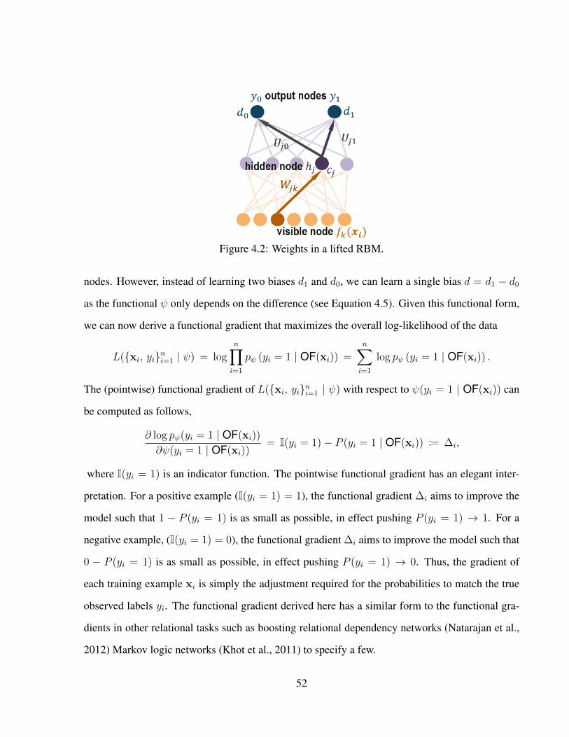
Figure 4.2: Weights in a lifted RBM.

nodes. However, instead of learning two biases d1 and d0, we can learn a single bias d = d1 − d0

as the functional ψ only depends on the difference (see Equation 4.5). Given this functional form,

we can now derive a functional gradient that maximizes the overall log-likelihood of the data

L({xi, yi}ni=1 | ψ) = logn∏i=1

pψ (yi = 1 | OF(xi)) =n∑i=1

log pψ (yi = 1 | OF(xi)) .

The (pointwise) functional gradient of L({xi, yi}ni=1 | ψ) with respect to ψ(yi = 1 | OF(xi)) can

be computed as follows,

∂ log pψ(yi = 1 | OF(xi))

∂ψ(yi = 1 | OF(xi))= I(yi = 1)− P (yi = 1 | OF(xi)) := ∆i,

where I(yi = 1) is an indicator function. The pointwise functional gradient has an elegant inter-

pretation. For a positive example (I(yi = 1) = 1), the functional gradient ∆i aims to improve the

model such that 1 − P (yi = 1) is as small as possible, in effect pushing P (yi = 1) → 1. For a

negative example, (I(yi = 1) = 0), the functional gradient ∆i aims to improve the model such that

0 − P (yi = 1) is as small as possible, in effect pushing P (yi = 1) → 0. Thus, the gradient of

each training example xi is simply the adjustment required for the probabilities to match the true

observed labels yi. The functional gradient derived here has a similar form to the functional gra-

dients in other relational tasks such as boosting relational dependency networks (Natarajan et al.,

2012) Markov logic networks (Khot et al., 2011) to specify a few.

52

Figure 4.3: A general relational regression tree for lifted RBMs when learning a target predicatet(x). Each path from root to leaf is a compound feature (also a logical clause Clauser) that entersthe RBM as a hidden node hr. The leaf node contains the weights θr = {dr, cr,W r, U r

0 , Ur1} of

all edges introduced into the lifted RBM when this hidden node/discovered feature is introducedinto the RBM structure.

4.3.2 Representation of Functional Gradients for LRBMs

Our goal now is to approximate the true functional gradient by fitting a regression function ψ(x)

that minimizes squared error over the pointwise gradients of all the individual training examples:

ψ(x) = arg minψ

n∑i=1

(ψ(xi | OF(xi))−∆i)2. (4.6)

We consider learning the representation of ψ as a sum of relational regression trees. The key

advantage is that a relational tree can be easily interpreted and explained. To learn a tree to model

the functional gradients, we need to change the typical tree learner. Specifically, the splitting

criteria of the tree at each node is modified; to identify the next literal to add to the tree, r(x), we

greedily search for the literal that minimizes the squared error (Equation 4.6).

For a tree-based representation, we employ a relational regression-tree (RRT) learner (Blockeel

and De Raedt, 1998) to learn a function to approximately fit the gradients on each example. If we

learn an RRT to fit ψ(xi | OF(xi)) in Equation (4.5), each path from the root to a leaf can be viewed

as a clause, and the leaf nodes correspond to an RBM that evaluates to the weight of the clause for

that training example. Figure 4.3 shows an RRT when learning a lifted RBM via gradient boosting

53

for some target predicate t(x). The node q(x) can be any subtree that has been learned thusfar,

and a new predicate r(x) has been identified as a viable candidate for splitting. On splitting, we

obtain two new compound features as evidenced by two distinct paths from root to the two new leaf

nodes. These clauses (paths) along with their corresponding leaf nodes identify a new structural

component of the RBM, along with corresponding parameters

(Clause1) θ1 : q(x) ∧ r(x)⇒ t(x),

(Clause2) θ2 : q(x) ∧ ¬r(x)⇒ t(x).

Note that the clause q(·) and the predicate r(·) are expressed generally, and their arguments are

denoted broadly as x. In practice, q(·) and r(·) can be of different arities and take any possible

entity types in the domain.

4.3.3 Learning Relational Regression Trees

Let us assume that we have learned a relational regression tree till q(x) in Figure 4.3. Now assume

that, we are adding a literal r(x) to the tree at the left-most node of the subtree q(x). Let the feature

corresponding to the left branch (Clause1) be f1(x) = I(q(x) ∧ r(x)), that is, feature f1(x) = 1

for all training examples x that end up at the leaf θ1 and zero otherwise. Similarly, let the feature

corresponding to the right branch (Clause2) be f2(x) = I(q(x) ∧ ¬r(x)). The potential function

ψ(yi = 1 | OF(xi)) can be written using (Equation 4.5) as:

ψ(yi = 1 | OF(xi)) =∏k=1,2

[dk + log

(1 + exp

(ck + Uk

1 +W kfk(xi))

1 + exp(ck + Uk

0 +W kfk(xi)))]fk(xi)

. (4.7)

In this expression, when a training example xi satisfies Clause1, it reaches leaf node θ1 and

consequently, we have f1(xi) = 1 and f2(xi) = 0. When a training example xi satisfies Clause2,

the converse is true and we have f1(xi) = 0 and f2(xi) = 1. Thus, only one term is active in

the expression above and delivers the potential corresponding to whether the training example xi

is classified to the left leaf θ1 or the right leaf θ2. We can now substitute this expression for the

54

potential in Equation 4.7 into the loss function (Equation 4.6). The loss function is used in two

ways to grow the RRTs:

1. First, we identify the next literal to add to the tree, r(x), by greedily searching for the atomic

domain predicate that minimizes the squared error. This is similar to the splitting criterion

used in other lifted gradient boosting models such as MLN-boosting (Khot et al., 2011).

2. Next, after splitting, we learn parameters for the newly introduced leaf nodes. That is, for

each split of the tree at r(x), we learn θ1 = [d1, c1,W 1, U10 , U

11 ] for the left subtree and θ2 =

[d2, c2,W 2, U20 , U

21 ] for the right subtree. We perform parameter learning via coordinate

descent (Wright, 2015).

4.3.4 LRBM-Boost Algorithm

We now describe LRBM-BOOST algorithm (Algorithm 2) to learn structure and parameters of

LRBM. The algorithm takes instantiated ground facts (Data) and training examples of target T as

input and learns N regression trees that fits the example gradients to set of trees. The algorithm

starts by considering prior potential value ψ0 in F0, and in order to learn a new tree, it first generates

the regression examples, S=[(xi,yi), ∆i], in (line 4) where regression value ∆i (I-P ) is computed

by performing inference of previously learned trees. These regression examples S serve as input

to FITREGRESSIONTREE function (line 5) along with the maximum number of leaves (L) in the

tree. The next tree Fn is then added to set of existing tree (line 6). The final probability of LRBM

can be computed by performing inference on all N trees in order to obtain ψ.

FITREGRESSIONTREE function (line 10) generates a relational regression tree with L leaf

nodes. It starts with an empty tree and greedily adds one node at a time to the tree. In order to

add next node to the tree, it first considers the current node N to expand as the one that has the

best score in the beam (line 14). The potential children C of this node N (line 15) are constructed

by greedily considering and scoring clauses where the parameters are learned using coordinate

descent. Once the c is determined, it is added as the leaf to the tree and the process is repeated.

55

Algorithm 2 LRBM-Boost: Relational FGB for Lifted RBMs1: function LRBM-BOOST(Data, T , N )2: F0 = ψ0 . set prior of potential function3: for 1 ≤ n ≤ N do4: S := GENERATEEXAMPLES(Fn−1, Data, T ) . examples for next tree5: Fn := FITREGRESSIONTREE(S, L, T ) . learn regression tree6: Fn = Fn + Fn−1 . add new tree to existing set7: end for8: P(yi = 1 | OF(xi)) ∝ exp(ψ(yi = 1| OF(xi)))9: end function

10: function FITREGRESSIONTREE(S, L, T )11: Tree := CREATETREE(T (X)) . create empty Tree12: Beam := {Root(Tree)}13: while (i ≤ L) do . till max clauses L is reached14: N := CURRENTNODETOEXPAND(Beam)15: C := GENERATEPOTENTIALCHILDREN(N)16: for each c in C do . greedily search best child17: [ SL, ∆L ] := EXAMPLESATISFACTION(N ∧ c, S) . left subtree18: Θc

L := COORDINATEDESCENT([SL,∆L]) . learn LRBM params19: [ SR, ∆R ] := EXAMPLESATISFACTION(N ∧ ¬c, S) . right subtree20: Θc

R := COORDINATEDESCENT([SR,∆R]) . learn LRBM params21: scorec := COMPUTESSE(Θc

L,ΘcR,∆L,∆R) . using eq.(4.6)

22: end for23: c := argmin

c(scorec)

24: ADDCHILD(Tree,N, c)25: INSERT(Beam, c.left, c.left.score)26: INSERT(Beam, c.right, c.right.score)27: end while28: return Tree29: end function

4.4 Experimental Section

We aim to answer the following questions in our experiments:

Q1 How does LRBM-Boost2 compare to other neuro-symbolic models?

Q2 How does LRBM-Boost compare to other relational functional gradient boosting models?

2https://github.com/navdeepkjohal/LRBM-Boost

56

Q3 Is an ensemble of weak relational regression trees more effective than a single strong rela-

tional regression tree for constructing Lifted RBMs?

Q4 Can we generate an interpretable lifted RBM from the ensemble of weak relational regres-

sion trees learned by LRBM-Boost?

4.4.1 Experimental setup

To answer these questions, we employ seven standard SRL data sets, six of which – UW-CSE,

IMDB, CORA, SPORTS, MUTAGENESIS, YEAST2 – have already been explained in Chapter

3. The target predicate to be predicted for each of them is also similar as in Chapter 3 - AdvisedBy,

WorkedUnder, SameVenue, TeamPlaysSport, MoleAtm, Cites respectively. The details of the

seventh dataset are explained below.

WEBKB (Mihalkova and Mooney, 2007) contains information about webpages of students,

professors, courses etc. from four universities. We aim to predict whether a person is CourseTA

of a given course.

For all data sets, we generate positive and negative examples in 1 : 2 ratio, perform 5-fold cross

validation for every method being compared, and report AUC-ROC and AUC-PR on the resulting

folds respectively. For all baseline methods, we use default settings provided by their respective

authors. For our model, we learn 20 RRTs, each with a maximum number of 4 leaf nodes. The

learning rate of online coordinate descent was 0.05.

4.4.2 Comparison of LRBM-Boost to other neuro-symbolic models

To answer Q1, we compare our model to two recent relational neural models. The first baseline is

Relational RBM (RRBM-C) (Kaur et al., 2017); as explained in previous chapter, this approach uses

relational random walks to generate relational features that describe the structure of the domain.

In fact, it propositionalizes and aggregates counts on these relational random walks as features to

57

Figure 4.4: Comparing LRNN, RRBM-C, MLN-Boost and LRBM-Boost on AUC-ROC.

describe each training example. It should be noted that a key limitation of RRBM-C is that it can

only handle binary predicates; LRBM-Boost on the other hand, can handle any arity.

The second baseline is Lifted Relational Neural Networks (LRNN) (Sourek et al., 2018). LRNN

mainly focuses on parameter optimization; the structure of the network is identified using a clause

learner: PROGOL (Muggleton, 1995). PROGOL generated four, eight, six, three, ten, five rules for

CORA, IMDB, MUTAGENESIS, SPORTS, UW-CSE and WEBKB respectively. As LRNN cannot

handle the temporal restrictions of YEAST2, we do not evaluate LRNN on it.

Figures 4.4 and 4.5 present the results of this comparison on AUC-ROC and AUC-PR. LRBM-

Boost is significantly better than LRNN for MUTAGENESIS and CORA on both AUC-ROC and

AUC-PR. Further, it also achieves better AUC-ROC and AUC-PR than LRNN on SPORTS and UW-

CSE data set. Compared to RRBM-C, LRBM-Boost performs better for SPORTS and WEBKB on

both AUC-ROC and AUC-PR. Also, our proposed model performs better on YEAST2 on AUC-

58

Figure 4.5: Comparing LRNN, RRBM-C, MLN-Boost and LRBM-Boost on AUC-PR.

ROC. Q1 can be now be answered affirmatively: LRBM-Boost either performs comparably to or

outperforms state-of-the-art relational neural networks.

4.4.3 Comparison of LRBM-Boost to other relational gradient-boosting models

Since LRBM-Boost is a neuro-symbolic model as well as a relational boosting model, we next

compare it to two state-of-the-art relational functional gradient-boosting baselines: MLN-Boost

(Khot et al., 2011) and RDN-Boost (Natarajan et al., 2012). Figures 4.4 and 4.5 compare

LRBM-Boost to MLN-Boost. LRBM-Boost performs better than MLN-Boost for CORA and WE-

BKB on AUC-ROC metric. Also, it performs better than MLN-Boost for IMDB, UW-CSE, SPORTS

and WEBKB on AUC-PR. For all other data sets, both models have comparable performance.

We compare LRBM-Boost to RDN-Boost in a separate experiment, owing to a key dif-

ference in experimental setting. We do not convert the arity of predicates to binary; rather, we

compare RDN-Boost and LRBM-Boost by maintaining the original arity of all the predicates.

59

Table 4.1: Comparison of LRBM-Boost and RDN-Boost.

Data Set Target Measure LRBM-Boost RDN-Boost

UW−CSE ADVISEDBYAUC-ROC 0.9719 0.9731AUC-PR 0.9158 0.9049

IMDB WORKEDUNDERAUC-ROC 0.9610 0.9499AUC-PR 0.8789 0.8537

CORA SAMEVENUEAUC-ROC 0.9469 0.8985AUC-PR 0.9207 0.8451

WEBKB COURSETAAUC-ROC 0.6142 0.6057AUC-PR 0.4553 0.4490

The results of this experiment on four domains are reported in Table 4.1. LRBM-Boost out-

performs RDN-Boost in across the board, and substantially so on larger domains such as Cora.

These comparisons allow us to answer Q2 affirmatively: LRBM-Boost performs comparably or

outperforms state-of-the-art SRL boosting baselines.

4.4.4 Effectiveness of boosting relational ensembles

To understand the importance of boosting trees to construct an LRBM, we compared the perfor-

mance of the ensemble of relational trees learned by LRBM-Boost to a single relational tree,

similar to trees produced by the TILDE tree learner (Blockeel and De Raedt, 1998; Neville et al.,

2003). For the latter, we learn a large lifted tree (of depth 10), construct an RBM with the hidden

layer being every path from root to leaf of this tree and refer to it as LRBM-NoBoost.

Table 4.2 compares the performance of an ensemble (first row) vs. a single large tree (last

row). LRBM-Boost is statistically superior on SPORTS, YEAST2 and CORA on both AUC-ROC

and AUC-PR and is comparable on others. This asserts the efficacy of learning ensembles of

relational trees by LRBM-Boost rather than learning a single tree, affirmatively answering Q3.

60

Table 4.2: Comparison of (a) an ensemble of trees learned by LRBM-Boost, (b) an explainableLifted RBM constructed from the ensemble of trees learned by LRBM-Boost and (c) learning asingle, large, relational probability tree (LRBM-NoBoost).

Model AUC Sports IMDB UW-CSE Yeast2 Cora WebKBEnsembleLRBM

ROC 0.78±0.03 0.95±0.05 0.98±0.02 0.77±0.02 0.86±0.14 0.63±0.05PR 0.64±0.03 0.86±0.11 0.94±0.06 0.64±0.03 0.82±0.21 0.46±0.08

ExplainableLRBM

ROC 0.75±0.01 0.95±0.05 0.95±0.04 0.65±0.05 0.80±0.19 0.61±0.13PR 0.57±0.01 0.85±0.14 0.89±0.06 0.53±0.06 0.70±0.29 0.46±0.10

NoBoostLRBM

ROC 0.75±0.03 0.95±0.05 0.98±0.02 0.64±0.12 0.75±0.21 0.66±0.09PR 0.61±0.01 0.86±0.11 0.94±0.05 0.50±0.14 0.61±0.30 0.48±0.07

4.4.5 Interpretability of LRBM-Boost

While Q1–Q3 can be answered quantitatively, Q4 requires a qualitative analysis. It should be

noted that boosted relational models (here, boosted LRBMs) learn and represent the underlying

relational model as a sum of relational trees. When performing inference, this ensemble of trees

is not converted to a large SRL model as it is far more efficient to aggregate the predictions of the

individual relational trees in the ensemble.

For LRBM-Boost, however, it is possible to convert the ensemble-of-trees representation into

a single LRBM. This step is typically performed to endow the model with interpretability, ex-

plainability or for relationship discovery. For LRBM-Boost, this procedure is not exact, and the

resulting single large LRBM is almost, but not exactly, equivalent to the ensemble of trees repre-

sentation. The procedure itself is fairly straightforward:

• learn a single RRT from the set of boosted RRTs (Craven and Shavlik, 1995) that make up

the LRBM, that is, we empirically learn a single RRT by overfitting it to the predictions of

the weak RRTs (Figure 4.6).

61

Figure 4.6: An example of combined lifted tree learned from ensemble of trees. To constructthis tree, we compute the regression value of each training example by traversing through all theboosted trees. A single large tree is overfit to this (modified) training set to generate a single tree.

Figure 4.7: Lifted RBM obtained from the combined tree in Figure 4.6. Each path along the treein that figure represents the corresponding hidden node of LRBM.

• transform this single RRT to a LRBM (Figure 4.7); each path from root to leaf is a conjunc-

tion of relational features and enters LRBM as a hidden node, with connections to all the

output nodes and to the input nodes corresponding to the predicates that appear in that path.

62

Figure 4.8: Ensemble of trees learned during training of LRBM-Boost. The ensemble oftrees is generated in SPORTS domain where predicate P, T, Z represent plays(sports, team),teamplaysagainstteam(team, team) and athleteplaysforteam(athlete, team) respec-tively and target R represents teamplayssport(team, sports).

Figure 4.9: Demonstration of the conversion of two lifted trees in Figure 4.8 to LRBM. We createone hidden node for each path in each regression tree.

This construction leads to sparsity as it allows for only one hidden node to be activated for each

example. Of course, using clauses instead of trees as with boosting MLNs (Khot et al., 2011), could

relax this sparsity as needed. For our current domains, this restriction does not significantly affect

the performance as seen in Table 4.2 showing the quantitative results of comparing the explainable

LRBM with the original ensemble LRBM. There is no noticeable loss in performance as the AUC

values decrease marginally, if at all.

63

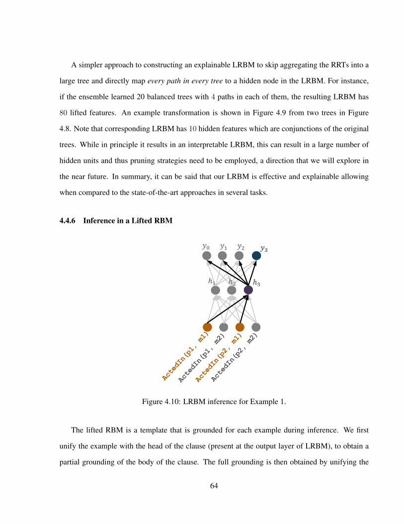
A simpler approach to constructing an explainable LRBM to skip aggregating the RRTs into a

large tree and directly map every path in every tree to a hidden node in the LRBM. For instance,

if the ensemble learned 20 balanced trees with 4 paths in each of them, the resulting LRBM has

80 lifted features. An example transformation is shown in Figure 4.9 from two trees in Figure

4.8. Note that corresponding LRBM has 10 hidden features which are conjunctions of the original

trees. While in principle it results in an interpretable LRBM, this can result in a large number of

hidden units and thus pruning strategies need to be employed, a direction that we will explore in

the near future. In summary, it can be said that our LRBM is effective and explainable allowing

when compared to the state-of-the-art approaches in several tasks.

4.4.6 Inference in a Lifted RBM

Figure 4.10: LRBM inference for Example 1.

The lifted RBM is a template that is grounded for each example during inference. We first

unify the example with the head of the clause (present at the output layer of LRBM), to obtain a

partial grounding of the body of the clause. The full grounding is then obtained by unifying the

64

partially-ground clause with evidence to find at least one instantiation of the body of the clause.

We illustrate the inference procedure for a Lifted RBM with three hidden nodes, and each hidden

node corresponding to the rules (h1)–(h3).

Example 1 We are given facts: ActedIn(p1, m1), ActedIn(p1, m2), ActedIn(p2, m1), ActedIn

(p2, m2). The number of substitutions depends on the query. Let us assume that the query

is Collab(p1, p2) (did p1 and p2 collaborate?), which results in the partial substitution: θ =

{P1/p1, P2/p2}. The inference procedure will proceed as follows:

• The bodies of the clauses (h1)–(h3) are partially grounded using θ = {P1/p1, P2/p2}:DirectedBy(M1, p1) ∧ InGenre(M1, G1)∧

ActedIn(p2, M2) ∧ InGenre(M2, G2)∧

¬ SameGenre(G1, G2)

(h1)

DirBy(M1, p1) ∧ ActedIn(P3, M1) ∧ SamePerson(P3, p2) (h2)

ActedIn(p1, M) ∧ ActedIn(p2, M). (h3)

• Next, since the facts do not contain any information about DirectedBy or SamePerson, h1

and h2 will not be satisfied.

• In order to prove the satisfiability of h3, we look at all the available facts as we attempt to

unify each fact with the partially-grounded clause. Say we first unify ActedIn(p1, m1) with

h3 that gives us:

ActedIn(p1, m1), ActedIn(p2, M), (h3)

resulting in the grounding: θ = {P1/p1, M/m1, P2/p2}. The second fact ActedIn(p1, m2)

does not unify with this partially-grounded clause. However, the third fact ActedIn(p2, m1)

unifies with h3 giving us a fully-grounded clause:

ActedIn(p1, m1), ActedIn(p2, m1). (h3)

65

The input nodes corresponding to the unified facts ActedIn(p1, m1), Acted In(p2, m1) are

activated. As soon as this clause is satisfied the search terminates. The main conclusion to

be drawn is that as soon as the clause is satisfied once, model does not check for another

satisfaction and terminates the search by returning true.

• The inputs are then propagated through the RBM, and the class output probabilities are

computed based on the RBM edge parameters/weights. The activation paths for inference

given this query and facts are shown in Figure 4.10.

Example 2 We are given facts: DirectedBy(m1, p1), InGenre(m1, g1), ActedIn (p2, m2),

InGenre(m2, g2), DirectedBy(m01, p01), ActedIn(p03, m01), SamePerson(p03, p02). Recall

that the number of substitutions depends on the query. Let us assume that the query is Collab(p01

, p02) (did p01 and p02 collaborate?), which results in partial substitution: θ = {P1/p01, P2/p02}.

The inference procedure will proceed as follows:

• The bodies of the clauses (h1)–(h3) are partially grounded using θ = {P1/p01, P2/p02}:DirectedBy(M1, p01) ∧ InGenre(M1, G1)∧

ActedIn(p02, M2) ∧ InGenre(M2, G2)∧

¬ SameGenre(G1, G2)

(h1)

DirBy(M1, p01) ∧ ActedIn(P3, M1) ∧ SamePerson(P3, p02) (h2)

ActedIn(p01, M) ∧ ActedIn(p02, M). (h3)

• Unifying the partially-grounded clauses with the facts, we will have that h1 and h3 will not

be satisfied. However, unification yields one fully-grounded h2 will:

DirBy(m01, p01) ∧ ActedIn(p03, m01) ∧ SamePerson(p03, p02), (h2)

which has the substitution: θ = {P1/p01, M/m01, P2/p02, P3/p03}. As before, once a satis-

fied grounding is obtained, the search is terminated.

66

• The RBM is unrolled as in Example 1, and the appropriate facts that appear in this ground-

ing are activated in the input layer. The prediction is obtained by propagating these inputs

through the network.

4.5 Conclusion

We presented the first learning algorithm for learning the structure of a lifted RBM from data. Mo-

tivated by the success of gradient-boosting, our method learns a set of RRTs using boosting and

then transforms them to a lifted RBM. The advantage of this approach is that it leads to learning

a fully lifted model that is not propositionalized using any standard approaches. We also demon-

strated how to induce a single explainable RBM from the ensemble of trees. The experimental

evaluation on several data sets demonstrated the efficacy and effectiveness along with the explain-

ability of the proposed approach.

67

CHAPTER 5

NEURAL NETWORKS WITH RELATIONAL PARAMETER TYING

Although the two models proposed in Chapters 3 and 4 have successfully lifted RBM to rela-

tional domains, yet the potential bottleneck of these two models is that they are centered on

one specific type of connectionist model: Boltzmann machines. In this chapter, we propose

a general relational neural network architecture (NNRPT) which is independent of any specific

probability distribution (Kaur et al., 2019).

5.1 Introduction

While successful, deep networks have a few important limitations. Apart from the key issue of

interpretability, the other major limitation is the requirement of a flat inputs (vectors, matrics,

tensors), which limits applications to tabular, propositional representations. On the other hand,

symbolic and structured representations (Getoor and Taskar, 2007; De Raedt et al., 2016; Getoor

et al., 2001; Richardson and Domingos, 2006; Bach et al., 2017) have the advantage of being

interpretable, while also allowing for rich representations that allow for learning and reasoning with

multiple levels of abstraction. This representability allows them to model complex data structures

such as graphs far more easily and interpretably than basic propositional representations. While

expressive, these models do not incorporate or discover latent relationships between features as

effectively as deep networks.

Consequently, there has been focus on achieving the dream team of logical and statistical learn-

ing methods such as relational neural networks (Kazemi and Poole, 2018; Sourek et al., 2016).

While specific architectures differ, these methods generally employ hand-coded relational rules

or Inductive Logic Programming (Lavrac and Dzeroski, 1993) to identify the domain’s structural

rules; these rules are then used with the observed data to unroll and learn a neural network. We

improve upon these methods in two specific ways: (1) we employ a rule learner that has been

68

recently successful to automatically extract interpretable rules that are then employed as hidden

layer of the neural network; (2) we exploit the notion of parameter tying from the perspective of

statistical relational learning models that allow multiple instances of the same rule share the same

parameter. These two extensions significantly improve the adaptation of neural networks (NNs)

for relational data.

We employ Relational Random Walks (Lao and Cohen, 2010) to extract relational rules from a

database, which are then used as the first layer of the NN. These random walks have the advantages

of being learned from data (instead of time-consumingly hand-coded), and interpretable (as walks

are rules in a database schema). Given evidence (facts), relational random walks are instantiated

(grounded); parameter tying ensures that groundings of the same random walk share the same

parameters with far fewer network parameters to be learned during training.

For combining outputs from different groundings of the same clause, we employ combina-

tion functions (Natarajan et al., 2008; Jaeger, 2007). For instance, given a rule: Professor(P),

Author(P, U), Author(S, U), Student(S), the ana-bob Professor-Student pair could have co-

authored 6 papers, while the cam-dan pair could have coauthored 10 publications (U). Combi-

nation functions are a natural way to compare such relational features arising from rules. Our

network handles this in two steps: first, by ensuring that all instances (papers) of a particular

Professor− Student pair share the same weights. Second, by combining predictions from each

of these instances (papers) using a combination function. We explore the use of Average combi-

nation function. Once the network weights are appropriately constrained by parameter tying and

combination functions, they can be learned using standard techniques.

We make the following contributions: (1) we learn a NN that can be fully trained from data

and with no significant engineering, unlike previous approaches; (2) we combine the successful

paradigms of relational random walks and parameter tying from SRL methods; this allows the

resulting NN to faithfully model relational data while being fully learnable; (3) we evaluate the

proposed approach against recent relational NN approaches and demonstrate its efficacy.

69

The rest of the chapter is organized as follows: we review the related work in Section 5.2

followed by discussing the proposed architecture in Section 5.3. This is followed by experimental

details in Section 5.4. We finally conclude in Section 5.6 after explaining connection between our

model and convolutional neural network in Section 5.5.

5.2 Related Work

The related work in this chapter has been categorized into four classes, each one of which is

discussed in the following Subsections 5.2.1-5.2.4.

5.2.1 Lifted Relational Neural Networks

Our work is closest to Lifted Relational Neural Networks (LRNN) (Sourek et al., 2016) in terms

of the architecture. LRNN uses expert hand-crafted relational rules as input, which are then in-

stantiated (based on data) and rolled out as a ground network. While at a high-level, our approach

appears similar to the LRNN framework, there are significant differences. First, while Sourek et

al., exploit tied parameters across examples within the same rule, there is no parameter tying across

multiple instances; our model, however, ensures parameter tying of multiple ground instances of

the rule (in our case, a relational random walk). Second, since they adopt a fuzzy notion, their

system supports weighted facts (called ground atoms in logic literature). We take a more standard

approach and our observations are Boolean. Third, while the previous difference appears to be lim-

iting in our case, note that this leads to a reduction in the number of network weight parameters.

Sourek et al. (2016), have extended their work to learn network structure using predicate

invention (Sourek et al., 2017); our work learns relational random walks as rules for the network

structure. As we show in our experiments, NNs cannot only easily handle such large number of

random walks, but can also use them effectively as a bag of weakly predictive intermediate layers

capturing local features. This allows for learning a more robust model than the induced rules,

which take a more global view of the domain.

70

Another recent approach is due to Kazemi and Poole (2018), as discussed in Section 1.1, who

proposed a relational neural network by adding hidden layers to their Relational Logistic Regres-

sion (Kazemi et al., 2014) model. A key limitation of their work is that they are restricted to unary

relation predictions, that is, they can only predict attributes of objects instead of relations between.

In contrast, ours is a general framework in that can be used to predict relations between objects.

Some of the earliest neuro-symbolic systems such as KBANN (Towell et al., 1990) date back to

the early 90s; KBANN also rolls out the network architecture from rules, though it only supports

propositional rules. Current work, including ours, instead explores relational rules which serve

as templates to roll out more complex architectures. Other recent approaches such as CILP++

(Franca et al., 2014) and Deep Relational Machines (Lodhi, 2013) incorporate relational infor-

mation as network layers. However, such models propositionalize relational data into flat-feature

vector and hence, cannot be seen as truly relational models. A rather distinctive approach in this

vein is due to Hu et al. (2016), where two independent networks incorporating rules and data are

trained together. Finally, NNs have also been trained to approximate ILP clause evaluation (Di-

Maio and Shavlik, 2004), perform SLD-resolution in first-order logic (Komendantskaya, 2007),

and approximate entailment operators in propositional logic (Evans et al., 2018).

5.2.2 Relational Random Walks

The Path Ranking Algorithm (Lao and Cohen, 2010) is a key framework, where a combination of

random walks replaces exhaustive search in order to answer queries. Recently, Das et al. (2017)

considered random walks between query entities to perform composition of embeddings of rela-

tions on each walk with recurrent neural networks. DeepWalks (Perozzi et al., 2014) performs

random walks on graphs by treating each node as a word, which results in learning embeddings

for each node of graph. Kaur et al. (2017) in Chapter 3 considers relational random walks to gen-

erate count and existential features to train a relational restricted Boltzmann machine (Larochelle

and Bengio, 2008). This feature transformation induces propositionalization that could potentially

result in loss of information, as we show in our experiments.

71

5.2.3 Tensor Based Models

As already discussed in Section 4.2, recently, several tensor-based models (Nickel et al., 2011;

Bordes et al., 2013; Socher et al., 2013; Bordes et al., 2012; Wang et al., 2014b) have been proposed

to learn embeddings of objects and relations. Such models have been very effective for large-

scale knowledge-base construction. However, they are computationally expensive as they learn

parameters for each object and relation in the knowledge base. Furthermore, the embedding into

some ambient vector space makes the models more difficult to interpret. Though rule distillation

can yield human-readable rules (Yang et al., 2015), it is another computationally intensive post-

processing step, which limits the size of the interpreted rules. We will explore these models further

in the part II of the dissertation.

5.2.4 Other Models

Several NNs have been utilized with relational databases schemas (Blockeel and Uwents, 2004;

Ramon and Raedt, 2000). These models differ on how they handle 1-to-N joins, cyclicity, and

indirect relationships between relations. However, they all learn one network per relation, which

makes them computationally expensive. In the same vein, graph-based models take graph structure

into consideration during training in (Pham et al., 2017; Niepert et al., 2016; Scarselli et al., 2009)

as already in Section 4.2. Finally, with the rapid growth of deep learning, relational counterparts

of most of existing connectionist models have been also proposed in Schlichtkrull et al. (2018),

Palm et al. (2018), Wang et al. (2015) and Zeng et al. (2014).

5.3 Neural Networks with Relational Parameter Tying: The proposed approach

We first introduce some notation for relational logic, which is used for relational representation,

with the domain being represented using constants, variables and predicates. We adopt the follow-

ing conventions: (1) constants used to represent entities in the domain are written in lower-case

72

(e.g., ana, bob); (2) variables and entity types are capitalized (e.g., Student, Professor); and

(3) relations and predicate symbols between entities and attributes are represented as Q(·, ·). A

grounding is a predicate applied to a tuple of terms (i.e., either a full or partial instantiation), e.g.

AdvisedBy(Student, ana), is a partial instantiation.

Rules are constructed from atoms using logical connectives (∧, ∨) and quantifiers (∃, ∀). Due

to the use of relational random walks, the relational rules that we employ are universally conjunc-

tions of the form h ⇐ b1 ∧ . . . ∧ b`, where the head h is the target of prediction and the body

b1 ∧ . . . ∧ b` corresponds to conditions that make up the rule (that is, each literal bi in the body is

a predicate Q(·, ·)). We do not consider negations in this work.

An example rule could be AdvisedBy(S, P) ⇐ Professor(P) ∧ WorksIn(P, T) ∧ PartOf(T,

S) ∧ Student(S). This rules states that if a Student is a part of the project that the Professor

works on, then the Student is advised by that Professor. The body of the rule is learned as a

random walk that starts with Professor and ends with Student. Such a random walk represents

a chain of relations that could possibly connect a Professor to a Student and is a relational

feature that could help in the prediction. The rule head is the target that we are interested in

predicting. Since these rules are essentially “soft” rules, we can also associate clauses with weights,

i.e., weighted rules: (R, w).

A relational neural network N is a set of M weighted rules describing interactions in the do-

main {(Rj, wj)}Mj=1. We are given a set of atomic facts F , known to be true and labeled relational

training examples {(xi, yi)}`i=1. In general, labels yi can take multiple values corresponding to a

multi-class problem. We seek to learn a relational neural network model N ≡ {(Rj, wj)}Mj=1to

predict a Target relation, given relational examples x, that is: y = Target(x).

73

Given: Set of instances F , Target relation, relational data set (x, y) ∈ D;

Construct (structure learning): Rj, relational random walk rules (relational feature describing

the network structure of N );

Train (parameter learning): wj , rule weights via gradient descent with rule-based parameter

tying to identify a sparse set of network weights of N

Example. The movie domain contains the entity types (variables) Person(P), Movie(M) and

Genre(G). In addition to this, there are relations (features): Directed(P, M), ActedIn(P, G) and

InGenre(M, G). The domain also has relations for entity resolution: SamePerson(P1, P2) and

SameGenre(G1, G2). The task is to predict if P1 worked under P2, with the target predicate (label):

WorkedUnder(P1, P2).

5.3.1 Generating Lifted Random Walks

The core component of a neural network model is the architecture, which determines how the var-

ious neurons are connected to each other, and ultimately how all the input features interact with

each other. In a relational neural network, the architecture is determined by the domain structure,

or the set of relational rules that determines how various relations, entities and attributes interact in

the domain as shown earlier with the AdvisedBy example. While previous approaches employed

carefully hand-crafted rules, we, instead, use relational random walks to define the network archi-

tecture and model the local relational structure of the domain. A similar approach was also used

by us in Chapter 3 (Kaur et al., 2017), though the random walk features were used to instantiate a

restricted Boltzmann machine, which has a limited architecture and that work is not lifted since it

instantiates the entire network before learning.

Relational data is often represented using a lifted graph, which defines the domain’s schema; in

such a representation, a relation Predicate(Type1, Type2) is a predicate edge between two type

nodes: Type1Predicate−−−−−→ Type2. A relational random walk through a graph, as discussed in Section

74

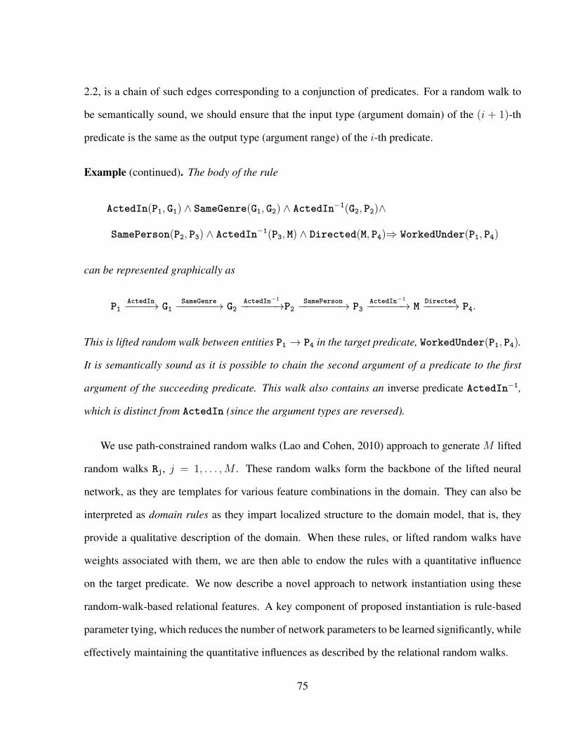
2.2, is a chain of such edges corresponding to a conjunction of predicates. For a random walk to

be semantically sound, we should ensure that the input type (argument domain) of the (i + 1)-th

predicate is the same as the output type (argument range) of the i-th predicate.

Example (continued). The body of the rule

ActedIn(P1, G1) ∧ SameGenre(G1, G2) ∧ ActedIn−1(G2, P2)∧

SamePerson(P2, P3) ∧ ActedIn−1(P3, M) ∧ Directed(M, P4)⇒ WorkedUnder(P1, P4)

can be represented graphically as

P1ActedIn−−−−→ G1

SameGenre−−−−−−→ G2ActedIn−1

−−−−−−→P2SamePerson−−−−−−−→ P3

ActedIn−1

−−−−−−→ M Directed−−−−−→ P4.

This is lifted random walk between entities P1 → P4 in the target predicate, WorkedUnder(P1, P4).

It is semantically sound as it is possible to chain the second argument of a predicate to the first

argument of the succeeding predicate. This walk also contains an inverse predicate ActedIn−1,

which is distinct from ActedIn (since the argument types are reversed).

We use path-constrained random walks (Lao and Cohen, 2010) approach to generate M lifted

random walks Rj, j = 1, . . . ,M . These random walks form the backbone of the lifted neural

network, as they are templates for various feature combinations in the domain. They can also be

interpreted as domain rules as they impart localized structure to the domain model, that is, they

provide a qualitative description of the domain. When these rules, or lifted random walks have

weights associated with them, we are then able to endow the rules with a quantitative influence

on the target predicate. We now describe a novel approach to network instantiation using these

random-walk-based relational features. A key component of proposed instantiation is rule-based

parameter tying, which reduces the number of network parameters to be learned significantly, while

effectively maintaining the quantitative influences as described by the relational random walks.

75

Figure 5.1: The relational neural network is unrolled in three stages, ensuring that the output is afunction of facts through two hidden layers: the combining rules layer (with lifted random walks)and the grounding layer (with instantiated random walks). Weights are tied between the input andgrounding layers based on which fact/feature ultimately contributes to which rule in the combiningrules layer.

5.3.2 Network Instantiation

The relational random walks (Rj) generated in the previous subsection are the relational features

of the lifted relational neural network, N . Our goal is to unroll and ground the network with

several intermediate layers that capture the relationships expressed by the random walks. A key

difference in network construction between our proposed work and recent approaches such as that

of Sourek et al., (Sourek et al., 2018) is that we do not perform an exhaustive grounding to generate

all possible instances before constructing the network. Instead, we only ground as needed leading

to a much more compact network. We unroll the network in the following manner (cf. Figure 5.1).

Output Layer: For the Target, which is also the head h in all the rules Rj, introduce an output

neuron called the target neuron, Ah. With one-hot encoding of the target labels, this architecture

76

can handle multi-class problems. The target neuron uses the softmax activation function. Without

loss of generality, we describe the rest of the network unrolling assuming a single output neuron.

Combining Rules Layer: The target neuron is connected to M lifted rule neurons, each corre-

sponding to one of the lifted relational random walks, (Rj, wj). Each rule Rj is a conjunction of

predicates defined by random walks:

Qj1(X, ·) ∧ . . . ∧ Qj

L(·, Z) ⇒ Target(X, Z), j = 1, . . . ,M, (5.1)

and corresponds to the lifted rule neuron Aj . This layer of neurons is fully connected to the output

layer to ensure that all the lifted random walks (that capture the domain structure) influence the

output. The extent of their influence is determined by learnable weights, uj between Aj and the

output neuron Ah.

In Figure 5.1, we see that the rule neuron Aj is connected to the neurons Aji; these neurons

correspond to Nj instantiations of the random-walk Rj. The lifted rule neuron Aj aims to combine

the influence of the groundings/instantiations of the random-walk feature Rj that are true in the

evidence. Thus, each lifted rule neuron can also be viewed as a rule combination neuron. The

activation function of a rule combination neuron can be any aggregator or combining rule (Natara-

jan et al., 2008). This can include value aggregators such as weighted mean, max or distribution

aggregators (if inputs to the this layer are probabilities) such as Noisy-Or. Many such aggregators

can be incorporated into the combining rules layer with appropriate weights (vji) and activation

functions of the rule neurons. For instance, combining rule instantiations out(Aji) with a weighted

mean will require learning vji, with the nodes using unit functions for activation. The formulation

of this layer is much more general and subsumes the approach of Sourek et al (2018), which uses

a max combination layer.

Grounding Layer: For each instantiated (ground) random walk Rjθi, i = 1, . . . , Nj , we introduce

a ground rule neuron, Aji. This ground rule neuron represents the i-th instantiation (grounding) of

the body of the j-th rule, Rjθi: Qj1θi ∧ . . . ∧ Qj

Lθi (cf. Equation 5.1). The activation function of a

77

ground rule neuron is a logical AND (∧); it is only activated when all its constituent inputs are true

(that is, only when the entire instantiation is true in the evidence).

This requires all the constituent facts Qj1θi, . . . , Qj

Lθi to be in the evidence. Thus, the (j, i)-th

ground rule neuron is connected to all the fact neurons that appear in its corresponding instantiated

rule body. A key novelty of our approach is regarding relational parameter tying: the weights

of connections between the fact and grounding layers are tied by the rule these facts appear in

together. This is described in detail further below.

Input Layer: Each instantiated (grounded) predicate that appears as a part of an instantiated rule

body is a fact, that is Qjkθi ∈ F . For each such instantiated fact, we create a fact neuron Af ,

ensuring that each unique fact in evidence has only one single neuron associated with it. Every

example is a collection of facts, that is, example xi ≡ Fi ⊂ F . Thus, an example is input into the

system by simply activating its constituent facts in the input layer.

Relational Parameter Tying: The most important thing to note about this construction is that we

employ rule-based parameter tying for the weights between the grounding layer and the input/facts

layer. Parameter tying ensures that instances corresponding to an example all share the same

weight wj if they occur in the same lifted rule Rj. The shared weights wj are propagated through

the network in a bottom-up fashion, ensuring that weights in the succeeding hidden layers are

influenced by them.

Our approach to parameter tying is in sharp contrast to that of Sourek et al. (2018), who learn

the weights of the network edges between the output layer and the combining rules layer. Fur-

thermore, they also use fuzzy facts (weighted instances), whereas in our case, the facts/instances

are Boolean, though their edge weights are tied. This approach also differs from our approach in

Chapter 3 which also used relational random walks. From a parametric standpoint, Chapter 3 used

relational random walks as features for a restricted Boltzmann machine, where the instance neu-

rons and the rule neurons form a bipartite graph. Thus, the RRBM formulation has significantly

more edges, and commensurately many more parameters to optimize during learning.

78

Figure 5.2: Example: unrolling the network with relational parameter tying.

Example (continued, see Figure 5.2). Consider two lifted random walks (R1, w1) and (R2, w2) for

the target predicate WorkedUnder(P1, P2)

WorkedUnder(P1, P2)⇐ActedIn(P1, M) ∧ Directed−1(M, P2),

WorkedUnder(P1, P2)⇐SamePerson(P1, P3) ∧ ActedIn(P3, M) ∧ Directed−1(M, P2).

Note that while inverse predicate Directed−1(M, P) is syntactically different from Directed(P, M)

(argument order is reversed), they are both semantically same. The output layer consists of a

single neuron Ah corresponding to the binary target WorkedUnder. The lifted rule layer (also

known as combining rules layer) has two lifted rule nodes A1 corresponding to rule R1 and A2

corresponding to rule R2. These rule nodes combine inputs corresponding to instantiations that

are true in the evidence. The network is unrolled based on the specific training example, for

instance: WorkedUnder(Leo, Marty). For this example, the rule R1 has two instantiations that

are true in the evidence. Then, we introduce a ground rule node for each such instantiation:

A11 :ActedIn(Leo, “The Departed”) ∧ Directed−1(“The Departed”, Marty),

A12 :ActedIn(Leo, “The Aviator”) ∧ Directed−1(“The Aviator”, Marty).

79

The rule R2 has only one instantiation, and consequently only one node:

A21 :SamePerson(Leo, Leonardo) ∧ ActedIn(Leo, “The Departed”)

∧ Directed−1(“The Departed”, Marty).

The grounding layer consists of ground rule nodes corresponding to instantiations of rules that

are true in the evidence. The edges Aji → Aj have weights vji that depend on the combining rule

implemented in Aj . In this example, the combining rule is average, so we have v11 = v12 = 12

and v21 = 1. The input layer consists of atomics fact in evidence: f ∈ F . The fact nodes

ActedIn(Leo, “The Aviator”) and Directed−1(“The Aviator”, Marty) appear in the ground-

ing R1θ2 and are connected to the corresponding ground rule neuron A12. Finally, parameters are

tied on the edges between the facts layer and the grounding layer. This ensures that all facts that

ultimately contribute to a rule are pooled together, which increases the influence of the rule during

weight learning. This ensures that a rule that holds strongly in the evidence gets a higher weight.

Once the network Nθ is instantiated, the weights wj and uj can be learned using standard

techniques such as backpropagation. We denote our approach Neural Networks with Relational

Parameter Tying (NNRPT). The tied parameters incorporate the structure captured by the relational

features (lifted random walks), leading to a network with significantly fewer weights, while also

endowing the it with semantic interpretability regarding the discriminative power of the relational

features. We now demonstrate the importance of parameter tying and the use of relational random

walks as compared to previous frameworks.

5.4 Experiments

Our empirical evaluation aims to answer the following questions explicitly1: Q1: How does NNRPT

compare to the state-of-the-art SRL models i.e., what the value of learning a neural net over stan-

dard models? Q2: How does NNRPT compare to propositionalization models i.e., what is the need

1https://github.com/navdeepkjohal/NNRPT

80

for parameterization of standard neural networks? Q3: How does NNRPT compare to other neuro-

symbolic models in literature?

Table 5.1: Data sets used in our experiments to answer Q1–Q3. The last column shows the numberof sampled groundings of random walks per example for NNRPT.

Domain Target #Facts #Pos #Neg #RW #Samp/RWUW-CSE advisedBy 2817 90 180 2500 1000

MUTAGENESIS MoleAtm 29986 1000 2000 100 100CORA SameVenue 31086 2331 4662 100 100IMDB WorkedUnder 914 305 710 80 -

SPORTS TeamPlaysSport 7824 200 400 200 100

5.4.1 Data Sets

We use six standard data sets to evaluate our algorithm (see Table 5.1). We experiment with UW-

CSE, IMDB, CORA, MUTAGENESIS, SPORTS datasets, details of the which are already explained

in Section 3.5 in Chapter 3. We predict AdvisedBy relationship between a professor and a student

in UW-CSE, whether an actor has WorkedUnder a director in IMDB, if one venue is SameVenue as

another in CORA, which sport a particular team plays i.e teamPlaysSports in SPORTS. We used

two variants of MUTAGENESIS in this work: one to answer Q1 and other to answer Q3. For Q1,

we formulated all atom and molecule properties as binary predicates, and performed relation pre-

diction of whether an atom is a constituent of a molecule or not (MoleAtm(AtomID, MolID)). For

Q3, we considered various properties of atoms and molecules as unary predicates (as described in

the experimental framework of LRNN, (Sourek et al., 2018)) and performed the binary classification

of whether a compound is mutagenetic or not.

The last dataset in our experiments is the Predictive Toxicology Challenge (PTC, (Helma et al.,

2001)) dataset. It further consists of four data sets where the aim in each is to predict the carcino-

genicity of a chemical based on its properties, constituent atoms and properties of the constituent

atoms. The true toxicity labels of the chemicals were generated by exposure of female rats (fr),

female mice (fm), male rat (mr) and male mice (mc) to these chemicals. This resulted in four data

sets, which we used to devise an experiment specifically to answer Q3.

81

5.4.2 Baselines and Experimental Details

To answer Q1, we compare NNRPT with the more recent and state-of-the-art relational gradient-

boosting methods, RDN-Boost(Natarajan et al., 2012), MLN-Boost (Khot et al., 2011), and relational

restricted Boltzmann machines RRBM-E, RRBM-C (Kaur et al., 2017). As the random walks chain

binary predicates in our model, we convert unary and ternary predicates into binary predicates

for all data sets. Further, to maintain consistency in experimentation, we use the same resulting

predicates across all our baselines as well. We run RDN-Boost and MLN-Boost with their default

settings and learn 20 trees for each model. Also, we train RRBM-E and RRBM-C according to the

settings recommended in Chapter 3.

For NNRPT, we generate random walks by considering each predicate and its inverse to be two

distinct predicates. Also, we avoid loops in the random walks by enforcing sanity constraints on the

random walk generation. We consider 100 random walks for MUTAGENESIS, CORA, 80 random

walks for IMDB, 200 random walks for SPORTS and 2500 random walks for UW-CSE as suggested

in Chapter 3 (Kaur et al., 2017) (see Table 5.1). Since we use a large number of random walks,

exhaustive grounding becomes prohibitively expensive. To overcome this, we sample groundings

for each random walk for large data sets. Specifically, we sample 100 groundings per random

walk per example for CORA, SPORTS, MUTAGENESIS, and 1000 groundings per random walk per

example for UW-CSE (see Table 5.1).

For all experiments, we set the positive to negative example ratio to be 1 : 2 for training, set

combination function to be average and perform 5-fold cross validation. For NNRPT, we set the

learning rate to be 0.05, batch size to 1, and number of epochs to 1. We train our model with

L1-regularized AdaGrad (Duchi et al., 2011). Since these are relational data sets where the data is

skewed, AUC-PR and AUC-ROC are better measures than likelihood and accuracy.

To answer Q2, we generated flat feature vectors by Bottom Clause Propositionalization (BCP,

(Franca et al., 2014)), according to which one bottom clause is generated for each example. BCP

82

considers each predicate in the body of the bottom clause as a unique feature when it proposition-

alizes bottom clauses to flat feature vector. We use Progol (Muggleton, 1995) to generate these

bottom clauses. After propositionalization, we train two connectionist models: a propositionalized

Restricted Boltzmann Machine (BCP-RBM) and a propositionalized neural network (BCP-NN). The

NN has two hidden layers in our experiments, which makes BCP-NN model a modified version of

CILP++ (Franca et al., 2014) that had one hidden layer. The hyper-parameters of both the models

were optimized by line search on validation set.

To answer Q3, we compare our model with Lifted Relational Neural Networks (LRNN, (Sourek

et al., 2018)) where in order to compare the two models, we perform five sub-experiments. Specifi-

cally, we learn the structure of the neural network by three ways: (a) expert provided (hand-coded)

rules as used in Sourek et al. (2018) (b) employ random walks as structure for both the mod-

els as proposed in our model (c) we perform structure learning by third independent ILP model,

specifically PROGOL (Muggleton, 1995) and input the same clauses to both LRNN and NNRPT.

For first experiment, we employed the hand-crafted rules of Sourek et al. (2018) with both LRNN

and NNRPT and predict the mutageneticity and carcinogeneticity on the MUTAGENESIS and PTC

data sets respectively. The hand-crafted rules consider chains of atoms to predict the target label;

for instance, two-chain rules (2c) consider the properties of two atoms. Since we do not perform

soft clustering at the hidden layer of our model, it is necessary to modify their chain rules to run

within our system. Specifically, LRNN first considers rules that represent the cluster of atom-types,

and then provides the resulting cluster predicate as input to chain rules. However, we formulate

the rules directly in terms of atom-type and bond-type. For example, a 2-chain rule in our model

looks like:

AtomType(B) ∧ AtomType(C) ∧ Bond(B, C, D) ∧ BondType(D)

∧ Contains(A, B) ∧ Contains(A, C)⇒ Mutagenetic(A)

where atoms B and C are connected by bond D, and A is the chemical whose mutageneticity is being

predicted by both the models.

83

Table 5.2: Comparison of different learning algorithms based on AUC-ROC and AUC-PR. NNRPTis comparable or better than standard SRL methods across all data sets.

Data Set Measure RDN-Boost MLN-Boost RRBM-E RRBM-C NNRPT

UW-CSEAUC-ROC 0.973±0.014 0.968±0.014 0.975±0.013 0.968±0.011 0.959±0.024AUC-PR 0.931±0.036 0.916±0.035 0.923±0.056 0.924±0.040 0.896±0.063

IMDBAUC-ROC 0.955±0.046 0.944±0.070 1.000±0.000 0.997±0.006 0.984±0.025AUC-PR 0.863±0.112 0.839±0.169 1.000±0.000 0.992±0.017 0.951±0.082

CORAAUC-ROC 0.895±0.183 0.835±0.035 0.984±0.009 0.867±0.041 0.952±0.043AUC-PR 0.833±0.259 0.799±0.034 0.948±0.042 0.825±0.050 0.899±0.070

MUTAG.AUC-ROC 0.999±0.000 0.999±0.000 0.999±0.000 0.998±0.001 0.981±0.024AUC-PR 0.999±0.000 0.999±0.000 0.999±0.000 0.997±0.002 0.970±0.039

SPORTSAUC-ROC 0.801±0.026 0.806±0.016 0.760±0.016 0.656±0.071 0.780±0.026AUC-PR 0.670±0.028 0.652±0.032 0.634±0.020 0.648±0.085 0.668±0.070

We perform five sub-experiments to answer Q3: (i) hand-coded chain rules with LRNN (HCRules-

LRNN); (ii) hand-coded chain rules (modified) with our approach (HCRules-NNRPT); (iii) lifted ran-

dom walks with LRNN; and (iv) lifted random walks with our approach (proposed) (v) PROGOL

clauses as structure for both the models.

5.4.3 Results

Table 5.2 compares our NNRPT to MLN-Boost, RDN-Boost, RRBM-E and RRBM-C to answer Q1. As

we see, NNRPT is significantly better than RRBM-C for CORA and SPORTS on both AUC-ROC and

AUC-PR, and performs comparably to the other data sets. It also performs better than MLN-Boost,

RDN-Boost on IMDB and CORA data sets, and comparably on other data sets. Similarly, it performs

better than RRBM-E on SPORTS, both on AUC-ROC and AUC-PR and comparably on other data

sets. Broadly, Q1 can be answered affirmatively in that NNRPT performs comparably to or better

than state-of-the-art SRL models.

Table 5.3 shows the comparison of NNRPT with two propositionalization models: BCP-RBM and

BCP-NN in order to answer Q2. NNRPT performs better than BCP-RBM on all the data sets except

MUTAGENESIS, where the two models have similar performance. NNRPT also performs better than

84

Table 5.3: Comparison of NNRPT with propositionalization-based approaches. NNRPT is signifi-cantly better on a majority of data sets.

Data Set Measure BCP-RBM BCP-NN NNRPT

UW-CSEAUC-ROC 0.951±0.041 0.868±0.053 0.959±0.024AUC-PR 0.860±0.114 0.869±0.033 0.896±0.063

IMDBAUC-ROC 0.780±0.164 0.540±0.152 0.984±0.025AUC-PR 0.367±0.139 0.536±0.231 0.951±0.082

CORAAUC-ROC 0.801±0.017 0.670±0.064 0.952±0.043AUC-PR 0.647±0.050 0.658±0.064 0.899±0.070

MUTAG.AUC-ROC 0.991±0.003 0.945±0.019 0.981±0.024AUC-PR 0.995±0.001 0.973±0.012 0.970±0.039

SPORTSAUC-ROC 0.664±0.021 0.543±0.037 0.780±0.026AUC-PR 0.532±0.041 0.499±0.065 0.668±0.070

BCP-NN on all data sets. It should be noted that BCP feature generation sometimes introduces a

large positive-to-negative example skew (for example, in the IMDB data set), which can some-

times gravely affect the performance of the propositional model, as we observe in Table 5.3. This

emphasizes the need for designing models that can handle relational data directly and without

propositionalization; our proposed model as an effort in this direction. Q2 can now be answered

affirmatively: that NNRPT performs better than propositionalization models.

Table 5.4 shows the comparison of NNRPT with LRNN with both approaches using expert hand-

coded rules (Sourek et al., 2018). NNRPT performs better than LRNN on the mut-3c data subset and

similarly on the mut-2c data subset. Furthermore, it can be observed that, while both LRNN and

NNRPT do not exhibit good performance on the PTC data sets, NNRPT is often better than LRNN. This

leads us to infer that chain rules proposed in Sourek et al., (2018) may not be an effective choice in

some domains. So how well do these approaches perform using relational random walk features?

Table 5.5 shows the results of this experiment, where, instead of employing expert hand-crafted

rules, we use lifted random walks. We restrict ourselves to two domains: IMDB and UW-CSE, as

the full grounding of the random walks generated for the other domains was too large for LRNN.

For UW-CSE, we varied the number of random walks as {100, 300, 400}. For IMDB, we provided

85

Table 5.4: Comparison of NNRPT and LRNN on AUC-ROC and AUC-PR on different data sets.Both the models were provided expert hand-crafted rules from Sourek et al., (Sourek et al., 2018).NNRPT is capable of employing rules to improve performance in some data sets.

Data Set Measure HCRules-LRNN HCRules-NNRPT

mut-2CAUC-ROC 0.8296±0.0589 0.7756±0.0636AUC-PR 0.9203±0.0302 0.8922±0.0408

mut-3CAUC-ROC 0.8359±0.0679 0.8389±0.0421AUC-PR 0.9182±0.0255 0.9293±0.0252

fm-2CAUC-ROC 0.5±0 0.5788±0.0761AUC-PR 0.4038±0.0028 0.5146±0.1149

fr-2CAUC-ROC 0.5±0 0.5198±0.0972AUC-PR 0.3449±0.0027 0.4025±0.0881

mm-2CAUC-ROC 0.5±0 0.5790±0.0299AUC-PR 0.3879±0.0045 0.5054±0.0532

mr-2CAUC-ROC 0.5±0 0.5623±0.0377AUC-PR 0.4478±0.0033 0.4862±0.0831

Table 5.5: Comparsion of LRNN and NNRPT using relational random walk features. Across all thedomains NNRPT could better exploit the power of relational random walks.

Model Measure imdb-20RW UWCSE-100RW UWCSE-300RW UWCSE-400RW

LRNNAUC-ROC 0.6493±0.1480 0.6054±0.1206 0.7902±0.1771 0.6962±0.1745AUC-PR 0.5255±0.1898 0.5462±0.1758 0.7146±0.1747 0.6177±0.1539

NNRPTAUC-ROC 0.7773±0.3299 0.9014±0.1155 0.9166±0.0413 0.9459±0.0376AUC-PR 0.7423±0.3598 0.8215±0.1926 0.8327±0.0827 0.8778±0.0965

20 random walks as LRNN could not work with larger set. For each of these settings, our proposed

framework significantly outperforms the LRNN framework. Also, while our framework can easily

scale to 2500 random walks for UW-CSE, the other frameworks cannot achieve this scale.

Tables 5.4 and 5.5 offer a deeper insight into the potential of our NNRPT approach. While

NNRPT can exploit expert hand-crafted rules when available, its true strength emerges on domains

like PTC. In situations where the hand-crafted rules come from domains where even experts have

limited understanding of the domain, NNRPT can help identify viable features and discover new

relationships. In contrast, LRNN cannot scale to as many relational random-walk features.

86

Table 5.6: Comparison of NNRPT and LRNN on AUC-ROC and AUC-PR on different data sets.Both the models were provided clauses learnt by PROGOL, (Muggleton, 1995). NNRPT is capableof employing rules to improve performance in some data sets.

Model Measure UW-CSE IMDB CORA MUTAGEN. SPORTS

LRNNAUC-ROC 0.923±0.027 0.995±0.004 0.503±0.003 0.500±0.000 0.741±0.016AUC-PR 0.826±0.056 0.985±0.013 0.356±0.006 0.335±0.000 0.527±0.036

NNRPTAUC-ROC 0.700±0.186 0.997±0.007 0.968±0.022 0.532±0.019 0.657±0.014AUC-PR 0.910±0.072 0.992±0.017 0.943±0.032 0.412±0.032 0.658±0.056

Finally, for the fifth sub-experiment in Q3, Table 5.6 compares the performance of NNRPT and

LRNN when both use clauses learned by PROGOL (Muggleton, 1995). PROGOL learned 4 clauses

for CORA, 8 clauses for IMDB, 3 clauses for SPORTS, 10 clauses for UW-CSE and 11 clauses for

MUTAGENESIS in our experiment. NNRPT performs better on UW-CSE, SPORTS evaluated using

AUC-PR. This result is especially significant because these data sets are considerably skewed.

NNRPT also outperforms LRNN on CORA and MUTAGENESIS. Lastly, NNRPT has comparable per-

formance on IMDB on both AUC-ROC and AUC-PR. The reason for this big performance gap

between the two models on CORA is likely because LRNN could not build effective models with the

fewer number of clauses (i.e. four) typically learned by PROGOL. In contrast, even with very few

clauses, NNRPT is able to outperform LRNN. This helps us answer Q3, affirmatively, that: NNRPT

offers many advantages over state-of-the-art relational neural networks.

In summary, our experiments clearly show the benefits of parameter tying as well as the ex-

pressivity of relational random walks in tightly integrating with a neural network model across a

wide variety of domains and settings. The key strengths of NNRPT are that it can (1) efficiently

incorporate a large number of relational features, (2) capture local qualitative structure through re-

lational random walk features, (3) tie feature weights (parameter-tying) in a manner that captures

the global quantitative influences.

87

5.5 Relation with Convolutional Neural Network

A typical convolutional neural network (CNN) is composed of three layers: convolution, max-

pooling and (fully-connected) output layers. NNRPT can be considered a special instance of a con-

volutional network in relational domains, where the fact-grounding layer edges are the equivalent

of convolution, combining rules layer represents pooling, and softmax layer is the fully-connected

layer. If we perform a full and exhaustive grounding of the neural network in NNRPT, M is the

number of lifted random walks (template rules), N is the number of grounded random walks (in-

stances of a template rule) and |F| is the number of all facts (atomic instances). The data can be

represented as a three-dimensional tensor B of size M × N × |F|, whose elements are precisely

Bijk = Qjkθi (see the discussion of the Input Layer in Section 5.3.1). In addition, if we consider

the rule layer as tensor T = M × 1 × |F|, where parameters are tied across |F|, then [wm1f ]Mm=1

constitutes the convolving filter that is repeatedly applied to each of |F| ground instances. The

resulting tensor G = M × N × 1 obtained by composing G = D ◦ T representing the output

of grounded layer passes through a pooling layer (which is the rule-combination layer, here) to

downsample the data produce a new tensor C = M × 1 × 1. The tensor C, when composed with

the fully-connected non-linear layer F = M × |O| of our model produces tensor of size 1 × |O|

that represents the probability of each class in the output: O.

5.6 Conclusion

We considered the problem of learning neural networks from relational data. Our proposed ar-

chitecture was able to exploit parameter tying i.e., different instances of the same rule shared the

same parameters inside the same training example. In addition, we explored the use of relational

random walks to create relational features for training these neural nets. Our extensive experi-

ments on standard relational domains demonstrated that the proposed NNRPT is on par with the

state-of-the-art SRL models and outperforms recent relational neural network methods as well as

propositionalization-based learning.

88

PART II

KNOWLEDGE GRAPH EMBEDDING MODELS

89

CHAPTER 6

TOPIC AUGMENTED KNOWLEDGE GRAPH EMBEDDINGS

Knowledge graph embeddings models have shown remarkable growth in the past few years. The

reason for their popularity can be ascribed to their “closer to the metal” representation (as learnable

flat-feature vectors) than the neural SRL models which makes them amenable for neural network

architectures. As every success comes at a certain price, the knowledge graph embedding models

are not without flaws. One major drawback of these models is that they are unable to reason about

newer data encountered at the test time. This issue is not prevalent in neural SRL models as can be

seen from our previous chapters. Inspired by this, we propose our first solution to make knowledge

graph embeddings generalizable in this chapter.

6.1 Introduction

A Knowledge Graph (KG) is typically represented as triples (h, r, t) where r is the relation that

exists between entities h and t. For instance, triple (Washington DC, capital, USA) describes

the fact that “Washington, D.C. is the capital of USA”. A KG encompasses everyday facts that are

crucial in solving advanced AI problems such as question answering (Bordes et al., 2014), relation

extraction (Wang et al., 2014a) and web search (Szumlanski and Gomez, 2010). Consequently, past

decade has seen surge in curation of huge knowledge graphs such as Freebase (Bollacker et al.,

2008), Dbpedia (Lehmann et al., 2014), Yago (Suchanek et al., 2007), Wordnet (Miller, 1995) and

NELL (Carlson et al., 2010) etc. These knowledge graphs are ever-expanding with newer facts

being added to them everyday (Shi and Weninger, 2018). Though gigantic, the major drawback of

most of these knowledge graphs is that they are necessarily incomplete and have important links

missing in them. For instance, in Freebase, 71% of people are missing their place of birth and 75%

have unknown nationality (Dong et al., 2014).

Knowledge Graph Embeddings (KGE) have emerged as one of the promising solution to over-

come this issue of missing link prediction in a given knowledge graph. A standard KGE model

90

Figure 6.1: An example of entity descriptions in Freebase

represents each entity or relation as a learnable vector in low-dimensional feature space. These

vectors, also known as embeddings encode the global and local KG properties in their parameters.

The link prediction task is then accomplished by considering each entity as a point in the embed-

ding space and relation as a geometric operation between them to generate a score whose value

decides the presence or absence of the relation between entities. Recent years have seen major

upsurge in such models that mainly differ from each other based on the scoring function (Bordes

et al., 2013; Nickel et al., 2016, 2011; Socher et al., 2013; Trouillon et al., 2016; Yang et al., 2015).

Undoubtedly, they have been enormously successful in solving link prediction problem resulting

in the state-of-the-art performance (Wang et al., 2017).

Although embedding based models are effective in modeling the link prediction task between

existing entities in KB, most of them suffer from a fundamental limitation: predicting the link

between newer (out-of-kb) entities introduced at the test time (Shi and Weninger, 2018). One

workaround for this problem is to exploit the supplementary information in the form of a concise

textual description of entities that KGs are equipped with. For instance, Figure 6.1 shows the

textual descriptions of two entities Friends and Comedy along with the knowledge graph triple

that depicts the genre of Friends sitcom as Comedy in Freebase. The features extracted from the

textual description can act as surrogate for the embedding when newer entity is encountered in the

knowledge graph link prediction task.

To this end, some of the recent research work (Xiao et al., 2017; Xie et al., 2016) have success-

fully harnessed the semantic content present the textual description of the entities. For instance,

91

one of the primitive models along this direction, DKRL (Xie et al., 2016), introduced two en-

coders: CBOW and deep convolutional neural networks to learn text embeddings of entities from

their corresponding descriptions. These encoders, combined with standard TransE model (Bordes

et al., 2013) that learn embedding from KG triples, can perform link prediction between newer

entities. This work has inspired several directions (Shah et al., 2019; Shi and Weninger, 2018;

Wang and Li, 2016; Xiao et al., 2017) to perform link prediction in the presence of newer entities.

It should be noted that all these models rely on some variant of deep learning models to exploit

the textual description of entities. For instance, Shi and Weninger (2018) utilize relation-aware

attention model, others (Shah et al., 2019; Xiao et al., 2017) use two different feature spaces to

learn embeddings from text and knowledge graphs respectively and further utilize transformation

matrices to project one kind of entities onto the feature space of the other.

Our proposed work tackles the problem of handling newer entities at the test time from dif-

ferent perspective. Rather than using the advanced deep models to exploit the semantic content

present in the entities, we rely on a variant of LDA model (Blei et al., 2003) to extract the hidden

topics present in the text and utilize those as substitute for the embeddings of the newer entities

encountered at the test time. The major advantage of the proposed approach is that, it is a step

towards learning interpretable embeddings, because we utilize the document-topic and topic-word

distribution learnt from the text to assign the meaning to each dimension of entity embedding.

Specifically, we are inspired by the idea of out-of-matrix prediction proposed in the Collabo-

rative Topic Regression model (Wang and Blei, 2011) and reformulate the model for the relational

data in order to bring it to the knowledge graph embeddings. The key idea is that we consider a

generative model that models both knowledge graph triples and the text description. We derive

the prior probability distribution of an entity from two sources: Dirichlet distribution that accounts

for the textual description of an entity and zero-mean spherical Gaussian prior distribution that

accounts for the interactions of the entity with triples present in the knowledge graph. Next, we

propose the likelihood of the triple based on the scoring function in DistMult (Yang et al., 2015).

92

We further derive a solution for learning the embedding of entities and relations that encompass

two sources of data. To summarize, the contribution of our work is threefolds:

• We propose a novel knowledge graph embeddings model: Topic Augmented Knowledge

Graph Embeddings (TAKE) that elegantly incorporates both textual and knowledge graph

triples information into the embedding of the proposed model. The proposed model is an

attempt to deal with zero-shot scenario where topics obtained by proposed model are used as

substitute for entity embeddings. We further show that our proposed model can assign topics

to each dimension of embedding, opening up the possibility of an interpreting a model.

• In addition to the newly occurring entities, scarcely occurring entities would also benefit

from our proposed model. As will be presented in the main section, the embedding of an

entity (h or r) is learnt as a combination of embeddings obtained from knowledge graph and

the topic models. As a result, sparsely occurring entities will benefit more by topics learned

from the text description. On the other hand, the embeddings of the frequently occurring

entities will be dominated by the knowledge graph triples information.

• Experimental results on two widely used datasets demonstrate that our model performs com-

parable or better than the baseline models. We obtain negative results for some questions too,

we reason about such cases in detail.

Rest of this chapter is organized as follows. Section 6.2 outlines the related work section. Next, we

explain the proposed TAKE model in detail presenting the algorithm for the same in Section 6.3.

Finally, we conclude the paper by presenting our extensive experimental evaluations on standard

KB datasets in Section 6.4 and outlining the areas for future research in Section 6.5.

6.2 Related Work

Our study of related work is organized along four axes. We first discuss the most popular models

in the standard knowledge graph embeddings. Then, we overview the various approaches that have

93

been proposed till date to combine the text into the knowledge graph embedding models. Since,

the priors of entities and relations in our proposed model are derived from Gaussian distribution,

we survey the past models on Gaussian embeddings in knowledge graphs. Finally, we review LDA

based models along the fourth dimension.

6.2.1 Knowledge graph embeddings models

Even though there has been numerous knowledge graph embedding models for missing link pre-

diction, for brevity, we focus on the most popular ones here. The most influential approach among

the embedding based models has been TransE (Bordes et al., 2013). In this model, the relation

embedding r is considered as a translation operation from the head entity h to the tail entity t i.e.

h+r ≈ t. The plausibility of a triple is obtained by L2 norm of this formula. Though useful in case

of 1-to-1 relations, this model fails to model 1-to-N, N-to-1 and N-to-N relations. To overcome

this flaw, TransH (Wang et al., 2014b) model projects both the entities in a triple to the relation-

specific hyperplane before performing translation operation between them. Likewise, TransR (Lin

et al., 2015) model considers a different feature space for each relation r and projects entities to

the corresponding relation space before performing translation operation between them.

In addition to translation based embedding models, another interesting approach is the compo-

sition based embedding models. The earliest model among them is DistMult (Yang et al., 2015)

where the score for a triple is computed by element-wise composition of embeddings of a given

triple. Though it has a simpler scoring function, DistMult model can not handle anti-symmetric

relations. Two more advanced models were proposed to handle anti-symmetric relations in KGs.

Holographic embedding model, HolE (Nickel et al., 2016), employs circular correlation to com-

pose the embeddings that measures the covariance between embeddings at different dimension

shifts. ComplEx model (Trouillon et al., 2016), on the other hand, handles anti-symmetry in re-

lation triples by performing tensor factorization of relational data in a complex feature space. In

addition to above two classes of single-hop models, there has been another line of work, e.g.

94

PTransE (Lin et al., 2015), that consider path between two entities and compute their score by

composing embeddings of all the relations existing along the path.

6.2.2 Text-aware Knowledge graph embeddings models

All the models discussed in the previous section focus on link prediction in those knowledge graphs

that have already learnt the representation of all the entities during the training. These models fail to

handle the newer entities encountered at the test time. A relatively unexplored area in knowledge

graph completion is to assert a triple for which at least one of entity is novel and has not been

encountered before. The first model that solved this issue was Jointly (Wang et al., 2014a). This

model jointly learnt the embeddings of knowledge graph entities, relations and word provided in

supplementary text in the same continuous vector space where entities and words embeddings

were aligned in the same vector space by utilizing entity names and wikipedia anchors. Zhong et

al. (2015) improved the above work by proposing a newer alignment approach between entities

and words that, instead, utilized the textual description of entities.

Starting with this work by Zhong et al. (2015), utilizing entity descriptions as auxiliary knowl-

edge in order to infer the missing links between newer entities has become a major trend in all

the research works that followed it. For instance, DKRL model (Xie et al., 2016) learns two types

of embedding representations of a given entity: structure-based representation that captures an

entity’s interaction in triples of KB by learning a standard TransE model (Bordes et al., 2013),

description-based embedding representation that captures the textual information about a given

entity by utilizing one of the two encoders - CBOW (Mikolov et al., 2013) and deep convolutional

neural network. Another model, SSP (Xiao et al., 2017), introduces a novel concept of semantic

hyperplane for each triple which is obtained from the topic models of the textual entity descrip-

tions. The error obtained from the triples learned from the standard knowledge graph embedding

model (TransE) is projected onto the semantic hyperplane and the goal of this model is to minimize

this newer error that captures the semantic relevance between entities in a given triple.

95

Another popular model, ConvMask (Shi and Weninger, 2018) proposed a novel relation-aware

attention model that extracts only that text snippet from the entire entity description that is relevant

to the given relation under consideration. It then passes the word embeddings of the chosen text

snippet from fully connected convolutional neural network in order to generate unique entity em-

bedding for a given description and employs it as a substitute for new entity. Finally, a very recent

OWE model (Shah et al., 2019) considers two vector spaces: word space where the word embed-

dings of the words present in a given entity description reside and triple space where structural

embeddings of a knowledge graph triples are located. These two types of embeddings are trained

independently in their respective feature spaces. The model then aggregates the word embeddings

of entity description existing in word space to generate an entity embedding, it further trains a

novel transformation function that can successfully project the entity embedding from the word

space to triple space in order to attain the desired objective.

Though aimed at solving different problems than zero-shot scenario, there are other research

works that have leveraged the text data to learn more efficient knowledge graph embedding models.

For instance, NTN model (Socher et al., 2013) represents entity vector as the average of the word

embeddings occurring in its entity name which allows entities sharing common words in their

name to lie close to each other in the vector space, thereby, improving the model’s performance.

Recent model, TEKE (Wang and Li, 2016), utilizes the textual context information of entities

to overcome lower performance on 1-to-N, N-to-1, N-to-N relations and KG sparseness. This

model starts by annotating the entities in given text, then learns the word embeddings of each

word in the text through word2vec model (Mikolov et al., 2013), obtains the context embedding

of an entity (or pair of entities) by computing aggregate on the word embeddings residing in its

context in the text, projects these resulting context embeddings into knowledge graph vector space

by incorporating transformation matrices into the model and finally train standard KG embedding

models: TransE/TransR/TransH to optimize the knowledge graph embeddings.

Another model with similar aim as TEKE was proposed by Xu et al. (2017) where the text

embeddings were extracted from entity description by employing three encoders: (i) NBOW (ii)

96

Bi-LSTM model (iii) a novel attention based LSTM encoder that selects the most relevant in-

formation from the text depending upon the context (relation) under consideration. Further, they

proposed a gating mechanism that strikes a balance between structural and text embedding when

combining them in the final objective function. TransConv model (Lai et al., 2019) proposed a

novel knowledge graph embedding model that is specifically designed for social networks like

Facebook or Twitter. This model augments the scoring function of TransH (Wang et al., 2014b)

with two novel conversational factors that are derived from the textual communication between

users on social media. Incorporation of textual conversation between users into the model defi-

nitely improves the performance as shown empirically in this model.

Finally, most close to our work is SSP (Xiao et al., 2017) as both the models are exploiting the

hidden LDA topics present in the textual information in order to infer the newer entities. How-

ever, both the models have different objective functions: whereas SSP model utilizes semantic

hyperplane projection to minimize the error captured from the knowledge graph embeddings, our

proposed model exploit LDA as a Dirichlet prior on the knowledge graph embeddings.

6.2.3 Gaussian Embeddings in Knowledge graphs

Owing to the fact that we employ Gaussian prior distributions for entities and relations in our

proposed model, in this section we survey the knowledge graph models based on Gaussian distri-

butions proposed in the past. Please note that these are standard KG embedding models, similar

to the ones discussed in Section 6.2.1, that discovers the links between existing entities and are

unable to tackle newer entities at the test time. Along this direction the first model was K2GE

(He et al., 2015), that learns density-based knowledge graph embeddings by modeling each entity

(h and t) and relation r as multivariate Gaussian distribution. It proposed the scoring function as

KL divergence between the distribution of vectors h - t and r (inspired by TransE model). The

unique feature of this model was that it could accounts for the uncertainties present in entities and

relations by capturing the them in variance of their Gaussian distributions.

97

Motivated by the observation that a given relation can further have multiple semantic sub-

clusters hidden within it depending upon the entity pairs it is participating in, TransG model

(Xiao et al., 2016) proposed a generative model for knowledge graph embeddings that employed

Bayesian non-parametric infinite mixture model for drawing knowledge graph embeddings. This

model generated multiple translation components for a relation by utilizing Chinese Restaurant

Process as relation’s prior distribution which accounted for its multiple sub-clusters. Likewise, in

order to incorporate semantic interpretability into knowledge graph embeddings, KSR (Xiao et al.,

2019) model proposed a novel multi-view clustering framework that leveraged two-level hierar-

chical generative process to represent semantic entities and relations such that the first level of the

model produced the semantic knowledge view that the entities belonged to and the second level

provided the cluster that each entity is drawn from within that view.

6.2.4 LDA based models

While topic models (Blei et al., 2003) are widely used for text modeling, their applicability to zero-

shot scenario in KB has been relatively limited. To the best of our knowledge, SSP (Xiao et al.,

2017) is the only model to have done that. Towards the other end of the spectrum lie KGE-LDA

model (Yao et al., 2017) that employed knowledge graph embeddings inside LDA topic modeling

in order to learn coherent topics inside LDA. This model uses same topic distribution to generate

the words and entities inside a document. However, while the words are drawn from the standard

multinomial topic-word distribution in LDA, a novel von Mises-Fisher (Gopal and Yang, 2014)

topic-embedding distribution was proposed to draw embeddings from a given topic. Finally, Col-

laborative Topic Regression (CTR) (Wang and Blei, 2011) is another relevant model that proposed

to avail topics as substitute for article embeddings while recommending newer articles to users,

which has inspired this work. However, they mainly focused on learning user and article vectors

based on user-item interactions and the abstract of articles, this work focuses on learning embed-

dings of multi-relational data in the knowledge graphs.

Given the related work, we now focus on the proposed model in the next section.

98

Figure 6.2: The proposed TAKE approach. Both the entities h and t in the triple (h, r, t) aredrawn from the distribution N (θ, λ−1e ) and the relation r is drawn from N (0, λ−1r ), whereas theprobability of triple (h, r, t) being true, P(yh,r,t = 1) is drawn from Equation 6.14 where P(1) andP(0) refers to the true part and three false terms in the equation respectively.

6.3 Topic Augmented Knowledge Graph Embeddings: the proposed TAKE approach

In this section, we describe in detail our proposed Topic Augmented Knowledge Graph Embeddings

(TAKE) framework. We consider a knowledge graph K = {E ,R, T ,D} where E , R and T =

{(h, r, t)}|T |n=1 are the set of entities, relations and knowledge graph triples as defined in any stan-

dard knowledge graph embedding model (similar to Section 2.4). In addition to that, the model has

access to the supplementary data which is the set of documentsD = {di}|E|i=1 where each document

di is the concise textual description about an entity ei present in the knowledge graph.

6.3.1 Problem Formulation

The underlying thought behind this framework is that the embeddings of entities in a knowledge

graph is generated by leveraging two data sources: the semantic information present in the concise

textual description of entities; the interaction of an entity with the other entities and relations

present in a given knowledge graph. Specifically, the information from the textual description is

captured as the semantic topics present in a document by employing the concept of topic modeling

99

and the interactions of the entity with other entities and relations in knowledge graph is acquired by

zero-mean spherical Gaussian prior. Mathematically, the prior probability of any entity embedding

variable, e ∈ RK , in E is sum of two variables: variable θe ∈ RK that captures the topics present in

the document description de ∈ D of the entity e and another variable kbe ∈ RK that represents the

interactions of an entity with the triples T in knowledge graph (see Figure 6.2). Furthermore, the

variable θe is generated from the Dirichlet distribution and the variable kbe is generated via zero-

mean spherical Gaussian prior with the λ−1e variance (Please refer to Section 2.4 and Section 2.5 for

detailed introduction to generative embeddings formulation (without topics) and topic modeling):

e = θe + kbe e, θe, kbe ∈ RK where (6.1)

θe ∼ Dirichlet(~α) and (6.2)

kbe ∼ N (0, λ−1e I) (6.3)

In case of entities that participate in large number of knowledge graph triples, the variable kbe will

contribute heavily to e in e = θe + kbe. However, the entities that occur in fewer facts will mostly

be determined by the content information present in θe. Altogether, the information acquired

from the two vectors complement each other and helps the proposed model to learn better entity

embeddings than embeddings obtained from any one of the source taken alone. We can integrate

the two sources of data explained in Equations 6.1-6.3 into one distribution and further conclude

that an entity embedding is drawn from the distribution below:

e ∼ N (θe, λ−1e I) (6.4)

While the generation of entity relies on two sources, the relation embeddings are drawn from the

zero-mean spherical Gaussian prior with variance λ−1r as discussed before in Equation 2.4:

r ∼ N (0, λ−1r I) (6.5)

100

And finally, the conditional probability of a triple is drawn from the softmax defined in the Equation

2.6-2.8. As a next step, in order to learn the model parameters, we define the complete log-

likelihood of the model as the linear combination of contribution due to the KG data and text

description in the following expression:

A = αA(KG) + (1− α)A(text) (6.6)

where A(KG) represents an approximate joint obtained from the knowledge graph triples and

A(text) is the joint probability of the text description of entities and the hidden topic parame-

ters obtained by employing topic modeling. Further, A(KG) can be defined as follows:

A(KG) = A(P (e)) +A(P (r)) +A(P (h, r, t)) (6.7)

We consider each of the above log-term in Equations 6.6 and 6.7 individually in detail. The

A(P (e)) andA(P (r)) terms are generated from the Equations 6.4 and 6.5 respectively as follows:

A(P (e)) = log

|E|∏i=1

N(θi, λ

−1e I)

= −λe2

|E|∑i=1

(ei − θi

)ᵀ(ei − θi)+ C1 (6.8)

A(P (r)) = log

|R|∏p=1

N(0, λ−1r I

)= −λr

2

|R|∑p=1

(rᵀprp

)+ C2 (6.9)

After considering entity and relation generation, we now focus onA(P (h, r, t)) term that specifies

the score function of the triples T in the knowledge graph and is expressed as log of the probability

term P(yh,r,t = 1 | h, r, t) defined in the Equation 2.7. As can be observed from the equation, the

softmax functions have very cumbersome normalization terms in their denominator, hence we wish

to replace them with manageable terms instead. Inspired by Wang et al. (2014a), we introduce the

A(P (h, r, t)) term as follows:

A(P (h, r, t)) ≈|T |∑n=1

(log P(hn | rn, tn) + log P(rn | hn, tn) + log P(tn | hn, rn)

)(6.10)

The above expression represents the cyclic dependency between three elements in a triple (h, r,

t) where one element can be approximated when the other two are given. Such cyclic dependency

101

in relation domains have also been exploited at the triple level in past SRL models, where one

triple can be infered when the other triples in the domain are given (Heckerman et al., 2001; Khot

et al., 2011; Lowd and Davis, 2010). However, even with the above design of A(P (h, r, t)), the

inconvenient summation term still exists in denominator of all three probabilities. For instance,

probability of P(h | r, t) defined as:

P(h | r, t) =exp(score(h, r, t))∑h∈|E| exp(score(h, r, t))

(6.11)

To overcome the intractable denominator in the above equation, the model samples C negative

examples by corrupting the head term in P(h | r, t) for each positive triple (h, r, t). This results in

corrupted head hc in resulting negative example (hc, r, t) and instead of optimizing log P(h | r, t),

the model optimizes the following term (Mikolov et al., 2013; Wang et al., 2014a):

log P(1 | h, r, t) +1

C

C∑c=1

[log P(0 | hc, r, t)

](6.12)

The probability P(1 | h, r, t) in the above term is defined as:

P(1 | h, r, t) = σ(a ∗ score(h, r, t)) (6.13)

where sigmoid function, σ(ax) = 1/(1 + exp (−ax)) has scaling hyper-parameter (aka tempera-

ture) a and scoring function is same as defined in Equation 2.8. The modified term for P(r | h, t)

and P(t | h, r) can be constructed in the similar manner by corrupting the relation r and tail t for

C times respectively. Our final approximate log-likelihood term, A(P (h, r, t)), turns out to be:

A(P (h, r, t)) ≈T∑n=1

(3 ∗ log P(1 | hn, rn, tn) +

1

C

C∑c=1

[log P(0 | hc, rn, tn)

]+

1

C

C∑c=1

log[P(0 | hn, rc, tn)

]+

1

C

C∑c=1

log[P(0 | hn, rn, tc)

]) (6.14)

We now consider A(text) term which represents the log of joint distribution of the hidden

variables {θ, z} and the known text data D = {di}|E|i=1. Here, the document description of i-th

102

entity, di, consists of Ni words; θi ∈ RK represents topic mixture being discussed in document

di and variable zi is a topic vector of length Ni that assigns topic to each word being generated in

document di. Given the parameters {~α,β}, A(text) is expressed as:

A(text) = log

|E|∏i=1

P (θi, di, zi | ~α, β) (6.15)

=

|E|∑i=1

log(P(di | zi,β) ∗ P(zi | θi) ∗ P(θi | ~α)

)(6.16)

We discuss each of the probability component in Equation 6.16 individually here. First, we assume

the value of the positive vector ~α to be one which consequently sets the Dirichlet distribution

P (θi | ~α) to be a constant value. Second, the variable zi draws the topic of each word in the

document from multinomial distribution (zij ∼Mult(θi)). Therefore, once the topic is known for

a given word (say zij = k) then the probability becomes P (zij = k | θi) = θik. However, the

topic of j-th word in the i-th document could be any of the K topics requiring us to sum over all

the topics that a word may be drawn from. Finally, the probability P (di | zi, β) of observing a

document di given that parameters zi and β are known, can be decomposed into the probability of

individual words and is defined as:

P(di | zi, β) =

Ni∏j=1

βzij , wij(6.17)

By bringing all the above considerations together, Equation 6.16 summarizes to:

A(text) =

|E|∑i=1

log( Ni∏j=1

K∑k=1

θikβk,wij

)=

|E|∑i=1

|Ni|∑j=1

logK∑k=1

θikβk,wij(6.18)

This formulation sum up the generative process of LDA as follows: the j-th word of the i-th

document could be generated from any of the K topics with probability θik, and for an given topic

k under consideration, generate j-th word by following the given βk ∈ RV distribution.

As the last step, we substitute the A(P (e)), A(P (r)), A(P (h, r, t)) and A(text) derived

in Equation 6.8, 6.9, 6.14 and 6.18 respectively into Equation 6.6 in order to obtain the final

103

expression of approximate complete log-likelihood of e, r, θ given λe, λr, α and β:

A = α

(− λe

2

|E|∑i=1

(ei − θi

)ᵀ(ei − θi)− λr2

|R|∑p=1

(rᵀprp

)+

T∑n=1

(3 ∗ log P(1 | hn, rn, tn)

+1

C

C∑c=1

[log P(0 | hc, rn, tn)

]+

1

C

C∑c=1

[log P(0 | hn, rc, tn)

]+

1

C

C∑c=1

[log P(0 | hn, rn, tc)

]))+ (1− α)

( |E|∑i=1

|Ni|∑j=1

logK∑k=1

θikβk,wij

)(6.19)

The above Equation 6.19 represents the final formulation of the proposed TAKE model. Hav-

ing discussed the model formulation for TAKE in this section, we now turn to learning the param-

eters {e, r, θ, β} of the model in the next section.

6.3.2 Learning the model parameters

The parameters of the proposed model are learnt iteratively by optimizing the knowledge graph

parameters {e, r} while fixing the topic parameters {θ, β} and vice versa. We now compute the

gradient expressions for all the four model parameters {e, r, θ, β} beginning with the derivative

of approximate complete log-likelihood A for the entity embedding e.

Derivative of update expression for parameter e

In order to compute the derivative ofA in Equation 6.19 with respect to a specific entity embedding

ei ∈ E , we must take into account the fact that a given entity ei might play the part of: (i) head

h (i.e. I(ei = h)), or (ii) tail t (i.e. I(ei = t)) in a given positive triple and (iii) corrupted

head h (i.e. I(ei = h)), or (iv) corrupted tail t (i.e. I(ei = t)) in a negative example generated

by corrupting different positive triple (the three expectation terms in Equation 6.19). Further, we

should consider the entity as is (i.e. I(ei = ei)) when it contributes as the prior following Equation

6.8. To summarize the approximate log-likelihoodA considered earlier in Equation 6.19 is further

sub-divided for a given entity ei as follows:

104

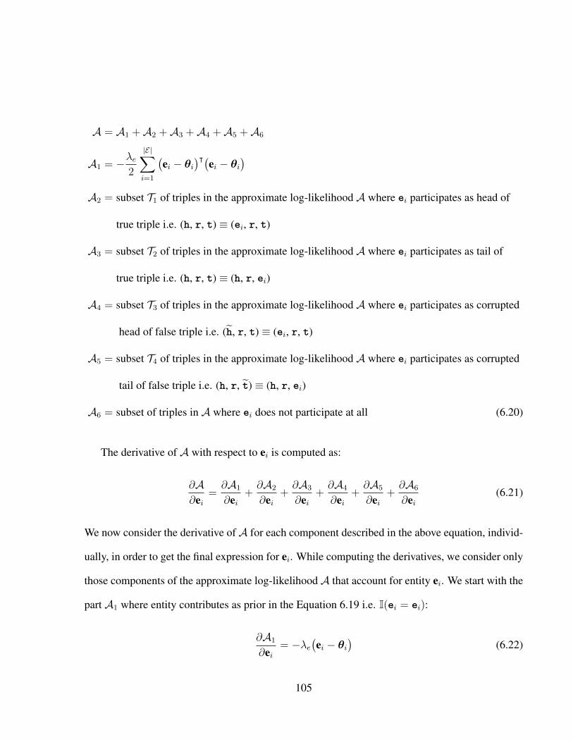
A = A1 +A2 +A3 +A4 +A5 +A6

A1 = −λe2

|E|∑i=1

(ei − θi

)ᵀ(ei − θi)A2 = subset T1 of triples in the approximate log-likelihood A where ei participates as head of

true triple i.e. (h, r, t) ≡ (ei, r, t)

A3 = subset T2 of triples in the approximate log-likelihood A where ei participates as tail of

true triple i.e. (h, r, t) ≡ (h, r, ei)

A4 = subset T3 of triples in the approximate log-likelihood A where ei participates as corrupted

head of false triple i.e. (h, r, t) ≡ (ei, r, t)

A5 = subset T4 of triples in the approximate log-likelihood A where ei participates as corrupted

tail of false triple i.e. (h, r, t) ≡ (h, r, ei)

A6 = subset of triples in A where ei does not participate at all (6.20)

The derivative of A with respect to ei is computed as:

∂A∂ei

=∂A1

∂ei+∂A2

∂ei+∂A3

∂ei+∂A4

∂ei+∂A5

∂ei+∂A6

∂ei(6.21)

We now consider the derivative ofA for each component described in the above equation, individ-

ually, in order to get the final expression for ei. While computing the derivatives, we consider only

those components of the approximate log-likelihoodA that account for entity ei. We start with the

part A1 where entity contributes as prior in the Equation 6.19 i.e. I(ei = ei):

∂A1

∂ei= −λe

(ei − θi

)(6.22)

105

Next we consider the case when entity represents the head in the true knowledge graph triples, i.e.

I(ei = h) and compute the derivative expression A2 as follows:

∂A2

∂ei= a ∗

T1∑n=1

(3 ∗(1− P(1 | ei, rn, tn)

)∗(rn ◦ tn

)− 1

C

C∑c=1

P(1 | ei, rc, tn) ∗(rc ◦ tn

)− 1

C

C∑c=1

P(1 | ei, rn, tc) ∗(rn ◦ tc

))(6.23)

In the above equation, T1 represents the set of all the true triples in the knowledge graph in which

entity ei plays the role of head entity. Also, operator ◦ in rn◦tn represents the element-wise product

between embeddings. Likewise, we compute the gradients of approximate complete log-likelihood

A when entity ei plays the role of tail (I(ei = t)) by considering component A3:

∂A3

∂ei= a ∗

T2∑m=1

(3 ∗(1− P(1 | hm, rm, ei)

)∗(hm ◦ rm

)− 1

C

C∑c=1

P(1 | hc, rm, ei) ∗(hc ◦ rm

)− 1

C

C∑c=1

P(1 | hm, rc, ei) ∗(hm ◦ rc

))(6.24)

In the above equation, T2 characterizes the set of all the true triples in the knowledge graph when

ei appears as the tail. We now consider the case where ei contributes as corrupt head I(ei = h) in

the false triples set T3 and compute the derivative of A4 as below:

∂A4

∂ei=

∂

∂ei1

C

T∑n=1

( C∑c=1

[log P(0 | I(hc = ei), rn, tn)

])= −a

C∗T3∑s=1

P(1 | ei, rs, ts) ∗(rs ◦ ts

)(6.25)

As final step in the derivative, we consider the case where entity participates in a false triple as

corrupt tail I(ei = t) and calculate the derivative of expression A5 as below:

∂A5

∂ei=

∂

∂ei1

C

T∑n=1

( C∑c=1

[log P(0 | hn, rn, I(tc = ei))

])= −a

C∗T4∑u=1

P(1 | hu, ru, ei) ∗(hu ◦ ru

)(6.26)

106

Finally, the derivative of expression A6 with respect to ei would be zero. As the last step, we

substitute the derivative ofA with respect to ei when it plays the role of e, h, t, h and t in a triple,

as derived in derived in Equation 6.22, 6.23, 6.24, 6.25 and 6.26 respectively into Equation 6.21 in

order to obtain final expression of approximate complete log-likelihood with respect to ei:

∂A∂ei

= λeα

((θi − ei

)+

aλe∗({ T1∑

n=1

(3CC∗(1− P(1 | ei, rn, tn)

)∗(rn ◦ tn

)− 1

C

C∑c=1

P(1 | ei, rc, tn) ∗(rc ◦ tn

)− 1

C

C∑c=1

P(1 | ei, rn, tc) ∗(rn ◦ tc

))}+{ T2∑m=1

(3CC∗(1− P(1 | hm, rm, ei)

)∗(hm ◦ rm

)− 1

C

C∑c=1

P(1 | hc, rm, ei) ∗(hc ◦ rm

)− 1

C

C∑c=1

P(1 | hm, rc, ei) ∗(hm ◦ rc

))}−{1

C

T3∑s=1

P(1 | ei, rs, ts) ∗(rs ◦ ts

)}−{1

C

T4∑u=1

P(1 | hu, ru, ei) ∗(hu ◦ ru

)}))(6.27)

As can be seen from the equation above, we can not obtain closed form solution for an entity.

Therefore, we optimize the above expression by utilizing stochastic gradient ascent. We now

proceed to the next derivation where we compute the update expression for the relation vector rp.

Update expression for parameter r

The parameter learning of a given relation rp in a knowledge graph is analogous to that of learning

in an entity as discussed in the previous section. A given relation rp might contribute to the

approximate log-likelihood A in Equation 6.19 as: (i) relation r when it is a part of true triple in

knowledge graph (i.e. I(rp = r)) (ii) corrupted relation r when it participates in a corrupted triple

(i.e. I(rp = r)) (iii) relation as is when it contributes as the prior (I(rp = rp)). We reconsider the

expression A in Equation 6.19 and disintegrate it further according to the role rp plays in it. This

can be mathematically outlined as follows:

107

A = A7 +A8 +A9 +A10

A7 = −λr2

|R|∑p=1

(rᵀprp

)A8 = subset T5 of triples in the approximate likelihood A where rp participates as a

true relation in true triple i.e. (h, r, t) ≡ (h, rp , t)

A9 = subset T6 of triples in the approximate likelihood A where rp participates as

corrupted relation in false triple i.e. (h, rp, t) ≡ (h, rp , ei)

A10 = subset of triples in A where rp does not participates at all (6.28)

The derivative of A with respect to rp is given by:

∂A∂rp

=∂A7

∂rp+∂A8

∂rp+∂A9

∂rp+∂A10

∂rp(6.29)

We consider each component of the derivative individually beginning with the case when the rela-

tion characterizes as the prior of the model I(rp = rp):

∂A7

∂rp= −λr

2

|R|∑p=1

(rᵀprp

)= −λrrp (6.30)

Next, we examine the case where relation contributes to A as a part of true triples (i.e. I(rp = r)):

∂A8

∂rp= a ∗

T5∑n=1

(3 ∗(1− P(1 | hn, rp, tn)

)∗(hn ◦ tn

)− 1

C

C∑c=1

P(1 | hc, rp, tn) ∗(hc ◦ tn

)− 1

C

C∑c=1

P(1 | hn, rp, tc) ∗(hn ◦ tc

))(6.31)

In the above expression, T5 represents the set of true triples in which rp appears. Finally, we

consider the case when relation rp operate as corrupted relation in the negative examples generated

108

in the model (i.e. I(rp = r)):

∂A9

∂rp=

∂

∂rp1

C

T∑n=1

( C∑c=1

[log P(0 | hn, I(rc = rp), tn)

])= −a

C∗T6∑

v=1

P(1 | hv, rp, tv) ∗(hv ◦ tv

)(6.32)

Finally, the derivative ofA10 with respect to rp is zero. Next, we substitute each role of relation as

rp, r and r derived in Equation 6.30, 6.31 and 6.32 into Equation 6.29 in order to obtain the final

derivative of approximate complete-likelihood with respect to relation embedding, rp, as below:

∂A∂rp

= α ∗ λr

(− rp +

aλr∗{ T5∑n=1

(3CC∗(1− P(1 | hn, rp, tn)

)∗(hn ◦ tn

)− 1

C

C∑c=1

P(1 | hc, rp, tn) ∗(hc ◦ tn

)− 1

C

C∑c=1

P(1 | hn, rp, tc) ∗(hn ◦ tc

))− 1

C

T6∑v=1

P(1 | hv, rp, tv) ∗(hv ◦ tv

)})(6.33)

As can be observed, we can not attain a closed-form solution for updating the relation rp, hence we

obtain the optimal value of relation embedding by stochastic gradient ascent. Also, note that the

above expression is dependent on only one data source: knowledge graph triples. We now proceed

to learning the topic model parameters {θ, β} in the next section while keeping (e, r) fixed.

Update expression for the parameter θ

In order to update the topic parameters, we consider only the fraction of approximate complete-

likelihood expression A in Equation 6.19 that involves the topic parameters {θ, β} and regard the

remaining proportion as constant C(e, r). We denote the expression involving {θ, β} parameters

as L(θ,β) as shown below:

L(θ,β) = α

(− λe

2

|E|∑i=1

(ei − θi

)ᵀ(ei − θi))+ (1− α)

( |E|∑i=1

|Ni|∑j=1

logK∑k=1

θikβk,wij

)(6.34)

109

In order to evade the summation inside the log expression in the second part of the equation

L(θ, β), we simplify it by noticing that the reason for summation over k is that the topic of j-th

word in the i-th document is unknown, i.e. variable zij is hidden. We denote observed parameters

of L(θ, β) as X= {θ, β} the hidden parameter as H = {z} in order to express the second part of

the equation as:

logK∑k=1

θikβk,wij= log

∑H

p(X,H) = log p(X) (6.35)

Next, we examine the expression log p(X) and expand it further as:

log p(X) = log∑H

p(X,H) = log∑H

p(X,H) ∗(q(H)

q(H)

)= log

(Eq[p(X,H)

q(H)

])≥ Eq

[log p(X,H)

]− Eq

[log q(H)

](from Jensen’s inequality)

≥ ELBO (6.36)

Instead of maximizing marginal probability log p(X), we maximize the Evidence Lower Bound

(ELBO) to find the parameters that gives as tight a bound as possible on the marginal probability.

In the above equation, q(H) is variational distribution over the hidden variable H defined as follows:

q(H) = q(zij = k) = φijk (6.37)

We consider the ELBO in Equation 6.36 and the definition of φ in Equation 6.37 and remodel the

likelihood function in Equation 6.34 for a given document di as:

L(θi,φi) = α

(− λe

2∗(ei − θi

)ᵀ(ei − θi))

+ (1− α)

(Ni∑j=1

(∑H

q(H) log p(X,H)−∑H

q(H) log q(H)))

(6.38)

= α

(− λe

2∗(ei − θi

)ᵀ(ei − θi))

+ (1− α)

(Ni∑j=1

K∑k=1

(φijk log θikβk,wij

− φijk log φijk))

(6.39)

110

After circumventing the summation inside the log expression, we are now prepared to compute the

update equations for the topic model parameters {θi, φijk, β}, beginning with the parameter θi:

∂L(θi,φi)

∂θi= α ∗ λe(ei − θi) + (1− α) ∗ ζi

θi(6.40)

where ζi ∈ RK is a vector whose k-th entry is defined asNi∑j=1

φijk. As we can observed, the closed

form solution for θi is not feasible, we employ projection gradient descent as in Wang and Blei

(2011) to update θi.

Update expression for the parameter φ

We next explain the update equation of the variational parameter φijk that represents the distri-

bution of k-th topic of j-th word in the i-th document. As we can observe, each word in the

document will have one of the K topics assigned to it, i.e.K∑k=1

φijk = 1, we introduce this equation

as Lagrange constraint in L(θi,φi) as follows:

L(θi,φi) = (1− α) ∗( Ni∑

j=1

K∑k=1

(φijk log θikβk,wij

− φijk log φijk))

+ λφ(K∑k=1

φijk − 1) + C(θ, ei)

(6.41)

We compute the derivative of the above equation with respect to φijk and set the result to zero in

order to obtain the final update expression for φijk:

φijk =θikβk,wij∑Kk=1 θikβk,wij

(6.42)

Update expression for the parameter β

After the learning algorithm has iterated over all the triples on the knowledge graph and updated the

parameters {e, r, θ, φ}, it can update the parameter β over all the text data, i.e. text documents of

all the entities. The generation of the update equation of β is similar to as in standard LDA model

111

with introduction of constraint that for a given topic k, the probability distribution of all the words

in vocabulary should sum to 1 resulting in the the following optimization equation for β:

L(β) = (1− α)

( |E|∑i=1

Ni∑j=1

K∑k=1

( V∑v=1

I(wij = v)φijk log(βk,v)))

+K∑k=1

λk( V∑v=1

βkv − 1)

+ C(θ, ei,φ) (6.43)

Solving the above equation by taking its derivative with respect to βk,v and each λk will yield the

following update expression for βk,v:

βk,v =

∑|E|i=1

∑Ni

j=1 φijk ∗ I(wij = v)∑Vv=1

∑|E|i=1

∑Ni

j=1 φijk ∗ I(wij = v)(6.44)

6.3.3 TAKE Algorithm

Having introduced the update expressions for the proposed model parameters {e, r, θ, β}, we now

present the proposed TAKE algorithm (Algorithm 3) in detail. The algorithm begins by initializing

the KG parameters {e, r} following a uniform distribution (line 1-3) or advanced initialization

procedure like setting the embeddings to pre-trained TransE vectors. The topic model parameters

are initialized to the final values obtained after executing LDA model on the text descriptions

of entities (line 4). TAKE algorithm then updates the model parameters over multiple epochs

until they have converged to stable values (line 5- 32). The convergence criteria is that change in

approximate log-likelihood over two consecutive epochs should be below a given threshold.

Within a given epoch, the algorithm maintains two temporary matrices Egradient, Rgradient that

store the gradient updates of entities and relations while iterating over all the triples of the knowl-

edge graph. The algorithm then retrieves the entity index of head hn, tail tn (line 9), corrupted

head hc (line 14), corrupted tail tc (line 18) in matrix E and computes their update expressions for

their roles as I(ei = hn), I(ei = tn), I(ei = hc) and I(ei = tc) in triple (hn, rn, tn) according

to Equation 6.27 and updates Egradient at the corresponding indexes. The model avails the values

112

Algorithm 3 Topic Augmented Knowledge Embeddings (TAKE)

Input: training data T = {hn, rn, tn}|T |n=1, set of entities E , set of relationsR, text description ofentities D = {di}|E|i=1, function F(e) that returns the index of input entity or relation, λe,λr, C: sample of negative examples

Output: entity embeddings E ∈ R|E|×K , relation embeddings R ∈ R|R|×K , topic vectors ofdescription Θ ∈ R|E|×K , topic-word distribution β ∈ RK×V

1: for l ∈ {E ∪ R} do2: l← Uniform() or pre-trained embeddings3: end for4: Θ and β ← LDA5: while not convergence do6: Set Egradient = 0, Rgradient = 0, Φ ∈ R|E|×Ne×K = 07: for each (hn, rn, tn) ∈ T do . update the KG parameters E and R8: Generate C negative triples {hc, rn, tn} with set of corrupt heads hC = {hc}C

c=1;negative triples {hn, rc, tc} with set of corrupt tails tC = {tc}C

c=1 and negativeexamples {hn, rc, tn} with set of corrupt C relations rC = {rc}C

c=1

9: h← F(hn); t← F(tn); r← F(rn)10: Update Egradient[h, : ] = Egradient[h, : ] +

(I(ei = h) part of Eqn. 6.27 using E and R

)11: Update Egradient[t, : ] = Egradient[t, : ] +

(I(ei = t) part of Eqn. 6.27 using E and R

)12: Update Rgradient[r, : ] = Rgradient[r, : ] +

(I(rp = r) part of Eqn. 6.33 using E and R

)13: for each hc in hC do14: h← F(hc);15: Update Egradient[h, : ] = Egradient[h, : ] +

(I(ei = h) part of Eq. 6.27 using E and R

)16: end for17: for each tc in tC do18: t← F(tc);19: Update Egradient[t, : ] = Egradient[t, : ] +

(I(ei = t) part of Eq. 6.27 using E and R

)20: end for21: for each rc in rC do22: r ← F(rc);23: Update Rgradient[r, : ] = Rgradient[r, : ] +

(I(rp = r) part of Eq. 6.33 using E and R

)24: end for25: end for26: for i = {1, 2, . . . | E |} do . update the topic parameters Θ and Φ27: Update Φ[i, :, : ] according to Equation 6.4228: Update θi by project gradient descent on Equation 6.4029: end for30: Et+1 ← Et+η ∗α

(λe(Θ−Et)+a∗Egradient

); Rt+1 ← Rt+η ∗α(−λr ∗Rt+ Rgradient

)31: Update β according to Equation 6.4432: end while

113

of E and R from the previous iteration in order to compute the update expressions for the above

parameters. It follows similar procedure to update Rgradient for relation rn and rc. The algorithm

then updates topic parameters Φ, Θ and β according to Equation 6.42, 6.40 and 6.44 respectively

(line 26-31). Once the algorithm has iterated over all the triples in KB (line 7-25), it updates E

by performing stochastic gradient ascent which considers the prior part I(ei = ei) in Equation

6.27 in addition to the remaining expression already stored in Egradient; likewise, R is updated by

considering I(rp = rp) part in addition to the final value of Rgradient (line 30). This marks the end

of one epoch. After the algorithm has converged, it returns the model parameters E, R, Θ and β

which are utilized for inferring newer links in the knowledge graph.

6.4 Experiments

Having discussed the proposed algorithm in previous section we now turn to its experimental eval-

uation where we solve two benchmark tasks: knowledge graph completion, entity classification.

Additionally, we perform qualitative analysis to answer two more questions about interpretabil-

ity of our model and the effect of our model on scarcely occurring entities in KG. We employ

two benchmark datasets, FB15K FB20K (Bordes et al., 2013) along with their entity descriptions

proposed in Xie et al. (2016) to evaluate our proposed algorithm. The triples in the datasets are

extracted from the Freebase knowledge graph (Bollacker et al., 2008) and the entity description of

each entity is crawled from the /ns/common/topic/description relation defined for each entity

in Freebase. While in FB15K dataset, we handle in-KB prediction where all the entities occurring

in the test set have already been encountered in the train and the validation set, FB20K dataset is

specifically designed for zero-shot scenario where at least one of the entity in every test set triple

is new and is never seen in the train or the validation set. The train and validation set of FB20K is

same as FB15K dataset. The detailed statistics of the datasets are provided in Table 6.1.

114

Table 6.1: Data sets used in our experiments on TAKE model (Xie et al., 2016)

DATASET #Relations #Entities #Train #Valid #TestFB15K 1341 14904 472860 48991 57803FB20K 1341 19923 472860 48991 30490

6.4.1 Knowledge Graph Completion

The goal of knowledge graph completion is to predict the true triple (h, r, t) when at least one of

the element h, r or t is missing in a triple. The efficiency of a given model for this task is evaluated

by corrupting the head h (or tail t, or relation r) of a given test triple by all the entities (or relations

in case of r) present in the dataset. The score of each resulting triple is computed according to

scoring function of proposed model and further sorted in decreasing order to obtain the rank of a

true triple among the corrupted triples in the sorted list.

Evaluation Protocol

The two standard metrics are reported in our experiments: Mean Rank of true test triples over the

entire test data and Hits @ n: the proportion of test triples placed among the top-n scores. These

two metrics further have two flavors: raw and filtered. In case of filtered metrics, we remove all

the triples that have already occurred in the train, validation or test dataset before computing the

score whereas we do not remove them for raw setting. In our experiments, we report Mean Rank,

Filtered Rank, Hits @ 10 (Raw and Filtered) for entities and Hits @ 1 (Raw and Filtered) for

relations. Lower ranks and higher Hits@n values are preferred during the evaluation.

Parameter Setting

We implemented our proposed model in C++ and further performed grid search on the following

hyper-parameter settings: λr(λe) ∈ {0.001, 0.01, 0.1, 1, 10, 100, 1000}, temperature a ∈ {3500

, 4000, 4500, 5000}, neg ratio C ∈ {1, 3, 5}, embedding dimension K ∈ {50, 80, 100, 150} and

learning rate η ∈ {0.01, 0.02, 0.1, 0.2} and recover the best combination of hyper-parameter by

115

Table 6.2: Mean Rank and Hits@10 (entity prediction) for models tested on FB15K dataset

FB15K Mean Rank Hits @ 10Raw Filtered Raw Filtered

TransE 210 119 48.5 66.1TransH 212 87 45.7 64.4

DKRL(BOW) 200 113 44.3 57.6DKRL(ALL) 181 91 49.6 67.4

SSP (Std.) 154 77 57.1 78.6SSP (Joint) 163 82 57.2 79.0

TAKE 195 72 44.0 60.8

evaluating them on validation set. Further, we initialize the {θ,β} parameters by running standard

LDA (Blei et al., 2003) on the text data and the stopping criteria of our algorithm is change in

likelihood between two consecutive epochs should be below a certain threshold. The optimal

settings of our model for knowledge graph completion for FB15K dataset are: λr = 0.1, λe = 0.1,

a = 4500, C = 1, α = 0.5 and K = 100 and η = 0.2. We use the same setting for FB20K dataset

while performing entity classification task.

As datasets are same, we reprint the experimental results of several baselines from the literature.

Specifically, we report the results for TransE (Bordes et al., 2013) and TransH model (Wang et al.,

2014b) models that rely on one source - knowledge graph triples - for learning the knowledge graph

embeddings. Also, we report results from two past models namely - DKRL (Xie et al., 2016) and

SSP (Xiao et al., 2017) that utilize both the knowledge graph triples and the text descriptions to

learn the entity embeddings. Each of these models further have two variants: DKRL(BOW) exploit

the CBOW encoder (Mikolov et al., 2013) for learning the word embeddings whereas DKRL(ALL)

is the weighted union of DKRL employing CNN encoder and TransE model. SSP(Std.) and

SSP(Joint) are the two variants of SSP model (Xiao et al., 2017). SSP(Std.) utilizes pretrained text

embeddings while SSP(Joint) jointly learns the text and the KB embeddings.

116

Table 6.3: Mean Rank and Hits@1 (relation prediction) for models tested on FB15K dataset

FB15K Mean Rank Hits @ 10Raw Filtered Raw Filtered

TransE 2.91 2.53 69.5 90.2TransH 8.25 7.91 60.3 72.5

DKRL(BOW) 2.85 2.51 65.3 82.7DKRL(ALL) 2.41 2.03 69.8 90.8

SSP (Std.) 1.58 1.22 69.9 89.2SSP (Joint) 1.87 1.47 70.0 90.9

TAKE 4.42 4.06 33.56 39.33

Results

The results of entity prediction and relation prediction for FB15K dataset are presented in the Table

6.2 and 6.3 respectively From the tables, we observe that:

(i) From Table 6.2, we conclude that our proposed model outperforms the existing “triples-

only” models on rank by a large margin. Further our model outperforms state-of-the-art text

augmented KG models on filtered rank.

(ii) From Table 6.3, we observe that the performance of our model is substandard for the relation

prediction compared to the state-of-the-art models. This might be due to the reason that

the proposed model has two hyper-parameters λe and λr for entity and relations. It shows

optimal performance for prediction relations and the entities for different set of parameters,

for instance, we were able to bring the Mean Filtered Rank of relation to 3.2 for FB15K

dataset when we set the parameters to λr = 0.1, λe = 1, a = 4000, C = 2 and K = 100.

6.4.2 Entity Classification

Most of the entities in the Freebase knowledge graph (Bollacker et al., 2008) have multiple types.

For instance, entity The Queen′s College in Freebase KG has following types: /base/oxford/

college and universities, /organization/organization and /education/university

117

etc. The goal of entity classification task is to predict all the possible entity type labels that an

entity may possess. Entity classification, therefore, is a multi-label classification task.

Evaluation Protocol

In order to perform our experiments, we acquire the FB15K entity classification datasets generated

in DKRL work (Xie et al., 2016) which has 13445 entities and 50 entity type labels which are

further randomly split into training and test split. For FB20K dataset, the 13445 in-KB entities

form the training set and newer 5019 out-of-KB entities form the test set. We obtain the out-of-KB

entity embeddings for FB20K dataset by optimize the Equation 6.39 while setting θi = ei in it as

proposed in Wang and Blei (2011). Further, for fair comparison, we train a Logistic Regression

classifier in one-vs-rest setting for multi-label classification task as done in DKRL work. The

evaluation metric is Mean Average Precision (MAP) which is a common metric used for evaluating

multi-label classification in literature (Neelakantan and Chang, 2015).

Table 6.4: The MAP Results for entity classification in FB15K and FB20K datasets

Model FB15K FB20KTransE 87.8 -BOW 86.3 57.5

DKRL(BOW) 89.3 52.0DKRL(ALL) 90.1 61.9

SSP (Std.) 93.2 -SSP (Joint) 94.4 67.4

TAKE 83.7 28.1

Results

The results of entity classification are presented in Table 6.4. From the results, we observe that

our model performs reasonable well on FB15K dataset and poorly on FB20K dataset. We con-

jecture that the reason of poor performance of out-of-KB entities in FB20K is the follows: our

model allows each dimension of KG entity embedding to have any range of values at the training

118

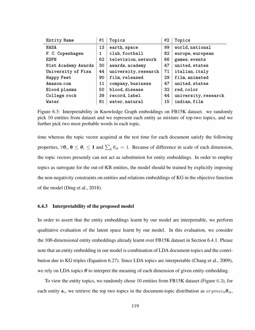
Entity Name #1 Topics #2 TopicsNASA 13 earth, space 99 world, nationalF. C. Copenhagen 1 club, football 82 europe, europeanESPN 62 television, network 66 games, events81st Academy Awards 30 awards, academy 47 united, statesUniversity of Pisa 44 university, research 71 italian, italyHappy Feet 90 film, released 29 film, animatedAmazon.com 11 company, business 47 united, statesBlood plasma 50 blood, disease 32 red, colorCollege rock 39 record, label 44 university, researchWater 81 water, natural 15 indian, film

Figure 6.3: Interpretability in Knowledge Graph embeddings on FB15K dataset. we randomlypick 10 entities from dataset and we represent each entity as mixture of top-two topics, and wefurther pick two most probable words in each topic.

time whereas the topic vector acquired at the test time for each document satisfy the following

properties, ∀θi, 0 ≤ θi ≤ 1 and∑

k θik = 1. Because of difference in scale of each dimension,

the topic vectors presently can not act as substitution for entity embeddings. In order to employ

topics as surrogate for the out-of-KB entities, the model should be trained by explicitly imposing

the non-negativity constraints on entities and relations embeddings of KG in the objective function

of the model (Ding et al., 2018).

6.4.3 Interpretability of the proposed model

In order to assert that the entity embeddings learnt by our model are interpretable, we perform

qualitative evaluation of the latent space learnt by our model. In this evaluation, we consider

the 100-dimensional entity embeddings already learnt over FB15K dataset in Section 6.4.1. Please

note that an entity embedding in our model is combination of LDA document-topics and the contri-

bution due to KG triples (Equation 6.27). Since LDA topics are interpretable (Chang et al., 2009),

we rely on LDA topics θ to interpret the meaning of each dimension of given entity embedding.

To view the entity topics, we randomly chose 10 entities from FB15K dataset (Figure 6.3), for

each entity ei, we retrieve the top two topics in the document-topic distribution as argmaxkθik,

119

Dimension 1 2 3 4 5#1 Topic famous club works california drama#2 Topic addition football published state series

Dimension 6 7 8 9 10#1 Topic team show islands stage played#2 Topic national television island career side

Figure 6.4: Table displays top two topics learnt along each of first 10 dimensions of 100-dimensional FB15K entity.

and for each topic k, we further retrieve the most probabilistic words in the topic from the topic-

word distribution β as argmaxvβk,v. For example, for an entity NASA, the most probabilistic topic

is topic number 13 (among the 100 topics learnt), which further has two most probable words

earth and space (obtained from β) and the second most probable topic is topic 99 whose two

most probable words are world and national. Although our model is compelling in recovering

the right topic for most of the entities, still it sometimes retrieves incorrect top topics because of

the presence of polysemic words in their document description. For example, in Figure 6.3, entity

Water refers to movie Water but the model retrieves compound ’water’ as the top topic.

By following a similar procedure, we could also interpret the top-n topic along each dimension

of any given entity in FB15K dataset. For example, we show the top two topics along the first

10 dimensions of FB15K entities in Figure 6.4 (leaving the rest of dimensions because of space

constraints). This shows that our model is interpretable as it can retrieve the topic being discussed

along each dimension of embedding.

6.4.4 Effect on sparsely occurring entities

Next, we aim to prove that the sparsely occurring entities in KG benefit more from the text doc-

uments while the frequently occurring entity’s embedding are dominated by the KG information.

To demonstrate that, we consider a smaller dataset, namely the validation set of FB15K to keep our

results manageable and train our proposed model on it with the following setting: λr = 1, λe = 1,

K = 100, C = 1, epochs = 10 and η = 0.1. In order to observe the effect of two data sources on

120

Figure 6.5: The effect of proposed model on sparsely occurring entities’ embeddings. The Y-axisplots average of offset=(e−θ)ᵀ(e−θ) value of each embedding while the X-axis plots the numberof times an embedding occurs in the KG.

entity embeddings, we compute the offset value (ei − θi)ᵀ(ei − θi) for each entity ei in KG.

This offset value (ei − θi) corresponds to amount of KG part being dominated in an embedding

as can be noticed by entity update Equation 6.27. We plot the offset value of each entity against

the count of occurrence of the corresponding entity in the KG in Figure 6.5. Specifically, each

Y-axis is the average of offset value of all the entities that have same count in the KG. Further,

the embedding values were learnt without performing the L2-norm of embeddings at the end of

each epoch, that accounts for the 1e11 value on the Y-axis.

As can be seen from the plot, the sparsely occurring entities have smaller offset value, hence

proving that their embeddings are benefiting more from the topic vectors learnt from text whereas

as the occurrence of entity in KG becomes frequent, it’s offset value is increasing showing that

its final embedding value is deviating away from topic vectors. This is because that the second half

of embedding update equation following a/λe in Equation 6.27 is more prominent and frequently

occurring embeddings are being endowed more with KG information.

121

6.5 Conclusion

We proposed a novel model that jointly learnt the entity and relation embeddings by exploiting

both the knowledge graph triples and the text description of entities in generative setting. The goal

of this model was two-folds: to instill interpretability in embeddings by relying on LDA topics and

to attain generalizability in embeddings by handling the out-of-KB entities. Our experimental re-

sults show that utilizing multi-modal data definitely helps us in learning high-quality embeddings.

Although, we were able to achieve the goal of interpretability in embeddings, we could not handle

the out-of-KB entities effectively and the required changes to attain this goal of generalizability in

the proposed model were also suggested.

122

CHAPTER 7

TEXT AUGMENTED ADVERSARIAL KNOWLEDGE GRAPH EMBEDDINGS

Much of the previous work on multi-modal learning of knowledge graph embeddings in the pres-

ence of entity text descriptions, discussed in the previous chapter, share one common design phi-

losophy: they consider the two sources of data as complementary to each other. In this work, we

distance ourselves from these approaches by considering an alternative view to multi-modal learn-

ing. Specifically, we consider two data sources in adversarial setting and propose a novel model

for text-enhanced knowledge graph embeddings.

7.1 Introduction

Knowledge Graphs (KG) (Bollacker et al., 2008; Miller, 1995; Suchanek et al., 2007) incorporate

rich information in them which can be leveraged to solve important AI problems such as ques-

tion answering (Bordes et al., 2014), coreference resolution (Ng and Cardie, 2002), web search

(Szumlanski and Gomez, 2010) and recommender systems (Zhang et al., 2016). As discussed in

the previous chapter in detail, knowledge graph embedding models have been front runners in ex-

ploiting the rich information present in the KGs. While early work on these models mainly focused

on leveraging only the knowledge graph triples to learn the distributional representation of entities

and relations (Bordes et al., 2013; Lin et al., 2015; Yang et al., 2015; Trouillon et al., 2016), lately,

the focus has shifted to exploit additional sources of information such as images (Xie et al., 2017),

types (Chang et al., 2014; Ma et al., 2017; Xie et al., 2016) and the text description of entities (Xie

et al., 2016; Wang and Li, 2016; Xiao et al., 2017) in order to learn high-quality KG embeddings.

Among the models utilizing auxiliary sources of information, models exploiting the entities text

description have been the most popular.

As already discussed in Chapter 6, Section 6.2.2, major work on text-enhanced knowledge

graph embeddings fall into three categories: (i) models in which semantic text embeddings and the

123

KB embeddings lie on the same features space and can further be combined in a novel way (Wang

et al., 2014a; Xie et al., 2016; Zhong et al., 2015) (ii) models in which semantic text embedding

and the KB embedding lie in different distributional space and a novel variant is proposed to

bring the text embedding onto the KB feature space (Shah et al., 2019; Wang and Li, 2016; Xiao

et al., 2017) (iii) models employing a novel attention mechanism to focus on specific words on

the text description of entities (Shi and Weninger, 2018; Xu et al., 2017). Although the above

models are effective, there is a common underlying assumption in all these models that the two

knowledge sources are complementary to each other. Most of them have not exploited the power

of adversarial models when working with multi-modal data in KGs, which have shown to be shown

to be successful in multiple applications (Fedus et al., 2018; Ma et al., 2017; Zhu et al., 2017).

We consider an alternative setting in our proposed work where the text descriptions and the

knowledge graph triples are posed in an adversarial setting. We consider the model generating

the semantic text embeddings from entity descriptions as generator and the model working with

the knowledge graph triples as discriminator. In GAN terminology, these semantic embeddings

form the counterfeit currency produced by the generator in order to deceive the discriminator and

the goal of generator is to generate the text embeddings as similar to KB entity embeddings as

possible. On the other hand, the goal of the discriminator is to learn to distinguish between entity

embeddings generated from knowledge graph triples data (pdata) and the counterfeit embeddings

(pz) aka text embeddings generated by the generator. Because of the competition, both the players

are improving their methods, which in turn produces high quality KG embeddings.

To the best of our knowledge, we are the first to consider the entity text description and the

knowledge graph triples in adversarial settings and propose a novel model to enhance the knowl-

edge graph embeddings by text descriptions. It must be mentioned that our proposed method

is model-agnostic. We can employ any of the existing knowledge graph embedding model like

TransE (Bordes et al., 2013), DistMult (Yang et al., 2015) etc inside the discriminator.

124

7.2 Related Work

Much of the related literature covering the text-enhanced knowledge graph embeddings have al-

ready been discussed in Sections 6.2.1 and 6.2.2. However, there have been three directions in

the past that have specifically considered knowledge graph embedding in adversarial setting. We

discuss them in detail here.

Typically, negative examples in knowledge graph embedding models are generated by corrupt-

ing either the head or the tail of a given positive example by either random sampling or Bernoulli

distribution (Wang et al., 2014b), which is not necessarily the optimal way of generating negative

examples. Two related research directions (Cai and Wang, 2018; Wang et al., 2018) in the past

have employed GANs to generate negative examples more intelligently. Collectively, the goal of

discriminator is to train a standard KB embedding model whereas the purpose of the generator

is to produce advanced negative examples such that the discriminator finds it hard to distinguish

between a given positive example and the negative example produced by generator. The model for-

mulation of both the models is nearly identical, they were proposed by two independent research

groups around the same time.

The most related work to ours is Qin et al. (2020), as they employ GAN to solve zero-shot

learning in KB embeddings by exploiting the text descriptions of a given relation. For a given triple

(h, r, t), they exploit the text description of relation r to learn its TD-IDF vector representation

that forms the noisy distribution of generator. The neighborhood information of both h and t is

exploited to learn the joint embedding of the pair (h, t) that forms the true data distribution of

the discriminator. This is followed by training of Wassertein GAN (Arjovsky et al., 2017) over

these two distributions. Our proposed model differs from them considerably as we do not utilize

GAN (or stacked NN) directly to train our model as them, our model is adversarial because the

two sub-modules designed inside it are satisfying opposing constraints.

125

Inspired by enormous success of GAN models (Zhu et al., 2017; Minervini et al., 2017; Chen

et al., 2016) in other applications, we next propose a novel multi-modal knowledge graph embed-

dings model trained in adversarial setting.

7.3 Adversarial Approach to learning KB embedding model

The problem under consideration is same as proposed in Chapter 6. The input is a knowledge

graph K = {E ,R, T ,S} where E , R and T = {(h, r, t)}|T |n=1 are the set of entities, relations

and knowledge graph triples. Besides, the model can take advantage of set of documents S =

{di}|E|i=1 where each document represents textual description di about an entity ei ∈ E present in

the knowledge graph K. The goal is to learn knowledge graph embedding by utilizing two sources

of data: the triples T and the entity descriptions S.

We aim to train a novel knowledge graph embedding model that poses two sources of data in

an adversarial setting. We further develop two models: generator G and discriminator D in our

formulation. The goal of generator is to generate the semantic text embeddings for each entity

ei ∈ E by utilizing the document di ∈ S. In particular, the generator deceives the discriminator

into believing that text embeddings are entity embeddings obtained from knowledge graph triples

T . It accomplishes this by employing constrained optimization over the text description where the

constraint forces each text embedding to lie close to corresponding entity embedding in KG in the

low-dimensional feature space. On the other hand, discriminator D aims at learning knowledge

graph embeddings from the triples T while ensuring that it drives KG entity embedding away from

the text embeddings generated by G. We conjecture that because of the additional constraints that

the proposed model has to guarantee, it would result in high-quality embeddings. After the training

is over, the embeddings learnt by discriminator are retained as the final KB embeddings.

Before we formulate the model, it must be mentioned that there are two set of parameters in our

model. The discriminator parameters ΘD = {E,R} consist of KG entity embedding E ∈ R|E|×k

and relation embeddings R ∈ R|R|×k. For a given triple (h, r, t), an entity’s embedding can be

126

obtained by its index in the matrix E i.e. Eᵀ(h,:) ≡ h and Eᵀ

(t,:) ≡ t and Rᵀ(r,:) ≡ r where h, r, t ∈ Rk

are the knowledge graph embeddings. The ΘD parameters are optimized inside the discriminator

model. The generator parameters are ΘG = {W ,M} and optimized inside generator. Also,

the parameter E is passed from discriminator to generator and is kept constant inside generator.

The parameter M is passed from the generator to discriminator and is kept constant inside the

discriminator. We now present the technical details of the model starting with the generator.

7.3.1 The Generator Design

The aim of the generator G is to learn text embedding (or topic vector) for each entity present in

the KG by tapping into the semantic information present in the entity description documents S,

while at the same time ensuring that each text embedding lie close to the corresponding KG entity

embedding. We employ Constrained Non-Negative Matrix Factorization (CNMF) (Liu and Wu,

2010; Xiao et al., 2017) over the entity descriptions in order to achieve the above two goals. We

first represent the entity descriptions S as a matrixC ∈ R|V |×|E| whose each column ci ∈ R|V | is a

count vector for entity ei extracted from description di. Specifically, each entry cji inC represents

the number of times jth vocabulary word occurred in the entity description of ei. The goal of

non-negative matrix factorization is to find two factors W ∈ R|V |×k and ST ∈ Rk×|E| that when

multiplied together generate the original matrix C. That is

C ≈WST (7.1)

where each row si ∈ Rk of matrix S represents the semantic text embedding of entity ei. The

factorization can be achieved by minimizing the Frobenius norm between the original matrix C

and the product of the factorsW and S as follows:

O = ‖C −WST‖ (7.2)

In order to incorporate the constraint that the text embeddings should lie close to the corresponding

KG entity embeddings, we consider the KG entity embedding as matrix E ∈ R|E|×k. The matrix

127

E is a discriminator paramater being optimized in D and is kept constant inside the generator G’s

optimization. Further, as both the text and the KG entity embeddings are derived from the two

different sources of information, we introduce a projection matrixM ∈ Rk×k that projects the KG

entity embeddings from the triple feature space onto text feature space. Our goal is to bring the

resultant projected KG entity embeddings close to text embeddings by introducing the following

constraint in the model:

S = EM (7.3)

In the above equation, matrix E represents the constraint (and hence, is considered a constant by

generator) that we wish the text embedding to follow.

Please note that this model can be extended to the out-of-KB setting where some entities, Ein,

have two data sources as defined above whereas the other set of entities, Eout, do not participate in

any KG triple and model only has access to their text descriptions. In that case the constraint in

Equation 7.3 will be modified as S = AM where matrixA ∈ R|Ein+Eout|×|k+Eout| is defined as:

A =

E|Ein|×k 0

0 I|Eout|×|Eout|

(7.4)

Here, I|Eout|×|Eout| is an identity matrix and M ∈ R|k+Eout|×k is the projection matrix. In this case,

the entities in Ein would satisfy the usual constraint that a given text entity should lie close to the

corresponding KB entity. However, for entities in Eout, the text embedding will be incorporated in

matrix M itself and these entities can not be constrained to lie close to KB entity embeddings as

KB entities will not be available for entities in Eout. For now, we only consider the case in Equation

7.3, where both the sources of data are available for each entity, i.e |Eout| = 0.

By introducing the constraint posed in Equation 7.3 into the objective function proposed in

Equation 7.2, the objective modifies as follows:

O = ‖C −W (EM)T‖

= ‖C −WMTET‖(7.5)

128

The non-negativity constraints in the modified objective function above are that each element wij

in matrix W and∑

k eik ∗ mkj in the product EM should be non-negative. Let αij and βij be

the Lagrange multiplier for the constraint wij ≥ 0 and∑

k eik ∗ mkj ≥ 0 respectively and we

further define matrix α ∈ R|V |×k and β ∈ R|E|×k which results in the final optimization function

of generator G as:

LG(W ,M) = ‖C −WMTET‖+αW T + β(EM )T (7.6)

Parameter Learning in Generator

Following the optimization steps in the Constraint Non-Negative Matrix factorization work (Liu

and Wu, 2010), we solve the objective function in Equation 7.6 as:

LG(W ,M ) = Tr((C −WMTET

)(C −WMTET

)T+αW T + β(EM )T

)= Tr

(CCT − 2CEMW T +WMTETEMW T +αW T + β(EM)T

)= Tr

(CCT

)− 2Tr

(CEMW T

)+ Tr

(WMTETEMTW T

)+ Tr

(αW T

)+ Tr

(β(EM )T

)(7.7)

Tr(W) represents the trace of the matrix and is obtained by taking sum of eigenvalues (Lipschutz,

1968). Taking the derivative of LG(W ,M) with respect to W and M and set them to zero, we

get the following:

∂LG∂W

= −2CEM + 2WMTETEM +α = 0 (7.8)

∂LG∂M

= −2ETCTW + 2ETEMW TW +ETβ = 0 (7.9)

Multiply Equation 7.9 byMT on both sides we get:

−2MTETCTW + 2MTETEMW TW +MTETβ = 0

−2MTETCTW + 2MTETEMW TW + (EM )Tβ = 0

(7.10)

129

In the resulting Equations 7.8 and 7.10, we use Kuhn-Tucker condition αijwij = 0 and (∑

k eik ∗

mkj) ∗ βij = 0, that generate the following equations:

(CEM )ijwij − (WMTETEM )ijwij = 0 (7.11)

(W TCEM )ijmij − (W TWMTETEM )ijmij = 0 (7.12)

The above equations will result in the final update equations of wij and mij as follows (Lee and

Seung, 2001):

wij ← wij(CEM )ij

(WMTETEM )ij(7.13)

mij ← mij(W TCEM )ij

(W TWMTETEM )ij(7.14)

7.3.2 The Discriminator Design

The goal of discriminator is to learn the relation and entity embedding for triples T present in the

KG K, while ensuring that it learns to discriminate between the entity embeddings E learnt from

KG and the semantic embedding S learnt from the text. Although, our discriminator is model-

agnostic and can utilize any of the existing scoring function like TransE (Bordes et al., 2013),

TransH (Wang et al., 2014b), TransR (Lin et al., 2015) to train our discriminator, we employ the

scoring function DistMult (Yang et al., 2015) for a given triple (h, r, t) as follows:

φ(h, r, t) =k∑l=1

hlrltl (7.15)

where h, r, t ∈ Rk are the KG embeddings of a given triple (h, r, t) in KG. We further utilize

sigmoid function, similar to (Trouillon et al., 2016), to generate the probability of a triple (h, r, t)

being true (or false) as below:

PD(Y |(h, r, t)

)= σ

(− Y φ(h, r, t)

)(7.16)

where Y = {1,−1} represents the label of the true (or false) triple. The above probability represents

the true (data) distribution probability (pdata) and the goal of discriminator is to maximize it. At

130

the same time, discriminator aims to learn to distinguish the KB entity embeddings from the text

embeddings. In order to achieve that, the discriminator acquire the text embedding of head and tail

of a given triple as follows:

hs = Sᵀ(h,:) = (E(h,:)M)ᵀ = Mᵀh and

ts = Sᵀ(t,:) = (E(t,:)M)ᵀ = M ᵀt

(7.17)

where hs and ts are the text embeddings for the head and the tail in triple (h, r, t) in discriminator.

They are obtained by applying the generator’s constraint in Equation 7.3. M ∈ Rk×k is the

projection matrix proposed in Equation 7.3 which is considered as a constant in the discriminator

model. The resulting scoring function of a discriminator for the text embedding is as follows:

φ(hs, r, ts) =k∑l=1

hlsrltls (7.18)

The probability of a triple being true based on the text embeddings of head and the tail is given by:

PG(Y |(hs, r, ts)

)= σ

(− Y φ(hs, r, ts)

)(7.19)

Please note that the probability in above Equation 7.19 represents the probability of noise pz(z)

generated by the generator. The goal of discriminator is to maximize the probability of true data in

Equation 7.16 while minimizing the probability of the noise in Equation 7.19 at the same time. In

order to achieve this, it maximizes the following objective function:

LD(E,R) = EY∼PD[

log(PD(Y |h, r, t)

)]+ EY∼PG

[log(1− PG(Y |h, r, t)

)](7.20)

7.4 The proposed algorithm

After explaining our generator and discriminator in detail, we now explain our proposed algorithm

- Text Augmented Adversarial Knowledge graph Embedding (TAAKE) (algorithm 4) in detail

here. The input to the algorithm is two data sources: knowledge graph triples T and the text

131

Algorithm 4 Text Augmented Adversial Knowledge Embeddings (TAAKE)

Input: training triples T = {hn, rn, tn}|T |n=1, set of entities E , set of relationsR, text descriptionof entities S = {di}|E|i=1

Output: Knowledge graph embeddings Θ = {E,R,W ,M} trained in adversarial setting

1: while not convergence do2: Sample mini-batch of data Tbatch from the triples T3: Set Ψ = 0 . entities to be optimized by Generator G4: for each triple (h, r, t) ∈ Tbatch do . Discriminator D optimization5: Ψ = Ψ ∪ {h} ∪ {t}6: Generate C negative examples for the given triple.7: Update the discriminator parameters Θ = {E,R} for given triple according to8: Equation 7.20 for both positive and negative examples:9: θD = θD + η∇θDLD(E,R)

10: end for11: for s in Ψ do . Generator G optimization12: Update the generator parameters Θ = {W ,M} for entity s according to iterative13: update algorithm proposed in Equation 7.13 and 7.14.14: end for15: end while

description of entities S. The algorithm would optimize and return four model parameters Θ =

{E,R,W ,M} at its completion. The algorithm iterates until the stopping criteria is met which

is a fixed number of iterations while allowing early stopping when the rank of true triples start

increasing over validation set. Within each epoch (line 1-15), the discriminator D first optimizes

the triple parameters (line 4-10). It samples batch, Tbatch, of triples (line 2) and for each triple

in the batch, generates C negative examples (line 6) by either corrupting the head h or the tail

t of a given triple. The discriminator parameters ΘD = {E,R} are updated for each triple by

performing stochastic gradient ascent (line 8-9) on the objective function in Equation 7.20. After

discriminator has updated one batch, the control is passed to the generator G which updates the

text embedding parameters for all the entities that occurred in a given batch Tbatch (line 11-14).

It updates the generator parameters ΘG = {W ,M} by iterative update algorithm proposed in

Equation 7.13 and 7.14. After the optimization is over, the model parametersE,R can be utilized

for link prediction on test data.

132

The rigorous evaluation of the proposed model is an immediate direction. Because of the ad-

versarial constraints, high-quality embeddings {E,R} of a given KG will be returned by discrim-

inator that could be utilized for knowledge graph completion, triple classification tasks (Bordes

et al., 2013). Also, it would be interesting to observe the performance of the model when the text

embeddings S are utilized as the substitute of the KG entity embeddings E. Because of the con-

straint that brings the two closer, we should see superior performance while substituting the KG

entities with the text embeddings. Further, we hypothesize that because the model is utilizing two

data sources to learning the KG embeddings, the performance of the model would be superior than

the existing models like TransE (Bordes et al., 2013), TransH (Wang et al., 2014b) which rely on a

single source of data, namely, KG triples.

133

CHAPTER 8

CONCLUSION

Our key goal in this dissertation was to develop methods that facilitate a tighter integration of neuro

symbolic systems that are scalable and are endowed with symbolic reasoning capabilities. To this

effect, we have proposed a set of novel neuro-symbolic architectures inside the framework of neu-

ral SRL that can reason about complex interactions present in the relational data. In addition,

we have presented some solutions to the novel problems encountered in knowledge graph embed-

dings sub-field in order to make these models more generic for handling relational data. While

these models take significant steps towards achieving true neuro-symbolic AI, there are some sub-

problems that still need to investigated. We elucidate a few of these problems in detail and propose

suitable solutions to them.

8.1 Future Directions

8.1.1 Knowledge Graph Alignment

Though highly useful in solving AI tasks, an important downside of current knowledge graphs is

that each of them has been developed by independent organizations by crawling facts from dif-

ferent sources, or by utilizing different algorithms. This results in knowledge graphs in different

languages/formats/structures. As a result, the knowledge embodied in these different graphs is het-

erogeneous and complementary (Zhu et al., 2017). This necessitates the need for integrating them

in order to form one unified knowledge graph that would form a richer source of knowledge to

solve AI problems more effectively. As a first step towards integrating these knowledge graphs, one

needs to address the following issues, which collectively are known as knowledge graph alignment:

(i) entity alignment (entity resolution) that aims at finding entities in different knowledge bases

being integrated which, in fact, refer to same real-world entity (ii) triple-wise alignment fo-

cuses on finding triples in two knowledge graphs that refer to the same real-world fact. For in-

stance, even though triple (m.030cx, tv program genre, m.01z4y) in Freebase and (Friends,

134

genre, Comedy) triple in Dbpedia refers to same fact - Friends sitcom has comedy genre - they

are represented with different identities of entities and relations in two knowledge graphs.

Motivated by their success inside single knowledge graph problems, more recently, embed-

dings have been employed to perform knowledge graph alignment across multiple knowledge

graphs. One of the early works along this line is by Chen et al. (2016), that encodes entities

and relations of two knowledge graphs into two separate embeddings space and proposes three

methods of transitioning from an embedding to its counterpart in other space. Following this,

more advanced approaches for knowledge graph alignment have been proposed that can mainly be

divided into three main categories:

• The first set of models overcome the problem of low availability of aligned entities and

aligned triples across multiple knowledge graphs. As low availability of training data can

hinder the performance of model, these works increase the size of the training data either

iteratively (Zhu et al., 2017); or via bootstrapping approach (Sun et al., 2018); or by co-

training (Chen et al., 2018) technique.

• Another line of research is based on the idea that in addition to utilizing the knowledge in

standard relation triples, there is rich semantic knowledge present in the knowledge graphs

in the form of properties and text description of entities which can be harnessed to improve

the performance of model (Sun et al., 2017; Zhang et al., 2019; Zhu et al., 2019).

• The third line of research is focused on designing models that overcome the limitations

of translation based embeddings models (Li et al., 2018), as they exploit standard Graph

Convolutional Networks (Wang et al., 2018), their relational variants (Wu et al., 2019; Ye

et al., 2019) and Wasserstein GAN (Pei et al., 2018) in order to learn the embeddings of

entities and relations in multiple knowledge graphs.

135

Motivation We propose a novel knowledge base alignment technique based upon string edit dis-

tance that addresses the following limitations of the existing models (Kaur et al., 2020a):

• Even though the past techniques have exploited the supplementary knowledge present in

KBs in the form of text description of entities, properties of entities as attributional embed-

dings; none of them exploited the rich semantic knowledge present in the type descriptions

of the entities. As shown in the past (Chang et al., 2014; Ma et al., 2017; Xie et al., 2016;

Krompaß et al., 2015), incorporating type information into a single KB model increases the

productive performance of the model. Likewise, we conjecture a performance improvement

in knowledge alignment task by utilizing the type information. Further, use of type informa-

tion can help the model deal with polysemy issues present in KBs.

• We consider multiple possible interactions between triples of two knowledge graphs by per-

forming all possible edit distances between two triples. This is different from the linear

transformation model (Chen et al., 2016) that only considers one possible transformation

between corresponding entities/relations in two triples. Multiple transformations allow mul-

tiple ways in which two similar triples can be brought closer in embedding space.

• Finally, all the past models have considered triple-wise alignment between binary relations

while our proposed model can find similarity between relations of any arity. For instance,

if our task is to perform threshold-based classification between two relations, let us say,

distance(advisedby(william, lisa), coauthor(william, lisa, tom)) < θ, where θ is the

threshold for positive classification, then our proposed model can find the edit distance be-

tween two relations of different arity.

Knowledge Alignment by String edit distance in embedding space: We consider a multi-

lingual knowledge base K that consists of a set L of languages. Specifically, we consider two

ordered language pairs (L1, L2) ∈ L2 where each language L1 = (E1, R1, T1) consist of set of

136

Figure 8.1: A Finite State Transducer. Operation a : b represent that the finite state transducerwould read input character a ∈ x and outputs character b ∈ y.

entities E1, relations R1 and triples T1 = r1(h1, t1)1 . Similarly, L2 = (E2, R2, T2). We aim

at finding the distance between triples (T1, T2) ∈ (L1, L2) such that the distance between aligned

triples is always less than misaligned triples. This is because entities (and relations) that participate

in similar triples, being semantically similar, will lie close to each other in the embedding space.

Formally,

dist(r1(h1, t1), r2(h2, t2)

)< dist

(r1(h1, t1), rq(hq, tq)

)(8.1)

where r1(h1, t1) ∈ T1, r2(h2, t2) ∈ T2 and rq(hq, tq) ∈ T′2. The corrupted sample set T ′2 is

defined as T ′2 = {rq(h2, t2) | ∀rq ∈ R2} ∪ {r2(hq, t2) | ∀hq ∈ E2} ∪ {r2(h2, tq) | ∀tq ∈ E2} where

r2(h2, t2) ∈ T2, a true triple existing in language L2.

String-edit distance: The distance function of our model is inspired by the edit distance com-

putation between a pair of strings (x, y) by memoryless stochastic transducer proposed by Ristad

and Yianilos (1998). The idea was that a transducer (Figure 8.1) receives an input string x and

1constants used to represent entities and relations in the domain are written in lower-case (e.g., r1, h1); set ofentities and relations are capitalized (e.g., E1, R2)

137

performs a sequence of edit operations until it reaches the terminal stage when it outputs string y.

Edit operations, δ(z), performed by transducer were defined as: δ(a, b): substitution of character

a ∈ x by character b ∈ y; δ(a, ε): deletion of character a ∈ x; δ(ε, b) : insertion of character b ∈ y.

One sequence of edit operations between (x, y), called edit sequence, is defined as the product of

all the edit operations along the sequence. The total edit distance between pair of strings is defined

as the sum of all the edit sequences edq :

dist(x, y) =∑edq

∏δ(z)∈ edq

δ(z) (8.2)

The cost of edit operations, δ(z), is a learnable cost that was optimized by EM algorithm (Moon,

1996) in the original model (Ristad and Yianilos, 1998; Oncina and Sebban, 2006).

String-edit operation δ(z): Inspired by learning of string-edit distance by Ristad and Yianilos

(1998), our goal is to compute the distance between two triples in Equation 8.1 by formulating

them as pair of strings. We aim at considering each aligned triple pair (T1, T2) ∈ (L1, L2) such

that T1 ∈ L1 is analogous to input string x and T2 ∈ L2 being analogous to output string y.

Specifically, by considering triple rj(ei, ek) as string rjeiek, edit distance computation between

two strings can be performed by making the following assumptions:

• Our basic unit of edit operation is one entity e or one relation r. Further, each entity or each

relation are represented by low-dimensional embedding.

• Our basic edit operation are: (a) substitution of an entity or a relation in T1 ∈ L1 by any

another entity or relation in T2 ∈ L2 i.e δ(e1, e2), δ(e1, r2), δ(r1, e2), δ(r1, r2) for every

e1 ∈ E1, e2 ∈ E2, r1 ∈ R1, r2 ∈ R2 (b) deletion of an entity or relation present in T1 ∈ L1

i.e. δ(e1, ε), δ(r1, ε) for every e1 ∈ E1, r1 ∈ R1 (c) insertion of an entity or relation present

in T2 ∈ L2 i.e. δ(ε, e2), δ(ε, r2) for every e2 ∈ E2, r2 ∈ R2. We aim to perform these edit

operations in embedding space.

138

Figure 8.2: Knowledge graph alignment by string-edit distance in embedding space.

As can be seen, some of the edit operations such as δ(e, r) and δ(r, e) are semantically incorrect. To

overcome this, we consider three embedding spaces: entity-space, relation-space and string-space

(Figure 8.2). This ensures that original entities’ (or relations’) information is preserved while they

participate in the string-edit distance computation. Secondly, this also guarantees that entities are

semantically different from relations as we locate them in separate vector space (Lin et al., 2015).

Specifically, we model all the entities in language L1 and L2 to reside in ke-dimensional em-

bedding space, i.e. ∀e1 ∈ E1, e2 ∈ E2, e1 ∈ Rke , e2 ∈ Rke . Further, all the relations in L1 and

L2 lie in kr-dimensional embedding space, i.e. ∀r1 ∈ R1, r2 ∈ R2, r1 ∈ Rkr , r2 ∈ Rkr . In order

to perform the edit operation between two triples (T1, T2) ∈ (L1, L2), their constituent entities

and relations are first projected onto the ks-dimensional string-space. For example, embedding

corresponding to the triple r1(h1, t1) ∈ T1 and r2(h2, t2) ∈ T2 in Equation 8.1 are projected onto

string-space as follows:

rs1 = r1Mr1 , rs2 = r2Mr2 , (8.3)

hs1 = h1M

r1h1−type, ts1 = t1M

r1t1−type, hs

2 = h2Mr2h2−type, ts2 = t2M

r2t2−type, (8.4)

where r1, r2 ∈ Rkr , h1, h2, t1, t2 ∈ Rke , Mr1 , Mr2 ∈ Rkr×ks , Mr1h1−type, Mr1

t1−type ∈

Rke×ks Mr2h2−type, Mr2

t2−type ∈ Rke×ks . Also, we enforce the constraints that the embeddings and

139

the projection matrix lie inside the unit ball i.e. ‖rs‖2 ≤ 1, ‖hs‖2 ≤ 1, ‖ts‖2 ≤ 1, ‖rMr‖2 ≤

1, ‖eMre−type‖2 ≤ 1. The matrices Mr1 and Mr2 are the projection matrices that project the

relations from the relation-space to the string-space. Similarly, Mr1h1−type is the projection matrix

that project entities from the entity-space to string-space. More specifically, projection matrices

Mr1h1−type and Mr1

t1−type represent the type-matrices that encode the type of entities h1 and t1

inside the relation r1 respectively. The total number of type-matrices will be equal to total possible

entity types in a knowledge base.

Once the entities and relations of the aligned pairs have been projected to the string-space,

they are considered semantically equal. Henceforth, they represent characters of strings upon

which we perform string-edit distance operations in the string-space. Consequently, aligned triples

(T1, T2) =(r1(h1, t1), r2(h2, t2)

)provided as training data represent transformed triple (T1, T2) =(

rs1(hs1, t

s1), r

s2(h

s2, t

s2))

after projection. These transformed triples are modeled as string pair

(x, y) =(rs1h

s1t

s1, r

s2h

s2t

s2

)in string-space, where each character of the string has its correspond-

ing embedding, which is obtained by projection operation on entities and relations residing in their

original embedding space. As a next step, we consider embeddings of characters of string x as set

a = {rs1,hs1, t

s1} and string y as b = {rs2,hs

2, ts2} and define edit operations - substitution, deletion

and insertion as follows:

• substitution operation is difference between embedding of character a in input string x and

character b in output string y, i.e. δ(a,b) = (a− b), a,b ∈ Rks

• deletion operation δ(a, ε) is the difference between embedding of character a in input string

x and special null embedding ε: δ(a, ε) = (a− ε), a ∈ Rks

• insertion operation δ(ε,b)is the difference between special null embedding ε and embedding

of character b in the output string y: δ(ε,b) = (ε− b), b ∈ Rks

The next step after computing the edit-operation is determining the edit-sequence between

string pair, which is explained as follows.

140

Edit-sequence and the Edit-distance computation As discussed previously, one edit-sequence

is a sequence of edit operations, δ(z), performed between a pair of strings (x, y) starting at input

string x and reaching output string y. We define one edit-sequence as an element-wise dot product

of embeddings obtained as a result of edit operation, δ(z), between string pairs (x, y). This is

followed by L2-norm, in order to obtain a scalar value for one possible edit distance between

(x, y). Formally,

edq(r1(h1, t1), r2(h2, t2)

)= ‖�

(δ(z1), δ(z2), . . . , δ(zk)

)‖22 =

ks∑i=1

[δ(z1)

(i)δ(z2)(i) . . . δ(zk)

(i)]2

(8.5)where δ(z1), δ(z2), . . . , δ(zk) are the vector obtained for each edit operation previously in the

string-space. � is the element-wise dot product of the vectors and δ(zk)i is the i-th element of the

vector δ(zk). As there can be multiple edit sequences possible between triples (T1, T2), the final

distance between the pair of relation triples is defined as an average of all the edit sequences.

dist(r1(h1, t1), r2(h2, t2)

)=

1

N

∑edq

edq(r1(h1, t1), r2(h2, t2)

)(8.6)

where N = |edq(r1(h1, t1), r2(h2, t2)

)|, number of edit sequences between triples r1(h1, t1),

r2(h2, t2). To train the proposed model, we minimize margin-based ranking criteria over the

aligned training pairs (T1, T2) ∈ (L1, L2):

LA =∑

(T1,T2)

[γA + dist

(r1(h1, t1), r2(h2, t2)

)− dist

(r1(h1, t1), rq(hq, tq)

)]+

(8.7)

where r1(h1, t1) ∈ T1 and r2(h2, t2) ∈ T2, [x]+ = max{0, x}, γA is the hyperparameter. The

negative example rq(hq, tq) is obtained by corrupting positive example r2(h2, t2) (cf. eqn (8.1)).

The model can be empirically evaluated by utilizing multi-lingual dataset, WN31, designed by

Chen et al. (2016). WK31 dataset contains English (En), French (Fr) and German (De) knowledge

graphs where the ground truth of the aligned triples of two languages (e.g. En−Fr and En−De)

are crawled from Dbpedia’s dbo : Person domain. The evaluation should be designed as binary

classification task where two multi-lingual triples are aligned if dist(r1(h1, t1), r2(h2, t2)) < θ,

141

where θ will be optimized over the validation set. By maintaining the positive to negative example

ratio as 1 and accuracy as the evaluation metric for the proposed model, we hope that the model

would yield efficient results.

8.2 Closing Remarks

The models that we have already developed in this dissertation in addition to the ones we aim to

investigate are our first steps in realizing the grand vision of neuro-symbolic integration. How-

ever, there are some directions that could be pursued beyond the scope of this thesis that could

facilitate the development of more sophisticated neuro-symbolic models. One direction to explore

would be to harness the human expert knowledge to learn more robust systems. Human advice is

especially crucial in the domains where the data is noisy, insufficient and incorrect. Because incor-

porating human knowledge in the context of neural networks (Towell and Shavlik, 1994), support

vector machines (Fung et al., 2002; Kunapuli et al., 2010), probabilistic logic models (Odom et al.,

2015; Odom and Natarajan, 2018, 2016b), reinforcement learning (Kunapuli et al., 2013; Odom

and Natarajan, 2016a) have already proven successful in the past, exploiting it in neuro-symbolic

systems would prove useful in the noisy and uncertain domains.

Knowledge graph embeddings can serve as starting point of exploring human knowledge in

the neuro-symbolic systems. For instance, it was observed in Xiong et al. (2018) that most of

the relations in knowledge graphs have very few instances. In such scenario, the human expert’s

advice can provide the qualitative influences (Altendorf et al., 2012; Yang and Natarajan, 2013;

Kokel et al., 2020) like monotonicities and synergies, that frequently occurring relation’s instances

can have on the scarcely occurring relation’s instances in knowledge graph embedding models,

thus improving the link prediction in scarcely occurring relations.

We considered binary input layer in case of LRBM-Boost model proposed in Chapter 4. Learn-

ing lifted Boltzmann machines models that support other distributions in the input layer like Pois-

son, Normal to learn truly hybrid models can lead to several adaptations on real data. Further, deep

142

learning models are made up of stacks of hidden layers, where one layer learns the higher-order ab-

stractions of the layer below it. Analogically, neuro-symbolic models can be proposed that invent

newer predicates (Kok and Domingos, 2007) by utilizing the data of layers beneath them. Design-

ing such relational models in the deep settings, say in deep Boltzmann machines (Salakhutdinov

and Hinton, 2009), would truly realize the dream of achieving deep neuro-symbolic systems.

143

REFERENCES

Altendorf, E., A. C. Restificar, and T. G. Dietterich (2012). Learning from sparse data by exploitingmonotonicity constraints. In UAI.

Arjovsky, M., S. Chintala, and L. Bottou (2017). Wasserstein Generative Adversarial Networks.PMLR 70, 214–223.

Bach, S., M. Broecheler, B. Huang, and L. Getoor (2017). Hinge-loss Markov random fields andprobabilistic soft logic. JMLR 18, 1–67.

Bengio, Y. (2009). Learning deep architectures for AI. Foundations and Trends in Machine Learn-ing 2(1), 1–127.

Bengio, Y., P. Lamblin, D. Popovici, and H. Larochelle (2006). Greedy layer-wise training of deepnetworks. In NeurIPS.

Bergstra, J. and Y. Bengio (2012). Random search for hyper-parameter optimization. JMLR 13,281–305.

Besold, T. R., A. S. d’Avila Garcez, S. Bader, H. Bowman, P. M. Domingos, P. Hitzler,K. Kuhnberger, L. C. Lamb, D. Lowd, P. M. V. Lima, L. de Penning, G. Pinkas, H. Poon,and G. Zaverucha (2017). Neural-symbolic learning and reasoning: A survey and interpretation.CoRR abs/1711.03902, 1–58.

Blei, D. and J. Lafferty (2009). Topic models. In Text Mining: Theory and Applications, pp. 71–89.Taylor and Francis.

Blei, D. M. and J. D. Lafferty (2005). Correlated topic models. In NeuRIPS.

Blei, D. M., A. Y. Ng, and M. I. Jordan (2003). Latent dirichlet allocation. JMLR 3, 993–1022.

Blockeel, H. and L. De Raedt (1998). Top-down induction of first-order logical decision trees.Artificial Intelligence 101, 285–297.

Blockeel, H. and W. Uwents (2004). Using neural networks for relational learning. In ICML-2004Workshop on SRL, pp. 23–28.

Bollacker, K., C. Evans, P. Paritosh, T. Sturge, and J. Taylor (2008). Freebase: a collaborativelycreated graph database for structuring human knowledge. In SIGMOD.

Bordes, A., X. Glorot, J. Weston, and Y. Bengio (2012). Joint learning of words and meaningrepresentations for open-text semantic parsing. In AISTATS.

Bordes, A., N. Usunier, A. Garcia-Duran, J. Weston, and O. Yakhnenko (2013). Translating em-beddings for modeling multi-relational data. In NeurIPS.

144

Bordes, A., J. Weston, and N. Usunier (2014). Open question answering with weakly supervisedembedding models. In ECML-PKDD.

Cai, L. and W. Y. Wang (2018). KBGAN: adversarial learning for knowledge graph embeddings.In NAACL-HLT.

Carlson, A., J. Betteridge, B. Kisiel, B. Settles, E. R. Hruschka, Jr., and T. M. Mitchell (2010).Toward an architecture for never-ending language learning. In AAAI, pp. 1306–1313.

Chang, J., S. Gerrish, C. Wang, J. L. Boyd-graber, and D. M. Blei (2009). Reading tea leaves:How humans interpret topic models. In NeuRIPS.

Chang, K.-W., W.-t. Yih, B. Yang, and C. Meek (2014). Typed tensor decomposition of knowledgebases for relation extraction. In EMNLP.

Chen, M., Y. Tian, K. Chang, S. Skiena, and C. Zaniolo (2018). Co-training embeddings ofknowledge graphs and entity descriptions for cross-lingual entity alignment. In IJCAI.

Chen, M., Y. Tian, M. Yang, and C. Zaniolo (2016). Multi-lingual knowledge graph embeddingsfor cross-lingual knowledge alignment. In IJCAI.

Chen, X., Y. Duan, R. Houthooft, J. Schulman, I. Sutskever, and P. Abbeel (2016). Infogan:Interpretable representation learning by information maximizing generative adversarial nets. InNeuRIPs.

Craven, M. W. and J. W. Shavlik (1995). Extracting tree-structured representations of trainednetworks. In NeurIPS, pp. 24–30.

Cristianini, N. and J. Shawe-Taylor (2000). An Introduction to Support Vector Machines: AndOther Kernel-based Learning Methods. Cambridge University Press.

Das, M., Y. Wu, T. Khot, K. Kersting, and S. Natarajan (2016). Scaling lifted probabilistic infer-ence and learning via graph databases. In SDM.

Das, R., A. Neelakantan, D. Belanger, and A. McCallum (2017). Chains of reasoning over entities,relations, and text using recurrent neural networks. In EACL.

Das, S., S. Natarajan, K. Roy, R. Parr, and K. Kersting (2020). Fitted Q-learning for relationaldomains. In KR.

Davis, J. and M. Goadrich (2006). The relationship between Precision-Recall and ROC curves. InICML.

De Raedt, L., K. Kersting, S. Natarajan, and D. Poole (2016). Statistical Relational ArtificialIntelligence: Logic, Probability, and Computation. Morgan and Claypool Publishers.

145

Deng, L. (2015). Connecting deep learning features to log-linear models. In Log-Linear Models,Extensions and Applications. MIT Press.

Desjardins, G., A. Courville, Y. Bengio, P. Vincent, and O. Dellaleau (2010). Parallel temperingfor training of restricted Boltzmann machines. AISTATS 9, 145–152.

DiMaio, F. and J. Shavlik (2004). Learning an approximation to inductive logic programmingclause evaluation. In ILP, pp. 80–97.

Ding, B., Q. Wang, B. Wang, and L. Guo (2018). Improving knowledge graph embedding usingsimple constraints. In ACL.

Domingos, P. and D. Lowd (2009). Markov Logic: An Interface Layer for AI. Morgan & ClaypoolPublishers.

Dong, X., E. Gabrilovich, G. Heitz, W. Horn, N. Lao, K. Murphy, T. Strohmann, S. Sun, andW. Zhang (2014). Knowledge vault: A web-scale approach to probabilistic knowledge fusion.In ACM SIGKDD.

Duchi, J., E. Hazan, and Y. Singer (2011). Adaptive subgradient methods for online learning andstochastic optimization. JMLR 12, 2121–2159.

Evans, R. et al. (2018). Can neural networks understand logical entailment? In ICLR.

Evans, R. and E. Grefenstette (2018). Learning explanatory rules from noisy data. JAIR 61(1),1–64.

Fedus, W., I. Goodfellow, and A. M. Dai (2018). Maskgan: Better text generation via filling in the—-. In ICLR.

Feldman, R. and J. Sanger (2006). Text Mining Handbook: Advanced Approaches in AnalyzingUnstructured Data. Cambridge University Press.

Fischer, A. and C. Igel (2012). An introduction to restricted Boltzmann machines. In CIARP, pp.14–36. Springer Berlin Heidelberg.

Franca, M. V. M., G. Zaverucha, and A. S. d’Avila Garcez (2014). Fast relational learning usingbottom clause propositionalization with artificial neural networks. Machine Learning 94, 81–104.

Friedman, J. (2001). Greedy function approximation: A gradient boosting machine. Annals ofStatistics 29(5), 1189–1232.

Fung, G. M., O. L. Mangasarian, and J. W. Shavlik (2002). Knowledge-based support vectormachine classifiers. In NeuRIPS.

146

Garcez, A. S. d., D. M. Gabbay, and K. B. Broda (2002). Neural-Symbolic Learning System:Foundations and Applications. Springer-Verlag.

Getoor, L., N. Friedman, D. Koller, and A. Pfeffer (2001). Learning Probabilistic RelationalModels, pp. 307–335. Springer.

Getoor, L. and B. Taskar (2007). Introduction to Statistical Relational Learning. MIT Press.

Goodfellow, I., Y. Bengio, and A. Courville (2016). Deep Learning. MIT Press.

Goodfellow, I., J. Pouget-Abadie, M. Mirza, B. Xu, D. Warde-Farley, S. Ozair, A. Courville, andY. Bengio (2014). Generative adversarial nets. In NeuRIPS.

Gopal, S. and Y. Yang (2014). Von mises-fisher clustering models. In ICML.

Gulrajani, I., F. Ahmed, M. Arjovsky, V. Dumoulin, and A. C. Courville (2017). Improved trainingof wasserstein gans. In NeuRIPS.

Gutmann, B. and K. Kersting (2006). TildeCRF: Conditional Random Fields for logical sequences.In ECML, pp. 174–185.

He, K., X. Zhang, S. Ren, and J. Sun (2016). Deep residual learning for image recognition. InCVPR.

He, S., K. Liu, G. Ji, and J. Zhao (2015). Learning to represent knowledge graphs with gaussianembedding. In CIKM.

Heckerman, D., D. M. Chickering, C. Meek, R. Rounthwaite, and C. Kadie (2001). Dependencynetworks for inference, collaborative filtering, and data visualization. JMLR 1, 49–75.

Helma, C., R. D. King, S. Kramer, and A. Srinivasan (2001). The predictive toxicology challenge2000-2001. Bioinformatics 17, 107–108.

Hinton, G., L. Deng, D. Yu, G. Dahl, A. rahman Mohamed, N. Jaitly, A. Senior, V. Vanhoucke,P. Nguyen, T. Sainath, and B. Kingsbury (2012). Deep neural networks for acoustic modelingin speech recognition. IEEE Signal Processing Magazine 29(6), 82–97.

Hinton, G. E. (2002). Training products of experts by minimizing contrastive divergence. NeuralComputation 14(8), 1771–1800.

Hinton, G. E. and S. Osindero (2006). A fast learning algorithm for deep belief nets. NeuralComputation 18, 1527–1554.

Hofmann, T. (1999). Probabilistic latent semantic analysis. In UAI.

147

Hu, H., J. Gu, Z. Zhang, J. Dai, and Y. Wei (2018). Relation networks for object detection. InCVPR, pp. 3588–3597.

Hu, Z., X. Ma, Z. Liu, E. H. Hovy, and E. P. Xing (2016). Harnessing deep neural networks withlogic rules. In ACL.

Huang, Y., W. Wang, and L. Wang (2015). Conditional high-order Boltzmann machine: A super-vised learning model for relation learning. In ICCV.

Jaeger, M. (1997). Relational Bayesian Networks. In UAI.

Jaeger, M. (2007). Parameter learning for relational bayesian networks. In ICML.

Kameya, Y. and T. Sato (2011). Parameter learning of logic programs for symbolic-statisticalmodeling. JAIR 15, 391–454.

Kaur, N., G. Kunapuli, S. Joshi, K. Kersting, and S. Natarajan (2019). Neural networks for rela-tional data. In ILP.

Kaur, N., G. Kunapuli, T. Khot, K. Kersting, W. Cohen, and S. Natarajan (2017). Relationalrestricted boltzmann machines: A probabilistic logic learning approach. In ILP.

Kaur, N., G. Kunapuli, and S. Natarajan (2020a). Knowledge graph alignment using string editdistance. ArXiv abs/2003.12145, 1–6.

Kaur, N., G. Kunapuli, and S. Natarajan (2020b). Non-parametric learning of lifted restrictedboltzmann machines. IJAR 120, 33–47.

Kazemi, S., D. Buchman, K. Kersting, S. Natarajan, and D. Poole (2014). Relational logisticregression. In KR.

Kazemi, S. M. and D. Poole (2018). RelNN: A deep neural model for relational learning. In AAAI,pp. 6367–6375.

Kersting, K. and L. D. Raedt (2007). Bayesian logic programming: Theory and tool. In AnIntroduction to Statistical Relational Learning.

Khot, T., S. Natarajan, K. Kersting, and J. Shavlik (2011). Learning Markov logic networks viafunctional gradient boosting. In ICDM.

Kok, S. and P. Domingos (2007). Statistical predicate invention. In ICML.

Kok, S. and P. Domingos (2009). Learning Markov logic network structure via hypergraph lifting.In ICML.

148

Kok, S. and P. Domingos (2010). Learning Markov logic networks using structural motifs. InICML.

Kok, S., M. Sumner, M. Richardson, et al. (2010). The Alchemy system for statistical relationalAI. Technical report, University of Washington.

Kokel, H., P. Odom, S. Yang, and S. Natarajan (2020). A unified framework for knowledge inten-sive gradient boosting: Leveraging human experts for noisy sparse domains. In AAAI.

Komendantskaya, E. (2007). First-order deduction in neural networks. In LATA.

Krizhevsky, A., I. Sutskever, and G. E. Hinton (2012). Imagenet classification with deep convolu-tional neural networks. In NeuRIPS.

Krompaß, D., S. Baier, and V. Tresp (2015). Type-constrained representation learning in knowl-edge graphs. In ISWC.

Kunapuli, G., K. P. Bennett, A. Shabbeer, R. Maclin, and J. Shavlik (2010). Online knowledge-based support vector machines. In J. L. Balcazar, F. Bonchi, A. Gionis, and M. Sebag (Eds.),ECML-PKDD.

Kunapuli, G., P. Odom, J. W. Shavlik, and S. Natarajan (2013). Guiding autonomous agents tobetter behaviors through human advice. In ICDM.

Lacroix, T., N. Usunier, and G. Obozinski (2018). Canonical tensor decomposition for knowledgebase completion. In ICML.

Lai, Y.-Y., J. Neville, and D. Goldwasser (2019). Transconv: Relationship embedding in socialnetworks. In AAAI.

Landwehr, N., A. Passerini, L. De Raedt, and P. Frasconi (2010). Fast learning of relational kernels.Machine Learning 78, 305–342.

Lao, N. and W. Cohen (2010). Relational retrieval using a combination of path-constrained randomwalks. Journal of Machine Learning 81(1), 53–67.

Larochelle, H. and Y. Bengio (2008). Classification using discriminative restricted boltzmannmachines. In ICML, pp. 536–543.

Lavrac, N. and v. Dzeroski (1993). Inductive Logic Programming: Techniques and Applications.Prentice Hall.

Lecun, Y., S. Chopra, R. Hadsell, R. Marc’aurelio, and F. Huang (2006). A tutorial on energy-basedlearning. In Predicting Structured Data. MIT Press.

Lee, D. D. and H. S. Seung (2001). Algorithms for non-negative matrix factorization. In NeuRIPS.

149

Lehmann, J., R. Isele, M. Jakob, A. Jentzsch, D. Kontokostas, P. Mendes, S. Hellmann, M. Morsey,P. Van Kleef, S. Auer, and C. Bizer (2014). Dbpedia - a large-scale, multilingual knowledge baseextracted from wikipedia. Semantic Web Journal 6(2), 167–195.

Li, K., J. Gao, S. Guo, N. Du, X. Li, and A. Zhang (2014). LRBM: A Restricted BoltzmannMachine based approach for representation learning on linked data. In ICDM, pp. 300–309.

Li, S., X. Li, R. Ye, M. Wang, H. Su, and Y. Ou (2018). Non-translational alignment for multi-relational networks. In IJCAI.

Lin, Y., Z. Liu, H. Luan, M. Sun, S. Rao, and S. Liu (2015). Modeling relation paths for represen-tation learning of knowledge bases. In EMNLP.

Lin, Y., Z. Liu, M. Sun, Y. Liu, and X. Zhu (2015). Learning entity and relation embeddings forknowledge graph completion. In AAAI.

Lipschutz, S. (1968). Schaum’s Outline of Theory and Problems of Linear Algebra. New York:McGraw-Hill.

Liu, H. and Z. Wu (2010). Non-negative matrix factorization with constraints. In AAAI.

Lodhi, H. (2013). Deep relational machines. In ICONIP, pp. 212–219.

Lowd, D. and J. Davis (2010). Learning markov network structure with decision trees. In ICDM.

Ma, L., X. Jia, Q. Sun, B. Schiele, T. Tuytelaars, and L. Van Gool (2017). Pose guided personimage generation. In NeuRIPS.

Ma, S., J. Ding, W. Jia, K. Wang, and M. Guo (2017). TransT: Type-based multiple embeddingrepresentations for knowledge graph completion. In ECML-PKDD.

Manhaeve, R., S. Dumancic, A. Kimmig, T. Demeester, and L. De Raedt (2018). DeepProbLog:Neural probabilistic logic programming. In NeuRIPS.

Marra, G. and O. Kuzelka (2019). Neural Markov Logic Networks. arXiv abs/1905.13462, 1–19.

Mihalkova, L. and R. Mooney (2007). Bottom-up learning of Markov logic network structure. InICML.

Mikolov, T., I. Sutskever, K. Chen, G. Corrado, and J. Dean (2013). Distributed representations ofwords and phrases and their compositionality. In NeuRIPS.

Mikolov, T., W.-t. Yih, and G. Zweig (2013). Linguistic regularities in continuous space wordrepresentations. In NAACL-HLT.

150

Miller, G. A. (1995). Wordnet: A lexical database for english. Communications of the ACM 38(11),39–41.

Minervini, P., T. Demeester, T. Rocktaschel, and S. Riedel (2017). Adversarial sets for regularisingneural link predictors. In UAI.

Mnih, V., K. Kavukcuoglu, A. A. Silver, David andRusu, J. Veness, M. G. Bellemare, A. Graves,M. Riedmiller, A. K. Fidjeland, G. Ostrovski, S. Petersen, C. Beattie, A. Sadik, I. Antonoglou,H. King, D. Kumaran, D. Wierstra, S. Legg, and D. Hassabis (2015). Human-level controlthrough deep reinforcement learning. Nature 518, 529–533.

Moon, T. K. (1996). The expectation-maximization algorithm. IEEE Signal Processing Maga-zine 13(6), 47–60.

Muggleton, S. (1995). Inverse entailment and progol. New Generation Computing 13, 245–286.

Muggleton, S. and L. D. Raedt (1994). Inductive Logic Programming: Theory and methods.Journal Of Logic Programming 19, 629–679.

Natarajan, S., S. Joshi, P. Tadepalli, K. Kersting, and J. Shavlik (2011). Imitation learning inrelational domains: A functional-gradient boosting approach. In IJCAI, pp. 1414–1420.

Natarajan, S., T. Khot, K. Kersting, B. Guttmann, and J. Shavlik (2012). Gradient-based boostingfor statistical relational learning: The relational dependency network case. MLJ 86(1), 75–100.

Natarajan, S., T. Khot, K. Kersting, and J. Shavlik (2016). Boosted Statistical Relational Learners:From Benchmarks to Data-Driven Medicine. SpringerBriefs in CS. Springer.

Natarajan, S., A. Prabhakar, N. Ramanan, A. Bagilone, K. Siek, and K. Connelly (2017). Boostingfor postpartum depression prediction. In CHASE.

Natarajan, S., P. Tadepalli, T. Dietterich, and A. Fern (2008). Learning first-order probabilisticmodels with combining rules. AMAI 54(1-3), 223–256.

Neelakantan, A. and M.-W. Chang (2015). Inferring missing entity type instances for knowledgebase completion: New dataset and methods. In NAACL-HLT.

Neville, J., D. Jensen, L. Friedland, and M. Hay (2003). Learning relational probability trees. InKDD, pp. 625–630.

Ng, V. and C. Cardie (2002). Improving machine learning approaches to coreference resolution.In ACL.

Nickel, M., L. Rosasco, and T. Poggio (2016). Holographic embeddings of knowledge graphs. InAAAI.

151

Nickel, M., V. Tresp, and H.-P. Kriegel (2011). A three-way model for collective learning onmulti-relational data. In ICML.

Niepert, M., M. Ahmed, and K. Kutzkov (2016). Learning convolutional neural networks forgraphs. In ICML, pp. 2014–2023.

Odom, P., T. Khot, R. Porter, and S. Natarajan (2015). Knowledge-based probabilistic logic learn-ing. In AAAI.

Odom, P. and S. Natarajan (2016a). Active advice seeking for inverse reinforcement learning. InAAMAS.

Odom, P. and S. Natarajan (2016b). Actively interacting with experts: A probabilistic logic ap-proach. In ECMLPKDD.

Odom, P. and S. Natarajan (2018). Human-guided learning for probabilistic logic models. Frontiersin Robotics and AI 5, 1–56.

Oncina, J. and M. Sebban (2006). Learning stochastic edit distance: Application in handwrittencharacter recognition. Pattern Recognition 39(9), 1575–1587.

Palm, R. B., U. Paquet, and O. Winther (2018). Recurrent relational networks for complex rela-tional reasoning. In ICLR.

Pearl, J. (1988). Probabilistic Reasoning in Intelligent Systems: Networks of Plausible Inference.San Francisco, CA, USA: Morgan Kaufmann Publishers Inc.

Pei, S., L. Yu, and X. Zhang (2018). Improving cross-lingual entity alignment via optimal trans-port. In IJCAI.

Perozzi, B., R. Al-Rfou’, and S. Skiena (2014). Deepwalk: online learning of social representa-tions. In KDD.

Pham, T., T. Tran, D. Phung, and S. Venkatesh (2017). Column networks for collective classifica-tion. In AAAI, pp. 2485–2491.

Poole, D. (1993). Probabilistic horn abduction and bayesian networks. AIJ 64(1), 81–129.

Poon, H. and P. Domingos (2007). Joint inference in information extraction. In AAAI.

Qin, P., X. Wang, W. Chen, C. Zhang, W. Xu, and W. Y. Wang (2020). Generative adversarialzero-shot relational learning for knowledge graphs. In AAAI.

Quinlan, J. (1990). Learning logical definitions from relations. Machine Learning 5(3), 239–266.

Quinlan, J. (1993). C4.5: Programs for Machine Learning. Morgan Kaufmann Publishers Inc.

152

Raedt, L. D., S. Dumancic, R. Manhaeve, and G. Marra (2020). From statistical relational toneuro-symbolic artificial intelligence. arXiv abs/2003.08316, 1–6.

Raedt, L. D., A. Kimmig, and H. Toivonen (2007). ProbLog: A probabilistic prolog and its appli-cation in link discovery. In IJCAI.

Ramanan, N., G. Kunapuli, T. Khot, B. Fatemi, S. M. Kazemi, D. Poole, K. Kersting, andS. Natarajan (2018). Structure learning for relational logistic regression: An ensemble approach.In KR, pp. 661–662.

Ramon, J. and L. D. Raedt (2000). Multi instance neural network. In ICML Workshop.

Richardson, M. and P. Domingos (2006). Markov Logic Networks. MLJ 62, 107–136.

Ristad, E. S. and P. N. Yianilos (1998). Learning string-edit distance. IEEE Transaction on PatternAnalysis and Machine Intelligence 20(5), 522 – 532.

Rocktaschel, T. and S. Riedel (2017). End-to-end differentiable proving. In NeuRIPS.

Rumelhart, D. E. and J. L. McClelland (1987). Information Processing in Dynamical Systems:Foundations of Harmony Theory, Chapter Parallel Distributed Processing: Explorations in theMicrostructure of Cognition: Foundations, pp. 194–281. MIT Press.

Salakhutdinov, R. and G. Hinton (2009). Deep Boltzmann Machines. In AISTATS.

Salakhutdinov, R. and A. Mnih (2007). Probabilistic Matrix Factorization. In NeuRIPS.

Salakhutdinov, R., A. Mnih, and G. Hinton (2007). Restricted Boltzmann machines for collabora-tive filtering. In ICML.

Salehi, F., R. Bamler, and S. Mandt (2018). Probabilistic knowledge graph embeddings. In Sym-posium on Advances in Approximate Bayesian Inference.

Santoro, A. et al. (2017). A simple neural network module for relational reasoning. In NeurIPS,pp. 4967–4976.

Scarselli, F., M. Gori, A. C. Tsoi, M. Hagenbuchner, and G. Monfardini (2009). The graph neuralnetwork model. IEEE Transactions on Neural Networks 20(1), 61–80.

Schlichtkrull, M., T. N. Kipf, P. Bloem, R. van den Berg, I. Titov, and M. Welling (2018). Modelingrelational data with graph convolutional networks. In ESWC, pp. 593–607.

Shah, H., J. Villmow, A. Ulges, U. Schwanecke, and F. Shafait (2019). An open-world extensionto knowledge graph completion models. In AAAI.

Shi, B. and T. Weninger (2018). Open-world knowledge graph completion. In AAAI.

153

Silver, D., J. Schrittwieser, K. Simonyan, I. Antonoglou, A. Huang, A. Guez, T. Hubert, L. Baker,M. Lai, A. Bolton, Y. Chen, T. Lillicrap, F. Hui, L. Sifre, G. van den Driessche, T. Graepel, andD. Hassabis (2017). Mastering the game of go without human knowledge. Nature 550, 354–359.

Snoek, J., H. Larochelle, and R. P. Adams (2012). Practical bayesian optimization of machinelearning algorithms. In NeuRIPS, pp. 2951–2959.

Socher, R., D. Chen, C. D. Manning, and A. Ng (2013). Reasoning with neural tensor networksfor knowledge base completion. In NeuRIPS.

Sourek, G., S. Manandhar, F. Zelezny, S. Schockaert, and O. Kuzelka (2016). Learning predictivecategories using lifted relational neural networks. In ILP.

Suchanek, F. M., G. Kasneci, and G. Weikum (2007). Yago: A core of semantic knowledge. InWWW.

Sun, Z., W. Hu, and C. Li (2017). Cross-lingual entity alignment via joint attribute-preservingembedding. In ISWC.

Sun, Z., W. Hu, Q. Zhang, and Y. Qu (2018). Bootstrapping entity alignment with knowledgegraph embedding. In IJCAI.

Sung, F., Y. Yang, L. Zhang, T. Xiang, P. H. S. Torr, and T. M. Hospedales (2018). Learning tocompare: Relation network for few-shot learning. In CVPR, pp. 1199–1208.

Sutskever, I. and G. Hinton (2007). Learning multilevel distributed representations for high-dimeasional sequences. In AISTATS.

Sutskever, I., O. Vinyals, and Q. V. Le (2014). Sequence to sequence learning with neural networks.In NeuRIPS.

Szumlanski, S. and F. Gomez (2010). Automatically acquiring a semantic network of relatedconcepts. In CIKM.

Taskar, B. (2002). Discriminative probabilistic models for relational data. In UAI.

Taylor, G. W., G. E. Hinton, and S. T. Roweis (2007). Modeling human motion using binary latentvariables. In NeurIPS.

Tieleman, T. (2008). Training restricted Boltzmann machines using approximations to the likeli-hood gradient. In ICML.

Towell, G. G. and J. W. Shavlik (1994). Knowledge-based artificial neural networks. AI 70(1–2),119–165.

154

Towell, G. G., J. W. Shavlik, and M. O. Noordewier (1990). Refinement of approximate domaintheories by knowledge-based neural networks. In AAAI.

Trouillon, T., J. Welbl, S. Riedel, E. Gaussier, and G. Bouchard (2016). Complex embeddings forsimple link prediction. In ICML.

Sourek, G., V. Aschenbrenner, F. Zelezny, S. Schockaert, and O. Kuzelka (2018). Lifted relationalneural networks: Efficient learning of latent relational structures. JAIR 62(1), 69–100.

Sourek, G., M. Svatos, F. Zelezny, S. Schockaert, and O. Kuzelka (2017). Stacked structurelearning for lifted relational neural networks. In ILP.

Wang, C. and D. M. Blei (2011). Collaborative topic modeling for recommending scientific arti-cles. In SIGKDD.

Wang, H., X. Shi, and D. Yeung (2015). Relational stacked denoising autoencoder for tag recom-mendation. In AAAI.

Wang, P., S. Li, and R. Pan (2018). Incorporating GAN for negative sampling in knowledgerepresentation learning. In AAAI.

Wang, Q., Z. Mao, B. Wang, and L. Guo (2017). Knowledge graph embedding: A survey ofapproaches and applications. IEEE Transactions on Knowledge and Data Engineering 29(12),2724–2743.

Wang, W. and W. Cohen (2016). Learning first-order logic embeddings via matrix factorization.In IJCAI.

Wang, Z. and J. Li (2016). Text-enhanced representation learning for knowledge graph. In IJCAI.

Wang, Z., Q. Lv, X. Lan, and Y. Zhang (2018). Cross-lingual knowledge graph alignment viagraph convolutional networks. In EMNLP.

Wang, Z., J. Zhang, J. Feng, and Z. Chen (2014a). Knowledge graph and text jointly embedding.In EMNLP.

Wang, Z., J. Zhang, J. Feng, and Z. Chen (2014b). Knowledge graph embedding by translating onhyperplanes. In AAAI.

Wright, S. J. (2015). Coordinate descent algorithms. Mathematical Programming 151(1), 3–34.

Wu, Y., X. Liu, Y. Feng, Z. Wang, R. Yan, and D. Zhao (2019). Relation-aware entity alignmentfor heterogeneous knowledge graphs. In IJCAI.

Xiao, H., Y. Chen, and X. Shi (2019). Knowledge graph embedding based on multi-view clusteringframework. IEEE Transactions on Knowledge and Data Engineering 1(1), 1–1.

155

Xiao, H., M. Huang, and X. Zhu (2016). TransG : A generative model for knowledge graphembedding. In ACL.

Xiao, H., M. Huang, and X. Zhu (2017). SSP: semantic space projection for knowledge graphembedding with text descriptions. In AAAI.

Xie, R., Z. Liu, J. Jia, H. Luan, and M. Sun (2016). Representation learning of knowledge graphswith entity descriptions. In AAAI.

Xie, R., Z. Liu, H. Luan, and M. Sun (2017). Image-embodied knowledge representation learning.In IJCAI.

Xie, R., Z. Liu, and M. Sun (2016). Representation learning of knowledge graphs with hierarchicaltypes. In IJCAI.

Xiong, C., V. Zhong, and R. Socher (2017). Dynamic coattention networks for question answering.In ICLR.

Xiong, W., M. Yu, S. Chang, X. Guo, and W. Y. Wang (2018). One-shot relational learning forknowledge graphs. In EMNLP.

Xu, J., X. Qiu, K. Chen, and X. Huang (2017). Knowledge graph representation with jointlystructural and textual encoding. In IJCAI.

Yang, B., W. Yih, X. He, J. Gao, and L. Deng (2015). Embedding entities and relations for learningand inference in knowledge bases. In ICLR.

Yang, S., T. Khot, K. Kersting, and S. Natarajan (2016). Learning continuous-time Bayesiannetworks in relational domains: A non-parametric approach. In AAAI, pp. 2265–2271.

Yang, S. and S. Natarajan (2013). Knowledge intensive learning: Combining qualitative constraintswith causal independence for parameter learning in probabilistic models. In ECML PKDD.

Yao, L., Y. Zhang, B. Wei, Z. Jin, R. Zhang, Y. Zhang, and Q. Chen (2017). Incorporating knowl-edge graph embeddings into topic modeling. In AAAI.

Ye, R., X. Li, Y. Fang, H. Zang, and M. Wang (2019). A vectorized relational graph convolutionalnetwork for multi-relational network alignment. In IJCAI.

Zeng, D., K. Liu, S. Lai, G. Zhou, and J. Zhao (2014). Relation classification via convolutionaldeep neural network. In COLING.

Zhang, F., N. J. Yuan, D. Lian, X. Xie, and W.-Y. Ma (2016). Collaborative knowledge baseembedding for recommender systems. In KDD.

156

Zhang, Q., Z. Sun, W. Hu, M. Chen, L. Guo, and Y. Qu (2019). Multi-view knowledge graphembedding for entity alignment. In IJCAI.

Zhang, S., L. Yao, A. Sun, and Y. Tay (2019). Deep learning based recommender system: A surveyand new perspectives. ACM Computing Survey 52(1), 1–38.

Zhong, H., J. Zhang, Z. Wang, H. Wan, and Z. Chen (2015). Aligning knowledge and text embed-dings by entity descriptions. In EMNLP.

Zhu, H., R. Xie, Z. Liu, and M. Sun (2017). Iterative entity alignment via joint knowledge embed-dings. In IJCAI.

Zhu, J.-Y., T. Park, P. Isola, and A. A. Efros (2017). Unpaired image-to-image translation usingcycle-consistent adversarial networks. In ICCV.

Zhu, Q., X. Zhou, J. Wu, J. Tan, and L. Guo (2019). Neighborhood-aware attentional representationfor multilingual knowledge graphs. In IJCAI.

157

BIOGRAPHICAL SKETCH

Navdeep Kaur is a PhD candidate in the Department of Computer Science at The University of

Texas at Dallas, advised by Professor Sriraam Natarajan. Her research interests include neuro-

symbolic computing, representation learning and statistical relational learning. She completed her

Master of Science (MS) degree in Computer Science from Indiana University, Bloomington. She

obtained her Bachelor of Technology (BTech) and Master of Technology (MTech) in Computer

Science & Engineering from Punjab Technical University (Punjab, India).

Before pursuing graduate studies, Navdeep worked in academia for several years with Punjab

Technical University. During her career in academia, she taught data structures, algorithm design

and algorithms and java programming to undergraduate classes in the university.

158

CURRICULUM VITAE

Navdeep Kaur

Contact Information:Department of Computer ScienceThe University of Texas at Dallas800 W. Campbell Rd., ECSS 3.214Richardson, TX 75080-3021, U.S.A.

Email: navdeep.kaur@utdallas.edu

Educational History:BTech, Computer Science & Engineering, Punjab Technical University, 2005MTech, Computer Science & Engineering, Punjab Technical University, 2009MS, Computer Science, Indiana University, Bloomington, 2018PhD, Computer Science, The University of Texas at Dallas, 2020

Efficient Combination of Neural and Symbolic Learning for Relational DataPhD DissertationComputer Science Department, The University of Texas at DallasAdvisors: Dr. Sriraam Natarajan

Employment History:Research Assistant, The University of Texas at Dallas, January 2020 – presentTeaching Assistant, The University of Texas at Dallas, August 2019 – December 2019Research Assistant, The University of Texas at Dallas, August 2018 – July 2019Research Assistant, Indiana University Bloomington, June 2015 – July 2018Teaching Assistant, Indiana University Bloomington, August 2014 – May 2015Assistant Professor, Punjab Technical University, India, July 2011 – July 2014Lecturer, Punjab Technical University, India, September 2009 – October 2010Research Intern, DTRL Lab, DRDO, Delhi, India, January 2009 – July 2009Lecturer, Punjab Technical University, India, March 2007 – December 2008

Professional Services:Reviewer: CODS-CoMAD 2020

Publications:Journal Papers:1. Navdeep Kaur, Gautam Kunapuli and Sriraam Natarajan, “Non-Parametric Learning of LiftedRestricted Boltzmann Machines”, in International Journal of Approximate Reasoning (Elsevier)2020 .

Conference Papers:2. Navdeep Kaur, Gautam Kunapuli and Sriraam Natarajan, “Topic Augmented Knowledge GraphEmbeddings”, under review.3. Navdeep Kaur, Gautam Kunapuli, Saket Joshi, Kristian Kersting and Sriraam Natarajan, “Neu-ral Networks for Relational Data”, in Inductive Logic Programming, 2019.4. Navdeep Kaur, Gautam Kunapuli, Tushar Khot, Kristian Kersting, William Cohen and Sri-raam Natarajan, “Relational Restricted Boltzmann Machines: A Probabilistic Logic Learning Ap-proach”, in Inductive Logic Programming, 2017.

Workshop Papers:5. Navdeep Kaur, Gautam Kunapuli and Sriraam Natarajan, “Boosting Relational Restricted Boltz-mann Machines”, in WiML workshop @ NeuRIPS 2019