JUL 15 2005 - DSpace@MIT

Benefits of Postponement for Fashion Products with

Forecast Updates

by

Huiling Gong

Submitted to the Engineering Systems Divisionin partial fulfillment of the requirements for the degree of

Master of Engineering in Logistics

at the

MASSACHUSETTS INSTITUTE OF TECHNOLOGY

May 2005 [ iu

© Massachusetts Institute of Technology 2005. All rights reserved.

A uthor........................................ ../ ... / .... .. ......Engineering System Divi ,on

May,6, 00Q5

C ertified by ..........................P s C a Yosi \heffi

Professor of Civil and Environmenta EngineeringProfessor of Engineering Systei s

Thesis Spprv$r

A ccepted by ...................................f.'Yossi Yeffi

Professor of Civil and Environmental EngineeringProfessor of Engineering Systems

Director, MIT Center for Transportation and Logistics

MASSACHU INS EOF TECHNOLOGY

JUL 15 2005 BARKER

LIBRARIES

Benefits of Postponement for Fashion Products with Forecast

Updates

by

Huiling Gong

Submitted to the Engineering Systems Divisionon May 6, 2005, in partial fulfillment of the

requirements for the degree ofMaster of Engineering in Logistics

Abstract

This thesis examines the benefit of postponement of fashion products by considering the

overage cost of the intermediate product and the correlation between the demand for each

end products produced from it. The benefit of postponement is measured by the percentage

increase in maximum expected profit after demand is realized. The production process is

modelled as a two stage newsvendor problem and the forecast update path follows an additive

martingale. An optimal solution and a myopic solution are proposed to solve this problem.

Numerical results indicate that the benefit of postponement decreases with the overage cost

of the intermediate product and the correlation between demand for each end products. It

becomes less sensitive to the overage cost of the intermediate product when end products are

more negatively correlated. It is also less sensitive to the demand correlation between end

products when the overage cost of the intermediate product is low. In addition, the benefit

of postponement is sensitive to the additional unit costs introduced by postponement. A

case study to NFL Jerseys purchase planning indicates that an increase of unit cost by 10%

can reduce the benefit of postponement by over 50%.

Thesis Supervisor: Yossi SheffiTitle: Professor of Civil and Environmental Engineering

Professor of Engineering Systems

3

Acknowledgments

The thesis would not have been possible without the insightful comments from my advisor,

Prof. Yossi Sheffi.

I am grateful to our director, Dr. Chris Caplice, for his passion toward the MLOG

program and his help and guidance for the nine months.

I would also like to thank Prof. John Tsitsiklis and Prof. Daniela Pucci de Farias for

their guidance in dynamic programming.

I would like to thank my wonderful MLOG classmates, who have made the past year

such a memorable experience.

Finally, I would like to thank my parents and my sister for their forever love and support.

5

Contents

Abstract 3

Acknowledgments 5

List of Figures 9

List of Tables 11

1 Introduction 13

1.1 Background ......... .................................... 13

1.2 Existing Models on the Benefit of Postponement ................ 15

2 Basic Model 17

2.1 Demand Realization Model .................................. 17

2.2 Forecast Evolution Model . . . . . . . . . . . . . . . . . . . . . . . . . . . . 19

2.2.1 Example 1: Derive Covariance Matrix from Historical Forecasts . . . 19

2.2.2 Example 2: Derive Covariance Matrix according to Expert Knowledge 20

2.3 Production Planning Model . . . . . . . . . . . . . . . . . . . . . . . . . . . 21

3 Problem Formulation and Analysis 23

3.1 W ithout Postponement . . . . . . . . . . . . . . . . . . . . . . . . . . . . . . 23

3.2 W ith Postponement . . . . . . . . . . . . . . . . . . . . . . . . . . . . . . . . 25

7

3.2.1 Optimal Solutions by Considering Forecast Updates at Stage One (Op-

timal Approach) . . . . . . . . . . . . . . . . . . . . . . . . . . . . . 26

3.2.2 Suboptimal Solution by Ignoring Forecast Updates at Stage One (My-

opic Approach) . . . . . . . . . . . . . . . . . . . . . . . . . . . . . . 40

4 Numerical Results and Discussion 41

4.1 D escription . . . . . . . . . . . . . . . . . . . . . . . . . . . . . . . . . . . . 41

4.2 R esults . . . . . . . . . . . . . . . . . . . . . . . . . . . . . . . . . . . . . . . 43

4.3 D iscussion . . . . . . . . . . . . . . . . . . . . . . . . . . . . . . . . . . . . . 51

5 Limitations and Extensions of the Model 55

5.1 Effect of Postponement Cost on the Optimal Solution . . . . . . . . . . . . . 55

5.1.1 Problem Formulation . . . . . . . . . . . . . . . . . . . . . . . . . . . 56

5.1.2 NFL Jerseys Case . . . . . . . . . . . . . . . . . . . . . . . . . . . . . 57

6 Conclusion 63

7 Future Work 65

Bibliography 69

8

List of Figures

2-1 Overview of production process: postponement v.s. non-postponement . . . 21

4-1 Optimal v.s. Myopic Solutions when 00 = 0 = 0.2 . . . . . . . . . . . . . . 44

4-2 Optimal v.s. Myopic Solutions when 00 = 0.1 and 0 = 0.2 . . . . . . . . . . 45

4-3 Optimal v.s. Myopic Solutions when 00 = 0.05 and 0 = 0.2 . . . . . . . . . 46

4-4 Optimal v.s. Myopic Solutions when 00 = 0.01 and 0 = 0.2 . . . . . . . . . 47

4-5 Profit as a Function of xo, when p = -1 . . . . . . . . . . . . . . . . . . . . 48

4-6 Profit as a Function of xo, when p = 0 . . . . . . . . . . . . . . . . . . . . . 49

4-7 Profit as a Function of xo, when p = 1 . . . . . . . . . . . . . . . . . . . . . 50

9

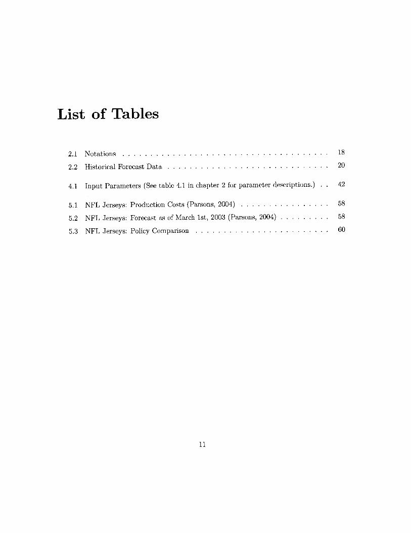
List of Tables

2.1 N otations . . . . . . . . . . . . . . . . . . . . . . . . . . . . . . . . . . . . . 18

2.2 Historical Forecast Data . . . . . . . . . . . . . . . . . . . . . . . . . . . . . 20

4.1 Input Parameters (See table 4.1 in chapter 2 for parameter descriptions.) . . 42

5.1 NFL Jerseys: Production Costs (Parsons, 2004) . . . . . . . . . . . . . . . . 58

5.2 NFL Jerseys: Forecast as of March 1st, 2003 (Parsons, 2004) . . . . . . . . . 58

5.3 NFL Jerseys: Policy Comparison . . . . . . . . . . . . . . . . . . . . . . . . 60

11

Chapter 1

Introduction

In today's competitive environment, customers expect broader product variety and novelty

and easy availability of the product with the configuration they desire. This customer expec-

tation has caused higher market dynamics and inventory risk. Postponement is a powerful

strategy that can help manufactures to alleviate inventory risk without sacrificing customer

expectations. Fashion products, that is, products with a short life cycle, generally have

higher inventory risk than products with a long life cycle; therefore, postponement strategies

tend to be more valuable. This thesis develops a quantitative model to analyze the benefit

of postponement for fashion products.

1.1 Background

Higher customer expectations have led to a general trend of product proliferation, short

product life cycle, and shorter required delivery time. "'Consumer electronics have become

almost like produce,' says Michael E. Fawkes, senior vice-president of HP's Imaging Products

Div. 'They always have to be fresh."' (Engardio and Einhorn, 2005) Product proliferation

increases demand uncertainty of each end product, resulting in higher forecast error for

each end product. Shorter product life cycle also contributes to higher forecast error and

increases inventory obsolescence risk. Lee and Billington (1994) notes that it is common for

13

high technology products to have a forecast error of 400%. Shorter required delivery time

excludes the option of make-to-order if the time to "make" exceeds the time a customer is

willing to wait.

Postponement is a strategy that delays product differentiation decisions until a later point

in the supply chain. By doing so, it allows the decision maker to gather more information

about customer demand and therefore make better decisions. Postponement, a term first

coined by Alderson (1950), is also called delayed differentiation, end of line configuration, and

late point differentiation (Lee and Carter, 1993) in some literature. Postponement strategies

can take different forms. Zinn and Bowersox (1988) describes four different ways of imple-

menting postponement in a supply chain: labelling, packaging, assembly, and manufacturing

postponement. Swaminathan and Lee (2003) describes three enablers of postponement in

product and process design: component standardization, process standardization and pro-

cess re-sequencing. The numerous successful implementations of postponement includes the

oft-cited examples such as the localization postponement in HP's DeskJet printers (Lee and

Billington, 1994), the vanilla box approach used in IBM's final assembly stage of RS6000

server machines (Swaminathan and Tayur, 1998), the front-end process standardization in

the production of Xilinx's integrated circuits (Brown et al., 2000), the process standard-

ization and vanilla box approach in Zara's product design (Harle et al., 2001), Beneton's

resequencing of dying and knitting process (Dapiran, 1992), and Xilinx's adoption of field-

programming integrated circuits to postpone the differentiation to the customer site (Brown

et al., 2000). More examples can be found in Venkatesh and Swaminathan (2001).

Rockhold and Hall (1998) classify costs affected by postponement in the the follow-

ing categories: asset-driven costs, logistics costs, material costs, and location-specific costs.

Asset-driven costs include inventory costs, depreciation of equipments and other fixed as-

sets. Postponement may lead to change in inventory holding locations or the form of the

inventory. Semi-finished products are often in a more compact form, resulting in lower trans-

portation costs. On the other hand, postponement can lead to loss of economies of scale

due to decentralized production of the finished products. Postponement affects material cost

14

due to a change in the location where the material is used, and the location affects material

procurement. Location-specific costs include labor costs, duties and taxes, which can be

influenced by tax-haven status, currency exchange rates, or local content rules.

In general, postponement strategies can help to reduce inventory cost, but often incur

higher total costs in manufacturing and assembly. Additional costs incurred by postpone-

ment include loss of economies of scale, additional variable costs associated with standard-

izing a process(Lee and Tang, 1997) or re-sequencing a process(Dapiran, 1992), and initial

investment and training costs.

From the certainty of information's point of view, postponement related costs can be

deterministic and stochastic. The deterministic costs are those not directly affected by

the uncertainty of demand, such as fixed asset costs, training costs, transportation costs,

labor costs, duties and taxes, etc. The stochastic costs are inventory costs which is directly

affected by the uncertainty of demand. Postponement reduced stochastic costs by using

better information, therefore stochastic costs reflect the value of information. Since the

evaluation of deterministic costs are straight-forward, the focus of this thesis is to develop a

quantitative model to analyze the stochastic costs related to postponement.

1.2 Existing Models on the Benefit of Postponement

Among the existing general analytical models of postponement benefits, the following three

models are most relevant to my work: the basic model in Lee (1996) which captures the

risk pooling effect of postponement, the extended model in Lee and Whang (1998) which

considers forecast improvement over time, and Aviv and Federgruen (2001)'s model which

analyzes the learning effect on forecast improvement.

Lee (1996) models the production process with postponement into two-stages: a standard

production process and a differentiated production process. This model assumes negligible

inventory of intermediate product, periodic review policy, identical and independently dis-

tributed (iid) demands over time, and equal-fractal allocation rule, meaning all end products

share a common safety stock factor. The mean and variance of steady state inventory level

15

are derived as a function of service level, from which inventory holding costs and fill rates can

be calculated. The major influence of Lee's model to this thesis is that the model captures

the risk pooling effect, that is, the variance of aggregated demand is smaller than the sum of

variance of the individual demands, but the model does not consider forecast improvement

over time.

Lee and Whang (1998) extends the above model by adding demand correlation across

different time periods. In particular, the future demand is modelled as a random walk from

current demand. This model captures the value of forecast improvement over time.

Aviv and Federgruen (2001) studied the value of postponement when the demand distri-

bution evolves in a Bayesian framework, that is, the parameters of the demand distributions

are random variables whose distribution is characterized via prior distributions. The model

considers the ordering, inventory holding, and backorder costs, and concludes that the learn-

ing effect from the Bayesian framework increases the benefits of postponement.

All of the above models are based on safety stock analysis and inventory levels are derived

from a common safety factor, rather than to optimize the total profit. In addition, they do

not consider the inventory obsolescence cost at the end of a product life cycle, therefore, are

not suitable for products with short life cycles, particularly fashion goods, where inventory

obsolescence cost is a major concern.

Parsons (2004) proposed a news-vendor model with risk pooling to plan inventory for

NFL Replica Jerseys. The news-vendor model with risk pooling is demonstrated to offer

higher expected profit than a traditional news-vendor model at comparable service level, but

this model does not provide a general approach to quantify how forecast improves over time,

and the second stage is make-to-order which is a special case of forecast improvement.

This thesis will develop a newsvendor model with forecast updates to analyze the benefit

of postponement for fashion products.

16

Chapter 2

Basic Model

In this thesis, the benefit of postponement is analyzed by comparing the maximum profit of

M end products under two different production settings: producing the end products with

and without postponement. The model consists of three parts: demand realization, forecast

evolution and production planning.

2.1 Demand Realization Model

The model assumes terminal demands, meaning all demands are realized instantly at the be-

ginning of the selling season. This is equivalent to assuming no replenishment opportunities

once the selling season starts. In reality, this assumption often holds when the selling season

is short relative to the delivery and production lead time, or when replenishment fixed cost

is too high.

Table 4.1 summarizes the notations used in this thesis.

17

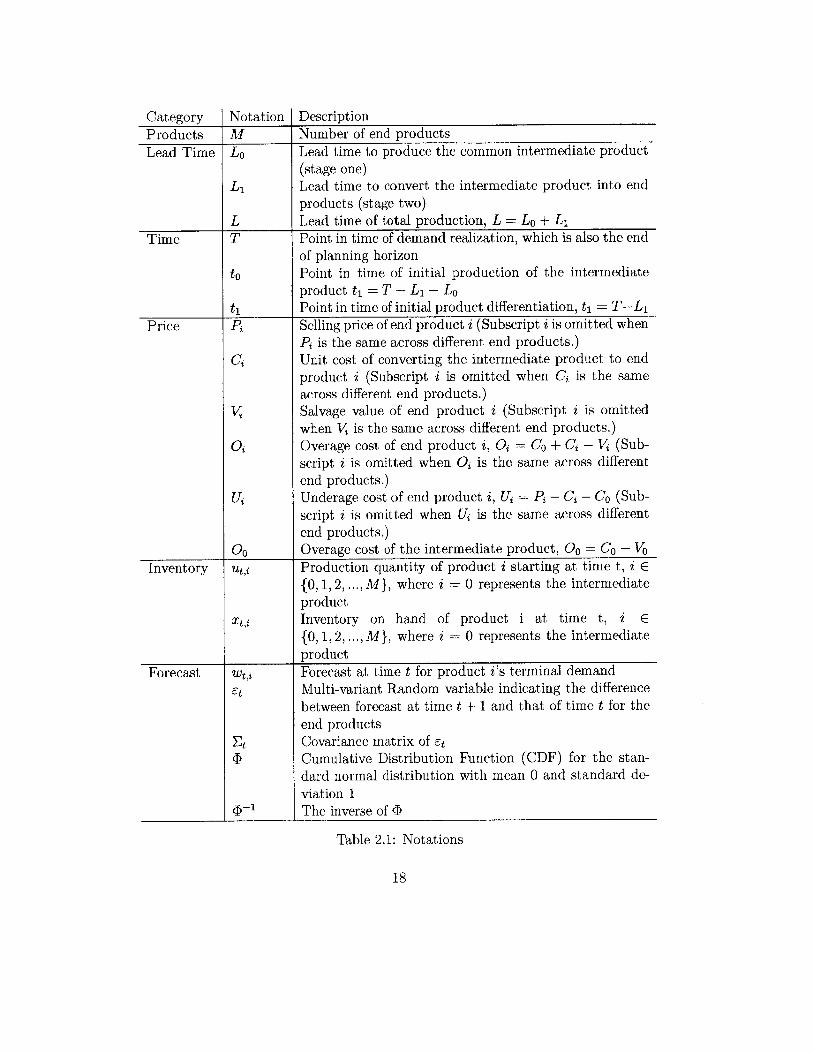
Products M Number of end products

Lead Time Lo Lead time to produce the common intermediate product(stage one)

L, Lead time to convert the intermediate product into end

products (stage two)L Lead time of total production, L = Lo + L,

Time T Point in time of demand realization, which is also the endof planning horizon

to Point in time of initial production of the intermediateproduct ti = T - L, - Lo

ti Point in time of initial product differentiation, ti = T-Li

Price P Selling price of end product i (Subscript i is omitted when

Pi is the same across different end products.)

Ci Unit cost of converting the intermediate product to endproduct i (Subscript i is omitted when Cj is the sameacross different end products.)

Vi Salvage value of end product i (Subscript i is omitted

when V is the same across different end products.)

i Overage cost of end product i, Oi = Co + Ci - V (Sub-

script i is omitted when O is the same across differentend products.)

Ui Underage cost of end product i, Uj = Pi - Ci - Co (Sub-script i is omitted when Uj is the same across differentend products.)

00 Overage cost of the intermediate product, Oo = Co - VoInventory t Production quantity of product i starting at time t, i E

{ 0, 1, 2, ..., M}, where i = 0 represents the intermediateproductInventory on hand of product i at time t, i E{0, 1, 2, ..., M}, where i = 0 represents the intermediate

productForecast Wti Forecast at time t for product i's terminal demand

Et Multi-variant Random variable indicating the difference

between forecast at time t + 1 and that of time t for the

end productsCovariance matrix of etCumulative Distribution Function (CDF) for the stan-

dard normal distribution with mean 0 and standard de-

viation 1-1 The inverse of 1

Table 2.1: Notations

18

Categzory Notation Description

2.2 Forecast Evolution Model

The forecast evolution model follows the Martingale Model of Forecast Evolution (MMFE)

developed independently by Graves and Qui (1986) and Heath and Jackson (1994). It is a

generic probabilistic model, which can accommodate both judgemental forecasts and time

series analysis. In particular, the forecast evolution is modelled as an additive model, that

is,

Wt+1 =Wt + Et (2.1)

where Et N(O, Et) (2.2)

where wt and wt+1 are demand forecasts of time t and t + 1 respectively, and et's are in-

dependent, identically distributed multivariate normal random vectors with mean 0 and a

covariance matrix Et. If the total number end products is M, then wt, wt+1 and et are

vectors of dimension M. This model suggests that the next demand forecast evolves from

the current forecast by some random amount. Note that the time intervals between adjacent

forecast updates do not need to have equal length.

In reality, the covariance matrix Et of random vector et can be obtained by analyzing

historical forecast evolution patterns or according to expert knowledge. We use two examples

from apparel industry to illustrated how to derive the covariance matrix of the random vector.

2.2.1 Example 1: Derive Covariance Matrix from Historical Fore-

casts

In the apparel industry, manufacturers often have very little idea about the final demand

when they start production, but as time progresses, the forecast becomes increasingly accu-

rate due to information gathered from trade shows, street trends, or early customer orders.

Assume that a manufacturer has the forecast data for similar products of the past ten years,

as summarized in Table 2.2:

19

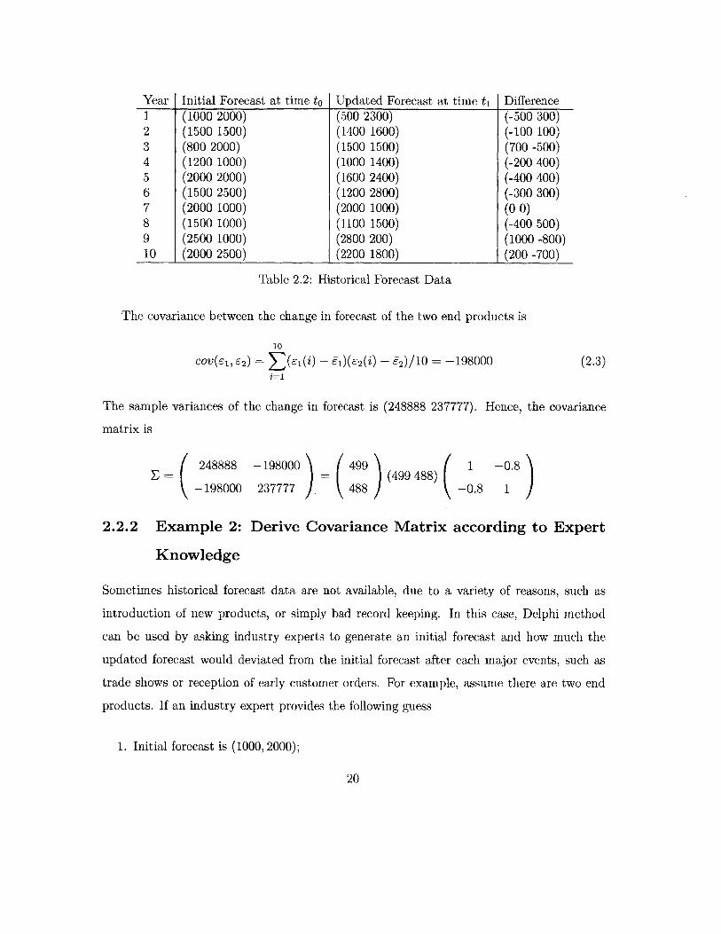
Initial Forecast at time to I Updated Forecast at time ti f1 (1000 2000) (500 2300) (-500 300)2 (1500 1500) (1400 1600) (-100 100)3 (800 2000) (1500 1500) (700 -500)4 (1200 1000) (1000 1400) (-200 400)5 (2000 2000) (1600 2400) (-400 400)6 (1500 2500) (1200 2800) (-300 300)7 (2000 1000) (2000 1000) (0 0)8 (1500 1000) (1100 1500) (-400 500)9 (2500 1000) (2800 200) (1000 -800)10 (2000 2500) (2200 1800) (200 -700)

Table 2.2: Historical Forecast Data

The covariance between the change in forecast of the two end products is

10COV(61, S2 ) Z(El W - If) (1- 2 (W - f2) /10 =-198000 (2.3)

The sample variances of the change in forecast is (248888 237777). Hence, the covariance

matrix is

248888

-198000

-198000

237777 J499

488 )(499 488) ( 1 -0.8

-0.8 1

2.2.2 Example 2: Derive Covariance Matrix according to Expert

Knowledge

Sometimes historical forecast data are not available, due to a variety of reasons, such as

introduction of new products, or simply bad record keeping. In this case, Delphi method

can be used by asking industry experts to generate an initial forecast and how much the

updated forecast would deviated from the initial forecast after each major events, such as

trade shows or reception of early customer orders. For example, assume there are two end

products. If an industry expert provides the following guess

1. Initial forecast is (1000, 2000);

20

Yeuar Difference

2. According to his/her experience, he/she is 95% confident that after the trade show 6

months later the forecast would be within range (1000 ± 500, 2000 ~F 500);

3. The total demand forecast is unlikely to change.

Then we can formulate this forecast update after the trade show as

Wt, = (1000, 2000) + E

500 1 -1 .where e ~ N(0, (500 500) )

(500 )(-1 1)

The model assumes discrete time, with a total planning horizon of T time periods. At

the beginning of each time period, the forecast is revised with the latest information and

decisions on the production quantity of each product is made based on the latest forecast.

The objective is to maximize the expected profit at time T, which is the end of the planning

horizon, or the start of the selling season.

2.3 Production Planning Model

L

LII

Lo

Without Postponement

With Postponement

t T time

Figure 2-1: Overview of production process: postponement v.s. non-postponement

As illustrated in Fig 2-1, without postponement, the products are differentiated at the

beginning of the entire production process. With postponement, the production process is

21

to

separated into two stages: during the first stage, only those operations that are common

to all the end products are carried out, and product differentiation decisions are made at

the beginning of the second stage. It is assumed that the total production lead time with

and without postponement is the same, the second stage production lead time (in the post-

poned production setting) for different end products are the same, and there is no capacity

constraint for both the intermediate product and the end products with and without post-

ponement. Let L be the total production lead time, Lo and L1 be the stage one and stage

two lead time with postponement (L = L1 + L2 ). Let to represent the point in time L pe-

riods before the demand realization time, and t1 be the point in time L1 periods before the

demand realization time, then under the above assumptions, it is optimal to make produc-

tion decisions at time to without postponement and at time to and t1 when postponement is

implemented.

22

Chapter 3

Problem Formulation and Analysis

Using the models described in chapter 2, we formulate the production planning problem with

and without postponement into a single-stage and two-stage stochastic programming problem

respectively. This chapter analyzes these problems and proposes optimal and suboptimal

solutions to them.

3.1 Without Postponement

Without postponement, the production planning problem can be formulated as a simple

single-stage stochastic programming problem. At time to = T - L, the production quantity

of each end product is decided.

(3.1)max J, (ut.)uto

23

where

Jut0,t 0, (Uto, wt.)

M

= Z J(to,i)

M

- Z Ei [-Ciut 0,i ± Pi~ minjXi, WT,i} ± Vi maXIXi - WT,i, OIjWto]i=1

M(Pi -ci)utoi - (Pi - Vi)

(Ui)uto, - (UA + O)

L

(UtOi - WTij) fui (WT,i)dWT,i

(Ut o ,i - WT,i)fVTei(wT,i)dwT,i

WTr~ N(wt0 , E ET-k)k=1

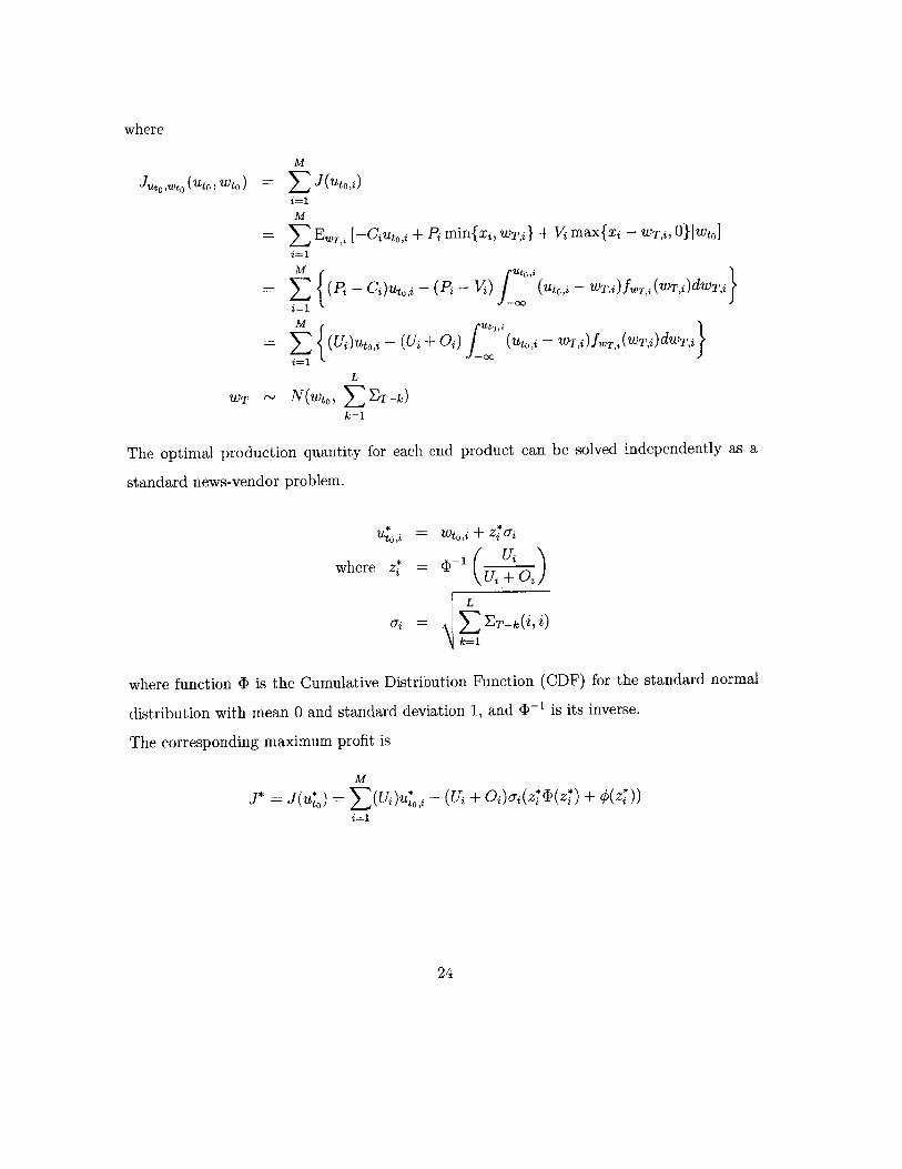
The optimal production quantity for each end product can be solved independently as a

standard news-vendor problem.

Ut = wto- i + z4o

where z U + O

L

E FT-k (i, i)k=1

where function D is the Cumulative Distribution Function (CDF) for the standard normal

distribution with mean 0 and standard deviation 1, and P-1 is its inverse.

The corresponding maximum profit is

M

J= J(uto) = (U)utoi - (Ui + Oi)o-i(z)4(z*) + #(zi))

24

3.2 With Postponement

With postponement, the production planning problem can be formulated as a two-stage

stochastic programming problem. Depending on whether postponement introduces addi-

tional variable cost, the problem can be formulated differently. In this chapter, we analyze

the basic case, that is, the total production cost is the same with and without postponement.

In chapter 5, the more general case is formulated and the effect of additional variable cost

introduced by postponement is discussed.

When postponement does not introduce additional costs, it is optimal to produce only

the intermediate product at the first stage. Let to = T - L, - Lo and t1 = T - L 1. At time

to, the production quantity of the common intermediate product uto,o is decided. At time ti,

the production quantity of each end product utl,i is decided given the production decision at

time to, where i 1, 2,..., M. The total stochastic programming problem is formulated as

max E., max Jt(utoo, Uti,i, Wti)]

such that

M

Xtio - uti,i 0 (3.2)i=1

where

Xti,o Uto (3.3)M

XT,O = Xti,o - Uti (3.4)i=1

Ll

wT N(wt 1 , ET-k) (3.5)k=1Lo

wt, N(wt., ZEtik) (3.6)

k=1

25

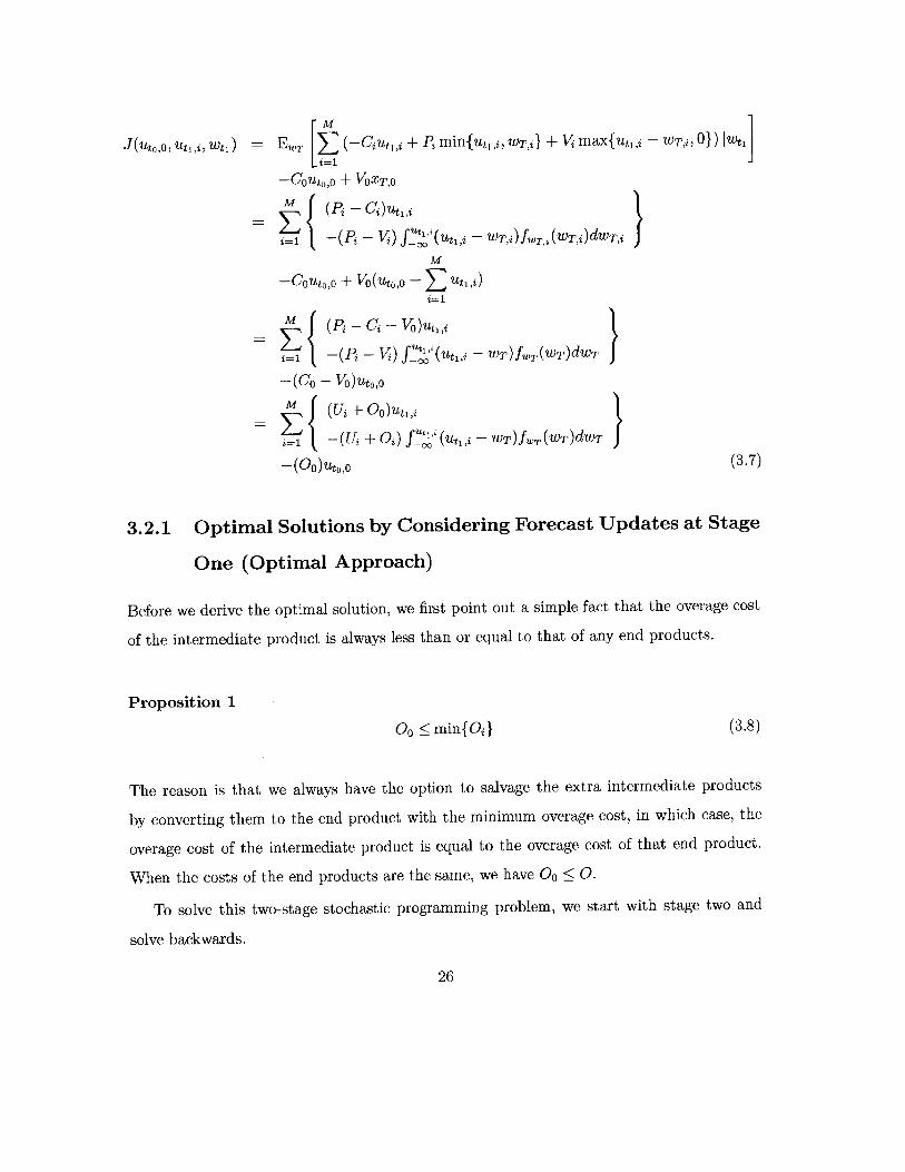
M

J(ut,o, ui, , w t) = E,, (-Ciut,i + Pi min{utl,iWT,i Vimax{tUi,iI =1

-Cout,O + VOXT,O

i=1 (Pi- i) futit(Utji WT,iVfwT~i(WT,i)dWT,i

-Coutoo + Vo(utoo - Uti)i= 1

M (P _ -C-Vo)ut,i

1 -(P - ) f"%'', - wT)fw,(wT)dwT

-(Co - Vo)ut0,o

M (U + Oo)uti,4

1 -(Ui + 0) f_"'( ~ - wT)fwT(wT)dWT

- (00)uto'o

- wTi, 01) 1WiI

}}

(3.7)

3.2.1 Optimal Solutions by Considering Forecast Updates at Stage

One (Optimal Approach)

Before we derive the optimal solution, we first point out a simple fact that the overage cost

of the intermediate product is always less than or equal to that of any end products.

Proposition 1

00 min{Oi} (3.8)

The reason is that we always have the option to salvage the extra intermediate products

by converting them to the end product with the minimum overage cost, in which case, the

overage cost of the intermediate product is equal to the overage cost of that end product.

When the costs of the end products are the same, we have 00 <0.

To solve this two-stage stochastic programming problem, we start with stage two and

solve backwards.

26

Decision at Stage Two

At stage two (time t 1 ), the problem is a multi-variable constrained optimization problem

described as follows:

max Jt1 (uto,o, Uti,, Wti) (3.9)

such that

M

uto,o - uti,i > 0 (3.10)i=1

where Jt1 (uto,o, utliI wti) is defined in equation (3.7).

We first propose the solution to the degenerate case, that is, when perfect demand infor-

mation is available at stage two, or

WT = Wti,

which corresponds to the "make-to-order" case. And then we derive the solution to a general

case, that is, when the demand information is uncertain at stage two.

To facilitate discussion, we assume the overage and underage costs across different prod-

ucts are the same, which is referred to as "balanced cost" for the rest of the thesis. In reality,

this assumption often holds when the end products belong to the same product family.

When Perfect Demand Information Is Available at Stage Two

Having perfect demand information when the decision at stage two has to be made corre-

sponds to the so called 'make-to-order' or 'customize-to-order', which has broad applications.

In this case, the optimal solution of stage two is to meet as much demand as possible,

and salvage extra intermediate products. The maximum expected profit for this degenerate

case is stated in the following proposition.

Proposition 2 If perfect demand information is available at the second stage, then the

27

maximum expected profit is

Uut,o - (U + Oo)(utto - EZ=1 wtii)Uuto,

if uto,O > Ei=1 wti; (3.11)otherwise.

The proof is straightforward, therefore is omitted.

When Demand Information Is Uncertain at Stage Two

When demand information is uncertain at stage two, the problem can be solved using

lagrange multiplier method as described below.

L(uto,o, uti, wT, A)

M (i + Oo)uti,i

E= -(U + 0i) f

-(Oo)uw 0 ,oM

-A(utOo - Zuti,)i=1

"'i (utl,i - wT)fwT (wT)dwT

aL -(Uautii + Oi)FWT(ut1,i) + Ui +0 - A = 0

A > 0M

uto - Zuti > 0i=1

M

A(utoo -Z uti,i) = 0i=1

Solving equation (3.14), we get

U* - F-1 (U + 0 -)tOt Wi, Ut + 02

= wt + zf_ 1 U + Oo - AWtn i (Uj + Oj

In general, the optimal policy u*i can only be solved numerically by searching for A such

that conditions (3.16) and (3.17) are satisfied. However, as demonstrated below, closed

28

(3.12)

}(3.13)

(3.14)

(3.15)

(3.16)

(3.17)

(3.18)

Jt* (uto'o, Wti)

formula for u*g can be derived when the end products have "balanced costs". Let 0 = Oi

and U = Uj for any i. Then equation 3.18 becomes

-* =AF :U +-A0 '.+z ) 1 U + O -A (3.19)

The following proposition describes the optimal solution at stage two when demand infor-

mation is uncertain.

Proposition 3 When the demand information at stage two is imperfect, the optimal solution

for the constraint optimization problem (3.9) is

ut*1 (ut0 ,o, Wti) Wti + oiz*(ut,,o, wt1 ) where

7i =T- L k (i,i) andk=1

- (U++0),

(t(utOO - E,)1. 1 t],o) I

(3.20)

(3.21)

when 00 < 0 and~t00 Z~=wt1 ,i + -D' (U+0) EMu~

otherwise.

(3.22)

And the maximum profit is

M M

Jt* (ut,o, wt1 ) = (U+Oo)Zwt,i + [(U +Oo)z* - (U +O)(z*T(z*) + q(z*))] >3O-i=1 i=1

(0) UtO)O (3.23)

Proof For a constrained optimization problem with inequality constraints, the con-

straints can be active or inactive with respect to the optimal solution.

When A = 0

In this case, constraint (3.10) is inactive, which corresponds to the case when some of the

intermediate product is not converted to any end product. This happens when ut0 ,O is high

and +00 < 1 (00 < 0), that is, the inventory on hand of of intermediate product is high

29

(because too many intermediate products were produced in stage one) and the overage cost

of the intermediate product is smaller than those of the end products, which happens when

the intermediate can be reused for other products or in the next product life-cycle. Then

the optimal policy is

U* ,- F-1aU+ Vi E { 1, 2, ..., M}

and u*, satisfies the following inequality.

M

UtOc ut'i4i=1

Let

z = wtl,oi

Since wT N(wt1 , ELZ E-k), we have z ~ N(0, 1). Hence, the optimal solution is

Z*(UtOO, Wi) U + 0

ut,(utoo, Wji) wt o-iz*(UtOO, Wti)

when 00 < 0 and ut,o wo +< (U O ME

i=1 i=1i

When A > 0

In this case, constraint (3.10) is active, that is

M

UtOO - Uti,3 = 0. (3.24)z=1

This corresponds to the case when all the intermediate products are converted to end prod-

ucts. This happens when ut,,o is low, or U+0 0 1 (00 = 0). Low uto,o means that theU+o

inventory on hand of the intermediate product is low because too little intermediate prod-

30

uct was produced in stage one. 00 = 0 means that the salvage value of the intermediate

product is the same as those of the end products. For example, this can happen when the

intermediate product is unstable or cannot be reused in the next product life cycle. In this

case, we have

U + 0 0 - Az* - +1( V i

Notice that z* is independent of i. Let z* = z. We have,

U* = W*i'i + Uiz*

Substituting ut1,, in 3.24 by 3.21, we get

M

(wt1 ,i + aiz*) = UtO Oi=1

=#- z"'(ut0 ,o, Wti) U 0-Zj 1 Wi,

From z*, we get,

A* = U + 00 - (U + 0)4(z*)

U*- (UtOwOUwl) = wtli+ UOiz*

UtoO ~ j=1 Wt1 a

j=1 ai

31

And the maximum profit is

M

= [(U + Oo)ut1,i - (U + O)(z*(z*) + 0(z*)) ] - (Oo)uto,o

M M

(U + Oo) u1ti - (U + O)(z* (z*) + #(z*))5ui - (Oo)ut0,o

M M

= (U + 00) (ti o z*) - (U + O)(z*I(z*) + #(z*))5 Ci - (Oo)utooi=1=1M M

(U + Oo) E wjo, + [(U + Oo)z* - (U + O)(z*@(z*) + #(z*))1 3i - (Oo)ut 0,oi=11

Decision at Stage One

With the formula for Jt* (uto,o, wti) from proposition 2 and 3, the optimal solution of stage one

(time to) can be derived. The decision problem of stage one is a single variable optimization

problem stated as follows:

max Jto (uto,o)utoo

where

= E 1 [JAt(uto,o, wtI)Iwto]

= J-0it (Uto,o, Wti)fwtl jwo (wtl)dwt,

Again the solution to the stage one problem depends on whether or not perfect demand

information is available at stage two.

Proposition 4 Jto(uto,o, wto) is concave with respect to ut0 ,o.

Proof

32

Jt* (Utoo, I t I)

Jto (Uto10)

1. When Perfect Demand Information Is Available at Stage Two

Let

M

y = t~i (3.25)j=1

Since wt, is a multivariate normal, and y is a summation of random variables with a

joint-normal distribution, therefore, y must be normal. From the joint distribution of

wtei,, we can derive the distribution of y as follows

y ~ N(po2M

where p = wti,i=1

LoU = 1'Zti-k1.

k=1

We can rewrite the profit function Jt0 (ut0 ,O) as follows.

Jto (uto,o) = Jt*, (uto0 o, wt1 )fJ Iwto (Wti)dwt,

UtOO - (U + 00) j (ut.,o - y)f,(y)dy

Uuto,o - (U + Oo) max{ut,o - p, 0}, if a 0; (3.26)Uut0 ,o - (U + Oo)a(zb(z) + #(z)), otherwise.

where z = . (3.27)

(a) If u > 0,

(Uto,o) = U - (U + Oo)O(z#(z)/U + <D(z)/u + 4'(z)/U)

= U - (U + Oo)1>(z) (3.28)

() (Uto,o) = -(U+ Oo)#(z)/u (3.29)02Uto,o

33

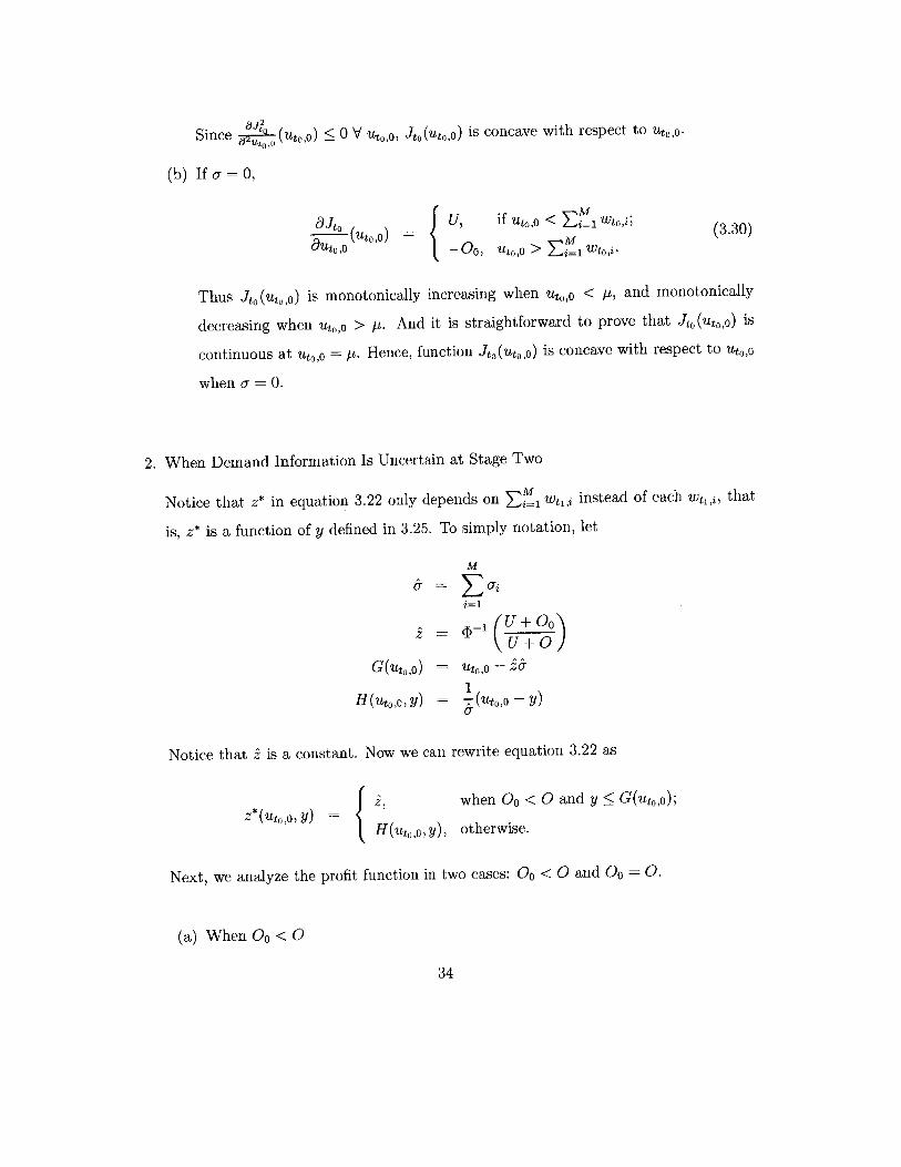
Since ---I o (uto,O) <; 0 V utoO, Jt0(uto,o) is concave with respect to uto,o.

(b) If a = 0,

t-, if Uto,O < i1 wtoi; (3.30)Bu00) -OUtO'O > Ej1 wto'i .

Thus Jt( (uto,o) is monotonically increasing when uto,o < p, and monotonically

decreasing when ut0 ,o > ft. And it is straightforward to prove that Jt0 (uto,o) is

continuous at uto,o = p. Hence, function Jt(uto,o) is concave with respect to uto,o

when a = 0.

2. When Demand Information Is Uncertain at Stage Two

Notice that z* in equation 3.22 only depends on EM, wt,,i instead of each wth,i, that

is, z* is a function of y defined in 3.25. To simply notation, let

M

&=

U + 0o

G (ut,o) =ut,,o- z1

H(ut,o, y) 7(utoO - y)a

Notice that 2 is a constant. Now we can rewrite equation 3.22 as

2, when Oo < 0 and y < G(ut,o);Z*(UtOO, y) =

H(uto,oI y), otherwise.

Next, we analyze the profit function in two cases: 00 < 0 and 00 = 0.

(a) When 0o < 0

34

In this case, we have

JtO (Utolo) = -0 J*,(UtO,O wti ) fwtl(Wtl) dwt,

- c [(U + Oo)z* - (U + 0)(z*(z*) + #(z*))] El O fy(y)dy

J-oO +(U + 0O)y - (Oo)ut.,o

/G(utoO) [(U + 00)2 - (U + 0)(5A (2) + 4(2))] &fy(y)dy

+ [(U + OO)H - (U + 0)(HD(H) + O(H))] &fy(y)dyJG(,uto,o)

+(U + Oo)p - OOutO,O

[-(U + O)#()&] Fy(G(ut.,o))

+ [(U + 0,)H - (U + O)(HD(H) + #(H))] &fy(y)dyJG(ut.,O)

+(U + Oo)p - (Oo)utO,o (3.31)

When o- 0,

U74 0,0 - (U + O)(uto,o - p)4((uto,o -

Jit (utO,o) = -(U + O)#((uvt,o - t)/6)&, when uto,O - za ; A;

-(U + O)0(i)& + (U + Oo)p - Oouto,o, otherwise.

H is a function of uto,o and y in the above equations. So the first derivative of JtO

over ut0 ,O is

a (uto)

- (U + O)#()&fy(G(uto,o)

[(U + O) - (U + O)@(H)] f,(y)dyG(uto,o)

Jyd

+(U + 0)()4fy(G(ut,o) - 00

= (U + O)(1 - Fy(G(utO,o))) - (U + 0) J (H)f,(y)dy - 00

(3.32)

35

When a = 0,

when uto,o - ZU A;

otherwise.

The second derivative is

&Jt20aU (Uto,o)

= -(U + OO)fv(G(utO,o)) - (U + 0)

+(U + O)P(2)f,(G(ut,o))

(!Ltoo --Y) ( ) dy)

When a = 0,

-(U + 0)b((uto,o -

0,

when ut0 ,o - za ;

otherwise.

Since a" (utOo)

Utb)

(b) When Oo - 0

< 0 V utO,O, function Jt0 (uto,O) must be concave with respect to

In this case, we have

Jto (utO,o) = f [(U + 0 0)H - (U + O)(H4(H) + O(H))] &fy(y)dy

+(U + Oo)pA - (Oo)utO,o (3.34)

36

(uto,o)aUtO,OU - (U + 0)b((UtOO- A)/0),-00,

O(H) fy(y)dy

< 0

(3.33)

{

J,(UtO A)

a j2(0 oo

a2Ut("o (UOO

=-(U +0) 0(JG(,UtO,O)

So the first derivative of Jto over ut,,O is

(utoo) = U-(U+O) <b(H)f(y)dyauto'O 00

(3.35)

The second derivative is

U (uto,O)a 2uto

= -(U + 0) (uto Y)b(y PIdy) 0

(3.36)

Since -7 0 (ut,O) 0 V uto, function Jto (uto,o) must be concave with respect to

uto'O-

Q.E.D.

When perfect demand information is available at stage two, the optimal solution can be

computed analytically, as shown in the following proposition.

Proposition 5 If perfect demand information is available at stage two, the optimal initial

production quantity of the intermediate product is

U*'O = A+z*- (3.37)

M

where it = wto'ii=1

Lo- = 1'ZEt1k1

k==1

z U

U+00

37

And the maximum expected profit is

Since, Jt (ut,o)

quantity of the

to 0. That is,

is concave with respect to uto,o (Proposition 4), the optimal production

intermediate product u*,0 can be derived by setting the first derivative

(u*,0) = U - (U + Oo) (z*) = 0.ato'O o

Hence,

z ~ UU + 00

Uto , 0

Jt*o

= P + z*

= Uu*,O - (U + Oo)U(z*I(z*) + 4(z*))

= U(P + Uz*) - (U + Oo)a(z* + #(z*))U + 00

= Upt - (U + Oo)O#(z*)

(3.41)

(3.42)

2. when a = 0

Jt(ut0 ,o) is not differentiable at uto,o = p, but Jt(uto,o) is monotonically increasing

when uto,O < p, and monotonically decreasing when utO,O > p. And Jto(uto,o) is contin-

uous at uto ,O = p. Therefore, the optimal solution is

Ut*o, = (3.43)

(3.44)

38

Jt'o = Up - (U + O)rb(z*)

Proof

1. when o > 0

(3.38)

(3.39)

(3.40)

Jt*o = Uut*o'O = Up

Notice that the above case (when a- 0) is a limiting case for when aggregated demand

information is uncertain at stage one. In other words, as a -+ 0 in stage one, we get

this case.

Q.E.D.

When perfect demand information is available at stage two, the optimal solution can be

computed analytically, as shown in the following proposition.

Proposition 6 If the demands for end products are perfectly negatively correlated, the op-

timal initial production quantity of the intermediate product at stage one is

uto'O = P + Z*& (3.45)M

where [t = Zwto,ii=1

M M Ll

& = Ea-= Y ET-k.(ii)i=1 i=1 k=1

UZ* = lb-'( ) (3.46)U +O

And the maximum expected profit is

Jt = Up - (U + Oo)C-#(z*) (3.47)

(3.48)

When demand information is uncertain at stage two and the demands are not perfectly

negatively correlated, the closed-form formula for the optimal solution at stage one (u* 0 )

does not seem to exist. The optimal solution can be computed numerically using standard

nonlinear optimization methods(Bertsekas, 1999). In the numerical examples in the next

chapter, we used the 'fminbnd' function in matlab to find the optimal solution.

39

3.2.2 Suboptimal Solution by Ignoring Forecast Updates at Stage

One (Myopic Approach)

In this section, we propose a heuristic approach, which is referred to as the Myopic Approach

in the rest of the thesis. The myopic policy chooses the optimal production quantity of

the intermediate product at time to by ignoring future forecast updates. In this case, the

stage two decision is still a constrained optimization problem with the same formulation

as before, but the decision at stage one becomes a standard single variable news-vendor

problem, regardless of the decision to be made at stage two. Hence, at stage one, the

optimal production quantity of the intermediate product is

U

where a =,i,i=1

L

9- 1 ETk.k=1

The expected profit can be calculated numerically using equation 3.31.

40

Chapter 4

Numerical Results and Discussion

This chapter demonstrates applications of the model to a series hypothetical settings. The

optimal solutions are computed and the benefit of postponement is discussed and compared.

This thesis restricts to the cases when the end products have balanced costs (see Chapter

3), which is a reasonable assumption for products within the same product family. In reality,

products within the same product family often have similar costs and price. For example,

different colors of iPod are priced the same in almost all stores. Different sizes and colors of

the blouses of the same style usually have similar costs and the same initial price. Here we

consider only the regular price. Promotion prices are out of the scope of this thesis.

4.1 Description

In the numerical experiments carried out in this chapter, it is assumed that the total cost

for producing an end product, including the cost of producing the intermediate product and

the cost of converting it to an end product, be unit 1, regardless of the postponement point.

The following table summarized the parameters used in the numerical experiment.

In this example, the number of end products is 2. The total production lead time is 10

periods. The cost for producing the intermediate product is 50% of the total cost. The price

41

Products M 2Costs CO 0.5

C 0.5Ctota =CO+C 1VO 0.30, 0.40, 0.45, 0.49V 0.8P 1.300 = CO - V 0.20, 0.10, 0.05, 0.010= Co +C- V 0.2U = P-Co - C 0.3

Forecasts p [10 10]0- [1 1]p -1, -0.5, 0, 0.5, 1 (correlation between demands for end

products)Lead Times L 10

Li 0, 2, 4, 6,8, 100, 0.2, 0.4, 0.6, 0.8, 1 (percentage of the first stage leadL

____________time)

Table 4.1: Input Parameters (See table 4.1 in chapter 2 for parameter descriptions.)

of each end product is 1.3 times the total cost. The salvage value of each end product is

80% of the total cost. From the price and cost information, we cali derive the underage cost

U and overage cost 0 of the end products.

U = P - C = 1.3 - 1.0 = 0.3 = 30%C

0 = C -V = 1.0 -0.8 = 0.2 = 20%C

The initial forecast for both end products is 10. The standard deviation introduced in each

additional forecast period is 1. -- , the percentage of the first stage lead time is an indicator

of the degree of postponement. L = 0 means that products are differentiated at the very

beginning, that is, no postponement is implemented. When 1, maximum postponement

is achieved, which is equivalent to the case when the decision of stage two is based on perfect

demand information. In other words, when -L' = 1, stage two is make-to-order. 0 < - < I

corresponds to the case when postponement is implemented, but stage two is still make-to-

42

|ValueCategory Parameter

forecast. As - increases, that is, the degree of postponement increases, stage two is making

to increasingly better forecast.

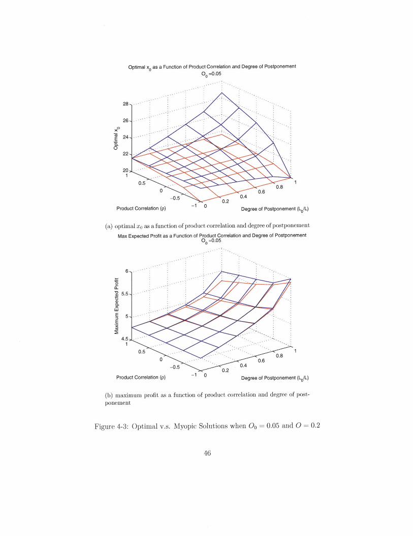
4.2 Results

Both the optimal and myopic solutions are computed for different degrees of postponement,

product correlation, and the overage cost of the intermediate product. The results are shown

in the following figures.

43

Optimal x0 as a Function of Product Correlation and Degree of PostponementCo =0.2

22 -

21.5,

0

20.5,

20

21

0.50 -0.6 0.

-0.5 0.2 0.4

p L0/L

(a) optimal xo as a function of product correlation and degree of postponement

Max Expected Profit as a Function of Product Correlation and Degree of Postponement00 =0.2

6

5.5 -

E -E

4.5> -

0.5.---1- 0.8

-0.5 0-6-0.5 ~ 0.2 0.

Product Correlation (p) -10Degree of Postponement (LO/L)

(b) maximum profit as a function of product correlation and degree of post-

ponement

Figure 4-1: Optimal v.s. Myopic Solutions when 00 = 0 =_ 0.2

44

Optimal x0 as a Function of Product Correlation and Degree of PostponementO =0.1

25,

24,-

x.P 23,

. 22,0

21

0.5-10 0.8

0 0.6-0.5 .2 0.4

Product Correlation (p) Degree of Postponement (L0/L)


Max Expected Profit as a Function of Product Correlation and Degree of PostponementO =0.1

6

(D 5.5,

E 5,E

4.5>

1 -

0.50- .o .8

S0.6-0.5 0.' 0.4



ponement

Figure 4-2: Optimal v.s. Myopic Solutions when 00 = 0.1 and 0 = 0.2

45

I I -

Optimal xO as a Function of Product Correlation and Degree of Postponement00 =0.05

26,

24, -0

22 -

20

0.5 0.0 .. 0.6

-0.5 0.2 0.4



Max Expected Profit as a Function of Product Correlation and Degree of Postponement00=0.05

6

5.5-

a-

Ex

Product Correlation (p) Degree of Postponement (L0IL)


ponement

Figure 4-3: Optimal v.s. Myopic Solutions when 00 0.05 and 0 =0.2

46

aa 61 i

Optimal xO as a Function of Product Correlation and Degree of Postponement00 =0.01

32-

30,

28,

26,--

0 24,--

22 -

201

0.5 006 08 1

-0.5 0.2 0.4



Max Expected Profit as a Function of Product Correlation and Degree of Postponement00 =0.01

6:

5.5

.5Qw

E -,

E

0.5 --. 0.80.

-0.5 0.2 0.40.2

Product Correlation (p) -1 0 Degree of Postponement (L0/L)


ponement

Figure 4-4: Optimal v.s. Myopic Solutions when 00 = 0.01 and 0 = 0.2

47

Profi aS a Funclion of X,Correlafion f -1

Ve 0 3

P: =.3j

(a) 0. 0.20V = [o.d =;. 1

5.5 - P, =113;1305.5 2n nd 102 1=:1I

5 2N0 25

44 -

3.5 -

2.S3

(a) Oo = 0.20FROM P as a Function of o w n

Correlaion p -1V, -0.4

&S -StP . = [ 11 115.5~~ Rape~d =2p~

5 -

4.51

(b) 00 = 0. 1PRofl as a Funwfion of x,

Corr tinp -1

5.8 -, = [a0.al8

C, =1{.5;0.51P, =[13;1.31

5.6 Adm.nD =z 0

5.4 -

5.2 -

5-

4.8 -

4.6

--

4.4-

414-

(c0O0 0.05

48

Figure 4-5: Profit as a Function of xO, when p =-I

PRo4 as a Fwntion o x,COSelion p =0

V, =0.3

6.=5.v =0o 0.2.0 =500. 8.,1

1 1.31.31

Num 0iu0000n p1-S

A.1110 p- - 10.Q

4.5-

4-

3.5 -

3 -

(a) Oo 0.20Profit as a Function of xw

Cornelaon p -DV, -a,4

C = .55.4 - v Je 1.;0

p, = (1.3 1 3j5.2~N -l =2 i1

Num1 Ld T5- Gr sm..1 I

4.8 -

4.6 -

4.4

4.2

4 -

3,8

(b) Oo =0.1ProfR ws a Function of x.

Correlaio p .0V, -0.45

5,6 - v 14.al.5P, jt. 131

5.4--

5-

4,8 -

4.6 -

4.4 -

4.2

4 ..

(c 0O = 0.05

49

Figure 4-6: Profit as a Function of xO, when p =0

Protil &S a Function of XoCOrlation p -1

V, -0.3

5 ----- 3

C5=0.5

c =[ 05:0 5P: 1 [131

10D rn =1;0

4.5- ~ w I Md 0(cRod )2

4 -

3.5 -

3 -

2.5 1

150

(a) Oo = 0.2PRof as a Function of xo

COrrfltlion p .1V, -(.4

5.2 - -- -

5 c. - a!.6 $P, = I1, k 31

4.1 - =1

4.6 -

4.4-

4.2

4 -

3.8 -

(b) 00 0.1Prolit &S a Function of X0

Corelation p .1VIc =045

- n81

141-

5 - 0 2

.6

4.5 -

(c 0O = 0.05

50

Figure 4-7: Profit as a Function of xO, when p=1

4.3 Discussion

Computational results give us the following observations:

1. Negative correlation between the end products increases the benefit of postponement.

This finding is consistent with the conclusion from Lee (1996).

Negative correlation between the products means that when the demand for one prod-

uct increases, the demand for the other products tend to decrease, resulting in a smaller

variance of the the total demand. The fact that the aggregated demand has a smaller

variance than individual demand is called risk-pooling. The more negatively correlated

the end products, the more risk-pooling we get. When the end products are perfectly

positively correlated, we get no risk-pooling.

In the above numerical experiments, when the overage cost of the intermediate product

is the same as that of the end products 4-1, postponement leads to a profit increase of

25% when products are negatively correlated, compared with no profit change when

products are positively correlated. In reality, examples of risk-pooling are often ob-

served and utilized. For example, in the Reebok NFL case (Parsons, 2004), the demand

for each NFL Jerseys is poor at the start of a football season, but the aggregated de-

mand is far more accurate, therefore, it is beneficial for Reebok to produce blank jerseys

at early stages of the season and convert the blank jerseys to dressed jerseys after the

demand information is more accurate as the season progresses.

2. Under the costs considered in this model, as the degree of postponement increases, the

maximum profit never decreases.

(a) When the overage cost of the intermediate product (O) is equal to that of the

end products (0), postponement is not beneficial if the end products are perfectly

correlated.

(b) When the overage cost of the intermediate product (O) is less than that of

the end products (0), the maximum profit strictly increases with the degree of

51

postponement, even when the end products are perfectly correlated. In addition,

other conditions equal, the maximum profit decreases with Oo.

Intuitively, when the intermediate product has a higher salvage value, or lower

overage cost than the end products, then postponement offers additional benefits

due to reduced obsolescence costs. In reality, the life-cycle of an intermediate

product is often longer than that of end products, which means that the interme-

diate product can be reused in the next product life cycle of the end products,

resulting in higher salvage value of the intermediate products. For example, in the

Reebok NFL case, the blank jerseys can be reused for the next season(Parsons,

2004). In pharmaceutical industry, a commonly used FDA approved frozen chem-

ical sometimes can last ten years resulting in an overage cost close to zero, while

a pill made of this chemical usually lasts only a few months to a couple of years.

A packaged medicine usually has an even earlier expiration date, and must be

discarded or repackaged to sell in other regions with different regulations when

the expiration date comes. Using the two-stage news-vendor model, the reduction

in obsolescence cost can be quantified.

(c) When Oo is close to zero, the maximum profit becomes insensitive to the demand

correlation between the end products.

This observation suggests that if the overage cost of the intermediate product is

really low, the manufacture does not need to worry about the demand correlation

much. Even if the the demands are perfectly correlated, postponement will achieve

similar savings as when the demands are negatively correlated. The rationale is

that there is an upper bound in the amount of savings postponement can achieve,

and when the overage cost of the intermediate product is close to zero, savings due

to reduced obsolescence cost itself is getting close to the total savings. In other

words, obsolescence savings become dominant in the total savings, therefore, the

savings from risk pooling have little effect on the total benefit of postponement.

Note that the maximum savings is achieved when the products are perfectly neg-

52

atively correlated and the second stage production is make-to-order. In this case,

decisions at both stage one and stage two are made based on perfect demand in-

formation - at stage one, perfect demand information for the total demand, that

is, the demand for the intermediate product is deterministic, although demand

information for each end product is uncertain; at stage two, perfect demand in-

formation for each end products is available. Therefore, postponement generates

maximum savings.

3. The maximum profit becomes less sensitive to 00 as the negative correlation between

end products increases. When the end products are perfectly negatively correlated,

the optimal solution does not change with Oo.

This observation suggests that if the manufacturer has good knowledge of the aggre-

gated demand at the initial production stage (even if individual demand is highly

uncertain), then the manufacturer does not need to worry much about the salvage

value of the intermediate product. The rationale is similar as the previous observation

2c, but in this case, the cost savings is dominated by the savings due to risk-pooling.

When the production quantity of the intermediate product can be determined with

high accuracy, there would be very little overage cost introduced by the intermediate

product, therefore the overage cost of the intermediate does not play an important role

in the total savings.

4. Myopic solution generates lower maximum expected profit, but the difference from the

optimal solution is small.

In the above numerical experiments, the largest difference between the maximum ex-

pected profit obtained from the myopic solution and the optimal solution is about 5%.

This observation can be explained by the shallow curvature of the curve of J(utoo) at

the neighborhood of the optimal u*' which can be observed from figure .

This finding tells us that the myopic solution does not sacrifice too much of the profit.

Since the myopic solution is much more computationally efficient - the computation

53

complexity of the myopic solution is linear to the number of simulations - therefore, the

myopic approach can be used to solve a much more complex problem, when computing

the optimal solution is too time-consuming.

54

Chapter 5

Limitations and Extensions of the

Model

The previous analysis gives us insight in the joint effect of overage cost of the intermediate

product and the negative correlation on the benefit of postponement. However, the model

ignores the additional costs introduced by postponement and must be extended in order

to adapt to real cases. This chapter demonstrates the effect of postponement costs on the

choice of optimal solutions.

5.1 Effect of Postponement Cost on the Optimal Solu-

tion

In reality, the total cost is often higher when postponement is implemented. For example, in

the Reebok NFL case, the total cost of producing a dressed Jersey is $11.9 if a blank Jersey

is produced first, as compared with $10.9 if the dressed Jerseys are produced directly. When

the cost with postponement is higher, the pure postponement strategy is not necessarily

optimal.

55

5.1.1 Problem Formulation

We first introduce some additional notations to represent the costs without postponement.

Notation Description

O total cost without postponement for any end product

6 overage cost of end product without postponement for

any end product

U underage cost of end product without postponement for

any end product

Let ut,,i be the planned direct production quantity for end product i (without producing

the common intermediate product first) at time to, where i = 1, 2, ..., M. Same as before, let

uto,o be the planned production quantity of the intermediate product at time to.

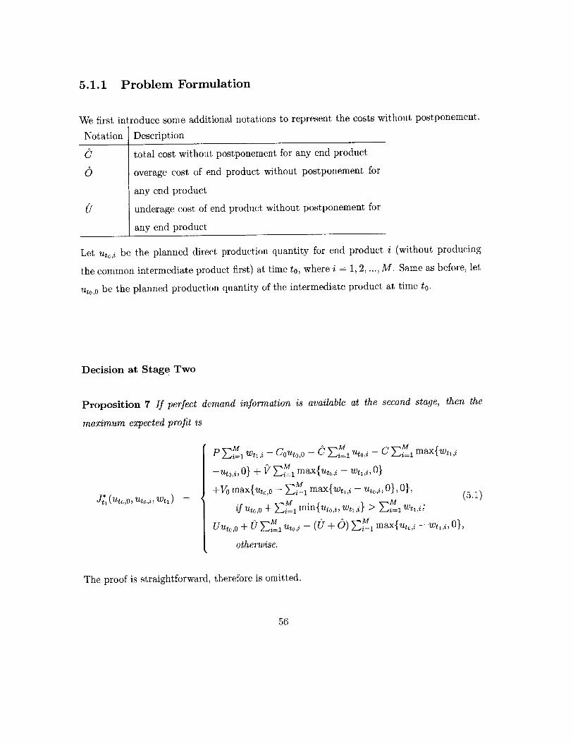
Decision at Stage Two

Proposition 7 If perfect demand information is available at the second stage, then the

maximum expected profit is

JA*(utCooutO'zIwtJ =

P =1 'i - CotoO - aEi uto,, - C j=1 max{wt,2

-uto,i, O} + V zE% max{uto,i - wti,i, 0}

+Vo max{utO,o - E i max{wtl,i - ut,,i, 0}, O}' (5.1)

if utoo + Ei= 1 min{ut0 ,j, wti,i} > Eli WtI'i;

Uuto,o + U zj:1 uto,i - (U + 0) Ejd max{ut,, - wti,i, o},

otherwise.

The proof is straightforward, therefore is omitted.

56

Decision at Stage One

Similar to the case when postponement does not introduce additional cost, the decision

problem at stage one is

max Jto (uto,o, uto,j) (5.2)utooUtoi

where

Jto (uto,o, uto,j) =Ewt, Jt*1 (uto,o, uto,i, Wt,) (5.3)

f-0 t (Uto,o, uto,i, Wti)fwtl (Wtl)dwt,(54

This problem is much more difficult than 3.37. First, the policy space at stage one is

much larger. Not only the production quantity for the intermediate product (u, ,o) needs

to be decided, but also that of each end products (utj,). In addition, the profit function

J* (uto,o, uto,i, Wti) is in a much more complex form (5.1), making it difficult to find the op-

timal solution efficiently. In general, some search algorithm can be used to find the best

solution within the search space, but it is time-consuming, and might not guarantee an opti-

mal solution. Parsons (2004) proposed an effective heuristic algorithm to find a suboptimal

solution. Next, we provide a brief review on Parsons's risk-pooling algorithm, and compare

the maximum expected profit under three different policies - full postponement strategy with

no end products produced at the first stage, the hybrid policy proposed in Parsons (2004)

and the policy without postponement.

The data used in this chapter are taken from Parsons (2004).

5.1.2 NFL Jerseys Case

In this case, Reebok has two ways of ordering NFL Jerseys shirts from its supplier located

overseas - to order directly the dressed Jerseys, or to order blank Jerseys, which can be

converted to dressed Jerseys in North America. The lead time between the order receival to

57

Parameter ValueCo: cost of blank 9.5VO: salvage value for blank 8.46C: cost of decorate in North America 2.40P: wholesale sales price 24V: salvage value for dressed 7C: cost of dressed 10.90 = C - V: overage cost of dressed if produced directly 3.9U = P - C: underage cost of dressed if produced directly 13.10 = Co + C - V: overage cost of dressed if produced from blank 4.9U = P - Co - C: underage cost of dressed if produced from blank 12.1

00 = Co - V: overage cost of blank 1.04

Table 5.1: NFL Jerseys: Production Costs (Parsons, 2004)

Notation Desc Mean (pt) Standard Deviation (o)wt. (total) NEW ENG PATRIOT Total 87679.5 19211.26701wto (0) Other Players 23274.9 10473.705wt0 (1) BRADY, TOM #12 30763.2 13843.44wto (2) LAW, TY #24 10569 4756.05wto (3) BROWN, TROY #80 8158.8 3671.46wt.(4) VINATIERI, ADAM #04 7269.6 4361.76wto (5) BRUSCHI, TEDY #54 5526.3 3315.78wto(6) SMITH, ANTOWAIN #32 2117.7 1270.62

Table 5.2: NFL Jerseys: Forecast as of March 1st, 2003 (Parsons, 2004)

order shipment is about 30 days, while the time for converting the blank Jerseys to dressed

Jerseys is very short. For detailed description of the case, see Parsons (2004). The following

table summarizes the pricing and cost information.

The following table provides the forecast information as of March 1st, 2003 (stage one):

The first stage decision is make-to-stock, while the second stage decision is customize-to-

order, which means that the blank Jerseys are converted to dressed Jerseys based on perfect

demand information.

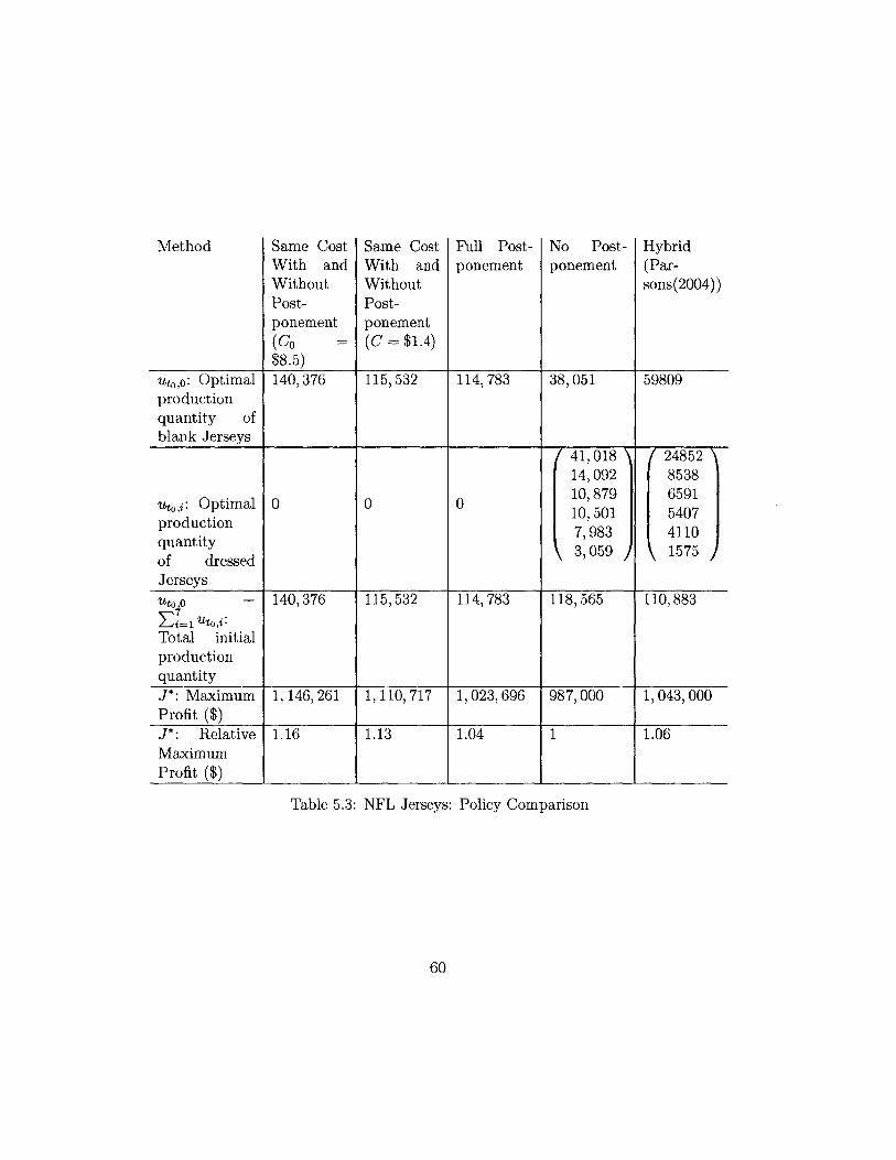
Three different policies are compared.

With the full postponement policy, only blank Jerseys are produced at the first produc-

tion stage, and they are converted to dressed Jerseys when perfect demand information is

available. The maximum expected profit can be obtained using equation 3.47.

58

Without postponement, at the first stage, the production quantity for each type of dressed

Jerseys are decided separately using standard newsvendor model; at the second stage the

blank Jerseys (produced to satisfy the demand for other players) can also be used to fulfill the

unmet demand for named players. The maximum expected profit is computed by simulation.

The hybrid policy first computes the critical ratio (the probability the terminal demand

can be fulfilled by blank Jerseys) of the blank Jerseys, r. And this critical ratio is used to

compute the estimated underage cost of dressed Jerseys, U. From U the optimal production

quantity for the dressed Jerseys (uto,) are derived. In the end, ut,,i are used to adjust the

demand for the blank Jerseys (p0 , a0 ) by considering the possibility of fulfilling the unmet

demand of the named Jerseys using the bland Jerseys. In summary,

r1 = U/(U+ 00)

U = ri(C+CO -0)+(1-ri)(P -)U

r2=U+6

z = P4(r2)

Uo i= I+ iz

E[LostSales](i) pi - uto, + oi(zI(z) + O(z))6

po (old) + E[LostSales](i)

6

i=0

UtOO PO + 90o 1()

The maximum expected profit is computed by simulation, and equation 5.1 is used.

To observe the effect of the additional costs introduced by postponement, we also include

the optimal solution for a hypothetical case, that is, the cost of converting a blank Jersey

is reduced by $1, making the total cost with and without postponement the same. The

computation results are summarized in the following table:

The difference between the maximum profits in the above table and the corresponding

59

Method Same CostWith andWithoutPost-ponement

(Co =$8.5)

Same CostWith andWithoutPost-ponement(C = $1.4)

Full Post-ponement

No Post-ponement

Hybrid(Par-sons(2004))

Uto,O: Optimal 140,376 115,532 114,783 38, 051 59809productionquantity ofblank Jerseys

41,018 2485214, 092 853810,879 6591

uri: Optimal 0 0 0 10, 501 5407production 7,983 4110quantity 3, 059 1575of dressedJerseys

Uto O + 140,376 115,532 114,783 118,565 110,883

Total initialproductionquantityJ*: Maximum 1, 146, 261 1,110,717 1,023,696 987,000 1,043,000Profit ($)J*: Relative 1.16 1.13 1.04 1 1.06MaximumProfit ($)

Table 5.3: NFL Jerseys: Policy Comparison

60

ones in Parsons (2004) are caused by different ways of evaluating the profit. We computed

the maximum profit using simulation, while Parsons (2004) estimated the maximum profit

by assuming all the unmet demand of the dressed Jerseys are fulfilled by the blank Jerseys,

which is an optimistic estimation. The above results suggest that a hybrid solution is bet-

ter than the full postponement solution by about 2%, which is quite significant, since the

profit increase by the fully postponed solution is only 4%. In addition, this example demon-

strates that the variable cost of postponement has significant impact on the total benefit

of postponement. By increasing production cost by about 10%, the profit increase achieved

by postponement is reduced by about 50% (6% v.s. 13%) if the additional cost is incurred

on the product differentiation phase, or about 62% (6% v.s. 16%) if the additional cost is

imposed in the common production phase.

61

Chapter 6

Conclusion

This thesis analyzes the benefit of postponement for fashion products using a two stage

newsvendor model with forecast evolution. The benefit of postponement is measured by the

percentage increase in maximum expected profit. Analytical and numerical results indicate

that

1. Other costs equal, the benefit of postponement decreases as the salvage value of the

intermediate product increases, or the correlation between the demand for end products

increases. However, for a set of perfectly negatively correlated products, benefit of

postponement becomes insensitive to the salvage value of the intermediate product.

And if the salvage value of the intermediate product is close to its cost, then the

benefit of postponement is insensitive to the correlation of the end products.

2. If postponement introduces additional costs, then the hybrid policy proposed by Par-

sons (2004) performs much better than a pure postponement policy. In addition,

reducing costs in the common production phase leads to a higher profit than reducing

the same amount of cost in the differentiated production phase.

The model and findings in this thesis can be used to analyze the benefit of postpone-

ment for fashion products related to uncertainty reduction, and can be integrated into more

complex models that includes other values and costs described in chapter 1.

63

Chapter 7

Future Work

To simplify notation and gain analytically insights, the analysis in this thesis assumes that

the demand evolution follows a multi-variant normal distribution (additive martingale (Heath

and Jackson, 1994)). However, multi-variate lognormal distribution (multiplicative martin-

gale) might be a more realistic approximation (Heath and Jackson, 1994), because it captures

the effect of demand size on its variance. The demand evolution model can be easily adapted

to any other distributions, but analytical solutions as proposed in chapter 3 might not exist.

Capacity constraints are ignored in the model proposed in this thesis. Adding capacity

constraint will push production decisions further back from demand realization time, forcing

productions to be made at higher uncertainty, hence, reduces optimal expected profit. It

would be interesting to analyze the effect of capacity on the benefit of postponement.

65

Bibliography

Alderson, W. 1950. Marketing efficiency and the principle of postponement. Cost and Profit

Outlook, September 3 .

Aviv, Y, and A. Federgruen. 2001. Design for postponement: a comprehensive characteriza-

tion of its benefits under unknown demand distribution. Operations Research 49:578-598.

Bertsekas, D.P. 1999. Nonlinear programming. Athena Scientific.

Brown, A.O., H.L. Lee, and R. Petrakian. 2000. Xilinx improves its semiconductor supply

chain using product and process postponement. Interfaces 30:65-80.

Dapiran, P. 1992. Benetton - global logistics in action. Asian Pacific International Journal

of Business Logistics 5:7-11.

Engardio, P., and B. Einhorn. 2005. Outsourcing innovation. BusinessWeek Online, March

25.

Graves, Meal H. C. Dasu S., S. C., and Y. Qui. 1986. Two-stage production planning in

a dynamic environement. In Multi-stage production planning and inventory control, ed.

Schneeweiss Ch. Axster, S. and E. Silver, Lecture notes in economics and mathematical

systems, 11-43. Springer-Verlag.

Harle, N., M. Pich, and L. Van der Hayden. 2001. Mark-spencer and zara: Process com-

petition in the textile apparel industry. Business School Case, INSEAD, Fontainebleau,

France .

67

Heath, D.C., and P.L. Jackson. 1994. Modeling the evolution of demand forecasts with

application to safety stock analysis in production/distribution systems. IIE Transactions

26:17-25.

Lee, C. Billington, H., and B. Carter. 1993. Hewlett-packard gains control of inventory and

service through design for localization. Interfaces 23:1-11.

Lee, H. 1996. Effective management of inventory and service through product and process

redesign. Operations Research 44.

Lee, H., and C. Billington. 1994. Designing products and processes for postponement, 102-

105. Boston: Kluwer Academic Publishers.

Lee, H., and C. S. Tang. 1997. Modeling the costs and benefits of delayed product differen-

tiation. Management Science 43.

Lee, H.L., and S. Whang. 1998. Value of postponement from variability reduction through

uncertainty resolution and forecast improvement, chapter 4, 66-84. Kluwer Publishers,

Boston.

Parsons, John C.W. 2004. Using a newsvendor model for demand planning of nfl replica

jerseys. Master's thesis, Massachusetts Institute of Technology.

Rockhold, Lee H., S., and R. Hall. 1998. Strategic alignment of a global supply chain for

business success. In Global supply chain and technology management, ed. H. Lee and S. Ng,

number 1 in POMS Series in Technology and Operations Management, 16-29. Baltimore,

MD: Production and Operations Management Society.

Swaninathan, J.M., and H.L. Lee. 2003. Design for postponement. North Holland Publish-

ing.

Swaminathan, J.M., and S. Tayur. 1998. Managing broader product lines through delayed

differentiation using vanilla boxes. Management Science 44:161-172.

68

Venkatesh, S., and J.M. Swaminathan. 2001. Managing product variety through postpone-

ment: Concepts and applications. , The Kluwer Publisher.

Zinn, W., and D. Bowersox. 1988. Planning physical distribution with the principles of

postponement. Journal of Business Logistics 9:117-136.

69

JUL 15 2005 - DSpace@MIT

Documents

Transcript of JUL 15 2005 - DSpace@MIT