jets with a time-periodic supply velocity: a numerical analysis
28
1 Mixing ventilation driven by two oppositely located supply 1 jets with a time-periodic supply velocity: a numerical analysis 2 using CFD 3 4 T. van Hooff 1,2,* , B. Blocken 1,2 5 6 1 Building Physics Section, Department of Civil Engineering, KU Leuven, Belgium 7 2 Unit Building Physics and Services, Department of the Built Environment, Eindhoven University of Technology, The 8 Netherlands 9 Email. [email protected] 10 11 Abstract 12 Ventilation is of primary importance for the creation of healthy and comfortable indoor environments 13 and it has a significant impact on the building energy heating and cooling demand. The aim of this study is 14 to assess the application of time-periodic supply velocities to enhance mixing in mixing ventilation cases 15 to reduce heating and cooling energy demands. This paper presents computational fluid dynamics (CFD) 16 simulations of a generic mixing ventilation case, in which the time-averaged velocities and pollutant 17 concentrations from a reference case with constant supply velocities were compared with those obtained 18 from a case with time-periodic supply velocities (sine function). The unsteady Reynolds-averaged Navier- 19 Stokes (URANS) CFD simulations indicate that the use of time-periodic supply velocities can reduce high 20 pollutant concentrations in stagnant regions, reduces the overall time-averaged pollutant concentrations 21 and increases contaminant removal effectiveness with about 20%. The influence of the period of the sine 22 function was assessed and the results showed that for the periods tested, the differences are negligible. 23 Finally, the URANS approach was compared with the large eddy simulations (LES) approach, indicating 24 that URANS leads to very similar results (NMSE < 3.2%) as LES and can thus be regarded as a suitable 25 approach for this study. 26 27 Keywords: Mixing ventilation, Ventilation efficiency, Time-dependent inlet velocity, Numerical 28 analysis, Unsteady RANS, Pollutant dispersion 29 30 Accepted for publication in Indoor and Built Environment. https://doi.org/10.1177/1420326X19884667
-
Upload
khangminh22 -
Category
Documents
-
view
1 -
download
0
Transcript of jets with a time-periodic supply velocity: a numerical analysis

1
Mixing ventilation driven by two oppositely located supply 1
jets with a time-periodic supply velocity: a numerical analysis 2
using CFD 3
4
T. van Hooff 1,2,*, B. Blocken 1,2 5
6 1Building Physics Section, Department of Civil Engineering, KU Leuven, Belgium 7
2Unit Building Physics and Services, Department of the Built Environment, Eindhoven University of Technology, The 8 Netherlands 9
Email. [email protected] 10 11
Abstract 12
Ventilation is of primary importance for the creation of healthy and comfortable indoor environments 13
and it has a significant impact on the building energy heating and cooling demand. The aim of this study is 14
to assess the application of time-periodic supply velocities to enhance mixing in mixing ventilation cases 15
to reduce heating and cooling energy demands. This paper presents computational fluid dynamics (CFD) 16
simulations of a generic mixing ventilation case, in which the time-averaged velocities and pollutant 17
concentrations from a reference case with constant supply velocities were compared with those obtained 18
from a case with time-periodic supply velocities (sine function). The unsteady Reynolds-averaged Navier-19
Stokes (URANS) CFD simulations indicate that the use of time-periodic supply velocities can reduce high 20
pollutant concentrations in stagnant regions, reduces the overall time-averaged pollutant concentrations 21
and increases contaminant removal effectiveness with about 20%. The influence of the period of the sine 22
function was assessed and the results showed that for the periods tested, the differences are negligible. 23
Finally, the URANS approach was compared with the large eddy simulations (LES) approach, indicating 24
that URANS leads to very similar results (NMSE < 3.2%) as LES and can thus be regarded as a suitable 25
approach for this study. 26
27
Keywords: Mixing ventilation, Ventilation efficiency, Time-dependent inlet velocity, Numerical 28
analysis, Unsteady RANS, Pollutant dispersion 29
30
Accepted for publication in Indoor and Built Environment. https://doi.org/10.1177/1420326X19884667
2
Introduction 31
Ventilation is essential to obtain a healthy indoor environment in buildings, but also in other enclosures 32
such as cars and airplanes. The amount of ventilation (ventilation rate (m3/s)) and the ventilation 33
efficiency (e.g. air exchange effectiveness, contaminant removal effectiveness) both have a large influence 34
on the indoor air quality, and together with indoor pollutant sources and sinks determine the overall indoor 35
air quality in an enclosure. A sufficient ventilation rate is required to keep the pollutant concentrations, air 36
temperature and relative humidity in an enclosure at acceptable levels. However, too high supply volume 37
flow rates should be avoided in the case of mechanical ventilation since it uses energy for heating/cooling 38
of the supply air and for fan operation. Also, in naturally ventilated buildings the ventilation rate should be 39
controlled to limit the energy losses. To provide healthy indoor environments and simultaneously reduce 40
energy demand, it is of primary importance to ventilate buildings and other enclosures as efficiently as 41
possible. One possibility for the enhancement of the overall ventilation efficiency, at least in mixing 42
ventilation cases, is the application of time-periodic supply velocities (i.e. supply flow rate) instead of 43
constant supply velocities. The use of time-periodic supply velocities could result in enhanced mixing due 44
to the expected breakup of recirculation cells and movement of stagnant regions throughout the enclosure. 45
An enhanced amount of mixing in an enclosure could lead to a reduction of the required supply volume 46
flow rates and thus of the required energy consumption, without compromising the indoor air quality, and 47
would thus be beneficial with respect to both building energy demand and indoor air quality. Additional 48
advantages can be found in an enhanced appreciation of the thermal conditions inside the enclosure, since 49
time-periodic supply velocities might lead to flow characteristics (e.g. turbulence intensity, power spectra) 50
that resemble the characteristics of natural ventilation flows. Fluctuating or intermittent ventilation flows 51
are considered to be favourable in warm/hot conditions (cooling conditions), due to their inherent transient 52
nature, with temporal variations in velocity and turbulence. 1-4 53
In the past decade, a few papers on time-periodic forcing for ventilation purposes have been published. 54
Schmidt et al. 5 studied the airflow patterns in a generic rectangular enclosure resulting from the 55
instationary operation of the available mixing ventilation system. Their results indicated a more uniform 56
time-averaged velocity distribution when time-periodic supply velocities were used than in the case of 57
constant supply velocities. Sattari and Sandberg 6 performed particle image velocimetry (PIV) 58
measurements of a ventilation flow which was driven by both a wall jet with a constant supply and one 59
with a rapidly varying supply velocity (0.5 Hz). Their measurements in a reduced-scale enclosure showed 60
that stagnation regions were reduced and turbulent kinetic energy was increased when a rapidly varying 61
supply velocity was used.6 Fallenius et al. 7 performed measurements in the setup used by Sattari and 62
Sandberg 6 for frequencies of 0.3, 0.4 and 0.5 Hz. Their results indicated an increase in the amount of 63
3
vortical structures inside the enclosure, which resulted in a higher mixing ventilation efficiency. Kabanshi 64
et al. 8 performed full-scale measurements in a classroom, which was ventilated by an intermittent air jet 65
strategy (IAJS), which operated according to a schedule of 3 min ON, and 3 min OFF. Based on their 66
measurements they concluded that the system provided a more comfortable indoor thermal environment at 67
elevated temperatures than was the case when conventional mixing and displacement ventilation systems 68
were used. Kabanshi et al. 9 also studied the effect of an IAJS, in which the supply provided air to the 69
room with intermittent velocities between 0.4 m/s and 0.8 m/s, on cooling energy demand in different 70
climates. Their results showed that the cooling energy demand could be significantly reduced by 71
application of IAJS in hot and humid climates, while in hot and dry climates considerable energy savings 72
could be achieved as well. However, they also concluded that an increased risk of occupant discomfort is 73
present for moderate climates during the heating season due to created draught.9 Finally, a recent review 74
paper 10 on advanced air distribution methods devoted one section to IAJSs, which stated that stagnation 75
zones and draught issues could be reduced by time-periodic supply flows. Although all aforementioned 76
publications indicated the possible positive effects of time-periodic (or intermittent) ventilation with 77
respect to mixing, ventilation efficiency and thermal comfort, the vast majority of the research papers on 78
mixing ventilation flows focused on constant supply velocities (for example 11-22) and a systematic study 79
on the potential of time-periodic supply velocities for different mixing ventilation cases is currently 80
lacking. 81
Different ventilation assessment methods exist, an elaborate description of which can be found in the 82
overview paper by Chen 23. One method to analyse ventilation flows numerically is computational fluid 83
dynamics (CFD). CFD allows a detailed spatial and temporal analysis of the ventilation flow inside a 84
building or other enclosure, which is more difficult, if not impossible, with other methods. Numerous 85
examples of previous studies on indoor airflows using CFD can be found in literature (e.g. 11-25). The 86
largest disadvantage of CFD is the need for solution verification and validation (e.g. 26-31) and the large 87
sensitivity of results to the large amount of choices a user needs to make when performing CFD 88
simulations (e.g. 32,33). 89
In this paper, unsteady Reynolds-averaged Navier-Stokes (URANS) CFD simulations using the 90
renormalization group (RNG) k-ε turbulence model and a large-eddy simulation (LES) using the dynamic 91
Smagorinksy subgrid-scale (SGS) model were performed for a mixing ventilation case with time-periodic 92
supply velocities, and the results were compared in terms of dimensionless time-averaged velocities and 93
contaminant levels inside the enclosure. The enclosure was ventilated by two oppositely located supply 94
openings (top) and two oppositely located exhaust openings (bottom). The rectangular room geometry was 95
based on previous studies by Nielsen 12 and Restivo 34. A comparison was made between the application 96
of a constant supply velocity and the application of time-periodic supply velocities, in which the two 97

4
supplies act out-of-phase. To assess the level of mixing in both cases, a passive and uniformly distributed 98
gaseous contaminant source was introduced in the enclosure. Both URANS and LES simulations were 99
conducted to assess the validity of URANS, which has a lower computational demand than LES. 100
Validation study 101
Experiments 102
The validation study was based on the experimental data by Nielsen 12 for a mixing ventilation flow in 103
a generic enclosure. The measurements were, among other things, used for the International Energy 104
Agency (IEA) Annex 20 case and subsequently, have been used extensively for CFD model validation 105
studies. The experimental setup consisted of a generic rectangular enclosure with dimensions 9 × 3 × 3 m3 106
(L × W × H). Air was supplied by a linear supply opening (h = 0.168 m) and left the enclosure through an 107
oppositely located linear exhaust (t = 0.48 m), both with a length l = 3 m, i.e. covering the entire depth of 108
the enclosure (see Fig. 1). 109
The measurements were conducted for Re = 5000, with Re = hU0/ν, with ν the kinematic viscosity (= 110
15.3 10-6 m2/s at air temperature 20°C), resulting in a supply velocity of U0 = 0.455 m/s. The supply 111
condition for turbulent kinetic energy (k0) was k0 = 1.5(IUU0)2, with IU the streamwise turbulence intensity 112
equal to 4%, while turbulent dissipation rate ε0 at the supply was calculated from ε0 = k01.5/l0, with l0 = 113
h/10 12. The numerical results were compared with measurement results along two vertical lines, at x = H 114
and at x = 2H, in the vertical centre plane (z/W = 0.5) (Fig. 1). 115
116
117 Fig. 1: Vertical cross section of room geometry used in the validation study, taken from IEA Annex 20 case 11, with 118 indication of two vertical lines in vertical centre plane (z/W = 0.5) along which experimental results are compared 119 with numerical results. 120
121
122

5
Computational settings and parameters 123
The computational geometry reproduces the geometry of the model used in the experiments described 124
by Nielsen 12 (see previous section and Fig. 1). The computational grid was created using the surface-grid 125
extrusion technique by van Hooff and Blocken 35 and is presented in Figure 2 (vertical cross section). The 126
computational grid consists of hexahedral cells only. The grid resolution was determined based on a grid-127
sensitivity analysis using three different grids, which were created by refining and coarsening the basic 128
grid with a factor of √2 in each direction. The resulting coarse, basic and fine grids contain 212,160 cells, 129
588,672 cells and 1,697,280 cells, respectively. The maximum dimensionless wall distances (y*) along the 130
ceiling (region of highest velocity and thus highest y* values) are 6.4, 3.6 and 2.5, for the coarse, basic and 131
fine grid, respectively. The average y* values along the ceiling are 3.8, 2.6 and 1.6, for the coarse, basic 132
and fine grid, respectively. 133
134
135 Fig. 2: (a) Computational grid in the vertical centre plane (z/W = 0.5) for the validation study (basic grid with 136 588,672 cells). (b) Close-up view of grid near the supply opening. 137
138
139
A grid-sensitivity analysis shows that the basic grid provides nearly-grid independent results (see Fig. 140
3). The values of the grid-convergence index (GCI) for the streamwise velocity (U) were calculated using 141
Eq. (1), 142
143
( ) 0
1
pbasic fine
basic S p
r U U UGCI F
r
− =−
(1) 144
145
where r is the linear grid refinement factor (r = √2), p the formal order of accuracy which is equal to the 146
value of 2 since second-order discretization schemes were used for the simulations. Fs is a safety factor, 147
taken to be 1.25, which is the recommended value when three or more grids are considered in the grid-148
sensitivity analysis.27 Figure 3c, d show the results for the GCI. The average GCI values along the two 149
vertical lines (at x = H and x = 2H) are 0.036 and 0.043, respectively. 150
151

6
The boundary conditions at the supply and exhaust were taken as equal to those reported by Nielsen 12; 152
i.e. U0 = 0.455 m/s, ε0 = k01.5/l0 = 6.59 10-4, while the values for k0 were based on the measured values in 153
the supply opening.12 The walls of the enclosure were modelled as no-slip walls, and zero static gauge 154
pressure was applied at the exhaust. 155
The commercial CFD code ANSYS Fluent 15 36 was used for the CFD simulations. The 3D steady 156
RANS equations were solved in combination with the RNG k-ε model 37 and the two-layer zonal model 36 157
(low Reynolds number modelling) was used as near-wall treatment. The SIMPLE algorithm was used for 158
pressure-velocity coupling, pressure interpolation was second order and second-order discretization 159
schemes were used for both the convective terms and the viscous terms of the governing equations. 160
Convergence was assumed to be obtained when all the scaled residuals level off and reached a minimum 161
value. The minimum values of the residuals are 10-5 for x, y, z velocities, k, and ε. 162
163
164 Fig. 3: Results of grid-sensitivity analysis. U/U0 at (a) x = H; (b) x = 2H. (c) GCI for basic grid at (c) x = H; (d) \x = 165 2H. 166
167

7
Results 168
Figure 4 shows comparisons between the measured values of the dimensionless time-averaged 169
streamwise velocity (U/U0) and dimensionless turbulent kinetic energy (k0.5/U0) and the values obtained 170
from the 3D steady RANS CFD simulations at x = H and x = 2H. In general, a good agreement is present 171
along the two vertical lines for U/U0, with the largest discrepancies near the floor of the enclosure (y/H < 172
0.3) and the best agreement in the wall jet region (y/H > 0.6), which corresponds to outcomes of earlier 173
validation studies using the same experimental data.38,39 The values of k0.5/U0 are fairly well predicted at x 174
= H (Fig. 4a), however, at x = 2H the numerical results show a consistent underprediction of k0.5/U0 with 175
about 10-20% (Fig. 4b). In the lower part of the enclosure (y/H < 0.1), the differences between k0.5/U0 176
obtained from experiments and simulations increase with decreasing height and can become larger than 177
100% near the ground surface. A possible reason for the higher values of k0.5/U0 in the experiments could 178
be the presence of a pronounced transient flow in the region near the floor, which cannot be reproduced by 179
the steady CFD simulations. The observed differences in k0.5/U0 could be related to the larger velocity 180
gradients in the lower region in the CFD simulations compared to those in the experiments. 181
182
183 Fig. 4: Results of validation study. U/U0 and k0.5/U0 at (a) x = H; (b) x = 2H. 184
185
Figure 5 shows two scatter plots with the CFD results and the experimental results. A perfect 186
agreement would mean the symbols are on the x = y line. The dashed lines indicate the 10%, 20% and 187
30% (in case of k0.5/U0) difference between the experimental results and the CFD results. Figure 5a shows 188
that the largest percentage differences occur in the low-velocity regions and that the best agreement is 189
present in the high-velocity regions. The majority of the predicted velocities lies within 20% difference of 190
the experimental results. Figure 5b shows an underprediction of k0.5/U0 by the CFD simulations. A bit 191
more than half of the predictions are within 20% difference, and more than 80% of the predictions are 192
within a 30% difference. 193

8
Overall, the validation study shows that the RNG k-ε turbulence model in combination with the other 194
employed computational settings and parameters is sufficiently capable of predicting mixing ventilation 195
flows in a generic enclosure with sufficient accuracy, especially with respect to the mean velocities. 196
Therefore, the employed turbulence model and settings are used in the case study in the following section. 197
198
199 Fig. 5: Scatterplot with results of validation study at x = H and x = 2H. (a)U/U0. (b) k0.5/U0. 200
201
Case study: computational geometry, settings and parameters 202
Computational geometry 203
The effect of time-periodic forcing of the supply velocity on the mixing ventilation flow was assessed 204
in a generic rectangular enclosure based on the IEA Annex 20 enclosure as presented in the Validation 205
study section, with dimensions 9 × 3 × 3 m3 (L × W × H).12 However, in this case, the air was supplied by 206
two oppositely located linear supply openings (hsupply = 0.168 m, lsupply is 3 m) in the upper part of the 207
enclosure and it leaves the enclosure through two oppositely located linear exhausts (hexhaust = 0.48 m, 208
lsupply is 3 m) in the bottom part of the enclosure (see Fig. 6). The results were analysed in the vertical 209
centre plane (z/W = 0.5) along three vertical lines (x/H = 1/3, x/H = 2/3, x/H = 1; Fig. 6). 210
211

9
212 Fig. 6: Vertical cross section of room geometry, with two opposite supply openings in the upper part and two 213 opposite exhaust openings in the lower part of the enclosure. The three dashed vertical lines indicate the locations 214 where the results were analyzed. 215
216
Computational settings and parameters 217
The 3D CFD simulations were performed in ANSYS Fluent.36 A vertical cross section of the 218
computational geometry is depicted in Figure 6, including indication of the coordinate system. The 219
computational grid was based on the grid resolution employed in the validation study and consists of 220
505,760 hexahedral cells, with higher grid resolutions in the boundary layer, shear layer and in the region 221
where the two opposite jets collide/interact in case of constant supply velocities (see Fig. 7). 222
223
224 Fig. 7: Computational grid for the case study (505,760 hexahedral cells). 225
226
One type of time-periodic supply velocity was used in the present paper, which was based on a sine 227
function. The sine function enables a supply velocity that varies over time t with period T and amplitude 228
∆U0 around a constant reference velocity U0,RC (= 0.5 m/s) and is described by Eq. (2) (supply 1) and Eq. 229
(3) (supply 2): 230
231 ( ) ( )0,supply1 0, 0 sin 2 /RCu t U U t Tπ= + ∆ ⋅ (2) 232
( ) ( )( )0,supply2 0, 0 sin 2 /RCu t U U t Tπ= − −∆ ⋅ (3) 233
234
235
10
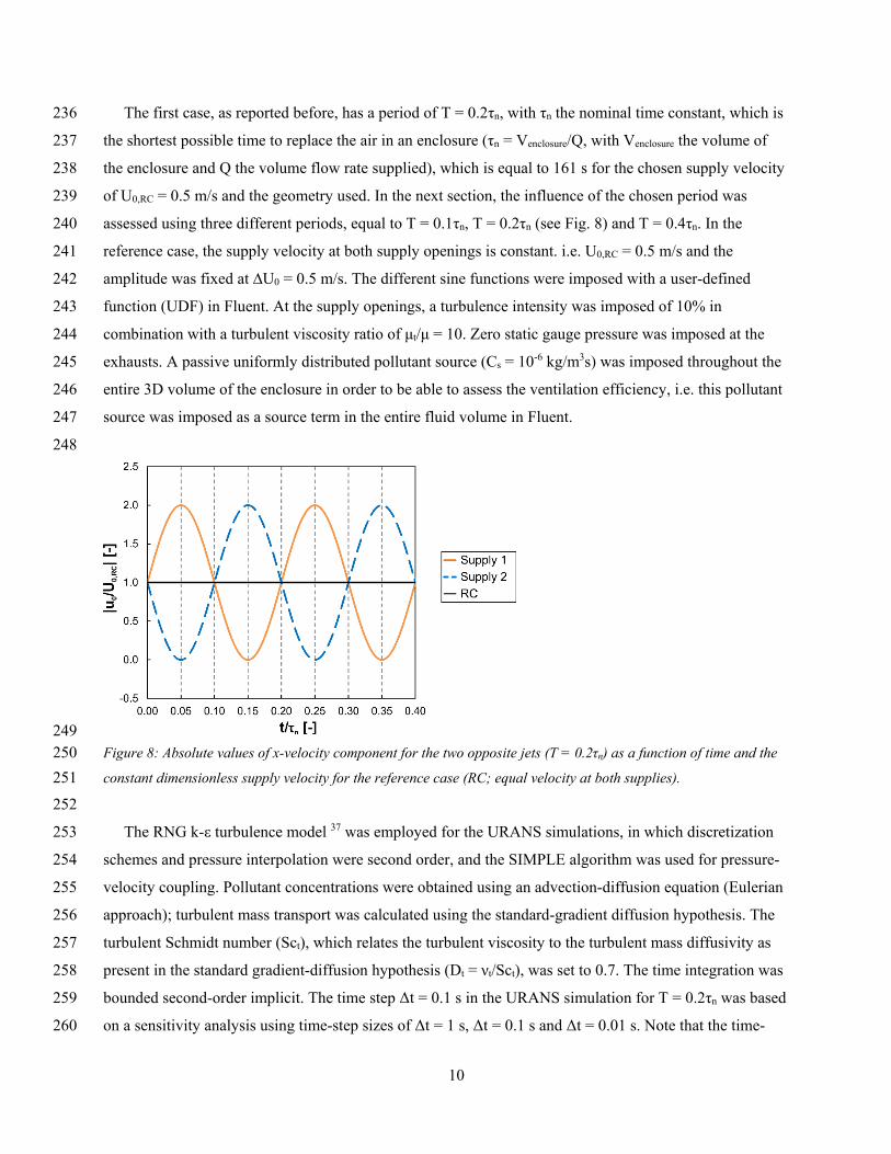
The first case, as reported before, has a period of T = 0.2τn, with τn the nominal time constant, which is 236
the shortest possible time to replace the air in an enclosure (τn = Venclosure/Q, with Venclosure the volume of 237
the enclosure and Q the volume flow rate supplied), which is equal to 161 s for the chosen supply velocity 238
of U0,RC = 0.5 m/s and the geometry used. In the next section, the influence of the chosen period was 239
assessed using three different periods, equal to T = 0.1τn, T = 0.2τn (see Fig. 8) and T = 0.4τn. In the 240
reference case, the supply velocity at both supply openings is constant. i.e. U0,RC = 0.5 m/s and the 241
amplitude was fixed at ∆U0 = 0.5 m/s. The different sine functions were imposed with a user-defined 242
function (UDF) in Fluent. At the supply openings, a turbulence intensity was imposed of 10% in 243
combination with a turbulent viscosity ratio of μt/μ = 10. Zero static gauge pressure was imposed at the 244
exhausts. A passive uniformly distributed pollutant source (Cs = 10-6 kg/m3s) was imposed throughout the 245
entire 3D volume of the enclosure in order to be able to assess the ventilation efficiency, i.e. this pollutant 246
source was imposed as a source term in the entire fluid volume in Fluent. 247
248
249 Figure 8: Absolute values of x-velocity component for the two opposite jets (T = 0.2τn) as a function of time and the 250 constant dimensionless supply velocity for the reference case (RC; equal velocity at both supplies). 251
252
The RNG k-ε turbulence model 37 was employed for the URANS simulations, in which discretization 253
schemes and pressure interpolation were second order, and the SIMPLE algorithm was used for pressure-254
velocity coupling. Pollutant concentrations were obtained using an advection-diffusion equation (Eulerian 255
approach); turbulent mass transport was calculated using the standard-gradient diffusion hypothesis. The 256
turbulent Schmidt number (Sct), which relates the turbulent viscosity to the turbulent mass diffusivity as 257
present in the standard gradient-diffusion hypothesis (Dt = νt/Sct), was set to 0.7. The time integration was 258
bounded second-order implicit. The time step Δt = 0.1 s in the URANS simulation for T = 0.2τn was based 259
on a sensitivity analysis using time-step sizes of Δt = 1 s, Δt = 0.1 s and Δt = 0.01 s. Note that the time-260
11
step size was halved and doubled for T = 0.1τn and T = 0.4τn, respectively. The number of iterations within 261
one time-step was equal to 10 and it was verified that both the number of iterations and the averaging time 262
are sufficient (i.e. > 100 periods) by monitoring the evolution of the instantaneous (within a time-step) and 263
time-averaged (over number of time-steps) velocities and pollutant concentrations. 264
Case study: Results 265
Constant supply vs. time-periodic supply 266
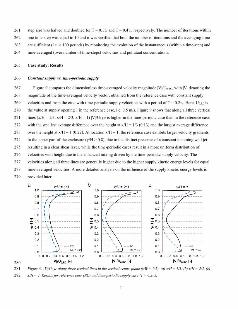
Figure 9 compares the dimensionless time-averaged velocity magnitude |V|/U0,RC, with |V| denoting the 267
magnitude of the time-averaged velocity vector, obtained from the reference case with constant supply 268
velocities and from the case with time-periodic supply velocities with a period of T = 0.2τn. Here, U0,RC is 269
the value at supply opening 1 in the reference case, i.e. 0.5 m/s. Figure 9 shows that along all three vertical 270
lines (x/H = 1/3, x/H = 2/3, x/H = 1) |V|/U0,RC is higher in the time-periodic case than in the reference case, 271
with the smallest average difference over the height at x/H = 1/3 (0.13) and the largest average difference 272
over the height at x/H = 1 (0.22). At location x/H = 1, the reference case exhibits larger velocity gradients 273
in the upper part of the enclosure (y/H > 0.8), due to the distinct presence of a constant incoming wall jet 274
resulting in a clear shear layer, while the time-periodic cases result in a more uniform distribution of 275
velocities with height due to the enhanced mixing driven by the time-periodic supply velocity. The 276
velocities along all three lines are generally higher due to the higher supply kinetic energy levels for equal 277
time-averaged velocities. A more detailed analysis on the influence of the supply kinetic energy levels is 278
provided later. 279
280 Figure 9: |V|/U0,RC along three vertical lines in the vertical centre plane (z/W = 0.5). (a) x/H = 1/3. (b) x/H = 2/3. (c) 281 x/H = 1. Results for reference case (RC) and time-periodic supply case (T = 0.2τn). 282

12
Figure 10 shows contours of |V|/U0,RC in the vertical centre plane. The stagnant (blue) regions as 283
present in Figure 10a for the reference case, have decreased due to the time-periodic supply velocities as 284
shown in Fig. 10b. In general, the time-averaged velocities are higher, which is also reflected in the 285
volume-averaged dimensionless time-average velocity, which is 0.258 in the reference case versus 0.399 286
for the case with time-periodic supply velocities. These results also indicate the influence of higher supply 287
kinetic energy levels resulting from the higher maximum velocities due to the use of a sine function for 288
the supply velocities. 289
290
291 Figure 10: Contours of |V|/U0,RC in vertical centre plane (z/W = 0.5). (a) Reference case. (b) Time-periodic supply 292 case (T = 0.2τn). 293
294
Figure 11 shows a comparison between the dimensionless time-averaged pollutant concentrations 295
(Cρ/Csτn) obtained from the reference case with steady supply velocities versus the case with time-296
periodic supply velocities with a period of T = 0.2τn. The largest differences (up to 74%; 1.455 vs. 0.834) 297
occur around mid-height of the enclosure (0.5 < y/L < 0.6) at x/H = 2/3 and x/H = 1, where in the 298
reference case high pollutant concentrations are present due to a stagnant region. In the case of time-299
periodic supply velocities the pollutant concentrations in this area are strongly reduced. In addition, the 300
pollutant concentration along all three vertical lines (below y/H = 0.9) are around 1 and are thus similar 301
throughout large parts of the domain, indicating enhanced mixing and the resulting more uniform 302
concentrations. 303

13
Figure 12 shows the time-averaged pollutant concentrations in the enclosure for both cases. Time-304
periodic supply velocities lead to substantially reduced concentration. The improved mixing leads to the 305
absence of high pollutant concentration regions and the relatively uniform distribution of pollutant 306
concentrations. 307
308
309 Figure 11: Cρ/Csτn along three vertical lines in the vertical centre plane (z/W = 0.5). (a) x/H = 1/3. (b) x/H = 2/3. (c) 310 x/H = 1. Results for reference case (RC) and time-periodic supply case (T = 0.2τn). 311
312
313 Figure 12: Contours of Cρ/Csτn in the vertical centre plane (z/W = 0.5). (a) Reference case. (b) Time-periodic supply 314 case (T = 0.2τn). 315

14
The volume-averaged value for the reference case is Cρ/Csτn = 1.018 versus 0.908 for the time-periodic 316
supply case. At the exhaust openings the area average value is 0.976 for the reference case versus 1.050 317
for the time-periodic supply case. The contaminant removal effectiveness (CRE) (εC) (e.g. 40,41) can be 318
calculated using Eq. (4), using the room-averaged time-averaged pollutant concentration (⟨C⟩), the time-319
averaged pollutant concentration at the supply (Cs), and the time-averaged pollutant concentration at the 320
exhaust (Ce): 321
100%Ce s
s
C CC C
⋅−ε =−
(4) 322
Fully mixed conditions would result in a value of 100%, piston flow would result in a value equal to or 323
greater than 100% (depending on location of pollutant source), and short-circuiting would result in values 324
below 100% (room averaged concentration would be larger than concentration at exhaust) (e.g. 40,41). The 325
CRE is equal to εC = 96% for the reference case, while it is 116% for the case with time-periodic supply 326
velocities. 327
Finally, Figure 13 depicts contours of instantaneous pollutant concentrations for the case with a period 328
of T = 0.2τn, during one period (T) starting after time-averaged values are obtained (i.e. after > 100 329
periods). Figure 13 shows the back and forth movement of the flow in the enclosure as driven by the wall 330
jets and the breakup of the recirculation cells. In the reference case two distinct recirculation cells are 331
visible (Fig. 12a), with stagnant regions in the middle of each recirculation cell resulting in higher 332
pollutant concentrations in these regions. Note that no symmetric flow can be observed during this period 333
due to the 3D nature of the flow, with randomly varying pollutant concentrations over the width of the 334
enclosure (not shown here for the sake of brevity). 335
336
Influence of period 337
The influence of the chosen period was analysed by simulations with three different periods, i.e. T = 338
0.1τn, T = 0.2τn, and T = 0.4τn. The amplitude was kept constant. The time-averaged supply velocity (and 339
thus supply volume flow rate) is constant (= 0.5 m/s) in all three cases. 340
Figure 14 compares the dimensionless time-averaged velocities from the reference case versus the 341
cases with time-periodic supply velocities with the three different periods. The influence of the period 342
appears to be limited, especially at x/H = 2/3 and x/H = 1. At x/H = 1/3 the largest differences are present; 343
the velocity profile for a period of T = 0.1τn differs from the other two velocity profiles. Nonetheless, 344
Figure 14 shows that the overall differences in velocity magnitude along the three vertical lines is limited. 345
Figure 15 compares the dimensionless time-averaged pollutant concentrations along the same three 346
lines. The difference between the different periods appears to be marginal along the lines analysed. The 347

15
average difference between the time-averaged pollutant concentrations over the three lines was within 348
1.3%, while the maximum differences were within 10%. This indicates that the periods tested do not 349
significantly influence the mixing and thus the resulting time-averaged pollutant concentrations, for this 350
particular case. 351

16
352 Figure 13: Contours of dimensionless instantaneous pollutant concentration (cρ/Csτn) in the vertical centre plane 353 (z/W = 0.5) during one period T for T = 0.2τn. 354
355
17
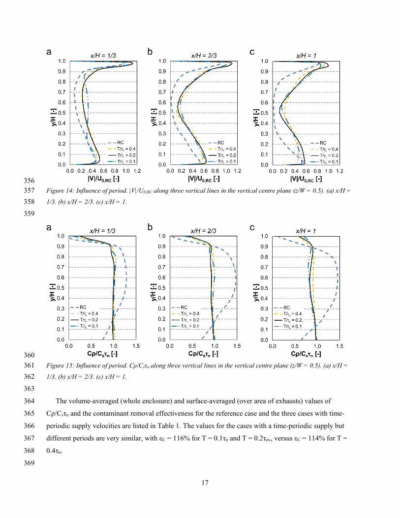
356 Figure 14: Influence of period. |V|/U0,RC along three vertical lines in the vertical centre plane (z/W = 0.5). (a) x/H = 357 1/3. (b) x/H = 2/3. (c) x/H = 1. 358
359
360 Figure 15: Influence of period. Cρ/Csτn along three vertical lines in the vertical centre plane (z/W = 0.5). (a) x/H = 361 1/3. (b) x/H = 2/3. (c) x/H = 1. 362
363
The volume-averaged (whole enclosure) and surface-averaged (over area of exhausts) values of 364
Cρ/Csτn and the contaminant removal effectiveness for the reference case and the three cases with time-365
periodic supply velocities are listed in Table 1. The values for the cases with a time-periodic supply but 366
different periods are very similar, with εC = 116% for T = 0.1τn and T = 0.2τnv, versus εC = 114% for T = 367
0.4τn. 368
369

18
Table 1: Influence of period on dimensionless time-averaged pollutant concentrations, averaged over the volume 370 (⟨C⟩ρ/Csτn) and averaged over the exhaust opening (Ceρ/Csτn), and CRE (εC). 371
RC T = 0.1τn T = 0.2τn T = 0.4τn ⟨C⟩ρ/Csτn 1.018 0.915 0.908 0.913 Ceρ/Csτn 0.976 1.058 1.050 1.042 εC 96% 116% 116% 114%
372
373
Equal supply volume flow rates vs. equal supply kinetic energy levels 374
In the simulations reported in the previous sections, the time-averaged supply velocity (and thus supply 375
volume flow rate) was taken equal in the reference case and in all three time-periodic supply cases. 376
Although this choice can be substantiated from the point of view of heating and cooling demands (the 377
energy needed to heat or cool a certain amount of air would be different when different supply volume 378
flow rates would be used), considering fan energy use, however, one should use the same time-averaged 379
supply kinetic energy values for the reference case compared to the time-periodic supply velocity cases. 380
Therefore, an additional simulation was conducted in which the time-averaged supply kinetic energy for 381
all cases is equal, which was achieved by increasing the supply velocity at both supplies in the reference 382
case to 0.61 m/s, based on Eq. 5: 383
02
0
( )12
T
k u tE m dtT
= ∫ (5) 384
385
with u0(t) being the supply velocity and m is the mass of air (equal in both cases). Figure 16 and Figure 17 386
compare the results focused on equal time-averaged supply volume flow rates versus equal time-averaged 387
levels of kinetic energy of the supply flow. Figure 16 shows that the time-averaged velocities along the 388
three vertical lines are slightly higher due to the higher supply velocity (0.61 m/s vs. 0.5 m/s) imposed for 389
the reference case with equal time-averaged supply kinetic energy levels (RC_KE). The increase is most 390
pronounced in the wall jet region (y/H > 0.9). The volume-averaged dimensionless time-average velocity, 391
which is 0.258 in the reference case with equal time-averaged supply volume flow rates (RC) versus 0.363 392
for the reference case with equal time-averaged kinetic energy of the supply flow (RC_KE), and 0.399 for 393
the case with time-periodic supply velocities. 394
395
396
397
398

19
399
400 Figure 16: |V|/U0,RC along three vertical lines in the vertical centre plane (z/W = 0.5). (a) x/H = 1/3. (b) x/H = 2/3. 401 (c) x/H = 1. For RC with time-averaged supply volume flow rates equal to time-periodic case (RC) and RC with 402 time-averaged kinetic energy of supply flow equal to time-periodic case (RC_KE) 403
404
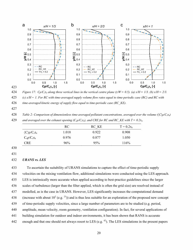
Figure 17 shows that the pollutant concentrations in RC_KE have decreased to a certain extent 405
compared to RC, however, the pollutant concentrations in both reference cases are still much higher at 406
mid-height than in the time-periodic supply case. The maximum decrease of Cρ/Csτn for RC_KE 407
compared to RC is around 8% at x/H = 1 and y/H ≈ 0.7. The time-averaged values of both the volume-408
averaged pollutant concentrations (⟨C⟩ρ/Csτn) and the surface-averaged pollutant concentration at the 409
exhaust opening (Ceρ/Csτn), and the CRE are listed in Table 2. Although the value for ⟨C⟩ρ/Csτn is about 410
10% lower for RC_KE compared to RC, it is still 1.5% higher for RC_KE than for the time-periodic 411
supply case. Moreover, the CRE for RC_KE is very similar (95%) to the one for RC (96%) and thus much 412
lower than the CRE in the time-periodic supply case (116%). The increased velocity in RC_KE thus 413
decreases the volume-averaged time-average pollutant concentration compared to RC but has no 414
significant effect on the CRE. The results indicate that the CRE in both reference cases is much lower than 415
in the time-periodic case, implying that at equal kinetic energy levels of the supply flow (and thus equal 416
fan energy) time-periodic ventilation can enhance mixing and the CRE. The volume-averaged pollutant 417
concentration for the time-periodic supply case is 1.5% lower than in RC_KE, and this decrease could be 418
achieved with equal energy use. Note that any possible changes in fan efficiency as function of supply 419
volume flow rate are not included here. 420
421
422
20
423 Figure 17: Cρ/Csτn along three vertical lines in the vertical centre plane (z/W = 0.5). (a) x/H = 1/3. (b) x/H = 2/3. 424 (c) x/H = 1. For RC with time-averaged supply volume flow rates equal to time-periodic case (RC) and RC with 425 time-averaged kinetic energy of supply flow equal to time-periodic case (RC_KE). 426
427
Table 2: Comparison of dimensionless time-averaged pollutant concentrations, averaged over the volume (⟨C⟩ρ/Csτn) 428 and averaged over the exhaust opening (Ceρ/Csτn), and CRE for RC and RC_KE with T = 0.2τn. 429
RC RC_KE T = 0.2τn ⟨C⟩ρ/Csτn 1.018 0.922 0.908 Ceρ/Csτn 0.976 0.877 1.050 CRE 96% 95% 116%
430
431
URANS vs. LES 432
To ascertain the suitability of URANS simulations to capture the effect of time-periodic supply 433
velocities on the mixing ventilation flow, additional simulations were conducted using the LES approach. 434
LES is intrinsically more accurate when applied according to best-practice guidelines since the larger 435
scales of turbulence (larger than the filter applied, which is often the grid size) are resolved instead of 436
modelled, as is the case in URANS. However, LES significantly increases the computational demand 437
(increase with about 102 (e.g. 23)) and is thus less suitable for an exploration of the proposed new concept 438
of time-periodic supply velocities, since a large number of parameters are to be studied (e.g. period, 439
amplitude, mean velocity, room geometry, ventilation configuration). In fact, for several applications of 440
building simulation for outdoor and indoor environments, it has been shown that RANS is accurate 441
enough and that one should not always resort to LES (e.g. 42). The LES simulations in the present papers 442

21
were conducted on the same grid as the URANS simulations. The dynamic Smagorinsky subgrid-scale 443
model 43-45 was used and the filtered momentum equations were discretized with a bounded central-444
differencing scheme. A second-order upwind scheme was used for the advection-diffusion equation. 445
Pressure interpolation is second order. Time integration is bounded second-order implicit. Pressure-446
velocity coupling was taken care of by the PISO algorithm. The non-iterative time advancement scheme 447
was used. The time step Δt was based on a maximum CFL number of 1 and is equal to Δt = 0.01 s. The 448
averaging time was verified as sufficient to obtain statistically-steady results by monitoring the evolution 449
of the time-averaged velocity and pollutant concentrations (moving average). 450
Figure 18 compares the results for a period of T = 0.2τn using URANS versus LES in terms of 451
dimensionless time-averaged velocities. Figure 19 does the same in terms of dimensionless time-averaged 452
pollutant concentrations. Figure 18 shows that the results obtained with LES are very similar to those with 453
URANS. The agreement between URANS and LES is even better with respect to the pollutant 454
concentrations, as depicted in Figure 19. 455
456
457 Figure 18: URANS vs. LES. |V|/U0,RC along three vertical lines in the vertical centre plane (z/W = 0.5). (a) x/H = 458 1/3. (b) x/H = 2/3. (c) x/H = 1. 459
460
461
462
463
464
465
466
22
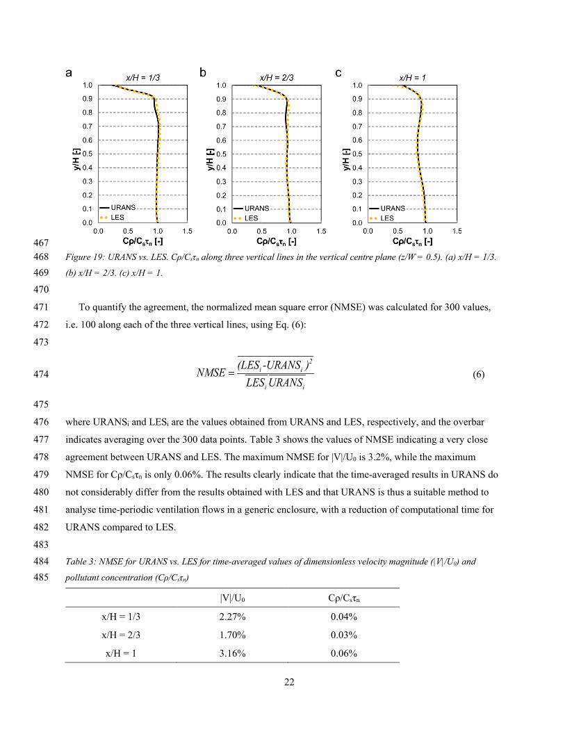
467 Figure 19: URANS vs. LES. Cρ/Csτn along three vertical lines in the vertical centre plane (z/W = 0.5). (a) x/H = 1/3. 468 (b) x/H = 2/3. (c) x/H = 1. 469
470
To quantify the agreement, the normalized mean square error (NMSE) was calculated for 300 values, 471
i.e. 100 along each of the three vertical lines, using Eq. (6): 472
473
2
i i
i i
(LES -URANS )NMSELES URANS
= (6) 474
475
where URANSi and LESi are the values obtained from URANS and LES, respectively, and the overbar 476
indicates averaging over the 300 data points. Table 3 shows the values of NMSE indicating a very close 477
agreement between URANS and LES. The maximum NMSE for |V|/U0 is 3.2%, while the maximum 478
NMSE for Cρ/Csτn is only 0.06%. The results clearly indicate that the time-averaged results in URANS do 479
not considerably differ from the results obtained with LES and that URANS is thus a suitable method to 480
analyse time-periodic ventilation flows in a generic enclosure, with a reduction of computational time for 481
URANS compared to LES. 482
483 Table 3: NMSE for URANS vs. LES for time-averaged values of dimensionless velocity magnitude (|V|/U0) and 484 pollutant concentration (Cρ/Csτn) 485
|V|/U0 Cρ/Csτn
x/H = 1/3 2.27% 0.04%
x/H = 2/3 1.70% 0.03%
x/H = 1 3.16% 0.06%
23
Limitations and future work 486
This study showed the potential of time-periodic supply velocities to enhance mixing in a generic 487
enclosure subjected to mixing ventilation. The CFD simulations consisted of URANS simulations, and a 488
comparison was made with LES. The study was subjected to a few limitations, which can incite future 489
research efforts with focus on: 490
491
• An experimental analysis of time-periodic ventilation flows in a generic enclosure. The 492
experimental data obtained can also be used for CFD validation purposes. 493
• The assessment of enhanced mixing for one-sided mixing ventilation flows and other cases in 494
which mixing ventilation flow can be used to provide a healthy indoor environment. 495
• The assessment of other periods and amplitudes to find an optimal combination of both with 496
respect to mixing in an enclosure. 497
• The analysis for intermittent (ON/OFF) or other types of time-periodic supply conditions. 498
• Extension of the results for this specific generic geometry to more practical cases; i.e. realistic 499
geometries, including buoyancy forces, other heat and momentum sources and sinks, etc., 500
including a detailed analysis of energy consumption by the fans and the heating and cooling 501
demand. 502
• More detailed analyses of the convective and turbulent mass fluxes and other flow properties 503
in an enclosure driven by time-periodic supply jets. 504
• The effect of time-periodic mixing ventilation on thermal comfort and thermal sensation, for 505
example using full-scale tests in climate chambers. 506
• The use of computationally less demanding numerical methods to allow a faster exploration of 507
the effects of time-periodic supply conditions (e.g. 46-48). 508
509
Conclusions 510
This paper presented the first results in a broader research effort on the enhancement of mixing in 511
mixing ventilation flows. URANS CFD simulations of mixing ventilation flow in a generic enclosure 512
subjected to both constant supply velocities and time-periodic supply velocities were conducted for 513
different cases. In all cases, two oppositely located supply openings in the upper part of the enclosure were 514
present, while two oppositely located exhaust openings were present in the lower part. In addition, a 515
comparison between the results from the URANS simulations and from LES simulations was made to 516
verify the chosen turbulence modelling approach. 517

24
From this study, the following main conclusions were made: 518
519
• The validation study showed the good performance of the RNG k-ε turbulence model in 520
predicting mixing ventilation flows; differences in mean velocity were generally within 10-521
20%, while 80% of the predictions of TKE were within 30% from the measurement results. 522
• The velocity and pollutant concentration fields were more uniform in the time-periodic supply 523
case than in the constant supply case. High pollutant concentrations in the enclosure were 524
strongly reduced due to the breakup of recirculation cells and the movement of stagnant 525
regions. 526
• The contaminant removal effectiveness was increased from 96% to 116% when time-periodic 527
supply velocities are used. 528
• The results obtained with three different periods T (T = 0.1τn, T = 0.2τn, T = 0.4τn), showed a 529
negligible influence on the time-averaged velocities and pollutant concentrations, and on the 530
contaminant removal effectiveness εC. 531
• Compared to RC and RC_KE, time-periodic supply velocities could significantly improve 532
mixing, reduce the high pollutant concentrations in the stagnant regions, and increase the 533
contaminant removal effectiveness at equal (RE_KE) or lower (RC) fan energy use (when 534
neglecting fan efficiency). The contaminant removal effectiveness in both reference cases is 535
almost equal (within 1%), however, in RC_KE the volume-averaged concentration is 10% 536
lower than in RC due to the higher supply velocity in RC_KE to obtain equal time-averaged 537
kinetic energy levels of the supply flow as in the time-periodic case. 538
• The LES results only showed marginal differences from the URANS results: NMSE for 539
|V|/U0,RC along three vertical lines is < 3.2%, while NMSE for Cρ/Csτn along these three 540
vertical lines is < 0.06%. This implies that for this study URANS can be considered 541
sufficiently accurate, which reduces the computational demand compared to the use of LES. 542
543
Acknowledgements 544
Twan van Hooff is currently a postdoctoral fellow of the Research Foundation – Flanders (FWO) and 545
acknowledges its financial support (project FWO 12R9718N). The authors also gratefully acknowledge 546
the partnership with ANSYS CFD. 547
548

25
Authors’ contribution 549
Twan van Hooff and Bert Blocken contributed 80% and 20% in the preparation of this article, 550
respectively. 551
552
Declaration of conflicting interests 553
The authors declared no potential conflicts of interest with respect to the research, authorship, and/or 554
publication of this article. 555
556
References 557
[1] Zhou X, Ouyang Q, Lin G, Zhu Y. Impact of dynamic airflow on human thermal response. Indoor 558
Air 2006; 16: 348-355. 559
[2] Wigö H. Effects of intermittent air velocity on thermal and draught perception during transient 560
temperature conditions. Int J Vent 2008; 7(1): 59-66. 561
[3] Wigö H. Effects of intermittent air velocity on thermal and draught perception – A field study in a 562
school environment. Int J Vent 2013; 12(3): 249-256. 563
[4] Kang KN, Song D, Schiavon S. Correlations in thermal comfort and natural wind. J Therm Biol 564
2013; 38: 419–426. 565
[5] Schmidt M, Kandzia C, Müller D. In-stationary operation of a ventilation system. In: Proceedings 566
of the 34th AIVC Conference, Athens, Greece, 25-26 September 2013, 8 pages. 567
[6] Sattari A, Sandberg M. PIV study of ventilation quality in certain occupied regions of a two-568
dimensional room model with rapidly varying flow rates. Int J Vent 2013; 12(2): 187-194. 569
[7] Fallenius BEG, Sattari A, Fransson JHM, Sandberg M. Experimental study on the effect of 570
pulsating inflow to an enclosure for improved mixing. Int J Heat Fluid Flow, 2013; 44: 108-119. 571
[8] Kabanshi A, Wigö H, Sandberg M. Experimental evaluation of an intermittent air supply system-572
Part 1: Thermal comfort and ventilation efficiency measurements. Build Environ 2016; 95: 240-250. 573
[9] Kabanshi A, Ameen A, Hayati A, Yang B. Cooling energy simulation and analysis of an 574
intermittent ventilation strategy under different climates. Energy 2018; 156: 84-94. 575
[10] Yang B, Melikov AK, Kabanshi A, Zhang C, Bauman FS, Cao G, Awbi H, Wigö H, Niu J, Cheong 576
KWD, Tham KW, Sandberg M, Nielsen PV, Kosonen R, Yao R, Kato S, Sekhar SC, Schiavon S, 577
Karimipanah T, Li X, Lin Z. A re-view of advanced air distribution methods - theory, practice, 578

26
limitations and solutions. Energy & Buildings 2019; 202: 109359. 579
https://doi.org/10.1016/j.enbuild.2019.109359. 580
[11] Nielsen PV. Flow in air conditioned rooms. PhD Thesis, Technical University of Denmark, 581
Copenhagen, 1974. 582
[12] Nielsen PV. Specification of a two-dimensional test case. Technical report: Air flow pattern within 583
buildings. Annex 20. International Energy Agency, Paris, 1990. 584
[13] Chen Q. Comparison of different k-ε models for indoor air-flow computations. Numer Heat TrPart 585
B: Fund 1995; 28: 353-369. 586
[14] Chen Q. Prediction of room air motion by Reynolds-stress models. Build Environ 1996; 31: 233-587
244. 588
[15] Zhang Z, Zhang W, Zhai Z, Chen Q. Evaluation of various turbulence models in predicting airflow 589
and turbulence in enclosed environments by CFD: part 2 – comparison with experimental data from 590
literature. HVAC&R Res 2007; 13(6): 871–886. 591
[16] Liu W, Wen J, Lin C-H, Liu J, Long Z, Chen Q. Evaluation of various categories of turbulence 592
models for predicting air distribution in an airliner cabin. Build Environ 2013; 65: 118-131. 593
[17] van Hooff T, Blocken B, van Heijst GJF. On the suitability of steady RANS CFD for forced mixing 594
ventilation at transitional slot Reynolds numbers. Indoor Air 2013; 23(3): 236-249. 595
[18] You R, Chen J, Shi Z, Liu W, Lin C-H, Wei D, Chen Q. Experimental and numerical study of 596
airflow distribution in an aircraft cabin mockup with a gasper on. J Build Perform Simul 2016; 9(5): 597
555-566. 598
[19] Kosutova K, van Hooff T, Blocken B. CFD simulation of non-isothermal mixing ventilation in a 599
generic enclosure: Impact of computational and physical parameters. International Journal of 600
Thermal Sciences 2018; 129: 343-357. 601
[20] Ren C, Cao SJ. Development and Application of Linear Ventilation and Temperature Models for 602
Indoor Environment Prediction and HVAC Systems Control. Sustainable Cities and Society 2019; 603
51: 101673. DOI: 10.1016/j.scs.2019.101673. 604
[21] Cao SJ, Ren C. Ventilation control strategy using low-dimensional linear ventilation models and 605
artificial neural network. Build Environ 2018: 144; 316-333. 606
[22] van Hooff T, Blocken B. Low-Reynolds number mixing ventilation flows: impact of physical and 607
numerical diffusion on flow and dispersion. Build Simul 2017: 10(4); 589-606. 608
[23] Chen, Q. Ventilation performance prediction for buildings: A method overview and recent 609
applications. Build Environ 2009; 44: 848-858. 610
[24] Li Y, Nielsen PV. CFD and ventilation research. Indoor Air 2011: 21; 442-453. 611
[25] Nielsen PV. Fifty years of CFD for room air distribution. Build Environ 2015: 91; 78-90. 612
27
[26] Roache PJ. Verification of codes and calculations. AIAA J 1998: 36(5); 696-702. 613
[27] Roache PJ. Quantification of uncertainty in computational fluid dynamics. Annu Rev Fluid Mech 614
1997: 29(1); 123-160. 615
[28] Oberkampf WL, Trucano TG, Hirsch C. Verification, validation, and predictive capability in 616
computational engineering and physics. Appl Mech Rev 2004: 57(5); 345-384. 617
[29] Celik IB, Ghia U, Roache PJ. Procedure for estimation and reporting of uncertainty due to 618
discretization in CFD applications. J Fluids Eng 2008: 130(7); 078001. 619
[30] Nielsen PV, Allard F, Awbi HB, Davidson L, Schälin A. REHVA Guidebook No 10: 620
Computational fluid dynamics in ventilation design. REHVA, Forssa, Finland, 2007. 621
[31] Blocken B. Computational Fluid Dynamics for Urban Physics: Importance, scales, possibilities, 622
limitations and ten tips and tricks towards accurate and reliable simulations. Build Environ 2015; 623
91: 219-245. 624
[32] Peng L, Nielsen PV, Wang X, Sadrizadeh S, Liu L, Li Y. Possible user-dependent CFD predictions 625
of transitional flow in building ventilation. Build Environ. 2016: 99; 130-141. 626
[33] van Hooff T, Nielsen PV, Li Y. CFD predictions of non-isothermal ventilation flow – how can the 627
user factor be minimized? Indoor Air 2018: 28(6): 866-880. 628
[34] Restivo AMO. Turbulent flow in ventilated rooms. PhD thesis, University of London, Imperial 629
College of Science and Technology, London, 1979. 630
[35] van Hooff T, Blocken B. Coupled urban wind flow and indoor natural ventilation modelling on a 631
high-resolution grid: A case study for the Amsterdam ArenA stadium. Environ Model Softw 2010; 632
25(1): 51-65. 633
[36] ANSYS, Inc. ANSYS Fluent user’s guide. Release 15.0. Canonsburg (PA), 2013. 634
[37] Yakhot V, Orszag SA, Thangam S, Gatski TB, Speziale CG. Development of turbulence models for 635
shear flows by a double expansion technique. Phys Fluids A 1992; 4: 1510–1520. 636
[38] Heschl C, Inthavong K, Sanz W, Tu J. Evaluation and improvements of RANS turbulence models 637
for linear diffuser flows. Comput Fluids 2013; 71: 272-282. 638
[39] Lim E, Ito K, Sandberg M. New ventilation index for evaluating imperfect mixing conditions – 639
Analysis of Net Escape Velocity based on RANS approach. Build Environ 2013; 61: 45-56. 640
[40] Liddament MW. AIVC: A guide to energy efficient ventilation, AIVC, Coventry, UK, 1996. 641
[41] Etheridge D, Sandberg M. Building ventilation: Theory and measurement. London: Wiley, 1996. 642
[42] Blocken B. LES over RANS in building simulation for outdoor and indoor applications: a foregone 643
conclusion? Build Simul 2018; 11(5): 821-870. 644
[43] Smagorinsky J. General circulation experiments with the primitive equations. I. The basic 645
experiment. Mon Weather Rev 1963; 91: 99-164. 646

28
[44] Germano M, Piomelli U, Moin P, Cabot WH. A dynamic subgrid-scale eddy viscosity model. Phys 647
Fluids A 1991; 3: 1760-1765. 648
[45] Lilly DK. A proposed modification of the Germano subgrid-scale closure method. Phys Fluids A 649
1992; 4: 633-635. 650
[46] Liu W, Jin M, Chen C, You R, Chen Q. Implementation of a fast fluid dynamics model in 651
OpenFOAM for simulating indoor airflow. Numer Heat Tr A-Appl 2016; 69(7): 748-762. 652
[47] Liu W, You R, Zhang J, Chen Q. Development of a fast fluid dynamics-based adjoint method for 653
the inverse design of indoor environments. J Build Perf Sim 2016; 10(3): 326-343. 654
[48] Lichtenegger T, Pirker S. Recurrence CFD – A novel approach to simulate multiphase flows with 655
strongly separated time scale. Chem Eng Sci 2016; 153: 394–410. 656
657
658
659
660
661
662