Physica D ( ) –

Contents lists available at ScienceDirect

Physica D

journal homepage: www.elsevier.com/locate/physd

Pacer cell response to periodic ZeitgebersD.G.M. Beersma b, H.W. Broer a, K. Efstathiou a, K.A. Gargar b, I. Hoveijn a,∗

a Johann Bernoulli Institute for Mathematics and Computer Science, The Netherlandsb Department of Chronobiology, University of Groningen, The Netherlands

a r t i c l e i n f o

Article history:Received 30 July 2010Received in revised form27 June 2011Accepted 27 June 2011Available online xxxxCommunicated by B. Sandstede

Keywords:Circadian clockPhase oscillatorZeitgeberSynchronizationCircle mapResonance tongue

a b s t r a c t

Almost all organisms show some kind of time periodicity in their behavior. In mammals, the neuronsof the suprachiasmatic nucleus form a biological clock regulating the activity–inactivity cycle of theanimal. The main question is how this clock is able to entrain to the natural 24 h light–dark cycle bywhich it is stimulated. Such a system is usually modeled as a collection of mutually coupled two-state(active–inactive) phase oscillators with an external stimulus (Zeitgeber). In this article however, weinvestigate the entrainment of a single pacer cell to the ensemble of other pacer cells. Moreover thestimulus of the ensemble is taken to be periodic. The pacer cell interacts with its environment by phasedelay at the end of its activity interval and phase advance at the end of its inactivity interval. We developa mathematical model for this system, naturally leading to a circle map depending on parameters likethe intrinsic period and phase delay and advance. The existence of resonance tongues in a circle mapshows that an individual pacer cell is able to synchronize with the ensemble. We furthermore show howthe parameters in the model can be related to biological observable quantities. Finally we give severaldirections of further research.

© 2011 Elsevier B.V. All rights reserved.

1. Introduction

1.1. Setting of the problem

Rhythmic behavior is present in almost all organisms. Theirrhythms can be autonomous and usually they are externallystimulated. One such stimulus is the 24 h natural light–darkcycle which governs the activity–inactivity cycle of many animalsand plants. The latter is the most common Zeitgeber or periodicstimulus, although an alternating high–low temperature cycle isanother example of a Zeitgeber. Aftermillions of years of evolution,many organisms exhibit periodic behavior with a period near24 h [1], even in conditions without information on the alternationof light and darkness. How the almost-24 h intrinsic period ofthe internal rhythm synchronizes with or entrains to an externalZeitgeber is one of themajor questions in circadian biology; see [2,3].

In mammals, the circadian clock resides in the suprachiasmaticnucleus, a neuronal hypothalamic tissue residing just above theoptic chiasm. It consists of about 10000 interconnected neurons orpacer cells [4–7]. In [8] a model appeared for explaining circadianrhythms of the suprachiasmatic nucleus as a collection of so-calledtwo-state phase oscillators. We now know that there are more

∗ Corresponding author.E-mail addresses: I.Hoveijn@rug.nl, ihoveijn@home.nl (I. Hoveijn).

cell types contained in the suprachiasmatic nucleus; see [9–12].Experiments in vitro with cells from the suprachiasmatic nucleus,for example in [10,13], reveal that not all cells show periodicactivity. It is not completely clear whether or how these cellscontribute to entrainment. Therefore, in this article, we considera set of similar, but not equal, two-state pacer cells that can bemodeled as two-state phase oscillators. Moreover we restrict to aninvestigation of entrainment of a single pacer cell to the ensembleof other pacer cells. For simplicity we assume that the signalprovided by the other cells is periodic. The mathematical work isinspired by earlier computational simulations of the interactingnetwork, which revealed that an ensemble of interacting pacershas characteristics that are not present at the level of individualcells. In particular, the ensemble can adjust the period of its rhythmto the period of the signal to which it is exposed. The ensemblecontinues to oscillate with about that period for a while, even ifthe synchronizing signal is turned off. This phenomenon, whichshows robustness of the biological clock against perturbations ofthe entraining signal, is functionally relevant even under normal24 h routines. The current investigation shows how individualcells synchronize to the ensemble. The biological clock as a wholegenerates a smooth and rather sinusoidal signal, whereas singlepacer cells are known to generate electrical activity rhythms thatcan hardly be considered continuous. Long intervals of silence arefollowed by relatively short intervals inwhich action potentials aregenerated. Although the discharge rate in these intervals varies,we simplify this in our model by assuming that cells demonstrate

0167-2789/$ – see front matter© 2011 Elsevier B.V. All rights reserved.doi:10.1016/j.physd.2011.06.019

2 D.G.M. Beersma et al. / Physica D ( ) –

two states: silence versus activity. Doing this, the dynamics of thebehavior of each cell is characterized by the timing of the statetransitions. The basis for our model of a single pacer cell is givenin [14,8] where the state of a pacer cell is determined by the phasein its activity–inactivity cycle. Furthermore an external stimulus,depending on its timing, has the effect of delaying the phase ofthe oscillator in the active state and advancing the phase in theinactive state. This model is used to explain the observation thatthe activity–inactivity cycle of an organism closely follows theperiod of a Zeitgeber like the 24 h light–dark cycle. Further detailsof the model will be presented in Section 2.

The translation into a mathematical model closely followsthe biological model just described. The result is a system ofcoupled oscillators with an external forcing. Despite certainresults, notably [15], the mathematical analysis of such systems isnotoriously hard. Therefore, in this article, we analyze a simplersystem, namely a single pacer cell subject to the net stimulus ofall other pacer cells and the external Zeitgeber. In this systemthe singled out pacer cell does not stimulate the others: so forsimplicitywe assume asymmetric coupling. In physics this is calledthe mean field approach. For the single pacer cell the sum of allstimuli is now the Zeitgeber. The latter can be a periodic, quasi-periodic or even more general function of time. But in this articlewe restrict to a (non-constant) periodic Zeitgeberwhere the periodis an average or prevailing period in the natural light and darkcycle or in the collective behavior of pacer cells in the environment.Translating the biological model for a single pacer cell with aperiodic Zeitgeber into a mathematical model naturally leads toa dynamical system consisting of a circle map. In future workwe will analyze more general Zeitgebers and systems with moresymmetric coupling.

In the literature there exist several models for biological clocks.A common aspect of these models is that the biological clock isconsidered as a collection of coupled oscillators. The assumptionsabout the oscillators are the most variant part. A class of modelsbased on biochemical reactions of gene expression and productsthereof in neurons take the Goodwin oscillator (see [16,17] andreferences therein) as a starting point. The original model [18]leads to a three-dimensional system of ordinary differentialequations. The system contains parameters describing the reactionkinematics and for a large set of parameter values there exists astable periodic orbit. Formodels includingmanymore biochemicalreactions see [19,20]. It follows from fairly general arguments [21]that every periodically forced oscillator will show tongue shapedregions of stability in the parameter plane of period versusforcing strength. This phenomenon is inevitably observed for theGoodwin oscillator. Moreover, there is numerical evidence (see forexample [17]) of synchronization in a large collection of Goodwinoscillators. At the other end of the spectrum we find models thatare based on observed responses of living organisms to externalstimuli in general; see [22]. Our model, using a phase oscillator,fits into this class by following [23] and in particular [14] forlight and dark stimuli. Here the assumption is that the observedresponse of the organism is a reflection of the response of theindividual neurons, although we keep in mind that a collection ofinteracting pacer cells may also show different behavior. The useof phase oscillators to model biological periodic phenomena datesback to at least 1967 [24]; see [25] for an overview. In betweenthese bottom-up and top-down approaches there are several othermodels using oscillatory systems. However, these are not alwaysbased on an underlying biological model, examples including theperiodically kicked oscillator in [26] and the van der Pol oscillatorin [27]. New in our approach is the combination of a two-statephase oscillator and the interaction with the Zeitgeber throughphase delay at the end of the activity interval and phase advanceat the end of the inactivity interval. Also new is the relation of the

four parameters in the model (see Sections 2 and 3), via a circlemapwith observable biological quantities, for example the range ofentrainment, and entrainment boundaries depending on the phasedelay and advance.

1.2. The main questions

Thus we study a model of a single pacer cell, stimulated by itsenvironment but not contributing to the collective behavior. Forsuch a situation the main questions that we wish to address are:

1. Can a single pacer cell synchronize with or entrain to a periodicZeitgeber?

2. If so, how does this depend on properties of the pacer cell?

To answer these questions we translate the biological model intoa mathematical model, in our case a dynamical system. In fact,it will turn out that the biological model leads to a circle map.This map depends on the parameters characterizing the pacercell. Typical dynamics of a circle map most relevant in view ofthe questions above are dynamics of fixed points and dynamicsof periodic points. Fixed points correspond to entrainment of thepacer cell which means that the sequence of onset times of theactivity interval has the same period as the Zeitgeber. Periodicpoints correspond to synchronization meaning that there are aninteger number p of different times of onset of the activity intervalduring another integer number q of periods of the Zeitgeber. Suchpoints are called p : q periodic points. In this vocabulary fixedpoints are 1 : 1 periodic points; in other words entrainmentis a special kind of synchronization. Then the questions for thesingle pacer cell are translated into the following questions for themathematical model.

1. Do stable fixed or periodic points exist for themapon the circle?2. If so, for which domain in parameter space?

The first question can be answered affirmatively by the generaltheory of circle maps. To answer the second question we need toknow more about the details of the circle map, and in particularhow it depends on the parameters characterizing the pacer cell.

1.3. A summary of the results

The analysis of the mathematical model for a single pacercell shows that synchronization occurs for certain values of theparameters. Indeed, several phenomena of circadian behavior canbe explained by ourmodel. First of all there is a range of entrainmentallowing pacer cells with shorter and longer intrinsic periods toentrain to the Zeitgeber. However, depending on the values of thedelay and advance parameters (see Section 2 for details), this rangeof entrainment favors either longer or shorter intrinsic periods.Similarly there are ranges of synchronization where the pacer cellshows for example multiple activity intervals during one period ofthe Zeitgeber; see Fig. 6. This means that only for a finite intervalof values of the intrinsic period, synchronization is possible, aphenomenon which is confirmed by biological experiments andobservations; see [28,2,29,25,30–32,23,33–37]. Outside the rangesof synchronization the model predicts quasi-periodic behavior ofthe pacer cell, which is related to the biological phenomenon calledrelative coordination. Furthermore, the model predicts that theonset of an activity interval increases with the intrinsic periodof the pacer cell, which has been observed for many organisms;see [29,28,38,37]. Thus in our model, the values of the parameterscan be related to biologically observable phenomena.

D.G.M. Beersma et al. / Physica D ( ) – 3

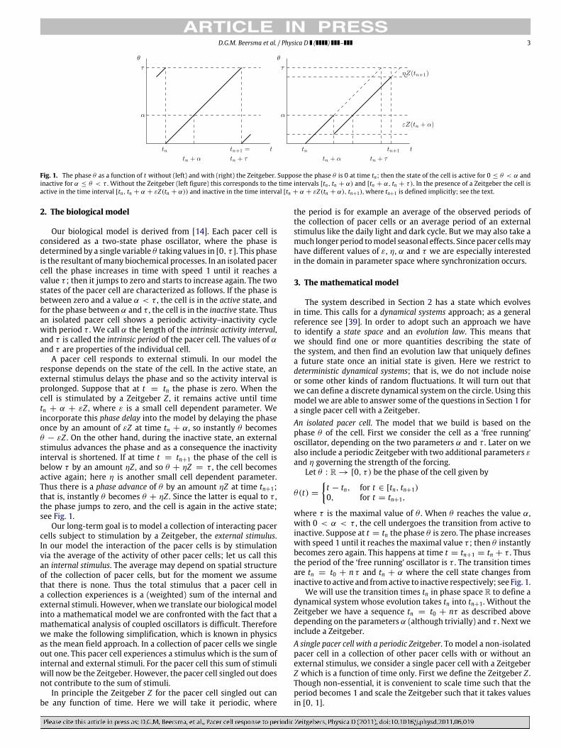
Fig. 1. The phase θ as a function of t without (left) and with (right) the Zeitgeber. Suppose the phase θ is 0 at time tn; then the state of the cell is active for 0 ≤ θ < α andinactive for α ≤ θ < τ . Without the Zeitgeber (left figure) this corresponds to the time intervals [tn, tn + α) and [tn + α, tn + τ). In the presence of a Zeitgeber the cell isactive in the time interval [tn, tn + α + εZ(tn + α)) and inactive in the time interval [tn + α + εZ(tn + α), tn+1), where tn+1 is defined implicitly; see the text.

2. The biological model

Our biological model is derived from [14]. Each pacer cell isconsidered as a two-state phase oscillator, where the phase isdetermined by a single variable θ taking values in [0, τ ]. This phaseis the resultant ofmany biochemical processes. In an isolated pacercell the phase increases in time with speed 1 until it reaches avalue τ ; then it jumps to zero and starts to increase again. The twostates of the pacer cell are characterized as follows. If the phase isbetween zero and a value α < τ , the cell is in the active state, andfor the phase between α and τ , the cell is in the inactive state. Thusan isolated pacer cell shows a periodic activity–inactivity cyclewith period τ . We call α the length of the intrinsic activity interval,and τ is called the intrinsic period of the pacer cell. The values of αand τ are properties of the individual cell.

A pacer cell responds to external stimuli. In our model theresponse depends on the state of the cell. In the active state, anexternal stimulus delays the phase and so the activity interval isprolonged. Suppose that at t = tn the phase is zero. When thecell is stimulated by a Zeitgeber Z , it remains active until timetn + α + εZ , where ε is a small cell dependent parameter. Weincorporate this phase delay into the model by delaying the phaseonce by an amount of εZ at time tn + α, so instantly θ becomesθ − εZ . On the other hand, during the inactive state, an externalstimulus advances the phase and as a consequence the inactivityinterval is shortened. If at time t = tn+1 the phase of the cell isbelow τ by an amount ηZ , and so θ + ηZ = τ , the cell becomesactive again; here η is another small cell dependent parameter.Thus there is a phase advance of θ by an amount ηZ at time tn+1;that is, instantly θ becomes θ + ηZ . Since the latter is equal to τ ,the phase jumps to zero, and the cell is again in the active state;see Fig. 1.

Our long-term goal is to model a collection of interacting pacercells subject to stimulation by a Zeitgeber, the external stimulus.In our model the interaction of the pacer cells is by stimulationvia the average of the activity of other pacer cells; let us call thisan internal stimulus. The average may depend on spatial structureof the collection of pacer cells, but for the moment we assumethat there is none. Thus the total stimulus that a pacer cell ina collection experiences is a (weighted) sum of the internal andexternal stimuli. However, whenwe translate our biological modelinto a mathematical model we are confronted with the fact that amathematical analysis of coupled oscillators is difficult. Thereforewe make the following simplification, which is known in physicsas the mean field approach. In a collection of pacer cells we singleout one. This pacer cell experiences a stimulus which is the sum ofinternal and external stimuli. For the pacer cell this sum of stimuliwill now be the Zeitgeber. However, the pacer cell singled out doesnot contribute to the sum of stimuli.

In principle the Zeitgeber Z for the pacer cell singled out canbe any function of time. Here we will take it periodic, where

the period is for example an average of the observed periods ofthe collection of pacer cells or an average period of an externalstimulus like the daily light and dark cycle. But we may also take amuch longer period tomodel seasonal effects. Since pacer cellsmayhave different values of ε, η, α and τ we are especially interestedin the domain in parameter space where synchronization occurs.

3. The mathematical model

The system described in Section 2 has a state which evolvesin time. This calls for a dynamical systems approach; as a generalreference see [39]. In order to adopt such an approach we haveto identify a state space and an evolution law. This means thatwe should find one or more quantities describing the state ofthe system, and then find an evolution law that uniquely definesa future state once an initial state is given. Here we restrict todeterministic dynamical systems; that is, we do not include noiseor some other kinds of random fluctuations. It will turn out thatwe can define a discrete dynamical system on the circle. Using thismodel we are able to answer some of the questions in Section 1 fora single pacer cell with a Zeitgeber.An isolated pacer cell. The model that we build is based on thephase θ of the cell. First we consider the cell as a ‘free running’oscillator, depending on the two parameters α and τ . Later on wealso include a periodic Zeitgeber with two additional parameters εand η governing the strength of the forcing.

Let θ : R → [0, τ ) be the phase of the cell given by

θ(t) =

t − tn, for t ∈ [tn, tn+1)0, for t = tn+1,

where τ is the maximal value of θ . When θ reaches the value α,with 0 < α < τ , the cell undergoes the transition from active toinactive. Suppose at t = tn the phase θ is zero. The phase increaseswith speed 1 until it reaches the maximal value τ ; then θ instantlybecomes zero again. This happens at time t = tn+1 = tn + τ . Thusthe period of the ‘free running’ oscillator is τ . The transition timesare tn = t0 + n τ and tn + α where the cell state changes frominactive to active and fromactive to inactive respectively; see Fig. 1.

We will use the transition times tn in phase space R to define adynamical system whose evolution takes tn into tn+1. Without theZeitgeber we have a sequence tn = t0 + nτ as described abovedepending on the parameters α (although trivially) and τ . Next weinclude a Zeitgeber.A single pacer cell with a periodic Zeitgeber. To model a non-isolatedpacer cell in a collection of other pacer cells with or without anexternal stimulus, we consider a single pacer cell with a ZeitgeberZ which is a function of time only. First we define the Zeitgeber Z .Though non-essential, it is convenient to scale time such that theperiod becomes 1 and scale the Zeitgeber such that it takes valuesin [0, 1].

4 D.G.M. Beersma et al. / Physica D ( ) –

Definition 1. The positive function Z : R → [0, 1] satisfies thefollowing:

(i) Z is differentiable,(ii) Z is periodic with period 1.

In the presence of a Zeitgeber the phase θ again increases withspeed 1, starting at θ = 0 at t = tn, but when θ reaches the valueα it instantly drops back by an amount of εZ(tn + α). Then it againincreases with speed 1 until it reaches a value at t = tn+1 such thatθ(tn+1) + ηZ(tn+1) = τ . Note that tn+1 is implicitly defined. Thusthe phase θ of the cell is given by

θ(t) =

t − tn, for t ∈ [tn, tn + α)t − tn − εZ(tn + α) for t ∈ [tn + α, tn+1)0, for t = tn+1.

(1)

Besides the parameters α and τ we now also have ε and η. Thelatter two give the ‘strength’ of the Zeitgeber. In order that themodel be consistent we impose the following conditions on theparameters:

0 < α < τ, ε ≥ 0, η ≥ 0, α − ε > 0, α − ε + η < τ,

so that θ remains between 0 and τ .The dynamical system. The state of the dynamical system that wedefine is the transition time tn rather than the phase θ . Indeedsolving the equation

θ(t) + ηZ(t) = τ

or equivalently t − tn − εZ(tn + α) + ηZ(t) = τ (2)

for t , under conditions to be specified later, yields a unique solutiont = tn+1 once tn is given. Thus we may write tn+1 = Fµ(tn) for amap Fµ : R → R depending on parameters µ = (ε, η, α, τ ).However, it turns out that Fµ has the property Fµ(t+1) = Fµ(t)+1,so Fµ is the lift of a circle map fµ : S1 → S1. This means that wenow have a dynamical system with phase space the circle S1 andevolution law fµ. Conceptually it is easier to work with the circlemap fµ but for actual computationswe usually prefer the lift Fµ. Letus summarize the result in the following proposition; for a proofsee the Appendix.

Proposition 2 (Circle Map and Lift). Let Z be as in Definition 1 anddefine the function Uε : R → R as Uε(t) = t + εZ(t). Then the mapFµ : R → R with

Fµ(t) = U−1η (Uε(t + α) − α + τ) (3)

defines a parameter dependent differentiable dynamical system,provided that Uη is invertible. The parameters are µ = (ε, η, α, τ ).Furthermore, Fµ is the lift of a circle map fµ : S1 → S1 of degree 1,given by

fµ(t) = U−1η (Uε(t + α) − α + τ) mod 1. (4)

A circle map is a one-dimensional map just like an interval map.The dynamics of the two have much in common; this feature ismost prominent when the circle map is studied via a lift. However,because the circle is different from the interval, there are alsodifferences in dynamical behavior. For example non-degeneratefixed points of a circle map come in pairs. See Fig. 2.

We now make a further distinction between two cases,namely whether fµ is invertible (a diffeomorphism) or not (anendomorphism). The difference between these cases is not only indynamical behavior but also because the second case has far richerbifurcation scenarios. Essentially it boils down to both ε and ηbeing ‘sufficiently small’ or one of them not meeting this criterion.However, there is a priori no reason to assume that either of themis small.

Fig. 2. Phase portrait of the circle map fµ and graph of the lift Fµ . fµ has two fixedpoints indicated by bullets. One is stable; the other is unstable, according to thearrows. The lift Fµ is a map on the interval [0, 1] with Fµ(1) = Fµ(0) + 1; drawnis Fµ − 1. t∗s (stable) and t∗u (unstable) satisfy Fµ(t) = t + 1. The Zeitgeber in thisexample is Z(t) =

12 (1 + sin(2π t)).

(a) Fµ is the lift of a circle diffeomorphism. In this case Fµ isdifferentiable and F−1

µ exists and is also differentiable. Both Uη

and Uε have to be invertible, which in turn means that ε andη must be small enough; in particular, 1 + εZ ′(t) > 0 and1 + ηZ ′(t) > 0 for all t .

(b) Fµ is the lift of a circle endomorphism. In this case Fµ is againdifferentiable but F−1

µ does not necessarily exist. Now only Uη

has to be invertible, which means that only η has to be smallenough.

Remark 1. Here ε ‘small enough’ means that Uε is invertible,for which we need that U ′

ε > 0. This depends on the specificform of the Zeitgeber. For the standard Zeitgeber Z(t) =

12 (1 +

sin(2π t)), small enough means that ε < 1π. Thus the circle

map fµ is a diffeomorphism if both ε and η are smaller than 1π.

The standard Zeitgeber has no biological meaning; we only useit as an illustration. Since every 1-periodic function has a Fourierseries containing sine and cosine terms, the standard Zeitgebercan be regarded as the simplest non-trivial example of such afunction. �

Remark 2. If η is not small, but ε is small enough that Uε isinvertible, F−1

µ is the lift of a circle endomorphism, but Fµ is multi-valued. This case is similar to case b with the roles of Fµ andF−1µ interchanged. However in the dynamical system defined withF−1µ , time is running backwards, so it describes the past ratherthan the future. Mathematically this is not a problem, but thebiological interpretation could be problematic. One could force Fµ

to be single-valued by choosing the smallest solution for t = tn+1of Eq. (2). Then Fµ again defines a dynamical system, though adiscontinuous one. �

Remark 3. If both ε and η are not small, Fµ and F−1µ are multi-

valued. In this case we do not have a well-defined dynamicalsystem at all. But a construction similar to that in the previousremark can be applied to define a possibly discontinuousdynamical system. �

4. Analysis of the mathematical model

Here we restrict ourselves to the case where Fµ in Proposition 2is the lift of a circle diffeomorphism fµ. In that case we can usethe rotation number which tells us howmuch on average an initialpoint is rotated along the circle by fµ. It is a powerful tool indetermining whether fµ has fixed points or periodic points. Theexistence of such points and their dependence on the parametersµ is the main topic of this section. Stable fixed or periodic pointsare the most relevant for our model and we will see how they losestability at certain bifurcations. For background on circle maps andfurther references to the literature see [21,39–41].

D.G.M. Beersma et al. / Physica D ( ) – 5

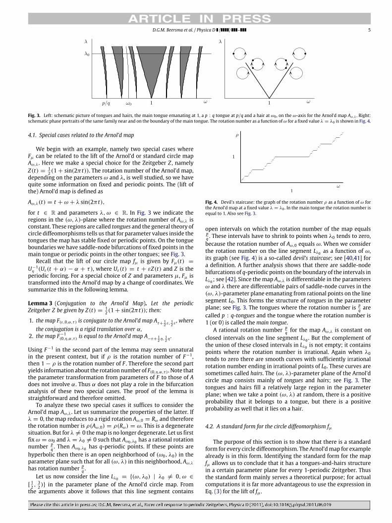
Fig. 3. Left: schematic picture of tongues and hairs, the main tongue emanating at 1, a p : q tongue at p/q and a hair at ω0 , on the ω-axis for the Arnol’d map Aω,λ . Right:schematic phase portraits of the same family near and on the boundary of themain tongue. The rotation number as a function ofω for a fixed value λ = λ0 is shown in Fig. 4.

4.1. Special cases related to the Arnol’d map

We begin with an example, namely two special cases whereFµ can be related to the lift of the Arnol’d or standard circle mapAω,λ. Here we make a special choice for the Zeitgeber Z , namelyZ(t) =

12 (1 + sin(2π t)). The rotation number of the Arnol’d map,

depending on the parameters ω and λ, is well studied, so we havequite some information on fixed and periodic points. The (lift ofthe) Arnol’d map is defined as

Aω,λ(t) = t + ω + λ sin(2π t),

for t ∈ R and parameters λ, ω ∈ R. In Fig. 3 we indicate theregions in the (ω, λ)-plane where the rotation number of Aω,λ isconstant. These regions are called tongues and the general theory ofcircle diffeomorphisms tells us that for parameter values inside thetongues the map has stable fixed or periodic points. On the tongueboundaries we have saddle-node bifurcations of fixed points in themain tongue or periodic points in the other tongues; see Fig. 3.

Recall that the lift of our circle map fµ is given by Fµ(t) =

U−1η (Uε(t + α) − α + τ), where Uε(t) = t + εZ(t) and Z is the

periodic forcing. For a special choice of Z and parameters µ, Fµ istransformed into the Arnol’d map by a change of coordinates. Wesummarize this in the following lemma.

Lemma 3 (Conjugation to the Arnol’d Map). Let the periodicZeitgeber Z be given by Z(t) =

12 (1 + sin(2π t)); then:

1. the map F(ε,0,α,τ ) is conjugate to the Arnol’d map Aτ+

12 ε, 12 ε

, wherethe conjugation is a rigid translation over α,

2. the map F−1(0,η,α,τ ) is equal to the Arnol’d map A

−τ+12 η, 12 η

.

Using F−1 in the second part of the lemma may seem unnaturalin the present context, but if ρ is the rotation number of F−1,then 1 − ρ is the rotation number of F . Therefore the second partyields information about the rotation number of F(0,η,α,τ ). Note thatthe parameter transformation from parameters of F to those of Adoes not involve α. Thus α does not play a role in the bifurcationanalysis of these two special cases. The proof of the lemma isstraightforward and therefore omitted.

To analyze these two special cases it suffices to consider theArnol’d map Aω,λ. Let us summarize the properties of the latter. Ifλ = 0, the map reduces to a rigid rotation Aω,0 = Rω and thereforethe rotation number is ρ(Aω,0) = ρ(Rω) = ω. This is a degeneratesituation. But forλ = 0 themap is no longer degenerate. Let us firstfix ω = ω0 and λ = λ0 = 0 such that Aω0,λ0 has a rational rotationnumber p

q . Then Aω0,λ0 has q-periodic points. If these points arehyperbolic then there is an open neighborhood of (ω0, λ0) in theparameter plane such that for all (ω, λ) in this neighborhood, Aω,λ

has rotation number pq .

Let us now consider the line Lλ0 = {(ω, λ0) | λ0 = 0, ω ∈

[12 ,

32 )} in the parameter plane of the Arnol’d circle map. From

the arguments above it follows that this line segment contains

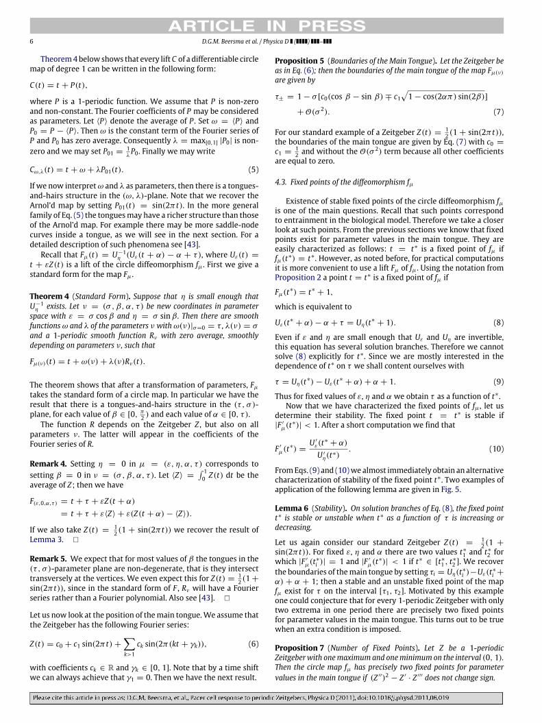
Fig. 4. Devil’s staircase: the graph of the rotation number ρ as a function of ω forthe Arnol’d map at a fixed value λ = λ0 . In the main tongue the rotation number isequal to 1. Also see Fig. 3.

open intervals on which the rotation number of the map equalspq . These intervals have to shrink to points when λ0 tends to zero,because the rotation number of Aω,0 equals ω. When we considerthe rotation number on the line segment Lλ0 as a function of ω,its graph (see Fig. 4) is a so-called devil’s staircase; see [40,41] fora definition. A further analysis shows that there are saddle-nodebifurcations of q-periodic points on the boundary of the intervals inLλ0 ; see [42]. Since the map Aω,λ is differentiable in the parametersω and λ there are differentiable pairs of saddle-node curves in the(ω, λ)-parameter plane emanating from rational points on the linesegment L0. This forms the structure of tongues in the parameterplane; see Fig. 3. The tongues where the rotation number is p

q arecalled p : q-tongues and the tongue where the rotation number is1 (or 0) is called themain tongue.

A rational rotation number pq for the map Aω,λ is constant on

closed intervals on the line segment Lλ0 . But the complement ofthe union of these closed intervals in Lλ0 is not empty; it containspoints where the rotation number is irrational. Again when λ0tends to zero there are smooth curves with sufficiently irrationalrotation number ending in irrational points of L0. These curves aresometimes called hairs. The (ω, λ)-parameter plane of the Arnol’dcircle map consists mainly of tongues and hairs; see Fig. 3. Thetongues and hairs fill a relatively large region in the parameterplane; when we take a point (ω, λ) at random, there is a positiveprobability that it belongs to a tongue, but there is a positiveprobability as well that it lies on a hair.

4.2. A standard form for the circle diffeomorphism fµ

The purpose of this section is to show that there is a standardform for every circle diffeomorphism. The Arnol’dmap for examplealready is in this form. Identifying the standard form for the mapfµ allows us to conclude that it has a tongues-and-hairs structurein a certain parameter plane for every 1-periodic Zeitgeber. Thusthe standard form mainly serves a theoretical purpose; for actualcomputations it is far more advantageous to use the expression inEq. (3) for the lift of fµ.

6 D.G.M. Beersma et al. / Physica D ( ) –

Theorem4belowshows that every liftC of a differentiable circlemap of degree 1 can be written in the following form:

C(t) = t + P(t),

where P is a 1-periodic function. We assume that P is non-zeroand non-constant. The Fourier coefficients of P may be consideredas parameters. Let ⟨P⟩ denote the average of P . Set ω = ⟨P⟩ andP0 = P − ⟨P⟩. Then ω is the constant term of the Fourier series ofP and P0 has zero average. Consequently λ = max[0,1] |P0| is non-zero and we may set P01 =

1λP0. Finally we may write

Cω,λ(t) = t + ω + λP01(t). (5)

If we now interpretω and λ as parameters, then there is a tongues-and-hairs structure in the (ω, λ)-plane. Note that we recover theArnol’d map by setting P01(t) = sin(2π t). In the more generalfamily of Eq. (5) the tonguesmay have a richer structure than thoseof the Arnol’d map. For example there may be more saddle-nodecurves inside a tongue, as we will see in the next section. For adetailed description of such phenomena see [43].

Recall that Fµ(t) = U−1η (Uε(t + α) − α + τ), where Uε(t) =

t + εZ(t) is a lift of the circle diffeomorphism fµ. First we give astandard form for the map Fµ.

Theorem 4 (Standard Form). Suppose that η is small enough thatU−1

η exists. Let ν = (σ , β, α, τ ) be new coordinates in parameterspace with ε = σ cosβ and η = σ sinβ . Then there are smoothfunctions ω and λ of the parameters ν with ω(ν)|σ=0 = τ , λ(ν) = σ

and a 1-periodic smooth function Rν with zero average, smoothlydepending on parameters ν , such that

Fµ(ν)(t) = t + ω(ν) + λ(ν)Rν(t).

The theorem shows that after a transformation of parameters, Fµ

takes the standard form of a circle map. In particular we have theresult that there is a tongues-and-hairs structure in the (τ , σ )-plane, for each value of β ∈ [0, π

2 ) and each value of α ∈ [0, τ ).The function R depends on the Zeitgeber Z , but also on all

parameters ν. The latter will appear in the coefficients of theFourier series of R.

Remark 4. Setting η = 0 in µ = (ε, η, α, τ ) corresponds tosetting β = 0 in ν = (σ , β, α, τ ). Let ⟨Z⟩ =

10 Z(t) dt be the

average of Z; then we have

F(ε,0,α,τ ) = t + τ + εZ(t + α)

= t + τ + ε⟨Z⟩ + ε(Z(t + α) − ⟨Z⟩).

If we also take Z(t) =12 (1 + sin(2π t)) we recover the result of

Lemma 3. �

Remark 5. We expect that for most values of β the tongues in the(τ , σ )-parameter plane are non-degenerate, that is they intersecttransversely at the vertices. We even expect this for Z(t) =

12 (1 +

sin(2π t)), since in the standard form of F , Rν will have a Fourierseries rather than a Fourier polynomial. Also see [43]. �

Let us now look at the position of themain tongue.We assume thatthe Zeitgeber has the following Fourier series:

Z(t) = c0 + c1 sin(2π t) +

k>1

ck sin(2π(kt + γk)), (6)

with coefficients ck ∈ R and γk ∈ [0, 1]. Note that by a time shiftwe can always achieve that γ1 = 0. Then we have the next result.

Proposition 5 (Boundaries of the Main Tongue). Let the Zeitgeber beas in Eq. (6); then the boundaries of the main tongue of the map Fµ(ν)

are given by

τ± = 1 − σ [c0(cos β − sin β) ∓ c11 − cos(2απ) sin(2β)]

+ O(σ 2). (7)

For our standard example of a Zeitgeber Z(t) =12 (1 + sin(2π t)),

the boundaries of the main tongue are given by Eq. (7) with c0 =

c1 =12 and without the O(σ 2) term because all other coefficients

are equal to zero.

4.3. Fixed points of the diffeomorphism fµ

Existence of stable fixed points of the circle diffeomorphism fµis one of the main questions. Recall that such points correspondto entrainment in the biological model. Therefore we take a closerlook at such points. From the previous sections we know that fixedpoints exist for parameter values in the main tongue. They areeasily characterized as follows: t = t∗ is a fixed point of fµ iffµ(t∗) = t∗. However, as noted before, for practical computationsit is more convenient to use a lift Fµ of fµ. Using the notation fromProposition 2 a point t = t∗ is a fixed point of fµ if

Fµ(t∗) = t∗ + 1,

which is equivalent to

Uε(t∗ + α) − α + τ = Uη(t∗ + 1). (8)

Even if ε and η are small enough that Uε and Uη are invertible,this equation has several solution branches. Therefore we cannotsolve (8) explicitly for t∗. Since we are mostly interested in thedependence of t∗ on τ we shall content ourselves with

τ = Uη(t∗) − Uε(t∗ + α) + α + 1. (9)

Thus for fixed values of ε, η and α we obtain τ as a function of t∗.Now that we have characterized the fixed points of fµ, let us

determine their stability. The fixed point t = t∗ is stable if|F ′

µ(t∗)| < 1. After a short computation we find that

F ′

µ(t∗) =U ′

ε(t∗+ α)

U ′η(t∗)

. (10)

FromEqs. (9) and (10)we almost immediately obtain an alternativecharacterization of stability of the fixed point t∗. Two examples ofapplication of the following lemma are given in Fig. 5.

Lemma 6 (Stability). On solution branches of Eq. (8), the fixed pointt∗ is stable or unstable when t∗ as a function of τ is increasing ordecreasing.

Let us again consider our standard Zeitgeber Z(t) =12 (1 +

sin(2π t)). For fixed ε, η and α there are two values t∗1 and t∗2 forwhich |F ′

µ(t∗i )| = 1 and |F ′µ(t∗)| < 1 if t∗ ∈ [t∗1 , t

∗

2 ]. We recoverthe boundaries of themain tongue by setting τi = Uη(t∗i )−Uε(t∗i +

α) + α + 1; then a stable and an unstable fixed point of the mapfµ exist for τ on the interval [τ1, τ2]. Motivated by this exampleone could conjecture that for every 1-periodic Zeitgeber with onlytwo extrema in one period there are precisely two fixed pointsfor parameter values in the main tongue. This turns out to be truewhen an extra condition is imposed.

Proposition 7 (Number of Fixed Points). Let Z be a 1-periodicZeitgeberwith onemaximumand oneminimumon the interval (0, 1).Then the circle map fµ has precisely two fixed points for parametervalues in the main tongue if (Z ′′)2 − Z ′

· Z ′′′ does not change sign.

D.G.M. Beersma et al. / Physica D ( ) – 7

Fig. 5. Fixed points t∗ of the map fµ as a function of τ . The solid curve represents a stable fixed point, the dashed curve an unstable one. At parameter valuesτ = τi there are saddle-node bifurcations; also see Fig. 3. Parameters ε, η and α are fixed. Left: the Zeitgeber is Z(t) =

12 (1 + sin(2π t)). Right: the Zeitgeber is

Z(t) =310 (2 + sin(2π t) + cos(4π t)).

Fig. 6. Tongues for the Arnol’d map Aω,λ in the (ω, λ)-plane. The algorithm forcomputing the pictures is based on the rotation number. The latter is defined forsufficiently small values of λ only. Therefore the tongue boundaries in the pictureare not well defined for large values of λ. The effect of this phenomenon is evenmore visible in the following picture.

For our standard example of a Zeitgeber Z(t) =12 (1 + sin(2π t)),

the quantity (Z ′′)2 − Z ′· Z ′′′ is equal to 1. The Zeitgeber Z(t) =

25 (

43 + sin(2π t) +

13 sin(4π t)) also has two extrema, but the

quantity (Z ′′)2−Z ′·Z ′′′ changes sign on [0, 1]. See the Appendix for

further implications. With a general periodic Zeitgeber there maybe more than one stable fixed point for parameter values in themain tongue. This occurs in general when the Fourier series of theZeitgeber contains more than just one term like in our standardexample. Let us look at a Zeitgeber with the following Fourierpolynomial: Z(t) =

310 (2 + sin(2π t) + cos(4π t)); then there

are four solutions of |F ′µ(t∗i )| = 1. Let us sort them such that

τi = Uη(t∗i ) − Uε(t∗i + α) + α + 1 increases with i. Then for fixedvalues of ε, η andα there are atmost four fixed points of fµ for eachτ ∈ [τ1, τ4]. We represent the results graphically in Fig. 5.

4.4. Examples of tongues and hairs for different Zeitgebers

Here we collect some examples of tongues-and-hairs figuresshowing differences from and similarities with the prototypefigure of tongues in the Arnol’d circle map. Therefore we start withthe latter; see Fig. 6. In this family the tongues are fixed, but inour family fµ, the tongues in the (τ , σ )-plane still depend on thevalues of β and α. Moreover they also depend on the Zeitgeber. Inorder to keep the number of pictures limitedwe only show tonguesfor two different Zeitgebers; see Figs. 7 and 8. As is to be expectedfrom the existence of a standard form (see Section 4.2), the picturesare qualitatively the same—that is, near the τ -axis or ω-axis in theArnol’dmap. Thewidth and the growth of thewidth of the tonguesdepend on parameters in the map. This is shown in Fig. 9, in thenext section, where its biological relevance is discussed.

5. Discussion

The main results of analyzing our model for a pacer cell with aperiodic Zeitgeber are:

Fig. 7. Tongues for the circle map fµ in the (τ , σ )-plane, with standard ZeitgeberZ(t) =

12 (1 + sin(2π t)). The values of the parameters µ = (ε, η, α, τ ) are

ε = σ cos β , η = σ sin β with β =π3 and α = 0.3.

Fig. 8. Tongues for the circle map fµ in the (τ , σ )-plane, with Zeitgeber Z(t) =310 (2 + sin(2π t) + cos(4π t)). The parameter values are as in Fig. 7.

1. there is a finite range of entrainment, namely the 1:1 tongue,2. there are finite ranges of synchronization in the more general

p : q tongues,3. the boundaries of the range of entrainment dependon the phase

delay and advance parameters in the model,4. outside the tongues the pacer cell shows quasi-periodic

behavior, known as relative coordination in circadian biology,5. the phase of entrainment, or onset of activity interval, depends

on the intrinsic period of the pacer cell.

In the following sections we will discuss these matters inmore detail. Let us remark that ranges of synchronization andentrainment apply to the intrinsic period, while the period ofthe Zeitgeber is kept fixed. From a biological point of view itseems more natural to keep the intrinsic period fixed and vary theperiod of the Zeitgeber. However, it is not hard to see that theseviewpoints are in fact equivalent.

5.1. The model

As explained in Section 2 our long-term goal is to study acollection of interacting pacer cells with a Zeitgeber acting asan external stimulus. However, there are serious difficulties inthe analysis of the mathematical model that is induced by thisbiological model; again see Section 2. Therefore we consider asimpler system of a single pacer cell that experiences stimuli fromother pacer cells as well as external sources. We regard the sum of

8 D.G.M. Beersma et al. / Physica D ( ) –

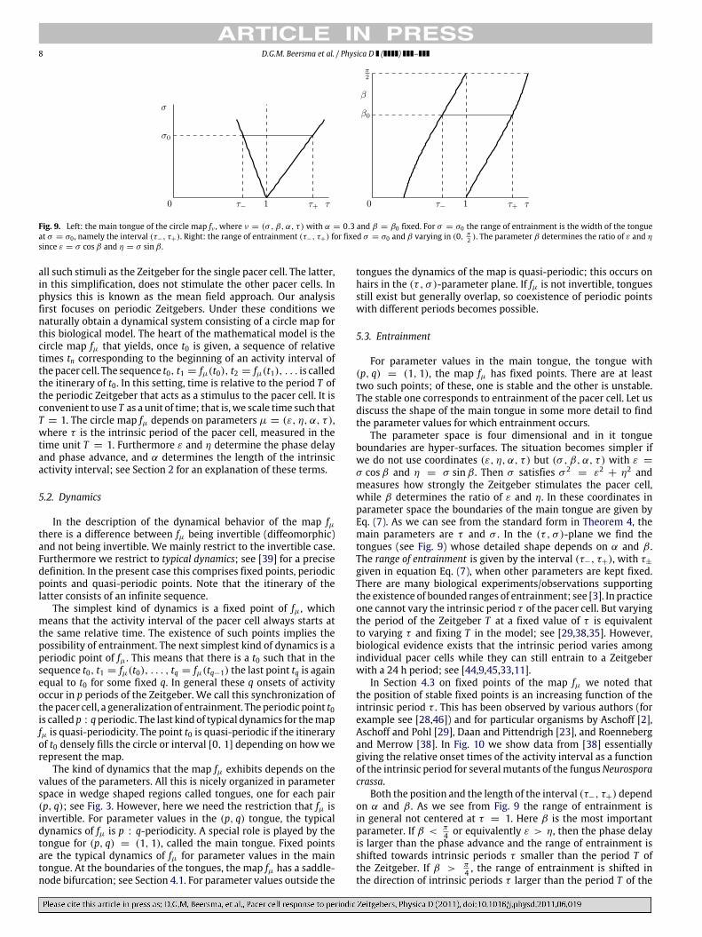
Fig. 9. Left: the main tongue of the circle map fν , where ν = (σ , β, α, τ ) with α = 0.3 and β = β0 fixed. For σ = σ0 the range of entrainment is the width of the tongueat σ = σ0 , namely the interval (τ−, τ+). Right: the range of entrainment (τ−, τ+) for fixed σ = σ0 and β varying in (0, π

2 ). The parameter β determines the ratio of ε and η

since ε = σ cosβ and η = σ sinβ .

all such stimuli as the Zeitgeber for the single pacer cell. The latter,in this simplification, does not stimulate the other pacer cells. Inphysics this is known as the mean field approach. Our analysisfirst focuses on periodic Zeitgebers. Under these conditions wenaturally obtain a dynamical system consisting of a circle map forthis biological model. The heart of the mathematical model is thecircle map fµ that yields, once t0 is given, a sequence of relativetimes tn corresponding to the beginning of an activity interval ofthe pacer cell. The sequence t0, t1 = fµ(t0), t2 = fµ(t1), . . . is calledthe itinerary of t0. In this setting, time is relative to the period T ofthe periodic Zeitgeber that acts as a stimulus to the pacer cell. It isconvenient to use T as a unit of time; that is,we scale time such thatT = 1. The circle map fµ depends on parameters µ = (ε, η, α, τ ),where τ is the intrinsic period of the pacer cell, measured in thetime unit T = 1. Furthermore ε and η determine the phase delayand phase advance, and α determines the length of the intrinsicactivity interval; see Section 2 for an explanation of these terms.

5.2. Dynamics

In the description of the dynamical behavior of the map fµthere is a difference between fµ being invertible (diffeomorphic)and not being invertible. We mainly restrict to the invertible case.Furthermore we restrict to typical dynamics; see [39] for a precisedefinition. In the present case this comprises fixed points, periodicpoints and quasi-periodic points. Note that the itinerary of thelatter consists of an infinite sequence.

The simplest kind of dynamics is a fixed point of fµ, whichmeans that the activity interval of the pacer cell always starts atthe same relative time. The existence of such points implies thepossibility of entrainment. The next simplest kind of dynamics is aperiodic point of fµ. This means that there is a t0 such that in thesequence t0, t1 = fµ(t0), . . . , tq = fµ(tq−1) the last point tq is againequal to t0 for some fixed q. In general these q onsets of activityoccur in p periods of the Zeitgeber. We call this synchronization ofthepacer cell, a generalization of entrainment. Theperiodic point t0is called p : qperiodic. The last kind of typical dynamics for themapfµ is quasi-periodicity. The point t0 is quasi-periodic if the itineraryof t0 densely fills the circle or interval [0, 1] depending on howwerepresent the map.

The kind of dynamics that the map fµ exhibits depends on thevalues of the parameters. All this is nicely organized in parameterspace in wedge shaped regions called tongues, one for each pair(p, q); see Fig. 3. However, here we need the restriction that fµ isinvertible. For parameter values in the (p, q) tongue, the typicaldynamics of fµ is p : q-periodicity. A special role is played by thetongue for (p, q) = (1, 1), called the main tongue. Fixed pointsare the typical dynamics of fµ for parameter values in the maintongue. At the boundaries of the tongues, the map fµ has a saddle-node bifurcation; see Section 4.1. For parameter values outside the

tongues the dynamics of the map is quasi-periodic; this occurs onhairs in the (τ , σ )-parameter plane. If fµ is not invertible, tonguesstill exist but generally overlap, so coexistence of periodic pointswith different periods becomes possible.

5.3. Entrainment

For parameter values in the main tongue, the tongue with(p, q) = (1, 1), the map fµ has fixed points. There are at leasttwo such points; of these, one is stable and the other is unstable.The stable one corresponds to entrainment of the pacer cell. Let usdiscuss the shape of the main tongue in some more detail to findthe parameter values for which entrainment occurs.

The parameter space is four dimensional and in it tongueboundaries are hyper-surfaces. The situation becomes simpler ifwe do not use coordinates (ε, η, α, τ ) but (σ , β, α, τ ) with ε =

σ cosβ and η = σ sinβ . Then σ satisfies σ 2= ε2

+ η2 andmeasures how strongly the Zeitgeber stimulates the pacer cell,while β determines the ratio of ε and η. In these coordinates inparameter space the boundaries of the main tongue are given byEq. (7). As we can see from the standard form in Theorem 4, themain parameters are τ and σ . In the (τ , σ )-plane we find thetongues (see Fig. 9) whose detailed shape depends on α and β .The range of entrainment is given by the interval (τ−, τ+), with τ±

given in equation Eq. (7), when other parameters are kept fixed.There are many biological experiments/observations supportingthe existence of bounded ranges of entrainment; see [3]. In practiceone cannot vary the intrinsic period τ of the pacer cell. But varyingthe period of the Zeitgeber T at a fixed value of τ is equivalentto varying τ and fixing T in the model; see [29,38,35]. However,biological evidence exists that the intrinsic period varies amongindividual pacer cells while they can still entrain to a Zeitgeberwith a 24 h period; see [44,9,45,33,11].

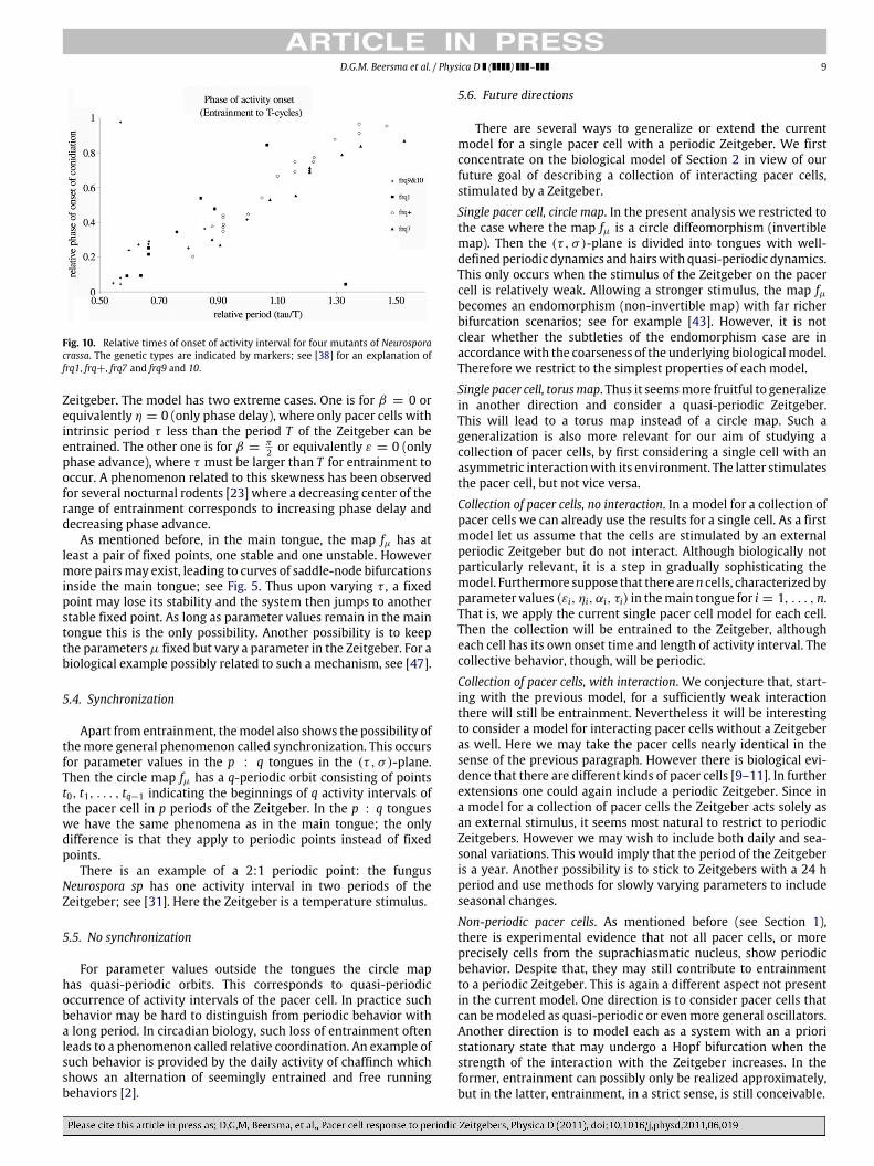
In Section 4.3 on fixed points of the map fµ we noted thatthe position of stable fixed points is an increasing function of theintrinsic period τ . This has been observed by various authors (forexample see [28,46]) and for particular organisms by Aschoff [2],Aschoff and Pohl [29], Daan and Pittendrigh [23], and Roennebergand Merrow [38]. In Fig. 10 we show data from [38] essentiallygiving the relative onset times of the activity interval as a functionof the intrinsic period for several mutants of the fungusNeurosporacrassa.

Both the position and the length of the interval (τ−, τ+) dependon α and β . As we see from Fig. 9 the range of entrainment isin general not centered at τ = 1. Here β is the most importantparameter. If β < π

4 or equivalently ε > η, then the phase delayis larger than the phase advance and the range of entrainment isshifted towards intrinsic periods τ smaller than the period T ofthe Zeitgeber. If β > π

4 , the range of entrainment is shifted inthe direction of intrinsic periods τ larger than the period T of the

D.G.M. Beersma et al. / Physica D ( ) – 9

Fig. 10. Relative times of onset of activity interval for four mutants of Neurosporacrassa. The genetic types are indicated by markers; see [38] for an explanation offrq1, frq+, frq7 and frq9 and 10.

Zeitgeber. The model has two extreme cases. One is for β = 0 orequivalently η = 0 (only phase delay), where only pacer cells withintrinsic period τ less than the period T of the Zeitgeber can beentrained. The other one is for β =

π2 or equivalently ε = 0 (only

phase advance), where τ must be larger than T for entrainment tooccur. A phenomenon related to this skewness has been observedfor several nocturnal rodents [23] where a decreasing center of therange of entrainment corresponds to increasing phase delay anddecreasing phase advance.

As mentioned before, in the main tongue, the map fµ has atleast a pair of fixed points, one stable and one unstable. Howevermore pairsmay exist, leading to curves of saddle-node bifurcationsinside the main tongue; see Fig. 5. Thus upon varying τ , a fixedpoint may lose its stability and the system then jumps to anotherstable fixed point. As long as parameter values remain in the maintongue this is the only possibility. Another possibility is to keepthe parametersµ fixed but vary a parameter in the Zeitgeber. For abiological example possibly related to such a mechanism, see [47].

5.4. Synchronization

Apart from entrainment, themodel also shows the possibility ofthe more general phenomenon called synchronization. This occursfor parameter values in the p : q tongues in the (τ , σ )-plane.Then the circle map fµ has a q-periodic orbit consisting of pointst0, t1, . . . , tq−1 indicating the beginnings of q activity intervals ofthe pacer cell in p periods of the Zeitgeber. In the p : q tongueswe have the same phenomena as in the main tongue; the onlydifference is that they apply to periodic points instead of fixedpoints.

There is an example of a 2:1 periodic point: the fungusNeurospora sp has one activity interval in two periods of theZeitgeber; see [31]. Here the Zeitgeber is a temperature stimulus.

5.5. No synchronization

For parameter values outside the tongues the circle maphas quasi-periodic orbits. This corresponds to quasi-periodicoccurrence of activity intervals of the pacer cell. In practice suchbehavior may be hard to distinguish from periodic behavior witha long period. In circadian biology, such loss of entrainment oftenleads to a phenomenon called relative coordination. An example ofsuch behavior is provided by the daily activity of chaffinch whichshows an alternation of seemingly entrained and free runningbehaviors [2].

5.6. Future directions

There are several ways to generalize or extend the currentmodel for a single pacer cell with a periodic Zeitgeber. We firstconcentrate on the biological model of Section 2 in view of ourfuture goal of describing a collection of interacting pacer cells,stimulated by a Zeitgeber.

Single pacer cell, circle map. In the present analysis we restricted tothe case where the map fµ is a circle diffeomorphism (invertiblemap). Then the (τ , σ )-plane is divided into tongues with well-definedperiodic dynamics andhairswith quasi-periodic dynamics.This only occurs when the stimulus of the Zeitgeber on the pacercell is relatively weak. Allowing a stronger stimulus, the map fµbecomes an endomorphism (non-invertible map) with far richerbifurcation scenarios; see for example [43]. However, it is notclear whether the subtleties of the endomorphism case are inaccordancewith the coarseness of the underlying biologicalmodel.Therefore we restrict to the simplest properties of each model.

Single pacer cell, torusmap. Thus it seemsmore fruitful to generalizein another direction and consider a quasi-periodic Zeitgeber.This will lead to a torus map instead of a circle map. Such ageneralization is also more relevant for our aim of studying acollection of pacer cells, by first considering a single cell with anasymmetric interactionwith its environment. The latter stimulatesthe pacer cell, but not vice versa.

Collection of pacer cells, no interaction. In a model for a collection ofpacer cells we can already use the results for a single cell. As a firstmodel let us assume that the cells are stimulated by an externalperiodic Zeitgeber but do not interact. Although biologically notparticularly relevant, it is a step in gradually sophisticating themodel. Furthermore suppose that there aren cells, characterizedbyparameter values (εi, ηi, αi, τi) in themain tongue for i = 1, . . . , n.That is, we apply the current single pacer cell model for each cell.Then the collection will be entrained to the Zeitgeber, althougheach cell has its own onset time and length of activity interval. Thecollective behavior, though, will be periodic.

Collection of pacer cells, with interaction. We conjecture that, start-ing with the previous model, for a sufficiently weak interactionthere will still be entrainment. Nevertheless it will be interestingto consider a model for interacting pacer cells without a Zeitgeberas well. Here we may take the pacer cells nearly identical in thesense of the previous paragraph. However there is biological evi-dence that there are different kinds of pacer cells [9–11]. In furtherextensions one could again include a periodic Zeitgeber. Since ina model for a collection of pacer cells the Zeitgeber acts solely asan external stimulus, it seems most natural to restrict to periodicZeitgebers. However we may wish to include both daily and sea-sonal variations. This would imply that the period of the Zeitgeberis a year. Another possibility is to stick to Zeitgebers with a 24 hperiod and use methods for slowly varying parameters to includeseasonal changes.

Non-periodic pacer cells. As mentioned before (see Section 1),there is experimental evidence that not all pacer cells, or moreprecisely cells from the suprachiasmatic nucleus, show periodicbehavior. Despite that, they may still contribute to entrainmentto a periodic Zeitgeber. This is again a different aspect not presentin the current model. One direction is to consider pacer cells thatcan bemodeled as quasi-periodic or evenmore general oscillators.Another direction is to model each as a system with an a prioristationary state that may undergo a Hopf bifurcation when thestrength of the interaction with the Zeitgeber increases. In theformer, entrainment can possibly only be realized approximately,but in the latter, entrainment, in a strict sense, is still conceivable.

10 D.G.M. Beersma et al. / Physica D ( ) –

Fig. 11. Period doublings and halvings for the map fµ with Zeitgeber Z(t) =

3+ sin(2π t)+ 2 cos(4π t). Shown are the positions of periodic points as a functionof the intrinsic period τ . The parameter values are α = 0.5, ε = 0.4 and η = 0.17.

6. Conclusion

The current model has been used to explain many properties ofthe mammalian circadian behavior [14]. In addition, we providedthe mathematical basis using the current model of at leastfive phenomena that are characteristic of circadian behaviorin general: (1) finite range of entrainment; (2) existence ofmultiple activity bouts per cycle (p : q tongues); (3) relativecoordination or cycleswith extremely long periods (quasi-periodicorbits); (4) relationship of the phase of entrainment to theperiod of the Zeitgeber; (5) asymmetry in the observed periodand the phase delay and phase advance components of phaseresponse curves. Aside from these, we also now have a setof four directly observable parameters to look at more closelyin biological systems. Most experiments in the past have onlysearched for genes and proteins responsible for the intrinsic periodτ . However, circadian clocks are also characterized by their phaseresponse curves which in the simple pacer model are definedwith only three more basic parameters α, ε, η. We think that animportant predictive value of the current work is our discoveryof the mathematical relationships between these four parametersand their contribution to various aspects of entrainment. Now,one direction that biologists should pursue is to do extensiveexperimentation to search in the complex biochemical system formolecular components which could be responsible for the phasedelay and phase advance parameters ε and η, respectively, aswell as the intrinsic activity length α. Finally, one may say thatthe model is too simple to capture the entire phase responsecharacteristics of whole organisms, or even of a single pacercell. The PRC used must be rather realistic for an individualpacemaker cell, at least if our assumption that the behavior canbe characterized by two states (electrical activity versus rest)is correct. The result of the interactions between the variouspacemaker cells and their response to light will eventually leadto the known PRCs of the ensemble, in which phase delays occurat the end of the photoperiod and advances at the beginning.However, we must emphasize that even this very simple modelwith only four parameters already captures those characteristicsmentioned above, that is, we did not use a more realistic phaseresponse curve [23] to simulate those characteristics. Propertiesthat we can see in the model such as hysteresis (see Fig. 5) andperiod-halving and period-doubling cascades (see Fig. 11) remainto be seen in experiments at the behavioral and lower levels.The underlying biochemical network that produces these fourparameters may just be details that are not really necessary inunderstanding entrainment of circadian rhythms itself, but haveimportant roles in other aspects of the biological system such asenergy expenditure and adaptation to changes in environment [1].

Acknowledgments

Wewould like to thank the anonymous referees of Physica D fortheir constructive criticism and valuable suggestions. These havebeen very useful in improving the paper.

Appendix A. Bifurcations

The tongues in the (σ , τ )-parameter plane are determinedby saddle-node bifurcations. But there may also be otherbifurcations even when the map fµ is a diffeomorphism, in otherwords invertible. The reason is that we have many parameters.Considering α as a relatively inaccessible parameter and keepingit fixed we may still vary σ , τ and β . Then we have three-dimensional tongues in (σ , τ , β)-parameter space. It is an almoststraightforward consequence of Proposition 7 that there are curvesof pitchfork bifurcations in this three-dimensional parameterspace, emanating from rational points on the τ -axis.

Corollary 8 (Pitchfork Bifurcation). Let Z be a 1-periodic Zeitgeber.If (Z ′′)2 − Z ′

· Z ′′′ has a simple zero, then parameter values exist forwhich fµ has a pitchfork bifurcation.

Proof. From the proof of Proposition 7 we see that the number ofsolution branches of Eq. (8) does change if Z ′′(t)2 − Z ′(t) · Z ′′′(t)has a simple zero. �

However, β may be considered as an inaccessible parameter aswell. But the Zeitgeber may also depend on a parameter. We mayin particular view seasonal change, which is slow compared to the24 h period, as parameter dependence. The quantity (Z ′′)2 −Z ′

·Z ′′′

may change sign depending on this parameter, so we find againpitchfork bifurcations.

If the map fµ is not a diffeomorphism (not invertible) thenthere are numerous other bifurcations; see [43]. This happensfor relatively large values of σ . On varying τ for fixed valuesof the other parameters in the main tongue, one generally findsa number of period doublings followed by the same number ofperiod halvings (or in opposite order). The reason is that there arecurves of period doublings in the (τ , σ )-parameter planewith localminima, considered as functions of τ , that are transversely crossed.For more details we refer the reader again to [43]. An example ofthis phenomenon is shown in Fig. 11.

Appendix B. Proofs

Proof of Proposition 2. The main point we have to show is thatEq. (2) can be solved uniquely with respect to t . Using theexpression for θ in (1) we obtain after some rearranging

tn+1 + ηZ(tn+1) = tn + α + εZ(tn + α) − α + τ . (11)

Since Z is 1-periodic, Uε has the property Uε(t + 1) = Uε(t) + 1,for all t . Then the equation for tn+1 reads

Uη(tn+1) = Uε(tn + α) − α + τ .

Introducing the operator Tα which takes a function f into Tα f =

T−α◦f ◦Tα where Tα is just a translation overα, that is Tα(t) = t+α,we can write the equation for tn+1 as

Uη(tn+1) = TαUε(tn) + τ . (12)

Solvability of (12) depends on the value of η. If η is small enough,Uη is invertible and we write

tn+1 = Fµ(tn) = U−1η (TαUε(tn) + τ).

Then Fµ is a differentiable map with the property Fµ(t + 1) =

Fµ(t)+1, whichmeans that Fµ is the lift of a circle map of degree 1.Note that Fµ depends on the parameters µ = (ε, η, α, τ ). �

D.G.M. Beersma et al. / Physica D ( ) – 11

Proof of Theorem 4. A consequence of Fµ(t + 1) = Fµ(t) + 1 isthat Fµ(t) − t is 1-periodic; thus there is a 1-periodic C∞ functionPν such that Fµ(t) = t + Pν(t). Pν has a Fourier series so we maysplit off the constant term andwewrite Pν(t) = ω(ν)+Qν(t)withω(ν) =

10 Pν(t) dt; then ω is a C∞ function of ν. Furthermore

Qν(t) = Pν(t) − ω(ν) so Qν is a 1-periodic C∞ function with 10 Qν(t)dt = 0. So far, Fµ(t) = t+ω(ν)+Qν(t). Forσ = 0wehave

Fµ(t) = t + τ , so ω(0, β, α, τ ) = τ and Q(0,β,α,τ )(t) = 0. Usingthe division property of C∞ functions, a 1-periodic, C∞ functionRν exists such that Qν(t) = σRν(t). Finally F(σ cos β,σ sin β,α,τ )(t) =

t + ω(ν) + σRν(t). �

Proof of Proposition 5. Recall that µ = (ε, η, α, τ ) and ν =

(σ , β, α, τ ) with ε = σ cosβ and η = σ sinβ . Then for smallσ and assuming that 1 − τ = O(σ ) we get

Fµ(ν) = U−η(Uε(t + α) − α + τ) + O(σ 2)

= t + τ + εZ(t + α) − ηZ(t + τ) + O(σ 2)

= t + τ + εZ(t + α) − ηZ(t) + O(σ 2).

The Zeitgeber Z has the following Fourier series: Z(t) = c0 +

c1 sin(2π t) +

k>1 ck sin(2π(kt + γk)). After a near identitytransformation followed by a time shift, we obtain that Fµ(ν) isequivalent to

Gµ(ν)(t) = t + τ + (ε − η)c0 + εc1 sin(2π(t + α))

− ηc1 sin(2π t) + O(σ 2).

It almost immediately follows that the boundaries of the maintongue of G and thus of F are as stated in the lemma. �

Proof of Proposition 7. The number of fixed points may change ifthe number of solution branches of Eq. (8), Uε(t + α) − α + τ =

Uη(t + 1), changes. This is equivalent to a changing number ofextrema of τ = Uη(t)−Uε(t +α)+α+1. Using Uε(t) = t +εZ(t)we get τ = ηZ(t)−εZ(t+α)+α+1. Thus the number of extremaof τ changes at parameter values for whichηZ ′(t) − εZ ′(t + α) = 0ηZ ′′(t) − εZ ′′(t + α) = 0.

This equation has trivial solutions for ε and η only if Z ′(t) · Z ′′(t +

α) − Z ′(t + α) · Z ′′(t) = 0. We rewrite this as

Z ′(t)Z ′′(t)

=Z ′(t + α)

Z ′′(t + α).

This inequality holds if h(t) =Z ′(t)Z ′′(t) is injective. Therefore a

sufficient condition is that h′ does not change sign. From

h′(t) =Z ′′(t)2 − Z ′(t) · Z ′′′(t)

Z ′′(t)2

the result follows. �

References

[1] C.H. Johnson, Testing the adaptive value of circadian systems, Methods inEnzymol. 393 (2005) 818–837.

[2] J. Aschoff, Freerunning and entrained circadian rhythms, in: J. Aschoff (Ed.),Biological Rhythms, in: Handbook of Behavioral Neurobiology, vol. 4, PlenumPress, New York, 1981, pp. 81–93.

[3] S. Daan, J. Aschoff, The entrainment of circadian systems, in: JosephS. Takahashi, Fred W. Turek, Robert Y. Moore (Eds.), Circadian Clocks,in: Handbook of Behavioral Neurobiology, vol. 12, Kluwer Academic/PlenumPublishers, New York, 2001, pp. 7–43.

[4] M.H. Hastings, E.D. Herzog, Clock genes, oscillators, and cellular networks inthe suprachiasmatic nucleus, J. Biol. Rhythms 19 (2004) 400–413.

[5] R.Y. Moore, V.B. Eichler, Loss of a circadian corticosterone rhythm followingsuprachiasmatic lesions in the rat, Brain Res. 42 (1972) 201–206.

[6] R.Y.Moore, Retinohypothalamic projection inmammals: a comparative study,Brain Res. 49 (1973) 403–409.

[7] M.R. Ralph, R.G. Foster, F.C. Davis, M. Menaker, Transplanted suprachiasmaticnucleus determines circadian period, Science 247 (1990) 975–978.

[8] J.T. Enright, The Timing of Sleep and Wakefulness: On the Substructure andDynamics of the Circadian Pacemakers Underlying the Wake–Sleep Cycle,Springer-Verlag, Berlin, 1980.

[9] S. Honma, W. Nakamura, T. Shirakawa, K. Honma, Diversity in circadianperiods of single neurons in rat suprachiasmatic nucleus depends on nuclearstructure and intrinsic period, Neurosci. Lett. 358 (2004) 173–176.

[10] A.B. Webb, N. Angelo, J.E. Huettner, E.D. Herzog, Intrinsic, nondeterministiccircadian rhythm generation in identified mammalian neurons, PNAS 106(2009) 16493–16498.

[11] D.K. Welsh, D.E. Logothetis, M. Meister, S.M. Reppert, Individual neuronsdissociated from rat suprachiasmatic nucleus express independently phasedcircadian firing rhythms, Neuron 14 (1995) 697–706.

[12] L. Yan, N.C. Foley, J.M. Bobula, L.J. Kriegsfeld, R. Silver, Two antiphaseoscillations occur in each suprachiasmatic nucleus of behaviorally splithamsters, J. Neurosci. 25 (2009) 9017–9026.

[13] M.D.C. Belle, C.O. Diekman, D.B. Forger, H.D. Piggins, Daily electrical silencingin the mammalian circadian clock, Science 326 (2009) 281–284.

[14] D.G.M. Beersma, B.A.D. van Bunnik, R.A. Hut, S. Daan, Emergence ofcircadian and photoperiodic system level properties from interactions amongpacemaker cells, J. Biol. Rhythms 23 (2008) 362–373.

[15] R.E. Mirollo, S.H. Strogatz, Synchronization of pulse-coupled biologicaloscillators, SIAM J. Appl. Math. 50 (1990) 1645–1662.

[16] C.P. Fall, Computational Cell Biology, in: Interdisciplinary Applied Mathemat-ics, vol. 20, Springer-Verlag, New York, 2002.

[17] D. Gonze, S. Bernard, C. Waltermann, A. Kramer, H. Herzel, Spontaneoussynchronization of coupled circadian oscillators, Biophys. J. 89 (2005)120–129.

[18] B.C. Goodwin, Oscillatory behavior in enzymatic control processes, Adv.Enzyme. Regul. 3 (1965) 425–438.

[19] H.P. Mirsky, A.C. Liu, D.K. Welsh, S.A. Kay, F.J. Doyle, III, A model of the cell-autonomousmammalian circadian clock, PNAS 106 (27) (2009) 11107–11112.

[20] J.Wang, T. Zhou, cAMP-regulated dynamics of themammalian circadian clock,BioSystems 101 (2010) 136–143.

[21] V.I. Arnol’d, Geometrical Methods in the Theory of Ordinary DifferentialEquations, Springer-Verlag, New York, 1983.

[22] A. Granada, R.M. Hennig, B. Ronacher, A. Kramer, H. Herzel, Phase responsecurves: elucidating the dynamics of coupled oscillators, Methods in Enzymol-ogy 454 (2009) (Chapter 1).

[23] S. Daan, C.S. Pittendrigh, A functional analysis of circadian pacemakers innocturnal rodents, II. Variability of phase response curves, J. Comparative Phys.A 106 (1976) 253–266.

[24] A.T. Winfree, Biological rhythms and the behavior of populations of coupledoscillators, J. Theoret. Biol. 16 (1967) 15–42.

[25] L. Glass, Synchronization and rhythmic processes in physiology, Nature 410(2001) 277–284.

[26] L. Glass, J. Sun, Periodic forcing of a limit cycle oscillator: fixed points, Arnol’dtongues and the global organization of bifurcations, Phys. Rev. E 50 (6) (1994)5077–5084.

[27] M.E. Jewett, R.E. Kronauer, Refinement of a limit cycle oscillator model of theeffects of light on the human circadian pacemaker, J. Theor. Biol. 192 (1998)344–354.

[28] J. Aschoff, Response curves in circadian periodicity, in: Jürgen Aschoff (Ed.),Circadian Clocks: Proceedings of the Feldafing Summer School, North-HollandPublishing Company, Amsterdam, 1965, pp. 95–111.

[29] J. Aschoff, H. Pohl, Phase relations between a circadian rhythm and itsZeitgeber within the range of entrainment, Naturwissenschaften 23 (1978)80–84.

[30] R.A. Hut, B.E.H. van Oort, S. Daan, Natural entrainment without dawn anddusk: the case of the European ground squirrel (Spermophilus citellus), J. Biol.Rhythms 14 (1999) 290–299.

[31] M. Merrow, C. Boesl, J. Ricken, M. Messerschmitt, M. Goedel, T. Roenneberg,Entrainment of theNeurospora circadian clock, Chronobiol. Internat. 23 (2006)71–80.

[32] S. Daan, C.S. Pittendrigh, A functional analysis of circadian pacemakers innocturnal rodents, IV. Entrainment: Pacemaker as Clock, J. Comparative Phys.A 106 (1976) 291–331.

[33] T. Shirakawa, S. Honma, Y. Katsuno, H. Oguchi, K. Honma, Synchronizationof circadian firing rhythms in cultured rat suprachiasmatic neurons, Eur. J.Neurosci. 12 (2000) 2833–2838.

[34] S.H. Strogatz, SYNC: the emerging science of spontaneous order, Hyperion(2003).

[35] S. Usui, Y. Takahashi, T. Okazaki, Range of entrainment of rat circadianrhythms to sinusoidal light-intensity cycles, Am. J. Physiol. Regul. IntegrativeComparative Phys. 278 (2000) R1148–1156.

[36] R. Wever, The duration of re-entrainment of circadian rhythms after phaseshifts of the zeitgeber, J. Theoret. Biol. 13 (1966) 187–201.

[37] R. Wever, Internal phase-angle differences in human circadian rhythms:causes for changes and problems of determinations, Int. J. Chronobiol. 1 (1973)371–390.

[38] T. Roenneberg, M. Merrow, The role of feedbacks in circadian systems,in: K. Honma, S. Honma (Eds.), Zeitgebers, Entrainment, and Masking of theCircadian System, Hokkaido Univ. Press, Sapporo, 2001, pp. 113–129.

[39] H.W. Broer, F. Takens, Dynamical Systems and Chaos, in: Appl. Math. Sci.,vol. 172, Springer, 2010.

[40] R.L. Devaney, An Introduction to Chaotic Dynamical Systems, Benjamin-Cumming, 1986.

[41] A. Katok, B. Hasselblatt, Introduction to the Modern Theory of DynamicalSystems, Cambridge University Press, 1997.

12 D.G.M. Beersma et al. / Physica D ( ) –

[42] Y.A. Kuznetsov, Elements of Applied Bifurcation Theory, 3rd ed., in: AppliedMathematical Sciences, vol. 112, Springer, Berlin, 2004.

[43] H.W. Broer, C. Simó, J.C. Tatjer, Towards global models near homoclinictangencies of dissipative diffeomorphisms, Nonlinearity 11 (1998) 667–770.

[44] K. Honma, S. Honma, T. Hiroshige, Response curve, free-running period, andactivity time in circadian locomotor rhythm of rats, Japan. J. Phys. 35 (1985)643–658.

[45] S. Honma, T. Shirakawa, Y. Katsuno, M. Namihira, K. Honma, Circadian periodsof single suprachiasmatic neurons in rats, Neurosci. Lett. 250 (1998) 157–160.

[46] T. Roenneberg, M.Merrow, The network of time: understanding themolecularcircadian system, Current Biol. 13 (2003) R198–R207.

[47] K. Spoelstra, Dawn and dusk: behavioural and molecular complexity incircadian entrainment, Chapter 4, Ph.D. Thesis, University of Groningen,2005.