ISOTOPE METHODS FOR DATIN

G OLD GROUNDW

ATER

@

ISOTOPE METHODS FOR DATING OLD GROUNDWATER

1

This book provides theoretical and practical information for using a variety of isotope tracers for dating ‘old’ groundwater, that is water stored in geological formations for periods ranging from about a thousand to a million years. Theoretical underpinnings of the methods and guidelines for using isotope tracers in different hydrogeological environments are described. The book also presents a number of case studies providing insight into how various isotopes have been used in aquifers around the world. The methods, fi ndings and conclusions presented in this publication will enable students and practising groundwater scientists to evaluate the use of isotope dating tools for specifi c issues related to the assessment and management of groundwater resources.

INTERNATIONAL ATOMIC ENERGY AGENCYVIENNA

ISBN 978–92–0–137210–9

ISOTOPE METHODS FOR DATING OLD GROUNDWATER

AFGHANISTANALBANIAALGERIAANGOLAARGENTINAARMENIAAUSTRALIAAUSTRIAAZERBAIJANBAHRAINBANGLADESHBELARUSBELGIUMBELIZEBENINBOLIVIABOSNIA AND HERZEGOVINABOTSWANABRAZILBULGARIABURKINA FASOBURUNDIcAMBODIAcAMEROONcANADAcENTRAL AFRIcAN

REPUBLIccHADcHILEcHINAcOLOMBIAcONGOcOSTA RIcAcÔTE D’IVOIREcROATIAcUBAcyPRUScZEcH REPUBLIcDEMOcRATIc REPUBLIc

OF THE cONGODENMARKDOMINIcADOMINIcAN REPUBLIcEcUADOREGyPTEL SALVADORERITREAESTONIAETHIOPIAFIJIFINLANDFRANcEGABONGEORGIAGERMANyGHANAGREEcE

GUATEMALAHAITIHOLy SEEHONDURASHUNGARyIcELANDINDIAINDONESIAIRAN, ISLAMIc REPUBLIc OF IRAQIRELANDISRAELITALyJAMAIcAJAPANJORDANKAZAKHSTANKENyAKOREA, REPUBLIc OFKUWAITKyRGyZSTANLAO PEOPLE’S DEMOcRATIc

REPUBLIcLATVIALEBANONLESOTHOLIBERIALIByALIEcHTENSTEINLITHUANIALUXEMBOURGMADAGAScARMALAWIMALAySIAMALIMALTAMARSHALL ISLANDSMAURITANIAMAURITIUSMEXIcOMONAcOMONGOLIAMONTENEGROMOROccOMOZAMBIQUEMyANMARNAMIBIANEPALNETHERLANDSNEW ZEALANDNIcARAGUANIGERNIGERIANORWAyOMANPAKISTANPALAU

PANAMAPAPUA NEW GUINEAPARAGUAyPERUPHILIPPINESPOLANDPORTUGALQATARREPUBLIc OF MOLDOVAROMANIARUSSIAN FEDERATIONRWANDASAUDI ARABIASENEGALSERBIASEycHELLESSIERRA LEONESINGAPORESLOVAKIASLOVENIASOUTH AFRIcASPAINSRI LANKASUDANSWAZILANDSWEDENSWITZERLANDSyRIAN ARAB REPUBLIcTAJIKISTANTHAILANDTHE FORMER yUGOSLAV

REPUBLIc OF MAcEDONIATOGOTRINIDAD AND TOBAGOTUNISIATURKEyUGANDAUKRAINEUNITED ARAB EMIRATESUNITED KINGDOM OF

GREAT BRITAIN AND NORTHERN IRELAND

UNITED REPUBLIcOF TANZANIA

UNITED STATES OF AMERIcAURUGUAyUZBEKISTANVENEZUELAVIETNAMyEMENZAMBIAZIMBABWE

The following States are Members of the International Atomic Energy Agency:

The Agency’s Statute was approved on 23 October 1956 by the conference on the Statute of the IAEA held at United Nations Headquarters, New york; it entered into force on 29 July 1957. The Headquarters of the Agency are situated in Vienna. Its principal objective is “to accelerate and enlarge the contribution of atomic energy to peace, health and prosperity throughout the world’’.

ISOTOPE METHODS FOR DATING OLD GROUNDWATER

INTERNATIONAL ATOMIc ENERGy AGENcyVIENNA, 2013

CoPYrIGHT NoTICE

All IAEA scientific and technical publications are protected by the terms of the Universal copyright convention as adopted in 1952 (Berne) and as revised in 1972 (Paris). The copyright has since been extended by the World Intellectual Property Organization (Geneva) to include electronic and virtual intellectual property. Permission to use whole or parts of texts contained in IAEA publications in printed or electronic form must be obtained and is usually subject to royalty agreements. Proposals for non-commercial reproductions and translations are welcomed and considered on a case-by-case basis. Enquiries should be addressed to the IAEA Publishing Section at:

Marketing and Sales Unit, Publishing SectionInternational Atomic Energy AgencyVienna International centrePO Box 1001400 Vienna, Austriafax: +43 1 2600 29302tel.: +43 1 2600 22417email: sales.publications@iaea.org http://www.iaea.org/books

© IAEA, 2013

Printed by the IAEA in Austria April 2013

STI/PUB/1587

IAEA Library Cataloguing in Publication Data

Isotope methods for dating old groundwater : — Vienna : International Atomic Energy Agency, 2013.

p. ; 30 cm. STI/PUB/1587ISBN 978–92–0–137210–9Includes bibliographical references.

1. Groundwater flow — Measurement. 2. Radioactive tracers in hydro- geology. 3. Groundwater recharge — Mathematical models. I. International Atomic Energy Agency.

IAEAL 13–00793

forEworD

In many parts of the world, groundwater constitutes a major source of water for agricultural, energy, industrial and urban use, and it is expected to play an even greater role in the next decades on a global scale. The rising importance of groundwater is a result of increasing water demands deriving from population growth and concerns about the impact of predicted climate change on the hydrological cycle. Unfortunately, in many cases, water officials and managers lack the knowledge of the local groundwater resources required to ensure adequate and long term access to available water resources. In order to adopt adequate policies and to share resources with limited accessibility, sound and comprehensive information on the amount and condition of existing water resources is required.

New scientific, technical, social and legal questions and a growing number of conflicts and issues regarding water usage require a better understanding of the movement, origin and age of groundwater. Isotope hydrology methods have great potential to provide the hydrogeological information required to rapidly and effectively assess and map groundwater resources. For several decades, one of the major tools for obtaining information about groundwater origin, and its properties and movement has been the use of isotopes, which has often provided insights not available using other techniques. Information on groundwater age is required to address aspects such as recharge rates and mechanisms, resource renewability, flow rate estimation in aquifers and vulnerability to pollution, especially when dealing with shared water resources. Age information, mainly provided by radionuclides and modelling, is considered highly relevant for validating conceptual flow models of groundwater systems, calibrating numerical flow models and predicting the fate of pollutants in aquifers. Isotope tracers are now used to study groundwater age and movement, covering time spans from a few months up to a million years.

The understanding of groundwater occurrence and movement in large continental basins has been a matter of debate among experts. Despite the large number of studies which have been carried out in the past, many open questions remain, and ideas and concepts are often revised based on new conceptual models, isotope and tracer analyses or water flow models. The book’s 14 chapters explain what is currently understood about the use and application of radionuclides and related geochemical tracers and tools to assess groundwater age and movement over time spans beyond a few thousand years.

The IAEA officers responsible for this publication were A. Suckow, P.K. Aggarwal and L. Araguas-Araguas of the Division of Physical and chemical Sciences.

EDITORIAL NOTE

Although great care has been taken to maintain the accuracy of information contained in this publication, neither the IAEA nor its Member States assume any responsibility for consequences which may arise from its use.

The use of particular designations of countries or territories does not imply any judgement by the publisher, the IAEA, as to the legal status of such countries or territories, of their authorities and institutions or of the delimitation of their boundaries.

The mention of names of specific companies or products (whether or not indicated as registered) does not imply any intention to infringe proprietary rights, nor should it be construed as an endorsement or recommendation on the part of the IAEA.

The IAEA has no responsibility for the persistence or accuracy of URLs for external or third party Internet web sites referred to in this book and does not guarantee that any content on such web sites is, or will remain, accurate or appropriate.

COntEnts

chapter 1. IntroductIon ......................................................................................................... 1

1.1.  BAcKgroUNd ........................................................................................................................ 1

1.2. objectIVes ............................................................................................................................. 2

1.3. scope ........................................................................................................................................ 2

1.4.  STrUcTUrE ............................................................................................................................. 3

chapter 2. characterIZatIon and conceptualIZatIon of groundwater flow systeMs ................................................................... 5

2.1. IntroductIon ...................................................................................................................... 5

2.2. the groundwater flow systeM ................................................................................ 52.2.1. hydrological cycle ........................................................................................................ 62.2.2. timescales for recharge and discharge ......................................................................... 7

2.3. characterIZatIon of groundwater flow systeMs ....................................... 82.3.1.  geological framework ................................................................................................... 82.3.2.  Hydrological framework ............................................................................................... 92.3.3.  Hydrochemical framework.......................................................................................... 12

2.4.  dEvELoPmENT of A NUmErIcAL groUNdwATEr fLow modEL ........................ 16

2.5. suMMary guIdelInes for the characterIZatIon of groundwater systeMs and theIr frequency dIstrIbutIons of age ................................... 17

chapter 3. defInIng groundwater age ......................................................................... 21

3.1. IntroductIon: why should groundwater be dated? .................................. 21

3.2.  wHAT doES ‘groUNdwATEr AgE’ mEAN? .................................................................. 21

3.3. groundwater age dIstrIbutIon .............................................................................. 243.3.1. examples of groundwater age distribution ................................................................. 26

3.4.  cHArAcTErISTIcS of IdEAL TrAcErS ........................................................................ 28

3.5. addItIonal lIMItatIons on tracer Model ages .............................................. 29

3.6.  TrAcErS IN THIS BooK ..................................................................................................... 30

appendIx to chapter 3 .............................................................................................................. 32

cHAPTEr 4.  radIocarbon datIng In groundwater systeMs ................................ 33

4.1.  INTrodUcTIoN .................................................................................................................... 33

4.2.  INTErPrETATIoN of rAdIocArBoN AgE of dISSoLvEd INorgANIc  carbon In groundwater ............................................................................................. 354.2.1.  determination of initial 14c in recharge water, Ao ....................................................... 36

4.3.  SUmmAry of PrEdomINANT gEocHEmIcAL rEAcTIoNS IN  groundwater systeMs affectIng InterpretatIon of radIocarbon age ............................................................................................................ 49

4.4.  gENErALIzEd gEocHEmIcAL AdjUSTmENT modELS ............................................ 52

4.5.  ToTAL dISSoLvEd cArBoN ............................................................................................. 54

4.6.  gEocHEmIcAL mASS TrANSfEr modELS .................................................................. 554.6.1.  Some practical precautions and special cases in geochemical mass 

balance modelling ....................................................................................................... 57

4.7.  ExAmPLES USINg NETPATH ............................................................................................. 584.7.1.  Alliston Aquifer System, ontario, canada .................................................................. 594.7.2.  floridan Aquifer System, fL, USA ............................................................................. 61

4.8.  rAdIocArBoN dATINg of dISSoLvEd orgANIc cArBoN ................................... 63

4.9.  HydrodyNAmIc ANd AqUIfEr mATrIx EffEcTS oN  radIocarbon ages .......................................................................................................... 664.9.1.  mixing processes ......................................................................................................... 664.9.2.  Subsurface production ................................................................................................. 664.9.3.  diffusive exchange with confining layers ................................................................... 664.9.4.  Transport models ......................................................................................................... 674.9.5.  Analytical solutions ..................................................................................................... 674.9.6.  matrix diffusion in unsaturated zones ......................................................................... 704.9.7.  general conclusions regarding the effects of hydrodynamics and 

heterogeneity on 14c model ages in groundwater ....................................................... 70

4.10.  gUIdELINES for rAdIocArBoN dATINg of dISSoLvEd cArBoN IN groundwater systeMs ................................................................................................. 71

APPENdIx To cHAPTEr 4 .............................................................................................................. 74

chapter 5. KryPToN-81 dATINg of oLd groUNdwATEr .............................................. 91

5.1. IntroductIon .................................................................................................................... 915.1.1.  Krypton in the environment ........................................................................................ 915.1.2.  Krypton in hydrology .................................................................................................. 92

5.2. large VoluMe gas saMplIng technIques .......................................................... 985.2.1. sampling requirements................................................................................................ 985.2.2. physical principles of gas extraction ........................................................................... 995.2.3. gas extraction system designs .................................................................................. 1005.2.4.  Specific parameters, remarks and extraction efficiencies ......................................... 1015.2.5. optimal design of gas extraction units ...................................................................... 102

5.3. gas preparatIon and purIfIcatIon ....................................................................... 1025.3.1. Introduction ............................................................................................................... 1025.3.2.  Purification system at the University of Bern ........................................................... 1055.3.3.  Purification system at the University of Illinois, chicago ........................................ 106

5.4.  dETEcTIoN mETHodS of NoBLE gAS rAdIoNUcLIdES....................................... 1075.4.1.  Low level counting .................................................................................................... 1085.4.2.  Accelerator mass spectrometry ................................................................................. 1095.4.3.  Atom trap trace analysis ............................................................................................ 1105.4.4.  resonance ionization mass spectrometry.................................................................. 112

5.5. fIrst atteMpts at 81Kr datIng: the MultItracer coMparIson In THE SoUTH-wESTErN grEAT ArTESIAN BASIN ....................................................... 1125.5.1. Introduction ............................................................................................................... 1125.5.2. study area .................................................................................................................. 1145.5.3.  Krypton-81 groundwater ages ................................................................................... 1145.5.4.  comparison with helium data ................................................................................... 1155.5.5.  comparison with chlorine-36 data ............................................................................ 1165.5.6.  Additional evidence for the correctness of krypton-81 ages ..................................... 1205.5.7. summary ................................................................................................................... 121

5.6. addenduM: sIgnal attenuatIon due to hydrodynaMIc dIspersIon ....................................................................................... 123

chapter 6. cHLorINE-36 dATINg of oLd groUNdwATEr ........................................... 125

6.1.  BASIc PrINcIPLES of cHLorINE-36 ............................................................................ 1256.1.1.  chlorine-36 in the hydrological cycle ....................................................................... 125

6.2.  SAmPLINg TEcHNIqUES for cHLorINE-36 .............................................................. 127

6.3.  cHLorINE-36 SAmPLE PrEPArATIoN ANd mEASUrEmENT ................................. 127

6.4.  cHLorINE-36 rESEArcH groUPS ANd LABorATorIES ........................................ 130

6.5. specIfIcs of the 36cl Method .................................................................................... 1316.5.1. Meteoric sources of 36cl ............................................................................................ 1326.5.2. secular variation in the atmospheric deposition of 36cl ............................................ 1346.5.3.  chlorine-36 from nuclear weapons fallout ............................................................... 1346.5.4.  Processes affecting 36cl during recharge ................................................................... 1366.5.5.  Subsurface processes influencing 36cl concentrations and 36cl/cl ........................... 1386.5.6. use of other environmental tracers to interpret chloride systematics ....................... 146

6.6. coMparIson of 36cl wIth other Methods of datIng .................................... 1486.6.1. comparison with radiocarbon ................................................................................... 1486.6.2. comparison with 4he ................................................................................................ 1496.6.3. comparison with 81Kr ............................................................................................... 1506.6.4.  comparison without a well defined flow path........................................................... 1516.6.5. summary ................................................................................................................... 152

chapter 7. datIng of old groundwater usIng uranIuM Isotopes — prIncIples and applIcatIons ................................................................ 153

7.1. IntroductIon .................................................................................................................. 1537.1.1. history ....................................................................................................................... 1537.1.2. scope and objective................................................................................................... 154

7.2. natural abundance of uranIuM Isotopes ...................................................... 154

7.3. uranIuM geocheMIstry ............................................................................................. 156

7.4.  UrANIUm ISoToPE mEASUrEmENTS .......................................................................... 158

7.5. uranIuM Isotope datIng Method .......................................................................... 1597.5.1. Introduction ............................................................................................................... 1597.5.2. Mathematical formulation of the model .................................................................... 1607.5.3.  Identification of model parameters............................................................................ 164

7.6. case studIes .................................................................................................................... 1707.6.1.  carrizo sandstone aquifer, South Texas, USA .......................................................... 1707.6.2.  continental Intercalaire aquifer, north-west Sahara .................................................. 173

7.7. suMMary ............................................................................................................................ 176

chapter 8. helIuM (and other noble gases) as a tool for understandIng long tIMescale groundwater transport ...... 179

8.1. IntroductIon .................................................................................................................. 179

8.2. the geocheMIcal construct for apparent 4he tracer ages ................. 179

8.3. saMplIng and analysIs .............................................................................................. 1818.3.1. sampling methods ..................................................................................................... 1818.3.2. laboratory processing methods ................................................................................ 1828.3.3. Mass spectrometry .................................................................................................... 182

8.4.  IdENTIfyINg mULTIPLE 4he coMponents froM MeasureMents ................. 1838.4.1.  Equilibrium with air, 4heeq ........................................................................................ 1838.4.2.  Excess ‘air’ components, 4heexc ................................................................................ 1858.4.3.  radiogenic production, 4herad ................................................................................... 1868.4.4.  Summary ................................................................................................................... 204

8.5. case studIes .................................................................................................................... 2048.5.1. setting the stage ........................................................................................................ 2048.5.2. simple open system aquifer models .......................................................................... 2058.5.3.  Helium-4 as a component in groundwater flow models evolves .............................. 2068.5.4.  Summary ................................................................................................................... 209

8.6. conceptual 4he tracer ages as a constraInt on groundwater age ......................................................................................................... 2098.6.1.  Helium-4 fluxes determined by vertical borehole variation in 3he/4he .................... 2108.6.2. cajon pass ................................................................................................................. 2118.6.3.  South African ultra-deep mine waters ....................................................................... 212

8.6.4.  deep borehole sampling ............................................................................................ 2128.6.5. summary ................................................................................................................... 215

chapter 9. systeM analysIs usIng MultItracer approaches .......................... 217

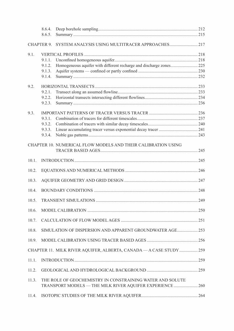
9.1. VertIcal profIles ......................................................................................................... 2189.1.1.  Unconfined homogeneous aquifer............................................................................. 2189.1.2.  Homogeneous aquifer with different recharge and discharge zones ......................... 2259.1.3.  Aquifer systems — confined or partly confined ....................................................... 2309.1.4.  Summary ................................................................................................................... 232

9.2. horIZontal transects ............................................................................................... 2339.2.1.  Transect along an assumed flowline .......................................................................... 2339.2.2.  Horizontal transects intersecting different flowlines ................................................. 2349.2.3. summary ................................................................................................................... 236

9.3. IMportant patterns of tracer Versus tracer ............................................. 2369.3.1. combination of tracers for different timescales ........................................................ 2379.3.2. combination of tracers with similar decay timescales .............................................. 2409.3.3. linear accumulating tracer versus exponential decay tracer .................................... 2419.3.4.  Noble gas patterns ..................................................................................................... 243

chapter 10. nuMerIcal flow Models and theIr calIbratIon usIng tracer based ages .......................................................................................... 245

10.1. IntroductIon .................................................................................................................. 245

10.2. equatIons and nuMerIcal Methods ................................................................... 246

10.3. aquIfer geoMetry and grId desIgn .................................................................... 247

10.4.  BoUNdAry coNdITIoNS ................................................................................................ 248

10.5. transIent sIMulatIons .............................................................................................. 249

10.6. Model calIbratIon ...................................................................................................... 250

10.7. calculatIon of flow Model ages ....................................................................... 251

10.8. sIMulatIon of dIspersIon and apparent groundwater age ................... 253

10.9. Model calIbratIon usIng tracer based ages ............................................... 256

chapter 11. mILK rIvEr AqUIfEr, ALBErTA, cANAdA — A cASE STUdy ................. 259

11.1. IntroductIon .................................................................................................................. 259

11.2.  gEoLogIcAL ANd HydroLogIcAL BAcKgroUNd ............................................... 259

11.3. the role of geocheMIstry In constraInIng water and solute TrANSPorT modELS — THE mILK rIvEr AqUIfEr ExPErIENcE ...................... 260

11.4.  ISoToPIc STUdIES of THE mILK rIvEr AqUIfEr .................................................... 264

11.4.1.   radiocarbon and stable isotopes .............................................................................. 26411.4.2.   dissolved gases ........................................................................................................ 26511.4.3.   chlorine-36 and chloride.......................................................................................... 26711.4.4.   Uranium isotopes ..................................................................................................... 269

11.5. conclusIons .................................................................................................................... 272

chapter 12. case study MIddle rIo grande basIn, new MexIco, usa .............. 273

12.1. IntroductIon .................................................................................................................. 273

12.2.  BAcKgroUNd: HydrogEoLogIcAL SETTINg ........................................................ 273

12.3. the unIted states geologIcal surVey MIddle rIo grande basIn study ...................................................................................................................... 276

12.4.  STABLE ISoToPES, 4he, radIocarbon ages and hydrocheMIcal Zones ............................................................................................... 27612.4.1.  Stable isotopes ........................................................................................................... 27612.4.2.  carbon-14 model age ................................................................................................ 27812.4.3.  Helium-4 ................................................................................................................... 28012.4.4.  Hydrochemical zones ................................................................................................ 28312.4.5.  Pre-development water levels ................................................................................... 28412.4.6.  variations in 14c model age with depth ..................................................................... 28612.4.7.  Stable isotopes, deuterium excess and radiocarbon age ........................................... 28612.4.8.  carbon-14 model age profiles and recharge rates ..................................................... 287

12.5. suMMary of cheMIcal and enVIronMental tracer constraInts on the flow systeM ..................................................................................................... 288

12.6. groundwater Model deVelopMent .................................................................... 289

12.7. refInIng conceptualIZatIon of groundwater flow In the basIn ...... 293

12.8. palaeorecharge rates .............................................................................................. 294

12.9.  coNcLUdINg rEmArKS ................................................................................................. 295

chapter 13. Methods for datIng Very old groundwater: eastern and central great artesIan basIn case study .............................. 297

13.1. IntroductIon .................................................................................................................. 297

13.2. deposItIon, structure and hydrogeology of the eastern great artesIan basIn ................................................................................................................ 299

13.3. settIng the stage ......................................................................................................... 300

13.4.  STABLE ISoToPE ANd 14c MeasureMents ............................................................... 301

13.5.  THE 1982 fIELdworK: STANNUm To INNAmINcKA ANd BoNNA vISTA to thargoMIndah ......................................................................................................... 302

13.6.  THE 1985 fIELdworK: fAIrLIgHT TrUST To cLAyToN, ATHoL To  mUTTI mUTTI ANd mT. crISPE To cUrdImUrKA .................................................... 308

13.7. ModellIng 36cl and 4he ................................................................................................. 309

13.8. geocheMIcal ModellIng of groundwater reactIon paths ................... 312

13.9.  THE 2000 BENcHmArK ANd SyNTHESIS ..................................................................... 314

13.10.  coNTINUINg worK IN THE grEAT ArTESIAN BASIN ............................................. 316

cHAPTEr 14. KryPToN-81 cASE STUdy: THE NUBIAN AqUIfEr, EgyPT ...................... 319

14.1.  NUBIAN AqUIfEr .............................................................................................................. 319

14.2.  mETHodS ............................................................................................................................. 319

14.3.  KryPToN-81 dATA ............................................................................................................. 320

14.4.  cHLorINE-36 dATA ........................................................................................................... 321

14.5.  corrELATIoN of 36cl and 81Kr data ........................................................................... 322

14.6.  HELIUm-4 dATA .................................................................................................................. 323

14.7.  cArBoN-14 dATA ............................................................................................................... 323

14.8.  HydrogEoLogIcAL ANd PALAEocLImATIc ImPLIcATIoNS of  groundwater age data .............................................................................................. 324

references ................................................................................................................................... 325contrIbutors to draftIng and reVIew ......................................................................... 357

1

Chapter 1

IntRODUCtIOn

P.K. AggArwALInternational atomic energy agency

1.1. BAcKgroUNd

groundwater is the largest component of fresh water accessible for human use. while two thirds of the surface area of planet earth is covered with water, most of it is sea water or saline and only 2.5% is fresh water (Shiklomanov and rodda (2004) [1]). A large portion of this fresh water — nearly 69% — is bound in ice and permanent snow cover in the antarctic and arctic, and in continental mountains. about 30% of fresh water, or 0.75% of all water on earth, is present as fresh groundwater. only 0.26% of the total amount of fresh water on Earth is in lakes, rivers and reservoirs that are most easily accessible for human use (the remaining 1% is estimated to occur as soil moisture, swamp water and permafrost). groundwater, in both renewable and non-renewable aquifers, accounts for about 95% of accessible fresh water or 0.7% of all water on earth, and provides more than half of all domestic and irrigation water used around the world (fig. 1.1). In semi-arid and arid regions, and in domestic supplies for rural areas, 80–100% of all fresh water may be derived from groundwater.

In many parts of the world, groundwater levels are rapidly declining as groundwater withdrawal far exceeds natural recharge. Irrigated agriculture, particularly from groundwater, has been responsible for many of the strides made in self-suffi cient food production in parts of Asia and has contributed to the ‘green revolution’ of the 1960s, resulting in greater food security. It is now estimated that more than half of the world’s food production is derived from irrigated agriculture. owing to the extent that fossil or non-renewable groundwater  is being used  to  increase food production, both  the water supply and food production may potentially become unsustainable in the future. The United Nations’ millennium development goals, adopted in 1999 by the governments of nearly 180 countries, and subsequent commitments, include the goal “to stop the unsustainable exploitation of water resources by developing water management strategies at the regional, national and local levels...”

sustainable use and management of aquifers necessitates an understanding of aquifer hydrogeology and its dynamics. this understanding can be gained over a period of decades by observations and measurements of precipitation, river fl ows, groundwater levels, etc. Early developments in groundwater hydrology focused on means to estimate aquifer storativity and hydraulic conductivity, which led to the establishment of the theory of transient groundwater fl ow (Anderson (2008) [2]). Isotope techniques 

FIG. 1.1. Occurrence of water on Earth (based on data from Shiklomanov and Rodda (2004) [1]).

Total water on Earth Components of fresh water

Sea water IceFresh water Soil moisture,

atmosphere, biosphere

Groundwater

Lakes, rivers

2

— and particularly those that can be applied to estimate the age of groundwater — help to cost effectively build a conceptual framework of aquifer hydrogeology and flow system. The use of groundwater age for estimating aquifer storage, the rate of groundwater renewal and flow velocity was conceived as early as the natural radioactivity of tritium and 14c was discovered more than sixty years ago (aggarwal et al. (2012) [3]). groundwater age also provides unmatched advantages for improving numerical models of groundwater flow in large, regional aquifers where water level data are normally scarce.

the age of groundwater ranges from less than a month to a million years, or perhaps more. old groundwater — defined in this book as groundwater with estimated ages greater  than about one thousand years — occurs in many african, asian and latin american aquifers as indicated by measured 14c activities (IAEA (2007) [4]). The Nubian Aquifer in northern Africa, for example, is estimated to contain groundwater that was recharged at various times over the past million years (sturchio et al. (2004) [5]). figure 1.2 shows the distribution of groundwater 14c in northern and central africa. this groundwater is presently used for drinking and irrigation. with an increasing population and potential changes in the current climate, it will become an even more important resource for meeting the fresh water demands of the region. It is crucial to understand the nature of recharge and groundwater flow in past climates in order to better characterize the changes that may be induced under new climate regimes.

1.2. objectIVes

This book aims to provide the reader with a comprehensive understanding of why groundwater age is an important parameter for characterizing aquifer hydrogeology, how to estimate groundwater ages using different isotopes and how best to use age data for the analysis of groundwater flow.

1.3. scope

a number of isotopes can be used to interpret groundwater ages over a wide range of timescales. (fig. 1.3). A need was identified to create a synthesis of various isotope methods to date old groundwater and to critically evaluate their advantages and disadvantages for use in hydrology. This book is intended to provide hydrogeologists with a guideline describing existing sampling and measurment methods, and to provide tools to ensure reliability of the resulting interpretation of isotope data. A ‘critical’ evaluation is intended to assess sampling efforts required in the field and to select possible cooperation partners 

FIG. 1.2. Distribution of 14C in groundwater in northern Africa.

120

0

Insufficient datafor extrapolation

14C (pMC)

3

and assess the problems inherent to each method, as well as model assumptions which lead to water age results of 20 000 to 1 million years.

It  is hoped  that  sufficient detail  and examples have been provided  to convey  to  the  reader  that obtaining meaningful hydrological information from groundwater age data requires careful planning and  sampling,  skilled  measurements  and  a  significant  number  of  cross  checks  to  evaluate  various assumptions. It is to be cautioned that an age estimate based on a single isotope or tracer at a single location may not be very informative. Multiple estimates, based on more than one tracer and at multiple locations, particularly when combined with a numerical model sufficient to represent the flow regime of the groundwater system of interest, are necessary to meaningfully use groundwater age data.

1.4.  structure

chapter 2 describes fundamental concepts, data needs, and approaches that aid in developing a general understanding of groundwater systems. chapter 3 discusses in detail the meaning of groundwater age in a physical hydrological system along with pitfalls to be avoided by misinterpreting or over-interpreting age data. The subsequent five chapters describe  the basis  for and use of various isotope methods for dating of old groundwater: 14c, 81Kr, 36cl, uranium isotopes and 4he.

the use of multiple isotope tracers and its potential advantages over single tracers are discussed in chapter 9. chapter 10 outlines the methods for combining results of groundwater age determination with  quantitative  numerical models  of  groundwater  flow  and  transport  processes within  an  aquifer. finally, a series of case studies on the use of groundwater ages to characterize large, regional aquifer systems is presented. These include the milk river aquifer in canada (fröhlich), the santa fe group aquifer system of the Middle rio grande basin in the united states of america (plummer et al.), the eastern great artesian basin in australia (torgersen) and the nubian aquifer system in northern africa (sturchio and purtschert).

a wide variety of readers involved in groundwater research or in the exploration, management, planning and utilization of groundwater resources may find this book useful. Those interested in the use of multiple tracers to determine and use groundwater age data may gain a better understanding of the subject by reading all of the chapters in the order they are presented. a reader new to the concepts of groundwater dating who wants  a general  overview of  the  topic may wish  to first  read chapter 2 (characterization and conceptualization), a definition of the concepts of groundwater age used in this book (chapter 3)  followed by case studies  (chapters 11–14). readers who are  familiar with  isotope 

FIG. 1.3. Isotope and chemical tracers use for estimating groundwater age.

0.1 1 10 100 1000 10 000 100 000 1 000 000

Groundwater timescale (a)

δ2H, δ18O: 0.1–3 a

3H: 1–50 a

85Kr: 1–40 a

CFC/SF6: 1–40 a

3H/3He: 0.5–40 a

39Ar: 50–1000 a

14C: 1 ka–40 ka

234U/238U: 10 ka–1 Ma

36Cl: 50 ka–1 Ma

81Kr: 50 ka–1 Ma

4He: 100 a–1 Ma

4

techniques  in  general  and  are  in  need  of  information  related  to  a  specific  isotope may  wish  to  go directly  to  chapters  4–8.  Hydrologists  and  modellers  who  may  not  be  interested  in  the  details  of the tracer techniques but in the application of groundwater tracers may wish to begin with chapters 2 and 3, followed by chapters 9 and 10 (system analysis using multitracer approaches and groundwater models, respectively).

5

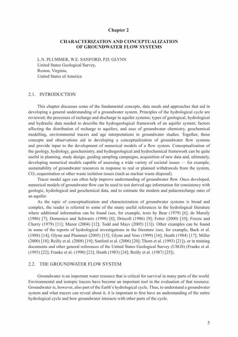
Chapter 2

CHARACtERIZAtIOn AnD COnCEPtUALIZAtIOn OF GROUnDWAtER FLOW sYstEMs

l.n. pluMMer, w.e. sanford, p.d. glynnunited states geological survey, reston, Virginia, united states of america

2.1. IntroductIon

this chapter discusses some of the fundamental concepts, data needs and approaches that aid in developing a general understanding of a groundwater system. principles of the hydrological cycle are reviewed; the processes of recharge and discharge in aquifer systems; types of geological, hydrological and hydraulic  data  needed  to  describe  the  hydrogeological  framework of  an  aquifer  system;  factors affecting the distribution of recharge to aquifers; and uses of groundwater chemistry, geochemical modelling, environmental tracers and age interpretations in groundwater studies. together, these concepts  and  observations  aid  in  developing  a  conceptualization  of  groundwater  flow  systems and  provide  input  to  the  development  of  numerical models  of  a  flow  system.  conceptualization  of the geology, hydrology, geochemistry, and hydrogeological and hydrochemical framework can be quite useful in planning, study design, guiding sampling campaigns, acquisition of new data and, ultimately, developing numerical models capable of assessing a wide variety of societal issues — for example, sustainability of groundwater resources in response to real or planned withdrawals from the system, co2 sequestration or other waste isolation issues (such as nuclear waste disposal).

Tracer model ages can often help improve understanding of groundwater flow. once developed, numerical models of groundwater flow can be used to test derived age information for consistency with geologic, hydrological and geochemical data, and to estimate the modern and palaeorecharge rates of an aquifer.

As  the  topic  of  conceptualization  and  characterization  of  groundwater  systems  is  broad  and complex, the reader is referred to some of the many useful references in the hydrological literature where  additional  information  can  be  found  (see,  for  example,  texts  by Bear  (1979)  [6];  de marsily (1986)  [7]; domenico  and Schwartz  (1998)  [8]; driscoll  (1986)  [9];  fetter  (2000)  [10];  freeze  and cherry  (1979)  [11]; mazor  (2004)  [12]; Todd and mays  (2005)  [13]). other examples can be  found in  some of  the  reports  of  hydrological  investigations  in  the  literature  (see,  for  example, Back  et  al. (1988) [14]; glynn and Plummer (2005) [15]; glynn and voss (1999) [16]; Heath (1984) [17]; miller (2000) [18]; reilly et al. (2008) [19]; Sanford et al. (2006) [20]; Thorn et al. (1993) [21]), or in training documents and other general references of the United States geological Survey (USgS) (franke et al. (1993) [22]; franke et al. (1990) [23]; Heath (1983) [24]; reilly et al. (1987) [25]).

2.2. the groundwater flow systeM

groundwater is an important water resource that is critical for survival in many parts of the world. environmental and isotopic tracers have become an important tool in the evaluation of that resource. groundwater is, however, also part of the Earth’s hydrological cycle. Thus, to understand a groundwater system and what tracers can reveal about it, it is important to first have an understanding of the entire hydrological cycle and how groundwater interacts with other parts of the cycle.

6

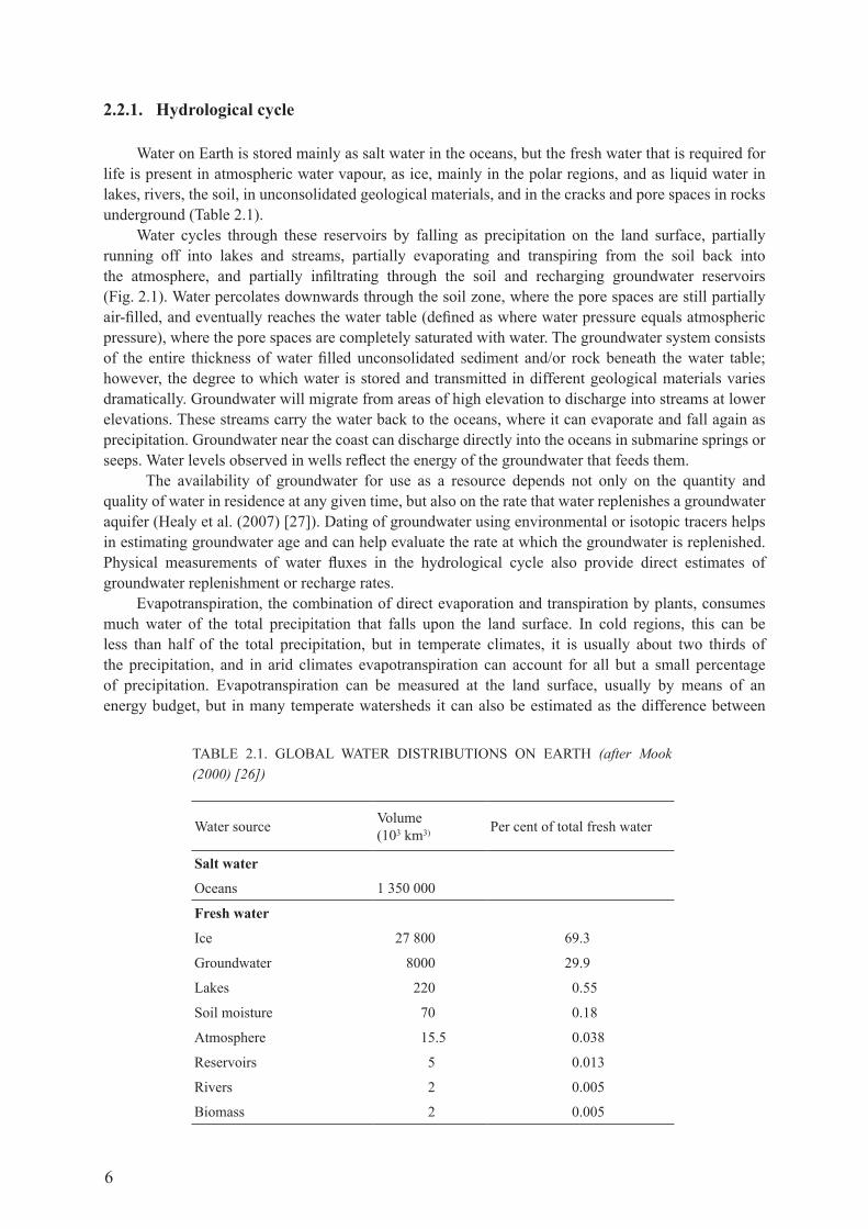
2.2.1. Hydrological cycle

water on earth is stored mainly as salt water in the oceans, but the fresh water that is required for life is present in atmospheric water vapour, as ice, mainly in the polar regions, and as liquid water in lakes, rivers, the soil, in unconsolidated geological materials, and in the cracks and pore spaces in rocks underground (table 2.1).

water cycles through these reservoirs by falling as precipitation on the land surface, partially running  off  into  lakes  and  streams,  partially  evaporating  and  transpiring  from  the  soil  back  into the  atmosphere,  and  partially  infiltrating  through  the  soil  and  recharging  groundwater  reservoirs (fig. 2.1). water percolates downwards through the soil zone, where the pore spaces are still partially air-filled, and eventually reaches the water table (defined as where water pressure equals atmospheric pressure), where the pore spaces are completely saturated with water. the groundwater system consists of  the  entire  thickness  of water filled  unconsolidated  sediment  and/or  rock beneath  the water  table; however, the degree to which water is stored and transmitted in different geological materials varies dramatically. groundwater will migrate from areas of high elevation to discharge into streams at lower elevations. These streams carry the water back to the oceans, where it can evaporate and fall again as precipitation. groundwater near the coast can discharge directly into the oceans in submarine springs or seeps. water levels observed in wells reflect the energy of the groundwater that feeds them.

the availability of groundwater for use as a resource depends not only on the quantity and quality of water in residence at any given time, but also on the rate that water replenishes a groundwater aquifer (Healy et al. (2007) [27]). dating of groundwater using environmental or isotopic tracers helps in estimating groundwater age and can help evaluate the rate at which the groundwater is replenished. Physical  measurements  of  water  fluxes  in  the  hydrological  cycle  also  provide  direct  estimates  of groundwater replenishment or recharge rates.

evapotranspiration, the combination of direct evaporation and transpiration by plants, consumes much water of the total precipitation that falls upon the land surface. In cold regions, this can be less than half of the total precipitation, but in temperate climates, it is usually about two thirds of the precipitation, and in arid climates evapotranspiration can account for all but a small percentage of precipitation. evapotranspiration can be measured at the land surface, usually by means of an energy budget, but in many temperate watersheds it can also be estimated as the difference between

table 2.1. global water dIstrIbutIons on earth (after Mook (2000) [26])

water source Volume (103 km3) per cent of total fresh water

salt water

oceans 1 350 000

Fresh water

Ice 27 800 69.3

groundwater 8000 29.9

Lakes 220 0.55

soil moisture 70 0.18

atmosphere 15.5 0.038

reservoirs 5 0.013

rivers 2 0.005

biomass 2 0.005

7

the average amount of precipitation falling on the watershed and the average discharge into streams from that watershed. the average discharge from a stream represents the water that has either run off during rain events or seeped into the stream as baseflow. This approach works best when inflow and outflow of groundwater as underflow directly from or to an adjoining watershed can be assumed to be small. Baseflow measurement within a stream and the exchange of groundwater and surface water are an important and frequently used method for estimating fluxes within a groundwater system.

The porosity, or storage capacity, of rocks and unconsolidated sediments can vary from less than 1% for fractured rocks to greater than 50% for fine grained sediments. The permeability, or hydraulic conductivity, of rocks or unconsolidated sediment  is a measurement of how easily  they can transmit water, and this can vary between geological materials by many orders of magnitude (freeze and cherry (1979) [11]; Heath (1983) [24]). rock types and/or unconsolidated sediments within the groundwater system of interest, therefore, have an enormous impact on its storage capacity, replenishment rate and capability to yield water to wells in substantial quantities. thus, it is essential that a hydrogeological study be performed as thoroughly as resources permit to determine the nature and distribution of the rocks and/or unconsolidated sediments, and to estimate their hydraulic properties.

2.2.2. timescales for recharge and discharge

Even within a groundwater system of a uniform rock type, the length of a flow path and the time of  travel  for water  along  that  path  can  vary  greatly. rolling  topography will  itself  create  flow path variability  within  a  system  (Tóth  (1963)  [28]). water  that  recharges  near  streams  will  stay  within local, shallow flow systems and discharge within a few years to tens of years after recharge. water that recharges further from streams will follow intermediate flow systems of moderate depth, and discharge hundreds to thousands of years after recharge. water that recharges near topographic divides furthest from streams can take deep flow paths in regional flow systems that discharge after tens of thousands of years or longer after recharge (fig. 2.2). such recharge may have occurred during different climatic

FIG. 2.1. The hydrological cycle. Numbers are annual water fluxes in 103 km3 per year (Mook (2000) [26]; see also: http://ga.water.usgs.gov/edu/watercycle.html).

vapour transport

precipitation

40

Hydrological cyclep recipit a tion

evaporation

runoff evapotranspirationevaporation

infilt rationocean

groundwater flowHydrological cycle

40

111

385

42571111

40

8

conditions, such as during the most recent glacial cycle when precipitation and recharge rates were frequently higher than observed today in many locations.

2.3. characterIZatIon of groundwater flow systeMs

In characterizing a groundwater flow system and developing a conceptualization of groundwater flow, three general classes of data are needed: geological, hydrological and geochemical.

2.3.1. Geological framework

one  way  of  developing  a  geological  framework  of  a  groundwater  flow  system  is  to  develop a three dimensional visualization describing its physical features. Basic features of a three dimensional geological  description  include  characterization  of  thickness  and  lithology  of  rocks/sediment  that compose the various geological units of the groundwater flow system and a description of geological structures. some lithologic properties that need to be considered include effective porosity, permeability, mineralogy and their spatial and depth variations.

mapping of faults, fracture systems, folds in rock and the orientation of these structures in relation to the direction of groundwater flow is critical in assessing the geological framework and controls on groundwater  flow. depending  on  their  physical  properties,  geological  structures,  such  as  faults,  can either  enhance or  retard groundwater flow. regional  variations  in  lithologic properties  contribute  to 

FIG. 2.2. Generalized block diagram showing conceptualization of groundwater recharge, discharge and groundwater age in a basin fill groundwater flow system (modified from Hely et al. (1971) [29]; Thiros (2000) [30]; not to scale).

9

aquifer heterogeneity. from the standpoint of interpreting environmental tracer data, it is important to have a good understanding of aquifer heterogeneity, such as low permeability zones, confining layers or highly fractured domains, because they can act as sources or sinks for some of the environmental tracers used for age estimation.

The  environmental  tracers  considered  in  this  book  can  be  affected  variously  by  interactions with confining layers, diffusion into or from low permeability zones, convergence/divergence of flow paths, in situ production through nuclear reactions and, in some cases, geochemical interaction with the minerals of the aquifer matrix or those in low permeability zones. Therefore, information on aquifer heterogeneity  is essential when  interpreting environmental  tracer data  in  ‘old’  (as used  in  this book, ‘old’ is defined as generally greater than 1000 a) groundwater.

There  are  a  number  of  geophysical  techniques  that  can  be  used  to  characterize  aquifer heterogeneity (see, for example, http://water.usgs.gov/ogw/bgas/g2t.html). however, there is never enough geophysical information from boreholes, well logs, cores or cuttings to completely describe aquifer heterogeneity throughout a system. surface geophysical techniques (such as seismic surveys) and  even  remote  sensing  techniques  (such  as  InSAr:  http://quake.usgs.gov/research/deformation/modelling/Insar/index.html) are also very useful in constructing a conceptual description of the hydrogeological framework.

geological mapping and construction of geological cross-sections of a groundwater flow system improve understanding of the spatial distribution of structural features, lithologic facies changes and, generally, the consequent spatial variations in hydraulic conductivity and mineralogy, as well as their heterogeneous distribution through the groundwater system being studied. sedimentary basin modelling, stratigraphic modelling and structural modelling are some of the types of geological evolution simulation modelling now being used more frequently by hydrogeologists to describe the evolution of aquifer units after development by the oil and gas industry. sedimentary basin modelling has also been used to understand the transport and fate of pore fluids and the palaeohydrology of sedimentary basins (Bethke (1985) [31]).

2.3.2. Hydrological framework

Essential  information  in  construction  of  a  hydrological  framework  includes  land–surface elevation, locations of rivers and other drainage, areal distribution of precipitation, delineation of recharge  and  discharge  areas,  determination  of  a  water  balance  for  the  groundwater  flow  system, mapping of the altitude of the potentiometric surfaces of the aquifers, and characterization of regional variability in the hydraulic properties of a groundwater flow system. The hydrological framework of a groundwater flow system can be visualized in maps of the potentiometric surface of aquifers, in cross-sections showing the relation of groundwater flow to the geological framework, and ultimately through a numerical model capable of simulating groundwater flow.

2.3.2.1. Water levels

darcy’s law states that groundwater flux is directly proportional to the gradient in the hydraulic head, or water level, and the hydraulic conductivity of the porous media (rock or sediment). Hydraulic gradients  can  be  determined  from  contours  drawn  on  maps  defining  lines  of  equal  head  depicting historical (pre-development, i.e. pre-pumping) water levels in unconfined aquifers or from water levels in piezometers  in confined aquifers  (see,  for example, Bexfield (2002)  [32]). groundwater generally flows down the hydraulic gradient in directions normal to the lines of equal head. In confined aquifers, the hydraulic gradient is determined by mapping water levels in wells open to the aquifer of interest. given the nature of aquifer heterogeneity and the fact that different wells can be open to different depths and different screened intervals within an aquifer, the mapped potentiometric surface is usually more

10

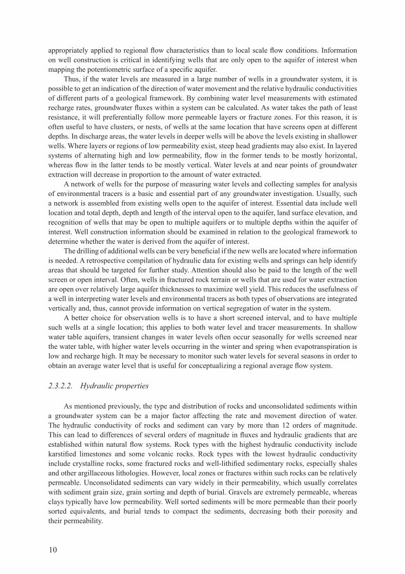
appropriately applied to regional flow characteristics than to local scale flow conditions. Information on well construction is critical in identifying wells that are only open to the aquifer of interest when mapping the potentiometric surface of a specific aquifer.

thus, if the water levels are measured in a large number of wells in a groundwater system, it is possible to get an indication of the direction of water movement and the relative hydraulic conductivities of different parts of a geological framework. By combining water level measurements with estimated recharge rates, groundwater fluxes within a system can be calculated. As water takes the path of least resistance, it will preferentially follow more permeable layers or fracture zones. for this reason, it is often useful to have clusters, or nests, of wells at the same location that have screens open at different depths. In discharge areas, the water levels in deeper wells will be above the levels existing in shallower wells. where layers or regions of low permeability exist, steep head gradients may also exist. In layered systems of  alternating high  and  low permeability, flow  in  the  former  tends  to  be mostly  horizontal, whereas flow in the latter tends to be mostly vertical. water levels at and near points of groundwater extraction will decrease in proportion to the amount of water extracted.

A network of wells for the purpose of measuring water levels and collecting samples for analysis of environmental tracers is a basic and essential part of any groundwater investigation. usually, such a network is assembled from existing wells open to the aquifer of interest. Essential data include well location and total depth, depth and length of the interval open to the aquifer, land surface elevation, and recognition of wells that may be open to multiple aquifers or to multiple depths within the aquifer of interest. well construction information should be examined in relation to the geological framework to determine whether the water is derived from the aquifer of interest.

The drilling of additional wells can be very beneficial if the new wells are located where information is needed. a retrospective compilation of hydraulic data for existing wells and springs can help identify areas that should be targeted for further study. attention should also be paid to the length of the well screen or open interval. often, wells in fractured rock terrain or wells that are used for water extraction are open over relatively large aquifer thicknesses to maximize well yield. This reduces the usefulness of a well in interpreting water levels and environmental tracers as both types of observations are integrated vertically and, thus, cannot provide information on vertical segregation of water in the system.

a better choice for observation wells is to have a short screened interval, and to have multiple such wells at a single location; this applies to both water level and tracer measurements. In shallow water table aquifers, transient changes in water levels often occur seasonally for wells screened near the water table, with higher water levels occurring in the winter and spring when evapotranspiration is low and recharge high. It may be necessary to monitor such water levels for several seasons in order to obtain an average water level that is useful for conceptualizing a regional average flow system.

2.3.2.2. Hydraulic properties

As mentioned previously, the type and distribution of rocks and unconsolidated sediments within a groundwater system can be a major factor affecting the rate and movement direction of water. The  hydraulic  conductivity  of  rocks  and  sediment  can  vary  by more  than  12  orders  of magnitude. This can lead to differences of several orders of magnitude in fluxes and hydraulic gradients that are established within natural flow systems. rock  types with  the highest hydraulic  conductivity  include karstified  limestones  and  some  volcanic  rocks.  rock  types  with  the  lowest  hydraulic  conductivity include crystalline rocks, some fractured rocks and well-lithified sedimentary rocks, especially shales and other argillaceous lithologies. However, local zones or fractures within such rocks can be relatively permeable. unconsolidated sediments can vary widely in their permeability, which usually correlates with sediment grain size, grain sorting and depth of burial. gravels are extremely permeable, whereas clays typically have low permeability. well sorted sediments will be more permeable than their poorly sorted equivalents, and burial tends to compact the sediments, decreasing both their porosity and their permeability.

11

The  hydraulic  properties  of  rocks  or  sediment  can  often  be  measured  in  situ.  measurements of hydraulic conductivity can also be made on core samples in the laboratory, but these small scale measurements usually have a low bias because they do not incorporate the larger scale features such as fractures or bedding. the hydraulic conductivity or transmissivity of an aquifer (its hydraulic conductivity multiplied by its thickness) is frequently measured using an aquifer test. The simplest form of these is a slug test, where a known volume of water is added or withdrawn quickly, and the water level is measured over time as it returns to its original level (ferris et al. (1962) [33]; Kruseman and de  ridder  (1990)  [34];  Shuter  and Teasdale  (1989)  [35]). Although  slug  tests  are  easy  to  perform, they often do not work well in highly permeable material (the water level equilibrates very quickly), and the measurement is only influenced by a limited volume of rock or sediment very near the well. a frequent alternative to simple slug tests is more complete aquifer tests, where water is extracted from a well at a constant rate over a period of time, usually at least 1–2 days. water levels are observed throughout such a test, preferably at a well that is located some distance from an extraction well. this type of test is influenced by a much larger volume of the aquifer than a slug test, so may provide a value that is more reflective of a regional average.

aquifer storage is also obtainable through an aquifer test, although with a little less accuracy than the transmissivity. In unconfined aquifers, a specific yield represents the volume of water released from  storage  from a  unit  area  of  the  studied  aquifer  per  unit  decline  in  the water  table.  In  bedrock aquifers,  the storage  term is  related  to compressibility of  the rock matrix, which releases water as  it undergoes  a drop  in fluid pressure. This  causes  a  reduction  in porosity  as  the matrix  is  compressed under the weight of the overburden.

2.3.2.3. Recharge amount and distribution

In spite of the wide range of hydraulic properties associated with various rock types, the recharge rate  frequently  controls  how  quickly  groundwater  is  replenished. This  is  especially  true  in  areas  of either  moderate  to  high  topographic  relief  and/or  areas  that  are  semi-arid  to  arid.  In  arid  regions, groundwater recharge is one of the most critical water balance components because of the difficulties in its measurement. Much research has been performed to develop various techniques for measuring recharge  directly  in  the  field  (de  vries  and  Simmers  (2002)  [36];  Scanlon  et  al.  (2002)  [37]),  but many of these techniques are limited by the fact that they make measurements only over small areas or small time periods, or both. conventional techniques for estimating recharge rate are based on water balance equations that include hydrometeorological (precipitation–evapotranspiration) and geohydrological (groundwater level changes) parameters. In these equations, recharge is determined as the difference between other balance quantities that are directly measurable. the uncertainty in the measurement of these quantities determines the uncertainty of the recharge rate. If recharge is high, such as in humid regions (10 to more than 100 cm/a), its uncertainty is relatively low. however, in semi-arid and arid areas with recharge rates from virtually 0 to less than 100 mm/a, the uncertainties of measured balance parameters cause very high uncertainty in the estimated recharge rate. thus, the very approximate nature of these groundwater balance estimations prompts chemical and isotopic studies to independently assess recharge rates. Especially for drier regions, geochemical and isotopic profiling in  the  unsaturated  and  shallow  groundwater  zone  is more  reliable  and  accurate  than water  balance methods and, thus, is practically indispensible for groundwater resource assessments. geochemical and isotopic tools for recharge rate determination include cl, chlorofluorocarbons (cfcs), 3h, 3h/3he and 14c. for groundwater systems with low or even negligible present day recharge, 14c is one of the most suitable tools.

It  is  usually  not  known  to  what  extent  modern  recharge  rates  can  be  applied  in  estimating palaeorecharge rates. Still, it is important to determine modern recharge rates to provide a benchmark for comparison to palaeorecharge rates once they are derived from groundwater age information and the application of models  to  the flow system. for a regional groundwater assessment,  long term and 

12

spatially averaged recharge rates are usually needed. local measurements must either be scaled up, or other methods used  that  integrate  larger spatial and  timescales. measurement of baseflow in streams was mentioned earlier as one such approach that can work fairly well in temperate or humid climates, where recharge is often fairly evenly distributed with precipitation.

In semi-arid to arid regions, the distribution of recharge is usually quite heterogeneous, occurring mainly in the mountains or along mountain fronts or ephemeral streams during intermittent runoff events. local measurement techniques can be useful in areas of focused recharge. In broad areas between mountain  ranges or  away  from streams,  recharge can be nearly zero or  essentially zero,  as can  be  determined  by  the  accumulation  of  solute  tracers within  the  unsaturated  zone which  occurs through continued conditions where evaporation removes the water but not the solutes. The chloride-mass balance technique (wood and Sanford (1995) [38]) is one method that has proven useful under such conditions.

In humid regions, shallow flow systems usually contain young groundwater. If ‘old’ groundwater exists  today  in  humid  regions,  it  usually  is  at  sufficient  depth  or  beneath  sufficient  hydraulic confinement that it is isolated from the active flow system. If of meteoric origin, ‘old’ groundwater was initially recharged at the land surface, perhaps in outcrop areas along basin margins, or along outcrops at mountain  fronts or  in outcrops of coastal, wedge shaped aquifers. Subsequent flow has permitted a fraction of this water to reach depths where it is sufficiently isolated from the active flow system on timescales of thousands to more than millions of years. most aquifers are ‘leaky’ to some extent and eventually flow to an area of discharge. ‘old’ groundwater is found in deep sedimentary basins, usually beneath sequences of confining layers (see, for example, Phillips et al. (1989) [39]), in coastal aquifers beneath confining  layers  (Aeschbach-Hertig et al.  (2002)  [40]; castro et al.  (2007)  [41]; Stute et al. (1992) [42]), or in arid regions where modern recharge is insufficient to replace the ‘old’ water or does so only very slowly (Patterson et al. (2005) [43]; Sturchio et al. (2004) [5]).

aquifers in arid regions today may have been recharged predominantly during pluvial (wet) climatic periods in the past, and today, ‘old’ water persists due to low recharge rates that are insufficient to flush  the  groundwater flow  system.  In  some  cases,  a  temporal  understanding  of  changes  in  areal recharge conditions may be gained from information on the past distribution of vegetation in an area or from other information on the relative pluviosity/aridity in an area. palaeobotanical studies of pollen or relict vegetation distribution in soils and lake sediment might be useful in this context. Examples of other measures of pluviosity/aridity include tree ring reconstructions; determination of sedimentation rates in varve sequences; radiocarbon dating of palaeolake levels; records of chloride, nitrate and other atmospherically derived solutes in unsaturated zones (walvoord et al. (2002) [44]) and archaeological evidence of past population migrations in water stressed regions.

In spite of the techniques that are available to directly measure recharge at the land surface, environmental tracers often prove to be the best tools for constraining estimates of long term and spatially averaged recharge rates.

2.3.3. Hydrochemical framework

data on the concentrations of dissolved solutes, gases and isotopes can provide information about  the  local area  from which  they were  recharged and can be used  to  trace groundwater flow on the  timescale  of  the  groundwater  flow  system. geochemical  data  can  be  used  to  delineate  zones  of leakage through confining layers, interpret flow in relation to faults and other geological or hydraulic properties of an aquifer, and estimate travel times in groundwater systems. dissolved gases and stable isotope data (2h and 18o of groundwater) can be used to recognize palaeowaters and interpret palaeoclimatic recharge conditions. owing to their different timescales for introduction into aquifers, some environmental tracers can be used to help recognize recharge and discharge areas. Estimates of tracer model age can help to quantify recharge rates.

13

as part of the well and spring inventory process, all available chemical and isotopic data on water from the aquifer should be compiled, plotted on maps and contoured with respect  to a known depth interval. where available, chemical and environmental tracer data should be plotted as a function of depth in an aquifer. for example, areas of recharge or upward leakage can sometimes be recognized on maps of cl– concentration in groundwater or from plots of cl– as a function of depth. In unconfined aquifers, data are  typically plotted at mid-depth below the water  table of  the open interval of a well (see chapter 12). In some cases, gradients in environmental tracer concentration (and tracer model age) can be used to estimate recharge rate. this analysis will aid in recognition of recharge and discharge areas, defining directions of groundwater flow (see below),  identifying areas  that  should be  targeted for additional investigation, and may also provide an assessment of past climatic and environmental changes and palaeorecharge information.

2.3.3.1. Hydrochemical facies — relation of chemistry to groundwater flow

Although the shape of the pre-development potentiometric surface can define recent groundwater flow  direction,  maps  of  the  potentiometric  surface  are  not  available  on  timescales  of  interest, such  as  during  the  last  glacial  maximum  (Lgm).  consequently,  maps  of  the  pre-development potentiometric  surface  may  not  exactly  apply  to  interpreting  palaeogroundwater  flow  conditions. Still,  the  shape  of  the  pre-development  potentiometric  surface  usually  represents  the  predominant features of the palaeoflow system. An alternative approach to interpreting palaeoflow directions is to map spatial patterns in water chemistry and isotopic composition that can indicate past directions of groundwater flow.

geochemical  reactions  along  groundwater  flow  paths  can  lead  to  regional  variations  in  water composition  that  evolve  in  the  direction  of  flow.  Iso-concentration  contours  of  reacting  dissolved constituents drawn on maps of water composition tend to align to the direction of groundwater flow. glynn and Plummer (2005) [15], Back (1960) [45] and Back (1966) [46] defined the hydrochemical facies  concept,  placing  geochemical  observations  in  the  context  of  groundwater  flow  in  aquifers  of relatively homogeneous hydrological and mineralogical properties.

In contrast, it is sometimes possible to distinguish different sources of water to the groundwater flow system on the basis of inert chemical or isotopic constituents (such as cl–; br–; dissolved noble gases and dissolved n2; 18o and 2h in water; and sometimes na+, li+ and other chemical and isotopic constituents). In cases where inert tracer concentrations vary spatially along the groundwater recharge area, the path followed by a tracer delineates flow direction (glynn and Plummer (2005) [15]). In this case,  hydrochemical  facies  (sometimes  referred  to  as  ‘hydrochemical  zones’)  will  align  parallel  to the flow direction. In more complex cases, the concentration of reactive constituents may vary spatially and temporally along a recharge area, and may also evolve along the direction of flow.

  Non-reactive  constituents,  salinity  and  reactive  constituents  that  reflect  the  minerals  and geochemical conditions encountered at the time of recharge and in the later geochemical evolution of the groundwater can also provide information on the geological area of recharge and on the geological units traversed by groundwater to their point of sampling. Knowledge of the source and geochemical evolution of the groundwater will be essential in interpreting and adjusting tracer model ages obtained through various dating techniques discussed in this book (such as 14c and 4he). together with improved/adjusted estimates of groundwater ages, characterization of different groundwater geochemical facies in  the groundwater system may also be used, as  is done,  for example, by Sanford et al.  (2004)  [47] and Sanford et al. (2004) [48] for the middle rio grande Basin to calibrate groundwater flow models (and/or eventually fully coupled reactive transport models).

Extracting  flow  and  hydrological  information  from  geochemical  observations  requires understanding the aqueous reactivity of aquifer materials and the spatial and temporal distribution of recharge compositions. Many of the geochemical patterns observed in groundwater systems can also be

14

related to heterogeneities in either reactive mineral abundances or in hydrological properties, and may be difficult to resolve, given the limited information typically available.

flow patterns in regional aquifers, deduced from mapping hydrochemical facies and zones, can indicate  flow  directions  that  have  occurred  over  timescales  considerably  greater  than  the  timescale over which present day or even pre-development water levels were established. differences between regional flow directions deduced from hydrochemical patterns and those indicated by a modern (pre-development) potentiometric surface can indicate changes in hydraulic conditions (such as recharge rate) on a shorter, more recent timescale than those responsible for hydrochemical observations (Plummer et al.  (2004)  [49]; Plummer et al.  (2004)  [50]; Plummer et al.  (2004)  [51]; Sanford et al. (2004) [47]; Sanford et al. (2004) [48]).

Especially  in  arid  areas,  groundwater  within  a  regional  groundwater  flow  system  may  have a number of possible source areas that include various nearby streams, mountain fronts or inflow from other basins. the solute or isotopic character of the water can give clues as to the source area. the study in the Middle rio grande basin of new Mexico, usa (chapter 12), is an example of how solutes can be used to determine the source of the water, and in turn help elucidate flow paths and the nature of a groundwater flow system.

2.3.3.2. Environmental tracers, hydrochemistry and timescales

Many different solutes and isotopes that recharge with water into a groundwater system provide information on the time since recharge, either because they decay at a known rate, accumulate in an aquifer from in situ processes, or because their concentration in precipitation has changed at a known rate over time (clark and fritz (1997) [52]; cook and Herczeg (1999) [53]). The range in groundwater ages that is reflected in the tracers can vary from a few years to tens or hundreds of thousands of years, to millions of years (chapter 1). The latter is the focus of this book, with examples given of the various tracers and various field examples. A tracer model age (see chapter 3) of a sample of water from a well can  be  combined  with  the  known  hydraulic  properties  of  the  hydrogeological  framework  to  back-calculate the recharge rate that would be required to yield the interpreted tracer model age. for ‘old’ groundwater, this may yield recharge rates that are not consistent with modern estimated rates, but that may be consistent with rates that would be expected during earlier and different climatic conditions. In this sense, some tracers can serve as a repository of information on past climatic conditions. The  combined  measurement  of  tracer  model  ages  along  presumed  hydrological  flow  paths  and  in vertical profiles in aquifers can be even more useful in estimating travel times and palaeorecharge rates in aquifers.

There are a few chemical and isotopic indicators that can be used in recognizing ‘old’ groundwater — at  least,  it may be possible  to recognize water from the Lgm, about 22 ka calendar years before present (bp). dissolved gases and the 18o and 2h isotopic composition of water may be used to estimate elevation and temperature at the time of recharge, and the intensity of recharge (by determining excess air entrapment) for given water samples. the relationship between 18o and 2h is also useful in determining recharge characteristics, including the extent to which infiltrating groundwater may have been exposed to evaporation. examples of using noble gas recharge temperatures or recharge temperatures determined from measurements of dissolved nitrogen and argon in groundwater in identifying waters recharged during colder climatic conditions are found in Stute and Schlosser (1993) [54], Aeschbach-Hertig et al. (2000) [55] and Heaton et al. (1983) [56]. consistently, an average cooling of about 5°c is observed at the Lgm globally, though Aeschbach-Hertig et al. (2002) [40] found cooling of nearly 9°c in New jersey, usa near the last glacial ice margin. shifts in the stable isotopic composition of groundwater at the lgM to more depleted values are often observed and attributed to lower condensation temperatures (dansgaard  (1964)  [57];  rozanski  et  al.  (1993)  [58];  Straaten  and mook  (1983)  [59])  and  changes in moisture source. however, in some coastal aquifers, the isotopic shift is towards enrichment at

15

the Lgm,  due  in  part  to  enrichment  of  the  stable  isotopic  composition  of  ocean water  (ice-volume effect) and changes in moisture source (Plummer (1993) [60]).

groundwater recharged during the last glacial period is generally regarded as non-renewable on human civilization timescales. That is, once withdrawn from aquifers, natural recharge processes are not  sufficient  to  replace  the water  on  timescales  of  thousands  of  years. recognizing  non-renewable groundwater resources is critical to managing water supplies for future generations. Similarly, very ‘old’ groundwater, water recharged on the hundred thousand to million year timescale, is fossil water and equally non-renewable. Its identification is equally critical in guiding future management decisions and the need to locate other water resources, including those that may provide sustainable water supplies for the future (Alley et al. (1999) [61]) or act as waste containment barriers.

2.3.3.3. Obtaining representative samples from wells

one of the most difficult problems in groundwater hydrochemistry is obtaining samples that are representative of unaltered formation water. part of the problem is that due to well construction or the physical properties of spring sources, almost all samples are mixtures, combining all of the flowlines reaching a well screen or discharge point. In some cases, water reaching the open interval of a well or discharging at a spring may be nearly uniform in age, but, in general, it is usually necessary to assume that discharge from wells and springs consists of different components with varying ages, i.e. consists of a frequency distribution of age (see chapter 3). such mixtures can occur naturally in an aquifer as a result of aquifer heterogeneity, but are also created through the sampling process. In the case of wells with  large open  intervals  to an aquifer,  the discharge  is a mixture of all of  the flowlines drawn  into the open interval of a well. In the case of springs, the discharge also typically represents a frequency distribution of age. In both cases, the tracer model age is a mixed age and needs to be evaluated in terms of the frequency distribution of age in discharge from a well or spring (see chapter 3).

another problem in obtaining representative samples from wells is caused by the introduction of tracers of interest into a formation during the well construction process. all drilling operations potentially introduce atmospheric components into an aquifer. well development procedures may not adequately remove these components and, without special precautions in the drilling process, there is normally not any way to determine whether formation water contains trace contamination from drilling processes. when sampling water from wells with the intent of estimating the tracer based model age of ‘old’ groundwater from measurements of environmental tracer concentrations, as discussed in this book,  additional  samples  should  be  collected  for  analysis  of  components  that  can  be  indicators  of the introduction of contamination from drilling processes. some useful indicators of contamination from young sources include tritium, 85Kr and cfcs. owing to their extremely low detection limit, cfcs can be ideal tracers of drilling contamination (Plummer et al. (2004) [49]). In some cases, the driller may have imported treated water from municipal supplies for use in drilling and well development. chlorinated water from municipal supplies may contain chloroform, which can be detected at extremely low concentrations using purge and trap gas chromatography with an electron capture detector (plummer et al. (2008) [62]). If new wells are constructed, it is recommended that gas tracers be introduced into the drilling mud, such as halon-1211, sulphur hexafluoride or cfcs. Air rotary drilling procedures are not recommended because they introduce atmospheric gases into an aquifer. If jetting is used in well development, which consists of injecting high pressure air into the casing, the air injection should be far enough above the open interval of the well so as not to inject air into the formation.

Springs  probably  are  the  least  desirable  sources  for  sampling  ‘old’  groundwater  because  their discharge  can  represent  a mixture  of many waters  of  generally  unknown  origin  (and  age).  Though the discharge of some springs may contain predominantly ‘old’ water,  it  is common to find fractions of tritium or cfcs, indicating a mixture. Not knowing the frequency distribution of age in a mixture or water source limits the usefulness of springs for groundwater dating purposes. flowing wells that are open to a narrow interval of confined aquifers at a known depth are probably the most useful for 

16

sampling ‘old’ groundwater, particularly if a well has been in use for many years. An example of this is provided by  the  sampling of  the Nubian sandstone aquifer  in Egypt  (Patterson et al.  (2005)  [43]) for 81Kr (see chapter 14). Production wells with turbine pumps or pumps with impellors may promote cavitation and gas phase separation, leading to uncertainty in tracer model age interpretation based on gaseous environmental tracers. one technique that has been used successfully is to place a relatively low capacity piston sampling pump at depth within or just above the well opening and a second higher capacity pump at a relatively shallow depth to maintain a fresh supply of formation water entering the well bore in the vicinity of the sampling pump.

2.4.  deVelopMent of a nuMerIcal groundwater flow Model

There  are  a  number of  approaches hydrologists  have  taken  in developing numerical models  of groundwater flow,  including  relatively  simple  analytical  solutions  (see,  for  example, genuchten and Alves  (1982)  [63]);  lumped  parameter  models  (see,  for  example,  małoszewski  et  al.  (1983)  [64]; małoszewski and zuber  (1996)  [65]);  and finite difference and finite element models  that  can  solve the  partial  differential  equations  of  groundwater  flow  and  solute  transport  in  three  dimensions  (see, for example, Huyakorn and Pinder (1983) [66]; Konikow and glynn (2005) [67]; wang and Anderson (1982) [68]).

In many studies of groundwater systems, a numerical model is constructed that represents the  hydrogeological  framework. Although many  simplifying  assumptions  are  ultimately made when constructing such a model, it is usually best to combine all of the information and data gathered on a system in a fashion that forces interpretation to follow the principles and observations of solute chemistry and the physics of groundwater flow. A model can often yield results that are not conceptually intuitive,  or  various  versions  of  the  framework  can  be  tested  to  eliminate  certain  hypotheses. once constructed  and  calibrated  to  the  hydrologist’s  satisfaction,  a  model  can  also  be  used  to  predict system behaviour when there are changes in outside stresses (increased pumping or reduced recharge, for example).

models  are  constructed  using  computer  software  which  solves  the  groundwater  flow  equation and  allows  users  to  assign  hydraulic  parameters  to  a  hydrogeological  framework  (see  chapter  10). The  framework can be  recreated numerically  to  follow  the degree of accuracy with which a  system can  be  described  in  the  field.  Boundary  conditions  must  also  be  assigned;  these  usually  represent impermeable boundaries at the base of a model and the amount and distribution of land surface recharge. equations are solved to provide a three dimensional distribution of hydraulic head (water levels) within a groundwater system. from these head maps, three dimensional velocity distributions can be calculated. The hydraulic parameters assigned can be adjusted to better fit simulated water levels in a system with  those which are observed. from the velocity fields,  the equation for advection and dispersion of a solute can be solved. tracer model age can be substituted as a solute in the transport equation  to  provide  the  flow model  age  throughout  the  system  (goode  (1996)  [69]).  flowlines  can be tracked throughout a model  to determine source areas for water within various parts of a system. The simulated flow model ages and water sources can then be compared with observed tracer model ages and the model can be adjusted or calibrated, to better agree with observed data. as water level and environmental tracer data are independent, the use of both types of information creates the opportunity to obtain a model that more closely reflects the real system under study.

The modfLow code (Harbaugh et al. (2000) [70]; mcdonald and Harbaugh (1988) [71]; reilly (2001) [72]) is one of the most widely used computer codes for development of groundwater models of  groundwater  flow  systems.  Particle  tracking  calculations  derived  from  the  pathline  programme, modPATH (Pollock (1989) [73]), provide a means of simulating travel times in groundwater systems and of estimating the frequency distribution of age in discharge from wells. Inverse modelling capabilities,  such  as  those  obtained  from  the  application  of  UcodE  (Poeter  and Hill  (1998)  [74]) to  modfLow–modPATH  calculations,  permit  refinement  of  the  groundwater  model  utilizing 

17

environmental tracer data. Modflow and an integrated family of compatible codes is freely available from the USgS (http://water.usgs.gov/nrp/gwsoftware/modflow.html). Sanford (chapter 10) discusses construction of groundwater models and applications of groundwater models in interpreting environmental tracer data.

development of  a numerical  simulation model of groundwater flow  in  an  aquifer  system  is  an evolving  process  that  utilizes  the  hydrogeological  framework  established  for  a  groundwater  system and  can  be  refined  as  new  hydrological,  geological  and  environmental-tracer  concentration  data become available.

2.5. suMMary guIdelInes for the characterIZatIon of groundwater systeMs and theIr frequency dIstrIbutIons of age

dating old water in a groundwater system requires a contextual understanding of the system, its geological structure, past and present hydrological conditions, and the geochemistry and geochemical evolution of its waters. funding limitations, temporal constraints, aquifer heterogeneity and limits on describing that heterogeneity will determine the extent of contextual understanding that can be reached. there will always be a threshold beyond which uncertainties in model age and frequency distribution in age cannot be reduced. a water resources manager or scientist trying to describe a groundwater system and understand its frequency distribution of age has the responsibility to incorporate as much information as possible, from a wide variety of sources, into a conceptual framework.

In a first step, a methodical approach might seek to obtain the following information needed to characterize a groundwater system:(a) characterize  the  geological  framework,  the  geological  structure  and  geological  properties  of 

the groundwater system:(i) determine the spatial distribution of strata or other geological units;(ii) determine the distribution of faults, fractures, folds and their geophysical properties;(iii) determine the porosity and mineralogy of the various geological units, and their boundaries

(faults, soil and bedrock);(iv) determine the spatial extent of aquifer heterogeneity, locating areas in which variations

in lithologic properties would affect the hydraulic properties of porosity, permeability, transmissivity and storage in aquifers;

(v) construct  visualizations  (geological  maps,  geological  cross-sections,  three  dimensional descriptions of stratigraphy and lithology) of the geological framework.

(b) characterize  the  hydrological  framework,  and  the  distribution  of  past  and  present hydrological conditions:

(i) determine the distribution of water levels in wells, including their distribution in space and  changes  over  time  that  reflect  seasonal  fluctuations  and  drawdowns  from  nearby extraction wells;

(ii) determine the position of perennial and intermittent streams across the system, and long term average flows or baseflows in those streams;

(iii) determine  the  distribution  of  areal  recharge  into  the  system  or,  more  specifically, the distribution of precipitation, and develop an understanding of the evapotranspiration processes,  surficial  geology  and  geomorphology  limiting  or  focusing groundwater infiltration;

(iv) assess the spatial distribution of hydraulic permeabilities and storativities associated with various geological units in the system;

(v) Assess  the potential  for groundwater  leakage  into  aquifers of  interest  and assess  lateral flows into, or out of, the groundwater system.

(c) characterize  the hydrochemical  framework, geochemical patterns,  environmental  tracers,  and geochemical evolution of the waters in time and space:

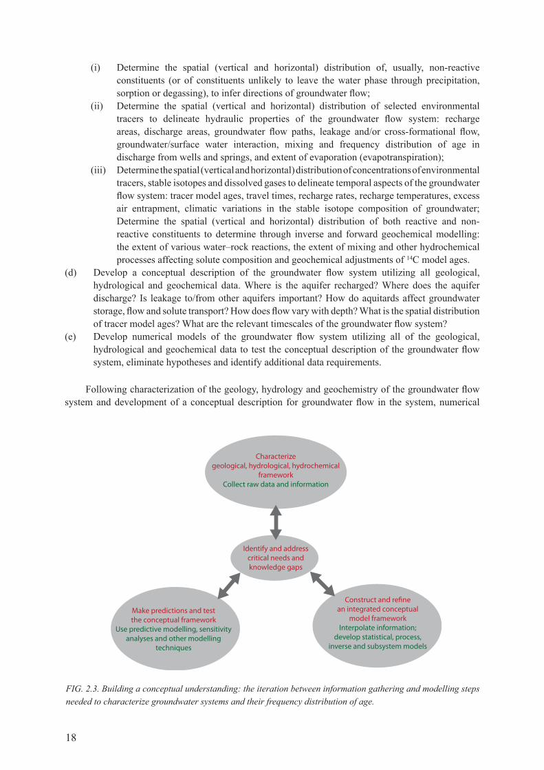
18

(i) determine  the  spatial  (vertical  and  horizontal)  distribution  of,  usually,  non-reactive constituents  (or  of  constituents  unlikely  to  leave  the water  phase  through  precipitation, sorption or degassing), to infer directions of groundwater flow;

(ii) determine  the  spatial  (vertical  and  horizontal)  distribution  of  selected  environmental tracers  to  delineate  hydraulic  properties  of  the  groundwater  flow  system:  recharge areas,  discharge  areas,  groundwater  flow  paths,  leakage  and/or  cross-formational  flow, groundwater/surface water interaction, mixing and frequency distribution of age in discharge from wells and springs, and extent of evaporation (evapotranspiration);

(iii) determine the spatial (vertical and horizontal) distribution of concentrations of environmental tracers, stable isotopes and dissolved gases to delineate temporal aspects of the groundwater flow system: tracer model ages, travel times, recharge rates, recharge temperatures, excess air entrapment, climatic variations in the stable isotope composition of groundwater; determine  the  spatial  (vertical  and  horizontal)  distribution  of  both  reactive  and  non-reactive constituents to determine through inverse and forward geochemical modelling: the extent of various water–rock reactions, the extent of mixing and other hydrochemical processes affecting solute composition and geochemical adjustments of 14c model ages.

(d) develop  a  conceptual  description  of  the  groundwater  flow  system  utilizing  all  geological, hydrological and geochemical data. where is the aquifer recharged? where does the aquifer discharge? Is  leakage  to/from other aquifers  important? How do aquitards affect groundwater storage, flow and solute transport? How does flow vary with depth? what is the spatial distribution of tracer model ages? what are the relevant timescales of the groundwater flow system?

(e) develop  numerical  models  of  the  groundwater  flow  system  utilizing  all  of  the  geological, hydrological and geochemical data  to  test  the conceptual description of  the groundwater flow system, eliminate hypotheses and identify additional data requirements.

following characterization of the geology, hydrology and geochemistry of the groundwater flow system and development of  a  conceptual description  for groundwater flow  in  the  system, numerical 

FIG. 2.3. Building a conceptual understanding: the iteration between information gathering and modelling steps needed to characterize groundwater systems and their frequency distribution of age.

Characterizegeological, hydrological, hydrochemical

frameworkCollect raw data and information

Identify and addresscritical needs andknowledge gaps

Make predictions and testthe conceptual framework

Use predictive modelling, sensitivityanalyses and other modelling

techniques

Construct and refinean integrated conceptual

model frameworkInterpolate information;

develop statistical, process,inverse and subsystem models

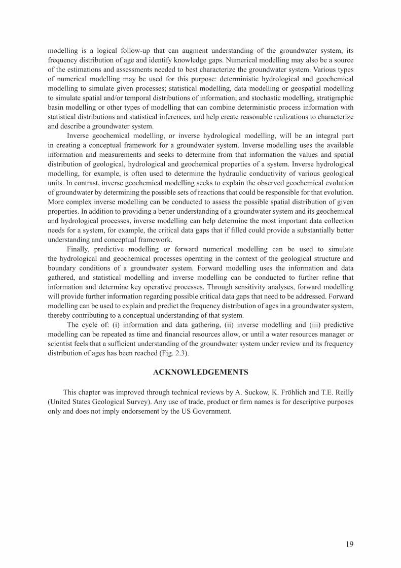
19

modelling  is  a  logical  follow-up  that  can  augment  understanding  of  the  groundwater  system,  its frequency distribution of age and identify knowledge gaps. Numerical modelling may also be a source of the estimations and assessments needed to best characterize the groundwater system. various types of numerical modelling may be used for this purpose: deterministic hydrological and geochemical modelling to simulate given processes; statistical modelling, data modelling or geospatial modelling to simulate spatial and/or temporal distributions of information; and stochastic modelling, stratigraphic basin modelling or other types of modelling that can combine deterministic process information with statistical distributions and statistical inferences, and help create reasonable realizations to characterize and describe a groundwater system.

Inverse geochemical modelling, or inverse hydrological modelling, will be an integral part in  creating  a  conceptual  framework  for  a groundwater  system.  Inverse modelling uses  the  available information  and measurements  and  seeks  to  determine  from  that  information  the  values  and  spatial distribution of geological, hydrological and geochemical properties of a system. Inverse hydrological modelling, for example, is often used to determine the hydraulic conductivity of various geological units. In contrast, inverse geochemical modelling seeks to explain the observed geochemical evolution of groundwater by determining the possible sets of reactions that could be responsible for that evolution. More complex inverse modelling can be conducted to assess the possible spatial distribution of given properties. In addition to providing a better understanding of a groundwater system and its geochemical and hydrological processes, inverse modelling can help determine the most important data collection needs for a system, for example, the critical data gaps that if filled could provide a substantially better understanding and conceptual framework.

finally, predictive modelling or forward numerical modelling can be used to simulate the hydrological and geochemical processes operating in the context of the geological structure and boundary conditions of a groundwater system. forward modelling uses the information and data gathered,  and  statistical  modelling  and  inverse  modelling  can  be  conducted  to  further  refine  that information and determine key operative processes. Through sensitivity analyses, forward modelling will provide further information regarding possible critical data gaps that need to be addressed. forward modelling can be used to explain and predict the frequency distribution of ages in a groundwater system, thereby contributing to a conceptual understanding of that system.

the cycle of: (i) information and data gathering, (ii) inverse modelling and (iii) predictive modelling can be repeated as time and financial resources allow, or until a water resources manager or scientist feels that a sufficient understanding of the groundwater system under review and its frequency distribution of ages has been reached (fig. 2.3).

ACknOWLEDGEMEnts

This chapter was improved through technical reviews by A. Suckow, K. fröhlich and T.E. reilly  (United States geological Survey). Any use of trade, product or firm names is for descriptive purposes only and does not imply endorsement by the us government.

21

Chapter 3

DEFInInG GROUnDWAtER AGE

t. torgersendepartment of Marine sciences, university of connecticut, groton, connecticut, united states of america

r. purtschertphysics Institute, university of bern, Bern, Switzerland

f.M. phIllIpsdepartment of earth and environmental science, new Mexico tech, socorro, new Mexico, united states of america

l.n. pluMMer, w.e. sanfordunited states geological survey, reston, Virginia, united states of america

A. SUcKowLeibniz Institute of Applied geophysics, hannover, germany

3.1. IntroductIon: why should groundwater be dated?

This book investigates applications of selected chemical and isotopic substances that can be used to recognize and interpret age information pertaining to ‘old’ groundwater (defined as water that was recharged on a timescale from approximately 1000 to more than 1 000 000 a). however, as discussed below, only estimates of  the ‘age’ of water extracted from wells can be inferred. These groundwater age estimates are interpreted from measured concentrations of chemical and isotopic substances in the groundwater. Even then, there are many complicating factors, as discussed in this book. In spite of these limitations, much can be learned about the physics of groundwater flow and about the temporal aspects of groundwater systems from age interpretations of measured concentrations of environmental tracers  in  groundwater  systems.  This  chapter  puts  the  concept  of  ‘age’  into  context,  including  its meaning and interpretation, and attempts to provide a unifying usage for the rest of the book.

3.2. wHAT doES ‘groUNdwATEr AgE’ mEAN?

The concept of an ‘idealized groundwater age’ (Δt) implies the time elapsed between when water entered  the  saturated  zone  (in  other  words,  when  it  entered  the  groundwater)  and  when  the  water was  sampled  at  a  specific  location  (x, y, z),  presumably  at  a  specific  distance  (Δs) downstream in

22

the groundwater system (fig. 3.1(a)). The  idea of  radiometric  ‘dating’ of groundwater was proposed as an extension of radiocarbon dating as applied to solid materials that contain carbon (such as wood, shells,  charcoal,  travertine)  (münnich  (1957)  [75]).  radiocarbon  dating  of  solids  usually  applies  to materials with a (presumably) well defined initiation time (e.g. the year a tree ring was laid down or a band of travertine precipitated). the difference between this initiation time and current time is the age of the sample. The atoms of carbon within the object are presumed to have remained fixed in place, with no new carbon added or old carbon lost, until the sample is analysed for its radiocarbon content. The  object  is  then  ‘dated’  by  applying  the  radioactive  decay  equation  using  the  current  measured radiocarbon content and assumed initial radiocarbon content. the interval of time calculated in this fashion is called the ‘14c  model  age’.  Provided  that  the  basic  assumptions  (the  initial  radiocarbon content amount and the presumption that atoms of carbon have been neither gained nor lost) are correct, the ‘14c model age’ should equal the actual age. However, in many cases, the basic assumptions are not valid and the 14c model age of the solid may significantly differ from its ‘true’ age.

groundwater literature has not always adequately distinguished the fundamental conceptual differences between the age of solid material and the age of groundwater that result from the mobile and mixable nature of water. As a result, much groundwater dating literature refers to an idealized concept of groundwater age (see above) which has a conceptual origin in what has been referred to as a ‘hydraulic age’  (davis and Bentley  (1982)  [76]). from darcy’s  law,  it  is known  that given  the permeability of a porous medium and the hydraulic gradient across it, one can calculate the specific discharge, and if the effective porosity  is  also known,  the average  interstitial velocity of  the water  can be calculated. by extrapolation, if the exact permeability distribution within an entire groundwater system and its distribution of hydraulic gradients are known, one can calculate velocity distributions and travel time from the water table to any given point within the system. the physics of groundwater movement, thus, dictates that any groundwater has travelled to its current location under a given set of physical conditions within a time frame determined by those conditions. this simple concept of groundwater movement has often been referred to as ‘piston’ flow. The difficulty of adequately characterizing the permeability distribution of subsurface materials has led to the measurement of environmental tracers as a means to estimate  this  ‘idealized groundwater age’. However, because solutes and  tracers disperse (mix)  in groundwater and because piston flow neglects many aspects of this dispersion and mixing, the information hypothetically contained within an estimate of such an ‘idealized groundwater age’ would still need to be  interpreted within a process context. consider,  for example,  the flow system depicted  in fig. 3.1, where the direction s  is  along  the  flow path  and  s┴1  and  s┴2  represent  orthogonal  directions  to  s. In  fig. 3.1,  (a)  equals  an  ‘idealized  groundwater  age’;  (Δt) would imply an elapsed time between the time water entered the saturated zone (when it entered the groundwater) and the time at which it was sampled at a specific position (x, y, z, t) at a specific distance (Δs) downstream in the groundwater basin. figure 3.1(b) shows, however, that even for 1-d systems, groundwater (even at the most minute sampling scale) represents a collection of water molecules that have individually undergone transport and mixing reactions along multiple transport paths as a result of, for example, longitudinal dispersive processes, creating water samples that alter any ‘idealized groundwater age’ to a frequency distribution. figure 3.1(c) shows that for more realistic 2-d and 3-d systems, additional transverse dispersion and finite sampling volumes may mix pathways of different lengths (possibly different recharge entryways) with the same velocity; or pathways with identical path lengths but different velocities. the net impact of 2-d and 3-d transverse dispersion is to create mixtures that affect the standard deviation about the mean of the frequency distribution of groundwater ages. figure 3.1(d) indicates that transverse dispersion will also ultimately mix (very, very old) aquitard groundwater with (old) aquifer groundwater. as aquitard groundwater is characterized by a distinctly older groundwater age, it will induce a long asymmetric tail on the old side of the sample frequency distribution of groundwater ages. figure 3.1(e) shows that the process of convergent mixing of different groundwater flows creates a mixture of component waters that is characterized by a bimodal probability distribution.

23

FIG. 3.1. The concept of groundwater dating represents levels of complexity. This is explained in the text below.

z Idealized groundwater age Aid

Δz

s(x,y,z), t(s)

s┴=0

p0

p1

Δx

Δz

s, t(s)

Δx, Δz ≠ 0

t

t

A

B

s┴≠0

y x

z

Δz

Δx

t

z

Δz

Δx

t

C

D

t

E

B+C+D+E….

Frequency distribution of idealized groundwater ages

Frequency distribution of idealized groundwater ages

Frequency distribution of idealized groundwater ages

Δx

idxzAppt =−Δ

→Δ→Δ)(lim 010,0

z

Δz

Δx

24

the following questions can be posed:— what if the groundwater arrived at position (x, y, z) mostly by flow in the s direction, but was

additionally under the influence of specific dispersive mixing parallel to the flow direction (Ds) as well as perpendicular to the flow direction (Ds┴1, Ds┴2)? How does simple flow and simple mixing influence the interpretation of an ‘idealized groundwater age’?

— what if the groundwater arrived at position (x, y, z) via flow from two (or more) similar but not identical entryway sources (figs 3.1(b) and 3.2)?

— how does multicomponent mixing from distinctly different source regions under convergent flow impact the meaning and interpretation of an ‘idealized groundwater age’ (fig. 3.1(e))?

— what if the groundwater system has not operated at a steady state, e.g. vs = f(t)? how does (would) the observed ‘idealized groundwater age’ at position x, y, z vary as a function of time (Δt = f(x, y, z, t)? when hydraulic heads may have varied significantly over the timescale of groundwater age, what if the groundwater arrived at position (x, y, z) via flow in a direction that is not equivalent to the currently defined flow direction? within the concept of this ‘idealized groundwater age’, a calculation of groundwater velocity in the s direction (vs) is possible but not meaningful in this context.

These examples illustrate that even within the simple definition of an ‘idealized groundwater age’, its interpretation in terms of the processes that control ‘idealized groundwater age’ remains complex. additionally, this illustrates an important concept:

— It is the net impact of all processes by which groundwater reaches the position (x, y, z, t) that determines groundwater age.

the corollary is:— The understanding of groundwater age at a specific location (x, y, z, t) requires knowledge of 

all processes by which groundwater flows to that specific location.These  considerations  demonstrate  that  a  more  physically  based  definition  of  groundwater  age 

is needed.

3.3. groundwater age dIstrIbutIon

‘Idealized  groundwater  age’  has  been  defined  above  as  the  elapsed  time  since  water  entered the  saturated  zone.  However,  samples  of  groundwater  are  finite  in  volume  and  contain  very  large numbers of molecules. In a bulk fashion, groundwater moves in response to spatial gradients in fluid potential. In addition to this, inasmuch as water is a fluid and the relative positions of molecules are not fixed, those molecules move in random paths as well as through bulk flow (fig. 3.2). These potential driven and entropy driven transport processes interact in a complex fashion to produce transport processes  variously  described  as  ‘advection’,  ‘diffusion’,  ‘hydrodynamic  dispersion’  and  so  on  (see Phillips  and  castro  (2003)  [77]  for  a  discussion  of  the  influence  of  various  transport  processes  on groundwater age tracers). one implication of groundwater transport is that the transport path of any individual molecule of water may (and almost certainly does) differ from the mean path obtained by averaging many molecules (fig. 3.1). (It is acknowledged that water molecules have a specific identity of  the order of picoseconds; for  this discussion,  this concept is  ignored.) The result  is  that any finite sized  sample of groundwater  contains water molecules  that have  resided  in  the  system  for differing periods of time. This being the case, a groundwater sample at a specific location cannot be adequately characterized by any single value of ‘age’; rather, it is characterized by a frequency distribution of ages (fig. 3.1(b), etc.).

The concept of fluid age defined by a frequency distribution of ages was introduced by danckwerts (1953) [78]. Since then, it has been widely applied in fluid dynamics, chemical engineering, atmospheric science,  oceanography  and  hydrology  (Hooper  (2003)  [79];  Loaiciga  (2004)  [80];  mcguire  and mcdonnell (2006) [81]). In the chemical engineering literature, the concept is generally referred to as 

25

the ‘residence time distribution function’. The residence time distribution is a mathematically rigorous and practically useful function (see references above for examples).

In  this  book,  ‘frequency distribution of  age’ will  generally  be  used  rather  than  ‘residence-time distribution’. This is simply to avoid confusion since ‘residence-time distribution’ has been traditionally used in the chemical engineering literature to refer to distribution in the discharge of a system, whereas distribution in a finite sample from within the system is generally being referred to. The mathematics of these two cases differs. małoszewski and zuber (1982) [82] have provided mathematical formulations applicable  to  frequency  distribution  of  age  in  groundwater  systems  and małoszewski  et  al.  (1983) [64]  show  examples  of  their  application. mcguire  and mcdonnell  (2006)  [81]  reviewed  analogous mathematical approaches  for  the outputs of drainage basins. goode  (1996)  [69] pioneered a flexible numerical approach to simulating age distributions in complex groundwater systems and Varni and carrera (1998) [83] estimated the frequency distribution of age at a single point.

an extreme example of frequency distribution for groundwater age would arise from an extensive, hydraulically uniform aquifer with a high recharge rate that is spatially localized (e.g. at a small outcrop area of the formation). this system will be advection dominated because the spatially uniform aquifer minimizes  the effects of dispersive mixing relative  to advective  transport and  the high  recharge  rate produces small gradients of groundwater age with flow distance. In the absence of convergent flowlines, the distribution of groundwater ages within a small sample of groundwater in this case will have a prominent mode with a relatively narrow distribution around that mode. as the ratio of dispersion to advection increases, the frequency distribution of ages (spread around the mode) increases.

Although  it  is  tempting  to characterize  the ‘age’ of a water sample by calculating some central tendency, unless the system is strongly advection dominated, this can yield quite misleading results. for example, imagine a small, rapidly recharged aquifer that is bounded by thick shale of extremely low permeability. the shale is still diffusing connate water (which was present when it was deposited in the cretaceous) into the aquifer. If 99.9% of the water discharged from the aquifer was recharged 5 years before the samplig date, and 0.1% is water from the shale (with an age of, for example, 65 million years), the average age of the discharge is 65 ka. This number conveys no useful information about  the system and is,  in fact, quite misleading if  taken at  face value. However, when a system is 

FIG. 3.2. A depiction of the role of dispersion in creating multipath routes from recharge to discharge in a 3-D groundwater system. Flow down the hydraulic head gradient produces decision points upon each encounter with the host grains of an aquifer. This probabilistic process creates dispersion in groundwater age arriving at position (Δx) downstream (Fig. 3.1(b)).

Path 1:

Path 2:

Path 3:

Path 4:

Δx

General groundwater flow direction

Path 1:

Path 2:

Path 3:

Path 4:

26

strongly advection dominated, an estimate of the mode of the frequency distribution of groundwater age can still provide useful information.

To summarize,  the ‘age’ of a groundwater sample  is a function of  the frequency distribution of the elapsed time since each of the individual water molecules crossed the water table (figs 3.1(b)–(d)). Unfortunately,  this  frequency  distribution  is  difficult  (to  impossible)  to  determine  for  groundwater systems, even in a coarse sense. for estimating groundwater ages, one must rely on either inferences from the concentration of chemical or isotopic tracers measured in a water sample, or on calculations based on  the physics of fluid mass  transport.  If  the  age  estimate  is obtained  from a  chemical  tracer measurement, then a conceptual/mathematical model must be employed to convert tracer concentrations into  an  age;  the  single  age  value  that  results  is  called  the  ‘tracer  based model  age’.  for  example, a groundwater age obtained using 14c-tracer data and the radioactive decay equation would be called a ‘tracer based model age’ or more specifically a ‘14c based model age’. This terminology reinforces the principle that calculated age is inseparable from the conceptual/mathematical model employed and the assumptions that model includes. It is, therefore, a useful measure of age only to the extent that the model corresponds to the characteristics of a system. following a not uncommon practice, the expression will be simplified (in a specific case) to ‘14c model age’ or (in a general case) ‘tracer model age’.

In the majority of cases, the mathematical models and assumptions employed to interpret tracer data do not include mixing processes and yield single values of tracer model ages (errors cited are typically associated with tracer measurement error and do not contain information about the frequency distribution of age). these single values of tracer model ages may correspond to the mean ages of age distributions, but  in most  cases probably do not. multiple  tracers,  combined with knowledge of the hydrogeology, can often aid in understanding (at least in a qualitative fashion) the relation between a single value of a tracer model age at a location and the frequency distribution of groundwater ages at that location.

3.3.1. Examples of groundwater age distribution

the examples given above illustrate possible forms of the frequency distribution of groundwater age in some simple hypothetical groundwater systems. several examples of frequency distributions in more realistic systems have been provided by numerical modelling.

As mentioned above, if an age estimate is obtained from application of the physics of fluid mass transport, it is called the ‘hydraulic age’, which represents one type of ‘flow model age’. In many cases, such calculations include only advective transport. In more complete models, additional processes may be included and in both cases a spatial distribution of ‘hydraulic ages’ may be calculated. An excellent example  of  this  approach  is  provided  by goode  (1996)  [69], who  illustrated  the  role  of  dispersion with a simple numerical groundwater flow model for a layered system (0–30 m, hydraulic conductivity is 10–5 m/s; 30–70 m, hydraulic conductivity is 10–6 m/s). figure 3.3(a) shows the hydraulic head contours  (0.2  m  contours)  of  a  simple  flow  system,  which  determine  the  streamlines  shown  in fig. 3.3(b). for a case involving only advection and no dispersion (fig. 3.3(c)), the groundwater age structure (10 a intervals) is noticeably different from a case of advection with dispersion (fig. 3.3(d); Dm = 1.16 × 10–8 m2/s; αL = 6 m, αT  =  0.6 m),  especially  at  the  boundary  of  the  slow  flow  region in  the  zone  of  upflowing  streamlines.  The  younger  ages  in  the  upflowing  streamline  region  under the advection with dispersion case (fig. 3.3(d)) are the result of dispersive mixing between slow moving streamlines and fast moving streamlines. The no-dispersion case (fig. 3.3(c)) results in a more isolated pocket of flow and older groundwater ages.

goode (1996) [69] and Bethke and johnson (2008) [84] generalized these dispersion mixing and convergent mixing issues that impact the transport and mixing processes in groundwater flow systems and that influence groundwater age distribution. for 1-d groundwater flow without dispersion (piston flow, fig. 3.1(a)),  groundwater  at  a  specific  location  should  result  in  a  single  idealized groundwater 

27

age. However, for groundwater flow with even 1-d longitudinal dispersion (in  the same direction as the  flow  velocity),  multiple  microscale  pathways  produce  a  frequency  distribution  of  groundwater ages. when 2-d and 3-d flow are included (fig. 3.2), transverse dispersion may mix: (i) pathways of different lengths (and possibly different recharge entryways) with the same velocity; or (ii) pathways with identical path lengths but different velocities. The net impact of 2-d and 3-d transverse dispersion is to create mixtures and increase the width of groundwater age distribution (fig. 3.1(c)).

for the longest timescale of flow, molecular diffusion may ultimately mix aquitard groundwater with the aquifer groundwater (fig. 3.1(d)). As aquitard groundwater is usually characterized by distinctly older ages, the mixing of aquitard water with aquifer water (noting the cretaceous shale example above) will induce a long asymmetric tail on the old side of age frequency distribution (fig. 3.1(d)). the frequency distribution of groundwater age is, thus, dependent upon how much aquitard water was incorporated and the frequency distribution of ages within the aquitard groundwater.

In addition  to simple dispersion  induced mixing, groundwater flow paths may also converge  to cause mixing; or an aquifer structure may induce mixing of groundwaters from layered aquifer systems. As illustrated in fig. 3.1(e), the process of convergent mixing of different groundwater flows creates a mixture of component waters that is characterized by a bimodal age distribution. Samples collected from pumping wells or springs are susceptible to even further turbulent mixing in the discharge conduit where the sample is collected.

FIG. 3.3. The results of Goode (1996) [69] showing a direct simulation of groundwater ages within a very simple aquifer where the upper 30 m of the aquifer has a hydraulic conductivity of 10–5 m/s and the lower 70 m has 10–6 m/s. (a) shows the hydraulic head contours (0.2 m contours) and the velocity vectors; (b) shows the streamlines from recharge to discharge; (c) shows simulated age contours for the advection only condition (no dispersion) with a 10 a contour interval; (d) shows simulated age contours with dispersion (see Goode (1996) [69] for a complete description of the simulation; from Goode 1996 [69], reproduced with permission of the American Geophysical Union).

28

3.4.  characterIstIcs of Ideal tracers

an ideal groundwater age tracer should exactly replicate the transport and mixing of the groundwater with which  it flows. As  such,  an  ideal  tracer:  (i)  should not be  subject  to  chemical  retardation with respect  to  the  water  flow;  (ii)  should  undergo mechanical  dispersion  identical  to  that  of  the  water molecules (and, thus, duplicate the frequency distribution of groundwater age); and (iii) should undergo molecular diffusion identical to that of the water molecules. an ideal groundwater tracer suitable for dating must then also change its concentration as a known and defined function of time from a defined initial condition to the location at which it can be sampled. the initial conditions for a tracer model age should be obtainable and should be established in the same location where the idealized groundwater age is zero. All of these attributes should result in the tracer, at the sampling location, having an age distribution that follows from the groundwater age distribution (e.g. for a radioactive tracer, this would correspond to the groundwater age distribution multiplied by the appropriate amount of decay for each age). In this context, the available choices of geochemical tracers suitable to dating needs are narrowed considerably; they are characterized by simple solubility controls, limited reactivity and known radioactive reaction rates for either ingrowth or decay (or in the case of stable tracers such as cfcs  (IAEA  (2006)  [85]),  known  variability  in  the  initial  condition,  simple  geochemistry  and  ‘no’ loss terms). with a known initial condition and a known reaction (such as radioactive decay or known production), the measured concentration of a tracer in a groundwater sample at location x, y, z, t can be converted into a tracer model age through a defined mathematical formula with specific assumptions.

however, the tracer model age is subject to interpretation (and potential complication) as a result of both dispersion controlled mixing and convergence controlled mixing. the interpretation of tracer

FIG. 3.4. The groundwater age of a water sample can be represented by some central measure of frequency distribution of ages (Figs 3.1(b) and (c)).

0

0.2

0.4

0.6

0.8

1

0 2 4 6 8 10

Tracer model age

Con

cent

ratio

n

weighted mix

tracermodel age

tmodel

tmix

Exponential decay

end member 1

end member 2

(b)

0

1

2

3

4

5

0 2 4 6 8 10

Tracer model age

Con

cent

ratio

n

end member 1

weighted mix

tmix = tmodel

Linear accumulation

end member 2

(a)

29

model age is functionally dependent upon whether the reaction term is linear, concave or convex versus distance/time and the timescale of the tracer.

for the case of a linearly changing (under ideal conditions, possibly 4he) tracer concentration with time (see fig. 3.4(a)), a mixture of young and old waters will create a mixture whose combined frequency distribution of groundwater ages accurately reflects the mixing and relative weighting of the old and the young water. however, for a tracer with exponential decay (such as 14c or 36cl), the mixing of old and a young groundwater will create a tracer mixture that is interpreted as younger than the weighted mean of  the  separate  tracer  ages  of  young  and old water would  imply  (see fig. 3.4(b)).  In  an  ideal world, the tracer model age (determined by some geochemical method) would be a true reflection of the  frequency distribution of groundwater  age. figure 3.4(a)  shows  that when a  tracer  increases  (or decreases) linearly with time (e.g. possibly 4he or a tracer the input of which is linearly changing as a function of time), a mixture of groundwaters with different ages would produce a mixed water whose tracer model age would be in agreement with the weighted mix of groundwater ages. however, fig. 3.4(b) shows that for a tracer whose variability with time is non-linear (typically exponential with time: 14c, 36cl, etc.), the effect of mixing (in this specific case) groundwaters with different ages would produce a tracer model age that does not agree with the weighted mix of groundwater ages. without independent  knowledge  of  what  was mixed  and  in  what  proportions,  it  is  not  possible  to  interpret a tracer model age unequivocally as a measure of the central tendency of the frequency distribution of groundwater age.

dispersion controlled mixing for tracers with concave functions such as radioactive decay will, therefore, always create conditions under which the tracer model age is an underestimate of the mean groundwater age; the degree of underestimation being a function of the degree of mixing and the decay constant.  for  convergence  controlled  mixing,  the  component  end members  are  likely  more  widely disparate in their groundwater age distributions and the impact of convergent mixing on the tracer will result in a greater difference between the mean (or mode) of groundwater age distribution and the tracer model age, again with the tracer model age being younger than the correctly interpreted mixture of component end member ages. tracer reaction rates and mixing end members must, therefore, be considered in the interpretation of tracer model ages. for cases in which the mean of the age distribution is not equal to the mode for the age distribution (e.g. fig. 3.1(d)), or where the age distribution is bimodal (fig. 3.1(e)), the interpretation of tracer model age and its relation to the mean or mode of age distribution becomes more complex.

3.5. addItIonal lIMItatIons on tracer Model ages

Under favourable circumstances, groundwater age can be characterized by some central measure (mean, median, mode) of the frequency distribution of groundwater ages within a groundwater sample (e.g. fig. 3.1(b)–(e)). however, because a groundwater sample has been aggregated (naturally or by some bias in the sampling protocol) via distinct and separate processes, interpreting some central tendency of distribution requires information on the nature of the distribution function. such information is difficult  to obtain for real world (as opposed to simulated, mathematically modelled) groundwater systems, and this greatly limits the ability to interpret single values of tracer model ages. to some extent, one can obtain information on the nature of age distribution via methods such as classical input–output  analysis  (Kirchner  et  al.  (2000)  [86]; mcguire  and mcdonnell  [81]  (2006); mcguire  et  al. (2005) [87]), interpretation of multiple tracers, especially radionuclides with a wide range of half-lives (castro et al. (2000) [88]), or numerical simulation of the system (castro and goblet (2003) [89]; Park et al. (2002) [90]; weissmann et al. (2002) [91]) and use these to help interpret individual tracer model ages, but even so the interpretations will have significant uncertainty associated with them.

It must be appreciated in groundwater dating that a single tracer model age is in fact a calculation that has a specific location/time associated with it (x, y, z, t), a specific initial condition and a specific Δs and Δt that delimit interpretation constraints. This means that only bulk properties between two flow 

30

connected sampling points can be quantified unless additional information is available from well tests, additional sampling, other tracers, other dating methods, etc. this implies that multiple measures along a flow path will provide more and better information if interpreted together rather than individually. It has been noted (Bethke and johnson (2008) [84]) that plots of tracer model age versus distance yield slopes in units of inverse velocity. such plots can be used to support the existence of a continuous flowline as well as discontinuities in flow velocity.

even when the conditions for appropriate application of a geochemical tracer for the calculation of a  tracer model age can be confirmed and appropriate  samples can be obtained,  the calculation of a tracer model age must still be interpreted with caution. a tracer model age is an interpretation and an approximation  that acknowledges all of  the assumptions,  idealizations and  limitations of a  tracer, as well as comparability of a tracer to the processes that determine groundwater age. due to aquifer heterogeneity, dispersive mixing, and other physical and chemical processes, macroscale groundwater age distribution cannot be defined by tracer model age. Still, tracer model ages provide information that helps constrain age distribution and the generalities of flow in groundwater systems.

3.6. TrAcErS IN THIS BooK

the tracers available for application and interpretation in terms of tracer model ages are limited for timescales greater than 1000 a. tracer model analysis of 4he, 14c, 36cl, 81Kr and 234u/238u provides valuable information and is discussed in the chapters that follow. however, the value of a tracer model age increases when two or more methodologies can be compared and contrasted in order to understand the relation between generally simplified assumptions inherent in tracer models and a more complex real system (see chapter 9).

The geochemical groundwater tracers discussed in this book (4he, 36cl, 14c, 81Kr, 234u/238u) have been used to calculate tracer model ages in multiple groundwater systems with sufficient cross checks to ensure at least a minimal level of confidence in the results. In the following chapters, tracer specific processes will be defined and discussed which contribute to the calculation of tracer model ages, as well as how various processes affect the interpretation of these tracer model ages. The ‘tracer model age’ will be referred to as a generality and in specific cases will refer to, for example, the ‘14c model age’ or the ‘4He model age’ to differentiate which specific tracer has been used and what specific model has been used to calculate the tracer model age.

the case studies discussed in the following chapters reinforce the principle that multiple sampling points with multiple tracers including temperature, water chemistry, hydraulic head, stable isotopes and well borehole tests will provide information that is generally necessary for adequately characterizing groundwater basins. these can then be interpreted with the aid of detailed mathematical reaction and transport models (‘flow model ages’). Additional constraints can often be imposed on the interpretation by optimizing hydraulic models to best simulate tracer transport data (Berger (2008) [92]). yet, even for the best tracers and the simplest groundwater systems, the system of equations describing reaction and  transport  in  a  groundwater  system  will  be  under-constrained.  In  order  to  solve  equations  that describe flow  in a groundwater basin, assumptions and simplifications must be made with  regard  to basin structure, the heterogeneity of basin properties and the evolution of a basin as a steady state or unsteady state flow system subject to temporally controlled uplift and erosion. given this complexity, simple physics based flow models (see castro et al. (2000) [88]; Torgersen and Ivey (1985) [93]) that include transport and mixing of groundwater as well as the source and sink functions that control tracer distribution  (Bethke  and  johnson  (2008)  [84]; Bethke  et  al.  (2000)  [94]; Bethke  et  al.  (1999)  [95]; castro and goblet (2003) [89]; castro et al. (1998) [96]; castro et al. (1998) [97]; zhao et al. (1998) [98]) are useful in evaluating the controls on groundwater movement and flow times.

flow in groundwater systems is typically dependent on a complex spatial distribution of hydraulic properties. data to constrain this distribution are generally sparse. the spatial distribution of hydraulic head is relatively insensitive to the distribution of hydraulic properties unless materials of differing

31

properties  are  arrayed  in  continuous  layers  of  strongly  contrasting  values  (gomez-Hernandez  and gorelick (1989) [99]). It is within this context that estimates of groundwater age via tracer model ages can provide  significant  constraints  on  the  structure  of  a  system. However,  even with  this  additional information,  groundwater  systems  are  always  under-constrained  with  regard  to  data  requirements and  the  resulting  models  are  always  non-unique.  To  some  extent,  this  limitation  can  be  overcome by employing geostatistically based multiple conditional simulations, but even this computationally intensive approach provides only an indication of the possible range of behaviour of a system. It benefits the conclusions of a study when groundwater scientists maintain an appropriate sense of complexity that exists in the natural systems they study.

32

APPEnDIx tO CHAPtER 3

age terMInology

old groundwater. water that was recharged on a timescale of greater than 1000 to  several  million  years;  a  practical  timescale  defined  by  the  tracers discussed in this book.

idealized groundwater age. the elapsed time between the time water entered the  saturated  zone  (when  it  entered  the  groundwater)  and  the  time the  same  water  was  sampled  in  a  specific  position  downstream  in the groundwater system.

frequency distribution of age. The  distribution  of  all  idealized  groundwater ages of all individual water molecules in a groundwater sample

tracer based model age or tracer model age. the single age value that is obtained from the application of a conceptual/mathematical model to a measurement of the concentration of a chemical tracer in a  groundwater  sample;  in  the  case  of  a  specific  tracer,  for  example, 14c model age

flow model age. A hydraulic age calculated within a flow model

hydraulic age. the single valued age estimate obtained from the application of physics of fluid mass transport in the groundwater system

mean age or average age. the mean age is the average age of all individual water molecules in a system or sample. In terms of the mass age concept, mean age is the sum of the product of fraction of water and age of that fraction for all water fractions/ages recognized in a system

33

Chapter 4

RADIOCARbOn DAtInG In GROUnDWAtER sYstEMs

l.n. pluMMer, p.d. glynnunited states geological survey, reston, Virginia, united states of america

“radiocarbon  dating  of  groundwater,  which  started  with  the  original  work  of  the  Heidelberg radiocarbon Laboratory  back  in  the  late  1950s,  is  certainly  one  of  the most —  if  not  the most — complicated and often questionable application of radiocarbon dating. the reason for this is to be found in the aqueous geochemistry of carbon in the unsaturated and saturated zones. Part of the carbon and radiocarbon content of dissolved carbon in groundwater is of inorganic and part is of organic origin.” (mook (1992) [100]).

4.1.  IntroductIon

the radioactive isotope of carbon, radiocarbon (14c), was first produced artificially  in 1940 by martin Kamen and Sam ruben, who bombarded graphite in a cyclotron at the radiation Laboratory at Berkeley, cA, in an attempt to produce a radioactive isotope of carbon that could be used as a tracer in biological systems (Kamen (1963) [101]; ruben and Kamen (1941) [102]). carbon-14 of cosmogenic origin was discovered in atmospheric co2 in 1946 by willard f. Libby, who determined a half-life of 5568 a. Libby and his co-workers (Anderson et al. (1947) [103]; Libby et al. (1949) [104]) developed radiocarbon dating of organic carbon of biological origin, which revolutionized research in a number of  fields,  including  archaeology  and  quaternary  geology/climatology,  by  establishing  ages  and chronologies of events that have occurred over the past approximately 45 ka.

cosmogenic 14c  is  produced  in  the  upper  atmosphere  by  the  nuclear  reaction  (mackay  (1961) [105]; mak et al. (1999) [106]):

14N + n → 14c + p  (4.1)

where 14c oxidizes to 14co and then 14co2, and mixes with the atmosphere. 14co2 is absorbed by plants  during photosynthesis  and becomes  incorporated  into  the Earth’s  biological  and hydrological cycles. the atmospheric mixing ratio of 14co2 is balanced by the rate of cosmogenic production, uptake by the various carbon reservoirs on Earth (atmosphere, oceans, marine organisms, plants) and radioactive decay. carbon-14 decays according to:

14c → 14n + ß−  (4.2)

with  a  generally  accepted  (consensus)  half-life  of  5730  ±  40  a  (godwin  (1962)  [107]).  chiu  et  al. (2007)  [108]  review  the various measurements of  14c half-life and suggest  that  the modern half-life may be underestimated by approximately 300 a.

the conventional radiocarbon age, t, in years is, by definition:

ln oAtA

τ=   (4.3)

34

whereτ   is the Libby mean-life (5568 a/ln 2, where 5568 is the Libby half-life);Ao is the initial 14c specific activity (in Bq/kg or mBq/g; 1 Bq = 1 disintegration per second);A is the measured 14c specific activity.

By  international  convention,  specific  activities  are  compared  to  a  standard  activity, Aox, where Aox = 0.95 times the specific activity of NBS oxalic acid (0.95 × 13.56 disintegrations per minute per gram of carbon (dpm/g c) in the year 1950 a.d.). the initial 14c specific activity, Ao, and the measured 14c specific activity of a sample, A, can be expressed as a percentage of this standard activity in per cent modern carbon (pmc) where pmc = (A/Aox) × 100 (mook (1980) [109]). The modern, pre-nuclear-detonation atmospheric 14c content is, by convention, 100 pmc, corresponding to 13.56 dpm/g c in the year 1950 A.d. (Stuiver and Polach (1977) [110]). conventional radiocarbon ages continue to be reported based on the Libby half-life, so as not to conflict with earlier studies, and 14c model ages are then defined  in  ‘radiocarbon years’. A  further complication  in  radiocarbon dating was  the discovery that the amount of 14co2 in the atmosphere has not been constant over time. past variations in the solar wind  and  the  geomagnetic fields  of  the  sun  and Earth  have  caused  variations  in  the flux of  cosmic rays reaching the earth, resulting in variations in the atmospheric concentration of 14co2 (Kalin (1999)  [111]).  It  is  likely  that  the  atmospheric  14c content has also changed in response to changes in the residence time of the major global reservoirs (terrestrial, biosphere and ocean). the discovery of past variations in the amount of atmospheric 14c  has  led  to  another  major  field  of  radiocarbon investigations in determining and refining radiocarbon calibration scales to convert radiocarbon years to calendar years. for example,  the  last glacial maximum (Lgm) occurred about 18 ka  radiocarbon years ago, which corresponds to about 21 ka calendar years (Bard et al. (1990) [112]). However, recent analysis of the Barbados sea level record places the Lgm at about 26 ka calendar years (Peltier and fairbanks (2006) [113]).

münnich  was  the  first  to  extend  radiocarbon  dating  to  dissolved  inorganic  carbon  (dIc)  in groundwater  (münnich  (1957)  [75];  münnich  (1968)  [114]).  over  the  past  50  years,  an  extensive literature of investigations and applications of radiocarbon in hydrological systems has followed. Many advances in collection and analysis of 14c have also followed and now 14c content is almost routinely determined on carbon samples as small as 1 mg by using accelerator mass spectrometry (aMs). Many of the original studies were reported in proceedings of symposia sponsored by the Isotope hydrology Section of the IAEA. A number of reviews summarize some of the advances, principles and problems in radiocarbon dating of dIc in groundwater (fontes (1983) [115]; fontes and garnier (1979) [116]; fontes (1992) [117]; geyh (2005) [118]; Kalin (2000) [111]; mook (1980) [109]; mook (2005) [119]). numerous studies have applied radiocarbon dating to establish chronologies of the (approximately) 0–40 ka  timescale  in hydrological systems,  to estimate modern and palaeorecharge rates  to aquifers, to recognize non-renewable palaeowaters, to extract palaeoclimatic information from the groundwater archive, to calibrate groundwater flow models, and to investigate the availability and sustainability of groundwater resources in areas of rapid population growth. It is beyond the scope of this chapter to review these many studies.

In spite of the many advances in collection, analysis and application of radiocarbon in the hydrological sciences, interpretation of the radiocarbon model age of dissolved carbon in groundwater is still limited by many uncertainties in determining the initial 14c content of dissolved carbon in recharge areas to aquifers and in accounting for the many chemical and physical processes that alter the 14c content along flow paths in aquifers. The purpose here is to summarize the current state of methods used to interpret 14c model age from measurements of 14c in dIc and dissolved organic carbon (doc) in groundwater.

historically, hydrologists and geochemists have resorted to simplifying assumptions regarding geochemical adjustments of radiocarbon in groundwater systems, often without sufficient data to know whether additional processes are needed to accurately date the dIc in groundwater systems. as many

35

geochemical interactions and hydrological processes in groundwater systems can affect radiocarbon content in aquifers, modern approaches to radiocarbon dating in groundwater systems are often treated within the context of geochemical modelling; that is, the study of geochemical evolution of water–rock systems. relatively large uncertainties in the 14c model age of dIc in groundwater systems remain, however, and as a result, although radiocarbon calibration is commonly applied to dating of biological carbon, such calibration is rarely warranted in radiocarbon dating of dIc in groundwater due to the many unknown geochemical and physical processes affecting the 14c content of dIc.

Bethke  and  johnson  (2008)  [84]  recently  distinguished  between  (i)  sample  age  calculated according  to  a  geochemical  age-dating  technique,  as  commonly  applied  in  ‘traditional’  radiocarbon adjustment models; and (ii) piston flow age, the time required to traverse a flowline from the recharge point  to  a  location  in  the  subsurface.  furthermore,  they  recognized  that  because  of  hydrodynamic processes occurring in aquifers, a groundwater sample is a collection of water molecules, each of which has its own age. Similarly, fontes (1983) [115] wrote:

“owing  to  dispersion,  the  ‘age’  of  a  groundwater  sample  corresponds  generally  to  a  time distribution of many elementary flows. Thus, except in the theoretical case of a pure piston flow system, or of stationary waters entrapped in a geological formation, the concept of groundwater age has little significance.”

These age concepts are discussed in chapter 3 in the context of this book.Although  hydrodynamic  processes  can  cause  difficulties  in  the  interpretation  of  tracer  model 

age, many hydrogeological settings have been investigated where radiocarbon dating has provided useful information on flow and recharge rates, and 14c model ages have been partially corroborated by concordance with other isotopic and environmental tracers on the 0–40 ka timescale. The interpretion of the 14c model age is provided below, where the model age is the 14c piston flow age calculated by a ‘traditional’ geochemical adjustment method that is applied to dIc. Then, some of the more advanced geochemical modelling  techniques  that  can help  refine a  14c model age and quantify hydrodynamic mixing on the basis of solution chemistry and isotopic compositions will be discussed. a discussion of advances in radiocarbon dating of doc follows. finally, the complexities of assessing the effects of diffusive processes and leakage from or through confining units will be examined.

this chapter reviews some of the past radiocarbon adjustment models, the conditions under which  they  apply,  and  summarizes  the  geochemical  modelling  approach  to  radiocarbon  dating  as implemented  in  the  inverse  geochemical modelling  code NETPATH  (Plummer  et  al.  (1994)  [120]) which applies radiocarbon dating to the total dissolved carbon (tdc) system (dIc + doc + ch4). In an effort not to obscure the presentation with too many equations and details, these have been placed in the Appendix to chapter 4, along with some example calculations. Units used in reporting radiocarbon measurements and conventional radiocarbon age are defined in the Appendix to chapter 4. Equations describing isotopic fractionation in  the carbonate system are summarized in  the Appendix to chapter 4, where they are generalized to systems of Tdc (dIc + doc + cH4). the appendix to chapter 4 also provides some guidance on radiocarbon calibration to calendar years. details pertaining to field sampling are provided as well as reference to available software used in radiocarbon dating of dIc in groundwater. finally, the Appendix to chapter 4 supplies a reference to selected AmS facilities providing radiocarbon determinations.

4.2.  InterpretatIon of radIocarbon age of dIssolVed InorganIc carbon In groundwater

carbon-14 of  cosmogenic origin  is  incorporated  in groundwater during  recharge by  interaction of  infiltrating  water  with  soil  co2 from plant root respiration and microbial degradation of soil organic  matter  (see,  for  example,  Kalin  (1999)  [111]).  following  recharge,  dIc  becomes  isolated 

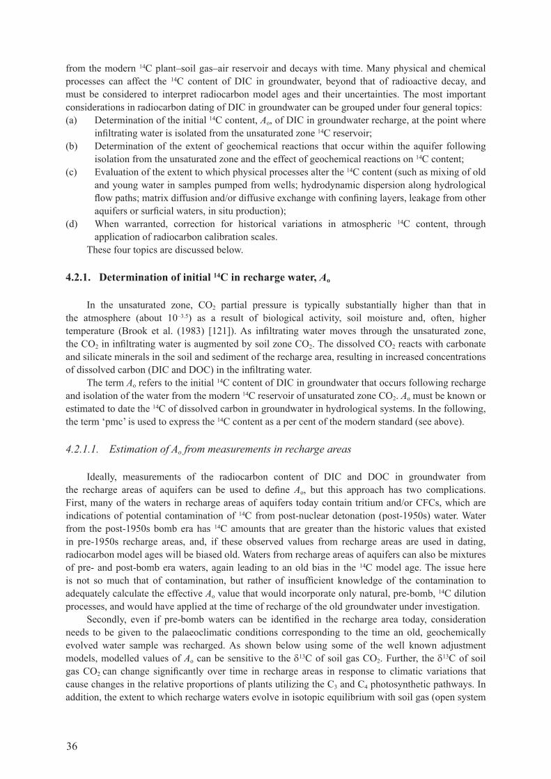
36

from the modern 14c plant–soil gas–air reservoir and decays with time. Many physical and chemical processes can affect the 14c content of dIc in groundwater, beyond that of radioactive decay, and must be considered to interpret radiocarbon model ages and their uncertainties. the most important considerations in radiocarbon dating of dIc in groundwater can be grouped under four general topics:(a) determination of the initial 14c content, Ao, of dIc in groundwater recharge, at the point where

infiltrating water is isolated from the unsaturated zone 14c reservoir;(b) determination of the extent of geochemical reactions that occur within the aquifer following

isolation from the unsaturated zone and the effect of geochemical reactions on 14c content;(c) evaluation of the extent to which physical processes alter the 14c content (such as mixing of old

and young water in samples pumped from wells; hydrodynamic dispersion along hydrological flow paths; matrix diffusion and/or diffusive exchange with confining layers, leakage from other aquifers or surficial waters, in situ production);

(d) when warranted, correction for historical variations in atmospheric 14c content, through application of radiocarbon calibration scales.

these four topics are discussed below.

4.2.1. Determination of initial 14C in recharge water, Ao

In  the  unsaturated  zone,  co2 partial pressure is typically substantially higher than that in the atmosphere (about 10–3.5) as a result of biological activity, soil moisture and, often, higher temperature  (Brook  et  al.  (1983)  [121]). As  infiltrating water moves  through  the  unsaturated  zone, the co2 in infiltrating water is augmented by soil zone co2. the dissolved co2 reacts with carbonate and silicate minerals in the soil and sediment of the recharge area, resulting in increased concentrations of dissolved carbon (dIc and doc) in the infiltrating water.

the term Ao refers to the initial 14c content of dIc in groundwater that occurs following recharge and isolation of the water from the modern 14c reservoir of unsaturated zone co2. Ao must be known or estimated to date the 14c of dissolved carbon in groundwater in hydrological systems. In the following, the term ‘pmc’ is used to express the 14c content as a per cent of the modern standard (see above).

4.2.1.1. Estimation of Ao from measurements in recharge areas

Ideally, measurements of the radiocarbon content of dIc and doc in groundwater from the  recharge  areas  of  aquifers  can  be  used  to  define Ao, but this approach has two complications. first, many of the waters in recharge areas of aquifers today contain tritium and/or cfcs, which are indications of potential contamination of 14c from post-nuclear detonation (post-1950s) water. water from  the post-1950s bomb era has  14c amounts that are greater than the historic values that existed in  pre-1950s  recharge  areas,  and,  if  these  observed  values  from  recharge  areas  are  used  in  dating, radiocarbon model ages will be biased old. waters from recharge areas of aquifers can also be mixtures of pre- and post-bomb era waters, again  leading  to an old bias  in  the  14c model age. the issue here is  not  so much  that  of  contamination,  but  rather  of  insufficient  knowledge  of  the  contamination  to adequately calculate the effective Ao value that would incorporate only natural, pre-bomb, 14c dilution processes, and would have applied at the time of recharge of the old groundwater under investigation.

Secondly,  even  if  pre-bomb waters  can  be  identified  in  the  recharge  area  today,  consideration needs to be given to the palaeoclimatic conditions corresponding to the time an old, geochemically evolved  water  sample  was  recharged. As  shown  below  using  some  of  the  well  known  adjustment models, modelled values of Ao can be sensitive to the δ13c of soil gas co2. further, the δ13c of soil gas co2 can  change  significantly  over  time  in  recharge  areas  in  response  to  climatic  variations  that cause changes in the relative proportions of plants utilizing the c3 and c4 photosynthetic pathways. In addition, the extent to which recharge waters evolve in isotopic equilibrium with soil gas (open system

37

evolution)  or  react  with  carbonates  following  recharge  (closed  system  evolution)  (clark  and  fritz (1997) [52]; deines et al. (1974) [122]) can lead to uncertainties in 14c model age of old groundwater as much as a full 14c half-life.  Isotopic  fractionation  in open and closed systems  is discussed  in  the Appendix to chapter 4. Even if it can be determined whether recharge waters presently evolve under open or closed system conditions, it is not known whether modern conditions prevailed when the old groundwater was recharged.

another assumption that is commonly made, and which is applicable in most but perhaps not all cases, is that the ‘recharge area’ of old groundwater was the same as that observed today. In some cases, differences in regional climate may have caused differences in the relative amounts of recharge from different areas over time. furthermore, modern water resource management activities can also affect the distribution of modern recharge. changes in aridity and other climatic factors in a recharge area over the timescale of an aquifer can cause changes in the distribution of c4 to c3 in plants, which can result in changes in the value of δ13c of soil gas co2. some of the models used to estimate values of Ao in recharge areas (see below) are quite sensitive to the value of δ13c of soil gas co2. finally, although geological and tectonic processes often have not had enough time to significantly alter the landscape of groundwater recharge over the 14c timescale, exceptions do occur.

still, if a set of groundwater samples can be obtained from the modern recharge area, or along a flow path, examination of the 14c content of dIc in relation to tritium (geyh (2005) [118]; Kalin (1999) [111]; verhagen  (1984)  [123]; verhagen  et  al.  (1974)  [124])  or  other  anthropogenic  environmental tracers, such as tritium and cfcs (IAEA (2006) [85]; Plummer et al. (2004) [49]; Plummer et al. (2004) [50]; Plummer and Busenberg (2000) [125]), or in relation to distance of flow in aquifers (geyh (2000) [126]; vogel (1970) [127]) can be used to estimate the modern, pre-bomb content of 14c.

figure 4.1 compares  14c specific activities of dIc, expressed as pmc, as a  function of cfc-12 and 3h concentrations for waters from recharge areas of the Middle rio grande basin aquifer system of New mexico, USA (Plummer et al. (2004) [50]). The data suggest that the pre-nuclear detonation content of 14c  of  dIc  in  recharge  areas  to  the  groundwater  system was  near  100  pmc.  carbon-14 values >100 pmc have cfc-12 piston flow ages from the mid-1960s for groundwater that  infiltrated 

FIG. 4.1. Carbon-14 content, expressed as pmc (per cent of the modern standard) of DIC in groundwater from the Middle Rio Grande Basin, NM, USA, as a function of (a) CFC-12 concentration (see graph in (b) for explanation of symbols) and (b) tritium.

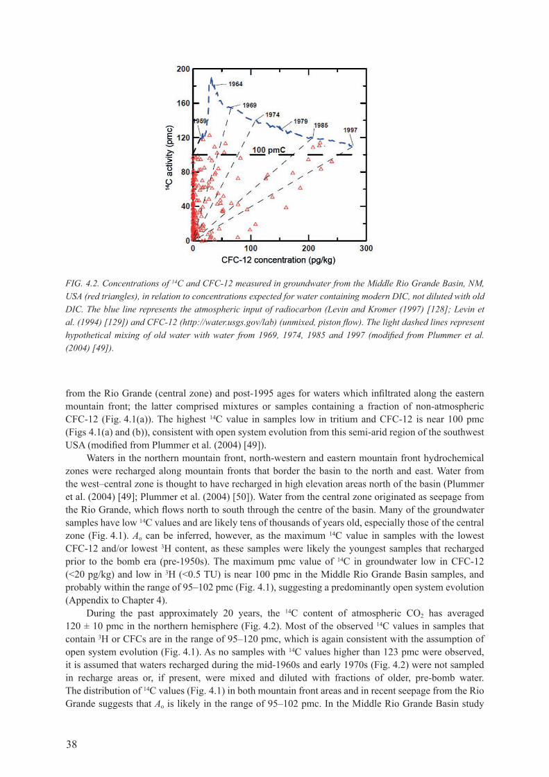
38

from the rio grande (central zone) and post-1995 ages for waters which infiltrated along the eastern mountain  front;  the  latter  comprised mixtures  or  samples  containing  a  fraction  of  non-atmospheric cfc-12  (fig. 4.1(a)). The highest  14c value  in  samples  low  in  tritium and cfc-12  is near 100 pmc (figs 4.1(a) and (b)), consistent with open system evolution from this semi-arid region of the southwest USA (modified from Plummer et al. (2004) [49]).

waters in the northern mountain front, north-western and eastern mountain front hydrochemical zones were  recharged along mountain  fronts  that border  the basin  to  the north and east. water  from the west–central zone is thought to have recharged in high elevation areas north of the basin (Plummer et al. (2004) [49]; Plummer et al. (2004) [50]). water from the central zone originated as seepage from the rio grande, which flows north to south through the centre of the basin. many of the groundwater samples have low 14c values and are likely tens of thousands of years old, especially those of the central zone  (fig. 4.1). Ao can be inferred, however, as the maximum 14c value in samples with the lowest cfc-12 and/or  lowest  3H content, as  these samples were  likely  the youngest samples  that recharged prior  to  the bomb era  (pre-1950s). The maximum pmc value of  14c  in groundwater  low  in cfc-12 (<20 pg/kg) and low in 3h (<0.5 tu) is near 100 pmc in the Middle rio grande basin samples, and probably within the range of 95–102 pmc (fig. 4.1), suggesting a predominantly open system evolution (Appendix to chapter 4).

during the past approximately 20 years, the 14c content of atmospheric co2 has averaged 120 ± 10 pmc in the northern hemisphere (fig. 4.2). most of the observed 14c values in samples that contain 3h or cfcs are in the range of 95–120 pmc, which is again consistent with the assumption of open system evolution (fig. 4.1). As no samples with 14c values higher than 123 pmc were observed, it is assumed that waters recharged during the mid-1960s and early 1970s (fig. 4.2) were not sampled in  recharge  areas  or,  if  present,  were  mixed  and  diluted  with  fractions  of  older,  pre-bomb  water. the distribution of 14c values (fig. 4.1) in both mountain front areas and in recent seepage from the rio grande suggests that Ao is likely in the range of 95–102 pmc. In the middle rio grande Basin study 

FIG. 4.2. Concentrations of 14C and CFC-12 measured in groundwater from the Middle Rio Grande Basin, NM, USA (red triangles), in relation to concentrations expected for water containing modern DIC, not diluted with old DIC. The blue line represents the atmospheric input of radiocarbon (Levin and Kromer (1997) [128]; Levin et al. (1994) [129]) and CFC-12 (http://water.usgs.gov/lab) (unmixed, piston flow). The light dashed lines represent hypothetical mixing of old water with water from 1969, 1974, 1985 and 1997 (modified from Plummer et al. (2004) [49]).

39

(Plummer et al. (2004) [49]; Plummer et al. (2004) [50]), a value of Ao equal to 100 pmc was assumed for all waters. the unadjusted 14c model  ages would decrease  by 400  a  if  a  value of Ao of 95 pmc were used instead of 100 pmc, and increase by 150 a if a value of Ao of 102 pmc were used instead of 100 pmc. these 14c model age differences are quite minor in comparison to uncertainties in age due to geochemical reactions.

4.2.1.2. Estimation of Ao using ‘traditional’ geochemical adjustment models

If geochemical reactions occur that affect the dIc, these reactions usually result in a lowering of the 14c content of dIc, independent of the radioactive decay of 14c. applied to the initial 14c value, the carbonate reactions will lower the adjusted value of Ao (termed And, where the subscript refers to ‘no decay’), resulting in adjusted 14c model ages that are younger than the unadjusted (or conventional) 14c model age. It is, therefore, important to recognize and quantify the effects of any geochemical reactions occurring that can affect the 14c content of dIc.

traditionally, hydrologists have applied models that account for some of the more important carbonate  reactions  that  occur  in  groundwater  systems  (Eichinger  (1983)  [130]; Evans  et  al.  (1979) [131];  fontes  (1983)  [115];  fontes  and  garnier  (1979)  [116];  fontes  (1992)  [117];  Ingerson  and Pearson jr. (1964) [132]; Kalin (1999) [111]; mook (1972) [133]; Tamers (1975) [134]) to the dIc of water from a single well to estimate adjusted 14c model ages  (fig. 4.3). Each  traditional adjustment model is based on a set of assumptions regarding chemical and isotopic fractionation reactions that may affect the dIc 14c content of a water sample, without radioactive decay of the 14c. the models produce an initial 14c value, Ao, that has been adjusted for geochemical reactions without accounting for radioactive decay (also denoted And). an effort is made in this publication to retain original notation; therefore, there is some redundancy in terminology. In the traditional approach to radiocarbon dating, values Ao or And, are compared to the measured 14c value in the decay equation to estimate 14c model age (fig. 4.3).

This  approach  is  best  suited  for  geochemical  systems  undergoing  relatively  simple water–rock reactions, such as usually occurs in shallow recharge areas, but, depending on the choice of model, can be applied to radiocarbon dating of dIc in groundwater systems undergoing carbonate mineral dissolution, gypsum dissolution, ca/na ion exchange, co2 gas dissolution and isotope exchange

FIG. 4.3. Conceptualization of the application of ‘traditional’ adjustment models in radiocarbon dating of DIC in groundwater. The models, such as those of Tamers, Fontes and Garnier, Mook, Ingerson and Pearson, Eichinger and others, are applied to a single water analysis in the system (Plummer and Sprinkle (2001) [135]).

40

between soil co2,  calcite  and dIc during  recharge. Some of  the well  known  traditional  adjustment models are described below.

The  geochemical  aspects  of  radiocarbon  dating  can  be  divided  into  two  parts:  (i)  definition  of the 14c content at an initial point in the system (Ao), such as in the recharge zone where water becomes isolated from the modern 14c reservoir and (ii) adjustment of this initial 14c value for chemical reactions occurring along the flow path to the final well where 14c content (A) has been measured (wigley et al. (1978) [136]). Traditionally, radiocarbon dating of groundwater has combined these two problems to develop an adjustment model that can be applied to a single water analysis at some point in the flow system. In this case, water chemistry, δ13c, and the 14c value of dIc are measured for a single water sample. an adjustment model accounting for inorganic reactions affecting the inorganic carbon reservoir is applied  to  the single water analysis  to define the 14c pmc value expected in the observed water if there were no radioactive decay of 14c. the adjusted 14c pmc value is compared to the measured 14c value through the radioactive decay equation to estimate the 14c model age of dIc in the water sample. time elapsed since recharge, t, is:

nd5730ln

ln 2A

tA

=

  (4.4)

where5730    is the modern half-life of 14c;And is the initial 14c content (pmc value) after adjustment for geochemical reactions without

radioactive decay, often referred to as Ao in traditional adjustment models;A is the measured 14c content (pmc value) in the sample.

the above decay equation differs from the conventional radiocarbon age in that Ao (and And) is no longer defined to be 100 pmc and the modern 14c half-life is used. To apply radiocarbon calibration scales,  the Libby  half-life  (5568  a)  is  used  or  age  is  converted  to  the Libby  half-life  (Appendix  to chapter 4). A series of adjustment models that have been used to estimate values of the adjusted initial 14c value in groundwater are summarized below. most of these models were discussed by fontes (1983) [115], fontes and garnier (1979) [116], fontes (1992) [117] and Kalin (1999) [111].

Vogel modelvogel (1967) [137] and vogel (1970) [138] assigned an estimate of 85 ± 5 pmc for Ao based on

approximately one hundred 14c measurements of dissolved carbon in groundwater from north-western Europe (fontes and garnier (1979) [116]), and isotope mass balance calculations that included isotope dilution and isotope exchange processes during recharge (vogel and Ehhalt (1963) [139]).

Tamers modelTamers  (1967)  [140]  assumed  that  the  initial  quantity  of  soil  zone  co2 containing 14co2 was

diluted  by  dissolution  of  radiocarbon-‘dead’  calcite  in  recharge  areas.  If  the  reactions  take  place  at approximately neutral to somewhat alkaline pH, where Hco! (and co2(aq)) are the predominant species, the reaction is:

caco3 + co2(aq) + h2o → ca2+ + 2hco! (4.5)

To a first approximation, half of the Hco! is derived from soil gas co2 (‘g’) and half from calcite (‘c’). Tamers assumed that co2(aq) (‘a’) was derived from soil gas co2. a carbon and 14c mass balance assuming ct = a + b (where ‘b’ is Hco!) is, following the notation of Kalin (1999) [111]:

Aotamersct = (a + 0.5b)Ag + 0.5bAc  (4.6)

41

or

Aotamers = [(a + 0.5b)Ag + 0.5bAc]/(a + b)  (4.7)

where A denotes the 14c pmc value.

owing to chemical equilibria in the carbonate solution, it is not exactly correct to assume that the quantity  ‘a’  (co2(aq)) is all from soil co2. a more general approach is to perform a carbon mass balance, assuming dIc was derived from soil co2, and carbonate minerals. this avoids the need to make assumptions about predominant species in the carbonate system.

the tamers model can be derived by using simple chemical and carbon isotope mass balance relations. the chemical evolution of precipitation (rain) in the calcite–co2 water system is as follows:

rain + co2 + calcite → groundwater composition  (4.8)

and the chemical mass balance relations are:

∆cdIc = ∆co2 + ∆calcite  (4.9)

and

∆ca = ∆calcite  (4.10)

where ∆ represents the change in moles, final (groundwater) minus initial (rain).

the 14c isotope mass balance is then:

Ao∆ct = Acalcite∆calcite + Aco2∆co2  (4.11)

and

Ao = (Acalcite∆calcite + Aco2 ∆co2)/∆ct ≡ Aotamers   (4.12)

The  Tamers  model  is  extended  in  NETPATH  (Plummer  et  al.  (1994)  [120])  to  the  co2–calcite–dolomite water system and to the co2–calcite–dolomite–gypsum water system. these are described below.

Tamers model in the CO2–calcite–dolomite–water systemhere, the carbonate minerals are assumed to be calcite and dolomite, and are referred to as the

‘Tamers model’, as implemented in NETPATH (denoted ‘Tamers, NP’). The geochemical reaction is:

rain + co2 + calcite + dolomite → groundwater composition  (4.13)

and the chemical mass balance relations are:

∆ct = ∆co2 + ∆calcite + 2∆dolomite  (4.14)

∆ca = ∆calcite + ∆dolomite  (4.15)

∆mg = ∆dolomite   (4.16)

Ao∆ct = Acalcite∆calcite + Aco2∆co2 + 2Adolomite∆dolomite  (4.17)

the solutions to these equations are as follows:

42

∆dolomite = ∆mg  (4.18)

∆calcite = ∆ca – ∆dolomite = ∆ca – ∆mg  (4.19)

∆co2 = ∆ct – ∆calcite – 2∆dolomite = ∆ct – ∆ca – ∆mg  (4.20)

Aotamers, np = [Acalcite(∆ca – ∆mg) + Aco2(∆ct – ∆ca – ∆mg) + 2Adolomite ∆mg]/∆ct  (4.21)

The term ‘∆’ represents the change in mass (moles) taken as final minus initial.

Tamers model in the CO2–calcite–dolomite–gypsum water systemthis model is another mass balance model implemented in netpath that is similar to

the previous modified Tamers model, but with the addition of a mass balance on So4, assumed from gypsum dissolution in the recharge area or soil, referred to as the ‘mass balance’ model in NETPATH (Plummer et al. (1994) [120]) (denoted ‘Tamers, mB’).

Aotamers, Mb = [Acalcite(∆ca – ∆mg – ∆So4) + Aco2(∆ct – ∆ca – ∆mg + ∆So4) + 2Adolomite ∆mg]/∆ct   (4.22)

Both modified forms of the Tamers model default to the Tamers model if there is no dissolution of dolomite or gypsum.

Pearson modelIngerson  and  Pearson  jr.  (1964)  [132]  solved  the  Tamers  model  for  the  dilution  of  soil  zone 

co2 by dissolution of carbonate minerals by using isotope mass balance relations for 13c and 14c (denoted ‘Pearson’):

δt∆dIc = δg∆g + δc∆c (13c isotope mass balance)  (4.23)

At∆dIc = Ag∆g + Ac∆c (14c isotope mass balance)  (4.24)

∆dIc = ∆g + ∆c (inorganic carbon mass balance)  (4.25)

g c t c t go pearson

c g

( ) ( )( )

A AA

δ − δ + δ − δ=

δ − δ  (4.26)

or

g c t co pearson c

g c

( )( )( )

A AA A

− δ − δ= +

δ − δ  (4.27)

whereA is 14c pmc value;δ is δ13c;and the subscripts t, g and c refer to total dIc, soil gas co2 and carbonate mineral(s), respectively, following the notation of fontes (1992) [117].

therefore, the tamers model and the pearson model account for the same processes; the tamers model finds a solution on the basis of chemical and 14c mass balance relations, and the pearson model uses only isotopic mass balance relations for 13c and 14c.

43

the tamers, mass balance and pearson models assume a simple mixing between co2 dissolved in soil water and carbon derived from the dissolution of carbonate minerals, with no other sources or sinks of carbon in the system. These assumptions imply that the groundwater evolves chemically and isotopically through dissolution of carbonate minerals under closed (to co2 gas exchange) conditions; that is, co2 enters the water in the unsaturated zone (open to co2 gas exchange) and carbonate minerals react in the saturated zone (closed to co2 gas exchange). although none of the mass balance models specifically  incorporate  isotope exchange,  it would be appropriate  to use values of δ13c and the 14c content of soil gas co2 as those in water in isotopic equilibrium with the soil gas, thus accounting for isotopic fractionation in dissolution of soil gas co2. examples of chemical and isotopic evolution of recharge waters in open conditions are provided in the Appendix to chapter 4. The remaining models (below) consider isotopic exchange.

Eichinger modelEichinger (1983) [130] modified the Pearson model (Eq. (4.26)) to include cases of partial isotopic 

exchange. The model is as follows, again following the notation of Kalin (1999) [111]1:

Aoeichinger = Aopearson× B  (4.28)

where

B = (δt – δe)/(δi – δe)  (4.29)

and

δi = [aδa + 0.5b(δa + δc)]/(a + b)  (4.30)

and

δe = [a(δc – εcb + εgb + εag) + b(δc – εcb)]/(a + b)  (4.31)

In  Eichinger’s model,  the  term Aopearson  is  the  Pearson model  (Eq.  (4.26)),  which  accounts  for the same geochemical processes as the tamers model, but is solved using 13c isotope mass balance relations, and δt is the measured value of δ13c of total dIc in the groundwater. the term δi estimates the value of δ13c of the total dIc after dissolution of the carbonate phase, but without any isotope exchange with carbonates. the term δe estimates the value of δ13c of the dIc if the groundwater is in isotopic equilibrium with the solid phase, where δc is δ13c of calcite, εcb is the additive fractionation factor between calcite and hco!, εgb is the additive fractionation factor between co2gas and hco!, and εag is the additive fractionation factor between co2(aq) and hco! (see the Appendix to chapter 4). the eichinger model only includes isotope exchange with the solid phase.

IAEA modelIn an IAEA study, Salem et al. (1980) [141] proposed that the Pearson model could be considered 

as a two step process: (i) equilibrium of the hco! with the gas phase followed by (ii) dissolution of solid carbonate. The equation is (fontes (1992) [117]):

t c g c g gb c co Iaea

g gb c

( )( ) ( )( )

A A AA

ε

ε

δ − δ − + δ − − δ=

δ − − δ  (4.32)

1 There  is  a  typographical  error  in Eq.  (10)  of Kalin  (1999)  [111] where  the  term δc should be replaced with δe, as above. further confusion regarding Eichinger’s equation was noted in Plummer et al. (1994) [120] and fontes (1992) [117], correcting a typographical error in Eichinger (1983) [130]. finally, although mathematically correct and programmed correctly in NETPATH, Plummer et al. (1994) [120] add to the confusion by erroneously defining the term δe.

44

As with  Pearson’s model,  this model  implies  that  all  chemical  reactions  can  be  accounted  for by the 13c isotopic composition of the end members (pure mixing), with one of them completely isotopically exchanged with the gas phase. the Iaea model can be solved in netpath by choosing the Pearson model and selecting the isotope mass balance model (‘mass balance with fractionation’) for definition of δ13c of soil gas co2. As pointed out by fontes (1992) [117], the IAEA model gives higher Ao values than the pearson model. In one numerical example, Ao  from Pearson’s model was approximately 58.2 pmc, but the IAEA model gave 96.2 pmc (fontes (1992) [117]).

Evans modelEvans  et  al.  (1979)  [131]  developed  a  model  to  account  for  isotopic  fractionation  during 

recrystallization  (dissolution–precipitation)  of  calcium  carbonate  in  groundwater.  It  is  assumed  that calcite is in isotopic equilibrium with dissolved hco!. Their equation, as modified by fontes (1992) [117] reduces to:

t cb coevans g c c

g cb c

( )( )

( )A A A A

εε

δ + − δ≈ − +

δ + − δ

  (4.33)

As pointed out by fontes (1992) [117], the modified model (Evans et al. (1979) [131]) is similar to Pearson’s model and produces Ao values similar to Pearson’s model despite the fact that the two models have quite different conceptualizations and derivations.

The Mook modelThe mook model (mook (1972) [133]; mook (1976) [142]; mook (1980) [109]) estimates Ao in

a step by step approach, considering partial or complete isotopic equilibration in the soil zone between co2 gas and all aqueous carbon bearing species, including part of the dissolving carbonate mineral (fontes  (1992)  [117]).  The  mook  model  is  more  appropriate  in  systems  in  which  reactions  with carbonate minerals are not dominant (fontes (1992) [117]; mook (1976) [142]). The mook model can be expressed as the Tamers model plus a correction term (fontes (1992) [117]). Here, the mook model is provided using the notation of Plummer et al. (1994) [120], which is mathematically equivalent to the form given by fontes and garnier (1979) [116]).

2 2 2 2

2 2

2 2 2 2

2 2

omook co aq co aq(o) co aq co aq(o) ls(o)

3( ) gb co aq(o) ls(o)

13 13 13 13co aq co aq(o) co aq co aq(o) ls(o)

13 3 13co g(o) gb co g(o)

0.5(1 )( )

( (1 2 10 ) 0.5( ))

c c 0.5(1 )( c c )

c (1 10 c ) 0.5

CO g o

A N A N A A

A A A

N N

ε

ε

−

−

= + − +

+ − × − +

δ − δ − − δ + δ×δ − + δ −

2

13 13co aq(o) ls(o)( c + c )δ δ

  (4.34)

whereN refers to the fraction of dIc represented by the subscripted species;the subscript o refers to the initial condition before isotope exchange;the subscript ls refers to limestone;and the subscript g refers to co2 gas.

Values of the additive fractionation factors (isotopic enrichment factor), εij are provided in the Appendix to chapter 4.

The Fontes and Garnier modelfontes and garnier (1979) [116] (see also fontes (1983) [115]; fontes (1992) [117]) present the 

‘global exchange–mixing model in closed system’ for estimation of Ao. this model considers the mixing of two end members, soil gas co2 and solid carbonate mineral, which is accompanied by a partial

45

isotopic exchange in a closed system during the mixing. the isotopic exchange is assumed to occur between a part of the co2 gas and calcite solid in the system (fig. 4.4), where q and q′ are the moles of calcite and co2gas that undergo complete isotopic exchange (with an isotopic enrichment factor, ε, between co2 gas and calcite). the partial isotope exchange in 13c (fontes and garnier (1979) [116]) is described by the following carbon isotope mass balance relations:

δtct = (cM – q)δM + (ct – cM)δg + q(δg – ε)    (4.35)

and

δtct = cM δM + (ct – cM – q' )δg + q' (δM + ε)  (4.36)

where (retaining the notation of fontes and garnier (1979) [116])δ is 13c content in ‰;c refers to carbon;t, M, g refer to total, solid carbonate and gas, respectively;q is the moles of solid carbonate in isotopic equilibrium with a part of the soil gas co2;q' is the moles of soil gas co2 in isotopic equilibrium with the solid carbonate;ε is the isotopic enrichment factor (additive fractionation factor) between co2 gas and solid

carbonate (εgc = δg – δc).

as q = – q', the isotope exchange is shown by:

q q= − =− − −

− −�

δ δ δ

δ δT T M M g T M

g M

C C (C C )

ε  (4.37)

where the sign of q indicates the direction of the exchange.

If q is positive, the isotopic exchange is dominated by gaseous co2, as might apply to infiltration water in contact with sediment that is low in carbonate mineral content in the soil zone, unsaturated zone or near the water table. calculated values of q that are less than zero imply that the isotopic exchange is dominated by solid carbonate mineral, as might be more common in the saturated zone. Both processes occur and the sign of q indicates which process predominates during the isotopic evolution.

FIG. 4.4. The global exchange-mixing model in a closed system (Fontes (1983) [115]; Fontes and Garnier (1979) [116]).

46

In fig. 4.4, cases 1 and 2 refer  to exchange controlled by gaseous co2 of isotopic composition δg, and solid carbonate (calcite) of isotopic composition δM, respectively. the variables q and q' are the molalities of calcite and co2gas that undergo complete isotopic exchange (with an enrichment factor ε between co2 and calcite). ct and cM are the molalities of dIc and dIc of mineral origin, respectively; this is taken from fontes and garnier (1979) [116].

The carbon isotope mass balance relations of fig. 4.4 can be written for 14c, prior to radioactive decay, so that Ao is:

A A A q A Ao T M M T M g g MC = C + (C C )− + − −( . )0 2ε (4.38)

whereA is the 14c pmc value;ε14c(%)≅ 0.2 ε13c(‰) (see craig (1954) [143] and the Appendix to chapter 4).

In developing their model, fontes and garnier (1979) [116] apply a chemical mass balance similar to that of the tamers model, with provision for base exchange (ca/na cation exchange) and gypsum dissolution to estimate the mass of carbon dissolved from inorganic sources, cM. fontes (1992) [117] shows  that  the  fontes  and garnier  (1979)  [116] model  reduces  to  the Tamers model  if  there  is  no isotopic exchange (k = 0):

of-g oTamersA A k= +   (4.39)

or

2

M Mof-g co g m

dIc dIc

c c1

c cA A A k= − + +

(4.40)

whereCM is the moles of carbon from carbonate mineral dissolution;CdIc is the moles of total dIc in the groundwater sample;Aco2g is the 14c value of co2 gas;AM is the average 14c pmc value of the carbonate minerals dissolving;

and

k A A= − −

− − −

−( )

CO g i j M

DICM

DICM

M

DIC

2

CCC

CCC

C0 2

113 13 13

. εδ δ δ CCO

CO i j M

2 g

2 gC Cδ δ13 13− −−

ε

(4.41)

where εi–j refers to the additive fractionation factor (also referred to as the isotopic enrichment factor; see Appendix to chapter 4) between species i and j.

In  using  the model  of  fontes  and garnier  (1979)  [116], k  is  first  solved  by  using  the  additive fractionation factor, εco2g–hco! (≅ δ13cco2g

– δ13chco! at isotopic equilibrium). If k is positive, then the exchange is primarily between co2gas and hco!, and Ao is calculated by using the value of k based on εco2g–hco!. If k is negative, the reaction is dominated by isotopic exchange between calcite and bicarbonate, and the additive fractionation factor is replaced with the value of εcalcite–hco! (appendix to chapter 4), (≅ δ13ccalcite – δ13chco! at isotopic equilibrium).

In  application  to  recharge waters,  the model of  (fontes  and garnier  (1979)  [116])  often yields quite reasonable estimates of Ao, but it is sensitive to values of δ13c of soil gas co2, which are often not

47

available. therefore, several models are available in netpath to estimate the δ13c of soil gas co2, as described below.

4.2.1.3. Models to estimate the δ13C of soil gas CO2

The models  of  Ingerson  and Pearson, Evans,  IAEA, mook, fontes  and garnier,  and Eichinger all require a definition of δ13c of soil gas co2. In the absence of measurement, several models were implemented in NETPATH (Plummer et al. (1994) [120]) to estimate values of δ13c of soil gas co2. These  are:  (i)  user  defined;  (ii)  closed  system  mass  balance  without  fractionation;  (iii)  a  two-step process in which the mass balance is solved by assuming that co2 gas dissolved into the initial water maintaining isotopic equilibrium with the dissolved co2 (aq) (open system), followed by carbonate dissolution in a closed system; and (iv) a complete open system in which the δ13c of soil gas co2

is calculated corresponding to isotopic equilibrium with the chemical and isotopic composition of the initial solution.

Model 1model 1, ‘user defined’, is used if δ13c measurements of soil gas co2 are available or if there is

climatic  evidence  that  the palaeo-δ13c of soil gas co2, at the time the water sample was recharged, differed from today.

Model 2Model 2 solves a carbon isotope mass balance without isotopic fractionation for the case of

dissolution of co2 gas, calcite, dolomite and gypsum:

2

2g

13 13 1313 dIc dIc calcite calcite dolomite dolomite

co aq(o)co

c c c 2 cc δ −Δ δ − Δ δδ =

Δ (4.42)

and

2 2

13 13co g(o) co aq(o)c cδ ≡ δ (4.43)

Model 3Model 3 solves the same carbon isotope mass balance as in model 2, but assumes that the dissolved

co2 is in isotopic equilibrium with the soil gas:

2 2 2 2

13 13co g(o) co aq(o) co g-co aqc c εδ ≡ δ + (4.44)

model 3 applies to recharge through an unsaturated zone devoid of carbonate minerals, followed by subsequent carbonate mineral dissolution in the saturated zone (closed system dissolution).

Model 4model 4 assumes that the recharge water evolved under open system conditions:

2 2 –

13 13co g(o) dIcc c

g sCOεδ ≡ δ + (4.45)

where εco2g–s is the ph dependent isotopic enrichment factor between co2 gas and the dIc of the aqueous solution (see wigley et al.  (1978) [136] and the Appendix to chapter 4). models 3 and 4  tend to be the most realistic. model 4 can apply, among other scenarios, to semi-arid regions with low recharge rates through carbonate bearing unsaturated zones.

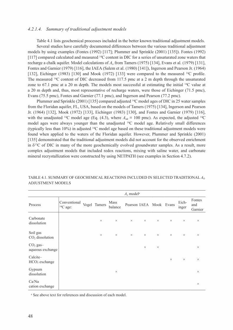
48

4.2.1.4. Summary of traditional adjustment models

Table 4.1 lists geochemical processes included in the better known traditional adjustment models.several studies have carefully documented differences between the various traditional adjustment

models by using examples (fontes (1992) [117]; Plummer and Sprinkle (2001) [135]). fontes (1992) [117] compared calculated and measured 14c content in dIc for a series of unsaturated zone waters that recharge a chalk aquifer. model calculations of Ao from Tamers (1975) [134], Evans et al. (1979) [131], fontes and garnier (1979) [116], the IAEA (Salem et al. (1980) [141]), Ingerson and Pearson jr. (1964) [132],  Eichinger  (1983)  [130]  and mook  (1972)  [133] were  compared  to  the measured  14c  profile. the measured 14c content of dIc decreased from 117.5 pmc at a 2 m depth through the unsaturated zone  to 67.1 pmc at a 20 m depth. The models most successful at estimating  the  initial  14c value at a 20 m depth and, thus, most representative of recharge waters, were those of eichinger (71.5 pmc), evans (75.5 pmc), fontes and garnier (77.1 pmc), and Ingerson and pearson (77.2 pmc).

Plummer and Sprinkle (2001) [135] compared adjusted 14c model ages of dIc in 25 water samples from the floridan aquifer, fL, USA, based on the models of Tamers (1975) [134], Ingerson and Pearson jr.  (1964)  [132], mook  (1972)  [133], Eichinger  (1983)  [130],  and fontes  and garnier  (1979)  [116], with the unadjusted 14c model age  (Eq.  (4.3), where And ≡ 100 pmc). As expected,  the adjusted  14c model ages were always younger than the unadjusted 14c model age. relatively small differences (typically less than 10%) in adjusted 14c model age based on these traditional adjustment models were found when  applied  to  the waters  of  the  floridan  aquifer.  However,  Plummer  and  Sprinkle  (2001) [135] demonstrated that the traditional adjustment models did not account for the observed enrichment in δ13c of dIc in many of the more geochemically evolved groundwater samples. as a result, more complex adjustment models that included redox reactions, mixing with saline water, and carbonate mineral recrystallization were constructed by using NETPATH (see examples in Section 4.7.2).

TABLE 4.1. SUmmAry of gEocHEmIcAL rEAcTIoNS INcLUdEd IN SELEcTEd TrAdITIoNAL Ao adjustMent Models

Ao modela

process conventional 14c age: Vogel tamers Mass

balance pearson Iaea mook evans Eich-inger

fontes and garnier

carbonate dissolution × × × × × × × ×

soil gas co2 dissolution × × × × × × × ×

co2 gas–aqueous exchange × × ×

calcite–hco! exchange × × ×

gypsum dissolution × ×

ca/na cation exchange ×

a see above text for references and discussion of each model.

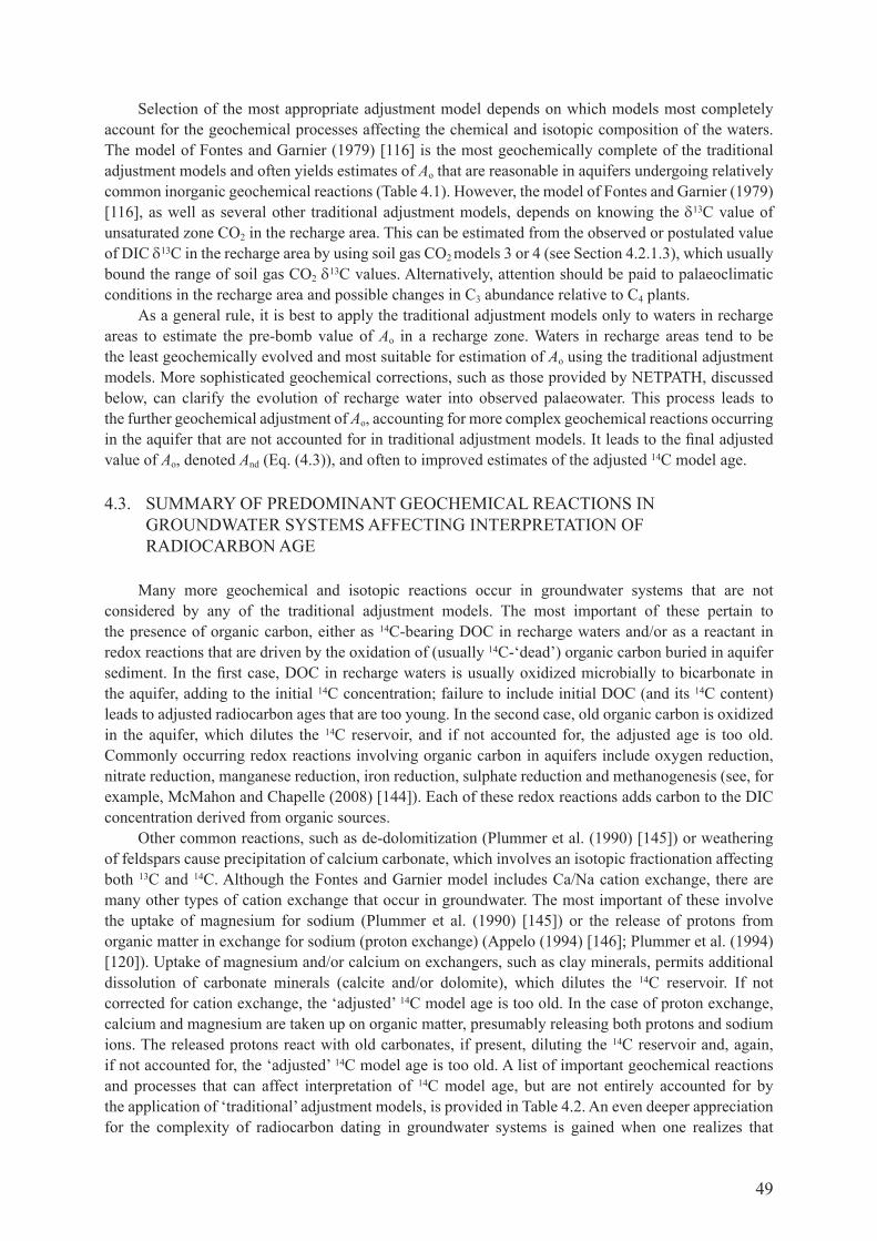
49

selection of the most appropriate adjustment model depends on which models most completely account for the geochemical processes affecting the chemical and isotopic composition of the waters. The model of fontes and garnier (1979) [116] is the most geochemically complete of the traditional adjustment models and often yields estimates of Ao that are reasonable in aquifers undergoing relatively common inorganic geochemical reactions (Table 4.1). However, the model of fontes and garnier (1979) [116], as well as several other  traditional adjustment models, depends on knowing the δ13c value of unsaturated zone co2 in the recharge area. this can be estimated from the observed or postulated value of dIc δ13c in the recharge area by using soil gas co2 models 3 or 4 (see Section 4.2.1.3), which usually bound the range of soil gas co2 δ13c values. alternatively, attention should be paid to palaeoclimatic conditions in the recharge area and possible changes in c3 abundance relative to c4 plants.

as a general rule, it is best to apply the traditional adjustment models only to waters in recharge areas  to  estimate  the  pre-bomb value  of Ao  in  a  recharge  zone. waters  in  recharge  areas  tend  to  be the least geochemically evolved and most suitable for estimation of Ao using the traditional adjustment models. More sophisticated geochemical corrections, such as those provided by netpath, discussed below, can clarify the evolution of recharge water into observed palaeowater. this process leads to the further geochemical adjustment of Ao, accounting for more complex geochemical reactions occurring in the aquifer that are not accounted for in traditional adjustment models. It leads to the final adjusted value of Ao, denoted And (Eq. (4.3)), and often to improved estimates of the adjusted 14c model age.

4.3.  suMMary of predoMInant geocheMIcal reactIons In groundwater systeMs affectIng InterpretatIon of radIocarbon age

Many more geochemical and isotopic reactions occur in groundwater systems that are not considered by any of the traditional adjustment models. the most important of these pertain to the presence of organic carbon, either as 14c-bearing doc in recharge waters and/or as a reactant in redox reactions that are driven by the oxidation of (usually 14c-‘dead’) organic carbon buried in aquifer sediment. In the first case, doc in recharge waters is usually oxidized microbially to bicarbonate in the aquifer, adding to the initial 14c concentration; failure to include initial doc (and its 14c content) leads to adjusted radiocarbon ages that are too young. In the second case, old organic carbon is oxidized in the aquifer, which dilutes the 14c reservoir, and if not accounted for, the adjusted age is too old. commonly occurring redox reactions involving organic carbon in aquifers include oxygen reduction, nitrate reduction, manganese reduction, iron reduction, sulphate reduction and methanogenesis (see, for example, mcmahon and chapelle (2008) [144]). Each of these redox reactions adds carbon to the dIc concentration derived from organic sources.

other common reactions, such as de-dolomitization (Plummer et al. (1990) [145]) or weathering of feldspars cause precipitation of calcium carbonate, which involves an isotopic fractionation affecting both 13c and 14c. although the fontes and garnier model includes ca/na cation exchange, there are many other types of cation exchange that occur in groundwater. the most important of these involve the  uptake  of magnesium  for  sodium  (Plummer  et  al.  (1990)  [145])  or  the  release  of  protons  from organic matter in exchange for sodium (proton exchange) (Appelo (1994) [146]; Plummer et al. (1994) [120]). Uptake of magnesium and/or calcium on exchangers, such as clay minerals, permits additional dissolution of carbonate minerals (calcite and/or dolomite), which dilutes the 14c reservoir. If not corrected for cation exchange, the ‘adjusted’ 14c model age is too old. In the case of proton exchange, calcium and magnesium are taken up on organic matter, presumably releasing both protons and sodium ions. the released protons react with old carbonates, if present, diluting the 14c reservoir and, again, if not accounted for, the ‘adjusted’ 14c model age is too old. a list of important geochemical reactions and processes that can affect interpretation of 14c model age, but are not entirely accounted for by the application of ‘traditional’ adjustment models, is provided in Table 4.2. An even deeper appreciation for  the  complexity  of  radiocarbon  dating  in  groundwater  systems  is  gained when  one  realizes  that 

50

TABLE

 4.2. SU

mmAry

 of 

SELE

cTE

d c

HEm

IcAL ANd P

HySIcAL 

ProcES

SES 

IN g

roUNdwAT

Er S

yST

EmS AffEc

TINg INTE

rPr

ETAT

IoN o

f r

ad

Ioc

ar

bo

n a

ge

(in a

dditi

on to

thos

e lis

ted

in T

able

4.1

)

proc

ess/

reac

tion

res

ultin

g w

ater

type

effe

ct o

n δ1

3 cef

fect

on

14c

effe

ct o

n un

adju

sted

age

dis

solu

tion

of c

alci

te a

nd d

olom

ite

(mar

ine

carb

onat

es)

ca–

Mg–

hc

o3

Incr

ease

in δ

13c

; iso

tope

dilu

tion

dec

reas

e in

14c

; iso

tope

dilu

tion

old

bia

s

cas

o4 d

isso

lutio

n (n

ot a

car

bon

sour

ce),

calc

ite p

reci

pita

tion

ca–

so4–

hc

o3

smal

l dec

reas

e in

δ13

c a

s 13c

is

enr

iche

d in

cal

cite

cem

ent;

isot

ope

frac

tiona

tion

smal

l dec

reas

e in

14c

of d

Ic a

s 14

c is

enr

iche

d in

cal

cite

cem

ent;

isot

ope

frac

tiona

tion

old

bia

s

cas

o4 d

isso

lutio

n (n

ot a

car

bon

sour

ce),

dolo

mite

dis

solu

tion

and

calc

ite

precipitation; de-dolomitization

ca–

Mg–

so4–

hc

o3

Incr

ease

in δ

13c

if d

olom

ite e

nric

hed

in 13

c, a

lso

slig

htly

opp

osite

tren

d fr

om c

alci

te c

emen

t for

mat

ion;

is

otop

e fr

actio

natio

n

dec

reas

e in

14c

; iso

tope

dilu

tion;

is

otop

e fr

actio

natio

no

ld b

ias

ca/

na

exch

ange

, Mg/

na

exch

ange

, pro

ton

exch

ange

(car

bona

te d

isso

lutio

n)n

a–h

co

3In

crea

se in

δ13

c; i

soto

pe d

ilutio

nd

ecre

ase

in 14

c; i

soto

pe d

ilutio

no

ld b

ias

recrystallization of calcite (aragonite, 

Mg–

calc

ites)

; iso

topi

c ex

chan

ge (c

alci

te)

no

chan

ge (i

ncre

ase

in s

r, M

g fr

om a

rago

nite

and

M

g ca

lcite

)In

crea

se in

δ13

c; i

soto

pe e

xcha

nge

dec

reas

e in

14c

; iso

tope

exc

hang

eo

ld b

ias

oxi

datio

n of

org

anic

mat

ter:

fe re

duct

ion

(feo

oh

)In

crea

se in

fe2+

and

hc

o!

dec

reas

e in

δ13

c; i

soto

pe d

ilutio

nd

ecre

ase

in 14

c; i

soto

pe d

ilutio

no

ld b

ias

oxi

datio

n of

org

anic

mat

ter;

sulp

hate

reduction (pyritization)

dec

reas

e in

so

4, po

ssib

le

incr

ease

in h

2s, d

ecre

ase

in f

e2+d

ecre

ase

in δ

13c

; iso

tope

dilu

tion

dec

reas

e in

14c

; iso

tope

dilu

tion

old

bia

s

ferm

enta

tion

of o

rgan

ic m

atte

r; m

etha

noge

nesi

sIn

crea

se in

ch

4 and

co

2In

crea

se in

δ13

c o

f co

2, de

plet

ed

ch

4; is

otop

e di

lutio

nd

ecre

ase

in 14

c; i

soto

pe d

ilutio

no

ld b

ias

dis

solu

tion

of p

lagi

ocla

se fe

ldsp

ar; d

isso

lutio

n of

oth

er p

rimar

y si

licat

es (c

alci

te p

reci

pita

tion)

na–

ca–

hc

o3

smal

l dec

reas

e in

δ13

c a

s 13c

is

enr

iche

d in

cal

cite

cem

ent;

isot

ope

frac

tiona

tion

smal

l dec

reas

e in

14c

as 1

4 c

is e

nric

hed

in c

alci

te c

emen

t; is

otop

e fr

actio

natio

nM

inor

or n

one

51

Leakage of saline waters (may cause 

carb

onat

e di

ssol

utio

n)n

a–c

lsm

all i

ncre

ase

in δ

13c

; is

otop

e di

lutio

nsm

all d

ecre

ase

in 14

c;

isot

ope

dilu

tion

old

bia

s

Leakage or exchange with aquitards; diffusion, 

mat

rix d

iffus

ion

Mul

tiple

Varia

ble

dec

reas

e in

14c

; iso

tope

dilu

tion

old

bia

s

add

ition

of c

o2 o

f mag

mat

ic o

rigin

(g

eoge

nic

co

2)M

ultip

leg

ener

ally

enr

iche

d in

δ13

c, r

ange

fr

om –

2 to

–6‰

dec

reas

e in

14c

; iso

tope

dilu

tion

old

bia

s

war

min

g al

ong

a ge

othe

rmal

gra

dien

t; ca

lcite

di

ssol

utio

n (c

lose

d sy

stem

)sm

all i

ncre

ase

in c

a2+

and

hc

o!

smal

l inc

reas

e in

δ13

c;

isot

ope

dilu

tion

smal

l dec

reas

e in

14c

; is

otop

e di

lutio

no

ld b

ias

Incr

ease

in h

ydro

stat

ic p

ress

ure

with

dep

th;

calc

ite d

isso

lutio

nsm

all i

ncre

ase

in c

a2+

and

hc

o!

smal

l inc

reas

e in

δ13

c;

isot

ope

dilu

tion

smal

l dec

reas

e in

14c

; is

otop

e di

lutio

no

ld b

ias

evap

otra

nspi

ratio

nIn

crea

se in

all

solu

tes i

n pr

opor

tion

to o

rigin

al w

ater

non

en

one

non

e

52

multiple reactions and processes, such as those listed in Table 4.2, often occur together or in sequence along flow paths in aquifers.

4.4.  generalIZed geocheMIcal adjustMent Models

wigley  et  al.  (1978)  [136]  and wigley  et  al.  (1979)  [147]  describe  the  chemical  and  isotopic evolution of inorganic carbon in groundwater by the differential equations:

Carbon mass balance

dIc1 1

( )N M

i ii i

d m dI dO= =

= −∑ ∑

(4.46)

Carbon isotope mass balance

*dIc

1 1( )

N M

i i s ii i

d Rm R dI R dOα −= =

= −∑ ∑   (4.47)

whereR is the isotope ratio;mdIc is the molality of dIc;I and O refer to incoming and outgoing moles of carbon, such as through dissolution and

precipitation, respectively;N and M are the total number of incoming and outgoing phases;i refers to the ith carbon-bearing phase;superscript * refers to the incoming phases;αi–s is the fractionation factor between the ith phase and the aqueous solution (adjusted

for ph effects on the distribution of inorganic carbon species in solution; see    Appendix to chapter 4).

analytical solutions to the two differential equations, in the form of rayleigh distillation processes, were  derived  by wigley  et  al.  (1978)  [136]  and wigley  et  al.  (1979)  [147]  for  the  cases  shown  in Table 4.3.

the analytical solutions to the isotope evolution problem assume constant relative rates of reaction along the evolutionary flow path from the initial to the final condition. Thus, the ratio of incoming to outgoing moles of  carbon  is  assumed  to be  constant  along  the flow path  and,  in  its  implementation 

TABLE 4.3. SUmmAry of ANALyTIcAL SoLUTIoNS To rAyLEIgH dISTILLATIoN modELSa

number of fractionating outputs

number of inputs

0 1 2 M0 × ×1 × × ×2 ×n netpath

a x: analytical solution in wigley et al. (1978) [136] and wigley et al. (1979) [147]. N and m refer to the total number of incoming and outgoing carbon-bearing phases, respectively.

53

in netpath, equal to that calculated from the net mass transfer for any particular model solved in the mass balance problem. although the net mass transfer is determined by using inverse modelling techniques, as in NETPATH, the relative rates of reaction may vary along flow paths in groundwater systems. In application of the wigley et al. equations to groundwater systems, it is also assumed that fractionation factors, αi–s, are constant over the path of the reaction, and that a single value applies for each, even though pH can vary on the path. Although not exhaustive, wigley et al. (1978) [136] and Plummer et al. (1983) [148] have shown that for some common geochemical reactions in groundwater systems, the modelled isotopic composition is not particularly sensitive to uncertainties in relative rates of reaction and variations in αi–s along the reaction path.

NETPATH  (Plummer  et  al.  (1994)  [120])  uses  equations  of  chemical  mass  balance,  electron balance and isotope mass balance to define all possible net geochemical reactions between the analysed initial and final water compositions along a flow path. As pairs of samples that occur along a specific flow  path  in  an  aquifer  cannot  always  be  identified,  representative  initial  water  compositions  can be constructed through the simulation of geochemical reactions by using computer codes such as PHrEEqc (Parkhurst and Appelo (1999) [149]); alternatively, waters in the recharge zone that apply to other flow paths can be selected  if  they can be assumed  to be representative of  initial conditions. the geochemical reactions are constrained to occur among reactant and product minerals and gases for the system, and to be consistent with the observed mineralogy, chemical and isotopic data of the aquifer and groundwater system.

having found all of the possible geochemical reactions that can account for the chemical and isotopic constraints, NETPATH (Plummer et al. (1994) [120]) solves the chemical reaction as a forward isotope  evolution model,  using  the general  case of N non-fractionating  inputs  (dissolving  carbonate phases)  and  m  fractionating  outputs  (precipitation  carbonate  phases)  (wigley  et  al.  (1978)  [136]; wigley et al. (1979) [147]). for each simulation, NETPATH calculates the 14c pmc value of tdc (tdc = dIc + doc + ch4), in the final water. NETPATH can be used to construct 14c adjustment models for a wide range of geochemical systems, including those considered in the ‘traditional’ adjustment models and many more systems that cannot be treated by previous dIc adjustment models. the approach is diagrammed in fig. 4.5.

FIG. 4.5. Conceptualization of radiocarbon dating of dissolved inorganic carbon (or total dissolved carbon, TDC) in NETPATH (from Plummer and Sprinkle (2001) [135]).

54

by combining carbon mass balance equations with rayleigh distillation equations for all incoming carbon sources and all isotopically fractionating outgoing carbon phases, the initial 14c (Ao) is adjusted for  the modelled geochemical  reactions  (fig. 4.5). Two evolutionary waters  are  selected  in fig. 4.5: the initial, A, and final, B. A and B are typically on a flow path but are only required to be representative of evolutionary pairs. Ao is modelled, measured or estimated in water from the initial well. netpath constructs geochemical adjustment models to estimate the 14c content of tdc in water from well b, without radioactive decay, And. The piston flow travel time between A and B is calculated from the decay equation (Eq. (4.4)).

NETPATH includes most of  the well known adjustment models described above, which can be applied to the initial water to obtain estimates of Ao. In radiocarbon dating of dIc in groundwater using NETPATH, the ‘traditional’ adjustment models are usually applied  to  the  initial water only;  in the recharge portions of aquifers, the geochemical reactions may be less complex than those further down  gradient. Application  of models  to  the  initial water  is  useful  in  defining Ao in recharge areas where the 14c content of dIc has not been measured or is contaminated with fractions of post-nuclear detonation 14c.

alternatively, netpath can be used to reconstruct the isotopic composition of the initial water by considering a reaction path beginning with precipitation that is in equilibrium with atmospheric co2, which subsequently reacts in open (or closed) systems with soil gas co2 and reactive minerals in  the recharge zone. In  this case,  the  initial water chemical composition is solved by using forward simulation models such as phreeqc.

In general use, the initial and final waters are defined separately in NETPATH. NETPATH is then used to describe the geochemical reactions that reproduce the chemical and δ13c isotopic composition of dIc in the final water. This approach develops a separate adjustment model for each water analysis. the adjustment is applied to the initial 14c to compute the 14c expected in dIc (or Tdc) at the final well in the absence of radioactive decay, And (fig. 4.5). The adjusted ‘no decay’ 14c pmc value is then used with the measured 14c pmc value to compute the apparent piston-flow travel time from the initial to  the  final  point.  further  details  of  radiocarbon  dating  applications  in  NETPATH  are  provided  in Plummer et al. (1994) [120].

4.5.  total dIssolVed carbon

radiocarbon  dating  is  usually  only  applied  to  the  dIc  of  a  system.  None  of  the  ‘traditional’ adjustment models described above allow for the presence of doc. all carbon isotopic calculations in netpath are made in terms of tdc (tdc = dIc + doc + ch4). for consistency with this definition of tdc, it is necessary to change the values of Ao calculated from the above inorganic models to the following:

4 4

14 14odIc dIc doc doc ch ch

otdctdc

c cA m m mA

m+ +

=

(4.48)

wheredoc is dissolved organic carbon;and m is molality.

If the concentrations of doc and ch4 are zero in the initial solution, then Ao is defined identically to the above described inorganic carbon Ao models. If doc and/or ch4 are present in the water to be 14c dated, their concentrations and 13c and 14c isotopic composition must be defined.

Special treatment is needed in NETPATH in defining the 13c and 14c composition of tdc. first, the carbon isotope fractionation factors, which are defined for inorganic carbon species, are calculated relative to Tdc by using measured or defined values of the carbon isotopic composition of doc and 

55

ch4 (Plummer et al. (1994) [120]) (see the Appendix to chapter 4). If doc and/or cH4 are present, netpath computes the average 14c model age of tdc. In netpath, doc represents the sum of the moles of carbon (expressed in millimoles of carbon per kilogram of H2o) of all of the dissolved organic species.

It  is  usually  not  possible  to  identify  all  of  the  individual  doc  species  that  make  up  doc. Similarly, it is difficult to determine the 13c and 14c content and oxidation state of carbon in individual organic species in solution. considering these uncertainties, netpath accepts an average 13c and 14c content, and average oxidation state of carbon for the total doc. If it is known, for example, from laboratory experiments that one or several of the dissolved organic species that make up the total doc are reactive, more realistic models would be obtained by using data specific to the reactive species.

4.6.  geocheMIcal Mass transfer Models

by using charge balance constraints and mass balance constraints on chemical, redox and isotopic constituents, inverse geochemical modelling helps eliminate reaction hypotheses that are inconsistent with chemical and isotopic observations, and can point to additional data needs that are critical to resolution of the problem. typically, inverse geochemical modelling leads to multiple hypotheses, also known as reaction model solutions or sets of reactions, that may explain the observations and hopefully improve the conceptualization of groundwater flow and geochemical evolution in the system (Parkhurst and Plummer (1993) [150]; Plummer et al. (1983) [148]). when applied to radiocarbon dating of dIc in groundwater, the modelling, though non-unique, can place constraints on the calculated tracer model age of the waters. Several approaches have been taken to address geochemical model uncertainty.

Pearson (1992) [151] combined geochemical mass balance modelling with radiocarbon dating to generate a distribution of possible 14c model ages considering the non-unique nature of the modelling process.  Parkhurst  developed  an  inverse  modelling  capability  in  PHrEEqc  that  considers the uncertainty in chemical data (Parkhurst (1995) [152]; Parkhurst (1997) [153]; Parkhurst and Appelo (1999)  [149]). This uncertainty can be  related  to  the analytical uncertainty of a particular  sample or to the variability of analyses for a series of samples that should represent a particular water. although phreeqc does not treat radiocarbon dating in a general way, it can adjust an initial 14c content for all of the possible geochemical reactions in the system, and, in principle, lead to an estimation of the range of 14c model ages consistent with all of the chemical and isotopic data. as the generally available version of phreeqc does not calculate fractionation factors as a function of solution composition, average isotopic compositions of precipitating or exsolving phases need to be calculated and entered manually. PHrEEqc also produces what  are  called  ‘minimal models’ within  the  inverse modelling mode. Minimal models are geochemical mass balance reaction models that include only reactants and products that, within the uncertainty in the chemical and isotopic data, must be included to account for the observed chemical and isotopic data.

glynn  and  Brown  (2012)  [154]  propose  the  combined  use  of  inverse  geochemical  modelling using codes such as netpath or phreeqc (in inverse modelling mode) and forward modelling (e.g. using PHrEEqc or other codes) as an efficient way to conceptualize the geochemical evolution of groundwater systems. Inverse geochemical modelling helps identify the key geochemical reaction possibilities that can explain observed field data. The possibilities considered by inverse geochemical modelling include the possible ‘mixing’ or contributions of water and solutes converging (or diffusing) from various confining and transmissive zones (or surface water bodies) to form the ‘final’ groundwater sample collected for analysis. NETPATH and PHrEEqc require that specific ‘initial’ water compositions be  defined,  as  opposed  to  having  a  continuum  of  solution  compositions,  to  represent  this  mixing process. following inverse geochemical modelling and the determination of possible reaction and ‘mixing’ processes, forward ‘predictive’ modelling can be used: (i) to estimate the relative movements of reaction fronts, water and solutes; (ii) to assess the degree to which the groundwater system can be considered to be at a chemical steady state for the purpose of inverse modelling and radiocarbon

56

dating with netpath; and (iii) to determine whether the mass transfers and 14c model ages calculated through  inverse  modelling  are  reasonable  given  the  hydrogeochemist’s  knowledge  of  hydrological processes (flow rates as well as dispersive and diffusive mixing), reaction kinetics, mineral abundances, and the availability of surfaces and exchange capacities for sorption. generally, the combined use of inverse and forward geochemical modelling will result in a better understanding of the essential data requirements; additional data and field observations are needed to improve the understanding of a groundwater  system (glynn and Plummer  (2005)  [15]). An  iterative, progressively more  informed process of data collection based on inverse and forward geochemical modelling, although not always practical, can provide an efficient framework for investigating groundwater systems.

netpath and phreeqc (in inverse modelling mode) have many complementary capabilities, which may often argue for both codes being used together in trying to estimate a 14c model age. PHrEEqc has  the  advantage  of  being  able  to  consider  uncertainties  in  ‘initial’  and  ‘final’  solution compositions, as well as some additional mass and charge balance constraints (such as balances on individual valence states for various elements, water mole balance, individual solution charge balances,  alkalinity  balance)  beyond  those  considered  by  NETPATH.  NETPATH  has  the  major advantage of solving the wigley et al. (1978) [136] and wigley et al. (1979) [147] isotope evolution equations, automatically (or manually if desired), calculating the relevant isotopic compositions of exsolving or precipitating phases, and allowing the straightforward calculation of 14c geochemical dilution adjustments (and Ao estimates following classical adjustment models). phreeqc does not currently (2010) have these capabilities. Thorstenson and Parkhurst (2004) [155], however, calculated thermodynamically rigorous individual isotope equilibrium constants for common geochemical reactions and isotopes, and phreeqc may eventually allow some automatic calculation of isotopic composition of exsolving phases in its forward modelling mode. phreeqc forces mass balance constraints on all of the elements and redox states represented by given mineral reactions; in contrast, netpath allows one to use a subset of elemental and isotopic constraints. for a given set of aqueous solutions and chemical reactions postulated by the modeller and given uncertainty limits provided for various chemical and isotopic constituents (and pH) for each solution, PHrEEqc will adjust ‘initial’ and  ‘final’  solution compositions  to  satisfy  individual  solution charge  imbalances, while minimizing the adjustments made. similar to netpath, phreeqc will also calculate all of the possible sets of reaction mass transfers and solution mixtures that can explain the evolution of the ‘initial’ waters into a ‘final’ water composition.

the modeller could combine the advantages of both codes through an iterative inverse modelling process: (i) using PHrEEqc to calculate adjusted ‘initial’ and ‘final’ solution compositions; (ii) entering the adjusted solutions (and postulated reactions) in netpath; (iii) running netpath to calculate the isotopic compositions of exsolving or precipitating phases; (iv) entering those isotopic phase constraints back into PHrEEqc; and (v) calculating new adjusted solutions in PHrEEqc and iterating in this fashion until a suitable set of netpath reaction models is obtained with a reasonable 14c model age calculation. A new version of NETPATH, NetpathxL (Parkhurst and charlton (2008) [156]) allows for the efficient combined use of a spreadsheet input data file for both codes, with minimal adjustment required to use either code. when developing inverse models in phreeqc, there is an option to write all of the solution data as defined into a .lon file that can be read by NetpathxL. In addition, there is an option  to write one  .pat file and multiple  .mod files  (one  for each model), which can be  read by NetpathxL. The  .pat file  contains  the  solution  compositions  as  adjusted by  the  inverse model,  so  it should be possible to run the exact phreeqc model in netpathxl to explore isotope compositions and 14c model ages. recently, the IAEA developed a windows based version of NETPATH (NETPATH-wIN and dB-wIN) that also permits spreadsheet input of data (El-Kadi et al. (2011) [157]).

some of the modelling efforts and concepts described above were the focus of previous research efforts.  Pearson  (1992)  [151]  considered  early  on  the  possible  effects  of  analytical  uncertainties  on the radiocarbon dating of groundwaters. In his approach to the issue, pearson used a spreadsheet version of BALANcE (Parkhurst et al. (1982) [158]), a precursor code to NETPATH and a commercial 

57

software code to automatically run a Monte carlo distribution of a spectrum of inverse model simulations (with changing input solution compositions), and thereby obtain a range of 14c model ages. cheng  and  Long  (1984)  [159]  programmed  a  carbon  isotope  subroutine  for  the  forward modelling code, PHrEEqE (Parkhurst et al. (1980) [160]), that allowed for the simulation of chemical and carbon isotopic compositions along a postulated reaction path. Phillips et al. (1989) [39] used this capability in their investigation of radiocarbon dating for groundwater in the san juan basin of new Mexico. It is anticipated that many new numerical simulation tools will be developed in the future for the investigation of tracer model ages, following on these early starts and building on our current capabilities.

4.6.1. some practical precautions and special cases in geochemical mass balance modelling

Inverse models (mass balance models) such as those produced in netpath and phreeqc are combinations of masses of minerals and gases that must enter and/or leave (dissolve or precipitate) the  initial water  as  it  evolves  chemically  (and  isotopically)  to  the  final water.  Each  combination  of phases and associated masses is a model, and exactly accounts for the change in moles of each element or isotope (selected as constraints) in the model between initial and final water. The model may include mixing with multiple waters in addition to calculated mass transfer and evaporation. as electrical neutrality  is  assumed,  errors  result  if mass balance models  are  constructed between  initial  and final waters that do not balance in charge. this is particularly critical in radiocarbon dating in systems in which oxidation of organic carbon is considered. as phases are electrically neutral combinations of cations and anions, charge imbalance in the mass balance is (mathematically) left to the phases in the model that are not combinations of cations and anions, such as co2, ch2o (a simplified formula for organic  carbon of oxidation  state  zero)  and cH4. netpath has an option that, prior to solving the mass balance models, distributes the charge imbalance in proportion to the equivalents of cations and anions in initial and final waters. PHrEEqc attains electrical neutrality through the adjustment of ph or the concentration of a selected ion. In general, it is best to construct geochemical models with complete chemical analyses.

Inverse geochemical models are not constrained by thermodynamics. some models may be found that indicate dissolution of one or more phases for which thermodynamic analysis indicates the waters are oversaturated with the phase(s). other models may require precipitation of a phase from undersaturated waters. neither situation is possible and can be eliminated on the basis of thermodynamic infeasibility (Plummer (1985) [161]; Plummer et al. (1983) [148]). more common are mineral–water reactions in partial equilibrium systems (Helgeson (1968) [162]) in which one or more phases dissolve and one or more phases precipitate, some of which remain near thermodynamic equilibrium. examples of partial-equilibrium chemical systems are provided in Plummer (1985) [161].

Individual inverse geochemical models may be found to be unreasonable for a wide variety of reasons,  in  addition  to  a  lack  of  thermodynamic  feasibility.  Some  models  may  indicate  reaction mass  transfers  that  are  unrealistic  given  what  is  known  regarding:  (i)  the  kinetics  of  the  reaction, (ii) the availability or concentration of a particular reactant, or (iii) the limited presence or absence of a particular reaction product. In addition, the ages calculated through inverse geochemical modelling may  be  unreasonable  given  the  hydrological  knowledge  of  a  system,  and  could  point  to  needed improvements in either the set of geochemical reactions considered to explain the observed evolution of the waters, or the possibility of additional hydrodynamic (and geochemical) processes. the calculation of a negative age for a groundwater sample is an obvious instance of such a discrepancy.

Any linear combination of ‘end member’ reaction models calculated by inverse modelling codes such as netpath or phreeqc can potentially supply a mathematically consistent explanation of observed geochemical evolution in a groundwater system (Plummer et al. (1983) [148]). The possibility that a linear combination of unreasonable models, or of a mix of unreasonable and reasonable models, may be mathematically consistent with the observations is a troubling possibility that should

58

nevertheless be kept in mind when analysing reaction and inverse model possibilities for the purpose of radiocarbon dating in groundwater systems. The best way to avoid this conundrum is to obtain sufficient data regarding the chemical and isotopic composition of groundwater along a flow path, and to apply a sufficient number of constraints in inverse modelling to algebraically constrain the number of inverse models that can be calculated.

recrystallization  of  carbonates  is  another  important  reaction  that  can  greatly  affect  calculated 14c model  age  (Buddemeier  et  al.  (1972)  [163]; garnier  (1985)  [164]; mozeto  et  al.  (1984)  [165]). recrystallization of calcite can be driven by small differences in gibbs free energy between primary and secondary solids. the differences can result from trace impurities in the original calcite, such as na and so4 in calcites of marine origin, that are released as the calcite recrystallizes into a more pure calcite in fresh water aquifers. recrystallization can also be driven by differences in the surface free energy of physically damaged calcite in aquifers undergoing tectonic stress or in carbonate minerals crushed by the scouring of glaciers. In netpath, it is possible to specify the moles of a carbonate mineral that exchange isotopically with a kilogram of water. An indication that calcite recrystallization may be occurring in carbonate groundwater systems is the observation that δ13cdIc (measured) > δ13cdIc (modelled). unfortunately, other uncertainties in the model can lead to the same observation, such as uncertainty in the isotopic composition of reactants or failure to consider all possible reactants.

4.7.  exaMples usIng netpath

In many aquifers, reliable radiocarbon ages have been interpreted by using the traditional adjustment models described above. these tend to be aquifers where the processes of carbonate mineral dissolution and isotopic exchange processes of co2 and calcite dominate the recharge process and evolution in the system. similar results can be obtained by using netpath in these systems. for

FIG. 4.6. Location of the regional confined Alliston aquifer, southern Ontario, Canada (from Aravena et al. (1995) [166]).

59

example, the initial water could be chosen as precipitation and the final water as a groundwater sample from the recharge zone.

here, two examples are considered where geochemical modelling was essential in interpreting 14c model age. The first example involves the Alliston aquifer of ontario, canada, where palaeorecharge in glacial drift has undergone extensive interaction with buried organic matter in the methanogenic sediment (Aravena et al. (1995) [166]). In the second case, radiocarbon dating of water in the floridan aquifer,  fL,  USA,  undergoing  de-dolomitization  (dolomite  and  gypsum  dissolution  with  calcite precipitation), oxidation of organic carbon (with iron reduction, sulphate reduction, pyrite formation), mixing  with  old  saline  water  and  recrystallization  of  marine  calcite  is  considered  (Plummer  and Sprinkle (2001) [135]).

4.7.1. Alliston Aquifer system, Ontario, Canada

Aravena et al. (1995) [166] present chemical and isotopic data from groundwater in the Alliston aquifer (fig. 4.6), a regional confined aquifer in southern ontario, canada, composed of sand and gravel lenses. The aquifer is confined above by a thick glacial till and below by Palaeozoic bedrock or by early wisconsin glacial till. the water chemistry was predominantly ca–Mg–hco! type in the recharge

FIG. 4.7. Regional groundwater flow pattern (arrows), potentiometric contours (feet above sea level; 1 ft = 0.3048 m) and sampling sites in the Alliston Aquifer (from Aravena et al. (1995) [166]).

60

areas. concentrations of hco!, na, cl, doc and ch4 increased along directions of groundwater flow, while concentrations of no3 and so4 decreased (to below detection in some cases).

concentrations  of  dissolved  carbon  species  in  the Alliston  aquifer were  169–428 mg/L Hco3, 2.0–18 mg/l doc and <10 to 3550 µmol/l ch4. the 14c content of dIc ranged from 0.7 to 63.8 pmc and δ13cdIc  ranged from –12.7 to +2.0‰ in the Alliston aquifer. Aravena et al.  (1995) [166] applied netpath to calculate 14c model ages in the alliston aquifer. several representative initial waters were selected and, because these waters contained bomb tritium, Aotdc (tdc = dIc + doc + ch4) was computed based on the tamers, pearson, fontes and garnier, and eichinger models, and Aotdc was estimated from the available data. the data and model results are provided in aravena et al. (1995) [166]. one example is the evolution of water from well ov29 in the recharge area to well ov49 further down gradient along flow path 2 (fig. 4.7):

oV29 + 5.59 ch2o + 0.12 nacl + 0.22 dolomite + 0.99 goethite + 0.69 na2x→  0.05 calcite + 0.79 siderite + 0.63 pyrite + 0.69 cax + ov49  (4.49)

where ch2o refers to sedimentary organic carbon of oxidation state 0, and masses of reactions are in millimoles per litre. the models were corroborated by close agreement in modelled and measured δ13c of tdc. the unadjusted 14c model age was 15.1 ka. By using data on the δ13c and 14c content of dIc, doc and ch4 measured in the groundwater samples, the adjusted 14c model age of tdc ranged from

FIG. 4.8. Location of wells sampled and flow paths I–V in relation to altitude of the pre-development potentiometric surface of the Upper Floridan aquifer. Contours in feet (1 ft = 0.3048 m; from Plummer and Sprinkle (2001) [135]).

61

5.5 to 5.8 ka at well ov49. overall, two groups of waters were found in the Alliston aquifer — one group of waters has 14c model ages of less than 13 ka, and the other group has 14c model ages between 15 and 23 ka. The 14c model age range calculated by netpath was in agreement with the age range based on doc age correction models (Aravena and wassenaar (1993) [167]).

4.7.2. Floridan Aquifer system, FL, UsA

Plummer  and  Sprinkle  (2001)  [135]  applied  geochemical  modelling  techniques  to  improve radiocarbon dating of dIc in the floridan aquifer system, fl, usa. water samples were obtained along five general directions of groundwater flow, based on the shape of the pre-development potentiometric surface (fig. 4.8).

by using netpath, the predominant geochemical reactions that affect the 14c content of the dIc were: (i) dissolution of dolomite and anhydrite with accompanying calcite precipitation (de-dolomitization);  (ii)  sulphate  reduction  accompanying  microbial  degradation  of  sedimentary organic matter;  (iii)  recrystallization of  calcite;  and  (iv) mixing of  fresh water with  as much  as  7% saline water in some coastal areas. none of these processes/reactions are accounted for by any of

FIG. 4.9. Distribution of cumulative mass of calcite recrystallized (mmols/kg water; from Plummer and Sprinkle (2001) [135]).

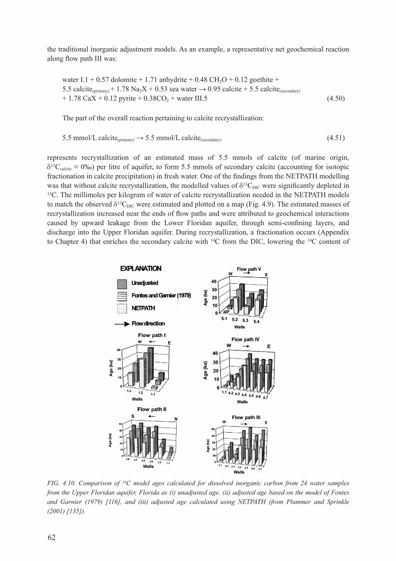
62

the traditional inorganic adjustment models. as an example, a representative net geochemical reaction along flow path III was:

water I.1 + 0.57 dolomite + 1.71 anhydrite + 0.48 cH2o + 0.12 goethite + 5.5 calcite(primary) + 1.78 na2x + 0.53 sea water → 0.95 calcite + 5.5 calcite(secondary) + 1.78 cax + 0.12 pyrite + 0.38co2 + water III.5  (4.50)

The part of the overall reaction pertaining to calcite recrystallization:

5.5 mmol/l calcite(primary) → 5.5 mmol/L calcite(secondary) (4.51)

represents  recrystallization  of  an  estimated  mass  of  5.5  mmols  of  calcite  (of  marine  origin, δ13ccalcite ≡ 0‰) per  litre of aquifer,  to form 5.5 mmols of secondary calcite (accounting for  isotopic fractionation in calcite precipitation) in fresh water. one of the findings from the NETPATH modelling was that without calcite recrystallization, the modelled values of δ13cdIc were significantly depleted in 13c. The millimoles per kilogram of water of calcite recrystallization needed in the NETPATH models to match the observed δ13cdIc were estimated and plotted on a map (fig. 4.9). The estimated masses of recrystallization increased near the ends of flow paths and were attributed to geochemical interactions caused  by  upward  leakage  from  the  Lower  floridan  aquifer,  through  semi-confining  layers,  and discharge into the Upper floridan aquifer. during recrystallization, a fractionation occurs (Appendix to chapter 4) that enriches the secondary calcite with 14c from the dIc, lowering the 14c content of

FIG. 4.10. Comparison of 14C model ages calculated for dissolved inorganic carbon from 24 water samples from the Upper Floridan aquifer, Florida as (i) unadjusted age, (ii) adjusted age based on the model of Fontes and Garnier (1979) [116], and (iii) adjusted age calculated using NETPATH (from Plummer and Sprinkle (2001) [135]).

63

dIc in dissolved hco!. Therefore, recrystallization of calcite lowers the value of And and, thus, lowers the adjusted radiocarbon age.

figure  4.10  compares  the  unadjusted  14c model  age  for waters  along  the  five  flow  paths with the 14c  model  ages  calculated  from  application  of  the  fontes  and  garnier  (1979)  [116]  model  to the final water,  and  the NETPATH calculated  14c model ages, which include the geochemical mass balance models with calcite recrystallization.

Most of the waters outside of the recharge area had adjusted 14c model ages of 20–30 ka (fig. 4.11).the measured 14c values of dIc in the floridan aquifer were low, and varied from about 33 pmc

in  the  recharge area  to as  low as 0.23 pmc on flow path  III. Along  the  same flow direction, δ13cdIc increased from –11.4 to –2.5‰. Unadjusted 14c model ages ranged from about 9 to more than 50 ka. the calculated 14c model ages using NETPATH ranged from 1.4 to about 27 ka (Plummer and Sprinkle (2001) [135]).

4.8.  radIocarbon datIng of dIssolVed organIc carbon

owing to the many geochemical interactions that can lower the 14c content of dIc and, if not quantified,  limit  the  usefulness  of  radiocarbon  dating  of  dIc  in  groundwater,  the  feasibility  of radiocarbon dating of doc in groundwater was investigated in a series of studies (drimmie et al. (1991)  [168]; Hendry  and wassenaar  (2005)  [169];  Long  et  al.  (1992)  [170]; murphy  et  al.  (1989) [171]; murphy et al.  (1989) [172]; Purdy et al.  (1992) [173]; Tullborg and gustafsson (1999) [174]; wassenaar et al. (1989) [175]; wassenaar et al. (1991) [176]). A generally accepted definition of doc is organic carbon  that passes  through a 0.45 µm filter  (drever  (1997)  [177]). groundwater  typically contains less than 2 mg/l (as c) of doc with a median concentration of about 0.7 mg/l (leenheer et al.

FIG. 4.11. Distribution of NETPATH adjusted 14C model ages of DIC in groundwater from the Upper Floridan aquifer, FL, USA (from Plummer and Sprinkle (2001) [135]).

64

(1974) [178]). with the development of 14c aMs analysis, radiocarbon dating of doc in groundwater is possible, although relatively large volumes of water (100–200 l) are needed to extract and separate high molecular weight (hMw) and low molecular weight (lMw) fractions of doc (Murphy et al. (1989) [171]; murphy et al. (1989) [172]). Although radiocarbon dating with doc can avoid many of the geochemical complications that affect the 14c content of dIc, research over the past two decades has shown that two of the problems that affect radiocarbon dating of dIc must also be evaluated in radiocarbon dating of doc; namely, definition of the initial 14c value of doc, Ao(fa), where fa refers to the fulvic acid (hMw) fraction, and adjustment of Ao(fa), to And(fa), for additional sources of (usually old) fulvic acid within the aquifer.

there are two main sources of doc in groundwater: (i) particulate organic carbon (poc) in the soil zone and unsaturated zone that can have radiocarbon ages of zero to at least several thousand years; and (ii) sedimentary organic matter (soM) such as lignite, peat or other forms of poc buried with the aquifer sediment that typically is radiocarbon-‘dead’. Both sources of doc can dilute the 14c content of doc in an aquifer.

Biogeochemical processes also significantly lower doc concentrations across unsaturated zones (Pabich  et  al.  (2001)  [179]).  Loss  of doc during  the  recharge  process  does  not,  alone,  complicate the definition of Ao(fa). The problem is that within the soil zone and unsaturated zone, Poc is not all modern and the assumption of 100 pmc for Ao(fa) is usually not valid. Little is known about the rates of the complex series of biogeochemical processes that alters Poc in soil zones, so that modelling of Ao(fa) is currently not possible. the alternative is to measure Ao(fa) in recharge waters of aquifers. one of the problems is that there is a spectrum of 14c values corresponding to the distribution of organic species and molecules recharging the groundwater system; generally, the ‘younger’ species will preferentially degrade  (through  fermentation  or  oxidation  processes)  relative  to  the  ‘older’  species. consequently, the distribution of 14c amongst the various organic molecular species will change through time, and generally decrease in 14c abundance, even in the absence of radioactive decay.

Methods of separating hMw and lMw fractions of doc are provided in thurman and malcolm  (1981)  [180], murphy  (1987)  [181], murphy et  al.  (1989)  [171] and murphy et  al.  (1989) [172]. The Hmw  fraction  is  composed  primarily  of  fulvic  acids with  a molecular weight  range  of 500–950  amu  (Aiken  and malcolm  (1987)  [182]), whereas  the Lmw  fraction  consists  primarily  of short chain aliphatic hydrocarbons and substituted alcohols (molecular weight of <140 amu). murphy et  al.  (1989)  [172]  found  large  and  varying  differences  in  the  14c content of the hMw and lMw fractions of doc in individual samples from the milk river aquifer, canada, demonstrating the diverse origin of doc in the aquifer and showing that radiocarbon dating of a composite doc sample (hMw + Lmw fractions) could be misleading. In the milk river aquifer, Lmw compounds generally had low 14c content, suggesting dilution with lMw doc from 14c-‘dead’ kerogen within the aquifer. The 14c content of the hMw doc generally followed that of the dIc, supporting a predominantly soil origin of the fulvic acid fraction (murphy et al. (1989) [172]). Although the Hmw (fulvic acids) doc fractions are also mixtures of organic molecules of different age, they are thought to be predominantly of soil origin (murphy et al. (1989) [172]) and probably better suited for radiocarbon dating than composite doc or the Lmw fraction of doc (clark and fritz (1997) [52]).

wassenaar et al. (1991) [176] found 14c values of the hMw fraction of doc decreased in young, tritiated recharge waters of the sturgeon falls aquifer and rodney aquifer in western canada to 75 and 76 pmc, respectively at depths of 16–18 m. the 14c content of the hMw fraction of doc ranged from 99 to 87 pmc in recharge waters from the alliston aquifer (canada), where the highest value was from a depth of 16–18 m and may have contained a higher fraction of fulvic acid from the bomb era than more shallow samples. the 14c content of the Hmw fraction of doc in recharge water from the milk river aquifer was estimated  to be as  low as 30 pmc  (drimmie et  al.  (1991)  [168]; wassenaar et  al. (1991) [176]). measurements from a clay rich till aquitard system in canada demonstrated that the 14c of the hMw fraction of doc decreased from 97 pmc at depths of 1.2 m to 13–15 pmc at depths of 15–43 m (Hendry and wassenaar (2005) [169]). The trend with depth was consistent with diffusive mixing 

65

between  two distinct end members: Som formed since  the Holocene (past 10 ka) and doc in pore fluids of the aquitard (Hendry and wassenaar (2005) [169]) suggesting, at least in this environment, that the hMw and lMw fractions of doc were geochemically and biochemically conservative.

In studies where the 14c of dIc and doc (or of the hMw fraction of doc) are measured, the 14c content of dIc is usually significantly lower than that of the doc (or of the Hmw fraction of doc) (Buckau et al. (2000) [183]; Burr et al. (2001) [184]; drimmie et al. (1991) [168]; murphy et al. (1989) [171]; Pettersson and Allard (1991) [185]; Purdy et al. (1992) [173]; wassenaar et al. (1991) [176]). the differences can be attributed to the relatively large number of geochemical reactions (as well as other processes such as matrix diffusion and isotopic exchange) that can lower the 14c content of dIc in old groundwater. The two most significant geochemical processes are dilution of dissolved inorganic 14c (dI14c) from dissolution of carbonates and formation of dIc from microbial degradation of old organic carbon within the aquifer. Thomas et al. (2001) [186] found unadjusted 14c model ages of dIc in groundwater from Nevada as much as 20 ka, that, when corrected on the basis of δ13c for carbonate rock recrystallization in this tectonically active aquifer, were in the range of 1–7 ka and similar to 14c model ages of doc in the aquifer.

Although  ‘traditional’  adjustment  models  adequately  compensate  for  carbonate  mineral dissolution, most studies comparing do14c and dI14c ages have not evaluated the organic source of dIc. geochemical models used to adjust the initial 14c value that included the degradation of organic matter in the aquifer (Aravena et al. (1995) [166]; Plummer (1993) [60]; Plummer et al. (1990) [145]; Plummer and Sprinkle (2001) [135]) yielded adjusted radiocarbon ages of dIc that were ‘reasonable’; i.e. consistent with other palaeoclimate indicators (stable isotopes and palaeorecharge temperatures) or with results from numerical flow models. Buckau et al. (2000) [183] applied ‘traditional’ adjustment models  to  the dIc of  the gorleben aquifer, germany, finding 14c model ages of 1–10 ka  in  tritium-containing recharge water, and dIc 14c model  ages up  to 31 ka  in waters  that had Holocene  stable isotope  signatures. By  taking  into  account  dilution  of  the dIc  from microbial  degradation  of doc in the aquifer, and determination that Ao(dIc) in  the  aquifer  was  near  50  pmc,  Buckau  et  al.  (2000) [183] demonstrated that the waters that contained elevated concentrations of doc were so young that significant 14c decay could not be detected, and that the ages were consistent with the age limits derived from 2h and 18o. Buckau et al. (2000) [187] demonstrate the release of large concentrations of Lmw (1.7–171 mg c/l) and hMw (2.6–22 mg c/l) doc fractions in waters of the gorleben aquifer compared to the relatively low doc concentrations in the recharge waters (0–2.2 mg c/l). the contribution of doc from sedimentary organic matter in the gorleben aquifer overwhelms the initial doc fractions, demonstrating  the difficulty of dating doc  in organic  rich  aquifers. The next  important  advance  in the application of radiocarbon dating of doc in groundwater will likely be in the field of compound specific radiocarbon dating (Ingalls and Pearson (2005) [188]; Kalin (1999) [111]).

Long et  al.  (1992)  [170]  suggested  that  the most  important  justification  for  the  study of  14c of doc in aquifers is for comparison with travel times inferred from 14c in dIc. differences in 14c model ages between dIc and doc can aid in refining geochemical adjustment models of the 14c content of dIc as well as help to interpret the 14c content of doc in aquifers. a useful approach to establishing radiocarbon chronologies in aquifers where inorganic and organic carbon sources contribute to the 14c dIc pool is to date the dIc. this is done by constructing geochemical adjustment models accounting for all of the predominant inorganic and microbially mediated organic degradation reactions in the tdc system, such as implemented in NETPATH (Plummer et al. (1994) [120]), and demonstrated by Aravena et al. (1995) [166] and Plummer and Sprinkle (2001) [135].

66

4.9.  hydrodynaMIc and aquIfer MatrIx effects on radIocarbon ages

4.9.1. Mixing processes

groundwater pumping extracts water preferentially from the most hydraulically conductive zones adjacent to well screens. this means that the waters extracted and their solutes, including dIc and doc, generally come preferentially from one or more transmissive aquifers, transmissive zones or from highly conductive fractures. It is important, however, to consider the spatial scale of the effects of groundwater pumping and movement. In a study investigating regional groundwater depletion, Konikow and Neuzil (2007) [189] showed that most of the regional groundwater depletion caused by pumping actually came from a change  in storage  in confining  layers. Thus, a significant  fraction of a water sample pumped from a well may represent water that has not only been residing in ‘mobile’ zones of the groundwater system.  Some  of  the  water  may  have  leaked  from/through  confining  layers.  If  the  leakage  occurs primarily from more recently recharged (usually shallower)2 horizons,  the water sample will contain a fraction of younger water and, possibly, younger solutes. If  the leakage occurs primarily from less recently recharged (usually deeper) horizons, the water will contain a fraction of older water and older solutes. In general, water samples extracted from given horizons will have a frequency distribution of water and tracer model ages (cf. review by Bethke and johnson (2008) [84]; chapter 3 in the present volume discusses this issue at length and how it affects groundwater ‘age’ concepts). This natural range in age distributions can be coupled with the following facts: (i) different solutes undergo different types and extents of reaction and, therefore, undergo varying extents of retardation in groundwater systems (Atteia  et  al.  (2005)  [190]; glynn  and Brown  (2012)  [154]; maloszewski  and zuber  (1991)  [191]); (ii) different solutes have different histories of recharge into the groundwater system (plummer et al. (1993) [192]), as well as different production and removal histories in their passage through the system; and (iii) different solutes may even have undergone different extents of dispersal and/or exclusion through the system (LaBolle et al. (2006) [193]; Neuzil (1986) [194]; Neuzil and Provost (2009) [195]). consequently,  it  is no surprise  to find  that different dating  techniques provide different  tracer model ages for a given sample (see dePaolo (2006) [196]; IAEA (2006) [85]; maloszewski and zuber (1991) [191]; Plummer et al. (1993) [192]).

4.9.2. subsurface production

the possibility of subsurface production of 14c was investigated by zito et al. (1980) [197] and with regard to the Stripa granite by Andrews et al. (1989) [198]. Although it is theoretically possible to produce 14c in groundwater from nuclear reactions induced by emissions from u and th nuclei, the effect is normally not important in waters younger than 50 ka (zito et al. (1980) [197]), which is approximately the limit for 14c dating. the minimum 14c content from in situ production in the stripa fracture fluids  corresponded  to  a decay  time of 32 ka,  for  an  initial  14c value of 50 pmc. however, the question of in situ production of 14c would  need  to  be  investigated  on  a  site  specific  basis  and depends on several  factors,  including  the  localization of U- and Th-bearing minerals with respect  to pore spaces and various target materials (Al, mg, o, Si, B) in the aquifer (zito et al. (1980) [197]).

4.9.3. Diffusive exchange with confining layers

In  addition  to  the  possible  advective  leakage  of  waters  from  other  conductive  zones  of a groundwater  system (through confining zones), diffusive exchange of water and solutes  is  also an 

2   one exception may occur when shallow, relatively less transmissive zones overlie deeper relatively more transmissive zones. In this situation, waters in the deeper zones may have been more recently recharged than waters in the shallower zones.

67

important process to consider. Any groundwater system may have a range of ‘stagnant’3 zones, typically containing old water and solutes which can possibly exchange diffusively with younger water and solutes in more mobile regions of the system. large chemical and isotopic concentration gradients are often found between mobile and stagnant zones in groundwater systems, with stagnant zones usually containing more highly concentrated, sometimes more chemically reducing waters. a wide range of stagnant zones can occur: confining beds or aquitards, clay or silt lenses, unfractured rock matrices with some connected porosity between mineral grains, connected porosity inside individual mineral grains, and internal exchange layer porosity in clay minerals. Many of the diffusion processes will involve aqueous ion diffusion through a water phase, although this phase can have varying electrochemical properties because of interfacial effects with the contacting solid surfaces. some of the diffusion can also occur through surface diffusion processes, including surface diffusion inside the double layer of clays  (Helfferich  (1995)  [199]). Atteia  et  al.  (2005)  [190]  offer  a  comprehensive  review  examining the contributions of diffusion and leakage from low permeability layers to the geochemical evolution of groundwater systems.

4.9.4. transport models

Ideally, the complex interplay between advective, dispersive and diffusive processes, geochemical reactions and radioactive decay (or production) would be investigated using forward-modelling reactive transport codes such as PHAST (Parkhurst et al. (2004) [200]). owing to the multiplicity of possible computer  intensive  simulations varying parameters,  processes  and  configurations,  inverse modelling is  needed  to  constrain  the  range  of  possible  simulations  and  optimize  parameter  values  (for  given configurations and processes chosen for a particular system). Inverse modelling could include inverse geochemical modelling with netpath/phreeqc to determine sets of possible reactions and mixing processes that might control the geochemical evolution of the groundwater. Inverse modelling with codes such as UcodE (Poeter and Hill (1998) [74]) could also be used to estimate and constrain flow and transport models and model parameters. Having sufficient high quality data and an understanding of what  is  reasonable  in  the  hydrological  and  geochemical  behaviour  of  a  system would  be  key  to the useful application of the modelling process.

4.9.5. Analytical solutions

In the absence of full featured but time consuming inverse and forward simulations of groundwater systems,  some  analytical  solutions  are  available  that  can  quickly  quantify  the  potential  importance of diffusive processes on observed radiocarbon ages for given groundwater samples. the solutions were first derived for the study of radionuclide transport in fractured rocks, initially for the transport of  a  radionuclide  through  a  single  fracture with  transverse  diffusion  into  a  rock matrix  (Neretnieks (1980) [201]; Neretnieks (1981) [202]; Tang et al. (1981) [203]), then for transport through a parallel set of fractures with transverse diffusion into the intervening rock matrix (Sudicky and frind (1982) [204]; Sudicky and frind  (1984)  [205]). A more general  3-d analysis  for  fractured  rock media was provided by Therrien and Sudicky (1996) [206]. Although Tang et al. (1981) [203] recognized early on the application of their analytical solution to radiocarbon dating of groundwater in a thin aquifer bounded by thick confining beds, Sanford (1997) [207] provided an elegant analytical derivation and solution for a parallel series of stagnant and flow zones, applicable either for porous or fractured rock media. The basic equations in Sanford (1997) [207] for the analytical solution under steady-state conditions 

3   Historically, hydrologists have often considered low permeability zones as zones that were completely impervious to flow, such as aquicludes, for example. In reality, advective flow generally does occur through low permeability zones and, more often than not, can be quantitatively meaningful when integrated over large regional areas and/or over large timescales. In this chapter, ‘stagnant’ zones is simply used to indicate zones for which diffusive transport processes dominate over advective ones over the time periods and areas of interest.

68

(with respect to both flow and transport) of a parallel flow and stagnant zone system, with a constant tracer input concentration (e.g. a 14c content of 100 pmc), constant flow zone width, wflow, and constant stagnant zone width, wstag, are further discussed in recent papers by cook et al. (2005) [208] and dePaolo (2006) [196]. Sanford’s steady state solution can take the form of a diffusion loss constant that can be added to the radioactive decay constant for a given tracer such as 14c. sanford relates the diffusion corrected, tc, and diffusion uncorrected, tu, ages for a sample through the following equation:

tc/tu = k /(k + kdiff) (4.52)

where k and kdiff are the radioactive decay and diffusive loss constants, respectively. for 14c, k is 1.21 × 10–4 per a or 3.83 × 10–12  per  s  (corresponding  to  a  half-life  of  5730  a). The  diffusive  loss constant, kdiff, can be calculated from the following equation:

stageffdiff

flow eff

2tanh

2wkD kk

w Dϕ

=

(4.53)

whereφ  is  the  porosity  in  the  flow  zone;  and  the  effective  diffusion  coefficient, Deff, can be related

to the aqueous diffusion coefficient, D0, through a variety of equations that generally include the effects of matrix (or stagnant zone) porosity, θstag, and tortuosity, τ.

these equations and the magnitude of Deff vary significantly in different studies. cook et al. (2005) [208] provide a fairly general formulation:

FIG. 4.12. Plot of the ratio of the diffusive rate constant, k’, to the decay constant of 14C, k, over the length scales at which vertical heterogeneties occur in porous media. Shaded regions indicate where diffusion is either negligible (white), significant (pale yellow) or dominant (pink). The ratios assume a porosity of the flow zone of 0.30, a coefficient of molecular diffusion of 1 × 10–10 m2/s, and a decay constant of 3.83 × 10–1/s (modified from Sanford (1997) [207]). Sanford’s analytical solution and the adjacent plot will generally tend to an overestimation of the effects of 14C diffusive loss on 14C model ages as discussed in the text.

69

eff 0 stagD D θ τ= (4.54)

the aqueous diffusion constant, D0, for carbonate and bicarbonate species is variously cited: 0.04 m2/a (1.3 × 10–9 m2/s) by cook et al. (2005) [208], and 0.03 m2/a (9.5 × 10–10 m2/s) by depaolo (2006)  [196],  who  may  be  including  a  tortuosity  effect  in  his  lower  number.  In  their  example describing a fractured rock system, however, cook et al. (2005) [208] assumed a tortuosity of 0.03 and a matrix porosity of 0.02. Porous media have higher stagnant-zone porosity and tortuosity compared to  fractured rock matrices. This explains  the  two orders of magnitude difference  in  the effective  14c diffusivities (Deff), 10–10 m2/s and 7.6 × 10–13 m2/s, used by Sanford (1997) [207] and cook et al. (2005) [208], respectively.

sanford used his steady state model calculations to estimate the effect of diffusive loss on radiocarbon dating of waters  in  the stratified basalts of  the  island of oahu, where he calculated  that the diffusive losses of 14c could result in a 14c model age that could be 100 times too old. he also applied his model to 14c dating of waters in the Bangkok Basin, an alluvial system of stratified clay, sand and gravel lenses, where he estimated the near equal removal of 14c through radioactive decay and diffusive loss. His calculations assumed that the clay lenses had an average thickness of about 6 m, and that the transmissive sand layers had a thickness of about 20 m. figure 4.12 (from Sanford (1997) [207]) can be used to estimate the relative importance of diffusive 14c loss in radiocarbon dating.

It must be noted that Sanford’s analytical solution did not consider the possibility of sorption and isotope exchange with the solid phase, a process that can be important in carbonate (limestone, dolomite) or chalk aquifers. małoszewski and zuber (1991) [191] added these processes in their own analysis of diffusive effects on radiocarbon dating. the additional retardation caused by the sorption and exchange of 14c leads to additional decay and loss of the isotope, even in a steady state system. In contrast to this loss, the concentrations of non-decaying constituents, such as 13c, are not affected by sorption and exchange processes under steady state conditions. however, groundwater systems are probably never in complete steady state with respect to all transport processes and geochemical reactions.

Sanford’s  analytical  solution  assumes  steady  state  conditions  and  may  either  overestimate or underestimate diffusive losses of 14c  in  groundwater  systems  with  changing  flow  and  transport conditions.  Sanford’s  analytical  solution  may  provide  a  good  estimate  of  14c diffusive loss (and the needed groundwater age correction) in the case of parallel transmissive and stagnant zones, where the water in the stagnant zones is truly stagnant. generally, however, Sanford’s analytical solution may tend to overestimate the diffusive losses of 14c for the following reasons:(a) The  solution  assumes  a  binary  layer  flow  system,  with  fast  flow  zones  and  stagnant  zones. 

Advection is a non-fractionating transport process. By assuming that advection is insignificant in stagnant zones, the diffusive loss of 14c in those zones is maximized.

(b) The  solution  assumes  a  ‘layer-cake’  alternating distribution  of flow and  stagnant  zones, with one  constant  width  for  the  flow  zones  and  one  constant  width  for  the  stagnant  zones,  and a diffusive gradient into the stagnant zones orthogonal to the flow direction in the flow zones. In  contrast,  stagnant  zones  in  alluvial  basins  are  likely  to  pinch  out  and  be  limited  in  areal extent. If the lenticular stagnant zones are small in their individual areal extents, diffusion into the  lenses may be  fast enough  that no significant  14c decay will occur. Therefore,  the  ‘layer-cake’ configuration assumed by Sanford’s analytical solution likely overestimates 14c diffusive losses in systems that have stagnant zones with very limited individual areal extents.

(c) The  solution  assumes  that  transverse  dispersion  is  great  enough  in  the  flow  zones  to  ensure a constant 14c content across the width of each flow zone. In systems with large flow zones, such as thick aquifers, this may not be the case and this could limit the overall diffusive loss of 14c.

(d) The solution assumes that fick’s law, as applied only to the 14c content in the water, controls the diffusion and the diffusive loss of 14c. It assumes that the chemical counter diffusion of ions from stagnant zones into flow zones does not affect 14c diffusion. In reality, major regional

70

aquitards  often  have  significantly  different  chemistry  from  their  neighbouring  aquifers  and are usually more saline.  In such systems, coupled diffusion processes might have  to be  taken into account. Multicomponent diffusion is a complex process that can speed up the diffusion of  certain  ions  and  slow  the  diffusion  of  others,  relative  to  the  diffusive  flux  that  might  be calculated by assuming single  ion diffusion. However,  in  the common case of stagnant zones that are significantly more saline  than  the flow zone of  interest,  intuition suggests  that strong chemical counter diffusion fluxes of ions into the flow zone could potentially slow the diffusive flux and loss of 14c into the stagnant zones, relative to the 14c loss that might occur in a situation without a strong chemical counter diffusion.

In  summary,  Sanford’s  analytical  solution  is  a  useful  tool  for  an  initial  estimation  of  potential 14c diffusive losses. however, it probably provides a maximum estimate of such losses, and is best applied to systems that have pervasive zones with no significant advective flow. It will probably not be applicable to alluvial basins with relatively coarse sediments and a paucity of truly stagnant zones, such as the Middle rio grande and san juan basins in new Mexico. after an examination of the geological information available for the middle rio grande Basin, Sanford et al. (2004) [47] and Sanford et al. (2004) [48] did not correct 14c model ages for diffusive losses in that basin. In their study on the san juan Basin, Phillips et al. (1989) [39] considered the potential effects of dispersive mixing and, more importantly,  inter-aquifer  leakage, on  the  sampled groundwater  14c model ages; they concluded that these effects did not significantly affect the estimated 14c model ages.

4.9.6. Matrix diffusion in unsaturated zones

Most of the studies that have investigated the effects of matrix diffusion on 14c dating of groundwater have considered only the effects that occur below the water table. there could be some situations in which the physical and chemical processes relating to diffusion, sorption, isotopic exchange and decay of 14c  in matrices,  lenses  or  grain  pores  in  the  unsaturated  zone  or  near  the water  table might also need to be considered, even though the effects could be mitigated by gas phase exchange processes. diffusive  processes  in  the  unsaturated  zone  or  in  perched  groundwater  could  potentially lower the initial 14c content, Ao, of recharging groundwater.

4.9.7. General conclusions regarding the effects of hydrodynamics and heterogeneity on 14C model ages in groundwater

some general conclusions can be stated regarding the effects of matrix diffusion on 14c dating of groundwater. Most groundwater sampled for 14c analysis and radiocarbon dating is pumped from the  more  transmissive  zones  of  a  groundwater  system.  owing  to  dispersive  and  diffusive  effects (and  usually  their  associated  geochemical  reactions),  the  groundwater  flow  rates  obtained  by  using the 14c model ages estimated4 for these transmissive zones will underestimate the actual groundwater velocities in these zones. further, the flow rates obtained will probably greatly overestimate the mean water velocity of the system as a whole (because the sampled water may not fully reflect the slower velocities and older ages of water  in  less  transmissive zones). consequently,  if a system is at steady state, overall recharge to the system5 will be overestimated if the recharge rate is determined from 14c measurements insufficiently corrected for diffusive processes. from a water management perspective, the  underestimation  of  water  velocities  in  transmissive  zones  could  cause  a  problem  if  water contamination is an issue; the overestimation of overall recharge to the system could be a problem from a water supply perspective.

4 without corrections for diffusion.5   The system, as defined here, is the entire groundwater system. It includes all of its transmissive, less transmissive and stagnant zones.

71

The geometry and distribution of more transmissive and less transmissive, and/or stagnant zones will be important in determining the relative effects of diffusive processes (and of advective leakage). The  relative  sizes of  stagnant and  transmissive zones will matter as can be  seen  from  the equations above. The orientation and aspect ratio of the zones relative to the recharge surface, and the distribution of these orientations and geometries will also be important. the use of multiple tracers with different effective diffusivities and decay or growth characteristics can potentially provide a better understanding of the distribution of model and actual groundwater velocities through the system.

simple, easy to use, estimation techniques and numerical modelling tools are useful and needed to obtain a good understanding of the geochemical and hydrological processes occurring in aquifers and their potential impacts on the distribution of 14c content throughout a groundwater system. ultimately, however, the heterogeneous nature and the structural and process complexity of groundwater systems may require more sophisticated  full-featured numerical  simulation  tools. The  full use of  these  tools, however, will  be warranted only when  there  is  sufficient  information  and data  available  to describe the groundwater system under investigation. In such a situation, 14c age dating may be used in conjunction with the chemical and isotopic characterization of various recharge and evolved waters, and the spatial delineation of their occurrence, to help calibrate full featured flow and transport simulations of a groundwater basin. Plummer et al. (2004) [49], Plummer et al. (2004) [50], Plummer et al. (2004) [51], Sanford et al. (2004) [47] and Sanford et al. (2004) [48] provide an example of such an application in an investigation of the hydrogeology of the Middle rio grande basin (see chapter 12 for a case study on the Middle rio grande basin). their study calculated the effective modern and palaeorecharge rates for the basin. the minimal corrections needed to adjust for 14c dilution through geochemical reactions in the Middle rio grande basin, and the extensive geochemical and hydrological data available were a great help in facilitating calibration of the flow model for the system. Several earlier efforts have also used radiocarbon dating, measured 14c values and geochemical modelling, to help determine regional recharge rates and the transmissivity of aquifers on large regional scales. some notable examples of such studies include Phillips et al. (1989) [39], Plummer et al. (1990) [145], and Plummer and Sprinkle (2001) [135]. In these efforts, the collection of an extensive set of chemical and isotopic analyses was often the key to obtaining confidence that calculated tracer model ages or velocities were reasonable. In the best situations, the ages obtained correlated with recharge palaeotemperatures derived from noble gas, n2/ar, 18o and 2h data.

4.10. guIdelInes for radIocarbon datIng of dIssolVed carbon In groundwater systeMs

nine guidelines essentially decribe the application of radicarbon measurements to groundwater dating:(1) although it is sometimes possible to reconstruct the 14c content of dIc in water samples that

are mixtures of young and old water, it is best to attempt radiocarbon dating on waters that are representative of in situ aquifer conditions. well construction and/or drilling practices can compromise the integrity of the 14c content of the formation water. tritium analyses and cfc analyses are useful in recognizing water samples or their mixtures that may be contaminated with fractions of post-bomb 14c and identifying those samples that may not be worthy of undergoing the expense of radiocarbon analysis. on the other side of the radiocarbon timescale, 36cl measurements may be useful for samples with low 14c to test for the possibility that the water is very old, but contains a small fraction of relatively young (radiocarbon timescale) water. given (i) the local tritium and 14c input function for the bomb era; (ii) the interpretation of initial 14c in recharge processes; and (iii) geochemical reaction corrections, it may be possible to test various mixing scenarios of young and old water that potentially affect interpretation of 14c model age for a given locality.

72

(2) Most radiocarbon laboratories report the measured 14c content according to that of stuiver and Polach (1977) [110], which provides values of per cent modern (pm) carbon normalized for 13c of the sample (see the Appendix to chapter 4). In radiocarbon dating of dIc (or Tdc) in aquifers, it is best to use unnormalized 14c values, pmc and/or δ14c, and use geochemical models to construct the adjusted 14c content. Equations to convert the normalized 14c to non-normalized values are provided  in  the Appendix  to chapter 4. geochemical adjustment models are  then constructed, such as in fontes and garnier (1979) [116] or through use of the code NETPATH (Plummer et al. (1994) [120]) as described above, to adjust the initial 14c for water–rock reactions.

(3) determination of the initial 14c value, Ao, in recharge areas of aquifers remains one of the most significant uncertainties  in radiocarbon dating of dIc in groundwater. In systems open to co2 gas exchange during recharge, such as in some arid regions, ao can be near 100 pmc. In systems closed to co2 gas exchange following recharge, Ao may be near 50 pmc if old carbonate rocks dissolve within the aquifer following recharge without further gas exchange with unsaturated zone air. Intermediate values, as well as values even lower than 50 pmc are also possible, depending on the extent of geochemical reactions occurring in the aquifer. the difference between open and closed system evolution — the difference between approximately 100 and 50 pmc in Ao alone — introduces 5730 a uncertainty in the adjusted 14c model age. however, as long as conditions in  the  recharge  area  have  not  substantially  varied,  groundwater  velocities  down  a  flow  path calculated from 14c model ages are not affected by the Ao error after the first sample.Two approaches have been taken in estimating Ao: (i) the initial 14c value of dIc in the recharge area can be estimated by locating water samples in the recharge area that are low in tritium or cfc content  (pre-nuclear detonation waters)  and analysing  the  14c content of dIc in these samples (fig. 4.1); and (ii) the initial 14c value of dIc can be estimated by applying one or more of the ‘traditional’ adjustment models discussed above to the chemical data from recharge waters or to the water sample being studied, as in netpath. alternatively, geochemical modelling techniques, such as in phreeqc, can be used to estimate Ao values pertaining to assumed conceptualizations of the geochemical evolution of initial waters.

(4)  Consideration should be given to the possibility that the chemical, isotopic and recharge conditions occurring today in the recharge area of the aquifer may not apply to the palaeoconditions prevailing at the time of recharge of the sample being dated with radiocarbon. changes in climatic conditions could lead to changes in the thickness of the unsaturated zone, recharge rate and the extent of open or closed system conditions. the predominant plant type in the recharge area could shift from one photosynthetic pathway to another, resulting in a change in δ13c of soil gas co2. as explained above, many of the models for reconstructing Ao in recharge waters are sensitive to the assumed δ13c of soil gas co2.

(5) constructing geochemical adjustments to initial radiocarbon values in aquifers can require considerable  geochemical  intuition  related  to  water–rock  reactions  in  a  system.  data  on the carbon isotopic composition of dIc, doc, ch4  and  Poc,  and  reacting  carbon-bearing phases in the system are usually needed or must be estimated, both within the recharge zone and the aquifer system.

(6) If  initial  and  final  water  compositions  can  be  proposed,  geochemical  mass  balance  reaction models can be used to adjust the initial 14c value for geochemical reactions along the flow path. the calculated 14c model age is the time required for decay of the reaction corrected initial 14c value to the measured (non-normalized) value in the final water. Inverse geochemical modelling codes such as netpath and phreeqc can estimate the effects of hydrodynamic mixing and geochemical processes on the dilution of observed 14c values. It may be possible to apply some analytical solutions to estimate the importance of matrix diffusion on 14c model ages.

(7) In some cases, such as silicate aquifers where geochemical adjustments to Ao can be small, it may be warranted to apply radiocarbon calibration scales to convert radiocarbon years to calendar years. before radiocarbon calibration can be applied, radiocarbon ages that have been calculated

73

by using the modern 14c half-life (5730 a, as in NETPATH) need to be converted to Libby half-life (5568 a) by using the equation

tlibby = 0.972t5730  (4.55)

this produces the adjusted 14c model age based on  the Libby half-life. calibrated radiocarbon ages, where warranted, are probably more reliably used in conjunction with numerical models of groundwater flow, as in Sanford et al. (2004) [47].

(8) efforts should be made to corroborate radiocarbon ages. Measurements of tritium and/or cfcs should always be made in conjunction with radiocarbon measurements, as discussed above. Measurements of 36cl  can  identify  mixing  of  pre-nuclear  detonation  water  with  very old groundwater (water on the 100 ka timescale). If the radiocarbon age places the sample near the Lgm (18 ka  radiocarbon age), comparison with data on  the stable  isotope composition of the water (rozanski (1985) [209]) or of the dissolved gas N2/Ar (Heaton (1981) [210]; Heaton et al. (1983) [56]; Heaton and vogel (1981) [211]), or recharge temperatures (Herzberg and mazor (1979)  [212];  Stute  et  al.  (1995)  [213];  Stute  et  al.  (1995)  [214];  Stute  and  Schlosser  (2000) [215]; Stute et al.  (1992) [42]) can be used to corroborate  the age. Examining the radiocarbon data  spatially  throughout  the  aquifer  in  relation  to  conceptualization  of  groundwater flow  can also help to corroborate or possibly invalidate some radiocarbon ages. Measurement of vertical 14c gradients in unconfined or deep aquifers and/or 14c gradients along flow paths complement geochemical correction procedures, for example, in estimating the initial 14c value, and determining recharge rates (see chapter 12). the gradient in 14c concentration can help to evaluate whether a 14c decrease with flow distance is due to radioactive decay or the combined effect of decay, retardation and geochemical processes. The process of refining age interpretation can be aided by use of numerical models of groundwater flow, recognizing ages that are consistent with the model and those that are not.

(9) the complexity of a hydrogeological setting may require more sophisticated full featured numerical simulation tools. the use of these tools will truly be warranted only when there is sufficient information and data available to describe the groundwater system under investigation. If this is the case, 14c model ages can be used in conjunction with geochemical characterization to help calibrate flow and transport simulations of a groundwater system.

AcKNowLEdgEmENTS

this chapter was improved by technical reviews from f.M. phillips, new Mexico tech, usa; K. fröhlich; P. Aggarwal, IAEA; and d.L. Parkhurst, United States geological Survey, USA. Any use of  trade, product or firm names is for descriptive purposes only and does not  imply endorsement by the us government.

74

APPEnDIx tO CHAPtER 4

the following appendix provides details that may be of use to hydrologists requiring additional  background  information.  It  summarizes  the  various  reporting  units  of  radiocarbon  and their interrelationships, reviews isotopic fractionation in carbonate systems open and closed to co2 gas,  summarizes  radiocarbon  calibration  and  its  possible  application  to  radiocarbon  dating  of  dIc in groundwater, provides information on methods of collection of radiocarbon samples, provides sources for selected geochemical and radiocarbon software, and contains information on locating radiocarbon laboratories.

a.1. radIocarbon reportIng unIts

radiocarbon measurements are reported following specific recommendations (Stuiver and Polach (1977)  [110]).  These  authors  recommend  that  in  reporting  14c measurements, all values should be normalized for isotope fractionation effects to a common δ13c value of –25‰. these recommendations have been adopted by most radiocarbon laboratories worldwide, providing conformity in reporting units between the various radiocarbon laboratories and continuity of results with previously reported data.

The  practice  of  normalization  of  14c measurements is well established in the radiocarbon community, and is an appropriate step in converting radiocarbon years to calendar years. geochemists and hydrologists sometimes lose sight of the fact that radiocarbon dating of dIc in groundwater (Eq.  (4.3))  is  based  on  non-normalized  14c  specific  activity  values  (Kalin  (1999)  [111]; mook  and van der Plicht  (1999)  [216]; Stuiver and Polach  (1977)  [110]). By  international convention,  specific activities are compared to a standard activity, Aox, where Aox = 0.95 times the specific activity of NBS oxalic acid (0.95 × 13.56 dpm/g c, in the year a.d. 1950). the initial 14c  specific activity, Ao, and the measured 14c specific activity of a  sample, A, can be expressed as a percentage of this standard activity in pmc, where pmc = (A/Aox) × 100 (mook (1980) [109]). Here, the notation pmc is used for the  non-normalized  ‘per  cent modern  carbon’  and  ‘pm’  for  the  commonly  reported  normalized  14c value, denoted ‘per cent modern’. The 14c values in pm have been modified (normalized) for assumed 13c isotope fractionation from an assumed initial value of –25‰ to the measured δ13c of the sample.

In some cases, such as in studies of 14c in plants, bones and tree rings, it is convenient and scientifically  justifiable  to normalize  14c values to a common δ13c value of –25‰, to correct for in vitro fractionation processes that affect both 13c and 14c. however, in groundwater, most of the isotopic variation in δ13c of dIc  is  caused  by water–rock  interaction  or  geochemical  reactions  occurring  in the aquifer. for example, the δ13c of dIc is typically more positive than –25‰ (such as for c3 plants) due to: (i) isotope fractionation between soil gas co2 and hco3 in recharge water; and (ii) isotope dilution from dissolution of carbonate rocks that are enriched in 13c, and not due to in vitro fractionation processes. when dating dIc in groundwater, the actual number of 14c atoms in the dIc is needed to determine the time elapsed since the dIc was isolated from the modern reservoir (that is, the soil co2 derived from plants and air) and its 14c atoms were recharged. corrections (adjustments) to the 14c of dIc are normally made through geochemical calculations, as discussed in this chapter.

currently, most radiocarbon measurements are made using aMs, which determines radiocarbon ages from a measured isotope ratio (14c/13c) or (14c/12c). for example, at the University of Arizona AmS facility, radiocarbon ages are determined from the measured 14c/13c ratio in a sample by comparing that ratio with a similar ratio measured in known standards (Linick et al. (1986) [217]). The measured ratios of standards and samples are corrected (normalized) to values corresponding to δ13c of –25‰ by using 13c/12c ratios measured in a stable isotope mass spectrometer and the ‘fraction of modern’, F, of the sample, S, is found using the Eq. (A.1), where the notation is that of donahue et al. (1990) [218]:

75

[ 25]

1950[ 25]

(14 /13)(14 /13)

SF −

−

=

(a.1)

where(14/13)S[–25]   denotes the 14c/13c atom ratio in the sample, S, normalized to a δ13c of –25‰;(14/13)1950[–25] is the 14c/13c atom ratio in a standard normalized to –25‰ in the year 1950.

The conventional radiocarbon age (denoted ‘Age’) of the sample is then:

age = –τlnF (a.2)

where τ is the libby mean life (8033 a; τ = 5568/ln(2) and 5568 is the Libby half-life of 14c).

donahue et al.  (1990)  [218] present equations  for  the conversion of measured  isotope  ratios  to forms that can be used in eqs (a.1) and (a.2).

Many other aMs radiocarbon laboratories measure the 14c/12c isotope ratio rather than the 14c/13c ratio. Equations are summarized below for results based on either the 14c/12c or 14c/13c ratio.

A.1.1. Recommended reporting units

for consistency with past practice, and following the recommendations of stuiver and polach (1977)  [110], mook  and  van  der  Plicht  (1999)  [216]  and  donahue  et  al.  (1990)  [218],  14c values will continue to be reported as pm, which has been normalized for 13c isotopic fractionation, and its associated ±1σ value along with the 13c value used to normalize pm. The nomenclature used here is as follows (table a.1).

A.1.2. Relation between radiocarbon reporting units

The  equations  that  follow  are  based  on  those  of  Stuiver  and  Polach  (1977)  [110],  and  were originally intended for 14c measurements made by counting beta decay in which the 14c specific activity was measured in disintegrations per minute per gram of carbon. as that gram of carbon contains, to within about 1/10 000, almost entirely 12c atoms,  the radiocarbon specific activity measured by beta 

table a.1. noMenclature used In reportIng 14c Values

Value unit uncertainty unit description

∆14c ‰ ± 1σ ‰ per mille depletion or enrichment relative to the nbs I oxalic acid standard normalized for 13c isotopic fractionation

δ14c ‰ ± 1σ ‰ per mille depletion or enrichment relative to the nbs I oxalic acid standard, not normalized for 13c isotopic fractionation

pM % ± 1σ per cent modern (pM) relative to the nbs I oxalic acid standard, normalized for 13c isotopic fractionation

pmc % ± 1σ % per cent modern carbon (pmc) relative to the nbs I oxalic acid standard, not normalized for 13c isotopic fractionation

t years ± 1σ years conventional radiocarbon age, years before 1950

76

decay can be expressed as the ratio of 14c/12c. The  terms  ‘fraction of modern’, F, and conventional radiocarbon  age  can  be  defined  similarly  as  in  the first  two  equations  above, which  use  the  14c/13c ratio,  that is, 14/13 is replaced with 14/12. However, in further calculations, such as those necessary for denormalization of  reported values of F or pm,  it  is necessary  to know which  isotope  ratio was measured in the aMs facility. the equations below are based on 14c/12c measurements, leading to squared terms in correcting for 14c fractionation. the exponent is changed from 2 to 1 when the isotope ratio 14c/13c is measured. donahue et al. (1990) [218] provided equations that relate radiocarbon AmS measurements based on 14c/13c and 14c/12c.

In radiocarbon dating of dIc, it may be desirable to make calculations based on δ14c or pmc, which have not been normalized with  13c differences from –25‰. as most radiocarbon laboratories report normalized values, it is sometimes necessary to ‘denormalize’ the reported value in making radiocarbon age calculations in groundwater environments. The actual equations used for ‘denormalization’ depend on which isotope ratio was measured at the aMs facility, for example 14c/12c or 14c/13c. In either case, the value of pmc is related to δ14c by:

pmcC

= +

δ14

10001 100

(a.3)

If the measurement is based on the 14c/12c isotope ratio, then δ14c is related to the normalized 14c by Stuiver and robinson (1974) [219]:

( )14

1422 13

1 c /1000c 1 10000.975 / 1 c /1000

+ Δ δ = − + δ

  (A.4)

If the basic measurement is from the 14c/13c isotope ratio, the denormalization is:

( )14

1413

1 c /1000c 1 10000.975 / 1 c /1000

+ Δ δ = − + δ

(a.5)

The pm relative to the NBS I oxalic acid standard, normalized for 13c isotope fractionation is:14cpM 1 100

1000 Δ

= +

(a.6)

the conventional radiocarbon age, t, is expressed in years before present (bp), where present is the year 1950, and is normalized for 13c differences from –25‰:

sn(in1950)

on(in1950)

pMln ln ln100

At F

Aτ τ τ

= − = − = − (a.7)

whereAsn(in1950) is  the  specific  activity  of  14c  in  the  sample  in  the  year  1950,  normalized  for

13c fractionation;Aon(in 1950)   is the specific activity of the standard in 1950.

the conventional radiocarbon age applies best to the dating of wood or other forms of organic matter, or in the dating of dIc in some groundwater systems where the initial 14c  specific  activity during recharge is near modern, and geochemical reactions affecting dIc in the aquifer can be ignored, such as in some silicate aquifers (Plummer et al. (2004) [49]; Plummer et al. (2004) [50]; Plummer et al.  (2004) [51]). However, generally,  the conventional  radiocarbon age  is biased  to old  in  the dating of  dIc  in  groundwater  due  to  geochemical  reaction  effects  (referred  to  as  ‘reservoir  effects’  in radiocarbon literature).

77

In some cases, it is necessary to ‘denormalize’ the commonly reported normalized 14c pmc value (mook and van der Plicht (1999) [216]). Normalized 14c pm values can be converted to non-normalized pmc values by the equation provided by mook and van der Plicht (1999) [216], for measurements based on the 14c/12c ratio:

( ) 213pmc pM 1 /1000 / 0.975 = + δ (a.8)

where 13 is the δ13c of the dIc.for 14c measurements based on the 14c/13c ratio:

( )13pmc pM 1 /1000 / 0.975 = + δ (a.9)

A.1.3. Relationships derived from the fraction of modern, F

In cases where radiocarbon measurements are reported in the normalized ‘fraction of modern’, F, terminology, the following equations can be used to deduce the parameters of table a.1 from the values of F and δ13c.

terminology:F = fraction of modern, normalized for 13c variationsf = fraction of modern, not normalized for 13c variationsAge = conventional radiocarbon age normalized for 13c variations (bp)age = conventional radiocarbon age not normalized for 13c variations (bp)pm = normalized per cent modern carbonpmc = not normalized per cent modern carbonδ14c = not normalized∆14c = normalized

Measured as 14C/12C Measured as 14C/13C

Age

ageC

ag

= −

= − − +

=

8033

8033 2 0 975 11000

13

ln

(ln ln( . ) / ( ))

exp(

F

F

f

δ

ee

pmc age

pM Age

Cpm

/ )

exp( / )

exp( / )

(

−

= −

= −

=

8033

8033 100

8033 100

14δcc

CpM100

1001 1000

1 100014

−

= −

)

( )∆

13

14

14

age 8033ln

cage 8033(ln ln(0.975) / (1 ))

1000

exp(age / 8033)

pmc exp( age / 8033)100

pM exp( age / 8033)100

pmcc ( 1)1000

100

pMc ( 1)1000

100

F

F

f

= −

δ= − − +

= −

= −

= −

δ = −

Δ = −

78

Example:given that F = 0.8633 and δ13c = –13.1‰ (based on measurement of the 14c/13c ratio):

parameter calculated

f 0.8633 (reported)

δ13c (‰) –13.1 (reported)

f 0.8738

age (years bp) 1181

age (years bp) 1083

pmc 87.38

pM 86.33

δ14c (‰) –126

∆14c (‰) –137

A.1.4. Absolute per cent modern carbon

Absolute pm and absolute pmc  refer  to  the normalized and non-normalized values of per  cent modern carbon that have been calculated, taking into account the decay of the oxalic acid standards for the elapsed time between 1950, when the standard was defined, and the date of collection of the sample. such corrections are on the order of 50 years and are unnecessary when dealing with geological samples; they are not included here. further details are provided in Stuiver and Polach (1977) [110], and mook and van der Plicht (1999) [216].

A.1.5. Age error from use of normalized 14C values

although there are many uncertainties in radiocarbon dating of dIc in groundwater, an unnecessary error is introduced if ages are based on the normalized pm value rather than the denormalized 14c pmc value. This  difference  is  not  always  recognized but,  fortunately,  the  error  resulting  from use  of  pm rather than pmc is relatively small. figure a.1 shows that the error in age varies almost linearly with the value of δ13c of the dIc. If δ13c of the dIc is greater than –25‰, the calculated radiocarbon age based on pM will be too old relative to the age properly based on pmc. when δ13c is more negative than –25‰, the calculated radiocarbon age will be too young relative to the age properly based on pmc. the δ13c of dIc in most groundwater is more positive than –25‰, and commonly in the range of –20 to approximately 0‰ (Vienna peedee belemnite scale). for this range of δ13c values, the age based on pm is approximately 100–400 a too old, respectively. considering the overall uncertainties in radiocarbon dating of dIc in groundwater, these errors are not generally significant, but do introduce an unnecessary bias in the radiocarbon age. In a few environments, such as where organic carbon is undergoing methanogenesis,  the dIc may  be  significantly  enriched  in δ13c, and ages based on pM could be as much as 1000 a too old. In environments where the dIc is derived from oxidation of highly depleted carbon sources, such as methane, the radiocarbon age can be as much as 1000 a too young if based on pM rather than correctly on pmc (fig. a.1).

In summary, radiocarbon dating of dIc in groundwater should be based on the measured 14c specific activity relative  to  the modern standard, and can be expressed  in δ14c or pmc values. small errors result if radiocarbon age is evaluated from normalized 14c values, ∆14c or pM. Measurements of pM should always be accompanied by the measured δ13c and associated 1σ errors.

79

a.2. IsotopIc fractIonatIon In carbonate waters

A.2.1. Definitions

Some  of  the  basic  definitions  are  listed  that  are  mostly  assumed  in  the  treatment  given  here. further information can be found in texts such as clark and fritz (1997) [52], and mook (2005) [119].

R refers to an isotope ratio and it is defined as the ratio of the abundance of the rare isotope divided by the abundance of the abundant isotope:

abundanceof rareisotopeabundanceof abundant isotope

R =

examples for 13c and 14c would be as follows:

2 2

13 13 1413 13 142 2

co co12 12 122 2

c co co; ;c co co

R R R= = = (a.10)

Isotope abundance is usually expressed in δ notation, which expresses the value of an isotope ratio of an element in a sample, s, relative to that ratio in a standard:

3aA-ref

ref

1 10RR

δ = − ×

per mille (a.11)

as values of δ are small dimensionless numbers, they are usually multiplied by 103 ‰:

13 12 14 1213 3 14 3s s

13 12 14 12ref ref

( c/ c) ( c/ c)1 10 ; 1 10( c/ c) ( c/ c)

δ = − × δ = − ×

(a.12)

Isotope fractionation is mathematically expressed by comparing the isotope ratios of two compounds that are in isotopic equilibrium. the isotope fractionation factor, αb–a, is:

(b)b a

(a)

RR

α − = (a.13)

FIG. A.1. Age error resulting from use of pM instead of pmc in radiocarbon dating as a function of δ13C of DIC in the water sample.

–80 –60 –40 –20 0 20 40

δ13 C (‰)

–1500

–1000

–500

0

500

1000

1500

Age

err

or (a

) (p

M a

ge –

pmc

age)

80

which expresses the isotope ratio of the phase or compound b relative to that in a. combining eqs (a.11, a.13), it can be shown that:

(b)b a

(a)

10001000

α −

+ δ=

+ δ  (A.14)

generally, fractionation factors, α, are near unity. Therefore, the deviation of α from 1 is commonly expressed as an ‘enrichment factor’, also referred to as an ‘additive fractionation factor’, because of an approximation that is described below. The ‘enrichment factor’, ε (in ‰) is related to α by:

( ) (b)3 3b a b a

(a)

1 (10 ) 1 10RR

ε α− −

= − = − ×

(a.15)

εb–a is referred to as the ‘additive fractionation factor’ because:

δb ≅ δa + εb–a or δb – δa ≅ εb–a (a.16)

approximations of the form of eq. (a.16) have been applied in the derivation of some of the traditional adjustment models for estimation of Ao described in this volume. all isotopic calculations in netpath and phreeqc are made in terms of R and α, without introduction of this approximation.

A further complication that arises in making isotopic calculations in co2–water systems stems from the fact that what is measured is the 13c or 14c isotopic composition of the total dIc in the groundwater sample. there is no means of routinely measuring the isotopic composition of individual molecules of co2(aq), hco! or co$ in solution. yet, isotopic fractionation occurs between molecules and phases, for which the isotopic fractionation factors are defined. A transformation is made to redefine pH dependent values of α (and ε) relative to the average isotopic composition of the solution. accordingly, 13RdIc is:

– 2–2aq 3 3

13 – 13 2– 132aq co 3 3hco co13

dIc – 2–2aq 3 3

co hco co

co hco co

R R RR

+ + = + +

(a.17)

dividing eq. (a.17) by 13Rhco!, and because 13αi–hco! = 13Ri/13Rhco!

– 2–2 aq 3 3

–3

13 – 2– 1313 2aq 3 3co -Hco codIc

13hco

co hco co RRR DIC

α + += (a.18)

Using Eq.  (A.14)  and defining  the  fraction of  the  concentration of  the  ith carbonate species to the total concentration of dIc, χi = [i]/dIc:

–3

– – 2– 2– –2 aq 2 aq 3 3 3 3 3

1313 dIc

13 13hcoco co -Hco Hco co co -Hco

1000 cc

χ α χ χ α+ δ

δ =+ +

(a.19)

similarly, the fractionation factor for calcite relative to dIc can be written as:

–3

– – 2– 2– –2 aq 2 aq 3 3 3 3 3

13

calcite-Hco13calcite-dIc 13 13

co co -Hco Hco co co -Hco

αα

χ α χ χ α=

+ + (a.20)

and for co2 gas relative to dIc as:

–2gas 3

2– – 2– 2– –2aq 2aq 3 3 3 3 3

13co -Hco13

13 13co co -Hco Hco co co -Hco

gasCO DIC

αα

χ α χ χ α− =+ +

(a.21)

81

A.2.2. Fractionation factors

two sets of fractionation factors in the calcite–co2–water system are commonly in use and available in NETPATH (Plummer et al. (1994) [120]). These are identified as the ‘mook set’ and the ‘deines set’ of fractionation factors. The mook set (mook (2005) [119]) was derived from experimental data obtaining temperature dependent expressions for the additive fractionation factors (enrichment factors) as follows:

Values of εi–j over the temperature range of 0–40°c are shown in Table A.2.deines  et  al.  (1974)  [122]  provide  the  following  relations  for  the  temperature  dependence  of 

selected fractionation factors in the calcite–co2 water system:

1000 0 91630013

2ln .αCO CO2 aq 2 gas− = − +

T (a.22)

1000 3 4870 00013

232ln .α

CO CO2 gas− −

= − +

T (a.23)

1000 3 631 194 00013

2ln .αcalcite CO2 gas− = − +

T

  (A.24)

table a.2. suMMary of expressIons for teMperature dependence of addItIVe fractIonatIon factors In the calcIte–co2 wATEr SySTEm ‘mooK SET’ (mooK (2005) [119])

equation reference

εg–b = –9483/T + 23.89‰ (1) mook et al. (1974) [220]

εa–g = –373/t + 0.19‰ (2) vogel et al. (1970) [138]

εa–b = –9866/T + 24.12‰ (3) from (1) and (2)

εc–b = –867/t + 2.52‰ (4) Thode et al. (1965) [221] and (1)

εcal–b = –4232/T + 15.10‰ (5) mook (2005) [119]a

εcal–g = +5380/t – 9.15‰ (6) from (1) and (5)a Based on evaluation of original data from rubinson and clayton (1969) [222], and Emrich et al. (1970) [223].

table a.3. Values of εi –j  cALcULATEd  from  THE  ‘mooK  SET’  ovEr  THE  TEmPErATUrE rANgE of 0–40°c

temperature (oc) εg–b εa–g εa–b εc–b εcal–b εcal–g

0 –10.83 –1.18 –12.00 –0.65 –0.39 10.55

5 –10.20 –1.15 –11.35 –0.60 –0.11 10.19

10 –9.60 –1.13 –10.72 –0.54 0.15 9.85

15 –9.02 –1.10 –10.12 –0.49 0.41 9.52

20 –8.46 –1.08 –9.54 –0.44 0.66 9.20

25 –7.92 –1.06 –8.97 –0.39 0.91 8.89

30 –7.39 –1.04 –8.42 –0.34 1.14 8.60

35 –6.88 –1.02 –7.90 –0.29 1.37 8.31

40 –6.39 –1.00 –7.39 –0.25 1.59 8.03

note: g = co2 (gas); a = co2 (aq); b = hco!; c = co$; cal = calcite.

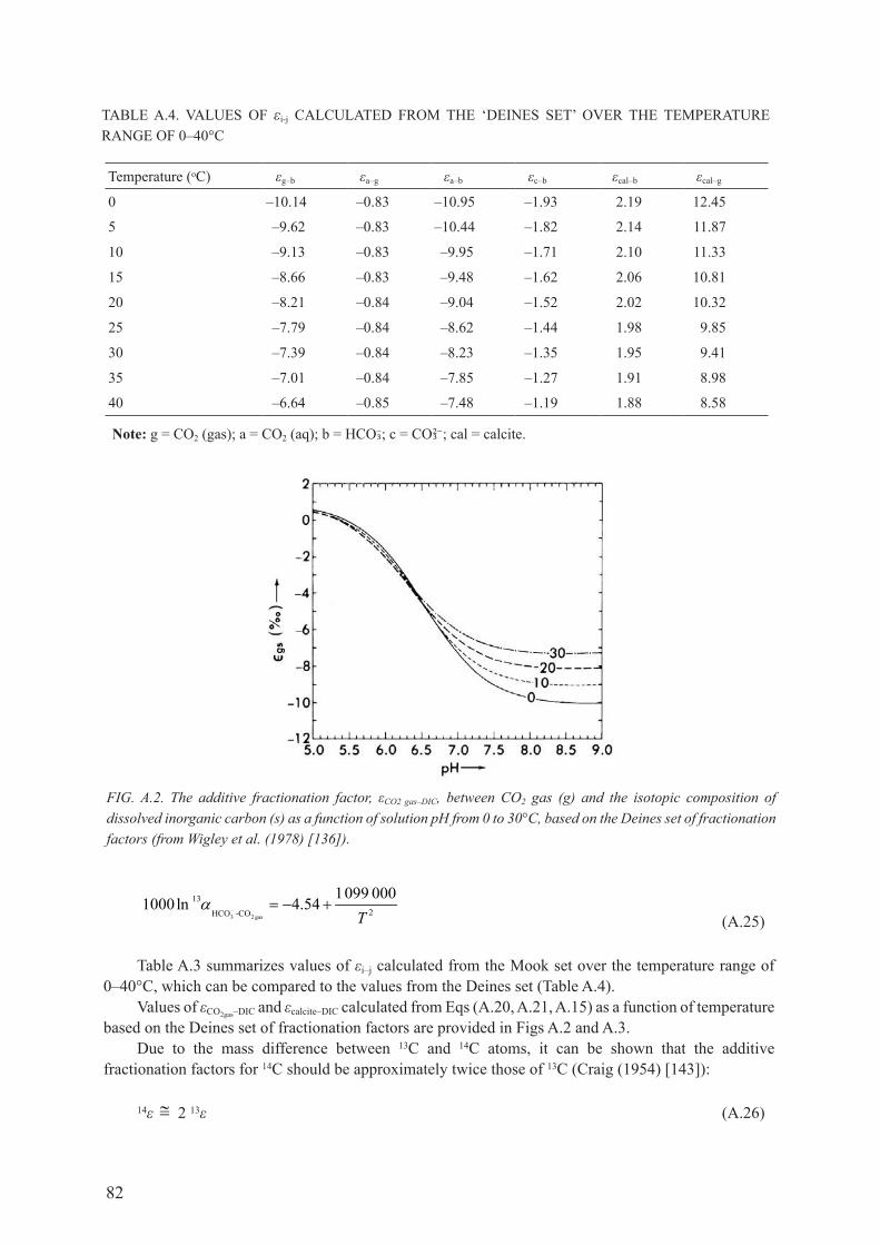
82

–3 2 gas

132Hco -co

1 099 0001000ln 4.54

Tα = − +

(a.25)

Table A.3 summarizes values of εi–j calculated from the mook set over the temperature range of 0–40°c, which can be compared to the values from the deines set (Table A.4).

Values of εco2gas–dIc and εcalcite–dIc calculated from eqs (a.20, a.21, a.15) as a function of temperature based on the deines set of fractionation factors are provided in figs a.2 and a.3.

due to the mass difference between 13c and 14c atoms, it can be shown that the additive fractionation factors for 14c should be approximately twice those of 13c (craig (1954) [143]):

14ε ≅ 2 13ε (a.26)

TABLE A.4.  vALUES  of  εi-j  cALcULATEd  from  THE  ‘dEINES  SET’  ovEr  THE  TEmPErATUrE rANgE of 0–40°c

temperature (oc) εg–b εa–g εa–b εc–b εcal–b εcal–g

0 –10.14 –0.83 –10.95 –1.93 2.19 12.45

5 –9.62 –0.83 –10.44 –1.82 2.14 11.87

10 –9.13 –0.83 –9.95 –1.71 2.10 11.33

15 –8.66 –0.83 –9.48 –1.62 2.06 10.81

20 –8.21 –0.84 –9.04 –1.52 2.02 10.32

25 –7.79 –0.84 –8.62 –1.44 1.98 9.85

30 –7.39 –0.84 –8.23 –1.35 1.95 9.41

35 –7.01 –0.84 –7.85 –1.27 1.91 8.98

40 –6.64 –0.85 –7.48 –1.19 1.88 8.58

note: g = co2 (gas); a = co2 (aq); b = hco!; c = co$; cal = calcite.

FIG. A.2. The additive fractionation factor, εCO2 gas–DIC, between CO2 gas (g) and the isotopic composition of dissolved inorganic carbon (s) as a function of solution pH from 0 to 30°C, based on the Deines set of fractionation factors (from Wigley et al. (1978) [136]).

83

This  relation  is  used  in NETPATH  (Plummer  et  al.  (1994)  [120]). There  is  some  experimental and theoretical evidence that the additive fractionation factors for 14c may be approximately 2.3 times greater than those for 13c (Saliege and fontes (1984) [224]; wigley and muller (1981) [225]).

A.2.3. total dissolved carbon

If Tdc is defined as mtdc = mdIc + mdoc + mcH4, then δ13ctdc becomes:

4 4

13 13 13dIc dIc doc doc ch ch13

tdctdc

c c cc

m m m

m

δ + δ + δδ = (a.27)

If methane and/or doc are present, the fractionation factors relative to the average isotopic composition of the solution need to be modified to reflect the presence of these additional species, even though  they are not  likely  to be  in  isotopic equilibrium with any carbon-bearing aqueous species  in the solution. therefore, to estimate values of fractionation factors in the system of tdc, concentrations and isotopic composition of doc and/or ch4  must  be  measured  or  defined.  following  the  above examples for calcite and co2 gas, eqs (a.20, a.21) become:

13

13

133

3 3

αα

χ α χcalcite TDCcalcite HCO

CO CO HCO HCO2 aq 2 aq

−

−

−

=+

−

− − ++ + +− − − − −− − −χ α χ α χ α

CO CO HCO DOC DOC HCO CH CH HCO4 432

32

3 3 3

13 13 13 (a.28)

and

13

13

133

3 3

αα

χ α χ χCO TDC

CO HCO

CO CO HCO HCO2 gas

2 gas

2 aq 2 aq

−

−

−

=+ +

−

− − CCO CO HCO DOC DOC HCO CH CH HCO32

32

4 4− − − − −− − −

+ +13 13 13

3 3 3α χ α χ α

(a.29)

In eqs (a.28, a.29), αdoc–hco! and αdoc–hco! are  treated  as  though  they  were  empirical  kinetic isotope  fractionation  factors  and  defined  from  the measured  (or  estimated)  isotopic  composition  of doc and ch4 in the groundwater sample:

FIG. A.3. The additive fractionation factor, εcalcite–DIC, between calcite (p) and the isotopic composition of dissolved inorganic carbon (s) as a function of solution pH from 0 to 30°C, based on the Deines set of fractionation factors (from Wigley et al. (1978) [136]).

84

–4 3

–

13ch13

13cH -Hcohco

1000 c1000 c

+ δ

+ δ (a.30)

and

–3

–3

1313 doc

13doc-Hcohco

1000 c1000 c

α + δ=

+ δ (a.31)

Values of δ13chco! are calculated from the measured δ13cdIc using eq. (a.19).

Examples: Open systemUsing the mook set of additive fractionation factors in the inorganic calcite–co2–water system,

the δ13cdIc of dIc is calculated as calcite dissolves, maintaining isotopic equilibrium among all dissolved species and calcite at 20ºc for a (constant) δ13cco2 gas value of –23‰; pointing to evolution in a system open to soil gas co2 of 13c isotopic composition of –23‰. The following ε values are obtained from Table A.2, at 20°c: εg–b = –8.46‰; εa–g = –1.08‰; εa–b = –9.54‰; εc–b = –0.44‰; εcal–b = 0.66‰; εcal–g = 9.20‰.

accordingly, for δ13cco2gas, which was defined to be –23‰, δ13ccalcite = –13.8‰, δ13chco! = –14.5‰, δ13cco3 = –14.9‰ and δ13cco2aq = –24.1‰. calculating the fractions of inorganic carbon species relative to dIc and using eq. (a.19), it can be seen that the value of δ13cdIc will increase with increasing ph, as calcite dissolves, from about –24‰ at pH5 and increases to about –14.5‰ at pH8.5 where nearly all of the dIc is hco! (fig. A.4). A similar result is obtained from the ‘deines set’ using the plot of fig. A.2 where at 20°c and pH8.5, εg–dIc is approximately –8‰ and δ13cdIc is about –15‰.

next, an estimation is made of the initial 14c pmc value of dIc in groundwater in equilibrium with a soil gas co2 value of 100 pmc at 20°c. As 14εg–dIc ≅ 2 13εg–dIc ≅ –16‰, Ao in an open system at 20°c is about 102 pmc:

FIG. A.4. The δ13CDIC of dissolved inorganic carbon in the open system calcite–CO2–water, for δ13CCO2 = –23‰ at

20°C (Mook’s set of fractionation factors).

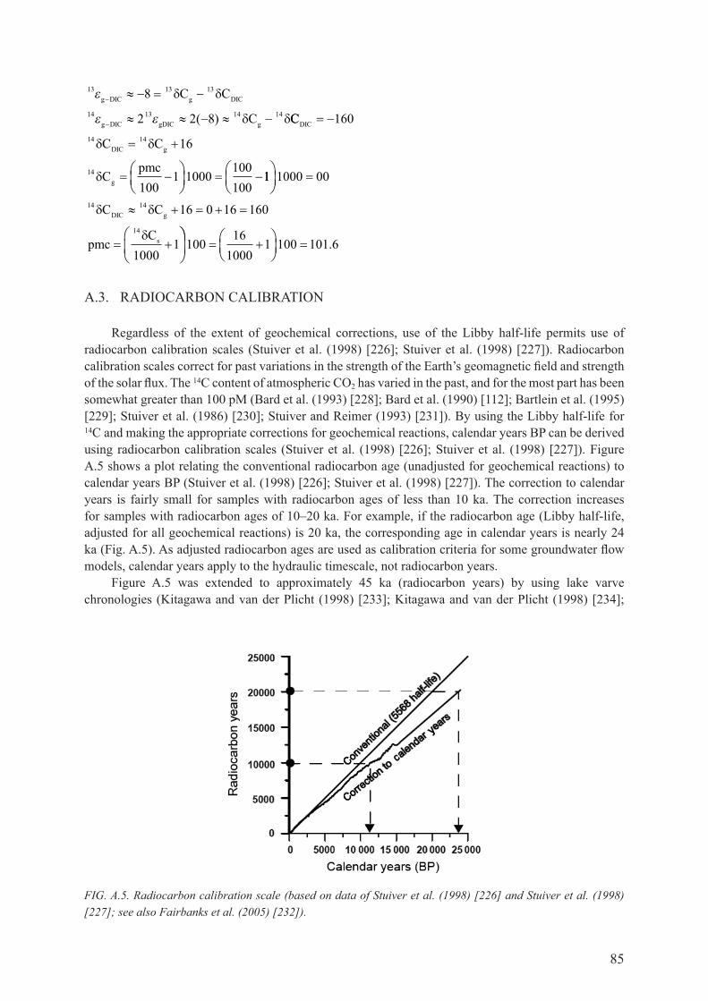
85

13 13 13

14 13 14 14

8

2 2 8

ε

ε ε

g DIC g DIC

g DIC gDIC g

C C

C−

−

≈ − = −

≈ ≈ − ≈ −

δ δ

δ δ( ) CC

C C

Cpmc

DIC

DIC g

g

= −

= +

= − = −

16

16

1001 1000

100100

14 14

14

0

δ δ

δ 11 1000 0

16 0 16 16

10001

14 14

14

=

≈ + = + =

= +

0

0δ δ

δ

C C

pmcC

DIC g

s

= + =100

161000

1 100 101 6.

a.3. radIocarbon calIbratIon

regardless  of  the  extent  of  geochemical  corrections,  use  of  the  Libby  half-life  permits  use  of radiocarbon calibration scales  (Stuiver et al.  (1998)  [226]; Stuiver et al.  (1998)  [227]). radiocarbon calibration scales correct for past variations in the strength of the Earth’s geomagnetic field and strength of the solar flux. The 14c content of atmospheric co2 has varied in the past, and for the most part has been somewhat greater than 100 pm (Bard et al. (1993) [228]; Bard et al. (1990) [112]; Bartlein et al. (1995) [229]; Stuiver et al. (1986) [230]; Stuiver and reimer (1993) [231]). By using the Libby half-life for

14c and making the appropriate corrections for geochemical reactions, calendar years BP can be derived using  radiocarbon calibration scales  (Stuiver et al.  (1998)  [226]; Stuiver et al.  (1998)  [227]). figure a.5 shows a plot relating the conventional radiocarbon age (unadjusted for geochemical reactions) to calendar years BP (Stuiver et al. (1998) [226]; Stuiver et al. (1998) [227]). The correction to calendar years  is  fairly  small  for  samples with  radiocarbon ages of  less  than 10 ka. The correction  increases for samples with radiocarbon ages of 10–20 ka. for example, if the radiocarbon age (Libby half-life, adjusted for all geochemical reactions) is 20 ka, the corresponding age in calendar years is nearly 24 ka (fig. A.5). As adjusted radiocarbon ages are used as calibration criteria for some groundwater flow models, calendar years apply to the hydraulic timescale, not radiocarbon years.

figure  A.5  was  extended  to  approximately  45  ka  (radiocarbon  years)  by  using  lake  varve chronologies (Kitagawa and van der Plicht  (1998) [233]; Kitagawa and van der Plicht  (1998) [234]; 

FIG. A.5. Radiocarbon calibration scale (based on data of Stuiver et al. (1998) [226] and Stuiver et al. (1998) [227]; see also Fairbanks et al. (2005) [232]).

86

Kitagawa and van der Plicht (2000) [235]) (fig. A.6). A polynomial (Eq. (A.32)) was fitted to the data of fig. A.6 and used to estimate calendar years from the unadjusted radiocarbon age (Libby half-life):

calendar years BP = –173.94 + 1.1713A – 2.0521 × 10–5A2 + 4.0150 × 10–9A3

– 2.4519 × 10–13A4 + 5.7738 × 10–18A5 – 4.6915 × 10–23A6 (a.32)

where A is the unadjusted radiocarbon age (Libby half-life) in years.

Although  the radiocarbon calibration data obtained from tree rings (Stuiver et al.  (1998) [226]; Stuiver  et  al.  (1998)  [227])  and  230th/234U  dating  of  corals  (Bard  et  al.  (1998)  [236])  are  relatively precise, larger uncertainties in radiocarbon calibration are associated with data obtained from varves (Kitagawa  and  van  der  Plicht  (1998)  [233];  Kitagawa  and  van  der  Plicht  (1998)  [234]).  recently, additional calibration data have been obtained from a stalagmite in the calendar year age range of 11–45 ka that indicate large variations in atmospheric 14c content of between 33 and 45 ka (Bard (2001) [237]; Beck et al. (2001) [238]). Although radiocarbon calibration to about 20 ka now seems well established for groundwater applications, extension of the calibration to the dating limits of the radiocarbon method (about 45 ka) has received considerable attention recently (chiu et al. (2007) [108]; chiu et al. (2005) [239]; chiu et al. (2006) [240]; fairbanks et al. (2005) [232]; Sanford et al. (2004) [47]; Sanford et al. (2004) [48]).

A.4.  fIELd coLLEcTIoN ProcEdUrES

A.4.1. Well selection

water samples for 14c determination have historically been obtained from a variety of groundwater sources, including municipal supply wells, monitoring wells, wells used for domestic or farm supply, windmills, flowing wells and springs. Prior to sampling, attention should be given to well construction, 

FIG. A.6. Extended radiocarbon calibration to approximately 45 ka radiocarbon years (based on the data of Bard et al. (1998) [236]; Kitagawa and van der Plicht (1998) [233]; Kitagawa and van der Plicht (1998) [234]; Kitagawa and van der Plicht (2000) [235]; Stuiver et al. (1998) [226]; Stuiver et al. (1998) [227]). The blue line is from Eq. (A.33) from Plummer et al. (2004) [49] (see Fairbanks et al. (2005) [232]).

87

depth and length of the interval open to an aquifer. commonly, municipal supply wells are open to large intervals of an aquifer, resulting in mixing across 14c model age gradients. samples pumped from fractured rock aquifers also tend to be mixtures. Preferred samples for radiocarbon dating are obtained from monitoring wells or flowing wells with a short open interval to the aquifer.

for recently constructed wells, a precaution is necessary; the possibility should be considered that  the  aquifer was  contaminated with  fluids  used  in  the  drilling  process. during  drilling,  such  as in mud-rotary drilling,  and  in well  development  after  completing  a well, water  is  often  imported  to the drilling site and pumped into the wellbore. If this imported water is not completely removed in well development, the dIc in the vicinity of the well opening can be contaminated. plummer et al. (2004)  [49] measured  the  concentrations  of  cfcs  in water  pumped  from  deep,  recently  completed monitoring wells in New mexico to identify samples that were likely still contaminated with imported water used in drilling and well development. the most reliable radiocarbon data were obtained from monitoring wells that were free of cfcs, and from domestic supply wells that tended to have more use and relatively short open intervals. as a general guide, water from recently drilled monitoring wells is more likely to be contaminated than water from older wells that have a long history of sampling (or extended well development). the problem is particularly acute in sampling very old water because, due to low flow velocities in an aquifer, groundwater contaminated during drilling may still reside in the vicinity of a well screen even many years after drilling. due to matrix diffusion into sediment pore spaces, many pore volumes may need to be pumped prior to sampling.

flowing wells can be another good source of uncontaminated water if there is a long history of use. finally, because of the possibility of mixing with young fractions, sampling for radiocarbon determination should always include determination of tritium (and possibly cfcs).

A.4.2. sample collection

water samples should be collected as close to the source as possible, and certainly before treatment, such as chlorination, ozonation or aeration, and only after sufficient flow to clear three wellbore volumes from the casing. In the case of domestic supply wells, it is recommended that samples be taken before water enters a pressure tank, where, in the case of a bladderless pressure tank, water would be exposed to a gas phase.

A.4.2.1. Tritium

Tritium  samples  are  collected  in  a  1  L  plastic-coated  glass  bottle  with  a  polycone  seal  cap. A headspace of approximately 2–3 mL is left in the bottles during filling to accommodate expansion upon warming. tritium analysis is used to detect contamination of old groundwater with water from the bomb era or contamination from drilling. In the case of very old water, as discussed here, tritium should be determined with a very low minimum detection level (<0.1–0.3 tu by electrolytic enrichment and liquid scintillation counting; or preferably <0.1 TU by the helium in-growth method (Bayer et al. (1989) [241]; clarke et al. (1976) [242]).

A.4.2.2. Carbon-13 and carbon-14 of dissolved inorganic carbon

water samples for the determination of δ13c and 14c of dIc should be filtered in the field (0.45 μm filter), collected  in safety coated glass bottles, and capped with a polycone seal cap,  leaving a small 2–3 ml headspace to accommodate water expansion. alternatively, if a sample will be analysed within a few months, a Teflon/silicon septum cap can be used; excluding headspace is recommended. In this case, the septum is normally depressed as the cap is put in place to allow for water expansion. although it

88

can be debated, addition of a preservative to stop possible microbial activity runs a risk of contamination of the sample with a fraction of modern 14c and is not recommended for old groundwater samples.

although most aMs facilities can determine 14c content of dIc with as little as 1 mg of carbon, it  is  recommended  that  the volume of water sample collected be sufficient  to contain a minimum of 5 mg of dIc (as c). for many water samples, a 250 mL sample will be sufficient. figure A.7 provides guidelines  for  sample  volumes  required  to  provide  a  minimum  of  5  mg  dIc  for  a  range  of  field alkalinities and pH. The two curves in the figure provide corresponding alkalinity and pH values for simple inorganic carbonate waters (at 25°c) that would contain 5 or 10 mg of dIc in a 250 mL volume. If, for example, the sample alkalinity is 150 mg/L (as caco3) or greater, a 250 mL bottle fitted with a Teflon/silicon septum is sufficient  for most pH. Sample volumes of 1 L or more will be needed  if field alkalinity is less than 80 mg/L (as caco3) and pH is greater than 7.0. If alkalinity is unknown at the time of sampling, it is recommended to fill two 1 L bottles.

A.4.3. Recommended method of collection (dissolved inorganic carbon)

fill  the appropriate bottle(s) fitted with a Teflon/silicon septum cap  to provide at  least 5 mg of dIc.  fill  the  sample  container(s)  from  the  bottom  of  the  vessel. Use  an  in-line  filter  (0.45  μm)  to eliminate the possibility of contamination of the dIc with particulates containing carbonate minerals. If there is concern about doc oxidation in the sample bottle, a silver filter can be used, though this is normally not needed. minimize contact with air while filling the bottle(s). This can be accomplished by establishing a closed path from the water source, through the filter, to the bottom of the container. fill from the bottom, allowing overflow of several litres of filtered water. for potentially low 14c samples (<10 pmc) or if relatively long times are required for filtering, place the sample bottle in a small bucket or beaker containing water from the same source, flush the sample bottle from the bottom of the bottle while still immersed in the bucket or beaker (allowing overflow of several litres) and cap with a Teflon/silicon septum cap under water. It is best to depress the septum slightly, without compromising the seal, as the cap is screwed onto the bottle to provide room for water expansion as the sample warms during transit and storage prior to analysis. Use plastic coated glass bottles fitted with a Teflon/silicon septum for most samples. the septum allows laboratory extraction of the water sample without contact with air.

FIG. A.7. Guidelines indicating amounts of groundwater sample required for collection to obtain at least 5 mg C/L as a function of alkalinity (as CaCO3) and pH (note: alkalinity (in mg/L as CaCO3) = alkalinity (in mg/L as HCO!) × 0.82014).

89

A.4.4. Carbon-13 and carbon-14 of dissolved organic carbon

the procedure for collection of hMw and lMw fractions of doc is provided in Murphy et al. (1989) [172] and is based on the original work of Thurman and malcolm (1981) [180], and murphy (1987) [181]. The sample is filtered (0.45 µm) in the field and collected using a field column system. The fulvic acids (primarily Hmw) typically make up about 30% of the doc in groundwater, and are collected on xAd-8 resin. The Lmw compounds are collected on Silicalite, a silica based molecular sieve. Prior to use, the Silicalite is preheated to 1000°c to remove organic contamination. The xAd-8 and Silicalite columns remove only about 30–60% of the total doc in groundwater. To characterize the fulvic acid fraction completely, a minimum of 200 mg of material is typically needed, and sample volumes of the order of 100–200 l are usually processed. further details are provided in Murphy et al. (1989) [172]. other procedures for collection of total doc can be found in Purdy et al. (1992) [173] and Burr et al. (2001) [184].

a.5. geocheMIcal ModellIng software

united states geological survey (usgs) geochemical modelling software of use in interpreting radiocarbon  data  (NETPATH,  NETPATH-wIN,  NetpathxL,  PHrEEqc,  PhreeqcI)  and  associated documentation can be downloaded from the web site:

http://wwwbrr.cr.usgs.gov/projects/gwc_coupled/other usgs geochemical software is available from:http://water.usgs.gov/software/geochemical.htmlthe calIb radiocarbon calibration programme is available from:http://calib.qub.ac.uk/calib/

a.6. selected accelerator Mass spectroMetry facIlItIes for radIocarbon analysIs

A list of active radiocarbon laboratories (conventional beta-counting facilities and AmS facilities), and  known  personnel  is  published  annually  in  the  journal  radiocarbon (see, for example, list of laboratories, radiocarbon 51(4) (2009) 1187–1211 and http://www.radiocarbon.org/Info/lablist.html).

91

Chapter 5

kRYPtOn-81 DAtInG OF OLD GROUnDWAtER

r. purtschertphysics Institute, university of bern, Bern, Switzerland

r. yoKocHI, N.c. STUrcHIodepartment of earth and environmental sciences, university of Illinois, chicago, Illinois, united states of america

5.1. IntroductIon

5.1.1. krypton in the environment

The  abundance  of  krypton  in  the  atmosphere  has  been  quoted  for  nearly  half  a  century  as 1.14 ± 0.01 ppm, which corresponds to a total atmospheric inventory of 4.51 × 1012 m3 stp (Verniani (1966) [243]). A recent re-evaluation yielded a value of 1.099 ± 0.009 ppmv, which is about 4% lower than the previously used value (Aoki and makide (2005) [244]).

Krypton has  six  stable  isotopes  of which  84Kr  is  the most  abundant,  comprising  about  57% of natural Kr (Table 5.1). Eleven major radioactive isotopes of Kr exist but only 81Kr and 85Kr, with half-lives of 229 000 and 10.76 a, respectively, exceed 2 d and are, therefore, suitable for the investigation of environmental processes. Krypton-81 is produced in the atmosphere by cosmic ray induced spallation of heavier stable Kr isotopes and by the nuclear reactions 80Kr(n, γ)81Kr and 82Kr(γ, n)81Kr.

the atmospheric 81Kr/Kr ratio has been measured three times by different methods and research groups  (fig. 5.1;  collon  et  al.  (1997)  [245];  Kuzminov  and  Pomansky  (1983)  [246];  Loosli  and oeschger  (1969)  [247]).  The  mean  value  of  5.2  ±  0.6  ×10–13  corresponds  to  a  specific  activity  in the modern atmosphere of 1.47 mBq · L–1 Kr.1 Variations in the production rate, for example, due to modulations  of  the  geomagnetic  field  intensities with  a  period  of  10–30  ka  (Plummer  et  al.  (1997) [248]), are likely to be averaged out on the timescale of the 81Kr mean lifetime (the atmosphere is well mixed within a timescale of ~1 a). this, and the fact that the atmosphere represents the main terrestrial Kr reservoir, provides evidence that  the  81Kr abundance in the atmosphere is rather constant over  its applicable age dating range.

the production of 81Kr from 235u or 238U fission is expected to be very small because the nuclide is shielded by stable 81Br.  The  direct  fission  yield  of  81Kr  is  estimated  to  be  only  7  ×  10–11 atoms 81Kr/atoms Udecayed. for this reason, anthropogenic sources such as nuclear weapon testing and releases from  the nuclear  industry are probably  insignificant. This has been confirmed by  the comparison of post-bomb and pre-bomb atmospheric samples, for which the most recent measurements resulted in an agreement at the 8% precision level (du et al. (2003) [249]). Likewise, subsurface production of 81Kr in  rocks  is expected  to be very  small;  the equilibrium concentration of  81Kr  from fission production is 5 × 10–6 81Kr atoms · kg–1

rock  · ppm–1 u. production due to neutron capture by 80Kr is probably of the same order of magnitude (Lehmann et al. (1993) [250]).

1 10–3 dis · s–1 · Lstp–1 Kr.

92

5.1.2. krypton in hydrology

5.1.2.1. Dating principles

during recharge, water approaches solubility equilibrium with the atmosphere according to the local temperature and barometric pressure at the water table (fig. 5.2). gas partitioning at the free air–water interface is described by Henry’s law:

cgas/cwater = h(T, S) (5.1)

wherecgas and cwater denote the concentration of a given gas species in the gas phase and water

phase, respectively;h(T, S)     is  the  dimensionless Henry  coefficient,  which  depends  on water  temperature T and

salinity S.

water in equilibrium with the atmosphere at 10°c and 1 atm contains ~1300 atoms 81Kr/L water (table 5.1). this is more than seven orders of magnitude larger than the equilibrium concentration of  fission  81Kr  in  the  crust  (see  above),  indicating  that  subsurface  production  of  81Kr  is  negligible compared with the groundwater source. In the (unlikely) case of a 100% 81Kr release rate from the rock into the water filled pore volume, for a rock porosity of 30% and a uranium concentration of 50 ppm, a 81Kr activity in the water of less than 1‰ of the modern level would result. for a temperature of 10°c, a mean ocean salinity of 35‰ and a total world ocean water volume of 1.4 × 1018 m3, a total ocean Kr inventory of 1011 m3 is estimated, which corresponds to about 2% of the global inventory. therefore, exchange between ocean and atmosphere (e.g. as a result of changing temperature) has little impact on the atmospheric Kr inventory.

during  recharge,  Kr  (and  other  atmospheric  gases)  may  additionally  be  introduced  by the dissolution of excess air (fig. 5.2) (Heaton and vogel (1981) [211]). In contrast to other gaseous tracer methods, which rely on absolute concentrations of dissolved constituents (such as 3h/3he, sf6 or 4he), 81Kr and 85Kr (and 39ar), gas tracers are insensitive to absolute concentration that is affected by the addition of excess air, degrees of degassing (both in nature and during sampling; see also chapter 8) and recharge conditions because these methods are based on isotope ratios of the same element (81Kr/Kr, 81Kr/Kr, 39ar/ar, etc.).

FIG. 5.1. Measurements of the modern atmospheric 81Kr/Kr ratio.

93

after the air saturated water parcel has moved to depths of greater than about 20 m, the 81Kr (or 39ar) exchange with the source (atmosphere) stops and the 81Kr/Kr ratio decreases due to radioactive decay (fig. 5.2). according to the exponential decay law, the time elapsed since the water was in contact with the atmosphere can be calculated according to:

sample

81 air

1 lnKr

Rt

R

(5.2)

whereλ81 is the 81Kr decay constant (3.03 ± 0.14 × 10–6/a);Rsample and Rair are the 81Kr/Kr ratios of the sample and modern air respectively (Table 5.1).

TABLE 5.1. KryPToN IN THE ENvIroNmENT: SomE USEfUL NUmBErS

Kr species/physical characteristic Value unit reference

Kr concentration in the atmosphere 1.1 ppm Aoki and makide (2005) [244]

Isotopic composition (stable)

Kr-78 0.35 % ozima and Podosek (2002) [251]

Kr-80 2.26 % ozima and Podosek (2002) [251]

Kr-82 11.52 % ozima and Podosek (2002) [251]

Kr-83 11.48 % ozima and Podosek (2002) [251]

Kr-84 57 % ozima and Podosek (2002) [251]

Kr-86 17.4 % ozima and Podosek (2002) [251]

Kr-85/Kr (2008) 2.4 ×10–11 winger et al. (2005) [252]

Kr-81/Kr (air) 5.2 ± 0.6 ×10–13 du et al. (2003) [249]; collon et al. (1997) [245]

Kr-85/Kr-81 (2008) 46.2 du et al. (2003) [249]; collon et al. (1997) [245]

Half-life Kr-85 10.76 a firestone and shirley (1996) [253]

Half-life Kr-81 229 000 a firestone and Shirley (1996) [253]

Kr-85 atoms/l water (2008) 57 845du et al. (2003) [249];

collon et al. (1997) [245]

Kr-81 atoms/l water (modern) 1253 du et al. (2003) [249]; collon et al. (1997) [245]

Kr solubility in water (10°c) 0.081 cm3stp · cm–3

water · atm–1 weiss and Kyser (1978) [254]

diffusion coefficient of Kr in air (20°c) ~0.13 cm2/s weast (1981) [255]

diffusion coefficient of Kr in water (20°c) ~6.2 10–5 cm2/s weast (1981) [255]

94

Rsample can also be expressed as %modern in relation to Rair = 100%modern. as underground production can be neglected, the only process other than decay that might change the isotopic ratio in the groundwater system is mixing driven by diffusive/dispersive processes (especially with aquitards) and/or convergent flow (Lehmann et al. (2003) [256]).

the suitable dating range of 0.2 × 105–106 a (~5 half-lives), the presumably constant and known input concentration, the potential absence of underground production and the fact that dating is based on an isotope ratio (81Kr/Krtotal) which is not sensitive to climate variations and phase transition processes, makes  81Kr  an  ideal  tracer  for  dating  old  groundwater  or  ice. The  fundamental  limitation  hindering the routine use of 81Kr in environmental science is the analytical challenge of sampling and measuring 81Kr concentrations at natural levels.

5.1.2.2. Diffusive exchange with stagnant zones

there are only a few processes that may affect the interpretation of 81Kr  activities  in  terms of groundwater age. the two most potentially critical processes are: (i) mixing of different water flow path components as for any radiometric dating tracer and (ii) diffusive exchange between the aquifer (active flow zone) and the less permeable adjacent aquitards (‘stagnant zones’). In (i), ages calculated on the basis of the radioactive decay law yield a lower age limit for mixtures due to the concave shape of the exponential function (see chapters 3 and 9). for (ii), diffusive loss of 81Kr atoms into stagnant zones of the system, on the other hand, dilutes tracer concentration in the active flow zone and results in tracer model ages which are too old compared with pure decay based idealized ages (see also Section 4.9.3). The  larger  the  tracer diffusion accessible volume  in  relation  to  the advective system volume, 

FIG. 5.2. Scheme of relevant processes for radio-noble gas dating. Cosmic ray induced production in the atmosphere, gas dissolution in the recharge water due to solubility equilibrium and trapped air bubbles in the quasi-saturated soil zone (excess air) and radioactive decay in the subsurface.

Radioactive decay

Atmospheric input

Sampling

Subsurface processes

Tracer age

Rsa

mpl

e/Rat

mos

pher

e

Solubility equilibrium+ dissolution of excess air

Radioactive decay1

Diffusive exchange with aquitard

Gas exchange

Cosmic rays

14C, 39Ar, 81Kr Target nuclides in theatmosphere

95

the older the tracer model age becomes compared with the hydraulic age. the ratio of tracer model age to hydraulic age is expressed by the effective retardation factor R (małoszewski and zuber (1985) [257]). Both processes are competitive  in  terms of  their effect on  81Kr model age (fig. 5.3). the top image in fig. 5.3 depicts the evolution of a stable tracer (in blue). The initially tracer free stagnant zone is  increasingly  penetrated  due  to  the  concentration  gradient  between  the  active  and  stagnant  zones. Steady state is achieved when concentration gradients are equalized in the whole system. The bottom image depicts the diffusion limit of a radioactive tracer (brown) with a diffusion length L < b/2 (fig. 5.3 modified after cook et al. (2005) [208]).

The  accessible  system  volume  is  tracer  (half-life)  specific  and  depends  on  the  effective  tracer diffusion coefficient Deff in the pore space of the stagnant zones. for a stable tracer, the diffusion path length L(t) increases steadily and indefinitely as a function of time (Einstein (1905) [258]):

eff( )L t D t (5.3)

for radioactive tracers on diffusion, length at steady state is constrained by the mean lifetime τ = 1/λ of the tracer.

effra eff

DL D

  (5.4)

The situation is illustrated in fig. 5.3 for an idealized system of parallel flow and stagnant zones with thicknesses a, b and porosities na, nb, respectively. It is assumed that the tracer concentration in

FIG. 5.3. Diffusive tracer retardation in simplified double porous media. The advective flow system with aperture a and porosity na may either be a fracture (na = 1 in this case) surrounded by a rock matrix (with porosity nb) or an aquifer between two aquitards, each with thickness b. The process is depicted at a specific location as a function of time increasing from left to right.

L(t)>>b/2

Lra<b/2

TimeSteadystate

b

a

nbab

na

Lra

b/2b/2

L(t)

t1 t2 t3 t∞

96

the stagnant zone is initially zero and that sorption reactions are negligible. The retardation factor R is provided by the ratio of the total tracer accessible pore volume to the mobile water volume.

a b

a

2 ( )( )

a n L t nR t

a n

(5.5)

for short flow times and/or slow diffusion L(t) becomes small and the retardation factor Ir(t) is ~1 (fig. 5.3, t1). with increasing flow time, L(t) increases according to eq. (5.3) and the tracer delay R(t) increases as well (t2–t3). The steady state situation depends on the half-life of the tracer, the diffusion coefficient and  the spacing b between the mobile zones. A diffusion  length L(t) or Lra exceeding b/2 (fig. 5.3, t∞ top) will result in a retardation factor R which is simply provided by the ratio of total system porosity to the porosity of the advective flow system (małoszewski and zuber (1985) [257]):

a b

a

a n b nR

a n

(5.6)

FIG. 5.4. Plots of the logarithm of steady state retardation factor Rss as a function of the logarithm of the thickness of the stagnant zone (b) and the thickness of the transmissive zones (a). The relations are shown for 3H, 14C and 81Kr assuming reasonable effective diffusion coefficients and a porosity of the flow zone of 0.3 (Sanford (1997) [207]). The system characteristics of the Great Artesian Basin (Section 5.5) and the Nubian aquifer (Chapter 14) are also indicated in the 81Kr plot.

14C3H

81Kr-3 -2.5 -2 -1.5 -1 -0.5 0 0.5 1 1.5 2 2.5 3

-3

-2.5

-2

-1.5

-1

-0.5

0

0.5

1

1.5

2

2.5

3

-3 -2.5 -2 -1.5 -1 -0.5 0 0.5 1 1.5 2 2.5 3

log b (m)

-3

-2.5

-2

-1.5

-1

-0.5

0

0.5

1

1.5

2

2.5

3

lo g a

(m)

-3 -2.5 -2 -1.5 -1 -0.5 0 0.5 1 1.5 2 2.5 3-3

-2.5

-2

-1.5

-1

-0.5

0

0.5

1

1.5

2

2.5

3

-0.20.20.611.41.82.22.633.43.84.24.655.4

81Kr

GABNubian Aquifer

log b (m) log b (m)

log

a ( m

)

l og a

( m )

log Rss

97

for fast decaying radioactive tracers and/or slow diffusion in large impermeable zones (Lra< b/2), the retardation factor is limited to a maximal steady state value Rss (fig. 5.3, case d bottom).

a ra bss

a

2a n L nR

a n

(5.7)

with Lra  given  in  Eq.  (5.3).  The  mobile  and  stagnant  zones  can  be  interpreted  either  as  aquifers surrounded by aquitards or as fractures within a rock matrix. In the latter case, na = 1.

steady state retardation factors for 3h, 14c and 81Kr are shown in fig. 5.4 as functions of the system parameters a and b for reasonable porosities and effective tracer diffusion coefficients (Sanford (1997) [207]). As deduced above, diffusive retardation is small for thick aquifers (large a) with thin aquitards (small b; blue area) and increases with increasing b for constant a. If the extension of the stagnant zones exceeds the tracer diffusion length Lra (the location of the sharp bend on the b axes), R levels off with increasing b. The longer the diffusion length (or half-life of the tracer),  the higher the maximal retardation factor for a given geometry of the system. fractures with small apertures (a) and long flow times may produce retardation factors R of up to 103 (fig. 5.4; cook et al. (2005) [208]). for several hundred metre  thick regional aquifers such as  the j-sandstone aquifer  in  the great Artesian Basin or the nubian aquifer in egypt (see case studies), relatively moderate steady state 81Kr retardation factors can  be  expected  (coloured  boxes  in  fig. 5.4).  Equations  (5.5–5.7)  probably,  in most  circumstances, overestimate the retardation R of the tracer. This is because (i) the permeability in ‘stagnant zones’ in most cases still allows some advective flow and (ii) because  timescales may be  too short  to achieve a steady state equilibrium between the active and passive flow systems.

5.1.2.3. Additional noble gas tracers (85Kr, 37Ar and 39Ar)

with the current status of analytical techniques, 81Kr  sampling  and measurement  require  large volume water  degassing  in  the  field  (see  next  sections).  The  collected  gas  offers  the  possibility  to measure not only 81Kr  but  also  three  other  shorter  lived  noble  gas  radionuclides  that  may  provide additional valuable information.

Krypton-85

Krypton-85 is the second radioactive Kr isotope that is suitable for groundwater dating for reasons similar to that of 81Kr. However, the shorter half-life (t1/2 = 10.76 a) limits the dating range of 85Kr to <50 a. Krypton-85 is produced as a fission product of uranium and plutonium decay. over the past 50 a, the increasing release of 85Kr from nuclear fuel reprocessing plants (such as Sellafield, La Hague) has completely overwhelmed the natural activity of about 10–7 bq/cm3

stp Kr (Lehmann and Loosli (1984) [259]). The current specific activity in the atmosphere is about 1.4 Bq/cm3

stp Kr, which corresponds to an atomic ratio of 85Kr/Krtotal of 2 × 10–11 (see also fig. 5.10). Air saturated water (10°c, 1 atm) contains about 58 000 85Kr atoms/L water (Table 5.1). Krypton-85 detected in gas extracted from groundwater indicates either the admixture of young groundwater (Althaus et al. (2007) [260]) or, in the case of very old groundwater, can be used as an indication of atmospheric air contamination during sampling and gas purification (Loosli et al. (2000) [261]).

Argon-39

Argon-39 is produced through the interaction of cosmic rays with nuclides of potassium and argon in the atmosphere. the resulting atmospheric equilibrium activity is constant at 1.67 × 10–2 bq/m3

of air (Loosli (1983) [262]), corresponding to an atmospheric 39ar/ar ratio of ~10–15 (anthropogenic sources are neglible). with a half-life of 269 a, 39Ar fills the dating gap between young residence time indicators 

a maximal steady state value Rss (Fig. 5.3, Case D bottom).

a ra bss

a

2a n L nR

a n

(5.7)with Lra given in eq. (5.3). the mobile

98

(cfc, 3h/3he,  etc.)  and  the  radiocarbon method  (corcho  et  al.  (2009)  [263];  corcho  et  al.  (2007) [264]). owing to the very low isotopic abundance of 39ar, a relatively large amount of water (~2000 l) has to be degassed in the field to obtain a sufficient number of 39Ar atoms. Although first attempts have been made to use the accelerator mass spectrometry (aMs) technique which would reduce this volume (collon et al. (2004) [265]), and laser atom trap methods are currently being developed (williams et al. (2010) [266]), the detection of 39ar is currently only practical using the radioactive decay counting technique (Loosli (1983) [262]). The 39ar activity of the argon separated from groundwater is measured in high pressure proportional counters in an ultra-low background environment (see Section 5.4.1).

the interpretation of 39ar activities in terms of groundwater residence time may be complicated because of subsurface production of 39ar via the 39K(n, p)39Ar reaction (Loosli et al. (1989) [267]). In such rarely occurring cases, more care has to be taken in the interpretation of the data (Purtschert et al. (2001) [268]).

In the investigation of very old groundwater systems, 39ar can be useful (i) as an indicator of the presence of water components in the age range 60–1000 a which cannot be identified by 3h, 85Kr or cfc measurement, and (ii) as a formation specific indicator with a ‘flow history memory’ of a few hundred years (Purtschert et al. (2001) [268]).

Argon-37

Argon-37  is  produced  in  the  atmosphere  by  cosmic  rays  in  spallation  reactions. The  resulting specific  activity  is  about  1  mBq/m3

air (see also fig. 5.10), corresponding to an 37ar/ar ratio of ~2 × 10–20. Because of the short half-life of 37ar (t1/2 = 35 d), any atmospheric components would have decayed in water which was underground for more than about half a year. owing to the similarities in 39ar and 37ar production, 37ar provides a monitor for the strength of underground production of 39ar. this underground release strength is also an important factor for the interpretation of helium data (chapter 8).

5.2. large VoluMe gas saMplIng technIques

5.2.1. sampling requirements

Although  future  increases  in  the  detection  efficiency  of  81Kr  are  likely  to  eventually  decrease the sample size to practically transportable amounts (less than tens of litres of water), existing studies of 81Kr have used gases obtained from 17 t (Lehmann et al. (2003) [256]) to 3 t (Sturchio et al. (2004) [5]) of water, requiring gas extraction in the field. Such a degassing system has to (i) be leaktight to avoid sample contamination by modern air, (ii) have a high extraction yield to reduce sampling and extraction  time  and  also  the  volume  of water  necessary,  and  (iii)  be  suitable  for  fieldwork  (e.g.  be simple, light and robust). the performance of a gas extraction system is determined by the extraction efficiency at a given water flow rate. maximal water flow rate is limited by the productivity of a well and the pressure drop through a system.

as old water usually has lower tracer concentrations than the atmosphere, a very small amount of air contamination could seriously affect dating results. A rigorous leak check is, therefore, mandatory (see box for an example of a leak check method).

There is a series of technical measures for efficiency optimization if an extraction is carried out in a laboratory or on a research ship (Smethie and mathieu (1986) [269]). It is also possible to pre-enrich extracted gases in the field (Sidle and fischer (2003) [270]). However, the operational practicality is more critical for groundwater hydrology, which demands sampling at remote locations.

99

5.2.2. Physical principles of gas extraction

physical extraction of 81Kr from water requires the opposite process of the air equilibration process discussed  earlier. According  to Henry’s  law,  the  amount of  gas dissolved  in  a  liquid  is  proportional to the partial pressure of the gas in equilibrium with the liquid at a constant temperature, i.e. gas and liquid phases in contact will eventually reach solubility equilibrium. at recharge, groundwater dissolves atmospheric gases at atmospheric pressure (≈1 bar). By exposing the air saturated water to a gas phase having lower partial pressure of a component than the previous equilibrium, the dissolved gas component becomes repartitioned into the gas phase to attain a new solubility equilibrium. In practice, low Kr partial pressure is achieved either by applying a vacuum so that the partial pressure of any dissolved gas component is lower than that of the atmospheric air previously equilibrated with the sampled groundwater, or by putting the water in contact with a pure and inert gas phase such as he or n2 in which Kr partial pressure is nominally zero.

The efficiency of gas extraction from groundwater, therefore, depends on: (i) the partial pressure of the gas phase in equilibrium with the water, (ii) the solubility of Kr in the water, and (iii) the rate of gas transfer. The pressure in the gas phase depends on the capability of the pump and the gas flux, which is a function of the water flux and the gas content of the water. the limiting factor of the gas transfer rate from water to gas phase is the rate of gas diffusion in water. the most effective method of enhancing the efficiency of the apparatus is to increase the specific gas–water interfacial surface area by spraying the water or by using a membrane contactor characterized by a large surface area.

Method of leak checking

prior to gas collection, the entire degassing system needs to be evacuated, and carefully checked  for  leaks.  commonly,  the  system  is  evacuated  in  the  field  and  pressure  increase  is monitored to evaluate the leak rate of the entire system. To guarantee a leak rate of less than X%, the following conditions have to be fulfilled: 

∆

∆

ptV Q c e X⋅ < ⋅ ⋅ ⋅ %

where Δp is the pressure increase (mbar) in time Δt (min);V is the volume of the gas part of the system (l);Q is  water flux (L/min);c is gas content of water (cm3

stp /l);e is extraction yield (%).

the typical parameters for an extraction system such as those used by patterson et al. (2005) [43], are a water flow rate of 20 L/min, a gas content of 16 cm3

stp /L (ASw 10°c), an extraction yield of 80% and a volume of the extraction system (including sample container) of 30 l. for <1% air contamination, the pressure increase during a leak test must be less than 0.1 mbar/min or 2.5 mbar/30 min. A leak test of at least 30 min is, therefore, adequate in this case. during a leak test, all gas pumps and compressors should be in operation in a closed circuit (active test).

After a  leak test,  the system must be flushed with sample water and gas for at  least  three system volumes. Alternatively, a flushing gas such as helium or pure N2 may be used.

100

during these gas extraction processes, the elemental and isotopic ratios of noble gases are expected to fractionate, depending on their solubility. Extraction efficiency of two substances i and r (Ei and Er) with solubility Si and Sr are expected to follow a relation:

r ir i

r i1 1E E

S SE E

(5.8)

in the case where solubility equilibrium is attained. a theoretical limit on the maximum possible isotopic fractionation is provided by assuming rayleigh fractionation using the square root of the mass ratio as the  isotopic  fractionation  factor.  for  an  extraction  efficiency  of  >50%,  the  isotopic  fractionation  of the 81Kr/84Kr ratio is expected to be <1%, much smaller than the uncertainty of the current measurements. thus, the measured isotopic abundance of 81Kr does not require any correction for isotopic fractionation during sample processing and the same applies to other noble gas radionuclides of interest.

5.2.3. Gas extraction system designs

Two categories of systems have been applied in the field for large volume gas extraction: (i) vacuum extraction using an extraction chamber and (ii) membrane contactors. In both systems, sample water is transferred from the well into the system and discharged after gas extraction (fig. 5.5). large particles in  the water are filtered out, and water flux and inlet pressure are monitored using a flow meter and a pressure gauge. check valves are used to prevent flows of water or gas in undesired directions.

In the extraction units, the contact area between the water and the gas phase is increased either by producing small water droplets (spraying) or by means of hydrophobic microporous hollow fibre membrane  contactors.  In  the  vacuum  cylinder  gas  extraction  system,  the  groundwater  sample is  sprayed  through  nozzles  of  optimal  size  (2–6  mm)  into  a  transparent  cylinder  containing  two phases, gas and water, separated by gravity. the water is continuously removed from the bottom of the  cylinder  at  a  desired  rate  regulated with magnetic floating  sensors  to maintain  a  range of water 

FIG. 5.5. Schematic diagram of water degassing systems: (a) vacuum cylinder extraction; (b) membrane extraction (P0: water inlet pressure; P1: gas extraction pressure; P2: gas pressure in the sampling container).

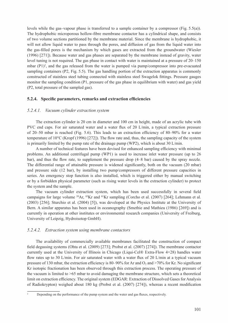
101

levels while the gas–vapour phase is transferred to a sample container by a compressor (fig. 5.5(a)). The hydrophobic microporous hollow-fibre membrane contactor has a cylindrical shape, and consists of two volume sections partitioned by the membrane material. since the membrane is hydrophobic, it will not allow liquid water to pass through the pores, and diffusion of gas from the liquid water into the  gas-filled  pores  is  the mechanism  by which  gases  are  extracted  from  the  groundwater  (wiesler (1996) [271]). Because water and gas phases are separated by the membrane instead of gravity, water level tuning is not required. the gas phase in contact with water is maintained at a pressure of 20–150 mbar (p1)2, and the gas released from the water  is pumped via pump/compressor  into pre-evacuated sampling containers (p2, fig. 5.5). the gas handling portion of the extraction apparatus is commonly constructed of stainless steel tubing connected with stainless steel Swagelok fittings. Pressure gauges monitor the sampling condition (p1, pressure of the gas phase in equilibrium with water) and gas yield (p2, total pressure of the sampled gas).

5.2.4. Specific parameters, remarks and extraction efficiencies

5.2.4.1. Vacuum cylinder extraction system

the extraction cylinder is 20 cm in diameter and 100 cm in height, made of an acrylic tube with Pvc  end  caps.  for  air  saturated water  and  a water  flux  of  20  L/min,  a  typical  extraction  pressure of  20–50 mbar  is  reached  (fig.  5.6).  This  leads  to  an  extraction  efficiency  of  80–90%  for  a water temperature of 10°c (Kropf (1996) [272]). The flow rate and, thus, the sampling capacity of the system is primarily limited by the pump rate of the drainage pump (wp2), which is about 30 l/min.

A number of technical features have been devised for enhanced sampling efficiency with minimal problems. an additional centrifugal pump (wp1) is used to increase inlet water pressure (up to 26 bar),  and  thus  the flow  rate,  to  supplement  the pressure drop  (4–8 bar)  caused by  the  spray nozzle. The differential  range of attainable pressure  is widened significantly, both on  the vacuum (20 mbar) and pressure side (12 bar), by installing two pump/compressors of different pressure capacities in series. an emergency stop function is also installed, which is triggered either by manual switching or by a forbidden physical parameter (such as rising water levels in the extraction cylinder) to protect the system and the sample.

The  vacuum  cylinder  extraction  system,  which  has  been  used  successfully  in  several  field campaigns for large volume 39ar, 85Kr and 81Kr sampling (corcho et al. (2007) [264]; Lehmann et al. (2003)  [256]; Sturchio et al.  (2004)  [5]), was developed at  the Physics  Institute at  the University of Bern. A similar apparatus has been used in oceanography (Smethie and mathieu (1986) [269]) and is currently in operation at other institutes or environmental research companies (university of freiburg, University of Leipzig, Hydroisotop gmbH).

5.2.4.2. Extraction system using membrane contactors

the availability of commercially available membranes facilitated the construction of compact field degassing systems (ohta et al. (2009) [273]; Probst et al. (2007) [274]). The membrane contactor currently used at  the University of  Illinois  in chicago  (Liqui-cel® Extra-flow 4×28) handles water flow rates up to 30 L/min. for air saturated water with a water flux of 20 L/min at a typical vacuum pressure of 130 mbar, the extraction efficiency is 80–90% for Ar and o2 and >70% for Kr. No significant Kr isotopic fractionation has been observed through this extraction process. The operating pressure of the vacuum is limited to >65 mbar to avoid damaging the membrane structure, which sets a theoretical limit on extraction efficiency. The original system (EdgAr: Extraction of dissolved gases for Analysis of radiokrypton) weighed  about  180 kg  (Probst  et  al.  (2007)  [274]), whereas  a  recent modification 

2   depending on the performance of the pump system and the water and gas fluxes, respectively.

102

halved  the  size.  Smaller  membrane  contactors  are  now  available  with  lower  water  flow  capacity (<5 L/min), and may be applied for smaller sampling (ohta et al. (2009) [273]).

5.2.5. Optimal design of gas extraction units

the systems described above are complementary, and a suitable or optimal gas extraction method needs to be adjusted according to the local environmental conditions at the sampling site, the required sample size and the isotope of interest. Table 5.2 summarizes the most important features, benefits and disadvantages of the two systems.

5.3. gas preparatIon and purIfIcatIon

5.3.1. Introduction

existing analytical methods for 81Kr  (and  39ar) require relatively large quantities (~15 µl) of pure Kr gas. The gas phases extracted in the field have to be processed and purified in the laboratory. Alternatively, an initial noble gas pre-enrichment can already be achieved in the field (Sidle and fischer (2003)  [270]).  The  composition  of  dissolved  gas  in  groundwater  can  be  highly  variable  (fig. 5.7). the air saturated seepage water may acquire different amounts of excess air through the partial or complete dissolution of air bubbles that are trapped at the capillary fringe in the unsaturated soil zone. carbon dioxide can be accumulated from different sources in the unsaturated (biogenic co2) or

FIG. 5.6. Vacuum cylinder apparatus for field gas extraction of dissolved gases. Components indicated with dotted lines are optional (see text). In the water part (left side), the water is filtered and transferred to the extraction cylinder from where it is pumped out after degassing. An emergency valve (EV1) protects the cylinder from overflow (closed when the water level reaches LE). The gas is extracted with a vacuum pump (GP1) compressed (K1) into the sampling container. An additional compressor (K2) can be attached if higher pressures are required because of high gas contents and/or small sample containers (Pmax ~ 15 bar).

WP 1

WP 2

GP1

K1

K2

E V 1 EV 2

Fil t e r

H 2 O- flu x

P2

P1

P3

Wa tercyc l e

Gascycle

S a mp l i n g t a p

P 0

L 1

L 2

L E

L E

: Valve: One-way valve

P: Pressure gaugesEV : Emergency valveWP : Water pumpGP : Gas pumpK: CompressorL: Water level sensor

Sample contain e r

Sample contain e r

103

the saturated zone (biogenic, chemogenic or thermogenic). Under reducing conditions, o2 is consumed and ch4 can be produced by methanogenesis or co2  reduction  (Klass  (1984)  [275]). As a  result of denitrification, N2 is another common subsurface gas source in many aquifers. Thus, a Kr purification system must be able to separate Kr efficiently from large quantities of gas of variable composition. In the case of multitracer studies, including, for example, additional 39Ar measurements, a combined Kr and Ar purification process is necessary. There are several methods of separating noble gases from gas mixtures. Some of the most common processes used in large volume Kr–Ar purification systems are outlined below.

Distillation

Isolating and/or enriching components from a gas mixture based on differences in condensation points of the gas components (such as cooling traps for co2 or water vapour removal from the gas mixture).

Adsorption

Separating gas mixtures using microporous solids (adsorbents) that have strong affinities for one or more of the components in the mixtures at variable temperature and partial pressure.

table 5.2. coMparIson of dIfferent gas extractIon systeMs

Benefits disadvantages

extraction chamber

Insensitive to chemical and physical water composition (ph, temperature, hydrocarbons, suspended matter, etc.)

requires low extraction pressure and is, therefore, more sensitive to leaks

easy to repair by experienced personnel in case of breakdown (important in remote areas)

careful leak testing and set-up requires experienced personnel

operational for a large range of water fluxes relatively high flow resistance may limit water flow rate

allows a low extraction pressure, thus higher extraction efficiency

not commercially available and, therefore, expensive to construct

Benefits disadvantages

Membrane contactors

commercially available membrane contactors, relatively inexpensive

sensitive to chemical and physical water composition:

not suitable in the presence of substances which reduce the surface tension of water

not suitable for a high temperature environment (i.e. >70°c)

suspended or precipitated matter may clog the pores

Modular: several contactors can be combined in parallel (increased water flux) and/or in series (increasedextraction efficiency)

compact and relatively easy to operate in the field

Low inlet water pressure facilitates high water flux; operational over large flux range

a damaged membrane requires a relatively complex regeneration processes

104

Absorption

selective physical solution or chemical bonding of chemically active species, mainly used to remove substances other than noble gases. the process can be reversible (e.g. oxidation of copper to remove o2 and the subsequent reduction of the cuo using h2 gas) or irreversible (such as with Ti-getters).

New  gas  purification  techniques  and  materials  (membranes,  nanotubes,  cation  exchanged zeolites, etc.) have recently been developed, and as the efficiency of 81Kr measurements increases and required sample size decreases, separation and purification techniques will converge towards techniques 

FIG. 5.7. Composition of atmospheric air () relative to the Kr concentration in air and subsurface processes (arrows) affecting the composition of dissolved gases in groundwater.

10 -2 10-1 10

0 101 102 103 104 105 106 10 7

N2

O2

Ar

CO2

Ne

CH4

He

K r

H2

Xe

Methanogenesis, CO2 reduction

Thermogenic CO 2

root respiration,decompositionof organic matter

Denitrification

Redox reactionN2 O2

ArCO 2

Ne

CH 4

He

K rH2

Xe

N2 O2

ArCO 2

Ne

CH 4

He

K rH2

Xe

cx/cK r

FIG. 5.8. Krypton sampling and purification techniques as a function of water sample volume (L). The reduction in the required sample volume is triggered by the increased sensitivity of analytical methods for 81Kr detection.

107 106 105 104 103 102 10 1

Detection methods

Sampling methods

Noble gas (Kr, Ar) separation methods

LLC (1969)

Water volume

ATTA-1(1999)

AMS(1997)

ATTA-2(2003)

ATTA-3(2010, goal)

Vacuum chamber

Membrane extractor

Water collection

GC separation

+distillation

Getter

105

that  are  in  use  for  stable  noble  gas  isotopic  analyses  (Beyerle  et  al.  (2000)  [276]). The  procedures described  here  or  elsewhere  in  recent  literature  (Loosli  and  Purtschert  (2005)  [277];  Smethie  and mathieu  (1986)  [269]; yokochi  et  al.  (2008)  [278])  are,  therefore,  to be  regarded as  a  ‘snapshot’ of the  present  capability.  In  the  following  sections,  two  selected  large  volume  noble  gas  purification systems will be presented in more detail.

5.3.2. Purification system at the University of Bern

the low level counting laboratory at the physics Institute of the university of bern has a long history in the separation and analysis of noble gas radionuclides through low level counting (llc) (Loosli (1983) [262]; Loosli et al. (2000) [261]; Loosli et al. (1986) [279]; Loosli and Purtschert (2005) [277]). The required amount of gas extracted from groundwater for LLc is constrained by the decay rate of the isotope of interest. Measuring 81Kr  in  groundwater  via  decay  counting  is  not  feasible, but LLc was used for the first detection of 81Kr in the atmosphere (Loosli and oeschger (1969) [247]). the powerful combination of 85Kr and 39Ar dating in hydrology (corcho et al. (2007) [264]; Purtschert (2008) [280]) requires purification of both Ar and Kr. If Ar or Kr is exclusively of interest, the procedure can be optimized and simplified accordingly. with the separation system of the LLc laboratory in Bern, samples with a gas volume between ten (for 85Kr measurements)  and  several  hundred  litres  can  be processed serially in portions of about 2 l.

Combined Ar–Kr separation procedure

The gas is transferred from the sample cylinder into a first cooling trap filled with activated charcoal (Ac). Using the bulk gas as a carrier, water vapour and co2 are removed using a molecular sieve 5a, and o2 is removed by oxidation of cu to cuo in a cu furnace at 600°c. The sample is then released into a buffer volume, and injected as a sequence of 2 l aliquots into the gas chromatograph (gc) separation system. The two large packed columns of the gc (1 m long, 7 cm diameter, T = 20°c) are filled with ac and with a molecular sieve 5a, respectively, and sequentially. helium is used as a carrier gas, and the gas effluent is analysed by a thermal conductivity detector. The fractions containing Ar and Kr are collected separately in cooling traps filled with Ac at N2(l) temperature. this procedure separates ar from Kr, so that the Kr in the Ar fraction is reduced by a factor of at least 104 to eliminate present day atmospheric 85Kr activity. The argon fraction is then passed a second time through the gc columns and finally purified from any remaining traces of o2 and n2 in a Ti-furnace at 800°c. If present, a fraction of ch4 is collected together with Kr because the Kr and cH4 retardation times overlap if more than 1 cm3 stp ch4 was present in the original sample. The final Kr purification is done with a separation system optimized for Kr. Any traces of radon (released, for example, from Ac in the system) are removed in a cold finger filled with glass pellets at N2(l) temperature.

Krypton purification

Krypton typically extracted from 300–500 L of water, or from the residual gas from the Ar–Kr system described above (the Kr enriched portion),  is separated by three gc separation steps. If only Kr  (for  85Kr  or  81Kr  measurements)  is  of  interest,  the  procedure  starts  at  this  point  (collon  et  al. (2000) [281]).

the sample gas is exposed to a molecular sieve (5a (Ms1)) bed for water vapour and co2 removal and subsequently adsorbed on an Ac cold finger (Ac1).

the trap (ac1) is then heated to room temperature, and the desorbed gases (mainly n2 and ar) are pumped away during the first five minutes. The trap is then flushed with the carrier gas (He) and the effluent  is monitored using a  thermal  conductivity detector. After  the Ar(o2) and n2  peaks have 

106

passed, the two way valve is switched to divert the gas flow through the second trap (mS2) filled with a 5a molecular sieve cooled at n2(l) temperature. from this trap, the desorption procedure is repeated to further purify and freeze Kr  in  the  third cooling  trap (Ac2), filled with Ac. In each step,  the gas volume is reduced by a factor of ~10 and the remaining gas volume in Ac2 is about 20–100 μL STP (collon et al. (2000) [281]). Ac2 is then removed from the system and connected to a commercial gc system (varian Star 3400) where the Kr is further purified, mixed with a P10 mixture as a quench gas

(90% argon and 10% ch4) and finally transferred into the low level counter for activity measurement in the underground laboratory (fig. 5.9(b)). If the Kr and cH4 abundances in the sample are comparable, they can be easily separated and the final amount of recovered Kr is determined from the area of the Kr peak.  If  the methane and Kr peaks cannot be separated,  the Kr content  in  the counter gas has  to be measured after the activity measurement by mass spectrometry.

large ch4 concentration in  the sample gas requires further measures  in order  to purify Kr. for example, ch4  can  be  used  as  a  carrier  gas  for gc  separation  (Sidle  and  fischer  (2003)  [270]).  In the laboratories of the university of bern, ch4 is oxidized in a cuo coated furnace at 800°c, followed by the separation of the resulting co2 and h2o.

5.3.3. Purification system at the University of Illinois, Chicago

Major constituents of the atmosphere, n2, o2 and Ar, have much higher vapour pressure than Kr. consequently, cryogenic distillation enriches the residual phase in Kr. Large scale cryogenic distillation with refined engineering control has indeed been the most widely applied method of producing pure gas substances from the atmosphere. eliminating sophisticated engineering controls, a simple method of  cryogenic  Kr  enrichment  at  an  easily  attainable  constant  temperature  (77  K)  was  developed  at the University of Illinois, chicago (yokochi et al. (2008) [278]). Pure Kr is obtained through subsequent gc separation and Ti-gettering. The system uses a quadrupole mass spectrometer (qmS) to monitor gas  effluent  composition  during  separation,  which  enables  (i)  small  scale  cryogenic  distillation  in a controlled manner, (ii) gas chromatographic separation of parts per million by volume (ppmv) level

FIG. 5.9. Krypton purification system (for details, see text). Pure Kr is obtained by several GC separation steps (a). Krypton is then transferred into a cooling trap (AC2), purified, mixed with P10 gas, and finally fed into the proportional counter (b).

GC1

Varian

AC4

P1 P2

AC3

Counter

AC2

carrierexit

Carrierexit

Vacuum pump

He carrier

P10 Gas

P3GC1 GC2

AC2MS2

AC1

He carrier

Sample

MS1

P1 P2 P3

Carrier exit

Vaccum pump

2 way valves

Pos1 Pos2

a)

b)

107

of Kr from a significantly large quantity of gas (up to a few litres), and brings (iii) the applicability of the method to natural groundwater samples characterized by variable chemical compositions.

after h2o and co2  removal using a molecular sieve 4A, sample gas  is condensed in an empty container at liquid n2 temperature, then distilled at that temperature assisted by a vacuum compressor. the rate of the cryogenic distillation is about 3 l/min for a system dominated by n2, and 0.5 l/min for a system dominated by o2. the n2/Ar ratio of the distillation gas effluent is continuously monitored to determine the progress of the distillation based on a model calculation assuming gas–liquid equilibrium partitioning. Efficient separation of Kr and cH4 from ar, o2 and n2 can be achieved for up to a few litres of the distillation residue gas by using an Ac column (Ac2) at room temperature. The Kr peak following these major species overlaps with the peak tails, but the use of a qmS for monitoring gas composition enables identification and further selective processing of the Kr enriched portion. A molecular sieve 5A separates Kr from cH4 (up to a few hundred cubic centimetres stp) at low temperature (around –20ºc). Pure Kr is collected in a small (0.7 cm3) stainless steel container filled with Ac.

5.4.  detectIon Methods of noble gas radIonuclIdes

despite their excellent tracer properties, radioactive noble gases are still not used on a routine basis in environmental science; for 81Kr, only  three field  investigations have been completed  to date (Lehmann et al. (1991) [282]; Lehmann et al. (2003) [256]; Sturchio et al. (2004) [5]). The main issue limiting the widespread use of noble gas radionuclides has been a lack of convenient analytical methods to measure these isotopes at natural concentrations. the problem is depicted in fig. 5.10, where typical values of atmospheric activities, concentrations and specific isotope ratios are plotted as a function of the half-lives of corresponding noble gas  isotopes. The numbers can vary depending on  the specific situation, but correspond roughly to modern waters under average environmental conditions. first, the extremely low isotopic abundances (<10–11) of these noble gas radionuclides far exceed the dynamic range of conventional gas source mass spectrometers. the activities in 1 l of water for 37ar, 39ar, 85Kr and 81Kr are 10–4, 10–1, 10–3 and 10–7 mbq, respectively. while the 85Kr activity of a modern sample 

FIG. 5.10. Typical values of atmospheric activities (squares), concentrations (circles) and specific isotope ratios (e.g. 81Kr/Kr; triangles) dissolved in 1 L of water at 10°C versus half-life of noble gas radionuclides (Lehmann and Loosli (1984) [259]).

106 108 1010 1012 101410-8

10-6

10-4

10-2

100

102

104

106

10-21

10-19

10-17

10-15

10-13

10-11

10-9

Atom counting

85Kr 81Kr39Ar37Ar

Half-life (s)

Wat

er (a

tom

s/L)

W

ater

(Bq/

L)

Decay counting

Isotope ratio

108

can be measured in a number of laboratories worldwide, 39ar and 37ar can currently only be measured in one underground laboratory at the university of bern, using ar extracted from a few tons of water. As seen in fig. 5.10,  the specific  81Kr activity  is out of range of any reasonable sampling and decay counting system, thus 81Kr has to be measured by other atom counting methods. AmS (collon et al. (2000) [281]) and new ultrasensitive atom counting methods (chen et al. (1999) [283]; du et al. (2003) [249]) have been applied in studies of 81Kr in hydrology. The analytical methods that are suitable for noble gas radionuclides, particularly 81Kr, will be briefly discussed in the following section.

5.4.1. Low level counting

for decades, LLc was the only method for detecting radioisotopes of Ar and Kr at atmospheric levels. The first  determination of  81Kr activity  in  the  atmosphere was undertaken using proportional counting with 5 L of pre-bomb Kr (Loosli and oeschger (1969) [247]). The current LLc laboratory at  the University of Bern  is  shown  in fig. 5.11  (Acosta-Kane et al.  (2007)  [284]). The  laboratory  is located at a depth of 35 m, providing a reduction of the muon flux by a factor of ~10. The laboratory walls  utilize  special  concrete  selected  for  its  low  radioactivity  content  to minimize  gamma  ray flux within the laboratory. the proportional counters are built of high conductivity, oxygen free cu and filled with the sample gas at a pressure of 2–30 bar, then placed in a cylindrical lead shield 5 cm thick. only a fraction of the particle decay energy is released within the counter before it reaches the counter wall.  The  deposited  energy  increases  with  increasing  pressure  and  is  recorded  by  a  7-bit  multi-channel analyser  (mcA) with a  linear energy range of 0–35 kev. for  further background reduction, the proportional  counter  is  constructed with  low background materials  and uses  an anti-coincidence proportional counter to reduce background. The small volume of the counters reduces the background 

FIG. 5.11. Schematic of the set-up utilized to measure noble gas radionuclides at the Low Level Counting Underground Laboratory at the University of Bern. For 85Kr measurements, the counters are filled with a P10 mixture (10% methane, 90% argon) at pressures in the range of 2–10 bar. The measurements are performed at a depth of 35 m. Low activity lead shielding and an anti-coincidence arrangement provide a further reduction in the background count rate.

35 m

Old lead shields

Counting gas

Wire Counter

Guard counter

Pre-amplifier

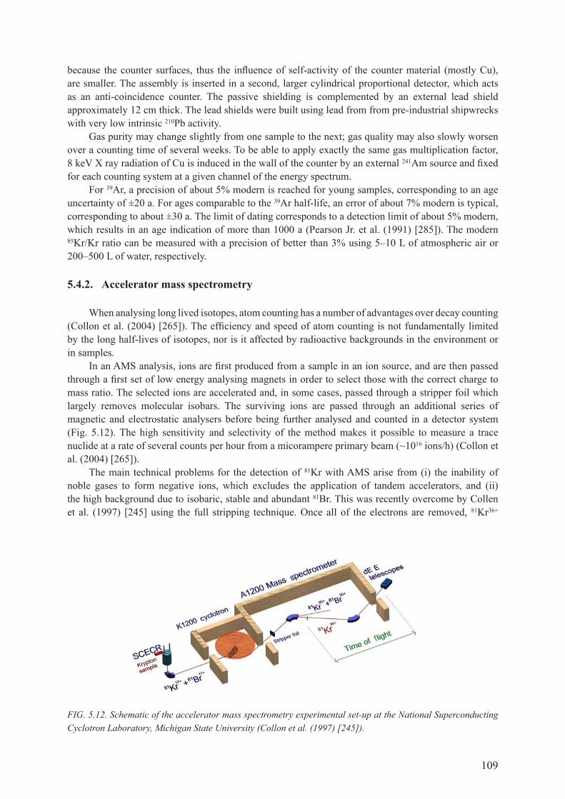
109

because  the counter  surfaces,  thus  the  influence of  self-activity of  the counter material  (mostly cu), are smaller. the assembly is inserted in a second, larger cylindrical proportional detector, which acts as  an  anti-coincidence  counter.  The  passive  shielding  is  complemented  by  an  external  lead  shield approximately 12 cm thick. The lead shields were built using lead from from pre-industrial shipwrecks with very low intrinsic 210pb activity.

gas purity may change slightly from one sample to the next; gas quality may also slowly worsen over a counting time of several weeks. To be able to apply exactly the same gas multiplication factor, 8 kev x ray radiation of cu is induced in the wall of the counter by an external 241Am source and fixed for each counting system at a given channel of the energy spectrum.

for 39ar, a precision of about 5% modern is reached for young samples, corresponding to an age uncertainty of ±20 a. for ages comparable to the 39Ar half-life, an error of about 7% modern is typical, corresponding to about ±30 a. The limit of dating corresponds to a detection limit of about 5% modern, which results in an age indication of more than 1000 a (Pearson jr. et al. (1991) [285]). The modern 85Kr/Kr ratio can be measured with a precision of better than 3% using 5–10 L of atmospheric air or 200–500 l of water, respectively.

5.4.2. Accelerator mass spectrometry

when analysing long lived isotopes, atom counting has a number of advantages over decay counting (collon et al. (2004) [265]). The efficiency and speed of atom counting is not fundamentally limited by the long half-lives of isotopes, nor is it affected by radioactive backgrounds in the environment or in samples.

In an AmS analysis, ions are first produced from a sample in an ion source, and are then passed through a first set of low energy analysing magnets in order to select those with the correct charge to mass ratio. the selected ions are accelerated and, in some cases, passed through a stripper foil which largely removes molecular isobars. the surviving ions are passed through an additional series of magnetic and electrostatic analysers before being further analysed and counted in a detector system (fig.  5.12). The  high  sensitivity  and  selectivity  of  the method makes  it  possible  to measure  a  trace nuclide at a rate of several counts per hour from a micorampere primary beam (~1016 ions/h) (collon et al. (2004) [265]).

the main technical problems for the detection of 81Kr with AmS arise  from (i)  the  inability of noble gases to form negative ions, which excludes the application of tandem accelerators, and (ii) the high background due to isobaric, stable and abundant 81br. this was recently overcome by collen et  al.  (1997)  [245] using  the  full  stripping  technique. once all  of  the  electrons  are  removed,  81Kr36+

FIG. 5.12. Schematic of the accelerator mass spectrometry experimental set-up at the National Superconducting Cyclotron Laboratory, Michigan State University (Collon et al. (1997) [245]).

110

(Z = 36) can be cleanly separated from 81br35+ (Z = 35). the aMs measurements of 81Kr in atmospheric Kr were performed using the K1200 Superconducting cyclotron at michigan State University, which accelerated ions to an energy (3.6 gev) high enough for efficient full stripping. After the acceleration in the cyclotron, the 81Kr17+ ions were passed through a be foil (18.8 mg/cm2), which provided a 70% stripping efficiency to reach the 36+ charge state. The fully stripped 81Kr36+ was then separated from the 81br35+ using the a1200 mass spectrometer, and detected with two Δe–e telescope detectors (collon et al. (1997) [245]).

the nuclear reaction products induced by the high 81br17+ background in the stripper foil heavily dominated the final spectrum and had to be suppressed by several orders of magnitude before 81Kr in natural samples could be detected. As Kr and Br have very different melting temperatures (–156.6°c and –7.2°c, respectively), Br in the sample was suppressed by freezing the sample with liquid nitrogen. In addition, tests revealed that the largest suppressor of 81br was the support gas used in the ion source. by using ar as a support gas, reductions in br contamination by two orders of magnitude were obtained (collon  et  al.  (1999)  [286]).  These  steps  opened  the  door  to  possible measurements  of  81Kr  below the natural level of 5 × 10–13. This AmS set-up was used to perform 81Kr dating of groundwater samples (collon  et  al.  (2000)  [281])  and  to  compare  pre-bomb  and  post-bomb  abundances  of  atmospheric 81Kr/Kr (collon et al. (1999) [286]).

5.4.3. Atom trap trace analysis

In atom trap trace analysis (atta), an atom of a particular isotope is selectively captured by a laser trap and then detected by observing its fluorescence while in the trap (chen et al. (1999) [283]). A magneto-optical  trap  (moT) — a  type of  robust  and efficient  atom  trap —  is used as  a  selective concentrator (chen et al. (1999) [283]; du et al. (2003) [249]). when the laser frequency is tuned to within a few natural line widths of the low frequency side of the targeted isotope resonance, only atoms of this particular isotope are trapped. Atoms of other isotopes are either deflected before reaching the trap or are allowed to pass through the trap without being captured. this method allows for the counting of single atoms with a high signal to noise ratio and, since selectivity depends exponentially on the number of photons detected in a burst, also ensures superb selectivity. Indeed, atta is practically immune to contamination from other isotopes, elements or molecules.

the vacuum system consists of the following components: the sample reservoir, the source chamber, the transverse cooling chamber and the trap chamber. a getter pump in the source chamber removes reactive gases, such as hydrogen, water, etc.  from the vacuum system while  leaving the Kr sample intact. Either a Ti-sapphire ring laser system or a diode laser system can be used to generate the  811  nm  light  needed  to  trap Kr  atoms  in  the metastable  5 s  [3/2]2  level  by  repeatedly  exciting 

FIG. 5.13. Schematic layout of the krypton ATTA-2 apparatus. Metastable krypton atoms are produced in the discharge. The atoms are then transversely cooled, slowed and trapped by laser beams, shown as solid red arrows. The total length of the set-up is about 2.5 m (Lu and Mueller (2010) [287]).

Discharge

Transverse cooling

Zeeman slower

Photon detector

Anti-Helmholtz coilsKr inlet

Kr atom beam

Trapping laser beams

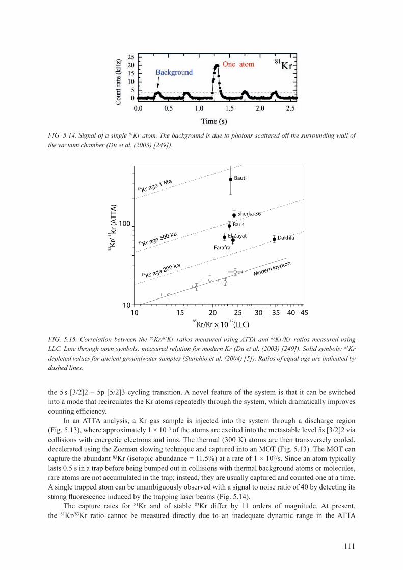
111

the 5 s  [3/2]2 – 5p [5/2]3 cycling  transition. A novel feature of  the system is  that  it can be switched into a mode that recirculates the Kr atoms repeatedly through the system, which dramatically improves counting efficiency.

In  an ATTA  analysis,  a  Kr  gas  sample  is  injected  into  the  system  through  a  discharge  region (fig. 5.13), where approximately 1 × 10–3 of the atoms are excited into the metastable level 5s [3/2]2 via collisions with energetic electrons and ions. The thermal (300 K) atoms are then transversely cooled, decelerated using the Zeeman slowing technique and captured into an Mot (fig. 5.13). the Mot can capture the abundant 83Kr (isotopic abundance = 11.5%) at a rate of 1 × 109/s. since an atom typically lasts 0.5 s in a trap before being bumped out in collisions with thermal background atoms or molecules, rare atoms are not accumulated in the trap; instead, they are usually captured and counted one at a time. A single trapped atom can be unambiguously observed with a signal to noise ratio of 40 by detecting its strong fluorescence induced by the trapping laser beams (fig. 5.14).

the capture rates for 81Kr  and  of  stable  83Kr  differ  by  11  orders  of  magnitude.  At  present, the 81Kr/83Kr  ratio  cannot  be  measured  directly  due  to  an  inadequate  dynamic  range  in  the ATTA 

FIG. 5.14. Signal of a single 81Kr atom. The background is due to photons scattered off the surrounding wall of the vacuum chamber (Du et al. (2003) [249]).

FIG. 5.15. Correlation between the 85Kr/81Kr ratios measured using ATTA and 85Kr/Kr ratios measured using LLC. Line through open symbols: measured relation for modern Kr (Du et al. (2003) [249]). Solid symbols: 81Kr depleted values for ancient groundwater samples (Sturchio et al. (2004) [5]). Ratios of equal age are indicated by dashed lines.

100

85 Kr

/81

Kr (A

TTA

)

10 15 20 25 30 35 40 4510

Sherka 36

Baris

El Zayat Dakhla

Bauti

85Kr/Kr × 10

–12(LLC)

Farafra

Modern krypton

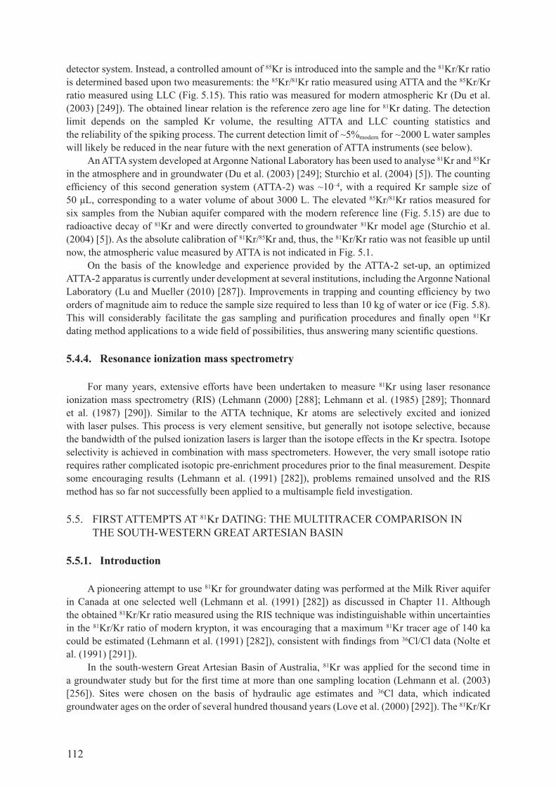
112

detector system. Instead, a controlled amount of 85Kr is introduced into the sample and the 81Kr/Kr ratio is determined based upon two measurements: the 85Kr/81Kr ratio measured using ATTA and the 85Kr/Kr ratio measured using LLc (fig. 5.15). This ratio was measured for modern atmospheric Kr (du et al. (2003) [249]). The obtained linear relation is the reference zero age line for 81Kr dating. The detection limit  depends  on  the  sampled  Kr  volume,  the  resulting  ATTA  and  LLc  counting  statistics  and the reliability of the spiking process. The current detection limit of ~5%modern for ~2000 l water samples will likely be reduced in the near future with the next generation of ATTA instruments (see below).

an atta system developed at argonne national laboratory has been used to analyse 81Kr and 85Kr in the atmosphere and in groundwater (du et al. (2003) [249]; Sturchio et al. (2004) [5]). The counting efficiency of  this  second generation  system  (ATTA-2) was ~10–4, with a  required Kr  sample  size of 50 μL, corresponding to a water volume of about 3000 L. The elevated 85Kr/81Kr ratios measured for six samples from the nubian aquifer compared with the modern reference line (fig. 5.15) are due to radioactive decay of 81Kr and were directly converted to groundwater 81Kr model age (Sturchio et al. (2004) [5]). As the absolute calibration of 81Kr/85Kr and, thus, the 81Kr/Kr ratio was not feasible up until now, the atmospheric value measured by atta is not indicated in fig. 5.1.

on  the  basis  of  the  knowledge  and  experience  provided  by  the ATTA-2  set-up,  an  optimized ATTA-2 apparatus is currently under development at several institutions, including the Argonne National Laboratory (Lu and mueller (2010) [287]). Improvements in trapping and counting efficiency by two orders of magnitude aim to reduce the sample size required to less than 10 kg of water or ice (fig. 5.8). This will  considerably  facilitate  the  gas  sampling  and  purification  procedures  and finally  open  81Kr dating method applications to a wide field of possibilities, thus answering many scientific questions.

5.4.4. Resonance ionization mass spectrometry

for many years,  extensive  efforts have been undertaken  to measure  81Kr using  laser  resonance ionization mass spectrometry (rIS) (Lehmann (2000) [288]; Lehmann et al.  (1985) [289]; Thonnard et  al.  (1987)  [290]).  Similar  to  the ATTA  technique,  Kr  atoms  are  selectively  excited  and  ionized with laser pulses. this process is very element sensitive, but generally not isotope selective, because the bandwidth of the pulsed ionization lasers is larger than the isotope effects in the Kr spectra. Isotope selectivity is achieved in combination with mass spectrometers. however, the very small isotope ratio requires rather complicated isotopic pre-enrichment procedures prior to the final measurement. despite some  encouraging  results  (Lehmann  et  al.  (1991)  [282]),  problems  remained  unsolved  and  the rIS method has so far not successfully been applied to a multisample field investigation.

5.5. fIrst atteMpts at 81Kr datIng: the MultItracer coMparIson In THE SoUTH-wESTErN grEAT ArTESIAN BASIN

5.5.1. Introduction

a pioneering attempt to use 81Kr for groundwater dating was performed at the milk river aquifer in canada at one  selected well  (Lehmann et  al.  (1991)  [282])  as discussed  in chapter 11. Although the obtained 81Kr/Kr ratio measured using the rIS technique was indistinguishable within uncertainties in the 81Kr/Kr ratio of modern krypton, it was encouraging that a maximum 81Kr tracer age of 140 ka could be estimated (Lehmann et al. (1991) [282]), consistent with findings from 36cl/cl data (nolte et al. (1991) [291]).

In the south-western great Artesian Basin of Australia, 81Kr was applied for  the second time in a groundwater study but for the first time at more than one sampling location (Lehmann et al. (2003) [256]).  Sites  were  chosen  on  the  basis  of  hydraulic  age  estimates  and  36cl data, which indicated groundwater ages on the order of several hundred thousand years (Love et al. (2000) [292]). The 81Kr/Kr 

113

ratios of four wells were measured using the AmS technique (collon et al. (2000) [281]; Section 5.4.2) and  for  the  first  time  allowed  for  a  check  of  the  applicability  of  81Kr  methods  and  a  cross-check with tracer ages and conclusions derived from 36cl and 4he data. the comparison of all data in such a multitracer study yields more information about the flow system than is possible from single tracer measurements. Moreover, limitations and uncertainties about individual tracer methods can be reduced and possibly quantified. Specifically, the following issues are addressed in the following pages.

Krypton-81  dating  is  a  new  method  and  its  validity  must  be  demonstrated  in  comparison  to the more established 36cl and 4he methods. although theoretical considerations indicate that variations in 81Kr input activity and underground production should be low (Lehmann et al. (1993) [250]), this has to be verified in field studies. The strength of diffusive exchange between an aquifer and its surrounding aquitards is another potential problem that needs further investigation (section 5.1.2.2).

for 4He, the most critical factor is quantification of the local accumulation rate, which is composed of an ‘on-line’ in situ production rate (easy to calculate) and an influx of helium that was produced either external to the aquifer (Torgersen and clarke (1985) [293]; Torgersen et al. (1992) [294]; Torgersen and Ivey (1985) [93]) or helium that accumulated ‘off-line’ in the past which is now being released within an aquifer via diffusion from rocks into pore spaces (Solomon et al. (1996) [295]; chapter 8).

for 36cl dating, the ‘initial value problem’ (davis et al. (1998) [296]) concerns the 36cl/cl ratio at the recharge area’s geographical location, as well as an estimate of the cl concentration of recharging water, which depends strongly on prevailing climatic conditions which may change as a function of time. during groundwater flow, subsurface processes other than radioactive decay may alter the number of 36cl atoms and/or the number of cl atoms dissolved in the water (chapter 6).

FIG. 5.16. Location map of the south-west margin of the Great Artesian Basin, showing the locations of wells for 36Cl dating () (Love et al. (2000) [292]) and the four sites that have been sampled for 81Kr measurements () (Lehmann et al. (2003) [256]). The shaded areas indicate the sandstone aquifer outcrop. The dashed line represents the transition from unconfined to confined conditions (where the water level of the aquifer is above the overlying Bulldog Shale).

114

the part of the great artesian basin investigated here (see below) provides unfavourable conditions for the interpretation of 36cl data due to high and variable evaporation rates and the occurrence of subsurface cl sources. the systematic use of helium as a dating tool is also complicated by the presence of  different  helium  sources  (Torgersen  and  clarke  (1985)  [293]).  It  is,  therefore,  an  ideal  area  to demonstrate  the  interrelation  between  different  tracer  methods  in  such  ‘real  world  scenarios’  and the potential of multitracer studies. the intention is not to favour any of the applied methods or to explain the flow system in this hydrologically complex part of the great Artesian Basin. Significantly more data would be required, including 81Kr, to reach this goal.

5.5.2. study area

The study area is located in the great Artesian Basin south-western flow system of the Eromanga Basin. Piezometric contours indicate that the major direction of groundwater flow is from the western margin towards the south-east and east (fig. 5.16). chlorine-36 dating was previously performed along two transects and based on these data the test sites for 81Kr measurements were chosen  (Love et al. (2000) [292]). The southernmost site (rc) was sampled because other sites along the northern transect were inaccessible due to inclement weather and poor road conditions.

All wells  tap  the j-K sandstone aquifer  that  is overlain by  the 200–400 m  thick Bulldog Shale aquitard. The transects start in the outcrops and unconfined parts of the aquifer. further downstream, the aquifer becomes confined or eventually artesian (Love et al. (2000) [292]).

5.5.3. krypton-81 groundwater ages

The four wells, rc, od, dH and wc (fig. 5.16), were sampled during a field campaign in 1998 in collaboration with the department of water, land and biodiversity conservation of south australia, the Institute of Isotope research Vienna (aMs measurements) and the university of bern (sampling and sample preparation). The project was partly supported by the IAEA within the framework of a research programme called “Isotope techniques for the assessment of slow Moving deep groundwaters”. About 16 t of water was degassed in the field and the extracted gas was processed in the University of Bern laboratories according to the procedures explained above. The purified Kr samples (~0.5 cm3

stp) were shipped to the aMs laboratory at Michigan state university for 81Kr/Kr ratio determination.

Measured 81Kr  activities  expressed  in  terms  of  the  air  normalized  ratio  (81Kr/Kr)sample/(81Kr/Kr)modern air range from 51% to 30%modern. a simple age calculation using the exponential law for radioactive decay yields 81Kr model ages of between 230 and 400 ka (Table 5.3),  in agreement with expectations from 36cl data (Love et al. (2000) [292]). the uncertainty in calculated groundwater tracer age is about 10–20% because of the analytical error in these first 81Kr measurements using cyclotron aMs. contamination during sampling was excluded through 85Kr  measurements  carried  out  on subsamples of the same gas used for aMs.

these 81Kr model ages are piston flow ages and, thus, neglect dispersion in the aquifer, possible diffusive exchange with aquitards and any underground production of 81Kr. The effect of dispersion is minor for tracers with a constant input because the concentration gradient is small in the direction of flow (in contrast to peak shape inputs as for 3h). for reasonable dispersivities (gelhar et al. (1992) [297]), the effect would lead to an underestimation of groundwater age on the order of <15% for 81Kr piston flow ages <500 ka. Underground production is expected to be very likely <10%modern and likely to be <4%modern (Lehmann et al. (1993) [256]). However, upper limits for the subsurface production of 81Kr and  its  escape  to groundwater  still need  to be established by field measurements. Underground production would lead to an underestimation of age if not considered in the model age calculation (the produced activity feigns a younger age). diffusive exchange with stagnant aquitards (depleted in 81Kr compared with the studied aquifer) would cause an overestimation of model ages if not considered 

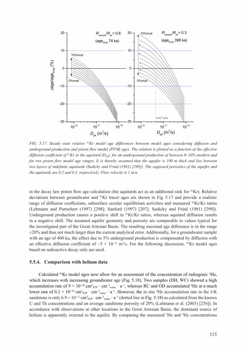
115

in the decay law piston flow age calculation (the aquitards act as an additional sink for 81Kr). relative deviations between groundwater and 81Kr  tracer  ages  are  shown  in fig. 5.17  and provide  a  realistic range of diffusion coefficients, subsurface secular equilibrium activities and measured  81Kr/Kr ratios (Lehmann  and  Purtschert  (1997)  [298];  Sanford  (1997)  [207];  Sudicky  and  frind  (1981)  [299]). underground production causes a positive shift in 81Kr/Kr  ratios, whereas  aquitard  diffusion  results in a negative shift. the assumed aquifer geometry and porosity are comparable to values typical for the investigated part of the great artesian basin. the resulting maximal age difference is in the range ±20% and thus not much larger than the current analytical error. Additionally, for a groundwater sample with an age of 400 ka, the effect due to 5% underground production is compensated by diffusion with an  effective  diffusion  coefficient  of  ~5 ×  10–12 m2/s. for the following discussion, 81Kr model  ages based on radioactive decay only are used.

5.5.4. Comparison with helium data

calculated 81Kr model ages now allow for an assessment of the concentration of radiogenic 4he, which increases with increasing groundwater age (fig. 5.18). two samples (dh, wc) showed a high accumulation rate of 9 × 10–10 cm3

stp · cm–3water · a–1, whereas rc and od accumulated 4he at a much

lower rate of 0.2 × 10–10 cm3stp · cm–3

water · a–1. however, the in situ 4He accumulation rate in the j-K sandstone is only 6.9 × 10–12 cm3

stp · cm–3water · a–1 (dotted line in fig. 5.18) as calculated from the known 

U and Th concentrations and an average sandstone porosity of 20% (Lehmann et al. (2003) [256]). In accordance with observations at other locations in the great artesian basin, the dominant source of helium is apparently external to the aquifer. by comparing the measured 3he and 4he concentrations

FIG. 5.17. Steady state relative 81Kr model age differences between model ages considering diffusion and underground production and piston flow model (PFM) ages. The relation is plotted as a function of the effective diffusion coefficient of 81Kr in the aquitard (Deff), for an underground production of between 0–10% modern and for two piston flow model age ranges. It is thereby assumed that the aquifer is 100 m thick and lies between two layers of indefinite aquitards (Sudicky and Frind (1981) [299]). The supposed porosities of the aquifer and the aquitards are 0.2 and 0.3, respectively. Flow velocity is 1 m/a.

10-12 10-11 10-10-30

-20

-10

0

10

20

5·10-12 m2/s

2

4

6

0%mod

10%mod

8

10-12 10-11 10-10-30

-20

-10

0

10

20

10%mod Δ

age/

age PF

M (%

)

Deff (m2/s)

Rsample/Rair= 0.8

(agePFM 74 ka)

Deff (m2/s)

Rsample/Rair= 0.3

(agePFM 398 ka)

0%mod

116

in four groundwater samples to the calculated in situ 3he/4he production ratio (fig. 5.18, right), it appears at least plausible that the source of the excess helium is located in the rocks and pore waters of the bulldog shale. this he exchange between the sandstone and the shale seems to be more effective at the end of the northern transect where dh and wc are located than for the locations of the other two wells, od and rc.

5.5.5. Comparison with chlorine-36 data

the chloride and 36cl data along the two sampled transects are shown in fig. 5.19. In the confined part (solid symbols) of the aquifer for the 81Kr study, both 36cl and 36cl/cl decrease with decreasing hydraulic head (and distance), indicating increasing ages along the flow path. chloride concentrations are relatively high and range from 600 to 3000 mg/l. the cl decrease along the southern transect is likely the result of lower rates of evapotranspiration in the past (Love et al. (2000) [292]). this was also demonstrated by a good correlation between cl concentrations and δ18Ο values for the southern transect (not shown here). concentrations of cl along the northern transect are lower and show less variability, indicating that the input conditions were more humid and more constant in the recharge area of those samples. this observation is in line with other studies that also indicate spatially variable recharge and input conditions in this part of the great Artesian Basin (Torgersen et al. (1991) [300]). In this study area, 36cl dating is apparently complicated by the unfortunate situation that both evaporative cl enrichment during recharge (Ci) and varying subsurface cl sources (Ca) occur simultaneously and with varying (and a priori unknown) strengths. The hypothesis of a spatially and temporally varying contribution of subsurface cl is further strengthened by the weak correlation between δ18Ο and the cl concentration along the northern transect (Love et al. (2000) [292]). This implies once more that processes other than evaporation control cl concentration. neither dating by the 36cl/cl ratio (insensitive to evaporation) nor by the 36cl concentration (rather insensitive to the addition of 36cl-‘dead’ chloride) offers an evident solution to this problem.

In light of the calculated 81Kr model ages,  it  is possible  to demonstrate how such an ambiguity can be reduced by means of a multitracer comparison. as a starting point, the temporal evolution of the different 36cl components in a groundwater sample and their corresponding initial parameters (expressed as isotope ratios R = 36cl/cl multiplied with the cl concentrations C) are reconsidered (Bentley et al. (1986) [301]):

FIG. 5.18. Helium-4 accumulation as a function of 81Kr model ages (left panel) and 3He/4He signatures compared with calculated values in the sandstone and the Bulldog Shale (right panel). The dotted line indicates the increase of helium due to in situ U and Th decay within the aquifer.

1

RC

OD

DH

WC

RC

OD

DH

WC

0 100 200 300 400 5000

1

2

3

4

5

6

7

8

in situ production

9 ×10 cm STP/g a

0.2 × 10 cm STP/g a

4 He

(cm

3 STP

/g 1

0–5)

81Kr age (ka)

0 1 2 3 4 5 6 7 8 90

2

4

6

8

10

12

sandstone

shale

3 He

(cm

3 STP

/g 1

0–12

)

4He (cm3 STP/g 10–5 )

–10

–10

117

i i 36 se i 36 i exexp( ) (1 exp( )) ( )RC RC t R C t C C RA CB D

(5.9)

whereA is measured 36cl concentration (atoms/l water);B is decay of the initial 36cl concentration in recharge water;C   is the in-growth of a secular subsurface equilibrium 36cl concentration within the aquifer (Rse);D is 36cl accumulation due to the addition of cl from subsurface sources with a 36cl/cl ratio

of Rex.

FIG. 5.19. Chloride and 36Cl versus distance for south-western Great Basin groundwaters (from Love et al. (2000) [292]).

RCWC

ODDH

118

apart from the groundwater age t, which is the target parameter for dating, it is necessary to estimate the meteoric 36cl/cl initial ratio Ri, the recharge of cl concentrations Ci, the secular equilibrium ratio Rse within the aquifer, and the ratio Rex of any admixed or dissolved cl. for this area of the great artesian basin, a Ri of 125 × 10–15 was estimated based on relatively young samples in the recharge area which are 3h free and, therefore, not affected by thermonuclear 36cl  (Love et  al.  (2000)  [292]; Torgersen et al. (1991) [300]). It was further assumed that higher frequency variations of the 36cl fallout (Plummer et al. (1997) [248]) were smoothed out due to hydrodynamic dispersion (see Section 5.6).

a secular equilibrium ratio Rse of 6.5 × 10–15 for j-K aquifer sandstone was calculated based on the measured elemental composition of several rock samples from the aquifer (Lehmann et al. (2003) [256]).  Similarly,  a  ratio Rex of 20 × 10–15 was obtained for the adjacent bulldog shale formation. the only residual free parameter is the chloride concentration that represents a recharge value (Ci), and

table 5.3. reconstructed contrIbutIons of MeteorIc (CI) and subsurface (Ca) cl SoUrcES IN THE SoUTH-wESTErN grEAT ArTESIAN BASIN

rc od dh wc

81Kr age t (ka) 230 ± 40 350 ± 50 290 ± 40 400 ± 50

C (mg/l) 1260 680 850 1040

Ci (mg/l) 1050 620 120 210

Ca = C – Ci (mg/l) 210 60 730 830

K = Ca/t (mg · ka–1 · L–1) 0.95 0.15 2.54 2.07

FIG. 5.20. Variations in 36Cl/Cl and 36Cl concentrations down two transects of the south-western Great Artesian Basin. Triangles indicate 81Kr dated locations (sampling date: 1995 1998). Lines represent the evolution for (a) decay, (b) a temporally linear Cl accumulation rate k of 0.5 mg · ka–1 · L–1 and (c) k = 1.6 mg/L ka starting with Cl concentrations of 200 mg/L and 800 mg/L, respectively. A 36Cl/Cl ratio of 20 × 10–15 for the accumulated Cl was assumed for cases b and c.

0

2E-14

4E-14

6E-14

8E-14

1E-13

1.2E-13

1.4E-13

1.6E-13

0.0E+00 5.0E+08 1.0E+09 1.5E+09 2.0E+09

36Cl concentration (atoms/L)

36C

l/C

l

Northern transect

Southern transect

EvaporationDilution

Solution of 36Cl poor Cl

C i = 200 mg/L C i = 800 mg/L

a

b

c

a'

b'c'

Decay

RC

OD

WC

DH

119

that depends on the climatic conditions during recharge. It is known that several glacial cycles occurred over the timescales of the 36cl method dating range. the four well case study (Ci) can now be calculated because the second unknown t in eq. (5.5) can be independently determined using 81Kr dating. In other words, the Ci value for each sample was determined by inserting the 81Kr  age  t = t81 into eq. (5.9) and solving for Ci. the subsurface input (Ca) corresponds to the difference between measured (C) and the initial cl concentration (Ci). finally, the cl accumulation rate k = Ca/t = t81 can be calculated (table 5.3).

reconstructed input concentrations Ci vary over almost one order of magnitude between 120 mg/l (dh) and 1050 mg/l (rc). the subsurface cl accumulation rate k is small for two of the samples (<1 mg · ka–1 · L–1 for rc, od) but more significant for dH and wc (2–3 mg · ka–1 · L–1). In fig. 5.20, 36cl/cl ratios are plotted as a function of the 36cl concentrations. straight lines (a, a’) indicate the theoretical evolution for decay and an underground secular equilibrium ratio of 20 × 10–15 but without any addition of subsurface cl (terms B and C in eq. (5.9)). the curved lines (b, b’, c, c’) represent cases for different cl accumulation rates (term D in eq. (5.9)). It is thereby assumed that cl concentration increases linearly with time, starting with initial Ci concentrations of 200 mg/l (b, c) and 800 mg/l (b’, c’), respectively. the large scatter of measured values on both transects is one more indication that evaporative  enrichment  and  the  accumulation of  subsurface cl  are  both  significant  processes which possibly overwhelm the decay signal. data along the southern transect can only be explained by a high evaporative cl enrichment during recharge and/or an elevated cl accumulation rate in the subsurface. samples low in 36cl (dh and wc) can either be the result of a high input concentration Ci (~800 mg/l) and a low accumulation rate (scenario a’) or a low cl input (200 mg/L) and a higher accumulation rate of ~1–2 mg · ka–1 ·L–1 (scenario c).

The  best  estimate  setting  has  either  to  be  identified  by  a  clear  trend  along  a  flowline  (e.g.  in fig. 5.20) or by means of supplementary data such as 81Kr in this case. The results provided in Table 5.3 point to scenario c for dH and wc and scenarios a’–c’ for rc and od.

FIG. 5.21. 36Cl/Cl ratios versus Cl concentration of 81Kr dated samples (dashed red lines: pure mixing; blue solid lines: mixing + decay). Initial Cl concentrations as well as the quantification of 36Cl/Cl reduction due to ageing are based on 81Kr data (Table 5.3).

0

2E-14

4E-14

6E-14

8E-14

1E-13

1.2E-13

1.4E-13

0 500 1000 1500

Cl (mg/L)

36Cl

/Cl ×

10

–15

OD RCDH WC R i=125 × 10

Evaporation

36Cl decayMixing with aquiclude Cl R e=12 × 10 –15

ageing

20

40

60

80

100

120

140

ageing

C i

–15

120

the impact of the different scenarios on 36cl dating results becomes more evident upon looking at the relation between the cl concentration and the 36cl/cl ratio (fig. 5.21). the dashed lines represent pure mixing lines of the initial chloride with chloride in secular equilibrium with the bulldog shale (no radioactive decay). The solid lines include radioactive decay as quantified by 81Kr measurements. the same initial 36cl/cl ratio of 125 × 10–15 was assumed for all of the samples. for samples dh and wc, 93% and 89% of the 36cl/cl ratio decrease is caused by the addition of subsurface chloride. only the remaining 10% drop of the 36cl/cl ratio is attributed to radioactive decay and, thus, to ageing. for od and rc, on the other hand, the situation is quite different. the decrease in 36cl/cl is dominated by  the  decay  of  atmospheric  input.  chlorine-36  dating  for  these  samples,  therefore, seems to be straightforward. The identification and quantification of relative amounts of meteoric and subsurface cl has to be based on additional tracers such as 81Kr, as deduced in Section 6.6.3.

5.5.6. Additional evidence for the correctness of krypton-81 ages

sparse experience with 81Kr dating  can  raise  questions  about  the  conclusions  discussed  above. fundamentally, it poses the question of whether 81Kr ages are correct. Is it possible that processes other than admixture of cl from the underlying shale are responsible for the disagreement of 81Kr and 36cl model ages for two of the samples? again, the answer to these questions can only be obtained with additional evidence from other tracer measurements. the importance of multitracer approaches is once more emphasized (this is true for any groundwater investigation, not only for old groundwater).

the evaporative enrichment of initial cl concentration Ci as a function of recharge temperature T is found using:

( )( )p

i

C PC T

R T⋅

= (5.10)

whereR(T) is the recharge rate (mm/a) as a function of the evaporation rate that is closely related to

the recharge temperature T (°c);Cp is the cl concentrations in precipitation (mg/l);P is the mean annual precipitation rate (mm/a).

from this simple chloride mass balance, a positive correlation is expected between recharge temperature T and the initial chloride concentration (warmer temperatures lead to a higher cl enrichment in the recharge). recharge temperatures can be reconstructed based on concentrations of dissolved noble gases (Aeschbach-Hertig et al. (1999) [302]; mazor (1972) [303]). Noble gas recharge temperatures (ngrt) of the four wells are compared with reconstructed cl input concentrations Ci in fig. 5.22(a) (Lehmann et al. (2003) [256]). The reasonable correlation provides supporting evidence for the plausibility of estimated initial cl concentrations (and derived 81Kr ages) because the parameters Ci and ngrt are analytically completely independent.

the second line of evidence comes from the comparison between accumulated radiogenic helium and accumulated cl concentrations (Ca). Model calculations have shown that downward diffusion from the Bulldog Shale aquitard is most  likely the process by which variable amounts of subsurface cl  are  added  (Love  et  al.  (2000)  [292]). measured  δ37cl  values  in  rocks  and  groundwater  support that  the  Bulldog  Shale  is  the main  source  of  cl  in  the  aquifer  (see  zhang  et  al.  (2007)  [304]  and Section 6.4.2). moreover, the Bulldog Shale has already been identified to be the probable source for most of the accumulated he in the aquifer based on 3he/4he ratios (fig. 5.18). It is an intriguing further piece of evidence that subsurface chloride accumulation (Ca) reconstructed on the basis of the 81Kr ages correlates well with the amount of accumulated 4he (fig. 5.22(b)). It should be noted that the 4he concentration and noble gas temperatures are again completely independent parameters. a correlation

121

between 4he and cl concentrations was also observed in other deep aquifer systems (lehmann et al. (1996) [305]).

despite the small number of samples, the conclusion has been drawn that the consistency of a whole set of different independent isotope tracers (81Kr, 36,37cl, 3,4he, ngrt) points to:

(a) the validity of 81Kr model ages in the range of 200–450 ka, which seem not to be significantly affected by secondary processes such as underground production, diffusion or variations in input concentration;

(b) distinct cl accumulation histories with lower input concentrations and high cl accumulation for two samples (dh, wc) and higher input concentrations and low subsurface accumulation for the other samples (rc, od);

(c) external sources of helium and chloride that are at least correlated.

5.5.7. summary

the ten currently (2010) available 81Kr measurements  in old groundwater3 certainly do not yet permit a comprehensive evaluation of the 81Kr  method.  despite  the  sparse  amount  of  data,  some important conclusions can be drawn with regard to the analytical procedure of the 81Kr  method and the applicability of 81Kr  for dating old groundwater. An assessment of  a novel  technique  is  not meaningful without a comparison with more established methods. owing to the comparable half-lives and dating ranges of 36cl and 81Kr, the focus is on the relationship between these two methods.

5.5.7.1. Krypton-81 methodology

In  the past 15 years,  significant progress has been made  in  the development of  instruments  for analysing 81Kr at natural concentration  levels. The  required amount of water has been  reduced  from about 17 t to about 1 t (2010) and is likely to be reduced further in the near future to approximately a few tens of litres (Lu and mueller (2010) [287]). Sampling via gas extraction in the field has been proven to be practical and reliable. The gas processing and Kr separation procedure can be done using standard methods and will be further facilitated in the future with a probable decrease in sample volume.

3   milk-river: 1 sample; gAB: 4 samples; Nubian aquifer (see chapter 14): 6 samples.

FIG. 5.22. (a) 81Kr derived initial chloride concentrations Ci versus calculated NGRT; (b) chloride of subsurface origin (Ca) versus concentration of radiogenic 4Herad.

WC

DH

OD

RC

0

200

400

600

800

1000

1200

1400

21 23 25 27

NGRT (°C)

Ci (

mg

/L)

WCDH

OD

RC

0

100

200

300

400

500

600

700

800

900

1000

0 2 4 6 8 10

4He rad (cm3 STP

/g × 10–5)

Ca (m

g/L

)

a) b)

122

5.5.7.2. Krypton-81 application

so far, nine out of ten 81Kr analyses from groundwater were significantly depleted compared with modern atmospheric krypton, with the lowest activity of 5%modern found in the nubian aquifer (sturchio et al. (2004) [5]). The proof-of-principle test of the 81Kr method is, therefore, fulfilled. The initial results confirm — within  remaining  uncertainties —  the  expected  advantageous  characteristics  of  the  81Kr method, namely a constant input concentration and negligible underground production. this can be concluded from a comparison of 36cl/cl data and 81Kr model  ages  from all  currently  available data pairs (fig. 5.23, left). the lines in the plot indicate the calculated and expected relationship assuming different scenarios for the 36cl evolution. The first two scenarios represent pure decay (d) and decay with a subsurface 36cl/cl equilibrium ratio of 10 × 10–15 (d + r). the scenario (d + r + a) assumes, in addition, a subsurface cl accumulation with a 36cl/cl ratio of 10 × 10–15 at a rate of 2 mg · ka–1 · L–1. all samples from the nubian aquifer and two samples from the great artesian basin agree with uncertainties within the range of the above mentioned 36cl accumulation scenarios. without going into details of the local hydrology, this is already an encouraging coincidence, indicating the validity of the basic assumption for 81Kr model  ages.  It  is  also  a demonstration of  the  applicability of  the  36cl dating method despite some factors that could potentially affect the age interpretation of this isotope. however, for two of the great artesian basin samples, 81Kr  and  36cl ages disagree. the possible reasons  are  numerous  and  could  originate  from  both  tracers,  but  a  look  at  cl  concentrations  (right panel in fig. 5.23) makes simplified 36cl interpretation more doubtful. In the nubian aquifer, chlorinity is low and rather constant over time, representing ideal conditions for 36cl dating. In comparison, cl concentrations in the great artesian basin case study are much higher and more variable. this is just another element of the unfavourable 36cl dating conditions prevailing in this part of the great artesian basin. however, if the fraction of subsurface cl addition can be estimated using other means, it is nevertheless possible to calculate realistic tracer ages within the age of <1 Ma, even if a large fraction of cl is of subsurface origin (Phillips (2000) [306]). The problem associated with dH and wc samples (open symbols) is that a high subsurface cl accumulation rate goes together with a reduced meteoric

FIG. 5.23. 36Cl/Cl ratios as a function of 81Kr model ages (left plot) and Cl concentrations (right plot). Green triangles: samples from the Nubian aquifer; blue circles: samples from the Great Artesian Basin; solid circles: 36Cl/Cl evolution dominated by decay; open circles: 36Cl/Cl evolution dominated by the accumulation of Cl from subsurface sources. The lines indicate different calculated temporal 36Cl/Cl evolutions (see text. D: Pure decay starting from 36Cl/Cl = 120 × 10–15, R: Considering a subsurface secular equilibrium Rse = 10 × 10–15A: Considering a subsurface Cl accumulation at a rate of (2 mg · ka–1 · L–1)

0 500 1000 150081Kr age (ka)

36C

l/C

l ×

10

–15

D

D+R

D+R+A

A

GAB data

Nubian Data

0 500 1000 1500Cl (mg/L)

14

12

10

8

6

4

2

0

14

12

10

8

6

4

2

0

123

input concentration. future studies and more data are required for the verification of this hypothesis, which is based on the results of only four wells.

5.6. addenduM: sIgnal attenuatIon due to hydrodynaMIc dIspersIon

fluctuations of initial recharge conditions and climate signal variations are propagated into the aquifer by advection and dispersion. these input signals are attenuated and phase shifted due to hydrodynamic dispersion. attenuation factor A  defined  as  the  ratio  of  the  remaining  amplitude  to 

FIG. 5.24. Attenuation of a periodic climate signal as a function of groundwater age for different signal periods and Pe numbers (solid lines: Pe = 10; broken lines: Pe = 100).

FIG. 5.25. Temperature variations reconstructed from the Dome C ice core record (Luethi et al. (2008) [308]) compared with noble gas temperatures of four Great Artesian Basin wells.

10 100 1 × 103

1 × 104

1 × 105

1 ×106

0

0.2

0.4

0.6

0.8

Pe=10

1 ka

10 ka

100 ka

100 10 100 10 100

16%

68%

Groundwater age (a)

Att

enua

tion

15

20

25

30

35

40

0 100 200 300 400 500

Groundwater age (ka)

Tem

pera

ture

(°C

)

Piston Flow Pe=1000 Pe=100 Pe=10

RC

DH

OD

WC

124

the initial amplitude of the signal as a function of the period (T) of the initial (climate) signal, the flow time t in the aquifer and the strength of the hydrodynamic dispersion which can be expressed by means of the dimensionless peclet number Pe = vx/D (roberts and valochi (1981) [307]) is:

A = exp(– α ) with 28

0.5 0.5 1 12

Pe tT Pe

(5.11)

for example, an attenuation factor A of 0.7 corresponds to a reduction of the initial periodic (sinusoidal) signal by 30%. In fig. 5.24, A is plotted as a function of groundwater age (assuming a flow velocity of 1 m/a) for different periods of the initial signal and for two different peclet numbers, 10 and 100.

The remaining amplitude of a signal with a period of 10 ka after a flow time of 10 ka is 16% for a Pe number of 10 and 68% for a Pe number of 100 (fig. 5.24). An aquifer system acts consequently as a  low pass filter. only  long  term  low frequency  input variations are  recorded  in old groundwater systems. an example are the noble gas temperatures (ngts) of the four wells of the present great artesian basin study compared in fig. 5.25 with estimated temperature variations as recorded in δ18Ο values from the Antarctic dome c ice core (Luethi et al. (2008) [308]). The δ18o/t relation was arbitrarily adjusted to local climate conditions. despite the relatively large uncertainties in 81Kr ages and the ngts, it can be concluded that small amplitudes of the observed variations are roughly in accord with the model calculations for a reasonable range of peclet numbers between 10 and 100 (gelhar et al. (1992) [297]). Larger temporal variations cannot be expected or are, if present, possibly the result of different recharge areas with distinct recharge conditions.

125

Chapter 6

CHLORInE-36 DAtInG OF OLD GROUnDWAtER

f.M. phIllIpsdepartment of earth and environmental science, new Mexico tech, socorro, new Mexico, united states of america

6.1. BASIc PrINcIPLES of cHLorINE-36

chlorine-36 has been widely used for dating old groundwater. The 36cl used for this purpose is produced in the atmosphere through the interaction of cosmic rays with argon atoms. the 36cl then mixes with ordinary atmospheric chloride (mostly derived from the ocean). the mixture is deposited on the land surface dissolved in rain or snow or as dry aerosols. groundwater recharge carries the 36cl into  the  subsurface where  the  radiometric  ‘clock’  is  set.  chloride  is  conservative  in  the  subsurface and, thus, the 36cl is rarely retarded with respect to the water velocity by adsorption or geochemical reactions. groundwater age can be estimated using the radiometric decay equation and the decrease in 36cl from the amount in the recharge water. the main complication is variations in the cl concentration of groundwater. this can potentially be due to variable evapotranspiration during recharge or to the addition of cl in the aquifer. If the cause of cl concentration variations is understood, the age calculation can be corrected to account for the process. chlorine-36 dating is generally applicable to water in the age range 100 ka–1 ma.

6.1.1. Chlorine-36 in the hydrological cycle

the principal application of 36cl to the dating of old groundwater is defining age through measuring the decay of atmospheric 36cl. chlorine-36 is produced in the atmosphere by cosmic ray spallation of 40Ar (Lal and Peters (1967) [309]). It decays to 36Ar with a half-life of 301 000 ± 4000 a (Bentley et al. (1986) [310]). The average global production rate lies between 20 and 30 atoms m2/s (phillips (2000) [306]). This meteoric 36cl then mixes with stable oceanic cl in the atmosphere, resulting in relatively low ratios of 36cl to stable cl (36cl/cl) near coastlines, but these ratios increase to high values near the centres of continents owing to the decrease in the atmospheric concentration of stable chloride (davis et al. (2003) [311]; Keywood et al. (1997) [312]; moysey et al. (2003) [313]).

the mixture of 36cl and stable chloride is deposited on the land surface dissolved in precipitation and as dry aerosols. groundwater recharge transports the chlorine isotopes to the water table where they begin to be advected along with the flowing groundwater. As groundwater age increases, 36cl decays. In an ideal system (i.e. one with no subsurface sources of either 36cl or stable cl and no sinks except radiodecay), calculating the 36cl model age is a simple matter of entering the initial and measured 36cl concentrations (or 36cl/cl ratios) into the radioactive decay equation and solving for time.

In actual aquifers, although anomalous loss of either 36cl or stable cl is seldom a problem, both species are often introduced in the subsurface. concentrations of cl and 36cl can also vary due to temporal or spatial changes in evapotranspiration in the aquifer recharge area. the challenge of 36cl dating of old groundwater is, thus, separating the changes in 36cl due to radioactive decay from these other processes  (Phillips  (2000)  [306]). A  representative  schematic of  36cl in the hydrological cycle is shown in fig. 6.1. The grey  lines  in  the graphs on  the bottom part of  the figure  show  the  simple exponential evolution of the 36cl/cl ratio and 36cl concentration as a function of distance when no cl

126

is added in the subsurface. when cl is added from bounding formations (which is common), the black lines show the evolution with distance. for the purposes of illustration, the assumed cl concentration and 36cl/cl ratio (which is shown by 36cl/clse in the right hand graph) are unusually high. the 36cl/cl ratio varies only moderately from the exponential case, but the 36cl concentration actually increases (due to the high equilibrium concentration in the bounding formation).

6.1.1.1. Historical summary

application of 36cl  to geochronology was fi rst suggested by davis and Schaeffer  (1955)  [314]. Although  they  did  perform  a  few  successful  measurements  on  rocks  and  water  containing  fallout from  nuclear  weapons  testing,  the  screen-wall  beta  counter  technology  of  the  time  was  incapable of quantifying 36cl in typical groundwater. this problem was partially solved with the development of  liquid scintillation counting (ronzani and Tamers  (1966)  [315]; Tamers et al.  (1969)  [316]). This method could measure 36cl at, and below, the levels typical of groundwater recharge, but suffered from the limitation that several grams of cl were required. Inasmuch as groundwater recharge with high values of 36cl/cl is typically fairly dilute, and subsurface water with high concentrations of cl

FIG. 6.1. Schematic of 36Cl in the hydrological cycle. Numerical values are only representative. At the right hand side, marine Cl containing very little 36Cl is lofted into the troposphere and over the continents. As it is advected inland, it mixes with 36Cl produced by cosmic ray reaction with argon in the upper atmosphere. This mixture is deposited on the recharge area of an aquifer and the 36Cl decays during groundwater fl ow.

40Ar

cosmic-ray neutron

36Cl

R36<1

Cl R36 = 50

R36 = 100

R36 = 500

R36 = 40 CCl = 400

40Ar

cosmic-ray neutron

36Cl

R36<1

Cl R36 = 50

R36 = 100

R36 = 500

R36 = 40 CCl = 400

127

typically shows fairly low 36cl/cl, this analytical advance was limited to only a small number of practical applications.

The  real  breakthrough  in  the  application  of  36cl was the development of accelerator mass spectometry  (AmS)  as  an  analytical  tool  (Elmore  et  al.  (1979)  [317]).  This  technique was  capable of measuring  down  to  background  levels  of  36cl/cl  on milligram-sized  samples  and,  thus,  enabled analysis of nearly any groundwater sample (davis et al. (1983) [318]). The fi rst successful applications to old groundwater were in the great Artesian Basin (Australia) and the milk river aquifer (canada) (Bentley et al. (1986) [310]; Phillips et al. (1986) [319]). These studies both illustrated the feasibility of 36cl as a method for dating old groundwater and pointed out the complications that result from variable evapotranspiration combined with subsurface sources of cl and 36cl.  Since  the mid-1980s, the  technique has been widely applied around the world (see Phillips (2000) [306], and Phillips and castro (2003) [77] for a summary of studies).

6.2. SAmPLINg TEcHNIqUES for cHLorINE-36

ease of sampling is one of the advantages of 36cl. sampling is normally done by collecting suffi cient water to contain at least ~10 mg of cl in a clean container and precipitating the cl as Agcl by adding excess agno3 solution. Acidifi cation is helpful in promoting the precipitation and fl occulation of the agcl.

The  only  case  in  which  signifi cant  diffi culty  is  likely  to  be  encountered  is  if  the  water  to  be sampled contains very low cl concentrations (<~5 mg/l). In this case, a large water sample (5–10 l) must be collected. flocculation for such dilute solutions is typically poor and isolation of the agcl precipitate may be  diffi cult  or  impossible. This  problem can be  addressed  in  two ways. The fi rst  is the use of an anion exchange resin column. typically, the exchange resin is loaded with nitrate, which is displaced by cl– as  the water sample fl ows  through  the column. However, anion exchange resins, as sold, typically have signifi cant amounts of cl– adsorbed and great care must be taken to ensure that all of this cl– is fl ushed before the column is used for sampling. As the water being sampled is dilute, even small amounts of cl– contamination may be a serious problem. this method has been described in detail (jannik (1989) [320]).

an alternative approach to dealing with low cl concentrations is the addition of carrier. the carrier can either be 36cl-free ordinary cl or one in which either 35cl or 37cl has been enriched. If an isotopically enriched carrier is used, the cl concentration of the sample can be determined by means of isotope dilution mass  spectrometry  (IdmS)  (desilets  et  al.  (2006)  [321])  during AmS  analysis. This  offers a very signifi cant advantage over separate measurement of the cl concentration due to the diffi culties involved in conventional measurement of cl at low concentrations. disadvantages of this approach are that if both the cl concentration and the 36cl/cl ratio are low, dilution of the ratio by addition of a carrier may signifi cantly increase the uncertainty of the AmS measurement, and that carrier addition must be performed with great precision, which can be diffi cult under fi eld conditions. for this reason, unless practical problems prevent shipment of the water sample to the laboratory, it is preferable to add the spike and precipitate the sample in the laboratory where the spike can be precisely weighed out. there is no single reliable source of isotopically enriched cl and researchers are encouraged to contact the aMs laboratory that will provide their analyses for recommendations.

6.3. cHLorINE-36 SAmPLE PrEPArATIoN ANd mEASUrEmENT

chlorine-36 measurements  in natural waters are almost entirely performed using AmS (Elmore et  al.  (1979)  [317];  Elmore  and  Phillips  (1987)  [322]).  This  technique  employs  a  tandem  van  de graaff particle accelerator, originally designed for particle physics research, as a high energy mass spectrometer. one advantage of this instrument is that when the charge of the ion beam is reversed

128

in the high voltage terminal by passing through a thin foil (the ‘tandem’ aspect of the accelerator), all molecular species are broken up, eliminating molecular interference that would otherwise overwhelm the 36cl detector. a second advantage is that the very high energies imparted to the ion beam allow the use of a rate of energy loss detector that separates 36cl from its isobar 36s, based on their differences in proton number. the history of aMs and recent advances have been surveyed (elmore and phillips (1987) [322]; gove (1992) [323]; muzikar et al. (2003) [324]; Suter (2004) [325]).

one recent advance that is now becoming frequently used for analysis of 36cl in environmental water samples is IdmS (desilets et al. (2006) [321]). In this approach, an isotopically enriched spike of cl (usually enriched in 35cl) is added to the sample before the cl is precipitated as Agcl. Knowing the isotope ratio of the cl spike and the masses of spike and sample, the cl concentration of the sample (and, thus, also the 36cl concentration) can be calculated from the 35cl/37cl ratio that is measured during the aMs analysis. R36,sample, the actual sample 36cl/cl ratio (atoms 36cl ∙ (atoms 35cl + 37cl)–1), is calculated from the following formula, given R36,meas, the 36cl/cl ratio measured by the aMs; ss, the atomic 35cl/37cl ratio measured by the aMs; R35,n, the atomic 35cl/cl ratio (i.e. 35cl/(35cl + 37cl)) of natural cl (0.7573); and R35,sp, the 35cl/cl ratio of the isotopically labelled spike:

R RR SS R

R SS R36,sample 36,meas35,n 35,n

35,sp 35,sp

1

11

( )

(6.1)

the cl concentration of the sample (Ccl,sample) in mg cl/kg solution is correspondingly shown by:

cl,soln soln n 35,sp 35,sp

water 35,sp 35 35,sp 37 35,n 35,n

cl,sample

1000 1

1 1

C M A R SS R

M R A R A SS R RC

(6.2)

whereCcl,soln is the cl concentration of the spike solution (mg cl/g solution);Msoln   is the mass of spike solution added to the sample (g);An   is the atomic mass of natural cl (35.4527 g/mol);Mwater is the mass of the aqueous sample (g);A35 is the atomic mass of 35cl (34.9688 g/mol);A37 is the atomic mass of 37cl (36.9659 g/mol).

This  methodology  takes  advantage  of  the  high  precision  and  accuracy  of  isotope  ratio  mass spectrometry to obtain a very reliable value for the cl concentration of the sample. It is especially valuable for samples with low cl concentration, where it not only provides a superior measurement of the cl concentration, but also increases the cl content of the water sample, thus facilitating precipitation and isolation of the agcl and reducing the volume of water that must be collected.

as described above, cl for 36cl analysis is collected through precipitation of agcl. fortunately, Agcl can be used as the target in the ion source of an AmS system. However, the sample must first be purified of S. Although  the rate of energy  loss detector  is highly efficient at separating  36cl from 36s, concentrations of s greater than a few milligrams per litre in the agcl can still produce enough 36s counts to seriously degrade the precision of the 36cl analysis, especially if the 36cl/cl ratio is low. The sample preparation procedure, therefore, focuses on reducing the S concentration to make it as low as possible.

the standard 36cl preparation procedure was originally developed by h.w. bentley (bentley et al.  (1986)  [310]; Bentley et al.  (1986)  [301]; Phillips et al.  (1986)  [319]). The procedure consists of  first  dissolving  the Agcl  precipitate  in NH4oh, reprecipitating it through the addition of hno3, redissolving it and then adding bano3 solution. the ba2+ precipitates sulphur as baso4. the solution is then separated from the baso4 precipitate and the agcl reprecipitated through the addition of hno3. the repeated dissolution/reprecipitation steps also lower the s content of the agcl by partitioning the s

129

into the solution with each precipitation. depending on the sulphur concentration of the water sampled, this procedure may be repeated two or three times.

the main disadvantages of this procedure are that it may require one to several days, depending on the number of bano3 steps, and that a small amount of cl is lost with each cycle. an alternative procedure has recently been developed (jiang et al. (2004) [326]). This procedure employs ion exchange columns to concentrate the cl and reduce s contamination. the authors claim that cl recovery is >90% and that the procedure takes less than one day, however, it has not yet been widely tested.

After drying, the Agcl can be packed into a holder and placed in the ion source of an accelerator mass spectrometer. the machine measures the 36cl/cl ratio and the 35cl/37cl ratio (assuming an isotopically enriched spike has been added) of the Agcl. This analysis typically uses between 15 min and  1  h  of  beam  time.  The  analyses  are  standardized  by  normalization  to  recognized  international standards  (unlike  14c,  these  standards  are  arbitrary  and  do  not  reflect  any  natural  material).  from these  ratios and associated  information on sample volume and  the mass of  the  sample  spike  36cl/cl ratio, the cl concentration and 36cl concentration can be calculated. If IdMs has not been employed, the cl concentration must be analysed using an independent method. Ion chromatography is generally the preferred method.

Assuming the sample has been spiked with 35cl or 37cl, the AmS laboratory will report back either the 36cl/(35cl + 37cl) ratio or the 36cl/35cl ratio and the 35cl/37cl ratio. the user must combine this with data on the sample mass, the spike isotope ratio, and the mass of spike added in Eqs (6.1, 6.2), to obtain the sample 36cl/cl and cl concentration.

until recently, any systematic comparisons of 36cl analyses’ reliability have been very limited in scope. However, mahara et al.  (2004) [327] have recently published a very  thorough interlaboratory comparison. they sent 15 natural water samples to three aMs laboratories around the world (the laboratories were not identified by name). Each of the 15 samples was subjected to two treatments: the  first  aliquot was  processed  in mahara’s  laboratory  using  a  uniform processing  procedure, while the second aliquot was sent to the aMs laboratory as an untreated water sample and processed there by whatever procedure was standard in that laboratory. this constituted a total sample of 90 aMs analyses, which is a sufficient basis for statistical evaluation. The chloride concentrations of the samples ranged from 9 to 17 900 mg/l and the mean 36cl/cl ratios ranged from 0.5 to 410 × 10–15, a typical range for deep groundwater samples.

The outcome of  this comparison is summarized in Table 6.1 and shown graphically in fig. 6.2. The results are divided  into ‘all samples’  (a  total of either 90 or 45 analyses, depending on whether both treatments or only one are being considered) and ‘36cl/cl > 10 × 10–15’,  which  constituted  9 of  the 15  samples. The  ‘analytical  standard deviation’  is  the mean of  the 1σ standard deviations for each  analysis,  converted  to  a  coefficient  of  variation  using  the  mean  of  the  six  replicate  analyses. The next  three columns provide  the coefficients of variation  for both  treatments combined and each 

table 6.1. statIstIcal eValuatIon of Interlaboratory coMparIson data (from Mahara et al. (2004) [327])

Average coefficient of variation (%) analytical bias relative to average (%)

analytical sample sample sample lab a lab b lab c

both treatments

both treatments

uniform preparation

laboratory preparation

all data 46 37 30 38 0 6 21

36cl/cl > 10 × 10–15 10 14 12 16 3 –1 –3

130

separately. finally,  the  last  three  columns  summarize  the  analytical bias  (relative  to  the mean of  all six replicates) for the three aMs laboratories. figure 6.2 shows that for samples with 36cl/cl less than ~20 × 10–15, the coeffi cients of variation are reasonably small, but that they in some cases rise to values over 100% as the 36cl/cl  ratio  approaches  zero. The  reported  analytical  standard  deviations  appear to predict the actual measured standard deviations reasonably well. for samples with 36cl/cl greater than 10 × 10–15, having the sample preparation performed in three separate laboratories, as opposed to a single laboratory, increased the coeffi cient of variation from 12% to 16%. This difference of 4% would appear to be a reasonable estimate of the magnitude of variability that might be expected as a result of differing laboratory preparation procedures. the bias evaluation indicates that samples can be expected to be reproducible between laboratories to ~3%, which is quite adequate for the purposes of groundwater dating.

6.4.  cHLorINE-36 rESEArcH groUPS ANd LABorATorIES

owing  to  the  size  and  expense  of  accelerator mass  spectrometers,  the  number  of  laboratories around the world that are capable of 36cl analysis on typical deep groundwater samples is limited. however, because such major laboratories are almost always operated as shared facilities, they are accessible to outside investigators, and as a result there are many research groups employing 36cl in groundwater studies.

the institution that performed the original 36cl aMs analyses was the tandem accelerator laboratory at the University of rochester (New york, USA), but this facility has since been closed down. Analyses were  taken over by  the center  for Accelerator mass Spectrometry at Lawrence Livermore National  Laboratory  (Livermore,  cA, USA)  (roberts  et  al.  (1996)  [328]),  the  Purdue rare  Isotope 

FIG. 6.2. Reproducibility of AMS 36Cl/Cl measurements on water samples as a function of the 36Cl/Cl ratio of the sample, based on data from Mahara et al. (2004) [327]. ‘Uniform preparation’ refers to samples prepared in Mahara’s laboratory, ‘Lab preparation’ to samples prepared at several AMS laboratories, and ‘All data’ to the two data sets combined.

0

50

100

150

200

250

0 50 100 150 200 250 300 350 400 450

Mean 36

Cl/Cl (×10–15

)

Co

eff

icie

nt

of va

ria

tio

n (

%)

All data

Uniform preparation Lab preparation

131

measurement  Laboratory  (west  Lafayette,  IN,  USA;  ‘PrImE  Lab’)  (Elmore  et  al.  (1996)  [329]), the AmS  laboratory  at  the Paul Scherrer  Institute  (zurich,  Switzerland)  (Synal  et  al.  (1994)  [330]), the research group and laboratory of the technical university of Munich (garching, germany), and the laboratory at Australia National University (canberra, Australia) (fifield (2000) [331]). for many years, these facilities have performed the bulk of 36cl analyses around the world, but they have recently been joined by several laboratories that have more recently developed the 36cl capability. these include the Scottish Universities Environmental research centre (East Kilbride, United Kingdom) (freeman et al. (2004) [332]), the china Institute of Atomic Energy (jiang et al. (2004) [326]), the University of Tokyo (Tokyo, japan) (Aze et al. (2007) [333]), the University of Tsukuba (Tsukuba, Ibaraki, japan)(Sasa et al. (2007) [334]), the University of Uppsala (Uppsala, Sweden) (Alfimov et al. (2007) [335], and oak ridge National Laboratory (oak ridge, TN, USA) (galindo-Uribarri et al. (2007) [336]).

6.5. specIfIcs of the 36cl Method

Unlike many groundwater tracers and dating agents that may undergo complex chemical reactions in the subsurface (such as 14c or uranium isotopes), 36cl  is  virtually  inert.  This  greatly  simplifies the interpretation of its behaviour. In spite of this relative simplicity, the interpretation is often not straightforward. the major complications in using 36cl to estimate groundwater age are the introduction of subsurface chloride, subsurface production of 36cl, and variation in the input of 36cl due to changes in evapotranspirative concentration or changes in cosmogenic production. high chloride concentrations arising from connate waters, evaporite dissolution, or possibly rock–water interaction are common in sedimentary basins and deep crystalline rocks. These may either diffuse upward or be advected  into aquifers by cross-formational flow. In general, this subsurface-source chloride is not 36cl free, because 36cl is produced at low levels (compared with meteoric chloride) in the subsurface by absorption by 35cl of thermal neutrons produced by U and Th series decay and U fission (fabryka-martin et al. (1988) [337]; Lehmann et  al.  (1993)  [250]; Phillips  (2000)  [306]).  In  addition  to  subsurface  addition of cl isotopes, the production of 36cl in the atmosphere and, thus, the input at the recharge area may also change with time as a result of fluctuations in the intensity of the terrestrial and solar magnetic fields (Plummer et al. (1997) [248]; wagner et al. (2001) [338]). finally, changes in climate can affect both the distance from the ocean shore  (Bentley et al.  (1986)  [310]; Purdy et al.  (1996)  [339]) and,  thus, the accession of stable marine chloride to the recharge area, and the amount of evapotranspiration of the recharge water (Love et al. (2000) [292]; zhu et al. (2003) [340]), which concentrates cl and 36cl equally.

As a general working principle, 36cl dating of old groundwater is most straightforward and least ambiguous in situations where the meteoric 36cl/cl ratio at the aquifer recharge area is high relative to the steady state subsurface ratios and where subsurface input of chloride is minimal. subsurface equilibrium ratios typically vary from about 5 × 10–15 to 50 × 10–15. the ratios at the higher end of this range are most commonly found in acidic plutonic or volcanic formations and the large sedimentary aquifers in which 36cl is commonly employed usually have subsurface equilibrium ratios of less than 20 × 10–15. Meteoric 36cl/cl in aquifer recharge may be below this ratio close to the ocean, but rises to values of 100–1000 × 10–15  in  continental  interior  settings.  Thus,  the  ‘cleanest’  applications  of the method are likely to be found in large sedimentary basin aquifers with recharge in the continental interior and permeabilities high enough to flush most connate solutes. recent studies in the Australian interior at Palm valley  (wischusen et al.  (2004)  [341]),  the Amadeus Basin  (cresswell et al.  (1999) [342]; Kulongoski et al. (2008) [343]), the coonamble embayment in the great Artesian Basin (mahara et al. (2007) [344]), and, in North Africa, the Nubian aquifer (Patterson et al. (2005) [43]; Sturchio et al. (2004) [5]) provide good examples of this favourable situation.

132

6.5.1. Meteoric sources of 36Cl

In most cases, as described above, the fundamental basis for 36cl dating of groundwater is the radiodecay, during subsurface residence, of relatively high concentrations of 36cl introduced to aquifers,  along with  recharging groundwater.  Successful  dating,  thus,  requires  knowledge  of  36cl in atmospheric deposition.

the ultimate source of 36cl in the atmosphere is the interaction of high energy cosmic rays (principally protons and neutrons) with the nucleus of 40Ar atoms (see Phillips (2000) [306] for more information on the nuclear reactions). this production is highest near the geomagnetic poles and lowest near the geomagnetic equator because the magnetic field of the earth deflects primary cosmic ray protons where the field lines are quasi-horizontal near the equator, but allows the cosmic ray particles to reach the atmosphere following the near-vertical field lines at the poles (desilets and zreda (2003) [345]; Lal and Peters (1967) [309]; Powell (1955) [346]; Simpson and Uretz (1953) [347]). chlorine-36 deposition on the land surface, however, does not peak at the geomagnetic poles. most of the 36cl production takes place in the stratosphere because the cosmic ray flux is higher there than in the troposphere, and it is the position of maximum stratosphere–troposphere mixing that largely determines the concentration distribution of 36cl  in  the  troposphere.  This  mixing  is  greatest  at  ~40°  latitude,  during  the  spring season. this produces the characteristic maximum in deposition at this latitude, decreasing towards both the pole and equator as deposition removes 36cl from the atmosphere during turbulent transport northward and southward (fig. 6.3) (Bentley et al. (1986) [310]; Phillips (2000) [306]).

were the tropospheric 36cl concentration is directly proportional to 36cl deposition on the land surface, 36cl in groundwater recharge would be straightforward to predict. In reality, the processes involved in 36cl deposition are considerably more complex. chlorine-36, along with stable cl, adheres to  atmospheric  aerosols.  depending  on  their  size,  these  aerosols  are  deposited  at  differing  rates (Buseck and Schwartz (2003) [348]). They may serve as nuclei for the condensation of water droplets or be engulfed by droplets after they have formed. depending on the degree of water saturation of the atmosphere, the droplets may grow rapidly and precipitate to the land surface or may simply persist in the atmosphere. as a result of these interactions, 36cl may have both varying residence times and varying deposition rates in different parts of the troposphere.

FIG. 6.3. Estimated latitudinal distribution of 36Cl deposition. Empirical data are compared to calculations by Parrat et al. (1996) [349], and Lal and Peters (1967) [309]. (Figure modified from Phillips (2000) [306].)

0

1 0

2 0

3 0

4 0

5 0

6 0

7 0

8 0

Latitude

Nor

mal

ized

36C

l d

epos

ition

(ato

ms

m–2

s–1

)

( o)

0 1 0 2 0 4 0 5 0 6 0 7 0 8 03 0

Lal & Peters

Parrat et al.

Parrat et al. x 1.47

133

the most detailed time series of 36cl in precipitation was produced by Knies (1994) [350], who measured over 350 samples from west lafayette, Indiana, usa, between june 1992 and june 1993. concentrations in individual samples (multiple samples were collected during storms) varied from 105 to 107 atoms/l and the range of concentrations in an individual event sometimes spanned an order of magnitude. averaged over a large number of storm events, 36cl concentrations and deposition rates do form spatially coherent patterns, but a very high degree of short term variability shows that the controls on deposition are very sensitive to environmental conditions.

the average monthly 36cl deposition rate of the samples from Knies’ data set exhibited a strong correlation to average monthly precipitation (0.052 ± 0.006 atoms 36cl · m–2 · s–1 · (mm/a)–1 converted to annual units; r2 = 0.85)  (Phillips  (2000)  [306]). This  suggests  that  some of  the variability  in  36cl deposition can be explained by variations in precipitation. Phillips (2000) [306] used this correlation to  normalize  36cl deposition measurements spanning the globe, obtaining a global average value of ~30 atoms · m–2 · s–1. he also used it, in concert with an estimate of the latitudinal distribution of 36cl deposition and the geographic distribution of precipitation and stable chloride deposition, to calculate the distribution of the 36cl/cl ratio over the usa. however, other data sets bearing on this relation have not showed as strong a correlation (Hainsworth et al. (1994) [351]; moysey et al. (2003) [313]). A large set of data on 36cl in groundwater collected yielded a slope for the 36cl deposition/precipitation relation that was about half that of the Knies data (davis et al. (2003) [311]; moysey et al. (2003) [313]).

this observation may help to reconcile previous estimates of 36cl deposition and the distribution of the 36cl/cl ratio. If the slope from the Moysey/davis data (~0.025 atoms 36cl · m–2 · s–1 · (mm/a)–1) is used in the Phillips (2000) [306] equation for calculating global average 36cl deposition, a value of ~25 atoms · m–2 · s–1 is obtained, which is closer to that calculated by moysey et al. (2003) [313] and several other authors. the empirical map of 36cl/cl ratios over the usa produced by davis et al. (2003) [311] and moysey et al. (2003) [313] (fig. 6.4) showed a pattern similar to that predicted by Phillips (2000)  [306],  but  in general  lower values.  If  both  the  lower  slope  from moysey  et  al.  (2003)  [313] and the lower global deposition value calculated above are substituted in the algorithm from phillips (2000) [306] for the distribution of the 36cl/cl ratio, the match is markedly improved. However, 36cl/cl ratios  in  the  south-eastern USA are  still  lower  than  calculated. The most  likely  explanation  for  this 

FIG. 6.4. The distribution of meteoric 36Cl/Cl ratios over the USA estimated by Davis et al. (2003) [311], based on empirical data.

134

systematic  deviation  is  that much of  the cl  deposited  over  the  south-eastern  region originates  from the lower latitudes of the north atlantic ocean, where 36cl atmospheric concentration is less than in the area where the 36cl is eventually deposited on the land surface.

The strongest correlation that moysey et al. (2003) [311] found for the 36cl/cl ratio was an inverse one with stable cl deposition. this is encouraging, suggesting that the deposition of 36cl is fairly uniform, with dependence on amount of precipitation as a second order effect, and that the geographical variation of the 36cl/cl ratio can be explained mostly by the amount of dilution from stable cl deposition. for the remainder of the globe that has been studied for 36cl deposition less intensively than the usa, this indicates that with current knowledge of the latitudinal variation of 36cl deposition, precipitation distribution and stable cl deposition (which is much easier to measure than 36cl deposition), ratios of 36cl/cl in groundwater recharge might be satisfactorily estimated.

6.5.2. secular variation in the atmospheric deposition of 36Cl

as described above, the penetration of the primary cosmic radiation into the atmosphere of the earth  is modulated by  the strength of  the  terrestrial magnetic field  (Elsasser et al.  (1956)  [352]). Large fluctuations in both the intensity of the dipole magnetic field and in the position, configuration and intensity of the non-dipole field have been well documented (Korte and constable (2006) [353]; valet et al. (2005) [354]). cosmogenic production of 36cl has, therefore, varied with time. this inference has been verified by measurement of 36cl in the meteoric proxy archives of ice cores (baumgartner et al.  (1998)  [355]; wagner et al.  (2001)  [338]) and  fossil  rat urine  (Plummer  (1996)  [356])  (fig. 6.5). the magnitude of variation in both of these records was about a factor of two. the extent to which these fluctuations in atmospheric production are reflected in the initial 36cl content of old groundwater samples has not been determined. over the long timescales usually considered (>100 ka), dispersion and mixing may average out the input variations. In one of the few continental archives over this timescale, a very deep vadose zone profile from the mojave desert, these variations in production were not readily apparent, although the deep chloride did have higher 36cl/cl ratios than expected based on modern samples (Tyler et al. (1996) [357]).

In addition to the atmospheric production variation, the 36cl/cl ratio of atmospheric deposition can vary as a result of changes in the stable cl deposition. such changes could be produced by variation in the distance between the aquifer recharge area and the ocean, driven by sea level changes. trends in the 36cl/cl ratio down flowlines in the carrizo aquifer (Texas, USA) (Bentley et al. (1986) [310]) and the Aquia aquifer (maryland, USA) (Purdy et al. (1996) [339]) have been attributed to this mechanism.

6.5.3. Chlorine-36 from nuclear weapons fallout

The USA  tested  numerous  thermonuclear weapons  in  the  Pacific ocean  during  the  1950s  and 1960s. Thirty-five of  these, between 1954 and 1958, were conducted with devices placed on barges in the ocean (zerle et al. (1997) [358]). The resultant thermal neutron activation of 35cl in sea water and dispersion in the stratosphere produced a global pulse of 36cl fallout between 1954 and 1965. This peaked at deposition rates approximately two orders of magnitude greater than natural atmospheric 36cl production. Phillips (2000) [306] has presented a global reconstruction of the latitudinal distribution of the fallout pulse.

owing to the magnitude and duration of this pulse, it presents a potential complication to the 36cl dating of old groundwater. contamination of old groundwater samples by relatively small proportions of bomb era recharge could markedly increase the apparent 36cl concentration of old groundwater. for this reason, it is common to analyse samples for 36cl, for 3h or for 3h/3he in order to provide assurance that such contamination is negligible.

135

the bomb 36cl pulse can also complicate the estimation of the initial 36cl ratio or concentration by  contamination  of  young  samples  collected  to  assess  the  initial  condition.  Samples  of  post-bomb recharge (as established by cfc or 3h/3he dating) could potentially be used for this purpose, but this is complicated by retention of bomb 36cl in vegetation and subsequent soil/plant recycling (see Section 6.5.4.2).

Scheffel et al. (1999) [359] have reported 36cl deposition rates several times the expected natural ones  for  post-bomb  precipitation  samples.  They  attributed  this  to  recycling  of  bomb  36cl. If this attribution is correct, then precipitation samples should also not be used to establish the initial 36cl for groundwater dating. however, the cl concentration data in precipitation reported by scheffel et

FIG. 6.5. (a) Chlorine-36 deposition variations in a Greenland ice core (Wagner et al. (2001) [338]) (a) variation in the virtual axial dipole moment of the earth over the past 75 ka, (b) 36Cl concentration in the ice. It should be noted that 36Cl concentration varies as a function of ice deposition rate as well as production. (b) 36Cl/Cl in fossilized rat urine from the south-western USA over the past 40 ka (from Plummer et al. (1997) [248]).

a

b

136

al. (1999) [359] also appear to be unreasonably high (cf. values reported in Berner and Berner (1987) [360]). This process, rather than bomb 36cl recycling, may explain anomalous 36cl deposition rates.

6.5.4. Processes affecting 36Cl during recharge

during deposition on the land surface and infiltration through the vadose zone, 36cl concentrations and ratios can potentially be affected by several processes. the most prominent of these are evaporation, transpiration, biological uptake, differential transport through fast and slow flow paths, and weathering release of 36cl from minerals.

6.5.4.1. Effects of evapotranspiration

Virtually all recharge water is concentrated to some extent by evapotranspiration (lerner et al. (1990) [361]). In arid regions, cl– in recharge water can be enriched over precipitation by up to 500-fold (Scanlon et al. (2006) [362]; Tyler et al. (1996) [357]). climate variations at the glacial/interglacial timescale can produce large changes in the evapotranspirative concentration of recharge (walvoord et al.  (2002) [44]). Trends  in cl concentration down flow paths  that were produced by  this mechanism have  been  noted  in  the  great Artesian  Basin  (Airey  et  al.  (1983)  [363])  and  other  aquifers.  This phenomenon  can  produce  significant  problems  in  attempts  to  date  such  groundwater  using  changes in 36cl concentration. use of the 36cl/cl ratio is generally preferable in this case, since 36cl and cl are concentrated equally by evapotranspiration.

6.5.4.2. Effects of plant uptake of Cl and 36Cl

chlorine  is  an  essential  nutrient  for  plants  and  is,  thus,  taken  up  by  their  roots  and  utilized  in plant  tissues  and  fluids  (Sheppard  et  al.  (1999)  [364]).  Scarce  nutrients  such  as No! and p exhibit concentration profiles through the root zone that decrease with depth; this is an indication that they are being semi-quantitatively retained in the soil via biological recycling. In contrast, cl– typically shows concentration profiles  that  increase with depth,  reflecting predominant  control  by  evapotranspirative concentration  (jobbagy  and  jackson  (2001)  [365]).  In  general,  the  effect  of  plant  uptake  is  most prominent when cl– concentrations in soil water are low.

the cl–  taken  up  by  plant  roots  is  incorporated  into  organic  compounds  within  the  plant. the concentration of cl in plant tissue (dry mass basis) is typically ten times that of the cl– in the soil water from which the plants grew, and in some plants may be 150 times the soil water concentration (Kashparov  et  al.  (2007)  [366];  Sheppard  et  al.  (1999)  [364]).  most  of  this  cl  is  released  back to the soil by decomposition, either after leaves are shed or after the plant dies, but some fraction may be incorporated in volatile organic molecules such as chloroform, tetrachloromethane and 1,1,1-trichloroethane (Laturnus and matucha (2008) [367]). chlorine-36 in these compounds may then be volatilized to the atmosphere, although the fraction lost this way is probably generally small.

some of the cl incorporated in plant tissues is directly released to the soil water as cl– during decomposition, but a significant fraction can be retained in relatively refractory humic and fulvic acids in the soil (myneni (2002) [368]). These, and similar, compounds in soil can then adsorb additional cl– from the soil water (Lee et al. (2001) [369]). A small fraction of the cl– deposited on the soil surface may be immobilized over geological time in these refractory compounds, but a strong trend towards increasing concentration with depth (jobbagy and jackson (2001) [365]) shows that most cl– eventually passes through the soil column. The effect of vegetation uptake and chemical transformation is, thus, to retard and homogenize cl– deposited from the atmosphere.

This retardation (relative to the flux of associated water) is clearly evidenced by the slowness in passing through the hydrological system of the pulse of 36cl released by nuclear weapons testing in

137

the late 1950s (Elmore et al. (1982) [370]; zerle et al. (1997) [358]). Numerous studies have noted that in situations where consideration of hydrological fluxes indicate that surface water or soil water should have been flushed of the bomb pulse, fallout 36cl is still found at high levels in the system (alvarado et al. (2005) [371]; Hogan et al. (2007) [372]; milton et al. (1997) [373]; van valkenburgh (1996) [374]). Measurements of 36cl in various species of conifers in canada have verified that twenty or more years after the bomb fallout peak, the vegetation retained 36cl/cl ratios similar to that of the peak (milton et al. (1997) [375]). cornett et al. (1997) [376] estimated a mean residence time of ~40 a for cl in vegetation and soil under relatively humid, heavily vegetated conditions in ontario, canada. given the subsequent discovery  of  cl  sequestration  in  relatively  refractory  organo-chlorine  compounds  (myneni  (2002) [368]), the residence time distribution is undoubtedly skewed, with a tail of quite long residences.

The  net  effect  of  biological  uptake  of  36cl  is  to  provide  a  low  pass  filter  at  the  front  end  of the groundwater system. residence times in the organic reservoir (plants plus soil) are almost certainly quite short compared with the residence time in aquifers being considered for 36cl dating, but the retention helps to smooth short term fluctuations in 36cl and cl deposition.

6.5.4.3. Effects of transport through the vadose zone

Transport  through  the  vadose  zone  is  a  necessary  step  prior  to  atmospherically  deposited  36cl becoming a groundwater solute. In most cases, this constitutes a geologically instantaneous transfer and has little influence on 36cl dating of old groundwater. however, cl– residence times in the vadose zone can vary widely depending on climate and vadose zone thickness, varying from a few days to >105 a. In arid regions with thick vadose zones, the residence time of cl– may be significant in comparison to subsurface  residence  times of  interest. for example, Tyler et al.  (1996)  [357] has shown  that  36cl is retained in deep (>200 m) vadose zones of the mojave desert for over 120 000 a. modelling of this system by walvoord et  al.  (2002)  [44]  indicates  that plausible climate change events are capable of flushing this accumulated cl– into underlying aquifers in a matter of a few thousand years.

Large contrasts  in  the hydraulic properties of vadose zones can produce similar effects without the  necessity  for  a  very  arid  climate.  for  example,  foster  and  Smith-carrington  (1980)  [377]  have shown that diffusion into low permeability matrix blocks has retarded the arrival of agricultural nitrate by decades during  transport  through  a  fractured  chalk vadose  zone  in England. conversely,  at  least small amounts of bomb 36cl are apparently bypassing large amounts of cl– that entered the vadose zone at yucca Mountain, nevada, during the pleistocene and are now entering a tunnel at hundreds of metres depth (campbell et al. (2003) [378]; cizdziel et al. (2008) [379]). dual media vadose zones (usually high permeability fractures in a low permeability but high porosity matrix) can have the apparently paradoxical property of retaining large reservoirs of solutes while permitting the rapid transmission of water. If aquifer recharge areas intended for 36cl dating have dual media characteristics, the effect on the recharge value for the 36cl should be carefully evaluated.

6.5.4.4. Effects of weathering release of cosmogenic in situ 36Cl

In addition to the effects of the vegetation–soil–vadose zone on 36cl transport, this zone can also be a source of the nuclide. Nuclear reactions provoked by the actions of cosmic radiation on the nuclei of atoms making up soil and rock can produce 36cl within the mineral phases (gosse and phillips (2001) [380]). The production rate of 36cl increases quasi-exponentially with altitude. Phillips (2000) [306] has described the production reactions in some detail and evaluated their importance for groundwater dating. given normal weathering rates, these in situ reactions are of negligible importance for most rock types at sea level. However, at elevations >3 km, this source can increase the flux of 36cl to the water table by more than 50%, especially at tropical latitudes where atmospheric deposition rates are low. limestone is of particular importance in this regard because it has both a high concentration of the target element

138

calcium and it weathers unusually rapidly. Even at sea level at mid-latitudes, weathering of 36cl from limestone can contribute ~10% of the atmospheric flux, whereas at high elevations near the equator it can release 36cl amounting to >200% of the atmospheric flux. The release of this ‘epigene’ 36cl (bentley et al. (1986) [310]) should always be considered in evaluating the accession rate of 36cl to the aquifer if the recharge area is above a ~2 km elevation.

6.5.5. Subsurface processes influencing 36Cl concentrations and 36Cl/Cl

6.5.5.1. Hypogene production of 36Cl

chlorine-36  is  unusual  (although  not  unique)  among  nuclides  used  for  groundwater  tracing  in that it can be produced by a thermal neutron absorption reaction, in this case 35cl(n, γ)36cl (davis and Schaeffer (1955) [314]). This means that any water that contains cl–, which is virtually ubiquitous, and undergoes a neutron flux will produce 36cl. neutrons are released in the subsurface below the reach of cosmic radiation by nuclear reactions, principally neutrons directly emitted from the nuclei of uranium atoms undergoing spontaneous fission and as a secondary result of α particles released during the decay of uranium series nuclides and absorbed by light nuclei that then eject a neutron (feige et al. (1968) [381]).  These  neutrons  are  rapidly  slowed  to  thermal  energies  and  may  then  be  absorbed  by  35cl. the reaction 39K(α, n)36cl can also produce 36cl in the subsurface, but  it  is generally insignificant in comparison to the neutron absorption reaction on cl (Lehmann et al. (1993) [250]).

The production of neutrons  as  a  result  of  spontaneous fission  emission  is  simply  a  function of the concentration of U in the rock:

n,sf u0.429P C (6.3)

wherePn,sf   is the production rate in neutrons · (g rock)–1 · a–1;Cu is the concentration of U in parts per million (fabryka-martin (1988) [382]).

The production by alpha-n reactions is shown by:u th

n n

n,

i i i ii i

i ii

S C Y S C Y

S CP

  (6.4)

wherePn,α    is the production rate in neutrons · (g rock)–1 · a–1;Si is the mass stopping power of element i for α particles of a given energy in mev · cm2 · g–1;Ci is the concentration of element i in parts per million;Yn

u and Ynth are the neutron yields of element i per parts per million of u or th in secular equilibrium

with their daughters (fabryka-martin (1988) [382]; feige et al. (1968) [381]).

Values for these constants are given in table 6.2.when neutrons are emitted by the reactions described above, they are at energies well

above the thermal level dictated by the ambient temperature (<0.5 eV). they are slowed and lose energy principally by collision with light atomic nuclei. during this energy moderation process, some  of  the  neutrons  may  be  absorbed  by  nuclei  they  encounter.  The  equilibrium  neutron  flux (neutrons · cm–2 · a–1) is provided by a balance between the neutron production rate and the rates of absorption in the thermal energy range and the epithermal energy range just above the thermal level:

139

table 6.2. Values for paraMeters used In calculatIng 36cl productIon by neutron flux In the subsurface (from Fabryka-Martin (1988) [382])

Si Ynu Yn

th σth,i Ia,i σsc,i Ai ξi

element

Mass stop-ping power

(mev · cm2

· g–1)

neutron yield

(n per ppm u)

neutron yield

(n per ppm th)

thermal n abs.

cross-section

(10–24 cm2/ atom)

dilute resonance integral

(10–24 cm2/ atom)

neutron scattering

cross-section

(10–24 cm2/ atom)

atomic weight

(g/mol)

energy loss per collision

(unitless)

h 1542 0.33 0 20.5 1.0 1.000

li 548 21.1 9.6 70.5 0 0.95 6.9 0.264

be 529 265 91.2

b 527 62.3 19.2 767 343 4.27 10.8 0.174

c 573 0.45 0.18 0.0034 0.0016 4.74 12.0 0.158

o 527 0.23 0.079 0.0002 0.0002 3.76 16.0 0.12

f 472 30.8 11.8

na 456 14.5 6.8 0.53 0.311 3.025 23.0 0.084

Mg 461 5.8 2.6 0.063 0.038 3.42 24.3 0.08

al 444 5.1 2.6 0.23 0.17 1.41 27.0 0.072

si 454 0.69 0.335 0.17 0.082 2.04 28.1 0.07

cl 420 33.5 13.7 15.8 35.45 0.055

p 433 0 0 0.165 0.079 3.13 31.0 0.063

s 439 0 0

K 414 0.45 0.305 2.15 1.00 2.04 39.1 0.05

ca 428 0 0 0.43 0.235 2.93 40.1 0.049

ti 375 0 0 6.1 3.1 4.09 47.9 0.041

cr 3.1 1.6 3.38 52.0 0.038

Mn 353 13.3 13.4 2.20 54.9 0.036

fe 351 0.19 0.205 2.56 1.39 11.35 55.8 0.035

sm 9640 1400 38 150.4 0.013

gd 41 560 390 172 157.3 0.013

uo2 74.7 0.077 0.027

140

Φnth

mn,total

th

effn,total= +

−( ) ( )( )p EP

p EI

Pσ

1 (6.5)

wherePn,total is equal to the sum of Pn,sf and Pn,α;p(Eth) is the probability that a neutron will escape the epithermal energy range without being

absorbed, called the resonance escape probability (unitless);σm   is the macroscopic thermal neutron absorption cross-section (cm2/g);Ieff is the effective dilute resonance integral (cm2/g) (fabryka-martin (1988) [382]).

The first term on the right hand side of Eq. (6.5) is the thermal neutron flux and the second term is the epithermal neutron flux. The macroscopic thermal neutron absorption cross-section and the effective dilute resonance integrals are equivalent to the total absorption cross-sections of all of the elements in the rock and pore fluid in the thermal and epithermal energy ranges, respectively, and are shown by:

m th ,i ii

N (6.6)

eff a ,i ii

I N I (6.7)

whereNi is the concentration of element i in atoms–1;σth,i   is the thermal neutron absorption cross-section of element i (cm2);Ia,i is the dilute resonance integral for element i.

The elemental concentrations are referenced per gram of rock plus pore fluid and the summations should include concentrations in the pore fluid as well as rock.

the resonance escape probability is found by:

p EINi i i

i

theff

sc

( ) = −

∑exp

,ξ σ (6.8)

whereσsc,i   is the neutron scattering cross-section for element i;ξi is the average log decrement of energy loss per collision with an atom of element i.

for hydrogen, ξi is equal to 1.0 and for heavier elements it is a function of the atomic number, A:

20.667i

iA

(6.9)

Values for σth,i, σsc,i, Ia,i, Ai and ξi are provided in table 6.2.given the fluxes as calculated above, the production rate for 36cl in the pore water (atoms 36cl in

pore water · (g aquifer)–1 · a–1) is then simply the product of the neutron fluxes at the two energy levels and the cross-sections for the reactions yielding 36cl at those energies:

35,pw 35 35,pw a,3536,pw th n,total th n,total

m eff

1N N I

P p E P p E PI

(6.10)

whereN35,pw is the concentration of 35cl in the pore water (atoms 35cl in pore water · (g aquifer)–1);

141

σ35   is the cross-section for the reaction 35cl(n, γ)36cl in the thermal energy range, equal to (43.6 ± 0.4) × 10–24 cm2/atom;

Ia,35 is the dilute resonance integral for the same reaction in the epithermal energy range, equal to (18 ± 2) × 10–24 cm2/atom (fabryka-martin (1988) [382]).

for the purpose of estimating the age of old groundwater, the quantities of interest are usually the secular equilibrium 36cl concentration (atoms 36cl · (L pore water)–1) and the secular equilibrium 36cl/cl ratio in the pore water (unitless):

CP n

n36,se36,pw B e sol

e

=+

λ

ρ ρ

36

310 (6.11)

RP n

n36,se36,pw n,Cl

Cl v

B e sol

e

AC A

=+

λ

ρ ρ

36

610 (6.12)

whereλ36 is the decay constant of 36cl (2.303 × 10–6/a);ρb   is the dry bulk density of the aquifer (g/cm3);Ccl is the concentration of cl– in the pore water (mg/l);ρpw is the density of the pore water solution (g/cm3);ne is the effective porosity (unitless);an,cl   is the atomic mass of natural cl (35.4527 g/mol);av  is Avogadro’s number (6.023 × 1023 atoms/mol).

It  should  be  noted  that,  strictly,  the  ‘secular  equilibrium’  concentration  or  ratio  refers  to the  theoretical  value  of  these  quantities  for  a  chloride  solution  in  contact with  a  specific  rock  over a very long period (>2 Ma). actual groundwater may move through formations of varying chemistry or porosity, or change cl concentration with time, and thus not achieve true equilibrium with the rock.

typical values for R36,se range from <1 × 10–15  in ultramafic rocks  to ~50 × 10–15 in granites or rhyolites  (Bentley  et  al.  (1986)  [310];  fabryka-martin  (1988)  [382];  Lehmann  et  al.  (1993)  [250]; Phillips (2000) [306]). Lithologies having exceptionally high concentrations of U and Th can support ratios as large as 10–10,  but  these  are  rarely  encountered  (fabryka-martin  (1988)  [382]).  Phillips (2000) [306] compared 36cl secular equilibrium ratios measured on 56 water samples with the ratios calculated (by the authors of the papers) from chemical analyses of the host rocks. The average bias of the calculated ratios relative to the measured ones was <3% and the average absolute error was 33%. this constitutes an acceptable level of accuracy and precision for most hydrological purposes.

6.5.5.2. Subsurface systematics of 36Cl

as described above, the simplest and most straightforward applications of 36cl dating are to aquifers recharging in the continental interior and permeable enough that subsurface sources of cl– have been flushed away. In this case, 36cl model age as a function of flow distance can be obtained by application of the radioactive decay equation to the measured distribution of 36cl/cl ratios. figure 6.6 shows an example of this simple type of behaviour from the nubian sandstone aquifer of north africa (Patterson et al. (2005) [43]). Here, one set of samples (in blue) follows a clearly defined decay line between the initial recharge value and the subsurface secular equilibrium value. a second set (in red) has a more complicated history, evidently originating from a more evaporated recharge source and in some cases showing evidence of subsurface cl– addition. nevertheless, both sets can be at least approximately dated by their positions down their respective decay lines.

142

In many cases, however, significant increases or fluctuations in cl concentration, often accompanied by corresponding variations in the 36cl concentration or ratio are encountered. the most important processes affecting 36cl in the subsurface are radioactive decay, hypogene production (discussed above), mixing with other subsurface water, and the addition of cl– from evaporite dissolution. The basic equations for evaluating these systematics were laid out by Bentley et al. (1986) [301] and Phillips  et  al.  (1986)  [319]  (see  also michelot  (1988)  [383]).  They  are  based  on  the  simultaneous interpretation of the 36cl concentration, the 36cl/cl ratio and the cl concentration. If the systematics of cl variation can be reliably inferred, the simple mixing/decay equations from these sources can be employed to calculate 36cl model ages. even if unambiguous arguments for one mechanism cannot be asserted, it is often possible to calculate 36cl model ages based on alternative hypotheses and, thus, provide  useful  bounds  on  the  possible  range  of  groundwater  ages  (Phillips  (2000)  [306]). Although more sophisticated numerical models can yield a detailed understanding of 36cl systematics in specific situations (e.g. Park et al. (2002) [90]), these fundamental equations still provide a sound basis at least for initial interpretations.

a mass balance of 36cl in the subsurface can be expressed as follows:

36 meas meas 36,re re 36 36,se1 36,se2 re 36 36,se2 meas reexp 1 1 expC R C R C t f R fR C t R C C (6.13)

whereC36 is the 36cl concentration (atoms 36cl/l);R36,re is the recharge 36cl/cl ratio;Cre is the recharge cl– concentration (atoms cl–/l);R36,se1 is the secular equilibrium 36cl/cl ratio in the aquifer;R36,se2 is the secular equilibrium 36cl/cl ratio in some source of cl– (such as a brine, an evaporite,

diffusion out of an aquitard) being added to the system;Cmeas is the measured cl– concentration of the sample (atoms/l);Rmeas is the measured 36cl/cl ratio of the sample and f = (dC/dt)(λCre) is a term that accounts for

the rate of addition of aquifer external subsurface cl to the sample.

FIG. 6.6. Variation in 36Cl/Cl and the 36Cl concentration down two flow paths in the Nubian sandstone aquifer of north Africa (Patterson et al. (2005) [43]).

143

R36,se2 may or may not be the same as R36,se1. If R36,se1 is the same as R36,se2, the solution of eq. (6.13) is:

meas 36,meas 36,se

36 re 36,re 36,se

1ln

C R Rt

C R R

  (6.14)

There are several circumstances that allow simplification of this formulation. one is that the cl– being added originates from dissolution of bedded halite. In this case, Rse equals zero (fabryka-martin et al. (1987) [384]; Phillips (2000) [306]), no additional 36cl is added, and Eq. (6.14) reduces to:

meas 36,meas

36 re 36,re

1ln

C Rt

C R

(6.15)

alternatively, variations in the concentration of 36cl and cl– down the flow path may arise from temporal variations in the amount of evapotranspiration during recharge, or from subsurface enrichment due to ion filtration. In either case, the 36cl and cl– are concentrated equally, the 36cl/cl ratio does not change and eq. (6.13) becomes:

36,meas 36,se

36 36,re 36,se

1ln

R Rt

R R

(6.16)

equation (6.16) also applies when there is no change in the cl– concentration. finally, there is the case where the cl– concentration increases due to diffusion of, or mixing with, brine that has a secular equilibrium 36cl/cl different from that of the aquifer itself (i.e. R36,se1 ≠ R36,se2). In this case, the solution is:

re 36,se2 36,se1 meas 36,meas 36,se2

36 re 36,re 36,se1

1ln

C R R C R Rt

C R R

(6.17)

FIG. 6.7. Hypothetical evolution of 36Cl and Cl– down four flow paths having a common initial composition, which is Cl– = 50 mg/L, 36Cl/Cl = 500 × 10–15 and 36Cl concentration = 4.25 × 108 atoms/L. The aquifer is assumed to have a secular equilibrium of 36Cl/Cl of 10 × 10–15. Arrows indicate the direction of the evolution. For all flow paths except B, the symbols are spaced at 50 ka intervals. Case A is simple decay towards R36,se. Case B is dilution by ‘dead’ Cl without ageing. Case C is variable evapotranspiration during recharge. Case D is the addition of Cl due to diffusion out of an aquitard having R36,se of 50 × 10–15. Colour keyed translucent arrows show the corresponding evolution paths in the two dimensional bounding planes.

144

figure 6.7 illustrates four different evolutionary paths for water having a common initial composition, which is cl– = 50 mg/l, 36cl/cl = 500 × 10–15 and 36cl  concentration  =  4.25  ×  108 atoms/l (this is equivalent to the closest vertex of the cube formed by the three coordinates in fig. 6.7). the aquifer is assumed to have a secular equilibrium 36cl/cl of 10 × 10–15. case a is simply constant recharge  conditions  and  radiodecay  down  the  flow  path. The  evolution  is modelled  over  2 ma  and the  points  are  at  50  ka  intervals  (this  is  the  same  for  all  cases  except B). case A  shows  the  linear correlation of C36,meas and R36,meas, together with invariant cl–, that is characteristic of simple decay in a closed system. case B illustrates a situation in which the flow is so fast that 36cl decay is negligible but cl– progressively increases due to dissolution of halite (R36,se = 0). the decrease in the 36cl/cl ratio down the flow path may give the appearance of decay, but the invariant 36cl concentration and linear relation with inverse cl– identifies this path as merely dilution by ‘dead’ cl–. case c features variable cl– concentrations, ranging between 50 and 100 mg/L, and observed down the flow path due to climate driven changes in evapotranspirative concentration in the recharge area. the characteristic signature of this process is correlated changes in cl– and 36cl concentration (the snaky path followed by the dots in the figure), but a relatively smooth decrease in 36cl/cl with flow distance. Instead of following case B in a linear pattern to the right (low inverse cl–), the data points lie in the same plane as cases a and d. finally, case d is similar to case a, except that cl– concentration  increases steadily down  the flow path to 150 mg/l due to the diffusion of cl– having a 36cl/cl of 50 × 10–15 out of a bounding shale. here, instead of the linear pattern produced by simple decay, the various measures of concentration show a pronounced curvature ‘hooking’ to the right (i.e. towards low inverse cl–). figure 6.7 illustrates how differing histories produce characteristic and distinctive patterns that can be used to diagnose the appropriate approach to estimating groundwater age.

6.5.5.3. Examples of subsurface systematics

three examples of 36cl  systematics  are  provided  in  fig. 6.8.  The  first  (fig. 6.8(a))  is  from the Nubian sandstone aquifer (Patterson et al. (2005) [43]). As noted above, the 36cl systematics of this aquifer are very simple, having a relatively high meteoric input and simple decay without significant subsurface addition of cl or 36cl. In fig. 6.8, the 36cl evolution exhibits a linear trend sloping diagonally downwards towards low 36cl concentration and low 36cl/cl. This is similar to the trend of line ‘A’ in fig. 6.7, for simple 36cl decay.

The data points from the milk river aquifer (Nolte et al. (1991) [291]; Phillips et al. (1986) [319]) differ from the nubian sandstone in that they start at a lower inverse cl concentration and form a trend that curves towards higher 1/cl as the 36cl concentration and 36cl/cl ratio decrease. figure 6.8(b) is expanded from fig. 6.8(a)  in order  to  illustrate  this  trend  in more detail  for  the distal flow path, but it leaves out the samples from the proximal portion of the flow path. This curved trajectory is similar to that of line ‘d’ in fig. 6.7. Line ‘d’ modelled an increase of cl concentration in the aquifer due to diffusion of cl out of bounding aquitards. The same mechanism is believed to be operative in the milk river aquifer (fabryka-martin et al. (1991) [385]; Nolte et al. (1991) [291]).

The third data set in fig. 6.8(a) is from the Tokachi Basin in japan (mahara et al. (2007) [344]). This trend first shows a decrease in 36cl/cl accompanied by an increase in cl (decrease in 1/cl), but without a significant decrease in the 36cl concentration. after the samples reach an inverse cl <0.05 l/mg (cl concentration >20 mg/L), they ‘turn the corner’ and the 36cl concentration increases along with cl concentration, but the 36cl/cl remains relatively constant. This pattern is unusual. The trend in the first part of  the flow path  is  indicative of decay of meteoric  36cl/cl accompanied by increasing cl. once the 36cl/cl approaches secular equilibrium, it stabilizes but  the cl and 36cl increase. the stable 36cl/cl is maintained by the cl and 36cl  increasing at  the same rate. mahara et al.  (2007) [344] attribute this pattern to progressive solute concentration increase driven by ion filtration (reverse osmosis) and the trend shown in fig. 6.8 is consistent with this explanation. however, the trend also resembles that  of  case  ‘d’  in fig. 6.7  (subsurface cl  addition) with  an  extended  ‘tail’.  Inferences  drawn  from 

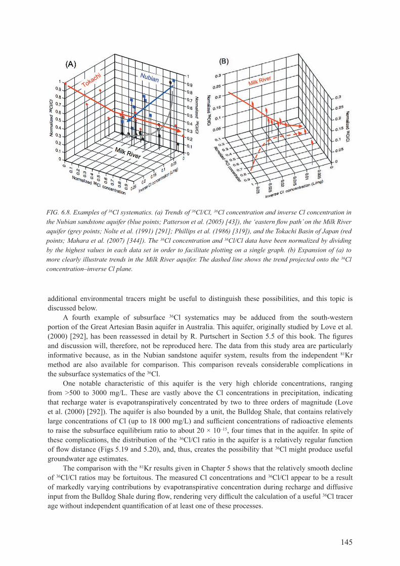
145

additional environmental tracers might be useful to distinguish these possibilities, and this topic is discussed below.

a fourth example of subsurface 36cl  systematics  may  be  adduced  from  the  south-western portion of the great artesian basin aquifer in australia. this aquifer, originally studied by love et al. (2000)  [292], has been reassessed  in detail by r. Purtschert  in Section 5.5 of  this book. The figures and discussion will, therefore, not be reproduced here. the data from this study area are particularly informative because, as in the nubian sandstone aquifer system, results from the independent 81Kr method are also available for comparison. this comparison reveals considerable complications in the subsurface systematics of the 36cl.

one notable characteristic of this aquifer is the very high chloride concentrations, ranging from >500 to 3000 mg/l. these are vastly above the cl concentrations in precipitation, indicating that recharge water is evapotranspiratively concentrated by two to three orders of magnitude (love et al. (2000) [292]). The aquifer is also bounded by a unit, the Bulldog Shale, that contains relatively large concentrations of cl (up to 18 000 mg/L) and sufficient concentrations of radioactive elements to raise the subsurface equilibrium ratio to about 20 × 10–15, four times that in the aquifer. In spite of these complications, the distribution of the 36cl/cl ratio in the aquifer is a relatively regular function of flow distance (figs 5.19 and 5.20), and, thus, creates the possibility that 36cl might produce useful groundwater age estimates.

the comparison with the 81Kr results given in chapter 5 shows that the relatively smooth decline of 36cl/cl ratios may be fortuitous. the measured cl concentrations and 36cl/cl appear to be a result of markedly varying contributions by evapotranspirative concentration during recharge and diffusive input from the Bulldog Shale during flow, rendering very difficult the calculation of a useful 36cl tracer age without independent quantification of at least one of these processes.

FIG. 6.8. Examples of 36Cl systematics. (a) Trends of 36Cl/Cl, 36Cl concentration and inverse Cl concentration in the Nubian sandstone aquifer (blue points; Patterson et al. (2005) [43]), the ‘eastern flow path’ on the Milk River aquifer (grey points; Nolte et al. (1991) [291]; Phillips et al. (1986) [319]), and the Tokachi Basin of Japan (red points; Mahara et al. (2007) [344]). The 36Cl concentration and 36Cl/Cl data have been normalized by dividing by the highest values in each data set in order to facilitate plotting on a single graph. (b) Expansion of (a) to more clearly illustrate trends in the Milk River aquifer. The dashed line shows the trend projected onto the 36Cl concentration–inverse Cl plane.

146

the results from the 81Kr comparison bear out the concerns of Love et al. (2000) [292], who warned that “The preceding discussion emphasizes that estimates of ‘absolute’ groundwater age using 36cl data are subject to large uncertainties because of problems of estimating the initial concentration of 36cl… and correcting for sources or sinks of chloride…”. As emphasized above in this chapter, 36cl dating is most likely to yield useful results when the cl and 36cl systematics are simple and the subsurface 36cl is dominated by meteoric input. The south-western great Artesian Basin offers strong support for this caution. the combination of extreme (and, therefore, potentially highly variable) evapotranspirative concentration and large subsurface sources of cl and 36cl warns of complications that are too large for reliable dating corrections. potential users of the method should carefully evaluate their study areas for similar problems.

6.5.6. Use of other environmental tracers to interpret chloride systematics

as illustrated above, although the end member cases illustrated in fig. 6.6 are clearly distinguishable,  in  some  real  world  cases  there  may  be  multiple  processes  influencing  36cl and cl  patterns,  or  there  may  be  insufficient  data  to  distinguish  fully  between  alternative  hypotheses. the past 20 years have seen a major advance in the development of additional tracers that can be examined in conjunction with the 36cl and cl patterns and that can provide independent constraints on chloride systematics.

probably the simplest and most cost effective of these is measurement of the concentration of br– along with cl–  (davis  et  al.  (1998)  [296]; davis  et  al.  (2004)  [386]; whittemore  (1995)  [387]). Most meteoric waters over the continents have a cl/br (mass:mass) value lower than that of sea water, which is 290. this is because during the formation of marine aerosols, br is preferentially fractionated into the smaller particles which persist longer in the atmosphere and are, thus, more readily transported towards  the  continental  interiors  (davis  et  al.  (2004)  [386]).  cl/Br  ratios  between  50  and  150  are characteristic of continental interiors.

In contrast, solutions originating from dissolution of marine evaporites or from connate fluids tend to have ratios of between 300 and 1000 (whittemore (1995) [387]). Such solutions start at the marine 

FIG. 6.9. The evolution of the 36Cl concentration and the Cl/Br ratio for the same hypothetical cases as in Fig. 6.7.

147

ratio of 290 and, inasmuch as br is excluded during the precipitation of halite, can have ratios of up to several thousand. these characteristics are convenient for the differentiation of cl sources, since recharge water will generally possess a low cl/br value and subsurface sources of cl will have high cl/br values. figure 6.9 illustrates the use of cl/br to distinguish sources of cl in the scenarios illustrated in fig. 6.6. the recharge water is assumed to have a cl/br ratio of 100 and the subsurface source a ratio of 1000. the cases in which subsurface cl is added show an evolution to the right of the graph whereas those where changes in cl are not subsurface related only evolve in the vertical.

the stable isotope composition of the cl is another environmental tracer that is integral to the halides and can help elucidate  the origins of cl within aquifer systems (rao et al.  (2005) [388]; Stewart and Spivack (2004) [389]; whittemore (1995) [387]). The δ37cl of the ocean and of marine evaporites has apparently been within ±0.5‰ of 0‰ throughout the Phanerozoic (Eastoe et al. (2007) [390]). However, the δ37cl of cl– in pore fluids of shales seems to range between –1 and –2‰ (zhang et al. (2007) [304]) and addition of cl from this source is probably responsible for the generally negative 

FIG. 6.10. (a) Relation between δ37Cl and the Cl concentration in groundwater from the Great Artesian Basin of Australia (Zhang et al. (2007) [304]); (b) relation between δ37Cl and 1/Cl in the Nubian aquifer of north Africa (Patterson et al. (2005) [43]).

-3.0

-2.5

-2.0

-1.5

-1.0

-0.5

0.0

0.5

0 200 400 600 800 1000 1200 1400 1600 1800

Cl concentration (mg/L)

δ3

7C

l (‰

SM

OC

)

Northern transect Southern transect

a

b

148

(~0  to  –2‰)  values  often  found  in  sedimentary  basin  waters  (weaver  (2000)  [391]).  In  contrast, marine aerosols usually have positive δ37cl,  varying  between  +0.5  and  +2.5‰  (volpe  and  Spivack (1994) [392]). This difference in atmospheric and subsurface isotopic signatures can help to fingerprint the origin of cl– in water being dated with 36cl.

figure 6.10 relates cl– and δ37cl in two systems: the great artesian basin (Zhang et al. (2007) [304]) and the Nubian aquifer (Patterson et al. (2005) [43]). The great Artesian Basin data show a clear trend of decreasing δ37cl with increasing cl– concentration. direct measurement of cl– in pore water from bounding  shale  units  confirmed  that  diffusion of cl–  out  of  the  shale was  the  likely  source of the increased cl– with flow distance in this aquifer. However, three samples show increased cl– with relatively constant δ37cl. These are from a distinct portion of the basin and the likelihood that this cl– increase is due to recharge area evaporation is supported by independent evidence.

The data from the Nubian aquifer (Patterson et al. (2005) [43]) exhibit a more complex pattern. the spacing of wells in the western desert of egypt is irregular and does not permit as comprehensive a view of the spatial distribution of water quality. however, the δ37cl clearly aids in distinguishing different groups of waters characterized by differing cl– concentrations and, thus, aids in interpreting 36cl data.

In summary, even though cl has unusually simple geochemistry, the evolution of the 36cl concentration and the 36cl/cl ratio down flow paths can still exhibit considerable complexity that reflects the heterogeneity of water sources and transport mechanisms in the subsurface. these trends have generally been thought of as requiring ‘correction’ of the calculated 36cl model ages, but are perhaps better considered as hallmarks of the water history. for example, diffusion of low 36cl/cl chloride out of an aquitard into an aquifer is also indicative of diffusion of ‘old’ water molecules out of the aquitard, and correspondingly, diffusion of  ‘young’ aquifer water  into  the aquitard. variable  36cl ratios due to variable evapotranspiration during recharge probably also indicate variations in the recharge rate, and hence groundwater velocity. as noted in chapter 1, the interpretation of age tracer data is most valuable when it is comprehensive, in other words, when a large number of different tracers can be interpreted within a reasonably well defined hydrogeological framework and be reconciled with a single, coherent history and set of processes. this chapter has focused on the calculation of single valued 36cl tracer ages, but integrating the 36cl patterns into a more comprehensive data set may permit estimation of actual frequency distribution of groundwater age.

A significant amount of recent research has explored the use of additional environmental tracers to yield information on halide systematics. examples include 129I (fabryka-martin et al. (1991) [385]; Snyder  and fabryka-martin  (2007)  [393]),  the cl/Br  ratio  (davis  et  al.  (2000)  [394]; Hurwitz  et  al. (2005) [395]; metcalfe et al. (2007) [396]; rao et al. (2005) [388]), δ37cl (Lehmann et al. (2003) [256]; zhang et al. (2007) [304]) and 4He (Kulongoski et al. (2008) [343]; mahara et al. (2007) [344]; Patterson et al. (2005) [43]). The application of one or several of these tracers, all associated with the systematics of cl or 36cl in some way, can greatly help to constrain sources of cl and 36cl or to explain variations in their distributions.

6.6. coMparIson of 36cl wIth other Methods of datIng

As  discussed  in  the  introduction  to  this  book,  interpretation  of  age  dating  tracers  is  most informative when multiple methods can be compared. In this section, the patterns of 36cl are compared with those of other tracers in several aquifer systems.

6.6.1. Comparison with radiocarbon

unfortunately, the useful range of 36cl in groundwater does not overlap with that of radiocarbon. the decay of 36cl is still small when 14c has decayed beyond the limit of practical application. this is

149

illustrated in fig. 6.11, where radiocarbon and 36cl are compared in the ojo alamo and nacimiento aquifers  of  the  San  juan  Basin,  south-western USA  (Phillips  (2000)  [306];  Plummer  (1996)  [356]; Stute et al. (1995) [213]). The 14c activity exhibits a quasi-exponential decrease with flow distance, as expected. By ~30 km, the activity is too low to yield useful groundwater age estimates. As predicted, the 36cl/cl is approximately constant over this interval. the open squares in fig. 6.11 show the 36cl/cl corrected for decay using the radiocarbon model age. given the observed variability in the 36cl/cl, this decay is too small to be useful for groundwater age estimation. the pattern of lower holocene 36cl/cl compared with the late pleistocene is due to secular variation of the 36cl production, modulated by the dipole geomagnetic field strength.

6.6.2. Comparison with 4He

  only a few age tracers significantly overlap with 36cl. one of the best is 4he accumulation. figure 6.12 compares 4he accumulation, 36cl and 14c along the ‘eastern flow path’ in the milk river aquifer (drimmie et al. (1991) [168]; Nolte et al. (1991) [291]; Phillips et al. (1986) [319]). The 14c adds little information, but is consistent with the other tracers. The first sample on the flow path contains about 10 pmc and the rest negligible 14c.

the 36cl shows a quasi-exponential decay with flow distance. In fig. 6.12, this profile has been fitted using the following equation:

R x Rxq36 36( )

= −o,36

s

exp λ (6.18)

whereR36(x) is the 36cl/cl ratio as a function of flow distance;Ro,36 is the initial 36cl/cl ratio;qs is the seepage velocity of the groundwater.

FIG. 6.11. Variation of 14C activity and 36Cl/Cl with flow distance in the Ojo Alamo and Nacimiento aquifers of the San Juan Basin, south-western USA. Data are from Phillips (2000) [306], Plummer (1996) [356] and Stute et al. (1995) [213]. The open squares are 36Cl/Cl corrected for radioactive decay using the inferred 14C model age.

150

The fit illustrated employed Ro,36 = 700 × 10–15 and qs = 5 cm/a. this simplistic dating approach neglects subsurface addition of cl and 36cl, which is undoubtedly significant in this case (Nolte et al. (1991) [291]; Phillips (2000) [306]), but gives a first order idea of the behaviour of the system.

The  good  fit  to  this  simple  equation  (Eq.  (6.18))  indicates  that  flow  velocity  is  approximately constant. If this is the case, and if 4he is introduced to the aquifer at a constant rate, then 4he should accumulate linearly with distance. figure 6.12 shows that there is indeed a linear accumulation, with 4he increasing at the rate of 1.3 × 10–6 cm3 STP · cm–3

h2o · km–1. assuming a seepage velocity of 5 cm/a,  this  is  equivalent  to a helium  influx of 6 × 10–11 cm3 STP  · cm–3

h2o  ·  a–1. the calculated contribution rate of 4He  from  the  rock matrix  is  approximately one order  less  than  this value,  if  all the 4He produced is assumed to diffuse into the pore water (Andrews et al. (1991) [397]). If the 4he is instead assumed mostly to access the aquifer water by upward diffusion from the crust beneath, the 4he flux would be approximately 5 × 10–4 cm3 STP · m–2 · a–1. This is not an especially large flux. In any case, the exponential dependence of the 36cl/cl ratio with distance and the linear dependence of the 4he confirm that the trends are consistent with the basic conceptual models for both isotopes that have been presented in this volume.

6.6.3. Comparison with 81kr

another dating method that overlaps very well with 36cl is 81Kr,  with  a  half-life  of 229 000 a. although the technology for 81Kr measurement  is  relatively new and has,  therefore, only been studied in relatively few localities, both nuclides have been measured in the nubian sandstone aquifer system (Sturchio et al. (2004) [5]). figure 6.13 shows the 36cl/cl ratio as a function of the model 81Kr  age.  If  the  two  dating methods  are  consistent,  36cl/cl should fall along a trend determined by the following equation:

36meas

36o

36se

36seCl Cl Cl Cl Cl Cl Cl Cl= − − + ( )exp λ36 81t (6.19)

FIG. 6.12. Trends of 36Cl/Cl, 4He and 14C with flow distance down the Milk River aquifer. Data are taken from Drimmie et al. (1991) [168], Nolte et al. (1991) [291] and Phillips et al. (1986) [319]. The red line illustrates the fit of an exponential decay model (Eq. (6.18)) to the 36Cl/Cl data and the blue line the fit of a linear accumulation model to the 4He model. Details are discussed in the text.

151

where36cl/clo is the recharge ratio;36cl/clse is the secular equilibrium ratio;t81 is the model 81Kr age.

In fig. 6.12, the data have been fitted to Eq. (6.19) with 36cl/clo = 131 × 10–15 and 36cl/clse = 8 × 10–15. an initial 81Kr/Kr  ratio of 1.10(±0.05) × 10–12 was used in calculating the simple exponential decay 81Kr model age. The agreement between the calculated and measured 36cl/cl ratios is generally good, especially considering that no effort was made to correct the model 36cl ages for subsurface additions of cl and 36cl.

6.6.4. Comparison without a well defined flow path

In some cases, general concordance between 36cl trends and those of independent tracers can be established even if a clear-cut flow path cannot be distinguished. This is illustrated in fig. 6.14, where 36cl and 4He  data  from  the Tokachi Basin  in  japan  are  plotted  (mahara  et  al.  (2007)  [344]). Here, the data are too scattered and irregular to allow evaluation of a flow path. However, the relation between the temporal patterns of accumulation of 36cl and 4he can still be evaluated. a simplistic model for the dependence of 36cl/cl on time is shown by:

36 3636

36361Cl/Cl Cl/Cl Cl/Clo set t t( ) ( ) ( )[ ]= − + − −exp expλ λ (6.20)

where 36cl/clo is the recharge 36cl/cl ratio and 36cl/clse the secular equilibrium ratio. the 4he accumulation is equally simplistically given by:

FIG. 6.13. 36Cl/Cl ratios measured in the Nubian sandstone aquifer of Egypt as a function of groundwater age calculated using measured 81Kr/Kr ratios, from Sturchio et al. (2004) [5]. The blue line is the 36Cl/Cl ratio calculated from the 81Kr model age using Eq. (6.19).

0 200 400 600 800 1000 1200 1400 1600 1800 0

10 20 30 40 50 60 70 80 90

100 110 120 130 140

Bauti 1

Sherka 36

Baris Farafra 6

El Zayat 12 36

Cl/C

l (×

10 –1

5 )

81 Kr age (ka)

Gum Horia

152

4he(t) = a4Het (6.21)

where A4He is the accumulation rate of 4he. equation (6.21) can be substituted into eq. (6.22) to yield:

36 3636

436

361Cl/Cl Cl/ClHe

Cl/Clo4He

setA

( )

= − + − −exp expλ λ

44 He

4HeA

(6.22)

In fig. 6.14, the solution of equation 6.22 is shown for 36cl/clo = 60 × 10–15, 36cl/clse = 10 × 10–15, and A4He = 9 × 10–7 cm3 STP · cm–3 · a–1. This calculated curve matches the data well, confirming that both 36cl and 4he are following the expected conceptual models and allowing the 4he accumulation rate to be estimated. As for the milk river aquifer, the original authors offer a more nuanced interpretation.

6.6.5. summary

chlorine-36 has been used to estimate groundwater ages  in numerous old groundwater systems over the past 20 years. the systematics are well understood, with 36cl principally produced in the atmosphere and entering the aquifer along with groundwater recharge. once in the subsurface, 36cl acts quite conservatively, leaving radiodecay as the only significant sink. The main complication for 36cl dating of old groundwater is the subsurface introduction of chloride, with accompanying 36cl. however, straightforward corrections for this mixing are possible if the nature of the subsurface processes is evaluated. results from 36cl dating of old groundwater can now be compared with those from a variety of other methods of dating. these comparisons are generally internally consistent and support the widespread use of 36cl for dating old groundwater.

FIG. 6.14. 36Cl/Cl ratio as a function of 4He content in groundwater from the Tokachi Basin, Japan. Data are from Mahara et al. (2007) [344]. The blue line is 36Cl/Cl as a function of 4He accumulation, calculated from Eq. (6.22).

153

Chapter 7

DAtInG OF OLD GROUnDWAtER UsInG URAnIUM IsOtOPEs — PRInCIPLEs AnD APPLICAtIOns

K. frÖHLIcHVienna, austria

7.1. IntroductIon

This chapter provides background on the behaviour of uranium isotopes in groundwater and shows that uranium isotope disequilibrium presents a method that has the potential to play an important role within the concerted application of techniques to date old groundwater. depending on the geochemistry of the aquifer system, the potential dating range extends from about 10 ka up to 1 ma, which overlaps the 14c and the 36cl/81Kr dating ranges. Uranium isotopes can provide independent information relevant to groundwater age that complements other dating approaches and may help resolve ambiguities in data interpretation. Moreover, uranium isotopes in groundwater have the potential for quantifying geochemical parameters of the water–rock interaction and represent natural analogues for radioactive waste. any multitracer application to date old groundwater should integrate uranium isotope measurements, which can easily be afforded by the use of modern mass spectrometric techniques.

among the natural decay series radionuclides, the uranium isotopes 234u and 238u and the ratio of activity of these isotopes (234u/238u) provide the greatest potential to trace natural water and to date old groundwater. Moreover, they are very useful as natural analogues in assessing the behaviour of radionuclides in nuclear waste disposal sites.

7.1.1. History

In 1955, V.V. cherdyntsev and p.I. chalov discovered that in secondary minerals and natural water, 234u and 238u predominantly occur in radioactive disequilibrium, i.e. the activity ratio 234u/238u is  different  from  unity  (cherdyntsev  et  al.  (1955)  [398]).  Subsequent  studies  have  shown  that  this disequilibrium is a consequence of the energetic alpha decay of 238u that causes recoil fractionation between 234u and 238u due to differential release of 234u and 238U from the rock into the surrounding water  (chalov and merkulova (1966) [399]; cherdyntsev (1969) [400]; osmond and cowart  (1976) [401]; osmond and cowart (1982) [402]). This disequilibrium found wide application in surface and groundwater studies.

In aerobic aqueous systems, measurements of uranium and 234u/238u have been used to trace the flow of  river water and groundwater  (Plater et  al.  (1992)  [403]; Porcelli  and Swarzenski  (2003) [404]; Sarin et al.  (1990)  [405]; Tuzova (1986)  [406]; Tuzova and Novikov (1991)  [407]), establish timescales of weathering processes (Andersen et al. (2009) [408]; dosseto et al. (2008) [409]; vigier et  al.  (2006)  [410]),  quantify mixing  of  surface  and  groundwater  (Briel  (1976)  [411]),  and  identify groundwater inflow into surface water (durand et al. (2005) [412]).

The suitability of uranium isotope disequilibrium as a tracer and timer of groundwater was first demonstrated  by osmond  et  al.  (1968)  [413]  and  later  by chalov  et  al.  (1979)  [414], osmond  and cowart (1976) [401], and osmond et al. (1983) [415]. given the long half-life of 234U (2.45 × 105 a), many attempts have been made to apply 234u/238u and/or the 234u excess (difference in the activity concentration of 234u and 238u) to date old groundwater up to hundreds of thousands of years (andrews et al. (1982) [416]; Andrews and Kay (1983) [417]; Barr et al. (1979) [418]; cowart and osmond (1974) [419]; Eshova (1981) [420]; fröhlich et al. (1984) [421]; Ivanovich et al. (1991) [422]; Kigoshi (1973) 

154

[423]; Kronfeld and Adams  (1974)  [424]; Pearson et  al.  (1983)  [425]). cowart  and osmond  (1974) [419] noted that groundwater age derived from the decay of 234u excess may represent the migration time of the uranium tracer rather than the travel time of the groundwater. consequently, any attempt to use the uranium isotope disequilibrium for groundwater studies requires a thorough knowledge of the sorption behaviour of these isotopes in the aquifer system (fröhlich and gellermann (1987) [426]).

the past two decades have seen a rapid expansion in the use of uranium series disequilibrium in a variety of disciplines such as geochronology, geochemistry and hydrology. among others, applications of  uranium  isotopes  to  groundwater  studies  are  reported  by  Bonotto  (2000)  [427],  Bonotto  (2006) [428], deschamps et al. (2004) [429], Luo et al. (2000) [430], rogojin et al. (1998) [431] and Tricca et al. (2001) [432]. many recent studies take advantage of new analytical techniques, which began in the late 1980s with the use of thermal ionization mass spectrometry for the measurement of uranium isotopes and other radionuclides of the natural decay series (chen et al. (1986) [433]). The application of multicollector inductively coupled plasma mass spectrometry (Mc–Icp–Ms) especially allowed measurement  of  much  smaller  water  samples  with  greater  accuracy  and  a  significant  increase  in the measuring  capacity  in  comparison  to  alpha  spectrometry  (goldstein  and  Stirling  (2003)  [434]). the Mc–Icp–Ms technique enables high precision measurements of previously undetectable variations in many elements, including isotopic fractionation between 235u and 238u in water (rademacher et al. (2003) [435]). Achievements have also been made in quantifying the effects of preferential release of 234U in weathering and erosion studies both by laboratory and field experiments (Andersen et al. (2009) [408]). In conclusion, the advent of mass spectrometric analysis of uranium isotopes, which is quicker and more precise, may enable broader application of this method and its practical application.

7.1.2. scope and objective

this review is focused on the uranium isotope disequilibrium in groundwater and its relevance to dating of old groundwater. first, the natural abundance of uranium isotopes and their geochemical behaviour  in groundwater will  briefly be discussed. Second,  a  critical  review of  the models used  to derive information from uranium isotope measurements on groundwater age will be given. special emphasis is placed on a conceptual model incorporating water–rock interaction that has been used for dating old groundwater. finally, some case studies will be discussed which demonstrate the strengths and limitations of the uranium isotope groundwater dating technique and its integration into multitracer approaches to date old groundwater. developments in the use of uranium and 234u/238u have been reviewed  by  cherdyntsev  (1971)  [436],  osmond  (1980)  [437],  osmond  and  cowart  (1976)  [401], osmond and cowart (1992) [438], and osmond and cowart (2000) [439]. monographs on this subject have been published by Ivanovich and Harmon (1982) [440], Ivanovich and Harmon (1992) [441] and, more recently, by Bourdon et al. (2003) [442].

7.2. natural abundance of uranIuM Isotopes

naturally occurring uranium consists of three alpha active isotopes: 238u, 235u and 234U. The first two isotopes are initial members of the corresponding natural radioactive decay series and the latter one is a decay product of 238u (fig. 7.1). the 235u activity in natural uranium is less than 5% of the 238u activity and, thus, has not been used for hydrological applications. given the relatively short half-life of 234U (2.455 × 105 a) compared with 238U (4.468 × 109 a), these two uranium isotopes are expected to be globally in secular radioactive equilibrium, i.e. 234u/238u = 1. It was, therefore, a surprise when cherdyntsev  et  al.  (1955)  [398]  reported  that  in  some geological  objects,  radioactive  equilibrium  is disturbed. In groundwater, the 234u/238U ratio is usually >1, while in weathered rock, for instance, this ratio can be distinctly <1.

155

the quantities used to express uranium abundance and measuring results include the following:— uranium activity concentration = uranium activity (bq or mbq) divided by volume of water

(l) in which uranium is dissolved.— uranium concentration = mass of uranium (mg or µg) divided by volume of water (l) in

which uranium is dissolved.— Specific activity of uranium = uranium activity (Bq or mBq) divided by mass of substance (kg) 

containing the uranium.— (relative) uranium content = mass of uranium divided by mass of substance containing

the uranium (g/g, ppm = 1 mg U/1 kg of substance, or 1 ppb = 1 µg U/1 kg of substance).— uranium activity ratio = activity of 234u divided by activity of 238u in a given sample.

It should be noted that 1 ppm uranium corresponds to a specific activity of 12.4 Bq/kg.In ocean water, related to a salinity of 35‰, uranium concentration ranges from 3.162 to

3.281 µg/L (chen et al. (1986) [433]) and the activity ratio is 1.147 ± 0.001 (Andersen et al. (2007) [443];  robinson  et  al.  (2004)  [444])  (Table  7.1).  In  continental  surface water,  the  uranium  content varies between 10–3 and 103 ppb, and the activity ratio ranges from 1 to 2 (osmond and cowart (1976) [401]). most of the 234u/238U values of lakes and rivers are between 1.1 and 1.4 (chabaux et al. (2003) [445]; ferronsky and Polyakov (1982) [446]). 

groundwater shows the largest variation both of uranium concentration and the activity ratio. an evaluation of nearly 800 measurements published at the beginning of the 1980s (gellermann and fröhlich (1984) [447]) uncovered a logarithmic normal distribution of uranium concentration with an average value of 1 ppb and a range from 10–3 to 104 ppb. the lower end of this distribution corresponds to  the  analytical  detection  limit  by  alpha  spectrometric  measurements  of  uranium  made  in  1984; in reality, uranium concentrations may be even lower. the activity ratios in groundwater ranged from 0.5 to about 30; values >5 were mainly associated with low uranium concentrations. none of the published activity ratio values were below 0.5; this appears to be in agreement with theoretical considerations of Bondarenko (1981) [448]. The frequency distribution of  the 234u/238u activity ratio is  generally  asymmetric  and  strongly  depends  on  the  type  of  water-bearing  rocks.  In  an  extensive study of groundwater  from Kazakhstan, Syromyatnikov  (1961)  [449]  found characteristic  frequency distributions of 234u/238U for various rock types (fig. 7.2).

FIG. 7.1. Part of the 238U decay series (from 238U to 222Rn).

156

7.3. uranIuM geocheMIstry

In  natural waters,  the  prevailing  valence  states  of  uranium  are  +4  and +6. during weathering, uranium is oxidized to the hexavalent uranyl ion Uo*+ which forms soluble complexes with co$ and po'– under near-neutral conditions, and with So%–, f– and cl– at lower ph values (langmuir (1978) [450]). The presence of these complexing ions inhibits adsorption and, hence, is mainly responsible for the mobility of uranium observed in natural waters (rose and wright (1980) [451]). Under oxidizing conditions, typical uranium concentrations in water are close to 1 ppb (osmond and cowart (1992) [438]). Under  reducing  conditions,  uranium occurs  in  the  tetravalent  state  and  is  stable  as U(oH)4; the maximum uranium concentration is at about 0.06 ppb, which corresponds to the solubility limit of uraninite (uo2) (gascoyne (1992) [452]).

table 7.1. uranIuM content and 234u/238U IN rocKS ANd NATUrAL wATErS

object uranium content (ppm) 234u/238u

Sedimentary rocks

carbonates 0.6 ± 0.5 0.92 ± 0.01

clays 2 ± 1 0.9 ± 0.1

phosphorites 100 1.0–1.15

Igneous rocks

mafic 0.9 (1.0)

diorites 2 (1.0)

granodiorites 2.6 (1.0)

silicic volcaneous 5 (1.0)

Magma (basalt) 0.078 (1.0)

ocean water 3.3 × 10–3 1.147 ± 0.001

groundwater 1 × 10–3 (1–10–6)

1.5 (0.5–30)

FIG. 7.2. Histograms of 234U/238U distribution in the groundwater of igneous rocks (a), sedimentary and metamorphic rocks (b) and uranium ores (c) (from Ferronsky and Polyakov (1982) [446]).

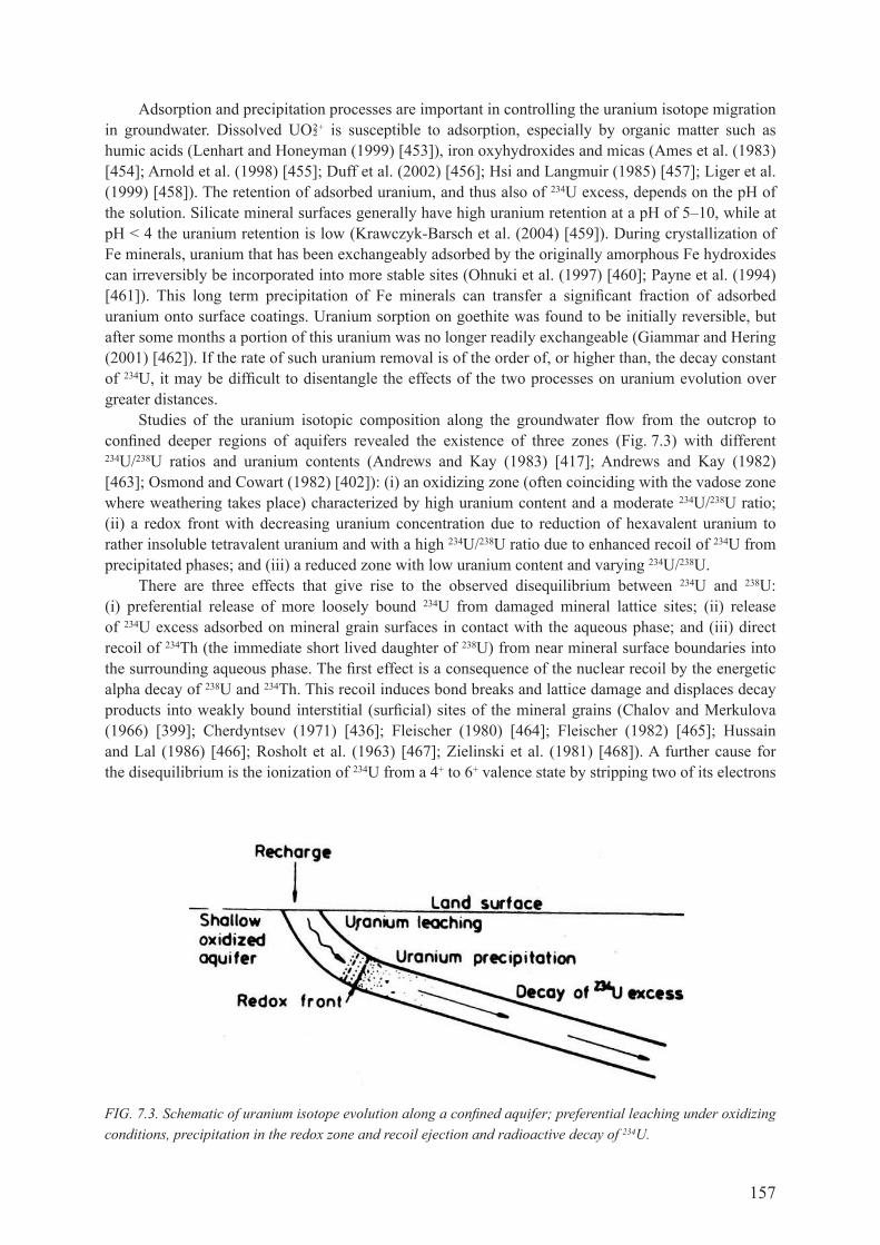
157

adsorption and precipitation processes are important in controlling the uranium isotope migration in groundwater. dissolved uo*+ is susceptible to adsorption, especially by organic matter such as humic acids (Lenhart and Honeyman (1999) [453]), iron oxyhydroxides and micas (Ames et al. (1983) [454]; Arnold et al. (1998) [455]; duff et al. (2002) [456]; Hsi and Langmuir (1985) [457]; Liger et al. (1999) [458]). The retention of adsorbed uranium, and thus also of 234u excess, depends on the ph of the solution. silicate mineral surfaces generally have high uranium retention at a ph of 5–10, while at pH < 4 the uranium retention is low (Krawczyk-Barsch et al. (2004) [459]). during crystallization of fe minerals, uranium that has been exchangeably adsorbed by the originally amorphous fe hydroxides can irreversibly be incorporated into more stable sites (ohnuki et al. (1997) [460]; Payne et al. (1994) [461]).  This  long  term  precipitation  of  fe  minerals  can  transfer  a  significant  fraction  of  adsorbed uranium onto surface coatings. uranium sorption on goethite was found to be initially reversible, but after some months a portion of this uranium was no longer readily exchangeable (giammar and hering (2001) [462]). If the rate of such uranium removal is of the order of, or higher than, the decay constant of 234U, it may be difficult to disentangle the effects of the two processes on uranium evolution over greater distances.

Studies  of  the  uranium  isotopic  composition  along  the  groundwater  flow  from  the  outcrop  to confined  deeper  regions  of  aquifers  revealed  the  existence  of  three  zones  (fig. 7.3)  with  different 234u/238U  ratios  and  uranium  contents  (Andrews  and  Kay  (1983)  [417]; Andrews  and  Kay  (1982) [463]; osmond and cowart (1982) [402]): (i) an oxidizing zone (often coinciding with the vadose zone where weathering takes place) characterized by high uranium content and a moderate 234u/238u ratio; (ii) a redox front with decreasing uranium concentration due to reduction of hexavalent uranium to rather insoluble tetravalent uranium and with a high 234u/238u ratio due to enhanced recoil of 234u from precipitated phases; and (iii) a reduced zone with low uranium content and varying 234u/238u.

there are three effects that give rise to the observed disequilibrium between 234u and 238u: (i) preferential release of more loosely bound 234u from damaged mineral lattice sites; (ii) release of 234u excess adsorbed on mineral grain surfaces in contact with the aqueous phase; and (iii) direct recoil of 234th (the immediate short lived daughter of 238u) from near mineral surface boundaries into the surrounding aqueous phase. The first effect is a consequence of the nuclear recoil by the energetic alpha decay of 238u and 234Th. This recoil induces bond breaks and lattice damage and displaces decay products  into weakly bound  interstitial  (surficial) sites of  the mineral grains (chalov and merkulova (1966)  [399];  cherdyntsev  (1971)  [436];  fleischer  (1980)  [464];  fleischer  (1982)  [465];  Hussain and Lal  (1986)  [466]; rosholt et al.  (1963)  [467]; zielinski et al.  (1981)  [468]). A further cause  for the disequilibrium is the ionization of 234U from a 4+ to 6+ valence state by stripping two of its electrons

FIG. 7.3. Schematic of uranium isotope evolution along a confined aquifer; preferential leaching under oxidizing conditions, precipitation in the redox zone and recoil ejection and radioactive decay of 234U.

158

during the decay sequence 238U(4+) → 234Th (4+) → 234pa (5+) → 234u (6+) (dooley et al. (1966) [469]). an alternative explanation of the 234u oxidation has been found by computer simulations of the recoil process (Adloff and roessler (1991) [470]). These simulations suggest that recoiling 234th atoms push the oxygen atoms of the mineral in front of it so that the final resting location of 234th becomes enriched in oxidizing species. These species subsequently oxidize 234u after decay of 234th.

The various mineral phases of a given rock type do not only have different susceptibility to lattice damage induced by alpha decay, but also differring ability to anneal (recover from) this damage. In general, lattice defect recovery is a slow process at normal groundwater temperatures and, thus, some silicate minerals are comparatively susceptible to preferential release of 234u from damaged lattice sites (Andersen et al. (2009) [408]; Eyal and fleischer (1985) [471]). In contrast, minerals such as monazite and  apatite  show  a  rapid  recovery  (chaumont  et  al.  (2002)  [472];  Eyal  and olander  (1990)  [473]; Hendriks and redfield (2005) [474]).

Kigoshi (1971) [475] found that 234u/238u ratios >3 cannot be explained by this preferential 234u release alone, but require a combination with an additional fractionation mechanism based on direct alpha recoil ejection of 234Th from the solid into the aqueous phase (see also Hussain and Krishnaswami (1980)  [476], and rama and moore  (1984)  [477]). At  the  transition  from oxic  to anoxic conditions, high groundwater 234u/238u ratios are produced due to recoil effects and preserved by the anoxic water. thus, uranium is concentrated on secondary phases by precipitation. as a consequence, uranium concentrations strongly decrease and 234u/238u ratios increase due to recoil from these phases (osmond and  cowart  (1992)  [438]).  The  recoil  effect  depends  on  the  uranium  concentration  in  the mineral, the  grain  size  of  the mineral,  the  recoil  range  of  234th (about 20 nm) and the time (depaolo et al. (2006) [478]; Kigoshi (1971) [475]). Provided the 234th residence time in the aqueous phase is long enough compared with its half-life, 234u is produced directly within the aqueous phase by the decay of recoil ejected 234th. If, however, 234Th is quickly adsorbed by mineral surfaces (Langmuir and Herman (1980) [479]), then 234u is produced at these surface sites from which it can easily enter the surrounding groundwater. Note that over long time scales (of the order of 100 ka) in slow moving groundwater and at low leaching (weathering) rates (<10–6/a), direct recoil may overcompensate radioactive decay of 234u and, thus, cause an increase of 234u/238U along the groundwater flow (Andersen et al. (2009) [408]).

7.4.  uranIuM Isotope MeasureMents

the uranium isotopes 238u and 234u are alpha emitters and thus, until recently, have been measured by alpha spectrometry combined with isotope dilution methods using 232u or 236u as analytical tracers (Lally (1992) [480]). This technique is still cost effective and well suited for applications where higher detection limits and lower precision and longer measuring (counting) times (several days per sample) are acceptable. Alpha spectrometry laboratories often simultaneously operate dozens of solid state alpha detectors and small vacuum chambers. In the late 1980s and early 1990s, mass spectrometry became an alternative to decay counting techniques (chen et al. (1992) [481]). Although much more expensive, it facilitates more accurate measurements in a shorter time and with much smaller samples (table 7.2).

for alpha spectrometry of uranium isotopes, at least 10 l of water is necessary. when using mass spectrometry, water samples of the order of 10 mL are sufficient for analysis. If water samples contain particulate matter, filtering (usually with 0.45 µm membranes) is required. Adsorption of uranium onto the container walls or suspended matter can be avoided by adding, as soon as feasible during sampling, enough nitric acid to lower the ph of the water to approximately 1. (If other u–th series nuclides are to be measured also, a more sophisticated sampling procedure is necessary, which, for example, is described by Tricca et al. (2001) [432]).

In the laboratory, a weighed amount of spike solution (usually with the shorter lived 232u for alpha spectrometry and the longer lived 233u or 236u for mass spectrometry) has to be added to the water sample. for alpha spectrometric analysis, the water volume must be reduced by evaporation or through co-precipitation of uranium with, for example, ferric hydroxide as carrier. The precipitate is re-dissolved 

159

in an acid medium and then passed through an anion exchange column to isolate uranium from other nuclides that might cause interference during counting. finally, the uranium is deposited on a suitable substrate (e.g. electrodeposition on polished stainless steel planchets) for alpha spectrometric analysis. more details of this laboratory procedure can be found in Lally (1992) [480]. for mass spectrometric measurements,  the  following  procedure  is  used:  addition  of  a  spike  (233u or 236u), drying, anion exchange and loading onto filaments for analysis.

table 7.2 compiles parameters that allow comparison of the various methods currently available for the measurement of 234u and 238U in natural water samples (goldstein and Stirling (2003) [434]). there are several suitable mass spectrometric methods which basically differ regarding the type of ion  source,  ionization method  and  ion  collector  system. The first mass  spectrometric measurements of uranium and thorium isotopes were performed with thermal ionization mass spectrometers (TImS) (chen et  al.  (1986)  [433]; Edwards  et  al.  (1987)  [482]; goldstein  et  al.  (1989)  [483]). Sample  size, measuring precision and time of analysis have improved at least one order of magnitude since that time. since the 1990s, inductive coupled plasma mass spectrometry (IcpMs) has become more commonly used as an alternative to tIMs with comparable or even better precision. IcpMs facilitates a fast and easy acquisition of data. analysis times are typically less than 10 min (goldstein and stirling (2003) [434]).  Since  the  end  of  the  1990s,  mc-IcPmS  (multiple-collector-IcPmS)  is  increasingly  being used. It facilitates an even better precision than conventional IcpMs. the cost per sample analysis is presently about us $25.

7.5. uranIuM Isotope datIng Method

7.5.1. Introduction

a straightforward dating of old groundwater by uranium isotope disequilibrium would be possible  if:  (i)  the  initial  state  of  disequilibrium  were  known  and  (ii)  the  concentrations  of  both isotopes had not changed by chemical and physical processes other than radioactive decay. the initial state of disequilibrium can be estimated empirically by extrapolation of measured values along the  groundwater  flow  direction.  However,  the  second  requirement  is  difficult  to  satisfy  because  of the various geochemical processes (including dissolution, precipitation, sorption/desorption) involved in the water–rock interaction that affect the evolution of uranium in groundwater. A range of attempts have been made by various authors to interpret uranium isotope measurements in terms of groundwater age. In the following, a model is described that allows a critical review of such approaches and helps

table 7.2. coMparIson of analytIcal Methods for uranIuM Isotope analysIs (Goldstein and Stirling (2003) [434])

alpha spectrometry

thermal ionization mass 

spectrometry

multiple-collector thermal

ionization mass  spectrometry

Inductive coupled

plasma mass spectrometry

multiple-collector inductive coupled

plasma mass spectrometry

sample size (µg) uranium 1–100 0.1–2 0.01–1 0.01–0.45 0.01–0.45

precision (2σ) (%)

238u 2–10 0.1 0.1 0.1–5 <0.1

234u/238u 2–10 0.5 0.1–0.2 0.1–10 0.05–0.2

Meas. time uranium 1–28 d 4 h 1–2 h 1–10 min 15–30 min

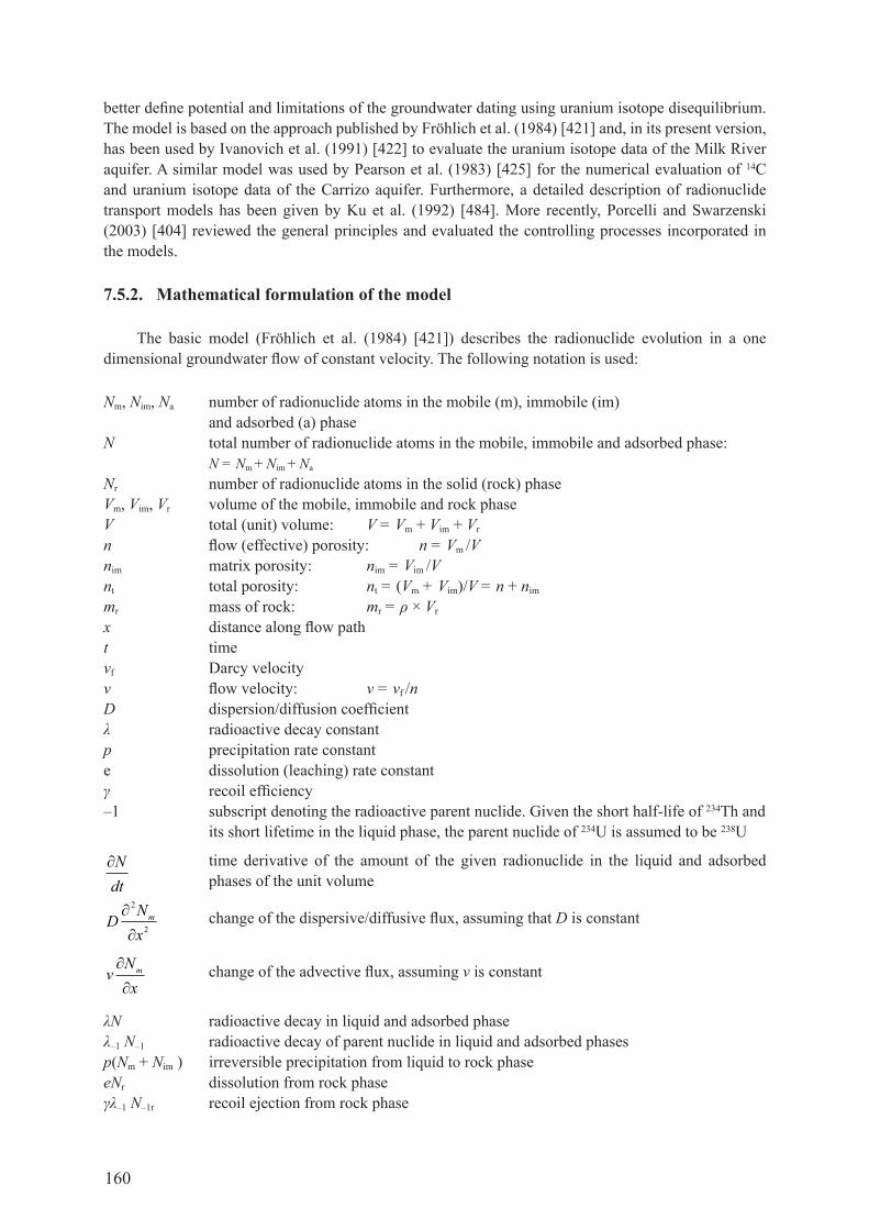
160

better define potential and limitations of the groundwater dating using uranium isotope disequilibrium. The model is based on the approach published by fröhlich et al. (1984) [421] and, in its present version, has been used by Ivanovich et al. (1991) [422] to evaluate the uranium isotope data of the milk river aquifer. A similar model was used by Pearson et al. (1983) [425] for the numerical evaluation of 14c and uranium  isotope data of  the carrizo aquifer. furthermore, a detailed description of  radionuclide transport models  has been given by Ku et  al.  (1992)  [484]. more  recently, Porcelli  and Swarzenski (2003) [404] reviewed the general principles and evaluated the controlling processes incorporated in the models.

7.5.2. Mathematical formulation of the model

The  basic  model  (fröhlich  et  al.  (1984)  [421])  describes  the  radionuclide  evolution  in  a  one dimensional groundwater flow of constant velocity. The following notation is used:

Nm, Nim, Na number of radionuclide atoms in the mobile (m), immobile (im)and adsorbed (a) phase

N total number of radionuclide atoms in the mobile, immobile and adsorbed phase:N = Nm + Nim + Na

Nr     number of radionuclide atoms in the solid (rock) phaseVm, Vim, Vr  volume of the mobile, immobile and rock phaseV total (unit) volume: V = Vm + Vim + Vr

n     flow (effective) porosity:   n = Vm /Vnim matrix porosity: nim = Vim /Vnt total porosity: nt = (Vm + Vim)/V = n + nim

mr mass of rock:    mr = ρ × Vr

x     distance along flow patht timevf darcy velocityv     flow velocity:    v = vf /nD     dispersion/diffusion coefficientλ radioactive decay constantp precipitation rate constante dissolution (leaching) rate constantγ     recoil efficiency–1     subscript denoting the radioactive parent nuclide. given the short half-life of 234th and its short lifetime in the liquid phase, the parent nuclide of 234u is assumed to be 238u

∂Ndt

time derivative of the amount of the given radionuclide in the liquid and adsorbed phases of the unit volume

DNxm∂

∂

2

2  change of the dispersive/diffusive flux, assuming that D is constant

vNxm∂

∂     change of the advective flux, assuming v is constant

λN radioactive decay in liquid and adsorbed phaseλ–1 N–1 radioactive decay of parent nuclide in liquid and adsorbed phasesp(Nm + Nim )  irreversible precipitation from liquid to rock phaseeNr     dissolution from rock phaseγλ–1 N–1r    recoil ejection from rock phase

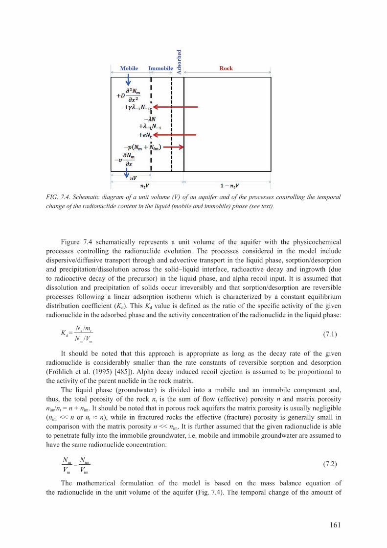
161

figure  7.4  schematically  represents  a  unit  volume  of  the  aquifer  with  the  physicochemical processes controlling the radionuclide evolution. the processes considered in the model include dispersive/diffusive transport through and advective transport in the liquid phase, sorption/desorption and precipitation/dissolution across the solid–liquid interface, radioactive decay and ingrowth (due to radioactive decay of the precursor) in the liquid phase, and alpha recoil input. It is assumed that dissolution and precipitation of solids occur irreversibly and that sorption/desorption are reversible processes  following  a  linear  adsorption  isotherm  which  is  characterized  by  a  constant  equilibrium distribution coefficient (Kd). this Kd value is defined as the ratio of the specific activity of the given radionuclide in the adsorbed phase and the activity concentration of the radionuclide in the liquid phase:

KN mN Vd

a r

m m

// (7.1)

It should be noted that this approach is appropriate as long as the decay rate of the given radionuclide is considerably smaller than the rate constants of reversible sorption and desorption (fröhlich et  al.  (1995)  [485]). Alpha decay  induced  recoil  ejection  is  assumed  to be proportional  to the activity of the parent nuclide in the rock matrix.

the liquid phase (groundwater) is divided into a mobile and an immobile component and, thus,  the  total  porosity  of  the  rock nt  is  the  sum  of  flow  (effective)  porosity n and matrix porosity nim/nt = n + nim. It should be noted that in porous rock aquifers the matrix porosity is usually negligible (nim << n or nt  ≈ n), while  in  fractured  rocks  the  effective  (fracture)  porosity  is  generally  small  in comparison with the matrix porosity n << nim. It is further assumed that the given radionuclide is able to penetrate fully into the immobile groundwater, i.e. mobile and immobile groundwater are assumed to have the same radionuclide concentration:

m im

m im

N NV V

(7.2)

the mathematical formulation of the model is based on the mass balance equation of the  radionuclide  in  the unit volume of  the aquifer  (fig. 7.4). The  temporal change of  the amount of 

FIG. 7.4. Schematic diagram of a unit volume (V) of an aquifer and of the processes controlling the temporal change of the radionuclide content in the liquid (mobile and immobile) phase (see text).

162

the radionuclide is given by the difference between the input and output of the radionuclide as well as by its production and decay. the mass balance includes both the liquid and adsorbed phases in the unit volume:

∂

∂

∂

∂

∂

∂

Nt

DNx

vNx

N N p N N eN N= − − + − + + +− − − −( )2

2 1 1 1m m

m im r 1rλ λ γλ (7.3)

The various terms of Eq. (7.3) are schematically shown in fig. 7.4 and are explained in the above notation. considering that:

N = Nm + Nim + Na

taking into account Eqs (7.1, 7.2) and the definitions of the various porosities, it can be shown that:

N = R × Nm

where R is the retardation factor:

t td

1 n nR Kn n

  (7.4)

similarly, it can be shown that Nm + Nim of the precipitation term in eq. (7.3) can be replaced by t

mn Nn

. thus, with eq. (7.3), it follows that:

RNt

DNx

vNx

Rnnp N R N eN Nt∂

∂∂∂

∂∂

m m mm 1m r 1r= − − + + + +− − − − −

2

2 1 1 1( )λ λ γλ (7.5)

finally, replacing the number of radionuclide atoms in eq. (7.5) by the corresponding activity

concentration m

m

NaV

, aNV

m

m−

− −=11 1λ

, rr Na

V and a

NVr

r−

− −=11 1�

λ, and multiplying both

sides by mV

leads to:

Rat

Dax

vax

Rnnp a R a ea n a n

∂

∂

∂

∂

∂

∂= − − + + + +

− − −

2

2 1 1 1λ λ γλtr r/ / (7.6)

this equation describes the evolution of any radionuclide of the natural decay series (fröhlich et al.  (1995) [485]). for  the determination of  234u/238u disequilibrium, eq. (7.6) represents a system of three partial differential equations that has to be solved for the three members of the decay sequence 238U  →  234Th  →  234u. the following simplifying assumptions allow a straightforward analytical solution of these equations. In aquifer systems with old groundwater, the radionuclide distributions are supposed to be in steady state ( 0a

t

). thus, the partial differential equations change to ordinary

differential equations. the 234th activity concentration in groundwater is, in general, very low or even negligible, which reduces the system to two equations. furthermore, it is assumed that the parameters characterizing the water–rock interaction (R, p, nt, n) and the activity concentrations in the rock phase (ar amd a–1r)  are  constant  along  the  considered groundwater flow path. consequently,  the  system of Eq. (7.6) reduces to two ordinary linear differential equations of second order with constant coefficients, for which the following solutions for the 238u and 234u activity concentrations can easily be obtained:

8 8 80 8 8( ) exps sa a a a (7.7)

4 4s 40 4s 4( ) expa a a a (7.8)

163

table 7.3. coMpIlatIon of earlIer atteMpts to date old groundwater usIng uranIuM Isotopes (from Fröhlich and Gellermann (1987) [426])

authors study area; aquifer rock type dating formula(s) results

Kronfeld (1971) [486], Kronfeld and Adams (1974) [424]

hosston aquifer (texas, usa); sandstone

ar = ar0exp(–λ4τ)*(water rock interaction neglected)

flow velocity 0.2–1.0 m/a derived

cowart and osmond (1974) [419], cowart and osmond (1977) [487]

carrizo aquifer (texas, usa); sandstone

X = Xs + (X0 – Xs)exp(–λ4τ)**(retardation, precipitation, leaching neglected)

apparent groundwater flow rate of 8 cm/a about 20 times lower than the one determined by other techniques

pearson et al. (1983) [425]

carrizo aquifer (texas, usa); sandstone

groundwater and radionuclide transport equation incorporating water rock exchange

14c data (uncorrected) used to validate numerical solution of the transport equation; uranium retardation factor in reducing zone about 30

Barr et al. (1979) [418]

delaware basin (new Mexico–texas, usa); evaporite, limestone

ar = ars + (ar0 – ars)exp(–λ4τ)(retardation, precipitation, leaching neglected)

ars = 1 assumed and ar0 estimated; calculated ages between 0.3 and 1.1 Ma

Eshova (1981) [420] Bachardensky aquifer (Turkmenistan)

ar = 1 + (ar0 – 1)exp(–λ4τ)(retardation, precipitation, leaching neglected)

estimated groundwater age 60 ka

fritz et al. (1980) [488]

stripa test site (sweden); granite

ar =1 + (ar0 – 1)exp(–λ4τ) Vertical age differences of 0.14 ma estimated; model assumptions not supported by chemical dataandrews et al. (1982)

[416]

ar = 1 + (ar0 – 1)exp(–λ4τ) + βa[1 – exp(–λ4τ)], where βa ≈ a8r/a8

Andrews and Kay (1983) [417], Andrews et al. (1984) [489]

east Midlands aquifer (united Kingdom); sandstone

ar = 1 + (ar0 – 1)exp(–λ4τ) + βa[1 – exp(–λ4τ)], where βa ≈ a8r/a8

u isotopes are related to the hydrochemistry and difficult to relate to groundwater age

fröhlich et al. (1984) [421]

triassic aquifer (germany); sandstone

groundwater and radionuclide transport equation incorporating water –rock exchange

combined meaurements of 14c and uranium isotopes; for reducing zone, the uranium retardation factor is between 30 and 80

Ivanovich et al. (1991) [422]

milk river sandstone aquifer, canada

groundwater and radionuclide transport equation incorporating water–rock exchange

234u (238u) age in good agreement with results obtained by hydraulic and 36cl methods (see Table 7.4)

164

The subscripts 8 and 4 indicate 238u and 234u, respectively, 0 and s indicate initial and stationary values, respectively, and τ is the groundwater age, or more precisely the time the groundwater parcel needs to travel along a distance x of the flow path:

/x v (7.9)

The parameters included in Eqs (7.7, 7.8) are defined as follows:

ii

vD

DKv

2

21 2

21 1

4( ) / (7.10)

ti i

nK R pn

(7.11)

a8s = e8a8r/(nK8) (7.12)

a4s = (e4a4r +γλ4a8r) /(nK4) (7.13)

the dispersivity D/v in deep aquifer systems is assumed to be small, i.e. D/v << v/4Ki. thus, expressing the square root in eq. (7.10) by a taylor series, the terms i

2

4DKv

with ν > 1 can be neglected, so that eq. (7.10) reduces to:

i iK   (7.14)

a numerical example of the practical application of the above equations represents the evaluation of uranium isotope data of the continental Intercalaire aquifer provided in section 7.6.

Using Eqs (7.7, 7.8) (with the parameters defined by Eqs (7.9–7.14)), fröhlich and gellermann (1987) [426] reviewed earlier attempts of groundwater dating using uranium isotopes. They found that the dating equations used in most of these studies (table 7.3) represent special cases of eqs (7.7, 7.8) for which  the uranium isotope exchange between water and  rock were neglected. As can be seen  in table 7.3, the uranium isotope results are often expressed by the 234u/238u activity ratio (ar) and 234u excess (X). with the notation used in eqs (7.7, 7.8), it follows that:

ar = 234u/238u = a4/a8

X = 234u – 238u = a4 – a8

It should be noted that, apart from analytical solutions of the radionuclide transport equation, numerical solution techniques have also been used (e.g. Pearson et al. (1983) [425]). Such numerical solutions have certain advantages over analytical solutions if spatial variations of the hydraulic and geochemical properties of the aquifer systems are significant. moreover, in order to simulate real field problems, transport in two or even three dimensions must be evaluated; this can only be realized with numerical techniques.

7.5.3. Identification of model parameters

In the following, the properties (behaviour) and values of the geochemical parameters that are incorporated in the model, are discussed.

165

7.5.3.1. Generalized dating equation and dating range

model  Eqs  (7.7–7.14)  indicate  that  groundwater  age  can  be  derived  from  uranium  isotope measurements provided that the parameters quantifying water–rock exchange processes are known for the given aquifer system. combining eqs (7.7, 7.8), it follows that:

8 8 40 4

4 4 4s 80 8s

1 s sa a a alnR a a a a

(7.15)

This  equation  shows  that  groundwater  dating  with  uranium  isotopes  requires  knowledge (determination) of the uranium retardation factor and the initial and stationary activity concentrations of both isotopes. It should be noted that in deriving this relationship the precipitation rate has been eliminated,  recognizing  that precipitation  is  an element  specific  rather  than  isotope  specific process. figure 7.5 illustrates the dating range that can be covered under favourable conditions, in particular for those cases where the 238u activity concentration is found to be constant along the studied groundwater flow path (negligible precipitation).

for  the  sake  of  simplicity,  fig. 7.5  assumes  that  the  stationary value of the 234u activity concentration is zero. Using the error propagation law, the relative error of the model age  d

has been

calculated: re-arranging Eq. (7.8), replacing κ4 by K4 and neglecting p and as, it follows that:

4 404

4

/ 1 exp(2 )d da a RR

where da4/a40 is the relative analytical error of the uranium isotope measurement.

fig. 7.5 clearly shows that the dating range depends on the analytical accuracy and on the  retardation factor.  If  the dating range  is defined as  the age range for which  the  relative errror of the uranium isotope model age is lower than 25%, then fig. 7.5 shows that for R = 1 the dating range is from about 50 to 1000 ka, while for R = 5 this range goes from about 10 to 200 ka. Therefore, fig. 7.5 clearly demonstrates that the retardation factor is a key parameter that controls the dating range. If there 

FIG. 7.5. Characterization of the uranium isotope dating range (see text). The red curves correspond to a retardarion factor of R = 1 and the blue curves R = 5. The curves have been calculated assuming a relative analytical error of the uranium isotope measurement da4/a40 of 2% (lower red and blue curves) and 4% (upper red and blue curves), respectively.

166

is a retardation factor >1, the uranium isotope dating range may overlap the one of 14c dating and, in this way, fill the gap between the upper limit of 14c and the lower limit of 36cl and 81Kr dating.7.5.3.2. Retardation factor

first of all, it should be noted that the retardation factor R is relevant to all radiometric dating methods: conservative radionuclides (3h, 81Kr) can be subject to retardation in groundwater of fractured rocks because of  the double porosity  (nt/n  in Eq.  (7.4)); non-conservative  radionulides  (such as  14c, uranium and radium isotopes) are subject to sorption/desorption processes and, thus, to retardation in all rock types (Eq. (7.4)). garnier (1985) [164] concluded from 14c field studies that “the interaction between 14c species (in the mobile and immobile phases) make ages obtained by 14c overestimated”. the Kd value defining the effect of sorption processes on the radionuclide retardation (Eq. (7.4)) can be  determined  by  laboratory  experiments. However,  deviations  between  laboratory  and  field  results may occur due to differences between laboratory and field conditions. for example, fjeld et al. (2001) [490] in laboratory experiments with aquifer rocks found a uranium retardation factor of 30. Porcelli and Swarzenski (2003) [404] noticed that this value was different from values derived from field study and attributed this difference to “difficulties of using laboratory data as an average for the larger scales of  the  aquifer  or  limitations of  the mathematical model  that was  applied  to  the field data”. Pearson et  al.  (1983)  [425]  estimated,  from  14c  and  uranium  isotope  data  of  the  carrizo  sandstone  aquifer, a  uranium  retardation  factor of 30. for  a Permian–Triassic  sandstone,  Ivanovich  et  al.  (1991)  [422] found considerably higher values of 0.8–7 × 103. given the variability of the retardation factor values, it is essential to determine this parameter for the groundwater formation of interest. In the following, examples of the determination of the retadation factor will be discussed; further practical aspects will be included under section 7.6.

constant 238u activity concentrations under reducing conditions suggest that leaching and precipitation are negligible and that any increase of 234u can be attributed to recoil ejection. a typical example is shown in fig. 7.6, where at an almost constant 238U value along a flow path in the reducing part of a sandstone aquifer the 234U activity concentration increases remarkably with the 14c piston flow model age as suggested by eq. (7.8). the 14c ages were determined without geochemical adjustment

FIG. 7.6. Activity concentration of 238U (•) and 234U (°) as a function of the 14C model age in the reducing zone of a Triassic sandstone aquifer in Thuringia, Germany (from Fröhlich et al. (1984) [421]).

167

of the 14c initial concentration. fitting the measured to the calculated data (eq. (7.5)), K4 has been determined: K4 = (1.1 – 2.4) × 10–4/a. given that precipitation is negligible, from eq. (7.11) it follows that  the  retardation  factor  is between about 40 and 80. This  result  is  in  rather good agreement with the one found by Pearson et al. (1983) [425] for the carrizo sandstone aquifer, and it underlines that, under reducing conditions, the ‘effective decay constant’ K4 can be about one order of magnitude higher than the radioactive decay constant, i.e. the ‘effective life time’ of 234u in the investigated groundwater can be accordingly shorter than the radioactive lifetime of 234u of 1/λ4 = 3.54 × 105 a.

7.5.3.3. Precipitation rate

although the dating formula (eq. (7.15)) does not explicitly include the precipitation rate, knowledge  of  this  parameter  is  important.  If  its  value  is  of  the  same  order  of  magnitude  or  even higher than the radioactive decay rate of 234u, groundwater dating with uranium isotopes becomes a geochemical rather than a radiometric dating method (see eq. (7.11)). an approach to determine the precipitation rate is demonstrated in figs 7.7(a) and 7.7(b), where the relationship between 234u and 238u is shown; this has been calculated with eqs (7.7, 7.8) for given ratios between stationary and initial concentrations of both uranium isotopes. It can be seen that with increasing removal rate r = (nt/n)p/R, the curves come close to a straight line. furthermore, a concave curve shape indicates an increase in uranium isotope concentrations along the flow path (fig. 7.7(a)); when concentrations decrease, the shape is convex (fig. 7.7(b)).

a practical example of the diagrams in fig. 7.7 is provided by the 234u–238u diagrams in fig. 7.8, where  the uranium  isotope data of  the Hosston aquifer  (Kronfeld  (1971)  [486])  are plotted  together with trend lines calculated for different values of the parameter r. The data appear to fit trend lines with r ≥ 2λ4, i.e. precipitation may not be negligible in these aquifer sections. overall, trend line analysis appears to be an important approach to constrain precipitation effects as well as initial and stationary uranium isotope concentration. typical values of the parameter r derived from earlier uranium isotope

FIG. 7.7. Uranium isotope evolution along a flow path at given ratios between saturation and initial concentrations: a4/a40 = 20; a8s/a80 =10 (a) and a4s/a40 = 0.4; a8s/a80 = 0.1 (b) (see text for a definition of r/λ4).

168

studies by this approach range from about 10–6 to 10–4 a–1 (fröhlich and gellermann (1987) [426]). Thus, irreversible uranium precipitation cannot a priori be disregarded in uranium isotope groundwater dating.

7.5.3.4. Leaching and recoil ejection

Under  oxidizing  conditions,  the  recoil  ejection  of  234u appears to be negligible compared to leaching because of the very low 234u decay rate (eq. (7.13)). such conditions usually exist in the shallow unconfined part of an aquifer system in which the groundwater age is comparatively short, so that K4τ << 1 can be assumed. thus, from eqs (7.7, 7.8), it follows that the activity of 238u (234u) increases in proportion to groundwater age, where the proportional factor is the leaching terms e8a8r/n and e4a4r/n, respectively. In fact, combined 14c and uranium isotope measurements in the unconfined part of a triassic sandstone aquifer in thuringia, germany, have shown a linear increase in the activity of both uranium isotopes with slopes e8a8r/n =  0.1 mBq  ·  L–1  ·  a–1 and e4a4r/n = 0.15 mBq  ·  L–1  · a–1  (fröhlich  et  al.  (1984)  [421]). with  typical  values  of a8r/n ≈ a4r/n for sandstone of this aquifer, the following values have been found: e8 ≈ 0.2 × 10–6/a and e4 ≈ 0.4 × 10–6/a. the higher value for 234u is attributed to preferential leaching.

for the reducing part of this aquifer, the stationary value of 234u was estimated to be in the range of 30 to 50 mBq/L (fig. 7.6), and for the ‘effective decay rate’ a value of K4 = (1.1–2.4) × 10–4/a was obtained (see also section 7.5.3.2). finally, with eq. (7.13), it follows for the recoil ejection term that γλ4a8r/n ≈ a4s × K4 ≈ (3–12) × 10–3 mBq · L–1 · a–1. thus, the recoil ejection rate for 234u appeared to be about one to two orders of magnitude lower than the leaching rate under oxidizing conditions.

7.5.3.5. Summary

the retardation effect is relevant to all radiometric dating methods. retardation affects dating with conservative radionuclides (3h, 81Kr) in fractured rocks owing to double porosity (nt /n in Eq. (7.4)) and affects non-conservative radionulides (14c, uranium and radium isotopes) in all aquifer rocks owing to reversible water–rock exchange.

given the observed variability of the retardation factor, it is essential to determine the uranium retardation for each location of interest. reliable values for the retardation factor of uranium should be  derived  from field  (rather  than  laboratory)  studies  that  include  the  use  of  other  dating  tools,  for 

FIG. 7.8. Uranium isotope evolution in the Hosston aquifer (Sections 1 and 2) and theoretical trend curves for selected values of the removal rate r. Full line: r >> λ4; dot dashed line: r = 2λ4; broken line: r = λ4 (after Fröhlich and Gellermann (1987) [426]).

169

example, 14c dating of the upstream section of the aquifer flow, where the relatively young groundwater is amenable to 14c dating.

analysis of uranium isotope trend lines can help constrain values of the precipitation rate. using data from earlier uranium isotope dating attempts, it has been shown that the precipitation rate, p, can be remarkably higher than the ‘apparent decay rate’, Rλ4; i.e. under such conditions, uranium isotope dating would be a geochemical rather than a radiometric dating method (see figs 7.7 and 7.8). More generally, it can be concluded that the study of trend lines (234u as a function of 238u or the 234u/238u ratio as a function of 1/238U (e.g. osmond and cowart (2000) [439])) are a prerequisite for any attempt to derive values of the groundwater age from uranium isotope measurements.

oxidizing zones typically contain relatively young groundwater with ages below the dating range of uranium isotopes. however, measurements of uranium isotopes together with suitable dating tools, such as 14c, may be used to determine the leaching rates under field conditions, which may be relevant for other applications of uranium isotopes, in particular as natural analogues in connection with nuclear

FIG. 7.9. The study area in southern Texas. The Carrizo sandstone dips gently towards the south–southeast. A–A' is the line of the cross-section of Fig. 7.10. The projections of sample points onto this line are made parallel to the strike of the formation. An underlined sample number, such as 410, indicates that no uranium data are available for that location (from Cowart and Osmond (1974) [419]).

170

waste disposal (IAEA (1989) [491]). Typical values of the leaching rate found for 238u and 234u are at about 0.2 × 10–6/a and 0.4 × 10–6/a, respectively.

under reducing conditions, a steady increase of 234u activity concentration at constant 238u activity concentration can be attributed to the effect of recoil ejection. characteristic activities have been found to range from 3–12 × 10–3 mBq · L–1 · a–1 (IAEA (1989) [491]), which is about one to two orders of magnitude lower than the leaching rate under oxidizing conditions.

7.6. case studIes

there are numerous studies on the use of the uranium isotope disequilibrium to date old groundwater.  Early  attempts  are  summarized  in Table  7.3. Here,  the  uranium  isotope  dating  results of  the  carizzo  aquifer,  USA  are  discussed  and  evaluation  is  made  of  recently  published  uranium isotope  data  of  the continentale  Intercalaire  aquifer,  in  the  north-western  Sahara. The  discussion  is aimed at demonstrating the potential and limitations of uranium isotope dating in practical applications. The uranium  isotope  studies  of  groundwater  from  the milk river  aquifer, canada,  are  discussed  in chapter 11.

7.6.1. Carrizo sandstone aquifer, south texas, UsA

one  of  the  earliest  uranium  isotope  studies  of  old  groundwater  was  related  to  the  carrizo sandstone aquifer, South Texas, USA (cowart  and osmond  (1974)  [419]). The carrizo  formation  is eocene coastal plain sandstone which crops out nearly parallel to the coast and dips towards the gulf of mexico (fig. 7.9). The carrizo is a well confined aquifer with little leakage in or out of the sand; it was hydrogeologically and hydraulically well studied and had many observation wells for sampling.

FIG. 7.10. Cross-section along A–A' of Fig. 7.7, showing the sample well locations relative to the dipping Carrizo aquifer (upper). The 234U/238U activity ratios (linear scale on left) and the U concentration values (logarithmic scale on right) as a function of corresponding well positions (lower) (from Cowart and Osmond (1974) [419]).

171

Moreover, earlier 14c data were used to determine flow velocity and age of the groundwater (Pearson and white (1967) [492]).

The water of the carrizo is of meteoric origin and infiltrates in the outcrop area under oxidizing conditions. The aquifer consists mainly of quartz sand with a thickness varying from about 180 m near the outcrop to ca. 400 m at a distance downdip of some 90 km (fig. 7.10, upper part). In the outcrop region, relatively high uranium concentrations associated with low 234u/238u ratios were found (fig. 7.10,  lower part), which  is characteristic  for oxidizing conditions. Somewhat downdip, a  sharp decrease in the uranium concentration indicated a change to reducing conditions with strong uranium precipitation. radioactive decay of the precipitated uranium at the grain surfaces associated with recoil ejection of the daughter nuclide 234th were suggested to be the cause of increasing 234u excess and, thus, high activity ratios. The activity ratio reached a maximum of nine at about 33 km, and further downdip it decreased, while low 238u values remained comparatively constant. the boundary between low and high activity ratios was rather well defined.

cowart and osmond (1974) [419] ascribed this decrease in the activity ratio to radioactive decay of 234u excess X according to the relationship:

Xp = Xs + (X0 – Xs )exp(–λ4 τ) (7.16)

whereXp is the observed 234u excess at any point;XS is the steady state (stationary) excess;X0 is the initial excess;τ is the time elapsed between the initial condition (X0) and the time of measurement (Xp);λ4 is the radioactive decay rate of 234u.

replacing time, τ, by the distance, x, down the flow direction τ = x/v, v = flow velocity, Eq. (7.16) corresponds  to  a  straight  line  in  a  semi-logarithmic  plot  of  (Xp – Xs) versus x, where the slope of the  line  is  shown  by  λ4/v.  figure  7.11  shows  the  plot  of  the measured  data  and  the  best  fit  line  in 

FIG. 7.11. Plot of 234U excess as a function of distance down the flow direction and in the direction of increasing water age. The dash dotted line has been drawn assuming a velocity of 150 cm/a and a radioactive decay of 234U excess from an initial value of 0.020 ppb (238U equivalents). The broken line is the best fit to the data points and corresponds to an ‘apparent flow velocity’ of about 8 cm/a (from Cowart and Osmond (1974) [419]).

172

a semi-logarithmic diagram. The slope of this line corresponds to an apparent flow velocity (also called ‘uranium migration velocity’)  of  less  than 8  cm/a. However,  hydrological  estimates  (Alexander  and white (1966) [493]) and 14c dating (Pearson and white (1967) [492]) indicated a value of at least 150 cm/a, which is about 20 times higher.

Pearson et al. (1983) [425] followed up the evaluation of these 14c and uranium isotope data, using a groundwater flow and  radionuclide  transport model  that  incorporates water–rock exchange similar to eq. (7.6). the solute transport equation (conservation of mass for one dimensional groundwater flow) was solved by a numerical technique, validated using the 14c data (fig. 7.12) and then applied to simulate 234u and 238U movement in the reducing part of the carrizo. calculating the 234u/238u ratio for several Kd values and comparing the simulated with the measured ratios, the authors were able to determine the best fit Kd value and, thus, the uranium retardation in the system.

figure  7.13  demonstrates  that  uranium  transport  in  the  reducing  zone  down  gradient  of  about 33 km in the carrizo is best simulated using a Kd of 6.0. from Eq. (7.4), it follows with nt ≈ n = 0.35 and ρr = 2.6 g/cm3  (Pearson et al. (1983) [425])  that  the retardation factor  is 30, or  that  the uranium migration velocity in the carrizo is only 1/30th of the flow velocity of groundwater movement. This result explains the disparity in the flow velocities of water and uranium found by cowart and osmond (1974)  [419].  Their  model  (Eq.  (7.16))  did  not  account  for  the  reversible  sorption  of  uranium  in the carrizo aquifer. However, it is interesting to note that the ratio between groundwater flow velocity derived from hydrological estimates and 14c determinations, and the velocity derived from the decrease of 234U excess was of the same order as the retardation factor obtained by Pearson et al. (1983) [425].

overall, the carrizo case study clearly demonstrates that, in sandstone aquifers, exchange between dissolved and adsorbed uranium may occur that retards the velocity of uranium movement relative to that of the water itself. therefore, determination of the retardation factor through combined 14c and uranium isotope measurements in the upstream part of an aquifer (younger groundwater) can facilitate

FIG. 7.12. Measured and simulated 14C contents with distance down gradient from outcrop (from Pearson et al. (1983) [425]).

173

the use of uranium isotope dating downstream where the age of the groundwater is beyond the 14c dating range.

7.6.2. Continental Intercalaire aquifer, north-west sahara

The  continental  Intercalaire  is  one  of  the  largest  confined  aquifer  systems  in  the  world.  It  is located in the north-western part of the Sahara and covers an area of some 600 000 km2. It occupies the continental formations of the lower cretaceous (neocomian, barremian, aptian, albian) and extends from the saharan atlas in the north to the tassili mountains of the hoggar in the south, and from western Algeria in the west to the Libyan desert in the east (fig. 7.14). The depth of the aquifer roof is approximately 1000 m below the surface in the lower sahara in the south and reaches 2000 m in the north in the region of the saline lakes of chott melrhir (Algeria) and chott djerid (Tunisia). There are three groundwater flow paths which all converge towards a single discharge zone in Tunisia (chott djérid/chott fejej region and gulf of gabès). The main flow path comes from the Saharan Atlas and reaches up to the chott djérid and the gulf of gabès in Tunisia (see lower part of fig. 7.14).

the groundwater of the continental Intercalaire aquifer system was subject to various isotopic investigations  over  the  past  50  years  (Edmunds  et  al.  (2003)  [494];  Edmunds  et  al.  (1997)  [495]; gonfiantini  et  al.  (1974)  [496]; UNESco  (1972)  [497]). Using  radiocarbon  as  a  dating  tool,  it was found that, except near outcrops, the radiocarbon ages are at or below the dating limit. first attempts to date the old continental Intercalaire groundwater by 36cl were published by Michelot et al. (1989) [498], followed in 1994 by additional sampling for 36cl. guendouz and michelot (2006) [499] published all of their data and their evaluation in terms of groundwater age; values of up to 1 Ma were obtained. The first uranium isotope measurements of continental Intercalaire groundwater were carried out by chkir et al. (2009) [500] to study the variability of these isotopes in the aquifer system.

FIG. 7.13. Measured and simulated uranium activity ratios with distance down gradient from outcrop (from Pearson et al. (1983) [425]).

174

FIG. 7.14. The Lower Cretaceous outcrops forming the Continental Intercalaire aquifer system and its piezometric surface leading to discharge in the area of the Chotts of Tunisia. The lower part shows the sites chosen by Edmunds et al. (2003)[494] for sampling along the cross-section from the Saharan Atlas (Algeria) to the Tunisian Chotts (main flow path) (from Edmunds et al. (2003) [494]).

175

In the following, the uranium isotope composition of groundwater from the continental Intercalaire is examined to determine groundwater age. To this end, data available for the main flow path (region extending from 2°E to 10°E and 32°N to 34°N; see fig. 7.14) were selected. The 14c and 36cl data of this region (Edmunds et al. (2003) [494]; guendouz and michelot (2006) [499]) are also examined in terms of groundwater age.

figure 7.15(a) shows that the uranium concentration remains nearly constant from about 2.5°E to about 4.5°E from where it rapidly decreases to about 0 ppb. This abrupt decrease matches the sudden increase in  the fe concentration (Edmunds et al.  (2003) [494]) which indicates  that  the groundwater becomes reducing. therefore, the decrease of 234u at nearly constant 238u can be attributed to radioactive decay of 234u. except near outcrop, where 14c indicates holocene groundwater, 14c is virtually absent (fig. 7.15(b)) and, thus, the groundwater age is beyond the 14c dating range. It should, however, be

FIG. 7.15. Distribution of 238U and 234U (a), and of 14C and 36Cl (b) along the main flow path of the Continental Intercalaire from its outcrop to its discharge area (about 2°E to 10°E). It should be noted that in the given latitude region, a longitude difference of 1° corresponds to a distance of about 90 km.

FIG. 7.16. Exponential regression lines fitting the uranium isotope and 36Cl data of the selected section along the main flow part: (a) 234U concentration and 234U excess concentration, (b) 36Cl concentration and 36Cl** concentration corrected for in situ production equivalent to a stationary 36Cl/Cl ratio of 5 × 10–15. It should be noted that x* is the longitude (in °E) along the flow path. For the sake of simplicity, the curvature of the flow path (Fig. 7.14, lower part) has been ignored. Thus, a longitude difference of 1° is approximately equivalent to a flow path distance of 93 km.

176

noted that downstream of about 8°E the 14c values increase above the detection limit. this behaviour, also replicated by the uranium isotope concentrations, can be associated with the convergence of all continental  Intercalaire groundwater flowlines near  the Tunisian chotts between about 8°E and 9°E (Edmunds  et  al.  (2003)  [494]).  In  particular,  the  higher  14c values point to a second recharge area located  in  the  dahar  uplands  in  southern  Tunisia  (Edmunds  et  al.  (1997)  [495]).  Therefore,  only uranium isotope and 36cl data from about 3°E to 7°E along the main flow path appear to be suitable for estimating the groundwater flow velocity (age).

since uranium and 234U  stationary  values  approach  zero  (fig. 7.15(a),  from  about  5.5°E  to 7.5°E), a simple exponential decrease can be assumed for 234u as well as 234u excess which, according to Eqs (7.7–7.14), should be proportional to exp(–Rλ4τ), where τ = x/v. In fact, fig. 7.16(a) suggests that the data fit an exponential function reasonably well. Similarly, 36cl values can be fitted to an exponential function exp(–λ36τ). apart from the directly measured 36cl values, the evaluation also includes 36cl values corrected for in situ production (36cl**, fig. 7.16(b)). A ‘reasonable’ value for the situ production was assumed that corresponded to a stationary 36cl/cl ratio of 5 × 10–15.  from  the  coefficients  of the exponential functions given in figs 7.16(a) and 7.16(b) and the decay constants of 234u and 36cl, groundwater flow velocity was estimated. The results compiled in Table 7.4 show that the flow velocity estimated by 36cl is lower than the one derived from 234u and 234u excess. thus, the uranium retardation appears to be negligible (R = 1). given the uncertainties inherent in the approach, it can be concluded that the estimated flow velocities overlap. consequently, the uranium isotopes have provided estimates of groundwater flow velocity and ages which are close to the ones derived from 36cl.

7.7. suMMary

old groundwater typically occurs under reducing conditions in deep aquifer formations where, in addition to radioactive decay, processes of reversible sorption (retardation factor), irreversible precipitation (precipitation rate) and recoil ejection may affect the evolution of uranium isotopes. so far, attempts to date old groundwater using uranium isotopes have only been of limited success, mainly because of the inappropriate modelling that did not match the geochemical conditions in the studied aquifers. This chapter has provided evidence that any dating model must take full recognition of water–rock interaction processes controlling the behaviour of the uranium isotopes in groundwater.

favourable conditions for groundwater dating exist where uranium (238u) concentration along a given section of the groundwater flow is constant (but ≠ 0), so that irreversible precipitation of uranium can be assumed to be negligible.  In  these cases,  the only remaining unknowns are retardation factor and the stationary value of 234u. the latter parameter can be determined by extrapolation of the 234u trend (‘evolutionary trend’) along the flow path. The retardation factor can be determined by combining 

TABLE 7.4. comPILATIoN of THE dATINg rESULTS ESTImATEd oN THE BASIS of UrANIUm Isotope and 36cl MeasureMents of groundwater of the contInental IntercalaIre

dating method v/R (m/a) v (m/a) age a (Ma)

234u 0.53 0.94

234u excess 0.39 1.3

36cl 0.39 1.3

36cl** (in situ production) 0.28 1.8

a At a distance of 500 km from the outcrop.

177

uranium isotope dating with an independent dating method, for example, 14c dating of groundwater in the upstream region of the flow path (as in the case of the carizzo aquifer) or 36cl dating (as in the case of the continental Intercalaire aquifer). In this context, it should also be noted that determination of uranium isotope geochemical parameters such as precipitation rate and retardation factor are highly relevant for the use of uranium isotopes as natural analogues in assessment of nuclear waste disposals (IAEA (1989) [491]).

The discussion of the carrizo case study has shown that in sandstone aquifers exchange between dissolved and adsorbed uranium may occur, retarding the movement of uranium relative to the water. this retardation causes a faster decrease of 234u (see eq. (7.11)) than expected from pure radioactive decay of 234u and, thus, results in an accordingly older ‘234U based age’ than the age of the groundwater itself. assuming that in the upstream part of the aquifer, which is amenable to 14c dating,  the flow velocity derived from 14c data represents groundwater velocity, the retardation factor (ratio of groundwater velocity and uranium migration velocity) can be determined. In  the case of  the carrizo aquifer, the estimated value was about 30 and, thus, considerably higher than that derived from the continental Intercalaire aquifer where uranium retardation was found to be negligible (retardation factor = 1). for this aquifer, flow velocities derived from 36cl data and the one determined by uranium isotope data show fairly good agreement (Table 7.4).

although the interpretation of uranium isotope data in terms of groundwater age is not an easy task,  this method  shows  potential  for  playing  an  important  role within  the  concerted  application  of techniques to date old groundwater. depending on the geochemistry of the aquifer system, the potential dating range extends from about 10 ka up to 1 ma, which overlaps the 14c and the 36cl/81Kr dating range. uranium isotopes can provide independent information relevant to groundwater age that complements other dating approaches and may help to resolve ambiguities in data interpretation. Moreover, uranium isotopes  in  groundwater  have  the  potential  to  quantify  geochemical  parameters  of  the  water–rock interaction and represent natural analogues for radioactive waste. any multitracer application to date old groundwater should integrate uranium isotope measurements which can easily be afforded by the use of modern mass spectrometric techniques.

179

Chapter 8

HELIUM (AnD OtHER nObLE GAsEs) As A tOOL FOR UnDERstAnDInG LOnG tIMEsCALE GROUnDWAtER tRAnsPORt

t. torgersendepartment of Marine sciences, university of connecticut, groton, connecticut, united states of america

M. stutebarnard college and lamont doherty earth observatory, columbia university, Palisades, New york, united states of america

8.1. IntroductIon

Helium-4 is the alpha decay product from the radioactive decay of U–Th series elements that occur naturally  in  the Earth. As both U and Th have  long half-lives  in comparison  to  typically anticipated groundwater ages, the accumulation of 4He along a groundwater flow path has long been explored and evaluated as a groundwater dating tool. a simple age, Δt, can be defined in the following way:

∆∆

tCI

=∑[ ] (8.1)

whereΔC is the change in concentration of 4he with respect to an initial condition;ΣI is the sum of 4he inputs the groundwater parcel.

Δt is usually called the 4he model age, which using certain assumptions under favourable conditions  can  be  interpreted  with  respect  to  an  idealized  water  age.  It  should  then  be  possible  to estimate,  for  example,  flow  velocities,  provided  there  is  some  additional  evidence  that  the  suite  of 4He samples  is along a flowline. However, because 4He diffusion coefficients are higher  than that of water, and because groundwater is an open system with regard to both locally produced 4he (which can accumulate or be lost) supplied on the grain scale as well as externally imposed sources and sinks for 4He which can exert  influences on the kilometre scale,  the methodology becomes considerably more complex. this paper presents the 4he methodology as a geochemical construct and then illustrates how such information can be interpreted and applied to problems of basin scale groundwater flow. The goal is to enable a valuable groundwater tracer (4he and other noble gases) to be understood from a practical standpoint and interpreted in a realistic environment.

8.2. the geocheMIcal construct for apparent 4he tracer ages

Helium-4  is  present  in  the  atmosphere  at  levels  of  5.24 ppm and  is  sparingly  soluble  in water (ozima  and Podosek  (2002)  [251]). As water  accumulates  near  the water  table,  it  equilibrates with soil  gas  (idealized  as  air)  and  acquires  an  initial  concentration  of  4he. when the vertical recharge

180

velocity of the groundwater isolates the water parcel from the atmosphere (e.g. the recharge velocity moves  the  water  parcel  away  from  the  groundwater  table  faster  than  diffusion-like  exchange  can re-equilibrate the water parcel with the soil gas; Peclet number (vΔx/D > 1)), the water is initialized to a concentration of 4he controlled by the partial pressure of he at the water table, temperature, salinity and the dissolution of soil air bubbles due to water table fluctuations (‘excess air’). for systems such as 36cl, the assumption is that the water parcel then acts as a closed system and loses 36cl through radioactive decay without mixing with other water parcels. the comparable assumption for 4he would be that radioactive decay of dissolved u–th series elements produces alpha particles (4he++) which then accumulate in the water parcel. however, for most systems, the contribution from dissolved phase U–Th series  alpha decay  is  insignificant  and  the  idealized geochemical  construct must be altered  to allow 4he sources from the solid phase (which changes as a function of time/space as determined by the  groundwater  flow  velocity).  The  simplifying  assumptions  are  that  the  solid  phase  composition and  its  porosity  are  homogeneous  along  the flow path. However,  given  this  is  an open  system,  4he sources from outside the moving water parcel and outside the sample collection space (ΔxΔyΔz) can contribute to the accumulation of 4he within the water parcel. thus, the calculation of a 4he model age for the water parcel is dependent upon specific knowledge of an open system for which the source and sink terms for 4He are known. Inadequate knowledge of the open system sources and sinks (potentially heterogeneous in time and space) will limit the interpretability or applicability of the 4he model age in addition to the conditions discussed above. thus, the calculation of an appropriate 4he model age in a groundwater parcel is dependent upon the definition of a known initial condition, including:(a) Initial solubility equilibrium;(b) Excess air incorporated during the water table initialization process;(c) possible gas loss (by, for example, bubble ebullition in situ);(d) Specific knowledge of the local, grain scale source strengths for 4he in the solid phase (which is

changing as the water parcel moves) and how such sources vary in time and space with:— the volume of solid phase associated with the water parcel (as determined by the porosity,

Ф = f(x,y,z,t));— direct release of alpha particles from the solid phase (which may vary in space and time) to

the fluid phase;— diffusive release of solid phase, accumulated 4he and its variability over time/space;— weathering release of solid phase, accumulated 4he and its variability over time/space by

the dissolution of the solid phase during chemical reaction (a function of x,y,z,t);— Mechanically or thermally induced fracturing and subsequent diffusion of solid phase,

accumulated 4he to the pore space (this term is applicable on both the microscale and the macroscale);

— Specific  knowledge  of  the  external  sources  (and  loss  terms)  for  4he to the pore space groundwater and how such external sources (and loss terms) vary with time/space including:• fluxes across local aquifer/aquitard boundaries (sources and losses);• Sources from fluxes that permeate the crust and degas to the atmosphere;• Magma based sources as evidenced by excess 3he attributable to mantle sources and

the 4he that accompanies such a source;• tectonically controlled 4He fluxes and their variability that induce 4He fluxes as a result of 

extension, intrusion, volcanism and basin deformation.the above forms a conceptual outline for the following discussion. as a part of the discussion,

it will become apparent that calculation of a 4he model age requires measures of gases in addition to 4he (e.g. ne, 36Ar, Kr, xe, N2), some of which can also be used to provide temporal constraints with  differing  sensitivities  to  sources,  sinks  and  variability  (e.g.  40Ar,  fissionogenic  136xe, 84Kr  and nucleogenic (α, n)21Ne and (n, α)3he). details about these other gases are provided elsewhere (Matsuda (1994)  [501]; ozima and Podosek  (2002)  [251]; Porcelli  et  al.  (2002)  [502])  and only  those details especially pertinent to the discussion of 4he will be addressed. Information is also included on sampling

181

techniques, instrumentation and mass spectrometric constraints to enable intelligent negotiation when seeking collaborative 4he analyses.

8.3. saMplIng and analysIs

8.3.1. sampling methods

sampling groundwater for 4he requires collection of in situ water that is (i) not subject to gas loss by the sampling process and (ii) not subject to air contamination during the sampling process. additionally, 4he diffuses through typical glass/plastic containers with/without special caps on a timescale (hours to weeks) that is typically incompatible with shipping samples to the laboratory and mass spectrometer analysis schedules. Helium-4 also diffuses through borosilicate glass on a timescale of hours to weeks even when closed by flame sealing (Suckow et al. (1990) [503]). consequently, the traditional method for collecting 4He samples has been in ~1 cm outer diameter crimped copper tubes (weiss (1968) [504]). Soft refrigeration-type (dehydrated) copper tubing is used to avoid contamination by tritiogenic 3he and loss of gas (the crimping device creates a cold weld as opposing walls of the copper tube are pressed together). Such sampling devices are also suitable for other (non-reactive) gases although the volumes required for some gases may be larger, so multiple samples would need to be collected. In such cases, it is necessary to ensure that samples represent ‘duplicates’ of the groundwater and at least one gas should be measured in both sampling devices. Even for the case of He, Ne-only, replicate copper tube samples are often taken to evaluate the sampling procedure and the suitability of the well/borehole preparation.

the most common sampling approach for wells is to use a submersible pump connected via pressure tight tubing to a tee. one branch leads to an outflow that can be regulated and acts as a bypass. the other branch is connected to the copper tube with a clear piece of tubing and a needle valve on the other end. By adjusting the pump rate and the flow rates in the two outflows, it is usually possible to set the pressure in the copper tube to a level larger than the sum of the partial pressures of all dissolved gases to avoid degassing. the clear tube can be monitored for signs of bubbles, indicating leaks or degassing (for details, see, for example, http://water.usgs.gov/lab/3h3he/sampling/). many old groundwaters are free of dissolved oxygen and a simple o2 measurement with  a  chemical kit  or  an o2 sensor can place an upper limit on contamination with atmospheric air during sampling. for wells with short screens, several bore volumes should be pumped out before a sample is collected. wells with long screens should be packed-off at appropriate intervals to avoid cross-flow self-contamination (wellbore induced mixing). Alternatives to submersible pumps include borehole fluid samplers that can be used to retrieve water at depth (e.g. Kuster sampler (Solbau et al. (1986) [505])). If wells tap into artesian aquifers, flow at the surface is often sufficient to ensure a good sample but depressurization as water flows up the well may induce bubble formation which can strip gases from the fluid. As wellhead conditions are often not known before sampling and return visits are often not possible, backup sampling systems and variations on the sampling procedure are common, and creativity in the field is required.

copper tube sampling has been shown to be robust and samples can be shipped with minimal concern and stored for considerable time prior to analysis. the most common shipping problem is loss of the crimped/exposed end of the copper tube which may lead to crimp failure and leakage of 4he or may create sample processing issues if one or both ends are lost (connection to vacuum processing line becomes difficult). As only the gas within the water parcel needs to be collected, some investigators have relied on gas only sampling in the field. Sanford et al. (1996) [506] describe a vacuum extraction technique.  Sheldon  (2002)  [507]  and  Loose  et  al.  (2009)  [508]  summarize  techniques  in  which the dissolved gases are equilibrated with a sample host across a gas permeable membrane. after equilibrium is achieved, the sampler is removed and the equilibrium headspace in the sampler can be analysed. Sanford et al. (1996) [506] describe the use of a semi-permeable silicon tubing to sample for dissolved gases. dyck and Silva (1981)  [509], and gascoyne and Sheppard (1993)  [510] used ping-pong balls to collect gases for 4he analysis (but these cannot be stored for long periods and require

182

measurement in the field). Spalding and watson (2006) [511] used silicon tubing attached to a syringe for sampling and direct injection of samples analysed for h2, o2 and co2. gardner and solomon (2009) [512] recently described a passive headspace diffusion sampler that maintains the total dissolved gas pressure.  In  cases where wells  are  not  available  or  the  specific  yield  of  the  formation  is  too  small, rock  samples  have  been  collected  and  stored  in  evacuated  stainless  steel  vessels.  over  time  (often weeks to months), gases dissolved in the pore fluids accumulate in the headspace and can subsequently be  extracted  for  measurement  (Ali  et  al.  (2010)  [513];  osenbrück  (1996)  [514];  osenbrück  et  al. (1998) [515]).

8.3.2. Laboratory processing methods

typical extraction procedures for the laboratory involve attaching the free end of the crimped copper tube to the processing line, opening the crimp or container into an evacuated processing system, degassing of the water under vacuum (or vacuum boiling) and isolation of the extracted gases on the downstream side of a fine capillary (rudolph (1981) [516]; Torgersen (1977) [517]). The capillary allows a large flow rate of water vapour so that gases of interest cannot effectively back-diffuse against the large scale advection of water vapour. the isolated gases are then cleaned of water vapour and unwanted gases (ch4, co2, o2, etc.) with a series of traps that may retain gases (e.g. water vapour), adsorb gases or  react gases  to absorbable species  (e.g. Smith and Kennedy (1983)  [518]; Smith and Kennedy (1985) [519]). gases are then quantitatively transferred into a sample container or directly into the mass spectrometer, originally by a toepler pump (Torgersen (1977) [517]), but now most commonly with a set of one or two cryogenically cooled traps used to accumulate the gases and separate the he/ne fraction from the other gases. reactive gases are removed using titanium (heated sponge or filament), cu/cuo or alloy (st101 or 707) getter pumps, either right after extraction and removal of water vapour; or after desorption from the cryogenic traps. sample aliquots can be stored for analysis at a later time in all metal containers; or in flame sealed borosilicate (Ne, Ar, Kr, xe), corning 1720 or Pb (He) glass ampoules. The diffusion coefficients of He in these specific glasses are sufficiently low that samples can be stored for years at temperatures typically < 0°c (depending on gas and glass type (Suckow et al. (1990) [503])). In recent years, more and more analysis systems have been automated, at least from the water sample extraction step onwards, which has improved the reproducibility of the measurements and the sample throughput.

8.3.3. Mass spectrometry

Helium-4 and noble gases are measured mass spectrometrically and require specialized machines with defined resolution. for helium, measurement of  4he and 3He are often necessary (identification of mantle sources and tritiogenic 3he). clear measurement of 3he requires separation of the hd+ peak from the 3he+  peak  and,  thus, machine  resolution  of  over  630  is  required.  If  only measures  of  4he are required, much simpler mass spectrometers can be employed and very high concentrations can be measured with gas chromatography. However, unless the field site and the problem are well determined, 4He ‘dating’ in the research mode usually requires the use of a well equipped and specialized noble gas mass spectrometer which can produce (at a minimum) 3he, 4he, ne, 36ar, 40Ar, Kr and xe measures. measures of the complete noble gas suite aid in the definition of the initial condition and the recharge temperature. the better laboratories can additionally provide measures of 20,21,22ne (to potentially support 4He  model  age  times  with  nucleogenic  Ne  model  ages);  and Ar,  Kr  and  xe  isotopes  (to potentially support 4he model ages with 40Ar model ages as well as fissionogenic 136xe and 84Kr model ages). A suite of noble gas isotopic measures is also important in the identification of mass dependent fractionation as an analytical problem. for analytical detail, the reader is referred to bayer et al. (1989) [241], Beyerle et al. (2000) [276], clarke et al. (1976) [242], Ludin et al. (1998) [520], mamyrin and 

183

Tolstikhin (1984) [521], rudolph (1981) [516], Smith and Kennedy (1983) [518], Smith and Kennedy (1985) [519], Stute (1989) [522] and Torgersen (1977) [517].

8.4.  IdentIfyIng MultIple 4he coMponents froM MeasureMents

the total 4he in a measured sample is a composite of 4he from multiple sources as well as sampling induced 4he additions and losses (e.g. degassing in situ or during sampling). these components can be generally expressed for any noble gas (ing) as:

itot

ieq

iexc

iradis i

nucis

fissis i

radterrNg Ng Ng Ng Ng Ng Ngi= + + + + + ++ + + −i i iNg Ng Ng Lnuc

terrfissterr

manterr Σ (8.2)

where the subscripts tot, eq, exc, rad, nuc, fiss and man indicate total (=measured), equilibrium with air, excess air, radiogenic, nucleogenic, fissiogenic (only relevant for Ne, Kr, and xe) and mantle origin, which correspond to the various source (sum of inputs, ΣI) terms as well as potential gas losses which are included as ΣL (sum of loss terms). All components marked ‘is’ (in situ) represent sources inside the water parcel (contained within a mobile ΔxΔyΔz), while  those with  ‘terr’  (terrigenic)  have  their origin outside.

for 4he, the rad term is u–th series alpha decay and for 3he the rad term is 3h decay, often termed 3hetri. fissiogenic he is not relevant, and nucleogenic 3he is produced by the reaction 6Li(n, α)3H(β–)3he. he of mantle origin can often be found in areas affected by tectonic activity. the 3he/4he ratio of radiogenic and mantle he is on the order of 10–8 or 10–5, respectively. for he, separation of components in the total measured gas by a source/production process is easier than by origin (in situ or terrigenic). Additionally, the analysis must be able to recognize and correct for several gas loss, L, possibilities that presumably  reduce each Ng component via  equilibrium  fractionation or bulk non-fractionating  loss. calculation of a 4he model age is based on in situ and terrigenic components.

8.4.1. Equilibrium with air, 4Heeq

the 4heeq is governed by the solubility of noble gases in water as a function of Henry’s law. As solubility is a function of temperature, pressure and salinity, most calculations of ingeq are generalized from a limited suite of laboratory measurements. weiss (1970) [523], weiss (1971) [524], and weiss and Kyser (1978) [254] provide empirical equations that yield solubility concentrations from air. clever (1979)  [525], clever  (1979)  [526] and clever  (1979)  [527] provide mole  fraction  solubilities which Aeschbach-Hertig  et  al.  (1999)  [302]  have  combined  with  the  salting-out  coefficients  (Smith  and Kennedy (1983) [518]) to provide solubilities as a function of pressure, temperature and salinity. Table 8.1 (after Kipfer et al. (2002) [528]) provides the equations by which to calculate noble gas solubilities.

It should be noted that calculation of ingeq requires the definition of an assumed recharge elevation and pressure. additional assumptions are required with regard to changes in temperature and salinity that may occur along the flow path from recharge to the sampling point. It is often assumed that recharge occurs and ingeq is established at the mean annual temperature and pressure of the (assumed) recharge zone and that subsequent changes in temperature (as a result of heat gain along a geothermal gradient) have  no  impact  on  this  initial  equilibrium  solubility. changes  in  ‘salinity’  as  a  result  of weathering and/or opening of fluid inclusions may also be assumed to have no impact on this initial equilibrium solubility. however, changes in salinity by mixing from different sources and/or halite dissolution cannot be viewed in such a simplistic sense: strong increases in salinity by halite dissolution were demonstrated  to  impact  transport of noble gases (Suckow and Sonntag (1993) [529]).  It  is unknown to what extent mixing of waters impacts ng concentrations versus the impacts that are the result of in situ increases in t and p. some correlations between cl and 4he could be the result of progressive nacl addition by halite dissolution, whereas other changes in cl could be the result of weathering and

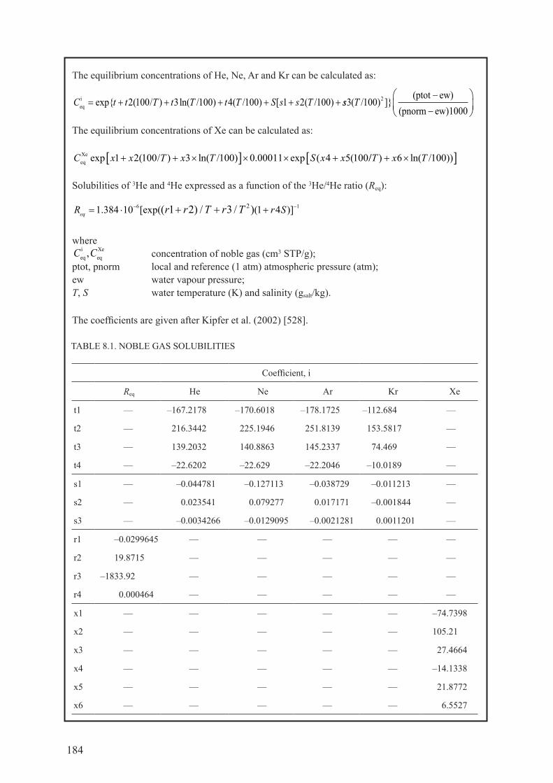
184

table 8.1. noble gas solubIlItIes

coefficient, i

Req he ne ar Kr xe

t1 — –167.2178 –170.6018 –178.1725 –112.684 —

t2 — 216.3442 225.1946 251.8139 153.5817 —

t3 — 139.2032 140.8863 145.2337 74.469 —

t4 — –22.6202 –22.629 –22.2046 –10.0189 —

s1 — –0.044781 –0.127113 –0.038729 –0.011213 —

s2 — 0.023541 0.079277 0.017171 –0.001844 —

s3 — –0.0034266 –0.0129095 –0.0021281 0.0011201 —

r1 –0.0299645 — — — — —

r2 19.8715 — — — — —

r3 –1833.92 — — — — —

r4 0.000464 — — — — —

x1 — — — — — –74.7398

x2 — — — — — 105.21

x3 — — — — — 27.4664

x4 — — — — — –14.1338

x5 — — — — — 21.8772

x6 — — — — — 6.5527

The equilibrium concentrations of He, Ne, Ar and Kr can be calculated as:

C t t T t T t T S s s Teqi / / / /= + + + + + +exp{ ( ) ln( ) ( ) [ ( )2 100 3 100 4 100 1 2 100 ss T3 100 2( ) ]}/

(ptot ew)(pnorm ew)1000

−

−

the equilibrium concentrations of xe can be calculated as:

C x x T x T S x xeqXe / /exp ( ) ln( ) . exp ( (1 2 100 3 100 0 00011 4 5 100+ + × × × +[ ] // /T x T) ln( ))+ ×[ ]6 100

solubilities of 3he and 4he expressed as a function of the 3he/4he ratio (Req):

R r Seq r r T r T= ⋅ +− −+ +1 384 10 1 46 11 2 3 2. [exp( ( )]( ) / / )

wherei xeeq eq,C C

concentration of noble gas (cm3 stp/g);ptot, pnorm local and reference (1 atm) atmospheric pressure (atm);ew water vapour pressure;T, S    water temperature (K) and salinity (gsalt/kg).

The coefficients are given after Kipfer et al. (2002) [528].

185

release of fluid inclusions (presumably rich in cl). Ballentine et al. (2002) [530] provide a discussion of the background theory. Nonetheless, the isolation and quantification of  ingeq and

4heeq requires a suite of assumptions not all of which have been checked and not all of which can be checked. This is a theme that will continue.

8.4.2. Excess ‘air’ components, 4Heexc

the creation of 4heexc is the result of soil processes by which excess air is occluded in the recharge process and is eventually dissolved as pressure increases. Bulk dissolution of unfractionated air is one possibility that requires the use of an ng tracer that is controlled primarily by dissolution of air (e.g. ne) rather than in situ and external sources (e.g. 4He). Early research used a definition of the Ne components in groundwater to define the excess air component of Ne which, for unfractionated air, could then be scaled to the 4heexc, rewriting eq. (8.2) for ne:

netot = neeq + neexc – ∑L (8.3)

and assuming no losses:

neexc = netot – neeq  (8.4)

this allows the excess 4he component to be calculated as:

4 He NeHeNeexc exc

air

=

(8.5)

as ne solubility is the least temperature sensitive of the noble gases, such an assumption and calculation were tenable. however, this assumes that air is in excess and that its process of dissolution is non-fractionating and non-equilibrating. cross-checking these assumptions with the noble gas suite has shown this to be oversimplified (Aeschbach-Hertig et al. (1999) [302]). yet, in most cases, the Neexc component is less than 30% and, thus, the calculated 4heexc is also small, especially considering that the 4heterr and the 4herad are often orders of magnitude larger. as mass spectrometric measurement of 4He usually also acquires Ne, analytical costs can often be reduced by making these assumptions and acquiring he and ne concentrations only.

If measures of the complete noble gas suite are acquired, such measures can be evaluated in terms of the palaeorecharge temperature that has found application in palaeoclimate research (stute et al. (1995) [213]; Stute et al. (1995) [214]; Stute et al. (1992) [42]). considerable research has been devoted to evaluating the ingexc component in order to best fit the ingeq components to a recharge temperature. Stute et al. (1995) [213] and Stute et al. (1995) [214] explored partial re-equilibration where an initial air bubble was dissolved and partial re-equilibration occurred by molecular processes across the water table. Peeters et al. (2002) [531] suggested the use of 20ne/22Ne ratios to test the partial re-equilibration model but where measures have been made, no significant diffusive fractionation of the isotopes has been  uniquely  identified. Kipfer  et  al.  (2002)  [528]  propose  a multistep  re-equilibration model  that would allow for large excess air (accommodated at pressure well beyond the water table). however, as multistep re-equilibration reduces to partial re-equilibration in the limiting case and the lack of evidence for diffusive fractionation of 20ne/22Ne  (Peeters  et  al.  (2002)  [531]),  such  a model  is  also  less  than adequate. The closed system equilibration model  (Aeschbach-Hertig et al.  (2001)  [532]; Aeschbach-Hertig et al. (1999) [302]; Aeschbach-Hertig et al. (2000) [55]; Peeters et al. (2002) [531]) appears to allow direct physical interpretation of the excess air component and its variance across the ng suite in most cases. direct verification of a mechanistic link between excess Ne and water table fluctuations is not available (Kipfer et al. (2002) [528]) but experiments with sand columns appear to support the basic 

186

mechanistic possibilities  (Holocher  et  al.  (2002)  [533]). A widely used Excel/matlab  routine  can be downloaded  from:  http://www.eawag.ch/organisation/abteilungen/wut/schwerpunkte/umweltisotope/methoden/interp_en

8.4.3. Radiogenic production, 4Herad

radiogenic production via alpha decay of u–th series elements creates 4herad. other sources of α particles (e.g. Nd decay) and 4He as a result of (n, α) interactions can be considered quantitatively insignificant. Under the assumption that U–Th series elements have reached radioequilibrium, the 4he production rate from rock can be expressed as:

4he cm3 STP · grock–1 · a–1 = j’he = 0.2355 × 10–12([U](1 + 0.123([Th]/[U] – 4)))  (8.6)

4He atoms · grock–1 · a–1 = j’he = 2.688 × 1019(0.2355 × 10–12([U](1 + 0.123([Th]/[U] – 4)))  (8.7)

where [U] and [Th] are concentrations expressed in parts per million (craig and Lupton (1976) [534]; Torgersen (1980) [535]).

for groundwater calculations, it is then necessary to quantify how much of this in situ production becomes available to the fluid phase. This has been generalized as a release factor Λhe and the accumulation of 4He in the fluid phase can be calculated as:

4he cm3STP · gh2o–1 · a–1 = jhe = j’he(ρΛhe((1 – Ф)/Ф))   (8.8)

whereρ is the density of the solid (g/cm3);Ф  is the porosity (cm3

h2o/cm3total).

FIG. 8.1. Mechanisms for the release of α decay 4He from rock: (1) recoil of the α particle (30–100 µm); (2) recoil followed by rapid diffusion along recoil damage tracks, grain imperfections and microfractures; (3) molecular diffusion in the solid state with no advantages from recoil damage or grain imperfections; (4) weathering and dissolution release (after Torgersen (1980) [535]).

187

quantification of Λhe  is  a  challenge. figure 8.1  (modified  from Torgersen  (1980)  [535])  shows schematically the various mechanisms by which 4he can enter the pore space from the solid phase: (i) direct recoil, (ii) rapid diffusion in imperfections, (iii) slow diffusion in the solid phase and (iv) weathering or dissolution.

8.4.3.1. Mechanism 1: direct recoil

the recoil path  length  of  an  α  particle  in  silicate  material  (Rα) is of the order of 30–100 µm (Andrews (1977) [536]) and the direct recoil loss of α particles by the solid phase has been evaluated by flügge and zimens (1939) [537], and summarized by Torgersen (1980) [535]. from the grain size and the recoil path length, Λhe can be calculated as:

Λ α αHe = −

34

116

3Rr

Rr

for 2r ≥ Rα (8.9)

Λhe = 1 for Rα > r (8.10)

wherer is the grain radius;Rα is the recoil path length.

FIG. 8.2. Helium concentrations versus groundwater hydraulic (flow model) age (as supported by 36Cl model ages) for the Great Artesian Basin, Australia. For groundwaters younger than 40 ka, the accumulation rate is 4.6 × 10–12 cm3 STP 4He · cm–3

H2O · a–1 which agrees with the calculated rate (ΛHe = 1) of 3.95 × 10–12 cm3 STP 4He · cm–3

H2O · a–1. For groundwaters greater than 100 ka, the rate of accumulation is 2.91 × 10–10 cm3 STP 4He · cm–3

H2O · a–1 or 74× in situ production. An external bottom boundary flux provides the best explanation for the source and the timescale over which it can be seen (from Torgersen and Clarke (1985) [293]).

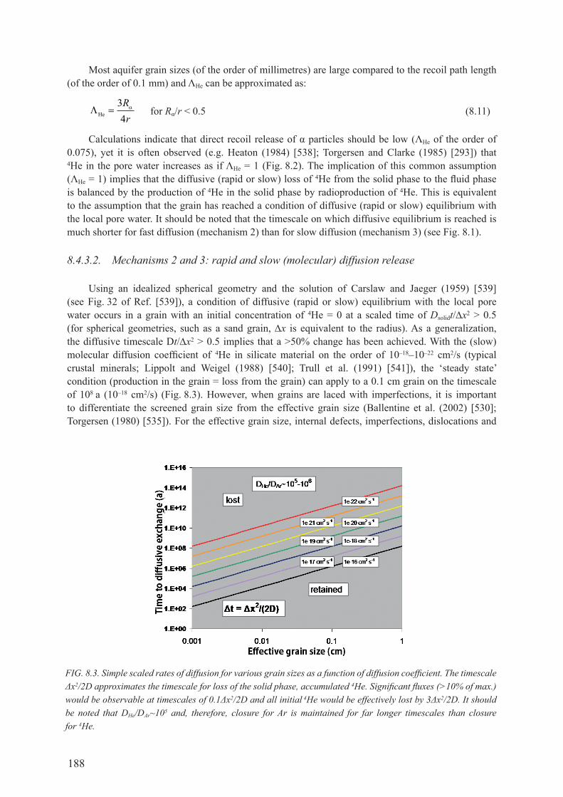
188

most aquifer grain sizes (of the order of millimetres) are large compared to the recoil path length (of the order of 0.1 mm) and Λhe can be approximated as:

ΛHe =34Rrα for Rα/r < 0.5 (8.11)

calculations  indicate  that direct  recoil  release of α particles should be  low (Λhe of the order of 0.075),  yet  it  is  often  observed  (e.g. Heaton  (1984)  [538]; Torgersen  and clarke  (1985)  [293])  that 4He in the pore water  increases as  if Λhe = 1 (fig. 8.2). the implication of this common assumption (Λhe = 1) implies that the diffusive (rapid or slow) loss of 4He from the solid phase to the fluid phase is balanced by the production of 4he in the solid phase by radioproduction of 4he. this is equivalent to the assumption that the grain has reached a condition of diffusive (rapid or slow) equilibrium with the local pore water. It should be noted that the timescale on which diffusive equilibrium is reached is much shorter for fast diffusion (mechanism 2) than for slow diffusion (mechanism 3) (see fig. 8.1).

8.4.3.2. Mechanisms 2 and 3: rapid and slow (molecular) diffusion release

Using  an  idealized  spherical  geometry  and  the  solution  of  carslaw  and  jaeger  (1959)  [539] (see fig. 32  of ref.  [539]),  a  condition  of  diffusive  (rapid  or  slow)  equilibrium with  the  local  pore water occurs in a grain with an initial concentration of 4he = 0 at a scaled time of Dsolidt/Δx2 > 0.5 (for spherical geometries, such as a sand grain, Δx  is  equivalent  to  the  radius). As  a generalization, the diffusive timescale dt/Δx2 > 0.5 implies that a >50% change has been achieved. with the (slow) molecular diffusion coefficient  of  4he in silicate material on the order of 10–18–10–22 cm2/s (typical crustal  minerals;  Lippolt  and  weigel  (1988)  [540];  Trull  et  al.  (1991)  [541]),  the  ‘steady  state’ condition (production in the grain = loss from the grain) can apply to a 0.1 cm grain on the timescale of 108 a (10–18 cm2/s) (fig. 8.3). however, when grains are laced with imperfections, it is important to  differentiate  the  screened  grain  size  from  the  effective  grain  size  (Ballentine  et  al.  (2002)  [530]; Torgersen (1980) [535]). for the effective grain size, internal defects, imperfections, dislocations and 

FIG. 8.3. Simple scaled rates of diffusion for various grain sizes as a function of diffusion coefficient. The timescale Δx2/2D approximates the timescale for loss of the solid phase, accumulated 4He. Significant fluxes (>10% of max.) would be observable at timescales of 0.1Δx2/2D and all initial 4He would be effectively lost by 3Δx2/2D. It should be noted that DHe/DAr~105 and, therefore, closure for Ar is maintained for far longer timescales than closure for 4He.

189

microfractures  render  the  distance  to  a  pore  space-available  boundary  to  be  significantly  less  than the  screen-sorted  grain  size  (the  rapid  diffusion  case  of  Torgersen  (1980)  [535];  see  fig. 8.1).  for example, an effective grain size of 0.01 cm will reach steady state (production = loss) on a timescale of the order of 106 a (100 times faster) if transport time in the ‘imperfection pathway’ is not considered significant. Additionally, the (slow) diffusion coefficient of 4he in grains may increase with time due to radiation damage, microfracturing, etc. and the effective grain size may, therefore, decrease with time. as this loss of 4he from a grain is typically not measureable in the laboratory on a reasonable timescale, a measure of loss at a higher temperature can often be scaled to the in situ lower temperature (Mamyrin and Tolstikhin (1984) [521]). Although such measures are possible, this laboratory measure of Dsolid will only reflect conditions now rather  than conditions over  the timescale of  the 4he model age (the time over which solid material contributed  to  the fluid parcel). of additional concern  is  the possibility of variability  in Λhe  in  space or  time.  Is  the  rock  sample  acquired  representative of  the  ‘average’  rock the water parcel has seen over its residence time? As effective grain sizes in aquifers are typically small and the diffusion coefficients for 4he in the solid phase are typically large, an in situ production rate equivalent to Λhe = 1 is often assumed.

8.4.3.3. Mechanism 4: bulk dissolution or weathering

Bulk  dissolution  or weathering  of  grains  should  also  result  in  the  release  of  4he accumulated within the grain (see fig. 8.1). as grains dissolve from the outside and diffusion will create gradients in the solid phase that decrease the concentration towards the outside of grains, quantification of a priori dissolution release of 4He is difficult. Both Torgersen and clarke (1985) [293], and Heaton (1984) [538] calculate a simple rate for dissolution release of 4he based on an assumed uniform concentration of 4he in the grain. these concentrations are usually based on the metamorphic or depositional age of the formation and, hence, represent a maximum value. Both Torgersen and clarke (1985) [293], and Heaton  (1984)  [538] calculate  the  rate of  ‘weathering’  release of  4he from their systems to be <1% of the Λhe = 1 condition and, thus, weathering release may be unimportant. however, it is still to be determined whether this is a general condition.

Heaton (1984) [538] estimates a bulk rate of surface chemical weathering from the chemistry of world rivers to be 3 mgrock · kg–1

rock · a–1. simplistically, this is equivalent to a timescale for dissolution of  0.3 ma.  However,  Heaton  (1984)  [538]  advises  that  subsurface  dissolution  will  be  of  the  order of 0.1–0.01× slower, indicating subsurface timescales for dissolution of the order of 3–30 Ma. this ‘dissolution  timescale’  can  be  compared  to  the  timescale  for  solid  phase  loss  of  4he by molecular diffusion. Using  a  ‘fast’ molecular  diffusion  coefficient  (10–18 cm2/s) for grains of 0.1 cm, yields of the order of 300 Ma as a timescale for loss (fig. 8.3). thus, one might expect weathering release or chemical dissolution to be an important release mechanism. however, the observation that release equivalent  to Λhe = 1  is  often observed  suggests  that  effective grain  sizes  for diffusion might be  as small as 0.5 × 10–3 cm (Δx = (DΔt)0.5, where D = 10–18 cm2/s and Δt = 10 ka; fig. 8.3). These arguments suggest that 4he release via chemical dissolution should be considered but may often be dismissed.

8.4.3.4. Effective release at low rates (ΛHe < 1)

under conditions where Dsolidt/Δx << 0.5, the solid phase can release 4he at a rate that is equivalent to Λhe < 1. However, the authors are aware of no documented cases for which Λhe << 1 has been unequivocally shown. this condition may require formation of new grains from new material (authigenic material) with no pre-existing 4He, which is likely an artificial case.

190

FIG. 8.4. The accumulation of 4He in various groundwater aquifers as a function of travel time (flow model age). Typical in situ production is 0.18 µcm3/kg over 60 a. The data indicate rates >100 times the expected in situ production via radiodecay. This enhanced source is the result of slow release of solid phase, accumulated 4He (accumulated over the metamorphic age of the rock) that occurs as a result of comminution of large blocks/grains into smaller grains. The source is exemplary of mechanism 3 of Fig. 8.1. (From Solomon et al. (1996) [295], reproduced with permission of the American Geophysical Union.)

FIG. 8.5. Model calculations showing the timescale over which solid phase, accumulated 4He can be released into the groundwater. The fluxes from the solid phase to the groundwater are a function of the grain size (labelled on various curves), the initial 4He concentration before comminution (metamorphic age of the solid; compare initial concentration of 60 µcm3/g to 6 µcm3/g) and the diffusion coefficient for 4He in the solid (graphs present the case for only a single diffusion coefficient DHe = 4.5 × 10–21 cm2/s). (From Solomon et al. (1996) [295], reproduced with permission of the American Geophysical Union.)

191

8.4.3.5. Enhanced release (ΛHe > 1) by comminution, microfracturing and macrofracturing

The case where Λhe > 1 can and does occur as a  result of a decrease  in effective grain size by comminution, micro-  and macrofracturing.  In  such  a  case,  a  large  effective grain  size  (>1  cm) may retain most of its in situ production of 4he but release that 4He when  the  grain  size  is  reduced.  In the case of the Sturgeon falls site in ontario, canada, Solomon et al. (1996) [295] hypothesized that Precambrian canadian Shield  rocks  (>1 ga)  that  occur  in  large  blocks  (fracture  to  fracture  spacing on the order of 1–10 m) were reduced by glacial action to the 1 mm grains that comprise the aquifer. the accumulated 4he would then be released from 1 mm grains on a timescale of the order of 108 a (10–18 cm2/s) to 1010 a (10–20 cm2/s)  (see fig. 8.3). Such  release  (Λhe order 100) was confirmed by  laboratory measuresments (Solomon et al.  (1996) [295]). Based on a comparison of groundwater 4He  accumulation  rates  and  independently  estimated  travel  times  (fig. 8.4),  this  scenario  (glacially produced comminution and Λhe >> 1) may be common at high latitudes. the enhanced release of 4he (Λhe >> 1) can continue for a considerable time (fig. 8.5) and may provide a dominant 4he input within an aquifer.

This  concept  of  comminution/fracturing  is  scalable.  Honda  et  al.  (1982)  [542]  have  shown  in laboratory experiments that rock fracturing can lead to the release of 4He. In the 1-d case, Torgersen and o’donnell (1991) [543] have shown that fracturing creates large gradients and surface areas that lead to high 4He fluxes (Λhe >> 1) (fig. 8.6). The resultant ‘pieces’ continue to lose 4He (Λhe >> 1) for timescales on the order of 2 < Dt/Δx2 < 5 depending on the initial condition. It should be noted that the flux from the slab (fig. 8.7) is reduced by half in the timescale defined by Dt/Δx2 = 1, but that, in some cases, the flux remaining to be released may still be larger than in situ production. Thus, increased stress  leading  to microfracturing can  result  in Λhe >> 1 through new surfaces and/or the creation of imperfections  and  microcracks  which  creates  shorter  routes  and  higher  gradients  to  enable  high transport rates to imperfections. At the larger scale (1–1000 m), it has been shown that 1 km of uplift 

FIG. 8.6. The bulk fracturing model of Torgersen and O’Donnell (1991) [543] illustrated the 1-D case for simple comminution. Before fracturing, the slab of thickness L can acquire a noble gas concentration that is (initial condition 1) 0.005 times the steady state or (initial condition 2) the steady state concentration of Ao L2/D. Fracturing then reduces the slab thickness from L to l. Fracturing is quantified as the ratio L:l and can have any value >1. It should be noted that the higher L:l, the larger the surface area available for diffusion into the pore space. (From Torgersen and O’Donnell (1991) [543], reproduced with permission of the American Geophysical Union.)

192

or downdrop will result in thermal stresses sufficient to produce stresses approaching the yield strength of rock (Knapp and Knight (1977) [544]; Savage (1978) [545]). The 1-d modelling of Torgersen and o’donnell  (1991)  [543] shows  that stress-induced macrofracturing  leads  to  large fluxes from blocks (Λhe > 104) and although such fluxes decrease with time, they can produce Λhe >> 1 for timescales on the order of 2 < Dt/Δx2 < 5 (see fig. 8.7). the results in fig. 8.7 show that fracturing/comminution can result in large local sources of 4he to the pore space that can persist for characteristic timescales of 1 < Dt/l2 < 5 but Dt/l2 = 0.5 marks  the point where approximately half of  the accumulated noble gas has been lost to the pore space. given that Dhe/Dar ~ 105, the entire accumulated 4he could be lost from the slab while 40ar loss continues for a considerable longer time. It should be noted that the concentration in the pore fluid is governed not only by the flux from the slab but also by the residence time in the post-fractured system.

The  net  result  of  microscale  fracturing  coupled  to  larger  scale  (km)  macrofracturing  is  that retention of 4He in the crust becomes difficult and there can be a resultant significant flux of 4he from the crust to the atmosphere.

8.4.3.6. Crustal fluxes of 4Herad

the concentration and residence time of 4he in the atmosphere suggest that on a continental space scale and a megayear (ma) timescale, the flux of 4He from the Earth’s crust to the atmosphere is comparable to the net in situ production by U–Th series element α decay in 30–40 km of the crust (Torgersen (1989) [546] and Torgersen (2010) [547]). This is not equivalent  to a steady state loss of 4He from the crust to the atmosphere as implied by Ballentine et al. (2002) [530], as any measure of flux contains within it a characteristic time and space scale, whereas steady state implies that the flux is constant in time and space. however, the implication of the atmospheric 4he mass balance is that in situ crustal production of 4He must both be released to a mobile phase (see above discussion of Λhe) and that that mobile phase must be transportable to the Earth’s surface on timescales of the order of 1 ma although it may take longer (109 a) for that flux to be established (see fig. 8.8).

with regard to the interpretation of 4he in groundwater systems, the issue becomes one of a possible dominant flux of 4he into a water parcel from external sources rather than the internal production terms encountered in the space ΔxΔyΔz (acknowledging that ΔxΔyΔz is heterogeneous and that the solid phase

FIG. 8.7. The flux of noble gas (y axis) to the pore space relative to in situ production as a function of diffusion time, Dt/l2 (from the general case Dt/∆x2). Dashed lines are calculated for the IC1 (0.005 times steady state concentration at time of fracturing) and solid lines are calculated for IC2 (steady state concentration at time of fracturing). (From Torgersen and O’Donnell (1991) [543], reproduced with permission of the American Geophysical Union.)

193

remains in place while the water flows). Table 8.2 shows the measured 4He degassing flux in locations around the world. Although the analysis of Torgersen and o’donnell (1991) [543] suggests fluxes from individual blocks can be 104 times in situ production and that Λhe < 1 remains an unobserved possibility, it is of note that area- and time-weighted mean flux (3.3 × 1010 4He atoms · m–2 · s–1) is approximately equivalent  to  the mean  crustal  production. when  the fluxes  of Table  8.2  are  evaluated with  respect to  their  log-normal mean (4.18 × 1010 4He atoms · m–2  ·  s–1), the variability in measured 4He flux  is approximately ±1.5 orders of magnitude (Torgersen (2010) [547]; see also fig. 8.9).

FIG. 8.8. The effective time for diffusive transport as a function of layer thickness and effective diffusion coefficient. The timescale Δx2/2D approximates the timescale for diffusive exchange of produced/accumulated 4He. Significant fluxes into the layer and/or out of the layer (~20% of the max.) would be observable at timescales of 0.1Δx2/2D and all exchangeable species would be effectively lost/gained in 3Δx2/2D.

FIG. 8.9. A statistical analysis of the measured flux of 4He into 271 Canadian Shield lakes using the data of Clarke et al. (1977) [548], Clarke et al. (1983) [549], and Top and Clarke (1981) [550]. These data typically provide one sample per lake, including both a measure of excess 4He and the 3H/3He model age.

194

tab

le 8

.2. t

he

hel

IuM

flu

x f

ro

M c

on

tIn

enta

l r

egIo

ns

reg

ion

4 He flux 

(a

tom

s ∙ m–2

∙ s–1

× 1

010)

Met

hod

plot

ted,

eva

luat

ed

4 He flux (atoms ∙

m–2

∙ s–1

× 1

010)

tim

esca

lesp

ace

scal

e (km)

ref

eren

ce

con

tinen

ts2.

8ca

lcul

atio

n fr

om u

,th

2.8

2 M

a>5

000

1,2,

3

gre

at a

rtesi

an b

asin

3.1

Mea

sure

d ac

cum

in g

w3.

11

Ma

500

2

gre

at h

unga

rian

plai

n0.07-0.45

Mea

sure

d ac

cum

in g

w0.

21

Ma

200

7

gre

at h

unga

rian

plai

n8

Mea

sure

d ac

cum

in g

w8

1 M

a20

08

paris

bas

in0.4–4

Mea

sure

d ac

cum

in g

w a

nd m

odel

110 ka

100–

500

11,12,13,14

p aris

bas

in0.4

Mea

sure

d ac

cum

in g

w a

nd m

odel

0.4

10 ka

100–

500

11

Mol

asse

bas

in0.

2M

easu

red

accu

m in

gw

0.2

250 ka

50

9

carrizo Aquifer, Tx

1M

easu

red

accu

m in

gw

and

mod

el1

100 ka

75

23

Black Sea

1.3

Profile and model

1.3

440 a

661

26

san

juan

bas

in, n

M0.

8M

easu

red

accu

m in

gw

and

mod

el0.

840 ka

40 

23

east

ern

paris

bas

in3.

8–15

Mea

sure

d ac

cum

in g

w a

nd m

odel

1010 ka

75

15

auo

b sa

ndst

one

0.09

–3M

easu

red

accu

m in

gw

120 ka

50

5

auo

b sa

ndst

one

2.6

Mea

sure

d ac

cum

in g

w2.

620 ka

50

2

Serra  grande, Brazil

2.4

Mea

sure

d ac

cum

in g

w2.4

20 ka

40 

24, 28

cas

pian

sea

1.9–

5.9

Lake profile

425

a60

922

Lake Baikal

14–28

Lake profile

2110

a17

7 22

Lake Huron

not

det

ecta

ble

Lake profile

0.00

1*0.

5 a

243

20, 2

8

Lake Erie

not

det

ecta

ble

Lake profile

0.00

1*0.

5 a

161

20, 2

8

Lake ontario

not

det

ecta

ble

Lake profile

0.00

1*0.

5 a

136

20, 2

8

Lake van

25Lake profile, volcanic area

252

a60

22

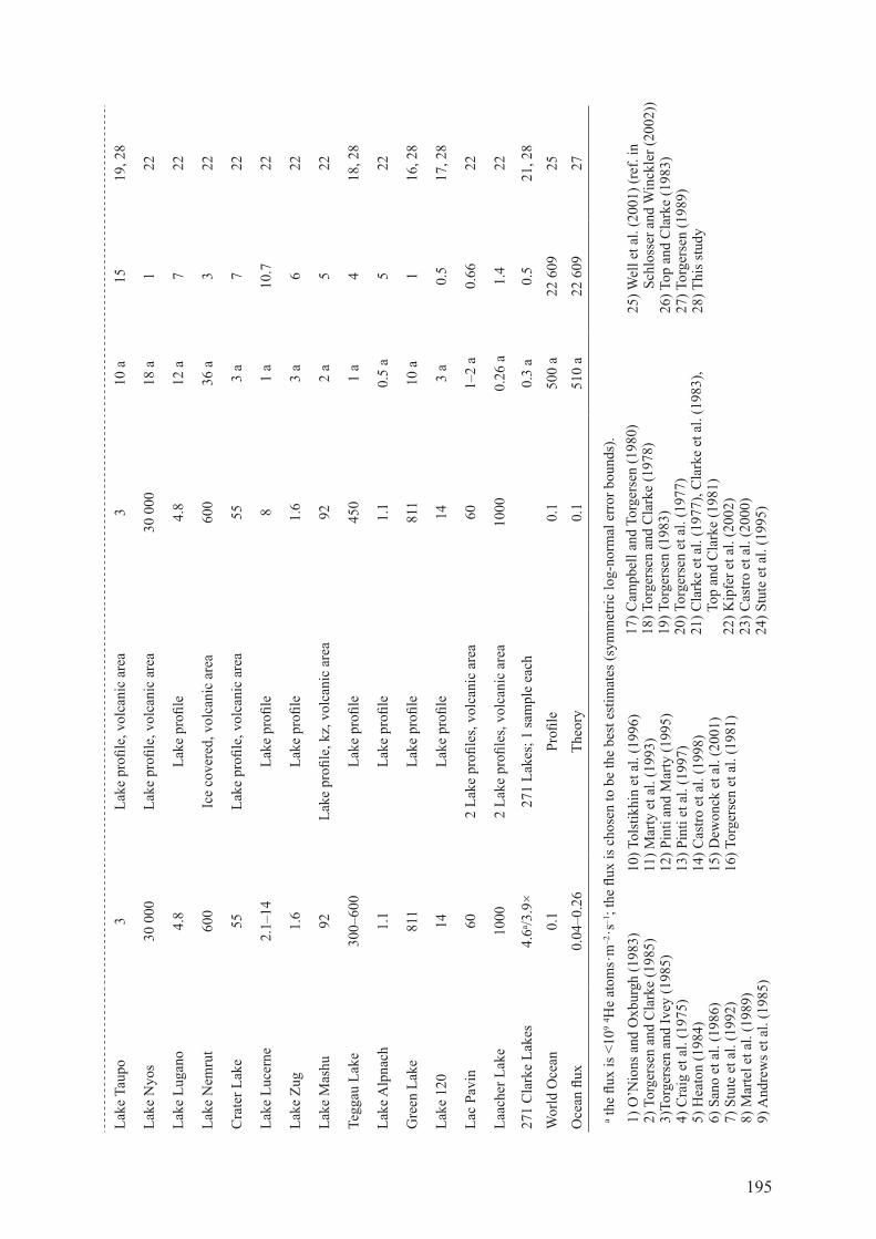
195

Lake Taupo

3Lake profile, volcanic area

310

a15

19, 2

8

Lake Nyos

30 0

00Lake profile, volcanic area

30 0

0018

a1

22

Lake Lugano

4.8

Lake profile

4.8

12 a

722

Lake Nem

rut

600

Ice

cove

red,

vol

cani

c ar

ea60

036

a3

22

crater L

ake

55Lake profile, volcanic area

553

a7

22

Lake Lucerne

2.1–14

Lake profile

81

a10

.722

Lake zug

1.6

Lake profile

1.6

3 a

622

Lake m

ashu

92Lake profile, kz, volcanic area

922

a5

22

Teggau Lake

300–

600

Lake profile

450

1 a

418

, 28

Lake Alpnach

1.1

Lake profile

1.1

0.5

a5

22

green Lake

811

Lake profile

811

10 a

116

, 28

Lake 120

14Lake profile

143

a0.

517

, 28

lac

pavi

n60

2 Lake profiles, volcanic area

601–

2 a

0.66

22

Laacher  L

ake

1000

2 Lake profiles, volcanic area

1000

0.26

a1.4

22

271 clarke Lakes

4.6a

/3.9

×271 Lakes; 1 sample each

0.

3 a

0.5

21, 2

8

wor

ld o

cean

0.1

Profile

0.1

500

a22

609

25

ocean flux

0.04–0.26

t heo

ry0.

151

0 a

22 6

0927

1) o’Nions and oxburgh (1983)

2) Torgersen and clarke (1985)

3)to

rger

sen

and

Ivey

(198

5)4) craig et al. (1975)

5) Heaton (1984)

6) s

ano

et a

l. (1

986)

7) s

tute

et a

l. (1

992)

8) M

arte

l et a

l. (1

989)

9) a

ndre

ws e

t al.

(198

5)

a  the flux is <10

9 4h

e at

oms ∙ m

–2 ∙ s

–1; the flux is chosen to be the best estimates (sym

metric log-normal error bounds).

10) Tolstikhin et al. (1996)

11) M

arty

et a

l. (1

993)

12) p

inti

and

Mar

ty (1

995)

13) p

inti

et a

l. (1

997)

14) c

astro et al. (1998)

15) d

ewonck et al. (2001)

16) t

orge

rsen

et a

l. (1

981)

17) c

ampb

ell a

nd t

orge

rsen

(198

0)18)  Torgersen and clarke (1978)

19) t

orge

rsen

(198

3)20

) tor

gers

en e

t al.

(197

7)21) c

larke et al. (1977), c

larke et al. (1983), 

 Top and clarke (1981)

22) K

ipfer et al. (2002)

23) c

astro

et a

l. (2

000)

24) S

tute et al. (1995)

25) w

ell e

t al.

(200

1) (r

ef. i

n  Schlosser and w

inckler (2002))

26) Top and clarke (1983)

27) t

orge

rsen

(198

9)28

) thi

s stu

dy

196

It is acknowledged that the fluxes in Table 8.2 represent fluxes distributed over an area appropriate to the measurement. for instance, the quantified external flux into the great Artesian Basin (Torgersen and clarke (1985) [293]) is roughly equivalent to whole crustal production and is influxed to the base of the aquifer over the space/timescale of the basin. This, of necessity, means that the flux above the aquifer directly  from  the  soil  to  the atmosphere  is very  low. furthermore,  the net flux  to  the atmosphere  in the discharge  zone would be  locally very  large  since  it  reflects  the  input  of  crustal  production over the whole basin and not just the discharge zone. These measures of the degassing fluxes of 4he must, therefore, be carefully interpreted with respect to their applicable time and space scale. for the range of basin scale fluxes to be this constrained, vertical transport must not be only relatively rapid but also relatively pervasive.

figure  8.9  shows  a  simple  analysis  of  the U  prospecting  data  of clarke  and  others  (clarke  et al.  (1977)  [548]; clarke  et  al.  (1983)  [549]; Top  and clarke  (1981)  [550])  for  271  lakes  for which only  one  sample  is  obtained  per  lake. The  calculation  in  the  figure  assumes  the  depth  of  sampling (most  often  below  the  thermocline)  is  an  approximation  of  the  mean  lake  depth.  The  calculation likely  has  an  error  based  on  assumptions  that  is  of  the  order  of  three  times. Also  shown  are fluxes based on the data in table 8.2 for which both an area multiplied by a time weighted mean has been calculated, as well as a log-normal mean and deviation. The agreement between the mean and standard deviation for the clarke lakes and Table 8.2 data suggest the magnitude of the crustal degassing flux is approximately equivalent to whole crustal production with variance of a factor of 44.6 times or 1.5 orders of magnitude. one, therefore, has a 68% probability of measuring a flux between 0.1 × 1010 and 186 × 1010 atoms 4He · m–2 · s–1 in any one study. the analysis suggests strong spatial and temporal variability in the measured flux.

although such data only captures of the order of 0.5 a of 4He flux over a specific lake area and is likely subject to errors on the order of three times due to the assumptions necessary (the assumptions also  suggest  the  estimate  is  ~50%  too  high),  the mean flux measured  by  these  lakes  is  4.57 ×  1010 4He  atoms · m–2 · s–1  (log-normal mean with  a  standard  deviation  of  a  factor  of  3.9  times written  as */3.9×). The lake regions sampled by clarke and others is an area of the Precambrian canadian Shield which was depressed by about 1 km due to coverage by 3 km of ice sheet approximately 20 ka ago. Thus, it is noteworthy both that the mean measured flux (4.57 × 1010 4He atoms · m–2 · s–1 log-normal mean with a standard deviation of */3.9×) is not much larger than whole crustal production (3 × 1010 4He atoms · m–2 · s–1 (Torgersen (1989) [546]; Torgersen and clarke (1985) [293]); and that the variance of  the  flux  is  consistent  with  the  range  reported  from  much  larger  basins  (see  Table  8.2).  while the coverage of the planet with regard to crustal flux measurements remains limited, these measurements (Table 8.2, fig. 8.9)  support  a hypothesis  that  the mean flux of  4he from the continental crust is of the same order as the in situ production from u–th series decay in the continental crust. however, the  variance  of  the  crustal  degassing  flux  is  significant  (a  factor  of  106 (95th per centile) for short time (0.5 a) and short space scales (1 km) (Torgersen (2010) [547])) and is likely unpredictable, thus, complicating the potential use of 4He  as  a method of  groundwater  ‘dating’.  Such  a  conclusion  also requires that the net rate of vertical transport in the crust be examined.

8.4.3.7. Vertical transport of 4Heterr in the crust

simple scaling arguments can be used to evaluate the necessary rates of vertical transport in the continental crust in order to achieve surface crustal fluxes equivalent to the rate of whole crustal in situ production. as the data in fig. 8.9 and table 8.2 represent multiple time and space scales, the problem is constrained by the limit: continental degassing and basin scale measures of the degassing flux (on the time and space scale of 106 a and 1000 km) can be approximated as equivalent to the in situ production from 30–40 km of crust but with considerable variance (Torgersen (2010) [547]). This does not  imply steady state degassing  is applicable everywhere at all  times; but  it does acknowledge  that the range exhibited in table 8.2 and fig. 8.9 is relatively small. In order to achieve the crustal degassing

197

flux  in  the great Artesian Basin, Torgersen  and clarke  (1985)  [293]  used  a  timescale  of  2  ×  108 a (corresponding to a jurassic age for the aquifer material) and assumed that most of the u–th resided in the upper 7 km of crust to calculate a scaled effective diffusion coefficient (fig. 8.8) of 8 × 10–6 cm2/s for that 7 km of crust. Torgersen (1989) [546], using a solution from carslaw and jaeger (1959) [539], scaled these observations to effective vertical diffusivities of 10–5–10–6 cm2/s (Torgersen (1989) [546]) or vertical velocities of 0.1–1cm/s. given the diffusivity of gas in water is of the order of 10–5 cm2/s and that the porosity (Ф = 0.1) and tortuosity effects will reduce this quiescent water to DФ2 = 10–7 cm2/s, it is clear that over the long time and space scale, continental crust must transport significant quantities of 4He and water at rates that are significantly faster than would be measured by typical (short time and space scale) well tests.

such rates of transport are surprising when one considers the hydraulic conductivity of consolidated, non-granular  rocks  (freeze and cherry  (1979)  [11]) but  less  surprising when  the  rates of  metamorphic  processes  are  considered  (Etheridge  et  al.  (1984)  [551];  Etheridge  et  al.  (1983) [552]). The  low hydraulic  conductivities  and  transport  often  encountered  in  bulk  non-granular  rock are measured over small timescales (<1 a) with small space scale (of the order of centimetres) pieces of rock. In contrast, metamorphic processes reflect the transport in the crust on the larger time/space scales. this conclusion of rapid transport and high volumes of water is consistent with the requirements of the observed products in metamorphic geology (e.g. Etheridge et al. (1984) [551]; Etheridge et al. (1983) [552]). metamorphic rock structure also suggests that fluid transport is episodic with periods of ‘no transport’ followed by periods of ‘very high transport’. Thus, the effective degassing of continental crust is supportive of and supported by the fluid transport required by metamorphic processes. when the time/space scale for transport is large, the effective rate of crustal scale transport is higher than might be predicted. However,  any specific quantification of vertical  transport  in  the crust may yield numbers which  suggest  that  such  crustal  scale  transport  is  not  viable. This  feature was  specifically addressed by the Torgersen and clarke (1992) [294] study at cajon Pass drillhole, where the vertical transport measured by borehole tests showed rates of 10–5 cm/a while effective rates estimated from the apparent 4He tracer ages of the fluid implied vertical rates of 0.04–0.6 cm/a. vertical transport in the continental crust must, therefore, be episodic (as required by metamorphic geology; etheridge et al. (1984) [551]; Etheridge et al. (1983) [552]), with long periods of slow transport and short periods with a very high transport rate. Thus, what is ‘seen’ in the crustal scale transport of 4he is comparable to travel in city subway systems: one can travel by subway from downtown Manhattan to uptown in a specific period of  time (effectively several kilometres per hour) but when viewed  in detail,  this transport is accomplished by a series of stops (velocity of 0 km/h) interrupted by bursts of high speed (tens of kilometres per hour) travel. It would, thus, not be surprising for the external flux of 4he (4heterr) to become quite important in many aquifer systems. for a more detailed discussion of vertical transport of 4heterr, see Torgersen (2010) [547].

8.4.3.8. In situ production of 3He

radiogenic production of 4he is accompanied by a small but important nucleogenic production of 3he as a result of thermal neutron interactions with 6li in the solid phase:

6Li(n, α)3H(β–)3he (8.12)

Helium-3  produced  according  to  Eq.  (8.12)  is  defined  as  nucleogenic  3he whereas radiogenic (tritiogenic) 3he is produced by an atmospheric source of 3h. to initiate the reaction (eq. (8.12)), the production of neutrons in the solid matrix by (α, n) reactions and spontaneous fission neutrons must be calculated:

n =  (n, α)U + (sf, n)U + (α, n)Th  (8.13)

198

The dominant target elements for the (α, n) reactions are Na, mg, Al, Si and c (although water is  also  a  viable  and  variable  sink  for  neutron  capture)  and  the  net  production  of  thermal  neutrons (n (neutrons · g–1 · a–1)) can be expressed as (Ballentine and Burnard (2002) [553]):

n = + + + +0.01[U](13.8[Na] 5.4[Mg] 5.0[Al] 1.31[Si] 2.0[C])   (8.14)

+ + + + + +0.4788[U] 0.01[Th](6.0[Na] 2.45[Mg] 2.55[Al] 0.56[Si] 0.833[C])

where [U] and [Th] are expressed in parts per million and the remaining components are in per cent.

these thermal neutrons are captured by further interactions with the solid phase where typical slow neutron path lengths in silicate are of  the order of 1 m. This suggests  that  the bulk solid phase composition can be used to estimate 3he production. such calculations are well developed. based on the  initial work  by morrison  and  Pine  (1955)  [554]  and  fiegge  et  al.  (1968)  [555],  the  fraction  of the thermal neutron flux captured by 6li (Fli

thn) can be calculated as (Andrews (1985) [556]; Andrews and Kay (1982) [463]):

FNi i

i iNLiThn

(8.15)

whereσi   is the thermal neutron cross-section;Ni   is the molar abundance for important components of the rock composition (see Table 8.3).

table 8.3. paraMeters for calculatIon of 3he/4he productIon ratIos (after Andrew and Kay (1982) [463])

element Molecular weight (g/mol) ϕth (barns)

li 6.94 71

b 10.81 755

na 22.989 0.534

Mg 24.305 0.064

al 26.981 0.232

si 28.086 0.16

cl 35.453 32.6

K 39.098 2.07

ca 40.080 0.44

ti 47.900 6.1

cr 51.996 3.1

Mn 54.938 13.3

fe 55.847 2.56

ni 58.71 4.54

co 58.933 37.5

sm 150.4 5820

gd 157.25 49 000

199

TABLE 8.4. 3he/4he productIon ratIos (after Ballantine and Burnard (2002) [553])

rock type3he/4he calculated

× 108

3he/4he measured × 108 reference

upper continental crust 3.90 — Torgersen and clarke (1987), Torgersen (1989)

lower continental crust 0.21 — Torgersen and clarke (1987), Torgersen (1989)

upper crust 1.08 — ballentine and burnard (2002)

Middle crust 0.40 — ballentine and burnard (2002)

lower crust 0.37 — ballentine and burnard (2002)

oceanic crust 0.029 — Torgersen and clarke (1987), Torgersen (1989)

basalt 1.3 — andrews (1985)

Ultramafic 0.114 — andrews (1985)

hooray sandstone 2.2–3.3 — Torgersen and clarke (1987)

Sandstone, UK 2.23 — andrews (1985)

sandstone, avg 0.58 — andrews (1985)

clay and shale 1.99 — andrews (1985)

limestone 0.1 — torgersen et al. (1981)

Limestone, UK 1.14 — andrews (1985)

limestone, avg 0.23 — andrews (1985)

typical granite 5–15 — fiege et al. (1968)

granite 2.23 — andrews (1985)

wr, stripa 0.594 — andrews et al. (1989)

whole rock 1.6 1.6

gerling et al. (1971),samples from rapakiwi

orthoclase — 40

biorite — 12

plagioclase — 5

quartz — 15

amphibole — 4.5

Zircon — 2

1-whole rock 1.6 1.6

Tolstikhin and drubetskoy (1977),mamyrin and Tolstikhin (1984)

2-whole rock 1.7 1.9

4-whole rock 1.4 0.3

43-whole rock 0.7 0.8

27-whole rock 0.09 6

ss1-wr — 0.21

Martel et al. (1990), samples from carnmenellis

ss1-feldspar — 0.238

ss1-mica — 0.462

ss1-quartz — 0.0084

rh1g-wr 6.4 0.21

rh12d-wr1 6.7 0.154rh12d-wr2 6.7 0.49uraninite — 0.0098

200

combining Eqs (8.14, 8.15) yields a rate of production of 3he which can be further combined with eq. (8.7) to calculate the 3he/4he production ratio. It should be noted that the rate of 3he production is based on the neutron production rate which is a function of [U] and [Th], but the 3he/4he production ratio is determined by the rock composition and is a function of the Li/U–Th ratio.

Table  8.4  shows  the  3he/4He  production  ratio  for  average  crust  as well  as  selected  rock  types based on specific  rock compositions  from  the  literature. while  there  is a  large degree of agreement, the observed differences and variability are significant. Table 8.4 further shows that differences between the observed 3he/4he production rate and the calculated 3he/4He production rate are also significant. As (α, n) reactions occur within one alpha path length (0–40 µm) of the decaying nuclei, inhomogeneities in  rock  chemistry  on  the  space  scale  of  40  µm  can  impact  the  specific  3he yield. furthermore, the assumption of homogeneous rock over a space scale of 1 m may be problematic for  the  thermal neutron capture and the relative siting/separation of the trace elements, u, th, li, gd and sm (the last two elements have very large cross-sections), or the relative presence of water may significantly impact the  specific  3He  yield.  Such  issues  were  discussed  by martel  et  al.  (1990)  [557]  who  investigated carnmenellis granite 3he/4He production (see also discussion by Ballentine and Burnard (2002) [553]). chazal  et  al.  (1998)  [558]  revisited Stripa granite  and  found  that  the measured  3he/4He  ratio was 4 times the calculated ratio. Specific causes for the differences between the observed/measured 3he/4he ratios  and  calculated  production  ratios  have  not  been  unequivocally  identified  but  the  data  in Table 8.4 and analysis of studies mentioned above serve to provide context for the use of calculated 3he/4he production ratios and an interpretation of the errors that might be appropriate to that value. based on the data in Table 8.4 and the discussion of martel et al. (1990) [557], Ballentine and Burnard (2002) [553], and Tolstikhin et al. (1996) [559], it would appear that a calculated 3he/4he production ratio is uncertain up to a factor of ten of the given figure. The best way to determine the 3he/4he production ratio is by collecting a number of 3h free groundwater samples from the aquifer and to use the component separation process described below.

8.4.3.9. Separation of He components

As multiple He sources are likely in groundwater systems and each source may have a different isotope  composition,  separating  the  various  components  and  specifically  identifying  the He  isotope ratio associated with that component can improve the analysis of he. transforming the isotopic mass balances for 4he and 3he (e.g. eq. (8.2)) to a measured ratio:

3

4tot

3

4measured

eq exc triHeHe

HeHe

He He He

= =

+ + +3 3 3 3 HHe HeHe He He He

is terr

eq excis 4 terr

+

+ + +

3

4 4 4 (8.16)

where3hetri is tritiogenic 3he;iheis and iheterr represent in situ produced and terrigenic contributions, respectively.

the latter two contain he of radiogenic, nucleogenic and sometimes mantle origin. using the method of weise (1986) [560] (see also castro et al. (2000) [88]; Stute et al. (1992) [561]; weise and moser (1987) [562]) yields an equation in the form of (y) = [m]x + b:

3 3

4 4 4

He HeHe He

HeHe

tot exc

tot exceq is,terr

3tri

eq

−

−= − +

R R

−+

4

4 4

HeHe He

eq

tot excis,terrR (8.17)

where Ris,terr represents the 3he/4he ratio originating from both in situ and terrigenic sources.

201

They  are  merged  into  one  isotope  ratio,  because  they  are  difficult  to  separate  based  on  field measurements only:

Ris,terr

3is,terr

4is,terr

nucis

nucterr

manteHe

HeHe He He

= =+ +3 3 3 rrr

radis

radterr

manterrHe He He4 4 4+ +

(8.18)

as radiogenic and mantle helium may both contribute to in situ and terrigenic 4he, the graphical determination of the ratio Ris,terr provides specific information regarding the source of non-atmospheric 4he in the system. the y axis is the measured 3he/4he isotope ratio corrected for the excess air addition; the x axis measures the relative importance of 4heeq to the other 4he components minus 4heexc. 3heexc

and 4heexc can be either derived from ne measurements using eq. (8.5) or by using concentrations of all stable noble gases and the inverse model as discussed above (Aeschbach-Hertig et al. (2001) [532]; Aeschbach-Hertig et al. (2000) [55]).

data plot along linear (he component) mixing lines if Ris,terr is constant for the data set and if the amount of 3hetri is constant or negligible (fig. 8.10(a)). If 3hetri is present, data will scatter somewhat around the mixing line because the variable 4heeq is part of the slope in eq. (8.17). however, the temperature and recharge elevation dependence of 4heeq is small and slopes typically do not vary by more than 2% due to this effect. the addition of mantle derived helium (assuming Rman = 1.2 × 10–5, e.g. craig and Lupton (1981) [563]) increases the y axis intercept, while the presence of 3hetri anchors the right end of the mixing lines (fig. 8.10(a)). If Ris,terr is variable in a data set and 3hetri is present and variable, He components cannot be separated  in a unique way. Assuming  that  the pre-nuclear bomb 3h concentrations in precipitation were fairly constant, a 3h measurement on the samples can be used as an indicator of anthropogenic 3hetri and serve as a flag for those cases where a separation may be more complicated or impossible. It should be noted that the area underneath the lowest mixing line in fig. 8.10(a) is a forbidden area because no known process can produce data that fall into this domain. similar appearing graphs can be obtained by plotting 3he/4hetot versus ne/4hetot or just versus 1/4hetot. however,, because of variable amounts of 4heexc, it is not possible to draw accurate mixing lines in these diagrams.

as an example of the component separation, the he data set from the great hungarian plain aquifers  (Stute  et  al.  (1992)  [561])  is  discussed.  for  the  purpose  of  this  paper,  Heeq and neeq were

FIG. 8.10. Graphical separation of the individual He components. (a) This panel outlines the meaning of the various mixing lines with their end members; (b) Data from the Great Hungarian Plain. Samples containing more than 1 TU of tritium and samples collected in recharge areas (with vertical downward hydraulic gradient) are highlighted with open circles. (After Stute et al. (1992) [561]).

202

calculated using the solubility data of weiss (1971) [524], assuming an elevation of the recharge area of 200 m and an average recharge temperature of 6 ± 6°c, which covers the glacial/interglacial temperature range derived from noble gas temperatures in the great Hungarian Plain (Stute (1989) [522]; Stute and deak (1989) [564]). Heexc was then determined with eq. (8.5) by using ne concentration data.

Samples  from  recharge  areas  (characterized  by  a  downward  hydraulic  gradient)  and  samples containing 3h > 1 tu at the time of sampling (1985) are highlighted by open symbols (fig. 8.10(b)). Error bars reflect 1σ analytical errors and the uncertainty in recharge temperature. the inverse model (see Aeschbach-Hertig et al.  (2001)  [532] and Aeschbach-Hertig et al.  (2000)  [55] discussed above) was also used to determine heexc from all of the noble gas concentrations. It yields slightly smaller error bars, but the two plots (not shown) are identical within the error bars of fig. 8.10(b).

assuming 3hetri = 0, the upper limit of Ris,terr may be estimated by placing an envelope line below the data points (fig. 8.10(b)). The resulting intercept with the y axis, (4 ± 4) × 10–8, is consistent with isotope ratios of He released from sediments (mamyrin and Tolstikhin (1984) [521]) and is our best estimate for the 3henuc/4herad ratio in the great hungarian plain. If Ris,terr is assumed to be constant, data points above the lower line in fig. 8.10(b) have to contain either 3hetri or 3heman. there are no 3h data for many of the deeper samples. however, they can be assumed not to contain 3h because of their low radiocarbon content (Stute and deak (1989) [564]; Stute et al. (1992) [561]). Samples from the recharge areas plot slightly above the lower envelope line, and are unlikely to contain significant amounts of mantle He. Tritium measurements indicate that samples are of pre-nuclear bomb test origin. the sum of derived 3hetri (1.6 ± 1.7 TU) and measured 3H (0.5 ± 0.2 TU) is 2.1 ± 1.7 TU, providing an estimate of the natural 3h in recharge before anthropogenic 3h was added to the hydrological cycle. This value  is  lower  than  the pre-bomb estimate by roether  (1967)  [565] of 5 ± 1.5 TU, possibly as a result of partial loss of 3hetri across the water table due to low recharge rates in hungary (schlosser et al. (1989) [566]; Stute et al. (1992) [561]). Assuming 3henuc/4herad = 4 ± 4 × 10–8, 3hetri = 1.6 ± 1.7 TU and Rman = 1.2 ± 0.1 × 10–5 are representative for the great hungarian plain, the mantle component (4heman/(4heis + 4heterr)) yields values up to 16%, consistent with the geological history of the pannonian basin undergoing extension. a detailed discussion of the interpretation of this he data set can be found in Stute et al. (1992) [561].

8.4.3.10. Nucleogenic and fissionogenic noble gases: iNgnuc , iNgfiss

The contribution of nucleogenic and fissionogenic processes in the production of other noble gas isotopes can be an important diagnostic for 4he. In particular, nucleogenic 20,21,22Ne, and fissionogenic 83,84,86Kr  and  129,131,132,134,136xe can be produced, although only the dominant isotope can be observed in  very  old  groundwater  systems  (Kennedy  et  al.  (2002)  [567];  Lippmann  et  al.  (2003)  [568]).  In such  cases,  the  nucleogenic  isotope  and  fissionogenic  isotope  accumulation  can  be  compared  to the accumulation of 4He. If the release factor for each noble gas isotope is assumed to be Λng = 1, then apparent 21,22ne, 86Kr and 136xe tracer model ages should concur with apparent 4he tracer model ages. however, because Dng decreases with increasing atomic mass, the release factor for each noble gas is likely to follow the order Λhe > Λne > ΛKr > Λxe (drescher et al. (1998) [569]), and one might expect the simple noble gas tracer model age (τng) to reflect the order τhe > τne > τKr > τxe. such diagnostics can be critical in the evaluation of noble gas model ages from very old groundwaters (lippmann et al. (2003) [568]).

the difference between ingrad, ingnuc, ingfiss and ingterr is often defined by whether  the observed isotopic ratios can be produced in the host rock (ingrad

is, ingnucis, ingfiss

is) or whether the isotopic ratio indicates  that  it must  have  its  source  in  another  type  of  rock  (ingrad

terr, ingnucterr, ingfiss

terr), including the aquitard. 3he/4he ratios can often suggest a terrigenic (external) contribution to the groundwater, especially where aquitard rock has significantly different bulk compositions to the aquifer rock, although the reader is cognizant of the error in calculation of the  3he/4he production ratio. however, because the external terrigenic sources are not known a priori, a comparison with the possible production ratio 

203

calculated for an adjacent rock may not constrain the problem when the observed anomalous isotopic composition could also be explained by a mixture between local aquifer rock and an external ‘exotic’ rock. while one could feel fairly confident regarding the input of a mantle source of 3he, calculation of a per cent mantle contribution is potentially misleading because the mantle end member has inherent variability (hot spots have 3he/4He ratios of 4–35 Ra where Ra is the ratio in air, Ra = 1.384 × 10–6 (clarke et al. (1976) [242]) and such ratios will also vary with the age (time since eruption; Torgersen (1993) [570] and Torgersen et al. (1994) [571]). This suggests that evidence of a non-local contribution (Ngterr) based on measured isotopic ratios should be seen as evidence to evaluate and model several different mechanisms by which such observations could be produced and observed in situ. the calculation of the per cent mantle 3he contribution when that mantle source is of the order of millions of years old begins to lose meaning.

8.4.3.11. The special case of 40Ar

The  above  discussion  can  be  generalized  to  include  40arrad which is the decay product of 40K. the production rate for 40arrad (atoms · g–1 · a–1) is:

40arrad = 102.2[K]  (8.19)

where [K] is the concentration of potassium in parts per million.

the 4herad/40arrad production ratio can be derived from eqs (8.19, 8.7) to give:

4 40 6 53 242 10 7 710 10 102 2He / Ar U Th / Krad rad = × + ×{ . [ ] . [ ]} { . [ ]} (8.20)

In many cases, 40arrad model ages can be calculated for comparison to 4he model ages. for the  calculation  of Λ40rad, the  above  criteria  generally  apply.  However,  it  should  be  noted  that  K  is typically associated with major phases within  the rock whereas U–Th series elements are associated with minor phases. In this sense, K may be located in very large grains and/or U–Th may be associated with the surface of grains. thus, it is often encountered that the release factor for 40arrad  (Λ40rad) is less than the release factor for 4He  (Λ40rad  < Λ4rad). This  has  been  confirmed  by  the  experiments  of 

FIG. 8.11. The 4He/40Arrad ratio measured in gas/oil reservoirs which reflect the accumulation of local and crustal degassing sources and their mode of release from the solid phase production. It should be noted that as time increases (as defined by increasing 4He or 40Ar/36Ar), the 4He/40Arrad ratio decreases from values well above the production ratio to values that integrate and approach the production ratio. (From Torgersen et al. (1989) [573].)

220

200

180

160

140

120

100

80

60

40

20

100 200 300 400 500 600

He/

Ar

4He (cm3 STP/cm3 × 103)

PANHANDLE

PEN

SYLV

AN

IA

E. OK.

PEC

OS

Zartman et al. (1961)

Wasserburg et al. (1963)

220

200

180

160

140

120

100

80

60

40

20

300 500 700 900 1100 1300 1500

(a) (b)

Zartman et al. (1961)

Wasserburg et al. (1963)

COLO-WYOPANHANDLE

PENSYLVANIA

COLO-WYO

E. OK.PECOS

He/

Ar

40He/36Ar

2720256029100

281825663175

3716; 4150; 530022500; 34000

50

204

Krishnaswami  and  Seidemann  (1988)  [572],  and  is  intuitive  with  regard  to  the  difference  in  their respective  diffusion  coefficients  (Dar/Dhe = 10–5–10–6;  see Ballentine  and Burnard  (2002)  [553];  for calculating diffusion coefficients,  see Table 9 of ref.  [553]). Alternatively,  the combination of grain size and diffusion coefficient may have enabled 4he to reach steady state after comminution, whereas the slower loss of 40arrad may still impose a local input of 40arrad that is significantly in excess of local production (Torgersen and o’donnell (1991) [543]). Thus, 40arrad model ages can be non-confirmatory of 4He model  ages, but yet  still  provide knowledge about processes within  the aquifer  system. This separation of 4he and 40arrad

can be explicitly seen as noble gases accumulate in oil production reservoirs (see fig. 8.11). Initially, with short times suggested by low concentrations of 4he or small 40ar/36ar ratios, 4he/40arrad ratios are far in excess of in situ production. however, with time and the integrated accumulation of the late release of 40arrad, the 4he/40arrad ratio approaches that typical of crustal production (~5; Torgersen et al. (1989) [573]).

In the case where 40arrad and 4herad may both have viable external (to the aquifer) sources (40arradterr

and 4heradterr), the above possibilities, with respect to relative release factors in the external source, apply.

additionally, diffusive transport into the local water parcel may separate 40arrad and 4herad. torgersen et al. (1989) [573] found that the great Artesian Basin was dominated by external fluxes of 4herad and 40arrad, both of which were approximated by the whole crustal rate of in situ production (with some degree of variation). yet, Torgersen et al. (1989) [573] emphasize that 40arrad has spatial heterogeneity not apparent in 4herad. Additionally, castro et al. (1998) [96] and castro et al. (1998) [97] found that diffusive separation of 4herad

and 40arrad across aquitards within the paris basin created differing and contrasting mechanisms of 4herad

or 40arrad accumulation in different layers. thus, a comparison of terrigenic 40arrad

terr and 4heradterr may again not be confirmatory, and 40arrad

requires additional boundary and initial conditions that make any solution non-unique.

8.4.4. summary

the various components that contribute to the total measured 4he in a groundwater sample show that noble gas isotopic measures in addition to 4he are a requirement for the separation of components. furthermore, the overall complexity of noble gas groundwater processes suggests that any tracer model age calculation should be cross-checked with other methods (e.g. 36cl, 40arrad). It is then necessary to use such information within a simplified basin flow model (Bethke and johnson (2008) [84]; Bethke et al. (2002) [574]; castro and goblet (2003) [89]; castro et al. (1998) [96]; castro et al. (1998) [97]; castro et al. (2000) [88]; fritzel (1996) [575]; zhao et al. (1998) [98]) to arrive at the best conceptualization of the aquifer and its timescale of transport, which may still provide a non-unique solution.

8.5. case studIes

8.5.1. setting the stage

In spite of the potential for the application of 4he model ages to groundwater transport, it was recognized early that the method raises considerable questions. geochemists are, of necessity, sceptical of direct application of concepts and have rightly devoted considerable time to testing the underlying assumptions for the use of 4He  in  groundwater  systems. marine  (1979)  [576]  evaluated  4he model ages  in groundwater based on assumptions  regarding Λhe but cross-checked Λhe with measures from the solid phase indicating 0.73 < Λhe < 0.97. however, his analysis did not include external, open system sources of 4He (large fluxes from the crust and/or aquitards) that could transport 4he into the system (it should be noted that solid phase measures indicating Λhe ~ 1.0 almost demands a resultant crustal flux). Andrews and Lee (1979) [577] evaluated 4He model ages of the Bunter sandstone based on only-local 4He inputs but cross-checked such ages with 14c analysis. The results indicated significant excess 4he

205

(four times) and excessively large 4He model ages. Torgersen (1980) [535] evaluated 4he model ages based on only-local sources from gas wells, geothermal systems and groundwater, and found 4he model ages of the order of 1000 times in excess of 3h–3He model ages for cold springs. Heaton (1984) [538] compared 4he model ages to 14c model ages for two aquifer systems and found only-local source 4he model ages were 10–100 times the calculated 14c model ages. Heaton (1984) [538] calculated the rate of 4he addition due to weathering (dissolution) input of 4He (Torgersen (1980)  [535]) but dismissed that source as insignificant. Torgersen and clarke (1985) [293] also evaluated a 4he source associated with weathering  input  and  also  found  that  source  to  be  insignificant. Notable  in  the Heaton  (1984) [538], and Torgersen and clarke (1985) [293] studies was an increase in the rate of 4he accumulation down the presumed flowline (assuming a flow model). These studies clearly demonstrated an inherent complication in the calculation of 4He  model  ages  in  groundwater  that  had  yet  to  be  specifically identified, although Heaton (1984) [538] did note that an external flux of 4he from below the aquifer could be an important source.

8.5.2. simple open system aquifer models

In  a  study  of  the  great Artesian  Basin  in Australia,  Torgersen  and  clarke  (1985)  [293],  and Torgersen and Ivey (1985) [93] had the good fortune of evaluating a well defined system with existing and available hydraulic ages (flow model ages based on darcy’s law), 14c model ages and 36cl model ages (Airey et al. (1983) [363]; Airey et al. (1979) [578]; Bentley et al. (1986) [301]). After evaluating local 4He production and its downflow variability via 222rn, in situ U–Th-series abundances and possible sources via weathering release from the solid phase, Torgersen and clarke (1985) [293] concluded 4he in the great artesian basin must have a dominant external source from outside (below) the aquifer. A key component  in  this analysis  is  that simple  local-source-only  4he concentrations agree with 14c model ages and hydraulic flow model ages for timescales less than 40 ka. yet, for longer timescales, 4He concentrations exceed the local-source-only 4He concentration by 74 times (see fig. 8.2). within this largely uniform aquifer, the local-source-only production rate is likely to be constant throughout the aquifer without  large  scale variation and  this was confirmed with  222rn analyses (torgersen and clarke (1985) [293]). Torgersen and Ivey (1985) [93] used a simple, piston flow, 2-d model adapted from carslaw and jaeger (1959) [539] which included a 2-d aquifer of uniform vertical diffusion and uniform horizontal velocity:

2

x z 2

C Cv D I

x z

∂ ∂= +

∂ ∂ (8.21)

with vx, Dz and I constant, a constant flux across the bottom boundary and zero flux across the top boundary, Torgersen and  Ivey  (1985)  [93] were able  to evaluate  the variability of  4he as a tracer of groundwater processes rather than as a groundwater dating methodology. they demonstrated that the change in the apparent rate of 4he accumulation with time/distance along the aquifer was related to  the  time needed  to  diffuse  a  bottom boundary flux  vertically  through  the  aquifer.  Secondly,  they were able to demonstrate that the external bottom flux dominated the sources of 4he at long timescales. Although the simple model (Torgersen and Ivey (1985) [93]) did not allow a loss term for the 4He flux out the top of the aquifer, their analysis shows that such a flux would be minimal on the timescale of the great artesian basin system. their analysis proceeded to evaluate simply the parameter sensitivity of the tracer flow model (from carslaw and jaeger (1959) [539]) by evaluating the sensitivity of the 4he measures obtained with regard to relative depth within the aquifer, aquifer thickness, aquifer porosity and the vertical rate of diffusion/dispersion. the model was also applied to the aoub sandstone data of Heaton (1981) [210], which was much  thinner and much younger and allowed a sensitivity analysis of the impact of the bottom boundary input flux. castro et al. (2000) [88] ultimately re-sampled and re-evaluated the (Stampriet) Auob aquifer (Heaton (1981) [210]; Heaton (1984) [538]), and obtained 

206

a bottom boundary 4He  flux  ~2  times  larger  than  estimated  by  Torgersen  and  Ivey  (1985)  [93]. castro et al. (2000) [88] additionally quantified the carrizo aquifer  in Texas and the ojo Alamo and Nacimiento aquifers (San juan Basin, Nm). These crustal fluxes are reported in Table 8.2. Torgersen et al. (1989) [573] showed that the accumulation of 40arrad from an external bottom boundary flux of 40arrad in the great artesian basin system also dominated in situ production of 40arrad in the aquifer. The key  contribution of  these papers  is  the  transition  from a  theoretical  calculation of  a  4he model age to the incorporation of 4He  into  simplified groundwater flow models  as  a  component  subject  to reaction and transport in the groundwater systems. as such, 4He allows finer scale tuning of knowledge about transport, mixing, sources and sinks to/in aquifer systems. The disadvantage is that some prior knowledge about the structure of the aquifer system is required.

Stute et al. (1992) [561] used a 2-d model of flow in the great Hungarian Plain with a bottom boundary  flux  equivalent  to  0.25  times  the  value  of Torgersen  and  Ivey  (1985)  [93];  equivalent  to whole crustal production, but allowing flux out of the top boundary. fitting the observed 4he and 3he concentrations to the 2-d model, Stute et al. (1992) [561] were able to constrain vertical flow velocities in this aquifer system and provide an estimate of groundwater turnover in the system to be of the order of 105 a. An important contribution of  this work is  the ability  to examine the discharge region of an aquifer system in terms of the peclet number (Δzvz/Dz) which defines the basic transport of the system. castro et al. (2000) [88] further evaluated the model of Torgersen and Ivey (1985) [93] for the carrizo aquifer system and verified the basic assumptions of the system, including the assumption of a topmost no-flux boundary. Although emphasizing that fluxes across boundaries can be the result of advection, dispersion and diffusion, they concluded that many systems are sufficiently young or short to operate as  if  there were no flux across  the  top boundary. The corollary  to  this observation  is  that  4He fluxes measured at the land surface will be highly variable; for such an aquifer, the flux leaving the ground surface to the atmosphere will be very low, while the 4He flux to the atmosphere at the discharge zone will be very high. the transport properties and mechanisms of the continental crust dictate a high degree of spatial variability.

8.5.3. Helium-4 as a component in groundwater flow models evolves

fritzel  (1996)  [575]  and  zhao  et  al.  (1998)  [98]  inserted  4he (and 3he) within established groundwater flow models  (Bethke et al.  (1993)  [579]). zhao et al.  (1998)  [98] show (fig. 8.12)  that for  a  base  case  (in  situ  production  plus  a  large  basal  bottom  flux;  fig. 8.12.2),  4he in the vertical section  of  the  aquifer  increases  from  the  top  to  the  bottom,  reflecting  the  importance  of  the  basal flux. However, for the exemplar case in which the bottom boundary flux is insignificant (fig. 8.12.3), the 4He  concentration  in  the  aquifer  increases  from  the  top  to  the bottom,  reflecting  the  importance of  ‘old water’  in  the  upper  confining  shale  as  a  source  of  high  4he concentration. the Zhao et al. (1998) [98] examination of an irregular basal flux (fig. 8.12.4) shows that if 4He basal flux is confined to an area one tenth of the original and is ten times the original, then 4he decreases downstream of the basal flux region as a result of hydrodynamic dispersion and mixing. As shown by both Torgersen and  Ivey  (1985)  [93],  and zhao  et  al.  (1998)  [98],  increasing  the  vertical  rate  of  dispersion/mixing results in a shorter period of local in situ production dominance, less vertical variation and a system dominated by horizontal variability over vertical variability (fig. 8.12.5). zhao et al. (1998) [98] also evaluate the impact of subregional flow cells induced by basin topography as a control on aquifer 4he distribution  (fig. 8.12.6).  These  studies  show  how  the  quantification  of  large  scale  average  aquifer transport properties can be fine-tuned with the inclusion of 4he in reaction and transport models, even under conditions where the details of the basal flux variability may not be explicitly defined.

In relation to fig. 8.12, the utilization of He data for quantification of groundwater flow requires consideration of the aspects listed below. It should be noted that in all cases in the figure, the (a) panel shows 4he concentrations in units of 10–5 cm3 stp 4he/cm3

h2o while the (b) panel shows the 3he/4he ratio in units of 10–8.

207

— fig. 8.12.1: The conceptual model for numerical simulations is as follows: 1000 km basin with a basin tilt of 0.7 km/1000 km and an aquifer thickness of 1 km.

— fig. 8.12.2: The base case scenario proscribed with a basal flux from Torgersen and Ivey (1985) [93] shows (fig. 8.12.2(a)) an increase in 4He along flowlines and from the top to the bottom of the aquifer. figure 8.12.2(b) shows a decrease in the 3he/4he ratio downstream that is the result of both in situ dilution of the air-saturated initial condition with in situ production as well as the basal flux which has been set to have a greater 3he/4he ratio than in situ production.

— fig. 8.12.3:  The  condition  where  the  basal  flux  is  zero  shows  (fig. 8.12.3(a))  the  4he concentration decreasing with increasing depth in the aquifer as a result of input from the overlying shale aquitard and (fig. 8.12.3(b)) a lower 3he/4he ratio resulting from the lower in situ production ratio.

— fig. 8.12.4: The condition where the basal flux is highly localized (one tenth of the area but at ten times the flux). fig. 8.12.4(a) shows that the localized basal flux is significantly diluted downstream by dispersion.

— fig. 8.12.5: the variability of the 4he concentration as a result of different dispersivities (fig. 8.12.5(a)) used assumes no mechanical dispersion (fig. 8.12.5(b)), and shows the condition for a longitudinal dispersivity of 100 m and transverse dispersivity of 10 m. It should be noted that fig. 8.12.2(a) shows the intermediate case of longitudinal dispersivity of 10 m and a transverse dispersivity of 1 m.

FIG. 8.12. The utilization of He data in the quantification of groundwater flow and transport problems (from Zhao et al. (1998) [98]) in the Great Artesian Basin, Australia.

12.1

12.2

12.3

12.4

12.5

12.6

12.7

208

— fig. 8.12.6: the variability of 4He under the influence of subregional flow cells is imposed by regional topography.

— fig. 8.12.7: a comparison of the 4he concentrations along the top of the aquifer and the bottom of the aquifer is shown for each illustrated case. It should be noted that all cases show a general increase with distance but that variability along the flow path can be identified with specific cause/effect hypotheses that are model testable.

Unless otherwise specified, the model is defined with:Aquifer length  1000 kmAquifer thickness   1 kmTopographic slope  700 m/1000 kmpermeability sandstone 1 µm2

permeability shale 5 × 10–5 µm2

dispersivity longitudinal 10 mdispersivity transverse 1 mdiffusion coefficient  3 × 103 cm2/a In situ production of 4he, sandstone 3.07 × 10–13 cm3 stp 4He · cm–3

h2o · a–1

In situ production of 4he, shale 8.78 × 10–12 cm3 stp 4He ·cm–3h2o · a–1

Basal flux  0.14 × 10–5 cm3 stp 4He · cm–2tot · a–1

3he/4he meteoric recharge 138.6 × 10–8

3he/4he production in sandstone 1.80 × 10–8

3he/4he production in shale 1.85 × 10–8

3he/4He of basal flux  3.5 × 10–8

Bethke  et  al.  (1999)  [95]  re-evaluated  the  4He  data  of Torgersen  and clarke  (1985)  [93] with the helium capabilities of the enhanced basin flow model (Bethke et al. (1993) [579]). They show that 4he measurements obtained in the upper 20% of the aquifer vertical section are controlled not only by the lateral flow (vx) and the vertical mixing (Dz) of  the basal flux up into the aquifer, but also by the vertical water velocity encountered in the recharge area and the discharge area, a subject that was also  addressed  in  simpler  form by Stute  et  al.  (1992)  [561].  Such  dependency  is  not  discernable  in the simplistic model of, for example, Torgersen and Ivey (1985) [93] because it  is based on a piston flow  concept.  Significantly,  Bethke  et  al.  (1999)  [95]  were  able  to  address  the  high  concentrations and variability of 4He in this great Artesian Basin aquifer system without resorting to stagnant zones (mazor  (1995)  [580]). This  did much  to  reconcile  the  geochemical  concepts  of  4he inputs, sources and accumulation with established concepts of flow in large aquifer systems. Bethke et al. (2000) [94] combined the use of 36cl and 4he to conclude that isotope distributions can be used to obtain internally consistent descriptions of deep groundwater flow directions and rates.

castro et al. (1998) [96] and castro et al. (1998) [97] used a finite element code model of transport in the Paris Basin (wei et al. (1990) [581]), with multiple aquifers arranged vertically. within this study, castro et al. (1998) [96] and castro et al. (1998) [97] examined the vertical flux of not only 4he and 3he but also 40arrad and 21ne. this study demonstrated the potential for diffusive separation of noble gases as they are transported across various aquitards in the system (very small peclet numbers). while this analysis is not disputed here, castro et al. (1998) [96] admit that the model is extremely sensitive to  parameter  variations,  in  particular  to  changes  in  flow  rate  and  permeability. given  the  degree  of structural complexity in the model, the sheer number and spatial variability of parameters that control water flow and noble gas  transport,  together with  the  relatively  few noble gas measures and aquifer transport parameter measures from the paris basin, the question is raised as to whether the conclusion (diffusion controlled separation of 4he and 40arrad) is unique. sensitivity to parameter choice/variability is  an  important  constraint  in modelling  and  the  tests  run  by zhao  et  al.  (1998)  [98]  (see  fig. 8.12) and  Bethke  et  al.  (2000)  [94]  provide  for  greater  interpretation  around  the  conclusions.  The  study 

209

of castro and goblet (2003) [89] in the carrizo aquifer system suggests that 4he can and often does constrain the conceptual transport model for the aquifer system as only one of five conceptual models of the carrizo successfully captured the 4He distributions that had been measured. Berger (2008) [92], reported in Bethke and johnson (2008) [84], used the Paris Basin model and optimized the flow field with constraints provided by 4he, head, salinity and temperature.

Bethke and johnson (2008) [84] discuss in detail the use of 4he, 36cl, etc. as tracers in groundwater modelling, and assimilate a rigorous definition of groundwater age. The concept of groundwater age incorporates many  complexities,  as  discussed  in  chapter  3,  because  groundwater  flow  systems  are subject to: (i) lateral dispersion/diffusion; (ii) vertical groundwater velocity distributions resulting from recharge area downflow and discharge area upflow; and (iii) convergence and divergence of streamlines. the interpretation of, for example, a 4He model age as an idealized groundwater age is, thus, specific and  limited. The most  important  of  the  groundwater  flow field  complexities  is  the mixing  of water parcels. Such issues of groundwater mixing are well established in short timescale groundwater flow where multiple tracers (3h–3he, cfc, bomb 14c, etc.) are often used to quantify both vx and Dx in a 1-d system (Ekwurzel et al. (1994) [582]; Plummer et al. (2004) [50]). This is possible because the input function for 3h is much different to, for example, the input function for cfcs, and a comparison of the distribution of both  tracers  enables  the quantification of  two controlling parameters.  In very old groundwater systems, the viable groundwater ‘dating’ methods are 14c, 4he, 81Kr and 36cl. since 4he is typically controlled by (i) an internal production of 4he that is often constant and (ii) a large external flux that may be assumed to be constant, the use of combined dating methods of, for example, 4he and 36cl (with its exponential decay control) provides a powerful means by which to constrain the parameter values describing flow and mixing in aquifer systems, although model optimization with other tracers including temperature (Berger (2008) [92]) are possible and enlightening.

8.5.4. summary

the concept of using 4He to derive an idealized groundwater age has largely been abandoned in favour of the use of 4he (other noble gas isotopes, 36cl and 81Kr) as a component in groundwater reaction and transport models to constrain the complexity of transport in specific aquifers. The inclusion of 4he in  standard  groundwater  transport models  has  the  ability  to  constrain  the  fundamental  aquifer  flow conceptualization as well as  to refine the quantification of  the controlling flow parameter values and their distribution. building such conceptual transport models of aquifer systems requires some degree of  foreknowledge  about  the  basic  aquifer  structure,  the  general  transport  properties  of  the  structure (hydraulic conductivity of the aquitards versus hydraulic conductivity of the aquifer) as well as the in situ 4he production (concentration of u–th and porosity) of the basin structural components. In such cases, the use of 4he and adequate samples of 4He across  the groundwater flow system can provide significant constraints on flow. Still  to be addressed, however, are systems for which  little structural information is known and for which the basic parameters controlling flow are poorly known in space/time. These issues are exemplified by drillhole sampling that present unique opportunities and problems.

8.6. conceptual 4he tracer ages as a constraInt on groundwater age

the material presented above shows the simple concept of 4He model ages as a proxy for idealized groundwater age is likely inapplicable in most systems. This does not negate the value of 4he tracer applications, but it does imply that the physical meaning of the 4he model age must be evaluated. simple 4He model age calculations in the idealized 1-d system (piston flow and vertical gradients of 4He as a result of bottom flux) demonstrate that direct comparison of 1-d piston flow model ages and 

210

4He model ages is inappropriate at best. furthermore, the possibility that a bottom boundary flux could also be lost out of the top of the control volume further indicates that the 4he model age calculated is applicable only to 4He and that it has no parallel in groundwater flow.

the calculation of a 4he model age, in most cases, will involve the amount of 4he in a control volume (atoms/m3) as well as fluxes (atoms · m–2 · s–1) across boundaries of that control volume. this necessitates the definition of a layer thickness to which the 4he concentration measures apply. even if one can obtain closely spaced 4He concentrations to define a gradient, one would be pressed to define whether  the  influx  across  the  bottom  boundary  were  advection  controlled  or  diffusion  controlled, and  knowledge  of  vz and/or Dz  would  require  additional  knowledge  about  the  aquifer  structure,  its composition and its transport properties. the calculation of 4he model age as a proxy for groundwater age, thus, becomes a geochemical ‘artform’.

calculations of the 4He model age are more specifically generalized as:

τ ρρHe He rock

He

H2O

He=−

+

−

[ ] '44

11

ΛΦ

Φ ΦJ

Fz

Σ (8.22)

whereJ ' he is the internal rate of 4he production from u–th series decay (eqs (8.6, 8.7)); ρrock   is rock density;ρh2o is water density;Φ   is porosity;ΣFhe   are the boundary fluxes of 4He into/out-of the system (atoms · m–2 · a–1) of thickness z (m).

The first term in Eq. (8.22) bracket represents the local source of 4he as a result of local u–th series element decay and the second term in the same equation represents the external flux to the system across  a  (bottom)  boundary.  The  ‘artform’  comes  not  only  in  choosing Λhe, Fhe and z but also in explicitly defining meaning for τhe in relation to a 4He model age and an idealized groundwater age. one example is the case where the vertical flux through the system has reached a steady state and the flux into the bottom is equal to the flux out of the top. ΣFhe for this case is zero but the concentration in the vertical position is linearly variable, giving linearly variable 4he model ages in the vertical. the loss terms will be specifically avoided in the following analysis for this reason. Nonetheless, the concept of a 4he model age calculation is worth exploring in unique opportunities.

8.6.1. Helium-4 fluxes determined by vertical borehole variation in 3He/4He

Sano et al. (1986) [583] examined natural gas wells in Taiwan and identified a 3he/4he ratio that decreased as samples approached the surface. this scenario can be modelled if the base of the system is ‘tagged’ with a mantle 3he (3he/4he ~ 10–5) signature, the system is vertically controlled and in situ production by radioactive decay of U–Th series elements in the layer (thickness = zi) between measures supplies an input of crustal He of known ratio (3he/4he ~ 10–8) that dilutes the mantle 3He flux with crustal production as it is transported vertically in the rock column. for a horizontally homogeneous system with both a 3He enriched component at depth and an in situ production of helium, the flux of helium from the top of the layer (F1) is (generalized from Sano et al. (1986) [583]):

i i 2 i1

2 1

( )( )

Pz R RF

R R

(8.23)

and the flux into the bottom of a layer (F2) is:

i i 1 i2

2 1

( )( )

Pz R RF

R R

  (8.24)

211

wherePi is the production rate of 4he;R1 and R2 are the isotopic ratios of 3he/4he at the top and bottom of the layer, respectively;Ri is the production ratio of 3he/4he in the layer;zi      is the thickness of a layer.

If the system contains multiple layers with differing rates of in situ production, the appropriate equations are:

FPz R Pz R

R R12

1 2

=−

−

[ ]Σ Σi i i i i

( ) (8.25)

and

F F Pz2 1= − Σ i i (8.26)

where Pizi is the in situ production of individual layers between the surfaces defining F1 and F2.

Using Eqs (8.23) and (8.24), Sano et al. (1986) [583] quantified the fluxes of 4he in two taiwan natural gas fields to be 2.7 0.6 × 1010 atoms 4He · m–2 · s–1 and 2.4 ± 0.8 × 1010 atoms 4He · m–2 · s–1 (Table 8.2). These continental degassing fluxes are in agreement with measures from the great Artesian Basin (Torgersen and clarke (1985) [293]; Torgersen and Ivey (1985) [93]) and the atmospheric mass balance (Torgersen (1989) [546]), and could have been used to calculate apparent 4he model ages as per eq. (8.22). torgersen and Marty (unpublished data)1 applied such relations to the paris basin and obtained ages that were roughly ten times larger for the dogger aquifer than were obtained by castro et al. (1998) [96] and castro et al. (1998) [97] using a full scale hydrological flow model. These results suggest that although the mathematics of the approach is appealing, the underlying assumptions are likely  too  restrictive  to  apply  to  the  general  case.  It would  be  interesting  to  apply  Eqs  (8.23–8.26) to modelled results of zhao et al. (1998) [98], for example, to determine when/whether these simple relations have meaning.

8.6.2. Cajon Pass

Torgersen and clarke (1992) [294] evaluated the 4he model age for waters collected in the cajon Pass scientific drillhole to constrain groundwater flow and heat transport in and around the San Andreas fault. Samples were collected with a downhole sampler (Solbau et al. (1986) [505]) after the drillhole had been given over wholly  to fluid  inflow during a prolonged period of no drilling  (due  to  lack of funds). The drillhole was pumped and the water remaining was spiked with fluorescein to differentiate contaminant water  from fracture water  inflow. Specific  intervals were packed-off  to define  layers of fracture water inflow that were allowed to accumulate over periods of months. careful sampling enabled some vertical structure in the inflow water to be defined but the evaluation of 4he tracer model ages was based on bulk concentrations of the fluorescein (contaminate)-corrected inflow water 4he concentration.

cASE (1) calculations in Torgersen and clarke (1992) [294] assumed Fhe = 0, used a Λhe value quantified  by  the  222rn  concentration  after  the  method  of  Torgersen  (1980)  [535]  and  calculated the source function from u–th series decay (J 'he)  from  estimated  rock  composition.  The  resultant apparent 4He  model  age  was  0.9–5  ma  which  implies  a  vertical  fluid  velocity  of  0.04–0.2  cm/a (v = Δz/Δt where Δz = 2000 m). cASE (2) calculations in Torgersen and clarke (1992) [294] assumed a release factor of Λhe = 1. the resultant 4He model age was 33–330 ka, implying a vertical fluid velocity 

1 torgersen, t., Marine sciences, university of connecticut, Marty, b., centre de recherches pétrographiques et géochimiques, nancy, unpublished data.

212

of 0.6–6 cm/a. They further evaluated the possibility of a non-steady state source (loss of 4he as a result of fracturing (Torgersen and o’donnell (1991) [543])) which possibly mimics the Λhe > 1 defined by Solomon et al. (1996) [295] and concluded that Λhe = 1 was a good approximation. this gives a range for the vertical fluid velocity of 0.04–6 cm/a. cASE (3) is added to their analysis, where it is assumed that the accumulation of 4he in the cajon pass groundwater was dominated by the crustal degassing flux. Assuming an externally  imposed degassing flux equivalent  to  the whole crustal production and assuming the concentration measured at ~2000 m applies to the whole layer from 0–2000 m depth, a 4he model age of 1667 a would be calculated, giving a vertical fluid velocity of 120 cm/a. Torgersen and clarke (1992) [294] show that excess heat generated by fault zone friction is not significantly removed by vertical fluid flow estimate for cASE (1), demonstrating that the San Andreas fault system is likely a low strength/low coefficient of friction system. furthermore, the vertical fluid velocity estimated from 4He model ages was compared to drillhole well tests that estimate vertical fluid velocities of 10–5 cm/a. If one assumes  that both quantifications  represent  reality but over different  timescales  (the drillstem test provides an estimate of fluid velocity on the timescale of months for a space equivalent to the open hole section; and the 4he tracer age based velocity is applicable over the residence time (tracer age) and the 2000 m depth of the sample), then the comparison suggests that fluid transport is episodic with short intervals of rapid fluid transport and longer timescales of very slow fluid transport. Such a conclusion is in agreement with metamorphic geology literature and the mechanisms of fluid transport suggested by Nur  and walder  (1990)  [584]. Adding cASE  (3) does not change the conclusion with regard to episodic transport but it does enable hydrothermal heat flow (estimated to be <65–130 w/m2) to remove any fault zone generated heat (estimated to be <85–90 w/m2) if such a vertical fluid transport rate can be verified. Thus, the principles of 4he model age calculations can be applied to constrain systems for which little information is available.

8.6.3. south African ultra-deep mine waters

Lippmann  et  al.  (2003)  [568]  evaluated  the  noble  gas  isotope  composition  of  groundwaters collected from seeps in the ultradeep mines of south africa. they calculated noble gas tracer ages based on 4he, 40arrad, 134xe and 138xe on the basis of the generalization of Eq. (8.22) from 4he to other noble  gases.  Scenario  1  calculations were  based on  in  situ  local-only  sources  of  noble  gas  isotopes (ΣFhe = 0) with  an  assumed Λhe = 1  and Λar = 1. for xe  isotopes,  0.1 < Λxe < 0.5 was  artfully fit based upon a much smaller recoil distance involved in the fissionogenic production of these isotopes. Scenario 2 includes the possibility of a whole crustal production degassing flux (Fhe = 8 × 109 atoms 4He · cm–2 · s–1; see table 8.2) applicable over the layer from the surface to the depth of sampling. their calculations indicate noble gas tracer model ages on the order of 10–100 Ma (scenario 1) and 0.1–20 Ma (scenario 2). given that 36cl measures in the same water indicate 36cl model ages in excess of 1.5 Ma, the noble gas estimated ranges for  tracer age can be used as a zeroth order estimate of  the idealized groundwater age. The vertical fluid velocities estimated (sample depth is of the order of 2000–3000 m) from these noble gas tracer ages are 0.003–0.02 cm/a which are consistent with hydraulic conductivity in  tight  rock  (freeze and cherry  (1979)  [11]; unfractured metamorphic and  igneous  rocks assuming hydrostatic gradients) as well as in situ measures of vertical transport rates at the cajon pass, california (coyle and zoback (1988) [585]; Torgersen and clarke (1992) [294]).

8.6.4. Deep borehole sampling

osenbrück  (1996)  [514]  explored  a  new  sampling  method  for  deep  borehole  rock  in  which either inflow of water was minimal and/or the restrictions of the drilling schedule/cost were such that direct groundwater  sampling was not  feasible. The method  (osenbrück  (1996)  [514]) depends upon the relatively slow diffusion of noble gases  in  the matrix pore fluids of  intact rock (hours)  to enable 

213

rock  sampling  (drillcore  retrieval)  that  preserves  noble  gas  concentrations  from  matrix  pore  fluids recovered  from depth. The principle  assumption  is  that matrix pore fluids  are  equivalent  to  fracture filling  pore  fluids  which  are  likely  the  major  mode  of  transport.  In  a  typical  sampling  operation, drillcore is recovered at the surface within hours of being cut and intact rock is subcored to avoid rock on the exterior of the drillcore that had already been microfractured and had begun to release pore fluids. The subcored rock is then introduced into a vacuum container, purged of air and left either under low n2  pressure or  vacuum  for  an  extended period of  time. The natural  relaxation of  the  rock  then causes expansion, dilatation and draining of pore fluids into the sealed container. The container may be maintained at room temperature or at elevated temperatures (e.g. equivalent to in situ temperatures) to increase the diffusivity in water and, thus, speed the release of pore fluid to the container (Ali et al. (2008) [586]; Ali et al. (2010) [513]). opening the container to the mass spectrometer will then enable measures of the amount of water released as well as the noble gases contained in those pore fluids.

Using  the  method  of  osenbrück  (1996)  [514]  to  obtain  pore  fluid  samples,  osenbrück  et  al. (1998)  [515]  explored  the  tracer  model  ages  in  a  potential  nuclear  waste  repository  in morsleben, germany. Their  results  show a profile of  4He  in pore fluids  that  is  consistent with vertical diffusive transport in a horizontally homogeneous system. They assume that transport occurs at a rate determined by  tortuosity-  and  porosity-corrected  molecular  diffusivity,  and  calculate  a  diffusion  coefficient of D = 2 × 10–6 cm2/s. Using  this  diffusion  coefficient  and  the measured gradient  in  pore fluid  4he concentration, they calculate a vertical flux of 2 × 10–7 cm3 stp 4He · cm–2 · a–1 which is in agreement with other measured fluxes (see Table 8.2). Using the characteristic timescale for such a steady state profile to be obtained (from carslaw and jaeger (1959) [539]):

FIG. 8.13. The release fraction, ΛNg, as determined from whole rock samples recovered from the German Continental Deep Drilling programme borehole (Drescher et al. (1998) [569]). The results represent an analysis of rock and the results confirm the general trend of ΛHe > ΛNe > ΛAr > ΛXe as would be expected from their respective diffusion coefficients in the solid phase. (From Drescher et al. (1998) [569].)

214

τπ

= 42

2

∆xD

(8.27)

they calculate a lower limit on the pore water age of 6 Ma. here, the tracer model age based on the 4He concentration and the sum of the in situ production and the crustal flux can be calculated for comparison. for depths of 300–700 m, where 4He is approximately constant at 4 × 10–4 ccstp 4he/gh2o, the tracer model age is given by Eq. (8.22). The data of osenbrück et al. (1998) [515] yield 7.5 ma using the calculation of the local crustal flux (which is circular reasoning) or 4.3 ma if the local 4he crustal flux is equivalent to the whole crustal production as estimated from the measures in Table 8.2.

The  osenbrück  (1996)  [514]  methodology  for  sampling  pore  fluids  opens  the  more  general case  for dating deep borehole pore fluids. drescher et al.  (1998)  [569] collected deep borehole  rock samples from the german continental deep drilling (KTB) programme (depths from 100–9000 m) and measured the solid phase concentration of 4he, 40arrad, 21ne, 84,86Kr and 134,136xe. these are converted to an effective noble gas tracer model age of the rock which can be compared to the metamorphic age of the rock as determined by, for example, 87sr/86sr, 40arrad/K and/or other dating methods. The release fraction for each noble gas to the pore fluid can then be quantified as (drescher et al. (1998) [569]):

ΛNgmeas Ng

rock

meta

= −1τ

τ (8.28)

direct measurements and Eq. (8.28) (drescher et al. (1998) [569]) indicate the release factor from the KTB borehole rock to be Λhe = 0.88 ± 0.11 (fig. 8.13), which is in agreement with the generally assumed value of Λhe = 1.0. Similar values can be obtained  from  the case  study of Tolstikhin et al. (1996) [559]. Assuming the rock samples of drescher et al. (1998) [569] are representative of the crust, they  imply  a  crustal  flux  of  0.88  times  whole  crustal  production  with  similar  estimates  for  21ne, 40arrad and 136xe (fig. 8.13). It should be noted that the depth at which these samples were collected removes a significant fraction of the crust as a contributor to the net crustal flux. The approach can be further generalized.

these simple measures of τrock need to be corrected for the time necessary to establish a gradient through which to diffuse the in situ production. τrock, therefore, establishes a minimum constraint on the true value of Λhe and a best estimate for Λhe might be:

1 12

− < < −−

=τ

τ

τ

τ

τNgrock

metaNg

meas Ngrock

meta

corr-Ngrock

Λ∆x DHe/

ττmeta

(8.29)

whereΔx   is the effective grain size;Dhe   is the diffusion coefficient of He in the grain.

since Dhe > Dne > Dar > Dxe, the correction will be relatively more important for the heavier noble gases.

drescher et al. (1998) [569] were unable to collect pore fluid samples from the KTB by the method of osenbrück et al.  (1998) [515], but  this analysis can proceed  in  the  theoretical sense. Parts of  this analysis  are  applied  to Ali  et  al.  (2010)  [513]. Any  one  sample  obtained  at  depth  can  be  evaluated with respect to local or external sources with measures of [Ng]h2o and [Ng]rock, and a metamorphic age of  the rock.  If  it  is assumed  that  the sample operated as a closed system,  then conservation of mass indicates that:

[ ( ) [ ] ( )Ng] 1 Ngrock H2O internal meta⋅ − + ⋅ ⋅ ⋅ −Φ Φ Φ= J ρ τ 1 (8.30)

215

and all (for example) 4He produced in the metamorphic age of the rock (at which time it was assumed that 4He was initialized to zero) is contained in either the rock or the pore fluid. rearranging Eq. (8.30) and including the internal production from the solid phase with regard to the release fraction gives:

[Ng] [Ng]1

rock

internal

H2O

internalNgmeta

J+

J=

⋅ ⋅⋅

−ρ ρτ

ΛΦ

Φ( ) (8.31)

or:

τ τ τrock Ng metaH2O+ =' Λ (8.32(a))

where τ'h2o is the 4he tracer model age in the water calculated with the assumption that (eq. (8.22)) Fhe = 0 and the appropriate solution should be bracketed by corrected (Eq. (8.29)) and uncorrected values of τrock. thus, for the closed system sample volume, ΔxΔyΔz, for example, the helium age of the rock (τrock) plus a portion (Λhe) of the 4He tracer model age in the fluid (τ'h2o) is equal to the metamorphic age of the rock (as determined by 40ar and/or 87sr/86Sr dating of specific mineral separates). clear indications of an open system with respect to, for example, 4he in the volume ΔxΔyΔz, but with distinctly different meanings, are expressed as:

τ τ τrock Ng metaH2O+ ' Λ < open system, ‘no’ external source  (8.32(b))

τ τ τrock Ng metaH2O+ ' Λ > open system, significant external source  (8.32(c))

for the inequality expressed by eq. (8.32(b)), there has been a net loss of ng from the local crustal volume ΔxΔyΔz. The most likely means to lose 4he (or 40Ar) is by transport in the fluid phase. Thus, τꞌh2o (eq. (8.22) with the assumption Fhe = 0) provides a first order estimate of the age of fluids within the matrix porosity in the sample and the tracer model age. with the assumption that matrix pore fluids have equilibrated in situ with the fracture-filling and transporting pore fluids, the Ng tracer model ages and the transport in the deep crust can be estimated.

for the inequality expressed by eq. (8.32(c)), there is a clear indication of an external source of noble  gas  to  the  system  (or  noble  gas  enrichment  due  to  phase  separation  and  re-dissolution which must  be  handled  in  an  alternative manner). Again,  the mechanism  of  transport  is most  likely  to  be via the fluid phase in fractures and, as was seen above, the first order estimate of the external flux is 3.63 × 1010 4He atoms · m–2 · s–1 with a variability of 36 times. the methods discussed in this section are actively being applied for samples recovered from the san andreas fault observatory at depth (ali et al. (2008) [586]; Ali et al. (2010) [513]; Stute et al. (2007) [587]).

8.6.5. summary

the application of 4He model ages in groundwater as a proxy for the idealized groundwater age and  a method  for  groundwater  ‘dating’  has  proven  to  be  difficult  to  apply  but  ultimately  valuable. The most  common  complication  is  the  dominance  of  external  fluxes  of  noble  gas which  occurs  as the result of small and large scale transport within the crust. Estimates of the crustal flux of 4he range from 0.03 to 36 times the total crustal in situ production and have been documented in a number of areas. It is to be appreciated that such crustal fluxes have associated with them a specific time and space scale. furthermore, it is to be recognized that these fluxes are generally conceptualized as near-uniform over the basin in question. Hence, a flux into an aquifer may result in little vertical flux to layers above as well as a concentrated outflux at the discharge zone.

over the past several decades, research has moved the application of 4he model ages from the case where individual samples might be ‘datable’ to the case where large suites of samples are utilized and 

216

4he is incorporated as a constituent tracer in large scale reaction and transport models. such models then optimize the groundwater transport parameters and the 4he tracer distributions relative to the various in situ production and crustal flux terms. However, the field has also enlightened the subject to the degree that open system methodologies for placing bounds on groundwater ages using 4he are possible and may be applicable. This is especially true in the field of deep borehole sampling where the number of samples is limited and samples are limited to vertical profiles.

217

Chapter 9

sYstEM AnALYsIs UsInG MULtItRACER APPROACHEs

A. SUcKowLeibniz-Institute of Applied geophysics, hannover, germany

Previous chapters of this book (i) introduced the subject of dating ‘old’ groundwater (chapter 1); (ii) reviewed information needs and approaches for refining conceptualization of flow in groundwater systems  and  how  the  aquifer  properties  can  be  constrained  with  geoscientific  knowledge  (chapter 2);  (iii)  provided more  detailed  discussion  of  the  concept  of  groundwater  ‘age’  and  its  implications for groundwater systems (chapter 3); and (iv) summarized approaches for estimating  the age of old groundwater, based on measurements of chemical and isotopic environmental tracers in groundwater (14c, 81Kr, 36cl, 234u/238u and 4he), and the special strengths and problems connected with each of these methods (chapters 4–8, respectively). The present chapter offers a qualitative or semi-quantitative step towards a synthesis of the information that the different tracers provide. It also offers some criteria that can be used to help assess the reliability of selected tracer data in evaluating tracer model ages from measurements of concentrations of multiple environmental tracers in the system. In most of the literature on  isotope hydrology,  the  term  ‘apparent  age’  is used  instead of  ‘tracer model  age’,  and within  this chapter the two terms are considered synonymous. this approach testing reliability of tracer data is only a first  step and performs a black and white selection of  the  tracer data. Some consistency  tests are performed, and for data passing these tests there is at least no obvious reason known that the tracer model age is not a valid description. for data that fail these tests, it is obvious that a straightforward calculation of tracer model ages will not give the intended result.

This enables the user to perform the following two steps: (i) find a description of the groundwater system which consistently describes all of the tracer model ages for those data that pass the test and (ii) find a system description which can explain the measured values for all (tracer) data. It should be noted that, during the second step, calculation of ages is no longer necessary. this chapter is complemented by the modelling chapter (chapter 10), which presents a more detailed and quantitative approach to such a synthesis. finally, four case studies are presented that demonstrate how the techniques in this book have been applied in actual groundwater systems.

In chapter 3, there was discussion of some of the terminological and practical questions arising when  a  term  such  as  ‘age’, with  an  obvious meaning  for  human beings,  is  applied  to  groundwater, where this meaning is by no means obvious. one of the statements was that for principal reasons it is impossible to deduce the exact shape of the frequency distribution of ages in a single sample. this remains true in general terms. however, this chapter presents some methods and approaches to constrain the age distribution when tracer data for many samples or data from multiple tracers (or ideally both) are available. for a single sample, this is achieved by excluding parts of the age distribution when combining the results for several tracers. for the aquifer as a whole, this is achieved by examining patterns in measured tracer concentrations in vertical profiles or along horizontal transects. This way, the tracer data can be tested against observations which are to be expected based on very simple hypothetical models of groundwater flow. It was also demonstrated in the introductory chapters how the conceptual model of groundwater flow is refined and evolves as new data, including environmental tracer data, are considered. this chapter presents some graphical methods that can test aspects of the conceptual model of groundwater flow.

As  seen  in  chapters  4–8,  each  tracer  has  weaknesses  and  every  tracer  needs  to  constrain parameters and assumptions to allow interpretation in terms of age of groundwater. examples include:

218

(i) determination of the initial 14c content; (ii) estimating the strength and isotopic composition of external  helium  fluxes  or  internal  helium  production;  (iii)  accounting  for  the  secular  variations  in the 36cl production, initial values of the 36cl/cl ratio and underground production of 36cl. therefore, another purpose of this chapter is to demonstrate how some of the necessary parameters for one tracer can be deduced by using other tracers.

This chapter uses some examples of groundwater flow for which the idealized groundwater age is described analytically by mathematical functions, and in all but one case the discussion is made without calculating an age from tracer data. the intention is to provide a toolbox for estimating hypothetical tracer patterns where  tracer model  ages  are  close  to  idealized ages  and  to distinguish  these patterns from mixing scenarios where idealized ages and tracer model ages are very different and, consequently, the  tracer  model  ages  are  not  very  meaningful.  Utilizing  data  from  a  single  tracer,  the  distinction between  dominant  advective  flow  and mixing  cases  is  almost  never  possible, which  is why,  in  this chapter, multiple tracers are considered in the same groundwater system.

9.1. VertIcal profIles

vertical  profiles  of  tracer  values  in  an  aquifer  system  are  among  the  most  valuable  data  to understanding the flow system. As a general rule, discrete samples from well defined depths in a vertical profile can provide more insight into the flow system than samples taken along an assumed flowline or samples randomly selected over an aquifer system. However, samples from well defined depths in vertical profiles within an aquifer are often difficult to obtain. Although the number of multilevel well nests used in scientific studies is increasing, and although these wells are probably optimal in detailed aquifer studies,  the number of vertical profiles  that can be sampled is often  limited. Therefore, most groundwater studies rely on sampling of ‘wells of opportunity’, that is, single wells, often with several screens or fracture zones within one borehole, or wells that are open to wide intervals of the aquifer, which may be all that are available. Sophisticated packer systems can be used to sample some wells with multiple completions. other methods employ dual-valve bailers, and, for some gas tracers, chains of passive samplers have been used. There will be discussion on some of  the effects of  large-screen mixing to demonstrate how to identify mixed samples and why they are difficult to interpret, although they start with ideal sampling conditions.

As a general  accepted geoscientific convention, depth profiles are always presented with depth increasing downwards along the y axis. the presentation in this chapter proceeds from simple to more complicated hydrological systems, starting with a very simple flow system in a homogeneous aquifer, continuing  with  a  more  complicated  flow  system  in  a  homogeneous  aquifer  and  finally  discussing inhomogeneous cases.

9.1.1. Unconfined homogeneous aquifer

Although homogeneous phreatic (unconfined) aquifers with long travel times are uncommon and very often an oversimplification, this conceptual model presents a useful starting point for examining tracer patterns  in aquifers. first, vertical profiles will be considered at one site and with  two simple cases for which analytical solutions exist.

first, consider the hypothetical case where groundwater flow is purely vertical downward, with a constant speed, as might conceptually apply to infiltration at a groundwater divide in an unconfined homogeneous aquifer. on a small scale, this could be an infiltration area, and the downward movement could be caused by recharge. In this case, the distance velocity is the recharge rate divided by the aquifer porosity. any tracer evolution with time will be translated into a tracer evolution with depth, as shown in fig. 9.1. a radioactive tracer showing exponential decay with time, such as 14c (green line), will show exponential decrease with depth, a tracer with linear increase in time, such as 4he (red line), will

219

show a linear increase with depth, and any historical change in tracer concentration, such as the seasonal pattern of stable isotopes (blue) or the shift in stable isotopes and noble gas recharge temperatures at the last glaciation (black), will be translated into a corresponding depth pattern.

this simple conceptual construct is sometimes a valid approach for short timescales: seasonal variations in stable isotope signals are discernible after crossing several metres of unsaturated zone in the outflow of a lysimeter and can be used to age-date the water (Stumpp et al. (2009) [588]; vitvar and Balderer (1997) [589]), and tritium depth profiles can show the historical record in precipitation over the past 50 a (Lin and wei (2006) [590]). for long timescales, however, this approach is completely unrealistic, since the following simplifications are not valid:(a) on  long  timescales,  the  vertical  downward  movement  changes  into  horizontal  and  later  to 

upward movement, simply because with increasing depth there is not enough space for all of the groundwater.

(b) diffusion and dispersion will dampen any sharp transitions, such as the palaeoclimate signal, as well as the amplitude of any variations as discussed in section 5.5.6. this is shown for the blue and black lines in fig. 9.1.

(c) mixing of different groundwaters,  infiltrated at different  locations and  times, will  create new patterns which are an averaged combination of those in fig. 9.1 for the corresponding point in time and the mixing ratio.

this chapter cannot discuss all of these effects in detail but will outline the impact of some of them. The first step is to consider the influence of the transition into horizontal groundwater movement if the aquifer depth is limited. two analytical solutions exist for this problem.

9.1.1.1. The ‘Vogel’ aquifer

vogel (1967) [137] described a simple homogeneous 2-d aquifer system and derived analytical solutions for the resulting frequency distribution of ages that can be used to calculate the resulting tracer depth profiles. The concept of the vogel aquifer is illustrated in fig. 9.2. The aquifer is assumed to  have  a  rectangular  vertical  cross-section  of  thickness,  L, to be of homogeneous transmissivity and  homogeneous  porosity  Φ  and  to  receive  uniform  recharge  at  a  rate  of  R at the top. the left

FIG. 9.1. Conversion of time evolution into a depth profile for the hypothetical case of purely downward vertical movement.

220

and  bottom boundaries  are  impervious,  such  that  all  recharge  has  to  leave  the flow  system  through the right boundary.

vogel (1967) [137] deduced the following formula which describes the idealized groundwater age as a function of depth (z) within the aquifer:

lnL L

tR L z

(9.1)

This  age  distribution  is  independent  of  the  horizontal  position  x within the Vogel aquifer. while this aquifer model has been used widely to interpret age distributions for young groundwater (0–50 a timescale) using environmental tracers, such as tritium, 85Kr  and  the  cfcs  (IAEA  (2006) [85]),  it  can of  course be  easily  scaled  to  large  timescales  if  the parameters R, L  and Φ are  chosen accordingly. It is, therefore, a good starting point to derive the expected pattern for age-dating tracers in general.  In  the  following,  idealized ages were computed  from Eq.  (9.1) and converted  into  tracer concentrations  using  the  equation  for  first  order  decay  for  an  assumed  initial  tracer  activity  and a decay  time of  the  idealized age. These  tracer concentrations were  then averaged numerically over the well-screen lengths.

9.1.1.2. Tracer depth profiles for the Vogel aquifer

A depth profile for an exponentially decaying tracer such as 14c, 81Kr or 36cl in a Vogel aquifer will always decrease with depth due to radioactive decay with increasing age. however, this decrease will be visible in the depth profile of the aquifer only if the timescale of the aquifer is similar to the timescale of the tracer. A tracer with too short a half-life (1/λ << ΦL/R) will decay within the topmost part of the aquifer. A tracer with too long a half-life (1/λ >> ΦL/R) will show its decay only at the very bottom of the aquifer, which in many practical cases may not be observed.

Radiocarbonfigure 9.3 shows the case for a set of parameters describing an aquifer in which radiocarbon

shows a discernible decay  (Φ = 0.2, L = 1000, R = 0.01). Initial radiocarbon content is assumed to be 100 pmc in this and all following computations in this chapter, such as might be observed under open-system conditions, and 14c activity changes only by radioactive decay, as might be observed in a siliciclastic aquifer (chapter 4).

the red squares in fig. 9.3, which closely follow the blue line, represent mixed samples from 100 m filter screens with midpoints at depths of 50, 250, 450, 650 and 950 m below the water table. 

FIG. 9.2. Geometry and boundary conditions of the Vogel aquifer.

221

at the topmost sample, it is obvious that the initial radiocarbon activity can only be observed if near the groundwater surface and sampling is possible with a very narrow depth resolution. as it is, the topmost sample with a screen length from the groundwater surface down to 100 m results in an average 14c activity of 88.5 pmc. often, this screen resolution from five separate zones is not feasible in practice, but wells are encountered having several screens at different depths. such a case in this example results in an averaged 14c activity of 34.8 pmc if all five depth zones contributed equally to a single well. Also indicated in fig. 9.3 as a green triangle with error bars over the whole thickness of the aquifer is the 14c activity of 29.3 pmc which is obtained if a sample is taken from a well that is fully screened from the top to the bottom of the aquifer.

If the radiocarbon data in this simple case were to be converted into 14c tracer model age with an initial condition of 100 pmc, the 14c tracer model ages from the single screens would correspond well to the idealized age (fig. 9.4, idealized ages indicated as a blue line). The three shallowest samples would fit a  linear relation of age to depth, which can be used to deduce the recharge rate of  the system. In the case of the chosen parameters, a fit would result in a vertical distance velocity of 0.04 m/a, which is indicated by the broken red line in fig. 9.4. The slope of this fit corresponds nearly but, due to the non-linearity of the system, not exactly to the vertical distance velocity at the groundwater surface (Φ ×R = 0.05). the deepest two samples, however, would not follow this trend, but indicate a much older age due to the non-linearity of idealized ages versus depth in Eq. (9.1).

The more common sampling situation of all five screens averaged in one single sample will result in a 14c tracer model age of 8726 a, indicated by the vertical line of red diamonds and error bars. The continuous flow-weighted sampling over the whole depth of the aquifer results in a 14c tracer model age of 10 150 a and is indicated as a green triangle in fig. 9.4. The blue curve in the figure indicates 

FIG. 9.3. Depth profile for 14C activity to be expected in a Vogel aquifer: the blue line indicates idealized point sampling and a direct conversion of idealized age (Eq. (9.1)) into 14C activity. Vertical error bars represent hypothetical screen lengths of 100 m. Red squares give the average 14C activity of five separate samples, if averaged over each 100 m screen length for each depth range. The red diamonds indicate the average 14C activity from a single well with five contributing zones, corresponding to those of the red squares — 34.8 pmc. A larger green triangle displays the average 14C activity if the whole aquifer is sampled with homogeneous inflow — 29.3 pmc.

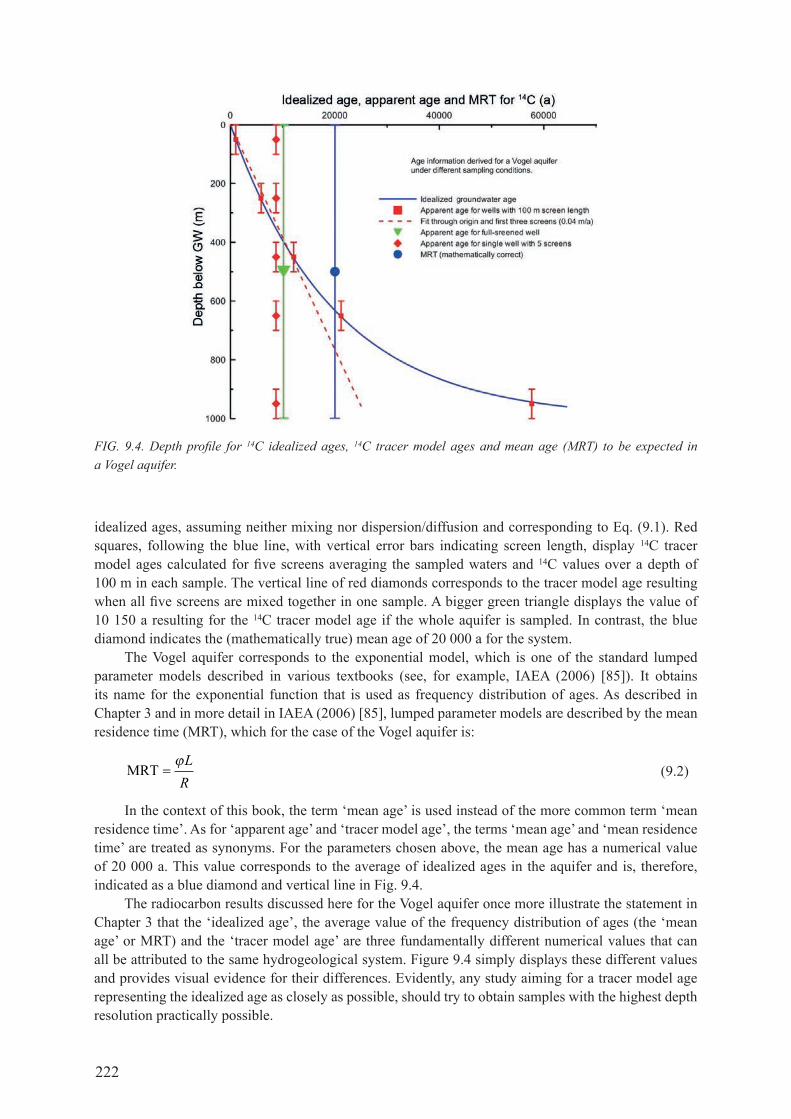
222

idealized ages, assuming neither mixing nor dispersion/diffusion and corresponding to Eq. (9.1). red squares, following the blue line, with vertical error bars indicating screen length, display 14c tracer model ages calculated for five screens averaging  the sampled waters and  14c values over a depth of 100 m in each sample. the vertical line of red diamonds corresponds to the tracer model age resulting when all five screens are mixed together in one sample. A bigger green triangle displays the value of 10 150 a resulting for the 14c tracer model age if the whole aquifer is sampled. In contrast, the blue diamond indicates the (mathematically true) mean age of 20 000 a for the system.

the Vogel aquifer corresponds to the exponential model, which is one of the standard lumped parameter  models  described  in  various  textbooks  (see,  for  example,  IAEA  (2006)  [85]).  It  obtains its name for the exponential function that is used as frequency distribution of ages. as described in chapter 3 and in more detail in IAEA (2006) [85], lumped parameter models are described by the mean residence time (Mrt), which for the case of the Vogel aquifer is:

MRT =ϕLR

(9.2)

In the context of this book, the term ‘mean age’ is used instead of the more common term ‘mean residence time’. As for ‘apparent age’ and ‘tracer model age’, the terms ‘mean age’ and ‘mean residence time’ are treated as synonyms. for the parameters chosen above, the mean age has a numerical value of 20 000 a. This value corresponds to the average of idealized ages in the aquifer and is,  therefore, indicated as a blue diamond and vertical line in fig. 9.4.

the radiocarbon results discussed here for the Vogel aquifer once more illustrate the statement in chapter 3 that the ‘idealized age’, the average value of the frequency distribution of ages (the ‘mean age’ or mrT) and the ‘tracer model age’ are three fundamentally different numerical values that can all be attributed to the same hydrogeological system. figure 9.4 simply displays these different values and provides visual evidence for their differences. evidently, any study aiming for a tracer model age representing the idealized age as closely as possible, should try to obtain samples with the highest depth resolution practically possible.

FIG. 9.4. Depth profile for 14C idealized ages, 14C tracer model ages and mean age (MRT) to be expected in a Vogel aquifer.

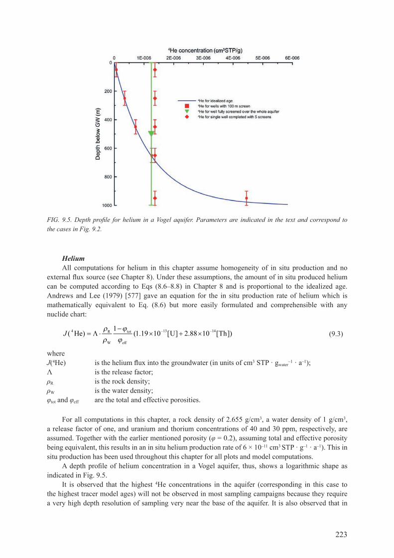
223

Heliumall computations for helium in this chapter assume homogeneity of in situ production and no

external flux source (see chapter 8). Under these assumptions, the amount of in situ produced helium can  be  computed  according  to  Eqs  (8.6–8.8)  in chapter  8  and  is  proportional  to  the  idealized  age. Andrews  and Lee  (1979)  [577]  gave  an  equation  for  the  in  situ  production  rate  of  helium which  is mathematically equivalent to eq. (8.6) but more easily formulated and comprehensible with any nuclide chart:

J ( ) ( . [ ] . [ ])4 13 1411 19 10 2 88 10He U ThR

W

tot

eff

= ⋅−

× + ×− −Λρρ

ϕϕ

(9.3)

whereJ(4He)      is the helium flux into the groundwater (in units of cm3 STP · gwater

–1 · a–1);Λ      is the release factor;ρr      is the rock density;ρw is the water density;φtot and φeff are the total and effective porosities.

for all computations  in  this chapter, a rock density of 2.655 g/cm3, a water density of 1 g/cm3, a release factor of one, and uranium and thorium concentrations of 40 and 30 ppm, respectively, are assumed. together with the earlier mentioned porosity (φ = 0.2), assuming total and effective porosity being equivalent, this results in an in situ helium production rate of 6 × 10–11 cm3 STP · g–1 · a–1). this in situ production has been used throughout this chapter for all plots and model computations.

A depth profile of helium concentration  in a vogel  aquifer,  thus,  shows a  logarithmic  shape as indicated in fig. 9.5.

It is observed that the highest 4he concentrations in the aquifer (corresponding in this case to the highest tracer model ages) will not be observed in most sampling campaigns because they require a very high depth resolution of sampling very near the base of the aquifer. It is also observed that in

FIG. 9.5. Depth profile for helium in a Vogel aquifer. Parameters are indicated in the text and correspond to the cases in Fig. 9.2.

224

the case of helium, the fully screened sample (green triangle in fig. 9.5) corresponds more closely to the average of screens (red triangles in fig. 9.5), since helium concentration increase with time is linear and mixing is linearly weighted. However, an additional crustal flux of helium from below the aquifer would further increase the helium concentration at the bottom of the aquifer. In this case, helium would not show identical depth profiles for every x coordinate within the aquifer, but higher helium concentrations would be observed at x coordinates of elevated crustal flux.

Tracer combinationIn this section, consideration is  taken of possible  interpretations resulting from measurement of 

concentrations of a suite of environmental tracers (in this case, tritium, 14c and 81Kr) in discharge from a multilevel well  in  a vogel  aquifer  (fig. 9.6). Keeping  the  parameters  constant,  tritium  as  a  tracer for the time range younger than 60 a can, of course, only be observed near the water table, down to a depth of approximately 3 m where the idealized age in this model reaches 60 a. However, because the uppermost screen in the multilevel well receives water from this layer, tritium is detectable in this sample, and for a northern hemisphere tritium input function, the sample contains nearly 1 tu if measured in the year 2000. As the half-lives of 81Kr and 36cl are considerably greater than that of 14c, the decay effect of 81Kr (and 36cl, not shown in fig. 9.6) is much less visible than for 14c (fig. 9.6) in the depth profile from the five open intervals in the well.

combining various tracers in a simple homogeneous aquifer such as that described by Vogel (1967) [137],  thus, gives age information specific to each of the tracers, each tracer displaying more details of the whole aquifer system. only if the sampling conditions are good, do tracer model ages for the different tracers agree. good sampling conditions include short screens and the tracer chosen fitting  to  the  time range of ages  in  the mixture. Table 9.1 displays  the calculated results  for samples obtained in the screens for each of the tracers and for the case of equal mixing across each screen

FIG. 9.6. Depth profiles of tritium, 14C and 81Kr in a Vogel aquifer. Solid lines represent concentrations obtained for idealized ages. Full symbols with error bars represent values obtained for sampling a screened well, where the error bar represents the screened interval. Vertical lines with open symbols represent concentrations obtained for a full-screened well. Colours represent tritium (purple), 14C (blue), 4He (red) and 81Kr (green).

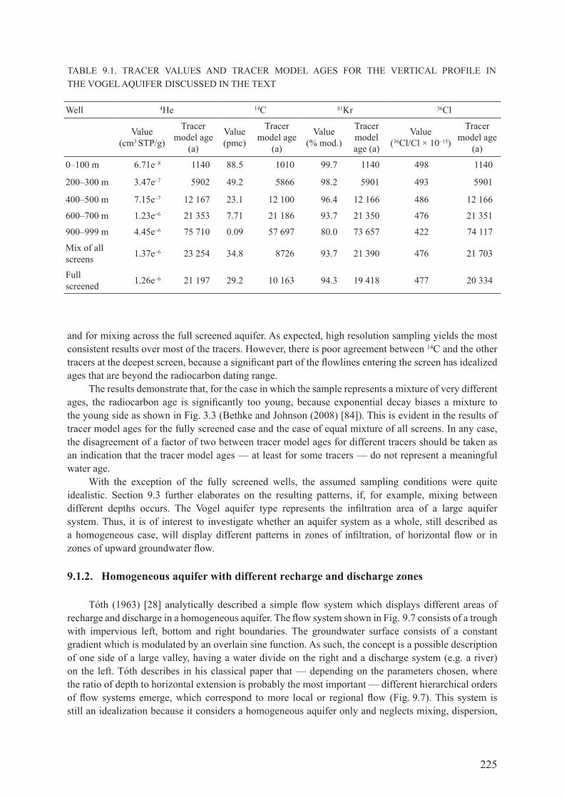
225

and for mixing across the full screened aquifer. as expected, high resolution sampling yields the most consistent results over most of the tracers. however, there is poor agreement between 14c and the other tracers at the deepest screen, because a significant part of the flowlines entering the screen has idealized ages that are beyond the radiocarbon dating range.

the results demonstrate that, for the case in which the sample represents a mixture of very different ages,  the  radiocarbon  age  is  significantly  too young,  because  exponential  decay biases  a mixture  to the young side as shown in fig. 3.3 (Bethke and johnson (2008) [84]). This is evident in the results of tracer model ages for the fully screened case and the case of equal mixture of all screens. In any case, the disagreement of a factor of two between tracer model ages for different tracers should be taken as an indication that the tracer model ages — at least for some tracers — do not represent a meaningful water age.

with the exception of the fully screened wells, the assumed sampling conditions were quite idealistic. section 9.3 further elaborates on the resulting patterns, if, for example, mixing between different  depths  occurs.  The  vogel  aquifer  type  represents  the  infiltration  area  of  a  large  aquifer system. thus, it is of interest to investigate whether an aquifer system as a whole, still described as a homogeneous  case, will  display different  patterns  in  zones of  infiltration,  of  horizontal flow or  in zones of upward groundwater flow.

9.1.2. Homogeneous aquifer with different recharge and discharge zones

Tóth  (1963)  [28]  analytically described a  simple flow system which displays different  areas of recharge and discharge in a homogeneous aquifer. The flow system shown in fig. 9.7 consists of a trough with impervious left, bottom and right boundaries. the groundwater surface consists of a constant gradient which is modulated by an overlain sine function. as such, the concept is a possible description of one side of a large valley, having a water divide on the right and a discharge system (e.g. a river) on the left. tóth describes in his classical paper that — depending on the parameters chosen, where the ratio of depth to horizontal extension is probably the most important — different hierarchical orders of flow systems emerge, which correspond  to more  local or  regional flow  (fig. 9.7). This  system  is still an idealization because it considers a homogeneous aquifer only and neglects mixing, dispersion, 

table 9.1. tracer Values and tracer Model ages for the VertIcal profIle In the Vogel aquIfer dIscussed In the text

well 4he 14c 81Kr 36cl

Value (cm3 stp/g)

tracer model age

(a)

Value (pmc)

tracer model age

(a)

Value (% mod.)

tracer model age (a)

Value (36cl/cl × 10–15)

tracer model age

(a)

0–100 m 6.71e–8 1140 88.5 1010 99.7 1140 498 1140

200–300 m 3.47e–7 5902 49.2 5866 98.2 5901 493 5901

400–500 m 7.15e–7 12 167 23.1 12 100 96.4 12 166 486 12 166

600–700 m 1.23e–6 21 353 7.71 21 186 93.7 21 350 476 21 351

900–999 m 4.45e–6 75 710 0.09 57 697 80.0 73 657 422 74 117

Mix of all screens 1.37e–6 23 254 34.8 8726 93.7 21 390 476 21 703

full screened 1.26e–6 21 197 29.2 10 163 94.3 19 418 477 20 334

226

diffusion and external fluxes. Nevertheless, it is useful to distinguish age patterns observed in recharge areas, areas of horizontal flow and discharge areas.

the parameters chosen for this example are: depth L = 5000 m, horizontal extension = 20 000 m, linear gradient = 0.001, amplitude and wavelength of the hills around this gradient = 5 and 6100 m, respectively, porosity = 0.3 and the kf value = 10–6  m/s.  Tóth  (1963)  [28]  gives  an  equation  for the potential as a function of horizontal extent, x, and the vertical coordinate, z. To create depth profiles, an approximate depth below groundwater surface is also displayed, which is computed as L–z (right z axis in fig. 9.7) and will be used in all subsequent graphs. for the discussion in the following, this formula  was  differentiated  and  multiplied  by  porosity  to  obtain  the  (distance)  velocities.  Idealized ages were computed by integration of this flow field to obtain idealized ages. The tracer values were computed  from  these  idealized  ages.  These  tracer  values  were  then  averaged  over  different  screen positions as above in the Vogel case.

9.1.2.1. Infiltration areas

The  horizontal  locations  indicated with  the  large  letter A  in  fig. 9.7  correspond  to  infiltration areas  of  different  flow  systems  and  are  always  associated  with  the  hilltops  in  the  groundwater surface. Evidently, these infiltration areas feed different flow (sub)systems in the Tóth aquifer: A1 at x = 19 800 m corresponds to the infiltration area of the largest flow system, whereas A2 (x = 14 000) and a3 (x = 8000) correspond to smaller watersheds with one (a2) or two (a3) underlying larger flow systems. for each of the depth profiles, the calculations that follow assume that there are eleven screens, the shallowest one centred at z = 4985 with 28 m screen length and the deeper ones built with 

FIG. 9.7. Vertical cross-section for a groundwater flow system in a homogeneous aquifer as described by Tóth (1963) [28]. Lines of equal groundwater potential are shown in red, lines of groundwater flow in blue, with arrows indicating the flow direction. The vertical exaggerated profile on top indicates the groundwater surface creating this flow field. Vertical age and tracer profiles at horizontal positions A (infiltration), B (horizontal flow) and C (upward flow) are discussed in the text.

227

a 280 m screen length at regular intervals of 500 m starting at a centre of z = 4650 (fig. 9.8). figure 9.8 shows the resulting depth profiles for 4he, 14c and 81Kr.

The  mathematical  solution  of  the  Tóth  model  has  zones  of  very  low  groundwater  velocity between the first and the second flow system. This results in high idealized ages that create high 4he concentrations and low 14c and 81Kr activities in areas of low groundwater velocity. However, unless the depth resolution in sampling is extremely high, these ‘stagnant’ zones will probably not be sampled and in most cases will be of no practical importance. The transition from one flow system to the next, however, results in concentration steps in the tracer depth profile. depending on the depth resolution during sampling, probably not all of these transitions are visible in the tracer depth profile: it would be possible from the 4he and 81Kr depth profiles of filtered screens, to postulate a second circulation system at greater depth, but hard to decide whether there are one or two different ones in the a3 case in fig. 9.8. with the parameters used here, 14c will not be measurable in the older, underlying flow systems.

with the appropriate combination of tracers covering the timescales of the aquifer, and with suitable depth resolution, it is feasible to determine recharge rates, to discern whether a recharge area belongs to a regional or only-local flow system, and if further flow systems are beneath. It is, thus, of interest if depth profiles for the more vertical downward flow of an infiltration area can be distinguished from areas of horizontal flow.

9.1.2.2. Areas of horizontal flow

The horizontal  locations  indicated with  the  large  letter B  in fig. 9.7 correspond  to areas where the flowlines are mainly horizontal in the selected Tóth model. They are associated with the maximum head gradient, where the sine wave determining the local groundwater gradient in fig. 9.7 equals the  straight  line  determining  the  regional  groundwater  gradient.  In  all  cases,  the  depth  profiles  tap 

FIG. 9.8. Depth profiles of 4He, 14C, 81Kr in infiltration areas. Locations of profiles A1 (red), A2 (blue) and A3 (purple) are indicated in the flow field (top left). Vertical bars correspond to extension of well-filter screens.

228

different flow systems, and the positions chosen for further discussion are B1 at x = 18 000 m, b2 at x = 12 000 m and b3 at x = 6200 m. figure 9.9 shows the resulting depth profiles for 4he, 14c and 81Kr.

At first glance, there seems to be little difference in the shape of the tracer profiles between figs 9.8 and 9.9. Again,  the transition from a shallow flow system to the next deeper flow system appears as a  step  in  the depth profile of  the age  tracers. A closer  comparison  reveals  that  the numerical values are different: there is more 4He and less of the radioactive tracers at similar depths in the profiles of the horizontal flow situation as compared to infiltration areas. for 14c, it is remarkable that the different profiles  cross  each  other  (fig. 9.9,  lower  left):  14c  has  the  highest  time  resolution  since  its  half-life is best suited for the timescale of flow in the shallow systems. Therefore,  the different age gradients of the shallow flow systems become more evident here — although they are present in the top parts of  the depth profiles of  4he and 81Kr,  they are not as clearly discernible as  in  the  14c profile. Profile B1  represents  the  infiltration  area  of  the  largest  regional  flow  system.  for  the  chosen  parameters, groundwater  on  this  profile  infiltrates  down  to  a  depth  of  4000  m  within  the  dating  range  of  14c (50 000 a). Profile B3 represents the shallowest system. Here, the idealized ages cover values between zero and the dating range of 14c within a depth interval of 0–2500 m.

without  a  conceptualization of  the hydrology of  the flow  system,  it would be difficult  to  even distinguish recharge areas from regions of dominant horizontal flow on the basis of tracer data alone. This illustrates that hydrogeological knowledge of the flow system is necessary before age studies are initiated (see chapter 2), and that  the purpose of  the age tracers  is  to help quantify the flow system, not  to  a  priori  investigate  its  dominant  direction  of  groundwater  flow.  However,  this  similarity  of patterns between recharge area and area of horizontal flow raises the question of whether the regions of upward directed flow, where groundwater discharges to surface water or to shallower systems, show different patterns.

FIG. 9.9. Depth profiles of 4He, 14C, 81Kr in areas of horizontal flow. Locations of profiles B1 (red), B2 (blue) and B3 (purple) are indicated in the flow field (top left). Vertical bars correspond to extension of well-filter screens.

229

9.1.2.3. Areas of upward flow

A naive understanding of ‘upward flow’ might lead to the expectation that water ages increase in the upward direction, because this is the flow direction. Basically, it would be as though the patterns in  the  right  part  of  fig. 9.1 were  flipped  upside  down. This would  result  in  an  upward  increase  of 4he and an upward decrease of the radioactive tracers 14c and 81Kr and is called an ‘age inversion’ in stratigraphy. closer investigating the details of the flowlines in fig. 9.7 reveals that a vertical profile in an area of upward directed flow will hardly ever sample only one flowline. This easily explains why the tracer depth profiles for 4he, 14c and 81Kr, in regions with partly or dominant upward flow, seldom show an age inversion (fig. 9.10). vertical profiles for this case are situated at x = 10 000 m for profile c1 and at x = 4830 m and x = 80 m for profiles c2 and c3, respectively. regions of upward directed flow may show age inversions in part of the vertical profile, as the upper three screens in profile c1 show for 4he and 81Kr. However, even in this profile, the values for 14c do not show this inversion for the last two screens, because the screen at a depth of 350 ± 150 m samples a mixture of very different 14c concentrations and, as such, is biased young. for the aquifer parameters chosen here, radiocarbon is measurable only in profiles c1 and c2, and in these radiocarbon content is so small (<1 pmc) that in many practical cases it will probably provoke discussions about contamination during sampling among the scientists in the project.

As a summary, depth profiles in areas of upward flow are generally characterized by large depth regions where the age-indicating tracers are constant with depth. This is observed on a level of activity (14c and 81Kr)  or  concentration  (4he) that indicates considerable age. In areas where the upward directed flow belongs  only  to  the  local  groundwater  systems,  such  as  the c3 profile,  again  steps  in the tracer profile may occur, but these are less pronounced as in the case of horizontal flow. with these characteristic  features,  discharge  zones  should,  in many  cases,  be  clearly  discernible  from  recharge zones and areas of horizontal flow, given an adequate resolution in the vertical scale of sampling.

FIG. 9.10. Depth profiles of 4He, 14C and 81Kr in discharge areas. Locations of profiles C1 (red), C2 (blue) and C3 (purple) are indicated in the flow field (top left). Vertical bars correspond to extension of well-filter screens.

230

all of these considerations of course neglect two natural processes important for the depth profiles: first, dispersion and diffusion are neglected. Taking these into consideration, the ‘singularities’ shown in figs 9.8–9.10 at the transition zones from one flow system to the next will be considerably smoothed. The general shape of the depth profiles computed for screened well intervals, however, will not be altered. Second, external fluxes are neglected. Especially  for  the  4He depth profiles,  this may be an unrealistic assumption, as pointed out in detail in chapter 8. qualitatively, external fluxes will increase the 4He concentration  towards  the bottom of  the aquifer  in all depth profiles.  If  this mainly diffusion driven flux is not  too large,  the profile  in  the ‘global’  infiltration area (profile A1, fig. 9.8) will  not  be  altered  too  much,  since  the  downward  groundwater  movement  will  flush  the  helium influx from the bottom of the aquifer. In areas of horizontal flow, however, 4he gradients with depth will be considerably  larger, especially near  the base of  the aquifer.  In  the areas of upward flow,  4he concentrations will  be  orders  of magnitude higher,  although  the  general  shape of  the  profiles  is  not necessarily altered.

The most unrealistic assumption of the Tóth model (Tóth (1963) [28]) is to assume homogeneous aquifer transmissivity. the next step is, thus, to consider a layered aquifer with varying transmissivity. this is not as easily examined in a quantitative and detailed manner, because analytical solutions to the flow system are not available as they are for the vogel or Tóth models.

9.1.3. Aquifer systems — confined or partly confined

while the case considered in section 9.1.2 is easily understandable, it is not very realistic. In natural systems, a sediment layer of 5 km thickness with only one kf value is rarely the case. although sedimentary basins of  this  thickness exist  in various areas of  the world,  the sedimentation processes changed, and  these changes created  layers of varying grain  size, different  sorting of grain  sizes and different compaction, resulting in different transmissivity. this transmissivity can vary by orders of magnitude, as discussed in chapter 2. deep systems tend to be layered into aquifers (comparably high transmissivity), aquitards (smaller transmissivity) and aquicludes (transmissivity so low that groundwater  flow  is  negligible  as  compared  to  flow  in  aquifers).  Even  if  a  layer  is  regarded  to  be ‘homogeneous’ from the sedimentological point of view, variations of a factor of five in the kf value are still possible, simply because deducing the kf from sedimentological information involves an uncertainty of  this magnitude. All  smaller variations are very difficult  to detect by  sedimentological methods or even from data obtained from sophisticated pump tests.

9.1.3.1. Single depth profile in various aquifers

As an  example,  the depth profile  sketched  in fig. 9.11  is  considered. The  sediment  consists  of several aquifers of different thicknesses, separated by aquitards, which are assumed to be impervious with respect to flow and diffusion. Horizontal flow is assumed through each aquifer layer, the distance velocity  is  calculated  from dary’s  law  and  porosity,  and  this  idealized  age  is  converted  into  tracer concentrations as in the previous sections. In detail, this implies the following assumptions: the aquifers are assumed to have different kf values. for the sake of simplicity, all aquifers (i) are assumed to be recharged  in  the  same  area  at  a  distance  of  100  km,  (ii)  are  assumed  to  have  the  same  gradient  of 1 × 10–4 in hydraulic potential and (iii) are assumed to have the same porosity of 20%. further, (iv) it is assumed  that all aquifers have  the same properties  in  the  infiltration area which  leads  to  identical 4he production rates, and all have 14c and 36cl (‘no decay’) initial conditions. In fact, the only varying parameter is the kf value, which is indicated for the aquifers in fig. 9.11.

The first impression looking at the tracer depth profiles is the absence of the systematic patterns observed in the homogeneous aquifers. In the homogeneous case, the radioactive tracers 14c and 81Kr decreased in a more or less monotonic manner with depth in nearly all cases, whereas 4he increased

231

with depth. the inhomogeneous case is completely dominated by the transmissivity values and shows a very irregular pattern of decreasing and increasing tracer values with depth.

A closer  inspection  of  the  depth  profile  of  different  tracers  in  this multi-aquifer  system  shows the expected pattern with lower values for the radioactive decaying tracers 14c and 81Kr (larger age) in aquifers of lower kf value. Important to note is that a comparably small difference in kf values can be easily discerned from the tracer results: the difference of 1 × 10–3 and 2.5 × 10–3 m/s between the topmost two aquifers results in clearly different 14c signals. It is also important to note that different tracers with different timescales are necessary to cover the transmissivity values in this example: aquifers IV and v show ‘infinitely old’ water on the 14c timescale whereas 4he and 81Kr give results which are clearly different from the aquifers of high transmissivity above and below, and which are still discernible from each other.

Since purely advective flow to simulate the tracers is again considered, a qualitative discussion is helpful with regard to the difference between the derived tracer values in this artificial case and tracer values  in  a more  realistic  case. one  important  but  neglected parameter  is  aquitard  leakage between aquifers. only  rarely do aquifer  stacks  in nature have  the  same hydraulic potential; often, pressures are  different  between  aquifers.  This  means  that  flow  is  induced  in  the  vertical  direction  through the aquitards. Although the amount of water flowing per square meter through the aquitards between adjacent aquifers may be very small, it has to be multiplied by the entire area over which the pressure difference exists; an area that may amount to many square kilometres. Therefore, the amount of cross-aquifer flow will, in many cases, have a measurable effect on the tracer values, caused by mixing of different waters. cross-aquifer flow will generally decrease  the differences of  tracer values between aquifers. In this case, this will probably influence aquifers III, Iv and v the most, because these have the largest differences in tracer values compared to their neighbours. If the flow through the aquitard needs a considerable amount of time, however, it will not cause water of the age ab of the adjacent aquifer b to mix into aquifer a but water of an age ab + t where t is the time needed for the transfer through the aquitard. the same also holds true for any other parameter changed within the aquitard (amount of dissolved solids, ion exchange, etc.).

FIG. 9.11. Vertical tracer profiles in an aquifer system with separating aquitards.

232

diffusion of radioactive tracers into the aquitards or of helium out of the aquitards may also have a noticeable influence. This can be simulated with the theory of dual porosity aquifer systems which are discussed in chapters 4, 5, 8 and 10. finally, any helium flux from external sources was neglected, in this case from below the whole aquifer system sketched in fig. 9.11. As discussed in detail in chapter 8, such an external flux will increase the helium concentration in the deepest aquifers, until an aquifer is reached which is able to transport all of the helium of this flux to the surface. Above this aquifer — in this case probably the deepest one, vII — helium from crustal flux is negligible, but helium from the adjacent aquitards may still increase the concentration above the one produced in situ.

9.1.4. summary

section 9.1 has demonstrated possible tracer patterns that can be obtained sampling an aquifer with multilevel wells. It also demonstrated how mixing of waters from different depths with different age  can  influence  the  result.  It  demonstrated  that  it will  be  difficult  or  impossible  from  tracer  data alone to distinguish recharge areas from areas of horizontal flow, because their tracer patterns are very similar. Therefore,  a  conceptual model  of  the  groundwater  flow  system  is  necessary  before  starting the tracer study. In contrast, discharge areas can be more easily detected. section 9.1 also demonstrated that in aquifer systems consisting of aquifers and intercalated aquitards, tracer results will be dominated by the transmissivity of the aquifer.

there are some conclusions of this section which can be translated into practical advice for the application of environmental tracers to study groundwater age:(a) optimum wells for the purpose of age dating of groundwater are constructed to obtain an

unmixed  sample  from  a  defined  depth with  a  depth  range  being  very  small  as  compared  to the total depth of the well. well nests constructed this way to obtain a depth profile of samples are the optimum choice.

(b) optimum depth resolution of multilevel well nests should be higher near the groundwater surface and near the bottom of the aquifer. this is because, at these interfaces, the largest variation of tracer data is to be expected.

(c) whenever it is possible in the early stage of a groundwater study to influence the construction of observation wells, the facts above should be taken into consideration.

(d) section 9.1 also allows the following conclusions to be drawn for most practical cases where sampling conditions are not optimal, for example, where only wells completed with multiple screens are available, where open boreholes in fractured rock have to be sampled, etc.

geotechnical methods should be considered to obtain samples with optimum depth resolution for the given case (packer systems, sampling with the dual-pumping technique (rapp et al. (1998) [591]), chains of passive samplers, etc.).

different (hydrochemical and isotopic) tracers should be applied to enable the deconvolution of mixtures (see section 9.3 for further multitracer techniques to detect mixtures).

direct conversion of tracer values to tracer model ages in most such cases will give no useful results; therefore, this should be considered only after the deconvolution of mixtures was possible.

tracer concentrations and activities for these samples should be directly described (without converting  them  to  tracer model  ages),  applying  the  knowledge  about  the  sampling  conditions  and using an interpretation model that describes the transport conditions as closely as possible.

for instance, for the Vogel case discussed in section 9.1.1.1 where the sample was obtained from a full screened well penetrating the whole aquifer, the direct conversion of tracer values into tracer model ages will not give a reasonable result. fitting the tracer values for the fully screened well to an exponential model, however, will result in the correct mean age time of 20 000 a. an exponential model applied to interpret the single well completed with five screens will also give a more useful result than the direct conversion of the tracer data into a tracer model age.

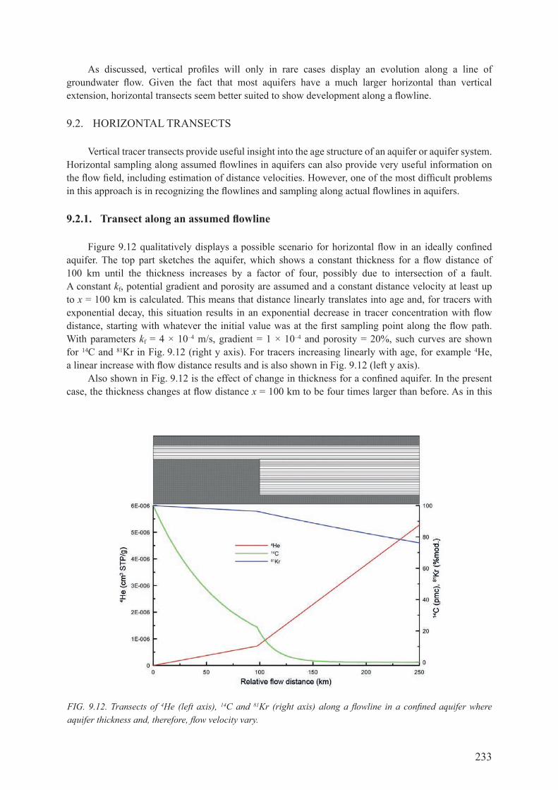
233

As  discussed,  vertical  profiles  will  only  in  rare  cases  display  an  evolution  along  a  line  of groundwater  flow.  given  the  fact  that  most  aquifers  have  a  much  larger  horizontal  than  vertical extension, horizontal transects seem better suited to show development along a flowline.

9.2. horIZontal transects

Vertical tracer transects provide useful insight into the age structure of an aquifer or aquifer system. Horizontal sampling along assumed flowlines in aquifers can also provide very useful information on the flow field, including estimation of distance velocities. However, one of the most difficult problems in this approach is in recognizing the flowlines and sampling along actual flowlines in aquifers.

9.2.1. Transect along an assumed flowline

figure 9.12 qualitatively displays a possible scenario  for horizontal flow in an  ideally confined aquifer. The  top  part  sketches  the  aquifer, which  shows  a  constant  thickness  for  a  flow  distance  of 100  km  until  the  thickness  increases  by  a  factor  of  four,  possibly  due  to  intersection  of  a  fault. a constant kf, potential gradient and porosity are assumed and a constant distance velocity at least up to x = 100 km is calculated. This means that distance linearly translates into age and, for tracers with exponential decay,  this  situation  results  in an exponential decrease  in  tracer concentration with flow distance, starting with whatever  the  initial value was at  the first sampling point along  the flow path. with parameters kf = 4 × 10–4 m/s, gradient = 1 × 10–4 and porosity = 20%, such curves are shown for 14c and 81Kr in fig. 9.12 (right y axis). for tracers increasing linearly with age, for example 4he, a linear increase with flow distance results and is also shown in fig. 9.12 (left y axis).

Also shown in fig. 9.12 is the effect of change in thickness for a confined aquifer. In the present case, the thickness changes at flow distance x = 100 km to be four times larger than before. As in this 

FIG. 9.12. Transects of 4He (left axis), 14C and 81Kr (right axis) along a flowline in a confined aquifer where aquifer thickness and, therefore, flow velocity vary.

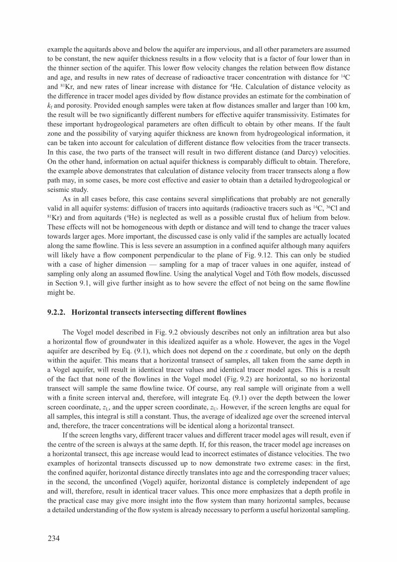
234

example the aquitards above and below the aquifer are impervious, and all other parameters are assumed to be constant, the new aquifer thickness results in a flow velocity that is a factor of four lower than in the thinner section of the aquifer. This lower flow velocity changes the relation between flow distance and age, and results in new rates of decrease of radioactive tracer concentration with distance for 14c and 81Kr,  and new  rates of  linear  increase with distance  for  4he. calculation of distance velocity as the difference in tracer model ages divided by flow distance provides an estimate for the combination of kf and porosity. Provided enough samples were taken at flow distances smaller and larger than 100 km, the result will be two significantly different numbers for effective aquifer transmissivity. Estimates for these  important hydrogeological parameters are often difficult  to obtain by other means.  If  the  fault zone and the possibility of varying aquifer thickness are known from hydrogeological information, it can be taken into account for calculation of different distance flow velocities from the tracer transects. In this case, the two parts of the transect will result in two different distance (and darcy) velocities. on the other hand, information on actual aquifer thickness is comparably difficult to obtain. Therefore, the example above demonstrates that calculation of distance velocity from tracer transects along a flow path may, in some cases, be more cost effective and easier to obtain than a detailed hydrogeological or seismic study.

As in all cases before,  this case contains several simplifications  that probably are not generally valid in all aquifer systems: diffusion of tracers into aquitards (radioactive tracers such as 14c, 36cl and 81Kr) and  from aquitards  (4He)  is neglected as well as a possible crustal flux of helium from below. these effects will not be homogeneous with depth or distance and will tend to change the tracer values towards larger ages. More important, the discussed case is only valid if the samples are actually located along the same flowline. This is less severe an assumption in a confined aquifer although many aquifers will  likely have a flow component perpendicular  to  the plane of fig. 9.12. This can only be  studied with a case of higher dimension — sampling for a map of tracer values in one aquifer, instead of sampling only along an assumed flowline. Using the analytical vogel and Tóth flow models, discussed in Section 9.1, will give further insight as to how severe the effect of not being on the same flowline might be.

9.2.2. Horizontal transects intersecting different flowlines

The vogel model described in fig. 9.2 obviously describes not only an infiltration area but also a horizontal flow of groundwater in this idealized aquifer as a whole. However, the ages in the vogel aquifer are described by eq. (9.1), which does not depend on the x coordinate, but only on the depth within the aquifer. This means that a horizontal transect of samples, all taken from the same depth in a Vogel aquifer, will result in identical tracer values and identical tracer model ages. this is a result of  the  fact  that  none  of  the flowlines  in  the vogel model  (fig. 9.2)  are  horizontal,  so  no  horizontal transect will  sample  the  same flowline  twice. of course,  any  real  sample will originate  from a well with a finite screen interval and,  therefore, will  integrate Eq. (9.1) over the depth between the lower screen coordinate, zl, and the upper screen coordinate, zu. however, if the screen lengths are equal for all samples, this integral is still a constant. Thus, the average of idealized age over the screened interval and, therefore, the tracer concentrations will be identical along a horizontal transect.

If the screen lengths vary, different tracer values and different tracer model ages will result, even if the centre of the screen is always at the same depth. If, for this reason, the tracer model age increases on a horizontal transect, this age increase would lead to incorrect estimates of distance velocities. The two examples  of  horizontal  transects  discussed  up  to  now  demonstrate  two  extreme  cases:  in  the  first, the confined aquifer, horizontal distance directly translates into age and the corresponding tracer values; in  the  second,  the  unconfined  (vogel)  aquifer,  horizontal  distance  is  completely  independent  of  age and will, therefore, result in identical tracer values. This once more emphasizes that a depth profile in the practical case may give more insight into the flow system than many horizontal samples, because a detailed understanding of the flow system is already necessary to perform a useful horizontal sampling.

235

The  case  of  the Tóth  aquifer  is more  complicated,  since  local  infiltration  and  upward  directed flow alternate in this case. figure 9.13 shows three horizontal transects, sampled at depths of 700 m (shallow, red curves), 2500 m (intermediate, blue curves) and 4200 m (deep, purple curves) for 4he, 14c and 81Kr in the Tóth aquifer discussed in fig. 9.7. As before, computed tracer values were averaged over depths corresponding to 200 m of well-screen.

from all tracers, it is evident that the shallow transect samples the local circulation systems and only the deep transect shows an increase of age with flow distance. for example, 4he in the deep transect shows monotonous increase in flow direction (right to left in this picture). The shallow 4he transect in contrast in most areas shows hardly any excess 4He but does contain local spikes that might be missed without detailed horizontal sampling. A similar pattern is observed for 81Kr, although in the opposite sense, since this tracer shows radioactive decay. the values for 81Kr  in most  screens of  the  shallow transect show minimal variation; only if, by chance, one of the screens is situated at a position of upward  directed flow,  a  sudden  decrease  in  81Kr  values may  be  observed. The  deep  transect  shows the expected decrease of 81Kr with flow distance. Both of these tracers, 4he and 81Kr (and 36cl), are on a timescale too long to produce discernable age variations in the shallow transect.

radiocarbon, in contrast, has a decay constant that is on an appropriate timescale for the shallow transect and partly also  for  the  intermediate  transect. carbon-14 clearly  reflects  the  infiltration areas with high radiocarbon values and the zones of upward directed flow with low radiocarbon values. In the intermediate transect, 14c also indicates evidence of young water at the right side, close to the deep-reaching infiltration area. Later in the intermediate transect and in the whole deep transect, groundwater circulates on a timescale too large for detection of flow patterns using 14c.

The assumption  to  sample  the  same flowline along a horizontal  transect  following  the gradient of groundwater potential may be a reasonable and valid approach in confined aquifers. It is, however, normally invalid in phreatic aquifers with only small variations in aquifer transmissivity. In phreatic

FIG. 9.13. Three horizontal transects for 4He, 14C and 81Kr in the Tóth aquifer of Fig. 9.7. The depth of the transects is 4200 m (purple), 2500 m (blue) and 700 m (red), corresponding to model-z coordinates of 800, 2500 and 4300 m, respectively.

236

aquifers, horizontal  transects along an assumed flow direction can result  in constant  tracer values as demonstrated in the vogel case, or in tracer values reflecting a series of locally young and old waters in the regional flow direction. This may seem unexpected on first sight, but is nevertheless in accordance with the general direction of flow. As Tóth (1963) [28] pointed out, a regional flow system circulation on long timescales may be present depending on aquifer parameters, but will then be observable only with very good depth resolution and only in the deep parts of the aquifer.

9.2.3. summary

Section 9.2 demonstrated that horizontal  tracer  transects along an assumed flowline can help to obtain  important  information on  the groundwater flow  system  such  as distance velocity  and  aquifer transmissivity. The discussion of the vogel aquifer in Section 9.1.1 also demonstrated that a horizontal transect in the direction of groundwater flow does not necessarily result in an increase of tracer model age in the flow direction. The discussion of the Tóth aquifer even demonstrated the possibility of locally decreasing ages in the general flow direction which pointed to the existence of local flow systems.

The first two sections of this chapter, 9.1 and 9.2, demonstrate the following:(a) To  understand  the  details  of  a  flow  system,  many  measurements  of  age-dating  tracers  are 

necessary, not just a single measurement of one particular tracer.(b) A combination of different tracers covering different timescales is necessary, if a flow system as 

a whole is to be understood.(c) If development of a conceptual understanding of the flow system is still in its initial state, a depth 

profile of tracer measurements is advantageous to gain further understanding.(d) Horizontal transects aiming to sample a single flowline promise further useful details if the flow 

system is well constrained — either because it is a confined aquifer or because a detailed flow model has already been constructed. only this allows the choice of sampling wells that may be on a flowline.

(e) Horizontal  transects  not  showing  the  tracer  pattern  expected  are  a  clear  indication  that either  the  flow  model  needs  refinement  or  that  unexpected  tracer  specific  phenomena  are occurring.  Possible  reasons  include  changes  in  aquifer  thickness,  changes  in  flow  direction, flow  convergence,  changes  in  tracer  fluxes  in  or  out  of  the  aquifer  (especially  for  4he) and geochemical alteration of the tracer (in the case of 14c or 36cl). Isotope hydrological tracers demonstrated their suitability  to boost  the necessary model refinements (see chapters 11–14). often, new sampling on a different spatial scale is necessary to achieve the necessary insight for such refinements.

the results here were obtained assuming excellent sampling conditions: multilevel sampling with several well isolated screens at different depths was a prerequisite for the considerations in sections 9.1 and 9.2. of course, this gives rise to the question of what may happen if the sampling conditions were not as ideal. what happens if there are several screens, but all in one borehole, leading to mixed samples from different depths? the next section presents methods that use measurements of several different tracers to resolve instances of borehole mixing.

9.3. IMportant patterns of tracer Versus tracer

The  combination  of  tracers  reflecting  different  timescales  is  both  a  powerful  and  necessary approach when studying old groundwater. whenever a tracer for a long timescale is used with the final goal of deriving an age, it should be supplemented by tracers for young components and, if possible, also by tracers for the next longer timescale. the reason is that most groundwater samples represent mixtures of an a priori unknown kind. As discussed in the introductory chapters,  it  is very 

237

improbable that the frequency distribution of ages represented by a water sample consists only of one (idealized) age. In most cases, it will at least be broadened by diffusion and dispersion. As discussed using the Vogel and tóth aquifer models, it can also show different, sometimes systematically varying idealized ages over the length of the screen. It may also consist of different non-overlapping age ranges (see fig. 3.1) which normally are described as (binary, ternary, etc.) mixtures. such mixtures will result in tracer model ages that may be very different from the ages of the (two or more) water end members that dominate the mixture. as seen in table 9.1, such a multicomponent mixture manifests itself by tracer model  ages  that  are  different  for  each  tracer. often,  these mixtures  can  be  identified  plotting one tracer versus another. In addition, if the age of the groundwater approaches the maximum dating range of a certain tracer, any small admixture of younger water will keep this tracer close to but not within the dating range. for example, a 2% admixture of 150 a old water to a 100 ka old water body will keep the 14c value near 2 pmc and the tracer model age near 32 ka — which surely will not be a representative age for the bulk of the water. However, combining the measurements of two different tracers with very different dating ranges can make the presence of such mixtures obvious by showing discrepant ages for the different tracers. even before calculating any ages with the tracers, simple plots of one tracer relative to another can characterize samples consisting of waters of different age. Such tracer–tracer plots are presented below.

9.3.1. Combination of tracers for different timescales

plotting a tracer a which decays fast or is relevant only for a small timescale versus another tracer b for a larger timescale gives insights into mixtures, initial conditions and practical detection limits. A typical plot  is sketched in fig. 9.14:  in this case,  the short-time tracer is plotted on the y axis and the  long-time  tracer on  the x  axis.  If  the  long-time  tracer  is  radioactive,  it  is best  to plot  the x  axis with a logarithmic and descending scale. doing so, a distance on the x axis represents a distance in time,  independent  of  any  initial  ‘no  decay’  value  and without  calculating  an  age. A  possible  tracer combination might be tritium on the y axis and 14c on the x axis. Instead of tritium, cfcs can be used

FIG. 9.14. A plot of tracers of different timescales reveals initial values for the old tracer, shows practical detection limits for the young tracer and makes mixtures of waters with different ages obvious.

238

(see chapter 4). However, the same principle applies for radiocarbon as a short-time tracer on the y axis in combination with 36cl as a long-time tracer on the x axis.

what are the patterns that can be observed on such a plot? In the simplest case, showing only idealized  ages,  all  samples would  plot  along  and  very  close  to  the  x  and  y  axes  of  fig. 9.14. This is  because  short  timescale  tracers  (e.g.  tritium or cfcs) will  decrease with  age  to  zero before  long timescale tracers (e.g. 14c) will show any noticeable decrease. the young samples containing short timescale tracers plot along the y axis, with the x value (long timescale tracer) close to the initial value. As age  further  increases,  the  long-time  tracer will  decrease while  the  short-time  tracer  is  already at zero, plotting the older samples along and close to the x axis. However, because many other processes and factors can affect tracer concentrations, this simple picture is disturbed.

first, the short-time tracer may show some behaviour with time. Tritium and the cfcs show peaks with time, the peak of tritium being around 1963 and the peaks of cfcs in the early 1990s. If the long-time tracer shows no such anthropogenic influence, such as 81Kr, then still all points containing the short-time tracer lie along the y axis. However, as discussed in chapter 4, radiocarbon in atmospheric co2 raised by nearly a factor of two above natural values due to the bomb tests, and this happened and remained measurable during the same time span as the peaks in tritium and cfcs. As a consequence, a plot of tritium and cfcs versus radiocarbon will — even for idealized ages — plot along a curve close to the y axis. this is similar for the combination 14c/36cl, because both show anthropogenic increase due to bomb production.

Second,  some  long-time  tracers have no well defined  initial value. This  is  true  for  14c because the  ‘no decay’ value  is  influenced by chemical processes  in  the unsaturated zone and  in  the aquifer, as  discussed  in  detail  in  chapter  4.  This  is  true  for  36cl, since the initial 36cl/cl ratio depends on the recharge area and the climatic conditions during recharge, as discussed in chapter 6. therefore, a plot of tritium versus 14c or of 14c versus 36cl/cl can give information on the initial value of the long-time tracer on the x axis (14c and 36cl/cl, respectively) as indicated by the red bracket ‘initial value’ in fig. 9.14.

third, all tracers have practical detection limits. these depend on the method of measurement and on the sampling conditions. for tritium, the analytical detection limit is typically around 0.5–0.1 tu for beta-counting after enrichment; for the 3he ingrowth technique, it can be as low as 0.005 tu; and for cfcs it is around 0.01–0.03 pmol/l. for 14c and 36cl/cl, it is around 0.1 pmc and 10 × 10–15, respectively, as discussed in chapters 4 and 6. Practical detection limits due to the sampling conditions (leaky well casing, reagents used in the field, contamination due to difficult field conditions, etc.) may be higher than these analytical detection limits. for instance, using normal sampling and transport methods, one would not interpret tritium values greater than 0.05 tu as representing samples containing significant amounts of young water, or treat samples with 0.3 pmc as ‘radiocarbon free’. The plot in fig. 9.14 can provide an estimate of  these practical detection  limits, because  this  is  the range where the concentrations of the short term tracers level off as the long-time tracer concentration decreases, as indicated by the horizontal red line and the crosses below.

fourth,  actual  groundwater  samples  do  not  contain  water  of  only  one  idealized  age.  Instead, a sample consists of waters containing a narrow or wide age distribution, or can even be a mixture of two or more waters with disjunctive ages. Imagine, for instance, a deep borehole with several screens  or  an  open  borehole  in  fractured  rock with  several water-bearing  fractures.  Such  binary  or multicomponent mixtures will plot  in  the  triangle area  in fig. 9.14, denoted  ‘mixtures’. Any sample plotting in this triangle area of fig. 9.14 is a mixture of young and old water and, generally, within this triangle the tracer model age is not a good estimate for the groundwater age.

In principle, mixtures from the triangle area may be deconvoluted into the components, and ages for the mixing components may be computed. This is a difficult task, however, and often not possible in the practical case. deconvolution of the mixture needs at least as many analysed parameters as mixing components are present, to narrow down the original water masses and their ‘initial’ tracer values. In general, the age of the two components is also unknown, which needs at least two additional age-tracer 

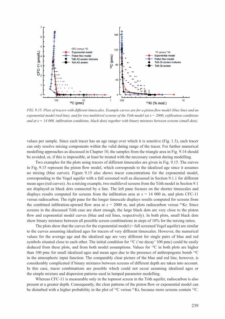
239

values per sample. since each tracer has an age range over which it is sensitive (fig. 1.3), each tracer can only resolve mixing components within the valid dating range of the tracer. for further numerical modelling approaches as discussed in chapter 10, the samples from the triangle area in fig. 9.14 should be avoided, or, if this is impossible, at least be treated with the necessary caution during modelling.

two examples for the plots using tracers of different timescales are given in fig. 9.15. the curves in fig. 9.15 represent the piston flow model, which corresponds to the idealized age since it assumes no mixing (blue curves). figure 9.15 also shows tracer concentrations for the exponential model, corresponding to the Vogel aquifer with a full screened well as discussed in section 9.1.1 for different mean ages (red curves). as a mixing example, two multilevel screens from the tóth model in section 9.1 are displayed as black dots connected by a  line. The  left pane focuses on  the shorter  timescales and displays  results  computed  for  screens  from  the  infiltration  area  at x  =  14 000 m,  and plots cfc-11 versus radiocarbon. the right pane for the longer timescale displays results computed for screens from the  combined  infiltration-upward flow area  at x = 2000 m, and plots radiocarbon versus 81Kr. Since screens in the discussed Tóth case are short enough, the large black dots are very close to the piston flow and exponential model curves (blue and red lines, respectively). In both plots, small black dots show binary mixtures between all possible screen combinations in steps of 10% for the mixing ratios.

the plots show that the curves for the exponential model (= full screened Vogel aquifer) are similar to the curves assuming idealized ages for tracers of very different timescales. However, the numerical values  for  the  average  age  and  the  idealized  age  are  very  different  for  single  pairs  of  blue  and  red symbols situated close to each other. the initial condition for 14c (‘no decay’ 100 pmc) could be easily deduced from these plots, and from both model assumptions. Values for 14c in both plots are higher than 100 pmc for small idealized ages and mean ages due to the presence of anthropogenic bomb 14c in the atmospheric input function. the comparably clear picture of the blue and red line, however, is considerably complicated if binary mixtures between screens of different depth are taken into account. In  this  case,  tracer  combinations  are  possible  which  could  not  occur  assuming  idealized  ages  or the simple mixture and dispersion patterns used in lumped parameter modelling.

whereas cfc-11 is measurable only in the topmost screen in the Tóth aquifer, radiocarbon is also present at a greater depth. consequently, the clear patterns of the piston flow or exponential model can be disturbed with a higher probability in the plot of 14c versus 81Kr, because more screens contain 14c.

FIG. 9.15. Plots of tracers with different timescales. Example curves are for a piston flow model (blue line) and an exponential model (red line), and for two multilevel screens of the Tóth model (at x = 2000, exfiltration conditions and at x = 14 000, infiltration conditions, black dots) together with binary mixtures between screens (small dots).

240

this seems initially to be an unsatisfactory result; however, on the contrary, if the absence of cfcs, tritium and even 14c can be demonstrated, this leads to the conclusion that even small admixtures of young water can be excluded, ‘young’ meaning, in this case, waters up to several thousand years of age.

plotting tracers of different timescales versus each other is, therefore, a useful tool for the detection of unwanted mixtures, possibly created during sampling. It also allows the necessary determination of initial values for 14c and 36cl close to the infiltration area. A direct comparison of ages, or a detection of processes that influence the long time tracer only, needs a comparison of tracers with similar timescales.

9.3.2. Combination of tracers with similar decay timescales

The combination of different age-dating tracers with similar timescales is always desirable since the  assumptions  of  one  tracer  application  can  be  checked  against  another  tracer,  providing  greater confidence in the interpretation of both sets of tracers. many details of this approach were discussed in the cfc guidebook (IAEA (2006) [85]) for young groundwaters. for old groundwaters, however, there are only two radioactive tracers available that operate on the same timescale, namely 36cl and 81Kr. The basic effects that can influence the comparison of these two tracers were described in chapters 5 and 6, and are summarized in fig. 9.16.

no study has yet (as of 2012) been published with enough 81Kr data for a detailed comparison, but the number of available 81Kr data will probably increase soon, and in view of the comparably low effort needed, measurements of 36cl will probably always be included for the same samples. since 36cl

and 81Kr have very similar half-lives, their evolution with increasing idealized groundwater age should follow a straight line with a slope close to one as indicated by the thin black line (fig. 9.16). As was shown for radiocarbon and 36cl, the comparison of 81Kr and  36cl should enable the determination of ‘initial’ 36cl/cl ratios. furthermore, small deviations of measured values from the straight line may be attributed to secular variations in the initial 36cl/cl ratio. possible reasons were discussed in chapter 6 and may include variations in proximity of recharge areas to marine coastal areas resulting from changes in sea level, or variations in cosmic 36cl production. Addition of chlorine from sediments will influence only the 36cl/cl ratio but not 81Kr, and  should be visible as a horizontal  shift  towards  lower  36cl/cl ratios as indicated by the green arrow (fig. 9.16). More problematic for the ages but nearly invisible in the plot are mixtures of waters with different age. these are evident for tracers with very different

FIG. 9.16. Comparison of 36Cl/Cl and 81Kr, and possible changes in one or both tracers relevant for age dating.

241

timescales because the evolution according to idealized age creates a very convex curve. Since both 36cl and 81Kr radioactively decay with similar half-lives, the plot of 36cl versus 81Kr creates a straight line. Mixtures will also follow this line and with the present accuracy in measurement and interpretation will not be detectable. In addition, invisible in the plot of 81Kr versus 36cl is a possible loss of 81Kr and 36cl by diffusion into aquitards. This process was described in chapter 5 and will influence both isotopes in a similar manner, since their diffusion constants are not very different.

9.3.3. Linear accumulating tracer versus exponential decay tracer

chapter 8 discussed and demonstrated many of the uncertainties connected with the use of helium as a tracer for age dating. However, despite these uncertainties, helium has some significant advantages. first, due to its linear increase with time, its concentration changes during mixing the same way as average age changes during mixing. second, a stable isotope which is produced linearly with time has no limit concerning the dating range. this allows helium results to be compared both with 14c and with 81Kr and 36cl. finally, helium can be measured with much less cost than 36cl and 81Kr, even if the 3he/4he isotope ratio and ne concentration are to be determined as well. this allows helium to be applied to a larger number of samples than might be possible for measurement of 14c, 36cl or, particularly, 81Kr.

the comparison of the linearly increasing tracer helium with the tracers observing radioactive decay, such as 14c, 36cl and 81Kr, in some aspects is similar to the case of comparing 81Kr with 36cl, but there are some very important and sometimes useful differences, which are illustrated in fig. 9.17.

In the simplest case, helium concentrations increase only by in situ production or by a constant flux at a constant rate and the radioactive tracer decreases only by radioactive decay due to idealized age. In this case, the plot of excess helium (see chapter 8 for the definition of excess helium) versus the log of a radioactive tracer should display a straight line, starting at a point where the radioactive tracer has its initial condition and at an excess helium value of zero. The slope of this line is a function of the in situ production rate and the radioactive decay constant only. the in situ production rate, as described by eq. (9.3), can vary within a single aquifer due to changes in u and th content, and probably differs between different aquifers. this implies that different aquifers may have different slopes, as indicated with the blue and black line of in situ production in fig. 9.17.

FIG. 9.17. Plot of helium versus a radioactive tracer concentration, with development lines due to the different processes in in situ production, external flux, mixing and helium loss.

242

As waters grow older along a flowline, helium from external sources, such as  the ‘crustal flux’ discussed in chapter 8, will become prominent and these external sources will generally show a much higher slope in fig. 9.17. of course, the slope of the in situ production might also vary due to different uranium and thorium contents of the aquifer rocks. However, a different in situ production is generally a smaller variation (around a factor of two to five typically) as compared to external fluxes, which was described to be as much as a factor of 70 higher than in situ production in chapter 8. If helium is lost to overlying formations as well, then a balance of influx and diffusive loss may be reached, resulting in constant helium concentrations with further increases in age. this, in most cases, will require very large timescales.

on the timescale of radiocarbon, another process is important, which applies to samples approaching the dating limit for radiocarbon. the analytical detection limit for radiocarbon may be as low as 0.1 pmc. however, in practice, this corresponds to an admixture of less than 0.1% young water, and such ‘clean’ samples may be difficult to obtain. regardless of whether the practical detection limit is 1 or 0.1 pmc, eventually the 14c detection limit will be reached along the flowline. In this case, the samples will follow the vertical green arrow indicated in fig. 9.17, because the radiocarbon value will not decrease further and the helium concentration will continue to increase with time.

mixtures  of waters with  a  different  age  along  a  single  in  situ  production  line will  be  difficult to detect: they will manifest themselves by following an evolution that is linear for both tracers in fig. 9.17  instead of an exponential  evolution  for  radioactive decay. on a  semi-logarithmic plot,  this linear relation is a curved line which does not differ very much from the straight line. admixtures of waters which are beyond the dating range for the radioactive tracer, however, will plot above the in situ production line. Mixtures will also be discernible if waters with considerable contributions from external sources mix with those still on the in situ production line. these cases are indicated by red double-arrows in fig. 9.17.

FIG. 9.18. Helium in comparison with the radioactive tracers 14C and 81Kr. Blue lines represent the piston flow model. Black dots represent tracer values as computed with the Tóth model and presented in Section 9.1.2. In the left panel, black dots display profile A2 in infiltration area at x = 14 000 m; in the right panel, a depth profile with same screen depths, but located at x = 2000 m. Small black diamonds represent binary mixtures between pairs of screens of these depth profiles. Low 14C values in the left panel are fixed to be not smaller than a practical detection limit of 0.1 ± 0.1 pmc.

243

The case of mixtures  can  also be  easily demonstrated using  the  infiltration depth profile A2 at x = 14 000 m in the Tóth aquifer and is shown in fig. 9.18: the waters in the underlying regional flow system are beyond the dating range for radiocarbon. to illustrate their possible radiocarbon values, taking  into  account  that  their measurement  uncertainty  is  different  from  zero,  a  random  number  of (0.1 ± 0.1) pmc was added to the model results computed and displayed in fig. 9.8.

It is evident from the left plot in fig. 9.18 that binary mixtures between pairs of different screens do not follow the in situ production line in the plot versus radiocarbon. Mixtures can, thus, be easily identified. In the plot of binary mixtures of different screens for the tracer pair 4he versus 81Kr, however, these fall close to the in situ production line (right panel in fig. 9.18). Here, a depth profile at x = 2000 m was chosen to display larger ages. ages of waters are not beyond the dating range of 81Kr in this case. Therefore, mixtures of waters with different age plot very close to the lines of the piston flow model and to the tóth screens. Mixtures will not be detectable with the right plot in fig. 9.18.

9.3.4. noble gas patterns

water in solubility equilibrium with the atmosphere has helium concentrations between 3 × 10–8 and 5 × 10–8 cm3 STP/g, the former value being for 25°c and 2500 m above mean sea level and the latter at sea level for a temperature of 0°c. This value and the presence of a possible excess-air component (see chapter 8 for details) can be determined with an accuracy of better than 10%, which means that excess values of 4he as small as 6 × 10–9 cm3 stp/g can be detected. with the in situ production of 6 × 10–11 cm3 STP · g–1 · a–1 used in this chapter, this implies that the excess helium concentration of a water with an  idealized age of 100 a or  larger may be detectable. while  this  is not  an age within the scope of the present book and although the estimate may vary from aquifer to aquifer, such small helium excess values may be of interest for other tracers; if attempts are made to determine the initial 14c value from a plot of cfcs or tritium versus 14c as shown in fig. 9.15, it is surely of interest if the cfc or tritium value represents an unmixed sample or one with a contribution of water older than 100 a. To obtain this kind of information, a plot of neon versus helium is useful, which is indicated in fig. 9.19.

helium and neon in solubility equilibrium plot along a curve on which the noble gas content is given  for  a  range  of  (infiltration)  temperatures,  indicated with  blue  crosses. The  black  straight  line 

FIG. 9.19. Neon versus helium concentration with lines for solubility equilibrium, excess air and excess helium.

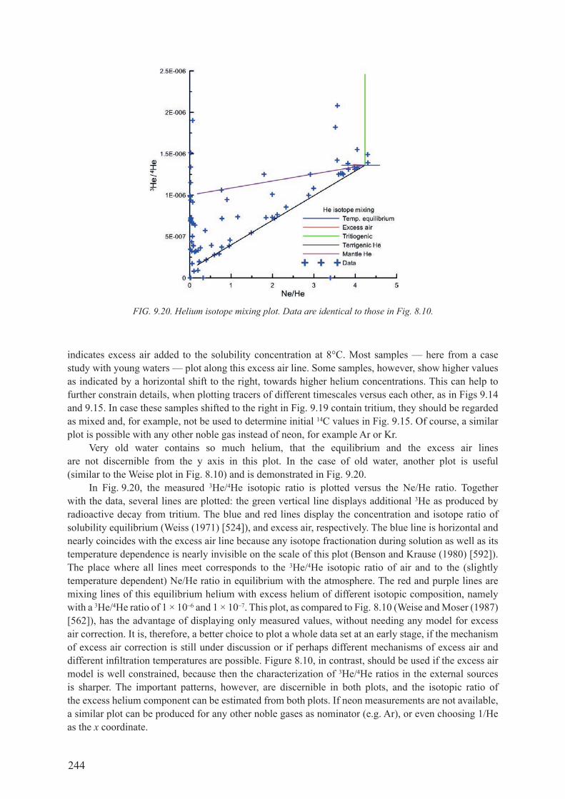
244

indicates excess air added  to  the  solubility concentration at 8°c. most  samples — here  from a case study with young waters — plot along this excess air line. some samples, however, show higher values as indicated by a horizontal shift to the right, towards higher helium concentrations. This can help to further constrain details, when plotting tracers of different timescales versus each other, as in figs 9.14 and 9.15. In case these samples shifted to the right in fig. 9.19 contain tritium, they should be regarded as mixed and, for example, not be used to determine initial 14c values in fig. 9.15. of course, a similar plot is possible with any other noble gas instead of neon, for example Ar or Kr.

Very old water contains so much helium, that the equilibrium and the excess air lines are not discernible from the y axis in this plot. In the case of old water, another plot is useful (similar to the weise plot in fig. 8.10) and is demonstrated in fig. 9.20.

In fig. 9.20, the measured 3he/4he isotopic ratio is plotted versus the ne/he ratio. together with the data, several lines are plotted: the green vertical line displays additional 3he as produced by radioactive decay from tritium. the blue and red lines display the concentration and isotope ratio of solubility equilibrium (weiss (1971) [524]), and excess air, respectively. The blue line is horizontal and nearly coincides with the excess air line because any isotope fractionation during solution as well as its temperature dependence is nearly invisible on the scale of this plot (Benson and Krause (1980) [592]). the place where all lines meet corresponds to the 3he/4he isotopic ratio of air and to the (slightly temperature dependent) ne/he ratio in equilibrium with the atmosphere. the red and purple lines are mixing lines of this equilibrium helium with excess helium of different isotopic composition, namely with a 3he/4he ratio of 1 × 10–6 and 1 × 10–7. this plot, as compared to fig. 8.10 (weise and Moser (1987) [562]), has the advantage of displaying only measured values, without needing any model for excess air correction. It is, therefore, a better choice to plot a whole data set at an early stage, if the mechanism of excess air correction is still under discussion or if perhaps different mechanisms of excess air and different infiltration temperatures are possible. figure 8.10, in contrast, should be used if the excess air model is well constrained, because then the characterization of 3he/4he ratios in the external sources is sharper. the important patterns, however, are discernible in both plots, and the isotopic ratio of the excess helium component can be estimated from both plots. If neon measurements are not available, a similar plot can be produced for any other noble gases as nominator (e.g. ar), or even choosing 1/he as the x coordinate.

FIG. 9.20. Helium isotope mixing plot. Data are identical to those in Fig. 8.10.

245

Chapter 10

nUMERICAL FLOW MODELs AnD tHEIR CALIbRAtIOn UsInG tRACER bAsED AGEs

w. sanfordunited states geological survey,reston, Virginia,united states of america

10.1. IntroductIon

Any  estimate  of  ‘age’  of  a  groundwater  sample  based  on  environmental  tracers  requires  some form of geochemical model to interpret the tracer chemistry (chapter 3) and is, therefore, referred to in this chapter as a tracer model age. the tracer model age of a groundwater sample can be useful for obtaining information on the residence time and replenishment rate of an aquifer system, but that type of data is most useful when it can be incorporated with all other information that is known about the  groundwater  system  under  study.  groundwater  fl ow models  are  constructed  of  aquifer  systems because they are usually the best way of incorporating all of the known information about the system 

FIG. 10.1. Flow chart of the groundwater fl ow modelling process (after Reilly (2001) [72]).

Define problemLiterature reviewPreliminary analysisData collection

Develop conceptual modelProcessesBoundary conditionsHydrogeologyData collection

Develop mathematical modelDifferential equationsAnalytical methodsNumerical methods

CalibrationHistory matchingSensitivity analysisData collection

Assessment of problem using model

Apply results

Re-evaluation of the problem and objectivesin light of the simulation results

Completion of project

246

in  the  context  of  a mathematical  framework  that  constrains  the model  to  follow  the known  laws of physics and chemistry as they apply to groundwater flow and transport. It is important that the purpose or objective of  the study be  identified first before choosing the  type and complexity of  the model  to be constructed, and to make sure such a model is necessary. The purpose of a modelling study is most often to characterize the system within a numerical framework, such that  the hydrological responses of the system can be tested under potential stresses that might be imposed given future development scenarios. As this manual discusses dating as it applies to old groundwater, most readers are likely to be interested in studying regional groundwater flow systems and their water resource potential.

model  development  occurs  in  stages  (fig. 10.1)  where  the  model  developer  must  (i)  define the problem and the purpose for the model; (ii) develop the conceptual model; (iii) design the model grid; (iv) calibrate the model (adjusting the hydraulic parameters to fit the available data); and (v) apply the model to predict future responses. In some cases, the purpose of the model may be only to improve the understanding of the flow system, in which case stage (v) might never be employed. given the high uncertainties associated with future predictions based on most models that have relatively limited data and complex hydrogeology, models are often most useful when used to understand and quantify the flow system at the end of stage (iv), or when the results of the predictions are still useful in spite of large accompanying error bars. all models represent systems based on data that are currently available, and so many studies require a return to the data collection phase after an initial model reveals where additional data are needed  to  improve model predictions. This  feedback between data and modelling  results  is often carried out as an interaction between the hydrologist constructing the model and the geochemist collecting and analysing the data. It is important for the two to have good communication and a working relationship. The  feedback  can  happen  both ways —  the  data  control  how  the model  is  developed, and the model results can indicate where and what type of additional data need to be collected. this chapter will cover the basics of model design, development and calibration, especially with the use of tracer model ages.

10.2. equatIons and nuMerIcal Methods

A groundwater  flow model  describes  the  distribution  of  heads within  an  aquifer  system  based on  the  solution  of  the  fundamental  groundwater  flow  equation,  which  can  be  derived  solely  from the principles of mass balance and darcy’s law. A general form of this equation for three dimensions, transient flow and constant fluid density can be written as:

, , ,x y z sh h h hK K K S Q x y z t

x x y y z z t

∂ ∂ ∂ ∂ ∂ ∂ ∂∂ ∂ ∂ ∂ ∂ ∂ ∂

(10.1)

whereh      is the hydraulic head within the flow system;Kx, Ky and Kz are hydraulic conductivity in the x, y and z directions, respectively;Ss     is the specific storage;Q     is a general source (+) or sink (–) of water to the aquifer system that can vary in space  

and time to represent injections or withdrawals at points in space or over regions or boundaries;

t is time.

The derivation of this equation can be found in standard textbooks on hydrogeology (domenico and Schwartz (1998) [8]; Schwartz and zhang (2003) [593]).

to solve this partial differential equation, a description of the hydraulic properties (K and Ss) are needed  in  three dimensions, head and/or flux conditions at  the boundaries of  the domain, and  initial conditions at the simulation starting time. for steady state conditions (often assumed for aquifers

247

under  pre-development  conditions),  the  left  term  on  the  right  side  of  Eq.  (10.1)  becomes  zero  and the specific storage is not a required parameter, nor is an initial condition required. The solution to this equation gives the distribution of head, h,  in  three dimensions, and  then by using darcy’s  law, flow rates within the aquifer can subsequently be calculated. The seepage velocity (that taken by a solute or water molecule) is the specific discharge divided by the porosity and, therefore, by using an estimate of porosity, one can simulate a velocity field within the aquifer by first solving the flow equation. given two points within the system along a flow path, the seepage velocity between those points divided by the distance yields a time of travel for water or, if the point of origin is the water table, a flow model age.

In some cases, it may be useful initially to consider the flow system as having a simple geometry and boundary conditions, to the extent that an analytical solution might be available. an analytical solution is a continuous solution across the domain where the head or hydraulic (or flow model) age value, for example, can be evaluated at any point. for some simple flow systems, the distribution of the flow model age can be represented by such a function (cook and Böhlke (1999) [594]). A number of other analytical solutions have been taken from the heat flow literature (carslaw and jaeger (1959) [539]), as heat flow is mathematically analogous to fluid flow in porous media. In most cases though, the geometry, boundary conditions and hydraulic parameter distribution are complicated to the extent that no analytical solution exists. for these cases, a numerical solution is the next best alternative. A numerical solution to the flow equation is a distribution of head values at a finite number of discrete, pre-specified  points  (or  nodes)  within  the  aquifer  system.  The  two  numerical  solution  techniques most commonly used to solve the flow equation are finite difference and finite elements. The former requires the user to define a rectangular grid of points or cells at which the solution will be obtained, and the latter requires points that are connected by elements that are usually triangular or rectangular in shape, but not necessarily arranged along a regular grid. the more points in the grid, the more detailed and accurate the solution to the equation, but the more computer time and storage are required. with current computer capabilities, it is possible to have of the order of one million nodes in a grid. finite elements provide the flexibility of arranging the nodes freely to fit the geometric features of the system, but such an arrangement requires more sophisticated graphical user interfaces to construct the ‘mesh’, as this could not be reasonably constructed manually if the node number were in the thousands or more.

many modelling  codes have been developed  that  solve  the  equations of  groundwater flow and solute transport, most of which are adequate for modelling a groundwater system. the only codes chosen to be listed here are those published and supported by the united states geological survey (usgs), not because they are necessarily superior, but because they have been the most widely used in the world (and, thus, widely tested), and perhaps more importantly for this manual because the codes and their user guides can all be downloaded free from the Internet (http://water.usgs.gov/software/). The most widely used groundwater flow code has been modfLow (mcdonald and Harbaugh (1988) [71]), of which the latest release is modfLow2005 (Harbaugh (2005) [595]). The code uses integrated finite  differences  and  has  a  number  of  different  ‘modules’  that  can  be  used  to  incorporate  different conceptual grid designs and different types of boundary conditions. one recent addition to Modflow is  the ability  to  refine  the grid  in subdomains of  local  interest within a more  regional coarse grid  in a process known as local grid refinement (mehl and Hill (2005) [596]; mehl and Hill (2007) [597]). Several graphical user interfaces for modfLow are available on the open market, but the USgS has also  created  one  recently  (winston  (2009)  [598])  that  is  free  of  charge. viewing  three  dimensional results from modfLow is possible through the post-processing programme modELvIEwEr (Hsieh and winston (2002) [599]).

10.3. aquIfer geoMetry and grId desIgn

once a decision has been made to create a numerical model of an aquifer system, one of the first steps is to begin to conceptualize how the system will be represented by a grid or mesh of nodes. A basic understanding of the aquifer system and its geometry (chapter 2) should be obtained before this grid

248

is created. although three dimensional simulation is now tractable computationally for most systems, sometimes a two dimensional model may be sufficient to meet the desired objective, or it may serve as a good preliminary model that will provide some key understanding for a much smaller investment of time and resources. a two dimensional areal model could be appropriate for an aquifer that is essentially a  single  hydrogeological  layer. on  the  other  hand,  in  sedimentary  basins,  a  two  dimensional  cross-section along a flowline can often provide the necessary vertical detail between multiple aquifers and aquitards, and can be simulated such that a great deal is learned about the contrast between the hydraulic conductivity of layers and how flow model ages would be influenced by such contrasts.

If a three dimensional model is to be constructed, some thought must go into how finely the layers are to be discretized in the vertical dimension, and how to balance the vertical resolution requirement with the horizontal grid resolution that is desired to represent landscape features. Aquifers and aquitards can be represented by single layers, but if solute transport and dispersion are to be represented (chapter 10.8), more than one model layer per hydrogeological layer is usually desirable. there are many issues to consider in grid design (Anderson and woessner (1992) [600]). All of the boundaries of the flow system of interest must be identified; sometimes, these boundaries are at a substantial distance from the sections of the system that are of most interest. some hydrologists prefer the analytical element  method  (Haitjema  (1995)  [601])  in  this  case,  which  can  more  efficiently  handle  distant boundary  conditions.  finite  elements  can  be  arranged  to  fit  boundaries  exactly. As  finite  difference grids are rectangular by nature and flow systems are not, certain sections of the grid will ultimately be outside of the flow system and must be characterized as inactive cells. refinement of the grid in certain subdomains can be accomplished either by using a finite element method or local grid refinement with finite differences. grid refinement can also be accomplished with finite differences by using variable grid  spacing,  which  is  usually  a  standard  option,  but  this  is  somewhat  less  efficient  (although  less complicated) than using local grid refinement.

hydrogeological units in sedimentary basins can be represented either by having them coincide exactly with model layers (fig. 10.2), or by treating them independently and then calculating the effective hydraulic parameters for each model cell depending on how the model layers intersect the  hydrostratigraphy. The  latter  approach  can be more  efficient when dealing with  highly  complex stratigraphy,  and  has  been made  easier  with  the  development  of  software  specifically  designed  for this  purpose  (Anderman  and  Hill  (2000)  [602]; Anderman  and  Hill  (2003)  [603]).  finite  element models are better designed to handle hydraulic conductivity fields whose directions of maximum and minimum values do not coincide with the rectangular grids of finite-difference methods (e.g. yager et al. (2008) [604]).

10.4. boundary condItIons

In  order  to  solve  the  flow  equation  for  the  domain  of  interest,  boundary  conditions  must  be specified  at  the  domain  boundaries.  mathematically,  these  boundary  conditions  take  the  form  of constant head, specified flux or mixed type. In order to create a model that simulates the conditions that occur in the real system, the real hydraulic boundaries must be expressed in terms of one of the three mathematical types.

constant head is for boundaries where the head will remain constant no matter what stress is placed within the system; the internal changes in head will not affect the head at this boundary. an ideal example of this would be a large body of water, such as the ocean, that has such a large reservoir of water whose level will not be affected by changing flow conditions within the domain. Specified flux can represent a number of different field conditions. on the external boundaries, a flux of zero represents an impermeable surface. this is often the condition placed on the bottom boundaries or lateral edges of the domain. A groundwater divide would also represent a specified flux of zero. recharge at the top boundary is a very common flux that is specified at the top boundary of the domain. recharge can be distributed across the top of the model in a fashion that is consistent with field conditions. In humid 

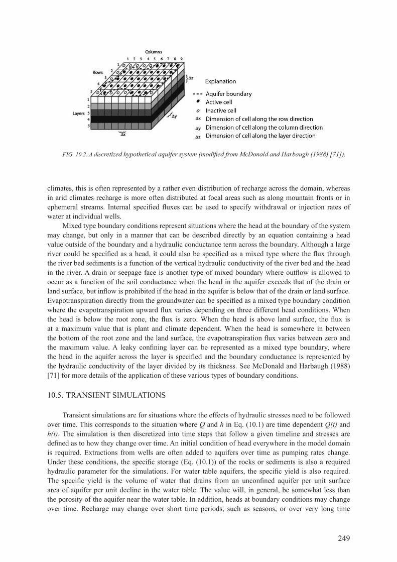
249

climates, this is often represented by a rather even distribution of recharge across the domain, whereas in arid climates recharge is more often distributed at focal areas such as along mountain fronts or in ephemeral  streams.  Internal  specified fluxes  can  be  used  to  specify withdrawal  or  injection  rates  of water at individual wells.

Mixed type boundary conditions represent situations where the head at the boundary of the system may change, but only in a manner that can be described directly by an equation containing a head value outside of the boundary and a hydraulic conductance term across the boundary. although a large river could be specified as a head,  it could also be specified as a mixed type where the flux through the river bed sediments is a function of the vertical hydraulic conductivity of the river bed and the head in  the river. A drain or seepage face  is another  type of mixed boundary where outflow is allowed to occur as a function of the soil conductance when the head in the aquifer exceeds that of the drain or land surface, but inflow is prohibited if the head in the aquifer is below that of the drain or land surface. Evapotranspiration directly from the groundwater can be specified as a mixed type boundary condition where the evapotranspiration upward flux varies depending on three different head conditions. when the  head  is  below  the  root  zone,  the  flux  is  zero. when  the  head  is  above  land  surface,  the  flux  is at a maximum value that is plant and climate dependent. when the head is somewhere in between the bottom of the root zone and the land surface, the evapotranspiration flux varies between zero and the maximum  value. A  leaky  confining  layer  can  be  represented  as  a mixed  type  boundary,  where the head  in  the aquifer across  the  layer  is specified and  the boundary conductance  is  represented by the hydraulic conductivity of the layer divided by its thickness. See mcdonald and Harbaugh (1988) [71] for more details of the application of these various types of boundary conditions.

10.5. transIent sIMulatIons

transient simulations are for situations where the effects of hydraulic stresses need to be followed over time. this corresponds to the situation where Q and h in eq. (10.1) are time dependent Q(t) and h(t). The  simulation  is  then discretized  into  time  steps  that  follow a given  timeline  and  stresses  are defined as to how they change over time. An initial condition of head everywhere in the model domain is required. extractions from wells are often added to aquifers over time as pumping rates change. Under  these conditions,  the specific storage (Eq.  (10.1)) of  the rocks or sediments  is also a required hydraulic parameter  for  the  simulations. for water  table aquifers,  the  specific yield  is also  required. The  specific  yield  is  the  volume  of  water  that  drains  from  an  unconfined  aquifer  per  unit  surface area of aquifer per unit decline in the water table. the value will, in general, be somewhat less than the porosity of the aquifer near the water table. In addition, heads at boundary conditions may change over time. recharge may change over short time periods, such as seasons, or over very long time

FIG. 10.2. A discretized hypothetical aquifer system (modified from McDonald and Harbaugh (1988) [71]).

250

periods, as the result of climate change. for regional systems where old groundwater has been dated, the travel times of the groundwater are usually of the order of thousands of years or more. In these cases, simulating steady state conditions as they existed before aquifer development began is frequently the approach taken. It is often more realistic for long time periods if a transient simulation is chosen and recharge is varied to simulate changing climate, during the recent ice age, for example.

10.6. Model calIbratIon

the objective of most groundwater modelling studies is to create the best numerical model of the aquifer system possible given the available data on the hydraulic characteristics of the system. Adjusting  the hydraulic parameters of  the model until a best or satisfying fit  to  the observed data  is achieved is known as the ‘model calibration’ (Hill (1998) [605]; Hill and Tiedeman (2007) [606]). This should not be confused with the terms ‘model verification’, which refers to the testing of the mathematics in the code to solve the equations accurately, and ‘validation’, which refers to the general process of producing a model that is ‘valid’ or represents the system well — although, in a strict sense, groundwater models  cannot  be  validated  (Konikow and Bredehoeft  (1992)  [607]). The hydraulic  parameters  that need to be adjusted during calibration include the hydraulic conductivity of the hydrogeological units and  potentially  its  distribution  within  the  units,  recharge  and  its  distribution,  and  specific  storage for transient problems. observed data almost always include head measurements and some type of measurements  or  estimates  of  flux.  Some  knowledge  of  the  hydraulic  properties  of  the  rocks  or sediment is often known a priori, as is some estimate of recharge. This is frequently referred to as prior information. as prior information is usually obtained from small scale or local tests or studies, and a model is most often developed to represent a large scale or regional system, the prior information is not usually assigned directly to the parameters, but rather serves as a guide for reasonable values within which the parameters should be adjusted during the calibration process.

As the model is based on darcy’s law, using only heads and head gradients as observations will result  in a very, if not completely, non-unique calibration. The head gradient is based on the ratio of the flux to the hydraulic conductivity, so using head values alone will only constrain the ratio of flux to hydraulic conductivity, not individual values of either. Thus, some type of flux observation needs to be included in addition to heads. The most common flux observation used is the baseflow to a stream. The baseflow is directly related to the long term recharge in the stream’s watershed. Although recharge is  also  a  flux,  it  usually  cannot  be measured  directly  as  an  observation,  especially  in  an  integrated manner over space and time, and so it is often adjusted as a parameter of the model. tracer model ages give  information on  the  travel  time  (flux) within  the  system, and  so can also be used  in addition  to hydraulic head data, or in addition to both hydraulic-head and base flow data to calibrate a model.

the simplest approach to calibrating a model is by trial and error. It is recommended to start with a simpler model and add complexity over time as the data permit. If there are only a few parameters in a model to adjust, they can be adjusted by hand to create the model that best fits the observed data. for any given set of parameter values, the model is run and the simulated values at the observation locations are compared with the data collected from those observation locations. the goal is to minimize the error difference between the simulated and observed data, most often done by calculating the sum of the squared errors (or some similar quantity). as computers have become faster, they have allowed models to become more complex to the point that they can include dozens or more parameters (usually these are different values of hydraulic conductivity in different units and regions of the model). automated parameter estimation codes have been developed to greatly accelerate the calibration process (doherty (2004) [608]; Poeter et al. (2005) [609]). These codes are shell programmes that are able to call  any model  and keep adjusting  the parameters  and  rerunning  the model  in  a direction  that  leads to the minimization of the total sum of squared errors. This is done through a continuous cycle of (i) changing the parameter values in the input files, (ii) running the model and (iii) examining the simulated observations. The result is a set of parameters that gives a model with the best fit to the data. However, 

251

the best fit does not always indicate the best model and the calibration process must be guided carefully to avoid erroneous parameter values (Hill (1998) [605]; reilly and Harbaugh (2004) [610]).

10.7. calculatIon of flow Model ages

In order to use tracer model ages to calibrate a model, the model must be able to simulate a flow model age. Alternatively,  a  tracer concentration at  any given point  (usually a well or  spring) can be simulated and compared directly with the measured concentrations, an approach discussed in Section 10.8. one simple and straightforward way to obtain an age from a flow model is to calculate it as a hydraulic time of travel. This is done by dividing the distance between two points along a flowline by  the  interstitial  velocity  calculated using darcy’s  law.  In  a  discretized groundwater model,  this  is done over regional distances by calculating the advective path line that an imaginary particle of water will travel along through the aquifer from one model cell to the next, and the time required to move along  the  path  line  given  the  hydraulic  conditions  defined  in  the  model.  Solute  dispersion  within the groundwater system for this type of calculation is neglected, and although this is not reality, and it  is known  to  introduce some error during a calibration process,  that error  is often small  relative  to the uncertainties in the hydraulic properties of the system. finite difference groundwater models are aptly suited for the calculations of such path lines and flow model ages. velocities at cell boundaries can be calculated from the head values at  the cell nodes using darcy’s  law and a specified porosity. A particle of water can be followed from cell to cell, either forwards or backwards, from any specified starting point based on the calculated velocity field for the model grid. A post-processing programme (modPATH;  Pollock  (1994)  [611]),  available  for  use with modfLow,  calculates  such  path  lines and  travel  times.  To  calculate  a  unique  path  that  a  particle  of  water  would  follow  across  a  finite-difference  cell,  the  assumption  is first made  that  the velocity  along each coordinate direction varies only in that coordinate direction and not along the other directions (fig. 10.3). this assumption allows the simplification of the calculation of the distance travelled to the far side of a cell as a smooth curved path. the time required to traverse that distance in the x direction becomes:

∆∆

tx

V VVVx x

x

xp

=−

2 1

2ln (10.2)

where∆t is the travel time to the far side of the cell;∆x is the distance to the far side the cell;Vx2 is the velocity at the far cell wall;Vx1 is the velocity at the near side of the cell;Vxp is the velocity at the x location of the particle.

the integration of the changing velocity across the cell yields the natural log term in eq. (10.2). a similar equation is written for the y direction. whichever ∆t is less (x or y) is the time of travel to the cell wall at the point the particle exits the cell. the exit point can then be calculated and the exit point  becomes  the  entrance  point  of  the  neighbouring  cell.  The  particle  is,  thus,  tracked  through the cells until a discharge cell is reached (or a recharge cell if backward tracking is being used). full details on these particle calculations can be found in Pollock (1994) [611]. for finite element models, the velocity is usually regarded as a constant across any given element, and so similar travel times could be calculated for particles to traverse elements. no such software has, however, currently been developed for the widely used finite-element code SUTrA.

Hydraulic path line simulations can be made either in the forwards or backwards direction. Thus, in Modpath, the time of travel of a particle can be calculated from the water table forwards to its

252

FIG. 10.3. Schematic showing the computation of exit point and travel time for the case of two dimensional flow in the x–y plane (after Pollock (1994) [611]).

FIG. 10.4. Simulated flow paths and flow model ages in the Middle Rio Grande Basin in comparison with 14C model ages (after Bartolino and Cole (2002) [612]).

253

discharge location (e.g. a stream) or the time of travel can be calculated from a well screen backwards to its recharge location (e.g. the water table). The latter can be used to calculate a flow model age at any point within an aquifer system given the set of parameters currently being assigned to the model. for  a  transient  flow model  (e.g.  with  transient  recharge),  the  procedure  has  the  added  requirement of  storing  the  flow field  at  each  time  step.  flow model  ages  can  be  calculated  for multiple  sites  at a time and, therefore, a set of tracer model ages can be compared with the flow model ages (fig. 10.4) intermittently as parameters are adjusted during the calibration, and the errors can be added to the total sum of squared errors being calculated for the model calibration. for long screen wells, multiple particles can be simulated along the well screen, with the result being a range of different flow model ages assigned  to and  ‘mixing’  in  the well bore.  It  should be noted, however,  that  for  environmental tracers it is the concentration of the solute species that is actually mixing and not idealized groundwater ages. for tracers where the solute or isotopic concentrations are not linear functions of time, the average of the flow model ages will not give the equivalent result to the more appropriate average of simulated concentrations that are each back calculated from the flow model ages. A useful visualization technique is to start particles at the centre of every cell in the model and track backwards to the origin location. all of the travel times for these paths are then plotted at their starting cell locations. the result is the flow model age distribution throughout the entire system that can be visualized in two dimensions as maps of flow model age across an entire model layer or cross-sections (e.g. fig. 13 of Sanford et al. (2004) [47]).

10.8. sIMulatIon of dIspersIon and apparent groundwater age

Advective path lines and flow model ages are straightforward to calculate following groundwater flow simulations, but environmental tracers are subject to hydrodynamic dispersion as well as advection. dispersion of a solute occurs because heterogeneity in the hydrogeological framework creates variations in velocities from the pore scale to the field scale. These heterogeneities are inherently present but too small  to discretize  all  into  the model domain. A potentially more  accurate model  calibration can be undertaken if the effect of the dispersion on the tracer is also known and simulated. Such a simulation could produce dispersion model ages, as opposed to the previously discussed flow model ages, which are strictly advection model ages. the advection–dispersion transport equation can be written with concentration as the dependent variable and groundwater velocity as a parameter in cartesian–tensor notation as:

'C C

D CV C Q Rij ix x x ti j i

∂ ∂ ∂ ∂

∂ ∂ ∂ ∂ (10.3)

whereC is concentration;Vi is the seepage velocity;C ꞌ  is the concentration of a fluid entering the domain at rate Q;R is the chemical reaction rate of the solute or isotopic species;Dij the hydrodyanamic dispersion tensor, which is a function of the velocity components in each

direction, the dispersivity and molecular diffusion (Konikow and grove (1977) [613]).

The  velocity  field  is  predetermined  from  the  flow  simulation  and  can  vary  in  space  and  time. the source term Q and reaction term R can also vary in space and time. the dispersivity is a parameter that describes the inherent make-up of the porous or fractured media that causes spreading, and is usually assumed to simplify into two components, a longitudinal dispersivity that is parallel to the direction of flow and a  transverse dispersivity that  is perpendicular  to  the direction of flow. In three dimensional flow systems, two different transverse dispersivities can be used that are perpendicular to each other.

254

Several codes have been developed that solve Eq. (10.3) (Koch and Prickett (1993) [614]; Konikow et  al.  (1996)  [615]; voss  and Provost  (2002)  [616]; zheng  and wang  (1999)  [617]). The  numerical methods used are either Eulerian (fixed reference frame) or Lagrangian (moving reference frame), or a  combination  of  the  two. Eulerian  techniques  include finite  differences  or finite  elements, whereas Lagrangian techniques include random walk or the method of characteristics. The nature of Eq. (10.3) is such that  in systems with a high ratio of velocities  to dispersivities (known as  the Peclet number) Eulerian mathematical solutions (e.g. standard finite differences or finite elements) become unstable. Thus,  when  simulating  transport  with  dispersion,  special  care must  be  taken  to make  the  grid  fine enough to avoid numerical oscillations or numerical dispersion. The random walk method tracks a large number of particles, most often from a point source, and randomly adds variability to the particle path in directions both longitudinal and transverse to the flow direction (Prickett et al. (1981) [618]). As this method requires large numbers of particles to get repeatable results, it is not often feasible to use in regional transport problems where tracer model ages are measured. the method of characteristics was developed as a particle tracking technique with the advantage of particle tracking, but with a Eulerian dispersion component, but it has its own set of inherent limitations (Konikow and Bredehoeft (1978) [619]). for all of these methods, the fine resolution requirement of the grid often precludes full three dimensional advection–dispersion simulations of an aquifer on a regional scale.

The final term of Eq. (10.3), R, represents the chemical reactions that the tracer of interest may be involved in that either remove it from or add it to the solution. radioactive decay is the most common of these that would be included for environmental tracers when the objective is to simulate the  concentration  field  of  the  tracer  directly.  carbon-14  has  a  number  of  potential  reactions  and exchanges that can take place with the mineral phase in the aquifer material (e.g. Kalin (1999) [111]; see chapter  4),  and  such  reactions  could  also  be  included  if  the  14c  concentration  field were  to  be simulated directly. geochemical codes are available that solve multiple species reactions with transport in one (PHrEEqc; Parkhurst and Appelo (1999) [149]) or more (PHAST; Parkhurst et al. (2004) [200]) dimensions. each of the tracers that might be used to date old groundwater that are described in this book have their own set of issues to be considered when using their tracer model ages in conjunction with a flow and/or transport model. A list of these tracers and the issues are listed in Table 10.1. A more general table of old age tracers are listed in table 1.1.

reviews of field studies by gelhar (1986) [620] and Schulze-makuch (2005) [621] have suggested that dispersivity is scale dependent and that the longitudinal dispersivity is roughly about 10% of the distance of  travel; however,  the most detailed field studies (LeBlanc et al.  (1991) [622]) suggest that this may greatly overestimate dispersivity, which can often be closer to 1% of the distance of travel. transverse dispersivity is typically 1–10% of the longitudinal dispersivity. dispersivity almost certainly also varies spatially within most formations and is difficult to measure directly without special tracer tests, so although dispersion can be simulated, the uncertainty with respect to the accuracy of simulated concentration fields is usually high. one regional effect is that under steady state conditions 

table 10.1. tracer Methods and Issues to consIder for joInt use wIth nuMerIcal flow Models

tracer method Issues to consider14c Long term variable input, definition of initial 14c, often reactive, dispersion, matrix diffusion

he generated in situ, uncertain production rate, quantifying basin flux36cl long term variable input, mixing with other cl sources, matrix diffusion

81Kr Input variations only in the very long term, sampling still difficult at the time of the publication of this book

u generated in situ, uncertain production rate

255

(not  always  applicable)  the  flow  model  age  of  groundwater  is  not  a  function  of  the  interchange (transverse dispersion) of solutes between aquifers and interbeds, but simply a function of the ratio of  the  total porosity of  the  system  to  the porosity of  the aquifer  (Bethke and johnson  (2002)  [623]; Sanford (1997) [207]). for  tracers with  long half-lives (e.g.  14c and 36cl), the relatively constant (or slowly changing) input function through time creates a condition where the longitudinal dispersion of the solute is relatively small (5–10%) relative to its decay rate (johnson and dePaolo (1996) [624]), indicating that advective path line and flow model age calculations may not be a bad assumption for many old groundwater simulations.

In spite of the uncertainty associated with the simulation of dispersion in groundwater, hypothetical simulations can illustrate well the expected behaviour on environmental tracers. when possible, it is most straightforward to simulate the tracer of interest, as each tracer may have a different input function or reactive behaviour in the subsurface. these individual tracer characteristics can be included directly  in  the  simulation  parameters. A more  generalized  approach  is  also  possible where a dispersion model  age can be  simulated directly  (goode  (1996)  [69]) by  setting R in eq. (10.3) to a value of one, and Q to zero. This approach is often known in the modelling community as ‘direct age simulation’. The reaction  term R  is used  to represent  the passing of  time and  the concentration field becomes the dispersion age field. much discussion has surrounded the simulation of dispersion model ages  in  this manner (Bethke and johnson (2008) [84]; Perrochet and Etcheverry (2000) [625]; varni and carrera (1998) [83]). The technique for simulating the dispersion model age can also be used to calculate the frequency distribution of groundwater ages expected to be encountered at a sampling site such as a  long screened well  (varni and carrera  (1998)  [83]). A dispersion model age simulation  is useful for visualizing the potential impact of dispersion on advection model age simulations (fig. 10.5). This approach is also useful for finite element models that do not have advection model age calculation software available. from fig. 10.5, it can be seen that dispersion spreads out the transport model age

FIG. 10.5. The effect of dispersion on the patterns and magnitudes of flow model ages. Dashed lines are equipotentials. Arrowed lines are flow directions. Solid lines without arrows are contours of equal advection or dispersion model age (in years). Grey regions have lower hydraulic conductivity. (Modified from Goode (1996) [69]).

256

and  typically  reduces  the  size and magnitude of pockets of old water  that may  result  from stagnant regions of circulation.

10.9. Model calIbratIon usIng tracer based ages

a number of regional modelling studies have used tracer model ages effectively as constraints (e.g. castro et al. (1998) [96]; Park et al. (2002) [90]; Sanford and Buapeng (1996) [626] and Sanford et al. (2004) [47]). Some of these studies have been described in detail in other chapters of this manual. Tracer model ages can be valuable data with which to help calibrate a model (Sanford (2011) [627]). They provide information directly related to the fluxes in the system, which are often more difficult to obtain than heads. Baseflows to streams, a common measurement of flux in the system, cannot always be easily measured, especially in arid environments, and so tracer model ages can provide another much  needed  source  of  flux  data.  Tracer  model  age  data,  however,  require  one  additional  type  of information, porosity, to be used as model constraints. flow model ages are based on travel paths that are based on seepage velocities that include porosity in their calculations. Simulated baseflows do not require porosity measurements. this porosity requirement does not necessarily hamper the use of tracer model ages to calibrate a model. In unconsolidated sediments, porosity can often be easily estimated or measured and so can be added to the model as prior information. when both baseflow and tracer model age data are available in hard rock terrains, the tracer model ages can help constrain the porosity, which might otherwise be poorly known.

A  number  of  different  hydraulic  characteristics  of  a  groundwater  flow  system  can  affect the  distribution  of  the  flow model  age  within  that  system  (fig. 10.6),  including  the  distribution  of recharge, the vertical anisotropy and the regional scale heterogeneity. homogeneous systems with

FIG. 10.6. Spatial patterns of groundwater age as a result of various distributions of recharge and hydraulic conductivity (K). Contour values are flow model age (in years). Arrows show general direction of flow. The vertical anisotropy ratio in the middle set of simulations is 10 000 horizontal to 1 vertical. The confining layer contrast in K in the lower set of simulations is 1000 to 1. (After Sanford (2011) [627].)

257

evenly distributed recharge can be expected to have flow model ages that increase with depth and have lines of equal flow model age that are nearly horizontal. If  the recharge is distributed predominantly towards  the upper  reaches of  the flow system, however, as  is often  the case  in arid environments or low  lying areas where  the water  table closely mimics  the  topography,  the  lines of equal flow model age can become closer to vertical. Increasing vertical anisotropy in a system nearly always increases the vertical gradient in the flow model age.

regional  heterogeneities  such  as  confining  layers  can  create  pockets  of  older  water  where substantial vertical hydraulic gradients are not present. In general, the distribution, connectivity and vertical hydraulic conductivity of the confining layers are one of the largest controlling factors on both the flow model ages and the tracer model ages within a groundwater flow system. The conceptual model adopted  for  the  presence  of  confining  layers  is  important.  for  example,  a  system conceptualized  as having a large regional vertical anisotropy, but not a discrete heterogeneity, cannot under any conditions yield a depth profile of flow model ages that are overturned (younger beneath older), whereas overturned tracer model ages in regional systems are not uncommon in discharge areas. the fact that hydraulic properties  can  greatly  impact  the  flow model  age  distribution  is  equally  an  indicator  that  spatially distributed  tracer  model  age  data  can  provide  good  information  on  the  nature  of  the  flow  system. this equally demonstrates that tracer model age data can be quite valuable in constraining conceptual and numerical models of flow systems. This  is additionally supported by  the fact  that  regional scale confining unit properties are often the most difficult to measure directly.

A  number  of  field  studies  using  tracer model  ages  to  calibrate  groundwater  flow models  have demonstrated that matching of individual flow model ages to tracer model ages is more difficult than matching simulated water  levels  to observed water  levels. water  levels  represent a potential field of energy within a groundwater system, and as such values vary relatively smoothly within the system as a function of the spatial distribution of the hydraulic property distribution and the boundary conditions. In addition, boundary conditions using specified water levels already partially constrain the simulated water level values. on the other hand, flow model ages are calculated based on the velocity field, which is based on the gradient or first derivative of the water level (potential) field. As the flow field is usually complicated by heterogeneity  in  the hydraulic properties and recharge distribution,  the velocity field is usually relatively complex both in magnitude and direction. It, therefore, becomes very common for  the variations  that  exist within  the velocity fields  (creating,  for  example,  local flow cells within regional  flow  cells)  to  be  misrepresented  at  the  very  local  scale  at  which  the  tracer  samples  were collected and  the flow model ages were simulated. A well screen,  for example, may be  located near the boundary between a local and regional flow subsystem, and the slightest misrepresentation of those systems in  the model might cause the equivalent flow model age to be calculated at a very different value because it is located within the wrong flow subsystem. In addition, the first derivates (velocities) are not continuous across the boundaries of flow subsystems, and this can further complicate automated calibration tools that rely on the parameter sensitivities (first derivatives). The resulting end effect very often appears like a poor match between tracer model ages and flow model ages. Two recent examples of this using 14c model ages demonstrate this issue (fig. 10.7). Although this demonstrates the difficulty in using tracer model ages to calibrate flow models at fine scales, it still does not negate the usefulness of tracer model ages in the calibration of flow models at coarser scales.

In spite of the usefulness of tracer model ages in model calibration, a number of caveats should be noted. Steady state model assumptions are often used for regional models with relatively old flow model ages, but these assumptions are not always valid. climatic changes leading to changing recharge rates over time may need to be considered. substantial groundwater withdrawals from wells may also need to be included in the model as these can affect the distribution of flow model and tracer model age  in  the system (zinn and Konikow (2007)  [628]). Use of advection model ages alone will create some degree of  error  from  the  lack of  considering dispersion. Simulating dispersion with  advection can reduce this error, but the uncertainty in the appropriate field dispersivities to assign to the model may  offset  this  benefit.  Simulation  of  dispersion  in  three  dimensions  is  also  computationally  very 

258

challenging on a regional scale without introducing numerical dispersion (sanford and pope (2010) [629]). Thus, although, in theory,  it  is possible to simulate dispersion model ages,  this is usually not tractable for three dimensional groundwater models. In spite of the assumptions behind advection model age simulation, it is still an efficient and potentially very useful tool for model calibration. This is especially  true considering  that  there  is often a  lack of other basic flux  information  in addition  to that provided by tracer model ages, and groundwater models lacking in adequate flux information can remain relatively unconstrained.

FIG. 10.7. Plots of observed versus simulated water levels in (a) central Hungary and (b) New Mexico, USA; and 14C model and flow model ages in (c) central Hungary and (d) New Mexico, USA (after Sanford et al. (2004) [47] and Sanford et al. (2001) [630]). It should be noted that the age plots are in log–log scale, yet still have more visual scatter around the perfect match (solid) lines than the water level plots.

259

Chapter 11

MILk RIVER AQUIFER, ALbERtA, CAnADA — A CAsE stUDY

K. frÖHLIcHVienna, austria

11.1. IntroductIon

The milk river  aquifer  is  a  complex  system  in  terms  of  origin  and  evolution  of  the  chemical and isotopic composition of the groundwater. fortunately, a wealth of physical and chemical data of the groundwater and the bonding shales was collected by numerous authors over a period of about 15 a that allowed applying various complementary approaches in dating the groundwater. although these milk river aquifer studies were carried out more than two decades ago, they can still be considered an outstanding example for dating of old groundwater.

The  milk  river  aquifer  fits  the  definition  of  an  idealized  confined  aquifer  system,  and  dips gently  from  its  outcrop  area  (~5  m/km).  A  short  distance  from  the  recharge  area,  the  ‘idealized groundwater age’1 extends beyond the 14c dating limit and further downstream reaches values up to more than one million years. owing to this feature, the milk river aquifer was selected for an IAEA sponsored international project that was aimed at evaluating all isotope techniques available for dating of old groundwater; it finally resulted in the most comprehensive application of isotope and geochemical techniques to an individual aquifer system at that time. analyses were carried out for halides and other major and minor ions, stable isotopes (2h, 3he, 4he, 13c, 18o) and radioactive isotopes (222rn, 85Kr, 37ar,

39ar, 14c, 81Kr, 36cl, 129I, 234u, 238u). the results of the various isotopic and geochemical studies were published in a special edition of Applied geochemistry (Ivanovich et al. (1991) [631]). The following is a summary and comparative discussion of the results, with particular emphasis on the determination of the groundwater age in the milk river aquifer system.

11.2. gEoLogIcAL ANd HydroLogIcAL BAcKgroUNd

The milk river aquifer underlies 15 000 km2 of southern alberta. Most of the area is covered by Pleistocene glacial  drift  (Hendry  et  al.  (1991)  [632]). The  aquifer  crops out  in  southern Alberta, canada,  predominantly  on  the  flanks  of  Sweetgrass Hills,  northern montana, USA,  at  the  southern end of  the study area  (fig. 11.1). The milk river formation  is composed of sandstone  (30–75 m  in thickness) sandwiched between shales. It is confined above by marine shale of the Pakowki formation (typically 120 m thick) and below by the colorado group that ranges in thickness from 500 to 650 m (fig. 11.2). the transmissivity of the aquifer decreases from south to north, and from west and east.

this decrease is caused by a general thinning of the sandstone in these directions and a decrease in hydraulic conductivity towards the north due to an increase in the shale content. the groundwater flow  is generally  towards  the north, west  and east,  following  the dip of  the  aquifer. Two main flow paths were identified by valleys of low cl– concentrations (fig. 11.3). since the sandstone pinches out in all directions,  the aquifer must discharge by upward and downward leakage. All water that leaves the aquifer must, therefore, pass through the shale/sand interface. Hendry and Schwartz (1988) [633] suggested that about 500 ka ago the outcrop area was uncovered by erosion and meteoric water replaced connate water at that time. In fact, groundwater model ages of this order were found by 36cl dating (Phillips et al. (1986) [319]).

1   The  ‘idealized  groundwater  age’  is  defined  in chapter  3  of  this  book.  for  the  sake  of  simplicity,  in  the  following the expression ‘groundwater age’ is used.

260

11.3. the role of geocheMIstry In constraInIng water and solute TrANSPorT modELS — THE mILK rIvEr AqUIfEr ExPErIENcE

The  geochemistry  of  the  milk  river  aquifer  was  studied  by  numerous  authors  (Hendry  and Schwartz (1988) [633]; Hitcheon and friedman (1969) [634]; meyboom (1960) [635]; Phillips et al. (1986) [319]; Schwartz and muehlenbachs (1979) [636]; Schwartz et al. (1981) [637]; Swanick (1982) [638]). It is characterized by significant changes in major ion concentrations along the groundwater flow. Ion exchange of ca2+ (and Mg2+) for na+ creates calcite undersaturation that forces calcite dissolution down the flow path and raises the Hco! concentration. concentrations of so%– are high in groundwater of the recharge area but due to bacterial reduction virtually disappear in the central part of the aquifer. the concentrations of cl– and I– strongly  increase  in  the flow direction; near  the recharge area,  they are less than 0.5 and 0.001 mmol/l, respectively, and increase to more than 100 and 0.15 mmol/l,

FIG. 11.1. Study area (from Hendry and Schwartz (1988) [633]).

FIG. 11.2. Geology of the Milk River aquifer along the S–N cross-section (from Hendry et al. (1991) [632]).

261

respectively, at the northern edge of the aquifer. similarly, the 18o (δ2h) values increase from less than –21‰ (–167‰) near the recharge area to –8‰ (–70‰) in the north. while the δ18o and δ2h values of the recharge waters plot on the global meteoric water line, further downstream, the data deviate from  the meteoric water  line  and  fit  a  line with  a  slope  of  6.3  instead  of  8  (Hendry  and  Schwartz (1988)  [633]).  Several  alternative  mechanisms  were  proposed  to  explain  the  observed  distribution of  non-reactive  species  in  the milk river  aquifer  (fig. 11.4):  (i)  introduction  of  connate  formation water  through  the colorado shale and subsequent mixing with  infiltrating meteoric water  (Schwartz and muehlenbachs  (1979)  [636];  Schwartz  et  al.  (1981)  [637]);  (ii) meteoric  recharge mixing with more  saline water  in  the  aquifer  (domenico  and robbins  (1985)  [639]);  (iii)  chemical  and  isotopic enrichment due to ion filtration (Phillips et al. (1986) [319]); and (iv) aquitard diffusion (Hendry and Schwartz (1988) [633]).

Hendry  and  Schwartz  (1988)  [633]  reviewed  the  previously  proposed  mechanisms  (i)–(iii), especially  ion  filtration,  and  concluded  that  these  mechanisms  are  not  supported  by  hydraulic conductivity and hydraulic head data, cl– concentrations of drill cuttings and isotope values from colorado shale groundwater. they proposed an alternative mechanism based on diffusion between saline, isotopically enriched water of the colorado shale and fresher, isotopically depleted water in the aquifer. using an analytical mass transport model, the authors found that the pattern in cl–, I–, δ18o and δ2H in the aquifer can be explained by aquitard diffusion. The best model fit to both cl– and δ18o data yielded an effective aquitard diffusion coefficient  (the most critical parameter  in  the model) of 6 × 10–12 m2/s for these species. on the basis of this aquitard diffusion mechanism, Hendry and Schwartz (1988) [633] evaluated 36cl data published by Phillips et al. (1986) [319]. The derived 36cl model ages of the groundwater were found to be consistent with earlier age estimates based on hydraulic modelling (Swanick  (1982)  [638]).  consequently, Hendry  and  Schwartz  (1988)  [633]  concluded  that  aquitard 

FIG. 11.3. Contour plot of the Cl concentrations with the two main flow paths (I = eastern flow path, II = western flow path) along the valleys of the Cl concentrations. The numbers give the concentration in mmol/L (from Nolte et al. (1991) [291]).

262

diffusion must be considered when using 36cl to date groundwater in aquifer–aquitard systems such as the milk river aquifer.

In  contrast,  Phillips  et  al.  (1990)  [640]  concluded  from  an  in-depth  review  of  Hendry  and Schwartz’s arguments, that there was no evidence for aquitard diffusion. on the basis of a Peclet number analysis with parameter values selected from Hendry and Schwartz’s paper, they found that “transport in the aquitard is strongly advection dominated”. however, it should be noted that the peclet numbers referred  to by Phillips et al.  (1990)  [640] are proportional  to  the square of  the seepage velocity and that this parameter was estimated from the measured hydraulic conductivity. given that the hydraulic conductivity values of the aquitard ranged from less than 10–11 up to about 10–8 m/s (hendry and Schwartz  (1988)  [633]),  it  can  be  concluded  that  the  uncertainty  of  the  Peclet  numbers  estimated by Phillips  et  al.  (1990)  [640]  is very high. Thus,  the observed ambiguity  in  the conceptual models on  the  solute  transport  appears  to be associated with high uncertainty of  the field data used  in both approaches. Phillips et al. (1990) [640] came to the conclusion that “the reality is that we very seldom posses even a  fraction of  the field data necessary  to constrain  such models”.  It  should, however, be 

FIG. 11.4. Conceptual models to explain the origin of chemical patterns in the Milk River aquifer: (a) megascopic dispersion; (b) partial area of recharge; (c) membrane filtration; and (d) aquitard diffusion (from Hendry and Schwartz (1988) [633]).

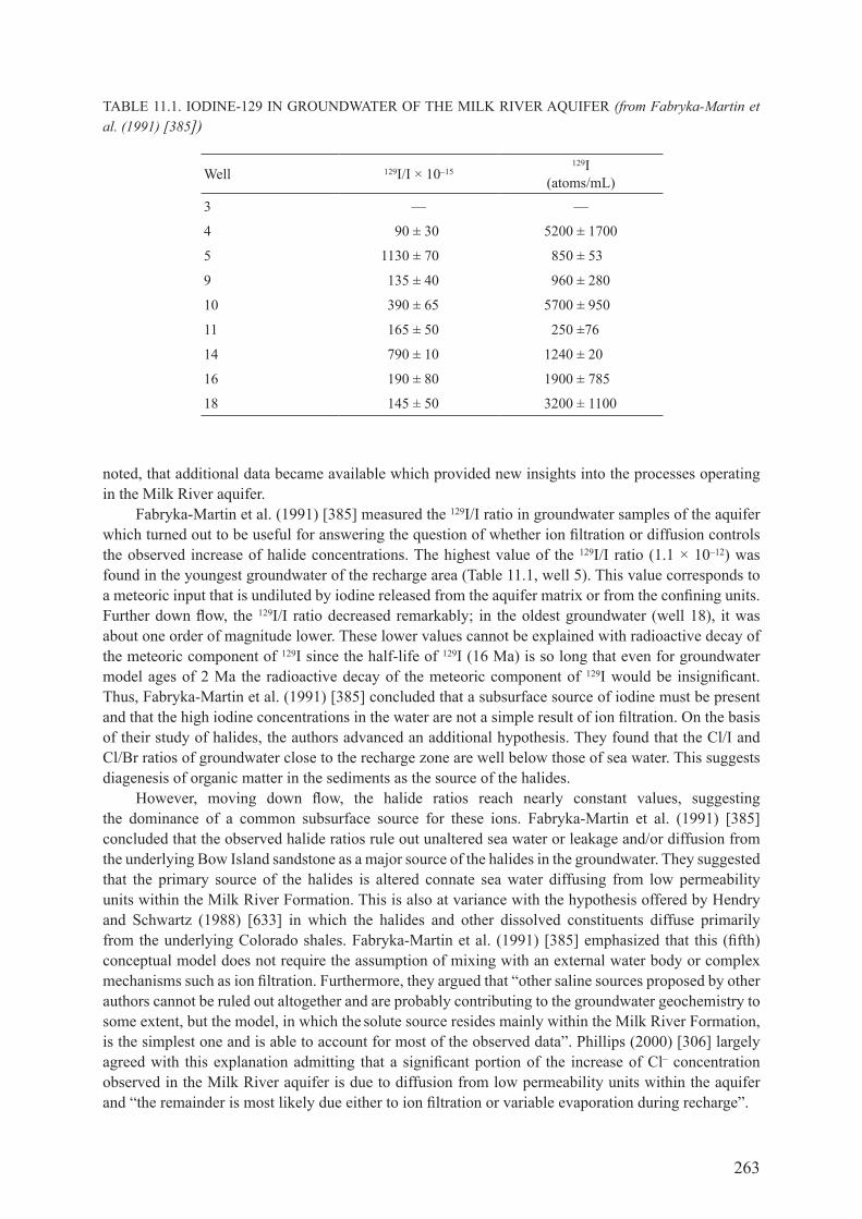
263

noted, that additional data became available which provided new insights into the processes operating in the milk river aquifer.

fabryka-martin et al. (1991) [385] measured the 129I/I ratio in groundwater samples of the aquifer which turned out to be useful for answering the question of whether ion filtration or diffusion controls the observed increase of halide concentrations. the highest value of the 129I/I ratio (1.1 × 10–12) was found in the youngest groundwater of the recharge area (table 11.1, well 5). this value corresponds to a meteoric input that is undiluted by iodine released from the aquifer matrix or from the confining units. further down flow,  the  129I/I  ratio decreased remarkably;  in  the oldest groundwater  (well 18),  it was about one order of magnitude lower. these lower values cannot be explained with radioactive decay of the meteoric component of 129I since the half-life of 129I (16 Ma) is so long that even for groundwater model ages of 2 Ma the radioactive decay of the meteoric component of 129I would be  insignificant. Thus, fabryka-martin et al. (1991) [385] concluded that a subsurface source of iodine must be present and that the high iodine concentrations in the water are not a simple result of ion filtration. on the basis of their study of halides, the authors advanced an additional hypothesis. they found that the cl/I and cl/Br ratios of groundwater close to the recharge zone are well below those of sea water. This suggests diagenesis of organic matter in the sediments as the source of the halides.

However,  moving  down  flow,  the  halide  ratios  reach  nearly  constant  values,  suggesting the  dominance  of  a  common  subsurface  source  for  these  ions.  fabryka-martin  et  al.  (1991)  [385] concluded that the observed halide ratios rule out unaltered sea water or leakage and/or diffusion from the underlying bow Island sandstone as a major source of the halides in the groundwater. they suggested that the primary source of the halides is altered connate sea water diffusing from low permeability units within the milk river formation. This is also at variance with the hypothesis offered by Hendry and  Schwartz  (1988)  [633]  in  which  the  halides  and  other  dissolved  constituents  diffuse  primarily from the underlying colorado shales. fabryka-martin et al.  (1991) [385] emphasized that  this (fifth) conceptual model does not require the assumption of mixing with an external water body or complex mechanisms such as ion filtration. furthermore, they argued that “other saline sources proposed by other authors cannot be ruled out altogether and are probably contributing to the groundwater geochemistry to some extent, but the model, in which the solute source resides mainly within the milk river formation, is the simplest one and is able to account for most of the observed data”. Phillips (2000) [306] largely agreed with  this explanation admitting  that a  significant portion of  the  increase of cl– concentration observed in the milk river aquifer is due to diffusion from low permeability units within the aquifer and “the remainder is most likely due either to ion filtration or variable evaporation during recharge”.

TABLE 11.1. IodINE-129 IN groUNdwATEr of THE mILK rIvEr AqUIfEr (from Fabryka-Martin et al. (1991) [385])

well 129I/I × 10–15129I

(atoms/ml)

3 — —

4 90 ± 30 5200 ± 1700

5 1130 ± 70 850 ± 53

9 135 ± 40 960 ± 280

10 390 ± 65 5700 ± 950

11 165 ± 50 250 ±76

14 790 ± 10 1240 ± 20

16 190 ± 80 1900 ± 785

18 145 ± 50 3200 ± 1100

264

finally, it has to be noted that in the case of the milk river aquifer a possible glacial ‘squeezee’ effect should be taken into account. It  is known that the aquifer experienced massive glacial loading moving from north to south and, thus, potentially squeezing water out of the shale into the aquifer at the initiation of glaciation and reversing the flow at glacial retreat (f. Phillips, personal communication2). recent  research  on  glacial  chronology  of  the  area  in  south-western Alberta,  canada,  suggests  that there was perhaps only one glacial advance over the study area, the wisconsinan (jackson and Little (2004) [641]).

overall, the situation that a number of alternative mechanisms were suggested for the explanation of observed geochemical data points to an ambiguity that seems to be inherent in complex systems such as the milk river aquifer. In such systems, shale aquitards and interbeds can play a critical role as sources of the chemistry of the groundwater in the aquifer. Tackling this ambiguity is a formidable challenge in connection with dating of old groundwater.

11.4.  ISoToPIc STUdIES of THE mILK rIvEr AqUIfEr

11.4.1. Radiocarbon and stable isotopes

Measurements of 2h, 3h and 18o in groundwater, 2h and 13c in methane, 18o and 34s in so%–, 13c

and 14c in dIc and doc have been discussed by drimmie et al. (1991) [168]. Here, focus is put on interpretation of the 18o and 2h data and the 14c results. plotting δ18o against δ2h, the authors were able to identify three distinct clusters (fig. 11.5): cluster a with δ18o values of approximately –19‰, cluster b with δ18o of –16‰, and cluster c with δ18o of –8‰. cluster a represents groundwater near the recharge area in the southern part of the aquifer (some samples contained measurable levels of bomb tritium). the isotopic signatures are not followed by even more negative δ18o and δ2H values down flow as might be expected if pleistocene recharge were present. this absence of a glacial signature suggests that  this  groundwater was  recharged  before  15  ka,  and  that  the  Pleistocene  period  of  that  region  is characterized by insignificant recharge over long periods. The uniform δ18o and δ2h values found in groundwater to about 20 km distance from the recharge zone indicate a minimum flow rate of about 1 to 1.5 m/a in this part of the aquifer. the data in cluster b fall close to the modern meteoric water line for the region. however, this groundwater contains no measurable 14c and could, thus, have been recharged before the last glaciation.

Assuming  constant  flow  rates  beyond  the milk  river  on  the  order  of  0.l m/a,  drimmie  et  al. (1991) [168] suggested groundwater model ages >50 ka BP and possibly as much as 600 ka BP along path I. cluster c data represent groundwater in the most distant section of the milk river aquifer. They follow a  line  that deviates  from the meteoric water  line. Hendry and Schwartz  (1988)  [633] suggest that  this  line represents diffusive mixing between isotopically enriched water  in  the confining shales and meteoric water recharged during warm climate phases. Alternatively, Phillips et al. (1990) [640] mentioned that the slope of this line is consistent with ion filtration (see chapter 3).

radiocarbon was measurable only in ground water sampled from wells  located within 20 km of the recharge zone. Although the dIc 14c pmc values are much lower than those for doc in both wells, the age differences between the two wells are quite similar, averaging about 14 ka (fig. 11.6). The lower dIc values led to the conclusion that the dIc 14c content when the water entered the aquifer was as low as 30 pmc. from these data, a flow rate of ~1 m/a has been estimated for the distance of 12 km between the two wells (fig. 11.6). This flow rate agrees surprisingly well with the stable isotope data but is an order of magnitude higher than the flow rates estimated for the northern part of the aquifer by hydraulic modelling (Hendry and Schwartz (1988) [633]; Swanick (1982) [638]), 36cl data (nolte et al. (1991) [291]; Phillips et al. (1986) [319]) and uranium isotope measurements (Ivanovich et al. (1991) [422]). Thus,  the  14c  derived flow  rates  for  the  southern  part  cannot  be  adopted  for  the  entire flow 

2 phIllIps, f., department of earth and environmental science, new Mexico tech, personal communication.

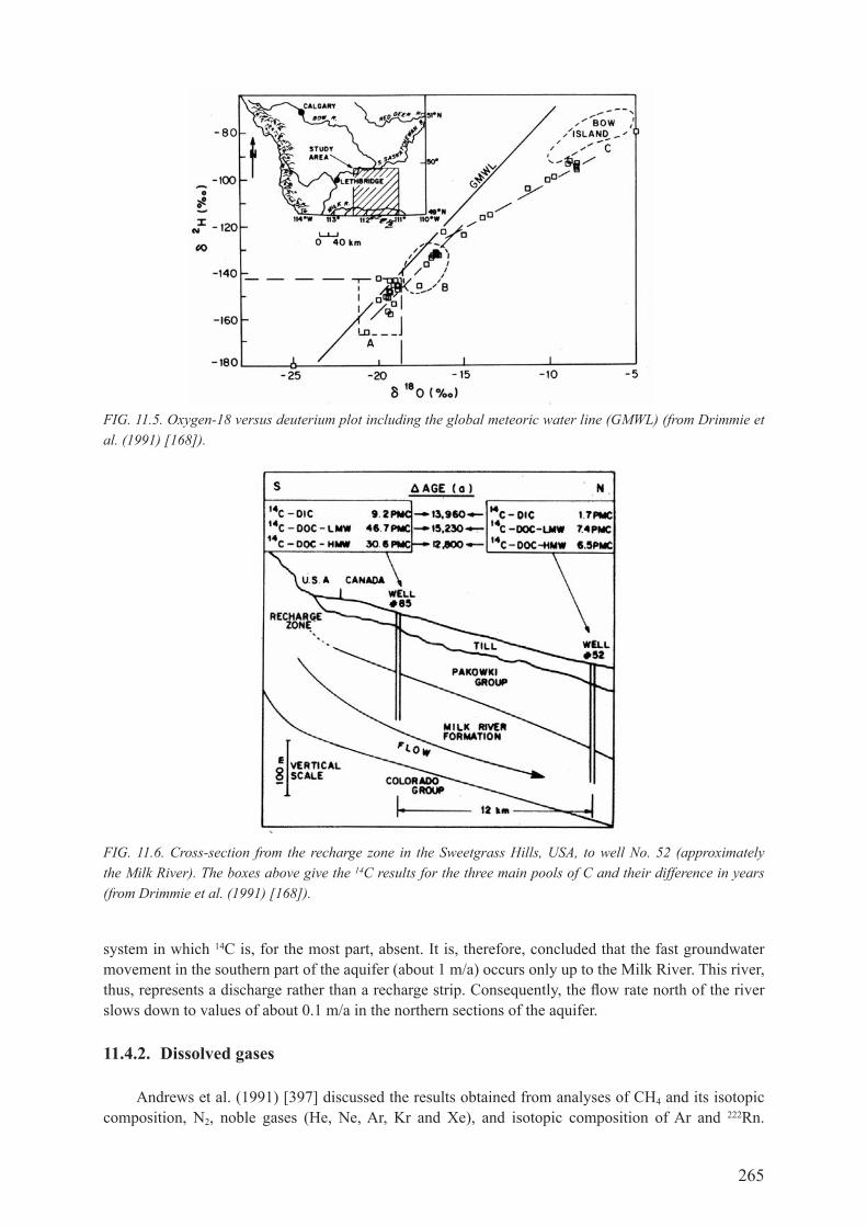
265

system in which 14c is, for the most part, absent. It is, therefore, concluded that the fast groundwater movement in the southern part of the aquifer (about 1 m/a) occurs only up to the milk river. This river, thus, represents a discharge rather than a recharge strip. consequently, the flow rate north of the river slows down to values of about 0.1 m/a in the northern sections of the aquifer.

11.4.2. Dissolved gases

Andrews et al. (1991) [397] discussed the results obtained from analyses of cH4 and its isotopic composition, n2,  noble  gases  (He,  Ne, Ar,  Kr  and  xe),  and  isotopic  composition  of Ar  and  222rn.

FIG. 11.5. Oxygen-18 versus deuterium plot including the global meteoric water line (GMWL) (from Drimmie et al. (1991) [168]).

FIG. 11.6. Cross-section from the recharge zone in the Sweetgrass Hills, USA, to well No. 52 (approximately the Milk River). The boxes above give the 14C results for the three main pools of C and their difference in years (from Drimmie et al. (1991) [168]).

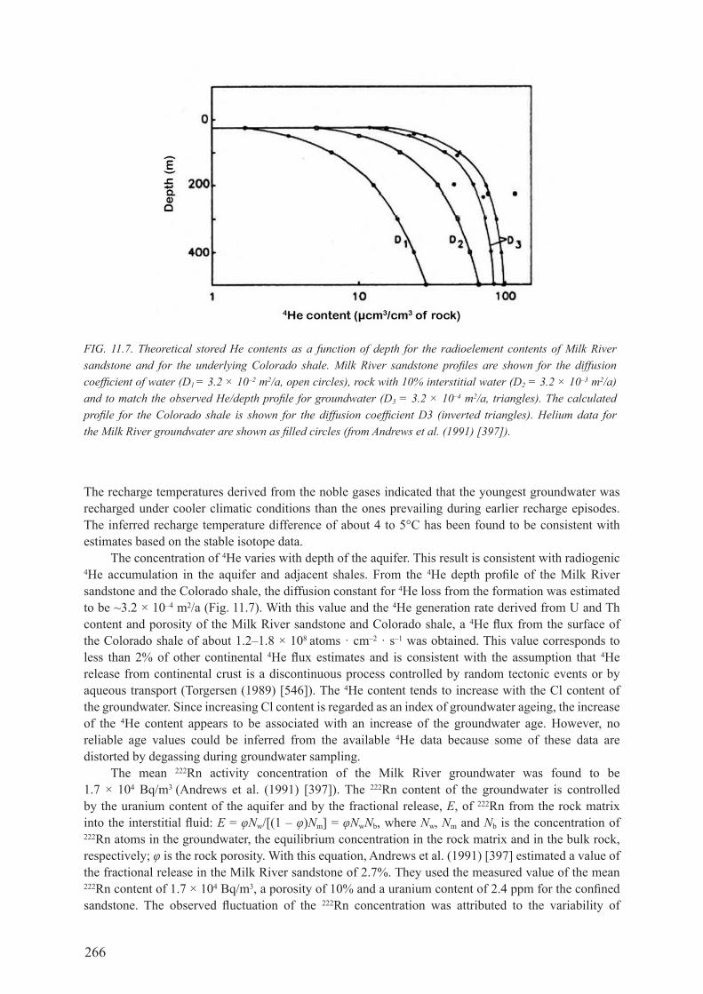
266

the recharge temperatures derived from the noble gases indicated that the youngest groundwater was recharged under cooler climatic conditions than the ones prevailing during earlier recharge episodes. The inferred recharge temperature difference of about 4 to 5°c has been found to be consistent with estimates based on the stable isotope data.

the concentration of 4he varies with depth of the aquifer. this result is consistent with radiogenic 4he accumulation in the aquifer and adjacent shales. from the 4He  depth  profile  of  the milk river sandstone and the colorado shale, the diffusion constant for 4he loss from the formation was estimated to be ~3.2 × 10–4 m2/a (fig. 11.7). with this value and the 4he generation rate derived from u and th content and porosity of the milk river sandstone and colorado shale, a 4He flux from the surface of the colorado shale of about 1.2–1.8 × 108 atoms · cm–2 · s–1 was obtained. this value corresponds to less than 2% of other continental 4He flux  estimates  and  is  consistent with  the  assumption  that  4he release from continental crust is a discontinuous process controlled by random tectonic events or by aqueous transport (Torgersen (1989) [546]). The 4he content tends to increase with the cl content of the groundwater. since increasing cl content is regarded as an index of groundwater ageing, the increase of the 4he content appears to be associated with an increase of the groundwater age. however, no reliable age values could be inferred from the available 4he data because some of these data are distorted by degassing during groundwater sampling.

the mean 222rn  activity  concentration  of  the  milk  river  groundwater  was  found  to  be 1.7 × 104 bq/m3 (Andrews  et  al.  (1991)  [397]). The  222rn content of the groundwater is controlled by the uranium content of the aquifer and by the fractional release, E, of 222rn from the rock matrix into the interstitial fluid: E = φNw/[(1 – φ)Nm] = φNwNb, where Nw, Nm and Nb is the concentration of 222rn atoms in the groundwater, the equilibrium concentration in the rock matrix and in the bulk rock, respectively; φ is the rock porosity. with this equation, Andrews et al. (1991) [397] estimated a value of the fractional release in the milk river sandstone of 2.7%. They used the measured value of the mean 222rn content of 1.7 × 104 bq/m3, a porosity of 10% and a uranium content of 2.4 ppm for the confined sandstone.  The  observed  fluctuation  of  the  222rn concentration was attributed to the variability of

FIG. 11.7. Theoretical stored He contents as a function of depth for the radioelement contents of Milk River sandstone and for the underlying Colorado shale. Milk River sandstone profiles are shown for the diffusion coefficient of water (D1 = 3.2 × 10–2 m2/a, open circles), rock with 10% interstitial water (D2 = 3.2 × 10–3 m2/a) and to match the observed He/depth profile for groundwater (D3 = 3.2 × 10–4 m2/a, triangles). The calculated profile for the Colorado shale is shown for the diffusion coefficient D3 (inverted triangles). Helium data for the Milk River groundwater are shown as filled circles (from Andrews et al. (1991) [397]).

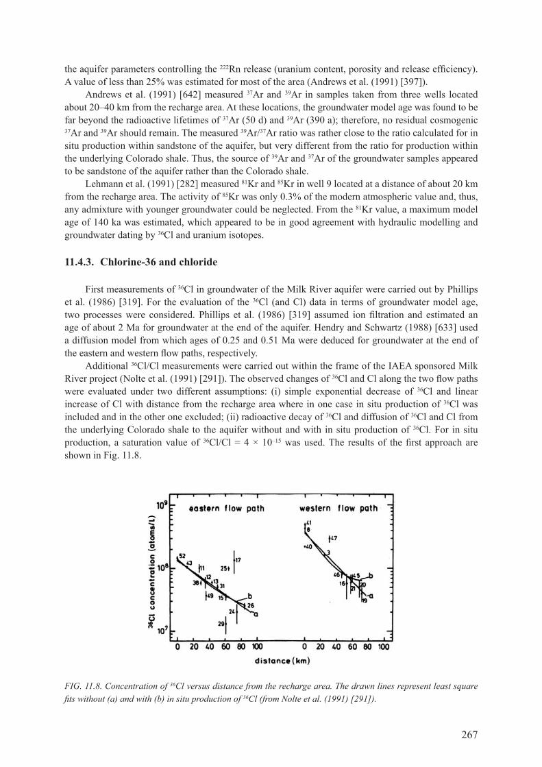
267

the aquifer parameters controlling the 222rn release (uranium content, porosity and release efficiency). A value of less than 25% was estimated for most of the area (Andrews et al. (1991) [397]).

Andrews et al.  (1991)  [642] measured  37ar and 39Ar  in samples  taken  from  three wells  located about 20–40 km from the recharge area. At these locations, the groundwater model age was found to be far beyond the radioactive lifetimes of 37ar (50 d) and 39ar (390 a); therefore, no residual cosmogenic 37ar and 39ar should remain. the measured 39ar/37ar ratio was rather close to the ratio calculated for in situ production within sandstone of the aquifer, but very different from the ratio for production within the underlying colorado shale. thus, the source of 39ar and 37ar of the groundwater samples appeared to be sandstone of the aquifer rather than the colorado shale.

Lehmann et al. (1991) [282] measured 81Kr and 85Kr in well 9 located at a distance of about 20 km from the recharge area. the activity of 85Kr was only 0.3% of the modern atmospheric value and, thus, any admixture with younger groundwater could be neglected. from the 81Kr value, a maximum model age of 140 ka was estimated, which appeared to be in good agreement with hydraulic modelling and groundwater dating by 36cl and uranium isotopes.

11.4.3. Chlorine-36 and chloride

first measurements of 36cl in groundwater of the milk river aquifer were carried out by Phillips et al.  (1986)  [319]. for  the evaluation of  the  36cl (and cl) data in terms of groundwater model age, two  processes were  considered.  Phillips  et  al.  (1986)  [319]  assumed  ion filtration  and  estimated  an age of about 2 ma for groundwater at the end of the aquifer. Hendry and Schwartz (1988) [633] used a diffusion model from which ages of 0.25 and 0.51 Ma were deduced for groundwater at the end of the eastern and western flow paths, respectively.

additional 36cl/cl measurements were carried out within the frame of the IAEA sponsored milk river project (Nolte et al. (1991) [291]). The observed changes of 36cl and cl along the two flow paths were evaluated under two different assumptions: (i) simple exponential decrease of 36cl and linear increase of cl with distance from the recharge area where in one case in situ production of 36cl was included and in the other one excluded; (ii) radioactive decay of 36cl and diffusion of 36cl and cl from the underlying colorado shale to the aquifer without and with in situ production of 36cl. for in situ production, a saturation value of 36cl/cl = 4 × 10–15 was used. The  results  of  the first  approach  are shown in fig. 11.8.

FIG. 11.8. Concentration of 36Cl versus distance from the recharge area. The drawn lines represent least square fits without (a) and with (b) in situ production of 36Cl (from Nolte et al. (1991) [291]).

268

The groundwater flow velocities were obtained by  least  square fits  of  the  theoretical  curves  to the experimental data. figure 11.9 shows the results of the diffusion model with in situ production for the eastern flow path.

Table  11.2  compiles  all  values  of  the  groundwater  flow  velocity  obtained  with  different assumptions. In the first approach (without diffusion), consideration of in situ production yields a value of the flow velocity that is only 75% of the value without in situ production. The flow velocities inferred from the diffusion model (second approach) are about 30% greater than the values deduced without consideration of diffusive losses of 36cl.  Thus,  Nolte  et  al.  (1991)  [291]  conclude  that  radioactive decay of 36cl rather than diffusive loss controls the 36cl concentration in groundwater during advective transport  in  the  aquifer. The flow velocities  are  in  the  range  0.09–0.14 m/a  (eastern flow path)  and 0.06–0.10 m/a (western flow path). The corresponding groundwater model ages at a distance of 80 km from the recharge area are in the range of 0.6–0.9 Ma (east) and 0.8–1.6 Ma (west). for comparison: using ion filtration to describe the evolution of cl in the milk river groundwater, Phillips et al. (1986) [319] obtained ages of up  to about 2 ma at  the end of  the aquifer. on  the other hand,  the values of the groundwater velocity determined by Hendry and Schwartz (1988) [633] are remarkably larger than the ones deduced by Nolte et al. (1991) [291]. for the eastern flow path, they obtained 0.32 m/a and for the western flow path 0.16 m/a. comparing the various 36cl dating approaches of the milk river aquifer,  Phillips  (2000)  [306]  suggested  that  the  age  estimates  derived  from  the  36cl/cl ratio under assumption of ion filtration (‘ion filtration age’, Phillips et al. (1990) [640]) may be more accurate for regions close to the recharge zone while further away dating based on the 36cl concentration (nolte et al. (1991) [291]) may be more adequate.

although in situ production of 36cl  in aquifer matrices  is generally known to be significant,  its contribution to the 36cl  content  of milk river  aquifer  groundwater  appeared  to be  relatively  low  in 

FIG. 11.9. Concentration of Cl and 36Cl along the eastern flow path calculated by the diffusion model, with in situ 36Cl production (from Nolte et al. (1991) [291]).

table 11.2. coMparIson of flow VelocItIes deterMIned (after Nolte et al. (1991) [291])

Eastern flow path western flow path

without in situ production

with in situ production

without in situ production

with in situ production

flow velocity (m/a)

without diffusion 0.11 0.09 0.08 0.06

with diffusion 0.14 0.5 0.1 0.07

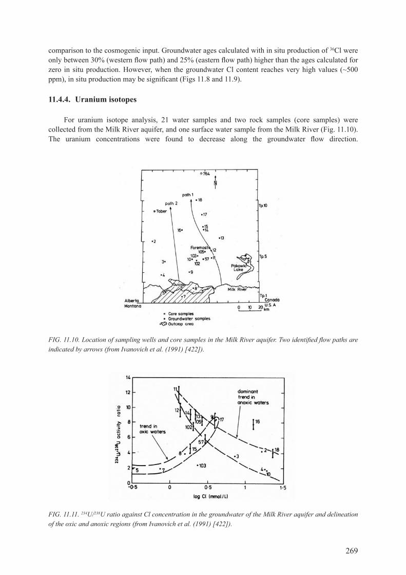
269

comparison to the cosmogenic input. ground water ages calculated with in situ production of 36cl were only between 30% (western flow path) and 25% (eastern flow path) higher than the ages calculated for zero  in  situ production. However, when  the groundwater cl content  reaches very high values  (~500 ppm), in situ production may be significant (figs 11.8 and 11.9).

11.4.4. Uranium isotopes

for  uranium  isotope  analysis,  21  water  samples  and  two  rock  samples  (core  samples)  were collected from the milk river aquifer, and one surface water sample from the milk river (fig. 11.10). The  uranium  concentrations  were  found  to  decrease  along  the  groundwater  flow  direction. 

FIG. 11.10. Location of sampling wells and core samples in the Milk River aquifer. Two identified flow paths are indicated by arrows (from Ivanovich et al. (1991) [422]).

FIG. 11.11. 234U/238U ratio against Cl concentration in the groundwater of the Milk River aquifer and delineation of the oxic and anoxic regions (from Ivanovich et al. (1991) [422]).

270

In the oxidizing zone near the recharge area, the uranium concentrations ranged from about 12 to 0.7 µg/l and under anoxic conditions from 0.07 to 0.007 µg/l.

parallel geochemical investigations of dissolved ions in groundwater (Ivanovich et al. (1991) [422]) have shown that all groundwater samples are undersaturated with respect to common uranium minerals, which suggests that uranium minerals do not precipitate. furthermore, the cl concentrations were found to increase with the groundwater age. the 234u/238u ratios tend to increase with distance down flow of  the outcrop  in  the oxic  zone  and  reach  a maximum at well  11 where  the  redox  front is  positioned.  In  the  downstream  anoxic  zone,  the  234u/238u ratios decrease with increasing cl concentrations, i.e. increasing groundwater age (fig. 11.11). the decrease in 234u/238u is accompanied

FIG. 11.12. Decrease of the relative 234U excess (234U/238U activity ratio – 1) along flow path 1 (from Ivanovich et al. (1991) [422]).

FIG. 11.13(a). Plot of the 238U activity concentration against the distance along the flow path from the outcrop of the Milk River aquifer. The solid line represents the best-fit line of approach to using the complete data set (after Ivanovich et al. (1991) [422]).

FIG. 11.13(b). Plot of the 234U activity concentration against the distance along the flow path from the outcrop of the Milk River aquifer. The solid line represents the best-fit line of approach to using the complete data set (after Ivanovich et al. (1991) [422]).

271

by a constant but low 238u concentration, and the change in 234u/238u ratio could, thus, be attributed to the radioactive decay of 234u and exchange between the liquid and adsorbed phase (retardation). It should be noted that a similar pattern of the evolution of the uranium isotopes (low and basically constant uranium concentration at decreasing 234u/238U  ratios  downdip  the  anoxic  zone)  was  also observed in other regional aquifers such as the Hosston aquifer (Kronfeld and Adams (1974) [424]), carrizo aquifer (cowart and osmond (1974) [419]), Lincolnshire limestone (Edmunds (1973) [643]) and Lincolnshire chalk (cuttell et al. (1986) [644]).

The  milk  river  uranium  isotope  data  were  evaluated  by  two  different  approaches.  In  a  first approach, only the data of the anoxic part of the aquifer were evaluated, assuming constant 238u concentration and exponential decrease of 234U excess down flow. The model corresponds to Eq. (7.17) assuming that the stationary value of the 234U excess  is zero  (no  234u production by recoil ejection). figure 11.12 shows the best fit line of the model to the experimental data in a semi-logarithmic plot. according to eq. (7.17), the slope of this line represents the ratio λ234/v*, from which the velocity, v*, can be calculated. The obtained value is 0.12 m/a (Ivanovich et al.  (1991) [422]). Using a hydraulic model, Hendry and Schwartz  (1988)  [633] determined a groundwater flow velocity v of 0.3 m/a for the same flow path. obviously, the velocity v* characterizes the uranium migration velocity which is related to the groundwater flow velocity by the expression v* = v/R, where R is the retardation factor. Thus, for the considered anoxic part of the milk river aquifer, the uranium retardation factor appears to be R = 0.3/0.12 = 2.5.

In a second approach, all measured 238u and 234u concentrations were plotted against distance along  a  generalized  flow  path  from  the milk  river  outcrop  area  (figs 11.13(a)  and  11.13(b)).  for the estimation of the distances, the position of each sampled well was projected onto the generalized N–S  flow  path. The main  feature  of  the  semi-logarithmic  plots  in  figs 11.13(a)  and  11.13(b)  is  an approximately linear decrease of the uranium isotope concentrations with increasing distance along the flow path. However, there are considerable deviations of individual data from the linear trend lines which point  to significant  local fluctuations of  the geochemical and/or hydrological conditions along groundwater flow.

nevertheless, the absence of any independent evidence for these inhomogeneities in the aquifer was deemed to justify this statistical approach that does not explicitly take into consideration the influence of a redox front. Assuming, as in the first approach, that the stationary values of the uranium isotope concentrations are negligible, the slope, s,  of  the  best-fit  lines  in  figs 11.13(a)  and  11.13(b)  can  be derived from eqs (7.7, 7.8), respectively (see chapter 7). the following expression is obtained:

si = Ki /v (11.1 )

whereKi   is defined by Eq. (7.11);i stands for 234u and 238u, respectively.

the following values have been determined by this approach: s8 = 5.8 × 10–5/m and s4 = 4.7 × 10–5/m. thus, within the accuracy of this estimate, the two lines have the same slope of about 5 × 10–5/m. adopting the value of the parameter K  determined  by  fröhlich  and  gellermann  (1987)  [426]  for the hosston aquifer (K8 ≈ K4 ≈ (1–3) × 10–5/a), Ivanovich et al. (1991) [422] estimated a groundwater flow  rate  for  the  milk  river  aquifer  of  between  0.2  and  0.6  m/a.  within  the  range  of  the  given uncertainties, this result seems to be in good agreement with estimates by other methods (table 11.3), which indicates “that uranium isotope data are a viable tool for dating very old groundwater provided the local uranium geochemistry is understood adequately” (Ivanovich et al. (1991) [422]).

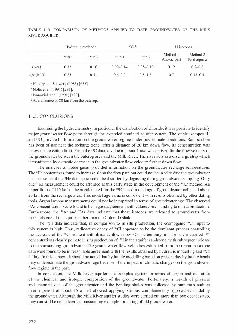
272

11.5. conclusIons

examining the hydrochemistry, in particular the distribution of chloride, it was possible to identify major groundwater flow paths  through  the extended confined aquifer system. The stable  isotopes  2h and 18o provided information on the groundwater regime under past climate conditions. radiocarbon has been of use near  the  recharge zone; after a distance of 20 km down flow,  its  concentration was below the detection limit. from the 14c data, a value of about 1 m/a was derived for the flow velocity of the groundwater between the outcrop area and the milk river. The river acts as a discharge strip which is manifested by a drastic decrease in the groundwater flow velocity further down flow.

the analyses of noble gases provided information on the groundwater recharge temperatures. the 4He content was found to increase along the flow path but could not be used to date the groundwater because some of the 4he data appeared to be distorted by degassing during groundwater sampling. only one 81Kr measurement could be afforded at this early stage in the development of the 81Kr method. An upper limit of 140 ka has been calculated for the 81K based model age of groundwater collected about 20 km from the recharge area. This model age value is consistent with results obtained by other dating tools. argon isotope measurements could not be interpreted in terms of groundwater age. the observed 39ar concentrations were found to be in good agreement with values corresponding to in situ production. furthermore, the 39ar and 37ar data indicate that these isotopes are released to groundwater from the sandstone of the aquifer rather than the colorado shale.

the 36cl data indicate that, in comparison to in situ production, the cosmogenic 36cl input to this system is high. thus, radioactive decay of 36cl appeared to be the dominant process controlling the decrease of the 36cl content with distance down flow. on the contrary, most of  the measured 129I concentrations clearly point to in situ production of 129I in the aquifer sandstone, with subsequent release to the surrounding groundwater. The groundwater flow velocities estimated from the uranium isotope data were found to be in reasonable agreement with the results obtained by hydraulic modelling and 36cl dating. In this context, it should be noted that hydraulic modelling based on present day hydraulic heads may underestimate the groundwater age because of the impact of climatic changes on the groundwater flow regime in the past.

In  conclusion,  the  milk  river  aquifer  is  a  complex  system  in  terms  of  origin  and  evolution of the chemical and isotopic composition of the groundwater. fortunately, a wealth of physical and chemical data of the groundwater and the bonding shales was collected by numerous authors over a period of about 15 a that allowed applying various complementary approaches in dating the groundwater. Although the milk river aquifer studies were carried out more than two decades ago, they can still be considered an outstanding example for dating of old groundwater.

TABLE  11.3.  comPArISoN  of  mETHodS  APPLIEd  To  dATE  groUNdwATEr  of  THE  mILK rIVer aquIfer

hydraulic method a 36cl b u isotopes c

path 1 path 2 path 1 path 2 Method 1 anoxic part

Method 2 total aquifer

v (m/a) 0.32 0.16 0.09–0.14 0.05–0.10 0.12 0.2–0.6

age (Ma)d 0.25 0.51 0.6–0.9 0.8–1.6 0.7 0.13–0.4

a Hendry and Schwarz (1988) [633].b Nolte et al. (1991) [291].c Ivanovich et al. (1991) [422].d At a distance of 80 km from the outcrop.

273

Chapter 12

CAsE stUDY MIDDLE RIO GRAnDE bAsIn, nEW MExICO, UsA

l.n. pluMMer, w. sanfordunited states geological survey, reston, Virginia, united states of america

12.1. IntroductIon

chemical and isotopic patterns in groundwater can record characteristics of water sources, flow directions and groundwater age information. This hydrochemical information can be useful in refining conceptualization of groundwater flow,  in  calibration of numerical models of  groundwater flow and in estimation of palaeo- and modern recharge rates. This case study shows how chemical and isotopic data were used to characterize sources and flow of groundwater in the middle rio grande Basin, New Mexico, usa. the 14c model ages of the groundwater samples are on the tens of thousands of years timescale. These data changed some of the prevailing ideas about flow in the middle rio grande Basin, and were used to improve a numerical model of the aquifer system.

12.2. BAcKgroUNd: HydrogEoLogIcAL SETTINg

The middle rio grande Basin covers about 7800 km2 along the rio grande rift in central new mexico, USA (fig. 12.1). The rio grande rift is a zone of faults and sediment filled basins that extends from northern Mexico to southern colorado, usa. the basin consists of generally unconsolidated cenozoic  basin-fill  sediment  with  a maximum  thickness  of  about  4300 m  (fig. 12.2).  The  average elevation is about 1500 m, with surrounding mountains approaching 3300 m. the primary aquifer system of the Middle rio grande basin consists of generally unconsolidated to moderately consolidated basin-fill sediment of the Santa fe group.

The  Santa  fe  group  aquifer  system  is  defined  by  Thorn  et  al.  (1993)  [21]  as  including  both the santa fe group deposits, which are of oligocene to middle pleistocene age, and the more recent (post-Santa fe group) flood plain, channel and basin-fill deposits of Pleistocene to Holocene age that are in hydraulic connection with the Santa fe group. The Santa fe group deposits range in thickness from about 900 to 4300 m. The lower Santa fe group ranges in thickness from about 300 to 1000 m and consists largely of piedmont-slope, eolian sand and silt, and fine to medium grained basin-floor deposits (fig. 12.2). The middle Santa fe group deposits range in thickness from about 75 to 2740 m and consist of  piedmont-slope  sediments  and  fluvial  deposits  (identified  mostly  as  medium  sand  in  fig. 12.2). The upper Santa fe group sediments are generally less than 300 m thick and consist predominantly of piedmont-slope and fluvial basin-floor deposits, and are the most productive part of the aquifer system (denoted axial gravel, blanket sand/gravel, and medium–coarse sand in fig. 12.2). A red–brown clay separates the upper and middle santa fe group deposits at albuquerque. geophysical measurements have recognized three sub-basins within the middle rio grande Basin that are separated by structural highs  (grauch  et  al.  (1999)  [645]; grauch  et  al.  (2001)  [646];  see Bartolino  and cole  (2002)  [612] for further details). Most production wells are completed in the upper and/or middle santa fe group, although wells on the west side of the rio grande reach parts of the lower santa fe group.

In the 1980s, there was the perception that albuquerque was situated over a large and almost unlimited supply of fresh groundwater, and optimism prevailed for seemingly unlimited growth potential. however, as new and detailed geological and hydrological data were gathered (bartolino

274

and  cole  (2002)  [612];  cole  (2001)  [647];  connell  et  al.  (1998)  [648];  Hawley  and Haase  (1992) [649]; Thorn et al. 1993) [21]), the conceptualization of the aquifer system greatly changed. The most productive part of the aquifer system was found to be limited to a relatively small area of ancestral rio grande sediments under parts of albuquerque.

water  level  declines  of  as  much  as  40  m  (130  ft)  were  observed  between  1960  and  2002  at Albuquerque  (fig. 12.3).  Until  recently,  groundwater  was  the  sole  source  of  drinking  water  for Albuquerque. during  the  1990s,  basin-wide  pumping was  about  200 mm3 annually and about 75% of this water was withdrawn for public supply at Albuquerque. It is now thought that the basin-wide pumping rate amounted to about three times the modern recharge rate for the entire basin.

recharge occurs along and near the basin margin. this includes mountain front processes, infiltration  from  arroyos  and  subsurface  groundwater  inflow. The  other major  source  of  recharge  is surface water, particularly from the rio grande in central parts of the basin, its tributaries and, more recently, irrigation canals. Today, areal recharge is thought to be negligible across the semi-arid basin.

01020 kilometers

COLORADO

ARI

ZON

A NEW MEXICO

Albuquerque

MiddleRio Grande

Basin

RioGrande

San JuanBasin

Man

zano

Mtn

s.

Sandia Mtns.

Sier

ra L

ucero

Sierra

Nacim

iento

Los P

inos

Mtn

s

EspañolaBasin

Esta

ncia

Ba

sin

LadronPeak

Jemez Mtns.

MiddleRio Grande

Basinboundary

MesaLucero

ManzanitaMtns.

35º30'

35�N

34º30'

106º30'W107º W

JoyitaHills

ALBUQUERQUEALBUQUERQUE

ArroyoR ioG

rand

e

Tonque

Rio Sa l ado

Arroyo Chico R io

Puerco

Jemez River

Rio

Salado

Jem

ezRi

ver

Santa F eRiver

GalisteoC reek

Las H uertasC

re ek

Abo Ar royo

Rio Puerco

Rio

Sa n JoseR

ioG

r an

de

Jemez CanyonReservoir

Cochiti Lake

Tijeras

Arroyo

Inne

rV

alle

y

SanFelipePueblo

Bernalillo

SandiaPueblo

CorralesRio Rancho

Los Lunas

Belen

Bernardo

SanAcacia

FIG. 12.1. Location of the Middle Rio Grande Basin in west-central New Mexico, USA, and other physiographic features of the region.

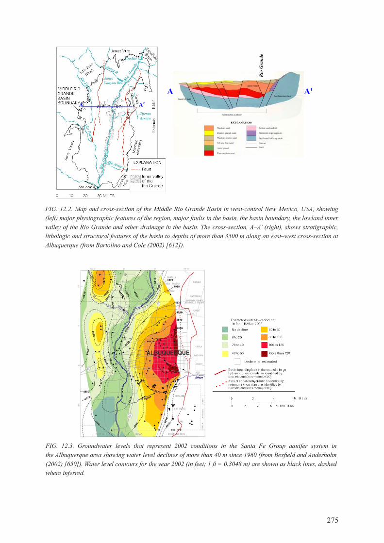
275

FIG. 12.2. Map and cross-section of the Middle Rio Grande Basin in west-central New Mexico, USA, showing (left) major physiographic features of the region, major faults in the basin, the basin boundary, the lowland inner valley of the Rio Grande and other drainage in the basin. The cross-section, A–A’ (right), shows stratigraphic, lithologic and structural features of the basin to depths of more than 3500 m along an east–west cross-section at Albuquerque (from Bartolino and Cole (2002) [612]).

FIG. 12.3. Groundwater levels that represent 2002 conditions in the Santa Fe Group aquifer system in the Albuquerque area showing water level declines of more than 40 m since 1960 (from Bexfield and Anderholm (2002) [650]). Water level contours for the year 2002 (in feet; 1 ft = 0.3048 m) are shown as black lines, dashed where inferred.

A′A A A'

Rio GranRi

o G

rand

e

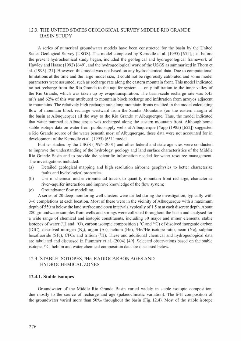
276

12.3. the unIted states geologIcal surVey MIddle rIo grande basIn study

a series of numerical groundwater models have been constructed for the basin by the united States geological Survey (USgS). The model completed by Kernodle et al. (1995) [651], just before the  present  hydrochemical  study  began,  included  the  geological  and  hydrogeological  framework  of Hawley and Haase (1992) [649], and the hydrogeological work of the USgS as summarized in Thorn et al. (1993) [21]. However, this model was not based on any hydrochemical data. due to computational limitations at the time and the large model size, it could not be rigorously calibrated and some model parameters were assumed, such as recharge rate along the eastern mountain front. this model indicated no net recharge from the rio grande to the aquifer system — only infiltration to the inner valley of the rio grande, which was  taken up  by  evapotranspiration. The  basin-scale  recharge  rate was  5.45 m3/s and 62% of this was attributed to mountain block recharge and infiltration from arroyos adjacent to mountains. the relatively high recharge rate along mountain fronts resulted in the model calculating flow  of  mountain  block  recharge  westward  from  the  Sandia  mountains  (on  the  eastern  margin  of the basin at albuquerque) all the way to the rio grande at albuquerque. thus, the model indicated that water pumped at albuquerque was recharged along the eastern mountain front. although some stable isotope data on water from public supply wells at Albuquerque (yapp (1985) [652]) suggested a rio grande source of the water beneath most of albuquerque, these data were not accounted for in development of the Kernodle et al. (1995) [651] model.

further studies by the usgs (1995–2001) and other federal and state agencies were conducted to improve the understanding of the hydrology, geology and land surface characteristics of the Middle rio grande Basin and  to provide  the  scientific  information needed  for water  resource management. the investigations included: (a) detailed  geological  mapping  and  high  resolution  airborne  geophysics  to  better  characterize 

faults and hydrological properties; (b) Use of  chemical  and  environmental  tracers  to  quantify mountain  front  recharge,  characterize 

river–aquifer interaction and improve knowledge of the flow system;(c) groundwater flow modelling.

a series of 20 deep monitoring well clusters were drilled during the investigation, typically with 3–6 completions at each location. Most of these were in the vicinity of albuquerque with a maximum depth of 550 m below the land surface and open intervals, typically of 1.5 m at each discrete depth. about 280 groundwater samples from wells and springs were collected throughout the basin and analysed for a wide range of chemical and isotopic constituents, including 30 major and minor elements, stable isotopes of water (2h and 18o), carbon isotopic composition (13c and 14c) of disolved inorganic carbon (dIc), dissolved nitrogen (n2), argon (ar), helium (he), 3he/4he isotope ratio, neon (ne), sulphur hexafluoride  (Sf6), cfcs and tritium (3h). these and additional chemical and hydrogeological data are tabulated and discussed in Plummer et al. (2004) [49]. Selected observations based on the stable isotope, 14c, helium and water chemical composition data are discussed below.

12.4. stable Isotopes, 4he, radIocarbon ages and hydrocheMIcal Zones

12.4.1. stable isotopes

groundwater of the Middle rio grande basin varied widely in stable isotopic composition, due mostly to the source of recharge and age (palaeoclimatic variation). the δ2h composition of the groundwater varied more  than 50‰  throughout  the basin  (fig. 12.4). most of  the  stable  isotope 

277

FIG. 12.4. Variations in the stable isotopic composition of groundwater samples (blue + signs) in the Middle Rio Grande Basin. The solid line shows the least squares fit to the values and is compared to the global meteoric water line (dashed line). The red circles show the median isotopic composition of the hydrochemical zones (12 zones of recharge and one of discharge; see Fig. 12.12). The data suggest that discharge from the basin is dominated by water recharged from the Rio Grande (central zone and water from the west-central zone). There is typically more than 50‰ variation in δ2H of Middle Rio Grande Basin groundwater (Plummer et al. (2004) [49]; Plummer et al. (2004) [50]).

FIG. 12.5. The δ2H isotopic composition, in per mille, of groundwater was mapped throughout the basin and is indicative of the source of recharge. Contours for deuterium align generally north to south in the central part of the basin, parallel to the regional north to south direction of groundwater flow (from Plummer et al. (2004) [51]).

278

values plotted below the global meteoric water line (fig. 12.4) and fitted a least squares line of δ2h = 7.62 δ18o + 2.48.

Spatial patterns  in  the chemical  and  isotopic  composition of groundwater were  recognized and mapped  basin-wide  for  approximately  the  upper  60 m  of  the  aquifer  (Plummer  et  al.  (2004)  [49]). the contours for deuterium (fig. 12.5) aligned generally north to south in the central part of the basin, parallel  to  the  regional  north  to  south  direction  of  groundwater  flow,  and  reflected  the  isotopic composition of the source.

The most depleted water was found throughout the west-central part of the basin. Enriched water was found in the western and south-western parts of the basin, –90s‰ values in δ2h were found along the rio grande, and the –70s and –80s‰ range occurred along the eastern and northern margins of the basin (fig. 12.5). the δ2H composition of groundwater from the narrow-screened monitoring wells, mostly in the albuquerque vicinity, show that δ2H was  nearly  constant  to  depths  of more  than  400 m below the water table at albuquerque, and was similar in isotopic composition to that of the rio grande measured during the late winter to spring runoff period (fig. 12.6). the red line in well nest (f)  (fig. 12.6)  is  in  the depleted zone  that  extends down  through  the west-central part of  the basin. the green line (j) is adjacent to the eastern mountain front. line a (magenta) appears to be water recharged at low altitude along the northern margin of the basin. other well nests (K, S, I) appear to contain fractions of either depleted or enriched water at intermediate depths.

12.4.2. Carbon-14 model age

the measured 14c content of dIc in groundwater from 211 sites ranged from 0.62 to 123.1 pmc. Most of the contours in 14c align in a north–south direction that roughly parallels the pattern in δ2h (fig. 12.7). the unadjusted 14c model age of dIc in the upper 60 m of the aquifer (fig. 12.8) is based on the measured non-normalized 14c pmc value of dIc in groundwater and was calculated using an initial 14c  value  of  100  pmc  in  recharge water  (see  fig. 4.1, chapter  4).  Patterns  in  14c model age were similar to the patterns in 14c content of the dIc. carbon-14 values were highest along the eastern mountain front, along the northern margin of the basin, and along the inner valley of the rio grande

FIG. 12.6. δ2H composition of groundwater from narrow-screened monitoring wells, mostly in the Albuquerque vicinity, as a function of depth below the water table (Plummer et al. (2004) [49]).

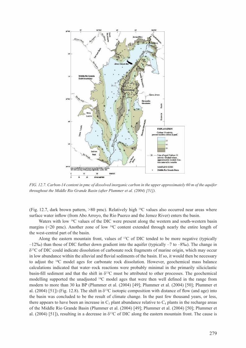
279

(fig. 12.7, dark brown pattern, >80 pmc). relatively high 14c values also occurred near areas where surface water inflow (from Abo Arroyo, the rio Puerco and the jemez river) enters the basin. 

waters with low 14c values of the dIc were present along the western and south-western basin margins  (<20  pmc). Another  zone  of  low  14c content extended through nearly the entire length of the west-central part of the basin. 

along the eastern mountain front, values of 13c of dIc tended to be more negative (typically –12‰) than those of dIc further down gradient into the aquifer (typically –7 to –8‰). the change in δ13c of dIc could indicate dissolution of carbonate rock fragments of marine origin, which may occur in low abundance within the alluvial and fluvial sediments of the basin. If so, it would then be necessary to adjust the 14c  model  ages  for  carbonate  rock  dissolution.  However,  geochemical  mass  balance calculations  indicated  that water–rock  reactions were  probably minimal  in  the  primarily  siliciclastic basin-fill  sediment and  that  the shift  in δ13c must be attributed to other processes. the geochemical modelling supported the unadjusted 14c model  ages  that  were  then well  defined  in  the  range  from modern to more than 30 ka BP (Plummer et al. (2004) [49]; Plummer et al. (2004) [50]; Plummer et al. (2004) [51]) (fig. 12.8). The shift in δ13c isotopic composition with distance of flow (and age) into the basin was concluded to be the result of climate change. In the past few thousand years, or less, there appears to have been an increase in c3 plant abundance relative to c4 plants in the recharge areas of the middle rio grande Basin (Plummer et al. (2004) [49]; Plummer et al. (2004) [50]; Plummer et al. (2004) [51]), resulting in a decrease in δ13c of dIc along the eastern mountain front. the cause is

FIG. 12.7. Carbon-14 content in pmc of dissolved inorganic carbon in the upper approximately 60 m of the aquifer throughout the Middle Rio Grande Basin (after Plummer et al. (2004) [51]).

280

not known but possible factors include increased precipitation in recharge areas and, more recently, an increase in the atmospheric mixing ratio of co2  (Plummer et al.  (2004) [49]; Plummer et al.  (2004) [51]). geochemical modelling  of water–rock  reactions  and  quantification  of mixing  of waters  from adjacent  hydrochemical  zones  were  critical  in  demonstrating  that  geochemical  corrections  were negligible in the siliciclastic sediments of the Middle rio grande basin, even though a shift to enriched δ13c of dIc was evident between the recharge area and older waters further down gradient.

12.4.3. Helium-4

Helium-4 concentrations  in middle rio grande Basin groundwater  increased with depth below the water table and with 14c model age (fig. 12.9). the 4he concentrations ranged from values near air–water equilibrium (~ 5 × 10–8 cm3 stp/g) to about 1.2 × 10–4 cm3 stp/g.

the isotopic composition of dissolved helium, along with amounts of dissolved he and ne, were determined by mass spectrometry in a relatively small subset of the Middle rio grande basin samples — basically a subset that was thought to contain a fraction of young water that might possibly be dated by the 3h–3he method. unfortunately, relatively few of the samples could be dated by this method due to large excesses of (predominantly) mantle-derived helium.

a log–log plot of the 3he/4he isotope ratio as a function of the ne/he ratio for these samples indicates two sources of he in the Middle rio grande basin waters: (i) a crustal source with a 3he/4he

FIG. 12.8. Unadjusted 14C model age in thousands of years BP in the upper approximately 60 m of the aquifer throughout the Middle Rio Grande Basin (after Plummer et al. (2004) [51]).

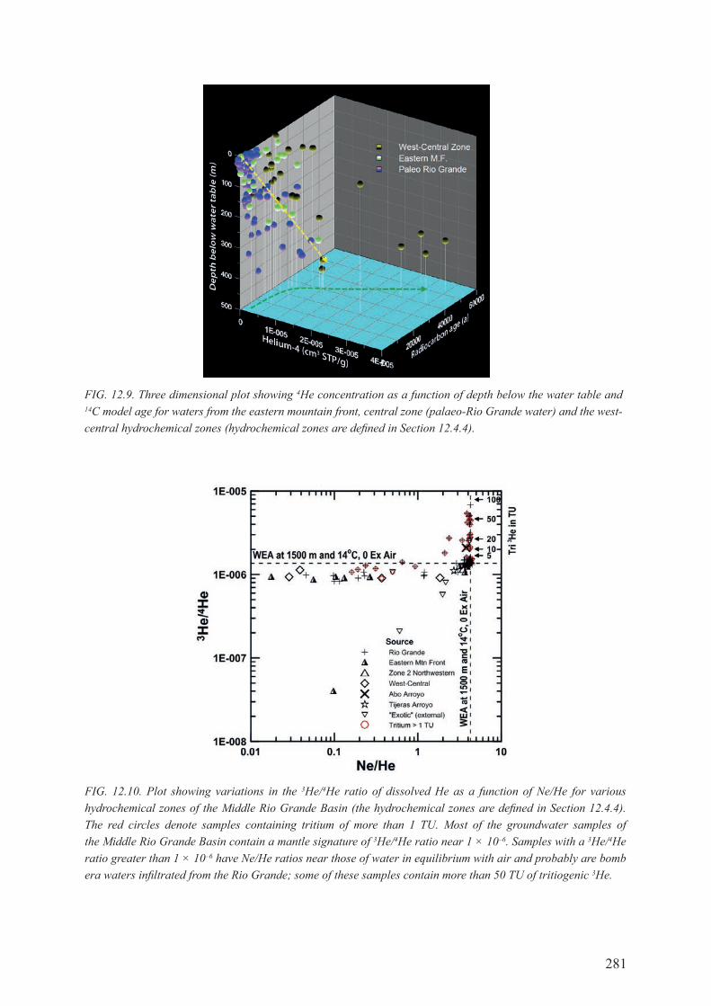
281

FIG. 12.9. Three dimensional plot showing 4He concentration as a function of depth below the water table and 14C model age for waters from the eastern mountain front, central zone (palaeo-Rio Grande water) and the west-central hydrochemical zones (hydrochemical zones are defined in Section 12.4.4).

FIG. 12.10. Plot showing variations in the 3He/4He ratio of dissolved He as a function of Ne/He for various hydrochemical zones of the Middle Rio Grande Basin (the hydrochemical zones are defined in Section 12.4.4). The red circles denote samples containing tritium of more than 1 TU. Most of the groundwater samples of the Middle Rio Grande Basin contain a mantle signature of 3He/4He ratio near 1 × 10–6. Samples with a 3He/4He ratio greater than 1 × 10–6 have Ne/He ratios near those of water in equilibrium with air and probably are bomb era waters infiltrated from the Rio Grande; some of these samples contain more than 50 TU of tritiogenic 3He.

282

ratio of approximately 1 × 10–8, and (ii) a mantle source, which predominates most of the samples, with a 3he/4he ratio near 1 × 10–6 (fig. 12.10).

the red circles in fig. 12.10 denote those samples that contain more than 1 tu of tritium. Many of the tritiated samples plot along the Ne/He line for water in equilibrium with air (at 1500 m, 14°c) and were identified as samples of rio grande water that has infiltrated the middle rio grande Basin. the 3he/4he ratio of these samples indicates some of them originally contained more than 50 tu of tritiogenic 3He, and are likely representative of rio grande water from the bomb era. The largest amount of tritium in any of the samples was 28 tu when sampled in 1996–1998. a few samples probably contain a crustal he signature near 1 × 10–8, and are derived from water sourced outside the eastern basin margin.

The samples containing more than 1 TU (red-circled samples in fig. 12.10) and having a Ne/He ratio less than that of water in equilibrium with air are mixtures of young and old water pumped from wells open to both the shallow aquifer and considerable depth (several hundred metres). excluding the samples with a crustal 3he/4he signature, there are 23 samples with ne/he < 1.0. the average 3he/4He ratio of these samples was 1.02 ± 0.15 × 10–6. No trend was recognized in He isotope ratio with regard to source or location in the basin for those samples with a mantle signature (fig. 12.10).

It appears that the samples with the crustal signature represent relatively shallow water, with a recharge source outside the eastern margin of the basin. The one sample originally identified as being from  the  eastern mountain  front  zone with  the  lowest  3h/4he ratio (fig. 12.10) was obtained down gradient from where the other ‘exotic’ samples were obtained and the water could have originated along with that of the other ‘exotic’ samples just outside the eastern margin of the basin. All of the samples with the mantle signature were obtained within the middle rio grande rift zone (fig. 12.11).

FIG. 12.11. Helium-4 accumulation in the Middle Rio Grande Basin plots in two groups with average accumulation rates of about 1.3 × 10–10 cm3 STP · g–1 · a–1 and 0.05 × 10–10 cm3 STP · g–1 · a–1. Many of the samples with the lowest 4He accumulation rates are from the west-central zone, beneath deep unsaturated zones.

283

the rate of he accumulation varied more than two orders of magnitude in the Middle rio grande basin samples (fig. 12.11). using the unadjusted 14c  model  ages  that  were  more  than  1  ka,  and calculating the He accumulation rates for samples from monitoring wells (and other narrow-screened wells), the He accumulation rates varied from 0.044 to 7.7 × 10–10 cm3 stp · g–1 · a–1. this rate can be compared to an average value of 1.3 × 10–10 reported by Solomon et al. (1996) [295] for a variety of sedimentary environments. Some of the samples, particularly from the west-central and central zones have very low 4he accumulation rates (fig. 12.11) and may be in sediment that is particularly low in u and th content (see chapter 8). given the observed wide variations in he accumulation rate, additional data on u and th abundance in sediment of the Middle rio grande basin, and data on he flux in the basin would be needed for application of He accumulation as a reliable age indicator in this complex hydrogeological environment.

12.4.4. Hydrochemical zones

using much of the available chemical and isotopic data, including the deuterium, 14c and major and minor element composition, 12 separate zones of recharge to the basin and a zone of groundwater discharge (zone 13) were recognized (Plummer et al. (2004) [49]). The hydrochemical zones (fig. 12.12) provided insight into likely recharge sources, flow paths and aquifer properties. zone 12 (fig. 12.12) was determined to be water sourced from the rio grande. Mountain front recharge waters were identified along the northern, eastern and southern margins of the basin (zones 1, 8 and 6; fig. 12.12). Palaeowater that entered the basin along the northern margin either as underflow (subsurface inflow) or recharge from the jemez mountains north of the basin margin, extends down the west-central part of the basin. It flows beneath zone 2 in the north, and beneath parts of zones 1 and 12 in the northern and central parts of the basin, as denoted by the dashed line on fig. 12.12. the arrows (fig. 12.12) show the inferred directions of flow based on identified source and location of hydrochemical zones. most of the flow in the basin appears to be from north to south.

FIG. 12.12. Location of 12 sources of water to the Middle Rio Grande Basin identified based on chemical and isotopic characteristics (after Plummer et al. (2004) [49]). The arrows show the inferred directions of groundwater flow based on the chemical and isotopic data.

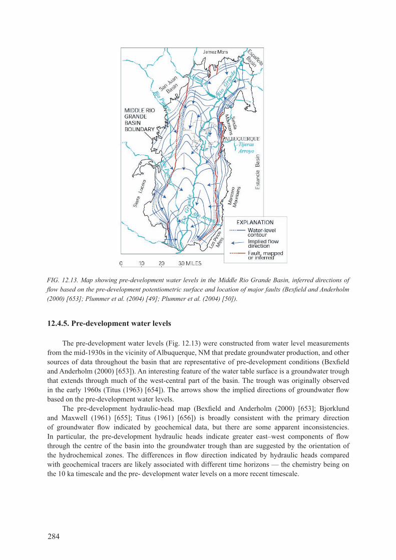
284

12.4.5. Pre-development water levels

The pre-development water levels (fig. 12.13) were constructed from water level measurements from the mid-1930s in the vicinity of Albuquerque, Nm that predate groundwater production, and other sources of data  throughout  the basin  that are  representative of pre-development conditions (Bexfield and Anderholm (2000) [653]). An interesting feature of the water table surface is a groundwater trough that extends  through much of  the west-central part of  the basin. The  trough was originally observed in the early 1960s (Titus (1963) [654]). The arrows show the implied directions of groundwater flow based on the pre-development water levels.

The  pre-development  hydraulic-head  map  (Bexfield  and  Anderholm  (2000)  [653];  Bjorklund and  maxwell  (1961)  [655];  Titus  (1961)  [656])  is  broadly  consistent  with  the  primary  direction of  groundwater  flow  indicated  by  geochemical  data,  but  there  are  some  apparent  inconsistencies. In  particular,  the  pre-development  hydraulic  heads  indicate  greater  east–west  components  of  flow through the centre of the basin into the groundwater trough than are suggested by the orientation of the  hydrochemical  zones. The  differences  in  flow  direction  indicated  by  hydraulic  heads  compared with geochemical tracers are likely associated with different time horizons — the chemistry being on the 10 ka timescale and the pre- development water levels on a more recent timescale. 

FIG. 12.13. Map showing pre-development water levels in the Middle Rio Grande Basin, inferred directions of flow based on the pre-development potentiometric surface and location of major faults (Bexfield and Anderholm (2000) [653]; Plummer et al. (2004) [49]; Plummer et al. (2004) [50]).

285

FIG. 12.14. Cross-section of the Upper Santa Fe aquifer system at Albuquerque showing ranges of 14C model age as a function of depth and water sources. The slanted grey patterns denote approximate locations of hydrochemical zone boundaries. The direction of groundwater flow is generally north to south, that is, out of the plane of the cross-section (see Fig. 12.2 for approximate location of cross-section; after Plummer et al. (2004) [49]).

FIG. 12.15. Comparison of δ2H in groundwater recharged along the eastern mountain front of the Middle Rio Grande Basin and infiltration from the Rio Grande (central zone) as a function of 14C model age (Plummer et al. (2004) [49]; Plummer et al. (2004) [51]).

0 20 00010 000-110

-100

-90

-80

-70

-60

δ2 H (‰

)

EXPLANATIONCentral zoneEastern Mountain Front zone

14C model age (a)

286

12.4.6. Variations in 14C model age with depth

A cross-section of the middle rio grande Basin aquifer system through central Albuquerque, Nm (fig. 12.14; at approximately the same location as cross-section A–A’ in fig. 12.2), shows ranges of 14c model ages (less than 5 ka, 5–20 ka and >20 ka) in relation to water sources (hydrochemical zones). 

There  is  a  large  central  core  of  palaeo-rio  grande  water  beneath Albuquerque,  the  base  of which was not located. the boundary between water recharged along the eastern mountain front and infiltration from the rio grande is nearly vertical. Palaeowater of the west-central zone flows beneath palaeo-rio grande water under the river. Palaeowater of more than 20 ka was at the water table beneath deep unsaturated zones west of Albuquerque.

12.4.7. stable isotopes, deuterium excess and radiocarbon age

during the past 5 ka, δ2H of water from the central zone (rio grande origin) increased by nearly 6‰ from a minimum near –98‰; and δ2h of moisture recharged along the eastern mountain front became more depleted in 2h, by about 7‰ (fig. 12.15).

most groundwater samples from the eastern mountain front zone, with radiocarbon ages greater than  5  ka  BP,  ranged  in  2h isotopic composition from about –90 to –70‰ with little evidence of temporal variability (fig. 12.15). water recharged from the rio grande to the central zone apparently had a minimum δ2H  isotopic  composition  at  approximately  5  ka BP,  reached  a maximum  at  about 15 ka BP, but was relatively depleted in 2H at about 22 ka BP (fig. 12.15). The changes in δ2h of water from the central and eastern mountain front zones during the past 20 ka were interpreted in terms of changes in palaeoclimatic conditions (Plummer et al. (2004) [49]; Plummer et al. (2004) [51]), i.e. (i) changes in temperature; (ii) changes in the balance between the amount of precipitation falling within

FIG. 12.16. Comparison of the deuterium excess in groundwater recharged from the palaeo-Rio Grande, water recharged along the eastern mountain front, and palaeowater from the west-central part of the Middle Rio Grande Basin as a function of 14C model age. Water recharged to the west-central zone during the last glacial maximum had the lowest deuterium excess and that recharged 3–5 ka BP during the mid-Holocene warm period has relatively high deuterium excess.

water collected just north of Albuquerque from December 1996 through May 1999 were analysed for stable isotope composition (Plummer et al. (2004a) [49]). Values of dexcess

0 10 000 20 000 30 000 40 00014C model age (a)

0

4

8

12

16

Deu

teriu

m e

xces

s (‰

)

Palaeo-Rio Grande Eastern Mountain Front West-Central zone

287

the basin and that falling within the mountain watershed source areas to the rio grande; and (iii) shifts in season of predominant runoff (snowmelt) affecting discharge within the rio grande. although affected by many climatic variables, the most depleted waters in the Middle rio grande basin had 14c model ages of about 20 ka. Similarly, the waters with the lowest recharge temperatures, based on dissolved n2 and ar measurements, also had 14c model ages of about 20 ka (Plummer et al. (2004) [51]), consistent with cooling during the lgM. therefore, the stable isotope and dissolved gas data helped to corroborate the 14c model ages. during the past 5 ka, the δ2h isotopic composition of recharge along the eastern mountain front decreased about 7‰ (fig. 12.15), suggesting an average cooling of about 1.5°c following  the mid-Holocene warm period (Plummer et al.  (2004)  [49]; Plummer et al.  (2004) [51]). over the same time span, the δ2h isotopic composition of rio grande water increased 5–10‰, consistent with a shift in season of peak snowmelt into the beginning of the summer monsoon season, which is again, likely a result of cooling during the past 5 ka.

In fig. 12.16, the deuterium excess as a function of 14c model age for waters from three hydrochemical zones is examined: (i) the central zone, which represents palaeo-infiltration from the rio grande;  (ii)  the  eastern mountain  front  zone, which  represents mountain  recharge  along  the  eastern margin of the basin; and (iii)  the palaeowaters that fill  the west-central part of the basin, which may represent  recharge  from  the jemez mountains north of  the basin or  subsurface  inflow from north of the Middle rio grande basin.

the deuterium excess, dexcess in per mille, is defined as dexcess = δ2h – 8 × δ18o, and can be related to  relative  humidity  (and,  thus,  sea  surface  temperature)  for  the  oceanic  source water  (jouzel  et  al. (1982) [657]; merlivat and jouzel (1979) [658]; Straaten and mook (1983) [59]). The highest values of dexcess were found in waters of the eastern mountain front zone (12.6‰), and the lowest values were in waters from the west-central zone (0.6‰). The median values of dexcess for water from the west-central, eastern mountain  front  and central  zones were 5.0, 9.3 and 7.2,  respectively during  the past 40 000 radiocarbon years. Values of dexcess are expected to be low during the last glacial minimum (lgM) due to lower sea surface temperature, resulting in elevated relative humidity over the oceanic source relative  to  today  (jouzel  et  al.  (1982)  [657]; merlivat  and  jouzel  (1979)  [658];  Straaten  and mook (1983) [59]), and elevated during warm periods due to lower relative humidity at the source in response to the elevated sea surface temperature. the data of fig. 12.16 at least partially support this expectation, showing a peak in dexcess approximately 3–5 ka during the time of the mid-Holocene warm period, and low values of dexcess at approximately 20–25 ka during the Lgm. This, at least qualitatively, provides further evidence in support of the 14c model ages.

A strong El Nino was observed in the Pacific ocean during the period 1997–1998 (oceanic ENSo Index of 2.5, http://ggweather.com/enso/oni.htm). Monthly samples of rio grande water collected just north of albuquerque from december 1996 through May 1999 were analysed for stable isotope composition  (Plummer et al.  (2004)  [49]). values of dexcess increased from about 5‰ in late 1996 to 8‰ in january 1998, then fell again to about 4–5‰ in late 1998 to early 1999. Although a number of factors, including moisture source, can affect the values of dexcess, this correlation suggests there may be, at least in part, a connection today between dexcess of precipitation reaching the Middle rio grande Basin and sea surface temperatures in the Pacific ocean.

12.4.8. Carbon-14 model age profiles and recharge rates

In addition to providing information on spatial variations in 14c model age throughout the basin, the radiocarbon data help to constrain recharge-rate estimates. Along the eastern mountain front, there appear to be two different age–depth relations (fig. 12.17). water from the eastern mountain front zone found north of Albuquerque, or south of Tijeras Arroyo, just south of Albuquerque (red symbols), had a relatively high age gradient (approximately 6.6 a/cm) in relation to waters from the eastern mountain front zone at Albuquerque (approximately 0.4 a/cm) (blue symbols; fig. 12.17). Apparently, over at least the past 10 ka, there was appreciably more recharge along the eastern mountain front at 

288

albuquerque than either to the north or south of albuquerque. assuming a porosity of 30%, a recharge rate of 7.5 mm/a is found at albuquerque from the linear depth–age relation (blue line) compared to 0.5 mm/a for recharge north and south of albuquerque from the linear depth–age relation (red line). If an exponential model is fitted to the data at Albuquerque, assuming an aquifer thickness of 500 m, the recharge rate is 8 mm/a (green line). factors that may contribute to this difference are: (i) a greater thickness of ancestral rio grande sands and gravels at Albuquerque than elsewhere along the eastern mountain  front  (Hawley  and Haase  (1992)  [649]);  (ii)  the  presence  of  structural  features,  including the Hubble Bench and Tijeras and Hubble Springs fault zones to the south, which place low permeability rocks at shallow depths; and (iii) higher precipitation rates along the Sandia mountains at Albuquerque than along lower altitude portions of the eastern mountain front.

12.5. suMMary of cheMIcal and enVIronMental tracer constraInts on the flow systeM

This study demonstrates some of the benefits of obtaining a diverse and extensive chemical and isotopic  dataset  when  characterizing  hydrological  processes  and  tracer  model  age  in  groundwater systems  and when  there  is  a  need  to  refine  the  conceptual model  of  the  groundwater  flow  system. A wide  range of chemical and  isotopic constituents were  identified  in groundwater  from the middle rio grande Basin (Plummer et al. (2004) [49]; Plummer et al. (2004) [50]; Plummer et al. (2004) [51]). selected results from stable isotope, 14c, helium and major element chemistry are summarized below.

the δ2h composition of groundwater in the Middle rio grande basin varied regionally more than 50‰, and in combination with other chemical and isotopic constraints, allowed recognition and mapping of flow from 12 separate recharge sources to the basin, and a zone of discharge.

FIG. 12.17. Carbon-14 model ages of dissolved inorganic carbon in groundwater of the Middle Rio Grande Basin at Albuquerque and in areas just north and south of Albuquerque (south of Tijeras Arroyo) as a function of depth below the water table. Two depth–age gradients imply recharge rates, assuming 30% porosity, of 7.5 mm/a at Albuquerque compared to 0.5 mm/a north and south of Albuquerque. The fit to the exponential model suggests a slightly higher recharge rate, 8 mm/a, at Albuquerque. The depth–age relations can be related to lithologic and structural features along the eastern margin of the basin (Plummer et al. (2004) [49]; Plummer et al. (2004) [50]).

0 5000 10000 15000 20000 2500014C model age (a)

300

200

100

0

Mid

-dep

th b

elow

wat

er ta

ble

(m)

Eastern Mountain FrontAlbuquerque vicinity South of Tijeras Arroyo North of Albuquerque Exponential model

8 mm/a

7.5 mm/a

0.5 mm/a

289

the boundaries between waters of different recharge sources align parallel to the general north to south direction of groundwater flow, a property of inert tracers in groundwater systems (glynn and Plummer  (2005)  [15]),  and  are  generally  in  agreement with  regional  north  to  south  flow  directions indicated by the pre-development water levels.

The  chemical  and  isotopic  patterns  trace  groundwater  flow  regionally  on  the  timescale  of the aquifer system (tens of thousands of years ),  but  locally  are  inconsistent  with  flow  directions implied by a trough in the pre-development surface through the central part of the basin. The trough in the pre-development surface is thought to be the response of the water levels to a recent lowering of recharge rate along the basin margin (see modelling section).

the stable isotope data showed that groundwater at albuquerque is mostly derived from the rio grande and not from the eastern mountain front, as early groundwater models had predicted.

carbon-14 content was highest  along  the eastern mountain  front,  along  the northern margin of the basin, along the inner valley of the rio grande, and along other surface water sources, indicating areas of recent recharge (past several thousands of years).

In this semi-arid region, the initial  14c content in recharge areas was found to be near 100 pmc in  pre-bomb waters  (open  system  conditions).  geochemical mass  balance  calculations  showed  that water–rock  interactions  were  negligible  in  the  primarily  siliciclastic  sediments  of  the  middle  rio grande basin, justifying use of the unadjusted 14c model age. shifts in the stable isotope composition of mountain front recharge over the past 5 ka, and of palaeo-rio grande water over the past 20 ka were consistent with known climate variation and support  the unadjusted  14c model ages. other evidence helping to corroborate the 14c model ages was found in recharge temperatures calculated from dissolved n2 and ar data, and in the deuterium excess as a function of 14c model age.

gradients in 14c model age (and inferred recharge rates) varied by more than an order of magnitude in the vicinity of albuquerque, resulting mostly from geological factors.

the waters sampled as a part of the investigation were representative of only relatively shallow parts of the aquifer system (typically, the upper 60 m of the aquifer, though some samples were from as deep as 500 m below the water table). the lowest 14c content measured was 0.6 pmc and beyond the usefulness of radiocarbon as an age indicator.

excess helium in the Middle rio grande basin is dominated by a mantle source and has a remarkably uniform 3he/4He ratio of 1.02 ± 0.15 × 10–6. helium accumulation rates in groundwater from the Middle rio grande rift vary more than two orders of magnitude and could be used only as a quasi-age indicator in the middle rio grande Basin.

12.6. groundwater Model deVelopMent

A groundwater flow model developed with modfLow (mcdonald and Harbaugh (1988) [71]) was used to estimate recharge to the Middle rio grande basin. travel times to observation wells were calculated using modPATH (Pollock (1994) [611]). The modfLow and modPATH representations of  the  basin were  calibrated using UcodE  (Poeter  and Hill  (1998)  [659]). The model  domain was divided into a rectilinear grid comprised of 156 rows and 80 columns of equally spaced 1 km sized cells (Sanford et al. (2004) [47]; Sanford et al. (2004) [48]). The eastern and western model boundaries mostly were coincident with faults that either act as barriers to horizontal groundwater movement or separate areas with different thickness of permeable sediment (Kernodle et al. (1995) [651]). The vertical extent of the aquifer system was represented by nine model layers of variable thickness down to the base of the Santa fe group sediments at 2400 m below sea level at the deepest point. 

river-cell boundaries were implemented over the width of the inner valley of the rio grande, and along  the  jemez river  and rio Puerco  to  represent  the groundwater/surface water  interaction along those waterways. the recharge was divided into segments along the eastern and southern mountain fronts and arroyos. Several underflow segments were specified, extending  the  length of  the northern and western model boundaries. The hydraulic conductivity zones for the basin were based on the three 

290

dimensional geological model of cole (2001) [647] (see also Bartolino and cole (2002) [612]). A total of 18 hydraulic  conductivity  zones were defined within  the groundwater flow model  (Sanford et  al. (2004)  [47]; Sanford et  al.  (2004)  [48]). vertical  conductances  in  the groundwater flow model were divided into 12 zones — the associated parameters were represented as values of vertical anisotropy. Two fault zones, representative of the cat mesa fault zone in the south-western part of the basin and the Sandia fault zone along the eastern mountain front at Albuquerque, were added to the groundwater flow model as discrete (low), hydraulic conductivity zones (fig. 12.13).

Porosity  for  the  unconsolidated  sediment  of  the  basin was  estimated  from  field measurements (Haneberg  (1995)  [660];  Stone  et  al.  (1998)  [661])  and  assigned  separately  for  the  model  layers, beginning with 36% for model layer 1 and decreasing 2% per layer down to 20% for layer 9.

Hydrochemical tracer data were used as a part of the calibration of the groundwater flow model. groundwater ages obtained from 14c measurements were one set of these data. simulated ages were obtained by using modPATH to track the line of travel of a parcel of water from the observation well backwards  to  its  recharge  location. Hydrodynamic dispersion  in  these calculations was neglected, as the effect of dispersion on the concentrations from a nearly invariant source over a 100 km basin would be negligible for values of longitudinal dispersivity less than 1 km (johnson and dePaolo (1996) [624]; Phillips et al. (1989) [39]).

another source of tracer information that was used for model calibration was the delineation of  the hydrochemical zones  (fig. 12.12),  representing different water  sources. modPATH was used to  simulate  the  locations of  the boundaries  between hydrochemical  zones, which were  compared  to the observed locations (fig. 12.12).

The groundwater model was calibrated using a combination of a non-linear least squares regression method as it is implemented in the computer code UcodE (Poeter and Hill (1998) [659]), and manual adjustment of individual parameters. a total of 200 hydraulic heads, 200 14c measurements, and the locations of two of the river water hydrochemical zones within nine hydrochemical target regions were used as observations, making a grand total of 409 observations (Sanford et al. (2004) [47]; Sanford et al. (2004) [48]). The groundwater model was first set up to simulate steady state groundwater flow prior to the development of groundwater as a resource within the basin. the head data were compiled by Bexfield  and Anderholm  (2000)  [653]  from many  sources  (fig. 12.13),  and  the  hydraulic  heads from the final simulation matched relatively well with the observed heads (Sanford et al. (2004) [47]; Sanford et al. (2004) [48]).

Values for hydraulic conductivities were calibrated to values mostly between 3 × 10–6 and 3 × 10–5 m/s, and were similar to estimates from previous models (Kernodle et al. (1995) [651]; mcAda and  Barroll  (2002)  [662];  Tiedeman  et  al.  (1998)  [663])  and  prior  field  measurements  concerning the basin-fill material (Thorn et al. (1993) [21]). The anisotropy (Kv/Kh) was calibrated for 12 individual zones within the basin, and the calibrated values all ranged between 1 × 10–4 and 1 × 10–2. these values are consistent with what might be expected for a layered aquifer system where the individual layers are isotropic and have hydraulic conductivity values that vary by two to four orders of magnitude.

 during  each  of  the  time  steps,  all  recharge  and  underflow boundary  cells were multiplied  by a single coefficient. These coefficients, or multipliers, were all given an initial value of 1.0 to reproduce the conditions in the steady state simulation. the multiplier for each time step was then adjusted until an optimum fit was obtained between the measured and simulated observations. The non-linear regression routine in ucode was initially used to reduce the total sum of the squared errors, but eventually the individual recharge multipliers were adjusted manually to obtain the ‘best-fit’ multiplier values.

the observed hydraulic heads are strongly correlated with the simulated heads along the 1:1 line (fig. 12.18(a)), but the observed 14c pmc values show a substantially greater amount of scatter about the 1:1  line compared  to  the simulated values  (fig. 12.18(b)). This poorer fit  to  the  14c data than to the head data results from the fact that the heads represent a smoothly varying potential field that can be fitted without much difficulty  to  the  solution of  the flow equation,  but  the groundwater  ages  are 

291

a function of velocities that are, in turn, a function of the first derivatives of the groundwater potential field and, thus, are more difficult to fit.

This difficulty in matching observed and simulated 14c values exists because, although the travel time to a point in the aquifer is an integration of the upstream velocity field, errors in calculated velocities can accumulate down a flow path. In addition, multiple source areas in the middle rio grande Basin (fig. 12.12) create age patterns within the basin that are discontinuous (fig. 12.19), increasing further the complexity and difficulty in fitting the age related simulations to observations. The multiple sources of water in the middle rio grande Basin create numerous flow divides. These divides often have very sharp gradients in age across them and are difficult to match exactly, increasing the scatter in simulated versus observed 14c model ages.

The  final  model  configuration  reproduced  the  groundwater  trough  that  extends  north  to  south through  the west-central part of  the basin,  although not as  far north as  some of  the measured water levels  indicate  (fig.  12.13).  Earlier  models  (e.g.  Kernodle  et  al.  (1995)  [651])  did  not  manage  to reproduce this feature. Attempts were also made by Tiedeman et al. (1998) [663] to investigate different conceptual models of what was creating the trough, including a high permeability zone or a north–south trending fault. Sanford et al. (2004) [48], however, demonstrated that by lowering the basin boundary recharge in the model, the aquifer system changed from one dominated by the movement of water from the boundaries  towards the rio grande to one dominated by water  leaking from and back into the rio grande. the latter conceptual system results in heads to the west of the rio grande that are lower than the river, and is consistent with the presence of the trough and the relatively low recharge values estimated with the model. The final model configuration also reproduces the section of the rio grande that loses water into the aquifer, just north of albuquerque (fig. 12.13). additional details of the groundwater flow model and calibration procedure are given in Sanford et al. (2004) [47], Sanford et al. (2004) [48] and Plummer et al. (2004) [51].

from the water level contours (fig. 12.13), one can see that groundwater moves away from the rio grande, both to the west towards the trough, and to the south beneath albuquerque, as is also shown by the pre-development water table map (fig. 12.13). This zone of rio grande water beneath the city of Albuquerque is also corroborated by the hydrochemical zone delineation (figs 12.12 and 12.14).

FIG. 12.18. Comparison of (a) observed and simulated hydraulic heads, and (b) observed and simulated 14C values in per cent modern carbon (Sanford et al. (2004) [47]; Sanford et al. (2004) [48]).

292

Simulated  groundwater  flow model  ages  are  shown  in  fig. 12.19  for  two  of  the model  layers. young water  (<3000 a),  represented by  the dark blue  areas  in  layer 2,  is  present near  the mountain fronts where recharge occurs at the land surface, and along the rio grande and rio puerco near where the rivers are losing water to the aquifer system. flow model ages in layer 6 at depths of 300–500 m below the water table are shown in the right panel of fig. 12.19. A cross-section of the simulated ages reveals a general pattern of increasing simulated age with depth, but the heterogeneity of the system in some places creates local inversions where old water is simulated above younger water moving through a more permeable zone. The hydrochemical zones were also simulated with modPATH, using source area delineation of path lines, as shown in fig. 12.19.

recharge was not specified directly for the rio Puerco and the jemez river in the model, but was calculated through their riverbed conductance values. The calculated recharge rates were 0.14 m3/s for the rio puerco and 0.01 m3/s for the jemez river (Plummer et al. (2004) [51]; Sanford et al. (2004) 

FIG. 12.19. Simulated groundwater flow model ages at relatively shallow depths (50–100 m, model layer 2) and deeper depths (300–500 m, model layer 6). Simulated hydrochemical zones (source areas) are delineated by black lines and labelled (Plummer et al. (2004) [51]; Sanford et al. (2004) [47]; Sanford et al. (2004) [48]).

293

[47]; Sanford et al. (2004) [48]). The recharge for the rio Puerco was similar to values used in earlier models, but the jemez river recharge value was much lower. recharge from the eastern mountain front was estimated to be 0.33 m3/s, with 0.04 m3/s of additional recharge from abo arroyo. these numbers are appreciably lower than previous estimates that were based on rainfall–runoff equations (Kernodle et al.  (1995)  [651]), but are similar  to estimates of  recharge of 0.35 and 0.05 m3/s along the eastern mountain front and Abo Arroyo and vicinity,  respectively, made from a field study of chloride mass balance (Anderholm (2001) [664]). mcAda and Barroll (2002) [662] created a groundwater flow model of the basin partially incorporating preliminary results from this study. they used a combination of some higher recharge values used in the earlier studies, and lower values estimated by anderholm (2001) [664], Sanford et al. (2004) [47] and Sanford et al. (2004) [48]. 

Total recharge to the basin was estimated by Sanford et al. (2004) [47] and Sanford et al. (2004) [48] to be 2.14 m3/s, with 0.78 m3/s of the total attributed to infiltration from the rio grande. The basin-margin recharge estimated from the model, 1.37 m3/s, is one fourth of the 5.45 m3/s estimate used in the Kernodle et al. (1995) [651] model and one half of that used by mcAda and Barroll (2002) [662]. overall, the lower recharge values are consistent with the presence of the groundwater trough and zone of rio grande water in the central basin. mcAda and Barroll (2002) [662] partially reproduced these features by adding n–s trending fault barriers in the centre of the basin.

12.7. refInIng conceptualIZatIon of groundwater flow In the basIn

Some of  the  results of Plummer et  al.  (2004)  [49], Plummer et  al.  (2004)  [50], Plummer et  al. (2004) [51], Sanford et al. (2004) [47] and Sanford et al. (2004) [48] helped change conceptualization of groundwater flow in the middle rio grande Basin.

The Kernodle et al. (1995) [651] model obtained a modern basin-scale recharge rate of 5.45 m3/s, which was mostly derived from mountain front and arroyo recharge, with no net recharge from the rio grande.  In  comparison,  the  Sanford  et  al.  (2004)  [47]  and  Sanford  et  al.  (2004)  [48] model  found a basin-scale recharge rate of 2.14 m3/s, which is only about 39% of the previous model, with mountain front recharge at albuquerque only about 20% of the previous model. further, the sanford et al. model shows that there is much more recharge from the rio grande than previously thought (36% of the basin recharge is from the rio grande). from a water management perspective, the results show that there is even less modern recharge to the aquifer in the vicinity of albuquerque than previously thought (fig. 12.20). The Sanford model  benefited  from  the  revised  hydrogeological  data  for  the  basin,  and was calibrated using water levels, the determined 14c model ages and locations of hydrochemical zone boundaries. The pie areas in fig. 12.20 are in proportion to the modelled modern basin-wide recharge rate: (a) 5.45 m3/s; (b) 2.14 m3/s.

The Sanford et al. model and hydrochemical data show that groundwater flow paths are generally parallel to the rio grande, rather than perpendicular, near the eastern mountain front, and especially beneath albuquerque.

most  of  the  locations  of  the  hydrochemical  zones  are  consistent  with  the  pre-development surface, but the groundwater trough is not, and may represent a recent lowering of recharge along the basin margins.

steep gradients in 14c model age with depth indicate most flow occurs in upper parts of the aquifer (large vertical anisotropy); spatial differences in 14c model age gradients indicate differences in geological and hydrological conditions. a recharge rate of 3 cm/a was found along the mountain front at albuquerque and beneath the rio grande at albuquerque.

There  appear  to  be  relatively  large  amounts  of  groundwater  inflow  into  the  northern  part  of the basin, either under or from the jemez mountains.

294

12.8. palaeorecharge rates

finally, a  transient groundwater flow simulation was performed using twelve 2500 a  time steps (Plummer et al. (2004) [51]; Sanford et al. (2004) [47]; Sanford et al. (2004) [48]) to investigate the effect of time-varying recharge rates over the past 30 ka. results from the transient simulation indicate that recharge was greater before 15 ka ago than today. The optimal values for the recharge multipliers are greater than ten for the period between 20 ka and 25 ka BP. Evidence for a wetter climate during this period  is present  in  the Estancia Basin,  just east of  the Sandia mountains,  in  the form of playa  lake deposits (Allen and Anderson (2000) [665]; Bachhuber (1992) [666]). Although precipitation may have increased by a factor of approximately 2.5 during the lgM relative to today (thompson et al. (1999) [667]), a small percentage increase in rainfall in arid regions can easily lead to a much larger percentage increase in recharge. the palaeorecharge rates from the transient simulation were accompanied by high degrees of uncertainty. Underflows ten times modern rates would also require hydraulic gradients ten times greater, and this rate is highly unlikely, if not physically impossible in some regions. In addition, vertical  transverse  dispersivity  likely  contributes  additional  14c to some older waters of the basin, leading to ages that are younger than advective travel times and, in turn, higher palaeorecharge rates. The highest values of palaeorecharge predicted should, therefore, be seen as maximum rates, and likely greater than the actual rates. the results consistently point to an amount of recharge just before or at the beginning of the holocene that was lower than modern values.

FIG. 12.20. Pie diagrams showing modelled quantities of recharge to the Middle Rio Grande Basin, in per cent of each source to the total modelled basin recharge. (a) Kernodle et al. (1995) [651] show a MODFLOW model using an earlier hydrogeological framework, pre-development water levels and assumed mountain front recharge rates that did not account for evapotranspiration. (b) Sanford et al. (2004) [47] and Sanford et al. (2004) [48] is based on a MODFLOW–MODPATH calibration procedure using inverse modelling with UCODE.

295

12.9. coNcLUdINg rEmArKS

the overall lesson from the Middle rio grande basin study is that geochemical and isotopic data were of considerable value in refining the conceptual model of groundwater flow and improving the calibration of numerical models of groundwater flow in the basin. The model was improved by new hydrogeological data collected as a part of this study. the modelling exercise is viewed as an iterative process of data gathering and model refinement (as discussed in chapter 2).

Acknowledgements

This chapter was improved by technical reviews from A. Suckow, P. Aggarwal and r. Purtschert. Any use of trade, product or firm names is for descriptive purposes only and does not imply endorsement by the us government.

297

Chapter 13

MEtHODs FOR DAtInG VERY OLD GROUnDWAtER: EAstERn AnD CEntRAL GREAt ARtEsIAn bAsIn CAsE stUDY

t. torgersendepartment of Marine sciences, university of connecticut, groton, connecticut, united states of america

13.1. IntroductIon

the great artesian basin extends across 1.7 × 106 km2 or one fifth of  the Australian continent. annual rainfall ranges from 100 mm in the arid western parts to a maximum of 600 mm near the main recharge areas along the eastern basin margin. average annual runoff is less than 10 mm and generally less than 5 mm. ephemeral rivers dominate the land surface of the basin, except for a few perennial rivers in the most northern, tropical parts of the region. most interior rivers drain into Lake Eyre (a dry salt pan at 12 m below sea level); however, the river waters often evaporate or infiltrate before reaching Lake Eyre because of the long distances. with little or no surface water present in the dry, hot and harsh climate of Australia’s interior, the ability of the early settlers to explore and exploit the resources of this region were limited.

artesian water was discovered in this vast interior region in the late 1870s and eventually most of the 4700 flowing artesian waterbores were drilled into the artesian aquifers in the cadna-owie formation and  Hooray  Sandstone  aquifers,  the  main  exploited  confined  aquifers  in  the  Lower  cretaceous–jurassic  sedimentary  sequence  (Habermehl  (1980)  [668];  Habermehl  (2001)  [669]).  In  addition, the overlying cretaceous aquifers are tapped by 20 000 pumped waterbores. this degree of exploitation led to a significant drawdown of the artesian groundwater levels and by 1970–2000, only 3100 wells remained flowing under artesian pressure and many of the artesian bores which ceased flowing were pumped, usually by windmills (Habermehl (1980) [668]; radke et al. (2000) [670]). recent estimates of the artesian groundwater in storage in the great artesian basin (8.70 × 1012–1.0 × 1015 m3) make it one of the largest artesian aquifers in the world (radke et al. (2000) [670]). Investigations including the geology, groundwater hydrology and borehole measurements have been conducted since the early 1900s, but a significantly increased scientific effort has been in effect beginning in the early 1970s to understand the hydrogeology, hydrodynamics, hydrochemistry and isotope hydrology characteristics of this system, as well as its recharge, discharge and groundwater movement.

In the following sections, a case study is developed to demonstrate how the eastern and central great Artesian Basin was studied, quantified and evaluated. This case study deals predominantly with the structure and components of the scientific study of very old groundwater and places this in a logical framework,  so  that  the  knowledge,  precedents  and  the  lessons  of  the  great Artesian  Basin  can  be applied to other systems.

the great artesian basin comprises multiple subsystems or three sedimentary basins which are hydraulically connected, the eromanga, surat and carpentaria basins (fig. 13.1), with each system subject to differing developmental pressures as well as unique recharge flow and discharge conditions. jack  (1923)  [671]  recognized  the  convergence  of  two  separate  flow  systems  near  longitude  138°E characterized by high alkalinity waters from the east and high sulphate waters from the west. In this case study, the focus will be on the primary, long timescale flow within the central Eromanga Basin portion of the great artesian basin. the primary groundwater use in the central eromanga basin is the pastoral industry, with an emphasis on cattle for beef and sheep for wool. additionally, the artesian

298

groundwater is also the vital supply for town water and homesteads, and for the petroleum (since the 1960s) and mining (since the 1980s) industries. The driving economics of the Basin are utilization of a sustainable resource, with conservation, rehabilitation and/or removal of some waterbores. as the artesian groundwater in this part of the great Artesian Basin has some of the longest flowlines and some of the slowest flow rates, it provides an end member for the application, analysis and evaluation of methods for dating very old groundwater.

Habermehl  (1980)  [668],  Habermehl  (2001)  [669],  and  Habermehl  and  Lau  (1997)  [672]  set the  stage  for detailed  scientific  investigations of  the great Artesian Basin  system and  the  individual studies discussed below. the discussion in the following sections is largely an overview of the information contained within the individual studies with a historical context to elucidate how dating methods and field sampling were guided by existing information. The reader is referred to these primary literature sources for greater detail. radke et al. (2000) [670] provide details about the field sampling and detailed interpretations of the combined geological, hydrogeological, hydrodynamics, hydrochemical, radiochemical and isotopic analyses, and is an example of how information can be combined, integrated and utilized for the fullest understanding of very old groundwater basins.

FIG. 13.1. The Great Artesian Basin of Australia (from Radke et al. (2000) [670]). The basin is composed of several sub-basins that are both hydrologically and structurally identifiable. The recharge areas, the reconstructed 1880 potentiometric surface and the inferred flow directions are also shown.

299

13.2. deposItIon, structure and hydrogeology of the eastern great artesIan basIn

the primary deposition of the sediments comprising the aquifers and the aquitards of the great Artesian Basin began with an intracratonic downwarp (Shaw (1990) [673]; veevers (1984) [674]) of the eastern Australian continent. during jurassic–cretaceous  (200–100 ma)  time, fluvial and fluvio-lacustrine sediments were deposited in the three constituent sedimentary basins of the great artesian Basin (the Eromanga, Surat and carpentaria Basins; Senior et al. (1978) [675]), as a result of drainage from the east, west and south. rising sea levels in the early cretaceous deposited shallow marine sediments over much of the previous fluvio-lacustrine sequences from the north with maximum marine inundation around 120–110 ma (Struckmeyer and Brown (1990) [676]). major uplift of the continent commenced around 95 ma  ago  and  reached 200 m over  a  time  span of  110–60 ma  (gurnis  et  al.  (1998)  [677]). These fluvio-lacustrine and marine  sediments were converted  to a hydrogeological groundwater  system by regional uplift along the eastern margins of the continent between 10–15 Ma (senior and habermehl (1980)  [678])  and  5 ma  ago  (Toupin  et  al.  (1997)  [679]). The  eastern margin  of  the  present great Artesian  Basin  was  marked  by  jurassic  and  cenozoic  volcanism  (duncan  and  mcdougall  (1989) [680]). The present hydrogeological structure of the great Artesian Basin is shown in fig. 13.2.

FIG. 13.2. The regional geological and hydrogeological structure of the Great Artesian Basin of Australia (from Radke et al. (2000) [670]). It should be noted that north is to the left.

300

this hydrogeological history is important in the subsequent evaluation because the residence times of groundwaters in the great artesian basin (of the order of 1 Ma) may or may not have had time to flush connate waters from the aquifers  in  the cadna-owie formation and Hooray Sandstone, and/or from the overlying marine and continental connate waters in the cretaceous aquifers. secondly, because  cenozoic  volcanism  was  common  along  the  eastern  margin  of  the  great Artesian  Basin, specific  locales  have  been  ‘spiked’ with  components  representing  contact with  the  volcanic  centres including low 87sr/86Sr groundwater (collerson et al. (1988) [681]) and high 3he/4he ratios (torgersen et al. (1987) [682]).

After  the  uplift  of  the  eastern  margins,  it  is  likely  that Australia  was  latitudinally  positioned to  benefit  from  coastal  rains  in  summer  along  the  north-east  slopes  of  the  great  dividing range  that  include  parts  of  the  eastern  recharge  zone  as  well  as  monsoon  rains  that  provide precipitation for the main recharge areas on the western slopes of the great dividing range and that can penetrate deeper into the arid continental interior. the palaeoclimatic records of  Lake  Eyre  (magee  et  al.  (2004)  [683])  and  the  fluvial  records  of  the  interior  (Nanson  and Price  (1999)  [684];  Nanson  et  al.  (1992)  [685])  suggest  a  clear  trend  towards  aridity  from 130 ka to the present. The analysis of Torgersen et al. (1985) [686] and Torgersen et al. (1988) [687] suggests that pleistocene–holocene climates in the gulf of carpentaria region (northern parts of the great artesian basin) were similar to the present.

13.3. settIng the stage

The  synthesis  of  Habermehl  (1980)  [668]  summarized  the  geology  and  hydrogeology  of the great artesian basin, its primary aquifers and its fundamental chemical characteristics. hydraulic conductivities of the aquifers are found to be generally in the range of 0.1–10 m/d with transmissivities

FIG. 13.3. Regional drawdown (m) of the potentiometric surface of the Cadna-owie–Hooray aquifer following development during the period 1880–1970 (from Habermehl (1980) [668]; copyright Commonwealth of Australia).

301

on the order of 1–2000 m2/d. artesian pressure heads had been mapped and the 1970 potentiometric contours defined the drawdown of potentiometric head and the loss of storage relative to the reconstructed 1880  (pre-development)  potentiometric  head  (fig. 13.3). This  reconstruction  and  the  bore-measured hydraulic conductivities enabled  the numerical groundwater flow model of Seidel  (1980)  [688]; and the interpretation and definition of artesian groundwater flow directions (fig. 13.4) and estimates of flow velocities for broad sections of the great artesian basin. regional scale applications of the model were developed (Habermehl and Seidel (1979) [689]), and model application and calibration were reported in Seidel (1980) [688]. Subsequent updates of artesian groundwater flow models have preserved these basic characteristics while defining details. The basic bidirectional artesian groundwater flow pattern that defines  the eastern and central great Artesian Basin from the western great Artesian Basin was confirmed by the distribution of water chemistry types and confirmed the preliminary analysis of jack (1923)  [671]  and  in more  detail  by Habermehl  (1986)  [690]. The  original  hydrodynamic model  of Seidel  (1980)  [688] was  subsequently  replaced  by  (steady  state  and  transient) modfLow models described by welsh (2000) [691], welsh and doherty (2005) [692], and welsh (2006) [693].

13.4. stable Isotope and 14c MeasureMents

Airey  et  al.  (1979)  [578]  reported  stable  isotope  (2h, 18o) measurements from bores within the eastern part of the great artesian basin and showed that the composition was consistent with

FIG. 13.4. Recharge, natural spring discharge areas and directions of regional groundwater flow in the primary Cadna-owie–Hooray aquifer of the Great Artesian Basin based on 1980 data sources (from Habermehl (1980) [668]; copyright Commonwealth of Australia). These inferred flowlines were used to guide the sampling locations for the 1982 and 1985 fieldwork (should be compared with Fig. 13.1).

302

a rainwater source and minimal interaction with the host rock. The minimal variation in the stable isotope ratios along apparent flowlines  indicated a minimal climate signal over  the  timescale represented by the transect and the time interval allowed by the bore spacing. transects of na, cl and hco3 indicated some co-variation down flowlines (fig. 13.5) that may or may not have resulted from rainfall variations (Kershaw (1978) [694]; Kershaw (1994) [695]; Kershaw and Nanson (1993) [696]). carbon-13 ratios were shown to co-vary with Hco3 (calf and Habermehl (1984) [697]). This variation was interpreted as a  two-component system where Hco3 introduced during recharge increasingly reacts with and is diluted by dissolved caco3 of marine origin along the flow path.

13.5. THE 1982 fIELdworK: STANNUm To INNAmINcKA ANd BoNNA vISTA to thargoMIndah

The  above  studies  set  the  stage  for  the  fieldwork  in  the  great Artesian  Basin  in  1982  which focused  on  sampling  bores  located  along  artesian  groundwater  flowlines  (fig. 13.6)  identified  by the potentiometric head and previous chemistry and stable isotope profiles. This field effort included sampling for 14c, 36cl and 4He that had the potential to quantify groundwater ages and flow rates within the eastern and central great artesian basin in addition to chemistry and stable isotopes.

Stable  isotope  measurements  from  the  1982  fieldwork  (Airey  et  al.  (1983)  [363];  calf  and Habermehl (1984) [697]) confirmed flowlines inferred from potentiometric heads (Habermehl (1980) [668])  (fig. 13.7).  Specifically,  the  deuterium  contours  show  tongues  of  isotopically  heavier  water (Airey et al. (1983) [363]) that are consistent with those flow directions. Numerous 14c samples collected

FIG. 13.5. Chemical profiles along multiple flowlines within the Central Eromanga Basin of the eastern Great Artesian Basin. (a) Chloride, (b) sodium, (c) bicarbonate, (d) initial bicarbonate based on a 13C balance. The solid lines indicate 8-point moving averages of all wells except those in parentheses. Differing symbols represent various flowlines within the central Eromanga Basin. The insert in part (a) shows the variation of rainfall for the region over the past 120 ka. These data (from Airey et al. (1979) [578]) provided guidance for 1982 fieldwork.

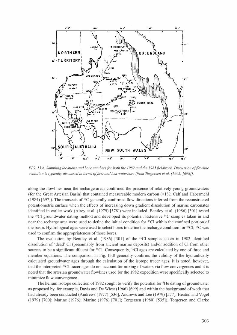
303

along the flowlines near the recharge areas confirmed the presence of relatively young groundwaters (for the great artesian basin) that contained measureable modern carbon (>1%; calf and habermehl (1984) [697]). The transects of 13c generally confirmed flow directions inferred from the reconstructed potentiometric surface when the effects of increasing down gradient dissolution of marine carbonates identified in earlier work (Airey et al. (1979) [578]) were included. Bentley et al. (1986) [301] tested the 36cl groundwater dating method and developed its potential. extensive 14c samples  taken  in and near the recharge area were used to define the initial condition for 36cl within the confined portion of the basin. Hydrological ages were used to select bores to define the recharge condition for 36cl; 14c was used to confirm the appropriateness of those bores.

The  evaluation  by  Bentley  et  al.  (1986)  [301]  of  the  36cl  samples  taken  in  1982  identified dissolution of ‘dead’ cl (presumably from ancient marine deposits) and/or addition of cl from other sources to be a significant diluent for 36cl. consequently, 36cl ages are calculated by one of three end member  equations. The  comparison  in fig. 13.8 generally  confirms  the validity of  the hydraulically calculated groundwater ages through the calculation of the isotope tracer ages. It is noted, however, that the interpreted 36cl tracer ages do not account for mixing of waters via flow convergences and it is noted that the artesian groundwater flowlines used for the 1982 expedition were specifically selected to minimize flow convergence.

the helium isotope collection of 1982 sought to verify the potential for 4he dating of groundwater as proposed by, for example, davis and de wiest (1966) [699] and within the background of work that had already been conducted (Andrews (1977) [536]; Andrews and Lee (1979) [577]; Heaton and vogel (1979)  [700]; marine  (1976); marine  (1976)  [701];  Torgersen  (1980)  [535]).  Torgersen  and  clarke 

FIG. 13.6. Sampling locations and bore numbers for both the 1982 and the 1985 fieldwork. Discussion of flowline evolution is typically discussed in terms of first and last waterbore (from Torgersen et al. (1992) [698]).

304

(1985) [293], working with knowledge that the apparent hydraulic groundwater ages had been confirmed by 36cl measures, showed that (relatively) ‘young’ groundwaters of the great Artesian Basin increased their 4he concentration at a rate that was consistent with a 4he source derived from local sources within the  aquifer  sandstones. However,  further  along  flowlines  in  ‘older’  groundwaters,  the  rate  at which 4He increased was up to 74 times the rate of in situ production (fig. 13.9). Measurements of 222rn in the 1982 groundwater samples showed no significant increase in the 222rn activity in the older portion (high 4He flux region) of the flowline and, thus, no evidence that a stronger, local, in situ source of 4he was acting to increase the rate of 4he introduction. these helium results indicated the predominance of an external source of 4He that was consistent with a basal flux derived from U–Th series decay in the Earth’s  crust  beneath  the great Artesian Basin. most  importantly,  the  inference of  a  large  basal flux of 4He was supported by the simple hydraulic flow model of Torgersen and Ivey (1985) [93] that accounted for the delay time (see fig. 13.9) before the enhanced rate of 4he accumulation (the basal

FIG. 13.7. Contours of deuterium isotopes (top) show a tongue of isotopically heavy water following the trends in flow directions seen in Fig. 13.4. Contours of 13C isotopes (bottom) reflect the trend in flow directions and the dissolution of marine carbonates (from Airey et al. (1983) [363]).

305

FIG. 13.8. 36Cl/Cl versus 36Cl concentration for the Great Artesian Basin (top) and the comparison (bottom) of apparent 36Cl tracer ages to apparent groundwater ages calculated from hydraulic properties (from Bentley et al. (1986) [310]; reproduced with permission of the American Geophysical Union).

306

flux) was observed. owing to the predominance of this external 4he source, the 4he tracer ages were never calculated from the great artesian basin 4he measurements.

helium isotope measurements from the 1982 and 1985 expeditions (torgersen et al. (1987) [682]) showed that the isotope ratio of helium accumulating along most flow paths was consistent with the calculated in situ production ratio and was, additionally, indistinguishable from an expected deep crustal production ratio (both order 10–8; fig. 13.10). however, some paths showed 3he/4he ratios that were  significantly  elevated  (fig. 13.10)  and  suggested  a mantle  source of  helium  (3he/4he ratios of the order of 10–5). these data suggest a point source input of a 3He-rich  component  that  is  diluted along  the  groundwater  flow  path  by mixing  and  addition  of  helium  from  the  basal  fluxes  to  the  in situ  production. This  stable  helium  tracer,  thus,  defines  a  unique  source  region within  the  recharge area that can be tracked downstream to define a flow path. This 3He-rich tracer,  thus, further defines and supports  the flow paths  inferred by Habermehl (1980) [668] from the potentiometric surface.  In addition, collerson et al. (1988) [681] showed that recharge area groundwaters were ‘spiked’ with low 87sr/86Sr ratios (and a higher ca/Sr ratio) as a result of cenozoic volcanic intrusions, and jurassic and 

FIG. 13.9. Helium concentrations versus groundwater hydraulic age (as supported by 36Cl dates (Bentley et al. (1986) [310])) for the Great Artesian Basin, Australia as deduced from the 1982 fieldwork. For groundwaters younger than 40 ka, the accumulation rate is 4.6 × 10–12 cm3 STP 4He · cm–3

H2O · a–1 which agrees with the calculated rate (ΛHe = 1) of 3.95 × 10–12 cm3 STP 4He · cm–3

H2O · a–1. For groundwaters greater than 100 ka, the rate of accumulation is 2.91 × 10–10 cm3 STP 4He · cm–3

H2O · a–1 or 74 times in situ production. An external bottom boundary flux provides the best explanation for the source and the timescale over which it can be seen (Torgersen and Clarke (1985) [293]).

307

younger volcanic activity that was active in and along the eastern margin of the sedimentary basin of what would become the great artesian basin (fig. 13.11). the downstream dilution of this recharge area 87sr/86Sr  ‘spike’  again  serves  to  strongly  support  the  validity  of  the  flowlines  identified  from potentiometric surfaces.

Torgersen et al. (1989) [573] show that 40ar results appear to follow the same dynamics as 4he in the great artesian basin and are also consistent with in situ production followed by input from an external basal flux. The 4he and 40ar data are generally explained by similar processes but the 4he/40ar ratio  remains  quite  variable.  This  suggests  that  these  deep  crustal  noble  gas  fluxes  are  decoupled. decoupling of 4he and 40Ar from their U–Th series and K sources is likely accomplished by processes at the grain scale including recoil, diffusive release and dissolution as well as large scale fracturing that

FIG. 13.10. Mantle 3He is identified in portions of the two flowlines of the Great Artesian Basin (Fairlight Trust to Wilfred Downs and Juanbong to Bonna Vista; lower right numbers in parentheses indicate bore number for cross-referencing with the top two figures) based on the occurrence of the high ratio in 3He/4He as seen by the slope of the line. The occurrence of Cenozoic volcanism (left) in the area of recharge and the groundwater flowlines (top right) show how this signal is carried into the interior of the Great Artesian Basin (from Torgersen et al. (1987) [682]; reproduced with permission of the American Geophysical Union).

1500

1000

500

010005000 1500 2000 2500

4He (cm3 STP/g × 108)

3 He

(cm

3 STP

/g ×

1014

)

JUANBONG(67)

1982

1985

COCKLAURINA(1338)

KAHMOO(2271)

WILFREDDNS

(12039)

FAIRLIGHTTRUST

(57)

OAKWOOD(5287) BONAVISTA

(2049)

58×10–8

84×10

–8

12×10–8

6.75×10–8

1.6×10–8

308

will additionally separate 4he and 40Ar  (Torgersen  and o’donnell  (1991)  [543]). given  the  relative signal strengths, the 40ar results suggest that 4he is more useful for basins with very old groundwater.

13.6. THE 1985 fIELdworK: fAIrLIgHT TrUST To cLAyToN, ATHoL To mUTTI mUTTI ANd mT. crISPE To cUrdImUrKA

In  continuing  to  build  a  knowledge  base  of  the flow paths  and flow  rates  of  the  eastern great Artesian  Basin,  fieldwork  in  1985  addressed  additional  flowlines  in  the  eastern  and  central  great Artesian Basin as well as a flowline  in  the western great Artesian Basin  that  is not  included  in  this discussion. The flowlines sampled explore  the northern area of  the basin and  the  role of converging flowlines as a complication in the application and use of tracer age calculations.

Torgersen et al. (1991) [300] identified an increase in cl and So4 down the flowline for the Athol to Mutti Mutti group which also showed 36cl ages on the high side of hydraulic ages (see fig. 13.12). a discontinuous 36cl  evolution  is  distinct  near  meerabooka  where  the  east–west  transect  possibly intersects the north–south transect. distinct addition of cl is also evident near the end of the north–south transect at clayton bore, as flowing groundwater rises from depth and is subject to convergent mixing. the impact of such mixing on the calculated tracer age was estimated based on linear mixing along an exponential decay curve. for this flowline, convergent mixing was suspected to cause minimal offset of the apparent tracer age.

Torgersen  et  al.  (1992)  [698]  combine  the  helium  isotope  data  of  1982  and  1985  fieldwork, and show the area of highest he concentration to be coincident with the oldest water and the lowest

FIG. 13.11. The evolution of dissolved 87Sr/86Sr within two flowlines of the Great Artesian Basin (north is Stannum to Innamincka and south is Bonna Vista to Thargomindah). The low 87Sr/86Sr ratio is acquired in the recharge zone, likely via contact with Cenozoic volcanics (see Fig. 13.9 and note also the acquired 3He signature). As the flowing groundwaters dissolve the host rock (87Sr/86Sr ~ 0.7111) and marine carbonates (87Sr/86Sr ~ 0.709234) in situ, that end member is steadily acquired in the dissolved phase (after the measurements of Collerson et al. (1988) [681]).

336

0.7040

0.7050

0.7060

0.7070

0.7080

0.7090

0.7100

0.7110

0.7120

0 200 400 600 800 1000Linear distance (km)

87Sr

/86Sr

N recharge

N flowline

S recharge

S flowline

309

(and near radioequilibrium) 36cl  concentration  (compare  figs 13.13  and  13.14).  The  helium  data also show  the  impact of  the western  recharge area and  the  limited  recharge along  the north-western recharge margin.

13.7. ModellIng 36cl and 4he

The results of  the 1982 and 1985 fieldwork for both  36cl and 4he presented new data and new methods for the evaluation of very old groundwater. discussion in the literature regarding the approach, assumptions and necessary conditions for the application of new methods (Bentley et al. (1986) [310]) is common. Andrews and fontes (1991) [702], Andrews and fontes (1993) [703], fontes and Andrews (1993) [704], and mazor (1992) [705] presented an evaluation of great Artesian Basin 36cl data that explained spatial variations in 36cl as the result of mixing between groundwaters along flowlines and 

FIG. 13.12. Chlorine-36 measures along the Fairlight Trust to Clayton flowline show a distinct discontinuity at Meerabooka, possibly indicating flowline mixing as deduced by both the 36Cl/Cl versus the 36Cl plot (bottom) and the tracer 36Cl age versus the hydraulic groundwater age (top) (from Torgersen et al. (1991) [300]; reproduced with permission of the American Geophysical Union).

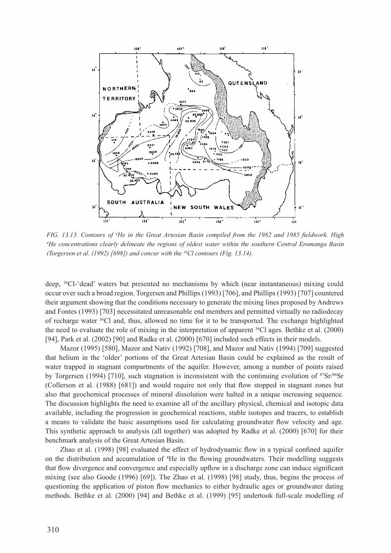
310

deep, 36cl-‘dead’ waters  but  presented  no mechanisms  by which  (near  instantaneous) mixing  could occur over such a broad region. Torgersen and Phillips (1993) [706], and Phillips (1993) [707] countered their argument showing that the conditions necessary to generate the mixing lines proposed by andrews and fontes (1993) [703] necessitated unreasonable end members and permitted virtually no radiodecay of recharge water 36cl and, thus, allowed no time for it to be transported. the exchange highlighted the need to evaluate the role of mixing in the interpretation of apparent 36cl ages. Bethke et al. (2000) [94], Park et al. (2002) [90] and radke et al. (2000) [670] included such effects in their models.

mazor (1995) [580], mazor and Nativ (1992) [708], and mazor and Nativ (1994) [709] suggested that  helium  in  the  ‘older’  portions  of  the great Artesian  Basin  could  be  explained  as  the  result  of water trapped in stagnant compartments of the aquifer. however, among a number of points raised by Torgersen  (1994)  [710],  such stagnation  is  inconsistent with  the continuing evolution of  87sr/86sr (collerson  et  al.  (1988)  [681])  and would  require  not  only  that  flow  stopped  in  stagnant  zones  but also that geochemical processes of mineral dissolution were halted in a unique increasing sequence. the discussion highlights the need to examine all of the ancillary physical, chemical and isotopic data available, including the progression in geochemical reactions, stable isotopes and tracers, to establish a means  to  validate  the  basic  assumptions  used  for  calculating  groundwater  flow  velocity  and  age. This synthetic approach to analysis (all  together) was adopted by radke et al. (2000) [670] for  their benchmark analysis of the great Artesian Basin.

zhao et al.  (1998) [98] evaluated the effect of hydrodynamic flow in a  typical confined aquifer on the distribution and accumulation of 4He  in  the flowing groundwaters. Their modelling  suggests that flow divergence and convergence and especially upflow in a discharge zone can induce significant mixing  (see also goode  (1996)  [69]). The zhao et al.  (1998)  [98] study,  thus, begins  the process of questioning  the application of piston flow mechanics  to either hydraulic ages or groundwater dating methods. Bethke  et  al.  (2000)  [94]  and Bethke  et  al.  (1999)  [95]  undertook  full-scale modelling  of 

FIG. 13.13. Contours of 4He in the Great Artesian Basin compiled from the 1982 and 1985 fieldwork. High 4He concentrations clearly delineate the regions of oldest water within the southern Central Eromanga Basin (Torgersen et al. (1992) [698]) and concur with the 36Cl contours (Fig. 13.14).

311

the  great Artesian  Basin  groundwater  flow  system,  including  the  4he accumulation and concluded that the distribution of 4He  is  controlled  not  only  by  lateral  flow but  also  by  upflow and downflow regions that develop in response to basin topography and structure. this modelling effort showed that the spatial distribution of 4He can be quantitatively reconciled with groundwater flow patterns using a 3-d modelling  framework. Similar modelling of  the  36cl dynamics  (Park et  al.  (2002)  [90]) again confirmed  the  need  to  consider  3-d  flow  in  aquifer  systems  and  the  role  of  upflow,  downflow  and 

FIG. 13.14. Contours of 36Cl from Radke et al. (2000) [670]. The primary recharge areas (high 36Cl) are clearly delineated as is the locale for very old groundwater (low 36Cl). The agreement between the areas of low 36Cl and high 4He (older) and between high 36Cl and low 4He (younger) (Fig. 13.13) is clear.

312

convergent flow in the reconciliation of hydraulic ages with tracer based ages. The summary manuscript (Bethke and johnson (2008) [84]) reiterates these principles.

13.8. geocheMIcal ModellIng of groundwater reactIon paths

Herczeg et al. (1991) [711] conducted a detailed analysis of the groundwater geochemistry from the 1985 fieldwork using PHrEEqE (Parkhurst et al. (1980) [160]). That study explained the increase in total dissolved solids (TdS) along flowlines and distinct chemical differences between the eastern great artesian basin (na–hco3 type) and the western great artesian basin (na–so4–cl type) waters. figures  13.15  and  13.16  show  clearly  the  strong  increase  in  alkalinity, dIc  and δ13c along eastern great Artesian Basin  groundwater  flowlines  as well  as  the  slowly  increasing Na, cl  and TdS,  and the decreasing ca and mg. Herczeg et al. (1991) [711] discussed the increase in TdS as a result of: (i) mixing of flowline groundwaters with saline waters within the deeper portions of the basin; (2) ion filtration through mudstone membranes; and (3) dissolution of evaporates, carbonate minerals or other minerals in situ. They inferred that saline waters most likely originated from the overlying cretaceous marine  sediments  and were  introduced  by  downward  diffusion  into  the  aquifers  of  the cadna-owie formation and Hooray Sandstone. However, given the upward leakage of artesian groundwater from 

FIG. 13.15. Evolution of Na and K chemistry and TDS along the 1985 sampling lines as reported by Herczeg et al. (1991) [711]. It should be noted that the western Great Artesian Basin (Mt. Crispe-o-Curdimurka) is distinct from the eastern Great Artesian Basin and that mixing with the eastern Great Artesian Basin flow is apparent at the end of the western flowline.

313

the deeper, stratigraphically lower aquifers to the stratigraphically higher cretaceous aquifers, mixing is likely to be slight. Herczeg et al. (1991) [711] further inferred that ion filtration is likely to be minimal based on the 36cl studies of Bentley et al. (1986) [301], and concluded that variable evapotranspiration in  the  recharge  areas  in  combination with mineral  dissolution  along  flowlines  represented  the most plausible mechanism for the chemical evolution observed in figs 13.15 and 13.16.

The eastern great Artesian Basin flowline trends of increasing Na alkalinity and dIc together with the decreasing ca and mg were evaluated (Herczeg et al. (1991) [711]) in terms of a model proposed by Blake (1989) [712] which includes: (i) dissolution of carbonate minerals resulting in increased ca, mg and hco3; (ii) cation exchange of ca and Mg for na in clay minerals, followed by; (iii) a reaction of Na with kaolinite to produce Na–smectite. reasoning that the down gradient flow increase in alkalinity can only be accomplished by carbonate dissolution in the presence of high pco2, they concluded that co2 respiration by plants in the recharge zone can drive the δ13c of dIc resulting from these reactions from an initial –15‰ to approximately –12‰. however, to enable the reactions to continue requires the addition of co2 as a result of anaerobic fermentation and reduction of co2 to methane.

FIG. 13.16. Evolution of alkalinity, 13C, Ca+2 and Mg+2 chemistry along the 1985 sampling lines as reported by Herczeg et al. (1991) [711]. It should be noted that the western Great Artesian Basin (Mt. Crispe-to-Curdimurka) is distinct from the eastern Great Artesian Basin and that mixing with the eastern Great Artesian Basin flow is apparent at the end of the western flowline.

0.0

5.0

10.0

15.0

20.0

25.0

0 200 400 600 800 1000 1200 1400

Linear distance (km)

Alk

(meq

/kg)

Athol-to-Mutti Mutti

Fairlight-to-Clayton

MtCrispe-to-Curdimurka

0.00

1.00

2.00

3.00

4.00

5.00

6.00

0 200 400 600 800 1000 1200 1400

Ca

2+

Athol-to-Mutti MuttiFairlight-to-ClaytonMtCrispe-to-Curdimurka

-16.0

-14.0

-12.0

-10.0

-8.0

-6.0

-4.0

-2.0

0.0

0 200 400 600 800 1000 1200 1400

δ 13

C (

‰)

Athol-to-Mutti Mutti

Fairlight-to-Clayton

MtCrispe-to-Curdimurka

1

10

100

1000

10000

0 200 400 600 800 1000 1200 1400

Mg

2+ (m

mol

/kg)

Athol-to-Mutti MuttiFairlight-to-ClaytonMtCrispe-to-Curdimurka

Linear distance (km)

Linear distance (km)Linear distance (km)

(mm

ol/k

g)

314

13.9. THE 2000 BENcHmArK ANd SyNTHESIS

following the seminal paper of Habermehl (1980) [668], the publication by radke et al. (2000) [670]  is  a compilation and  synthesis of  the hydrogeology, hydrochemistry and  isotope hydrology of the great Artesian Basin.  It  is  based  largely  on  samples  and  laboratory  results  of  the  fieldwork  by habermehl and others during the 1970s, 1980s and 1990s, with some additions of analyses and results from queensland and South Australia. This benchmark paper synthesized groundwater flow models, geochemical reaction and transport models, and the dating of the artesian groundwater in the aquifers of the cadna-owie formation and Hooray Sandstone to infer the timescale of recharge and the in situ flow rates.  It  further utilized distinctive hydrogeochemical anomalies  to  infer details of groundwater flow in these aquifers. In the few paragraphs that follow, these findings are summarized, especially as they relate to this case study and the additional detail deduced through the use of modern hydrodynamic and hydrogeochemical codes.

The mapped (radke et al. (2000) [670]) spatial distributions of modern 14c (fig. 13.17) and 36cl (fig. 13.14) are consistent with previous work. The location of very old groundwater (near equilibrium values of 36cl) is consistent with the mapped regions of very high 4He  (fig. 13.13). recharge, flow direction  and  discharge  zones  (figs 13.18  and  13.19)  reported  by  radke  et  al.  (2000)  [670]  were similar to the original diagrams of Habermehl (1980) [668]. recharge is estimated to be on the order of 1012 L/a with an unknown proportion distributed between rainfall and river infiltration. This current recharge rate may be enhanced as a result of the previous century of drawdown. natural discharge is of the order of 0.5 × 1012 l/a with most discharge via upward leakage and minimal discharge via outlet springs (see table 13.1). the range of estimates for great artesian basin storage of water is significant  (Table 13.1),  leading  to vastly different  simple  estimates of groundwater  residence  times (storage volume divided by input rate (or output rate)). the climate reconstructions of, for example, magee et al. (2004) [683] suggest a decline in rainfall over Pleistocene time and discharge springs have experienced a significantly reduced head over the past century. Thus, it is not anticipated that discharge rates  contribute  significantly  to  this  residence  time  discrepancy.  Using  the  Habermehl  and  Seidel (1979)  [689]  estimated  storage  (1018  L)  would  yield  recharge-based  and  discharge-based  residence times of 1 and 2 Ma which are in general agreement with estimates from 36cl and hydraulic estimates. the precision and the precise meanings of these differences in storage are not clear but it may be the difference between in situ storage and recoverable storage.

The eastern great Artesian Basin is characterized by increasing TdS and alkalinity along flowlines. chemical anomalies are noted along the Birdsville-diamantina Track with additional high cl anomalies along the Eulo-Nebine ridge area. groundwater temperatures increase with depth of the aquifers and anomalous geothermal gradients throughout the basin (Habermehl and Pestov (2002) [713]; Habermehl et al. (2002) [714]) and the central Eromanga Basin shows a distinct increase in Na especially when expressed as sodium excess (e.g. [Na] – [cl]). High fluoride concentrations occur over basement highs where  the  aquifer  is  possibly  in  contact with  igneous  and metamorphic  basement  rocks. The  stable isotopic signature of the groundwater suggests that heavy monsoon rainfall in the eastern recharge zone  is  responsible for  the majority of  recharge although evapotranspiration before recharge may be significant. Stable isotopes throughout the basin (radke et al. (2000) [670]) show little variation. This apparent lack of any palaeoclimatic signature may be the result of minimal climatic variation and/or attenuation by dispersive mixing. Hydrodynamic models of groundwater flow calibrated against 14c in and near the recharge areas suggest flow rates range from 1.4 to 2.9 m/a (radke et al. (2000) [670]). flow rates calculated by hydrodynamic models and estimates of the 36cl controls indicate several areas with artesian groundwater flow rates as low as 0.03–0.3 m/a (see fig. 13.18). very slow flow regions are areas of predominant water loss via upward leakage although the hydrochemical signatures in low flow  areas  also  indicate  the  possibility  of  downward  diffusion  of  some  ions  from  overlying  Lower cretaceous aquitards into the lower cretaceous–jurassic aquifers (fig. 13.19). It would appear that discharge from artesian springs (11%) is small compared to discharge via upward leakage (89%) for 

315

a total natural discharge of 0.5 × 109 l/a. however, spring discharges might have been much larger in past geological times (Prescott and Habermehl (2008) [715]). Anthropogenic discharge (0.57 × 109 l/a) is estimated to currently be slightly in excess of natural discharge.

overall,  the benchmark paper of radke et al.  (2000) [670]  is  in general agreement with earlier studies including the flow rate and age of groundwater inferred from 14c, 36cl and 4he studies. however, their  detailed  analysis  appears  to  identify  high  flow  regimes  with  lower  salinities  in  the  shallow depth of burial regions. NETPATH (Plummer et al. (1994) [120]) modelling of great Artesian Basin geochemistry produced  results  in  agreement with  the overall  net  reactions postulated by Herczeg et al. (1991) [711] but suggested that carbonate dissolution reactions are the primary driving mechanism rather  than  smectite–kaolinite  transformations.  Thermal  convection  (Pestov  (2000)  [716])  has  not been substantiated.

FIG. 13.17. Contours of 14C (in per cent modern) from Radke et al. (2000) [670]. The primary recharge areas are clearly delineated and the loss of 14C in the older regions of the Great Artesian Basin is clear.

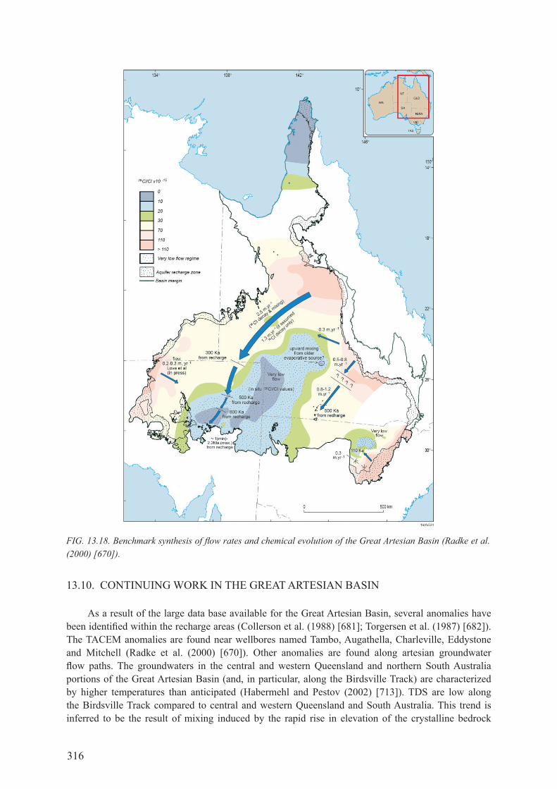
316

13.10. coNTINUINg worK IN THE grEAT ArTESIAN BASIN

as a result of the large data base available for the great artesian basin, several anomalies have been identified within the recharge areas (collerson et al. (1988) [681]; Torgersen et al. (1987) [682]). the taceM anomalies are found near wellbores named tambo, augathella, charleville, eddystone and  mitchell  (radke  et  al.  (2000)  [670]).  other  anomalies  are  found  along  artesian  groundwater flow  paths.  The  groundwaters  in  the  central  and western  queensland  and  northern  South Australia portions of the great Artesian Basin (and, in particular, along the Birdsville Track) are characterized by  higher  temperatures  than  anticipated  (Habermehl  and  Pestov  (2002)  [713]).  TdS  are  low  along the Birdsville Track compared  to central and western queensland and South Australia. This  trend  is inferred  to  be  the  result  of mixing  induced  by  the  rapid  rise  in  elevation  of  the  crystalline  bedrock 

FIG. 13.18. Benchmark synthesis of flow rates and chemical evolution of the Great Artesian Basin (Radke et al. (2000) [670]).

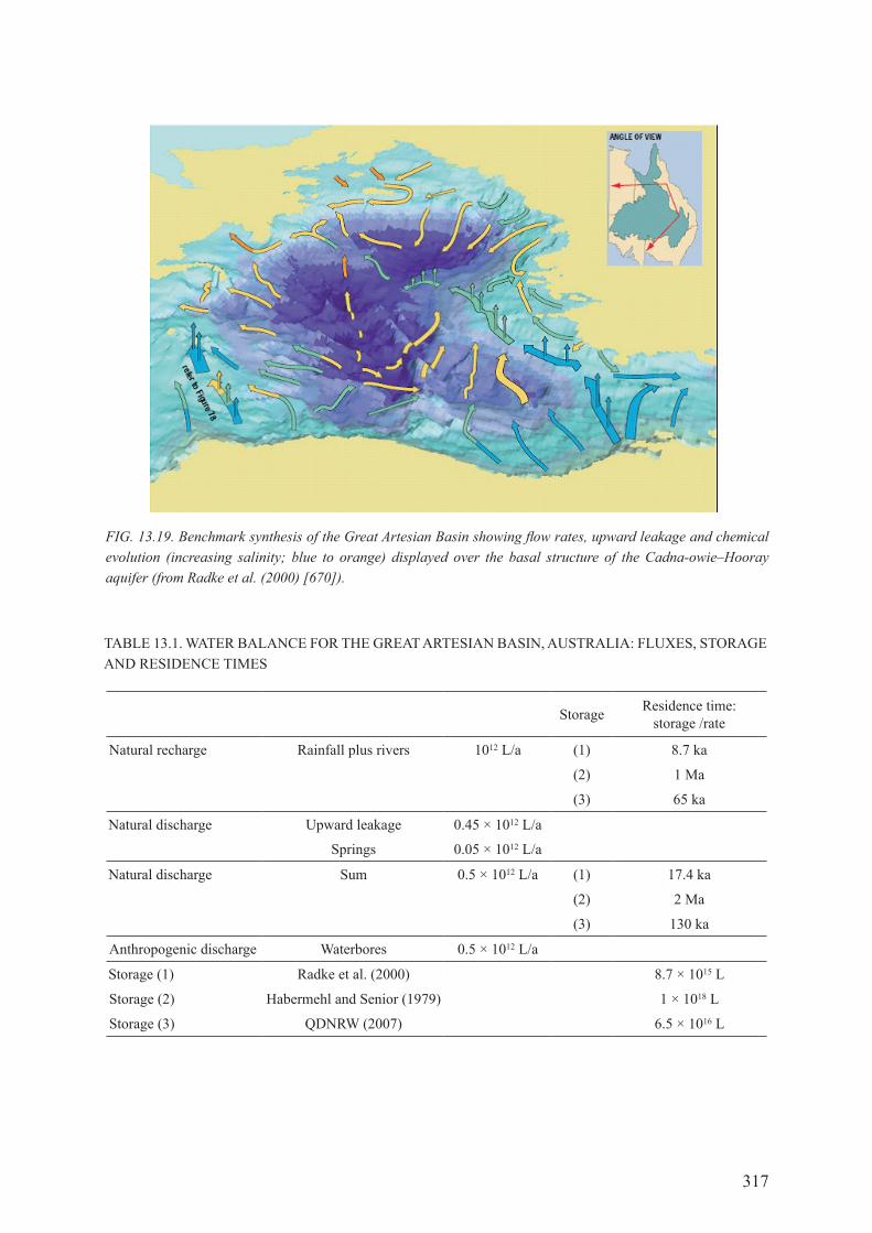
317

FIG. 13.19. Benchmark synthesis of the Great Artesian Basin showing flow rates, upward leakage and chemical evolution (increasing salinity; blue to orange) displayed over the basal structure of the Cadna-owie–Hooray aquifer (from Radke et al. (2000) [670]).

table 13.1. water balance for the great artesIan basIn, australIa: fluxes, storage and resIdence tIMes

storage residence time: storage /rate

natural recharge rainfall plus rivers 1012 l/a (1) 8.7 ka

(2) 1 Ma

(3) 65 ka

natural discharge Upward leakage 0.45 × 1012 l/a

springs 0.05 × 1012 l/a

natural discharge sum 0.5 × 1012 l/a (1) 17.4 ka

(2) 2 Ma

(3) 130 ka

anthropogenic discharge waterbores 0.5 × 1012 l/a

storage (1) radke et al. (2000) 8.7 × 1015 l

storage (2) habermehl and senior (1979) 1 × 1018 l

storage (3) qdnrw (2007) 6.5 × 1016 l

318

based on geothermometry studies of Pirlo (2004) [717]. Evidence for this mixing of waters is provided by the discord among silica geothermometers and cation geothermometers. as silica geothermometers re-equilibrate  relatively  quickly  compared  to  cation  geothermometers,  the  low  Si  temperatures and the high cation temperatures indicate mixing from deeper, hotter (faster reactions) regions and shallow regions.

o’Shea and jankowski (2006) [718] have performed hierarchical cluster analysis on the chemical compositions in the coonamble Embayment (south-eastern great Artesian Basin and an area in New South wales not discussed above) and compared  them with  traditional Piper diagrams (Piper (1944) [719]), durov diagrams  (chiligar  (1956)  [720])  and  a modification of Piper  analysis  (chada  (1999) [721]). This cluster analysis indicates three main geochemical water types that can be associated with processes of ion exchange, precipitation and mixing from different sources. they were also able to identify  an  anomalous  sample  that  is  suspected  to be  influenced by magmatic  sources of co2. this indication of magmatic co2 is consistent with the location of other anomalies observed in 87sr/86sr (collerson  et  al.  (1988)  [681])  and  3he/4He  (Torgersen  et  al.  (1987)  [682])  that  are  geographically associated with the eastern recharge zone that was subject to considerable cenozoic and pre-cenozoic volcanism (duncan and mcdougall (1989) [680]).

recharge, recharge processes and rates, detailed hydrochemistry and isotope studies, including stable (δ2h, δ18o and δ13c) and radioactive (14c, 36cl) isotopes have been carried out in the queensland (Kellett et al. (2003) [722]) and New South wales (Habermehl et al. (2009) [723]) parts of the great artesian basin and recharge rates range from 0.5 to 10 mm/a, with some higher values. a detailed study of recharge along the western margin and discharge in the south western region of the great artesian basin commenced in 2009.

Shimada et al. (1998) [724], Shimada et al. (1999) [725] and Shimada et al. (1997) [726] sampled several transects in the coonamble embayment in 1996 and interpreted the hydrochemistry, and stable (δ2h, δ18o and δ13c) and radioactive (14c, 36cl) isotope results for this south-eastern part of the great artesian basin, which has its own recharge area.

Extensive  sampling  of  flowing  artesian  waterbores  tapping  the  aquifers  in  the  cadna-owie formation and hooray sandstone was carried out in 2002 and 2003 along transects similar to the 1982 and 1985 transects, with additional transects in the queensland, south australia and northern territory parts of the great Artesian Basin. This was followed in 2004 and 2005 by the construction of fully cored drill-holes  through  the Lower cretaceous  aquitards  into  the  aquifers near  the north-eastern  recharge area and the south-western discharge area. Laboratory results on hydrochemistry, stable isotopes (δ2h, δ18o and δ13c), radioactive isotopes (14c, 36cl) and noble gases (4he, 3he/4he, ne) were analysed and interpreted and confirm the results of earlier studies. Additional 36cl and 4he measures continue to show they remain useful indicators for groundwater residence times of very old groundwater (hasegawa et al. (2009) [727]; mahara et al. (2009) [728]).

319

Chapter 14

kRYPtOn-81 CAsE stUDY: tHE nUbIAn AQUIFER, EGYPt

n. sturchIodepartment of earth and environmental sciences, chicago, Illinois, united states of america

r. purtschertphysics Institute, university of bern, Bern, Switzerland

14.1. nubIan aquIfer

The Nubian aquifer of north-east Africa is one of the world’s largest fresh groundwater resources (~150 000 km3). an area in the western desert of egypt, for which a number of earlier studies provided sufficient background data on the Nubian aquifer, was selected for the first application of the atom trap trace analysis (ATTA) method (Section 5.4.3) for measurement of 81Kr in groundwater. This area has relatively simple geology, potential for containing very old groundwater, and favourable characteristics for comparison of the 81Kr and 36cl methods (Sturchio et al. (2004) [5]). Before this work, little evidence regarding absolute groundwater residence time in the nubian aquifer was available. estimates of groundwater age in the range of 0.54 × 106–1.58 × 106 a had been obtained from he/ar ratios (himida (1967) [729]). A large number of 14c data had been obtained for the nubian aquifer waters in egypt (fröhlich et al. (2007) [730]; Sonntag et al. (1979) [731]). chlorine-36 data indicated possible residence times of up to ~9 × 105 a (unpublished data1).

14.2. Methods

nubian aquifer groundwater was sampled in May 2002 from six irrigation wells in major oasis areas of the western desert of egypt for measurements of 81Kr, 36cl, 14c, 4he and other chemical and isotopic constituents. dissolved gas was extracted from several 103 kg of water at the field sites using the  Bern  vacuum-stripping  method  described  above  (Section  5.4.1).  Krypton  was  separated  from the extracted gas samples at bern by molecular sieve absorption and gas chromatographic methods; LLc was used to confirm that the abundances of 85Kr in these samples were indeed low (85Kr/Kr < 3% of modern air) as expected for old groundwaters, verifying minimal air contamination during sampling. for  normalization  in ATTA  analyses,  a  calibrated  amount  of  85Kr was mixed with  each Kr  sample. the 81Kr/85Kr ratios  in  the spiked Kr samples were  then measured using ATTA at Argonne National Laboratory (du et al. (2003) [249]). chloride concentrations in water samples were measured by ion chromatography and cl was then precipitated as agcl for measurements of 36cl that were performed by aMs at the prIMe lab of purdue university. noble gas samples were collected in copper tubes and measurements were performed on separate sets of samples at both ETH zurich and Lawrence Berkeley National Laboratory. Aliquots of purified co2 were measured for 14c abundance at the university of Arizona accelerator mass spectrometry facility; these samples were obtained from a portion of the gas used for Kr extraction.

1 sturchIo, n., university of Illinois, purtschert, r., university of bern, unpublished data.

320

14.3. KryPToN-81 dATA

results of the nubian aquifer groundwater analyses for 81Kr are shown in fig. 14.1 and Table 14.1. Krypton-81 is expressed in terms of the air-normalized ratio, R/Rair = (81Kr/Kr)sample/(81Kr/Kr)air, where Rair is the modern atmospheric ratio (81Kr/Kr)air = 1.10 (± 0.05) × 10–12 as measured by atta (du et al.  (2003)  [249]). measured R/Rair  values  in Nubian  aquifer  groundwater  samples  range  from  4.8% to 52.6% modern. using the simple expression for radioactive decay, and the 81Kr  decay  constant λKr = 3.03 (± 0.14) × 10–6/a, the 81Kr tracer age tKr of a groundwater sample is given by:

Krair

1ln

Rt

R

  (14.1)

the range of ages thus derived is 0.2–1.0 × 106 a (fig. 14.1). These are apparent piston flow ages because the extent of age mixing within the sampled wells is unknown.

Ages  increase  progressively  along  flow  vectors  predicted  by  numerical  hydrodynamic models (Brinkman et al. (1987) [732]), verifying distant lateral flow of deep groundwater towards the north-east  from  a  recharge  area  south-west  of  dakhla.  The  correspondence  of  81Kr  age  with  predicted hydrodynamic age indicates negligible input of 81Kr  from  subsurface  sources,  in  agreement  with theoretical calculations and conclusions reached from 81Kr measurements of groundwater from the milk river Aquifer  in  canada  (Lehmann  et  al.  (1991)  [282])  and  the  great Artesian  Basin  in Australia (collon  et  al.  (2000)  [281]). The  estimated  diffusive  loss  of  81Kr  to  aquitards was  limited  to  ≤20% for the great Artesian Basin (Lehmann et al. (2003) [256]), and is expected to be even lower within 

FIG. 14.1. Map showing sample locations (red circles) in relation to oasis areas (shaded green), Precambrian basement areas (patterned) and other regional features. Groundwater flow in the Nubian aquifer is generally towards the north-east, but diverges towards the north and east as shown by arrows (Brinkman et al. (1987) [732]; Hesse et al. (1987) [733]). Krypton-81 ages are shown in blue numbers (in units of 105 a).

3.3 ± 0.4 2.1 ± 0.4

3.9 ± 0.4

6.8 ± 0.8

4.9 ± 0.5

10 +6/−2

321

the nubian aquifer because of the lower porosity and smaller proportion of aquitard formations within this aquifer system (see figs 5.3 and 5.4).

Krypton-81 ages increase progressively with distance to the north and east of dakhla; their areal distribution  indicates  a  flow velocity  of  ~2 m/a  from dakhla  towards farafra,  and  a  lower  velocity towards  Kharga  and  Baris  and  from  farafra  to  Bahariya.  These  observations  are  consistent  with the distribution of hydraulically conductive sandstone within the aquifer and they provide support to some  of  the  early  hydrodynamic models  (Brinkman  et  al.  (1987)  [732]; Hesse  et  al.  (1987)  [733]). South-westward  extrapolation  of  the  ~2 m/a  flow  rate  inferred  from  the  difference  in  81Kr  ages  for dakhla and farafra is consistent with recharge in the area of the Uweinat uplift near the Egypt–Sudan border. In this area, the nubian sandstone is exposed (or buried beneath sand sheets or dunes) at elevations between 200 and 600 m above sea level over a wide area, forming a broad catchment for recharge of the nubian aquifer.

14.4. cHLorINE-36 dATA

Patterson  et  al.  (2005)  [43]  presented  36cl data for 22 groundwater samples from the nubian aquifer in the western desert of egypt, including the six samples also measured for 81Kr. The areal distribution of groundwater ages derived from this data set is shown in comparison with basin 2 hydrodynamic model ages in fig. 14.2. The best estimates of groundwater ages from 36cl data range from about 2 × 105 to 7 × 105 a, and the distribution of these ages indicates flow from south to north, in agreement with 81Kr ages and hydrodynamic models. The 36cl ages agree with hydrodynamic model ages within ±30%. 

TABLE 14.1. ISoToPIc dATA for NUBIAN AqUIfEr wATEr SAmPLES

well name (depth)*

cl (mg/l)

36cl/cl (10–15)

81Kr/Kr (R/Rair %)

4he (10–6 cm3 stp/g)

14c (pmc) δ2h (‰)40ar

(10–5 cm3 stp/g)

dakhla oasis

gum horia (1200 m) 20 76.5 (±3.4) 52.6 (±6.1) 3.0 (±0.3) n.a. –81 57 (±6)

el Zayat 12 (720 m) 59 72.7 (±1.7) 30.6 (±3.6) 3.3 (±0.3) <1.6 –82 33 (±3)

Kharga oasis

Sherka 36 (750 m) 95 12.2 (±5.1) 12.8 (±3.0) 43 (±4) 0.28 (±0.11) –82 67 (±7)

Baris-Aden (600 m) 92 45.6 (±2.1) 22.8 (±3.0) 32 (±3) 3.26 (±0.21) –81 50 (±5)

farafra oasis

farafra 6 (800 m) 24 65.0 (±3.0) 36.5 (±4.2) 3.7 (±0.4) 0.96 (±0.11) –79 50 (±5)

bahariya oasis

bauti 1 (1200 m) 52 20.2 (±1.6) 4.8 (±3.8) 5.1 (±0.5) n.a. –81 40 (±4)

note: n.a. = not analysed; *sample locations shown in fig. 14.1; 1σ errors in parentheses.

322

14.5. correlatIon of 36cl and 81Kr data

there is a good correlation between 36cl/cl ratios and 81Kr ages (fig. 14.3), in samples for which both measurements were made, providing a firm basis for calibrating apparent 36cl ages to an apparent value of (36cl/cl)initial = Ri for the Nubian aquifer. A best-fit curve through the data using the function:

meas Se i Se Kr cl( ) exp( )R R R R t λ= + − −   (14.2)

where tKr is the 81Kr age in years, λcl = 2.30(±0.02) × 10–6/a is the 36cl decay constant and RSe = 8(±3) 10–15 is the secular equilibrium in situ production value for the aquifer (assuming constant cl concentration in water) gives Ri = 131(±11) × 10–15, which coincidentally agrees with the initial value of 125 (±10) × 10–15 estimated for the great Artesian Basin (Love et al. (2000) [292]). Krypton-81 and 36cl ages for most of these samples agree within error, but two samples exhibit significant age discordance that may be explained by deviations from assumptions used for calculating the best-fit curve (i.e. different values of Rse and/or Ri, or addition of subsurface cl). stable cl isotope ratios and cl concentrations for these and other nubian aquifer groundwater samples measured for 36cl (Patterson et al. (2005) [43]) indicate subsurface cl addition  for  some samples and,  in  fact, age calculations  taking  into account added cl using Eq. (14.2) (Section 5.5 and chapter 6) yield 36cl ages in excellent agreement with 81Kr ages. These results demonstrate that the integrity of the 36cl chronometer is vulnerable to additions of cl at any point along a flow path, whereas, in contrast, the potential for open system behaviour of Kr is minimal after water has reached the aquifer. nonetheless, methods for correcting 36cl ages for subsurface additions of cl and 36cl are well established (section 5.5 and chapter 6). the main uncertainty in 81Kr ages is diffusional exchange of Kr between different water masses (Section 5.1.2.2).

FIG. 14.2. Map of the Western Desert of Egypt showing hydrodynamic ages (black numbers) and 36Cl ages (red numbers) in the Nubian aquifer calculated from 36Cl/Cl ratios and assuming Ri = 130 × 10–15, Rse

sandstone = 5 × 10–15 and Rseshale = 15 × 10–15 (from Patterson et al. (2005) [43]). Age units are 103 a.

323

14.6. HELIUm-4 dATA

Measured 4he and 40Ar concentrations in the Nubian aquifer samples are provided in Table 14.1. concentrations of 40ar range from 33–67 × 10–5 cm3 stp/g and indicate excess air incorporation at recharge. ratios of 40ar/36Ar were not measurably different from the atmospheric ratio of 295.5 ± 0.5, so it appears that 40ar production and accumulation within the sandstone aquifer is minimal. however, 4He concentrations (3.0–43 × 10–6 cm3 STP/g) are two to three orders of magnitude greater than the air-saturated water concentration of 4He at 20°c, indicating subsurface addition of 4He that could reflect groundwater age. 4heter concentrations show apparently linear accumulation along the dakhla-Bahariya flow path (Table 14.1), suggesting qualitatively  that groundwater age  increases by nearly a  factor of two  between dakhla  and Bahariya. Using  rock  compositions  that  gave  the  best  fit  of  the measured 36cl/cl data in the basin 2 model, and by assuming that the aquifer is composed of 80% sandstone and 20% shale,  the flux of  4he produced in situ, Jhe, then equals 3.3 × 10–12 cm3 STP · g–1  · a–1 and the corresponding 4He residence times (assuming zero external flux of 4he into the aquifer) range from 870 to 1500 ka. These apparent 4he ages are two to four times greater than either the hydrodynamic ages or the 36cl ages, which indicates that the assumed 4He production rate or the assumption of zero external He flux is inaccurate. Thus, 50–80% of the 4he in these four samples may be from a source external to the aquifer. an external source of 4He is apparent in the Sherka-36 and Baris samples, for which 4he concentrations are much higher and 4he was not used to estimate residence time.

14.7. cArBoN-14 dATA

radiocarbon data for four of the 81Kr samples is given in Table 14.1. The co2 samples for which these measurements were made were  purified  from  aliquots  of  the  dissolved  gas  extracted  for  81Kr measurements. unfortunately, aliquots from two other samples were lost during shipping between laboratories  because  of  damage  to  the  package  containing  them. The  fraction  of modern  carbon  in these samples is uniformly low and ranges from about 0.01 to 0.03. these data constrain the upper limits of atmospheric contamination of the Kr samples as well as possible mixing fractions of young 

FIG. 14.3. Correlation of 36Cl/Cl ratio with 81Kr age. The blue line is an exponential best fit assuming a secular equilibrium 36Cl/Cl ratio of 8 × 10–15 (with the input ratio Ri as a free fitting parameter).

0 200 400 600 800 1000 1200 1400 1600 1800 0

10 20 30 40 50 60 70 80 90

100 110 120 130 140

Bauti 1

Sherka 36

Baris Farafra 6

El Zayat 12 36

Cl/C

l (×

10 –1

5 )

81 Kr age (ka)

Gum Horia

324

groundwater, and are in good agreement with the constraints from 85Kr data. The measured 14c activities of these samples are at the low end of the range for Nubian aquifer waters (fröhlich et al. (2007) [730]), indicating minimal contributions from young groundwater.

14.8. hydrogeologIcal and palaeoclIMatIc IMplIcatIons of groundwater age data

the concordance of the 36cl and 81Kr data supports mean groundwater residence times approaching 106 a in the western desert of egypt. a steady state, two dimensional hydrodynamic model incorporating constraints from 36cl and available measurements of aquifer hydraulic parameters yields groundwater velocities in the range of 0.5 to 3.5 m/a, consistent with residence times estimated from 81Kr (Patterson et al. (2005) [43]). A model proposed by fröhlich et al. (2007) [730] estimates a recharge rate of 0.4 mm/a and a discharge rate of 0.65 mm/a for water in the deep portion of the aquifer. further progress in understanding the aquifer hydrodynamics will require extensive, depth dependent sampling and measurement of multiple stable and radioactive isotopic tracers.

stable isotope ratios of hydrogen and oxygen in the nubian aquifer (and equivalent) groundwaters from  across  Saharan  North  Africa  indicate  a  clearly  defined  continental  isotope  effect  involving precipitation from air masses having an atlantic moisture source; δ2h values decrease gradually from west to east with a geographic pattern resembling that observed in modern european groundwaters (Sonntag et al. (1979) [731]). In the deep Nubian aquifer samples, nearly constant δ2h values (from –82 to –79) as a function of 81Kr age reveal that this Atlantic moisture source was recurrent during all major pre-Holocene pluvial periods  throughout  the past 1 × 106 a. In contrast, the isotopic composition of modern precipitation in the study area, which mostly delivers moisture from the Mediterranean, is much less depleted in 2h (δ2H ranges from –28 to +14‰) (El Bakri et al. (1992) [734]). These observations indicate that nubian aquifer groundwaters were recharged under a climatic regime in which there had been a persistent southward shift of the intertropical convergence zone relative to modern climate in the region.

Acknowledgements

This work was supported by the United States National Science foundation and the United States department of energy.

325

REFEREnCEs

[1]  SHIKLomANov, I., roddA, j.c., world water resources at the Beginning of the Twenty-first century, UNESco, International Hydrology Series, cambridge University Press, Paris (2004).

[2]  anderson, M., groundwater, IAHS Benchmark Papers in Hydrology No. 3, International Association of Hydrological Sciences, wallingford, UK (2008).

[3]  aggarwal, p., et  al.,  Isotope  Hydrology,  IAHS  Benchmark  Papers  in  Hydrology  No.  8,  International Association of Hydrological Sciences, wallingford, UK (2012).

[4]  InternatIonal atoMIc energy agency, atlas of Isotope hydrology: africa, Iaea, Vienna (2007).

[5]  sturchIO, N.C., et al., one  million  year  old  groundwater  in  the  Sahara  revealed  by  krypton-81  and chlorine-36, geophys. res. Lett. 31 (2004).

[6]  bear, j., Hydraulics of groundwater, mcgraw-Hill, New york (1979).

[7]  de MarsIly, g., quantitative hydrogeology — groundwater hydrology for engineers, academic press, orlando, fl (1986).

[8]  doMenIco, p.a., schwartZ, f.w., physical and chemical hydrogeology, john wiley and sons, new york (1998).

[9]  drIscoll, f.g., groundwater and wells (1986).

[10]  fetter, c.w., Applied Hydrogeology, Prentice-Hall, Inc., Englewood cliffs, Nj (2000).

[11]  freeZe, r.a., cherry, j.a., groundwater, Prentice-Hall, Englewood cliffs, Nj (1979).

[12]  MaZor, e., chemical and Isotopic groundwater Hydrology, marcel dekker, New york, Basel (2004).

[13]  Todd, d.K., mAyS, L.w., ground-water Hydrology, john wiley and Sons, New york (2005).

[14]  BAcK, w.,  roSENSHEIN,  j.S.,  SEABEr,  P.r., “hydrogeology”, the geology of north america, the geological society of america, boulder, co (1988).

[15]  glynn, p.d., pluMMer, l.n., geochemistry and the understanding of ground-water systems, Hydrogeol. j. 13 (2005) 263–287.

[16]  glynn, p.d., Voss, c.I., geochemical characterization of Simpevarp ground waters near the Äspö Hard rock Laboratory, Swedish Nuclear Power Inspectorate (SKI) report (1999).

[17]  heath, r.c., ground-water regions of the United States, U.S. geological Survey water-Supply Paper 2242 78 (1984).

[18]  MIller, j.a., ground water atlas of the united states, u.s. geological survey hydrologic atlas, u.s. geological survey (2000).

[19]  rEILLy, T.E., dENNEHy, K.f., ALLEy, w.m.,  cUNNINgHAm, w.L., ground-water  availability  in  the united states, u.s. geological survey circular 1323 (2008) 70.

[20]  sanford, w.e., caIne, j.s., wIlcox, d.a., Mcwreath, h.c., nIcholas, j.r., research opportunities in interdisciplinary ground-water science in the U.S. geological Survey, U.S. geological Survey circular 1293 (2006) 21.

[21]  THorN, c.r., mcAdA, d.P., KErNodLE, j.m., geohydrologic framework and hydrologic conditions in the Albuquerque Basin, central New mexico, U.S. geological Survey water-resources Investigations report 93-4149 (1993) 106.

[22]  frANKE, o.L., rEILLy, T.E., BUxToN, H.T.,  SImmoNS, d.L., study guide for a beginning course in ground-water  hydrology:  Part  2 —  instructor’s  guide,  open-file  report  92-637, u.s. geological survey (1993) 128.

[23]  frANKE, o.L., rEILLy, T.E., HAEfNEr, r.j., SImmoNS, d.L., study guide for a beginning course in ground-water  hydrology:  Part  1 —  course  participants, open-file report 90-183, u.s. geological survey (1990) 184.

[24]  heath, r.c., Basic ground-water hydrology, U.S. geological Survey water-Supply Paper 2220 (1983) 84.

[25]  rEILLy,  T.E.,  frANKE,  o.L.,  BUxToN,  H.T.,  BENNETT,  g.d., A  conceptualization  for  ground-water solute-transport studies with emphasis on physical mechanisms of solute movement, U.S. geological Survey water-resources Investigations report 87-4191 (1987) 44.

326

[26]  mooK,  w.g., environmental Isotopes in the hydrological cycle, principles and applications, Vol. I: Introduction.  Theory, methods,  review,  UNESco  International  Hydrological  Programme  (IHP-v),  Paris, Vienna (2000).

[27]  HEALy, r.w., wINTEr, T.c., LABAUgH, j.w., frANKE, o.L., water budgets: foundations for effective water-resources and environmental management, U.S. geological Survey circular 1308 (2007) 90.

[28]  tÓth, j., A  theoretical  analysis  of  groundwater  flow  in  small  drainage  basins,  j.  geophys.  res.  68 (1963) 4795–4812.

[29]  hely, a.g., Mower, r.w., han, c.a., water resources of Salt Lake county, Utah, Utah department of natural resources technical publication 21 (1971) 244.

[30]  thIros, s.a., quality of shallow ground water in areas of recent residential and commercial development in Salt Lake valley, Utah, 1999, USgS fact Sheet, U.S. geological Survey (2000).

[31]  BETHKE,  c.m., A  numerical  model  of  compaction-driven  groundwater  flow  and  heat  transfer  and  its application to the palaeohydrology of intracratonic sedimentary basins, j. geophys. res. 90 (1985) 6817–6828.

[32]  bexfIeld, l.M., ground-water-level maps and how they are used to understand the aquifer, U.S. geological survey circular 1222 (2002) 47–48.

[33]  fErrIS, j.g., KNowLES, d.B., BrowN, r.H., STALLmAN, r.w., theory of aquifer tests, u.s. geological Survey water-Supply Paper 1536-E (1962) 174.

[34]  KrUSEmAN, g.P., de rIdder, n.a., analysis and evaluation of pumping test data, International Institute for land reclamation and Improvement, wageningen, the netherlands (1990).

[35]  shuter, e., teasdale, w.e., application of drilling, coring, and sampling techniques to test holes and wells, Techniques of water-resources Investigations of the United States geological Survey (1989).

[36]  de VrIes, j.j., sIMMers, I., groundwater recharge: an overview of processes and challenges, hydrogeol. j. 20 (2002) 5–17.

[37]  ScANLoN, B.r., HEALy, r.w., cooK, P.g., choosing appropriate techniques for quantifying groundwater recharge, hydrogeol. j. 10 (2002) 18–39.

[38]  wood, w.w., sanford, w.e., chemical and isotopic methods for quantifying ground-water recharge in a regional, semiarid environment, ground water 33 (1995) 458–468.

[39]  PHILLIPS,  f.m., TANSEy, m.K.,  PEETErS,  L.A.,  cHENg,  S.,  LoNg, A., an isotopic investigation of groundwater  in  the  central  San  juan Basin, New mexico: carbon-14  dating  as  a  basis  for  numerical  flow modeling, water resour. res. 25 (1989) 2259–2273.

[40]  AEScHBAcH-HErTIg, w., cLArK, j.f., STUTE, m., rEUTEr, r.f., ScHLoSSEr, P., a palaeotemperature record derived from dissolved noble gases in groundwater of the aquia aquifer (Maryland, usa), geochim. cosmochim. acta 66 (2002) 797–817.

[41]  castro, M.c., hall, c.M., patrIarche, d., goblet, p., ellIs, b.r., a new noble gas palaeoclimate record in texas — basic assumptions revisited, earth planet. sci. lett. 257 (2007) 170–187.

[42]  STUTE, m.,  ScHLoSSEr,  P.,  cLArK,  j.f.,  BroEcKEr, w.S., palaeotemperatures in the southwestern united states derived from noble gas measurements in groundwater, science 256 (1992) 1000–1003.

[43]  patterson, l.j., et al., cosmogenic, radiogenic, and stable isotopic constraints on groundwater residence time in the nubian aquifer, western desert of egypt, geochem. geophys. geosystems 6 (2005) 1–19.

[44]  walVoord, M., phIllIps, f.M., tyler, s.w., hartsough, p.c., deep arid system hydrodynamics, Part 2: Application to palaeohydrologic reconstruction using vadose-zone profiles from the northern mojave desert, water resour. res. 38 (2002) 1291.

[45]  BAcK, w., origin or hydrochemical facies of ground water in the atlantic coastal plain, 21st Int. geol. congr., copenhagen (1960).

[46]  BAcK, w., Hydrochemical facies and ground-water flow patterns in northern part of Atlantic coastal Plain, u.s. geol. surv. prof. pap. 498-A (1966).

[47]  sanford, w.e., pluMMer, l.n., McAdA, d.P., BExfIELd, L.m., ANdErHoLm, S.K., hydrochemical tracers in the middle rio grande Basin, USA: 2. calibration of a ground-water flow model, Hydrogeol. j. 12 (2004) 389–407.

327

[48]  sanford, w.e., pluMMer, l.n., McAdA,  d.P.,  BExfIELd,  L.m.,  ANdErHoLm,  S.K., use of environmental tracers to estimate parameters for a predevelopment-ground-water-flow model of the middle rio grande Basin, New mexico, U.S. geological  Survey water-resources  Investigations report 03-4286 (2004) 102.

[49]  PLUmmEr,  L.N.,  BExfIELd,  L.m.,  ANdErHoLm,  S.K.,  SANford,  w.E.,  BUSENBErg,  E., geochemical characterization of ground-water flow in the Santa fe group aquifer system, middle rio grande Basin, New mexico, U.S. geological Survey water-resources Investigations report 03-4131 (2004) 395.

[50]  PLUmmEr,  L.N.,  BExfIELd,  L.m.,  ANdErHoLm,  S.K.,  SANford,  w.E.,  BUSENBErg,  E., Hydrochemical  tracers  in  the middle rio grande Basin, USA:  1.  conceptualization  of  groundwater  flow, hydrogeol. j. 12 (2004) 359–388.

[51]  PLUmmEr, L.N., SANford, w.E., BExfIELd, L.m., ANdErHoLm, S.K., BUSENBErg, E., “using geochemical data and aquifer  simulation  to characterize  recharge and groundwater flow  in  the middle rio grande basin, new Mexico”, groundwater recharge in a desert environment: the southwestern united states (hogan, j.f., phIllIps, f.M., scanlon, b.r., eds), american geophysical union, washington, dc (2004).

[52]  cLArK, I.d., frITz, P., environmental Isotopes in hydrogeology, springer Verlag, berlin, heidelberg, new york (1997).

[53]  cooK, P.g., HErczEg, A.L., Environmental Tracers  in Subsurface Hydrology, Kluwer Academic Press, boston, Ma (1999).

[54]  stute, M., schlosser, p., “principles and applications of the noble gas palaeothermometer”, climate change in continental Isotopic records (SwArT, P.K., LoHmANN, K.c., mcKENzIE, j., SvIN, S., eds), geophysical Monograph, american geophysical union (1993).

[55]  AEScHBAcH-HErTIg, w., PEETErS, f., BEyErLE, U., KIPfEr, r., palaeotemperature reconstruction from  noble  gases  in  ground  water  taking  into  account  equilibration  with  entrapped  air,  Nature  405 (2000) 1040–1044.

[56]  heaton, t.h.e., talMa, a.s., Vogel, j.c., origin and history of nitrate in confined groundwater in the western Kalahari, j. Hydrol. 62 (1983) 243–262.

[57]  dansgaard, w., stable isotopes in precipitation, tellus 16 (1964) 436–468.

[58]  rozANSKI,  K.,  ArAgUÁS-ArAgUÁS,  L.,  goNfIANTINI,  r., “Isotopic patterns in modern global precipitation”, climate change in continental Isotopic records (SwArT,  P.K.,  LoHmANN,  K.c., McKENzIE, j., SvIN, S., eds), american geophysical union (1993).

[59]  STrAATEN, c.m.v.d., mooK, w.g., “stable isotopic composition of precipitation and climatic variability”, palaeoclimates and palaeowaters: a collection of environmental Isotope studies, panel proceedings series No. 146, IAEA, vienna (1983).

[60]  pluMMer, l.n., stable isotope enrichment in palaeowaters of the southeast atlantic coastal plain, united states, science 262 (1993) 2016–2020.

[61]  ALLEy, w.m.,  rEILLy, T.E.,  frANKE, o.L., Sustainability  of  ground-water  resources,  U.S.  geological survey circular 1186 (1999) 79.

[62]  pluMMer, l.n., et al., Low-level detections of halogenated volatile organic compounds  in groundwater: use in vulnerability assessments, j. hydrol. eng. 13 (2008) 1049–1068.

[63]  genuchten, M.t.V., alVes, w.j., Analytical  solutions  of  the  one-dimensional  convective-dispersion solute transport equation, tech. bull. 1661 (1982) 151.

[64]  mAŁoSzEwSKI, P., rAUErT, w., STIcHLEr, w., HErrmANN, A., Application of flow models  in an alpine catchment area using tritium and deuterium data, j. hydrol. 66 (1983) 319–330.

[65]  mAŁoSzEwSKI,  P.,  zUBEr, A., “lumped parameter models for interpretation of environmental tracer data”, Manual on the Mathematical Models in Isotope hydrogeology 910 (1996) 9–59.

[66]  HUyAKorN, P.S., PINdEr, g.f., computational Methods in subsurface flow, academic press (1983).

[67]  KoNIKow, L.f., gLyNN, P.d., “modeling ground-water flow and quality”, Essentials of medical geology (selInus, o., ed.), academic press (2005).

[68]  wang, j.f., anderson, M.p., Introduction to groundwater Modeling, freeman, san francisco, ca (1982).

[69]  goode, d.j., direct simulation of groundwater age, water resour. res. 32 (1996) 289–296.

328

[70]  harbaugh, a.w., banta, e.r., hIll, M.c., Mcdonald, M.g., modfLow-2000,  The  U.S. geological Survey modular groundwater model-User guide  to modularization concepts  and  the ground-water flow Process, open-file report, U.S. geological Survey (2000).

[71]  Mcdonald, M.g., harbaugh, a.w., A modular three-dimensional finite-difference ground-water flow model, Techniques of water-resources Investigations of the United States geological Survey (1988).

[72]  reIlly, t.e., System  and  boundary  conceptualization  in  ground-water  flow  simulation,  U.S.  geological Survey Techniques of water-resources Investigations (2001).

[73]  PoLLocK, d.w., documentation of a computer program to compute and display pathlines using results from the U.S. geological Survey modular three-dimensional finite-difference ground-water flow model, U.S. geological survey, open file report 89-381 (1989).

[74]  poeter, e.p., hIll, M.c., documentation of ucode, a computer code for universal inverse modeling, u.s. geological Survey water-resources Investigations report (1998).

[75]  mÜNNIcH,  K.-o., Messung des 14c-gehaltes  von  hartem  grundwasser,  Naturwissenschaften  34 (1957) 32–33.

[76]  daVIs, s.n., bentley, h.w., “dating groundwater: a short review”, nuclear and chemical dating techniques, Interpreting the environmental record (currIe, l.a., ed.), american chemical society, washington, dc (1982).

[77]  phIllIps, f.M., castro, M.c., groundwater dating and residence time measurements, treatise on geochemistry 5 (2003) 51–497.

[78]  dANcKwErTS,  P.v., continuous  flow  systems:  distribution  of  residence  times,  chem.  Eng.  Sci.  2 (1953) 1–13.

[79]  hooper, r.p., diagnostic tools for mixing models of stream water chemistry, water resour. res. 39 (2003).

[80]  loaIcIga, h.a., residence time, groundwater age, and solute output in steady-state groundwater systems, advances in water resources 27 (2004) 681–688.

[81]  McgUIrE, K.j., mcdonnell, j.j., a review and evaluation of catchment transit time modeling, j. hydrol. 330 (2006) 543–563.

[82]  mAŁoSzEwSKI, P., zUBEr, A., determining the turnover time of groundwater systems with the aid of environmental tracers, I. Models and their applicability, j. hydrol. 57 (1982) 207–231.

[83]  VarnI, M., carrera, j., simulation of groundwater age distributions, water resour. res. 34 (1998) 3271–3281.

[84]  BETHKE, c.m., joHNSoN, T.m., groundwater age and groundwater age dating, annu. rev. earth planetary sci. 36 (2008) 121–152.

[85]  InternatIonal atoMIc energy agency, Use of chlorofluorocarbons in Hydrology: A guidebook, Iaea, Vienna (2006).

[86]  KIrcHNEr, j.w., fENg, x.H., NEAL, c., fractal stream chemistry and its implications for contaminant transport in catchments, nature 403 (2000) 524–527.

[87]  McgUIrE, K.j., et al., The role of topography on catchment-scale water residence time, water resour. res. 41 (2005).

[88]  castro, M.c., stute, M., schlosser, p., comparison of 4he ages and 14c ages in simple aquifer systems: implications for groundwater flow and chronologies, Appl. geochem. 15 (2000) 1137–1167.

[89]  castro, M.c., goblet, p., calibration  of  regional  groundwater  flow models: working  toward  a  better understanding of site-specific systems, water resour. res. 39 (2003).

[90]  PArK,  j.,  BETHKE,  c.m.,  TorgErSEN,  T.,  joHNSoN,  T.m., transport modeling applied to the interpretation of groundwater 36cl age, water resour. res. 38 (2002) 1043.

[91]  weIssMann, g.s., Zhang, y., labolle, e.M., fogg, g.e., dispersion of groundwater age in an alluvial aquifer system, water resour. res. 38 (2002).

[92]  berger, p. M., An optimization approach to groundwater age dating: how old is water in the Paris Basin? Msc thesis, university of Illinois (2008).

[93]  torgersen, t., IVey, g.n., helium accumulation in groundwater: II, a model for the accumulation of the crustal 4He degassing flux, geochim. cosmochim. Acta 49 (1985) 2445–2452.

329

[94]  BETHKE,  c.m.,  TorgErSEN,  T., PArK,  j., The  ‘age’  of  very  old  groundwater:  insights  from  reactive transport models, j. geochem. explor. 69–70 (2000) 1–4.

[95]  BETHKE,  c.m.,  zHAo,  x.,  TorgErSEN,  T., groundwater  flow  and  the  4he distribution in the great artesian basin of australia, j. geophys. res. 104 (1999) 12 999–13 011.

[96]  castro, M.c., goblet, p., ledoux, e., VIolette, s., MarsIly, g.d., noble gases as natural tracers of water circulation in the Paris Basin 2, calibration of a groundwater flow model using noble gas isotope data, water resour. res. 34 (1998) 2467–2483.

[97]  castro, M.c., jaMbon, a., MarsIly, g. d., schlosser, p., noble gases as natural tracers of water circulation in the paris basin 1, Measurements and discussion of their origin and mechanisms of vertical transport in the basin, water resour. res. 34 (1998) 2443–2466.

[98]  zHAo, x.,  frITzEL, T.L.B., qUINodoz, H.A.m., BETHKE, c.m., TorgErSEN, T., controls on the distribution and isotopic composition of helium in deep groundwater flows, geology 26 (1998) 291–294.

[99]  gomEz-HErNANdEz, j.j., gorELIcK, S.m., Effective groundwater model parameter values: Influence of spatial variability of hydraulic conductivity, leakance, and recharge, water resour. res. 25 (1989) 405.

[100]  mooK,  w.g., “preface to hydrology section”, radiocarbon after four decades: an Interdisciplinary Perspective, Springer (1992) 241.

[101]  KAmEN, m.d., Early history of carbon-14, Science 140 (1963) 584–590.

[102]  rUBEN, S., KAmEN, m.d., Long-lived radioactive carbon: c14, Phys. rev. 59 (1941) 349–354.

[103]  anderson, e.c., et al., natural radiocarbon from cosmic radiation, phys. rev. 72 (1947) 931–936.

[104]  lIbby, w.f., anderson, e.c., arnold, j.r., Age determination by  radiocarbon content: world-wide assay of natural radiocarbon, science 109 (1949) 227–228.

[105]  mAcKAy, c., the elementary chemistry of atomic carbon, chemical effects of nuclear transformations 2 (1961) 17–26.

[106]  mAK, j.E., BrENNINKmEIjEr, c.A.m., SoUTHoN, j.r., direct measurement of the production rate of 14c near Earth’s surface, geophys. res. Lett. 26 (1999) 3381–3384.

[107]  godwIn, h., half life of radiocarbon, nature 195 (1962) 984.

[108]  cHIU,  T.c.,  fAIrBANKS,  r.g.,  cAo,  L.,  morTLocK,  r.A., analysis of the atmospheric 14c record spanning the past 50,000 years derived from high-precision 230th/234u/238u, 231pa/235u and 14c dates on fossil corals, j. radioanal. nucl. chem. quaternary sci. rev. 26 (2007) 18–36.

[109]  mooK, w.g., carbon-14 in hydrological studies, The Terrestrial Environment A1, Elsevier (1980) 49–74.

[110]  stuIVer, M., polach, h.a., discussion of reporting of 14c data, radiocarbon 19 (1977) 355–363.

[111]  KALIN, r.m., “radiocarbon dating of groundwater systems”, environmental tracers in subsurface hydrology (cooK, P.g., HErczEg, A.L., Eds), Kluwer Academic Press, Boston, mA (1999).

[112]  BArd, E., HAmELIN, B., fAIrBANKS, r.g., zINdLEr, A., calibration of the 14c timescale over the past 30,000 years using mass spectrometric u–th ages from barbados corals, nature 345 (1990) 405–410.

[113]  PELTIEr, w.r., fAIrBANKS, r.g., global glacial ice volume and last glacial Maximum duration from an extended barbados sea level record, j. radioanal. nucl. chem. quaternary sci. rev. 25 (2006) 3322–3337.

[114]  mÜNNIcH, K.-o., Isotopen-datierung von grundwasser, Naturwissenschaften 55 (1968) 158–163.

[115]  foNTES, j.-c., dating of groundwater, guidebook on Nuclear Techniques in Hydrology, Tech. rep. Ser. 91 (1983) 285–317.

[116]  foNTES, j.-c., gArNIEr, j.-m., determination of the initial 14c activity of the total dissolved carbon: a review of the existing models and a new approach, water resour. res. 15 (1979) 399–413.

[117]  fontes, j.c., chemical  and  isotopic  constraints  on c-14  dating  of  groundwater, radiocarbon  after  four decades (1992) 242–261.

[118]  geyh, M.a., “dating of old groundwater — history, potential, limits and future”, Isotopes in the water cycle: past, present and future of a developing science (AggArwAL, P.K., gAT, j.r., frÖHLIcH, K., eds), springer, the netherlands (2005).

[119]  mooK, w.g., Introduction to Isotope hydrology, Iah series, taylor & francis (2005).

330

[120]  PLUmmEr, L.N., PrESTEmoN, E.c., PArKHUrST, d.L., an interactive code (netpath) for modelling net  geochemical  reactions  along  a  flow  path,  version  2.0,  water  resources  Investigations  report,  U.S. geological Survey (1994).

[121]  BrooK, g.A., foLKoff, m.E., Box, E.o., a world model of soil carbon dioxide, earth surface processes and landforms 8 (1983) 79–88.

[122]  deInes, p., langMuIr, d., harMon, r.s., stable carbon isotope ratios and the existence of a gas phase in the evolution of carbonate groundwaters, geochim. cosmochim. acta 38 (1974) 1147–1164.

[123]  Verhagen, b.t., “Environmental  isotope  study  of  a  groundwater  supply  project  in  the  Kalahari  of gordonia”, Isotope Hydrology 1983, IAEA, vienna (1984).

[124]  Verhagen, b.t., MaZor, e., sellshop, g.p.f., radiocarbon and tritium evidence for direct rain recharge to ground waters in the northern Kalahari, Nature 249 (1974) 643–644.

[125]  pluMMer, l.n., busenberg, e., “chlorofluorocarbons”, Environmental Tracers in Subsurface Hydrology (cooK, P.g., HErczEg, A.L., Eds), Kluwer Academic Press, Boston, mA (2000).

[126]  geyh, M.a., an overview of 14c analysis in the study of groundwater, radiocarbon 42 (2000) 99–114.

[127]  vogEL, j.c., grooTES, P.m., mooK, w.g., Isotopic fractionation between gaseous and dissolved carbon dioxide, zeitschrift für Physik 230 (1970) 225–238.

[128]  LEvIN, I., KromEr, B., twenty years of atmospheric 14co2 observations schauinsland station, germany, radiocarbon 39 (1997) 205–218.

[129]  leVIn, I., et al., “14co2 record from sites in central europe”, trends ‘93: a compendium of data on global change (1994) 203–222.

[130]  eIchInger, l., a contribution to the interpretation of 14c groundwater ages considering the example of a partially confined sandstone aquifer, radiocarbon 25 (1983) 347–356.

[131]  EvANS,  g.v.,  oTLET,  r.L.,  dowNINg,  A.,  moNKHoUSE,  r.A.,  rAE,  g., “some problems in the interpretation  of  isotope  measurements  in  United  Kingdom Aquifers”,  Isotopes  in  Hydrology  II,  IAEA, Vienna (1979).

[132]  Ingerson, e., pearson f.r., jr., “estimation of age and rate of motion of groundwater by the 14c-method”, recent researches in the fields of atmosphere, hydrosphere, and nuclear geochemistry, sugara festival Volume (mIyAKE, y., KoyAmA, T., Eds), maruzen, Tokyo (1964).

[133]  mooK, w.g., “on the reconstruction of the initial 14c content of groundwater from the chemical and isotopic composition”, 8th Int. conf. on radiocarbon dating 1 (1972) 342–352.

[134]  taMers, M.a., Validity of radiocarbon dates on groundwater, geophys. surveys 2 (1975) 217–239.

[135]  PLUmmEr, L.N., SPrINKLE, c.L., radiocarbon dating of dissolved inorganic carbon in groundwater from confined parts of the Upper floridan aquifer, florida, USA, Hydrogeol. j. 9 (2001) 127–150.

[136]  wIgley, t.M.l., pluMMer, l.n., pearson f.j., jr., Mass transfer and carbon isotope evolution in natural water systems, geochim. cosmochim. acta 42 (1978) 1117–1139.

[137]  Vogel, j.c., “Investigation of groundwater flow with radiocarbon”, Isotopes in Hydrology, vienna (1967).

[138]  Vogel, j.c., “14c-dating  of  groundwater”,  Isotope Hydrology  1970,  Proceedings  Series No.  131,  IAEA, Vienna (1970).

[139]  Vogel, j.c., ehhalt, d., “the use of carbon isotopes in groundwater studies”, radioisotopes in hydrology, proceedings series no. 38, Iaea, Vienna (1963).

[140]  taMers, M.a., “Surface-water infiltration and groundwater movement in arid zones in venezuela”, Isotopes in hydrology, proceedings series no. 80, Iaea, Vienna (1967).

[141]  saleM, o., VIsser, j.h., dray, M., gonfIantInI, r., “environmental isotopes used in a hydrogeological study of north-eastern Brazil”, Arid-zone Hydrology: Investigations with Isotope Techniques, Panel Proceedings Series No. 134, IAEA, vienna (1980).

[142]  mooK,  w.g., “The  dissolution-exchange  model  for  dating  groundwater  with  14c”, Interpretation of environmental Isotope and hydrochemical data in groundwater hydrology, panel proceedings series no. 108, Iaea, Vienna (1976).

[143]  craIg, h., carbon-13 in plants and their relationships between carbon-13 and carbon-14 variations in nature, j. geol. 62 (1954) 115–149.

331

[144]  McMahon, p.b., chapelle, f.h., redox processes and water quality of selected principal aquifer systems, ground water 46 (2008) 259–271.

[145]  pluMMer, l.n., busby, j.f., lee, r.M., hanshaw, b.b., geochemical modeling of the Madison aquifer in parts of montana, wyoming, and South dakota, water resour. res. 26 (1990) 1981–2014.

[146]  appelo, c.a.j., cation and proton exchange, ph variations, and carbonate reactions in a freshening aquifer, water resour. res. 30 (1994) 2793–2805.

[147]  wIgley, t.M.l., pluMMer, l.n., pearson, f.j., errata, geochim. cosmochim. acta 43 (1979) 1395.

[148]  PLUmmEr, L.N., PArKHUrST, d.L., THorSTENSoN, d.c., development of reaction models for ground-water systems, geochim. cosmochim. acta 47 (1983) 665–686.

[149]  PArKHUrST, d.L., APPELo, c.A.j., User’s guide  to PHrEEqc — A computer program  for  speciation, batch-reaction,  one-dimensional  transport,  and  inverse  geochemical  calculations,  U.S.  geological  Survey water-resources Investigations report, U.S. geological Survey (1999).

[150]  PArKHUrST, d.L., PLUmmEr, L.N., geochemical models, regional ground-water quality (1993) 199–225.

[151]  pearson, f.j., “effects of parameter uncertainty in modeling 14c in groundwater”, radiocarbon after four decades, an Interdisciplinary perspective (1992) 262–275.

[152]  PArKHUrST,  d.L., User’s  guide  to  PHrEEqc  —  A  computer  program  for  speciation,  reaction-path, advective-transport,  and  inverse  geochemical  calculations,  U.S.  geological  Survey  water-resources Investigations report 95-4227 (1995) 143.

[153]  PArKHUrST,  d.L., geochemical  mole-balance  modeling  with  uncertain  data,  water  resour.  res.  33 (1997) 1957–1970.

[154]  glynn, p.d., brown, j.g., “Integrating field observations and inverse and forward modeling: Application at a site with acidic, heavy-metal-contaminated groundwater”, geochemical modeling of groundwater, vadose and geothermal systems (bundschuh, j., ZIlberbrand, M., Eds), crc Press (2012) 181–234.

[155]  THorSTENSoN,  d.c.,  PArKHUrST,  d.L., calculation of individual isotope equilibrium constants for geochemical reactions, geochim. cosmochim. acta 68 (2004) 2449–2465.

[156]  PArKHUrST, d.L., cHArLToN, S.r., NetpathxL — An Excel® interface to the program NETPATH, U.S. geological survey techniques and Methods (2008) 11.

[157]  EL-KAdI, A.I., PLUmmEr, L.N., AggArwAL, P.K., NETPATH-wIN: An interactive user version of the mass-balance model, NETPATH, ground water 49 (2011) 593–599.

[158]  PArKHUrST, d.L.,  PLUmmEr,  L.N., THorSTENSoN, d.c., balance — a computer program for calculating mass transfer for geochemical reactions in ground water, water-resources Investigations report, u.s. geological survey (1982).

[159]  cheng, s.l., long, a., “Implementation of a carbon isotope subroutine to the computer program phreeqe and the application to 14c ground-water dating”, Hydrology and water resources in Arizona and the Southwest, 1984 meeting of  the Arizona Section of  the American water resources Association and  the Hydrogeology Section of the Arizona–Nevada Academy of Sciences (1984) 121–135.

[160]  PArKHUrST,  d.L.,  THorSTENSoN,  d.c.,  PLUmmEr,  L.N., phreeqe — a computer program for geochemical calculations, water resources Investigations report, u.s. geological survey (1980).

[161]  pluMMer, l.n., “geochemical modeling: a comparison of forward and inverse methods”, first canadian/american conference on hydrogeology (HITcHoN, B., wALLIcK, E.I., eds), national water well assoc., banff, alberta (1985).

[162]  helgeson, h.c., evaluation of irreversible reactions in geochemical processes involving minerals and aqueous solutions, I. thermodynamic relations, geochim. cosmochim. acta 32 (1968) 853–877.

[163]  BUddEmEIEr, r.w., oKAmoTo, H.S., HUrd, d.c., HUfEN, T.H., “effects of solution and exchange on the radiocarbon dating of sediments and natural waters”, 8th Int. conf. on radiocarbon dating (1972) c73–c86.

[164]  gArNIEr, j.-m., retardation of dissolved radiocarbon through a carbonated matrix, geochim. cosmochim. acta 49 (1985) 683–693.

[165]  MoZeto, a.a., frItZ, p., reardon, e.j., experimental observations on carbon isotope exchange in carbonate-water systems, geochim. cosmochim. Acta 48 (1984) 495–504.

332

[166]  araVena, r., wassenaar, l.I., pluMMer, l.n., estimating 14c groundwater ages in a methanogenic aquifer, water resour. res. 31 (1995) 2307–2317.

[167]  araVena, r., wassenaar, l.I., dissolved organic carbon and methane in a regional confined aquifer, southern ontario, canada: carbon isotope evidence for associated subsurface sources, appl. geochem. 8 (1993) 483–493.

[168]  drIMMIe, r.j., et  al.,  radiocarbon  and  stable  isotopes  in  water  and  dissolved  constituents,  milk  river aquifer, alberta, canada, appl. geochem. 6 (1991) 381–392.

[169]  hendry, M.j., wassenaar, l.I., origin and migration of dissolved organic carbon fractions in a clay-rich aquitard: 14c and δ13c evidence, water resour. res. 41 (2005) w02021.

[170]  LoNg, A., mUrPHy, E.m., dAvIS, S.N., KALIN, r.m., “natural radiocarbon in dissolved organic carbon in groundwater”, radiocarbon after four decades: an Interdisciplinary perspective (1992) 288–308.

[171]  Murphy, e.M., daVIs, s.n., long, a., donahue, d., jull, a.j.t., 14c in fractions of dissolved organic carbon in groundwater, nature 337 (1989) 153–155.

[172]  Murphy, e.M., daVIs, s.n., long, a., donahue, d., jull, a.j.t., characterization  and  isotopic composition of organic and inorganic carbon in the milk river aquifer, water resour. res. 25 (1989) 1893–1905.

[173]  purdy, c.b., burr, g.s., rubIn, M., helZ, g.r., MIgnerey, a.c., dissolved organic and inorganic 14c concentrations and ages for coastal palin aquifers in southern Maryland, radiocarbon 34 (1992) 654–663.

[174]  tullborg, e.l., gustafsson, e., 14c in bicarbonate and dissolved organics — a useful tracer? appl. geochem. 14 (1999) 927–938.

[175]  wassenaar, l.I., araVena, r., frItZ, p., the geochemistry and evolution of natural organic solutes in groundwater, radiocarbon 31 (1989) 865–876.

[176]  wASSENAAr, L.I., ArAvENA, r., HENdry, m.j., frITz, P., BArKEr, j.f., radiocarbon in dissolved organic carbon, a possible groundwater dating method: case studies from western canada, water resour. res. 27 (1991) 1975–1986.

[177]  dreVer, j.I., the geochemistry of natural waters: surface and groundwater environment, 2nd edn, prentice hall (1997).

[178]  LEENHEEr, j.A., mALcoLm, r.L., mcKINLEy, P.w., EccLES, L.A., occurrence of dissolved organic carbon in selected groundwater samples in the united states, u.s. geological survey, j. res. 2 (1974) 361–369.

[179]  pabIch, w.j., ValIela, I., heMond, h.f., relationship between doc concentration and vadose zone thickness and depth below water table in groundwater of cape cod, U.S.A., Biogeochemistry 55 (2001) 247–268.

[180]  thurMan, e.M., MalcolM, r.l., preparative isolation of aquatic humic substances, environ. sci. technol. 15 (1981) 463–466.

[181]  Murphy, e.M., carbon-14 Analyses and characterization of dissolved organic carbon in ground water, phd thesis (1987).

[182]  AIKEN, g.r., mALcoLm, r.L., Molecular weight of aquatic fulvic acids by vapor pressure osmometry, geochim. cosmochim. acta 51 (1987) 2177–2184.

[183]  BUcKAU, g., et al., 14c dating of gorleben groundwater, appl. geochem. 15 (2000) 583–507.

[184]  burr, g.s., et al., sample preparation of dissolved organic carbon in groundwater for aMs 14c analysis, radiocarbon 43 (2001) 183–190.

[185]  pettersson, c., allard, b., dating of groundwaters by 14c-analysis  of  dissolved humic  substances, humic substances in the aquatic and terrestrial environment 33 (1991) 135–141.

[186]  thoMas, j.M., Morse, b.s., burr, g.s., reines, d.l., “age dating groundwater using dissolved organic carbon — an example from southern Nevada, USA”, Tenth Int. Symp. wrI-10 (cIdu, r., Ed.), A.A. Balkema, Villasimius, Italy (2001).

[187]  BUcKAU, g., et al., groundwater in-situ generation of aquatic humic and fulvic acids and the mineralization of sedimentary organic carbon, appl. geochem. 15 (2000) 819–832.

[188]  Ingalls, a.e., pearson, a., Ten  years  of  compound-specific  radiocarbon  analysis, oceanography 18 (2005) 18–31.

[189]  KoNIKow, L.f., NEUzIL, c.E., A method to estimate groundwater depletion from confining layers, water resour. res. 43 (2007).

333

[190]  atteIa, o., andre, l., dupuy, a., franceschI, M., contributions of diffusion, dissolution, ion exchange, and leakage from low-permeability layers to confined aquifers, water resour. res. 41 (2005).

[191]  mAŁoSzEwSKI, P., zUBEr, A., Influence of matrix diffusion and exchange reactions on radiocarbon ages in fissured carbonate aquifers, water resour. res. 27 (1991) 1937–1945.

[192]  pluMMer, l.n., MIchel, r.l., thurMan, e.M., glynn, p.d., “environmental tracers for age dating young ground water”, regional ground-water quality (alley, w.M., ed.), Van nostrand reinhold, new york (1993).

[193]  labolle, e.M., fogg, e.g., eweIs, j.b., diffusive fractionation of 3h and 3he in groundwater and its impact on groundwater age estimates, water resour. res. 42 (2006) w07202.

[194]  neuZIl, c.e., groundwater flow  in  low-permeability  environments, water resour. res. 22 (1986) 1163–1195.

[195]  neuZIl, c.e., proVost, a.M., recent experimental data may point to a greater role for osmotic pressure in the subsurface, water resour. res. 45 (2009) w03410.

[196]  depaolo, d.j., Isotopic effects  in  fracture-dominated  reactive fluid-rock  systems, geochim. cosmochim. acta 70 (2006) 1077–1096.

[197]  ZIto, r., donahue, d.j., daVIs, s.n., bentley, h.w., frItZ, p., possible subsurface production of carbon-14, geophys. res. Lett. 7 (1980) 235–238.

[198]  andrews, j.n., et al., The in-situ production of radioisotopes in rock matrices with particular reference to the stripa granite, geochim. cosmochim. acta 53 (1989) 1803–1815.

[199]  helfferIch, f., Ion exchange, dover publications (1995).

[200]  PArKHUrST,  d.L.,  KIPP,  K.L.,  ENgESgAArd,  P.,  cHArLToN,  S.r., phast — a program for simulating ground-water flow, solute transport, and multicomponent geochemical reactions, U.S. geological Survey Techniques and methods (2004) 154.

[201]  NErETNIEKS, I., diffusion in the rock matrix: An important factor in radionuclide retardation, j. geophys. res. 85 (1980) 4379–4397.

[202]  NErETNIEKS,  I., Age dating of groundwater  in fissured  rocks:  Influence of water volume  in micropores, water resour. res. 17 (1981) 421–422.

[203]  TANg, d.H., frINd, E.o., SUdIcKy, E.A., contaminant transport in fractured porous media: analytical solution for a single fracture, water resour. res. 17 (1981) 555–564.

[204]  SUdIcKy, E.A., frINd, E.o., contaminant transport in fractured porous media: analytical solutions for a system of parallel fractures, water resour. res. 18 (1982) 1634–1642.

[205]  SUdIcKy, E.A., frINd, E.o., contaminant transport in fractured porous media: analytical solution for a two-member decay chain in a single fracture, water resour. res. 20 (1984) 1021–1029.

[206]  THErrIEN, r., SUdIcKy, E.A., Three-dimensional analysis of variably-saturated flow and solute transport in discretely-fractured porous media, j. contam. Hydrol. 23 (1996) 1–44.

[207]  sanford, w.e., correcting  for  diffusion  in  carbon-14  dating  of  groundwater,  groundwater  35 (1997) 357–361.

[208]  cooK, P.g., LovE, A.j., roBINSoN, N.I., SImmoNS, c.T., groundwater ages in fractured rock aquifers, j. hydrol. 308 (2005) 284–301.

[209]  rozANSKI, K., deuterium and oxygen-18 in European groundwaters — Links to atmospheric circulation in the past, chem. geol. 52 (1985) 349–363.

[210]  heaton, t.h.e., dissolved gases: some applications to groundwater research, trans. geol. soc. south afr. 84 (1981) 91–97.

[211]  heaton, t.h.e., Vogel, j.c., ‘Excess air’ in groundwater, j. Hydrol. 50 (1981) 201–216.

[212]  herZberg, o., MaZor, e., hydrological applications of noble gases and temperature measurements in underground water systems: examples from Israel, j. hydrol. 41 (1979) 217–231.

[213]  STUTE, m.,  cLArK,  j.f.,  ScHLoSSEr,  P.,  BroEcKEr, w.S.,  BoNANI,  g., a 30,000 yr continental palaeotemperature record derived from noble gases dissolved in groundwater from the san juan basin, new Mexico, quaternary res. 43 (1995) 209–220.

334

[214]  stute, M., et  al.,  cooling  of  tropical  Brazil  (5°c)  during  the  Last  glacial  maximum,  Science  269 (1995) 379–383.

[215]  stute, M., schlosser, p., “atmospheric noble gases”, environmental tracers in subsurface hydrology (cooK, P.g., HErczEg, A.L., Eds), Kluwer Academic Press, Boston, mA (2000).

[216]  mooK, w.g., vAN dEr PLIcHT, j., reporting 14c activities and concentrations, radiocarbon 41 (1999) 227–239.

[217]  LINIcK, T.w., HyLL, A.j.T., rooLIN, L.j., doNAHUE, d.j., operation of the NSf-Arizona accelerator facility for  radio-isotope analysis and results  from selected collaborative research projects, radiocarbon 28 (1986) 522–533.

[218]  doNAHUE, d.j., LINIcK, T.w., jULL, A.j.T., Isotope-ratio and background corrections for accelerator mass spectrometry radiocarbon measurements, radiocarbon 32 (1990) 135–142.

[219]  stuIVer, M., robInson, s.w., University of washington geosecs North Atlantic carbon-14 results, Earth planet. sci. lett. 23 (1974) 87–90.

[220]  mooK, w.g., BommErSoN, j.c., STAvErmAN, w.H., carbon isotope fractionation between dissolved bicarbonate and gaseous carbon dioxide, earth planet. sci. lett. 22 (1974) 169–176.

[221]  THodE, H.g.,  SHImA, m., rEES, c.E., KrISHNAmUrTy, K.v., carbon-13  isotope  effects  in  systems containing carbon dioxide, bicarbonate, carbonate, and metal ions, can. j. chem. 43 (1965) 582–595.

[222]  rubInson, M., clayton, r.n., carbon-13  fractionation  between  aragonite  and  calcite,  geochim. cosmochim. acta 33 (1969) 997–1002.

[223]  EmrIcH, K., EHHALT, d.H., vogEL, j.c., carbon isotope fractionation during the precipitation of calcium carbonate, earth planet. sci. lett. 8 (1970) 363–371.

[224]  salIege, j.f., fontes, j.c., essai de détermination expérimentale du fractionnement des isotopes 13c et 14c du carbone au cours de processus naturels, Int. j. appl. radiat. Isot. 35 (1984) 55–62.

[225]  wIgley, t.M.l., Muller, a.b., fractionation corrections in radiocarbon dating, radiocarbon 23 (1981) 173–190.

[226]  stuIVer, M., et al., INTcAL98 radiocarbon age calibration, 24,000–0 cal BP, radiocarbon 40 (1998) 1041–1083.

[227]  stuIVer, M., reIMer, p.j., braZIunas, t.f., High-precision radiocarbon age calibration for terrestrial and marine samples, radiocarbon 40 (1998) 1127–1151.

[228]  BArd, E., ArNoLd, m., fAIrBANKS, r.g., HAmELIN, B., 230Th-234u and 14c ages obtained by mass spectrometry on corals, radiocarbon 35 (1993) 191–199.

[229]  BArTLEIN, P.j., EdwArdS, m.E., SHAfEr, S.L., BArKEr, E.d.j., calibration of radiocarbon ages and the interpretation of palaeoenvironmental records, quarternary res. 44 (1995) 417–424.

[230]  STUIvEr, m., KromEr, B., BEcKEr, B., fErgUSoN, c.w., radiocarbon age calibration back to 13,300 years b.p. and the 14c age matching of the german oak and US Bristlecone pine chronologies, radiocarbon 28 (1986) 980–1021.

[231]  stuIVer, M., reIMer, p.j., extended 14c data base and revised calIb 3.0 14c age calibration program, radiocarbon 8 (1993) 534–540.

[232]  fAIrBANKS, r.g., et al., radiocarbon calibration curve spanning 0 to 50,000 years bp based on paired 230th/234u/238u, 231pa/235u and 14c dates on pristine corals, quaternary sci. rev. 24 (2005) 1781–1796.

[233]  KITAgAwA, H., vAN dEr  PLIcHT,  j., A  40  000  years  varved  chronology  from Lake  Suigetsu,  japan: extension of the 14c calibration curve, radiocarbon 40 (1998) 505–515.

[234]  KITAgAwA, H., vAN dEr PLIcHT, j., Atmospheric radiocarbon calibration to 45,000 yr B.P.: Late glacial fluctuations and cosmogenic production, Science 279 (1998) 1187–1190.

[235]  KITAgAwA, H.,  PLIcHT,  j.v.d., Atmospheric  radiocarbon  calibration  beyond  11,900  cal  BP  from Lake suigetsu laminated sediments, radiocarbon 42 (2000) 369–380.

[236]  BArd,  E.,  ArNoLd,  m.,  HAmELIN,  B.,  TISNErAT-LABordE,  N.,  cABIocH,  g., radiocarbon calibration by means of mass spectrometric 230th/234u and 14c ages of corals: an updated database including samples from barbados, Mururoa and tahiti, radiocarbon 40 (1998) 1085–1092.

[237]  bard, e., extending the calibrated radiocarbon record, science 292 (2001) 2443–2444.

335

[238]  BEcK, j.w., et al., extremely large variations of atmospheric 14c concentration during the last glacial period, science 292 (2001) 2453–2458.

[239]  cHIU, T.c., fAIrBANKS, r.g., morTLocK, r.A., BLoom, A.L., extending the radiocarbon calibration beyond 26,000 years before present using fossil corals, quaternary sci. rev. 24 (2005) 1797–1808.

[240]  chIu, t.c., et al., redundant 230th/234u/238u, 231pa/235u and 14c dating of fossil corals for accurate radiocarbon age calibration, j. radioanal. nucl. chem. quaternary sci. rev. 25 (2006) 2431–2440.

[241]  bayer, r., et al., Performance and blank components of a mass spectrometric system for routine measurement of helium isotopes and tritium by the 3He ingrowth method, Sitzungsberichte der Heidelberger Akademie der wissenschaften, mathematisch-naturwissenschaftliche Klasse 5 (1989) 241–279.

[242]  cLArKE, w.B., jENKINS, w.j., ToP, z., determination of tritium by mass spectrometric measurement of 3he, Int. j. appl. radiat. Isot. 27 (1976) 515–522.

[243]  VernIanI, f., The total mass of the earth’s atmosphere, j. geophys. res. 71 (1966) 385–391.

[244]  AoKI, N., mAKIdE, y., The concentration of krypton in the atmosphere — its revision after half a century, chem. lett. 34 (2005) 1396.

[245]  collon, p.b., et al., Measurement of 81Kr in the atmosphere, Nucl. Instrum. meth. B 123 (1997) 122–127.

[246]  KUzmINov, v.v., PomANSKy, A.A., “81Kr production rate in the atmosphere”, 18th Int. cosmic ray conf. (durgaprasad, n., ed.), Int. union of pure and appl. physics, bangalore, India (1983).

[247]  looslI, h.h., oeschger, h., 37ar and 81Kr in the atmosphere, Earth Planet. Sci. Lett. 7 (1969) 67–71.

[248]  pluMMer, M.a., et al., chlorine-36 in fossil rat urine: An archive of cosmogenic nuclide deposition during the past 40,000 years, Science 277 (1997) 538–541.

[249]  du, x., et al., a new method of measuring 81Kr and 85Kr abundances in environmental samples, geophys. res. lett. 30 (2003) 2068.

[250]  LEHmANN, B.E., dAvIS, S.N., fABryKA-mArTIN, j., atmospheric and subsurface sources of stable and radioactive nuclides used for groundwater dating, water resour. res. 29 (1993) 2027–2040.

[251]  ozImA, m., PodoSEK, f.A., noble gas geochemistry, cambridge university press (2002) 367.

[252]  wINgEr, K., fEIcHTEr, m.B., KALINowSKI, m., SArTorIUS, H., ScHLoSSEr, P., a new compilation of the atmospheric 85krypton inventories from 1945 to 2000 and its evaluation in a global transport model, j. environ. radioact. 80 (2005) 183–215.

[253]  fIrestone, r.b., shIrley, V.s., Table of Isotopes, john wiley, New york (1996).

[254]  wEISS, r.f., KySEr, T.K., Solubility of krypton in water and seawater, j. chem. Eng. data 23 (1978) 69–72.

[255]  weast, r.c., Handbook of chemistry and Physics, crc Press, cleveland, oH (1981).

[256]  lehMann, b.e., et al., a comparison of groundwater dating with 81Kr, 36cl and 4he in four wells of the great artesian basin, australia, earth planet. sci. lett. 211 (2003) 237–250.

[257]  mAŁoSzEwSKI, P., zUBEr, A., on the theory of tracer experiments in fissured rocks with a porous matrix, j. hydrol. 79 (1985) 333–358.

[258]  eInsteIn, a., Über  die  von  der  molekularkinetischen  Theorie  der wärme  geforderte  Bewegung  von  in ruhenden flüssigkeiten suspendierten Teilchen, Annalen der Physik 17 (1905) 549–560.

[259]  lehMann, b.e., looslI, h.h., Use  of  noble  gas  radioisotopes  for  environmental  research  rIS  1984, Knoxville, TN (1984).

[260]  althaus, r., et  al.,  “cross-border  groundwater  management:  The  contribution  of  deep  groundwater  to quaternary basins deduced from isotope data”, advances in Isotope hydrology and its role in sustainable water resource Management (hIs–2007) (proc. symp. Vienna, 2007), 2 vols, Iaea, Vienna (2007).

[261]  looslI, h.h., lehMann, b.e., sMethIe, w.M.j., “noble gas radioisotopes: 37ar, 85Kr,  39ar, 81Kr”, environmental tracers in subsurface hydrology (cooK, P.g., HErczEg, A.L., Eds), Kluwer Academic press, boston, Ma (2000).

[262]  looslI, h.h., a dating method with 39ar, earth planet. sci. lett. 63 (1983) 51–62.

[263]  corcho, a., et  al.,  European  climate  variations  over  the  past  half-millennium  reconstructed  from groundwater, geoph. res. lett. 36 (2009) 5.

336

[264]  corcho, j.a., et al., constraining groundwater age distribution using 39ar: a multiple environmental tracer (3h, 3he, 85Kr, 39ar and 14c) study in the semi-confined fontainebleau Sands aquifer (france), water resour. res. 43 (2007).

[265]  collon, p., et al., developing an aMs method to trace the oceans with 39ar, nucl. Instrum. Meth. b 223–224 (2004) 428–434.

[266]  wIllIaMs, w., et al., Towards laser trapping of argon-39 — A spectroscopic study of the metastable cycling transition at 811.8 nm, bull. am. phys. soc. 55 (2010) w5/1.

[267]  looslI, h.h., lehMann, b.e., balderer, w., Argon-39, argon-37, and krypton-85 isotopes in Stripa groundwaters, geochim. cosmochim. acta 53 (1989) 1825–1829.

[268]  purtschert, r., lehMann, b.e., looslI, h.h., “groundwater dating and subsurface processes investigated by noble gas isotopes (37ar, 39ar, 85Kr,  222rn, 4He)”, water rock  Interaction  (cIdu, r., ed.), wrI–10, Villasimus, Italy (2001).

[269]  sMethIe, w.M.j., MathIeu, g., measurement of krypton-85 in the ocean, marine chem. 18 (1986) 17–33.

[270]  sIdle, w.c., fIscher, r.a., detection of 3h and 85Kr  in  groundwater  from  arsenic-bearing  crystalline bedrock of the goose river basin, maine, Environ. geol. 44 (2003) 781–789.

[271]  wIesler, f., Membrane contactors: an Introduction to the technology, ultrapure water 13 4 (1996) 27–33.

[272]  KroPf,  S., Bestimmung  der Altersverteilung  junger  grundwässer  mit  Hilfe  des  Edelgasisotops  85Kr  und tritium, unpublished diploma thesis, univ. bern (1996).

[273]  ohta, t., et al., Separation of dissolved Kr from a water sample by means of a hollow fiber membrane, j. hydrol. 376 (2009) 152–158.

[274]  ProBST, P.c., yoKocHI, r., STUrcHIo, N.c., “Method for extraction of dissolved gases from groundwater for radiokrypton analysis”, 4th mini conf. on Noble gases in the Hydrosphere and in Natural gas reservoirs, gfZ, potsdam, germany (2007).

[275]  KLASS, d.L., Methane from aerobic fermentation, science 223 (1984) 1021–1028.

[276]  beyerle, u., et al., a mass spectrometric system for the analysis of noble gases and tritium from water samples, environ. sci. technol. 34 (2000) 2042–2050.

[277]  looslI, h.h., purtschert, r., “rare gases”, Isotopes in the water cycle: past, present and future of a developing science (aggarwal, p., gat, j.r., froehlIch, K., Eds), IAEA/Springer (2005).

[278]  yoKocHI, r., HErATy, L.j., STUrcHIo, N.c., method for purification of krypton from environmental samples for analysis of radiokrypton isotopes, Anal. chem. 80 (2008) 8688–8693.

[279]  looslI, h.h., Moell, M., oeschger, h., schotterer, u., ten years of low level counting in the underground laboratory in Bern, Swizerland, Nucl. Instrum. meth. B 17 (1986) 402–405.

[280]  purtschert, r., “timescales and tracers”, the natural baseline quality of groundwater (edMunds, w.M., shand, P., Eds), Blackwell Publishing, oxford (2008).

[281]  collon, p., et al., 81Kr in the great Artesian Basin, Australia: a new method for dating very old groundwater, earth planet. sci. lett. 182 (2000) 103–113.

[282]  lehMann, b.e., looslI, h.h., rauber, d., thonnard, n., wIllIs, r.d., 81Kr  and  85Kr  in groundwater, milk river aquifer, Alberta, canada, Appl. geochem. 6 (1991) 419–424.

[283]  chen, c.y., et al., Ultrasensitive isotope analysis with a magneto-optical trap, Science 286 (1999) 1139–1141.

[284]  AcoSTA-KANE, d., et al., discovery of underground argon with low level of radioactive 39ar and possible applications to wImP dark matter detectors, Nucl. Instrum. meth. B 587 (2007) 46–51.

[285]  pearson f.j., jr., et al., “Applied isotope hydrogeology: A case study in Northern Switzerland”, Studies in environmental science, elsevier, amsterdam (1991).

[286]  collon, p., et al., measurement of the long-lived radionuclide 81Kr in pre-nuclear and present day atmospheric krypton, radiochim. Acta 85 (1999) 13–19.

[287]  LU, z.-T, mUELLEr, P., “atom trap trace analysis of rare noble gas isotopes”, advances in atomic, Molecular, and optical physics (berMan, p., arIMondo, e., lIn, c., eds), elsevier (2010).

[288]  lehMann, b.e., counting radioactive noble gas atoms: lasers, accelerators or decay counters resonance Ionization Spectroscopy and Its Applications, Knoxville, TN (2000).

337

[289]  lehMann, b.e., et al., counting 81Kr  atoms  for  analysis  of  groundwater,  j.  geophys.  res.  90 (1985) 11 547–11 551.

[290]  thonnard, n., wIllIs, r.d., wrIght, M.c., daVIs, w.a., lehMann, b.e., resonance ionization spectroscopy and the detection of 81Kr, Nucl. Instrum. meth. B 29 (1987) 398–406.

[291]  nolte, e., et al., Measurements and interpretations of 36cl  in  groundwater, milk  river  aquifer, Alberta, canada, appl. geochem. 6 (1991) 435–445.

[292]  LovE, A.j., HErczEg, A.j., SAmPSoN, L., crESSwELL, r.g., fIfIELd, L.K., sources of chloride and implications for 36cl dating of old groundwater, southwestern great artesian basin, water resour. res. 36 (2000) 1561–1574.

[293]  TorgErSEN, T., cLArKE, w.B., helium accumulation in groundwater, I: an evaluation of sources and the  continental  flux  of  crustal  4he in the great artesian basin, australia, geochim. cosmochim. acta 49 (1985) 1211–1218.

[294]  TorgErSEN, T., cLArKE, w.B., geochemical constraints on formation fluid ages, hydrothermal heat flux and crustal mass transport mechanisms at cajon pass, j. geophys. res. 97 (1992) 5031–5038.

[295]  SoLomoN, d.K., HUNT, A., PorEdA, r.j., Source of radiogenic helium-4 in shallow aquifers: Implications for dating young groundwater, water resour. res. 32 (1996) 1805–1813.

[296]  daVIs, s.n., dewayne, c., Zreda, M., sharMa, p., chlorine-36  and  the  initial  value  problem, hydrogeol. j. 6 (1998) 104–114.

[297]  gELHAr, L.w., wELTy, c., rEHfELdT, K.r., A critical review of data on field-scale dispersion in aquifers, water resour. res. 28 (1992) 1955–1974.

[298]  lehMann, b.e., purtschert, r., radioisotope dynamics — the origin and fate of nuclides in groundwater, appl. geochem. 12 (1997) 727–738.

[299]  SUdIcKy, E.A., frINd, E.o., carbon-14 dating of groundwater in confined aquifers: Implications of aquitard diffusion, water resour. res. 17 (1981) 1060–1064.

[300]  torgersen, t., et al., chlorine-36 dating of very old groundwater: further studies in the great Artesian basin, australia, water resour. res. 27 (1991) 3201–3213.

[301]  bentley, h.w., et al., chlorine-36 dating of very old groundwater, 1. The great Artesian Basin, Australia, water resour. res. 22 (1986) 1991–2001.

[302]  AEScHBAcH-HErTIg,  w.,  PEETErS,  f.,  BEyErLE,  U.,  KIPfEr,  r., Interpretation of dissolved atmospheric noble gases in natural waters, water resour. res. 35 (1999) 2779–2792.

[303]  MaZor, e., palaeotemperatures and other hydrological parameters deduced from noble gases dissolved in groundwaters: jordan rift Valley, Israel, geochim. cosmochim. acta 36 (1972) 1321–1336.

[304]  Zhang, M., et al., chlorine stable isotope studies of old groundwater, southwestern great artesian basin, australia, appl. geochem. 22 (2007) 557–574.

[305]  lehMann, b.e., looslI, h.h., purtschert, r., andrews, j.n., “a comparison of chloride and helium concentrations in deep groundwaters”, Isotopes in water resources Management, Iaea, Vienna (1996).

[306]  phIllIps, f.M., “chlorine-36”, Environmental Tracers in Subsurface Hydrology (cooK, P.g., HErczEg, a.l., Eds), Kluwer Academic Press, Boston, mA (2000).

[307]  roberts, p.V., ValochI, a.j., Principles  of  organic  contaminant  behaviour  during  artificial  recharge, quality of groundwater, elsevier, amsterdam (1981).

[308]  lÜthI, d., et al., High-resolution carbon dioxide concentration record 650,000–800,000 years before present, nature 453 (2008) 379–382.

[309]  lal, d., peters, b., “cosmic ray produced radioactivity on the earth”, Handbuch der Physik (SITTE, K., Ed.), Springer-verlag, Berlin (1967).

[310]  bentley, h.w., phIllIps, f.M., daVIs, s.n., “chlorine-36 in the terrestrial environment”, Handbook of environmental Isotope geochemistry (frITz, P., foNTES, j.-c., eds), elsevier, amsterdam (1986).

[311]  daVIs, s.n., Moysey, s., cecIl, l.d., Zreda, M., chlorine-36  in groundwater of  the United States: empirical data, hydrogeol. j. 11 (2003) 217–227.

[312]  KEywood, m.d., cHIvAS, A.r., fIfIELd, L.K., crESSwELL, r.g., AyErS, g.P., the accession of chloride to the western half of the australian continent, aust. j. soil res. 35 (1997) 1177–1189.

338

[313]  Moysey, s., daVIs, s.n., Zreda, M., cecIl, l.d., the distribution of meteoric 36cl/cl in the united states: a comparison of models, hydrogeol. j. 11 (2003) 615–627.

[314]  daVIs, r.j., schaeffer, o.a., chlorine-36 in nature, Ann. Ny Acad. Sci. 62 (1955) 105–122.

[315]  ronZanI, c., taMers, M.a., Low-level  chlorine-36  detection  with  liquid  scintillation  techniques, radiochem. acta 6 (1966) 206–210.

[316]  taMers, M.a., ronZanI, c., scharpenseel, h.w., Naturally occuring chlorine-36, Atompraxis 15 (1969) 433–437.

[317]  elMore, d., et al., analysis of 36cl in environmental water samples using an electrostatic accelerator, nature 277 (1979) 22–25.

[318]  daVIs, s.n., bentley, h.w., phIllIps, f.M., elMore, d., Use of cosmic-ray produced radionuclides in hydrogeology, eos 64 (1983) 283.

[319]  PHILLIPS, f.m., BENTLEy, H.w., dAvIS, S.N., ELmorE, d., SwANIcK, g.B., chlorine-36 dating of very old groundwater, 2. milk river aquifer, Alberta, canada, water resour. res. 22 (1986) 2003–2016.

[320]  jANNIK, N.o., Lake history in the palaeo-owens river system, california, for the past 2.0 myr based on 36cl dating of evaporites from Searles Lake (1989) 190.

[321]  desIlets, d., Zreda, M., alMasI, p.f., elMore, d., determination of cosmogenic cl-36 in rocks by isotope dilution: innovations, validation and error propagation, chem. geol. 233 (2006) 185–195.

[322]  elMore, d., phIllIps, f.M., Accelerator mass spectrometry for measurement of long-lived radioisotopes, science 236 (1987) 543–550.

[323]  goVe, h.e., “the history of aMs, its advantages over decay counting: applications and prospects”, radiocarbon after four decades (TAyLor,  r.E.,  LoNg,  A.,  KrA,  r.j.,  Eds),  Springer-verlag,  New york (1992).

[324]  mUzIKAr, P., ELmorE, d., grANgEr, d.E., accelerator mass spectrometry in geologic research, geol. soc. am. bull. 115 (2003) 643–654.

[325]  suter, M., 25 years of aMs — a review of recent developments, nucl. Instrum. Meth. b 223–224 (2004) 139–148.

[326]  jIang, s., lIn, y., Zhang, h., Improvement of the sample preparation method for aMs measurement of 36cl in natural environment, nucl. Instrum. Meth. b 223–224 (2004) 318–322.

[327]  mAHArA, y., ITo, y., NAKAmUrA, T., KUdo, A., comparison of cl-36 measurements at three laboratories around the world, nucl. Instrum. Meth. b 223–24 (2004) 479–482.

[328]  roberts, M.l., et al., the llnl aMs facility, nucl. Instrum. Meth. b 123 (1996) 57–61.

[329]  elMore, d., et al., status and plans for the prIMe lab aMs facility, nucl. Instrum. Meth. b 123 (1996) 69–72.

[330]  SyNAL, H.-A., BEEr, j., BoNANI, g., LUKASczyK, c., SUTEr, m., 36cl measurements at the Zurich aMs facility, nucl. Instrum. Meth. b 92 (1994) 79–84.

[331]  fIfIELd, L.K., advances in accelerator mass spectrometry, nucl. Instrum. Meth. b 172 (2000) 1223–1274.

[332]  freeMan, s., et al., Initial measurements with the suerc accelerator mass spectrometer, nucl. Instrum. Meth. b 223–24 (2004) 195–198.

[333]  aZe, t., et al., Improvement of the 36cl-AmS system at mALT using a monte carlo ion-trajectory simulation in a gas-filled magnet, Nucl. Instrum. meth. B 259 (2007) 144–148.

[334]  SASA, K., et al., 26al and 36cl AmS system at the University of Tsukuba: A progress report, Nucl. Instrum. Meth. b 259 (2007) 41–46.

[335]  alfIMoV, V., possnert, g., aldahan, a., Measurements of 36cl with a gas-filled magnet at the Uppsala tandem laboratory, nucl. Instrum. Meth. b 259 (2007) 199–203.

[336]  gALINdo-UrIBArrI, A., et al., pushing the limits of accelerator mass spectrometry, nucl. Instrum. Meth. b 259 (2007) 123–130.

[337]  fABryKA-mArTIN,  j., et  al.,  Iodine-129  and  chlorine-36  in  uranium  ores:  2.  discussion  of  AmS measurements, chem. geol. 72 (1988) 7–16.

339

[338]  wagner, g., et al., reconstruction of the palaeoaccumulation rate of central greenland during the last 75 kyr using the cosmogenic radionuclides 36cl and 10Be and geomagnetic field intensity data, Earth Planet. Sci. lett. 193 (2001) 515–521.

[339]  purdy, c.b., et al., aquia aquifer dissolved cl– and 36cl/cl: Implications for flow velocities, water resour. res. 32 (1996) 1163–1172.

[340]  Zhu, c., wInterle, j.r., loVe, e.I., late pleistocene and holocene groundwater recharge from the chloride mass balance method and chlorine-36 data, water resour. res. 39 (2003) 1182.

[341]  wIScHUSEN, j.d.H., fIfIELd, L.K., crESSwELL, r.g., hydrogeology of palm Valley, central australia: a Pleistocene flora refuge? j. Hydrol. 293 (2004) 20–46.

[342]  crESSwELL,  r.g.,  jAcoBSoN,  g.,  wIScHUSEN,  j.,  fIfIELd,  L.K., ancient groundwaters in the Amadeus Basin, central Australia: evidence from the radio-isotope 36cl, j. hydrol. 223 (1999) 212–220.

[343]  KULoNgoSKI,  j.T., HILToN, d.r., crESSwELL, r.g., HoSTETTEr, S.,  jAcoBSoN, g., Helium-4 characteristics  of  groundwaters  from  central  Australia:  comparative  chronology  with  chlorine-36  and carbon-14 dating techniques, j. Hydrol. 348 (2008) 176–194.

[344]  mAHArA, y., HABErmEHL, m.A., mIyAKAwA, K., SHImAdA, j., mIzUocHI, y., can the 4He clock be calibrated by 36cl for groundwater dating? nucl. Instrum. Meth. b 259 (2007) 536–546.

[345]  desIlets, d., Zreda, M., Spatial and temporal distribution of secondary cosmic-ray nucleon intensities and applications to in situ cosmogenic dating, earth planet. sci. lett. 206 (2003) 21–42.

[346]  powell, c.f., the primary cosmic radiation, observatory 75 (1955) 14–27.

[347]  sIMpson, j.a., uretZ, r.b., cosmic-ray  neutron  production  in  elements  as  a  function  of  latitude  and altitude, phys. rev. 90 (1953) 44–50.

[348]  BUSEcK, P.r., ScHwArTz, S.E., “tropospheric aerosols”, the atmosphere (KEELINg, r.f., ed.), oxford university press, oxford (2003).

[349]  parrat, y., et al., atmospheric production rates of 36cl, paul scherrer Institute, annual report 1996, annex IIIa (1996).

[350]  KNIES, d.L., cosmogenic radionuclides in Precipitation, Phd Thesis, Purdue Univ. (1994).

[351]  HAINSworTH, L.j., mIgNErEy, A.c., HELz, g.r.,  SHArmA, P., KUBIK, P.w., modern  chlorine-36 deposition in southern Maryland, usa, nucl. Instrum. Meth. b 92 (1994) 345–349.

[352]  ELSASSEr,  w.,  NEy,  E.P.,  wINcKLEr,  j.r., cosmic-ray  intensity  and  geomagnetism,  Nature  178 (1956) 1226–1227.

[353]  KorTE, m., coNSTABLE, c.g., centennial to millennial geomagnetic secular variation, geophys. j. Int. 167 (2006) 43–52.

[354]  vALET, j.-P., mEyNAdIEr, L., gUyodo, y., geomagnetic dipole strength and reversal rate over the past two million years, nature 435 (2005) 802–805.

[355]  bauMgartner, s., et al., geomagnetic modulation of the 36cl  flux  in  the  grIP  ice  core,  greenland, science 279 (1998) 1330–1332.

[356]  pluMMer, M.a., Secular variation of cosmogenic nuclide production from chlorine-36  in  fossil pack rat middens, Msc thesis, new Mexico Institute of Mining and technology (1996).

[357]  tyler, s.w., et al., Soil–water flux in the southern great Basin, United States: Temporal and spatial variations over the last 120,000 years, water resour. res. 32 (1996) 1481–1499.

[358]  zErLE,  L.,  fAESTErmANN, T., KNIE, K., KorScHINEK, g., NoLTE,  E., the 41ca bomb pulse and atmospheric transport of radionuclides, j. geophys. res. 102 (1997) 19 517–19 527.

[359]  scheffel, c., et al., 36cl in modern atmospheric precipitation, geophys. res. lett. 26 (1999) 1401–1404.

[360]  BErNEr, E.K., BErNEr, r.A., The global water cycle: geochemistry  and Environment, Prentice-Hall, englewood cliffs, nj (1987).

[361]  lerner, d.n., Issar, a.s., sIMMers, I., groundwater recharge — a guide to understanding and Estimating Natural recharge, verlag Heinz Heise, Hannover (1990).

[362]  scanlon, b.r., et al., global synthesis of groundwater recharge in semiarid and arid regions, hydrol. proc. 20 (2006) 3335–3370.

340

[363]  aIrey, p.l., et al., “Isotope hydrology of the great artesian basin” groundwater and Man (proc. Int. conf.), australian government publishing service, sydney (1983).

[364]  sheppard, s.c., eVendon, w.g., Macdonald, c.r., Variation among chlorine concentration ratios for native and agronomic plants, j. environ. radioact. 43 (1999) 65–76.

[365]  joBBAgy,  E.g.,  jAcKSoN, r.B., the distribution of soil nutrients with depth: global patterns and the imprint of plants, biogeochemistry 53 (2001) 51–77.

[366]  KASHPArov, v., coLLE, c., LEvcHUK, S., yoScHENKo, v., SvydyNUK, N., transfer of chlorine from the environment to agricultural foodstuffs, j. environ. radioact. 94 (2007) 1–15.

[367]  laturnus, f., Matucha, M., chloride — a precursor in the formation of volatile organochlorines by forest plants? j. environ. radioact. 99 (2008) 119–125.

[368]  MynenI, s.c.b., formaton of stable chlorinated hydrocarbons in weathering plant material, science 295 (2002) 1039–1041.

[369]  lee, r.t., shaw, g., wadey, p., wang, x., Specific association of 36cl with low molecular weight humic substances in soils, chemosphere 43 (2001) 1063–1070.

[370]  elMore, d., et al., the 36cl bomb pulse measured in a shallow ice core from dye 3, greenland, nature 300 (1982) 735–737.

[371]  alVarado, j.a.c., et al., cl-36 in modern groundwater dated by a multi-tracer approach (H-3/He-3, Sf6, cfc-12 and Kr-85): a case study in quaternary sand aquifers in the odense Pilot river Basin, denmark, Appl. geochem. 20 (2005) 599–609.

[372]  hogan, j.f., et al., geological origins of salinization  in a semiarid  river: The role of sedimentary brines, geology 35 (2007) 1063–1066.

[373]  MIlton, g.c.d., et  al.,  A  new  interpretation  of  the  distribution  of  bomb-produced  chlorine-36  in  the environment, with special reference to the Laurentian great Lakes, Nucl. Instrum. meth. B 123 (1997) 382–386.

[374]  vAN vALKENBUrgH, j., chlorine-36 in southern maryland soil, mSc Thesis, University of maryland (1996).

[375]  MIlton, g.M., et al., 36cl — a potential palaeodating tool, nucl. Instrum. Meth. b 123 (1997) 371–377.

[376]  cornett, r.j., et al., Is 36cl from weapons’ test fallout still cycling in the atmosphere? Nucl. Instrum. meth. b 123 (1997) 378–381.

[377]  foSTEr, S.S.d., SmITH-cArrINgToN, A., The  interpretation of  tritium  in  the chalk unsaturated zone, j. hydrol. 46 (1980) 343–364.

[378]  cAmPBELL,  K.,  woLfSBErg,  A.,  fABryKA-mArTIN,  j.,  SwEETKINd,  d., chlorine-36  data  at yucca mountain: Statistical  tests of conceptual models for unsaturated-zone flow, j. contam. Hydrol. 62–3 (2003) 43–61.

[379]  cIZdZIel, j.V., et al., recent measurements of 36cl in yucca mountain rock, soil and seepage, j. radioanal. nucl. chem. 275 (2008) 133–144.

[380]  gosse, j.c., phIllIps, f.M., Terrestrial in-situ cosmogenic nuclides: Theory and application, quaternary sci. rev. 20 (2001) 1475–1560.

[381]  fEIgE, y., oLTmAN, B.g., KASTNEr, j., production rates of neutrons in soils due to natural radioactivity, j. geophys. res. 73 (1968) 3135–3142.

[382]  fABryKA-mArTIN, j.T., Production of radionuclides in the Earth and Their Hydrogeologic Significance, with Emphasis on chlorine-36 and Iodine-129, Phd Thesis, Univ. Arizona (1988).

[383]  mIcHELoT,  j.-L., hydrologie isotopique des circulations lentes en milieu cristallin fracturé: essai méthodologique, Phd Thesis, Univ. Paris-Sud (1988).

[384]  fABryKA-mArTIN,  j.,  dAvIS,  S.N.,  ELmorE,  d., applications of 129I and 36cl to hydrology, nucl. Instrum. Meth. b 29 (1987) 361–371.

[385]  fABryKA-mArTIN, j., wHITTEmorE, d.o., dAvIS, S.N., KUBIK, P.w., SHArmA, P., geochemistry of halogens in the milk river aquifer, Alberta, canada, Appl. geochem. 6 (1991) 447–464.

[386]  dAvIS, S.N., fABryKA-mArTIN, j.T., woLfSBErg, L.E., Variations in bromide in potable ground water in the united states, ground water 42 (2004) 902–909.

341

[387]  whItteMore, d.o., geochemical differentiation of oil and gas brine from other saltwater sources contaminating water resources: case studies from Kansas and oklahoma, Environ. geosci. 2 (1995) 15–31.

[388]  rao, u., et al., The use of cl-36 and chloride/bromide ratios in discerning salinity sources and fluid mixing patterns: a case study at saratoga springs, chem. geol. 222 (2005) 94–111.

[389]  STEwArT, m.A.,  SPIvAcK, A.j., The  stable-chlorine  isotope  composition  of  natural  and  anthropogenic materials, rev. Mineral. geochem. 55 (2004) 231–254.

[390]  EASToE, c.j., PEryT, T.m., PETrycHENKo, o.y., gEISLEr-cUSSEy, d., stable chlorine isotopes in Phanerozoic evaporites, Appl. geochem. 22 (2007) 575–588.

[391]  weaVer, t.r., “stable isotopes of chlorine”, environmental tracers in subsurface hydrology (cooK, P., hercZec, a.l., Eds), Kluwer Academic, Boston, mA (2000).

[392]  voLPE, c., SPIvAcK, A.j., stable chlorine isotopic composition of marine aerosol particles in the western atlantic ocean, geophys, res. lett. 21 (1994) 1161–1164.

[393]  SNydEr, g.T., fABryKA-mArTIN, j.T., I-129 and cl-36 in dilute hydrocarbon waters: marine-cosmogenic, in situ, and anthropogenic sources, appl. geochem. 22 (2007) 692–714.

[394]  dAvIS,  S.N.,  fABryKA-mArTIN,  j.,  woLfSBErg,  L.,  moySEy,  S., chlorine-36  in  ground  water containing low chloride concentrations, ground water 38 (2000) 912–922.

[395]  hurwItZ, s., MarIner, r.h., fehn, u., snyder, g.t., systematics of halogen elements and their radioisotopes in thermal springs of the cascade range, central oregon, western usa, earth planet. sci. lett. 235 (2005) 700–714.

[396]  Metcalfe, r., et  al., characteristics of  deep groundwater flow  in  a basin marginal  setting  at Sellafield, Northwest England: cl-36 and halide evidence, Appl. geochem. 22 (2007) 128–151.

[397]  andrews, j.n., drIMMIe, r.j., looslI, h.h., hendry, M.j., dissolved gases in the milk river aquifer, alberta, canada, appl. geochem. 6 (1991) 393–404.

[398]  cHErdyNTSEv, v.v., cHALov, P.I., KHASdArov, g.z., “on isotopic composition of radioelements in natural objects, and problems of geochronology”, 2012 trans. 3rd session of the commission on determination of Absolute Age of geological formations, Izv. Acad. Nauk SSr (1955).

[399]  cHALow,  P.I., mErKULovA, K.I., comparative oxidation rates of 234u/238u atoms in certain minerals, dokl. AN SSr 167 (1966) 669–671.

[400]  cherdyntseV, V.V., Uranium-234, Atomisdat, moscow (1969).

[401]  oSmoNd, j.K., cowArT, j.B., the theory and uses of natural uranium isotopic variations in hydrology, atom. energy rev. 14 (1976) 621–679.

[402]  oSmoNd,  j.K.,  cowArT,  j.B., “groundwater”, uranium series disequilibrium: applications to environmental problems (IVanoVIc, M., harMon, r.s., eds), oxford university press, oxford (1982).

[403]  plater, a.j., IVanoVIch, M., dugdale, r.e., uranium series disequilibrium in river sediments and waters: the significance of anomalous activity ratios, Appl. geochem. 7 (1992) 101–110.

[404]  PorcELLI,  d.,  SwArzENSKI,  P.w., The  behavior  of  U-  and  Th-series  nuclides  in  groundwater,  rev. Mineral. geochem. 52 (2003) 317–361.

[405]  SArIN,  m.m.,  KrISHNASwAmI,  S.,  SomAyAjULU,  B.L.K.,  moorE,  w.S., chemistry of uranium, thorium, and radium isotopes in the ganga-Brahmaputra river system: weathering processes and fluxes to the bay of bengal, geochim. cosmochim. acta 54 (1990) 1387–1396.

[406]  tuZoVa, t.V., Study of the runoff distribution and estimation of water resources of the Sarydzhaz river basin from uranium isotopic composition data, translation of Vodnye resursy 12 (1986) 99–105.

[407]  TUzovA,  T.v.,  NovIKov, v.N., Uranium  isotope-related  features  of  streamflow  formation  for  Pyandzh river, translation of Vodnye resursy 18 (1991) 59–65.

[408]  andersen, M.b., erel, y., bourdon, b., experimental evidence for 234u–238u fractionation during granite weathering with implications for 234u/238u in natural waters, geochim. cosmochim. acta 73 (2009) 4124–4141.

[409]  dosseto, a., bourdon, b., turner, s.p., Uranium-series isotopes in river materials: insights into the timescales of erosion and sediment transport, earth planet. sci. lett. 265 (2008) 1–17.

342

[410]  VIgIer, n., et  al., The  relationship between  riverine U-series  disequilibria  and  erosion  rates  in  a  basaltic terrain, earth planet. sci. lett. 249 (2006) 258–273.

[411]  brIel, l.I., an Investigation of the 234u/238u disequilibrium in the natural waters of the santa fe river basin of North-central florida, Phd Thesis, florida State Univ. (1976).

[412]  durand, s., chabaux, f., rIhs, s., durInger, p., elsass, p., u isotope ratios as tracers of groundwater inputs into surface waters: example of the upper rhine river hydrosystem, chem. geol. 220 (2005) 1–19.

[413]  oSmoNd,  j.K.,  rydELL,  H.S.,  KAUfmAN, m.I., uranium disequilibrium in groundwater: an isotope dilution approach in hydrologic investigations, science 162 (1968) 997–999.

[414]  cHALov, P.I., TUzovA, T.v., TIKHoNov, A.I., mErKULovA, K.I., SvETLITcHNAyA, N.A., uranium disequilibrium as indicator in studies of recharge and circulation processes of groundwater, geochimia 10 (1979) 1499–1507.

[415]  oSmoNd,  j.K., cowArT,  j.B.,  IvANovIc, m., uranium isotopic disequilibrium in ground water as an indicator of anomalies, Int. j. appl. radiat. Isot. 34 (1983) 283–308.

[416]  andrews, j.n., et al., radioelements, radiogenic helium and age relationships for groundwaters from the granites at stripa, sweden, geochim. cosmochim. acta 46 (1982) 1533–1543.

[417]  ANdrEwS,  j.N.,  KAy,  r.L.f., the u contents and 234u/238u activity ratios of dissolved uranium in groundwaters from some triassic sandstones in england, Isot. geosci. 1 (1983) 101–117.

[418]  barr, g.e., laMbert, s.j., carter, j.a., “uranium isotope disequilibrium in groundwaters of southeastern new Mexico and implications regarding age dating of waters”, Isotope hydrology 1978 (proc. neuherberg, 1978), Iaea, Vienna (1979).

[419]  cowArT, j.B., oSmoNd, j.K., “234u and 238U in  the carrizo Sandstone aquifer of South Texas”,  Isotope Techniques in groundwater Hydrology 1974, Proceedings Series No. 186, IAEA, vienna (1974).

[420]  eshoVa, M.p., “use of uranium isotopes in investigations of the formation of mineral waters”, Investigations of natural water with Isotope Methods (fErroNSKIj, v.I., Ed.), Nauka, moscow (1981).

[421]  frÖHLIcH, K., gELLErmANN, r., HEBErT, d., “uranium isotopes in a sandstone aquifer. Interpretation of data and implications for groundwater dating”, Isotope hydrology 1983 (proc. Vienna, 1983), Iaea, vienna (1984).

[422]  IvANovIcH, m., frÖHLIcH, K., HENdry, m.j., Uranium-series radionuclides in fluids and solids, milk river aquifer, alberta, canada, appl. geochem. 6 (1991) 405–418.

[423]  KIgoSHI, K., Uranium 234/238 disequilibrium and age of underground water, IAEA Panel on Interpretation of uranium Isotope disequilibrium as a hydrological tracer, Iaea, Vienna (1973).

[424]  KroNfELd,  j., AdAmS,  j.A.S., hydrologic investigations of the groundwaters of central texas using 234u/238u disequilibrium, j. hydrol. 22 (1974) 77–88.

[425]  pearson, f.j., norowha, c.j., andrews, r.w., Mathematical modelling of the distribution of natural 14c, 234u, and 238u in a regional groundwater system, radiocarbon 25 (1983) 291–300.

[426]  frÖHLIcH,  K.,  gELLErmANN,  r., on the potential use of uranium isotopes for groundwater dating, chem. geol. 65 (1987) 67–77.

[427]  bonotto, d.M., “some constraints on the modelling using the uranium isotopes 238u and 234u for dating groundwaters from guarany aquifer, South America”, risk Analysis  II  (brebbIa, c.a., ed.), wIt press, southampton (2000).

[428]  bonotto, d.M., Hydro(radio)chemical  relationships  in  the giant guarani  aquifer, Brazil,  j. Hydrol. 323 (2006) 353–386.

[429]  deschaMps, p., et al., 234u/238U disequilibrium along stylolitic discontinuities in deep mesozoic limestone formations of the eastern paris basin: evidence for discrete uranium mobility over the last 1–2 million years, hydrol. earth syst. sci. 8 (2004) 35–46.

[430]  LUo,  S.,  KU,  T.-L.,  roBAcK,  r.,  mUrELL,  m.,  mclIng, t.l., In-situ  radionuclide  transport  and preferential groundwater flows at INEEL (Idaho): decay-series disequilibrium studies, geochim. cosmochim. acta 64 (2000) 867–881.

[431]  rogojIN, v., cArmI, I., KroNfELd, j., 14c and 234U-excess dating of groundwater in the Haifa Bay region, Israel, radiocarbon 40 (1998) 945–951.

343

[432]  TrIccA, A., wASSErBUrg, g.j., PorcELLI, d., BASKArAN, m., The  transport of U- and Th-series nuclides in a sandy unconfined aquifer, geochim. cosmochim. Acta 65 (2001) 1187–1210.

[433]  chen, j.h., edwards, r.l., wasserburg, g.j., 238u, 234u, and 230th in seawater, earth planet. sci. lett. 80 (1986) 241–251.

[434]  goldsteIn, s.j., stIrlIng, c.h., Techniques  for measuring  uranium-series  nuclides  1992–2002, rev. Mineral. geochem. 52 (2003) 23–57.

[435]  rAdEmAcHEr,  L.K.,  LUNdSTrom,  c.,  joHNSoN,  T.c., high precision Measurements of 235u/238u Isotopic fractionations resulting from uranium reduction Induced by Zero Valent Iron, fall Meeting 2003, american geophysical union (2003).

[436]  cherdyntseV, V.V., Uranium-234, Keter Press, jerusalem (1971).

[437]  oSmoNd,  j.K., “Uranium  disequilibrium  in  hydrologic  studies”,  Handbook  of  environmental  Isotope geochemistry (frItZ, p., fontes, j.c., eds), elsevier, amsterdam (1980).

[438]  oSmoNd, j.K., cowArT, j.B., “ground water”, applications to earth, Marine and environmental sciences, uranium series disequilibrium (IVanoVIc, M., harMon, r.s., eds), clarendon press, oxford (1992).

[439]  oSmoNd,  j.K., cowArT,  j.B., “U-series  nuclides  as  tracers  in  groundwater  hydrology”, Environmental tracers in subsurface hydrology (cooK,  P.g., HErczEg, A.L.,  Eds), Kluwer Academic  Press, Boston, Ma (2000).

[440]  IVanoVIch, M., harMon, r.s., uranium series disequilibrium: applications to environmental problems, oxford university press, oxford (1982).

[441]  IVanoVIch, M., harMon, r.s., uranium series disequilibrium: applications to earth, Marine and environmental sciences, clarendon press, oxford (1992).

[442]  bourdon, b., henderson, g.M., lundstroM, c.c., turner, s.p., Uranium-Series geochemistry.reviews in Mineralogy & geochemistry, geochemical society, Mineralogical society of america (2003).

[443]  andersen, M.b., et al., the tracing of riverine u in arctic seawater with very precise 234u/238u measurements, earth planet. sci. lett. 259 (2007) 171–185.

[444]  robInson, l.f., belshaw, n.s., henderson, g.M., u and th concentrations and isotope ratios in modern carbonates and waters from the bahamas, geochim. cosmochim. acta 68 (2004) 1777–1789.

[445]  chabaux, f., rIotte, j., dequIncey, o., U-Th-ra  fractionation  during  weathering  and  river transport (2003).

[446]  fErroNSKy,  v.I.,  PoLyAKov,  v.A., environmental Isotopes in the hydrosphere, john wiley and sons (1982).

[447]  gELLErmANN,  r.,  frÖHLIcH,  K., Nutzung  der  Uranisotope  234u und 238u in der hydrologie und hydrogeologie, freiberger forschungshefte C397 (1984) 48–57.

[448]  BoNdArENKo, g.N., on the formation of the isotopic composition of uranium in groundwater, Isotopes in the hydrosphere, symposium, tallin (1981).

[449]  SyromyATNIKov,  N.g., uranium, thorium and radium Isotope Migration and Interpretation of radioactive Anomalies, Izd. AN KazSSr, Alma-Ata (1961).

[450]  langMuIr, d., Uranium solution-mineral equilibria at low temperatures with applications to sedimentary ore deposits, geochim. cosmochim. acta 42 (1978) 547–569.

[451]  rose, a.w., wrIght, r.j., geochemical exploration models for sedimentary uranium deposits, j. geochem. explor. 13 (1980).

[452]  gascoyne, M., “geochemistry  of  the  actinides  and  their  daughters”,  Uranium-Series  Equilibrium: applications to earth, Marine and environmental sciences (IVanoVIc, M., harMon, r.s., eds), clarendon press, oxford (1992).

[453]  lenhart, j.j., honeyMan, b.d., uranium (VI) sorption to haematite in the presence of humic acid, geochim. cosmochim. acta 63 (1999) 2891–2901.

[454]  AmES, L.L., mcgArrAH, j.E., wALKEr, B.A., SALTEr, P.f., uranium and radium sorption on amorphous ferric oxyhydroxide, chem. geol. 40 (1983) 135–148.

[455]  arnold, t., Zorn, t., bernhard, g., nItsche, h., sorption of uranium (VI) onto phyllite, chem. geol. 151 (1998) 129–141.

344

[456]  duff, M.c., coughlIn, j.u., hunter, d.b., Uranium  co-precipitation  with  iron  oxide  minerals, geochim. cosmochim. acta 66 (2002) 3533–3547.

[457]  hsI, c.d., langMuIr, d., adsorption of uranyl onto ferric oxyhydroxides, application of the surface complexation site-binding model, geochim. cosmochim. Acta 49 (1985) 1931–1941.

[458]  lIger, e., charlet, l., cappellen, p.V., surface catalysis of uranium (VI) reduction by iron (II), geochim. cosmochim. acta 63 (1999) 2939–2955.

[459]  KrAwczyK-BArScH, E., et al., formation of secondary fe-oxyhydroxide phases during the dissolution of chlorite effects on uranium sorption, appl. geochem. 19 (2004) 1403–1412.

[460]  oHNUKI, T., et al., change in sorption characteristics of uranium during crystallization of amorphous iron minerals, j. nucl. sci. technol. 34 (1997) 1153–1158.

[461]  payne, t.e., daVIs, j.a., waIte, t.d., uranium retention by weathered schists — the role of iron minerals, radiochim. acta 66 (1994) 297–303.

[462]  gIaMMar, d.e., herIng, j.g., Time scales for sorption-desorption and surface precipitation of uranyl on goethite, environ. sci. technol. 35 (2001) 3332–3337.

[463]  ANdrEwS, j.N., KAy, r.L.f., Natural production of tritium in permeable rocks, Nature 298 (1982) 361–363.

[464]  fleIscher, r.l., Isotopic disequilibrium of uranium: Alpha-recoil damage and preferential solution effects, science 208 (1980) 979–981.

[465]  fleIscher, r.l., Alpha-recoil damage and solution effects in minerals: uranium isotopic disequilibrium and radon release, geochim. cosmochim. acta 46 (1982) 2191–2201.

[466]  hussaIn, n., lal, d., “preferential solution of 234U from recoil tracks and 234u/238u radioactive disequilibrium in natural waters”, proc. Indian acad. sci., earth planet. sci. 95 (1986) 245–263.

[467]  rosholt, j.n., shIelds, w.r., garner, e.l., Isotope fractionation of uranium in sandstone, science 139 (1963) 224–226.

[468]  zIELINSKI, r.A., PETErmAN, z.E., STUcKLESS, j.S., roSHoLT, j.N., NKomo, I.T., the chemical and isotopic record of rock-water interaction in the Sherman granite, wyoming and colorado, contrib. mineral. petrol. 78 (1981) 209–219.

[469]  dooley, j.r., granger, h.c., rosholt, j.n., Uranium-234 fractionation in the sandstone-type uranium deposits of the Ambrosia Lake district, New mexico, Econ. geol. 61 (1966) 1362–1382.

[470]  AdLoff,  j.P.,  roESSLEr, K., recoil and transmutation effects in the migration behaviour of actinides, radiochim. acta 52/53 (1991) 269.

[471]  eyal, y., fleIscher, r.l., Preferential  leaching  and  the  age  of  radiation-damage  from  alpha-decay  in minerals, geochim. cosmochim. acta 49 (1985) 1155–1164.

[472]  cHAUmoNT,  j.,  SoULET,  S., KrUPA,  j.c., cArPENA,  j., competition between disorder creation and annealing in fluoroapatite nuclear waste forms, j. Nucl. mater. 301 (2002) 122–128.

[473]  eyal, y., olander, d.r., Leaching of uranium and thorium from monazite, 1. Initial leaching, geochim. cosmochim. acta 54 (1990) 1867–1877.

[474]  HENdrIKS,  B.w.H.,  rEdfIELd, T.f., Apatite  fission  track  and  (U–Th)/He  data  from  fennoscandia:  an example of underestimation of fission track annealing in apatite, Earth Planet. Sci. Lett. 236 (2005) 443–458.

[475]  KIgoSHI,  K., Alpha-recoil  thorium-234:  dissolution  into  water  and  the  uranium-234/uranium-238 disequilibrium in nature, science 173 (1971) 47–48.

[476]  HUSSAIN, N., KrISHNASwAmI, S., U-238 series radioactive disequilibrium in groundwaters: implications to the origin of excess U-234 and fate of reactive pollutants, geochim. cosmochim. Acta 44 (1980) 1287–1291.

[477]  raMa, Moore, w.s., mechanism of transport of U-Th series radioisotopes from solids into groundwater, geochim. cosmochim. acta 48 (1984) 395–399.

[478]  dePAoLo, d.j., mAHEr, K., cHrISTENSEN, j.N., mcmANUS, j., sediment transport time measured with U-series isotopes: results from odP North Atlantic drift site 984, Earth Planet. Sci. Lett. 248 (2006) 394–410.

[479]  langMuIr, d., herMan, j.s., the mobility of thorium in natural waters at low temperatures, geochim. cosmochim. acta 44 (1980) 1753–1766.

345

[480]  lally, a.e., “chemical  procedures”, Uranium-series disequilibrium: Applications  to  Earth, marine,  and environmental sciences (IVanoVIch, M., harMon, r.s., eds), clarendon press, oxford (1992).

[481]  chen, j.h., edwards, r.l., wasserburg, g.j., “mass spectrometry and applications to uranium-series disequilibrium”, Uranium-series disequilibrium: Applications to Earth, marine, and Environmental Sciences (IVanoVIch, M., harMon, r., eds), clarendon press, oxford (1992).

[482]  edwards, r.l., chen, j.h., wasserburg, g.j., 238U–234U–230Th–232Th  systematics  and  the precise measurement of time over the past 500,000 years, earth planet. sci. lett. 81 (1987) 175–192.

[483]  goLdSTEIN, S.j., mUrrELL, m.T., jANEcKy, d.r., th and u isotopic systematics of basalts from the juan de fuca and gorda ridges by mass spectrometry, earth planet. sci. lett. 96 (1989) 134–146.

[484]  KU, L.-T., LUo, S., LESLIE, B.w., HAmmoNd, d.E., “decay-series disequilibria applied to the study of rock-water interaction and geothermal systems”, Uranium-series disequilibrium:  Applications to Earth, marine, and environmental sciences (IVanoVIch, M., harMon, r.s., eds), clarendon press, oxford (1992).

[485]  frÖHLIcH,  K.,  BATTAgLIA,  A.,  cEccArELLI,  A.,  rIdoLfI,  A.,  PANIcHI,  c., radium isotopes contribution to geothermal exploration in central Italy, world geothermal congr. florence (1995).

[486]  KroNfELd,  j., Hydrologic  Investigations  and  the  Significance  of  234u/238u disequilibrium in the groundwaters of central texas, phd thesis, rice univ. (1971).

[487]  cowArT, j.B., oSmoNd, j.K., Uranium isotopes in groundwater:  their use in prospecting for sandstone-type uranium deposits, j. geochem. expl. 8 (1977) 365–379.

[488]  frItZ, p., et al., ”geochemical and isotopic investigations at the stripa test site (sweden)”, underground disposal of radioactive wastes (proc. otaniemi, 1979), Iaea, Vienna (1980).

[489]  andrews, j.n., et al., “environmental isotope studies in two aquifer systems: a comparison of groundwater dating methods”, Isotope Hydrology 1983 (Proc. vienna, 1983), IAEA, vienna (1984).

[490]  fjeld, r.a., et  al., characterization of  the mobilities of  selected actinides  and fission/activation products in laboratory columns containing subsurface material from the Snake river Plain, Nuclear Technology 135 (2001) 92–108.

[491]  InternatIonal atoMIc energy agency, natural analogues in performance assessments for the disposal of Long Lived radioactive wastes, Technical reports Series No. 304, IAEA, vienna (1989).

[492]  pearson, f.j.j., whIte, d.e., carbon-14 ages and flow rates of water in carrizo Sand, Atacosa county, texas, water resour. res. 3 (1967) 251–261.

[493]  alexander, w.h., whIte, d.e., ground-water resources of Atascosa and frio counties, Texas, Texas water development board rep. 32 (1966).

[494]  edMunds, w.M., et al., groundwater evolution in the continental Intercalaire aquifer of southern algeria and tunisia: trace element and isotopic indicators, appl. geochem. 18 (2003) 805–822.

[495]  edMunds, w.M., et al., recharge characteristics and groundwater quality of the grand erg oriental basin, hydrogeology series, bgs, wallingford (1997).

[496]  gonfIantInI, r., conrad, g., fontes, j.c., sauZay, g., payne, b., “etude isotopique de la nappe du continental Intercalaire et ses relations avec les autres nappes du sahara septentrional”, Isotope techniques in groundwater Hydrology 1974, Proceedings Series No. 186, IAEA, vienna (1974).

[497]  unIted natIons educatIonal, scIentIfIc and cultural organIZatIon, projet eress, etude des ressources en eau du sahara septentrional, unesco, paris (1972).

[498]  mIcHELoT,  j.-L., et  al.,  “chlorine-36  in  deep  groundwaters  and  hostrocks  of  northern  Switzerland: sources,  evolution  and  hydrological  implications”, water-rock  Interaction  (MIles,  d.L.,  Ed.),  Balkema, rotterdam (1989).

[499]  gUENdoUz,  A.,  mIcHELoT,  j.-L., chlorine-36  dating  of  deep  groundwater  from  northern  Sahara.  j. hydrol. 328 (2006) 572–580.

[500]  cHKIr, N., gUENdoUz, z.A., zoUArI, K., HAdj AmmAr, f., moULLA, A.S., uranium isotopes in groundwater from the continental intercalaire aquifer in algerian tunisian sahara (northern africa), j. environ. radioact. 100 (2009) 649–656.

[501]  Matsuda, j., Noble gas geochemistry and cosmochemistry, Terra Scientific Publishing, Tokyo (1994).

346

[502]  porcellI, d., ballentIne, c.j., wIeler, r., “an overview of noble gas in geochemistry and cosmochemistry”, noble gases in geochemistry and cosmochemistry, rev. Mineral. geochem. 47 1 (2002) 1–19.

[503]  SUcKow, A., ScHLoSSEr, P., rUPP, H., BAyEr, r., diffusion and permeation constants of helium in various glasses, glass technology 31 (1990) 160–164.

[504]  weIss, r.f., Piggyback  samplers  for  dissolved  gas  studies  on  sealed  water  samples,  deep  Sea  res.  15 (1968) 659–699.

[505]  SoLBAU, r., wErES, o., HANSEN, L., dUdAK, B., description of a high  temperature downhole fluid sampler, Lawrence Berkeley Lab, Berkeley, cA (1986).

[506]  SANford, w.E., SHroPSHIrE, r.g., SoLomoN, d.K., dissolved gas tracers in groundwater: Simplified injection, sampling and analysis, water resour. res. 32 (1996) 1635–1642.

[507]  sheldon, a.l., diffusion of radiogenic helium in shallow groundwater: Implications for crustal degassing, phd thesis, univ. utah (2002).

[508]  loose, b., stute, M., alexander, p., sMethIe, w.M., design and deployment of a portable membrane equilibrator for sampling aqueous dissolved gases, water resour. res. 45 (2009) w00d34.

[509]  dycK, w., dA SILvA, f.g., The use of ping-pong balls and latex tubing for sampling of the helium content of lake sediments, j. geochem. Explor. 14 (1981) 41–48.

[510]  gascoyne, M. sheppard, M.I., evidence of terrestrial discharge of deep groundwater on the canadian shield from helium in soil gases, environ. sci. technol. 27 (1993) 2420–2426.

[511]  spaldIng, b., watson, d., Measurement of dissolved h2, o2, and co2 in groundwater using passive samplers for gas chromatographic analyses, environ. sci. technol. 40 (2006) 7861–7867.

[512]  gArdNEr, P., SoLomoN, d.K., an advanced passive diffusion sampler for the determination of dissolved gas concentrations, water resour. res. (2009) w06423.

[513]  ALI, S., STUTE, m., TorgErSEN, T., wINcKLEr, g., KENNEdy, B.m., Helium measurements of pore-fluids obtained from SAfod drillcore, Hydrogeol. j. 19 1 (2010) 237–247.

[514]  oSENBrÜcK, K., Alter und dynamik tiefer grundwässer: eine neue methode zur Analyse der Edelgase im porenwasser von gesteinen, phd thesis, univ. heidelberg (1996).

[515]  oSENBrÜcK, K., LIPPmANN, j., SoNNTAg, c., dating very old pore waters in impermeable rocks by noble gas isotopes, geochim. cosmochim. acta 62 (1998) 3041–3045.

[516]  rudolph, j., edelgase, palaeotemperaturen und heliumalter 14c-datierter Paläowässer, Phd Thesis, Univ. heidelberg (1981).

[517]  torgersen, t., Limnologic Studies Using the Tritium-helium-3 Tracer Pair: A Survey Evaluation of the Method, phd thesis, columbia univ. (1977).

[518]  SmITH,  S.P.,  KENNEdy,  B.m., the solubility of noble gases in water and in nacl brine, geochim. cosmochim. acta 47 (1983) 503–515.

[519]  SmITH, S.P., KENNEdy, B.m., Noble gas evidence for two fluids in the Baca (vales caldera) geothermal reservoir, geochim. cosmochim. acta 49 (1985) 893–902.

[520]  LUdIN,  A.,  wEPPErNINg,  r.,  BÖNIScH,  g.,  ScHLoSSEr,  P., Mass spectrometric measurement of helium  isotopes  and  tritium  in  water  samples,  Lamont-doherty  Technical  report,  Lamont–doherty  Earth observatory (1998).

[521]  mAmyrIN, B.A., ToLSTIKHIN, I.N., Helium Isotopes in Nature, Elsevier, New york (1984).

[522]  stute, M., Edelgase  im  grundwasser  —  Bestimmung  von  Paläotemperaturen  und  Untersuchung  der dynamik von grundwasserfließsystemen, Phd Thesis, Univ. Heidelberg (1989).

[523]  weIss, r.f., the solubility of nitrogen, oxygen and argon in water and seawater, deep sea res. 17 (1970) 721–735.

[524]  weIss, r.f., solubility of helium and neon in water and seawater, j. chem. eng. data 16 (1971) 235–241.

[525]  cleVer, h.l., argon, International union for pure and applied chemistry solubility data series, pergamon Press, New york (1979).

347

[526]  cleVer, h.l., helium–neon — gas solubilities, International union for pure and applied chemistry Solubility data Series, Pergamon Press, New york (1979).

[527]  cleVer, h.l., Krypton, xenon and radon Solubilities, International Union for Pure and Applied chemistry Solubility data Series, Pergamon Press, New york (1979).

[528]  KIPfEr, r., AEScHBAcH-HErTIg, w., PEETErS, f., STUTE, m., “Noble gases in lakes and groundwaters”, noble gases in geochemistry and cosmochemistry, rev. Mineral. geochem. 47 1 (2002) 615–700.

[529]  SUcKow, A., SoNNTAg, c., “The influence of salt on the noble gas thermometer”, Isotope Techniques in the study of past and current environmental changes in the hydrosphere and atmosphere (proc. Int. conf. Vienna, 1993), Iaea, Vienna (1993).

[530]  ballentIne, c.j., burgess, r., Marty, b., “Tracing fluid origin, transport and interaction in the crust”, noble gases in geochemistry and cosmochemistry, rev. Mineral. geochem. 47 1 (2002) 539–614.

[531]  peeters, f., et al., Improving noble gas based palaeoclimate reconstruction and groundwater dating using 20ne/22ne ratios, geochim. cosmochim. acta 67 (2002) 587–600.

[532]  AEScHBAcH-HErTIg, w., BEyErLE, U., HoLocHEr,  j.,  PEETErS, f., KIPfEr, r., “excess air in groundwater as a potential indicator of past environmental changes”, study of environmental change using Isotope techniques (proc. Int. conf. Vienna, 2001), Iaea, Vienna (2001).

[533]  holocher, j., et al., Experimental investigations on the formation of excess air in quasi-saturated porous media, geochim. cosmochim. acta 66 (2002) 4103–4117.

[534]  craIg, h., lupton, j.e., primordial neon, helium and hydrogen in oceanic basalts, earth planet. sci. lett. 31 (1976) 369–385.

[535]  torgersen, t., controls on porefluid concentration of 4he and 222rn and the calculation of 4he/222rn ages, j. geochem. explor. 13 (1980) 57–75.

[536]  andrews, j.n., “radiogenic and inert gases in groundwater”, Second Int. Symp. on water rock Interaction (paquet, h., tardy, y., eds), Insitut de géologie, université louis pasteur, strasbourg (1977).

[537]  fLÜggE,  S.,  zImENS,  K.E., die  Bestimmung  von  Korngrössen  und  von  diffusionskonstanten  aus  dem emaniervermögen, Z. phys. chem. b343 (1939) 179–200.

[538]  heaton, t.h.e., rates and sources of 4he accumulation in groundwater, hydrolog. sci. j. 29 (1984) 29–47.

[539]  carslaw, h.s., jaeger, j.c., conduction of heat in solids, clarendon press, oxford (1959).

[540]  lIppolt, h.j., weIgel, e., 4he diffusion in 40Ar-retentive  minerals,  geochim.  cosmochim.  Acta  52 (1988) 1449–1458.

[541]  TrULL, T.w., KUrz, m.d., jENKINS, w.j., diffusion of cosmogenic 3He in olivine and quartz: Implications for surface exposure dating, earth planet. sci. lett. 103 (1991) 241–256.

[542]  HoNdA, m., KUrITA, K., HAmANo, y., ozImA, m., experimental studies of he and ar degassing during rock fracturing, Earth Planet. Sci. Lett. 59 (1982) 429–436.

[543]  TorgErSEN, T., o’doNNELL, j., The degassing flux from the solid earth: release by fracturing, geophys. res. lett. 18 (1991) 951–954.

[544]  KNAPP, r.B., KNIgHT, j.E., differential expansion of porefluids: fracture propagation and microearthquake production in hot pluton environments, j. geophys. res. 82 (1977).

[545]  saVage, w.Z., The development of residual stress in cooling rock bodies, geophys. res. Lett. 5 (1978) 633–636.

[546]  torgersen, t., Terrestrial helium degassing fluxes and the atmospheric helium budget: Implications with respect to the degassing processes of continental crust, chem. geol. 79 (1989) 1–14.

[547]  torgersen, t., continental  degassing  flux  of  4he and its variability, geochem. geophys. geosys. 11 (2010) q06002.

[548]  cLArKE, w.B., ToP, z., BEAvAN, A.P., gANdHI, S.S., dissolved helium in lakes; uranium prospecting in the precambrain terrain of central labrador, econ. geol. 72 (1977) 233–242.

[549]  cLArKE,  w.B.,  ToP,  z.,  EISmoNT,  w.c., “Helium  isotope  and  tritium  content  of  lakes  and  uranium exploration in the NEA/IAEA Athabasca test area”, Uranium Exploration in Athabasca Basin, Saskatchewan, canada (caMeron, e., ed.), geol. survey canada (1983).

348

[550]  ToP,  z.,  cLArKE,  w.B., dissolved  helium  isotopes  and  tritium  in  lakes:  further  results  for  uranium prospecting in central labrador, econ. geol. 76 (1981) 2018–2031.

[551]  etherIdge, M., wall, V.j., cox, s.f., Vernon, r.h., High  fluid  pressures  during  regional metamorphism: implications for mass transport and deformation mechanisms. j. geophys. res. 89 (1984).

[552]  etherIdge, M., wall, V.j., Vernon, r.h., The role of the fluid phase during regional metamorphism and deformation, j. Metamorph. geol. 1 (1983) 205–226.

[553]  ballentIne, c.j., burnard, p.g., “production release and transport of noble gases in the continental crust”, noble gases in geochemistry and cosmochemistry, rev. Mineral. geochem. 47 1 (2002) 481–538.

[554]  MorrIson, p., pIne, j., radiogenic  origin  of  the  helium  isotopes  in  rocks,  Ann.  N.y.  Acad.  Sci.  62 (1955) 69–92.

[555]  fIEggE, y., oTTmAN, B.g., KASTNEr, j., production rates of neutrons in soils due to natural radioactivity, j. geophys. res. 73 (1968) 3135–3142.

[556]  andrews, j.n., the isotopic composition of radiogenic helium and its use to study groundwater movement in confined aquifers, chem. geol. 49 (1985) 339–351.

[557]  mArTEL,  d.j.,  o’NIoNS,  r.K.,  HILToN,  d.r.,  oxBUrgH,  E.r., the role of element distribution in production and release of radiogenic helium; the carnmenellis granite, southwest england, chem. geol. 88 (1990) 207–221.

[558]  chaZal, V., et al., Neutron background measurements in the underground laboratory of modane, Astroparticle phys. 9 (1998) 163–172.

[559]  ToLSTIKHIN, I., LEHmANN, B.E., LooSLI, H.H., gAUTScHI, A., Helium and argon isotopes in rocks, minerals,  and  related groundwaters: A case  study  in northern Switzerland, geochim. cosmochim. Acta 60 (1996) 1497–1514.

[560]  weIse, s.M., Heliumisotopen-gehalte  im  grundwasser,  messung  und  Interpretation,  Phd  Thesis,  Univ. Munich (1986).

[561]  STUTE, m.,  SoNNTAg, c., dEAK,  j.,  ScHLoSSEr, P., helium in deep circulating groundwater in the great Hungarian Plain: flow dynamics and crustal and mantle helium fluxes, geochim. cosmochim. Acta 56 (1992) 2051–2067.

[562]  weIse, s.M., Moser, h., “groundwater dating with helium isotopes”, Int. symp. on Isotope techniques in water resources development, Vienna (1987).

[563]  craIg, h., lupton, j.e., “Helium-3  and mantle  volatiles  in  the occan  and  the oceanic  crust”, The Sea (eMIlIanI, c., Ed.), wiley, New york (1981).

[564]  STUTE, m., dEAK,  j., environmental isotope study (14c, 13c, 18o, d, noble gases) on deep groundwater circulation systems in hungary with reference to palaeoclimate, radiocarbon 31 (1989) 902–918.

[565]  roether, w., “estimating the tritium input to groundwater from wine samples: groundwater and direct run-off contribution to central European surface waters”, Isotopes in Hydrology (Proc. vienna, 1966), IAEA, Vienna (1967) 73–91.

[566]  ScHLoSSEr, P., STUTE, m., SoNNTAg, c., mÜNNIcH, K.-o., tritiogenic 3he in shallow groundwater, earth planet. sci. lett. 94 (1989) 245–256.

[567]  KENNEdy,  B.m.,  TorgErSEN,  T.,  vAN  SoEST,  m., Multiple atmospheric noble gas components in hydrocarbon reservoirs: a study of the northwest shelf, delaware basin, se new Mexico, geochim. cosmochim. acta 66 (2002) 2807–2822.

[568]  lIppMann, j., et al., dating ultra-deep mine waters with noble gases and 36cl, witwatersrand basin, south africa, geochim. cosmochim. acta 67 (2003) 4597–4619.

[569]  drEScHEr, j., KIrSTEN, T., ScHAfEr, K., the rare gas inventory of the continental crust, recovered by the KTB continental deep drilling Project, Earth Planet. Sci. Lett. 154 (1998) 247–263.

[570]  torgersen, t., defining  the  role of magmatism in extensional  tectonics: helium-3 fluxes  in extensional basins, j. geophys. res. 98 (1993) 16 257–16 269.

[571]  TorgErSEN,  T.,  drENKArd,  S.,  fArLEy,  K.,  ScHLoSSEr,  P.,  SHAPIro,  A., “Mantle helium in  the  groundwater  of  the mirror  Lake Basin, New Hampshire, U.S.A.”, Noble gas  in geochemistry  and cosmochemistry (Matsuda, j., Ed.), Terra Scientific Publishing company (TErrAPUB), Tokyo (1994).

349

[572]  KrISHNASwAmI, S., SEIdEmANN, d.E., comparative study of 222rn, 40ar, 39ar and 37Ar  leakage from rocks and minerals: Implications for the role of nanopores in gas transport through natural silicates, geochim. cosmochim. acta 52 (1988) 655–658.

[573]  torgersen, t., et al., Argon accumulation and the crustal degassing flux of 40ar in the great artesian basin, australia, earth planet. sci. lett. 92 (1989) 43–56.

[574]  BETHKE,  c.m.,  LEE,  m.,  PArK,  j., basin Modelling with basin2, release 5, hydrolgeol. prog. univ. Illinois, Urbana-champaign (2002).

[575]  frItZel, t.l.b., numerical modeling of the distribution of 3he and 4He in groundwater flow systems with applications in determining the residence times of very old groundwaters, Msc thesis, univ. Illinois (1996).

[576]  MarIne, I.w., the use of naturally occurring helium to estimate groundwater velocities for studies of geologic storage of radioactive waste, water resour. res. 15 (1979) 1130–1136.

[577]  andrews, j.n., lee, d.j., Inert gases in groundwater from the bunter sandstone of england as indicators of age and palaeoclimatic trends, j. hydrol. 41 (1979) 233–252.

[578]  aIrey, p.l., et al., “aspects of the isotope hydrology of the great artesian basin, australia”, Isotope hydrology 1978 (proc. neuherberg, 1978), Iaea, Vienna (1979).

[579]  BETHKE,  c.m.,  LEE,  m.,  qUINodoz,  H.A.m.,  KrEILINg,  w.N., basin modeling with basin2 and Basin2view, University of Illinois, Urbana-champaign (1993).

[580]  MaZor, e., Stagnant aquifer concept Part 1. Large-scale artesian systems — great Artesian Basin, Australia, j. hydrol. 173 (1995) 219–240.

[581]  weI, h.f., ledoux, e., MarsIly, g.d., regional modelling of groundwater flow and salt and environmental tracer transport in deep aquifers in the paris basin, j. hydrol. 120 (1990) 341–358.

[582]  EKwUrzEL,  B., et al., dating of shallow groundwater: comparison of the transient tracers 3h/3he, chlorofluorocarbons, and 85Kr, water resour. res. 30 (1994) 1693–1708.

[583]  SANo, y., wAKITA, H., HUANg, c.w., Helium flux in a continental land area estimated from 3he/4he ratio in northern taiwan, nature 323 (1986) 55–57.

[584]  nur, a., walder, j., “Time  dependent  hydraulics  of  the  Earth’s  crust”,  The  role  of  fluids  in  crustal processes, geophysics study committee, national academy of science press, washington, dc (1990).

[585]  coyLE, B.j., zoBAcK, m.d., In situ permeability and fluid pressure measurements at ~2km depth in the cajon pass research well, geophys. res. lett. 15 (1988) 1029–1032.

[586]  ALI,  S.,  STUTE, m.,  TorgErSEN,  T., wINcKLEr,  g., “SAfod  helium  isotope  study  on  pore  fluids obtained from drill core samples”, agu abstract, san francisco, ca (2008).

[587]  STUTE, m., TorgErSEN, T., wINcKLEr, g., ScHLoSSEr, P., helium Isotope Measurements on Matrix fluids from the safod drillcore earthscope national Mtg, Monterey, ca (2007).

[588]  STUmPP, c., STIcHLEr, w., mALoSzEwSKI, P., application of the environmental isotope 18o to study water flow  in unsaturated soils planted with different crops: case  study of a weighable  lysimeter  from  the research field in Neuherberg, germany, j. Hydrol. 368 (2009) 68–78.

[589]  VItVar, t., balderer, w., estimation of mean water residence time and runoff generation by 18o  measurements  in  a  Pre-Alpine  catchment  (rietholzbach  Eastern  Swizerland),  Appl.  geochem.  12 (1997) 787–796.

[590]  LIN,  r., wEI,  K., Tritium  profiles  of  pore  water  in  the  chinese  loess  unsaturated  zone:  Implications  for estimation of groundwater recharge, j. hydrol. 328 (2006) 192–199.

[591]  rapp, M.c., et  al.,  The  dual  pumping  technique  (dPT)  for  level-determined  sampling  in  fully  screened groundwater wells, j. hydrol. 207 (1998) 220–235.

[592]  BENSoN, B.B., KrAUSE, d.j., Isotopic fractionation of helium during solution: a probe for the liquid state, j. solution chem. 9 (1980) 895–909.

[593]  schwartZ, f.w., Zhang, h., fundamentals of ground water, john wiley & Sons, New york (2003).

[594]  cooK,  P.g.,  BÖHLKE,  j.-K., “determining  timescales  for  groundwater  flow  and  solute  transport”, environmental tracers in subsurface hydrology (cooK, P.g., HErczEg, A.L., Eds), Kluwer Academic press, boston, Ma (1999).

350

[595]  harbaugh, a.w., modfLow-2005, The U.S. geological Survey modular ground-water model — The ground-water flow Process, Survey Techniques and methods, U.S. geological Survey (2005).

[596]  Mehl, s.w., hIll, M.c., modfLow-2005,  the U.S. geological  Survey modular ground-water model — documentation of Shared Node Local grid refinement (Lgr) and the Boundary flow and Head (BfH) Package, Techniques and methods, U.S. geological Survey (2005).

[597]  Mehl, s.w., hIll, M.c., modfLow-2005, the U.S. geological Survey modular ground-water model — documentation of multiple refined-areas of Local grid refinement (Lgr) and the Boundary flow and Head (BfH) Package, Techniques and methods, U.S. geological Survey (2007).

[598]  wInston, r.b., modelmuse — A graphical User Interface for modfLow-2005 and PHAST, Techniques and Methods, u.s. geological survey (2009).

[599]  hsIeh, p.a., wInston, r.b., User’s guide to model viewer, a Program for Three-dimensional visualization of ground-water model results, open-file report, U.S. geological Survey (2002).

[600]  anderson, M.p., woessner, w.w., applied groundwater Modeling: simulation of flow and advective transport, academic press, san diego, ca (1992).

[601]  haItjeMa, h.M., analytic element Modeling of groundwater flow, academic press (1995).

[602]  anderMan, e.r., hIll, M.c., modfLow-2000,  the  U.S.  geological  Survey modular  ground-water model — documentation of the Hydrogeologic-Unit flow (HUf) Package, open-file report, U.S. geological survey (2000).

[603]  anderMan, e.r., hIll, M.c., modfLow-2000,  the  U.S.  geological  Survey modular  ground-water model  —  Three  Additions  to  the  Hydrogeologic  Unit  flow  (HUf)  Package:  Alternate  Storage  for  the Uppermost Active cells, flows in Hydrogeologic Units, and  the Hydraulic-conductivity depth-dependence (KdEP) capability, open-file report, U.S. geological Survey (2003).

[604]  yager, r.M., southworth, s., Voss, c.I., Simulation of ground-water flow in the Shenandoah valley, virginia  and west  virginia,  Using  variable-direction Anisotropy  in  Hydraulic  conductivity  to  represent Bedrock Structure, Scientific Investigations report, U.S. geological Survey (2008).

[605]  hIll, M.c., methods and guidelines for Effective model calibration, water-resources Investigations report, u.s. geological survey (1998).

[606]  hIll, M.c., tIedeMan, c.r., Effective  groundwater  model  calibration,  wiley-Interscience,  New jersey (2007).

[607]  KoNIKow, L.f., BrEdEHoEfT,  j.d., ground-water models cannot be validated, Adv. water resour. 15 (1992) 75–83.

[608]  doherty, j., PEST: model Independent Parameter Estimation, watermark computing, Brisbane (2004).

[609]  poeter, e.p., hIll, M.c., banta, e.r., Mehl, s.w., chrIstensen, s., UcodE-2005 and Six other computer codes for universal sensitivity analysis, calibration, and uncertainty evaluation, techniques and Methods, u.s. geological survey (2005).

[610]  reIlly, t.e., harbaugh, a.w., guidelines  for  Evaluating  ground-water  flow  models,  Scientific Investigations report, U.S. geological Survey (2004).

[611]  PoLLocK, d.w., User’s  guide  for modPATH/modPATH-PLoT, version  3: A  Particle  Post-processing Package for modfLow, the U.S. geological Survey finite-difference ground-water flow model, open-file report, U.S. geological Survey (1994).

[612]  bartolIno, j.r., cole, j.c., ground-water resources of the middle rio grande Basin, U.S. geological survey circular (2002).

[613]  KoNIKow,  L.f.,  grovE,  d.B., derivation of equations describing solute transport in ground water, water-resources Investigations report, U.S. geological Survey (1977).

[614]  KocH, d.H., PrIcKETT, T.A., “rAN3d, a three-dimensional ground-water soluter transport model, user’s manual”, engineering technologies associates, ellicot city, Md (1993).

[615]  KoNIKow,  L.f.,  goodE,  d.j.,  HorNBErgEr,  g.z., A  Three-dimensional  method-of-characteristics Solute-transport model (moc3d), water-resources Investigations report, U.S. geological Survey (1996).

[616]  Voss, c.I., proVost, a.M., SUTrA - A model for Saturated-unsaturated variable density ground-water flow with Solute or Energy Transport, water-resources Investigations report, U.S. geological Survey (2002).

351

[617]  zHENg,  c.,  wANg,  P.K., mT3dmS:  A  modular  Three-dimensional  multispecies  Transport  model  for simulation of advection, dispersion, and chemical reactions of contaminants in groundwater systems; documentation and User’s guide, U.S. Army corp of Engineers (1999).

[618]  PrIcKETT, T.A., NAymIK, T.g., LoNNqUIST, c.g., A ‘random walk’ solute transport model for selected groundwater quality evaluations, bull. Illinois state water survey, champaign, Il (1981).

[619]  KoNIKow, L.f., BrEdEHoEfT, j.d., ”computer model of two-dimensional solute transport and dispersion in  ground water”, Techniques  of water  resources  Investigations  of  the U.S. government  Printing office, washington, dc (1978).

[620]  gelhar, l.w., stochastic subsurface hydrology from theory to applications, water resour. res. 22 (1986) 135S–145S.

[621]  ScHULzE-mAKUcH,  d., longitudinal dispersivity data and implications for scaling behaviour, ground water 43 (2005) 443–456.

[622]  leblanc, d.r., et al., Large-scale natural gradient tracer test in sand and gravel, cape cod, massachusetts, 1, experimental design and observed tracer movement, water resour. res. 27 (1991) 895–910.

[623]  BETHKE, c.m., joHNSoN, T.m., paradox of groundwater age, geology 30 (2002) 107–110.

[624]  johnson, t.M., depaolo, d.j., reaction-transport models for radiocarbon in groundwater: the effect of longitudinal dispersion and the use of Sr isotope ratios to correct for water-rock interaction, water resour. res. 32 (1996) 2203–2212.

[625]  perrochet, p., etcheVerry, d., direct simulation of groundwater transit-time distributions using the reservoir theory, hydrogeol. j. 8 (2000) 200–208.

[626]  sanford, w.e., buapeng, s., Assessment of a groundwater flow model of the Bangkok Basin, Thailand, using carbon-14-based ages and palaeohydrology, Hydrogeol. j. 4 (1996) 26–40.

[627]  sanford, w.e., calibration of models using groundwater age, hydrogeol. j. 19 (2011) 13–16.

[628]  zINN, B.A., KoNIKow, L.f., potential effects of regional pumpage on groundwater age distribution, water resour. res. 43 (2007) w06418.

[629]  sanford, w.e., pope, j.p., current challenges in forecasting seawater intrusion: lessons from the eastern shore of Virginia, usa, hydrogeol. j. 18 (2010) 73–93.

[630]  SANford, w.E., rEvESz, K., dEAK, j., “Inverse modeling using 14c ages: application to groundwater in the danube-Tisza interfluvial region of Hungary”, New Approaches to characterizing groundwater flow (Seiler, K.-P., wohnlich, S., Eds), A.A. Balkema, Lisse (2001).

[631]  IvANovIcH, m., frÖHLIcH, K., HENdry, m.j., dating very old groundwater, milk river aquifer, Alberta, canada, appl. geochem. 6 (1991) 367–475.

[632]  hendry, M.j., schwartZ, f.w., robertson, c., Hydrogeology and hydrochemistry of the milk river aquifer system, alberta, canada: a review, appl. geochem. 6 (1991) 369–380.

[633]  hendry, M.j., schwartZ, f.w., an alternative view on the origin of chemical and isotopic patterns in groundwater from the milk river aquifer, canada, water resour. res. 24 (1988) 1747–1763.

[634]  hItcheon, b., frIedMan, I., geochemistry and origin of formation waters in the western canada sedimentary basin, I. stable isotopes of hydrogen and oxygen, geochim. cosmochim. acta 33 (1969) 1321–1349.

[635]  MeybooM, p., geology and groundwater resources of the milk river sandstone in southern Alberta, mem. 2, alberta res. counc., edmonton, alberta 2 (1960) 89.

[636]  ScHwArTz, f.w., mUEHLENBAcHS, K., Isotope and ion geochemistry of groundwaters in the milk river aquifer, alberta, water resour. res. 15 (1979) 259–268.

[637]  ScHwArTz,  f.w.,  mUEHLENBAcHS,  K.,  cHorLEy,  d.E., flow-system  controls  of  the  chemical evolution of groundwater, j. hydrol. 54 (1981) 225–243.

[638]  SwANIcK, g.B., The Hydrochemistry and Age of the water in the milk river Aquifer, Alberta, canada, mSc Thesis, Univ. Arizona (1982).

[639]  doMenIco, p.a., robbIns, g.a., the displacement of connate water from aquifers, bull. geologic. soc. amer. 96 (1985) 328–335.

352

[640]  PHILLIPS, f.m., KNowLToN, r.g., BENTLEy, H.w., comment on ‘an alternative view on the origin of chemical and isotopic patterns in groundwater from the milk river aquifer, canada’ by m.j. Hendry and f.w. Schwartz, water resour. res. 26 (1990) 1693–1698.

[641]  jAcKSoN, L.E.j., LITTLE, E.c., “A single continental glaciation of rocky mountain foothills, south-western alberta, canada”, quaternary glaciations — extent and chronology, part II: north america (ehlers, j., gIbbard, P.L., Eds) (2004).

[642]  ANdrEwS,  j.N.,  fLorKowSKI,  T.,  LEHmANN,  B.E.,  LooSLI,  H.H., underground production of radionuclides in the milk river aquifer, Alberta, canada, Appl. geochem. 6 (1991) 425–434.

[643]  edMunds, w.M., “Trace element variations across an oxidation-reduction barrier in a limestone aquifer”, Symp. Hydrogeochemistry and Biogeochemistry, clarke co, Tokyo (1973).

[644]  cuttell, j.c., lloyd, j.w., IVanoVIch, M., A study of uranium and thorium series isotopes in chalk groundwaters of Lincolnshire, U.K., j. Hydrol. 86 (1986) 343–365.

[645]  grAUcH, v.j.S., gILLESPIE, c.L., KELLEr, g.r., “discussion of new gravity maps for the albuquerque basin area”, albuquerque geology, new Mexico geological society fiftieth annual field conf. (paZZaglIa, f.j., lucas, s.g., eds), new Mexico geological society (1999).

[646]  grAUcH,  v.j.S.,  SAwyEr,  d.A.,  KELLEr,  g.r.,  gILLESPIE,  c.L., “contributions of gravity and aeromagnetic studies to improving the understanding of subsurface hydrogeology, Middle rio grande basin, New mexico”,  U.S.  geological  Survey middle  rio  grande  Basin  Study  (Proc.  fourth Annual workshop albuquerque, nM, 2000) (cole, j.c., Ed.), open-file report, U.S. geological Survey (2001) 00-488.

[647]  cole, j.c., “3-d geologic modeling of regional hydrostratigraphic units in the Albuquerque segment of the rio grande rift”, fourth Annual workshop (cole, j.c., ed.), u.s. geological survey, albuquerque, nM (2001).

[648]  connell, s.d., allen, b.d., hawley, j.w., subsurface stratigraphy of the santa fe group from borehole geophysical logs, albuquerque area, new Mexico, new Mexico geology 17 (1998) 79–87.

[649]  hawley, j.w., haase, c.s., Hydrogeologic framework of  the Northern Albuquerque Basin, open-file report new Mexico bureau Mines and Mineral resour., socorro, nM (1992).

[650]  BExfIELd, L.m., ANdErHoLm, S.K., Estimated water-level declines in the Santa fe group Aquifer System in  the Albuquerque Area,  central  New mexico,  Predevelopment  to  2002, water-resources  Investigations report, u.s. geological survey (2002).

[651]  KErNodLE, j.m.m., mcada, d.p., thorn, c.r., Simulation of ground-water flow in the Albuquerque Basin, central New mexico, 1901–1994, with Projections  to 2020, water-resources  Investigations report, u.s. geological survey (1995).

[652]  yapp, c.j., d/h variations of meteoric waters in albuquerque, new Mexico, usa, j. hydrol. 76 (1985) 63–84.

[653]  BExfIELd, L.m., ANdErHoLm, S.K., Predevelopment water-level map of  the Santa fe group Aquifer System in the middle rio grande Basin Between cochiti Lake and San Acacia, New mexico, water-resources Investigations report, u.s. geological survey (2000).

[654]  tItus, f.b., geology and ground-water conditions in Eastern valencia county, New mexico, ground-water report, new Mexico bureau of Mines and Mineral resources socorro, nM (1963).

[655]  BjorKLUNd, L.j., mAxwELL, B.w., availability of groundwater in the albuquerque area, bernalillo and sandoval counties, new Mexico, engineer tech. rep., new Mexico state (1961).

[656]  tItus, f.b., “ground-water geology of the rio grande trough in north-central New mexico, with sections on the jemez caldera and Lucero Uplift”, guidebook of the Albuquerque country (northrop, s.a., ed.), new Mexico geol. soc. (1961).

[657]  jouZel, j., MerlIVat, l., lorIus, c., deuterium excess in an east antarctic ice core suggests higher relative humidity at the oceanic surface during the last glacial maximum, nature 299 (1982) 688–691.

[658]  MerlIVat, l., jouZel, j., global  climatic  interpretation  of  the  deuterium-oxygen-18  relationship  for precipitation, j. geophys. res. 84 (1979) 5029–5033.

[659]  poeter, e.p., hIll, M.c., documentation of ucode, a computer code for universal Inverse Modeling, water-resources Investigations report, U.S. geological Survey (1998).

[660]  haneberg, w.c., depth-porosity  relationships  and virgin  specific  storage  estimates  for  the  upper Santa fe group aquifer system, central albuquerque basin, new Mexico, new Mexico geology 17 (1995) 62–71.

353

[661]  stone, b.d., et al., preliminary lithostratigraphy, Interpreted geophysical logs, and hydrogeologic characteristics of the 98th Street core Hole, Albuquerque, New mexico, open-file report, U.S. geological survey (1998).

[662]  Mcada, d.p., barroll, p., Simulation of ground-water flow in the middle rio grande Basin between cochiti and San Acacia, New mexico, water-resources Investigations report, U.S. geological Survey (2002).

[663]  TIEdEmAN, c.r.,  KErNodLE,  j.m., mcada, d.p., Application  of Nonlinear-regression methods  to  a ground-water flow model of the Albuquerque Basin, New mexico, water-resources Investigations report, u.s. geological survey (1998).

[664]  ANdErHoLm, S.K., mountain-front recharge along the East Side of the Albuquerque Basin, central New mexico (revised), water-resources Investigations report, U.S. geological Survey (2001).

[665]  allen, b.d., anderson, r.y., A continuous, high-resolution record of late Pleistocene climate variability from the estancia basin, new Mexico, geol. soc. am. bull. 112 (2000) 1444–1458.

[666]  bachhuber, f.w., “A pre-late wisconsin palaeolimnologic record from the Estancia valley, central New mexico”, The Last Interglacial-glacial Transition in North America (cLArK, P.U., LEA, p.d., eds) (1992).

[667]  THomPSoN,  r.S.,  ANdErSoN,  K.H.,  BArTLEIN,  P.j., quantitative palaeoclimatic reconstructions from Late Pleistocene Plant macrofossils of the yucca mountain region, open-file report, U.S. geological survey (1999).

[668]  haberMehl, M.a., the great artesian basin, australia, bMr j. aust. geol. geophys. 5 (1980) 9–38.

[669]  haberMehl, M.a., “hydrogeology and environmental geology of the great artesian basin, australia”, gondwana to greenhouse — australian environmental geoscience (gostIn, V.a., ed.), geological society of australia (2001).

[670]  rAdKE, B.m., fErgUSoN, j., crESSwELL, r.g., rANSLEy,  T.r.,  HABErmEHL, m.A., hydrochemistry and Implied Hydrodynamics of the cada-owie-Hooray Aquifer great Artesian Basin, Bureau of rural Sciences, australia (2000).

[671]  jAcK, r.L., “the composition of the waters of the great australian artesian basin in south australia and its significance”, Trans. Proc. royal Soc. South Australia 47 (1923) 316–321.

[672]  haberMehl, M.a., lau, j.e., hydrogeology of the great artesian basin, australian geological survey organisation, canberra (1997).

[673]  shaw, r.d., “The seismo-tectonics of southeastern queensland”, The Eromanga-Brisbane Transect: A guide to  Basin  development  across  Phanerozoic Australia  in  Southern  queensland  (fInlayson, d.M., ed.), bureau of Mineral resources, geology and geophysics, australia (1990).

[674]  VeeVers, j.j.e., Phanerozoic Earth History of Australia, oxford University Press, New york (1984).

[675]  senIor, b.r., Mond, a., harrIson, p.l., geology of the eromanga basin, bureau of Mineral resources, geology and geophysics, canberra, bull. 167 (1978).

[676]  STrUcKmEyEr, H.I.m., BrowN, P.j., australian sealevel curves, part 1, australian Inundation curves, bureau of Mineral resources, australia (1990).

[677]  gurnIs, M., Muller, r.d., MoresI, l., cretaceous vertical motion of australia and the australian–antarctic discordance, science 279 (1998) 1499–1504.

[678]  senIor, b.r., haberMehl, M.a., structure, hydrodynamics and hydrocarbon potential of the central eromanga basin, queensland, australia, bMr j. aust. geol. geophys. 5 (1980) 47–55.

[679]  toupIn, d., et al., petroleum hydrogeology of the cooper and eromanga basins, australia: some insights from mathematical modeling and fluid inclusion data, AAPg Bull. 81 (1997) 577–603.

[680]  duncan, r.a., Mcdougall, I., “Time-space relationships for cainozoic intraplate volcanism in Eastern australia, the tasman sea and new Zealand”, Intraplate Volcanic activity in australia and new Zealand (johnson, j.w., ed.), cambridge university press, cambridge (1989).

[681]  coLLErSoN, K.d., ULLmAN, w.j., TorgErSEN, T., ground waters with unradiogenic 87sr/86sr ratios in the great artesian basin, australia, geology 16 (1988).

[682]  TorgErSEN, T., HABErmEHL, m.A., cLArKE, w.B., helium isotopic evidence for recent subcrustal volcanism in eastern australia, geophys. res. lett. 14 (1987) 1215–1218.

354

[683]  Magee, j., MIller, g.h., spooner, n.a., questIaux, d., continuous  150  kyr  monsoon  record from  Lake  Eyre, Australia:  insolation  forcing  implications  and  unexpected  Holocene  failure,  geology  32 (2004) 885–888.

[684]  nanson, g.c., prIce, d.M., the drying of australia during the Middle and late quaternary long records workshop, geology department, Australian National University, canberra (1999).

[685]  nanson, g.c., prIce, d.M., short, s.a., wetting and drying of Australia over the past 300 Ka, geology 20 (1992) 791–794.

[686]  torgersen, t., jones, M.r., stephens, a.w., searle, d.e., ullMan, w.j., late quaternary hydrologic changes in the gulf of carpentaria, nature 313 (1985) 785–787.

[687]  torgersen, t., et al., late quaternary environments of the carpentaria basin, australia, palaeogeogr. palaeoclimatol. palaeoecol. 67 (1988) 285–261.

[688]  seIdel, g.e., application of the gabhyd groundwater model of the great artesian basin, australia, bMr j. aust. geol. geophys. 5 (1980) 39–45.

[689]  haberMehl, M.a., seIdel, g.e., “groundwater resources of the great artesian basin”, second Invitation symposium land and water resources of australia — dynamics of utilisation (hallsworth, e.g., woodcocK, j.t., eds), australian academy of technological sciences, sydney (1979).

[690]  haberMehl, M.a., “regional groundwater movement, hydrochemistry and hydrocarbon migration in the eromanga basin”, contributions to the geology and hydrocarbon potential of the eromanga basin (grAvESTocK, d.I., moorE, P.S., PITT, g.M., eds), geological society of australia (1986).

[691]  welsh, w.d., gABfLow: A steady state groundwater flow model of the great Artesian Basin, Bureau of rural sciences, canberra (2000).

[692]  welsh, w.d., doherty, j., ”great artesian basin groundwater modelling”, 29th hydrology and water resources symp., engineers australia, canberra (2005).

[693]  welsh, w.d., great artesian basin transient groundwater Model, australia, bureau of rural sciences, canberra (2006).

[694]  KErSHAw,  A.P., record  of  the  last  interglacial-glacial  cycle  from  northeastern  queensland,  Nature 272 (1978).

[695]  KErSHAw,  A.P., pleistocene vegetation of the humid tropics of northeastern queensland, australia, palaeogeogr. palaeoclimatol. palaeoecol. 109 (1994) 399–412.

[696]  KErSHAw, A.P., NANSoN, g.c., the last full glacial cycle in the australian region, global planet. change 7 (1993) 1–9.

[697]  calf, g.e., haberMehl, M.a., “Isotope hydrology and hydrochemistry of the great artesian basin, Australia”, Isotope Hydrology 1983 (Proc. vienna, 1983), IAEA, vienna (1984).

[698]  TorgErSEN, T., HABErmEHL, m.A., cLArKE, w.B., crustal helium fluxes and heat flow in the great artesian basin, australia, chem. geol. 102 (1992) 139–152.

[699]  daVIs, s.n., de wIest, r.j.M., Hydrogeology, john wiley, New york (1966).

[700]  heaton, t.h.e., Vogel, j.c., gas concentrations and ages of groundwaters in beaufort group sediments, south africa, water south africa 5 (1979) 160–170.

[701]  MarIne, I.w., geochemistry of groundwater at the savannah river plant, e.I. dupont de nemours co. savannah river laboratory ntIs (1976).

[702]  ANdrEwS, j.N., foNTES, j.-c., “Importance of in situ production of chlorine-36, argon-36 and carbon-14 in hydrology and hydrochemistry”, Isotope techniques in water resources development (proc. Vienna, 1991), Iaea, Vienna (1991).

[703]  ANdrEwS, j.N., foNTES, j.-c., comment on ‘chlorine-36 dating of very old groundwater: further studies in the great Artesian Basin, Australia’ by Torgersen et al., water resour. res. 27 (1991), water resour. res. 29 (1993) 1871–1874.

[704]  foNTES, j.-c., ANdrEwS, j.N., comment on ‘reinterpretation of 36cl data: physical processes, hydraulic interconnections and age estimations in groundwater systems’ by E. mazor, Appl. geochem. 8 (1993) 663–666.

[705]  MaZor, e., reinterpretation of cl-36 data: physical processes, hydraulic interconnections, and age estimates in groundwater systems, appl. geochem. 7 (1992) 351–360.

355

[706]  torgersen, t., phIllIps, f.M., reply  to  comment  on  ‘chlorine-36  dating  of  very  old  groundwater: further studies in the great Artesian Basin, Australia’, water resour. res. 29 (1993) 1875–1877.

[707]  phIllIps, f.M., comment on ‘reinterpretation of 36cl data: physical processes, hydraulic interconnections and age estimations in groundwater systems’ by E. mazor, Appl. geochem. 8 (1993) 643–647.

[708]  MaZor, e., natIV, r., Hydraulic  calculation of groundwater flow velocity  and  age: Examination of  the basic premises, j. hydrol. 138 (1992) 211–222.

[709]  MaZor, e., natIV, r., stagnant groundwater stored in isolated aquifers: implications related to hydraulic calculations and isotope dating, reply, j. hydrol. 154 (1994) 409–418.

[710]  torgersen, t., Hydraulic  calculation  of  groundwater  flow  velocity  and  age:  Examination  of  the  basic premises — comment, j. hydrol. 154 (1994) 403–408.

[711]  hercZeg, a.l., torgersen, t., chIVas, a.r., haberMehl, M.a., geochemistry of ground waters from the great artesian basin, australia, j. hydrol. 126 (1991) 225–245.

[712]  BLAKE, r., “The origin of high sodium bicarbonate waters in the otway Basin, victoria, Australia”, water-rock Interactions (MIles, d.L., Ed.), Balkema, rotterdam (1989).

[713]  haberMehl, M.a., pestoV, I., geothermal resources of the great Artesian Basin, Australia, geo-Heat center quarterly bull. 23 (2002) 20–26.

[714]  haberMehl, M.a., pestoV, I., ransley, t., “sustainable development of geothermal resources in the great artesian basin, australia”, balancing the groundwater budget (proc. Int. groundwater conf. darwin, 2002).

[715]  prescott, j.r., haberMehl, M.a., luminescence dating of spring mound deposits in the southwestern great artesian basin, northern south australia, aust. j. earth sci. 55 (2008) 167–181.

[716]  pestoV, I., thermal convection in the great artesian basin, australia, water resour. Manag. 14 (2000) 391–403.

[717]  pIrlo, M.c., Hydrogeochemistry and geothermometry of  thermal groundwaters  form the Birdsville Track ridge, great artesian basin, south australia, geothermics 33 (2004).

[718]  o’SHEA,  B.,  jANKowSKI,  j., detecting subtle hydrochemical anomalies with multivariate statistics: an  example  from  ‘homogeneous’  groundwaters  in  the  great Artesian  Basin,  Australia,  Hydrol.  Proc.  20 (2006) 4317–4333.

[719]  pIper, a.M., a graphical procedure in the geochemical interpretation of water analyses, trans. amer. geophys. union 25 (1944) 914–923.

[720]  chIlIgar, g.V., durov’s  classification  of  natural  waters  and  chemical  composition  of  atmospheric precipitation in ussr, a review, trans. amer. geophys. union 37 (1956) 193–196.

[721]  cHAdA, d.K., A proposed new diagram for geochemical classification of natural waters and interpretation of chemical data, hydrogeol. j. 7 (1999) 431–439.

[722]  KELLETT, j.r., et al., groundwater recharge in the great Artesian Basin intake beds, queensland, queensland department of natural resources and Mines (2003).

[723]  haberMehl, M.a., deVonshIre, j., Magee, j.w., Sustainable groundwater allocations in the intake beds of the great artesian basin in new south wales: final report, bureau of rural sciences, canberra (2009).

[724]  SHImAdA,  j.,  HABErmEHL,  m.A.,  mAHArA,  y.,  KAyANE,  I., 100 000 year palaeohydrological Information from Artesian groundwater in the great Artesian Basin, Australia gLocoPH ’98, Third Int. mtg on global continental palaeohydrology — palaeohydrology with an emphasis on humid, temperate, and Tectonically Active zones, rissho University, Kumagaya, japan (1998).

[725]  SHImAdA,  j.,  HABErmEHL,  m.A.,  mAHArA,  y.,  KAyANE,  I., “use of 36cl to compile the recent 200 K year palaeohydrological  information  from artesian groundwater  in great Artesian Basin, Australia”, groundwater in environmental problems (proc. Int. symp.), chiba university, japan (1999).

[726]  shIMada, j., et al., a 100 000 year palaeohydrological Information from artesian groundwater in the great Artesian Basin, Australia International workshop on global change and Terrestrial Environment in monsoon, Asia, Tsukuba, japan (1997).

[727]  HASEgAwA, T., mAHArA, y., NAKATA, K., HABErmEHL, m.A., “verification of 4he and 36cl dating of very old groundwater in the great artesian basin, australia”, Integrating groundwater science and human well-Being (36th IAH congress), Toyama, japan (2009).

356

[728]  Mahara, y., et  al.,  groundwater  dating  by  estimation  of  groundwater  flow  velocity  and  dissolved  4he accumulation rate calibrated by 36cl in the great artesian basin, australia, earth planet. sci. lett. 287 (2009) 43–56.

[729]  hIMIda, I.h., remarks on the absolute age determination of the artesian water of the oases of the western desert with a special reference to Kharga oasis, Bulletin de l’Institut du désert d’Égypte xII (1967) 61–124.

[730]  frÖHLIcH, K., AggArwAL, P.K., gArNEr, w.A., “an integrated approach in evaluating isotope data of the nubian sandstone aquifer system (nsas) in egypt”, advances in Isotope hydrology and its role in sustainable water resources Management (proc. symp. Vienna, 2007), 2 vols, Iaea, Vienna (2007).

[731]  sonntag, c., et al., “Palaeoclimatic information from deuterium and oxygen-18 in carbon-14-dated north saharian groundwater formation in the past”, Isotope hydrology 1978 (proc. neuherberg, 1978) Iaea, Vienna (1979).

[732]  BrINKmAN, P.j., HEINdL, r., HoLLANdEr, r., rEIcH, g., retrospective simulation of groundwater flow and transport in the Nubian Aquifer system, Berliner geowiss. Abh. 75 (1987) 465–516.

[733]  HESSE, K.H., et al., hydrogeological investigations in the nubian aquifer system, eastern sahara, berliner geowissenschaftliche abhandlungen A 75 2 (1987) 397–464.

[734]  EL BAKrI, A., BLAvoUx, B., drAy, m., “Sources of water recharge identified by isotopes in El minya governate (nile valley, Middle egypt)”, Isotope techniques in water resources development 1991 (proc. Vienna, 1991), Iaea, Vienna (1992).

357

COntRIbUtORs tO DRAFtInG AnD REVIEW

Aggarwal, P.K.   International Atomic Energy Agency

fröhlich, K.  vienna, Austria

glynn, p.d. united states survey, united states of america

phillips, f.M. department of earth and environmental science, united states of america

plummer, l.n. united states geological survey, united states of america

Purtschert, r.  University of Bern, Switzerland

reilly, t.e. united states geological survey, united states of america

sanford, w.e. united states geological survey, united states of america

sturchio, n.c. university of Illinois, united states of america

stute, M. barnard college and lamont doherty earth, united states of america

Suckow, A.  Leibniz-Institut für Angewandte geophysik, germany

torgersen, t. university of connecticut, united states of america

yokochi, r.   University of Illinois, United States of America

AFGHANISTANALBANIAALGERIAANGOLAARGENTINAARMENIAAUSTRALIAAUSTRIAAZERBAIJANBAHRAINBANGLADESHBELARUSBELGIUMBELIZEBENINBOLIVIABOSNIA AND HERZEGOVINABOTSWANABRAZILBULGARIABURKINA FASOBURUNDICAMBODIACAMEROONCANADACENTRAL AFRICAN

REPUBLICCHADCHILECHINACOLOMBIACONGOCOSTA RICACÔTE D’IVOIRECROATIACUBACYPRUSCZECH REPUBLICDEMOCRATIC REPUBLIC

OF THE CONGODENMARKDOMINICADOMINICAN REPUBLICECUADOREGYPTEL SALVADORERITREAESTONIAETHIOPIAFIJIFINLANDFRANCEGABONGEORGIAGERMANYGHANAGREECE

GUATEMALAHAITIHOLY SEEHONDURASHUNGARYICELANDINDIAINDONESIAIRAN, ISLAMIC REPUBLIC OF IRAQIRELANDISRAELITALYJAMAICAJAPANJORDANKAZAKHSTANKENYAKOREA, REPUBLIC OFKUWAITKYRGYZSTANLAO PEOPLE’S DEMOCRATIC

REPUBLICLATVIALEBANONLESOTHOLIBERIALIBYALIECHTENSTEINLITHUANIALUXEMBOURGMADAGASCARMALAWIMALAYSIAMALIMALTAMARSHALL ISLANDSMAURITANIAMAURITIUSMEXICOMONACOMONGOLIAMONTENEGROMOROCCOMOZAMBIQUEMYANMARNAMIBIANEPALNETHERLANDSNEW ZEALANDNICARAGUANIGERNIGERIANORWAYOMANPAKISTANPALAU

PANAMAPAPUA NEW GUINEAPARAGUAYPERUPHILIPPINESPOLANDPORTUGALQATARREPUBLIC OF MOLDOVAROMANIARUSSIAN FEDERATIONRWANDASAUDI ARABIASENEGALSERBIASEYCHELLESSIERRA LEONESINGAPORESLOVAKIASLOVENIASOUTH AFRICASPAINSRI LANKASUDANSWAZILANDSWEDENSWITZERLANDSYRIAN ARAB REPUBLICTAJIKISTANTHAILANDTHE FORMER YUGOSLAV

REPUBLIC OF MACEDONIATOGOTRINIDAD AND TOBAGOTUNISIATURKEYUGANDAUKRAINEUNITED ARAB EMIRATESUNITED KINGDOM OF

GREAT BRITAIN AND NORTHERN IRELAND

UNITED REPUBLICOF TANZANIA

UNITED STATES OF AMERICAURUGUAYUZBEKISTANVENEZUELAVIETNAMYEMENZAMBIAZIMBABWE

The following States are Members of the International Atomic Energy Agency:

The Agency’s Statute was approved on 23 October 1956 by the Conference on the Statute of the IAEA held at United Nations Headquarters, New York; it entered into force on 29 July 1957. The Headquarters of the Agency are situated in Vienna. Its principal objective is “to accelerate and enlarge the contribution of atomic energy to peace, health and prosperity throughout the world’’.

@No. 22

Where to order IAEA publicationsIn the following countries IAEA publications may be purchased from the sources listed below, or from major local booksellers. Payment may be made in local currency or with UNESCO coupons.

AUSTRALIADA Information Services, 648 Whitehorse Road, MITCHAM 3132 Telephone: +61 3 9210 7777 • Fax: +61 3 9210 7788 Email: service@dadirect.com.au • Web site: http://www.dadirect.com.au

BELGIUMJean de Lannoy, avenue du Roi 202, B-1190 Brussels Telephone: +32 2 538 43 08 • Fax: +32 2 538 08 41 Email: jean.de.lannoy@infoboard.be • Web site: http://www.jean-de-lannoy.be

CANADABernan Associates, 4501 Forbes Blvd, Suite 200, Lanham, MD 20706-4346, USA Telephone: 1-800-865-3457 • Fax: 1-800-865-3450 Email: customercare@bernan.com • Web site: http://www.bernan.com

Renouf Publishing Company Ltd., 1-5369 Canotek Rd., Ottawa, Ontario, K1J 9J3 Telephone: +613 745 2665 • Fax: +613 745 7660 Email: order.dept@renoufbooks.com • Web site: http://www.renoufbooks.com

CHINAIAEA Publications in Chinese: China Nuclear Energy Industry Corporation, Translation Section, P.O. Box 2103, Beijing

CZECH REPUBLICSuweco CZ, S.R.O., Klecakova 347, 180 21 Praha 9 Telephone: +420 26603 5364 • Fax: +420 28482 1646 Email: nakup@suweco.cz • Web site: http://www.suweco.cz

FINLANDAkateeminen Kirjakauppa, PO BOX 128 (Keskuskatu 1), FIN-00101 Helsinki Telephone: +358 9 121 41 • Fax: +358 9 121 4450 Email: akatilaus@akateeminen.com • Web site: http://www.akateeminen.com

FRANCEForm-Edit, 5, rue Janssen, P.O. Box 25, F-75921 Paris Cedex 19 Telephone: +33 1 42 01 49 49 • Fax: +33 1 42 01 90 90 Email: formedit@formedit.fr • Web site: http://www. formedit.fr

Lavoisier SAS, 145 rue de Provigny, 94236 Cachan Cedex Telephone: + 33 1 47 40 67 02 • Fax +33 1 47 40 67 02 Email: romuald.verrier@lavoisier.fr • Web site: http://www.lavoisier.fr

GERMANYUNO-Verlag, Vertriebs- und Verlags GmbH, Am Hofgarten 10, D-53113 Bonn Telephone: + 49 228 94 90 20 • Fax: +49 228 94 90 20 or +49 228 94 90 222 Email: bestellung@uno-verlag.de • Web site: http://www.uno-verlag.de

HUNGARYLibrotrade Ltd., Book Import, P.O. Box 126, H-1656 Budapest Telephone: +36 1 257 7777 • Fax: +36 1 257 7472 • Email: books@librotrade.hu

INDIAAllied Publishers Group, 1st Floor, Dubash House, 15, J. N. Heredia Marg, Ballard Estate, Mumbai 400 001, Telephone: +91 22 22617926/27 • Fax: +91 22 22617928 Email: alliedpl@vsnl.com • Web site: http://www.alliedpublishers.com

Bookwell, 2/72, Nirankari Colony, Delhi 110009 Telephone: +91 11 23268786, +91 11 23257264 • Fax: +91 11 23281315 Email: bookwell@vsnl.net

ITALYLibreria Scientifica Dott. Lucio di Biasio “AEIOU”, Via Coronelli 6, I-20146 Milan Telephone: +39 02 48 95 45 52 or 48 95 45 62 • Fax: +39 02 48 95 45 48 Email: info@libreriaaeiou.eu • Website: www.libreriaaeiou.eu

JAPANMaruzen Company Ltd, 1-9-18, Kaigan, Minato-ku, Tokyo, 105-0022Telephone: +81 3 6367 6079 • Fax: +81 3 6367 6207 Email: journal@maruzen.co.jp • Web site: http://www.maruzen.co.jp

REPUBLIC OF KOREAKINS Inc., Information Business Dept. Samho Bldg. 2nd Floor, 275-1 Yang Jae-dong SeoCho-G, Seoul 137-130Telephone: +02 589 1740 • Fax: +02 589 1746 • Web site: http://www.kins.re.kr

NETHERLANDSDe Lindeboom Internationale Publicaties B.V., M.A. de Ruyterstraat 20A, NL-7482 BZ Haaksbergen Telephone: +31 (0) 53 5740004 • Fax: +31 (0) 53 5729296 Email: books@delindeboom.com • Web site: http://www.delindeboom.com

Martinus Nijhoff International, Koraalrood 50, P.O. Box 1853, 2700 CZ Zoetermeer Telephone: +31 793 684 400 • Fax: +31 793 615 698 Email: info@nijhoff.nl • Web site: http://www.nijhoff.nl

Swets and Zeitlinger b.v., P.O. Box 830, 2160 SZ Lisse Telephone: +31 252 435 111 • Fax: +31 252 415 888 Email: infoho@swets.nl • Web site: http://www.swets.nl

NEW ZEALANDDA Information Services, 648 Whitehorse Road, MITCHAM 3132, Australia Telephone: +61 3 9210 7777 • Fax: +61 3 9210 7788 Email: service@dadirect.com.au • Web site: http://www.dadirect.com.au

SLOVENIACankarjeva Zalozba d.d., Kopitarjeva 2, SI-1512 Ljubljana Telephone: +386 1 432 31 44 • Fax: +386 1 230 14 35 Email: import.books@cankarjeva-z.si • Web site: http://www.cankarjeva-z.si/uvoz

SPAINDíaz de Santos, S.A., c/ Juan Bravo, 3A, E-28006 Madrid Telephone: +34 91 781 94 80 • Fax: +34 91 575 55 63 Email: compras@diazdesantos.es, carmela@diazdesantos.es, barcelona@diazdesantos.es, julio@diazdesantos.esWeb site: http://www.diazdesantos.es

UNITED KINGDOMThe Stationery Office Ltd, International Sales Agency, PO Box 29, Norwich, NR3 1 GN Telephone (orders): +44 870 600 5552 • (enquiries): +44 207 873 8372 • Fax: +44 207 873 8203 Email (orders): book.orders@tso.co.uk • (enquiries): book.enquiries@tso.co.uk • Web site: http://www.tso.co.uk

On-line orders DELTA Int. Book Wholesalers Ltd., 39 Alexandra Road, Addlestone, Surrey, KT15 2PQ Email: info@profbooks.com • Web site: http://www.profbooks.com

Books on the Environment Earthprint Ltd., P.O. Box 119, Stevenage SG1 4TP Telephone: +44 1438748111 • Fax: +44 1438748844 Email: orders@earthprint.com • Web site: http://www.earthprint.com

UNITED NATIONSDept. I004, Room DC2-0853, First Avenue at 46th Street, New York, N.Y. 10017, USA (UN) Telephone: +800 253-9646 or +212 963-8302 • Fax: +212 963-3489 Email: publications@un.org • Web site: http://www.un.org

UNITED STATES OF AMERICABernan Associates, 4501 Forbes Blvd., Suite 200, Lanham, MD 20706-4346Telephone: 1-800-865-3457 • Fax: 1-800-865-3450 Email: customercare@bernan.com · Web site: http://www.bernan.com

Renouf Publishing Company Ltd., 812 Proctor Ave., Ogdensburg, NY, 13669 Telephone: +888 551 7470 (toll-free) • Fax: +888 568 8546 (toll-free) Email: order.dept@renoufbooks.com • Web site: http://www.renoufbooks.com

Orders and requests for information may also be addressed directly to: Marketing and Sales Unit, International Atomic Energy Agency Vienna International Centre, PO Box 100, 1400 Vienna, Austria Telephone: +43 1 2600 22529 (or 22530) • Fax: +43 1 2600 29302 Email: sales.publications@iaea.org • Web site: http://www.iaea.org/books

ISOTOPE METHODS FOR DATIN

G OLD GROUNDW

ATER

@

ISOTOPE METHODS FOR DATING OLD GROUNDWATER

1

This book provides theoretical and practical information for using a variety of isotope tracers for dating ‘old’ groundwater, that is water stored in geological formations for periods ranging from about a thousand to a million years. Theoretical underpinnings of the methods and guidelines for using isotope tracers in different hydrogeological environments are described. The book also presents a number of case studies providing insight into how various isotopes have been used in aquifers around the world. The methods, fi ndings and conclusions presented in this publication will enable students and practising groundwater scientists to evaluate the use of isotope dating tools for specifi c issues related to the assessment and management of groundwater resources.

INTERNATIONAL ATOMIC ENERGY AGENCYVIENNA

ISBN 978–92–0–137210–9