Isotope Geology

This page intentionally left blank

ISOTOPE GEOLOGY

Radiogenic and stable isotopes are used widely in the Earth sciences to determine the ages of rocks,

meteorites, and archeological objects, and as tracers to understand geological and environmental

processes. Isotope methods determine the age of the Earth, help reconstruct the climate of the past, and

explain the formation of the chemical elements in the Universe. This textbook provides a comprehensive

introduction to both radiogenic and stable isotope techniques. An understanding of the basic principles

of isotope geology is important in a wide range of the sciences: geology, astronomy, paleontology,

geophysics, climatology, archeology, and others.

Claude Allegre is one of the world’s most respected and best-known geochemists, and this textbook has

been developed from his many years of teaching and research experience.

Isotope Geology is tailored for all undergraduate and graduate courses on the topic, and is also an

excellent reference text for all Earth scientists.

c l a u d e a l l e g r e is extremely well known globally in the Earth science research and teaching

community. He is currently an Emeritus Professor at the Institut Universitaire de France, Universite

Denis Diderot, and the Institut de Physique du Globe de Paris, and has had a long and illustrious career in

science. He is a former Director of the Department of Earth Sciences, Universite Paris VII, former

Director of the Institut de Physique du Globe de Paris, past President of the French Bureau of Geological

and Mining Research (BRGM), and former National Education Minister for Research and Technology

for the French government. In his career he has won most of the available honours and awards in the

geosciences, including the Crafoord Prize from the Swedish Royal Academy of Sciences, the Goldschmidt

Medal from the Geochemical Society of America, the Wollaston Medal from the Geological Society of

London, the Arthur Day Gold Medal from the Geological Society of America, the Medaille d’Or du

CNRS, the Holmes Medal from the European Union Geosciences, and the Bowie Medal from the

American Geophysical Union. He is member of several academics: Foreign Associate of the National

Academy of Sciences (USA), ForeignMember of the Academy of Art and Science, ForeignMember of the

Philosophical Society, Foreign Member of the Royal Society, Foreign Member of the National Academy

of India, and Membre de l’Academie des Sciences de Paris. He is also a Commandeur de la Legion

d’Honneur, a past President of the European Union of Geosciences, past President of the NATO Earth

Sciences Committee, and former editor of the journals Physics of the Earth and Planetary Interiors and

Chemical Geology. He has written hundreds of research articles, and 25 books in French.

Isotope Geology

CLAUDE J. ALLEGRE

Institut de Physique du Globe de Paris

and

Universite Denis Diderot

CAMBRIDGE UNIVERSITY PRESS

Cambridge, New York, Melbourne, Madrid, Cape Town, Singapore, São Paulo

Cambridge University Press

The Edinburgh Building, Cambridge CB2 8RU, UK

First published in print format

ISBN-13 978-0-521-86228-8

ISBN-13 978-0-511-45524-7

© Claude J. Allegre 2008

2008

Information on this title: www.cambridge.org/9780521862288

This publication is in copyright. Subject to statutory exception and to the

provision of relevant collective licensing agreements, no reproduction of any part

may take place without the written permission of Cambridge University Press.

Cambridge University Press has no responsibility for the persistence or accuracy

of urls for external or third-party internet websites referred to in this publication,

and does not guarantee that any content on such websites is, or will remain,

accurate or appropriate.

Published in the United States of America by Cambridge University Press, New York

www.cambridge.org

eBook (EBL)

hardback

Dedication

I dedicate this book to all those who have helped me to take part in the extraordinaryadventureofdeveloping isotopegeology.Tomy family,whohaveprobablysu¡ered frommyscienti¢chyperactivity.Tothosewhowereparagonsformeandhavebecomeverydear friends: JerryWasserburg,

PaulGast,GeorgeWetherill,AlNier, JohnReynolds,MitsunobuTatsumoto,ClairPatterson,GeorgeTilton, Harmon Craig, Samuel Epstein, Karl Turekian, Paul Damon, Pat Hurley,EdgarPicciotto,WallyBroecker, andDevendraLal. Ihavetried tostandontheir shoulders.To my colleagues and friends with whom I have shared the intense joy of international

scienti¢c competition: StanHart,KeithO’Nions,AlHofmann,Marc Javoy,DonDePaolo,CharlesLangmuir, JeanGuySchilling,ChrisHawkesworth, andmanyothers.Tomy undergraduate andgraduate students, andpostdoctoral fellows, tomylaboratory

sta¡ and ¢rst and foremost to those who have participated in almost all of this adventure:Jean-LouisBirck,Ge¤ rardManhe' s,Franc� oiseCapmas,LydiaZerbib, andthe sorelymissedDominique Rousseau.Without them, none of this would have been possible, becausemodern research isprimarily teamwork inthe full senseoftheword.

CONTENTS

Preface ix

Acknowledgments xi

1 Isotopes and radioactivity 1

1.1 Reminders about the atomic nucleus 1

1.2 The mass spectrometer 2

1.3 Isotopy 11

1.4 Radioactivity 18

2 The principles of radioactive dating 29

2.1 Dating by parent isotopes 29

2.2 Dating by parent–daughter isotopes 30

2.3 Radioactive chains 36

2.4 Dating by extinct radioactivity 49

2.5 Determining geologically useful radioactive decay constants 54

3 Radiometric dating methods 58

3.1 General questions 58

3.2 Rich systems and solutions to the problem of the open system 64

3.3 Poor systems and the radiometric isotopic correlation diagram 78

3.4 Mixing and alternative interpretations 94

3.5 Towards the geochronology of the future: in situ analysis 99

4 Cosmogenic isotopes 105

4.1 Nuclear reactions 105

4.2 Carbon-14 dating 112

4.3 Exposure ages 126

4.4 Cosmic irradiation: from nucleosynthesis to stellar and galactic radiation 138

5 Uncertainties and results of radiometric dating 153

5.1 Introduction 153

5.2 Some statistical reminders relative to the calculation of uncertainties 155

5.3 Sources of uncertainty in radiometric dating 166

5.4 Geological interpretations 180

5.5 The geological timescale 188

5.6 The age of the Earth 193

5.7 The cosmic timescale 200

5.8 General remarks on geological and cosmic timescales 209

5.9 Conclusion 215

6 Radiogenic isotope geochemistry 220

6.1 Strontium isotope geochemistry 220

6.2 Strontium–neodymium isotopic coupling 234

6.3 The continental crust–mantle system 248

6.4 Isotope geochemistry of rare gases 277

6.5 Isotope geology of lead 294

6.6 Chemical geodynamics 313

6.7 The early history of the Earth 341

6.8 Conclusion 353

7 Stable isotope geochemistry 358

7.1 Identifying natural isotopic fractionation of light elements 358

7.2 Modes of isotope fractionation 364

7.3 The modalities of isotope fractionation 373

7.4 The paleothermometer 382

7.5 The isotope cycle of water 393

7.6 Oxygen isotopes in igneous processes 400

7.7 Paleothermometry and the water cycle: paleoclimatology 406

7.8 The combined use of stable isotopes and radiogenic isotopes and the

construction of a global geodynamic system 421

7.9 Sulfur, carbon, and nitrogen isotopes and biological fractionation 428

7.10 The current state of stable isotope geochemistry and its future prospects 432

8 Isotope geology and dynamic systems analysis 436

8.1 Basic reservoir analysis: steady states, residence time, and mean ages 439

8.2 Assemblages of reservoirs having reached the steady state 443

8.3 Non-steady states 445

8.4 The laws of evolution of isotope systems 459

References 473

Appendix 490

Further reading 496

Solutions to problems 497Index of names 508Subject index 510

The color plates are situated between pages 220 and 221.

viii Contents

PREFACE

Isotopegeology is theo¡springofgeologyononehandandof the concepts andmethodsofnuclearphysicsontheother. Itwas initiallyknownas‘‘nucleargeology’’andthenas‘‘isotopegeochemistry’’before its currentnameof isotopegeologycame tobepreferredbecause it isbasedonthemeasurementand interpretationofthe isotopic compositionsofchemical ele-ments making up the various natural systems.Variations in these isotope compositionsyield useful information for the geological sciences (in the broad sense). The ¢rst break-through for isotope geology was the age determination of rocks and minerals, which at astroke transformedgeology intoaquantitative science.Nextcamethemeasurementofpasttemperatures and the birth of paleoclimatology.Then horizons broadened with the emer-genceofthe conceptof isotopictracerstoencompassnotonlyquestionsoftheEarth’s struc-tures and internal dynamics, oferosion, andofthe transportofmaterial, but alsoproblemsofcosmochemistry, including those relating totheoriginsofthe chemical elements.Andsoisotopegeologyhasnotonlyextendedacross the entire domainofthe earthsciencesbuthasalso expandedthatdomain, openingupmanynewareas, fromastrophysics to environmen-tal studies.This book is designed to provide an introduction to the methods, techniques, andmain

¢ndingsof isotopegeology.Thegeneral characterofthe subject de¢nes its potential reader-ship: ¢nal-year undergraduates andpostgraduates in the earth sciences (or environmentalsciences), geologists, geophysicists, orclimatologistswantinganoverviewofthe¢eld.This is an educational textbook.To my mind, an educational textbook must set out its

subject matter and explain it, but it must also involve readers in the various stages in thereasoning. One cannot understand the development and the spirit of a science passively.The reader must be active.This book therefore makes constant use of questions, exercises,and problems. I have sought towrite a bookon isotope geology in the vein of Turcotte andSchubert’s Geodynamics (Cambridge University Press) or Arthur Beiser’s Concepts ofModernPhysics (McGraw-Hill),whichtomymindare exemplary.As it is an educational textbook, information is sometimes repeated in di¡erentplaces.As

modern research in the neurosciences shows, learning is based on repetition, and so I haveadopted this approach. This is why, for example, although numerical constants are oftengiven in themain text,manyofthemare listedagain in tables at the end. Inother cases, I havedeliberatelynotgivenvalues sothat readerswill have to lookthemup for themselves, becauseinformationonehastoseekoutisrememberedbetter than informationserveduponaplate.Readers must therefore work through the exercises, failing which they may not fully

understandhowthe ideas followon fromoneanother. Ihavegiven solutions aswegoalong,

sometimes in detail, sometimes more summarily. At the end of each chapter, I have set anumberofproblemswhosesolutions canbefoundatthe endofthebook.

Another message Iwant to get across to students of isotope geology is that this is not anisolated discipline. It is immersed both in the physical sciences and in the earth sciences.Hence the deliberate use here and there of concepts from physics, from chemistry(Boltzmanndistribution,Arrheniusequation,etc.),or fromgeology(platetectonics,petro-graphy, etc.) to encourage study of these essential disciplines and, where need be, to makereaders look up information in basic textbooks. Isotope geology is the outcome of anencounter between nuclear physics and geology; this multidisciplinary outlook must bemaintained.

Thisbookdoesnotsetouttoreviewall theresultsof isotopegeologybuttobringreaderstoapointwhere theycan consult theoriginal literature directlyandwithoutdi⁄culty.Amongcurrent literature on the same topics, this book could be placed in the same category asGunter Faure’s IsotopeGeology (Wiley), to be read in preparation for AlanDickin’s excel-lentRadiogenic IsotopeGeology (CambridgeUniversityPress).

The guideline I have opted to followhas been to leave aside axiomatic exposition and totake instead a didactic, stepwise approach.The ¢nal chapter alone takes a more syntheticperspective,whilegivingpointers for futuredevelopments.

I have to give a warning about the references. Since this is a book primarily directedtowards teaching I have notgiven a full setof references for each topic. I have endeavored togive due credit to the signi¢cant contributorswith theproperorderofpriority (which is notalways the case in modern scienti¢c journals). Because it iswhat I ammost familiar with, Ihavemade extensive use ofworkdone in mylaboratory.This leads to excessive emphasis onmyown laboratory’s contributions in some chapters. I feel sure my colleagues will forgivemeforthis.Thereferencesattheendofeachchapteraresupplementedbyalistofsuggestionsfor further readingatthe endofthebook.

x Preface

ACKNOWLEDGMENTS

Iwould liketothankall thosewhohavehelpedme inwriting thisbook.MycolleaguesBernardDupre¤ ,BrunoHamelin,E¤ ricLewin,Ge¤ rardManhe' s, andLaure

Meynadier made many suggestions and remarks right from the outset. Didier Bourles,Serge Fourcade, Claude Jaupart, and Manuel Moreira actively reread parts of themanuscript.I am grateful too to thosewhohelped in producing the book: Sandra Jeunet, whoword-

processed a di⁄cult manuscript, Les E¤ ditions Belin, and above all Joe« l Dyon, who did thegraphics.ChristopherSutcli¡ehasbeenamostco-operativetranslator.Myverysincerethanks toall.

CHAPTER ONE

Isotopes and radioactivity

1.1 Reminders about the atomic nucleus

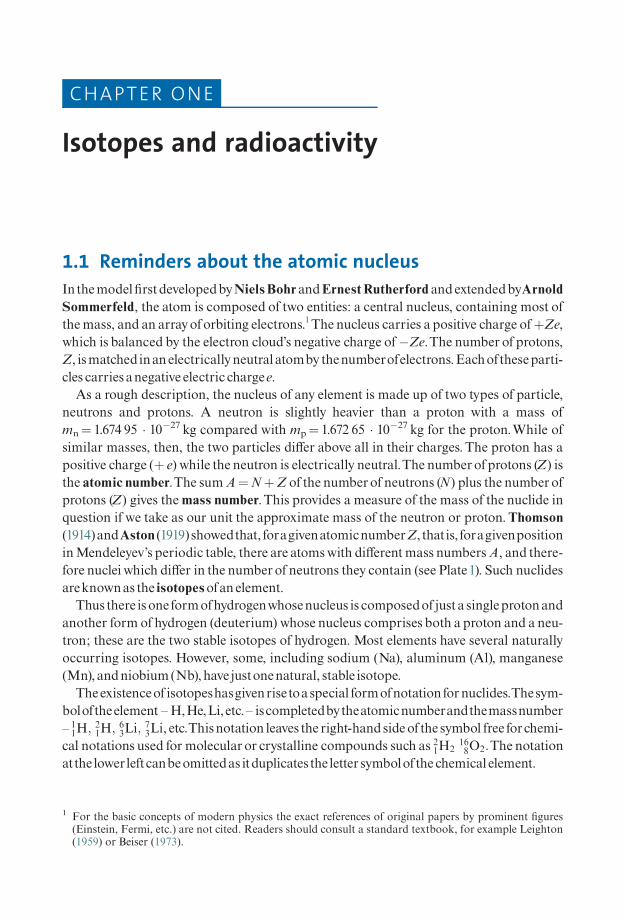
In themodel¢rstdevelopedbyNiels BohrandErnestRutherford and extendedbyArnoldSommerfeld, the atom is composed of two entities: a central nucleus, containing most ofthemass, and an arrayoforbiting electrons.1The nucleus carries a positive charge ofþZe,which is balanced by the electron cloud’s negative charge of�Ze.The number of protons,Z, ismatched inan electricallyneutral atomby thenumberofelectrons.Eachoftheseparti-cles carries anegative electric chargee.As a rough description, the nucleus of any element is made up of two types of particle,

neutrons and protons. A neutron is slightly heavier than a proton with a mass ofmn¼ 1.674 95 � 10�27 kg compared with mp¼ 1.672 65 � 10�27 kg for the proton.While ofsimilar masses, then, the two particles di¡er above all in their charges. The proton has apositive charge (þ e) while the neutron is electrically neutral.The numberofprotons (Z) isthe atomic number.The sumA¼NþZ of the numberof neutrons (N) plus the numberofprotons (Z) gives themass number.This provides a measure of the mass of the nuclide inquestion if we take as our unit the approximate mass of the neutron or proton.Thomson(1914)andAston (1919)showedthat, foragivenatomicnumberZ, thatis, foragivenpositioninMendeleyev’s periodic table, there are atomswith di¡erentmass numbersA, and there-fore nuclei which di¡er in the numberof neutrons they contain (see Plate1). Such nuclidesareknownas the isotopesofan element.Thus there isoneformofhydrogenwhosenucleus is composedof justa singleprotonand

another form of hydrogen (deuterium) whose nucleus comprises both a proton and a neu-tron; these are the two stable isotopes of hydrogen. Most elements have several naturallyoccurring isotopes. However, some, including sodium (Na), aluminum (Al), manganese(Mn), andniobium(Nb),have justonenatural, stable isotope.Theexistenceof isotopeshasgivenrisetoaspecial formofnotation for nuclides.Thesym-

boloftheelement ^ H,He,Li,etc.^ iscompletedbytheatomicnumberandthemassnumber^ 11H;

21H;

63Li;

73Li, etc.Thisnotation leaves the right-handsideofthe symbol free forchemi-

cal notations used for molecularor crystalline compounds such as 21H2

168O2:The notation

atthe lowerleftcanbeomittedas itduplicates the letter symbolofthe chemical element.

1 For the basic concepts of modern physics the exact references of original papers by prominent figures(Einstein, Fermi, etc.) are not cited. Readers should consult a standard textbook, for example Leighton(1959) or Beiser (1973).

The discovery of isotopes led immediately to that of isobars. These are atoms with thesame mass numbers but with slightly di¡erent numbers of protons.The isobars rubidium8737Rbandstrontium 87

38Sroralternatively rhenium18775Reandosmium 187

76Osdonotbelong inthe same slots in theperiodic table and soare chemicallydistinct. It is importanttoknowofisobarsbecause, unless theyareseparated chemicallybeforehand, they ‘‘interfere’’withoneanotherwhen isotopeabundancesaremeasuredwithamass spectrometer.

1.2 The mass spectrometer

Justas therewouldbeno crystallographywithoutx-raysnorastronomywithouttelescopes,so there would be no isotope geology without the invention of themass spectrometer.Thiswas themajor contributionofThomson (1914) andAston (1918).Astonwonthe1922NobelPrize for chemistry fordeveloping this instrument and for the discoveries it enabled him tomake.2 Subsequent improvements were made by Bainbridge and Jordan (1936), Nier(1940), and Inghram and Chupka (1953). Major improvements have been made usingadvances in electronics and computing. A decisive step was taken by Arriens andCompston (1968) andWasserburg etal. (1969) in connectionwithMoon explorationwiththe development of automated machines. More recent commercial machines haveimprovedquality, performance, andreliability tenfold!

1.2.1 The principle of the mass spectrometer

The principle is straightforward enough. Atoms of the chemical element whose isotopiccomposition is to be measured are ionized in a vacuum chamber.The ions produced arethen accelerated by using a potential di¡erence of 3^20 kV. This produces a stream ofions, and so an electric current, which is passed through a magnetic ¢eld. The magnetic¢eld exerts a force perpendicular to the‘‘ionic current’’and sobends thebeamof ions.Thelighter ions are de£ected more than the heavier ones and so the ions can be sorted accord-ing to their masses.The relative abundance ofeach isotope canbemeasured from the rela-tive values of the electron currents produced by each stream of ions separated out in thisway.

Let us put this mathematically. Suppose atoms of the element in question have beenionized.The ionaccelerationphase is:

eV ¼ 1

2mv2

whereeV is the electrical energy, 12mv2 is thekinetic energy,e is the ion’s charge,v its speed,mitsmass, andV thepotentialdi¡erence. Itcanbededucedthat:

v ¼ 2eV

m

� �12

:

2 The other inventor of the mass spectrometer, J. J. Thomson, had already been awarded the 1906 NobelPrize for physics for his discovery of the electron.

2 Isotopes and radioactivity

Magnetic de£ection isgivenbyequating themagnetic forceBev to centripetal acceleration(v2/R) multiplied bymassm, whereB is the magnetic ¢eld andR the radius of curvature ofthede£ectedpath:

Bev ¼ mv2

R

� �:

Itcanbededucedthat:

v ¼ BeR

m:

Makingthetwovaluesofvequal,which istantamounttoremovingspeedfromtheequation,gives:

m

e¼ B2R2

2V:

ThereforeR isproportionaltoffiffiffiffimp

, foran ionofagivencharge.Allowingforelectroncharge,elementalmass,3 anddi¡erences inunits,we canwrite:

m ¼ B2R2

20 721V� 1012

inwhichB is in teslas,m in atomicmassunits,R inmeters, andV involts.

Exercise

A mass spectrometer has a radius of 0.3 m and an acceleration voltage of 10 000 V. The

magnetic field is adjusted to the various masses to be measured. Calculate the atomic mass

corresponding to a field of 0.5 T.

AnswerJust apply the formula with suitable units:

m ¼ ð0:5Þ2 � ð0:3Þ2

20 721 � ð104Þ � 1012 ¼ 108:58:

Exercise

If hydrogen ions (mass number¼ 1) are accelerated with a voltage of 10 kV, at what speed are

they emitted from the source?

AnswerJust apply the formula v ¼ ð2eV=mÞ

12. The electron charge is 1.60219 � 10�19 coulombs and

the atomic mass unit is 1.660 540 2 � 10�27 kg.

v ¼ffiffiffiffiffiffiffiffiffiffiffiffiffiffiffiffiffiffiffiffiffiffiffiffiffiffiffiffi1:9272 � 1012p

¼ 1388 km s�1

3 Atomic mass unit: m¼ 1.660 540 2 � 10�27 kg, electron charge: e¼ 1.602 19 � 10� 19 C, thereforee/m¼ 0.964 � 108 C kg�1 (C¼ coulomb).

3 The mass spectrometer

which is about 5 million km per hour. That is fast, admittedly, but still well below the speed of

light, which is close to 1 billion km per hour! Heavy ions travel more slowly. For example ions

of m¼ 100 would move at just a tenth of the hydrogen speed.

1.2.2 The components of a mass spectrometer

The principal components ofamass spectrometer are the source, themagnet, and the col-lectorandmeasurementsystems, allofwhicharemaintainedunder vacuum.

The sourceThesourcehas three functions:

� Togenerate ions fromatoms.The ionsmaybepositiveor negative.� To accelerate the ion by potential di¡erences created by plates at di¡erent potentials

(fromgroundto20KeV,and inacceleratormass spectrometers toseveralMeV).� Toshape thebeam, through calibrated slits in thehigh-voltageplates.Thebeam fromthe

source slit isusually rectangular.

ThemagnetThe magnet has two functions. It deviates the ions and this de£ection separates them bymass. At the same time it treats the various components of the ionbeamora singlemass asanoptical instrumentwould. It handlesboth colors (masses) and alsobeamgeometry.Oneof itsproperties is to focus each ionbeam foreachmassonthe collector.The characteristicsof focusing vary with the shape of themagnet and the shape of the pole face, which maybecurved invariousways (Figure1.1andPlates 2 and 3).A further recent improvement, usingcomputer simulation, hasbeentofocus thebeamnotonly inthexandydirectionsbut inthez direction too. Inmodern solid-sourcemass spectrometers, the angulardispersion of ionsis fully corrected and almost all the ions leaving the source end up in the collectors whicharearranged inafocalplane.

The collectorsThe collectors collect and integrate the ion charges so generating an electric current. ThecollectormaybeaFaradaybucket,whichcollectsthechargesandconvertsthemintoacurrentthat is conducted along awire to an electrical resistor. Bymeasuring the potential di¡erenceacross the resistor terminals, the current can be calculated from Ohm’s law,V¼ IR. Theadvantage is that it is easy to amplify a potential di¡erence electronically. It is convenient toworkwithvoltagesofabout1V.As the currents tobemeasured range from10�11to10�9A, byOhm’s law, the resistors commonly used range from1011 to 109 �. This conversion may bemade for small ion £uxes of electron multipliers or ion counters.4 In all cases the results areobtained by collecting the ion charges and measuring them. Just ahead of the collectorsystem is a slit that isolates the ion beam. This is explained below.

4 Each ion pulse is either counted (ion counter) or multiplied by a technical trick of the trade to give ameasurable current (electron multiplier).


ThevacuumAfourth importantcomponent is thevacuum. Ions cantravel fromthe source to the collec-tor only if they are in avacuum. Otherwise they will lose their charge by collision with airmolecules and return to the atom state.The whole system is built, then, in a tube where avacuum can be maintained. In general, a vacuum of 10�7 millibars is produced near thesource andanother vacuumof10�9millibars orbetter near the collector. Even so, someair

Magnet

Amplifier

ION SOURCE COLLECTOR

Filament

High voltage

FaradaycupIn

ten

sity

(V

)

Strontium

STRONTIUM ISOTOPES

88878684

x33

x10

x10

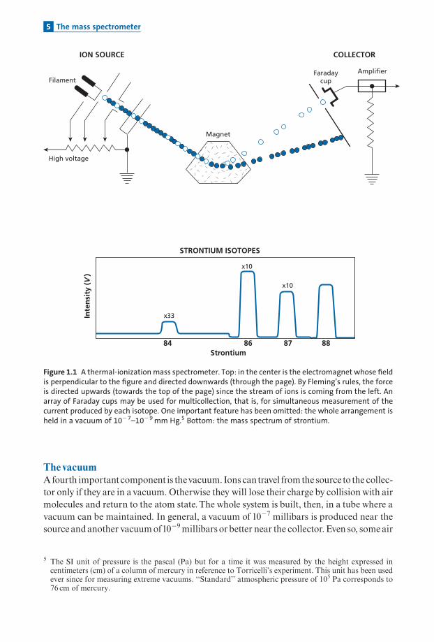
Figure 1.1 A thermal-ionization mass spectrometer. Top: in the center is the electromagnet whose fieldis perpendicular to the figure and directed downwards (through the page). By Fleming’s rules, the forceis directed upwards (towards the top of the page) since the stream of ions is coming from the left. Anarray of Faraday cups may be used for multicollection, that is, for simultaneous measurement of thecurrent produced by each isotope. One important feature has been omitted: the whole arrangement isheld in a vacuum of 10� 7–10� 9 mm Hg.5 Bottom: the mass spectrum of strontium.

5 The SI unit of pressure is the pascal (Pa) but for a time it was measured by the height expressed incentimeters (cm) of a column of mercury in reference to Torricelli’s experiment. This unit has been usedever since for measuring extreme vacuums. ‘‘Standard’’ atmospheric pressure of 105 Pa corresponds to76 cm of mercury.


molecules remain inside the mass spectrometer and collide with the beams, partiallydisrupting their initial rectangular section.

All of these components contribute to the quality of the data obtained. Mass spectro-meterquality is characterizedbyanumberoffeatures.

E⁄ciencyThis isgivenby the ratio

Number of ions collected

Number of atoms in source¼ E

Number of ions ¼ intensity� duration� 6:24� 1018

Z ion charge

Number of atoms ¼ mass

atomic mass�Avogadro’s number:

E⁄ciencyvarieswithatomicmass.Ionization e⁄ciency of the source (I) and transmission e⁄ciency of the total ion

optics (T):

I� T ¼ E

ThevalueofT isvariable:1%for ICP-MS,25%for ionprobes.The values of I have been greatly improved but vary with the nature of the element and

the ionizationprocess.The range is 5%00 to100%(ICP-MS)!

Powerof resolutionThequestion is, what is the smallest di¡erence in mass that canbe separated and thenmea-suredusingamass spectrometer?A formalde¢nition is:

Figure 1.2 (a) Incident beam in the focal plane. (b) Magnet focalization. The beam from the source has acertain aperture. The trajectories of some ions that are not strictly perpendicular to the source arerefocused by the magnetic field. The refocusing surface for the various masses at the collector end iscurved if the magnet faces are plane, but may be plane if a curved magnet face is used. The figure showsschematically how the magnet separates three isotopes in both configurations.


resolving power RP ¼ M1

�M

whereM1is themass.�M is de¢nedasM2¼M1þ�M,whereM2 is the closestmass toM1

thatdoesnotoverlapbymorethan50%inthe collector.We canalsode¢nearesolvingpowerat1%.Thedistance�xbetweentwobeams inthe focalplane iswritten:

�x ¼ K�m

m:

Dependingontheangleofthe incidentbeamtothemagnet,K¼R foranangleof incidenceof908;K¼ 2R foranangleof278.Fromtheformulaabove:

RP ¼ CR

�x;

R being the radius of curvature and �x the distance between two beams of M andMþ�M.This is just to show that when one wants to separate two masses more e⁄ciently, the

radius has to be increased and then the voltage adjusted accordingly. Suppose we want toseparate 87Rb and 87Sr by the di¡erence in mass of neutrons and protons alone. A‘‘mon-ster’’ mass spectrometer would be required. However, interferences between two massescan be avoided when separating isotopes of an element from contaminating molecules.(Methane 12CH4 has the same mass as 16O and benzene C6H6 interferes at mass 78 withkrypton.)

Abundance sensitivityAnother importantcharacteristic is the�xdistance (inmillimeters)betweenthebeams.Wehave to comeback to the slits in the collectors.The problem is easy enough to understand.At¢rst, thebeam is rectangular. Collisionswith residual air moleculesmeans that, when itreaches the collector slit, thebeam iswiderand trapezoid-shapedwith long tails. Collectorslits areopen so that they can receiveonemassbutno contribution from theadjacentmass.When the abundances oftwoadjacent isotopes areverydi¡erent, the tail of themore abun-dant isotope forms background noise for the less abundant one. Measuring the less abun-dant isotope involves reconstructing the tail of the more abundant one mathematically.This is possible only if the tail is not too big. Narrowing the collector slit brings about arapiddecline in sensitivity.Abundance sensitivity is themeasurementof the contribution of the tail ofone isotope

to the signal of the neighboring isotope. It is given as a signal/noise ratio multiplied bythe mass ratios. Special instruments have been developed for measuring abundancesensitivity in extreme cases, such as measuring 14C close to the massively more abundant12C. Abundance sensitivity is related to resolving power but also to the quality of theionoptics.


Exercise

The isotopic composition of the element rubidium (Rb) is measured, giving a current

i¼ 10�11 A for the mass of 87Rb. How many ions per second is that? If the measurement

lasts 1 hour how much Rb has been used if the ionization yield is 1%?

AnswerThe intensity of an electrical current is defined by i¼ dq/dt, where dq is the quantity of electrical

charge and dt the unit of time. Electrical current is therefore the quantity of electrical charge

flowing per unit time. The ampere, the unit of electrical current, is defined as being 1 coulomb

per second, the coulomb being the unit of electrical charge. The charge of an electron is

–1.6 � 10�19 coulombs. The positive charge is identical but with the opposite sign. An

intensity of 10�11 amps therefore corresponds to 10�11 coulombs per second / 1.6 � 10�19

coulombs¼ 62.5 � 106 ions per second.

If this intensity is maintained for 1 hour: 6.25 � 107� 3600¼ 2.2464 � 1011 ions of 87Rbþ. As

the ionization is 1%, this corresponds to 2.2464 � 1013 atoms of 87Rb placed on the emitter

filament. As 85Rb/87Rb¼ 2.5933, Rbtotal (in atoms)¼ 87Rb (in atoms) (1þ 2.5933).

So a total number of 8.0719 � 1013 atoms of Rb is placed on the filament. As the atomic

mass of Rb is 85.468 g, the total weight of Rb is 11 ng.

Exercise

How much rock is needed to determine the isotopic composition of Rb by measuring a sample

for 20 minutes at 10�11 A if its concentration in Rb is 10 ppm (parts per million)?

AnswerIf 11 ng of Rb are needed for 1 hour, for 20 minutes we need (11� 20)/60¼ 3.66 ng, that is

3.66 � 10�9/10�5¼ 0.36 mg of rock or mineral.

It can be seen, then, that mass spectrometry is a very sensitive technique.

1.2.3 Various developments in mass spectrometers

Mass spectrometers have come a long way since the ¢rst instruments developed by J. J.ThomsonandF.Aston.Togive some ideaoftheadvancesmade,whenAlNierwasmeasur-ing lead isotopes as apostdoctoral fellowatHarvard in1939 (moreaboutthis later), heusedagalvanometer projectingabeamoflightontothewall andmeasured thepeakwitharuler!Nowadays everything takes the formofacomputeroutput.

IonizationThe ¢rst technique was to use the element to be measured as a gaseous compound.Whenbombardedbyelectrons, atomsofthegas lose electrons and sobecome ionized (Nier,1935,1938,1939). Later came the thermal-ionization technique (TIMS) (Inghram and Chupka,1953). In the so-called solid-sourcemass spectrometer, a saltof the element is depositedonametal¢lament (Ta,W,Pt).The¢lamentisheatedbytheJoule e¡ectofan increasingelectriccurrent. At a certain temperature, the element ionizes (generally as positive ions [Sr, Rb,Sm,Nd,U, Pb] but also as negative ions [Os]). Ionizationbecamea fundamental character-isticofmass spectrometry.


Nowadays, asanalternative,plasmaisusedforoptimal ionization in instrumentsnamedICP-MS.

Ion opticsSubstantial e¡ort has been put into optics combining various geometries and assemblies.Bainbridge and Jordan (1936) used a magnetic ¢eld to turn the beam through 1808.Mattauch andHerzog (1934) combined electric and magnetic ¢elds to separate ions andfocusbeams.Magnetshapesweremodi¢edto improvetransmission e⁄ciency.Computerized numerical simulation has allowed tremendous advances in ion optics

design. All of the techniques used tended to maximize ionization and transmission, toincrease resolution power and abundance sensitivity, and to minimize the high voltagerequirement and the size of themagnet, which areboth big factors in cost. However, whenthe ionization process created a wide dispersion in ion energies, more sophisticated ionoptics were required to refocus the ion beam in a narrow band on the collectors. So ICP-MS, ionprobe, andAMSinstrumentshavebecomelargeandmore expensive.Collectorsareanother important issue.Earlymass spectrometershadasingle collector.By

scanningthemagnetic¢eld, theionbeampassedinsequencethroughthecollectorandaspec-trum of ion abundance was recorded (Figure 1.1). Nowadays most mass spectrometers usesimultaneous ion collectionwithanarrayofcollectors sidebyside, each collectorcorrespond-ing to a distinct mass. This seems an obvious technique to use as it eliminates £uctuationsbetweentherecordingsofonemass(peak)toanother.However, itistechnicallyextremelydi⁄-culttoachieve,bothmechanically,accurately installingseveral collectors inasmallspace,andelectronically, controlling drifting of the electronic circuits with time. These problems havenow been virtually eradicated. It is worth noting that, unlike in most areas of science, alladvancessince1980havebeenmadebyindustrialengineersratherthanbyacademicscientists.However, because of electronic ‘‘noise’’and electrical instabilities, all isotopic measurementsare statistical. On each run, thousands of spectra are recorded and statistically processed.Onlysincemicrocomputershavebeenavailablehavesuchtechniquesbecomefeasible.

1.2.4 Preparatory chemistry and final accuracy

In mostmass spectrometry techniques (except for ion probes) chemical separation is usedbefore measurement to purify the element whose isotopic composition is under study.Since the elements tobemeasured are present as traces, theyhave tobe separated from themajor elementswhichwouldotherwiseprevent any ionization as themajor elements ratherthan the trace elementswould give out their electrons. For example, an excess ofK inhibitsany Rb ionization. Chemical separation also prevents isobaric interference between, say,87Rband87Sror187Reand187Os.Chemicalseparation canbedoneingaseousforminpuri¢cation lines,asfor raregasesor

for oxygen or hydrogen measurement, or in liquid solution for most elements. The basictechnique in the latter case is the ion-exchange column as introduced by Aldrich et al.(1953).All theseoperationshavetobeperformedinverycleanconditions,otherwisesamplecontaminationwill ruinmeasurement.Thegreater the accuracyofmass spectrometry, thecleaner the chemistry required.The chemistry is carried out in a clean roomwith special


equipmentusingspecially preparedultra-clean reagents, thatare farcleaner thananycom-mercialversions.

Whenjudgingmeasurementreliability, investigatorshavetostatethe leveloftheirblanks.Theblank istheamountofthetargetelementsmeasuredinachemicalprocessdonewithoutanysample.Theblankhastobenegligibleorverysmall comparedwiththeamountofmater-ial tobemeasured. So increases in accuracyare linkednotonlywith the improvementofthemass spectrometerbutalsooftheblanks.

Although this is nottheplace togive full technicaldetails about conditions for preparingand measuring samples, as these can only be learned in the laboratory and not from text-books, afewgeneral remarksmaybemade.

Moderntechniquesallow isotope ratios tobemeasuredwithadegreeofprecisionof10�5

or10�6 (a fewppm!) on samplesweighing just a fewnanograms (10�9 g) or even a fewpico-grams (10�12 g). For example, if a rock contains10 ppm of strontium, its isotope composi-tion canbemeasured on10�9 g with a degree ofprecision of 30 ppm.Therefore just10�4 g,that is, 0.1mg would be needed to make the measurement. This method can be used forstudying precious rocks, such as samples of moon rock or meteorites, or minor or rareminerals, that is,minerals that are di⁄cult to separate and concentrate.Whatdo such levelsofprecision mean?Theymeanwe can readily tell apart two isotope ratios ofstrontium, say0.702 21and0.702 23, that is, towithin0.000 03, evenwherelowconcentrationsare involved.Toachieve suchprecision themeasurementmustbe‘‘internally calibrated.’’Whenmeasur-ing the abundance ratio (A1/A2) of two isotopes, the electrical current ratio (I1/I2) detectedis slightlydi¡erent from (A1/A2).The di¡erence is engenderedby themeasurement itself.Thisis termedmass discrimination.6Eitheroftwomethods isusedforcalibratingmeasurements.

The ¢rst is the internal standard method. If the element has three or more isotopes oneparticular ratio is chosenas the reference ratioandcorrection ismade formass discrimina-tion. So if the abundances are A1, A2, A3, we take (A1/A3)¼R.The measurement (I1/I2) iswrittenR(1þ ��m), where�m is the di¡erence in massbetweenA1andA3.The fractiona-tion coe⁄cient� is calculatedandthenapplied tothemeasurementofthe ratio (A1/A2).

7

The second method is to measure a standard sample periodically and to express thevaluesmeasured intermsofthatstandard.

The extraordinary precision themass spectrometer can achievemustnotbe jeopardizedbyaccidental contaminationwhen preparing samples.To this endultra-clean preparatorychemistry is developedusingultra-pure chemical reagents in clean rooms (Plate3bottom).

1.2.5 Ionization techniques and the corresponding spectrometers

Four major ionization techniques are used dependingon the characteristics of the variouschemical elements (ionizationpotential).

Thermal-ionizationmass spectrometry (TIMS)The element to be analyzed is ¢rst puri¢ed chemically (especially to separate any isobars)anddepositedon arefractory¢lament.Heating the¢lament in avacuumby the Joule e¡ect

6 Such discrimination depends on the type of mass spectrometer used. It decreases with mass for any giventype.

7 In high-precision mass spectrometry an exponential law rather than a linear one is used to correct massfractionation.


ionizes the elements,which either lose an electronbecomingpositive ions, as in the casesofRbþ, Srþ, and Pbþ, or gain an electronbecoming negative ions aswithOsO3

� andWO3�.

Instrumental mass fractionation is of the order of1% bymass deviation for light elements(Li) and0.1%bymass deviation forheavyelements (Pb,U).

Electronic bombardmentLightelements suchashydrogen (H), carbon (C),nitrogen (N),andoxygen (O)or raregasesare analyzed as gases (H2, CO2, N2, O2, or atoms of He, Ne, At, or Xe) bombarded in avacuum by an electron beam. Positive ions are thus formed by stripping an electron fromsuch molecules or atoms. The ions are then accelerated and sorted magnetically as inTIMS. Substances are prepared for analysis in gaseous formby extracting the gas from thesample under vacuum either by fusion or by chemical reaction.The gas is then puri¢ed invacuum lineswhereothergases are captured eitherbyadsorption orbymanipulating theirliquefactiontemperatures.

Inductivelycoupledplasmamass spectrometry (ICPMS) inanargonplasmaThe sample is ionized in an argon plasma induced by a high-frequency electrical ¢eld(plasma torch).The high temperature of the plasma, about10 000K, means elements likehafnium or thorium, which are di⁄cult to ionize by thermal emission, can be completelyionized. The element to be analyzed is atomized and then ionized. It is sprayed into theplasma from a solution as a liquid aerosol. Or it may be released from a solid sample bylaserablation.Thesolidaerosolsoformed is injected intotheplasmatorch.Mass fractiona-tion is between a twentieth of1% for a light element like boron and1% for heavy elements.Fractionation is corrected for by using the isotope ratios ofother similar elements as inter-nal standards, because, atthe temperatureoftheplasma, fractionation is due tomass aloneand isnota¡ectedby the element’s chemical characteristics.

Ionic bombardment in secondary-ionmass spectrometry (SIMS)The solid sample (rock, mineral) containing the chemical element for analysis is cut,polished, andput into thevacuum chamber where it isbombardedbya‘‘primary’’ beamofions (argon, oxygen, or cesium). This bombardment creates a very-high-temperatureplasma at about 40 000K inwhich the element is atomized and ionized.The developmentofhigh resolution secondary-ionmass spectrometers (ionmicroprobes)means in-situ iso-topemeasurements can bemade onvery small samples and, above all, on tinygrains.Thisis essential for studying, say, thefewgrainsof interstellarmaterial contained inmeteorites.

RemarkAll of the big fundamental advances in isotope geology have been the result of improved

sensitivity or precision in mass spectrometry or of improved chemical separation reducing con-

tamination (chromatographic separation using highly selective resins, use of high-purity materials

such as teflon). These techniques have recently become automated and automation will be more

systematic in the future.

1.3 Isotopy

Assaid,eachchemicalelementisde¢nedbythenumberofprotonsZ in itsatomicstructure.It is the numberofprotonsZ thatde¢nes the element’s position in theperiodic table. But in

11 Isotopy

eachposition there are several isotopeswhich di¡erby the numberofneutronsN they con-tain, that is, by their mass.These isotopes are created during nuclear processes which arecollectively referred to as nucleosynthesis and which have been taking place in the starsthroughoutthehistoryoftheUniverse (seeChapter 4).

The isotopic composition of a chemical element is expressed either as a percentage ormore convenientlyasaratio.A reference isotope is chosen relative towhichthequantitiesofother isotopes are expressed. Isotope ratios are expressed in terms of numbers of atomsandnotofmass.Forexample, to study variations inthe isotopic compositionofthe elementstrontium brought about by the radioactive decay of the isotope 87Rb, we choose the87Sr/86Sr isotope ratio. To study the isotopic variations of lead, we consider the206Pb/204Pb, 207Pb/204Pb, and 208Pb/204Pbratios.

1.3.1 The chart of the nuclides

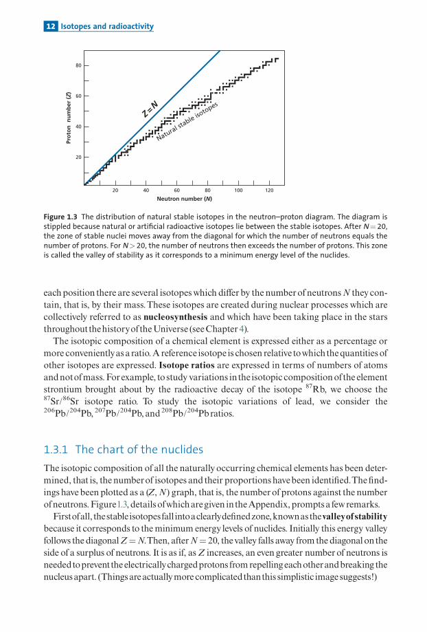
The isotopic composition of all the naturally occurring chemical elements has been deter-mined, that is, the numberof isotopes and their proportionshavebeen identi¢ed.The¢nd-ings havebeen plotted as a (Z,N) graph, that is, the numberofprotons against the numberofneutrons.Figure1.3, detailsofwhicharegiven intheAppendix,promptsafewremarks.

Firstofall, thestableisotopesfall intoaclearlyde¢nedzone,knownasthevalleyofstabilitybecause it corresponds to theminimum energy levels of nuclides. Initially this energy valleyfollows the diagonalZ¼N.Then, afterN¼ 20, thevalley falls away fromthe diagonalontheside of a surplus of neutrons. It is as if, asZ increases, an even greater numberof neutrons isneededtopreventthe electricallychargedprotons fromrepellingeachotherandbreaking thenucleusapart. (Thingsareactuallymore complicatedthanthis simplistic imagesuggests!)

80

60

40

20

20 40 60 80

Neutron number (N)

Pro

ton

nu

mb

er (

Z)

100 120

Z = N

Natural stable iso

topes

Figure 1.3 The distribution of natural stable isotopes in the neutron–proton diagram. The diagram isstippled because natural or artificial radioactive isotopes lie between the stable isotopes. After N¼ 20,the zone of stable nuclei moves away from the diagonal for which the number of neutrons equals thenumber of protons. For N> 20, the number of neutrons then exceeds the number of protons. This zoneis called the valley of stability as it corresponds to a minimum energy level of the nuclides.


Asecond remark relates toparity. Elements for whichZ is an even numberhave farmoreisotopes than elements for which Z is an odd number. Fluorine (Z¼ 9), sodium (Z¼ 11),phosphorus (Z¼ 15), andscandium(Z¼ 21)have justa single isotope.Lastly, andnot least importantly, theheaviest elementwith stable isotopes is lead.8

1.3.2 Isotopic homogenization and isotopic exchange

As the isotopes ofanygiven chemical element all have the same electron suite, theyall haveprettymuch the same chemical properties. But in all chemical, physical, or biological pro-cesses, isotopes ofanygiven elementbehave slightlydi¡erently from eachother, thusgivingrise to isotopic fractionation. Such fractionation is very weak and is apparent above all inlightelements. It is also exploited in isotopegeologyas shallbe seen inChapter 7.Initially we shall ignore such fractionation, exceptwhere allowancehas tobemade for it

as with 14C or when making measurements with a mass spectrometer where, as has beenseen, correctionmustbemade formass discrimination.Thisvirtually identicalbehaviorofchemical isotopes entails a fundamental consequence in the tendency for isotopic homogen-ization to occur.Where two or more geochemical objects (minerals within the same rock,rocks in solution, etc.) are in thermodynamic equilibrium, the isotope ratios of the chemicalelements present are generally equal. If theyare unequal initially, they exchange some atomsuntil theyequalize them. It is important tounderstand that isotopic homogenization occursthrough isotopic exchange without chemical homogenization. Each chemical componentretains its chemical identity,ofcourse.Thispropertyof isotopichomogenization‘‘across’’che-micaldiversity isoneofthe fundamentalsof isotopegeochemistry.Asimplewayofobservingthis phenomenon is to put calcium carbonate powder in the presence ofa solution of carbo-nate in water in proportions corresponding to thermodynamic equilibrium.Therefore nochemical reaction occurs. Repeat the experiment but with radioactive 14C in solution in theformofcarbonate. Ifafter10daysorsothesolid calciumcarbonate is isolated, itwillbefoundtohavebecome radioactive. It will have exchanged some of its carbon-14 with the carbonateofmass12and13whichwere inthesolution.

Exercise

A liter of water saturated in CaCO3 whose Ca2þ content is 1 � 10�2 moles per liter is put in the

presence of 1 g of CaCO3 in solid form. The isotopic ratio of the solid CaCO3 is 40Ca/42Ca¼ 151.

The isotopic ratio of the dissolved Ca2þ has been artificially enriched in 42Ca such that40Ca/42Ca¼ 50. What is the common isotopic composition of the calcium when isotopic

equilibrium is achieved?

Answer40Ca/42Ca¼ 121.2.

As said, when two or more geochemical objects with di¡erent isotopic ratios are ineach other’s presence, atom exchange (which occurs in all chemical reactions, including at

8 Until recently it was believed to be bismuth (Z¼ 83), whose only isotope is 209Bi. In 2003 it wasdiscovered to be radioactive with a half-life of 1.9 � 1019 years!

13 Isotopy

equilibrium) tends tohomogenize thewhole in termsof isotopes.This is known as isotopicexchange. It isakineticphenomenon,dependingthereforeonthetemperatureandphysicalstate of the phases present. Simplifying, isotope exchange is fast at high temperatures andslow at low temperatures like all chemical reactions which are accelerated by temperatureincrease. In liquids andgases, di¡usion is fast and so isotope exchange is fast too. In solids,di¡usion is slowandsoisotopeexchangeis slowtoo. Inmagmas(high-temperatureliquids),then, both trends are compounded and isotope homogenization occurs quickly.The sameistrueofsupercritical£uids, thatis,£uidsdeepwithintheEarth’scrust.Conversely, insolidsatordinary temperatures, exchange occurs very slowlyand isotopeheterogeneities persist.Two important consequences follow from these two properties.The ¢rst is that a magmahas the same isotope compositionas the solid source fromwhich ithas issuedby fusion, butnotthe same chemical composition.The second is that, conversely, a solid atordinary tem-peratures retains its isotopic composition over timewithoutbecoming homogeneouswithitssurroundings.This iswhy rocksare reliable isotoperecords.Thispropertyisadirectcon-sequenceofthe di¡usionpropertiesofnatural isotopes in liquids andsolids.

The theory of di¡usion, that is, the spontaneous motion of atoms in£uenced by di¡er-ences in concentration,provides anapproximatebutadequateformula:

x �ffiffiffiffiffiffiDtp

wherex is thedistancetraveledby the element, t is time in seconds, andD thedi¡usion coef-¢cient (cm2 s�1).

Exercise

In a liquid silicate at 1200 K the diffusion coefficient for elements like Rb, Sr, or K is

D¼ 10�6 cm2 s�1. In solid silicates heated to 1200 K, D¼ 10�11 cm2 s�1.

How long does it take for two adjacent domains of 1 cm diameter to become homogeneous:

(1) within a silicate magma?

(2) between a silicate magma and a solid, which occurs during partial melting when 10% of

the magma coexists with the residual solid?

Answer(1) In a silicate magma if D¼ 10�6 cm2 s�1, t� x2/D¼ 106 s, or about 11 days.

If it takes 11 days for the magma to homogenize on a scale of 1 cm, on a 1-km scale

(¼ 105 cm), it will take t� x2/D¼ 1010¼ 1016 s, or close to 3 � 108 years, given that

1 year� 3 � 107 s.

In fact, homogenization at this scale would not occur by diffusion but by advection or

convection, that is, a general motion of matter, and so would be much faster.

(2) In the case of a magma impregnating a residual solid with crystals of the same dimen-

sions (1 cm), t� x2/D¼ 1011 s or about 3 � 105 years, or 300 000 years, which is rather fast

in geological terms. For 1-mm crystals, which is more realistic, t� 10�2/D¼ 3 � 103 years,

or 3000 years. So isotope equilibrium is established quite quickly where a magma is in the

presence of mineral phases.

Asecond importantquestion iswhether rocks atordinary temperatures can retain theirisotope compositions without being modi¢ed and without being re-homogenized. To


answer this, it must be remembered that the di¡usion coe⁄cient varies with temperatureby theArrhenius law:

D ¼ D0 exp�DHRT

� �

where�H is the activation energy, which is about 40 kcal per mole,R is the ideal gas con-stant (1.987 calperKpermole), andT theabsolute temperature (K). IfD¼ 10�11cm2 s�1insolids at1300 8C,what is thedi¡usion coe⁄cientDoratordinary temperatures?

Dor

D1300¼ exp

�DHR

I

Tor� I

T1300

� �� ¼ hBi

fromwhichDor ¼ Bh i D1300.Calculate Bh i to¢ndthat itgives1.86 � 10�25, thereforeDor¼ 2 � 10�36 cm2 s�1.Tohomogenizea1-mmgrainatordinary temperatures takes

t ¼ 10�2

2 � 10�36 ¼ 0:5 � 1034s � 1:5 � 1026 years;

which is in¢nitelylong toall intents andpurposes.

Important remarkRocks therefore retain the memory of their history acquired at high temperatures. This is the prime

reason isotope geology is so incredibly successful and is the physical and chemical basis of isotope

memory. The phenomenon might be termed isotopic quenching, by analogy with metal which, if it is

immersed when hot in cold water, permanently retains the properties it acquired at high temperature.

1.3.3 A practical application of isotopic exchange:isotopic dilution

Supposewewish tomeasure the rubidium contentofa rock.Rubidiumhas two isotopes, ofmass 85 and 87, in the proportion 85Rb/87Rb¼ 2.5933. (This is the value foundwhen mea-suring theRb isotope compositionofnatural rocks.)The rock is dissolvedwithamixtureofacids.To the solution obtained,we add a solutionwith aknownRb contentwhich hasbeenarti¢cially enriched in 85Rb (spike), whose 85Rb/87Rb ratio in the spike is known.The twosolutionsmixandbecomeisotopicallybalanced.Onceequilibriumisreached, theabsoluteRb contentof the rockcanbe determinedbysimplymeasuring the isotope composition ofa fractionofthemixture.Writing

85Rb87Rb

� �¼ 85

87

gives:

85

87

� �mixture

¼ð85RbÞrock þ ð85RbÞspikeð87RbÞrock þ ð87RbÞspike

¼8587

spikeþ 85

87

rock

87Rbrock87Rbspike

h i1þ 87Rbrock

87Rbspike

h i :

Topandbottomare dividedby 87Rb,bringingout 8587

.

A littlemanipulationgives:

87Rbrock ¼ 87Rbspike85

87

� �spike

8587

spike� 85

87

mixture

8587

mixture

� 8587

rock

" #:

15 Isotopy

Becauseweknowthe87Rbcontentofthespike, theRbcontentoftherockcanbeobtainedbysimply measuring the isotope ratio of the mixture, without having to recover all the Rb bychemical separation.

Suppose, say, the isotopic composition of the spike ofRb is 85Rb/87Rb¼ 0.12.The natu-rally occurring 85Rb/87Rb ratio is 2.5933.We dissolve1g of rock and add to the solution1gofspike containing3 ngof 87Rbpercubic centimeter.After thoroughlymixing the solutioncontaining the dissolved rockand the spike solution,measurementofa fraction of themix-tureyields a ratio of 85Rb/87Rb¼ 1.5.TheRb contentofthe rockcanbe calculated.We sim-plyapply the formula:

87Rbrock ¼ 87Rbspike0:12� 1:5

1:5� 2:59

� �¼ 1:266;

or

87Rbrock ¼ 1:266� 87Rbspike ¼ 1:266 � 3 � 10�9 g ¼ 3:798 � 10�9 g:

As we took a sample of 1g of rock, C87Rb¼ 3:798 ng g�1 ¼ 3:798 ppb. Therefore

C87total ¼ C87Rbð1þ 2:5933Þ ¼ 13:42 ppb.

This method can be used for all chemical elements with several stable isotopes for whichspikeshavebeenpreparedthatarearti¢ciallyenrichedinoneormoreisotopesandforelementswith a single isotope, provided it is acceptable to use a radioactive isotope (and so potentiallydangerousforwhoeverconductstheexperiment)asaspike.Themethodhasthreeadvantages.

First,aftermixingwiththespike,chemicalseparationmethodsneednotbeentirelyquanti-tative. (The yields of the various chemical operations during analysis do not count.) Isotoperatiosalonematter,aswell asanycontamination,whichdistorts themeasurement,ofcourse.

Then, as themass spectrometer makes very sensitive andvery precise measurements ofisotope ratios, isotopic dilution may be used to measure the amounts of trace elements,eventhetiniesttraces,withgreatprecision.

Isotope dilutionwas invented for theneedsof laboratoryanalysisbutmaybe extended tonatural processes. As shall be seen, variable isotope ratios occur in nature. Mixes of themcanbe used to calculate proportions bymass of the geochemical elements involved just bysimplemeasurementsof isotope ratios.

As canbe seen, isotope dilution is an essential method in isotope geochemistry. But justhowprecise is it?This exercisewillallowustospecify theerror (uncertainty) in isotopedilu-tionmeasurement.

Exercise

The isotope ratios of the spike, sample, and mixture are denoted RT, RS, and RM, respectively.

We wish to find out the quantity X of the reference isotope Cj in the sample. To do this,

quantity Y of spike has been mixed and the isotope ratios (Ci/Cj)¼ R of the spike, sample, and

mix have been measured. What is the uncertainty of the measurement?

AnswerLet us begin with the formula

X ¼ YR T � R M

R M � R S

��


which may be written RMX – RSX¼ RTY – RMY or RM (Xþ Y)¼ RTYþ RSX, or alternatively

R M ¼ R TY

X þ Yþ R S

X

X þ Y:

We posit XX þ Y ¼W and Y¼ 1�W. Let us calculate the logarithmic derivative and switch to �

(finite difference):

DX

X¼ DY

Yþ DðR T � R MÞðRT � RMÞ

þ DðR M � R SÞðR M � R SÞ

:

We can transform (RT – RM) and (RM – RS) as a function of (RT – RS), from which:

DX

X¼ DY

Yþ 2DR M

ðR T � R SÞ1

Wþ 1

1�W

� �¼ DY

Yþ 2DR M

ðR T � R SÞ1

W ð1�W Þ

� �:

Neglecting the uncertainty on RT and RS, which are assumed to be fully known, uncertainty is

minimum when:

� RT – RS is maximum. A spike must therefore be prepared whose composition is as remote as

possible from the sample composition.

� 1/[w(1�w)] is maximum for given values of RT and RS, that is, when W¼ 0.5, in other words

when the samples and spike are in equal proportions.

By way of illustration, let us plot the curve of relative error �X/X as a function of W. It is

assumed that DR M=ðR T � R MÞ ¼ 10�4 and DY=Y ¼ 10�4:

The curve is shown in Figure 1.4.

Conversely, the formulae for isotope dilution show how contamination of a sample byreagents used in preparatory chemistrymodi¢es the isotope composition ofa sample tobe

40

30

20

10

0.25 0.5

W

Rel

ativ

e er

ror

(10–4

)

0.75

Error-minimizingzone

Figure 1.4 Relative error due to isotope dilution. Relative error is plotted as a function of the ratio W,which is the proportion of the isotope from the sample in the sample–spike mixture. The greatestprecision is achieved with comparable amounts of spike and sample, but with a relatively largetolerance for this condition.

17 Isotopy

measured.Toevaluatethisuncertainty(error)(orbetterstilltomakeitnegligible), isotopedilu-tion isusedtogaugethequantityofthe elementtobemeasuredthathasbeen introducedacci-dentally during preparation.To do this, a blank measurement is made with no sample.Theblank is the quantity of contamination from the preparatory chemistry. A good blank has anegligible in£uenceonmeasurement.SeeProblem3attheendofthe chapter formoreonthis.

1.4 Radioactivity

Radioactivity was discovered and studied byHenri Becquerel and thenPierre andMarieCurie from 1896 to 1902. In 1902 Pierre Curie (1902a) and independently ErnestRutherfordandFrederickSoddy (1902a, b, c) proposedan extremelysimplemathematicalformalization for it.

1.4.1 Basic principles

Radioactivity is the phenomenon by which certain nuclei transform (transmute) sponta-neously into other nuclei and in so doing give o¡ particles or radiation to satisfy thelaws of conservation of energy and mass described by Albert Einstein. TheCurie^Rutherford^Soddy (CRS) law says that the numberof nuclei that disintegrate perunit time is a constant fraction of the number of nuclei present, regardless of the tempera-ture, pressure, chemical form,orotherconditionsofthe environment. It iswritten:

dN

dt¼ �lN

where N is the number of nuclei and l is a proportionality constant called the decay con-stant. It is theprobability thatanygiven nucleuswill disintegrate in the intervaloftime dt. Itis expressed inyr�1 (reciprocaloftime).

TheexpressionlN is calledtheactivityandisthenumberofdisintegrationsperunittime.Activity is measured in curies (1Ci¼ 3.7 � 1010 disintegrations per second, which is theactivityof1g of 226Ra). Avalue of1Ci is averyhigh level of activity, which is why themilli-curie or microcurie are more generally used.The international unit is now the becquerel,corresponding to1disintegrationper second.1Ci¼ 37gigabecquerels.

This law is quite strange a priori because it seems to indicate that the nuclei ‘‘communi-cate’’with eachother todrawbylots thosetobe‘‘sacri¢ced’’ateach instantatanunchangingrate. Andyet it hasbeen shown tobevalid for nucleiwithvery short (a few thousandths ofasecond) or very long (several billion years, or more than1020 s) lifespans. It holdswhateverthe conditions of the medium.Whether the radioactive isotope is in a liquid, solid, or gasmedium, whether heated or cooled, at high pressure or in a vacuum, the law of decayremainsunchanged. Foragiven radioactive nucleus, l remains the sameover the course oftime. Integrating theCurie^Rutherford^Soddylawgives:

N ¼ N0 e�lt

whereN is the numberof radioactive nuclei nowremaining,N0 the initial numberof radio-active atoms, and t the interval of time measuring the length of the experiment.Thus the


numberofradioactiveatomsremaining is afunctionof justthe initial numberofradioactiveatomsandoftime.Each radioactive isotope is characterized by its decay constant l.We also speak of the

mean life � ¼ 1/l.The equation is thenwritten:

N ¼ N0e�ðt=�Þ:

Radioactivityisthereforeastopwatch,anatural clock,which, likeanhourglass,measuresthe passage of time unperturbed. The phenomenon can be displayed graphically in twoforms.On an (N, t) graph, the negative exponential decreasesbecoming tangential to thex-axis

at in¢nity (Figure1.5a).Onasemi-log (lnN, t) graph, as lnN¼N0 ^lt, the curvedescribingdecay is astraight lineofslope ^l (Figure1.5b).Tocharacterizethespeedwithwhichthe‘‘nuclearhourglass’’empties inalessabstractway

than by the decay constant l, the half-life (T) (also writtenT12) of a radioactive element is

de¢ned by the time it takes for half the radioactive isotope to disintegrate. From the funda-mental equationofradioactivitywehave: ln (N0/N)¼ ln 2¼ lT, fromwhich:

T12¼ ln 2=l ¼ 0:693 �;

whereT12is thehalf-life,l the radioactive constant, and � themean life.

Thehalf-life (likethemean life) is expressedinunitsoftime, inthousands,millions,orbil-lionsofyears.9 It canbeused to evaluate, in a simpleway, the speedatwhichany radioactiveisotope decays. Reviewing these half-lives, it is observed that while some are very brief, amillionth of a second (or even less), others are measured in thousands and in billions ofyears.This is the caseof 238Uor 87Rbandother isotopesweshallbeusing.Thisobservationimmediately prompted Pierre Curie in 1902 and independently Ernest Rutherford andFrank Soddy to thinkthat geological time could bemeasuredusing radioactivity.Thiswas

Radiumdecay

Activity= λN

80

40

29.3620

10

Thalf-life

τTime (years)

5

4770

a

1590

2294

Logactivity

80

3T 4T

4029.36

τTime (half-lives)

10

5

2.5

1.25T

half-life

b

1590

2294

Figure 1.5 Curves of the radioactive decay of radium established by Pierre and Marie Curie. The activitycurve is shown with normal coordinates (a) and semi-logarithmic coordinates (b). Both plots show thehalf-life, that is, the time taken for half of the atoms to disintegrate, and the mean life, that is, thereciprocal of l.

9 Care is required because tables may give either the half-life or the mean life.

19 Radioactivity

probably the most important discovery in geology sinceHutton in 1798 had laid down itsfoundations from¢eldobservations.

Exercise

Given that the decay constant of 87Rb is l¼ 1.42 � 10�11 yr�1 and that there are 10 ppm of Rb

in a rock, how much Rb was there 2 billion years ago?

AnswerWe have seen that Rb is composed of two isotopes of masses 85 and 87 in the ratio85Rb/87Rb¼ 2.5933. The atomic mass of Rb is therefore:

85� 2:5933þ 87� 1

3:5933¼ 85:556:

In 10 ppm, that is, 10 � 10�6 by mass, there is 10� 10�6

85:556 ¼ 0:116 � 10�6 mole of Rb. There

is therefore 0:116 � 10�6 � 13:5933 ¼ 0:032 282 � 10�6 mole of 87Rb and

0:116�10�6 � 2:59333:5933 ¼ 0:083 717 � 10�6 atom g�1 of 85Rb.

N¼N0 e�lt, therefore with l¼ 1.42 � 10�11 yr�1 and t¼ 2 � 109 yr, e�lt¼ 0.97199.

Therefore, 2 billion years ago there was 0.032 282 / 0.971 99¼ 0.033 212 2 � 10�6 mole of 87Rb.

The isotopic composition of 87Rb was 85/87¼ 2.5206, or a variation of 2.8% relative to the

current value in isotopic ratio, which is not negligible.

Exercise

The 14C method is undoubtedly the most famous method of radioactive dating. Let us look at

a few of its features that will be useful later. It is a radioactive isotope whose half-life is 5730

years. For a system where, at time t¼ 0, there are 10�11 g of 14C, how much 14C is left after

2000 years? After 1 million years? What are the corresponding activity rates?

AnswerWe use the fundamental formula for radioactivity N¼N0 e�lt. Let us first, then, calculate

N0 and l. The atomic mass of 14C is 14. In 10�11 g of 14C there are therefore 10�11/

14¼ 7.1 � 10�13 atoms per gram (moles) of 14C. From the equation lT¼ ln 2 we can calculate

lC¼ 1.283 � 10�4 yr�1.10

By applying the fundamental formula, we can write:

N¼ 7.1 � 10�13 exp(–1.283 � 104� 2000)¼ 5.492 � 10�13 moles.

After 2000 years there will be 5.492 � 10�13 moles of 14C and so 7.688 � 10�12 g of 14C.

After 106 years there will remain 1.271 � 10�68 moles of 14C and so 1.7827 � 10�67 g, which

is next to nothing.

In fact there will be no atoms left because 1:271�10�68 moles6:02�1023 � 2 � 10�44 atoms!

The number of disintegrations per unit time dN/dt is equal to lN.

The number of atoms is calculated by multiplying the number of moles by Avogadro’s number

6.023 � 1023. This gives, for 2000 years, 5.4921 � 10�13� 6.023 � 1023� 1.283 � 10�4¼ 4.24 � 107

disintegrations per year. If 1 year� 3 � 107 s, that corresponds to 1.4 disintegrations per

second (dps), which is measurable.

10 This value is not quite exact (see Chapter 4) but was the one used when the method was first introduced.


For 106 years, 1.27 � 10�68� 6.023 � 1023� 1.283 � 10�4¼ 9.7 � 10�49 disintegrations per

year. This figure shows one would have to wait for an unimaginable length of time to observe

a single disintegration! (1048 years for a possible disintegration, which is absurd.)

This calculation shows that the geochronometer has its limits in practice! Even if the 14C

content was initially 1 g (which is a substantial amount) no decay could possibly have been

detected after 106 years!

This means that if radioactivity is to be used for dating purposes, the half-life of the chosen

form of radioactivity must be appropriate for the time to be measured.

Exercise

We wish to measure the age of the Earth with 14C, the mean life of which is 5700 years. Can it

be done? Why?

AnswerNo. The surviving quantity of 14C would be too small. Calculate that quantity.

1.4.2 Types of radioactivity

Four types of radioactivity are known. Their laws of decay all obey theCurie^Rutherford^Soddy formula.

Beta-minus radioactivityThe nucleus emits an electron spontaneously. AsEnrico Fermi suggested in1934, the neu-tron disintegrates spontaneously into aproton and an electron.To satisfy the lawof conser-vation of energy andmass, it is assumed that the nucleus emits an antineutrino along withthe electron.Thedecayequation iswritten:

n! pþ �� þ ��

neutron! protonþ electronþ antineutrino

Too¡setthe (þ ) charge created inthenucleus, theatomcapturesan electronandso‘‘movesforwards’’ in theperiodic table:

AZA! A

Zþ1Bþ e� þ ��:

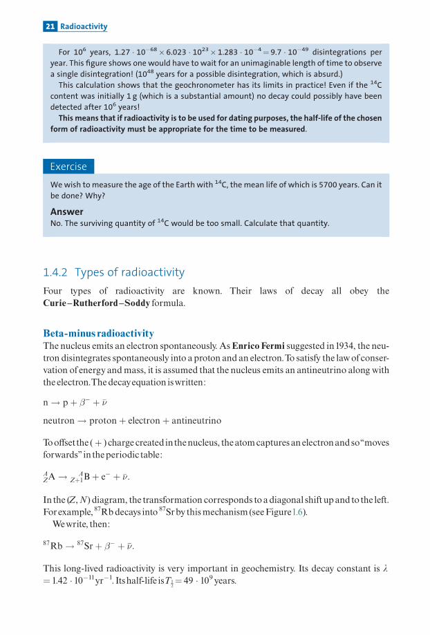
In the (Z,N) diagram, the transformation corresponds to adiagonal shiftup and to the left.Forexample,87Rbdecays into 87Srby thismechanism(seeFigure1.6).Wewrite, then:

87Rb! 87Srþ �� þ ��:

This long-lived radioactivity is very important in geochemistry. Its decay constant is l¼ 1.42 � 10�11yr�1. Itshalf-life isT1

2¼ 49 � 109years.

21 Radioactivity

Beta-plus radioactivityandelectron captureThe nucleus emits a positron (anti-electron) at the same time as a neutrino. A protondisintegrates into a neutron. A similar but di¡erent process is electron capture by aproton.

pþ e� ! nþ �

protonþ electron! neutronþ neutrino

Theatomemits aperipheral electronto ensurethenuclide remainsneutral.

AZA! A

Z�1Bþ eþ þ � �þ radioactivity

or

AZAþ e� ! A

Z�1Bþ � electron capture:

This is represented in the (Z, N) diagram by a diagonal shift down and to the right.Notice that neither of these forms of radioactivity involves a change in mass number. It

Neutron number (N)

Sm α

Nd

Pro

ton

nu

mb

er (

Z)

α radioactivity

N increases by 1

Z decreases by 1

N decreases by 2

N decreases by 1

Z decreases by 1

Z decreases by 2

β + radioactivityor electron

capture

β −radioactivity

144 147 148 149 150 152 154

142

Sr

Rb

84 86

85

87 88

87

Al

Mg 24

26

25

27

26

143 144 145 146 148 150

Valley o

f stabilit

y

Figure 1.6 The various types of radioactivity in the neutron–proton diagram. Notice that all forms ofdisintegration shift the decay products towards the valley of stability. Radioactivity seems to restore thenuclear equilibrium of nuclides lying outside the valley of stability and so in disequilibrium.


is said to be isobaric radioactivity. For example, potassium-40 (40K) decays into argon-40 (40Ar):

40Kþ e� ! 40Arþ �:

This is avery important form of radioactivity for geologists and geochemists. Its radio-active constant is l40K¼ 0.581 �10�10 yr�1 and its half-lifeT1

2¼ 1.19 � 1010 years.11We shall

be lookingat it again.

Alpha radioactivityThe radioactive nucleus expels a helium nucleus 4

2He (in the form of Heþ ions) and heat isgiveno¡.The radiogenic isotopedoesnothavethesamemassas theparentnucleus.Bycon-servationofmassandcharge, thedecayequation canbewritten:

AZA! A�4

Z�2Bþ42 He:

Inthe(N,Z)diagram,thepath isthediagonalofslope1shiftingdowntotheleft.Forexam-ple, samarium-147 (147Sm)decays intoneodymium-143 (143Nd)by thedecayscheme:

147Sm! 143Ndþ 42He

withl¼ 6.54 � 10�12 yr�1andT12¼ 1.059 � 1011years.

This formofdecayhasplayed an importanthistorical role in the developmentof isotopegeologyandweshallbeusing itonmanyoccasions.

Spontaneous ¢ssionFission is a chain reaction caused by neutrons when they have su⁄cient energy. Theelementary reaction splits a uranium nucleus into two unequal parts ^ for example akrypton nucleus and a xenon nucleus, a bromine nucleus and an iodine nucleus ^ andmany neutrons.These neutrons in turn strike other uranium atoms and cause new ¢ssionreactions, and neutron reactions on the nuclei formed by ¢ssion.This is ‘‘statistical break-up’’of uranium atoms into two parts of unequal masses. The nucleus that splits does notalways produce the same nuclei but awhole series ofpairs. Figure1.7 shows the abundanceofthevarious isotopesproducedbyspontaneous¢ssionof 238U.Noticethatthelasttwotypesofradioactivity (�and¢ssion)breakupthenucleus.Theyare

calledpartition radioactivity.Rememberthatspontaneous¢ssiontooobeysthemathemati-cal (CRS) lawofradioactivity.

E X A M P L E

The Oklo natural reactor

The isotope 238U undergoes spontaneous fission while 235U is subject to fission induced by the

impact of neutrons. Both these forms of fission occur naturally.

11 This is for disintegration of 40K into 40Ar. 40K also disintegrates giving 40Ca, as shall be seen later.

23 Radioactivity

Spontaneous fission of 238U has an extremely low decay constant l¼ 8.62 � 10�17 yr�1.

Induced fission of 235U is a reaction produced in the laboratory or in nuclear reactors by

bombarding uranium with neutrons.

In 1973, a natural nuclear reactor some 2 billion years old was discovered in the Oklo

uranium mine in Gabon. This uranium deposit worked like an atomic pile, that is, with

induced fission of 235U. Apart from a negative anomaly in the abundance of 235U, the

whole series of fission-induced products corresponding to this isotope was detected. This

fission of 235U, which was believed to be confined to laboratories or industrial nuclear

reactors, therefore occurred naturally, probably triggered by � disintegration of 235U,

which was much more abundant at the time. Nature had discovered nuclear chain

reactions and atomic piles some 2 billion years before we did! Oklo is a unique example

to date.

Exercise

Given that the 238U/235U ratio nowadays is 137.8, what was the activity level of 235U per gram

of ore 2 billion years ago for a uranium ore that today contains 30% uranium?

The decay constants are l238¼ 0.155 125 � 10�9 yr�1 and l235¼ 0.9885 � 10�9 yr�1.

AnswerThe activity of 235U was 1247 disintegrations per second per gram (dsg). Today the activity of235U is 172 dsg.

Light nuclei

Fissile nuclei

Neutrons

Neutrons generatedby fission process

a10

1.0

0.1

0.01

60 80 100 120Mass number

Yie

ld %

140 1600.001

b

Figure 1.7 Spontaneous fission: (a) chain reactions multiply the number of neutrons as the reactionunfolds; (b) the curve of the distribution of fission products as a function of their mass number.


Exercise

What types of radioactivity are involved in the following very important reactions in cosmo-

chronology and geochronology: 146Sm! 142Nd, 53Mn! 53Cr, 230Th! 226Ra?

AnswerSee Chapter 2, Section 2.4.3.

1.4.3 Radioactivity and heat

Each formofradioactive decay is associatedwith the emissionofparticles or� electromag-netic radiation. Interaction of this radiationwith thematerial surrounding the radioactiveisotope createsheat, asPierreCurie andAlbert Laborde realized in1903, just 7 years afterBecquerel’s discovery. This heat is exploited in nuclear reactors to generate electricity.Inside theEarth, the radioactivityof 40K, 238U, 235U, and 232Th isoneofthemain sourcesofinternal energy, giving rise to plate tectonics andvolcanism and to the heat £owmeasuredatthesurface. Inthe earlystagesoftheEarth’shistory, this radioactiveheatwasgreater thantodaybecause the radioactive elements 40K, 238U, 235U,and 232Thweremoreabundant.12

A L I T T L E H I S T O R Y

The age of the Earth

In the mid nineteenth century, when Joseph Fourier had just developed the theory of heat

propagation, the great British physicist William Thomson (Lord Kelvin)13 had been studying how

the Earth cooled from measures of heat flow from its interior. He had come to the conclusion

that the Earth, which was assumed to have been hot when it first formed, could not be more

than 40–100 million years old. That seemed intuitively too short to many geologists, particularly

to Charles Lyell, one of the founders of geology, and also to an obscure naturalist by the name of

Charles Darwin. Lyell had argued for the existence of an unknown heat source inside the Earth,

which Kelvin, of course, dismissed as unscientific reasoning! It was more than 50 years before

Pierre Curie and Laborde in 1903 measured the heat given off by the recently discovered

radioactivity and Rutherford could redo Kelvin’s calculations and prove Lyell right by confirming

his intuition. See Chapter 5 for more historical information on the age of the Earth.

Exercise

Heat emissions in calories per gram and per second of some isotopes are:14

238U 235U 40K 232Th

2.24 � 10�8 1.36 � 10�7 6.68 � 10�9 6.44 � 10�9

12 At the time there were other radioactive elements such as 26Al which have now disappeared but whoseeffects compounded those listed.

13 See Burchfield (1975) for an account of Kelvin’s work on the age of the Earth.14 These values include heat given off by all isotopes of radioactive chains associated with 238U, 235U, and

232Th (see Chapter 2).

25 Radioactivity

Calculate how much heat is given off by 1 g of peridotite of the mantle and 1 g of

granite given that 40K¼ 1.16 � 10�4 Ktotal;238U/235U¼ 137.8; Th/U¼ 4 for both materials; and

that the mantle contains 21 ppb U and 260 ppm K and that the granite contains 1.2 ppm U and

1.2 � 10�2 K.

AnswerCalculation of heat given off by 1 g of natural uranium:

0:992 79� 2:24 � 10�8 þ 0:007 20� 1:36 � 10�7 ¼ 2:32 � 10�8 cal g�1 s�1:

Calculation of the heat given off by 1 g of potassium:

6:68 � 10�9 þ 1:16 � 10�4 ¼ 7:74 � 10�13 cal g�1 s�1:

Calculation for the mantle:

2:32 � 10�8 � 21 � 10�9ð Þuranium

þ 6:44 � 10�9 � 84 � 10�9ð Þthorium

þ 7:74 � 10�13 � 2:60 � 10�4ð Þpotassium

¼ ð48:7þ 54þ 20Þ � 10�17

¼ 0:1227 � 10�14 cal g�1s�1:

To convert this result into SI units, 1 calorie¼ 4.18 joules and 1 watt¼ 1 joule per second.

Therefore 1 g of peridotite of the mantle gives off 0.512 � 10�14 W s�1. Calculation for

granite:

½2:32 � 10�8 � 1:2 � 10�6� þ ½6:44 � 10�9 � 4:8 � 10�6�þ½7:74 � 10�13 � 1:2 � 10�2� ¼ 2:78 � 10�14 þ 3:09 � 10�14 þ 0:928 � 10�14

¼ 6:79 � 10�14 cal g�1s�1:

1 g of granite gives off 28.38 � 10�14 W.

It can be seen that today the two big contributors are 238U and 232Th; 40K contributes less and235U is non-existent. The granite produces 55 times more heat than the mantle peridotite.

Exercise

The decay constants of 238U, 235U, 232Th, and 40K are l238¼ 0.155 125 � 10�9 yr�1, l235

¼ 0.984 85 � 10�9 yr�1, l232¼ 0.049 47 � 10�9 yr�1, and lK¼ 0.5543 � 10�9 yr�1, respectively.

Calculate heat production 4 billion years ago for the peridotite of the mantle and the granite

of the continental crust.

AnswerTotal heat production H can be written:

H ¼ 0:9927 � C U0 � P 238 expð0:155 125 T Þ

þ 0:007 20 � C U0 � P 235 expð0:984 85 T Þ

þ C Th0 � P 232 expð0:049 47 T Þ

þ 1:16 � 10�4 C K0 � P K 40ð0:5543 T Þ:


With T¼ 4 � 109 years, the result for the mantle is: 8.68 � 10�16þ 10.56 � 10�16þ 6.59 � 10�16þ18.4 � 10�16¼ 44.23 � 10�16 cal g�1 s�1¼ 1.84 � 10�14 W g�1 s�1.

For granite of the continental crust: 4.96 � 10�14þ 6.03 � 10�14þ 3.76 � 10�14þ 8.537 � 10�14¼23.28 � 10�14 cal g�1 s�1 or 97.3 � 10�14 W g�1 s�1.

Notice that, at the present time, radioactive heat is supplied above all by the disintegration

of 238U and to a lesser extent 40K and 232Th. Four billion years ago heat was supplied mainly by40K and 235U (Figure 1.8). It will be observed, above all, that 4 billion years ago the mantle

produced 3.5 times as much heat as it does today. So it may be thought that the Earth was 3.5

times more ‘‘active’’ than today.

Problems

1 Which molecules of simple hydrocarbons may interfere after ionization with the masses of

oxygen 16O, 17O, and 18O when measured with a mass spectrometer? How can we make sure

they are absent?

2 The lithium content of a rock is to be measured. A sample of 0.1 g of rock is collected. It is

dissolved and 2 cm3 of lithium spike added with a lithium concentration of 5 � 10�3 moles per

liter and whose isotope composition is 6Li/7Li¼ 100. The isotope composition of the mixture is

measured as 6Li/7Li¼ 10.

Given that the isotopic composition of natural lithium is 6Li/7Li¼ 0.081, what is the total

lithium content of the rock?

3 A sample contains 1 mg of strontium. What must be the maximum acceptable chemical blank,

that is, the quantity with which the sample is accidentally contaminated, if precision of

measurement with the mass spectrometer of 87Sr/86Sr �0.7030 bears on 0.0001?

The 87Sr/86Sr ratio of the blank is 0.7090. What must the blank be if precision is 10 times

better?

4 We are to construct a mass spectrometer for separating 87Rb from 87Sr. What should its

radius be?

1000 020003000400046000

1

10

100

total

Time (Ma)

Hea

t p

rod

uct

ion

(10

–12

W k

g–1

)

40K

235U

232Th

238U

Figure 1.8 Heat production by various forms of radioactivity in the Earth versus geological age.

27 Problems

5 Suppose that 1 mg of purified uranium has been isolated. It contains two (main) isotopes 238U

and 235U in the current proportions of 238U/235U¼ 137.8. What was the total activity of this

milligram of uranium 4.5 billion years ago and what is its activity today if l238¼0.155 125 � 10�9 yr� 1 and l235¼ 0.9875 � 10� 9 yr� 1?

6 The Urey ratio is the ratio of heat from radioactivity to total heat which includes heat from the

accretion of the Earth and the formation of its core. The average heat flow measured at the

Earth’s surface is 4.2 � 1013 W, which is 42 terawatts.

(i) In a first hypothesis the mantle composition is assumed to be uniform, with:

U¼ 21 ppb (Th/U)mass¼ 4 and K¼ 210 ppm.

Calculate the Urey ratio today.

(ii) In a second hypothesis, it is assumed that the entire mantle is similar to the upper mantle.

The upper mantle has a uranium content of 5 ppb, and the Th/U ratio is 2. Calculate the

Urey ratio.


CHAPTER T WO

The principles of radioactive dating

It can never be repeated enough that radioactive dating was the greatest revolution in thegeological sciences. Geology is an historical science which cannot readily be practisedwithoutaprecisewayofmeasuringtime.Itis safetosaythatnomoderndiscoveryingeologycould havebeen madewithout radioactive dating: reversals of themagnetic ¢eld, plate tec-tonics, the puzzle of the extinction of the dinosaurs, lunar exploration, the evolution of life,humanancestry, nottomentiontheageoftheEarthoroftheUniverse!The ages involved in the earth sciences are very varied.They are measured in years (yr),

thousandsofyears (ka),millionsofyears (Ma),andbillionsofyears (Ga).Geological clocksmustthereforebevariedtoo,withmean lives ranging fromayear toabillionyears.

2.1 Dating by parent isotopes

Imagine we have a radioactive isotope R and N�R is the number of atoms of this isotope.Suppose thatgeological circumstances (crystallizationofarockormineral, say) encloseaninitial quantityofR, i.e., the numberofatomsofRat time zero, writtenN�Rð0Þ, in a‘‘box.’’ Iftheboxhas remained closed fromwhen it¢rst formeduntil today, thenumberofatomsofRremaining isN�RðtÞ ¼ N�Rð0Þe�lt, where t is the time elapsed since theboxwas closed. Ifweknow the quantityN�Rð0Þ and the decay constant l, by measuringN�RðtÞ we can calculatethe age tatwhich theboxclosedbyusing the radioactivity formula‘‘upside down’’:

t ¼ 1

lln

N�Rð0ÞN�RðtÞ

� �:

Methods where the initial quantities of radioactive isotopes are well enough known areabove all those where the radioactive isotope is produced by irradiation by cosmic rays.This is the caseofcarbon-14 (14C)andberyllium-10 (10Be).

Exercise

The half-life of 14C is 5730 years. The 14C content of the atmosphere is 13.2 disintegrations per

minute and per gram (dpm g�1) of carbon (initial activity A0). We wish to date an Egyptian

artefact dating from approximately 2000 BC. What is the approximate activity (A) of this

artefact? If our method can measure 1 dpm, what mass of the (probably precious) sample will

have to be destroyed?

AnswerIf the half-life T¼ 5730 years, the decay constant is l ¼ ln2=T ¼ 1:209 � 10�4 yr�1. 2000 BC

corresponds to a time 4000 years before the present, therefore since A0¼ 13.2 dpm g�1 and

A¼A0 e�lt, A¼ 7 dpm g�1.

Making the measurement means using at least 1/7 g, or 142 mg of the sample.

As seen in the examples, the abundance of a radioactive isotope is estimated relative to a

reference. For 14C we use total carbon. The dating formula is therefore:

t ¼ 1

llnð14C=CÞ0ð14C=CÞt

� �

where (14C) and (C) represent the concentrations of 14C and total carbon, respectively.

In other cases, a neighboring stable isotope that is not subject to radioactive decay is taken

as the reference. So for 14C, we use stable 13C and we write:

t ¼ 1

llnð14C=13CÞ0ð14C=13CÞt

" #:

This formulation has the advantage of bringing out isotopic ratios, that is, the ratios mea-

sured directly by mass spectrometry.

2.2 Dating by parent–daughter isotopes

2.2.1 Principle and general equations

Thedi⁄cultywithdatingby theparent isotope isofcourseknowingN�Rð0Þ, thatis, knowingexactlyhowmanyradioactiveatomsweretrapped intheboxatthebeginning.Thisdi⁄cultyis overcomeby involving the stable daughter isotope produced by the disintegration noted(D) (the asteriskbeing a reminderof the radioactive origin of the isotopeR*).The parent^daughter relation iswritten:

ðRÞ� ! ðDÞl

:

FromtheCurie^Rutherford^Soddylaw,we canwrite:

dN�RðtÞdt

¼ �l N�RðtÞ

dNDðtÞdt

¼ � dN�RðtÞdt

¼ l N�RðtÞ:

Integrating the ¢rst equation yields the decay law, N�RðtÞ ¼ N�Rð0Þ e�lt. The second isthereforewritten:

dNDðtÞdt

¼ l N�Rð0Þe�lt;

30 The principles of radioactive dating

which integrates to:

NDðtÞ ¼ �N�Rð0Þe�lt þ C:

The integration constant C is determined by writing in t¼ 0, ND¼ND(0), hence:C ¼ NDð0Þ þN�Rð0Þ.Thisgives:

NDðtÞ ¼ NDð0Þ þN�Rð0Þð1� e�ltÞ:

But this expression leaves the troublesome unknown N�Rð0Þ. This is advantageouslyreplacedby:

N�Rð0Þ ¼ N�RðtÞ elt:

Thisgives:

NDðtÞ ¼ NDð0Þ þN�RðtÞðelt � 1Þ:

If the box remains closed for both the radioactive isotope and the radiogenic isotope, bymeasuring the present valuesND(t) andNR(t), we can calculate t, providedweknowND(0).This canbeplottedas (ND(t), t).Theslopeofthe curveateachpointequals:

dNDðtÞdt

¼ � dN�RðtÞdt

¼ lN�RðtÞ ¼ lN�Rð0Þe�lt:

It therefore equalslNR(t), at l times the parent isotope content.As this content decays con-stantly, theslopeofthetangentdoes likewise, andthe curve is concavedownwards.Tocalcu-lateanage,wewritethedatingequation:

t ¼ 1

lln

NDðtÞ �NDð0ÞN�RðtÞ

� �þ 1

� �:

Thevalues ofND(t) andN�RðtÞ canbemeasured, but t canonlybe calculated ifND(0) canbeestimated or ignored and, of course, ifwe know the decay constant l. Figure 2.1 illustratesall thesepoints.

E X A M P L E

Rubidium–strontium dating

Let us take rubidium–strontium dating by way of an example. As seen, 87Rb decays to87Sr with a decay constant l¼ 1.42 � 10�11 yr�1. The parent–daughter dating equation is

written:

t ¼ 1

lRbln

87Srðt Þ � 87Srð0Þ87Rbðt Þ þ 1

� �;

where 87Sr(0) is the quantity of 87Sr present at time t¼ 0, and 87Rb(t) and 87Sr(t) the quantities

of 87Rb and 87Sr present at time t. (The term quantity must be understood here as the number

of atoms or atom–grams.) Notice that time can be reversed and the present time considered

as the starting point, which is more practical. The initial time is then in the past, age (t) such

that T¼ t.

31 Dating by parent–daughter isotopes

The equation is then written:

T ¼ 1

lln

87SrðpÞ � 87SrðT Þ87RbðpÞ þ 1

� �;

where 87Sr(p) and 87Rb(p) relate to the present-day values (p¼present), and 87Sr(T) relates to

the initial values at time (T). When dealing with minerals that are very rich in Rb such as

biotite and muscovite, the initial 87Sr is negligible relative to the 87Sr produced by decay of87Rb. For such systems, which are said to be radiogenically rich (or just rich for short), the

dating formula is written:

T ¼ 1

lln

87SrðpÞ87RbðpÞ þ 1

� �:

This formula can be extended to rich systems in general:

T ¼ 1

lln

NDðpÞNRðpÞ

þ 1

� �:

As seen, if l is known, the age can be calculated directly from measurements of the present-

day abundances of ND(p) and NR(p). The only assumption made, but which is crucial, is

that the box to be dated, that is, the mineral or rock, has remained closed ever since the

time it formed and that closure was short compared with the age to be measured. This

is indeed the case when a mineral crystallizes or a magma solidifies as with volcanic or

plutonic rock.

NR(0)

ND(0)

N*R

Time graduated in periods

N*R

ND

ND(0)

2 4 60

N*R

ND =

0Time graduated in periods

Nu

mb

er o

f at

om

s o

f R

or

D

2 4 6

NR(0)

ND = ND(0) + NR(0) (1–e–λt)

N*R = NR(0) e–λt

ND(0)

+ (eλt –1)

Figure 2.1 Left: the decrease in the radioactive isotope and the increase in the radiogenic isotope. Right:the increase in the radiogenic/radioactive isotope ratio.N*R number of atoms of the radioactive isotope (R)ND number of atoms of the radiogenic isotope (D)NR(0) number of atoms of R at time t¼ 0ND(0) number of atoms of D at time t¼ 0l radioactive decay constant


RemarkWhere l is very small relative to the age, the exponential can be approximated by elt� 1þ l. This

is the case for the constant l of rubidium (l¼ 1.42 � 10�11 yr�1) and for many others. The dating

formula is then:

T � 1

l

87SrðpÞ87RbðpÞ

� �:

Exercise

Suppose we have a specimen of biotite from Querigut granite (Pyrenees Orientales, France)

whose age is to be determined from 87Rb ! 87Sr decay. We measure the total content of

Rb¼ 500 ppm and of Sr¼ 0.6 ppm. Knowing that Rb is composed of 87Rb and 85Rb in the

proportions 85Rb/87Rb¼ 2.5, that the Sr is ‘‘pure’’ radiogenic 87Sr, and that the decay constant

is l¼ 1.42 � 10�11 yr�1, calculate the age of the biotite in Querigut granite.

AnswerThe Rb content is written Rbtotal¼ 85Rbþ 87Rb¼ (2.5þ 1) 87Rb, therefore:

87Rb ¼ Rbtotal

3:5� 142:8 ppm:

The 87Sr content is 0.6 ppm. (There is no need to come back to atom–grams since 87Rb and 87Sr

have virtually the same atomic mass.) We can therefore write directly:

T � 1

1:42 � 10�11

0:6

142:8

� �� 298 � 106 yr ¼ 298 million years:

If we had not adopted the linear approximation, we would have obtained:

T � 1

1:42 � 10�11ln

0:6

142:8þ 1

� �� 297:36 � 106 yr:

As can be seen, the linear approximation is valid for the 87Rb/87Sr system when the age is not

too great.

2.2.2 Special case of multiple decay

Letus consider the caseofthe long-period 40K radioactive isotopewhich decays in two dif-ferentways, either by electron capture giving 40Aror by �� decaygiving 40Ca, eachwith itsowndecayconstantleandl�� , respectively:

e–cap40Ar

40K

β –40Ca

What is the dating formula?Letusgetbacktobasics:

d=dt½NKðtÞ� ¼ �ðle þ l�ÞNKðtÞ


whereNK is thenumberof 40Knuclides andNAr thenumberof 40Ar nuclides.

d=dt½NArðtÞ� ¼ leNKð0Þe�ðleþl�Þt:

Integratingusing theusual notationwith 40Kand 40Ar0gives:

40ArðtÞ ¼ 40Ar0 þ 40KðtÞ lele þ l�

eðleþl�Þt � 1�

withle¼ 0.581 �10�10 yr�1andl�¼ 4.962 � 10�10 yr�1.

l ¼ le þ l� ¼ 5:543 � 10�10 yr�1:

The initial 40Ar is usually negligible.We are therefore generally dealing with rich systemsbut notwithvery young systemswherewhat is known as excess argon raises di⁄culties foraccurateage calculations.

Exercise

We analyze 1 g of biotite extracted from Querigut granite by the 40K–40Ar method. The biotite

contains 4% K and 40K¼ 1.16 � 10� 4 of Ktotal.

The quantity of argon measured at standard temperature and pressure is 4.598 � 10�5 cm3

of 40Ar. What is the radiometric age of this biotite?

AnswerThe dating formula to calculate the age is written:

T ¼ 1

le þ lbln

40Ar40K� le þ lb

le

� �þ 1

� �:

We must therefore calculate the 40Ar/40K ratio in atoms.

As there are 22 400 cm3 in a mole at standard temperature and pressure, the value of 40Ar

in number of moles is:

4:598 � 10�5

22 400

� �¼ 2:053 � 10�9 moles of 40Ar:

The value of 40K is:

0:04� 1:16 � 10�4

40¼ 1:16 � 10�7 moles of 40K:

Therefore:

T ¼ 109

0:5543ln

2:053 � 10�9

1:16 � 10�7� 0:1048

� �þ 1

� �¼ 280 million years:

Comparing this with the result obtained previously using the 87Rb–87Sr method, we find

about the same age but slightly younger.

There is another branched decay used in geology, that of 138Lawhich decays into 138Baand138Ce (Nakaıetal.,1986).


e–cap138Ba λCap e– = 4.44 . 10–12 yr–1

λβ = 2.29 . 10–12 yr–1

138La

β –138Ce

There is also a case where even more intense multiple decay occurs, in the spontaneous¢ssion of 238U, which yields a whole series of isotopes. Luckily, ¢ssion decay is negligiblecomparedwith�decay. In the dating equationwe can consider the constant l�alone as thedecay constant, but allowancemustbemade, of course, for the¢ssion products. For exam-ple, for136Xewewrite thedatingequation:

136Xeradio238U

¼ Ylfissionl�ðel�t � 1Þ

whereY is theyieldof136Xeproducedduring¢ssion�0.0673,withl¢ssion¼ 8.47 � 10�17yr�1andl�¼ 1.55 � 10�10 yr�1.Wesawwhen lookingatdatingbyparentisotopesthatitwasconvenienttoexpressthedat-

ing equationby introducing isotope ratios rather than moles of radioactive and radiogenicisotopes.This is callednormalization.Thusfor 87Rb^87Srweuseastablestrontiumisotope,86Sr.Thedatingequation is thenwritten:

t ¼ 1

lln

87Sr86SrðtÞ � 87Sr

86Srð0Þ

87Rb86Sr

!þ1

" #:

This is the form inwhich dating equationswill be expressed from nowon. A systemwill berichwhen:

87Sr86Srð0Þ

87Sr86SrðtÞ:

2.2.3 Main geochronometers based on simpleparent–daughter ratios

Rubidium^Strontium 87Rb ��87Sr; l¼ 1.42 � 10�11 yr�1.The normalization isotope is86Sr.Developed in itsmodern formbyAldrich et al. (1953). Potassium^Argon 40K^40Ar, with the constants alreadygiven.The reference isotope is

36Ar.Developed in itsmodern formbyAldrichandNier (1948a). Rhenium^Osmium 187Re �� 187Os with l¼ 1.5 � 10�11 yr�1. The reference isotope is

186Os and more recently 188Os. Developed by Luck, Birck, and Alle' gre in 1980 after a¢rstattemptbyHirtetal. in1963.

These are the three simple clocks that are commonly found as rich systems in nature.Weshall see thatother formsofdecaycanbeusedbutundermoredi⁄cultcircumstances.

Samarium^Neodymium 147Sm�143Nd; l¼ 6.54 � 10�12 yr�1.Normalizationby144Nd.DevelopedbyLugmairandMarti in1977afteranattemptbyNotsu etal. in1973.


Lutetium^Hafnium 176Lu ��176Hf; l¼ 2 � 10�11 yr�1. Normalization with 177Hf.DevelopedbyPatchett andTatsumoto (1980a,1980b).

These methods are supplemented by others related to radioactive chains which are to beexamined next, by the extinct radioactive methods covered in Section 2.4, and by theinducedradioactivemethods examined inChapter 4.

2.3 Radioactive chains

2.3.1 Principle and general equations

When238U,235U,and232Thdecay, theygive risetothreeother radioactive isotopeswhich, inturn, decay into new radioactive elements, and so on.The process stops when the last iso-topes produced are the three lead isotopes 206Pb, 207Pb, and 208Pb, which are stable. It wasradioactive chains which allowed both Pierre and Marie Curie and Rutherford andSoddy to discover themechanismsof radioactivity.A radioactive chain canbe representedbywriting:

ð1Þ� ! ð2Þ� ! ð3Þ� ! ð4Þ� ! . . .! ðnÞ stable:

Decayinvolves�and� radioactivity.Alpharadioactivitygiveso¡heliumnuclei.Theirpath,in the (Z,N) plot, brings the endproduct intothevalleyofstability.

Figure 2.2 shows the precise structure of the three chains.Mathematically, as studied byBateman (1910), radioactive chains can be described by the Curie^Rutherford^Soddylawswrittenoneafter theother:

dN1ðtÞdt

¼ �l1N1ðtÞdN4ðtÞdt

¼ l3N3ðtÞ � l4N4ðtÞ

dN2ðtÞdt

¼ l1N1ðtÞ � l2N2ðtÞ ...

dN3ðtÞdt

¼ l2N2ðtÞ � l3N3ðtÞdNn

dt¼ lNn�1ðtÞ

whereNi is the numberof nuclides of elements i andNn the numberof nuclides of the ¢nalstable isotope. Successive integration of these equations presents no real di⁄culty and iseven agood revision exercise for integrating¢rst-orderdi¡erential equationswith constantcoe⁄cients. Letus leave that for nowand concentrate on a fewsimple and important limit-ingcases.

2.3.2 Secular equilibrium: uranium–lead methods

We suppose that, in view of the length of geological time, the radioactive chain reaches astationarystatewhere the contentofall the intermediate radioactive isotopes remains con-stant (this isknownas secularequilibrium):

dN2

dt¼ dN3

dt¼ � � � ¼ dNn�1

dt¼ 0:


Inthis case,wethereforehave:

l1N1 ¼ l2N2 ¼ l3N3 ¼ . . . ¼ ln�1Nn�1;

therefore:

dNn

dt¼ l1N1:

It is as iftherewas justa single directdecayreaction (1)! (n).Considering the fact that in the course of geological time natural radioactive chains

rapidly reach equilibrium, the initial products give the end products directly. Dating equa-tions canthenbewritten:

206Pb ¼ 238Uðel8t � 1Þ þ 206Pb0207Pb ¼ 235Uðel5t � 1Þ þ 207Pb0208Pb ¼ 232Thðel2t � 1Þ þ 208Pb0

where constantsl8,l5, andl2 arethoseof238U, 235U,and 232Th.

92

92

90

88

90

88

86

84

82

90

88

86

84

86

84

82

124 126 128 130 132 134 136 138 140 142 144 146

82 206Pb

208Pb208TI3.1 m

207Pb°

210Po138 d

207Ti4.8 m

211Bi2.2 m

211Pb36 m

215Po2x10–3 s

219Rn3.9 s

223Ra11 d

227Th17 d

227Ac22 yr

224Ra3.6 d

220Rn55 s

216Po0.16 s

212Po3x10–7 s

212Bi61 m

212Pb11 h

231Th26 h

210Bi50 d

214Bi20 m

214Pb27 m

218Po3.1 m

222Rn38 d

214Po2x10-4s

210Pb22 yr

226Ra1622 yr

235U713 Ma

232Th14 Ba

228Ra6.7 yr

230Th75 ka

234Pa1.2 m

234Th24 d

238U4.5 Ba

N

Z

228Th1.9 yr

231Pa34 ka

234U248 ka

228Ac6.1 h

Figure 2.2 Radioactive chains represented on the proton–neutron graph. Each slot contains the symbolof the isotope and its period T1

2. Identify the various types of radioactivity of the three chains for yourself.

37 Radioactive chains

238U! 206Pb l238 ¼ l8 ¼ 1:551 25 � 10�10 yr�1235U! 207Pb l235 ¼ l5 ¼ 9:8485 � 10�10 yr�1232Th! 208Pb l232 ¼ l2 ¼ 4:9475 � 10�11 yr�1:

This comes downto direct parent^daughter dating.Warning!Linearapproximation can-not be usedwith these chronometers.To be convinced of this, let us compare the values of(elt� 1)with (lt) for time intervalsof 1 and 2 billion years for 235U and 238U.

Letus consider the quantity ½ðelt � 1Þ � lt�=½elt � 1� �

�100, which is the relative errorthatcanbe expressedasapercentage.

With 235U, for1billion the error is 41.2% and for 2 billion 68.2%!With 238U, for1billionthe error is 7.5% and for 2 billion14.7%.These are highly non-linear systems, then, as canbeseen fromtheshapeofthe typical curves inFigure2.3.

2.3.3 The special case of lead–lead methods

Wehave seen that on the geological timescale radioactive chains attain equilibrium and itcan be considered that 238U decays directly to 206Pb, 235U to 207Pb, and 232Th to 208Pb.For uranium-rich minerals like zircon, uraninite, or even monazite, the initial amount oflead can be considered negligible. Assuming the system has remained closed, we canwrite:

206Pb ¼ 238Uðel8t � 1Þ207Pb ¼ 235Uðel5t � 1Þ:

Taking the ratio, remembering thatnowadays1the ratio 238U/235U¼ 137.8,weget:

207Pb206Pb

¼ 1

137:8

el5t � 1

el8t � 1

� �:

It can be seen that the 207Pb/206Pb isotope ratio of lead alone gives a direct measurementof time. This function is implicit and calculating it requires prior numerical values(Table 2.1).

Exercise

The 206Pb/207Pb ratio of a uranium ore deposit is found to be 13.50. What is the age of the ore

supposing it has remained closed since it crystallized and that common lead can be ignored?

AnswerWe shall invert the ratio so Table 2.1 can be used. 207Pb/206Pb¼ 0.074. The table shows that

the ratio measured lies between 1 and 1.2 � 109 years. The result can be improved either by

refining the table by calculating the ratio el5t � 1=el8t � 1�

in the interval 1 and 1.2, or by

1 The two uranium isotopes decay each at their own rate from the time that they are first formed. Theirratio is constant as there is no isotopic fractionation between them. However, this ratio has varied overgeological time.


using a linear approximation between 1 and 1.2 � 109 years. The value 207Pb/206Pb for 1.2

billion is 0.080 12 and for 1 billion is 0.0725. The variation is therefore:

0:080 12� 0:0725

200¼ 3:8 � 10�5per million years:

The difference is between 0.0740 and 0.0725, that is, 1.5 � 10�3 million years.

1

0.4

0.2

207 P

b*/

206 P

b*

0

0.6

0.8

2 3 4Time (Ga)

Time (Ga)

1.0

0.5

0.00 1 2 3

Age (Ga)

P/P 0

235U-207Pb

40K-40Ar

238U-206Pb

T = 0.70

Ag

e o

f th

e Ea

rth

4.56

Ga

87Rb-87Sr

4 5

T = 48.8

T = 4.47

T = 1.25

235 U

0

0.5

1

21 3 4

207 P

b*

0

1

0.5

1 2 3 4

0.2

206 P

b*

0

0.4

0.6

1 2 3 4

0.6

0.4

0.8

1

238 U

1 2 3 4

Figure 2.3 Non-linear decay of 235U and 238U and their end products 207Pb and 206Pb. (a) The radioactiveconstants of these reactions are very different. The curve on the right shows the change in radiogenicratio 207Pb*/206Pb* versus time. (b) Comparison in the same figure of the principal radioactive clocksused in geology, emphasizing the behavior of U–Pb systems compared to others.


The approximate age is therefore 1040 Ma. Direct calculation from the 207Pb/206Pb ratio for

1040 Ma gives 0.073 98. The age is therefore 1042 Ma, but such precision is illusory because

error is far greater (see Chapter 5) than the precision displayed.

2.3.4 The helium method

Natural chains feature many instances of � decay, that is, expulsion of 4He nuclei. Thus238Udecayultimatelyproduces eight 4He, 235Udecayproduces seven 4He, and 232Thdecayproduces six 4He.We canthereforewrite:

d 4He

dt¼ 8l8238Uþ 7l5235Uþ 6l2232Th:

RemarkThis equation underlies the first helium dating method thought up by Rutherford (1906).

Integrating the equation, assuming4He(0)¼ 0, gives:

4He ¼ 8 238Uðel8t � 1Þ þ 7 235Uðel5t � 1Þ þ 6 232Thðel2t � 1Þ:

Table 2.1 Numerical values of the radiogenic 207Pb/206Pb isotope ratio

Time (Ga) el1t� 1 el2t� 1207Pb206Pb

� radiogenic

0 0.0000 0.00000.2 0.0315 0.2177 0.050120.4 0.0640 0.4828 0.054710.6 0.0975 0.8056 0.059920.8 0.1321 1.1987 0.065811.0 0.1678 1.6774 0.072501.2 0.2046 2.2603 0.080121.4 0.2426 2.9701 0.088791.6 0.2817 3.8344 0.098721.8 0.3221 4.8869 0.110002.0 0.3638 6.1685 0.122982.2 0.4067 7.7292 0.137832.4 0.4511 9.6296 0.154822.6 0.4968 11.9437 0.174362.8 0.5440 14.7617 0.196803.0 0.5926 18.1931 0.222663.2 0.6428 22.3716 0.252413.4 0.6946 27.4597 0.286723.6 0.7480 33.6556 0.326343.8 0.8030 41.2004 0.372124.0 0.8599 50.3878 0.424984.2 0.9185 61.5752 0.486234.4 0.9789 75.1984 0.557144.6 1.0413 91.7873 0.63930


Byadmitting linearapproximations,which isvalidonly fordurations thatarenotexcessive,elt� 1� ltandobserving that 235U/238U¼ 1/137.8andthat 232Th/238U� 4weobtain:

4He ¼ 238U 8 l8 þ7

137:8l5þ6�4�l2

� �t:

BynotingL ¼ 8l8 þ 7l5137:8þ 24l2

� ¼ 14:889 � 10�10 yr�1,weobtain

� � 1

L

4He238U

� �:

This formula isvalid for youngages.

Exercise

Take 1 kg of rock containing 2 ppm of uranium. How many cubic centimeters of 4He will it

have produced in 1 billion years?

AnswerAt 2 ppm 1 kg of rock represents 103 g� 2 � 10�6¼ 2 � 10�3 g of uranium, and 2 � 10�3 g of

uranium corresponds to2 � 10�3

238¼ 8:4 � 10�6 moles. Using the approximate formula:

4He ¼ Lt U ¼ 14:89 � 10�10 � 109 � 8:4 � 10�6

4He � 125 � 10�7moles:

If 1 mole of 4He corresponds to 22.4 liters at standard temperature and pressure, the amount

of 4He produced in 1 billion years is 0.28 cm3.


The beginnings of radioactive datingRutherford performed the first radioactive age determination in 1906. He calculated the

amount of helium produced by uranium and radium per year and per gram of uranium and

found 5.2 � 10�8 cm3 yr�1 g�1 of uranium.

Ramsay and Soddy had measured the helium content (long confused with nitrogen

because it is inert like the noble gases) in a uranium ore known as fergusonite. The

fergusonite contained 7% uranium and 1.81 cm3 of helium per gram. Rutherford calculated

an age of 500 million years. The following year he found uranium ores more than 1 billion

years old! At that time Lord Kelvin was claiming the Earth was less than 100 million years old!

(See previous chapter.)

2.3.5 The fission track method

Fission reactions emit heavy atoms.The atoms ejected by ¢ssion create £aws in crystals.Suchdefects ^ knownas tracks ^ canbeshownuponmineralsurfaces throughacidetching


whichpreferentiallyattacks damaged areas, thosewhere atomshavebeen displaced (PriceandWalker,1962) (Figure 2.4).

Thenumberof¢ssiontracks iswritten:

Fs ¼lfissionl�

238Uðel�t � 1Þ

lfission ¼ 7 � 10�17 yr�1 t1=2 ¼ 9:9 � 1015 yr�1:

In practice, a thin section is cut and the number of surface tracks (and not in a volume) ismeasured.Thevisibleproportion�s is calculated:

�s ¼ qlfissionl�

238Uðel�t � 1Þ

whereq is ageometric factor for switching fromasurface toavolume.To measure 238U, we take advantage of knowledge that 238U/235U¼ 137.8 and measure

235U by causing induced ¢ssion (by placing the ore under study in a reactor), which pro-duces tracks that are revealed and counted.We then have the number of tracks before (�s)andafter (�i) irradiation.Thegeometric factordisappears:

�s�i¼ lfission

l�

137:8

�Gðel�t � 1Þ:

Wecalibratethe£ux�ofneutrons inducing235U¢ssionandthee¡ective cross-section�.2

By using a standard samplewhoseuranium content is knownandwhich is irradiated at thesame time as the study sample and by counting the ¢ssion tracks produced, we can thencalculatet.

Ionization Electrostaticdisplacement

Relaxation andelastic deformation

Figure 2.4 Creation of fission tracks in an insulating material.

2 The effective cross-section is the probability of a reaction occurring, that is, here, the probability ofproducing a fission with a given flux of neutrons. The characteristics of this will be seen in Chapter 4.


2.3.6 Isolation of a part of the chain and dating younggeological periods

The various radioactive isotopes of the radioactive chain belong to di¡erent chemical ele-mentssothat,undercertaingeologicalconditions,oneor twoisotopes inthe chain fraction-ate chemically and become isolated, thereby breaking the secular equilibrium. Onceisolated they create a new partial chain in turn.Two straightforward speci¢c cases are ofpractical importance.

The radioactive isotopebecomes isolatedon its ownFirst,when a radioactive isotope in the chain (butwith a long enoughperiod) becomes iso-lated on its own, it gives rise to a partial chain, but being isolated from the parent it decaysaccording tothe law:

NiðtÞ ¼ Nið0Þe�lt

whereNi(0) is the numberofnuclides of the intermediate element at time t¼ 0. If this num-ber can be estimated, the decay scheme can be used as a chronometer.This is equivalent,then, todatingby theparent isotope.

E X A M P L E

The ionium method and the rate of sedimentation

Thorium is virtually insoluble in sea water. Thus 230Th (still known as ionium from the

terminology of the pioneers of radioactivity), a decay product of 234U with T12¼ 75 ka,

precipitates on the sea floor, is incorporated in the sediment and so gradually buried. There,

now isolated, it decays.

At any depth x of sediment from the surface (Figure 2.5) we can write:

230ThðxÞ ¼ 230Thð0Þe�l230t

where 230Th(0) is the surface content which is assumed constant over time. If the sedimenta-

tion rate is constant, time can be replaced by the ratio t¼ x/Vs where Vs is the sedimentation

rate and x the length (depth):

230ThðxÞ ¼ 230Thð0Þ exp x=V s½ �lð Þ

or in logarithms:

lnð230ThðxÞÞ ¼ ln�

230Thð0Þ�� x

V sl:

The slope of the curve (ln 230Th, x) gives a direct measure of sedimentation rate and the

ordinate at the origin gives 230Th(0). (Note its order of magnitude of a millimeter per

thousand years.)

This method only works, of course, if it is assumed that 230Th(0), that is the thorium content

at the sediment surface, is constant and if the sediment has not been disturbed by chemical,

physical, or biological phenomena.


Exercise

The lead isotope 210Pb (as a member of the radioactive chain) is radioactive with a decay

constant l¼ 3.11 � 10�2 yr�1. This natural radioactive lead is incorporated into ice deposited

in Greenland by forming successive layers of ice which can be studied like sedimentary strata.

The activity of 210Pb is measured at four levels in disintegrations per hour per kilogram of ice

(dph kg�1). Table 2.2 shows the results.

Calculate the sedimentation rate of the ice. Assuming a constant rate and a compaction

factor of 5, how thick will the glacier be in 5000 years? Calculate the 210Pb content of fresh ice.

AnswerThe dating equation is written noting activity by square brackets:

210Pb�

¼ 210Pb�

e�lt :

If the rate of deposition is V and height h, we have t¼ h/V.

The equation becomes:

210Pb�

¼ 210Pb�

exp lh=Vð Þ

or

ln 210Pb�

¼ ln 210Pb�

0� lh

V:

If the 210Pb content has remained constant over time, the data points must be aligned in a (ln

[activity, h]) plot. The slope is therefore �l=V . The data points are plotted on the graph and

the slope determined. This gives V¼ 45 cm yr�1.

Depth (cm)

50

10

5

10 20 40

230 T

hex

(dp

m g

–1)

60

100

4.3 mm ka–1

Figure 2.5 Decreasing 230Th content in a core from the sea floor and determination of thesedimentation rate. Thex is the excess thorium compared with the equilibrium value counted indisintegrations per minute per gram (dpm g�1).


In 5000 years’ time, allowing for compaction, there will be 5000� 45=5 ¼ 450 m of ice.

The 210Pb content is calculated: surface activity is 75 dph kg�1 ice.

l210 � N 210 ¼ 75 dph kg�1

hence

N 210 ¼75

3:1110�2 � 8760ð Þ�1 ¼75

3:5 � 10�7¼ 21:4 � 107atoms of210Pb nuclides

per kilogram of ice;

8760 being the number of hours in a year. As a mass that gives:

21:4 � 107 � 210

6:023 � 1023¼ 7:5 � 10�14 kg of ice;

where Avogadro’s number is in the denominator and the previous atomic mass of 210Pb in the

numerator.

The 210Pb content is 7.5 � 10�17, which is very little! This shows the incredible sensitivity of

radioactive methods because 210Pb in Greenland’s glaciers really can be measured and used

for estimating the rate of sedimentation of ice.

Theparent isotope is isolatedandengenders its daughtersThis iswhathappenswithuranium; forexample,when certainsolidphaseslike calciumcar-bonate are precipitated uranium is entrainedwith calcium and then isolated. For the ¢rstradioactiveproductofanynotablehalf-life,wethen have:

l2�3N2�3ðtÞ ¼ l1UðtÞ e�l1t � e�l2�3t� �

whereN2^3 is the number of nuclides in the third intermediate product in the chain.Why?Because the chain includes very short-lived radioactive products such as thorium-234(234Th) or protactinium-234 (234Pa) which reach equilibrium very quickly. Thus, 238Udecays to 234Th, an element whose lifespan is 24 days, then 234Pa, whose lifespan is 1.18minutes: it canbe considered, then, that 238Udirectlygives 234Uwhosehalf-life is 2.48 � 105years forall typesofusual samples (corals, speleothems, travertines, etc.).Such a method is applied, for example, to secondary mineralizations of uranium.The

soluble uranium migrates and is deposited further away, leaving the insoluble thoriumwhere it is. Itthen‘‘resumes’’ its decaygiving230Thandwe canwrite:

l230230Th ¼ l230238U e�l238t � e�l230t� �

:

Thereforetheageofmigration canbedeterminedbymeasuring230Thand238U.

Table 2.2 Activity of 210Pb with depth

Depth

0m 1m� 20 cm 1.50m� 40 cm 2.50m� 50 cm

dphkg�1 75 32� 5 24� 5 10� 3


Exercise

Uranium-238 (238U) decays to 234U which is itself radioactive with l¼ 2.794 � 10� 6 yr�1.

Sea water is not in secular equilibrium relative to uranium isotopes as 234U weathers better

than 238U from rocks of the continental crust and is enriched in the rivers flowing into the

ocean. In activity, noted in square brackets [ ], 234U=238U½ �seawater ¼ 1:15. When limestone

forms from sea water, it is isotopically balanced with the sea water and so takes the value 1.15.

A fossil mollusk has been found in a Quaternary beach formation and its activity ratio measured

as 234U=238U½ � ¼ 1:05. Work out the dating equation. What is the age of the mollusk?

AnswerThe dating equation is:

234U238U

� �¼

234U238U

� �0

e�lt þ 1� e�l234t� �

because l234� l238 and l238 t � 0 if t> 106 years.

This gives:

T ¼ 1

lln

234U238U

h i0�1

234U238U

� � 1

0@

1A and T¼ 393 000 years.

2.3.7 General equation and equilibration time

Weshalldoanexercise tohelpunderstandequilibrationtimeandby thesametokengivethetheoretical answer totheprevious exercise.

Exercise

Establish the general equation for evolution of an isotope in a radioactive chain and where the

parent has a longer half-life and the daughter a markedly shorter half-life. We shall take the

example of 234U! 230Th decay to get our ideas straight.

AnswerThis is a review exercise for mathematics on integrating a linear differential equation with

constant coefficients:

d 234U

dt¼ l238

238U� l234234U

d 230Th

dt¼ l234

234U� l230230Th

with 238U being considered constant.

Integrating the two previous equations in succession for the example in question gives:

l234234U ¼ l234

234U0e�l234t þ l238238U 1� e�l234t

� �l230

230Th ¼ l230230Th0e�l230t þ l234

234U e�l234t � e�l230t� �

:

These two equations can be written with the activity notation in square brackets: lN¼ [N],

which simplifies notation and means the l constants can be dispensed with. This gives:


234U�

¼ 234U0

� e�l234t þ 238U

� 1� e�l234t� �

230Th�

¼ 230Th0

� e�l230t þ 234U

� e�l234t � e�l230t� �

:

This is the general equation for equilibration of a radioactive chain used for chronological

purposes.

From there, without resorting to long and tedions numerical simulation, let us try to answer

the question: at what speed does a greatly disturbed radioactive chain return to secular

equilibrium? Let us consider the preceding equation with l234 l230. The equation becomes:

l230230Th ¼ l230 Th0e�l230t þ l234

234U 1� e�l230t� �

:

For the chain to achieve equilibrium, it is necessary and sufficient that:

l230230Th � l234

234U:

For this e�l230t must be virtually zero. So t must be less than to 6–10 periods of 230Th. The

chains therefore achieve equilibrium after more than six half-lives of the daughter product

(with the smaller radioactive decay constant).

If 234U/238U isotope fractionation occurs, which is the case in surface processes, it is 234U

which is the ‘‘limiting factor’’ for the 238U chain. The time required is therefore 1.5 million

years.

If there is no 234U/238U isotope fractionation, the limiting factor is 230Th and the equilibra-

tion time is 450 000 years.

For the 235U chain the limiting factor is 231Pa and therefore a time of 194 000 years. Both

chains of the two uraniums are equilibrated at about the same time in this case.

The isotopes of radioactive series used as geochronometers are those with decay constants of

more than one year.

Uranium-238 chain

234U, half-life 248 ka, is used in sedimentary or alteration processes because 234U/238Uvaries during alteration. The radioactive recoil of 234U extracts this uranium from itscrystallographic siteandso it is easilyaltered. 230Th, half-life 75 ka.This element, named ionium, is certainly themostwidely used for

surfaceandvolcanicprocesses. 226Ra, half-life 1.622 ka. It is used like 230Th but for shorter-lived surface or volcanic

processes. 210Pb, half-life 22 years. Used for studying glaciers, oceans or volcanics involving very

youngphenomena.

Uranium-235 series

231Pa, half-life 32.48 ka. This is the sister of 230Th but slightly more di⁄cult to masteranalytically. 277Ac, half-life 22 years.This element is not much used as yet because of di⁄culties in

makingpreciseanalyses.


Thorium-232 chain

228Ra,half-life6.7years.This is complementary to 226Rato constrainthetimescaleofRafractionation. 228Th,half-life1.9years.Averygoodcomplement for 228Raand 230Th.

These elements canbemeasuredbyalphaandgammaradioactive spectroscopyorbymassspectrometry.The second technique is far more precisebut less sensitive than counting. Inpractice, 234U, 230Th, 226Ra, and 231Pa are measured bymass spectrometry and the othersbycounting.Pb-210canbemeasuredbymass spectrometrybutthis entailsgreatdi⁄cultiesandrequires specialprecautions.Forageneral reviewsee Ivanovich (1982).


The polemic that followed the discovery of radioactivityHenri Becquerel discovered radioactivity almost by chance in 1898 while studying rays

from phosphorescent uranium salts excited by sunlight and trying to understand the

nature of x-rays discovered by Rontgen. But one day, although there was no sunlight, a

sample from the Joachimsthal mine in Bohemia spontaneously emitted radiation which

blackened a photographic plate, indicating as yet unknown properties of matter (see Barbo,

2003).

Some years later, when measuring the effect of these radioactive substances on an

electrometer (the particles ionized the air of the electrometer which then discharged)

Pierre and Marie Curie proposed calling the phenomenon radioactivity (activity created by

radiation). For them, it was the property certain substances, including uranium, had of

spontaneously emitting radiation.

They immediately came in for harsh criticism from British scientists relying on a crucial

observation: when the activity of 1 g of purified uranium was measured with an electro-

meter, the activity was less than that of 1 g of uranium contained in, say, 100 g of uranium

ore. In other words 1 g of uranium ‘‘diluted’’ in 100 g of inert rock was more ‘‘active’’ than 1 g

of pure uranium.

How could concentrated uranium be less active than diluted uranium? It smacked of

magic. It was Marie Curie who came up with the hypothesis of intermediate radioactive

products to explain this paradox. The discovery of radium must be set in this polemical

context, thus taking on its full significance. It was the second intermediate radioactive

product to be found after polonium.

The New Zealander Ernest Rutherford brought grist to the Curies’ mill and within a few

years the mechanisms of successive ‘‘cascade’’ decay was understood. Radioactive chains had

been discovered.

Shedding light on a paradoxNowadays the paradox of diluted uranium being more active than pure uranium can be fully

explained. Suppose a radioactive chain is in equilibrium, say the 238U chain:

l1N 1 ¼ l2N 2 ¼ l3N 3 ¼ � � � ¼ lnN n

noting N1, N2, . . ., Nn the numbers of nuclides in the various isotopes of the chain. Thus in

secular equilibrium there is 14 times the l1N1 activity of 238U in the chain. (The input from

the 235U chain must be added to this although its contribution is small.)


This is what happens in a rock several hundred million years old in which the chain has had

time to attain secular equilibrium.

Now, in purified uranium, the activity is merely l1N1.

So, if the ‘‘activity’’ of 1 g of uranium is measured, it will be 14 times less than the activity

of 100 g of 1% uranium ore. Indeed, the ore would be slightly more active because there must

also be at least 0.5 g of thorium whose chain also produces 11 times more activity than pure

thorium. However, as the thorium constant is 3.5 times less, the outcome would be an

increase in the uranium activity of about 1.5 times.

In all, the rock is about 15.5 times more active than purified uranium. This is the paradox

behind the polemic!

2.4 Dating by extinct radioactivity

2.4.1 The historical discovery

Chemical elements ^ thatis, thenucleithatmakeupmostoftheirmass ^ havebeenmanufac-tured in stars ever since the Universe came into being.This is nucleosynthesis. Of the nucleiformed, somearestableandothers radioactive.Amongthe radioactivenuclei somehaveveryshorthalf-lives: theydecayquicklygiving rise totheirstabledaughter isotopes.Allofthisgoeson everywhere in interstellar space and iswhat provides the ordinarymatterof theUniverse.These isotopesare incorporated intointerstellarmatterasgasesordust (seeChapter4).But suppose thatnucleosynthesis ofheavyelements (explosionofa supernova) occurred

in the vicinityof the place where the Solar System formed giving rise to certain short-livedradioactive isotopes. Suppose too that the solidbodies ofthe Solar System formwhile theseradioactive isotopes arenotyetextinct.These‘‘young’’radioactive isotopeswill be incorpo-rated with the other interstellar material in these solid bodies (planets or meteorites) andthere they will decay and give rise to daughter isotopes.The solid objects having receivedsuch inputswill thereforehave abnormal isotope abundances for the isotopesproducedbydecayofthe radioactive isotope.Detectingsuchanomalies is thereforethe¢rststep in show-ing the existenceofextinctradioactivity.In1960 JohnReynolds at Berkeleydiscovered a large excess of the isotope129 in the iso-

topic composition of xenon in the Richardton (H4) meteorite (see Reynolds, 1960)(Figure2.6).Now, this isnotanyoldisotopebutthedecayproductof iodine-129(radioactiveiodine we know how to make in nuclear reactors) whose half-life is 17 million years andwhich, if it formedbefore thebirthof the Solar System, has disappeared today.And indeednaturallyoccurring iodinehasonlyasingle isotope,127I.To prove that the excess 129Xe did come from the 129I, Peter Je¡rey and John Reynolds

came up with a most ingenious experiment combining neutron activation analysis, massspectrometry, and stepwise outgassingby temperature increments.They irradiated a sam-pleoftheRichardtonmeteoriteusinga£uxofneutrons.The127Iwastransformedbynuclearreaction (n, �) into radioactive128Iwhich transformedby��decay into128Xe.This reactioniswritten

127Iðn; �Þ128I �!��

128Xe:

49 Dating by extinct radioactivity

They thenheatedthe irradiatedsampleprogressively, after placing it in thevacuumandpuri-¢cation line of a mass spectrometer.They analyzed the isotope composition of the xenonextracted at each temperature increment and observed that the excess 129Xe was extractedatthesametemperatureashalfofthe128Xe,whereas‘‘ordinary’’xenonwasextractedatadif-ferent temperature. Je¡reyandReynolds (1961) concluded that129Xe is situatedatthe same(crystallographic) siteasnatural iodineandtherefore is indeedthedaughterof129I.

This extraordinary discovery has two important consequences. First, it shows that,before the Solar System formed (at a time in the past 5^10 times the half-life of 129I, that is,85^170 million years), there was a synthesis of heavy chemical elements. In addition, thisradioactive decayprovidedan exceptional andunexpecteddating tool for studying theper-iodwhen meteorites (and also, as we shall see, the Earth) were formed (see Figure 2.7).Weshall concentrateonthis aspectnow.

2.4.2 Iodine–xenon dating

Let129I*(0)bethenumberofnuclidesformedbynucleosynthesisattimet¼ 0,de¢nedastheendofthenucleosyntheticprocess.The radioactive iodine decaysby the law:

129I�ðtÞ ¼ 129I�ð0Þe�lt:

Supposenowthat,attimet1, someoftheiodineis incorporatedinameteorite(A)andattimet2 someother iodine inameteorite (B).We canwrite:

129I�Aðt1Þ ¼ KA129I�ð0Þe�lt1

129I�Bðt2Þ ¼ KB129I�ð0Þe�lt2 :

x 10

136 134 132 131130129 128 126 124

x 1

Xenon

Figure 2.6 Mass spectrum of xenon in the Richardton meteorite as measured by Reynolds. The barsindicate the height of ordinary, say atmospheric, xenon.


HereKAandKBarethefactorsof incorporationof iodinebetweenthe interstellarcloudandmeteorites A and B, which is the ratio between iodine concentration in the interstellarcloud and in themeteorite. For twometeorites ofdi¡erent chemical compositions,KAandKB are di¡erent. In eachmeteorite, the129Idecays completely into radiogenic129Xe,129Xe*(withanasterisk):

129Xe�A ¼ 129 IAðt1Þ 129Xe�B ¼ 129IBðt2Þ:

Howcanthisbeused fordatingaswedonotknowthevaluesofKA,KB, and I(0)?Iodine has a stable isotope 127I (the only one for that matter).We divide the express-

ions describing 129I decay by 127I.We can assume that the incorporation of iodine by themeteorites obeys chemical laws, and so the same rules apply for the 129 isotope as for the127 isotope.This means the Kvalues are the same for both isotopes.The K coe⁄cients canthereforebe removed from the equations describing the evolution of the isotopic ratios.Thisgives:

129I127Iðt1Þ

� �A

¼129I127Ið0Þ

� �e�lt1

129I127Iðt2Þ

� �B

¼129I127Ið0Þ

� �e�lt2 :

There remains one unknown in these equations, namely the ratio129I�=127I 0ð Þ, in otherwordsthe(129I/127I) isotoperatioattheendofnucleosynthesis. It isareasonableassumptionthat it was identical throughout the Solar System (and so for all meteorites).We can then¢ndthe ratiobetweenthetwoisotope ratiosofour twometeorites:

129I�

127Iðt1Þ

� �A

129I�

127Iðt2Þ

� �B

¼ elðt2�t1Þ:

ΔT

129Xeaccumulation

Presentday

Condensation andplanetary accretion

(around 4.55 Ga)

Nucleosynthesis of 129I

Time (arbitrary scale)

Figure 2.7 Evolution of 129I in the Solar System and its trapping in planetary bodies; �T is the timebetween the end of nucleosynthesis and the accretion of planetary objects.


Bymeasuring the 129I�=127IðtÞ�

ratios inbothmeteorites,we can inprinciple calculatethetime interval between the formation of the two meteorites (t2� t1).This method thereforeprovidesabsolute^relative dating!

The problem comes down to measuring the (129I*/127I) isotope ratio at the time themeteorite formed.Total 129Xe is the sum of initial 129Xeþ 129I*(t).Today 129I*(t)¼ 129Xe*,since129Ihas decayedentirely.Therefore:

129Xe� ¼ 129Xetotal �129Xeinitial:

The interesting ratio is:

129I127IðtÞ ¼

129Xe�

127I¼

129Xe�

Xetotal� Xetotal

Itotal

� �¼ A e�lt

withA ¼ 129I=127I 0ð Þatthe endofnucleosynthesis.The problem comes down tomeasuring the fraction of radiogenic129Xe* in total xenon,

andthenmeasuring the chemical (Xe/I) ratio, since the iodine is all127I.We can calculate the age to the nearest coe⁄cient and therefore, by taking the ratio

between the values for the twometeorites, determine the relative age of the twometeorites.Thebeautyofthismethod lies in its capacity tomeasureverybrief intervalsoftimebetweentheformationofplanetaryobjectsbillionsofyearsago.

Exercise

The 129I/127I isotope composition measured on the Karoonda and Saint-Severin meteorites is

1.3 � 10�4 and 0.8 � 10�4, respectively. Given that the half-life of iodine is 17 Ma, what is the

age difference between the two meteorites?

AnswerIf T1

2¼ 17 Ma

l ¼ ln 2

T¼ 4 � 10�8 yr�1:

The dating formula is applied:

129I127I

� A

129I127I

� �B

¼ 1:3 � 10�4

0:8 � 10�4¼ el Dt ;

hence Dt ¼ 1l ln 1:3=0:8ð Þ ¼ 12:1 million years. This age is actually the maximum interval

measured.

Exercise

Given that the half-life of 129I is 17 Ma, what is the shortest interval of time that can be

estimated, given the uncertainty in measuring the 129Xe*/127I ratio is 2%?

AnswerSuppose we always take the same reference, say, Karoonda. There will no longer be any error

relative to Karoonda but everything will be expressed in terms of this reference. Let us take


the previous measurement and look at the limits of uncertainty. The value 0.8 has two limits,

at 0.816 and 0.784. Let us calculate the age �t. We obtain 11.64 and 12.64, or 1 million years.

The age of Saint-Severin (relative to Karoonda) is written 12.1� 0.5 Ma.

2.4.3 Discoveries of other forms of extinct radioactivity

Since then many forms ofextinct radioactivityhavebeen discovered, whichwe shall use asrequired.Eachdiscoveryhas required the identi¢cationbyexperimentofparent^daughterrelations inmeteorites.Wereviewthemwithafewbriefcomments.

Iodine^Xenon129I^129Xe, � ¼ 25Ma,discoveredbyReynolds (1960). Plutonium^Xenon 244Pu^Xe¢ssion,� ¼ 84Ma.Thisradioactivity,discoveredbyKuroda

(1960), produces ¢ssion tracks and the ¢ssion isotopes of xenon 131Xe, 132Xe, 134Xe, and136Xe. It is an important supplement to the iodine^xenon method and was discoveredveryshortlyafter it. Samarium^Neodymium 146Sm^142Nd, � ¼ 146Ma.This form of radioactivity, discov-

ered at SanDiegobyLugmair et al. (1975), is interesting because it is has a long half-lifeandallowsus to connect long-durationphenomenathatoccurredaround the timeof 4.5billionyearsago. Aluminum^Magnesium 26Al^29Mg, � ¼ 1Ma. This form of radioactivity was ¢rst

detected in certain minerals from very ancient meteorites by the team of GeraldWasserburg at the California Institute of Technology (Caltech) (Lee etal.,1977). It wasofhistorical importancebut it is probablymore important still that aluminum is a deci-sive constituent of meteorites (2^3%). It is probable that 26Al was instrumental in theveryearly thermalhistoryofplanetesimalsandits in£uenceshouldbeaddedtothe calcu-lationsalreadydoneonthis topic inChapter1. Palladium^Silver 107Pd^107Ag, � ¼ 9.4Ma.This form of radioactivity was detected in

iron meteorites by the Caltech team (Kelly andWasserburg, 1978). It has shown howold these meteorites are.This means that metallic iron di¡erentiation is a very ancientphenomenon intheprocessesofformationoftheSolarSystem. Manganese^Chromium 53Mn^53Cr, � ¼ 5.3Ma.This formof radioactivity, discovered

in Paris by Birck and Alle' gre in 1985, is interesting because the manganese and chro-miumfractionatebecauseoftheirdi¡erentvolatilities. Iron^Nickel 60Fe^60Ni, � ¼ 2.1Ma.This form of radioactivity has been found in just a

fewbasalticmeteoritesbyShukolyukovandLugmair (1993)atSanDiego.Itis importantbecause iron is averyabundantelement. Calcium^Potassium 41Ca^41K, � ¼ 0.143Ma. This form of extinct radioactivity is

importantbecauseof its shorthalf-life. ItwasdiscoveredbySrinivasan etal. (1994). Hafnium^Tungsten 182Hf^182W, � ¼ 13Ma.This form of extinct radioactivity, discov-

eredbyHarper andJacobsen (1994) atHarvard and thenbyLee andHalliday (1995) atthe University of Michigan, is very important because Hf and W fractionate duringmetal^silicate separation, allowing this separation tobe dated, including inplanets (dif-ferentiationofthe core).Weshalluse this schemelateron. Niobium^Zirconium 92Nb^92Zr, � ¼ 36Ma. This newcomer to the ‘‘club’’ of forms of

extinctradioactivity,discoveredinZurichbySchonbachleretal. (2002),isyettobeexploited.


Chlorine^Sulfur 36Cl^98% 36Ar / 2% 36S, � ¼ 0.43Ma was discovered recently by aChinese team,Lin etal. (2005).Noanomalyon 36Arwas found,onlyon 36S. Beryllium^Boron 10Be^10B, T¼ 15 Ma was discovered by McKeegan, Chaussidon,

andRobert (2000). Lead^Thallium 205Pb^205Tl, T¼ 15.1 Ma was recently discovered by Neilsen,

Rehka« mper, andHalliday (2006).

Othershavenotbeen con¢rmedandarenot listedhere.

2.5 Determining geologically useful radioactivedecay constants

Asjustseen,whatallowsus to calculateageand is theveryessenceofthe radioactive clock isthe radioactive constant l, namely theprobability that anucleuswill decay.Howcan thisbedetermined? This is di⁄cult a priori, given that the constants are generally very smallbecause activity is low (see Figure 2.8). To simplify there are three methods more or lessderived fromthedatingmethod:

(1) directmeasurementofradioactivitybylNactivity: ifweknowN,we candeducel;(2) measurement of accumulation of the daughter isotope (both these series of measure-

ments aredone in the laboratory);(3) geological ‘‘comparison’’ofagesobtainedby variousmethods.

Weshall examinethese three techniques in the caseof 87Rb.

2.5.1 Measurement of activity

Westartwiththe fundamental equationdescribingdecay

d87Rbdt ¼ l87Rb;

that is, thenumberof�particles emittedbyunittime is equal tol 87Rb.Let us take 1kg of 87Rb, which corresponds to 103=87� 6:023 � 1023g (6.23 � 1023 is

Avogadro’s number), or 6.92 � 1024 atoms of 87Rb. If l¼ 1.42 � 10�11 yr�1, the number of� particles emitted in 1 year is 6.92 � 1024�1.41 �10�11, or 9.8264 � 1013 particles.

2.0

1.6

1.2

0.81930 1940 1950 1960 1970

147Sm half-life by year of publication

T = 1.06 ± 0.01 x 1011yr

T (1

011yr

)

Figure 2.8 Improvement in determination of decay constants over time: the example of 147Sm.


Remembering that1year� 3 � 107 seconds, that corresponds to 3.275 � 106 disintegrationsper second,which is ameasurablevalue: even10 gofpure rubidiumwill su⁄ce.The di⁄culty lies in measuring ��particles. Someof these particles are absorbedby the

rubidiumdeposit itself. It is fundamental then tomake layers of rubidiumofvariable thick-nessesandtocorrectwhatisknownasauto-absorption.Thesearetrickymethodstomaster.

2.5.2 The radiogenic isotope produced

For 87Rb we try to measure the 87Sr accumulated.Take1kg of pure 87Rb. How much 87Srdoes itproduce in1year?

87Sr¼103g�1:42 � 10�11¼1:42 � 10�8g;

that is14.2 ng.As strangeas itmayseem, suchaquantitycan easilybemeasuredwithamassspectrometerby isotopedilution.Naturally, inpracticewetry tousebothmethodsandto comparethe results.Thequestion

is,ofcourse,howdoweobtain1kgofpureoralmostpure 87Rb?Isotopeseparation is expen-sivesowetryrather tousenatural rubidium, inwhichthere isonlyafractionof87Rb.Thedif-¢culty is that there must be very little 87Sr in the rubidium being measured.The rubidiummust thereforebe very carefully puri¢ed by chemical methods, which is di⁄cult for such alargeamountofrubidium.Themeasurementuncertaintystems fromthis.

2.5.3 The method of geological comparison

If we know the age of certain rocks from methods with decay constants that are easier todetermine (such as uranium) we can then calculate the constant lRb by measuring the87Sr/87Rbratiosonaseriesofrocksormineralswhose (U/Pb)age isknown.Thismethodtoo is di⁄cultto implementaswemustbe surethatthevarious systemshave

remained closed, as we shall see in the next chapter. Even so, the method is essential forensuring the geological reliabilityof the di¡erentmethods.To avoid geological di⁄culties,much use is made of cross-calibrations with meteorites andmoon rocks.Why so? Becausemeteorites are rocks dating fromtheoriginoftheSolar System (andthereforeold) andhavenot been subjected to major ‘‘disruptive’’events.We proceed by trial and error combiningthe di¡erentapproaches.An international commissionmakes regular reviewsandupdatesthe constants asneedbe.Let us give three important geological comparisons that use the constants given in the

table.

Moon rocksWechooseRock10072,whichhascomeinforparticularlyclosescrutiny.AstheU/Pbratioislowthisdatingmethodisnotgoodbutit isagoodwayofcomparingRb^Sr,K^Ar,andSm^Nd.

Datingmethod

Rock10072 K^Ar Rb^Sr Sm^Nd

Time (Ga) 3.52�0.4 3.57�0.05 3.57�0.03

55 Useful radioactive decay constants

Eucrites (basaltic achondrites)These are basalt meteorites, in other words ancient extraterrestrial lava £ows. Dating byU^Pb is extremely precise because the U/Pb ratios are high. As said, the uranium decayconstants are the references.However, Rb^Sr is not very precise as Rb/Sr ratios are reallylow. (We are anticipating a little on the next chapter.) TheKÂr, Lu^Hf, and Sm^Nddat-ingsarealsorelativelyprecise.

Datingmethod

Eucritemeteorites

U^Pb Rb^Sr KÂr Sm^Nd Lu^Hf

Time (Ga) 4.55�0.05 4.50�0.14 4.50�0.1 4.53�0.04 4.57�0.19

OrdinarychondritesThese are the most common meteorites characterized by the presence of chondrules.ComparisonofPb^PbandRb^Srdatings isveryprecise. Similarly,KÂrandReÔsarein suitableagreement.

Datingmethod

Ordinarychondrites U^Pb Rb^Sr KÂr ReÔs

Time (Ga) 4.55�0.05 4.55�0.08 4.52�0.05 4.54�0.02

Table 2.3 Comparison of methods for determining radioactive decay constants

Isotope Laboratorycounting Accumulation Geological comparison

238U, 235U, 232Th,andradioactivechains

This is the referencemethodand is (relatively)precise

Notused This is the referenceforothermethods

87Rb Di⁄cultbecauseofauto-absorptionof�� raysbythepowderbeingcounted

Di⁄culttoshowupbecauseoftracesof initial87Sr,which ishardtoremove

Comparisonbetweenmethodsand inparticularbetweenmeteorites is essential

187Re Impossible: insu⁄cient� energy (highauto-absorption)

This is thebestmethod;wemeasureaccumulated187Os

Comparisonwithothermethodsandparticularlymeteorites remainsessential

176Lu Poordetermination Di⁄cultbecauseoftheimportanceof initialHf

Comparisonsbetweenmethodsareuseful

147Sm Poordetermination Di⁄cultbecauseofinitialNd,which ishardtoremove

Comparisonsbetweenmethodsareuseful

40K Veryprecise counting Shouldbepossible in awell-sealed£ask

Comparison is di⁄cultbecause 40Ardi¡usesreadily


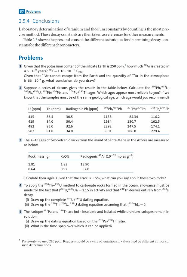
2.5.4 Conclusions

Laboratorydetermination ofuranium and thorium constants by counting is themost pre-cisemethod.Thesedecayconstants are thentakenas references forothermeasurements.Table 2.3 shows the pros and cons of the di¡erent techniques for determining decay con-

stants for thedi¡erentchronometers.

Problems

1 Given that the potassium content of the silicate Earth is 250 ppm,3 how much 40Ar is created in

4.5 � 109 years? 40K¼ 1.16 � 10�4 Ktotal.

Given that 40Ar cannot escape from the Earth and the quantity of 40Ar in the atmosphere

is 66 � 1018 g, what conclusion do you draw?

2 Suppose a series of zircons gives the results in the table below. Calculate the 206Pb/238U,207Pb/235U, 207Pb/206Pb, and 208Pb/232Th ages. Which ages appear most reliable to you? If we

know that the samples must be of the same geological age, which age would you recommend?

U (ppm) Th (ppm) Radiogenic Pb (ppm) 206Pb/204Pb 207Pb/204Pb 208Pb/204Pb

415 86.4 30.5 1138 84.34 116.2

419 84.0 30.4 1984 130.7 162.5

482 85.0 32.6 2292 147.5 174.1

507 81.8 34.0 3301 206.0 229.4

3 The K–Ar ages of two volcanic rocks from the island of Santa Maria in the Azores are measured

as below.

Rock mass (g) K2O% Radiogenic 40Ar (10�12 moles g�1)

1.81 1.83 13.90

0.64 0.92 5.60

Calculate their ages. Given that the error is � 5%, what can you say about these two rocks?

4 To apply the 230Th–238U method to carbonate rocks formed in the ocean, allowance must be

made for the fact that (234U/238U)0¼ 1.15 in activity and that 230Th derives entirely from 234U

decay.

(i) Draw up the complete 234U/238U dating equation.

(ii) Draw up the 230Th, 234U, 238U dating equation assuming that (230Th)0¼ 0.

5 The isotopes231Pa and 230Th are both insoluble and isolated while uranium isotopes remain in

solution.

(i) Draw up the dating equation based on the 231Pa/230Th ratio.

(ii) What is the time-span over which it can be applied?

3 Previously we used 210 ppm. Readers should be aware of variations in values used by different authors insuch determinations.

57 Problems

CHAPTER THREE

Radiometric dating methods

We have so far examined the principles of radioactive dating with simple assumptions,namely that the initial amountofdaughter isotope is negligible and that the system (mineralor rock)whoseage is tobedeterminedhas remainedclosedsince it¢rst formed, that is, ithasneither lost norgainedparentordaughter isotopes in the course of its geological past.Thesetwoconditionsdonotusuallypertain in nature.Sohowcanthesedi⁄cultiesbeovercome?

3.1 General questions

3.1.1 Rich systems, poor systems

Thedatingequation showedthatadistinction has tobemadebetween systemswith negligi-ble initial radiogenic isotope and systems with abundant initial radiogenic isotope. In the¢rst instance, thatofa rich system (understoodas radiogenically rich), an age canbe calcu-lated in theory fromdirectmeasurementoftheparent anddaughter isotopes. In the secondinstance, thatofapoor system, somemethodmustbe found forestimating the initial abun-danceofthe radiogenic isotope.

For a system tobe considered rich, the radioactive isotopemust be abundant comparedwith the radiogenic element.The chemical composition of the systemunder studymustbesuch thatthe ratio ofthe radioactive isotope to the stable reference isotope1is veryhigh.Thetime for which it has been decaying must be long enough for radioactive disintegration tohaveproducedenoughofthe radiogenic isotope.

Exercise

The [87Rb/86Sr] ratio in a biotite is 3000. Can a 300-million-year-old biotite be considered arich system?

AnswerThe [87Sr/86Sr] radiogenic ratio is written [87Sr/86Sr]� [87Rb/86Sr] lt. Calculation with T¼3� 108 years and l¼ 1.42 � 10�11 yr�1 gives:

½87Sr=86Sr� ¼ 3 � 103 � 1:42 � 10�11 � 3 � 108 ¼ 12:6:

1 The reference isotope is an isotope close to the radiogenic isotope of the same chemical element which isstable and is not itself a product of radioactivity.

The initial [87Sr/86Sr] ratios of common strontium vary from about 0.720 to 0.705. Thesevariations are negligible compared with 12.6. The biotite is indeed therefore a rich system.

In practice, the initial daughter isotope ratio is not completely ignored when calcu-lating the age of rich systems but this so-called normal ratio is estimated from meas-urements of various minerals and a conventional value is taken to make the correction.A catalog of rich systems for each radioactive clock has been drawn up by the system-atic study of the commonest rocks and minerals. In each case, allowance must be made fortheageofthesystem,which isanessential feature,ofcourse.This catalog isrelativelylimited.For the 87Rb^87Sr method, it comprises above all micas like biotite K(Mg,

Fe)3AlSi3O10(OH)2 andmuscovite KAl2Si3O10(OH)2 as well as some quite old potassiumfeldspars (KAlSi3O8).ForU^Th^Pbmethodsthereareuraniumoresproper,andthenuranium-richminerals.

The commonest is zircon (ZrSiO4) but there are also sphene (CaTiSiO5) and apatiteCa5(PO4)3(OH).For 40K^40Ar and U^4He methods, all systems may be considered rich since rocks

usuallyhavenegligible initial argonorheliumcontents (excepttheveryyoungones).For the 187Re^186Os method, the current rich mineral is molybdenite (MoS2), but also

basaltic or granitic rocks (where [187Re/186Os] ratios are frequently 500^20 000) as well asmineralsofthese rocks suchasolivineor thepyroxenes.Rich systems are very rare for the other chronometers such as 147Sm^143Nd or

176Lu^176Hf because geochemical systems do not clearly separate samarium from neo-dymiumorlutetium fromhafnium.

3.1.2 Closed system, open system

The fundamental assumption in radioactive dating is that the box (the rockormineral) hasremained closed, that is, it has neither lost nor gained parentor daughter nuclides throughexchangewith its environmentsince it¢rstclosed.Now,while this assumption is accepted for parent elements nestled in suitable crystallo-

graphic sites (Rb inplaceofK,UinplaceofZr, etc.) it is lessobvious fordaughter elements.The daughter isotopes produced by radioactivity are intruders in the crystallographic lat-tice. They have been introduced ‘‘arti¢cially’’ by radioactive transmutation.Why shouldtheystay there?This is particularly true ofrich systems, since these radiogenic isotopes arevery abundant.They have been produced in a mineral which is ‘‘unfamiliar’’ to them, andwill thereforetendto escapefrom it.

E X A M P L E

The use of biotite in radiometric datingBiotite is a black mica containing potassium (K) in its structural formula. Rubidium, which isan alkali similar to potassium, can enter its structure and remain there. Potassium forms aKþ ion and rubidium a Rbþ ion. However, when it decays, 87Rb yields 87Sr.

59 General questions

Strontium is an alkaline earth element similar to calcium. In ionic form it is bivalent withformula Sr2þ. It is not structurally stable in biotite and so tends to escape by diffusionwhenever it can. The biotite system therefore has little chance of remaining closed for the87Rb–87Sr pair, above all if, in the course of its history, it has been subjected to meta-morphic heating or weathering, which provide conditions amenable to the diffusion of 87Srfrom biotite.

The question of whether a system is open or closed has been asked since the earliestwork in geochronology. Before trying to answer it, let us see what the e¡ects are ofany leakage from the system. Let us take the example of rich systems, where the equa-tion is of the form:

RM

Tapp.

Continuous lossof parent

Episodic loss Episodic loss

Continuous lossof parent

Time Time

TR

daug

hter

loss

RM

Tapp.TR

RM

Tapp. TRT1

RM

R

RR

R

Tapp.TRT1

daughter lossparent loss

close

d sy

stem

close

d sy

stem

closed sy

stem

pare

nt lo

ss

clo

sed

syst

em

Figure 3.1 Opening of a radiometric dating system: R is the radiogenic/radioactive parent ratio; RM is themeasured ratio. The top two figures show continuous, constant losses over time. The bottom two figuresshow a sudden episodic loss followed by a long period in a closed system. TR¼ real time, Tapp.¼ apparenttime. Where TR> Tapp. the system becomes younger and there is a loss of the radiogenic daughter isotope(left-hand diagram). Where TR< Tapp. the system becomes older and there is a preferential loss of theradioactive parent isotope. Where both are lost, the outcome depends on the relative values of the losses.If they are equal, the system is equivalent to a closed system. If more daughter isotope than parentisotope is lost, the left-hand diagram is relevant, and vice versa.

60 Radiometric dating methods

R ¼ IDIP¼ ’ðtÞ

where’ is an increasing functionoftime, IDand IP the daughterandparent isotopes, andRtheparent^daughter ratio. Ifa littleofthedaughter isotope is lost, theage calculatedwillbefalsebecause‘‘tooyoung.’’ This isby far the commonest case. If a little of the parent isotopeis lost, the age calculatedwill be falsebecause‘‘too old.’’Again in ID or IP would, of course,havetheopposite e¡ect (Figure3.1).

3.1.3 Continuous or episodic losses

The question of the closed character of the boxes arises with two very di¡erent geologicalscenarios.In the ¢rst scenario, the system continuously loses (or more rarelygains) radiogenic iso-

topes over the course of geological time.This process has been evoked for argon, helium,and the other rare gases, which are not chemically bondedwithin minerals and so tend toescape constantlybydi¡usion. Itmayalsobetrueof isotopesofsoluble elements exposedtochemical alterationattheEarth’s surface (K,Rb,Sr,U,Pb).Thealternative scenario involves sudden events thatpunctuategeological time: tectono-

metamorphic crises, igneous intrusions, volcanic eruptions, folding, etc. Over a short per-iod (comparedwith the durationofgeological time) the system losesorgains the isotopes inquestion.There may also be a combination of both circumstances, when the history of a rock is

divided into two episodes: one, say, at low temperature when the system is closed and theother at high temperature where continuous loss occurs between moments of ‘‘crisis.’’Naturally, the more complex the scenario the more di⁄cult it is to decipher and above allthemoredi⁄cult it is to comeupwithasingle interpretation.

Exercise

Suppose we have the rich 87Rb–87Sr system of muscovite (white mica). The simplifieddating equation is [87Sr*/87Rb]¼lt.

(1) Suppose that recent heating has caused the mineral to lose 30% of its 87Sr*.If the mineral is really 1 billion years old, what will be its apparent age determined bymeasuring 87Sr* and 87Rb today?

(2) Suppose the muscovite has been weathered by water which has leached 10% of

the Sr and 50% of the Rb (the Rb was more soluble than the Sr). What will its apparent

age be?

Answer(1) The simplified expression can be written:

t apparent

t real¼

87Srreal

87Srclosed

� �

giving

87Srreal ¼ ð1� 0:3Þ 87Srclosed ¼ 0:7 87Srclosed:


Therefore, tapparent¼700 million years.

(2)

t apparent

t real¼

87Srapparent

87Srclosed

� ��

87Rbclosed

87Rbapparent

� �¼ 0:9

0:5¼ 1:8:

The apparent age will be 1.8 billion years.

3.1.4 Concordant and discordant ages

With this concern, how can we be sure that a geological age is reliable? The methodunanimously employed for testing whether a result is reliable is the age concordanceand discordance method. Suppose that, with the methods just described, that is, thoseapplicable to rich systems, we wish to test whether a geological age determination isreliable.

Suppose we measure the ages of potassium feldspar, muscovite, and biotite minerals ofthe same granitic rock by the 87Rb^87Sr method.We can hope they will be identical andyieldanageforwhenthegranite crystallized.

If the ages are concordant, that is, if theyare close to eachother,weacceptthere is agoodchance the common age is geologically signi¢cant.This is becausewe admit that a disrup-tive eventwill havedi¡erente¡ectsondi¡erentclocksbecauseoftheirchemicaldi¡erences.Therewill then remain thematterofrelating this age toa speci¢cgeological event (magma-tism, metamorphism, sedimentation, etc.). Suppose that, for the Que¤ rigut granite alreadydiscussed, the 87Rb^87Srmethodwere toyieldagesof 296millionyears for potassium feld-spar, 295 million years for muscovite, and 293 million years for biotite.These ages can beconsidered concordant around 296million years. Given the geological setting (ages of theterrain they cut across andofthe overlying terrains) it is reasonable to accept that this is theage ofemplacement (intrusion) of the granite. Suppose, though, that for a rockof the samegranite sampled close to a faultwe¢nd ages of110million, 90million, and 50millionyearsfor the samethreeminerals.Wewould conclude thatthe systemhadbeendisruptedbysomesecondary phenomenon, probably related to the formation of the fault, and so that properage determination is not possible.There are two stages in the reasoning, then. In the ¢rst,concordance supports the idea that the age is geologically signi¢cant. In the second, thegeological context allows the age to be identi¢ed, that is, to be attributed to some speci¢cgeologicalphenomenon.

If the ages are discordant, then we accept that the basic assumptions of the modelhavebeenbreachedand thatthe ages so determinedarenotgeologicallymeaningful. Fromnowon, therefore, we shall speakof apparent age for a crude date measurement and shallreserve the term‘‘age’’forgeologicallysigni¢cantdates.

RemarkApparent age is an isotope ratio converted into time units. Validating it as a geological age is acomplex process. The apparent age is chemical and isotopic. It is of temporal and geologicalsignificance only if certain conditions are met.


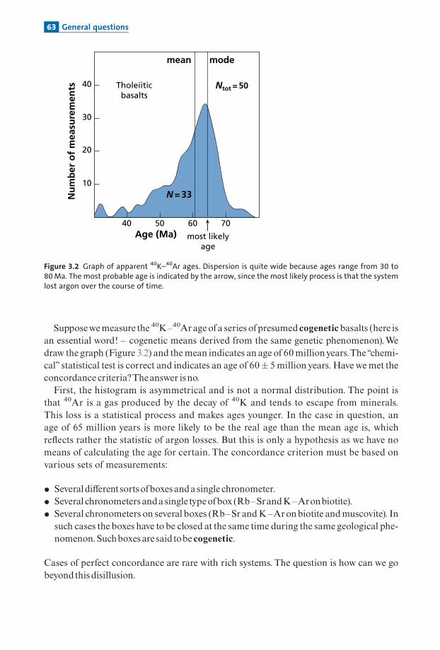
Supposewemeasure the 40K^40Arageofa series ofpresumed cogeneticbasalts (here isan essential word! ^ cogenetic means derived from the same genetic phenomenon).Wedraw the graph (Figure 3.2) and themean indicates an age of 60millionyears.The‘‘chemi-cal’’ statistical test is correct and indicates an age of 60� 5 million years. Havewemet theconcordance criteria?Theanswer isno.First, the histogram is asymmetrical and is not a normal distribution. The point is

that 40Ar is a gas produced by the decay of 40K and tends to escape from minerals.This loss is a statistical process and makes ages younger. In the case in question, anage of 65 million years is more likely to be the real age than the mean age is, whichre£ects rather the statistic of argon losses. But this is only a hypothesis as we have nomeans of calculating the age for certain. The concordance criterion must be based onvarious sets of measurements:

� Severaldi¡erentsortsofboxesandasingle chronometer.� Several chronometers andasingle typeofbox (Rb^SrandK^Aronbiotite).� Several chronometers on several boxes (Rb^SrandK^Aronbiotite andmuscovite). In

such cases the boxes have to be closed at the same time during the same geological phe-nomenon.Suchboxesaresaidtobe cogenetic.

Cases of perfect concordance are rare with rich systems. The question is how can we gobeyondthis disillusion.

40

30

20

10

40 50 60 70Age (Ma)

Tholeiiticbasalts

Ntot = 50

N = 33

modemean

most likelyage

Nu

mb

er o

f m

easu

rem

ents

Figure 3.2 Graph of apparent 40K–40Ar ages. Dispersion is quite wide because ages range from 30 to80 Ma. The most probable age is indicated by the arrow, since the most likely process is that the systemlost argon over the course of time.


3.2 Rich systems and solutions to the problemof the open system

3.2.1 The semi-quantitative systematic comparative approach

Thebasic idea is simple enough.Foragivenproblem in agivengeological case,wemeasureapparent ages by various methods applied to various minerals.We compare the apparentages and try to establish a systematics. For example, we observe that amphibole generallyhas a greater apparent age than biotite when measured by the KÂr method.We deducethat amphibole conserves its argon better than biotite does. Similarly, we observe that theapparent Rb^Sr age of biotite is generally greater than its apparent KÂr age.We deducethatbiotite retains the radiogenic 87Sr*better than itdoes the 40Ar. Inthis speci¢c instance,these purely comparative studieswere¢rstbasedon¢eld studies thatwe looked tomultiply.Laboratorystudiesofdi¡usionwere requiredtosupplementthis approach.

Laboratory studyofdi¡usionandextrapolationDi¡usionistheprocesswherebyachemicalspeciespropagatesinarandomwalk,justlikeheat,say,canpropagate.MathematicallyitobeysFourier’slaw,writtenhereforasingledimension:

@C

@t¼ D

@2C

@x2

whereC is concentration, t is time,x isdistance,andD the coe⁄cientofdi¡usion.This lawisalso expressedbyasimpler-looking formula:

Q ¼ �D @C

@x

� �

where @C=@xð Þ is the concentration gradient andQ the £ux of matter which di¡uses.Thedi¡usion coe⁄cient D is expressed in cm2 s�1 or in m2 s�1 (be careful as other units aresometimes found inthe literature).

The analytical solutions of this equation areknown for simple geometrical cases: plates,spheres, half-planes, etc. Nowadays computers can provide numerical solutions to all pro-blems, or almost all. It is therefore easy to calculate the evolution ofa radioactive system ina box of given shape and size by superimposing di¡usion on radioactive decay. Figure 3.3shows the results of such calculations for aKÂr system supposed to evolve from a sphereinwhich eitherargonorpotassiumcandi¡use.

Solutions to the di¡usion equations are generally expressed by the approximationx �

ffiffiffiffiffiffiDtp

wherex is distance, t time, andD the di¡usion coe⁄cient.The relevantparameterfor di¡usion is (D/a2), where a is the radius of the sphere.The di¡usion coe⁄cientD obeysArrhenius’equation:

D ¼ D0 exp�ERT

� �

whereT is temperature(indegreesKelvin),Eactivationenergy,andR the idealgasconstant.D0 is aconstantdependentonthenatureofthemineralbut is independentoftemperature.


In addition, as might be expected, mineral size is essential: the larger it is the better theretention of argon. This is just what is found when we study, say, the K^Ar age versusmineral size (WasserburgandHayden,1955).

RemarkTo determine diffusion coefficients in the laboratory we take a mineral whose shape anddimensions have been ‘‘measured’’ under the microscope and we measure the amount ofisotopes escaping from it by heating the mineral progressively at different controlled tempera-tures. By plotting log D in these results versus (1/T), we can calculate the activation energy andestimate D0 from the formula D ¼ D 0 exp �E=RT Þ or log D ¼ log D 0 �E=RT Þðð (Figure 3.4).

Toconductsuch laboratoryexperiments it is essential to takenatural samples containing‘‘intrusive’’radiogenic isotopes, andthusquiteold samples,which havenotbeen exposedtosecondary phenomena (metamorphism, erosion, etc.). (These are rare and precious sam-ples.)Howcanthe resultsbeapplied?A¢rstexercisewill helpuswith this.

Exercise

What is the diffusion coefficient of 40Ar in biotite at 50 8C and at 1000 8C if we know thatthe activation energy is E¼ 21 kcal per mole and that at 600 8C D/a2¼2 �10�10 per second(dividing by a2 removes the dimension in cm2)?

AnswerTemperatures are converted into Kelvin, giving 323 K and 1273 K. For the temperaturesconsidered, E/R� 104 since R¼ 1.98 cal mol�1 K�1. By using Arrhenius’ equation this givesD323/a2¼ 1.3 � 10�16 s�1 and D1273/a2¼ 7 � 10�7 s�1.

0.2

0.10

0.20

0.30

1.0 1.8 2.6

6.8 10–18

6.8

10–1

8

5.7

10–2

0

40A

r/40

K

Time (Ga)No

diff

usio

n

2.1 10–18

2.1

10–1

8

6.4 10–19

6.4

10–1

9

5.7 10–20

D = 0a2

Potassiumdiffusion

Argondiffusion

Figure 3.3 Calculation of the diffusion of 40Ar and 40K over geological time out of a spherical mineraland its effect on the chronometric curve. The figures are relative to the parameter D/a2 expressed in s�1.

65 Rich systems

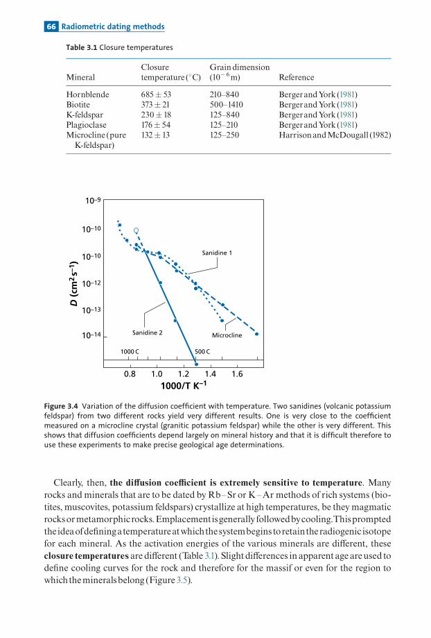
Clearly, then, the di¡usion coe⁄cient is extremely sensitive to temperature. Manyrocks and minerals that are to be dated by Rb^Sr or K^Ar methods of rich systems (bio-tites, muscovites, potassium feldspars) crystallize at high temperatures, be theymagmaticrocksormetamorphicrocks.Emplacementisgenerally followedbycooling.Thispromptedtheideaofde¢ningatemperatureatwhichthesystembeginstoretaintheradiogenic isotopefor each mineral. As the activation energies of the various minerals are di¡erent, theseclosure temperatures are di¡erent (Table 3.1). Slightdi¡erences in apparent age areused tode¢ne cooling curves for the rock and therefore for the massif or even for the region towhichthemineralsbelong (Figure3.5).

10–14

10–13

10–12

10–10

10–10

10–9

0.8

1000 C 500 C

1.0 1.2 1.4 1.6

D (

cm2 s–

1 )

1000/T K–1

Sanidine 1

Sanidine 2 Microcline

Figure 3.4 Variation of the diffusion coefficient with temperature. Two sanidines (volcanic potassiumfeldspar) from two different rocks yield very different results. One is very close to the coefficientmeasured on a microcline crystal (granitic potassium feldspar) while the other is very different. Thisshows that diffusion coefficients depend largely on mineral history and that it is difficult therefore touse these experiments to make precise geological age determinations.

Table 3.1 Closure temperatures

MineralClosuretemperature (8C)

Graindimension(10� 6m) Reference

Hornblende 685� 53 210^840 BergerandYork (1981)Biotite 373� 21 500^1410 BergerandYork (1981)K-feldspar 230� 18 125^840 BergerandYork (1981)Plagioclase 176� 54 125^210 BergerandYork (1981)Microcline (pure

K-feldspar)132� 13 125^250 HarrisonandMcDougall (1982)


RemarkThe cases most studied by these methods are of thermal variations during orogeny (mountainbuilding) where estimations are made of how the crustal block cooled as it rose to the surface;at what speed and over what temperature range, etc.

The studyofcontactmetamorphismThe decisive step in this type of semi-quantitative approach was the study by StanleyHart (1964) (Figure 3.6), then a student at the Massachusetts Institute of Technology,con¢rmed by Gil Hanson and Paul Gast (1967), then at the University of Minnesota,who studied the ages obtained by the di¡erent methods for an instance of contactmetamorphism.Contact metamorphism occurs when granite is intruded into a geological series.

Physically, such metamorphism corresponds to sudden heating by a body of de¢ned geo-metry.The thermal evolution of such a problem can be readily processed mathematically.The isotherms and their variations over time are easily obtained. Hart chose to study theresult of a Tertiary intrusion some 60Ma old (Eldora) in the Precambrian terrain ofColorado. There is a big age di¡erence between the intrusion and the surrounding rock.He studied the variation in Rb^Sr, K^Ar, and U^Pb ages on di¡erent rich minerals ofthe Precambrian formation with distance from the point of contact. The ‘‘apparent’’ ageof all the minerals varied with distance from the contact, whichwas what he expected. Atthe contact point, it is the same as the age of the intrusion and then it progressively con-verges towards the age of the surrounding rock at a great distance from the contact.Whatis interesting is that at any given distance from the contact, the order of apparent agesdetermined by the various methods on the various minerals obeys a coherent logicalschema.The reliabilityof ‘‘rich’’chronometershasbeen estimatedon thebasis ofsuch a sequence

and a few laboratory experiences.Theyare ranked here in decreasingorderof reliabilityoftheagesobtained.

T (°

C)

K/Ar ages (Ma)

Feldspar

Biotite

Hornblende

400

1000 900 800 700 600 500

200

600

800

Figure 3.5 Cooling curve of an orogenic segment of Grenville Province, Canada, based on K–Ar apparentages and on the retentivity of the different minerals. After Berger and York (1981).

67 Rich systems

206Pb�207 Pb zircon4206Pb�238 U zircon440Ar�40 K amphibole487Rb�87Sr muscovite487Rb�87 Sr biotite440Ar�40 K biotite440Ar�40 K feldspar

Although there aremanyexceptions to this ranking, it allows a series ofapparent ages tobegauged rapidly.Thuswhen, say, 207Pb^206Pb on zircon gives the same age as 40Ar^40Konbiotite there is agood chance the age is correct.When the di¡erencebetween the 40Ar^40Kon amphibole and 87Rb^87Sr on muscovite ages is slight, we consider we are close to thetrue age, etc. While this empirical approach is useful, it does not, alas, provide a

1400

1200

1000

800

600

400

200

10

500 15001000 2000 m

100

Distance from contact

Ageof the

intrusion

Ap

par

ent

age

(Ma)

100

0

200

300

400

500

600

100 1 000 10 00010

C

A

Max

. tem

per

atu

re (

°C)

1000

BiotiteK-Ar

Feldspar208Pb/204Pb

Feldspar206Pb/207Pb

HornblendeK-A

Zircon207Pb/206Pb

Zircon206Pb/238U

10 000 20 000

1600

BiotiteRb-Sr

60 Maintrusion Metamorphic

zoneBasement dated1450 to 1600 Ma

a

b

Figure 3.6 Contact metamorphism of the Eldora stock, Colorado, studied by Stanley Hart. This figure isfamous. Top: the geological section. The scale of distances in (a) and (b) is logarithmic. (a) The thermalprofile, that is, the maximum temperatures reached at each point versus distance. Curves A and C arefrom two values of thermal diffusivity. (b) Apparent ages versus distance.


thoroughgoingsolutiontothe issueofreliability. Inparticular, howcananagebe calculatedwhenthehypothesesofthesimplemodelarenotsatis¢ed?

Exercise

Analysis of a granite yields: U–Pb on zircon, 520 Ma; K–Ar on amphibole, 480 Ma; K–Ar onbiotite, 400 Ma; Rb–Sr on biotite, 460 Ma; Rb–Sr on muscovite, 470 Ma. What seems thelikely age of intrusion of this granite to you? How reliable is the result?

AnswerThe true age is probably around 550–540 Ma. The reason being that some disruptivephenomenon has affected the region as there is clearly a discordance in ages. The mostrobust of the chronometers is U–Pb on zircons, but it is not perfect and this apparent agemay be made a little older. But this reasoning is very rough and ready as can be seen!

3.2.2 The concordia method

This method hasbeen devised for calculating a system’s true age even though the system isan open one.This is doneby exploiting pairings of chemical behavior which maybe foundwithvarious radiochronometers.

Uranium^lead systemsUranium^lead systems using 238U! 206Pb and 235U! 207Pb decay have an interestingfeature: both parents and both daughters are of the same chemical nature but have verydi¡erent decay constants. This pairing is exploited for determining geological ages evenwhenthesystem is anopenone.Let us consider auranium-rich material. It maybe zircon (ZrSiO4), a common mineral

in granite rocks, sphene, uraninite, or apatite, minerals containing little ‘‘common’’ lead(detectedbymeasuring the non-radiogenic isotope 204Pb).The initial lead can thereforebeneglected in chronometric equations (richsystems)andwewrite :

206Pb

238U¼ el238t � 1� �

207Pb

235U¼ el235t � 1� �

:

Twoages canthereforebe calculatedbymeasuring the 206Pb, 207Pb, 238U,and235Ucontentsofminerals. If everything compliedwith the assumptions (closed system, rich system, etc.)these two ages should be identical, that is, concordant.The common age would thereforeindicate the time the zircon orapatite crystallized in the granitemagma.This is sometimesthe case, but generally ages are found to be di¡erent and so discordant.To bring out theseage discrepancieswe consideraplot:

x ¼207Pb235U

� �; y ¼

206Pb238U

� �:

69 Rich systems

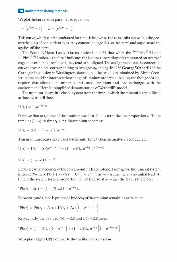
Weplotthe curveoftheparametric equation:

y ¼ el238t � 1� �

; x ¼ el235t � 1� �

:

This curve, which canbegraduated for time, is known as the concordia curve. It is the geo-metric locus of concordant ages. Any concordant age lies on the curve and anydiscordantage lieso¡ the curve.

The South African Louis Ahrens noticed in 1955 that when the 206Pb*/238U and207Pb*/235Uratios (asbefore * indicates the isotopes are radiogenic)measuredon suites ofcogeneticminerals areplotted, they tend tobealigned.Thesealignments cutthe concordiacurve at two points, corresponding to two ages (t0 and t1). In1956GeorgeWetherill of theCarnegie Institution inWashington showed that the two ‘‘ages’’obtained by Ahrens’con-structions couldbe interpretedas theageofuraniumore crystallizationandtheageofadis-ruption that a¡ected the minerals and caused uranium and lead exchanges with theenvironment.Here is a simpli¢eddemonstrationofWetherill’smodel.

Theuraniumdecays in a closed system from the timeatwhich themineral is crystallizedattimet¼ 0until timet1.

Uðt1Þ ¼ U0e�l238t1 :

Suppose that at t1 some of the uraniumwas lost. Let us term the lost proportion �.Thereremains (1^�).Attimet1þ�t, theuraniumbecomes:

Uðt1 þ�tÞ ¼ ð1� �ÞU0e�lt1 :

Thisuraniumdecays inaclosedsystemuntil timetwhentheanalysis is conducted:

UðtÞ ¼ Uðtþ�tÞe�lðt�t1Þ ¼ ð1� �ÞU0 e�lt1 e�lðt�t1Þ

UðtÞ ¼ ð1� �ÞU0 e�lt:

Letus seewhatbecomesofthe corresponding lead isotope. From t0 to t1themineral systemis closed.We have Pbðt1Þ as ðt1Þ ¼ U0ð1� e�lt1Þ, as we assume there is no initial lead. Attime t1 the system loses a proportion (�) of lead so at (t1þ�t) the lead is therefore:

Pbðt1 ��tÞ ¼ ð1� �ÞU0ð1� e�lt1Þ:

Betweent1and t, lead isproducedbydecayoftheuraniumremainingatthattime.

PbðtÞ ¼ Pbðt1 þ�tÞ þUðt1 þ�tÞ 1� e�lðt�t1Þh i

:

Replacingby their valuesPb(t1þ�t) andU(t1þ�t) gives:

PbðtÞ ¼ ð1� �ÞU0 1� e�lt1

þ ð1� �ÞU0 e�lt1 1� e�lðt�t1Þh i

:

WereplaceU0byU(t) to returntothetraditional expression:


U0 ¼UðtÞeltð1� �Þ :

Wehave to changevariablesbecausewehave decided to take the present time as the origin.Inthenewnotation (in capitals),T¼ t,T1¼ t ^ t1.Thisgives:

Pb

U¼ 1� �

1� �

� �elT � elT1

þ elT1 � 1

:

But for the decay constant the expressions are identical for both 206Pb^238U and207Pb^235Upairs, because the two lead isotopes and the two uranium isotopes must reactchemically inan identicalmanner tothe‘‘crisis’’whicha¡ectedthesystemsatT1.Wewrite:

206Pb238U

� �¼ r1

207Pb235U

� �¼ r2

r1 ¼1� �1� �

� �el8T � el8T1

þ el8T1 � 1

r2 ¼1� �1� �

� �el5T � el5T1

þ el5T1 � 1

:

Wecan eliminate ð1� �Þ=ð1� �Þ½ �betweenthetwoequations, sogiving:

r1 � el8T1 � 1

r2 � el5T1 � 1½ � ¼el8T � el8T1

el5T � el5T1

� �:

For¢xedTandT1, this expression takes the form:

r1 � y0r2 � x0

¼ constant:

This is the equation ofa straight line in an (r1, r2) plot.When�¼�¼ 0, that is, when the sys-tem has remained closed, r1 ¼ el8T � 1

� �and r2 ¼ el5T � 1

� �.Theupper interceptwith

the concordiatherefore corresponds toT, which is the initial ageofthemineral population.When �¼ 1, that is, when the minerals have lost all their lead at T1,r1 ¼ el8T1 � 1

� �and r2 ¼ el5T1 � 1

� �:

The lower intercept with the concordia corresponds toT1.When � and � are between 0and1, the data points are on the straight line joining the two points of the concordiaTandT1.When more lead than uranium is lost the points are betweenTand T1.When more ura-nium than lead is lost the points are ‘‘above’’ T and therefore above the concordia (seeFigure3.7).We can then address the inverseproblemand say thatwhen the datapoints obtainedon a

series ofuranium-rich cogeneticminerals arealigned in the (206Pb/238U, 207Pb/235U) plot,the intersections of the straight line they de¢ne with the concordia curve determine theinitial ageofthe familyofminerals andtheageofthe disruption experienced.Wegivea sim-ple historical example, that of theMorton gneiss ofMinnesota.TheU^Pbmeasurementsbeingmadeon zircons,weobtain theageoftheperturbation (Figure 3.8).

71 Rich systems

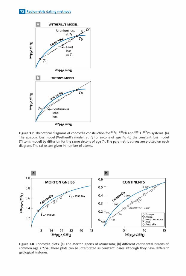
T1

T0

T1

T0

206 P

b*/

238 U

206 P

b*/

238 U

206Pb*/235U

WETHERILL'S MODEL

Uranium lossat T1

Leadlossat T1

TILTON'S MODEL

207Pb*/235U

Concordia

Concordia

Continuousleadloss

a

b

Figure 3.7 Theoretical diagrams of concordia construction for 238U–206Pb and 235U–207Pb systems. (a)The episodic loss model (Wetherill’s model) at T1 for zircons of age T0; (b) the constant loss model(Tilton’s model) by diffusion for the same zircons of age T0. The parametric curves are plotted on eachdiagram. The ratios are given in number of atoms.

Concordia

Concordia

207Pb*/235U

1.0

0.8

T = 1850 Ma

1

23

4T0 = 3550 Ma

MORTON GNEISS CONTINENTS

0.6

0.4

0.2

8207Pb*/235U

206 P

b*/

238 U

0.6

2 500

2 000

1 500

1 000

100

50

10

25 x 10–12yr–1 = D/a2

EuropeAfricaNorth AmericaAsiaAustralia

0.5

0.4

0.3

0.1

0.2

5 10 1516 24 32 40 48

500

a b

Figure 3.8 Concordia plots. (a) The Morton gneiss of Minnesota; (b) different continental zircons ofcommon age 2.7 Ga. These plots can be interpreted as constant losses although they have differentgeological histories.


Wetherill ’s model has been used abundantly. Generally it is borne out but it has oftenbeen observed that the lower intercept is di⁄cult to interpret in geological terms becausethe age determined corresponds to neither a known tectonic nor a metamorphic episode.Thus, taking zircons of several continents of the same age of 2.7Ga, and plotting theU^Pb results on the concordia diagram, they seem to de¢ne the same lower intercept,while the geological histories of the various parts of the continents and in particular thetectono-metamorphic episodes later than 2.7Ga are very di¡erent.To account for this, inthe 1960s George Tilton, at the Carnegie Institution, developed another model (Tilton,1960). He assumed a continuous loss of lead throughout the rock’s history. In such a case,the ¢rst part of the curve of evolution in the concordia diagram is a straight line startingfrom the initial age. It then curves towards the origin. From this model, the lower interceptisgeologicallymeaningless anddepends solelyon the initial age.This canbe demonstratedmathematicallyby using kinetic equations. Ifwe considera continuous lead loss, the equa-tions arewritten:

dPb

dt¼ lU� G Pb

dUdt ¼ �lU

(

where G is a coe⁄cient of lead loss which is assumed constant to simplify matters (weassumethere isnouranium loss).Therefore:

d Pb

U

dt¼ lþ ðl� GÞPb

U:

BypositingPb*/U¼ randby integrating r8 and r5,weobtain:

r8 ¼l8

l8 � Geðl8�GÞt � 1� �

; r5 ¼l5

l5 � Geðl5�GÞt � 1� �

:

Numerically, it can be seen that in an (r8, r5) plot supposing G is identical for bothlead isotopes, the curve is a straight line in its ¢rst part and only curves towards the ori-gin. It therefore has no signi¢cant lower intercept. Only the initial age is signi¢cant. Ifa straight line is drawn through the data points, the upper intersection with the concor-dia indeed gives the initial age but the lower intersection with the concordia ismeaningless.Alle' gre, Albare' de,Gru« nenfelder, andKo« ppel (1974) showed that we could switch from

onemodel to theother. Ifseveral tectono-metamorphic crises are superimposed, theymayalso generate a discordiawhose lower intersectionwith the concordia is meaningless.Thisis the case ofold inherited zircons in theAlps. Acomplexpolymetamorphichistorygener-ates regularities similar toacontinuous loss.As seen, interpreting the lower intercept is neither straightforward nor unequivocal!

Each case must be carefully examined, that is, onemust have sound geological knowledgeof the region before reaching any conclusion. However, the upper intercept, when wellde¢nedmathematically (spaceddatapoints), seemsmore robust.

73 Rich systems

Of course, an ‘‘apparent age’’ can be determined for each discordant mineral by the207Pb/206Pb method alone.These apparent 207P/206P ages vary from the age of the lowerintersectiontothe initial age.Wethereforehaveawhole seriesofapparentages.2

And yet the chronometric equation is misleading a priori since if we consider only the207Pb^206Pb dating equation and suppose that lead is lostwithout isotopic fractionation, itis easy to believe the system has remained closed for lead! This is what was thought some50 years agowhen someworkers asserted that since the samegranitehad 207Pb/206Pb agesranging from say 200million to1billionyears, thatwas evidence it had formedbydi¡usionin solid state overhundreds ofmillions ofyears! In fact, the dating equation contains ahid-denvariable ^ uranium!Thetrue equationofthe 207Pb/206Pbratio, in the caseofaepisodicloss, iswritten:

207Pb206Pb

¼ 1

137:8

1� �1� �

� �el5T � el5T1� �

þ el5T1�1� �

1� �1� �

� �el8T � el8T1� �

þ el8T1�1� �

2664

3775:

This equation shows thatthe ratio dependson the coe⁄cientsof loss� and� (unlessT1¼ 0,that is, if the loss is at the presentday).This also illustrates that apparent and true agesmustnotbemixedwithout care! Ofcourse, it is tempting tomeasure the 207Pb/206Pb ratio alonebecause itrequiresjustan isotopemeasurementofleadwithoutmeasuring theleadandura-nium content, but, as has been seen, its interpretation is ambiguous. It must therefore beusedby takingcertainprecautions andbybeing familiarwith the limits.

Exercise

We assume a continuous loss with G ¼ 2l8. Calculate the apparent 206Pb/238U, 207Pb/235U,and 207Pb/206Pb* ages for a zircon whose initial age is 2.7 Ga.

Answer206Pb/238U¼1.8 Ga, 207Pb/235U¼2.18 Ga, and 207Pb/206Pb*¼ 2.480 Ga.

Generalizing the concordiamethodAlle' gre (1964) and Alle' gre andMichard (1964) extended this approach to other pairs ofchronometers (Figure3.9).

� Uranium/lead^thorium/lead.Thiswas anatural extension.Thebigdi¡erencewas thattheTh/U ratio is variable and so the ‘‘magical’’conditions of the U^Pb system do nothold.The discordia straight line cuts the concordia at the upper intercept only.There isno lower intercept as the discordia is actually a curve (Steiger and Wasserburg, 1966;Alle' gre,1967) (Figure 3.9).� Rubidium/strontium^potassium/argon.Hereagainthediscordiacutsthe concordiaat

one pointonly.This generalization has con¢rmed the coherence of the two systems andtheirbehaviorwhendisrupted (Alle' greandMichard,1964).

2 Apparent ages are measured by the slope of the straight line joining the origin and the experimental pointon the (r5, r8) plots.


� Uranium^230Th,U^231Pa.This approach hasbeen used fordating secondarymineral-izations of uranium. It was then extended recently to other examples of dating corals.Thesearementionedherebutnotelaboratedon (Alle' gre,1964).

Such generalization of the concordiamethod is above all of fundamental methodologicalinterest. It shows that the behavior of the various radiogenic isotopes, although original,is not ‘‘autonomous’’ and that there is redundancy which explains the regularitiesobservedandallows simplemathematicalmodeling.

3.2.3 Stepwise thermal extraction

The ideabehindthis approach is tosupposethat,whendisruptivephenomenaoccur, radio-genic isotopes migrate by di¡usion towards the mineral boundaries or to cracks and thatthere are‘‘cores’’which have resisted andwhich canbe considered tobe closedboxes.Wego

0.90 231Pa*/ U

Chalcocites

CONCORDIA 230Io-231Pa

Autunites

about100 000 years

230 T

h*/

U

87Sr*/87Rb

207Pb*/235U

Ontario and Minnesota40

Ar*

/40 K

208 P

b*/

232 T

h

CONCORDIA

0.5

Concord

ia

Concord

ia

2600

500

1000

1500

2000

2250

2500 27503000

2 660

2460

2200

2000

a

b c

Figure 3.9 Generalization of the concordia method. (a) U–Th–Pb concordia; (b) Concordia applied tomethods of radioactive disequilibrium; (c) concordia applied to K–Ar, Rb–Sr methods. After Allegre(1967), Allegre (1964), and Allegre and Michard (1964).

75 Rich systems

and get the ‘‘information’’ by causing arti¢cial di¡usion.Two chronometers have been thesubject of such an approach: that of the K^Ar method on various minerals or rocks andthatoftheU^Pbmethodon zircon.

The 39Ar^40ArmethodThis method ¢rst came to light at Berkeley in the laboratory ofJohn Reynolds (Merrihueand Turner, 1966) but was above all the product of work by Grenville Turner (1968) atShe¡reldUniversity in England.Here iswhat it involves. First the sample under test is irra-diated by a stream of neutrons. A nuclear reaction transforms the 39K into 39Ar.This is aneutron^proton (n, p) reaction. Once this operation hasbeen accomplished, the test sam-ple is heated by temperature stages and the 40Ar/39Ar ratio measured at each step(Figure 3.10).

Naturally, at the same time as the sample, we irradiate a control sample containing aknownquantityofKwhose 39Arcontent is tobeanalyzed.The 40Ar/39Ar ratio is equivalentto an 40Ar/40K ratio and so the dating formula can be applied to it.We therefore obtain arangeof (apparent) ages dependingontheoutgassing temperature.

ΔT1 ΔT2

ΔT

Closed system

Open system

Mo

no

do

mai

nPo

lyd

om

ain

s

Co

mp

ute

d a

ges

Temperature (°C)

Co

mp

ute

d a

ges

Thermalevent

just before Tt just after Tt

40K40K 40K

40Ar

40K

40Ar

40Ar

40K

40Ar

40K

40Ar

40Ar

0–d +d 0–d +d 0 100 800

Temperature (°C)100 800

–d +d

0–d +d 0–d +d0–d +d

ΔT

Tt today

Figure 3.10 The 39Ar–40Ar method. Each small rectangle represents horizontally the size of a mineral(the center has coordinate zero and the edges þd, –d). The ordinates show the 40K and 40Ar contents.Top: evolution over time in a closed system. Notice that 40K decreases and 40Ar increases. When theexperiment is conducted we find a simple clear plateau indicating the age. Bottom: the evolution of anopen system. We suppose a thermal event occurred at Tt, thermal diffusion occurred, and argon escapedfrom the rims, hence the bell-shaped distribution. Then the system remained closed and 40K decayedproducing 40Ar. When the argon is extracted stepwise, it can be seen that a certain temperature isrequired to reach the plateau because the edges are degassed first. The bottom plot is analogous exceptwe have supposed a mineral with a complex structure with several domains separated by cracks, faults,or grain joints. The first part of the extraction has a complex appearance.


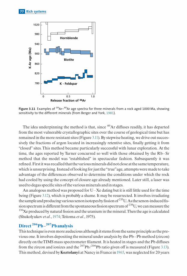
The idea underpinning the method is that, since 40Ar di¡uses readily, it has departedfrom the most vulnerable crystallographic sites over the course ofgeological time but hasremained in themore resistant sites (Figure 3.11). By stepwise heating, we drive out succes-sively the fractions of argon located in increasingly retentive sites, ¢nally getting it from‘‘closed’’ sites.This method became particularly successful with lunar exploration. At thetime, the ages reported by Turner concurred so well with those obtained by the Rb^Srmethod that the model was ‘‘established’’ in spectacular fashion. Subsequently it wasre¢ned.First itwas recalled thatthevariousminerals didnotcloseatthe sametemperature,which is unsurprising. Insteadof looking for just the‘‘true’’age, attemptsweremade to takeadvantage of the di¡erences observed to determine the conditions under which the rockhad cooled by using the concept of closure age already mentioned. Later still, a laser wasusedtodegas speci¢c sitesofthevariousminerals and in stages.An analogous methodwas proposed for U^Xe dating but it is still little used for the time

being (Figure 3.12), which is probably a shame. It maybe resurrected. It involves irradiatingthesampleandproducingvariousxenonisotopesby¢ssionof235U.Asthexenon-induced¢s-sionspectrum isdi¡erentfromthespontaneous¢ssionspectrumof 238U,we canmeasurethe136Xe producedby natural ¢ssion and the uranium in themineral.Then the age is calculated(Shukolyukov et al., 1974;Teitoma et al., 1975).

Direct 206Pb^207PbanalysisThis technique is evenmoreaudaciousalthough itstemsfromthesameprincipleas thepre-vious one. It involves depositing themineral under analysis by the Pb^Pbmethod (zircon)directlyon theTIMSmass spectrometer ¢lament. It is heated in stages and the Pb di¡usesfrom the zircon and ionizes and the 207Pb/206Pb ratio given o¡ is measured (Figure 3.13).Thismethod, devisedbyKoztolanyi atNancy in France in1965,was neglected for 20 years

Hornblende

Biotite

K - Feldspar

0 0.5 1.0

Release fraction of 39Ar

K-A

r ag

e (M

a)

780

820

860

900

940

980

1020

Figure 3.11 Examples of 39Ar–40Ar age spectra for three minerals from a rock aged 1000 Ma, showingsensitivity to the different minerals (from Berger and York, 1981).

77 Rich systems

before being taken up by Kober in 1986! It yields interesting and sometimes impressiveresults, even ifall criteriaofconcordance ordiscordance are lost, preventing any reliabilitycheckas the concordiadiagramcannotbeused.

3.3 Poor systems and the radiometric isotopiccorrelation diagram

Withpoor systems, themainproblem isnotjustthequestionofopennessbutalsothatoftheinitial presence, when the system closes, of a certain amount of radiogenic isotope. Howcanthisbe evaluated?

1.0

0.5

2.0

1.5

500 100Percentage Xe degassed

t(Xe–Xe) = 1.59 ± 0.12 Gat(Pb–U)= 1.57 ± 0.05 Ga

Ag

e (G

a)

Figure 3.12 Example of a spectrum of the 133Xe–136Xe method imitated from 39Ar–40Ar for a Rapakivigranite from Finland. After Shukolyukov et al. (1994).

0.40

0.35

0.30

3.6

3.7

3.8

3.9

4.0

4.1

4.2

1450

Evaporation temperature (°C)

207 P

b/2

06Pb

Ag

e (M

a)

1500

Figure 3.13 The 207Pb–206Pb spectrum obtained by thermo-ionization of lead. This spectrum isobtained by progressively heating the filament after having deposited zircon on it. The exampleshown is of detrital zircon from Australia, among the oldest recorded (Kober, 1986).


3.3.1 The 87Rb–87Sr system

Thismethodwasproposed, after an initial attemptbyAustraliansWilliamCompston andPeter Je¡rey (1959), then at the University of Western Australia, by Louis Nicolaysen(1961) of South Africa’sWitwatersrandUniversity for the 87Rb^87Sr system, but it is moregeneral andapplies toall parent^daughter systems.Letus turnbacktothefundamental 87Rb^87Srdecayequation inaclosedsystem:

87SrðtÞ ¼ 87Srð0Þ þ 87RbðtÞðelt � 1Þ:

Let us divide member bymember by 86Sr, which is one of the stable Sr isotopes andwhoseabundance is notdependenton radioactivityand is therefore constantover time.The equa-tionbecomes:

87Sr86Sr

� �t

¼87Sr86Sr

� �0

þ87Rb86Sr

� �t

ðelt � 1Þ:

The mathematical operation of 87Sr normalization by 86Sr is not just a simple algebraicmanipulation. It brings out the strontium isotope ratios in the equation.This is themagni-tudemeasuredbythemass spectrometer.Now,wehaveseenthat isotope ratiosobeypreciselaws,particularly thoseof isotope exchange.Letusnowconsidera seriesofcogeneticboxes (assumedtobe in thermodynamic equili-

brium).As a resultof isotopic equilibration, theyhave the same initial 87Sr=86SrÞ0�

isotoperatio and the sameage. In an 87Sr=86Sr; 87Rb=86Sr

plot theyarealignedon a straight line

ofslope(elt�1)andofordinateattheoriginof 87Sr=86Sr� �

0.This straightlineisan isochron,

which is the locus of boxes of the same age (Figure 3.14). Ifwewish to break down the waythe system evolves over time, we can say that at time t¼ 0, the points representing all theboxes lie on a horizontal line, each boxbeing characterized by its own 87Rb/86Sr ratio butwith the same strontium isotope ratios.Then eachbox evolves along adiagonal of slope�1with þd87Sr=dt ¼ �d87Rb=dt. The straight line rotates around the ¢xed point87Sr=86Sr� �

0. Its slope is constantly (elt� 1).

RemarkThe inverse problem is interesting, of course. Let us take the example of a series of minerals (ortotal rocks) which are assumed to be cogenetic (minerals from the same rock, or rock from thesame massif). The 87Sr/86Sr and 87Rb/86Sr isotope ratios of each of them are measured. If therepresentative points lie in a straight line, the slope of the straight line is equal to (elt� 1) andthe age of the system of boxes can be calculated.

Exercise

Annie Michard measured the Mont-Louis, granite, Milhas, and Querigut in the PyreneesOrientales (France) (Table 3.2). Draw the isochron graph and calculate the age of the seriesof granite rocks of the Querigut and the initial ratio (Michard and Allegre, 1979).

Answer

79 Poor systems

We calculate the 87Rb/86Sr ratios. The experimental points are plotted on the87Sr=86Sr; 87Rb=86Srð Þ graphs not shown here. The straight line through the points ‘‘yields’’

an age of T¼271�10 Ma, with an 87Sr=86Srð Þinitial ratio¼0.710� 0.005.

Thismethod,oftencalledthe isochronmethod, isoneofthepillarsofradiochronology. Itboth dispenseswith theassumption (accepted for rich systems) that the 87Sr(0) is negligibleor constant and so allows poor systems to be used and tests the closed system hypothesisby alignment or non-alignment of the measurements made on the di¡erent boxes. If Rb

5

4

3

2

1 2 3 4 5 6 787Rb/86Sr

87Sr

/86 S

r

87Sr0

slope –1

isochron at ti

me τ

α = tan–1 eλτ–1⌠⌠ ⌠⌠

86Sr⌠⌠⌠⌠

0.760

0.700

1 2 3 487Rb/86Sr

87Sr

/86 S

r

isochron at ti

me τ = 1 Ga

Figure 3.14 Principle of the 87Rb–87Sr isochron method. At time t¼ 0 the points have the samestrontium isotope ratio and different 87Rb/87Sr ratios. They therefore all lie on a horizontal linecorresponding to (87Sr/86Sr)(0). After time T, the points are aligned on a straight line of slope(elt� 1)� lt. In practice, in real graphs, the straight lines of evolution do not have a slope of � 1because the 87Rb/86Sr ratio varies little and the 87Sr/86Sr ratio varies greatly, given the chosen scales.The evolution vectors are very steep.


and Sr havemigrated di¡erentially, then the representative points of the various boxeswillnot remain aligned. In the favorable case, thismethod canbeused tomeasure anage (t) andto determine the initial 87Sr/86Sr ratio, whichwewill see later to be important. Measuringan age therefore involves measuring the Sr isotopic ratio, measuringRb and Sr concentra-tions foreachboxandthis is fora seriesofcogeneticboxes.

3.3.2 Two-stage models

Imagine we have a series of cogenetic boxes evolving in a closed system. All the systemsare therefore aligned on an isochronous straight line. Suppose that at t1 a sudden eventoccurswhich re-homogenizes theboxes isotopically.This eventmaybemetamorphism, forexample. The sub-systems will exchange their atoms and become isotopically homoge-neous.The representative points of theboxes then lie on ahorizontal linewhose ordinate attheorigin iswritten 87Sr=86Sr

� �m; t1

withm, t1signifying themeanvalueatt1.Thentheboxesevolve radiogenically until the present time in a closed system. The alignment observedbetween thepoints representing theboxeshas a slopeof elt1�1

� �andanordinate at theori-

ginof 87Sr=86Sr� �

m; t1.

Let us explain our model a little to make it realistic.We consider the cogenetic boxesare both whole rocks and minerals. Metamorphism occurs at time t1 which re-homo-genizes the minerals isotopically around the value of the whole rock, but it is notintense enough to re-homogenize the whole rocks at the scale of the entire massif(Figure 3.15).

Table 3.2 Mont-Louis, Milhas, and Querigut granites

[87Sr/86Sr] Rb (ppm) Sr (ppm)

Mont-Louis sample numbers:4B1 0.721 157 1814B2 0.719 146 200Milhas sample numbers:V90 0.723 150 146V92 0.717 164 302Que¤ rigut sample numbers:A 0.714 105 241B 0.719 189 214C 0.723 161 135A4 0.720 160 153X 0.7205 155 170Q1 0.742 202 88Q2 0.743 257 90Q3 0.746 245 74Ap1 0.780 192 32Ap2 0.875 257 18

81 Poor systems

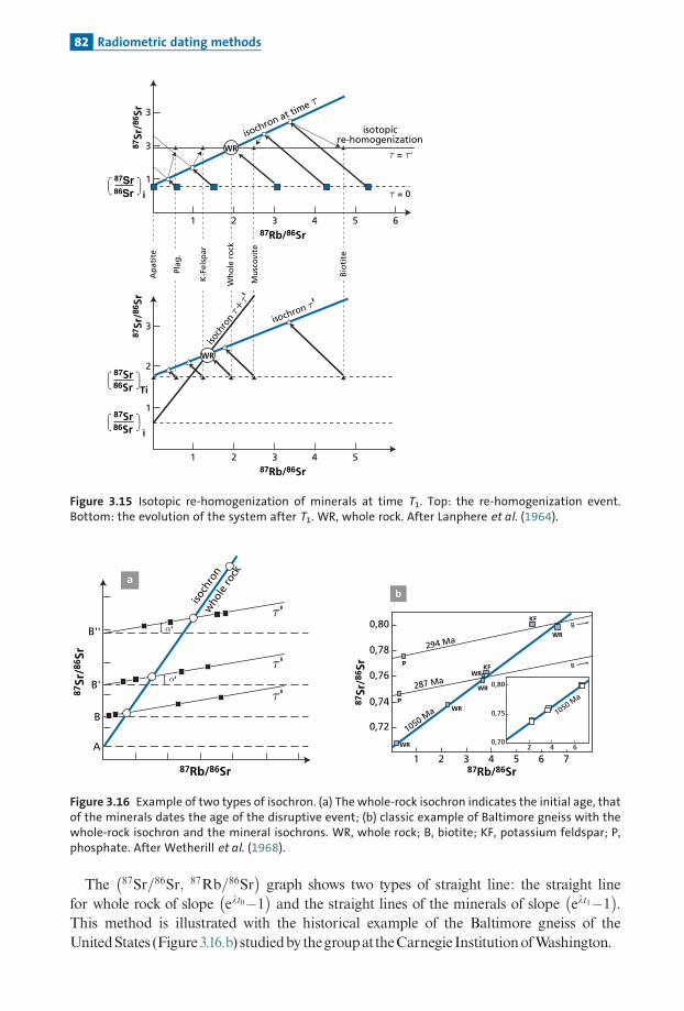
The 87Sr=86Sr; 87Rb=86Sr� �

graph shows two types of straight line: the straight linefor whole rock of slope elt0�1

� �and the straight lines of the minerals of slope elt1�1

� �.

This method is illustrated with the historical example of the Baltimore gneiss of theUnitedStates (Figure3.16.b) studiedby thegroupattheCarnegie InstitutionofWashington.

3

3

1

1 2 3 4 5 6

87Sr86Sr

⌠⌠⌠⌠

isotopicre-homogenization

isochron at time τ

1

2

3

1 2 3 4 5

i

i

Ti

isochron τ'

τ = 0

τ = τ'

87Rb/86Sr

87Rb/86Sr

87Sr

/86 S

r87

Sr/8

6 Sr

87Sr86Sr

⌠⌠⌠⌠

87Sr86Sr

⌠⌠⌠⌠

Ap

atit

e

K-F

elsp

ar

Wh

ole

ro

ck

Mu

sco

vite

Bio

tite

Plag

.

isoch

ron

τ + τ'

WR

WR

Figure 3.15 Isotopic re-homogenization of minerals at time T1. Top: the re-homogenization event.Bottom: the evolution of the system after T1. WR, whole rock. After Lanphere et al. (1964).

a

B''

B'

B

A

87Rb/86Sr

87Sr

/86 S

r

α'

α'

τ'

τ'

τ'

isoch

ron

who

le ro

ck

b

0,80

0,78

0,76

0,74

0,72

21 43

1050 Ma 1050 M

a

287 Ma

B

294 Ma

6 75

WR

WR

WR

WR

WR

KF

KFP

P

B

87Rb/86Sr

87Sr

/86 S

r

0,80

0,75

0,702 4 6

Figure 3.16 Example of two types of isochron. (a) The whole-rock isochron indicates the initial age, thatof the minerals dates the age of the disruptive event; (b) classic example of Baltimore gneiss with thewhole-rock isochron and the mineral isochrons. WR, whole rock; B, biotite; KF, potassium feldspar; P,phosphate. After Wetherill et al. (1968).


3.3.3 Extension of the isochron graph to other radiochronometers

The method initially developed for 87Rb^87Sr was extended to other chronometers withspeci¢c features for each, particularly di¡erent sensitivities to disruptive phenomena.Without this isochron method, the147Sm^143Nd and176Lu^176Hfmethodswould not havecometolight, as theyhavenorichsystems.

The case of 147Sm^144NdThis methodwas introduced byNotsu et al. (1973) and developed byLugmair andMarti(1977).Thebasic datingequation iswritten:

143Nd144Nd

¼143Nd144Nd

� �0

þ147Sm143Nd

� �l147t l147 ¼ 6:54 � 10�12yr�1:

The stable reference isotope is144Nd.Thismethodhas the advantage ofbeingapplicableto ultrabasic and basic rocks, which cannot be readily dated by 87Rb^87Sr, and to granites(Figure 3.17).With regard to minerals, garnet and pyroxene are useful since geochemicalfractionationbetweenSmandNd, althoughslight, is relativelyconstantacross thepetrolo-gicalspectrum.

Exercise

Calculate the initial 143Nd/144Nd ratio of a rock of which we know the age (2 Ga), thepresent-day 143Nd/144Nd ratio (0.512 556) and whose neodymium and samarium contentsare 36 and 10.4 ppm respectively. What do you think the error is if samarium and neody-mium are measured to the nearest 3%, the isotope ratio to 1.10�5 and age to�10%?

Answer143Nd/144Nd¼ 0.510 31 Absolute error ¼�0.000 35.

0.513

0.512

0.511

0.10 0.15 0.20

Basicrocks

Intermediaterocks

Acidic gneiss

147Sm/144Nd

Age = 29

20 M

a

143 N

d /

144

Nd

Lewisiangneiss

(Scotland)

Figure 3.17 Example of a 147Sm–143Nd isochron on rocks of the Lewisian Complex of Scotland. AfterHamilton et al. (1979).

83 Poor systems

The case of 176Lu^176HfInthis casewetakethe177Hf isotopeas thestable reference.

176Hf177Hf

¼176Hf177Hf

� �0

þ176Lu177Hf

� �lt l176 ¼ 1:94 � 1011 yr�1

This method, introduced byJohn Patchett andMitsunobuTatsumoto (1980) working atthe U.S. Geological Survey in Denver was long neglected because of analytical di⁄cultiesinmeasuringhafnium.Ithasbeen increasinglyusedwiththeadventofICPMS(Figure3.18).

Exercise

The question of metamorphism related to the subduction of the Himalayas is an importantone for geologists. One way of determining this age is to use eclogite (that is, basaltmetamorphosed at high pressure) whose mineral composition is sodium pyroxene termedomphacite and pyrope garnets.

The occurrence of garnet and pyroxene makes lutetium–hafnium dating easier. Table 3.3gives the results obtained on eclogite rock from Ladakh. Calculate the age of metamorph-ism (formation of eclogite) (De Sigoyer et al., 2000).

Answer55 Ma.

The case of 187Re^187OsThis methodwas introduced byHirt et al. (1963) and developed byLuck et al. (1980).Thereference isotopebeing186Osandmore recently188Os,we canwrite:

187Os186Os

¼187Os186Os

� �0

þ187Re186Os

� �l187t l187 ¼ 1:62 � 10�11yr�1:

This method is potentially importantbut, although meaningful on meteorites (Luck etal.,1980), it is di⁄cult to applybecause the systemdoesnotseem to remain closed, particularly

0.2820

0.2816

0.2812

0.2808

0.2804

0.010 0.020

3.58 ± 0.22 Ma

176Lu/177Hf

Amitsoqgneiss

176 H

f/17

7 Hf

Figure 3.18 The lutetium–hafnium isochron of the Amitsoq gneiss. After Blichert-Toft et al. (1999).


for molybdenite, although containing a large amount of Re, nor for basalt, with a veryhighRe/Os ratio. Even so the present authorobtained isochrons includingone forDeccanbasalt (Figure 3.19).

The case of uranium^thorium^leadTaking204Pbas the reference isotope, thedatingequationsarewritten:

206Pb204Pb

¼206Pb204Pb

� �0

þ238U204Pb

� �el8t�1� �

207Pb204Pb

¼207Pb204Pb

� �0

þ235U204Pb

� �el5t�1� �

208Pb204Pb

¼208Pb204Pb

� �0

þ232Th204Pb

� �el2t�1� �

:

Table 3.3 Dating of eclogite rock from Ladakh

Lu(ppm) Hf (ppm) Lu/Hf 176Hf/177Hf

Whole rock 0.3630 3.5991 0.1009 0.282996� 0.014310Garnet 0.7324 3.0907 0.2370 0.283012� 0.033630Pyroxene 0.0302 3.0727 0.0098 0.28977� 0.001400

Source:AfterdeSigoyeretal. (2000).

500 1000 1500 2000187Re/188Os

187 R

e/18

8 Os

Deccanbasalts(India)

1

0

2

T = 65.6 ± 0.3 Ma

Figure 3.19 The rhenium–osmium isochron of the Deccan Traps. After Allegre et al. (1999).

85 Poor systems

These methods have undoubtedly been insu⁄ciently used (Figure 3.20) although theyare very powerful as they have an internal concordance criterion (chemically identicalparent and daughter isotopes) guaranteeing their reliability. They should combine theadvantages of the isochron and concordia methods. Unfortunately this is not yet thecase.

Exercise

Given that the 238U/204Pb ratio of granite varies from 2 to 30 and that the Th/U ratios varyfrom 1 to 10, calculate the deviation in the 206Pb/204Pb, 207Pb/204Pb, and 208Pb/204Pb ratiosfor granites of 1, 2, and 3 Ga.

In calculating the 206Pb/204Pb, 207Pb/204Pb, and 208Pb/204Pb ratios of the granite, it isassumed that this granite derives from evolution of a reservoir with ratios 238U/204Pb¼7and Th/U¼4, having evolved for 4.5 Ga. The initial ratios of these reservoirs are206Pb/204Pb¼ 9.30, 207Pb/204Pb¼10.29, and 208Pb/204Pb¼29.47.

Answer�(206Pb/204Pb)¼15.534–29.998, �(207Pb/204Pb)¼ 14.44–16.18, and �(208Pb/204Pb)¼35.14–79.69.

3.3.4 The lead–lead method

Wehave come across the 206Pb/207Pbmethodwhen the two isotopes were ofpurely radio-genic origin. Minerals or rocks generally contain some initial lead.The speci¢c feature of

1100 Ma

1050 Ma

Plagioclase

Perthite

Perthite

Apatite

Sphene

Sphene

Magnetite

Leachedwhole rock

Leachedwhole rock

Unleached whole rock

Unleached whole rock

50

50

238U/204Pb

206 P

b/2

04Pb

207 P

b/2

34Pb

70

30

10

0.20

235U/204Pb

15

16

17

0.40 0.60 0.80 1.00 1.20

100 150 200

Plagioclase

Figure 3.20 Isochrons of lead–uranium minerals of the Essonville granite. After Tilton et al. (1958).


the two U^Pb systems can be exploited provided correction is made for the initial lead.Combining the¢rsttwo equationsofthepreviousparagraphsgives:

206Pb

204Pb�

206Pb

204Pb

� �0

207Pb

204Pb�

207Pb

204Pb

� �0

¼ 137:8el8t � 1� �el5t � 1ð Þ ¼

206Pb

207Pb;

206Pb*and 207Pb*being the radiogenic fractionsof 206Pband 207Pb.In a 206Pb=204Pb; 207Pb=204Pb

� �plot, if a suite of cogenetic boxes becomes isotopically

homogenized, the representative points will cluster in a point, instead of a straight line inthe simple parent^daughter case (Figure 3.21). The radioactive system will evolve

207 P

b/2

04Pb

207 P

b/2

04Pb

206Pb/204Pb

M3

t1

TWR1

WR2

WR3

T = initial aget1 = metamorphic age

t1

t1

M2metamorphic age

Isotopic ratiosof re-homogenization

M'2

Isochron T

M1

WR

Isochron T1

Figure 3.21 Plot of 207Pb–204Pb and 206Pb–204Pb isotope evolution for a complex geological history.(a) The system is assumed to have re-homogenized at T1 as a result of a secondary event; (b) theevolution of three rocks (WR1, WR2, and WR3) whose minerals re-homogenized at t1.

87 Poor systems

subsequently with di¡erent trajectories depending on the 238U/204Pb ratios. But if thesystem remains closed, the cogeneticboxeswill remain on a straight line (Figure 3.22).Theinitial age t0 of the system canbe determined bymeasuring the slope ofwhole rocks and t1canbedeterminedbymeasuring the isochronoftheminerals.Asthismethodinvolvesmea-suring lead isotope compositions only, with no need tomeasure Uand Pb concentrations,it is fareasier to implementexperimentally. It isverywidelyemployed.

Exercise

The Pb isotope composition and U and Pb contents of the Muntshe Tundra massif inRussia’s Kola Peninsula have been determined (Manhes et al., 1980) (Table 3.4).Determine the Pb–Pb age. What can you say of the U–Pb or Th–Pb ages?

AnswerThe Pb–Pb isotope age is 2.13�0.25 Ga. No age can be determined from the U–Pb isotopeplot. The Th–Pb isotope plot indicates an age of 2.09�0.28 Ga.

27

16

20206Pb/204Pb

207 P

b/2

04Pb

Sphene

Magnetite

Apatite

Leached whole rocks

1100 Ma

Plagioclase

Perthite WR

30 40

Figure 3.22 Mineral isochron (Pb–Pb) of the Essonville granite. Data after Tilton et al. (1958).

Table 3.4 Lead isotope composition and uranium, thorium, and lead contents of theMuntshe Tundra massif

Sample 206Pb/204Pb 207Pb/204Pb 208Pb/204Pb Pb (ppm) U(ppm) Th (ppm) 232Th/204Pb

1B 14.70 14.88 35.07 3.63 0.0391 0.375 6.042B 14.83 14.91 35.18 8.93 0.0318 0.928 6.113B 14.72 14.89 35.15 0.97 0.0038 0.1194 7.24B 15.38 14.98 35.72 1.40 0.0413 0.299 12.25B 15.84 15.03 36.29 1.02 0.0625 0.287 16.856B 15.12 14.95 35.55 9.85 ^ 1.55 9.45

Source:AfterManhe' setal. (1980).


3.3.5 The 230Th–238U method and disequilibria of radioactivechains

These are methods related to radioactive chains for periods younger than 300 000 years.Radioactive equilibrium is assumed to have been destroyed as a result of some geologicalphenomenonorother (volcanism, formationofa shell in theocean, erosion).As seen in theprevious chapter, the systemthentends to return to equilibrium.Letus dealwith the caseof230Th.Thegeneral equation iswritten:

l230 230Th ¼ l230 230Th0 e�lt þ l8 238U 1�e�l2t

� �:

Noticing that 232Th has a very long period which may be considered constant relative to230Th (Alle' gre,1968),we canwrite:

l0 230Th

l2 232Th¼ l0 230Th

l2 232Th

� �0

e�ltþ l8 238U

l2 232Th

� �1�e�l0t� �

:

On a l2300 Th=l2322 Th; l2388 U=l2322 Th� �

plot that is in activity 230Th=232Th; 238U=232Th

,the cogenetic boxes lie at time zero (timewhen the radioactive equilibrium is destroyed) onahorizontal lineandthen evolvealongastraight linewhoseslope is 1�e�l1t

� �.

This straight line cuts the¢rstbisector,which is the locusofpoints in secularequilibrium(equiline); the point of intersection (equipoint) is a ¢xed point aroundwhich the isochronpivots. It corresponds to theoriginal [230Th/232Th]0 value.Thismethod isused successfullyfor youngvolcanic rocks (Figures 3.23and3.24).

Equilin

e

Equilin

eIsochron

238U/232Th

Init

ial 2

30Th

/232

Th

at time t = 0 at time t = T

238U/232Th

Initial238U/232Th

ratio

Figure 3.23 Principle of the (230Th–232Th, 238U–232Th) dating method. The sub-systems are isotopicallyhomogeneous in thorium at time T¼ 0. They lie on a horizontal line representing isotopic equilibrium.The system has evolved by isotopic decay of 238U and 230Th. It evolves along an isochronous straight linewhose slope gives the age. After about 10 periods the system is once more in radioactive equilibriumdefined by the equiline. The initial isotopic ratio is given by the intersection with the equiline since thispoint is fixed because it is in equilibrium. After Allegre and Condomines (1976).

89 Poor systems

Exercise

Table 3.5 gives the concentrations and isotope ratios measured on an andesite rock of theIrazu volcano, Costa Rica (Allegre and Condomines, 1976). Calculate the age of the lava.What was its initial 230Th/232Th isotope ratio?

AnswerAge: 68 000 years; initial ratio in activity: 1.17.

The same method may be used for other isotopes of radioactive chains. Unfortunately226Ra has no stable isotope and barium is used for normalization. Similarly, 231Pa has nostable isotope, and niobium is used as the norm.These slight di⁄culties explain why the230Th^238Umethod is themostwidelyused.

3.3.6 Extinct radioactivities

These are radioactive elements that were present when the Solar System ¢rst formed andwhich havebecome extinct since.We shall speakof theirorigin in the next chapter (see alsoWasserburg,1985).

1

1.5

2

0.5

00.5 1 1.5 2 2.5

Whole rock

PlagioclaseHypersthene

Augite

t = 110 000 yr

± 16 000

238U/232Th

230 T

h/2

32Th

Equilin

e

Magnetite

Figure 3.24 Isochron of minerals on a volcanic rock from lrazu, Costa Rica. After Allegre andCondomines (1976).

Table 3.5 Concentrations and isotope ratios measured on andesite rock of the Irazu volcano, Costa Rica

Activity ActivitySampleCA12 U(ppm) Th (ppm) Th/U (238U/232Th) (230Th/232Th)

Whole rock 5.83 16.4 2.80 1.07 1.13� 0.02Magnetite 0.45 1.34 2.98 1.01 1.08� 0.04Plagioclase 0.30 0.73 2.43 1.22 1.16� 0.05Hypersthene 0.53 1.43 2.70 1.12 1.14� 0.04Glass 7.15 19.4 2.71 1.11 1.15� 0.03Apatite 14.0 53.6 3.83 0.78 0.98� 0.04

Source:AfterAlle' greandCondomines (1976).


The case of 26Al^26MgThe aluminum isotope 26Al is radioactive. It decays to 26Mgwith a half-life of 0.72millionyears. Imagine that 26Al is incorporated in ameteorite at time t. Fromwhatwehavealreadysaidofextinctradioactivity, bynoting the initialmagnesium26Mg(i) and 26Al incorporatedattimet 26Al*(t ),we canwrite:

26Mg ¼ 26MgðiÞ þ 26AlðtÞ:

Ifthe stableandnon-radiogenic isotopes 27Aland 24Mgare introducedas references:

26Mg24Mg

¼26Mg24Mg

� �ið Þ þ

26Al27Al

tð Þ27Al24Mg

:

Ina 26Mg=24Mg, 27Al=24Mg� �

plot, theslopeoftheisochronstraightlinegives 26Al=27Al� �

t

Now,weknowthat:

26Al27Al

� �t

¼26Al27Al

� �t¼0

e�lt;

t¼ 0being the endofthenucleosyntheticprocess thatengendered 26Al.Ifwehavetwometeorites (I) and (II)we canthereforewrite:

26Al27Al

� �t1

" #I

26Al27Al

� �ðt2Þ

" #II

¼ elðt2�t1Þ:

Therefore, as in the case of iodine^xenon (see below), we can date the di¡erence in age offormationoftwometeorites (seeFigure3.25).

Allendechondrite

Feldspar(CaAl2Si2O8)

Feldspar(CaAl2Si2O8)

Melilite(Ca2MgSi2O7 + Ca2Al2SiO7)

26Al/24Mg

26M

g/24

Mg

Spinel (MgAl2O4)

0.155

0.150

0.145

0.140

0 100 200

Figure 3.25 Plot of the 26Mg–24Mg, 26Al–24Mg isochron obtained for the Allende meteorite. AfterWasserburg (1985).

91 Poor systems

The case of 129I^129XeAs said, this techniquewaspioneeredbyReynolds (1960).As shown in Section 2.4.2,129Xetoday is the sum of (129Xe)0 plus

129Xe produced by the complete decay of 129J. Ifwe choseto refer to a non-radiogenic xenon isotope130Xe, introducing the stable iodine isotope127I,we canwrite:

129Xe130Xe

� �total

¼129Xe130Xe

� �0

þ129I

130Xe¼

129Xe130Xe

� �0

þ129I127I

� �t1

�127I

130Xe

� �:

As stated above, to measure 127I, we resort to the neutron activation method of analysis hituponbyJe¡reyandReynolds consisting intransforming127I into128Xe.

127I ¼ k128Xe;

where k is a proportionality factor relative to the activation analysis.This ¢nally yields thedatingequation:

129Xe130Xe

� �total

¼129Xe130Xe

� �0

þ129I127I

� �k

128Xe130Xe

� �:

In practice, the meteorite is irradiated and then degassed in stages (in a combinationbetweenthe 39Ar^40Arand isochronmethods).The isotope compositionofXeismeasuredateachstepandaplotmadeof129Xe/130Xeas afunctionof128Xe/130Xe.

The slope of the straight line is equal to (129I/127I) at the time the meteorite formed.Theordinate to the origin is equal to (129Xe/130Xe)0 at the time the meteorite formed(Figure3.26).

By taking a given meteorite as a reference (the Bju« rbole meteorite) the various‘‘ages’’ of di¡erent meteorites can be calculated step by step. This was done by the teamat Berkeley under the supervision of John Reynolds (Hohenberg et al., 1967)(Figure 3.26).

The isochron plot thereforeworks in the samewayas for the other pairs. In just the sameway, similar plots canbe constructed:

53Cr54Cr

;55Mn54Cr

� �;

182W184W

;180Hf184W

� �; etc:;

forotherextinct radioactivities: 53Mn^53Cr,182Hf^182W, etc.

Exercise

Table 3.6 gives the 182Hf–182W experimental results for three meteorites. Plot the iso-chrons. What are the relative ages of the three meteorites given that the reference for theformation of the Solar System is 182Hf/180Hf¼ 2.5 � 10�4?

AnswerThe relative ages in respect of the initial reference are 5 Ma, 3 Ma, and 3 Ma. Estimate theerrors for yourself.


Shallowaterchondrite

129 X

e*/1

28X

e*12

9 Xe*

/130

Xe*

128Xe*/130Xe*

200

250

50 100 150

45

30

15

15 20 30 40

200

150

100

50

1,2

1,5

1000 1500 2000Temperature (°C)

150

100

50

a

b

Figure 3.26 Dating by (I–Xe) on the Shallowater meteorite. (a) Isochron representation; (b) stepdegassing. After Hohenberg et al. (1998).

Table 3.6 Studies of three meteorites

Hf (ppb) W(ppb) (180Hf/184W)atomic 182W/184W

ForestValeM-L 3.61 647 0.00658 0.864716� 16M-B-L 14.8 758 0.023 0 0.864690� 50M-B-2 63.0 642 0.1157 0.864737� 17M-R 204 588 0.4087 0.864800� 33WR 172 178 1.14 0.864945� 43NM 176 114 1.82 0.865049� 29Sainte-MargueriteM-L 156 761 0.241 0.864751� 24M-B* 9.81 754 0.0154 0.864700� 41M-R 77.6 1523 0.0601 0.864778� 28WR 141 166 1.01 0.864888� 31RichardtonM-B-1* 56.2 460 0.144 0.864681� 44M-B-2 53.2 582 0.108 0.864680� 31NM 87.1 41.2 2.49 0.865110� 43

Source:AfterLeeandHalliday (2000).

93 Poor systems

3.3.7 Conditions of use of the isochron diagram

The essential criterion for using the isotopic correlation diagram and the isochron con-struction is thatthe experimentalpoints shouldbealigned.Otherwiseoneofthe conditionsforapplyingthemodel isnolongermetandnostraightlinecanbeplottedtomakeanagecal-culation.When the data points form a cloud, this criterion is easy enough to apply. But inpractice,where eachpoint is a¡ectedbyexperimental error, thealignment is imperfect andit is no simplematter to decidewhetheror not there is a straight line.We shall comebacktothis issuewhendiscussinguncertainties.

When dealing with minerals, whether in rocks or in meteorites, there is a phenomenononemustbewaryofandwhich is related to isotopic exchange.Richminerals (typicallybio-tite andmuscovite for 87Rb/87Sr and zircon or apatite forU^Pb systems) tend to lose theirradiogenic isotopes as those isotopes have been introduced ‘‘indirectly’’ throughradioactivity.

Butwheredothese radiogenic isotopesgowhentheymigrate?The places where they might be accommodated are the usual crystallographic sites of

their chemical element, that is, generally in ‘‘poor minerals’’ (apatite and sphene for87Rb/87Sr and feldspar for U^Pb).Thus 87Sr will migrate frombiotite to apatite (and evenmore easily as often apatite is included inbiotite). Similarly 206Pbwill migrate from zircontofeldspar (andagainthereareoften zircon inclusions in feldspar).

In the isochron diagram, the data point of the recipient mineral will move verticallysometimes greatly and somove o¡ the isochron, and sometimes little and sowill tend tobeindistinct.

Caution is required, then, with these ‘‘poor,’’ purely radiogenic minerals close to they-axis. Onemight thinkthey couldbeused to determine the initial isotopic ratio (87Sr/86Sror 206Pb/204Pb) accurately, as often they aremore radiogenic than it is! This is the way thedonor^acceptor pair works. Failure to allow for it has led to errors, particularly when dat-ingmeteorites.

3.4 Mixing and alternative interpretations

3.4.1 Mixing

Using the two methods just exposed (concordia and isochron) it is possible to determinethe age of the formation of a cogenetic rocky system and also to obtain some infor-mation about its complexgeological history.These arevaluablemethods therefore for any-onewanting to study thegeologicalhistoryofcontinents, anoften complexhistorymadeofsuperpositions of geological events. But the interpretations we have developed are notunique !

Whenweobtain a straight line in the 87Sr=86Sr; 87Rb=86Sr

plot,wemayconsider itnotas an isochron but as a straight line ofmixing (Alle' gre and Dars,1966) (Figure 3.27).Thesame is trueofthe 206Pb=238U; 207Pb=235U

concordiadiagram.

Lettherebe two reservoirs,1and 2,with distinct 87Sr/86Srand 87Rb/86Sr ratios.Themixofthe tworeservoirs iswritten:


87Sr86Sr

� �mixture

¼87Sr� �

1þ 87Sr� �

286Srð Þ1þ 86Srð Þ2

¼

87Sr86Sr

� �1

86Sr� �

1þ

87Sr86Sr

� �2

86Sr� �

2

86Sr� �

1þ 86Sr� �

2

:

Bynotingx ¼ 86Sr� �

1=½ 86Sr� �

1þ 86Sr� �

2�andR¼ 87Sr=86Sr,weobtain:

Rmixture ¼ R1xþ R2ð1� xÞ:

Ifasamemixingequation iswrittenwith the‘‘chemical’’ratior¼ 87Rb/86Sr,weget:

rmixture ¼ r1xþ r2ð1� xÞ:

Wecan eliminatexbetweenthetwoprecedingequations, hence:

Rmixture�R2

rmixture� r2¼ R1�R2

r1� r2:

In an (R, r) plot this is the equationofa straight line through the coordinates (R1, r1) and (R2,r2) andwhose slope, equal to ðR1 � R2Þ=ðr1 � r2Þ, is unrelatedapriori tolt.Note thatthesearethe sameequationsas for isotopedilution.

Exercise

Calculate the apparent age of an alignment on a 87Rb=86Sr; 87Sr=86Srð Þ plot which actuallyresults from mixing of a limestone component for which 87Rb/86Sr¼0.001 and87Sr/86Sr¼0.708 and a schist component for which 87Rb/86Sr¼1 and 87Sr/86Sr¼ 0.720.

Answer857 Ma.

206 S

r/23

8 Sr

54

3

T1

T2

21

mixing

207Pb/235U

b

A

B

87Sr

/86 S

r

mixing

reserv oir 2

reserv oir 1

87Rb/86Sr

a

α = "f alse" age

Figure 3.27 Mixing straight lines. (a) The mixing line in the (87Sr/86Sr, 87Rb/86Sr) plot. It represents thestraight line homogenized by the mixture in variable proportions between reservoir 1 and reservoir 2.(b) A mixing straight line in the concordia diagram between two populations of zircon of ages T1 and T2.

95 Mixing and alternative interpretations

E X A M P L E

The Sidobre graniteThe Sidobre granite of the Montagne Noire in the south of the Massif Central (France) nearCastres is intruded in schists transformed by contact into hornfels (Figure 3.28). It containsschist enclaves but also ‘‘basic’’ enclaves. This granite is composed of two imbricated facies:one is light (and richer in SiO2) and the other dark. The latter has a high ‘‘basic’’ enclavecontent.

Analyses of the light facies, dark facies of a ‘‘basic’’ enclave, and hornfels define a straightline whose slope corresponds to 400 Ma. The analysis of biotites gives about 300 Ma.

A subsequent analysis of whole rock from the same massif gives 285 Ma.The interpretation is that the straight line at 400 Ma is a straight line of mixing between the

enclosing rock and the basic magma which penetrated and cannibalized the enclosing rock.There are more complex cases where the mixture occurs among several components. In

principle they do not give a single straight line but in some circumstances they may mimic apseudo-straight line.

Exercise

(1) At time t¼ 1 Ga, an ultra-basic magma mixes with the enclosing granite. The

ultrabasic magma has isotopic ratios 147Sm/144Nd¼ 0.35 and 143Nd/144Nd¼ 0.511 25.

0.730

Enclaves

0.720

1 2 43 5 6 7 8 9

0.714

0.710

Darkfacies

Lightfacies

Hornfels

87Rb/86Sr

Sidobre granite(Tarn, France)

300 Ma

Bio

tite

s

400 Ma

87Sr

/86 S

r

Figure 3.28 The Sidobre granite. The age of emplacement is 300 Ma. The apparent age due to mixing is400 Ma (from Allegre and Dars, 1966).


Ratios for the surrounding granite are 147Sm/144Nd¼ 0.1 and 143Nd/144Nd¼ 0.510 358,

respectively.Calculate the equation of the straight line of mixing.

(2) Radioactive decay has occurred and today we analyze the rocks produced by the mixing.

What apparent age we will obtain? What is the initial 143Nd/144Nd ratio? Is it the same as

that of the mix?

Answer(1) Apparent age: 1558 Ma.

(2) Initial ratio: 143Nd/144Nd¼ 0.5100. This is the same as the ratio of the mixture as its Sm/

Nd ratio is zero and so it cannot evolve over time.

Mixtures are extremely common in geological phenomena: when a magmatic rock isemplaced, it digests the surrounding rock.When a sediment forms it is always amixture ofvarious detrital components andsome chemical component, etc.Whenmixing is followedby isotopic re-homogenization it doesnota¡ect theage calcu-

lationbutmaysometimesbe detected by examining the initial isotope ratio.Themixture istroublesome when not followed by homogenization, either at low temperature or becausethesystemcoolsveryquickly (theseare thesortofcaseswehave referredto).

3.4.2 The (1/C) test

Letus returntothemixingequation:

RM ¼ R1xþ R2 ð1� xÞ;

RM,R1, andR2being the isotopic ratiosofthemixtureandofthe twocomponents:

x ¼ m1 C1

m CM

wherem1is themassofcomponent1whose concentration isC1,m is themassofthemixture,andCMthe concentrationofthemixture.Letusposit:

� ¼ m1

mx ¼ C1

CM� �:

Ifweexaminethe concentrationofthemixture,wehave:

CM ¼ C1 � þ C2ð1� �Þ orCM � C2

C1 � C2¼ �:

RMbecomes:

RM ¼ R1 �C1

CMþ R2 1� � C1

CM

� �or

RM � R2

R1 � R2¼ � C1

CM:

Wecan eliminate� fromboth equations.This simpli¢es to:

97 Mixing and alternative interpretations

RM ¼ A1

CM

� �þ B:

TheplotofRM ¼ f 1=CMð Þ is a straight line.

E X A M P L E

Carbonatites of East AfricaA series of carbonatites (lava composed of CaCO3) from East Africa has been analyzed for itsPb isotope composition (Lancelot and Allegre, 1974) (Figure 3.29). They define a straightline in the 207Pb=204Pb ; 206Pb=204Pbð Þ plot corresponding to an apparent age of 1300 Ma.In fact, the true age is very recent!

The 206Pb=204Pb; 1=Pbð Þ plot shows it is in fact a mixture of two components. In thiscase, the isotopic composition of one component can be determined 206Pb/204Pb¼ 20.8.

For the 206Pb=238U; 207Pb=235U� �

concordiadiagram, theproblemofthemixture is alsoa fundamental issue.The mathematical demonstration is identical to the foregoing. Hereagain, it can be easily understood that a population of zircons is a mixture between twopopulationsofdi¡erentages.Thedi¡erencehereis thattheinformationgivenbythe concor-diaconstruction is chronologicallycorrect. Itde¢nes theageoftwopopulations.

Anexampleis theanalysisofU^PbzirconofgneissfromtheAlpsbyMarcGru« nenfelderof the Eidgeno« ssische Technische Hochschule of Zurich and colleagues (Ko« ppel andGru« nenfelder, 1971).The paragneiss was found to have avery wide spread of age distribu-tionssuchasthatshown,whereastheorthogneissyieldedverydi¡erentandtightlyclustereddistributions (Figure3.30).

Howcanthese twotypesofdistributionbeaccounted for?TheZurichteamgavea simpleexplanation.The orthogneisses have ages of crystallization of granite of 450Ma and were

19

15.60

15.40

15.80

206Pb/204Pb

207 P

b/2

04P

b

P621350 Ma

P40P50P27

P41P38

P37

P39

20 2118

0 0.1 0.2 0.31/Pb

20

20

19.51.26

1.30

1.28

1.32

20.5

206 P

b/2

04P

b

206 P

b/2

07P

b

Ugandan carbonatites

Figure 3.29 Carbonatites of Uganda. After Lancelot and Allegre (1974).


gneissi¢ed during the Alpine orogeny between 100 and 300Ma.The ages are somewhatyounger but relatively close.The paragneiss contains veryold zircon (whose exact geologi-cal origin is unknown) inherited from ancient rocks whose debris is found in sedimentsformed450Maago.Theparagneiss discordia is thereforeamixingstraight lineof inheritedzircon and zircon formed 450Ma ago, or possibly of zircon which seeded from pieces ofinherited zirconaroundwhichtheygrew.As can be seen, sound geological knowledge is called for when interpreting

measurements.

3.5 Towards the geochronology of the future:in situ analysis

Over the last15 years or so, new spot geochronology measuring methods have been devel-oped. Insteadofmechanically separatingminerals, grinding them, and dissolving them inacids to extract the elements for analysis, the mineral matter is pulverized in one spotand then analyzed without any preparatory chemistry. Various techniques are available.We shall review them succinctly, describing those that arealreadyoperational, thoseunderdevelopment, andthosethatarestillonlyatthe ideastage.

3.5.1 The ion probe

This is a method already mentioned in Chapter 1 invented by the two French physicistsCastaing and Slodzian (1962) at the University of Orsay, consisting of bombarding therock samplewith abeamofoxygen or cesium ions.Themineral material is thus pulverizedand ionized to form an ionized plasma.This plasma, made up of ions of di¡erent naturesand species, is analyzed using a mass spectrometer, that is, the ions are accelerated and

207Pb/235U

206 P

b/2

38U

Concordia

SILVRETTA(Austro-alpine nappes)

900 Ma

paragneiss

orthogneiss

1 840 Ma600 Ma

300 Ma

0.15

0.5 1.0 1.5

0.10

0.05

Alpine gneisses

Figure 3.30 Zircon measured in the Alps. The paragneiss results from a mixture of zircon1590–1840 Ma old and of 380-Ma-old zircon. After Koppel and Grunnenfelder (1971).

99 In situ analysis

then sortedbymasswithamagnetic analyzerand¢nallycollectedbyoneofvariousmodelsofcollector (Figure3.31).

Drawbackswiththis techniqueare that:

� the energiesofthe ions emittedarevariableandthereforetheeV termofthe fundamentalequationofthemass spectrometer (seeChapter1) isnotconstant;� numerous ions are ionized including complex ions formed by ionized molecular

assemblages;� ofcourse, as therehasbeen no chemical separation, thereare isobaric interferences such

asbetween 87Rband87Sr, to cite justone example.

In practice the problem has been solved with large appliances (large radii of curvature,largemagnets) forU^Pbmethods on zircon. Ancient zircon grains havebeen analyzed inthis way, some allegedly 4.2^4.3Ga old! Credit for this goes to Bill Compston at theAustralian National University at Canberra who developed this method and to his teamwhoexploited it (Compston etal.,1984).

Collector

Magneticfield

Mass spectrometer Primary ion generator

Energyanalyzer

Ionbeam

Opticalmicroscope

Sample

Mirror

Electrostatic lens

Electrostatic lens

Oxygengas

Duoplasmatronprimary source

Primarymass spectrometer

Primary beam

Source slit

10 000

204 206

Nu

mb

er o

f co

un

ts

Mass number

207 208

1 000

100

10

204 206 207 208

Zr2O

Zr2O

Zr2OZr2SiPb

Hf SiHf Si

Pb

Pb

Pb Pb

Hf Si

Hf Si

PbHf Si

PbHf Si

Hf O2

PbHf Si

Hf O2

Hf O2 Hf O2

0.2 a.m.u. Resolution =1000 Resolution = 3200 0.1 a.m.u.

Figure 3.31 An ionic probe and mass spectra. Top: diagram of an ionic probe. Bottom: mass spectraobtained at resolutions of 1000 and then 3200. The solution to the problem of isobaric interference canbe seen. Plate 3 (top) also shows an ion probe.


It has been shown generally that zircons are assemblages with complex geologicalhistories, each crystal having an ancient core and younger growth zones, somethinglike a restored cathedral where the apse is ancient and the transepts ‘‘modern.’’ Thismethod opens up extraordinary perspectives. First, it is fast and many zircons can beanalyzed inashorttime.Next, itallowsthemineral tobedissected isotopically, allowingustogobeyondthestandardquestionsofwhether thesystem isopenorclosed,whether it ismixedor not.Another spectacular resulthasbeenobtained in datingmeteoritesby the 26Al^26Mgmethodonmeteorites(Zinner,1996).Ithasbeenpossibletoshowtheexistenceofseveralgen-erations of fusionwithin a single meteorite in an interval of time of less than1million years,illustrating the complexearlyhistoryoftheSolarSystem.Generalizationofthismethod is anopenquestiontodaybut ithas abrightfuture.

3.5.2 Laser ionization

Instead ofabeamof ions, the surface of the rockor mineral is bombarded bya laser beam.This beam pulverizes and ionizes the elements and the isotopes extracted.They are thenanalyzed with a mass spectrometer. This technique is used for the 39Ar^40Ar method(York et al., 1981). A zone in the mineral is chosen and then progressively heated and the40Ar^39Ar ratios are recorded stepwise.The coreoftheminerals and their rims can thusbeanalyzedwith adegassing spectrum in each case.This is an extraordinarymethod fordeci-phering the thermal historyofa region and fordetermining trueages.The technique is nowextended to other elements by coupling laser extraction and ICPMS ionization (high-temperature plasma). In the current state ofknowledge this method is underdevelopment,butU^Pbanalysison zircon is alreadyoperational.And the future? It undoubtedly lies in selective ionization using the multifrequency

laser for selectively ionizing 87Sr and not 87Rb and vice versa; this will replace chemistry.This method is already used at the University of Manchester by Grenville Turner and histeam for analyzing xenon isotopes. I shall say no more as it is di⁄cult to foretell thefuture and science is forging ahead! But the discussions about open or closed, mixed ornot will be asked in a very di¡erent context tomorrow! It is important that the theoreticalmodels ^ probablystatisticalmodels (as theyallowmanymeasurements tobemade) ^ shouldkeep pace with analytical advances! This is not the case today as the current trend is fortoo-careless workers to believe that the accumulation of enormous amounts of often impre-cisedatabyautomaticmachinescanreplacegeochemicalthinkingandquantitativemodeling!

Problems

1 Let us consider the 40K–40Ar system in a biotite which formed 1 Ga ago. Over the last 1 Ga the

biotite has been buried at depth in the Earth’s crust where it constantly lost argon by the law:

d40Ar

dt¼ �G40Ar;

where G¼ 0.11 � 10�9. Then faulting brings the material to the surface. During frictionrelated to tectonism, the biotite loses 75% of its Ar. Supposing there was no initial 40Ar,calculate the apparent age of the biotite.

101 Problems

2 Argon losses during a sudden event can be written:

d 40Ar

dt¼ �K 40Ar;

where K¼ aTþb, T being the temperature. What is the law for the loss of Ar withtemperature?

3 Canada’s Abitibi Belt contains associations of basic and ultrabasic lavas known as komatiites.

The lead isotope composition of these rocks has been measured in three locations. The results

are shown in Table 3.7.

(i) Calculate the ages.

(ii) The sulfides have been measured (Table 3.8). What do you conclude?

Table 3.7 Lead isotope composition in komatiites of Canada

206Pb/204Pb 207Pb/204Pb 208Pb/204Pb Pb (ppm)

Pyke HillMT1 30.716� 22 17.778�17 47.285�63 0.02MT2 a 16.584� 11 15.059�15 35.651�46 0.08MT2 b 15.953� 15 14.972�17 35.455�51MT3 a 16.128� 10 14.981�15 35.595�45 0.11MT3 b 15.894� 12 14.951�16 34.400þ47 0.13MT3 c 16.050� 17 14.970�15 35.541�48MT4 a 15.613� 11 14.897�17 34.933�52 0.14MT4 b 16.474� 10 15.044�14 35.690�45Fred’s FlowF1 18.466� 16 15.452�18 37.939�58F2 18.083� 13 15.388�15 37.679�52 0.36F3 a 16.184� 11 15.074�15 35.945�49 0.35F3 b 15.842� 11 14.999�14 35.587�45 0.45F5 21.001� 14 15.943�16 41.554�55 0.15F6 a 24.928� 24 16.568�20 42.688�65F6 b 23.845� 16 16.406�16 42.741�54 0.17F6 c 27.141� 31 16.928�23 44.556�72Theo’s FlowT2 a 19.479� 12 15.722�15 38.816�49 0.69T2 b 23.605� 15 16.277�15 41.840�53T3 a 17.567� 12 15.273�15 36.978�47 1.1T3 b 20.152� 16 15.794�16 39.319�52T6 a 17.378� 11 15.343�15 37.105�47 0.41T6 b 17.540� 12 15.288�16 36.971�52

Source: Brevart et al. (1986).

Table 3.8 Lead isotope composition of sulfides (chalcopyrite)

206Pb/204Pb 207Pb/204Pb 208Pb/204Pb Pb (ppm)

F5 a 13.352 14.461 33.153F5 b 13.268 14.444 3.082


4 Here Table 3.9 shows the results of an analysis of two rocks (garnet pyroxenite) from the Beni-

Bossera massif of Morocco.

(i) Plot the isochrons.

(ii) Calculate the Lu–Hf and Sm–Nd ages.

(iii) What do you conclude?

5 Table 3.10 gives the results of U–Th analyses on zircon in apparent ages.

(i) Construct the (238U–206Pb, 235U–207Pb) and (235U–207Pb, 232Th–208Pb) concordia.

(ii) Calculate the ages of these three populations of zircon.

Table 3.9 Analysis of garnet pyroxenite from Morocco

Samples Lu*

(ppm)

Hf

(ppm)

176Lu/177Hf 176Hf/177Hf Sm

(ppm)

Nd

(ppm)

147Sm/144Nd 143Nd/144Nd

M 214 rt 0.469 1.69 0.0393 0.283 19� 4 2.58 5.73 0.2722 0.513 043� 14

M 214 gt 0.974 0.604 0.2289 0.283 257� 11 2.22 1.42 0.9458

0.513 023� 157

M 214 cpx 0.0631 2.42 0.0037 0.283 124� 10 3.05 8.29 0.2221 0.513 051� 10

M 101 0.498 1.04 0.0681 0.283 12� 10 1.25 3.05 0.2467 0.513 029� 9

M 101 1.61 0.268 0.8492 0.283 505� 14 0.34 0.12 1.7371 0.513 255� 37

M 101 0.0947 0.875 0.0154 0.283 107� 13 0.62 1.02 0.3686 0.513 044� 12

Source: Blichert-Toft et al. (1999).

Table 3.10 Apparent ages of zircon by U–Th analysis

Locality

Apparent ages

206Pb/238U 207Pb/235U 208Pb/232Th

Little Belt Mountains (Montana) 560 830 320

910 1210 700

810 1130 950

1140 1400 1080

1290 1540 1550

1860 1890 1790

830 1190 1260

1170 1670 1500

1570 1980 1790

Finland 2520 2660 2750

1890 2270 1790

1820 2240 1815

1820 1870 1960

1610 1720 1860

Maryland 497 511 486

357 370 308

404 422 350

103 Problems

6 If one of the criteria for identifying a mixture is the (R, 1/C) plot, can it be generalized to three

dimensions?Supposing a straight line observed in the (87Sr/86Sr, 87Rb/86Sr) isotope plot is a straight lineof mixing, and so satisfies the relation (87Sr/86Sr, 1/C), what is the geometrical locus of thedata points in a three-dimensional (87Sr/86Sr, 1/C, 87Rb/86Sr) plot? Demonstrate this byalgebra or geometry.


CHAPTER FOUR

Cosmogenic isotopes

Nuclear reactions occur in nature.Aswell as the reactionswhich takeplace in the stars andsupernovaeandwhichmanufactureallofthe chemical elements,£uxesofchargedparticlesof cosmic or solarorigin also produce nuclear reactions on rocks, both meteoritic and ter-restrial.These reactions generate radioactive or stable isotopeswhich can be used for geo-logical or cosmological dating. Before examining the main types, let us recall some of thebasicprinciplesofnuclear reactions.

4.1 Nuclear reactions

4.1.1 General principles

Flows of particles, whether they occur naturally or are arti¢cial, interact with matter.Depending on their energy levels, they may cause ionization by stripping electrons fromatoms, create crystal defects by displacing atoms, or trigger nuclear reactions if they haveenough energy. Here we shall concentrate on this ¢nal case. Nuclear reactions lead to onenucleus being transformed into another.They are noted using a formal system similar tothatused forchemical reactions.Hereareafewexamples:

2311Naþ 1

0n! 2411Naþ �

147Nþ 1

0n! 146Cþ 1

1p

126 Cþ 1

1p! 137Nþ �

wheren stands foraneutron,p foraproton, and� forgammaradiation.The ¢rst of these equations means that a neutron acts on a 23Na nuclide to give 24Na

by emitting a gamma ray. The others are interpreted by following the same notations.In fact, theyaresymbolized inacompact formwherewewrite in succession:

� the initial nucleus (called the targetbecause, in experiments, it is a nucleus submitted toparticle£ux,which is similar tobombardingatarget);� the initialparticle (hereaneutronorproton);� theparticle emitted (hereagammaray, aneutron, aproton, oraneutrino);� thenucleusproduced.

Thus the reactionsabovearewritten:

23Na ðn; �Þ 24Na

14N ðn; pÞ 14C12C ðp; �Þ 13N:

All of the reactions obey laws of conservation similar to the laws of conservation ofchemical equations except as concerns mass and energy. In any nuclear reaction there isconservationof:

� mass^energy, and in this domain there is an equivalencebetween the transformation ofmassandenergy inaccordancewithEinstein’s equation�E¼�mc2;� thenumberofnucleons (protonsandneutrons);� the electrical charge;� nuclearspin.

RemarkIt is the conservation of the number of nucleons that balances nuclear reactions.

Takethe reaction:

168Oþ 16

8O! 2814Siþ 4

2�þ 9:6 MeV

(1MeV¼ 106 electronvolts. The electron volt (eV) is the energy of an electron when sub-mitted to a potential di¡erence of1V: 1eV¼ 1.602 � 10�19 joules.) Conservation of protonsandneutronsmeans thenumberofprotons andneutrons canbebalanced:8þ 8! 14þ 2

and 16þ 16 ! 28þ 4:

Exercise

What type of nuclear reaction (write the complete reaction and its abridged form) allows us to

move from 12C to 16O, given that the particle emitted is a gamma ray; from 16O to 20Ne, where

a gamma ray is also emitted; from 13C to 14N, where once again a gamma ray is emitted?

AnswerSee the end of the chapter.

4.1.2 Effective cross-sectional area

Thekinetics ofanuclear reactionHowmany new nuclei are produced from old nuclei? Suppose we have a layer of materialwith a surface areaof1unit and thickness dx. Suppose thematerial contains n target atomsper unit volume.The number of target atoms is n dx. Suppose also that for the process inquestion, each nucleus has aprobabilityof interaction noted�, termed the e¡ective cross-sectional area (Figure 4.1).

106 Cosmogenic isotopes

If _N1 is thenumberof incidentparticles crossingaunitofsurfaceareaperunittime (£ux),N2 is the numberof new nuclei produced, then the numberof ‘‘actual’’ interactions duringthetime intervaldt iswritten:

dN2 ¼ �n dx � _N1dt ¼ �d _N1

or

dN2

dt¼ � n dx _N1;

where _N1 is the £uxof incident particles which is oftenwritten _N1¼<N1>V1(E), inwhich<N1> is the mean number of incident particles per unit area andV1(E) is the speed of theparticles.Theunitofe¡ective cross-sectionalareais thebarn (1barn¼10�28m2¼ 100squarefemt-

ometers). It is as though the target nuclei had an areamultiplication factor (which explainsitsunit) relative tonuclear reactions.1

Exercise

A flux of 1012 cm�2 s�1 of slow neutrons bombards 23Na to give 24Na. The effective cross-

sectional area of this reaction is 0.53 � 10�24 cm2 per atom. How many atoms of (radioactive)24Na are produced per gram of sodium?

AnswerFor one atom of 23Na, the production of 24Na is 0.53 � 10�24� 1012¼ 0.53 � 10�12 atoms per

second per atom of 23Na.

1 gram corresponds to 6:023 � 1023=23 atoms, therefore 1.387 � 1010 atoms of 24Na are

produced per second per gram of sodium.

dx

N particlesper cm2

Velocity V

N of atoms per cm3

Figure 4.1 Effective cross-sectional area.

1 The idea of the effective cross-section dates from Rutherford’s scattering experiments on calculating thesize of the nucleus. He accepted that there was a halo around each nucleus. If the incident particle struckthe target in this halo then an interaction occurred. The halo had width b and so the interaction surfacearea was pb2.

107 Nuclear reactions

Energydependence of the e¡ective cross-sectional areaThe cross-sectional area � is speci¢c to each nuclear reaction. The cases of chargedparticles, protonsor�particlesmustbe clearlydistinguished fromthe caseofneutrons.

Whenaprotonpenetratesmatter, it interactswith electronsbyelectrostatic attraction. Ina number of cases it captures an electron and changes into a hydrogen atom. In otherinstances, it strikes atargetnucleus.Then, to interactwith thenucleus itmustovercome theelectrostatic repulsion (because the two nuclei are positively charged). It must thereforehave enough energy to cross the potential barrier either directly or by the tunnel e¡ect.Then andonly then does anuclear reaction occur.Ananalogousphenomenonoccurswith�particles,which eitherchange intoneutral heliumnucleior producenuclear reactions.

When a neutron penetratesmatter, no electromagnetic interaction occurs. It penetratesuntil it strikes anucleus.There, either it is de£ectedor itcauses anuclear reaction.

Nuclear interactions depend on the energy of the incident particles. The e¡ectivecross-sectional area therefore depends also on the energy, and the quantitative relationsabove must be developed for each type of reaction, and for each energy domain, afterwhich, toobtain a¢nal result, the sum (integral) is calculated.More speci¢cally, the energydependence of incident particles comprises two terms.The ¢rst is a mean trend: with pro-tons, theprobabilityofareaction increaseswith energyaboveacertain level;withneutrons,this probability varies with Ed, that is, the energy with an exponent�1.The second com-prises speci¢cresonancesforcertainenergies, correspondingtofrequenciesofstablevibra-tionsofnuclei,which favor the reaction for those energies.

Naturally all nuclear reactions are associated with subsequent readjustments in energyandthereforewiththe emissionofvaryingnumbersofgammarays.

4.1.3 Classification of nuclear reactions

NucleonabsorptionNucleon absorption corresponds to a (p, �) or (n, �) reaction. The nucleus absorbs anincident particle, vibrates, and, to return to equilibrium, emits gamma radiation. If theincidentparticle is aproton, thenucleus formed is chemicallydi¡erent. If it is aneutron, thenucleus formed is a new isotope of the same element.We have already come across suchreactions, forexamplewhen studying the iodine^xenonmethod:

127I ðp; �Þ 128Xe:

Anotherexample is:

23Na ðn; �Þ 24Na:

Proton^neutronor neutron^proton exchangeThe target nucleus absorbs a proton (or neutron) and gives out a neutron (or proton). Ineithercasethere is achangeofchemical elementduring the reaction, forexample:

36Ar ðn; pÞ 36Cl; 14N ðn; pÞ 14C; and 48Ti ðp;nÞ 48V:

(Writeoutthe corresponding reactions in full as an exercise.)


Reactions involving�particlesTheseare either (n,�) or (p,�) reactionsoralternatively (�, n)or (�, p) reactions.Letus cite,for instance, the reactions that occur in rocks when the � particles emitted by radioactivechains produce isotopes of, say, neon: 17O (�, n) 20Ne,18O (�, n) 21Ne, 24Mg (n,�) 21Ne, and25Mg(n,�) 22Ne.Wewillbeusing these reactions lateron.

Spallation reactionsSpallation reactions aremuchmoreviolent and the targetnucleus isbrokenupproducingamuch lighter nucleus andasuiteofparticles.Forexample, the irradiationof ironbyprotonsofcosmicrays iswritten:

56FeþHþ ! 36Clþ 3Hþ 24Heþ 3Heþ 3Hþ þ 4 neutrons:

Itcanbeseenthatthis reactionproducesadaughter nucleusandnumerousneutrons,whichinturnmayproduceother spallation reactions.

Fission reactionsWehavealreadyspokenofspontaneous¢ssion.Fission reactionsoccuralsounder the in£u-ence of neutrons and produce in turn a greater number of neutrons, giving rise to a chainreaction (seeChapter 2, Section 2.3).Themost common example is, of course, thatofman-made nuclear reactors. But as described inChapter1, the isotopic compositions ofmostofthe elements found in the Oklo uranium mine near Franceville in Gabon were so strangethat itwas concludedtherewasanatural nuclear reactor there2billionyearsago.The result of induced ¢ssion is a distribution curve of the elements similar to that for

spontaneous¢ssionbut slightlyo¡setwith two symmetrical peaksofstatistical abundance(seeChapter1). Such nuclear reactionsgive rise to stable or radioactive isotopes dependingonwhetheror nottheymovethenucleusproducedaway fromthevalleyof stability.

4.1.4 Absorption of particles by matter in the caseof nuclear reactions

It is very important toknowhoweasily each typeofparticle penetrates the di¡erentnaturaltargets.These targetsmaybe rocks (meteorites), gases (atmosphere), or,more rarely, £uids.Letus try to calculate thevariation in thenumberof incidentparticlesN1with the thicknessofthetarget.Webeginwiththe equation:

� dN1

N1¼ n� dx:

(N 1 is the integrated £ux during the time of irradiation.) This integrates immediately to:

N ¼ N0 expð�n�xÞ:

The number of surviving particles N decreases exponentially with distance. This decreasedepends, of course, on the type of particle, the target, the e¡ective cross-sectional areas, andthe energy spectrum of the incident particles. But the exponential law is very general for all


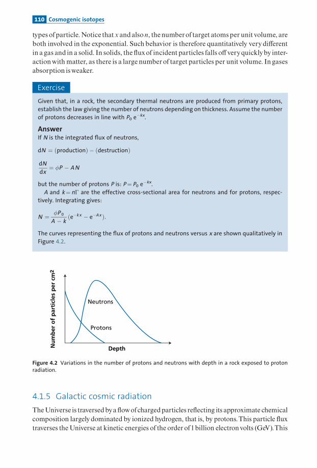
types ofparticle.Notice thatx andalson, the numberof target atomsper unit volume, areboth involved in the exponential. Such behavior is therefore quantitatively very di¡erentin agas and in a solid. In solids, the £uxof incident particles falls o¡ veryquicklyby inter-actionwith matter, as there is a large numberof target particles per unit volume. In gasesabsorption isweaker.

Exercise

Given that, in a rock, the secondary thermal neutrons are produced from primary protons,

establish the law giving the number of neutrons depending on thickness. Assume the number

of protons decreases in line with P0 e�kx.

AnswerIf N is the integrated flux of neutrons,

dN ¼ ðproductionÞ � ðdestructionÞ

dN

dx¼ �P � A N

but the number of protons P is: P¼ P0 e�kx.

A and k¼n� are the effective cross-sectional area for neutrons and for protons, respec-

tively. Integrating gives:

N ¼ �P 0

A � kðe�k x � e�A x Þ:

The curves representing the flux of protons and neutrons versus x are shown qualitatively in

Figure 4.2.

4.1.5 Galactic cosmic radiation

TheUniverse is traversedbya£owofchargedparticles re£ecting its approximate chemicalcomposition largely dominated by ionized hydrogen, that is, by protons.This particle £uxtraverses theUniverse at kinetic energies of the orderof1billion electronvolts (GeV).This

Nu

mb

er o

f p

arti

cles

per

cm

2

Depth

Neutrons

Protons

Figure 4.2 Variations in the number of protons and neutrons with depth in a rock exposed to protonradiation.


isknownasgalactic cosmic radiation. It is thoughtthatthese ions are emittedbyexplodingsupernovaeacceleratedbytheir shockwavesandbyothercomplexphenomenaofmagneticpulsation in ionizedenvironmentsoccurring in themagnetic¢eldsofstars.These charged particles interact with matter whether in gaseous state as in the atmo-

sphere or in solid state as in meteorites or terrestrial rocks. In general, proton interactionleads above all to the production of secondary neutrons and to successive nuclear reac-tions as in the atmosphere (Figure 4.3). High-energy, secondary neutrons produceother neutrons in a chainwhose energydecreasesuntil it is‘‘thermal.’’2 Thermal neutronsareverye⁄cient at causing nuclear reactions. In the atmosphere, for example, this occursby the reaction 14N (n, p) 14C*, giving rise to 14C. When thermal neutrons reactwith rock, they produce spallation reactions giving rise either to stable isotopes or toradioactive isotopes. It is from such nuclear reactions that we calculate what are calledexposure ages.

neutrons(or protons)

N, O, or Ar nucleus

14C

14CO2 gas

37Ar,39Ar

raregases

mixing mixingadsorption

ondust particle

fall tosurface

localmixing

photosynthesisof green

plants

trapped inrain or snow

10Be

Figure 4.3 The destiny of radioactive nuclei produced by nuclear reactions in the atmosphere under theinfluence of cosmic rays. Gases like argon remain in the atmosphere, some like 14C oxidize, while otherslike 10Be are adsorbed onto solid particles and fall to the ground with them.

2 Thermal neutrons are neutrons which, after colliding and interacting with matter, have energy levels ofkT, where k is Boltzmann’s constant and T temperature (kT � 0.025 eV). In this energy spectrum theyhave maximum probability of creating nuclear reactions.


All of these phenomenawerebrought to light and investigated littleby little in particularthrough the pioneering work of Devendra Lal of the Physical Research Laboratory ofAhmedabad and the University of California at San Diego (see Lal [1988] and Lal andPeters [1967] forareview).

Eachoftheotherthreesectionsofthischapterdealswithatypeofnuclearreaction.The¢rstconcentrates on 14C and concerns the radionuclides produced in the atmosphere and theiruse ingeochronology.The seconddealswith exposure ages¢rst in meteorites and then in ter-restrial rocks.Thethirdsectiongivesanoverviewofstellarprocessesofnucleosynthesis.

4.2 Carbon-14 dating

Ofall the radiometricmethods, this isundoubtedly themostfamous, theonethatis familiarto thegeneral public and theone thatpeople (mistakenly) thinkofwhen speakingoftheageoftheEarthorofrocks.ThismethodwasdevelopedbyWillardLibby (1946)whoeventuallyreceivedtheNobelPrize forchemistry forhiswork.

4.2.1 The principle of 14C dating

Carbon-14 is produced in the atmosphereby cosmic rayswhose protons engender second-aryneutrons.Theseneutrons reactwith14N:

14Nðn; pÞ 14C�:

In this reaction, 14N is the target nucleus, n (neutron) is the projectile, and p (proton) is theparticle ejected; 14C*istheradioactive isotopeproducedwhichdisintegratesby��radioac-tivity to give14N.As soon as it has formed, the14C combineswith oxygen to give CO2. IfwenoteN(14C) the numberof 14C atoms at the time ofmeasurement t and [N(14C)]0 the initialnumberofcarbonatoms, thenwemaywrite:

Nð14CÞ ¼ Nð14CÞh i

0e�lt:

Libbyshowed that the proportion of14C in the atmospherewas roughly constantover time.Whataccounts for this constancy?Letuswriteoutthebalance for14Cproduction:

ddt

N 14C� ��

¼ F� lN 14C� �

:

" "

production destruction by radioactivity

:

Ifa stationarystate is attained:

d

dtN 14C� ��

¼ 0 from which N 14C� �

¼ F

l

� �;

where F is the product of the £ux � of neutrons by the number N(14N) of atoms of 14Nby the e¡ective cross-section�.

The£ux�varieswith latitudebecause cosmicrays,whichare composedofprotons,andsoare positively charged, are de£ected by the Earth’s magnetic ¢eld.The poles receive much


more radiation than the equator. The £ux also varies with altitude, because the Earth’satmosphere ‘‘absorbs’’and transforms the incident £ux (Figure 4.4).Forourpurposes, themainphenomenon is thattheprimaryprotonsproduce secondary

neutrons, which produce others in a snowball e¡ect. It is these neutrons that produce the14C. As said, as soon as it has been produced, the 14C reacts with oxygen (or ozone) to giveCO2, andthisCO2mixeswith the remainderoftheatmosphere.Sincetheatmosphereitself iswellmixedinafewweeks, the14Cishomogenizedallaround

the planet on the timescale of interest to us. It can be taken, then, that the mean amountof14Cproduced intheatmosphere is avalid, uniformbenchmark.Libbyand his co-workers (Libby etal.,1949) determined the quantityof14C produced in

the steady state.They expressed it as the number of disintegrations per minute (dpm) pergramofcarbon:

lN 14C� �

Ncarbon¼ F

Ncarbon¼ 13:5:

They also determined the decay constant of 14C as l¼ 1.209 � 10�4 yr�1 (the half-life istherefore5730years).3

Nu

mb

er o

f n

eutr

on

s m

in–1

Pressure (millibars)

100 200 300 400

L = 90L = 60

L = 50

L = 40

500 600 700 800 900 1000Sea levelHigh

atmosphere

160

120

9070

50

30

2016

12

8

4

1.6

6

L = 30

L = 20

L = 10

Figure 4.4 Number of neutrons with altitude and latitude. Geomagnetic latitude is given by theparameter L. Altitude varies with pressure, which is measured in millibars here. The value of Lincreases as we move from the equator to the poles.

3 These values have been amended slightly today.

113 Carbon-14 dating

Exercise

What is the 14C/12C isotopic composition of atmospheric carbon, given that the isotopic

composition of stable carbon is defined by 13C/12C¼ 0.011 224 or the reciprocal12C/13C¼ 89.09, or 12C¼ 98.89% and 13C¼ 1.11%?

AnswerThe atomic mass of carbon is 12.011. One gram of carbon therefore represents 1/12.011�6.023 13 � 1023¼ 5.014 � 1022 atoms, including 5 � 1022� 0.9889¼ 4.95 � 1022 atoms of 12C. The

basic relation of radioactivity is lN¼ 13.5 dpm (where N is the number of 14C atoms).

In one year there are 5.26 � 105 minutes, therefore there are 13.5� 5.26 � 105¼ 71.48 � 105

disintegrations per year. Since l¼ 1.209 � 10�4 yr�1, we have 5.88 � 1010 atoms of 14C.

Therefore:

14C12C¼ 5:88 � 1010 atoms 14C

4:96 � 1022 atoms 12C¼ 1:1849 � 10�12 � 1:18 � 10�12:

This ratio is tiny and cannot be measured by a conventional mass spectrometer, because the12C peak is too high compared with the 14C peak. This is why it was long preferable to measure14C with a Geiger counter.

When carbon is incorporated in a living organism (plantor animal), its isotopic composi-tion (and so its activity) is equal to thatof the atmosphere and is determinedby phenomenasuch as photosynthesis or respiration. As soon as the organism dies, such exchanges ceaseand radioactive decay is the onlysource ofvariation in the14C content.The timeofdeath ofanorganism(ormoreprecisely thetimeatwhich itstoppedexchangingCO2withtheatmo-sphere) canthereforebedatedby theformula:

ð14C=CÞ ¼ 13:5 e�lt

t ¼ 1

lln

13:5

ð14C=CÞmeasured

" #:

Exercise

Let us take one of the examples that helped to make 14C dating so popular: Egyptology (see

Figure 4.5). A sample was taken from a wooden beam in the tomb of the vizier Hemaka at

Saqqara. He was an official of the First Dynasty of Egyptian pharaohs. After measuring the 14C

content of the wood, Libby announced it was 4880 years old. (Archeologists reported that the

royal seal-bearer had lived between 3200 and 2700 BC.) How did Libby manage this feat?

Answer

t ¼ 1

lln

14C=Cð Þatmosphere

14C=Cð Þsample

" #


The intricate measurement of the 14C/C ratio Libby made on the wooden artefact yielded 6.68

dpm g�1. Applying the age measurement formula then gave t¼ 4880 years.4

This method was highly successful and brought about a revolution in archeology. By thesameprinciple,apapyrus,bones,andburntorpetri¢edtreesweredated, therebyprovidinganarcheological chronometer thatwasunknownuntil then.Thismethodhas thedrawbackofdestroying theobject that is tobe dated,whichmeans acareful choicemustbemade.Thisis why recent advances in 14C analysis made with accelerator mass spectrometers, whichrequireonlyone-hundredthoftheamountofmaterial, are so importantandhavemade themethodevenmore incisive.

4.2.2 Measuring 14C

Measuring14C isadi⁄cultbusiness, aswehavejustseen.Aseriesofsimple calculationswillprovide insight into this di⁄culty, which has alreadybeen illustrated in an earlier exercise.One gramof ‘‘young’’carbon gives o¡ 13.5 dpm, or1disintegration every 4.5 seconds. Ifwehave just 10 mg of carbon, we will have one disintegration every 7.4 minutes, which is notmuch given a laboratory radioactive environment and also given that cosmic rays emitradiation inthe sameorderofmagnitude.

15

16

14

13

12

11

10

9

8

2000 4000Historical ages in years

Spec

ific

act

ivit

y, C

(d

pm

g–1

)

6000 80007

tree rings(1072 BC)

tree rings(1072 BC)

Hemaka(2950 ± 200 BC)

Sneferu(2625 ± 75 BC)

Soser(2700 ± 75 BC)

Sesostris (1800 BC)

Redwood (979 ± 52 BC)

Tayinat (675 ± 50 BC)

Ptolemy (2001 ± 50 BC)

Bible (100 ± 100 BC)

(580 BC)(575 BC)

Figure 4.5 Calibration of the reliability of 14C dating on historical data in Egyptology.

4 In fact, Libby found a constant l¼ 1.244 � 10�4 yr�1 and therefore t¼ 5568 years, which corresponds to7.35 dpm g�1. Oddly enough, 14C specialists still use Libby’s constants and then make a correction. Fordidactic reasons we shall not follow this practice.


Butsupposewehave a sample some 55 000 yearsold. Itnowemits just1.7 � 10�2 dpm, or1disintegration per hour (on average, of course, since radioactivity is a statistical law). Now,over the course of the hour, other particles have been emitted in the vicinity of the gram ofcarbon for many reasons: the various materials surrounding the counter (brick, cement,etc.) probably contain uranium impurities of the order of 1 ppb (and therefore also theirderived daughters: calculate them!), and the sky showers particle £ows on the Earth fromthe cosmos or the Sun, etc. How canwe eliminate these disturbances and make a reliablemeasurement?

The countingmethodLibby’s answer was tobuild aGeiger counter whose internal gas itself contained14C chan-ged intoCO2 (Figure4.6).

With themain counter surrounded byan arrayof secondaryGeiger counters, any exter-nal radiation could be subtracted because it ¢rst passed through the outer counters (theanti-coincidencemethod). Lastly, it was all buried and surrounded by ‘‘old’’ lead shieldingto prevent interference radiation.Howmuchbackground noise did the counters measure?Without shielding 1500 disintegrations per hour were detected, with shielding the ¢gurewas just 400, andwith the anti-coincidence counters it was just 8! Itwas thereforevirtuallyimpossible to measure an artefact 55 000 years old since it gave o¡ just one disintegrationperhour!Measurementwas intricateandnecessarilylasted fora long time.

Theacceleratormass spectrometrymethod (AMS)Since the late 1980s mass spectrometry has been adapted for 14C by using small particleacceleratorswith energiesofmore than1MeV(seeKieseretal.,1986); this is theacceleratormass spectrometry (AMS) method. The high energy imparted to the ions puri¢es the

Iron

Paraffin and boric acid

14C counters

Anti-coincidencecounters

Oldlead

Lead

Figure 4.6 Libby’s anti-coincidence counting. Geiger counters whose gas contains the 14C to bemeasured are surrounded by a series of layers of shielding as protection from cosmic rays (only oldlead is used so that the uranium chains are dead and there is no decay from them). When the smallcounters record a disintegration, it is due to cosmic radiation and so is subtracted from the valuerecorded by the central counter.


organic beam of any molecules and other impurities by passing them either throughthin sheets of gold or through gas streams. The carbon ions pass through these whileanymoleculesare‘‘deactivated’’andstopped. Inthiswaythemethod’s speedofanalysis, sen-sitivity, and precision have been increased compared with counting. A measurement thatoncetookmorethanaweekcannowbemade inan hour.Butaboveall, themethodrequiressamples of one-tenth of the size and achieves levels of precision 100 times greater (seeFigure4.7).

Exercise

If the maximum that can be measured by AMS for the 14C/12C ratio in 1 mg of carbon is 1.2 �10�17, what is the maximum age that can be measured with 14C?

Answer10 000 years.

Exercise

If the limit of detection by counting methods is 10 disintegrations per hour, what quantity of

carbon is required to measure the same age?

Answer2.213 kg!

Pre-selection electrode Stripping canal

Stripping gaspump

Voltagemultiplier

GasionizationdetectorExtraction electrode

Sample holder

Microscope

Cesiumgun

L5F3

M2

M3

L2

L1

E1

F1

L3

F2L4

M1F4

F5

Figure 4.7 Accelerator mass spectrometer. This device is much larger and more complex than anordinary mass spectrometer as it operates at much higher ion acceleration energies, but the principleis unchanged. The ions are extracted on the left by being bombarded with a beam of cesium ions andare then deflected first by an electrostatic field E1 and then by a magnetic field M1. In the center of thefigure, a microchannel injects gas which collides with the beams and destroys any molecules (this isknown as ‘‘stripping’’). The purified ions are then deflected by two electromagnets M2 and M3 andcollected by a detector similar to an ionization chamber used in particle physics.


4.2.3 Conditions for performing 14C dating

Applying the formula 14C ¼ 14Cð0Þ e�l14t to ¢nd an age entails meeting a number ofextremelystringentconditions.

The systemmusthave remained closed since the timethat is tobe dated.Thismeans ifwewish to date a parchment, it must have neither gained nor lost any 14C since the time thelamborsheepwhosehidewasusedtomaketheparchmentdied.Weneedtoknow14C(0)pre-cisely, that is the initial 14C content, that is theproportion of14C/C in the animal at the timeof its death.Theremust remain enough14C for ittobemeasurable.

Lastly, and this is not the least of the problems, the event whose age is to be determinedmustbede¢ned.

Canwebe certainaboutall fourconditions inpractice?

The closed systemThegreatestdanger fromanopen system is contaminationofthe sample,whether naturalorarti¢cial.Take the caseofatree trunkwewish to date. Ifthe trunkhasbeen lying in humus forsome time it will be impregnated, contaminated, by the carbon in the humus.Now, this car-bon is‘‘older’’thanthe carbonofthetreethathas justdiedandsodistorts themeasurement.

Letus take the exampleofatree trunkwhose speci¢c activity, that is, the14C radioactivitypergramofcarbon, is r1. It lies for some time in humuswhose radioactivity, in14C pergramofcarbon, is r2.Whatis the levelofradioactivityofthemixturesupposingthat10%ofthe car-bon comes fromthehumus?

r1 ¼14C

C

� �tree

; r2 ¼14C

C

� �humus

rtotal ¼14Ctree þ14Chumus

Ctree þ Chumus¼

14C

C

� �tree

Ctree

Ctree þ Chumusþ

14C

C

� �humus

Chumus

Ctree þ Chumus

rtotal ¼14C

C

� �tree

wþ14C

C

� �humus

ð1� wÞ:

Thevalue ofw¼Ctree/Ctotal variesbetween 0 and1. (This is the samemixing formula as inthe sectionon isotopic dilution.)

Assuming that (14C/C)tree¼ 12.5 dpm g�1 and that (14C/C)humus¼ 4 dpm g�1, thenrtotal¼ 12.5� 0.9þ 4� 0.1¼ 11.65dpmg�1,w¼ 0.9.

This corresponds to an error of 7% by default. The age measured is older than the realage.Conversely, ifwesuppose the tree trunk found in the sedimenthadbeen in soilwhichwasstill involved inatmospheric exchanges, thenthe contamination, that is, themixturebetween14C inthedeadtreeandthegroundwouldcontinuallymakethewood‘‘younger.’’

Determining the initial 14CcontentLibbyhadassumedthatthevalueof13.5dpmg�1ofcarbonwasthe currentvalueandvalidasthe initial value throughout time. However, several complications have arisen since then.Not all plants absorb carbon isotopes in an identical manner. If (14C/C)present¼ r0, the


value absorbed by living organisms is (14C/C)organism¼R r0, whereR is a partition coe⁄-cient.This coe⁄cient has been determined and to check it wemeasure the 13C/12C ratio oftheobjecttobedated (Figure4.8) (this ismorefullyexplained inChapter 7).Onthe left is the �13Cscale, suchthat:

d13C ¼

13C12C

� sample

� 13C12C

� standard

13C12C

� �standard

264

375 � 103:

The standard is a carbonate. In practice, this fractionation is converted into an age di¡er-enceby takingareference standard.Weassumethatfractionation isdirectlyproportionaltothedi¡erenceinmass.Therefore,

ifR3/2 is the partition coe⁄cient between some plant and the atmosphere, for the 13C/12Cratiode¢nedby:

13C12C

� plant

13C12C

� atmosphere

¼ R3=2

thepartition coe⁄cient for the (14C/12C) ratio

14C12C

� plant

14C12C

� atmosphere

¼ R4=2

is suchthatR4/2¼ 2�R3/2.It ispossible, then, to correct for natural fractionationof14Candexpress this correction

inage,which is doneonthe rightofFigure 4.8.It was realized that the14C contentof the atmospherehadvaried over the course of time.

This e¡ect was shownbymeasuring the 14C of tree rings.Tree rings are evidence of annual

δ13 C

(‰

)

Ag

e co

rrec

tio

n (Δt

), y

ears0 400

–10

300

200

100

–100

0

–20

–30

Marinecarbonates

Soilscarbonates Freshwater

carbonates

Bicarbonates insubsurface water

C4 plants (grass)

C3 plants (wood)

Atmospheric CO2

Animalbone

Figure 4.8 Carbon isotope fractionation relative to the atmosphere depending on the nature of thesubstrate.


growth, with each ring representing one year. By counting the rings, we can work backthrough time, yearby year.This isknownas dendrochronology. Itwasnoticed thattheagesofringsmeasuredby14Candtheagesobtainedbycounting the samerings failed tomatch.

Systematic investigation has shown that multiple phenomena are involved in this. Theburningof coal and oil, that is, materialswhose 14C is ‘‘dead,’’ has diluted the‘‘natural’’ 14Ccontentof the atmosphere.The present-day content is too low comparedwithwhat itwouldbe without this e¡ect. Likewise, for recent periods, nuclear testing by explosions in theatmosphere has injected a large quantity of 14C, which has largely disrupted the naturalcycle (Figure4.9) and,ofcourse, increasedthe14Ccontentoftheatmosphere.

The £uxofcosmic particles and therefore the production of14C varies over the course oftime. This is related to solar activity, to £uctuations in the Earth’s magnetic ¢eld, etc.Wetherefore need a calibration curve describing variation of the14C/C ratio over time.At¢rstsight, this looks something like a chicken-and-egg situation becausewewish to determinean age from the 14C/C measurement but at the same time we wish to calculate the 14C/Cratio by using age measurement.The curve of 14C/C variation in the atmospherewas con-structed by dating samples using a di¡erent method. For recent periods, tree rings wereused as thebenchmark, and for earlier periods dateswere ascertainedby radioactive dise-quilibriummethods.

To calibrate the 14C/C ratio, we ¢rst seek to calculate (14C/C)initial¼ (14C/C)measured elt,

where t is the independentlydetermined age. In this waya correction can be applied to theagemeasured by the conventional method (Figure 4.10). It is then possible to drawa curveconnecting14C dates tohistorical calendarages.To do this,1950was taken as the referencedate for14C. Supposewe calculate a14C dateof 3000 yearsbefore1950 (ifwemade themea-surementintheyear2000wewouldremove50years!).ToobtaintheBCdate,wemustthere-foresubtract1950: 3000^1950¼ 1050BC(Figure4.11).

Years

Perc

enta

ge

exce

ss 1

4 C

100

80

60

40

20

1963 1964 1965

41° S

1966 1967 1967

36° N

21° N9° N

18° N

71° N

38° N

Figure 4.9 Changes in excess 14C injected into the atmosphere by U.S. atom-bomb testing in thePacific. Each symbol corresponds to a latitude. The various, ever weaker, injection dates can be seen:1963, 1964, 1965, 1966. It took several decades to return to equilibrium. After Libby (1970).


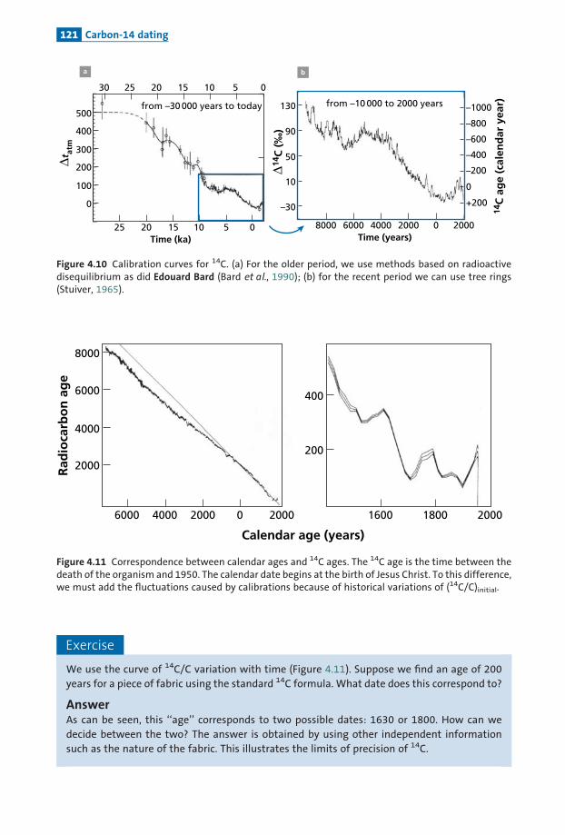
Exercise

We use the curve of 14C/C variation with time (Figure 4.11). Suppose we find an age of 200

years for a piece of fabric using the standard 14C formula. What date does this correspond to?

AnswerAs can be seen, this ‘‘age’’ corresponds to two possible dates: 1630 or 1800. How can we

decide between the two? The answer is obtained by using other independent information

such as the nature of the fabric. This illustrates the limits of precision of 14C.

Δtat

m

130 –1000

90–800

–600

–400

–200

+200

0

50

10

–30

8000 6000

from –10 000 to 2000 years

Time (ka) Time (years)

from –30 000 years to today

4000 2000 20000

500

400

0

100

200

300

25 20 15

15 10 5 0202530

10 5 0

a b

14C

ag

e (c

alen

dar

yea

r)

Δ14 C

(‰

)Figure 4.10 Calibration curves for 14C. (a) For the older period, we use methods based on radioactivedisequilibrium as did Edouard Bard (Bard et al., 1990); (b) for the recent period we can use tree rings(Stuiver, 1965).

8000

6000

4000

2000

6000 4000 2000

Calendar age (years)

Rad

ioca

rbo

n a

ge

0 2000

200

1600 1800 2000

400

Figure 4.11 Correspondence between calendar ages and 14C ages. The 14C age is the time between thedeath of the organism and 1950. The calendar date begins at the birth of Jesus Christ. To this difference,we must add the fluctuations caused by calibrations because of historical variations of (14C/C)initial.


Synthetic formula forage calculationWhenmakingcalculations,we can converteverything totheadditionofmagnitudeswhichthemselves have age dimensions.When applying theuncorrected conventional formulaweobtain:

tapparent ¼1

lln

Ac

Am

� �

whereAc is the initial conventional activityandAm is the activityasmeasured.The true agemustbewritten:

ttrue ¼1

lln

A0;real P2;4

Am

� �

whereA0,real is the real, initial activityoftheatmosphereandP2,4 is the isotopefractionationfactor.We can also introduce in the parenthesis the referencevalueAc for the initial activity.Dividing thetopandbottomgives:

ttrue ¼1

lln

A0;real

Ac� Ac

Am� P2;4

� � �:

Takingadvantageoftheadditivepropertyoflogarithms,wehave:

ttrue ¼1

lln

Ac

Am

� �þ 1

lln P2;4

� �þ 1

lln

A0;real

Ac

� �:

Fromwhich,by transformingeverything intotimeunits:

ttrue ¼ tapparent þ Dtfractionation þ Dtatmospheric correction

where:

Dtfractionation ¼1

llnðP2;4Þ and Dtatmospheric correction ¼

1

lln

A0;real

Ac

� �;

withalittleextracalculationtrickbecause A0;real=Ac

� �canbeevaluatedasafunctionoftime

only.We therefore calculate t1¼ tapparentþ�tfractionation, then we can use t1 to calculate

�tatmospheric correctionusing the£uctuation curvesofFigure4.11, andwethenobtainttrue.

Exercise

We measure the activity of a camel bone found in the tomb of the vizier Hemaka as 6.68 dpm g�1.

What is the real date of the vizier’s death? (Use the existing calculations and graphs.)

AnswerIn an exercise in Section 4.2.1 we dated the death of vizier Hemaka (4880 years ago) using an

ordinary wooden beam.

t 1 ¼ t apparent þ Dt fractionation


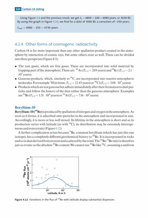
Using Figure 4.8 and the previous result, we get t1¼ 4800þ 100¼ 4980 years, or 3030 BC.

By using the graph in Figure 4.10, we find for a date of 3000 BC a correction of –250 years:

t real ¼ 4980� 250 ¼ 4730 years:

4.2.4 Other forms of cosmogenic radioactivity

Carbon-14 is far more important than any other spallation product created in the atmo-sphere by interaction of cosmic rays, but some others exist as well. These can be dividedintothreegroups (seeFigure4.3):

� The rare gases, which are free gases. These are incorporated into solid material bytrapping part of the atmosphere.These are 39Ar (T1/2¼ 269 years) and 81Kr (T1/2¼ 2.1 �105years);� Gaseous products, which, similarly to 14C, are incorporated into reactive atmospheric

molecules.Forexample 3H(tritium;T1/2¼ 12.43years) or 36Cl (T1/2¼ 3.08 �105years);� Productswhicharenotgaseousbutadhere immediatelyafter their formationtodustpar-

ticles and follow the history of the dust rather than the gaseous atmosphere. Examplesare10Be (T1/2¼ 1.51 �106years)or 26Al (T1/2¼ 7.16 �105years).

Beryllium-10Beryllium-10(10Be) isproducedbyspallationofnitrogenandoxygen intheatmosphere.Assoon as it forms, it is adsorbed onto particles in the atmosphere and incorporated in rain.Accordingly, it is more or less well mixed. Its lifetime in the atmosphere is short and as itsproduction varies with latitude (as with 14C), its distribution may be extremely heteroge-neousandeven erratic (Figure4.12).A further complication arises because 9Be, common beryllium (which has just this one

isotope), has a completelydi¡erent geochemical history to10Be. It is incorporated in rocksandsoindustderivedfromerosionandscatteredbythewind.The10Be/9Beratiois thereforejust as erratic as the absolute10Be content.We cannotuse10Be like14C, assumingauniform

Latitude, N or S

10B

e fl

ux

(106

ato

ms

cm–2

yr–1

) 4

30° 60° 90°

2

1

Figure 4.12 Variations in the flux of 10Be with latitude display substantial dispersion.


value for the entire Earth at anygiven time. Onemethod is to assume that, at a given place,£uctuations in the 10Be/9Be ratio are low and at any rate much lower than those arisingfromthe radioactive decayof10Be. It is thenpossible touse10Beas achronometer.

Exercise

We wish to measure the rate of accretion of manganese nodules found in the ocean. How can

we set about this, knowing that the variation in the 10Be/9Be ratio with depth is10Be/9Be¼ (10Be/9Be)0 e�lt?

Answer

t ¼ x thicknessð Þa accretion rateð Þ,

from which:

10Be9Be

� �¼

10Be9Be

� �0

e�lxa .

Switching to logarithms gives:

ln10Be9Be

� �¼ ln

10Be9Be

� �0

� lx

a:

The logarithm of the ratio 10Be/9Be plotted as a function of thickness is a straight line of slope

l=aÞð , which gives the rate of accretion, a.

O’Nions et al. (1998) measured the 10Be/9Be ratios in manganese crusts of the NorthAtlantic. Figure 4.13 shows the results theyobtained.Thismethodyielded an accretion rateof2.37 0.15mmMa�1.

10–8

10–9

10–10

10–7

5 10 15 20 25Thickness (mm)

10B

e/9 B

e

a = 2.37 ± 0.15 mm/ Ma–1

Figure 4.13 Variation in the 10Be/9Be ratios in a manganese concretion from the Atlantic Ocean.Magnitude a indicates the rate of accretion of the nodule. After O’Nions et al. (1998).


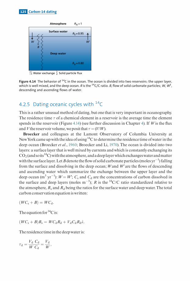
4.2.5 Dating oceanic cycles with 14C

This is a rather unusual method ofdating, but one that is very important in oceanography.The residence time � of a chemical element in a reservoir is the average time the elementspends in the reservoir (Figure 4.14) (see further discussion in Chapter 4). IfW is the £uxandV the reservoir volume,wepositthat � ¼ (V/W).Broecker and colleagues at the Lamont Observatory of Columbia University at

NewYorkcameupwith the ideaofusing14C to determine the residence timeofwater in thedeep ocean (Broecker et al., 1960; Broecker and Li, 1970). The ocean is divided into twolayers: a surface layer that is well mixed by currents andwhich is constantly exchanging itsCO2(andsoits

14C)withtheatmosphere,andadeeplayerwhichexchangeswaterandmatterwith the surface layer. LetB denote the £owofsolid carbonate particles (moles yr�1) fallingfrom the surface and dissolving in the deep ocean;WandW0are the £ows of descendingand ascending water which summarize the exchange between the upper layer and thedeep ocean (m3 yr�1):W¼W0; Cs and Cd are the concentrations of carbon dissolved inthe surface and deep layers (moles m�3); R is the 14C/C ratio standardized relative tothe atmosphere,Rs andRd being the ratios for the surface water and deepwater.The totalcarbon conservation equation iswritten:

ðWCs þ BÞ ¼WCd:

The equation for14C is:

ðWCs þ BÞRs ¼WCdRd þ VdCdRdl:

Theresidence time inthedeepwater is:

�d ¼Vd Cd

W Cd¼ Vd

W;

Atmosphere

Surface water

Deep water

RA = 1

RS = 0.95

Rp = 0.80

W'W

B

Water exchange Solid particle flux

Figure 4.14 The behavior of 14C in the ocean. The ocean is divided into two reservoirs: the upper layer,which is well mixed, and the deep ocean. R is the 14C/C ratio. B, flow of solid carbonate particles; W, W1,descending and ascending flows of water.


which, giventheforegoingequations, iswritten:

�d ¼Rs

Rd� 1

� �1

l:

Now,l¼ 1.209 � 10�4 yr�1, therefore �d¼ 1550years.

4.3 Exposure ages

4.3.1 Meteorites

Meteorites are fragments ofplanetarybodies resulting from collisions andwhose primaryage is close to that of the Solar System (4.55 Ga, as an indication).They are pieces of rock‘‘£oating’’ in interplanetary space. Most come from the asteroid belt, between Mars andJupiter,which isformedofrockdebris,piecesofwhichmaymeasureakilometerorsoacross(Ceres). Somewere ripped fromMarsor theMoon.These rocks drift loose in spaceandarecontinuallysubjected to cosmic radiationwhoseaverage energy is1GeV. Just ashappens intheatmosphere,when cosmic‘‘primary’’protonspenetrate these rocks theygive rise to sec-ondary neutrons, which produce most of the nuclear reactions.5 These particles producenuclear reactions at depths ranging from a few tens of centimeters up to a meter at most.Thesurface layersofrocks exposedto cosmicraysarethereforethesiteofnuclear reactions,usually spallation reactions.Theygive rise to isotopes of lower mass than the target, whichare known as cosmogenic isotopes (see Paneth etal.,1952; Honda andArnold,1964).Thenuclei engenderedbysuch reactions include radioactive and stable isotopes. Both types areverynumerous.

Stable isotopesThenumberofcosmogenic stable isotopesNsproducedperunittime iswritten:

dNsðtÞdt

¼ ��s Nc!s;

where� is the particle £ux,�s is the e¡ective cross-section of the reaction, that is, the prob-abilityofanuclear reaction occurring, andNc!s the numberoftarget atomsproducing thestable daughter isotope, s, by nuclear reaction. If the £ux is constant in terms of intensityandspectral energy, then:

NsðtÞ ¼ ��s Nc!s t:

Thenumberofdaughter isotopes is directlyproportional tothe irradiationtime.Itseemsstraightforwardenoughtocalculatetheageof irradiation,providedweknow�,�s,

andNc!s. It is comparatively easy tomeasure the parameterNc!s: it is the concentration of

5 As explained, protons carry a positive charge and do not penetrate readily into matter because they arerepelled electronically. Neutrons carry no charge and so penetrate much more readily.


the targetproductwhich, bynuclear reaction, yields the cosmogenic isotope. Sometimes it issingle. This is so in iron meteorites composed of a metallic alloy of iron and nickel.Sometimes there are more than one, as in ordinary meteorites where krypton isotopes areproducedbyspallationonrubidium,strontium,yttrium,andzirconium.Theprimary£uxofcosmicrays� iscomposedofprotons(andsomeHeþ ions)(andofallthe

isotopes intheUniverse intheionizedstatebutinverysmallabundances). Ithasboth intensity(number of particles per unit of surface area and per unit time) and an energy spectrum,because in factthere areN1,N2, . . .,N3 particles, corresponding to energylevels1, 2, . . ., n.Assaid, thisprimary£uxofprotonsproducesbarelyanythingother than reactions atthemeteo-rite’s surface, sinceas soonas itpenetratesbyafewcentimeters itgeneratesasecondary£uxofneutrons, which penetrate more deeply.These neutrons also have an energy spectrumwhichchanges as they penetrate, diminishing, of course.The £ux and energy spectrum of cosmicradiationmay varywith time (weknowneitherhow, nor themagnitudeofsuch £uctuations).Whatwemeasure isthe resultof£uxaggregatedoverseveralmillionorevenbillionyears.A further, although generally minor, complication is that in addition to cosmic

radiation there is also a £ux of particles from the Sun. Generally, this £ux is weak andof low energy, but from time to time it may become intense and of high energy. Thesebursts in £uxareknownas solar £ares.They toomayengender spallation reactions.The e¡ective cross-sections for production of new isotopesby nuclear reactions are also

dependent on energy and therefore on penetration inside the meteorite. Figure 4.15 showstheproductionofvarious isotopesversus depth.As, inaddition, someisotopesresult fromspallationonseveral targetnucleiwhose e¡ects

are cumulative,we can imagine thesheercomplexityofthephenomenon ifwewishtodeter-mine all the contributions.That would involve estimating amean £ux and its energy spec-trum and localizing the sample to be measured inside the meteorite. For these reasons, asimplerwayofmaking the calculation hasbeen sought.

59N

i, 60

Co

(dp

m k

g–1

)

36C

l (d

pm

kg

–1)

Distance (cm)

300

50 100 150

200

100 –10

–20

–30

0

60Co

36Cl

59Ni

Figure 4.15 Production of 36Cl, 59Ni, and 60Co by (n, �) reactions in a supposedly spherical chondriticmeteorite. Distance is measured from the meteorite’s surface towards its center. Cl¼ 100 ppm,Ni¼ 1.34%, Co¼ 700 ppm. � 35Cl¼ 45 barns, � 58Ni¼ 4.4 barns, � 59Co¼ 37 barns. Initial flux S0¼ 0.5neutron cm� 3s� 1.

127 Exposure ages

Radioactive isotopesIn this case, the equation in the preceding subsection must be supplemented by the decaytermlrNr,whereNr is thenumberofradioactiveatoms:

dNr

dt¼ ��r Nc!r � lr Nr:

Let us posit � �r Nc!r¼T. It is considered to be constant to simplify things, or else it isassumedweknow itsmeanvalue.The equationbecomes:

dNr

dt¼ T� lr Nr:

Integratinggives:

Nr ¼T� C e�lrt

lr:

whereC is the integration constant. Ifatt¼ 0,Nr¼ 0,C¼T.Fromthis:

Nr ¼T

lr1� e�lrt� �

¼ ��r Nc!r

lr1� e�lrt� �

:

Nowsupposewehave two isotopes, one stable andone radioactive, producedbyspallationunder similarconditionsofenergyand£ux.We can establishthe ratio:

NsðtÞNrðtÞ

¼ �s

�r

Nc!s

Nc!r

t

1� e�lrt

� lr:

Ifwewait long enough for productionanddestructionofthe radioactiveproduct toachieveasteadystate, then e�lt! 0.Thisgives:

NsðtÞNrðtÞ

¼ �s

�r

Nc!s

Nc!rlr t:

Notice thatwehave eliminated the £ux factor. If, in addition, the two isotopes are productsofthe sameelement, thenNc!s=Nc!r ¼ 1andthe equationbecomes:

NsðtÞNrðtÞ

¼ �s

�rt lr;

hence:

t ¼ 1

lNs

Nr

�r

�s:

In this way, we determine the time elapsed since the meteorite was subjected to cosmicradiation without knowing anything more about the cosmic radiation but having just theratioofthe e¡ective cross-sections.Theexposureage is thetimesincethemeteoritewasbro-ken intopieces, leading to its exposureto cosmic rays (Figure4.16).


One of the conditions for successfully applying this method is that the isotopes usedshould have e¡ective cross-sections that are sensitive to the same ranges ofenergyand £uxto justify the simpli¢cation ofmathematically eliminating £ux. Accordingly, we are inter-ested in isotopes either of the same element or of adjacent elements in the periodic table.Thepairsmostusedare 3He^3He*, 22Ne^22Na*,38Ar^39Ar*,83Kr^81Kr*, and 41K^40K*(* indicates thatthe isotope is radioactive).The only point that remains undetermined if we are to be able to calculate the age

is the ratio of e¡ective cross-sections and their level of constancy depending onparticle £ux and energy. The determination of e¡ective cross-sections has, of course,bene¢ted from the extraordinary research activity in nuclear energy and we have agoodcatalogofe¡ective cross-sections fromwhich ithasbeenpossibletoderiveprecise laws.

Exercise

The 83Kr–81Kr method is used to calculate exposure ages (Marti, 1982). The decay constant of81Kr is l¼ 0.32 � 10�5 yr�1. What is the minimum age we can calculate using the steady state

formula?

AnswerFor this, e�lt must be negligible compared with 1. If we accept that e�lt must be less than

0.01, then t¼ 1.4 million years.

Exercise

Can we not use this method for ages of less than 1.4 Ma?

AnswerThe evolution equation is

N r

N s¼ �s N c!r

�r N c!s

�1� e�lt

lt

�:

Nu

mb

er o

f n

ucl

ei

Rad

iog

enic

arg

on

con

cen

trat

ion

cm

–3

Exposure age (years) Exposure age (years)

Stableisotopes

Radioactiveisotopes

39Ar*(radioactive)

38Ar (stable)

10–13

2x10–13

0 1000 2000λ –12

λ 2

λ –11

λ1 = 2λ2

a b

Figure 4.16 Pairwise chronometry (stable isotope, radioactive isotope) for cosmogenic isotopes. (a) Thegeneral theoretical case; (b) the example of 38Ar/39Ar, which is used extensively in glaciology (seeOeschger, 1982).

129 Exposure ages

We need to just calculate the curve ð1� e�lt Þ=t and use the value of the ratio Nr/Ns. We

know that Nc!r is identical to Nc!s for krypton. Calculate the curve for the 81Kr/83Kr ratio,

given that �r/�s � 1.6612.

Exercise

The 83Kr–81Kr method can be used for calculating exposure ages in stony meteorites by the

formula:

T ¼ 1

l�81

�83

83Kr83Kr

� �cosmogenic

where 1/l¼ 0.307 Ma. To be rid of any complications and given that many Kr isotopes are

produced by spallation, the ratio of effective cross-sections is calculated from the formula:

�81

�83¼ 0:95

2

80Kr83Krþ

82Kr83Kr

� �:

Calculate the exposure age of the Juvinas meteorite if the isotopic measurement of Kr in it

is by convention:

AnswerT¼ 10.7 �106 years.

Exercise

We use the 41K–40K method to date iron meteorites (Voshage and Hintenberger, 1960). The

only target is therefore iron and we take it that l40¼ 0.5543 � 10�9 yr�1. As the effective cross-

sections are �40¼ 9.4 millibarns and �41¼ 14.7 millibarns, what is the cosmogenic isotopic

composition of 41K/40K for two meteorites whose exposure ages are 100 Ma and 1 Ga?

AnswerFor 100 Ma (41K/40K)cosmogenic¼ 1.60; for 1 Ga (41K/40K)cosmogenic¼ 2.038.

Whatarethemain conclusions tobedrawn fromthesemeasurementsofexposureages?Exposureagesaregenerallymuchyounger thantheagesofmeteoriteformation(ormeta-

morphism).Theyrangefromafewmillionyears toafewhundredmillionyears. (Agesoffor-mation are closer to 4.5 billion years, as we have seen.) This shows that for most of theirlifetime meteorites are inside their parent body, where they are shielded from cosmic rays,and that the fracturingofmeteorites has occurred relatively late (but longbefore they fall toEarth!).

84Kr 78Kr 80Kr 81Kr 82Kr 83Kr 86Kr

1 0.157 0.460 0.0166 0.767 0.968 0.182


The distribution ofmeteorite exposure ages seems to display peaks at 5.7 and 20millionyearsforordinarystonymeteoritesandat700millionyearsfor ironmeteorites (Figure4.17).The di¡erences in exposure ages for iron and chondritic meteorites is problematic.Why

should iron meteorites have so much older exposure ages? It was ¢rst thought that theycame from a di¡erent part of the Solar System. It is now thought that the exposure ages ofiron meteorites are older because iron withstands impacts better than the silicate assem-blages thatmake up chondritic meteorites, which havebeen subjected to impacts resultingin more recent fragmentation. In any event, the results show thatmeteorites have long life-times in interplanetaryspace.

4.3.2 Terrestrial rocks

The principle for terrestrial rocks (see reviewbyOeschger,1982) is the same as for meteor-ites.Galactic cosmic radiation causes nuclear reactions in rocks.The nuclei produced canbemeasured,andifweknowthe£uxwecan calculatethedurationof irradiation.Thedi¡er-ence with meteorites is that the intensity of cosmic radiation at the Earth’s surface is farlowerbecause ithasbeenattenuatedby theabsorptionofprotonsandneutrons intheatmo-sphere. It was not until measurement sensitivity had been improved that these methodscould be applied to terrestrial rocks. A second di⁄culty is that until now methods usingisotope ratios employed for meteorites, such as 40K/41K and 83Kr/81Kr, have not beenapplicable for terrestrial rocks. For the ¢rst method, no equivalent hasbeen found for ironmeteorites, which do not contain large quantities of initial K, which dilutes the e¡ectsproduced by irradiation. For the second method, sensitivity is still insu⁄cient, but thatmay change. Unlike the case of meteorites, where the particle £ux � is eliminated, here itmustbe calibrated carefully.Now, the £uxdiminishes, ofcourse, as itpenetrates intoarock.Hence there is a furtherdi⁄culty, which hasbeen solved empirically, thatof calibrating the£ux�, orcalibratingabsorption.

Iron meteorites

Exposure age (years)

Chondrites N

N

5

0106 107 108 109

10

10

0

20

30

Figure 4.17 Exposure ages of various types of meteorites.

131 Exposure ages

Exploitable chronometersInpractice,weuse the four radioactive isotopes14C*,10Be*, 26Al, and 36Cl and the two raregases 3Heand 21Ne,whichare stable isotopes. For radioactive elements,weuse the formulaestablished formeteorite exposureages:

Nr ¼��Nc!r

l1� e�lrt� �

:

Buthere, equilibrium isnotachieved.BynotingT theproduction rate��Nc!r,weobtain:

Nr ¼T

l1� e�lrt� �

:

Forexample, forberyllium,

10Be ¼ T

lBe1� e�lBet� �

:

The di⁄cultylies in determining the £uxandassuming it tobe constantover timeand thenestimating theabundanceoftargetnuclei.

For 3He and 21Ne, exposure ages are also calculated by the method described for stableisotopes inmeteorites.Thisgives:

Ns ¼ ��Nc!s t:

Theproduction rate iswritten asP¼��Nc!s.Thegases3Heand 21Neaccumulate linearly

withtime, therefore3He¼Ptor21Ne¼Pt.Heretooweneedtoknowthe£ux(andtoassumethat it is constant) andtheabsorption laws.

For the target, 3Heproduction doesnotdependmuchon its compositionwhereas 21Ne isproduced byspallation ofMg and depends greatlyon the chemical composition of the tar-get.To make it uniform, olivine, whose Mg content is more or less constant, is separatedandmeasurements aremadeonthismineral.

Calibration of production rates, erosion rates, etc.The particle £ux varies with both altitude and latitude,6 as we said when discussing 14C.The £ux has therefore to be calibrated in each place where the measurement is made.There are twoways to do this. First, general lawshavebeen established giving thevalue of£ux by altitude and latitude. To get some idea of this, let us say that at an altitude of5000m, the £ux is 20 times greater than at sea level. At the poles, at a constant altitude, itis 60 timesgreater thanatthe equator.This iswhy£ux is calibrated locally,wherepossible,bymeasuring10Be, 26Al,3He,or 21Ne contentson sampleswhoseagehasbeendeterminedbyothermethods.

Let us look at two important examples that will help in understanding the thinkingbehind themethodbutwhichwill show its‘‘fruitful complications’’and so suggest its futuredevelopments.

6 The first measurements were made in the Antarctic where the flux is greatest and, in addition, the erosionrate is low.


Erosion ratemeasurementsOur job is to measure the exposure age of a basalt £ow from the Piton de la Fournaisevolcano on the island of Re¤ union (Staudacher and Alle' gre, 1993).This lava £ow is at analtitude of 2300 m and there is no indication that its altitude has varied over the courseof time.We decide to use the cosmogenic age method based on 3He applied to olivine.We

therefore separate the olivine from a rock sampled from the surface and measure the3He content of the sample.To obtain the 3He of cosmogenic origin, we must, of course,correct for 3He of internal origin.To do this, we measure the 3He/4He ratio of internalorigin on olivine sampled at a great distance from the surface.We can calculate thecosmogenic 3He content by measuring the (3He/4He)total ratio and the total concentra-tion in 3He.

Exercise

Given (3He)total, (3He/4He)internal, and (3He/4He)total, establish the formula for calculating

cosmogenic 3He.

Answer

3He� �

cosmo¼ 3He� �

total

3He4He

� total� 3He

4He

� internal

3He4He

� �internal

24

35:

When all the calculations havebeen made, we¢nd1.3 � 10�12 cm3 g�1at standard tempera-ture andpressureof 3Heof cosmogenic origin.The production rateP0 of

3He in the olivinehasbeen calculated for the latitudeandaltitudeofthe sampleas 2.2 �10�17 cm3 g�1per yearatstandardtemperatureandpressure.

Table 4.1 Usable cosmogenic nuclides

Isotope Half-life (yr)Measurementmethod Di⁄culties

Production rate(atoms/yr)Sealevellatitude>558N Time-span

3He Stable Mass spectrometer Di¡uses easily 160 (olivine) 1ka ^3Ma10Be 1.5 �106 AMS Atmospheric

contamination6 (quartz) 3ka ^8Ma

26Al 7.16 �105 AMS Atmosphericcontamination

37 (quartz) 5ka ^2Ma

36Cl 3.08 �105 AMS Atmosphericcontamination

8 (basalt) 5ka ^1Ma

21Ne Stable Mass spectrometer Commonneon 45 (olivine) 7ka ^10Ma14C 5730years AMS Contamination 20 (basalt) 1ka ^40ka41Ca 103 �103 AMS Verydi⁄cultto

measure^300ka

133 Exposure ages

It is easy thento calculatethe exposureage:

Tcosmo¼ 3He/P0¼ 59 090years.

In addition, the ‘‘geological’’ age of the basalt £ow has been calculated by the K^Armethod as 65 200 2000 years.The surface rock has been irradiated for 65 200 years andyet its exposureage is just 6000years attheyoungest.Howcome?

After examining the various sources of error, we accept that the age di¡erence is dueto erosion.The rock sampled at the surface today was in fact located at depth for much ofitshistory. Itonlycameto the surface throughablationofthematerial above it, byerosion.

Now,weknow that the particle £uxdecreases exponentially with the thickness of rock ithaspenetrated.Weneed, then, tomodel thephenomenon.

We canwritethe rateofproductionof 3He inthe form:

P ¼ P0 exp�XðtÞL

� �

whereX(t) is thethickness countingfromthesurfaceandL is theattenuation factorofradia-tionwithdepth.

Tosimplifymatters,we canassumethatthe rateoferosion is constant.We canwrite:

X ¼ X0� 2 t

where2 is the erosion rateandX0 the initialdepthofthe sample.We canthereforewrite:

d 3He� �dt

¼ P0 exp� X0� 2 tð

L

�:

We integrate this equation between 0 and t and then replace X0 by its value X0¼Xþ2t(remembering thatX is counteddownwards).Thisgives:

3He ¼ P0L

2 exp�XL

� �1� exp

� 2 tL

� h i:

ThenX is the currentdepth coordinate.Ourobjective is todeterminethe erosion rate,2.We know t (65 200 years) and P0 (2.2 � 10�17 cm3 g�1 yr�1 at standard temperature and

pressure), buttherearestill twounknowns:2andL.TomeasureL, webore a small core and so take samples at various depths.We isolate the

olivineandmeasurethe cosmogenic 3Heon eachsampleof it.We cannowdraw theplot:

ln ð3HeÞcosmo

h i¼ fðXÞ:

Ifour assumptions about the £ux and erosion rate are valid, the relation is a straight line ofthe form:

ln ð3HeÞcosmo

� �¼ �X

Lþ A

whereA is aconstant.Theslope is ( 1/L).


Exercise

A core was taken from the lava of the island of Reunion discussed before. Olivine was

extracted at each level and the 3He content measured. After correcting for 3He of internal

origin, the following results were found as a function of depth X (Table 4.2).

Calculate the attenuation factor L.

Notice that depth X in this table is expressed in grams per square centimeter, which is an

unusual unit of length! The reason for this is that attenuation is, of course, dependent on the

quantity of matter penetrated and so depends on the density of that matter (attenuation per

unit length penetrated is not the same in rock, soil, or a layer of atmosphere). If attenuation

were expressed per mil length, we would have to multiply it by density, and so the effective

value would be:

length ðcmÞ mass ðgÞvolume cm3ð Þ

which is equivalent to mass per square centimeter. Naturally enough, L too will be expressed

in g cm�2.

AnswerAfter calculating ln(3He) as a function of X (do it) we find for the slope:

L ¼ 165 g cm�2 5:

How can we now calculate the erosion rate 2?

Let us go back to the expression as a function of X but now start from where X¼ 0, that is, at

the present-day surface. The expression becomes:

3He ¼ P 0L

2 1� exp� 2 t

L

� � �:

We can develop the exponential in series limiting ourselves to the first three terms.

Remembering that 3He¼ Tcosmo� P0, we can finally write:

2¼ 2L

t

� �� t � T cosm

t

� �:

If we note the relative difference between the geological age and cosmogenic age as �T/T:

2¼ 2DT

T� L

t

� �:

Table 4.2 Relation of 3He content to depth in olivinefrom lava on Reunion

X (gcm�2) 3He (10�13 cm�3 g�1)

10.45 1337.86 9.12131.95 6.9217.42 3.58318.41 1.74

135 Exposure ages

In the present case we find 2¼ 4.7 g cm�2 yr�1.

If we accept a density of 2 g cm�3 because the lava sampled is ‘‘bubbly’’ and contains many

cavities, then 2¼ 2.1 mm yr�1¼ 2.1 mm per 1000 yr.

Exercise

Cosmogenic 21Ne contents were measured on the same samples of olivine from the island

of Reunion (Table 4.3). Given that the production rate of 21Ne is 6.28 � 10�18 cm�3 g�1 at

the latitude and altitude in question, calculate the attenuation factor L and the erosion rate2.

How do you account for the result for L compared with that found for 3He? Which seems to

you to be the more accurate rate of erosion, that determined with 3He or that with 21Ne? To

what do you attribute the difference?

Answer

L ¼ 160 gcm�2:

It is identical to that for 3He because the particle flux at the origin of 3He and 21Ne is the

same for both. The cosmogenic age of the surface sample is Tcosmo¼ 52 388 years.

2¼ 9:6g cm�2 yr�1 ¼ 4:8 mm per 1000 yr:

The 21Ne age is greater than the 3He age probably because helium diffuses more readily

than neon and the sample has probably lost a lot of helium. This invites caution when

interpreting helium ages (Figure 4.18).

Table 4.3 Relation of 21Ne content to depth in olivinefrom lava on Reunion

X (g cm�2) 21Ne (10�13 cm�3g�1)

10.45 3.2937.86 1.73131.95 1.59217.42 0.96318.41 0.52

–28

–27

–29

–30

–31100 200 300 400

Depth (g cm–2)

3He

21NeIn(2

1 Ne c

, 3H

e c)

Figure 4.18 Attenuation curves for the creation of 3He and 21Ne in rocks of Reunion given by way ofexample.


Measuring the rate of upliftAs said, the particle £ux at 500meters altitude is 20 times higher than the £ux at sea level.Suppose, then,wehavea lavathathas£owedatsea level. Subsequently the terrain itoverlieshasbeen lifted toanaltitudeof500m.Of course, the lavawould be irradiatedmuch more over the course ofuplift.This type of

model canbe calculated inthe samewayasbefore:

d3He

dt¼ P0 exp

XðtÞL

� �

whereX(t) is thealtitudeforwhich zerois takenat100mandL is theattenuation factor intheatmosphere. Ifwe call the rateofupliftU,weget:

U ¼ 2Tcosmo � t

t

� �L

t:

Ascanbeseen,Tcosmo¼ theageofexposureand isgreater thanthe‘‘geological’’age.Naturally, erosion has notbeen allowed for in this example. Ifweaddthe erosion rate,we

will need other constraints and other chronometers to solve the problem because we willthen havetwounknowns,2andU.Here,weareatthe frontierofcurrentresearch.

Interestand limits of thesemethodsThemethods areof interest foranumberofreasons:

� erosion rates canbedetermined(providedtheyarenottoohighbecausesensitivity is lost,ofcourse);� we can date the timea surface comes tobe exposed to the air, for example a fault planeor

thewallofacollapsed caldera;� the rateofupliftofmountains canbemeasured.

There are many limitations, the main one for terrestrial rocks being that £ux isweak (except at high altitudes near the poles). Very sensitive methods are thereforerequired.Ofcourse, the‘‘boxes’’musthave remained closedas fordatingwith natural radioactivity.

For reliable results, measurements must be made by various methods such as 21Ne or 10Beor by combinations of methods (26Al/10Be) as proposed by Lal (Lal et al., 1958; Lal andPeters,1967).Thevariousmethods are dependenton the chemical composition of rocks orminerals, ¢rst because the targetmust not contain toomany non-cosmogenic natural iso-topes, and second because reaction yields depend on the chemical composition of thetarget.Theproductionof 21Ne, for instance, canbewritten:

ð21NeÞcosmo ¼ C1 Mgþ 0:36Alþ 0:19 Siþ 0:04Caþ 0:01 ðFeþNiÞ

�

inwhichC is aconstant.

137 Exposure ages

Lastly, of course, the £uxes must be calibrated in terms of altitude, latitude, and theirvariationsover timeandaveragedout (see the reviewbyLal,1988).

4.4 Cosmic irradiation: from nucleosynthesis to stellarand galactic radiation

Wespeakofcosmogenic isotopes as something special.But, in fact, all the isotopes in nat-ure are cosmogenic.They were born of nuclear reactions in the cosmos by what is callednucleosynthesis.Wehavementionedthisphenomenon several times. It answers theques-tion of the alchemists ofold: how were the chemical elements created? Forour purposes,we need to complete this question: how were the various isotopes formed and in whatproportions? In the manufacture of an atom, what is important, as we have said, isthe nucleus, because it is in the nucleus that all the mass is concentrated, the electronsbeing captured subsequently to populate the surrounding orbitals. Here, then, is a ¢rstpart of the answer: the chemical elements are the outcome of nuclear reactions. Nuclearreactions produce both isotopes and chemical elements. Such reactions are not merelythe invention of nuclear physicists, theyoccur naturally throughout the Universe, wherethe same causes produce the same e¡ects, governed by the laws of nuclear reactions.Upon examination, the table of chronometers based on cosmogenic isotopes looks verysimilar to the table of extinct radioactivity.Why should the two converge like this? Toanswer this, we need to broaden our ¢eld of view and raise the more general issue ofnucleosynthesis.

Nucleosynthesis and the theory explaining it are the foundation of modern astro-physics. It is also the starting point of what is called chemistry of the cosmos or cosmo-chemistry. This is hardly the place to develop this theory in full as it would take us tothe heart of astronomy and very far from our present subject matter. None the less, it isworth expounding brie£y a few important concepts,7 particularly as astronomy and theearth sciences have moved closer on these topics over the last 20 years (reread Chapter1onthis).

The chemical elements were made in the stars by nuclear reactions. The levels ofenergy involved (MeVor GeV) are so great that only the stars can be the sites of suchsynthesis on so great a scale. These are the only environments in the Universe wherethe ‘‘ambient energies’’are intense enough and extensive enough for nuclear reactions tobe generated creating new chemical species in such large masses.The alchemists of oldwere out by a factor of a million.They wanted to transform matter with burning coals,that is, with energies of the order of the electronvolt (eV) whereas it takes energies of theorder of MeV at least to change nuclei and so atoms.With their athanors8 they could

7 It is worth reading the few well-documented, introductory books on this, particularly D.D. Clayton(1983), Principles of Stellar Evolution and Nucleosynthesis, Chicago University Press or C. Cowley(1995), Introduction to Cosmochemistry, Cambridge University Press.

8 Athanors are receptacles used by alchemists to do their experiments.


alter the atoms’ outer electron shells, whereas making an atom involves altering thenucleus.The idea that the nucleosynthesis of chemical elements occurred mainly in stars, ¢rst

hituponbyAtkinson andHoutermans (1929) and thenbyGamow (1946),was con¢rmedonly in 1952 by the astronomer Merrill, who observed the presence of technetium-98around a star. Now, all the isotopes of this element are radioactive, with a period of lessthan1million years. If this element is found near an isolated star in the Universe, it musthavebeen created recentlyby the starotherwise it would be‘‘dead,’’destroyed by radioac-tive decay.The theoryofnucleosynthesiswas developed synthetically in1957 in apioneering paper

known as B2FH by Margaret Burbidge, Je¡ Burbidge,Willy Fowler, and Fred Hoyle(Burbidgeetal.,1957).9 Themajor stages areas follows. It all beginswith theproton, that is,the hydrogen atom, synthesized at the time of the Big Bang. After that, it all happens bynuclear reactions in the stars, but not just any stars. Let us look at the successive stages innuclear terms.

4.4.1 The transition from the proton to helium

This is no straightforward transition. It ¢rst involves the intermediate products Dand 3He. The entire process is written as a series of nuclear reactions in anavalanche:

1Hþ 1H! 2Dþ �þþ �

2Dþ 1H! 3Heþ �

3Heþ 3He! 4Heþ 21H

where� is aneutrinoand� isgammaradiation.These nuclear reactions occur in ordinary stars like the Sun. It is the most widespread

activity in stars. It requires temperaturesofseveralmilliondegrees.10

4.4.2 The synthesis of � elements

Helium-4 (� radiation) is an exceptionally stable building block in nuclear terms(two protons and two neutrons). The nuclear reactions involving this nucleus arewritten:

4Heþ 4He! 8Be*.

9 Al Cameron of Harvard developed a similar theory at the same time but failed to publish any summaryin a major scientific journal but just gave conferences and lectures on the subject.

10 It is these reactions we cannot manage to ‘‘calm’’ to produce ‘‘domestic’’ energy, we can only producethem artificially in hydrogen bombs.

139 Cosmic irradiation: from nucleosynthesis to stellar and galactic radiation

Beryllium-8* is an unstable isotope which reacts quickly to give, in its turn, 12C by theequation:

8Be*þ 4He!12C.

Therefore, all told:

3 4He!12C.

This iswhat is called helium fusion, that is, the formation of12C.This type of nuclear reac-tion continues.Wehave:

12Cþ 4He!16Oþ �

16Oþ 4He! 20Neþ �

20Neþ 4He! 24Mgþ �.

Alongside the addition of successive ‘‘blocks’’of 4He, fusion of carbon and oxygen nucleioccurs, thesenuclei themselvesbeing formedby theadditionofthreeandfour 4He:

12Cþ 12C! 24Mgþ �

12Cþ 12C! 23Naþ p

12Cþ 12C! 20Neþ 4He

12Cþ 12C! 23Mgþ n

12Cþ 12C!16Oþ 2 4He

or

16Oþ 16O! 32Sþ �

16Oþ 16O! 31Pþ p (1H)

16Oþ 16O! 31Sþ n

16Oþ 16O! 28Siþ 4He

16Oþ 16O! 24Mgþ 2 4He.

Triggering these nuclear reactions requires considerable energies to overcome the naturalrepulsion between positively charged nuclei.The ¢rst stages begin at 100 million degreesandend in stagesatclose to1billiondegrees.


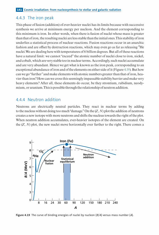
4.4.3 The iron peak

This phase of fusion (addition) of ever-heavier nuclei has its limits because with successivesynthesis we arrive at minimum energy per nucleon. And the element corresponding tothis minimum is iron. In other words, when there is fusion of nuclei whose mass is greaterthanthatof iron, the resulting nuclei are less stable thanthe initialones.This stabilityof ironunderlies a statistical process of nuclear reactions. Fusion reactions occur in an anarchicfashion and are o¡set by destruction reactions, which may even go as far as releasing 4Henuclei.We are dealing herewith temperatures of 6 billion degrees. But all of these reactionshave a natural limit: we cannot ‘‘exceed’’ the atomic number of nuclei close to iron, nickel,and cobalt,whichareverystable too in nuclear terms.Accordingly, such nuclei accumulateand are very abundant. Hencewe get what is known as the iron peak, corresponding to anexceptional abundanceof ironandofthe elementson either sideof it (Figure 4.19).Buthowcanwego‘‘further’’andmake elementswith atomic numbers greater than thatof iron, hea-vier than iron?Howcanwe cross this seemingly impassable stabilitybarrierandmakeveryheavy elements? After all, these elements do occur, be they strontium, rubidium, neody-mium,oruranium.This ispossible throughthe relationshipofneutronaddition.

4.4.4 Neutron addition

Neutrons are electrically neutral particles. They react in nuclear terms by addingto the nucleuswithout doing toomuch‘‘damage.’’On the (Z,N) plot the addition of neutronscreates a new isotopewith more neutrons and shifts the nucleus towards the rightof the plot.When neutron addition accumulates, ever-heavier isotopes of the element are created. Onthe (Z, N) plot, the new nuclei move horizontally ever further to the right. There comes a

A

Iron (Fe)

4He12C

Nuclearfusion

Neutronaddition

B/A

(M

eV)

3

08 16 24 30 60 90 120 150 180 210 240

9

8

7

6

5

4

Statisticalequilibrium

Figure 4.19 The curve of binding energies of nuclei by nucleon (B/A) versus mass number (A).


point, then, when the new nucleus lies outside the valley of nuclear stability. It is thereforeunstable.To return to the valley of stability it disintegrates by �� radioactivity.The neutronchanges intoaproton.By the sametoken,Z increases.Anewchemical elementhas thereforebeenmade.New isotopes andnewchemical elements canbemadebyneutronaddition.Thisis a general outline. In actual fact, the neutron addition process has two variants dependingon the relative number of neutrons and the equilibrium established between the addition ofneutronsandradioactivity.

If theneutron£ux isweak, theradioactivityof isotopestotherightofthevalleyofstabilityis abarrier. Such isotopes disintegrate as soon as they form andwe zigzag across the (Z,N)plot (Figure4.20).

If the neutron £ux is veryhigh, radioactivityhasnotimetodisintegrate fully the radioac-tive nucleiwhich are‘‘loaded’’with extra neutrons and in turn give rise to other radioactiveisotopes which move further to the right of the (Z,N) plot (Figure 4.21). Of course, decayalso occurs and a £ux of new nuclei is formed, with larger Z numbers. New chemical ele-mentshavebeen synthesized.

The two ¢gures (Figures 4.20 and 4.21) clearly show the two processeswhich are termeds-process (slow)and r-process (rapid), respectively.

A few simple rules can be laid down to check whether an isotope of a heavy elementhas been synthesized by an s-process or an r-process or by both. A stable isotope to theright of a radioactive isotope (short period) cannot have been formed by an s-processsince the radioactive isotope is a barrier to any further horizontal rightwards shift.If itoccurs innature, then itmusthavebeen formedbyanr-process.However,anyadjacentstable isotope may be the outcome of an s-process. Conversely, any stable isotopelocatedonthe samenegative diagonal as an isotopeofanotherelementof lowermass can-not have been created by an r-process as it is ‘‘shielded,’’ protected by the other isotope(Figure 4.21).

Averysimpleandconvenientequationwhichthe s-processobeys is:

NA�1NA

¼ AA�1

whereN is the abundance, the e¡ective cross-section of neutron absorption, and A andA^1aretwoisotopeswith decreasingmassnumbers.

Theabundance ratiosofthetwoisotopesare in inverseproportiontotheire¡ective cross-sectionsofneutron absorption.Letus show this simply.Thekinetic equationofproductionof isotopeA iswritten:

d NAð Þdt

¼ � A�1 NA�1 � A NAð Þ

where �n is the neutron £ux,NA^1andNA are the numbers of atoms of atomic numbers AandA^1,andA^1andAarethe e¡ective cross-sections.

This is a classic destruction^production equation like the one written for 14C. If equili-brium is attained:

d NAð Þdt

¼ 0:


Therefore:

A�1 NA�1 ¼ A NA:

Ourassertion hasbeendemonstrated.Nowconsider the transitionby��decay:

d AZN��

dt¼ �NA�1

A�1Z N� l A

ZN�:

Protonnumber

P

N N+1 N+2 N+3 N+4Neutron number

P+1 β radioactivity

1 neutron 2 neutrons 3 neutrons

Unstable

Protonnumber

26

Neutron number

27

28

29

30

Iron

Cobalt

Nickel

Copper

Zinc

30 31 32 33 34 35 36 37 38 39

Figure 4.20 The s-process on the proton–neutron plot. Top: theoretical pathway of neutron reactions.In blue, the first radioactive isotope. There is a change of elements up to the left by �� decay. Bottom:example of s-process pathways on the proton–neutron plot allowing the creation of elements heavierthan iron. After Broecker (1986 ).


Protonnumber

P

N N+1 N+2 N+3 N+4 N+5 N+6 N+7 N+8 N+9

Neutron number

Proton number

Zirconium 40

Molybdenum 42

Yttrium 39

Strontium 38

Rubidium 37

Krypton 36

Bromine 35Selenium 34

Niobium 41

Arsenic 33

Germanium 32

Gallium 31

48 49 50 51 52 53 54 55 56Neutron number

Stable isotope produced by r-process

Stable isotope not produced by r-process

Radioactive isotope on pathway of r-process

Neutron capture by r-process

β radioactivity during r-process

β radioactivity after r-process

Figure 4.21 The r-process on the proton–neutron plot. The neutron flux is intense enough forconsiderable horizontal shift to the right before radioactivity becomes a barrier. But, of course, allradioactivity plays a part before the barrier effect kicks in. After Broecker (1986).


Productionofthebarrier radioactive isotope is notedwithan asterisk (*), andl is the decayconstant.

d AZþ1N� �dt

¼ l AZN� � �N A A

Zþ1N�:

If equilibrium occurs, the radioactive term between the two equations is eliminated,giving:

A�1A�1

ZN ¼ A AZþ1N:

This is the samerelationasbefore.The abundance of isotopes of type s (i.e., formed by the s-process) heavy elements is

therefore determined by the e¡ective cross-sections of absorption of neutrons. Thesecross-sections canbemeasured inthe laboratory (theyare required forconstructingatomicreactors).

Exercise

Strontium has three isotopes, of masses 88, 87, and 86. Their effective cross-sections of

neutron absorption are 4.8, 60, and 48 millibarns, respectively. The ‘‘primitive’’ isotope ratios

of strontium are: 88Sr/86Sr¼ 8.3754, 87Sr/86Sr¼ 0.698, and 88Sr/87Sr¼ 11.99.

Can strontium isotopes be synthesized by the s-process?

AnswerLet us first apply the rule N1/N2¼2/1. We find the ratios 88Sr/86Sr¼ 10, 87Sr/86Sr¼ 0.8, and88Sr/87Sr¼ 12.5.

Let us compare this with observations. In view of the uncertainties on effective cross-

sections, the agreement is quite good. This is odd because 88Sr derives from both the s- and

the r-processes, which proves that the r-process is not important here.

Exercise

Table 4.4 gives the abundance N, the effective cross-section , and the product N for

samarium isotopes.

Calculate the proportion of the r-process involved in the formation of 147 and 149 isotopes.

Table 4.4 Data for samarium isotopes

Samarium isotope NA% Classa c (millibarn) N

144 2.87 p 119 55 342147 14.94 rs 1173 192 17600 2900148 11.24 s 258 48 2 930 540149 13.85 rs 1622 279 22500 4000150 7.36 s 370 72 2770 535152 26.90 ror rs 411 71 11100 1900154 22.84 r 325 61 7430 1400

aFordetailsofthep-process, seenextsubsection.


AnswerIf we take the 148 isotope, which is a pure s-process isotope, the (s) isotopes give a N value�2930.

We can therefore write:

percentage (r) of 147 ¼ 17 600� 2930

17 600

� �� 100 ¼ 83:35%

percentage (r) of 149 ¼ 22 500� 2930

22 500

� �� 100 ¼ 86:97%:

4.4.5 The p-process

Some isotopes are depleted in neutrons (and so have ‘‘surplus’’protons). In the chart of thenuclides they lie to the left of the valley of stability, o¡ the s-process pathway, and shieldedfrom the r-process.They include for example 84Sr, 92Mo, 124Xe, and 144Sm.They are calledp-process nuclides (or p-isotopes) andare said tobe formedby the p-process.The produc-tion process is fairly obscure but we do know that the abundance of p-isotopes plottedagainst (Z) forms a curvewhich roughly follows thatof the s- and r-isotopes except that theabundance levels are much lower.To get some idea, the abundance ratios for silicon are:s-process¼ 1, r-process¼ 0.5, andp-process¼ 0.02.

It canbe inferred, then, thatthep-process is secondaryand tracks the s- and r-processes,thus supplementing them. Nowadays it is thought that the p-process is mainly caused by(�,) reactions in supernovae.

4.4.6 The light elements lithium, beryllium, and boron

When the abundance of chemical elements is plotted against their atomic number(Figure 4.22), it can be seen that three light elements, lithium, beryllium, and boron, areunderabundant compared with their atomic numbers. The He burning nucleosyntheticprocess seems to have leapfrogged them, with three 4He nuclei eventually combining togive12C.Andyetthese elements doexist!Howdidtheycometobe?

Their formation is attributedtotwocauses:

� theBigBang for lithium inpart;� spallation reactions in interstellar space caused bygalactic cosmic radiation and acting

on interstellarmaterial.

This explains the abundance curve of the chemical elements and isotopes (Figure 4.22).Butwhatstructuresproducethese reactions?Wenowneedto speakaboutthe stars.

4.4.7 The stellar adventure: the life and death of stars

Letusnowlookatwhatnucleosynthesis is as theastrophysicist sees it.The Universe is populated by stars clustered into galaxies. These stars are of di¡erent

sizes andbrightnessesbut theyare all gigantic nuclear reactors.Nuclear reactions take place


inside the starswhichgiveo¡energy. Electromagnetic radiation, and light radiation inparti-cular, is given o¡ from the star’s surface. Abalance is established between the two processesanditishowlongthisbalanceismaintainedthatdeterminesthestar’slifetime.Whentheequi-librium isdisrupted, that is,whenthefuel is exhausted, thestarchangesnature.The characteristic feature of nuclear reactions is that they need a certain amount of

energy to‘‘ignite.’’Once triggered,mostof themproduce considerable quantities ofenergyintheir turn,becausetheyconvertmatter into energy, inaccordancewithEinstein’s famousformula�E¼�mc2.What is the source of energy triggering these nuclear reactions?Gravitational energy. A

star isbornwhen an interstellar cloudofgas anddust contractunder the in£uence ofgravity,that is the mutual attraction exerted by all components of matter. The contraction of thecloudgenerates energyby the impactsproducedbetween‘‘portions’’ofmatter.Whenthetem-perature reaches about10million degrees, hydrogen fusion occurs and a star isborn.This iswhathappenedforourSunsome4.57Gaago.Thebirthofordinarystars is themosteveryday,the most commonplace phenomenon in the Universe. Most stars are of this type. Like theSuntheycanmakeonlyhelium.The stars are classi¢edby theHertzsprung^Russell (H^R)diagram on which we plot brightness against color, that is, the star’s temperature(Figure 4.23).White is veryhot and red is cooler.Most stars lie on the leading diagonal of thediagram,which is therefore calledthemainsequence.

OXYGENMAGNESIUM

SILICONIRON

Constitutiveelements

ofinner

planets

1010

108

106

104

102

10–20

1

20 30 40 50 60 70 80 90 10010

Proton number (Z)

Ab

un

dan

ce r

elat

ive

tosi

lico

n n

orm

ed t

o 1

06 {

HYDROGEN

HELIUM

CARBON

NITROGEN

{ Constituentelements

ofgiant

planets

Trace elements in planets and meteorites

αelements

Ironpeak Neutron addition

Figure 4.22 Abundance charts of elements in the cosmos. The scale is logarithmic. Silicon (Si) is taken asthe reference. After Broecker (1986).


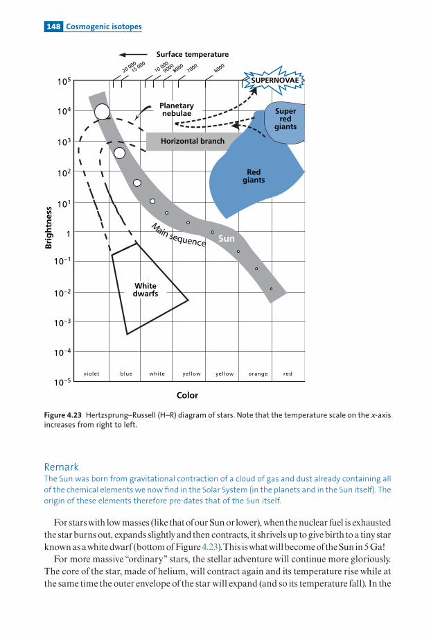
RemarkThe Sun was born from gravitational contraction of a cloud of gas and dust already containing all

of the chemical elements we now find in the Solar System (in the planets and in the Sun itself). The

origin of these elements therefore pre-dates that of the Sun itself.

Forstarswith lowmasses (like thatofourSunorlower),whenthenuclear fuel is exhaustedthe starburns out, expands slightlyand then contracts, it shrivels up togivebirth toatinystarknownasawhitedwarf (bottomofFigure4.23).This iswhatwillbecomeoftheSun in5Ga!

For more massive ‘‘ordinary’’ stars, the stellar adventure will continue more gloriously.The core of the star, made of helium, will contract again and its temperature rise while atthe same time the outer envelope of the star will expand (and so its temperature fall). In the

20 00015 000

10 0009000

80007000

6000

Surface temperatureB

rig

htn

ess

violet blue white yellow yellow orange red

105

104

103

102

101

1

10–1

10–2

10–3

10–4

10–5

Color

Whitedwarfs

Sun

Planetarynebulae

Redgiants

Superred

giants

Horizontal branch

SUPERNOVAE

Main sequence

Figure 4.23 Hertzsprung–Russell (H–R) diagram of stars. Note that the temperature scale on the x-axisincreases from right to left.


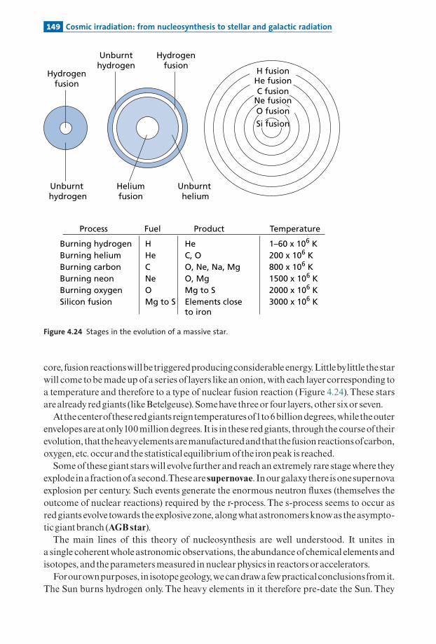
core, fusion reactionswillbetriggeredproducingconsiderable energy.Littlebylittlethestarwill come tobemadeup ofa series of layers like an onion, with each layer corresponding toa temperature and therefore to a type of nuclear fusion reaction (Figure 4.24).These starsarealreadyredgiants (likeBetelgeuse). Somehavethreeor four layers, other sixor seven.Atthe centeroftheseredgiantsreigntemperaturesof1to6billiondegrees,whiletheouter

envelopesareatonly100milliondegrees. It is in these redgiants, throughthe courseoftheirevolution, thattheheavyelementsaremanufacturedandthatthefusion reactionsofcarbon,oxygen, etc. occurandthe statistical equilibriumofthe ironpeak is reached.Someofthesegiant starswill evolve furtherand reach an extremely rare stagewhere they

explodeinafractionofasecond.Theseare supernovae. Inourgalaxythereisonesupernovaexplosion per century. Such events generate the enormous neutron £uxes (themselves theoutcome of nuclear reactions) required by the r-process.The s-process seems to occur asredgiants evolvetowards the explosivezone, alongwhatastronomersknowastheasympto-ticgiantbranch (AGBstar).The main lines of this theory of nucleosynthesis are well understood. It unites in

a single coherentwholeastronomicobservations, theabundanceofchemical elements andisotopes, andtheparametersmeasured in nuclearphysics in reactorsoraccelerators.Forourownpurposes, in isotopegeology,wecandrawafewpractical conclusionsfromit.

The Sun burns hydrogen only. The heavy elements in it therefore pre-date the Sun. They

Hydrogenfusion

Unburnthydrogen

Hydrogenfusion

Unburnt hydrogen

Burning hydrogen H He 1–60 x 106 K

Process Fuel Product Temperature

Burning helium He C, O 200 x 106 KBurning carbon C O, Ne, Na, Mg 800 x 106 KBurning neon Ne O, Mg 1500 x 106 KBurning oxygen O Mg to S 2000 x 106 KSilicon fusion Mg to S Elements close

to iron3000 x 106 K

Heliumfusion

Unburnt helium

H fusionHe fusionC fusion

Ne fusionO fusion

Si fusion

Figure 4.24 Stages in the evolution of a massive star.


were formed in red giants or ancient supernovae.This simple remark allows us to under-stand that thehistoryof theUniverse is ahistoryofstellar cycles. Stars areborn, synthesizeelements, and die, and their material is scattered into interstellar space.There the variousclouds mix and mingle the material synthesized previously.They wander around the cos-mos until the day newgravitational contraction occurs.This gives rise to a new star, whichin turnmakesmatteranddisperses it in theUniverseand soon.One supernovapercenturyis not a lot, but that still makes 10 thousand every million years, or 40 million since theEarth¢rst formed (and inourgalaxyalone).

Thesepre-solarheavyelementswerethereforemade in redgiants andsupernovaedatingfromsolar prehistoryandthen extensivelymixed in interstellar space.

Forus earthlings, aspartsoftheSolar System, thereare twomajordates in this cosmichis-tory: theBig Bang and the formation of the Solar System.The Big Bang was the event withwhich our universebegan.Astronomers nowdate it to13 billionyears ago. For them, it is theinstant atwhich matterasweknow it came intobeing in aphenomenal process ofexpansionand heating. In the course of thisprocess hydrogen, helium, anda little lithiumwere formed.Then everything arranged itself into galaxies, stars, and planetary systems. It was in thecourseofthis stellarhistory thatall theotherelementsheavier than lithiumweresynthesized.

The formation of the Solar System occurred4.6^4.5 billionyears ago.Weshall go into thisdatemore closelybutatthispointanorderofmagnitudeisenough.TheSolarSystemgatheredupmattermadeinpreviousstellarprocessesincludingexplosionsofsupernovaeorredgiants.All this matter was mixed and arranged itself into a central star with orbiting planetarybodies. But to account for the existence at the time the Solar System formedofwhat are nowextinct forms of radioactivity we must accept that red giants and supernovae existed andexplodedjustbefore its formationandthattheyarethesourceoftheseformsofradioactivity.

This scenarioof late explosivenucleosynthesis (redgiantand/orsupernovae) tosynthe-sizeheavyelements in the Solar System has recentlybeen challenged (or supplemented) byasecondscenario, thatofprimitive irradiation. Inthismodel it is acceptedthatas itformedthe young Sun emitted extremelyhigh-energy particles which in turn produced spallationreactions on the solar material and that these reactions in particular produced the extinctformsofradioactivity.This scenario is thoughtnecessary toproduce the10Be discoveredbyateamfromNancy(France) (McKeegan etal.,2000)andthe 36CldiscoveredmorerecentlybyaChinese team (Lin etal., 2005).However, itdoesnotseemtobeable tomake 53Mn.Thetwoprocesses probablyoccurred in succession, but inwhat proportions? This is averyhotsubjectatpresent.

All these eventshave left traces inmeteorites.Theseobjects, which date fromthe time theEarth, planets, and Sun were formed, contain extraordinary information. Near their sur-faces are cosmogenic isotopeswhich informus about cosmic radiation, but also about thetimetheyhave spent in theUniverseas smallpiecesofrock.However, someofthemcontaingrainsof interstellardustwhose isotopic composition in certain elements informsus aboutthe r- and s-processes of nucleosynthesis. These processes, as described, occurred wellbefore thebeginnings ofour Solar System.This is true for most, save one category: extinctradioactivity,whichwehavealreadycomeacross.Meteorites arean invaluable linkbetweencosmic and terrestrial processes. For physics, there is a continuumbetween stellar nucleo-synthesis and nuclear reactions produced by particle £uxes from the Sun or from cosmicradiation.


This scenario is the one that has occurred tirelessly in the Universe over10 or14 billionyears. But in the beginning, what was there? What matter? The beginning was the BigBang, which synthesized the elementary particles, hydrogen, helium, and lithium andenacted an essential event . . .which lies outside the scope of thisbook, although it impreg-nates everypartof it!

Problems

1 Carbon-14 is produced by nuclear reactions on 14N, but it also decays to 14N. We propose to use

this decay scheme for dating purposes as is done with 87Rb–87Sr or 40K–40Ar, for example.

We consider that to make a measurement, 14N/15N must differ from the normal value (� 276)

by 1 � 10�5. What should the C/N ratio be to apply this method to objects that are, say, 15 000

years old? Do you think this would be feasible?

2 The Holy Shroud of Turin long posed a problem for believers. Was it really the shroud in which

Christ had been wrapped? It first appeared in 1350 and the monks asserted it was a genuine

relic. It could not be dated by the traditional 14C method as there was not enough material, but

with AMS it could be dated with just 150 mg of cloth. The 14C age was between 600 and 800

years old. Given the correspondence curve in Figure 4.25, what is the age of the Holy Shroud?

3 We measure the isotopic composition of K in an iron meteorite having undergone cosmic

irradiation for 500 Ma. The mass spectrum of K measured is a mixture between the cosmo-

genic mass spectrum and the normal mass spectrum. Estimating that (40K)normal is negligible,

establish the equation for determining (41K/40K)cosmogenic. (Suppose the normal K isotope

ratios are known.)

500

3001100

850

Years BP

650 450

1300 1500

700

900

1100

Calendar age

Rad

ioca

rbo

n a

ge

Figure 4.25 Correspondence curve of the radiocarbon age and calendar age of the Turin Shroud.

151 Problems

4 Chlorine-36 is created in the atmosphere by spallation reactions on 40Ar, and T1/2¼ 3 � 105

years. From the time of its creation, the chlorine is incorporated in water masses and in the

hydrological cycle. The 36Cl/Cltotal ratio is 100 20 � 10�5 in rainwater at the Earth’s surface.

We analyze the water sampled from a deep aquifer and find 5 � 10�15 for the 36Cl/Cltotal ratio.

How old is the groundwater?

5 Here is a series of 10Be/9Be measurements on a manganese crust.

(i) What is the rate of accretion?

(ii) What is the error?

Depth (mm) 10Be/9Be 2

Surface 3.940.32 � 10�8

0–1.0 3.230.12 � 10�8

1.5–2.0 2.190.25 � 10�8

2.5–3.0 1.790.08 � 10�8

3.5–4.0 1.410.06 � 10�8

4.0–5.0 1.040.07 � 10�8

5.0–5.7 9.000.52 � 10�9

5.7–6.0 5.980.88 � 10�9

6.0–7.0 5.200.44 � 10�9

8.0–8.5 3.940.26 � 10�9

8.5–9.0 2.690.62 � 10�9

9.0–10.0 2.390.40 � 10�9

10.7–11.7 1.850.44 � 10�9


CHAPTER FIVE

Uncertainties and results ofradiometric dating

5.1 Introduction

Thepurposeofthis chapter istoreviewradiometricdatingmethodsasappliedbothtoterres-trialandtocosmicproblems.Weshallspeakofthemajorresultsthatnow¢xthechronologicalframeworkoftheEarth’shistory, not forgetting thatwhattheymean is inseparable fromhowreliable theyare.The central questionwe shall be dealingwith in this chapter is: how reliablearethegeologicalageswedetermine?Inotherwords,whatis thelevelofuncertaintya¡ectinganagedetermination?1Whatguaranteehavewethatthisage isgeologicallymeaningful?Ascertaining theuncertainty�,whenweobtainavalueT, allowingustowritethattheage

is T��, is a problem that breaks down into various sub-problems, some of which areuncommon even in books on uncertainty. Let us get our ideas straight with a simpleexample.Supposewemeasure a series ofrocksby the 87Rb^87Srmethodand theanalytical results

are just aboutalignedonthe (87Sr/86Sr,87Rb/86Sr) diagram.Howcanwemeasure the slopeof the straight line isochron to calculate the age of the rocks? Any experimental physicistwill tell you that you ¢rst need to know the uncertainty a¡ecting each individual physicalmeasurement: the strontium isotope ratios and the absolute values in 87Rb and 86Sr. Andthenthatyouneedtoestimatetheslopeofthestraight linebyusingtheleast-squaresmethodwhere the ‘‘weight’’of each data point is measured by its individual uncertainty.We thenobtain an age and an uncertainty value re£ecting the dispersion of data points relative tothe straight line we calculated.This approach, which has been tried and tested by years ofstatisticalpractice, seemsunassailableonthefaceof it.Andyet,as soonas it isputintoprac-tice, it raises questions that are not to do with mathematical statistics but with what wemightcallgeological understanding.The ¢rst question is: should we attribute the analytical uncertainty measured in the

laboratory to all the datapoints?Despite the reassuring lookofthis question,which invitesus to answer ‘‘yes,’’ we need to realize that such‘‘automatic’’attribution is not as safe as wemightthink. In fact, the rockswith thehighest 87Rb/86Sr values andtherefore 87Sr *values,are probably those that, in the course of geological history, have been the most likely to

1 To avoid any confusion with the word ‘‘error’’ used in ordinary language it is now recommended to use theterm uncertainty in scientific work. The word error is used when we know the difference between the true

value and the measured value; uncertainty is an estimate of this error. I shall try to abide by this logical rule,although it goes against decades of habit. Indeed, it has often been used in the first three chapters.

lose 87Sr* through exchanges with adjacent rocks. Logically, we should therefore attributegreater uncertainty to theirages than to thoseofother rocks andmeasure the de¢cit in geo-logical robustness.Moreover, suchuncertaintywouldbeasymmetricalbecause the lossof87Sr* leads to a reduction in the 87Sr/86Sr ratio (Figure 5.1). Should we therefore increasetheanalyticaluncertaintyofageologicaluncertainty?

Another question arises. Given that we are working with a natural system and that theconditionsofthebasicmodel (perfect initial isotopichomogenization, boxclosed since theorigin)haveprobablynotbeenstringentlyobserved, thedatapointsaredistributed‘‘statisti-cally’’ (thatis,moreorlessaccurately)aroundthebeststraight-line¢t.Howmuchdispersionis acceptable for it to be considered that we are indeedworking within the frameworkof atheoretical model and therefore that the age determination is legitimate? This is a di⁄cultquestion and evenmore so ifyou thinkthat, aswegoback in time, thevagaries ofdisruptivegeological phenomena become ever more probable and that the alignment must be lessgood for Precambrian rocks than for rocks of the Secondary era, say.Therefore geologicaltolerance for non-alignmentmust logically increasewithage.Byhowmuch?Towhatextentcanweacceptnon-alignment, even for veryold rocks?Wemust remember that, in additiontomeasurementuncertainty, analyticaluncertainty too is a functionofage.There is, then, aseriesofpriorquestions toourcentralquestion: is agedetermination reliable?

There is a second aspect to this issue of the reliability ofmeasurements, that of the geo-logical signi¢cance ofthe age obtained. Imaginewehave an age in thousands,millions, orbillions ofyears, together with its uncertainty.What does the numberobtained correspondtogeologically?Letus return toour series of rockswhoseageshavebeen determinedby the87Rb^87Srmethod. Is the 87Rb^87Sr straight line a‘‘mixing line’’or an isochron?Chapter 3(Section 3.4) gave us a test for deciding between these two hypotheses. Supposewe think it

Geologicaluncertainties

87Sr

/86 S

r

87Rb/86Sr

a b

Excluded

c

Figure 5.1 A series of Rb–Sr measurements plotted on the isochron diagram. After examining thedispersion of data points, there seem to be three options for obtaining the ‘‘best age.’’ (a) We cancalculate the best straight-line fit using all of the data points to which analytical uncertainty has beenattributed and obtain an age determination. The uncertainty of the pattern suggests that this age isvery much influenced by samples 6 and 7. (b) We add a geological uncertainty to samples 6 and 7because they are the most radiogenic and so liable to have lost 87Sr. We then calculate the best straight-line fit. (c) We eliminate samples 6 and 7 and use samples 1–5 alone to calculate the best straight-line fit.

154 Uncertainties and results of radiometric dating

plausible we have an isochron.What does this mean? Our basic model is of a closed box inwhichwe enclose radioactive and radiogenic isotopes at awell-de¢ned‘‘instant’’T0. But towhat does this formal theoretical model correspond in the world of nature? Suppose that,togetour ideas straight, the series ofrocks in question is a series ofgranite rocks froma sin-glemassif. Is theageobtainedtheagewhenthegranitewas emplacedasamagmaor theageof the metamorphic basement whose partial melting gave rise to the granite mass?Assuming it is the emplacement of the granite that is dated, what is the exact time of thatemplacement?When themagma¢rst intruded?When it crystallized?Or is itwhen hydro-thermal circulation occurred, which seems to end the emplacement of granite massifs asattestedbyquartzveinssometimescontainingmetallicminerals?Onceagain, thisquestionis not unconnected to the age measured. And if we measure the minerals, have they notbeen subjectedtosomesubsequentevent?Didtheyall crystallizeatthesame instant?The duration of emplacement of granite being estimated at 1Ma in all (perhaps 2Ma),

whenwe date a granite that is 2 billion years old this question is irrelevant as our power ofresolution is insu⁄cient to distinguish the various episodes in its emplacement. But whenwedatethegranitesofthe islandofElba (Italy)as7or8Maold, thequestionbecomesacru-cial one.Weare left to‘‘date’’somethingwithout reallyknowingwhat it isweare dating! Theagewillbean‘‘averageage’’ofthe emplacementofgraniteonthe islandofElba, butwemustnot read more into it than that! That is, unless we have other independent informationtohand.This is the sortofquestionwearegoing to try to answer while exploring themajor results

obtainedby radiometric datingmethods. Eachwill be placed in the contextofhow reliableit is.We shall see that the preceding chapters have given some pointers for some of the pro-blems.Forothers,weshallneedtogivesubstancetoour intuitionsandattempttorationalizethem . . . or qualify them. But the ultimate test of any age determination by radiometricmethods ishowcoherent it iswithwhatwealreadyknow.Thisknowledgeformsthe chronologicalsettingwithinwhichthenewdetermination is to

be¢tted.Theoverall framework is formedby thegeological andcosmic timescale.The age of the Earth orof the Sun is a ¢xedpoint andour ultimate reference point in any

‘‘cosmic’’ chronology. At the same time, these general references are only known with adegree ofuncertainty because of all the sources we have referred to and are going to study.There is, then, constant feedbackbetweenadvancesonuncertainties and themajor results.Themajor results are tobe looked on as numbers that are liable to vary somewhator to seetheir underlying meaning change (we shall see this is the case for the age of the Earth).Weshall see there is abroad range ofuncertaintyas regards the chronologyof formation of theelements. Itistoemphasizethefundamental connectionbetweentheuncertainties inherentto the methods of radiochronology and its main ¢ndings that they have been broughttogetherhere inasingle chapter.

5.2 Some statistical reminders relative to thecalculation of uncertainties

WhenwemakeNmeasurements ofx, they are represented in a (N, x) plot by grouping thevalues ofx into classes.This is a histogram.WhenN is large and the results are distributed

155 The calculation of uncertainties

randomly, we consider that the best estimation of the true value sought is themean of themeasuredvalues (noted �x).

�x ¼ x1 þ x2 þ � � � þ xNN

¼

PNi

xi

N:

Toestimatetheuncertaintyassociatedwiththis,we consider thedispersionofthemeasure-mentsobtainedbycalculating the deviations fromthemean foreachmeasurementandtak-ing theiraverage. Inpractice,we calculatethesumofthe squareddeviations:2

Vx ¼XNi

ðxi � �xÞ2

andwedivideby thenumberofmeasurementsNminus1togetthemeanvariance:3

Vx ¼

Pi

ðxi � �xÞ2

ðN� 1Þ :

The standarddeviation is the square rootofthevariance:

�x ¼ffiffiffiffiffiffiVx

p¼

ffiffiffiffiffiffiffiffiffiffiffiffiffiffiffiffiffiffiffiffiffiffiffiPi

ðxi � �xÞ2

ðN� 1Þ

vuut:

The drawbackofusing�x is that it is expressed in units ofx. Sowe cannot compare, say, thedispersion for the isotopic measurement of lead and that of strontium.Tomake such com-parisonswede¢nethe reduced dispersion ��bydividing�xby �x:

�� ¼ �x�x:

This dispersionor reduceddeviation is expressedaspercent, permil, etc.Whenuncertainty is considered tobea random£uctuation due to factors that arepoorly

determined but which a¡ect each measurement and make it deviate around its true value,then results oftheoretical statistics canbeapplied. It canbe shown that if therewerean in¢-nite numberof randommeasurements, thevaluesmeasuredwouldbe distributed aroundameanvalueinaccordancewithwhatisknownastheLaplace^Gaussornormaldistribution(Figure5.2).The curveofthenormaldistribution iswritten:

y ¼ 1

�xffiffiffiffiffiffi2pp exp � 1

2

x� �x

�x

� �2" #

wherey is themeasurement frequencyand isafunctionofthevariablex.

2 We use the square so that positive and negative deviations are added and do not cancel out bysubtraction.

3 Suppose we have just one measurement. If we divide by N, the uncertainty would be zero whereas if wedivide by N� 1, that is by zero, it is indeterminate, which is indeed the case!


The curvey¼ f(x) has the famousbell shape. It is symmetrical about �x (mean).The stan-dard deviation �x is the distance between the point of in£ection and the mean.The maxi-mumdeviation is equal toabout�3�x or 99.7%.

RemarkThe converse of this last observation is important: if a distribution is random and we know its

maximum dispersion D, we can then estimate �x¼D/6. This dispersion is known as the maximum

range.

In practice, the distributions and parameters calculated are increasingly signi¢cant as weapproach the theoretical distribution, that is, as the numberofmeasurementsN increases.Unfortunately,N isnotalwayshigh.When the shapeofthehistogramcanbe representedbyabell-shaped curve,weapply the

results obtained for the ideal distribution with a very large N to such histograms(Figure 5.3). Let us say that in making this assimilation we are being optimistic about theuncertainty. In statistics it is shown that this uncertainty is estimated by multiplying thestandard deviation of the histogram measured (�) by 1=

ffiffiffiffiNp

.The more measurements wemake, the lower the riskofuncertainty, of course, but this decrease obeys the square-rootlaw.Uncertaintyonx,written�x, is thereforede¢nedas:

Dx ¼�xffiffiffiffiNp� �

:

As, in the absence of other information, the standard deviation is the quadratic mean ofdeviations, thetotaluncertainty is therefore:

Dx ¼

ffiffiffiffiffiffiffiffiffiffiffiffiffiffiffiffiffiffiffiffiffiffiffiPi

ðxi � �xÞ2

ðN� 1Þ

vuut2664

3775 � 1ffiffiffiffi

Np :

0.4

–2σ –σ 0

Pro

bab

ility

σ 2σ 3σ–3σ

0.3

0.2

0.1

σx

x − x−

Figure 5.2 The normal curve. The probability of a measurement occurring, or its frequency, is plotted againstthe value of the measurement on a scale expressed in x–x (value corrected by the mean). The distancebetween the points of inflection is the dispersion �. Note the geometrical signification of 2� and 3�.


Naturally, relativeuncertaintymayalsobede¢nedhere:

�D ¼ Dx

�x:

Thisuncertaintyhasnounitand is expressedaspercent,permil, etc.This formulabywhichuncertainty varies as1=

ffiffiffiffiNp

is absolutely fundamental. It indicates that after estimatingdispersionbasedon thehistogramofexperimentalvalues,we estimate the reliabilityofthisuncertainty by attributing to it a weight of 1=

ffiffiffiffiNp

. If we make 10, 100, 1000, and 10 000measurements, precision improves to30%,10%,3%,and1%.

RemarkIt can be shown in statistics that if, for a normal distribution, we consider an uncertainty��x, we

have a 63% chance of the real value lying within this interval. If we take � 2�x, that is a greater

uncertainty, this probability reaches 95%. In the first case we speak of high-risk uncertainty, and in

the second of low-risk uncertainty.

In practice, then, we measure uncertainties to the nearest sigma or two sigmas, by theexpressions:

� �xffiffiffiffiNp or � 2�xffiffiffiffi

Np

whereN is thenumberofmeasurements.A further procedure must be added to these: that of the elimination of aberrant values

(outliers).Somevaluesmeasuredare completelyoutoflinewiththehistogram.These‘‘aber-rant’’ values are thought to arise from some random accident during measurement (typi-cally a sudden £uctuation in electric current when making a measurement on the massspectrometer, or the sampling of an apparently sound rockwhich proves to be weatheredwhen analyzed more closely).The following criterion is used to eliminate these values: all

N

Concentration (ppm)

10

19.0 20.0 21.0

8

6

4

2

12

Figure 5.3 Histogram of 100 measurements of strontium concentration in a series of rocks from asingle site. The histogram and the normal curve approximating it are shown. The mean is 20 ppm, thedispersion �¼ 0.5 ppm. We can therefore write concentration C¼ 20� 0.5 ppm. Relative uncertainty iswritten 0.5/20¼ 2.5%.


the values beyond �3� are eliminated, and then the entire calculation is repeated. Theresulting uncertainty that has been ‘‘cleaned’’ of extreme outliers is denoted �x* or �D�dependingonwhether it is anabsoluteor relativeuncertainty.We now need to introduce a few useful distinctions (Figure 5.4).The accuracyof a mea-

surement is estimated from the deviation between the measured value and the true valuesought.Precision or reproducibility is the dispersion ofameasurement repeatedN times:it is this dispersion dividedby themeanvalue.Reproducibility canbe estimated fromahis-togram ofmeasurements. Accuracy can only be estimated if we have independent knowl-edge (or an estimate) of the true values. The power of resolution in geochronology is thesmallest age di¡erencewe can measurewith anyguarantee of reliability. It is de¢ned as thequantity signi¢cantly di¡erent from zero that can be estimated between two events:R¼ t1� t2.ToestimateR,weassumethedeviationmustbegreater thanthesumofthestan-darddeviations:R � �t1 þ �t2 .

Exercise

The 206Pb/204Pb ratio of a rock is measured six times giving: 18.35, 18.38, 18.39, 18.32, 18.33,

and 18.35. What value will we give for the isotopic composition of this rock? What is the

precision achieved? Is it worth making another six measurements given that the reproduci-

bility of each measurement is 3ø?

N

x measuredvalues

truevalue

N

xtruevalue

a

c xtruevalue

xtruevalue

b

d

Figure 5.4 The difference between reproducibility and accuracy. (a) Good reproducibility but pooraccuracy; (b) poor reproducibility and poor accuracy; (c) poor reproducibility but good accuracy; (d)good reproducibility and good accuracy.


AnswerSupposing the uncertainty values of each measurement are equal, we calculate:

�x ¼ 18:353;� ¼ 0:025;Dx ¼ �x=ffiffiffiffiNp¼ 0:010; �D ¼ Dx=x ¼ 5:4 � 10�4:

We can therefore write �x ¼ 18:353� 0:010 with 63% confidence and �x ¼ 18:353� 0:02 with

95% confidence.

If we were to make another six measurements, precision would move from 0.01 to 0.0077,

which is a gain of 4 � 10�4. But the precision of a single measurement is 3 � 10�3, therefore it

is not worthwhile (except in special cases).

RemarkIt is worth pondering that the numerical calculation gives more figures after the decimal point for

a much larger number of measurements (to be exact �¼ 0.024 94). Now, we have written

�¼ 0.025 because the figures 94 are not significant. This approach is in line with the answer to

the famous question: can we measure the length of a table to the nearest tenth of a millimeter

using a measuring rod graduated in centimeters? Common sense is as good a guide to the answer

as mathematics.

Exercise

Here are two histograms of measurements of 87Sr/86Sr ratios for a single sample

(Figure 5.5). The first consists of 20 measurements with a mean value of 0.709 166, with

�x¼ 2.31 � 10� 5. The second consists of 400 measurements with a mean value of 0.709 184

with �x¼ 4.34 � 10� 6.

6

0.70

9 1

0.70

9 15

0.70

9 2

0.70

9 25

4

2

87Sr/86Sr

Freq

uen

cy

a

87Sr/86Sr

40

30

20

10

0.70

9 25

0.70

9 2

0.70

9 15

0.70

9 1

Freq

uen

cy

b

Figure 5.5 Histogram of 87Sr/86Sr ratios measured on a single sample. (a) 20 measurements, (b) 400measurements. Notice that the classes become narrower as the number of measurements rises.


(1) What is the uncertainty affecting the measurement?

(2) How many measurements need to be made to get a standard deviation of 1 ppm?

(3) In this last case, do you think the uncertainty should be taken as� �x=ffiffiffiffiffiNp

or� 2�x=ffiffiffiffiffiNp

?

Answer(1) Intrinsic uncertainty is determined from the (ln �, ln

ffiffiffiffiffiNp

) curve as 111 ppm.

(2) It would take 10 000 measurements.

(3) With ��x=ffiffiffiffiffiNp

, the 400 ratio measurement lies outside the uncertainty limits on the 20

measurement expression. However, with �2�x=ffiffiffiffiffiNp

it is within limits. The latter expres-

sion is therefore required.

Exercise

Two 14C ages are measured: 3230� 70 years and 3260� 60 years. Are these ages significantly

distinct? What is the power of resolution of 14C for 3000 years?

AnswerThe two ages are not significantly different as their standard deviations overlap. The power

of resolution of 14C for 3000 years is 2%, or 60 years, which is a somewhat optimistic

estimate!

5.2.1 Systematic uncertainties

Randomuncertaintiesaredeviationsofmeasuredvalues fromthetruevalue causedbyvag-aries obeying the lawsofchance.‘‘Chance is aword thathides our ignorance,’’as themathe-matician and great scholar of probability E¤ mile Borel used to say. But some uncertaintiesaresystematic, thatis, theya¡ecttheoutcomeofmeasurementsbythesamefactor,althoughthat factor is not necessarily a known one. These really are random ‘‘errors.’’ Here’s anexample.As stated, radioactive constants are a¡ected by measurement uncertainty and so are

periodically ‘‘updated,’’ that is, improved.When we calculate an age with one of the dat-ing formulae we have developed, with the given value of a constant, we invariably intro-duce the same uncertainty (but the amplitude of the uncertainty is not always thesame). Such uncertainty is not really troublesome when the same method is used sys-tematically.We then draw up a dating scale which can always be adjusted as required.But whenever we wish to use ages obtained by methods based on di¡erent decay ratesand compare them, uncertainties about decay constants become very troublesomeindeed.Another systematicuncertaintymayarise fromthe systemofphysicalmeasurements.As

described, international standards are used for calibrating any systematic uncertaintiestheremaybe among laboratories. Avalue is set for these standards although one cannotbesure it is accurate.Hereagain, this approach,whilenecessary, isnot fullysatisfactorywhen-ever several methods are used. And what if some of the standards were wrong? After all,even the U.S. National Bureau of Standards, the ¢nal arbiter, makes ‘‘errors’’ too and givesits resultswithmarginsofuncertainty!


5.2.2 Pseudo-random uncertainties

In theproblemswe dealwith, uncertainty is often a combination ofsystematic and randomphenomena.When we spoke in Chapter 3 of the histogram of 40K^40Ar ages, which isasymmetrical, we said it was better to take not the mean as the most likely age value butthe mode (the value most frequently measured) as the asymmetry was probably caused bydi¡usion of the radiogenic isotope 40Ar, which tends to‘‘lower’’ the age. Superimposed ona random distribution due, say, to measurement uncertainties, we have a systematic trendofargon di¡usion. Evenwhen a large numberofmeasurements aremade, pseudo-randomdistributions are generally asymmetrical relative to the normal distribution (Figure 5.6).Anyofthreetypesofparametermayrepresentthetruevaluesought.

Themean is de¢nedas inthenormaldistributionby:

�x ¼Xi

xiN:

Themode is the value occurring most frequently in the distribution. It is, mathematically,themost likely value.Themedian is the value dividing the samplemeasured into two equalhalves. It iswhatwemightcall thehalfwayhouse.

Exercise

The U–He age of a series of magnetites is measured. Table 5.1a shows the distribution of

apparent ages and Table 5.1b the distribution of uranium contents.

(1) Draw the corresponding histograms.

(2) Calculate the mean age and mean U content. Calculate the modes and medians.

(3) What is your geological interpretation of these results?

AnswerMean age¼ 26.3 Ma; median age¼ 27 Ma; modal age¼ 30 Ma.

Mean U content � 25 ppb; median U content � 25 ppb; modal U content � 25 ppb.

The most likely geological age is 30 Ma since the distribution of uranium is virtually normal,

which is evidence that it has not been disrupted subsequently. The asymmetry seems to result

Freq

uen

cy

X

mode medianmean

Figure 5.6 The difference between mode, median, and mean illustrated on an asymmetrical distribution.


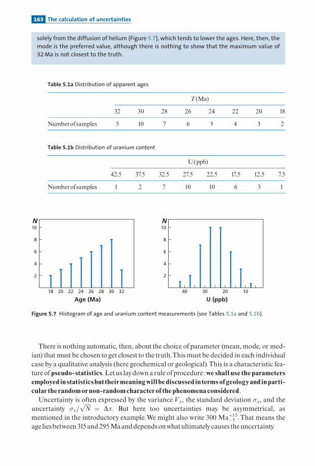
solely from the diffusion of helium (Figure 5.7), which tends to lower the ages. Here, then, the

mode is the preferred value, although there is nothing to show that the maximum value of

32 Ma is not closest to the truth.

There is nothing automatic, then, about the choice of parameter (mean, mode, or med-ian) that mustbe chosen to get closest to the truth.This must be decided in each individualcase by a qualitative analysis (here geochemical or geological).This is a characteristic fea-ture of pseudo-statistics. Letus laydown a rule ofprocedure:we shall use the parametersemployed in statisticsbuttheirmeaningwill be discussed in termsofgeologyand inparti-cular the randomor non-randomcharacterof thephenomenaconsidered.Uncertainty is often expressed by the varianceVx, the standard deviation �x, and the

uncertainty �x=ffiffiffiffiNp

¼ Dx. But here too uncertainties may be asymmetrical, asmentioned in the introductory example.We might also write 300 Maþ15�5 . That means theage liesbetween315and295Maanddependsonwhatultimatelycauses theuncertainty.

Table 5.1a Distribution of apparent ages

T (Ma)

32 30 28 26 24 22 20 18

Numberofsamples 3 10 7 6 5 4 3 2

2

4

6

8

10

18 20 22 24 26 28 30 32

N

Age (Ma)

2

4

6

8

10

40 30 20 10

N

U (ppb)

Figure 5.7 Histogram of age and uranium content measurements (see Tables 5.1a and 5.1b).

Table 5.1b Distribution of uranium content

U(ppb)

42.5 37.5 32.5 27.5 22.5 17.5 12.5 7.5

Numberofsamples 1 2 7 10 10 6 3 1


5.2.3 Composite uncertainty

We de¢ne the possible estimated deviation between the measured value and the truevalue by the absolute uncertainty �x.This uncertainty is therefore expressed in the sameunits as x.We also de¢ne relative uncertainty �x/x. This has no units and is expressedin per cent, per mil, etc. Both types of uncertainty are very important in radiometricdating. Absolute uncertainty determines what time interval we can measure, which isphysically essential, of course, and is re£ected in the expression of the power of resolu-tion. Relative uncertainty represents the measurement quality, which is a very usefulpointer too.

Inwhat follows, we take the standard deviation of the measurement � as the estimate ofuncertainty.

When aprocess leading to ameasurement consists in a series ofoperations, the calcula-tionofthe¢naluncertainty involves somequite strict rules.

Addition ofoperationsIftheprocess isanadditionofoperationsx¼ auþ bvwhereaandbmaybepositiveor nega-tive, thenweaddvariances:

V2x ¼ a2�2u þ b2�2v þ 2ab�2u;v

whereVu,v is the correlationbetweenvariancesu andv, that is, the covariance:

Vu;v ¼Xi

ðxi � �xÞðyi � �yÞN� 1

¼ �2u;v:

If b is negative and a positive, the covariance is subtracted. But be careful, the covarianceitselfmaybe either positiveor negative.The covariance canbewritten:

�2u;v ¼ �u;v � �u � �v

andthe linearcorrelative coe⁄cent is:

�u;v ¼�2u;v�u � �v

:

Thevalueof�u,v liesbetween0and�1 (Figure5.8).Ifx¼ uþ v,we canwrite:

�x ¼ffiffiffiffiffiffiffiffiffiffiffiffiffiffiffiffiffiffiffiffiffiffiffiffiffiffiffiffiffiffiffiffiffiffiffiffiffiffiffiffiffiffiffi�2u þ �2v þ 2�u;v �u �v

q:

Notice thatwhen covariance ishighand is subtracted�xmaybeverylow. This lowvarianceis the resultofacompensation e¡ectand ismisleading.

Thus, for example, whenwewish to calculate the erroron the radiogenic (207Pb/206Pb)*slope after making an isotopic measurementof lead, this error is very slightbecause of theclose correlation between the errors on 206Pb/204Pb and 207Pb/204Pb created by the highuncertaintyon 204Pb.


Multiplication ordivision operationsIftheprocess involvesmultiplicationordivisionoperations:

x ¼ a � u � v

or similarly

x ¼ au

v:

Onceagainvariances are required,butthis timetheymustbeweighted:

V2x

x2¼ �

2u

u2þ �

2v

v2þ2�2u;vuv

for multiplication

V2x

x2¼ �

2u

u2þ �

2v

v2�2�2u;vuv

for division:

(Toobtain this expression, justshiftto logsandwe comebacktoadditions.)

�xx¼ x

ffiffiffiffiffiffiffiffiffiffiffiffiffiffiffiffiffiffiffiffiffiffiffiffiffiffiffiffiffiffiffi�2uu2þ �

2v

v2�2�2u;vuv

s¼ ��x;

thatis, reduceddispersion. Inthis case, covarianceisaddedformultiplicationandsubtractedfordivision. In fact, thisuse of variance is essentialwhenuncertainties are correlated.Ifthere isno correlation,we candealdirectlywithstandarddeviations, aswithdi¡erential

deviations (obeying the rulesofdi¡erentiation).Foraddition

x ¼ au� bv

wewrite:

�x ¼ a�u þ b�v:

u

X

v

= 0_

0.6

= –0.95

2 4 6 8

2

1

∼

ρ

ρρ

Figure 5.8 Diagram showing how errors on u and v in a product u �v may be correlated and how thefactor �u,v varies (see text for definition of symbols).


Formultiplication

x ¼ a � uv

wewrite:

�xx� �u

uþ �v

v:

Letusexaminethescopeofapproximationonasimpleexamplewherex¼ uþ v. If�u,v¼ 0itcanbe seen that�x corresponds to the lengthof the diagonal of the rectangle ofdimensions�u and�v:

�x ¼ffiffiffiffiffiffiffiffiffiffiffiffiffiffiffiffi�2u þ �2v

q:

Ifwemake the approximation: �x��uþ �v it holds good if �u and �v are quite di¡erent. Ifthey are of the same order of magnitude, we can make a maximum error of 2=

ffiffiffi2p¼ 1:4,

which is notbad for an uncertaintygiven that we gain in ease ofestimation comparedwiththe calculation involvingvariance.

Notice thatboth expressions consist in di¡erentiatingand then replacing the di¡erencesby ¢nite increases which are taken to be equal to �. This practice is generalized when theuncertaintyofavalue stems fromamathematical formula.

Wedi¡erentiateandthen replace thedi¡erentialsby the�values.Ifx¼ uv:

�x ¼ �ðu; vÞ ¼ u�v þ v�u QED:

Likewise ifx¼ un:

�x ¼ jnjun�1�x

andsoon.This istheapproachweshalladoptinwhatfollows,unlessotherwisestated.Ifwehavesev-

eralmeasurements in each case, thenwemustsystematically replace�byD ¼ �=ffiffiffiffiNp

.Noticethattobeabletoadduncertaintieswhentheyareofdi¡erenttypes, theymustallbe

expressed in the same units. A convenient way to do this in geochronology is to expressthem all as ages (aswehave alreadydone for 14C).This makes it easier to compare di¡erentgeochronometers.

5.3 Sources of uncertainty in radiometric dating

Letus recall the stageswegothrough indeterminingageological age:

� wecollectthesamples tobeanalyzed: rocks,minerals,wood, etc.;� weanalyze these samples inthe laboratory for their isotopic andchemical ratios;� weusethesemeasurements to calculateanage;� wesituate this agewithinageological scenariowhichwe construct.

Eachstage is a¡ectedbypotentialuncertainties (Figure5.9).


5.3.1 Uncertainties introduced when collecting samples

A question arises before taking samples. Should the sample be taken at random? Suchan approach looks rigorous as it rules out any subjectivity. Unfortunately, if we set aboutthis ‘‘blindly’’ we would ‘‘knowingly’’ introduce systematic uncertainties. For example,if we sample rocks from a massif of granite, a random sample may include weatheredrocks, rocks in contact with neighboring ones of di¡erent origins and ages, andwhich areliable tobe contaminatedbysuch contact at tectonic faults, etc. In practice, we try to de¢nea homogeneous and representative geological whole (various units of the granite massif)and then try to take a random sample of that. It is di⁄cult to evaluate the uncertainty ofa sample if only one sample is taken. If several are taken, the results must be treated as foranordinarymeasurement, assumingarandomuncertaintyof1=

ffiffiffiffiNp

whereN is thenumberof samples collected. Each investigator must think about this sampling question andsolve it (not forgetting any hidden structures) by combining statistics and . . . geologicalcommonsense!

5.3.2 Physical uncertainties on an individual measurement

Uncertainties onages obtained fromparent decaymethods (14C,10Be, etc.)Webeginwith the dating equation, noting�¼ 14C/Ctotal or�¼ 10Be/9Be.�¼�0 e� lt fromwhich t¼ 1/lln (� 0/�).Following the rulesgiven earlier, theuncertainties arewritten:

Dt ¼ D1

l

� �lnð�0=�Þ þ

1

lDð�0=�Þð�0=�Þ

Dt ¼ Dl

l2� ltþ 1

lD��þ D�0

�0

� �

Dt ¼ Dll

� �tþ D�

l�þ D�0

l�0

SamplingChemical and isotopic

analysis Age computationGeological

interpretation

Samplinguncertainties

Systematic + random

Analyticaluncertainties

Uncertainties with:Geochronological

modelwith total

uncertainty=

Sum of uncertainties

• Computation• Histograms• Correlations

• Chemical contamination• Physical measurement

++

Figure 5.9 Determining a geological age while allowing for uncertainties affecting each stage.

167 Sources of uncertainty in radiometric dating

Dt ¼ Dll

� �tþ D�

e�ltþ D�0

� �1

l�0:

Wesupposethat�land��0 arenegligible.Thus:

Dt � D��0 le�lt

:

Exercise

We wish to calculate the uncertainty associated with the determination of a 14C age. We

accept that the uncertainty on the 14C/C measurement is 2%. We ignore the uncertainty

affecting the estimate of (14C/C)0 (which is far from negligible in practice) and consider that

the uncertainty on the radioactive constant is 1/1000.

Calculate the absolute and relative uncertainties committed for ages of 500, 5000, 10 000,

and 30 000 years. Plot the relative uncertainty curve against age.

AnswerWe get:

Age (yr) 500 5000 10 000 30 000

�t (yr) 176 302 554 6219

�t/t (%) 35 6 5.5 20

The curve of (�t/t) diverges towards the low and high values of t (Figure 5.10).

Overall estimation of uncertaintyon long half-life parent^daughtermethodsThe chronometric equation with the usual notational conventions is written in the linearapproximation, with � being the radiogenic isotope ratio and � the parent^daughter iso-tope ratio:

� ¼ �0 þ l�t

Δt/t

Age (years)

Uncertainty on 14C

500 5000 10 000 30 000

30%

20%

10%

Figure 5.10 Relative uncertainty on a 14C age determination as a function of that age. Notice the scale islogarithmic.


fromwhich

t ¼ 1

l�� 0

�

� �:

Theuncertainties arethenwritten:

Dtt¼ Dl

lþ Dð�� 0Þð�� 0Þ

þ D��

but (��0)¼�lt, hence:Dtt¼ Dl

lþ 1

�

D��ltþ D�

� �

where�� is theuncertaintyonthemeasurementof�, and��thatonthemeasurementof�.We note�*�¼��0. Letus leave aside the uncertaintya¡ecting the decay constant. Foragiven radiometric datingmethod:

Dtt¼ D�

l�tþ D�

�:

Wenoticeimmediatelythatuncertaintyrisesveryquicklywhenlt!0.Thereforeeachchron-ometer based on the parent^daughter pair has a lower limit of applicationTmin. In all of thelong-period methods we have considered, � never tends towards zero. So there is no upperlimit.Allofthese chronometers candate events fromTminuntil theageoftheUniverse.4

Measurement uncertainty is related to the measurement of � and �, and again this wasconsidered inChapter1.Therearetwokindsofmeasurementuncertainty: chemical uncer-tainties in thepreparation stagebecauseofpossible contaminationor poor practice in iso-topic dilutionandphysical uncertainties relatedtotheprecisionofthemass spectrometer.Inpractice, tominimizethe¢rstofthese, the reagents arepuri¢edsoas tomake contami-

nation negligible. For themass spectrometer, we increase the numberofmeasurements toimprovethestatistics, as alreadydescribed.

Exercise

Typically, precision on the measurement of the 87Sr/86Sr ratio is 10� 4 and does not vary much

with the ratio, which is about 0.7. The uncertainty on the decay constant is 2 � 10� 2. Precision

on measurement of the 87Rb/86Sr ratio is not as good because concentrations of elements

must be measured by isotopic dilution (we shall estimate it at 3.5 � 10� 3). By taking the

example of granite where 87Rb/86Sr¼ 3.5, calculate �t and �t/t as a function of age.

Answer

Dt

t¼ 2 � 10�2 þ 1

3:5

10�4

1:4 � 10�11 � t þ 3:5 � 10�3

� �:

Figure 5.11 illustrates the variation of �t/t and of �t over time.

4 This remark applies neither to radioactive chains nor to extinct radioactivity, because in both these casesthere is a Tmin and a Tmax as in dating methods based on the parent isotope.


Exercise

Lanthanum-138 decays by electron capture to 138Ba and by �� emission to 138Ce. The decay

constants are lcap¼ 4.4 � 10� 12 yr� 1 and l�¼ 2.255 � 10� 12 yr� 1. (This is a similar situation to

the branched decay of 40K into 40Ar and 40Ca.)

(1) Establish the general chronometric equation and its linear approximation.

(2) Lanthanum-138 represents 0.089% of normal lanthanum. Barium-138 makes up 88% of

naturally occurring barium. The uncertainty on the measurement of the 138Ba/137Ba ratio

is� 10� 4 for a ratio greater than 6.3997, which is the normal value. This value is the value

of the initial ratio for all rocks and terrestrial minerals.

What must the 138La/137Ba and therefore the La/Ba ratio be for us to use this method to date

rocks 2 � 109 years old (neglecting the uncertainty on l) with an uncertainty of less than� 2%?

(Notice that if we measure a ratio with a relative precision of � 2 � 10� 4, the absolute

precision on the ratio of 6.4 is about � 1.3 � 10� 3.)

Answer

(1)138Ba137Ba

¼138Ba137Ba

� �0

þ138La137Ba

� �lcap

lcap þ l�ðeðlcapþl�Þ � 1Þ:

The linear approximation of this formula is:

138Ba137Ba

¼138Ba137Ba

þ138La137Ba

� �lcapt :

(2) To solve the problem, 138La/137Ba must be roughly equal to 3.6, that is the La/Ba ratio

must be about 557. This is a substantial La/Ba ratio seldom found in nature.5 Here are a

few ratios for common rocks, to give us an idea: peridotite¼ 0.1, granite¼ 0.75,

basalt¼ 0.5. This is why this method is little used in practice.

100 10–1

10–2

10–3

10

1

Δt (

Ma)

Δt/t

1 Ga 100 Ma 10 Ma4 Ga

relative uncertainty

absolute uncertainty

Time

Figure 5.11 Variation of absolute and relative uncertainty on the 87Rb–87Sr age of a granite as afunction of its age. For the granite 87Rb/86Sr¼ 3.5. Notice that the relative uncertainty declines withage. Notice too that the age scale is logarithmic.

5 High ratios are found only in a few rather rare minerals such as allanite. This is the mineral used todetermine this date.


5.3.3 Uncertainties on age calculations

After the measurement phase we have either a single measurement or a series ofmeasure-ments. In the¢rst instance,weapply the dating formulawhichyieldswhatwehave calledanapparent age andwemove on to the next stagewhich is the geological interpretation. Ifwehave a series ofmeasurements, which is usually the case nowadayswith the faster methodsofanalysis available, anyofseveral situationsmayarise.

Case 1.The series of measurements relates to various chronometers on various coge-netic rich systems.This is the semi-quantitative problemwe have already addressed.Theage is limited at the lower bound by the age of the most retentive mineral, say, the206Pb^207Pb age on zircon or hornblende if it is K^Ar alone.This situation is nowadaysof historical and didactic interest only, since modern studies are made on a set ofmeasurements.Case 2.We have manymeasurements made byonemethod on one type ofmineral.This

case isbecomingevermoregeneralwiththedevelopmentof in-situmethodsofanalysis: ser-ies of 206Pb^207Pb measurements on zircon using an ion probe, series of 39Ar^40Ar or40K^40Aronmicaorbasaltglassusing laserextractiontechniques.Case 3.Aseriesofpairedmeasurementsmaybeusedto de¢nea straight-line isochronor

adiscordia.

In the latter two instances, which are now the most common, there is a twin problemto overcome. First, can a valid age be calculated from the values measured? In otherwords, do the conditions for applying the theoretical reference models prevail? Is thealignment acceptable? This is the issue of acceptability. After answering this ¢rst ques-tion, how do we calculate the most reliable age mathematically, and with what uncer-tainty? This is the age calculation proper. Obviously, the answer may involve bothgeological and experimental considerations.We have adopted the following rules.Weshall introduce the geological criteria at the same time as the acceptability criterion,but not when calculating the age proper. This means we shall not attribute geologicaluncertainties to each samplemeasuredbecausewehaveno rationalmeans of ¢xing themquantitatively.We shall therefore calculate ages and their uncertainties from standard statistical meth-

ods on measurements that are geologically accepted.We then have an age and an uncer-tainty. We shall then introduce geological uncertainties when making the geologicalinterpretation.To return to the example given in the introduction, if we have a series of measurements

plotted in the (87Rb/86Sr, 87Sr/86Sr) diagramwe shall introduce a geological appraisal todecide whether the alignment of experimental measurements is acceptable or not andwhether some peculiar measurements mustbe eliminated (we shall seehow to do thiswithan objective statistical criterion). If the answer is positive, we shall calculate the age using aweighted least-squares method.6 We then introduce geological uncertainties when inter-preting thegeologicalageobtained (Figure5.12).

6 Thus in the theoretical example in the introduction we use option (c) in Figure 5.1.


Individual age statisticsThese individual apparent age statistics relate to measurements made on rich systems.Theproblemisanalogoustothatofphysicalmeasurements.Forexample, ifwemeasuretheappar-ent 207Pb^206Pb age onwhat we think is a cogenetic series of zircon samples, we constructthehistogramofdata.This distributionwill be generallyasymmetrical, with the asymmetrybeing established towards the younger ages because of the di¡usion of the daughter isotopewhich tends to lower the age. From that point, we choose themodal value as the age and thestandard deviation of the distribution as the uncertainty. By way of example, here is a207Pb^206Pb asymmetrical age distribution obtained by using an ion probe on zircon(Figure 5.13). But when we analyze detrital zircons in sedimentary rocks, not only grain bygrainbutevenbyseveralmeasurementsonasinglegrain, thehistogramisextremelycomplex.Itcanonlybe interpretedaftergeologicalandquantitativestatisticalanalyses.

Uncertainties inmeasuring straight lines of isotope evolutionPresence orabsence ofalignmentWemust also knowhow to estimate the uncertainty on a series of measurements that door do not de¢ne an isochron or a straight line on the concordia diagram.This is what we

Data

Filter

Geologicalacceptability

Statisticalprocessing

Result withuncertainties

Geologicaldata

Interpretationwith

uncertainties}Figure 5.12 The points in the procedure at which geological knowledge is introduced.

N

Age (Ma)450 500 550 600

10

5

Figure 5.13 A series of apparent 207Pb–206Pb ages determined on zircon using ion probe spot analysis.The proposed age is 560� 20 Ma.


may call the alignment uncertainty, because for themethodof the straight line of isotopeevolution as for the concordia method, data points are rarely perfectly aligned and allthe less so as the precision of the experimental method increases.What causes this non-alignment? A shortcoming in the initial natural isotopic homogenization, that is, at thetime the rock crystallized? A slight opening of the system? The choice of samples?Admittedly, the mathematical uncertainty can be calculated with a least-squares pro-gram,which isultimatelywhatwedo (becauseweknowofnoalternative), but is this areli-able method? As long as we ignore what caused the uncertainty, its meaning remainsambiguous.The ¢rst estimate of the alignment orotherwise ofdata points must bemade visuallyon

the diagrams, making allowance, of course, for the experimental uncertainties attributedto each measurement. Next we turn to statistical methods as theyallow the approach toberationalized.All these words of warning are intended to emphasize the fact that there is no auto-

matic process or mathematical formula to be blindly applied. Instead, each steprequires all of the physical, chemical, and geological knowledge available in eachinstance.

The correlation coe⁄cientLet there be twovariables (y, x) and a series of paired values (y1, x1), (y2, x2), . . . , (yN, xN),that is, for us, a couple of analyses of two isotopic or chemical ratios.We can calculate themean forbothvariables:

�y ¼ 1

N

XN1

yi and �x ¼ 1

N

XN1

xi:

Wecan calculate thevariances relative tothemeanvaluesofxandy:

Vx ¼1

N

Xðxi � �xÞ2 and Vy ¼

1

N

Xðyi � �yÞ2:

Thestandarddeviations,whichare thesquare rootsofthevariances, arewritten

�x ¼

ffiffiffiffiffiffiffiffiffiffiffiffiffiffiffiffiffiffiffiffiffiffiffiPðxi � �xÞ2

N

sand �y ¼

ffiffiffiffiffiffiffiffiffiffiffiffiffiffiffiffiffiffiffiffiffiffiffiPðyi � �yÞ2

N

s:

Wehaveanalogouslyde¢nedwhat is termedcovariance (alreadyencountered):

Vxy ¼ Vyx ¼1

N

Xðyi � �yÞðxi � �xÞ:

Thiscovarianceiszeroifthevaluesofyandxvaryindependentlyofoneanother.Ifthevaria-tions are correlated, themagnitudewillbe either positiveor negative dependingonthesignof the correlation. This covariance could re£ect the value of the correlation. However, ifitwere leftso, itwoulddependontheactualvaluesofbothxiand �xandofyiand �y.Forexam-ple, it would be di¡erent for a pair of variables measured in ppm and another measured


in percent where the correlation looked the same.Tomake the correlation measurementindependent of the units chosen for measuring y and x, we de¢ne the correlation coe⁄-cient r :

r ¼Pðyi � �yÞðxi � �xÞffiffiffiffiffiffiffiffiffiffiffiffiffiffiffiffiffiffiffiffiffiffiffiPðyi � �yÞ2

q ffiffiffiffiffiffiffiffiffiffiffiffiffiffiffiffiffiffiffiffiffiffiffiPðxi � �xÞ2

q ¼ VxyffiffiffiffiffiffiffiffiVyy

p ffiffiffiffiffiffiffiffiVxx

p :

Whenxandyareuncorrelated, r¼ 0;whentheyarefullycorrelated jrj ¼ 1 (þ1forapositivecorrelation and�1for a negative correlation).Thiswas the parameter �u, v used previouslyin combiningstatistics.

Exercise

We have a series of 87Rb–86Sr analyses given in Table 5.2. These analyses are plotted on the

diagram in Figure 5.14 as stars. (The white dots are for the next exercise.)

Calculate the coefficient of correlation.

AnswerWe posit 87Sr/86Sr¼ y and 87Rb/86Sr¼ x. The mean values are calculated as: �x ¼ 4 and�y ¼ 0:769 28.

Hence �x¼ 2, �y¼ 0.0284, Vxy¼ 0.0568, and r¼ 0.9375.

Now, as can be seen (Figure 5.14), the points are not perfectly aligned. If dealing with a

very old age (>2 Ga) we would be tempted to accept this procedure for calculating ages.

For younger ages, we must bear in mind that the result is affected by substantial

uncertainty.

Exercise

We posit 87Sr/86Sr¼ y and 87Rb/86Sr¼ x. Consider the table of measurements below (Table 5.3).

Calculate the means, standard deviations, covariance, and coefficient of correlation (see

Figure 5.14).

Sample 1 2 3 4 5 6 7

x i � �x 3 2 1 0 �1 �2 � 3

y i � �y 0.0308 0.0258 0.0208 0.0058 0.0008 �0.0342 �0.0492

x i � �xð Þ y i � �y� �

0.0924 0.0516 0.021 0.008 �0.0684 0.1476 0.3728

Table 5.2 Series of 87Rb/86Sr analyses

1 2 3 4 5 6 7

87Sr/86Sr¼ y 0.800 0.795 0.790 0.775 0.770 0.735 0.72087Rb/86Sr¼ x 7 6 5 4 3 2 1


Answer�x ¼ 4:5185; �y ¼ 0:7647.

Hence �x¼ 2.5158, �y¼ 0.028 633 6, Vxy¼ 0.060 88, and r¼ 0.985.

It can be seen that r is closer to 1 than in the previous exercise. This shows us also the

sensitivity of the correlation coefficient to dispersion.

Figure 5.15 shows some examples of positive correlations with their correlation coe⁄-cients r.

Table 5.3 Further measurements from 87Rb/86Sr analyses

1 2 3 4 5 6 7

x 7.1 6.53 6 5.5 3 2.5 1y 0.801 0.791 0.785 0.775 0.746 0.735 0.720

87Sr

/86 S

r

87Rb/86Sr

0.80

0.75

0.702 4 6 8

r = 0.9375r = 0.985

Figure 5.14 Analyses of 87Rb–86Sr plotted on the (87Sr/86Sr, 87Rb/86Sr) diagram.

Sample 1 2 3 4 5 6 7

xi � �x 2.5815 2.015 1.4815 0.9815 �1.518 �2.0185 �3.5185

yi � �y 0.0363 0.0263 0.0203 0.0103 �0.0187 �0.0297 �0.0447

xi � �xð Þ yi � �yð Þ 0.0937 0.0529 0.02398 0.010 10 0.002839 0.05994 0.1572


RemarkIn practice, when the coefficient of correlation is less than 0.90 we consider the data points are

poorly aligned. We do not attempt to identify a straight line. We are outside the conditions accepted

for the various models: no initial isotopic homogeneity, complex opening of the system, etc. If

r> 0.90 we calculate the parameters of the straight line of best fit by the least-squares method.

Inclusionofexperimental uncertaintiesIn these calculationswehave ignored the individual experimentaluncertainties. Implicitlywehave considered they were all equal. In practice, when these uncertainties varybetweenmeasurements, we must weight them and make allowance for them. Let us take the meanvalue �xasan example.

Insteadofsimplycalculatingthemeanby �x ¼P

xi=N,weweightitallowingforvariance:

�x� ¼

Pi

xi�2i

Pi

1�2i

:

Let us take a simple example.We have three very di¡erent measurements of uncertainty:3� 0.1; 4� 2, and 2.5� 0.1. If we make the usual calculation, �x ¼ 3:16. If we make theweighted calculation �xT ¼ 551=200:25 ¼ 2:75. There is a 14% di¡erence between theresults.

The variance ofuncertainty (here it is a‘‘true error’’) committed is �2 ¼P�2i

� ��1, or�¼ 0.07and �xT ¼ 2:75� 0:07.

If all the uncertainties are identical, the variance is �2�x ¼ �2i =N.We ¢nd D ¼ �i=ffiffiffiffiNp

again.

m+

2σm

-2σ

mr = 0.500

m+

2σm

-2σ

m

r = 0.750

m+

2σm

-2σ

m

r = 0.980

r = 0.950

m+

2σm

-2σ

m

Figure 5.15 Measurements that are more or less closely correlated with various values for thecorresponding correlation coefficient.


An analogous procedure ofweighting by uncertainties is followed to calculate varianceandcovariance:

Vx ¼1

N�1Pi

1�2iðxi � �xÞ2

h i1N

Pi

1�2i

and Vxy ¼1

N�1Pi

1�2iðxi � �xÞðyi � �yÞ1N

Pi

1�2i

:

In each case, themeansare calculatedby theweightedmethod:

�x ¼

Pi

1�2i

xi

Pi

1�2i

:

As canbe seen, all of this gives expressionswhich are a little heavy tomanipulatebutwhicharenotrouble forcomputer programs!

5.3.4 Calculating the equation of the straight line of correlation

We shall set out the principle of the least-squares method in a simple case. Let us lookfor the equation of the straight line that statisticallydescribes the cloud of points �xi; �yið Þ.We accept without proving it (it seems acceptable intuitively) that the straight line willpass through the mean point of coordinates �x; �yð Þ.We are therefore looking for an equa-tion of the type y¼ axþ b. The idea in the least-squares method is to look for the best(least bad) straight line passing through a cloud of points by using a precise criterion.The usual criterion is to minimize the distance between the points observed and thestraight line we are looking for, which is done by minimizing the sum of the squares ofthe distance between the data points and their respective vertical projections. This isthe simple case we shall work through mathematically to make the reasoning clear. If xand y are connected by a straight line, for the various values (x1, y1), (x2, y2), . . . ,(xN, yN)we have y1¼ ax1þ b, y2¼ ax2þ b, . . . , yN¼ axNþ b. But this is not quite right becausethe straight line does not pass exactly through each point. The square of the distances,then, iswritten:

ðy1 � b� ax1Þ2 þ ðy2 � b� ax2Þ2 þ � � � þ ðyN � b� axNÞ2 ¼ D2:

We try to minimize the distances from our two unknown parameters a and b.We there-fore write: @ðD2Þ=@a ¼ 0 and @ðD2Þ=@b ¼ 0, which gives two equations with twounknowns:

@ðD2Þ@a

¼Xi

�2xiðyi � b� axiÞ ¼ 0

@ðD2Þ@b

¼Xi

�2ðyi � b� axiÞ ¼ 0:


Itcanbeseenthenthattheproblemis soluble:wehavetosolveasystemofequationswithtwounknownsaand b.The solutiontothisproblemcanbewrittenverysimply:

a ¼ �y� r�y�x

�x

b ¼ r�y�x

where r is the correlation coe⁄cient.The equationofthebeststraight-line¢tpasses through �xand �y:

y ¼ �yþ r�y�xðx� �xÞ:

Theuncertaintyonthe slope iswritten:

fpg ¼ �y�x

ffiffiffiffiffiffiffiffiffiffiffiffi1� r2p

ffiffiffiffiNp :

Theuncertaintyontheordinateattheorigin is:

fIg � �xfpg; or fIg ¼ �x�y

ffiffiffiffiffiffiffiffiffiffiffiffi1� r2p

ffiffiffiffiNp :

Letus turnbacktoTable 5.2 andFigure 5.14.Wehave calculated the coe⁄cientofregressionr¼ 0.9375; it is legitimate, then, to try to calculate the equation of the best straight-line ¢twhose slope will give us the age, andwhose intercept bwill give us the initial isotope ratio.The calculationgives:

a ¼ r�y�x¼ 0:013 25 and b ¼ 0:704 84:

By eye, taking a little care, we read a¼ 0.0128 and b¼ 0.705, which is not sobad in the end!The uncertainties are: on the slope,0.0003476, thereforep¼ 0.01325� 0.0003476, whichcorresponds inagetot¼ 939� 24Ma.

Theordinateattheorigin is I¼� 0.001567.Hence

ð87Sr=86SrÞ0 ¼ 0:704 84� 0:001 56:

In practice, to be rigorous, we must take account of the experimental uncertainties on xand y, whichare notnecessarily related to the distance from thebest straight-line¢t.Theymeasure the importance attributed to each point in calculating the least squares. Thesmaller the uncertainty, the more ‘‘important’’ the point is, of course. Introducing theseuncertainties leads to complications in themathematics, especiallywhere therearemanydata.

All of this is done nowadays by computer programs associated with spreadsheets. Butvigilance is called for since these least-squaresprogramsavailableonvarious computersorinbooksareofvery variable typesandquality.Generally, theyareprogramsthatdonotpro-vide for weighting by experimental uncertainties.Where experimental uncertainties aretaken intoaccount, theyareusually uncertainties relative toa single axisbecause theyoften


a b

c

d

e

y

0 5 10 15–10

0

10

20

y

0 5 10 15–10

0

10

20

x x

y

0 5 10 15–10

0

10

20

x

Regression relative to yCrude data

Regression relative to x

Squared regression

Regression by surface

y

0 5 10 15–10

0

10

20

x

y

0 5 10 15–10

0

10

20

x

s = 1.48yi = –2.17

s = 4.05yi = –18.2

d'

f

y

0 5 10 15–10

0

10

20

x

mean

Squared regression

Regression with variableand correlated uncertainities

y

x0 10 20

–5

0

5

10

15

20

s = 2.45yi = –8.22

s = 2.68yi = –10.22

s = slope yi = intercept

s = 2.45yi = –8.21

Figure 5.16 The principle of least squares with experimental uncertainties. (a) We consider a cloud ofdata points on x and y. (b) We have calculated least squares relative to y, which comes down toaccepting that uncertainty on x is negligible compared with that on y. (This is the program on goodlittle pocket calculators, the mathematics of which we have set out.) (c) Here the least squares arecalculated relative to x, the opposite case from that in (b): an enormous difference can be seen in theoutcome of these two techniques. (d) By a more elaborate procedure, the least squares are calculatedtaking account of uncertainties on x and y and taking as the criterion the orthogonal projection whoselength is minimized. (d0) Right: the true orthogonal projection; left: the representation is distorted to givea plot with the same look as those before and after. (e) The idea here is to take account of uncertaintieson x and y by minimizing the areas of the projection triangles. (This is what we did with our simplifiedmethod of calculation.) Notice this method gives acceptable results. (f) We consider each point to beaffected by uncertainties of variable amplitudes on x and y, which are correlated. So each point issurrounded by an ellipse of uncertainty. This is the most elaborate program and is the benchmark. Noticethat if we average out the results of (b) and (c), we get values close to (f) p¼ 2.76 and yi¼�10.18.


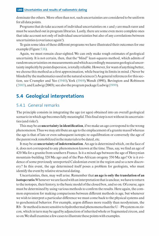
dominate the others.More often than not, suchuncertainties are considered tobeuniformforall datapoints.

Programs thatdo take accountof individual uncertainties onx and yaremuch rarerandmustbe searchedout in program libraries. Lastly, there are some even more complete onesthat take account notonlyof individual uncertainties but also of any correlations betweenuncertainties (covarianceagain!).

To gain some idea of these di¡erent programswehave illustrated theiroutcomes foroneexample (Figure 5.16).

Again, we must remain clear-sighted.We can only make rough estimates of geologicaluncertainty. It is not certain, then, that the ‘‘blind’’ least-squares method, which admits ofrandomuncertaintiesonmeasurementsandwhichaccordinglymeasuresgeologicaluncer-tainty implicitlybypointdispersion, is totallyreliable.However, forwantofanythingbetter,we choose thismethod as a¢rst approximation, whilebearing its limits in mind. (Neverbeblindedby themathematicsused inthenatural sciences!)Asgeneral references for this sec-tion, see Crumpler and Yeo (1940),York (1969),Wendt (1991), Bevington and Robinson(2003), andLudwig (2003); seealsotheprogrampackageLudwig (1999).

5.4 Geological interpretations

5.4.1 General remarks

The principle consists in integrating the age (or ages) obtained into an overall geologicalscenario inwhichagebecomes fullymeaningful.This¢nal step isnotwithout itsuncertain-ties (andrisks!).

Thismaybean uncertainty in identi¢cation, ifwemakean age correspond to thewrongphenomenon.Thuswemayattributeanage to the emplacementofagranitemassifwhereasthe age is that of late or even subsequent isotopic re-equilibration or conversely the age oftheparentrock remobilized in thematerials tobedated, etc.

Itmaybe an uncertaintyof indetermination. An age is determinedwhich, on the face ofit, does not correspond to any phenomenon known at the time.Thus, say, we¢nd an age of420Ma for a granite from southern France. Is it amixed agebetween the age ofHercynianmountain-building 320Ma ago and of the Pan-African orogeny 550Ma ago? Or is it evi-dence of some previously unreported Caledonian event in the region and so a newdiscov-ery? In this event, the age determined itself poses a problem for geologists, who mustidentify the eventbyrelative structuraldating.

Uncertainties, then, may well arise. Remember that an age is only the translation of anisotope ratio.Wheneverwearefacedwithan interpretationthat isunclear,wehavetoreturnto the isotopes, theirhistory, to thebasicmodelofthe closedbox, and soon.Ofcourse, agesmustbe determinedby using variousmethods to con¢rm the results.Here again, the com-mon expression for making comparisons between di¡erent methods is age, but wheneverwewish to interpret a particular di¡erencewemust comebackto the physical systems andto geochemical behavior. For example, argon di¡uses more readily than neodymium, theRb^SrmethodismoresensitivetohydrothermalphenomenathantheU^Pbsystemon zir-con,which in turnmaybeagedbyadjunctionof inheritedwholeor fragmented zircon, andsoon.Weshall examineafewcases to illustratethesepointswith examples.


5.4.2 Case studies

The aim here is not to achieve systematic coveragebut to give a few examples to illustrate amethod, its di⁄culties, its limits, and its level of reliability.This approach will allow us totest the various methods of quantitative discussion of geochronology, to compare them,and to seehow they canbe integrated into thegeological context.After noting howwe shiftfromthequalitativeuseofapparentages to quantitativemodels (isochron, concordia, step-wise degassing),wehavetomeasurehowreliable eachapproach is.

Contactmetamorphismof theEldora stockWe have made a qualitative study of discordances in apparent ages from this example. Itis interesting, then, to see what the result was of the various more elaborate methods inthis geologically well-de¢ned case. As these studies, conducted by StanleyHartwhen astudent at theMassachusetts Institute ofTechnology (seeHartetal.,1968), are ratherold,we only have results for the U^Pb, Rb^Sr, and KÂr systems (see Figure 5.17 andChapter 3).

TheU^Pb systemon zirconWe obtain a discordia cutting the concordia at 1600� 50Ma and 60� 5Ma, givingapparently the ages of the Precambrian schist and the Eldora intrusion, respectively.The points on the discordia are placed regularly with distance from the contact. Themost discordant ones are those closest to the contact.

The 87Rb^87Sr system in isochron constructionThemeasurementsweremademainlyonfeldsparsbecausetheymightprovenotverysignif-icanton thewhole rockof the schists.Theyare aligned on an approximate straight line iso-chron corresponding to an ageof1400� 100Ma, except for the apatites and epidotes closeto the intrusion (87Sracceptors).

The (Rb^Sr,KÂr)measurements onmicas discussedwith the generalizedconcordiadiagramThe discordia is a curve and not a straight line as in the U^Pb systems.We obtain the twointersections corresponding to the age of the intrusion of 60Ma and the ‘‘schist age.’’However,we cannotsaywhether the latter is1480or1600Ma. It is1480þ100�20Ma.

The 40Ar^39ArmeasurementsTheseweremade lateron hornblende, biotite, and feldspar (Berger,1975).We can de¢neplateaus giving increasing ages with distance from the contact. The hornblende andlarge biotite minerals give an age of 1450� 20Ma, that is, about the same as the87Rb^87Srage.We canenvisagetheageoftheschists as1450Maandtheagemeasuredby theU^Pb con-

cordia of1600Ma corresponds to a few inherited pieces of detrital zircon. But what doesthe schist age mean? Is it the age of metamorphism or of earlier sedimentation? The39Ar^40Ar ages on biotite and the (KÂr, Rb^Sr) concordia age suggest the age ofmeta-morphism, because it was then that the minerals crystallized. The age of 1600Ma is

181 Geological interpretations

206 P

b/2

38U

207Pb/235U

40A

r/40

K

87Sr/87Rb

0.3

1.0

1500

5054

25'12'

2'

1000

500

Front range (Colorado) biotite

Line A

2.0 3.0 4.0

0.2

0.1

0.2 0.4 0.6 0.8

0.76

0.74

0.72

1600

1200

800

400

10010intrusive

age

Zircon238U/206Pb

Zircon207Pb/206Pb

Concordia

500

1000

1500

1600

Line B

1440

Concord

ia

Discordia

87Sr

/86 S

r

87Sr/87Rb

240020

248

85

2400Epidote

2400Apatite

2500

r = 1400 Ma

0.4 0.6

290

350

0.8 1.00.20

1500

1000

500

Fraction 39Ar* outgassed

Hornblende

Ap

par

ent

age

(Ma)

a

b c

d

Figure 5.17 Radiometric ages of the Eldora stock examined in Chapter 3 in terms of apparent ages. (a)The U–Pb system on zircon (Hart et al., 1968). (b) The two 87Rb–87Sr methods on biotite in thegeneralized Rb–Sr, K–Ar concordia. (c) The 87Rb–87Sr method on feldspar. (d) Stepwise 40Ar–39Ar ages(after Berger, 1975). The numbers indicate distances from the granite intrusion (Chapter 3).


probably that of the earlier granites whose zircon was eroded and redeposited in the claysfromwhich the schists were formed. But the questioning and the answers are themselves ameasureofuncertaintyofthe result.Whatdoes theageofformationofaschistmean?

Theveryancient rocks ofGreenlandThe rocks of Greenland are the oldest in the world.7 They have been studied by variousmethods: U^Pb on zircon, 206Pb^207Pb on whole-rock isochrons, 86Rb^87Sr, and147Sm^143Nd. Steve Moorbath of the University of Oxford was both the pioneer and theprincipal investigator (Moorbath and Taylor, 1981; Moorbath et al., 1986). These studies,combinedwithprecisemappingofthe terrain, led to the identi¢cation of two separate geo-logical formations (Figure 5.18), theAmitsoq gneiss and the IsuaGroup (the mountain of

0.7

1.0 2.0

3.0 4.0

3.0 40

0.5

0.3

0.7

0.8

0.1

206 P

b/2

38U

207Pb/235U

3.5

4

2

58

937

6

3.824 +12–9

3.9

3.8

3.7

3.6

3.5error

3.65 3.824

2.5

1.5

3

Amitsoq gneiss

t = 3640 ± 120 MaεNd,0(t) = 0.9 ± 1.4

t = 3776 ± 52 MaεNd,0(t) = 2.0 ± 0.6

Baadsgard discordia lin

e

2

1

0.5

0.080.06 0.10 0.12 0.14

0.5102

0.5106

0.5110

0.5098

143 N

d/1

44N

d

147Sm/144Nd147Sm/144Nd

Isua boulders

0.08 0.14 0.18 0.220.06

0.514

0.512

0.510

143 N

d/1

44N

d

Figure 5.18 Results obtained by various methods for the Amitsoq and Isua gneisses. After Michard-Vitrac et al. (1977); Moorbath et al. (1997).

7 There are older minerals (zircon) but they are detrital and separated from their parent rock in which theycrystallized.


references includes:Michard-Vitrac etal.,1977;Moorbath etal.,1986,1997;Nutman etal.,1996;KamberandMoorbath,1998).

The ¢rst is dated 3.65� 0.03Ga and the second 3.74 and 3.82Ga. These are the oldestgroupsofrock in theworld.As canbe seenbyexaminingTable 5.4 andFigure5.18, summar-izing the results obtained by the various methods, the two groups are quite distinct.However, small di¡erences can be noticed in the absolute values obtained by the variousmethods and whose precise meaning is unclear.We have no explanations other than thatthe rockswere subjectedto subsequentmetamorphismandthe chronological systemswereprobablydisruptedsomewhat.

The Australian group from Canberra has used ion probe point analysis methods tomeasure zircongrainbygrain anddetermine theU^Pbages on theAmitsoqgneiss.A his-togramcanbemade (Figure 5.19). It shows the twopeaks at 3.60Gaand3.80Ga, providingwetakethemodeofthe twoasymmetricaldistributionsas thevalue.Thetwostatistical agesseemtobe inagreementwiththeagesmeasuredbyconventionalmethods.

Letusdiscussandinterprettheseresults.ThedistributionoftheAmitsoqandIsuaforma-tions is clear enough.The age of the Amitsoq gneiss is 3.64� 0.05Ga, with �t/t¼ 1.3%.The Isua formation is a little older but not as well de¢ned. The age of 3.66Ga given by87Rb^86Sr on whole rocks from Isua must be considered to be re-homogenization at thetimetheAmitsoqgneiss formed.

There seem to be rocks dating from 3.82Ga, particularly in the form of conglomerateswhosezircon‘‘survived’’thegeologicalperturbations.

Table 5.4 Results obtained by various methods for the Amitsoq gneiss and the Isua Group

Datingmethods Amitsoqgneiss (Ga) IsuaGroup (Ga)

U^Pb concordia (zircon) 3.45� 0.05 3.824� 0.05 (conglomerate)3.77� 0.01 (massive rock)

87Rb^87Sr (whole rock) 3.64� 0.06 3.66� 0.06147Sm^143Nd(whole rock) 3.640� 0.12 3.776� 0.05207Pb^206Pb (whole rock) 3.56� 0.10 3.74� 0.12

40

2.80 3.20 3.60 4.00

30

20

10

Nu

mb

er o

f sa

mp

les

Age (Ga)

Figure 5.19 Histogram of 207Pb–206Pb ages obtained by ion microprobe methods on Amitsoq zircon.After Nutman et al. (1996).


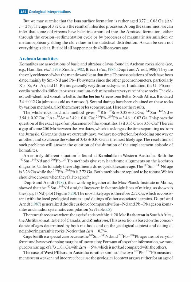
But we may surmise that the Isua surface formation is rather aged 3.77� 0.08Ga (�t/t¼ 2%).Theageof3.82Ga is the resultof inheritedprocesses.Along the same lines,we caninfer that some old zircons have been incorporated into the Amitsoq formation, eitherthrough the erosion^sedimentation cycle or by processes of magmatic assimilation ormetamorphism yielding the old values in the statistical distribution. As can be seen noteverything is clear.But itdidall happen nearly4billionyearsago!

Archean komatiitesKomatiites are associations of basic and ultrabasic lavas found in Archean rocks alone (see,e.g.,Hamilton etal.,1979;Zindler,1982;Bre¤ vartetal.,1986;Dupre¤ andArndt,1986).Theyaretheonlyevidenceofwhatthemantlewas likeatthattime.Theseassociationsofrockhavebeendatedmainlyby Sm^Nd and Pb^Pb systems since the other geochronometers, particularlyRb^Sr,Ar^Ar,andU^Pb,aregenerally verydisturbedsystems. Inaddition, theU^Pb,con-cordiamethod is di⁄culttouseasuranium-richmineralsarevery rare inthese rocks.Theold-estwell-identi¢edkomatiitebelt is theBarbertonGreenstoneBelt in SouthAfrica. It is dated3.4� 0.12Ga (almost as old as Amitsoq!). Several datings havebeen obtained on these rocksbyvariousmethods,allofthemmoreorless concordant.Herearetheresults.The whole-rock isochron method gives: 87Rb^87Sr¼ 3.35� 0.2Ga; 147Sm^143Nd¼

3.54� 0.07Ga; 40Ar^39Ar¼ 3.49� 0.01Ga; 206Pb^207Pb¼ 3.46� 0.07Ga.Thisposes thequestion ofthe exact ageofemplacementofthekomatiites. Is it 3.35Gaor 3.53Ga?There isagapofsome200Mabetween the twodates,which is as longas the time separatingus fromthe Jurassic.Given the datawe currentlyhave, wehave no criterion fordecidingonewayoranother, and so choose the value of 3.45� 0.10Ga as the most likely age.The resolution ofsuch problems will answer the question of the duration of the emplacement episode ofkomatiites.An entirely di¡erent situation is found at Kambalda in Western Australia. Both the

147Sm^143Nd and 206Pb^207Pb methods give very handsome alignments on the isochrondiagrams.Unfortunately, these alignments donotyield the sameage.The147Sm^143Ndageis 3.26Gawhile the 206Pb^207Pb is 2.72Ga. Both methods are reputed tobe robust.Whichshouldwe choosewhenthey fail toagree?Dupre¤ and Arndt (1987), then working together at the Max-Planck Institute in Mainz,

showed thatthe147Sm^143Ndstraight lineswere in fact straight lines ofmixing, as shown inthe ("Nd,1/Nd) plot (Figure 5.20).Themost likelyage is therefore 2.72Ga, which is consis-tent with the local geological context and datings of other associated terrains. Dupre¤ andArndt (1987)generalizedthediscussionofcomparativeSm^NdandPb^Pbagesonkoma-tiites andmadeasystematic compilation (seeTable 5.5).Therearethreecaseswheretheageis¢xedtowithin� 20Ma:Barberton inSouthAfrica,

theAbitibi komatiitebeltofCanada, andZimbabwe.This assertion isbasedonthe concor-dance of ages determined by both methods and on the geological context and dating ofneighboringgranitic rocks.Notice that�t/t¼ 0.7%.CapeSmith is aspecial casebecausethe147Sm^143Ndand207Pb^206Pbagesarenotverydif-

ferentandhaveoverlappingmarginsofuncertainty.Forwantofanyother information,wemustputdownanageof1.73� 0.1Gawith�t/t¼ 5%,which isnotbadcomparedwiththeothers.The case ofWest Pilbara in Australia is rather similar.The two 207Pb^206Pb measure-

ments seemweakerand incorrectbecause thegeological contextargues rather foranageof


3.56Ga. It is the context alone that allows anyconclusion, butthe 207Pb^206Pb results indi-cate therewasasecondary,disruptivephenomenon.

As said, Kambalda is the opposite case. The geological context indicates that it is the207Pb^206Pb systemthatyields themore reliableage.

The results ofthese last two cases show that there is nothingautomatic about theprocessandotherdatingsprobablyneedtobemadebyathirdmethodorconstrainedbyothergeolo-gicaldata.

The rhyolite of LongValley,CaliforniaIt isprobablyonthisveryamenable rockthattheUniversityofCalifornia^LosAngeles teamaroundMaryReid (Reidetal.,1997)madethebestuseofthevariousmethodsfordeterminingtheagesofgeologicalunitsofvery recentmagmatic origin.Theageoferuptionandofempla-cement are estimated, allowing for erosion, as 140 ka.The results obtained by the di¡erentmethods are: 257 ka (87Rb^87Sr) and 200^235 ka (isochronous 230Th^238U), and the39Ar^40Aragesaremuchyounger, ranging from100to150 ka (Reid etal.,1997).

The discordanceshere (several thousandyears) are construed as not arising from subse-quent disruptive phenomena but rather from complex magmatic sequences (Figure 5.21).

Table 5.5 Comparative Sm–Nd and Pb–Pb ages on komatiites (these are solely ages for whichalignments are statistically reliable)

147Sm^143Ndages 206Pb^207Pbages Most likelyage

WestPilbara� 3.5Ga 3.560Ga� 30Ma � 3.15Ga 3.5Ga?Barberton� 3.5Ga 3.540Ga� 30Ma 3.460Ga� 70Ma 3.45GaAbitibiMunroe

Alexo (2.7Ga)Newton

2.662Ga� 120Ma2.750Ga� 90Ma2.826Ga� 64Ma

2.724Ga� 20Ma2.690Ga� 15Ma� 2.65Ga� 15Ma

2.7Ga

Kambalda� 2.7Ga 3.260Ga� 40Ma3.230Ga� 120Ma

2.720Ga� 105Ma2.730Ga� 30Ma

2.7Ga

Zimbabwe� 2.7Ga 2.640Ga� 140Ma2.933Ga� 147Ma

2.690Ga� 1Ma 2.7Ga

CapeSmith�1.8Ga 1.871Ga� 100Ma 1600Ga� 150Ma 1.73Ga

3

4

5

2

1

0.5 1

1/Nd

ε Nd

0

Figure 5.20 Diagram of (2Nd, 1/Nd) plot on komatiites of Kambalda (Australia) showing a correlation inagreement with the idea that the rocks are a mixture. After Dupre and Arndt (1987).


The 87Rb^87Sr age is thought tomarkthe intrusion of themagmabeneath the volcano andthe creationofamagmachamber.The 230Th^238Uages supposedlydate the crystallizationof zircon in the samemagma chamber.The 39Ar^40Arages date the eruptions.This exam-ple raises not the question ofuncertaintybutof identi¢cation.What age is the radiometricphenomenonassociatedwith?Whatexactly is itthatwedate?In theprevious exampleswebarely posed the question just raised forLongValley (except

for the Eldora gneiss). For the komatiites the answer is clear enough: we want to date themagmaintrusion.ForGreenland, it is a little fuzzier. Is it the emplacementofgranitebeforemetamorphism? Is itthemetamorphic episode? It isnotabsolutelyclear.Here, with the LongValley rhyolite, there is no getting round the question.The ages can

only be interpreted in the context of a geological scenario, a general model. At the sametime, itcanbeseenthatthedi¡erentchronometersarenotusedfordatingthesamephenom-ena.The very idea of concordance of ages obtained by the various methods, so far consid-ered as the criterion of absolute reliability, must be re¢ned. Perhaps the uncertainty thatcanbe estimated by the variousmethods re£ects merelyaproblemof identi¢cation. Letustry to extendthis typeof interpretation.Thus,whenweobserve that 87Rb^87Srages onwhole rockmeasured ingranite aregen-

erallya littleyounger than theagesobtainedon zirconby the concordiamethod,weques-tion what this di¡erence means. It may arise because zircon is the ¢rst mineral tocrystallize whereas 87Rb^87Sr is re-homogenized by the circulation of hydrothermal£uid which is driven o¡ towards the end of granite crystallization and gives rise to theaplite and pegmatite seams. This is not the only interpretation.We might also considerthat the zircon is agedbecause it has inheritedolder zircon. Ionmicroprobe examination

36A

r/40

Ar

39Ar/40Ar

Mammoth Knolls IC-42Plateau age = 101 ± 8 ka

0.003

2 4 6 8 10

0.002

0.001

36A

r/40

Ar

39Ar/40r

LSR Flow IC-2440Ar/36Ar = 296.5 ± 2.4 ka

Age = 151 ± 4 ka

PA = 152 5

0.003

1 2 3 4 5

0.002

0.001

T = 202.6 ± 0.9 kaglass

230 T

h/2

32Th

238U/232Th

IC-245

1 2 3 4 5

4

3

2

1

zircon

T = 235.6 ± 1.2 ka230 T

h/2

32Th

238U/232Th

IC-42

1 2 3 4

4

3

2

1

zirconMammoth

KnollsDeer

Mountain

Age = 257 ± 39 ka87Rb/86Sri = 0.70628 ± 2

87Sr

/86 S

r

87Rb/86Sr10 20 30

0.706 28

0.706 32

0.706 36

0.706 40

Figure 5.21 Results obtained by various methods for the rhyolite of Long Valley, California. After Reidet al. (1997).


of zircon minerals has now provided an answer but before we were in a position ofindeterminacy!

ConclusionsThere are two conclusions tobe drawn from these studies (whichwe could havemultipliedinde¢nitely). First, it has been seen that the quantitative methods of interpreting isotopemeasurements actuallygavevery coherent ages (despite the slightuncertaintieswith decayconstants).Second,wehavejustobservedthatbetterunderstandingofthesemeasurementsrequires themtobe included in geological schemas of interpretation.Thegeological inter-pretationbene¢ts on the onehand from the results of radiometric datingbut in exchange italone canmakethe¢guresyieldedby thevariousmethods fullymeaningful.

Let us repeat, there is nothing automatic about interpreting radiometric ages. Ageis meaningful only in a given geological context. In addition, in return, inclusion in ageological context enlightens the geochemical behavior of the various chronometers.Each radiochronometer may bear original information, but for it to be credible it mustbe matched against other sources of information. It must be consistent with theother things we know, with the usual behavior of the chronometer in question comparedwith other chronometers, and with the speci¢c geological history under study. Thescienti¢c approach is more like detective work than the application of automaticprogramming.

5.5 The geological timescale

5.5.1 History

The making of the geological timescale, which is the greatest revolution geologyhas seen,paradoxically has a long history. It took longer for it to become accepted than for its mainlines tobe established. As stated, the ideaofusing radioactive decay tomeasure geologicalages seems to have occurred independently but at about the same time toPierre Curie inFrance (see Barbo, 1999) and to Ernest Rutherford in Canada (see Eve, 1939) in the earlytwentieth century.

It was Rutherford who ¢rst attempted to translate this insight into an actual measure-ment. He had just identi¢ed � particles as helium atoms. His colleague Ramsay had justshown how the proportions and abundances of the rare gases could be measured.Rutherford suggested tohimmeasuring the amountofhelium contained in auraniumore.Hedidso.Rutherfordfoundanageofmorethan1billionyears.Thiswas in1906,aboutacen-turyago.Rutherford’s discovery was abombshell: geological terrainsweremore than1bil-lion years old! The second stage took place in 1907 at Yale University, where Rutherfordwent to deliver the prestigious Silliman Lecture. Now, at Yale there was a chemist namedBoltwood, whowas interested in chemical transformations related to radioactivity.He sus-pected that the end product of radioactive chains, which he was analyzing by chemicalmethods, was lead. Rutherford suggested he should test out his idea geologicallyby takingwhatgeologists reportedtobeyoungandolduraniumoresandanalyzingtheirleadcontent.Theolderones should contain more lead than theyoungerones. Boltwood (1907)made thecorresponding series of measurements and con¢rmed there was a connection between


leadanduraniumchains.Inturn,hethendecidedtousethemethodtodatetheuraniumoresby analyzing the uranium and lead content of each, and he calculated the ages by applyingthe exponential law for decay. These were purely chemical measurements, not isotopemeasurements.After Boltwood’s discovery, inspired by Rutherford, the chemical dating of lead was

improvedby the discovery that thorium toowas the parentofa radioactive chain ending inlead.Thedating formulawasmodi¢edslightly to read:

Age ¼ ðPbÞtotalðUÞ þ 0:38 ðThÞ 7400Ma

where (Pb), (U), and (Th) are the lead, uranium, and thorium contents in grams,respectively.However, the chemical U^Pbmethod soon ran intowhat seemed at the time an insolu-

ble technical problem. Uranium ores could be dated, but what of ordinary rocks?Chemical methods of the day were not sensitive enough and could notbe used to measureeither uranium or lead contents in ordinary rocks. These contents are measured in partsper million and at the time such elements could be measured only if their abundanceswere of the orderof1%.That iswhy in1908R. J.Strutt,who laterbecamethe famousLordRayleigh, undertook

tomeasure the age ofordinary rocks by using the heliummethod (Strutt,1908).To do this,hemeasuredtheradiationproducedbytherock,whichgavehimthe instantaneousquantityof 4He produced. He next measured the quantity of 4He contained in the rock. It was thenpossible to make a simple age calculation. Although Strutt was aware from the outset thathelium di¡uses readily from minerals and rocks and so a¡ects the age measured, themethod developed quickly in various parts of the world: in Britain with Strutt himself, inthe United States with Piggot, and in Germany with Paneth, who applied it to meteoritesabove all. In this race to develop a reliable geochronological method, one of Strutt’s stu-dents, the ScotArthurHolmes, made a name for himself andwas to play an essential partin geological age determinations for the next 40 years (see Holmes,1946). He is one of thefoundersof isotopegeology.Althoughgeochronologicalmethodsbasedon leadandheliumare subject to limitations

and uncertainties, geologists embarked upon the adventure of constructing an absolutegeological timescale to attribute durations to thegeological eras and stagesofthe stratigra-phers.The¢rst successfully tobuild a coherentwholewasBarrell in1917.AsHolmeswas todo later, Barrell used radioactive datings and stratigraphic and geological observations tocorrelate them. He judged some ages unrealistic, others acceptable, and by a series ofapproximations and trials and errors he came upwith a genuine quantitative stratigraphicscale in millions ofyears.Table 5.6 shows the¢guresofhis scale alongside the‘‘modern’’¢g-ures.With hindsight, Barrell’s workwas outstanding ^ and yet no one believed it! When Ibegan studying geology in Paris in1958^9 wewere told therewas an absolute stratigraphicscalebut that it was highlyapproximate and largely wrong and so should notbe learned. Iftruthwillout, it sometimes takesquiteawhile todoso!This absolute scale, and even more so the reasoning that underpinned it, that is, the age

attributions to geological phenomena in millions orbillions ofyears, and the awareness of

189 The geological timescale

the extraordinarygeological myopiaofclassical geologybasedon stratigraphic stages, didnotcometobetrulyaccepteduntil the late1960s.

This scale must be subdivided into two separate periods because the conditions for agedeterminationarenotthesame (seePlate6).

� The Precambrian period extends from the formation of the Earth to the appearanceof the ¢rst ‘‘unquestioned’’ fossils 550 million years ago. This period began with theearliest rocks, the ¢rst terrestrial rocks of Greenland, which, as we have seen, areaged 3.82Ga.� The ‘‘classical’’ period is that of traditional geology where fossil-based geology

applies. Within this period a special place must be made for the interval rangingfrom 0 to 200Ma during which we have samples of a real oceanic crust overlain bysediments that are well identi¢ed paleontologically thanks to microfossils. The under-taking was to match the terrains identi¢ed on a worldwide scale and to classifythem, through their fossils, in time intervals measured in millions of years. The ¢rstjob, then, was to put numbers on the stratigraphic scale developed by stratigraphicpaleontology which divides the periods for which there is fossil evidence into erasand stages. This scale was then extended to very ancient ages, and after that, its reso-lution was improved for recent times.

5.5.2 The absolute scale of fossiliferous (Phanerozoic) times

The great di⁄culty in this undertaking is that the usual methods for dating long durationssuch as 87Rb^87Sr, 238U^206Pb, 147Sm^143Ne, 187Re^187Os, or 40K^40Ar cannot readilybe

Table 5.6 The absolute scale of geological times in millions of yearsa

Barrell(1917)

Holmes(1947)

Holmes(1960)

Lambert(1971)

Modernages

Quaternary(Noozoic)

Pleistocene 1^1.5 1 1 4

Tertiary(Cenozoic)

Pliocene 7^9 12^15 11 7 12Miocene 19^23 26^32 25 26 26Oligocene 35^39 37^47 40 38 37PaleoceneEocene

55^65 58^68 70 65 65

Secondary(Mesozoic)

Cretaceous 120^150 127^140 135 135 141Jurassic 155^195 152^167 180 200 195Triassic 190^240 182^196 225 240 235

Primary(Paleozoic)

Permian 215^280 203^220 270 280 280Carboniferous 300^370 255^275 350 370 345Devonian 350^420 313^318 400 415 395Silurian 390^460 350 440 445 435Ordovician 480^590 430 500 515 500Cambrian 550^700 510 600 590 570

a Single dates indicate thebeginningoftheperiod.Source:AfterHallam(1983), inwhichthe references citedmaybefound.


used for dating sedimentary rocks. Now, the stratigraphic scale is de¢ned by index sedi-mentary strata containing fossil associations chosen as theboundarybeds.The reasons itis di⁄culttodatesedimentarystrataarethateithersedimentaryrocksaremadeupof inher-ited material (sandstone and schists) ofvaried provenance and age and, in such cases, thecriteria for initial isotopichomogeneityarenotsatis¢ed, or theyarenewly formedmaterial(limestone), in which case the rock is sensitive to secondary phenomena (particularlywater circulation) and are not closed systems. Despite painstaking studies, which have notbeen entirely unsuccessful (which are always cited, of course) no general method hasemerged.Theabsolute chronologyofsedimentarystrata isgenerallyestablished indirectlybydating

igneous rocks whose geometric and chronological relations with the strata are known.Interstrati¢ed volcanism is a particularly favorable case, of course. Another case directlyderived from the process of oceanic expansion is that of the ancient ocean ridges, that is,sea-£oorspreadingwhereastill-fresh layerofbasalt (thatcanberadiometricallyandmagnet-icallydated) is overlainbya layerof limestone that isvery rich in microfossils.Ocean drillinghas allowed such dating (although the basalt must not be overly a¡ected by hydrothermalcirculation or by exchange with sea water at low temperature). The most commonly usedmethod fordatingbasalt is the 39Ar^40Armethod.Butsuch dating is increasinglydi⁄cultaswe goback in timebecause ofweathering, since the older theyare, themore thebasalts havebeenalteredbyreactionwithseawater,withwhichthesediment is impregnated.In addition, directmethods yield dates for a few reference strataonly. Other results must

be interpolated from them.The principle behind the method is simple enough. Supposethat inwhat is considered a continuous sedimentaryseriesweknow fromoneofthe earliermethods the ages t1 and t2 of two points in the series, separated by a thicknessD(X)¼X1�X2. As a ¢rst approximation, all of the strata in the interval may be dated byinterpolation.Thesedimentation rateofthe series is

V ¼ X2 � X1

t1 � t2

� �;

sotheaget3ofapoint locatedatX3 is

t3 ¼ t1 �X3 � X1

V

� �:

To apply the method, ¢rst the series must be continuous, in other words, there must be nosedimentary gap or hiatus, which stratigraphers are experienced at detecting. Next, sedi-mentationmustbeofthe sametype ifwearetoassumethe sedimentation ratehas remainedconstant. All of this is doneby comparing, correlating, obtaining newdates, bymodifyingolddata, orcon¢rmingotherdata, littlebylittle and casebycase.As canbe seen, it is a long,hard slog and there is scope for constant improvement. It is understandable, then, that theage boundaries between stages or eras are a¡ected by uncertainty which varies with thedateofpublication.The stratigraphic scale is shown in Plate 6. A fewbrief remarks are called for.The eras,

which our forebears thought were about equal in length, are in fact highly unequal:

191 The geological timescale

Paleozoic (Primary) 340Ma, Mesozoic (Secondary) 145Ma, Cenozoic (Tertiary) 65Ma,andQuaternary 5Ma. Ifwe plot the geological eras and the traditional subdivisions, it canbeseenthatthe lossof information is aboutexponentialwith time (Figure 5.22).

RemarkWith scientific advances, the names of the reference terrains do not change, but the ages of these

terrains are constantly changing. Uncertainties on the limits are not symmetrical because geolo-

gical constraints are not symmetrical either.

The case of theQuaternaryIn recent periods, ranging from 1 to 5Ma, which is the time in which humankind hasappeared and developed, the situation is very di¡erent for two reasons. The ¢rst is thatmanydating methods canbe applied directly to sediments.This is the casewith14C, 10Be,and methods based on radioactive disequilibrium. Direct dating can therefore be prac-ticed.The second is that there aremany indirectmethods: £uctuations in18O/16O isotoperatios (to whichwe shall return in Chapter 8), ¢ssion tracks, paleomagnetism, micropa-leontology, etc. All of these methods can be used for intercalibration and re¢nedinterpolation.

In short, we can nowdraw up avery precise chronological scale for the Quaternarybutonethat isbasedon climaticphenomena.Weshall speakofthis inChapter 6.

5.5.3 The Precambrian timescale

TheCambrian is theageatwhichthe¢rstcommon fossil faunas appeared.Thetwotypesofcharacteristic fossils are trilobites and Archeocyatha. Its lower boundary is dated540þ40�10 Ma.

As Precambrian terrains cannotbe subdivided on the basis of fossils, wework the otherway around: we set numerical limits and then map the corresponding terrains at de¢nedtime intervals.The essential boundary has been set at 2.5Ga. It divides the period before,known as the Archean, and the period ranging from 2.6Ga to 0.4Ga, known as the

Tim

e (l

og

)

Age (log)

Quaternary

Cenozoic

Mesozoic

Paleozoic

Precambrian8

2 4 6 8

6

4

2

Figure 5.22 Relationship between duration and ages of geological eras. ‘‘Classical geologists’’ thoughtthese durations were about equal. We are indeed dealing with a case of geological myopia.


Proterozoicbecausewesupposethat itwasduringthisperiodthat lifedeveloped.Theques-tion,ofcourse, ishowtodeterminethe lower limitto this scale.We assume that the continental crust as it is today has not existed since the ¢rst age of

the Earth but that it appeared after a time T0 or that it appeared at an early date butwas destroyed by multiple phenomena (meteorite bombardment?) and subsisted fromT0 only.This ageT0 is therefore the upper limit of the Archean. Between the formation oftheEarthandT0wehavede¢nedaperiod forwhichthere is littleandoftenonly ‘‘indirect’’evidence (meaning there are no whole rocks) and that is known as the Hadean (seeChapter 7).Butwhat is thevalue ofT0?Howold are the oldest terrains, in the sense ofuninterrupted

geological formations that can be mapped? The Isua and Amitsoq formations ofGreenland already mentioned and dated 3.77Ga and 3.65Ga, respectively, are the oldestterrestrial rocks known as yet. But sedimentary rocks inAustralia havebeen found to con-tain zirconwhoseU^Pbages concordat 4.3Ga (andafewevenat 4.37Ga).Theseare indis-putably the oldest terrestrial minerals. But what is the meaning of that? Zircon is a typicalmineral ofgranitic rocks, and so the remains seem to testify that therewere pieces of conti-nent at that time. Were those continents preserved, buried somewhere, or were theydestroyed by erosion, meteorite bombardment, andHadean tectonism? This is a questiongeochronology raises.We therefore provisionally ¢x the Hadean^Archean boundary at3.8Ga (see Plate 6 for the azoic (Precambrian) timescale).Herewehave anuncertaintydueto lackof information.Wemustthereforebeprepared to change these¢gures asnewdiscov-eries aremade.

5.6 The age of the Earth

The age of the Earthwas touched upon in Chapter 2 and could in itself be the subject of anentire book, such is its historical and philosophical signi¢cance.We shall give abrief sum-mary of it, emphasizing the approaches taken by those who attempted to answer thequestion.

5.6.1 History

TheBible indicates thattheEarth is 4000yearsold.Around1650ArchbishopUssherestab-lished bybibliographical studies that the Earth hadbeen created on 26October in the year4004BCat9.00 inthemorning!By contrast with this, in the late seventeenth century, the founder of geology, Scotsman

JamesHutton, haddismissed thevery ideaoftheEarth havinganagewe can estimate.TheEarthhadalwaysbeenhereandwastheseatofthesamephenomenadescribedbygeologicalcycles and would be until the end of time.‘‘No vestige of a beginning ^ no prospect of anend,’’asheput it.Inthemidnineteenthcentury,while classicalgeologywasthriving, theBritishphysicist

WilliamThomson, later to becomeLord Kelvin, began to criticize the idea of an eternalEarth and repetitive geology.His ideawas simple.Geological processes consume energy,if only to make reliefs, power volcanoes, or generate earthquakes. Now, the energy theEarth contains is not inexhaustible.He identi¢ed the source of terrestrial energyasbeing

193 The age of the Earth

of thermal origin.The inside of the Earth is hot and the Earth is cooling because it losesheat from its surface by radiation. He thus came upwith the ¢gure of100Ma, con¢rmedin twoways. First, he had used the same theory to calculate an age for cooling of the Sun(this time by calculating the energy dissipated by radiation) of 100Ma. Second, theIrishman Joly had also calculated the age of the ocean and found 100Ma. The age of100Mawas amust!

However, geologists, and foremost among them Charles Lyell and Charles Darwin,rejected this age which they thought too young.8 In 1910 Rutherford and then Boltwooddetermined the ¢rst radiometric ages exceeding 1 billion years. Pierre Curie andLaborde showed that radioactivitygave o¡ heat, and so therewas an energysource insidetheEarth,which impliedLordKelvin’s calculationwas false.Andyet itwas onlyafter theSecond World War that Kelvin’s ¢gure was seriously revised (see Burch¢eld, 1975;Dalrymple,1991).

E X A M P L E

Kelvin’s problem

Kelvin considered the cooling of the Earth, ignoring its roundness. He assumed the surface

was plane and supposed it was maintained at constant temperature as it lost its heat by

radiation into space.

For a semi-infinite solid separated by a plane surface, Fourier’s theory states that if we take

depth (z) with depth at the surface z¼ 0 and assume the solid is at a temperature T0 at the

initial time and we allow it to cool by conduction, the temperature T(z) is a function of T0 and

of z/2(kt)1/2, where t is time and k is thermal conductivity. The thermal gradient (or geothermal

gradient as we say for the Earth) is written:

T

z¼ T0

ðkt Þ1=2exp

�z 2

4kt

� �:

Near the surface z¼ 0 and the exponential equals 1. The geothermal gradient G is:

G ¼ T 0ðpkt Þ�1=2:

If we take T0¼ 7000 8F, then G¼ 1/1480. With k¼ 0.0118 we get t¼ 0.93 Ma.

E X A M P L E

The age of the oceans

The Irishman Joly (who was one of the first to use radioactivity in geology) decided to calculate

the age of the ocean (but attributed to it the same age as the Earth).

His reasoning ran like this: in the beginning the sea was fresh water. It became salty

through the input of rivers and evaporation of water. So if we divide the mass of sodium in

the ocean by the mass added annually by rivers, we will get the age of the ocean. To do this,

8 Kelvin changed his calculation somewhat and at different times his age for the Earth varied between25Ma and 400Ma, but that did not change the order of magnitude at stake!


he used the values of his day. That of sodium in rivers was 2 � 10� 4 moles kg� 1 while the

sodium content of sea water was 0.5 moles kg� 1. And he asked: how long has it taken to make

the sea salty? Given that the mass of the ocean is 1.5 � 1024 g and the mass of inflow from

rivers is 4 � 1019 g, he found an age of

0:50

2 � 10�4 mass of ocean

mass of rivers¼ 0:93 � 107years:9

5.6.2 The isotopic approach

In1938AlfredNier, thendoingpostdoctoralworkatHarvardUniversity,measuredthe iso-topic compositionoflead ingalena (PbS) fromvariousgeological settingsandtowhichvar-ious ‘‘geological’’ ages had been attributed. Nier undertook to calculate the 207Pb^206Pbages of the galena and found ages of 2.5 billion years. Now, at that time the astronomerEdwin Hubble, working at the California Institute of Technology, had used the gradualrecession ofgalaxies to determine the age of theUniverse and had comeupwith a ¢gure of2billionyears!Rocks that were older than the Universe! Wasn’t that impossible? Three scientists set

about using Nier’s results to recalculate the age of the Earth: Gerling (1942), Holmes(1946), andHoutermans (1946).Their common starting point was Nier’s isotope analyseson galena in 1938 at Harvard. Some of the samples were from geological formations ofknownage.Asgalenadoesnot containuranium its isotopic composition is frozen fromthetime it becomes isolated. If we write the isotopic compositions �¼ 206Pb/204Pb and�¼ 207Pb/204Pb and assume that the isotopic composition of the galenawas‘‘constituted’’in a closed system (mantle or crust) which has been isolated since the origins of the Earth,we canwrite:

� ¼ �0 þ238U204Pb

ðelT0 � elT1Þ

� ¼ �0 þ235U204Pb

ðel0T0 � el0T1Þ

whereT0 is theageoftheEarth,T1theageofthegalena,�0and�0 the initial isotopic compo-sitions of the Earth, and where l corresponds to 238U and l0 to 235U. As we have alreadydone,we can rewrite these equationsas:

�� 0

� � �0¼ 137:8

elT0 � elT1

el0T0 � el

0T1

� �:

Unfortunately, to calculate theageoftheEarthT0 in this equation, twounknownsaremiss-ing, the initial isotopic compositionsofterrestrial lead (�0 and�0).Gerling, attheInstituteofPrecambrianGeologyatLeningrad(nowSt.Petersburg), sim-

pli¢ed the problem and adopted a newassumption (Gerling,1942) (Figure 5.23). He chose

9 This age is now referred to as the residence time of sodium in the oceans. See Chapter 8.


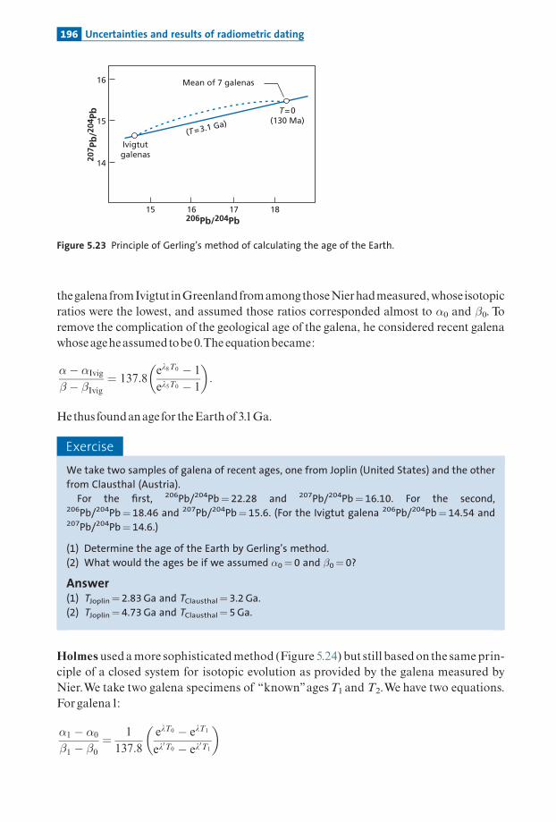
thegalenafromIvigtut inGreenlandfromamongthoseNierhadmeasured,whose isotopicratios were the lowest, and assumed those ratios corresponded almost to �0 and �0. Toremove the complication of the geological age of the galena, he considered recent galenawhoseageheassumedtobe0.The equationbecame:

�� Ivig

� � �Ivig¼ 137:8

el8T0 � 1

el5T0 � 1

� �:

Hethus foundanagefor theEarthof3.1Ga.

Exercise

We take two samples of galena of recent ages, one from Joplin (United States) and the other

from Clausthal (Austria).

For the first, 206Pb/204Pb¼ 22.28 and 207Pb/204Pb¼ 16.10. For the second,206Pb/204Pb¼ 18.46 and 207Pb/204Pb¼ 15.6. (For the Ivigtut galena 206Pb/204Pb¼ 14.54 and207Pb/204Pb¼ 14.6.)

(1) Determine the age of the Earth by Gerling’s method.

(2) What would the ages be if we assumed �0¼ 0 and �0¼ 0?

Answer(1) TJoplin¼ 2.83 Ga and TClausthal¼ 3.2 Ga.

(2) TJoplin¼ 4.73 Ga and TClausthal¼ 5 Ga.

Holmes used amore sophisticatedmethod (Figure 5.24) but still basedon the sameprin-ciple of a closed system for isotopic evolution as provided by the galena measured byNier.We take two galena specimens of ‘‘known’’agesT1 and T2.We have two equations.Forgalena1:

�1 � �0

�1 � �0¼ 1

137:8

elT0 � elT1

el0T0 � el

0T1

� �

15 16 17

Mean of 7 galenas

(T = 3.1 Ga)

Ivigtutgalenas

T = 0(130 Ma)

18

16

15

14207 P

b/2

04Pb

206Pb/204Pb

Figure 5.23 Principle of Gerling’s method of calculating the age of the Earth.


andforgalena2:

�2 � �0

�2 � �0¼ 1

137:8

elT0 � elT2

el0T0 � el

0T2

� �;

andthreeunknownquantities�0,�0, andT0.Holmes (1946) thenhituponthe ideaofasortofstatisticalmethodandreasonedlikethis:

suppose Igivemyself ages of the EarthT0¼ 2Ga,3Ga, and 4Ga. Ifwe replaceT0 by thesevalues in the equations, we can calculate the two unknowns �0 and �0 on a case-by-casebasis (Figure5.25). Sowe canplotan (�0,T0) diagram.Thisoperationmaybe repeatedwith

2.00T = 3.33 Ga

α0 = 11.22

3.00 4.00

14

12

10

206 P

b/2

04Pb

Time (Ga)

Solutions forsamples 18 and 25 Solutions for

samples 1 and 19

Figure 5.24 Measurements giving the age of galena by Holmes’s method.

2.00 2.50 3.00 3.50

Mode: 3.35 Ga

Solutionswithanomalouslead fromJoplin

Solutionswithothergalenas

Mean(without Joplin):

3.29 Ga

Mean:3.20 Ga

4.00

200

160

120

80

40

Nu

mb

er o

f so

luti

on

s

Time (Ga)

Figure 5.25 Age statistics determined by Holmes with his two-by-two galena method.


a secondpairofgalena specimens, givingus a second curve,with athirdpair, and soon.Wejusthave to take themeanofthe intersectionsbetween the curves togetthe real pair (�0,T0)andT0. Holmes cameupwith 3.4Ga, an astonishing convergencewith the date calculatedby Gerling.Houtermans (1946) adopted much the same method, leading him to a resultcloseto3Ga.

Inthe1950s, then,wehadanestimatefor theageoftheEarthofabout3.5Ga. (MeanwhileastronomershadrecalculatedHubble’s equationandfoundanageof4Gafor theUniverse.)

In1950, advances inmass spectrometrymeantthe isotopic composition of leadofordin-aryrockscouldbemeasuredalthoughthis elementisonlyfoundintraces. InhisPh.D.thesisat Chicago University, Clair Patterson (1953) ¢rst measured two meteorites, an ironmeteorite (Canyon Diablo) and a basaltic meteorite (Nuevo Laredo) by the 206Pb^207Pbmethod (Figure 5.26). By joining up the two points in the (206Pb/204Pb, 207Pb/204Pb) dia-gram, he calculated an age of 4.55Ga, which he claimed to be the age of planetaryobjects(Patterson,1953,1956).

He then measured a present-day volcanic rock from Hawaii, which supposedly repre-sentedwhatwas assumedtobe thehomogeneous interioroftheEarth, ¢ne sediments fromthe Paci¢c, and a manganese nodule supposed to represent averages of rocks from theEarth’s surface.These three rocks lay roughlyon the straight line at 4.55Ga. He attributedto the Earth the same age as themeteorites and asserted thiswas the age atwhich the SolarSystem formed.This is the age which now features in all the textbooks. It also determinesthe initialvalues�0 and�0.

These values have since been determined more precisely as (206Pb/204Pb)0¼ 9.307,(207Pb/204Pb)0¼ 10.294, and (208Pb/204Pb)0¼ 29.476.

Apart fromthevalueoftheageoftheEarthandthebenchmark itprovides for thehistoryofgeological times, Patterson’sworkhas an important consequence. It canbeused to‘‘situ-ate’’ the isotopic compositions ofgalena measured in geological formations relative to the

40

30

20

10

10 20 30 40 50

20

7P

b/2

04P

b

206Pb/204Pb

Nuevo Laredo meteorite

Canyon Diablometeorite

(sulfur)

Sea water

Recentsediments

Hawaiianbasalt Age 4.55 Ga

Figure 5.26 The age of the Earth as determined by Clair Patterson, 1953–6.


initial reference point (�0,�0) andby the same token to allowa series ofcalculations for theageoftheEarth fromeachsampleofgalena.Weshallseewhatthiswork leadstoinChapter6.

Exercise

Calculate the age of the Earth from Casapalca and Yancey galena samples given by Nier in

Figure 5.24 and Table 5.7, assuming �0 and �0 to be the values known today and assuming

their age is about zero.

AnswerTCasapalca¼ 4.39 Ga and TYancey¼ 4.45 Ga.

5.6.3 The modern approach

A¢rst,probablysomewhatdisarming,observation is thatwithmodernanalyticalmethods(see Alle' gre et al., 1995) we cannot repeat Patterson’s measurements and ¢nd the sameresult! The points that are supposed to represent the Earth donot lie on the straight line formeteoritesbut formacloud.Moreover, thedecayconstants foruraniumhavebeen changedsince, and so we would no longer ¢nd 4.55Ga with modern values. And yet, Patterson’sresult is about right (Tatsumoto et al., 1973)! Unfortunately for him, the very concept oftheageoftheEarth has changedandhasbecomemuch lesswellde¢nedthan in his day.First, it hasbeen realized that the Earth’s historyhasbeenvery complicated and that the

models ofevolution of lead involving just a single episode in a closed systemdonot apply toany terrestrial reservoir.All ofthe systems ^ crust^mantle^ocean ^ areopen systems thatexchange material with each other: there is absolutely no ground for applying the closed-box model to reservoirs like themantle or continental crust as Patterson did, even as a ¢rstapproximation (asweshall see inChapter 6).Then,with theadvances inplanetaryexplora-tion and planetological models, it was realized that the Earth had not been formed in aninstant but by a slow process (named accretion) which probably lasted 100^150Ma.Wecome back to the question we raised at the beginning of this chapter: for dating we need abox that closes at a de¢nite given time. Ifwe date the Earthbyany particular method, whatis themeaningofthatage? Is itthetimethe coreformed,or the endofdegassingoftheatmo-sphere? Is ittheageofthesolidmaterial that is itsmain component?WeshallreturntothisprobleminChapter6.LetusbecontenttosaythattheEarth formed

over a period of 100 to 120Ma and that the process began 4.567Ga ago! The concept of

Table 5.7 Samples of galena used by Nier in two-by-two determinations

206Pb/204Pb 207Pb/204Pb Age (Ma) Numbera

Casapalca (Peru) 18.83 15.6 25 1Ivigtut (Greenland) 14.54 14.70 600 19Yancey (NorthCarolina) 18.43 15.61 220 18GreatBearLake (Canada) 15.93 15.30 1330 25

a SeeFigure5.24.


dating can be applied in several ways. Either we date thebeginning and end ofaccretion oftheEarth,orwedeterminean‘‘averageage’’offormationoftheEarthwith noprecisemean-ing.We can see that analytical uncertainty is no longer an issue, but that it is ‘‘geologicaluncertainty’’or even conceptual uncertainty that challenges the validity of the referencemodeloutsideofwhichanyage ismeaningless.This, then, is agood exampleofthe di¡erentmeaningswe can attribute touncertaintyofageological agemeasurement! For fun,we canend by noticing that if we represent the age of the earth in semi-logarithmic coordinatesagainst the date of research into the subject (Figure 5.27), we obtain a straight line: this isfood for thought about themeaningofcorrelationswith no theoretical support. (Perhaps asociologistorapsychologistcoulddrawconclusions fromthis?)

5.7 The cosmic timescale

One of the great success stories of radiometric dating is that it has been able to extend itsinvestigativepowerbeyondtheterrestrialdomainand¢xchronologicalmarkers forcosmicevolution.

5.7.1 Meteorite ages

Meteorites are pieces of embryonic planets dating from early times, whichwere sent hur-tling o¡ into space after collisions and spent millions of years in interplanetary spacebefore falling toEarth.

Wehavesaidthat,asa¢rstapproximation,meteoritesareasoldastheformationoftheSolarSystemandtheplanets (around4.55Ga),butwehavejustseenthatthisage ispoorlyde¢ned.

Modern U^Pb methods applied to uranium-rich phases developed in Paris byGe¤ rardManhe' s,Christa Go« pel, and the present author have yielded meteorite ages with a preci-sionofabout 300 000years,while theage is close to 4.55Ga, givingarelativeuncertaintyof3 �105/4.5 �109 (60 ppm),which corresponds toaprecisionof60years foradateof1millionyears!Using theseU^Pbmethods as our reference, wehavebeen able to establish aprecisechronology (Go« peletal.,1994) (Figure5.28).

20001950190018501800

1010

108

106

104

Ag

e o

f th

e Ea

rth

(yr

)

Year

Patterson

Holmes

Boltwood

JolyKelvin

Buffon

Thousand years

Millionyears

Billionyears

Figure 5.27 Changes in the age attributed to the Earth as geological sciences have developed.


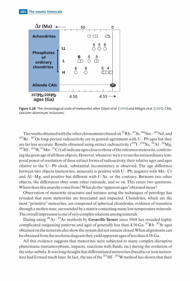
Theresultsobtainedwiththeotherchronometersbasedon87Rb^87Sr,146Sm^143Nd,and187Re^187Os long-period radioactivity are in general agreement with U^Pb ages but theyare far less accurate. Results obtained using extinct radioactivity (129I^129Xe, 26Al^26Mg,182Hf^182W,53Mn^53Cr)all indicateages closetothoseofthe referencemeteorite, con¢rm-ingthegreatageofall theseobjects.However,wheneverwetry tousethe extraordinary tem-poral powerof resolution of these extinct formsof radioactivity, their relative ages andagesrelative to the U^Pb clock, substantial inconsistency is observed. The age di¡erencebetween two objects (meteorites, minerals) is positive with U^Pb, negative with Mn^Crand Al^Mg, and positive but di¡erent with I^Xe, or the contrary. Between two otherobjects, the di¡erences obey some other rationale, and so on. This raises two questions.Where does this anarchycomefrom?Whatdothe‘‘apparentages’’obtainedmean?Observation of meteorite structures and textures using the techniques of petrology has

revealed that most meteorites are brecciated and impacted. Chondrites, which are themost ‘‘primitive’’ meteorites, are composed of spherical chondrules, evidence of transitionthroughamolten state, surroundedbyamatrix containingmanylow-temperatureminerals.Theoverall impression isoneofverycomplexrelationsamongminerals.Dating using 40Ar^39Ar methods by Grenville Turner since 1968 has revealed highly

complicated outgassing patterns and ages of generally less than 4.56Ga. 87Rb^87Sr agesobtainedontheminerals also showthe systemdidnotremain closed.Whenalignments canbeobtained fromthe isochrondiagramtheyyieldapparentagesofless than4.56Ga.All this evidence suggests that meteorites were subjected to many complex disruptive

phenomena (metamorphism, impacts, reactions with £uids, etc.) during the evolution ofthe solar nebula. Itwas long thoughtthatdi¡erentiatedmeteorites (basaltic or ironmeteor-ites) had formedmuch later. In fact, the use of the182Hf^182Wmethod has shown that their

0

207Pb/206Pbages (Ga)

Achondrites

Phosphatesof

ordinarychondrites

Allende CAIs

4.50 4.55

L

H

LL

[

50Δt (Ma)

5 5 6

6 5 5 5

6 56 4

Figure 5.28 The chronological scale of meteorites after Gopel et al. (1994) and Allegre et al. (1995). CAIs,calcium–aluminum inclusions.

201 The cosmic timescale

di¡erentiation, that is their fusion in small bodies,was alsoveryold, dating from3 to 4mil-lion years after the Allende meteorite (Lee and Halliday, 2000). It must therefore be con-cluded that most of the ages obtained on meteorites are disrupted by secondaryphenomenathatoccurredrightatthebeginningoftheSolarSystem.

Inthecurrentstateofknowledge,wecansaythattheoldestobjectsarethecalcium-andalu-minum-rich, white inclusions in Allende. They are aged 4.567� 0.0003Ga (Alle' gre et al.,1995). Chondrites anddi¡erentiated ironmeteorites formed in the 2millionyears (probablyfor less) that followed.Basaltic achondrites formed in the¢rst 4 (maybe¢rst 2)millionyears.Theseobjectswerethensubjectedover50to100millionyearstoimpacts,heating,andchemi-cal reactions with £uids. All these phenomena brought about chemical and mineralogicalchanges in these objectsmaking theprimitiveness of theirdating extremelydoubtful, not justin terms of the ¢gures obtained but also in terms ofwhat the datemeans. Here is an exampleofuncertainty that isnotanalyticaland ismathematicallydi⁄culttoquantify.

E X A M P L E

Meteorites

Meteorites are rocks that fall from the sky (see Wood, 1968; Wasson, 1984; Hutchinson,

2004). Although they have been known since ancient times, their scientific value came to be

understood less than a century ago. They are pieces of small planetary bodies gravitating for

the most part in the asteroid belt between Mars and Jupiter. They are produced by impacts

between these bodies and then move through interplanetary space before falling to Earth.

During their travels, they are irradiated by galactic cosmic rays, as we have seen. This means

they can be identified positively because they contain radioactive isotopes that are specific to

such irradiation. They are of huge interest because the material dates from the time the Solar

System and the planets formed. All meteorites are aged about 4.56 Ga. The chemical composi-

tion of some of them, the carbonaceous chondrites, is similar to that of the solar photosphere.

Meteorites are classified into two main categories: chondrites and differentiated meteorites

(Table 5.8).

Table 5.8 Summary classification of meteorites

ChondritesThey are formed by theagglomeration of smallspheresofsilicates (chon-drules) inamaterial com-posedofsmallminerals

* Carbonaceous Theycontainnometal.Theirchemicalcomposition is similar to that of thesolarphotosphere.

* Ordinary These are the most numerous. Theyare formed fromamixtureofmetalliciron minerals and silicate minerals.Their composition is close to a mix-ture of peridotites and of metalliciron.

* Enstatite All the iron is in the form of FeS ormetallicFe.

Di¡erentiatedmeteorites * Basaltic achondrites(eucrites)

These are basalts analogous to terres-trialbasalts.

* Mesosiderite and pal-lasite (ironandrock)

Large pieces of metallic iron asso-ciatedwithpiecesofsilicates.

* Ironmeteorites Alloyofmetallic ironandnickel.


The chondrites are the more common. They contain small spheres known as chondrules and

their chemical composition is roughly similar to that of the whole Earth. They contain silicates

but also scattered metallic iron minerals. The distribution of iron forms a subdivision into

enstatite chondrites, ordinary chondrites, and carbonaceous chondrites. In enstatite chondrites

(E) all of the iron is in the form of metal or iron sulfide FeS. In ordinary chondrites, the iron is

divided between metal sulfide and silicates. Some have high (H) and others low (L) iron

contents. Carbonaceous chondrites (C) have no metallic or sulfidic iron and all their iron is in

the silicates and oxides.

A further classification is superimposed on the mineralogical–chemical one, based on the

extent of metamorphism of the chondrites. Chondrites were subjected to reheating after the

formation of the bodies from which they derived. This heating wrought more or less intense

mineralogical changes in all of the chondrites, except for the carbonaceous ones, thus causing

varying degrees of metamorphism. This metamorphism is rated on a scale from 1 to 6. So we

speak of H(3), L(5), or E(3) chondrites, etc.

Differentiated meteorites are the relicts of liquid–solid separation phenomena that

occurred within small planetary bodies upon their formation. Some of them are basalts

(eucrites), others are enormous blocks of metallic iron whose textures show they were

initially molten (iron meteorites). Yet others are made up of an assemblage of massive

metallic iron and of silicates such as olivine and pyroxene (pallasites and mesosiderites).

These structures are indicative of the differentiation of the metal cores of the small

protoplanets.

As can be seen, the distribution of iron between metal and silicate is fundamental in

meteorite classification. This must be related to the case of the Earth, where iron is mostly

present in the core in metallic form and less present in the mantle where it is scattered among

the silicates olivine and pyroxene. Most meteorites come from the asteroid belt between

Mars and Jupiter, but some have quite different origins. They are pieces of planets broken off

by impacts. Some are known to come from the Moon and it is thought others come from Mars

(Figure 5.29).

Collision

0.3 Ga4.56 Ga

Accretion Fragmentation

Figure 5.29 History of a meteorite.


Meteorites can be studied by using radiochronometers with long half-lives, by cos-mogenic isotopes, and by extinct radioactivity. They are prize items for radiometricdating.

5.7.2 The history of the Moon

Moon rocks (seeTaylor,1982) broughtbackby theAmericanApollo and Soviet Lunamis-sions have also been dated by various geochronological methods. Here verybrie£y are themain¢ndings.

There is anultrabasic lunar rockaged 4.50Ga (the oldest evidence of theMoon) but thatapart, theMoon is composedoftwogeological entities:

(1) thehighlandswherethedominantrock is anorthosite (calciumplagioclase)withanagerangeof4.3^4.0Ga;

(2) the maria, which are large depressions formed by gigantic impacts and are made upof basalts ranging in age from 3.7Ga (Sea of Fecundity) to 3.2 Ga (Sea ofTranquillity).10

Since that date it seems therehasbeen no internal geological activityon theMoon.Themost important informationderived fromthese studies isprobably thataboutthenumberof impact craters, which varies with time, decreasing markedly between 4.3 and 3.2Ga.As these craters result from the impactof celestial ‘‘thunderbolts,’’which after impact arecaptured andaccretedby theMoon, it is inferred that the phenomenon of lunaraccretion(and by extension accretion of the other planets) declinedvery rapidly in the earlydays ofthe Solar System (Figure 5.30).This provides an indirect indication about the process of

Age (Ga)

Imp

act

crat

er d

ensi

ty(r

elat

ive

to S

ea o

f Tr

anq

uill

ity)

10

Flux of constantbombardment

half-life= 3 x 108 yr

4 3 2 1

1

0.1

half-life= 8 x 107 yr

Figure 5.30 Density of impact craters on the Moon versus age as measured by the Apollo missions. Thereference curve indicates what the density would be if the meteorite flux were constant. The half-livesmeasure the speed of decline of these meteorite straight lines.

10 A lunar rock dated to 2.8Ga was found in November 2004, but the context of its formation is not wellunderstood.


formation of the Earth by the successive, progressive build-up of ever larger planetarybodies.ToillustratehowtheMoon is situated inthedevelopmentofplanetaryobjects,Figure5.31

shows the abundanceof rockswith theirages in three di¡erentplanetaryenvironments.Nolong speeches are need to explain the value of comparative planetology for constructing ahistoryofplanetary formation.

5.7.3 Pre-solar cosmochronology

The chemical elements were synthesized in the stars (seeHohenberg, 1969;Wasserburget al., 2006). This is the process of nucleosynthesis already discussed. The heaviestchemical elements form in massive stars only and in particular during spectacularexplosionsknownassupernovae.The ideaaroseofdating thetimeofformationofthe che-mical elements by explosive nucleosynthesis.This dating system11 is based on the abun-dance of heavy radioactive elements and even more so on the abundance ratio of tworadioactive isotopes with di¡erent decay periods. Let us take the classic example of the

fromMars

fromthe

Moon

highlands

Ko

daï

dal

2.0 3.0 4.0 4.5

N

Earth

Moon

Meteorites

Age (Ga)5.01.0

3.0 4.0 4.5

N

5.01.0 2.0

3.0 4.0 4.5

N

5.01.0 2.0

}

sea

}

Figure 5.31 Histograms of radiometric ages measured on three types of planetary object: Earth, Moon,and meteorites. This illustrates how the dating of rock can be used for comparative planetology.

11 Two important references are Hohenberg (1969) andWasserburg et al. (2006). See also Clayton (1968).


isotopic ratio of 238U and 235U, both of which have long decay periods (one being muchlonger than the other, though).Thehistoryof these two isotopes canbebroken down intotwo episodes:

(1) thetimebetweentheBigBangandtheformationoftheSolarSystemduringwhichtheseisotopesweresynthesized in supernovatypestars;

(2) the period since the formation of the Solar System during which these isotopes havebeen incorporated into rockyobjects (meteorites or planets), after their nuclear synth-esisofstellaroriginhadended,andtheyhavethendecayedover these4.55Gabynaturalradioactivity.

If we are to build a quantitative scenario of explosive nucleosynthesis, we must ¢rst goback 4.55Ga, just before the Solar System formed, and calculate the 235U/238U isotoperatioatthattime.

Exercise

Given that the 235U/238U ratio is now 1/137.8, calculate the ratio 4.55 � 109 years ago.

AnswerUranium-255 decays by the law: 235U ¼ ð235UÞ4:55Ga e�l5t . Uranium-238 decays by the law:238U ¼ ð238UÞ4:55Ga e�l8t . Therefore:

235U238U

� �present

¼235U238U

� �4:55 Ga

e�l5t

e�l8t

with l5¼ 0.984 85 � 109 yr�1 and l8¼ 0.155 129 � 109 yr� 1. Therefore: (235U/238U)4.55 Ga¼ 0.31.

This iswhatwe shall have to reproduce in the chronological scenario ofnucleosynthesis.Weshall examine two extremescenarios,whichwill serveas references andonthatbasisweshalldiscuss the constructionofamoreplausible scenario.

The di¡erent scenarios of uraniumnucleosynthesis12

In the sudden nucleosynthesis model, we assume that all the uranium in the Universeformedshortlyafter theBigBang inaveryshortperiodoftimewhenaconsiderablenumberofsupernovae existed, synthesizing theheavychemical elements in their explosions. In thisscenario, the remainderofcosmic timeafter theBigBangwitnessedonly the decayofuran-iumbyradioactivity.We can write:

235U238U

� �4:55Ga

¼235U238U

� �e�l5Dt

e�l8Dt

where�t is the timebetweentheBigBangandtheformationoftheSolarSystem.The question is, of course, howdowe¢nd the 235U/238Uratio at the timeofnucleosynth-

esis, just after the supernova explosion? This production ratio is not well known.

12 From D.D. Clayton (1968).


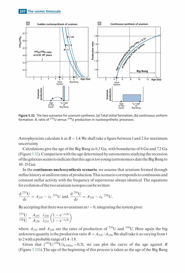
Astrophysicists calculate it asR¼ 1.4.We shall take a ¢gurebetween1and 2 for maximumuncertainty.Calculations give the age of the Big Bang as 6.5Ga, with boundaries of 6Ga and 7.2Ga

(Figure 5.32). Comparisonwith the age determinedbyastronomers studying the recessionofthegalaxies seems to indicate thatthis age is tooyoung (astronomers date theBigBang to10^15Ga).In the continuous nucleosynthesis scenario, we assume that uranium formed through

stellarhistoryatuniformratesofproduction.This scenario corresponds to continuousandconstant stellar activity with the frequency of supernovae always identical.The equationsforevolutionofthe twouranium isotopes canbewritten:

d 235U

dt¼ A235 � l5 235U and

d 238U

dt¼ A238 � l8 238U:

Byaccepting thattherewasnouraniumatt¼ 0, integrating the systemgives:

235U238U

¼ A235

A238� l238l235

1� e�l5Dt

1� e�l8Dt

� �

where A235 and A238 are the rates of production of 235U and 238U. Here again the bigunknown quantity is the production ratioR¼A235 /A238.We shall take it as varying from1to2withaprobable rangeof1.4^1.8.Given that (235U/238U)4.55Ga¼ 0.31, we can plot the curve of the age against R

(Figure 5.32b).The age of the beginning of this process is taken as the age of the Big Bang

0.2

1 2 3 4 5 6 7

0.3

0.4

0.5

0.6

0.7

235 U

/238

U

Age (Ga)

Ura

niu

mp

rod

uct

ion

Big Bang

Sudden nucleosynthesis of uranium

SolarSystem

Ageof theEarth

T0 = ageof

Big Bang

235U/238U ratioat 4.55 109 years

R =

1.4

R =

1.8

R =

1

a

1.0

2 4 6 8 10 12

1.2

1.4

1.6

1.8

Pro

du

ctio

n r

atio

Age (Ga)

Ura

niu

mp

rod

uct

ion

Big Bang

Continuous synthesis of uranium

SolarSystem

Ageof theEarth

T0 = ageof

Big Bang

at b

egin

ning

of S

olar Syste

m

Age

cor

resp

ondi

ng to

235 U/2

38 U = 0.31

b

Figure 5.32 The two scenarios for uranium synthesis. (a) Total initial formation; (b) continuous uniformformation. R, ratio of 235U versus 238U production in nucleosynthetic processes.


and varies between 8 and14Ga. Notice that as l238/l235¼ 0.157, it would only need a pro-duction ratioRof1.96 for the age to be in¢nite.Wewould then have auniformUniverse ofin¢nite age, which shows the extreme sensitivity of the entire scenario to the uranium pro-duction ratio.This is a¢ne exampleofthe relative reliabilityofradiochronometricmethods.Aswith the age of theEarth, the age oftheUniverse is related to the de¢nition ofa scenario(hereacosmic scenario).

The contribution ofextinct radioactivityLetus consider the caseof129I.Weknowwe canwrite:

129I127I

� �meteorites

¼129I127I

� �initial

e�lt:

Ifweknowthe isotopicratio129I/127Iatthe endofnucleosynthesis,we cancalculatethetimebetween nucleosynthesis and the formation of the meteorite.The various scenarios astro-physicistsproposefor nucleosynthesis indicate that (129I/127I)initialffi1.

As the ratios measured for meteorites are about10 � 10� 4, the age calculation�T¼ 1/lln(104) gives 210Ma. So there was a nucleosynthetic event less than 230Mabefore the for-mation of the Solar System during which 129I was born. But the discovery of other extinctformsofradioactivitysuchas 26Alandthen 41Caand36Clshowsthatnucleosynthetic eventsalso occurred 5Ma and1Ma before the formation of the Solar System for 26Al and 41Ca,respectively.13 Thus all the evidence points to the occurrence of explosive nucleosyntheticevents justbeforetheSolarSystem formed.Somescientists claimthese supernovaebroughtabout the collapse of the proto-Sun’s nebula by the mechanical action of the shockwaves.Nucleosynthesis, that is, the synthesis of the chemical elements, is therefore a process thattookplace throughoutcosmic timeand isprobablystillgoingon inthe stars.

DiscussionandconclusionsIt is immediatelyobvious thatanycombinationofthetwoscenarios, thatis, initialproductionfollowedbycontinuousproduction,willyieldBigBangagesof 6.5 to14Ga.Sinceastrophysi-cists thinkthattherewere supernovaexplosionswellafter theBigBangandthatextinctformsofradioactivityprovethattheyoccurredalso4.5Gaago (orshortlybefore that),wemustcon-cludethatthesuddensynthesismodelofalluraniumatthebeginningoftheUniverse isunac-ceptable.Ontheotherhand, all theastrophysicalmodels seem to show thattheUniversewasamuchmoreactiveplace shortlyafter theBigBang than it is today. It is therefore legitimatetogivegreaterweighttotheolderepochswhen itcomestonucleosynthesis (Figure5.33).

All of that suggests amixedmodel involving initial synthesis and continuous formation.Ifwe consider thatR¼ 1.5 is themost likelyproduction ratio, theageofthebeginningoftheUniverse canbe estimatedat10� 2Ga.

Naturally, one might ask why we do not try to con¢rm this calculation with anotherchronometer. In fact, we have used 232Th and the 232Th/235Uratio.This ratio is chemicallyfractionated andwe do not really know its value in the cosmos. However, taking a ratio of

13 We have taken the criterion of 6 half-lives for the element to still be ‘‘alive.’’


232Th/235U¼ (Th/238U)present¼ 4, we can repeat the calculations for the same scenariosandweobtain comparable results. Samething ifweuse187Re^187Os (Luck et al., 1980).Byusingthe recessionofthegalaxies, astronomersdatetheBigBangto13^14Ga.We can

concludethatradiochronology‘‘con¢rms’’theageoftheBigBangasdeterminedbyastron-omers and the validity of the scenario of continuous nucleosynthetic activity in theUniverse. Here we have an example of very large uncertainties because of the conceptsemployedandwhich faroutweightheanalyticaluncertainties.

5.8 General remarks on geological andcosmic timescales

5.8.1 Overall geological myopia

As we have said, the deeper we go into the past, the more our absolute uncertaintiesincrease. In recent times we can separate events 1000 years apart (and less) whereas thisis impossible, of course, in the Precambrian. As spectroscopists would say, for recent per-iods we have high resolution and for earlier periods low resolution. Thus, we can makeout clearly the alternating pattern of glacial and interglacial periods in the Quaternary.In the Secondary period we can no longer ‘‘see’’ these alternations clearly, and yet, if theyare connected with Milankovitch cycles, as we shall see, they should also have occurredin the more remote past too. The closer we get to the present, the more clearly we canmake out events separated by shorter time-spans. This is compounded by the fact that,in the course of their history, terrestrial rocks are subjected to the destructive eventsof erosion or metamorphism. The more time passes, the more destruction occurs andthe fewer traces we ¢nd and the more the probability of sampling a rock of age t

Big Bang(10–12 Ga)

Formation ofSolar System

(~4.5 Ga)

Present day

Stableisotopes

Nucleosynthesis

Radioactiveisotopes

Figure 5.33 Nucleosynthesis of elements forming the Solar System before 4.5 Ga. Isotopes aresynthesized (and destroyed) in stars. From 4.5 Ga, stable isotopes maintain the same abundanceratios and radioactive isotopes decay.

209 General remarks on timescales

diminishes with t. There is a dual e¡ect: the further we go back into the past, the fewerrocks we have of any given age and the less certain their age is.This is the phenomenon ofgeological myopia. Statistically, the further back into the past we travel, the lower thepower of resolution. This is an intrinsic di⁄culty of any historical science. And yet,where radiometric dating is concerned, there is an exception!

Theextinctformsofradioactivity129I,182Hf,109Pd,146Sm,etc.canbeusedtostudytheear-liest times oftheEarth’shistory with extraordinary precision, as if the time the Sun and theplanetary bodies formed were suddenly ‘‘lit up.’’ Resolution for these primordial times ofthe Earth’s history is almost as good as for the Quaternary.This quite incredible circum-stancearisesbecauseoneormore supernovaorAGBstarexplosionsmade radioactive iso-topes1or 2millionyearsbefore the¢rst rocksofthe Solar System formed.Thus the curveofthe power of resolution against time is not monotonic, contrary to what might have beenexpected (Figure5.34)!

5.8.2 The use of radiochronometers

Advances in analytical techniques mean that we now have an impressive array of potentialradiochronometers at hand: there are currently more than 40 of them and more are beingdeveloped.Thus anyone wanting to use radiometric dating is confronted with a problem ofchoice: which chronometer should be used for dating a particular phenomenon at such andsuchaperiod?

Withoutanyneed for longcalculations,wehaveunderstoodthat14Ccan nomorebeusedfor determining the age of the Earth than 87Rb^87Sr can be used for dating limestones ofless than 1Ma. But beyond these obvious examples lies the more general question of ourpowerofobservation of the past: which chronometers canbe used, for which periods, andforwhich rocks?

Domains for usinggeochronometers basedonanalytical criteriaIfthetime-spantobemeasuredis farlonger thanthehalf-lifeoftheradioactive isotope, thenthe radioactive product will have died prematurely and so indicate nothing more. If thetime-span isverymuchshorter thanthehalf-life, then the radioactivitywillbe insigni¢cantand its result undetectable.We are thus brought back to the calculations of uncertaintyalreadycovered (seePlate7).

Res

olv

ing

po

wer

of

rad

iom

etri

c d

atin

g m

eth

od

s

Age

100 Ma

10 Ma

1 Ma

100 ka

10 ka

1 ka

100 yr

1 Ga 100 Ma 10 Ma 1 Ma 100 ka4.55 Ga

Figure 5.34 Resolving power of all dating methods versus age.


Exercise

Can we measure an age close to 2 Ga for a rock with 87Rb/86Sr ratios whose maximum

deviations from the origin are 10, 1, 0.1, 0.01? We accept that the precision of the measure-

ment on the 87Sr/86Sr ratio is � 10� 4 and on 87Rb/86Sr � 10�3.

AnswerWe can determine an age in each of these cases. For �¼ 10, T¼ 2� 0.001 Ga, for �¼ 0.01,

T¼ 2� 0.5 Ga.

Exercise

Why is the use of 14C limited with counting to 6 half-lives whereas with mass spectrometry it

can reach 10 half-lives?

Can we measure the same age with the 234U–238U method, given that we have a rock

containing 10% uranium (uranium ore)? Why?

AnswerThe answers are deliberately withheld here. Readers must find them for themselves to

understand what comes next.

Formethodsbasedon decayof theparent, the datingequation iswritten:

� ¼ �0 e�lt

where � is 14C/C, 10Be/Be, etc. Analysis of uncertainty (Section 3.2.1) has shown that thismethod applies only ifT is neither too large nor too small. In practice, we considerTmustcomplywith thedouble inequality:

10 half-lives5T510�3 half-lives:

Ofcourse, thedomainofapplicationofamethod is extendedas improvements inanalyticaltechniques aremade, andprogress is continuouswith noprospectofan end.Still, letusgiveananswer to theprevious exercise.Formodern equipment,14C/Cactivity

is 13.4 dpm g�1 of carbon. Six half-lives represents 1 disintegration per hour, whereas thebackground noise is at least 5^10 disintegrations per hour.The uncertainty is intolerable.However, with themass spectrometer wemeasure a ratiowhich at the present time is10� 12

and is advancing to 10� 15, which is not easy but can be done, especially if we increase theamountofmatteranalyzedbyafactorof10or100!For long-period parent^daughter systems, with the usual conventions, the dating

equation is written:

� ¼ �0 þ �ðelt � 1Þ:

There is nophysical upper limit to theuse of thesemethods.The lower limitofapplicabilityarisesbecausethequantity (��0)mustbemeasurableandthereforedependsonthepreci-sionofthe isotopicmeasurementofthedaughter product:


� ðelt � 1Þ4D�:

Weknow that, depending on the methods and techniques used, ��maybe10� 3,10� 4, oreven of the order of 10� 6 with a wealth of precautions. There is therefore a connectionbetween�andtheminimumageTmin thatcanbemeasured:

� ¼ D�elt � 1

� �:

This calculation has been done for the main long-period chronometers and in eachcase for the main rocks and most ‘‘useful’’ minerals. It is illustrated for 87Rb^87Sr inFigure 5.35.

Exercise

Calculate the range of use of 176Lu–176Hf. What are the common minerals that give the best

results? (Look for the necessary parameters in the scientific literature!)

AnswerUp to 1 or 2 Ma. Garnet is the most effective.

In the case of methods related to radioactive chains, the calculation is a little more com-plex.Allowancemustbemadeforboth the radioactiveparentand the radioactive daughter

Rb

/Sr

Age

100

50

2

0.1

0.01

Granites 10–4

10–3

10–5

Basalts

1 Ga 0.1 Ga 0.01 Ga 0.001 Ga 0.0001 Ga4.55 Ga

GranitesBasalts

100 Ma 10 Ma 100 ka1 Ma

Figure 5.35 Domain of use of 87Rb–87Sr applied to whole rocks. The x-axis shows the minimum agesthat can be measured. The y-axis shows the values of the chemical ratio Rb/Sr. The diagonals indicatethree precisions on the measurement of the 87Sr/86Sr ratio: 10� 3, 10� 4, and 10� 6.


andfor the causeofdisequilibrium(isolationoftheparentordaughter).Withoutgetting intothe calculations, where the principle is identical to the previous ones, we can say that theages determinable are such that: 5 half-lives>T> 10� 2 half-lives of the daughter isotope(Figure5.36).

Exercise

We consider the isochron method applied to the 238U–230Th pair. Empirically, we calculate the

value of the slope of the isochron against age and plot it (Figure 5.37). What do you conclude

about its domain of use?

AnswerWe obtain 5 � 103< T< 5 � 105.

0.06 half-lives< T< 6 half-lives.

We are within the orders of magnitude defined.

2.0

1.5

0.5

0.0

1.0

100 101 102 103 104 105 106 Act

ivit

y ra

tio

s p

aren

t–d

aug

hte

r

Time since chemical fractionation (years)

(210Pb)

Excess daughter

Excess parent

(226Ra) (226Ra) (230Th)

(234U)(238U)

(231Pa) (235U)

(230Th) (234U)

Figure 5.36 Intervals for use of the various chronometers based on radioactive disequilibrium.

1 2 3 4 51104

5 × 104

1 × 105

2 × 105

1 × 106 1 × 107

6 7

1.0

0.8

0.6

0.4

0.2

Slo

pes

log t (yr)

Ages (years)

Figure 5.37 Variation of the slope of the 238U–230Th isochron with age. (Notice the logarithm is to base 10.)


Geological modulation of the time domains for the use of radiochronometersThequestion here is howdo thegeological constraints alter the conclusion about the rangeof application of the various methods established based on analytical errors. As we haverepeated incessantly, a radiochronometer ismerelyan isotope ratio expressed as an agebythe formula re£ecting radioactive decay.The conceptofage in itself is‘‘virtual’’andapurelyarithmetic one.Wemust therefore thinkabout the physical system, its history, the chemicalproperties of the elements, and the initial conditions, and connect these considerationswith geological historybeforewe can attribute a signi¢cant age to ameasurement (ora ser-iesofmeasurements).

Examination of the criteria to ensure theboxes remain closed hasbeen one of themajorconcerns ofgeochronology. How can any ‘‘untimely’’opening be detected? A form of sys-tematic approach has arisen empirically from these studies, although it cannotbe said thatwe have any absolute criteria because geological situations are so varied and complex. Aswehavealreadysaid, the reasons systemsopenare straightforward enough: radiogenic iso-topes are intruder atoms in the crystalline structures where they are found and so tend toescape. Can this phenomenon be quanti¢ed generally? There is no mathematical methodforestimatinggeologicalvagaries‘‘forcertain.’’Wecanmakeafewcalculationsondi¡usiontogetour ideas straightandgiveusordersofmagnitude,but littlemorethanthat.

Letus takeargonasanexample.Atordinary temperatures,di¡usion coe⁄cients for 40Arareoftheorderof10� 20 cm2s� 1. Ifwerecall thedistance covered isx �

ffiffiffiffiffiffiDtp

, then, in1bil-lion years x� (3 � 107 109 10� 20)1/2¼ 0.005 cm.Therefore, at ordinary temperatures,eventhe smallestminerals are closedsystems.

However, at 250 8C, which is a low-grade metamorphic situation, the di¡usion coe⁄-cientofargon is of the orderof10� 12 cm2 s� 1.This time, for100Ma, the distance covered is54 cm, therefore all of theminerals are open.Now, such conditions (100Maat 250 8C) cor-respond, say, to a rock located at a depth of10 km in the Earth’s crust.This mayhappen bychance to a granite either when caught up in tectonic folding or when covered by a thicklayer of sediment during the formation of a sedimentary basin. But each region and eachrockmassifhas itsowngeologicalhistory.

We have therefore given precedence to experience amassed through hundreds (or nowperhaps thousands) ofexamples like thosewehavementioned fromwhichwehave derivedempirical rules, the variety of which does not lend itself to quantitative systematization.Thiswas¢rstdonefor isolatedapparentages, then for themore elaboratemethods (concor-dia, isochrons, etc.).Hereareafewexamplesofthese results.

The most sensitive methods to di¡usion phenomena are those using the rare gases40K^40Ar or U^He.The reason for this extreme susceptibility is simple.When a rare gashas leftthe crystallographic sitewhere itwas createdand¢nds itselfonthe rimofthe crystalor in a crystal defect, as it is not electrically charged, it is gaseous and lighter than the sur-roundingrocks, itmigratesupwards.This iswhy,saveinexceptional circumstances (meteor-ites), 40K^40Ardoes notprovide any reliable ages for rocks older than1Ga.The 39Ar^40Armethod is farmore e¡ective.

For older ages, we adopt the opposite approach. Knowing the true age by other meth-ods (Rb^Sr, U^Pb, or Sm^Nd), we determine the apparent K^Ar age to estimate themore or less complex geological history of the rock. A K^Ar age close to the true age is


indicative of a quiet geological history. This is a valuable clue. If the KÂr age is muchlower than the ‘‘more robust’’ ages, the rock has been subjected to periods of heating. Ifthe KÂr age is older (which it seldom is), aqueous weathering has dissolved thepotassium.Adespairing case is187Re^187Os. Inprinciple thismethodshouldbealmost ideal fordat-

ing granites andbasalts ofall agesbecause theReÔs ratios areveryhigh (ratios of1000 to5000 are commonplace). We could hope to pin ages down to a few thousand years.Unfortunately, whole rocks do not generally behave like closed systems and so dating bythismethod is restrictedandagedeterminationsaredi⁄cult.

Exercise

We have measured the rhenium and osmium contents of olivine in oceanic basalt as 4112 pg

g� 1 and 3361 pg g� 1, respectively.

Supposing we know the initial ratio of the basalt 187Os/188Os¼ 0.1265 and that the187Os/188Os ratio measured in the olivine is 0.1859, what is the age of the olivine?

If we can measure the 187Os/188Os ratio with a precision of 1% at these very low levels,

what is the age of the olivine assuming it has remained in a closed system?

Answer565 ka.

12 300 ka.

To summarize this researchwhich is above all empirical, the geochronologist’s toolboxis shown inPlate7.Beware, though, this isnoautomaticgearbox!Letusrepeatonceagain,nooneradiochronometeralone canresolveaproblemandguar-

antee a result.Geochronological redundancy, in other words the con¢rmation of a resultby various other methods, is an essential concept. Now there areverymany chronometersthat canbeused, but each series ofmeasurements is di⁄cult, time-consuming, and expen-sive. Sowe cannotapplyeverychronometer to everyproblem.Wemustchoose themostsui-tableones . . .anddoalittle thinking.

5.9 Conclusion

This chapterhas allowedus tovalidate thevariousgeochronometers through the analysisofuncertainties. Overall they are reliable and yield consistent results. However, we mustnever forget the concept of essential uncertainty which must always be taken intoaccount.Each geochronological result is a¡ected by uncertainty. Ifwe do not know (estimate)

this uncertainty, a result is scienti¢cally meaningless.We have analyzed these uncertain-ties to show theyareofdi¡erent types: theymaybe due to sampling, laboratorymeasure-ments, adaptation of methods to the problem in question, or to the geological or cosmicscenario.In this contextwemust emphasize ad nauseam that age is simplyan isotopic or chemical

ratio that is converted into time by a mathematical formula. Such conversion is practical

215 Conclusion

becausewe can directly compare thevariousmethods and, ofcourse, connect themethodswith thegeological history for which theyare oneofthe referencemarkers. But as soon as adi⁄cultyarises,wemust comebackto the isotopic ratios and the chemicalproperties oftheelements. It isgeochemicalhistory thatcontrols theway the chronometersbehave.

This is thegeneral context inwhichwehave reviewedthemain¢ndingsofgeochronologywhichthemselves areassociatedwithuncertaintyoreven indetermination.

Problems

1 An expedition to Mars to bring back samples is under preparation and you are the Rb–Sr

specialist for dating the rocks. Preliminary missions with soil analyses by in situ techniques and

analogies with shergottite-type meteorites indicate that the rocks found will be basalts with

average Rb/Sr ratios of 0.1 and 4, respectively, and average Sr contents of 300 ppm and

30 ppm, respectively.

(i) How much rock needs be collected to make analyses with a precision of 10� 4? (We know

we will need to have 100 ng of strontium and 50 ng of rubidium.)

(ii) Given that the probable ages are between 2 Ga and 500 Ma, do you think the determi-

nation will be reliable? What sort of isotope ratios do you expect?

(iii) What will be the error you make on the age if it is 500 Ma? If it is 2 Ga?

(iv) Only 1 kg of rock can be brought back. Would you prefer to have a single compact rock or

five fragments of different rocks of 200 g each? Why?

2 Here are the results obtained by the 238U–230Th method on a volcanic rock of Costa Rica.

After calculating the age of the rock, estimate the error on this age in various ways: graphical,

least-squares method. Then state your estimate.

3 Here are results for a granite of the Montagne Noire (France).

Can you estimate the age and the error you make on the age in this situation?

4 (i) The measurement of 14C by accelerator mass spectrometry gives for modern (present-day)

carbon the ratio 14C/12C¼ 1.2 � 10� 12. For a current of 2 � 10� 6 A of 12C obtained by

238U–230Th 230Th–232Th

Whole rock 1.41� 0.05 1.21� 0.04

Magnetite 2.41� 0.02 1.92� 0.12

Plagioclase 1.37� 0.03 1.18� 0.07

Augite 0.62� 0.01 0.78� 0.04

Hypersthene 1.02� 0.08 1.01� 0.05

87Sr–86Sr 87Rb–86Sr

Whole rock 0.728� 0.002 3.62� 0.05

Biotite 2.32� 0.01 408� 4

Muscovite 0.735� 0.002 8.07� 0.05

Apatite 0.733� 0.002 0.03� 0.003

Plagioclase 0.7127� 0.001 1.44� 0.02


bombarding 1 mg of carbon with a stream of cesium ions, the flow of 14Cþ ions is 15

ions per second.

(a) For the same intensity of current of 12C, how many 14C ions are obtained per unit

time for 1 mg of carbon aged 55 ka?

(b) If the measurement lasts 20 minutes, what is the uncertainty on the age determina-

tion? Compare it with the error on the measurement of the present-day 14C/12C ratio.

(c) What is the minimum age we can hope to measure in the same conditions if we

decide the difference to be measured with the present day must be at least five

times greater than the uncertainty?

(d) If we wanted to make the same measurement by counting � radioactivity and the

maximum counting time for a sample was 8 days, how much carbon would need to

be purified?

(ii) We wish to use the 238U–230Th method to test the 14C age of corals assumed to be about

55 000 years old. To simplify, we ignore the 234U/238U fractionation and assume that

(230Th)0¼ 0. The dating equation is written:

230Th232Th

¼238U

232Th

� �ð1� el230t Þ:

Given that the uncertainty on the 230Th/232Th ratio measurement is 1% and that the uncer-

tainty on the 232Th and 238U measurements is about 5ø, what is the uncertainty on the age?

Is this a good method for checking the results obtained by 14C in this age range?

5 We are confronted with the geological situation shown in the section in Figure 5.38.

A geological formation of foliated and folded gneiss is cross-cut by a granodiorite which is

itself foliated.

(i) We wish to measure the age of the gneiss and to do so we make a series of 87Rb/86Sr

measurements on the whole-rock. The results are given in Table 5.9. The Sr concentrations

of the various facies are very similar. Calculate the 87Rb/87Sr age using a simple least-

squares method (without experimental uncertainties).

(ii) We determine the age of the granite by U–Pb methods applied to zircons from the granite.

Table 5.10 shows the results. Calculate the U–Pb age again by the simple least-squares

method and the concordia method. How would you interpret the result in geological

terms? Can you give a brief geological history of the region?

87Rb-87Sr(Whole rock)

U-Pb(Zircons)

Figure 5.38 Geological formation of gneiss cross-cut by granodiorite.

217 Problems

6 A granite from south-eastern Canada is dated by various methods. The apparent age

results are:

Can you reconstruct the geological history of this granite and explain the ages measured?

7 We can determine the Permian–Triassic boundary at a given location. A granite cross-cutting

the Permian formation but with pebbles at the base of the Triassic is dated 243� 5 Ma. The

Triassic is dated by two basalt flows located in a section 100 m above the Permian–Triassic

boundary at 229� 8 Ma and another 200 m above the Permian–Triassic boundary at

215� 3 Ma. What is the approximate age of the Permian–Triassic boundary? What is the

error on the age determination at 218� 3 Ma?

8 You are asked to explore the possibility of using the U–He chronometer.

(i) What time-span do you think best corresponds to the potential of the method?

(ii) What types of rock or mineral do you think are interesting a priori?

9 Half a century ago the question of the origin of granite was a subject of much debate. The

American Bowen showed by laboratory experiment around 1930 that rock of granitic com-

position could be made from basaltic magma (which we know is itself the product of partial

melting of the mantle). Bowen and Winkler in Germany showed, again by experiment, that

the melting of detrital sediments (shales and sandstones) to which sodium has been added

Table 5.9 Samples from the gneiss in Figure 5.38

Sample 87Sr/86Sr 87Rb/86Sr

1 0.713�0.0005 0.1�0.00052 0.718�0.0005 0.35�0.00053 0.719�0.0005 0.45�0.00054 0.722�0.0005 0.6�0.00055 0.724�0.0005 0.8�0.00056 0.723�0.0005 0.9�0.0005

Table 5.10 Samples from the granite in Figure 5.38

Sample 206U*/238U 207Pb*/235U

A 0.3� 0.01 5�0.3B 0.26� 0.01 4�0.3C 0.24� 0.01 3.5�0.3D 0.2� 0.01 2.5�0.3

Method U–Pb

concordia

Rb–Sr

whole

rock

Sm–Nd

whole

rock

Rb–Sr on

biotite

39Ar–40Ar Rb–Sr on

muscovite

Apparent

age (Ga)

2.8� 0.1 2.7� 0.1 2.7� 0.1 1.7� 0.2 1� 0.1 1.7� 0.2


also gives rise to a granitic magma. Subsequently, other experiments showed that the partial

melting of ‘‘wet’’ basalts produced granitic fluids.

These experimental data were supplemented by field observations and then more recently

by 87Sr/86Sr measurements supporting the idea that almost all continental granites result

from the remelting of continental crust. The model of granites derived directly from the

mantle was abandoned. Yet, in the middle of the mid-Atlantic ridge, in Iceland, the famous

Hekla volcano has spewed out lava of granitic composition (rhyolites). The 87Sr/86Sr ratios of

about 0.7032 give no clear answer to their origin as they are similar to those of many basaltic

lavas of Iceland.

The Icelander Sigmarsson studied the (230Th/232Th, 238U/232Th) ratios of these rhyolites

with the 230Th–238U isochron diagram. The mantle beneath Iceland is in secular equilibrium,

corresponding to 238U/232Th ratios of 1.1 to 1.3 (in activity). The oldest basalt crust of Iceland

has (active) 238U/232Th ratios ranging from 0.9 to 1.1. It too is in secular equilibrium. The

rhyolites have a 230Th/232Th ratio of 0.95 and 238U/232Th of about 0.8. What do you think is

the origin of this rhyolite?

10 Calculate the range of application of the 238U–206Pb dating method for rocks and minerals

with the chemical ratios shown in the table below, given that the isotopic measurement is

affected by several relative uncertainties �x of 10�3, 10�4, and 10�5.

Draw the graphs corresponding to Figure 5.35. Calculate for the Rb/Sr ratio, and for U–Pb

applied to whole rocks and the main minerals that can be dated by this method.

Type of rock or

mineral

Granite Basalt Ultramafic Zircon Sphene

U/Pb 0.2 0.1 0.05 100–10 2

219 Problems

CHAPTER SIX

Radiogenic isotope geochemistry

Our main concern in the previous chapters has been to calculate geological (or cosmo-logical) ages and to clarify their geological meanings. In the next chapters we are going toaddress isotope geochemistry, which has a markedly di¡erent viewpoint although it isbased on the same physical laws andon the same equations.We are going to look not at agebut at the isotope ratios measured and the ways in which their natural variations may beinterpreted.

This chapter, then, focuseson isotope ratioswhosevariationsarisemainly fromradioac-tive decay.Chapter 7will be about isotopevariations causedbyphysical and chemical pro-cesses. Examination of the variations in isotopic ratios will lead us to develop amethodologyinwhichtheseratiosareusedas tracers formajorgeologicalandgeodynamicphenomena. The purpose of these studies is therefore to determine the major structuresand exchanges ofmatteroccurring (or havingoccurred) among themajor terrestrial reser-voirs (crust, mantle, core, and atmosphere).The notion of age will crop up again, but in amuchmoregeneral context, although in complete continuitywiththe earlierchapters.

6.1 Strontium isotope geochemistry

6.1.1 Continents and oceans: granite and basalt

Thenatural isotopic compositionofstrontiumvarieswith 87Rb decay. Systematic collationof 87Sr/86Sr isotope compositions of terrestrial basalt andgranite (basaltbeing an isotopic‘‘messenger’’fromthemantlewhilegranite is a sampleofcontinental crust) revealsverydif-ferent distributions. Strontium isotope ratios for granites from the various continents arehighly variable, ranging from 0.705 to 0.850 andmore. Strontium isotope ratios for basaltsaremuchmoreuniform.They range from0.7020 to 0.7070 and foroceanicbasalts fromjust0.7022 to0.7045.

Let us get these orders of magnitude clear. ‘‘Ordinary’’ analytical precision on the87Sr/86Sr isotope ratio is at least1.5 � 10�4 (relative) and therefore, on ratios close to 0.7, theuncertainty isbetter than10�4 (absolute).Thismeans that 0.7022 canbe distinguished from0.7021for certain. For granite, variations range from 0.850 to 0.705, corresponding to1500measurementunits. Foroceanicbasalts, the range is 25measurementunits, oradispersionratioof60 times less than forgranites.

This di¡erence in the distributions of strontium isotope ratios between continents andmantle can be explained by the geological historyof the two reservoirs fromwhich granite

Pla

te1

Per

iod

icta

ble

of

the

elem

ents

.Th

eis

oto

pes

mo

stco

mm

on

lyu

sed

inis

oto

pe

geo

log

ya

rein

dic

ate

d.

Magnet

Magnet

Multicollector

Multicollector

Ionbeams

Ionbeams

Electrostaticanalyzer

Multi-filamentturret

Plasmagenerator

Source

Plate 2 Modern mass spectrometers. In each case, the mechanical components are shown at the top and the ionbeam pathways below. Top: TIMS (thermal-ionization mass spectrometry). At the source, a turret allows severalsamples to be tested in succession; at the collector, multicollection allows the various beams from differentisotopes to be analyzed without scanning. Bottom: ICPMS (inductively coupled plasma mass spectrometry). Inaddition to the magnet, an electrostatic analysis sorts the ions by energy levels. The source is a plasma generator.Multicollection is used as in TIMS.

Plate 3 Actual laboratory equipment. Top: A Cameca ion probe. Bottom: A clean room where samplesare prepared.

6090

180

120

60 900

60

0

6060

0

Dar

k re

d

0-1

Ma

Med

ium

red

1

-4 M

a

Lig

ht

red

4

-9 M

a

Ora

ng

e

9-20

Ma

Bro

wn

20

-35

Ma

Lig

ht

bro

wn

35

-52

Ma

Yel

low

52

-65

Ma

Gre

en-y

ello

w

65-8

0 M

a

Lig

ht

gre

en

80-9

5 M

a

Med

ium

gre

en

95-1

10 M

a

Dar

k g

reen

11

0-12

5 M

a

Gre

en-b

lue

125

-140

Ma

Blu

e 1

40-1

60 M

a

Purp

le

160-

180

Ma

Pla

te4

Ma

po

fo

cea

nfl

oo

ra

ges

.Aft

erSc

late

r,Ja

up

art

,an

dG

arl

son

(19

80

).

0.25 - 0 Ga

0.7 - 0.25 Ga

1.7 - 0.7 Ga

2.5 - 1.7 Ga

3.8 - 2.5 Ga

3.8 - 1.7 Ga

Plate 5 Map of age provinces of continents. Top: world map. Bottom: more detailed map of NorthAmerica. After Hofmann (personal communication, modified).

3.8

3.6

3.2

2.8

Present day

Formationof the Earth

Hadean

Archean

Isua formationGreenland

Barberton

Great Canadianorogeny

Cambrian

8Ga

Phanerozoic time

West-Africanorogeny

Proterozoic

Grenvilleorogeny

Pan-Africanorogeny

Eoarchean

Paleoarchean

Mesoarchean

Neoarchan

4.0

4.5

2.5

1.6

1.0

0.55

Paleoproterozoic

Mesoproterozoic

Neoproterozoic

Ga

Big Bang

Precambrian times

12Ga

10Ga

Plate 6 Geological timescales. Left: Precambrian times. Right: Phanerozoic times.

CENOZOIC

MESOZOIC

PALEOZOIC

4.5Ga

0.55Ga

+5

-30⌠⌠

+5

-5⌠⌠

+5

-5⌠⌠

NEOGENEPLIOCENE

MIOCENE

OLIGOCENE

EOCENE

PALEOCENE

PALEOGENE

CRETACEOUS

JURASSIC

TRIASSIC

PERMIAN

CARBONIFEROUS

DEVONIAN

SILURIAN

ORDOVICIAN

CAMBRIAN

PRECAMBRIAN

CENOZOIC

MESOZOIC

PALEOZOIC


Hadean

Archean

Isua formationGreenland

Barberton

Great Canadianorogeny

Cambrian

Phanerozoic time

West-Africanorogeny

Proterozoic

Grenvilleorogeny

Pan-Africanorogeny

Eoarchean

Paleoarchean

Mesoarchean

Neoarchan

Paleoproterozoic

Mesoproterozoic

Neoproterozoic

NEOGENEPLIOCENE

MIOCENE

OLIGOCENE

EOCENE

PALEOCENE

PALEOGENE

CRETACEOUS

JURASSIC

TRIASSIC

PERMIAN

CARBONIFEROUS

DEVONIAN

SILURIAN

ORDOVICIAN

CAMBRIAN

PRECAMBRIAN

570

500

435

395

345

280

235

195

141

6557372612

Ma


Firsthumans

Precambriantimes

Phanerozoictimes

Phanerozoic times

4.55 Ga 1 Ga 100 Ma 10 Ma 1 Ma 100 ka 10 ka 1 ka 100 years

1 Ma 100 ka 10 ka 1 ka 100 years

14C

231Pa

230Th

234U

10Be8.9

226Ra

500 Ma

107Pd-107Ag

129I-129Xe

182Hf-182W

146Sm-142Nd

244Pu-Xef

CONDENSATION

FORMATION OF THE EARTH

METEORITES

GranitesBasalts

KspathsMuscovitesBiotites

GarnetsGranites, BasaltsSm/Nd

or Lu/Hf

U/Pb

Rb/Sr

Re/Os

K/ArK/Ar

U/He

100 Ma10 Ma1 Ma100 ka10 ka

BasaltsGranitesSphenes, ApatitesZircons

Precambrian Paleoz Mesozoic Cenozoic Quaternary

Pleistocene Holocene

Cam

bri

an

Ord

ovi

cian

Silu

rian

Dev

onia

n Ca

rbon

ifero

usPe

rmia

nTr

iass

ic

Jura

ssic

Cre

tace

ou

s

Eoce

ne

Olig

oce

ne

Plio

cen

e

Mio

cen

e

53Mn-53Cr

60Fe-60Ni

26Al-26Mg

41Ca-41K

Plate 7 Ranges of the main geological clocks. Notice that the timescales are logarithmic.

and basalt arise.Granite is the essential constituent of continental crust.The continentalcrust is a permanent feature of the Earth’s surface and is very, very old, at least 4Ga andpossibly older.When granites are systematically dated on a continent and the datingsmapped, geological age provinces are de¢ned. The classical example is that of NorthAmerica, as we have seen, and the same is true of other continents. There are granitesaged 3.8Ga (Greenland), 2.7Ga (Canada, Scandinavia), and 2Ga (Ivory Coast,Sahara), but also granites aged 50Ma (Himalayas) or even 5Ma (Himalayas, Andes,Alps) (see Plate 5).Asgeologicalstudieshaveshown, theseprovincescorrespondtowell-de¢nedepisodes in

geological history during which orogeny, that is, mountain building, occurred. Rockwasfolded andmetamorphosed and granite was formed bymelting of the lower crust andwasinjected into theupper partofthe crustduring theseorogenic episodes. In accordancewithoneofthebasicprinciples ofplate tectonics, thesepiecesofcontinent£oatonthe surfaceofthe mantle, they are broken up and drift about but are not swallowed up as suchwithin themantle by subduction.They therefore form a mosaic of blocks of di¡erent geological ageswhich have accumulated, brokenup, anddrifted togetherat theEarth’s surface throughoutgeological time.In the course of geological cycles, with the succession of erosion, sedimentation, meta-

morphism,andfoldingandformationofgranites, theisotopicgeologicalclockswehavestu-died in the previous chapters are more or less reset and so date these episodes more or lessaccurately. But a great part of the ancient continental material is preserved and recycled,whether it is rejuvenatedor not.Basalt is the primary constituent of oceanic crust. Unlike continental crust, oceanic

crust is very young. Oceanic crust arises from the mid-ocean ridges, spreads, and thenplunges at subduction zones to be recycled in the mantle. The oldest oceanic crust is200Ma, theaverageagebeing80Ma.Bycontrast, the rocksofthepresent-dayocean ridgesarevirtuallyofzeroage.Oceanicbasalts aretheproductofmantle-meltingandas thatmelt-ingoccursathightemperatures isotopic equilibrium is achieved.This iswhyoceanicbasaltre£ects the isotopic compositions of the present-day mantle. Now, the mantle, being sub-jected tovigorous convectivemotion, isprobablywellmixed. It is only tobe expected, then,that the isotopic compositions of such a medium should be far less heterogeneous thanthose of a medium that is segmented like a mosaic of old pieces of various ages, which iswhatthe continental crust is (Figure6.1).Let us now try to explain the di¡erence in the strontium isotope structure of the conti-

nents and of the oceanic basalts in more quantitative terms. By the same token, we shallbring together the reasoning already employed and which helped us in developinggeochronology.

6.1.2 Isotope evolution diagrams and multi-episodeevolution models

One simplewayof representing changes in 87Sr/86Sr ratios is to plot a diagramof 87Sr/86Srversus time. Ifwewrite asour reference the evolutionofan isotope ratio in a closed environ-ment, by using the linear approximation, we obtain an equation we have already comeacross:

221 Strontium isotope geochemistry

87Sr86Sr

� �t

¼87Sr86Sr

� �0

þ87Rb86Sr

� �lt:

This is the equation ofa straight line in the87Sr86Sr

; t

� �diagramwhose slope is l

87Rb87Sr

� �and

so is proportional to the Rb/Sr chemical ratio.The higher �¼ 87Rb/86Sr is, the faster the87Sr/86Sr isotope ratio grows, and the steeper the slope of the straight line of evolution(Figure6.2).

Let us now consider a system comprising two episodes.We begin with a (87Sr/86Sr)0isotope ratio¼�0. During the ¢rst episode fromT0 toT1 (the ages are counted from thepresent day) the system has a 87Rb/86Sr ratio¼�0.Then, atT1, the chemical ratio changesbecause the initial system is separated into several sub-systems, A, B, and C, whose87Rb/86Sr ratios are noted �A, �B, and �C, respectively. The three sub-systems evolve asclosed systemsuntil thepresentday.The evolution equations foreachmediumarewritten:

Sub-system A ¼ �Apresent day ¼ �0 þ l�0ðT0 � T1Þ þ l�AT1 ¼ �T1

þ l�AT1

Sub-system B ¼ �Bpresent day ¼ �0 þ l�0ðT0 � T1Þ þ l�BT1 ¼ �T1

þ l�BT1

Sub-system C ¼ �Cpresent day ¼ �0 þ l�0ðT0 � T1Þ þ l�CT1 ¼ �T1

þ l�CT1

where�T1is the common isotope ratioat�T1

¼ �0 þ l�0ðT0 � T1Þ.Graphically, in the (�,T) plane, these three equations are represented ¢rst by a single

straight line joining theorigin to thepointof convergence (T1,�1) and thenby three straightlineswhichdiverge inproportiontotheirdi¡erent�values (Figure6.2).

Let us return now to the question of the di¡erence in dispersion between granites andbasalts, that is, between continental crustandmantlematerials.

The mantle has very low 87Rb/86Sr ratios, ranging from 0.01 to 0.1.The evolution of its87Sr/86Sron the isotope evolution diagram is almost a horizontal line ifwe take dispersion

87Sr/86Sr

NMORB

Granitesand

gneisses

0.700 0.750 0.800

Figure 6.1 Histogram of 87Sr/86Sr ratios. Ratios are measured in the mid-ocean-ridge basalts (MORBs)and in the granulites of the lower continental crust and the granitoids of the upper continental crust.Notice the wide dispersion of values for granite compared with MORB values.

222 Radiogenic isotope geochemistry

measured on granite as our scale.The ratios representing the continental crust are muchhigher: theyrangefrom0.3 to5.Letusgettheorderofmagnitude clear inourminds.

Exercise

Suppose that granites from the continental crust derive from the mantle, which has a 87Sr=86Sr� �

isotopic ratio �0¼ 0.701. Calculate the present-day 87Sr/86Sr ratios of the granites assuming

that their ages are 3, 2, and 1 Ga, respectively, with 87Rb/86Sr ratios of 1, 2, and 3, correspond-

ing to the time when they became granites, therefore when they were extracted from the

mantle. Plot the isotope evolution on an (�, T ) diagram.

AnswerHere is the matrix of the results for the 87Sr/86Sr ratios of these granites (Table 6.1). Assuming

the mantle has a 87Rb/86Sr ratio of 0.01, the evolution of the granites is shown in the (�, T)

diagram in Figure 6.3. It shall be seen that the Rb/Sr ratios and age dispersions assumed in the

model are enough to explain the wide dispersion of continental granites observed.

T1Time

A*Differentiation

B*

C*

AA

B

C

presentT0

α0

αT

presentT0

α0

87R

b/8

6 Sr

T1Time

presentT0

87R

b/8

6 Sr

87Sr

/86 S

r87

Sr/8

6 Sr

presentT0

B

C

A*

B*

C*

tg = λ87Rb86Sr

Figure 6.2 Diagrams of the evolution of isotope systems with time. Left: the 87Rb/86Sr parent–daughterratio versus time. Right: the 87Sr/86Sr ratios for the same systems under the same conditions. Top:evolution of several closed systems where the 87Rb/86Sr ratios are constant. Bottom: a two-stageevolution. The first episode has a constant Rb/Sr ratio and evolves in a closed system. At T1 a suddenchemical differentiation event occurs giving rise to two systems (A) and (B) with two different Rb/Srratios. Afterwards, the systems evolve separately as closed systems. Right: the chemical scenario as ittranslates on the isotope evolution diagram.


E X A M P L E

The history of the granites of western Greenland

A real case is represented in the strontium isotopic evolution diagram (Figure 6.4), that of the

granites of western Greenland studied by Steve Moorbath of the University of Oxford and his

various co-workers. Notice that this real diagram (almost) matches the diagram for the

theoretical model (see Moorbath and Taylor, 1981).

Letustiethis inwithwhatwelearnedinChapter3aboutthe isochrondiagram.Inthethe-oretical two-stage model of evolutionwith di¡erentiation at T1, we represented the systeminan (�,T) diagram.The equations for the three straight lineswere:

�A ¼ �T1þ l�A T1

Table 6.1 Present-day (87Sr/86Sr) ratios

Age (Ga)

� 3 2 1

3 0.8288 0.7862 0.74362 0.7862 0.7578 0.72901 0.7436 0.7294 0.7152

3 2 1

0.800

0.750

0.700

87Sr

/86 S

r

Time (Ga)

Figure 6.3 Theoretical (87Sr/86Sr, T) isotope evolution diagrams.


�B ¼ �T1þ l�B T1

�C ¼ �T1þ l�C T1:

In these equations the common isotope composition at timeT1 is noted �T1.The three sys-

tems couldhavebeen represented in an (�,�) diagram (Figure 6.5).This is the isochron dia-gram, which is one of the foundations of geochronology.Why use (�, �) in geochronologyand (�,T) in isotopegeochemistry?Theanswer is importantas itde¢nesamethod.In geochronology,what we measure directly are a and m. It is therefore normal to plot

the two types of measurement that are to de¢ne a correlation diagramwhose slope, thatis, the age, we shall calculate. In isotope geochemistry, we determine agesTand initial

0.730

4

A

D

BC

3 2 1 0

0.720

0.710

0.700

87Sr

/86 S

r

Time (Ga)

Mantle

Greenland granites

Figure 6.4 Isotope evolution diagrams for rocks of western Greenland. A, Amitsoq gneiss; B, Nuk gneiss;C, Ketelidian gneiss; D, Quorguq granites. After Moorbath and Taylor (1981).

λT1

μC μB μA

αA

αB

αC

αT1

87Sr

/86 S

r

87Rb/86Sr

A*

B*

C*

Figure 6.5 Equivalent to the diagram at the bottom of Figure 6.2, but plotted differently.


ratios �0 by isochron construction diagrams on the various sets of rock, of varied ages.Ourdatawill thereforebe�0 andT. It is normal, once again, toplot the data forone againstthe other.The unknown (provided by the slope) is the 87Rb/86Sr ratio, which is therefore achemical parameter.

6.1.3 Granites and granites

Inthetheoreticalmodelofevolutionofgranites inthe exercise,weassumedthatthegranitesderived from di¡erentiation of the mantle.Their initial isotope ratios were therefore thoseof the mantle. This idea of granite deriving from the mantle by chemical di¡erentiationfrombasalticmagmawas¢rst proposedbyNorman Bowen. In the1920s and1930s he con-ductedthe¢rstpetrologyexperiments inthe courseofwhichhemadeapieceofgranitearti-¢ciallybycrystallizingameltofbasaltbystages (fractional crystallization) (Bowen,1928).

After thewar,asecondideaarose.Having¢rstbeenevokedbyBowen himself itwasactu-allydevelopedby theGerman school andparticularlyHelmutWinkler.Hetoomadegran-ite in the laboratory, but this time in a quite di¡erent way, by melting clastic sediments(Winkler,1974). Inpetrology, thisprocess isknownasanatexis.Granite is thoughttobe theendproductofextrememetamorphismwherethe increase in temperature causesmelting.

Thesetwotheoriesontheoriginofgranitehaverepercussionsfor isotopegeochemistry.Ifa granite derives frombasalt, its initial 87Sr/86Sr ratio is close to that of basalt and so verylow (close to0.703).Onthe contrary, if itderives fromancientsediment,which itselfderivedfrom the erosion of ancient granite, its 87Sr/86Sr ratiowill be much higher (more like 0.720to 0.780).The corollary of this observation is that, by measuring the initial isotope ratios(that is, bycorrecting forageby the isochron construction), theoriginofgranites canbesys-tematicallystudied.

E X A M P L E

Himalayan granites

If we measure the initial 87Sr/86Sr isotope ratio of Lhasa granite (Tibet) dated 50 Ma, we find

0.705 whereas the corresponding ratio for granite of the geographically very close High

Himalayas near Mount Everest, dated 30 Ma, is 0.780. Comparing these ratios with the

histogram in Figure 6.1 reveals that the two granites have very different sources, origins

and histories. The Lhasa granite Sr initial isotope ratio is similar to 87Sr/86Sr ratios for the

mantle. It may originate directly from the mantle or indirectly from the intrusion of magma

from the mantle which has crystallized and remelted. By contrast, the High Himalayas granite

collected from the slopes of Mount Everest has a Sr isotope ratio situating it clearly among

values for the continental crust. This granite derives from remelting of older continental crust.

Himalayan granites are therefore of two separate origins (author’s unpublished results).

There, then, is a ¢rst example of an isotopic tracing technique. A straightforward mea-surementof strontium isotope ratios has provided a solution to a problem over which gen-erations ofpetrologists have argued, that of the origin ofgranites, and tomake a quick andsimple inventoryof them.We shall return to this issue lateron as it is central to the origin ofthe continental crust.


6.1.4 Basalt and oceanic basalt

Given thegreatdi¡erence in 87Sr/86Sr isotopic compositionbetween continental crust andmantle, it is better, if we wish to determine the chemical and isotopic composition of themantle, to avoid taking samples from continental volcanoes (such as those of the MassifCentral in France, for example). In this way, we avoid contamination by continental mate-rial, which is alwayspossible andwould skewresults.We shall therefore look¢rst atoceanicvolcanism. Since the oceanic crust isbasaltic, the 87Sr/86Sr ratiosofmagmas and theocea-nic crustaresimilar,which reduces the riskofanydisastrous contamination.

Exercise

A basaltic magma with a 87Sr/86Sr ratio of 0.7025 and a Sr concentration of 300 ppm passes

through granitic crust with a 87Sr/86Sr ratio of 0.750 and a Sr concentration of 150 ppm. The

basalt assimilates granite in the proportions of 1%, 2%, and 5%. What are the isotope ratios of

the contaminated magmas? What precision is required on the 87Sr/86Sr ratio measurement to

detect the phenomenon?

Answer

Notice that if we measure the isotope ratio to the nearest 1%, that is,�7 on the third figure,

we cannot detect these finer points. At 1% we cannot detect anything for sure either. It can

only be seen with precision of at least 1%.

There are two types of oceanic basalt: mid-ocean-ridge basalt (MORB), which isemplaced on the sea £oor at oceanic ridge crests and has very characteristic forms of £owknown as pillow lavas, and ocean-island basalt (OIB) produced very largely by subaerialvolcanism and which forms island chains (Hawaii, Tahiti) or archipelagos (Azores,Canaries, Gala¤ pagos).These two types of basalt are statisticallydi¡erent in terms of theirpetrologyandchemistry.The MORBs are said to be tholeiitic. They contain lower concentrations of alkali ele-

ments (sodium, potassium) andare slightly richer in silicon.Conversely,OIBs tend tohavehigher alkali contents. (But again this is a statistical observation, because tholeiitic basaltis found on ocean islands and some alkali basalts are found in the vicinity of mid-oceanridges.) Isotope analysis of both types of basalt (removing the altered parts for submarinebasalts) indicates thatMORBshave 87Sr/86Sr ratios ranging from0.7022 to0.7034while thecorresponding rangeforOIBs is 0.7030^0.7050.The 87Sr/86Sr isotope ratios of MORBs are statistically lower than the ratios for OIBs.

To understand this, we need to turn to geological observation, that is, the geological con-text in which samples are collected. Samples of MORBs are collected from zones wherethe ocean £oor is spreading, as if the mantle were almost cropping out at the surface,whereas OIB forms island chains ‘‘independently’’ of sea-£oor spreading. These areplumes of magma that cross the tectonic plates and so come from reservoirs that lie

1% 2% 5%0.702 72 0.702 96 0.703 65


deeper than the ocean-ridge reservoirs.This is the hot spot hypothesis proposed byJasonMorgan of Princeton University (Morgan, 1971). If we accept that Sr isotope ratios arepreserved during partial melting of the mantle and transport, this suggests that the man-tle is isotopically strati¢ed, with an upper layer as the source of MORB, with a very lowRb content (compared with Sr) and a lower layer as the source of OIB, which is a littlericher in Rb (compared with Sr) (Figure 6.6). Let us introduce some quantitative con-straints to make this clearer.

6.1.5 Comparative ‘‘prehistoric’’ evolution of MORB and OIB:the concept of a model age

Supposewehave two oceanic volcanic rocks, one collected bydredging along the centerofan oceanic ridge and the other collected from a Recent volcano of the Canary Islands.Their 87Sr/86Sr ratios are 0.7025 and 0.7045, respectively.What canwe sayabout the prehis-toryof the two rocks? Using just the Sr isotope ratios, we can assert that the rocks are fromdi¡erent sources with di¡erent 87Sr/86Sr signatures and that those di¡erences are ancient.But how ancient? Suppose now that we measure the 87Rb/86Sr ratios of these rocks and¢nd0.01and0.1, respectively.Ofcourse, these ratios are notthoseofthe sources in theman-tle.To make a volcanic rock from the solid mantle, a liquid magma has had to be created,which implies partial melting of the mantle and associated chemical fractionation, and sovariations in the chemical Rb/Sr ratio.This is followed by the transferof themagma to thesurface with possible contamination on its way up. But laboratory experiments, observa-tions, andmeasurementsonvolcanic serieshave taughtus that rubidiumenters themagmamuchmore readily thanstrontium.Consequently,we can infer that:

Upper mantlesource of MORB

Oceanic islandsMid-ocean ridges

0.70350.7025

OIB sourcemantle

Oceanic l i thosphere

Figure 6.6 The origins of mid-ocean-ridge basalt (MORB) and ocean-island basalt (OIB). The diagramshows how the two types of oceanic basalt may have arisen on the basis of isotope analyses andelementary geodynamics. The values are 87Sr/86Sr ratios.


87Rb86Sr

� �volcanic rock

�87Rb86Sr

� �mantle source

:

The chemical Rb/Sr ratios measured on the basalts are therefore the upper bounds of thesource ratiosofthesebasalts.Letusmakea furtherassumption: as these twovolcanic rockscome from the mantle (we shall suppose that at one time theyboth belonged to the Earth’sprimitivemantlewhichwashomogeneous, identical throughout) andthen thattheir sourcedomains separated (orbecame individualized) throughgeodynamicandgeochemicalpro-cessesofvaryingcomplexity.Can this scenariobe put into quantitative terms? Letus put it graphically ¢rst.We plot a

(87Sr/86Sr,T) graph and construct vectors of evolution for the sources of the two rocks(Figure 6.7).They pass through the present-daymeasurement points, the two isotope com-positions.Their maximum slopes are l 87Rb=86Sr

� �.The two vectors intersect at about1.4

billionyears. (Plotthegraphto checkthis asan exercise.)Ifweaddress thequestionusing algebra,we canwrite the evolution equations for the two

sources by noting the 87Sr/86Sr isotope ratios � and the 87Rb/86Sr ratios �. Using a linearapproximation,weget:

�tridge ¼ �0 þ l�ridge T1

�tCanaries ¼ �00 þ l�Canaries T 01:

8<:If the twovolcanic rocks are from identicalmediawhich separated at timeT1, we can calcu-lateT1andtheircompositionbypositing�0¼�00 andT1¼T1

0.This thengives:

T Sr1 ¼

1

l�ridge � �Canaries

�ridge � �Canaries

� �:

Withl¼ 1.42 � 10�11yr�1,wegetT1Sr¼ 1.40billionyears.

But, one might object, we have used the 87Rb/86Sr ratios of the volcanic rocks and notthose of the mantle. Now, as we said, these are maximumvalues and not real values.Thismeans that the1.4 billion is aminimumvalue.The two real vectors may well intersect at an

87Sr

/86 S

r

T1max

CanaryIslands

Mid-oceanicridge

Time

Figure 6.7 Calculation of a model age of differentiation of two basalts, one from the Canary Islands andone from a mid-ocean ridge. The solid lines show the vectors of isotope evolution for (Rb/Sr) measuredon the rocks and the dashed lines are the more plausible vectors.


earlier time. So the true age ofdi¡erentiationTD is greater than (or equal to) the age calcu-latedwith strontium¼T1�T1

Sr.To interpret the 87Sr/86Sr ratios of the two basalts, one of MORB and one of OIB, we

presume the two domains of the mantle from which the basalts were extracted wereseparated more than1.4 billion years ago and evolved independently thereafter.This is astrong constraint as to the present-day structure of the mantle and as to the way it hasevolved historically. However, one point has to be clari¢ed.This reasoning assumes, assaid, thatwhenthemagmaformsatdepth, it is isotopicallyre-equilibratedwiththesourcedomain, that is, it has the same isotopic composition as the source domain (this is theisotopic equilibration assumption) and that subsequently, during its time at the surface,the basalt’s isotopic composition is not altered either by mixing with the crust (which iswhywe chose twooceanicbasalts), orby interactionwith surface £uids (the closed systemassumption), or by weathering.With a few precautions, these assumptions are generallyborneout.

As canbe seen, theprinciplesbehind thismodel arevery simple andyettheylead toveryimportant results.

RemarkUntil now, with dating, we were concerned about the history of rocks. In studying initial isotope

ratios, we are interested in their pre-history and in that of the chemical elements of which they are

composed.

Exercise

ExerciseThe 143Nd/144Nd isotope ratios were measured on the same basalts as before from the mid-

oceanic ridge (0.513 50) and the Canaries (0.512 95). The 147Sm/144Nd ratios are 0.25 for the

MORB and 0.20 for the OIB. Supposing the two reservoirs of these rocks first had a common

history in the same mantle reservoir before separating and differentiating at time T1, write

the evolution equations for the 147Sm/143Nd system. What is the approximate age T1 at

which the two media of origin of the two basalts separated?

Given that during genesis of basalts from the mantle, the magma is more enriched in

neodymium than in samarium, is the age calculated a minimum or a maximum? By compar-

ing it with the model age for strontium, can you improve your knowledge of T1? What do you

conclude from this?

AnswerT1

Nd¼ 1.69 Ga and T1Nd� T1� T1

Sr, therefore T1¼ 1.55� 0.13 Ga.

6.1.6 The problem of mixtures

In the phenomenawe have considered so far, the process by which magma is generated isstraightforward enough: partial melting with isotope equilibration followed by transfertowards the surface. In fact, actual geological phenomena aremore complexbecausemix-ingphenomenaoccur frequently in nature.Wehavealreadycomeacross thesewhendealingwithproblemsofgeochronologyandthen inthe exercise inSection6.1.4.


Togetour ideas straight, letusbeginwithanexample.Letus consider the caseoftwocon-tinental basalts located in, say, La Chaıne des Puys in theMassif Central (France). One ofthebasalts containsxenoliths1ofmantle rock (peridotite), showing thatthemagmadidnotremain inamagmachamberas itwastransferredtothesurface,otherwisetheheavierxeno-liths would have settled out. Its 87Sr/86Sr ratio is similar to that of peridotitic xenoliths at0.7035.The second basalt contains slightly more silica and does not contain any xenolithsofdeep origin, but, on the contrary, xenoliths ofgranitewhichwere probably scoured fromthe continental crust.The secondbasalt has a 87Sr/86Sr ratioof 0.706.Thegranitexenolithshave 87Sr/86Sr ratiosof0.740.Weinterpretsuchanoccurrencebyconsideringthatthesecondbasalthasbeen contami-

nated by continental crust.What is the extent of this contamination? From the mixing for-mulaalreadystudiedatthe endofChapter 3:

87Sr86Sr

� �mixture

¼87Sr86Sr

� �mantle magma

�xþ87Sr86Sr

� �continental crust

�ð1� xÞ

where x ¼ ðmm CSrm Þ=ðmm CSr

m þ mcc CSrccÞ is the mass of uncontaminated magma, mcc

the mass of continental crust dissolved in the magma, CmSr the strontium concentration

of the uncontaminatedmagma¼ 300 ppm, andCccSr the strontium concentration of conti-

nental contaminants¼ 100ppm.With (87Sr/86Sr)mixture¼ 0.705, (87Sr/86Sr)magma¼ 0.7035,and(87Sr/86Sr)cc¼ 0.740,weget:

x ¼ 0:740 � 0:706

0:740 � 0:7035¼ 0:931

for theproportionofstrontiumofdeeporigin (mantle).Let us now determine the contaminated quantity. If we posit u ¼ mc=ðmc þmmÞ,

which is the proportion of the continental crust assimilated, we ¢nd u¼ 0.18 or 18%.Themagmais contaminatedbyabout 20%inmass.Wherewehaveseveralsamples,masscontaminationphenomenamaybeshownupbythe

linear relation 87Sr=86Sr; 1=CSr� �

whereCSr is the strontium concentration. (LookbackatChapter 3.)

Exercise

Analysis of a series of rocks related to a carbonatite2 volcano yields the results shown in

Table 6.2.

Given that the granite country rock contains 100 ppm of strontium and has a 87Sr/86Sr ratio

of 0.715, can this suite of rocks be interpreted as contamination of a deep magma in a granitic

environment? How can this be demonstrated? Can the isotope composition of the deep

magma be ascertained and what is its value?

AnswerYes, it is a mixture. This can be shown by applying the (1/C) test of Chapter 3, Section 3.4.2.

The composition of the uncontaminated magma is 0.7030.

1 Xenoliths are pieces of rock that are ‘‘foreign’’ to the magma, having been picked up during its transfertowards the surface.

2 Look up what this and the words in the table mean in a petrology textbook.


Table 6.2 Analysis of volcanic rocks

Rock 87Sr/86Sr CSr (ppm)

Carbonatite 0.7040 1000Ijolite 0.7062 350Syenite 0.7070 280Nephelinite 0.7107 150

μ = 8

7 Rb

/86 S

r

TimeT1

Secondstage

Firststage

A

Bmixture

α = 8

7 Sr/

86Sr

TimeT1

A

B

mixture

α =

87 S

r/86

Sr

TimeT1

μ = 8

7 Rb

/86 S

r

TimeT1

A

B α = 8

7 Sr/

86Sr

TimeT1

BB

A

A

a

c

b

d e

Figure 6.8 Evolution over time of two systems involved in mixing at T1. (a) The 87Rb/86Sr ratios do notchange until T1, when mixing occurs. (b) The corresponding evolution of the 87Sr/86Sr ratio.(c) Reconstructed evolution with a shift in the 87Sr/86Sr ratio at T1. The shift could also be negative!This is the only case where the radiogenic 87Sr/86Sr ratio can decrease. Otherwise, it invariably increasesas a result of radioactivity. (d, e) Evolution of two systems which underwent isotopic exchange at T1

without changing their chemistry.


These mixing phenomena may occur at depth or near the surface during the system’sisotopic evolution, for example, during tectonic phenomena where rocks are mixed bythinning and folding or by breaking and mixing, or during mantle convection processesassociatedwith stirring.Theyalso occur, of course, in the processes oferosion, sedimenta-tion, transport, andtheformationofoceansand lakes.Theyhavesubstantial repercussions,asweshall seeonmanyoccasions inwhat follows.Each time, they introducea hiatus in the(87Sr/86Sr,t) isotope evolution diagram.This isotope ratio may rise or fall suddenly.Thechemical 87Sr/86Sr ratiomayalso changeabruptly.Thus, the slopeofevolutionaftermixingchanges suddenly (Figure6.8).

6.1.7 Isotopic exchange

We spoke of isotope exchange at the beginning of this bookwhen discussing the isotopicdilution method. But the phenomenon extendswell beyond the con¢nes of the laboratory.In nature, when two systems (rocks, minerals, water/rockmixtures) are in chemical equili-briumbut have di¡erent isotope compositions, both systems exchange their atoms to tendtowards isotopic homogeneity (while being, it is worth repeating, chemically heteroge-neous).The¢nal isotopic composition forheavyelements is equal,ofcourse, totheweightedmeanofthe systems involved.As we have said, it is the di¡usion processes that control the rate at which isotopic

exchanges occur.They are faster in liquid phases than in solid phases and are activated bytemperature.Wehavemadeuseofthisphenomenon inthe caseofthe isochrondiagram.Here,wewish

to remind readers that it plays a role in all chemical processes, but naturally this isotopicexchangemaybepartialor totaldependingon circumstances.

6.1.8 The Schilling effect

Jean-Guy Schilling of Rhode Island University discovered an intermediate structurebetween MORB and OIB, which appears to complicate matters but in fact con¢rms thedual origins of the basalts. Hot-spot injections occur at some points on the mid-oceanicridges, as re£ected by the ridges being subjected to topographic bombardment (see reviewinSchilling,1992) (Figure 6.9).The ¢rst reported and most spectacular case of such hot-spot injection beneath mid-

oceanicridges is thatofIceland.An immensevolcanicstructureofdeeperorigin liesastridethe mid-Atlantic ridge creating a huge oceanic island. A less spectacular case is foundon the Atlantic ridge near the Azores.There the bombment remains submarine, becausethe emerged islandsareshifted tothe east.Now, analysis of the isotope compositions of these mixed structures reveals 87Sr/86Sr

values that are intermediatebetweenMORBandOIB values.The distribution of 87Sr/86Srisotope ratios along themid-ocean ridge follows the pro¢le of the topography (Figure 6.9).It is only at some considerable distance from the hot spot that isotope values typical ofMORBrecur.


WhentheareasoftheworldwheretheSchillinge¡ectoccursare removedfromthestatis-tics, the dispersion of MORB values declines. The range of variation is then just0.7022^0.7027, and so is far narrower than the variation observed for OIB, which is0.7032^0.7050.This observation, which has been con¢rmed for manyocean ridges, showsthere is a clear statistical distinction between MORB sources with a narrow range of verylow 87Sr/86Sr ratios and thehigherandmore scattered 87Sr/86Sr ratios ofthehotspots.Thisshows that samples mustbe collected fromocean ridgesusing knowledge of the geologicaland geodynamic context before interpreting the isotope measurements and before distin-guishing the MORB interacting with hot spots from the others (Hart et al., 1973)(Figure 6.10).

6.2 Strontium–neodymium isotopic coupling

The development of neodymium isotopic geochemistry was a key moment inisotope geology. It was brought about by three teams: the present author’s team at theInstitutdePhysiqueduGlobe inParis (Richard etal.,1976),JerryWasserburg’s teamattheCalifornia Institute of Technology (DePaolo and Wasserburg, 1976a, b), and the team ofKeith O’Nions then at Columbia University, NewYork (O’Nions et al., 1977). This was adecisive stage in the use of isotope tracers for understanding geodynamic processes andthe historical evolution of terrestrial reservoirs because, for the ¢rst time, two chemicallydi¡erent isotopic tracersyieldedcoherent, complementary information.

87Sr

/86 S

r

sea level

63°65° 61°Latitude N

Dep

th

58° 52°

63°65° 61° 58° 52°

0

500 m

0.7026

0.7030Reykjanes

ridge

Iceland

Figure 6.9 Study of samples collected south of Iceland. Variation in the 87Sr/86Sr ratio along the mid-oceanic ridge southwards from Iceland along with variation in submarine topography. The parallel isastonishing. After Hart et al. (1973).


As said in the previous chapters, 147Sm decays by � radioactivity to 143Nd with a half-life of1.5576 � 1011years and a decay constant lof 6.42 � 10�12 yr�1. It is possible, then, inprinciple to study variations in 143Nd/144Nd isotope ratios in basalts and granites aswith 87Sr/86Sr ratios.The di⁄culty is that these Nd isotope variations are very small, ofthe order of 1 per 10 000. It was therefore not until very precise mass spectro-metry techniques were developed for the Apollo missions that this program could becarried out.

6.2.1 Neodymium isotope variations

Itwas thereforenotuntil1975 in Paris, and then 6months later in Pasadena, that variationsin the isotope composition ofneodymiumofterrestrial originwere shown to existbydraw-ingonthegiant leap inmass spectrometry:

� MORBshave143Nd/144Ndisotope ratiosofabout0.51320;� OIBshave143Nd/144Nd isotope ratiosofabout 0.5128;� the isotope ratios ofgranitic rocks rangewidely from0.508 to 0.511dependingon the age

ofthe rock.

Qualitatively, thephenomenon is the sameas for 87Sr/86Sr ratios, except that thevariationsare in the opposite direction.The most radiogenic strontium ratios are for granites, whilethemost radiogenic neodymium ratios are found inMORBs.This inverse variation calledfor closer study and examination of the isotope correlation between Sr and Nd measuredonthesamesamples.

6.2.2 The "Nd notation

Tomake the variations easier to read, we shall express theNdvariations as variations rela-tive to a reference sample.This reference sample is chosen from among meteorites whose

E MORB

NMORB

87Sr / 86Sr

N

0.702 0.703 0.704 0.705

OIB

Figure 6.10 Histogram of isotope ratios measured on various types of oceanic basalts. Hoffmann hascalled the MORB subjected to the Schilling effect E-MORB. Normal N-MORB is located outside of thesepeculiar areas.

235 Strontium–neodymium isotopic coupling

present-day isotope ratio is constant (whichever meteorite itmaybe) at 0.512 638.3 The "Nd

unit is de¢ned (seeDePaoloandWasserburg,1976a)by:

"Nd ¼

143Nd144Nd

� �sample

�143Nd144Nd

� �chondrite

143Nd144Nd

� �chondrite

26664

37775�104:

Inshort,"Ndisarelativevariationexpressedper10mil,which ismore convenientforexpres-sing variations and canbe used tomanipulate numbers like 2,10, or 20whether positive ornegative.

Exercise

Calculate the "Nd ratios for two samples: one is a MORB whose 143Nd/144Nd ratio is 0.513 10

and the other a billion year-old granite whose 143Nd/144Nd ratio is 0.509 00.

AnswerBy using the isotope ratio of chondrites as a reference, we find "¼þ9.36 for the MORB and

"¼ –70.6 for the granite.

Exercise

The isotopic composition of a mixture (noted RM) of two components A and B of isotopic

composition RA and RB is

R M ¼ R Ax A þ R Bð1� x AÞ;

xA being the mass fraction of component A in the mixture. Show that if we use the " notation,

the mixture "M between two components (A) and (B) with "A and "B can be written:

"M ¼ "Ax A þ "Bð1� x AÞ:

AnswerBegin with RM¼ RAxAþ RB (1 – xA). Subtracting RS (standard) from each side gives:

RM – RS¼ (RA– RS) xAþ (RB – RS)(1 – xA).

Dividing both sides by RS and multiplying by 104 gives:

"M ¼ "A xA þ "Bð1� x AÞ

6.2.3 The Sr–Nd isotope correlation of basalts

Asmightbe expectedafter the initialmeasurements,when the SrandNd isotope composi-tions aremeasured on a series ofoceanic basalts, they are found tobe anti-correlated.The

3 Sometimes another value is given in the literature because of the way stable Nd isotopes are normalized.This difference is removed with the " notation.


correlation observed is good (Figure 6.11) and is an inverse correlation (DePaolo andWasserburg,1976b;Richard etal.,1976;O’Nions etal.,1977).Oceanicbasalts de¢ne a straight line ofcorrelationwith lowdispersion.This correlation

is very importantas it shows coherencebetweenNdandSr isotopevariations.Thesevaria-tions, then, are not causedbysomeminor chemical processes speci¢c to SrorNd elementsbutbygeneral grand-scale geological processes. It canbe considered, at least as aworkinghypothesis, thattheSrandNdisotope ratios togetheractas tracers for themajorgeologicalphenomena,because together theykeeparecordofthesephenomena.Firstofall, twoessentialreferenceparameterscanbeextractedfromthiscorrelation: theNd

and Sr isotope values for the Bulk Earth and the Sm/Nd and Rb/Sr ratios for the BulkEarth.TheBulkEarth isacomplexsystemcomprisingvarious entities: the continental crust,oceanic crust,mantle, and core. It isnot easy toobtain a singlemeanvalue for thewhole. But,conversely,whenwedoobtain suchavalue, itactsasa‘‘universal’’referenceforall theothers.Letus comebackbrie£y to themeteoriteswe tookas the reference standard for calculat-

ing the � parameters of neodymium (as already speci¢ed in Chapters 4 and 5). Meteoriteshave extremely varied chemical compositions. Some have chemical compositions quiteclose to thatofthe Sun.These‘‘primitive’’meteorites are carbonaceous chondrites.Others,by contrast, have chemical compositions analogous to thatofbasalt.Theyare the productsofvolcanismandareknownasbasaltic achondrites.Yetothers aremadeup of iron^nickelalloys: these are the iron meteorites. Other better knownbecausemore abundantones arechemically intermediate: thesearetheordinarychondrites as seen intheprevious chapters(seeJacobsen andWasserburg,1980). All of thesemeteorites are of the same age towithin

0.703 0.704 0.705 0.706

5

0

–5

–10 0.511 976

0.512 638

0.513 300

10

ε Nd

143 N

d/1

44N

d

87Sr/86Sr

Bulk Earthfor

143Nd / 144Nd

Bulk Earth

Bulk Earthfor

87Sr/86SrOIB

MORB

Figure 6.11 Strontium–neodymium isotope correlation established by the Paris, Pasadena, andColumbia teams (1976–7) on oceanic basalts. Thousands of measurements have been added since,and we shall see later how the initial correlation has been altered. The correlation is used fordetermining the 87Sr/86Sr ratio of the Earth from the 143Nd/144Nd value of the Earth as determinedfrom meteorites (and then taken as a reference for calculating ").


a few million years: around 4.55� 0.05Ga. Now, all of them have the same present-day143Nd/144Nd ratio of 0.512 638, but not the same 87Sr/86Sr ratio!4 It is therefore reasonableto suppose that if these meteorites, which represent the primordial planetary material,havethesameNdisotopecompositionandanear-constant147Sm/144Ndratio, theprimitivematerial of the Earth must also have the same isotopic and chemical composition.Theseratios arethereforeprobably thoseoftheBulkEarth.

On the strength of this and of the (Sr^Nd) isotope correlation, we can determine thestrontium isotope composition of the Earth (Figure 6.11) and, assuming an age of 4.55Gafor the Earth, we can determine its 87Rb/86Sr ratio. Note that we know the initial(87Sr/86Sr)0 ratiowhich is the initial ratio ofmeteorites of 0.698 98 and is assumed tobe thesamefor the earlymaterialoftheEarth.

Exercise

Calculate the Rb/Sr ratio of the Earth given that the present-day 87Sr/86Sr ratio is

0.7050.

AnswerWe write the equation for evolution in a closed system, which is legitimate for the Bulk Earth

since neither Rb nor Sr escapes from it. If the age of the Earth is T0, we have:

87Sr86Sr

� �t

¼87Sr

86Sr0

� �0

þ87Rb86Sr

� �ðelT 0 � 1Þ:

Hence:

87Rb86Sr

¼

87Sr86Sr

� �t

�87Sr86Sr

� �0

ðelT 0 � 1Þ ¼ 0:705� 0:6989

0:006 674 5

87Rb86Sr

� �Earth

¼ 0:091� 0:004:

The second stage is more difficult than it looks. We must shift from an atomic isotope ratio to

a gravimetric chemical ratio:

Rbtotal ¼ ð87Rbþ85 RbÞ � atomic mass of Rb

Rbtotal ¼ 87Rb 1þ85Rb87Rb

� �� atomic mass of Rb

Srtotal ¼ ð88Srþ 87Srþ 86Srþ 84SrÞ � atomic mass of Sr

4 The explanation for this is that Sm andNd are ‘‘refractory’’ elements, that is, they do not vaporize easily.Strontium is refractory too, but Rb is volatile. When solid bodies were created in the primordial solarnebula, fractionation between refractory and volatile elements was an essential phenomenon. However,refractory elements behave quite coherently. Thus Sm/Nd ratios of meteorites are almost constantwhereas Rb/Sr ratios vary greatly.


Srtotal ¼ 86Sr 1þ88Sr86Srþ

87Sr86Srþ

84Sr86Sr

� �� atomic mass of Sr:

If we wish to make a precise calculation, we must recalculate the atomic mass of strontium

because the 87Sr/86Sr ratio is not exactly that of the standard samples, which is 0.709. This is

not an easy operation because we must calculate the atomic mass of each isotope (or look it

up in tables).5 We shall ignore this difficulty. The standard isotope ratios are:

85Rb=87Rb ¼ 2:5926; 88Sr=86Sr ¼ 8:3752; 84Sr86Sr ¼ 0:056 584:

The atomic mass of Sr is 87.613 and of Rb is 85.35.

We therefore find:

Rb

Sr

� �mass

¼87Rb86Sr

� 0:341;

which gives:

Rb

Sr

� �Earth

¼ 0:031

Exercise

Calculate the relation between the 147Sm/144Nd ratio and the Sm/Nd gravimetric chemical

ratio.

AnswerRead on!

6.2.4 Position of granites in the (Sr, Nd) diagram

Analysis ofgranites ofvarious ages initiallyby teams in Paris andCambridge (1978^80) (seeAlle' gre and Ben Othman, 1980;O’Nions et al., 1983; Ben Othman et al., 1984) showed, asexpected,muchwiderdispersionof isotoperatiosthanforthemantle.Insteadofhavingasim-plealmost linearcorrelationas foroceanicbasalts, continentalgranites, gneisses, andgranu-lites de¢nea fairlybroaddomain, but in a‘‘symmetrical’’position to thebasalts relative to thereference point of the primitive mantle (Figure 6.12). This pattern of distribution of pointsrepresenting the continental crust is the outcome of two combined e¡ects: forone thing, thecontinentalcrustismadeupoftectonicsegmentsofdi¡erentages¢ttedtogetherlikeamosaic;for another, in the complex processes occurring in the continents (erosion, sedimentation,metamorphism, hydrothermalism, anatexis, folding), fractionation betweenRb and Sr andbetweenSmandNdaredi¡erentandsothe isotopicresultsarevaried.

5 The precise atomic mass of an isotope is not just the number of neutrons� neutron massþ number ofprotons� proton mass, expressed as a unit of mass (1/12 of 12C), because the bonding energy�E¼�mc2, related to the energy of formation of the atomic nucleus, must be subtracted.


6.2.5 Back to the isotope evolution diagrams

We can nowplot the isotope evolution diagram for the 87Sr/86Sr ratioversus time forbasaltand granite.The novelty is that we can now plot the straight line of isotope evolution of theEarth, that is, of the primitive mantle as the reference since none of Rb, Sr, Nd, or Sm isincorporated in the Earth’s core.6 Figure 6.13 shows that granites, which constitutemostofthe continental crust, are situated above the primitive mantle, and oceanic basalts below,with theMORBbeing themostextreme.

BymeasuringtheRbandSrcontentsofthe continental crust,wecanestimatetheslopeofthe straight line of evolution for the continents as equal to l 87Rb=87Sr

� �. The 87Rb/86Sr

ratios of continental rocks range from0.5 to 3.Thevalue1is agoodaverage. Conversely, the87Rb/86Sr ratios of MORBs are very low (�0.001). The straight line of evolution of theMORBsourcemedium isvirtuallyhorizontal.

As said, the continents are made up of segments of tectonic provinces that are piecedtogether and formed at di¡erent times. It is therefore a series of vectors of evolution thatmust be considered andwhich lie behind the wide dispersion of the present-day 87Sr/86Srisotope ratios (Figure6.1).

Let us try to construct an analogous diagram for the 143Nd/144Nd ratio.To do this, wemustmeasurethe compositionofgraniteswhichturnouttohaveverynegative"parameters(theBulkEarthbeing takenas the referencewith "Earth¼ 0).Whenweplotthe results on theNd isotope evolution diagram, we observe a similar distribution as for Sr but in reverse.The values of the granites are below those of the primitive mantle and the basalt valuesabove,withtheMORBlying furthestout,with thehighest "parameters (Figure6.13).

143 N

d/1

44N

d Granites

Present-dayBulk Earth

Oceanicbasalts

0.7050.700

0.513

0.512

0.511

0.510

0.509

0.710

87Sr/86Sr

Figure 6.12 Position of granites in the (Sr, Nd) isotope correlation diagram. Notice the domain is muchbroader than that of basalt. The straight lines of evolution of oceanic basalts and of the Earth’s primitivemantle are shown.

6 We shall use the terms ‘‘Earth,’’ ‘‘Bulk Earth,’’ and ‘‘primitive mantle’’ interchangeably when speakingof Rb/Sr or Sm/Nd ratios, since the corresponding ratios are all identical.


Topindownthequantitative evolutionsof143Nd/144Ndratios,wehave soughtto evaluatethe 147Sm/144Nd ratios of the two ‘‘symmetrical’’ reservoirs: the continental crust and themantle, which is the MORB source. For the crust, the 147Sm/144Nd ratios are close(0.10^0.12). For the MORB source, the 147Sm/144Nd ratios range from 0.15 to 0.3. Unlikewith 87Sr/86Sr, the evolutionoftheMORBsources intermsof147Sm/144Ndisnotahorizon-tal line.On this basis, a simple geodynamic model can be developed.The continental crust has

di¡erentiated at the expense of the mantle probably through volcanism or magmatic pro-cesses related to subduction.The continental crust is enriched (comparedwith themantle)in elements such as potassium, rubidium, cesium, rare earths, thorium, and uranium.According to the plate tectonics paradigm, the continents ‘‘£oat’’ on the mantle and arenever swallowedup againby it: the enriched elements ofthe continental crust are thereforestoredattheEarth’s surface.Thus theyare removed fromtheuppermantle,which is conse-quentlydepleted in these elements.Measurements of concentrations reveal that the continental crust is greatly enriched in

Rb and less so in Sr.Therefore, the Rb/Sr ratio of the continental crust is far higher thanthat remaining in the mantle after extraction (residual mantle). Likewise, the continentalcrust is much more enriched in Nd than in Sm, and so the Sm/Nd ratio of the continentalcrust is lower than in the residualmantle.This explains theorigin ofthe inverse isotope cor-relation.The di¡erences in chemicalbehaviorbetween theRb^SrandSm^Ndsystemsareimportant in dispersion. As Figure 6.14 shows, the Sm/Nd ratio is just as widelydispersedin MORBs as it is in granite, whereas the dispersion of Rb/Sr is very di¡erent in the twomedia (MORB values showing little dispersion).This is because of the properties of rareearths,whichareverysimilar to eachother.Extraction ofelementsby the continental crust at the expense of themantle is a complex

geologicalprocess thatmustbe evaluatedbutwhichprobably involvesmagmaticprocesses.

MORB

BulkEarth

Continentalcrust

MORB

+10

0.7025

0.7050

0.7100

0.7125

0.7150

0.7175

0.7200

–20

0

87Sr

/86 S

r

Earth

Earth

4.55 Ga present dayTime 4.55 Ga present dayTime

ε Nd

Continentalcrust

Figure 6.13 Isotope evolution diagrams inferred directly from the (Sr, Nd) isotope correlation. Thesediagrams show how we can imagine the surface part of the Earth evolved, with continental crust havingpreferentially extracted some elements and a depleted oceanic mantle (MORB source) as a result of thatextraction. Positions in the isotope evolution diagrams are ‘‘symmetrical’’ relative to the Bulk Earth.


Geologicalmapping(seePlate5)andthe isotopicdispersionofcontinental rockssuggestthat this di¡erentiation of the continents has been going on throughout geological time insuccessive episodes.Theuppermantle fromwhich the continental crusthasbeen extractedandwhich is termed ‘‘depleted’’mantle (that is, depleted in certain elements such as potas-sium, uranium, thorium, rubidium, etc.) is therefore the residue of this extraction process.Buttheuppermantle is also involved in thegigantic processofplate tectonics. It is thereforea medium in which convection processes occur, with transport of matter over great dis-tances but also with vigorous mixing.This medium is therefore relatively homogeneous,which explains thenarrow isotopic spreadofMORBs inFigure6.1.

It seems that MORBs are samples from the part of the mantle that is most a¡ected byextraction of the continental crust. As MORBs crop out at the ocean £oor along oceanicridges, it is assumed that this reservoir is theupper partofthemantle (as con¢rmednowbytomographic imageryobtainedbyseismology).

In contrast, OIB comes from themore primitive, deeper mantle; it is contaminated as itcrosses the upper mantle and so its isotopic compositions lie midway between those ofMORBandthoseofthemoreprimitivemantle (Figure 6.15).

6.2.6 Evolution of time in the (Nd, Sr) isotope diagram and thequestion: geochemical differentiation or mixing?

Intheforegoing reasoning, to illustrate changes intheSrandNdisotope ratios,we returnedto the diagramsof isotope ratiosversus time, addingan essential component, the referenceconstituted by the straight lines of evolution of the Bulk Earth (Alle' gre et al., 1979). Canthese evolutionsnotbe showndirectlyon the (Sr,Nd) isotope diagram?Ofcourse theycan,and this presentation has the advantage of clearly situating the isotope domains observed.

20

30

10

01 3 5

87Rb/86Sr

N

Granitoids

10

5

0

0.1 0.2 0.3147Sm/144Nd

15

10

20

30

MORB40

20

MORB

Granitoids

Figure 6.14 Statistical distribution of 87Rb/86Sr and 147Sm/144Nd ratios in MORB and granitoids.


ThestraightlineofevolutionoftheEarthsystemcanbedrawn.Thetwoevolutionequationsare:

87Sr86Sr¼

87Sr86Sr

� �0

þ87Rb86Sr

� �Earth

lRbt

143Nd144Nd

¼143Nd144Nd

� �0

þ147Sm144Nd

� �Earth

lSmt

8>>><>>>:Eliminatingtgives:

143Nd144Nd

�143Nd144Nd

� �0

87Sr86Sr�

87Sr86Sr

� �0

¼

147Sm144Nd

� �Earth

87Rb86Sr

� �Earth

lSmlRb¼ 0:196 � 6:54 � 10�12

0:091 � 1:42 � 10�11 ¼ 0:9919:

Therefore in the 143Nd=144Nd; 87Sr=86Sr� �

diagram, the evolution is a straight line witha slope very close to unity. This straight line is graduated in time, of course. The twostraight lines of evolution leading to the average of the continental crust and of the resi-dual mantle, the MORB source, can be drawn. Their slopes can be easily calculatedand are equal to:

147Sm144Nd

� �87Rb86Sr

� � lSmlRb

:

Depletedupper mantle

Continental crustMORBOIB

Primitivedeep mantle

T4 T3 T2 T1

Figure 6.15 The standard model of the mantle. The mantle is separated into two layers: the MORBderived from the upper layer and the OIB from the deeper layer. The upper layer is depleted in someelements by extraction of the continental crust. The deeper layer is more primitive (that is, closerto the value of the Bulk Earth). The continents are made up of a series of provinces of varied agesT1, T2, T3, T4.


With the approximatevalues for the continental crust and theprimitivemantle, we¢nd theslope of the straight line of evolution of the depleted mantle is very, very steep (more than100) andthatofthe continental crust is close to0.05.

Exercise

Given that the slope of the straight line of evolution of the depleted mantle is very high and

the extreme value of MORB is 143Nd/144Nd¼ 0.513 50 and 87Sr/86Sr¼ 0.7021, what is the

minimum age of differentiation of the crust–mantle?

AnswerThe age is greater than 2 Ga.

On the basis of this reasoning, we can trace the curves of evolution of the depleted mantleand the continental crust (Figure 6.16), assuming that the continental crust has beenextracted in a series of episodes.When the theoretical models are compared with experi-mentaldata,aquestionarises.Howcanweexplainthedispersionofvalues for the continen-tal crustandthe lesserdispersionofbasalts?

A priori, there are two hypotheses: di¡erentiation ormixing? (or a combination of thetwo?).Were there multiple crust^mantle di¡erentiations giving rise to di¡erent pieces ofcrust and leaving di¡erent pieces of depleted mantle? Or, on the contrary, are all the inter-mediate points the result of mixing between two extreme components? Before discussingthese questions, we need to know how a mixture is represented in the (143Nd/144Nd,

143 N

d/1

44N

d Granitesof

continentalcrust

Granitesof

continentalcrust

Present-dayBulk Earth

Bulk EarthMixing

Dep

lete

dm

antl

e

1 Ga

2 Ga

3 Ga

Oceanicbasalts

0.7050.700

0.513

0.512

0.511

0.510

0.509

143 N

d/1

44N

d

0.71087Sr/86Sr

0.7050.700

0.513

0.512

0.511

0.510

0.509

0.710

BasaltsMORB

a b

Figure 6.16 Diagram of (Nd–Sr) isotope evolution over geological time. (a) We have supposed that thecontinental crust was extracted in a series of episodes and that the residual mantle reflected theseextractions in a continuous, gradual manner. (b) We have supposed the extraction episodes of pieces ofcontinents were followed by mixing phenomena both in the residual mantle to the left of the straightline of evolution of the Earth and in the continental pieces (one case is shown, to the right of the straightline of evolution of the Earth). After Allegre et al. (1979).


87Sr/86Sr) diagram.We have spoken of mixing in the isochron diagrams but not yet in thecaseofpaired isotope ratios.

6.2.7 Mixing in isotope ratio correlation diagrams

Imagine we have two reservoirs characterized by their isotope ratios noted here R and �(e.g., 87Sr/86Sr and143Nd/144Nd).How is amixture represented in the (R, �) diagram? Ifwewrite the equations of the mixtureM between two extreme reservoirs (1) and (2), where AandBarethe twochemical elementswhose ratios areunderconsideration,weget:

RM ¼ RA x1 þ RBð1� x1Þ

�M ¼ �A y1 þ �Bð1� y1Þ

where x1 ¼ m1 C1A=m1 C

1A þm2 C

2A and y1 ¼ ðm1 C

1BÞ=ðm1 C

1B þm2 C

2BÞ; CA

1 and CA2

being the concentrations of element A in poles 1 and 2, and CB1 and CB

2 being the concen-trations for element B. Let us calculate the mixing equation in the (R, �) diagram.Combining thetwoequations for thetworatiosgives:

R1 � RM

RM � R2

� �¼ K

�1 � �M�M � �2

� �;

with K ¼ ðC1A=C

1BÞ�ðC2

A=C2BÞ. If the denominator of the two ratios is identical (as is the

case, for example, with lead isotopeswhose denominator is common lead, 204Pb), themix-ing equation is a straight line.The same is true if the denominators are di¡erent, butK¼ 1,that is, if the chemical ratios ofthe two elements are identical for1and2 (for example ifNd/Sr is constant inbothsystems).Generally, whenK is di¡erent from1, themixing curve is a hyperbolawhose shape varies

with K (Figure 6.17). However, if K is not too di¡erent from1, the mixing curve is almost astraight line. (We shall makemuchuse of thisproperty inwhat follows.) This isgenerally thecaseformixturesbetweenmantle rocksorbetween continental rocksfor theNd^Srsystem.

Exercise

We suppose a granite has been formed from a mixture of a basalt intrusion and pre-existing

acidic rock. The characteristics of the basalt magma are "Nd¼þ 10, CNd¼ 7 ppm,87Sr/86Sr¼ 0.7025, and CSr¼ 300 ppm; those of the pre-existing rock are: "Nd¼� 20,

CNd¼ 20 ppm, 87Sr/86Sr¼ 0.725, and CSr¼ 100 ppm. Calculate the mixing curve for the various

granite facies, supposing the mcrust/mmagma ratio varies from 0.1 to 1. (See Figure 6.18.)

AnswerTable 6.3 Mixing curve

Number mcrust/mmantle "Nd87Sr/86Sr

1 0.1 –18.98 0.719 002 0.25 –17.58 0.715 2003 0.5 –15.53 0.711 504 0.75 –13.75 0.709 335 1 –12.2 0.708 12


Di¡erentiation results in straight lines, while the mixtures in the Nd^Sr isotope dia-grams are almost straight lines. By virtue of a powerful mathematical theorem bywhich, in a linear (or near-linear) system, when there are two solutions, any combina-tion of the two solutions are also solutions, there is no means of distinguishing by

ε Nd

87Sr/ 86Sr

K = = 0.1 (Sr/Nd)1 1

CNd 2

CNd (Sr/Nd)2

0.51

10

50

100

+10

+5

K = 10

2

0.705

m1

m2K = 2

K = 1

K = 0.5

K = 0.1

1

0

0.703 0.7040.702

Figure 6.17 Theoretical mixing diagram between two poles 1 and 2 in the (Nd, Sr) isotope diagram forvarious values of relative concentrations of Nd–Sr of 1 and 2. Parameters are shown in the figure: K isthe ratio of Sr/Nd chemical ratios, the ratio of Nd concentrations is taken as 0.1, and the result isgraduated in mass ratio m1/m2.

0.708

–12

–14

–16

–18

0.710

5

4

3

2

1

0.712 0.714 0.716 0.718

87Sr/86Sr

εNd

0

Figure 6.18 Representation of the various granite facies resulting from the crust–mantle mixture in theexercise above.


analyzing the experimental data which of di¡erentiation or mixing predominate inexplaining the Sr^Nd isotope correlation diagram as a whole. Geological considera-tions suggest that both phenomena are involved in the dispersion of the pointsobserved. In the mantle, magma arises from di¡erentiation which separates a magmacomposition from that of a residue. Conversely, convection in the mantle results inmechanical mixing. In the continental crust, the formation of granites as well as theerosion cycle, chemical sedimentation, and metamorphism also correspond to chemicaldi¡erentiation. Sedimentation and tectonic folding are mixing processes. These twophenomena probably occurred in the past and in recent periods (genesis and transferof magma).We asked the question: di¡erentiation or mixing? The answer seems to bedi¡erentiation and mixing. There’s a simple example of a non-unique solution, or, ifyou like, of quantitative uncertainty.

6.2.8 The Sr–Nd–Hf system

Wehave just explored the coherencewithin theNd^Sr isotope systems.Wearegoing toaddto this the176Lu^176Hfsystem,whichwill strengthen the cohesionwithoutcontributinganyfundamental newinformation.Lutetium is aheavy rare earthwhilehafniumhasgeochemical properties close to those

of light rare earths. Lutetium-176 disintegrates into 176Hf at a decay rate l¼ 1.94 � 10�11yr�1. It was only natural, then, to try to connect the variations in 176Hf/177Hf isotopecomposition with the variations observed in 143Nd/144Nd. But this endeavor waslong unsuccessful because of di⁄culties in correctly analyzing the isotope compositionof Hf in the low amounts in which it occurs in rocks. This di⁄culty was overcome in1980 by Patchett and Tatsumoto (1980), working for the U.S. Geological Surveyin Denver. Since then, a substantial amount of rock has been measured by teams atthe University of Arizona at Tucson and the E¤ cole Normale Supe¤ rieure in Lyon and theresult is an extraordinarily coherent correlationbetween the isotope compositions ofNdand Hf (Figure 6.19). This correlation is important because it strengthens cohesion(Blichert-Toft and Albare' de, 1997; see alsoPatchett, 1983;Vervoort and Blichert-Toft,1999). It shows that the isotopic variations observed for Nd are not the outcome of someproperty peculiar to Nd but that they obey more general rules. As we did with Nd, wede¢ne:

"Hfð0Þ ¼

176Hf177Hf

�176Hf177Hf

� �p

176Hf177Hf

� �p

66666647777775� 104:

The constants required for these calculationsare:

Ratio at 4:55 Ga ð176Hf=177HfÞ0 ¼ 0:279 78

Present-day Bulk Earth ð176Hf=177HfÞp ¼ 0:282 95:


The value of (176Lu/177Hf)p canbe calculated from the growth of the (176Hf/177Hf)p ratios,giving�Lup ¼ 0:036.

Exercise

Three rocks (1, 2, and 3) are measured with 176Hf/177Hf isotope compositions of 0.2835,

0.2832, and 0.281, respectively. Calculate "Hf(0). Can you identify the rocks from the Nd–Hf

correlation?

Answer"1¼þ19, "2¼þ8.8, and "3¼�68.9.

1¼MORB, 2¼OIB, and 3¼ very old granitoid rock.

6.3 The continental crust–mantle system

Examination of the regularities and correlations in Sr^Nd^Hf systems sparked the ideathatthefundamentalprocessbehindchemicaldi¡erentiationoftheupperpartoftheplanetwas the extraction of continental crust and its repercussions on the mantle.We shall try tolook more closely at this process in quantitative terms using the model developed byAlle' gre,Hart, andMinster (1983a).

MORB

BE

OIB0 MaT > 0.09 Ma

T < 0.8 Ma

T > 1.15 Ma

0.2835

0.2830

0.2825

0.2820

0.2815

0.5110 0.5114 0.5118 0.5122 0.5126 0.5130

MORBOIBContinental material

143Nd/144Nd

176 H

f/17

7 Hf

Figure 6.19 Modern (Nd, Hf) isotope correlations after data from Patchett and Tatsumoto (1980) andVervoort and Blichert-Toft (1999). The correlation is excellent and extends linearly to rocks of thecontinental crust for which only a few points are shown.


6.3.1 The chronology of extraction of continental crust

We saw when examining the results of geochronology that the continents are made up ofprovinces ofvariablebutwell-de¢ned ages (see Plate 5).Thisgeological distribution seemsto show thatcontinental crusthasbeenprogressivelyextracted fromthemantle throughoutgeological time.But if this is so,what is the exact rate ofextractionofthematerialmaking itup? Is it auniformrate? Is itmodulated?In opposition to this idea of continuous extraction, it can be assumed that continental

crustwas extracted fromthemantle right at thebeginning, in early times,when di¡erentia-tionoftheEarthoccurred,andthatsincethen ithasbeen recycledcontinuously throughoutgeological time (erosion, sedimentation, orogeny) but without any new material beingcreated from the mantle, just ‘‘old material reworked into new.’’ Age provinces wouldthenbe evidenceofthese recycling processes or internal rearrangementsof the continentalcrust (reworking).One way of addressing this issue is to calculate what is called the mean age of

continental crust materials. Let us suppose the continental crust is made up ofsegments of ages t1, t2, . . . , tn of respective massesm1,m2, . . .,mn.The fractions by mass ofthese segments are thereforex1¼m1/M, x2¼m2/M, . . ., xn¼mn/M, where themagnitudeM¼m1þm2þ . . .þmn is themassofthe continental crust.Themeanageofthematerials is equal to

hTi ¼ x1t1 þ x2t2 þ � � � þ xntn;

inotherwords it is anageweightedby thefractionbymass:

Th i ¼Pni¼1

xiti

(see JacobsenandWasserburg,1979).Wecande¢nean isotopicageofthematerialsassumingthatthedi¡erentiationofthe con-

tinental crustoccurredall atonetimeatTdi¡.Letusnote:

� �cc is the87Sr/86Sror143Nd/144Nd isotope ratioofthe continental crust;

� �p is the87Sr/86Sror143Nd/144Nd isotope ratiooftheprimitivemantle;

� �cc is the 87Rb/86Sr or 147Sm/144Nd parent^daughter isotope ratio of the continentalcrust;� �p is the 87Rb/86Sr or 147Sm/144Nd parent^daughter isotope ratio of the primitive

mantle.

Then,�cc(present-day)¼�p(T)þ�cclTdi¡, but since the primitivemantle follows the evo-lution�p(present-day)¼�p(T)þ�plTdi¡, fromwhich, eliminating�p(T) gives:

�cc � �p ðpresent-dayÞ ¼ lð�cc � �pÞT:

Themodelage is thereforewritten:

Tdiff ¼1

l�cc � �p

�cc � �p

� �:

249 The continental crust–mantle system

Moreover, the model age of the continental material is equal to the model age of mantledepletion,which iswritten (subscriptddenotes thedepletedmantle):

T ¼ 1

l�d � �p

�d � �p

� �:

We shall now demonstrate that this age is indeed the mean age de¢ned above. To dothis, we are going to exploit mathematically a geochemical property of the continentalcrust, which is that its average chemical composition is almost constant whatever itsage. Let us calculate, then, the mean age of the continental crust using the constancyof �cc (and of course of �p):

hTi ¼ 1

lð�cc � �pÞf½�ccðt1Þ � �px1 þ ½�ccðt2Þ � �px2 þ � � � þ ½�ccðtnÞ � �pxng

where�cc(tn) is thepresent-dayisotoperatioofasegmentofcontinentalcrustofagetnand�pis thepresent-dayBulkEarthvalue.

�ccðt1Þx1 þ �ccðt2Þx2 þ � � � þ �ccðtnÞxn ¼ �cc present day:

Sincex1þ x2þ . . .þ xn¼ 1,

T ¼ 1

l�cc � �p

�cc � �p

� �:

This is themodelage.Thereforewedohavethefundamental relationshipof:

mean age ¼ model age

hTi ¼ T:

As seen, weknow�p and�p for Rb^Sm and Sm^Nd isotope systematics.We can estimate�d quitewell because theuppermantle corresponding to theMORBsource is fairlyhomo-geneous. Estimating �d is more di⁄cult since, when basalt is formed, chemical fractiona-tionoccurs andtheRb/SrorSm/Ndratiosmeasured inMORBarenotthoseofthemantle.It is di⁄cult to evaluate�cc (average continental crust) since the continents aremade up ofprovinces ofdi¡erent ages and thesemustbe averaged.This is a di⁄cultoperationbecausedi¡erent segments have di¡erent means, di¡erent isotopic compositions, and so on. It ismuch easier to estimate�cc as the chemical composition ofcontinental crust is almost con-stant and can be measured directly by sampling and analyzing surface rocks.To overcomethese di⁄culties,welooktouseafewtricksofthe trade (Figure 6.20).

FortheRb^Srsystem, itcanbeobservedthat�d¼ 0sincetheRb/SrratioofMORBisverylow (0.001) and the ratiomeasured inbasalts is amaximumvalue, aswehave said, becausethe Rb/Sr ratio increases during basalt formation.We can therefore calculateTwith �d, �p,and �p. Using the ratios �d

Sr¼ 0.7022, �pSr¼ 0.705, and �p¼ 0.0091, we getT ¼ 2:16 Ga.

Graphically, this amounts to drawing a horizontal line from the value 0.7022 and observingtheageof intersectionwiththestraight lineofevolutionoftheprimitivemantle (Figure6.20).

The second trick concerns the Sm^Nd system, in which the average isotope ratio of thecontinentalcrustcanbeevaluatedbecauserareearthsareinsolubleelementsand¢neoceanic


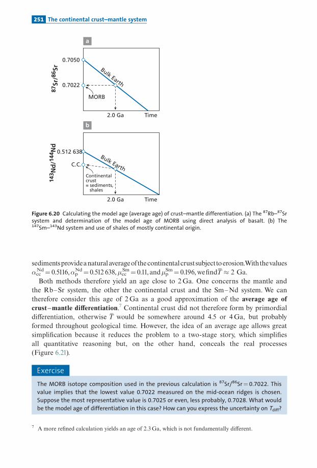
sedimentsprovideanaturalaverageofthe continental crustsubjecttoerosion.Withthevalues�ccNd¼ 0.5116,�p

Nd¼ 0.512 638,�ccSm¼ 0.11,and�p

Sm¼ 0.196,we¢ndT 2 Ga.Both methods therefore yield an age close to 2Ga. One concerns the mantle and

the Rb^Sr system, the other the continental crust and the Sm^Nd system. We cantherefore consider this age of 2Ga as a good approximation of the average age ofcrust^mantle di¡erentiation.7 Continental crust did not therefore form by primordialdi¡erentiation, otherwise T would be somewhere around 4.5 or 4Ga, but probablyformed throughout geological time. However, the idea of an average age allows greatsimpli¢cation because it reduces the problem to a two-stage story, which simpli¢esall quantitative reasoning but, on the other hand, conceals the real processes(Figure 6.21).

Exercise

The MORB isotope composition used in the previous calculation is 87Sr/86Sr¼ 0.7022. This

value implies that the lowest value 0.7022 measured on the mid-ocean ridges is chosen.

Suppose the most representative value is 0.7025 or even, less probably, 0.7028. What would

be the model age of differentiation in this case? How can you express the uncertainty on Tdiff?

87Sr

/86 S

r

2.0 Ga

0.7022

0.7050

Time

Bulk Earth

MORB

143 N

d/1

44N

d

2.0 Ga

C.C.

0.512 638

Time

Bulk EarthContinentalcrust= sediments, shales

a

b

Figure 6.20 Calculating the model age (average age) of crust–mantle differentiation. (a) The 87Rb–87Srsystem and determination of the model age of MORB using direct analysis of basalt. (b) The147Sm–143Nd system and use of shales of mostly continental origin.

7 A more refined calculation yields an age of 2.3Ga, which is not fundamentally different.


Answer

(87Sr/86Sr)MORB¼ 0.7025 and T¼ 1.93 Ga.

We find (87Sr/86Sr)MORB¼ 0.7028 and T¼ 1.70 Ga.

As can be seen, the first result barely changes the reasoning. Taking the first value, the result,

allowing for uncertainty, may be written T ¼ 2þ0:1�0:3 Ga.

6.3.2 The mass of the depleted mantle and the mantle structure

Letus consider the systemmade up of three reservoirs: mantle, continental crust, and pri-mitivemantle.Extractionofthe continental crustandthe correspondingdepletionofafrac-tionofthemantle iswritten likeamassbalance relation:

primitive mantle ¼ continental crustþ depleted mantle:

This is the opposite of amixture, although arithmetically it is the same thing.Returning tothe formulafor isotopedilutionormixing,we canwrite:

�p ¼ �cc Wþ �dð1�WÞ

withW ¼ ðmcc CccÞ=ðmp CÞ:Here,W is the mass fraction of continental crust, mcc is the mass of the continental

crust, whichwe know from seismology:mcc¼ 2.2 � 1022 kg,mp is the mass of the primitivemantle that hasbeen depleted andwhichweare trying to estimate,Ccc is the concentration

Continentalcrust

Depletedmantle

670 km

Dep

th

2 Ga (model age)T0 Today

Time

Primitivemantle

Figure 6.21 Diagram summarizing the approach and results obtained with the simple model ofevolution of the crust–mantle system, assumed to be a two-stage process separated by a suddenperiod of differentiation.


ofthe elementin the continental crust,whileCp is the initial concentrationofthe element intheprimitivemantle.The idea is to calculateW fromthe¢rstequation,andthento calculatemp, themassofthe

mantlewhich hasbeen depleted. Is this the totalmass of themantle? Is itmerelya fraction?Tobring thisout,we canwrite:

W ¼ mcc

Mp

Mp

mp

� �� Ccc

Cp

whereMp is the totalmassofthemantle:Mp¼ 4.10 � 1024kg. Ifwenotemp/Mp¼ � thefrac-tionofthedepletedmantle,weget:

f ¼ mcc

Mp� Ccc

Cp� 1W

withmcc=mp ¼2:2 � 10224:10 � 1024 ¼ 0:0054.

The di⁄culty lies in estimating the � parameters.We know �p and we can estimate �d

quitewell fromMORBmeasurements.Hereagain the di⁄culty is in estimating�ccbecauseof the segmentation of the continents. Howdoyou take the average value of a mosaic? ForSr, it is di⁄cult to do. A statistical estimate of 0.720 byPatrick Hurley etal. (1962), then atthe Massachusetts Institute of Technology, is a likely value but subject to considerableerror. For Nd, we have seen that ¢ne marine sediments seem to be a good approximationwith "d¼þ 10.ThenWNd¼ 0.32. Ifwetake for theabsolute concentrationsCcc

Nd¼ 28ppm,Cp

Nd¼ 1.1ppmwe calculate f¼ 0.43.The depletedmantle thereforemakesup about 43%ofthetotalmantle.Seismology has shown there is a marked seismic discontinuity at a depth of 670 km,

which is interpreted as the transition from a silicate with tetrahedral structures (SiO4) toperovskite-type octahedral structures (SiO6) and that this discontinuity is a strongbarrieragainst movementofmatter.This boundary is taken as the lower limit of the upper mantleinaconvectivemantle.The upper mantle above 670 km represents 25% of the mantle. So the mass of the

depleted mantle is greater than the upper mantle alone.While the continental crust hasdi¡erentiated from the upper mantle, the upper mantle has exchanged matter with thelowermantle.

Exercise

Write the equation giving W in the " notation. If the extreme values of "cc are �16 and �25,

and those of "d areþ15 andþ10, what are the extreme values of the estimate of W? What

extreme values of � do they correspond to?

AnswerResults are given by the matrix. The first number is W and the second in brackets is f.

"d

þ10 þ15

"cc�25 0.285 (0.4822) 0.375 (0.366)�16 0.3846 (0.3617) 0.483 (0.286)


The extreme values of W are 0.28 and 0.48, which correspond to �-values of 0.482 and

0.286. As can be seen, these results differ with the extreme values but the reasoning does not

change qualitatively, namely a part only of the mantle is depleted and that part is greater

than the upper mantle alone. This implies that exchanges have occurred between the upper

and lower mantle.

Exercise

The estimation of the Nd concentration of the primitive mantle is highly constrained:

its error is estimated at�0.1 ppm at most; that of the continental crust is estimated

at�2 ppm. Do possible errors with the absolute Nd concentrations in the continental crust

and in the primitive mantle greatly increase the estimated limits of �? What are the two

extreme values we obtain for � by combining the preceding uncertainties and uncertainties

on concentrations?

AnswerThe extreme values for � are 0.567 and 0.231. Once again, quantitatively the difference is

great, but qualitatively the result is not overturned in geochemical terms and so yields

quantitative limits.

Howcanwe calculateWSrandtheparameters for theRb^Sr system fordi¡erentiationofthe crustandmantle?

The idea is to comebacktotheNdsystemandtoexploitthe reliable cross-referenceddatawe have between the Sm^Nd and Rb^Sr systems.The way to evaluateWSr is to return toneodymium.

Wewrite:

WNd

WSr¼ Nd NdSr= Srð Þcc

Nd NdSr= Srð Þp;

with Ndcc¼ 28 ppm, Srcc¼ 230 ppm, Ndp¼ 1.1, and Srp¼ 20. This gives WSr¼ 0.144.ThenWNd/WSr¼ 2.212.

Exercise

Roughly speaking, the continental crust is made up of a deep layer (lower crust) and a surface

layer (upper crust). Studies of heat flow have shown that the deep crust is depleted in certain

soluble elements (uranium, potassium, and probably rubidium too) which have been trans-

ferred to the upper crust. Accordingly, the Rb/Sr ratio measured in the upper parts of the crust

is not representative of the whole crust. Given that WSr is 0.144 and that the 87Rb/86Sr ratio of

surface continental rocks is 0.8, what is the maximum thickness of the deep crust? The Sr

content is assumed to be identical for the whole of the continental crust, which is certainly an

oversimplification.


AnswerThe value of WSr is the same for budget equations of � and � values. Since �d

Rb 0, we have:

�Rbcc ¼

�Rbp

W¼ 0:09

0:144¼ 0:625:

Let us write the equation giving the average composition of the continental crust.

�Rbcc ¼ �Rb

u Q þ �Rb1 ð1� Q Þ:

where �uRb and �1

Rb are the � parameters for the upper and lower crust.

If we note

Q ¼ mass of upper crust=mass of whole crust

thickness is maximum when �1Rb¼ 0, corresponding to all Rb being transferred to the upper

continental crust. In this case Q¼ 0.625/0.8¼ 0.78.

Maximum thickness of the upper crust is about 78% of that of the whole crust. Here is a

new structural constraint derived from isotope data. If we consider the upper crust is enriched

in Rb by a factor of 2 compared with the lower crust, then the lower crust represents 56% of

the continental crust.

RemarkIn practice, all of the unknowns such as ages, W,�,�, etc. are calculated globally by what is termed the

generalized inverse model in mathematics, by which all the equations can be solved simultaneously.

All the equations, including the � balances, � balances, and the model ages as well as the various

relations among the elements, for example on the Sr/Nd ratio measured in the crust or the mantle

samples, are calculated with a margin of uncertainty for each, which is essential. We then calculate all

the values in one go. To do this, we introduce values estimated on an a-priori basis, optimizing the

result with their estimated uncertainties and we solve a gigantic least-squares problem. It is difficult

to solve as it is non-linear, with some unknowns multiplying each other. We shall see the spirit of it in

one of the problems proposed at the end of the chapter (see Allegre et al., 1983b).

6.3.3 Changes in the Rb–Sr and Sm–Nd systemsover geological time

In the foregoing,wehaveusedpresent-day results and haveprojected into the past. But thistechniquehasa limitedpowerofresolution.Weknowthattheaverageageofthe continentalcrust isabout2Ga.Butwewouldalsolike

toknowexactlyhowthisgrowthcameabout:was the rateofextraction fromthemantleuni-form,modulated, etc.?

Exercise

We consider the following eight models of continental growth (A–H). Each is represented by a

distribution of continental orogenic segments for which the table shows the contribution

from continents and the average age of each segment.


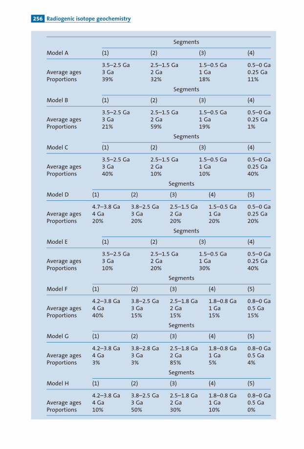
Segments

Model A (1) (2) (3) (4)

3.5–2.5 Ga 2.5–1.5 Ga 1.5–0.5 Ga 0.5–0 GaAverage ages 3 Ga 2 Ga 1 Ga 0.25 GaProportions 39% 32% 18% 11%

Segments

Model B (1) (2) (3) (4)


Segments

Model C (1) (2) (3) (4)


Segments

Model D (1) (2) (3) (4) (5)

4.7–3.8 Ga 3.8–2.5 Ga 2.5–1.5 Ga 1.5–0.5 Ga 0.5–0 GaAverage ages 4 Ga 3 Ga 2 Ga 1 Ga 0.25 GaProportions 20% 20% 20% 20% 20%

Segments

Model E (1) (2) (3) (4)


Segments

Model F (1) (2) (3) (4) (5)


Segments

Model G (1) (2) (3) (4) (5)


Segments

Model H (1) (2) (3) (4) (5)



In each case, calculate the average age of the continent and draw the cumulative growth

curve of the continents and variations in the rate of growth (see Figure 6.22). Which

models do you think are compatible with the results for the crust–mantle system with

current data?

AnswerFour models are acceptable with an age of 2� 1 Ga: A, B, D, and G.

CommentsAs the exercisehas justdemonstrated, theaverageage found for the continental crustusingthe calculation of the previous paragraph can indeed be used to eliminate some scenarios,but still leaves scope for a range ofpossible scenarios. For example, onemight equally wellenvisage either steadycontinuousgrowth (modelD)or suddengrowth (modelG).Togetarealpictureofthekineticsofcontinental extraction (examinationoftheshapesof

the curvesofgrowth rates is extremelydemonstrative) outside themantle,wehadthe ideaoftrying to obtain isotopic information for Sr andNd for di¡erent geological epochs so as tocalculateWasafunctionoftimeW(t).These studies, which looked as if they should be straightforward, have proved verydi⁄-

cult. The ¢rst problem was the relevance of the evidence of ancient massifs. For recentrocks,weknow thatbasalt rocks collected fromocean ridges are evidenceofdepletedman-tle. But in the past,whenweno longer havemid-ocean ridges, howcanwe recognizewhichbasalts can be used as evidence of ancient depleted mantle like the present-day MORB?

50%

100%

34 2 1 0

<T> = 2.017 Ga

A

3 2 1 0

<T> = 2.012 Ga

B

50%

100%

34 2 1 0

<T> = 1.1 Ga

E

34 2 1 0

<T> = 2.6 Ga

H

34 2 1 0

<T> = 2.5 Ga

F

4 3 2 1 0

<T> = 1.5 Ga

C

4 3 2 1 0

<T> = 2 Ga

D

4

34 2 1 0

<T> = 1.97 Ga

G

Figure 6.22 The results for the various models calculated in the exercise. On each graph, the x-axisshows time in Ga and the y-axis the percentage of continental crust formed. The integral curve is inblack, the derivative curve, that is the growth rate, in blue. At the top of each graph hTi indicates theaverage age calculated. The models shaded in blue are those that are compatible with an average age ofabout 2 Ga.


Forcontinents,howcouldweestablishanaveragesampleofthe continentsatagivenperiodin the past? Are the current mappings of various age provinces representative in relativeabundanceofwhattheywere inthepast?

� For evidence about the upper mantle, we adopt a pragmatic attitude. Up to 600Ma, weuse ophiolite massifs, which are pieces ofoceanic crust that have been obducted on thecontinents. For terrains older than 2Ga, we use komatiites, which are associations ofrock put in place under the seas andwhich associate ultrabasic and basic lava (which ispeculiar to Archean times). But these are working hypotheses that have not really beendemonstrated (other thanthattheydonotseemabsurd).� For the continental crust, the only evidence of what it was like at a given time are the

shales of the time in question.Theyare a sample ofeverything that hadbeen eroded andthenmixed intheoceanatthetime.Theyareanaverageoftheuppercontinental crust.

Inanyevent, thefollowingprogramcanbeset.

(1) Chooseagroupofrockswhoseorigin hasbeen identi¢ed foragiventime-span.(2) Determine its age and initial isotope ratio precisely (which takes usbackto the consid-

erationson isochrons inChapter 3).

Wethen justneed to repeattheoperation for severalgeological epochs andsoobtain SrandNdisotope evolution curves forour tworeservoirs (Figure 6.23).

This program has involved some 20 or so research teams worldwide over 10 years.Theresults of the quest have been very disappointing.Why? Not because the teams were bad,but because, in the past, isotope systems seldom remained strictly closed and thereforeuncertainties on initial ratios increase statistically with time.Without going into detailsthatextendbeyondthescopeofthisbook,wecan remember tworelated ideas: considerabledi⁄culties andpoor and inconsistent results. However, let us summarize the all too scarcepositive¢ndings.

StrontiumWhole-rock isochronsofancientbasic andultrabasic rocksarevery rarely reliable.To resolvethe problem, we bring in analysis of pure clinopyroxene extracted from rocks containingalmost no Rb and providing a fairly accurate re£ection of initial 87Sr/86Sr ratios.We deter-minetheageofthebasicmassifs inquestion independentlybyotherchronologicalmethods.

Thismethodhasyieldedfewreliable results.Evenso, theoverallshapeofthe curveofevo-lution (Figure6.24) is clearenough. It is virtuallyalignedon the straight lineof isotope evo-lution of the primitive (closed) mediumup to 3Ga and then is practically horizontal from1Gaonwards.

It is impossibletoobtainthe curveof isotopeevolutionoftheaverage continental crustforSr fromtheanalysis ofancientshales.There are two reasons for this: the¢rst is that apartofthe erosion of Sr is soluble andwas deposited in limestone; the second is that shales them-selves areopen systems forSr.

NeodymiumThesituation isfarmorefavorablebecausebothSmandNdaremuchmorechemically inert(less soluble) elements than Rb and Sr. But the variations are, of course, very small: to


express variations in the143Nd/144Nd ratio, we adopt the "notation. Instead of referring tothe present-day primitivemantle, we refer to the primitivemantle at the time for which the143Nd/144Ndratio isbeingestimated.Wehave:

"NdðTÞ ¼�NdðtÞ � �Nd

p ðTÞ�Ndp ðtÞ

" #� 104:

On aplot like this, the primitive mantle evolves along a horizontal line, the initial ratios ofthe various massifs considered as evidence of the upper mantle are located relative to thisstraight line, the equation forwhich is:

�Ndp ðTÞ ¼ �Nd

p ðpresent dayÞ � l�pT;

Tbeing theage,with�pNd (presentday)¼ 0.512 638and�p¼ 0.196.

For the depletedmantle,DonDePaolo of theUniversityof California at Berkeleyman-aged to establish aprettyacceptable curve of "(t) (seeDePaolo,1988).This curve follows thehorizontal line of the reference primitive mantle up to 2.7Ga and then curves around to

Ocean

I5 T5

Continents

1 Ga2 Ga

2.5 Ga

3 Ga

Presenttime

Init

ial i

soto

pic

rat

io

I4

T4

I4I5

I2

I1

T5Presentday Time (Ga)

T4 T3 T2 T1

I3

I3

T3

I2

T2

I1

T1

87Rb/86Sr

87Sr

/86 S

r

87Sr

/86 S

r

Figure 6.23 Theoretical diagram of the approach we would like to take to determine the isotopeevolution of strontium in the mantle over geological time. Top: we sample rocks from the mantlewhose age is determined by an isochron diagram. Middle: each isochron corresponds to an initial87Sr/86Sr isotope ratio. Bottom: the initial ratios are plotted as a function of age.


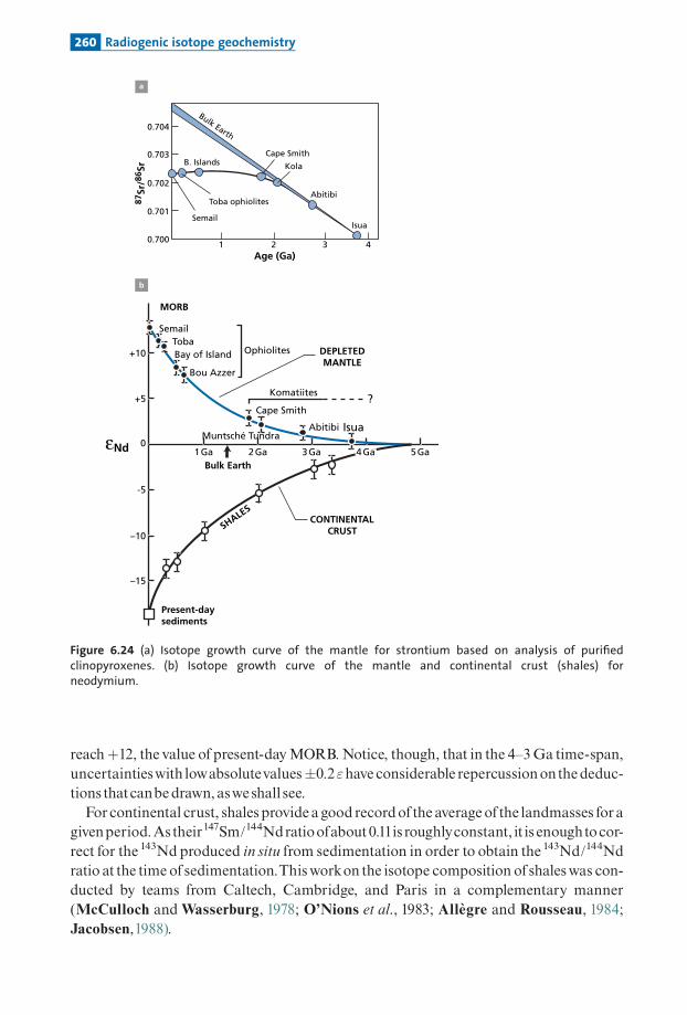
reachþ12, the value of present-dayMORB.Notice, though, that in the 4^3Ga time-span,uncertaintieswith lowabsolutevalues�0.2"have considerable repercussiononthededuc-tions thatcanbedrawn, asweshall see.

For continental crust, shalesprovide agood recordofthe averageofthe landmasses foragivenperiod.Astheir147Sm/144Ndratioofabout0.11is roughlyconstant, it is enoughtocor-rect for the 143Nd produced in situ from sedimentation in order to obtain the 143Nd/144Ndratio at the time ofsedimentation.Thisworkon the isotope composition ofshaleswas con-ducted by teams from Caltech, Cambridge, and Paris in a complementary manner(McCulloch and Wasserburg, 1978; O’Nions et al., 1983; Alle' gre and Rousseau, 1984;Jacobsen,1988).

0.704

0.703

0.702

0.701

0.700 21 3 4Age (Ga)

87Sr

/86 S

r

Semail

Toba ophiolites

B. IslandsCape Smith

Isua

Bulk Earth

Kola

Abitibi

+10

+5

-5

–15

–10

01 Ga

Bulk Earth

DEPLETEDMANTLE

CONTINENTALCRUSTSHALE

S

2 Ga 3 Ga 5 Ga

MORB

SemailTobaBay of Island

Bou Azzer

Komatiites

Muntsché Tundra

Cape Smith

Abitibi Isua

?

Ophiolites

εNd

Present-daysediments

4 Ga

a

b

Figure 6.24 (a) Isotope growth curve of the mantle for strontium based on analysis of purifiedclinopyroxenes. (b) Isotope growth curve of the mantle and continental crust (shales) forneodymium.


Wethereforehave two curvesof "(t) evolutionofNd, one for the depletedmantle andonefor the continental crust.We canthereforewrite epochbyepochthebalance equation:

0 ¼ "ccðtÞ �WðtÞ þ "MðtÞ½1�WðtÞ

andtherefore calculateW(t) stepbystep.Accepting that the volume of the upper mantle has remained constant and corresponds

to that determined on the present-daybalance (which is not proved at all), the evolution ofthe continentalmass extracted fromthemantle canbe calculated.Theoutcome is shown inFigure6.25.Naturally, this curveinvolvesconsiderableuncertaintyforveryancientperiods.

Exercise

To get this point across, let us consider the evolution between 2.8 and 2.7 Ga, between the

Isua time and the great Canadian orogeny. Now, the literature contains extremely varied

50

3 2 1 0

100

Mas

s p

erce

nta

ge

of

pre

sen

t-d

ayco

nti

nen

tal c

rust

Age (Ga)

Age (Ga)

3.5 0.2 –1.5

3 1.2 –3

2 2.5 –5

1 5.5 –9.5

0 13 19

M(t)ε CC(t)ε

<T> = 2.5 Ga

Growth rate

Figure 6.25 Growth curve of continents deduced from the curves of strontium and neodymium isotopeevolution. The numerical values used are shown below.


values for ancient rocks, whose reliability is unknown, leaving considerable scope for

interpretation.

Let us assume the values from 2 Ga are well constrained and identical to the overall

calculation. We consider two extreme scenarios corresponding to the "Nd values below.

Given that the current WNd¼ 0.4 and assuming the same values of the upper mantle mass

entering into the process and the Nd concentration of continental crust, calculate the growth

curves of the continents and the average age in each case.

Answer

This result of the exercise (see Figure 6.26) shows us the possibility of an a-priori surprising

phenomenon in scenario A. Some 3.8 billion years ago, the volume of continental crust might

have been twice what it is today.

The conclusionofthis is thatthisprimitive crust,whichmaybetheresultofmajorchemicaldi¡erentiationoftheprimordialEarth, disappeared,wasdestroyed, andwas swallowedup inthemantle, and that only later did the crust as we know it nowbegin to form.This is just oneextremescenario,butitraises such fundamental issues that itmustbe exploredfurther.

Letus leave this subject for the endofthe chapter whenwe shall dealwith the primordialEarth.These examples showhowimportant it is totakeaccountofmeasurementuncertain-tieswhich sometimes lead to considerable uncertainties in the scenarios proposed. Sohowcanwe improveourknowledge?Bygettingaway fromthenarrowscenario and introducingotherconstraints fromother sourcesof information.

For example, we can test the models using the results of evaluation of the crust^mantlesystem obtained with present-day data. The average age, it will be remembered, is2Ga� 0.1. In this way, we can calculate the average ages of the various scenarios (seeFigure 6.26). It shall be seen that the model extracted from the two growth curves giveshT i¼ 2.5Ga,which is a littlehigh. ScenarioA,wherethe initialpeakdisappears, ofcourse,

Average age (Ga) "M(t ) "cc(t )

Scenario A 3.8 þ1.9 �0.53 þ0.5 �32.7 þ1 �3.5

Scenario B 3.8 0 03 þ1 �32.7 þ2 �4

Age (Ga)Percentage ofpresent-day continents hTi

Scenario A 3.8 2003 24 1.82 Ga2.7 57

Scenario B 3.8 03 65 2.08 Ga2.7 82


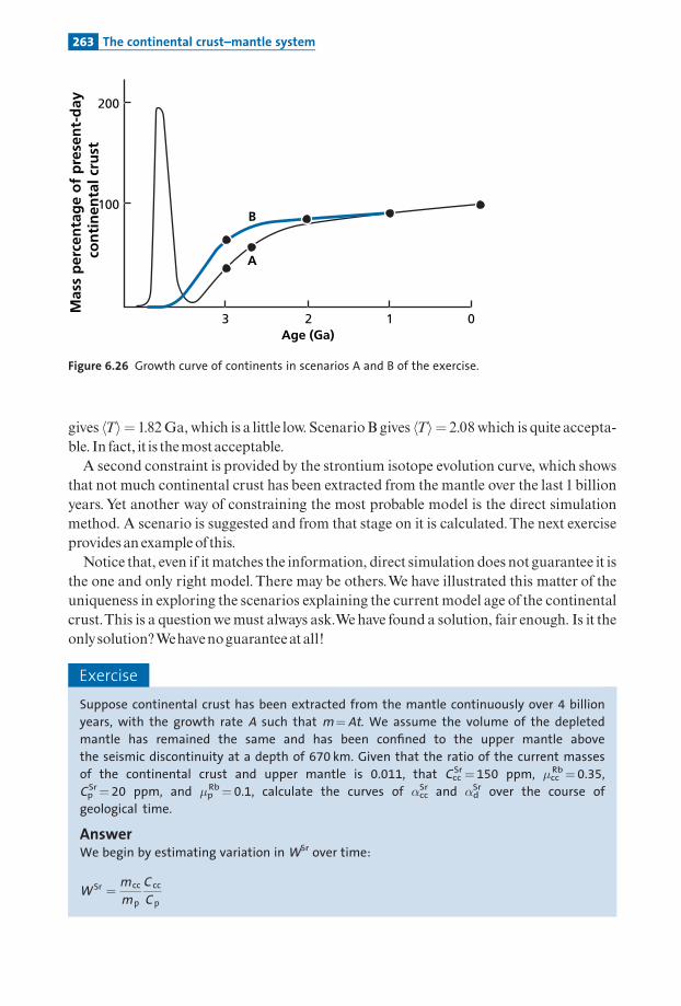
gives hTi¼ 1.82Ga,which is a little low. ScenarioB gives hTi¼ 2.08which is quite accepta-ble. In fact, it is themostacceptable.A second constraint is provided by the strontium isotope evolution curve, which shows

that not much continental crust has been extracted from the mantle over the last 1billionyears.Yet another way of constraining the most probable model is the direct simulationmethod. A scenario is suggested and from that stage on it is calculated.The next exerciseprovides an exampleofthis.Notice that, even if it matches the information, direct simulation does notguarantee it is

the one and only right model.There may be others.We have illustrated this matter of theuniqueness in exploring the scenarios explaining the current model age of the continentalcrust.This is a questionwemust always ask.Wehave found a solution, fair enough. Is it theonlysolution?Wehavenoguaranteeatall!

Exercise

Suppose continental crust has been extracted from the mantle continuously over 4 billion

years, with the growth rate A such that m¼At. We assume the volume of the depleted

mantle has remained the same and has been confined to the upper mantle above

the seismic discontinuity at a depth of 670 km. Given that the ratio of the current masses

of the continental crust and upper mantle is 0.011, that CccSr¼ 150 ppm, �cc

Rb¼ 0.35,

CpSr¼ 20 ppm, and �p

Rb¼ 0.1, calculate the curves of �ccSr and �d

Sr over the course of

geological time.

AnswerWe begin by estimating variation in WSr over time:

W Sr ¼ m cc

m p

C cc

C p

100

3 2 1 0

200

Mas

s p

erce

nta

ge

of

pre

sen

t-d

ay

con

tin

enta

l cru

st

Age (Ga)

A

B

Figure 6.26 Growth curve of continents in scenarios A and B of the exercise.


therefore

W Srðt Þ ¼ A t

m p� C cc

C¼ A �t :

The value of A*¼ 0.0205 if t is measured in Ma.

We then estimate the variation in �dRb from the mass balance equation:

�d ¼��T � �cA �t

��1� A �t

� :

Table6.4 shows the calculation for1,2,3, and4billionyears. It ispossible thento calculatethe isotope evolution of the depleted mantle starting from �pSr (4Ga)¼ 0.6996 and thencalculating by stages with �Rb(t) being determined.To calculate the evolution of the conti-nental crust, weuse themassbalance equation again.Weobtain�cc

Sr from theW(t) values.Acomparison is made with the curve for the total di¡erentiation of the continental crust at4Ga (Figure6.27).

RemarkComparison of the �d

Sr (t ) curve of evolution of the depleted mantle from the synthetic model with

the actual curve (which requires care!) from measurements on rock shows that the theoretical

evolution of the exercise is more progressive and less sudden than the real curve. This reflects the

fact that production of continental crust is probably shifted more towards the past than the

uniform growth model indicates. Past growth was therefore greater than recent growth.

Exercise

Calculate the average age from the model in the previous problem.

AnswerThe average age written as an integral is defined by

hT i ¼ 1

M

ZT

0

t m dt

where m is the fraction produced per unit time (here m¼A ). We therefore have:

hT i ¼ 1

M

ZT

0

t A dt ¼ AT 2

2M¼ AT 2

2AT¼ T

2:

Table 6.4 Isotope evolution of the depleted mantle and of the continental crust

Time (Ga) �A WSr �pSr �d

Sr

1 0.0817 0.068 0.701 0.700742 0.06064 0.136 0.7024 0.701583 0.03592 0.204 0.7038 0.702084 0.00659 0.27 0.705 0.702172


As T¼ 4 Ga, hTi¼ 2 Ga. We find the age calculated before. In a population where the rate of

accumulation is constant, the average age is half the maximum age. In the human population,

the maximum age is 80 years, the average age 40 years! (We shall be discussing this idea again.)

6.3.4 The process of development of continental crust overgeological time

Continental reworkingWe have just established a growth curve for continental crust using strontium and neody-mium (above all the latter!) isotopebalances.Now,wehave seen (see Plate 5) that theworldhasbeenmapped in termsofageprovincesbysystematicgeochronology.HurleyandRand(1969)oftheMassachusetts InstituteofTechnologyhavetransformedthismap intopercen-tagesbyage (Figure6.28).

Exercise

Translate the graph (Figure 6.28) into percentages and calculate an average age using the

proportions of age provinces.

AnswerhTi¼ 0.7 Ga.

Evolving depleted mantle

Evol

ving

cont

inen

tal c

rust

Primitiv

e mantle

Primitiveextraction

ofcontinental

crust

0.702

0.700

0.706

0.704

0.710

0.708

0.714

0.712

0.716

0.718

0.720

4 3 2 1

87Sr

/86 S

r

Time (Ga)

Figure 6.27 The (87Sr/86Sr, t ) isotope evolution curves in the model of the previous exercise. Blue curvesare for continuous evolution. Black curves are for initial differentiation of continental crust at 4 Ga.Clearly, present-day ratios do not result from simple initial differentiation.


As shown by the exercise and by comparing the two growth curves, there is a contradic-tion between the isotope geochemistry approach and the geochronological approach inthe plates. How can this di¡erence be accounted for? By reworking of the continentalmaterials (see Figure 6.29). Provinces of recent age are the result of reworking in thegeological cycle (erosion, sedimentation, metamorphism, anatexis) of ancient pieces ofcontinental crust. The ancient provinces have been cannibalized, that is eroded andincorporated into younger provinces. The older they are, the more likely it is that theywill have been given a new lease of life in this way. Notice that this interpretation isconsistent with the idea of constancy of geological phenomena over time. The processesby which continental crust is formed have operated throughout geological time inmuch the same way but the type of material involved in the processes has changed. Inancient times these materials must have been mostly mantle. In more recent times, onthe contrary, it was above all recycled material of the continental crust, making newout of old!

Exercise

The initial Nd isotope composition of a granite dated 1 Ga is measured as 143Nd/144Nd¼0.510 62. The local gneiss basement has a present-day isotope composition of "Nd(0)¼�28

and a 147Sm/144Nd ratio of 0.11. Assuming the mantle contribution to the granite mixture is

from the primitive mantle, calculate the percentage of this contribution if the Nd concentrations

of the mantle and recycled components are identical.

AnswerThe isotope compositions of the gneiss and mantle 1 billion years ago must be calculated

first and then the proportions of the mixture. We find a 13% contribution from the

mantle.

Time (Ga)

Perc

enta

ge

of

con

tin

ents Gondwana

age provinces

40

50

4 3 2 1

30

20

10

Figure 6.28 Continent growth rates: established by geochronology and mapping by Hurley and Rand(1969) (blue), and also showing isotope ratio evolution models (dashed curve).


Exercise

Geological history is divided into four periods: 4–3 Ga, 3–2 Ga, 2–1 Ga, and 1–0 Ga.

Mapping formations dated by radiometric methods converted into percentage of mater-

ials gives:

Thin plastic crust

Mantle

Geosyncline

Geosyncline Geosyncline

Foldedgeosyncline

Foldedgeosyncline

Foldedgeosyncline

Mountain range

Recentmountain ranges

Ancientmassif

Erosion

Rift andocean ridge

Ocean Ocean

Ocean Ocean

Ocean

Ocean

Ocean

Ocean

Subduction

SubductionSubduction

Rift andocean ridge

Formation offirst

continents

Formationof

recentcontinents

δT

Figure 6.29 The formation and growth of the early continents. This diagram is reworked from Dietz(1963) and shows how the early continents might have formed and grown over geological time, withthe proportion of recycled material increasing constantly.

Period (Ga) 4–3 3–2 2–1 1–0Percentage 5 15 20 60


Conversely, the study of growth of continents by initial Nd ratios gives as proportions of

continental crust made from the mantle:

It is assumed that at each new period, part of the continent is made of a neoformed (from

the mantle) fraction and a fraction of material reworked from earlier periods.

(1) For each segment, calculate the proportion of material from the period in question and

from the preceding periods.

(2) The ratio (R ) of reworked mass to total mass of a segment is known as the reworking

coefficient. Calculate this coefficient for the four periods.

(3) By taking the median age for each segment (3.5 Ga, 2.5 Ga, 1.5 Ga, and 0.5 Ga, respec-

tively), calculate the mean age for each segment. Plot the mean age (or model age) on a

graph as a function of geological age.

AnswerThe 20% created in the 4–3 Ga interval is divided as:

The 50% created in the 3–2 Ga interval is divided as:

The 30% created in the 2–1 Ga interval is divided as:

The reworking coefficient is given in the table below.

The mean ages are given below.

SeeFigure6.30 forasummaryofdataandresults.

Period (Ga) 4–3 3–2 2–1 1–0Percentage 20 50 30 0

Period (Ga) 4–3 3–2 2–1 1–0Share of 20% 5 3.5 2.87 8.6Percentage 25 17.5 14.35 43

Period (Ga) 4–3 3–2 2–1 1–0Share of 50% 11.5 9.62 28.9Percentage 23 19.24 57.9

Period (Ga) 4–3 3–2 2–1 1–0Share of 30% 7.5 22.5Percentage 25 75

Period (Ga) 4–3 3–2 2–1 1–0R 0 0.23 0.37 1

Period (Ga) 4–3 3–2 2–1 1–0Mean age (Ga) 3.5 2.7 2.25 2.25


Theneodymiummodelageand itsgeologicalapplicationsThe fact that Sm/Nd fractionation is almost zero in geological surface processes afterextraction fromthemantlemeans amodel age canbeattributed toanyneodymium isotopemeasurement of a material belonging to the crust. In an ideal scenario, this is the age atwhichthematerial (or itsprecursors)wasextractedfromtheEarth’smantletobegin its‘‘con-tinental geological life.’’ This is the idea hit upon by Malcolm McCulloch and JerryWasserburgoftheCaliforniaInstituteofTechnologyin1978.Nosuchmodelage canbecal-culated for Rb^Sr as the Rb/Sr ratio varies considerably during the surface history(althoughwe shall see in Chapter 7 that it can still be used for limestone). Aswill be seen, itispossible touseLu^Hf in a similarmannerbecause lutetiumandhafniumarealsoalmostinsoluble inwater.To calculate this model age (whichwe have already come across in calculating present-

day balances of the crust^mantle system), let us consider the straight line of isotopeevolution of the closed mantle (Figure 6.31). Imagine that a piece of continental crustseparated from the mantle at time TM, and has evolved since with constant �cc

Sm/Nd

growth. This straight line of evolution intersects the time axis at �ccNd. How can we

calculate timeTM in return?Letus call the two parameters ofevolution of the primitivemantle�pm

Nd and �pmNd, the two

parameters for the segmentofcontinental crust�ccNd and�cc

Sm/Nd, and the common isotoperatio corresponding toTMwecall I.

Age provinces

20

4 23 1 0

40

60

%80

Age (Ga)

Formation of continentalcrust at expense of mantle

4 23 1 0

Geological age

Mo

del

ag

e

1

3 2 1 0

3

4

2

Figure 6.30 Data and results of the exercise. Top: starting data. Left: proportions of continentsdetermined by mapping age provinces. Right: proportions of continents as a function of extractionfrom mantle. (Data corresponding to the two tables.) Bottom: what becomes of the various materialsextracted from the mantle, then the model ages as a function of geological age.


Wethen havethe twoequations:

�Ndpm ¼ I þ l�Sm=Nd

pm TM

�Ndcc ¼ I þ l�Sm=Nd

cc TM:

Byeliminating I,weget:

TM ¼1

l

�Ndcc � �Nd

pm

�Sm=Ndcc � �

Sm=Ndpm

!:

For the continental crust,�ccSm/Nd¼ 0.11and for theprimitivemantle�pm

Sm/Nd¼ 0.196.But �cc

Sm/Nd��pmSm/Nd¼ 0.11� 0.196¼ 0.086 is constant. Recalling the de¢nition of"(0):

"Nd 0ð Þ ¼�Ndcc � �Nd

pm

�Ndpm

!� 104

weobtain:

TM ¼10�4 " 0ð Þ �pm

6:54 � 10�12 � 0:086¼ �0:091 " 0ð Þ:

Ifwewant an approximation ofTM inGa, wehave aboutTM¼ 0.09 "(0), which is handyfor switching from "(0) toTM. (It is almost "(0)dividedby10withachangeofsign!)

Naturally, if the crustalmaterial contains a little of theoriginalmantlematerial, the Sm/Nd ratio is slightlyhigher than 0.11and�cc

Nd is also a little largerand the previous formula isnotstrictlyapplicable.But itprovides a¢rstapproximation.

TimeTM

PM

I

Model age

143 N

d/1

44N

dsample

Evolution ofprimitivemantle

Figure 6.31 Principle of model age calculation. Start from the sample. Draw a straight line of slope 0.11cutting the straight line of mantle evolution at I, corresponding to the model age TM.


Exercise

We have a sediment of mixed origin: 90% is from continental crust with an average

"(0)¼�25; 10% is from the ancient mantle with "(0)¼þ5. The Sm/Nd ratio of the

continental crust is 0.11 and that of the mantle is 0.21. It is taken that the two components

have the same Nd concentration.

(1) Calculate �(0) of the sediment and its conventional model age.

(2) Calculate the model age using the Sm/Nd ratio measured on the sediment itself.

(3) Compare these ages with the model age of continental crust.

Answer(1) 2 Ga.

(2) 2.26 Ga.

(3) 2.27 Ga.

By using the effective Sm/Nd age of the sediment, the dilution effect is ‘‘corrected’’ and we

get the age of differentiation of the continental fraction.

Exercise

If a shale is found with "(0)¼�20, what is its model age?

AnswerTM¼ 1.82 Ga.

Exercise

Supposing we apply the same formalism to Lu–Hf, given that (176Lu/177Hf)cc¼ 0.02 and

(176Lu/177Hf)pm¼ 0.036, calculate the model age of a schist whose "Hf(0)¼�25.

AnswerIf "Sch

Hf (0)¼�25 �SchHf¼ ("(0)10�4þ 1) �pm

Hf¼ 0.282 24

T ¼ 1

l

�HfSch � �Hf

pm

�HfSch � �Hf

pm

!¼ 2:3 Ga:

Neodymiummodelagesofgranitesovergeological timeDalila Ben Othman and the present author measured the initial isotope ratios of gran-ites (major constituents of continental crust of varied ages) for the ¢rst time in 1979(Alle' gre and Ben Othman, 1980; Ben Othman et al., 1984). The Nd model age is plottedagainst geological age (Figure 6.32). If all the granites were derived from the mantle,the points would lie on a straight line of slope 1. Now, this is generally so for ancientgranites (Mont d’Or granite of Zimbabwe is a spectacular exception) while for morerecent granites, their model age is much older than their ‘‘geological age.’’ This con-¢rms the idea of recycling which increases with time. Let us try to be even morespeci¢c.


GeneticcartographyofcontinentsWe have spoken of geological maps showing the di¡erent tectonic provinces which areassembled to form the continents andwe have given an overall explanation of these maps.DonDePaolo (1981a,1981b)andhisgroupattheUniversityofCaliforniaatBerkeleyunder-tookasimilarapproach (FarmerandDePaolo,1983;BennettandDePaolo,1987), consider-ing the model ages ofNd only, that is, by trying to eliminate continental recycling. He andhis team studied two cases from thewesternUnited States: thatofColoradoand the neigh-boring states where the age of emplacement ofgranites is1.8Ga and the west of the region(RockyMountains)wherethegranite intrusionsare of Tertiary age (Figure 6.33).

In the Colorado province, there is a central part formed1.8Ga ago and which di¡eren-tiated from the mantle at that time, and then bordering parts to the north andwest whosemodel age is 2^2.3Ga. It can be seen that the 1.8Ga materials also extend into the pro-vince to the south in NewMexico and Texas dated1.2^1.5Ga. Heading west, towards theRockyMountains, the Berkeley team traced isoclines with the same "Nd(0) value showingthat when moving from the continent toward the oceanic margins, "Nd(0) becomesincreasingly positive, that is ever closer to mantle values (Figure 6.34). The percentagesof mantle material in the make-up of the granite can be calculated: they increase fromeast to west.

These two examples showhow continental tectonic segments arebuilt up byaddition toancient sediment. Probably through subduction processes, as shown in the Rocky

0

1

2

3

3 2 1 0

Nd

mo

del

ag

e (G

a)

Geological age of emplacement (Ga)

Recentgranites

Stra

ight l

ine o

f conco

rdan

ce

Figure 6.32 Model ages of granites of varied geological ages. After Allegre and Ben Othman (1980); BenOthman et al. (1984).


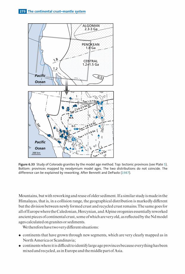
Mountains, butwith reworkingandreuseofolder sediment. Ifa similar study ismade intheHimalayas, that is, in a collision range, the geographical distribution is markedlydi¡erentbut the divisionbetween newly formed crust and recycled crust remains.The samegoes forallofEuropewheretheCaledonian,Hercynian, andAlpineorogenies essentially reworkedancientpiecesofcontinental crust, someofwhichareveryold, as re£ectedby theNdmodelages calculatedongranitesor sediments.Wethereforehavetwoverydi¡erentsituations:

� continents that have grown through new segments, which are very clearly mapped as inNorthAmericaorScandinavia;� continentswhere it is di⁄cultto identifylargeageprovincesbecause everythinghasbeen

mixedandrecycled, as inEuropeandthemiddlepartofAsia.

200 km

32°

36°

40°

122° 114° 106°

Pacific

OceanSA

F

TDM = 1.7–1.8 GaTDM = 1.8–2.0 Ga

TDM > 2.7 Ga

M.R.

G.C.

PENOKEAN1.8 Ga

ALGOMAN2.3-3 Ga

CENTRAL1.2+1.5 Ga

0.53

1.8

1.2

TDM < 1.4 Ga

TDM = 2.0–2.3 Ga

OK8

N+

Pacific

Ocean

Figure 6.33 Study of Colorado granites by the model age method. Top: tectonic provinces (see Plate 5).Bottom: provinces mapped by neodymium model ages. The two distributions do not coincide. Thedifference can be explained by reworking. After Bennett and DePaolo (1987).


RemarkThe main mechanisms of continental growth seem to be well understood. One question remains.

We have drawn a general map of the tectonic provinces. The Colorado study gives details of one

specific case. There is no doubt that continental crust in a given continent is extracted during

mountain-building episodes of well-defined ages. But is this true at the scale of all the continents?

Does not the combination of all orogenies lead to continuous extraction?

AustraliandetritalzirconsThese ideas about dual mechanisms of formation of continental crust ^ reworking of oldmaterialandformationofnewsegmentsofcontinentmaterial ^ arewonderfully illustratedbyworkonAustraliandetrital zirconsbyChrisHawkesworth’sBristol teamusingthelatestinsitu isotopeanalysis technology (HawkesworthandKemp,2006).

+6 +2

–2 –6–10–14–18

+6+2–2–6

GF

Pacific

Ocean

500 km

100

0250 500

Distance (km)

εNd

Perc

enta

ge

of

man

tle

Nd

in g

ran

ites

750 1 000

SAF

>1.63 Ga

TNd =

0.18 Ga

TM =

0.91 Ga

TM =

1.5 Ga

TM =

1.63 Ga

}

Figure 6.34 Neodymium isotope study of the Rocky Mountains in California. The curves of the "Nd

isotope ratios are plotted. An E–W curve is shown below. The proportion of mantle decreases veryrapidly eastwards. After Farmer and DePaolo (1983).


Thisworkbeganwith the analysis ofdetrital zircons. Zircons (ZrSiO4), which are primeminerals for U^Pb radiometric dating, are extremely resistant to erosion.They are engen-deredbytheformationofgraniticrocks.Theywithstandweatheringverywellandaretrans-ported mechanically and mix with clastic sediments (sandstones and, to a lesser extent,shales).They may undergo a second phase of erosion and be re-sedimented. At that timethey canmixwith zirconsborn in anewgeneration ofgranites.Thus, a sandstonemaycon-tain zircons ofvarious ages.This pseudo-immortalityof zirconswas revealed in studiesbyLedent etal. (1984), whowere attempting to determine amean age for continental crustbyanalyzing a zircon population.Using grain-by-grain zircon analysis,Gaudette etal. (1981)showedthereweremanyepisodesofgranitization recordedinasinglepopulationofdetritalzircons. But such studies using conventional methods were time-consuming and tedious.This approach was revolutionized by the team from the Australian National UniversitywhenBillCompston and IanWilliams (1984) developedtheSHRIMP ionprobeforU^Pbisotope analysis of zircons. Advances in automation mean that 500 zircons can now bemountedon aplate and theirU^Pb analyses completed in amatterofdays. Itwaswith thismethodthattheAustralianteamdiscovered the existenceofzircons aged4.3Gaand evenafewgrains aged 4.4Ga in Precambrian clastic sediments.Theyalsomade a further discov-ery thathadbeensuspectedfor sometime.Zircongrainshave complex individualhistories.Around an ancient core, which is often rounded by erosion, newgrowth zones have devel-opedgivingthezirconcrystalstheappearanceofadoublepyramid.Thezirconcrystals con-tainarecordofthedi¡erentperiodsoftheir individualhistories.This is proof, if any were needed, that some granites were formed from the remelting of

earlier sediments, which themselves contained detrital zircons. These ancient zirconsacted as seed crystals for newadditions of zircon around them.A single zircon may tell thecomplexgeological historyofaregion!The Bristol teamworking in conjunctionwith the Australian National University team

tooka sandstone fromthePrimaryperiod (400Ma) as their startingpoint.Aftermechani-callyseparating the zircons, theyanalyzed theU^Pbages ofseveral hundred zircons.Theyalsoanalyzedthe coresofzircons fromagranite dated430Ma.Theyobtainedagesbetween3.2Ga and the age of the granite. A whole series of ages, with maxima and minima, isshown inFigure 6.35.They thenusedthefactthat zirconsare rich in hafnium(Hf is the elementjustbelowZr in

theperiodic table) andvery poor in lutetium.They thusmanaged toanalyze theHf isotopecomposition and calculate their model age for each zircon, in the same way as is done forNd.This yielded a model age at which the material fromwhich the zircon derives becameseparated from themantle.ThehighHf content of zircon meant this analysis could be per-formed by laser ablation followed by ICPMS analysis. But they added a further criterion.They analyzed the 18O/16O isotope composition of zircons with an ion probe. As we shallsee in the next chapter, basic magmatic rocks have very constant 18O/16O compositionswith �varying from 5.5 to 6.5.They therefore selected zirconsgrainswith �18O< 6.5. In thisway zircons derived frommaterials extracted from themantle could be selected.This dou-ble-sorting process yielded an extraordinary result.Themodel ageswere clustered aroundtwovaluesof2Gaand3.2Ga (Figure6.36).The conclusion is that new continental crust was only formed from the mantle at these

two periods. However, continental crust (granites) has formed throughout geological


Hf model age(δ18O<6.5‰)

Gondwanasedimentary

rocks

20

40

60

4.0

3.080

2.0

1.0

1.0 2.0 3.0 4.00

Age (Ga)

Nu

mb

er

Nd

mo

del

ag

e (G

a)

U-Pb crystallization age

Nd model age

Figure 6.35 Composite zircon age diagram. The histogram in black shows the crystallization agesdetermined on different zircons using an ion probe. The histogram in blue is the model age ofhafnium computed for individual zircons with �18O< 6.5. The blue curve is the neodymium modelage obtained on Australian sediments. After Hawkesworth and Kemp (2006).

Bulk Earth

Hf model age

176Lu/177Hf = 0.021R2 = 0.75

176Lu/177Hf = 0.017R2 = 0.94Zircon

Lu/Hf ratio of average crust

depleted mantle

–30

–20

–10

0

10

1 000 2 000 3 0000

ε Nd

Age (Ma) U–Pb age (Ma)

ε Hf

(t)0

500 1000 1500 2000 2500

depleted mantle

Figure 6.36 How hafnium model ages are obtained by laser ablation ICPMS. Zircons on spot size on theleft. The principle of hafnium model age competition. Results for Australian zircons.


history, as shownbyU^Pb dating, butthese episodesweremerely the reworkingofancientcrust.Newthingsweremadeoutofold!This new method, once extended to various regions of the planet, will indicate exactly

howcontinental crust formed.Did it form continuously throughout geological time,moreor less in relationwith the activity of subduction zones, but in di¡erent geographical loca-tions?Ordid it formworldwideduringspeci¢c episodesof intenseactivity?When a histogram is drawn ofgeological ages measured on the various continents, peaks

arefoundat600Ma,1100Ma,1600Ma,2100Ma,2700Ma,and3200Ma.Theirdispersion is�100Maon average.What do these peaksmean? Are they the heartbeat of the planet or there£ectionthatsomeregionslikeChinaorIndiaarestillunder-explored?StudiesofthewesternUnited Statesby the team fromBerkeley seem to show that the formation of new continentalcrust is also associated geographically with reworking processes. But is this a general result?We can entertain high expectations of the results of this research because the method devel-opedatBristol andattheAustralianNationalUniversitysuggests thatwenowhavethemeanstosolvetheproblem.

6.4 Isotope geochemistry of rare gases

There are ¢ve rare gases.They form the ¢nal column of the periodic table of the elements:helium (He), neon (Ne), argon (Ar), krypton (Kr), and xenon (Xe). Some isotopes of raregases are producedbylong-period radioactiveprocesses and so causevariations in isotopeabundance (Tables 6.5 and6.6).Wehavealready referred to 4Heand 40Arwhendealingwithgeochronology (Chapter 5).The decay schemes leading to rare gas isotopes are recalled inTable 6.7.All rare gas atoms share the common property of having their outer electron shell satu-

rated and so being chemically inert.They are transported by physical processes only andtend to migrate upwards, towards the atmosphere where they accumulate. In the atmo-sphere, theirbehavior varies dependingontheiratomicmass.Helium, avery light element, is not retained by the Earth’s atmosphere as its mass is too

low. Itescapes continuously intospacelike (andwith)hydrogen.Neon is retainedby thepre-sent-day atmosphere, but it is thought that some neon was lost in the Earth’s early history.Argon,krypton,andxenonareretainedbytheatmosphere.Howcantheescapeoftheseele-ments be interpreted? As a ¢rst approximation, it can be understood quite simply. For anobjectto escapefromtheEarth, itsvelocitymustexceedtheEarth’sgravitational attraction.Since1/2mVe

2¼mgR, thevelocityVemustbegreater thanffiffiffiffiffiffiffiffiffi2gRp

.Now, acceleration due togravity is g10m s�2 and the Earth’s radiusR is 6400 km, therefore the escape velocity isVe¼ 11.28 kms�1.Letus supposethatescape isby thermalmeansonly.

1

2mV2

e ¼3

2kT and Ve ¼

ffiffiffiffiffiffiffiffiffi3kT

m

r:

Hence:

3kT

m4ð11:2 km s�1Þ2

wherek isBoltzmann’s constant, T is absolutetemperature, andm ismass.

277 Isotope geochemistry of rare gases

Table 6.5 Composition of the atmosphere

Isotope Atomicabundance (%)

Helium3 0.0001404 100

Neon20 90.5021 0.26822 9.23

Argon36 0.336438 0.063240 99.60

Krypton78 0.346980 2.257182 11.52383 11.47784 57.0086 17.398

Xenon124 0.951126 0.0887128 1.919129 26.44130 4.070131 21.22132 26.89134 10.430136 8.857

MajorgasesMolecularmass Fractionby volume

Totalbalance

Bymass (kg) Byvolumeatstandardtemperatureandpressure

N2 28.0134 0.78014 3.866 � 1018 3.093 � 1024O2 31.9988 0.20948 1.185 � 1018 8.298 � 1023CO2 44.0099 (3.40) � 10�4 2.450 � 1015 1.248 � 1021He 4.0026 (5.24� 0.05) � 10�6 3.707 � 1012 2.076 � 1019Ne 20.179 (1.818� 0.004) � 10�5 6.484 � 1013 7.202 � 1019Ar 39.948 (9.34� 0.01) � 10�3 6.594 � 1016 3.700 � 1022Kr 83.80 (1.14� 0.01) � 10�6 1.688 � 1013 4.516 � 1018Xe 131.30 (8.7� 0.1) � 10�8 2.019 � 1012 3.446 � 1017

Table 6.6 Rare gases in sea water

Concentration (atstandardtemperatureandpressure)

He (10�8) Ne (10�7) Ar (10�4) Xe (10�8)

Surfaceseawater (25 8C) 3.7 1.47 2.26 0.65Deepwater (4 8C) 4.22 1.85 3.51 1.1


Exercise

The temperature of the very high atmosphere is typically 700–900 K. Calculate the escape

velocity of atomic hydrogen and then compare it with that of the molecule H2.

AnswerThe mass of an atom or molecule is the molar mass divided by Avogadro’s number,

6.023 � 1023. The mass of a hydrogen atom is 0.001/6.023 � 1023, which is 1.65 � 10�27 kg.

For H,

ffiffiffiffiffiffiffiffiffi3kT

m

r¼ 3� 1:381 � 10�23 � 800

1:65� 10�27

� �1=2

therefore Ve¼ 4.48 km s�1.

For H2, Ve¼ 3.16 km s�1.

The twovelocities calculated in the exercise above are less than11.2 km s�1.Theyseem toindicate that hydrogen does not escape from the Earth. Now, this is not so, as observationsandmeasurements prove!Where is themistake? In fact, thevelocities of thevarious atomsor molecules do not have constant values: theyobeyBoltzmann’s statistical distribution.And foravelocityof4.48 kms�1, some10%of 2Hparticles escape everysecond.For 4He,Ve¼ 2.24 km s�1. Some 10�15 atoms have the necessary velocity to escape per

second.That represents a substantial quantityof atoms in geological terms, when the timemeasured is multiplied bymillions ofyears. However, for the other rare gases, the numberof particles attaining escape velocity is too low to be e¡ective: they remain trapped by thegravitational ¢eld.Theupshot for us is that, as theatmosphere derives fromdegassingofthemantle andnot

(as for themajor planets) from retention ofaprimarygas envelope, the atmospheremaybeconsidered as the complement of the mantle (as continental crust was for strontium and

Table 6.7 Decay systems leading to rare gas isotopes

Radioactivity Radioactiveproduct Isotope ratios studied

238U, 235U, 237Th radioactivechains

!4He!

4He3He

� �18O(�, n) 21Ne !21Ne

!21Ne20Ne

� �40Ke�cap !40Ar

!40Ar36Ar

� �129I (extinct)�� !129Xe

!129Xe130Xe

� �238Uspontaneous¢ssion 131Xe,132Xe,134Xe,136Xe

!131;132;134;136Xe

130Xe244Puextinctspontaneous¢ssion

131Xe,132Xe,134Xe,136Xe!

131;132;134;136Xe130Xe


neodymium) for argon, krypton, and xenon, but not for helium and probably not for neoneither, ifwe consider all ofgeological time. For argon, krypton, and xenon, we canwrite abalance equation:

atmosphereþmantle ¼ whole Earth:

The isotope composition of the rare gases of the atmosphere has been known for about50 years. However, it was for a long time di⁄cult to obtain a measurement of the isotopecompositionsofthe raregases of themantle.Thiswasbecause itwas too easy for samples tobe contaminatedby theatmosphere,whichskewedthe results.Raregasesoccur in lowcon-centrations in rocksfromthemantle (basalts)andanycontactwiththeatmospherecontam-inates them.Wheremolten lava is in contact with the air, contamination is catastrophic. Itis much the same for submarine contact, as rare gases are soluble in seawater, which con-taminates the gas itself (hence the importance of knowing the solubility of rare gases inwater).Thegeochemistryof raregasesbeganwith the discoveryofpillow lavas, whose rimsturn to glass at the contact of seawater, preventing the seawater containing dissolved raregases from contaminating the lava. Moreover, when pillow lavas are emplaced, the raregases migrate and concentrate in gaseous inclusions concentrating the rare gases 1000times comparedwith magmas.More recently it has been possible to analyze He andNe ingaseous inclusions inolivinephenocrysts.

Thesecondfactormaking this analysis di⁄cult is the lowabundanceofraregases,whichdecreases with their mass. The atmosphere does not retain He and Ne quantitatively, assaid, so He and Ne concentrations are relatively low in the atmosphere (and in seawater).As the concentrations of rare gases are higher in magmas, magmas are the less di⁄cult toanalyzebecause theyare less likely tobe contaminatedby theatmosphere.

Measuring rare gases with a mass spectrometer is a di⁄cult but very sensitive business.Special equipment is required to extract gases without them being contaminated by theatmosphereorbyprevious sampling (seeFigure6.37).

Exercise

The rare gas composition of the atmosphere is expressed in cubic centimeters at standard

temperature and pressure in Table 6.8 below.

(1) What is the composition of the atmosphere in rare gases expressed in moles?

(2) What is the composition of the atmosphere in rare gases expressed in grams?

(3) What is the composition in 3He and 40Ar in moles and grams, given that 40Ar/36Ar¼ 296.8

and that 3He/4He¼ 1.4 � 10�6?

(4) What is the concentration of these gases if related to the mass of the Earth?

AnswerUnder standard conditions, 1 mole of an ideal gas occupies 22.4 liters. The table below shows

the answers to questions (1) and (2).

4He 20Ne 36Ar 84Kr 130Xe

Composition(mole)

0.0926 � 1016 0.29098 � 1016 0.0555 � 1017 0.1149 � 1015 0.06263 � 1013

Composition (g) 0.3704 � 1016 5.8196 � 1016 1.998 � 1017 9.6516 � 1015 8.1449 � 1013


Crucible

V 8

V 7

Sample storage

Ti 1

SAESgetter trap

CH 2

V 0

CH3

V 1V 2V 3V 4

V 5

Turbo-molecularpump

CH 1

AirIon

pump

to mass spectrometer

to coldhead

Ti 2

Extraction line

Mass spectrometer

ElectromagnetIon source

SAES gettertrap

Thermo-ionizationgauge

Gas inlet toion pump

Collection system:- Faraday collector- Electron multiplier- Ion counter

Figure 6.37 Laboratory equipment for measuring the isotope composition of rare gases. Thefundamental point is that the measurement enclosure is at very low pressure of 10�9 mm Hg. Itcomprises two parts: (i) the extraction line made of special glass (or metal). This is a circuit where themuch more abundant gases (H2O, O2, N2, CO2, CH4) are captured because their presence in the massspectrometer would lower the partial pressure of the rare gases too much for them to be measured.(ii) The mass spectrometer. The purified gases are fed one at a time into the mass spectrometer with itselectron bombardment source and where the gases are enclosed (we speak of static measurement):helium, neon, argon, krypton, and xenon are measured in turn. Concentrations are very low. The signalis measured either with a Faraday cup or by an ion counter.


(3) The results are shown in the table below.

40Ar 3He

Concentration 65.8 1018 1.647 24 � 1018

Composition (mole) 3.8892 � 109 1.296 � 108

(4) The mass of the Earth is 6.057 � 1027 kg. The results are shown in the table below.

4He 36Ar

Concentration 3.47 � 10�8 2.083 � 10�8

6.4.1 Isotope geochemistry of helium

Helium-3 was ¢rst discovered byAlvarez and Cornog (1939). After the Second World War,AldrichandNier (1948)discoveredthevariationsinterrestrialabundances,butheliumisotopegeochemistrywas initiatedby theSovietteamunder the impetusof IgorTolstikhin (Mamyrinetal.,1969;Tolstikhin etal.,1974) andbyBrianClarke andHarmonCraig (Clarkeetal.,1969)attheScripps InstitutionofOceanographyandtheirstudentsand laterbyMarkKurz andBillJenkins (1981)attheWoodsHoleOceanographicInstitution.

The principles are as follows. Helium-4 is the product of collateral disintegration ofradioactive chains (� particles): 8� for the 238Uchain,7� for the 235Uchain, and 6� for the232Th chain. Helium-3 is a stable isotope.The 4He/3He ratio in a closed systemvaries withthe equation:

4He3He¼

4He3He

� �0

þ238U3He

� �� fðtÞ:

Thefunction�(t) is de¢nedasbelow:

Ift is small, fðtÞ ¼ 8l8 þ7l5137:8

þ 6Th

U

� �l2

� �t 2:47t, ift is inGa.

Ift is large, f tð Þ ¼ 8 el8t � 1� �

þ 7

137:8el5t � 1� �

þ 6Th

Uel2t � 1� ��

.

In keeping with an odd practice introduced byHarmon Craig, the helium isotope ratio inbasalt rocks isoften expressed‘‘upsidedown’’:

3He4He¼ R �

3He4He

� �atmosphere

with3He4He

� �atmosphere

¼ 1:4 � 10�6:

Table 6.8 Rare gas composition of the atmosphere

4He 20Ne 36Ar 84Kr 130Xe

Composition (cm3) 2.076 � 1019 6.518 � 1019 1.245 � 1020 2.245 � 1018 1.403 � 1016


When R¼ 8, the value is 8 times that of the atmosphere. If R¼ 30, it is 30 times that ofthe atmosphere, and so on. In what follows, we shall give the results in 4He/3He ratiosbut we shall add the R(3He) notation for comparison with papers and books using thisnotation.Measurements of 4He/3He on ocean basalts display a very di¡erent distribution for

MORBandOIB(Figure 6.38).TheMORBdistribution is tightly clustered around 4He/3He¼ 90 000 whereas the OIB

distribution is verydispersedwith ratios ranging from13 000 to130 000.However, lookingmore closely, large islands likeHawaii or Iceland, with largevolumes ofbasalt, havevaluesbetween13 000and36 000 (Figure6.38).The simplest interpretation resulting from the standard model is to say that MORB

derives from the upper-mantle reservoir with a high 238U/3He ratio and so by radioactivedecayahigh4He/3Heratio;OIBderivesfromamoreprimitivereservoirwherethe 3Hecon-tent ishigher, andsothe 238U/3He ratio is smalleras is the 4He/3Heratio.This isbecause theupper reservoir, which is directly involved in the tectonic plate mechanism, is highlydegassed, whereas the deep reservoir is much less degassed (Figures 6.39 and 6.40).Thisdual origin is con¢rmedby the existence of the Schilling e¡ect, that is amixingofOIB andMORB along some mid-ocean ridges. Thus, the mid-Atlantic ridge southwards fromIcelanddisplays avariation in 4He/3He ratios, which increase from Iceland (14 000) south-wardswheretheyreach120 000.This isanalogoustowhatwesawforSr isotopecomposition(Kurz andJenkins,1981).

Exercise

Accepting that the lower mantle is a closed system for U and He, calculate the 238U/3He

ratio¼�1He given that 4He/3He¼ 15 000 and that (4He/3He)initial¼ 2500. If the 4He/3He

60 OIB

40

20

100 000

"High 3He" "Low 3He"

Tristan, Gough, São Miguel

Loihi

60 MORB N

4He/3He

40

200 000 300 000

20

Figure 6.38 Distribution of 4He/3He ratios in MORB and OIB. The difference in dispersion can beobserved.


ratio¼ 100 000 (still the hypothesis of a closed system), calculate �2He. (We take Th/

U 4.)

AnswerWe use the dating formulae established in Chapter 2 and recalled above. We find: �1

He¼ 684

and �2He¼ 5300.

Little degassedlower mantle

Highlydegassed

upper mantle

AtmosphereHeNe Ar, Kr, Xe

Figure 6.39 The standard model developed from the results for helium isotope analysis and extendedto all rare gases. With an atmosphere that retains argon, krypton and xenon but lets helium (and neonin the past) diffuse, the upper mantle is highly degassed but not so the lower mantle.

80

70

60

50

40

30

20

10

4.5 4.05.0 3.0

Time (Ga)

4 He

/ 3H

e x

103

2.0 1.0 0

OIB

MORB

Figure 6.40 Possible changes in 4He/3He ratios in the MORB (upper mantle) and OIB source reservoirs. Itis assumed they evolved in a closed system over 4.5 � 109 years in both cases, which is undoubtedly anextreme oversimplification, but gives an order of ideas. The values of 238U/3He¼mU, He considered are4900 for the upper mantle and 800 for the lower mantle.


Exercise

For four basalts, we give the helium isotope composition with Craig’s 3He/4He¼NRA notation

in the table below.

(1) Calculate the 4He/3He composition of the four samples and plot the curve

NRA¼ �(4He/3He).

(2) Suppose we have measured the Sr isotope ratios in the same samples as set out below.

Draw the Sr–He isotope correlation using both notations (see Figure 6.41). What do you conclude?

Answer(1)

(2) The three curves for the abundances of the two radiogenic isotopes 4He and 87Sr are shown

below. Craig’s RA notation destroys perfect linear correlation.

6.4.2 Isotope geochemistry of neon

Neon has three isotopes: 20Ne, 21Ne, and 22Ne.The abundance of 21Ne varies with nuclearreactions causedby�particles emittedbyuraniumandthoriumchains18O (�, n) 21Neor, for17%,24Mg(n,�) 21Ne.Thesevariationsaresaidtobenucleogenic,although in facttheyfollowthemathematical lawsofradiogenicproduction(Wetherill,1954).Weshowthe isotopevaria-tions observed in nature in a plot of (20Ne/22Ne, 21Ne/22Ne) where the two ratios vary in thebasalts but for two di¡erent reasons.The 21Ne/22Ne ratios vary for nucleogenic reasons.The20Ne/22Ne ratios vary in nature because the Earth’s atmosphere has a di¡erent value fromthatoftheEarth’smantle (which is closer tothatoftheSun) (CraigandLupton,1976).

20Ne22Ne

� �atmosphere

¼ 9:520Ne22Ne

� �Sun

¼ 13:5:8

Basalt

B1 B2 B3 B4

N 40 5 10 20

Basalt

B1 B2 B3 B4

N 0.7035 0.7022 0.7029 0.7033

Basalt

B1 B2 B3 B4

(4He/3He) 17 800 142 000 71 400 35 710

8 Terrestrial values can vary by only 20Ne/22Ne from the Sun’s values but may be very different from theatmospheric value.


This circumstance is not fully elucidated9 but is a godsend because, for each isotope ratiomeasurement, the proportion contaminated by the Earth’s atmosphere can be calculatedand uncontaminated values obtained. Measurements on MORB and OIB by the Paris

87Sr

/86 S

r

4He/3He x 103

0.7035

10 20

0.7033

0.7029

0.7022

30

0.7030

0.7025

0.7020

0.7015

3 He/

4 He

= N

RA

4He/3He x 10350 100

10

20

30

87Sr

/86 S

r

3He/4He = NRA

0.7035

10 20 30 40

0.7030

0.7025

0.7020

0.7015

a

b

c

Figure 6.41 Results. (a) 4He/3He�3He/4He in NRA. (b) 87Sr/86Sr�4He/3He linear correlation. (c) Samerelations but with 3He/4He¼NRA notation.

9 It is thought that, early in the Earth’s history, the atmosphere was very hot and neon probably escapedby isotope fractionation by a process known as hydrodynamic escape.


group (Sarda et al., 1988;Moreira andAlle' gre, 1998;Moreira et al., 1998) can be used tode¢ne two clearly distinct distributions (Figure 6.42). The experimental measurementsform straight lines, connecting the pure composition tobemeasuredwith the atmosphericvalue. The MORB de¢nes a ‘‘low-angle’’ straight line passing through the atmosphericvalue. The OIB de¢nes steeper straight lines, close to the atmosphere^Sun straight-linesegment.Wede¢ne (21Ne/22Ne)* ratios,whichareuncontaminatedby theatmosphereatthe inter-

sectofthehorizontal lineofthesolar ratio (orslightlylower)withthestraightlines (sample^atmosphere). These (21Ne/22Ne)* ratios are automatically corrected for atmosphericcontamination.Thesevalues are closeto7.5 � 10�2 forMORBandto3.8 � 10�2 forOIB. (By taking10�2 as

the unit, we dealwith ¢gures like 7.5 or 3.8, which is handier.)Moreover, it can be seen thatintermediate values occur where hot spots underlie mid-oceanic ridges (Schilling e¡ect)(Figure6.43).Neon isotopes therefore con¢rm the idea of the mantle being two reservoirs (an upper

highlydegassedand lowermoreprimitivemantle) described fromhelium isotopes.

Exercise

Imagine we have a measurement of the raw isotope composition of neon of an oceanic basalt:20Ne/21Ne¼ 11.5 and 21Ne/22Ne¼ 5 � 10�2. Calculate (21Ne/22Ne)*.

Answer(21Ne/22Ne)*¼ 7 � 10�2.

(21Ne/22Ne)*

21Ne/22Ne

20N

e/22

Ne MORB

Haw

aii

Icel

and

mas

s fr

acti

on

atio

n li

ne

13

14

12

11

10

0.04 0.05 0.06

Nucleogenic

0.07

Uppermantle

Terrestrial line

Air

Lowermantle

Sun

Figure 6.42 Correlation diagrams for (20Ne/22Ne, 21Ne/22Ne). Results for oceanic basalts are used todefine what is called [21Ne/22Ne]*.


6.4.3 Isotope geochemistry of argon

This isundoubtedly theoldest formofraregasgeochemistry. Itwas¢rst introducedbyPaulDamon and Larry Kulp (1958) and by Karl Turekian (1959) when they were working atColumbiaUniversitybut su¡ered greatly from the di⁄culty in correcting the values meas-ured for atmospheric contamination. And yet, argon has considerable advantages com-pared with other rare gases. It is retained by the atmosphere, meaning that a balanceequation canbewritten.There isnoinitial 40Ar,as40Ar isnotmadeinstellar nucleosynthesisand is entirely produced by 40K decay. However, the big disadvantage is its extremesensitivity to atmospheric pollution.Therefore aerial basalts, for example, are unsuitable formeasurement, as aremany submarinebasalts. All of the 40Ar/36Ar isotope ratios published

21N

e/22

Ne e

xtra

p

Latitude (S)

ShonaDiscovery

0.04

0.06

0.08

0.10

46°44°42° 50°48° 54°52°

4 He/

3 He

0.04

0.06

0.08

0.10

a

b

Figure 6.43 Variation of 4He/3He and [21Ne/22Ne]* ratios on the mid-Atlantic ridge between 428 and548 S. There are two hot spots beneath the ridge in this area, with topographic effects known as theDiscovery and Shona seamounts. They are illustrations of the Schilling effect. In both cases the two hotspots are clearly detected by helium and neon systematics. After Sarda et al. (2000).


in the literature over a long period were heavily contaminated and so too low. In 1985, theauthor’s Paris team ¢nally managed to measure reliable 40Ar/36Ar ratios for MORB byusing pillow lava glass, yielding 40Ar/36Ar¼ 30 000 (compared with the 40Ar/36Ar¼ 296ratio of the atmosphere) (Sarda et al., 1985). From this, a mass balance for the Earth’s 40Arcould be estimated (Alle' gre et al.,1996) (Figure 6.44).The K content of the silicate Earth isquitewellknown(250^280ppm).10Knowingthat40Kis1.16 � 10�4oftotalK,wecancalculatethe total 40Ar produced in 4.55 � 109 years: from140 � 1018 g to156 � 1018 g, depending on thevalueusedforK.Now,thetotalquantityofargonintheatmosphereis66 � 1018g.Ifweevaluate40Ar in the continental crust at a maximum of 4^10 � 1018 g, there remains 60^86 � 1018 g of40Ar, which is themissing argon inside the Earth.Thismeans that for 40Ar, the Earth is onlyhalfdegassed.11There is little 40Ar intheuppermantle.The£owof 3Hefromtheocean ridgesis estimated at 1.1 �103 moles yr�1. Using the 4He/3He and 4He/40Ar ratios measured inMORB,we¢nd an 40Ar £uxof 2 � 107molesyr�1. Ifwe accept that the oceanic lithosphere isentirely degassedwhen it passes through the ocean ridgesby the fusion processes occurringthere, we can calculate the quantityof argon in the mantle if the mantle were homogeneous.We¢nd2.4�1.8 � 1018g,whichdoesnotmatchtheamountofmissingargon.Where is the missing argon then? Experimental measurements have shown that

neither argon nor potassium is soluble in iron even at high pressures. Therefore theargon is not stocked in the Earth’s core. That leaves just the lower mantle. Supposing, inthe standard model, an upper layer above 670 km convecting separately from the lower

Upper mantle

Atmosphere

670

km

Continental crust

Lower mantle

M40Ar = 2.8–3.5 x 1018 g

M40Ar = 4–10 x 1018g

M40Ar = 66 x 1018 g

M = Mass

K = 1.7%

K = 40 ppm

M40Ar = 60–80 x 1018 g K = 220 ppm

Figure 6.44 The 40Ar mass balance of the Earth. After Allegre et al. (1996).

10 We know the terrestrial uranium value quite well as it is analogous to that of carbonaceous chondrites(as is Nd which is also a refractory chemical element). Now, the K/U ratio, which is about constant onEarth, is between 10 000 and 12 000. We can therefore deduce K.

11 This is not the case for 36Ar, but 40Ar was produced later by K decay.We shall see the explanation at theend of this chapter.


mantle: by the same calculation as before we ¢nd that the upper mantle contains 2 � 1018g of argon. Therefore 60^86 � 1018 g of 40Ar is stored in the lower mantle. This modeltherefore also supports the standard model with two layers which are degassed to di¡er-ent extents.

In all, then, the three raregases con¢rmthe two-layer standardmodel: adegasseduppermantle and a less-degassed (more primitive) lower mantle.This is an extremely importantcon¢rmationbecausedegassingofraregaseshasnothingtodowiththegeologicalphenom-ena associated with di¡erentiation of the continental crust and which causes Rb/Sr, Sm/Nd, and Lu/Hf fractionation.Yet both approaches lead to the same outcome: a mantledivided intotwolayers.

Twoimportantconsequencesfollowfromthispatternofargondistribution inthemantle.First, given the present-daydistribution of roughlyhalfof the total 40Ar being found in theatmosphere and half in the lower mantle but none in the upper mantle, and assuming theinitialdistributionwasuniform, theatmospheric 40Ar is derived fromcompleteoutgassingof the upper mantle and one-third outgassing of the lower mantle. Since this calculationconcerns 40Ar, which has no primitive component, the observation relates to ‘‘geologicaloutgassing’’from4.4Gatothepresentday.

Second, the (primitive) 36Arconcentration is about200 timeshigher inthe lowermantlethan in theuppermantle.Therefore the outgassingof the lower mantlehas tobe such that ittravels through the upper mantle as a transient. Otherwise it would contaminate the uppermantle.

Exercise

Just as we calculated the age of the continental crust we can calculate the mean age of the

atmosphere using argon isotopes. Given that the mass of the mantle is about 4 � 1027 g, the

potassium content is 250 ppm with 40K¼ 1.16 � 10�4 Ktotal; the mass of 40Ar in the atmo-

sphere is 66 � 1018 g and we can estimate the 40K/36Ar ratio of the Earth from

(40Ar/36Ar)atmosphere¼ 296. In addition we assume 36Ar is degassed by 90–100%. Calculate

the age of the atmosphere.

AnswerWe write the equation

40Ar36Ar

� �atmosphere

¼40Ar36Ar

� �Earth

elT 0 � elT atm� �

:

We obtain T¼ 3.3 Ga. So the indication from argon is that the atmosphere formed much

earlier than the mean age of the continents. But this is not the end of the story!

6.4.4 Isotope geochemistry of xenon

Xenon has nine isotopes, ofmasses124,126,128,129,130,131,132,134, and136. On Earth,variations inabundancerelatedtoradioactivedecayareoftwotypes: extinctformsofradio-activityand spontaneous fusion of 238U.Tothesemustbeadded the exceptional ¢ssionpro-cess induced by 235U in the Oklo nuclear reactor. Xenon-130 is taken as the reference


isotope because it does not derive from any of these processes. Hence we can speak of129Xe/130Xe,131Xe/130Xe,132Xe/130Xe, and136Xe/130Xe ratios.The¢rstoftheseratiosvariesbecause129Xeisthedecayproductof129I,which isanextinct

form of radioactivity (Reynolds,1960).We saw in Chapter 3 how this form of radioactivitywas exploited for determining age di¡erences among meteorites. Now, this ratio varies onEarthand is an essentialdatum.The 131^136Xe/130Xe ratios vary too, but the situation here is more complex as

their variations may be attributed to extinct spontaneous ¢ssion from 244Pu or tovery-long-period spontaneous ¢ssion of 238U. These isotope ratios were measured inprimitive carbonaceous meteorites, in the atmosphere, and also in rocks from theEarth’s mantle. That is, like helium, neon, and argon, xenon too is found in the glassymargins of MORBs.It has long been known that xenon isotope compositions in the Earth’s atmosphere are

di¡erent from those in carbonaceous chondrites, proving that the Earth’s atmosphereformed after the carbonaceous chondrites did, because the isotopes in the denominatorsofthe isotoperatiosaremoreabundantintheatmospherethan in carbonaceouschondrites.As theyareofradiogenicorigin, theyaredemonstrablyyounger.The second important discovery, made byThomas Staudacher and the present author

(1982), is that the 129Xe/130Xe isotope ratios and the 132Xe/130Xe isotope ratios (to choosejustone¢ssiogenic ratio) ofMORBs aregreater than those of the atmosphere.They vary inacorrelatedmanner (Figure6.45).By contrast, the isotope ratios of what corresponds to OIBs, whether in Hawaii or in

Iceland, are only marginally greater than those of the atmosphere. For the 129Xe/130Xeratio, this is unambiguous. It is proofof the intense 129I activity in the upper mantle early intheEarth’shistory.The situation ismore complex for131^136Xe/130Xe isotope ratiosbecause their variations

stem either from extinct ¢ssion of 244Pu or from long-period 238U¢ssion (Kuroda,1980).Theverydi⁄cultworkofdistinguishingbetween the e¡ectofeach has led to acceptance ofthefollowingapproximation:

� in MORBs, the excess of 131^136Xe compared with the atmosphere (normed to 130Xe) ismostlydueto 244Pu;� ingranites,onthe contrary, it is 238U¢ssionthat is responsible for the essentialvariations.

Analysis ofMORBsplottedon the (129Xe/130Xe,132Xe/130Xe) diagram (Figure 6.45) showsthere is an excellentcorrelationpassing throughtheatmosphericvalue.To derive the most information possible from this observation we concentrate here on

129Xe from the mantle. The value observed in MORBs is 129Xe/130Xe¼ 7.65. The valuefound in OIBs (Hawaii, Iceland, the Gala¤ pagos Islands) is 7 at most. The atmosphericvalue is 6.5.Thesevalues con¢rmthe di¡erencebetween theMORBandOIBreservoirs.Aswith neon, helium,andargon, theMORBreservoir (uppermantle) ismore radiogenic thantheOIBreservoir.There is coherence then.Except that the di¡erencehere can onlyhavebeen established

in the early historyof the Earth, since 129Xe came from the decayof 129I, which is extinctradioactivity.TheMORB andOIB reservoirs must have separated in the ¢rst150 millionyears of the Earth’s history and not have been merged since. Exchanges of the MORB


reservoir bothwith the atmosphere and with the OIB reservoir have been limited for 4.3billionyears.

We shall return to other repercussions for the age of the early Earth, but it is alreadyapparent that the ages we are dealing with here are much older than the ‘‘age of theatmosphere’’ calculated from a simple mass balance equation for the 40K�40Arsystem.

6.4.5 Coherence in rare gas geochemistry

We have seen that the use of four rare gases yielded coherent and complementary resultswhen taken independently (Alle' gre et al., 1983c). It is natural and essential to see whetheranalyses on the same samples yield coherent results too.Two graphs give the correlationsobtained between all the rare gases in MORBs and in OIBs (Figure 6.46) obtained byMoreira etal. (1998).

For all rare gases (helium is not shown herebecause it is not contaminated by the atmo-sphere) we can distinguish two separate reservoirs with distinctive isotopic signatures.Notice, though, that the essential thing about these correlations is the mixing that occurs

air

136Xe/130Xe

129 X

e/13

0 Xe

Sourcemantle7.80

7.60

7.40

7.20

7.00

6.80

6.60

6.40

6.20

2.202.00 2.30 2.40 2.50 2.60

Figure 6.45 Correlation diagram of xenon isotope ratios in MORB. The 129Xe/130Xe ratios are evidenceof extinct 129I radioactivity. The 136Xe/130Xe ratios are mostly from extinct 244Pu fission and are coupledwith spontaneous long-term 238U fission. The variations are due to mixing with atmospheric air eitherin nature or in the laboratory during measurement.


betweenthegas intheoriginalrockandtheair,which invariablycontaminatesthemeasure-mentto somedegreeandmakes raregasgeochemistrysoverydi⁄cult. In all casesMORBsaremore radiogenic thanOIBs.

Exercise

Isotope ratios measured in the same glassy margin of a MORB are 21Ne/22Ne¼ 0.055,20Ne/22Ne¼ 11.8, 40Ar/36Ar¼ 18 000, and 129Xe/130Xe¼ 7.2. Can you estimate the isotopic

compositions of the source, correcting for atmospheric contamination?

AnswerYes, assuming contamination is identical for all rare gases. We take the value of neon as

the reference: 12.5 (or 13.5) and given the values of the isotope ratio of the atmosphere,

the other ratios can be computed. The answers are dependent on the chosen reference for

neon.

Exercise

Why do we not adopt the same reasoning for helium and neon as we used for argon by

computing the budget between the atmosphere, upper mantle, and lower mantle?

AnswerBecause the atmosphere is not closed for helium and so the extent of outgassing is unknown.

The situation is even worse for neon. The atmosphere has a very different 20Ne/22Ne isotopic

composition from the mantle. In other words, the present-day atmospheric content cannot be

considered as the product of mantle outgassing.

Despitethese intrinsicdi⁄cultieswiththelightraregases,wecanestimatethedi¡erencesin concentrations between the upper and lower mantle for non-radiogenic isotopes byusingmeasured isotope ratios:

(21Ne/22Ne) x 103

air

lm

um um um

20N

e/22

Ne

10

9

11

12

13

10

9

11

12

13

0.03 0.04 0.05 0.06

(40Ar/36Ar) x 103

air

lm

1 2 3

(129Xe/130Xe) x 103

2σ

air

Icel

and

Icel

and

Icel

and

lm

6.5 7 7.5 8

MORBMORB

MORB

Figure 6.46 Correlation diagram of various rare gas isotope ratios related to radioactivity with the20Ne/21Ne ratio. The diagrams can be used to correct for atmospheric contamination. On one side is theslope for MORBs and the other the result of the study on Iceland by Trieloff et al. (1998), supposedlyrepresenting the lower mantle. lm, lower mantle; um, upper mantle.


ð4He=3HeÞum ¼ ð4He=3HeÞinitial þ ðU0=

3HeÞumfumðtÞ

ð4He=3HeÞlm ¼ ð4He=3HeÞinitial þ ðU=

3HeÞlmflmðtÞ

whereumandlmaretheupperandlowermantle, fum(t)and flm(t) theexpressionsofradioac-tive decay, andUtheuraniumconcentration.

By taking the ratiosbetweenthetwoexpressions:

3Helm3Heum

¼

4He3He

� �um

�4He3He

� �initial

4He3He

� �lm

�4He3He

� �initial

� Ulm

Uum� flmðtÞfumðtÞ

weobtain (4He/3He)initial 6000andUlm/Uum 4.Ifwe take themean age of the lower mantle tobe 4.5 � 109 years and less than1 �109 years

for theuppermantle,

flmðtÞ 18:58 and fumðtÞ 2:12:

3Helm=3Heum 360:

Thisyields similar ratios toargonandneon.The di¡erence in concentration between the lower and the upper mantle is such that a

piece ofcontaminated lower mantle can onlydisplay upper-mantle values ifmixed in min-ute proportions.Therefore, if theOIBswere from the lower mantle exclusively, the isotopiccomposition of the rare gases they contain would be uniform (except in the unlikely caseof the lower mantle being highly heterogeneous). Since OIB composition is not uniform(see Figure 6.38 for He), it must be concluded that OIBs are a mixture of lower and uppermantle, butwithonlysmallproportionsofmaterial fromthe lowermantle.

6.5 Isotope geology of lead

As seen when discussing geochronology, three of the isotopes of lead are produced by the¢nal decay of radioactive chains: 206Pb by 238U, 207Pb by 235U, and 208Pb by 232Th.Assuming the chains are in secular equilibrium (given the length of geological time), wecan suppose that Uand Th decaydirectly to the Pb isotopes (see Chapters 2 and 3). Just aswith Sr and Nd, we can try to ¢nd out whether the lead isotope ratios vary in basalts andgranites and so seek con¢rmation of the models developed with the threesome Rb^Sr,Sm^Nd,andLu^Hfandwiththe raregases.

In fact, the advantage with lead isotopes is that the results are naturally correlated sincethe two decay schemes are chemically similar and it is only the decay constant that di¡ers.


It should also be remembered that as the Pb isotope ratios have the same denominator(204Pb),mixtures arealways shownbystraight linesonthevariousplots.

6.5.1 The (Pb–Pb) isotope diagram or Holmes–Houtermansdiagram12

Oneoftheuniqueadvantageswithuranium^leadsystems is that it isapriori easy to calcu-late theoretical models to act as references for the experimental data involving only iso-tope compositions that aremore robust than theparent^daughter ratios (seeRussell andFarquhar, 1960). Let us see how a model Earthwould behave if it di¡erentiated into twoenvelopes, say, from thebeginningof the Earth’s history if the two envelopes (continentalcrust andmantle) evolved ever since as closed systems. Asusual (238U/204Pb)today iswrit-ten�U.Then�cc

U¼ 14 and�UM1¼ 8. It is assumed that the initial value of lead isotope com-

position is given by the analysis of sul¢des from iron meteorites which, as they do notcontain any uranium, record the isotope composition of the ¢rst instants of the SolarSystem.Bynoting:

6� ¼206Pb204Pb

; 7� ¼207Pb204Pb

; l238 ¼ l8; l235 ¼ l5; � ¼238U204Pb

;

andgiven that 238U=235U �

today¼ 137:8, the equations for the evolutionofthe four suppo-

sedlyclosedsystemsup tothepresentcanbewritten:

6�cc ¼ 6�0 þ �cc el8T0 � 1� �

7�cc ¼ 7�0 þ�cc

137:8el5T0 � 1� �

;

where the subscript (cc) stands for continental crust. Similarly, for the mantle (m) we canwrite:

6�m ¼ 6�0 þ �m el8T0 � 1� �

7�m ¼ 7�0 þ�m

137:8el5T0 � 1� �

:

whereT0 is theageoftheEarth.The initial ratios�0¼ 9.307and�0¼ 10.294havebeendeter-mined exactly by various analyses of iron meteorites and carbonaceous chondrites(Tatsumotoetal.,1973).

RemarkLook back at Chapter 2 for how to reach these equations from the laws of radioactivity. Reread the

exercise on the Rb/Sr ratio at the beginning of this chapter to calculate � from chemical composi-

tions of uranium and lead.

12 We have already mentioned the Pb–Pb method when discussing the age of the Earth. We shall review itmore fully here. It might then be useful to reread the part of Chapter 5 about the age of the Earth.

295 Isotope geology of lead

Theseequationsaretheparametricequationsoftwocurves, theleadingparameterbeing�,that is the ratio (238U/204Pb)today. Notice that these are the same equations as for the Rb^SrorSm^Ndsystems,exceptthat, inviewofthevaluesofthedecayconstants, thelinearapprox-imation is no longer valid. Let us represent them as a function of time (calculate themfrom the formula � ¼ �0 þ � elT0 � elT

� �. It will be observed that the form of variation

with time is very di¡erent for the 206Pb/204Pb ratio and the 207Pb/204Pb ratio. The latterincreasesveryrapidlyat¢rstandthenmuchmoreslowly. It isalmostanextinctformofradio-activity. The 206Pb/204Pb ratio increases much more steadily, but not linearly. Once again,this is because of the di¡erence between the decay constants.The isotope evolution referredtoincorrelationdiagramscanalsoberepresented:(206Pb/204Pb,207Pb/204Pb)(Figure6.47c).

Notice ¢rst that the three curves are concave downwardsbut to di¡erent degrees.This isbecauseofthe di¡erentdecayconstants. Letus try to de¢ne the isochrons (geometric locusofpoints ofthe sameage) inFigure 6.47c.We can do thisgraphicallyby taking, for example,points for 3billion, 2billion, and1billionyears and for thepresenttime in the three systemsde¢ned above (let us take the �0 and �0 values used for calculating the age of the Earth inChapter 5).We observe that each de¢nes a straight line, with the whole determining anarrayofstraight lines converging towards (� 0

6,� 07) (dashed inFigure 6.47).

Letustrytodemonstratethismathematically.ForagivenageT,whatis theequationofthegeometric locus of representative points independentlyof� ? From the equationsgiving�6

and�7,we cantherefore eliminate�8 bywriting:

�7ðTÞ � �70�6ðTÞ � �6

0

¼ 1

137:8

el5T0 � el5T

el8T0 � el8T

� �:

HereT0 is commonat4.55 � 109years (or4.50 � 109years), andT is¢xed.The equationthere-foretakes theform:

y� y0x� x0

¼ C:

This is the equation of a straight line through the point (x0, y0), that is the original isotopecompositions.We ¢nd the result ofour numerical construction.This arrayof straight linestherefore calibrates the diagram in ages. These straight lines are the geometric locus ofpointsofthesameageandareknownas isochrons.

We thereforehave an (�,�) plot formedbya series ofcurves cutbyan arrayofconvergingstraight lines. The point of convergence is (�0, �0), the initial composition of the Earth(Figure 6.47c).This isknownas theHolmes^Houtermans (H^H)diagram.13

Ifwe assume the Earth is made up of concentric envelopes isolated from each other andhaving evolved as closed systems since the ‘‘beginning,’’ then the initial ratios of anygeologicalobject (mineral, rock,massif) (�i

6,�i6) plottedonthe diagramshow theageofthe

objectandthe�ofthesystem inwhich ithasbeen since the‘‘beginning.’’Muchusewasmadeofthis diagram in the earlydays of isotopegeochemistry for extract-

ing information fromPbisotopemeasurementsongalena.Galenacrystalswiththeformula

13 After the two scientists, the Scotsman Arthur Holmes and the Russo-Swiss Fritz Houtermans, whodeveloped it independently in 1946 (see Holmes, 1946; Houtermans, 1946).


PbS contain neither uranium nor thorium and so the lead isotope measurement corre-sponds to initial isotope ratios at the time they formed. Unfortunately it is often di⁄cult todetermine the absolute age of galena directly with precision and very often we must settlefor an age of the geological setting.Whenworking with galena, it can be seen that very fewgalenacrystalslieontheisochronscorrespondingtotheirsupposedages,meaningthatgen-erally the idea of evolution in the closed system of envelopes that have been isolated since

βo

αo

6 = μ8 = μ

α = 206Pb/204Pb

9 = μ10 = μ

12 = μ14 = μ

T = 0 GaT = 1 GaT = 2 Ga

T = 3 Ga

T = 4 Ga

10

11

12

13

14

15

16

17

18

12 14 16 18 20 22 24

β =

207 P

b/2

04Pb

20β

μ = 14

μ = 8

18

16

14

4

12

3 2 1

18.7918.5618.11

16.89

15.65

13.62

12.19

13.35

14.0714.76 15.02 15.12

0

20

α

μ = 14

μ = 8

Time (Ga)Time (Ga)

18

16

14

4

12

3 2 1

10.48

12.62

14.16

16.026

17.29

23.29

21.07

18.34

15.13

11.39

0

a b

c

Figure 6.47 Evolution of 206Pb/204Pb and 207Pb/204Pb ratios as a function of time for two � values(�¼ 14 and �¼ 8). (a, b) Notice that the 206Pb/204Pb variation is very progressive while the 207Pb/204Pbratio varies very little after 2 Ga. (c) Plot of � versus �: 206Pb/204Pb¼�, 207Pb/204Pb¼� for the previoustwo � values (and some other values of �). Time is present here in parametric form. We distinguish thegeometric locus of points evolving over time with the same � (growth curves) from the geometric locusof points of the same age having evolved with different � values (isochrons) (dashed lines).


thebeginnings of the Earth does not correspond to geological reality. Nowadays, that doesnot surprise us after all that has been said about the evolution of the crust^mantle systemand its complexity.These results simply con¢rm this complexity, but in1950 this was a realdiscovery.14

In practice, galena crystals have H^Hmodel ages that are either older or younger thantheir geological ages. Some even have ‘‘model ages’’ in the future. Lead with H^H modelages that are older than the actual age are known in geochemical jargon as B-type lead(after Bleiberg mine in Austria) while those with model ages younger than the real age areknown as J-type lead (after Joplin mine in Missouri).These ages were ¢rst interpreted byJohannesGeissofBerne in1954, byassumingatwo-stagegeological historywithachangein 238U/204Pb¼ 8� ratios (Figure6.48).

The equationsofatwo-stagemodelarewritten:

� ¼ �0 þ �1 el8T0 � el8T1� �

þ �2 el8T1 � 1� �

� ¼ �0 þ�1

137:8el5T0 � el5T1� �

þ �2137:8

el5T1 � 1� �

:

When �2>�1 the model age is younger (J-type).When �2<�1 the model age is older (B-type). Everything then comes down to constructing a grid analogous to theH^H diagramwith a growth curve and isochron, but making the system start from a certain timeT1withinitial ratios�(T1) and�(T1) (Figure6.48).

β

α

μB

μJ

T1

T1

T1

11

10 12 14 16 18 20

12

13

14

15

16

BGeo

chro

n

J

Secondary isochron

Figure 6.48 Diagram of (�, �) explaining how J-type or B-type lead is produced with a two-stage historyand change of �. The first stage is evolution from T0 to T1 in the same reservoir with �1. Two newreservoirs are formed at T1. One has a � value greater than �1 and another a � value less than �1. Thefirst yields J-type lead, the second B-type lead.

14 Nier was already alert to this, which is probably why he did not want to calculate an ‘‘age of the Earth.’’


Exercise

We have lead with a two-stage geological history. Stage 1: evolution in a closed system from

T0¼ 4.55 � 109 years to T1¼ 2 � 109 years with �¼ 238U/204Pb¼ 8. Stage 2: from T1 to the

present day in system A with �¼ 10 and in system B with �¼ 5.

Calculate the isotope compositions of lead given that �0¼ 0.30 and �0¼ 10.29. Show by

calculation and then analytically that A, B, and point P representing the closed system are

aligned and that the straight line cuts the primordial evolution curve at a point whose age

shall be determined.

AnswerSystem A: �¼ 16.28 and �¼ 14.97. System B: �¼ 18.1 and �¼ 15.41.

For the mathematical demonstration, just notice that in the equations

� ¼ �0 þ f�1 el8T 0 � el8T 1� �

þ �2 el8T 1 � 1� �

� ¼ �0 þ�1

137:8el5T 0 � el5T 1� �

þ �2

137:8el5T 1 � 1� �

the episode from T0 to T1 is the same in both scenarios. We can therefore posit:

�0ðT 1Þ ¼ �0 þ � el8T 0 � el8T 1� �

�0ðT 1Þ ¼ �0 þ�

137:8el5T 0 � el5T 1� �

:

The equations are then written:

� ¼ �0ðT 1Þ þ �2 el8T 1 � 1� �

� ¼ �0ðT 1Þ þ�2

137:8el5T 1 � 1� �

:

Hence:

�� 0ðT 1Þ� � �0ðT 1Þ

¼ el8T 1 � 1

el5T 1 � 1

� ��137:8:

This is the equation of a straight line cutting the curve of primordial evolution at �0(T1) and

�0(T1), that is at T¼ 2 Ga.

This is the same demonstration as for the isochrons in the H–H diagram.

6.5.2 The geochron and the age of the Earth’s core

Letusnowlookatthe isochron correspondingtoT¼ 0, that is thepresentday. It isnowcom-mon practice to call this particular isochron, corresponding to the present time, the geo-chron. All points having evolved in a closed system since the origin of theEarthmust lie onthis straight line forwhichthe equation is:

�7 � �70�6 � �6

0

¼ 1

137:8

el5T0 � 1

el8T0 � 1

� �:


The slope of this straight line depends onT0 alone, which is the age of the Earth.The oldertheEarth, the steeper the geochron.Theyounger theEarth, the lower the angle of thegeo-chron. As they all go through (�0

6, �07), the lower the angle of the slope, the further to the

right it is shifted (Figure6.49).

Exercise

Calculate and draw the geochrons for ages of the Earth of 4.65, 4.55, 4.50, and 4.40 Ga. Use

values �0¼ 9.307 and �0¼ 10.294.

AnswerThe answer is given in Figure 6.49.

ItcanthereforebesupposedthattheBulkEarth, aswiththe references considered for theSr andNd isotopes, must lie on the geochron. By simple analogy withwhat we noticed forSr^Nd, it can be supposed that the points representing the continental crust and thedepletedmantle,which is theMORBsource,will lie on either sideofthegeochron (or if theextraction of continental crust is avery, veryancient phenomenon, on the geochron itself).Now,weobservethattheMORBslikegranites lie tothe rightofwhatweshall call the‘‘classi-cal’’geochronwithanageoftheEarthof4.55Ga.Howcanweexplainthisanomalycontraryto expectations?DoweneedtorevisetheageoftheEarth?Itseemedtohavebeenwell estab-lishedbymeteorites, though!

To account for this anomaly, it hasbeenproposed to shift the geochron, invoking the for-mationofthe core.TheEarth’s coreprobably formedveryearly in theEarth’shistory, at thetime the Earthwas¢rst di¡erentiating. It is essentiallyan iron and nickel alloy. But to form,the iron was probably associated with sulfur, because the Fe^FeS eutectic has a meltingpointbelow thatofsilicates, allowing themoltenmetal topercolate throughtheporous sili-cate lattice.The core therefore contains sulfur. (This scenario has been largely con¢rmedbyother means.) But if the core contains sulfur, it also contains lead because PbS is averystable compound and forms easily.The �¼ 238U/204Pb of the mantle is therefore a¡ected

β0

α0

207 P

b/2

04Pb

207 P

b/2

04Pb

206Pb/204Pb 206Pb/204Pb

16.5

4.55

Ga

4.50

Ga

4.45

Ga

4.40

Ga

16

15.5

15

17 18 19 20

Figure 6.49 Geochrons calculated for various values of the ‘‘age of the Earth.’’ Notice that when agedeclines, the geochrons shift to the right.


byextractionbythe core. Imaginethe coretookseveralhundredmillionyearstoform: then,the relevant geochron for our reasoning corresponds not to the age of the Earth (inPatterson’s sense) but to the mean age of di¡erentiation of the core. Let us explore thisscenario, remembering that the smaller the ageT0, the further to the right the geochron isshifted.Bygoingbackto thegraphandshifting thegeochron tohaveacontinental crust-depleted

mantle arrangement comparable with Sr^Nd, we obtain an average age of the core of4.45^4.42Ga (Gangarz and Wasserburg, 1977; Doe and Zartman, 1979; Alle' gre et al.,1999) (Figure6.50).If the age oftheEarth, or rather thatofthemeteorites, is 4.55Ga,we can conclude that it

tookthe core100millionyears tosegregate, relativetotheageofformationofthemeteorites.We saw when examining the Sr^Nd isotopes that the average age of di¡erentiation of thecontinental crust was about 2 billion years, with an S-shaped extraction curve.Examination of the (�, �) Pb isotope diagram shows that the main di¡erence between thedistribution ofpoints for the continental crust and for themantle source ofMORBis in the207Pb/204Pb ratios. The 207Pb/204Pb ratios of the continental crust (that is, granites) arehigher than those of basalts. Now, that could only have come about in the past, when 235Uwas abundant enough tovary the 207Pb/204Pb ratios.This con¢rms that a good part of thecontinental crustbecamedi¡erentiatedveryearly ingeologicalhistoryandthemore recentcontinental crusthasbeen formedbyrecyclingofancientcrust.Canwegobeyond such qualitative reasoning?Notice ¢rst that the di¡erence is notgreat

for the 206Pb/204Pb ratio.This suggests that for mostofgeological history�crust and�mantle

of theMORB reservoir have notbeenverydi¡erent. Now, the �values of the oceanic crustarehigher than those of themantle: therefore, in the formation of continental crust there isa process which compensates and enriches the crust more in Pb than in U, so that the out-come is a lack of fractionation. (Is it island-arc volcanism and magmatism that is rich inH2OandthatfractionatesPbmorethanU?)

207 P

b/2

04Pb

206Pb/204Pb

4.56

Ga

4.42

Ga

Geo

chro

n

Geo

chro

n

15.8

17 18 19 20 21

15.6

15.4

Geo

cG

eoc

eoc

Granitesand gneiss

Oceanicbasalt

Deepcontinental

gneiss

Figure 6.50 Position of domains representing rocks from the continental crust, rocks from the mantle,and the two reference geochrons in the (�, �) lead diagram. If the geochron is at 4.55 Ga (or older), mostof the data points are in the J domain. Notice also that for the 206Pb/204Pb ratio, the extent of thedomain is not very different for continental crust and ocean basalt.


This state of a¡airs has an unfortunate and a fortunate consequence.The unfortunateconsequence is that theU^Pb systems are not very e¡ective for con¢rming theRb^SrandSm^Ndsystems in the crust^mantle di¡erentiationprocess.The fortunate consequence isthat we can clearly distinguish di¡erentiation of the oceanic crust from di¡erentiation ofthe continental crust which, further to fractionation, is often confused for both Sm^NdandRb^Sr.Weshall takeadvantageofthis.

6.5.3 The (Pb, Pb) isotope diagram and the OIB source

WehavenotspokenmuchoftheoriginofOIBsincethestandardmodelwasdevelopedandwehave continuedtoacceptthattheOIBsourcewasthe lowermantle,which is similar ifnot iden-ticaltotheprimitivemantle.LetusplottheresultsofOIBleadisotopeanalysesonthe(�,�)dia-gram.It isobservedthatalarge categoryofOIBslieswell tothe rightofthegeochronat4.55Gaand even at 4.42Ga (Figure 6.51).Nomodi¢cationofthe ageoftheEarth canaccount for this.It isparticularly trueof islandslikeSt.HelenaintheAtlanticorMangaiainthePaci¢cOcean.

Now, by de¢nition, the geochron is the geometric locus of systems that have evolved inclosed systems since the origin of the Earth.TheOIB source is therefore not the primordialmantle.Moreover, theOIBsdonot liebetweentheMORBsandthegeochron, contrary tothearrangement in theNd^Sr isotope diagrams.Wemusteitherabandon the ideaofaprimitive,closed lowermantle, which is one of the components of the standardmodel, or challenge theidea that the OIBs come from the lower mantle. Lead isotopes therefore invite us to questionsomeofthe ideasacceptedsofar.Butwhichones?The standardmodel is no longer tenable!

18

Hawaii

19 20 21

15.8

15.6

μ=8.4

8.3

8.2

8.1

15.4

207 P

b/2

04Pb

206Pb/204Pb

4.55

Ga

geoc

hron

NunivakPribilof Is.

Iceland–Reykjanes RidgeJuan de Fuca and Gorda ridges and seamounts

Trinidad

Ascension

AzoresGuadaloupe

Canary Is.

Ross Is.

St.HelenaFernandode Noronha

Bouvet

CapeVerde

EasterDiscoveryTablemountGough

Kerguélen

MORB

Tristan daCunha

Réunion

4.42 Ga geochron

Figure 6.51 Diagram of (�, �) for OIBs. We shall see they are all in the J domain compared with the4.55 Ga and 4.42 Ga geochrons. The first comprehensive modern synthesis was by Sun (1980).


Exercise

Take a two-stage geological history of a basalt. Stage 1: from T0¼ 4.45 Ga to T1¼ 2 Ga, its

‘‘ancestor’’ evolved in a system with �U¼ 7.5. Stage 2: from T1 to the present day, it evolved in

a system with �U¼ 14. Calculate the �6, �7 values of the basalt. Do the same calculation if

T1¼ 3.5 Ga, 3 Ga, and 0.5 Ga. What do you conclude?

AnswerThe equations for the evolution of a two-stage model are written:

�6 ¼ �60 þ �1 el8T 0 � el8T 1

� �þ �2 el8T 1 � 1

� �:

�7 ¼ �70 þ

�1

137:8el5T 0 � el5T 1� �

þ �2

137:8el5T 1 � 1� �

:

Therefore �06¼ 9.30 and �0

7¼ 10.29, l8¼ 0.155 512 5 � 109, and l5¼ 0.984 85 � 109.

T1 (Ga) �6 �7

3.5 21.66 16.283 20.72 15.662 19.23 15.100.5 17.39 14.84

Two points on the geochron can be calculated for �¼ 7.5 and �¼ 14. It is observed that the

curve joining up the points for the different ages of differentiation is neither a straight line

nor a ‘‘common’’ function. (Drawing is believing!)

In addition, if we suppose evolution in a closed system represents the evolution of the

primitive mantle and that the various two-stage models represent a theoretical continental

crust, the relative size of �(207/204) to �(206/204) increases from T1¼ 1 to T1¼ 4.

6.5.4 The (Sr, Pb) isotope diagram

Letusnowtry to connectup the (Hf,Nd,Sr) systemswiththeirown internal coherenceandthe (Pb6, Pb7, Pb8) systems which also have their own, but apparently di¡erent, internalcoherence.To do thiswe shall use the (87Sr/86Sr, 206Pb/204Pb) diagram.Letusplot the datapointsmeasuredonbasalts inthis diagramas inSunandHanson (1975) (Figure6.52).TheMORBs de¢ne a restricted domain.The OIBs cover much of the diagram, with no

general correlation. Itwas¢rstthoughtthatthisdispersedpatternshowedtheSrandPb iso-tope tracers were incoherent. However, Bernard Dupre¤ , Bruno Hamelin, and the presentauthor were able to provide new data for deciphering this diagram.We ¢rst showed thatmostMORBswere aligned, with apositive slope, seeming to indicate covariationbetween87Sr/86Sr and 206Pb/204Pb. Such variation seems to link many of the samples from theNorthAtlantic andPaci¢c (Dupre¤ andAlle' gre,1980).However, examinationofoceanic ridges in the SouthAtlantic and IndianOcean showed

that while there were alignments, their slopes were di¡erent from those of the NorthAtlantic and the Paci¢c. Close study by the team of Jean Guy Schilling of Rhode IslandUniversityshowedthat, in each case, thealignments endedwithanearbyOIB(Figure6.53).Weare dealing, basically,with a series ofSchilling e¡ects, which looktobegeneralbut are


sometimes very di⁄cult to detect depending on topographical criteria, as these are notreadily visible (seeSchilling,1992).

Counter-proof that these correlations are not of the same kind as the (Sr, Nd) or (Nd,Hf) isotope correlations is that, if we determine the 206Pb/204Pb ratio corresponding to

0.706

0.705

0.704

0.703

0.70218.50 19.50

206Pb / 204Pb

87Sr

/ 8

6 Sr

20.5017.50

MORB

HawaiiIceland

Réunion Tahiti

Samoa

Gough Tristan da CunhaDiscovery Tablemount

Kerguélen

Bouvet Guadaloupe

AscensionSt.Helena

Tubuaï

Ross IsEaster

Is

CapeVerde

Figure 6.52 Correlation diagram for 87Sr–207Pb showing the somewhat elongated MORB domain andthe much larger and dispersed OIB domain. Modified from Sun and Hanson (1975).

0.705

0.704

0.703

18 18.5 19 19.5 20

87Sr

/86 S

r

206Pb/204Pb

Discoveryseamount

GoughTristan da Cunha

Indian ridge

S. A

tlan

tic

rid

ge

N. Atlantic

ridge

S. Atlantic near St.Helena

S. Atlanticnear

Discovery

Hawaii

CanaryIslands

Amsterdam

St.Helena

DD

Kerguélen

S. AtlaS. Atlaneaneascovscov

Figure 6.53 Various (87Sr/86Sr, 206Pb/204Pb) alignments of MORBs of various regions, one of whosecomponents is invariably an OIB of the same region. These alignments support the idea that (Sr, Pb)isotope alignments are brought about by generalization of the Schilling effect.


the 87Sr/86Srof about 0.7047 of the Bulk Earth, for example, the (Sr, Pb) correlation of theNorth Atlantic (Figure 6.54), and if we plot this (206Pb/204Pb)* value on the equivalent(206Pb/204Pb, 207Pb/204Pb) correlation obtained from the same samples, we get a pointlying well away from the geochron. Now, lets us repeat, the geochron is the geometriclocus of all systems having evolved as closed systems since the beginning of the Earth’shistory.The same observation applies for the other straight lines of (Sr, Pb) correlation for

MORBofother regions.This clearly shows that (Sr, Pb) correlations are di¡erent from thegeneral (Sr,Nd)or (Nd,Hf) correlations.TheOIB domain in the (87Sr, 207Pb) isotope diagram is highlydispersed, but itbegins to

make sense if we try to examine how it ties in with the geographical distribution.BernardDupre¤ , Bruno Hamelin (now at the universities of Toulouse and Marseille, respectively),and the present author identi¢ed avery characteristic province nowknownby the nameofDupal (Hart,1984).15Thisprovince comprisestheIndianOceanandSouthAtlantic. Its iso-topic signature is very clear: a high 87Sr/86Sr ratio for the same 206Pb/204Pb ratio. Theimportantpointis thattheIndianOceanMORBsalsoseemtobeenrichedin87Srcomparedwith thoseofthePaci¢c andNorthAtlantic (Dupre¤ andAlle' gre,1983;Hamelin etal.,1984;Hamelin andAlle' gre,1985;Hamelin etal.,1986) (Figures6.53and6.55).

0.7047

0.704

0.703

18 19 20 21 21.5

87Sr

/86Sr

15.8

15.4

15.0

16 18 20 22

207 P

b/20

4 Pb

206Pb/204Pb

Geochron

μ = 8

MORB

BulkEarth

BulkEarth

Figure 6.54 Isotope correlations for (87Sr/86Sr, 206Pb/204Pb) for the North Atlantic. The (Sr, Pb) isotopecorrelation for the North Atlantic is in blue. Determining the 206Pb/204Pb ratio for the value of the Earth(87Sr/86Sr)¼ 0.7047 gives 206Pb/204Pb¼ 21.5. The same correlation in the 207Pb–206Pb diagram showsthat the point is in the J domain.

15 Dupal is formed from the contraction of the names Dupre and Allegre.


Whatwouldbeacoherent interpretation ofthis?The initial ideaofthe standardmodel1,thatOIB came froma closedprimordialmantle, has alreadybeenunderminedbylead iso-tope observations.The (Sr, Pb) isotope diagram con¢rms that OIBs do not come from aclosed system, otherwise theywouldall lie on acurve joining theMORBs and thehomoge-neous source reservoir inquestion.

Atthispoint,weneedtointroducetheHofmann^White (H^W)hypothesis.Aftermanyquite technical geochemical comparisons,AlHofmann andBillWhite of theMax-PlanckInstitute inMainz came up in1982 with the hypothesis that OIBs come from remelting ofoldoceanic crust reinjected into themantle atadepthwhich theysituatedatthe core^mantleboundary while subsequent workers (including the present author) preferred to situate

206Pb/204Pb18

0.706

0.705

0.704

0.70318.5 19 19.5 20 20.5

87Sr

/86 S

r

DUPAL

Ga

A

HoCaCV

KeCo

NR

WTG

CrK

APE

I

Figure 6.55 Geographical correspondence of the Dupal domain identified in the (87Sr/86Sr, 206Pb/207Pb)diagram as plotted originally by Dupre and Allegre (1983). I, Iceland; A, Azores; Ca, Canaries; CV, CapeVerde; Ho, Hoggar; Ga, Galapagos; E, Easter Island; TG, Tristan da Cunha and Gough; W, Walvis Ridge;Cr, Crozet; K, Kerguelen; R, Reunion; AP Amsterdam and St. Paul; N, Ninety East Ridge; Ke, Kenya; Co,Comoros.


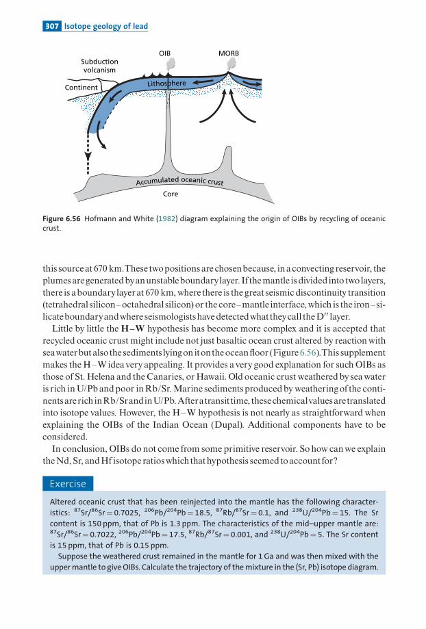
this sourceat670 km.Thesetwopositionsare chosenbecause, inaconvecting reservoir, theplumesaregeneratedbyanunstableboundarylayer. If themantle is divided intotwolayers,there is aboundarylayerat 670 km,where there is thegreatseismic discontinuity transition(tetrahedral silicon^octahedral silicon)or the core^mantle interface,which is the iron^si-licateboundaryandwhere seismologistshavedetectedwhattheycall theD00 layer.Little by little the H^W hypothesis has become more complex and it is accepted that

recycled oceanic crust might include not just basaltic ocean crust altered by reactionwithseawaterbutalsothesediments lyingon itontheocean£oor (Figure6.56).This supplementmakes theH^Wideavery appealing. It provides averygood explanation for such OIBs asthose of St. Helena and the Canaries, orHawaii. Old oceanic crust weathered by seawateris rich inU/Pbandpoor inRb/Sr.Marine sedimentsproducedbyweatheringofthe conti-nentsarerich inRb/SrandinU/Pb.Afteratransittime, these chemicalvaluesaretranslatedinto isotope values. However, the H^W hypothesis is not nearly as straightforward whenexplaining the OIBs of the Indian Ocean (Dupal). Additional components have to beconsidered.In conclusion, OIBs do not come from some primitive reservoir. So how canwe explain

theNd,Sr, andHf isotope ratioswhichthathypothesis seemedtoaccountfor?

Exercise

Altered oceanic crust that has been reinjected into the mantle has the following character-

istics: 87Sr/86Sr¼ 0.7025, 206Pb/204Pb¼ 18.5, 87Rb/87Sr¼ 0.1, and 238U/204Pb¼ 15. The Sr

content is 150 ppm, that of Pb is 1.3 ppm. The characteristics of the mid–upper mantle are:87Sr/86Sr¼ 0.7022, 206Pb/204Pb¼ 17.5, 87Rb/87Sr¼ 0.001, and 238U/204Pb¼ 5. The Sr content

is 15 ppm, that of Pb is 0.15 ppm.

Suppose the weathered crust remained in the mantle for 1 Ga and was then mixed with the

upper mantle to give OIBs. Calculate the trajectory of the mixture in the (Sr, Pb) isotope diagram.

Lithosphere

Accumulated oceanic crust

Continent

Subductionvolcanism

OIB

Core

MORB

Figure 6.56 Hofmann and White (1982) diagram explaining the origin of OIBs by recycling of oceaniccrust.


AnswerWe first calculate the isotopic characteristics of the altered oceanic crust after 1 Ga:87Sr/86Sr¼ 0.703 92, 206Pb/204Pb¼ 21.01.

We then observe that Sr/Pb is about constant. Therefore the mixtures are straight lines. All

that remains to do is to draw the straight line joining the weathered oceanic crust aged 1 Ga

and the mid–upper mantle.

Exercise

Suppose now that sediments are injected along with the oceanic crust. The characteristics of

these sediments at the time they are reinjected are: 87Sr/86Sr¼ 0.712 and 87Rb/86Sr¼ 0.1

(because of the amount of limestone which is rich in Sr), 206Pb/204Pb¼ 18.5, and238U/204Pb¼ 10. The Sr content is 400 ppm and the Pb content 3.46 ppm. These sediments

also remain for 1 Ga with the oceanic crust. Calculate the trajectories of the upper mantle–

sediment and the sediment–buried oceanic crust mixtures. If 5% of the mass of sediments is

mixed, draw the mixing trajectory.

AnswerIsotopic characteristics of sediments aged 1 Ga: 87Sr/86Sr¼ 0.713 42 and 206Pb/204Pb¼ 20.17.

Once again the Pb/Sr ratios are about constant and so the mixing ‘‘curves’’ are straight

lines (Figure 6.57). The mixture of 5% mass corresponds to the mass fraction of Sr at 34%;

we can therefore obtain the point on a straight line between that of sediments and of

the oceanic crust. It can be seen we have thus roughly reproduced the OIBs which are not

Dupals.

0.702

0.704

0.706

0.708

0.710

0.712

0.714

17 18 19 20 21 22206Pb/204Pb

87Sr

/86 S

r

Averageuppermantle

Alteredoceanic

crust + 5%sediments

Altered oceaniccrust at 1 Ga

Sediments

Figure 6.57 Graph of the results for the two exercises above.


In conclusion,whenweobserve the (Sr, Pb) isotopediagramwhichseeks tounify the twoseriesofcorrelations (Sr^Nd^Hf)ontheonehandand (206Pb^207Pb^208Pb)ontheother,it can ¢rst of all be seen there are not two completely separate domains for OIBs andMORBs.On the contrary, there is no gap, even in regions inwhichplumes are injected intoocean ridges (Schilling e¡ect),wherethetwodomainsoverlap.This topologydoesnotsug-gestamodelwherebyOIBscomefromaseparateandrelativelyhomogeneouslowermantle.The secondobservation,which isbroughtoutby the (Sr, Pb) isotope diagram, is that regio-nalizationoccurs.Therearegenuine isotopicprovinces.Themost general division, as said, is between basalts from the Indian Ocean and South

Atlantic onone sideandthoseofthePaci¢c andtheNorthAtlantic ontheother side.This ismarkedbyhigher 87Sr/86Sr ratios than for theNorthAtlantic^Paci¢c province, fora same206Pb/204Pb ratio and therefore occupies the top part of the (Sr, Pb) isotope diagram.Thisdistinction isparticularly true forOIBsbut is alsofoundforMORBs.Moreover, this ‘‘Indian’’ isotope signature is veryold, as it is found inTibetan ophiolites

(135Ma pieces of oceanic crust trapped in the India^Asia collision zone inTibet) (Go« peletal.,1984).Howcanthisbeaccountedfor?Whatreadilydistinguishesrocksfromcontinen-tal crust and rocks from the mantle is their much higher 87Sr/86Sr ratio while the206Pb/204Pb ratios are similar. If apiece of continental crust is swallowedupby themantleandmixeswith it, the 206Pb/204Pb ratio increases littlewhile the 87Sr/86Sr increasesgreatly.The di¡erence with sediment recycling is that sediments contain a large amount of lime-stone whose isotope ratios are close to 0.707^0.709 and are very rich in Sr (1000 ppm).They thereforebu¡er theSr isotope ratios.When continental crustassociatedwith its litho-sphereisdelaminated, thereisno‘‘limestonee¡ect.’’Now,theprovincewheretheIndiansig-nature is found is the provincewhere continents existed (Gondwana) in the past andbrokeup, probably leading to delamination.The overall conclusion from examining the (Sr, Pb)isotope diagram is thatOIBs comefroman isotopically veryheterogeneous sourcebuthav-inga⁄nitieswiththeMORBsourceofthe sameregion.Thus, webeganbydrawing a clear distinctionbetweenMORBandOIB and now we are

saying there is no gap between them. How can this be explained? How can rare gases beworked into the schema since we have seen an extremely clear distinction in their isotopicratiosbetweenOIBsandMORBs?This is anas-yet-unansweredquestion.

6.5.5 The 187Re�187Os system and (Os, Pb) isotope diagrams

We have already come across the 187Re�187Os system for which the decay constant isl¼ 1.64 � 10�11yr�1.Howdoes the187Os/188Os ratio evolve in theEarth’smantle?Byexam-iningosmiridiums, that is, osmium-rich minerals containing no rhenium, associatedwithultrabasic rocks,Alle' greandLuck (1980)wereable to show the isotope evolutionofmantleosmiumcorrespondedtoachondriticmantlewith187Re/186Os1.This isbecauseosmiumis an element that remains in themantlewhen partial melting gives rise to oceanic crust. Itis more ‘‘compatible’’ than either nickel or chromium.The Os concentration of ultrabasicrocks is closeto6ppmand is 0.06ppm inthe continental crust. Ifwewrite the crust^mantlebalance equation:

�OsT ¼ �Os

cc WOs þ �Os

m 1�WOs� �


thevalueofWOs is:

WOs ¼ mc

md� C

Oscc

COsT

0:15 � 0:06

6¼ 1:5 � 10�4:

Therefore:

�Osm ¼

�OsT � �Os

c W

ð1�WÞ �OsT :

This iswhat we actuallyobserve: extraction of continental crust has no e¡ect on the iso-tope evolution of Os of the upper mantle. However, what we do notice is that Re is fractio-nated a little like lutetium during magmatic processes. It concentrates in the liquid, butweakly.Accordingly theRe/Os ratios ofbasalts are extraordinarilyhigh.Valuesof 50 or100are commonplace for the187Re/188Osratio,whereas themantlehas ratios closeto0.1.

The continental crust has Os isotope ratios similar tobasalts.This means there is a highlevel of fractionation at the mid-ocean ridges but that it is neutral at the subduction zones.Thediagramof isotope evolutiontherefore looks like that inFigure6.58.

Perhaps the most spectacular illustration of this di¡erence in concentration betweencrust and mantle is the (Nd, Os) isotope diagram for the Stillwater Complex inMontana,which is an ultrabasic massif. The magma is known to have been contaminated by thecrust. The mixing curve is spectacular and needs no comment (Lambert et al., 1989)(Figure 6.59).

While the187Re�187Os systemdoesnotprovidemanyresources for studying thedi¡eren-tiation of continental crust andmantle, it is an excellent tracer for studying the reinjection

187 O

s/18

6 Os

187 O

s/18

6 Os

187 O

s/18

8 Os

187 O

s/18

8 Os

1.1

1

0.9 0.111

0.0987

0.1234

2.468

1.851

1.234

0.617

0.8

1 2 3

Time (Ga) 4 4.55

10

15

20 Continental crust

Mantle

25

5

1 2 3

Time (Ga) 4 4.55

Witwatersrand

Tasmania Waratah

Urals Columbia

Meteorite initial ratio

a b

Figure 6.58 (a) Evolution of the 187Os/186Os ratio of the mantle from osmiridiums associated withultrabasic rocks. (b) Isotope evolution of the continental crust and mantle. The mantle slopecorresponds to a chondritic Re/Os ratio as shown by Allegre and Luck (1980).


ofoceanic crustorcontinentalmaterials intotheEarth’smantle.Withthisobjective inmind,weshall examinethe (Os, Pb) isotope correlation diagramsobtained forbasaltsbycompar-ing the (Pb, Sr) diagrams (Figure 6.60). Letus examine the (187Os/188Os, 206Pb/204Pb) dia-gram for basalts.We consider only basalts whose Os content is greater than 45 ppt (theothers are suspected ofbeing either victims ofanalytical errororof secondary contamina-tionduring theirgenesis).This diagram brings out something very di¡erent from the corresponding (Sr, Pb) dia-

gram.There is no sample in the bottom right.This is because the mantle is very rich in Osand the mixtures are shown by very curved paths.Mathieu Roy Barman and the present

2

0

–2

20

40

6080

–4

1 2 3 4 50.1233 0.616

ε Nd

187Os/186Os

Primitivemagma

Continentalcrust

Stillwater

187Os/188Os

Figure 6.59 Isotope diagram for (Os, Nd) in the Stillwater Complex, a mixture of ultra-basic magma andcontaminating continental crust. The Nd/Os ratio is 400 for the ultrabasic magma and 400 000 for thecontinental crust. After Lambert et al. (1989).

1.8

18.0

Pela

gic

sed

imen

t

Terr

igen

ou

s se

dim

ent

Oce

anic

sed

imen

t

Oce

anic

cru

stw

ith

sed

imen

t

60%

60% 60%

40

2020

40

20%

40

10

20

19.0 20.0 21.0 22.0

22.0

1.6

1.4

1.2

0.120

0.140

0.160

0.180

0.200

0.220

Depletedmantle

0.150

0.144 1.20

1.10

1.0

0.138

0.132

0.126

1918 2120

187 O

s/18

8 Os

187 O

s/18

8 Os

187 O

s/18

6 Os

187 O

s/18

6 Os

206Pb/204Pb

206Pb/204Pb

DMM

Hawaii

Kerguélen

Pitcairn

RarotongaIceland

Comors

Canaries

St.Helena

Basalts > 45 ppt OsSamoa

Society islanda

Azores

Macdonaldhot spot

a

b

Figure 6.60 Isotope correlation diagram for (Os, Pb) and theoretical mixing models. (a) Theoreticalmixing models between the mantle and the various components swallowed up by the mantle. Theboxed part corresponds to (b). (b) Isotope correlation diagram for (Os, Pb) for basalts. DMM, depletedupper mantle. After Hauri and Hart (1993); Roy Barman and Allegre (1994).


author (1994), andalsoEricHauriandStanHart (1993)oftheWoodsHoleOceanographicInstitution, calculatedatheoreticalmixingmodelwithvarious components. Its trajectoriesprovide quite good explanations for the observations.The important point here is that therecycledmaterialsmustbe in quite large proportions for them tobe detected.Nonetheless,this model gives quite a good explanation of the Os isotope diversity in oceanic basalts inthe contextoftheH^Wmodel.

6.5.6 Conclusions

After these ¢rst ¢ve dense and often di⁄cult sections, it is probably worthwhile (or essen-tial?) to review these matters. Our method has been to use isotope correlation diagramstwo by two, to extract the useful information from them and then to combine the resultscrosswise to con¢rmthem, refutethem, clarify them,ordevelop them:

� Examination of the Sr^Nd^Hf isotope systems established that extraction of continen-tal crust from themantle left anuppermantle thatwas‘‘depleted’’ in some elements (andso in some isotope ratios) andwasofa lowermass thanthetotalmantle.� This ideaofatwo-layerstructureofthemantlewascon¢rmedbyexaminationoftherare-

gas isotope composition, the upper mantle being both ‘‘depleted’’and ‘‘degassed.’’ Theupper mantle is theMORB source.The complementary reservoirs of these transfers arethe continental crust and the atmosphere where the elements expelled from the mantlehaveaccumulated.� However, since themass of the depletedmantle is greater than that of the upper mantle,

wehavetoacceptmass exchangesbetweentheupperand lowermantle (theuppermantlebeingde¢nedas everythingabove670km).� Thecontinental crustis structuredintotectonicsegments, representingtheepisodesdur-

ingwhich continental crust formedat the expenseofthemantle.However, the continen-tal crust is composedof ‘‘young’’materials from themantle andalso reworkedmaterialsthat are older continental materials which have been eroded, deposited as sediment,metamorphosed, andgranitized.Thewholeprocess seems tobewellunderstoodand, ofcourse, to¢t inwith theschemasdevelopedbygeologists.� Studiesoflead isotopes con¢rmedthata largepartofthe continental crustwas extracted

from the mantle before 3Ga, as best evidenced by the 207Pb/204Pb isotope signaturecomparedwith ratios for themantle.� Theatmosphere seems tohavebeen sealed forargon, krypton, andxenonbutpermeable

for helium, which escapes into space, and ‘‘semipermeable’’ for neon.The age of forma-tionoftheatmosphere isveryancientandgreater than3Ga, and, so its seems, older thanthemeanageofthe continents. Butwehave said thatthis questionwasnotsettledandweshall returnto it.� Di⁄cultiesarosewhen itcametothegenesisofOIBs. Initially, itwas consideredthatthey

stemmedfromthe lowermantle,which isbothmoreprimitiveand less degassedthantheupper mantle.This was what was termed the standard model. Study of the lead isotopecomposition overthrew this simple model. Either the OIBs do not come from the lowermantle, or the lower mantle is not primitive.This brings in the subsidiaryquestion: whydoOIBshave rare-gas isotope signatures someofwhich seemveryprimitive?


� At this point in the discussionwe introduced theHofmann^White hypothesis by whichOIBsare relatedto recyclingofoceanic crust.Butwhere does this recyclingoccur? In theupper mantle? Then how can the rare-gas measurements from Hawaii or Iceland beinterpreted? Or in the lower mantle? But how can the upper mantle mechanism and itsformationbe explained?

All told, then, twomajorquestions remainunanswered: theoriginofOIBandthenatureofthe lower mantle (which questions are connected).This uncertainty notwithstanding, wecan develop an overviewof the physical and chemical processes related to the geodynamiccycle.

6.6 Chemical geodynamics

This model, which the present author formalized ¢rst in 1980 and then in 1982 (seeAlle' gre, 1987), is the result of a long evolution of ideas.The ¢rst attempts to relate isotopevariations and major geological phenomena concerned the interpretation of variationsin the isotopic composition of galenas. For example, studies by Paul Damon atColumbia University, New York (Damon, 1954) and Don Russell at the University ofToronto (Russell, 1972) sought to go beyond the age of the Earth and to look at the work-ing of the planet as a whole.The decisive steps that followed were made by Patterson andTatsumoto (1964) studying the formation of continental crust with lead isotopes andPatrick Hurley’s team at the Massachusetts Institute of Technology using strontium iso-topes (1962).The next stage was by Paul Gast in the 1960s with two signi¢cant papers, one on the

limitation of mantle composition (1960) while the other, written withTilton and Hedge(1964), showed for the ¢rst time that the mantle was not isotopically homogeneous(Patterson, 1963).Wasserburg (1964) sought to tie in the development of continentalcrust and the complementary evolution of the mantle using a quantitative model. Otherimportant contributions con¢rming the isotopicheterogeneityofthemantleweremadebyTatsumoto (Tatsumoto et al., 1965; Tatsumoto, 1966) for lead and Hart et al. (1973) forstrontium.The chemicalgeodynamicapproach cameaboutafter the discoveryofNd isotopevaria-

tions, which began with the (Sr, Nd) correlation, and gave some coherence to the variousisotopic measurements.The approach involved combiningobservedvariations in isotopiccomposition into a logical and coherent scheme within the framework of plate tectonics(Alle' gre, 1982; Alle' gre et al., 1982; Hart and Zindler, 1986; Zindler and Hart, 1986; Hart,1988;Hofmann,1988).

6.6.1 The foundations of the model

In this approach, itwasproposed to construct a coherentmodeloftheEarthbasedonthreefundamental features:

(1) The Earth’s structure, ¢rst of all, as determined by seismology: a continental crustand an oceanic crust, a marked p- and s-wave seismic discontinuity at 670 km, and amantle^corediscontinuity.

313 Chemical geodynamics

(2) Plate tectonics, next, with cycles ofspreadingofocean£oorsbasedon the formation oflithosphereat themid-ocean ridges and its recyclingat subduction zones.On this cycleis superimposed the injection ofmagmas from deeper-lying hot spots.The continentsbreak up, drift around, and collide but remain at the Earth’s surface. The use of thismodel for the entire geological timescale results from the application to geochemistryofafoundingprincipleofgeology,uniformitarianism.16Nocall ismadeon‘‘extraordin-ary’’phenomenato explain the past.Yet, nothing shows it is true. Perhaps theworkingsof the Earth in the pastwere quite di¡erent fromwhatwehave reconstituted for the lastfew million years.The supposition in the chemical geodynamic model is that if it wasthe case, thevariations remainedwithinacontextsimilar to theonewe¢ndnowadays.

(3) The data of isotope geochemistry, lastly, and tobeginwith those for Sr andNd. In thismodel, it is assumedthatthe continents are the‘‘scum’’of theEarth, and result fromdif-ferentiationofthemantlewhichhas extractedfromthemantle elements likepotassium,rubidium, and the rare earths as well as uranium and thorium. Geological mappingsuggests that the extraction of continental material from the mantle occurred over thecourseofgeological time, giving rise toanewtectonicprovince eachtime (seePlate4).

This convection process divided the Earth’s mantle little by little into two reservoirs: theupper reservoir, the MORB source, depleted in some chemical elements by extractionof the continents, and the lower mantle less depleted (but not primitive!). This divisionalso a¡ects the rare gases which have degassed from the (consequently depleted) uppermantlebut remain more concentrated in the lower mantle, the escaped heavygases havingcollected in theatmosphere.

The cycleofoceanic crustwhich is extracted fromthemantleandthen returnedto itaftera timeofspreading at the surface acts as the extractorofmantle elements.Themagmaphileelements (potassium, rubidium, cesium,uranium, thorium, etc.)were enriched for the¢rsttime in liquid during themagmatic processes offormation ofoceanic crust. (The partitioncoe⁄cientD¼Csolid/Cmagmaofthese elements isverylow for solid^magmapartitionphe-nomena.) Then, they were enriched a second time during subduction processes, whichtransfer elements from the oceanic crust to the continents viamore complex fractionation,butwhosepartition coe⁄cients aresomewhatdi¡erentfromthoseofthemid-ocean ridges.If we term the processes occurring along the mid-ocean ridges theR-process (ridge) andthe processes occurring during subduction the S-process (subduction), the extraction ofelements from the mantle to the continental crust corresponds to the sum (Rþ S).We canwrite symbolically:

continental crust ¼ SðR�mantleÞ;

withRoperatingonthemantleandSontheproductofthis¢rstoperation.17

The oceanic crust modi¢ed by the S-process plunges back into themantle and ismixedmechanically with it by mantle convection. In this way, an increasingly ‘‘depleted’’mantleis formed.The raregases areoutgassedby theR-processbut S-processvolcanismalso leadstooutgassing,preventing the raregases frombeing recycled intothemantle.

16 This dates back to one of the founders of geology, Charles Lyell, and underpins the development of thisdiscipline on a scientific basis.

17 Not to be confused with the notation for the r- and s-processes in nucleosynthesis!


Themantle is thereforemadeupofanuppermantle,which is‘‘depleted’’ in elements suchas potassium, uranium, thorium, and rubidium, anddegassedofmostof its raregases andof a lower mantle, which, while not pristine, is less depleted in potassium, uranium, thor-ium,andrubidium,and is richer in raregases.If, as some investigators asserton thebasis ofseismic tomography, the downgoing plates

were recycled in the lowermantle throughoutgeological history, the lowermantlewouldbedepleted because it is the downgoing plates that convey the depletion (the extraction ofele-ments concentrated in the continental crust). It is essential, therefore, that the plates havebeen reinjected for themost part intheuppermantle.Likewise, ifall themantleweretotallyoutgassed, there would not be anymarked di¡erence in the isotope ratios of the rare gaseslike helium and neon contained in MORB and OIB. The mantle is therefore necessarilycomposedoftwoseparate (butnot isolated) reservoirs.

6.6.2 The internal geochemical cycle

Twofundamentalgeochemical processes that are an integral partofgeodynamicprocessesoccur in the upper mantle.The oceanic lithosphere is formed at the mid-ocean ridges andseparates abasaltic ocean crust enriched in certain elements (relative to themantle) suchaspotassium, rubidium, uranium, the rare earths, etc. and anunderlying, ultrabasic residuallithosphere depleted in these elements and whose remelting cannot create much basaltbecause the essential elements making up certain basalt minerals (feldspars, clinopyrox-enes) such as calcium and aluminum havebeen extracted tomanufacture oceanic crust. Itisoften said inpetrologists’ jargonthatthedeepocean lithosphere is infertilebecause itcannolongerproducebasaltbyfusion.Thisoceaniclithosphere(crustandresidual lithosphere)is reinjected into the mantle where it mixes backwith the upper mantle (McKenzie, 1979;Alle' greetal.,1980;WhiteandHofmann,1982).Mixing is mechanical. Pieces of the lithosphere are caught up in the convective move-

ments of the mantle. In this process, rock is stretched, folded, and pinched. Rock from theocean crust, generally basaltic, is transformed mineralogically by metamorphism duringsubduction intorocks suchas eclogite (assemblyofgarnetandpyroxene).Theuppermantlelooks likeamarbledcake (Alle' greandTurcotte,1986)withabasicperidotite (pyroxeneandolivine)composition interspersedwithstrandsofeclogites,drawnoutandstretchedtovary-ing degrees.These strands are shreds of ancient oceanic crust which has been laminated,pinched, and folded by mantle movements. After some time, these ever-thinner strandswill end up reacting mineralogically with the peridotite mantle and will disappear(Hofmann andHart,1978; Alle' gre and Turcotte,1985), while the mantle will be fertilizedby this absorption, that is, made capable of basalt extraction by melting again. But theseslivers of continental crust are not uniform. Some have dragged layers of sediments downwith them.These sediments carried by the downgoing plate are dehydrated, compacted,and then metamorphosed. They are also stretched, thinned, pinched, and folded(Figure6.61).Some of the pieces of oceanic crust reinjected into the mantle are very peculiar as they

have lost the chemical elements thatwill give rise tovolcanism in the subduction zones andthrough that to continental crust.These are the materials which e¡ect the depletion of themantle in some elements (rubidium, uranium, etc.) andwhich is re£ected in isotope ratios,


becauseallofthematerials swallowedupbytheuppermantlehavevariedisotoperatiosandchemical ratios.

Is thismarbledmantleapurely theoreticalmodeldreamtupbygeochemists andgeophy-sicists? Not a bit of it! It is real enough. It can be seen cropping out in a few special placeswhere tectonic processes have brought pieces of mantle to the surface.This is the case insouthern Spain near the little town of Ronda (the temple of bull¢ghting), in northernMorocco near the village of Beni-Bousera (Figure 6.62), at Lhez (France) in the Pyrenees,andatLanzonearTurin (Italy).

Thesemassifs areoftenmadeup ofperidotite, often depleted in aluminumand calcium,with isotope signatures of the upper mantle.They contain strands of eclogites which havebeen shown to come from ancient oceanic crust.They also contain ancient sediments andeven diamond transformed into graphite, that is, old limestones rich in organic materialthat hasbeen reduced and changed into diamonds.Theuppermantle is indeedmadeup ofa thorough mixture of peridotite and eclogite. By contrast, the lower mantle contains farfewer strandsand ismuchmoreuniform.

Atmosphere

(S) MORB(S)(R)

meltingzone

meltingzone

meltingzone MIXING

UPPERMANTLE

LOWERMANTLE

Figure 6.61 Fractionation of the geodynamic cycle. The internal geodynamic cycle exhibits mixing,differentiation, and removal phenomena, mostly in the upper mantle.


6.6.3 Statistical geochemistry

Sofarwehavespokenagreatdealofreservoirs exchangingmaterial, consideringthatconti-nental crust is segmented intoageprovinces and thereforeheterogeneousbutthat theman-tle is homogeneous (at least at regional scale).Theupshotof this is thatwehave consideredan average value to characterize each reservoir.Without relinquishing such modeling,which is straightforward and extremely useful, we have to supplement it with anotherdescription, which is statistical. Each reservoir is described not by a single average valuebutbyadistributionofvalues, isotope ratios, orchemical concentrations.When an oceanic plate dips into the mantle it is chemically and isotopically heteroge-

neous. Admittedly, when oceanic crust forms at the mid-ocean ridges it is isotopicallyhomogeneous (bymelting) but chemicallyheterogeneous, with the crustbeing enriched inrubidium comparedwith strontium, the lithospherebeing depleted inRb/Sr, and the sedi-ments rich in Rb/Sr when detrital and poor when they are limestone.These chemical het-erogeneities are re£ected by isotopic heterogeneities during the ridge^subduction zonejourney,byradioactivedecay.Then,ofcourse, thesamehappens inthemantlewith radioac-tivitycontinuing its inexorable decayand its creationofnewisotopes.The upper mantle, then, is not isotopically or chemically homogeneous, but hetero-

geneous. It is not characterized by a single average isotope ratio, as in the ‘‘box’’ modelwe dealt with when examining the earlier crust^mantle system, but by a spread ofisotope ratios, with an average, variance (standard deviation), and a degree of asym-metry for each type of ratio.This statistical distribution also has, of course, a geographi-cal distribution.

a

b

2-3 cm 1-2 cm

3 m

2-10 cm

2-10 cm

5 cm30 cm30 cm

5 mc

2 md

15cm10 cm

50cm

10 cm

12 cm

15 cm60cm

Figure 6.62 Garnet pyroxenite (eclogite) bed structures in the peridotites of Beni-Bousera massif,Morocco. Pyroxenite in blue, peridotite in white. (a) Series of pyroxenite beds of different sizes in theperidotite; (b) pinching and swelling; (c, d) folding. After Allegre and Turcotte (1986).


Forexample, the�Srand�Rbparameters are each replacedbyadistributionnotatedas:

�Sr�

¼ �Sr m; �; dð Þ� �

and �Rb�

¼ �Rb m; �; dð Þ� �

wherem is themeanof�Sror�Rb,� the standarddeviation, andd theasymmetry.Naturallyenough, themorethesystem is subjectedto convectionthemore it ismixedand

themorehomogeneous it is, andthesmaller� is.Twoantagonisticphenomenaarethereforeinaction: chemical fractionation near theEarth’s surface,whichtends to increase chemical(and so isotopic) heterogeneity, and convective mixing phenomena within the mantle,whichtendtoreducethem. It is acontestofchemical di¡erentiationversusmixing.

Partial melting andvolcanism (at the ridges and hot spots) of the heterogeneous mantleyield samplesofthemantle,whicharemoreor less random, fromwhichwe canmeasure the87Sr/86Sr, 143Nd/144Nd, 87Rb/86Sr, and 147Sm/144Nd ratios, etc., for which we can alsode¢ne distributions andwith them a mean, a standard deviation, and an asymmetry. (Wenotate these distributions by { }: �Sr

� �¼ �Sr m; �; dð Þ� �

and similarly for�Rb� �

¼ �Rb m; �; dð Þ� �

.)An importantstep inourproject is,ofcourse, todeterminetheactualdistributionsof iso-

tope ratios in the mantle from the distributions sampled and measured at the surface. Apriori, it mightbe thought that the larger the sample, the closer �f g is to �h i.We take as aworkinghypothesis that �h i¼K �f g, that is, the distributionmeasured from surface sam-ples is proportional to the distribution of themantle atdepth.Whenthedistributionsmea-sured onvarious samples ofa same type ofbasalt aremore dispersed than thosemeasuredon another type, it is legitimate to suppose thatthe sources of the formeraremoreheteroge-neous than the sources of the latteror that the phenomenagiving rise to thebasalts did nothomogenize them asmuch (becausewe aremindful, of course, that the phenomenaofpar-tialmeltingofthemantle, thenofpoolingoftheliquidsgivingrisetomagmas, tendtohomo-genize the isotope ratios).They therefore e¡ect a sort of natural average of the zone wherepartial melting occurred (statistical sampling). As it is accepted that isotope homogeniza-tion occurs at such temperatures, basalt sampling provides a representative average of thesample space. Studyofthebasaltpopulation is thereforea sampleofthemantleonthe scaleof a fewkilometers. But at the same time, these phenomena ofmagmatogenesis erase anysmaller local heterogeneities, as themagmaaverages themout.Now,whenwe speakofhet-erogeneityofthemantle,wemustbe clearwhatwemeanby it.Therearevarious typesofhet-erogeneity, asFigure6.63 shows.

6.6.4 Geochemical fractionation

Since thebeginningof this chapter, wehave spoken of chemical fractionationwhich modi-¢es theRb/Sr,Sm/Nd,U/Pb chemical ratios, etc.,modi¢cations thatare re£ectedby isoto-pic changes.The variations in isotope ratios are the re£ection, with a time lag, of chemicalfractionation. It is customary to say that radiogenic isotope ratios are chemical fossils.Weshould therefore lookalittlemore closelyatgeochemical fractionation.

The essential fractionations in chemical geodynamics are those related to the formationofmagma, at themid-ocean ridges tomanufacture oceanic crust, at the subduction zonestoproducearcvolcanismandextractcontinental crust, and in the deep continental crusttoyieldgranites.All are relatedtothepartialmeltingprocess (Gast,1968).


Whenapolycrystallineassemblage is in conditionsoftemperatureandpressureatwhichitmelts,melting ispartial melting prettywellobeying the thermodynamic rulesofeutecticequilibrium. Melting is characterized by a degree of partial melting F and a chemicalcompositionofthe liquidwhich is di¡erent fromthatofthe solid.Trace elementsarepartitionedbetween liquidandsolidstates.Thispartition is character-

ized by the partition coe⁄cient Di¼ concentration in solid/concentration in liquid ofelement i.

a

b

c

Figure 6.63 The types of heterogeneity the mantle may conceal. (a) Different domains scattered in awhole. Sampling a small part brings out the heterogeneities, while more extensive sampling makes themdisappear. (b) Large-scale heterogeneities with several domains, each of which is homogeneous.Heterogeneity is observed geographically. (c) Types (a) and (b) combined. (Of course, other types may exist.)


Itobeysasimplebalance equation:

Ci0 ¼ Ci

l F þ Cis 1� Fð Þ

where C0i is the initial concentration of the solid for element i, C1

i is the concentration ofelement i in the magma, Cs

i the concentration of element i in the residual solid, and F thedegree ofpartial melting. If the overall partial melting coe⁄cient of element i is de¢ned inthe process considered by Cs

i/C1¼Di, without worrying whether the process is in equili-brium or not, whether it is complex or simple, but such thatDi is about constant, then thepartialmelting equation canbewritten:

Ci1 ¼

Ci0

FþDið1� FÞ :

The concentration in the residualsolid is therefore:

Cis ¼ Di Ci

0

FþDið1� FÞ :

Afundamental resultoftheseformulaefor thegeodynamic cycle isTreuil’s approximation.Michel Treuil of the Institut de Physique du Globe in Paris noticed in 1973 (Treuil, 1973;Treuil and Joron, 1975) that for some elements with low D, Di (1�F) becomes negligiblecomparedwith1; therefore he named those elements ‘‘magmaphile’’ but some others havenamedthem‘‘incompatible.’’

C1 ’C0

F:

For these elements the concentration depends directly on F (the smaller F is the moreconcentrated the liquid) and, yetmore importantly, if the ratioofthe two elements is taken,F is eliminated:

Cil

Cjl

¼ Ci0

Cj0

;

that is, the ratios are conserved across partial melting, which is true for isotope ratios ofheavy elements and for ratios of a numberof trace elements whose partition coe⁄cientsDarevery, verysmall and sonegligible comparedwith1, suchasTh,U,Rb,Nd, andPbundercertain circumstances. This is fundamental because not only can we obtain the isotoperatios of the mantle such as 87Sr/86Sr, 143Nd/144Nd, etc. but we can also obtain the Rb/SrandSm/Ndchemical ratiosofthemantle (oratanyrategoodestimatesofthem).

Exercise

ExerciseIs Treuil’s approximation by which (for low values of D) we can write:

C il

C jl

¼ C i0

C j0


still valid in the two instances below?

� DTh¼ 0.01 and DU¼ 0.02. Study the Th/U ratio as a function of the degree of partial melting

F, taking the values of 0.11, 0.05, and 0.01.

� DTh¼ 0.02 and DU¼ 0.1.

In both cases, plot the curve (Th/U)liquid/(Th/U)source¼ f(F)¼ R.

AnswerWe write:

C 1l

C 2l

� �,C 1

0

C 20

� �¼ D 2 þ Fð1� D 2Þ

D 1 þ Fð1� D 1Þ¼ R:

In the first case, we find R¼ 1.08 (0.1), 1.159 (0.05), 1.4897 (0.01). In the second case, we

find R¼ 1.61 (0.1), 2.10 (0.05), 3.65 (0.01). This shows the limits of Treuil’s approximation.

Exercise

At the ocean ridges, U/Pb fractionation is such that �¼ 238U/204Pb shifts from 5 in the upper

mantle to 10 and more in the oceanic crust. If D ðRÞU ¼ 0:03 and if F¼ 0.08, what is the value

of D ðRÞPb ?

This oceanic crust is melted in the S-process. In the andesite lava �¼ 8.5. Supposing that

D ðSÞU ¼ 0:03 and F¼ 0.10, what is the value of D ðSÞPb ?

AnswerFirst we find D ðRÞPb ¼ 0:135 and then D ðSÞPb ¼ 0:01. Lead is less compatible than uranium during

subduction.

Wehave the answer to an earlier question: whydoes leaddistinguish themantle from thecontinental crust so poorly? Because the U/Pb R and S chemical fractionation processespartially o¡set one another in this case. There are two results from these investigations.First, if the melting rates are high, the ratios between the elements that interest us (Rb/Sr,Sm/Nd,U/Th, andU/Pb)are justaboutpreserved.Accordingly, themixing lines in the isotope correlation diagrams (see thebeginningof

this chapter) aremore or less straight.This iswhy roughly correct correlationswere foundbetween many isotope ratios. Because everything is almost linear : fractionation, mixing,and radioactive decay. (For lead isotope ratios, where growth of radioactive origin is non-linear, the parent^daughter identity preserves linearity; when such linearity is lost, the iso-topediagramsbecomemore complex.)Bycontrast,whendealingwith elements that fractionatedduringdi¡erentprocesses, lin-

earity is not preserved.This is the case, for example, of isotopes of lithophile elements (Sr,Nd,Hf) andof the raregases, because theyobey two di¡erent rationales. Fractionation forone is related to extraction from the continental crust, and forothers tomantle outgassing.The former are sensitive to processes of reinjection of oceanic or continental crust, theothers are not reinjected. An example of this is the (Sr, He) non-correlation established byMark Kurz of the Woods Hole Oceanographic Institution (Kurz et al., 1982). Another


example is the case that impliesosmium,because itsgeochemicalbehavior is atypical com-paredwith thatofotherelements (Lambertetal.,1989).

Forelementswhoseonly isotopefractionsare createdbyextractionofcontinental crust,adouble chemical fractionationprocessoccurs: oneatthemid-ocean ridges, theother in thesubduction zones.Wehave just seenwith the example of lead that the twoprocesses are notidentical (in the case of Pb/U, fractionation is reversed).We shall look more closely at thisquestionusingother isotopetracers, thosefromradioactive disequilibria.

6.6.5 Consequences for the Earth’s energy regime

Uranium, thorium, andpotassium,whichareall elementswhose radioactivity is an impor-tantsourceofheatfor theinternalactivityofourplanet,aregreatlyenrichedinthe continen-tal crust and therefore depleted in the upper mantle. The lower mantle is much richer inthese elements.It is therefore the lowermantle that supplies the uppermantle’s convectiveheat.Theuppermantle isheatedfrombelowandcooledfromaboveby theocean. It is there-fore in an almost ideal situation for convecting, by an admittedly complex process butwhich is akin towhat isknown inphysics asRayleigh^Be¤ nard convection (seeTurcotteandSchubert, 2002), which can be observed when a pan of water is put on the cooker to boil.The lower mantle too convects, because it is veryhot and is of large dimensions, but it con-vects in a di¡erent manner, by internal heating particularly by the radioactive elements itcontains (itmightbeworth lookingbackat the endofChapter1, where the calculations setoutwerepreparation forcurrentreasoning).

Exercise

We wish to test the two-layer convective model in respect of heat flow (see Chapter 1). The

measurements on MORB give the results: U¼ 50 ppb, Th/U¼ 2.2, and K/U¼ 104. Accepting

that the three elements are wholly incompatible, that is, that Cliquid¼Csolid/F where F is the

degree of partial melting estimated at 10%, calculate the heat flow of radioactive origin

produced by the upper mantle. Calculate the heat flow produced by the lower mantle if we

assume that for the mantle U¼ 21 ppb, K/U¼ 104, and Th/U¼ 4.2. Calculate the heat flow of

the continental crust given that K¼ 1.2%, K/U¼ 104, and Th/U¼ 5. Given that the total flow is

41 � 1012 W, what proportion is produced by radioactivity? What makes up the difference?

AnswerThe heat flows from radioactivity are: upper mantle: 0.95 � 1012 W (terawatts), lower mantle

15.3 � 1012 W, continental crust: 6.25 � 1012 W, making a total of 22.5 � 1012 W. The proportion

created by radioactivity (Urey ratio) is 0.5. The difference comes from energy stored when

the Earth formed and from differentiation of the core. It is stored in the lower mantle and

core (gravitational energy transformed into heat). The lower mantle therefore transmits

36.8 � 1012 W whereas the upper mantle produces just 1 � 1012 W.

6.6.6 Radioactive disequilibria and the difference betweenR- and S-processes

Wehavejusttouchedupon itwithregardtoU/Pbfractionation,butweshallseeindetailwiththeexampleof230Th/238Usystems,whichwehavealreadydealtwith intermsofchronology,


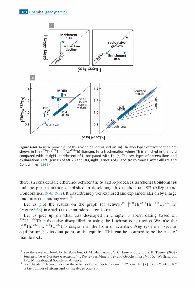
there is a considerable di¡erencebetween the S- andR-processes, asMichel Condominesand the present author established in developing this method in 1982 (Alle' gre andCondomines,1976; 1982). It was extremely well explored and explained later on by a largeamountofoutstandingwork.18

Let us plot the results on the graph (of activity)19 230Th=232Th; 238U=232Th� �

(Figure6.64), inwhich (a) is areminderofhow it is read.Let us pick up on what was developed in Chapter 3 about dating based on

238U�230Th radioactive disequilibrium using the isochron construction. We take the(230Th/232Th, 238U/232Th) diagram in the form of activities. Any system in secularequilibrium has its data point on the equiline. This can be assumed to be the case ofmantle rock.

1.2

1.4

1.0

0.8

[230

Th/2

32Th

]

[230

Th/2

32Th

]

radioactivedecline

equiline

equiline

[238U/232Th]

MORB

MORBsource(upper

mantle)

OldMORB

Bulk Earth

OIB

Enrichmentin U

radioactivegrowth

1.2

1.4

1.0

0.8

[238U/232Th]

OldMORB

Sediments

Isla

nd

arc

Depletedmantle

a

b

Enrichmentin Th

Figure 6.64 General principles of the reasoning in this section. (a) The two types of fractionation areshown in the (230Th/232Th, 238U/232Th) diagram. Left: fractionation where Th is enriched in the fluidcompared with U; right: enrichment of U compared with Th. (b) The two types of observations andexplanations. Left: genesis of MORB and OIB; right: genesis of island arc volcanoes. After Allegre andCondomines (1982).

18 See the excellent book by B. Bourdon, G.M. Henderson, C. C. Lundstrom, and S. P. Turner (2003)Introduction to U-Series Geochemistry, Reviews inMineralogy and Geochemistry Vol. 52. Washington,DC: Mineralogical Society of America.

19 See Chapter 3. Remember that the activity of a radioactive element R* is written [R]¼ lR R*, where R*is the number of atoms and lR the decay constant.


� If the partial melting process involves enrichment of the liquid in (Th) comparedwith (U), the point representing the magma will shift horizontally to the left. The sys-tem will return to equilibrium through decay of its excess 230Th (excess relative tothe 238U value). The 230Th/232Th isotope ratio of the magma will decrease over timewith the data point shifting vertically downwards.When it returns to equilibrium, itwill lie on the equiline again but in a lower position (with a lower 230Th/232Th ratioin U/Th).� If, on the contrary, the partial melting process involves enrichment of the melt in (U)

compared with (Th), the data point will shift horizontally to the right.The systemwillreturn to equilibrium by recreating 230Th through 238U decay.The point will thereforerise vertically.When it reaches equilibrium, the 230Th/232Th ratio will have increased.TheU/Th ratiowill thenbefargreater thanthatofthe initial solid.

The evolution equation is, it will be recalled (with ratios in square brackets in the form ofactivities):

230Th232Th

� �¼

230Th232Th

� �0

e�l230t þ238U232Th

� �1� e�l230t� �

:

If we measure the composition of a magma, the age since it underwent partial melting iswritten:

t ¼ 1

lln

230Th232Th

� �0

�238U232Th

� �230Th232Th

� ��

238U232Th

� �0BBB@

1CCCA:

Calculatingan age like this involvesmeasuring the isotopic composition ofthoriumandthe 238U/232Th (chemical) ratio. But one datum is missing: the initial isotope ratio of thethorium. One can also reason backwards and calculate the initial isotope ratio of the thor-iumiftheageisknown.Letusleaveasidethis issueofcalculatingtheageandtheinitial ratiosfor themomentandturntothe resultsofanalysesonpresent-daylavas fromvarious typesofvolcanic rocks.

Ofcourse, therocksmustbefromthepresentdaysosigni¢cantcomparisonscanbemade.Otherwise radioactive decay since eruptionwill have shifted the position of the data pointvertically inthe(230Th/232Th,238U/232Th)diagram.Wemustbewaryofcontaminationpro-cesses, too.As for rare gases, seawater is apowerful contaminant for the 230Th/232Th ratiobecause it has extremely high 230Th/232Th ratios (values of 50 or 100 are commonplacewhile the values of basalt lavas are close to unity). Even slight contamination by seawatershifts thedatapointupwards.

Having takenthe requisiteprecautions,whatdoweobserve?MORBandOIBare locatedto the left of the equiline.They therefore correspond to cases of magmabeing enriched inTh relative toUsince theU/Th ratiohas fallen.

It isobservedthatstatistically theOIBliesbelowtheMORB.Anenrichmentcoe⁄cientisde¢ned k¼ (U/Th)magma/(U/Th)source. From the exercises in the previous section, thelower the degree of partial melting, the smaller k is. Petrologists tell us that the extent of


partial melting of OIB is much less than that ofMORB (1% versus10%). Now, the relativeposition on the (230Th/232Th, 238U/232Th) diagram is not so clear.This canbe explainedbyaccepting that the genesis of OIB is often complex, involving phenomena ofmixing, con-tamination by ancient oceanic crust, and multiple transfer times (Figure 6.65).When thedatapoints for islandarcvolcanoes are plottedon the same diagram, theyare found, on thecontrary, to lie to the rightof the equiline.Their genesis involved processeswhich enrichedthemagmainUmorethan inTh. It is alsoobservedthatmanypoints representingthesevol-canoes havemuch greater thorium isotope ratios than are found forMORB andOIB.Thisis interpreted in the frameworkofmodelswhich havebeendevelopedby thegenesisofmag-mas in subduction zones. It is accepted that the downgoing plate begins tomelt, but that itpasses on to the overlying mantle wedge a silica-rich £uid with a very highwater content.This £uid has probably also derived some of its material from the subducted sediments.The £uid inducesmeltingof thematerial in themantlewedge overlying the plunging plate.The initial material is therefore amixture ofuppermantle similar to thatwhichgave rise totheMORB, ofa subducted sedimentwhose 238U/232Th ratiosmaybe as lowas 0.4, andofawater-rich£uidwhich is enrichedmore inUthan inThasUismoresoluble inwater thanTh.There is abig di¡erence, then, between magmaswhich result frompartial meltingof the

mantle, like MORB, and island arc magmas whose genetic processes are more complex.Thegenesis ofOIBbelongs to the family wheremelting processes dominate, but in detail itisobservedthattheTh isotope ratiosofoneandthe same islandarevariable.Detailed studies have shown complex phenomena to be involved. First of all, there are

variable types of source, as seenwith lead isotopes.Then there are processes of interactionwith the oceanic crust through which the OIB makes its way. So there are three types ofmagma-producingprocesses. Simplepartialmelting (MORB), partialmelting followedbymixing (OIB),andpartialmelting inthepresenceofwaterandamixtureofmultiple compo-nents (island arcs). But the diagrams showa continuous spreadofdatapoints among thesedi¡erenttypes, indicating the existenceofcertaina⁄nities.

Exercise

A domain of the mantle is considered whose [230Th/232Th] ratio in terms of activity is 1.4.

Suppose this domain undergoes 8% partial melting to form oceanic crust. This oceanic crust

returns to radioactive equilibrium. Then it undergoes 5% partial melting in a subduction zone.

The transfer time of the magma to the surface is 40 000 years. What are the [230Th/232Th] and

[238U/232Th] ratios of magma in terms of activity? It is assumed the solid/melt global

fractionation coefficients are DU¼ 0.015, DTh¼ 0.0034.

Answer[230Th/232Th]¼ 1.15. [238U/232Th]¼ 1.

Letusmoveon now totransit timesbetween the sourceandthe surface.Despite complextheoretical models that predicted a quite long and complex transfer from themelting zoneto the surface (McKenzie,1989) the transfer rate forMORB is quite high. ForMORB, theissuehasbeenaddressed in twoways.The¢rst is to calculate the initialvalueof [238U/232Th]of the source mantle by estimating the degree of partial melting using the fractionation


238U/ 232U

23

0Th

/ 2

32Th

equiline

1.00

TongaKermadecSundaMarianasKamchatkaAleutiansNicaragua

2.00

3.00

1.000 2.00 3.00 4.00

150 ka

50 ka

30 ka

0.7 0.8 0.9 1 1.1 1.2 1.3 1.4 1.5

0.7

0.8

0.9

1

1.1

1.2

1.3

1.4

1.5

1.6

230 T

h/2

32Th

238U/232Th

MORB

Azores

4.1

3.1

2.8

2.6

2.4

2.25

k = 0.5

1% 2% 5%Degree of

partial melting

Th/U10%

k = 0.6 k = 0.7 k = 0.8k = 0.9

Bulk Earth

equilin

e

Pitcairn

Comoroes

Faial

Tahiti

Hawaii

Réunion

PicoArdoukola

MAR 37

Iceland

Macdonald

a

b

Figure 6.65 Actual cases of disequilibrium data. (a) The MORB zone in blue, the OIB zone in white withthe main OIBs shown. Note the two domains are continuous. (b) Subduction zones with variousisochrons showing a very different representation of MORB and OIB. After Condomines et al. (1988);Condomines and Sigmarsson (1993).


coe⁄cientsdeterminedinthelaboratory forUandTh.Thesecondisbasedonthefollowingremark. A radioactive pair has returned to equilibriumwhen the time since the disequili-briumwas created is six times the shorter half-life. As many 230Th/232Th ratios ofMORBare far from equilibrium, it can be estimated that the transit times are very much less than300 000years.

238U/ 232Th

238Th ingrowthover 30 ka

238Th ingrowthover 350 ka

U addition by fluids

23

0Th

/ 2

32Th

equi

line

0.6

0.8

1.0

1.2

1.4

0.90.5 1.3 1.7 2.1

averageMarianassediment

sediment melting

Figure 6.66 (a) Diagram of current understanding of the formation of island arc volcanoes; (b) thevarious stages of genesis explaining the observations. The example of the Marianas Islands, studied byElliot et al. (1997).

Volcano

Melting

Fluidtransfer


But there is a more interesting observation.The 226Ra/230Th and 210Pb/226Ra ratios arenot in equilibrium.The transit time is less than 6 times the half-lives of 226Ra and 210Pb of1.622 � 103 years and 22.26 years, respectively.This corresponds to a date for 226Ra of lessthan10 000 years, but for 210Pb of less than135 years. If it is accepted thatmid-ocean ridgemagmas formatdepthsof30 km, this corresponds totransitspeedsof200myr�1.The con-straintofradium corresponds to 3myr�1.Therefore, the speed is instantaneous forMORBand it should be considered that the 230Th/232Th ratios measured on present-day rocksyield the U/Thvalue of their source mantle directly and better than the directly measuredchemical ratiobecause it is fractionated.

Calculating transfer times for OIB is much more complicated because of the complexprocesses involved, such as magma chamber processes, lithosphere interaction, and so on(seeHawkesworth,1979;Elliotetal.,1997;Turneretal., 2003).

Island arcs have very long andvariable transit times. Some aremore than 300 000 yearsbecause the data points are very high on the equiline, far above the MORB points. In thecase of theMarianas Island arc,Tim Elliott of the University of Bristol and his colleagueshave managed to put a ¢gure on the ¢nal stages and to show that there were two stages ofinput fromthe downgoingplate.A¢rst stage involving sedimentshavingoccurred 300 000yearsbeforea secondmelting stage,which itselfoccurred150 000yearsbefore the eruption(seeFigure 6.66a).Allofthis clearlyshows the di¡erence inbehaviorof islandarcvolcanoescomparedtoMORBandOIB.

Exercise

The radioactive disequilibrium of an OIB is measured giving [230Th/232Th]¼ 1.08 and

[238U/232Th]¼ 0.8. In addition, [238U/230Th]source¼ 1.1. Calculate the fractionation coeffic-

ients D¼ (U/Th)source/(U/Th)magma, the transit time between fractionation and reaching the

surface, as well as the rate of ascent, if it is assumed the process began 20 km beneath the

ocean ridge.

AnswerD¼ 1.43, T¼ 1380 years, v¼ 15 m yr�1.

6.6.7 The major elements

Themajorelementsarethosethatmakeupmineralsandthereforerocks.Theirabundanceismeasured in percent by mass.They are oxygen, silicon, magnesium, aluminum, calcium,iron, and sodium.Theydetermine the physical properties of the Earth’s interior and so areresponsible for the properties measured in geophysics (velocity of seismic waves, density,magnetism).Now,what is important is that thesemajor elements are practically una¡ectedby themajor processesgoverning chemical geodynamics.To show this, letus take an extre-melysimple calculation.

Let us consider theweight analyses of peridotite (an essential constituent of themantle)andofgranite (an essential constituentofthe continental crust) (Table 6.9).

The proportions by mass between continental crust and upper mantle are 0.01 (for theupper mantle above the seismic discontinuity at 670 km). Let us suppose the peridotite


comes from the depleted upper mantle, and let us calculate the composition of the‘‘recon-structed’’primitivemantle (Table 6.10) before extraction of the continental crustbymixingofcontinental crustwithdepletedmantle:

½Aprimitive ¼ ½peridotite � 0:99þ ½granite � 0:01:

This composition is almost identical to thatoftheperidotite analyzed.Theonlyelement forwhichadi¡erence canbe clearlyseen ispotassium,which isnotamajorelement!Thosedif-ferencein composition cannotbedistinguishedbyanygeophysical, seismological,orgravi-metricmeasurements.

RemarkRemember this warning in chemical geodynamics: minor elements mean major problems. Whereas

in petrology, major elements mean key problems!

Wehave translated this in Figure 6.67, remembering wehave calculated factorsW. It willbe recalled that:

Wi ¼ micc C

icc

mip Ci

p

where mcci is the mass of continental crust, and mp

i is the mass of the primary mantlebefore depletion; we can take it to be equal to the upper mantle, such thatmcc/mp¼ 0.015;

Table 6.9 Composition of granite and of peridotite of the mantle

Oxide Element Peridotite Granite

percentweightofoxide

percentweightofmajorelement

percentweightofoxide

percentweightofmajorelement

O 43.36 50.38SiO2 Si 41.82� 0.80 19.51 72.30� 0.50 33.13Al2O3 Al 3.50� 0.10 1.26 14.15� 0.10 5.094Fe2O3 Fe 9.06� 0.15 6.33 1.91� 0.02 1.33MgO Mg 37.99� 0.5 22.86 0.040� 0.008 0.03MnO Mn 0.17� 0.01 0.14 0.370� 0.001 0.22CaO Ca 3.02� 0.06 2.15 1.33� 0.01 0.949Na2O Na 0.82� 0.1 0.6 3.49� 0.03 2.589K2O K 0.03� 0.006 0.0250 2.55� 0.06 2.12

Table 6.10 Composition of the primitive mantle

O Si Al Fe Mg Mn Ca Na K

‘‘Reconstructed’’primitivemantle (%)

43.42 19.64 1.298 6.28 22.603 0.1389 2.137 0.6198 0.4595

Depletedmantle 43.36 19.51 1.26 6.33 22.86 0.14 2.15 0.6 0.025


Ccci is the concentration of element i in the continental crust, Cp

i is the concentration ofelement i in the primitive mantle, and W is the proportion of the element concentratedin the continental crust.20

It ispossible to calculateW fora fewmajorandminorelements.The scale (in log10) is sepa-rated in twoby the values�¼ 0.015; an element that does not fractionate between crust andmantle has this value. Above this value the element is enriched in continental crust; below, itis depleted. It shall be seen that while silicon and manganese are not very di¡erent from it,below� the elements are enriched in themantle, while above they are enriched in the crust.Table 6.11gives thevaluesof thevarious isotope ratios that canbeused for studying the conti-nental crust^mantle system.

Hofmann’s two-stagemodelHofmann (1988) developeda simplemodel thatgives aprettygoodaccountofthe chemicalcomposition of the continental crust, the oceanic crust, and the upper mantle. Althoughunsophisticated, it does allow us to getour thinking straight. It assumes, as already estab-lished, that the continental crust became di¡erentiated from the primitivemantle through

1.0

0.4

0.15

0.06

0.045

0.015

0.0004

Os

Mg

Fe

MnSiAlNa

Th, Rb, K, U, PbW

W1.0

0.8

0.9ThRb

K, UPb

Enri

ched

ele

men

tsin

th

e cr

ust

Enri

ched

ele

men

tsin

th

e m

antl

e

Φ

Sr

HfNd

ReLu

Figure 6.67 The W scale for some elements. W is the fraction of an element contained in thecontinental crust relative to the sum total (crustþupper mantle), and � is the proportion by mass ofthe lower mantle–upper mantle. It separates the elements enriched in the crust from those enriched inthe mantle.

20 We know it is an approximation because the mass of the depleted mantle is greater than that of theupper mantle. However, it helps to get our ideas straight.


partialmeltingwithadegreeofmeltingF1andthatthis extraction leftadepletedmantle.Thedepleted mantle then underwent a second stage of partial melting in much more recenttimes with a degree ofmelting F2. For example, the di¡erentiation of the continental crustmay have a mean age of about 2Ga.The di¡erentiation of ocean crust is far more recent,less than100Ma.Theequationswithwhichtocomputesuchamodelarestraightforward.Webeginwiththe

formulafor the creationofmeltbypartialmeltingatequilibrium,assumingthatthe compo-sitionofthismeltrepresents theaverage compositionofthe continental crust:

Cie ¼

Ci0:s

Dis=1þ F 1�Di

s=1

�where Ce

i is the concentration of element (i) in the melt, Ci0:s is the concentration in the

initial solid, Dis=1

is the fractionation factor between the magmatic melt and the residualsolid, and F is the degree of partial melting.After the ¢rst melting episode producing the continental crust with a degree ofmelting

(F1), the concentration foran element (i) ofthe residualmantle is:

Cis ¼

Dis=1� Ci

0:s

Dis=1þ F1 1�Di

s=1

� :If the residual solid is subjected to a new melting episode, the concentration of the melt(magma) foran element (i) iswritten:

Ci12¼

Dis=1� Ci

0:s

Dis=1þ F1 1�Di

s=1

��Di

s=1þ F2 1�Di

s=1

� :

Table 6.11 Average isotope ratios of the three reservoirs of the silicateEarth

Continental crust Depletedmantle Primitivemantle

87Rb/86Sr 0.35 0.0014 0.08787Sr/86Sr 0.7123 0.7021 0.70475147Sm/144Nd 0.11 0.252 0.1975143Nd/144Nd 0.51155 0.51330 0.51265176Lu/177Hf 0.0073 0.0459 0.0333176Hf/177Hf 0.28169 0.28343 0.28287187Re/188Os 37.54 0.3622 0.3850187Re/186Os 312 3.01 3.20187Os/188Os 1.40 0.1251 0.1254187Os/186Os 11.7 1.040 1.0422238U/204Pb 9.58 5.77 8.78232Th/238U 4.55 2.54 4.27206Pb/204Pb 18.59 17.43 18.34207Pb/204Pb 15.586 15.42 15.55208Pb/204Pb 39.56 37.13 39.05


The degree of melting needed to produce the continental crust may be estimatedfrom the concentration of the most highly magmaphile elements (rubidium, barium,thorium) in the crust. For such elements, the coe⁄cient Ds=1 is close to zero so that theequation

Ci1 ¼

Ci0=s

Dis=1þ F 1�Di

s=1

�

reduces to

Ci1

Ci0=s

F:

Since the average concentration of these elements in the continental crust isapproximately

Ci1

Ci0=s

100

weobtainamelt fractionof

F1 0:01:

We can then calculate empirical partition (fractionation) coe⁄cients for all the other ele-ments from their estimated mean concentrations in the continental crust, Cl, the value ofF1¼ 0.01, and the initial bulkmantle compositionC0, using the equilibriummelting equa-tion. Finally, we can calculate the composition of the second melting event producing theoceanic crust using these formulaewith the same partition coe⁄cients and letting F2 varyaround0.1.

This is the approach Al Hofmann took in 1988. Hofmann assumed, and this is his bighypothesis, that fractionation coe⁄cients are identical for the creation ofboth continentalcrust andoceanic crust.Themodel thereforegives an exclusive role topartialmeltingofthemantle. Again, this hypothesis is debatable and even simplistic, but it does have the advan-tageofbeingclearandofsetting limits andprovidingabenchmark forothermore elaboratemodels.

Because there are good reasons to thinkthat the processes forming the continental crustaremore complex than just simple, equilibriumpartial melting,Hofmann etal. (1986) alsoused an alternative method for determining solid^liquid fractionation factors. Thismethod isbasedentirelyonobservations fromnaturallyoccurringoceanicbasalts.

For thispurpose, heusedamethodoriginallyproposedbyMichelTreuil foranotheruse.Suppose thatthepartialmelting formulamightbeapproximatedby:

Ci1 ¼

Ci0

Dis=1þ F

where C1i is the concentration of element (i) in the liquid, and C0

i the concentration of ele-ment (i) in the initialsolid.


ThismeansconsideringthatDs=1 is small relativetotheunitinthegeneral formula.Wecanthen write the ratio between two elements for which this approximation can be made,whichwenote (i) and (j):

CðiÞ1

CðjÞ1

¼ CðjÞ0

CðiÞ0

þDðiÞs=1�D

ðjÞs=1

CðiÞ0

CðjÞ1 :

Zr/S

m

Zr (ppm)

Hf (ppm)

MORB

OIB

35

30

25

2080 120 160

R = 0.48

200 240 280

Hf/

Sm

MORB

OIB

1.0

0.8

0.6

32 4 5 6 7

R = 0.31

Hf (ppm)

Hf/

Eu

MORB

OIB

2.4

2.8

2.0

1.6

32 4 5 6 7

R = 0.78

Figure 6.68 Illustration of Hofmann’s second method for determining the fractionation factors of thevarious magmaphile elements. The slope defines the relative value of the solid/magma fractionationfactors. It is seen here that DZr>DSm, DSm>DHf, and DHf>DEu.


No

rmal

ized

co

nce

ntr

atio

n

D

Primitive mantle

F1 = 0.016 Continental crust

Resid

ual m

antle

F 2 =

0.01

100

10

1

0.1

0.0010.0001 0.01 0.1 1 10

Figure 6.69 Hofmann’s calculation to explain the composition of continental crust and oceanic crust.After Hofmann (1988).

No

rmal

ized

co

nce

ntr

atio

n

Compatibility(oceanic basalts)

MORB

Continentalcrust

10

Rb ThBa

Rb Ce Pr Sr

Sr

Hf Ti

Ti

Gd Dy Y Tm Lu Al Sc Fe Co NiU K La Pb

Pb

Nb(Ta)

Nd Sm Zr Eu Tb Ho Er Yb Na Ca Cu Si Mg

100

1

0.1

Figure 6.70 Actual distribution of the composition of continental crust and of MORBs. Notice theanomalies for niobium, (tantalum), lead, strontium, and titanium. From Hofmann (1988).


This equation, fromwhich themelt fractionF hasbeen eliminated, gives the concentrationratios of two elements in themelt as a function of their respective ratio in the source and oftheir partition coe⁄cients.Ina Ci

1=Ci1;C

j1

� �diagram, that is aratioofelementsasafunctionofthe concentrationof

one element in the liquid (magma), the process is represented by a straight line whoseslope is proportional toDj

s=1�Di

s=1. IfDj

s=14Di

s=1, the slope is positive andvice versa. It can

be seen then that by plotting the ratiosbetween two elements as a function of the concen-tration of one of them, it can be determined whetherDj

s=1is greater than or less thanDi

s=1(Figure 6.68).This approach of estimating the relative magnitudes of the partition coe⁄cients can

be used to test the above crust^mantle di¡erentiation model: if we plot abundanceson the y-axis and the sequence of chemical elements on the x-axis, ordered accordingto their decreasing solid^ liquid fractionation factors, there should be no major dis-continuities for MORBs. Hofmann et al. (1986) also calculated theoretical models(Figure 6.69).When the calculations are compared with actual observations, it can be seen that the

model does not re£ect the observations exactly although the di¡erence is not great(Figure6.70).

(1) Elements with very low fractionation factors are more abundant in the real worldthan in the model. Hofmann et al. (1986) overcame this di⁄culty by assuming that asmall partof themelt is retained in themantle.This is an adhochypothesisbutthere isno reason to rule it out since, through erosion and subduction, this process certainlyoccurred.

(2) The second di⁄culty concerns the elements Nb and Ta, Ce and Pb, Sr and Ti, which‘‘cause’’ peaks or valleys in the abundance diagram. Hofmann et al. (1986) ascribedthese‘‘anomalies’’ to the fact that the actual fractionation factors involved in the di¡er-entiation of continental crust and those involved in the di¡erentiation ofoceanic crustarenot identical.This relatesbackto the di¡erencebetween theR- and the S-processes,onewithoutwater, theotherwithwater.

Accordingly,Hofmann’sapproach is interesting for teachingpurposes. Itshowsthatwithavery simple model, the general relationships between continental and oceanic crust canbe reasonably wellmodeled, butthat aprecise description involves distinguishingbetweendi¡erentiation of continental crust and partial melting occurring at themid-ocean ridges.It is agoodexampleofmodeling tomeditateon.

6.6.8 The origin of MORB and OIB and the mantle structure

Letus turnbacknowtothequestionoftheoriginofoceanicbasalts.Letus examinethepro-blemof the origin of the twomain types ofoceanic basalt,MORBandOIB, on thebasis ofthe statistical distribution of their isotope composition. Both types of basalt are the resultof a threefold process: partial melting of the mantle, collection of magma, and transfer to


the surface.These three processes apply to a mantle source made up of the mixing of thinfolded layers of a basaltic component (eclogite) in an ultrabasic matrix (peridotite).Weknow frompetrological experiments (partial melting experiments in the laboratory invar-iedconditionsofpressureandtemperature) thattheMORBscorrespondtoagreaterdegreeofpartialmelting(5^10%)thantheOIBswhicharecloser to0.1^1%.ThereforeOIBssamplea larger volume of mantle per cubic meter of magma than MORBs do. But on the otherhand, thevolumegivenoutby theocean ridges (MORB) is somuchgreater thanthevolumefromplumes (OIB) that amuch greater volumetric proportion of themantle is sampled bytheMORBs thanby theOIBs.

Exercise

Calculate the volume of mantle sampled in 5 million years by the MORB. What proportion

does that correspond to for the upper mantle?

Answer4 � 107 m (ridge length) � 4 � 10�2 (spreading) � 6 � 104 (thickness) � 3.2 � 103 (density) �5 � 106 (duration) � 10¼ 1.5 � 1022 kg. Now, the mass of the mantle is 1 � 1024 kg, there-

fore more than 100% is sampled in 500 Ma. If the sampling were random, all of it would

be sampled! (But in practice some domains are sampled several times because of

recycling.)

That said, the statistical distribution of 87Sr/86Sr, 4He/3He, or 206Pb/204Pb isotope ratiosfor MORB and OIB exhibits much greater dispersion for OIB than for MORB (White,1985;Alle' gre,1987).

This is particularly obvious if all the zones where the Schilling e¡ect is observed areremovedfromthestatistics.

Measurementsofleadisotope compositionshaveshownthatthesignaturesofthevariousOIBs are very varied (Figure 6.51).The accumulation of Sr and Nd isotope data have alsorevealed the same phenomenon.The SrandNd isotope correlation is not a simple straightlineas earlystudieshadsuggested (Figure6.71).

TheMORBs, then, have veryhomogeneous isotopic compositions.This corresponds towhatweknowabouttheir source (theuppermantle),which iswellmixedbymantle convec-tionprocesses.

In contrast, OIBs come from a much less well mixed zone of the mantle.The idea thathas developed, and which combines this last observation and the physical conditionsfor manufacturing plumes, as in £uid mechanics experiments, is, as said, that OIBsare generated in the boundary layers at the base of the convective systems (Figure 6.72).Plumes arise from the instability of the boundary layers, like those that give rise to hotspots. These boundary layers are relatively stagnant zones located at the frontierbetween convecting systems. They are stagnant layers which receive surface material(oceanic crust, oceanic crust and sediment, continental lithosphere).They are thereforepoorly mixed and so heterogeneous. The dispersion observed in the various isotopicdiagrams is interpreted as the result of mixing between a mantle that is analogous tothat which generated the MORBs (depleted mantle) and various extraneous compon-ents (e.g., sediments, recycled oceanic crust, or delaminated lithosphere). In the


0

30

20

10

40

39

38

37

atm

702

703

704

705

5

10São

Miguel

São Miguel

São Miguel

St.Helena

St.Helena

Hawaii

Hawaii

St.Helena

Kerguélen

Tristan

Tristan da Cunha

Kerguélen

Kerguélen

MORB

MORB

MORB MORB

0.702 0.703 0.704 0.705

206Pb/204Pb20

8 Pb

/204

Pb

87Sr

/86 S

rε N

d

3 He

87Sr/86Sr0.702 0.703 0.704 0.705

18 18 19 20 2119 20 21

Tristan da Cunha

Gough

Kerguélen

Figure 6.71 With the increased number of measurements, multiple correlations, which were simplewhen chemical geodynamics began, have become more complicated. This diagram (after Allegre andTurcotte, 1985) shows the comparative dispersion of MORB and OIB measurements in variouscorrelation diagrams but also the continuity between their domains.

670 km

OIB

OIBMORB

MORB

Mesosphereboundarylayer

Subduction

Subduction

Collision

LOWER MANTLE

Figure 6.72 Diagram showing how one can think of the upper mantle convecting separately from thelower mantle but exchanging matter with the lower mantle. After Allegre and Turcotte (1985).


Dupal zone, these zones receive pieces of continents delaminated by continental colli-sion phenomena. Elsewhere, they receive recycled oceanic crust with or withoutsediments.

Thequestion is:whereis (are) theboundarylayer(s) fromwhichtheOIBtaketheirsource?Twozonesofthemantle are tobe considered: the 670-kmboundarylayerabove the seismicdiscontinuityandthe core^mantle interfaceboundarylayer.

The present author still believes mostobservations canbe explainedbyOIB originatingat a depth of 670 km (mesosphere boundary layer) as proposed by Alle' gre and Turcotte(1985).

(1) In the contextofatwo-reservoir mantle as requiredby the isotopegeochemistryof raregases and as is consistentwith the isotopicmassbalances of Sr,Nd, andHf, the ideaofOIB rising from the 670-kmboundary provides anatural explanation of the continuityobserved betweenMORB and OIB in the various isotope diagrams if they come fromthe same reservoirs.This includes the fact that theDupal signature exists for bothOIBandMORB(Figure6.71).

(2) The duality observed in the isotopic composition of rare gases and not in the isotopiccomposition ofthe elements Sr,Nd,Hf, or Pb canbeaccounted forby the entrainmentphenomenon proposedbyO’Nions andOxburgh (1983).When an instabilitygives riseto a plume in aboundary layer, the process entrains a fraction of the lower layerof lessthan2^5%.

The concentration ratioofraregasesbetweenthe lowermantleandtheuppermantleis 100 to 500, as can be extracted from the mass balance of various rare gases.Whenplumes form, the mixture so created is dominated by the signature of the lower layer,but to variable degrees depending on the proportion of entrainment. Large plumesentrain a greater proportion of the lower layers compared with small plumes.This isindeedwhat is observed: thebig hot spots (Hawaii, Iceland) havemore‘‘primitive’’Heor Ne signatures than small hot spots. However, such entrainment phenomena do notleave traces in the Sr and Nd isotope signatures because, for these elements the di¡er-ence in concentrationbetween lower andupper mantle is a factorof 2 or 3 and not100or500 (Alle' gre,1987;Alle' greandMoreiva, 2004).

Exercise

Imagine a plume starting from the boundary layer and entraining 5% by mass of material

from the lower mantle. Suppose that "Ndplume source ¼þ5, "Nd

lm ¼ þ2, and the concentration ratio

C Ndlm

Ndlm C Nd

um

�¼ 2. Calculate the plume’s "Nd value.

Answer"plume¼þ4.7, which is difficult to distinguish from values like þ5 or þ6, which are usual for

OIB.

The outcome is that we have no direct information about Sr, Nd, Hf, or Pb for thelower mantle. It is a hidden reservoir and its properties can only be determineddi¡erentially.


The opposing model by whichOIB stems from the core^mantle boundaryat a depth of2900 km is based primarily on seismic tomography. The method yields two essentialresults:

(1) In various locations corresponding to subduction zones, slabs can be ‘‘seen’’ plungingintothemantlebeyondthe670-kmboundary (seeVanderHilstetal.,1991;Grand etal.,1997).

(2) Fine-scale imageryseems to showsomeplumes arise from the core^mantleboundarywhileothers seemtooriginateat670 km(Montelli etal., 2004).

This model is not supported by any clear and direct geochemical arguments.There aremanycounterarguments to the interpretationsoftheseobservations:

(1) Ifdowngoing plateshadplunged into the lowermantle completely throughoutgeologi-cal time, we would have a global mantle convection regime. But, as we have seen, therare gases require a two-layer mantle. As these slabs are chemically ‘‘depleted struc-tures’’ because of the extraction of continental crust, it is the lower mantle that wouldhavean isotopic signature depleted in SrandNd.Conversely it is themid-ocean ridges,whose surface origin is attested by the most reliable part of seismic tomography, thathavesuchasignature.There are severalways ofovercoming this contradiction between seismic tomogra-

phyand isotope geology.The¢rst is toacceptthatthegeophysicalobservationsrelatetothepresentperiodalone.Thesituation must havebeen di¡erent in the past.Theremust havebeen a two-layer mantle formost of geological time, and this layering must have been destroyed only recently. In thepast,onlya small fractionofthe slabsmighthaveplunged intothe lowermantle.Thiswouldeasilyexplainthe isotopicmassbalancesofNdandSr.The second is to accept that what the seismic tomography images show is not a down-

going plate but a cold current in the lower mantle convection pattern. A combination ofboth interpretations is alsopossible.Thethird is to consider thatonlyapart, aboutone-third,oftheplate is subducted intothe

lowermantlewhilemostof the slabspile up in theuppermantle as observedbyFukao etal.(1992).(2) How, then, can the seismic images of plumes be interpreted? By accepting that the

regimesbetweenupperand lowermantle are thermallyandnotmechanically coupled.Lower mantle plumes provide heat, which triggers certain instabilities in the 670-kmboundarylayer.Andthis isprobably thegeneral explanation.The lowermantle^uppermantle coupling is largely thermal. This in no way means there are no exchanges ofmass between the upper mantle and the lower mantle. Such exchanges have been sub-stantial and about one-third of the lower mantle is reinjected material from the uppermantle according to the Sr and about Nd isotopic mass balance calculation.This pro-vides a picture, then, of the mantle and of exchanges which have taken place betweenthevarious reservoirs throughoutgeological time (Figure6.73).

But we have to distinguish between structure and texture. The structure consists oftwo layers convecting independently but exchanging mass and energy continuously. Thetexture is the intimate mixture of pyroxenite strips which are elongated, folded, and


embedded into peridotite in the upper mantle or ringwoodite (garnet plus spinel) in thetransition zone.

Since pyroxenite melts more readily than peridotite, the proportion of pyroxenites con-tributing to thebasalticmelt ishigher thantheiractual presence in themantle.Thispropor-tion depends on the degree of partial melting and also the proportion of pyroxenite in thesource. Recent work by Sobolev et al. (2007) estimates those proportions in various typesofbasalt at10% inMORBand 70% inOIB.Remember thatMORBcorresponds to10%ofpartialmeltingandOIB to2%.

The MORB source is a well-stirred reservoir where pyroxenite has been partiallydestroyed.OIBscamefromasourcewherepyroxenitemakesup10^15%ofthemassbecausetheyareformedwhen subducted slabspileup.

6.6.9 Comparison and limits of the model

We now have a coherent model of mantle structure and dynamics.While it should notbe taken as an eternal truth, it should not be abandoned either, until we have somethingbetter.

Uppermantle

Upper mantle

Atmosphere

Continent

Continent

OIBRidge

Ridge

Lower mantle

Lower mantle

OIB

Figure 6.73 Two diagrams of geodynamic mechanisms. Top: using strontium, neodymium, andhafnium isotopic tracers. Bottom: using rare gases.


Direct comparison of geochemical models and geophysical observations21 is a delicatebusiness, because, as pointed out, the fundamental processes do not involve themajor ele-ments much.Yet it is themajor elements that, through mineralogyand the physical proper-ties of minerals, condition geophysics observations. A second reason is that geophysicalobservations are made on the Earth as it is today, whereas isotopic geochemical observa-tions cover the 4.5 billionyears of its history.Andasweknow, theEarth has evolvedduringitshistory.Onevery importantpointtomake is thatthere isnoguarantee thatthis cyclicprocesshas

been constantthroughoutgeological times, either in termsofspeedor in termsofthe‘‘qual-ity’’oftheprocess.Assaid,oneofthesourcesoftheEarth’s energypoweringmantle convec-tion is the radioactivity of uranium, potassium, and to a lesser extent thorium. Thisradioactivityhasdeclinedovergeological time.Itmaybe, then, thatconvectionwasstrongerinthepast,oreventhat itsoverall structurewasdi¡erentfromwhatweknowtoday.Theformationofoceanic crustandthe extractionofcontinental crustmayhavebeendif-

ferent in the past.What suggests this is that we ¢nd in the Archean submarine ultrabasiclavas (komatiites), which are unknown nowadays and the continental crust contains acidrocks that are unknown today such as the TTG association (tonalite, trondhjemite,granodiorite).Themodelwehavedeveloped,basedontheparadigmofplatetectonics,coversthe4.4bil-

lion years of the Earth’s history, provided the phenomena are qualitatively similar.However, studies ofancient rocks have not shown anymajor contradiction.The agreementobtained between avision by extrapolation into the past of present-day Sr and Nd isotopedata and the studyofpast variations of these isotopes in shales orkomatiites shows theyareconsistent.We thereforehave nohard facts that currently require us to radically change ourmodel, but there is no guarantee this positionwill not change in the future if newstudies sorequire. Meanwhile, let us work with it, without being dogmatic, but without qualms.Science is neitheran unchangeable dogmanoradomainwhere‘‘anythinggoes.’’

6.7 The early history of the Earth

Isotopegeologyhasachievedresultsofconsiderablescope concerningtheEarth’s structureand evolution.Whynotapply the samemethodsofreasoning to extinct formsofradioactiv-ity, whichwould allow us a more precise vision of our planet’s early history? Why depriveourselvesofaclose-upofthe¢rstdaysoftheEarth’shistory?The initial idea is very straightforward, then. Before setting it out in a few examples ^

becausehereas throughoutthis textbook, thefocus isonmethod ^ it isuseful torecall a littlevocabulary. It is generally considered that the solidmaterial making up the telluric planetscondensed fromamostlygaseousprimordial nebula to form solid dust particles.This solidmaterial then accreted to form ever larger bodies: grains formed beads, then balls, andthenbodiesof1km,10 km,100 km indiameter, andsoon.Thiswas theprocessofaccretionduringwhich a fraction of the nebula’sgaseswere trapped inside the solids. In this context,thereare two extremescenarios forexplaining theformationoftheEarth (Figure6.74).

21 Especially the wonderful pictures produced by seismic tomography.

341 The early history of the Earth

Inthehomogeneous accretion scenario, theaccretedmaterialswereallofthesame com-position.The primordial Earthwas therefore a large sphere ofuniform compositionwhichthen di¡erentiated through a large melting phenomena to make the core, the mantle, andthe atmosphere and perhaps even an embryonic crust as on the Moon.The energy of thisgeneralmelting episode came fromaccretion (transformation ofpotential energy intoheatabove all through impacts at the end of accretion), extinct radioactivity and above all 235Uand 40Kradioactivity,whichweremore‘‘active’’atthe time (seeChapter1).

Theotherscenariois thatofheterogeneousaccretion,whichassumesthattheEarth¢rstaccreted its iron core, then subsequently the silicatemantle, and¢nally theatmosphereandocean.This raises many questions.What was the relative timing of these processes? Whatare the mutual relations between them? In an extreme scenario, condensation, accretion,anddi¡erentiation occurred in succession. Inmore complex scenarios all three operationsare consideredasmoreor less simultaneousorcombined.

We have already answered three essential questions using radiogenic isotopes with longhalf-lives.Firstofall, thedi¡erentiationofthe continental crustoccurredthroughoutgeolo-gical time but was more active in the past and has an average age of 2^2.3Ga (this wasderived from Sr^Nd isotope pairs).The core di¡erentiated very early on, with a mean ageof 4.4Ga (this information was obtained from lead isotopes).The atmosphere outgassed

Core differentiation andfinal bombardment

HOMOGENEOUS ACCRETION

HETEROGENEOUS ACCRETION

4.55 4.50 4.454.60

Finalbombardment

Mantleaccretion

Coreaccretion

Age (Ga)

Figure 6.74 The two types of accretion.


relativelyearlyonwithanaverageageof3.3Ga(thiswasobtainedfrom40Ar).Wearegoingtotestor re¢netheseassertionsusingextinct radioactivities.

6.7.1 The age of the atmosphere and the way it formed

From the 40Arbalance, it hasbeen established that 50%of the 40Ar was in the atmosphereand50% in themantle.Fromthis, and fromthe 40Ar/36Ar isotope compositionsmeasuredin the atmosphere and mantle, we have calculated a ‘‘model age’’ for the atmosphere of3.3Ga. Is thismodelage reliable?Letuslook¢rstatthebalanceof 36Ar, thenon-radiogenic isotope.Weknowthattheman-

tle is made up of two layers convecting separately: the upper one is largely degassed, thelowerone little degassed.The 40Ar/36Ar ratiosofthese two reservoirs havebeenmeasured.In the upper mantle, 40Ar/36Ar¼ 40 000 while the ratio in the lower mantle is 4000.Theratio intheatmosphere is 40Ar/36Ar¼ 296.8.

Exercise

What is the extent of degassing of 36Ar?

AnswerFrom the quantities of 40Ar in the atmosphere and mantle, it can be estimated that the

quantity of 36Ar in the atmosphere is 2.3 � 1017 g and the quantity of 36Ar in the lower mantle

is 1.7 � 1016 g (the quantity of 36Ar in the upper mantle 5 � 1013 g is negligible). Therefore, in

total 36Ar¼ 2.3 � 1017þ 1.7 � 1016¼ 2.47 � 1017g. Therefore the extent of degassing is 93%.

How can we explain the enormous di¡erence highlighted in the preceding exercisebetween the extent of degassing of 40Ar (50%) and of 36Ar (93%)? It is because 40Ar ispurely radiogenic.Therewasno 40AratthebeginningoftheEarth, only 36Arand 38Ar.Theextentofdegassingof 40Armeasures aboveall outgassing throughoutgeological historybyvolcanism and particularly along ocean ridges.The extent of degassing of 36Ar measuresboththatrelatedtotheprimordial historyandthatrelatedtosubsequentgeological history.TheEarth’shistory falls into twoepisodes:

Geological historyPrimordial history

Ifwe call the extentofprimordial degassingPand the extentof subsequentdegassingG, the36Ar content of the mantle is equal to (1�P)� (1�G).We can estimate 1�G¼ 0.5 and1�P¼ 0.07, hence P¼ 86%.The extent of primordial degassing of the Earth is enormousand dominant.Most of the atmosphere formed therefore at thebeginning of the Earth’s his-tory (Figure 6.75).This is not the impressionwe gained from the 40Ar balance! Remember,though, that 40Ar was not present initially. It has built up progressively over time. It isnotagoodrecordingsystemforearlytime,butitisagoodrecordingsystemforgeologicaltime.We are going to re-examine the problem addressedwith the argon isotopesbut this time

using extinct radioactive 129I, which, as we know, decays to give 129Xe. Xenon-130 is the


stable reference isotope.Todothis,wetakeabalanceofradiogenic129Xe.SupposetheEarthis degassed tox%.The quantity of 130Xe in the atmosphere is 130Xetotal � x.The quantity of129Xe* (129Xe* is the excessof129Xe relative to theusual abundance inmeteorites relative toother isotopes) of the atmosphere is estimated at 3.63 � 1013g. If x% degassing is high, thequantity of 129Xe* in the atmosphere is equal to that of 129I at the time the Earth began toretain its atmospherequantitatively, that is, the timetheEarthwasbigenough for xenon notto escape.

For primordial gas, we take a rate analogous to that of 36Ar of 90%. If130Xeatmosphere¼ 8 � 1013 g and the extentofdegassing is 90%, we therefore have abalance:130Xetotal¼ 8.8 � 1013g.

Therefore129Xe/130Xe¼ (129I/130Xe)accretion¼ 0.4125.But129Xe/130Xe¼ (129I/127I)� (127I/130Xe).This expression is intended to bring out the isotope ratio of iodine which does not frac-

tionate at the time ofaccretionbut varieswith the radioactive decayof129I. Iodine-127maybe estimated at 25 ppb of iodine in 4 � 1027 g, which is the mass of the mantle, making1 �1020 g inall.Wethereforeobtain127I/130Xe¼ 1.13 � 106, hence129I=127I ¼ 0:36 � 10�6:

Wecanthen calculateamodelagerelativetoameteoritewhose initial iodine isotoperatiohas been determined. The carbonaceous meteorite taken as the reference has a(129I/127I)initial ratio¼ 1.1 �10�4.

4 3 2 1 0

2

3

1

0

40A

r fl

ux

(101

0 g

yr–

1 )

10 20

1

30

2

3

4

Ma

4 3 2 1 0

106

108

1010

0

36A

r fl

ux

(g y

r–1 )

g a1

10 20

107

30

108

109

1010

Ma

2

4 3 2 1

1

0129 X

e* f

lux

(105

g y

r–1 )

Age (Ga)

20 40

1

2

Ma

Radiogenic gas

0

Figure 6.75 Scenario of primordial degassing of the Earth’s atmosphere. After Sarda et al. (1985).


DT ¼ 1

lln

129I127I

� �initial

129I127I

� �Earth

66666647777775;

therefore�T=148Ma.TheEarththerefore retaineditsatmosphere150Maafter theforma-tionofthe carbonaceous chondrites, orasanabsolutevalue,

Tacc ¼ Tch � 0:148 ¼ 4:565� 0:148 ¼ 4:41 Ga;

an average age, which, it should be noted, corresponds almost to the mean age of the coredeterminedusing leadisotopes.Wehavejustseenthenthatmostoftheatmospherewasdegassedveryearlyon,but10%or

so comes from subsequent degassing, probably from the upper mantle and in conjunctionwith the plate tectonics cycle.We accordinglyhave a picture of the primordial Earthwith averyhigh extentofdegassing, intensebombardmentbylargeobjects, volcanism, anddi¡er-entiationofthe core.

6.7.2 The age of the Earth’s core and the mode of terrestrialaccretion

Wehavealreadydeterminedanage for theEarth’s corewith lead isotopesusing the factthatlead has a great a⁄nity for lead sul¢de (PbS). We can test this result using extinct182Hf^182Wradioactivity, for whichT1/2¼ 9Ma.This isotope pair has a peculiar chemicalproperty which is that tungsten is a siderophile element: it enters metallic ironwhenever itcan, whereas hafnium is lithophile.The iron^silicate division therefore corresponds to avery important W^Hf chemical fractionation. This is how it has been possible to datemeteoritesandstudy the evolutionofthis formofradioactivity inthe solar nebula.Weshall examinethisaspect¢rstbefore concerningourselveswiththeageoftheEarth. It

is possible, as we saw when studying chronological methods, to make precise datings ofeventswhichtookplacewhen182Hfradioactivitywasnotyet‘‘dead.’’To study these events, we have isochron diagrams of ancient objects (182Hf/184W,

182W/184W) (see Chapter 4). The slope of the isochron gives the 182Hf/184W ratio. This182Hf/180Hf isotope ratio doesnot fractionate during the chemical fractionationprocesses.Itdecaysby the law

182Hf=180Hf ¼ ð182Hf=180HfÞ0e�lHft;

which allows us to determine a relative age as soon as a reference has been ¢xed for the(182Hf/180Hf)initial ratio. Inthisway time canbemeasured inabsoluteterms.We also have the (182W/184Winitial) ratios of isochrons constructed for meteorites

(Figure6.76).This ratio increases asage increases (thereforeas182Hfdecreases).If it is supposed that meteorites derive from the condensation of the primordial solar

nebulaandsupposing thatthisnebula evolves in a closed system, the (182W/184W)initial ratiovarieswiththe equation:


182W184W

� �initial

tð Þ ¼182W184W

� �present

�180Hf184W

� ��

182Hf180Hf

� �:

Ifwe draw a graph, positingY ¼ 182W=184W� �

and x ¼ e�lt ¼ 182Hf=180Hf, the evolu-tion of the primordial nebula is therefore a straight line whose (negative) slopeis ^(180Hf/184W), and therefore proportional to the Hf/Wchemical ratio.Whenwe plot onthe graph the values extracted from the chondrite isochrons and the current 182W/184Wratio ofcarbonaceous chondritesCI, we do indeedde¢ne a straight linewhose slope corre-sponds to the chemical Hf/Wratio of CI:

180Hf/184W¼ 1.55, which value corresponds toHf/W¼ 1.31.

This graph is the equivalent of the (87Sr/86Sr, t) isotope evolution diagram, except thattime isgraduated exponentiallyby the182Hf/180Hfratio.

It is interesting to situate two types of di¡erentiated meteorite on this diagram: ironmeteorites and basaltic achondrites. For iron meteorites, the straight line of evolution inthe isotope evolution diagram is horizontal since Hf¼ 0. Now, the 182W/184W ratios arevery low, among the lowest measured for meteorites. These ratios correspond to veryancient, primordial ratios.This shows that iron di¡erentiatedveryearlyon in the small par-ent bodies known as planetesimals. Basaltic achondrites have very high 182W/184Wratiosand their initial ratios lie far above the straight line of evolution of the nebula.The Hf/Wratio of silicates of the parent body, which can be estimated, set the di¡erentiation at 3 to8Ma after that of the iron meteorites, but at the same time as di¡erentiation ofmeteoritescomposedofthe iron^metalmixture.

AndtheEarth?TheEarthhasa182W/184Wvaluethatstandsapart fromthatofthe carbo-naceous chondrites.This shows that Hf/W di¡erentiation, that is, segregation of the corefrom the mantle, occurred when 182Hfwas not yet extinct (Figure 6.77). But what, then, isthemodelageofthis di¡erentiation?

Exercise

We are given 182W=184W� �Earth

present¼ 0:8650. The 182W=184W

� �carbonaceouschondritespresent

ratio is equal to that of

the nebula, 0.864 83. The Hf/W ratio of the nebula is 1.31 and the Hf/W ratio of the Earth’s

mantle is 20. We suppose that:

182Hf/184W

ε W

182Hf/180Hf =(1.0 ± 0.5) x 10–4(σ)

NM-3

NM-2

M

Forest Vale

NM-14

2 4 6

2

0

-2

NM-3

M

St.Marguérite

NM-1

ε W

182Hf/180Hf = (0.85 ± 0.05) x 10–4(2σ)

2 6 10 14

0

8

4

NM-2

Figure 6.76 Graphs of 186Hf–186W isochrons of two chondrites. After Kleine et al. (2004).


180Hf184W

¼ Hf

W

� �chemical

� 0:845:

Calculate the model age of core–mantle differentiation estimated by 182Hf–182W chronology.

AnswerWe wish to calculate the initial (182Hf/180Hf)initial ratio of the Earth’s mantle. The time at

which it acquired its current chemical ratio is written Tdiff. The equation for evolution of the

solar nebula is:

182W184W

� �present

¼182W184W

� �T diff

�180Hf184W

� �nebula

182Hf180Hf

� �initial

:

Likewise:

182W184W

� �Earth

¼182W184W

� �T diff

�180Hf184W

� �mantle

182Hf180Hf

� �:

The solution to this system of two equations with one unknown gives:

ð182Hf=180HfÞinitial ¼ 1:1 � 10�5:

0.8650

0.8649

0.8648

0.8647

0.8646

10 20 30

182Hf/180Hf×104

182 W

/184

WBulk Earth

CC

TLA Ironmeteorites

M

Basalticachondrites

FV

Ordinarychondrites

Solarnebula

Figure 6.77 Isotope evolution diagram for W–Hf. M, St. Marguerite; CC, carbonaceous chondrites; TLA,Tlacotepec (an iron meteorite); FV, Forest Vale; carbonaceous chondrites.


If we consider the initial reference ratio for the Solar System is 182Hf/180Hf¼ 2.4 � 10�4, then:

DT ¼ 1

lln

2:4 � 10�4

1:1 � 10�5

� �

and 1/l¼ 13 Ma. Hence �T¼ 40 Ma after the formation of the chondrites.

The Hf^Wage of 40Ma calculated in the previous exercise is very di¡erent from the150Ma estimated from Pb isotopes. How canwe overcome this contradiction? By comingback to meteorites and remembering that in their small parent bodies, iron became di¡er-entiated very early on.The bodies that accreted to form the Earthwere therefore probablyalready di¡erentiated bodies where the iron was already separated from the silicates.Theage of 40Ma is a mixed age between these primordial ‘‘meteorite’’ ages and the averageage of di¡erentiation of the core indicated by lead isotopes. It is therefore an indicationthat accretion of the Earth involved solid bodies that were already di¡erentiated. This isan intermediate scenario between homogeneous and heterogeneous accretion. It ishomogeneous accretion of a heterogeneous product! The core di¡erentiated 150Maafter primitive condensation but its di¡erentiation occurred on solid bodies in which sili-cate^iron had already di¡erentiated.The Hf^W 40Ma age is a mixture between the twoevents.

Exercise

The isotope ratios of the Earth and carbonaceous chondrites are known with a precision of 15

ppm. The initial ratio is known with precision of 20%. Uncertainties on Hf/W ratios are

assumed negligible. What are the uncertainties on the estimation of �T of Earth–core

differentiation calculated by Hf–W?

AnswerDT ¼ 40þ44

�35 Ma, or 10 Ma, which does not alter the reasoning.

6.7.3 The primitive crust and 146Sm–142Nd

Samarium-146 decays to 142Nd by �decay with a decay constant l¼ 6.849 � 10�9 (nearly athousandtimeslessthan147Sm!). It isanextinctradioactivity.Wehaveseenthatthe continen-tal crust has a lower Sm/Nd ratio than the mantle. Accordingly 143Nd/144Nd ratios ofMORB are positive when expressed in "Nd, whereas values for the continental crust arenegative.The idea thenwas to try to determinewhetheraprimitive crust had separatedoutduring the early di¡erentiation of the Earth and if such segregation had left traces in the142Nd/144Ndratio suchasare foundfor the129Xe/130Xe ratio.

This ideawas put forward by Stein Jacobsen ofHarvardUniversity. He and his studentChrisHarper (HarperandJacobsen,1992) claimedtohavefoundapositive142NdanomalyinveryancientrocksofGreenland.Thiswasnot �Ndmeasured in104butdi¡erences inppm10�6 (100 ")�1.They reported enrichments of 30 ppmof142Nd comparedwithuniformandidentical values of MORB, OIB, and recent and ancient rocks. The measurements were


repeatedby the teamsofBernard Bourdon in the Paris laboratory (Caro etal., 2003) yield-ing an excess of 142Nd in the Isua rocks of Greenland dated 3.8Ga, but ofonlyþ10 toþ15ppm (Figure 6.78). Notice that the precision reported in themeasurementof isotopic com-positions is the extremelimitofwhatcurrenttechniques canachieve.Datingofthe same rocksby the conventional147Sm^143Ndmethod con¢rmed the ageof

3.8Ma and yielded the initial 143Nd/144Nd ratio expressed in "CHUR¼þ2. It is possible,then, to reason in terms of a two-stage model.The ¢rst stage involves meteoritic materialfrom 4.576Ga toT1.Then, fromT1 to 3.8Ga, the primitive crust (or the primitive residualmantle),T1being theageofterrestrialdi¡erentiation.Todothe calculation,wetake4.576Gaas theorigin,which ismore convenient forextinct

radioactivities.Letus call the twoisotopic ratiosofNd�and�.

�143Nd=144Nd; � ¼142 Nd=144Nd:

Wenote "143 in10�4 and f142 in10

�6 as relativevalues againsta standard:

�143ND¼ 143=144 Ndsample

143=144 Ndstandard� 1

� �� 104

f143ND¼ 143=144 Ndsample

143=144 Ndstandard� 1

� �� 106

�0 ¼147Sm144Nd

;

ε142Nd (ppm) x 100

Metasediments

Orthogneisses

Metabasalts

AmphiboliteenclaveAcasta

Barberton

Pitcairn (EM I)

Societys. (EM II)

MORBs

-5 0 5 10 15 20 25

Figure 6.78 Measurements of 142Nd anomaly in the Isua rocks of Greenland. After Caro et al. (2005).


but is calculatedat 4.576Gaandnotatthepresenttime.

a ¼146Sm147Sm

at 4:576 Ga:

The two evolution equations arewritten asmulti-stagemodelwithas the fractionationfactorbetweenthe chondritic episodeandtheprimitiveEarth episode.

� ¼ �0 þ �0 1 � e�l7T1� �

þ �0 e�l7T1 � e�l7T2� �

� ¼ �0 þ �0 a 1 � e�l6T1� �

þ �a0 e�l6T1 � e�l6T2� �

;

�0 and � being the initial isotopic ratios, l7 and l6 the two radioactive constants, and T2

being thetime3.8Gacalculatedsince4.576, that is,T2¼ 0.776Ga.This non-linear systemof two equationswith twounknowns andT1canbe solved gra-

phicallybyconstructing the two curves corresponding to the two equationswith thevaluesmeasured for�,�0,�,�0,a, and�0.

A fewvalues areneededfor the calculation.

ð143Nd=144NdÞt¼0 ¼ 0:506 677 48

�present day ¼ ð147Sm=144NdÞBulkEarth ¼ 0:1966; or�0 ¼ 0:201 942 for 4:567 Ga

ð147Sm=144SmÞpresent day ¼ 4:888 99; or 5:037 316 6 for 4:567 Ga

142Nd=144Nd ¼ 1:141 838 2; or 1:141 478 8 for 4:567 Ga

ð146Sm=144SmÞ0 ¼ 0:008:

From this it canbe deduced that146Sm/147Sm¼ a¼ 0.001588178 and therefore the param-eter�0a¼ 0.000320719.

The curves ¼ f(T1) are therefore drawn for the pairs 147Sm^143Nd and 146Sm^142Ndtaking twovalues forobservationsat3.8Ga.

"143 ¼ þ 1:5 and þ 2 f142 ¼ 15 and 10 ppm:

It can be seen that the two curves intersect between 4.46 and 4.35Ga for (T1) (Figure 6.79).This is about the age determined for the di¡erentiation of the core and the atmosphere,with � for the present day of 0.216.

The question is what does this age mean? The rocks analyzed by Caro et al. (2003)were mostly metamorphic and metasedimentary rocks. They interpreted the resultsas being the value of a primitive depleted mantle which was the complement of di¡eren-tiation of the ¢rst continental crust. Given the nature of the rocks, it is not obvious thatthis was their origin. An alternative interpretation would be that these values are thoseof a lunar-type primitive crust, that is, one rich in plagioclase. The residual mantle (notfound) would have a negative "142 value. As things stand, both interpretations are possi-ble. In addition Harrison et al. (2005) using hafnium isotopes in old zircons claim theexistence of a very early crust. The precise age of this crust and its nature are still sub-jects of debate.


ISUA

CHONDRITES μ = 0.196

100x

ε / 14

2 /14

4

146Sm / 144Sm

-30

-20

-10

-3.5

0 1

1 2 3 4 5

4.5 Ga 4.4 Ga 4.3 Ga

6 7 8

μ = 0.216

μ = 0.11

4.576 Ga 4 Ga

b

K-1

Time relative to 4.576 (Ga)

4.46

μ = 0.216 present time

0.1

0.2

0.3

0.4

100 200 0 300 400 500 600

4.38

εNd =1.5

=100 εNd

εNd =10 εNd

=15

147Sm

146Sm

a

εNd =2

εNd

Figure 6.79 (a) Age determination of differentiation of the primitive crust using the two Sm–Ndsystems. (b) Isua anomalies represented on the isochron diagram.


RemarkMore recently Boyet and Carlson (2005) have asserted that ordinary chondrites have a f142 value of

–20 ppm compared with the Earth. Unfortunately, there are few C1 and C2 carbonaceous chon-

drites in their measurement sets and the dispersion is quite wide. What are the values for Bulk

Earth? It is best to wait a while, then, before incorporating these results into this textbook although

readers need to know of their existence and should follow the development of this chapter.

6.7.4 The 187Re–187Os system and accretion–differentiationchronology

Examination of the evolution of the 187Os/186Os ratio of the Earth’s mantle showedus thattheRe/OschemicalratioofthemantlewasveryclosetotheRe/Osratioofthecarbonaceouschondrites.Now, this is a surprising result given thatbothRe andOs arehighly siderophileelements, that is, theyenter liquid iron inpreference tosilicates.

Laboratory experiments for these elements give a partition coe⁄cient D¼CFe/Csilicate104^105.MostReandOs thereforepasses into the iron core, as theyare in the ironphase ofordinary chondrites and in themetallic iron of iron meteorites. But Re andOs donothave exactly the samea⁄nity for iron:Os ismore siderophile thanRe.Wespeakofa fac-torof10 to100betweenthem.

Letus lookatthiswithasimplemodel.Fromthepartition equationoftrace elements:

Cmantle ¼ C0=FþDð1� FÞ

whereF is theproportionofthemantle (between0and1).In the caseofReandOs,becauseD isverylarge,F<<D (1�F), therefore:

Cmantle ¼ C0=Dð1� FÞ:

Accordingly, the ratiobetweenthetwoelementsReandOs iswritten:

CRe

COs

� �mantle

¼ CRe

COs

� �0

DOs

DRe:

Therefore:

ðRe=OsÞmantle410ðRe=OsÞ:

Now,observationshows that (Re/Os)mantle¼ (Re/Os)initial.How can this apparent contradiction be accounted for? By admitting that the accretion

process continued after di¡erentiation of the core and so contributed enough Re and Os,incorporated in themantle (probablyby primary subduction processes) for them to domi-nate the Re and Os balance of the present-day mantle. Let us try to put this in somewhatmorequantitativeterms.Letuswriteabalance equation:

COsmantle ¼

COsmeteorite m

Mmantle

where COs is the concentration in osmium, Mmantle the mass of the mantle, and m theadded mass. Now, Cmantle

Os ¼ 3 ppb and CchondritesOs ¼ 490 ppb. Hence m/M¼ 0.6%. Less


than 1% of the mass of the mantle was added after 4.4Ga by the accretion processes.This indicates that accretion probably decreased very rapidly after 4Ga, as the curveof lunar craters also indicates.

Exercise

(1) Given that CmantleRe ¼ 0.26 ppb and Cchondrites

Re ¼ 37 ppb, calculate the ratio (m/M).

(2) If we underestimate the abundance in the mantle by 100%, how is the result altered?

Answer(1) 0.7%.

(2) The ratio changes to 1.4%, which does not alter the conclusion in qualitative terms.

Ifweattempttomakea(provisional) reviewofthesestudiesoftheprimordialEarth,whatcan we say today? First of all, a methodological point we shall return to in quantitativeterms in the ¢nal chapter: extinct forms of radioactivity do not record primordial pheno-mena in the same way as long-period forms of radioactivity. The former are sensitive toshort-term £uctuations, the latter on the contrary average variations out more over thelong term.Together they give complementary views of primordial phenomena, each of which is

insu⁄cient in itself.This is the case for 40Ar and 129Xe for the atmosphere and for 206Pb,207Pb, and 182Hf for the core, andwill be the case for any new form of extinct radioactivitythatmightbeused in the future.Accretion is a process that lasted for quite some time after 4.4Ga.The formation of the

core isaphenomenonthatwaspreparedbydi¡erentiationof iron inplanetesimalsanditselfoccurred rather suddenly (perhaps in less than 100 or 1000 years) sometime between 4.4and4.35Ga.Theatmospherewasproducedbyoutgassingofthemantle. It¢rst formedverysuddenly at 4.4Ga and has been enriched throughout geological time through volcaniceruptions.And the continents? The interpretation of the 142Nd anomalies is still a matter of debate,

but workers agree that if there was a primordial crust dating from the great di¡erentiationof 4.4Ga, that crust was destroyed and digested by the mantle, because we have no recordof that 142Nd in rocks as old as 3.4Ga.The existence of detrital zircons dated 4.3 to 4.4Gaseemtocarryasimilarmessage.Nocontinental rocks.Onlydetritalminerals.Allofthis sug-gests that the primordial continental crust was ephemeral. Apart from this possible occur-rence of a very primordial continental crust (perhaps a plagioclast crust like that on theMoon) thegrowth curvesofcontinents inthegeological andgeochemical senseofthe term iswhatwehave established.Allof this is roundedup in a summary¢gure.ThePAT (Patterson)age is themythical ageof4.55GadeterminedbyPatterson (Figure6.80) (seeChapter5).

6.8 Conclusion

Like the remainderof this textbook, this chapter placesmore emphasis on methods of rea-soning than on any would-be ¢rm and ¢nal results. However, it exposes results that seemeither tobe robustorwhichprobably forma¢rstapproximationofreality.

353 Conclusion

Thegeneralmethoddeveloped in this chapter isbasedon the ideaofusing radiogenic iso-topesas tracers ofphenomena.Biologists injectradioactivetracerstounderstandthephysio-logyofananimalbodyora cell; hydrologists orchemistsuse coloringagents tomonitor £uidmovement. Like them, we too use tracers to study geological phenomena.This method hasprovedextraordinarilye¡ectivefordeciphering thestructureandphysiologyoftheplanet.

4.7 4.6 4.5 4.4 4.3 4.2 4.1 4.0 3.9 3.8

PAT age Age (Ga)

MET

EOR

ITES

Accretion

Condensation

Core

Atmosphere

Continents?

Differentiationof iron

Figure 6.80 Timescale of the different phenomena that occurred in the early Solar System and the differentphases of early formation and differentiation of the Earth from the isotope results. PAT age, Patterson age.


Geological tracers have an original feature comparedwith other tracers in that they arechronometers too.They move aroundwith the motion ofmatter but keep a record of theirhistory, which iswhatmakes them sovaluable. In addition, they canbeused for exploring awidetimerange:notonly the12billionyearsofthehistoryoftheUniverseandthe4.5billionyears of the Earth’s historybut also the details ofplanetogenesis some 4.5 billionyears agoor recentphenomenaofthe lastmillennia.A second original feature is that the isotopic variations explored here are tiny, ranging

from10�3 to10�5. Inotherwords,none of thiswouldbe feasiblewithoutthe incredibly pre-ciseand sensitive technique ofmass spectrometry.Lastly, andthis isnotthe leastadvantage,wehaveahighnumberof isotopic tracers (more

than 40).Thus extremely varied problems can be addressed with the same techniques andthe samemethods.There is no doubtthatthe futurewill seemore detailed studiesofthevar-ious fundamental phenomena (ocean ridges, subduction) and of the primordial Earthusing the samemethodology.

Problems

1 We consider the following geological history of a granite. Some 1500 Ma ago a volcanic–

detrital sediment formed by mixing in the proportions of 1/3 and 2/3. The volcanic

sediment has a 87Sr/86Sr ratio of 0.703, and the Sr and Rb concentrations are 300 ppm and

10 ppm, respectively. For the detrital sediment, the 87Sr/86Sr ratio¼ 0.720 and the Sr and

Rb concentrations are 100 ppm and 100 ppm, respectively. The sediment is changed into

rock and sinks progressively over 500 Ma. At that time, caught up in orogenic convulsions,

it undergoes anatexis, which gives rise to a granite by partial melting. The Rb/Sr ratio of

the melt is (Rb/Sr)melt¼ 3(Rb/Sr)sediment. The granite then evolves over 1 Ga.

(i) Show the isotope history of the granite on a graph.

(ii) Calculate the initial and present-day 87Sr/86Sr ratios of the granite.

2 In some cases, workers ascribe an important role to the metal core to modify classical

conclusions about the mantle.

(i) We assume the core contains potassium in a concentration of about 100 ppm. How does

that affect the 40Ar balance as it has been envisaged? Calculate the mass of 40Ar in the

core and the lower mantle.

(ii) Core–mantle reactions are also evoked to explain the lead isotope compositions of OIB. Take

the 238U/204Pb ratios for the current � value of the Earth of 1; the ratio of the primordial

mantle is 7 and that of the core is 0. Calculate the lead concentration in the core, given that

the total lead concentration of the core–lower mantle system is CmPb¼ 0.696 ppm and that

in the lower mantle, after initial differentiation of the core, CmPb¼ 0.1611.

(iii) Suppose that after initial differentiation, the core continues to deplete the lower mantle

of lead. Schematically, let us accept that 20% of the lead disappears (increasing the

�mantle value) and that the phenomenon can be modeled by a two-stage process involving

an extraction episode followed by an episode with no extraction, the age of the change in

regime being 3 Ga. Calculate the 206Pb/204Pb and 207Pb/204Pb ratios of the lower mantle.

Locate them relative to the 4.5 Ga geochron.

(iv) Do the same calculation with Tdiff¼ 4 Ga.

(v) Can you draw any geochemical conclusions from these calculations?

355 Problems

3 The Canadian Dick Armstrong (1981) proposed a new model of continent growth. This problem

looks more closely at his idea. Armstrong supposed that all of the continental crust differentiated

say 4.5 Ga ago (like the core and most of the atmosphere) but that since then, during each

mountain-building episode, part of the continent is reinjected into the mantle (as sediment or as

detachment from the lithosphere) and that symmetrically an identical piece of continent is

formed at the expense of the mantle.

In this model, the � of the mantle and continental crust remain constant. It is supposed there

were four periods of exchange: at 3.5 Ga, 2.5 Ga, 1.5 Ga, and at the present day. It is assumed

that at present a quarter of the continental crust is swallowed up and regenerated.

(i) Calculate and draw the two (�, t) curves of evolution for average continental crust and for

the supposedly isolated upper mantle.

(ii) Calculate and draw the statistical age diagrams for 143Nd/144Nd represented in (t ),87Sr/86Sr, 147Sm/144Nd¼�Sm, 87Rb/86Sr¼�Rb. The subscripts c, m, and 0 represent the

continent, mantle, and Earth, respectively. We note 143Nd/144Nd¼�Nd, 87Sr/86Sr¼�Sr at

4.4 Ga, the starting point of the calculation.

So:

�Nd0 ¼ 0:506 677; �Sr

0 ¼ 0:6989

�Smc ¼ 0:11;�Sm

m ¼ 0:25

�Rbc ¼ 1;�Rb

m ¼ 0:05:

(iii) What do you conclude?

4 The residence time of oceanic lithosphere in the primitive upper mantle is 1 Ga. It can be

assumed that when it goes through the mid-ocean ridge, the corresponding 70 km of mantle is

entirely degassed. The 4He in the upper mantle is the sum of two terms. The radiogenic part,

formed in situ over 1 Ga, and the part from the lower mantle at the same time as 3He during

the same period. This second part will be ignored.

(i) Calculate the quantity of 4He accumulated in 1 Ga in the upper mantle, knowing that

U¼ 5 ppb and Th/U¼ 2.5.

(ii) Given that degassing of 3He from the ocean ridges is 1 � 103 moles yr�1 and that

(4He/3He)¼ 105, calculate the residence time of 4He in the upper mantle. What do you

conclude about the processes involved?

5 We consider the continental crust–depleted mantle system, as in Section 6.3.

(i) We wish to calculate the best 143Nd/144Nd and 147Sm/144Nd ratios for the continental

crust ( )cc, primitive mantle ( )pm, and residual mantle ( )dm.

We note the isotope ratios �Nd and the 147Sm/144Nd ratio¼�Sm/Nd.

We give:

�Ndpm ¼ 0:512 62� 0:000 01

�Nddm ¼ 0:513 15� 0:000 01:

From which �ccNd is between 0.511 and 0.5120.

�Sm=Ndpm ¼ 0:197� 0:01

�Sm=Ndcc ¼ 0:11� 0:01:

From which �dmSm/Nd is between 0.227 and 0.280.


Calculate the factor W Nd ¼ M CC C NdCC

m T C NdT

where mcc is the mass of the continental crust and mT the mass of the primitive mantle, which

differentiated by extraction of the continental crust.

Calculate the model age of differentiation of the continental crust.

(ii) We also give the values for the 87Sr/86Sr ratio noted �Sr and �Rb/Sr for 87Rb/86Sr:

�Srpm ¼ 0:7047; �Sr

dm ¼ 0:7020; �Srcc ¼ variable

�Srcc ¼ 0:3� 0:5; �Rb=Sr

pm ¼ 0:09; �Rb=Srdm �

Rb=Srdm ¼ 0:

Given that WNd/WSr¼ 1.5, calculate WSr, �ccSr, the strontium model age, and �cc

Rb/Sr.

357 Problems

CHAPTER SEVEN

Stable isotope geochemistry

When de¢ning the properties of isotopes we invariably say that the isotopes of an elementhave the same chemical properties, because theyhave the same electron shell, but di¡erentphysicalproperties,becausetheyhavedi¡erentmasses.However, ifthebehaviorof isotopesof any chemical element is scrutinized very closely, small di¡erences are noticeable: in thecourse of a chemical reaction as in the course of a physical process, isotope ratios varyandisotopic fractionation occurs. Such fractionation is very small, a few tenths or hundredthsof1%, and is only well marked for the light elements, let us say thosewhose atomic mass islessthan40.However, thankstotheextremeprecisionofmodernmeasurementtechniques,values can be measured for almost all of the chemical elements, even if they are extremelysmall for theheavyones.

When we spoke of isotope geochemistry in the ¢rst part of this book, we voluntarilyomitted suchphenomena and concentratedon isotopevariations related to radioactivity,which are preponderant.We now need to look into the subtle physical and chemicalfractionation of stable isotopes, the use of which is extremely important in the earthsciences.

7.1 Identifying natural isotopic fractionationof light elements

The systematic studyof the isotopic composition of light elements in the various naturallyoccurring compoundsbrings out variationswhich seem to comply with apurely naturalis-tic logic. These variations in isotope composition are extremely slight, and are generallyexpressed inaspeci¢cunit,the dunit.

d ¼ sample isotope ratio� standard isotope ratio

standard isotope ratio

� �� 103:

Ultimately,d isarelativedeviation fromastandard,expressedasthenumberofpartspermil(ø). Isotope ratios are expressedwiththeheavier isotope inthenumerator.

Ifd ispositivethenthesample is richer intheheavy isotopethanthestandard. Ifd isnega-tive then the sample is poorer in the heavy isotope than the standard.The terms‘‘rich’’and‘‘poor’’are understood as relative to the isotope in the numeratorof the isotope ratio in theformula above: by convention it is always the heavy isotope.Thus we speakof the 18O/16O,D/H, 13C/12C ratio, etc. The standard is chosen for convenience and may be naturally

abundant such as seawater for 18O/16O and D/H, a given carbonate for 13C/12C, or even acommercial chemical (Craig,1965).

Exercise

Oxygen has three stable isotopes, 16O, 17O, and 18O, with average abundances of 99.756%,

0.039%, and 0.205%, respectively. The 16O/18O ratio in a Jurassic limestone is 472.4335. In

average sea water, this same ratio is 16O/18O¼ 486.594. If average sea water is taken as the

standard, what is the d of the limestone in question?

AnswerBy convention, d is always expressed relative to the heavy isotope. We must therefore invert

the ratios stated in the question, giving 0.002 116 7 and 0.002 055 1, respectively. Applying

the formula defining d18O gives d18O¼þ30.

Exercise

The four naturally occurring, stable isotopes of sulfur are 32S, 33S, 34S, and 36S. Their average

abundances are 95.02%, 0.75%, 4.21%, and 0.017%, respectively. Generally, we are interested

in the ratio of the two most abundant isotopes, 34S and 32S. The standard for sulfur is the

sulfide of the famous Canyon Diablo meteorite1 with a 32S/34S value of 22.22. We express drelative to the heavy isotope, therefore:

d ¼ð34S=32SÞsample

ð34S=32SÞstandard

� 1

!� 103:

If we have a sample of sulfur from a natural sulfide, for example, with 32S/34S¼ 23.20, what is

its d34S?

AnswerGiven that the standard has a 34S/32S ratio of 0.0450 and the sample a ratio of 0.0431,

d34S¼� 42.22. Notice here that the sign is negative, which is important. By definition, the

standard has a value d ¼ 0.

7.1.1 The double-collection mass spectrometer

Variations in the isotope compositionoflightelements are small, evenverysmall.Apreciseinstrument is required to detect them (and a fastone, ifwewant enough results to representnatural situations).We have already seen the principle of how a mass spectrometer works.Remember that in a scanning spectrometer, themagnetic ¢eld is varied and the ionbeamscorrespondingtothedi¡erentmasses (ordi¡erentisotopes)arepickedupinturn inacollec-tor.The collector picks up the ions and provides an electric current which is fed through aresistor togiveavoltage read-out.As we have already said, in multicollector mass spectrometers, the collectors are ¢xed

andthebeamsofthevarious isotopesarereceivedsimultaneously. Inthiswaywegetaround

1 Canyon Diablo is the meteorite that dug Meteor Crater in the Arizona desert.

359 Natural isotopic fractionation of light elements

the temporary £uctuations that may occur during ionization. However, the recording cir-cuits for thevarious collectorsmustbe identical.

Since1948, the double-collectionmass spectrometer inventedbyNier hasbeenused formeasuring slight isotopic di¡erences for elements which can be measured in the gaseousstate and which are ionized by electron bombardment (Nier, 1947; Nier et al., 1947).2 Thetwo electrical currents, picked up by two Faraday cups, are computed using aWheatstonebridge arrangement, whichwe balance (we measure the resistance values required to bal-ancethebridge).Theratioofelectrical currentsIa/b is thereforedirectlyrelatedtotheisotoperatioRa/bby the equation:

Ia=b ¼ KRa=b

whereK is a fractionation factorand re£ectsbias thatmayoccurduringmeasurement. It isevaluatedwith an instantaneous calibration systemusing a standard.The standard sampleismeasured immediatelyafter theunknownsamplex.Thisgives:

Is ¼ KRs:

EliminatingK fromthetwoequationsgives:

Ix

Is¼ Rx

Rs:

Themeasurementofthe relative deviation is then introducedquitenaturally:

Dx ¼Rx � Rs

Rs¼ Rx

Rs� 1

� �IxIs� 1

� �:

Aswearehandlingsmallnumbers, thisnumber ismultipliedby1000forthesakeofconveni-ence. This is where the de¢nition of the d unit comes from, which is therefore provideddirectlyby themass spectrometermeasurement, sinced¼�x � 103.

This gas-source, double-collection mass spectrometer automatically corrects two typesof e¡ect. First, it eliminates time £uctuations which mean that whenwe‘‘scan’’ by varyingthemagnetic ¢eld (see Chapter1), the emission at time twhen isotope1is recordedmaybedi¡erentfromemissionattime(tþ�t)when isotope2isrecorded.Second, itcorrectserrorsgeneratedby theapplianceby thesample^standardswitching technique.

The measurement sequence is straightforward: sample measurement, standard meas-urement, samplemeasurement, etc.Theoperation is repeatedseveral times to ensuremeas-urement reproducibility. Fortunately, many light elements can enter gas compounds.Thisis the case of hydrogen in the form H2 (or H2O), of carbon and oxygen as CO2, of sulfur(SO2) or (SF6), of nitrogen (N2), of chlorine (Cl2), and so on. For other elements such asboron, lithium, magnesium, calcium, and iron, it was not until advances were made insolid-source mass spectrometry or the emergence of inductively coupled plasma massspectrometry (ICPMS), originally developed for radiogenic isotope studies, that an

2 Multicollector mass spectrometers for thermo-ionization or plasma sources have been routinely usedonly since the year 2000 because of electronic calibration difficulties.

360 Stable isotope geochemistry

e¡ective multicollection technique could be used.This domain is booming today and weshall touchupon itatthe endofthis chapter.3

7.1.2 Some isotope variations and identifying coherence

OxygenThis is the most abundant chemical element on Earth, not only in the ocean but alsoin the silicate Earth (Figure 7.1). Its isotope composition varies clearly, which is agodsend!Oxygen has three isotopes: 18O,17O, and16O (themost abundant).Wegenerallystudy var-

iations in the18O/16O ratio expressed, of course, in � units, takingordinary seawater as thebenchmark (with d¼ 0byde¢nition).4 Systematicmeasurementofvariousnaturallyoccur-ring compounds (molecules, minerals, rocks, water vapor, etc.) reveals that theyhave char-acteristic isotope compositions that are peculiar to their chemical natures and theirgeochemical origins, whatever their geological ages or their geographical origins. Forigneous or metamorphic silicate rocks d is positive, ranging from þ5 to þ13. Such rocksare therefore enriched in 18O (relative to sea water). Limestones are even more enrichedsince their d valuesvary fromþ25 toþ34.Ofcourse,wemayaskwhat ‘‘o¡sets’’such enrich-ment in18O.

50

30

10

-10

-30

-50

Freshwater

O2 bydissociation

O2 dissolvedin ocean

water

Atm.O2

Photosyntheticocean - O2

α = 1.005

α =

1.0

41 a

t 25

°Cα =

1.0

3 to

25°

C

Carbonates

SandstonesShales

Diatomites

Exchange withfresh water at

high temperature

Igneousrocks

GranitesBasaltsMeteorites

12

45

41

3430

15

10

25

7

23

75

Ocean water

Atm.CO2

Volcanic water

δ18 O

(‰

)

Limestones(exchange)

Figure 7.1 Distribution of oxygen isotope compositions in the main terrestrial reservoirs expressed ind18O. The isotope fractionation factors are shown for various important reservoirs. The smallernumbers indicate extreme values. Values are of d18O expressed relative to standard mean oceanwater (SMOW). After Craig and Boato (1955).

3 The technique of alternating sample and standard used with electron bombardment of gas sources isdifficult to implement whether with sources working by thermo-ionic emission or by ICPMS because ofthe possible memory effects or cross-contamination.

4 It is called standard mean ocean water (SMOW).


Which compoundshavenegative d values?Weobserve thatthoseoffreshwaterarenega-tive, ranging from �10 to �50. A few useful but merely empirical observations can beinferred from this. As we know that limestones precipitate from seawater, enrichment in18O suggests that limestone precipitateswith enrichment in the heavy isotope. Conversely,we know that fresh water comes from evaporation and then condensation of a universalsource, theocean. Itcanthereforebededucedthatthereisdepletion in18Oduringthehydro-logical cycle (evaporation^condensation).Theseobservationssuggestthere isaconnectionbetween certain natural phenomena, their physical and chemical mechanisms, the originoftheproducts, and isotopefractionation.

HydrogenLetusnowlookatthenatural isotopicvariationsofhydrogen, thatis,variations inthe(D/H)ratio (D is the symbol for deuterium). Taking mean ocean water as the standard, it isobserved thatorganic products, trees, petroleum, etc. and rocks are enriched in deuteriumwhereas freshwatercontains lessof it (Figure7.2).

We¢nd similar behavior to that observed foroxygen, namelydepletion of the heavy iso-tope in fresh water and enrichment in rocks and organic products.The product in whichhydrogen and oxygen are associated is water (H2O). It is important therefore to knowwhether the variations observed for D/H and 18O/16O in natural water are ‘‘coherent’’ornot. Coherence in geochemistry is ¢rst re£ected by correlation. Epstein and Mayeda(1953) from Chicago and then Harmon Craig (1961) of the Scripps Institution ofOceanographyat theUniversityof California observed excellent correlation for rainwaterbetween D/Hand18O/16O, which shows that there is ‘‘coherence’’ in isotopic fractionationrelated to the water cycle (Figure 7.3).This invites us therefore to look more closely at anyquantitative relationsbetween isotopefractionationandthemajor naturalphenomena.

500

300

100

-300

-100

-500

F reshwa ter

10

–16

+4

Ocean w ater

Net prog ressiv e Denrichment of ocean

T reesfruits

petroleumetc

ω

Organicproducts

Meteoritescarbonaceous

chondr ites

Atm. H 2

Photodissociation

Escape from atmosphere

J uv enile w ater

?δD (

‰)

0%

Figure 7.2 Distribution of isotope compositions of hydrogen expressed in dD in the main terrestrialreservoirs. After Craig and Boato (1955).


7.1.3 Characterization of isotope variations

Between two geological products A and B, related bya natural process, andwhose isotoperatiosarenotatedRAandRB,we canwrite:

�AB ¼RA

RB

where �AB is the overall fractionation factor between A and B.With dA and dB beingde¢ned as previously, we canwrite:

�AB ¼1þ �A

1000

1þ �B1000

� 1þ ðdA � dBÞ1000

following theapproximation 1þ "ð Þ= 1þ "0ð Þ � 1þ "� "0ð Þ.We note �AB¼ dA� dB. This yields a fundamental formula for all stable isotope

geochemistry:

1000ð�AB�1Þ � DAB:

Exercise

Given that the d18O value of a limestone is þ24 and that the limestone formed by precipita-

tion from sea water, calculate the overall limestone–sea water fractionation factor �.

AnswerDLim�H2O ¼ dCa � dH2O ¼ 24� 0. We deduce that �¼ 1.024.

0

–100

100

–200

–300

–40 –30 –20 –10 0 +10 +20–50

δD(‰

)

δO18(‰)

δD = 8 × δ18O + 10

Closedbasins

Craig's meteoric water line

Figure 7.3 Correlation between (D/H, 18O/16O) of rainwater. After Craig (1961).


It is possible, then, to calculate the overall fractionation factors for various geologicalprocesses: the transition from granite to clay by weathering, the evaporation of waterbetween ocean and clouds, the exchange of CO2 in the atmosphere with that dissolved intheoceanorwith carbonofplants, andsoon.

This is a descriptive approach, not an explanatory one.Various chemical reactionsand physical processes have been studied in the laboratory to determine the variationsin theirassociated isotope compositions.Thus, for instance, ithasbeenobserved thatwhenwater evaporates, the vapor is enriched in light isotopes for both hydrogen and oxygen.Fractionation factors havebeen de¢ned for eachprocess from carefulmeasurementsmadein the laboratory.These elementary fractionation factorswillbe denoted�.

Geochemists have endeavored to synthesize these two types of information, that is,to connect q and a, in other words, to break down natural phenomena into a series ofelementary physical and chemical processes whose isotope fractionations are measuredexperimentally. This approach involves making models of natural processes. We thencalculate � frommeasurements of�made in the laboratory.When the agreementbetween �so calculated and � observed in nature is ‘‘good,’’ the model proposed can be considered a‘‘satisfactory’’ imageofreality.Thus,while the studyof the isotopic compositions ofnaturalcompounds is interesting in itself, it also provides insight into the underlying mechanismsofnatural phenomena.Hence the role oftracers ofphysical^chemicalmechanisms ingeo-logicalprocesses thatareassociatedwithstudiesoflight-isotopefractionation.

In attempting to exposematters logically, we shall not trace its historical development.Weshall endeavor ¢rst to present isotope fractionation associatedwithvarious types ofphysicalandchemicalphenomenaandthentolookatsomeexamplesofnatural isotopefractionation.

7.2 Modes of isotope fractionation

7.2.1 Equilibrium fractionation

As a consequence of elements having several isotopes, combinations between chemical ele-ments, that is molecules and crystals, have many isotopic varieties. Let us take the moleculeH2Obywayof illustration.Thereare di¡erent isotopicvarieties:H2

18O,H217O,H2

16O,D218O,

D217O,D2

16O,DH18O,DH17O,DH16O (omitting combinationswith tritium,T).These di¡er-entmolecules are known as isotopologs. Of these,H2

16Oaccounts for 97%,H218O for 2.2%,

H217O for about 0.5%, and DH16O for about 0.3%.When the molecule H2O is involved in a

chemical process, all of its varieties contribute andwe shouldwrite the various equilibriumequationsnotjustforH2Oalonebutforall the corresponding isotopicmolecules.

Chemical equilibriaLetus consider, forexample, the reaction

Si18O2 þ 2H162 O! Si16O2 þ 2H18O;

which corresponds toamassaction law:

ðH218OÞ2ðSi16O2Þ

ðH216OÞ2ðSi18O2Þ

¼ KðTÞ:


HaroldUrey (1947),andindependentlyBigeleisenandMayer (1947),showedusingstatisti-cal quantummechanics that this kindofequilibrium constant, although close to1, is di¡er-entfrom1.Moregenerally, foran isotope exchange reaction aA1þ bB2! aA2þ bB1,whereB andA

are compounds and the subscripts1and 2 indicate the existence of two isotopes of an ele-ment common toboth compounds, we canwrite in statistical thermodynamics, followingUrey (1947) andBigeleisenandMayer (1947):

K ¼ QðA2ÞQðA1Þ

� �a� QðB1ÞQðB2Þ

� �b:

FunctionsQaretermedpartition functionsofthemoleculeandaresuchthatforagiven sin-gle chemical specieswe canwrite:

Q2

Q1¼ �1�2

M2

M1

� �3=2 P exp �E2i

kT

� �P

exp �E1i

kT

� � � I1I2:

Inthis equation�1and�2 arethesymmetrynumbersofmolecules1and2,E2iandE1iarethedi¡erent rotational or vibrational energy levels of the molecules, M1 and M2 are theirmasses, and I1and I2 aretheirmomentsof inertia.Thegreater theratioM1/M2 thegreater thefractionationbetween isotopespecies,all else

beingequal. It canalsobe shownthat lnK, as foranyequilibriumconstant, canbeput in theform a0 + b0/T+c0/T2, which induces the principle of the isotopic thermometer. It can bededuced from the formulathat asT increasesK tends towards1.At veryhigh temperatures,isotope fractionation tends tobecome zeroandat low temperature it ismuchgreater.5 Ifwede¢ne the isotope fractionation factor � associated with a process by the ratioA2=A1ð Þ= B2=B1ð Þ ¼ �AB, � and K are related by the equation � ¼ K1=n, where n is thenumberofexchangeableatoms.Thus, intheprevious example,n¼ 2as therearetwooxygenatomstobe exchanged, butusually�¼K.Letus nowwrite the fractionation factor�AB in d notation, noting each isotope ratioRA

andRB:

dA ¼RA

RS� 1

� �103 dB ¼

RB

RS� 1

� �103;

RSbeing the standard.

� ¼1þ �A

1000

1þ �B1000

!� 1þ ðdA � dBÞ

1000;

sincedAanddBaresmall.

5 Remember that isotope geology studies phenomena from �80 8C (polar ice caps) to 1500 8C (magmas)and in the cosmic domain the differences are even higher.

365 Modes of isotope fractionation

We come back to the equation (�AB� 1) 1000¼ dA� dB¼�AB, which we met for thefactor�.

Exercise

We measure the d 18O of calcite and water with which we have tried to establish equilibrium.

We find dcal¼ 18.9 and dH2O ¼ �5. What is the calcite–water partition coefficient at 50 8C?

Calculate it without and with the approximation ð1þ d1Þ=ð1þ d2Þ � 1þ ðd1 � d2Þ.

Answer(1) Without approximation: �cal�H2O ¼ 1:024 02.

(2) With approximation: �cal�H2O ¼ 1:0239.

Physical equilibriaSuch equilibrium fractionation is not reserved for the sole casewhere chemical species aredi¡erent, but also applies when a phase change is observed, for instance.The partial pres-sure of a gas is Pg¼Ptotal � Xg, where Xg is the molar fraction. Moreover, the gas^liquidequilibrium obeys Henry’s law.Thus, when water evaporates, the vapor is enriched in thelight isotope. If the mixture H2

18O andH216O is considered perfect, and if thewater vapor

is aperfectgas,we canwrite:

PðH216OÞ ¼ Xe

H216

O� P0ðH2

16OÞ

PðH218OÞ ¼ Xe

H218

O� P0ðH2

18OÞ

whereP is thetotalpressure,Xdesignatesthemolar fractions intheliquid,andP0 (H2O)thesaturatedvapor pressure.Then (prove it as an exercise):

�ðvapor�liquidÞ ¼ P0ðH218OÞ

P0ðH216OÞ ;

thedenser liquidbeing thelessvolatileP0 (H218O)<P0 (H2

16O)and�< 1.Likeall fractiona-tion factors,� isdependentontemperature.UsingClapeyron’s equation, itcanbeshownthatln� canbewritten in the form ln � ¼ ða=TÞ þ b. Forwaterat 20 8C(this is thevapor^liquidcoe⁄cient,nottheopposite!),�18O ¼ 0:991 and �D ¼ 0:918.At208Cfractionationisthere-foreabouteighttimesgreater fordeuteriumthan for18O. (Remember this factorof8 forlater.)

Exercise

What is the law of variation of � with temperature in a process of gas–liquid phase change?

We are given that �¼ P0 (X1)/P0 (X2), where X1 and X2 are the two isotopes.

AnswerLet us begin from Clapeyron’s equation:

dP

dT¼ L vapor

TV vapor


where T is the temperature, V the volume, and Lvapor the latent heat of vaporization.

1

P

dP

dT¼ L

T V P:

Since PV¼nRT (Mariotte’s law):

1

P

dP

dT¼ L

R T 2 hencedP

P¼ L

R T 2 dT :

Integrating both terms gives ln P ¼ LRT þ C .

Since � ¼ P 0ðX1Þ=P 0ðX2Þ, we have:

ln� ¼ ln P 0ðX1Þ � ln P 0ðX2Þ ¼L X1� L X2

R Tþ C :

Exercise

The liquid–vapor isotope fractionation is measured for oxygen and hydrogen of water at three

temperatures (see table below):

Temperature (8C) �D �18O

þ 20 1.0850 1.0098

0 1.1123 1.0117

� 20 1.1492 1.0141

(1) Draw the curve of variation of � with temperature in (�, T), [ln(�), 1/T], and [ln(�), 1/T2].

(2) What is the d value of water vapor in deuterium and 18O at 20 8C and at 0 8C, given that

water has d¼ 0 for (H) and (O)?

(3) Let us imagine a simple process whereby water evaporates at 20 8C in the temperate zone and

then precipitates anew at 0 8C. What is the slope of the precipitation diagram (d D, d 18O)?

Answer(1) The answer is left for readers to find (it will be given in the main text).

(2) At þ 20 8C, d D¼�85 and d 18O¼�9.8, and at 0 8C, d D¼�112.3 and d 18O¼�11.7.

(3) The slope is 14.3. In nature it is 8, proving that we need to refine the model somewhat (the

liquids have as starting values at 20 8C, d D¼ 0 and d 18O¼ 0 and at 0 8C, d D¼�27.3 and

d 18O¼�1.9).

7.2.2 Kinetic fractionation

Forageneral accountofkinetic fractionation seeBigeleisen (1965).

Transport phenomenaDuring transport, as isotopic species have di¡erent masses, they move at di¡erent speeds.The fastest isotopes are the lightest ones. Isotopic fractionation may result from these


di¡erences in speed. Suppose we have molecules or atoms with the same kinetic energyE¼ 1

2mv2. For two isotopicmolecules1and 2 ofmassesm1andm2, we canwritev1, v2 beingthevelocities:

v1v2¼ m2

m1

� �1=2

:

The ratio of the speed of two‘‘isotopic molecules’’ is proportional to the square root of theinverse ratio of their mass.This law corresponds, for example, to the isotopic fractionationthat occurs during gaseous di¡usion for which the fractionation factor between two iso-topesof16Oand18Ofor themoleculeO2 iswritten:

� ¼ 32

34

� �1=2

¼ 1:030:

Note in passing that such fractionation is ofthe sameorderas the fractionationwe encoun-tered during equilibrium processes! Such fractionation is commonplace during physicaltransportphenomena.Forexample,whenwaterevaporates, vapor is enriched inmoleculescontaining light isotopes (H rather than D, 16O rather than 18O). In the temperate zone(T¼ 20 8C), for water vapor over the ocean �18O¼�13, whereas for vapor in equilibriumthevalue is closer to �18O¼�9, as seen.

Chemical reactionsIsotopically di¡erent molecules react chemically at di¡erent rates. Generally, the lightermolecules react more quickly. Lighter molecules are therefore at a kinetic advantage.Thisis due to two combined causes. First, aswehave just seen, lightmolecules move faster thanheavymolecules.Therefore lightmoleculeswill collidemore. Second, heavymolecules aremore stable than lightones.Duringcollisions, theywillbe dissociated lessoftenandwillbeless chemically reactive.Thedetailsofthemechanismsaremore complex.Duringachemi-cal reaction, there is avariation in isotopic compositionbetween the initialproduct andtheendproduct.Letus consider, forexample, the reaction:

CþO2 ! CO2:

Intermsofoxygen isotopes, thereare twomain reactions:

Cþ16 O18O! C16O18O

Cþ16 O16O! C16O2:

RemarkThe other possible reactions are not important. The reaction Cþ 18O16O!C16O18O is identical to

the first in terms of its result. The reaction Cþ 18O18O!C18O2 yields a molecule of very low

abundance as 18O is much rarer than 16O.

Thesetworeactionsoccuratdi¡erentspeeds,withtwokinetic constants,K18andK16.Letusnote the initial concentrations of the product containing the isotopes18 and16 asU18 and


U16, giving16O16O,andnoteasY18andY16 the concentrationsofC

18O16OandC16O2.We canwrite:

� dU18

dt¼ K18 U18 ¼

dY18

dt

and

� dU16

dt¼ K16 U16 ¼

dY16

dt:

Ifthe concentrationof initialproducts iskeptconstant

Y18

Y16¼ K18

K16

U18

U16:

Therefore

18O16O

� �CO2

¼ �18O16O

� �O2

;

or:

� ¼ K18

K16:

The isotopic fractionation factor is equal to the ratio of the kinetic constants for eachisotope.A fuller expressionofthis ratiomaybeobtainedbystatisticalmechanicsby using the fact

that the kinetic process consists of two transitions, one towards the activated complex andtheother towardsthestable compound.Naturally,weusuallyhavevery fewdataonthisacti-vated complex which is very short-lived. Two reactions with two di¡erent isotopes (seeLasaga,1997)arewritten:

Aþ BC�!K1ABþ C and Aþ BC0�!K2

ABþ C0:

Itcanbeshownthat

K1

K2¼ QABC0 QBC

QABC QBC0;

Q being partition functions corresponding to theactivated complexandto themolecules.It should be possible to determine the parameters by spectrometry and so check theprecision of this theory but in fact the problem is so complex that we are far from havingresolved the theoretical approach and having determined the necessary spectroscopicparameters. But we do understand the general sense of the mechanisms, which is themost important thing. Experimental data are therefore used to model naturalphenomena.


The temperature e¡ectDuring transport, isotopic fractionation is insensitive to temperature as it is in (m1/m2)

1/2.However, collisions and molecular recombinations are a function of energy and thereforeoftemperatureandaretheoreticallyactivated. It isunderstandable, then, that isotopic frac-tionationvarieswith temperature duringkineticprocesses.

Roughlyspeaking, temperature shouldpromotekinetic fractionation.Havingmade thissimple observation, things become more complicated. Isotopic exchange, the process bywhich equilibrium is attained, is itself a kinetic process and is therefore activated by tem-perature, so much so that the increased fractionation because of kinetic e¡ects is progres-sively cancelled because the equilibrium processes become dominant and thereforefractionationwill diminishwiththe increase intemperature.

This doublegeneral processwill thus leadtoa lawofkinetic fractionation representedbyabell-shaped curve: fractionation increasing with temperature at ¢rst, and then decliningbeyond a certain temperature.This rule is modulated byspeci¢ckinetic mechanisms.Thisis why, despite many attempts, we have never managed to give a general expression forkinetic isotopic fractionationbasedon statisticalmechanics.

Biological e¡ectsMany (if not all) biochemical reactions involve isotopic fractionation. A number of thesefractionation phenomena have been studied in vitro and in vivo, elucidating the intimatemechanisms of certain important biochemical reactions. It is understandable, then, thatsomebiologicalmechanisms, formedby the combinationor the successionofbiochemicalreactions, produce isotopic e¡ects someofwhichare particularly important in geochemis-try and so deserve our attention. Let us discuss two of them: sulfate^sul¢de reduction byDesulfovibrio desulfuricans bacteria and chlorophyll photosynthesis (Harrison andThode,1957,1958).

Sulfate^sul¢de reduction byDesulfovibriodesulfuricansbacteria The reaction for thereduction of sulfate to sul¢de is written SO2�

4 ) S2�. It involves a big change in thedegreeofoxidation ofsulfur (þ6) to (�2),which ismadepossible at low temperature onlyby the intervention of the bacteria in question (conversely, the reaction S2� ! SO2�

4 iseasy). This bacterial reduction goes along with isotopic fractionation favoring the lightisotope of sulfur but whose amplitude is well below that of the sul¢de, sulfate equili-brium process, governed by the mass action law (�¼ 1.025 at 25 8C versus �¼ 1.075 forthe equilibrium process). This means the sulfate is enriched in the heavy isotope (34S)when there is fractionation with the sul¢de.This fractionation plays a role in nature andhelps to¢x the isotopic composition of low-temperature naturallyoccurring sul¢des (seethe endofthis chapter).

Chlorophyll photosynthesis During this process atmospheric CO2 is ¢xed andthe reduced carbon is incorporated into organic molecules. An enrichment in 12C com-pared with 13C is observed.The d13C value of atmospheric CO2 is �8ø. For carbonatesediments, d13C varies from þ5 to �5ø. However, plants have d13C values ranging,depending on varieties, from �15 to �35ø. Park and Epstein (1960) of the California


Institute of Technology showed that an important step in 12C enrichment occurred inthe process of photosynthesis. They were even able to attribute partition coe⁄cients tothe di¡erent photosynthetic mechanisms (this is outside our ¢eld but is important inbiochemistry).In short, letus say thatthebiochemical e¡ects are important.Theyare even fundamental

in some instances in geochemistry for understanding awhole series ofphenomena such asthose related to the CO2 cycle or the sulfur cycle. But need they be considered as speci¢ce¡ects of living organisms that are not bound by ordinary physical and chemical laws?Various studies have shown on the contrary that biological processes involving enzymesare in fact a series of chemical reactions.These reactions are associatedwith isotopic frac-tionation,generallyofthekinetic type.Theredonotseemtobe certainspeci¢cmechanisms(such as the spin e¡ect) for biological reactions.Thesebiological fractionations of isotopeshavebeendiscussed indetailbyEricGalimov (1985).

7.2.3 The effects of molecular symmetry: mass-independentfractionation

All the e¡ects we have examined so far fractionate isotopes according to laws propor-tional to the di¡erence in mass of the isotopes.Thus, in carbonate precipitation, 18O/16Ofractionation is twice17O/16O fractionation. Inbacterial reduction ofsulfate, 34S/32S frac-tionation is half 36S/32S fractionation. However, kinetic fractionation has been discov-ered where di¡erences do not depend on the mass di¡erence but on the symmetry ofthe molecule. Thus, 18O/16O and 17O/16O fractionation is the same. Mark Thiemens ofthe University of California at San Diego has referred to these phenomena explainingsome fractionation observed byRobert Clayton in meteorites (Figure 7.4). Hehas provedthe reality of this phenomenon in the laboratory (Thiemens and Heidenreich, 1983).These e¡ects also occur in nature, for instance, with ozone (O3) in the atmosphere andfor sul¢des in meteorites and also in Precambrian rocks. Although their theoreticalexplanation is complex,6 it does seem that the decisive parameter in such fractionation ismolecular symmetry.In this sense, two molecules 16O�18O or 16O�17O, both equally asymmetrical, should

have similardegreesoffractionation.During theozone-forming reaction in thehighatmo-sphere (at an altitude of 50 km),which reaction is extremely important as ozone not onlyabsorbsultraviolet radiationandprotects theEarth,

OþO2 ! O�3

andthen

O�3 þM! O3 þM

in which O�3 is the excited molecule, and M is the molecule with which O�3 collides andbecomesde-excited.

6 This explanation was given by Rudy Marcus’s team at the California Institute of Technology chemistrydepartment, but is quite complicated. See Gao and Marcus (2001) for an example.


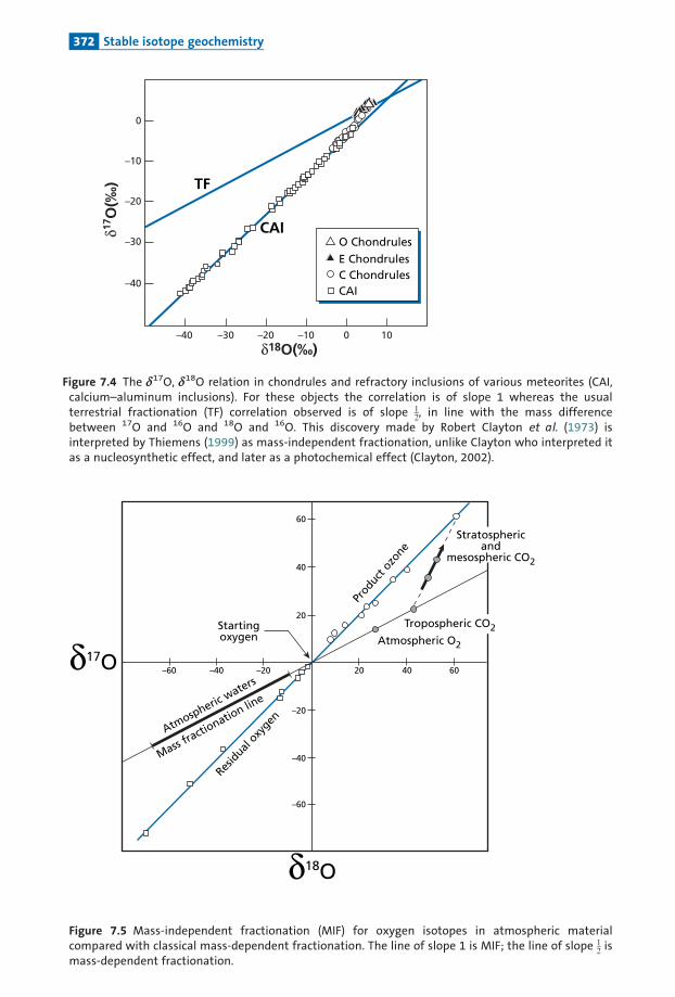
0

–10

–20

–30

–40

–40 –30 –20 –10 0 10

δ17O

(‰)

δ18O(‰)

TF

CAI

CAIC ChondrulesE Chondrules O Chondrules

Figure 7.4 The d17O, d18O relation in chondrules and refractory inclusions of various meteorites (CAI,calcium–aluminum inclusions). For these objects the correlation is of slope 1 whereas the usualterrestrial fractionation (TF) correlation observed is of slope 1

2, in line with the mass differencebetween 17O and 16O and 18O and 16O. This discovery made by Robert Clayton et al. (1973) isinterpreted by Thiemens (1999) as mass-independent fractionation, unlike Clayton who interpreted itas a nucleosynthetic effect, and later as a photochemical effect (Clayton, 2002).

60

40

–20

–40

–60

20

20–20 40

δ18O

δ17O –40–60 60

Startingoxygen Atmospheric O2

Prod

uct o

zone

Atmospheric

waters

Mass fractio

nation lin

e

Resid

ual o

xygen

Stratosphericand

mesospheric CO2

Tropospheric CO2

Figure 7.5 Mass-independent fractionation (MIF) for oxygen isotopes in atmospheric materialcompared with classical mass-dependent fractionation. The line of slope 1 is MIF; the line of slope 1

2 ismass-dependent fractionation.


Ithasbeen shownthatozoneofmass 54 (18O18O18O) is notenriched relative to16O16O16Oozone ofmass 48, whereas the asymmetrical molecule 16O17O18Oofmass 51is enriched by200%. It has also been shown that symmetrical ozone molecules 17O17O17O or 18O18O18Oare depleted, whereas all the asymmetrical molecules 16O17O17O or 17O18O18O, etc. areenriched.This e¡ect, which is calledmass-independent fractionation andmightbe moreappropriately termed the molecular symmetry e¡ect, seems to act with reactions such asOþCO!CO2,Oþ SiO!SiO2, etc.This is an important process in the atmosphere and seems to have played a role in the

presolar primitive nebula as a linear relation of slope1is found in carbonaceous meteor-ites between �17O and �18O (Figure 7.5).This is an important e¡ect but highly speci¢c tocertain processes. It is just beginning to be exploited but already very successfully (seebelow).

7.3 The modalities of isotope fractionation

7.3.1 Kinetic effects or equilibrium effects? Isotopic exchange

Wehave already spoken of this in the earlier chapters. Letus recall a few facts here, as it is avery important but often neglected phenomenon. Let us bring into contact two chemicalcompounds, AO and BO, with at least one element in common, for example, both havingoxygen in their formulas. One of these species has been prepared with 18O exclusively, theotherwith16O.Aftera certain time in contact it canbe seen thatthe18O/16O compositionofthetwocompounds is suchthat:

ð18O=16OÞAO

ð18O=16OÞBO¼ KðTÞ

where K (T) is the equilibrium constant. In other words, the isotopes 18O and 16O haveexchanged suchthatequilibriumhasbeenattained.The rateofthis isotope exchange canbemeasuredandseveralphenomenaobserved:

(1) It is fasterathigher temperatures.(2) It is faster in gases or liquids than solids. If one of the compounds is a solid it

becomes very slow (in this case the rate of di¡usion in the solid limits the kineticsof the process).

(3) It depends largely on the position oxygen occupies in the steric con¢guration ofcompounds AO and BO,7 that is, the nearer oxygen is to the outside of themolecular structure, the faster the kinetics8 ^ this isotope exchange is essential ingeochemistry as it provides understanding of various fundamental observations(Figure7.6).

7 Which relates to the spatial arrangement of the atoms composing the molecule.8 For example, in the complex ion SO4, oxygen exchanges much faster than sulfur. This is why in sulfatewater S retains the memory of its source but O does not.

373 The modalities of isotope fractionation

Letus supposewehave a reactionA!B together with kinetic isotope fractionation. IfA and B are left in contact for long enough, the isotopes of A and B swap over, and even-tually the fractionation between A and B is of the equilibrium fractionation type. Tomaintain kinetic fractionation, the initial product and the end product must not be leftin contact. An example of this is the reduction of the sulfate ion SO2�

4 to the sul¢de S2�

(bybacteria) which goes along with an out-of-equilibrium isotope e¡ect. If, after partialreduction, the sulfate ion remains in contact with the sul¢de ion, the system tends toestablish sulfate^sul¢de isotopic equilibrium. Conversely, if the sul¢de ion S2� is in thepresence of a ferrous ion Fe2þ, the following reaction occurs: 2S2�þFe2þ!FeS2.Thisiron sul¢de crystallizes and ‘‘isolates’’ the sul¢de from any further isotopic exchange whichwould cancel out the kinetic e¡ect. This is why a number of naturally occurring sul¢deshave isotope compositions re£ecting the kinetic e¡ect (bacterial) related to sulfatereduction.

Isotope exchange is activated by temperature; therefore, at high temperatures,only swift and complete isolation of the resulting product can prevent equilibriumfractionation from taking over. In practice, except for the case of gases that escape andbecome isolated, such as gases fromvolcanoes, it is generally di⁄cult to observe kinetice¡ects at high temperatures. In these circumstances, equilibrium e¡ects are mostlypreponderant.

15

11

7

3

–1

–5

1 2 3 4 5Time (days)

C

B50

%ex

chan

ge

75%

exch

ang

e

97%

exch

ang

e

A

Δ18 O

(q

uar

tz–H

2O)

at 5

00 °C

equilibrium

Figure 7.6 Kinetic curve showing the speed of equilibration by water–quartz exchange. The quartz hasa d18O value of 10. Three types of water with different compositions are brought into contact with thequartz at 500 8C. The initial isotope compositions of the waters are expressed in d: A (�5), B (þ5), and C(þ15). The equilibrium value is 3. It can be seen that the three equilibration curves converge towardsthe equilibrium value in a matter of days. After O’Neil (1986).


7.3.2 A consequence: isotopic memory

As we have already said when discussing radiogenic isotopes, it is fundamental to under-stand that all isotope geochemistry, including that of stable light isotopes, is based on thefact that isotope exchange in the solidphase at low temperatures is veryslowandthe systemisnotconstantlyre-equilibrated,otherwisetherewouldbenoisotopicmemory.Thisderivesfromthe issuesofdi¡usion coveredpreviously.Let us take the example of calcareous fossil shells. A shell records the 18O/16O isotope

composition of the sea water it was formed in and also the ambient temperature. Onceformed, the shellmoves aroundwith the animal that carries it andwhen the animal dies theshell falls tothesea£oor.Thereit is incorporated intosedimentsandwiththemwillbepetri-¢ed in a certain proportion and possibly, much later, will be brought to the surface on thecontinentsby tectonicprocesses. Itwill remain there formillionsofyearsbeforeageologistcomes along and collects it for analysis. During this time, the fossil shell is in contact withthe groundwater that circulates in the outer layerof the Earth.Howdoes the shell behave incontactwith this newwater? If it is isotopically re-equilibratedwith the freshwater whose dvalue isverydi¡erentfrom zero, it loses its former isotopic compositionandsoitspaleother-mal memory. Its isotopic composition no longer re£ects the conditions of the old oceanbut the conditions of recent aqueous circulation. In fact, in most (but not all!) cases, theshell remains compact and no isotope exchange occurs.The low rate ofdi¡usion ofoxygenin calciteat lowormoderatetemperatures limits themechanism.Andall thebetter forgeol-ogists! Theycan determine thepast temperatureoftheoceanwhere the animalwhose shellitwas lived.An important phenomenon is cooling. Isotopic equilibrium among minerals is

established at high temperature.The mineral assemblage cools and so follows a decreas-ing thermal trajectory. The isotope equilibrium constant is dependent on temperature,and isotope reactions should continue to take place constantly matching temperatureand isotope composition. If this were so, the system would lose all memory of its pastat high temperature and isotope analysis would merely re£ect the low-temperatureequilibrium. In fact, as isotope exchange at low temperatures occurs very slowly, ifcooling is rapid, theminerals often retain the composition acquired at high temperature.But this is not always so. Cooling is not always rapid. In metamorphism especially,exchanges are sometimes accelerated by certain factors and ‘‘initial’’ isotope composi-tions are not alwaysmaintained. But as the oxygen di¡usion constants of the various sili-cateminerals are di¡erent, the temperatures indicatedby thevariousminerals also di¡er.There is a sort of disequilibrium allowing us to detect the occurrence of any secondarye¡ect.All of this means that when measuring a compound’s isotopic composition we

must question the meaning of the message it carries and the time it was encoded.Does it correspond to the period when the object formed? Is it the outcome of second-ary phenomena? If so, what phenomena? Once again, everything is dominated by iso-tope exchange mechanisms. The importance of these e¡ects is attested by the answerto the following general observation. Why is sulfur isotope geochemistry not usedmore often, since it has substantial natural variations (from þ60 to �40)? Because in


many compounds, and particularly in sul¢des, secondary isotope exchange occursvery rapidly. Through this exchange, the compounds lose much of the isotope memoryof their origins. Another reason is the fact that sulfur geochemistry is highly complexwith many degrees of oxidation, etc. However, interesting results have been obtainedwith sulfur isotopes.

7.3.3 Open system or closed system

The open systemor in¢nite reservoirWhenoneofthe reservoirspresent is of in¢nite size (or is in direct contactwithaboundlessreservoir) the modalities of isotope fractionation are governed by the initial fractionationconditions and by conditions related to subsequent isotope exchange. No mass balancee¡ectdisturbs the relationbetween�and�:

� ¼ �equilibrium; � ¼ �kinetic; or � ¼ �mixed;

dependingonthenatureofthe initial fractionation and the subsequent isotope exchange. Ifthe isotope composition of the in¢nite reservoir isR0, the‘‘large’’reservoir imposes its iso-tope compositionthroughthefractionation factor:

R ¼ �R0 and � � �0 þ ð�� 1Þ 1000:

Exercise

Sea water has a d18O value of 0. Liquid–vapor fractionation at equilibrium at 20 8C is

�¼ 1.0098. What is the composition of the water vapor evaporating if it is in equilibrium

with the water?

AnswerThe fractionation factor 18O=16Oð Þvapor=

18O=16O�

liquid¼ 1=� ¼ 0:990 29: Therefore (�� 1)¼

�0.0097, or d18O¼�9.7ø.

The closed systemWhere the system is closed, a balance e¡ect is superimposed on the modalities described.We note the isotope composition of the initial system R0 and assume that from there twocompounds,AandB, areproducedwith isotopic ratiosRAandRB.We canwrite an isotopefractionation law (without specifyingwhether it is for equilibriumor not) characterized by�AB, and an atom conservation equation.This gives:R0¼RAxþRB (1� x), wherex is themolar fractionofthe element. In � notation, thisgives:

d0 ¼ dAxþ dBð1� xÞ or d0 ¼ ðdA � dBÞxþ dB or d0 ¼ DABxþ dB:

Exercise

Let us consider bacterial reduction SO2�4 ! S2� by Desulfovibrio desulfuricans. The kinetic

fractionation factor 34S/32S between sulfate and sulfide at 25 8C is 1.025 (Harrison and


Thode, 1958). Let us suppose that bacterial reduction occurred in oceanic sediment that was

continually supplied with sulfate ions. The sulfate stock can therefore be considered infinite.

What is the composition of the S2� on the ocean floor if the d34S of the sulfate is þ24?

AnswerApplying the equation �AB¼ 103 ln � gives �¼þ24.6.

dsulfate� dsulfide¼þ24.6 hence it can be deduced that dsulfide¼�0.6.

Exercise

Let us suppose now that the sediment becomes isolated from the ocean and is no longer

supplied with sulfate ions and that the same phenomenon occurs. The quantity of organic

matter is such that the proportion of sulfur in the state of sulfate is 1/3. Suppose that, in the

initial state, all of the sulfur was in the sulfate state at d34S¼þ24. What is the isotope

composition of S2�? What is the isotope composition of the sulfate?

AnswerWe apply the equation:

d0 ¼ DABx þ dB; or dB ¼ d0 � DABx :

From this we obtain dS2� ¼ 15:8; dSO4 ¼ 40:4.

As seen in the previous exercise, the result ismarkedlydi¡erent foranopen system, as the dvalue is thenpositive.The e¡ectofthe closed systemhas shifted the isotopevaluesofthe sul-fate and sul¢de, but not the fractionation factor, of course! (The limiting caseswherex¼ 0andx¼ 1shouldbe examined.)However, a £aw can be found in the foregoing reasoning. If the sul¢des remained in a

closed system as ions long enough, it might be that there was some isotopic exchange andthat the sulfate and sul¢de attained thermodynamic equilibrium. In this case �¼ 1.075 at25 8C (Tudge and Thode, 1950). Repeating the calculation with this value givesd34

sul¢de¼ 0.14and d34sulfate¼ 72.4.

Intermediatescenarios canbe imaginedandtherefore, in nature, thevalueswillprobablybe intermediateones.As just seen, then, widely di¡erent isotope values are obtained for the same phenom-

enon but di¡erent modalities. It is probably the diversity of modalities that accounts forthegreat isotopicvariation in sul¢desofsedimentaryorigin (Figure 7.7).

DistillationHerewe lookat a rather special (butwidelyapplicable!) casewhere the system is closedbutwhere theproduct is isolatedas it forms.LetX2 andX1representthenumberofatomsofthetwoisotopes.Ateachmoment in time,wehave:

dX2=dX1

X2=X1ð ÞA¼ �


where�maybeanequilibriumorkineticvalue, dX2 is thequantityof isotope2ofAwhich istransformed intoB, anddX1is thequantityof isotope1ofAwhich is transformed intoB.Byseparating thevariables and integrating,weget:

XA2 ¼ cX�

1

therefore:

X2=X1ð ÞA¼ cX��11 :

Attimet¼ 0 X2=X1ð ÞA ¼ X2=X1ð Þ0 andX1¼X1,0, therefore: c ¼ X2=X1ð Þ 1X��1

1;0

.Hence:

X2=X1ð ÞA¼ X2=X1ð Þ0 X1=X1;0

� ��1:

If the transformed remaining fraction of X1 is called f, we get the famousRayleigh distil-lation law:

RA ¼ R0f��1:

Coal

a = 1.075

Biogenicsulfide

SO4fresh

waters

Oil

Sedimentarysulfide

Granites

Hydrothermalsulfur

Volcanic S

MeteoritesBasicigneous

rocks

a = 1.025

Sulfates ininterstitial

waters

Seawater

sulfatesOld

sediments

VolcanicSO2

40

30

50

60

20

10

0

–10

–20

–30

–40

–50

–60

δ34S

(‰)

Figure 7.7 Analysis of 34S/32S isotope composition in the main terrestrial reservoirs. Notice that thedomains are very extensive for all reservoirs. This corresponds to highly variable reducing conditions towhich sulfur is subjected.


Figure 7.8 shows the Rayleigh lawas a function of fwhere�> 1and�< 1.We shall see thatthe e¡ects are oppositebut are only extremewhen f is very small.We seehowAevolves, andalsoB, forwhich, ofcourse,wehave

RB ¼ �R0f��1:

Themean compositionofA iswritten:

RA ¼ RA;0f � � 1

f� 1

� �:

Itcanbeseenthatwhenf is small, the compositionsofthetwocompoundsseemtoconverge.Andyet their partition coe⁄cient remains constant! But it is clear that as small variationsin f lead to large variations in d, the optical illusion gives the impression of convergence.Notice too that when f¼ 0, R¼RA,0, because of course ‘‘matter is neither created ordestroyed’’asLavoisier said (except in nuclear reactionsathigh energy!).

Exercise

Find the Rayleigh formula expressed in d.

Answerd ¼ d0þ 103 (�� 1) ln f. See the next exercise.

Exercise

Let us go back to our example of the formation of sedimentary sulfides. For the time being, we

assume that as soon as the sulfide is formed, it reacts with iron dissolved in solution and

a

b

δ18 O

(‰)

f

20

0.8 0.6

δE α = 1.01

δE α = 0.99

δR α = 0.99

δR α = 1.01

α = 1.01

α = 0.99

0.4 0.2

-20

δ0R

δ

δ–δ 0

lnf–2–1

20

0

–20

δR = δEα = 1

Figure 7.8 Changes in the instantaneous isotopic composition of a reservoir (dR) and an extract (dE)during a Rayleigh distillation process as a function of the partition coefficient (1.01 and 0.99respectively). We have �ext-res> 1, �ext-res¼ 1, and �ext-res< 1 and an initial isotopic composition ofthe reservoir d0R¼ 0; f is the remaining fraction of the reservoir and (1� f) the extent to which thereaction has progressed. After Fourcade (1998).


forms FeS2, without isotope fractionation (in fact, things are more complex than this). Being

heavy in its solid state, the iron sulfide settles out and is removed from contact with the

sulfates. This is a distillation effect. Given that in the end sulfates make up only one-third,

what are the sulfide compositions?

AnswerThe initial d 34S is still þ24. The kinetic coefficient � is 1.025. Let us first apply the Rayleigh

equation, which we can use in a handier form with d. Its mathematical form invites us to shift

to logarithms. The formula becomes:

ln R ¼ ln R 0 þ ð�� 1Þ ln f :

Given that R¼ RS (1þ d/1000) with the logarithmic approximations ln(1þ ")� ", and approx-

imating the two terms ln RS, we get:

d ¼ d0 þ 103 ð�� 1Þ ln f :

This is the form we shall use. The final composition of the sulfates is d¼ 24þ 25 ln(1/3)¼24þ 27.7¼ 51.7.

The sulfides precipitating in the end have a d value of þ27.1. The average sulfide is

obtained by the balance equation dS average¼þ10.4.

Exercise

In the first quantitative studies to estimate the degassing rate of magmas, Franc� oise

Pineau and Marc Javoy (1983) of the Institut de Physique du Globe in Paris measured the13C/12C partition coefficient of CO2 in a magma at 1200 8C and found 4.5ø (CO2 being

enriched in 13C). Let us take a basalt with an initial d13C value of �7. After degassing we find

d13C¼�26ø, with a carbon content of 100–150 ppm. If we assume a Rayleigh distillation,

what is the extent of degassing of the magma? What was the initial carbon content of the

magma?

AnswerWe apply the Rayleigh law in d:

d � d0 ¼ 1000 ð�� 1Þ ln f :

Hence: �20¼ 4.5 ln f and f¼ 0.011, therefore the magma was degassed to 98.8%. Its initial

carbon content was therefore 9000–13 000 ppm.

E X A M P L E

Isotopic evolution of a cloud shedding rain

A cloud forms over the sea. It then migrates over a landmass or migrates to higher latitudes

and loses rain. It is assumed that the cloud formed by the evaporation of sea water and that

the fractionation factor for the oxygen isotopes remains constant at �¼ 1.008. Figure 7.9

summarizes the isotope evolution of the cloud and of the rain that falls as it evolves. It is

described by a simple Rayleigh distillation.


7.3.4 Mixing

Aswehavealreadyseen several times,mixingoftwosources is an extremely importantphe-nomenon ingeochemistry.Forexample,seawater isamixtureofthevarious inputsofrivers,submarine volcanoes, rain, and atmospheric dust.We have a mixture of two componentsA1andA2with isotopic compositions:

xAyA

� �1

andxByB

� �2

:

The isotope compositionofthemixture is:

xAyA

� �m

¼xA1 þ xA2

yA1 þ yA2¼

xAyA

� �1yA1 þ

yAyA

� �2yA2

yA1 þ yA2:

Ifweposit:

yA1

yA1 þ yA2¼ x1 and

yA2

yA1 þ yA2¼ 1 � x1;

and ifwewrite the ratios

x=yR :x=y Rm ¼x=y R1x1 þx=yR2ð1� x1Þ;

then replacingRby the d notationgives:

–30

–25

–20

–15

–10

–5

010.5

(1–f )

–35

Cloud

Rain

VaporLiquid

(the liquidis continuouslyextracted from

the system)

α = 1.008δ1

8 O

Figure 7.9 Rayleigh distillation between a cloud and rain for d18O. The liquid (rain) is continuouslyremoved. The vapor fraction is 1� f. After Dansgaard (1953).


dm ¼ d1x1 þ d2ð1� x1Þ:

We¢ndafamiliarold formula!

Exercise

Carbonates have a 13C/12C isotope composition expressed in d13C of 0ø. Organic products

precipitating on the sea floor have a d13C value of �25ø. What is the mean value of d13C of

the sediments, given that 80% of the sedimentary carbon is in the carbonates and 20% in the

organic products?

AnswerThe main isotopic component of carbon is 12C. Therefore x and (1� x) are 0.2 and 0.8,

respectively. This gives 0.2� (�25ø)þ 0.8� 0ø¼�5ø. The average composition of the

sediments is therefore �5ø.

Mixing inacorrelationdiagramoftwoisotoperatiosobeystheequationsalreadydevelopedforradiogenic isotopes. Let the two elements whose isotopes are under study be A and B.Remember that ifthe (CA/CB) ratio is constant for thetwocomponentsofthemixture, themix-ture is representedbyastraight line. Ifthe tworatios are di¡erent, themixture is representedbyahyperbolawhosedirectionofconcavity isdeterminedbythe concentrationratiosofAandB.

7.4 The paleothermometer

In some sense, paleothermometry is to stable isotopes what geochronometry is to radio-genic isotopes, bothan exampleandasymbol.

7.4.1 The carbonate thermometer

Anexampleofthis¢eldofresearchhasbecomealegendofsorts. In1947,HaroldUrey (1934Nobel Prize winner for his discovery of deuterium, the hydrogen isotope 2H) andBigeleisen andMayer published two theoretical papers in which they calculated isotopefractionation occurring in a series of chemical equilibria. In 1951, while professor atChicagoUniversity, Urey and his co-workers used his method of calculation to determinethe isotope equilibriumofcarbonate ionsCO2�

3 andwater (H2O) and calculated the isoto-pic fractionation that must a¡ect the 18O and 16O oxygen isotopes whose common naturalabundances are 0.205% and 99.756%, respectively. The (18O/16O)carbonate/(

18O/16O)waterratiomustbe a function ofthe temperature atwhich the two species are in equilibrium.Thevariations Urey predicted were small but could be measured, after converting the CO2�

3

into CO2 gas, on the double-collection mass spectrometer already developed byAlfredNierandhisstudentsattheUniversityofMinnesotaatthetime.Thisfractionationwasmea-sured experimentallybyUrey’s teamwith the special involvementofSamuel Epstein, whowas to become one of the big names in the speciality.Together, they developed the simplethermometric equation (in fact, theoriginal coe⁄cientswereslightlydi¡erent):

T 8C ¼ 16:5� 4:3 d18CO3� d18

H2O

� þ 0:13 d18

CO3� d18

H2O

� 2


whereT8C is the temperature in degrees centigrade, and d18CO3

the isotope composition oftheCO2 extracted from the carbonate,which is expressedbyadeviation fromthe referencecarbonatesample:9

d18CO3¼

18O=16O�

CO2; carbonateX� 18O=16O�

CO2; standard

18O=16O�

CO2; standard

264

375 � 103:

The standard chosen is a reference limestoneknownas PDB.TheChicago teamdecided touse its carbonate thermometer tomeasuregeological temperatures.To dothis, theychoseacommon, robust fossil, the rostrum (the front spike on the shell) ofa cephalopodknown asa belemnite that lived in the Jurassic (�150Ma) and was similar to present-day squids.Suppose that in the course of geological time, the isotopic composition of oxygen in seawaterhadremained constantatd18O¼ 0.Thenthe18O/16Ooxygen isotopic compositionofthe carbonate of the fossils re£ects the temperature of the sea water in which the shellformed.This isotope composition became ¢xed when the carbonate was incorporated ascalcite crystals in the fossil shells (as solid-phase reactions at low temperatureareveryslow,there is little chance that the compositionwas altered bysecondary processes). Bymeasur-ing the isotope composition of fossils, it is possible to determine the temperature of theancient seas.To con¢rm this idea, the Chicago team thereforemeasured a series of belem-nite rostrafromvariousgeographicareasandofdi¡erentstratigraphic ages (Figure 7.10).The results, ¢rst announced in preliminary form at the 1950 annual meeting of the

Geological SocietyofAmericawere spectacular and immediately claimed the attention ofthe entiregeological community.Letus summarize them.At the scale of the planet, for the Jurassic, when belemnites lived, isotope temperature

obtained varied from12 to 18 8C.These are likely and coherent temperatures; likely becauseotherpaleoecological indicatorsare inagreementwiththem,coherentbecausevariationsovertime in various measurements in various parts of the world concord.Thus it has been deter-minedthatthemaximumtemperaturewas intheLateCretaceous,usingsamples fromasinglearea(Sweden,Britain)orsamples includingfossils collectedfromNorthAmericaandEurope.Encouragedby theseworldwide results, theChicago scientists set about dissecting indi-

vidual rostra.Each rostrum ismadeupofconcentric layerswhichareevidenceofbelemniteannual growth. Layer-by-layer analysis revealed regularly alternating temperatures.Therewerethereforesummersandwintersatthetime!Theyevenmanagedtoshowthatoneparti-cular individualwasborn inthe fall anddied in springtime!

Exercise

The standard chosen for oxygen is SMOW (d18O¼ 0). McCrea and Epstein’s simplified thermo-

metric equation is:

T 8C ¼ 16:5� 4:3 d18OCO3:

9 This is an important detail. It is not the isotopic composition of the CO2�3 that is measured but that of the

CO2 in equilibrium with the carbonate!

383 The paleothermometer

The precision of measurement of oxygen isotope composition is 0.1 in d units. What is the

power of resolution in temperature of the isotope method defined by Urey?

AnswerDifferentiating the formula above gives �T¼ 4.3 �d. So the precision is 0.43 8C. One

might envisage further increasing the precision when making measurements with the

mass spectrometer to attain 0.01%, but this raises a geochemical problem: what do

the tiny differences revealed signify? We shall get some inkling of an answer in what

follows.

T(°C

)

Radius (cm)0.2 0.4 0.6 0.8 1.0 1.2 1.4

40

30

20 20°C1918171615

δ13C

T

20

15

10

5

W

W

S

S

WSW

a

b

Figure 7.10 Study of a Jurassic belemnite rostrum. (a) A famous figure of a cross-section through aJurassic belemnite rostrum. Samples were taken a different radial distances (S, summer; W, winter;numbers of rings are counted from the outside). (b) Values of d13C and below d18O converted directlyinto temperature. The curve shows that the belemnite was born in the fall and died in spring! After Ureyet al. (1951).


This exceptional scienti¢c success story opened the way to a new geological discipline,paleothermometry, or the studyofpast temperatures on aprecise scienti¢cbasis, which gavetremendous impetus to paleoclimatology. It also encouraged researchers to forge ahead. Ifstable isotopes ofoxygen hadyielded such signi¢cant results in their ¢rst application in geol-ogy, itcouldbehopedthatthe examinationofotherproblems,otherproperties, andotherele-mentswouldbe equallysuccessful.Thishopegave rise totheworkthat founded stable isotopegeochemistry.However, theChicagoteam’spaleothermometerwasbasedontheassumptionthat �seawater¼ 0hasbeen constantthroughoutgeological times.Aswe shall see, thishypoth-esis probablyholds over the average for millions ofyears but not on the scale of thousands ofyearswhich is thetimescaleoftheQuaternaryera (Epsteinetal.,1953;Epstein,1959).

7.4.2 The 18O/16O isotope composition of silicatesand high-temperature thermometry

It is relativelyeasy tomeasure the isotopic compositionofoxygen in carbonates sinceCO2�3

reacts with phosphoric acid to transform into CO2, which can be measured directly indouble-collector mass spectrometers. It is far more di⁄cult to extractoxygen from silicateminerals. This means using £uorine gas or even the gas BrF5 and then transforming theoxygen into CO2 by burning. Of course, all such processes should be performed with noisotopic fractionation or well-controlled fractionation! These techniques were developedat theCalifornia Institute ofTechnologybyHughTaylor andSamEpstein in the late1960s(EpsteinandTaylor,1967).Measuring the oxygen isotope composition of silicate minerals reveals systematic

variations with the type of mineral and the type of rock to which the mineral belongs.These compositions can be characterized by measuring isotope fractionation betweenminerals.Now,oneofthegreatfeaturesof isotopes is thatisotopefractionation isverylargelyindependent of pressure and dependent mainlyon temperature.Variations in volume asso-ciated with exchange reactions are virtually zero.Therefore isotope equilibrium reactionsare very useful for determining the temperatures at which natural mineral associationsformed. Indeed�varieswithtemperatureandtendstowardsunityatveryhightemperatures.Aswehavesaid, thevariationof�withT takes theform:

ln � ¼ Bþ C

Tþ A

T2:

The form of this equation is preserved for � and �. Between two minerals m1 and m2 inequilibrium:10

Dm1m2¼ �m1

� �m2� A 106 T�2

� �þ B ¼ 1000 ln �:

The term1/T is generally negligible. Oxygen isotopes are especially useful here. Oxygenis the most abundant element in silicates and the 18O and 16O isotopes fractionate innature in proportions that can be easily measured by mass spectrometry. Experimentalstudies conducted mostly by the Chicago University group under Robert Clayton and

10 Tables usually give absolute temperatures so degrees must be converted from Celsius to Kelvin.


Jim O’Neil and supplemented by theoretical workof Yan Bottinga andMarc Javoy at theInstitutdePhysique duGlobe inParishaveprovideda seriesofreliablevalues forcoe⁄cientsAandB (seeO’Neil andClayton,1964;BottingaandJavoy,1975; Javoy,1977).

In the experimental procedure, the isotope fractionation between minerals andwater ismeasured¢rst.This is a convenientmethodas isotope equilibration is attainedquiterapidlyatabout80^100 8C.Thefractionationbetweenminerals is thencalculated.

Tables7.1and7.2showthevaluesofcoe⁄cientsAandB forvariousmineral^waterequili-bria (we shall see the intrinsic importance of such fractionation later) and then for fractio-nationbetweenpairsofminerals.

Exercise

What is the d18O composition of a muscovite in equilibrium with water at 600 8C whose d ¼�10?

AnswerThe � is written:

1:9 106 � 1

ð873Þ2

!�3:1 ¼ �0:6

where �¼ dmusc� dwater.

From this we obtain dmusc¼�10.6.

Table 7.1 Isotope fractionation for mineral–water pairs

Mineral Temperature (8C) A B

Calcite (CO3Ca) 0^500 2.78 � 2.89Dolomite 300^500 3.20 � 1.5Quartz 200^500 3.38 � 2.90Quartz 500^800 4.10 � 3.7Alkali feldspar 350^800 3.13 � 3.7Plagioclase 500^800 3.13 � 3.7Anorthite 500^800 2.09 � 3.7Muscovite 500^800 1.9 � 3.10Magnetite (reversedslope) 0^500 � 1.47 � 3.70

Table 7.2 Results of 18O isotope thermometry based on 18O/16Ofractionation of mineral pairs

Pair A B

Quartz^albite 0.97 0Quartz^anorthite 2.01 0Quartz^diopside 2.08 0Quartz^magnetite 5.57 0Quartz^muscovite 2.20 � 0.6Diopside^magnetite 5.57 0

Source:AfterO’Neil (1986)modi¢edbyBottingaandJavoy (1975).


Theseareshown inFigure7.11intwoways:asafunctionoftemperature (8C)andasafunctionof106/T2 because the fractionations are linear.We plot1000 ln�, that is�, on the ordinates,which means we can calculate �water¼ dmineral ^ dwater directly. Notice that fractionationcancels itselfout at high temperatures. On the experimental curves, this convergence seemsto occur at less than�¼ 0, but this e¡ect is probablydue to experimental errors.Thatwouldmeanthatmineralsandwaterwereofthesame compositionathightemperatures.

Exercise

Water with dwater¼�10 and rock (composed of several minerals) with an initial d value of

d(0)rock¼þ6 are put together. If we mix 100 g of rock and 110 g of water and heat them to

high temperature (500 8C in an autoclave) for which we take a zero overall � value, what will

be the composition of the rock and water after the experiment, given that the rock contains

50% oxygen and 90% water?

Answerdwater¼ drock¼�4.29.

So having the valuesA and B for several minerals, we can calculate fractionation betweenmineralpairs foreachtemperature:

100 200 300 400 500 600 700 800

10

-5

0

20

30

T(°C)

Δ (M

–H2O

)

Quartz

K-spar

Anorthite

Muscovite

Calcite

a

5 10

0

10

Qua

rtz

Calci

te

Mus

covit

e

Anorthite

K-sp

ar

20

30

25 0100 800 300

(106/T2)

Δ (M

–H2O

)

T(°C)

b

Figure 7.11 Isotope fractionation curves for water and some minerals as a function of temperature(T, or 106/T2). Notice that the curve should theoretically converge to zero. The error is the resultof experimental uncertainty. After O’Neil (1986).


Dm1�m2¼ Dm1�water � Dm2�water:

Letus takethe caseofquartz^muscovitebetween500and800 8C:

Dquartz�musc ¼ 2:20 � 106=T2 � 0:6:

We can set about geological thermometry using these various pairs ofminerals. Havingmeasured�m1�m2

,we returntothe established formulaandcalculateT.In thisway, the temperatures ofvariousmetamorphic zones havebeen determined. But,

ofcourse,muchaswithconcordanceofagesbyvariousmethods,wemustmakesurethevar-iouspairsofmineralsyieldthe sametemperature.

MarcJavoy,SergeFourcade,andthepresentauthor,attheInstitutdePhysiqueduGlobein Paris, came upwith a graphical discussion method: after choosing a reference mineral,wewrite foreachmineral:

D quartz�mineral � B ¼ A=T2:

Inaplotof��BagainstA, thevariousmineralsofarock in isotopic equilibriumarealignedon a straight line through the origin whose slope (1/T2) gives the temperature at which theyformed (Figure 7.12). If thepoints are not aligned, the rock is not in equilibriumand the tem-perature cannotbedetermined. Itwasthuspossibletodrawupatableofthethermaldomainswhere the main rocks were formed (Figure 7.13).These ¢ndings are consistent with indirectevidencefrommineralsynthesis experimentsandmetamorphiczoneography.

Exercise

The d18O values of the minerals of a metamorphic rock are: quartz þ14.8, magnetite þ5.

(1) Calculate the equilibrium temperature of quartz–magnetite.

(2) Calculate the d18O of an aqueous fluid in equilibrium with the rock.

Answer(1) 481 8C.

(2) þ11.3.

Mg

777 °C

Px

Hb

P

2

2

4

6

4 6

A

Δ–B

Figure 7.12 Javoy’s method of determining paleotemperatures, used here for San Marcos gabbro. P,plagioclase; Hb, hornblende; Px, pyroxene; Mg, magnetite; A and B are defined in the text.


7.4.3 Paleothermometry of intracrystalline isotopicorder/disorder

After the paleothermometry of silicate rocks, one might legitimately ask with hindsightwhy the same approach was not adopted for low-temperature paleothermometry andwhy several minerals were not used instead of calcite alone to break free of the hypothesisof a constant � value for seawater? In fact, researchwas conducted along these lines and,for this, the isotopic fractionation between water and calcium phosphate and water andsilica was measured since these minerals are commonplace in marine sediments and inparticular in ¢sh teeth for phosphates and diatoms for silica. Unfortunately, asFigure 7.14 shows, while the fractionations are di¡erent for the three minerals (CaCO3,CaPO4, and SiO2), their variations with temperature are parallel.They may therefore notbe used two-by-two to eliminate the unknown factor which is the isotopic compositionof seawater!Anewmethodhasvery recentlyemergedto eliminate theunknownquantityofthe isoto-

pic composition of ancient water. It was developed by the new team around John Eiler attheCalifornia Institute ofTechnology. It isbasedon isotopic fractionations existingwithina single molecular species among the di¡erent varieties of isotope (see Ghosh et al.,2006b). Let us take the carbonate ion CO2�

3 as an example. This ion comprises num-erous isotopic varieties: 12C16O16O16O, 12C16O16O18O, 12C16O18O18O, . . ., 13C16O16O16O,13C16O16O18O, . . ., etc. These are what are called isotopologs (see Section 7.2.1). Table 7.3provides an inventory and gives their mean proportions in the ‘‘ordinary’’carbonate ion.Each is characterizedbyadi¡erentmolecularmass.

Tem

per

atu

re (

°C)

103 In α Δ- =δ~AA δB ABB

200

2 4 6 8

sillimanite zone

garnet zone

biotite zone

chlorite zone

staurotide – kyarite

10 12

400

600

800

1000

Quartz – Feldspar – A

lkaline

Quartz – Biotite

Quartz – M

agnetite

Quartz – M

uscovite - Alkaline

Figure 7.13 Isotope temperature of different metamorphic grades determined from pairs of minerals.After Garlick and Epstein (1967).


In a calcium carbonate crystal, thermodynamic equilibria in the sense of Urey occuramong the various isotopic species. Keeping to the most abundant varieties, we canwritethe equilibrium:

13C16O2�3 þ 12C18O16O2�

2 , 13C18O16O2�2 þ 12C16O2�

2 :

masses: ð61Þ ð62Þ ð63Þ ð60Þ:

Theequilibriumconstantdependsontemperature.Thelower thetemperature, themorethereaction favors the right-handmembers, that is thememberswith theheavy isotopesofcar-bon and oxygen (the most advantaged would be 13C18O18O18O, but as its abundance is94 ppt, itcanbarelybemeasured). In fact, thisreactionmaybeconsideredanorder/disorderreaction. The lower the temperature, the greater the ordering (light species with light,heavy species with heavy).The higher the temperature, the more disordered the assemblyandthe equilibriumconstanttends towardsunity.

It is a smart ideatouse these equilibriawithin the calcite crystal, butthere is amajordif-¢culty inpractice.Calciumcarbonate isotopic compositions cannotbemeasureddirectlyinthelaboratory (theymaybemeasurableonedaywith instrumentsfor insitu isotopeana-lysis, but for the time being they are not precise enough). To measure the isotopic

+25 +30

Pho

sph

ate – water

Carb

on

ate – water

Silica – water

+35 +40

0

10

15

20

25

Δ18O = δmineral –

δwater

Tem

per

atu

re (

°C)

Figure 7.14 Fractionation for 18O/16O for various minerals with water. The curve shows clearly thatthey are parallel. After Longinelli and Nutti (1973); Labeyrie (1974).


compositionofCO2�3 radicals theyare transformed intoCO2moleculesbyareactionwith

phosphoric acid.Thebreakthroughby the Caltech teamwas to have developed a technique for extracting

carbonate isotopevarieties and transforming them into clearly identi¢able CO2moleculesand in particular for distinguishing 13C18O16O (mass¼ 47), 12C16O16O (mass¼ 44),12C18O16O (mass¼ 46), and 13C16O16O (mass¼ 45) and showing they re£ect the propor-tions of CO2�

3 molecules (by adding 16O to each). To do this, they de¢ned the unit �47

betweenthe ratiosmeasured formasses 47and44:

D47 ¼ ð47=44Þsample � ð47=44Þreferenceh i

� 103:

Table 7.3 Isotopologs

Mass Abundance

CO216O12C16O 44 98.40%16O13C16O 45 1.10%17O12C16O 45 730 ppm18O12C16O 46 0.40%17O13C16O 46 8.19 ppm17O12C17O 46 135 ppm18O13C16O 47 45 ppm17O12C18O 47 1.5 ppm17O13C17O 47 1.5 ppm18O12C18O 48 4.1ppm17O13C18O 48 16.7 ppm18O13C18O 49 46 ppbCO312C16O16O16O 60 98.20%13C16O16O16O 61 1.10%12C17O16O16O 61 0.11%12C18O16O16O 62 0.60%13C17O16O16O 62 12 ppm12C17O17O16O 62 405 ppb13C18O16O16O 63 67 ppm12C17O18O16O 63 4.4 ppm13C17O17O16O 63 4.54 ppb12C17O17O17O 63 50 ppt12C18O18O16O 64 12 ppm13C17O18O16O 64 50 ppb12C17O17O18O 64 828 ppt13C17O17O17O 64 0.5 ppt13C18O18O16O 65 138 ppb12C17O18O18O 65 4.5 ppb13C17O17O18O 65 9 ppt12C18O18O18O 66 8 ppb13C17O18O18O 66 51ppt13C18O18O18O 67 94 ppt


98 10 13 141211

40407 (Deep sea coral)

Mm97-Bc (Sumatran surface coral)

47413 (Deep sea coral)

0.5

0.4

0.5

0.7

0.8

0.9

106 /T2 (K)

Δ 47

Δ47 = – 0.02T2

a

20 1015

Present day

12.5

10

15

20

25

30

17.7

28.4

5

0

1

2

3

4

Age (Ma)

Uplift of the Andes

Alt

itu

de

(km

)

Tem

per

atu

re (

°C)

b

Figure 7.15 (a) Calibration of the isotopic order/disorder thermometer with the correspondingformula. (b) Uplift of the Andes reconstructed by the isotopic order/disorder chemometer. AfterGhosh et al. (2006).


The reference (47/44) is the ratio that would pertain if the isotopic distribution among thevarietiesof isotopeswerepurely random.Theyestablishedthefractionation curve (�47, as afunctionoftemperature).The temperature can therefore be determined from a measurement of �47. The exact

formula (between0and50 8C) is:

D47 ¼ 0:0592 � 106T�2 � 0:02:

Precision is estimatedtobe�2 8C.An interesting application of this method has been to determine the rate of uplift of

the Bolivian Altiplano. Samples of carbonates contained in soil were taken from theplateau but of di¡erent ages and dated by other methods.The temperature at which thesecarbonates formedwas then calculated.As the curveoftemperaturevariationwithaltitudeintheAndes isknown, the curveofaltitudeversus time couldbedetermined (Figure 7.15).

Exercise

Do you think this isotopic order/disorder method could apply to SiO2 at low temperature

(diatoms)? Write the equivalent equation to that written for carbonate. What would the

isotopic parameter be? Do you see any practical difficulty in this?

AnswerYes, in principle. The order/disorder equilibrium equation would be:

30Si16O2 þ28 Si18O16O,30 Si18O16Oþ28 Si16O2

mass : ð62Þ ð62Þ ð64Þ ð60Þ

D64 ¼ ð64=60Þsample � ð64=60Þreference

h i� 103 (or 104 as necessary):

The difficulty is that with the present-day method, Si is measured in the form of SiF4 on the

one hand, oxygen being extracted on the other hand. To apply the method, direct measure-

ment by an in situ method in the form of SiO2 would be required. This will probably be feasible

in the future with ion probes or laser beam ionization.

7.5 The isotope cycle of water

Let us return to the water cycle mentioned at the beginning of this chapter. On Earth, it isdominatedby thefollowing factors.

(1) The existence of four reservoirs. A series of exchanges among the ocean, the ice caps,freshwater, and the atmospheremakeup thewater cycle. It is anotherdynamic system.The reservoirs are of very di¡erent dimensions: the ocean (1370 million km3), the icecaps (29million km3), river water and lakes (0.00212million km3).The transit time ofwater in each reservoir varies roughly inversely with its size, each reservoir playing animportantgeochemical role.Thus thequantityofwater thatevaporates andprecipitates

393 The isotope cycle of water

is 500million km3 per thousand years, or more than one-quarter of the volume oftheoceans.11

(2) The ocean^atmosphere hydrological cycle. Water evaporates from the ocean andatmospheric water vapor forms clouds that migrate and may occasionally producerain.Thus salt water is changed into freshwater and transferred from tropical to polarregions and from the ocean to the landmasses. The hydrological cycle has a doublee¡ect.Cloudsmovefromlowtohigh latitudesandalsofromtheoceantothe continents.The freshwater that falls as rain over the landmasses re-evaporates in part, runs o¡orseeps in, thusformingthefreshwater reservoirwhichultimately£owsbacktotheocean.

(3) Thepolarregions.Whenprecipitation fromcloudsoccurs inpolar regions,wenolongerhave rain but snow.The snow accumulates and changes into ice forming the polar icecaps. These ice caps £ow (like mountain glaciers, but more slowly) and eventuallybreakup intheoceanas icebergsandmixwiththeocean.

Thewholeofwatercirculationontheplanetandthevariousstagesofthe cyclehavebeenstu-died in terms of isotopes.We have seen, when examining theoretical aspects, that whenwater and water vapor are in equilibrium, oxygen and hydrogen isotope fractionation areassociated.This double pairof isotopes has allowedus to construct quantitative models ofwatercirculation.However, theproblemsraisedbythesestudiesarenotas simpleas thethe-oretical studysuggested.

7.5.1 Isotope fractionation of clouds and precipitation

Acloudis composedofwaterdroplets inequilibriumwithwatervapor.Watervaporanddro-plets are in isotopic equilibrium. All of this comes, of course, from water which initiallyevaporated.

Letus takeacloudnear the equatorand follow itas itmoves tohigherlatitudes.The cloudis enriched as awhole in 16O relative to seawater, as we have seen, and so has a negative �value.As itmoves itdischarges someof itswateras rainfall.The rainwater is enriched in theheavy isotope, and sothe cloudbecomes increasinglyenriched in the light isotope.Thepre-cipitation is increasingly rich in light isotopes, which e¡ect is o¡set in part by the fact thatthefractionation factorvarieswith1/T.Aswemoveawayfromtheequator, itcanbeseensta-tistically thattheprecipitation has increasinglynegatived18Ovalues (Figure7.16).

As clouds undergo genuine distillation, by progressively losing their substance, their iso-tope composition obeys a Rayleigh law, but a‘‘super law’’ because as they move polewards,thetemperaturefalls, thefractionation factoralsoincreasesanddistillationbecomes increas-inglye¡ective (Figure7.17), somuchsothatatthepolesthed18Ovaluesare extremelynegative.

Weobservegeographical zoning for which the d18Ovalueandmeanair temperature canbe related (Epstein etal.,1965;DansgaardandTauber,1969) (Figure7.18).

The general cycle of clouds is repeated at local scale, when clouds move over landmassesandprogressivelyshed theirwater.Thus, freshwaterhasnegative d values.Thisphenomenonhas been studied using the paired tracers 18O/16O and D/H.Harmon Craig of the ScrippsInstitution of the University of California showed that rain and snow precipitation and the

11 1 km3� 1012 kg.


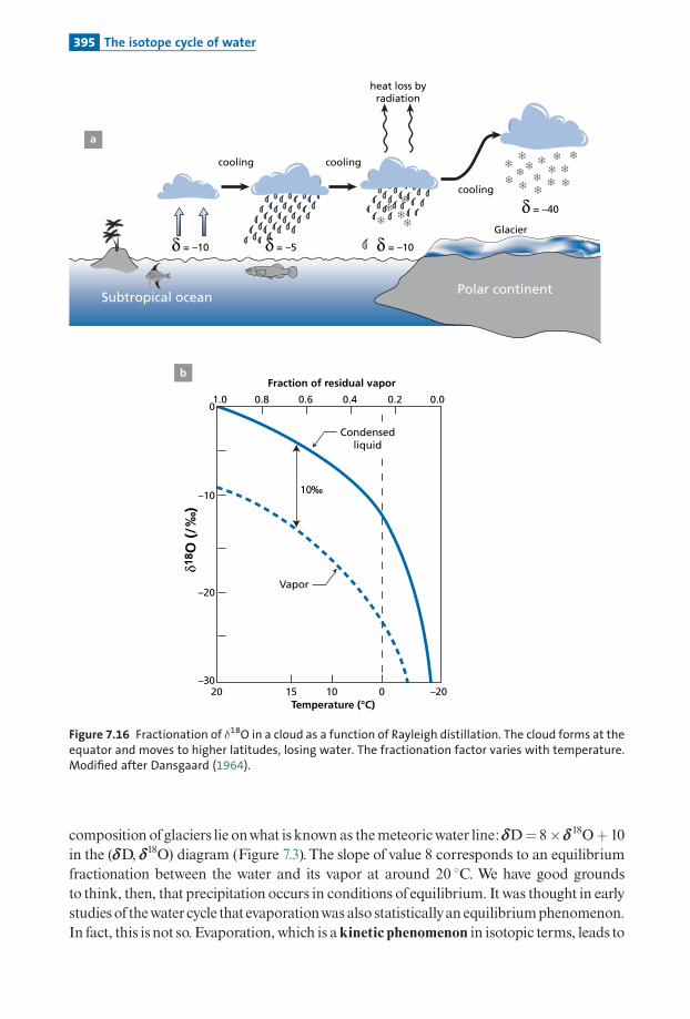
composition ofglaciers lie onwhat is known as themeteoricwater line: dD¼ 8� d18Oþ 10in the (dD, d18O) diagram (Figure 7.3).The slope of value 8 corresponds to an equilibriumfractionation between the water and its vapor at around 20 8C. We have good groundsto think, then, that precipitation occurs in conditions of equilibrium. It was thought in earlystudies ofthewater cycle that evaporationwasalso statisticallyan equilibriumphenomenon.In fact, this is not so. Evaporation,which is akinetic phenomenon in isotopic terms, leads to

a

b

Subtropical ocean

cooling

cooling

Glacier

heat loss byradiation

Polar continent

δ = –5δ = –10 δ = –10

δ = –40

cooling

–10

–20

–3020 15

0.81.0 0.6 0.4 0.2 0.0

010Temperature (°C)

Fraction of residual vapor

–20

0

Condensedliquid

10‰

Vapor

δ18 O

(/ ‰

)

Figure 7.16 Fractionation of �18O in a cloud as a function of Rayleigh distillation. The cloud forms at theequator and moves to higher latitudes, losing water. The fractionation factor varies with temperature.Modified after Dansgaard (1964).


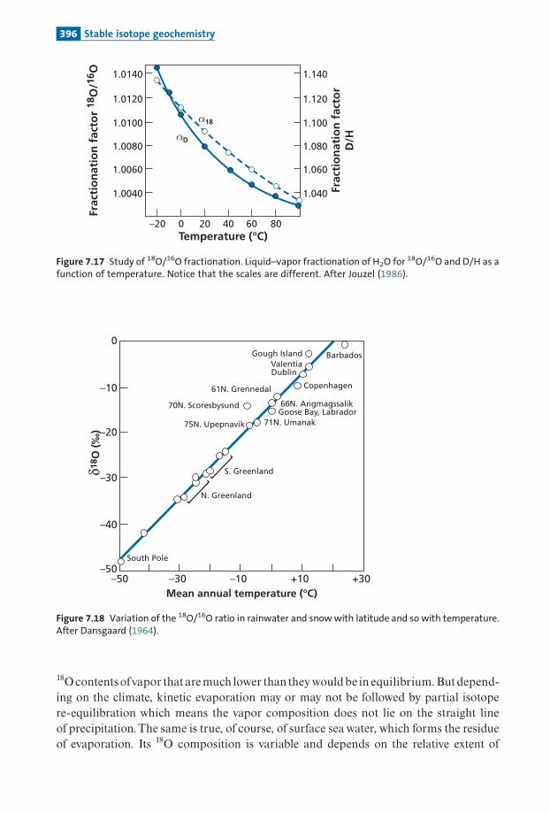
18Ocontentsofvapor thataremuch lower than theywouldbe in equilibrium.Butdepend-ing on the climate, kinetic evaporation may or may not be followed by partial isotopere-equilibration which means the vapor composition does not lie on the straight lineof precipitation.The same is true, of course, of surface seawater, which forms the residueof evaporation. Its 18O composition is variable and depends on the relative extent of

–20 20 40 60 800

1.0140

1.0120

1.0100

1.0080

1.0060

1.0040

1.140

1.120

1.100

1.080

1.060

1.040

Frac

tio

nat

ion

fac

tor

18O

/16 O

Frac

tio

nat

ion

fac

tor

D/H

Temperature (°C)

α18

αD

Figure 7.17 Study of 18O/16O fractionation. Liquid–vapor fractionation of H2O for 18O/16O and D/H as afunction of temperature. Notice that the scales are different. After Jouzel (1986).

–10

0

–20

–30

–40

–50–30 –10

Mean annual temperature (°C)

δ18 O

(‰

)

+10 +30–50

]]

Gough IslandValentiaDublin

Copenhagen

S. Greenland

N. Greenland

South Pole

66N. AngmagssalikGoose Bay, Labrador

71N. Umanak

61N. Grennedal

70N. Scoresbysund

75N. Upepnavik

Barbados

Figure 7.18 Variation of the 18O/16O ratio in rainwater and snow with latitude and so with temperature.After Dansgaard (1964).


evaporation and ofprecipitation (which are substantial over the ocean) and of the input offresh water.These variations are particularly sensitive in the North Atlantic (Epstein andMayeda,1953).Wevisualize thevariations and the in£uence ofthevariousphenomenathatcauses them in a (d18O, Sø) plot, where Søis the salinityof seawater (Figure 7.19). As canbe seen, there is avery close correlationbetween the two.All ofthis shows thatthis is awell-understood¢eldofresearch.

E X A M P L E

Precipitation in North America

This is a map of dD and d18O for precipitation in North America (Figure 7.20). From what has

just been said about the effect of isotope distillation of clouds, the pattern of rainfall over

North America is described. The main source of rainfall comes from the Gulf of Mexico with

clouds moving northwards and becoming distilled. This distribution is modified by several

factors. First, the relief, which means the clouds penetrate further up the Mississippi valley

but discharge sooner over the Appalachian Mountains in the east and the Rocky Mountains in

the west. Other rain comes in from the Atlantic, of course, so the distribution is asymmetrical.

Conversely rain from the Pacific is confined to the coast and moves inland little, so the lines

are more tightly packed to the west.

Exercise

From the information given since the beginning of this chapter, use theoretical considerations

to establish Craig’s equation:

d18O ¼ þ8; dD þ10:

E > PEquator

P > E

PoleP > E

Freezingeffect

δ18 Oδ18 O

0

–5

–10

20 25 30 35 40

Salinity (‰)Salinity

43°NNorwegian Sea

Gulf of Maine

NADW

35°N East coast of

Greenland

Off coast of Greenland

a

b

Figure 7.19 Relations between d18O and salinity. (a) Theoretical relation. P, precipitation; E, evaporation.(b) Various measurements for the North Atlantic. NADW, North Atlantic Deep Water. After Craig (1965).


AnswerClouds obey a Rayleigh law:

dD � dD;O þ 103ð�D � 1Þ ln f

dO � d18O;Oþ 103ð�O � 1Þ ln f :

This simplifies to:

dD � dD;O

d18O � d18O;O

� �D � 1

�O � 1

� �:

At 20 8C, as seen in the previous problem, �D¼ 1.0850 and �18O � 1:0098, hence:

�D � 1

�18O � 1� 8:

We therefore have the slope. The ordinate at the origin seems more difficult to model because

for vapor formed at 20 8C, dD;O � 8d18O;O ¼ �6:8 whereas we should find 10. We shall not go

into the explanation of this difference, which is a highly complex problem, as shown by Jean

Jouzel of the French Atomic Energy Commission. The different aspects of the hydrological

cycle, including kinetic effects during evaporation, play a part.

7.5.2 Juvenile water

It iswellknownthat inthewatercycle, there isan inputfromhotwater fromthedepthsoftheEarth. Itwas long thoughtthat thishotwater was thegradual degassingofwater trappedbythe Earthwhen it ¢rst formed, aswith the primitive ocean. If thiswere so, thiswater wouldprogressively increase the volume of thehydrosphere.Water fromdeepbeneath the surface

–170

(–22

.5)

–150(–20)

-130(–17.5)

–110

(–15)

–90(–12.5)

–70(–10)

–50

(–7.

5)

–30

(– 5)

Figure 7.20 Distribution of 18O/16O and D/H in rainfall in North America. The 18O/16O ratios are inbrackets. After Taylor (1974).


is still referred to as juvenile water.Harmon Craig (he again) studied geothermal water todetermine the isotope composition of any juvenile water. He showed that the d values ofgeothermalwaters fromthesamesource canbeplottedona (dD,d18O)diagramon straightlines pretty well parallel to the d18Oaxis andwhich cut the straight line ofprecipitation cor-responding to the composition of rainwater for the region. And so the composition ofgeothermalwater canbe explainedby the evolutionofmeteoricwater via isotope exchangeofoxygenwith the country rock.There is no need to invoke juvenile water from the mantleto explainthese isotope compositions (Figure7.21).As these relations are systematic forall thegeothermal regions studied,Craig concluded

thatthe inputof juvenilewater into the currentwatercycle isnegligibleandthatgeothermalwaters are only recycled surface water. The same goes for water from volcanoes. Thishypothesis hasbeen con¢rmedbymore elaborate studies ofvariations in the isotope com-position of geothermal water over time. In many cases, it has been shown that variationstrackedthoseobserved in the sameplace for rainwater,withatime lag corresponding to thetransittimewhichvaried frommonths toyears.12

E X A M P L E

Iceland’s geysers

In some instances, such as the geysers of Iceland, the straight line of (dD, d18O) correlation is

not horizontal but has a positive slope (Figure 7.22).

0

–50

–100

–150–15 –10 –5 0 5

WairakeiLaederello

The Geysers

Iceland

Niland

Hekla

Lassen Park

Steamboat Springs

δD

δ18O

Figure 7.21 Correlation diagram for (18O/16O, D/H) in geothermal waters. They form horizontal linescutting the meteoric straight line at the point corresponding to local rainwater. This is interpreted bysaying that water has exchanged its oxygen isotopically with the rock but the hydrogen of water doesnot change because it is an infinite hydrogen isotope reservoir compared with rocks that are relativelypoor in hydrogen. After Craig (1963).

12 A spa water company signed a research contract with a Parisian professor to study the isotopiccomposition of the water it sold to prove it was ‘‘juvenile’’ water, a name whose advertising value canbe well imagined. As the studies showed the water was not juvenile, the company terminated thecontract and demanded that the results should not be published!


Suppose we begin with rainwater of local composition and that this water undergoes

distillation by evaporating. Then:

dD � dO;D þ 103ð�D � 1Þ ln f :

d18O � d18O;Oþ 103ð�18O� 1Þ ln f :

Eliminating ln f gives:

dD � dO;D

d18O� d18O;O� �D � 1

�O � 1

� �:

We know that at 100 8C, for water–vapor fractionation, �D¼ 1.028 and d18O¼ 1.005. The

slope corresponds to 5.6, a lower value than that of equilibrium fractionation (8). The effect is

therefore a combination between exchange and distillation.

In fact, in nature, isotopic compositions of geothermal water or vapor are combinations

between Rayleigh distillation and the water–rock oxygen isotope exchange, between kinetic

fractionation and equilibrium fractionation. A horizontal slope indicates that isotope

exchange has been possible and so the transit time is long. When the slope is identical to

that of the Rayleigh law, the transit time has been short.

7.6 Oxygen isotopes in igneous processes

Examination shows that the18O/16O isotope composition ofunaltered rockofdeep origin,whether ocean basalts or ultrabasic rocks, is extraordinarily constant at d18O¼þ5.5(Figure 7.23).This value is analogous to themeanvalue ofmeteorites. It has thereforebeenagreed that this value is the reference value for the mantle.When taking stockofmeasure-ments on basic or acid, volcanic or plutonic igneous rocks, the results are found to dividebetween:

0

-10

-20

-30 -20 -10 0 +10

δD (

%)

δ18O (‰)

Meteoric lin

e

Geysers

Figure 7.22 Correlation diagram for (18O/16O, D/H) in acidic geothermal waters and geysers. The diagramis identical to the previous one except that these are acidic geothermal waters with a high sulfate contentwhose pH is close to 3 and for which the correlated enrichment in D and 18O results mostly from morerapid evaporation of light molecules with kinetic fractionation into the bargain. After Craig (1963).


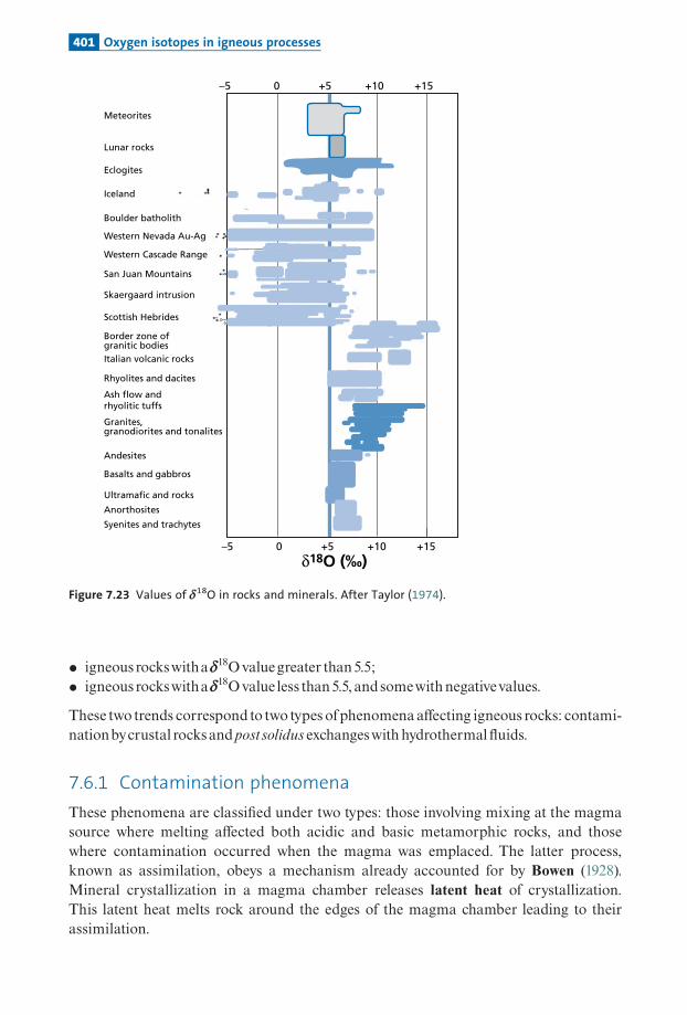
� igneous rockswithad18Ovaluegreater than5.5;� igneous rockswithad18Ovalue less than5.5, andsomewith negativevalues.

These two trends correspond to two typesofphenomenaa¡ecting igneous rocks: contami-nationbycrustal rocksandpostsolidus exchangeswith hydrothermal£uids.

7.6.1 Contamination phenomena

These phenomena are classi¢ed under two types: those involving mixing at the magmasource where melting a¡ected both acidic and basic metamorphic rocks, and thosewhere contamination occurred when the magma was emplaced. The latter process,known as assimilation, obeys a mechanism already accounted for by Bowen (1928).Mineral crystallization in a magma chamber releases latent heat of crystallization.This latent heat melts rock around the edges of the magma chamber leading to theirassimilation.

–5

Syenites and trachytes

Anorthosites

Ultramafic and rocks

Basalts and gabbros

Andesites

Granites,granodiorites and tonalites

Ash flow andrhyolitic tuffs

Rhyolites and dacites

Italian volcanic rocks

Border zone ofgranitic bodies

Scottish Hebrides

Skaergaard intrusion

San Juan Mountains

Western Cascade Range

Western Nevada Au-Ag

Boulder batholith

Iceland

Eclogites

Lunar rocks

Meteorites

0 +5 +10 +15

–5 0 +5 +10 +15

δ18O (‰)

Figure 7.23 Values of d18O in rocks and minerals. After Taylor (1974).

401 Oxygen isotopes in igneous processes

m # L ¼ m " CP DT;

whereL is the latentheat,m# themassofcrystalsprecipitatingperunittime,m" themassofrockassimilated,CP thespeci¢cheatofthesurroundingrocks,and�T thetemperaturedif-ference between the wall rock and the magma. If we can writem#¼ kM, then kML¼m#CP�T, therefore:

m"M

� �¼ kL

CP DT

� �:

Themagmais contaminated isotopically tooby themixing law:

ðd18OÞHy ¼ ðd18OÞmagmað1� xÞ þ ðd18OÞcountry rockðxÞ

with x¼ m #=Mð Þ, because the oxygen contents of the country rock and the magma arealmost identical. This was shown by Hugh Taylor (1968) of the California Institute ofTechnology (see also Taylor, 1979).

Exercise

What is the d18O value of a basaltic magma whose d18O¼ 0 and which assimilates 1%, 5%,

and 10% of the country rock whose d18O¼þ20?

Answer

The contamination effect therefore increases the d18O value because sedimentary and

metamorphic rocks have positive d18O values. An interesting approach to studying the

contamination of magmas by continental crust is to cross the studies of oxygen isotopes

with those of strontium isotopes. The (O–Sr) isotope diagram can be calculated quite simply

because it is assumed that the oxygen content is analogous in the different rocks. The mixing

diagram depends only on the Sr contents of the two components of the mixture. Figure 7.24 is

the theoretical mixing diagram.

Such combined studies have been made of volcanic rocks of the Japan arcs and the

Peninsular Range batholith in California (Figure 7.25).

Exercise

A basaltic magma is emplaced and assimilates 1%, 5%, and 10% of the country rock. The d18O

values are those of the previous exercise. The 87Sr/86Sr values are 0.703 for the magma and

0.730 for the country rock. The Sr content of the magma is 350 ppm and that of the country

rock is 100 ppm. Calculate the isotopic compositions of the mixture and plot the (d18O,87Sr/86Sr) diagram.

Assimilation

1% 5% 10%

d18O 5.64 6.22 6.95


AnswerThe d18O values have already been given.

It is left to the reader to plot the diagram.

6.0

0.703 0.705 0.707 0.709 0.711

8.0

10.0

12.0x = 5.0

x = 1.0

δ18 O

(‰

)

87Sr/86Sr

Crustalcontamination

C

M Sourcecontamination

1:10

2:11:1

1:2Sr m

Sr c = 5:1

x = 0.2

Figure 7.24 Theoretical O–Sr isotope mixing plots. The x values show the proportion of country rockrelative to the magma. The Srmagma/Srcountry rock parameter varies from 5 to 0.1. M, magma; C, crust.After James (1981).

0.704

Marianasarc

Californiabatholith

MORB

Japanese arc

0.702 0.706

9

8

7

6

δ18 O

wh

ole

ro

ck

87Sr/86Sr whole rock

Figure 7.25 Example of an O–Sr isotope correlation diagram showing the Japan arcs and batholithgranites in California. After Ito and Stern (1985).

Assimilation

1% 5% 10%

87Sr/86Sr 0.703 08 0.7034 0.703 94


7.6.2 Water–rock interaction

As we have said, isotope memory is retained if no exchange occurs after crystallization.When this is not the case, secondary isotopic disturbances canbe turned to account.HughTaylorandhis studentsobservedwhen examining variousgranitemassifs orhydrothermalmineral deposits that the 18O/16O isotope compositions had been disrupted after theirinitial crystallization by water^rock exchanges. The calibration made on water^mineralfractionationwas thereforeturneddirectly toaccount.

Whereas the d18O values of minerals and rocks of deep origin are generally positive(betweenþ5 andþ8), these rocks had negative d18O values of�6 to�7. In the same cases,relative fractionation as can be observed between minerals, such as quartz^potassiumfeldspar fractionation, was reversed.Taylor remembered Craig’s results on thermal watersand postulated that, rather than observing the waters, he was observing rockwith whichthe waters had swapped isotopes. From that point, he was able to show that the emplace-mentofgranite plutons, especially thosewith associatedmineral deposits, involves intense£uid circulation in the surrounding rock.Ofcourse, the existenceofsuch£uidswas alreadyknownbecause theygive rise toveins ofaplite andquartz pegmatite and theyengender cer-tain forms of mineralization around granites, but their full importance was notunderstood.

Inaclosedsystem,we canwrite themassbalance equation:

Wgw d0;W þ Rgr d0;R ¼Wgw dW þ Rgr dR

whereW is the mass of water and R the mass of rock, gw is the proportion of oxygen inthe water and gr the proportion of oxygen in the rock, d0,W and d0,R are the initialcompositions of water and rock, and dW and dR are the ¢nal compositions thereof.

W

R¼ gr

gw

� �dR � d0;R

d0;W � dW

� �;

since dW and dR are related by fractionation reactions dW¼ dR��. This gives:

W

R¼ gr

gw

� �dR � d0;R

d0;W � ðdR � DÞ

� �grgw� 0:5:

Indeed,gr¼ 0.45andgw¼ 0.89.Weestimated0,R fromthenatureofthe rockandthe catalogof sound rock (close toþ5), andwe estimate � by calibrating and estimating temperatureby fractionation amongminerals.This temperature canbe comparedwith the temperatureobtainedby theheatbudget.

Acalculationmaybemade, for example, fora feldsparwithd18O¼þ8and dW;18O ¼ �16at various temperatures (Figure 7.26a). It shows that in a closed system, theW/R ratiosmaybe extremely variable.


Exercise

What is the W/R ratio of a hydrothermal system supposedly working in a closed system at

400 8C?

The initial d18O value of feldspar is þ8, that of the water determined by the meteoric

straight line is d0,W¼�20. The �feldspar–water fractionation factor is 3.13� 106 T�2� 3.7. The

d18O of feldspar is measured as dR¼�2.

AnswerThe fractionation factor D ¼ 3:13 � 106=ð673Þ2 � 3:7 ¼ 3:21 ¼ dR � dW ðW=R Þ ¼ 0:34:

δ18O

δ D M

eteo

ric lin

e

Measuredpoint

Initial compositionof the fluid

Computation of W/R

10

6

2

-2

-6

-10

10.50 2 3 4 6 10 15 20 25

150 °C TO –3.3

TO –8.9

TO –12.0

250 °C

350 °C

(W/R) closed system

δ18 O

ro

ck

δRR = 8.5 δRW = –16

a

b

Figure 7.26 Variation in d18O composition and (dD, d18O) correlation diagram. (a) The variation in the d18Ocomposition of a feldspar with an initial composition d ¼þ18 is calculated as a function of (W/R) forvarious temperatures, with the initial composition of water being d¼�16. (b) It is assumed the alteredrocks are represented by the blue area in the (dD, d18O) diagram. We can try to determine the initialcomposition of the fluid by assuming, as a first approximation, that the dD values of the rock and waterare almost identical. The intersection between the horizontal and the (dD, d18O) correlation diagram ofrainwater gives the value of water involved in alteration. Reconstructed from several of Taylor’s papers.


Exercise

Let us now suppose the W/R ratio¼ 5, that is, there is much more water. All else being equal,

what will be the d18O value of the feldspar measured?

Answerd18O¼�14.54.

Theprocessdescribed intheprevious exercise involvesadouble exchangeand it is either thewater or the rock that in£uences the isotopic composition of the other depending on theW/R ratio.

Allowing for the point that�varieswith temperature, awhole range of scenarios canbegenerated.

Exercise

Let us pick up from where we left off in the previous exercise. Imagine an exchange between

sea water and oceanic crust whose d0,R¼þ5.5. The exchange occurs at W/R¼ 0.2. What will

the isotope composition of the water and rock be?

AnswerAt high temperature �¼ 0; maintaining gr/gw¼ 0.5 gives drock¼þ3.64 and dwater¼þ3.64.

Exercise

Let us imagine now that the water is driven out of the deep rock and rises to the surface and

cools to, say, 200 8C. It attains equilibrium with the country rock and its minerals. If the rock

contains feldspar, what will the isotope composition of the feldspar be?

AnswerAt 100 8C, �feldspar–water¼ 10. Therefore the feldspar of the rock will have a d value of

13.92�þ14.

It canbe seen from thewater cycle in the previous exercise that hydrothermal circulationreduces the d value ofdeep rocks and increases the d value of surface rocks. (This iswhat isobserved inophiolitemassifs.)

7.7 Paleothermometry and the water cycle:paleoclimatology

We have just seen how hydrothermalism can be studied by combining information on theisotope cycle ofwater and that of isotope fractionation.We are going to see how these twoe¡ects combine to give fundamental information on the evolution ofour planet and its cli-mate. After the initial impetus from Cesare Emiliani at Miami University and SamEpsteinattheCaliforniaInstituteofTechnology,Europeanteamshavebeenthemoreactive


ones in this ¢eld: for sedimentpaleothermometry, the teams fromCambridge andGif-sur-Yvette; forglacial records, those fromCopenhagen,Berne,Grenoble, andSaclay.

7.7.1 The two paleoclimatic records: sediments and polar ice

Carbonate paleoclimatologyIn order to use oxygen isotopes as a thermometer, wemust, strictly, know the d18O values oftwo compounds in equilibrium: water and carbonate.The formula established byUrey andhis team for the carbonate thermometer draws on d

18OCaCO3

and d18OH2O

. In a ¢rst approach, theChicagoteamhadconsideredthatdH2O, that is the �ofseawater,was constantovergeologi-cal timeandtherefore thatthed

18OCaCO3

measurementgavepaleotemperatures directly.Thedis-covery of extreme d18O values for Antarctic ice challenged this postulate. If the amount ofAntarctic ice lost every year into the ocean varies, the d18O value of the ocean must varytoo, since this icemayhave d18O values as lowas�50. In this case, thehypothesis of constantdH2O is untenable and it seems that temperatures cannotbe calculated simply. On the otherhand, if the dissolutionofAntarctic ice in theoceanvaries involume, thisphenomenonmustberelatedtoclimateandtherefore,tosomeextent,mustre£ecttheaverageglobaltemperature.The ¢rst idea developed byEmiliani in1955 was therefore tomeasure the d18O values of

carbonate foraminifera in Quaternary sediment cores for which (glacial and interglacial)climatic£uctuationshavelongbeenknown.Variations in isotope compositionareobserved(Figure 7.27) and seem to be modulated by glacial and interglacial cycles and more

Dep

th in

th

e co

re (

cm)

Zon

es

Stag

es

500

0 1 2

Z

Y

X

W

V

U

3 Cold Warm Temperature (°C)

Ericson curve for G. menardi

abundance

600

300

200

100

400

20 25 30 1

Isotopic curve from

Emiliani

2

3

4

5

6

7

8

9

10

11

12

13

Figure 7.27 The first isotope determination using �18O of Quaternary paleotemperatures by Emiliani(1955) compared with glacial–interglacial divisions by Ericson. (Globorotalia menardi is a foraminifer.)

407 Paleoclimatology

speci¢cally to follow the theoretical predictionsoftheYugoslavastronomerMilankovitch.Are these variations a direct e¡ect of temperature on (carbonate^water) fractionation orare they the e¡ectof18Odilutionbypolar ice?Thequestion remainedunanswered.Theformula:

TC ¼ 16:9� 4:2 d18OCaCO3

� d18OH2O

� þ 0:13 d

18OCaCO3

� d18OH2O

� 2shows us that that two e¡ects work in the same direction. When T increases,dCaCO3�dH2Oð Þ fractionation decreases and so dCaCO3 decreases if dH2O remainsconstant. If, with constant local� fractionation, d

18OH2O

decreases for wantofpolar ice thend

18OCaCO3

also declines.Nick Shackleton of the University of Cambridge suggested that the18O/16O variations measured in forams were the result of £uctuations in the volume ofpolar ice, aclimate-relatedphenomenon.

Jean-Claude Duplessy and his colleagues in the Centre National de la RechercheScienti¢que (CNRS) at Gif-sur-Yvette had the idea of comparing d18O £uctuations ofsurface-living (pelagic) foraminifera and bottom-dwelling (benthic) foraminifera. It isknownthatthe temperatureofthedeepoceanvaries littlearoundþ4 8C.

In conducting their study they realized thatd18O£uctuationsofpelagic andbenthic spe-cieswerevery similar (Figure 7.28). Atmost, extremely close scrutiny reveals an additional£uctuationof 2øinthed18Oofpelagic species,whereasnogreatdi¡erenceappears for thesame comparison with d13C. This means, then, that the d18O variations in foraminiferare£ect just as muchvariation in the d value of seawater as variations in local temperature.Thesignal recorded is thereforemeaningful for theglobal climate (Emiliani,1972).

In fact,morerecentstudieshave con¢rmedthat, forpelagic species, some50%ofthesig-nal re£ects a Urey-type local temperature e¡ect (remember that when temperature risesd18O falls), above all in the temperate zones, and 50% the e¡ect of melting of the polar ice

δ18 O

0

-1

1

3

4

50 50 100

10050 200

150 200 250 300

Globigerinoides sacculifer

Planulina wuellestorfi

Depth in the core (cm)

Time (Ma)

Figure 7.28 Variation in d18O in samples of two species of foraminifer. Top: a pelagic (ocean surface)species. Bottom: a benthic (ocean floor) species. Modified after Duplessy et al. (1970).


caps. For benthic species, the dominant factor is the isotopic £uctuation of the ocean asShackleton (1967b) had surmised. In addition, Duplessy’s group and Shackleton estab-lished that an additional isotope fractionation occurred which was characteristic of eachspecies of foraminifera studied. But those ‘‘vital e¡ects’’ were calibrated and so isotopicmeasurementsondi¡erentspecies couldbemade consistentwith eachother.

Exercise

We have just seen that the d18O variation of foraminifera was mostly due to d16O variation

because of melting ice. Let us look more closely at the quantitative influence of melting polar

ice on d18O. Imagine an intense glacial period when the sea level falls by 120 m. What would

be the volume of polar ice and the d18O value of sea water?

AnswerThe ocean surface area is 3.61 � 108 km2. The volume of the ocean is 1370 � 106 km3. The

volume of present-day polar ice is 29 � 106 km3. If the sea level is 120 m lower, 46 � 106 km3

has been stored in the ice caps, corresponding to a mass fraction of the hydrosphere of 3.3%.

The polar ice caps were 1.6–2 times larger than today.

If we take the d18O value of ice as�50ø, then�50ø� 0.033¼�1.65ø. There is indeed a

difference in d18O of this order of magnitude between glacial and interglacial periods. Notice

that, as with radiogenic isotopes, these effects could not be detected if we did not have a very

precise method for measuring d18O.

GlaciersAnother interesting application of this fractionationwasbegun on glaciers independentlyby Samuel Epstein of theCalifornia Institute of Technologyand (more systematicallyandcontinuously) byWilli Dansgaard ofCopenhagenUniversity.When a core ofpolar glacierice is taken, it has layers of strati¢ed icewhich canbe datedby patient stratigraphyandvar-ious radiochronological methods. Now, the study of these ice strata reveals variations ind18O and dD (Dansgaard, 1964; Epstein et al., 1965; Dansgaard and Tanber, 1969)(Figures7.29and7.30).For a single region such variations are analogous and mean the sequence ofone glacier

can be matched with the sequence of a neighboring glacier. An isotope stratigraphy ofglaciers can be de¢ned. We can venture an interpretation of these facts in two ways.Either we accept that the origin of precipitation has varied over recent geological timeand we then have a way of determining variations in the meteorological cycle of the past.Or we consider that the fractionation factor has varied and therefore the temperature hasvaried.Research by Dansgaard and his team on the ice ¢rst of Greenland and then of

Antarctica showed that the temperature e¡ect is predominant. By simultaneouslymeasuring isotope composition and temperature, he showed that the d18O and dDcorrelation did indeed correspond to this e¡ect. Moreover, the qualitative rule is thereverse of the carbonate rule: when the temperature rises, both d18O and dD increase,because fractionation diminishes with temperature; but the d values are negative and somove closer tozero (Figure7.31).Asimple empirical rule is thatwhenever thetemperaturerisesby18C,d18O increasesby 0.7ø.


We can investigate why d18OH2O

£uctuation is very important for foraminifera andwhy it isthe local temperature e¡ect that dominates with ice. Because isotope fractionation at verylow temperatures becomes very large and dominates isotope £uctuation related to thewatercycle.Butweshall see thatthis assertionmustbequali¢ed.Modern studiesof isotope£uctuations of glaciers use a combination of both e¡ects, local temperatures and isotopicchanges in thewatercycle, as for foraminifera, butwithdi¡erentrelativeweightings.

7.7.2 Systematic isotope paleoclimatology of the Quaternary

Wehave justseentherearetwowaysofrecordingpasttemperatures.

(1) Oneisbasedon�18Oanalysisoffossilshells insedimentaryseries (marineandcontinen-tal cores).

(2) Theotheruses �18Oanalysisofaccumulated layersof ice in the ice caps.

Both these methods have progressively converged to allow very precise studies of climatic£uctuations in the Quaternary and more especially for the last million years. NickShackletonandWilliDansgaard sharedtheCrafoordPrize in recognitionoftheircomple-mentaryachievement. Eachmethodhas its limits, and it is onlygradually thatwehavebeenable to compareandusebothtypesofrecords in a complementaryway to decipherclimaticvariations thathavea¡ectedourplanetover the lastmillionyearsandwhich consist inalter-natingglacial andwarmer interglacialperiods.

δ18 O

(‰)

Depth (m)

2

1 3 5

GlacialGlacial

7 9

3

4

δ13 C

(‰) 0

1 3 5 7 9

-1Inter-glacial

Inter-glacial

Cibicides sp.Neogloboquadnina. pachyderma

Figure 7.29 Comparison of d13C and d18O fluctuations in a pelagic (blue circles) and a benthic (whitecircles) species of foraminifer from the Antarctic Ocean. The d13C variation (above) is represented toshow there is a shift for d18O (below) but not for d13C.


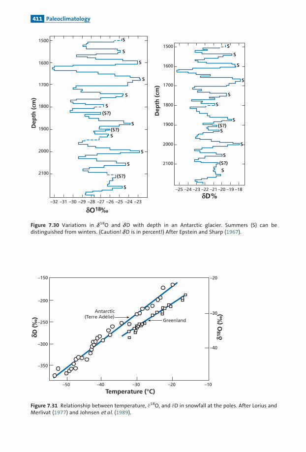
2100

2000

1900

1800

1700

1600

1500

–32 –31 –30 –29 –28 –27 –26 –25 –24 –23

Dep

th (

cm)

δO18‰

2100

2000

1900

1800

1700

1600

1500

–25 –24 –23 –22 –21 –20 –19 –18

Dep

th (

cm)

δD%

S

S

S

S

S

S

S

S

S

S

S

S

S

S

(S?)

(S?)

S

S

S

S

S

S

S

S

(S?)

(S?)

(S?)

Figure 7.30 Variations in d18O and dD with depth in an Antarctic glacier. Summers (S) can bedistinguished from winters. (Caution! dD is in percent!) After Epstein and Sharp (1967).

–200

–30

–20

–40

–150

–250

–300

–350

–50 –40 –30

Temperature (°C)

δD (

‰)

δ18 O

(‰

)

–20 –10

Antarctic(Terre Adélie)

Greenland

Figure 7.31 Relationship between temperature, �18O, and �D in snowfall at the poles. After Lorius andMerlivat (1977) and Johnsen et al. (1989).


Core sampling (sequential records)Coresofmarine sediments canbe taken fromall latitudes and longitudes (in theocean andfrom continents and lakes); however, two conditions restrict their use. First, sedimentationmust have occurred above the‘‘carbonate compensation depth’’ for there tobe anymeasur-able fossil tests left. And second, sedimentation must have been very rapid to provide arecordwithgoodtime resolution. Sedimentarycoreshavenotime limitsother thanthe life-span of the ocean £oor. Quaternary,Tertiary, and Secondary cores can be studied up to120Ma, which is the age of the oldest remnants of oceanic crust that have not been swal-lowedupbysubduction (ancient cores are compactedand transformed intohard rocks andsotime resolution isnotasgood).

For ice caps, the¢rstproblem is, ofcourse, their limitedgeographical andtemporal extent.Geographically, records are primarily from the glaciers of Antarctica and Greenland.Mountainglaciershavealsorecordedclimatic eventsbutovermuchshorter time-spans.13

Ice caps are limited in time. For a long time, the longest core was one from Vostokin Antarctica covering 420 000 years. A new core of EPICA has been drilled and covers700 000 years. Cores from the big mountain glaciers go back a mere 2000 years or so. Forboth types of record ^ sediments and ice ^ precise, absolute dating is essential, but hereagain many di⁄culties arise. Especially because as research advances and as studiesbecomeevermorere¢nedforeversmaller time-spans, theneedforprecision increases con-stantly.There is scope for 14C dating and radioactive disequilibriummethods on sedimen-tarycores, but their precision leaves something tobe desired.Useful cross-checking canbedonewithpaleomagnetism andwell-calibratedpaleontological methods. In turn, the oxy-gen isotopesofawell-datedcore canbeusedtodatethelevelsofothercores.Thus,gradually,amoreor less reliable chronology is established,whichmustbe constantly improved.Datingis di⁄culton ice caps except for themostrecentperiodswhereannual layers canbe counted.Methods based on radioactive isotopes such as 14C, 10Be, 36Cl, 87Kr, and 37Ar are used, buttheyare extremelydi⁄cultto implementbothanalytically (ice is averypurematerial!) and intermsof reliability. Switzerland’sHansOeschger (and his team) is associatedwith the devel-opment of these intricate techniques for dating ice, which, despite their limitations, havebroughtaboutdecisiveadvances indeciphering the ice record (Oeschger,1982).

These clari¢cations should make it understandable that establishing time sequences ofrecords is adi⁄cultand lengthy jobthat is constantlybeing improved.All reasoningshouldmakeallowancefor this.

Deciphering sedimentaryseries and the triumphofMilankovitch’s theoryBetween 1920 and 1930, the Yugoslav mathematician and astronomer MilutinMilankovitch developed a theory to account for the ice ages that had alreadybeen identi-¢ed by Quaternary geologists (see Milankovitch, 1941). These periods were thought tobe colder.The polar ice extended far to the south andmountain glaciers were more exten-sive too (Figure 7.32). Alpine glaciers stretched down as far as Lyon in France. Theseglacial traces can be identi¢ed from striated rock blocks forming what are known asmoraines.

13 They have been used by Lony Thompson of Ohio State University for careful study of recent tempera-ture fluctuations (see his 1991 review paper).


Milankovitch’s theory gave rise to vehement controversy (as vehement as that overWegener’s theoryofcontinental drift14).Andyetthis vision ofthepioneers ofthe1920swaslargelyaccurate.This isnottheplacetosetoutthis theory in full. Itcanbefoundintextbooksonpaleoclimatology, for example, Bradley (1999).However,we shalloutline themainprin-ciples andtheterms to clarifywhatwehavetosayabout it.TheEarth’s axisofrotation isnotperpendicular to itsplaneofrotationaroundtheSun. It

deviates from it by 238 on average. But the axis of this deviation rotates around the verticalover a period of 23 000 years. A further movement is superimposed on these, which is the£uctuation of the angle ofdeviationbetween 21.88 and 24.48.The period of this £uctuationis 41000 years.The ¢rst of these phenomena is termed precession, the second is obliquity.A third phenomenon is the variation in the ellipiticity of the Earth’s orbit, with a periodof 95 000 years. These three phenomena arise from the in£uence on the Earth of theSun, Jupiter, and the other planets and the tides. They not only combine but are

Today

18 000 years ago

Figure 7.32 Worldwide distribution of ice in glacial and interglacial times.

14 Wegener had been the first, with his father-in-law Koppen, to suggest an astronomical explanation forthe ice ages before becoming an ardent defender of Milankovitch.


a

b

c

0.05

400

Total

Precession

Obliquity

Excentricity

200

413100

41

23

19

0 600 800

0.02

0.024.5

23.3

22.0-0.07

-0.02

0.04

2.7

0.0

2.7

Time (ka BP)

Fou

rier

sp

ectr

um

Summersolstice

Wintersolstice

Autumnequinox

Winterequinox

Sun Perihelion

Precession

Obliquity

Apheliondpda

Age (ka)

I IIInsolation in June

1230

950

80°N

60°N

40°N

20°N

0°N

20°N

40°N

60°N

80°N

1130

9001140

930

880

740870

520360280100

1000

0

1080

910

1000 200 300Age (ka)

I IIInsolation in December

1000

1000

80°N

60°N

40°N

20°N

0°N

20°N

40°N

60°N

80°N

1000 200 300

370270670

520810

7401080

8801150

9301150

9101260

980

Figure 7.33 The principle of Milankovitch’s theory. (a) The three parameters that change: eccentricity ofthe orbit, obliquity, and precession. (b) Variations in the three parameters calculated by astronomicalmethods with their Fourier spectrum on the right. (c) Variation in the sunlight curves in June andDecember with latitude, calculated by the theory.


superimposed, leading to complexphenomena.Thus, at present, the Earth is closest to theSun on 21December, but the Earth’s axis is aligned away from the Sun, and so, in all, thenorthern hemisphere receives little sunlight. It is winter there, but other conjunctionsalso occur. Thus we can calculate the sunshine received during the year at various lati-tudes. Celestial mechanicsmean such calculations canbemade precisely (see Figure 7.33for a simpli¢ed summary). As Milankovitch understood, if little sunshine reaches theEarth at high latitudes in summer thewinter icewill remain, thewhite surfacewill re£ectsolar radiation,andthe coolinge¡ectwillbeampli¢ed.This isagoodstartingpointforcli-matic cooling.What should be remembered is that whenwebreakdown the complex signal of sunlight

received by the Earth using Fourier analysis methods (that is, when we identify the sine-wave frequencies that are superimposed to make up the signal) we ¢nd peaks at 21 000,41000,and95000years.WhenweconductasimilarFourierdecomposition ford18Ovaluesrecorded by foraminifera in sedimentary series, we ¢nd the same three frequencies(Figure7.34).The d18O variations re£ect those of the Earth’s temperatures. This ¢nding con¢rms

Milankovitch’s theory (at least as a ¢rst approximation) and so fully bears out the earlystudies of Emiliani. In complete agreement with the theory, the sedimentary series alsoshowed that climatic variations were very marked at the poles (several tens of degrees),very low in the intertropical zone, and intermediate in the temperate zones (of the orderof�5 8C).Figures7.35and7.36giveafairlycompletesummaryoftheessential isotopicobservations

madefromsedimentarycores.Thesedimentarycore record(Figure7.35)alsoshows indetailhowthetemperaturevar-

iations evolved. Cooling is slow, followed by sudden warming. Finer £uctuations aresuperimposed on these trends but their frequencies match those of the Milankovitchcycles.

Con¢rmation ofMilankovitch cycles byAntarctic isotope recordsItwassomeconsiderabletimebeforeMilankovitchcycleswerecon¢rmedintheicerecords,for two reasons.Therewere no ice cores long enough and so covering a long enough time-spanandthedatingmethodsweretoo imprecise.It was only after the famous Vostok core from Antarctica was studied by the Franco-

Russian teamthatevidenceofMilankovitch cycleswas found in the ice record.Butthe coreyieldedmuchmore thanthat: it allowed climatic variations tobe correlatedwithvariationsofotherparameters:

� dust content: itwas realized thatduring ice ages therewasmuchmore dust and thereforemorewindthanduring interglacialperiods.� greenhousegas (CO2andCH4) content in airbubbles trapped in the ice ^ when the tem-

perature increases there is an increase inCO2 (in theabsenceofhumanactivity!).

This last question on the debate about the in£uence of human activity on the greenhousee¡ect and so on climate is a fundamental one.Which increased ¢rst, temperature or CO2

levels? It is a di⁄cult problem to solve because temperature is measured by dD in ice


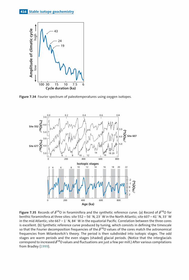
100 30 15 10 7.5 6

Am

plit

ud

e o

f cl

imat

ic c

ycle

hig

hlo

w

Cycle duration (ka)

43

24

19

Figure 7.34 Fourier spectrum of paleotemperatures using oxygen isotopes.

3.0

5.0

4.0

3.0

4.0

5.0

0

0.0 0.2 0.4 0.6 0.8

200

2 6 8 10 12 14

16 18 20

400 600 800

3.0

4.0

5.0

δ18 O

(‰)

δ18 O

(‰)

δ18 O

(‰)

δ18 O

(‰)

Isotopic stages

2 1 0 -1 -2

2

200 0 400 600 800

Age (ka)

4 6 8 10 12 14 16 18 20 22

Site 677

Site 552

Site 607

Figure 7.35 Records of d18O in foraminifera and the synthetic reference curve. (a) Record of d18O forbenthic foraminifera at three sites: site 552 – 568 N, 238 W in the North Atlantic; site 607 – 418 N, 338 Win the mid Atlantic; site 667 – 18 N, 848 W in the equatorial Pacific. Correlation between the three coresis excellent. (b) Synthetic reference curve produced by tuning, which consists in defining the timescaleso that the Fourier decomposition frequencies of the d18O values of the cores match the astronomicalfrequencies from Milankovitch’s theory. The period is then subdivided into isotopic stages. The oddstages are warm periods and the even stages (shaded) glacial periods. (Notice that the interglacialscorrespond to increased d18O values and fluctuations are just a few per mill.) After various compilationsfrom Bradley (1999).


whereas CO2 is measured from its inclusion in ice. Now, gaseous inclusions are formedby the compacting of ice and continue to equilibrate with the atmosphere, that is, the airsamples areyounger thanthe ice thatentraps them(Figure7.37).We need, then, to be able to measure the temperature of inclusions directly and com-

pare it with the temperature measured from the �D value of the ice. A method has beendeveloped by Severinghaus etal. (2003) for measuring the temperature of £uid inclusionsusing 40Ar/36Ar and 15N/14N isotope fractionation. After stringent calibration, the teamsat the Institut Simon-Laplace at Versailles University and at the Scripps Institution ofOceanography (La Jolla, California) managed to show that the increase in CO2 lagsbehind the increase in temperature by 800 years (Figure 7.38) and not the other wayround as asserted by the traditional greenhouse-e¡ect model (Severinghaus et al., 1999;Caillon et al., 2003). Now, we know that CO2 solubility in sea water declines as tempera-ture rises and that the characteristic time for renewal of the ocean water is 1000 years.The ¢rst phase of temperature increase followed by the increase in CO2, with a lag of800 years, can be readily understood, then, if we invoke the lag because of the thermalinertia of the ocean.There may also be some feedbackof the CO2 e¡ect on temperature.

Inso

lati

on

(J)

65° N

CH

4(p

pb

v)C

O2

(pp

bv)

δ18 O

atm

(‰

)Te

mp

erat

ure

(°C

)

Age (years BC)

280

a

a

bc

d

e

b

c

d

e

100 000 200 000 300 000 400 000

240

700600500400

10050

0

20020

–2–4–6–6

–0.5–0.00.51.0

Du

stIc

evo

lum

eδD

(‰

)

Na

(pp

b)

δ18 O

atm

(‰

)

100 000 200 000 300 000 400 000

–420–440–460–480

0.00.51.0

1.51.00.5

110 ka 390 ka

5.4

11.2

4

5.1

5.3

5.5

7.1

7.3

7.5

8.5

9.1

9.3

11.3

11.1

050100

1.00.50.0–0.5

Figure 7.36 Various parameters recorded in the Vostok ice core. After Jouzel et al. (1987) and Petit et al.(1999).


Exercise

Argon and nitrogen isotope fractionations are caused by gravitational fractionation in the ice

over the poles. Using what has been shown for liquid–vapor isotope fractionation, find the

formula explaining this new isotope thermometer.

AnswerIf we write the fractionation:

Age (BC) for δ40Ar

Age in years (BC) for CO2

235 000 240 000 245 000 250 000

235 000 240 000 245 000 250 000

200

220

240

260

2.20

2.15

2.10800 years

2.05

2.00

δ40 A

r (‰

)

CO

2 (p

pm

)

CO2

δ40Ar

Figure 7.38 Records of �40Ar and CO2 from the Vostok core after shifting the CO2 curve 800 yearsbackwards. After Caillon et al. (2003).

Dep

th (

m)

50-120 0.83

0.80

0.55

Density (g cm–3)Surface

15

0

Free contactwith atmosphere

Isolated air

Diffuse contactwith atmosphere

Co

mp

acti

on

Δt =

inte

rval

of

tim

e

Sno

wIc

e

Closure ofgas inclusion

Figure 7.37 As ice is compacted, the air trapped is younger than the snow.


� ¼ C m1P ð1Þ

C m2P ð2Þ

ln� ¼ ln P m1 � ln P m2 ¼ Dmgz

RT:

From the approximation formulae we have already met:

Dd1000

� Dmgz

RT

� with g¼ 10 m s�1, T¼ 200 K, for z¼ 10 m, and R¼ 2.

This gives �d ¼ 0.25 for nitrogen and �d ¼ 1.1 for argon. Once again, extremely precise

methods for measuring isotope ratios had to be developed.

GreenlandandAntarctica records comparedand the complexityofclimaticdeterminantsAlthoughstudies ofGreenland ice corespre-dated thatoftheVostokcoreby far, itwasonlyafter theVostokcorehadbeen deciphered that the signi¢cation of theGreenland coreswasfully understoodbycontrast (Figure7.39). Itwasobservedthatthe recordoftheoxygenandhydrogen isotopes at Vostok was much simpler than in Greenland and that theMilankovitch cycleswere clearly recorded.Things are more complex in Greenland because sudden climatic events are superim-

posed on theMilankovitch cycles.The ¢rst well-documented event is a recurrent cold per-iod at the time of transition from the last ice age to the Holocene reported byDansgaard’steam in 1989.While some 12 800 years ago a climate comparable to that of today set in, itwas interrupted 11 000 years ago by a cold episode that was to last about 1000 years andwhich isknownas theYoungerDryas.This eventwas foundsomeyears later inthesedimen-tary recordoftheNorthAtlantic.Generalizingon this discovery,Dansgaardusedoxygen isotopes to show that the glacial

period was interrupted by warm periods that began suddenly and ended more gradually.These events, oftheorderofa few thousandyears, correspond toa 4^5øchange in the �18Ovalue of the ice and so to a temperaturevariation ofabout 7 8C.Dansgaard’s team reported24 instancesofthis typeofD^Oepisode, as theyare called (D is forDansgaardandO is forOeschger), between12000and110 000yearsago.Theyhavebeendetected inthesedimentaryrecords of the North Atlantic and as far south as the intertropical zone. Cross-referencingbetween sedimentary cores andpolar ice cores has proved so instructive thatboth types ofrecordcontinuetobeusedtoanalyzeoneandthe same event.A second series of events was read this time from the sedimentary records.These were

brief events characterized by the discharge of glaciers as far as the Azores.There are 34 ofthese H events (see Heinrich,1988) during the last glacial period and nothing comparablehasbeen identi¢ed in the ice ofGreenland.The relationshipbetweenD^OandHevents isunclear, butwhat is clear is thattheyarenot identicalhappenings.What compounds the mystery is that these brief events are recorded very faintly in

Antarctica,withatime lag.Thereare thereforeoneormoremechanismsgoverning climate


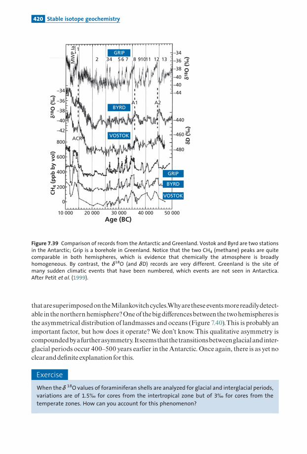
thataresuperimposedontheMilankovitchcycles.Whyarethese eventsmorereadilydetect-able in thenorthern hemisphere?Oneofthebigdi¡erencesbetween the twohemispheres isthe asymmetrical distribution of landmasses and oceans (Figure 7.40).This is probably animportant factor, but how does it operate? We don’t know.This qualitative asymmetry iscompoundedbyafurtherasymmetry. Itseemsthatthetransitionsbetweenglacialandinter-glacial periods occur 400^500 years earlier in the Antarctic. Once again, there is as yet noclearandde¢nite explanation for this.

Exercise

When the d 18O values of foraminiferan shells are analyzed for glacial and interglacial periods,

variations are of 1.5ø for cores from the intertropical zone but of 3ø for cores from the

temperate zones. How can you account for this phenomenon?

0

200

400

–440

–460

–480

600

800

–42

–40

–38

–36

–34

ACR

A1

2

1

MW

P Ia

34 5 6 7 8 9 1110 12 13

A2

Age (BC)

CH

4 (p

pb

by

vol)

δ18 O

(‰

)

δD (

‰)

–34

–36

–38

–40

–40

–44

δ18 O

(‰

)

10 000 20 000 30 000 40 000 50 000

VOSTOK

BYRD

GRIP

VOSTOK

BYRD

GRIP

Figure 7.39 Comparison of records from the Antarctic and Greenland. Vostok and Byrd are two stationsin the Antarctic; Grip is a borehole in Greenland. Notice that the two CH4 (methane) peaks are quitecomparable in both hemispheres, which is evidence that chemically the atmosphere is broadlyhomogeneous. By contrast, the d18O (and dD) records are very different. Greenland is the site ofmany sudden climatic events that have been numbered, which events are not seen in Antarctica.After Petit et al. (1999).


AnswerTemperature variations between glacial and interglacial periods are very large at the poles,

very low in the intertropical zone, and intermediate in the temperate zones. The variation of

1.5ø for the intertropical zone is caused by the melting of ice. It must therefore be considered

that the additional variation of 1.5ø of the temperate zones is due to a local temperature

effect. Applying the Urey–Epstein formula of the carbonate thermometer

T 8C ¼ 16:3�4:3ð�dÞ=0:13ð�dÞ2

gives �T� 4.3 �d. This corresponds to 5–6 8C, the type of temperature difference one would

expect in the temperate zone between a glacial and interglacial period.

Veryrecently, the ice recordhasbeen extendedto700 000years thanks tothe coredrilledbyan international consortium in Antarctica at the EPICA site. As Figure 7.41shows, thisfacilitates comparison between sedimentary and ice records. New data can be expectedshortly.

7.8 The combined use of stable isotopes and radiogenicisotopes and the construction of a global geodynamicsystem

Climate isacomplexphenomenonwithmultipleparameters.Temperature,ofcourse, isacar-dinal parameter, but the distribution of rainfall, vegetation, mountain glaciers, and windsareessential factorstoo.Oxygenanddeuteriumisotopesprovidevital informationabouttem-peratures and the volume of the polar ice caps. The 13C/12C isotopes are more di⁄cult to

Perc

ent

per

5°

of

lati

tud

e

LatitudeN S

Surface (%)

70

80° 80°90° 90°

50

30

10

90

98 8694 50 0 50 75 86 94 98 10075100

60° 60°40° 40°20° 20°0°

Ocean : 361 x 109 km2

Continent:149 x 106 km2

Equ

ato

r

Figure 7.40 Distribution of landmasses and continents by latitude. The difference between northernand southern hemispheres is clearly visible.

421 The Construction of a global geodynamic system

interpretbutyieldusefulpointers, forexample,aboutthetypeofvegetation(C3/C4plants)andits extent. But such information, which should in principle enable us to construct a biogeo-chemicalpicture, is stillverydi⁄culttodecipherandhasbeenoversimpli¢edinthepast.

The use of long-lived radiogenic isotopes has a similar objective, namely to determinehow climatic £uctuations are re£ected in the planet’s erosional system. Erosion is a funda-mental surface process. It is what changes volcanoes or mountain ranges into plains andpeneplains.The end products oferosion are of two types. Some chemical elements are dis-solved as simple or complex ions, while others remain in the solid state. The former aretransported in solution, the latter as particles.Whichever state they are in, they are carriedby rivers down to the oceans where they form sea water in one case and sediments in theother.The radiogenic isotope ratios are preserved throughout these erosion and transportprocesses.They are then mixed in the ocean, either as solutions in seawateror as particlesin sediments.The erosion sites have characteristic radiogenic isotope signatureswhich dis-tinguishold landmasses,youngcontinents,andvolcanicproductsofmantleorigin.Theiso-topic compositionsofthemixture thatmakesup seawater thus re£ecttheproportionofthevarious sources involved in the erosionprocesses.

65° N July

75 S /year11.35.5

EPICA

Vostok 16.2 18.4

0 200 400 600

Age (ka)800

Inso

lati

on

(75

°S)

(W m

–2)

Inso

lati

on

(75

° S)

(W m

-2)

Du

st in

mas

s (μ

g k

g-1

)δD

(‰

)δ1

8 O-m

arin

e (‰

)

120185190

480

440

400

-380

-410

-440

-470-3.0

3.0

1.200

800

400

0

-1.5

1.5

0

a

b

c

d

Figure 7.41 Comparisons of (a) insolation and sedimentary (c) and glacial (b, d) records at the EPICA site.After the EPICA Community (2004).


7.8.1 Strontium in the ocean

A¢rstexample is the 87Sr/86Sr isotopic compositionofpresent-dayseawater.The 87Sr/86Srratio is 0.70917 and is identical whichever ocean is considered.Where does the Sr comefrom?Obviously fromtheerosionoflandmassesandsubaerialorsubmarinevolcanicactiv-ity.Measurementofthe isotopic composition of Srdissolved in riversyields ameanvalueof0.712� 0.001.The mean isotopic composition of the various volcanic sources (mid-oceanridges, islandvolcanoes, and subduction zones) liesbetween 0.7030 and 0.7035 (dependingon the relative importance attributed to the various sources). From the mass balanceequation:

87Sr86Sr

� �sea water

¼87Sr86Sr

� �continental rivers

xþ87Sr86Sr

� �volcanic input

ð1� xÞ:

The fraction from continental rivers corresponds to 66%� 2% of the Sr in sea water.(Notice this fraction x re£ects the mass of chemically eroded continent modulated by thecorrespondingabsolute concentrationofSr.)

x ¼ _mc Cc

_mc Cc þ _mv Cv

where _mc is themass of continent eroded chemically per unit time, _mv is themass ofvolca-noes eroded chemically per unit time, and Cc and Cv are the Sr contents of rivers £owingfromcontinents andof volcanoes, respectively.We can go a little further in this breakdown.The isotopic composition of Sr in rivers is

itself a mixture of the erosion of silicates of the continental crust, whose mean isotopiccomposition we have seen is 87Sr/86Sr� 0.724� 0.003,15 and the erosion of limestones,which are very rich in Sr and are the isotopic record of the Sr of ancient oceans. For rea-sons we shall be in a better position to understand a little later on, the mean compositionof these ancient limestones is 87Sr/86Sr¼ 0.708� 0.001. The mass balance can bewritten:

87Sr86Sr

� �rivers

¼87Sr86Sr

� �limestones

yþ87Sr86Sr

� �silicates

ð1� yÞ;

whichmeans thatlimestonesmakeup71%oftheSrcarriedtotheocean insolution fromthecontinents.Therefore, all told, the Srof seawater is madeup of 49.5% from reworked lime-stone, of16.5% from the silicate fraction of landmasses, and of 34% fromvolcanic rockofmantle origin. Of course, these ¢gures must not be taken too strictly.The true values mayvarya little fromthese, butnotthe relativeordersofmagnitude.The 87Sr/86Sr isotopic composition ofpresent-daymarine carbonates is identical to that

of seawater in all the oceans. It is assumed, then, that the 87Sr/86Sr isotopic compositionsmeasuredonmoreancient limestoneswere identical to thoseoftheoceans fromwhich theyprecipitated (Figure7.42).

15 Corresponding to the mean value of detrital particles transported by rivers.


These isotopic compositions havebeen studied and are found to have varied in the past.The curve ofvariation of strontium in the course of the Cenozoic has been drawn up withparticularcare (Figure7.43).

Itshowsthatthe87Sr/86Sr ratiowaslower65Maagothan itis todayandremainedroughlyconstant from 65Ma to 40Ma, fromwhich date it began to rise, at varying rates, up to thepresent-day value.Whydidthesevariationsoccur?

Returning toour fundamentalmassbalance equation,wemustconcludethatthegrowthin the ocean’s 87Sr/86Sr ratio since 40Ma can be attributed to a variation in the relativeinputoferosion fromthe landmassesor the input fromthemantle, orboth. Initially, a¢ercecon£ict opposed proponents of the growth of continental input with mantle input suppo-sedly remaining constant and their adversaries who thought that it was the mantle inputthat had varied along with the intensity of erosion. For the former, the predominant phe-nomenonwas theupliftoftheHimalayas after India collidedwithAsia 40Maago (RaymoandRuddiman,1992). For the latter, the essentialvariationwas in theactivityofmid-oceanridges in the form of the hydrothermal circulation occurring there (Berner et al., 1983).Now, itwasonce thoughtthatthe total activityofthemid-ocean ridgeshadvariedovergeo-logical time and in particular had declined since 40Ma ago.We no longer think this.Theideatoday is thatboth changesare concomitant.The increasederosionbecauseoftheupliftof the Himalayas is consistent with reduced input from the mantle, which derives mostlyfrom erosion of subduction zone volcanoes. Such erosion has been partially slowed by thedisappearance of a signi¢cant sourcewhichwas swallowed up in theHimalayan collision.All in all, then, it is the formation of the Himalayas that explains the 87Sr/86Sr curve as

Silicates Carbonates

Seawater

Marinecarbonates

Mid-oceanridge

hydrothermalism

Continentalrivers

Mantle

Volcanicislands

Figure 7.42 The determining factors of the isotope composition of strontium in sea water. The strontiumin the ocean comes from alteration of the continents and volcanic arcs. Hydrothermal circulation alongthe ridges also injects strontium into sea water. Limestones reflect the isotopic composition of the oceanat the time they formed. They are recycled either by erosion or by inclusion in the mantle.


suggestedby the formerColumbia team (RaymoandRuddiman,1992) and JohnEdmond(1992) fromMITindependently.Regardlessofanycausal explanations, the curve isnowadaysusedtodateCenozoic lime-

stones.This is known as Sr stratigraphic dating.The idea is straightforward enough. Sincethe curve is identical for all the oceans, it is an absolute marker. As the variation in the87Sr/86Sr curve is all one way, the measurement of an 87Sr/86Sr ratio for any limestone canbe used to determine its age from the curve. As can be seen, this clock is e¡ective from 0 to40Ma, butbarelybeyond that as the curve £attens out.The precision achieved for an age is�1Ma.This is auseful couplingwithmicropaleontological techniques.But,ofcourse,whateveryonewants toknowiswhythe 87Sr/86Sr ratio curve in limestones

is identicalwhichever the ocean? The answer is that the residence time of Sr in the ocean isvery much greater than its mixing time and so it has time to homogenize on a global scale.Thiswillbe explained in thenextchapter.The second question relates to climate. As it is observed that d18O increased through-

out the Cenozoic, corresponding to a general cooling, what relation is there betweentectonic activity and climate? This is a fundamental question to which there is as yet noclear answer.

Exercise

There are two inputs to the isotope composition of continental rivers: one from silicates and one

from carbonates, in the proportions of 75% from carbonates and 25% from silicates, with average

isotope ratios of (87Sr/86Sr)silicates¼ 0.708 for carbonates and (87Sr/86Sr)limestone¼ 0.724 for

10 20 30 40 50 60 70

Age (Ma)

0.7080

0.7085

0.7090

87Sr

/86Sr

G (

t)/G

(o

)

0,9

1,0

1,1

1,2

1,3

1,4

1,5

Isotopic compositionof Sr

Figure 7.43 Curve of evolution of the 87Sr/86Sr ratio in sea water in Tertiary times (Cenozoic).


silicates. Suppose that carbonate recycling falls to 70%. How much will the Sr content of sea

water vary assuming that the Sr content of rivers remains the same (which is unrealistic, of

course)?

AnswerIn the current situation, the Sr isotope ratio of rivers is 0.712 with 75% carbonate and 25%

silicate. Recycled limestone has a Sr isotope composition of about 0.708 while that of silicates

is 0.724. The composition for rivers with the new proportions becomes 0.7128, which gives a

value of 0.709 52 for sea water. The recycling of limestone is clearly an important parameter,

then.

Exercise

Assuming the isotope different compositions and inputs remain constant and the flow from

volcanic sources remains the same, by how much does the Sr flow from rivers have to vary to

change the ocean values from 0.708 to 0.709?

AnswerThe calculation is the same as before:

�R

R¼ �x

ð1� xÞx :

Therefore �F/F¼þ0.49. So the flow from rivers must increase by 50%.

7.8.2 Isotopic variations of neodymium in the courseof glacial–interglacial cycles

As with Sr, the isotopic variations of Nd are related to long-period radioactivity.Whenisotopic variations aremeasured inQuaternarysedimentary cores, thesevariations canbeattributed to di¡erences in origin alone.The in situ decayof 147Sm in the core has virtuallyno in£uence.The fundamentaldi¡erencebetweenthebehaviorof SrandofNd intheoceanis that Sr, havinga long residence time (1or 2Ma), is isotopicallyhomogeneouson the scaleof the world’s oceans whereas Nd, having a shorter residence time (500^2000 years),varies isotopically between oceans and even within oceans. For example, the "Nd

value todayaverages�12 for the Atlantic Ocean,�3 for the Paci¢c, and�7 for the IndianOcean.These variations are interpreted by admitting that the Nd of seawater is a mixturebetween avolcanic source coming from subduction zones ("� 0 toþ 6) and a continentalsource ("�^12� 2).The "Ndvaluevaries dependingonthe degreeofvolcanic activity in theregion relative to continental input (seeGoldsteinandHemming,2003).

StudyofaQuaternary core from the IndianOcean, southof theHimalayas, has allowedthe Paris laboratory (Gourlan et al., 2007) to highlight an interesting phenomenon. Thesedimentarycore ismostly carbonated (more than 70%carbonate). Byappropriate chemi-cal treatment, it is possible to extract theNdof ancient seawater trapped in the small coat-ings of Mn surrounding foraminifers. Isotopic analysis of the Nd shows that "Nd variesfrom �7.5 to �10.5 and that the variations follow the pattern of 18O/16O £uctuation


correspondingtotheglacial^ interglacialpattern.There isanexcellent (inverse)correlationbetweend18Oand "Nd (Figure7.44).SouthoftheBayofBengal, themixtureofout£ow fromIndonesiaandthe input fromthe

RiversGanga^Brahmaputra (butalsotheIrrawaddyandtheSalween rivers)homogenizesthevaluesofseawaterofabout "��6� 1.Sowe can suppose that in the Bay of Bengal the £uctuation during glacial^ interglacial

alternation corresponds to the £uctuation in the impact from the Ganga^BrahmaputraRivers from the Himalayas.Those variations are linked with variations in intensity of the

–10

–9

–8

–7

0

–1

–2

Island arc

Himala y a

–130 200 400 600 800

–12

–11

ε Nd

SEA W ATER

DETRIT AL

δ18 O

Interglacial

Glacial

AGE (ka)

Figure 7.44 Variation in the isotopic composition of neodymium in sea water expressed as "Nd in apredominantly calcareous marine sedimentary core from the Ninety East Ridge in the Indian Ocean,representing the last 800 ka. Top: the curve of d18O variations allowing comparison of climaticfluctuations. Bottom: isotopic composition of the detrital fraction. (a) Oxygen isotopes comparedwith "Nd variations. (b) Enlargement before 2 Ma. (c) Oxygen-neodymium maxima and minimacorrelations.


monsoon and the existence of large glaciers during glacial periods in the highHimalayas.Monsoons areweakerduring glacial times andglaciers accumulate snowand then stop (orstrongly reduce) the river runo¡.

Exercise

Calculate the relative input of the Ganges–Brahmaputra (GB) Rivers between interglacial and

glacial if we suppose that "GBND ¼ �12 and "ocean

Nd ¼ �6. The measured ratios of concentration

are "Nd¼�10 during interglacials and "Nd¼�7.5 during glacials, the concentration of Nd in

river and ocean staying the same during all periods.

AnswerWe applied the mixing formula. Notating concentration as CNd and the masses as m, we have:

"measuredNd ¼ "GB

Ndx þ "oceanNd 1� xð Þ

x ¼ mass of fresh water � C riverNd

mass ocean � C oceanNd þmass of fresh water � C river

Nd

:

With a little manipulation

m river

m ocean¼ C ocean

Nd

C riverNd

1

x�1 � 1

� �:

So for the ratios between interglacial (i) and glacial (g):

m iriver

m griver

¼x�1

g � 1

x�1i � 1

!¼ 3

0:5¼ 6:

The river £ux from the Himalayas was 6 times higher in interglacial than in glacialtimes.

This is a simple example in a work in progress in author’s laboratory to illustrate thepowerof investigationofcombiningOandNdisotopes.

7.9 Sulfur, carbon, and nitrogen isotopes andbiological fractionation

We give two examples of how stable isotope geochemistry can be used in various typesofstudy.

7.9.1 A few ideas on sulfur isotope fractionation

When we examine the 34S/32S composition of naturally occurring sulfur isotopes as afunction of their geological characteristics, several features stand out. All sul¢des asso-ciated with basic or ultrabasic rocks have extremely constant compositions close to


34S/32S¼ 0.045 (�¼ 0), that is, largely analogous to that of sulfur in meteorites (Nielsen,1979).Sulfur mineralization in veins crossing geological structures, with a gangue of quartz,

£uorite, or barite, have � values of about 0 which are very constant. It is therefore legiti-mate to attribute a deep origin to them or at least an origin related to deep-lying rocks.Cluster mineralization exhibits much morevariable compositions, particularlyminerali-zation related to sedimentary strata. Its composition may range from �¼þ22 to �¼�52.This observation is tied in with the point that oxidation^reduction reactionsS2� , SO

2�4 are accompanied by equilibrium isotope fractionation which, at low tem-

peratures, is substantial (1.075 at 25 8C) (Tudge and Thode, 1950). Moreover,S2� ! SO

2�4 is an easy reaction at low temperature. However, reduction can only occur

through Desulfovibrio desulfuricans bacteria. This bacterial reduction is accompaniedby an isotopic e¡ect that is weaker than the equilibrium reaction (�¼ 1.025 at 25 8C)(Harrison and Thode,1958). Remembering that sulfates of seawater and freshwater haved34S values that range fromþ26 toþ4, we can explain the dispersion observed byassum-ing that the sul¢des related to strata derive from bacterial reduction of sulfates, but thatsuch reduction exhibits a number of variations. Sometimes reduction may involve seawater, sometimes groundwater circulation. Sometimes it occurs in replenished systems,sometimes in bounded reservoirs (Rayleigh distillation). Sometimes it is followed by iso-tope exchange leading to equilibrium fractionation, sometimes not. Here we ¢nd, but ina di¡erent context, variations in scenarios similar to what was calculated for bacterialreduction in sediments.In any event, case by case, the sulfur isotope composition, associatedwith metallogenic

and geological observations, allows distinctions to be drawn between the various types ofdeposits (Figure7.45)andthenallowsthepotentialmechanismfor theoriginofmineraliza-tiontobelimited.Generally, thesedatahavemade itpossible toasserttheoccurrenceofsul-fur mineralization of exogenous origin, which many workers had contested before,claiming thatallmineralizationderived fromthedepthsoftheplanetthroughmineralizing£uids (OhmotoandRye,1979).One particularly fascinating observation with sulfur isotope geochemistry relates to

mass-independent fractionation (MIF). Such fractionation has been mentioned foroxygen,butitexists forsulfur too.Sulfurhas four isotopes: 32S,33S,34S,and36S. Interrestrialsulfur compounds variations in 33S/32S ratios account for about half of 34S/32S fractiona-tions (0.515 tobeprecise). Ifwede¢ne�33S¼ (�33S)^0.515 (�34S), thisdi¡erence isgenerallyzero.Whenmeasuring the isotopic composition ofsul¢des and sulfates ofgeologically var-ied ages, we obtain an unusual result. Between 2.30Ga and the present day, �33S¼ 0. Forsamplesof2.30^2.60Ga,�33Svarieswithanamplitudeof12ø.Forolder samples, £uctua-tions are smaller but around 4ø. Samples of barium sulfate are depleted in 33S (comparedwith ‘‘normal’’ fractionation, their �33S is negative). Sul¢de samples are enriched in 33S(their�33S is positive).This observation cannotbe easily interpreted.James Farquhar andhis team thinkthat therewas little oxygen in the atmosphere in ancient periods.The ozonelayer surrounding theEarthatanaltitudeof30kmandwhich now¢lters theSun’sultravio-let rays did not exist. Sulfur reduction phenomena shifted sulfur from the degree ofoxida-tion �2 (sul¢de) to þ6 (sulfate) via a cycle of photochemical reactions involving theseultraviolet rays. Now, laboratory experiments show that photochemical reactions (that

429 Biological fractionation

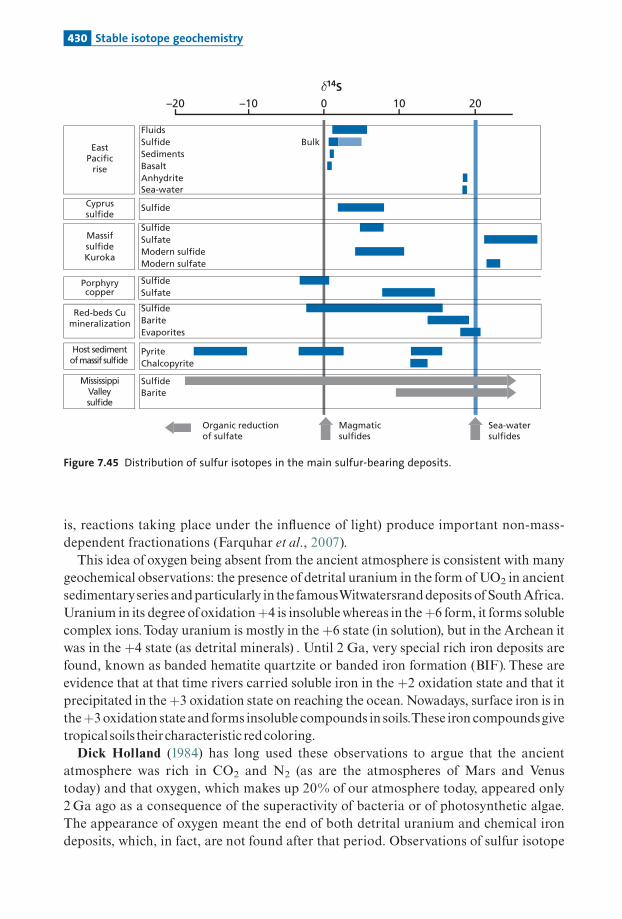
is, reactions taking place under the in£uence of light) produce important non-mass-dependent fractionations (Farquhar et al., 2007).

This idea of oxygen being absent from the ancient atmosphere is consistent with manygeochemical observations: the presence of detrital uranium in the form of UO2 in ancientsedimentaryseries andparticularly in the famousWitwatersranddeposits of SouthAfrica.Uranium in its degree ofoxidationþ4 is insolublewhereas in theþ6 form, it forms solublecomplex ions.Today uranium is mostly in the þ6 state (in solution), but in the Archean itwas in the þ4 state (as detrital minerals) . Until 2 Ga, very special rich iron deposits arefound, known as banded hematite quartzite or banded iron formation (BIF). These areevidence that at that time rivers carried soluble iron in the þ2 oxidation state and that itprecipitated in theþ3 oxidation state on reaching the ocean. Nowadays, surface iron is intheþ3oxidation stateand forms insoluble compounds in soils.These iron compoundsgivetropical soils theircharacteristic redcoloring.

Dick Holland (1984) has long used these observations to argue that the ancientatmosphere was rich in CO2 and N2 (as are the atmospheres of Mars and Venustoday) and that oxygen, which makes up 20% of our atmosphere today, appeared only2Ga ago as a consequence of the superactivity of bacteria or of photosynthetic algae.The appearance of oxygen meant the end of both detrital uranium and chemical irondeposits, which, in fact, are not found after that period. Observations of sulfur isotope

FluidsSulfide BulkSedimentsBasalt

SulfideCyprussulfide

AnhydriteSea-water

–20 –10 10 200δ14S

EastPacific

rise

SulfideSulfateModern sulfide

Sea-watersulfides

Modern sulfate

MassifsulfideKuroka

SulfideBarite

Barite

Evaporites

Red-beds Cumineralization

PyriteChalcopyrite

Sulfide

Host sedimentof massif sulfide

MississippiValleysulfide

SulfideSulfate

Porphyrycopper

Magmaticsulfides

Organic reductionof sulfate

Figure 7.45 Distribution of sulfur isotopes in the main sulfur-bearing deposits.


fractionations by Thiemens’s team re¢ne this model. They seem to indicate that thegrowth of oxygen in the atmosphere occurred very quickly, almost suddenly, between2.5 and 2.1 Ga and that this growth was accompanied by the progressive formation ofthe ozone layer protecting the Earth’s surface from excessive solar ultraviolet radiation(Figure 7.46).

7.9.2 Carbon–nitrogen fractionation and the dietof early humans

Biochemical operators fractionate carbon and nitrogen isotopes. Gradually the mechan-ismsandthepracticalrulessuch fractionationobeyshavebeendetermined.Thus, itwascor-rectlypredictedthatC3plants (the¢rstproductofphotosynthesiswith three carbonatoms)(trees, wheat, and rice) fractionate di¡erently from C4 plants (corn, grass, sugar cane). Ithas also been shown that marine plants are di¡erent again. From these observationsMichaelDeNirooftheUniversityofCaliforniaatLosAngeles studiedthe isotope compo-sition ofherbivores (eating the various types ofplant) andof carnivores eating those herbi-vores. Oddly enough, a numberof regularitieswere preserved and turnedup in the isotopecomposition of bone (in the mineral matter and also in collagen which withstood decayquitewell).Hewas thus able to determinewhat earlyhumans ate (Figure 7.47).Those of theNeolithic ateC3 plant leaves and thenpeople later certainlybegan to eat corn (C4).Wheatdoes not seem to have been grown until much later.This is an example of isotope tracingwhich is developing in biology and archeology. Stable isotopes measured on bone andtooth remains of extinct animals canbe used to answer questions about the type ofmeta-bolismof certain dinosaurs (hotor coldblooded), the dietofextinct animals, or the e¡ectof paleoclimate on the cellulose of tree rings. Once again this discipline o¡ers consider-ableprospects.

1 2 3 4

-1.0

0

1.5

2.0

Δ 33

S

Age (Ga)

Figure 7.46 �33S¼ (d33S)� 0.515 (d34S). The figure shows 33S variation in �33S of sulfides and sulfatesof various ages.

431 Biological fractionation

7.10 The current state of stable isotope geochemistryand its future prospects

As has been repeated incessantly throughout this book, developments in isotope geologyhave always tracked advances in measurement methods, which themselves are often theconsequence of technological progress. The development of the double-collection massspectrometerbyNierandhis collaborators (Nier,1947;Nieretal.,1947)made it possible tostudy the e¡ects ofvery weak isotopic fractionation (oxygen, hydrogen, carbon, and sulfur)in carbonates,water, rock, and livingmatter.

Since then technical advances havemoved in three directions.The¢rstwas thatof sensi-tivity. It has become possible to analyze isotopic fractionation on small quantities ofmate-rial. Hugh Taylor managed to analyze D/H in rocks while Franc� oise Pineau and MarcJavoyhaveanalyzed13C/12Cand15N/14Ninbasalts.

The second directionwas that of precision. In1950, ratios could be measured to 0.5ø.Nowthe¢gure is0.05ø.Thishasmade itpossibletoanalyzesedimentarycoreswithpreci-sion and to highlight Milankovitch cycles. Robert Clayton was able to discover paired17O/16O and 18O/16O fractionations of meteorites, which had many consequences forthe study of meteorites even if the initial interpretations have been modi¢ed. MarkThiemens hasbeen able tomove on from there to openup the studyofmass-independentfractionation.

The third advance has been the automation of analytical procedures which has enabledlarge numbers ofsamples tobe studiedboth in sedimentary carbonates and in polar ice forO,C, andHisotopes.Climatologyhasgainedenormously fromthis.

Today twonewtechnical advanceshaveoccurred:multicollectionICPMSandthedevel-opment of in situ probes, ion probes, or ICPMS laser ionization. In addition, advances

+15

+20

+10

–20

+5

–15 –10 –5–250

Eskimos

Marine carnivores

Terrestrial carnivoresfeeding on C3 herbivores

TehuacanIndians

NeolithicEuropeans

Terrestrial carnivoresfeeding on C4 herbivores

Terrestrial herbivoresfeeding on C4 plants

Terrestrial herbivoresfeeding on C3 plants

Terrestrial herbivoresfeeding on leguminous plants

δ15 N

(‰

)

δ13C (‰)

Figure 7.47 Isotopic composition of fossil plants, animals, and humans in the d15N and d13C diagram.After DeNiro (1987).


in computing and electronics have brought progressive gains in precision, sensitivity, andmeasurement time for all conventional techniques, TIMS, or double-collection gasspectrometry.What will come of all this? It is probably too early to answer this question but the

trends as perceived can be set out. The most spectacular trend is probably the rush tostudy isotopic fractionation of ‘‘non-classical’’elements that are often present in terres-trial materials.These include some major elements (Si, Mg, Fe, or Ca) for which physi-cochemical fractionations have been identi¢ed and then minor light elements like Band Li and minor heavy elements like Cr, Cu, Zn, Cd, Se, Mo, or Tl (the list is notexhaustive) (see the review edited by Johnson et al., 2004). It is undeniable that someinteresting results have been obtained for the major elements Mg, Fe, Ca, and Si as wellas for B, Li, Cu, Mo,Tl, and Cl. For trace elements, no result has as yet allowed new tra-cers of geological phenomena to be introduced, as is the case for the isotopes of themajor elements H, O, C, and S. Analyses are di⁄cult, the results are often uncertain,and approaches are not systematic enough.These attempts have not achieved the resultsexpected.The present author thinks, but this is open to question, that the most interest-ing processes are:

� ¢rst in biogeochemistry. It seems that living organisms fractionate some isotopes: Cafor the food chain ending with shells, Si for the food chain ending with diatoms, Cufor cephalopods. This, combined with C, N, and S geochemistry, may be the adventof the famous biogeochemistry we have been waiting for since Vernadsky’s 1929book!� then, for pH conditionsboron is ahope, provided thehypothesis of constant d11B for the

ocean over geological time is eliminated. The degree of oxidation^reduction with theuseof iron isotopes andmolybdenum isotopes is also relevant.We shall review this if thisbookruns toanewedition!

The other trend is illustrated by John Eiler’s program at the California Institute ofTechnology. He is trying to take advantage of the improvement in techniques ofanalysis oftraditional elements to develop newandoriginalmethods, themost spectacularofwhich isintercrystalline order^disorder fractionation, which we have spoken of, but also for18O/16OorD/Hfractionations in high-temperaturephenomena.The study of non-mass-dependent fractionation by Mark Thiemens’s team has

probably still not yielded all its results but perhaps requires a more structuredapproach.

Problems

1 Take a cloud that evaporates at the equator with a mass M0 dH2O ¼ 0 for D and 18O (to

simplify). It moves polewards and when the temperature is þ10 8C loses one-third of its

mass as rain and continues in the same direction. In the cold zone, where the temperature is

0 8C, it loses one-third of its remaining mass. It moves on and loses another one-third of its

remaining mass at �20 8C. When it reaches temperatures of �30 8C it loses a further one-

third of its mass. The fractionation factors at three temperatures are given in Table 7.4

below.

433 Problems

(i) Calculate the dD and d18O composition of the rain and snow.

(ii) Plot the (dD, d18O) curve and calculate its slope.

(iii) Plot the dD and d18O curves as a function of the remaining fraction of the cloud.

2 Take a magma chamber whose magma has an initial d18O isotope composition ofþ5.5. Some

30% of olivine Mg2SiO4 precipitates in the chamber. Then we precipitate a eutectic mixture

with equal proportions of olivine–pyroxene. We precipitate 30% of the remaining melt and

then the olivine, orthopyroxene, and plagioclase mixture in equal proportions for 20% of the

remaining melt. Given the melt–silicate partition coefficients in Table 7.5 below, calculate the

isotope evolution of the melt and the minerals.

3 Consider rainwater with dD¼�70ø. This water penetrates into the ground and finally reaches

a metamorphic zone where it meets a schist whose proportion relative to water is 15% and

whose composition is O¼ 53.8%, Si¼ 33.2%, Al¼ 7.8%, Fe¼ 2.8%, Ca¼ 7.1%, Na¼ 0.6%,

K¼ 1.5%, and C¼ 1.8%. This schist contains the following minerals which equilibrate with

water at 550 8C in a closed system. The composition of the rock is: 40% quartz, 4% magnetite,

16% plagioclase, 15% muscovite, 20% alkali feldspar, and 5% calcite. Calculate the oxygen

isotope compositions of the minerals and the water in the end.

4 The CO2 content of the recent atmosphere is 320 ppm, its d13C value is �7. As a result of

burning of coal and oil the d13C value has shifted from �7 to �10 in 20 years.

(i) Given that d13Coil¼�30, what quantity of carbon has been burned?

(ii) However, a problem arises. The CO2 content of the atmosphere is 330 ppm. How can you

explain this?

(iii) Suppose the �calcite–CO2fractionation at 20% is 1.0102. What is the variation observed in

the d value in the calcites precipitating in sea water?

(iv) Does the d13C isotope analysis of limestone seem to you a good way of testing CO2

degassing in the atmosphere by human activity? Mass of the atmosphere: 5.1 � 1021 g.

5 Basalt magma contains sulfur in the form S2� (sulfide) and SO2�4 (sulfate), whose proportions

vary with oxygen fugacity.

S2� þ 2 O2 , SO2�4

S2� �O2½ 2

SO2½ ¼ K ðT Þ:

Table 7.5 Partition coefficients

Plagioclase–melt Olivine–melt Pyroxene–melt

� 0.6ø � 0.2ø � 0.3ø�¼ 0.9994 �¼ 0.9998 �¼ 0.9997

Table 7.4 Fractionation factors

T (8C) �D �18O

þ20 1.085 1.0098

0 1.1123 1.0117

�20 1.1492 1.0411


Therefore:

S2�

SO2�4

¼ K ðT Þ½O22

:

When the magma degasses, it loses almost exclusively its SO2 and the H2S content is usually

negligible (even if it smells). Determine the partition �gas–magma¼ (d34S)g – (d34S)m.

Given that the magma contains S2� and SO2�4 , show that degassing of the magma leads to an

increase in the d13S value of the solidified magma or to a decrease depending on oxygen

fugacity (after Sakaı et al., 1982). (We know that DSO2

S2� ¼ þ3 and DSO2�4

S2� ¼ þ7.)

6 Various scenarios are imagined in which the temperature of the Earth reaches extremes. The

first scenario, known as the snowball scenario, says that all the landmasses are covered by a

layer of ice 100 m thick in addition to the present-day polar ice which has doubled in volume.

The second, reverse, scenario says that the Earth has heated and the polar ice caps melted. In

the first scenario the d18O of continental ice is supposed to reach �30, with the polar ice caps

being like today at �50. The ocean is at d¼ 0.

(i) What is the d value of sea water in the snowball scenario?

(ii) In the scorching Earth scenario, what is the d value of sea water?

(iii) Examine each scenario. Calculate the rate of increase (or decrease) of d18O in meters

above sea level.

(iv) Does this figure vary with the speed of the process?

435 Problems

CHAPTER EIGHT

Isotope geology and dynamicsystems analysis

WehaveseenthattheEarth canbesubdivided into¢vemain reservoirs:

(1) the continental crust, where elements extracted from the mantle are stored (K, Rb,U,Th, rare earths, etc.) andwhich ismadeupofageprovinces assembled likeamosaic;

(2) the upper mantle, theMORB source, which is mainly a residue of extraction of conti-nental crustandtheplacewhereoceanic crust is formedanddestroyed;

(3) the lower mantle, ofwhich little is knownbydirect information other than that it is thesourceofthe raregas isotope signature inOIB;

(4) the atmosphere, which is the recipient of rare gases given out by the mantle and is notsealed for somegases (He,Ne); and

(5) the hydrosphere, which is the driving force and the potential vector of all transfers ofmaterial atthesurface, throughthe cycleoferosion, transfer, andsedimentation.

These reservoirs exchange material with each other. Material is extracted from theupper mantle to form the continental crust, probably during subduction processes.Material fromthe landmasses is reinjected into theuppermantle, eitherduring subductionor during episodes when the continental crust is delaminated and falls into the mantle(Dupal province).

Exchanges probably occur between the lower and upper mantle, as shown by mass bal-ance calculations for the depleted mantle and the results for rare gases, implying the exis-tence of two reservoirs in the mantle, with injection of the lower mantle into the uppermantle. But the exact processes are unknown even if it is obvious that mantle plumes andsubductionare related in somewaywiththese exchanges.

Exchanges with the atmosphere are by volcanic outgassing and, for the continentalcrust, erosion (which destroys rock and releases some of the rare gases in rock) or hydro-thermal processes. It seems that gases are reinjected into the mantle through subductionphenomena as shown by Marc Javoy and colleagues of the Institut de Physique duGlobe in Paris for CO2 and N2 (Javoy et al., 1982) when these gases are transformed intochemical compounds. This does not seem to be so for rare gases, for which subductionis apparently a barrier, and which return to the atmosphere through volcanism in sub-duction zones.

There remain major questions that are the subject of ¢erce debate. Do subductionprocesses a¡ect the lower mantle?Are plumes created in theuppermantle, the lowerman-tle, or both, and by what processes? Does the lower mantle exchange material with theupper mantle? All of these questions are suggested by the ¢ndings of seismic tomography

whichprovides spectacularcolor imagesbutwhich cannotreadilybe interpretedbecause itis di⁄cult to distinguish between heat and mass transfers. This is a reality that relates tothe present day for geophysicists while isotope geochemistry includes thewhole historyoftheEarth.These exchanges ofmaterial between reservoirs havebeen modulated by the vagaries of

geological historyand, for the external reservoirs, by thevagariesofclimate.Allofthis cre-ateswhat is nowadays termedadynamic system, or several interlockingdynamic systems ifyouprefer (Figure8.1).Wehave looked at the Earth’s external systemwhere the ocean exchangeswith the atmo-

sphere, is fed water charged with ions by the landmasses, precipitates some compounds,and stores water in ice and releases it under the in£uence of dynamic £uctuations(Figure8.2).Onceagain, this isahugedynamicsystem.Thewayinwhichthesystemreceivesenergy from the Sun, distributes it, and modulates it triggers the water cycle, modi¢es thesurfacetemperatureanddetermines the climate.Quite what the relative in£uence is of the greenhouse e¡ect, caused by CO2 or CH4,

and of the hydrological cycle, an extraordinary thermal machine, remains an unre-solved issue. Geographical distribution is essential in this dynamic system and, ashas been seen, the very di¡erent e¡ects between the northern hemisphere with manylandmasses and the southern hemisphere, which is largely ocean, are still poorlyunderstood.The evolution and determining factors of the chemical workings of the oceans and the

questionofthe relative in£uenceofchemical elements extracted fromthemantle compared

Core

Lowermantle

??

?

Uppermantle

Atmosphere

SubductionOcean Continental

crust

Delamination

DupalOIB

RidgesHot spots

Figure 8.1 The structure and dynamics of the mantle–landmass–atmosphere system. The Earth systemis made up of reservoirs exchanging matter and energy with each other.

437 Isotope geology and dynamic systems analysis

with those from the landmasses on the recordof the past chemical or isotopic compositionof the oceans depend largely on closely interconnected parameters.This is the example ofvast dynamic systemswith complex interactionswhose determining factorswe still do notunderstandproperly.

Future developments of paleo-oceanography or paleoclimatology, like those ofchemical geodynamics, are related to our understanding of such complex systems.Accordingly, at the end of this book, it has been thought useful to address, in an admit-tedly very elementary and succinct way, but prospectively, what is now a huge ¢eld ofstudy in the earth sciences but whose formal features exceed our present frameworkand apply equally to biology and the chemical industry as well as to ecology or to phy-sics. It is this methodology that we call dynamic systems analysis.When we say thatthe Earth is a ‘‘chemical plant’’ it is not just for the pleasure of a new image. The samemethods of systems analysis apply to chemical plants as to the Earth and its componentparts.

We shall give a few very elementarybases of thesemethods thatwe shall apply, of course,to the system that the Earth constitutes, looking at the questions speci¢c to it, but, morethan that, opening up future prospects. In this context, isotopes appear as tracers, indica-tors, like radioactive tracers inbiologyor industrial chemistry, but they contain awealth ofinformation as we shall see (for general references see: Jacobsen and Wasserburg, 1981;Beltrani, 1987; Jacobsen, 1988; Albare' de, 1995; Haberman, 1997; Lasaga and Berner,1998;Rodhe,2000).

Oceans[1 350 000 000]

Flow from rivers 40 000

Subsurfacewater

[122 000] Groundwater[15 300 000]

Atmosphere[13 000]

Transportto landmass

Glaciers[33 000 000]

425 000385 000

40 00071 000

111 000

Figure 8.2 The hydrological cycle considered as a system. The masses of the reservoirs are shownin brackets. Flows are marked by arrows. Units are km3, corresponding to 1012 kg, and km3 yr�1

for flows.


8.1 Basic reservoir analysis: steady states, residencetime, and mean ages

8.1.1 Well-mixed, simple reservoirs

Letus considera¢rst simple example.A reservoirofmassM, in a steadystate, intowhich a£owofmatter _M# enters (and fromwhich a quantityofmatter _M" exits).The reservoir itselfis well mixed and is assumed to be statistically homogeneous.1The reservoir might be theEarth’s mantle, the ocean or the mass of sediments, etc. For the steady state _M# ¼ _M", wede¢ne the residence time as the average timematter spends in the reservoir.The residencetimeR is de¢nedby

R ¼ M

_M"¼ M

_M#:

The dynamic equation is written dM/dt¼ _M# ^ _M", with _M# ¼ _M" in the steady state.Whatgoes intothe reservoirequalswhatcomesoutof it, andsoresidencetime canbe calcu-latedbyconsideringeither the inputtermor theoutputterm.Toreason in termsofage,wemustspeakofthemeanage ofmaterial leaving the reservoir

andwhich enteredattimet¼ 0.What is themeanageofmaterial in the reservoir?The output £ow _M"maybewritten in the form: _M" ¼ kM, where k is the fraction of the

reservoir exiting per unit time. Then dM¼ kM dt, which may be written dM/dt¼ kM.Thus kmay be considered as the probability that an element of the reservoir will exit at atime t. As it is notated, k¼ 1/R is the inverse of residence time.We can thereforewrite thatthequantityofparticles exiting the reservoir is:

dM=dt ¼ �kM;

henceM ¼M0e�kt.

This equation translates the evolution attime tofthenumberofparticles that entered thereservoirattime t¼ 0. It is also theage distributionofthe‘‘particles’’ofmatter present in thereservoir.Theproportionofparticlesofaget still in the reservoir iswritten:

MðtÞ=M0 ¼ e�kt:

Themeanageofparticles inthe reservoir iswritten:

Th i ¼Z10

te�kt dt ¼ 1

k

Z10

kt e�kt dt:

Integratingbyparts,R10

kt e�kt dt ¼ 1, therefore Th i ¼ 1=k ¼ R.

In thiswell-mixed reservoir, themeanageofparticles is equal to the residence time.Thisis a fundamental result.

1 We often refer to such reservoirs as boxes (a single box or multiple boxes).

439 Basic reservoir analysis

Exercise

The mantle may be thought of as a reservoir from which mantle escapes at the ocean ridges

and which it enters at the subduction zones. Accepting that it operates in a steady state, what

is the residence time of a lithospheric plate in the upper mantle? We ask the same question

for the whole mantle.

It is taken that the rate of formation of ocean floor is 3 km2 yr�1, the thickness of a plate is

8 km, and its mean density 3.5.

AnswerThe area subducted (swallowed up by the mantle) equals the area created, therefore the mass

of the lithosphere subducted is 8.4 � 1014 kg yr�1.

The mass of the upper mantle is 1.05 � 1024 kg, therefore the corresponding residence time

is R¼ 1.25 Ga. The mass of the total mantle is 4.02 � 1424 kg, therefore for the whole mantle

R¼ 4.78 Ga.

Exercise

Suppose we wish to calculate the residence time of the ocean crust alone, which would tend

to suggest the ocean lithosphere is made up of oceanic crust and a piece of average mantle

attached to it. What is the residence time of such an ocean crust in the upper mantle?

AnswerOceanic crust is 6 km thick, the mass of oceanic crust subducted is therefore 8.4 � 1013 kg yr�1.

Hence R¼ 12.4 Ga for the upper mantle alone.

Exercise

The quantity of 3He in the atmosphere is 1.26 � 109 moles. The degassing rate of 3He at the mid-

ocean ridges is 1100 moles yr�1. Atmospheric 3He is lost to space. Accepting that the atmo-

sphere is in a steady state for helium, what is the residence time of 3He in the atmosphere?

AnswerR is about 1 million years, 1.18 Ma to be precise.

Let us now try to calculate the residence time of a chemical element i in a well-mixed

reservoir (Galer and O’Nions, 1985). We reason as before. Let Ci# be the chemical concentra-

tion of the element entering the reservoir and CiM that present in the reservoir:

Ri ¼ M CiM

_M # C i#¼ R

CiM

C i#

where M and _M # are the overall mass and the mass of the flow entering the reservoir,

respectively, and R is the residence time of the material.

Exercise

Suppose the ocean is a system in a steady state. The mass of the ocean is M¼ 1.39 � 1021 kg,

and the mass of water entering from rivers _M # ¼ 4:24 � 1016 kg yr�1.


Given the Sr and Nd concentrations in sea water and rivers in the table below, what is the

residence time of these elements in sea water?

AnswerFor Sr, R¼ 4 � 106 yr. For Nd, R¼ 2500 yr.

Exercise

It is considered that most of the chemical elements in sea water disappear into pelagic

sediments by various processes (absorption, precipitation, biochemical reaction, etc.), that

the sedimentation rate for such sediments is 3�10�3 kg m�2, that the ocean area, excluding

continental margins is 3.1 �1014 m2, and that the average concentrations of Sr and Nd of these

sediments are CSr¼ 2000 ppm and CNd¼ 40 ppm. Calculate the residence time of Sr and Nd in

sea water and compare this result with the previous one.

AnswerFor Sr, R¼ 5.5 �106 yr. For Nd, R¼ 1162 yr.

The figures are similar to the previous ones, which confirms the hypothesis that the ocean is

in a steady state. (These values are controversial and not hard and fast, but they do give a

good order of magnitude.)

Exercise

What is the residence time of U and Ni in the upper mantle if we consider the ocean crust is

‘‘independent’’ of its underlying lithosphere? The enrichment of U in the oceanic crust is given

as 10 and that of Ni as 0.1.

AnswerRU¼ 12.4/10¼ 1.24 Ga and RNi¼ 12.4/0.1¼ 124 Ga. They differ by a factor of 100.

The average age is calculated using exactly the same process and leads to the various

elements being differentiated by their geochemical properties. The ocean lithosphere struc-

ture is probably intermediate between the two extremes evoked. It is composed of an oceanic

crust, a part of the depleted mantle, the residue of partial melting, and perhaps also a

thermally added part which is just accreted averaged mantle.

8.1.2 Segmented reservoirs

Letus now look at averydi¡erent kind of reservoir formed by the juxtaposition of cells (orboxes)whichdonotmixbutareadjacentandpassedthrough inturn.This reservoir is segmented. It takes a timeT to go from the ¢rst to the last segment.

The maximum age of the reservoir is the exit age from the reservoir, which is the

Sr (ppm) Nd (ppt)

Sea water 7.65 3.1Rivers 0.06 40

441 Basic reservoir analysis

residence time R¼T. The mean age of the reservoir, supposing it is created in a uni-form way, is:

Th i ¼ 1

M"T

ZT0

t _M" dt ¼ T

2:

An example is that of the human population. The residence time is 80 years, the meanage 40 years. Of course, if _M" is not constant, Th i is di¡erent fromT/2 and varies between0andT.

Reasoning like this can be applied to the continental crust, supposing the survival of aportion of the continent depends on its age and therefore that the pieces of continents aredestroyed by the geodynamic processes (erosion, metamorphic recycling, etc.) and thattheir maximum age is 4.2Ga and their mean age 2.2Ga, as calculated for the (Sr, Nd)isotopebalances.The relation between residence time andmean age of a reservoir re£ectsthe internaldynamicsofthis reservoirand its internal structure.

Exercise

Calculate the mean age of a continental reservoir made up of four segments aged 3.5, 2.5, 1.5,

and 0.5 Ga whose masses in arbitrary units are in a first instance 10, 6, 3, and 1 and in a second

instance 1, 3, 6, and 10.

AnswerThe proportions of the four segments are 0.5, 0.3, 0.15, and 0.05 respectively, and the inverse for

the second case. The mean ages areT ¼ 2.75 Ga in the first case andT ¼ 1.25 Ga in the second.

Exercise

Let us suppose regular mantle convection (without mixing with the environment) with,

for example, subduction, a loop, and partial melting at a mid-ocean ridge (Figure 8.3).

Suppose the subduction rate is 4 cm yr�1, that the ridge is 20 000 km from the subduction

zone (Pacific), and the depth is 400 km. What is the residence time of this portion of the

mantle?

Melting

Subduction

T1

T2T3

T11

Figure 8.3 Regular mantle convection. T1, T2, . . ., T11 are a set of subduction dates with T11 the earliest.


AnswerThe length of time spent in the mantle is written:

T ¼ distance

speed¼ 400� 2þ 20 000 � 105

4¼ 502 Ma:

This is just under half the residence time measured in the upper mantle. But such a process is

very similar to that of a segmented reservoir!

8.2 Assemblages of reservoirs having reached thesteady state

Awhole series of complex (multi-box) systems can be imagined by combining the twotypes (well mixed or segmented) of simple system.We shall give a few examples whichcould apply to the upper mantle but also to the ocean, considered as a series of separatereservoirs (Atlantic, Indian,Paci¢c, surfacewater, deepwater, etc.).

8.2.1 Model 1

Letus consideramantlemadeupoftwolayerswhich exchangematerial (Figure 8.4). Itmaybe the upper mantle^lower mantle system or even the upper mantle separated into twolayersby the400-kmseismic discontinuity.LetM1andM2 be themasses of the twomantles. Let _S and _Dbe the £owofmatter in the

subduction zone and at the mid-ocean ridge.We have _S ¼ _D. In addition, let _M1�2 be the£ow of material from mantle 1 to mantle 2 and _M2�1 the £ow from mantle 2 to mantle 1.Supposing a steady state (therefore _M1�2 ¼ _M2�1), what are the residence times (andthereforethemeanages)?

S

M1–2

D••

•

•

Subduction Ridge

M2–1

M1

M2

Figure 8.4 Model of mantle with two layers exchanging matter (and energy). M1 and M2 are thereservoir masses; M

�1–2 and M

�2–1 are the mass fluxes.

443 Assemblages of reservoirs at the steady state

R1 ¼M1

_Sand R2 ¼

M2

_M1�2:

Thetotal residencetime � is suchthat:

R ¼M1 þ M2

_S¼M1

_Sþ M2

_S¼M1

_Sþ M2

_M1�2� M1�2

_S:

PositingM1�2= _S¼ f,weget:

R ¼ R1 þ R2 f:

Themeanagesare equal to the residence times.

Exercise

Calculate R, R1, and R2 assuming a division between upper and lower mantle with f¼ 0.1.

AnswerR¼ 4.75 Ga; R1¼ 1.28 Ga; R2¼ 34.7 Ga.

Exercise

Let us now suppose the upper mantle is divided in two by the 400-km discontinuity. Assuming

f¼ 0.3, calculate R, R1, and R2.

AnswerRounding the figures, the mass of the mantle above 400 km is 0.60 �1024 kg and from 400 to

670 km it is 0.4 �1024 kg.

R¼ 1.28 Ga; R1¼ 0.769 Ga; R2¼ 1.7 Ga.

8.2.2 Model 2

The upper mantle is assumed to be divided into two reservoirs: an upper layer (astheno-sphere) and a lower layer (transition zone) of massesM1andM2 (Figure 8.5). Subductioninjects 50% into theupper layerand 50% into the lower layer.Theupper layer is assumed tobe well mixed, while the lower layer is segmented and matter advances horizontally insequenceand is then¢nally injected intotheupperlayer.

Wehave:

R1 ¼M1

_S

becausethe input isbothdirectand indirect, and

R2 ¼M2

_M1!2

;

and T1h i ¼ �1 and T2h i ¼�22:


With M1¼ 0.6 � 1024 kg and M2¼ 0.4 � 1024 kg, we get: R1¼ 0.714Ga, R2¼ 0.952Ga,T1h i ¼ 0:714Ga, and T2h i ¼ 0:47Ga.Itcanbeseenthatthemeanageofthedeepreservoir is lessthanthatoftheupper reservoir,

while theoppositeapplies for residence time.In these examples, information can be deduced about the convective structure of the

reservoirs by juggling with residence times and mean ages. Such a model can be con-structed for ocean dynamics with di¡erent time constants. The upper layer is the well-mixed surface layer, and the lower layer is traversedbyslowmoving, deep currents, similartoasegmentedreservoir.

8.3 Non-steady states

8.3.1 Simple reservoirs

General equationsLetusgobackto the simple caseofa reservoir fedbyan in£uxJ, withanout£owconsideredproportional to the quantity of materialM in the reservoir. Let k be the kinetic constant.Thedynamic equation iswritten:

dM

dt¼ J� kM;

with at t ¼ 0;M ¼M0 ¼ 0:

Integratinggives:

M ¼ J

k1� e�kt� �

:

It is con¢rmed that when t! 0, M! 0.When t!1, M tends towards J/k, that is, thesteady state, since J/k is the solution to the di¡erential equation at equilibriumwhen dM/dt¼ 0.

Figure 8.5 Model 2 of the mantle (left) and ocean (right) showing the two layers that exchange material.

445 Non-steady states

Butwhat is the signi¢canceofk?Atequilibrium, the residence time isR¼M/kM¼ 1/k,thereforeR¼ 1/k. Sok is the inverseofresidencetime, asalreadysaid.

Letus rewritethe solutiontothe equation:

M ¼ JR 1� et=R� �

:

The equilibrium solution for the full reservoir is therefore:M¼ £ow� residence time.The‘‘speed’’toattain equilibrium isproportional to1/R¼ k.

Suppose now that the reservoir is full, and so its mass isM¼ JR.We decide to empty it.What is thedrainage law?

dM

dt¼ �kM

henceM ¼ JR et=R:

The constantofthe drainage time is the residence time. Likewise,R controls the time thesystemtakes toattain the stateofequilibrium.

Exercise

How long does the system take to attain 99% of its equilibrium mass?

Answert¼ 4R.

Exercise

What is the mean age of the reservoir in this case? Remember that

T ¼ 1

m

Z10

tdm

dtdt :

Answerd M

dt¼ J� k

J

k1� e�kT Þ:�

Hence, as with the simple case of the well-mixed reservoir, T¼ R.

Such a model could apply to the growth of the continents where it is considered that at

each period the same amount of material is formed and that the material is destroyed over

time and reinjected into the mantle. As we shall see, this is a very general equation.

The case ofchemical elementsThe problemof the evolution of concentrations ofa chemical element in a reservoir is trea-ted analogously following Galer and O’Nions (1985). Let us consider the evolution of themassofan element i:


d CiMð Þdt

¼ Ciex J� k iC iM

where Ci is the concentration in the reservoir, Ciex the concentration in the £ow of

material entering from outside, J the £ux of incoming material, and M the mass of thereservoir.If the mass is constant, we can divide by M. This gives:

dCi

dt¼ Ci

ex

J

M

� �� kCi:

Theresidencetimeofthe chemical element iswritten:

R ¼MCi

JCiex

¼ RMCi

Ciex

¼ 1

k;

where RM is the residence time of the mass making up the reservoir, a formula we havealreadyestablished inthe steadystate.

The case ofa radioactive isotopeLetuswrite the equation for the evolutionofthe radioactive isotope:

dC�

dt¼ Q� � kC� � lC�

withQ� ¼ C�ex (J/M) (l is the radioactive constant).The constantk is replaced in this equa-tionby (kþ l)¼ k*.The residence time isR*¼ 1/k*.As canbe seen, radioactivity is involved in residence time. Ifl is very large, it reduces the

residence time.

Exercise

The residence time of carbon in the ocean is 350 years. What is the residence time of 14C?

AnswerAbout the same since for 14C, l¼ 1.209 � 10�4 yr�1.

k*¼ 1.2 � 10�4þ 2.8 � 10�3¼ 2.92 � 10�3.

R14C¼ 342 years.

8.3.2 Creation–destruction processes

The Earth is a living planet; all terrestrial structures are created by some processes anddestroyed by others.What we observe is merely the outcome of antagonistic processes:birth and death.Thus, magmatic volcanic and metamorphic processes create portions ofcontinents.These landmasses are then destroyedbyerosion orby recyclingof their materi-als in a newmetamorphic cycle.The oceanic crust is formed at the mid-ocean ridges. It isswallowed up in the mantle in the subduction zones.There it is destroyed either by beingthoroughly mixed with the middle mantle or by being fed back through an ocean ridge


where it is again melted and reformed. These problems are analogous to those of birthanddeath indemography, as canbeseenbyconsultingbooksonthesubject.

Letus¢rstconsider thequestionofthegeodynamic cycle.LetDbethequantityofmantledi¡erentiatedatthemid-ocean ridges.Wehave:

d Dð Þdt¼ J� k Dð Þ

where J is the rate offormation at the ocean ridge, and k(D) is the destruction ofquantityDwhich is fed back through an ocean ridge. But J¼ kV, ifV is the total volume of themantleand ifthe residence timeR is suchthatR¼ 1/k.

dD

dt¼ k V�Dð Þ:

Thesolutionofthis di¡erential equationwhereV is constant is:

D ¼ V 1� e�kt� �

:

Timeis settot¼ 0,4.55Gaago.SoD/V¼ (1^ e^kt) tends towards1whent is large, andD¼ 0whent¼ 0.Thequestion is, ofcourse,whatvaluetotakefork.

Letus takethevaluefor the residencetimeoftheuppermantle recycledbyplatetectonicsand assumed tobe in a steady state:R¼ 1.2 � 109 yr and k¼ 0.83 � 10�9 yr�1 (Figure 8.6). Itmay also be that there was more recycling in the past because more heat was produced inthemantleandthetimemayhavebeen0.7Ga, that is,k¼ 1.4 � 10�9 yr�1.

Onthisbasis then, letus lookattwoissues.The¢rst is to determinethequantityofvirginupper mantle, that is, mantle that has not been melted at a mid-ocean ridge.This part ofthe virgin mantle is the complement of the mantle that has been recycled through oceanridges:

1 ¼ V 1� e�kt� �

þ virginmantle ðV0Þ

V0

V¼ e�kt:

It can be seen therefore that the mass of the virgin mantle decreases with time, of course.What of the upper mantle? For k¼ 0.83 � 10�9 yr�1, it is 2.3ø. For k¼ 1.4 � 10�9 yr�1 it is1.8ø(thesearepermilvalues!).

Exercise

What proportion of virgin mantle would be preserved if the flow at the ocean ridges were

identical but the system were the entire mantle?

AnswerLet us now try to calculate the age spectrum of this recycled mantle. It is the age distribution

at the time the mantle went through the ridge-subduction cycle. It follows the law:

NðtnÞ ¼ kV e�kt :

As can be seen, the mathematical equations are analogous to those of the previous example,

but their physical meaning is very different. It is an example to remember.


8.3.3 Time-dependent formation

Letus nowconsidera slightlymore complex casewhere the formation termdecreaseswithtime.This is geologically fairly logical as we know that the creation of radioactive energyhas decreasedwith time.The equationbecomes:

dM

dt¼ J0 e

�qt � kM:

This is averygeneral equation found in many cases (Alle' gre and Jaupart,1985). For exam-ple, forcontinentalgrowth,where the equations foundcanbemodi¢edasaconsequenceoralsofordegassingofthemantle,whichwehave lookedat.Integratinggives:

M ¼ J0k� q

e�qt � e�kt� �

:

ThereforeMdependsonthetwoconstantskandq.Togetour ideas straight, letus take the caseofdegassingof 40Ar fromtheuppermantle,

andstudy the 40Arcontentoftheuppermantle:

d 40Ar

dt¼ le 40K0 e

�lt � G 40Ar

0.1

0.3

0.5

0.7

4 3 2

k = 0.83 10–9 yr–1

R = 1.2 GaR

emai

nin

g f

ract

ion

s o

f ea

ch a

ge

Age (Ga)

1 00.90

0.1

0.3

0.5

0.7

4 3 2

k = 0.5 10–9 yr–1

R = 2 Ga

1 0

Figure 8.6 Spectrum calculation for k¼ 0.83 � 10� 9 yr� 1 and 0.5 � 10� 9 yr� 1. Notice the very rapidgrowth towards recent times. This is because the probability of double or triple recycling increases veryrapidly with time.


where le is the fraction of 40K giving 40Ar; l is the total decay constant of 40K; G is theconstantofoutgassing (Figure8.7).The equation canbe easily integrated:

40Ar ¼ le 40K0

G� le�lt � e�Gt� �

:

We are going to study the behavior of 40Ar for the di¡erent values of G, arbitrarily settingG0¼ 1.

The qualitative behavior is understandable.When G is quite large, the quantity of 40Arreaches a maximum and then declines. So let us try to apply this information to the actualuppermantle.

The present-day potassium level in the non-depleted mantle is K¼ 250 ppm, and40K¼ 1.16 � 10�4 or 116 ppm.The decay constant is l¼ 0.554 � 10�9 yr�1. Some 4.55 � 109yearsago, the 40K levelwas12 timeshigherandso equal to0.35 ppm.

Given that the mass of the upper mantle is 1 �1027 g, 4.55Ga ago, there was therefore0.35 �1021g of 40K.Fromthepreviouscalculationweobtainthefollowingvaluesof 40Artoday:

Time (Ga)

with K extraction by landmassG = 0

G = 0.25 10–9 yr–1

5×108G = 0.75 10–9 yr–1

0.05 20×1018

0.02

0.01

0.04

0.03

44.5 3 2 1 02×1018

Time (Ga)

40A

r40

Ar

0.05

0.1

4 3 2 1 0

1.5×1019

3.2×1019

1.1×1019

5×1018

4.5

G = 0

G = 0.25 10–9 yr–1

G = 0.375 10–9 yr–1

G = 0.75 10–9 yr–1

without K extraction a

b

Figure 8.7 Mantle degassing model. (a) Evolution of 40Ar in the mantle over time, assuming that 40Kvaries by radioactive decay alone. The scale on the right is drawn assuming 40K0¼ 1. The scale on the leftis in 1019 g of 40Ar and corresponds to the total mass of 40Ar on the hypotheses made in the main text.(b) Evolution of 40Ar in the mantle assuming 40K decreases both by extraction from the continentalcrust and by radioactive decay. The scale on the left is in 1018 g of 40Ar. On the right, it is assumedthat 40K0¼ 1.


Thepresent-daymass is estimatedat2^3 � 1018g,which isnotbad!Thereisoneassumption inthemodelthatisnotverysatisfactorybecauseitwasconsidered

that 40Kdecreased in theuppermantleby radioactive decayalone.Now,weknow thatKhasalsodecreasedintheuppermantlebecauseithasbeenextractedatthesametimeascontinen-tal crust inwhich it is enriched.Letus therefore consider that 40Kdecreasesby the law:

40K ¼ 40K0 e�ðlþ�Þt

where � is the constant for extraction of K from the mantle to the continental crust. (Suchextractiondoesnotobeyan exponential lawexactly, but it is a¢rstapproximation.)We take �¼ 0.35 � 10�9 yr�1 because, with this constant, total K evolves from 250 ppm

to 50 ppm in 4.5 � 109 years, which is about the value estimated for the degree of depletionof the upper mantle in K.The change in 40Ar contentof themantle can thereforebe calcu-latedbyreplacing thevalueofl¼ 0.5 � 10�9 yr�1by (lþ�)¼ 0.85 � 10�9 yr�1.

40Ar ¼ leG� lþ �ð Þ e� lþ�ð Þt � e�Gt

� �:

As can be seen from the curves, we obtain an acceptable value: 2.77 � 1018 g of 40Ar in theupper mantle for G¼ 0.75 � 10�9 yr�1. Now, what does 0.75 � 10�9 yr�1 represent? Thevalue1/G¼ 1.3 � 109 is about the residence time ofplates subducting into themantle. If it istaken that the oceanic lithosphere degasses entirely by being fed through the mid-oceanridges, a plausible scenario canbe reconstructed for degassing the upper mantle.Which isnoguaranteeatall thatthemodel is aproper re£ectionofreality!

8.3.4 Effects of cyclic fluctuations

General equationsWe saw when examining climatic variations that the Earth’s temperature varied cyclically(Milankovitch cycles).We can readily imagine that theEarth’s tectonic activity varies cycli-cally (Wilson’s plate tectonic cycles). How will such variations a¡ect a dynamic system, areservoirwhich receives andexchangesmatter?2

Let us consider the equation for the dynamic evolution ofa reservoir as wehave alreadyexamined it:

dM=dt ¼ J� kM;

but inwhichwewrite that the input £ux varies periodically with the formula J¼ J0þ b sin!t,where!¼ 2p/T,Tbeing theoscillationperiodand k¼ 1/R,Rbeing the residence time.

G (10�9yr�1)

0.25 0.375 0.75 040Ar (g) 1.5 � 1019 1.1 �1019 0.49 � 1019 3.2 � 1019

2 This problem has been addressed by Richter and Turekian (1993) and then by Lasaga and Berner (1998).The latter presentation has inspired the one given here.


The equation formass evolutionM (orconcentration inan element) is therefore:

dM

dt¼ J0 þ b sin !t� kM:

The equation canbewritten inthe form:

kM þ dM

dt¼ J0 þ b sin !t:

The ¢rst term of this equation depends on M alone, the second term being the forcingimposedon the system fromoutside (we shall also call this the source term).The questionis, of course, how does the system react and what is its response to external stimulus(Figure 8.8).

We integrate this ¢rst-order di¡erential equation with constant coe⁄cients in thestandard manner: integrate the equation without the second member dependent on t,then calculate the ¢rst integration ‘‘constant.’’ In the course of calculation, we get on theintegral:Z

ekt sin!t dt:

This is theonlyminormathematicaldi⁄culty.Zex sin x dx

is integratedbyparts, integrating twice.This leads to:Zex sin x dx ¼ ex sin x� ex cos x�

Zex sin x dx;

hencethe calculationofÐex sinxdx. Integrating thisgeneral equationthereforegives:

M ¼M0 e�kt þ J0

k1� e�kt� �

þ b!

k2 þ !2e�kt þ bk

k2 þ !2sin !t

� �

� b!

k2 þ !2cos !t

� �:

Source Response

Forcing

System

Figure 8.8 Model of response of a system subjected to external action.


Itcanbeseenthat ifM0¼ 0and b¼ 0,we¢ndthe equation inSection8.3.1:

M ¼ J0k

1� e�kt� �

:

Whenevert is quite large (saymorethan3/k), the equation is simpli¢edandcanbewritten:

M ¼ J0kþ bk

k2 þ !2sin !t� b!

k2 þ !2cos !t:

If ! << k, that is, if R << T (the residence time is very much less than the oscillationperiod), the cosineterm isnegligible.The equation canthenbewritten:

M ¼ J0kþ b

ksin !t

whereJ0/k is the equilibriumvaluearoundwhichoscillationoccurs.The system response is in phasewith the sourceoscillation.Theamplitudeof£uctuation

aroundequilibriumdependsonthe ratioJ0/b, that is, onthe relativevaluebetweenthe equi-librium value and the pulse value, but if this ratio is not too large, the amplitude remainslarge.Conversely, if !>> k, that is,R>>T (the residence time is verymuch greater than oscil-

lationperiod), the equationbecomes:

M ¼ J0k� b

wcos !t:

But we have the trigonometric equality cos !t¼ ^ sin(!t ^ p/2). Therefore the systemoscillation is delayedby (p/2), that is, bya quarterofa period relative to the source oscilla-tion.Moreover, the amplitude is subtracted from a term J0/k, which is very large since k isverysmall, whichgreatlydamps the signal. Between the two extremeswe¢nd intermediatebehavior.Let us examine the consequences of this mathematical result. Suppose ¢rst that the

source oscillation period is set, say at100 ka. Chemical elements whose residence time inthe oceans is much less than100 ka, for example neodymium (R¼ 1000 years), will be sub-jected to £uctuations (if the geochemical processes governing them are involved) inphase with the source oscillations andwhich maybe of large amplitude depending on thecorrespondingJ0/b ratio (Figure8.9).The chemical elementswithvery long residence times like strontium (R¼ 2^4Ma)) will

be subjected to £uctuations with a time lag of half a period comparedwith the source, butthataregreatlydampedtoo. If, forexample, thedisturbancere£ects theglacial^ interglacialcycles, the strontium£uctuationswillbeo¡setanddamped.Let us examine the e¡ect of the oscillation period.We stay with strontiumwith its resi-

dence time of 2^4Ma. If the £uctuations are of the order of 100 or 1000 ka (climate, forexample) the resultswill be as alreadydescribed. If the £uctuations are from somegeologi-cal source of the order of 20^30Ma (tectonic), the strontium £uctuations will follow thesource £uctuations, in phase and without any attenuation. Of course intermediate casesarisebetweenthese twoextremes.


The relative importance of the sine and cosine terms depends on the ratio k/!.We shallsee thattheseproperties extendtothe£uctuationsof isotopic compositions.

Exercise

We consider sea water and the disturbance to its chemical composition as a result of climatic

disruptions introducing different concentrations in rivers. We consider a sinusoidal distur-

bance with a period of 10 000 years.

We assume the disturbance follows the law: J¼ aþb sin !t.

For four chemical elements Pb, Nd, Os, and Sr whose residence times in sea water are

RPb¼ 103 years, RNd¼ 3 � 103 years, ROs¼ 3 � 104 years, and RSr¼ 2 � 106 years, respectively, we

represent the fluctuations by changing the values of a and b so that a/R¼ 1 and b¼ 1 (this

greatly amplifies the Os and Sr fluctuations).

Draw the response curves for the different elements and estimate the phase-shift values.

Try to identify any quantitative relationship between residence time and phase shifts. Next

try to evaluate damping, taking a¼ 1 and b¼ 1 for all of the elements.

AnswerThe equation describing the response curve is written:

dC

dt¼ aþ b sin !t � kC :

Integrating gives:

C ¼ a

kþ bk

k2þ !2sin !t � b!

k2þ !2cos !t :

Short residence time

C /

CE

C /

CE

Time

Long residence time

Artificially amplifiedresponse curve

Forcingcurve

Forcingcurve

Responsecurve

Figure 8.9 Relationship between residence time and lag in the response curve. The response curve atthe top has been greatly amplified vertically so the effect can be seen. C, concentration; CE, equilibriumconcentration.


We take 103 years as the time unit and !¼ 2p/T¼ 0.628.

For Pb, k¼ 1; for Nd, k¼ 0.033; for Os, k¼ 0.033; and for Sr, k¼ 5 � 10�4.

The curves are illustrated in Figure 8.10 ignoring damping. They show the offset in terms of

residence time. When the logarithm of R (residence time) is plotted against the phase shift,

we get a curve similar to a hyperbola3 with two asymptotes corresponding to the two limiting

cases where k/! is very large and k/! is very small (Figure 8.11).

To evaluate damping we take a¼ 1 for all the elements, therefore a/k is 1, 3, 30, and 2000

for Pb, Nd, Os, and Sr, respectively. We evaluate the percentage variation:

2

1

0

0.1 0.2 0.3 0.4 0.5 0.6 0.7 0.8 0.9 1 1.1 1.2

ΔtSr

Sr

Forcing

Forcing

Response

Response

Os

2

1

0

0.1 0.2 0.3 0.4 0.5 0.6 0.7 0.8 0.9 1 1.1 1.2

ΔtNd

2

1

0

0.1 0.2 0.3 0.4

Pb

Nd

OsSr

Forcing

Time (104 yr)

Time (104 yr)

Time (×104 yr)

C /

CE

C /

CE

x 20

00C

/ C

E x

1.5

Response

RPb = 1000 yr

RNd = 3000 yr

ROs = 3 x 104 yrRSr = 2 x 106 yr

0.5 0.6 0.7 0.8 0.9 1 1.1 1.2

ΔtPb

Figure 8.10 Response curves of Pb, Nd, Os, and Sr concentrations in the ocean, if the sources varysinusoidally with the characteristics given in the main text. �C¼ concentration – equilibrium concentration.

3 In fact, it is the curve tg !.�t¼!R.


DC�C¼ DC=

a

k

� �:

We find 90%, 65%, 0.2%, and 0.15% for the fluctuations of Pb, Nd, Os, and Sr, respectively.

We shall see that these properties extend to fluctuations in isotope composition.

GeneralizationExtension toall forcing functionsThe great interest of this study of response to a sinusoidal source is that a response can beobtained for anysource functionbydecomposing it into its Fourier sine functions and then¢nding the responseforeachsinefunctionandsumming them.


Joseph Fourier

When he was prefect of France’s Isere department under Napoleon, Joseph Fourier (after

whom Grenoble’s science university is named) proposed one of the most important theorems

in mathematics. He showed that any periodic function could be represented by the sum of the

sine and cosine functions with appropriate amplitudes and phases. He then showed that

when a function was not periodic ‘‘by nature,’’ it could be made periodic by truncating it and

then repeating the sampled portion. On this basis, any function can be separated into its

Fourier components and so represented as a spectrum (frequency, amplitude). Milankovitch

cycles are an example that we have already mentioned.

6

10

14

0.05 0.1 0.15 0.2 0.25 0.3

Ln R

Phase shift500 years

Figure 8.11 Relationship between residence time as a logarithm and phase shift, expressed in intervalsof 10 000 years.


Exercise

We take a system (borrowed from Lasaga and Berner) obeying the previous equations with

an imposed fluctuation of F(t)¼ 4þ sin(5t)þ sin(t/2). The residence time constant is

taken as 1 in the arbitrary time units (t). Calculate and represent the function at the reservoir

outlet.

AnswerSee Figure 8.12. Notice the phase shift, the damping of high frequencies, and the slight

alteration of low frequencies.

The case of radioactive isotopesWe have said that for radioactive systems, the residence time should take account of themean lifeofthe radioactive element,which isasortof intrinsic residencetime.Thedynamicequations we have seen are identical, except for this modi¢cation of residence time. Insome cases, when the residence time of the reservoir is very large, it is the isotope’s lifetimethatdetermines theoverall residence time.The same reasoning applies depending on the value of the l/!ratio, where ! is the fre-

quencyof the periodic disturbance and l is the decay constant.The £uctuations imposedby the source shall be taken into account di¡erentially with or without a phase shift andwithorwithoutamplitudedamping.

5.0

4.0

3.0

2.0

1.0

5.0 10.0 15.0Time

Qu

anti

ty in

res

ervo

ir

Forcing imposed by source

Response

Figure 8.12 Quantity in the reservoir as a function of time. After Lasaga and Berner (1998).


E X A M P L E

Cosmogenic isotopes in the atmosphere

There are three types of cosmogenic isotope in the atmosphere we can look at: 10Be, 3H, and 14C.

For 3H, l¼ 5.57 � 10�2 yr�1, for 10Be, l¼ 4.62 � 10�7 yr�1, and for 14C, l¼ 1.209 � 10�4 yr�1.

When we observe fluctuations in the abundance of these isotopes, 3H reflects rapid

fluctuations in the atmosphere whereas 14C largely damps these variations. However, 10Be,

with a much smaller decay constant, should damp them even more than 14C. In fact, it reflects

rapid oscillations. Why? Because its residence time in the atmosphere of 1–3 years is very

short and it is this constant that prevails.

For similar reasons when it comes to deciphering the Earth’s early history, the information

provided by extinct forms of radioactivity is not the same as that provided by long-lived forms,

as we have seen.

8.3.5 Non-linear processes

In all the examples examined so far, thebasic di¡erential equation hasbeen linear, even if theforcing termwasnon-linearover time,as inthepreviousexample.LetusnowconsideramodelofgrowthoftheEarth’s core.LetthevariableNrepresentthequantityof iron inthe core.Then:

dN

dt¼ K 1 � Nð Þ

where (1 ^ N) is themass fractionof iron in the core, the totalquantityof ironbeing normal-ized to unity. It can be considered that the attraction of this iron dispersed in the form ofsmallminerals isproportionallystrongerwhenthequantityof iron inthe core ishigh (gravi-tational attraction).To characterize thequantityN,we canthereforetakeK¼QN.

Thisgives the equation:

dN

dt¼ QN 1 � Nð Þ:

This is awell-knownequation, especially inpopulationdynamics. It is the logistic equation(seeHaberman,1997):

dN

N 1 � Nð Þ ¼ Q dt:

Byseparatingoutthe simple elements,we canwrite:

1

Nþ 1

1 � Nð Þ

� dN ¼ Q dt:

Integratinggives:

ln Nj j � ln 1 � Nj j ¼ Qt þ C;

hence:


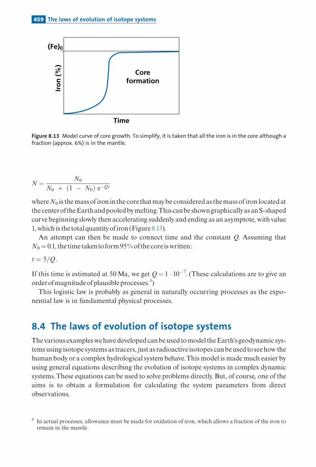
N ¼ N0

N0 þ 1 � N0ð Þ e�Qt

whereN0 is themassof iron in the corethatmaybe consideredas themassof iron locatedatthe centeroftheEarthandpooledbymelting.This canbeshowngraphicallyasanS-shapedcurvebeginning slowly then accelerating suddenlyand ending as an asymptote, withvalue1,which is the totalquantityof iron (Figure8.13).An attempt can then be made to connect time and the constant Q. Assuming that

N0¼ 0.1, the timetakentoform95%ofthe core iswritten:

t ¼ 5=Q:

If this time is estimated at 50Ma, we get Q¼ 1 �10�7. (These calculations are to give anorderofmagnitudeofplausibleprocesses.4)This logistic law is probably as general in naturally occurring processes as the expo-

nential law is in fundamental physical processes.

8.4 The laws of evolution of isotope systems

Thevarious exampleswehave developed canbeused tomodel theEarth’sgeodynamic sys-temsusing isotope systemsas tracers, just as radioactive isotopes canbeused to seehow thehumanbodyor a complex hydrological systembehave.This model is mademuch easier byusing general equations describing the evolution of isotope systems in complex dynamicsystems.These equations can be used to solve problems directly. But, of course, one of theaims is to obtain a formulation for calculating the system parameters from directobservations.

Time

Coreformation

(Fe)0

Iro

n (

%)

Figure 8.13 Model curve of core growth. To simplify, it is taken that all the iron is in the core although afraction (approx. 6%) is in the mantle.

4 In actual processes, allowance must be made for oxidation of iron, which allows a fraction of the iron toremain in the mantle.

459 The laws of evolution of isotope systems

8.4.1 Equation for the evolution of radiogenic systems:Wasserburg’s equations

Let us begin with a straightforward case. A reservoir exchanges radioactive and referenceisotopes 87Rb, 87Sr, 86Sr, notated r, i, j, with the outside.Wenotatewhat enters the reservoir( )# andwhat exits ( )".The decay constant is notated l.The £uxes are notated r

�; i�

; j�

. We canthenwrite the equations:

dr

dt¼ �lr � Hrð Þ" þ r

�ð Þ#:

di

dt¼ lr � Gið Þ" þ i

�� #:

dj

dt¼ � Gjð Þ" þ j

�� #:

Wehavewrittenwhat leaves the reservoirasproportional towhat is in the system, assum-ing thefactor is the samefor (i) and (j), that is, assumingnoisotopefractionationoccurs.Letus combine these equations to bring out the ratios (r/j) and (i/j), that is, by our notations(87Rb/86Sr) and (87Sr/86Sr):

dr

j

� �dt¼ r

j

� �dr

r dt� dj

j dt

� ¼ r

j

� ��l � H þ

r�ð Þ#rþ G

j�� #

j

" #:

Wehavenotateddr/dtanddj/dtas r�and j�

respectively,as isoftendone.Bybringingout(r/j)#,that iswhat leaves the system,andbywriting:

_rð Þ#r¼

_rð Þ#j�� #

j�� #

rð Þ ;

then bymultiplying the bracketed termby (r/j), and noting r/j¼�, as is our standard prac-tice,weget:

d�

dt¼ G � Hð Þ � l½ �� þ �ex � �ð Þ

j�� #

j:

Doing the same calculations for (i/j)¼�gives:

d�

dt¼ l� þ �ex � �ð Þ

j�� #

j:

Bynoting _j� �#=j¼L(t) andG�H¼F,we¢nallyobtain:

d�

dt¼ F � l½ � � þ �ex � �ð Þ L tð Þ

d�

dt¼ l� þ �ex � �ð Þ L tð Þ:

2664


TheseareWasserburg’s equations (seeWasserburg,1964) (Figure 8.14).Let us make a few remarks about them. Notice that parameter Fmaybe either positive

or negative depending on whether the daughter element ‘‘leaks’’ from the reservoir faster(G>H) or more slowly (G<H) than the parent element.These are two concatenated (andnot paired) equations. One (�) describes the system’s chemical evolution. It thereforeinvolves achemical fractionation factor for thematerial leaving the reservoir.Theother (�)involves twoterms, one for radioactive decayl�and theother formixing (�ex��). Solvingthe problem entails integrating the ¢rst and then the second.These are very general equa-tions applying to all systems ^ minerals, rocks, atmosphere,mantle ^ and thus canbeusedinbothgeochronologyand isotope geology.Notice that L(t) is the inverse of residence time1=R tð Þð Þ.

8.4.2 The steady-state box model

Thismodel is developedhere throughtwo examples.

dμdt

= – λ + F( ) μ + μ ex –μ( ) Ldαdt

= λ μ + α ex –μ( ) L

L =

Closedenvironment

Mixing andfractionation

Mixing

Open environmentwith loss

andfractionation

Generalequation

0 L= 0F = 0

dμ = –λ μdαdt

= λ μ

dμdt

= – λ + F( ) μ

dαdt

= λ μ

λ smallF

λ smallF = 0 dμ

dt= – F μ + μ ex –μ( ) L

dαdt

= α ex –α( ) L

dμdt

= μ ex –μ( ) L

dαdt

= α ex – α( ) L

Figure 8.14 Schema explaining the generality of Wasserburg’s equations. Most of the basic equationswe have used for radioactive–radiogenic systems can be found in his figure.


Exercise

Take a reservoir into which flows material from a single external source with a constant

chemical and isotopic composition over time (�ex and �ex) and a constant flow rate. Let us

assume that the reservoir attains a steady state.

What is the residence time if we suppose the reservoir is well mixed (that is, having a

homogeneous isotope composition �)?

AnswerWe find:�l� þ �ex � �ð Þ 1=R ¼ 0 and l� þ �ex � �ð Þ 1=R ¼ 0.

This gives:

R ¼ 1

l�ex

�� 1

� �:

We find quite simply the residence time calculated for the 14C/C ratio of the deep ocean if

�¼ 14C/C and �ex is the 14C/C ratio of the surface water in equilibrium with the atmosphere.

The time can be computed from the simple radioactive decay �¼�ex e–lt or �ex¼� elt. If we

develop the Taylor series and keep the first two terms:

�ex ¼ �ðlþ lt Þt ¼ 1

l�ex

�� 1

� �:

As for the isotope ratio:

R ¼ 1

l� � �ex

�

� �¼ �:

This is the expression of the model age of the reservoir, so we are back to the equality:

residence time¼model age.

(This is not so for 14C because the product 14N is drowned in normal 14N.)

Exercise

The 87Sr/86Sr isotope composition of sea water is the result of erosion of the continents and of

exchange at the mid-ocean ridges where Sr from the mantle is injected into sea water, but

also of alteration by volcanoes in subduction zones and oceanic islands. We denote the

isotope ratios of the continental crust ( )cc and of the mantle ( )m: (�Sr)cc¼ 0.712,

(�Sr)m¼ 0.703, (�Sr)sea water¼ 0.709.

What are the relative flows Lcc and Lm, given that the residence time of Sr is RSr¼ 4 � 106

years and that a steady state is attained in the ocean? If we know the ratio of the mass of river

water inflow to the mass of the ocean is 3 � 10�5, calculate the river/ocean Sr concentration

ratio.

AnswerWe write the simplified Wasserburg equations, as there is no radioactive decay or growth

term:

�Srcc � �Sr

water

� �L cc þ �Sr

m � �Srwater

� �L m ¼ 0:

We obtain:


L m

L cc¼ �Sr

cc � �Srwater

�Srwater � �Sr

m

� �¼ 0:5:

We also have:

L m þ L cc ¼ 1=R ¼ 2:5 � 10�7 yr�1;

hence Lcc¼ 1.66 � 10�7 yr�1 and Lm¼ 0.83 � 10�7 yr�1.

We then have:

L cc ¼river water flow� Sr concentration in rivers

ocean mass� Sr concentration in ocean;

hence

Sr concentration in rivers

Sr concentration in sea water¼ 0:005:

Exercise

Suppose the variation in continental Sr input into sea water follows the tectonic cycle with a

period of 100 Ma. Suppose also that this fluctuation occurs with constant isotope composi-

tion for the continental crust and mantle. By how much would the 87Sr/86Sr isotope ratio of

sea water as indicated by limestone be offset?

AnswerIt would not be offset. See Section 8.4.

8.4.3 The non-steady state

Naturally enough, in the general case, all of the parameters are a function of time: F(t),�ex(t),and L(t). It is not generally very easy to integrate these equations when we are unaware apriori of the formofvariation of the various parameters. It can easilybe seen that ifwewriteL(t)¼ 0, that is, ifwe are in the case of evolutionwith no input fromoutside, withoutmixing,we come back to the equations developed in Chapter 3 for open geochronological systemswithF(t) taking the formofan episodic orcontinuous loss.Conversely, ifwe cancel the termsofradioactivedecay,wearedealingwithpuremixing.Themixingequationweareusedtois:

�M ¼ �1xþ �2ð1� xÞ:

Letus assume that�M¼� (tþ 1) and�¼� (t) are the twovalues ofthe reservoir at (tþ 1)and (t). Ifwemodify the value � of the reservoir by adding a corresponding quantity to �xfromtheoutside, then:

�2ðtþ 1Þ ¼ ð�1 � �ðtÞÞ�xþ �ðtÞ;

therefore


�ðtþ 1Þ � �ðtÞ ¼ �� ¼ ð�1 � �Þ�x:

This is the expression fordi¡erentialmixingalreadyestablished.Wasserburg’s equations maybe extended to several reservoirs exchanging material and

with di¡erent isotope ratios.Foreach reservoir,wewrite:

d�

dt¼

Xi¼ni¼1

Fi � l

" #� þ

Xi¼ni¼1

�i � �ð Þ Li

d�

dt¼ l� þ

Xi¼ni¼1

�i � �ð Þ Li

8>>>><>>>>:whereFi is the totaloffractionation factors.

There are as many pairs of equations as there are reservoirs and we switch thereforeto amatrix systemwhose solution is complex and generally di⁄cult to solve because thereare many unknown, time-dependent parameters. However, in some cases it can beapproximated.

Exercise

A simplified three-reservoir system is considered: the lower mantle (lm), upper mantle (um),

and atmosphere (a) with transfers of radiogenic rare gases described by the transfer coeffi-

cients shown in Figure 8.15, plus a chemical fractionation (F ) during the transition from the

upper mantle to the atmosphere.

Write the matrix equation describing the dynamic evolution of the system. It is assumed

there is no reverse transfer either from the atmosphere to the upper mantle or from the upper

Atmosphere

Uppermantle

Lowermantle Mlm

Mum

aLum a

Llm um

•

•

Figure 8.15 The simplified three-reservoir system.


to the lower mantle and that transfer from the lower to upper mantle does not involve

chemical fractionation.

Keep the � and � notations as used in this book.

AnswerThe subscripts to denote the reservoirs are a¼ atmosphere, um¼upper mantle, lm¼ lower

mantle.

� ¼�a

�um

�lm

24

35 and � ¼

�a

�um

�lm

24

35:

d�

dt¼ T �

��

where T �

�is the transfer matrix of �.

d�

dt¼ T�½ � � þ l�

where T �½ � is the transfer matrix of �.

T �

�¼

0 0 00 � l � F þ L lm!umð Þ þL lm!um

0 0 �l

�� and T�½ � ¼

�L um!a þL um!a 00 �L lm!um þL lm!um

0 0 0

��:

This exercise is designed to show how complex the problems are, but also to prepare

readers for the mathematical processing used in research work.

The cases of stable isotopes may also be covered by generalizing from these equations

somewhat, but in this case, we must consider a combined formula because while there is no

radioactive decay to be considered there is isotope fractionation.

By positing �s = stable isotope ratio, we can write:

d�s

dt¼ F i �s þ

Xi

Fex �is � �s

� �L i tð Þ

where Fi is fractionation internal to the system and Fex is fractionation for elements entering

the system. This equation shows how worthwhile but how difficult it is to use stable isotopes

in balance processes, because it involves an extra parameter – fractionation.

E X A M P L E

The crust–mantle system

Consider the continental crust-mantle system. Let us take the example of exchange between

the continental crust and the mantle. Let us keep our conventional use of � and �; let us take

the 87Rb/86Sr system to clarify things. To simplify, we shall assume that the � values for the

mantle are much lower than those for the continental crust.

The evolution of the crust is written:

d�cc

dt¼ �l�cc þ �#m � �cc

� �L


d�cc

dt¼ þl�cc þ �#m � �cc

� �L

where �#m and �#m indicate the transfer from the mantle to the continental crust.

It is assumed, to simplify matters, that L is constant over time. Integrating the equation in �

gives:

�cc ¼�m# L

l þ L1� e� lþLð Þth i

þ �0cc e� lþLð Þt ;

�0cc being the initial value for continental crust. Notice straight away that since

1 – eðlþL Þt eðlþL Þt ¼ 1, this is a mixing-type equation whose proportions are time dependent.

If x(t)¼ eðlþL Þt , we get:

�cc ¼�m# L

l þ L1� x tð Þð Þ þ �0cc x tð Þ;

from which L is of the order of 0.3 � 10�9 yr�1 and l¼ 0.0142 � 10�9 yr�1. Therefore�m#L

l þ L� �m#, which is much less than �cc and is ignored.

d�cc

dt¼ l �0cc e� lþLð Þt þ �m# � �cc

� �L :

Integrating gives:

�cc ¼ �cc þ l�0cc t½ � e� lþLð Þt þ �m# 1 � e� lþLð Þth i

:

Notice that this is a mixing equation between the evolution of isolated continental crust

(whose evolution is written �0ccþ l�0cc t) and the �m# coming from the mantle, which we

have taken to be constant, the terms of the mix being weighted by e–Lt (Figure 8.16).

0.760

0.750

0.740

0.730

0.720

0.710

0.700

3 2 1 0

Time (Ga)

(λ + L) = 0.3.10–9 yr –1

(λ + L) = 0.2.10–9 yr –1

87Sr

/86 S

r

Closed co

ntinenta

l cru

st

Figure 8.16 Results of the exercise above with �cc¼ 0.1.


Exercise

Write the Wasserburg equation for stable isotopes (e.g., 18O/16O) in d notation.

Answer

dddt¼ d � Ds"� �

þX

d i � Di#� �

Li tð Þ:

The �i# are isotopic fractionations during transfer from sources to the exterior, and �s" is

the isotopic fractionation towards the reservoir, the Li(t) are identical to those already

defined.

Exercise

Consider the sea water reservoir. The concentration of elements is determined by the influx of

products of erosion from rocks of continental and mantle origin.

We assume the equation governing this composition is written for element i:

dC i

dt¼ J i tð Þ � ki Ci

and that 1/ki¼ Ri is the residence time of element i. It is assumed that:

Ji (t)¼ J0iþbi sin !t

where ! ¼ 2p=104 yr�1.

For all elements we take J0¼Gi¼ 1.

Calculate the curves of variation of Ci for the elements Nd: Ri¼ 1000 years, Os: Ri¼ 30 000

years, and Sr: Ri¼ 2 � 106 years.

AnswerSee Figure 8.10.

8.4.4 Statistical evolution of radiogenic systems: mixing times

Here, we shall again take the example of the upper mantle, butour approach is more gen-eral and could apply to other convective geochemical reservoirs like the ocean, the atmo-sphere, or a river.We are nowgoing to lookat not just the averagevalues although theyareessential, but also the statistical distributions that can be described summarily by theirdi¡erent statistical parameters: a mean, a dispersion, an asymmetry, etc. (Alle' gre andLewin,1995).As said, the upper mantle is subjected to two types of antagonistic processes. First,

chemical fractionation (extraction of oceanic crust, extraction of continental crust, rein-jection of material via subduction phenomena). These processes result in chemical andisotopicheterogeneitywiththehelpoftime.Second, it is alsosubjectedtomixingprocessesrelated to mantle convection, which stretch the rocks, break them, fold them, and mixthem.There are alsomelting processeswhich also tend tohomogenize the isotope ratios ofthesourcezone.


Thus two types ofphenomena are opposed: those producing chemical and isotopic dis-persion and those which mix, homogenize, and tend to destroy the heterogeneities (seeMcKenzie,1979;Alle' greetal.,1980;Alle' greandTurcotte,1986).

Exercise

Suppose that unaltered oceanic crust, altered oceanic crust, and fine sediments plunge

into the mantle in a subduction zone. The extreme compositions for the 87Rb–86Sr

system for unaltered oceanic crust are �Sr0 ¼ 0.7025 and �Rb/Sr¼ 0.1 and for the sediments

�SrS ¼ 0.712 and �Rb/Sr¼ 0.4. The altered crust has intermediate values: �Sr

0A¼ 0.705 and

�Rb/Sr¼ 0.2.

What will be the dispersion of the � isotope ratios if this subducted oceanic crust is in the

mantle without mixing for 1 billion years?

AnswerDispersion can be evaluated by calculating the two extreme values. We obtain 0.703 92 and

0.717 68 respectively for the pieces of unaltered oceanic crust and for the sediments. The

difference �� is 0.0137, while the difference in �Sr values during subduction was 0.0095.

We can also calculate it directly:

D� ¼ ðD�Þinitial þ lðD�ÞT :

Hence � indicates the dispersion: ��¼ 0.0095þ 0.004 26¼ 0.0137. (Notice that given the

value of l, the term –l� is negligible in the evolution of �.)

Suppose now that these subduction products are subjected to multiple mixing processes in

the mantle. Suppose the result is that ��i, which was 0.3 initially, becomes ��¼ 0.1, and that

�� becomes 0.003.

The effectiveness of this isotopic mixing can be measured by the ratio 30/137¼ 0.21

whereas chemical mixing, measured by 0.1/0.3¼ 0.33, is not quite as effective. (This reason-

ing probably fails to allow for isotope exchange, but it is a first approximation.)

Letustrytogeneralizethesesimple examples.WearelookingtowriteanequationderivedfromWasserburg’s, but dealing with distributions. So we take as variables not the averagevalues, which has already been done, but the dispersions. Dispersion can be measured bythe standard deviation (or by the standard deviation of two extreme values, which, as weknow,areaboutthreetimes the standarddeviation) (Alle' greandLewin,1995).

Thefollowingequation canbederivedfromWasserburg’s equationsbynotingdispersionhi.Thus we note the dispersion of isotope ratios �h i and the dispersion of chemical ratios�h iwith subscripts�ex (external),�i (internal),�ex (external), and�i (internal).

d �ih idt¼ �exh i � �ih i½ � L�M �ih i

where the term ^l �ih i is ignored (Figure8.17).Thenew term thathasbeen introduced isM �ih i, the termofhomogenizationofthemix-

ture;Mhas the dimensionofthe inverseofatimeweshall callmixing time (�). It is the timeit takes to reduce the dispersion �h i by a factor (e) exponential. Suppose a steady state isattained, then:


�ih i ¼ �exh i L

M þ L:

ReplacingLby its expression1/residence time¼ 1/RandM¼ 1/� , gives:

�ih i ¼ �exh i �

R þ �:

If � <<R,mixing isveryrapidand �ih i ! 0when �!0.This is intuitive enough. Ifmixingtime is short, homogenization is vigorous and therefore the standard deviation is zero. If,conversely, � >>R, homogenization is poor and �ih i ¼ �exh i: dispersion in the reservoir isthesameas that introduced.For isotope ratios, the equation for standarddeviation iswritten:

d �ih idt¼ �exh i � �h i

2Rþ l

2�h i � �h i

2�:

Letusmaketworemarks.The¢rst, apurelyarithmeticalone, is thatthe factor1/2 is foundeverywhere because the calculation made rigorously with variance is d �h i2=dt ¼ 2 �h i d �h i=dt.The second andmore important remark is that in the terms of creation

N

μ

N

α

N

μ

N

α

N

α

α

N

μ

μ

N

α

N

μ

MIXTURE

Figure 8.17 Diagram explaining how the histograms for parameters � and � evolve during thegeodynamic cycle. Values of � and � are represented by histograms. We start on the left with adispersed histogram for � and �. In the mantle the spread is reduced by mixing but supplementary � isheated by radioactivity (white in histogram). Then melting reduces the spread of� but not so much as for�.


ofheterogeneity, there is the termofexternal inputs in �exh ibut also aterm from the disper-sionof �h ivalues.

Ifl is small enough forus tospeakofasteadystate,weget:

�ih i ¼ l �ih iR�

R þ �

� �þ �exh i �

R þ �

� �:

If � is small comparedwithR (veryactivemixing):

�ih i � l �ih i � þ �exh i �

R

� �:

If � is very small, �ih i in themixture is also very small.Themantle is therefore isotopicallyveryhomogeneous (small standarddeviation).

If � ismuch larger thanR,mixing ispoor, and the standarddeviation is equal to the stan-darddeviationof�multipliedbyresidence time,plus the deviationof input fromoutside.

Letus examinethe relationship theremaybebetweenthedispersionof �h iandthatofthe�h i values.We saw when calculating the least squares that in an (�, �) plot, the statisticalslope equals �h i/ �h i (the ratio of standard deviations multiplied by the correlation coe⁄-cientofapproximately1).

Ifwe plot the points representing mantle rockon an (�, �) diagram, e.g., (143Nd/144Nd,147Sm/144Nd) or (87Sr/86Sr, 87Rb/86Sr), the slope of the straight line yielding an apparentage is equal to the ratiosofthestandarddeviationsofthe (�) and (�) values.

If it canbe considered that �exh i is about constant (this is notthe absolutevalueof�exbutits dispersion!), the slope is equal toR�=ðRþ �Þ(Figure 8.18).

If � is small compared with R, the slope is about equal to (�), the mixing time.Unfortunately it is not easy to estimate �h i, the‘‘chemical’’dispersion ratio, because chemi-cal fractionation in basalt formation greatly increases �h i dispersion even if it can beassumedthat �h iremains thesame.

Theslopeofthe correlationdiagramobtained forbasalts is thenwritten:

DR�

R þ �

� �

α

μ~ 6<μ>~

~ 6<α

>~

slope = λ RτR+τ

Figure 8.18 Mantle isochrons constructed from dispersion of (�) and (�). The slope gives a pseudo-age(Rþ � ).


whereD is acoe⁄cientgreater thanunityandratherdi⁄cultto estimate.This di⁄cultymakes the exercise somewhat hazardous. Letus attempt it none the less to

get an orderof ideas. An isochron hasbeen obtainedon oceanicbasalt by the147Sm/144Ndmethodwithanageof350Ma.Letus admitavalue forDbetween2and1.5andavalueofR¼ 1Gafor the residence time

oftheuppermantle.Thisgives amixing time � of530Ma.Another wayofaddressing the issue is touse the 4He/3He ratios (Alle' greetal.,1995).The

ratios measured in MORB are the outcome of mixing of OIB ratios which represent anunmixedmantle.AsFigure6.18 shows, the 4He/3HeratiosofMORBseemtobeslightlydis-persedaroundtheaverageforOIB.Suppose, as a ¢rst approximation, that the dispersion caused by the decayofuranium is

faithfully re£ectedby theOIB.We canthenwrite:

�MORBh i�OIBh i ¼

�

R þ �:

With �OIBh i¼ 45 � 103 and �MORBh i¼ 9, and still takingR¼ 1Ga,we¢nd � ¼ 0.25Ga.Weare still dealing with the same order ofmagnitude but this time it is for the mantleMORBsourcealone.There are two important points to remember from this section. If we have an (�, �) rela-

tion for present-day rocks from the mantle, therefore from a convecting reservoir, theslope does not measure the age of some sudden past event but is related to the physicalcharacteristics of the reservoir: mixing time and residence time.Wemust henceforth setabout describing geochemical reservoirs not by average parameters but by distributionsandevenbyregionalizeddistributions.Work isunderway inthis direction.Notice too that anumberofconclusions aboutthe casewhere externaldispersion £uctu-

ates with sin !t can be applied to the dispersion equation.The decisive parameter in thiscaseisL=ðM þ LÞ, thatis:�=ðR þ �Þ.Dispersionwillbeinphaseoroutofphase,dampedorundamped,dependingonthevalueofthisparameter.Weleavethismatter to readerswhowish to investigate this area further and who, for this purpose, may transpose the calcula-tionsalreadysetout.

Exercise

It is supposed that the 4He/3He ratios of the upper mantle vary as a result of dis-

persion introduced by variable ratios of the OIBs and of mantle convection (see Allegre

et al., 1995). The values measured on OIB by 4He/3He ratios are: mean 93 390, dispersion

45 330.

The values measured for MORB of the North Atlantic ridges are: mean 8938, dispersion

9330.

Calculate the upper mantle mixing time in the North Atlantic, given that the residence time

for the Atlantic lithosphere is 1.3 Ga.

The residence time of the North Pacific upper mantle is 582 Ma and the dispersion 3000.

Calculate the mixing time of these two zones of the upper mantle.

AnswerThe mixing times for the two upper mantle zones are 300 Ma for the North Atlantic and 40 Ma

for the North Pacific.


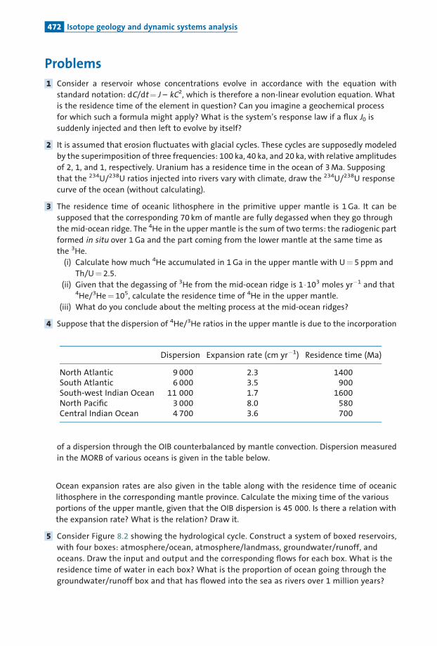
Problems

1 Consider a reservoir whose concentrations evolve in accordance with the equation with

standard notation: dC/dt¼ J – kC2, which is therefore a non-linear evolution equation. What

is the residence time of the element in question? Can you imagine a geochemical process

for which such a formula might apply? What is the system’s response law if a flux J0 is

suddenly injected and then left to evolve by itself?

2 It is assumed that erosion fluctuates with glacial cycles. These cycles are supposedly modeled

by the superimposition of three frequencies: 100 ka, 40 ka, and 20 ka, with relative amplitudes

of 2, 1, and 1, respectively. Uranium has a residence time in the ocean of 3 Ma. Supposing

that the 234U/238U ratios injected into rivers vary with climate, draw the 234U/238U response

curve of the ocean (without calculating).

3 The residence time of oceanic lithosphere in the primitive upper mantle is 1 Ga. It can be

supposed that the corresponding 70 km of mantle are fully degassed when they go through

the mid-ocean ridge. The 4He in the upper mantle is the sum of two terms: the radiogenic part

formed in situ over 1 Ga and the part coming from the lower mantle at the same time as

the 3He.

(i) Calculate how much 4He accumulated in 1 Ga in the upper mantle with U¼ 5 ppm and

Th/U¼ 2.5.

(ii) Given that the degassing of 3He from the mid-ocean ridge is 1�103 moles yr�1 and that4He/3He¼ 105, calculate the residence time of 4He in the upper mantle.

(iii) What do you conclude about the melting process at the mid-ocean ridges?

4 Suppose that the dispersion of 4He/3He ratios in the upper mantle is due to the incorporation

of a dispersion through the OIB counterbalanced by mantle convection. Dispersion measured

in the MORB of various oceans is given in the table below.

Ocean expansion rates are also given in the table along with the residence time of oceanic

lithosphere in the corresponding mantle province. Calculate the mixing time of the various

portions of the upper mantle, given that the OIB dispersion is 45 000. Is there a relation with

the expansion rate? What is the relation? Draw it.

5 Consider Figure 8.2 showing the hydrological cycle. Construct a system of boxed reservoirs,

with four boxes: atmosphere/ocean, atmosphere/landmass, groundwater/runoff, and

oceans. Draw the input and output and the corresponding flows for each box. What is the

residence time of water in each box? What is the proportion of ocean going through the

groundwater/runoff box and that has flowed into the sea as rivers over 1 million years?

Dispersion Expansion rate (cm yr�1) Residence time (Ma)

North Atlantic 9 000 2.3 1400South Atlantic 6 000 3.5 900South-west Indian Ocean 11 000 1.7 1600North Pacific 3 000 8.0 580Central Indian Ocean 4 700 3.6 700


REFERENCES

Chapter 1

Aldrich,L.T.,Doak, J. B., andDavis,G. (1953).Theuseof ion exchange columns inuniversalanalysisforagedetermination.Am.J.Sci.251,377^80.

Arriens,P. A.andCompston,W. (1968).Amethodfor isotopic ratiomeasurementby voltagepeakswitchingand its applicatonwithdigital input. Int.J.Spectrom.IonPhys.1,471^81.

Aston,F.W. (1919).Apositive rayspectograph.Phil.Mag. (Series6)38,707^14.Bainbridge,K.T.andJordan,E. B. (1936).Mass spectrumanalysis.HarvardUniv.,Je¡ersonPhys.

Lab.Contrib. (Series 2)3,No.2.Becquerel,H. (1896a).Surlesradiations invisibles e¤ misesparphosphorescence.ComptesRend.Acad.

SciencesParis122,420.Becquerel,H. (1896b). Surles radiations invisibles e¤ misespar les corpsphosphorescents.Comptes

Rend.Acad.SciencesParis122,501.Becquerel,H. (1896c).Surlesradiations invisibles e¤ misesparles sels d’uranium.ComptesRend.Acad.

SciencesParis122,689.Beiser,A. (1973).ConceptsofModernPhysics.NewYork:McGraw-Hill.Burch¢eld, J.D. (1975).LordKelvinandtheAgeoftheEarth.London:Macmillan.Curie,P. (1902a). Sur laconstante detemps caracteristiquede ladisparitionde laradioactivite¤ induite

par le radiumdansune enceinte ferme¤ e.ComptesRend.Acad.SciencesParis135,857.Curie,P. (1902b).NobelLecture (6June1902). InNobelLectures, Stockholm:RoyalSwedishAcademy.Curie,P.andLaborde,A. (1903).Surlachaleurde¤ gage¤ espontane¤ mentparles selsderadium.Comptes

Rend.Acad.SciencesParis136,673^5.Ingram,M.G.andChupka,W.A. (1953). Surface ionisationsourceusingmultiple¢laments.Rev.Sci.

Instrum.24,518^20.Mattauch,R.H. (1934).U« bereineneuenMasspektrographen.Z.Physik89,786^95.Nier,A.O. (1940).Amass spectrometer for routine isotopeabundancemeasurements.Rev.Sci.

Instrum.11, 212^16.Rutherford,E. andSoddy,F. (1902a).The causeandnatureofradioactivity.Pt. I.Phil.Mag. (Series6)

4,370^96.Rutherford,E.andSoddy,F. (1902b).The causeandnatureofradioactivity.Pt. II.Phil.Mag. (Series6)

4,569^85.Rutherford,E. andSoddy,F. (1902c).The radioactivityofthoriumcompounds.Pt. II.The causeand

natureofradioactivity.J.Chem.Soc.Lond. 81,837^60.Rutherford,E. andSoddy,F. (1903).Radioactive change.Phil.Mag. (Series6)5,576^91.Thomson, J. J. (1914).Raysofpositive electricity.Proc.Roy.Soc.Lond. (Series 5)89,1^20.Wasserburg,G. J.,Papanastassiou,D.,Nerow,E.V.,andBauman,C.A. (1969).Aprogrammable

magnetic¢eldspectrometerwithonlinedataprocessing.Rev.Sci.Instrum.40,288^95.

Chapter 2

Aldrich,L.T. andNier,A. O. (1948a).Argon40 inpotassiumminerals.Phys.Rev.74,876^7.Aldrich,L.T. andNier,A. O. (1948b).Theoccurrenceof 3He in naturalsourcesof helium.Phys.Rev.

74,1590^4.Aldrich,L.T.,Herzog,L.,Holve,W.,Witting,F., andAhrens,L. (1953).Variation in isotopic

abundanceofstrontium.Phys.Rev. 86,631^4.Barbo,L. (2003).LesBecquerel:UneDynastiedesScienti¢ques. Paris:Belin.Bateman,H. (1910). Solutionofasystemofdi¡erential equationsoccurring inthetheoryofradio-

active transformations.Proc.CambridgePhil.Soc.15,423^7.Birck, J. L. andAlle' gre,C. J. (1985).Evidencefor thepresenceof 53Mn in the earlysolar-system.

Geophys.Res.Lett.12,745^8.Harper,C. L. andJacobsen,S. B. (1994). Investigationof182Hf^182Wsystematics.LunarPlan.Sci.

25,509^10.Hirt,B.,Tilton,G.R.,Herr,W., andHo¡meister,W. (1963).Thehalf-lifeof187Re. InGeiss, J.

andGoldberg,E.D. (eds.)EarthScienceandMeteorites,Amsterdam:North-Holland,pp.273^80.Ivanovich,M. (1982).Uraniumseries disequilibriaapplication ingeochronology. In Ivanovich,M.

andHarmon,R. (eds.)UraniumSeriesDisequilibrium:ApplicationtoEnvironmentalProblems,Oxford,UK:OxfordUniversityPress, pp.56^78.

Je¡rey,P.M.andReynolds,J.H.(1961).Originofexcess129Xeinstonemeteorites.J.Geophys.Res.,66,3582^3.

Kelly,W.R.andWasserburg,G. J. (1978).Evidencefor the existenceof 107Pd inthe earlySolarSystem.Geophys.Res.Lett.5,1079^82.

Kuroda,P.K. (1960).Nuclear ¢ssion in the earlyhistoryoftheEarth.Nature187,36^8.Lee,D.-C.andHalliday,A.N. (1995).Hafnium^tungsten chronometryandthetimingofterrestrial

coreformation.Nature378,771^4.Lee,T., Papanastassiou,D.A., andWasserburg,G. J. (1977).Aluminium-26 in the earlysolar-system:

fossilor fuel?Astrophys.J.(Lett.)211,L107^10.Leighton,R. B. (1959).PrinciplesofModernPhysics.NewYork:McGraw-Hill.Lin,Y.,Guan,Y.,Leshin,L. A.,Ouyang,Z.,andWang,D.(2005).Short-livedchlorine-36 inaCa-and

Al-rich inclusion fromtheNingqiangcarbonaceous chondrite.Proc.NatlAcad.Sci.USA102,1306^11.

Luck, J.M.,Birck, J. L., andAlle' gre,C. J. (1980).187Re^187Os systematics inmeteorites: earlychronologyofthe solarsystemandtheageofthegalaxy.Nature283, 256^9.

Lugmair,G.W.andMarti,K. (1977). Sm^Nd^Putimepieces in theAngradosReismeteorite.EarthPlanet.Sci.Lett.35, 273^84.

Lugmair,G.W., ScheininN. B., andMarti,K. (1975). Search forextinct146Sm.Pt. I.The isotopicabundanceof143Ndinthe Juvinasmeteorite.EarthPlanet.Sci.Lett.27, 9479^84.

McKeegan,K.D.,Chaussidon,M., andRobert,F. (2000). Incorporationofshort-lived10Be inacalcium^aluminium-rich inclusion fromtheAllendemeteorite.Science289,1334^7.

Nakaı, S., Shimizu,H., andMasuda,A. (1986).Anewgeochronometerusing lanthanum-138.Nature320,433^5.

Nielsen,S. G.,Rehka« mper,M., andHalliday,A.N. (2006).Largethallium isotopicvariation in ironmeteorites andevidenceforlead-205 inthe earlysolarsystem.Geochim.Cosmochim.Acta70,2643^57.

Notsu,K.,Mabuchi,H.,Yoshioka,O.,Matsuda, J., andOzima,M. (1973).Evidenceofthe extinctnuclide146Sm in‘‘Juvinas’’achondrite.EarthPlanet.Sci.Lett.19, 29^36.

Patchett,P. J. andTatsumoto,M. (1980a).Lu^Hftotal rocks isochron foreucritemeteorites.Nature288, 263^7.

Patchett,P. J. andTatsumoto,M. (1980b).A routinehigh-precisionmethod forLu^Hf isotopegeochemistryandchronology.Contrib.Mineral.Petrol.75, 263^7.

474 References

Price,P. B.andWalker,R.M.(1962).Observationoffossilparticletracks innaturalmicas.Nature196,732^4.

Ramsay,W.andSoddy,F. (1903).Gasesoccluded in radiumbromide,Nature68, 246.Reynolds, J.H. (1960).Determinationoftheageofthe elements.Phys.Rev.Lett.4,8^10.Rutherford,E. (1906).RadioactiveTransformations.NewYork:CharlesScribner’s Sons.Schonbachler,M.,Rehka« mper,M.,Halliday,A.N., etal. (2002).Niobium^zirconiumchronometry

andearlySolarSystemdevelopment.Science295,1705^8.Shukolyukov,A.andLugmair,G.W. (1993).Live iron-60 inthe earlysolarsystem.Science259,

1138^42.Srinivasan,G.,Ulyanov,A.A.,andGoswami,J.N.(1994).41CaintheearlySolarSystem.Astrophys.J.

(Lett.)431, L67^70.

Chapter 3

Ahrens,L.H. (1955). ImplicationsoftheRhodesiaagepattern.Geochim.Cosmochim.Acta8,1^15.Aldrich,L.T. andNier,A.O. (1948a).Argon-40 inpotassiumminerals.Phys.Rev.74,876^7.Aldrich,L.T. andNier,A.O. (1948b).Theoccurrenceof 3He in naturalsourcesofhelium.Phys.Rev.

74,1590^4.Aldrich,L.T. andWetherill,G.W. (1958).Geochronologybyradioactivedecay.Ann.Rev.NuclearSci.

8, 257^98.Alle' gre,C. J. (1964).Ge¤ ochronologie:del’extensiondelame¤ thodede calculgraphique concordiaaux

mesuresd’a“ ges absolus e¡ectue¤ s a' l’aidedude¤ se¤ quilibre radioactif ^ cas desmine¤ ralisationssecondairesd’uranium.ComptesRend.Acad.SciencesParis259,4086^9.

Alle' gre,C. J. (1967).Me¤ thodedediscussionge¤ ochronologique concordiage¤ ne¤ ralise¤ e.EarthPlanet.Sci.Lett.2,57^66.

Alle' gre,C. J. (1968). 230Thdatingofvolcanic rocks: acomment.EarthPlanet.Sci.Lett.5, 209^10.Alle' gre,C. J. andCondomines,M. (1976).Fine chronologyofvolcanicprocessesusing 238U/230Th

systematics.EarthPlanet.Sci.Lett.28,395^406.Alle' gre,C. J. andDars,R. (1966).Chronologieau rubidium^strontiumetgranitologie.Geol.

Rundschau8^55, 226^37.Alle' gre,C. J. andMichard,G. (1964). Sur les discordancesdesa“ gesobtenuspar lesme¤ thodesau

strontiumeta' l’argon.ComptesRend.Acad.SciencesParis259,4313^16.Alle' gre,C. J.,Albare' de,F.,Gru« nenfelder,M.,andKo« ppel,V.(1974).238U/206Pb^235U/207Pb^232Th/208Pb

zircongeochronology inAlpineandnon-Alpine environments.Contrib.Mineral.Petrol.43,163^244.

Alle' gre,C. J.,Birck, J.-L.,Capmas,F., andCourtillot,V. (1999).AgeoftheDeccanTrapsusing187Re^187Os systematics.EarthPlanet.Sci.Lett.170,197^204.

Berger,G.W.andYork,D. (1981).Geothermyfrom40Ar/39Ardating experiments.Geochim.Cosmochim.Acta45,795^811.

Blichert-Toft, J.,Albare' de,F., andKornpolst, J. (1999).Lu^Hf isotope systematicsofgarnetpyroxenites fromBeni-Bousera,Morocco: implication frombasaltorigin.Science283,1303.

Bre¤ vart,O.,Dupre¤ , B., andAlle' gre,C. J. (1986).Lead^leadageofthekomatiitic lavas andlimitationsonthe structureand evolutionofthePrecambrianmantle.EarthPlanet.Sci.Lett.77, 293^303.

Castaing,R.andSlodzian,G. (1962).Optique corpusculaire: premiers essais demicroanalysepare¤ mission ioniquesecondaire.J.Microsp.395,185^9.

Compston,W. and Je¡rey, P.M. (1959).Anomalous common strontium ingranite.Nature184,1792^3.

Compston,W.,Williams, I. S., andMeyer,C. (1984).U^Pbgeochronologyofzircons from lunarbreccia73217usingasensitivehighmass-resolution ionmicroprobe.J.Geophys.Res.89 (Suppl.),B525^34.

475 References

Davis,G.andAldrich,L.T. (1953).Determinationoftheageoflepidolitesby themethodof isotopedilution.Bull.Geol.Soc.Amer.64,379^80.

DeSigoyer, J.,Chavagnac,V.,Blichert-Toft, J., etal. (2000).Dating the Indian continentalsubductionandcollisional thickening inthenorth-westHimalayamultichronologyoftheMorai eclogites.Geology28,487^90.

Hamilton,P. J.,Evensen,N.M.,O’Nions,R.K., andTarney, J. (1979). Sm^NdsystematicsofLewisiangneisses: implications for theoriginofgranulites.Nature277, 25^8.

Hanson,G.N.andGast,P.W. (1967).Kinetic studies in contactmetamorphiczones.Geochim.Cosmochim.Acta31,1119^53.

Harrison,T.M.andMcDougall, I. (1981).Excess 40Ar inmetamorphicrocksfromBrokenHill.EarthPlanet.Sci.Lett.55,123^49.

Hart,S. R. (1964).Thepetrologyand isotopic^mineral age relationsofacontact zone intheFrontRange,Colorado.J.Geol.72,493^525.

Hirt,B.,Tilton,G.R.,Herr,W., andHo¡meister,W. (1963).Thehalf lifeof 187Re. InGeiss, J.andGoldberg,E. (eds.)EarthScienceandMeteorites,Amsterdam:North-Holland,pp.273^80.

Hohenberg,C.M.,Podosek,F., andReynolds, J. H. (1967).Xenonîodine: sharp isochronism inchondrites.Science156, 233^6.

Hohenberg,C.M.,Brazzle,R.H., Pravdivtseva,O., andMeshik,A. P. (1998). Iodine^xenon.Proc.IndianAcad.Sci.107 (no.4),1^11.

Kober,B. (1986).Whole-grain evaporation for 207Pb/206Pb-age investigationson singlezirconsusingadouble-¢lamentthermal ion source.Contrib.Mineral.Petrol.93,482^90.

Ko« ppel,V. andGru« nnenfelder,M. (1971).Astudyof inheritedandnewly formed zircons fromparagneisses andgranitized sedimentsoftheStrona-Ceneri zone (SouthernAlps).Schweiz.Miner.Petrog.Mitt.51,387^411.

Koztolanyi,C. (1965).Nouvelleme¤ thoded’analyse isotopiquedes zirconsa' l’e¤ tatnaturel.ComptesRend.Acad.SciencesParis260,5849^51.

Lancelot, J. R.andAlle' gre,C. J. (1974).Originofcarbonatiticmagmainthe lightofthePbÛ^Thisotopesystem.EarthPlanet.Sci.Lett.22, 233^8.

Lanphere,M.A.,Wasserburg,G. J.,Albee,A. L., andTilton,G.R. (1964).Redistributionofstrontiumandrubidium isotopes duringmetamorphism,WorldBeatercomplex,PanamintRange,California. InCraig,H.,Miller, S. L., andWasserburg,G. J. (eds.), IsotopicandCosmicChemistry,Amsterdam:North-Holland,pp.269^320.

Lee,D.-C.andHalliday,A.N. (2000).Hf^Winternal isochron forordinarychondritesandthe initial182Hf180Hfofthesolarsystem.Chem.Geol.169,35^43.

Luck, J.M.,Birck, J. L., andAlle' gre,C. J. (1980).187Re^187Os sytematics inmeteorites: earlychronologyofthe solarsystemandtheageofthegalaxy.Nature283, 256^9.

Lugmair,G.W.andMarti,K. (1977). Sm^Nd^Putimepieces in theAngradosReismeteorite.EarthPlanet.Sci.Lett.35, 273^84.

Manhe' s,G.,Alle' gre,C. J.,Dupre¤ ,B., andHamelin,B. (1980).Leadisotopic studyofbasicûltrabasiclayercomplexes: speculationsabouttheageoftheEarthandprimitivemantle characteristics.EarthPlanet.Sci.Lett.47,370^82.

Merrihue,C. andTurner,G. (1966). Potassiumârgondatingbyactivationwith fastneutrons.J.Geophys.Res.71, 2852^7.

Michard,A.andAlle' gre,C. J. (1979).Astudyoftheformationandhistoryofapieceofcontinental crustbythe87Rb^87Srmethod: the caseoftheFrenchorientalPyrenees:Contrib.MineralPetrol.50,257^85.

Nicolaysen,L. O. (1961).Graphic interpretationofdiscordantagemeasurementsonmetamorphicrocks.Ann.N.Y.Acad.Sci.91,198^206.

Nier,A.O. (1939).Theisotopic constitutionofradiogenicleadsandthemeasurementofgeologictime.Pt. II.Phys.Rev.55,153^63.

476 References

Notsu,K.,Mabuchi,H.,Yoshioka,O.,Matsuda, J., andOzima,M. (1973).Evidenceofthe extinctnuclide146Sm in‘‘Juvinas’’achondrite.EarthPlanet.Sci.Lett.19, 29^36.

Patchett,P. J. (1983). ImportanceoftheLu^Hf isotopic system instudiesofplanetarychronologyandchemical evolution.Geochim.Cosmochim.Acta47,81^91.

Patchett,P. J. andTatsumoto,M. (1980).A routinehigh-precisionmethod forLu^Hf isotopegeochemistryandchronology.Contrib.Mineral.Petrol.75, 263^7.

Reynolds, J.H. (1960).Determinationoftheageofthe elements.Phys.Rev.Lett.4,8^10.Shukolyukov,Y., Ashkinadze, G., and Komarou, A. (1974). A new Xes^Xen neutron induced

method of mineral dating. Dokl. Akad. Nauka USSR 219, 952^4. (in Russian)Shukolyukov, A., Meshik, A., Meshik, D., Krylov, D., and Pravdivtseva, O. (1994). Current status

of Xes^Xen dating. InMatsuda, X. (ed.)Noble Gas Geochemistry and Cosmochemistry,pp.125^00.

Steiger,R.H.andWasserburg,G. J. (1966). Systematics in the 208Pb^232Th, 207Pb^235U, 206Pb^238Usystems.J.Geophys.Res.71,6065^90.

Teitoma,A.W.,Clarke,C. J., andAlle' gre,C. (1974). Spontaneous¢ssion ^ neutron¢ssion in xenon: anewtechniquefordatinggeological events.Science189,878^80.

Tilton,G.R. (1960).Volumedi¡usionasamechanism fordiscordant leadages.J.Geophys.Res.65,2933^45.

Tilton,G. etal. (1958). Isotopic compositionanddistributionoflead,uraniumandthorium inaPrecambriangranite.Bull.Geol.Soc.Amer.66,1131^48.

Turner,G. (1968).Thedistributionofpotassiumandargon in chondrites. InAhrens,L.H. (ed.)OriginandDistributionoftheElements,NewYork:Pergamon,pp.387^97.

Vervoort, J. D., Patchett, P. J.,Gehrels,G. E., andNutman,A. P. (1996).Constraintson earlyEarthdi¡erentiation fromhafniumandneodymium isotopes.Nature379,412^14.

Wasserburg,G. J. (1985). Short-lived nuclei in the earlysolar system. InBlack,D. C. andMatthews,M. S. (eds.)ProtostarsandPlanets II,Tucson,AZ:UniversityofArizonaPress,pp.703^37.

Wasserburg,G. J. andHayden,R. J. (1955).Time intervalbetween nucleogenesis andtheformationofmeteorites.Nature176,130^1.

Wetherill,G.W. (1956).Discordanturanium^leadages.Trans.Am.Geophys.Union37,320^7.Wetherill,G.W.,Tilton,G.R.,Davis,G. L.,Hart,S. R., andHopson,C.A. (1966).Agemeasurements

intheMarylandPiedmont.J.Geophys.Res.71, 2139^55.Wetherill, G.W., Davis, G. L., and Lee-Hu, C. (1968). Rb^Sr measurements on whole rocks and

separated minerals from the Baltimore Gneiss, Maryland. Bull. Geol. Soc. Amer. 79,757^62.

York,D.,Hall,C.M.,Yanese,Y.,Hanese, J. A., andKenyon,W. J. (1981).40Ar/39Ardatingofterrestrialmineralswithacontinuous laser,Geophys.Res.Lett. 8,1136^8.

Zinner,E. (1996).Presolarmaterial inmeteorites. InBernatowicz,T. J. andZinner,E. (eds.)Astrophysical ImplicationsoftheLaboratoryStudyofPresolarMaterial,NewYork:AmericanInstituteofPhysics,59^72.

Chapter 4

Arnold, J. R. (1956).Beryllium-10producedbycosmic rays.Science124,584^5.Atkinson,R.andHoutermans,F.G. (1929).ZurFragederAufbaumo« glichkeitderElemente in

Sternen.Z.Physik54,656^65.Bard,E.,Hamelin,B., Fairbanks,R.G., andZindler,A. (1990).Calibrationofthe14C timescaleover

thepast 30 000yearsusingmass spectrometricU^Thages fromBarbados corals.Nature345,405^10.

Broecker,W. S. andLi,Y.H. (1970). Interchangesofwaterbetweenthemajoroceans.J.Geophys.Res.75,354^55.

477 References

Broecker,W. S.,Gerard,R.,Ewig,M., andHeezen,B. C. (1960).Natural radiocarbon intheAtlanticOceanJ.Geophys.Res.65, 2903^31.

Burbidge,E.M.,Burbidge,G.R.,Fowler,W.A.,andHoyle,F. (1957).Synthesisoftheelements instars.Rev.Mod.Phys.29,547^647.

Gamow,G. (1946).ExpandingUniverseandtheoriginofelements.Phys.Rev.70,572^5.Harrison,T.M.andMcDougall, I. (1981).Excess 40Ar inmetamorphicworks fromBrokenHill.

EarthPlanet.Sci.Lett.55,123^49.Honda,M.andArnold J. R. (1964).E¡ectsofcosmic raysonmeteorites.Science143, 203^212.Kieser,W. E.,Beukens,R. P.,Kilius,L. R.,Lee,H.W., andLitherland,A. E (1986). Isotrace

radiocarbon analysis: equipment and procedures. Nucl. Instrum. Meth. Phys. Res. B 15,718^21.

Lal,D. (1988). Insitu-produced cosmogenic isotopes in terrestrial rocks.Ann.Rev.EarthPlanet.Sci.16,355^88.

Lal,D.andPeters,B. (1967).Cosmicray-producedradioactivityontheEarth. InHandbookofPhysics,vol.46/2,Berlin: Springer-Verlag, pp.551^612.

Lal,D.,Malhotra,K., andPeters,B. (1958).Ontheproductionofradioisotopes in theatmospherebycosmicradiationandtheirapplicationtometeorology.J.Atmos.Ten.Phys.12,306^28.

Lee,D.-C.andHalliday,A.N. (2000).Hf^Winternal isochron forordinarychondritesandthe initial182Hf/180Hfofthe solarsystem.Chem.Geol.169,35^43.

Libby,W. F. (1946).Atmospherichelium-3andradiocarbon fromcosmic radiation.Phys.Rev.69,671^672.

Libby,W. F. (1970).Ruminationson radiocarbondating. InOlsson, I. U. (ed.)RadiocarbonVariationsandAbsoluteChronology,NewYork: JohnWiley, pp.629^40.

Libby,W. F.,Anderson,E. C., andArnold, J. R. (1949).Agedeterminationbyradiocarbon content:world-wideassayofnatural radiocarbon.Science109, 227^8.

Lin,Y.,Guan,Y.,Leshin,L.A.,Ouyang,Z., andWang,D. (2005).Short-livedchlorine-36 inaCa- andAl-rich inclusion fromtheNingqiangcarbonaceous chondrite.Proc.NatlAcad.Sci.USA102,1306^11.

Marti,K. (1982).Krypton-81datingbymass spectrometry. InLloyd,A. (ed.)NuclearandChemicalDatingTechniquesinInterpretingtheEnvironmentalRecord,AmericanChemicalSociety,pp.129^00.

McKeegan,K.D.,Chaussidon,M., andRobert,F. (2000). Incorporationofshort-lived10Be inacalcium^aluminium-rich inclusion fromtheAllendemeteorite.Science289,1334^7.

Merrill P.W. (1952).Technetium inthe stars.Science115,484^5.Oeschger,H. (1982).The contributionofradioactiveandchemicaldating totheunderstandingofthe

environmentalsystem. InLloyd,A. (ed.)NuclearandChemicalDatingTechniquesinInterpretingtheEnvironmentalRecord,AmericanChemicalSociety, pp.5^12.

O’Nions,R.K.,Franck,M., vonBlanckenburg,F., andLing,H.-F. (1998). Secular variationofNdandPb isotopes in ferromanganese crusts fromtheAtlantic, IndianandPaci¢cOceans.EarthPlanet.Sci.Lett.155,15^28.

Paneth,F.,Raesbeck,P. andMayne,K., (1952).Helium-3contentandageofmeteorites.Geochim.Cosmochim.Acta2,300^3.

Staudacher,T. andAlle' gre,C. J. (1993).AgesofthesecondcalderaofPitonde laFournaisevolcano(Re¤ union)determinedbycosmic rayproduced 3Heand21Ne.EarthPlanet.Sci.Lett.119,395^404.

Stuiver,M. (1965).Carbon-14contentof18th- and19th-centurywood:variations correlatedwithsunspotactivity.Science149,533^5.

Voshage,H.andHintenberger,H. (1960).Cosmogenicpotassium in ironmeteorites andcosmic rayexposureage. InSummerCourseonNuclearGeology, Pisa:Laboratorio diGeologicaNucleare,pp.81^235.

478 References

Chapter 5

Alle' gre,C. J.,Manhe' s,G., andGo« pel,C. (1995).TheageoftheEarth.Geochim.Cosmochim.Acta59,1445^56.

Barbo,L. (1999).PierreCurie:LeRe“ veScienti¢que. Paris:Belin.Barrell, J. (1917).Rhythmsandthemeasurementofgeologic time.Bull.Geol.Soc.Amer.28,745^50.Berger,G.W. (1975).40Ar/39Arstepheatingofthermallyoverprintedbiotite, hornblendeand

potassium feldspar fromEldora (Colorado).EarthPlanet.Sci.Lett.26,387^90.Bevington,P. RandRobinson,K. (2003).DataReductionandErrorAnalysisforPhysicalSciences.

NewYork:McGraw-Hill.Boltwood,B. B. (1907).Ontheultimatedisintegrationproductsoftheradioactiveelements.Pt. II.The

disintegrationproductsofuranium.Am.J.Sci.23,78^88.Bre¤ vart, O.,Dupre¤ , B., andAlle' gre, C. J. (1986). Lead^ lead age ofkomatiitic lavas and limitations

on the structure and evolution of the Precambrian mantle.Earth Planet. Sci. Lett.77,293^303.

Burch¢eld,H. P. (1975).LordKelvinandtheAgeoftheEarth.London:Macmillan.Clayton,D.D. (1968).PrinciplesofStellarEvolutionandNucleosynthesis.NewYork:McGraw-Hill.Crumpler,T. B. andYeo, J. H. (1940).ChemicalComputationandErrors.NewYork: JohnWiley.Dalrymple,B. (1991).TheAgeoftheEarth. Stanford,CA:StanfordUniversityPress.Dupre¤ , B. andArndt,N.T. (1987)Komatiites: te¤ moinspre¤ cieuxpour retracer l’e¤ volutiondumanteau.

Bull.Soc.Ge¤ ol.Fr. III,1125^32.Eve,A. S (1939).Rutherford.NewYork:Macmillan.Gerling,E.K. (1942).AgeoftheEarthaccording to radioactivitydata.Dokl.Akad.NaukaUSSR

34^9, 259^72.Go« pel,C.,Manhe' s,G., andAlle' gre,C. J. (1994).U^Pbsystematicsofphosphates fromequilibrated

ordinarychondrites.EarthPlanet.Sci.Lett.121,153^71.Hallam,A. (1983).GreatGeologicalControversies.Oxford,UK:OxfordUniversityPress.Hamilton,P. J.,Eversell,N.M.,O’Nions,R.K.,Smith,H. S., andErlank,A. J. (1979).Sm^Nddating

ontheOuverwachtgroupofvolcanoes, SouthAfrica.Nature279, 298.Hart,S. R.,Davis,G. L.,Steiger,R.H.,andTilton,G.R. (1968).Acomparisonofthe isotopicmineral

agevariationsandpetrological changes inducedbycontactmorphism. InHamilton,E. I. andFarquhar,R.M. (eds.)RadiometricDatingforGeologists,NewYork:Wiley Interscience,pp.73^110.

Hohenberg,C.M. (1969).Radioisotopesandthehistoryofnucleosynthesis inthegalaxy.Science166,212^15.

Holmes,A. (1911).Theassociationof leadwithuraniumrockminerals and its applicationtothemeasurementofgeological time.Proc.Roy.Soc.Lond.A85, 248^50.

Holmes,A. (1927).TheAgeoftheEarth:AnIntroductiontoGeologicalIdeas.London:ErnestBenn.Holmes,A. (1946).AnestimateoftheageoftheEarth.Nature157,680^4.Houtermans,F.G. (1946).Die Isotopen-Ha« u¢gkeiten imnatu« rlichenBleiunddasAlterdesUrans.

Naturwissenschaften33,185^7.Hutchinson,R. (2004).Meteorites.Cambridge,UK:CambridgeUniversityPress.Kanber,B. S. andMoorbath,S. (1998). InitialPboftheAmitsoqgneiss revisited: Implication for the

timingofearlyArchean crustal evolution inWestGreenland.Chem.Geol.15,19^41.Lee,D.-C.andHalliday,A.N. (2000).Hf^Winternal isochron forordinarychondrites andthe initial

182Hf/180Hfofthesolar system.Chem.Geol.169,35^43.Luck, J.M.,Birck, J. L., andAlle' gre,C. J. (1980).187Re^187Os sytematics inmeteorites: early

chronology of the Solar System and the age of the Galaxy. Nature 283, 256^9.Ludwig,K.R. (1999).UsingIsoplot/ExVersion2.01:AGeochonologicalToolk itforMicrosoftExcel.

Berkeley,CA:GeochronologicalCenter.

479 References

Michard-Vitrac,A.,Lancelot, J.,Alle' gre,C. J., andMoorbath,S. (1977).U^PbageonsinglezirconsfromEarlyPrecambrian rocksofWestGreenlandandtheMinnesotaRiverValley.EarthPlanet.Sci.Lett.35,449^53.

Moorbath,S. andTaylor, P. N. (1981). Isotopic evidencefromcontinentalgrowth inthePrecambrian.InKro« ner,A. (ed.)PrecambrianPlateTectonics,Amsterdam:Elsevier, pp.49^62.

Moorbath,S.,Taylor,P. N., andJones,N.W. (1986).Dating theoldestterrestrial rocks: factand¢ction.Chem.Geol.57 (1^2),63^86.

Moorbath,S.,Whitehouse,M. J., andKanber,B. S. (1997).ExtremeNdisotopeheterogeneity intheearlyArchean: factor¢ction? Illustrations fromnorthernCanadaandWestGreenland.Chem.Geol.135, 213^31.

Nier,A.O.(1938).Theisotopeconstitutionofcalcium,titanium,sulphurandargon.Phys.Rev.53,282^6.Nier,A. O.,Thompson,R.W., andMurphy,B. (1941).The isotopic compositionofleadandthe

measurementofgeologic timePt. III.Phys.Rev.60,112^16.Nutman,A. P.,McGregor,V. B., Friend,C. R. L.,Benson,V. C., andKinny,P.D. (1996).The Itsaq

gneiss complexofsouthernWestGreenland: theWorld’smostextensive recordofearlycrustalevolution,3900^3600Ma.Precamb.Res.78,1^39.

Patterson,C. C. (1953).The isotopic compositionofmeteoritic^basaltic andoceanic leadandtheageoftheEarth.Proc.Conf.NuclearProcessesinGeology,WilliamBay,36^40.

Patterson,C. C. (1956).Ageofmeteorites andtheEarth.Geochim.Cosmochim.Acta10, 230^7.Reid,M.,Coath,C.,Harrison,M., andMcKeegan,K. (1997).Prolongedresidencetimes for the

youngest rhyolitesassociatedwithLongValleyCaldera: 230Th^238Uionmicroprobedatingofyoung zircons.EarthPlanet.Sci.Lett.150, 27^39.

Strutt,R. J.(1908).Ontheaccumulationofheliumingeologicaltime.Proc.Roy.Soc.Lond.A76,88^101.Tatsumoto,M.,Knight,R. J., andAlle' gre,C. J. (1973).Timedi¡erences in theformationofmeteorites

asdeterminedfromthe ratiooflead-207 to lead-206.Science180,1279^83.Taylor,R. S.(1982).PlanetaryScience:ALunarPerspective.Houston,TX:LunarandPlanetaryInstitute.Wasson, J. (1984).Meteorites.NewYork:W.H.Freeman.Wasserburg,G. J.,Busso,M.,Gallino,R., andNollett,K.M. (2006). Short-livednuclei in the early

solarsystem:possibleAGBsources.Nucl.PhysA.777,5^69.Wendt, J., andCarl,C. (1991).Thestatisticaldistributionofthemeansquaredweighteddeviations.

Chem.Geol. 86, 275^85.Wood, J. (1968).MeteoritesandtheOriginofthePlanets.NewYork:McGrow-Hill.York,D. (1969).Leastsquares¢ttingofa straight linewith correlatederrors.EarthPlanet.Sci.Lett5,

320^4.Zindler,A. (1982).NdandSr isotopic studiesofkomatiitesandselected rocks. InArndt,N.T. and

Nisbet,E.G. (eds.)Komatiites,London:GeorgeAllen andUnwin, pp.103^22.

Chapter 6

Aldrich,L.T. andNier,A. O. (1948).TheoccurrenceofHe-3 in naturalsourcesofhelium.Phys.Rev.74,1590^4.

Alle' gre,C. J. (1982).Chemicalgeodynamics.Tectonophysics81,109^32.Alle' gre,C. J. (1987). Isotopegeodynamics.EarthPlanet.Sci.Lett. 86,175^203.Alle' gre,C. J. (1997).Limitationonthemass exchangebetweentheupperand lowermantle: the

evolving regimeoftheEarth.EarthPlanet.Sci.Lett.150,1^6.Alle' gre,C. J. andBenOthman,D. (1980).Nd^Sr isotopic relationship ingranitoid rocksand

continental crustdevelopment: achemicalapproachtoorogenesis.Nature286,335^342.Alle' gre,C. J. andCondomines,M. (1976).Fine chronologyofvolcanicprocessesusing 238U^230Th

systematics.EarthPlanet.Sci.Lett.28,395^406.Alle' gre,C. J. andCondomines,M. (1982).Basaltgenesis andmantle structurestudiedthroughTh-

isotopicgeochemistry.Nature299, 21^4.

480 References

Alle' gre,C. J. andJaupart,C. (1985).Continental tectonicsandcontinentalkinetics.EarthPlanet.Sci.Lett.74,171^86.

Alle' gre,C. J. andLuck, J.M. (1980).Osmium isotopesaspetrogenetic andgeological tracers.EarthPlanet.Sci.Lett.48,148^54.

Alle' gre,C. J. andMoreira,M. (2004).Raregas systematicsandtheoriginofoceanic islands: thekeyroleofentrainmentatthe670kmboundarylayer.EarthPlanet.Sci.Lett.228,85^92.

Alle' gre,C. J.andRousseau,D.(1984).ThegrowthofthecontinentsthroughgeologicaltimestudiedbyNdisotopeanalysisofshales.EarthPlanet.Sci.Lett.67,19^34.

Alle' gre,C. J. andTurcotte,D. L. (1985).Geodynamicalmixing inthemesosphereboundarylayersandtheorigin ofoceanic islands.Geophys.Res.Lett.12, 207^10.

Alle' gre,C. J. andTurcotte,D. L. (1986). Implicationsofatwo-componentmarble-cakemantle.Nature323,123^7.

Alle' gre,C. J.,BenOthman,D.,Polve¤ ,M., andRichard, P. (1979).TheNd^Sr isotopic correlation inmantlematerialsandgeodynamic consequences.Phys.EarthPlanet. Int.19, 293^306.

Alle' gre,C. J.,Bre¤ vard,O.,Dupre¤ ,B.,andMinster,J. F. (1980). Isotopicandchemicale¡ectsproducedinacontinuouslydi¡erentiatingconvectingEarthmantle.Phil.Trans.Roy.Soc.LondA297,447^77.

Alle' gre,C. J.,Hart,S. R., andMinster, J. F. (1983a).The chemicalstructureofthemantle determinedby inversionof isotopic data. I.Theoreticalmethod.EarthPlanet.Sci.Lett.66,177^90.

Alle' gre,C. J.,Hart,S. R., andMinster, J. F. (1983b).The chemical structureofthemantle determinedby inversionof isotopic data. II.Numerical experiments anddiscussion.EarthPlanet.Sci.Lett.66,191^213.

Alle' gre,C. J., Staudacher,T., Sarda,P. andKurz,M. (1983c).Constraintson evolutionofEarth’smantle fromraregas systematics.Nature303,762^6.

Alle' gre,C. J.,Manhe' s,G., andGo« pel,C. (1995).TheageoftheEarth.Geochim.Cosmochim.Acta59,1445^56.

Alle' gre,C. J.,Hofmann,A., andO’Nions,R.K. (1996).Theargon constraintsonmantle structure.Geophys.Res.Lett.23 (24),3555^7.

Alvarez,L. andCornog,R. (1939).Heliumandhydrogenofmass3.Phys.Rev.56,613^15.Armstrong,R. L. (1981).Radiogenic isotopes: the case forcrustal recyclingonanear steady-state

continentalgrowthearth.Phil.Trans.Roy.Soc.Lond.A301,443^72.Bennett,V. C. andDePaolo,D. J. (1987).Proterozoic crustal historyoftheWesternUnitedStates as

determinedbyneodymium isotopicmapping.Bull.Geol.Soc.Amer.99,674^85.BenOthman,D.,Polve¤ ,M., andAlle' gre,C. J. (1984).Nd^Sr isotope compositionofgranuliteand

constraintsonthe evolutionofthe lowercontinental crust.Nature307,510^15.Blichert-Toft, J. andAlbare' de,F. (1997).TheLu^Hf isotopegeochemistryofchondrites andthe

evolutionofthemantle^crustsystem.EarthPlanet.Sci.Lett.148, 243^58.Bowen,N. (1928).TheEvolutionoftheIgneousRocks. Princeton,NJ:PrincetonUniversityPress.Boyet,M.andCarlson,R. (2005).142Ndevidenceforearly (>4.53Ga)globaldi¡erentiationofthe

silicateEarth.Science 309,576^80.Caro,G.,Bourdon,B.,Birck, J.-L., andMoorbath,S. (2003).146Sm^142NdevidencefromIsua

metamorphosedsediments forearlydi¡erentiationoftheEarth’smantle.Nature423,428^32.Clarke,W.,Beg,M., andCraig,H. (1969).Excess 3He in thesea: evidencefor terrestrialprimoridal

helium.EarthPlanet.Sci.Lett.6, 213^30.Compston,W.andWilliams, I. S. (1984).U^Pbgeochronologyofzircons from lunarbrecchia 73217

usingasensitivehighmass resolution ionprobe.J.Geophys.Res. 89 (suppl.B),525^34.Condomines,M.andSigmarson,O. (1993).Whyaresomanyarcmagmas close to 238U^230Th

radioactive equilibrium?Geochim.Cosmochim.Acta57,4491^7.Condomines,M.,Hemond,C., andAlle' gre,C. J. (1988).U^Th^Raradioactive disequilibriaand

magmaticprocesses.EarthPlanet.Sci.Lett.31,369^85.Craig,H.andLupton, J. (1976).Primordial neon, heliumandhydrogen inoceanicbasalts.Earth

Planet.Sci.Lett.31,369^85.

481 References

Damon,P. E. (1954).Anabundancemodel for lead isotopesbasedonthe continuous creationoftheEarth’s sialic crust.Trans.Am.Geophys.Union.35,631^42.

Damon,P. E. andKulp, J. L. (1958). Inertgases andthe evolutionoftheatmosphere.Geochim.Cosmochim.Acta13, 280^300.

DePaolo,D. J. (1981a).AneodymiumandstrontiumisotopicstudyoftheMesozoic calcalkalinegraniticbatholithoftheSierraNevadaandPeninsular range,Calif.J.Geophys.Res.86,10470^88.

DePaolo,D. J. (1981b).Neodymium isotopes in theColoradoFrontRangeandcrust^mantleevolution in theProterozoic.Nature291,193^6.

DePaolo,D. J. (1981c). ImplicationofcorrelatedNdandSr isotopicvariations for the chemicalevolutionofthe crustandthemantle.EarthPlanet.Sci.Lett.43, 201^11.

DePaolo,D. J. (1988).NeodymiumIsotopeGeochemistry.Heidelberg: Springer-Verlag.DePaolo,D. J. andWasserburg,G. J. (1976a).Ndisotopicvariationsandpetrogeneticmodels.

Geophys.Res.Lett.3, 249^52.DePaolo,D. J. andWasserburg,G. J. (1976b). Inferences aboutmagmasources andmantle structure

fromvariationsofneodymium-143/neodymium-144.Geophys.Res.Lett.3,743^6.Dietz,R. S. (1963).Continentandoceanevolutionbyspreadingofthe sea£oor.Nature190,854^7.Doe,B. R. (1970).LeadIsotopes.Heidelberg: Springer-Verlag.Doe,B. R. andZartman,R. E. (1979).Plumbotectonics I: thePhanerozoic. InBarnes,H. L. (ed.)

GeochemistryofHydrothermalOreDeposits,NewYork: JohnWiley, pp.22^70.Dupre¤ , B. andAlle' gre,C. J. (1980).Pb^Sr^Ndisotopic correlationandthe chemistryoftheNorth

Atlanticmantle.Nature286,17^22.Dupre¤ , B. andAlle' gre,C. J. (1983).Pb^Sr isotopevariation in IndianOceanbasalts andmixing

phenomena.Nature303,142^6.Elliot,T.,Plank,T.,Zindler,A.,White,W., andBourdon,B. (1997).Elementtransport fromslabto

volcanic frontattheMarianaarc.J.Geophys.Res.12,1491^4.Farmer,G. L.andDePaolo,D. J. (1983).OriginofMesozoicandTertiarygraniteintheWesternUnited

Statesand implications for pre-Mesozoic crustalstructure. I.NdandSr isotopic studies inthegeoclineoftheNorthernGreatBasin.J.Geophys.Res. 88,3379^402.

Fukao,Y.,Obayashi,H., Inoue,H., andNeuberg,M. (1992). Subduction slabs stagnantin themantletransition zone.J.Geophys.Res.97,4809^22.

Gangarz,A. J. andWasserburg,G. J. (1977). InitialPboftheAmitsoqgneiss,WestGreenland, andimplications for theageoftheEarth.Geochim.Cosmochim.Acta41,1283^301.

Gast,P.W. (1960).Limitationsonthe compositionoftheuppermantle.J.Geophys.Res.65,1287^90.Gast,P.W. (1968).Trace element fractionationandtheoriginoftholeiitic andalkalinemagmatypes.

Geochim.Cosmochim.Acta32,1057^87.Gast,P.W.,Tilton,G.R., andHedge,C. E. (1964). Isotopic compositionofleadandstrontiumfrom

AscensionandGough Island.Science145,1181^88.Gaudette,H.,Vitrac-Michard,A., andAlle' gre,C. J. (1981).NorthAmericanPrecambrianhistory

recordedinasinglesample:highresolutionU^PbsystematicsofthePotsdamsandstonedetritalzircons,NewYorkState.EarthPlanet.Sci.Lett.54, 248^60.

Geiss, J. (1954). Isotopicanalysisofordinarylead.Z.Naturforsch.4/9, 218.Go« pel,C.,Alle' gre,C. J.,andRongHuaXu.(1984).LeadisotopicstudyoftheXiagazophiolite (Tibet):

theproblemofthe relationshipbetweenmagmatites (gabbros, dolerites, lavas) andtectonites(harzburgites).EarthPlanet.Sci.Lett.69,301^10.

Grand, S., vanderHilst,R., andWidiyautaro,S. (1997).Globalseismic tomography: a snapshotofconvection intheEarth.GSAToday7,1^17.

Hamelin,B. andAlle¤ gre,C. J. (1985).Large scale regionalunits in thedepleteduppermantle revealedbyan isotope studyofSouthwest IndianRidge.Nature315,52^5.

Hamelin,B.,Dupre¤ , B., andAlle' gre,C. J. (1984).Lead^strontium isotopicvariationsalong theEastPaci¢cRiseandtheMidAtlanticRidge: acomparative study.EarthPlanet.Sci.Lett.67,340^50.

482 References

Hamelin,B.,Dupre¤ ,B.,andAlle' gre,C. J. (1986).Pb^Sr^NdisotopicdataoftheIndianOceanRidge:newevidenceof large-scalemappingofmantleheterogeneities.EarthPlanet.Sci.Lett.76,288^98.

Harper,C. L. andJacobsen,S. B. (1992).Evidencefromcoupled147Sm^143Ndand146Sm^142Ndsystematics for veryearly (4.5Gyr)di¡erentiationoftheEarth’smantle.Nature360,728^32.

Harrison,T.M.,Blichert-Toft, J.,Mu« ller,W., etal. (2005).HeterogeneousHadeanhafnium: evidenceofcontinental crustat 4.4 to4.5Ga.Science 310,1950^70.

Hart,S.R.(1984).Alarge-scaleisotopeanomalyinthesouthernhemispheremantle.Nature309,753^7.Hart, S. R. (1988).Heterogeneousmantle domains: signatures, genesis andmixingchronologies.

EarthPlanet.Sci.Lett.90, 273^96.Hart, S. R.andZindler,A. (1986). In searchofabulkEarth composition.Chem.Geol.57, 247^67.Hart, S. R., Schilling, J. G., andPowell, J. L. (1973).Basalts fromIcelandandalong theReykjanes

Ridge: strontium isotopegeochemistry.Nature246,104^7.Hauri,E.H.andHart, S. R. (1993).Re^Os isotopesystematicsofHIMUandEMIIoceanic island

basalts fromtheSouthPaci¢cOcean.EarthPlanet.Sci.Lett.114,353^71.Hawkesworth,C. J. (1979).143Nd/144Nd,87Sr/86Srandtrace elementcharacteristicsofmagmasalong

destructiveplatemargins. InAtherton,M. P. andTarney, J. (eds.)OriginofGraniteBatholiths,Sevenoaks,UK:Shiva,pp.76^89.

Hawkesworth,C. J. andKemp,A. I. (2006).Usinghafniumandoxygen isotopes in zircons tounravelthe recordofcrustal evolution.Chem.Geol.226,144^7.

Hofmann,A. (1988).Chemicaldi¡erentiationoftheEarth: the relationshipbetweenmantle,continental crustandoceanic crust.EarthPlanet.Sci.Lett.90, 297^304.

Hofmann,A.andHart, S. R. (1978).Anassessmentof local andregional isotopic equilibrium inthemantle.EarthPlanet.Sci.Lett.38,44^62.

Hofmann,A.andWhite,W.M. (1982).Mantleplumes fromancientoceanic crust.EarthPlanet.Sci.Lett.57,421^36.

Hofman,A., Jochum,K., Seufert,M., andWhite,W.M. (1986).NdandPb inoceanicbasalts: newconstraintsonmantle evolution.EarthPlanet.Sci.Lett.79,33^45.

Holmes,A. (1946).AnestimateoftheageoftheEarth.Nature157,680^4.Houtermans,F.G. (1946).Die Isotopenha« u¢gkeiten imnatu« rlichenBleiunddasAlterdesUrans.

Naturwissenschaften33,185^7.Hurley,P.M.andRand,R. (1969).Pre-drift continental nuclei.Science164,1229^42.Hurley,P.M.,Hughes,H.,Faure,G.,Fairbairn,H.W., andPinson,W.H. (1962).Radiogenic

strontium-87modelofcontinent formation.J.Geophys.Res.67,5315^34.Jacobsen,S. (1988). Isotopic constraintson crustalgrowthandrecycling.EarthPlanet.Sci.Lett.90,

315^29.Jacobsen,S. andWasserburg,G. J. (1979).Themeanageofmantleandcrustal reservoirs.J.Geophys.

Res.84,7411^27.Jacobsen,S. andWasserburg,G. J. (1980).Sm^Ndisotopic evolutionofchondrites.EarthPlanet.Sci.

Lett.50,139^55.Kleine,T.,Munster,C.,Mezger,K., andPalme,H. (2002).Rapidaccretionandearlycoreformation

onasteroids andtheterrestrialplanets fromHf^Wchronometry.Nature418, 952^5.Kuroda,P.K. (1960).Nuclear¢ssion inthe earlyhistoryoftheEarth.Nature187,36^8.Kurz,M.andJenkins,W. J. (1981).Thedistributionofhelium inoceanicbasaltglasses.EarthPlanet.

Sci.Lett.53,41^54.Kurz,M., Jenkins,W. J., andHart, S. R. (1982).Helium isotopic systematicsofoceanic islands and

mantleheterogeneity.Nature297,43^7.Lambert,D.D.,Morgan,W. J.,Walker,R. J., etal. (1989).Rhenium^osmiumand

samarium^neodymium isotopic systematicsoftheStillwaterComplex.Science244,1169^74.Ledent,D., Patterson,C., andTilton,G.R. (1964).Agesofzirconandfeldsparconcentrates from

NorthAmericanbeachandriver sands.J.Geol.72,112^22.

483 References

Lupton, J. E. andCraig,H. (1975).Excess 3He inoceanicbasalts: evidencefor terrestrialprimordialhelium.EarthPlanet.Sci.Lett.26,133^9.

Mamyrin,B. A.andTolstikhin, I. (1984).HeliumIsotopesinNature.Amsterdam:Elsevier.Mamyrin,B. A.,Tolstikhin, I.,Anufriev,G. S., andKamensky, I. L. (1969).Anomalous isotopic

compositionofhelium involcanicgases.Dokl.Akad.NaukaUSSR184,1197^9.McCulloch,M.andWasserburg,G. J. (1978). Sm^NdandRb^Srchronologyofcontinental crust

formation.Science200,1003^11.McKenzie,D. (1979).Finite deformationduring £uid£ow.Geophys.J.Roy.Astron.Soc.58,

689^705.McKenzie,D. (1985). 230Th^238Udisequilibriumandthemelting processbeneaththe ridgeaxis.

EarthPlanet.Sci.Lett.72,149^57.Montelli,R.,Nolet,G.,Dahlen,A., etal. (2004).Finite frequency tomographyreveals avarietyof

plumes inthemantle.Science303,338^43.Moorbath,S. andTaylor, P. N. (1981). Isotopic evidencefromcontinentalgrowth inthePrecambrian.

InKro« ner,A. (ed.)PrecambrianPlateTectonics,Amstendam:Elsevier, pp.491^525.Moreira,M.andAlle' gre,C. J. (1998).Helium^neonsystematics andthe structureofthemantle.

Chem.Geol.147,53^9.Moreira,M.,Kunz,M., andAlle' gre,C. J. (1998).Raregas systematics inpopping rock: isotopic and

elementcompositions in theuppermantle.Science279,1178^81.Morgan,W. J. (1971).Convectionplumes in the lowermantle.Nature230,42^3.Nolet, G., Karato, S., and Montelli, R. (2004). Flux estimates from tomographic plume images

yield evidence for chemical strati¢cation in the mantle. EOS (Trans. Am. Geophys. U.) 85,117^26.

O’Nions,R.K.andOxburgh,E.R. (1983).Heatandhelium intheEarth.Nature306,429^36.O’Nions,R.K.,Hamilton,P. J.,andEvensen,N.M.(1977).Variations in143Nd/144Ndand87Sr/86Sr in

oceanicbasalts.EarthPlanet.Sci.Lett.34,13^22.O’Nions,R.K.,Hamilton,P. J., andEvensen,N.M. (1980).Di¡erentiationandevolutionofthe

mantle.Phil.Trans.Roy.Soc.Lond.A297,479^93.O’Nions,R.K.andHamilton,P. J. (1983).ANdisotope investigationofsediments relatedto crustal

development in theBritish Isles.EarthPlanet.Sci.Lett.63, 229^40.Patchett,P. J. (1983). ImportanceoftheLu^Hf isotopic system in studiesofplanetarychronologyand

chemical evolution.Geochim.Cosmochim.Acta47,81^91.Patchett,P. J. andTatsumoto,M. (1980).Hafnium isotopevariations inoceanicbasalts.Geophys.Res.

Lett.7,1077^80.Patterson,C. (1963).Characteristicsoflead isotope evolutiononacontinental crust. InCraig,H.,

Miller, S., andWasserburg,G. J. (eds.) IsotopicandCosmicChemistry,Amsterdam:NorthHolland,pp.244^68.

Patterson,C.andTatsumoto,M.(1964).Thesigni¢canceofleadisotopesindetrital feldsparwithrespectto chemicaldi¡erentiationwithintheEarth’smantle.Geochim.Cosmochim.Acta28,1^22.

Reynolds, J. (1960).Determinationoftheageofthe elements.Phys.Rev.Lett.4,5^9.Richard,P., Shimizu,N., andAlle' gre,C. J. (1976).143Nd/146Nd, anatural tracer: anapplicationto

oceanicbasalts.EarthPlanet.Sci.Lett.3, 269^78.RoyBarman,M.andAlle' gre,C. J. (1994).187Os/186Os ratiosofmid-ocean ridgebasalts andabyssal

peridotites.Geochim.Cosmochim.Acta58,53^84.Russell,R.D. (1972).Evolutionarymodel forleadisotopes in conformableoreandoceanicvolcanoes.

Rev.Geophys.SpacePhys.10,529^36.Russell,R.D.andFarquhar,R. (1960).LeadIsotopesinGeology.NewYork:Wiley Interscience.Sarda,P., Staudacher,T., andAlle' gre,C. J., (1985).40Ar/36Ar inMORBglasses: constraintson

atmosphereandmantle evolution.EarthPlanet.Sci.Lett.72,357^75.Sarda,P., Staudacher,T., andAlle' gre,C. J. (1988).Neon isotopes in submarinebasalts.EarthPlanet.

Sci.Lett.91,73^88.

484 References

Sarda,P.,Moreira,M.,Staudacher,T., Schilling, J. G., andAlle' gre,C. J. (2000).Raregas systematicsonthesouthernmostMid-AtlanticRidge: constraintsofthe lowermantleandDupalsource.J.Geophys.Res.83,5973^96.

Schilling, J. G. (1973). Icelandmantleplume: geochemical studyoftheReykjanesRidge.Nature242,565^571.

Schilling, J. G. (1992). InDuthous,X. (ed.)LesIsotopesRadioge¤ niquesenGe¤ ologie, Paris: Socie¤ te¤franc� aise deMineralogie etCristallographie, pp.1^34.

Sobolev,A.,etal. (2007).Theamountofrecycledcrust in sourcesofmantle-derivedmelt.Science316,412^17.

Staudacher,T. andAlle' gre,C. J. (1982).Terrestrial xenology.EarthPlanet.Sci.Lett.60,389^406.Sun,S. S. (1980).Lead isotopic studyofyoungvolcanic rocks frommid-ocean ridges, ocean islands

and islandarcs.Phil.Trans.Roy.Soc.Lond.A297,409^45.Sun,S. S.andHanson,G.N. (1975).Evolutionofthemantle:geochemical evidencefromalkalibasalt.

Geology3, 297^302.Tatsumoto,M. (1966).Genetic relationsofoceanicbasalts as indicatedbylead isotopes.Science153,

1088^94.Tatsumoto,M.,Hedge,C. E., andEngel,A. E. J. (1965).Potassium, rubidium, strontium, thorium,

uraniumandthe ratioofstrontium-87 tostrontium-86 inoceanic tholeiiticbasalt.Science150,886^8.

Tatsumoto,M.,Knight,R.,andAlle' gre,C. J. (1973).Timedi¡erences intheformationofmeteoritesasdeterminedfromthe ratioof lead-207 tolead-206.Science180,1278^83.

Tolstikhin, I.,Mamyrin, B.,Khabarin,L. U., andErlich,E. N. (1974). Isotope composition ofhelium inultrabasicxenoliths fromvolcanic rocksofKamchatka.EarthPlanet.Sci.Lett.22,75^84.

Treuil,M. (1973).Crite' respetrologiques, ge¤ ochimiques etstructurauxde lage¤ ne' se etde ladi¡e¤ rentiationdesmagmasbasaltiques, exemple de l’Afar.Ph.D. thesis,UniversityofOrleans.

Treuil, M. and Joron, J. L. (1975). Utilisation des elements HYB en la simpli¢cation de lamodelisation quantitative des processus magmatiques. Soc. Ital. Mineral. Petrol. 31,125^40.

Trielo¡,M.,Kunz,M.,Clague,D.,Harrison,D., andAlle' gre,C. J. (1998).Thenatureofpristinenoblegases inmantleplumes.Science288,1036^8.

Turcotte, D. and Schubert, G. (2002). Geodynamics. Cambridge, UK: Cambridge UniversityPress.

Turekian,K.K. (1959).Theterrestrial economyofheliumandargon.Geochim.Cosmochim.Acta17,37^43.

Turner, S.,Bourdon,B., andGill, J. (2003). Insights intomagmagenesis atconvergentmargins fromU-series isotopes.Rev.Mineral.Geochem.52, 255^315.

vanderHilst,R.,Engdahl,W.,Spakman,W., andNolet,G. (1991).Tomographic imagingofsubductedlithospherebelowtheNorthwestPaci¢c IslandArc.Nature353,37^43.

Vervoort, J. D.andBlichert-Toft, J. (1999).EvolutionofthemantleHf isotope evidencefromjuvenilerocks throughtime.Geochim.Cosmochim.Acta63,533^56.

Wasserburg,G. J. (1964).GeochronologyandIsotopicDataBearingontheDevelopmentoftheContinentalCrust.Cambridge,MA:MITPress.

Wetherill,G.W. (1954). Isotopicvariationsofneonandargonextracted fromradioactivematerials.Phys.Rev.96,679^83.

White,W. (1985). Sourcesofoceanicbasalts: radiogenic isotopic evidence.Geology13,115^22.White,W.andHo¡man,A. (1982). SrandNdisotopegeochemistryofoceanicbasalts andmantle.

Nature296,821^5.Winkler,H. (1974).PetrogenesisofMetamorphicRocks.NewYork:Springer-Verlag.Zindler, A. and Hart, S. R. (1986). Chemical geodynamics. Ann. Rev. Earth Planet. Sci. 14,

493^510.

485 References

Chapter 7

Berner,R. A.,Lasaga,A.C., andGarrels,R.M. (1983).The carbonate^silicategeochemical cycleand its e¡ectsonatmospheric carbondioxideover thepast100millionyears.Am.J.Sci.283,641^83.

Bigeleisen, J. (1965).Chemistryof isotope science.J.Chem.Phys.147,463^71.BigeleisenJ. andMayer,M. (1947).Calculationofequilibriumconstant for isotope exchange

reactions.J.Chem.Phys.15, 261^7.Bottinga,Y.andJavoy,M. (1975).Oxygen isotopepartitioningamongtheminerals in igneousand

metamorphic rocks.Rev.Geophys.SpacePhys.13,401^18.Bowen,N. L. (1928).TheEvolutionofIgneousRocks. Princeton,NJ:PrincetonUniversityPress.Bradley,R. S. (1999).Paleoclimatology.NewYork:AcademicPress.Burton,K.andVance,D. (1999).Glacial^ interglacialvariations intheneodymium isotope

compositionofseawater intheBayofBengal recordedbyplanktonic foraminifera.EarthPlanet.Sci.Lett.76,425^46.

Caillon,N., Severinghaus, J., Jouzel, J., etal. (2003).TimingofatmosphericCO2andAntarctictemperature changesacross termination. III.Science299,172^82.

Clayton,R.N.,Grossman,L., andMayeda,K. (1973).Acomponentofprimitivenuclearcompositionin carbonaceous chondrites.Science182,485^7.

Craig,H. (1961). Isotopicvariations inmeteoricwaters.Science133,1702^3.Craig,H. (1963).The isotopicgeochemistryofwaterandcarbon ingeothermalareas. In:Proceedings

ofConferenceonIsotopesinGeothermalWaters, Spoleto, Sept.9^13,Pisa:Laboratorio diGeologiaNucleare, pp.53^70.

Craig,H. (1965).Themeasurementofoxygen isotopepaleotemperatures. In:StableIsotopesinOceanographicStudiesandPaleotemperature,SpoletoJuly26^27,Pisa:LaboratoriodiGeologiaNucleare, pp.1^24.

Craig,H.andBoato,G. (1955). Isotopes.Ann.Rev.Chem.6,403^20.Craig,H.,Boato,G., andWhite,D. (1956). Isotopicgeochemistryofthermalwater.Procs.2ndConf.

NuclearProcessesinGeology, pp.29^42.Dansgaard,W. (1953).Theabundanceof18O inatmosphericwaterandwater vapour.Tellus5,461^9.Dansgaard,W. (1964). Stable isotopes inprecipitation.Tellus16,436^68.Dansgaard,W.andTauber,H. (1969).Glacieroxygen-18contentandPleistoceneoceantemperatures.

Science166,499.Dansgaard,W.,White, J.W., andJohnsen,S. J. (1969).TheabruptterminationoftheYoungerDryas

climatic event.Nature339,532^4.DeNiro,M. J. (1987)Stable isotopes inarcheology.Am.Scientist75,182^8.Duplessy, J. C.,Lalou,C., andVinot,A. (1970).Di¡erential isotopic fractionation inbenthic

foraminiferaandpaleotemperature re-assessed.Science168, 250^1.Edmond, J. (1992).Himalayantectonics,weatheringprocesses andthe strontium isotope record in

marine limestone.Science 258,1594.Emiliani,C. (1955).Pleistocenetemperature.J.Geol.63,538^78.Emiliani,C. (1972).Quaternarypaleotemperatures.Science154,851^78.EPICACommunity (2004).Eightglacial cycles fromanAntarctic ice core.Nature429,623.Epstein, S. (1959).Thevariationof18O/16Oratioin natureandsomegeological applications. In

Abelson,P. (ed.)ResearchinGeochemistry,NewYork: JohnWiley, pp.1217^40.Epstein, S. andMayeda,T. (1953).Variationof18Ocontentofwaters fromnatural sources.Geochim.

Cosmochim.Acta4, 213^24.Epstein,S.andSharp,R. (1967).Oxygenandhydrogen isotopevariations ina¢rmcore,EightStation,

WesternAntarctica.J.Geophys.Res.72,5595^618.Epstein, S. andTaylor,H. P. (1967).Variationof18O/16O inminerals androcks. InAbelson,P. (ed.)

ResearchinGeochemistry,NewYork: JohnWiley, pp.229^62.

486 References

Epstein, S.,Buchsbaum,R.,Lowenstam,H., andUrey,H. (1953).Revisedcarbonate^water isotopictemperaturescale.Bull.Geol.Soc.Amer.64,1315^26.

Epstein,S.,Sharp,R.,andGow,A. J. (1965).Six-year recordofoxygenandhydrogen isotopevariationinSouthPole¢rn.J.Geophys.Res.70,1809^14.

Farquhar, J.,Bao,H., andThiemens,M. (2001).Atmospheric in£uenceofEarth’s earliestsulphurcycle.Science289,757.

Farquhar, J., Peters,H., Johnston,D., etal. (2007). Isotopic evidenceformesoarcheananoxiaandchangingatmospheric sulfurchemistry.Nature449,706^9.

Fourcade,S. (1998).Les isotopes : e¡ets isotopiquesbases de laradiochimie. InHageman, J. andTreuil,M. (eds.) Introductiona' laGe¤ ochimie, Paris:CEA.

Galimov,E. (1985).TheBiologicalFractionationsofIsotopes,NewYork:AcademicPress.Gao,Y.Q.andMarcus,R. A(2001). Strangeandnon-conventional isotope e¡ect inozoneformation.

Science 293, 259.Garlick,G.D.andEpstein, S. (1967).Oxygen isotope ratios in coexistingminerals fromregionally

metamorphosedrocks.Geochim.Cosmochim.Acta31,181^214.Ghosh,P.,Garzione,C., andEiler, J. (2006a).RapidupliftoftheAltiplanorevealedthrough13C^18O

bonds inpaleosol carbonates.Science 311, 2093^4.Ghosh,P.,Adkins, J.,A¡ek,H., etal. (2006b).13C^18Obonds in carbonateminerals: anewkindof

paleothermometer.Geochim.Cosmochim.Acta70,1439^56.Goldstein, S. L. andHemming,S. R. (2003).Long-lived isotopic tracers inoceanography,paleo-

oceanographyand ice-sheetdynamics. InElder¢eld,H. (ed.),TreatiseonGeochemistry, vol.6,London:Elsevier, pp.625^000.

Harrison,A.G. andThode,H.G. (1957).Thekinetic isotope e¡ect in the chemical reductionofsulfate.Trans.FaradaySoc.53,1^4.

Harrison,A.G.andThode,H.G.(1958).Mechanismofthebacterial reductionofsulfatefromisotopefractionation studies.Trans.FaradaySoc.54,84^92.

Heinrich,M. (1988).Originandconsequencesofcyclic ice rafting in thenortheastAtlanticOceanduring thepast130 000years.Quatern.Res.29,143^52.

Holland,H. (1984).TheChemicalEvolutionoftheAtmosphereandOceans. Princeton,NJ:PrincetonUniversityPress.

Ito,E. andStern,R. J. (1985).Oxygenandstrontium isotopic investigationofsubduction zonevolcanism: the caseofthevolcanoarcandtheMarianas islandarc.EarthPlanet.Sci.Lett.76,312^20.

James,D. (1981).The combineduseofoxygenandradiogenic isotopesas indicatorsofcrustalcontamination.Ann.Rev.EarthPlanet.Sci.9,311^44.

Javoy,M. (1977). Stable isotopesandgeothermometry.J.Geol.Soc.Lond.133,609^36.Javoy,M.,Fourcade,S., andAlle' gre,C. J. (1970).Graphicalmethodforexaminationof18O/16O

fractionation in silicate rocks.EarthPlanet.Sci.Lett.10,12^16.Johnsen,S.,Dansgaard,W., andWhite, J.W. (1989).TheoriginofArcticprecipitationunderpresent-

dayglacial conditions.Tellus 41,452^69.Johnson,C.,Beard,B., andAlbare' de,F. (eds.) (2004).ReviewsinMineralogyandGeochemistry,

vol.55,GeochemistryofNon-TraditionalStableIsotopes,Mineralogical SocietyofAmerica.Jouzel, J. (1986). Isotopes in cloudphysics:multistepandmultistageprocesses. InHandbookof

Environmental IsotopeGeochemistry, vol.2, Amsterdam:Elsevier, pp.61^112.Jouzel, J., Lorius,C., andPetit, J. R. (1987).Vostok ice core: acontinuous isotopic temperature record

over the climatic cycle (160 000years).Nature329,403^8.Labeyrie,L. (1974).Newapproaches to surfacesea-water paleotemperaturesusing18O/16Oratios in

silicaofdiatom fructules.Nature248,40^2.Lasaga,A. (1997).KineticTheory. Princeton,NJ:PrincetonUniversityPress.Longinelli,A.andNutti, S. (1973).Revisedphosphate^water isotopic temperaturescale.Earth

Planet.Sci.Lett.19,373^6.

487 References

Lorius,C. andMerlivat,L. (1977).Distributionofmeansurface stable isotopevalues in eastAntarctica: observedchangeswithdepth in coastal areas. In IsotopesandImpuritiesinSnowandIce, IAHSPubl.118, pp.127^37.

Milankovitch,M.M. (1941).CaseofInsolationandtheIce-AgeProblem.Washington,DC:USDepartmentofCommerceandNationalScienti¢cFoundation.

Nielsen,H. (1979). Sulfur isotopes. In Ja« ger,E. andHunziker, J. C. (eds.)LecturesinIsotopeGeology,Berlin: Springer-Verlag,pp.283^312.

Nier,A. O. (1947).Amass spectrometer for isotopesandgasanalysis.Rev.Sci. Instrum.18,398^411.Nier,A. O.,Ney,E. P., and Inghram,M. (1947).Anewmethodfor the comparisonoftwoion currents

in amass spectrometer.Rev.Sci. Instrum.18, 294^7.O’Neil, J. R. (1986).Theoreticalandexperimentalaspectsof isotopic fractionation. InValley, J.M,

Taylor,H. P., andO’Neil, J. R. (eds.)ReviewofMineralogy,vol.16,StableIsotopes, pp.1^40.O’Neil, J. R.andClayton,R.N(1964).Oxygen isotopegeochemistry. InCraig,A.,Miller, S., and

Wasserburg,G. J. (eds.) IsotopicandCosmicChemistry,Amsterdam:North-Holland,pp.157^68.Oeschger,H. (1982).The contributionofradioactiveandchemicaldating intheunderstandingof

environmentalsystems. InLloyd,A. (ed.)NuclearandChemicalDatingTechniques: InterpretingtheEnvironmentalRecord,AmericanChemicalSociety, pp.5^18.

Ohmoto,H.andRye,R.O.(1979). Isotopesofsulfurandcarbon.InBarnes,H. L. (ed.)GeochemistryofHydrothermalOreDeposits,NewYork: JohnWiley, pp.509^67.

Park,M.andEpstein, S. (1960).Carbon isotopefractionationduringphotosynthesis.Geochim.Cosmochim.Acta27,110^26.

Petit, J. R., Jouzel, J.,Raynaud,D., etal. (1999).Climateandatmospherichistoryofthepast 420 000years fromtheVostok ice core,Antarctic.Nature399,429^36.

Pineau,F. andJavoy,M. (1983).Carbon isotopesandconcentrations inmid-oceanic ridgebasalts.EarthPlanet.Sci.Lett.62, 239^57.

Raymo,M.andRuddiman,W. (1992).Tectonic forcingof lateCenozoic climate.Nature259,117.Severinghaus, J. P. andBrook,E. (1999).Abruptclimate changeatthe endoftheglacialperiod

inferred fromtrappedair inpolar ice.Science 286, 930^4.Severinghaus, J. P.,Grachev,A.,Luzon,B., andCaillon,N. (2003).Amethodforprecise

measurementofargon40/36andkrypton/argon ratios in trappedair inpolar ice.Geochim.Cosmochim.Acta67, 325^43.

Shackleton,N. J. (1967a).Oxygen isotopeanalyses andthePleistocenetemperature re-assessed.Nature215,15^17.

Shackleton,N. J. (1967b).Oxygen isotopes, icevolumeandsea-levelQuaternary.ScienceRev.6,183^90.

Taylor,H. P. (1968).Theoxygen isotopegeochemistryof igneous rocks.Contrib.Mineral.Petrol.19,1^71.

Taylor,H. P. (1974).Oxygenandhydrogen isotope evidenceforlarge-scale circulationand interactionbetweengroundwatersand igneous intrusionwithparticular referencetotheSanJuanvolcanic¢eld. InHo¡man,A.W.,Giletti,B.,Yoder,H., andYund,R. (eds.)GeochemicalTransportandKinetics,Washington,DC:Carnegie InstitutionPress, pp.299^324.

Taylor,H. P. (1979).Oxygenandhydrogen isotope relationships in hydrothermalmineraldeposits. InBarnes,H. L. (ed.)GeochemistryofHydrothermalOreDeposits,NewYork: JohnWiley,pp.236^77.

Taylor,H. P. (1980).Oxygen e¡ectsofassimilationofcountry rocksbymagmason18O/16O,87Sr/86Srsystematics in igneous rocks.EarthPlanet.Sci.Lett.47, 243^54.

Thiemens,M.H. (1999).Mass-independent isotope e¡ects inplanetaryatmospheresandthe earlysolarsystem.Science 280,341.

Thiemens,M.H.andHeidenreich,J. E. (1983).Themass independentfractionationofoxygen:anovele¡ectandthepossible cosmochemical implication.Science219,1073.

488 References

Thompson,L. (1991). Ice core recordswith emphasisontheglobal recordofthe last 2000years. InBradley,R. S. (ed.)GlobalChangeofthePast,Boulder,CO:UniversityCorporation forAtmosphericResearch,pp.201^24.

Tudge,A. P. andThode,H.G. (1950).Thermodynamicpropertiesof isotopic compoundsofsulfur.Can.J.Res.B28,567^78.

Urey,H. C. (1947).Thethermodynamicpropertiesof istopic substances.J.Chem.Soc.Lond., 562^81.Urey,H. C.,Lowenstam,H.,Epstein, S., andMcKinney, C. R. (1951).Measurementof

paleotemperaturesoftheUpperCretaceousofEngland,Denmarkandthesouth-easternUnitedStates.Bull.Geol.Soc.Amer.62,399^426.

Chapter 8

Albare' de,F. (1995). IntroductiontoGeochemicalModeling.Cambridge,UK:CambridgeUniversityPress.

Alle' gre,C. J. andJaupart,C. (1985).Continental tectonicsandcontinentalkinetics.EarthPlanet.Sci.Lett.74,171^86.

Alle' gre,C. J. andLewin,E. (1995). Isotopic systemsandstirringoftheEarth’smantle.EarthPlanet.Sci.Lett.136,629^46.

Alle' gre,C. J. andTurcotte,D. (1985). Implicationsofatwo-componentmarble-cakemantle.Nature323,123^7.

Alle' gre,C. J.,Bre¤ vard,O.,Dupre¤ ,B., andMinster, J. F. (1980). Isotopicandchemicale¡ectsproducedinacontinuouslydi¡erentiatingconvectingEarthmantle.Phil.Trans.Roy.Soc.Lond.A297,447^77.

Alle' gre,C. J.,Moreira,M., andStaudacher,T. (1995).4He/3Hedispersionandmantle convection.Geophys.Res.Lett.22, 2325^8.

Beltrani,E. (1987).MathematicsforDynamicModeling.NewYork:AcademicPress.Galer, S. andO’Nions,R.K. (1985).Residencetimeofthorium,uraniumand lead inthemantlewith

implications formantle convection.Nature316,778^82.Haberman,R. (1977).MathematicalModels.NewYork:PrenticeHall.Jacobsen,S. (1988). Isotopic constraintson crustalgrowthandrecycling.EarthPlanet.Sci.Lett.90,

315^29.Jacobsen,S. andWasserburg,G. J. (1981).Transportmodels forcrustandmantle evolution.

Tectonophysics75,163^79.Javoy,M.,Pineau,F., andAlle' gre,C. J. (1982).Carbongeodynamic cycle.Nature300,171^3.Lasaga,A.andBerner,R. (1998).Fundamental aspectsofquantitativemodels forgeochemistry

cycles.Chem.Geol.145,161^74.McKenzie,D. (1979).Finite deformationduring £uid£ow.Geophys.J.Roy.Astron.Soc.58,689^705.Richter,F. andTurekian,K.K. (1993). Simplemodels for thegeochemical responseoftheoceanto

climatic andtectonic forcing.EarthPlanet.Sci.Lett.119,121^8.Rodhe,H. (2000).Modellingbiogeochemical cycles. In Jacobson,M.,Charlson,R.Rodhe,H. and

Orians,G. (eds.)EarthSystemScience,NewYork:AcademicPress, pp.62^92.Wasserburg,G. J. (1964).Pb^U^Thevolutionmodelsforhomogeneoussystemswithtransport.EOS

(Trans.Am.Geophys.U.)45,111^18.

489 References

APPENDIX

Table A.1 Symbols and orders of magnitude

Pre¢x Factor

exa (E) 1018

peta (P) 1015

tera (T) 1012

giga (G) 109

mega(M) 106

kilo (k) 103

hecto (h) 102

deca (da) 101

deci (d) 10�1

centi (c) 10�2

milli (m) 10�3

micro (�) 10�6

nano (n) 10�9

pico (p) 10�12

femto (f) 10�15

atto (a) 10�18

Table A.2 Constants

Symbol Value

Speedof light c 2.997 924 58 � 108ms�1

Electron charge e �1.60217733 � 10�19CPlanckconstant h 6.620 60755 � 10�34 J sBoltzmann constant k 1.380 658 � 10�23 JK�1Gravitational constant G 6.6726 � 10� 11Nm2 kg�2

Electron restmass me 0.910 938 97 � 10�30 kgAtomicmassunit u 1.660 540 2 � 10�27 kgAvogadro constant NA 6.0221367 � 1023mole�1

Idealgas constant R 8.314 510 Jmole�1K�1

1.989calmole�1K�1

Table A.3 Geological data

MassoftheEarth 5.9737 � 1024 kgVolume 1.08320 � 1021m3

Mean radiusassumingsphericalEarth 6371000mMeandensityofEarth 5515 kgm�3

Massofatmosphere 5.1 �1018 kgMassofoceans 1.37 � 1021kgMassof ice caps 2.9 � 1019 kgMassoffreshwater (rivers and lakes) 3 � 1016 kgMassofcontinental crust 2.36 � 1022 kgMassofwholemantle 4 � 1024 kgMassofuppermantle (above670 km) 1 �1024 kgMassofcore 1.950 � 1024 kgMassofoutercore 1.85 � 1024 kgMassof innercore 9.7 � 1022 kgAreaofEarth 5.100 655 � 108 km2

Areaofoceans 3.62 � 108 km2

Areaofcontinents (andcontinentalmargins) 2 � 108 km2

Areaofexposedcontinents 1.48 � 108 km2

AreaofAtlanticOcean 9.8 � 107 km2

Areaof IndianOcean 7.7 � 107 km2

AreaofPaci¢cOcean 1.7 � 108 km2

Hydrothermal£uxatoceanridges 1�2.3 � 1014 kgyr�1Fluxofrivers toocean 4.24 � 104 km3yr�1¼ 4.24 � 1016 kgyr�1Fluxofriver sediment load 1.56 � 1013 kgyr�1Fluxofoceanic crust formed 8.4 � 1013 kgyr�1Fluxofoceanic lithosphere created 8.4 � 1014 kgyr�1Lengthofoceanridges 50 000 kmFlux fromhotspots 2.5 � 1014 kgyr�1Average sea-£oor spreading rate 3 cmyr�1

Fluxoflithospheric subduction 8.4 � 1014 kgyr�1Averagealtitudeof landmasses 875mAveragedepthofoceans 3794mAveragethicknessofcontinents 35 kmAveragethicknessofoceanic crust 6.0 kmAverageheat£ow 87mWm�2

Totalgeothermal£ow 44.3TWAverage continentalheat£ow 65mWm�2

Averageoceanicheat£ow 101mWm�2

Solar £ux 1373Wm�2

491 Appendix

Table A.4 Long-lived radioactivity

Percentageofelement Decayconstant,l (yr�1) Mean life,T (yr) Half-life,T1=2 (yr) Product

40K1.167 � 10�4Ktotal

��4.962 � 10�10e�cap0.581 �10�10Total5.543 � 10�10

2.015 � 10917.21 �1091.80 � 109

1.397 � 10911.93 � 1091.25 � 109

40Ca40Ar

87Rb��0.25 1.42 �10� 11 70.42 � 109 48.8 � 109 87Sr

138La��

0:089e�cap

24 ��2.25.10� 12 4.44 � 1011 3.08 � 1011

138Ce138Ba

�

Latotal e�cap4.4 � 10�12Total6.65 � 10�12

2.2 � 10111.5 � 1011

1.57 � 10111.04 � 1011

147Sm�(15.07) 6.54 � 10�12 152.88 � 109 1.06 � 1011 143Nd176Lu��(2.6) 2 � 10�11 50 � 109 3.5 � 1010 176Hf187Re�� (63.93) 1.5 � 10�11 66.66 � 109 4.6 � 1010 187Os190Pt� (0.0127) 1.16 � 10�12 862 � 109 6 � 1011 186Os232Th (100) (6�,4��) 4.9475 � 10�11 20.21 �109 1.4010 � 1010 208Pb235U(0.73) (7�,5��) 9.8485 � 10�10 1.01538 � 109 0.703 809 9 � 109 207Pb238U(99.27) (8�,6��) 1.55125 � 10�10 6.44 � 109 4.4683 � 109 206Pb

Table A.5 Extinct radioactivity

Percentageofelement

Decayconstant,l(yr� 1)

Mean life,T(Ma)

Half-life,T1=2

(Ma)Product

26Al�þ 9.7 � 10�7 1.03 0.714 58 26Mg10Be�� 4.6 �10�8 2.16 �107 1.5 �107 10B36Cl�þ36Cl��

2.25 � 106 0.44 0.308 36Ar (98.1%)36S (1.9%)

41Ca�þ 6.7 � 10�6 0.15 0.1 41K53Mn�þ 1.886 � 10�7 5.3 3.3867 53Cr60Fe2�� 4.761 �10�7 2.2 1.456 60Ni92Nb�þ 2.777 � 10�8 36 25.67 92Zr107Pd�� 1.063 � 10�7 9.4 6.538 107Ag129I�� 4 � 10�8 25 17.327 129Xe146Sm� 6.849 � 10�9 146 101.19 142Nd182Hf2�� 7.692 � 10�8 13 9.01 182W205Pb�þ 4.62 � 10�8 21.64 15 205Tl244Pu¢ssion 8.264 � 10�9 121 83.91 Xe¢ssion247Cm2�,3�þ 4.4 � 10�8 22.5 15.6 235U

492 Appendix

Table A.6 Half-lives of radium isotopes used in geology

Parent Raisotope Half-life

238U 226Ra 1622years235U 223Ra 11.435days232Th 228Ra 6.7years232Th 224Ra 3.64days

Table A.7 Half-lives and decay constants of disintegrationreactions for radioactive chains used in geology

Nuclide Half-life (years) Decayconstantl (yr�1)

23492 U 2.48 �105 2.794 �10� 6

23090 Th 7.52 �104 9.217 �10� 6

22688 Ra 1.622 �103 4.272 �10� 4

21082 Pb 22.26 3.11 �10� 2

23191 Pa 3.248 �104 2.134 �10� 5

Table A.8 Mass ratios of selected elements

Chemicalmass ratio Isotope ratio

(Rb/Sr) 0.341 (87Rb/86Sr)(Sm/Nd) 1.645 (147Sm/144Nd)(Lu/Hf) 1.992 (176Lu/177Hf)(Re/Os) 0.212 (187Re/188Os)(Re/Os) 0.0252(187Re/186Os)(U/Pb) �70 (238U/204Pb)a

aThis is indicativeonlybecause the¢gurevarieswiththe lead isotope composition.Caremustbetakenwithchemicalvalues intheliteraturefor rockswhencomparedwith, say,carbonaceousmeteorites,which haveprimitive isotopic compositions.

Table A.9 Values of selected isotope ratios

Bulksilicate earth Initialvalues

143Nd/144Nd 0.512 638 0.505 83147Sm/144Nd 0.1966176Hf/177Hf 0.282 95 0.27978176Lu/177Hf 0.03687Sr/86Sr 0.7047 0.698 99887Rb/86Sr 0.031187Os/186Os 1.06 0.805187Os/188Os 0.130 0.0987187Re/186Os 3.3187Re/188Os 0.412206Pb/204Pb 18.426 9.307207Pb/204Pb 15.518 10.294208Pb/204Pb 39.081 29.476238U/204Pb 9.2232Th/238U 4.25

493 Appendix

Table A.10 Atomic number (Z), chemical symbol, and atomic mass(A) of the natural elements

Atomicnumber Element Atomicmass

1 Hydrogen (H) 1.00792 Helium(He) 4.002 603 Lithium(Li) 6.9414 Beryllium(Be) 9.012185 Boron (B) 10.816 Carbon (C) 12.0117 Nitrogen (N) 14.00678 Oxygen (O) 15.99949 Fluorine (F) 18.998 4010 Neon (Ne) 20.17911 Sodium(Na) 22.989812 Magnesium(Mg) 24.30513 Aluminum(Al) 26.9815414 Silicon (Si) 28.08615 Phosphorus (P) 30.9737616 Sulfur (S) 32.0617 Chlorine (Cl) 35.45318 Argon (Ar) 39.94819 Potassium(K) 39.09820 Calcium(Ca) 40.0821 Scandium(Sc) 44.955922 Titanium(Ti) 47.9023 Vanadium(V) 50.941424 Chromium(Cr) 51.99625 Manganese (Mn) 54.938026 Iron (Fe) 55.84727 Cobalt (Co) 58.933228 Nickel (Ni) 58.7129 Copper (Cu) 63.54530 Zinc (Zn) 65.3831 Gallium(Ga) 69.7232 Germanium(Ge) 72.5933 Arsenic (As) 74.921634 Selenium(Se) 78.9635 Bromine (Br) 79.90436 Krypton (Kr) 83.8037 Rubidium(Rb) 85.46838 Strontium(Sr) 87.6339 Yttrium(Y) 88.905940 Zirconium(Zr) 91.2241 Niobium(Nb) 92.906442 Molybdenum(Mo) 95.9443 Technetium(Tc) (97)44 Ruthenium(Ru) 101.0745 Rhodium(Rh) 102.905546 Palladium(Pd) 106.447 Silver (Ag) 107.86848 Cadmium(Cd) 112.4049 Indium(In) 114.82

494 Appendix

Table A.10 (cont.)

Atomicnumber Element Atomicmass

50 Tin (Sn) 118.6951 Antimony (Sb) 121.7552 Tellurium(Te) 127.6053 Iodine (I) 126.904554 Xenon (Xe) 131.3055 Cesium(Cs) 132.905456 Barium(Ba) 137.3457 Lanthanum(La) 138.905558 Cerium(Ce) 140.1259 Praseodymium(Pr) 140.907760 Neodymium(Nd) 144.2461 Promethium(Pm) (145)62 Samarium(Sm) 150.463 Europium(Eu) 151.9664 Gadolinium(Gd) 157.2565 Terbium(Tb) 158.952466 Dysprosium(Dy) 162.5067 Holmium(Ho) 164.930468 Erbium(Er) 167.2669 Thulium(Tm) 168.934270 Ytterbium(Yb) 173.0471 Lutetium(Lu) 174.9772 Hafnium(Hf) 178.4973 Tantalum(Ta) 180.947974 Tungsten (W) 183.8575 Rhenium(Re) 186.276 Osmium(Os) 190.277 Iridium(Ir) 192.278 Platinum(Pt) 195.0979 Gold (Au) 196.966580 Mercury (Hg) 200.6181 Thallium(Tl) 204.3782 Lead(Pb) 207.2 (variable)83 Bismuth (Bi) 208.980484 Polonium(Po) (209)85 Astatine (At) (210)86 Radon(Rn) (222)87 Francium(Fr) (223)88 Radium(Ra) 226.025489 Actinium(Ac) 227.027890 Thorium(Th) 232.038191 Protactinium(Pa) 231.035992 Uranium(U) 238.02993 Neptunium(Np) 237.04894 Plutonium(Pu) (244)95 Americium(Am) (243)96 Curium(Cm) (247)

495 Appendix

FURTHER READING

Albare' de,F., IntroductiontoGeochemicalModeling,CambridgeUniversityPress,1995.A¢nebookonmodelingalthoughalittlehardgoing for thosenotkeyedup inmathematics.

Bourdon,B.,Turner,S.,Henderson,G.,andLundstrom,C. C., IntroductiontoU-SeriesGeochemistry,Reviews inMineralogyandGeochemistry vol.52,Washington,DC,GeochemicalSocietyandMineralogical SocietyofAmerica,2003.Avery good book for the di¡erent applications ofradioactives series.

Bradley,R.,Paleoclimatology,NewYork,AcademicPress,1999.Anexcellentclari¢cationof isotopicmethodsandproblems in climatology.

Broecker,W. S. andPeng,T.-H.,TracersintheSea,NewYork,EldigioPressofColumbiaUniversity,1982.The referencebook for students andanyone interested inmarine isotopegeochemistry.

Clayton,D.D.,PrinciplesofStellarEvolutionandNucleosynthesis,UniversityofChicagoPress,1968.Aclearandwell-writtenbook foranyonewantingtogointothenitty-grittyofnuclearastrophysicsandnucleosynthesis.

Dalrymple,B.,TheAgeoftheEarth, StanfordUniversityPress,1991.AnoutstandingbookontheageoftheEarthandagood introductiontoisotopegeology.

De Paolo, D., Neodymium Isotope Geochemistry, Heidelberg, Springer-Verlag, 1988. The referencebook for neodymium isotope geochemistry.

Dickin, A., Radiogenic Isotope Geology, 2nd edn, Cambridge University Press, 2005. The bookfor advanced students to move on to after this one. Excellent.

EncyclopediaofEarthSystemsScience,London,AcademicPress,2005.Anexhaustive introductiontostudyingexternalgeodynamic systems.

Faure,G.,Principlesof IsotopeGeology,NewYork, JohnWiley,1986.Aprimer forageneration now.Muse¤ umnationald’histoirenaturelle,LesMe¤ te¤ orites, Paris,Bordas,1996.Aclearandsimple review

ofmeteoritesaccessible toall. (InFrench.)Roth,E. andPoty,B.,NuclearMethodsofDating,NewYork,Springer-Verlag,1989.Acollectionof

papers reviewing themainmethodsofnucleardating.Rowlinson,H.,UsingGeochemicalData,Harlow,UK,Longman,1993.Abookto initiate students in

theuseofgeochemicaldata.Turcotte,D.andSchubert,G.,Geodynamics,CambridgeUniversityPress,2002.Areferencebook for

geophysics.Valley, J.M.,Taylor,H. P., andO’Neil, J. R.,StableIsotopesinHighTemperatureGeologicalProcesses,

Reviews inMineralogy vol.16,Washington,DC,Mineralogical SocietyofAmerica.Agoodround-upofresearchonhigh-temperaturestable isotopegeochemistry, foradvancedstudents.

Walker, J.,NumericalAdventureswithGeochemicalCycles,OxfordUniversityPress,1990.Anexcellent introductiontogeochemical cyclesusingsimple computer technology.

SOLUTIONS TO PROBLEMS

Chapter 1

(1) The mass of one atom of 17O is 28:455 75 � 10�27 kg. Since the atomic mass unit is1:660 540 2 � 10�27 kg, themassof 17O inmassunit is17.136 4415.

The mass of each of the two molecules 12CDH3 and13CH4 is17.133367132 in mass

units. The di¡erence is 0.002 77, which in relative mass is about 1.610�4 which corre-sponds toaresolutionpowerof6100 for the interferenceofseparation.

(2) Thereare 31.7ppmoflithium inthe rock(3) The measured isotopic ration

87Sr86Sr¼ Rmes is equal to the real ratios þ the pollution

(estimatedbytheblank).Thesupposedisotopicratiooftheblank isRbl.Thereal isotopicratioofthe sample isRs. So:

Rmes ¼ Rsð1� xÞ þ RblðXÞ;

where (X) is the mass fraction of the blank in the mixture (this is the same formulaas isotope dilution).If the precision is measured at 1.10�4, Rmes ^ Rs should be greater than 10 times thisvalue:

Rmes � Rs51:10�5

which translates to

ðRbl � RsÞX510�5;

sinceRbl ^ Rs�0.006and

x51:6 10�3 x ’ blank

sample:

So if the sample is10�6g of Sr, x< 1.610�9g. Ifwe increase the accuracyby10 timestheblankshouldbe0.1610�9g.

(4) The radius must be 63 meters if the angle of incidence is at 908 to the electromagnet’sinput faces,31meters iftheangle is 27%.

(5) Presentday:13.59dps; 4.5 �109yearsago:77.15dps.

(6) Productionofradioactiveheatforamantleofprimitive composition:19.9 �1012W.Foramantleanalogous totheuppermantle: 2.6 �1012W.

Urey ratios: (i) 47%, (ii) 6%.The second ratio makes the production of radioactiveheat virtually negligible. All the internal heat would thereforebe related to the Earth’searlyhistory.

Chapter 2

(1) Answersonpp.288and following.(2) Apparent ages in Ma

206Pb/238U 207Pb/235U 207Pb/206Pb 208Pb/232Th

473 510 677 502472 489 572 469442 460 548 471439 457 547 492

(3) 5.14Ma;4.2Ma.Theycorrespondto lavafromdi¡erenteruptions.(4) Inactivity:

234U238U

� �¼

234U238U

� �0

e�l4t þ ð1� �l4t Þ

230Th238U

� �¼ l230

l230 � l234

234U238U

� 1

� �ð1� e�ðl230�l234ÞtÞ þ ½1� el230t �:

(5) (i)230Th231Pa

� �excess

¼230Th231Pa

� �initialexcess

e�ðl230�l231Þt

(ii) About300 000years.

Chapter 3

(1) 0.75Ga.(2) WithTbeing thetemperature,wehave:

40Ar ¼ ð40ARÞ0 exp �aT2

2þ GT

� ��

(3) (i) Theagesare:PykeHill: 2.75Ga;Fred’sFlow: 2.58Ga;Theo’sFlow: 2.46Ga.(ii) Thesul¢desnotcontaininguraniumlieontheisochronsandgiveroughlytheinitial

valuesofthe lead isotope compositions.

(4) Lu^Hfages:M101¼ 24.7� 1.2Ma,M214¼ 30.6� 2Ma.Sm^Ndages:M101¼ 23.6� 4.3Ma,M214¼ 20.0� 7Ma.TheSm^Ndages seemyounger thantheLu^Hfages, butthepyroxenitebedsareprob-ably24Mayearsold.

498 Solutions to problems

(5) Agesofthreepopulationsofzircons

LittleBeltMountains 1935^2000Ma and 2630^2650MaFinland 2700^2800Ma and 2000MaMaryland 600� 60Ma

Itcanbeseenthattwoofthezirconpopulationsaredouble.(6) Astraight line.

Chapter 4

(1) C/N¼ 14.4million!PlantshaveC/Nratiosof100^200.Drawyourown conclusions!(2) About1350years! It is thereforenottheshroud inwhichChristwaswrapped.

(3)41K40K

� �cosm

¼41K39K

� �cosm

�39K40K

� �measured

41K39K

� �measured

� 41K39K

� �normal

41K39K

� �cosm� 41K

39K

� �normal

264

375:

(4) 8.9 � 105years.(5) a¼ 1.62� 0.1mmMa�1.

Chapter 5

(1) (i) Basalt>1.6mg,granite>3mg.(ii) Yes: basalt (2 Ga)¼ 0.7072; basalt (0.5 Ga)¼ 0.700 98; granite (2 Ga)¼ 0.7829;

granite (0.5Ga)¼ 0.7197.(iii) 3øforSr,2%for theRb/Sr ratio.(iv) Five 200-g pieces arebetter than one1-kg piece.The result is cross-referenced and

there is ahopeofconstructingan isochron.(2) 110� 16ka.(3) 277� 5Ma.(4) (i) (a) 1.12 ionsperminute.

(b) Theuncertainty is�11540years, or 20%, comparedwith 0.7%uncertaintyonthepresent-daymeasurement.

(c) Minimumage: 311� 50years.(d) Counting for 8days,300mgofcarbonwouldhavetobe extracted.

(ii) The error by the 230Th^234Umethod is 420 years for an age of 55 000 years, whichcorresponds to 0.76%. It is therefore an excellent method for this half-life, farsuperior to 14C in theory. Geochemical conditions must hold for it to apply, that is:closedsystemandsu⁄cientabundance levels.

(5) (i) The 87Rb/87Srageofthegneisses is1.05Ga.(ii) Theageofthegranite determinedby the concordiadiagram is 2.11Gawithan inter-

cept less thanabout1Ga (see¢gure).Theapparent ages and thegeometric relationsestablishedbygeologyaretherefore contradictory.Agranitethatcross-cutsagneisscannotbe older than the gneiss! Eitherof twohypotheses mayhold.The ¢rst (A) isthat both gneiss and granite are about 1Ga old (given by the concordia interceptand theRb^Sr isochron).The second (B) is to accept that thegneiss is 2Gaoldand


thegranitealittleyounger,butthatthewholewassubjectedtoalargetectonic crisis1Ga ago, making the zircons discordant and partially re-homogenizing the87Rb^87Sr system.How do we choose between A and B? Hypothesis B is the more likely for two

reasons. First, it is the concordia diagram that gives two ages of 2 Ga and about1Ga.Now, the1Gacorresponds tothe 87Rb^87Srageofthegneisswhich hasapooralignment and above all a (87Sr/86Sr)initial ratio of about 0.713, which is very clearand indicates isotope re-homogenization. If we take the average of the 87Sr/86Srand 87Rb/86Sr ratios, we get an average point. Taking an initial ratio of 0.705, we¢nd an age of 1.95 Ga. Everything seems to be coherent therefore. However, ofcourse,aseriesofU^Pbmeasurementsonthezirconofthegranitewouldbeneededto con¢rmthis.

(6) Initialage: 2.7Ga,Grenvilleorogeny1.1Ga.Thezirconagesof2.8Gashowthatsomeofthezircon is inherited.

(7) 235� 5Ma.(8) (i) All the time intervals are mathematically possible. Allowing for di¡usion

T< 30 Ma.(ii) Rockof interestwould contain zircon, apatite, andsphene.

0.1 0.2 0.3 0.4 0.5

87Rb/86Sr

87Sr

/86 S

r

0.6 0.7 0.8 0.9

0.705

0.710

0.715

0.720

0.725

0.7180.35

~ 2 Ga

0.7190.45

0.7220.6

0.7230.9

0.730

0.7240.8

0.7130.1

(207/235)*5 10

2.5 Ga

2 Ga

1 Ga

15

0.1

0.2

0.3

0.4

0.5

0.6

Concordia

(206

/238

) *


(9) The rhyolite is the resultofpartialmelting (whether followedbydi¡erentiationor not)oftheancientbasaltcrust.Thisburiedhydrated crust isheatedandmelts a little togiverise tothe rhyolite.

(10) SeeFigure5.11forhowto constructthediagram.

Chapter 6

(1) (i) The initial two proportions in the twovolcanogenic sediments are 0.576 and 0.423,respectively, giving:

ð87Sr=86SrÞJ:Sedian ¼ 0:709 46 and ð87Rb=86SrÞSedian ¼ 0:1239:

(ii) Initial ratios: (87Sr/86Sr)granite¼ 0.718 65, (87Rb/86Sr)granite¼ 3.885.Final ratio: (87Sr/86Sr)granite¼ 0.7738.

(2) (i) Mass of 40Arassumed tobe contained in the core approx. 20 � 1018 g,mass of 40Arin the lower mantle 60 � 1018 g.This putative evaluation does not alter the generalideabehind the 40Ar balance, a missing part ofwhich must be in the mantle.

(ii) Concentrationofnon-radiogenic lead in the coreCPbN ¼ 1:81 ppm.

(iii) For T¼ 3 Ga, (206Pb/204Pb)lower mantle¼ 17.40, (207Pb/204Pb)lower mantle¼ 14.74.Thevalues for the closedsystemare17.35and14.53, respectively.Thepointis slightlytothe rightofthegeochronat4.5Ga.

(iv) TakingT¼ 4 Ga, we have (206Pb/204Pb)lower mantle¼ 17.90 and (207Pb/204Pb)lowermantle¼ 16.10.

(v) This phenomenon places the representative points in the J domain but is insu⁄-cient to give leadvalues with an isotope signature like the island of St. Helena. Forthis,50%ofthe lead in themantlewouldhavehadtopass into the coreafter 4.4Ga,which seems a lot.The idea ofexplainingOIBswith high �values by this mechan-ismdoesnotseemtobe corroboratedby thedata.

(3) (i) For themantle, the reinjection of continental crust plays virtually nopart.This isbecauseofthemass di¡erence.Only the initial di¡erentiation is seen.

U/Pb Whole rock

Age Age

Granites 0.2 10

–3

10–4

10–5

Basalts 0.1

Ultramafic 0.05

4.55 Ga 1 Ga 0.1 Ga 100 Ma

0.01 Ga 10 Ma

0.0001 Ga 100 Ka

0.001 Ga 1 Ma

4.55 Ga 1 Ga

Basalts

Basalts

Ultramafic

Ultramafic

Granites

Granites Sphenes, Apotites

Zircons

0.1 Ga 100 Ma

0.01 Ga 10 Ma

0.0001 Ga 100 Ka

0.001 Ga 1 Ma


For the continental crust, itdoesplayarole, but its evolution doesnotcorrespondto observation. The concavity observed with time is the opposite of what isobserved, which seems on the contrary to involve increasing recycling of conti-nental crust.

(ii) Neither the Nd nor Sr curves of mantle evolution show the evolution reallyobserved,which seeaprogressiveonsetofprimitivemantle evolution.

(iii) Overall, with the simplifyingassumptionsmadehere, thismodeldoesnotaccountfor theobservationsverywell (see¢gure).

(4) (i) The upper mantle has a mass of 1 � 1027g with 5 ppb uranium, corresponding to2 �1016moles.

(ii) Productionof 4He in1Ga is 2.12 times thatofuranium inmoles, therefore4.45 �1016moles.The quantity of 4He outgassed is about 108 moles yr�1.Therefore, the resi-dence time 4He¼ 440 Ma is equal to half the residence time of the lithosphere,which means that when the oceanic lithosphere forms at the mid-ocean ridges,there is enrichment in 4Hetowards themelting zone.

(5) (i) Values of WNd are calculated in both hypotheses �Ndcc ¼ 0:5110 and

�Ndcc ¼ 0:5120, which are the extremes using the balance equation �. Next the

TNd model ages are calculated using the two extreme data by the age formuladeduced from continental crust data. This gives a pair of values (WNd, TNd)which are (0.2465; 2.84 Ga) and (0.4608; 1.08 Ga).Values ofWNd are calculatedwith the �balance equation under both extreme conditions �Sm=Nd

dm ¼ 0:227 and�Sm=Nddm ¼ 0:28.ThenTNd is calculatedusing the formula for the depletedmantle.Weget apairof

values (WNd,TNd)of (0.256; 2.6Ga) and (0.4882; 0.964Ga).Wethen takea (WNd,T)plane and draw the two straight lines corresponding to the pair of values (W, T)

(I)Ndε

Time (Ga)

Mantle

Bulk Earth

Continentalcrust

Continentalcrust

withoutfiltering

1 2 3 4

20

10

0

-10

-15

-20

Time (Ga) Time (Ga)

87Sr

/86 S

r

Residualmantle

Bulk Earth

Continentalcrust

Continentalcrust

withoutexchange

1 2 3 4

0.725

0.720

0.715

0.710

0.705N

d m

od

el a

ge

Sediments

2 134 0

4

3

2

1

Concordia

Armstrong’s model of continent growth.


taken two by two (see ¢gure). Their point of intersection gives WNd¼ 0.335,TNd¼ 2.05 �109years.

Returning then to the balance equations, we get: �Ndcc ¼ 0:511 567 and

�Sm=Nddm ¼ 0:241.

(ii) UsingWNd,WSr is calculated as 0.22. From the balance equation for � values wededuce �cc¼ 0.409. From the balance equation for the � values, we deduce�Srcc ¼ 0:713 28.We check by calculating theTSr model age on the depleted mantle

valuesTSr¼ 2.1Ga; with continental crust valuesTSr¼ 1.90 Ga, for an average of2Ga.Theoverallpicture is fairlycoherent.

Chapter 7

(1) The¢rst job is to estimate the fractionation factors at themissing temperaturesþ10 8Cand�30 8C.(i) We plot the two curves �D, d18O against temperature and interpolate and extrapo-

late linearly, which is warranted because they seem to vary linearly.The completetable isgivenbelow.

�D �18O

þ20 1.085 1.0098þ10 1.10 1.01060 1.1123 1.0117^20 1.1492 1.0141^30 1.175 1.0155

Time (Ga)

W N

d

1 2 3

0.5

0.4

0.3

0.2


(ii) The results areasgivenbelow.

dDvapor dD

rain d18Ovap d18Orain

1 ^133 ^33 ^16.3 ^6.52 ^208 ^96 ^24.13 ^12.43 ^307 ^158 ^33.57 ^19.474 ^424 ^249 ^43.95 ^28.38

(iii) See¢gure.

(2) The equation is:

d ¼ d0 þ 103ð�� 1Þ ln f:

For the ¢rst phase, f varies from1 to 0.7. The results are given in the table and ¢gurebelow.

As canbeseen, greatprecision is requiredtobringoutthesevariations.

0

–100

–200

–300

0

–100

–200

–300

–40 –30 –20 0.9 0.8 0.7 0.6F

Rain

Vapor

0.5 0.4 0.3 0.2–10

P = 8

δ18Ο

δD δD

0

��1¼ 0.0002 ��1¼ 0.00025 ��1¼ 0.00035

f¼ 0.9 f¼ 0.7 f¼ 59,�f¼ 0.84 f¼ 0.49,�f¼ 0.7 f¼ 0.388,�f¼ 0.79

Melt 5.52 5.571 5.614 5.66 5.74Olivine 5.32 5.37 5.414 5.46 5.54Pyroxene 5.31 5.36 5.44Plagioclase 5.14


(3) With dD¼ 70%andCraig’s straight lineofprecipitation,wededuce dO ¼ 10%.We cal-culate thepartition coe⁄cientat 550 8C.�A�B¼A �106T� 2þB

A B �mineral^water

Quartz 4.10 �3.7 2.35Magnetite �1.47 �3.7 �5.8Muscovite 1.9 �3.10 �0.41Feldspar 3.13 �3.41 1.20Calcite 2.78 �2.89 1.21Plagioclase 2.15 �2.0 1.149

Thebalance equation iswritten:

dQ � dH2O

� x1 þ dMg � dH2O

� x2 þ dMg � dH2O

� � x3þ

dfeld � dH2Oð Þx4 þ dcal � dH2Oð Þx5 þ dplag � dH2O

� x6 ¼ Q:

Fromthisweget:

dsilicate � dH2O ¼ 0:99 ð2Þ;

butwealsoknowthe initialbalance:

d initial silicate � y1 þ d initial watery2 ¼ d initial

wherey1andy2 are calculatedallowing for the factthatbymass:

H2O ¼ 15%and silicate ¼ 85%:

In the silicates, oxygen¼ 54%; in thewater, oxygen¼ 88.8%.Therefore the initial over-allvalueofthe system, ifassumedclosed, is:

d initial ¼ 7� 0:77� ð�10Þ � 0:23 ¼ 5:39� 2:3 ¼ 3:09:

0.9

5.7

5.6

5.5

5.4

5.3

5.2

5.10.8

Magma

OlivinePyroxene

Plagioclase

0.7 0.6F

0.5 0.4 0.3 0.2

δ18Ο


This ispreserved, sowehave:

dsilicate þ dH2O ¼ 3:09 ð2Þ:

WethendeducedH2Obyeliminatingdsilicatebetween (1)and (2):

dH2O ¼ 1:05

All that is left is to calculate theminerald values:

dquartz ¼ þ3:4

dmagnetite ¼ �4:7

dmuscovite ¼ 0:68

dfeldspar ¼ þ2:29

dcalcite ¼ þ2:28dplagioclase ¼ þ2:39:

(4) (i) Thequantityofcarbonburnt is 5.9 � 1016g,which corresponds to410ppmofCO2.(ii) Now, the content is 330 ppm.The remainder has been dissolved in the ocean after

homogenization.(iii) Thed13Ccalcitehasgonefromþ3 to0.(iv) Ifd canbemeasuredwithaprecisionof0.1dor0.05d, this criterion canbeusedasa

pollution control.(5) Dg�m ¼ dg � dmaj ¼ dSO2

� xdS2� þ 1� xð ÞdSO2�4

h i

x ¼ S2�

S2� þ SO2�4

x ¼ K Tð Þ�2 þ K Tð Þð Þ

Dg�m ¼ 7:5x� 4:5:

Therefore ifx< 0.6�g^m it isnegative, otherwise it ispositive.(6) (i) d¼ 0.344and1.386, respectively.

(ii) d¼ ^1.05.(iii) 0.0081 d m�1 and 0.01108 d m�1 for the two snowball scenarios and for the

scorchedEarthscenario0.0148d m�1.(iv) No.

Chapter 8

(1) We¢nd:

R ¼ 1ffiffiffiffiffiJkp

:


Adecay reaction, for example, decay of organic matter, obeys a second-order kineticequation:

x ¼ J0J0 ktþ 1

:

(2) Thefrequency100kawillbe continuedunchanged.The40kaand20kafrequencieswillbephase-shiftedanddampedandthereforethe100kafrequencywillpredominate.

(3) (i) The upper mantle 1 � 1027 g with 5 ppm of U, corresponding to 2 � 1016 moles.Productionof 4He in1Ga is 2.2 times thatofuranium inmoles, therefore 4.4 � 108 yr.Thequantityof 4Hedegassed is about108molesper year.

(ii) Therefore the residence time of 4He of 440 Ma is twice the residence time in thelithosphere.

(iii) This means that when the oceanic lithosphere forms at the ocean ridges, there isenrichmentof 4Hetowards themelting zones.

(4) Mixing times in the upper mantle

Mixing time (Ma)

NorthAtlantic 350SouthAtlantic 138South-west IndianOcean 533NorthPaci¢c 42Central IndianOcean 77

Yes, there is arelationwith the expansion rate (see¢gure).

10

8

4

1

100 200 300

N. Pacific

CentralIndian

S. Atlantic

N. Atlantic S. W.Indian

400

Time

V

500


INDEX OF NAMES

Ahrens,L.H.,70Albare' de,F., 247,438Aldrich,L.T.,9,35,282Alle' gre,C. J.,35,53,73,74,75,85,89,

90,95,96,98,199,201,202,239,242, 244,248,260,271, 287,289,301,303,305,306,309,310,311,313,315,317,323,336,337,338,449,467,468,471

Alvarez,L.,282Arndt,N.T.,185Arnold, J. R.,1,126Aston,F.,1Atkinson, J.,139

Bainbridge,K.T., 2,9Bard,E.,121Barrell, J.,189,190Becquerel,H.,18,25Beltrani,E.,438BenOthman,D.,239,271,272Bennett,V. C.,272,273Berger,G.W.,66,67,77,181,182Berner,R.,424,438,451,457Bigeleisen, J.,365,367,382Birck, J. L.,35,53Blichert-Toft, J.,84,103,247,248Boato,G.,361,362Bohr,N.,1Boltwood,B. B.,188Bottinga,Y.,386Bourdon,B.,349Bowen,N.,226,401Boyet,M.,352Bradley,P.,413,416Bre¤ vard,O.Broecker,W.,125,143,144,147Burbidge, J.,139Burbidge,M.,139

Carlson,R.,352Castaing,R.,99Chaussidon,M.,54Chupka,W., 2,8

Clarke,W., 282Clayton,D.D.,138,206Clayton,R.,371,372,385,386,432

Compston,W.,2,79,100,275Condomines,M.,89,90,323,326Cornog,R., 282Craig,H.,282,285,359,361,362,363,394,397,399,400

Curie,M.,19,36Curie,P.,18,19, 25,188,194

Damon,P., 288,313Dansgaard,W.,381,395,396,409,419

Dars,R.,96Darwin,C.,25Davis,G.DeNiro,M.,431,432DePaolo,D.,234,236,237, 259,272,273,274

Doe,D.,301Duplessy, J. C.,408Dupre¤ ,B.,185,186,302,305,306

Edmond, J.,425Eiler, J.,389Einstein,A.,1Elliot,T.,327Emiliani,C.,406,407,408,415Epstein, S.,362,370,382,385,389,394,397,406,409,411

Ericson, J.,407

Farquhar, J., 295,429,430Farquhar,R.Fermi,E.,1Fourcade, S.,379Fourier, J., 25,456Fowler,W.,139

Galer, S.,446Gamow,G.,139Gangarz,A. J.,301

Ganoun,H.Gast,P.,67,313,318Gaudette,H.,275Geiss, J., 298Gerling,E.,195,196,198Ghosh,P.,389,392Goldstein, S.,426Go« pel,C., 200,201,309Gourlan,A.,426Grand,S.,339Gru« menfelder,M.,73,98,99

Haberman,R.,438,458Halliday,A.,53,54,93,202Hamelin,B.,303,305Hamilton,P. J.,83,185Hanson,G.,67,303,304Harper,C. L.,53,348Harrison,T.M.,66,350,429Hart,S. R.,67,68,181,182,234,

248,305,311,313Hauri,E.,311Hawkesworth,C., 276Hayden,R. J.,65Hedge,C.,313Heinrich,H.,419Hemming,S.,426Herzog,R.,9Hirt,B.,35,84Hofmann,A.,307,313,315,330,

332,334,335Hohenberg,C.,92,93,205Holland,R.,430Holmes,A.,189,190,195,197,296Honda,M.,126Houtermans, F., 139, 195,

198, 296Hoyle,F.,139Hubble,E.,195Hurley,P., 253,265,266,313Hutton, J.,193

Inghram,M.G.Ito,E.,403

Jacobsen, S., 53, 237, 249,260, 438

James,D.,403Jaupart,C.,449Javoy,M.,386,436Jeffrey,P.,79Jenkins,W., 282Johnsen,S.,411Joly, J.,194Jordan,E. B.,2,9Jouzel, J.,396,417

Kanber,B. S.Kelly,W.R.,53Kelvin,Lord,25,41,193Kemp,A. I., 274, 276Kieser,W. E.,116Kleine,T.,346Kober,B.,78Ko« ppel,V.,73,98,99Ko« ppen,W.,413Koztolanyi,C.,77Kulp,L., 288Kuroda,P.K.,53,291Kurz,M.,283,321

Labeyrie,L.,390Laborde,A., 25Lal,D.,112,137,138Lambert,D.D.,199,310,311,322Lancelot, J.,98Lasaga,A.,369,438,451,457Ledent,D.,275Lee,D. C.,53,93,202Lee,T.Lewin,E.,467,468Libby,W.,113,120Lin,Y.,54,150Longinelli,A.,390Lorius,C.,411Luck, J.M.,35,84,209,310Ludwig,K.R.,180Lugmair,G.,35,53,83Lupton, J., 285Lyell,C., 25,194,314

Manhe' s,G.,88,200Marcus,R.,371Marti,K.,83,129MassyrinB.Mattauch,M.,9Mayeda,T.,362,397Mayer, J.,365McCulloch,M.,260,269McKeegan,K.D.,54,150McKenzie,D. P.,315,325,468Merlivat,L.,411

Merrill, P.W.,139Meynadier,L., xiMichard,G.,74,75,183,184Michard-Vitrac,A.,184Milankovitch,M.,413Minster, J. F., 248Montelli,R.,339Moorbath, S.,183,184,225Moreira,M., 287, 292Morgan, J., 228

Nakai, S.,34Nicolaysen,L.,79Nielsen,H.,429Nielsen, S. G.Nier,A.O., 2,8,35,360,432Notsu,K.,83Nutman,A. P.,184Nutti, S.,390

Oeschger,H.,129,131,412,419Ohmoto,M.,429O’Neil, J.,374,386,387O’Nions,R.K.,124,234,237, 239,

260,338,446Oxburgh,R.,338

Paneth,F.,126Park,M.,370,399Patchett, J.,84,247,248Patterson,C. C.,198,199,313Peter,H.Petit, J. R.,417,420Piggot,C. S.,189Pineau,F.,432Price,P.,42

Ramsay,W.,41,188Rand,R., 265Rayleigh,Lord,189Raymo,M.,424,425Rehka« mper,M.Reid,M.,186,187Reynolds, J., 49, 50, 53,76, 92, 291Richard,P., 234,237Richter,F.,451Robert,F.,54,371,372,385,432Rodhe,H.,438Rousseau,D.,260RoyBarman,M.,311Ruddiman,W.,424,425Russell,D.,295,313Rutherford,E.,40,188Rye,D.,429

Sarda,P., 287,288,289,344Schilling, J. C.,233,304

Severngha,U. S.Shackleton,N.,408,409,410Sharp,R.,411Shukolyukov,A.,53,77,78Sigmarson,O.Slodzian,G.,99Sobolev,N.,340Soddy,F.,18Sommerfeld,A.,1Srinivasan,G.,53Staudacher,T.,133,291Stern, S.,403Struh,R. J.Strutt,R. J.,189Stuiver,M.,121

Tatsumoto,M.,36,84,199,247,248, 295,313

Tauber,H.,394Taylor,H.,183,204,225,385,398,401,402,404,432

Thiemens,M.,371,372,431,432,433

Thode,H.,370,377,429Thomson, J. J.,1, 2,8,25,193Tilton,G.,73,86,88,313Tolstikhin, I., 282Treuil,M.,320,332Tudge,A. P.,377,429Turcotte,D.,315,317,337,338Turekian,K.K.,288Turner,G.,76,77,101Turner,S.,323

Urey,H.,365

vanderHilst,H.,339

Walker,R.,42Wasserburg,G. J., 2,53,74,90,91,205,234,237,260,301,313,438

Wasson, J., 202Wegener,A.,413Wendt, J.,180Wetherill,G.W.,73,82,285

White,W.,307,315,336Williams, I. S.,Winkler,H.,226

Yeo, J. H.,180York,D.,67,77,101,180

Zartman,R.,301Zindler,A.,185,313Zinner,A.,101

509 Index of names

SUBJECT INDEX

� radioactivity,22,23,235acceleratormass spectrometry

(AMS),9,116^118,133acceptability,171,172accretion,51,124,199,200, 203,

204,341,342,344,345^348,352^353,354

accuracy,9^10,159,497activity,18,19,45,48,49,54^55,57,

89,90,114,115,118,120,122,129,139, 207,209, 213, 277,291,323,415,423,425,426,451

AGBstar,149age

apparent,62,64,66,67,74,76,78,96,163,171,172,181,182,201,214,218,292,470

of theatmosphere,292,343^345of theEarth,25,39,155,193^200,207,210,296,299^302,301,313,345^348

statistics,172,197Amitsoq,84,183,184,185,193, 225Antarctica,409,412,415,419^421Archean,185^186,192,193,258,

341,430argon,11,23,34,35,59,61,63,64,

65,74,76,77,111,129,162,180,277,278,280,281,284,288^290,291,343

atom,5,13,108,120,138,139atomicnumber (A),1,141,143,146Australia,72,78,79,100,184,185,

186,193, 274^277

� radioactivity, 22^23,36,112,142,144,217

basalts,85,133,134,191,198,218,220^221,226,227^228,231,237, 240, 250,251,282,283,301,315,318,324,335,340,430,470,471

belemnite,383,384beryllium-10,29,123^125

BigBang,139,150,151,207,209biological effects,370^371biotite,32,59,62,63,64,66,67,68,

77,82,94,181,182,216,218,389BulkEarth,237,240,241,242,243,

244,247,251,260,276,305,323,326,347,350

carbon-14,13,29,112^126carbonatite,98,232carbon isotopes,118,119chemicalgeodynamics,

313^341,438chondrites,91,93,236,346closedsystem,59^61,69,70,76,80,

81,118,195,196,199,223,230,282,284,297, 299,306,345,376^381,404,405

cogenetic,63,70,71,79,81,84,87,88,89,171,172

collector,4,5,6,7,9,100,281,359concordantage^discordant

age,70concordia,69^75,78,86,94,95,98,

99,103,172,181,182,184,185,187,214,217,218

continental crust,193,199, 221,222, 223, 226,227, 231,237,239,240,241, 242, 243,244,247,248^277,279, 289,290,295,300,301,302,309,310,311,312,313,314,315,318,321,322,328,329,330,331,332,334,335,339,341,348,350,353,423,436,442,450,451,466,467

continentalgrowth,449correlations,78^94,164,165,173,

174,177^180,186, 221,235,236^239,240,241,245^247,248,286,287,292,293,303,304,305,311,312,313,321,336,337,362,363,377,399,400,403,405,409,416,427,470

cosmic timescale,155, 200^215cosmochronology,205^209cosmogenic isotopes,105^152,204covariance,164,165,173,177,180cross-section,42,112,126,127,128,

129,142,145,384

decayconstants,19, 21,29,31,32,35,54^57,69,71,113,145,161,169,188,235,294,296,309,348,450,457,460

multiple,33^35detritial zircons,78,172,181,

274^277,353diffusion,14,15,64^67,72,75,76,

162,172,214,233,368,373,375distillation,377^381,394,395,429double collectionmass

spectrometer,359^361,382,432,433

dupal,305,306,307,338,436,437dynamics systems,393,436^472

"Ndnotation,186,235^236,237,246,260,351

Earthcore,289,299^302,345^348earlyhistoryof,277,291,341^353

Eldorastock,68,181^183electron

capture radioactivity,22^23,138multiplied,3,360

erosion rate,132,133,134,137errors,16,17,18,38,55,57,94,118,

134,161,164,165,166,176,183,189,214,253,311,360,387

exposureages,111,112,126^137extinctradioactivity,49^54,91,

138,150, 201, 204,208,291,342,353

fission,23^25,35,41,42,53,77,109,192,279,290,291, 292

fissiontrack,41^42,53,192fluctuation, cyclic,451^458foraminifera,407,408,409,410,

415,416

galactic cosmic radiation (GCR),110^112

garnet,83,85,315,317,340,389geological timescale,38,

188^193,314granites,62,67,69,74,78,86,88,96,

98,155,167,170,180,182,187,214, 220^221,222,223,226,231,240,241,246,271,272,275,329,364

Greenland,183^185,187,190,193,196,199,221,225,348,349,396,397,409,411,412,419^421

Hadean,193half-life,19,21,23,45,47^48,49,50,

53,54,91,113,133,168^170,204,210^213,327

heat fromradioactivity,194helium,40^41,61,139,147,148,

149,150,188,189,277,278,281,282^285,286,291,312,315

H^Hdiagramhigh-temperatureoxygen

thermometry,385^389Himalayas,221,273,424,426,

427,428

ICPMS, 11, 84, 101, 275, 276,360, 432

intracrystallinepaleothermometry,389^393

iodine^xenon,50^53ionium,47ion probe, 9, 99^101, 171, 172, 184,

275, 276, 432iron statistical equilibrium,141isobars, 2,9,10,23,100isochron,79,80,82,83^86,87,88,

89,90,91,92,93,94,153,154,155,171,172,181,185, 201,225,226,233,245,259,298,299,323,345,351,471

isotope evolutiondiagrams,221^226,233, 240^242,346,347

isotopes,1^28,29^36,105^152,400^406,421^428

isotopic dilution,15^18,118,169, 233

isotopic exchange,13^18,94,232,233,370,373^374,377

isotopic fractionation,13,74,358^364,367,368,369,370,371,382,385,389,432,433

isotopic homogenization,13^15, 173

isotopicmemory,375^376isotopic table

juvenilewater,362,398^400

komatiites,102,185^186,187,258,260,341

krypton,7,23,127,144,277,278,280,281, 284,312

laser ionization,101,432lead^leadmethods,38^40,

86^89lutetium^hafnium,84

major element, 21, 328^335,341, 433

mantledepleted,242, 244,252^255,257, 260, 264, 265, 276,301,311,314,323,331,336,350,356,436,450

evolutionof,270layered,339

marble cakemodel,315massdiscrimination,10mass-independentfractionation

(MIF),371^373,429,432massnumber (Z),1, 2,22, 24,

100,141mass spectrometer,2^11,50,99,

100,101,117,133,158,281,359^361,382

meanage,63,249,250,275,294,301,312,331,342,345,439^443,444,445

melting,partial,155,218, 219, 228,230,318,319,320,324,325,326,331,335,340

meteorites,49,50,51,91,92,93,127,128,193,198,200^204,310,344,346,347,348,352

mixing,94^99,111,154,230,232,233,242^247,292,310,311,315,316,318,321,325,336,381,401,403,425,461,467^471

mixing times,425,467^471modelage, 228^230,250,251, 252,

263,269,270,271,272,273,275, 276,298,343

Moon,2,10,55^56,204^205,342,353

MORB(MidOceanicRidgeBasalts), 222,227,228,229,233,234,235,237, 241,242,243, 244,248, 251, 257,260,283,284,286, 287,289,291,292,293,302,304,305,307,314,315,316,323,325,326,333,334,335^340,341,348,471

muscovite,62,68,82, 216,218,386,387,389,434

neon,109,149,227,278, 280, 281,284,285^288,291,294,312,315

nitrogen isotopes,428^432nuclear reaction,49,76,106^107,

108,126,127,140nucleosynthesis,12,49,50,51,

138^150,205,206,207,208,209,288

nucleus,1^11,12,18,21, 22,23,105,106,108,109,111,112,138,139,141,142

OIB(Oceanic IslandBasalts), 227,228^230,233,234,235,237,242, 243, 248,283, 284,286,287,291,292,294,302^303,304,307,315,323,325,326,328,333,335^340,348,437,471

Oklonatural reactor, 23osmium,2,35,85,309,322,352oxygen isotopesin igneousprocesses,400^406in rain,123,394

paleoclimatology,385,406^421,438paleothermometer (isotope),

382^393Phanerozoic,190^192polar ice cores,419potassium^argon,35power of resolution, 155, 159,

164, 210p-process,146Proterozoic,193protactinium,45pseudostatistics,153

Quaternary,190,192,209,210,385,407,410^421

radioactivechains,36^49,89^90,109,188,

189,212,279, 282,294dating,29^57,58,59,189disequilibrium,75,120,121,192,

213,323,412

511 Subject index

radioactivity,1^28,36,37,49^54,59,79,91,94,112,116,118,123^125,137,138,142,143,144,150,188,194,201,204,206,208,210,217,232,235,279,290,291,292,293,296,317,322,341,342,345,348,353,358,426,447,469

radiogenic isotopes,31,32,55,58,66,69,78,162,168,220^355,360,422

radiogenic systems, equationsof,460^461

raregases,9,11,61,111,123,132,188,214,277^294,309,314,315,321,324,338,339,340,436

reservoirs, analysisof,439^443residence time,125,425,426,

439^443,444,445,446,447,451,453,454,456,457,461,469,470,471

rhenium,2,35,85,309rhenium^osmium,85richsystems,34,35,58^59,60,62,

63,64^78,80,171,172ridges,222,227,228, 229, 233,

234, 267, 283,288,302,304,314,317,328,340,424,427,443,447,448

r-process,142,144,146,149,314rubidium^Strontium,35

samarium^neodymium,35,53Schillingeffect,233^234,235, 283,

287,288,303,304,336sedimentarycores,412,419,426,427sedimentation, rateof,44,191SIMS,11spallation reactions,109,111,126,

127,146,150s-process,142,143,145,146,149,

150,314,322^328,335stable isotopes,1,12,13,16,30,

36,51,90,105,111,126,129,132,140,142,144,209, 282,358^435

standarddeviation,156,157,163,164,172,317,318,468,469,470

strontium,2,5,10,12,35,79,80,127,141,144,153,156,158,220^248,258,259, 260, 261,263, 265,279,313,317,334,340,423^426,453

strontium^neodymium,234^248subduction,221,241,267,272,277,

307,310,314,315,317,318,322,325,326,335,337,339,352,412,423,424,426,436,437,442,443,444,447,467

sulfur isotopes,375,376,428,429,430

supernovae,105,111,146,148,149,150,205,206,207,208

thermalextraction,75^78thermo-ionization,78,281Thorium,11,44,45,48,57,74,

85,88,89,189, 241,242,285,297,314,315,322,324,325,332,341

TIMS,8,10^11,77,433trace elementfractionation,433

uncertainty,16,153,155,156,157,158,161,162,163,164^180,187,191,200,207,210,211, 215,247,313,387

uplift rate,137uranium isotopes,71uranium^heliumuranium^lead,36^38

water, cycleof,393^400water^rock interaction,

404^406

xenon,23,49,50^53,91,92,101,277,278,280,281,284,290^292,343,344

zircons,38,59,68,69,76,77,78,94,95,99,100,101,103,171,172,179,181,182,183,184,185,187,188,193,275, 276

512 Subject index

Isotope Geology

Documents

Transcript of Isotope Geology