1

- 3.8.-GROUNDWATER POLLUTION AND

MONITORING

2

3.8. GROUNDWATER POLLUTION AND MONITORING

Dr. Jan Willem Foppen (and Peter Kelderman)

UNESCO-IHE Institute for Water Education

(see Chapter 9, Chapman)

Online Module Water Quality Assessment

1. Groundwater concepts2. What are sources and fate of groundwater pollution?3. Groundwater monitoring: why, how, what, how often?4. Case studies

Course objectives

3

4

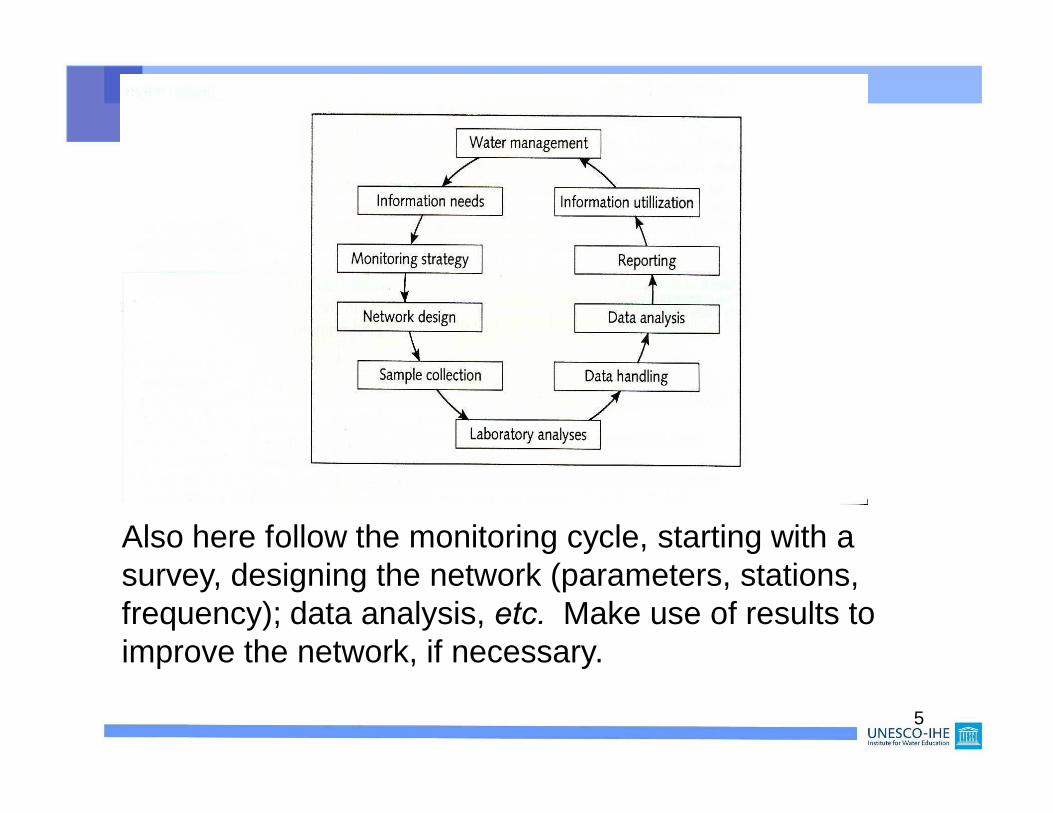
GROUNDWATER MONITORING

Objectives groundwater monitoring:

• To assess/understand general groundwater quality of the groundwater (ambient + operational monitoring)

• Finding major pollution sources (ambient/effluent monitoring)

• Compliance with regulations/ standards (effluent monitoring)

• Impact of an accidental pollution (early warning monitoring).

5

Also here follow the monitoring cycle, starting with a survey, designing the network (parameters, stations, frequency); data analysis, etc. Make use of results to improve the network, if necessary.

6

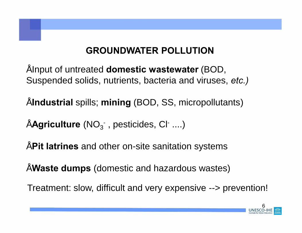
GROUNDWATER POLLUTION

Treatment: slow, difficult and very expensive --> prevention!

• Input of untreated domestic wastewater (BOD, Suspended solids, nutrients, bacteria and viruses, etc.)

• Industrial spills; mining (BOD, SS, micropollutants)

• Agriculture (NO3- , pesticides, Cl- ....)

• Pit latrines and other on-site sanitation systems

• Waste dumps (domestic and hazardous wastes)

7

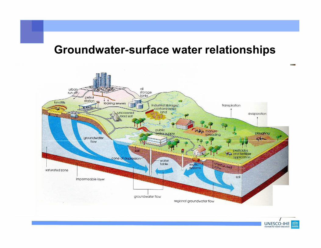
Groundwater-surface water relationships

8

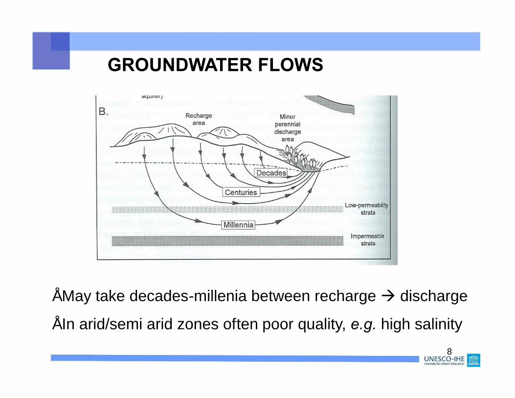
GROUNDWATER FLOWS

• May take decades-millenia between recharge à discharge

• In arid/semi arid zones often poor quality, e.g. high salinity

9

SOME CONCEPTS IN GROUNDWATER MONITORING

The unsaturated zone (above the water table)

Contains network of plant roots; usually < 2m thick;

Absent in humid areas, but with large thickness in arid areas;

Zone directly above groundwater table; water pressure is lessthan atmospheric (tension). Thickness ranges from 1-50 cm, dependent on rock type.

Zone with (saturated) groundwater. Pressure at the groundwater table is atmospheric.

10

Processes in the unsaturated zone

Water in unsaturated zone is prone to evapotranspiration and/or downward flow or‘groundwater recharge from precipitation’.

Assuming a precipitation event withgroundwater recharge, then after the eventstopped, downward flow will continue untilfield capacity is reached (curve 1). At field capacity, gravity forces acting on water equalsurface tensions exterted by the porestructure, and downward flow terminates. Field capacity depends on type of soil. The one shown here is typical for silty loam.

During dry periods, when there is nodownward flow, there may be upward flow orcapillary flow. When wilting point is reached, roots are not able to extract sufficientmoisture for plant survival. Curve 2 shows wilting point conditions for a silty loam.

11

The structure of rocks: porosityPorosity of rock is the ratio of the volume of open space in the rock and the total volume of rock (including the open space):

T

O

VVn =

T

O

VVn rock porosity

volume of the open space (m3)

total volume of the rock including open space (m3)

In consolidated rocks, openings are primarily present at fractures, joints, bedding planes, and solution holes. Thistype of porosity is referred to as secondary porosity.

In unconsolidated rocks, openings or pores are present between individual grains. Thistype of porosity is referred to as primary porosity.

12

The structure of rocks: porosityRock type Range of

porositiesUnconsolidatedrockGravelSandSilt..àclay

0.2-0.40.2-0.50.3-0.50.3.. -0.7à>0.95

In unconsolidatedrocks, (total) porosityranges from 0.2-0.7.

Porosity in this case relates to the packing, sorting, and shape of grains:

Porosity of sediment with cubic packing, well-sorted, well-rounded = ∼ 0.48

Porosity of similar sediment, butrhombohedrally packed = ∼ 0.26

When sorting is poor, and grains are notrounded, porosity decreases further.

13

The structure of rocksà permeability

Permeability is defined as the capacity of a rock to transmit groundwater (common unit: m/day, but also otherunits are used, like m/s, ft/m, ft/s, etc.).

There is no fundamental law or correspondence between permeability and porosity.

It is possible to have very high porosity without having any permeability at all, as in the case of clays and shales. The reverse of high permeability with a low porosity might also be true, such as in microfracturedcarbonates, and also in sand.

14

Relative classification of geological formations in a groundwater basin based on their hydraulic properties (rock permeability):

• Aquifer: geological formation or unit with a relatively large permeability. Able to transmit water. Examples: sand, karstic limestone

• Aquitard: geological formation or unit with a relatively low permeability. Still able to transmit water. Examples: silts, clays

• Aquiclude: geological formation or unit with a relatively very low permeability. Not able to transmit water.

• Aquifuge: geological formation or unit with a relatively very low permeability and porosity. Does not contain water: Solid rock

•Don’t take too absolute; it’s all relative !

15

Aquifer classification: based on the position of the water level in the aquifer.

Unconfined (phreatic) aquifers are in direct contact with the atmosphere (or: the unsaturated zone). At the groundwater table, pressure is atmospheric.

Semi-confined (leaky) aquifers are overlain and/or underlain by aquitards. Groundwater levels or ‘piezometric levels’ are usually above the top of the aquifer.

Confined aquifers are overlain and/or underlain by aquicludesor aquifuges. There is no vertical flow component. Groundwater levels or the piezometric level are above the top of the aquifer.

Perched water: not connected with other aquifers.16

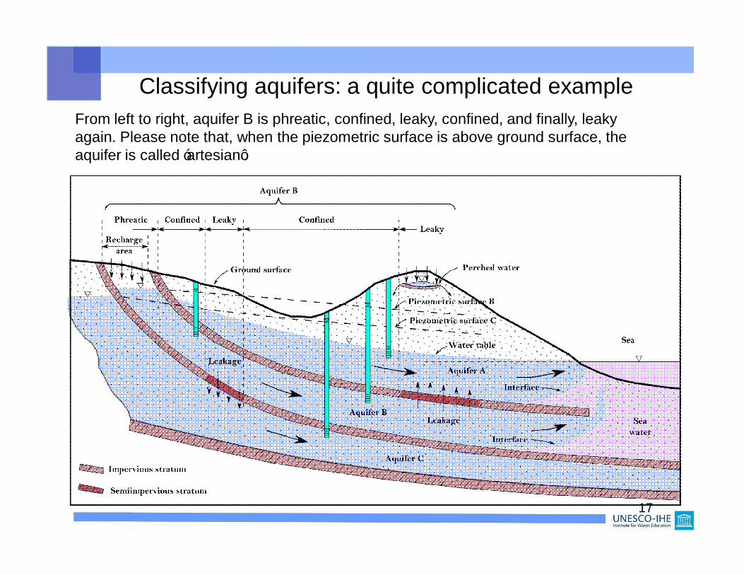
Classifying aquifers: a quite complicated exampleFrom left to right, aquifer B is phreatic, confined, leaky, confined, and finally, leakyagain. Please note that, when the piezometric surface is above ground surface, the aquifer is called ‘artesian’.

17

Equipotential plane: a plane where the hydraulic head is constant. For isotropic conditions, flow is perpendicular to these equipotential planes.

So in an aquifer (where flow is horizontal; “DupuitForchheimer assumption”), equipotential planes have vertical directions.

In an aquitard, where flow is vertical, equipotential planes have horizontal directions.

Observe the case of Zhengzhou city (next slide).

Regional flow and groundwater head contour maps

18

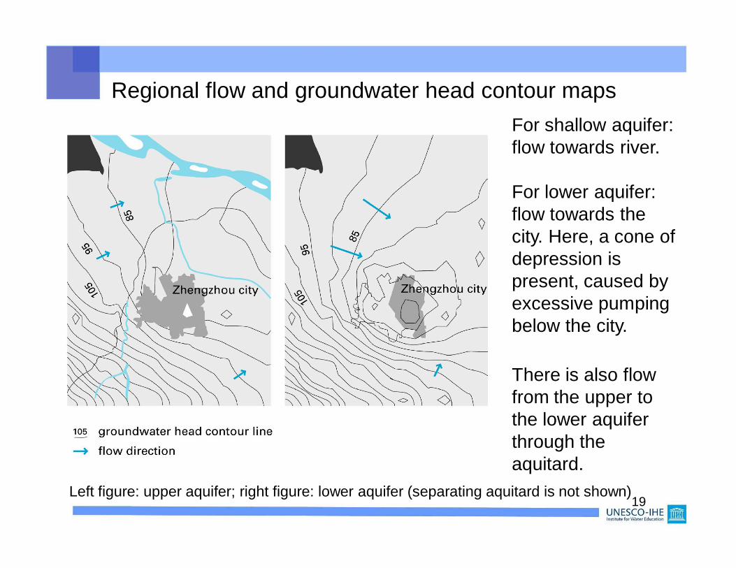
Regional flow and groundwater head contour maps

Left figure: upper aquifer; right figure: lower aquifer (separating aquitard is not shown)

For shallow aquifer: flow towards river.

For lower aquifer: flow towards the city. Here, a cone of depression is present, caused byexcessive pumpingbelow the city.

There is also flowfrom the upper to the lower aquiferthrough the aquitard.

19

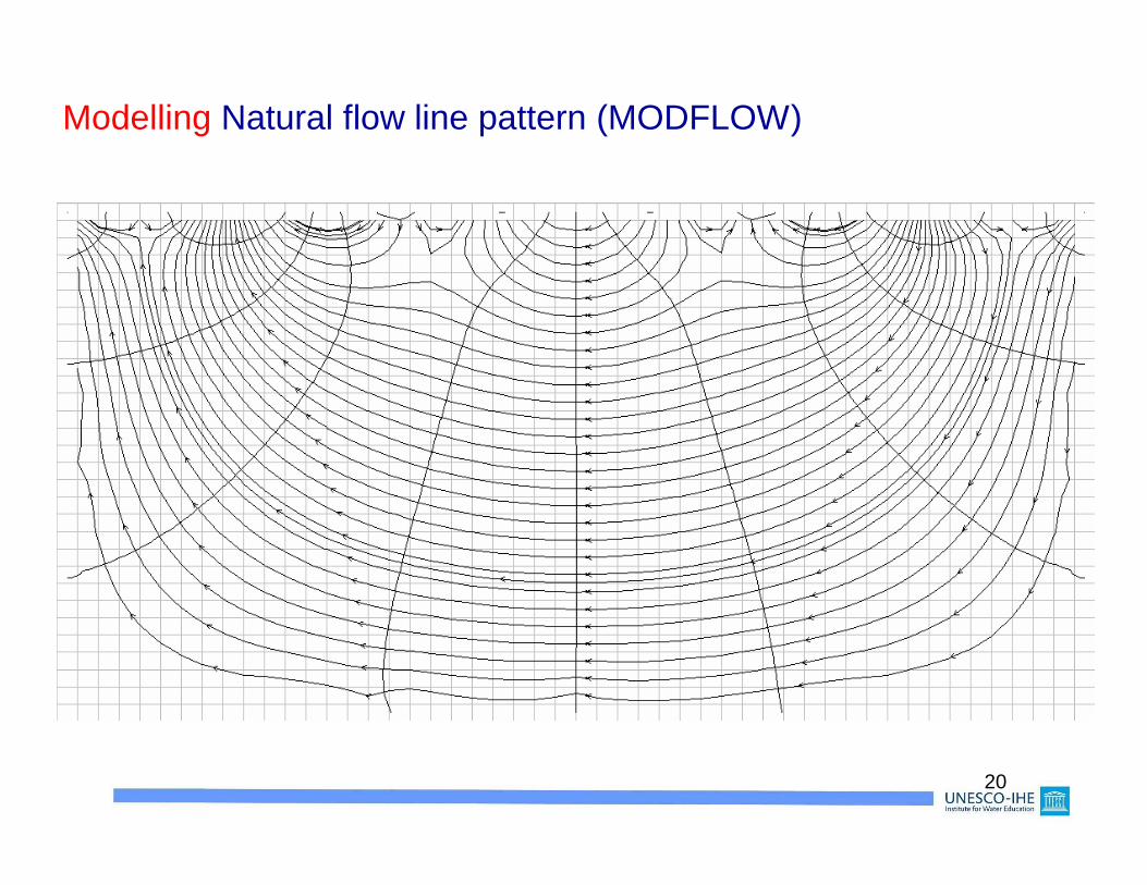
Modelling Natural flow line pattern (MODFLOW)

20

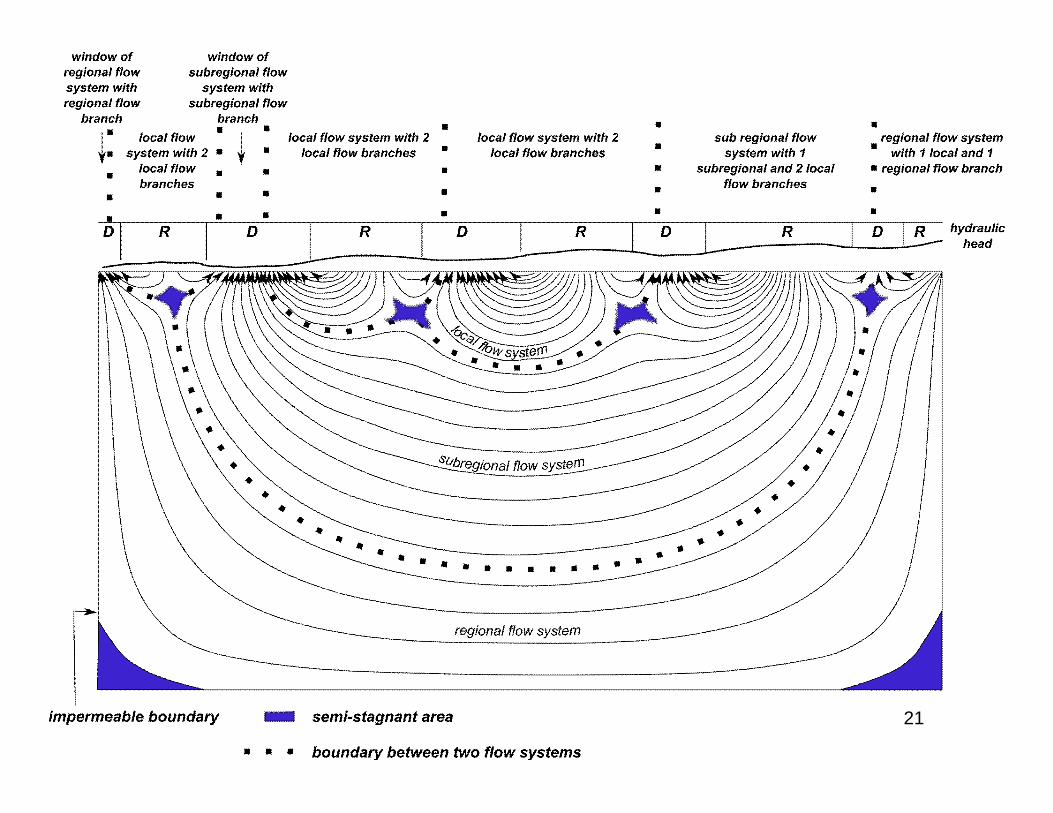
21

Groundwater sampling/ analysis

Hol

ocen

e C

over

Pleistocene 1st aquifer

Piezometer nests

in Exfiltration area

Peat

Clay

Clay

Sand

Peat

22

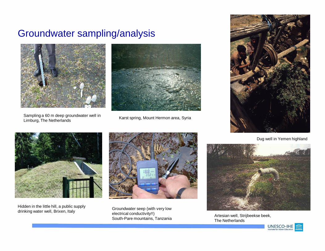
Dug well in Yemen highland

Groundwater sampling/analysis

Karst spring, Mount Hermon area, Syria

Artesian well, Strijbeekse beek, The Netherlands

Groundwater seep (with very low electrical conductivity!!) South-Pare mountains, Tanzania

Sampling a 60 m deep groundwater well in Limburg, The Netherlands

Hidden in the little hill, a public supply drinking water well, Brixen, Italy

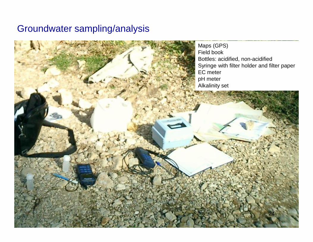
Groundwater sampling/analysisMaps (GPS)Field bookBottles: acidified, non-acidifiedSyringe with filter holder and filter paperEC meterpH meterAlkalinity set

24

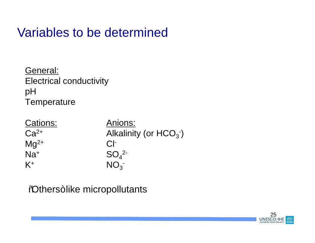
General:Electrical conductivitypHTemperature

Cations:Ca2+

Mg2+

Na+

K+

Variables to be determined

Anions:Alkalinity (or HCO3

-)Cl-SO4

2-

NO3-

25

“Others” like micropollutants

26

Types of groundwater pollutants

27

Natural inorganic constituents

Arsenic, fluoride, selenium, radon and uranium are examples of health-relevant naturally occurring groundwater constituents.

Their concentrations in groundwater are strongly dependent on hydrogeological conditions.

Parameter Guideline ValueArsenic 10 µg/lFluoride 1.5 mg/lSelenium 0.01 mg/lRadon 100 Bg/lUranium 15 µg/lNitrate (as NO3) 50 mg/lNitrite (as NO2) 3 mg/l

28

Fluoride, Selenium

Fluoride: n > 1.5 mg/L staining of tooth enamel, brittle teeth (dental fluorosis), n Skeletal fluorosis at prolonged intake of more than 15 mg/day;n Guideline: 1.5 mg/L;n In areas with acidic volcanic rocks (Sudan, Ethiopia, Kenya, Tanzania); fluorite,..n Especially when [Ca2+] is low (effective precipitation CaF2)

Selenium:n Essential trace element (1 µg per kg body weight and day for adults);n Too much Se can cause loss of hair and finger nails, finger deformities, skin lesions,

tooth decay and neurological disorders;n Guideline: 0.01 mg/L;n Co-precipitatation with pyrite: FeS2

29

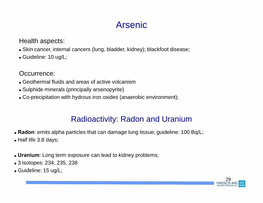
ArsenicHealth aspects:n Skin cancer, internal cancers (lung, bladder, kidney); blackfoot disease;n Guideline: 10 ug/L;

Occurrence:n Geothermal fluids and areas of active volcanismn Sulphide minerals (principally arsenopyrite)n Co-precipitation with hydrous iron oxides (anaerobic environment);

Radioactivity: Radon and Uranium n Radon: emits alpha particles that can damage lung tissue; guideline: 100 Bq/L;n Half life 3.8 days;

n Uranium: Long term exposure can lead to kidney problems;n 3 isotopes: 234, 235, 238n Guideline: 15 ug/L;

30

Aromatic hydrocarbons: BTEX

Health aspects:n benzene = highly carcinogenic!!

Occurrence:n Primary contaminants of concern associated with point sources of fuels and fuelrelated contamination from petroleum production;

Transport and attenuation:n Most petroleum products are LNAPLs;n Natural attenuation of BTEX is highly significant due to biodegradation;

Parameter (BTEX) Guideline ValueBenzene 10 µg/lToluene 700 µg/lEthylbenzene 300 µg/lXylene 500 µg/l

31

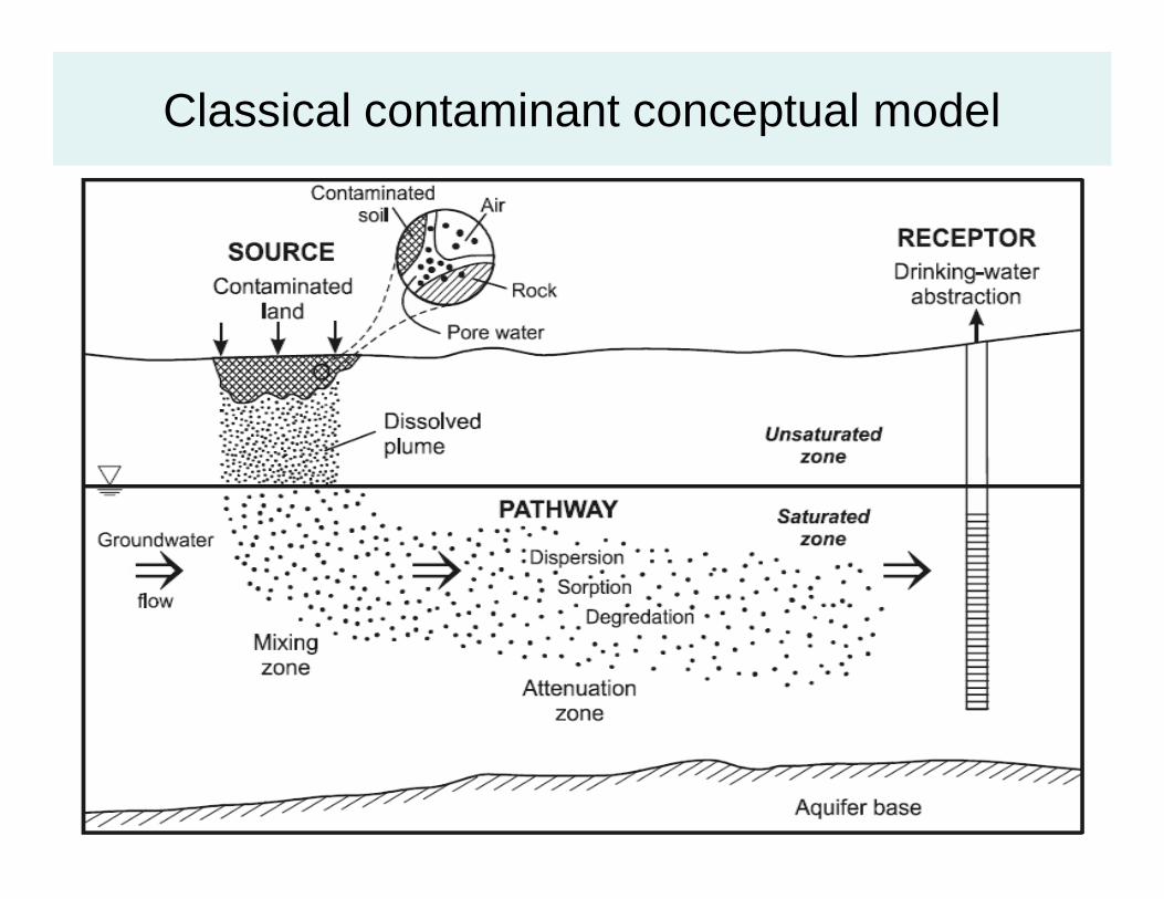
Classical contaminant conceptual model

32

LNAPL (light non-aqueous phase liquid; e.g. petrol, benzene)

33

DNAPL (Dense non-aqueous phase liquid, e.g. heavy oils)

34

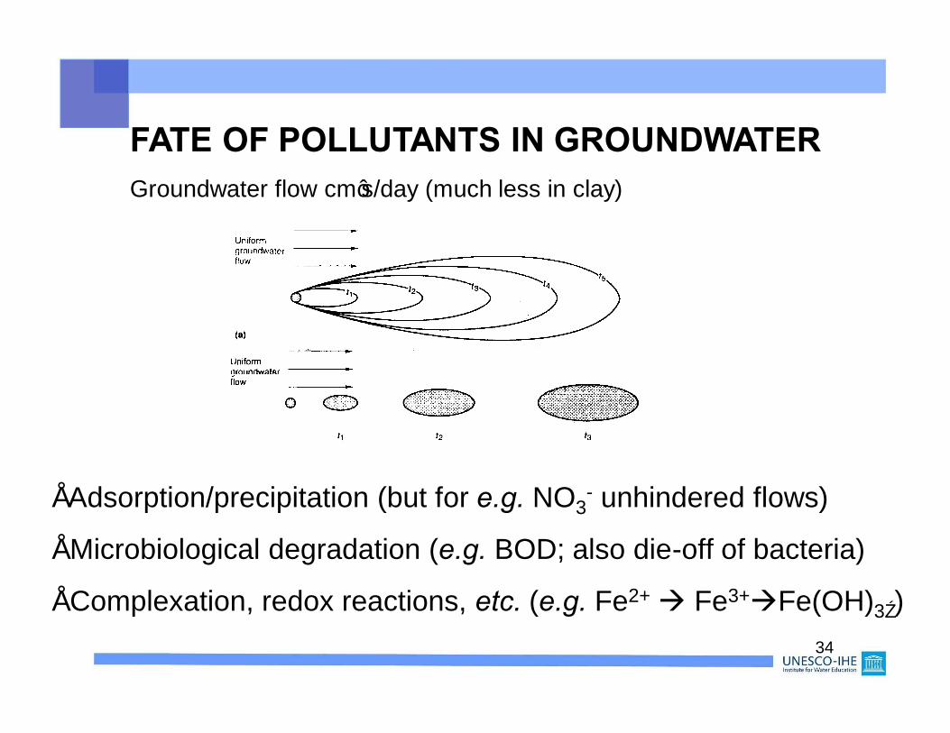
FATE OF POLLUTANTS IN GROUNDWATERGroundwater flow cm’s/day (much less in clay)

• Adsorption/precipitation (but for e.g. NO3- unhindered flows)

• Microbiological degradation (e.g. BOD; also die-off of bacteria)

• Complexation, redox reactions, etc. (e.g. Fe2+à Fe3+àFe(OH)3↓)

35

EXAMPLE

Bacteria and virus die-off proceeds via an exponential function:

Ntt = N0 x 10-kt

N0 , Nt : number of bacteria, viruses at t= 0, tk : decay rate constant (day-1)

For a decay rate of 0.1 day-1, to reach 99.9999% reduction (“6 log-reductions”):

Nt/N0 = 10-6

10 log (N0/Nt) = 6 = kt à t = 6/0.1 = 60 days.

36

So, under these conditions, it will take 60 days to reach99.9999% reduction in bacteria/viruses.

For a (reasonable) groundwater flow of 20 cm/day,

a travel time of 60 days would mean a distance of 12 m

So at short distance already relatively “safe” groundwaterquality (however larger distances needed for highervelocities (sand; high permeability!) and “short-circuiting”).

37

Main stages in the operation of a monitoring network(Broers, 2002)

1. Information analysis- system properties- monitoring objectives

7. Evaluation

5. Network exploitation- data collection- chemical analysis

2. Preliminary survey

3. Design and installation- sample size- locations- depths- screen lengths- monitoring frequency- measured chemical components- data analysis protocols

4. Set up of procedures- sampling- chemical analysis- QA-QC

6. Data analysis and reporting- overview of chemical status- changes in time

8. Optimization

38

1. Information analysis- monitoring objectives

Example of monitoring objectives (country wide efforts):

General policy information goals: To determine the effects of excessive infiltration of wastewater to groundwater resources.

Monitoring information goals: To determine the concentrations of nutrients and contaminants in sandy areas with urban land use in the first 25 m of the subsurface.

39

1. Information analysis- monitoring objectives

Example of monitoring objectives (local plume):1. Validate the conclusions of a remedial investigation or feasibility study;

2. Determine if contamination is migrating off site;

3. Determine if contamination will reach a receptor (such as a drinking water supply well);

4. Track contaminants exceeding some standard;

5. Track the changes in shape, size, or position of a contaminant plume;

6. Assess the performance of a remedial system (including monitored natural attenuation);

7. Assess the practicability of achieving complete remediation; or

8. Satisfy regulatory requirements (such as those for a landfill closure).

40

Risk concept (example: Dutch and Polish regional networks):

3. Design and installation- sample size- locations

Pollution loading Aquifer vulnerabilityLand use Soil type Geohydrological situation

Risk for contamination of shallow and deep groundwater

Vulnerability reflects the subsurface sensitivity to the leaching of contaminants to deeper groundwater

The risk concept is a combination of pollution loading and vulnerability

41

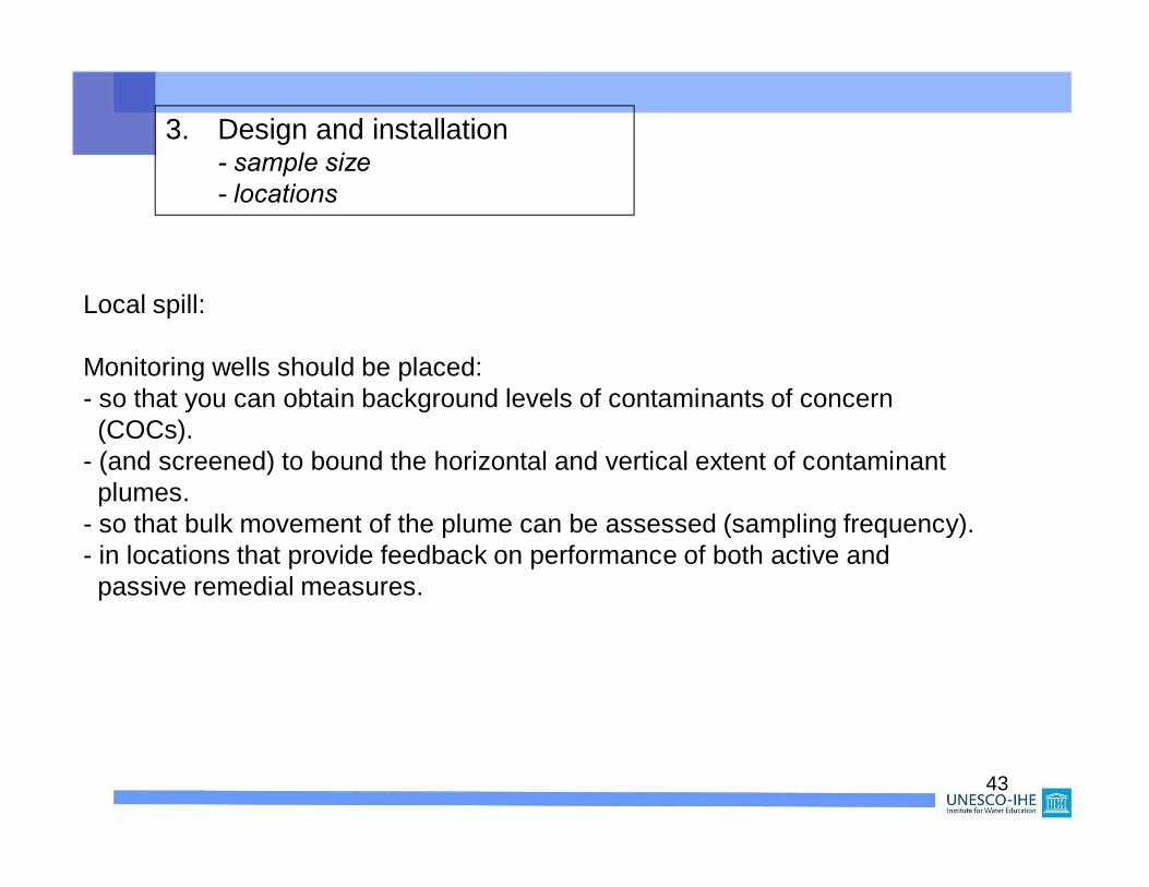
Local spill:

Monitoring wells should be placed:- so that you can obtain background levels of contaminants of concern(COCs).

- (and screened) to bound the horizontal and vertical extent of contaminantplumes.

- so that bulk movement of the plume can be assessed (sampling frequency). - in locations that provide feedback on performance of both active andpassive remedial measures.

3. Design and installation- sample size- locations

42

3. Design and installation- sample size- locations

Local plume of Local plume of pollutant(s)pollutant(s)

43

Local spill:

Monitoring wells should be placed:- so that you can obtain background levels of contaminants of concern(COCs).

- (and screened) to bound the horizontal and vertical extent of contaminantplumes.

- so that bulk movement of the plume can be assessed (sampling frequency). - in locations that provide feedback on performance of both active andpassive remedial measures.

3. Design and installation- sample size- locations

44

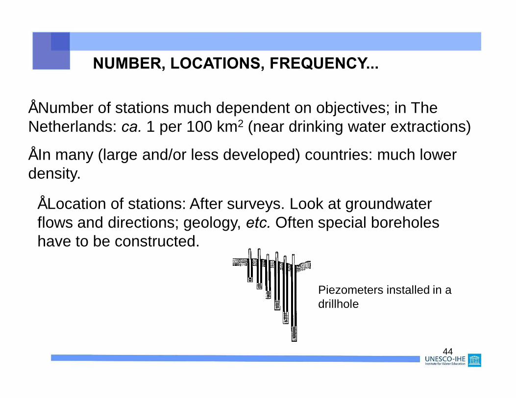
NUMBER, LOCATIONS, FREQUENCY...

• Number of stations much dependent on objectives; in The Netherlands: ca. 1 per 100 km2 (near drinking water extractions)

• In many (large and/or less developed) countries: much lower density.

• Location of stations: After surveys. Look at groundwater flows and directions; geology, etc. Often special boreholes have to be constructed.

Piezometers installed in a drillhole

45

• Sampling frequency: about 1-4 times per year; much more for:

• Specific research (see figure hereunder)

• Rapid groundwater flows; high permeability (sand)

NUMBER, LOCATIONS, FREQUENCY...

46

47

SOME CASE STUDIES

48

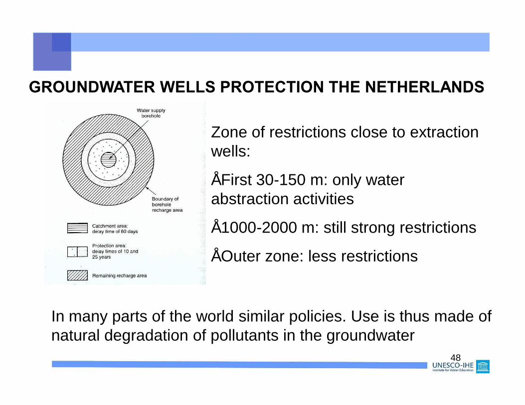
GROUNDWATER WELLS PROTECTION THE NETHERLANDS

Zone of restrictions close to extraction wells:

• First 30-150 m: only water abstraction activities

• 1000-2000 m: still strong restrictions

• Outer zone: less restrictions

In many parts of the world similar policies. Use is thus made of natural degradation of pollutants in the groundwater

49

Example: Gaza strip

• Limited water resources, leading to over-abstraction

à sea water intrusion giving soil salinization (chloride values up to 1500 mg/L!)

• Much use of fertilizers à nitrate (10 x WHO standard)

• Much (waste) water reuse in irrigation à high nitrate, pesticides and pathogens levels)

Rapid contamination due to high groundwater flows (sandy soil)

50

Correlation of high nitrate concentration with densely populated areas in Bermuda with unsewered sanitation (WHO guideline NO3-N = 11 mg/L)

Bermuda(Chapman, p. 444)

51

Industrial spill: Nassau County, USA(Chapman, p. 447)

Ground water pollution since 1940, by metal plating industry: Cr6+ and Cd2+.

• Pollution plume(1990s): 1300 m long; 300 m wide; 21 m thick

• > 10 mg Cr6+/L (WHO guideline drinking water: 0.05 mg/L)

• > 10 mg Cd2+/L (WHO guideline: 0.005 mg/L)

52

CASE STUDY GERMANY*Responsibility at the provincial (“State”) level• Monitoring stations: total about 2,000 of which 800 in “General Monitoring Network”

Three types of stations:• Basic stations: for general trend detection, impacts, etc.

• Operational stations (especially for drinking water extraction)

• Special emission stations (agriculture, waste dumps etc.)

* See MTM-II, p. 65; MTM-III, p.277

53

• Parameters: see GEMS programme discussed before. If necessary extra components are added, or left out

• Frequency of monitoring: normally 2-4 times per year. Higher in case of large variations. Lower in e.g. clay layers.

CASE STUDY GERMANY (Cont’d)

Example: State of Bavaria (70,000km2)

• 280 basic monitoring stations

• Construction cost 25,000 €; running cost 3,500 € /station.year

àAnnual cost (without data processing): about 1 million €/year

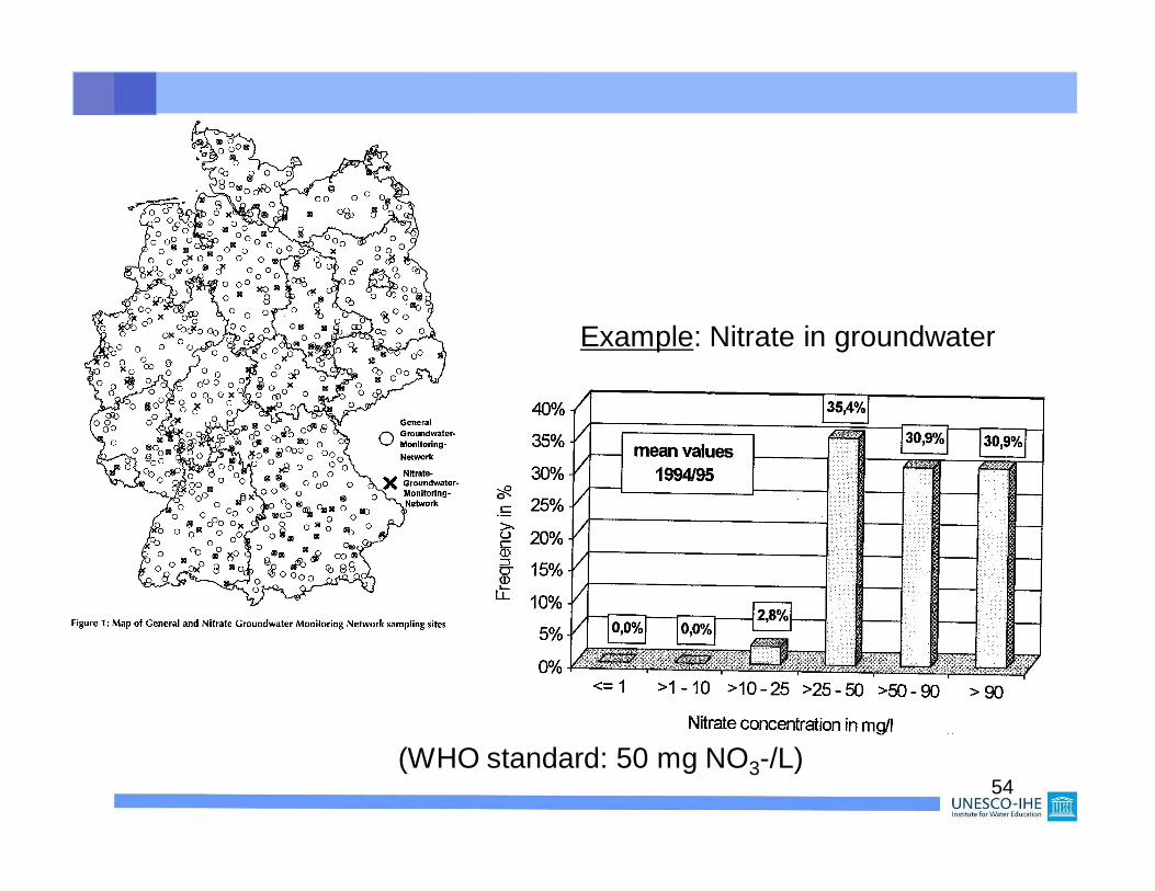
54(WHO standard: 50 mg NO3-/L)

Example: Nitrate in groundwater

55

WASTE DUMP, CANADA*• Period: 1940-1976; municipal and industrial solid waste

• Pollution plume in groundwater: about 700 m. Contamination “closed off” from aquifer by clay layer.

• Cl- was used as “tracer” for transport rate of pollutants; detailed studies were done within polluted zone.

* See Chapman, p.486

56

For more details on groundwater quality & monitoring:

• Book Chapman - Ch. 9

• See MTM-articles

• See EU-WFD (Additional material Course 3.2.)

• UNEP (1996) – Environment Library no 15: “Groundwater, a threatened resource” (http://new.unep.org/publications/search/pub_details_s.asp?ID=2884)