This article was downloaded by: [University Of South Australia Library]On: 24 November 2013, At: 21:01Publisher: Taylor & FrancisInforma Ltd Registered in England and Wales Registered Number: 1072954 Registered office: Mortimer House,37-41 Mortimer Street, London W1T 3JH, UK

Environmental ForensicsPublication details, including instructions for authors and subscription information:http://www.tandfonline.com/loi/uenf20

Optimal Identification of Groundwater PollutionSources Using Feedback Monitoring Information: A CaseStudySreenivasulu Chadalavada a b , Bithin Datta c & Ravi Naidu a ba Center for Environmental Risk Assessment and Remediation, University of South Australia ,Mawson Lakes , Australiab CRC for Contamination Assessment and Remediation of the Environment, University ofSouth Australia , Mawson Lakes , Australiac Discipline of Civil and Environmental Engineering, James Cook University , Townsville ,AustraliaPublished online: 07 Jun 2012.

To cite this article: Sreenivasulu Chadalavada , Bithin Datta & Ravi Naidu (2012) Optimal Identification of GroundwaterPollution Sources Using Feedback Monitoring Information: A Case Study, Environmental Forensics, 13:2, 140-153, DOI:10.1080/15275922.2012.676147

To link to this article: http://dx.doi.org/10.1080/15275922.2012.676147

PLEASE SCROLL DOWN FOR ARTICLE

Taylor & Francis makes every effort to ensure the accuracy of all the information (the “Content”) containedin the publications on our platform. However, Taylor & Francis, our agents, and our licensors make norepresentations or warranties whatsoever as to the accuracy, completeness, or suitability for any purpose of theContent. Any opinions and views expressed in this publication are the opinions and views of the authors, andare not the views of or endorsed by Taylor & Francis. The accuracy of the Content should not be relied upon andshould be independently verified with primary sources of information. Taylor and Francis shall not be liable forany losses, actions, claims, proceedings, demands, costs, expenses, damages, and other liabilities whatsoeveror howsoever caused arising directly or indirectly in connection with, in relation to or arising out of the use ofthe Content.

This article may be used for research, teaching, and private study purposes. Any substantial or systematicreproduction, redistribution, reselling, loan, sub-licensing, systematic supply, or distribution in anyform to anyone is expressly forbidden. Terms & Conditions of access and use can be found at http://www.tandfonline.com/page/terms-and-conditions

Environmental Forensics, 13:140–153, 2012Copyright C© Taylor & Francis Group, LLCISSN: 1527-5922 print / 1527-5930 onlineDOI: 10.1080/15275922.2012.676147

Contributed Articles

Optimal Identification of Groundwater Pollution Sources UsingFeedback Monitoring Information: A Case Study

Sreenivasulu Chadalavada,1,2 Bithin Datta,3 and Ravi Naidu1,2

1Center for Environmental Risk Assessment and Remediation, University of South Australia, Mawson Lakes, Australia2CRC for Contamination Assessment and Remediation of the Environment, University of South Australia, Mawson Lakes,Australia3Discipline of Civil and Environmental Engineering, James Cook University, Townsville, Australia

A feedback-based methodology has been developed for identifying the unknown pollution sources in groundwater-contaminatedaquifers. The methodology consists of models within an iterative feedback system, with the capacity of feeding back real-timemeasurements of pollutant concentrations for the sequential optimal designs and characterization of the contaminated aquifer studyarea. The resulting linked-simulation optimization model considers the delineation of the contaminant plume, optimally characterizingthe site in terms of pollutant sources and the optimal monitoring network leading to the remediation and/or management of thecontaminated aquifer. As part of the methodology, a simulation-optimization code was developed by linking a groundwater flow andtransport model with an optimization code for the purpose of identifying the unknown pollution sources. The proposed methodologyaddresses the source identification process with very limited information available regarding the observed contamination data forthe identification of unknown pollution sources. This methodology is applied to a chlorinated hydrocarbon contaminated site for theidentification of unknown pollution sources. Information regarding the sources such as the magnitude, location and the duration ofcontamination activity were not known for the study area considered in this work except the information regarding the likely activitiesthat led to its contamination. Developed methodology is applied to choose the optimal source locations from the identified potentiallocations. Depending on the availability of observed contaminant concentration values the domain for the methodology application isdivided into three different management periods. The optimal source estimates obtained at the end of the third management periodsuggests that only one potential source location, S2, confirms to be the source and active. The qualitative assessment of the results alsoperformed utilizing the contamination information obtained during the field investigations. The results demonstrate the practicabilityof the feedback-based methodology in identifying the unknown pollution sources in groundwater.

Keywords: simulation-optimization, groundwater, pollution source identification, feedback information

The presence of contaminants in the subsurface environment,and in particular in the groundwater, poses significant chal-lenges to its delineation and quantification. Although remedia-tion companies use many different strategies (both physical andchemical), subsurface contaminant source characterization hascontinued to pose significant difficulties. The current approachto groundwater source characterization uses mathematical mod-els that simulate the groundwater flow and transport processand optimization models that can prescribe optimal strategiesfor managing contamination based on simulation of the phys-ical process. Most of the existing models rely on groundwatercontaminant data obtained by using traditional approaches toassessing site assessment. These approaches include an initialhistory of the site, the location of the potential polluting activi-

Address correspondence to Bithin Datta, Discipline of Civil andEnvironmental Engineering, James Cook University, Townsville, QLD4811, Australia. E-mail: Bithin.Datta@jcu.edu.au

ties and subsequent estimation of sites where contamination ismost likely to be present.

The installation of monitoring wells is pivotal for under-standing the groundwater hydraulics and subsurface contami-nation but the process is expensive. The systematic study of thesubsurface system with the scarce data available regarding thegroundwater flow and the subsurface contamination can deter-mine the optimum number of monitoring wells for the effectivesite characterization. The site characterization primarily com-prises two components: the source characterization and plumecharacterization. The efficiency of any remediation strategy de-pends on how effectively we characterize the contaminationsource. Generally the contamination source zone is character-ized in terms of its location, magnitude, and duration. However,most contaminated sites lack historical information that can beused to characterize the source zone. This study reports a novelfeedback-based methodology developed for delineating ground-water contamination.

140

Dow

nloa

ded

by [

Uni

vers

ity O

f So

uth

Aus

tral

ia L

ibra

ry]

at 2

1:01

24

Nov

embe

r 20

13

Feedback Monitoring for Groundwater Pollution 141

The methodology consists of models within an iterative feed-back system, with the capacity of feeding back real-time mea-surements of pollutant concentrations and hydraulic heads forthe sequential optimal designs and characterization of the con-taminated aquifer study area. The resulting linked-simulationoptimization model considers the delineation of the contaminantplume, optimally characterizing the site in terms of pollutantsources and the optimal monitoring network leading to theremediation and/or management of the contaminated aquiferwhile quantifying the possible risks involved. The developedmethodology would be applicable for characterization ofcontaminated aquifer sites with limited data availability, andfor developing optimal strategies for remediation or control ofcontamination.

Site characterization involves the identification of unknownsource zones, which is vital for source characterization, which inturn is the key for adopting an appropriate remedial strategy forthe contaminated sites. While consulting companies use a stagedapproach for site characterization (and these characterizationsare rarely published), only a limited number of studies publishdetailed site characterization processes and outcomes.

Gorelick et al. (1983) demonstrated two hypothetical studyareas for identification of unknown pollutant sources using leastsquares regression and linear programming, together with re-sponse matrix. They considered both steady state and tran-sient flow conditions for transport phenomena. A review ofdistributed parameter modeling for groundwater managementhas been done by Gorelick (1983). Use of combined simulation-nonlinear programming for aquifer remediation has been con-sidered by Gorelick et al. (1984).

Datta et al. (1989) used statistical pattern recognition tech-niques in developing an expert system to identify groundwatercontamination sources. The flow and transport process has beensimulated using the response matrix approach. The effects ofparameter uncertainty and measurement errors on source iden-tification have also been studied. The simultaneous estimationof parameters (Wagner, 1992) and optimal identification of con-taminant sources plays an important role in contaminated sitecharacterization. The random walk method for identifying thepollution sources is used by Bagtzoglou et al. (1992). Skaggs andKabala (1994) developed a methodology to recover the releasehistory of contaminant plume from current spatial measure-ments of concentration by using Tikhonov regularization. Theperformance evaluation of their methodology has been carriedout by investigating the effects of measurement errors, parameterestimation errors, and numerical instability. The recent ad-vances in methodologies based on simulation-optimization forgroundwater management has been reviewed by Wagner (1995).

Mahar and Datta (1997) developed a dynamic optimal mon-itoring network for improved identification of pollutant sourcesin groundwater. The performance evaluations for the simplespatial and temporal combination of potential sources weredemonstrated by the methodologies adopted by Wagner (1992).Mahar and Datta (2000) considered the transient groundwa-ter system in identifying the pollution sources. Mahar and

Datta (2001) proposed a methodology using an optimizationmodel with flow and transport equations embedded as con-straints. They extended the source identification methodologyto the simultaneous estimation of aquifer parameters as wellas to the identification of unknown pollutant sources. Atmadjaand Bagtzoglou (2001a; 2001b) and Bagtzoglou and Atmadja(2003) discussed some of the recent methodologies in thisarea.

Singh and Datta (2006) used the genetic algorithm (GA)based simulation optimization approach for optimal identifica-tion of unknown pollutant sources. The combination of sourcecharacteristics, data availability conditions and concentrationmeasurement error levels are identified for performanceevaluation of the developed methodology. Artificial neuralnetwork (ANN) technique also been utilized in the groundwaterpollution source identification process. Singh et al. (2004)developed the ANN based source identification methodology.Nongradient based optimization techniques such as the GA,ANN and simulated annealing (SA) have a higher probabilityof reaching the global optimal solution compared to thegradient-based methods.

The characterization of source zones helps us to gain an un-derstanding of the complexity of the contaminated site beforeengaging in expensive remediation technologies. As the litera-ture review suggests, very limited work has been done regard-ing optimal characterization of source zones of contaminatedaquifers. Keeping this view in mind, a methodology has beenproposed which essentially deals with the application of a com-bination of simulation and optimization based models for sitecharacterization and optimal pollution management to a real lifecontaminated aquifer site.

Study Area

A brief description of the study area with reference to the sourcezone characterization is given in this section. The study area islocated in South Australia and was originally farmland that waslater developed into an explosives manufacturing facility in thebeginning of the Second World War (circa1940–1941). Severalpotentially contaminated areas have been identified within Edin-burgh Defense Precinct (EDP) due to historical defence-relatedactivities such as the use of the site as an air force base, missiledevelopment and testing ground, ordnance research, armytraining, weapons development and testing facility. The area iscomprised of sediments of Quaternary and Tertiary age. TheQuaternary sediments include Pooraka Formation (sandy andsilty clay material with inclusions of gravels) and HindmarshClay. Hindmarsh Clay separates the Pooraka Formation from theTertiary sediments. The groundwater system in this area consistsof shallow unconfined Quaternary and deep confined Tertiaryaquifers. The Hindmarsh Clay Formation is the confining unit.Groundwater in the area is encountered at a depth of 4.5–13m below ground level (Parsons and Brinkerhoff, 2002). Soilpermeability ranges between 0.233–0.259 m/day. The ground-water is mildly to strongly saline at the site and is not suitable

Dow

nloa

ded

by [

Uni

vers

ity O

f So

uth

Aus

tral

ia L

ibra

ry]

at 2

1:01

24

Nov

embe

r 20

13

142 S. Chadalavada et al.

for drinking or for irrigation. The hydrogeologic setting of thestudy area comprises an aquifer with silty sandy clay and a fewsand lenses at some places. The annual rainfall and the effectiveevopotranspiration at the site are recorded by the Australian Bu-reau of Meteorology as 427 mm and 400–500 mm, respectively.

The available history of the study site suggests that the areawas basically utilized for running a paint shop and that a fewevaporation pans existed nearby. Neither the likely sources ofcontamination nor the other characteristics of the pollution ac-tivity, such as magnitude and duration of the activity, are knownfor the study area, which complicates makes the source identifi-cation problem. In this study a feedback-based methodology isapplied to solve the source identification problem for the studyarea. The locations of pollution sources and the mass flux re-leased by the sources are unknown. The duration of industrialactivity is also unknown. Therefore the spatial distribution ofcontaminant concentrations observed at the current time pe-riod reflects the activity of contamination sources at the studyarea.

Source Identification Methodology

The source characterization methodology proposed in thiswork consists of a number of components interrelated witheach other, and utilizing feedback information. The distinctcomponents are: 1) a model for simulating the groundwaterflow and contaminant transport processes in the aquifer, 2) anoptimization algorithm for arriving at an optimal monitoringnetwork design based on available site information at varioustime steps, 3) an optimization model for optimal identificationof the unknown pollutant sources in terms of magnitude,location and time. A feedback-based methodology is developedusing the different component mentioned herein.

The important aspect of this methodology is the utilizationof feedback information obtained from sequentially designedmonitoring networks. The aim is to gradually improve theunknown groundwater contamination source identificationprocess, utilizing the information obtained from transientmonitoring networks. The developed methodology is schemat-ically represented in flowchart shown in Figure 1. The variouscomponents of the methodology involving the computationaltools and the interlinking of these tools are briefly described asfollows.

A groundwater flow and contaminant transport simulationmodel is essential for describing the flow and transport pro-cesses occurring in any contaminated site. Also, the simulationof the pollutant transport process can be used to predict any fu-ture contamination scenarios. Due to the complex nature of moststudy areas, it will not be possible to use analytical simulationmodels. Therefore, a suitable set of numerical simulation mod-els for flow and transport processes have been selected. In mostof the real-time contaminated site problems the basic concern ofthe decision makers is the lack of the sufficient observation data.Often very limited information is available regarding the site hy-drogeology as well as the contamination process. The method-

ology proposed in this study utilizes the simulation model forsimulating the spatial and temporal distribution of contami-nant concentration data in designing an optimal monitoring net-work, which supports the source identification process by givingthe sequential feedback information in terms of contaminantconcentrations.

Optimal Monitoring Network Design

An optimal monitoring network can play a vital role in the de-lineation of contaminant plume as well as serving as a databaseof contaminates. The methodology proposed here utilizes theoptimal monitoring network design as a tool for gathering thecontamination related information to be used in the source iden-tification model in a feedback-response system. The process ofsite characterization starts with limited historic data and scantycontaminant concentration data at a few observation locationsat the site. The design of the optimal monitoring network shouldpredict the set of monitoring wells required for sampling by con-sidering the available contamination information in an efficientway. The number of monitoring wells to be drilled in a drillingcampaign is subject to the budgetary allocations. Therefore thedesign should aim at identifying the optimal monitoring loca-tions within the budgetary locations as well as detecting thecontaminant plume.

Source Identification Model

Contamination sources are characterized in terms of magni-tude, location and duration of the activity. A source identifica-tion model is proposed in this methodology to identify the un-known pollution sources. A mathematical model representingthe source identification process proposed in the methodologycan be given shown in Equations 1 and 2:

Minimize :T∑

i−1

O∑

j=1

(Csimi,j − Cobsi.j

)2

(1)

Subjected to:

Csimi,j = F (S) (2)

Where:T = Total number of contaminant concentration observa-

tion time periodsO = Total number of observation locationsCsimi,j = Simulated contaminant concentration at the ith time

period, and jth locationCobsi,j = Observed contaminant concentration at ith time pe-

riod, and jth locationF(S) = Representation of simulation model as function of

source terms.

Dow

nloa

ded

by [

Uni

vers

ity O

f So

uth

Aus

tral

ia L

ibra

ry]

at 2

1:01

24

Nov

embe

r 20

13

Feedback Monitoring for Groundwater Pollution 143

Figure 1. Flow chart for the developed methodology.

Dow

nloa

ded

by [

Uni

vers

ity O

f So

uth

Aus

tral

ia L

ibra

ry]

at 2

1:01

24

Nov

embe

r 20

13

144 S. Chadalavada et al.

S is the simulated contaminant concentrations at any spatiallocation, for a set of candidate source solutions. These valuesare obtained from the simulation models linked to the optimiza-tion algorithm. F(S) represents the numerical simulation model.Simulated contaminant concentrations are function of sourceterms, which are the decision variables of the source identifi-cation model. The above mentioned equality constraints repre-sent the set of binding constraints for the objective function.Therefore the source identification model searches for the sim-ulated concentrations so that the objective function (defined assquared difference between the simulated and observed contam-inant concentrations) is minimized at the specified observationlocations. The source identification model presented above issolved through the process of a linked simulation-optimizationapproach. The optimization algorithm, which solves the abovementioned source identification model, needs the simulated con-taminant concentrations which will be obtained from a flowand transport simulation model. Therefore, the optimization al-gorithm has to be linked with the flow and transport simula-tion model to evaluate the objective function in searching forthe optimal source terms. The concept of a linked simulation-optimization model is presented in following text.

Linked Simulation-Optimization Model

A linked simulation-optimization model is developed for the op-timal identification of unknown pollution sources. The processof linking the physical simulation model with an optimization al-gorithm is computationally rigorous but is the most efficient wayto deal with the groundwater systems. As part of the methodol-ogy a computer code has been written which links the simulationmodel and optimization algorithm. Finite difference groundwa-ter flow MODFLOW 2000 (Harbaugh et al., 2000) and the con-taminant transport model MT3DMS (Zheng and Wang, 1999)have been used as simulation models to simulate the ground-water flow and pollutant transport processes respectively. Thesenumerical models are able to effectively simulate the complexphysical and chemical processes in the subsurface system. Link-ing of the optimization algorithm based model and the ground-water flow and transport simulation model would ensure thatthe optimization model can be solved by utilizing the simula-tion results iteratively. The simulation model in effect representsa set of constraints of the optimization model. Simulating thebehavior of the aquifer systems through external linking makesthe optimization process computationally feasible. It also allowsany sophisticated mathematical simulation model to be linked tothe optimization algorithm based model. So the source identifi-cation model is solved using the linked simulation-optimizationapproach. The process of linking a simulation model with anoptimization algorithm is shown Figure 2.

Feedback Based Identification Process

The principle objective of the work is the development of afeedback-based methodology to identify the unknown pollu-

3

Start

Read the contaminant concentration values at the

available observation locations Ni for the

Estimate the optimal source terms using the linked

simulation-optimization source identification

Simulate the contaminant transport process for the

management period Ti+1 (Ti+dt) utilizing the

Design and implement the optimal monitoring

network consisting of Ni+1 (Ni+dn) observation

locations for the management period T2 using the

Read the observation concentration values at the

Ni+1locations and utilize this information as the

Solve the source identification model for the

revised source estimates using the Ni+1

Further refinement of

source estimates

Stop

No

Yes

Figure 2. Schematic diagram of the feedback-based methodology.

tion sources. This section will describe how a feedback-basedsource identification methodology can be developed based onthe models, simulation tools and solution techniques describedearlier.

The first step in this methodology is to identify the pre-liminary source terms based on the available existing arbitraryobserved contaminant concentration measurements. The sourceidentification model described in Equation (1) is used to identify

Dow

nloa

ded

by [

Uni

vers

ity O

f So

uth

Aus

tral

ia L

ibra

ry]

at 2

1:01

24

Nov

embe

r 20

13

Feedback Monitoring for Groundwater Pollution 145

the preliminary estimates of source terms. The basic concentra-tion information available with the site will be used for thepreliminary identification process. Ideally, the source terms es-timated utilizing this arbitrary information would be poor inquality as the aim of this methodology is to show how these pre-liminary source estimates are improved in a sequential iterativeprocess.

The source identification model will be solved using thelinked simulation-optimization approach for the preliminaryestimates. The simulation model used in this methodology tosimulate the spatial and temporal distribution of contaminantconcentrations need not be calibrated and validated because themethodology developed will drive the process in sequential stepsto obtain the simulation model which represents the subsurfacesystem in a more reliable and efficient manner.

In the second step, the simulation model utilizes the prelim-inary source estimates to simulate the contamination process.Uncertainty involved with any process can be minimized whenthere is the availability of more reliable data. The amount of dataand the uncertainty in the system are generally inversely pro-portional. At the same time, acquiring more data in the contextof methodology by drilling more wells is an expensive processand budgetary considerations will try to limit that. Therefore,a process is needed to acquire the additional data in an opti-mal manner (considering the budgetary limitations). The sourceidentification process requires the additional observation wellsto improve the source estimates from the preliminary ones ob-tained. So the concept of optimal monitoring network design hasbeen made an integral part of the source identification process.The monitoring network design model developed in this method-ology will try to determine optimal observation wells using theinitial arbitrary observation data. The network design model alsoconsiders the budgetary limitations in the form of the maximumnumber of monitoring wells allowed in a management period.The component of optimal monitoring network will work as thefeedback-giving system. That approach means that the networkdesign model solves for the additional optimal monitoring wellsbased on the simulation scenarios derived from the pollutionsource estimates obtained. When the pollution source terms areto be estimated for a future period of duration T1 years from thetime the preliminary source estimates are estimated, the contam-inant concentrations are simulated ending T1 years, using thecontaminant transport model utilizing the preliminary pollutionsource terms obtained at time t. The network design model willbe solved for the design of optimal monitoring network designfor the period starting t and ending T1 years. The additionalobservation locations obtained for this period will be utilizedto estimate the pollution source terms for the same period. Itis understood that the monitoring provides the feedback to thesource identification model by designing and implementing theoptimal monitoring networks. The source identification modelsolved at this stage will give the improved pollution source termsfrom the preliminary estimates because of the greater numberof observation locations obtained from the monitoring networkdesigned.

The same procedure is continued for further time periods andthe optimal source estimates will show the improvement withthe progress of time period. The methodology developed will bea useful tool in source zone characterization, which plays a vitalrole in the remediation of any contaminated site. The perfor-mance evaluation and the application of methodology to a real-time contaminated site will be discussed in the further chapters.

Application of Methodology

The methodology application involves simulating the contam-inant concentrations assuming the known system parameters,whereas in the real world contaminated site problems, the pa-rameters regarding the function of pollution sources are notoften known. Therefore quantitative evaluation of source termsobtained for the real world problems are not always feasible.Evaluation of the results can be carried out using the qualita-tive information available with the site. This chapter explainshow a feedback-based linked simulation-optimization can beapplied to a real world contaminated site and the way the eval-uation of results are carried out. A description about modellingthe groundwater flow and pollutant transport process, design-ing of an optimal monitoring network and implementation ofthe feedback-based methodology is described under followingheadings.

Model Representation

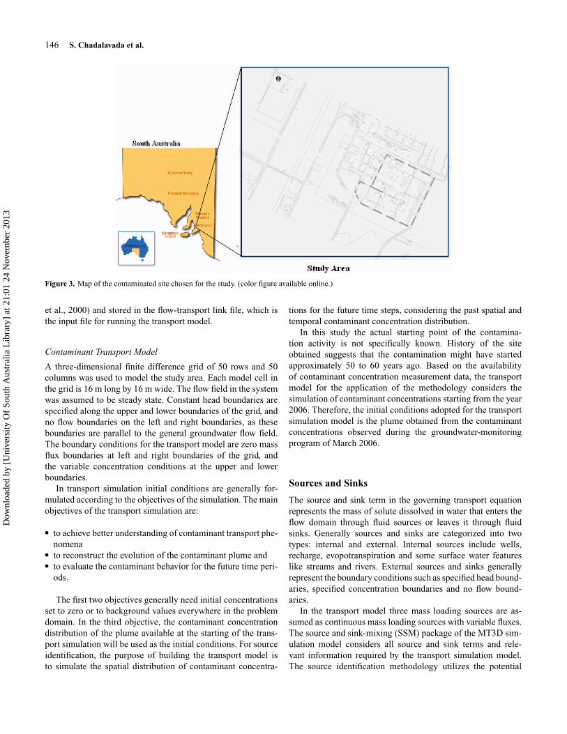
The groundwater flow and contaminant transport process forthe study area is schematically shown in Figure 3. The modelarea for the study site is 800 × 800 m. The direction of thegroundwater flow and the model orientation are northwest. Theinitial head is assumed to be uniform across the model area asthe general topographic gradient is very mild. A four-layeredmodel—representing the sandy clay (layer 1); sandy silty clay(layer 2); silty clay (layer 3); and clay (layer 4)—is assumedto be horizontal, homogenous and isotropic. The size of thefinite difference grid is 16 m x 16 m. The mean thickness of thesurface layer is 5 m and the thickness of the aquifer consideredis 15 m. The boundary conditions for the model are constanthead boundaries in the upstream and the downstream, and noflow boundaries on either side of the mean groundwater flowdirection. The steady state groundwater flow is simulated forthe period of 2.5 years. Heads and flow velocities at each gridcell required by the transport simulation model are solved usingthe strongly implicit procedure (SIP) solution technique. Sincethere are no external sinks and sources in the site, the hydraulicfield of the subsurface system assumed was mainly influencedby the seasonal variation of groundwater levels. It has beenobserved from the field data that the seasonal variations at thescale of the model are almost negligible. Therefore the flowfield in the system is simulated as steady state flow. The flowparameters required for the transport model MT3DMS (Zhengand Wang, 1999) are calculated by the MODFLOW (Harbaugh

Dow

nloa

ded

by [

Uni

vers

ity O

f So

uth

Aus

tral

ia L

ibra

ry]

at 2

1:01

24

Nov

embe

r 20

13

146 S. Chadalavada et al.

Figure 3. Map of the contaminated site chosen for the study. (color figure available online.)

et al., 2000) and stored in the flow-transport link file, which isthe input file for running the transport model.

Contaminant Transport Model

A three-dimensional finite difference grid of 50 rows and 50columns was used to model the study area. Each model cell inthe grid is 16 m long by 16 m wide. The flow field in the systemwas assumed to be steady state. Constant head boundaries arespecified along the upper and lower boundaries of the grid, andno flow boundaries on the left and right boundaries, as theseboundaries are parallel to the general groundwater flow field.The boundary conditions for the transport model are zero massflux boundaries at left and right boundaries of the grid, andthe variable concentration conditions at the upper and lowerboundaries.

In transport simulation initial conditions are generally for-mulated according to the objectives of the simulation. The mainobjectives of the transport simulation are:

� to achieve better understanding of contaminant transport phe-nomena

� to reconstruct the evolution of the contaminant plume and� to evaluate the contaminant behavior for the future time peri-

ods.

The first two objectives generally need initial concentrationsset to zero or to background values everywhere in the problemdomain. In the third objective, the contaminant concentrationdistribution of the plume available at the starting of the trans-port simulation will be used as the initial conditions. For sourceidentification, the purpose of building the transport model isto simulate the spatial distribution of contaminant concentra-

tions for the future time steps, considering the past spatial andtemporal contaminant concentration distribution.

In this study the actual starting point of the contamina-tion activity is not specifically known. History of the siteobtained suggests that the contamination might have startedapproximately 50 to 60 years ago. Based on the availabilityof contaminant concentration measurement data, the transportmodel for the application of the methodology considers thesimulation of contaminant concentrations starting from the year2006. Therefore, the initial conditions adopted for the transportsimulation model is the plume obtained from the contaminantconcentrations observed during the groundwater-monitoringprogram of March 2006.

Sources and Sinks

The source and sink term in the governing transport equationrepresents the mass of solute dissolved in water that enters theflow domain through fluid sources or leaves it through fluidsinks. Generally sources and sinks are categorized into twotypes: internal and external. Internal sources include wells,recharge, evopotranspiration and some surface water featureslike streams and rivers. External sources and sinks generallyrepresent the boundary conditions such as specified head bound-aries, specified concentration boundaries and no flow bound-aries.

In the transport model three mass loading sources are as-sumed as continuous mass loading sources with variable fluxes.The source and sink-mixing (SSM) package of the MT3D sim-ulation model considers all source and sink terms and rele-vant information required by the transport simulation model.The source identification methodology utilizes the potential

Dow

nloa

ded

by [

Uni

vers

ity O

f So

uth

Aus

tral

ia L

ibra

ry]

at 2

1:01

24

Nov

embe

r 20

13

Feedback Monitoring for Groundwater Pollution 147

Figure 4. Map of the study area showing the potential monitoring locations for the optimal monitoring network design. (color figure available online.)

monitoring locations as provided in Figure 4 for designing andimplementing the optimal monitoring networks.

Potential contaminant source locations are shown in Figure 5and are specified as potential locations. The identification modelestimates the source fluxes. To design the monitoring network,the source fluxes specified are those obtained by solving theidentification model. The hydrogeologic parameter values arebased on the site investigation data. Different input parametervalues are given in Table 1.

Source Identification Methodology

Pollution source identification for the study area involves thefeedback-response based methodology in which the optimalidentification process of the pollution sources is improved it-eratively, based on the response obtained from designing theoptimal monitoring network. It is observed from the history ofthe site that the contamination activity started approximatelyfive decades ago but the contaminant concentrations at the po-tential source locations are showing abnormal fluctuations. It isplausible that the potential source locations at this study areaare still active, i.e. contaminant mass transfer may be occurringfrom the vadose zone to the saturated zone. The contaminantconcentrations obtained from soil cores also support this point.

Therefore the developed methodology is applied to identify thepollution sources from the potential locations in terms of loca-tion and magnitude.

Observed Contaminant Concentrations

Simulating/measuring the contaminant concentrations are vitalin the source identification process. The monitoring networkfor the study area consists of 28 observation wells. The con-taminant concentrations are observed at these locations duringthe groundwater monitoring campaigns conducted at regular in-tervals in 1 year. From March 2006 until June 2008 are eighttime steps for which the observed contaminant concentrationsare available for all monitoring locations on the site. These ob-served concentration values are used in solving the optimizationmodel for the pollution source identification.

Design of Optimal Monitoring Network

The basic purpose of designing the optimal monitoring net-work is to improve the identification of the unknown sources ofgroundwater pollution in a planned and efficient way, i.e. usingfeedback observation data sequentially obtained from designedand implemented monitoring networks. For a situation of limited

Dow

nloa

ded

by [

Uni

vers

ity O

f So

uth

Aus

tral

ia L

ibra

ry]

at 2

1:01

24

Nov

embe

r 20

13

148 S. Chadalavada et al.

Figure 5. Map of the study area showing the initial arbitrary observation locations for the first management period.

information about the contamination, i.e. limited number of ob-servation locations is available, the optimal monitoring networkapproach helps us to improve the source identification process,and identify the unknown contaminant sources more reliably.

The source identification and monitoring network designsare improved sequentially by improving the source identificationprocess by using additional data from designed and implementedmonitoring networks. The feedback information in the form

Table 1. Groundwater flow and transport modal parameters

Modal Parameters:

Sl No Parameter Value

1 Cell size in horizontal direction (m) 162 Cell size in vertical direction (m) 163 Longitudinal dispersion (m) 54 Lateral dispersion (m) 0.755 Molecular diffusion coefficient 0

Hydraulic Conductivity and Porosity ValuesLayer Porosity Horizontal Hydraulic

Conductivity (m/d)Ratio of Horizontal and

Vertical conductivity1 0.25 2.5 12 0.2 1.25 13 0.15 0.6 14 0.1 0.07 1

Initial and Boundary conditionsSl No Item nature1 Upstream and downstream boundaries Constant head2 Lateral boundaries of model domain No flow

Dow

nloa

ded

by [

Uni

vers

ity O

f So

uth

Aus

tral

ia L

ibra

ry]

at 2

1:01

24

Nov

embe

r 20

13

Feedback Monitoring for Groundwater Pollution 149

of concentration measurements from the designed monitoringlocations is the feedback information utilized to improve thesource identification.

To design the initial monitoring network for the proposedstudy area, it is assumed that only three existing arbitrary obser-vation locations are available to monitor groundwater contami-nation. The source identification model is first solved using datafrom this initial monitoring network. The solution of the sourceidentification model provides the source fluxes for the first man-agement time period starting August 2006 to December 2006.The source terms obtained for this management period are onlypreliminary, so it is necessary to refine the source identificationprocess by choosing more observation locations through de-sign and implementation of a new optimal monitoring network.The solution of the source identification model is again usedas a feedback to the simulation model to simulate the transportprocess. The simulation results are then used to design a newoptimal monitoring network.

As part of the preliminary identification of contaminantsources, initially three arbitrary observation well locations areutilized. The source identification model is used to identify thesources using these observation locations at the end of the eachtime interval (T1 and T2) of 4 months’ duration in 2006. Thefirst set of optimal source fluxes obtained at the end of time in-terval 1 is designated as S11, S21, and S31. These source fluxesobtained at the end of two time steps in 2006 are used as inputto the simulation model to obtain the simulated contaminantconcentrations at the initial arbitrary observation locations todesign the optimal monitoring network at the end of December2007, based on these simulated contaminant concentrations.

A new monitoring network is designed for the new manage-ment period ending December 2007. Based on the observed dataat the designed optimal monitoring locations, source estimatesat the potential source locations are calculated. Therefore re-sulting source fluxes are for the new management period. Forthe second management period, the source fluxes S11 and S21are used to simulate the contaminant concentrations at the endof 2007. The maximum number of new monitoring wells per-mitted in the second management period is specified as three.An optimal monitoring network is designed for the period be-tween 2006 and 2007, using the optimal network design model,which has been discussed earlier. Therefore, the total number ofobservation locations used to identify the optimal source fluxesfor the second management period is six.

The new optimal contaminant source fluxes are obtainedby solving the source identification model using the total sixobservation locations at the end of 2008. The optimal sourcefluxes at the second management period are designated as S12,S22, and S32.

For the third management period, the optimal source fluxesobtained at the end of 2007 are used to simulate the contaminantconcentrations at the end of June 2008. In the second manage-ment period, the maximum number of monitoring wells is alsospecified as three. The new optimal monitoring network for thethird management period is designed using the network design

Table 2. Summary of optimal source estimates obtained for allmanagement periods.

ManagementPeriod Time Interval Source-1 Source-2 Source-3

1 T1 9.74 9.67 4.87T2 1.09 3.94 6.61

2 T1 2.703 9.23 0.308T2 0.047 9.727 8.69

3 T1 0.591 9.68 6.26T2 0.913 8.75 1.6

model utilizing the already existing six observation locations.The source identification model is then solved to identify theoptimal source fluxes at the end of June 2008, utilizing the nowexisting total nine observation locations. These source fluxesare designated as S13, S23 and S33. The summary of optimalsource flux estimates obtained during different time periods aretabulated in Table 2.

Results and Discussion

Preliminary Identification

Identification of the unknown pollution sources using the de-veloped methodology starts with the initial source estimatesutilizing the observed contaminant concentrations at monitor-ing locations chosen arbitrarily. Per the methodology, these pre-liminary source estimates should improve in accuracy with theutilization of more observation data obtained as feedback infor-mation from the sequentially designed and implemented mon-itoring networks. In this study the initial arbitrary observationlocations are GW913, GW907, MW906, MW901, and MW911.These observation locations along the potential source locationsare shown in Figure 5. The basic idea of applying the developedmethodology in this study area is to identify whether the poten-tial source locations, S1, S2, and S3, are active or not, and if so,to see what are the mass fluxes are at these locations. The linkedsimulation-optimization source identification model is solved toestimate the fluxes at these potential source locations for the twotime intervals in the year 2006. The source fluxes obtained us-ing the data available for the first management period show thatall three sources are very active and are releasing considerableamounts of flux at the two time intervals T1 and T2, in the year2006.

Second Management Period

These source estimations can be improved further by design-ing the optimal monitoring network for the second managementperiod ending 2007. The basic idea of developing this moni-toring network is that the initial source estimates are expectedto be improved sequentially by solving the source identificationmodel with more observation data from the monitoring net-works designed and implemented sequentially. The amount ofobservation concentration is directly proportional to the number

Dow

nloa

ded

by [

Uni

vers

ity O

f So

uth

Aus

tral

ia L

ibra

ry]

at 2

1:01

24

Nov

embe

r 20

13

150 S. Chadalavada et al.

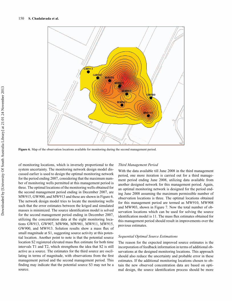
Figure 6. Map of the observation locations available for monitoring during the second management period.

of monitoring locations, which is inversely proportional to thesystem uncertainty. The monitoring network design model dis-cussed earlier is used to design the optimal monitoring networkfor the period ending 2007, considering that the maximum num-ber of monitoring wells permitted at this management period isthree. The optimal locations of the monitoring wells obtained forthe second management period ending in December 2007, areMW915, GW900, and MW913 and these are shown in Figure 6.The network design model tries to locate the monitoring wellssuch that the error estimates between the kriged and simulatedmasses is minimized. The source identification model is solvedfor the second management period ending in December 2007,utilizing the concentration data at the eight monitoring loca-tions GW913, GW907, MW906, MW901, MW911, MW915,GW900, and MW913. Solution results show a mass flux ofsmall magnitude at S1, suggesting source activity at this poten-tial location. Another point to note is that the potential sourcelocation S2 registered elevated mass flux estimate for both timeintervals T1 and T2, which strengthens the idea that S2 is stillactive as a source. The estimates for the third source are oscil-lating in terms of magnitude, with observations from the firstmanagement period and the second management period. Thisfinding may indicate that the potential source S3 may not be asource.

Third Management Period

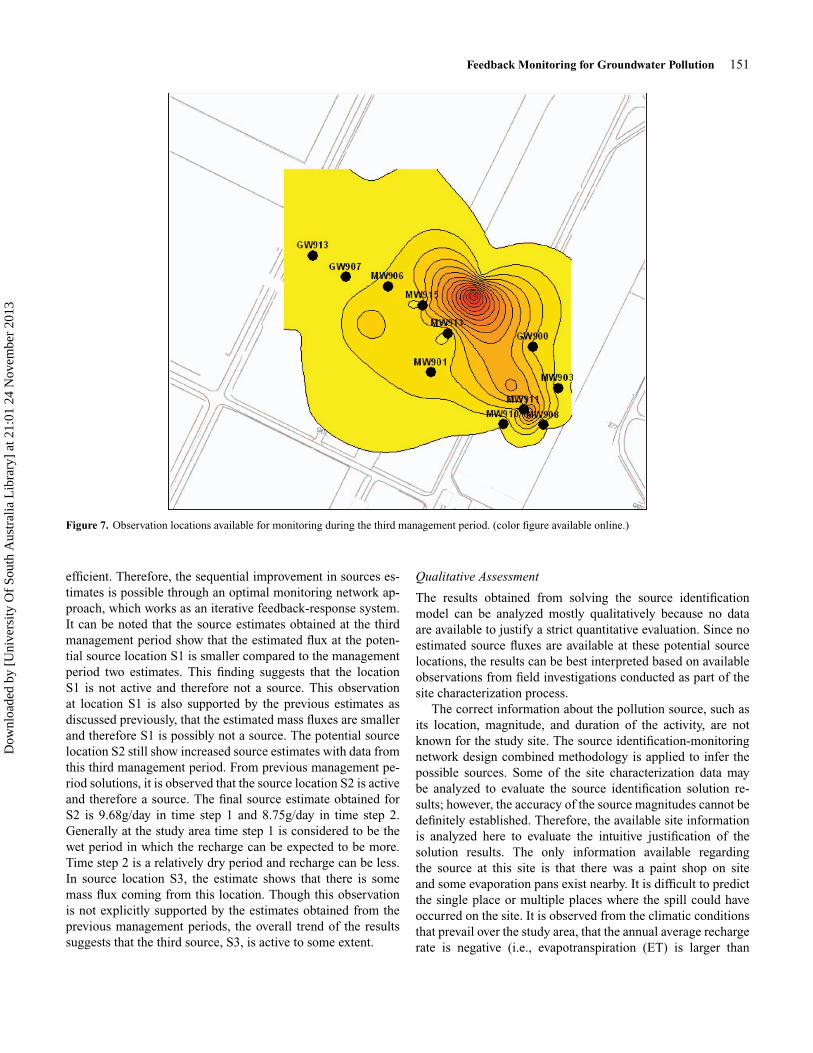
With the data available till June 2008 in the third managementperiod, one more iteration is carried out for a third manage-ment period ending June 2008, utilizing data available fromanother designed network for this management period. Again,an optimal monitoring network is designed for the period end-ing June 2008 assuming the maximum permissible number ofobservation locations is three. The optimal locations obtainedfor this management period are termed as MW910, MW908and MW903, shown in Figure 7. Now the total number of ob-servation locations which can be used for solving the sourceidentification model is 11. The mass flux estimates obtained forthis management period should result in improvements over theprevious estimates.

Sequential Optimal Source Estimations

The reason for the expected improved source estimates is theincorporation of feedback information in terms of additional ob-servations at the designed monitoring locations. This approachshould also reduce the uncertainty and probable error in theseestimates. If the additional monitoring locations chosen to ob-tain the new observed concentration data are based on opti-mal design, the source identification process should be more

Dow

nloa

ded

by [

Uni

vers

ity O

f So

uth

Aus

tral

ia L

ibra

ry]

at 2

1:01

24

Nov

embe

r 20

13

Feedback Monitoring for Groundwater Pollution 151

Figure 7. Observation locations available for monitoring during the third management period. (color figure available online.)

efficient. Therefore, the sequential improvement in sources es-timates is possible through an optimal monitoring network ap-proach, which works as an iterative feedback-response system.It can be noted that the source estimates obtained at the thirdmanagement period show that the estimated flux at the poten-tial source location S1 is smaller compared to the managementperiod two estimates. This finding suggests that the locationS1 is not active and therefore not a source. This observationat location S1 is also supported by the previous estimates asdiscussed previously, that the estimated mass fluxes are smallerand therefore S1 is possibly not a source. The potential sourcelocation S2 still show increased source estimates with data fromthis third management period. From previous management pe-riod solutions, it is observed that the source location S2 is activeand therefore a source. The final source estimate obtained forS2 is 9.68g/day in time step 1 and 8.75g/day in time step 2.Generally at the study area time step 1 is considered to be thewet period in which the recharge can be expected to be more.Time step 2 is a relatively dry period and recharge can be less.In source location S3, the estimate shows that there is somemass flux coming from this location. Though this observationis not explicitly supported by the estimates obtained from theprevious management periods, the overall trend of the resultssuggests that the third source, S3, is active to some extent.

Qualitative Assessment

The results obtained from solving the source identificationmodel can be analyzed mostly qualitatively because no dataare available to justify a strict quantitative evaluation. Since noestimated source fluxes are available at these potential sourcelocations, the results can be best interpreted based on availableobservations from field investigations conducted as part of thesite characterization process.

The correct information about the pollution source, such asits location, magnitude, and duration of the activity, are notknown for the study site. The source identification-monitoringnetwork design combined methodology is applied to infer thepossible sources. Some of the site characterization data maybe analyzed to evaluate the source identification solution re-sults; however, the accuracy of the source magnitudes cannot bedefinitely established. Therefore, the available site informationis analyzed here to evaluate the intuitive justification of thesolution results. The only information available regardingthe source at this site is that there was a paint shop on siteand some evaporation pans exist nearby. It is difficult to predictthe single place or multiple places where the spill could haveoccurred on the site. It is observed from the climatic conditionsthat prevail over the study area, that the annual average rechargerate is negative (i.e., evapotranspiration (ET) is larger than

Dow

nloa

ded

by [

Uni

vers

ity O

f So

uth

Aus

tral

ia L

ibra

ry]

at 2

1:01

24

Nov

embe

r 20

13

152 S. Chadalavada et al.

Figure 8. Trichloroethylene (TCE) in soil (µg/kg) along a imaginary plane passing through monitoring wells (CRC 2006).

effective precipitation). However, the recharge occurring duringwet months such as June, July, and August may be responsiblefor the transport of contaminants through the unsaturated zone.Besides the seasonal recharge contribution to the transport ofcontaminants, another important factor is that the preferentialflow paths in the unsaturated zone facilitate the relative move-ment of pollutants with gravitational forces. Other than thesetwo factors, no external sinks and sources alter the pollutanttransport process. The mass flux at the sources is assumed as noother activities are going on at the site. The seasonal variationof the contaminant concentrations at the study area are show-ing steep up and down gradients at few locations, giving rise tothe plausibility that these source locations are possible sourcesand probably active to date. The contaminants reported at thestudy area are nonaqueous phase liquids (NAPL), which are notsoluble in the water and will remain as such. The two types ofNAPLs are light NAPL (LNAPL) and dense NAPL (DNAPL).The important contaminant at this study area is trichloroethylene(TCE), which is considered as DNAPL. The main feature of theDNAPL is that the contaminant, while moving down through un-saturated zone, will try to occupy the pore spaces present in thesoil matrix and tends to remain there for an age, which poses achallenge towards predicting the transport process of DNAPLs.

Therefore, although no more mass loading occurs at the site, themass flux from the unsaturated zone to the groundwater flow isstill possible for a long time. The source identification modelis solved to identify whether there are multiple source regionsand if they are still active. The solution results obtained at theend of third management period suggest that among the threepotential source locations, the second source, S2, is the mostprobable source location at the site. This source may exist dueto some mass of TCE sitting in the unsaturated zone and reach-ing the groundwater flow. There are two other potential sourcelocations: the first, S1, is not identified to be active and this lo-cation may not be the source region for the site. The other, S3, islocated up gradient of the source location S2. Therefore, there isvery little possibility of mass transfer from S2 and contributingto a contaminant plume at S3.

Contaminants in soil cores . The major source of informa-tion that can be used to justify the source identification resultsis the measured distribution of contaminants in the soil profile.During the installation of the monitoring wells on the site, aseries of soil cores are taken at regular depth intervals fromthe surface to assess the soil contamination. The distribution ofcontaminant concentrations on an imaginary vertical plane pass-ing through two or more monitoring wells, at different depths

Dow

nloa

ded

by [

Uni

vers

ity O

f So

uth

Aus

tral

ia L

ibra

ry]

at 2

1:01

24

Nov

embe

r 20

13

Feedback Monitoring for Groundwater Pollution 153

along the potential source location S2, are presented in Figure8. It is observed from the concentration distribution profiles thatthe potential source location S1 has not registered any traces ofcontaminants above the groundwater table, whereas the potentialsource location S2 showed some traces of TCE concentrations,even at the depth of 5 m below the surface. This supports thepostulation that location S2 is the most probable source locationfor the study area. Quantitative assessment of the source loca-tion cannot be performed using the available field observations.The feedback information based linked simulation-optimizationmethodology presented in this study appears to perform satis-factorily for a hypothetical contaminated aquifer and also fora real-life complex contaminated aquifer. The utility of the se-quential feedback information mechanism from optimally de-signed monitoring network is demonstrated to result in improvedsource estimation.

Conclusions

A feedback-based methodology to identify the unknown pollu-tion sources is demonstrated here for a real contaminated site.Generally most of the contaminated sites lack information onpollution sources such as the location, magnitude and durationof the contamination activity. The field problem discussed inthis study also lacks the information regarding the source ofcontamination. A preliminary conceptual model is developed,based on the information obtained from the field investigationstudies during the site characterization process. The subsurfaceis divided into four important lithologic layers, such as sandyclay, sandy silty clay, silty clay, and clay. The hydrogeologicparameters obtained from the field investigations were used tobuild the flow model to simulate the groundwater flow at thestudy area. Contaminant transport process was simulated utiliz-ing the flow terms obtained from flow models and other relevanttransport parameters. Optimal source parameters obtained atthe end of third management period revealed that the potentialsource location, S2, is active and is the most probable sourcelocation. This source may exist due to some mass of TCE sit-ting in the unsaturated zone and reaching the groundwater flow.Source estimates obtained from the source identification modelis conformed to the actual field observations. The feedbackinformation based linked simulation-optimization methodologypresented in this study appears to perform satisfactorily for a hy-pothetical contaminated aquifer and also for a real life complexcontaminated aquifer. The utility of the sequential feedback in-formation mechanism from optimally designed monitoring net-work is demonstrated to result in improved source estimation.Although more rigorous evaluations are necessary, the evalua-tion results both for a hypothetical problem and a real life aquiferare encouraging.

Acknowledgment

The authors acknowledge CRC CARE and the Department ofDefence, Government of Australia for funding the research. Wewould also like to acknowledge University of South Australia,

former Hodrogeologists Dr. Subhas Nandy and Natalie Tokarevfor the hydrogeology data and subsurface understanding of thesite.

References

Atmadja, J., and Bagtzoglou, A. C. 2001a. Pollution source identifica-tion in heterogeneous porous media. Water Resources Research 37(8):2113–2125.

Atmadja, J., and Bagtzoglou, A. C. 2001b. State of the art report on mathe-matical methods to reliable of groundwater pollution source identification.Environmental Forensics 2(3): 205–214.

Bagtzoglou, A. C., and Atmadja, J. 2003. Marching-jury backward beamequation and quasi-reversibility methods for hydrologic inversion: Ap-plication to contaminant plume spatial distribution recovery. Water Re-sources Research 39(2): SBH 10–1, 10–14.

Bagtzoglou, A. C., Dougherty, D. E., and Tompson, A. F. B. 1992. Applica-tion of particle methods to reliable identification of groundwater pollutionsources. Water Resources Management 6:15–23.

CRC Care. 2006. Characterization and contamination assesment at Edin-burgh park site–9 and 14. Mawson Lakes, South Australia.

Datta, B., Beegle, J. E., Kavvas, M. L., and Orlob, G. T. 1989. Devel-opment of an expert system embedding pattern recognition techniquesfor pollution source identification. Completion report for USGS grantno. 14–08-0001-G1500. Davis, CA: Department of Civil Engineering,University of California.

Gorelick, S. M., Evans, B., and Ramson, I. 1983. Identifying sources ofgroundwater pollution: An optimization approach. Water Resources Re-search 19(3): 779–790.

Gorelick, S. M. 1983. A review of distributed parameter groundwater man-agement modelling methods. Water Resources Research 19(2): 305–319.

Gorelick, S. M., Voss, C. I., Gill, P. E., Murray, W., Saunders, M. A., andWright, M. H. 1984. Aquifer reclamation design: the use of contami-nant transport simulation combined with nonlinear programming. WaterResources Research 20(4): 415–427.

Harbaugh, A.W., Banta, E.R., Hill, M.C., and McDonald, M.G., 2000.MODFLOW-2000, the U.S. Geological Survey modular ground-watermodel—User guide to modularization concepts and the ground-waterflow process. In U.S. Geological Survey Open-File Report 00–92, 121:Virginia, USA: U.S. Geological Survey.

Mahar, P. S., and Datta, B. 1997. Optimal monitoring network andground–water–pollution source identification. Journal of Water Re-sources Planning and Management 123(4): 199–207.

Mahar, P. S., and Datta, B. 2000. Identification of pollution sources in tran-sient groundwater system. Water Resources Management 14(6): 209–227.

Mahar, P. S., and Datta, B. 2001. Optimal identification of groundwater pol-lution sources and parameter estimation. J. Water Resour. Plan. Manage.127(1): 20–29.

Skaggs, T. H., and Kabala, Z. H. 1994. Recovering the release history of agroundwater contaminant. Water Resources Research 30(1): 71–79.

Singh, R. M., Datta, B., and Jain, A. 2004. Identification of unknowngroundwater pollution sources using artificial neural networks. Journalof Water Resources Planning and Management 130(6): 506–514.

Singh, R.M., and Datta, B. 2006. Identification of groundwater pollutionsources using GA-based linked simulation optimization model. Journalof Hydraulic Engineering 11(2): 101–109.

Wagner, B. J. 1992. Simultaneous parameter estimation and contami-nant source characterization for coupled groundwater flow and contam-inant transport modelling. Journal of Hydraulic Engineering 135: 275–303.

Wagner, B. J. 1995. Recent advances in simulation-optimization ground-water management modeling. U.S. National Report to the InternationalUnion of Geodesy and Geophysics, 1991–1994. Reviews of Geophysics33(S1): 1021–1028.

Zheng, C., and Wang, P. P. 1999. MT3DMS: A modular three-dimensionalmultispecies transport model for simulation of advection, dispersion andchemical reactions of contaminants in groundwater systems documenta-tion and users guide. Contract Report SERDP-99–1. Vicksburg, MI: U.S.Army Engineer Research and Development Center.

Dow

nloa

ded

by [

Uni

vers

ity O

f So

uth

Aus

tral

ia L

ibra

ry]

at 2

1:01

24

Nov

embe

r 20

13