Journal of Hydrology 376 (2009) 48–57

Contents lists available at ScienceDirect

Journal of Hydrology

journal homepage: www.elsevier .com/locate / jhydrol

Simultaneous identification of unknown groundwater pollution sources andestimation of aquifer parameters

Bithin Datta a,*, Dibakar Chakrabarty b, Anirban Dhar c

a School of Engineering, James Cook University, Townsville, Australiab Department of Civil Engineering, National Institute of Technology, Silchar, Indiac Department of Civil Engineering, Indian Institute of Technology Kharagpur, Kharagpur, India

a r t i c l e i n f o a b s t r a c t

Article history:Received 12 September 2008Received in revised form 30 April 2009Accepted 7 July 2009

This manuscript was handled by L. CharletEditor-in-Chief, with the assistance ofGeorgia Destouni, Associate Editor

Keywords:Groundwater pollutionIdentificationOptimization modelsNonlinear programmingParameter estimation

0022-1694/$ - see front matter � 2009 Elsevier B.V. Adoi:10.1016/j.jhydrol.2009.07.014

* Corresponding author. Address: Discipline of Cineering, School of Engineering, James Cook UniveAustralia. Tel.: +61 07 47814983 (O), +61 07 4728368

E-mail address: bithin.datta@jcu.edu.au (B. Datta).

Pollution source identification is a common problem encountered frequently. In absence of prior informa-tion about flow and transport parameters, the performance of source identification models depends onthe accuracy in estimation of these parameters. A methodology is developed for simultaneous pollutionsource identification and parameter estimation in groundwater systems. The groundwater flow andtransport simulator is linked to the nonlinear optimization model as an external module. The simulatordefines the flow and transport processes, and serves as a binding equality constraint. The Jacobian matrixwhich determines the search direction in the nonlinear optimization model links the groundwater flow-transport simulator and the optimization method. Performance of the proposed methodology using spa-tiotemporal hydraulic head values and pollutant concentration measurements is evaluated by solvingillustrative problems. Two different decision model formulations are developed. The computational effi-ciency of these models is compared using two nonlinear optimization algorithms. The proposed method-ology addresses some of the computational limitations of using the embedded optimization techniquewhich embeds the discretized flow and transport equations as equality constraints for optimization. Solu-tion results obtained are also found to be better than those obtained using the embedded optimizationtechnique. The performance evaluations reported here demonstrate the potential applicability of thedeveloped methodology for a fairly large aquifer study area with multiple unknown pollution sources.

� 2009 Elsevier B.V. All rights reserved.

Introduction

Managing contaminated aquifers is a challenging task as aquiferremediation is very expensive process. Efforts to recover the cost ofremediation from parties potentially responsible for groundwatercontamination require identification of pollution sources. Gener-ally the source identification problem is dealt with by consideringaquifer parameters and boundary conditions to be known quanti-ties. However, in many real life situations, it may not be possibleto simulate the flow and contaminant transport processes due tothe fact that either all or some of the flow and transport parame-ters (e.g., hydraulic conductivity, porosity, dispersivity, etc.) arenot known. Often estimated values of the aquifer flow and trans-port parameters are not accurate, or are sparsely available. How-ever, reliable quantification of these parameters is essential asquality of the simulation model predictions depends on theseparameter estimates. Reliable estimation of aquifer flow and trans-

ll rights reserved.

vil and Environmental Engi-rsity, Townsville QLD 4811,4 (H).

port parameters is a prerequisite for accurate identification of un-known pollution sources. Identification of unknown sources ofgroundwater pollution, and especially simultaneous estimation ofunknown flow and transport parameters as well as unknown pol-lution sources in terms of location, magnitude and duration is achallenging problem. It requires accurate simulation of the coupledflow and transport processes and selection of optimal solution ofthe identification problem. Coupled source identification andparameters estimation methodology is proposed that uses a classi-cal nonlinear optimization model externally linked to a flow andtransport simulation model.

The development of source identification methodologies hasbeen a focus of attraction for the last two decades. A completeoverview of the developed methodologies can be found in Atmadjaand Bagtzoglou (2001b), Michalak and Kitanidis (2004) and Sunet al. (2006). In the course of methodology development differentapproaches were proposed; i.e., least square regression and linearprogramming with response matrix approach (Gorelick et al.,1983), statistical pattern recognition (Datta et al., 1989), randomwalk based backward tracking model (Bagtzoglou et al., 1992),nonlinear maximum likelihood estimation (Wagner, 1992), mini-mum relative entropy (Woodbury and Ulrych, 1996), nonlinear

Notation

b thickness of aquiferC dissolved mass fractionC* solute concentration of fluid sourcesc concentration vectorcL lower bound of concentration vectorcU upper bound of concentration vectorck

i concentration at spatiotemporal location (i, k)Dm apparent molecular diffusivity of solute in a porous

medium including tortuosity effects��D dispersion tensorf volumetric adsorbate source~g gravitational accelerationh hydraulic head vectorhL lower bound of hydraulic head vectorhU upper bound of hydraulic head vectorhk0

i0 hydraulic head at spatiotemporal location (i0, k0)��I identity tensori corresponds to spatial locationi0 corresponds to spatial locationK hydraulic conductivity tensorKxx longitudinal hydraulic conductivityKxx/Kyy hydraulic conductivity ratiok corresponds to temporal locationk0 corresponds to temporal location��k solid matrix permeability tensorkr relative permeability to fluid flowl corresponds to realizationNdp number of disposal periodsNdl number of disposal locationsNr number of realizationspm parameter vectorpL

m lower bound of parameter vectorpU

m upper bound of parameter vectorp fluid pressurepm component of parameter vector

QP fluid mass sourceq source characterization decision vectorqL lower bound of source characterization decision vectorqU upper bound of source characterization decision vectorqk

i flux at spatiotemporal location (i, k)Sw water saturationt time~v average fluid velocitywk

i weight corresponding spatiotemporal location (i, k)Zc set of spatiotemporal concentration observation loca-

tionsZh set of spatiotemporal head observation locationsaL longitudinal dispersivityaT transverse dispersivityCw solute mass in source fluid due to production reactionsDs error objective functione porosityd standard normal random variate for concentrationg weight constant for concentrationh weight constant for hydraulic headl fluid viscosityn error factorq fluid density# uniform variate for hydraulic headx frequencyhiact actual valuehiavg mean or average valuehic corresponds to concentrationhiest estimated valuehih corresponds to hydraulic headhiobs observed valuehiSD standard deviation valuehisim simulated value

B. Datta et al. / Journal of Hydrology 376 (2009) 48–57 49

optimization with embedding technique (Mahar and Datta, 1997,2000, 2001), correlation coefficient optimization (Sidauruk et al.,1998), backward probabilistic model (Neupauer and Wilson,1999), geostatistical inversion approach (Snodgrass and Kitanidis,1997; Butera and Tanda, 2003; Michalak and Kitanidis, 2004), Tik-honov regularization (Skaggs and Kabala, 1994; Liu and Ball, 1999),quasi-reversibility (Skaggs and Kabala, 1995; Bagtzoglou and Atm-adja, 2003), marching-jury backward beam equation (Atmadja andBagtzoglou, 2001a; Bagtzoglou and Atmadja, 2003), genetic algo-rithm based approach (Aral et al., 2001; Mahinthakumar and Say-eed, 2005; Singh and Datta, 2006), artificial neural networkapproach (Singh and Datta, 2004, 2007; Singh et al., 2004), con-strained robust least square approach (Sun et al., 2006), robustgeostatistical approach (Sun, 2007), classical optimization basedapproach (Datta et al., 2009).

Large numbers of studies have focused on the reliable estima-tion of either groundwater flow, or both flow and transport param-eters. A classic review of parameter identification methods ingroundwater hydrology is presented by Yeh (1986). Poeter and Hill(1997) discussed the requirements and benefits of nonlinear leastsquares regression method of inverse modeling. The concepts andvarious approaches to parameter estimation in groundwater sys-tems are available in Carrera (1988), Peck et al. (1988) and Sun(1994). Discussion regarding ill-posedness of inverse problems ingroundwater modeling can be found in Yeh (1986), Sun and Yeh(1990), Sun (1994), McLaughlin and Townley (1996) and Datta(2002).

Only a few studies (Wagner, 1992; Sidauruk et al., 1998; Maharand Datta, 2001; Singh and Datta, 2004; Bagtzoglou and Baun,2005) have attempted to solve the simultaneous source identifica-tion and parameter estimation problem. This approach, no doubt,makes the source identification problem more complex. In orderto solve this problem, ideally both concentration and hydraulichead measurement data may be used. However, it may be possibleto estimate the parameters using concentration measurementdata, for simple systems. In an optimization based inverse prob-lem, when aquifer parameters, along with the spatiotemporal pol-lution sources are not known, all unknown parameters becomedecision variables in the optimization formulation. Inverse prob-lems are often ill-posed (Yeh, 1986). The degree of ill-posednesscan be reduced by incorporating prior information. A unique solu-tion does not necessarily exist and the solution may be unstable tosmall changes in the input data (Liu and Ball, 1999). A methodol-ogy using the combined optimization–simulation approach is pre-sented here for simultaneously identifying the unknown pollutionsources and estimating the aquifer parameters. This methodologylinks an optimization method with a groundwater flow and trans-port simulator as an external module. Performance of the proposedsource identification methodology using spatiotemporal pollutantconcentration measurements are evaluated by solving illustrativeproblems. The proposed methodology is computationally moreefficient compared to the embedded optimization approach, asthe simulation model is linked externally. In the embedding ap-proach, the head and concentration at each discretization node at

50 B. Datta et al. / Journal of Hydrology 376 (2009) 48–57

all time steps are explicit decision variables in the optimizationmodel. In the proposed methodology number of decision variablesare drastically reduced by linking, hence significantly enhancingcomputational feasibility in a nonlinear optimization framework.

Flow and transport simulation model

The linked optimization–simulation approach for simultaneoussource identification and parameter estimation incorporates flowand transport simulation model as binding equality constraint inthe optimization formulation. In turn, during the search processof the optimization algorithm, the flow and transport processesin the aquifer are simulated simultaneously. In the proposed meth-odology, computation of the Jacobian matrix which guides thesearch process, links the derivative based optimization algorithmand the underlying flow and transport simulators. SUTRA (Voss,1984) is used in the present study for simulating the flow andtransport processes. It employs a two-dimensional hybrid Galerkinfinite element and integrated finite-difference method to approxi-mate the governing partial differential equations. SUTRA is capableof simulating fluid density dependent saturated or unsaturatedgroundwater flow, and either single species reactive solute trans-port or thermal energy transport. However, this study is confinedto simulation of steady or transient groundwater flow and trans-port of conservative single species solute for a fluid of constantdensity.

Groundwater fluid mass balance is expressed as (Voss, 1984):

@ðeSwqÞ@t

� ~r��kkrqlð~rp� q~gÞ

!¼ Q P ð1Þ

Solute transport of single species contaminant is simulated using(Voss, 1984):

@ðeSwqCÞ@t

¼ �f � ~r � ðeSwq~vCÞ þ ~r � ½eSwqðDm��I þ ��DÞ � ~rC�

þ eSwqCw þ Q PC� ð2Þ

Optimization model

The basic goal of an optimization based model for simultaneousestimation of aquifer parameters and source characterization is toidentify source characteristics (location, disposal duration, and sol-ute mass flux or volume disposal rates), and at the same time esti-mate unknown aquifer parameter values. The objective is to searchfor a feasible set of source characteristics and aquifer parametervalues which minimize some function of the deviations betweenthe observed and the simulated values of concentrations andhydraulic heads. This can be achieved by minimizing the weightedsum of the squared deviations (or absolute deviations) betweenobserved values of spatially and temporally varying hydraulic headand/or concentration, and the corresponding simulated values ofhydraulic head and concentration.

Given the initial and boundary conditions, withdrawal from andrecharge into the aquifer, an optimization model for optimal esti-mation of unknown aquifer parameters and identification of pollu-tion sources can be formulated. The objective function seeks tominimize the sum of weighted squared deviations between thespatiotemporally distributed observed hydraulic head and the con-centrations, and the corresponding simulated values. The simulta-neous source identification and parameter estimation model 1(SSIPEM1) can be written as:

Minimize :Xði; kÞ2Zc

hwki ic½hck

i iobs � cki �

2 þXði0 ;k0 Þ2Zh

hwk0

i0 ih½hhk0

i0 iobs � hk0

i0 �2

ð3Þ

Subject to:

c ¼ fðpm;qÞ ð4Þh ¼ gðpm;qÞ ð5ÞcL � c � cU ð6ÞhL � h � hU ð7ÞqL � q � qU ð8ÞpL

m � pm � pUm ð9Þ

Here, constraint set (4) and (5) represent the transport and flowsimulation models, respectively. These are nonlinear constraints.The source of nonlinearity in the decision model is different fromthe nonlinearity inherent in the numerical simulation model. Thesource identification model is a decision model where nonlinearityis introduced due to the combination of decision variables, i.e., as aproduct of variables. Treating the parameters as decision variables,along with the source fluxes, increases the nonlinearity of the deci-sion problem many fold. Therefore, the simultaneous source identi-fication and parameter estimation seems a more challengingproblem, computationally. In the combined optimization–simula-tion approach, where the simulation model is linked as a separatemodule to the optimization model, it is necessary to iterate be-tween the optimization model and the groundwater flow and trans-port simulator. As a result, the constraint sets represented by (4)and (5) are actually implicit constraints in the simultaneous sourceidentification and parameter estimation model.

The constraint sets (6) and (7) essentially reduce the feasiblesearch space. From practical considerations, these two sets of con-straints ensure that once a set of sources q and aquifer parameterspm (both q and pm are decision variables in the optimization for-mulation) are assumed, the resulting hydraulic heads and concen-trations are evaluated at different observation well locations atvarious times. Only those set of q and pm are considered accept-able, which result in simulated heads and concentrations withinsome predefined lower and upper bounds on the actually observedmeasurement data. The actual values of these bounds may be cal-culated by subtracting and adding, respectively, some tolerances tothe observed hydraulic head and concentration values. The lowerand upper bounds on the sources and parameters, (8) and (9) en-sures that practically acceptable range of values are considered.

The SSIPEM1 may be slightly modified by changing the originalobjective function. This results in adding another constraint to theoriginal set of constraints. The main advantage is that this simplemodification results in a linear objective function. Also, this modi-fication ensures that the derivatives of the objective function areknown analytically which reduces the computational burden. Thisis particularly advantageous, where the constraints are nonlinear(Chakrabarty, 2001). This modified simultaneous source identifica-tion and parameter estimation model 2 (SSIPEM2) may be repre-sented as:Minimize : Ds ð10Þ

Subject to:Xði; kÞ2Zc

hwki ic½hck

i iobs � cki �

2 þXði0 ;k0 Þ2Zh

hwk0

i0 ih hhk0

i0 iobs � hk0

i0

h i2� Ds ¼ 0

ð11Þand constraints (4)–(9). Ds is introduced as a new variable definedby (11) to modify the optimization model formulation for SSIPEM2.

SSIPEM1 and SSIPEM2 require specification of weights hwki ic and

hwk0

i0 ih: In all the performance evaluations reported in this study,the following weight type is chosen:

hwki ic ¼

1

½hcki iobs þ g�2

ð12Þ

B. Datta et al. / Journal of Hydrology 376 (2009) 48–57 51

and

hwk0

i0 ih ¼1

½hhk0

i0 iobs þ h�2ð13Þ

where g and h are constants. According to Keidser and Rosbjerg(1991), it is preferable to add a constant to the measured valuesto prevent large differences at low observed value to dominatethe solution. In this study, the value of g and h are assumed to be100 ppm and 100 m, respectively. However, it is possible to useother appropriate weights based on practical considerations. BothSSIPEM1 and SSIPEM2 should result in identical solutions as theserepresent the same decision problem. However, by transferringthe nonlinearity from the objective function to the constraints, solu-tion of the resulting nonlinear optimization models can becomecomputational more efficient. Especially for linked simulation–opti-mization models, this computational efficiency directly affects thenumber of calls to numerical simulation model in order to obtainan optimum solution (Chakrabarty, 2001).

A nonlinear optimization algorithm is required to solve SSI-PEM1 and SSIPEM2 models, which can be linked to an externalgroundwater flow and contamination transport simulator. In thisstudy, the nonlinear optimization algorithm available in MINOS(Murtagh and Saunders, 1993) and NPSOL (Gill et al., 1986) areused to solve the source identification problem. In solving the opti-mization models where an external simulator is linked as an inde-pendent module to the optimization method, the performance ofNPSOL is reported to be computationally superior to that of MINOS(Gorelick, 1990).

In the present study, finite difference approximations are usedfor estimating both the objective gradients and the Jacobian. Re-peated calls to the flow and transport simulator SUTRA are essen-tial for estimating the Jacobian and the gradients of the objectivefunction, whenever it is required. These required modificationsare implemented as part of the solution algorithm for the devel-oped linked simulation–optimization model.

Incorporating measurement errors

The performance evaluation of the proposed methodologies iscarried out using simulated synthetic spatiotemporal concentra-tion measurement data. In order to incorporate the effect of mea-surement errors, simulated concentrations are randomlyperturbed. These perturbed simulated concentrations are utilizedas erroneous observation data for evaluation purposes. Such ascheme of perturbing the numerically simulated concentrationdata may be analogous to collecting and then testing multiple sam-ples of contaminated groundwater at each spatiotemporal obser-vation locations. It is assumed that each perturbed datum can besampled from a normal distribution. The mean of the normal dis-tribution is this exact datum, and the standard deviation beingequal to some fraction (n) of the magnitude of the datum. There-fore, the observation data used for evaluation are obtained usingthe following relationship:

hcki iobs ¼ hck

i isim þ nhcki isimd; 8ði; kÞ 2 Zc ð14Þ

If measurements are assumed error free, it may represent a specialcase where the value of n is assumed to be zero. The above modelindicates that all data are analyzed with the same relative precision,i.e., larger concentration measurement errors are associated withlarger concentration values.

The hydraulic head data is also generated in a similar mannerusing (15). The numerically simulated data are perturbed by add-ing random measurement errors. It is assumed that hydraulic headmeasurement errors lie within some specified bounds. It alsomeans that the observed hydraulic head at a particular spatiotem-

poral location related to the corresponding simulated hydraulichead as follows:

hhk0

i0 iobs ¼ hhk0

i0 isim þ #; 8ði0; k0Þ 2 Zh ð15Þ

The errors in hydraulic heads # are assumed to be uniformly distrib-uted. In practical field situations, the hydraulic head measurementsare generally accurate to ±0.3–3.0 cm (Chakrabarty, 2001). For per-formance evaluation of the developed models, the lower and theupper limit of random uniform variate is specified to be �20 cmand 20 cm, respectively. No doubt, more accurate results are ex-pected when smaller bounds on the error term #, are specified.

Performance evaluation criteria

In order to quantify the performance evaluation of the proposedsource identification models, a normalized error estimate forsource fluxes (NEEf) is considered in this study. The NEEf in percentcan be defined as (Chakrabarty, 2001):

NEEf ð%Þ ¼PNdp

k¼1

PNdli¼1jhqk

i iest � hqki iactjPNdp

k¼1

PNdli¼1hqk

i iact

� 100 ð16Þ

The standard deviation of estimated source flux values for each of Nr

sets of solution is calculated as:

hqki iSD ¼

ffiffiffiffiffiffiffiffiffiffiffiffiffiffiffiffiffiffiffiffiffiffiffiffiffiffiffiffiffiffiffiffiffiffiffiffiffiffiffiffiffiffiffiffiffiPNrl¼1½hqk

i il � hqki iavg �

2

Nr � 1

sð17Þ

with average estimated value of

hqki iavg ¼

1Nr

XNr

l¼1

hqki il ð18Þ

The relative error (RE), in percent for a particular parameter is de-fined as:

REð%Þ ¼ hpmiest � hpmiact

hpmiact� 100 ð19Þ

Application of developed methodology

In order to establish the applicability of the proposed method-ology, it is applied to illustrative study areas. The flow and trans-port simulator SUTRA (Voss, 1984) is used for obtaining thesetime varying spatially distributed hydraulic head and solute con-centration data.

Illustrative study area-I (ISA-I)

The performance of the developed simultaneous source identi-fication and parameter estimation models is initially comparedwith the performance of embedding technique based model. Anexample problem presented in Mahar and Datta (2001) is utilizedfor this comparison. The study area is homogeneous, isotropic, andconfined with two-dimensional steady flow and transient trans-port processes. As the aim of these comparisons is to evaluatethe efficiency of the developed models and the nonlinear optimiza-tion algorithms, these comparisons are made assuming error freemeasurement data.

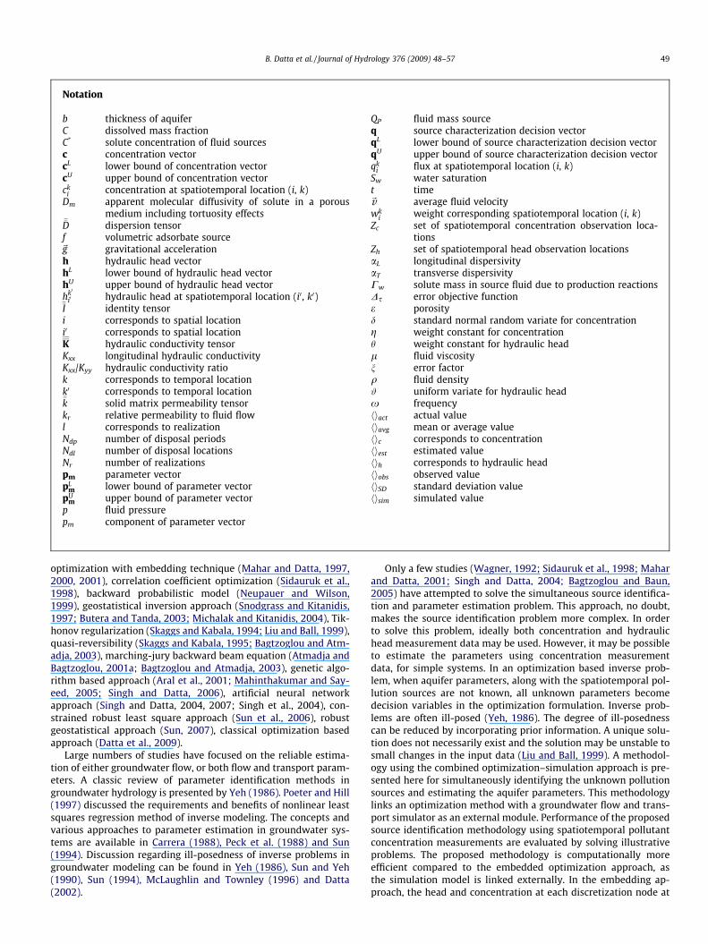
The study area (732 m � 549 m), identical to the one utilized inMahar and Datta (2001) is shown in Fig. 1. The top and bottomboundaries are impervious. Constant head boundary conditionsare assumed along the left and right edges of the illustrative studyarea. A constant head of 100 m is acting along the left edge of thestudy area while on the right edge the constant head is specified tobe 88 m. The coordinate axes of the illustrative study areas are as-

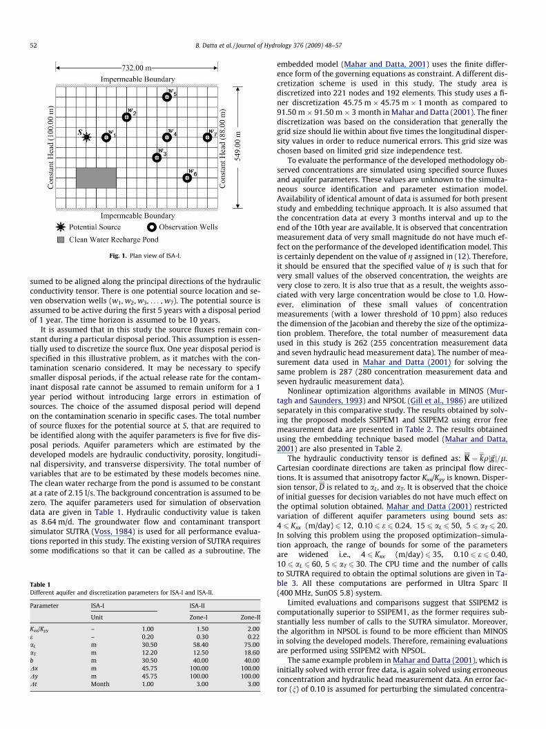
Fig. 1. Plan view of ISA-I.

52 B. Datta et al. / Journal of Hydrology 376 (2009) 48–57

sumed to be aligned along the principal directions of the hydraulicconductivity tensor. There is one potential source location and se-ven observation wells (w1, w2, w3, . . . , w7). The potential source isassumed to be active during the first 5 years with a disposal periodof 1 year. The time horizon is assumed to be 10 years.

It is assumed that in this study the source fluxes remain con-stant during a particular disposal period. This assumption is essen-tially used to discretize the source flux. One year disposal period isspecified in this illustrative problem, as it matches with the con-tamination scenario considered. It may be necessary to specifysmaller disposal periods, if the actual release rate for the contam-inant disposal rate cannot be assumed to remain uniform for a 1year period without introducing large errors in estimation ofsources. The choice of the assumed disposal period will dependon the contamination scenario in specific cases. The total numberof source fluxes for the potential source at S, that are required tobe identified along with the aquifer parameters is five for five dis-posal periods. Aquifer parameters which are estimated by thedeveloped models are hydraulic conductivity, porosity, longitudi-nal dispersivity, and transverse dispersivity. The total number ofvariables that are to be estimated by these models becomes nine.The clean water recharge from the pond is assumed to be constantat a rate of 2.15 l/s. The background concentration is assumed to bezero. The aquifer parameters used for simulation of observationdata are given in Table 1. Hydraulic conductivity value is takenas 8.64 m/d. The groundwater flow and contaminant transportsimulator SUTRA (Voss, 1984) is used for all performance evalua-tions reported in this study. The existing version of SUTRA requiressome modifications so that it can be called as a subroutine. The

Table 1Different aquifer and discretization parameters for ISA-I and ISA-II.

Parameter ISA-I ISA-II

Unit Zone-I Zone-II

Kxx/Kyy – 1.00 1.50 2.00e – 0.20 0.30 0.22aL m 30.50 58.40 75.00aT m 12.20 12.50 18.60b m 30.50 40.00 40.00Dx m 45.75 100.00 100.00Dy m 45.75 100.00 100.00Dt Month 1.00 3.00 3.00

embedded model (Mahar and Datta, 2001) uses the finite differ-ence form of the governing equations as constraint. A different dis-cretization scheme is used in this study. The study area isdiscretized into 221 nodes and 192 elements. This study uses a fi-ner discretization 45.75 m � 45.75 m � 1 month as compared to91.50 m � 91.50 m � 3 month in Mahar and Datta (2001). The finerdiscretization was based on the consideration that generally thegrid size should lie within about five times the longitudinal disper-sity values in order to reduce numerical errors. This grid size waschosen based on limited grid size independence test.

To evaluate the performance of the developed methodology ob-served concentrations are simulated using specified source fluxesand aquifer parameters. These values are unknown to the simulta-neous source identification and parameter estimation model.Availability of identical amount of data is assumed for both presentstudy and embedding technique approach. It is also assumed thatthe concentration data at every 3 months interval and up to theend of the 10th year are available. It is observed that concentrationmeasurement data of very small magnitude do not have much ef-fect on the performance of the developed identification model. Thisis certainly dependent on the value of g assigned in (12). Therefore,it should be ensured that the specified value of g is such that forvery small values of the observed concentration, the weights arevery close to zero. It is also true that as a result, the weights asso-ciated with very large concentration would be close to 1.0. How-ever, elimination of these small values of concentrationmeasurements (with a lower threshold of 10 ppm) also reducesthe dimension of the Jacobian and thereby the size of the optimiza-tion problem. Therefore, the total number of measurement dataused in this study is 262 (255 concentration measurement dataand seven hydraulic head measurement data). The number of mea-surement data used in Mahar and Datta (2001) for solving thesame problem is 287 (280 concentration measurement data andseven hydraulic measurement data).

Nonlinear optimization algorithms available in MINOS (Mur-tagh and Saunders, 1993) and NPSOL (Gill et al., 1986) are utilizedseparately in this comparative study. The results obtained by solv-ing the proposed models SSIPEM1 and SSIPEM2 using error freemeasurement data are presented in Table 2. The results obtainedusing the embedding technique based model (Mahar and Datta,2001) are also presented in Table 2.

The hydraulic conductivity tensor is defined as: K ¼ kqj~gj=l.Cartesian coordinate directions are taken as principal flow direc-tions. It is assumed that anisotropy factor Kxx/Kyy is known. Disper-sion tensor, D is related to aL, and aT. It is observed that the choiceof initial guesses for decision variables do not have much effect onthe optimal solution obtained. Mahar and Datta (2001) restrictedvariation of different aquifer parameters using bound sets as:4 6 Kxx (m/day) 6 12, 0.10 6 e 6 0.24, 15 6 aL 6 50, 5 6 aT 6 20.In solving this problem using the proposed optimization–simula-tion approach, the range of bounds for some of the parametersare widened i.e., 4 6 Kxx (m/day) 6 35, 0.10 6 e 6 0.40,10 6 aL 6 60, 5 6 aT 6 30. The CPU time and the number of callsto SUTRA required to obtain the optimal solutions are given in Ta-ble 3. All these computations are performed in Ultra Sparc II(400 MHz, SunOS 5.8) system.

Limited evaluations and comparisons suggest that SSIPEM2 iscomputationally superior to SSIPEM1, as the former requires sub-stantially less number of calls to the SUTRA simulator. Moreover,the algorithm in NPSOL is found to be more efficient than MINOSin solving the developed models. Therefore, remaining evaluationsare performed using SSIPEM2 with NPSOL.

The same example problem in Mahar and Datta (2001), which isinitially solved with error free data, is again solved using erroneousconcentration and hydraulic head measurement data. An error fac-tor (n) of 0.10 is assumed for perturbing the simulated concentra-

Table 2Comparative solution results for ISA-I with n = 0.

Parameters Units Actual value Mahar and Datta (2001) MINOS NPSOL

SSIPEM1 SSIPEM2 SSIPEM1 SSIPEM2

aL m 30.50 30.49 30.50 30.50 30.50 30.50aT m 12.20 12.19 12.20 12.20 12.20 12.20Kxx m/d 8.64 8.66 8.64 8.64 8.64 8.64e – 0.20 0.20 0.20 0.20 0.20 0.20Year 1, S gm/s 48.80 48.92 48.79 48.79 48.80 48.80Year 2, S gm/s 0.00 0.00 0.00 0.00 0.00 0.00Year 3, S gm/s 10.00 9.90 9.99 9.99 10.00 10.00Year 4, S gm/s 42.00 41.88 41.98 41.98 41.99 41.99Year 5, S gm/s 36.00 36.10 35.98 35.98 35.99 35.99

Table 3Comparison of computational complexity for ISA-I.

Nonlinear optimization algorithms Developed models Number of calls to SUTRA CPU time (s)

MINOS SSIPEM1 13,223 1031SSIPEM2 8038 836

NPSOL SSIPEM1 1228 136SSIPEM2 791 92

B. Datta et al. / Journal of Hydrology 376 (2009) 48–57 53

tion data. Hydraulic head measurements are perturbed by addingrandom uniform variate to the numerically simulated hydraulicdata. As stated earlier, for performance evaluation purpose, thelower and the upper limit of the random uniform variate # is spec-ified to be �20 cm and 20 cm, respectively. These limits are basedon plausible head measurement error bounds. No doubt, moreaccurate results are expected when smaller bounds on the errorterm # can be specified.

Corresponding source fluxes and parameter values, based on 20solutions obtained by using 20 perturbed measurement data setsare shown in Table 4. This study is limited to using 20 perturbeddata sets mainly due to the fact that any sample size smaller than20 would not be sensible. A larger sample set is however moredesirable to ensure that the statistical parameters such as varianceand coefficient of variance of the estimated values are compara-tively more stable. The CPU time required for solving this problemusing erroneous observation data varies between 50 and 70 s in Ul-tra Sparc II (400 MHz, SunOS 5.8) system. The number of calls to SU-TRA required for solution varies between 625 and 919. These resultsclearly show that the proposed methodology is computationallymuch more efficient than the embedding technique based simulta-neous source identification and parameter estimation models.

Illustrative study area-II (ISA-II)

In order to evaluate the performance of the developed method-ology for large-scale aquifers, SSIPEM2 in combination with NPSOL

Table 4Different solution results for ISA-I with n = 0.10.

Parameters Units Actual value Mahar and Datta (2

Mean

aL m 30.50 28.65aT m 12.20 10.05Kxx m/d 8.64 10.01e – 0.20 0.23S (year 1) gm/s 48.80 46.72S (year 2) gm/s 0.00 0.00S (year 3) gm/s 10.00 8.39S (year 4) gm/s 42.00 30.23S (year 5) gm/s 36.00 34.67

a SD = Standard deviation.b CV = Coefficient of variation.

is applied to a fairly large (6000 m � 4000 m) illustrative studyarea. The aquifer has two zones which are anisotropic and individ-ually homogeneous. The top and the bottom boundaries are con-sidered to be impervious. A time varying hydraulic head isassumed to be acting along the left edge of the aquifer, while a con-stant hydraulic head (72 m) is specified along the right edge of theaquifer. The aquifer is confined with two-dimensional flow andtransport processes. Eight potential source locations(S1, S2, . . . , S8), 18 observation wells (w1, w2, w3, . . . , w18), twopumping wells (p1, p2), and one clean water recharge pond(1000 m � 400 m) are considered. The study area is shown inFig. 2. Aquifer and discretization parameters used for generationof observation data are given in Table 1. Hydraulic conductivityvalues are taken as 2.28 � 10�4 m/s and 4.50 � 10�4 m/s forzone-I and zone-II, respectively.

In this illustrative problem all the sources are assumed to be ac-tive at least in few time periods. Therefore, no dummy source is in-cluded explicitly within the potential sources. However, unknownsource identification can involve estimation of spatial and tempo-ral fluxes. It is true that only when a potential location is such thatthe source fluxes at that location at all times are zero, the potentiallocation is not an actual source location or, a dummy location.However, if we combine spatial and temporal fluxes, the distinc-tion of a location being actual location, or not can be relevant toa given time period only. In fact, the illustrative problem solvedis more general in nature where some of the sources are activein some time domain and inactive in other time domains, at a given

001) Present study

SDa CVb Mean SDa CVb

0.98 3.40 30.52 2.02 6.620.20 1.99 12.23 0.25 2.020.65 6.44 8.86 0.55 6.270.015 6.86 0.203 0.013 6.423.41 7.29 47.98 3.00 6.25– – 0.59 – –2.93 34.92 10.19 0.87 8.49

10.14 33.55 43.04 3.38 7.855.73 16.53 37.10 3.28 8.84

Fig. 2. Plan view of ISA-II.

54 B. Datta et al. / Journal of Hydrology 376 (2009) 48–57

spatial location. Therefore, the capability of identifying sourcelocations is demonstrated with respect to multiple time domainsat different locations. Only a special case, where source flux is zeroat all time domains would address a special case problem of adummy source location. In fact, the problem solved here may bemore general in nature.

Although a 20 year time horizon is considered for solution, thesources are assumed to be active only during the first 5 years. Theindividual disposal period is assumed to be 1 year. As stated earlier,this disposal period is chosen only for this illustrative problem. Nodoubt it would be more desirable, if for accuracy smaller discretiza-tion periods are specified for the source fluxes. Ideally, even if theflux remains uniform for a longer period, a smaller discretizationin terms of unit disposal period should result in optimal solutionswhich identify the same magnitude of fluxes for each of the smallerdisposal periods constituting the longer period. If a longer disposalperiod is specified, during which the disposal rate does not remainuniform, decrease in solution accuracy is expected. This is because;one possibility would be that the solution obtained would be basedon averaging of the flux over a longer period. It is also assumed thatthe source flux from a particular potential location during a disposalperiod is constant. The clean water leakage from the pond is spec-ified to be 3.5 l/s. Water withdrawal rates from the two pumpingwells are given in Table 5. It is assumed that water is withdrawnfrom these pumping wells only during the first 10 years of the 20year time horizon. The illustrative problem assumes transient flowand transport of a conservative pollutant. The time varying hydrau-lic head h(t) is assumed to obey the following relationship:

hðtÞ ¼ 120 1þ sinðxtyÞ60

� �; 8t 2 ½ty; ty þ 1Þ ð20Þ

Table 5Pumping rates (l/s) for ISA-II.

Well Year

1 2 3 4 5 6 7 8 9 10

p1 5.60 4.00 4.50 6.65 6.40 3.80 5.20 5.50 6.20 5.00p2 8.00 6.50 7.50 5.00 7.00 5.60 6.70 4.80 5.50 4.60

It is also assumed that the h(t) remains constant throughout the t-thyear with frequency x = p/10 (year�1). The initial hydraulic headdata in the aquifer are generated by solving the SUTRA (Voss,1984) model. Steady state flow condition is assumed with a con-stant head of 120 m along the left edge, and a constant head of72 m along the right edge of the aquifer. Also, it is assumed thatthere is no pumping, no clean water recharge from the pond, andno source fluxes. The initial (background) concentration in the aqui-fer is assumed to be 100 ppm. The aquifer under study is discretizedinto 2501 nodes, and 2400 elements.

In the simultaneous source identification and parameter esti-mation problem, some of the aquifer parameters, along with thesource fluxes are considered to be unknown to the identificationmodel. The aquifer parameters which are estimated simulta-neously with the sources are hydraulic conductivity, porosity, lon-gitudinal dispersivity, and transverse dispersivity. Theperformance of SSIPEM2 is evaluated for different scenarios.

Three different scenarios are considered for demonstrating theefficiency of the proposed methodology. In the first two scenarios(Scenario-I and II), aquifer porosities (in the two zones) are consid-ered to be known. The model performance is evaluated using twobound sets on the decision variables except dispersivities. In Sce-nario-III, all the above mentioned parameters, including porosityand the source fluxes are considered unknown to the identificationmodel. Therefore, the number of decision variables in the identifi-cation formulation under Scenario-I and II is 46, and under Sce-nario-III it is 48, including 40 source fluxes. The bound set on thelongitudinal and transverse dispersivities used in all the scenariosare kept the same (10 6 aL 6 100, 5 6 aT 6 50). Bound sets on otheraquifer parameters are specified by multiplying the actual valuesof the parameters by some factors. In Scenario-I, the lower boundspecified is 0.50 times the actual known hydraulic conductivityvalues, and the upper bound is specified to be 1.50 times the actualvalues. The lower bound and upper bound factors for hydraulicconductivity are specified as 0.10 and 2.22, respectively for Sce-nario-II. Scenario-III is similar to the Scenario-I except that the zo-nal porosities are also considered as variables with the lower andthe upper bound factors 0.90 and 1.10, respectively. Therefore, inthis scenario, porosity is also considered as a decision variable in

B. Datta et al. / Journal of Hydrology 376 (2009) 48–57 55

the identification model. Hydraulic conductivity ratios (Kxx/Kyy) ofthe illustrative study area assumed to be known.

In evaluating the performance of the proposed model for thefairly large study area, observed concentration data from 18 wellsat an interval of 3 months are considered available for 20 years. Itis assumed that only one hydraulic head measurement data at theend of each year for 18 observation wells are available. The numberof hydraulic head measurement data available per observationwell for the entire time horizon is 20. Total number of head mea-surement data from eighteen observation wells is 360. In all thescenarios these hydraulic head data, along with 1041 concentra-tion data are provided to the simultaneous source identificationand parameter estimation model. Due to low concentration, 399values are not being included in the objective function. Also,numerically simulated hydraulic head and concentration data areconsidered erroneous. An error facto (n) of 0.10 is assumed forthe concentration measurement data. The hydraulic head mea-surement data are obtained by adding random uniform variatesto the simulated hydraulic heads. The results for first scenario withforty six decision variables are shown in Tables 6 and 7.

The CPU time required for solving these problems varies be-tween 44.8 and 125.9 h for Scenario-I, and between 40 and 130 hfor Scenario-II. The number of calls made to SUTRA ranges from5241 to 13,560 with Scenario-I, where Scenario-II requires 4591–15,050 calls. In Scenario-III, two more variables are added to theset of decision variables, as porosities of the two zones are consid-ered unknown to the identification model. The results are shown inTable 7. The CPU time required for solving the simultaneous sourceidentification and parameter estimation problem, having 48 deci-sion variables varies between 61 h and 146.5 h. The number of callsmade to the SUTRA ranges from 6153 to 16,522. These problemsare solved in Ultra Sparc II (400 MHz, SunOS 5.8) system.

Discussion of results

The source identification problem becomes much more compli-cated when some of the aquifer parameters are also unknown. Twomodels, i.e., SSIPEM1 and SSIPEM2 are developed to solve this com-plex identification problem. As in the case of source identificationmethodology, the simultaneous source identification and parame-ter estimation models are also based on linked optimization–sim-ulation approach. Performances of the developed models areevaluated for two illustrative study areas. Both concentration andhydraulic head data are incorporated for solving these models.Measurement errors, both in concentration and in hydraulic headdata, are considered for performance evaluation purpose.

Obtained solutions using the proposed SSIPEM1 and SSIPEM2models for identifying the source fluxes, and estimating the aquiferparameters simultaneously for ISA-I are compared. Performanceevaluations with error free observation data given in Table 2 indi-

Table 6Different parameter values obtained for ISA-II with n = 0.10.

Zones Parameters Units Actual value Scenario-I

Mean SDa

Zone-I aL m 58.40 56.96 1.95aT m 12.50 12.56 0.12Kxx � 10�4 m/s 2.28 2.29 0.03e – 0.30 – –

Zone-II aL m 75.00 73.58 5.48aT m 18.60 18.66 0.44Kxx � 10�4 m/s 4.50 4.46 0.13e – 0.22 – –

a SD = Standard deviation.b RE = Relative error in percent.

cate that SSIPEM2 is computationally more efficient than SSIPEM1.Also, the nonlinear optimization algorithm in NPSOL is found to besuperior to that in MINOS for solving the proposed linked optimi-zation–simulation problems. It may be mentioned that the CPUtime requirement, or the number of calls made to the external flowand transport simulator SUTRA is very much dependent on the ini-tial guesses, value of the derivative interval, and various functionprecision, optimality tolerance criteria used in the solution proce-dure. The solution results show that the estimated value of thesource fluxes and the parameters using error free data for ISA-I (Ta-ble 2) are identical to the actual values. However, this assumptionof error free observation data is idealistic. Assuming an error factor(n) of 0.10 for concentration and uniform random errors with-in ± 20.0 cm for hydraulic head measurement data, which repre-sent more realistic conditions, improvements (as compared toresults obtained in Mahar and Datta (2001)) in the estimation er-rors of these source fluxes and aquifer parameters are evident.The estimated values shown in Table 4, are averaged over 20 setsof solutions. The estimated hydraulic conductivity value is closerto the actual value of 8.64 m/d compared to the solution resultsof Mahar and Datta (2001). Solution results also show that theother estimated values are closer to the actual values. There areimprovements in the estimated standard deviations of all sourcefluxes and aquifer parameters except longitudinal and transversedispersivities.

Potential applicability of the proposed SSIPEM2 in combinationwith NPSOL is demonstrated for a fairly large study area(6000 m � 4000 m). Multiple source fluxes from multiple potentialsource locations, along with the aquifer parameters are identifiedin the illustrative applications. Illustrative application with 40source fluxes, and six aquifer parameters (Scenario-I and II) re-sulted in source identification errors (NEEf) of less than ten percent.The estimated NEEf value is 5.97% for Scenario-I. When Scenario-IIis considered, the estimated NEEf value is increased to 8.40%. Inboth the scenarios, the estimated aquifer parameters are closerto the respective actual values. The estimated deviations, standarddeviations, and relative errors changed only marginally for Sce-nario-II and Scenario-III as compared to Scenario-I. The results ob-tained in all the scenarios are satisfactory (i.e., errors are below 10–15%). The results also show that by increasing the range of thebound set on hydraulic conductivity up to a level does not havemuch effect on the solutions. It is true, that if the optimal solutionconverges to the global optimal solution, the imposed bounds maynot have any effect on the solution. Due to computational time lim-itation, the bounds were kept a bit tight. However, our evaluationshowed the solutions did converge to the same solutions whenbounds were increased, although larger number of iterations wasrequired for relaxed bounds. These evaluations results definitelyshow potential applicability of the proposed methodology forsimultaneous identification of pollution sources and estimation

Scenario-II Scenario-III

REb Mean SDa REb Mean SDa REb

�2.47 56.31 3.16 �3.58 56.96 1.95 �2.470.48 12.55 0.12 0.36 12.56 0.12 0.480.43 2.29 0.30 0.44 2.29 0.03 0.43– – – – 0.29 0.02 �0.03

�1.89 73.48 5.42 �2.03 73.58 5.48 �1.890.32 18.63 0.42 0.16 18.66 0.44 0.32�0.88 4.45 0.14 �1.11 4.46 0.13 �0.88– – – – 0.21 0.02 �0.05

Table 7Resulting source fluxes for different scenarios with n = 0.10.

Disposal period Source Loc. Scenario-I Scenario-II Scenario-III

Actual Mean SDa REb Mean SDa REa Mean SDa REa

1 S1 52.80 53.31 4.01 0.97 52.67 5.24 �0.25 50.73 6.5 �3.92S2 65.29 63.37 5.56 �2.94 63.69 5.11 �2.45 60.71 5.68 �7.01S3 24.37 24.05 2.57 �1.31 23.93 2.67 �1.81 23.31 2.83 �4.35S4 0.00 1.92 1.34 – 2.36 1.36 – 1.68 1.48 –S5 0.00 0.06 0.1 – 0.08 0.14 – 0.02 0.09 –S6 40.25 41.37 4.04 2.78 40.96 4.41 1.76 38.68 6.98 �3.90S7 75.64 74.65 3.92 �1.31 74.16 4.43 �1.96 75.25 9.7 �0.52S8 29.44 29.38 1.93 �0.20 29.35 2.05 �0.31 29.50 2.97 0.20

2 S1 42.64 42.27 11.22 �0.87 44.93 12.05 5.37 37.26 9.42 �12.62S2 53.92 57.87 11.39 7.33 57.97 12.9 7.51 55.87 9.85 3.62S3 20.86 22.2 4.56 6.42 21.83 4.45 4.65 20.64 4.96 �1.05S4 65.60 60.99 7.17 �7.03 58.20 7.03 �11.28 56.99 8.35 �13.13S5 0.00 0.28 0.49 – 0.28 0.53 – 0.06 0.17 –S6 55.32 51.69 11.62 �6.56 53.83 12.76 �2.69 51.12 14.29 �7.59S7 60.48 63.81 10.85 5.51 64.41 11.19 6.50 55.94 5.98 �7.51S8 56.75 55.47 4.39 �2.26 55.09 4.17 �2.93 52.27 5.88 �7.89

3 S1 35.37 35.84 13.82 1.33 32.09 15.17 �9.27 39.11 14.38 10.57S2 72.45 65.79 9.67 �9.19 65.48 10.61 �9.62 64.18 10.83 �11.41S3 36.28 34.76 2.66 �4.19 35.47 2.1 �2.23 34.69 4.35 �4.38S4 32.68 39.52 12.22 20.93 44.42 12.46 35.92 42.17 10.14 29.04S5 0.00 0.27 0.65 – 0.19 0.56 – 0.15 0.46 –S6 62.18 63.83 20.13 2.65 58.92 21.51 �5.24 60.51 26.79 �2.69S7 52.44 48.94 13.85 �6.67 47.84 13.42 �8.77 50.48 10.56 �3.74S8 0.00 1.52 2.23 – 1.61 2.2 – 1.31 1.69 –

4 S1 18.92 18.21 12.24 �3.75 21.64 13.01 14.38 15.29 10.26 �19.19S2 0.00 3.63 3.89 – 3.34 4 – 2.36 3.39 –S3 0.00 0.90 1.66 – 0.90 1.53 – 0.99 1.63 –S4 26.55 17.47 11.21 �34.20 13.47 10.98 �49.27 15.04 10.01 �43.35S5 0.00 0.05 0.16 – 0.10 0.3 – 0.16 0.45 –S6 58.72 58.62 23.03 �0.17 63.04 25.79 7.36 58.54 22.32 �0.31S7 39.25 39.80 9.96 1.40 39.62 8.63 0.94 39.31 9.06 0.15S8 0.00 0.12 0.21 – 0.14 0.24 – 0.05 0.1 –

5 S1 27.14 27.13 6.3 �0.04 25.65 6.39 �5.49 27.30 5.59 0.59S2 0.00 0.31 0.77 – 0.54 1.27 – 1.24 1.41 –S3 0.00 0.18 0.3 – 0.14 0.29 – 0.13 0.34 –S4 0.00 3.76 5.41 – 3.92 5.62 – 4.43 4.86 –S5 0.00 0.45 0.99 – 0.39 0.94 – 0.80 1.24 –S6 43.27 42.23 13.26 �2.40 39.69 15.05 �8.27 40.59 13.4 �6.19S7 25.63 26.56 5.72 3.63 27.71 5.06 8.12 24.03 6.8 �6.24S8 0.00 0.15 0.22 – 0.14 0.21 – 0.18 0.28 –NEEf 5.97 8.4 8.44

a SD = Standard deviation.b RE = Relative error in percent.

56 B. Datta et al. / Journal of Hydrology 376 (2009) 48–57

of parameters in fairly large-scale aquifers incorporating variousreal world complex situations.

It is observed that, computational burden due to repeated callsto the simulation model is a concern. Also, numerically computedJacobians are susceptible to loss of accuracy. Monitoring wellsclose to potential source location can improve the source identifi-cation. Even then identification of potential source locations maynot be easy. No doubt, uncertainties in the aquifer parameters aswell as in the boundary conditions need more rigorous consider-ations. It is worth mentioning that although evolutionary algo-rithms make it easier to link the optimization algorithm with theexternal simulator, these population based algorithms requiremore number of evaluations of the fitness function, which is com-putationally very expensive as it requires repeated solution of thesimulation model. Also, the computational time required by evolu-tionary algorithms increases exponentially with the increase innumber of decision variables.

Conclusions

The potential applicability of using a linked simulation optimi-zation model for optimal identification of unknown groundwater

pollution sources and simultaneous estimation of flow and trans-port parameters is demonstrated. The proposed methodologyincorporates solution algorithms of nonlinear programming, withexternal linking to a simulation model for simulating the flow andtransport parameters in the aquifer. The advantage of using a linearobjective function with nonlinear constraints in a nonlinear optimi-zation model is described. The performance evaluations for differ-ent scenarios of data availability and an illustrative study area ofrealistic size are presented. It is expected that the proposed meth-odology overcomes some of the severe computational limitationsof the embedded optimization approach. The proposed methodol-ogy is capable of solving the source identification problem for afairly large study area with both sources, and flow and transportparameters as unknowns. The identification results, although lim-ited in scope show the potential applicability of the proposed meth-odology. This study shows that it is possible to solve fairly largesource identification problems using the gradient based linked sim-ulation–optimization model, with computational efficiency.

References

Aral, M.M., Guan, J., Maslia, M.L., 2001. Identification of contaminant source locationand release history in aquifers. J. Hydrol. Eng. 6 (3), 225–234.

B. Datta et al. / Journal of Hydrology 376 (2009) 48–57 57

Atmadja, J., Bagtzoglou, A.C., 2001a. Pollution source identification inheterogeneous porous media. Water Resour. Res. 37 (8), 2113–2125.

Atmadja, J., Bagtzoglou, A.C., 2001b. State of the art report on mathematicalmethods to reliable of groundwater pollution source identification. Environ.Forensics 2 (3), 205–214.

Bagtzoglou, A.C., Dougherty, D.E., Tompson, A.F.B., 1992. Application of particlemethods to reliable identification of groundwater pollution sources. WaterResour. Manage. 6, 15–23.

Bagtzoglou, A.C., Atmadja, J., 2003. Marching-jury backward beam equation andquasi-reversibility methods for hydrologic inversion: application tocontaminant plume spatial distribution recovery. Water Resour. Res. 39 (2),10–14. SBH 10-1.

Bagtzoglou, A.C., Baun, S.A., 2005. Near real-time atmospheric contamination sourceidentification by an optimization-based inverse method. Inverse Probl. Sci. Eng.13 (3), 241–259.

Butera, I., Tanda, M.G., 2003. A geostatistical approach to recover the release historyof groundwater pollutants. Water Resour. Res 39 (12), 1372. doi:10.1029/2003WR002314.

Carrera, J., 1988. State of the art of the inverse problem applied to the flow andsolute transport equations. In: Custodia, E. et al. (Eds.), Groundwater Flow andQuality Modeling. D. Reidel Publishing Cp, pp. 49–583.

Chakrabarty, D., 2001. Identification of unknown groundwater pollution sourcesand simultaneous parameter estimation using linked optimization–simulationapproach” PhD Dissertation, I.I.T. Kanpur, India.

Datta, B., 2002. In: Aral, M.M., Guan, J., Maslia, M.L. (Eds.), Discussion onIdentification of Contaminant Source Location and Release History inAquifers. J. Hydrol. Eng. ASCE 7(5), 399–400.

Datta, B., Beegle, J.E., Kavvas, M.L., Orlob, G.T., 1989 Development of an expert-system embedding pattern-recognition techniques for pollution-sourceidentification, Technical Report: PB-90-185927/XAB, OSTI ID: 6855981, Dept.of Civil Engineering, California Univ., Davis, CA (USA).

Datta, B., Chakrabarty, D., Dhar, A., 2009. Optimal dynamic monitoring networkdesign and identification of unknown groundwater pollution sources. WaterResour. Manage. 1, 1–10. doi:10.1007/s11269-008-9368-z.

Gill, P.E., Murray, W., Saunders, M.A., Wright, M.H., 1986. User’s Guide for NPSOL(version 4.0): A Fortran Package for Nonlinear Programming, Technical ReportSOL 86-2, Dept. of Operation Research, Stanford University, Stanford, CA.

Gorelick, S.M., Evans, B., Ramson, I., 1983. Identifying sources of groundwaterpollution: an optimization approach. Water Resour. Res. 19 (3), 779–790.

Gorelick, S.M., 1990. Large scale deterministic and stochastic optimizationformulations involving simulation of subsurface contamination. Math.Program. 48, 19–39.

Keidser, A., Rosbjerg, D., 1991. A comparison of four inverse approaches togroundwater flow and transport parameter identification. Water Resour. Res.27 (9), 2219–2232.

Liu, C., Ball, W.P., 1999. Application of inverse methods to contaminant sourceidentification from aquitard diffusion profiles at Dover AFB, Delaware. WaterResour. Res. 35 (7), 1975–1985.

Mahar, P.S., Datta, B., 1997. Optimal monitoring network and ground-water-pollution source identification. J. Water Resour. Plan. Manage. 123 (4), 199–207.

Mahar, P.S., Datta, B., 2000. Identification of pollution sources in transientgroundwater system. Water Resour. Manage. 14 (6), 209–227.

Mahar, P.S., Datta, B., 2001. Optimal identification of ground-water pollutionsources and parameter estimation. J. Water Resour. Plan. Manage. 127 (1), 20–29.

Mahinthakumar, G., Sayeed, M., 2005. Hybrid genetic algorithm – local searchmethods for solving groundwater source identification inverse problems. J.Water Resour. Plan. Manage. 131 (1), 45–57.

McLaughlin, D., Townley, L.R., 1996. A reassessment of the groundwater inverseproblem. Water Resour. Res. 32 (5), 1131–1161.

Michalak, A.M., Kitanidis, P.K., 2004. Estimation of historical groundwatercontaminant distribution using the adjoint state method applied togeostatistical inverse modeling. Water Resour. Res. 40, W08302. doi: 10.29/2004WR003214.

Murtagh, B.A., Saunders, M.A., 1993. MINOS 5.4 User’s guide, Technical Report SOL83-20R, Dept. of Operation Research, Stanford University, Stanford, CA.

Neupauer, R.M., Wilson, J.L., 1999. Adjoint method for obtaining backward-in-timelocation and travel probabilities of a conservative groundwater contaminant.Water Resour. Res. 35 (11), 3389–3398.

Peck, A., Gorelick, S.M., de Marsily, G., Foster, S., Kovalevsky, V., 1988. Consequencesof Spatial Variability in Aquifer Properties and Data Limitations forGroundwater Modeling Practice. IASH Press, Wallingford, England.

Poeter, E.P., Hill, C., 1997. Inverse models: a necessary next step in ground-watermodeling. Ground Water 35, 250–260.

Sidauruk, P., Cheng, A.H.-D., Ouazar, D., 1998. Ground water contaminant sourceand transport parameter identification by correlation coefficient optimization.Ground Water 36 (2), 208–214.

Singh, R.M., Datta, B., 2004. Groundwater pollution source identification andsimultaneous parameter estimation using pattern matching by artificial neuralnetwork. Environ. Forensics 5 (3), 143–159.

Singh, R.M., Datta, B., Jain, A., 2004. Identification of unknown groundwaterpollution sources using artificial neural networks. J. Water Resour. Plan.Manage. 130 (6), 506–514.

Singh, R.M., Datta, B., 2006. Identification of groundwater pollution sources usingGA-based linked simulation optimization model. J. Hydrol. Eng. 11 (2), 101–109.

Singh, R.M., Datta, B., 2007. Artificial neural network modeling for identification ofunknown pollution sources in groundwater with partially missingconcentration observation data. Water Resour. Manage. 21 (3), 557–572.

Skaggs, T.H., Kabala, Z.J., 1994. Recovering the release history of a groundwatercontaminant. Water Resour. Res. 30 (1), 71–79.

Skaggs, T.H., Kabala, Z.J., 1995. Recovering the release history of a groundwatercontaminant plume: method of quasi-reversibility. Water Resour. Res. 31 (11),2669–2673.

Snodgrass, M.F., Kitanidis, P.K., 1997. A geostatistical approach to contaminantsource identification. Water Resour. Res. 33 (4), 537–546.

Sun, A.Y., Painter, S.L., Wittmeyer, G.W., 2006. A constrained robust least squaresapproach for contaminant source release history identification. Water Resour.Res. 42 (4), W04414. doi:10.1029/2005WR004312.

Sun, A.Y., 2007. A robust maximum likelihood approach to contaminant sourceidentification. Water Resour. Res. 43 (2), W02418. doi:10.1029/2006WR005106.

Sun, N.-Z., 1994. Inverse Problems in Groundwater Modeling. Kluwer Academics,Norwell, MA.

Sun, N.-Z., Yeh, W.-G., 1990. Coupled inverse problems in groundwater modeling. 1.Sensitivity analysis and parameter identification. Water Resour. Res. 26, 2507–2525.

Voss, C.I., 1984. A finite-element simulation model for saturated-unsaturated, fluid-density-dependent ground-water flow with energy transport or chemically-reactive single-species solute transport. US Geological Survey Water-ResourcesInvestigations Report 84-4369, 409.

Wagner, B.J., 1992. Simultaneous parameter estimation and contaminant sourcecharacterization for coupled groundwater flow and contaminant transportmodeling. J. Hydrol. 135, 275–303.

Woodbury, A.D., Ulrych, T.J., 1996. Minimum relative entropy inversion: theory andapplication to recovering the release history of a groundwater contaminant.Water Resour. Res. 32 (9), 2671–2681.

Yeh, W.W.-G., 1986. Review of parameter identification procedures in groundwaterhydrology: the inverse problem. Water Resour. Res. 22, 95–108.