INVERSE METHODS TO ESTIMATE ANTHOCYANIN DEGRADATION KINETIC PARAMETERS IN CHERRY POMACE DURING NON-ISOTHERMAL HEATING

By

Ibrahim Greiby

A DISSERTATION

Submitted to

Michigan State University in partial fulfillment of the requirements

for the degree of

Biosystems Engineering - Doctor of Philosophy

2013

ABSTRACT

INVERSE METHODS TO ESTIMATE ANTHOCYANIN DEGRADATION KINETIC PARAMETERS IN CHERRY POMACE DURING NON-ISOTHERMAL HEATING

By

Ibrahim Greiby

Fruit and vegeTables are a rich source of many bio-active compounds from

which value-added nutraceuticals can be produced. Anthocyanins (ACY), which are

unstable at high temperature (> 70°C), are the most abundant flavonoid compound and

are used as a natural colorant. ACY have health benefits and can be sourced from

inexpensive byproducts, such as cherry pomace. The most common method of using

the byproduct is to add it as an ingredient to foods that are thermally processed. To

design these processes, the kinetics of ACY degradation must be known as a function

of time, temperature, and moisture content. Therefore, the purpose of this work was to

estimate color kinetic parameters, and anthocyanin degradation parameters in cherry

pomace at different constant moisture contents. To do this, the thermal properties of

the pomace had to be estimated first.

The moisture content was kept constant by sealing the cherry pomace in cans.

The retention of ACY in the pomace was investigated during heating at two retort

temperatures 105 and 126.7°C. Tart cherry pomace was equilibrated to other lower

moisture contents (MC) and heated in sealed 54 × 73 mm cans for different times. ACY

retention of 70 MC wet basis (wb) cherry pomace decreased with heating time and

ranged from 76 to 10% for 25 and 90 min heating, respectively at 126.7°C, and ranged

from 60 to 40 % for 100 and 125 min heating, respectively at 105°C. The total color

difference (ΔE) increased with increasing heating time, whereas Browning Index (BI)

exhibited an inverse trend. Correlation between ACY and red color showed a linear

relationship at higher moisture content (70 MC, wb) of cherry pomace. Oxygen radical

absorbance capacity (ORAC) method showed stability during heating at different times.

Differential scanning calorimetery (DSC) was used to measure the specific heat. At ºC

25, the measured specific heat was 1671, 2111 and 2943 J kg-1

K-1

for 25, 41and 70

MC (wb), respectively. Ordinary least squares and sequential estimation methods were

used to estimate the thermal and kinetic parameters. Thermal conductivity (W m-1

K-1

)

was estimated as a linear function of temperature at 25°C (k1) and 125°C (k2). The

estimated k1 and k2 values and standard errors for 70, 41 and 25% MC (wb) were 0.49

+/- 0.00047 and 0.55 +/- 0.00058, 0.20 +/- 0.0015 and 0.39 +/- 0.0012, and 0.15 +/-

0.0034 and 0.28 +/- 0.0037 (W m-1

K-1

), respectively. The rate constant and activation

energy for 70% MC pomace were estimated as k 115.8 °C = 0.0129 ± 0.0013 min-1 and

75.7 ± 10.7 kJ/mol, respectively. The model fit well as shown by a RMSE of

approximately 9% of initial ACY concentration (about 65 mg/kg db) and relative error

less than 24% for the three MCs.

There was no significant effect of moisture content on the reaction rate constant.

Empirical correlations for ACY degradation with red color, thermal properties and kinetic

parameters were established. These results can be useful for processors desiring to

use cherry pomace to make value-added by-products at elevated temperatures.

Examples include extruded snacks and breakfast cereals, dried and powdered products

such as drink mixes, and baked goods such as breads, confectionaries, and candies.

These products are all heated at temperatures above 100°C, where ACY degrade.

iv

DEDICATION I dedicate this work to my father, Greiby Emhemed (May Allah have mercy on him), to

my mother, Aisha Abdu-Allah (May Allah give here a long life) for their love, support, and prayers.

v

ACKNOWLEDGEMENTS

( والتقديرالشكر )

(In the name of Allah, the Most Gracious, the Most Merciful) بسم اهلل الرحَمن الرحيم

My deep appreciation and heartfelt gratitude to my advisor, Dr. Kirk D. Dolan, for

the patience, guidance, knowledge and mentorship he provided to me throughout my

Ph.D. program. His consistent support and encouragement made my degree completion

possible. I would also like to thank my committee members, Dr. James Steffe, Dr.

Bradley Marks and Dr. Maurice Bennink for the friendly guidance, helpful suggestions,

and the general collegiality that each of them offered to me.

I sincerely thank Dr. Neil Wright, Department of Mechanical Engineering, for allowing

me to work in his lab for specific heat measurements needed for my research. My great

thanks to Dr. James Beck, Department of Mechanical Engineering, for all the time he

gave me for data analysis by teaching the use of his software (Prop1D). My high

appreciation goes to Dr. Muhammad Siddiq, Department of Food Science, for all his

guidance in chemical analyses, color measurements and scientific writing.

In a similar vein, I’d like to recognize: Mr. Steve Marquie for all his great help regarding

establishing all software for data collection; Mr. Phill Hill, for his help with maintaining

the steam retort, other equipment, and thermocouples modification.

My special thanks go to my friends and lab mates: Dharmendra Mishra, for all his help

and guidance for MATLAB codeing; Dr. Rabiha Sulaiman, for her support and care all

the time, who is now a faculty in University Putra Malaysia, she is the one who helped

and persuaded me to come to MSU in the first place. My best wishes and thanks to all

my friends: Shantanu Kelkar, Sunisa Roidoung, Ahmad Rady, Hayati Samsudin,

George Nyombaire, and Muhammad Eldosari for their support and camaraderie.

vi

Special thanks to my lovely country (Libya) for the scholarship and my liability to be

back and work hard to help building the country as free and progressive country.

My appreciation and thanks goes to all staff in Department of Biosystems &

Agricultural Engineering, Department of Food Science & Human Nutrition, Graduate

School and OISS for their support and resources during a hard time.

Last but not least, my sincere appreciation is due to my wife for the parenting (sons,

Asem & Ala, and daughter, Farah) and the bearing of household burdens while I

pursued my degree. Without her support and caring this work would not have been

possible. To my brothers and sisters for their care, support and encouragement.

vii

TABLE OF CONTENTS

LIST OF TABLES .............................................................................................................. x LIST OF FIGURES ............................................................................................................ xii KEY TO SYMBOLS ........................................................................................................... xvi CHAPTER 1 ...................................................................................................................... 1 INTRODUCTION ............................................................................................................... 1

1.1 Overview of the Dissertation ........................................................................... 2 1.2 Statement of the Problem ................................................................................ 4

1.3 Significance of the Study ................................................................................. 6 1.4 Objective of the Study ..................................................................................... 6

CHAPTER 2 ...................................................................................................................... 8 LITERATURE REVIEW ..................................................................................................... 8

2.1 Heat transfer theory ........................................................................................ 9

2.2 Cylindrical coordinates: ................................................................................... 10 2.3 Heat transfer boundary conditions: ................................................................. 11

2.3.1 Convection heat transfer function of time: ............................................... 11 2.3.2 Surface temperature as function of time (Ts) : ......................................... 13

2.4 Thermal conductivity k (T) (linear with T): ....................................................... 14

2.4.1 Thermal properties of foods: ................................................................... 15

2.4.2 Isothermal and non-isothermal Processing ............................................ 19

2.5 Cherry Pomace’s Anthocyanins ...................................................................... 22 2.5.1 Cherry pomace ........................................................................................ 22

2. 5.2 Anthocyanins in Nature .......................................................................... 23 2.5.3 Structure of Anthocyanins: ..................................................................... 23 2.5.4 Stability of Anthocyanins ......................................................................... 24

2.5.4.1 Effect of pH on ACY Stability ....................................................... 25 2.5.4.2 Effect of Temperature on Anthocyanins Stability ......................... 26

2.5.5 Anthocyanins Antioxidant Capacity ........................................................ 28 2.6 Kinetics And Mechanism of Degradation of Anthocyanins In Foods ............... 30

2.6.1 Kinetics Mechanism: ............................................................................... 30

2.6.2 Anthocyanins Degradation Model: .......................................................... 32

REFERENCES .................................................................................................................. 35 CHAPTER 3 ...................................................................................................................... 45

OBJECTIVE ONE.............................................................................................................. 45 Effect of Non-Isothermal Heat Processing and Moisture Content on the Anthocyanin Degradation and Color Kinetics of Cherry Pomace ........................................................... 45 Abstract ............................................................................................................................. 46

3.1 Introduction ..................................................................................................... 47 3.2 Materials and Methods .................................................................................... 49

viii

3.2.1 Pomace sample preparation ................................................................... 49

3.2.2 Measurement of visual color ................................................................... 50 3.2.3 Anthocyanins extraction .......................................................................... 51

3.2.4 Monomeric anthocyanin content determination ....................................... 52 3.2.5 Antioxidant Capacity ............................................................................... 52 3.2.6 Color kinetics ........................................................................................... 53

3.3 Results and Discussion ................................................................................... 54 3.3.1 Anthocyanin (ACY) degradation .............................................................. 54

3.3.2 Antioxidant Capacity ............................................................................... 55 3.3.3 Instrumental Color Changes ................................................................... 56

3.4 Kinetics of color degradation ........................................................................... 59 3.5 Correlation between red color and anthocyanins ............................................ 62 3.6 Conclusions ..................................................................................................... 64

APPENDICES ................................................................................................................... 65 Appendix A.1 Experimental design and preliminary data ...................................... 66

Appendix A.2 Oxygen Radical Absorbance Capacity (ORAC) Fluorescein Method .................................................................................................................. 74

REFERENCES .................................................................................................................. 76 CHAPTER 4 ...................................................................................................................... 80 OBJECTIVE TWO ............................................................................................................. 80

Estimation of Temperature-Dependent Thermal Properties of Cherry Pomace at Different Moisture Contents During Non-Isothermal Heating ............................................ 80 Abstract ............................................................................................................................. 81

4.1 Introduction ..................................................................................................... 82

4.2. Materials and methods ................................................................................... 85

4.2.1 Sample preparation ................................................................................. 85 4.2.2 Measurement of bulk density and specific heat....................................... 86

4.2.3 Thermal Processing ................................................................................ 88 4.2.3.1 Heat Transfer and governing equations ...................................... 88

4.2.4 Experimental design ............................................................................... 89

4.2.5 Thermal parameter estimation ................................................................ 91 4.2.5.1 Sensitivity Coefficients ................................................................. 91

4.2.5.2 Ordinary Least Squares (OLS) Procedure ................................... 92 4.2.5.3 Sequential Estimation Procedure ................................................ 93

4.3 Results and discussion .................................................................................... 94

4.3.1 Bulk density and Specific heat determination results: ............................ 94

4.3.2 Thermal Parameter Estimation Using Ordinary Least Squares ............... 97 4.3.3 Thermal Parameter Estimation Using the Sequential Procedure ............ 100

4.4 Model validation ............................................................................................. 104

4.5 Conclusions ..................................................................................................... 106 APPENDICES ................................................................................................................... 107

Appendix B.1 Experimental design and preliminary data ...................................... 108 Appendix B.2 Thermal properties determination (DSC) ........................................ 115 Appendix B.3 MATLAB syntax ............................................................................. 120

B.3.1 Script file for nlinfit method..................................................................... 120

ix

B.3.2 Function file (center can temperature prediction by Comsol) .................. 123

B.3.3 Script file for sequential parameter estimation method ........................... 128 REFERENCES .................................................................................................................. 132

CHAPTER 5 ...................................................................................................................... 137 OBJECTIVE THREE ......................................................................................................... 137 Inverse Methods to Estimate Anthocyanin Degradation Kinetic Parameters in Cherry Pomace During Non-Isothermal Heating ........................................................................... 137

Abstract ............................................................................................................................. 138 5.1 Introduction ..................................................................................................... 139 5.2 Materials and Methods ................................................................................... 141

5.2.1 Pomace sample preparation ................................................................... 141 5.2.2 Anthocyanins extraction .......................................................................... 143

5.2.3 Monomeric anthocyanin content determination ....................................... 144 5.2.4 Mathematical Modeling ........................................................................... 144

5.2.4.1 Estimation the kinetic parameters ................................................ 144

5.2.4.2 Arrhenius Reference Temperature .............................................. 148 5.2.4.3 Moisture content Constant ........................................................... 148

5.2.5 Parameter Estimation Techniques .......................................................... 149

5.2.5.1 Sensitivity Coefficient Plot ........................................................... 149 5.2.5.2 Ordinary Least Squares (OLS) Estimation Procedure ................. 150

5.2.5.3 Sequential Estimation Procedure ................................................ 150 5.3 Results and discussion .................................................................................... 152

5.3.1 Anthocyanin (ACY) degradation .............................................................. 152

5.3.2 Reference Temperature Plot ................................................................... 154

5.3.3 Scaled Sensitivity Coefficient Plot ........................................................... 155

5.3.4 Parameter Estimation using Ordinary Least Squares ............................. 156 5.3.4.1 Moisture content constant estimation .......................................... 163

5.3.5 Sequential Parameter Estimation ............................................................ 163 5.4 Conclusions ..................................................................................................... 165

APPENDICES ................................................................................................................... 166

Appendix C.1 Experimental design and preliminary data ...................................... 167 Appendix C.2 Predicted Temperatures data by Comsol software ......................... 172

Appendix C.3 MATLAB syntaxes .......................................................................... 188 C.3.1 Script file for reference temperature determination ................................. 188 C.3.2 Function file-1 and 2 ............................................................................... 188

C.3.3 Script file scaled sensitivity coefficients .................................................. 191

C.3.4 Script file for nlinfit method ..................................................................... 193 C.3.5 Script file for sequential parameter estimation method ........................... 197

REFERENCES .................................................................................................................. 204

CHAPTER 6 ...................................................................................................................... 209 Overall Conclusions and Recommendations ..................................................................... 209

6.1 Summary and Conclusions ............................................................................. 210 6.2 Recommendations for Future Research.......................................................... 212

x

LIST OF TABLES Table 2.1 Six Common Anthocyanidins ......................................................................... 24

Table 3.1 Hunter color L, a, b values, hue angle and chroma of cherry pomace after heat treatment at 126.7 °C. ........................................................................... 58

Table 3.2 The estimated kinetic parameters and the statistical values of zero-order and first-order models for Hunter color L, a, b values and total color change (ΔE) for various processing times of cherry pomace at three moisture contents (wb) at 126.7 °C. ..................................................................................... 61

Table 3.3 Coefficients of equations (3.7) and (3.8) for correlation between Hunter color a values and anthocyanins content .............................................................. 63

Table A.1 Cherry pomace ‘s anthocyanins concentration ( mg/kg,db) after retorting process at different times ........................................................................ 69

Table A.2 Raw data (sample) of retorting process of cherry pomace in a rotary steam retort at 126.7 °C ........................................................................................ 69

Table A.3 The average total antioxidant values of cherry pomace (treated 25%MC and untreated 70% MC,41%MC ,wb) retorted at 126.7 °C )( values for 5 replicates) .............................................................................................................. 75

Table 4.1 Thermal properties of cherry pomace at three moisture contents over temperature range 25-126.7 ºC ............................................................................. 97

Table 4.2 Estimation of thermal conductivity parameters for cherry pomace (90 min retorting) at T1=25 °C and T2= 125 °C. ................................................................ 98

Table 4.3 A comparative literature review of thermal conductivity values of some food products ...................................................................................................... 102

Table 4.4: comparative of thermal conductivity values of Cherry pomace by this study with Choi and Okos empirical equations . ................................................. 103

Table 4.5 Estimation of thermal conductivity (k(t)) parameters for cherry pomace (90 min retorting): OLS vs.Prop1D method ......................................................... 105

Table B.1 Cherry pomace ‘s bulk density at different Moisture contents ..................... 109

Table B.2 Can Steel (202×214) exact diminutions & (Steel properties (Singh, 2001). .................................................................................................................. 110

Table B.3 Example Specific heat’s (Cp) Excel sheet calculation steps for 70% moisture content (wb) Cherry pomace using DSC method ................................. 116

xi

Table B.4 Thermal properties estimation at two temperatures (25, 126) of cherry pomace J kg-1 K-1 ................................................................................................ 119

Table 5.1 Cherry pomace ACY concentration after retorting at two different temperatures for different times .......................................................................... 153

Table 5.2 Kinetic parameter estimates of ACY degradation in cherry pomace at three constant moisture contents after retorting processing ................................ 157

Table 5.3 Summary of published kinetic parameters of anthocyanin degradation by thermal treatments .............................................................................................. 159

Table 5.4 Correlation matrices Table of the kinetics parameters of Eq.(5.11). ............ 160

Table C.1 Absorbance versus Retorting time of Cherry pomace ACY’s extractions at three constant moisture content heated at 126.7°C ........................................ 169

Table C.2 Cherry pomace’s ACY concentration after retorting at two different temperatures for different times .......................................................................... 170

Table C.3 Part of predicted temperatures (°C) data at 15 gauss points (Pts) in the can for Cherry pomace (70% MC, wb) at126.7°C Retort Temperature). ............. 172

Table C.4 Part of predicted temperatures (°C) data at 15 gauss points (Pts) in the can for Cherry pomace (70% MC, wb) (105 °C Retort Temp). ............................ 178

xii

LIST OF FIGURES

Figure 1.1 Flow chart of experimental plan of cherry pomace retorting and estimation of kinetic parameters of anthocyanin degradation under the process. ................................................................................................................... 5

Figure 2.1 Cylindrical coordinates heat transfer by conduction .................................... 10

Figure 2.2 Anthocyanin ground structure, flavylium (2-phenylchromenylium) ............... 24

Figure 2.3 pH equilibrium forms of anthocyanins ......................................................... 26

Figure 2.4 Formation of radicals through the addition of AAPH .................................... 29

Figure 2.5 Possible thermal degradation mechanism of two common ACYs ............... 31

Figure 3.1 Can-center temperature profile of cherry pomace in a rotary steam retort at 126.7 °C for 40 min after 8 min come-up-time. (RT=Retort temperature; MC-70, MC-41, and MC-25 represent cherry pomace with 70, 41, and 25% moisture ( wet basis) , respectively). ..................................................................... 50

Figure 3.2 Degradation of cherry pomace anthocyanin (ACY) after non-isothermal treatment in a retort at 126.7 °C. (MC-70, MC-41, and MC-25 represent cherry pomace with 70, 41, and 25% moisture (wb), respectively) ....................... 55

Figure 3.3 The average total antioxidant values of the cherry pomace ( 70 and 41%MC not heated) and 25% MC (wb) after different heating times ................... 56

Figure 3.4 Total color difference (ΔE) and browning index (BI) of cherry pomace after retorting at 126.7 °C. (MC-70, MC-41, and MC-25 represent the moisture content % (wb), respectively). Means with different letters (a–c) at one heating time and (A–D) at different heating times, are significantly different (p≤0.05) ................................................................................................................. 59

Figure 3.5 Correlation between Hunter color a values and anthocyanins content of cherry pomace after thermal processing at 126.7 °C. Data three replicate. (MC-70, MC-41, and MC-25 represent cherry pomace with 70, 41, and 25% moisture (wb), respectively) .................................................................................. 63

Figure A.1 Process experimental design for ACY and pomace’s color degradation ..... 66

Figure A.2 Plots of retorting process of cherry pomace in a rotary steam retort at 126.7 °C for 25, 40, 60 and 90 min after 10 min come-up-time. (Rt=Retort temperature; MC-70, MC-41, and MC-25 represent cherry pomace with 70, 41, and 25% moisture (wb) , respectively). ........................................................... 67

xiii

Figure A.3 Typical Antioxidant Standard Curve (Trolox calibration curve) for ORAC value estimation .................................................................................................... 74

Figure A.4 Diagram of Antioxidant activity determination expressed as the net area under the curve (AUC). (http://www.biotek.com , accessed on Feb 2013) ..................................................................................................................... 74

Figure 4.1 Geometry diagram (by Comsol) of the can with thermocouples, Left: surface TC taped on the can. Right: cutaway schematic of half-can sliced axially .................................................................................................................... 86

Figure 4.2 Thermal curves from specific heat estimation using DSC method (MC-70) : ....................................................................................................................... 87

Figure 4.3 Meshing and center temperature profile by Comsol software. “The text in this figure is not meant to be readable but is for visual reference only”. ............ 89

Figure 4.4 Experimental design of retorting the cherry pomace (three constant moisture content, wb) ............................................................................................ 90

Figure 4.5 Temperature profiles for center of cherry pomace at three constant moisture content (wb), for surface temperature of the can, and steam temperature in a steam retort at 126.7 °C for 90 min. ........................................... 91

Figure 4.6 Specific heat of cherry pomace at three moisture contents ( wb) . ............... 95

Figure 4.7 Scaled sensitivity coefficients of thermal conductivity of cherry pomace (70% MC,wb) during 90 min of retorting ................................................................ 98

Figure 4.8 Time-temperature plot of observed and predicted center temperature of the cans of cherry pomace (70%MC) heated at 126.7ºC for 90 min ..................... 99

Figure 4.9 Residual plot of Predicted Temperature at the center of two cans of cherry pomace (70%MC) heated at for 90 min .................................................... 100

Figure 4.10 Sequential estimation of thermal conductivity (k1) =0.489 (W/m °C) of Cherry pomace (70% MC, wb) at 90 min of retorting. T1 =25 ºC. ...................... 101

Figure 4.11 Sequential estimation of thermal conductivity (k2) =0.581 (W/m °C) of Cherry pomace (70% MC, wb) at 90 min of retorting. T2=125 °C ...................... 101

Figure 4.12 Temperature vs. time profile at three location of cherry pomace (70%, wb) in the steel can after retorting at 126.7°C for about 20 min) ......................... 105

Figure B.1 Process experimental design for thermal properties estimation ................. 108

Figure B.2 Cherry pomace ‘s Bulk density at different Moisture contents ................... 110

xiv

Figure B.3 Gen5 Software view for temperature vs time data collection during retorting. “The text in this figure is not meant to be readable but is for visual reference only”. ................................................................................................... 111

Figure B.4 Images of Comsol simulation Steps of Can Heating. “The text in this figure is not meant to be readable but is for visual reference only”. .................... 112

Figure B.5 Steps Cherry pomace’s thermal properties measurement using DSC. “The text on the images is not meant to be readable but is for visual reference only...................................................................................................................... 115

Figure B.6 Sapphire Specific heat capacity ................................................................. 115

Figure 5.1 Can-center temperature profile of cherry pomace in a rotary steam retort at 126.7 °C for 90 min after 10 min come-up-time. (Rt=Retort temperature; MC-70, MC-41, and MC-25 represent cherry pomace with 70, 41, and 25% moisture (wb), respectively). ............................................................................... 143

Figure 5.2 Location of the 15 Gauss-Legendre points in the half-can based on axisymmetric heating........................................................................................... 145

Figure 5.3 Correlation coefficient of parameters kr and Ea as a function of the reference temperature Tr (for ACY degradation under retorting process) ........... 154

Figure 5.4 Scaled sensitivity coefficient plots of the three parameters at retort temperatures 105°C and 127°C, using initial parameter values of Ea =45kJ/mol, ........................................................................................................... 156

Figure 5.5 Plot of observed and predicted with confidence intervals of ACY values in cherry pomace (MC-70, wb)) after retorting at 126.7ºC and 105°C for different times. Prediction bands for 105°C are not shown, for clarity. ............... 161

Figure 5.6 Residual scatter plot of mass average of ACY in cherry pomace (MC-70) heated at retort temperatures(126.7°C &105°C ). ......................................... 162

Figure 5.7 Plots of frequency versus difference between observed and predicted ACY in cherry pomace (MC-70). ......................................................................... 162

Figure 5.8 Sequentially estimated parameter of activation energy (Ea). ...................... 164

Figure 5.9 Sequentially estimated parameter of reaction rate (kr115.8°C) (min-1). .......... 164

Figure 5.10 Sequentially estimated parameter of Initial concentration (C0) ................. 165

Figure C.1 Process experimental design for kinetic parameter estimation .................. 167

Figure C.2 Can-center temperature profile of cherry pomace in a retort at 105 °C for 100 min (A) and 125 min (B) (TRt=Retort temperature, Ts= can surface

xv

temperature; 70%, 41%, and 25% MC represent the pomace with 70, 41, and 25% moisture (wb), respectively). ....................................................................... 168

Figure C.3 Absorbance versus Retorting time of Cherry pomace ACY’s extractions at three constant moisture content (wb) heated at 126.7°C ............ 169

Figure C.4 Slope method for estimate the moisture constant (b) for the retorted cherry pomace samples ACY concentration ....................................................... 170

Figure C.5 Plot of gauss points in the can with cherry pomace 70% MC (wb), predicted by Comsol. “The text in this figure is not meant to be readable but is for visual reference only”. .................................................................................... 171

xvi

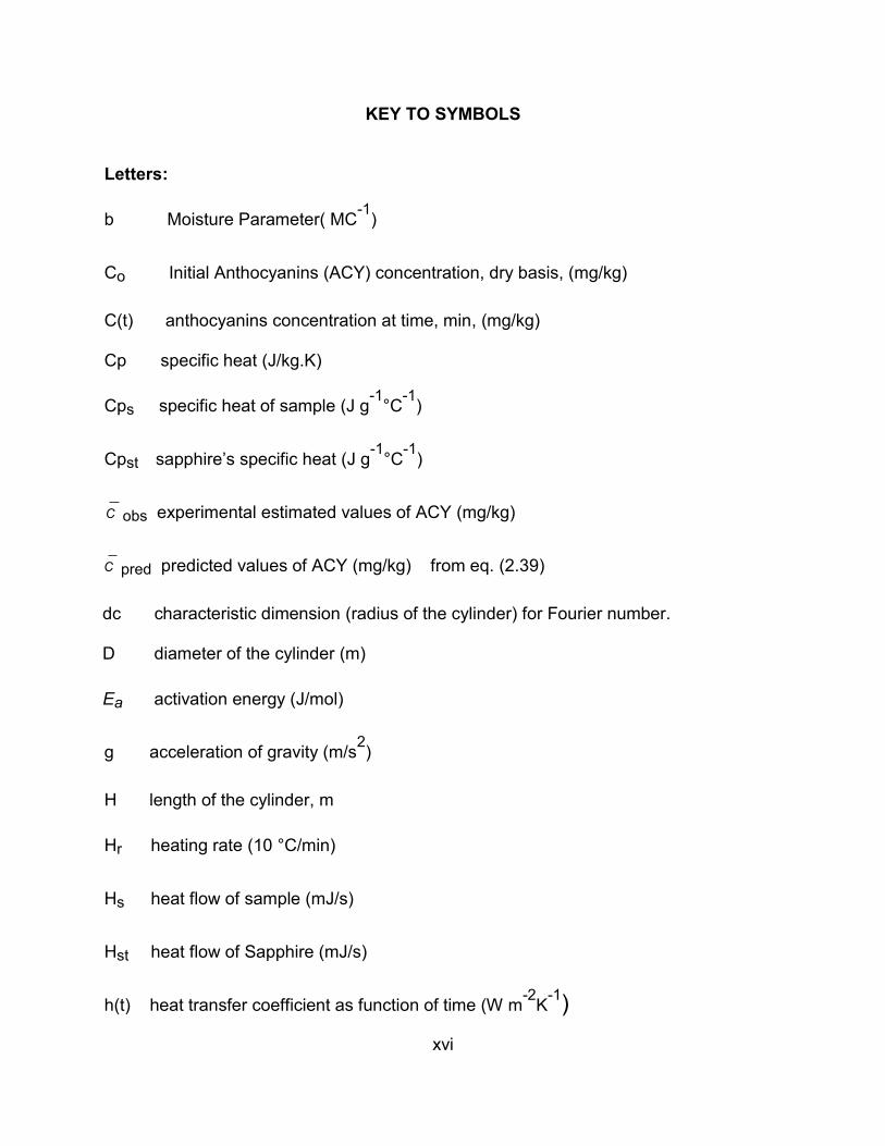
KEY TO SYMBOLS Letters:

b Moisture Parameter( MC-1

)

Co Initial Anthocyanins (ACY) concentration, dry basis, (mg/kg)

C(t) anthocyanins concentration at time, min, (mg/kg)

Cp specific heat (J/kg.K)

Cps specific heat of sample (J g-1

°C-1

)

Cpst sapphire’s specific heat (J g-1

°C-1

)

C obs experimental estimated values of ACY (mg/kg)

C pred predicted values of ACY (mg/kg) from eq. (2.39)

dc characteristic dimension (radius of the cylinder) for Fourier number.

D diameter of the cylinder (m)

Ea activation energy (J/mol)

g acceleration of gravity (m/s2)

H length of the cylinder, m

Hr heating rate (10 °C/min)

Hs heat flow of sample (mJ/s)

Hst heat flow of Sapphire (mJ/s)

h(t) heat transfer coefficient as function of time (W m-2

K-1

)

xvii

hfg latent heat of condensation in (J/kg) at Tsaturated

k thermal conductivity (W m-1

K-1

)

kr first-order degradation rate at reference temperature Tr (Min-1

)

k(T) thermal conductivity Function of temperature (W m-1

K-1

)

ks calibration constant (dimensionless)

k1 thermal conductivity at T1 (W m-1

K-1

)

k2 thermal conductivity at T2 (W m-1

K-1

)

MC Moisture content wet basis (decimal)

MCr Reference moisture content wet basis (decimal)

n number of data

p number of parameters

r radial coordinate of the cylinder (m)

R’ radius of the cylinder (m)

R Gas constant (3.418 J/mole K)

t time, s

tx total process time (sec)

tf end of process time, (sec)

T temperature of the sample as function of time (˚C)

Ti initial temperature of the sample (˚C)

T1 particular value of T ( low value ˚C)

xviii

T2 particular value of T (high value ˚C)

Tobs measured temperatures at can’s center (˚C)

Tprd predicted temperatures for the center of the can (˚C)

Tr reference temperature (°K)

TRt retort temperature (˚C)

Ts surface temperature on the can (˚C)

Wst sapphire weight (mg)

Ws sample weight (mg)

x thickness (m)

X’ scaled Sensitivity coefficient

z axial coordinate of the can (m)

Greek letters:

ρCp Volumetric heat capacity (J/m3.K)

ρ Density (kg/m3)

ρ1 Density of liquid (kg/m3)

ρv Density of vapor (kg/m3)

μ viscosity of liquid (Pa.s)

ΔT is (TRt –Ts)

α Thermal diffusivity ( m2/s)

xix

Ø Angular geometry for the can

β parameter

Ψ(t) time-temperature history for Eq. (2.28)

Dimensionless groups:

Bi Biot number h r

k

Internal diffusive resistance

Surface Convective resistance

Fo Fourier number 2

t

d c

Heat conduction

Heat storage

Nu Nusselt number h D

k f

Surface Convective resistance

Convective resistance

Pr Prandtl number

C p

k

Viscous effect

Thermal diffusion effect

Re Reynolds number D

Inertia force

Viscous force

1

CHAPTER 1

1. INTRODUCTION

2

1.1 Overview of the Dissertation

Anthocyanins (ACY) are the most abundant flavonoid constituents of fruits and

vegeTables. They are responsible for the wide array of colors present in flowers, petals,

leaves, fruits and vegeTables and are a sub-group within the flavonoids characterized

by a C6-C3-C6-skeleton (Zhang et al., 2004). The red color of cherries is due to several

water-soluble anthocyanin pigments. Pelargonidin, cyaniding, peonidin, delphinidin,

petunidin, and malvidin are the six common anthocyanidins found in nature. These

pigments are not very stable chemically and may degrade during thermal processing

(>70°C) which can affect color quality and nutritional components. ACY have

antioxidant effects, which play an important role in the prevention of neuronal and

cardiovascular illnesses, cancer and diabetes, among others. There are several studies

focusing on the effect of ACY in cancer treatments, human nutrition and its biological

activity, (Bohm et al., 1998); Konczak and Zhang (2004); (Lule and Xia, 2005).

Thermal processing of foods involves heating to temperature from 50 to 150 ºC.

Anthocyanin stability is not only a function of final processing temperature but also of

other properties (intrinsic) like pH, storage temperature, product moisture content,

chemical structure of the ACY and their initial concentration, light, oxygen, presence of

enzymes, proteins and metallic ions Patras et al. (2010). There are many studies

examining these factors individually or a combination of one or more of them on

degradation of food components. There is limited information available on the effect of

high temperature processing at different moisture contents on the stability of these

pigments in solid food products. Cherry pomace, left over after cherry juice processing,

is a good source of ACY and hence can be used as an ingredient in the food industry.

3

The temperature history of most food products during processing is non-isothermal.

However, kinetic parameters for liquid or high-moisture foods at temperatures below

100°C have typically been estimated using numerous isothermal experiments and two-

step linear regression. Because such high-moisture products can usually approach the

isothermal temperatures rapidly (< 1 min), with negligible temperature gradient, the

kinetic results have been useful for predicting commercial processes.

For Low- or intermediate-moisture solid foods at temperatures > 100°C, the

experimental procedure becomes technically difficult to perform, due to the following:

1. The sample container must be pressurized;

2. It becomes more difficult to attain isothermal conditions within a reasonable

experimental time, because of the decreased thermal diffusivity;

3. Temperature gradients within the sample become significant;

4. Even if an isothermal temperature is eventually approximated, by that time, the

nutrient degradation may be very large, rendering the experiment useless;

5. Non-isothermal estimated kinetic parameters may be significantly different from

isothermal estimates. Examples include thermal denaturation D71°C parameter for

lactoperoxidase and the z value for beta-lactogolobulin (Claeys et al., 2001); rate

constants and activation energies for zero- and first-order models for broccoli color,

vitamin C content, and drip loss during frozen storage (Goncalves et al., 2011a);

activation energies for fractional conversion models of pumpkin texture, color, and

vitamin C during frozen storage (Goncalves et al., 2011b); and inactivation

parameters D and z for B. stearothermophilus heated between 115 and 125°C

(Periago et al., 1998).

4

To deal with the low moisture situation, non-isothermal experiments are

recommended. The advantages include:

1. Difficulties # 2-5 above can be eliminated by using non-isothermal experiments and

analysis.

2. Because the parameters can be estimated from a single set of non-isothermal

experiments, the number of trials is significantly reduced compared to that for

isothermal methods, thereby saving time, cost, and effort.

3. The sample size can be large (>50g), allowing more accuracy in the measured

nutrient concentration;

4. The non-isothermal estimated parameters will be closer to those under actual

commercial conditions, and will have significantly increased accuracy;

Anthocyanins (ACY) are routinely processed in low-moisture solid foods under high

temperature and high pressure, such as in extruded foods, confectionaries, powders,

and baked goods. To design, simulate, and optimize nutrient retention, the ACY

degradation kinetics must be known. However, systematic methods to estimate the

kinetic degradation parameters in these foods do not exist. Therefore, this research is

focused on developing just such a method.

1.2 Statement of the Problem

The research was in two main parts. The sequences of the experimental and analysis

steps are given below:

1. Collect time and temperature at center of the cans of cherry pomace at three

constant moisture contents. ACY and color degradation measurements.

5

2. Estimate the cherry pomace specific heat at each MC by the DSC method as a

function of temperature. Use MATLAB with Comsol for the experimental data in (step

1 & 2) to estimate the thermal conductivity (k1 & k2) at each MC at two arbitrary

temperatures (T1 & T2). Use MATLAB with Comsol to estimate the kinetic

degradation parameters for ACY degradation inside the sealed cans after non-

isothermal heating at two different temperatures. Experimental steps were

summarized in Figure 1.1

Figure 1.1 Flow chart of experimental plan of cherry pomace retorting and estimation of kinetic parameters of anthocyanin degradation under the process.

“For interpretation of the references to color in this and all other figures, the reader is referred to the electronic version of this dissertation.”

Kinetic Parameter Estimation (Obj, 3)

Air Drying to two additional lower MC

Density, color, pH, ACY tests and Degradation analysis (Obj, 1)

Cp estimation by DSC Method

Canning TC fitting and sealing

Retorting & data collection

Comsol simulation of T 2D axisymmetric

MATLAB with Comsol (inverse problem)

Thermal conductivity estimation Prop1D, (Obj, 2)

70% 41% 25%

Experimental steps

Step 2

Step 4

Step 5

Step 3

Step 2

Step 4

Step 3

Step 1 Step 1

Data Analysis steps

6

1.3 Significance of the Study 1. A new method to estimate non-isothermal parameters in solid foods during dynamic

heating > 100oC was proposed and carried out.

2. Temperature-dependent thermal conductivity and specific heat of a solid food were

estimated for a large temperature range, 25-130oC.

3. Estimation of kinetic parameters could be used, for example, to predict the

anthocyanin retention during drying, where temperature is simultaneously increasing

with decreasing moisture content.

4. This method may apply analogously to estimate microbial inactivation or growth

parameters in low-moisture foods.

Processors want to dry fruit pomace rapidly but still maintain maximum

nutraceutical content to make a high-value by-product ingredient such as anthocyanin-

rich powder. ACY degrade more rapidly with temperature (T) and moisture content

(MC). Knowledge of the rates of degradation of anthocyanin with T & MC will allow

design of optimum drying processes, including tray drying, spray during, drum drying,

extrusion and other processes. The non-isothermal methods used in the study may

serve as a standard for other researches studying drying at temperatures > 100°C.

1.4 Objective of the Study

In this study, the effect of moisture content (MC) on degradation of ACY during

non-isothermal processing of cherry pomace was determined. The specific objectives

were to:

7

1. Determine the effect of non-isothermal heating and moisture content on the

anthocyanin retention, color changes, color kinetics and the total antioxidant

capacity of cherry pomace

2. To estimate the temperature-dependent thermal properties (specific heat and

conductivity) of cherry pomace during non-isothermal heating at temperatures up to

130oC

3. To estimate the kinetic parameters of ACY degradation in cherry pomace for

different constant moisture contents.

This dissertation is composed of various sections as follows :

Chapter 2 contains the literature review. The remaining chapters of the dissertation

consist primarily of three journal articles: Chapter 3, 4, and 5, based on each objective

studied, respectively. The final section of this dissertation (Chapter 6) gives the overall

conclusions and recommendations from the research.

8

CHAPTER 2

2. LITERATURE REVIEW

9

2.1 Heat transfer theory

Equati on Chapter 2 Secti on 2

In this section the theory of heat transfer during the retorting process will be

reviewed. The thermophysical parameters during heat conduction, heating or cooling

have been estimated by different methods. The inverse method is one solution method

(Bairi et al., 2007; da Silva et al., 2011; da Silva et al., 2010; Fernandes et al., 2010;

Mariani et al., 2008; Mariani et al., 2009; Simpson and Cortes, 2004). Some

researchers neglected the convective fluxes in thick creams and purees and used only

conduction theory (Betta et al., 2009; Mariani et al., 2009). In our study, the following

equations will be used to describe the heat transfer. The fundamental equation of

conduction heat transfer in a solid is Fourier’s equation (Bird et al., 1960; Datta, 2002a)

( )T

C p T q Qt

(2.1)

Where the left term of the equation (2.1) represent the stored energy and the right term

( q ) is rate of energy input per unit volume by conduction, and (Q) generation of the

energy. Each term has the units (W/m3). Conduction heat transfer depends on three

physical parameters: density (ρ), thermal conductivity (k) and specific heat (Cp). The

heat flux q (W/m2) is given by:

( )q k T T (2.2)

Substituting Eq. (2.2)into Eq. (2.1) we obtain:

( ) ( ( ) )T

C p T k T T Qt

(2.3)

Most common geometries used for kinetic studies are the finite plate; the specific forms

of Eq. (2.3) below for cylindrical coordinates in the following section. Thermal properties

10

k and Cp as functions of temperature were estimated, but not of direction (the product is

isotropic).

2.2 Cylindrical coordinates:

In general, the rate of heat transfer (steady state conduction) is expressed by

Fourier’s law for one-dimensional Eq. (2.4) (Datta, 2002a; Geankoplis, 2003; Sawaf et

al., 1995) is:

( )d T

q k Txd x

(2.4)

For this study, heat changes with time (transient heat transfer) during the retorting

process for food materials inside a can (Cylindrical coordinates), there are three spatial

coordinates of the system T (r, ø, z, t) as shown in Figure 2.1.

Figure 2.1 Cylindrical coordinates heat transfer by conduction

The components of energy flux (q, W/m3) for the cylindrical geometry are summarized

in the equation for cylindrical coordinates as follows (Bairi et al., 2007; Bird et al., 1960)

T(r,Ф,z)

Ф x

y

z

qФ

+dФ

qr+dr

qz

qr

r

rdФ

dz

dr

dФ

qz+dz

r

R’

r Qr

H

T(r,z,t)

Qr+QΔr Δr

T(R’,z,t)

11

1 1( ) ( ) ( ) ( )

2

T T T Tk T r k T k T Q C p Tg in

r r r z z tr

(2.5)

For the case of a can being heated in steam, the conditions are transient with no heat

generation. Because the boundary conditions are identical around the circumference

of the can, the problem is considered 2D (axial and radial) (Bairi et al., 2007).

Because heat transfer through ø direction goes to zero, and there is no heat

generation during the process, and thermal conductivity and specific heat are

temperature dependent properties, then equation (2.5) is written as follows: (Banga et

al., 1993; Betta et al., 2009; Telejko, 2004; Varga and Oliveira, 2000):

1( ) ( ) ( )

T T Tk T r k T C p T

r r r z z t

(2.6)

Initial condition;

T(r, z, 0) = Ti [t=0, 0≤ r ≤R’, 0≤ z ≤ H] (2.7)

Symmetry conditions: at r = 0

0T

kr

(2.8)

2.3 Heat transfer boundary conditions:

Heat transfer boundary conditions for the can (axisymmetric body) in the retort

will be based on one of two following conditions types (Naveh et al., 1983):

2.3.1 Convection heat transfer function of time:

Boundary conditions (1):

With T = TRt (t) [ 0< t ≤tx, r =R’, z = 0, z = H]

12

- ( ) ( ) ( ( , , ) - ( ))R t

Tk T h t T R z t T t

r

(2.9)

( ) ( ) ( ( , , ) ( ))T

k T h t T r H t T tR tz

(2.10)

Where: T∞ (t) is the time- varying steam temperature. The convection heat transfer is a

function of time. The transient heat transfer for equation (2.6) was solved by the finite-

element method using Comsol with MATLAB software.

Heat transfer resistance along the heat flow direction is represented by the Nusselt

number equation (2.11):

C o n d u c t io n re s is ta n c e

1 C o n v e c t io n re s is ta n c e

L

kh L flu idN u

k f lu id

h

(2.11)

The analytical solution of heat transfer coefficient depends on the relative internal and

external heat transfer resistance (a lumped parameter analysis), which represented by

Biot number as follows Eq. (2.12) :

h RB i

k (2.12)

Biot number >40 indicates that external resistance is negligible and Biot number <0.2

indicates that internal resistance is negligible, while Biot number between 0.2 and 40

indicates that both internal and external resistance to heat transfer is important

(Rahman, 1995b) .

For negligible internal resistance (Bi<0.2) the following Eq.(2.13) was used to estimate

heat transfer coefficients (h), (Singh and heldman, 2001):

13

lnT T R t h A s

tT i T R t V C p

(2.13)

For film condensation and Biot number between 0.2 and 40, internal resistance

not negligible, an empirical correlation (Nusselt number as a function of Re and Pr

numbers) recommended for vertical surface in laminar flow is : (Aston and Kirch, 2012;

Atayilmaz, 2011; Chand and Vir, 1979; Geankoplis, 2003; Lienhard, 2006; Naveh et al.,

1983; Reymond et al., 2008).

1/ 43

( ) . .1 10 .7 2 5

. .

g h Dh L v fgN N u

k k T

(2.14)

The heat flux at the solid surface in the selected direction is equal to the heat

convection at the same surface.

7 .6 3 a / a  0A C Y / A C Y    0 .0 0 0 5 e xp  t 0

R

2=0.89 (2.15)

The heat transfer coefficient was estimated experimentally using Eq. (2.14). With given

initial and boundary condition (Eqs.(2.7) to (2.10) ) and solved per the inverse method

with assuming 1D at the initial part of each experiment using finite-difference software

(IHCP1D Software, Beck Engineering Consultants Company, www. BeckEng.com).

2.3.2 Surface temperature as function of time (Ts) :

Obtaining temperature profile throughout the surface of the can will be a surface

boundary condition for Eq.(2.5) (Naveh et al., 1983; Welti-Chanes et al., 2003).

Initial and boundary conditions throughout the can surface at time, zero, or function of

time, could be defined by following equations

14

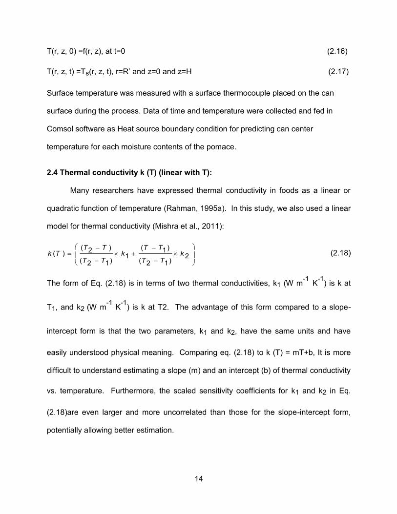
T(r, z, 0) =f(r, z), at t=0 (2.16)

T(r, z, t) =Ts(r, z, t), r=R’ and z=0 and z=H (2.17)

Surface temperature was measured with a surface thermocouple placed on the can

surface during the process. Data of time and temperature were collected and fed in

Comsol software as Heat source boundary condition for predicting can center

temperature for each moisture contents of the pomace.

2.4 Thermal conductivity k (T) (linear with T):

Many researchers have expressed thermal conductivity in foods as a linear or

quadratic function of temperature (Rahman, 1995a). In this study, we also used a linear

model for thermal conductivity (Mishra et al., 2011):

( ) ( )2 1( ) 1 2

( ) ( )2 1 2 1

T T T Tk T k k

T T T T

(2.18)

The form of Eq. (2.18) is in terms of two thermal conductivities, k1 (W m-1 K

-1) is k at

T1, and k2 (W m-1

K-1

) is k at T2. The advantage of this form compared to a slope-

intercept form is that the two parameters, k1 and k2, have the same units and have

easily understood physical meaning. Comparing eq. (2.18) to k (T) = mT+b, It is more

difficult to understand estimating a slope (m) and an intercept (b) of thermal conductivity

vs. temperature. Furthermore, the scaled sensitivity coefficients for k1 and k2 in Eq.

(2.18)are even larger and more uncorrelated than those for the slope-intercept form,

potentially allowing better estimation.

15

2.4.1 Thermal properties of foods:

Thermal conductivity (k) and specific heat capacity (Cp) are important thermal

properties of a material considered during heat transfer. Thermal conductivity describes

the heat transfer for a given temperature gradient. It quantifies the steady-state rate of

heat transfer at the applied direction of a temperature gradient and it is introduced by

Fourier’s law of heat conduction (Eq.(2.4)) (Rahman et al., 1997).

Many studies have been done on this subject for estimating these properties for

different kinds of food materials. Some studies used measured temperature profiles for

estimation of the thermophysical properties in inverse heat conduction problems (Beck

and Woodbury, 1998; Yang, 1998).

Estimation of thermal conductivity is classified by two methods: steady and transient

state heat transfer methods. Steady-state methods require long times, and moisture

content changing with time introduces significant error (Dutta et al., 1988).

The transient method (line source method) is more suitable for biological materials:

estimation of thermal conductivity is based on the relationship between the sample

temperature and heating time (Yang et al., 2002). However, this method is suitable

only for nearly isothermal conditions at temperatures below 100oC.

Appropriate software based on least square optimization of the finite difference

solution of Fourier’s equation have been developed for thermal diffusivity estimation via

heat penetration data from different heat treatments. (Betta et al., 2009).

The probe method is the most widely used method for thermal conductivity

estimation. The basic theory for this method is that the temperature rise at a point

close to a line heat source inside a sample, and thermal conductivity could be

16

calculated from the following equation (Baghekhandan et al., 1981; Buhri and Singh,

1993; Choi and Okos, 1983; Sweat, 1975) :

ln /2 0 1 0

4 2 0

Q t t t tk

t t

(2.19)

Use of T (t) = (Q/(4×π×k))×ln(t) shows that this equation is only for near-isothermal

conditions at <80˚C because moisture will begin to evaporate above 80oC. A plot of (T2-

T0) versus the logarithm of time (t2-t0) is linear until heat penetrates into the sample,

where the slope is used for thermal conductivity estimation.

Equation (2.19) was applied for measuring thermal conductivity under high pressure

(400MPa) for canned tomato paste and apple (Denys and Hendrickx, 1999; Shariaty-

Niassar et al., 2000)

Equations (quadratic models) were developed for predicting thermal conductivity of a

meat with a given water content and temperature at different ranges (Sweat, 1975).

Thermal conductivity of carrot and potato (solid food) were measured as well using the

probe method at a temperature range 30 -130 ˚C, correlation equation was established

for predicting the thermal conductivity (Gratzek and Toledo, 1993). The thermal

conductivity of porous foods, which have complex structure is difficult to predict (Sweat,

1995). Studies on linearly temperatur dependent thermal conductivity components

kx(T) and ky(T) and specific heat Cp(T) of transient heat conduction problem for an

orthotropic soild have been done using an inverse analysis as following equations:

( )0 1

k T k k Tx x x (2.20)

( )0 1

k T k k Ty y y (2.21)

17

( )0 1

C p T C p C T (2.22)

A disadvantage of these models is that the coefficients have different units. The

analysis was done based on minimizing the sum of squares function with the Leveberg-

Marquardt method (Sawaf et al., 1995). Studies using the inverse method to predict

the thermal conductivity and the heat of phase transition and the finite element method

are used to solve the heat conduction equation. Cylindrical steel samples were heated,

and assumed that the thermal conductivity below 720 ˚C temperature is a second-

degree polynomial Equation, and linear function above 770 ˚C (Telejko, 2004; Yang,

2000) :

2( ) 1 2 3k T b b T b T (2.23)

( ) 4 5k T b b T

(2.24)

A quadratic model ( Eq.(2.25)) for Thermal conductivity of Tofu as function of

temperature and moisture content (M) was established at temperature range (5-80˚C)

moisture content ( 0.3-0.7 w b) using probe method (Baik and Mittal, 2003).

4 20 .2 1 1 2 8 .9 4 3 1 0 0 .3 0 7 7k M T M

(2.25)

Thermal properties of borage seeds were determined using the line heat source, at

temperature range of 6 to 20oC and moisture content range from 1.2 to 30 % .Specific

heat was measured by differential scanning calorimetric (DSC) and ranged from 0.77 to

1.99 kJ kg-1

K-1

. Thermal conductivity increased with moisture content and contributed

the most to the uncertainty of thermal diffusivity. A quadratic equation was established

for estimating these thermal properties (Yang et al., 2002). Simple linear polynomial

models were established in a study on fruit juices, showing that specific heat and

18

thermal conductivity have linear dependency on water content and temperature, while

the density was nonlinearly related to water content (Gratao et al., 2005). Simultaneous

estimation of volumetric heat capacity and thermal conductivity was established using

nonlinear sequential parameter estimation method, transient temperatures

measurements for one dimensional conduction food sample were used to conduct the

study (Mohamed, 2009)

Studies on millets, grain and flours, showed that specific heat and thermal

conductivity are influenced by the moisture content of the materials, where they

increased as moisture content increased values of these two thermal properties were

different and this difference is due to a change in the grain and flours constituents and

proportions (Subramanian and Viswanathan, 2003). Thermal properties of coffee bean

powder were determined: specific heat was determined in a temperature range from

50 to 150 ˚C, thermal conductivity from 20 to 60 ˚C, bulk density was determined and its

change was negligible at temperature of roasting. Linear relationship for specific heat

was given as function of temperature, and for density as function of moisture content.

(Singh et al., 1997)

A proposed parallel model (Eq.(2.26)) for predicting thermal conductivity (k) as

a function of material temperature (T) reference temperature (Tr) and moisture content

(M) was established through the fitting of compiled literature data for some food

products during drying process (Maroulis et al., 2002) .

1 1 1 1 10e xp e xp0

1 1

E EM ik k k i

M R T T r M R T T r

(2.26)

19

Where: k0 is the thermal conductivity at moisture M =0 and temperature (T = Tr =60˚C),

Kr is the thermal conductivity at moisture M = ∞ and temperature (T = Tr =60˚C)

A thermal conductivity prediction regression equation was developed for some

foodstuffs beef, potato, apple, pears and squid as function of moisture content, porosity

and initial thermal conductivity. The correlation coefficient was 0.99. This correlation

assumed no effect of the temperature on the thermal conductivity (Rahman, 1992).

Quadratic models of Thermal conductivity as function of water contents of potatoes, and

apples were established (Mattea et al., 1986; Rahman et al., 1997) .

Literature shows that thermal conductivity data have wide variation because of

one or more of the following factors: 1) different experimental method applied, 2)

material composition, and 3) difference in the structure of the material. Thermal

conductivity depends strongly on temperature, moisture content, and material

structure. Thermal conductivity was estimated and presented from literature data (more

than 140 articles) for about 100 foodstuffs that vary in moisture contents and

temperature (Krokida et al., 2001).

2.4.2 Isothermal and non-isothermal Processing

Many foods which contain anthocyanin (ACY) are thermally processed prior to

consumption. This process can greatly influence ACY content in the final product.

These pigments are not very stable chemically and may degrade during thermal

processing (>70°C) thus affecting color, quality and nutritional components. ACY

degradation rate increases as temperature rises during processing and storage

(Palamidis and Markakis 1978). Thermal processing of foods involves heating up as

high as 150 ºC, depending on the process. There are many studies examining these

20

factors individually, or a combination of one or more of them, on degradation of food

components. There is limited information available on the effect of high temperature

processing at different moisture contents on the stability of these pigments in solid food

products. The majority of studies on the degradation kinetics of ACYs have been carried

out under isothermal conditions at temperatures below 100ºC on high-moisture

products. However, ACY degradation in low moisture solids or semi-solid foods such as

fruit or berry pomace, grains, and dried vegeTables is not isothermal. Therefore kinetic

modeling should include time-temperature history (Mishra et al., 2008).

Most processing and cooking operations are not isothermal. Therefore, studies

on prediction of pathogen behavior require the examination of the cumulative effect of

exposure to varying temperatures throughout the cooking process. Changes in

chemical and physical characteristics in foods during heating because of temperature

rise might affect different elements in the process. For example the “limiting reaction” at

a specific temperature might not be the same at lower or higher temperatures (Peleg

et al., 2009).

A study on blackcurrant ACYs degradation in the juice under isothermal and non-

isothermal condition (4-140˚C) showed that the ACY degradation followed first-order

kinetics (Harbourne et al., 2008).

The non-isothermal method gave much smaller relative errors compared with the

isothermal method for both the activation energy and the rate constants. Specifically,

the activation energies were estimated at 73 ± 2 kJ/mol for an isothermal temperature

range of 21-100 ˚C at six constant temperatures. For the non-isothermal experiments,

the estimates were 81.51 ± 0.03 kJ/mol at 110 oC and 91.09 ± 0.03 kJ/mol at 140 oC. In

21

this case the error in estimation of the activation energy was 2.7% for the isothermal

experiments, versus 0.03% for the non-isothermal method, an increased accuracy of

90-fold. Also, the isothermal method requires minimum five constant-temperature runs

(~60 data points) to estimate the kinetic parameter with accuracy, while the non-

isothermal method required only one run (4-10 data points) (Harbourne et al., 2008).

The same study indicated that to estimate ACY degradation at typical food industry

sterilization temperatures (>100 oC), using non-isothermal methods at these high

temperatures is recommended, because the degradation kinetics cannot be

extrapolated without significantly underestimating the ACY degradation (Harbourne et

al., 2008).

A study on an inactivation kinetics of alkaline phosphatase and lactoperoxidase

and denaturation kinetics of β-lactoglobulin in raw milk under isothermal and dynamic

temperature conditions demonstrated that the thermal inactivation of the three previous

compounds was accurately described by the first-order model. Isothermal parameters

predicted non-isothermal results well for alkaline phosphatase and lactoperoxidase, but

not for β-lactoglobulin (Claeys et al., 2001). More accurate parameter results were

obtained using the global nonlinear regression rather than the two-step linear regression

(Claeys et al., 2001).

In summary, there has been a lot of research on isothermal methods for

inactivation of organisms and some on degradation kinetics of nutrients and

nutraceutical compounds. Processing liquids at temperatures above 100 °C for short

times requires the use of non-isothermal methods to estimate degradation kinetics

parameters. Processing lower-moisture solids at temperatures above 100oC for any

22

length of time requires non-isothermal methods because of the changing temperature

gradient within the sample. For isothermal processes, the come-up time for heating and

come-down time for cooling must be negligible comparing with the longer holding

heating time. In non-isothermal processes, the sample temperature during the entire

process is included in the model. As shown from some literature, that accuracy in non-

isothermal processing is higher comparing with isothermal processing. The number of

experiments needed to estimate the kinetic parameters or inactivation parameters is

fewer than those for the non-isothermal process.

2.5 Cherry Pomace’s Anthocyanins

2.5.1 Cherry pomace

Cherry (Prunus cerasus L.) pomace is the solid waste or by-product of cherry

juice processing and consists of cherry skin and seeds. It accounts for over 90% of dry

matter with high quantity of lignin, cellulose, and dry fiber components (Nawirska A. ,

2005). Study on tart cherry indicated that Balaton contains about six times more ACY

than does Montmorency has (Wang et al., 1997). Cherries are known to contain

substantial quantities of ACY (Wang et al., 1999), which are mainly concentrated in the

skins (Chaovanalikit and Wrolstad, 2004; Tomas-Barberan et al., 2001) and constitute a

major portion of bioactive compounds in the pomace. Cherry pomace, an otherwise

waste material, could be processed into value-added ingredients for use in different

food products as colorant and/or neutraceuticals. For example, addition of tart cherry

tissue to cooked beef patties has been shown to inhibit lipid and cholesterol oxidation

(Britt et al., 1998). Cherry pomace powder or extract may also be added to breakfast

23

cereals, snacks, drink mixes, confectionaries, breads or other baked goods, or used as

a slow-release antioxidant in the packaging films.

2. 5.2 Anthocyanins in Nature

Anthocyanins are natural colorants that provide bright red to purple color in foods.

Researches on ACY have increased because of their possible role in reducing the risk

of coronary heart disease, cancer and stroke (McGhie and Walton, 2007; Wrolstad,

2004). ACY have antioxidant and anti-flammatory effects, which play an important role

in the prevention of neuronal and cardiovascular illnesses, cancer and diabetes, among

others. There are several studies focusing on the effect of ACY in cancer treatments,

human nutrition and its biological activity (Bohm et al., 1998; Konczak and Zhang, 2004;

Lule and Xia, 2005; Simunic et al., 2005; Zafra-Stone et al., 2007)

2.5.3 Structure of Anthocyanins:

ACY are the most abundant flavonoid constituents of fruits and vegeTables. They are

responsible for the wide array of colors present in flowers, petals, leaves, fruits and

vegeTables and are a sub-group within the flavanoids characterized by a C6-C3-C6-

skeleton, Figure 2.2. ACY are glycosylated anthocyanidins; sugars are attached to the

3-hydroxyl position of the anthocyanidin (sometimes to the 5 or 7 position of flavynium

ion,). Variations in chemical structure (Figure 2.2) are mainly due to differences in the

number of hydroxyl groups in the molecule, degree of methylation of these OH groups

(Table 2.1). They are responsible for the color ranges of fruits and vegeTables from red

at pH values below 4, to colorless at pH 4-4.5 and to blue at pH 7 and above. The red

color of cherries is due to several water-soluble anthocyanin pigments. Pelargonidin,

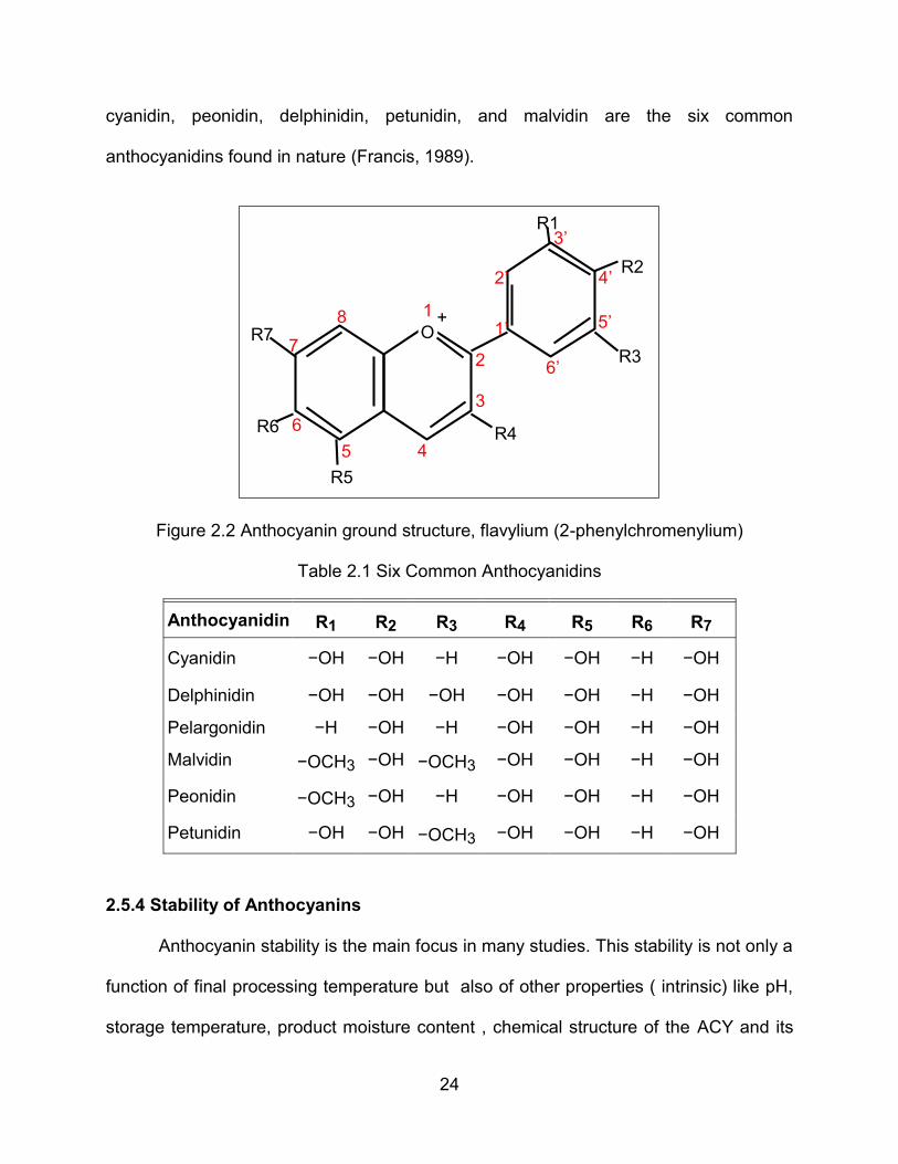
24

cyanidin, peonidin, delphinidin, petunidin, and malvidin are the six common

anthocyanidins found in nature (Francis, 1989).

Figure 2.2 Anthocyanin ground structure, flavylium (2-phenylchromenylium)

Table 2.1 Six Common Anthocyanidins

Anthocyanidin R1 R2 R3 R4 R5 R6 R7

Cyanidin −OH −OH −H −OH −OH −H −OH

Delphinidin −OH −OH −OH −OH −OH −H −OH

Pelargonidin −H −OH −H −OH −OH −H −OH

Malvidin −OCH3 −OH −OCH3 −OH −OH −H −OH

Peonidin −OCH3 −OH −H −OH −OH −H −OH

Petunidin −OH −OH −OCH3 −OH −OH −H −OH

2.5.4 Stability of Anthocyanins

Anthocyanin stability is the main focus in many studies. This stability is not only a

function of final processing temperature but also of other properties ( intrinsic) like pH,

storage temperature, product moisture content , chemical structure of the ACY and its

O

R1

R2

R3

R4

R5

R6

R7 1’

2’

3’

4’

5’

6’2

1

3

4

6

7

5

8 +

25

initial concentration ,light, oxygen, presence of enzymes, proteins and metallic ions

(Patras et al., 2010). Anthocyanin pigments readily degrade during thermal processing,

which has a dramatic impact on color and affects nutritional properties(Jimenez et al.,

2010). Anthocyanin stability of black carrots was studied at various solid contents and

pHs during both heating, 70–90 ºC, and storage at 4–37 ºC, degradation of monomeric

ACY increased with increasing solid content during heating, while it decreased during

storage (Ahmed et al., 2004; Kirca et al., 2007). The degradation kinetics of ACY in

blood orange juice was studied (Kirca and Cemeroglu, 2003) and the activation

energies for solid content of 11.2 to 69 °Brix were found to be 73.2 to 89.5 kJ/mole.

Thermal and moisture effects on grape anthocyanin degradation were investigated

using solid media to simulate processing at temperatures above 100 oC (Lai et al.,

2009). Anthocyanin degradation followed a pseudo first-order reaction with moisture

ACY degrading more rapidly with increasing temperature and moisture. The thermal

degradation of ACY has been studied in red cabbage (Dyrby et al., 2001), raspberries

(Ochoa et al., 1999), pomegranate, grapes (Marti et al., 2002), plum puree (Ahmed and

others 2004), blackberries (Wang and Xu, 2007), and blueberry (Kechinski et al., 2010).

Anthocyanin pigments readily degrade during thermal processing, which has a dramatic

impact on color and affects nutritional properties

2.5.4.1 Effect of pH on ACY Stability

ACY are more stable in acidic solutions than alkaline solutions, at different pH

values the ionic nature of ACY changes by changing in molecule structure , which

results in different colors in the solutions(Brouillard, 1982). In acidic solutions, ACY

exist in the four different equilibrium species: the quinoidal base, the flavylium cation,

26

the carbinol or pseudobase (hemiketal) and the chalcone (Figure 2.3). At very acidic

conditions, the flavylium cation AH+ is predominant and appears as the red color. As

the flavylium is hydrated by nucleophilic attack of water, the carbinol or pseudobase is

formed. In the carbinol form, the anthocyanin appears as colorless due to pH increase

(Socaciu, 2008). Hence, ACY are more stable in low pH. Metal ions, heat, pH values >

4, sulfites and oxygen are some factors that can accelerate anthocyanin breakdown.

(Garzon and Wrolstad, 2002)

Figure 2.3 pH equilibrium forms of anthocyanins

2.5.4.2 Effect of Temperature on Anthocyanins Stability

Many foods which contain ACY are thermally processed prior to consumption

and this process can greatly influence anthocyanin content in the final product. These

pigments are not very stable chemically and may degrade during thermal processing

O

R1

O

O gly

O-gly

HO

R2

Quinonoidal base blue

PH 7

-H+O

R1OH

O gly

O-gly

HO

R2

Flavylium cation(oxonium form)

orange to purpul PH 1

+

B

A

O

R1

OH

O glyO-gly

HO

R2

Carbinol pseudo-base (hemikital form)

Colorless PH 4.5

OH

+H20/-H+

O

R1

OHO gly

O-gly

HO

R2

Chalcone : Colorless

PH 4.5

OH

27

(>70°C) which can affect color quality and nutritional components. Anthocyanin

degradation rate increases as temperature rises during processing and storage

(Palamidis and Markakis 1978).

Thermal and storage stabilities at different temperature range (5-37, 60-90) on

ACY degradation in blackberry juice and concentrate was studied , results indicated that

thermal degradation followed first-order reaction kinetics and juice at higher soluble

solids ( higher activation energy) solids degraded more rapidly comparing with lower

soluble solids contents, which have lower activation energy comparing higher soluble

solids juice (Wang and Xu, 2007). There is limited information available on the effect

of high temperature processing at different moisture contents on the stability of these

pigments in solid food products. The majority of studies on the degradation kinetics of

ACY have been carried out under isothermal conditions at temperatures below 100ºC

on high-moisture products. However, anthocyanin degradation in low moisture solid or

semi-solid foods such as fruit or berry pomace, grains, and dried vegeTables is not

isothermal. Therefore kinetic modeling should include time-temperature history (Mishra

et al., 2008). Thermal processing easily degrades the ACY pigments, which has a

dramatic impact on color and affects nutritional properties (Jimenez et al., 2010).

Havlikova and Mikova (1985) showed that there was lower stability of ACY at pH 1.8

comparing with other pH (2 to 4) values in elderberry concentrate when it was heated at

70-100°C. Based on many studies the thermal stability of ACY depends on the pH value

only under aerobic conditions, while under anaerobic conditions (negligible oxygen

concentration) the stability is not influenced by pH in range 2-4. This fact might explain

the stability of ACY above 70°C, where the anaerobic conditions established (Havlikova

28

and Mikova, 1985). Commercial sources of ACY (strawberry, elderberry, and black

carrot) were investigated; ACY isolates were heated at 95°C, at pH 1. Total anthocyanin

content lightness, and Chroma, but not hue angle, were appropriate parameters to

monitor anthocyanin loss on a statistically significant level (Sadilova et al., 2006).

Thermal stability and composition of ACY were evaluated for purple corn extracts (Zhao

et al., 2008), thermal degradation kinetics of ACY from purple corn cob were studied at

selected temperatures (70 °C, 80 °C and 90 °C) at pH 4.0 (Chen et al., 2008).

2.5.5 Anthocyanins Antioxidant Capacity

Tart cherries are rich in ACY and retain high antioxidant activity. Study on

Michigan tart cherry for evaluating different quality showed that it has high oxygen

radical absorbing capacity (ORAC) of Balaton 145% as compared to Montmorency

100% (Siddiq et al., 2011). A study has shown that the ACY , acting primarily as

antioxidants, have anti-inflammatory, anti-carcinogenic, and anti-aging properties

(Blando et al., 2004). The development of a fluorescent probe (ORACFL) method is

attributed to Glazer (1990), Ghiselli et al. (1995) and Cao and others (1993) and is

classified as a Hydrogen Atom Transfer Assay (HAT). In HAT reactions, the antioxidant

will quench free radicals through the donation of a hydrogen atom. The ORACFL

method measures the ability of the antioxidant to search for peroxyl radicals using a

fluorescent probe (fluorescein sodium salt) for detection. The peroxyl radicals will

oxidize the fluorescent probe causing a decrease in the intensity of the fluorescence

that can be quantified over time using a fluorometer. Antioxidants in the system will

reduce the peroxyl radicals stopping the loss of intensity in the fluorescence. The

29

interface between the antioxidants, free radicals, and the fluorescent probe is illustrated

in Figure 2.4 (Ou et al., 2001; Zulueta et al., 2009).

Figure 2.4 Formation of radicals through the addition of AAPH

To build a decay curve for each sample and a blank sample, the relative

fluorescence intensity will be measured over time. The area under the curve (AUC) is

calculated using the following trapezoidal equation, normalized by dividing by the initial

fluorescence value:

12 3 ... . . . .

2 2

R R nA U C R R t

Where: R1 is the fluorescence measurement at the initial time of the oxidation reaction,

Rn is the final fluorescence measurement, and Δt is the difference of time between the

two measurements. The antioxidant capacity was determined by calculating the net

area under curve as follows Eq:

N e tA U C A U C A U Csa m p le B la n k

+N

N

H

N

N

H Cl

+

-H

+H ClN

-

N

N

C

H+H Cl

N

+

2

OO

H+H Cl

N

+

2

OO

antioxidants

Stable product

(loss of fluorescence)

Fluorescent probe

Stable product

30

The calculated net AUC of each sample was compared to a standard calibration curve,

which was constructed by plotting the net AUC of a compound called Trolox (6-hydroxy-

2, 5, 7, 8-tetramethylchroman-2-carboxylic acid) against five standard concentrations in

micromoles of Trolox. Therefore the ORAC value of a sample is expressed as

micromoles of Trolox equivalents per gram or liter of sample (mol TE/g or mol TE/L).

2.6 Kinetics And Mechanism of Degradation of Anthocyanins In Foods

2.6.1 Kinetics Mechanism:

Kinetic models are often used for an objective, fast and economic assessment of

food safety. Kinetic modeling may also be employed to predict the influence of

processing on critical quality indicators. Knowledge of degradation kinetics, including

reaction order, rate constant and activation energy, is vital to simulate and predict food

quality loss during storage as well as during thermal process treatments. One of the

important factors to be considered in food processing is the loss of nutrients. Therefore,

kinetic studies are needed to minimize the undesired change and to optimize quality of

specific foods. Anthocyanin degradation under non-isothermal heating is reported to

follow first order kinetics (Ahmed et al., 2004; Markakis et al., 1957). Equations (2.25)

and (2.26) are for ACY kinetic degradation and by adding constant of moisture content

(MC) as a new parameter for estimation (b) the following equations will result:

( ( ))( )

( ) e0

b M C M C rk er tC t C

(2.27)

( )

1 1

( , , )

0

t d t

E at

R T r z t T re

(2.28)

31

Thermal degradation of ACY can result in a variety of species depending upon the

severity and nature of heating. Figure 2.4 shows the degradation of ACY and formation

of various intermediate compounds (Patras et al., 2010).

Figure 2.5 Possible thermal degradation mechanism of two common ACYs (Patras et al., 2010)

Recently, (Harbourne et al., 2008; Mishra et al., 2008) studied thermal

degradation of ACY of grape pomace, (Harbourne and others 2008) studied

blackcurrant ACY in a model juice under non-isothermal conditions. Prior to this study

(Dolan, 2003) proposed a one-step kinetic model for determining kinetic parameters for

non-isothermal food process Equations (2.29) and (2.30). This model was employed by

(Harbourne et al., 2008) for non-isothermal processing of model blackcurrant juice.

exp ( ( ))0C t C kr t (2.29)

Cyanidin-3-glucoside Cyanidin

O

OH

OH

O Glu

OH

HO + B

A CDeglycocylation

O

OH

OH

OHOH

HO + B

A C Cleavage

O

HO

OHHO

B

4-hydroxybenzoic acid

O

OH

O Glu

OH

HO + B

A C

Pelargonidin-3-glucoside Pelargonidin

Deglycocylation

O

OH

OH

OH

HO + B

A C

CHO

HO OHA

OH

Phloroglucinaldehyde

Protocatechuic acid

O

HO

OH

OH

ACleavage

32

1 1

( , , )( )

0

E at

R T r z t T rt e d t

(2.30)

Recently, (Jimenez et al., 2010) studied Blackberry juice heated at a high

temperature in a hermetically sealed cell. Statistical analysis demonstrated that when

the temperature range (100-180°C) was divided into two sub ranges (100-140 and 140-

180 °C) for anthocyanin degradation, reaction kinetics were well represented by two

sequential first-order reactions. The non-isothermal method developed allows

estimating kinetic parameters and thereby generating temperature profiles of heat

processes that would help preserve the nutritional properties of foods during high-

temperature processes. In summary, for components in low moisture and high

temperature processed semi-solid foods such as pastries, baked goods, breads and

extruded snacks there are no established experimental procedures and statistical

analysis method of kinetic parameters. Also there is lack of nonlinear regression

techniques for analysis of food that is processed under unsteady-state conditions of

heating.

2.6.2 Anthocyanins Degradation Model:

In this study the reaction is following a first order reaction as following equation:

d Ck C

d t (2.31)

Integration of equation (2.31) with integration limits gives:

( )

00

C t td C

k td t

C

(2.32)

33

When k is function of temperature and moisture content, Eq. (2.32)is written as follows:

( )

( , )

00

C t td C

k T M C d td t

C

(2.33)

Where k (T, MC) is the reaction rate, which follows Arrhenius temperature dependence,

and includes the moisture content term:

1 1( )

( , , )

e x p( , )

E ab M C M C r

R T r z t T re

k T M C k r

(2.34)

kr is the rate constant at reference temperature (Tr) and at reference moisture content

(MCr). Substituting Eq. (2.34) in Eq.(2.33) yields:

1 1( )

( , , )ln ( ) ln 0

0

aEt b M C M C r

R T r z t T rC t C k e d tr

(2.35)

Let the time temperature history equal Ψ(t):

1 1

( , , )( )

0

E at

R T r z t T rt e d t

Then by solving for C(t) in Eq. (2.33) ,yields :

( ( ))( )

( ) e0

b M C M C rk t erC t C

(2.36)

Equation (2.36) will predict the degradation of ACY at any chosen point inside the

cylinder during heating for a constant MC and time temperature history Ψ (t). Because

ACY concentration cannot be measured at an infinitely small point, we must continue to

develop the equation for mass-average ACY concentration, which can be measured

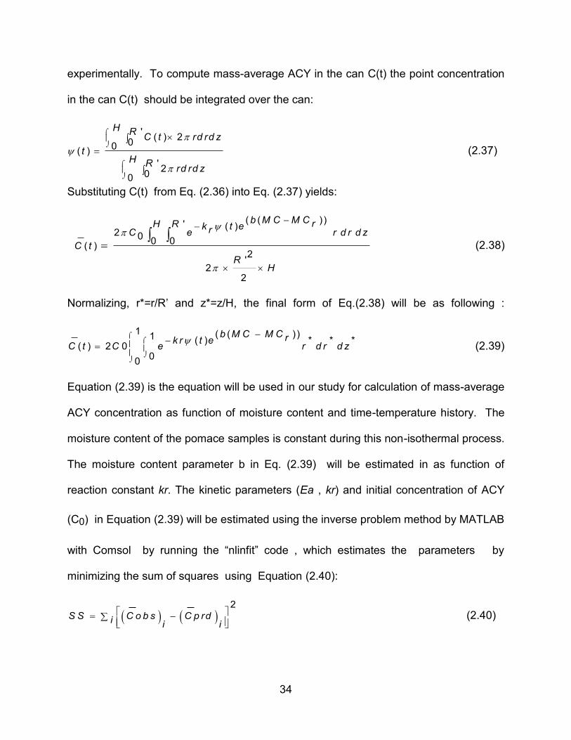
34

experimentally. To compute mass-average ACY in the can C(t) the point concentration

in the can C(t) should be integrated over the can:

'( ) 2

00( )

'2

00

H RC t rd rd z

tH R

rd rd z

(2.37)

Substituting C(t) from Eq. (2.36) into Eq. (2.37) yields:

( ( ) )' ( )2 0

0 0( )

2'

22

b M C M C rH R k t erC e r d r d z

C t

RH

(2.38)

Normalizing, r*=r/R’ and z*=z/H, the final form of Eq.(2.38) will be as following :

1 ( ( ))1 ( ) * * *( ) 2 0

00

b M C M C rk r t eC t C e r d r d z

(2.39)

Equation (2.39) is the equation will be used in our study for calculation of mass-average

ACY concentration as function of moisture content and time-temperature history. The

moisture content of the pomace samples is constant during this non-isothermal process.

The moisture content parameter b in Eq. (2.39) will be estimated in as function of

reaction constant kr. The kinetic parameters (Ea , kr) and initial concentration of ACY

(C0) in Equation (2.39) will be estimated using the inverse problem method by MATLAB

with Comsol by running the “nlinfit” code , which estimates the parameters by

minimizing the sum of squares using Equation (2.40):

2

S S C o b s C p rdi i i

(2.40)

35

REFERENCES

36

REFERENCES

Ahmed, J., Shivhare, U.S., Raghavan, G.S.V., (2004). Thermal degradation kinetics of anthocyanin and visual colour of plum puree. European Food Research and Technology 218(6), 525-528.

Aston, J.A.D., Kirch, C., (2012). Detecting and estimating changes in dependent functional data. Journal of Multivariate Analysis 109, 204-220.

Atayilmaz, S.O., (2011). Experimental and numerical study of natural convection heat transfer from horizontal concentric cylinders. International Journal of Thermal Sciences 50(8), 1472-1483.

Baghekhandan, M.S., Choi, Y., Okos, M.R., (1981). Improved line heat-source thermal-conductivity probe. Journal of Food Science 46(5), 1430-1432.

Baik, O.D., Mittal, G.S., (2003). Determination and modeling of thermal properties of tofu. International Journal of Food Properties 6(1), 9-24.

Bairi, A., Laraqi, N., de Maria, J.M.G., (2007). Determination of thermal diffusivity of foods using 1D Fourier cylindrical solution. Journal of Food Engineering 78(2), 669-675.

Banga, J.R., Alonso, A.A., Gallardo, J.M., Perezmartin, R.I., (1993). Mathematical-Modeling and Simulation of the Thermal-Processing of Anisotropic and Nonhomogeneous Conduction-Heated Canned Foods - Application to Canned Tuna. Journal of Food Engineering 18(4), 369-387.

Beck, J.V., Woodbury, K.A., (1998). Inverse problems and parameter estimation: integration of measurements and analysis. Measurement Science & Technology 9(6), 839-847.

Betta, G., Rinaldi, M., Barbanti, D., Massini, R., (2009). A quick method for thermal diffusivity estimation: Application to several foods. Journal of Food Engineering 91(1), 34-41.

Bird, R.B., Stewart, E.W., Lightfoot, E.N., (1960). Transport Phenomena . " The Equations of Change for Nonisothermal systems". New York . John Wiley & Sons, pp. 310-351.

37

Blando, F., Gerardi, C., Nicoletti, I., (2004). Sour cherry (Prunus cerasus L.) anthocyanins as ingredients for functional foods. Journal of Biomedicine and Biotechnology(5), 253-258.

Bohm, H., Boeing, H., Hempel, J., Raab, B., Kroke, A., (1998). Flavonols, flavones and anthocyanins as native antioxidants of food and their possible role in the prevention of chronic diseases. Zeitschrift Fur Ernahrungswissenschaft 37(2), 147-163.

Britt, C., Gomaa, E.A., Gray, J.I., Booren, A.M., (1998). Influence of cherry tissue on lipid oxidation and heterocyclic aromatic amine formation in ground beef patties. Journal of Agricultural and Food Chemistry 46(12), 4891-4897.

Brouillard, R., (1982). Chemical Structure of Anthocyanins. Anthocyanins as Food Colors. Markakis, P, Ed., . New York, Academic Press Inc, pp. 1-38.

Buhri, A.B., Singh, R.P., (1993). Measurement of food thermal-conductivity using differential scanning calorimetry. Journal of Food Science 58(5), 1145-1147.

Cao, G.H., Alessio, H.M., Cutler, R.G., (1993). Oxygen-radical absorbency capacity assay for antioxidants. Free Radical Biology and Medicine 14(3), 303-311.

Chand, J., Vir, D., (1979). Natural-convection heat-transfer from horizontal cylinders. Journal of Chemical Engineering of Japan 12(3), 242-247.

Chaovanalikit, A., Wrolstad, R.E., (2004). Total anthocyanins and total phenolics of fresh and processed cherries and their antioxidant properties. Journal of Food Science 69(1), C67-C72.

Chen, C.K., Wu, L.W., Yang, Y.T., (2008). Proposed modification to whole domain function specification method to improve accuracy of its estimations. Journal of Heat Transfer-Transactions of the ASME 130(5), 130p..

Choi, Y., Okos, M.R., (1983). The thermal properties of tomato juice concentrates. TRANSACTIONS of the ASAE 26(1), 305-311.

Claeys, W.L., Ludikhuyze, L.R., Van Loey, A.M., Hendrickx, M.E., (2001). Inactivation kinetics of alkaline phosphatase and lactoperoxidase, and denaturation kinetics of beta-lactoglobulin in raw milk under isothermal and dynamic temperature conditions. Journal of Dairy Research 68(1), 95-107.

da Silva, W.P., Silva, C.M.D.P.S.E., Lins, M.A.A., (2011). Determination of expressions for the thermal diffusivity of canned foodstuffs by the inverse method and

38

numerical simulations of heat penetration. International Journal of Food Science and Technology 46(4), 811-818.

da Silva, W.P., Silva, C.M.D.P.S.E., Silva, D.D.P.S.E., Neves, G.D., de Lima, A.G.B., (2010). Mass and heat transfer study in solids of revolution via numerical simulations using finite volume method and generalized coordinates for the Cauchy boundary condition. International Journal of Heat and Mass Transfer 53(5-6), 1183-1194.

Datta, A.K., (2002a). Biological and bioenvironmental heat and mass transfer. Boca Raton, Florida: Taylor & Francis. p. 424.

Denys, S., Hendrickx, M.E., (1999). Measurement of the thermal conductivity of foods at high pressure. Journal of Food Science 64(4), 709-713.

Dolan, K.D., (2003). Estimation of kinetic parameters for nonisothermal food processes. Journal of Food Science 68(3), 728-741.

Dutta, S.K., Nema, V.K., Bhardwaj, R.K., (1988). Thermal-properties of gram. Journal of Agricultural Engineering Research 39(4), 269-275.

Dyrby, M., Westergaard, N., Stapelfeldt, H., (2001). Light and heat sensitivity of red cabbage extract in soft drink model systems. Food Chemistry 72(4), 431-437.

Fernandes, A.P., Sousa, P.F.B., Borges, V.L., Guimaraes, G., (2010). Use of 3D-transient analytical solution based on Green's function to reduce computational time in inverse heat conduction problems. Applied Mathematical Modelling 34(12), 4040-4049.

Francis, F., (1989). Food Colorants: Anthocyanins. Critical Reviews in Food Science and Nutrition 28, 273-314.

Garzon, G.A., Wrolstad, R.E., (2002). Comparison of the stability of pelargonidin-based Anthocyanins in strawberry juice and concentrate. Journal of Food Science 67(4), 1288-1299.

Geankoplis, C.J., (2003). Transpot Processes and Separation process Principles."prinsibles of steady-state heat transfer". Pearson Education INC 4th Edition, Chapter 4 . pp 235-344.

Ghiselli, A., Serafini, M., Maiani, G., Azzini, E., Ferroluzzi, A., (1995). A fluorescence-based method for measuring total plasma antioxidant capability. Free Radical Biology and Medicine 18(1), 29-36.

39

Glazer, A.N., (1990). Phycoerythrin fluorescence-based assay for reactive oxygen species. Methods in Enzymology 186, 161-168.

Goncalves, E.M., Abreu, M., Brandao, T.R.S., Silva, C.L.M., (2011a). Degradation kinetics of colour, vitamin C and drip loss in frozen broccoli (Brassica oleracea L. ssp Italica) during storage at isothermal and non-isothermal conditions. International Journal of Refrigeration-Revue Internationale Du Froid 34(8), 2136-2144.

Goncalves, E.M., Pinheiro, J., Abreu, M., Brandao, T.R.S., Silva, C.L.M., (2011b). Kinetics of quality changes of pumpkin (Curcurbita maxima L.) stored under isothermal and non-isothermal frozen conditions. Journal of Food Engineering 106(1), 40-47.

Gratao, A.C.A., Junior, V.S., Polizelli, M.A., Telis-Romero, J., (2005). Thermal properties of passion fruit juice as affected by temperature and water content. Journal of Food Process Engineering 27(6), 413-431.

Gratzek, J.P., Toledo, R.T., (1993). Solid food thermal-conductivity determination at high-temperatures. Journal of Food Science 58(4), 908-913.

Harbourne, N., Jacquier, J.C., Morgan, D.J., Lyng, J.G., (2008). Determination of the degradation kinetics of anthocyanins in a model juice system using isothermal and non-isothermal methods. Food Chemistry 111(1), 204-208.

Havlikova, L., Mikova, K., (1985). Heat-Stability of anthocyanins. Zeitschrift Fur Lebensmittel-Untersuchung Und-Forschung 181(5), 427-432.

Jimenez, N., Bohuon, P., Lima, J., Dornier, M., Vaillant, F., Perez, M., (2010). Kinetics of anthocyanin degradation and browning in reconstituted blackberry juice treated at high temperatures (100-180 °C). Journal of Agricultural and Food Chemistry 58(4), 2314-2322.

Kechinski, C.P., Guimaraes, P.V.R., Norena, C.P.Z., Tessaro, I.C., Marczak, L.D.F., (2010). Degradation kinetics of anthocyanin in blueberry juice during thermal treatment. Journal of Food Science 75(2), C173-C176.

Kirca, A., Cemeroglu, B., (2003). Degradation kinetics of anthocyanins in blood orange juice and concentrate. Food Chemistry 81(4), 583-587.

Kirca, A., Ozkan, M., Cemeroglu, B., (2007). Effects of temperature, solid content and pH on the stability of black carrot anthocyanins. Food Chemistry 101(1), 212-218.

40

Konczak, I., Zhang, W., (2004). Anthocyanins - More than nature's colours. Journal of Biomedicine and Biotechnology(5), 239-240.

Krokida, M.K., Panagiotou, N.M., Maroulis, Z.B., Saravacos, G.D., (2001). Thermal conductivity: Literature data compilation for foodstuffs. International Journal of Food Properties 4(1), 111-137.

Lai, K.P.K., Dolan, K.D., Ng, P.K.W., (2009). Inverse method to estimate kinetic degradation parameters of grape anthocyanins in wheat flour under simultaneously changing temperature and moisture. Journal of Food Science 74(5), E241-E249.

Lienhard, J.H., (2006). A heat transfer textbook, 3nd ed. Englewood Cliffs, NJ: Prentice-Hall, , p. 439.

Lule, S.U., Xia, W.S., (2005). Food phenolics, pros and cons: A review. Food Reviews International 21(4), 367-388.

Mariani, V.C., de Lima, A.G.B., Coelho, L.D.S., (2008). Apparent thermal diffusivity estimation of the banana during drying using inverse method. Journal of Food Engineering 85(4), 569-579.

Mariani, V.C., do Amarante, A.C.C., Coelho, L.D., (2009). Estimation of apparent thermal conductivity of carrot puree during freezing using inverse problem. International Journal of Food Science and Technology 44(7), 1292-1303.

Markakis, P., Livingston., G., Fellers., C., (1957). Quantitive aspects of strawberry-pigment degradation. Food Research 22, 117-130.

Maroulis, Z.B., Saravacos, G.D., Krokida, M.K., Panagiotou, N.M., (2002). Thermal conductivity prediction for foodstuffs: Effect of moisture content and temperature. International Journal of Food Properties 5(1), 231-245.

Marti, N., Perez-Vicente, A., Garcia-Viguera, C., (2002). Influence of storage temperature and ascorbic acid addition on pomegranate juice. Journal of the Science of Food and Agriculture 82(2), 217-221.

Mattea, M., Urbicain, M.J., Rotstein, E., (1986). Prediction of thermal-conductivity of vegetable foods by the effective medium theory. Journal of Food Science 51(1), 113-&.

McGhie, T.K., Walton, M.C., (2007). The bioavailability and absorption of anthocyanins: Towards a better understanding. Molecular Nutrition & Food Research 51(6), 702-713.

41

Mishra, D.K., Dolan, K.D., Yang, L., (2008). Confidence intervals for modeling anthocyanin retention in grape pomace during nonisothermal heating. Journal of Food Science 73(1), E9-E15.

Mishra, D.K., Dolan, K.D., Yang, L., (2011). Bootstrap confidence intervals for the kinetic parameters of degradation of anthocyanins in grape pomace. Journal of Food Process Engineering 34(4), 1220-1233.

Mohamed, I.O., (2009). Simultaneous estimation of thermal conductivity and volumetric heat capacity for solid foods using sequential parameter estimation technique. Food Research International 42(2), 231-236.

Naveh, D., Kopelman, I.J., Pflug, I.J., (1983). The finite-element method in fhermal-processing of foods. Journal of Food Science 48(4), 1086-1093.

Nawirska A. , K.M., (2005). Dietary fibre fractions from fruit and vegetable processing waste. J of Food Chemistry 91, 221–225.

Ochoa, M.R., Kesseler, A.G., Vullioud, M.B., Lozano, J.E., (1999). Physical and chemical characteristics of raspberry pulp: Storage effect on composition and color. Food Science and Technology-Lebensmittel-Wissenschaft & Technologie 32(3), 149-153.

Ou, B.X., Hampsch-Woodill, M., Prior, R.L., (2001). Development and validation of an improved oxygen radical absorbance capacity assay using fluorescein as the fluorescent probe. Journal of Agricultural and Food Chemistry 49(10), 4619-4626.

Palamidis, N., Markakis , P., (1978). Stability of grape anthocyanin in carbonated beverages. Semana Vitivinicola 33, 2637-2639.

Patras, A., Brunton, N.P., O'Donnell, C., Tiwari, B.K., (2010). Effect of thermal processing on anthocyanin stability in foods; mechanisms and kinetics of degradation. Trends in Food Science & Technology 21(1), 3-11.

Peleg, M., Corradini, M.G., Normand, M.D., (2009). Isothermal and non-isothermal kinetic models of chemical processes in foods governed by competing mechanisms. Journal of Agricultural and Food Chemistry 57(16), 7377-7386.

Periago, P.M., Leontidis, S., Fernandez, P.S., Rodrigo, C., Martinez, A., (1998). Kinetic parameters of Bacillus stearothermophilus spores under isothermal and non-isothermal heating conditions. Food Science and Technology International 4(6), 443-447.

42

Piasecka, M., Maciejewska, B., (2012). The study of boiling heat transfer in vertically and horizontally oriented rectangular minichannels and the solution to the inverse heat transfer problem with the use of the Beck method and Trefftz functions. Experimental Thermal and Fluid Science 38, 19-32.

Rahman, M.S., (1992). Thermal-conductivity of 4 food materials as a single function of porosity and water-content. Journal of Food Engineering 15(4), 261-268.

Rahman, M.S., (1995a). Food Properties Handbook. "Phase Transitions In Foods" Boca Raton, FL: CRC Press., pp. 87-173.

Rahman, M.S., (1995b). Food Properties Handbook. "Thermal diffusivity of Foods" Boca Raton, FL: CRC Press., pp. 339-1390.

Rahman, M.S., Chen, X.D., Perera, C.O., (1997). An improved thermal conductivity prediction model for fruits and vegeTables as a function of temperature, water content and porosity. Journal of Food Engineering 31(2), 163-170.

Reymond, O., Murray, D.B., O'Donovan, T.S., (2008). Natural convection heat transfer from two horizontal cylinders. Experimental Thermal and Fluid Science 32(8), 1702-1709.

Sadilova, E., Stintzing, F.C., Carle, R., (2006). Thermal degradation of acylated and nonacylated anthocyanins. Journal of Food Science 71(8), C504-C512.

Sawaf, B., Ozisik, M.N., Jarny, Y., (1995). An inverse nalysis to estimate linearly temperature-dependent thermal-conductivity components and heat-capacity of an orthotropic medium. International Journal of Heat and Mass Transfer 38(16), 3005-3010.

Shariaty-Niassar, M., Hozawa, M., Tsukada, T., (2000). Development of probe for thermal conductivity measurement of food materials under heated and pressurized conditions. Journal of Food Engineering 43(3), 133-139.

Siddiq, M., Iezzoni, A., Khan, A., Breen, P., Sebolt, A.M., Dolan, K.D., Ravi, R., (2011). Characterization of new tart cherry (Prunus cerasus L.) selections based on fruit quality, Total Anthocyanins, and Antioxidant Capacity. International Journal of Food Properties 14(2), 471-480.

Simpson, R., Cortes, C., (2004). An inverse method to estimate thermophysical properties of foods at freezing temperatures: apparent volumetric specific heat. Journal of Food Engineering 64(1), 89-96.

43

Simunic, V., Kovac, S., Gaso-Sokac, D., Pfannhauser, W., Murkovic, M., (2005). Determination of anthocyanins in four Croatian cultivars of sour cherries (Prunus cerasus). European Food Research and Technology 220(5-6), 575-578.

Singh, P.C., Singh, R.K., Bhamidipati, S., Singh, S.N., Barone, P., (1997). Thermophysical properties of fresh and roasted coffee powders. Journal of Food Process Engineering 20(1), 31-50.

Singh, R.P., heldman, D.R., (2001). Introduction to Food Engineering , 3rd Edition in "Heat Transfer in Food Processing". Academic Press, Inc., New York, NY, pp. 283-296.

Socaciu, C., (2008). Anthocyanins in Foods. In Food Colorants Chemical and Functional Properties. Socaciu, C., Ed.; CRC Press, Taylor and Francis: Boca Raton, FL, pp. 241-256.

Subramanian, S., Viswanathan, R., (2003). Thermal properties of minor millet grains and flours. Biosystems Engineering 84(3), 289-296.

Sweat, V.E., (1975). Modeling the thermal conductivity of meats. TRANSACTIONS of the ASAE 18(3), 564-568.

Sweat, V.E., (1995). Thermal properties of foods. In Engineering Properties of Foods (M.A. Rao and S.S. Rizvi). Marcel Dekker Inc New York, NY., 99-138.

Telejko, T., (2004). Analysis of an inverse method of simultaneous determination of thermal conductivity and heat of phase transformation in steels. Journal of Materials Processing Technology 155, 1317-1323.

Tomas-Barberan, F.A., Gil, M.I., Cremin, P., Waterhouse, A.L., Hess-Pierce, B., Kader, A.A., (2001). HPLC-DAD-ESIMS analysis of phenolic compounds in nectarines, peaches, and plums. Journal of Agricultural and Food Chemistry 49(10), 4748-4760.

Varga, S., Oliveira, J.C., (2000). Determination of the heat transfer coefficient between bulk medium and packed containers in a batch retort. Journal of Food Engineering 44(4), 191-198.

Wang, H.B., Nair, M.G., Iezzoni, A.F., Strasburg, G.M., Booren, A.M., Gray, J.I., (1997). Quantification and characterization of anthocyanins in Balaton tart cherries. Journal of Agricultural and Food Chemistry 45(7), 2556-2560.

44

Wang, H.B., Nair, M.G., Strasburg, G.M., Chang, Y.C., Booren, A.M., Gray, J.I., DeWitt, D.L., (1999). Antioxidant and antiinflammatory activities of anthocyanins and their aglycon, cyanidin, from tart cherries. Journal of Natural Products 62(5), 294–296.

Wang, W.D., Xu, S.Y., (2007). Degradation kinetics of anthocyanins in blackberry juice and concentrate. Journal of Food Engineering 82(3), 271-275.

Welti-Chanes, J., Vélez-Ruiz, J.F., Barbosa-Cànovas, G.V., (2003). Transport Phenomena in Food Processing "Thermal Processing of Particulate Foods by Steam Injection. Part 2. Convective Surface Heat Transfer Coefficient for Steam". (CRC Press LLC, Washington,), pp. 331-343.

Wrolstad, R.E., (2004). Symposium 12: Interaction of natural colors with other ingredients - Anthocyanin pigments - Bioactivity and coloring properties. Journal of Food Science 69(5), C419-C421.

Yang, C.Y., (1998). A linear inverse model for the temperature-dependent thermal conductivity determination in one-dimensional problems. Applied Mathematical Modelling 22(1-2), 1-9.

Yang, C.Y., (2000). Determination of the temperature dependent thermophysical properties from temperature responses measured at medium's boundaries. International Journal of Heat and Mass Transfer 43(7), 1261-1270.

Yang, W., Sokhansanj, S., Tang, J., Winter, P., (2002). Determination of thermal conductivity, specific heat and thermal diffusivity of borage seeds. Biosystems Engineering 82(2), 169-176.

Zafra-Stone, S., Yasmin, T., Bagchi, M., Chatterjee, A., Vinson, J.A., Bagchi, D., (2007). Berry anthocyanins as novel antioxidants in human health and disease prevention. Molecular Nutrition & Food Research 51(6), 675-683.

Zhang, Z., Kou, X.L., Fugal, K., McLaughlin, J., (2004). Comparison of HPLC methods for determination of anthocyanins and anthocyanidins in bilberry extracts. Journal of Agricultural and Food Chemistry 52(4), 688-691.

Zhao, X.Y., Corrales, M., Zhang, C., Hu, X.S., Ma, Y., Tauscher, B., (2008). Composition and thermal Stability of anthocyanins from Chinese purple corn (Zea mays L.). Journal of Agricultural and Food Chemistry 56(22), 10761-10766.

Zulueta, A., Esteve, M.J., Frígola, A., (2009). ORAC and TEAC assays comparison to measure the antioxidant capacity of food products. Food Chemistry 114(1), 310-316.

45

CHAPTER 3

OBJECTIVE ONE

3. Effect of Non-Isothermal Heat Processing and Moisture Content on the Anthocyanin Degradation and Color Kinetics of Cherry Pomace

46

Abstract

Anthocyanins (ACY) and color changes in cherry pomace under non-isothermal

processing were investigated. Pomace at moisture content (MC) levels of 70 (MC-70),

41 (MC-41) and 25% (MC-25) was heated at 127°C in a retort for 25, 40, and 60 min.

Total ACY, Hunter color values, total color difference (ΔE), Chroma, hue angle (h°) and

browning index (BI) were analyzed. Thermal degradation kinetics for color parameters

were determined using zero- and first-order models. ACY degradation increased with

heating time and ranged from 34 to 68% for 25 and 60 min heating, respectively. The

ΔE increased with increasing heating time, whereas BI exhibited an inverse trend.

Except for ∆E for MC-70, the zero-order kinetic model showed better fit (R2=0.85–0.97)

to experimental data than did first-order for Hunter color b values and ∆E.

.

Key words: Anthocyanins, color, degradation, non-isothermal heating.

47

3.1 Introduction

Consumer interest in nutraceuticals has spurred the food industry to improve

nutritional content of foods. Byproducts of fruits and vegeTables can be used as low-

cost sources of nutraceuticals. An example is cherry pomace, which contains high

levels of anthocyanins. Cherry (Prunus cerasus L.) pomace is the solid waste or by-

product of cherry juice processing and consists of cherry skin and seeds. It accounts

for over 90% of dry cherry matter, with high concentration of lignin, cellulose, and dry

fiber components (Nawirska A., 2005). Cherries are known to contain substantial

quantities of anthocyanins (Wang et al., 1999), which are mainly concentrated in the

skins (Chaovanalikit and Wrolstad, 2004; Tomas-Barberan et al., 2001) and constitute a

major portion of bioactive compounds in the pomace. Cherry pomace, an otherwise

waste material, could be processed into value-added ingredients for use in different

food products as colorant and/or functional ingredient. For example, addition of tart

cherry tissue to cooked beef patties has been shown to inhibit lipid and cholesterol

oxidation (Britt et al., 1998). Cherry pomace powder or extract may also be added to

many kinds of foods dried or processed at elevated temperatures. Examples include

breakfast cereals, snacks, drink mixes, confectionaries, breads or other baked goods, or

used as a slow-release antioxidant in the packaging films.

Anthocyanins are the most abundant flavonoid constituents of fruits and

vegeTables. They are natural colorants and impart a bright-red to purple color to foods.

Anthocyanins are known for their antioxidant activity and anti-inflammatory properties

(Wang et al., 1999) and may play a role in prevention of heart disease, cancer and

diabetes (Chaovanalikit and Wrolstad, 2004; Konczak and Zhang, 2004). Anthocyanin

48

stability is of significant importance in processed foods. However, food processing often

involves the use of thermal treatments, which are detrimental to stability of

anthocyanins; such an effect is a function of processing temperature as well other

factors, including pH, and moisture content (Patras et al., 2010).

Anthocyanins are sensitive to temperatures above 70 °C (Markakis et al., 1956).

Cemeroglu et al., (Cemeroglu et al., 1994) studied the effect of isothermal treatment on

sour cherry juice concentrate and observed that only 30% of the original anthocyanins

were retained at 50 °C after 48 hours and less than 10% at 70 °C after 16 hours; the

rate of anthocyanin degradation followed first-order kinetics. (Bonerz et al., 2007)

studied anthocyanins in cherry juice during storage and observed about 70-75%

reduction in their levels during storage at 20°C. Anthocyanins degradation may be

modeled using the Arrhenius relationship (Ahmed et al., 2004). (Tsami and Katsioti,

2000) suggested that the color of the dehydrated product can be predicted by

controlling the process conditions. Other studies have reported anthocyanin degradation

in cherries, cherry juice and jams, but the kinetic parameters have not been estimated

(Forni et al., 1993; Kim and Padilla-Zakour, 2004).

The degradation of anthocyanins at elevated temperatures in both solids and

liquids has been seldom investigated. Therefore, this paper aims to provide a

methodology to determine the degradation of anthocyanins in cherry solids at different

constant moisture contents over a large (~100 °C) temperature range, typical of the

processes previously mentioned. The methodology includes an example anthocyanin

byproduct source (cherry pomace), an example container to maintain constant moisture

(a can), and an example heat source to elevated temperatures near 130 °C (steam).

49

The same methodology could be used for different nutraceutical sources, containers,

and heating methods. The results can be used to help design both drying and food

production unit operations for value-added foods. It is to be noted that most previous

related studies used isothermal conditions to monitor anthocyanin degradation;

however, the present study was done under non-isothermal conditions. This study

investigated the effect of thermal treatment and moisture content on anthocyanin

degradation in cherry pomace and examined the correlations between anthocyanin

content and instrumental color.

3.2 Materials and Methods

3.2.1 Pomace sample preparation

Montmorency cherry pomace was obtained from Cherry Growers Inc., (Grawn,

Michigan, U.S.A.). The moisture content (MC) of the samples was measured using a

Sartorius Moisture Analyzer – MA30 (Sartorius AG, Goettingen, Germany). The initial

MC of cherry pomace was 70% (wet basis, control). Two additional samples with MC of

41 and 25% (MC-41 and MC-25) were prepared using a pilot-scale cabinet dryer

(Proctor and Schwartz Inc., Philadelphia, Penn, U.S.A.) at 50 ± 2°C. Pomace samples

MC-70, MC-41, and MC-25 represent pomace with 70, 41, and 25% MC (wb),

respectively. Then each of the three cherry pomace samples were filled and sealed

under vacuum (20-mm Hg) in 202 ×214 steel cans (54-mm diameter and 73-mm height)

and heated at 126.7˚C, for heating time intervals (0, 25, 40 and 60 min) using a rotary

steam retort (FMC Steritort Laboratory Sterilizer, Madera, Calif, U.S.A.). Each can was

fitted with a needle thermocouple (Ecklund-Harrison Technologies Inc., Fort Myers,

Florida, U.S.A.) to measure the center temperature. The time-temperature profile of

50

retorting process (samples and retort) is shown in Figure 4.1. All experiments were

done in duplicate. The complete experimental design is shown in Appendices A (Figure

A.1). Plots of all running times are shown in Figure A.2 in Appendices. Example of Raw

data for retorting in duplicate for each moisture content showed in Table A.2 in the

Appendices.

Figure 3.1 Can-center temperature profile of cherry pomace in a rotary steam retort at 126.7 °C for 40 min after 8 min come-up-time. (RT=Retort temperature; MC-70, MC-41,

and MC-25 represent cherry pomace with 70, 41, and 25% moisture ( wet basis) , respectively).

3.2.2 Measurement of visual color

Hunter color L (lightness/darkness), a (redness/greenness), and b (yellowness/

blueness) parameters were determined using a Hunter Color Meter (Model: D25 L

0 10 20 30 40 50 60 7020

40

60

80

100

120

140

Retorting time (min)

Can C

ente

r T

em

pera

ture

(°C

)

MC-70

MC-41

MC-25

Rt

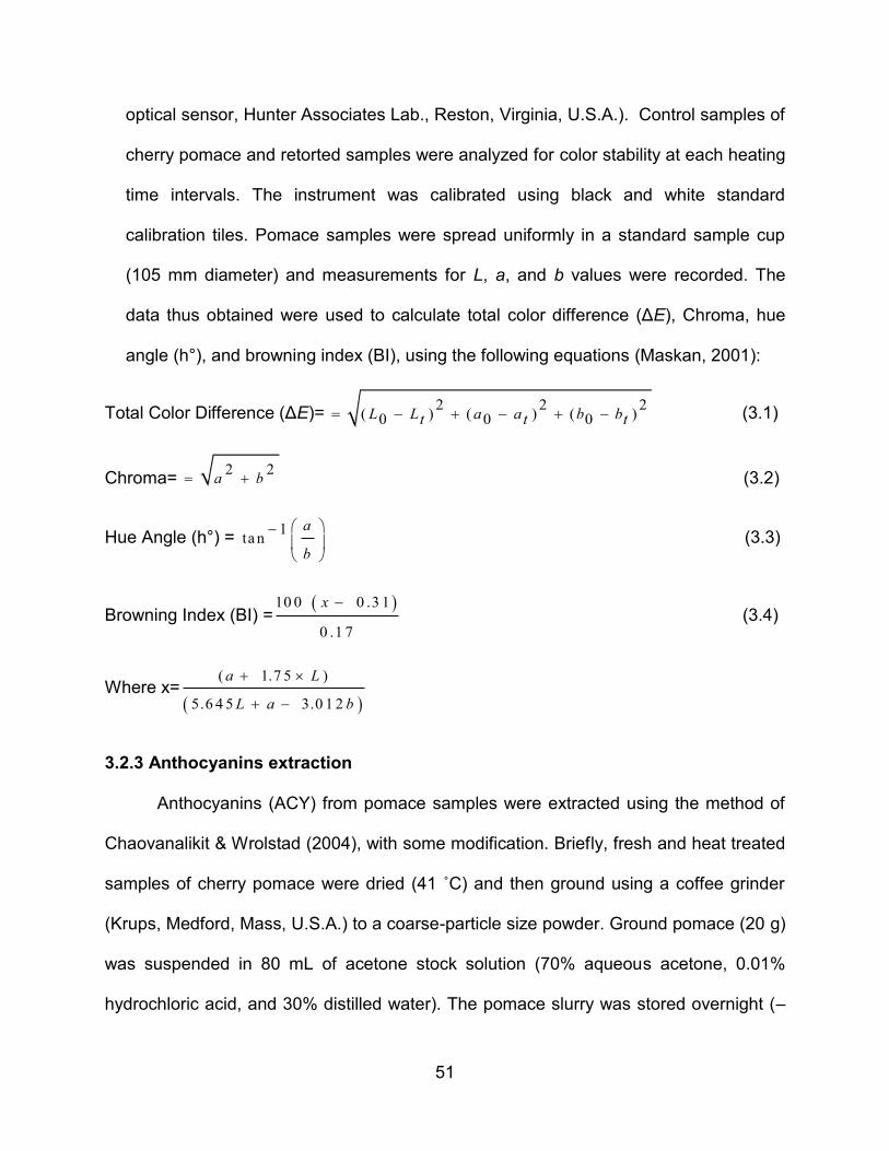
51

optical sensor, Hunter Associates Lab., Reston, Virginia, U.S.A.). Control samples of

cherry pomace and retorted samples were analyzed for color stability at each heating

time intervals. The instrument was calibrated using black and white standard

calibration tiles. Pomace samples were spread uniformly in a standard sample cup

(105 mm diameter) and measurements for L, a, and b values were recorded. The

data thus obtained were used to calculate total color difference (ΔE), Chroma, hue

angle (h°), and browning index (BI), using the following equations (Maskan, 2001):

Total Color Difference (ΔE)= 2 2 2

( ) ( ) ( )0 0 0 L L a a b bt t t (3.1)

Chroma= 2 2

a b (3.2)

Hue Angle (h°) = 1

ta n

a

b (3.3)

Browning Index (BI) = 10 0 0 .3 1

0 .1 7

x (3.4)

Where x=

( 1.7 5 )

5.6 4 5 3.0 1 2

a L

L a b

3.2.3 Anthocyanins extraction

Anthocyanins (ACY) from pomace samples were extracted using the method of

Chaovanalikit & Wrolstad (2004), with some modification. Briefly, fresh and heat treated

samples of cherry pomace were dried (41 ˚C) and then ground using a coffee grinder

(Krups, Medford, Mass, U.S.A.) to a coarse-particle size powder. Ground pomace (20 g)

was suspended in 80 mL of acetone stock solution (70% aqueous acetone, 0.01%

hydrochloric acid, and 30% distilled water). The pomace slurry was stored overnight (–

52

20˚C) in sealed glass jars, wrapped in aluminum foil to protect the sample from light, to

achieve an equilibrium state. The slurry was filtered through Whatman no. 4 filter paper

(Whatman Inc., Clifton, New Jersey, U.S.A.) using a Buchner funnel (under vacuum),

followed by a wash with 50 mL of stock buffer. The filtrate volume was made up to a

final volume of 130 mL and mixed with 40 mL of chloroform and stored overnight. The

supernatant was collected and used for the determination of monomeric anthocyanin

content.

3.2.4 Monomeric anthocyanin content determination

The total monomeric anthocyanin content was determined using the pH

differential assay (Rodriguez-Saona et al., 1999). Pomace samples were dissolved in

potassium chloride buffer (KCl, 0.025 M, pH 1.0) and sodium acetate

(CH3CO2Na3·H2O, 0.4 M, pH 4.5) and allowed to equilibrate, with a predetermined

dilution factor. The absorbance of each equilibrated sample of extracted ACY was then

measured at 510nm and 700 nm for haze correction, using a Genesys 5

spectrophotometer (Spectronic Instruments, Rochester, NY, USA) and 1 cm path-length

cells were used for spectral measurements. ACY contents was calculated, as cyanidin

3-glucoside equivalent (Lee et al., 2005), and reported as mg/100 g (dry-basis).

3.2.5 Antioxidant Capacity

The Oxygen Radical Absorbance Capacity (ORAC) assay using fluorescein as

fluorescent probe (ORACFL) was used to determine the antioxidant capacity (Cao et al.,

1993; Huang et al., 2002). The equipment used for this analysis was BioTekFL×800

Multi-Detection Microplate Reader (Biotek Instruments, Winooski, Vermont,USA). The

53

antioxidant capacity of cherry pomace was determined as Oxygen Radical Absorbance

Capacity (ORAC) values. The results are generally expressed as Trolox equivalent (TE)

– μm TE/g sample. Plot of the calibration curve (Figure A.3) and AUC (Figure A.4) are

shown in Appendices.

3.2.6 Color kinetics

Previous studies have evaluated the kinetics of color degradation in food

materials through zero order (Eq.(3.5)) and first order (Eq.(3.6)) models (Maskan,

2001).

C =C +k 0 tt 0 (3.5)

ln C = ln C +k 1 tt 0 (3.6)

Where, Ct is measured value of color at time t, C0 is initial value of color at time zero, t

is heating time (min), k1 the zero order kinetic constant (min–1

) and k1 the first order

kinetic constant (min–1

). Color measurements can be used for monitoring color

changes in foods, because it is simpler and faster than chemical analysis. Hunter color

measurements provided valuable data on describing color degradation during different

food processing treatments, such as canned strawberries (Kammerer et al., 2007),

mangosteen peel (Chiste et al., 2010), cupuacu puree (Silva and Silva, 1999). The

relationship between anthocyanins concentration and the a value, which represents the

redness of cherry pomace, was described by Eqs.(3.7) and (3.8) as follows (Bechtold et

al., 2007):

ACYt/ ACY0 = b1 (a/a0) – b2 (3.7)

54

ACYt/ ACY0 = b1 ×exp[b2 ×(a/a0)] (3.8)

Where: ACYt is measured value of anthocyanins at time t, ACY0 is initial value

of anthocyanins at time zero, a is the Hunter color a-value at time t, a0 is the intial

(control) Hunter color a-value, and b1 and b2 are the parameters to be estimated.

Statistical analysis

All data were analyzed using JMP 9.0 software (SAS Institute, Inc., Cary, North

Carolina, U.S.A.). One-way analysis of variance was used to analyze the data. The

separation of means or significant difference comparisons were made by Tukey’s HSD

test (α=0.05).

3.3 Results and Discussion

3.3.1 Anthocyanin (ACY) degradation

Initial ACY content in the control cherry pomace (MC-70) was 6.54 mg/100 g

(dry-basis). Thermal treatment in the rotary steam retort at 126.7 °C for 60 min

degraded the ACY to 2.38 mg/100 g. This process reduced the ACY to 6.21 mg/100 g

for MC-41 and 5.84 mg/100g for MC-25 pomace (Figure 4.2). The ACY degradation

was significantly (p≤0.05) higher in the lower-moisture pomace samples (MC-41 and

MC-25) than in the control (MC-70) at 25-min heating, whereas no differences were

observed for 0, 40, or 60 min heat treatment. Generally, the ACY loss was rapid during

the first 25 min of heating, regardless of the moisture content. Heat treatment (60 min)

further degraded the ACY to 1.73 mg/100 g in MC-41 and to 1.59 mg/100g in MC-25.

The fate of ACY in cherry pomace has not been studied previously; however,

Cemeroglu et al., (1994) observed that at 37 °C, the half-life of ACY drops from 38 to 11

55

days in cherry juice concentrate. Greater ACY loss was observed with both an increase

in thermal treatment time and the moisture content of cherry pomace. Similar

observations were reported by (Kirca and Cemeroglu, 2003).

Figure 3.2 Degradation of cherry pomace anthocyanin (ACY) after non-isothermal treatment in a retort at 126.7 °C. (MC-70, MC-41, and MC-25 represent cherry

pomace with 70, 41, and 25% moisture (wb), respectively)

3.3.2 Antioxidant Capacity

MC-25 pomace after retorting at 126.7 °C at different times showed no significant

difference in ORACFL values (p>0.05) as showed in Figure 3.3. The average values are

about 33.24±0.21 (TE–μm TE/g, db) at zero time for MC-25 Pomace and 33.75 ±3.02 ,

33.44±4.13 (TE–μm TE/g, db) for 40 and 60 min heating, respectively (Table A.3

Appendix A.2). This result showed kind of stability and a small elevation in the ORACFL

1

2

3

4

5

6

7

0 10 20 30 40 50 60

Com

ce

ntr

ation

( m

g/1

00

g, d

b)

Retorting time ( min)

MC-70 MC-41 MC-25

56

value, which has an agreement and similarity with a prior study on grape pomace after

it was heated for about 60 min with no significant change in ORACFL values (Mishra et

al., 2008). A study on sweet corn showed elevation in antioxidant capacity after

processing for 25 min at 115 °C (Dewanto et al., 2002)

Figure 3.3 The average total antioxidant values of the cherry pomace ( 70 and 41%MC not heated) and 25% MC (wb) after different heating times

3.3.3 Instrumental Color Changes

Hunter color measurements provided valuable data on describing color

degradation during different food processing treatments, in particular non-isothermal

processing such as canning of strawberries (Kammerer et al., 2007), mangosteen peel

(Chiste et al., 2010), cupuacu puree (Silva & Silva, 1999). Drying of cherry pomace

affected the instrumental color values (Table 3.1). MC-25 (wb) pomace was significantly

different (p≤0.05) with respect to decrease in Hunter L, a, b values, hue angle and

20

22

24

26

28

30

32

34

36

38

40

0 25 40 60

OR

AC

(µ

mo

l T

E/g

, d

b)

Heating time (min)

25-MC 41-MC 70-MC

57

chroma when compared with the control (MC-70) and MC-41 pomace samples. The

moisture content of cherry pomace did not have a significant (p≤0.05) effect on the

Hunter L values when compared across heating time. However, the cumulative effect of

60 min heat treatment significantly (p≤0.05) decreased the L value from 16.73 to

14.37(MC-70), from 16.37 to 12.90 (MC-41), and from 15.07 to 12.93 (MC-25). These

decreases in L values (lightness) have been correlated with pigment degradation and

may be considered as a measure of browning (Ibarz et al., 1999; Maskan, 2006;

Mohammadi et al., 2008). Similarly, a significant decrease in Hunter a value

(redness/greenness scale) and b value (yellowness/blueness) was observed with

increasing heating time. MC-25 pomace showed the greatest decrease in both Hunter

color a and b values after 60 min of heating at 126.7 °C.

Hunter color a and b values were converted to hue angle and chroma, which

represent an average person’s perception of type and richness of color, respectively

(Mcguire, 1992). The significant changes in Hunter color a and b values were not

reflected in the hue angle. Cherry pomace had hue angle of 42-48°, which indicated that

the pomace had a color between red-purple (0°) and yellow (90°) (Mcguire, 1992).

Chroma, which measures the degree of change from gray to chromatic color, decreased

by 47% for MC-70, 40% for MC-41 and 50% for MC-25 after 60 min heat treatment.

Total color change (ΔE) increased significantly with heating time (Figure 3.3). Browning

Index (BI) is a function of L, a and b values as defined in equation (3.4). Therefore, with

increasing heat treatment time, Hunter color values decreased and as a result, BI

decreased. BI represents the purity of brown color but, it is not an indicator of a

darkness of the sample since BI increases with L value at fixed a and b values.

58

Table 3.1 Hunter color L, a, b values, hue angle and chroma of cherry pomace after heat treatment at 126.7 °C.

Heating time (min) MC-70

1 MC-41

2 MC-25

3

Hunter Color L: 0 16.73 ±0.2Aa 16.37±0.03Aa 15.07±0.03Ab

25 16.03±0.4ABa 15.50±0.3Ba 15.57±0.1Aa

40 14.40±0.4Ba 14.73±0.2Ba 14.00±0.2Ba

60 14.37±0.7Ba 12.90±0.1Ca 12.93±0.2Ca

Hunter Color a: 0 7.93±0.1Aa 6.27±0.1Ab 5.53±0.03Ac

25 6.90±0.3BAa 6.27±0.03Aba 5.57±0.1Ab

40 6.17±0.3BCa 6.17±0.1Aa 4.73±0.03Bb

60 5.70±0.3Ca 4.97±0.03Ba 3.97±0.1Cb

Hunter Color b: 0 7.67±0.1Aa 6.90±0.1Ab 5.70±0.1Ac

25 6.63±0.2Ba 6.17±0.03Ba 5.47±0.03Ab

40 5.67±0.2Ca 5.60±0.1Ca 4.70±0.1Bb

60 5.53±0.3Ca 4.60±0.1Db 3.83±0.1Cc

Hue Angle (h°): 0 44.0±0.32Ac 47.7±0.32 Aa 45.8±0.34 ABb

25 43.9±0.34 Aab 44.5±0.27 Bb 44.5±0.52 Ba

40 42.6±0.38 Aab 42.2±0.58 Cb 44.8±0.54 Ba

60 44.2±0.43 Aa 42.8±0.41 BCa 44.0±0.26 Ba

Chroma: 0 11.0±0.11 Aa 9.3±0.12 Ab 7.9±0.05 Ac

25 9.6±0.32 Ba 8.8±0.02 Ba 7.8±0.06 Ab

40 8.4±0.32 BCa 8.3±0.03 Ca 6.7±0.02 Bb

60 7.9±0.39 Ca 6.8±0.05 Db 5.5±0.11 Cc

1,2,3 MC-70, MC-41, and MC-25 represent cherry pomace with 70, 41, and 25%

moisture (wb), respectively. Values are means ± SE of 3 replicates. Means with different letters (a–c) in rows and (A–D) in columns are significantly different (p≤0.05)

59

Figure 3.4 Total color difference (ΔE) and browning index (BI) of cherry pomace after

retorting at 126.7 °C. (MC-70, MC-41, and MC-25 represent the moisture content % (wb), respectively). Means with different letters (a–c) at one heating time and (A–D)

at different heating times, are significantly different (p≤0.05)

3.4 Kinetics of color degradation

Color values were fitted to equations describing the color change using zero- and

first-order kinetics and linear regression analysis. The kinetic parameters estimated

aA

aB

aC

abA

bB

aC

bA

bB

bC

0.0

0.5

1.0

1.5

2.0

2.5

3.0

3.5

4.0

4.5

5.0

0 25 40 60

To

tal C

olo

ur

Diffe

ren

ce

(ΔE)

MC-70 MC-41 MC-25

aA

aB aBC

aC

bA aA aA

bB cA

bB

cC

cD

50

55

60

65

70

75

80

85

90

95

100

0 25 40 60

Bro

wn

ing I

nd

ex (

BI)

Heating Time (min)

MC-70 MC-41 MC-25

60

from these data are presented in Table 3.2. Except for ∆E (MC-70), the zeroth-order

kinetic model showed slightly better fit to experimental data than first-order for Hunter

color b values and ∆E. Generally, the C0 kinetic parameters of color degradation were

larger for MC-70 pomace when compared to that of MC-41 and MC-25 for the zero-

order model. However, a mixed trend was observed with the k0 parameter. For the k1

parameter, MC-25 pomace had the largest kinetic parameters for Hunter color a, and b

values, and ∆E. Overall, Hunter color value b and ∆E showed good fits (R2=0.97–0.83,

range) for both zero- and first-order kinetics.

Deterioration of color occurs due to ACY and other pigments’ degradation,

oxidation of ascorbic acid and non-enzymatic Maillard browning reactions (Abers and

Wrolstad, 1979; Barreiro et al., 1997; Skrede, 1985). Abers & Wrolstad (1979) and

Skrede (1985) concluded that stable polymeric anthocyanins produced during heat

treatment contribute to brown color formation and loss of detectable free anthocyanins

measured by the pH differential method. However, Maskan (2006) and Cemeroglu et

al., (1994) noted that sugar and its degradation products might accelerate ACY

breakdown and enhance non-enzymatic browning during heat processing. Ibarz et al.,

(1999) suggested that zero-order model corresponded to formation of colored polymers

of pigments and was followed by first-order for the degradation of these polymers into

non-colored products. It is possible that ACY degradation may have proceeded via the

polymer formation followed by degradation route while greater non-enzymatic browning

may have occurred in the MC-25 pomace with higher soluble solids and therefore of

sugar.

61

Table 3.2 The estimated kinetic parameters and the statistical values of zero-order and first-order models for Hunter color L, a, b values and total color change (ΔE) for various processing times of cherry pomace at three moisture contents (wb)

at 126.7 °C.

Zero-order Model

k0 min−1

C0 R2

MC-701 MC-412 MC-25

3 MC-70 MC-41 MC-25 MC-70 MC-41 MC-25

Hunter L –0.044±0.0108 –0.056±0.0066 –0.0367±0.0095 16.75±0.41 16.65±0.25 15.63±0.36 0.62 0.88 0.60

Hunter a –0.038±0.0053 –0.012±0.0051 –0.0272±0.0042 7.87±0.20 6.54±0.19 5.81±0.16 0.83 0.61 0.81

Hunter b –0.038±0.0051 –0.038±0.0019 –0.0317±0.0035 7.55±0.19 7.00±0.08 5.91±0.13 0.85 0.97 0.89

ΔE 0.069±0.0093 0.071±0.0066 0.0543±0.0055 0.10±0.36 –0.31±0.25 –0.32±0.21 0.85 0.92 0.90

First-order Model

k1 min−1

C0 R2

MC-70 MC-41 MC-25 MC-70 MC-41 MC-25 MC-70 MC-41 MC-25

Hunter L –0.003±0.0007 –0.004±0.0004 –0.0027±0.0005 16.76±0.03 16.72±0.02 15.63±0.02 0.61 0.88 0.68

Hunter a –0.006±0.0008 –0.004±0.0009 –0.0057±0.0008 7.89±0.03 6.58±0.04 5.86±0.03 0.83 0.61 0.80

Hunter b –0.006±0.0008 –0.007±0.0005 –0.0067±0.0008 7.57±0.03 7.08±0.02 5.99±0.03 0.83 0.95 0.87

ΔE 0.009±0.001 0.008±0.0008 0.0091±0.0011 1.01±0.04 0.96±0.03 0.93±0.04 0.86 0.91 0.87

1,2,3 MC-70, MC-41, and MC-25 represent cherry pomace with 70, 41, and 25% moisture (wb), respectively.

Values represent average of triplicate ± standard error.

62

3.5 Correlation between red color and anthocyanins

Hunter a value (redness/greenness) of cherry pomace as well as the ACY

content decreased with increasing heating time. This effect was the most significant for

the lowest moisture content sample (MC-25) as observed in Table 1 and Figure 3.4.

The relationship between ACY and red color degradation was evaluated using

regression analysis and Eq. 3.7 and Eq. 3.8, as shown in Figure 3.5. The ACY

degradation showed a strong linear correlation, Eq.3.8 (R2=0.98) with red color values

for the fresh pomace sample, MC-70 (Table 3.3). Similar observations have been

reported with thermal processing of plum puree by(Ahmed et al., 2004). A study on

purple corn cob was also established a correlation between Hunter color parameters

and contents of ACY and showed that that Hunter color parameters could be used of

ACY contents during heating (Chen et al., 2008).

For MC-41 and MC-25 pomace, the correlation was exponential, as shown by

Eq. 3.8. Similar correlations for color with ACY concentration in grape pomace were

made by Bechtold et al., (2007). Thus, anthocyanin degradation in cherry pomace

during non-isothermal processing may be predicted from Hunter color a value using a

linear relationship in Eq. 3.7 for high moisture samples and a exponential relationship

Eq. 3.8 for lower moisture samples.

63

Figure 3.5 Correlation between Hunter color a values and anthocyanins content of cherry pomace after thermal processing at 126.7 °C. Data three replicate. (MC-70, MC-41, and MC-25 represent cherry pomace with 70, 41, and 25% moisture (wb),

respectively)

Table 3.3 Coefficients of equations (3.7) and (3.8) for correlation between Hunter color a values and anthocyanins content

Pomace Equation b1 b2 R2

MC-701 (3.7) 1.8929 0.9522

0.98

MC-701 (3.8) 0.0095 4.837 0.95

MC-412 (3.7) 2.0302 1.2778 0.76

MC-412 (3.8) 0.0026 5.7024 0.92

MC-253 (3.7) 1.4016 0.7053 0.71

MC-253 (3.8) 0.0005 7.636 0.89

1,2,3 MC-70, MC-41, and MC-25 represent cherry pomace with 70, 41, and 25%

moisture, respectively.

0.0

0.1

0.2

0.3

0.4

0.5

0.6

0.7

0.8

0.9

1.0

0.4 0.5 0.6 0.7 0.8 0.9 1.0

AC

Yt/A

CY

0

a/a0

MC-70

MC-41

MC-25

2

ACY / ACY 1 .8 9 a / a – 0 .9 52 , 0 .9 8 t 0 0 R

5 .7 a / a   20A C Y / A C Y    0 .0 0 2 6 e xp   , 0 .9 2   t 0 R

7 .6 3 a / a   20A C Y / A C Y    0 .0 0 0 5 e xp   ,  0 .8 9   t 0 R

64

3.6 Conclusions

Cherry pomace is an excellent source of ACY and has potential to be developed

into value-added products. This is the first study on cherry pomace that assessed the

effect of non-isothermal heat treatment on the free ACY content and color of pomace.

Many products such as extruded foods, baked goods and powders are manufactured

using processes that use non-isothermal heat treatment. Knowledge of the anthocyanin

thermal degradation kinetics will help design such industrial processing of this industrial

by-product. Overall, the extent of color degradation increased with heating time. A

significant decrease in Hunter color L, a, b and chroma values was observed at each

heating time. Loss of color due to heat treatment followed zero-order kinetics. Higher

ACY degradation was observed with increasing heating time for all pomace samples at

different moisture contents. ACY degradation may be correlated with changes in red

color. It showed a linear relationship at higher moisture content (MC-70) of cherry

pomace and an exponential relationship at lower moisture content of cherry pomace

(MC-41 and MC-25).

65

A. APPENDICES

66

Appendix A.1 Experimental design and preliminary data

Fresh and dried pomace

Retorted pomace AC Y values, color values and temperatures data

Figure A.1 Process experimental design for ACY and pomace’s color degradation

ACY Extraction steps PH Diff, ACY Concentration

Retorting Process Data collection Data Analysis

Fresh Cherry Pomace Drying lower MCs Filling ,Density, TCs fitting

70% 41 % 25%

70% 41% 25%

Data

Analysis

Color Measurements

Step 2

Step 4

Step 3

Step 1

1.5 4.5 1.5 4.5 1.5 4.5

67

Figure A.2 Plots of retorting process of cherry pomace in a rotary steam retort at 126.7 °C for 25, 40, 60 and 90 min after 10 min come-up-time. (Rt=Retort temperature; MC-70, MC-41, and MC-25 represent cherry pomace with 70, 41, and 25% moisture (wb) ,

respectively).

0 10 20 30 40 500

20

40

60

80

100

120

140

time (min)

Re

tort

an

d c

an

ce

nte

r te

mp

era

ture

s (

°C)

70MC1

70MC2

41MC1

41MC2

25MC1

25MC2

Rt

0 10 20 30 40 50 60 7020

40

60

80

100

120

140

time (min)

Re

tort

an

d c

an

ce

nte

r te

mp

era

ture

s (

°C)

70MC1

70MC2

41MC1

41MC2

25MC1

25MC2

Rt

68

Figure A.2 (cont’d)

0 10 20 30 40 50 60 70 800

20

40

60

80

100

120

140

time (min)

Re

tort

an

d c

an

ce

nte

r te

mp

era

ture

s (

°C)

70MC

41MC

25MC

Rt

0 20 40 60 80 100 120 1400

20

40

60

80

100

120

140

time (min)

Re

tort

an

d c

an

ce

nte

r te

mp

era

ture

s (

°C)

70MC1

70MC2

41MC1

41MC2

25MC1

25MC2

Retort,T

69

Table A.1 Cherry pomace ‘s anthocyanins concentration ( mg/kg,db) after retorting process at different times

Time (min)

Retorting Temperature 126.7°C

Cherry pomace Moisture contents (MC %, wb)

70-MC 41-MC 25-MC

0 57.89 44.61 37.27

0 59.70 69.33 57.89

0 78.70 59.79 60.42

25 37.99 40.48 28.22

25 44.32 32.20 31.12

25 47.04 30.82 29.33

40 19.00 22.08 14.47

40 37.99 12.88 28.58

40 36.18 32.20 25.69

60 28.04 17.48 21.35

60 19.00 19.78 17.37

60 24.42 14.72 8.32

90 1.81 5.98 0.00

90 10.85 9.66 0.00

90 7.24 0.00 0.00

Table A.2 Raw data (sample) of retorting process of cherry pomace in a rotary steam

retort at 126.7 °C

time(sec) MC-70 MC-70 MC-41 MC-41 MC-25 MC-25 Ts TRt

0 23.33 23.64 25.05 23.26 22.66 22.66 23.23 72.76 10 23.47 23.83 24.52 23.32 22.71 22.76 29.40 77.41 20 23.53 23.88 24.62 23.37 22.73 22.82 37.70 73.13 30 23.58 23.86 24.38 23.44 22.79 22.89 48.50 79.52 40 23.65 23.94 24.41 23.59 22.86 23.09 57.00 78.45 50 23.70 24.02 24.47 23.76 22.99 23.28 64.60 83.08 60 23.77 24.12 24.61 23.96 23.18 23.57 71.00 83.66 70 23.82 24.19 24.85 24.25 23.38 23.93 76.60 86.26 80 23.87 24.28 24.99 24.47 23.61 24.29 81.60 86.32 90 23.76 23.83 25.13 24.72 24.12 24.68 85.20 84.14

100 23.86 24.06 25.35 24.97 24.31 25.05 86.00 88.84 110 23.91 24.17 25.54 25.24 24.56 25.53 91.10 89.11 120 23.97 24.32 25.81 25.48 24.74 26.01 93.00 90.71 130 23.99 24.41 25.98 25.69 25.03 26.43 94.40 90.38

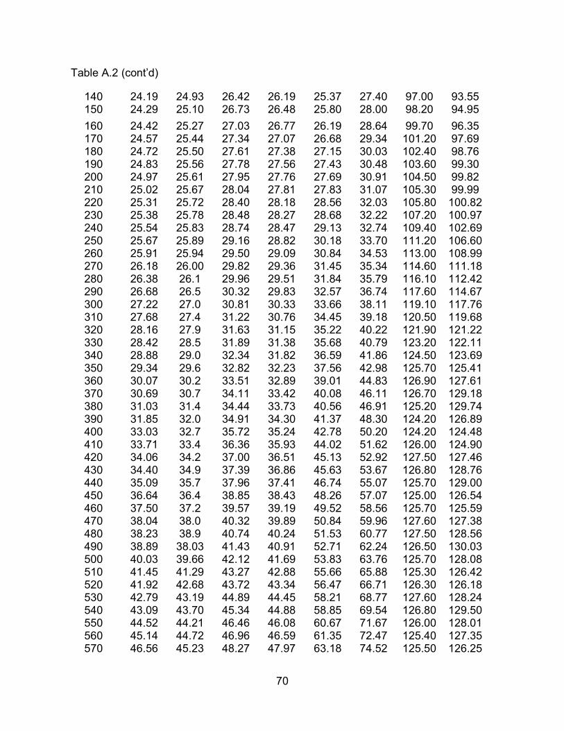
70

Table A.2 (cont’d)

140 24.19 24.93 26.42 26.19 25.37 27.40 97.00 93.55 150 24.29 25.10 26.73 26.48 25.80 28.00 98.20 94.95

160 24.42 25.27 27.03 26.77 26.19 28.64 99.70 96.35 170 24.57 25.44 27.34 27.07 26.68 29.34 101.20 97.69 180 24.72 25.50 27.61 27.38 27.15 30.03 102.40 98.76 190 24.83 25.56 27.78 27.56 27.43 30.48 103.60 99.30 200 24.97 25.61 27.95 27.76 27.69 30.91 104.50 99.82 210 25.02 25.67 28.04 27.81 27.83 31.07 105.30 99.99 220 25.31 25.72 28.40 28.18 28.56 32.03 105.80 100.82 230 25.38 25.78 28.48 28.27 28.68 32.22 107.20 100.97 240 25.54 25.83 28.74 28.47 29.13 32.74 109.40 102.69 250 25.67 25.89 29.16 28.82 30.18 33.70 111.20 106.60 260 25.91 25.94 29.50 29.09 30.84 34.53 113.00 108.99 270 26.18 26.00 29.82 29.36 31.45 35.34 114.60 111.18 280 26.38 26.1 29.96 29.51 31.84 35.79 116.10 112.42 290 26.68 26.5 30.32 29.83 32.57 36.74 117.60 114.67 300 27.22 27.0 30.81 30.33 33.66 38.11 119.10 117.76 310 27.68 27.4 31.22 30.76 34.45 39.18 120.50 119.68 320 28.16 27.9 31.63 31.15 35.22 40.22 121.90 121.22 330 28.42 28.5 31.89 31.38 35.68 40.79 123.20 122.11 340 28.88 29.0 32.34 31.82 36.59 41.86 124.50 123.69 350 29.34 29.6 32.82 32.23 37.56 42.98 125.70 125.41 360 30.07 30.2 33.51 32.89 39.01 44.83 126.90 127.61 370 30.69 30.7 34.11 33.42 40.08 46.11 126.70 129.18 380 31.03 31.4 34.44 33.73 40.56 46.91 125.20 129.74 390 31.85 32.0 34.91 34.30 41.37 48.30 124.20 126.89 400 33.03 32.7 35.72 35.24 42.78 50.20 124.20 124.48 410 33.71 33.4 36.36 35.93 44.02 51.62 126.00 124.90 420 34.06 34.2 37.00 36.51 45.13 52.92 127.50 127.46 430 34.40 34.9 37.39 36.86 45.63 53.67 126.80 128.76 440 35.09 35.7 37.96 37.41 46.74 55.07 125.70 129.00 450 36.64 36.4 38.85 38.43 48.26 57.07 125.00 126.54 460 37.50 37.2 39.57 39.19 49.52 58.56 125.70 125.59 470 38.04 38.0 40.32 39.89 50.84 59.96 127.60 127.38 480 38.23 38.9 40.74 40.24 51.53 60.77 127.50 128.56 490 38.89 38.03 41.43 40.91 52.71 62.24 126.50 130.03 500 40.03 39.66 42.12 41.69 53.83 63.76 125.70 128.08 510 41.45 41.29 43.27 42.88 55.66 65.88 125.30 126.42 520 41.92 42.68 43.72 43.34 56.47 66.71 126.30 126.18 530 42.79 43.19 44.89 44.45 58.21 68.77 127.60 128.24 540 43.09 43.70 45.34 44.88 58.85 69.54 126.80 129.50 550 44.52 44.21 46.46 46.08 60.67 71.67 126.00 128.01 560 45.14 44.72 46.96 46.59 61.35 72.47 125.40 127.35 570 46.56 45.23 48.27 47.97 63.18 74.52 125.50 126.25

71

Table A.2 (cont’d)

580 47.03 45.90 48.77 48.48 63.88 75.29 126.80 126.34 590 47.98 46.70 50.09 49.71 65.71 77.15 127.00 128.98 600 48.46 47.50 50.59 50.19 66.39 77.89 126.30 129.18 610 49.99 48.30 51.89 51.56 68.07 79.70 125.60 127.31 620 50.59 49.10 52.46 52.11 68.77 80.41 125.40 126.79 630 51.98 49.90 53.86 53.57 70.48 82.12 126.30 126.19 640 52.42 50.70 54.41 54.11 71.12 82.75 126.90 126.57 650 53.49 51.50 55.81 55.43 72.73 84.29 126.50 128.57 660 54.05 52.30 56.31 56.01 73.34 84.92 125.80 128.07 670 55.61 53.10 57.79 57.49 74.92 86.39 125.40 126.60 680 56.17 53.90 58.33 58.06 75.54 86.92 125.90 126.15 690 57.45 55.00 59.88 59.61 77.09 88.32 126.80 126.65 700 57.81 56.10 60.45 60.13 77.66 88.82 126.50 127.84 710 59.09 57.20 61.86 61.53 79.06 90.03 125.90 128.01 720 59.68 58.30 62.42 62.12 79.55 90.49 125.50 127.31 730 61.23 59.40 63.94 63.72 80.96 91.68 125.60 126.17 740 61.72 60.50 64.51 64.32 81.47 92.11 126.50 126.04 750 63.21 61.60 66.62 66.31 83.31 93.56 126.60 128.07 760 63.41 62.70 66.86 66.55 83.50 93.74 126.10 128.15 770 65.25 63.80 68.66 68.41 85.01 94.93 125.60 126.73 780 65.50 64.90 68.90 68.67 85.22 95.10 125.50 126.49 790 67.08 66.00 70.76 70.54 86.65 96.21 126.20 126.38 800 67.27 67.10 71.03 70.81 86.87 96.38 126.60 126.68 810 67.72 68.20 71.74 71.47 87.43 96.84 126.20 127.62 820 69.54 69.30 73.69 73.42 88.89 97.96 125.70 126.99 830 69.78 70.40 73.93 73.68 89.05 98.08 125.60 126.78 840 70.54 70.87 74.72 74.51 89.60 98.52 125.90 126.24 850 71.29 71.37 75.74 75.56 90.61 99.07 126.40 126.19 860 72.63 72.44 77.64 77.34 91.97 99.97 126.20 127.68 870 72.86 72.71 77.87 77.56 92.13 100.07 125.80 127.56 880 73.62 73.41 78.57 78.31 92.62 100.44 125.60 127.11 890 74.56 74.51 79.56 79.33 93.28 100.88 125.80 126.40 900 76.06 75.71 81.44 81.18 94.49 101.72 126.30 126.76 910 76.46 76.19 82.04 81.75 94.89 101.97 126.20 127.43 920 76.68 76.57 82.30 82.01 94.99 102.06 125.90 127.51 930 77.55 77.49 83.17 82.89 95.53 102.48 125.70 127.26 940 78.48 78.43 84.10 83.82 96.12 102.91 125.80 126.66 950 79.57 79.54 85.36 85.15 96.82 103.41 126.10 126.34 960 79.95 79.97 85.86 85.62 97.13 103.63 126.30 126.57 970 80.49 80.28 86.65 86.35 97.64 103.94 126.10 127.38 980 82.08 82.06 88.28 87.98 98.62 104.62 125.80 126.86 990 82.63 82.64 88.82 88.58 98.89 104.85 125.70 126.54

1000 82.85 82.84 89.08 88.86 99.04 104.94 125.90 126.44 1010 83.56 83.48 89.89 89.71 99.49 105.26 126.20 126.49 1020 84.81 84.80 91.36 91.12 100.26 105.87 126.20 127.48

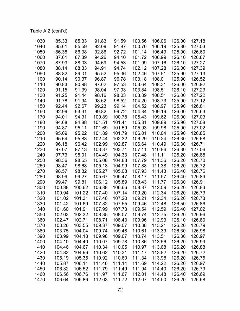
72

Table A.2 (cont’d)

1030 85.33 85.33 91.83 91.59 100.56 106.06 126.00 127.18 1040 85.61 85.59 92.09 91.87 100.70 106.19 125.80 127.03 1050 86.38 86.38 92.86 92.72 101.14 106.49 125.90 126.60 1060 87.61 87.89 94.26 94.10 101.72 106.99 126.10 126.87 1070 87.93 88.03 94.69 94.53 101.99 107.16 126.10 127.27 1080 88.14 88.33 94.91 94.74 102.12 107.28 126.00 127.39 1090 88.82 89.01 95.52 95.36 102.46 107.51 125.90 127.13 1100 90.14 90.37 96.87 96.78 103.18 108.01 125.90 126.52 1110 90.83 90.98 97.62 97.53 103.64 108.31 126.00 126.92 1120 91.15 91.39 98.04 97.93 103.84 108.51 126.10 127.23 1130 91.25 91.44 98.16 98.03 103.89 108.51 126.00 127.22 1140 91.78 91.94 98.62 98.52 104.20 108.73 125.90 127.12 1150 92.44 92.67 99.23 99.14 104.52 108.97 125.90 126.81 1160 92.99 93.31 99.82 99.72 104.84 109.19 126.00 126.63 1170 94.01 94.31 100.89 100.78 105.43 109.62 126.00 127.03 1180 94.68 94.88 101.51 101.41 105.81 109.89 125.90 127.08 1190 94.87 95.11 101.69 101.59 105.93 109.98 125.90 127.02 1200 95.09 95.22 101.89 101.79 106.01 110.04 125.90 126.85 1210 95.64 95.83 102.44 102.32 106.29 110.24 126.30 126.68 1220 96.18 96.42 102.99 102.87 106.64 110.49 126.30 126.71 1230 97.07 97.13 103.87 103.71 107.11 110.86 126.30 127.06 1240 97.73 98.01 104.49 104.33 107.48 111.11 126.20 126.88 1250 98.36 98.55 105.08 104.88 107.79 111.36 126.20 126.70 1260 98.47 98.68 105.18 104.99 107.88 111.38 126.20 126.72 1270 98.57 98.82 105.27 105.08 107.93 111.43 126.40 126.76 1280 98.99 99.27 105.67 105.47 108.17 111.57 126.40 126.89 1290 99.47 99.81 106.12 105.89 108.43 111.77 126.30 126.91 1300 100.38 100.62 106.88 106.66 108.87 112.09 126.20 126.83 1310 100.94 101.22 107.40 107.14 109.20 112.34 126.20 126.73 1320 101.02 101.31 107.46 107.20 109.21 112.34 126.20 126.73 1330 101.42 101.69 107.82 107.55 109.46 112.48 126.50 126.86 1340 101.60 101.91 107.99 107.73 109.54 112.59 126.40 127.02 1350 102.03 102.32 108.35 108.07 109.74 112.75 126.20 126.96 1360 102.47 102.71 108.71 108.43 109.96 112.93 126.10 126.80 1370 103.26 103.55 109.37 109.07 110.38 113.21 126.20 126.79 1380 103.75 104.04 109.74 109.48 110.61 113.39 126.30 126.98 1390 103.99 104.18 109.98 109.67 110.74 113.51 126.30 126.97 1400 104.10 104.40 110.07 109.78 110.86 113.56 126.20 126.99 1410 104.46 104.67 110.34 110.05 110.97 113.68 126.20 126.88 1420 104.82 104.96 110.62 110.31 111.17 113.82 126.20 126.72 1430 105.19 105.35 110.92 110.60 111.34 113.98 126.20 126.75 1440 105.87 106.11 111.46 111.14 111.69 114.22 126.20 126.97 1450 106.32 106.52 111.79 111.49 111.94 114.40 126.20 126.79 1460 106.56 106.76 111.97 111.67 112.01 114.48 126.40 126.69 1470 106.64 106.86 112.03 111.72 112.07 114.50 126.20 126.68

73

Table A.2 (cont’d)

1480 106.93 107.14 112.26 111.94 112.27 114.63 126.20 126.69 1490 107.21 107.47 112.49 112.18 112.36 114.73 126.10 126.87 1500 107.90 108.13 113.00 112.70 112.69 115.00 126.20 126.86 1510 108.31 108.54 113.29 113.01 112.92 115.15 126.30 126.69 1520 108.69 108.93 113.58 113.28 113.10 115.30 126.20 126.79 1530 108.73 108.96 113.61 113.33 113.11 115.30 126.10 126.86 1540 108.86 109.07 113.71 113.42 113.17 115.37 126.10 126.95 1550 109.11 109.37 113.89 113.61 113.32 115.47 126.20 126.99 1560 109.42 109.68 114.11 113.83 113.41 115.57 126.20 126.87 1570 109.72 110.00 114.31 114.04 113.61 115.68 126.20 126.71 1580 110.01 110.30 114.52 114.26 113.71 115.81 126.20 126.68 1590 110.49 110.65 114.93 114.66 114.04 116.01 126.10 126.98 1600 110.85 110.98 115.16 114.90 114.18 116.14 126.20 126.86 1610 111.18 111.27 115.38 115.14 114.37 116.28 126.10 126.69 1620 111.23 111.33 115.44 115.17 114.39 116.31 126.30 126.69 1630 111.29 111.41 115.48 115.22 114.39 116.33 126.30 126.67 1640 111.55 111.78 115.67 115.42 114.55 116.42 126.20 126.77 1650 111.81 111.89 115.83 115.61 114.65 116.53 126.10 127.01 1660 112.05 112.12 116.00 115.76 114.78 116.62 126.10 126.88 1670 112.57 112.64 116.35 116.13 115.02 116.82 126.20 126.67 1680 112.86 112.94 116.57 116.33 115.21 116.93 126.20 126.76 1690 113.12 113.20 116.74 116.52 115.33 117.03 126.20 126.96 1700 113.28 113.37 116.86 116.63 115.42 117.11 126.20 126.96 1710 113.34 113.42 116.87 116.67 115.44 117.11 126.10 126.91 1720 113.48 113.55 116.97 116.76 115.50 117.17 126.10 126.82 1730 113.71 113.79 117.12 116.92 115.64 117.28 126.30 126.70 1740 113.94 114.01 117.29 117.08 115.74 117.38 126.20 126.66 1750 114.15 114.23 117.42 117.24 115.87 117.47 126.10 126.81 1760 114.57 114.64 117.68 117.51 116.04 117.61 126.10 126.88 1770 114.82 114.89 117.86 117.69 116.18 117.71 126.10 126.68 1780 115.09 115.14 118.03 117.85 116.25 117.81 126.20 126.65 1790 115.23 115.29 118.11 117.94 116.33 117.87 126.20 126.77 1800 115.27 115.33 118.15 117.97 116.36 117.88 126.10 126.78 1810 115.37 115.44 118.22 118.05 116.41 117.92 126.20 126.92 1820 115.57 115.63 118.36 118.18 116.51 118.01 126.10 126.80 1830 115.77 115.83 118.48 118.32 116.62 118.09 126.10 126.70 1840 115.97 116.03 118.60 118.46 116.73 118.18 126.30 126.66 1850 116.29 116.36 118.82 118.67 116.88 118.31 126.20 126.85

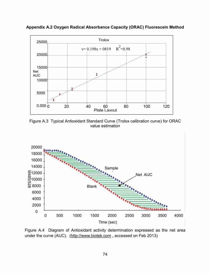
74

Appendix A.2 Oxygen Radical Absorbance Capacity (ORAC) Fluorescein Method

Figure A.3 Typical Antioxidant Standard Curve (Trolox calibration curve) for ORAC value estimation

Figure A.4 Diagram of Antioxidant activity determination expressed as the net area

under the curve (AUC). (http://www.biotek.com , accessed on Feb 2013)

Time (sec)

M485/5

28

20000

18000

16000

14000

12000

10000

8000

6000

4000

2000

00 500 1000 1500 2000 2500 3000 3500 4000

Net AUC

Sample

Blank

Trolox Curve

<Plate Layout Settings>

Ne

t A

UC

0 20 40 60 80 100 120

0.000

5.000

10.000

15.000

20.000

25.000

Plate Layout

Setting

Trolox

Curve

Net AUC

y= 0.198x + 0819 R2=0.98

0 20 40 60 80 100 120

25000

20000

15000

10000

5000

0.000

75

Table A.3 The average total antioxidant values of cherry pomace (treated 25%MC and untreated 70% MC,41%MC ,wb) retorted at 126.7 °C )( values for 5 replicates)

Retorting time (min)

ORAC (µmol TE/g pomace ,db)

25% 41% 70%

0 35.24 ± 1.21 30.44 ± 4.42 30.26 ± 2.51

25 35.62 ± 3.25 NA NA

40 35.75 ± 3.02 NA NA

60 33.44 ± 4.13 NA NA

76

REFERENCES

77

REFERENCES

Abers, J.E., Wrolstad, R.E., (1979). Causative factors of color deterioration in strawberry preserves during processing and storage. Journal of Food Science 44(1), 75-&.

Ahmed, J., Shivhare, U.S., Raghavan, G.S.V., (2004). Thermal degradation kinetics of anthocyanin and visual colour of plum puree. European Food Research and Technology 218(6), 525-528.

Barreiro, J.A., Milano, M., Sandoval, A.J., (1997). Kinetics of colour change of double concentrated tomato paste during thermal treatment. Journal of Food Engineering 33(3-4), 359-371.

Bechtold, T., Mahmud-Ali, A., Mussak, R., (2007). Anthocyanin dyes extracted from grape pomace for the purpose of textile dyeing. Journal of the Science of Food and Agriculture 87(14), 2589-2595.

Bonerz, D., Wurth, K., Dietrich, H., Will, F., (2007). Analytical characterization and the impact of ageing on anthocyanin composition and degradation in juices from five sour cherry cultivars. European Food Research and Technology 224(3), 355-364.

Britt, C., Gomaa, E.A., Gray, J.I., Booren, A.M., (1998). Influence of cherry tissue on lipid oxidation and heterocyclic aromatic amine formation in ground beef patties. Journal of Agricultural and Food Chemistry 46(12), 4891-4897.

Cao, G.H., Alessio, H.M., Cutler, R.G., (1993). Oxygen-Radical Absorbency Capacity Assay for Antioxidants. Free Radical Biology and Medicine 14(3), 303-311.

Cemeroglu, B., Velioglu, S., Isik, S., (1994). Degradation kinetics of anthocyanins in sour cherry juice and concentrate. Journal of Food Science 59(6), 1216-1218.

Chaovanalikit, A., Wrolstad, R.E., (2004). Total anthocyanins and total phenolics of fresh and processed cherries and their antioxidant properties. Journal of Food Science 69(1), C67-C72.

Chiste, R.C., Lopes, A.S., de Faria, L.J.G., (2010). Thermal and light degradation kinetics of anthocyanin extracts from mangosteen peel (Garcinia mangostana L.). International Journal of Food Science and Technology 45(9), 1902-1908.

Dewanto, V., Wu, X.Z., Liu, R.H., (2002). Processed sweet corn has higher antioxidant activity. Journal of Agricultural and Food Chemistry 50(17), 4959-4964.

78

Forni, E., Polesello, A., Torreggiani, D., (1993). Changes in anthocyanins in cherries (prunus-avium) during osmodehydration, pasteurization and storage. Food Chemistry 48(3), 295-299.

Huang, D.J., Ou, B.X., Hampsch-Woodill, M., Flanagan, J.A., Prior, R.L., (2002). High-throughput assay of oxygen radical absorbance capacity (ORAC) using a multichannel liquid handling system coupled with a microplate flourescence reader in 96-well format. Journal of Agricultural and Food Chemistry 50(16), 4437-4444.

Ibarz, A., Pagan, J., Garza, S., (1999). Kinetic models for colour changes in pear puree during heating at relatively high temperatures. Journal of Food Engineering 39(4), 415-422.

Kammerer, D.R., Schillmoller, S., Maier, O., Schieber, A., Carle, R., (2007). Colour stability of canned strawberries using black carrot and elderberry juice concentrates as natural colourants. European Food Research and Technology 224(6), 667-679.

Kim, D.O., Padilla-Zakour, O.I., (2004). Jam processing effect on phenolics and antioxidant capacity in anthocyanin-rich fruits: Cherry, plum, and raspberry. Journal of Food Science 69(9), S395-S400.

Kirca, A., Cemeroglu, B., (2003). Degradation kinetics of anthocyanins in blood orange juice and concentrate. Food Chemistry 81(4), 583-587.

Konczak, I., Zhang, W., (2004). Anthocyanins - more than nature's colours. Journal of Biomedicine and Biotechnology(5), 239-240.

Lee, J., Durst, R.W., Wrolstad, R.E., (2005). Determination of total monomeric anthocyanin pigment content of fruit juices, beverages, natural colorants, and wines by the pH differential method: Collaborative study. Journal of Aoac International 88(5), 1269-1278.

Markakis, P., Livingston, G.E., Fellers, C.R., (1956). Quantitative aspects of strawberry pigment degradation. Food Technology 10(12), 31-31.

Maskan, M., (2001). Kinetics of colour change of kiwifruits during hot air and microwave drying. Journal of Food Engineering 48(2), 169-175.

Maskan, M., (2006). Production of pomegranate (Punica granatum L.) juice concentrate by various heating methods: colour degradation and kinetics. Journal of Food Engineering 72(3), 218-224.

79

Mcguire, R.G., (1992). Reporting of objective color measurements. Hortscience 27(12), 1254-1255.

Mishra, D.K., Dolan, K.D., Yang, L., (2008). Confidence intervals for modeling anthocyanin retention in grape pomace during nonisothermal heating. Journal of Food Science 73(1), E9-E15.

Mohammadi, S., R., Z., E.-D., A., K., (2008). Kinetic models for colour changes in kiwifruit slices during hot air drying. World Journal of Agricultural Sciences 4 (3), 376-383.

Nawirska A. , K.M., (2005). Dietary fibre fractions from fruit and vegeTable processing waste. J of Food Chemistry 91, 221–225.

Patras, A., Brunton, N.P., O'Donnell, C., Tiwari, B.K., (2010). Effect of thermal processing on anthocyanin stability in foods; mechanisms and kinetics of degradation. Trends in Food Science & Technology 21(1), 3-11.

Rodriguez-Saona, L.E., Wrolstad, R.E., Pereira, C., (1999). Glycoalkaloid content and anthocyanin stability to alkaline treatment of red-fleshed potato extracts. Journal of Food Science 64(3), 445-450.

Silva, F.M., Silva, C.L.M., (1999). Colour changes in thermally processed cupuacu (Theobroma grandiflorum) puree: critical times and kinetics modelling. International Journal of Food Science and Technology 34(1), 87-94.

Skrede, G., (1985). Color quality of blackcurrant syrups during storage evaluated by Hunter L'-Value, L'a-value, L'b-value. Journal of Food Science 50(2), 514-&.

Tomas-Barberan, F.A., Gil, M.I., Cremin, P., Waterhouse, A.L., Hess-Pierce, B., Kader, A.A., (2001). HPLC-DAD-ESIMS analysis of phenolic compounds in nectarines, peaches, and plums. Journal of Agricultural and Food Chemistry 49(10), 4748-4760.

Tsami, E., Katsioti, M., (2000). Drying kinetics for some fruits: Predicting of porosity and color during dehydration. Drying Technology 18(7), 1559-1581.

Wang, H.B., Nair, M.G., Strasburg, G.M., Chang, Y.C., Booren, A.M., Gray, J.I., DeWitt, D.L., (1999). Antioxidant and antiinflammatory activities of anthocyanins and their aglycon, cyanidin, from tart cherries (vol 62, pg 296, 1999). Journal of Natural Products 62(5), 802-802.

80

CHAPTER 4

OBJECTIVE TWO

4. Estimation of Temperature-Dependent Thermal Properties of Cherry Pomace at Different Moisture Contents During Non-Isothermal Heating

81

Abstract

Fruit and vegeTables are a rich source of many bio-active compounds from

which value-added nutraceuticals can be produced. To design processes for these

solids, thermal properties must be known. Because many of the bio-active compounds,

e.g., anthocyanins and phenolics, degrade exponentially faster at elevated

temperatures (above 100oC), use of temperature-dependent thermal properties will give

more accurate results than those from constant properties. Differential scanning

calorimetery (DSC) was used to measure the specific heat of cherry pomace at three

constant moisture contents (MC). At 25 ºC, the measured specific heat was found to be

1671, 2111 and 2943 J kg-1

K-1

for 70, 41 and 25% moisture content, respectively.

Tart cherry pomace was equilibrated to 25, 41, and 70% MC wet basis (wb) and heated

in sealed 54× 73 mm cans at 127 °C in a steam retort for 25, 40, 60 and 90 min. Can

center temperature was recorded. For the ordinary least squares method, the sum of

squares of errors = (center temperature observed – center temperature predicted)2 was

minimized by nonlinear regression in MATLAB with Comsol. The sequential estimation

method was also used to determine how the addition of each datum affected the

thermal property estimates during the experiment. Thermal conductivity (W m-1

K-1

)

was estimated at 25°C (k1) and 125°C (k2), using a linear function of temperature. At 90

min heating, the estimated k1 and k2 values and standard errors for 70, 41 and 25% MC

were 0.49 +/- 0.00047 and 0.55 +/- 0.00058, 0.20 +/- 0.0015 and 0.39 +/- 0.0012 and

0.15 +/- 0.0034 and 0.28 +/- 0.0037 W m-1

K-1

, respectively. These results can be

useful for processors desiring to use cherry pomace to make value-added by-products

82

at elevated temperatures common in extrusion, spray-drying and other food drying

methods.

4.1 Introduction

Thermal processing of foods involves heating to temperatures typically from 50 to

150 ºC. Anthocyanin stability is a main focus in many studies. This stability is not only a

function of final processing temperature but also of other properties (intrinsic) like pH,

storage temperature, product moisture content , chemical structure of the anthocyanins

and its initial concentration, light, oxygen, presence of enzymes, proteins and metallic

ions(Patras et al., 2010) . There are many studies examining these factors individually

or a combination of one or more of them on degradation of food components. There is

limited information available on the effect of high temperature processing at different

moisture contents on the stability of these pigments in solid food products. A challenge

in collecting this information is the confounding decrease in moisture during heating at

temperatures greater than 100 °C. A study on the change in physical properties of

ground beef during cooking showed that thermal conductivity of ground beef varied

between 0.35 and 0.41 W/m °C in temperature range of 5 to 70 °C (Pan and Singh,

2001). Estimation methods for thermal conductivity are classified into two main

methods: steady- and transient-state heat transfer methods. Steady-state methods

require long times, and moisture content changing with time introduces significant error

(Dutta et al., 1988). Many studies have been done on this subject for estimating these

properties for different kinds of food materials. Some studies used measured

temperature profiles for estimation of the thermophysical properties in inverse heat

conduction problems (Beck and Woodbury, 1998; Yang, 1998).

83

Equations (quadratic models) were developed for predicting thermal conductivity of a

meat with a given water content and temperature at different ranges (Rahman, 1992;

Sweat, 1975). Thermal conductivity of carrot and potato (solid food) were measured as

well, using the probe method at a temperature range 30 -130 ˚C, a correlation equation

based on composition alone was established for predicting the thermal conductivity

(Gratzek and Toledo, 1993). The thermal conductivity of porous foods, which have

complex structure is difficult to predict (Sweat, 1995).

Thermal properties was determined for borage seeds, Specific heat was

measured by differential scanning calorimetric (DSC) and ranged from 0.77 to 1.99 kJ

kg-1

K-1

and thermal conductivity increased with moisture content and contributed the

most to the uncertainty of thermal diffusivity; however quadratic equations were

established for estimating these thermal properties (Yang et al., 2002). A study on

wheat, corn and rice flour proposed an equation to predict the specific heat of these

products as function of temperature, moisture content and protein content. The DSC

method was used in this study at a temperature range from 20 to 120 ˚C and moisture

content of 0-70% dry basis and 20 atm pressure (Kaletunc, 2007).

In a study on fruit juices, the specific heat and thermal conductivity of the juices

had linear dependency on water content and temperature, while the density was

nonlinearly related to water content (Gratao et al., 2005). Mohamed (2009) used

transient temperature measurements with known heat flux at boundary for one

dimensional conduction solid food sample for estimation of volumetric heat capacity and

thermal conductivity simultaneously using a nonlinear sequential parameter estimation

method.

84

Thermal properties of coffee bean powder were determined as functions of

temperature and a linear model for specific heat was given as a function of temperature,

and for density as a function of moisture content. (Singh et al., 1997). Thermal

conductivity of cherry (9 - 60 ºBrix) and sweet-cherry (12 - 50 ºBrix) juices and other

fruits was studied by a coaxial-cylinder technique (steady state) at a temperature range

20 to 120 ºC. A prediction model as function of temperature or temperature with

concentration was established for predicting thermal conductivity (Magerramov et al.,

2006a).

Changes in chemical and physical characteristics in foods during heating ( non-

isothemal) might affect the level of reactants and product concentrations in the process.

Competition between combination and degradation was indicated during the chemical

process or reaction that peaks at only high temperature, a model was established with

very different reactions in foods, this model can be converted into a dynamic rate

reaction for simulating a process under non-isothermal conditions (Peleg et al., 2009).

Cherry pomace, a by-product of juice processing, is a rich source of

anthocyanins, a functional food, and hence can be used as an ingredient in the food

industry. Examples include cherry powder added as a nutraceutical and colorant to

breakfast cereals, snacks, drink mixes and pet foods, and as a slow-release antioxidant

in packaging films. In the past decade, health properties of cherries have become more

prominent (McCune et al., 2011). Therefore, in this study, the objective was to estimate

specific heat and thermal conductivity of cherry pomace at different levels of moisture

content as function of temperature during non-isothermal heating.

85

4.2. Materials and methods

4.2.1 Sample preparation

Tart cherry pomace was obtained from Cherry Growers Inc., (Grawn, MI, USA).

The moisture content (MC) of the samples was measured using a Sartorius Moisture

Analyzer MA30 (Sartorius AG, Goettingen, Germany). The initial MC of the cherry

pomace was 70% (wet basis, control). Two additional samples with lower MC (41 and

25%) were prepared using a pilot-scale cabinet dryer (Proctor and Schwartz Inc. K2395,

Philadelphia, PA, USA) at 45 ±2°C. Pomace samples were identified as MC-70, MC-41,

and MC-25 representing pomace with 70, 41, and 25% MC (wet basis), respectively.

Each of the three cherry pomace samples were filled in duplicate (total 6 cans) and

sealed (Dixie Seamer, Athens, Georgia) under vacuum (20-mm Hg) in 54×73 steel cans

(Figure 4.1), the filling was manually by pressing the pomace in each can and recording

the weight each time (for density measurements, Table B.1 at Appendix B.1), The

pressing of the pomace was an important step to eliminate porosity effect on heat

penetration. The pomace at 25%MC was difficult to obtain zero no porosity ( the

assumption for this study was zero porosity). Then all cans were heated at 126.7˚C

using a still steam retort (FMC Steritort Laboratory Sterilizer, Madera, CA, USA) for 25,

40, 60 and 90 min. Each can was fitted with a needle-type thermocouple (Ecklund-

Harrison Technologies Inc., Fort Myers, FL, USA) to measure the center temperature.

All experiments were done in duplicate.

86

Figure 4.1 Geometry diagram (by Comsol) of the can with thermocouples, Left: surface TC taped on the can. Right: cutaway schematic of half-can sliced axially

4.2.2 Measurement of bulk density and specific heat

The bulk density of cherry pomace was determined by weighing of the pomace in

each can, which had effective volume of 136 cm3 (volume measured by water

replacement in the can) (Hsu et al., 1991). Samples at the three different moisture

contents were used to determine the bulk density; ten replications were made for each

moisture level. Specific heat was measured using the differential scanning calorimetric

(DSC) method following a similar procedure to that described by (Gill et al., 2010; Singh

et al., 1997; Yang et al., 2002) . Samples in triplicate of each moisture content of cherry

54 ×73 mm steel can -0.01 0 0.01 0.02 0.03

0.075

0.070.065

0.06

0.055

0.05

0.045

0.04

0.035

0.03

0.025

0.02

0.015

0.01

0.005

0

-0.005

-0.01r=0

Needle

Thermocouple

R’

H

87

pomace were weighed. Each sample for each MC was placed in the hermetically

sealed aluminum pans (baseline) and analyzed using the DSC as shown at Figure B.5

at Appendix B.2 . The samples were first cooled from 10°C to -50°C and then heated at

a ramp of 10°C/min from 10°C to 130°C with a with a standard material (reference

sample sapphire (Archer, 1993) ). Example of heat flow curves are shown in Figure

(4.2), which for 70% moisture content. Dry nitrogen gas flow was used to minimize the

condensation in the cell during the measurements. Specific heat capacity was

calculated based on follows:

6 0H sC p s k s

H r W s

(4.1)

Where 60 is the conversion constant (min to second). Table B.3 at Appendix B.2 shows

an example of specific heat calculation (MC-70) steps in Excel sheet.

Figure 4.2 Thermal curves from specific heat estimation using DSC method (MC-70) :

Lines; 1 =baseline, 2= sample and 3= sapphire

-5

-4

-3

-2

-1

0

1

0 10 20 30 40 50 60 70 80 90 100 110 120 130

Hea

t flow

(m

W)

Temperatures (°C)

88

4.2.3 Thermal Processing

4.2.3.1 Heat Transfer and governing equations

For the case of a can being heated is steam, the conditions are transient with no

heat generation. Because the boundary conditions are assumed to be nearly identical

around the circumference and lids of the can, the problem is considered 2D (axial and

radial) (Bairi et al., 2007). Because heat transfer through ø direction goes to zero, and

there is no heat generation during the process, and thermal conductivity and specific

heat are temperature dependent properties, the equation for cylindrical coordinates

(Eq.(4.2)) could be written as follows (Banga et al., 1993; Betta et al., 2009; Telejko,

2004; Varga and Oliveira, 2000)

1( ) ( ) ( )

T T Tk T r k T C p T

r r r z z t

(4.2)

Initial condition was uniform temperature throughout the samples:

T(r, z, 0) = Ti [t=0, 0≤ r ≤R’, 0≤ ≤ H] (4.3)

Axisymmetric conditions: at r=0 , axisymmetric

0T

kr

(4.4)

Boundary conditions (Abdul Ghani and Farid, 2006; Naveh et al., 1983):

With T = Ts (t) [ 0< t ≤ tf r=R’, z = 0, z = H (4.5)

T =T(r, H) =T(R’, z) =f (t)

Surface temperature was measured with a surface thermocouple taped on the can’s

surface during the process as showed in Figure 4.1, with the assumption that the

temperatures at all surfaces of the can were equal.

89

Simulation for the can geometry and meshing steps were done using Comsol software

Figure 4.3, where the thermocouple materials included in the simulation process. The

can materials were neglected because the very thin layer of steel (0.22 mm) and its

high thermal diffusivity of the can Table B.2 at Appendix B.1 shows all dimensions of the

can and thermal properties of the steel. Because of a this thin layer of the steel (can

surfaces) the thermal resistance (m2.°C/ W), which equal thickness divided by thermal

conductivity (Datta, 2002b) , is very small and could be neglected in comparison with

cherry pomace thermal resistance in the can. All Comsol simulation is shown in Figure

B.4, Appendix B.1.

Figure 4.3 Meshing and center temperature profile by Comsol software. “The text in this

figure is not meant to be readable but is for visual reference only”.

4.2.4 Experimental design

Cherry pomace samples were heated for 25, 40, 60 and 90 min in cans inside a

steam retort in duplicate at 126.7 °C. Figure 4.4 shows the design of the process. Cans

were placed stationary on the bottom of the retort on a steel mesh, to allow steam to

touch all can surfaces equally. Each can had one sealed fixed needle thermocouple

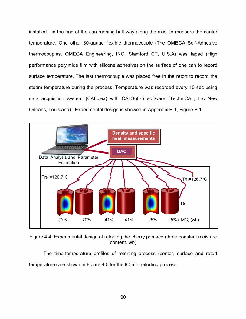
90

installed in the end of the can running half-way along the axis, to measure the center

temperature. One other 30-gauge flexible thermocouple (The OMEGA Self-Adhesive

thermocouples, OMEGA Engineering, INC, Stamford CT, U.S.A) was taped (High

performance polyimide film with silicone adhesive) on the surface of one can to record

surface temperature. The last thermocouple was placed free in the retort to record the

steam temperature during the process. Temperature was recorded every 10 sec using

data acquisition system (CALplex) with CALSoft-5 software (TechniCAL, Inc New

Orleans, Louisiana). Experimental design is showed in Appendix B.1, Figure B.1.

Figure 4.4 Experimental design of retorting the cherry pomace (three constant moisture content, wb)

The time-temperature profiles of retorting process (center, surface and retort

temperature) are shown in Figure 4.5 for the 90 min retorting process.

TRt=126.7°CTRt =126.7°C

Ts

DAQ

Density and specific

heat measurements

Data Analysis and Parameter

Estimation

(70% 70% 41% 41% 25% 25%) MC, (wb)

91

Figure 4.5 Temperature profiles for center of cherry pomace at three constant moisture

content (wb), for surface temperature of the can, and steam temperature in a steam retort at 126.7 °C for 90 min.

4.2.5 Thermal parameter estimation

4.2.5.1 Sensitivity Coefficients

The sensitivity coefficient Xij, where i is the time index, and j is the parameter

index, indicates how sensitive the dependent variable is to a parameter βj. Xij was

formed by taking the first derivative of the dependent variable with respect to a specific

parameter βj . The scaled sensitivity coefficient (X'ij) was used to compare directly to the

dependent variable temperature T. The X’ in the model should be large and

uncorrelated to be estimated accurately (Beck and Arnold, 1977) “ Large” means

greater than ~10% of the temperature rise. From the plots of the scaled sensitivity

coefficients it could be seen which parameters could be estimated most accurately, and

which parameters dominate. In this work we determined the scaled sensitivity coefficient

0 20 40 60 80 100 120 1400

20

40

60

80

100

120

140

time (min)

Re

tort

an

d c

an

ce

nte

r te

mp

era

ture

(°C

)

MC-70

MC-41

MC-25

TRt

Ts

92

(X′ij) of parameters (k1 and k2) using the forward finite difference method approximation

(Beck and Arnold, 1977) for each parameter as presented in Eq.(4.7) The dbj is some

relatively small quantity and given as 0.001×bj. Using MATLAB programming the scaled

sensitivity coefficients Eq. (4.7) were computed. For plotting the sensitivity coefficient,

the independent variables and approximate value of parameters must be known.

Sensitivity coefficient:

( ) ( 1,... , , , . . . ) ( 1,... , , . . . )T i T b b j d b j b p T b b j b pX i

b i b j

(4.6)

Scaled Sensitivity coefficient:

( ) ( 1,..., , ,... ) ( 1,..., ,... )'

0 .0 0 1

T i T b b j d b j b p T b b j b pX jij

b i

(4.7)

The index p in the previous equations is the number of parameters.

4.2.5.2 Ordinary Least Squares (OLS) Procedure

A commercial finite-element software (Comsol), was used to generate predicted center

temperatures (T(t) predicted), given the inputs of measured surface temperature Ts ,

heating time (t) as shown in Figure 4.1, and initial estimate of pomace thermal

conductivity k1 (thermal conductivity at temperature T1) and k2 (thermal conductivity at

temperature T2). T1 and T2 were arbitrarily chosen temperatures (T1<T2) within the

temperature range . MATLAB (nlinfit) was used to run nonlinear regression OLS with

Comsol. Temperature was inputted from Comsol, changing as the parameters k1 and k2

changed by the nonlinear regression routine. When the sum of the squares of errors of

(T(t) observed - T(t)predicted )2 was minimized (SS) given in Eq.(4.8) the final k1 and k2

93

were used as the best-fit values of the pomace thermal properties, giving a linear

function k(T) Eq. (4.9) for each constant MC (Mishra et al., 2009). All MATLAB syntax

for OLS method is shown in Appendix B.3 at Appendices.

2

-S S T o b s T p re di i i

(4.8)

( ) ( )2 1( ) 1 2

( ) ( )2 1 2 1

T T T Tk T k k

T T T T

(4.9)

4.2.5.3 Sequential Estimation Procedure

Non-linear Maximum A Posteriori (MAP) sequential estimation procedure given in

(Beck and Arnold, 1977 p. 277) was used in this section. The MAP equation is shown

in Eqs. (4.10) and (4.11):

T -1b =μ +P X ψ (Y -Xμ )M A P β M AP β (4.10)

T -1 1 -1P = ( X ψ X+V )M A P

(4.11)

Where Eqs. (4.10) and (4.11) are in matrix format, where bMAP is the matrix (px1) vector

parameter to be estimated; is matrix (px1) vector with prior information on the

parameters; PMAP is the covariance vector matrix of parameters (pxp) which gives

information about the variance (on the diagonal) and covariance (correlation between

parameter) on off-diagonal elements; X is the sensitivity coefficient matrix (nxp); is

covariance matrix (nxn) of errors, and Y is the measurement (nx1) vector and V is

covariance matrix of .

94

Sequential parameter estimation gives more insight into the estimation process.

Improvement in the estimation is indicated when estimating the parameters at each

data addition (Mohamed, 2009). Under sequential estimation we expect the parameters

to approach a constant as the number of observations increases. MATLAB

programming was used to conduct the sequential estimation. All MATLAB syntaxes for

sequential estimation method is shown in Appendix B.3.

4.2.6 Data analysis

Statistical analyses were performed using MATLAB software. Standard

deviations (Zuritz et al.), standard errors (SE) and correlation coefficients were

calculated. OLS and sequential estimation were performed using MATLAB software.

4.3 Results and discussion

4.3.1 Bulk density and Specific heat determination results:

Bulk density of cherry pomace increased with increasing moisture contents. The

density showed linear correlation with moisture content, which was fitted by following

equation:

(1 0 .5 0 6 ) 3 3 0 .2 6M C R2= 0.99 (4.12)

Where: MC was in decimal percent, e.g 70, 41 and 25% (wet basis).

A second-order polynomial correlation was used to model the specific heat of

cherry pomace as function of temperature (Valentas et al., 1997a) Figure 4.7 shows

the results of specific heat as estimated by the DSC method. Table B.3 at Appendices

B showed some the values of heat flow (mJ/s) ( MC-70) and the estimation steps of the

specific heat in triplicate

95

Figure 4.6 Specific heat of cherry pomace at three moisture contents ( wb) .

The estimation of specific heat followed a quadratic correlation with correlation

coefficient about 0.99 for the three samples of cherry pomace. The equations, which

were input to the Comsol software for center temperature prediction, are summarized as

following:

22 7 4 3 .3 7 .9 6 0 6 0 .0 2 2 1(7 0 )C p T TM C (4.13)

21 8 4 4 .4 1 1 .3 7 3 0 .0 3 6 7( 4 1 )C p T TM C (4.14)

21 2 0 9 .9 1 3 .3 6 4 0 .0 4 7 9(2 5 )C p T TM C (4.15)

Where: T was in ºC. This trend of specific heat with increase in temperature (as

shown in Table 4.1) have similarity with some studies like a study on specific heat and

thermal conductivity of softwood bark and softwood char particle from about 40 °C to

1300

1600

1900

2200

2500

2800

3100

3400

20 30 40 50 60 70 80 90 100 110 120 130

Sp

ecific

He

at (

J/k

g º

C)

Temperature (ºC)

Cp MC-70

Cp MC-41

Cp MC-25

96

140 °C, where both specific heat and thermal conductivity increased linearly with

temperature (Gupta et al., 2003)

Thermal diffusivity was estimated for the three different moisture contents of cherry

pomace using the following equation (Eq.(4.16)):

( , )( , )

( ) ( , )

k T M CT M C

M C C p T M C

(4.16)

The following Table (4.1) gives values of the specific heat, density, thermal conductivity

and the thermal diffusivity values at each moisture content and temperature of 25 to

126.7 ºC.

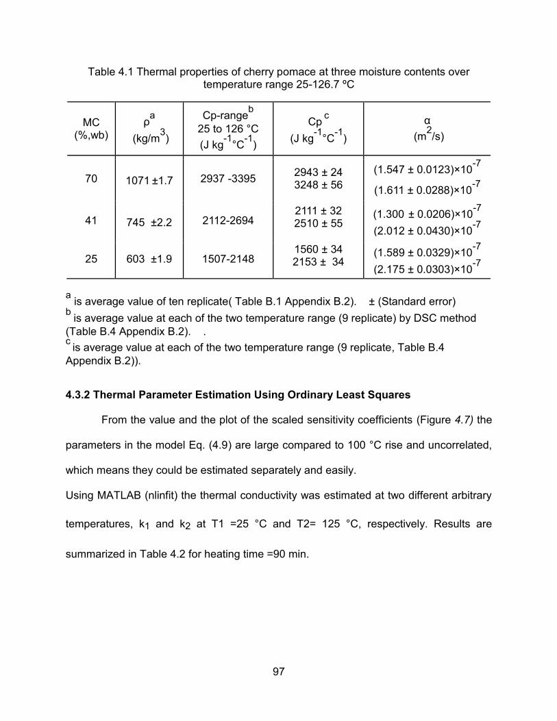
97

Table 4.1 Thermal properties of cherry pomace at three moisture contents over temperature range 25-126.7 ºC

MC (%,wb)

ρa

(kg/m3)

Cp-rangeb

25 to 126 °C

(J kg-1

°C-1

)

Cp c

(J kg-1

°C-1

)

α

(m2/s)

70 1071 ±1.7 2937 -3395 2943 ± 24 3248 ± 56

(1.547 ± 0.0123)×10-7

(1.611 ± 0.0288)×10-7

41 745 ±2.2 2112-2694 2111 ± 32 2510 ± 55

(1.300 ± 0.0206)×10-7

(2.012 ± 0.0430)×10-7

25 603 ±1.9 1507-2148

1560 ± 34 2153 ± 34

(1.589 ± 0.0329)×10-7

(2.175 ± 0.0303)×10

-7

a is average value of ten replicate( Table B.1 Appendix B.2). ± (Standard error)

b is average value at each of the two temperature range (9 replicate) by DSC method

(Table B.4 Appendix B.2). . c is average value at each of the two temperature range (9 replicate, Table B.4

Appendix B.2)).

4.3.2 Thermal Parameter Estimation Using Ordinary Least Squares

From the value and the plot of the scaled sensitivity coefficients (Figure 4.7) the

parameters in the model Eq. (4.9) are large compared to 100 °C rise and uncorrelated,

which means they could be estimated separately and easily.

Using MATLAB (nlinfit) the thermal conductivity was estimated at two different arbitrary

temperatures, k1 and k2 at T1 =25 °C and T2= 125 °C, respectively. Results are

summarized in Table 4.2 for heating time =90 min.

98

Figure 4.7 Scaled sensitivity coefficients of thermal conductivity of cherry pomace (70% MC,wb) during 90 min of retorting

Table 4.2 Estimation of thermal conductivity parameters for cherry pomace (90 min retorting) at T1=25 °C and T2= 125 °C.

MC (wb)

k

W m-1

°C-1

Estimate k

Std Err Correlation Coefficient

Confidence Interval (95%)

RMSE (ºC)

70% k1

k2

0.498 0.559

0.00047 0.00058 -0.84

0.4981 0.4981 0.5590 0.5591

0.67

41% k1

k2

0.204

0.375

0.00145 0.00124 -0.99

0.2043 0.2044 0.3752 0.3754 0.95

25% k1

k2

0.149

0.282

0.0034 0.0037 -0.92

0.1497 0.1499 0.2820 0.2824 4.2

Based on data on Table 4.2, thermal conductivity was correlated as function of the three

moisture contents and the following Eqs were found:

( ) 0 .0 0 8 0 4 3 0 .0 8 0 9 61 k M C M C R2= 0.95 (4.17)

0 20 40 60 80 100-10

0

10

20

30

40

time(min)

Sca

led

Se

nsitiv

ity C

oe

ffic

ein

ts (

ºC

)

X'k1

X'k2

99

( ) 0 .0 0 6 1 7 0 .1 2 5 22k M C M C R2=0.99 (4.18)

The slope in Eq. (4.17) has p =0.13 which means the effect of moisture is not

significant but the slope in Eq. (4.18) has p=0.014 which shows a significant effect of

moisture contents in cherry pomace on thermal conductivity as a function of

temperature. Predicted and observed temperature vs. time data by Comsol (for two

cans) was plotted with observed data and showed good fit with very small confidence

intervals as shown in Figure 4.8. Residuals for Comsol’s center temperature prediction

also showed small values after the first 10 min as shown in Figure 4.9. The residuals

were larger during the first 10 min, showing some difficulty in fitting. After the first 10

min, the residuals were additive and variance constant and the mean ≈ 0, meeting the

standard statistical assumptions.

Figure 4.8 Time-temperature plot of observed and predicted center temperature of the cans of cherry pomace (70%MC) heated at 126.7ºC for 90 min

0 20 40 60 80 10020

40

60

80

100

120

140

time(min)

can

cen

ter

te

mp

era

ture

(ºC

)

observed1

observed2

predicted

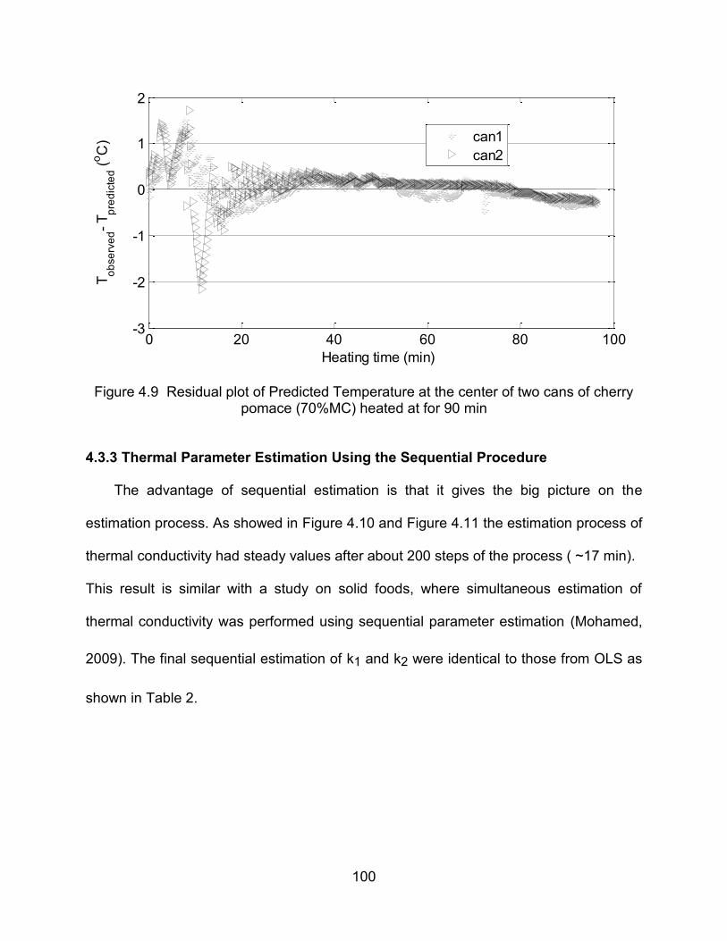
100

Figure 4.9 Residual plot of Predicted Temperature at the center of two cans of cherry pomace (70%MC) heated at for 90 min

4.3.3 Thermal Parameter Estimation Using the Sequential Procedure

The advantage of sequential estimation is that it gives the big picture on the

estimation process. As showed in Figure 4.10 and Figure 4.11 the estimation process of

thermal conductivity had steady values after about 200 steps of the process ( ~17 min).

This result is similar with a study on solid foods, where simultaneous estimation of

thermal conductivity was performed using sequential parameter estimation (Mohamed,

2009). The final sequential estimation of k1 and k2 were identical to those from OLS as

shown in Table 2.

0 20 40 60 80 100-3

-2

-1

0

1

2

Heating time (min)

To

bse

rve

d-

Tp

red

icte

d (

oC

)

can1

can2

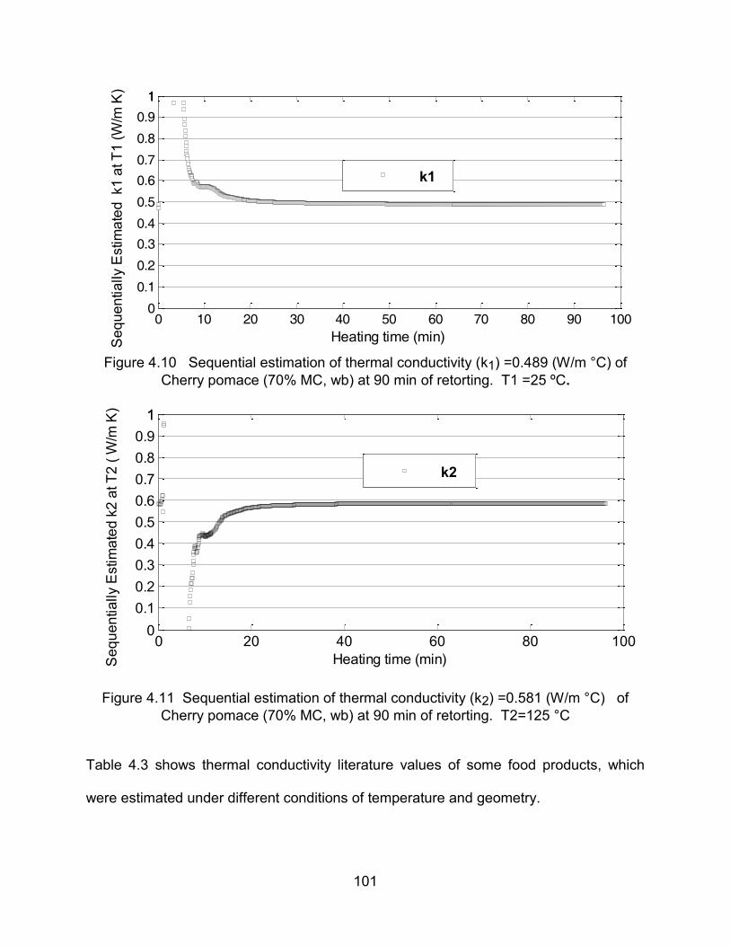
101

Figure 4.10 Sequential estimation of thermal conductivity (k1) =0.489 (W/m °C) of

Cherry pomace (70% MC, wb) at 90 min of retorting. T1 =25 ºC.

Figure 4.11 Sequential estimation of thermal conductivity (k2) =0.581 (W/m °C) of

Cherry pomace (70% MC, wb) at 90 min of retorting. T2=125 °C

Table 4.3 shows thermal conductivity literature values of some food products, which

were estimated under different conditions of temperature and geometry.

0 10 20 30 40 50 60 70 80 90 1000

0.1

0.2

0.3

0.4

0.5

0.6

0.7

0.8

0.9

11

Heating time (min)Se

qu

en

tia

lly E

stim

ate

d k1 a

t T

1 (

W/m

K)

k1

0 20 40 60 80 1000

0.1

0.2

0.3

0.4

0.5

0.6

0.7

0.8

0.9

11

Heating time (min)Se

qu

en

tia

lly E

stim

ate

d k

2 a

t T

2 (

W/m

K)

k2

102

Table 4.3 A comparative literature review of thermal conductivity values of some food products

Material Method Model's

functions MC

(%wb) Temp, (°C)

Thermal conductivity

(W m-1

K-1

)

Reference

Grape pomace Nonlinear regression

temperature 42 100 0.50 (Mishra et al., 2008)

Cherry tomato

Probe method

temperature

92

28

0.462

(Sweat and Haugh, 1974)

Potato &

Apple

Modified, Fitch

method

temperature

fresh

30

0.52 0.43

(Donsi et al., 1996)

Concentrated cherry juice

the coaxial cylinders method

temperature

Concentration &combination

°Brix ( 27)

20-140

0.48-0.56

(Magerramov et al., 2006b)

straw mushroom

Probe method

Temperature

MC

(30 to 90%)

50-80

0.212–0.668

(Tansakul and Lumyong, 2008)

103

Choi and Okos (1986) established empirical equations for thermal conductivity

estimation based on the main components of the food materials as a function of

temperature. The carbohydrate, fiber and water used for the comparison with this study

were the main components for the cherry pomace (McCune et al., 2011). The thermal

conductivity of cherry pomace for each moisture content (Table 4.4) was the sum of

each component multiplied by its volume fraction (Valentas et al., 1997b).

Table 4.4: comparative of thermal conductivity values of Cherry pomace by this study with Choi and Okos empirical equations .

MC%(wb) Temperatures

(°C) Choi &Okos

(1986) This study

70 25 0.475 0.498

126 0.573 0.559

41 25 0.340 0.204

126 0.419 0.375

25 25 0.265 0.149

126 0.335 0.282

As showed in Table 4.4 the values at 70%MC were close to those from study. For 41%

and 25% the Choi and Okos values were higher than those from this study.

104

4.4 Model validation

Cherry pomace at the three constant moisture content was filled in the steel

cans, which were fitted with three thermocouples, one in the center, the second one in

offset (at R/2) and the third one on the surface of the can. Figure 4.12 show a plot of

the temperatures vs time in the retort for the can with 70% cherry pomace.

All collected data of temperature vs time of the three constant moisture content

were entered in the Prop1D software (Prop1D Software, Beck Engineering Consultants

Company, www. BeckEng.com) and the k1 and k2 were calculated and compared with

the results for this study showed in Table 4.4. The Prop1D uses a finite difference code

for 1-D heat transfer. Results showed good agreement with the values in this study for

70 and 41 % MC (wb). The RMSE for the Prop1D method was much lower than this

study, but the experimental time for the Prop1D was also much shorter (about 600 s for

70% MC, wb) to maintain 1D heat transfer.

105

Figure 4.12 Temperature vs. time profile at three location of cherry pomace (70%, wb) in the steel can after retorting at 126.7°C for about 20 min)

Table 4.5 Estimation of thermal conductivity (k(t)) parameters for cherry pomace (90 min retorting): OLS vs.Prop1D method

MC (%,wb)

k(T)

(W m-1

°C-1

)

k(T) by OLS & sequential

k(T) by Prop1D

RMSE (ºC) OLS

RMSE (ºC)

Prop1D

70 k1

k2

0.498 0.559

0.502 0..641

0.67 1.019

41 k1

k2

0.204

0.375

0.263

0.382 0.95 1.07

25 k1

k2

0.149 0.282

0.297 0.469

4.2 1.92

0

20

40

60

80

100

120

140

0 200 400 600 800 1000 1200

Te

mp

era

ture

(°C

)

Retorting time (sec)

Center T

Offset T

Surface T

106

4.5 Conclusions

• Temperature-dependent specific heat of cherry pomace at three constant

moisture contents was determined using the DSC method in a temperature range

of 25 to 130 °C the specific heat increased with moisture content and

temperature.

• Thermal conductivity values for cherry pomace at three constant moisture

contents and temperature range 25 to 125 °C were successfully estimated using

OLS and sequential estimation. The values increased with temperature and

moisture content.

• Thermal diffusivity increased with temperature and decreased with moisture

content (from 25% to 70% moisture) 2.6% and 26 % decrease at 25 °C and

126.7 °C, respectively, due primarily to the significant increase in densities of the

pomace.

• This study presents one of the few inverse methods known to estimate

temperature-dependent thermal conductivity for solid food products in one

experiment at temperature above 100°C in approximately 30 min. This procedure

may be used for predicting nutraceutical degradation or microbial inactivation in

food processes.

107

B. APPENDICES

108

Appendix B.1 Experimental design and preliminary data

Experimental & predicted can center temperatures and other thermal properties

Figure B.1 Process experimental design for thermal properties estimation

Specific heat estimation Can center temp, prediction by Comsol

Data analysis, k1 & k2 estimation

Data

Analysis

Collecting experimental can surface and center temp

Step 2

Step 3

Step 1

+

109

Table B.1 Cherry pomace ‘s bulk density at different Moisture contents

a-(10 replicates)

b-Can effective volume is 136 cm3 (Water replacement)

Moisture Content

Weight

(g)a

MC% Density

b

kg/m3 AVG STDV SE

25%(wb)

79.73 25 586.3 603 12.7 1.3 80.3 25 590.4

79.53 25 584.8

81.32 25 597.9

81.3 25 597.8

83.11 25 611.1

84.44 25 620.9

83.4 25 613.2

82.6 25 607.4

84.3 25 619.9

41%(wb)

101.99 41 749.9 745 43.3 1.7 98.77 41 726.3

100.12 41 736.2

99.24 41 729.7

99.61 41 732.4

100.3 41 737.5

103.73 41 762.7

104.3 41 766.9

105.2 41 773.5

100.5 41 739.0

70%(wb)

147.55 70 1084.9 1071 106.2 2.0 147.77 70 1086.5

146.48 70 1077.1

144.89 70 1065.4

144.66 70 1063.7

144.49 70 1062.4

139.1 70 1022.8

146.33 70 1076.0

147.7 70 1086.0

147.9 70 1087.5

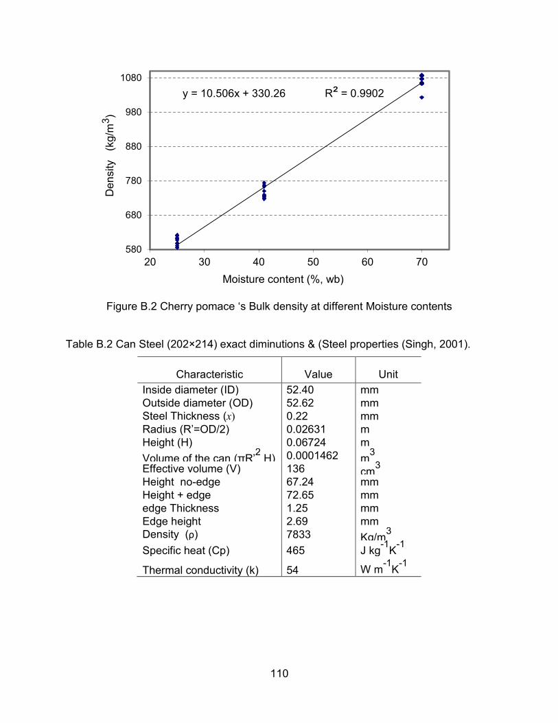
110

Figure B.2 Cherry pomace ‘s Bulk density at different Moisture contents

Table B.2 Can Steel (202×214) exact diminutions & (Steel properties (Singh, 2001).

Characteristic Value Unit

Inside diameter (ID) 52.40 mm

Outside diameter (OD) 52.62 mm

Steel Thickness (x) 0.22 mm

Radius (R’=OD/2) 0.02631 m

Height (H) 0.06724 m

Volume of the can (πR’2 H) 0.0001462 m

3

Effective volume (V) 136 cm3

Height no-edge 67.24 mm

Height + edge 72.65 mm

edge Thickness 1.25 mm

Edge height 2.69 mm

Density (ρ) 7833 Kg/m3

Specific heat (Cp) 465 J kg-1

K-1

Thermal conductivity (k) 54 W m-1

K-1

y = 10.506x + 330.26 R² = 0.9902

580

680

780

880

980

1080

20 30 40 50 60 70

Den

sity

(kg/m

3)

Moisture content (%, wb)

111

Figure B.3 Gen5 Software view for temperature vs time data collection during retorting. “The text in this figure is not meant to be readable but is for visual reference only”.

112

Image 1 .Parameters and geometry

Image 2. Materials Figure B.4 Images of Comsol simulation Steps of Can Heating. “The text in this figure is

not meant to be readable but is for visual reference only”.

113

Figure B.4 (cont’d)

Image 3 .Heat transfer boundary

Image 4 Meshing and elements

114

Figure B.4 (cont’d)

Image 5. Study ( Run steps)

Image 6 Results and predicted data collections

115

Appendix B.2 Thermal properties determination (DSC)

Figure B.5 Steps Cherry pomace’s thermal properties measurement using DSC. “The text on the images is not meant to be readable but is for visual reference only.

Figure B.6 Sapphire Specific heat capacity

ReferenceSample

1. Sample

preparation

2. Sample

placement

3. Data

collection

Reference Pan

Thermoelectric

Disc (constant)

Lid

Dynamic Sample Chamber

Thermocouple Junction

Sample Pan

y = -5E-06x2 + 0.0023x + 0.7193

R² = 1

0.7

0.75

0.8

0.85

0.9

0.95

1

0 10 20 30 40 50 60 70 80 90 100 110 120 130 140

Sp

ecific

he

at (k

J/k

g °

C)

Temperature (°C)

116

Table B.3 Example Specific heat’s (Cp) Excel sheet calculation steps for 70% moisture content (wb) Cherry pomace using DSC method

time min

Heat flow (mW) Spphair (St) and

baseline(Bs)

Cp and Calibration constant

Cp(st) ks

Heat flow (mw)

Sample 1 2 3

Heat flow Sample-baseline

(mw) 1 2 3

Specific heat (Cp)

(J kg-1

°C -1)

Cp1 Cp2 Cp3

*Statistic

AVG STD St Bs Bs-St

25.0 -3.44 0.09 3.53 0.77 0.80 -6.01 -4.83 -4.90 6.09 4.92 4.99 2942 3085 2937 2988 73

25.0 -3.44 0.09 3.53 0.77 0.80 -6.01 -4.84 -4.90 6.10 4.92 4.99 2942 3085 2938 25.0 -3.44 0.09 3.53 0.77 0.80 -6.01 -4.84 -4.91 6.10 4.92 4.99 2942 3085 2938 25.1 -3.44 0.09 3.53 0.77 0.80 -6.01 -4.84 -4.91 6.10 4.92 4.99 2943 3086 2802 2944 123

25.1 -3.44 0.09 3.53 0.77 0.80 -6.01 -4.84 -4.91 6.10 4.92 5.00 2943 3086 2803

25.1 -3.44 0.09 3.53 0.77 0.80 -6.01 -4.84 -4.91 6.10 4.92 5.00 2943 3086 2804

25.2 -3.44 0.09 3.53 0.77 0.80 -6.01 -4.84 -4.91 6.10 4.93 5.00 2944 3086 2804 2945 122

25.2 -3.44 0.09 3.53 0.77 0.80 -6.02 -4.84 -4.91 6.10 4.93 5.00 2944 3087 2805 25.2 -3.44 0.09 3.53 0.77 0.80 -6.02 -4.84 -4.91 6.10 4.93 5.00 2945 3087 2806 25.3 -3.44 0.09 3.53 0.77 0.80 -6.02 -4.84 -4.92 6.10 4.93 5.00 2945 3087 2806 2946 122

25.3 -3.44 0.09 3.53 0.77 0.80 -6.02 -4.84 -4.92 6.11 4.93 5.00 2945 3088 2807 25.3 -3.45 0.09 3.53 0.77 0.80 -6.02 -4.84 -4.92 6.11 4.93 5.00 2946 3088 2807 25.4 -3.45 0.09 3.53 0.77 0.80 -6.02 -4.84 -4.92 6.11 4.93 5.00 2946 3088 2807 2947 122

25.4 -3.45 0.09 3.53 0.77 0.80 -6.02 -4.84 -4.92 6.11 4.93 5.01 2946 3088 2807 25.4 -3.45 0.09 3.53 0.77 0.80 -6.02 -4.84 -4.92 6.11 4.93 5.01 2946 3089 2808 25.5 -3.45 0.09 3.53 0.77 0.80 -6.02 -4.85 -4.92 6.11 4.93 5.01 2946 3089 2809 2948 121

25.5 -3.45 0.09 3.53 0.77 0.80 -6.02 -4.85 -4.92 6.11 4.93 5.01 2947 3089 2810 25.5 -3.45 0.09 3.53 0.77 0.80 -6.02 -4.85 -4.93 6.11 4.93 5.01 2947 3090 2810 25.6 -3.45 0.09 3.54 0.77 0.80 -6.03 -4.85 -4.93 6.11 4.93 5.01 2947 3090 2810 2949 121

25.6 -3.45 0.09 3.54 0.77 0.80 -6.03 -4.85 -4.93 6.11 4.94 5.01 2947 3090 2811

117

Table B.3 (cont’d)

25.6 -3.45 0.09 3.54 0.77 0.80 -6.03 -4.85 -4.93 6.11 4.94 5.02 2947 3091 2811

25.7 -3.45 0.09 3.54 0.78 0.80 -6.03 -4.85 -4.93 6.11 4.94 5.02 2947 3091 2812 2951 120

25.7 -3.45 0.09 3.54 0.78 0.80 -6.03 -4.85 -4.93 6.12 4.94 5.02 2948 3091 2813 25.7 -3.45 0.09 3.54 0.78 0.80 -6.03 -4.85 -4.93 6.12 4.94 5.02 2948 3091 2814

25.8 -3.45 0.09 3.54 0.78 0.80 -6.03 -4.85 -4.93 6.12 4.94 5.02 2948 3092 2814 2951 120

25.8 -3.45 0.09 3.54 0.78 0.80 -6.03 -4.85 -4.94 6.12 4.94 5.02 2948 3092 2814

25.8 -3.45 0.09 3.54 0.78 0.80 -6.03 -4.85 -4.94 6.12 4.94 5.02 2948 3092 2814 25.9 -3.45 0.09 3.54 0.78 0.80 -6.03 -4.85 -4.94 6.12 4.94 5.02 2948 3092 2815 2952 120

25.9 -3.45 0.09 3.54 0.78 0.80 -6.03 -4.86 -4.94 6.12 4.94 5.02 2949 3092 2815 25.9 -3.46 0.09 3.54 0.78 0.80 -6.03 -4.86 -4.94 6.12 4.94 5.03 2949 3093 2815 26.0 -3.46 0.09 3.54 0.78 0.80 -6.04 -4.86 -4.94 6.12 4.94 5.03 2949 3093 2816 2953 120

26.0 -3.46 0.09 3.54 0.78 0.80 -6.04 -4.86 -4.94 6.12 4.94 5.03 2949 3093 2816

26.0 -3.46 0.09 3.54 0.78 0.80 -6.04 -4.86 -4.94 6.12 4.94 5.03 2950 3093 2816 26.1 -3.46 0.09 3.54 0.78 0.80 -6.04 -4.86 -4.94 6.12 4.94 5.03 2950 3093 2817 2953 120

26.1 -3.46 0.09 3.54 0.78 0.80 -6.04 -4.86 -4.94 6.12 4.94 5.03 2950 3093 2817 26.1 -3.46 0.09 3.55 0.78 0.80 -6.04 -4.86 -4.94 6.13 4.95 5.03 2949 3093 2817

26.2 -3.46 0.09 3.55 0.78 0.80 -6.04 -4.86 -4.95 6.13 4.95 5.03 2949 3093 2817 2953 119

26.2 -3.46 0.09 3.55 0.78 0.80 -6.04 -4.86 -4.95 6.13 4.95 5.03 2950 3093 2817

26.2 -3.46 0.09 3.55 0.78 0.80 -6.04 -4.86 -4.95 6.13 4.95 5.03 2950 3094 2818

26.3 -3.46 0.09 3.55 0.78 0.80 -6.04 -4.86 -4.95 6.13 4.95 5.03 2950 3094 2818 2954 119

26.3 -3.46 0.09 3.55 0.78 0.80 -6.04 -4.86 -4.95 6.13 4.95 5.04 2950 3094 2819

118

Table B.3 (cont’d)

26.3 -3.46 0.09 3.55 0.78 0.80 -6.04 -4.86 -4.95 6.13 4.95 5.04 2951 3094 2819 26.4 -3.46 0.09 3.55 0.78 0.80 -6.04 -4.86 -4.95 6.13 4.95 5.04 2951 3094 2819 2955 119

26.4 -3.46 0.09 3.55 0.78 0.80 -6.05 -4.86 -4.95 6.13 4.95 5.04 2951 3094 2819

26.4 -3.46 0.09 3.55 0.78 0.80 -6.05 -4.87 -4.95 6.13 4.95 5.04 2951 3095 2820 26.5 -3.46 0.09 3.55 0.78 0.80 -6.05 -4.87 -4.95 6.13 4.95 5.04 2951 3095 2820 2955 119

26.5 -3.47 0.09 3.55 0.78 0.80 -6.05 -4.87 -4.95 6.13 4.95 5.04 2951 3095 2820 26.5 -3.47 0.09 3.55 0.78 0.80 -6.05 -4.87 -4.96 6.13 4.95 5.04 2951 3095 2820

26.6 -3.47 0.09 3.55 0.78 0.80 -6.05 -4.87 -4.96 6.13 4.95 5.04 2951 3095 2820 2956 119

26.6 -3.47 0.09 3.55 0.78 0.80 -6.05 -4.87 -4.96 6.14 4.96 5.04 2951 3096 2821 26.6 -3.47 0.09 3.55 0.78 0.80 -6.05 -4.87 -4.96 6.14 4.96 5.04 2951 3096 2821 26.7 -3.47 0.09 3.55 0.78 0.80 -6.05 -4.87 -4.96 6.14 4.96 5.05 2951 3096 2822 2957 119

26.7 -3.47 0.09 3.56 0.78 0.80 -6.05 -4.87 -4.96 6.14 4.96 5.05 2951 3096 2822 26.7 -3.47 0.09 3.56 0.78 0.80 -6.05 -4.87 -4.96 6.14 4.96 5.05 2951 3096 2823 26.8 -3.47 0.09 3.56 0.78 0.80 -6.05 -4.87 -4.96 6.14 4.96 5.05 2952 3096 2823 2957 118

26.8 -3.47 0.09 3.56 0.78 0.80 -6.05 -4.87 -4.96 6.14 4.96 5.05 2952 3097 2823 26.8 -3.47 0.09 3.56 0.78 0.80 -6.06 -4.87 -4.97 6.14 4.96 5.05 2952 3097 2824 26.9 -3.47 0.09 3.56 0.78 0.80 -6.06 -4.88 -4.97 6.14 4.96 5.05 2952 3097 2824 2958 118

26.9 -3.47 0.09 3.56 0.78 0.80 -6.06 -4.88 -4.97 6.14 4.96 5.05 2953 3098 2824 26.9 -3.47 0.09 3.56 0.78 0.80 -6.06 -4.88 -4.97 6.14 4.96 5.05 2953 3098 2824 27.0 -3.47 0.09 3.56 0.78 0.80 -6.06 -4.88 -4.97 6.14 4.96 5.06 2953 3098 2825 2959 118

27.0 -3.47 0.09 3.56 0.78 0.80 -6.06 -4.88 -4.97 6.15 4.96 5.06 2953 3098 2825 27.0 -3.47 0.09 3.56 0.78 0.80 -6.06 -4.88 -4.97 6.15 4.97 5.06 2953 3098 2825

* Each temperature point done in 9 replicates (average and STDV was calculated)

119

Table B.4 Thermal properties estimation at two temperatures (25, 126) of cherry pomace J kg-1

K-1

Moisture %,(wb)

Specific heat ( J kg-1

K-1

) Thermal Diffusivity (m2/s)

ρ k Cp1 Cp2 Cp3 AVG SE α1 α2 α3 AVG SE

Values at 25 °C

25-MC 603 0.149 1507 1479 1692 1650 34 1.64E-07 1.67E-07 1.46E-07 1.59.E-07

0.033E-07

25-MC 1507 1480 1693

1.64E-07 1.67E-07 1.45E-07

25-MC 1057 1480 1693

1.64E-07 1.66E-07 1.45E-07

41-MC 745 0.204 1981 2178 2172 2111 32 1.38E-07 1.25E-07 1.26E-07 1.30.E-07 1.439.E-08

0.021E-07

41-MC 1981 2179 2173

1.38E-07 1.25E-07 1.26E-07

41-MC 1982 2180 2173

1.38E-07 1.25E-07 1.26E-07

70-MC 1071 0.495 2942 3085 2937 2988 24 1.57E-07 1.49E-07 1.57E-07 1.54E-07

0.04E-07

70-MC 2942 3085 2938

1.57E-07 1.49E-07 1.57E-07

70-MC 2942 3085 2938

1.57E-07 1.49E-07 1.57E-07

Values at 126 °C

25-MC 603 0.282 2265 2134 2059 2153 30 2.06E-07 2.19E-07 2.27E-07 2.18E-07 0.03E-07

25-MC 2267 2134 2059

2.06E-07 2.19E-07 2.27E-07

25-MC 2269 2135 2059

2.06E-07 2.19E-07 2.27E-07

41-MC 745 0.375 2351 2722 2461 2511 55 2.14E-07 1.85E-07 2.05E-07 2.01E-07 0.04E-07

41-MC 2351 2722 2461

2.14E-07 1.85E-07 2.05E-07

41-MC 2350 2722 2461

2.14E-07 1.84E-07 2.05E-07

70-MC 1071 0.559 3402 3314 3029 3248 56 1.53E-07 1.57E-07 1.72E-07 1.61E-07 0.03E-07

70-MC 3402 3314 3028

1.53E-07 1.57E-07 1.72E-07

70-MC 3402 3314 3028

1.53E-07 1.57E-07 1.72E-07

120

Appendix B.3 MATLAB syntax

B.3.1 Script file for nlinfit method

% estimating k1 and k2

%% Cleaning clc clear all close all format compact global RetortT_file rho siz Tin Tfi % % data =xlsread('25min_Ret.xls'); % first column time, %second Temp of 70%MC, %third Temp for 41%MC, fourth 25%MC, Retort temp [filedata, pathnamedata, filterindex] = uigetfile( ... { '*.xls','Data File (*.xls)'; ... '*.txt','Data File (*.txt)'; ... '*.xlsx','Data File (*.xlsx)'; ... '*.*', 'All Files (*.*)'}, ... 'Pick Retort File', ... 'MultiSelect', 'on'); data =xlsread(filedata); x=data(:,1);% time (Piasecka, #1707) % Request for Temperature input in F prompt = {'Enter 1st Column Number'... 'Enter 2nd Column Number'... 'Enter Product Density'}; name = 'Input for Parameter Estimation'; numlines = 1; def = {'6','7','603'};% which MC will be estimated,,( clmn1 , clmn 2, density) options.Resize='on'; options.WindowStyle='normal'; options.Interpreter='tex'; answer=inputdlg(prompt,name,numlines,def,options); col1 = str2num(answer{1}); col2 = str2num(answer{2}); yobs = [data(:,col1) data(:,col2)]; Tin = (data(1,col1)+data(1,col2))/2;% intial temperature in the two clolomn Tfi = (data(end,col1)+data(end,col2))/2;% final temperature in the two clolomn rho = answer{3};% density (kg/m^3) siz = size(yobs,2);%data in replicta yobs = yobs(:); %% Calling surface temperature as boundary condition

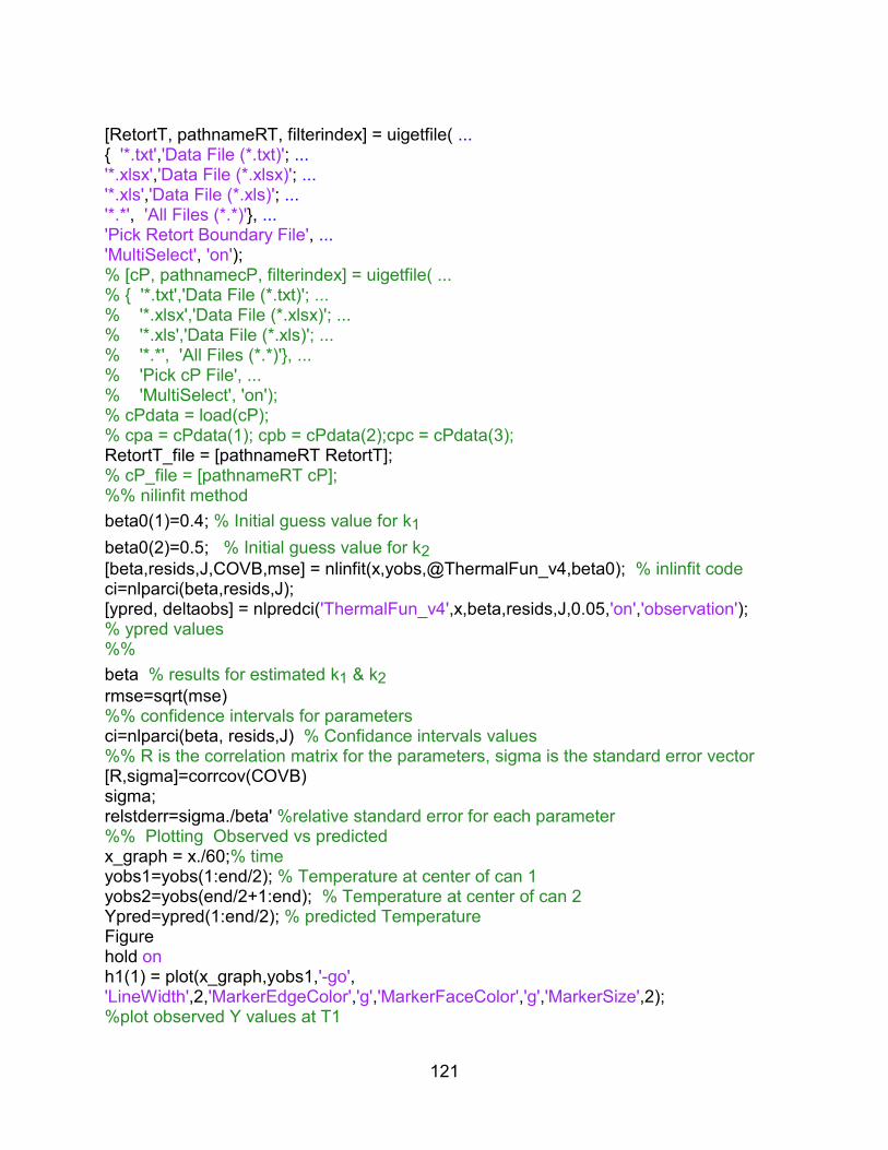
121

[RetortT, pathnameRT, filterindex] = uigetfile( ... { '*.txt','Data File (*.txt)'; ... '*.xlsx','Data File (*.xlsx)'; ... '*.xls','Data File (*.xls)'; ... '*.*', 'All Files (*.*)'}, ... 'Pick Retort Boundary File', ... 'MultiSelect', 'on'); % [cP, pathnamecP, filterindex] = uigetfile( ... % { '*.txt','Data File (*.txt)'; ... % '*.xlsx','Data File (*.xlsx)'; ... % '*.xls','Data File (*.xls)'; ... % '*.*', 'All Files (*.*)'}, ... % 'Pick cP File', ... % 'MultiSelect', 'on'); % cPdata = load(cP); % cpa = cPdata(1); cpb = cPdata(2);cpc = cPdata(3); RetortT_file = [pathnameRT RetortT]; % cP_file = [pathnameRT cP]; %% nilinfit method

beta0(1)=0.4; % Initial guess value for k1

beta0(2)=0.5; % Initial guess value for k2

[beta,resids,J,COVB,mse] = nlinfit(x,yobs,@ThermalFun_v4,beta0); % inlinfit code ci=nlparci(beta,resids,J); [ypred, deltaobs] = nlpredci('ThermalFun_v4',x,beta,resids,J,0.05,'on','observation'); % ypred values %%

beta % results for estimated k1 & k2

rmse=sqrt(mse) %% confidence intervals for parameters ci=nlparci(beta, resids,J) % Confidance intervals values %% R is the correlation matrix for the parameters, sigma is the standard error vector [R,sigma]=corrcov(COVB) sigma; relstderr=sigma./beta' %relative standard error for each parameter %% Plotting Observed vs predicted x_graph = x./60;% time yobs1=yobs(1:end/2); % Temperature at center of can 1 yobs2=yobs(end/2+1:end); % Temperature at center of can 2 Ypred=ypred(1:end/2); % predicted Temperature Figure hold on h1(1) = plot(x_graph,yobs1,'-go', 'LineWidth',2,'MarkerEdgeColor','g','MarkerFaceColor','g','MarkerSize',2); %plot observed Y values at T1

122

h1(2) = plot(x_graph,yobs2,'-.bs', 'LineWidth',2,'MarkerEdgeColor','b','MarkerFaceColor','b','MarkerSize',2); %plot observed Y values at T1 h1(3) = plot(x_graph,Ypred,':r*', 'LineWidth',1,'MarkerEdgeColor','r','MarkerFaceColor','y','MarkerSize',4); % plot predicted Y values at T1 legend(h1,'observed1','observed2','predicted','location','northwest'); xlabel('time(min)','FontSize',14) ylabel('Center temperature of can','FontSize',14); %% Plotting residuals Figure hold on h1(1) = plot(x_graph,resids(1:end/2),'g*'); h1(2) = plot(x_graph,resids(end/2+1:end),'r>'); L4 = ['Heating time (min) at ','tem','^{o}','C']; xlabel(L4); ylabel('Residuals','FontSize',14); legend(h1,'can1','can2','location','northwest'); YLine = [0 0]; XLine = [0 max(x_graph)]; plot (XLine, YLine,'R') %% Sensitivity coeifficent estaimation and plotting beta1 = beta; d=0.001; for i=1:length(beta) if i ==1 betain = [beta1(1)+beta1(1)*d beta1(2)]; elseif i==2 betain = [beta1(1) beta1(2)+beta1(2)*d]; end yhat{i} = ThermalFun_v4(betain,x); ysens{i} = (yhat{i}-ypred)/d; end % sensitivity coefficient plot Figure hold on ysens1 = ysens{1}; ysens2 = ysens{2}; gca=Figure('Units','inches','Position', [0.5 0.5 6 4]); %[left, bottom, width, height]: set(gca,'DefaultAxesFontName','Arial','DefaultAxesFontSize',12,'DefaultAxesFontWeight','Normal'); g1(1) = plot(x_graph,ysens1(1:end/2),':b','LineWidth',3);

123

g1(2) = plot(x_graph,ysens2(1:end/2),'-b.','LineWidth',3); YLine = [0 0]; XLine = [0 x_graph(end)];%max() plot (XLine, YLine,'R'); box on grid on

legend(g1,'k1','k2','location','best');

xlabel('time(min)','FontSize',14,'fontweight','Normal'); ylabel('Scaled Sensitivity Coefficeints','FontSize',14,'fontweight','Normal');

B.3.2 Function file (center can temperature prediction by Comsol)

function out = ThermalFun_v4(beta,x)

% Estimating k1 & k2

beta(1) beta(2) %global RetortT_file cP_file rho siz cpa cpb cpc Tin Tfi global RetortT_file rho siz Tin Tfi import com.comsol.model.* import com.comsol.model.util.* model = ModelUtil.create('Model'); fem.const={'x',x,'RetortT_file',RetortT_file,'rho',rho,'Tin',Tin,'Tfi',Tfi}; % RetortT_file= Surface temperature file % Building can as axisymetruc rectangular shape by Comsol model.param.set('L1', '73[mm]', 'Hight of the can (rectangle1)'); model.param.set('w1', '26[mm]', 'width of rectangle1(radius of can)'); model.param.set('L2', '36.5[mm]', 'hight of cylinder needle Tc'); model.param.set('w2', '0.11[mm]', 'width of rectangle3(radius of TCniddle)'); model.param.set('L3', '8.86[mm]', 'hight of copper around TC base'); model.param.set('w3', '5.045[mm]', 'width of copper around TC base'); model.param.set('L4', '3.34[mm]', 'hight sillicon around TC over copper'); model.param.set('w4', '3.12[mm]', 'width sillicon around TC over copper'); model.param.set('L5', '8.86[mm]', 'Hight of steel TC base (rectangle2)'); model.param.set('w5', '2.04[mm]', 'width of steel TC stapilizer 1'); model.param.set('L6', '4.7[mm]', 'hight of rectangle2(screw stable TC base)'); model.param.set('w6', '2.78[mm]', 'width of rectangle2(screw stable TC base)'); model.param.set('L7', '7.95[mm]', 'hight of screw TC stap in outside can'); model.param.set('w7', '5.64[mm]', 'width of screw TC stap in outside can'); model.param.set('L8', '6.5[mm]', 'width of outside TC fitteing Silicoun'); model.param.set('w8', '5.045[mm]', 'width of ousidet TC fitteing Silicoun'); model.param.set('L9', '2.75[mm]', 'hight of can sealing edg 1'); model.param.set('w9', '1.35[mm]', 'width ofcan sealing edg 1'); model.modelNode.create('mod1'); model.func.create('int1', 'Interpolation');

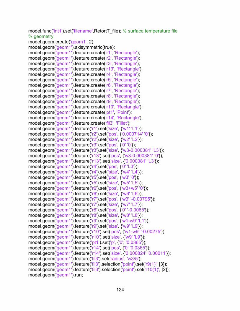
124

model.func('int1').set('filename',RetortT_file); % surface temperature file % geometry model.geom.create('geom1', 2); model.geom('geom1').axisymmetric(true); model.geom('geom1').feature.create('r1', 'Rectangle'); model.geom('geom1').feature.create('r2', 'Rectangle'); model.geom('geom1').feature.create('r3', 'Rectangle'); model.geom('geom1').feature.create('r13', 'Rectangle'); model.geom('geom1').feature.create('r4', 'Rectangle'); model.geom('geom1').feature.create('r5', 'Rectangle'); model.geom('geom1').feature.create('r6', 'Rectangle'); model.geom('geom1').feature.create('r7', 'Rectangle'); model.geom('geom1').feature.create('r8', 'Rectangle'); model.geom('geom1').feature.create('r9', 'Rectangle'); model.geom('geom1').feature.create('r10', 'Rectangle'); model.geom('geom1').feature.create('pt1', 'Point'); model.geom('geom1').feature.create('r14', 'Rectangle'); model.geom('geom1').feature.create('fil3', 'Fillet'); model.geom('geom1').feature('r1').set('size', {'w1' 'L1'}); model.geom('geom1').feature('r2').set('pos', {'0.000714' '0'}); model.geom('geom1').feature('r2').set('size', {'w2' 'L2'}); model.geom('geom1').feature('r3').set('pos', {'0' '0'}); model.geom('geom1').feature('r3').set('size', {'w3-0.000381' 'L3'}); model.geom('geom1').feature('r13').set('pos', {'w3-0.000381' '0'}); model.geom('geom1').feature('r13').set('size', {'0.000381' 'L3'}); model.geom('geom1').feature('r4').set('pos', {'0' 'L3'}); model.geom('geom1').feature('r4').set('size', {'w4' 'L4'}); model.geom('geom1').feature('r5').set('pos', {'w3' '0'}); model.geom('geom1').feature('r5').set('size', {'w5' 'L5'}); model.geom('geom1').feature('r6').set('pos', {'w3+w5' '0'}); model.geom('geom1').feature('r6').set('size', {'w6' 'L6'}); model.geom('geom1').feature('r7').set('pos', {'w3' '-0.00795'}); model.geom('geom1').feature('r7').set('size', {'w7' 'L7'}); model.geom('geom1').feature('r8').set('pos', {'0' '-0.0065'}); model.geom('geom1').feature('r8').set('size', {'w8' 'L8'}); model.geom('geom1').feature('r9').set('pos', {'w1-w9' 'L1'}); model.geom('geom1').feature('r9').set('size', {'w9' 'L9'}); model.geom('geom1').feature('r10').set('pos', {'w1-w9' '-0.00275'}); model.geom('geom1').feature('r10').set('size', {'w9' 'L9'}); model.geom('geom1').feature('pt1').set('p', {'0'; '0.0365'}); model.geom('geom1').feature('r14').set('pos', {'0' '0.0365'}); model.geom('geom1').feature('r14').set('size', {'0.000824' '0.00011'}); model.geom('geom1').feature('fil3').set('radius', 'w3/5'); model.geom('geom1').feature('fil3').selection('point').set('r9(1)', [3]); model.geom('geom1').feature('fil3').selection('point').set('r10(1)', [2]); model.geom('geom1').run;

125

model.variable.create('var1'); % Temperature model.variable('var1').set('T1', Tin, 'Initial temperature'); model.variable('var1').set('T2', Tfi, 'Final temperature'); % model.variable('var1').set('k2', '0.4[W/(m*K)]', 'Thermal difusivity of T1 to be evaluated');

model.variable('var1').set('k1',beta (1));

model.variable('var1').set('k2',beta (2));

model.variable.create('var2'); model.variable('var2').model('mod1');

model.variable('var2').set('k', '((T2-T)/(T2-T1))*k1+((T-T1)/(T2-T1))*k2');% model for

estimating k inversly model.view.create('view2', 3); % Materials model.material.create('mat4'); model.material('mat4').selection.set([6]); model.material.create('mat1'); model.material('mat1').propertyGroup.create('Enu', 'Young''s modulus and Poisson''s ratio'); model.material('mat1').propertyGroup.create('linzRes', 'Linearized resistivity'); model.material('mat1').selection.set([12]); model.material.create('mat2'); model.material('mat2').propertyGroup.create('Enu', 'Young''s modulus and Poisson''s ratio'); model.material('mat2').selection.set([5 7 9 13 14 15 16 17]); model.material.create('mat3'); model.material('mat3').propertyGroup.create('Enu', 'Young''s modulus and Poisson''s ratio'); model.material('mat3').propertyGroup.create('RefractiveIndex', 'Refractive index'); model.material('mat3').selection.set([1 2 3 4 8 10 11]); % heat transfer parameters model.physics.create('ht', 'HeatTransfer', 'geom1'); model.physics('ht').feature.create('temp1', 'TemperatureBoundary', 1); model.physics('ht').feature('temp1').selection.set([2 13 33 34 45 46 47 48 50 52 53 54 55 56 57]); % Mishing model.mesh.create('mesh1', 'geom1'); model.mesh('mesh1').feature.create('ftri1', 'FreeTri'); model.result.Table.create('tbl1', 'Table'); model.view('view1').axis.set('xmin', '-0.026209384202957153'); model.view('view1').axis.set('xmax', '0.052209384739398956'); model.view('view1').axis.set('ymin', '-0.012134999968111515'); model.view('view1').axis.set('ymax', '0.07993500679731369');

126

% Material for the pomace and thermocouple model.material('mat1').name('Copper'); model.material('mat1').propertyGroup('def').set('relpermeability', {'1' '0' '0' '0' '1' '0' '0' '0' '1'}); model.material('mat1').propertyGroup('def').set('electricconductivity', {'5.998e7[S/m]' '0' '0' '0' '5.998e7[S/m]' '0' '0' '0' '5.998e7[S/m]'}); model.material('mat1').propertyGroup('def').set('thermalexpansioncoefficient', {'17e-6[1/K]' '0' '0' '0' '17e-6[1/K]' '0' '0' '0' '17e-6[1/K]'}); model.material('mat1').propertyGroup('def').set('heatcapacity', '385[J/(kg*K)]'); model.material('mat1').propertyGroup('def').set('relpermittivity', {'1' '0' '0' '0' '1' '0' '0' '0' '1'}); model.material('mat1').propertyGroup('def').set('density', '8700[kg/m^3]'); model.material('mat1').propertyGroup('def').set('thermalconductivity', {'400[W/(m*K)]' '0' '0' '0' '400[W/(m*K)]' '0' '0' '0' '400[W/(m*K)]'}); model.material('mat1').propertyGroup('Enu').set('youngsmodulus', '110e9[Pa]'); model.material('mat1').propertyGroup('Enu').set('poissonsratio', '0.35'); model.material('mat1').propertyGroup('linzRes').set('rho0', '1.72e-8[ohm*m]'); model.material('mat1').propertyGroup('linzRes').set('alpha', '0.0039[1/K]'); model.material('mat1').propertyGroup('linzRes').set('Tref', '298[K]'); model.material('mat1').propertyGroup('linzRes').addInput('temperature'); % Steel model.material('mat2').name('Steel AISI 4340'); model.material('mat2').propertyGroup('def').set('relpermeability', {'1' '0' '0' '0' '1' '0' '0' '0' '1'}); model.material('mat2').propertyGroup('def').set('electricconductivity', {'4.032e6[S/m]' '0' '0' '0' '4.032e6[S/m]' '0' '0' '0' '4.032e6[S/m]'}); model.material('mat2').propertyGroup('def').set('thermalexpansioncoefficient', {'12.3e-6[1/K]' '0' '0' '0' '12.3e-6[1/K]' '0' '0' '0' '12.3e-6[1/K]'}); model.material('mat2').propertyGroup('def').set('heatcapacity', '475[J/(kg*K)]'); model.material('mat2').propertyGroup('def').set('relpermittivity', {'1' '0' '0' '0' '1' '0' '0' '0' '1'}); model.material('mat2').propertyGroup('def').set('density', '7850[kg/m^3]'); model.material('mat2').propertyGroup('def').set('thermalconductivity', {'44.5[W/(m*K)]' '0' '0' '0' '44.5[W/(m*K)]' '0' '0' '0' '44.5[W/(m*K)]'}); model.material('mat2').propertyGroup('Enu').set('youngsmodulus', '205e9[Pa]'); model.material('mat2').propertyGroup('Enu').set('poissonsratio', '0.28'); model.material('mat3').name('Silica glass'); model.material('mat3').propertyGroup('def').set('relpermeability', {'1' '0' '0' '0' '1' '0' '0' '0' '1'}); model.material('mat3').propertyGroup('def').set('electricconductivity', {'1e-14[S/m]' '0' '0' '0' '1e-14[S/m]' '0' '0' '0' '1e-14[S/m]'}); model.material('mat3').propertyGroup('def').set('thermalexpansioncoefficient', {'0.55e-6[1/K]' '0' '0' '0' '0.55e-6[1/K]' '0' '0' '0' '0.55e-6[1/K]'}); model.material('mat3').propertyGroup('def').set('heatcapacity', '703[J/(kg*K)]'); model.material('mat3').propertyGroup('def').set('relpermittivity', {'2.09' '0' '0' '0' '2.09' '0' '0' '0' '2.09'});

127

model.material('mat3').propertyGroup('def').set('density', '2203[kg/m^3]'); model.material('mat3').propertyGroup('def').set('thermalconductivity', {'1.38[W/(m*K)]' '0' '0' '0' '1.38[W/(m*K)]' '0' '0' '0' '1.38[W/(m*K)]'}); model.material('mat3').propertyGroup('Enu').set('youngsmodulus', '73.1e9[Pa]'); model.material('mat3').propertyGroup('Enu').set('poissonsratio', '0.17'); model.material('mat3').propertyGroup('RefractiveIndex').set('n', {'1.45' '0' '0' '0' '1.45' '0' '0' '0' '1.45'}); % Pomace materials model.material('mat4').propertyGroup('def').set('thermalconductivity', {'k' '0' '0' '0' 'k' '0' '0' '0' 'k'}); model.material('mat4').propertyGroup('def').set('density', rho); % Polynomial models for Cpo as estimated by DSC (70%, 41% and 25% moisture % contents) model.material('mat4').propertyGroup('def').set('heatcapacity', '(-0.0221*T^2+7.9606*T+2743.3)'); model.material('mat4').propertyGroup('def').set('heatcapacity', '(-0.0367*T^2+11.373*T+1844.4)'); model.material('mat4').propertyGroup('def').set('heatcapacity', '(-0.0479*T^2+13.364*T+1209.9)'); % Heat transfer model.physics('ht').name('Heat Transfer'); model.physics('ht').feature('init1').set('T', 'T1'); % Surfasce Temperature as heating boundary model.physics('ht').feature('temp1').set('T0', 'int1(t)'); model.mesh('mesh1').feature('size').set('hauto', 6); model.mesh('mesh1').run; % Results model.result.Table('tbl1').comments('Evaluation of T & k at center (k)'); model.study.create('std1'); model.study('std1').feature.create('time', 'Transient'); model.sol.create('sol1'); model.sol('sol1').study('std1'); model.sol('sol1').attach('std1'); model.sol('sol1').feature.create('st1', 'StudyStep'); model.sol('sol1').feature.create('v1', 'Variables'); model.sol('sol1').feature.create('t1', 'Time'); model.sol('sol1').feature('t1').feature.create('fc1', 'FullyCoupled'); model.sol('sol1').feature('t1').feature.create('d1', 'Direct'); model.sol('sol1').feature('t1').feature.remove('fcDef'); model.result.dataset.create('rev1', 'Revolve2D'); model.result.numerical.create('pev1', 'EvalPoint'); model.result.numerical('pev1').selection.set([6]); model.result.create('pg1', 'PlotGroup3D'); model.result('pg1').feature.create('surf1', 'Surface');

128

model.result.create('pg2', 'PlotGroup2D'); model.result('pg2').feature.create('surf1', 'Surface'); model.study('std1').feature('time').set('tlist',x); model.study('std1').feature('time').set('rtolactive', true); model.sol('sol1').feature('st1').name('Compile Equations: Time Dependent'); model.sol('sol1').feature('st1').set('studystep', 'time'); model.sol('sol1').feature('v1').set('control', 'time'); model.sol('sol1').feature('v1').set('notsolmethod', 'sol'); model.sol('sol1').feature('t1').set('tlist', x); model.sol('sol1').feature('t1').set('maxorder', '2'); model.sol('sol1').feature('t1').set('tstepsbdf', 'strict'); model.sol('sol1').feature('t1').feature('fc1').set('maxiter', '5'); model.sol('sol1').feature('t1').feature('fc1').set('jtech', 'once'); model.sol('sol1').feature('t1').feature('fc1').set('probesel', 'manual'); model.sol('sol1').feature('t1').feature('d1').set('linsolver', 'pardiso'); model.sol('sol1').runAll; ya = mphinterp(model,'T','coord',[0;0.0365]); % Center can temperature as predicted by Comsol out1 = [ya ya];% two cans out = out1(:); % data of temperature out to MATLAB file for inverse calculations

B.3.3 Script file for sequential parameter estimation method

% of k1 and k2

global RetortT_file rho siz Tin Tfi seqsort tol=1e-2; data =xlsread('90min_Ret.xls');% Expermental data for retorting cherry pomace at 1267 C for 90 min % MC70 Moisture content yobs1 = data(:,[1,2]); % choosing column 1&2 yobs2 = data(:,[1,3]);% choosing column 1&3 %MC41 Moisture content %MC25 Moisture content %yobs1 = data(:,[1,4]); %yobs2 = data(:,[1,5]); x=data(:,1); % time yobs3=[yobs1;yobs2]; % compining yobs1 &yobs2 in 808*2 matrix [tT,seqsort]=sortrows(yobs3,1);% sort all data Ynn=tT(:,2);%temps sorted siz = size(yobs3,2); %% density ant T_intial%T_final prompt = {'Enter Product Density'}; name = 'Input for Parameter Estimation'; numlines = 1; def = {'1071'}; options.Resize='on';

129

options.WindowStyle='normal'; options.Interpreter='tex'; answer=inputdlg(prompt,name,numlines,def,options); rho = answer{1}; % density Tin =yobs1(1,2); % average of two cans intial T Tfi =yobs1(end);% average of two cans Final T yvals = Ynn;%temps sorted %% Importing the surfCE T [RetortT, pathnameRT, filterindex] = uigetfile( ... { '*.txt','Data File (*.txt)'; ... '*.xlsx','Data File (*.xlsx)'; ... '*.xls','Data File (*.xls)'; ... '*.*', 'All Files (*.*)'}, ... 'Pick Retort Boundary File', ... 'MultiSelect', 'on'); RetortT_file = [pathnameRT RetortT];% Surface T beta= [0.4;0.5];% Initial guess p=length(beta); Y = yvals;%temps sorted sX = [length(yvals) length(beta)]; % changed from 1*2 to 2*1 sig = .1*ones(sX(1),1);% Ratio1 = 1;Ratio2 = 1; Ratio3= 1; plots=0; b_old =beta ; %% Figure hold on set(gca, 'fontsize',14,'fontweight','bold'); while Ratio1 > tol || Ratio2 > tol P = 100^1*eye(sX(2)); beta0 = b_old; beta = beta0 ypred = ThermalFun_v2(beta0, x);% predicted center can temperature by Comsol e = yvals-ypred; %--------------------------------------- d=0.001; for i = 1:p betain = beta; betain(i) = beta(i)+beta(i)*d; yhat{i} = ThermalFun_v2(betain, x); X{i} = (yhat{i}-ypred)/(beta(i)*d); end X1=X{:,1}; for i=2:p

130

X1=[X1 X{:,i}]; % changed from 1*2 to 2*1 end for k = 1:sX(1) if k == 1 beta = beta0; end clear A delta X1 = [X{:,1} X{:,2}];% changed from 1*2 to 2*1 A(:,k) = P*X1(k,:)'; %??? delta(k) = sig(k)^2+X1(k,:)*A(:,k); K(:,k) = A(:,k)/delta(k); beta = beta + K(:,k)*(e(k)-X1(k,:)*(beta-beta0)); P = P - K(:,k)*A(:,k)'; BBbP{k} = [beta P]; end h2(1)=plot(plots,b_old(1)/40,'s','MarkerEdgeColor','k','MarkerFaceColor','r','MarkerSize',10); h2(2)=plot(plots,b_old(2),'s','MarkerEdgeColor','k','MarkerFaceColor','g','MarkerSize',10) xlabel('Iteration','FontSize',16,'fontweight','bold'); ylabel('Sequentially Estimated Parameters','FontSize',16,'fontweight','bold'); b_new = BBbP{end}; plots = plots+1; Ratioall = abs((b_new(:,1)-b_old)./b_old); Ratio1 = Ratioall(1); Ratio2 = Ratioall(2); b_old = b_new(:,1); end legend(h2,'par1=Dr/40','par2= (Tinf-Ti)/z'); corrcoef = P(2,1)/(sqrt(P(1,1))*sqrt(P(2,2))); relerr=stderr./b_old; n=length(yvals);K=length(beta)+1; SS=e'*e; p=length(beta); mse=SS/(Lyons, #2152);rmse=sqrt(Rms, #1583); AICc= n*log(SS/n)+2*K+2*K*(K-1)/(n-K-1); Result = BBbP{end}; hold off for i = 1:length(BBbP) BB = BBbP{i}; SeqBeta(:,i) = BB(:,1); end

131

step=0:1:2*length(x)-1;

%% Ploting of sequential estimated k1 and k2

set(gca, 'fontsize',14,'fontweight','bold'); Figure h3(1)=plot(step,SeqBeta(1,:)','s','MarkerEdgeColor','b','MarkerFaceColor','r','MarkerSize',10);

legend(h3(1),'k1')

set(gca, 'fontsize',14,'fontweight','bold'); xlabel('step index','FontSize',16,'fontweight','bold');

ylabel('Sequentially Estimated k1 @21(min)','FontSize',16,'fontweight','bold');

Figure h3(2) = plot(step,SeqBeta(2,:)','s','MarkerEdgeColor','k','MarkerFaceColor','beta','MarkerSize',10); legend(h3(2),'k2') set(gca, 'fontsize',14,'fontweight','bold'); xlabel('step index','FontSize',16,'fontweight','bold'); ylabel('Sequentially Estimated k2 @125C','FontSize',16,'fontweight','bold');

132

REFERENCES

133

REFERENCES

Abdul Ghani, A.A.G., Farid, M.M., (2006). Sterilization of food in retort pouches. "thermal sterilization of food in cans". Springer, New York, pp. 45-90.

Archer, D.G., (1993). Thermodynamic properties of synthetic sapphire (Alpha-Al2o3), standard reference material 720 and the effect of temperature-scale differences on thermodynamic properties. Journal of Physical and Chemical Reference Data 22(6), 1441-1453.

Bairi, A., Laraqi, N., de Maria, J.M.G., (2007). Determination of thermal diffusivity of foods using 1D Fourier cylindrical solution. Journal of Food Engineering 78(2), 669-675.

Banga, J.R., Alonso, A.A., Gallardo, J.M., Perezmartin, R.I., (1993). Mathematical-modeling and simulation of the thermal-processing of anisotropic and nonhomogeneous conduction-heated canned foods - application to canned tuna. Journal of Food Engineering 18(4), 369-387.

Beck , J.V., Arnold, K.J., (1977). Parameter estimation in engineering and science. John Wiley & Sons, New York.

Beck, J.V., Woodbury, K.A., (1998). Inverse problems and parameter estimation: integration of measurements and analysis. Measurement Science & Technology 9(6), 839-847.

Betta, G., Rinaldi, M., Barbanti, D., Massini, R., (2009). A quick method for thermal diffusivity estimation: Application to several foods. Journal of Food Engineering 91(1), 34-41.

Choi, Y., Okos, M.R., (1986). Effects of temperature and composition on the thermal properties of Foods, . Food Engineering and Process Application. " Transport Phenomena". LeMaguer, M. andJelen, P, Eds Elsevier. New York. Vol. 1.

Datta, A.K., (2002b). Biological and bioenvironmental heat and mass transfer. " governing Equation and Boundary Conditions of Heat transfer". Boca Raton, Florida: Taylor & Francis., pp 50-55.

Donsi, G., Ferrari, G., Nigro, R., (1996). Experimental determination of thermal conductivity of apple and potato at different moisture contents. Journal of Food Engineering 30(3-4), 263-268.

134

Dutta, S.K., Nema, V.K., Bhardwaj, R.K., (1988). Thermal-Properties of Gram. Journal of Agricultural Engineering Research 39(4), 269-275.

Gill, P., Moghadam, T.T., Ranjbar, a.B., (2010). Differential scanning calorimetry techniques: Applications in biology and nanoscience. Journal of Biomolecular Techniques 21, 167-193.

Gratao, A.C.A., Junior, V.S., Polizelli, M.A., Telis-Romero, J., (2005). Thermal properties of passion fruit juice as affected by temperature and water content. Journal of Food Process Engineering 27(6), 413-431.

Gratzek, J.P., Toledo, R.T., (1993). Solid food thermal-conductivity determination at high-temperatures. Journal of Food Science 58(4), 908-913.

Gupta, M., Yang, J., Roy, C., (2003). Specific heat and thermal conductivity of softwood bark and softwood char particles. Fuel 82(8), 919-927.

Hsu, M.H., Mannapperuma, J.D., Singh, R.P., (1991). Physical and thermal-properties of pistachios. Journal of Agricultural Engineering Research 49(4), 311-321.

Kaletunc, G., (2007). Prediction of specific heat of cereal flours: A quantitative empirical correlation. Journal of Food Engineering 82(4), 589-594.

Magerramov, M.A., Abdulagatov, A.I., Abdulagatov, I.M., Azizov, N.D., (2006a). Thermal conductivity of peach, raspberry, cherry and plum juices as a function of temperature and concentration. Journal of Food Process Engineering 29(3), 304-326.

Magerramov, M.A., Abdulagatov, A.I., Azizov, N.D., Abdulagatov, I.M., (2006b). Thermal conductivity of pear, sweet-cherry, apricot, and cherry-plum juices as a function of temperature and concentration. Journal of Food Science 71(5), E238-E244.

McCune, L.M., Kubota, C., Stendell-Hollis, N.R., Thomson, C.A., (2011). Cherries and health: A review. Critical Reviews in Food Science and Nutrition 51(1), 1-12.

Mishra, D.K., Dolan, K.D., Yang, L., (2008). Confidence intervals for modeling anthocyanin retention in grape pomace during nonisothermal heating. Journal of Food Science 73(1), E9-E15.

Mohamed, I.O., (2009). Simultaneous estimation of thermal conductivity and volumetric heat capacity for solid foods using sequential parameter estimation technique. Food Research International 42(2), 231-236.

135

Naveh, D., Kopelman, I.J., Pflug, I.J., (1983). The finite-element method in thermal-processing of foods. Journal of Food Science 48(4), 1086-1093.

Pan, Z., Singh, R.P., (2001). Physical and thermal properties of ground beef during cooking. Lebensmittel-Wissenschaft Und-Technologie-Food Science and Technology 34(7), 437-444.

Patras, A., Brunton, N.P., O'Donnell, C., Tiwari, B.K., (2010). Effect of thermal processing on anthocyanin stability in foods; mechanisms and kinetics of degradation. Trends in Food Science & Technology 21(1), 3-11.

Peleg, M., Corradini, M.G., Normand, M.D., (2009). Isothermal and non-isothermal kinetic models of chemical processes in foods governed by competing mechanisms. Journal of Agricultural and Food Chemistry 57(16), 7377-7386.

Rahman, M.S., (1992). Thermal-conductivity of 4 food materials as a single function of porosity and water-content. Journal of Food Engineering 15(4), 261-268.

Singh, P.C., Singh, R.K., Bhamidipati, S., Singh, S.N., Barone, P., (1997). Thermophysical properties of fresh and roasted coffee powders. Journal of Food Process Engineering 20(1), 31-50.

Sweat, V.E., (1975). Modeling the thermal conductivity of meats. TRANSACTIONS of the ASAE 18(3), 564-568.

Sweat, V.E., (1995). Thermal properties of foods. in engineering properties of foods (M.A. Rao and S.S. Rizvi). Marcel Dekker Inc New York, NY., 99-138.

Sweat, V.E., Haugh, C.G., (1974). Thermal-conductivity probe for small food samples. Transactions of the Asae 17(1), 56-58.

Tansakul, A., Lumyong, R., (2008). Thermal properties of straw mushroom. Journal of Food Engineering 87(1), 91-98.

Telejko, T., (2004). Analysis of an inverse method of simultaneous determination of thermal conductivity and heat of phase transformation in steels. Journal of Materials Processing Technology 155, 1317-1323.

Valentas, K.J., Rotstein, E., Singh, P.C., (1997a). Handbook of food engineering practice. "Thermal and rheological properties of Foodstuffs". CRC Press LLC, pp: 425-486.

136

Valentas, K.J., Rotstein, E., Singh, P.C., (1997b). Handbook of food engineering practice. "Thermal and rheological properties of Foodstuffs". CRC Press LLC, pp: 427-431.

Varga, S., Oliveira, J.C., (2000). Determination of the heat transfer coefficient between bulk medium and packed containers in a batch retort. Journal of Food Engineering 44(4), 191-198.

Yang, C.Y., (1998). A linear inverse model for the temperature-dependent thermal conductivity determination in one-dimensional problems. Applied Mathematical Modelling 22(1-2), 1-9.

Yang, W., Sokhansanj, S., Tang, J., Winter, P., (2002). Determination of thermal conductivity, specific heat and thermal diffusivity of borage seeds. Biosystems Engineering 82(2), 169-176.

Zuritz, C.A., Sastry, S.K., Mccoy, S.C., Murakami, E.G., Blaisdell, J.L., (1989). A modified fitch device for measuring the thermal-conductivity of small food particles. Transactions of the Asae 32(2), 711-718.

137

CHAPTER 5

OBJECTIVE THREE

5. Inverse Methods to Estimate Anthocyanin Degradation Kinetic Parameters in Cherry Pomace During Non-Isothermal Heating

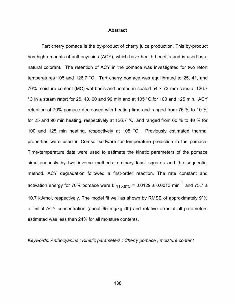
138

Abstract

Tart cherry pomace is the by-product of cherry juice production. This by-product

has high amounts of anthocyanins (ACY), which have health benefits and is used as a

natural colorant. The retention of ACY in the pomace was investigated for two retort

temperatures 105 and 126.7 °C. Tart cherry pomace was equilibrated to 25, 41, and

70% moisture content (MC) wet basis and heated in sealed 54 × 73 mm cans at 126.7

°C in a steam retort for 25, 40, 60 and 90 min and at 105 °C for 100 and 125 min. ACY

retention of 70% pomace decreased with heating time and ranged from 76 % to 10 %

for 25 and 90 min heating, respectively at 126.7 °C, and ranged from 60 % to 40 % for

100 and 125 min heating, respectively at 105 °C. Previously estimated thermal

properties were used in Comsol software for temperature prediction in the pomace.

Time-temperature data were used to estimate the kinetic parameters of the pomace

simultaneously by two inverse methods: ordinary least squares and the sequential

method. ACY degradation followed a first-order reaction. The rate constant and

activation energy for 70% pomace were k 115.8°C = 0.0129 ± 0.0013 min-1

and 75.7 ±

10.7 kJ/mol, respectively. The model fit well as shown by RMSE of approximately 9*%

of initial ACY concentration (about 65 mg/kg db) and relative error of all parameters

estimated was less than 24% for all moisture contents.

Keywords: Anthocyanins ; Kinetic parameters ; Cherry pomace ; moisture content

139

5.1 Introduction

Cherry (Prunus cerasus L.) pomace is the solid waste or by-product of cherry juice

processing and consists of cherry skin and seeds. It accounts for over 90% of dry

matter with high quantity of lignin, cellulose, and dry fiber components (Nawirska A.,

2005) . Cherries are known to contain substantial quantities of anthocyanins (Wang et

al., 1999), which are mainly concentrated in the skins (Chaovanalikit and Wrolstad,

2004; Tomas-Barberan et al., 2001). Anthocyanin stability of black carrots was studied

at various solid contents and pHs during both heating, 70–90 ºC, and storage at 4–37

ºC. Degradation of monomeric anthocyanins increased with increasing solid content

during heating, while it decreased during storage (Ahmed et al., 2004; Kirca et al.,

2007). The degradation kinetics of anthocyanins in blood orange juice was studied

(Kirca and Cemeroglu, 2003). The activation energies for solid content of 11.2 to 69

°Brix were found to be 73.2 to 89.5 kJ/mole. Thermal and moisture effects on grape

anthocyanin degradation were investigated using solid media to simulate processing at

temperatures above 100 °C (Lai et al., 2009). Anthocyanin degradation followed a

pseudo first-order reaction with moisture. Anthocyanins degraded more rapidly with

increasing temperature and moisture. The thermal degradation of anthocyanins has

been studied in red cabbage (Dyrby et al., 2001), raspberries (Ochoa et al., 1999),

pomegranate, grapes (Marti et al., 2002), plum puree (Ahmed and others 2004),

blackberries (Wang and Xu, 2007), purple corn cob (Yang et al., 2008) and blueberry

(Kechinski et al., 2010).

Kinetic studies for anthocyanins are needed to minimize undesired degradation and

to optimize quality of foods. Anthocyanin degradation under isothermal heating (50-90

140

°C) is reported to follow first order kinetics (Ahmed et al., 2004; Markakis et al., 1957).

Degradation of ACY in strawberry paste during high-temperature (80-130°C) high-

pressure (up to 700MPa) treatments showed that ACY degradation is increased by both

temperature and pressure, with the temperature effect being greatest (Verbeyst et al.,

2010). The Effect of water activity on ACY degradation was studied under Non-

isothermal heating (100-140 °C) results showed increase in reaction rate constant as

water activity decrease (Jimenez et al., 2012)

A higher activation energy implies that a smaller temperature change is needed

to degrade a specific compound more rapidly (Cemeroglu et al., 1994) . Studies on

ACY extracts from purple-flesh potato and grape showed significantly lower stabilities

than ACY in red-flesh potato and purple carrot extracts at 98 °C (Reyes and Cisneros-

Zevallos, 2007).

The Arrhenius equation is a common model used to describe the temperature

dependence of reaction rate in kinetic problems. Both reaction rate constant (kr) and

activation energy (Ea) are usually estimated from experimental data. These two

parameters have strong parameter correlation with each other (Schwaab et al., 2008).

Several works suggested the reparameterization of the Arrhenius equation by applying

the reference temperature (Tr) in the model (Himmelblau, 1970; Pritchard and Bacon,

1978). Another parameter estimation study established a new approach that was more

effective than the standard experimental design criteria in both reducing the uncertainty

regions of the parameters and improving the consistency of the estimates (Franceschini

and Macchietto, 2008).

141

Estimating parameters in nonlinear models is complex compared to linear models

(Dolan, 2003). However, estimation techniques provide several ways to accurately

estimate parameters in non-linear equations if input and the output data are known. A

better estimate of a parameter is obtained with prior information of the parameters. In

addition, sequential MAP estimation can be used for estimating the parameters in the

model simultaneously and sequentially (Beck and Arnold, 1977). A recent example in

the food literature of using sequential estimation was done successfully to obtain

improved parameter estimates for a generic starch viscosity model (Sulaiman and

Dolan, 2013; Sulaiman et al., 2013). Accurate parameter estimates are needed for any

food process design and optimization, such as designing drying, extrusion, and other

thermal processes for baked goods, confectionaries, breakfast cereals, and other foods

containing cherry pomace byproduct. These processes are typically non-isothermal and

require nonlinear modeling and estimation of all the parameters simultaneously.

Estimating the parameters using all the data simultaneously in a one-step regression

has been shown to give better accuracy than estimating the parameters from the same

data using two-step regression (Jewell, 2012). Therefore the objectives of this study

were to estimate the kinetic parameters for cherry pomace at three constant moisture

contents under non-isothermal processing.

5.2 Materials and Methods

5.2.1 Pomace sample preparation

Montmorency cherry pomace was obtained from Cherry Growers Inc., (Grawn,

Michigan, U.S.A.). The moisture content (MC) of the samples was measured using a

Sartorius Moisture Analyzer – MA30 (Sartorius AG, Goettingen, Germany). The initial

142

MC of cherry pomace was 70% (wet basis, control). Two additional samples with MC of

41 and 25% (MC-41 and MC-25) were prepared using a pilot-scale cabinet dryer

(Proctor and Schwartz Inc., Philadelphia, Penn, U.S.A.) at 50 ± 2°C. Pomace samples

MC-70, MC-41, and MC-25 represent pomace with 70, 41, and 25% MC, respectively.

Each of the three cherry pomace samples were filled and sealed under vacuum (20-

mm Hg) in 202 ×214 steel cans (54-mm diameter and 73-mm height) and heated at

126.7˚C, for heating time intervals (0, 25, 40, 60 and 90 min) using a rotary steam

retort (FMC Steritort Laboratory Sterilizer, Madera, Calif, U.S.A.) and at 105˚C for 100

and 125 min. Each can was fitted with a needle thermocouple (Ecklund-Harrison

Technologies Inc., Fort Myers, Florida, U.S.A.) to measure the center temperature. The

time-temperature profile of retorting process (samples and retort) is shown in Figure

5.1. Experimental design showed in Appendix C.1, Figure C.1.

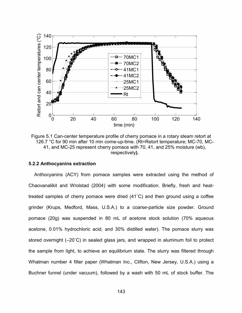
143

Figure 5.1 Can-center temperature profile of cherry pomace in a rotary steam retort at 126.7 °C for 90 min after 10 min come-up-time. (Rt=Retort temperature; MC-70, MC-

41, and MC-25 represent cherry pomace with 70, 41, and 25% moisture (wb), respectively).

5.2.2 Anthocyanins extraction

Anthocyanins (ACY) from pomace samples were extracted using the method of

Chaovanalikit and Wrolstad (2004) with some modification. Briefly, fresh and heat-

treated samples of cherry pomace were dried (41˚C) and then ground using a coffee

grinder (Krups, Medford, Mass, U.S.A.) to a coarse-particle size powder. Ground

pomace (20g) was suspended in 80 mL of acetone stock solution (70% aqueous

acetone, 0.01% hydrochloric acid, and 30% distilled water). The pomace slurry was

stored overnight (–20˚C) in sealed glass jars, and wrapped in aluminum foil to protect

the sample from light, to achieve an equilibrium state. The slurry was filtered through

Whatman number 4 filter paper (Whatman Inc., Clifton, New Jersey, U.S.A.) using a

Buchner funnel (under vacuum), followed by a wash with 50 mL of stock buffer. The

0 20 40 60 80 100 120 1400

20

40

60

80

100

120

140

time (min)

Re

tort

an

d c

an

ce

nte

r te

mp

era

ture

s (

°C)

70MC1

70MC2

41MC1

41MC2

25MC1

25MC2

Rt

144

filtrate was mixed with 40 mL of chloroform and stored overnight. The supernatant was

collected and used for the determination of monomeric anthocyanin content.

5.2.3 Monomeric anthocyanin content determination

The total monomeric anthocyanin content was determined using the pH

differential assay (Rodriguez-Saona et al., 1999). Specific volume of the supernatant

was dissolved in potassium chloride buffer (KCl, 0.025 M, pH 1.0) and sodium acetate

(CH3CO2Na3·H2O, 0.4 M, pH 4.5) and allowed to equilibrate, with a predetermined

dilution factor. The absorbance of each equilibrated sample of extracted ACY was then

measured at 510nm and 700nm for haze correction, using a Genesys 5

spectrophotometer (Spectronic Instruments, Rochester, NY, USA) and 1 cm path-length

cells were used for spectral measurements. ACY contents was calculated, as cyanidin

3-glucoside equivalent (Lee et al., 2005), and reported as mg/kg (dry-basis).

5.2.4 Mathematical Modeling

5.2.4.1 Estimation the kinetic parameters

The heating was assumed to be axisymmetric in the can. Gauss-Legendre

quadrature was used to choose a total of 15 points in half of the can (Figure 5.2).

Gauss-Legendre quadrature was chosen as the integration method because it is the

most accurate of all numerical integration techniques for a given number of points

(Chapra, 2011) . The point locations were normalized with r/R’, z/H, where R’ and H

were the can’s radius and height, respectively. Comsol was used to compute T(r, t, z)

at the 15 points, using the can dimensions based on all estimated thermal properties

from chapter 4 (density, specific heat and thermal conductivity), the measured dynamic

145

surface temperature (Ts), as the boundary heat source for all processes, and the

uniform initial temperature of the pomace at room temperature.

Figure 5.2 Location of the 15 Gauss-Legendre points in the half-can based on axisymmetric heating.

In this study the reaction is following a first order reaction: Equation Chapter 5 Section 5

d C

k Cd t

(5.1)

Integration of equation (5.1) with integration limits gives:

( )

00

C t td C

k td t

C

(5.2)

When k is a function of temperature and moisture content, Eq. (5.2) is written as follows:

13 14 15

10 11 12

78 9

4 5 6

1 2 3 r=R’

H

r=0

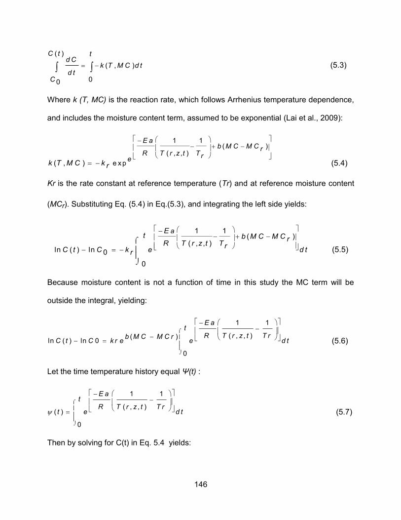
146

( )

( , )

00

C t td C

k T M C d td t

C

(5.3)

Where k (T, MC) is the reaction rate, which follows Arrhenius temperature dependence,

and includes the moisture content term, assumed to be exponential (Lai et al., 2009):

1 1( )

( , , )

e x p( , )

E ab M C M C r

R T r z t T re

k T M C k r

(5.4)

Kr is the rate constant at reference temperature (Tr) and at reference moisture content

(MCr). Substituting Eq. (5.4) in Eq.(5.3), and integrating the left side yields:

1 1( )

( , , )ln ( ) ln 0

0

aEt b M C M C r

R T r z t T rC t C k e d tr

(5.5)

Because moisture content is not a function of time in this study the MC term will be

outside the integral, yielding:

1 1

( , , )( )ln ( ) ln 0

0

E at

R T r z t T rb M C M C rC t C k r e e d t

(5.6)

Let the time temperature history equal Ψ(t) :

1 1

( , , )( )

0

E at

R T r z t T rt e d t

(5.7)

Then by solving for C(t) in Eq. 5.4 yields:

147

( ( ) )( )

( ) 0 e

b M C M C rk r t e

C t C

(5.8)

Equation (5.8) was predicted the degradation of ACY at any chosen point inside the

cylinder during heating for a constant MC and time temperature history (Ψ(t)). Because

ACY concentration cannot be measured at an infinitely small point, we must continue to

develop the equation for mass-average ACY concentration, which can be measured

experimentally. To compute mass-average ACY in the can (C (t)) the point

concentrations (C (t)) should be integrated over the can:

'( ) 2

00( )

'2

00

H RC t rd rd z

tH R

rd rd z

(5.9)

Substituting (C(t)) from Eq. (5.8) into Eq. (5.9) yields:

( ( ) )' ( )2 0

0 0( )

2'

22

b M C M C rH R k t erC e r d r d z

C t

RH

(5.10)

Normalizing, r*=r/R’ and z*=z/H, the final form of Eq. (5.10) will be

1 ( ( ))1 ( ) * * *( ) 2 0

00

b M C M C rk r t eC t C e r d r d z

(5.11)

Equation (5.11) is the equation that was used in this study for calculation of predicted

mass-average ACY concentration as function of moisture content and time-temperature

history.

148

5.2.4.2 Arrhenius Reference Temperature

The importance of the reference temperature Tr is that it controls the correlation

coefficient between the rate constant (kr) and activation energy (Ea). As the correlation

coefficient is minimized, the confidence interval for kr is also minimized, Datta (1993),

allowing estimation of both parameters simultaneously. The optimum Tr was found

iteratively by holding Tr at different fixed values, estimating the parameters for Eq. 5.11,

plotting the correlation coefficient and choosing the Tr where the correlation was nearly

zero (Dolan et al., 2013; Schwaab et al., 2008).

The estimation was done with a numerical procedure in MATLAB (Appendix C.3, at

C.3.1 –C.3.2). An initial guess of parameters, model equations, and experimental data

(ACY concentration at two retorting temperature, Table 5.1) collected on time and

temperature of the sample were entered into the program. Nonlinear regressions, using

the nlinfit function in MATLAB (Appendix C.3, at C 3.4), were used to estimate the

parameters. Finding the optimum reference temperature which lead to uncorrelated

model parameters involved a number of steps: after an initial parameter estimates with

initial guess of reference temperature, the reference temperatures was allowed to vary

and then the new covariance matrix of the parameter estimates was recalculated for

each new reference temperature .

5.2.4.3 Moisture content Constant

The moisture content of the pomace samples is constant during this non-

isothermal process. The moisture content parameter b in Eq.(5.6), was estimated by

applying the slope method,Lai et al. (2009). The reaction rate constant kr values at each

149

sample of cherry pomace (25, 41 and 70%) were used for b value estimation.

Readjusting Eq. (5.6) by setting T=Tr, yields:

( ) e xp ( ( ))k M C k r b M C M C r (5.12)

Using log to linearize Eq. 5.12, linear regression for Eq.(5.12), will give the slope which

equal to the parameter of moisture constant (b).

5.2.5 Parameter Estimation Techniques

5.2.5.1 Sensitivity Coefficient Plot

The sensitivity coefficient (Xij), where i is the time index, and j is the parameter

index, indicates how sensitive the dependent variable is to a parameter βj, is formed by

taking the first derivative of a dependent variable with respect to a specific parameter.

The parameters in the model can be estimated most accurately when its Xij is

maximized (Beck and Arnold, 1977). Estimation of kinetic parameters for non-isothermal

food processes using nonlinear parameter estimation has been discussed by (Dolan,

2003). To place the Xij on the same scale, we used a scaled sensitivity coefficient (X'ij).

The scaled sensitivity coefficient plots are helpful in determining which parameters can

be estimated most accurately, and which parameters are most important in the model.

Here, we determined the sensitivity coefficient (Xij) of parameter () using the finite

difference method of forward difference approximation (Beck and Arnold, 1977) for each

parameter as presented in Eq.(5.13). The bj is some relatively small quantity and is

given as Eq.(5.13). The scaled sensitivity coefficients shown in Eq. (5.14) were

150

computed using MATLAB (Appendix C.3, at C.3.3). To have a sensitivity coefficient plot,

we must have independent variable input and approximate value of parameters:

( ) ( 1,. . . , , , . . . ) ( 1,. . . , , . . . )C i C b b j d b j b p C b b j b pX ij

i b j

(5.13)

0 .0 0 1b i b i

( ) ( 1,. . . , , , . . . ) ( 1,. . . , , . . . )'

0 .0 0 1

C i C b b j d b j b p C b b j b pX jij

i

(5.14)

5.2.5.2 Ordinary Least Squares (OLS) Estimation Procedure

The kinetic parameters (Ea , kr) and initial concentration of ACY (C0) in

Equation (5.11) were estimated with the inverse problem method using MATLAB with

Comsol. The MATLAB function “nlinifit” (Appendix C.3, at C.3.4) was used to minimize

the sum of squares:

2

S S C o b s C p rdi i i

(5.15)

The 95% asymptotic confidence intervals (ci) of the parameters and the

correlation coefficient matrix of parameters were also computed in MATLAB (Dolan et

al., 2007; Mishra et al., 2008). Estimated parameters are significant when the ci does

not contain zero.

5.2.5.3 Sequential Estimation Procedure

The second method used to estimate model parameters is the sequential method.

Parameter values are updated in sequential estimation as experimental data of time and

temperature are added. The sequential method shows the changes in the values of

parameters being estimated until they reach a steady value.

151

Non-linear Maximum A Posteriori (MAP) sequential estimation procedure given in

(Beck and Arnold, 1977 p. 277) was used to find parameters in Eq.(5.16). The MAP

equation is shown in Eq.(5.17)

T -1b =μ +P X ψ (Y -Xμ )M A P β M AP β (5.16)

T -1 1 -1P M A P = ( X ψ X+V )

(5.17)

Eq.(5.16) and Eq. (5.17). are in matrix format, where bMAP is the matrix (px1) vector

parameter to be estimated; is matrix (px1) vector with prior information on the

parameters; PMAP is the covariance vector matrix of parameters (pxp) which gives

information about the variance (on the diagonal) and covariance (correlation between

parameter) on off-diagonal elements; X is the sensitivity coefficient matrix (nxp); is

covariance matrix (nxn) of errors, and Y is the measurement (nx1) vector and V is

covariance matrix of .

Sequential parameter estimation gives more insight into the estimation process.

Improvement in the estimation can easily be seen as the parameter is estimated and

plotted at each datum addition (Mohamed, 2009). Under sequential estimation we

expect the parameters to approach a constant as the number of observations increases.

MATLAB programming was used to conduct the sequential estimation (Appendix C.3, at

C.3.5). The sequential estimation was done by sorting on predicted ACY concentration,

rather than time. The reason for choosing this type of sort was that there were two

retort temperatures. Therefore, time of heating was not the only determining factor of

the anthocyanin retention. Different combinations of time and temperature affected

152

ACY concentration. To account for two retort temperatures, the ACY concentration,

starting at the highest concentration and proceeding to the lowest, was used as the sort.

5.3 Results and discussion

5.3.1 Anthocyanin (ACY) degradation

Initial average ACY content in the control cherry pomace (MC-70) was 65.4

mg/kg (dry-basis). Thermal treatment in the rotary steam retort at 126.7 °C for 90 min

degraded the ACY to a mean of 6.6 mg/kg. This process reduced the ACY to a mean of

5.2 mg/kg for MC-41 and 0 mg/kg for MC-25 pomace. The second heat treatment 105

°C (100 and 125 min) degraded the ACY to means of 22.5 ±2.2 mg/kg in MC-70, 12.5

±2.3 mg/kg in MC-41 and to 12.1 ±0.76 mg/kg in MC-25 at 125 min retorting time, as

shown in Table 5.1.Thus this study showed greater ACY loss with increasing

temperature history on the cherry pomace. Similar observations were reported in study

for black carrots at different solids contents at 70 to 90°C, degradation of ACY

increased with increasing solid content during heating Kirca et al. (2007). Non-

isothermal heating of grape pomace in wheat flour (with loss in moisture during heating,

which is a main difference with this study) up to 105 and 145°C showed also

degradation of ACY as temperature and moisture increased, Lai et al. (2009)

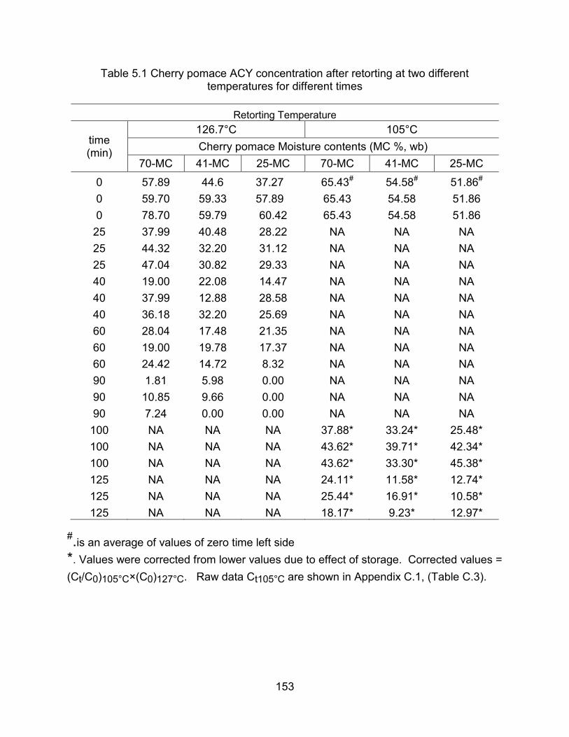
153

Table 5.1 Cherry pomace ACY concentration after retorting at two different temperatures for different times

Retorting Temperature

time (min)

126.7°C 105°C

Cherry pomace Moisture contents (MC %, wb)

70-MC 41-MC 25-MC 70-MC 41-MC 25-MC

0 57.89 44.6 37.27 65.43# 54.58# 51.86#

0 59.70 59.33 57.89 65.43 54.58 51.86

0 78.70 59.79 60.42 65.43 54.58 51.86

25 37.99 40.48 28.22 NA NA NA

25 44.32 32.20 31.12 NA NA NA

25 47.04 30.82 29.33 NA NA NA

40 19.00 22.08 14.47 NA NA NA

40 37.99 12.88 28.58 NA NA NA

40 36.18 32.20 25.69 NA NA NA

60 28.04 17.48 21.35 NA NA NA

60 19.00 19.78 17.37 NA NA NA

60 24.42 14.72 8.32 NA NA NA

90 1.81 5.98 0.00 NA NA NA

90 10.85 9.66 0.00 NA NA NA

90 7.24 0.00 0.00 NA NA NA

100 NA NA NA 37.88* 33.24* 25.48*

100 NA NA NA 43.62* 39.71* 42.34*

100 NA NA NA 43.62* 33.30* 45.38*

125 NA NA NA 24.11* 11.58* 12.74*

125 NA NA NA 25.44* 16.91* 10.58*

125 NA NA NA 18.17* 9.23* 12.97*

#.is an average of values of zero time left side

*. Values were corrected from lower values due to effect of storage. Corrected values =

(Ct/C0)105°C×(C0)127°C. Raw data Ct105°C are shown in Appendix C.1, (Table C.3).

154

5.3.2 Reference Temperature Plot

The reference temperature at each pomace moisture content of pomace samples

was estimated: The correlations of parameters with reference temperature Tr are

illustrated in Figure 5.3. For both heating temperature (126.7°C and 105°C), the Tr

values were found as 115.1, 115.1 and 115.8°C for 25, 41 and 70% MC (wb) ,

respectively based on the parameter correlation between kr and Ea nearly equal to zero

(Figure 5.3). This value 115.8 °C of Tr, which is close to maximum heating temperature

of 126.7°C Datta (1993), was used for the next estimation for all parameters for the all

moisture contents of cherry pomace samples. Figure 5.3 is similar in principle to results

shown by Dolan et al. (2013), Sulaiman and Dolan (2013), and (Sulaiman et al., 2013)

Figure 5.3 Correlation coefficient of parameters kr and Ea as a function of the reference

temperature Tr (for ACY degradation under retorting process)

110 111 112 113 114 115 116 117 118 119 120 121 122-0.5

-0.4

-0.3

-0.2

-0.1

0

0.1

0.2

0.3

0.4

0.5

Reference Temperature,Tr(oC)

Co

rre

latio

n C

oe

ffic

ient

of

kr and E

110 111 112 113 114 115 116 117 118 119 120 121 122

Reference Temperature Tr (ºC)

Co

rre

latio

n C

oeffic

ient o

f kr

an

d E

a

0.5

0.4

0.3

0.2

0.1

0

-0.1

-0.2

-0.3

-0.4

-0.5

155

5.3.3 Scaled Sensitivity Coefficient Plot

Sensitivity coefficient analysis helps to know whether or not the parameters are

linearly dependent or independent of each other, and which parameters will have the

smallest relative error. The three parameters (Co, kr and Ea) in Eq. (5.11) were

uncorrelated, which means they could be estimated separately. Figure 5.4 shows the

scaled sensitivity coefficient plots. The absolute value of the scaled sensitivity

coefficient plots for reaction rate constant (X′kr115.8°C) at both retorting temperatures

(127°C and 105°C) are larger than the size of X’Ea at the two retort temperatures

(Figure 5.4). Therefore, the parameter kr115.8 was estimated with more accuracy than

the parameter Ea (see relative errors in Table 5.2). However, Figure 5.4 shows that the

absolute vale of X’Ea at 105°C is about 10, which larger than the value at 127°C, which

was about 6. These two plots indicated that at least two experiments with two different

retort temperatures are needed to estimate the parameter Ea with high accuracy. The

most accurate parameter was Co, which has smallest relative error ( Table 5.2).

156

Figure 5.4 Scaled sensitivity coefficient plots of the three parameters at retort

temperatures 105°C and 127°C, using initial parameter values of Ea =45kJ/mol,

kr115.8°C = 0.019 min-1

and C0 = 60 mg/kg.

5.3.4 Parameter Estimation using Ordinary Least Squares

Estimated parameters for the cherry pomace ACY samples at three constant

moisture contents in Eq. (5.11) are shown in Table 5.2. Since the most important

parameters are the Arrhenius parameters, Tr was established where the correlation

coefficient between kr and Ea was nearly zero. The confidence intervals and the

percentage relative errors of the estimated parameters are given in Table 5.2. In

general, the confidence interval and the relative errors are small.

0 10 20 30 40 50 60 70 80 90 100-30

-20

-10

0

10

20

30

40

50

60

Heating time(min)

Sca

led

Se

nsitiv

ity C

oe

ffic

ein

ts (

un

its)

Ea-(kJ/mol)

127 oC

kr-(min-1

)127

oC

Co-(mg/kg)127

oC

Ea-(kJ/mol)105

oC

kr-(min-1

)105

oC

Co-(mg/kg)105

oC

157

Table 5.2 Kinetic parameter estimates of ACY degradation in cherry pomace at three constant moisture contents after retorting processing

MC %(wb)

OLS estimates Ea (kJ/mol)

kr (min-1

)

Co (mg/kg,db)

relative error (%)

CI (95%) RMSE (mg/kg)

70 75.7 ±10.7

0.0129 ±0.0013 65.256 ±2.72

14.2 9.8 4.2

53400 97930 0.01034 0.0156 59.59 70.92

7.02

41 69.66 ±12.7

0.01417 ±0.0016 54.5 ±2.77

18.3 11.4 5.1

43071 96265 0.01079 0.0176 48.66 60.25

7.00

25 77.8 ±17.9

0.0134 ±0.0022 51.65 ±3.62

23.0 16.4 7.0

40201 115580 0.00877 0.0180 44.05 59.26

9.15

Table 5.2 shows the results of parameters estimated at three constant moisture

contents of pomace. For 70% pomace ACY, the root mean square error (RMSE) is

about 7% of the total scale of about 65 as also shown in Figure 5.5, which indicates a

good fit. The lowest relative error was with the initial concentration parameter (Co),

equal to about 5% average for all moistures (Table 5.2), which means it was the easiest

parameter to be estimated as indicated by the scaled sensitivity coefficient plot (Figure

5.4). Also as predicted by Figure 5.4, the largest relative error was in Ea (Table 5.2) of

14 to 23%. All parameters were significant, as shown by the 95% CIs not containing

zero.

Table 5.3 shows a comparison of the kinetic parameter values of ACY in literature

and in this study. Similar materials with similar moisture content (41%) were compared.

The activation energies were similar, while the rate constant in this study was lower. It is

158

not clear why anthocyanins in cherry pomace would thermally degrade more slowly than

anthocyanins in grape pomace. The rate constant ( Mishra, 2008) was kr115.8°C =

0.0823 min-1

, Lai et al. (2009) was 0.0795 min-1 and Verbeyst et al. (2010) was 0.0472

min-1

(all converted from Table 5.3 using Arrhenius equation) versus 0.0142 min-1 in

this study. The activation energy values in the previous three studies, ranging from 65 to

75 kJ/mole, were very close values in comparison with this study as shown in Table 5.3.

Lai (2009) used the extruder to heat the sample to about 140°C under atmospheric

pressure, which means the moisture content decreased with time, and the data were

corrected for this change. In this study the heating was under constant pressure and

constant moisture content.

. In the latest two studies (Lai et al., 2009; Mishra et al., 2008) the parameters were

estimated using OLS only, while in this study sequential estimation was also used

where the parameters were estimated at each experimental step.

159

Table 5.3 Summary of published kinetic parameters of anthocyanin degradation by thermal treatments

using 1st – order model

Material Processing Temp, (°C)

Method ΔE

(kJ/mol) kTr (min-1

) Tr °C References

Cherry pomace (41% MC, wb )

105, 126.7 nonlinear regression

69.66 0.01416 115.8 This study

Grape pomace in wheat flour(30% MC)

100 minimizing SS of residual

75.3 0.0075 80 (Lai et al., 2009)

Grape pomace (42%MC,wb)

126.7 nonlinear regression

65.32 0.0607 110 (Mishra et al., 2008)

Purple-flesh potato Grape

Purple carrot

25,50,80,98

Arrhenius model ,forward problem

72.49 75.03 81.34

7.3 ×10-3

5.8×10-3

2.4 ×10-3

98 98 98

(Reyes and Cisneros-Zevallos, 2007)

blackcurrant juice

110;10;140

minimizing

SSE of C/Co

values

81.51 91.09

0.017 0.165

110 140

(Harbourne et al., 2008)

Blackberry juice (65°Brix)

5,25,37

Arrhenius model ,forward problem

75.5 0.0591

0.0216 37 25

(Wang and Xu, 2007)

Strawberry paste 80-130 n/a 63.3 0.0351 110 (Verbeyst et al., 2010) Sour cherry juice

45°Brix 71° Brix

50,60,70,80 50,60,70,80

Arrhenius model ,forward problem

75.9 80.1

9.8×10-4

1.62 ×10-3 80

80 (Cemeroglu et al., 1994)

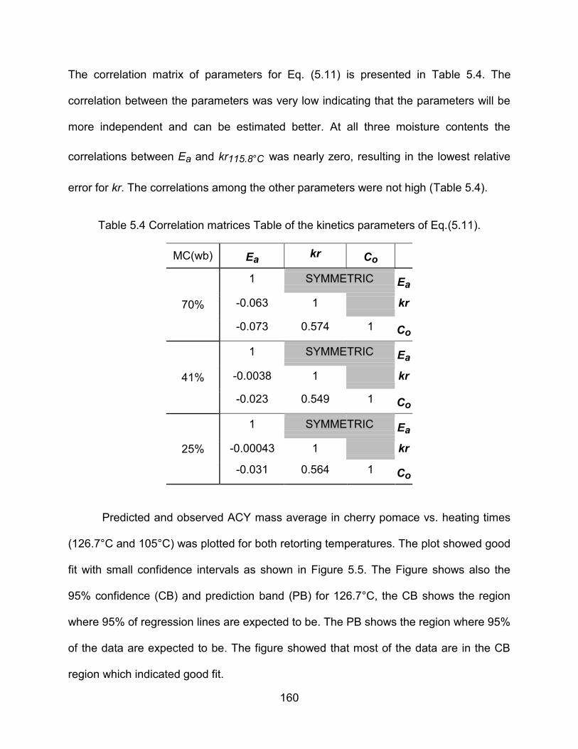
160

The correlation matrix of parameters for Eq. (5.11) is presented in Table 5.4. The

correlation between the parameters was very low indicating that the parameters will be

more independent and can be estimated better. At all three moisture contents the

correlations between Ea and kr115.8°C was nearly zero, resulting in the lowest relative

error for kr. The correlations among the other parameters were not high (Table 5.4).

Table 5.4 Correlation matrices Table of the kinetics parameters of Eq.(5.11).

MC(wb) Ea kr Co

70%

1 SYMMETRIC Ea

-0.063 1 kr

-0.073 0.574 1 Co

41%

1 SYMMETRIC Ea

-0.0038 1 kr

-0.023 0.549 1 Co

25%

1 SYMMETRIC Ea

-0.00043 1 kr

-0.031 0.564 1 Co

Predicted and observed ACY mass average in cherry pomace vs. heating times

(126.7°C and 105°C) was plotted for both retorting temperatures. The plot showed good

fit with small confidence intervals as shown in Figure 5.5. The Figure shows also the

95% confidence (CB) and prediction band (PB) for 126.7°C, the CB shows the region

where 95% of regression lines are expected to be. The PB shows the region where 95%

of the data are expected to be. The figure showed that most of the data are in the CB

region which indicated good fit.

161

Figure 5.5 Plot of observed and predicted with confidence intervals of ACY values in cherry pomace (MC-70, wb)) after retorting at 126.7ºC and 105°C for different times.

Prediction bands for 105°C are not shown, for clarity.

Residuals for prediction of ACY values were small, as shown in Figure 5.6.

Residuals were larger during the 0 min and after 40 min heating at 126.7 °C, showing

some difficulty in fitting. At other heating times the residuals were additive and variance

constant and the mean is close to zero (-0.071), which confirms a good fit of the

equation used for estimating the degradation parameters of ACY in cherry pomace. For

retorting at 105°C residuals also showed a good fit, with slightly larger residual at 125

min heating (Figure 5.6). The residual histogram (Figure 5.7) shows that the residuals

were nearly normally distributed.

0 20 40 60 80 100 120-20

0

20

40

60

80

100

Heating time (min)

Ma

ss a

ve

rag

e o

f A

CY

( m

g/k

g d

b)

ACYpred-(127oC)

ACYobs-(127oC)

95% confidence band

95% prediction band

ACYobs-(105oC)

ACYpred-(105oC)

95% confidence band

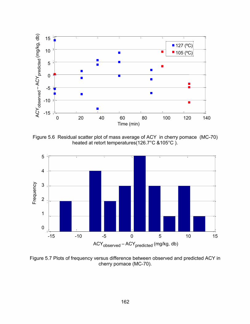
162

Figure 5.6 Residual scatter plot of mass average of ACY in cherry pomace (MC-70) heated at retort temperatures(126.7°C &105°C ).

Figure 5.7 Plots of frequency versus difference between observed and predicted ACY in cherry pomace (MC-70).

0 20 40 60 80 100 120 140-15

-10

-5

0

5

10

15

time (min)

AC

YO

bse

rve

d-A

CY

Pre

dic

ted (

mg

/kg

db

)

127oC

105oC

Time (min)

0 20 40 60 80 100 120 140

15

10

5

0

-5

-10

-15

127 (ºC)

105 (ºC)

AC

Yobserv

ed –

AC

Ypre

dic

ted (

mg/k

g,

db

)

-15 -10 -5 0 5 10 150

1

2

3

4

5

ACYObserved

-ACYPredicted

( mg/kg db)

Fre

qu

en

cy

ACYobserved – ACYpredicted (mg/kg, db)

-15 -10 -5 0 5 10 15

5

4

3

2

1

0

Fre

qu

en

cy

163

5.3.4.1 Moisture content constant estimation

From reaction rate constant values in Table 5.2 the moisture content parameter

was estimated by applying the linear regression for Eq. (5.4). The result (Appendix C.1,

Figure C.1.4) indicated that there was no significant effect of moisture content on the

ACY rate constant or activation energy during the retorting process (p=0.65, R2=0.28)..

5.3.5 Sequential Parameter Estimation

The sequentially estimated parameter values of Ea, kr, and Co were 75665 J/g mol,

0.01294 min-1

and 65.25 (Figure. 5.8 to Figure.5.10). The parameters Ea and kr115.8°C

reached a constant when the last three data points were added (Figure. 5.8 and

Figure.5.9), showing that almost all the data were needed for accurate estimation. The

final values for the parameters results are, as expected, very similar to the OLS results

given in Table 5.2 for the model. For the model studied, sequential results are the best

possible estimates, where the three parameters reach nearly a constant value by the

end of the experiment.

164

Figure 5.8 Sequentially estimated parameter of activation energy (Ea).

Figure 5.9 Sequentially estimated parameter of reaction rate (kr115.8°C) (min-1

).

0 5 10 15 20 257.4

7.6

7.8

8

8.2

8.4

8.6

8.8x 10

4

Step Index

Se

qu

en

tia

lly E

stim

ate

d E

a(

J/m

ol)

126.7 C

105 C

0 5 10 15 20 250.011

0.012

0.013

0.014

0.015

0.016

0.017

0.018

0.019

0.02

Step Index

Se

qu

en

tia

lly E

stim

ate

d k

r (m

in-1

)

126.7 C

105 C

165

Figure 5.10 Sequentially estimated parameter of Initial concentration (C0)

5.4 Conclusions

1. This study shows innovative data efficient methods to estimate the kinetic

parameters for cherry pomace ACY degradation at two different retorting

temperatures. These methods can be used to estimate other kinetic parameters for

non-isothermal conditions.

2. A minimum of two retort temperatures are needed to estimate Ea accurately,

because scaled sensitivity coefficient for Ea for only one retort temperature is small.

3. There was no significant effect of moisture content on the rate constant in this study.

4. Relative errors of the kinetic parameters were under 24%.

5. For future studies the parameter accuracy may be increased by applying optimal

experimental design to determine the best times and temperatures to collect data.

0 5 10 15 20 2558

59

60

61

62

63

64

65

66

Step Index

Se

qu

en

tially

Est

ima

ted

Co (

mg

/kg

)

126.7 C

105 C

166

C. APPENDICES

167

Appendix C.1 Experimental design and preliminary data

Figure C.1 Process experimental design for kinetic parameter estimation

ACY Concentration

values from step 1

(+ ACY values

from objective1 )

15 Gauss spatial

points for

integration

Data analysis

(OLS & Seq, Mtds)

Ea Kr Co

Estimation

Data

Analysis

Retorting 105 C

Thermal properties of

the pomace (for

Objective 2)

Step 2

Step 4

Step 3

Step 1

168

Figure C.2 Can-center temperature profile of cherry pomace in a retort at 105 °C for 100 min (A) and 125 min (B) (TRt=Retort temperature, Ts= can surface temperature; 70%,

41%, and 25% MC represent the pomace with 70, 41, and 25% moisture (wb), respectively).

15

25

35

45

55

65

75

85

95

105

0 20 40 60 80 100 120

Cen

ter

ca

n te

mp

era

ture

(°C

)

Retorting time (min)

A

MC-25

MC-25

MC-41

MC-41

MC-70

MC-71

Ts

TRt

15

25

35

45

55

65

75

85

95

105

0 20 40 60 80 100 120 140 160

Cen

ter

ca

n te

mp

era

ture

(°C

)

Retorting time (min)

B

MC-25

MC-25

MC-41

MC-41

MC-70

MC-71

Ts

TRt

169

Figure C.3 Absorbance versus Retorting time of Cherry pomace ACY’s extractions at three constant moisture content (wb) heated at 126.7°C

Table C.1 Absorbance versus Retorting time of Cherry pomace ACY’s extractions at three constant moisture content heated at 126.7°C

Absorbance(AU) Standard deviation

time(min) MC-70 MC-41 MC-25 MC-70 MC-41 MC-25

0 0.0320 0.0485 0.0515 0.0064 0.0094 0.0176

0 0.0330 0.0645 0.0800 0 0.0435 0.0650 0.0835 25 0.0210 0.0440 0.0390 0.0026 0.0057 0.0023

25 0.0245 0.0350 0.0430 25 0.0260 0.0335 0.0390 40 0.0105 0.0240 0.0200 0.0058 0.0105 0.0103

40 0.0210 0.0140 0.0395 40 0.0200 0.0350 0.0355 60 0.0155 0.0190 0.0295 0.0025 0.0028 0.0092

60 0.0105 0.0215 0.0240 60 0.0135 0.0160 0.0115 90 0.0010 0.0065 0 0.0025 0.0053 0

90 0.0060 0.0105 0 90 0.0040 0.0000 0

0.000

0.013

0.025

0.038

0.050

0.063

0.075

0.088

0.100

0 20 40 60 80 100

Ab

so

rba

nce

(AU

)

Retorting time (min)

MC-70 MC-41 MC-25

170

Table C.2 Cherry pomace’s ACY concentration after retorting at two different temperatures for different times

Concentration of ACY (mg/kg) dry basis

Temperature 127 °C Temperature 105 °C

time(min) MC-70 MC-41 MC-25 MC-70 MC-41 MC-25

0 65.4 ±6.7 54.8 ±5.1 51.9 ±5.9 65.4 ±6.7 54.8 ±5.1 51.9 ±5.9

25 43.1 ±2.7 34.5 ±3.0 29.2 ±1.0 NA NA NA

40 31.1 ±6.1 22.3 ±5.6 22.9 ±4.3 NA NA NA

60 23.8 ±2.6 17.3 ±1.5 15.7 ±3.9 NA NA NA

90 6.6 ±2.6 5.2 ±2.8 0 NA NA NA

100 NA NA NA 41.7 ±1.9 35.3 ±2.1 37.7 ±6.1

125 NA NA NA 22.5 ±2.2 12.5 ±2.3 12.1 ±0.76

Figure C.4 Slope method for estimate the moisture constant (b) for the retorted cherry pomace samples ACY concentration

y = -0.0011x - 4.3317

R² = 0.2802

-4.36

-4.35

-4.34

-4.33

-4.32

-4.31

-4.30

-4.29

-4.28

-4.27

-4.26

-4.25

-50 -40 -30 -20 -10 0

ln(k

r)

MC-MCr

171

Figure C.5 Plot of gauss points in the can with cherry pomace 70% MC (wb), predicted by Comsol. “The text in this figure is not meant to be readable but is for visual

reference only”.

13 14 15

10 11 12

7 8 9

4 5 6

1 2 3

Can’s G

auss 1

5 p

oints tem

pera

ture

s ( C

)

Heating time (sec)

172

Appendix C.2 Predicted Temperatures data by Comsol software

Table C.3 Part of predicted temperatures (°C) data at 15 gauss points (Pts) in the can for Cherry pomace (70% MC, wb) at126.7°C Retort Temperature).

time min

Pt 1 Pt 2 Pt 3 Pt 4 Pt 5 Pt 6 Pt 7

0.0 25.2 25.0 25.0 25.0 25.0 25.0 25.0 0.2 27.6 25.3 26.3 25.0 25.0 26.1 25.0 0.3 28.5 25.8 27.2 25.0 25.0 26.8 25.0 0.5 32.0 26.4 29.2 25.0 25.0 28.5 25.0 0.7 39.0 27.8 33.3 25.1 25.0 31.9 25.0 0.8 47.2 30.2 39.1 25.2 25.0 36.7 25.0 1.0 54.8 33.3 45.4 25.3 25.0 41.8 25.0 1.2 61.6 36.9 51.5 25.6 25.1 46.9 25.0 1.3 67.5 40.6 57.4 25.9 25.2 51.7 25.0 1.5 72.8 44.5 62.8 26.4 25.4 56.2 25.0 1.7 77.0 48.2 67.5 26.9 25.6 60.2 25.0 1.8 80.4 51.8 71.6 27.5 25.9 63.8 25.0 2.0 83.4 55.2 75.3 28.2 26.4 67.0 25.0 2.2 86.1 58.4 78.6 29.0 26.9 70.0 25.0 2.3 88.5 61.4 81.5 29.7 27.6 72.6 25.0 2.5 90.5 64.3 84.2 30.5 28.3 75.1 25.1 2.7 92.4 66.9 86.6 31.4 29.2 77.3 25.1 2.8 94.1 69.4 88.7 32.2 30.1 79.4 25.1 3.0 95.6 71.8 90.7 33.0 31.1 81.3 25.2 3.2 97.0 74.0 92.5 33.8 32.2 83.1 25.3 3.3 98.3 76.1 94.1 34.7 33.4 84.8 25.3 3.5 99.4 78.0 95.6 35.5 34.6 86.3 25.4 3.7 100.4 79.8 97.0 36.4 35.9 87.7 25.6 3.8 101.3 81.6 98.1 37.2 37.2 88.9 25.7 4.0 102.6 83.3 99.5 38.1 38.5 90.4 25.9 4.2 104.0 84.9 101.0 39.0 39.9 91.8 26.1 4.3 105.6 86.6 102.5 39.8 41.3 93.4 26.3 4.5 107.2 88.2 104.1 40.7 42.7 94.9 26.5 4.7 108.9 89.9 105.7 41.6 44.1 96.6 26.8 4.8 110.5 91.6 107.3 42.6 45.5 98.2 27.1 5.0 112.1 93.2 108.9 43.5 46.9 99.8 27.5 5.2 113.6 94.9 110.5 44.5 48.3 101.3 27.8 5.3 115.1 96.5 112.1 45.4 49.7 102.9 28.2 5.5 116.5 98.1 113.6 46.4 51.1 104.4 28.6 5.7 117.8 99.7 115.0 47.5 52.5 105.8 29.1 5.8 118.9 101.1 116.3 48.5 53.9 107.1 29.6 6.0 120.0 102.6 117.5 49.5 55.3 108.4 30.1 6.2 120.9 103.9 118.6 50.6 56.7 109.5 30.6

173

Table C.3, (Cont’d)

6.3 121.7 105.3 119.6 51.6 58.1 110.6 31.2 6.5 122.3 106.5 120.4 52.7 59.5 111.6 31.8 6.7 122.8 107.6 121.2 53.8 60.9 112.4 32.4 6.8 123.2 108.7 121.8 54.8 62.3 113.2 33.0 7.0 123.5 109.7 122.4 55.9 63.6 113.9 33.7 7.2 123.7 110.6 122.8 57.0 65.0 114.5 34.3 7.3 123.8 111.4 123.1 58.1 66.3 115.0 35.0 7.5 123.8 112.2 123.4 59.1 67.6 115.4 35.7 7.7 123.8 112.8 123.5 60.2 68.9 115.8 36.5 7.8 123.6 113.4 123.6 61.3 70.2 116.0 37.2 8.0 123.5 113.9 123.6 62.3 71.5 116.3 38.0 8.2 123.4 114.4 123.6 63.3 72.7 116.5 38.8 8.3 123.3 114.9 123.6 64.3 74.0 116.7 39.6 8.5 123.1 115.2 123.6 65.4 75.2 116.9 40.4 8.7 123.0 115.6 123.5 66.4 76.3 117.0 41.3 8.8 123.0 115.9 123.6 67.3 77.5 117.2 42.1 9.0 123.1 116.2 123.6 68.3 78.6 117.4 43.0 9.2 123.2 116.6 123.7 69.3 79.7 117.6 43.8 9.3 123.3 116.8 123.8 70.2 80.8 117.9 44.7 9.5 123.5 117.1 123.9 71.2 81.8 118.1 45.6 9.7 123.6 117.4 124.0 72.1 82.8 118.4 46.5 9.8 123.8 117.7 124.1 73.0 83.8 118.6 47.4

10.0 123.9 118.0 124.3 74.0 84.7 118.9 48.3 10.2 124.1 118.3 124.4 74.9 85.7 119.1 49.2 10.3 124.3 118.6 124.6 75.8 86.6 119.4 50.1 10.5 124.4 118.9 124.7 76.6 87.5 119.6 51.0 10.7 124.6 119.1 124.8 77.5 88.3 119.8 51.9 10.8 124.7 119.4 125.0 78.4 89.2 120.1 52.9 11.0 124.8 119.6 125.1 79.2 90.0 120.3 53.8 11.2 124.8 119.9 125.2 80.1 90.8 120.5 54.7 11.3 124.9 120.1 125.2 80.9 91.5 120.6 55.6 11.5 124.9 120.3 125.3 81.7 92.3 120.8 56.5 11.7 124.9 120.5 125.3 82.5 93.0 120.9 57.5 11.8 124.9 120.6 125.4 83.3 93.7 121.0 58.4 12.0 124.9 120.8 125.4 84.1 94.4 121.2 59.3 12.2 124.9 120.9 125.4 84.9 95.1 121.2 60.2 12.3 124.8 121.1 125.3 85.6 95.8 121.3 61.1 12.5 124.8 121.2 125.3 86.4 96.4 121.4 61.9 12.7 124.7 121.3 125.2 87.1 97.0 121.4 62.8 12.8 124.6 121.4 125.1 87.8 97.6 121.4 63.7 13.0 124.4 121.4 125.0 88.5 98.2 121.4 64.6 13.2 124.3 121.5 124.9 89.2 98.8 121.4 65.5 13.3 124.3 121.6 124.9 89.9 99.4 121.5 66.3 13.5 124.3 121.7 124.9 90.5 99.9 121.6 67.2 13.7 124.3 121.8 124.9 91.2 100.5 121.6 68.0

174

Table C.3, (Cont’d)

13.8 124.3 121.8 124.9 91.8 101.0 121.7 68.9 14.0 124.4 121.9 124.9 92.4 101.5 121.8 69.7 14.2 124.4 122.0 125.0 93.1 102.0 121.9 70.5 14.3 124.5 122.1 125.0 93.7 102.5 122.0 71.3 14.5 124.5 122.2 125.0 94.2 103.0 122.0 72.1 14.7 124.6 122.2 125.0 94.8 103.4 122.1 73.0 14.8 124.7 122.3 125.1 95.4 103.9 122.2 73.7 15.0 124.7 122.4 125.1 96.0 104.3 122.3 74.5 15.2 124.8 122.5 125.2 96.5 104.7 122.4 75.3 15.3 124.9 122.6 125.2 97.1 105.2 122.5 76.1 15.5 124.9 122.7 125.2 97.6 105.6 122.6 76.8 15.7 125.0 122.8 125.3 98.1 106.0 122.7 77.6 15.8 125.1 122.8 125.4 98.6 106.4 122.8 78.3 16.0 125.2 122.9 125.4 99.1 106.7 122.9 79.1 16.2 125.2 123.0 125.5 99.6 107.1 123.0 79.8 16.3 125.3 123.1 125.5 100.1 107.5 123.1 80.5 16.5 125.3 123.2 125.5 100.6 107.8 123.1 81.2 16.7 125.3 123.2 125.5 101.0 108.2 123.2 81.9 16.8 125.3 123.3 125.6 101.5 108.5 123.2 82.6 17.0 125.3 123.3 125.6 101.9 108.8 123.3 83.3 17.2 125.3 123.4 125.5 102.4 109.1 123.3 83.9 17.3 125.2 123.4 125.5 102.8 109.5 123.4 84.6 17.5 125.2 123.5 125.5 103.2 109.8 123.4 85.3 17.7 125.2 123.5 125.5 103.6 110.1 123.4 85.9 17.8 125.2 123.6 125.5 104.0 110.4 123.4 86.5 18.0 125.2 123.6 125.5 104.4 110.7 123.5 87.2 18.2 125.2 123.7 125.5 104.8 110.9 123.5 87.8 18.3 125.2 123.7 125.5 105.2 111.2 123.6 88.4 18.5 125.2 123.7 125.5 105.6 111.5 123.6 89.0 18.7 125.2 123.8 125.5 105.9 111.8 123.6 89.6 18.8 125.2 123.8 125.5 106.3 112.0 123.7 90.2

175

Table C.3, (Cont’d)

time min

Pt 8 Pt 9 Pt 10 Pt 11 Pt 12 Pt 13 Pt 14 Pt 15

0.0 25.0 25.2 25.0 25.0 25.0 25.5 25.1 25.0 0.2 25.0 26.1 25.0 25.0 26.1 25.2 25.3 26.3 0.3 25.0 26.8 25.0 25.0 26.8 25.8 25.7 27.2 0.5 25.0 28.5 25.0 25.0 28.4 26.6 26.4 29.2 0.7 25.0 31.9 25.0 25.0 31.9 27.9 27.8 33.3 0.8 25.0 36.7 25.0 25.0 36.7 30.0 30.0 39.1 1.0 25.0 41.8 25.0 25.0 41.8 33.0 33.0 45.4 1.2 25.1 46.8 25.0 25.1 46.9 36.2 36.3 51.5 1.3 25.2 51.6 25.0 25.2 51.7 39.7 39.7 57.4 1.5 25.3 56.2 25.0 25.3 56.2 43.1 43.2 62.8 1.7 25.5 60.2 25.0 25.5 60.2 46.3 46.6 67.5 1.8 25.7 63.7 25.1 25.8 63.8 49.4 49.8 71.6 2.0 26.0 67.0 25.1 26.1 67.0 52.4 52.8 75.3 2.2 26.4 69.9 25.1 26.5 70.0 55.1 55.7 78.6 2.3 26.9 72.6 25.2 27.1 72.6 57.6 58.4 81.5 2.5 27.5 75.0 25.3 27.7 75.1 60.0 61.0 84.2 2.7 28.1 77.3 25.4 28.4 77.3 62.2 63.4 86.6 2.8 28.8 79.3 25.6 29.2 79.4 64.2 65.6 88.7 3.0 29.5 81.2 25.8 30.0 81.3 66.2 67.8 90.7 3.2 30.3 82.9 26.0 31.0 83.1 68.0 69.8 92.5 3.3 31.1 84.6 26.2 32.0 84.7 69.7 71.7 94.1 3.5 32.0 86.0 26.5 33.0 86.2 71.2 73.5 95.6 3.7 32.9 87.4 26.9 34.1 87.6 72.7 75.3 96.9 3.8 33.9 88.6 27.2 35.2 88.9 74.1 76.9 98.0 4.0 34.8 90.0 27.7 36.4 90.3 75.5 78.5 99.4 4.2 35.8 91.4 28.1 37.5 91.8 77.0 80.1 100.9 4.3 36.8 92.9 28.6 38.8 93.3 78.4 81.7 102.4 4.5 37.8 94.4 29.1 40.0 94.8 79.8 83.3 103.9 4.7 38.8 96.0 29.7 41.2 96.4 81.2 84.9 105.5 4.8 39.8 97.6 30.3 42.5 98.0 82.6 86.5 107.2 5.0 40.9 99.1 30.9 43.7 99.6 84.1 88.1 108.7 5.2 41.9 100.6 31.6 45.0 101.2 85.6 89.7 110.3 5.3 42.9 102.1 32.3 46.3 102.7 87.0 91.3 111.9 5.5 44.0 103.6 33.1 47.5 104.2 88.5 92.8 113.4 5.7 45.0 104.9 33.8 48.8 105.6 89.9 94.3 114.8 5.8 46.1 106.2 34.6 50.1 106.9 91.2 95.8 116.0 6.0 47.1 107.4 35.5 51.4 108.1 92.5 97.2 117.2 6.2 48.2 108.5 36.3 52.6 109.3 93.7 98.5 118.3 6.3 49.2 109.5 37.2 53.9 110.3 94.9 99.8 119.3 6.5 50.3 110.5 38.1 55.2 111.3 96.0 101.0 120.2 6.7 51.3 111.3 39.0 56.4 112.1 97.1 102.1 120.9 6.8 52.4 112.0 39.9 57.7 112.9 98.1 103.2 121.6 7.0 53.5 112.6 40.9 59.0 113.6 99.0 104.2 122.1

176

Table C.3, (Cont’d)

7.2 54.5 113.2 41.8 60.2 114.1 99.9 105.1 122.5 7.3 55.6 113.7 42.8 61.5 114.6 100.7 105.9 122.8 7.5 56.6 114.0 43.8 62.7 115.1 101.4 106.7 123.1 7.7 57.6 114.4 44.8 63.9 115.4 102.1 107.4 123.2 7.8 58.7 114.6 45.8 65.1 115.6 102.7 108.0 123.3 8.0 59.7 114.8 46.9 66.3 115.9 103.2 108.6 123.3 8.2 60.7 115.0 47.9 67.5 116.1 103.8 109.1 123.3 8.3 61.7 115.1 49.0 68.7 116.3 104.2 109.6 123.3 8.5 62.7 115.3 50.0 69.8 116.4 104.7 110.0 123.3 8.7 63.7 115.4 51.1 70.9 116.5 105.1 110.4 123.2 8.8 64.7 115.5 52.1 72.0 116.7 105.5 110.9 123.2 9.0 65.6 115.7 53.2 73.1 116.9 105.9 111.3 123.3 9.2 66.6 115.9 54.2 74.2 117.1 106.3 111.6 123.3 9.3 67.5 116.1 55.3 75.2 117.4 106.7 112.0 123.4 9.5 68.4 116.3 56.4 76.2 117.6 107.1 112.4 123.5 9.7 69.3 116.5 57.4 77.2 117.8 107.6 112.8 123.6 9.8 70.2 116.8 58.5 78.2 118.1 108.0 113.1 123.8

10.0 71.0 117.0 59.5 79.2 118.3 108.4 113.5 123.9 10.2 71.9 117.3 60.6 80.1 118.6 108.8 113.8 124.1 10.3 72.7 117.5 61.6 81.0 118.8 109.2 114.2 124.2 10.5 73.5 117.7 62.6 81.9 119.1 109.6 114.5 124.4 10.7 74.3 117.9 63.6 82.8 119.3 110.0 114.8 124.5 10.8 75.1 118.2 64.7 83.6 119.5 110.3 115.2 124.6 11.0 75.9 118.4 65.7 84.4 119.7 110.7 115.5 124.7 11.2 76.7 118.5 66.6 85.2 119.9 111.1 115.8 124.8 11.3 77.5 118.7 67.6 86.0 120.1 111.4 116.0 124.9 11.5 78.2 118.8 68.6 86.8 120.2 111.7 116.3 125.0 11.7 78.9 119.0 69.5 87.5 120.3 112.0 116.6 125.0 11.8 79.7 119.1 70.5 88.3 120.5 112.3 116.8 125.0 12.0 80.4 119.2 71.4 89.0 120.6 112.6 117.0 125.0 12.2 81.1 119.3 72.3 89.7 120.7 112.9 117.2 125.0 12.3 81.8 119.4 73.2 90.4 120.7 113.1 117.4 125.0 12.5 82.5 119.4 74.1 91.1 120.8 113.4 117.6 125.0 12.7 83.2 119.5 75.0 91.8 120.8 113.6 117.7 124.9 12.8 83.8 119.5 75.9 92.4 120.8 113.8 117.9 124.8 13.0 84.5 119.5 76.8 93.0 120.8 114.0 118.0 124.7 13.2 85.1 119.5 77.6 93.7 120.8 114.2 118.1 124.6 13.3 85.8 119.6 78.4 94.3 120.9 114.4 118.3 124.6 13.5 86.4 119.6 79.3 94.9 121.0 114.6 118.4 124.6 13.7 87.0 119.7 80.1 95.5 121.1 114.8 118.5 124.6 13.8 87.6 119.8 80.9 96.0 121.1 115.0 118.7 124.6 14.0 88.2 119.9 81.6 96.6 121.2 115.2 118.8 124.7 14.2 88.8 120.0 82.4 97.1 121.3 115.4 119.0 124.7 14.3 89.4 120.1 83.2 97.6 121.4 115.6 119.1 124.7 14.5 89.9 120.2 83.9 98.2 121.5 115.8 119.2 124.7

177

Table C.3, (Cont’d)

14.7 90.5 120.3 84.6 98.7 121.6 116.0 119.3 124.8 14.8 91.1 120.4 85.4 99.2 121.7 116.2 119.5 124.8 15.0 91.6 120.5 86.1 99.6 121.8 116.4 119.6 124.8 15.2 92.1 120.6 86.8 100.1 121.9 116.6 119.7 124.9 15.3 92.7 120.7 87.5 100.6 121.9 116.8 119.9 124.9 15.5 93.2 120.8 88.1 101.1 122.1 117.0 120.0 125.0 15.7 93.7 120.9 88.8 101.5 122.2 117.2 120.1 125.1 15.8 94.2 121.0 89.4 101.9 122.3 117.3 120.3 125.1 16.0 94.7 121.2 90.1 102.4 122.4 117.5 120.4 125.2 16.2 95.2 121.3 90.7 102.8 122.5 117.7 120.5 125.3 16.3 95.7 121.4 91.3 103.2 122.5 117.9 120.7 125.3 16.5 96.2 121.4 91.9 103.6 122.6 118.0 120.8 125.3 16.7 96.6 121.5 92.5 104.0 122.7 118.2 120.9 125.3 16.8 97.1 121.6 93.1 104.4 122.7 118.3 121.0 125.3 17.0 97.6 121.6 93.7 104.8 122.8 118.5 121.1 125.3 17.2 98.0 121.7 94.2 105.1 122.8 118.6 121.1 125.3 17.3 98.4 121.8 94.8 105.5 122.9 118.7 121.2 125.3 17.5 98.9 121.8 95.3 105.9 122.9 118.9 121.3 125.3 17.7 99.3 121.8 95.8 106.2 122.9 119.0 121.4 125.3 17.8 99.7 121.9 96.4 106.5 123.0 119.1 121.5 125.3 18.0 100.1 121.9 96.9 106.9 123.0 119.2 121.6 125.3 18.2 100.6 122.0 97.4 107.2 123.0 119.4 121.6 125.3 18.3 101.0 122.1 97.9 107.5 123.1 119.5 121.7 125.3 18.5 101.4 122.1 98.4 107.9 123.1 119.6 121.8 125.3 18.7 101.8 122.2 98.9 108.2 123.2 119.7 121.8 125.3 18.8 102.1 122.2 99.3 108.5 123.2 119.8 121.9 125.3

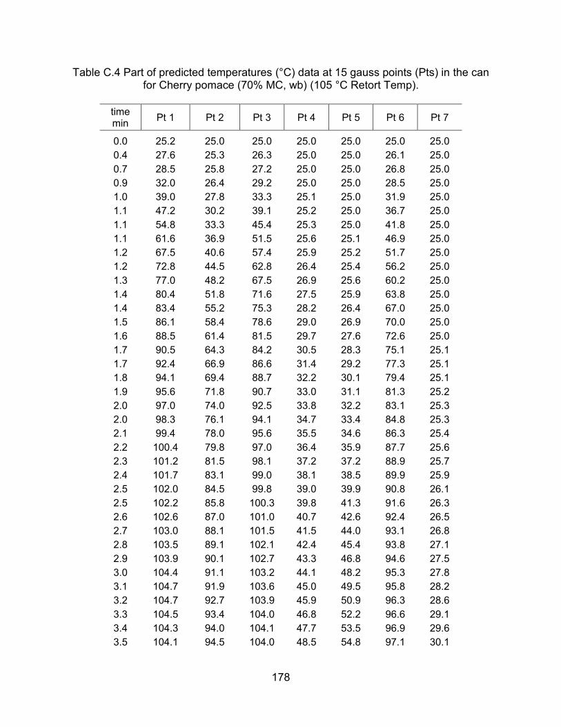
178

Table C.4 Part of predicted temperatures (°C) data at 15 gauss points (Pts) in the can for Cherry pomace (70% MC, wb) (105 °C Retort Temp).

time min

Pt 1 Pt 2 Pt 3 Pt 4 Pt 5 Pt 6 Pt 7

0.0 25.2 25.0 25.0 25.0 25.0 25.0 25.0

0.4 27.6 25.3 26.3 25.0 25.0 26.1 25.0

0.7 28.5 25.8 27.2 25.0 25.0 26.8 25.0

0.9 32.0 26.4 29.2 25.0 25.0 28.5 25.0

1.0 39.0 27.8 33.3 25.1 25.0 31.9 25.0

1.1 47.2 30.2 39.1 25.2 25.0 36.7 25.0

1.1 54.8 33.3 45.4 25.3 25.0 41.8 25.0

1.1 61.6 36.9 51.5 25.6 25.1 46.9 25.0

1.2 67.5 40.6 57.4 25.9 25.2 51.7 25.0

1.2 72.8 44.5 62.8 26.4 25.4 56.2 25.0

1.3 77.0 48.2 67.5 26.9 25.6 60.2 25.0

1.4 80.4 51.8 71.6 27.5 25.9 63.8 25.0

1.4 83.4 55.2 75.3 28.2 26.4 67.0 25.0

1.5 86.1 58.4 78.6 29.0 26.9 70.0 25.0

1.6 88.5 61.4 81.5 29.7 27.6 72.6 25.0

1.7 90.5 64.3 84.2 30.5 28.3 75.1 25.1

1.7 92.4 66.9 86.6 31.4 29.2 77.3 25.1

1.8 94.1 69.4 88.7 32.2 30.1 79.4 25.1

1.9 95.6 71.8 90.7 33.0 31.1 81.3 25.2

2.0 97.0 74.0 92.5 33.8 32.2 83.1 25.3

2.0 98.3 76.1 94.1 34.7 33.4 84.8 25.3

2.1 99.4 78.0 95.6 35.5 34.6 86.3 25.4

2.2 100.4 79.8 97.0 36.4 35.9 87.7 25.6

2.3 101.2 81.5 98.1 37.2 37.2 88.9 25.7

2.4 101.7 83.1 99.0 38.1 38.5 89.9 25.9

2.5 102.0 84.5 99.8 39.0 39.9 90.8 26.1

2.5 102.2 85.8 100.3 39.8 41.3 91.6 26.3

2.6 102.6 87.0 101.0 40.7 42.6 92.4 26.5

2.7 103.0 88.1 101.5 41.5 44.0 93.1 26.8

2.8 103.5 89.1 102.1 42.4 45.4 93.8 27.1

2.9 103.9 90.1 102.7 43.3 46.8 94.6 27.5

3.0 104.4 91.1 103.2 44.1 48.2 95.3 27.8

3.1 104.7 91.9 103.6 45.0 49.5 95.8 28.2

3.2 104.7 92.7 103.9 45.9 50.9 96.3 28.6

3.3 104.5 93.4 104.0 46.8 52.2 96.6 29.1

3.4 104.3 94.0 104.1 47.7 53.5 96.9 29.6

3.5 104.1 94.5 104.0 48.5 54.8 97.1 30.1

179

Table C.4, (Cont’d)

3.6 103.7 94.9 103.9 49.4 56.0 97.2 30.6

3.7 103.5 95.3 103.8 50.3 57.2 97.3 31.2

3.8 103.2 95.7 103.7 51.2 58.4 97.3 31.7

3.9 103.0 96.0 103.5 52.0 59.6 97.4 32.3

4.0 103.0 96.3 103.5 52.9 60.7 97.6 33.0

4.1 103.1 96.5 103.5 53.7 61.8 97.7 33.6

4.2 103.2 96.8 103.5 54.6 62.9 97.9 34.3

4.3 103.3 97.1 103.6 55.4 63.9 98.1 34.9

4.3 103.5 97.4 103.7 56.2 64.9 98.4 35.6

4.4 103.5 97.6 103.8 57.1 65.9 98.6 36.3

4.5 103.6 97.9 103.8 57.9 66.8 98.8 37.0

4.6 103.5 98.1 103.9 58.7 67.7 98.9 37.8 4.7 103.5 98.3 103.9 59.5 68.6 99.1 38.5

4.8 103.5 98.5 103.9 60.3 69.5 99.2 39.2

4.9 103.5 98.7 103.9 61.1 70.3 99.3 40.0

5.0 103.5 98.9 103.9 61.9 71.1 99.4 40.8

5.1 103.5 99.1 103.9 62.6 71.9 99.6 41.5

5.2 103.5 99.2 103.9 63.4 72.6 99.7 42.3 5.3 103.5 99.4 104.0 64.1 73.4 99.8 43.1

5.4 103.6 99.6 104.0 64.9 74.1 99.9 43.8

5.5 103.6 99.7 104.0 65.6 74.8 100.0 44.6

5.6 103.6 99.9 104.0 66.3 75.5 100.2 45.4

5.7 103.7 100.0 104.1 67.0 76.1 100.3 46.1

5.8 103.7 100.1 104.1 67.7 76.8 100.4 46.9

5.9 103.8 100.3 104.1 68.4 77.4 100.5 47.7

6.0 103.8 100.4 104.2 69.1 78.0 100.6 48.4

6.1 103.8 100.5 104.2 69.8 78.6 100.7 49.2

6.2 103.9 100.6 104.2 70.4 79.1 100.8 50.0

6.3 103.9 100.8 104.3 71.1 79.7 100.9 50.7

6.4 103.9 100.9 104.3 71.7 80.2 101.0 51.5

6.4 103.9 101.0 104.3 72.3 80.8 101.1 52.2

6.5 104.0 101.1 104.3 72.9 81.3 101.2 52.9

6.6 104.0 101.2 104.4 73.5 81.8 101.3 53.7

6.7 104.0 101.3 104.4 74.1 82.3 101.4 54.4

6.8 104.1 101.4 104.4 74.7 82.8 101.5 55.1

6.9 104.1 101.5 104.4 75.3 83.2 101.5 55.8

7.0 104.1 101.6 104.4 75.8 83.7 101.6 56.5

7.1 104.1 101.7 104.5 76.4 84.1 101.7 57.3

7.2 104.1 101.8 104.5 76.9 84.5 101.8 58.0

7.3 104.2 101.8 104.5 77.4 85.0 101.9 58.6

7.4 104.2 101.9 104.5 77.9 85.4 101.9 59.3

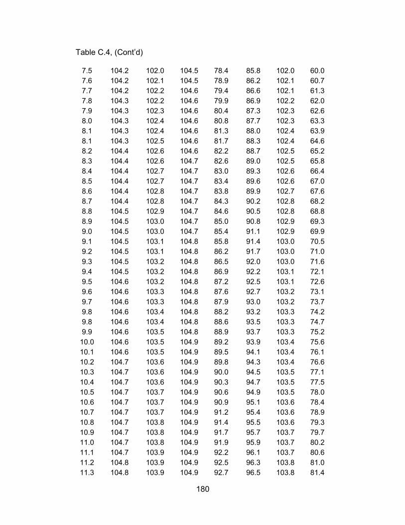
180

Table C.4, (Cont’d)

7.5 104.2 102.0 104.5 78.4 85.8 102.0 60.0

7.6 104.2 102.1 104.5 78.9 86.2 102.1 60.7

7.7 104.2 102.2 104.6 79.4 86.6 102.1 61.3

7.8 104.3 102.2 104.6 79.9 86.9 102.2 62.0

7.9 104.3 102.3 104.6 80.4 87.3 102.3 62.6

8.0 104.3 102.4 104.6 80.8 87.7 102.3 63.3

8.1 104.3 102.4 104.6 81.3 88.0 102.4 63.9

8.1 104.3 102.5 104.6 81.7 88.3 102.4 64.6

8.2 104.4 102.6 104.6 82.2 88.7 102.5 65.2

8.3 104.4 102.6 104.7 82.6 89.0 102.5 65.8

8.4 104.4 102.7 104.7 83.0 89.3 102.6 66.4

8.5 104.4 102.7 104.7 83.4 89.6 102.6 67.0

8.6 104.4 102.8 104.7 83.8 89.9 102.7 67.6

8.7 104.4 102.8 104.7 84.3 90.2 102.8 68.2

8.8 104.5 102.9 104.7 84.6 90.5 102.8 68.8

8.9 104.5 103.0 104.7 85.0 90.8 102.9 69.3

9.0 104.5 103.0 104.7 85.4 91.1 102.9 69.9

9.1 104.5 103.1 104.8 85.8 91.4 103.0 70.5

9.2 104.5 103.1 104.8 86.2 91.7 103.0 71.0

9.3 104.5 103.2 104.8 86.5 92.0 103.0 71.6

9.4 104.5 103.2 104.8 86.9 92.2 103.1 72.1

9.5 104.6 103.2 104.8 87.2 92.5 103.1 72.6

9.6 104.6 103.3 104.8 87.6 92.7 103.2 73.1

9.7 104.6 103.3 104.8 87.9 93.0 103.2 73.7

9.8 104.6 103.4 104.8 88.2 93.2 103.3 74.2

9.8 104.6 103.4 104.8 88.6 93.5 103.3 74.7

9.9 104.6 103.5 104.8 88.9 93.7 103.3 75.2

10.0 104.6 103.5 104.9 89.2 93.9 103.4 75.6

10.1 104.6 103.5 104.9 89.5 94.1 103.4 76.1

10.2 104.7 103.6 104.9 89.8 94.3 103.4 76.6

10.3 104.7 103.6 104.9 90.0 94.5 103.5 77.1

10.4 104.7 103.6 104.9 90.3 94.7 103.5 77.5

10.5 104.7 103.7 104.9 90.6 94.9 103.5 78.0

10.6 104.7 103.7 104.9 90.9 95.1 103.6 78.4

10.7 104.7 103.7 104.9 91.2 95.4 103.6 78.9

10.8 104.7 103.8 104.9 91.4 95.5 103.6 79.3

10.9 104.7 103.8 104.9 91.7 95.7 103.7 79.7

11.0 104.7 103.8 104.9 91.9 95.9 103.7 80.2

11.1 104.7 103.9 104.9 92.2 96.1 103.7 80.6

11.2 104.8 103.9 104.9 92.5 96.3 103.8 81.0

11.3 104.8 103.9 104.9 92.7 96.5 103.8 81.4

181

Table C.4, (Cont’d)

11.4 104.8 103.9 104.9 92.9 96.6 103.8 81.8

11.5 104.8 104.0 105.0 93.2 96.8 103.8 82.2

11.5 104.8 104.0 105.0 93.4 97.0 103.9 82.6

11.6 104.8 104.0 105.0 93.6 97.1 103.9 83.0

11.7 104.8 104.0 105.0 93.8 97.3 103.9 83.4

11.8 104.8 104.1 105.0 94.0 97.4 103.9 83.7

11.9 104.8 104.1 105.0 94.2 97.6 104.0 84.1

12.0 104.8 104.1 105.0 94.4 97.7 104.0 84.5

12.1 104.8 104.1 105.0 94.6 97.8 104.0 84.8

12.2 104.8 104.2 105.0 94.8 98.0 104.0 85.1

12.3 104.8 104.2 105.0 95.0 98.1 104.1 85.5

12.4 104.9 104.2 105.0 95.2 98.2 104.1 85.8

12.5 104.9 104.2 105.0 95.4 98.3 104.1 86.1

12.6 104.9 104.2 105.0 95.5 98.5 104.1 86.5

12.7 104.9 104.2 105.0 95.7 98.6 104.1 86.8

12.8 104.9 104.3 105.0 95.9 98.7 104.2 87.1

12.9 104.9 104.3 105.0 96.1 98.8 104.2 87.4

13.0 104.9 104.3 105.0 96.2 99.0 104.2 87.7

13.1 104.9 104.3 105.0 96.4 99.1 104.2 88.0

13.2 104.9 104.3 105.0 96.6 99.2 104.2 88.3

13.2 104.9 104.4 105.0 96.7 99.3 104.3 88.6

13.3 104.9 104.4 105.0 96.9 99.4 104.3 88.9

13.4 104.9 104.4 105.0 97.1 99.5 104.3 89.2

13.5 104.9 104.4 105.0 97.2 99.6 104.3 89.5

13.6 104.9 104.4 105.0 97.4 99.7 104.3 89.8

13.7 104.9 104.4 105.0 97.5 99.8 104.3 90.0

13.8 104.9 104.4 105.0 97.6 99.9 104.4 90.3

13.9 104.9 104.5 105.0 97.8 100.0 104.4 90.6

14.0 104.9 104.5 105.1 97.9 100.1 104.4 90.8

14.1 105.0 104.5 105.1 98.0 100.2 104.4 91.1

14.2 105.0 104.5 105.1 98.2 100.3 104.4 91.3

14.3 105.0 104.5 105.1 98.3 100.4 104.4 91.5

14.4 105.0 104.5 105.1 98.4 100.5 104.4 91.8

14.5 105.0 104.5 105.1 98.5 100.5 104.4 92.0

14.6 105.0 104.5 105.1 98.6 100.6 104.5 92.2

14.7 105.0 104.6 105.1 98.7 100.7 104.5 92.4

14.8 105.0 104.6 105.1 98.9 100.8 104.5 92.7

14.9 105.0 104.6 105.1 99.0 100.9 104.5 92.9

15.0 105.0 104.6 105.1 99.1 100.9 104.5 93.1

15.0 105.0 104.6 105.1 99.2 101.0 104.5 93.3

15.1 105.0 104.6 105.1 99.3 101.1 104.5 93.5

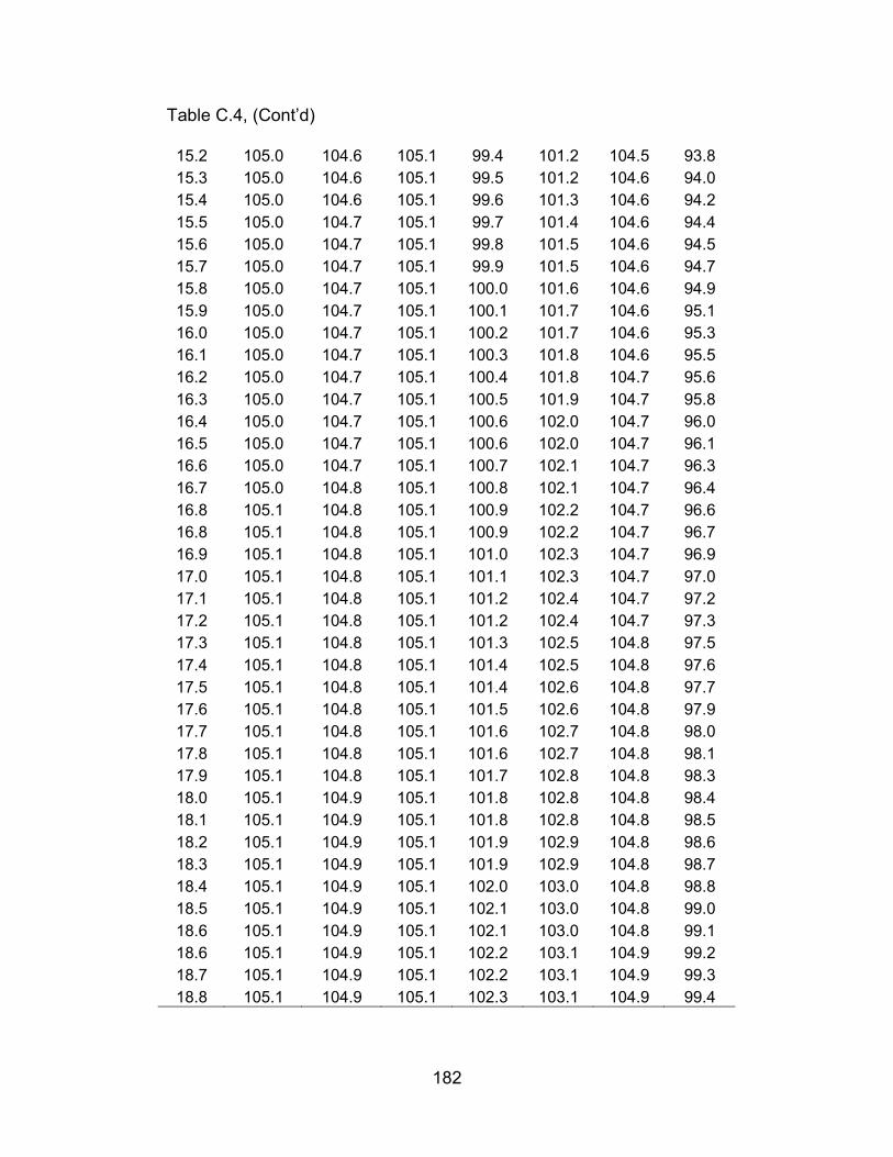
182

Table C.4, (Cont’d)

15.2 105.0 104.6 105.1 99.4 101.2 104.5 93.8

15.3 105.0 104.6 105.1 99.5 101.2 104.6 94.0

15.4 105.0 104.6 105.1 99.6 101.3 104.6 94.2

15.5 105.0 104.7 105.1 99.7 101.4 104.6 94.4

15.6 105.0 104.7 105.1 99.8 101.5 104.6 94.5

15.7 105.0 104.7 105.1 99.9 101.5 104.6 94.7

15.8 105.0 104.7 105.1 100.0 101.6 104.6 94.9

15.9 105.0 104.7 105.1 100.1 101.7 104.6 95.1

16.0 105.0 104.7 105.1 100.2 101.7 104.6 95.3

16.1 105.0 104.7 105.1 100.3 101.8 104.6 95.5

16.2 105.0 104.7 105.1 100.4 101.8 104.7 95.6

16.3 105.0 104.7 105.1 100.5 101.9 104.7 95.8

16.4 105.0 104.7 105.1 100.6 102.0 104.7 96.0

16.5 105.0 104.7 105.1 100.6 102.0 104.7 96.1

16.6 105.0 104.7 105.1 100.7 102.1 104.7 96.3

16.7 105.0 104.8 105.1 100.8 102.1 104.7 96.4

16.8 105.1 104.8 105.1 100.9 102.2 104.7 96.6

16.8 105.1 104.8 105.1 100.9 102.2 104.7 96.7

16.9 105.1 104.8 105.1 101.0 102.3 104.7 96.9

17.0 105.1 104.8 105.1 101.1 102.3 104.7 97.0

17.1 105.1 104.8 105.1 101.2 102.4 104.7 97.2

17.2 105.1 104.8 105.1 101.2 102.4 104.7 97.3

17.3 105.1 104.8 105.1 101.3 102.5 104.8 97.5

17.4 105.1 104.8 105.1 101.4 102.5 104.8 97.6

17.5 105.1 104.8 105.1 101.4 102.6 104.8 97.7

17.6 105.1 104.8 105.1 101.5 102.6 104.8 97.9

17.7 105.1 104.8 105.1 101.6 102.7 104.8 98.0

17.8 105.1 104.8 105.1 101.6 102.7 104.8 98.1

17.9 105.1 104.8 105.1 101.7 102.8 104.8 98.3

18.0 105.1 104.9 105.1 101.8 102.8 104.8 98.4

18.1 105.1 104.9 105.1 101.8 102.8 104.8 98.5

18.2 105.1 104.9 105.1 101.9 102.9 104.8 98.6

18.3 105.1 104.9 105.1 101.9 102.9 104.8 98.7

18.4 105.1 104.9 105.1 102.0 103.0 104.8 98.8

18.5 105.1 104.9 105.1 102.1 103.0 104.8 99.0

18.6 105.1 104.9 105.1 102.1 103.0 104.8 99.1

18.6 105.1 104.9 105.1 102.2 103.1 104.9 99.2

18.7 105.1 104.9 105.1 102.2 103.1 104.9 99.3

18.8 105.1 104.9 105.1 102.3 103.1 104.9 99.4

183

Table C.4, (Cont’d)

time min

Pt’ 8 Pt 9 Pt 10 Pt 11 Pt 12 Pt 13 Pt 14 Pt15

0.0 25.0 25.2 25.0 25.0 25.0 25.5 25.1 25.0

0.4 25.0 26.1 25.0 25.0 26.1 25.2 25.3 26.3

0.7 25.0 26.8 25.0 25.0 26.8 25.8 25.7 27.2

0.9 25.0 28.5 25.0 25.0 28.4 26.6 26.4 29.2

1.0 25.0 31.9 25.0 25.0 31.9 27.9 27.8 33.3

1.1 25.0 36.7 25.0 25.0 36.7 30.0 30.0 39.1

1.1 25.0 41.8 25.0 25.0 41.8 33.0 33.0 45.4

1.1 25.1 46.8 25.0 25.1 46.9 36.2 36.3 51.5

1.2 25.2 51.6 25.0 25.2 51.7 39.7 39.7 57.4

1.2 25.3 56.2 25.0 25.3 56.2 43.1 43.2 62.8

1.3 25.5 60.2 25.0 25.5 60.2 46.3 46.6 67.5

1.4 25.7 63.7 25.1 25.8 63.8 49.4 49.8 71.6

1.4 26.0 67.0 25.1 26.1 67.0 52.4 52.8 75.3

1.5 26.4 69.9 25.1 26.5 70.0 55.1 55.7 78.6

1.6 26.9 72.6 25.2 27.1 72.6 57.6 58.4 81.5

1.7 27.5 75.0 25.3 27.7 75.1 60.0 61.0 84.2

1.7 28.1 77.3 25.4 28.4 77.3 62.2 63.4 86.6

1.8 28.8 79.3 25.6 29.2 79.4 64.2 65.6 88.7

1.9 29.5 81.2 25.8 30.0 81.3 66.2 67.8 90.7

2.0 30.3 82.9 26.0 31.0 83.1 68.0 69.8 92.5

2.0 31.1 84.6 26.2 32.0 84.7 69.7 71.7 94.1

2.1 32.0 86.0 26.5 33.0 86.2 71.2 73.5 95.6

2.2 32.9 87.4 26.9 34.1 87.6 72.7 75.3 96.9

2.3 33.9 88.6 27.2 35.2 88.8 74.1 76.9 98.0

2.4 34.8 89.6 27.7 36.4 89.9 75.3 78.3 98.9

2.5 35.8 90.4 28.1 37.5 90.7 76.5 79.6 99.6

2.5 36.8 91.1 28.6 38.7 91.5 77.5 80.9 100.2

2.6 37.8 91.9 29.1 40.0 92.3 78.5 82.0 100.8

2.7 38.8 92.6 29.7 41.2 93.0 79.4 83.1 101.4

2.8 39.8 93.2 30.3 42.4 93.7 80.3 84.2 101.9

2.9 40.8 93.9 30.9 43.6 94.4 81.2 85.2 102.5

3.0 41.8 94.6 31.6 44.9 95.1 82.0 86.1 103.0

3.1 42.8 95.1 32.3 46.1 95.7 82.8 87.0 103.4

3.2 43.8 95.5 33.0 47.3 96.1 83.4 87.8 103.7

3.3 44.8 95.7 33.8 48.5 96.4 84.1 88.5 103.8

3.4 45.7 96.0 34.6 49.7 96.6 84.6 89.1 103.9

3.5 46.7 96.1 35.4 50.9 96.8 85.1 89.7 103.8

3.6 47.6 96.1 36.2 52.0 96.9 85.6 90.2 103.7

184

Table C.4, (Cont’d)

3.7 48.5 96.2 37.1 53.2 97.0 86.0 90.6 103.6

3.8 49.5 96.2 37.9 54.3 97.0 86.3 91.0 103.4

3.9 50.4 96.3 38.8 55.4 97.1 86.7 91.3 103.3

4.0 51.2 96.4 39.7 56.4 97.2 87.0 91.7 103.2

4.1 52.1 96.5 40.6 57.5 97.4 87.3 92.1 103.2

4.2 53.0 96.7 41.5 58.5 97.6 87.7 92.4 103.3

4.3 53.8 96.8 42.4 59.5 97.8 88.1 92.7 103.3

4.3 54.6 97.1 43.4 60.4 98.0 88.4 93.1 103.4

4.4 55.4 97.2 44.3 61.4 98.2 88.8 93.4 103.5

4.5 56.2 97.4 45.2 62.3 98.4 89.1 93.7 103.6

4.6 57.0 97.5 46.1 63.2 98.5 89.5 94.0 103.6 4.7 57.7 97.6 47.0 64.0 98.7 89.8 94.3 103.6

4.8 58.4 97.7 48.0 64.9 98.8 90.1 94.6 103.6

4.9 59.2 97.8 48.9 65.7 98.9 90.4 94.8 103.6

5.0 59.9 97.9 49.8 66.5 99.0 90.7 95.1 103.6

5.1 60.6 98.0 50.7 67.3 99.1 91.0 95.3 103.6

5.2 61.3 98.1 51.6 68.0 99.2 91.3 95.5 103.7 5.3 61.9 98.2 52.4 68.8 99.3 91.5 95.8 103.7

5.4 62.6 98.3 53.3 69.5 99.5 91.8 96.0 103.7

5.5 63.3 98.5 54.2 70.2 99.6 92.1 96.2 103.7

5.6 63.9 98.6 55.0 70.9 99.7 92.3 96.4 103.8

5.7 64.5 98.7 55.9 71.5 99.8 92.6 96.6 103.8

5.8 65.2 98.8 56.7 72.2 99.9 92.9 96.8 103.8

5.9 65.8 98.9 57.5 72.8 100.0 93.1 97.0 103.9

6.0 66.4 99.0 58.3 73.5 100.1 93.4 97.2 103.9

6.1 67.0 99.1 59.1 74.1 100.2 93.6 97.3 103.9

6.2 67.5 99.2 59.9 74.6 100.3 93.8 97.5 104.0

6.3 68.1 99.3 60.7 75.2 100.4 94.1 97.7 104.0

6.4 68.7 99.4 61.5 75.8 100.5 94.3 97.8 104.0

6.4 69.3 99.5 62.2 76.4 100.6 94.5 98.0 104.0

6.5 69.8 99.6 63.0 76.9 100.7 94.7 98.2 104.1

6.6 70.4 99.7 63.7 77.4 100.8 94.9 98.3 104.1

6.7 70.9 99.8 64.4 78.0 100.9 95.1 98.5 104.1

6.8 71.4 99.9 65.1 78.5 101.0 95.4 98.6 104.1

6.9 71.9 99.9 65.8 79.0 101.1 95.5 98.7 104.2

7.0 72.5 100.0 66.5 79.5 101.1 95.7 98.9 104.2

7.1 73.0 100.1 67.2 79.9 101.2 95.9 99.0 104.2

7.2 73.5 100.2 67.9 80.4 101.3 96.1 99.1 104.2

7.3 73.9 100.3 68.5 80.9 101.4 96.3 99.3 104.3

7.4 74.4 100.4 69.1 81.3 101.4 96.5 99.4 104.3

7.5 74.9 100.4 69.8 81.8 101.5 96.6 99.5 104.3

185

Table C.4, (Cont’d)

7.6 75.4 100.5 70.4 82.2 101.6 96.8 99.6 104.3

7.7 75.8 100.6 71.0 82.6 101.7 97.0 99.8 104.3

7.8 76.3 100.7 71.6 83.0 101.7 97.1 99.9 104.4

7.9 76.8 100.7 72.2 83.4 101.8 97.3 100.0 104.4

8.0 77.2 100.8 72.8 83.8 101.9 97.5 100.1 104.4

8.1 77.6 100.9 73.4 84.2 101.9 97.6 100.2 104.4

8.1 78.1 100.9 73.9 84.6 102.0 97.8 100.3 104.4

8.2 78.5 101.0 74.5 85.0 102.0 97.9 100.4 104.4

8.3 78.9 101.1 75.0 85.3 102.1 98.0 100.5 104.5

8.4 79.3 101.1 75.5 85.7 102.1 98.2 100.6 104.5

8.5 79.7 101.2 76.1 86.0 102.2 98.3 100.7 104.5

8.6 80.1 101.3 76.6 86.4 102.3 98.5 100.8 104.5

8.7 80.5 101.3 77.1 86.7 102.3 98.6 100.8 104.5

8.8 80.9 101.4 77.6 87.1 102.4 98.7 100.9 104.5

8.9 81.3 101.5 78.1 87.4 102.4 98.9 101.0 104.5

9.0 81.7 101.5 78.6 87.7 102.5 99.0 101.1 104.6

9.1 82.1 101.6 79.1 88.1 102.5 99.1 101.2 104.6

9.2 82.5 101.7 79.5 88.4 102.6 99.2 101.3 104.6

9.3 82.8 101.7 80.0 88.7 102.6 99.3 101.4 104.6

9.4 83.2 101.8 80.5 89.0 102.7 99.5 101.4 104.6

9.5 83.6 101.8 80.9 89.3 102.7 99.6 101.5 104.6

9.6 83.9 101.9 81.3 89.6 102.8 99.7 101.6 104.6

9.7 84.3 101.9 81.8 89.9 102.8 99.8 101.7 104.6

9.8 84.6 102.0 82.2 90.2 102.9 99.9 101.7 104.7

9.8 84.9 102.0 82.6 90.4 102.9 100.0 101.8 104.7

9.9 85.3 102.1 83.0 90.7 102.9 100.1 101.9 104.7

10.0 85.6 102.1 83.4 91.0 103.0 100.2 101.9 104.7

10.1 85.9 102.2 83.8 91.2 103.0 100.3 102.0 104.7

10.2 86.2 102.2 84.2 91.5 103.1 100.4 102.1 104.7

10.3 86.5 102.3 84.5 91.7 103.1 100.5 102.1 104.7

10.4 86.8 102.3 84.9 91.9 103.1 100.6 102.2 104.7

10.5 87.1 102.4 85.3 92.2 103.2 100.7 102.2 104.7

10.6 87.4 102.4 85.6 92.4 103.2 100.7 102.3 104.7

10.7 87.7 102.5 86.0 92.7 103.3 100.8 102.3 104.8

10.8 88.0 102.5 86.3 92.9 103.3 100.9 102.4 104.8

10.9 88.3 102.6 86.7 93.1 103.3 101.0 102.5 104.8

11.0 88.6 102.6 87.0 93.3 103.4 101.1 102.5 104.8

11.1 88.9 102.7 87.4 93.6 103.4 101.2 102.6 104.8

11.2 89.2 102.7 87.7 93.8 103.4 101.3 102.6 104.8

11.3 89.4 102.7 88.0 94.0 103.5 101.3 102.7 104.8

11.4 89.7 102.8 88.3 94.2 103.5 101.4 102.7 104.8

186

Table C.4, (Cont’d)

11.5 90.0 102.8 88.6 94.4 103.5 101.5 102.8 104.8

11.5 90.2 102.9 88.9 94.6 103.6 101.6 102.8 104.8

11.6 90.5 102.9 89.2 94.8 103.6 101.6 102.9 104.8

11.7 90.7 102.9 89.5 95.0 103.6 101.7 102.9 104.8

11.8 91.0 103.0 89.8 95.1 103.6 101.8 103.0 104.8

11.9 91.2 103.0 90.1 95.3 103.7 101.8 103.0 104.9

12.0 91.4 103.1 90.3 95.5 103.7 101.9 103.0 104.9

12.1 91.7 103.1 90.6 95.7 103.7 101.9 103.1 104.9

12.2 91.9 103.1 90.8 95.8 103.7 102.0 103.1 104.9

12.3 92.1 103.2 91.1 96.0 103.8 102.1 103.1 104.9

12.4 92.3 103.2 91.3 96.1 103.8 102.1 103.2 104.9

12.5 92.5 103.2 91.6 96.3 103.8 102.2 103.2 104.9

12.6 92.7 103.3 91.8 96.4 103.8 102.2 103.2 104.9

12.7 93.0 103.3 92.0 96.6 103.9 102.3 103.3 104.9

12.8 93.2 103.3 92.3 96.8 103.9 102.3 103.3 104.9

12.9 93.4 103.4 92.5 96.9 103.9 102.4 103.4 104.9

13.0 93.6 103.4 92.8 97.1 103.9 102.4 103.4 104.9

13.1 93.8 103.4 93.0 97.2 104.0 102.5 103.4 104.9

13.2 94.0 103.5 93.2 97.4 104.0 102.5 103.5 104.9

13.2 94.2 103.5 93.4 97.5 104.0 102.6 103.5 104.9

13.3 94.4 103.5 93.6 97.6 104.0 102.6 103.5 104.9

13.4 94.6 103.5 93.9 97.8 104.0 102.7 103.6 104.9

13.5 94.7 103.6 94.1 97.9 104.1 102.7 103.6 104.9

13.6 94.9 103.6 94.3 98.0 104.1 102.8 103.6 105.0

13.7 95.1 103.6 94.5 98.2 104.1 102.8 103.6 105.0

13.8 95.3 103.7 94.6 98.3 104.1 102.9 103.7 105.0

13.9 95.5 103.7 94.8 98.4 104.1 102.9 103.7 105.0

14.0 95.6 103.7 95.0 98.5 104.2 103.0 103.7 105.0

14.1 95.8 103.7 95.2 98.6 104.2 103.0 103.8 105.0

14.2 95.9 103.8 95.4 98.8 104.2 103.0 103.8 105.0

14.3 96.1 103.8 95.5 98.9 104.2 103.1 103.8 105.0

14.4 96.3 103.8 95.7 99.0 104.2 103.1 103.8 105.0

14.5 96.4 103.8 95.9 99.1 104.2 103.1 103.8 105.0

14.6 96.6 103.8 96.0 99.2 104.3 103.2 103.9 105.0

14.7 96.7 103.9 96.2 99.3 104.3 103.2 103.9 105.0

14.8 96.8 103.9 96.3 99.4 104.3 103.2 103.9 105.0

14.9 97.0 103.9 96.5 99.5 104.3 103.3 103.9 105.0

15.0 97.1 103.9 96.6 99.6 104.3 103.3 104.0 105.0

15.0 97.3 104.0 96.8 99.7 104.3 103.3 104.0 105.0

15.1 97.4 104.0 97.0 99.8 104.4 103.4 104.0 105.0

15.2 97.6 104.0 97.1 99.9 104.4 103.4 104.0 105.0

187

Table C.4, (Cont’d)

15.3 97.7 104.0 97.3 100.0 104.4 103.4 104.0 105.0

15.4 97.8 104.0 97.4 100.1 104.4 103.5 104.1 105.0

15.5 98.0 104.1 97.5 100.2 104.4 103.5 104.1 105.0

15.6 98.1 104.1 97.7 100.3 104.4 103.5 104.1 105.0

15.7 98.2 104.1 97.8 100.3 104.4 103.6 104.1 105.0

15.8 98.3 104.1 97.9 100.4 104.5 103.6 104.1 105.0

15.9 98.5 104.1 98.1 100.5 104.5 103.6 104.2 105.0

16.0 98.6 104.2 98.2 100.6 104.5 103.7 104.2 105.0

16.1 98.7 104.2 98.3 100.7 104.5 103.7 104.2 105.0

16.2 98.8 104.2 98.4 100.8 104.5 103.7 104.2 105.0

16.3 98.9 104.2 98.5 100.8 104.5 103.7 104.2 105.0

16.4 99.0 104.2 98.7 100.9 104.5 103.8 104.3 105.1

16.5 99.1 104.2 98.8 101.0 104.5 103.8 104.3 105.1

16.6 99.2 104.3 98.9 101.0 104.5 103.8 104.3 105.1

16.7 99.3 104.3 99.0 101.1 104.6 103.8 104.3 105.1

16.8 99.4 104.3 99.1 101.2 104.6 103.8 104.3 105.1

16.8 99.5 104.3 99.2 101.2 104.6 103.9 104.3 105.1

16.9 99.6 104.3 99.3 101.3 104.6 103.9 104.3 105.1

17.0 99.7 104.3 99.4 101.4 104.6 103.9 104.4 105.1

17.1 99.8 104.4 99.5 101.5 104.6 103.9 104.4 105.1

17.2 99.9 104.4 99.6 101.5 104.6 104.0 104.4 105.1

17.3 100.0 104.4 99.7 101.6 104.6 104.0 104.4 105.1

17.4 100.1 104.4 99.8 101.7 104.6 104.0 104.4 105.1

17.5 100.2 104.4 99.9 101.7 104.7 104.0 104.4 105.1

17.6 100.3 104.4 100.0 101.8 104.7 104.1 104.4 105.1

17.7 100.4 104.4 100.1 101.8 104.7 104.1 104.5 105.1

17.8 100.5 104.5 100.2 101.9 104.7 104.1 104.5 105.1

17.9 100.6 104.5 100.3 102.0 104.7 104.1 104.5 105.1

18.0 100.6 104.5 100.4 102.0 104.7 104.1 104.5 105.1

18.1 100.7 104.5 100.4 102.1 104.7 104.1 104.5 105.1

18.2 100.8 104.5 100.5 102.1 104.7 104.2 104.5 105.1

18.3 100.9 104.5 100.6 102.2 104.7 104.2 104.5 105.1

18.4 100.9 104.5 100.7 102.2 104.7 104.2 104.5 105.1

18.5 101.0 104.5 100.8 102.3 104.7 104.2 104.6 105.1

18.6 101.1 104.6 100.8 102.3 104.7 104.2 104.6 105.1

18.6 101.2 104.6 100.9 102.4 104.8 104.3 104.6 105.1

18.7 101.2 104.6 101.0 102.4 104.8 104.3 104.6 105.1

18.8 101.3 104.6 101.1 102.5 104.8 104.3 104.6 105.1

188

Appendix C.3 MATLAB syntaxes

C.3.1 Script file for reference temperature determination %for cherry pomace retorting % Retorting at 126.7 and 105 C for three MC( 70 41 and 25 %) %% cleaning work space clc clear close all format compact format shortG %% PLOT OF Tr VS Correlation for E and kr ( estimated parameter) % TrV = 110:2:130; % for starting evaluation TrV = 110:1:120; % for getting the exact Tr for i = 1:length(TrV); Tr = TrV(i); corr(i) = Call_calcC2Tr(Tr); % script File of kr and E estimation convert to Function file, which will % call the function file for all 15 points in the can for each MC % for ACY degradation data after Diff retorting times at Two RT temp end %% Plot to read the exact Tr Figure hold on set(gca, 'fontsize',18,'fontweight','bold'); h = plot(TrV,corr,'-k', 'linewidth',2.5); xlabel('Reference Temperature \it{T_r} , \rm\bf(^oC)','FontSize',16,'fontweight','bold'); ylabel('Correlation Coefficient of \it{k_r} and \itE','FontSize',16,'fontweight','bold'); plot([min(TrV),max(TrV)],[0,0], 'R','linewidth',2) grid on C.3.2 Function file-1 and 2 % ( was Script file for E kr and Co estimation) function corrkE=Call_calcC2Tr(Tr); format compact format shortG %% Read in ACY concentration data ACY =xlsread('ACY_con1.xls'); % 1st column time(min); each column onwards would represent ACY conc in (mg/L,db)... %(example: for 3 Moisture contents there would be three column..each column representing a specific MC ( MC-70 , MC-41, MC-25) % ht=ACY(:,1); %Retoorting time in in Mint

189

ACY1=[ACY(:,2);ACY(:,5)] ; % ACY concentration (mg/L,db) for MC-70 ACY1=ACY1(isfinite(ACY1)); % Command to take out all ANN ( no data) in the vector) and combine it % ACY2=[ACY(:,3);ACY(:,6)]; % ACY concentration (mg/L,db) for MC-41 % ACY3=[ACY(:,4);ACY(:,4)] % ACY concentration (mg/L,db) for MC-25 % ht=1; %% Initial parameter guesses E=50000; % initial guess activation energy %Ea must be in j/mol kr=0.05; % initial guess kinetic degradation constant %kr must be in min^-1 Co= 60; % initial guess of ACY initial concentration beta0(1)=E; %initial guess kfactor=exp((-beta0(1)/8.314)*(1/(Tr+273.15)-1/(122.5+273.15))); beta0(2)=kr*kfactor; %initial guess beta0(3)=Co; %initial guess % beta0(4)=m; %initial guess beta=beta0; %set beta=to the initial guesses %% Read in prediction 15 points data by Comsol foe each time and each MC two temp 126.7 global Prd_points3 Prd_points4 % for script and function file , Prd_points3 = xlsread('points70MC2.xls','90min');% all predicted temperature data with time at 15 gauss points in the can time=[0,181,271,391,571,631,781]; % steps heating times by Retort in Excel sheet (0 25 40 60 90 100 125 min) all + 5min come up time % for j = 1:length(ht); %% Read in prediction 15 points data by Comsol foe each time and each MC temp 105 Prd_points4 = xlsread('points70MC1.xls','90min');% all predicted data with time time=[0,181,271,391,571,631,781]; % steps heating times by Retort in Excel sheet (0 25 40 60 90 100 125 min) all + 5min come up time %% nlinfit returns parameters, residuals, Jacobean (sensitivity %coefficient matrix), %covariance matrix, and mean square error. timec=[0 0 0 25 25 25 40 40 40 60 60 60 90 90 90 0 0 0 100 100 100 125 125 125]; x1 =1:length(timec); timec=timec'; x1=x1'; x1(1,2)=Tr; ACY1=ACY1; [beta,resids,J,COVB,mse] = nlinfit(x1,ACY1,'calcC2Tr',beta0); % calling second function file with Trapz and gauss integration beta; rmse=sqrt(mse); %% confidence intervals for parameters ci=nlparci(beta, resids,J); %% R is the correlation matrix for the parameters, sigma is the standard error vector

190

[R,sigma]=corrcov(COVB); sigma; R; relstderr=sigma./beta'; %relative standard error for each parameter corrkE=R(2,1); % correlation matrix for E and kr end %%Function file-2 %integration ACY over the 15 points in the can function C70= calcC2Tr(beta,x) global Prd_points3 Prd_points4 ht=[181,271,391,571,631,781]; % heating times by Retort Rg = 8.314 ; % gas constant Tr = x(1,2)+273.15; % reference temperature Tr count=1; psiall=zeros(1,15); for m=1:2; % retort Temp loop data 15 points 2 files ( two Tretort) for j = 1:length(ht); % heating times , [25 40 60 90 100 125] if j==1 psiall(count,:)=0; count=count+1; end %Trapezoid method for i=1:15; % loop for the Temp data for15 points in the can if m==1 intgrnd1 = exp(-(beta(1)/Rg)*( 1./(Prd_points3(1:ht(j),i+1)+273.15) - 1/Tr)); % previous line for integration the % Eq.. Psi=exp(-E/R*((1/(T(r,z,t))-(1/Tr)) timex = Prd_points3(1:ht(j),1)./60; psia(i)=trapz(timex,intgrnd1);% Trapz Integration of Psi @ 127 C elseif m==2 intgrnd2 = exp(-(beta(1)/Rg)*( 1./(Prd_points4(1:ht(j),i+1)+273.15) - 1/Tr)); timex = Prd_points4(1:ht(j),1)./60; psia(i)=trapz(timex,intgrnd2);% Trapz Integration of Psi@105 C end end psiall(count,:)=psia; count=count+1; end end % psiall=psiall'; % psiall(2:5,:)=psiall(1:4,:); % psiall(1,:)=0;

191

% Gauss method wr=[5/9 8/9 5/9]; %Gauss nodes weight values 3 points wz=[0.2369268850 0.4786286705 0.5688888889 0.4786286705 0.2369268850]; %z direction r=[0.11270167,0.5,0.8872983]; %points nodes values for 0 to 1 dimintion r direction for k=1:14; % values of ACY at zero and Retorting times ( 0 25 40 60 90 100 125) ct=1; Csum=0; for j=1:5; % weight values at 5 points (z direction) for i=1:3; % radius values 3 points ( r direction) Csum=Csum+wr(i)*wz(j)*exp(-beta(2)*psiall(k,ct))*r(i); % for Eq.. ACY(C)=exp(-kr*(exp(-E/R*((1/(T(r,z,t))-(1/Tr)))*rdr ct=ct+1; end end C(k)=beta(3)*Csum/2; % for Eq.. ACY(t)=Acy(0)*exp(-kr*(exp(-E/R*((1/(T(r,z,t))-(1/Tr)))*rdr C70(3*(k-1)+1:3*(k-1)+3)=C(k); end C70=C70'; %values of predicted ACY values at all times two cans ( all data +ANN) C70=[C70(1:15);C70(22:24);C70(37:42)]; % to take only rows with data and combine them in vector 24by1, from 42by1 which have ann data end C.3.3 Script file scaled sensitivity coefficients %for the two retorting temperature % For invers problem estimation % Retorting Process at 126.7 C and 105 C %% Clean Up and organizing cell clc clear close all format compact format shortG %% Read in prediction 9 points data by Comsol foe each time and each MC temp 105 Prd_points3 = xlsread('points70MC2.xls','90min');% all predicted data with time time=[0,181,271,391,571,631]; % for j = 1:length(ht); % timet = Prd_points(1:time(j),1)./60; % end %% Read in prediction 9 points data by Comsol foe each time and each MC temp 127 Prd_points4 = xlsread('points70MC1.xls','90min');% all predicted data with time

192

time=[0,181,271,391,571,631]; % for j = 1:length(ht); % timet = Prd_points(1:time(j),1)./60; % end %% Scale Sensitivity Coefficient beta=[45000; 0.019; 60]; x1 =1:36; timec=[0 0 0 25 25 25 40 40 40 60 60 60 90 90 90 100 100 100 0 0 0 25 25 25 40 40 40 60 60 60 90 90 90 100 100 100]; timec=timec'; x1=x1'; ypred=calcC2T(beta,x1) beta1 = beta; % Sensitivity Coefficient d=0.001; for i=1:length(beta) if i ==1 betain = [beta1(1)+beta1(1)*d beta1(2) beta1(3)]; elseif i==2 betain = [beta1(1) beta1(2)+beta1(2)*d beta1(3)]; elseif i==3 betain = [beta1(1) beta1(2) beta1(3)+beta1(3)*d]; end yhat{i} = calcC2T(betain,x1); ysens{i} = (yhat{i}-ypred)/d; end %% sensitivity coefficient plot set(Figure,'Units','inches','Position',[7.1 0.3 6 4],'DefaultAxesFontName','Arial', ... 'DefaultAxesFontSize',12,'DefaultAxesFontWeight','Normal'); hold on set(gca, 'YGrid', 'on', 'XGrid','off'); ysens1 = ysens{1}; ysens2 = ysens{2}; ysens3 = ysens{3}; %g1(1) = plot(x_graph,ysens{1},'-','LineWidth',2); %g1(2) = plot(x_graph,ysens{2},':','LineWidth',2); plot(timec(1:18),ysens1(1:18),':bo','lineWidth',3,'MarkerEdgeColor','b','MarkerFaceColor','b','MarkerSize',6); plot(timec(1:18),ysens2(1:18),':ro','lineWidth',3,'MarkerEdgeColor','b','MarkerFaceColor','y','MarkerSize',6); plot(timec(1:18),ysens3(1:18),':go','lineWidth',2,'MarkerEdgeColor','b','MarkerFaceColor','y','MarkerSize',6);

193

plot(timec(19:36),ysens1(19:36),':bo','lineWidth',2,'MarkerEdgeColor','b','MarkerFaceColor','y','MarkerSize',6); plot(timec(19:36),ysens2(19:36),':k '̂,'lineWidth',2,'MarkerEdgeColor','r','MarkerFaceColor','y','MarkerSize',6); plot(timec(19:36),ysens3(19:36),':g '̂,'lineWidth',3,'MarkerEdgeColor','r','MarkerFaceColor','y','MarkerSize',6); box on YLine = [0 0]; XLine = [0 timec(length(timec))];%max() plot (XLine, YLine,'R'); legend('Ea -127 ^oC','kr-127 ^oC','Co-127 ^oC','Ea-105 ^oC','kr105 ^oC','Co105 ^oC','location','best'); xlabel('time(min)','FontSize',14,'fontweight','Normal'); ylabel('Scaled Sensitivity Coefficeints','FontSize',14,'fontweight','Normal'); C.3.4 Script file for nlinfit method % for kr, E , and Co of Cherry pomace % Retorting Process at 126.7 C and 105 C %% Clean Up and organizing cell clc clear close all format compact format shortG %% Read in ACY concentration data ACY =xlsread('ACY_con1.xls'); % 1st column time(min); each column onwards would represent ACY conc in (mg/L,db)... %(example: for 3 Moisture contents there would be three column..each column representing a specific MC ( MC-70 , MC-41, MC-25) ACY1=[ACY(:,2);ACY(:,5)] ; % ACY concentration (mg/L,db) for MC-70 at 127 C and 105 , respectively ACY1=ACY1(isfinite(ACY1)); % organizing all data one collomn 24 rows % ACY2=[ACY(:,3);ACY(:,6)]; % ACY concentration (mg/L,db) for MC-41 % ACY3=[ACY(:,4);ACY(:,4)] % ACY concentration (mg/L,db) for MC-25 % ht=1; %% Initial parameter guesses E=50000; % initial guess activation energy %Ea must be in j/mol kr=0.05; % initial guess kintek degradation constant %kr must be in min^-1 Co= 60; % initial guess of ACY initial concentration beta0(1)=E; %initial guess beta0(2)=kr; %initial guess beta0(3)=Co; %initial guess beta=beta0; %set beta=to the initial guesses

194

%% Read in prediction 15 points data by Comsol foe each time and each MC temp 126.7 C global Prd_points3 Prd_points4 % to connect data from script file with function file Prd_points3 = xlsread('points70MC2.xls','90min');% all predicted data with time %% Read in prediction 15 points data by Comsol foe each time and each MC temp 105 C Prd_points4 = xlsread('points70MC1.xls','90min');% all predicted data with time time=[0,181,271,391,571,631,781]; %% nlinfit returns parameters, residuals, Jacobean (sensitivity %coefficient matrix), timec=[0 0 0 25 25 25 40 40 40 60 60 60 90 90 90 0 0 0 100 100 100 125 125 125]; % heating time at the two temp x1 =1:length(timec); timec=timec'; x1=x1'; [beta,resids,J,COVB,mse] = nlinfit(x1,ACY1,'calcC2T',beta0); beta % results of estimation rmse=sqrt(mse) %% confidence intervals for parameters ci=nlparci(beta, resids,J) %% R is the correlation matrix for the parameters, sigma is the standard error vector [R,sigma]=corrcov(COVB); sigma R relstderr=sigma./beta' %relative standard error for each parameter %% Confidence and prediction intervals for the dependent variable % nonlinear regression confidence intervals-- 'on' means simultaneous % bounds; 'off' is for non-simultaneous bounds; must use 'curve' for % regression line, 'observation' for prediction interval [ypred, delta] = nlpredci('calcC2T',x1,beta,resids,J,0.05,'on','curve'); %confidence band for regression line [ypred, deltaob] =nlpredci('calcC2T',x1,beta,resids,J,0.05,'on','observation');%prediction band for individual points % ypred %simultaneous confidence bands for regression line CBu=ypred+delta; CBl=ypred-delta; % simultaneous prediction bands for regression line PBu=ypred+deltaob; PBl=ypred-deltaob; %% Plot Pred vs Obs of ACY set(Figure,'Units','inches','Position',[0.1 0.4 6 4],'DefaultAxesFontName','Arial', ... 'DefaultAxesFontSize',12,'DefaultAxesFontWeight','Normal'); hold on

195

h1(1)=plot(timec(1:15),ypred(1:15),'-b','Markerfacecolor', 'b'); %predicted y values h1(2)=plot(timec(1:15),ACY1(1:15),'square', 'Markerfacecolor', 'r'); set(gca, 'YGrid', 'on', 'XGrid','off'); box on; xlabel('time (min)','FontSize',14,'fontweight','Normal'); ylabel('ACYpred-ACYobs','FontSize',14,'fontweight','Normal'); title('ACYoobs vs ACYprd @127C') legend('pred','obs','location','best'); hold on %% Output --CIs and PIs %plot Cobs, Cpred line, confidence band for regression line hold on h1(3) = plot(timec(1:15),CBu(1:15),'--g','LineWidth',2); plot(timec(1:15),CBl(1:15),'--g','LineWidth',2); hold on %plot prediction band for regression line h1(4) = plot(timec(1:15),PBu(1:15),'-.r','LineWidth',2); plot(timec(1:15),PBl(1:15),'-.r','LineWidth',2); legend('ACYpred','ACYobs','CB','PB','location','best') %% residual scatter plot set(Figure,'Units','inches','Position',[0.5 0.6 6 4],'DefaultAxesFontName','Arial', ... 'DefaultAxesFontSize',12,'DefaultAxesFontWeight','Normal'); hold on plot(timec(1:24), resids(1:24), 'square','Markerfacecolor', 'b'); YLine = [0 0]; XLine = [0 max(timec)]; plot (XLine, YLine,'k'); %plot a straight red line at zero set(gca, 'YGrid', 'on', 'XGrid','off'); box on; ylabel('Observed ACY - Predicted ACY','fontsize',14,'fontweight','Normal'); xlabel('time (min)','fontsize',14,'fontweight','Normal'); %% residuals histogram--same as dfittool, but no curve fit here [n1, timecout] = hist(resids(1:24),10); %10 is the number of bins set(Figure,'Units','inches','Position',[0.5 0.6 6 4],'DefaultAxesFontName','Arial', ... 'DefaultAxesFontSize',12,'DefaultAxesFontWeight','Normal'); hold on set(gca, 'YGrid', 'on', 'XGrid','off'); box on; bar(timecout, n1) % plots the histogram xlabel('Y_{observed} - Y_{predicted}','fontsize',14,'fontweight','Normal'); ylabel('Frequency','fontsize',14,'fontweight','Normal');

196

%% Function file for estimating SSC and for inlinfit to estimate E kr and Co for ACY degradation function C70= calcC2T(beta,x) global Prd_points3 Prd_points4 ht=[181,271,391,571,631,781]; % j=1:length(ht); R = 8.314 ; % gas constant Tr = 114.9+273.15 ; % temp reference ,Tr count=1; psiall=zeros(1,15); for m=1:2;% retort Temp data 15 pints 2 files for j = 1:length(ht); % heating times , [25 40 60 90 100 125] if j==1 psiall(count,:)=0; count=count+1; end % TRAPZ method for i=1:15; % Temp data for 15 points in the can if m==1 intgrnd1 = exp(-(beta(1)/R)*( 1./(Prd_points3(1:ht(j),i+1)+273.15) - 1/Tr)); timex = Prd_points3(1:ht(j),1)./60; psia(i)=trapz(timex,intgrnd1);% Trapz Integration of Psi @ 127 C elseif m==2 intgrnd2 = exp(-(beta(1)/R)*( 1./(Prd_points4(1:ht(j),i+1)+273.15) - 1/Tr)); timex = Prd_points4(1:ht(j),1)./60; psia(i)=trapz(timex,intgrnd2);% Trapz Integration of Psi@ 105 C end end psiall(count,:)=psia; count=count+1; % psia end end % xlswrite('Ssiall_ACy70.xls', psia); % psiall=psiall'; % psiall(2:5,:)=psiall(1:4,:); % psiall(1,:)=0; % Gauss method wr=[5/9 8/9 5/9]; %Gauss nodes weight values 3 points wz=[0.2369268850 0.4786286705 0.5688888889 0.4786286705 0.2369268850]; %z direction r=[0.11270167,0.5,0.8872983]; %points nodes values for 0 t0 1 dimintion r direction

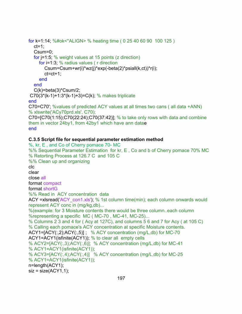
197

for k=1:14; %#ok<*ALIGN> % heating time ( 0 25 40 60 90 100 125 ) ct=1; Csum=0; for j=1:5; % weight values at 15 points (z direction) for i=1:3; % radius values ( r direction Csum=Csum+wr(i)*wz(j)*exp(-beta(2)*psiall(k,ct))*r(i); ct=ct+1; end end C(k)=beta(3)*Csum/2; C70(3*(k-1)+1:3*(k-1)+3)=C(k); % makes triplicate end C70=C70'; %values of predicted ACY values at all times two cans ( all data +ANN) % xlswrite('ACy70prd.xls', C70); C70=[C70(1:15);C70(22:24);C70(37:42)]; % to take only rows with data and combine them in vector 24by1, from 42by1 which have ann datae end C.3.5 Script file for sequential parameter estimation method %, kr, E , and Co of Cherry pomace 70- MC %% Sequential Parameter Estimation for kr, E , Co and b of Cherry pomace 70% MC % Retorting Process at 126.7 C and 105 C %% Clean up and organizing clc clear close all format compact format shortG %% Read in ACY concentration data ACY =xlsread('ACY_con1.xls'); % 1st column time(min); each column onwards would represent ACY conc in (mg/kg,db)... %(example: for 3 Moisture contents there would be three column..each column %representing a specific MC ( MC-70 , MC-41, MC-25)... % Columns 2 3 and 4 for ( Acy at 127C), and columns 5 6 and 7 for Acy ( at 105 C) % Calling each pomace's ACY concentration at specific Moisture contents. ACY1=[ACY(:,2);ACY(:,5)] ; % ACY concentration (mg/L,db) for MC-70 ACY1=ACY1(isfinite(ACY1)); % to clear all empty cells % ACY2=[ACY(:,3);ACY(:,6)]; % ACY concentration (mg/L,db) for MC-41 % ACY1=ACY1(isfinite(ACY1)); % ACY3=[ACY(:,4);ACY(:,4)] % ACY concentration (mg/L,db) for MC-25 % ACY1=ACY1(isfinite(ACY1)); n=length(ACY1); siz = size(ACY1,1);

198

%% Initial parameter guesses E/R=40000/8.314; % initial guess activation energy %Ea must be in J/mol kr=0.05; % initial guess kintek degradation constant %kr must be in min^-1 Co= 60; % initial guess of ACY initial concentration (mg/kg) % m=0.5; % initial guess of MC parameter beta0(1)=E; %initial guess beta0(2)=kr; %initial guess beta0(3)=Co; %initial guess beta=beta0; %set beta=to the initial guesses beta=beta'; beta0=beta0'; %% Read in prediction 15 points data by Comsol for each time and each MC temp 126.7 C global Prd_points3 Prd_points4 seqsort Prd_points3 = xlsread('points70MC2.xls','90min');% all predected Gauss temperature data with time %% Read in prediction 15 points data by Comsol foe each time and each MC temp 105 Prd_points4 = xlsread('points70MC1.xls','90min'); % time=[0,181,271,391,571,631,781]; % steps at Excel file for each time %% Heating time at Retort timec=[0 0 0 25 25 25 40 40 40 60 60 60 90 90 90 0 0 0 100 100 100 125 125 125]; x=1:length(timec); timec=timec'; x=x'; %% Estimating the ACy predected Concentration % For estimation the ACY predicted based of the 15 Temperature Gauss points ypred =calcC2T(beta0, x); % for Indicating the Retort temperature of the Figures ypredRT=[ypred 127*ones(length(ypred),1)]; ypredRT(16:24,2)=105; % for arranging the ACY pred from high to low [tT,seqsort]=sortrows(ypredRT,-1); Ynn=ACY1(seqsort);%ACY cons sorted p=length(beta);% all initial gess parameters yvals=Ynn; Y = yvals; sX = [length(yvals) length(beta)]; % changed from 1*2 to 2*1 sig = 8*ones(sX(1),1);% making vector 1colomn by 24 raws( 1*0.1) Ratio1 = 1;Ratio2 = 1; Ratio3= 1; plots=0; b_old =beta ; tol=1e-4; % For Iteration limit for repeating of calculation set(Figure,'Units','inches','Position',[7.1 0.3 6 4],'DefaultAxesFontName','Arial', ...

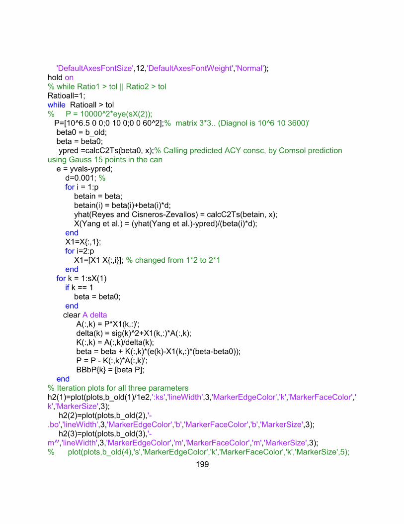
199

'DefaultAxesFontSize',12,'DefaultAxesFontWeight','Normal'); hold on % while Ratio1 > tol || Ratio2 > tol Ratioall=1; while Ratioall > tol % P = 10000^2*eye(sX(2)); P=[10^6.5 0 0;0 10 0;0 0 60^2];% matrix 3*3.. (Diagnol is 10^6 10 3600)' beta0 = b_old; beta = beta0; ypred =calcC2Ts(beta0, x);% Calling predicted ACY consc, by Comsol prediction using Gauss 15 points in the can e = yvals-ypred; d=0.001; % for i = 1:p betain = beta; betain(i) = beta(i)+beta(i)*d; yhat(Reyes and Cisneros-Zevallos) = calcC2Ts(betain, x); X(Yang et al.) = (yhat(Yang et al.)-ypred)/(beta(i)*d); end X1=X{:,1}; for i=2:p X1=[X1 X{:,i}]; % changed from 1*2 to 2*1 end for k = 1:sX(1) if k == 1 beta = beta0; end clear A delta A(:,k) = P*X1(k,:)'; delta(k) = sig(k)^2+X1(k,:)*A(:,k); K(:,k) = A(:,k)/delta(k); beta = beta + K(:,k)*(e(k)-X1(k,:)*(beta-beta0)); P = P - K(:,k)*A(:,k)'; BBbP{k} = [beta P]; end % Iteration plots for all three parameters h2(1)=plot(plots,b_old(1)/1e2,':ks','lineWidth',3,'MarkerEdgeColor','k','MarkerFaceColor','k','MarkerSize',3); h2(2)=plot(plots,b_old(2),'-.bo','lineWidth',3,'MarkerEdgeColor','b','MarkerFaceColor','b','MarkerSize',3); h2(3)=plot(plots,b_old(3),'-m '̂,'lineWidth',3,'MarkerEdgeColor','m','MarkerFaceColor','m','MarkerSize',3); % plot(plots,b_old(4),'s','MarkerEdgeColor','k','MarkerFaceColor','k','MarkerSize',5);

200

xlabel('Iteration','FontSize',14,'fontweight','Normal'); ylabel('Sequentially Estimated Parameters','FontSize',14,'fontweight','Normal'); b_new = BBbP{end}; plots = plots+1; % Ratioall = abs((b_new(:,1)-b_old)./b_old); Ratioall = max(abs((b_new(:,1)-b_old)./b_old)); % Ratio1 = Ratioall(1); % Ratio2 = Ratioall(2); b_old = b_new(:,1); end set(gca, 'YGrid', 'on', 'XGrid','off'); legend(h2,'par1=Ea*10^{3}','par2= kr','par3=Co','Location','Best'); corrcoef = P(2,1)/(sqrt(P(1,1))*sqrt(P(2,2))); % [R,sigma]=corrcov(P); % relerr=stderr./b_old n=length(yvals);K=length(beta)+1; SS=e'*e; p=length(beta); mse=SS/(n-p);rmse=sqrt(mse) AICc= n*log(SS/n)+2*K+2*K*(K-1)/(n-K-1); % Data estimated for each parameter Result = BBbP{end}; hold off for i = 1:length(BBbP) BB = BBbP{i}; SeqBeta(:,i) = BB(:,1); end % Plotting the Sequential Estimation for Each parameter %% 1. Plot for Activation Energy (Ea) ( J/mol) step=1:n; set(Figure,'Units','inches','Position',[0.1 0.4 6 4],'DefaultAxesFontName','Arial', ... 'DefaultAxesFontSize',12,'DefaultAxesFontWeight','Normal'); hold on for i=1:24; if tT(i,2)==127; h3(1)=plot(i,SeqBeta(1,i)*8.314','-rs','LineWidth',1.5,'MarkerEdgeColor','k','MarkerFaceColor','g','MarkerSize',8); elseif tT(i,2)==105; h3(2)=plot(i,SeqBeta(1,i)*8.314','-ro','lineWidth',1.5,'MarkerEdgeColor','k','MarkerFaceColor','w','MarkerSize',8); end end h3(3)=plot(step,SeqBeta(1,:)*8.134','-k','lineWidth',2);

201

set(gca, 'YGrid', 'on', 'XGrid','off'); legend(h3,'126.7 \circC','105 \circC','Ea (J/mol)','location','northWest'); box on ylabel('Sequentially Estimated E( J/mol)','FontSize',14,'fontweight','Normal'); xlabel('step Index','FontSize',14,'fontweight','Normal'); %% 2. Plot for Reaction rate (kr) ( min^-1) set(Figure,'Units','inches','Position',[7.3 3.3 6 4],'DefaultAxesFontName','Arial', ... 'DefaultAxesFontSize',12,'DefaultAxesFontWeight','Normal'); hold on for i=1:24; if tT(i,2)==127; h3(1)=plot(i,SeqBeta(2,i)','-.ks','lineWidth',1.5,'MarkerEdgeColor','k','MarkerFaceColor','g','MarkerSize',8); elseif tT(i,2)==105; h3(2)=plot(i,SeqBeta(2,i)','-.ro','lineWidth',1.5,'MarkerEdgeColor','k','MarkerFaceColor','w','MarkerSize',8); end end h3(3)=plot(step,SeqBeta(2,:)','-k','lineWidth',2); set(gca, 'YGrid', 'on', 'XGrid','off'); legend(h3,'126.7 \circC','105 \circC','kr (min^{-1})','location’,’ northeast'); box on xlabel('step Index','FontSize',12,'fontweight','Normal'); ylabel('Sequentially Estimated kr(min^{-1})','FontSize',12,'fontweight','Normal'); %% 3. Plot for Reaction rate (Co) ( mg/kg) set(Figure,'Units','inches','Position',[0.1 3.2 6 4],'DefaultAxesFontName','Arial', ... 'DefaultAxesFontSize',12,'DefaultAxesFontWeight','Normal'); hold on for i=1:24; if tT(i,2)==127; h3(1)=plot(i,SeqBeta(3,i)','ks','lineWidth',1.5,'MarkerEdgeColor','k','MarkerFaceColor','g','MarkerSize',10); elseif tT(i,2)==105; h3(2)=plot(i,SeqBeta(3,i)','ro','lineWidth',1.5,'MarkerEdgeColor','k','MarkerFaceColor','w','MarkerSize',10); end end hold on h3(3)=plot(step,SeqBeta(3,:)','-k','lineWidth',2); set(gca, 'YGrid', 'on', 'XGrid','off'); legend(h3,'126.7 \circC','105 \circC','C_{\ito}(mg/kg)','location','best'); box on xlabel('step Index','fontname','Arial','FontSize',14,'fontweight','Normal');

202

ylabel('Sequentially Estimated C_{\ito}(mg/kg)','fontname','Arial','FontSize',14,'fontweight','Normal'); %% Function 1 for seq script file to estimate ACY predicted data (Seq Sorted data) %% Function 1 for estimating ACY pridected data (Seq Sorted data) % Trapezoidal and Gauss Integration for the can function C70= calcC2Ts(beta,x) %for sequential global Prd_points3 Prd_points4 seqsort ht=[181,271,391,571,631,781]; R = 8.314 ; % gas constant Tr = 114.9+273.15 ; % temp reference ,Tr count=1; psiall=zeros(1,15); for m=1:2;% retort Temp data 15 pints 2 files for j = 1:length(ht); % heating times , [25 40 60 90 100 125] if j==1 psiall(count,:)=0; count=count+1; end for i=1:15; % Temp data for 15 points in the can if m==1 intgrnd1 = exp(-(beta(1))*( 1./(Prd_points3(1:ht(j),i+1)+273.15) - 1/Tr)); timex = Prd_points3(1:ht(j),1)./60; psia(i)=trapz(timex,intgrnd1);% Trapz Integration of Psi @ 127 C elseif m==2 intgrnd2 = exp(-(beta(1))*( 1./(Prd_points4(1:ht(j),i+1)+273.15) - 1/Tr)); timex = Prd_points4(1:ht(j),1)./60; psia(i)=trapz(timex,intgrnd2);% Trapz Integration of Psi@ 105 C end en psiall(count,:)=psia; count=count+1; end end % Gauss method wr=[5/9 8/9 5/9]; %Gauss nodes weight values 3 points wz=[0.2369268850 0.4786286705 0.5688888889 0.4786286705 0.2369268850]; %z direction r=[0.11270167,0.5,0.8872983]; %points nodes values for 0 t0 1 dimintion r direction for k=1:14; %#ok<*ALIGN> % heating time ( 0 25 40 60 90 100 125 ) ct=1;

203

Csum=0; for j=1:5; % weight values at 15 points (z direction) for i=1:3; % radius values ( r direction Csum=Csum+wr(i)*wz(j)*exp(-beta(2)*psiall(k,ct))*r(i); ct=ct+1; end end C(k)=beta(3)*Csum/2; C70(3*(k-1)+1:3*(k-1)+3)=C(k); % makes triplicate end C70=C70'; % xlswrite('ACy70prd.xls', C70); C70=[C70(1:15);C70(22:24);C70(37:42)]; C70=C70(seqsort); end

204

REFERENCES

205

REFERENCES

Ahmed, J., Shivhare, U.S., Raghavan, G.S.V., (2004). Thermal degradation kinetics of anthocyanin and visual colour of plum puree. European Food Research and Technology 218(6), 525-528.

Beck, J.V., Arnold, K.J., (1977). Parameter estimation in engineering and science. John Wiley & Sons, New York.

Cemeroglu, B., Velioglu, S., Isik, S., (1994). Degradation kinetics of anthocyanins in sour cherry juice and concentrate. Journal of Food Science 59(6), 1216-1218.

Chaovanalikit, A., Wrolstad, R.E., (2004). Total anthocyanins and total phenolics of fresh and processed cherries and their antioxidant properties. Journal of Food Science 69(1), C67-C72.

Chapra, S.C., (2011). Applied numerical methods W/MATLAB: for Engineers & Scientists McGraw-Hill Science/Engineering/Math; 2 edition, 426-444.

Datta, A.K., (1993). Error estimates for approximate kinetic parameters used in food literature. Journal of Food Engineering 18(2), 181-199.

Dolan, K.D., (2003). Estimation of kinetic parameters for nonisothermal food processes. Journal of Food Science 68(3), 728-741.

Dolan, K.D., Valdramidis, V.P., Mishra, D.K., (2013). Parameter estimation for dynamic microbial inactivation: which model, which precision? Food Control 29(2), 401-408.

Dolan, K.D., Yang, L., Trampel, C.P., (2007). Nonlinear regression technique to estimate kinetic parameters and confidence intervals in unsteady-state conduction-heated foods. Journal of Food Engineering 80(2), 581-593.

Dyrby, M., Westergaard, N., Stapelfeldt, H., (2001). Light and heat sensitivity of red cabbage extract in soft drink model systems. Food Chemistry 72(4), 431-437.

Franceschini, G., Macchietto, S., (2008). Novel anticorrelation criteria for model-based experiment design: Theory and formulations. Aiche Journal 54(4), 1009-1024.

206

Harbourne, N., Jacquier, J.C., Morgan, D.J., Lyng, J.G., (2008). Determination of the degradation kinetics of anthocyanins in a model juice system using isothermal and non-isothermal methods. Food Chemistry 111(1), 204-208.

Himmelblau, D.M., (1970). Process analysis by statistical methods. New York: Wiley., (pp. 148-149, 186-201).

Jewell, K., (2012). Comparison of 1-step and 2-step methods of fitting microbiological models. International Journal of Food Microbiology 160(2), 145-161.

Jimenez, N., Bohuon, P., Dornier, M., Bonazzi, C., Perez, A.M., Vaillant, F., (2012). Effect of water activity on anthocyanin degradation and browning kinetics at high temperatures (100-140 degrees C). Food Research International 47(1), 106-115.

Kechinski, C.P., Guimaraes, P.V.R., Norena, C.P.Z., Tessaro, I.C., Marczak, L.D.F., (2010). Degradation kinetics of anthocyanin in blueberry juice during thermal treatment. Journal of Food Science 75(2), C173-C176.

Kirca, A., Cemeroglu, B., (2003). Degradation kinetics of anthocyanins in blood orange juice and concentrate. Food Chemistry 81(4), 583-587.

Kirca, A., Ozkan, M., Cemeroglu, B., (2007). Effects of temperature, solid content and pH on the stability of black carrot anthocyanins. Food Chemistry 101(1), 212-218.

Lai, K.P.K., Dolan, K.D., Ng, P.K.W., (2009). Inverse method to estimate kinetic degradation parameters of grape anthocyanins in wheat flour under simultaneously changing temperature and moisture. Journal of Food Science 74(5), E241-E249.

Lee, J., Durst, R.W., Wrolstad, R.E., (2005). Determination of total monomeric anthocyanin pigment content of fruit juices, beverages, natural colorants, and wines by the pH differential method: Collaborative study. Journal of Aoac International 88(5), 1269-1278.

Markakis, P., Livingston., G., Fellers., C., (1957). Quantitive aspects of strawberry-pigment degradation. Food Research 22, 117-130.

Marti, N., Perez-Vicente, A., Garcia-Viguera, C., (2002). Influence of storage temperature and ascorbic acid addition on pomegranate juice. Journal of the Science of Food and Agriculture 82(2), 217-221.

Mishra, D.K., Dolan, K.D., Yang, L., (2008). Confidence intervals for modeling anthocyanin retention in grape pomace during nonisothermal heating. Journal of Food Science 73(1), E9-E15.

207

Mohamed, I.O., (2009). Simultaneous estimation of thermal conductivity and volumetric heat capacity for solid foods using sequential parameter estimation technique. Food Research International 42(2), 231-236.

Nawirska A. , K.M., (2005). Dietary fibre fractions from fruit and vegeTable processing waste. Journal of Food Chemistry 91, 221–225.

Ochoa, M.R., Kesseler, A.G., Vullioud, M.B., Lozano, J.E., (1999). Physical and chemical characteristics of raspberry pulp: Storage effect on composition and color. Food Science and Technology-Lebensmittel-Wissenschaft & Technologie 32(3), 149-153.

Pritchard, D.J., Bacon, D.W., (1978). Prospects for reducing correlations among parameter estimates in kinetic-models. Chemical Engineering Science 33(11), 1539-1543.

Reyes, L.F., Cisneros-Zevallos, L., (2007). Degradation kinetics and colour of anthocyanins in aqueous extracts of purple- and red-flesh potatoes (Solanum tuberosum L.). Food Chemistry 100(3), 885-894.

Rodriguez-Saona, L.E., Wrolstad, R.E., Pereira, C., (1999). Glycoalkaloid content and anthocyanin stability to alkaline treatment of red-fleshed potato extracts. Journal of Food Science 64(3), 445-450.

Schwaab, M., Lemos, L.P., Pinto, J.C., (2008). Optimum reference temperature for reparameterization of the Arrhenius equation. Part 2: Problems involving multiple reparameterizations. Chemical Engineering Science 63(11), 2895-2906.

Sulaiman, R., Dolan, K.D., (2013). Effect of amylose content on estimated kinetic parameters for a starch viscosity model. Journal of Food Engineering 114(1), 75-82.

Sulaiman, R., Dolan, K.D., Mishra, D.K., (2013). Simultaneous and sequential estimation of kinetic parameters in a starch viscosity model. Journal of Food Engineering 114(3), 313-322.

Tomas-Barberan, F.A., Gil, M.I., Cremin, P., Waterhouse, A.L., Hess-Pierce, B., Kader, A.A., (2001). HPLC-DAD-ESIMS analysis of phenolic compounds in nectarines, peaches, and plums. Journal of Agricultural and Food Chemistry 49(10), 4748-4760.

Verbeyst, L., Oey, I., Van der Plancken, I., Hendrickx, M., Van Loey, A., (2010). Kinetic study on the thermal and pressure degradation of anthocyanins in strawberries. Food Chemistry 123(2), 269-274.

208

Wang, H.B., Nair, M.G., Strasburg, G.M., Chang, Y.C., Booren, A.M., Gray, J.I., DeWitt, D.L., (1999). Antioxidant and antiinflammatory activities of anthocyanins and their aglycon, cyanidin, from tart cherries (vol 62, pp 296, 1999). Journal of Natural Products 62(5), 802-802.

Wang, W.D., Xu, S.Y., (2007). Degradation kinetics of anthocyanins in blackberry juice and concentrate. Journal of Food Engineering 82(3), 271-275.

Yang, Z.D., Han, Y.B., Gu, Z.X., Fan, G.J., Chen, Z.G., (2008). Thermal degradation kinetics of aqueous anthocyanins and visual color of purple corn (Zea mays L.) cob. Innovative Food Science & Emerging Technologies 9(3), 341-347.

209

CHAPTER 6

Overall Conclusions and Recommendations

210

6.1 Summary and Conclusions

The goal of the work was to estimate the kinetic parameters of anthocyanin

degradation in cherry pomace under non-isothermal heat treatments at three constant

moisture contents. The three moistures were fresh pomace (70%MC) high moisture,

and dried pomace (41% and 25%) as low-moisture product, was determined. The

following were the specific objectives: (a) To measure the color changes and estimate

the color kinetic parameters and correlation between red color and ACY degradation

under different times of heating. (b) To estimate the temperature-dependent thermal

properties (thermal conductivity and specific heat) of the pomace in a wide dynamic

temperature range (25 -130 °C) under nonisothermal heating; (c) To estimate the kinetic

parameters of ACY degradation under this process.

The novel contributions of this study were as follows:

1. Presents one of the few inverse methods known to estimate temperature

dependent thermal conductivity for solid food products in one experiment at

temperature above 100 C in approximately 30 min.

2. The scaled sensitivity coefficients plots helped determine optimal

experimental design to estimate which kinetic parameters in the model were

most important.

3. The sequential method was used to estimate both thermal properties and

kinetic degradation parameters in solid foods during dynamic heating at

temperatures greater than 100oC. The sequential results showed that all

parameters approached a constant before the end of the experiment,

indicating that the model was appropriate for the data.

211

Overall, the extent of color degradation increased with heating time. A significant

decrease in Hunter color L, a, b and Chroma values was observed at each heating time.

Loss of color due to heat treatment followed zero-order kinetics. Higher ACY

degradation was observed with increasing heating time for all pomace samples at

different moisture contents. Significant effect of moisture content on cherry pomace

thermal conductivity as function of temperature was observed more at high

temperatures. There was no significant effect of moisture content on the rate constant in

this study. Relative errors of the kinetic parameters were under 24%.

For cherry pomace at 70% MC the following equation was established:

1. ACY and red color correlation:

1 .8 9 2 9 0 .9 5 2 2

0 0

A C Y at

A C Y a

2. Specific heat as function of temperature:

22 7 4 3 .3 7 .9 6 0 6 0 .0 2 2 1(7 0 )C p T TM C

3. Temperature dependent thermal conductivity at 70% moisture:

( ) ( )2 1( ) 0 .4 9 8 0 .5 5 9

( ) ( )2 1 2 1

T T T Tk T

T T T T

4. Kinetic parameters of ACY degradation:

7 5 6 6 5 1 1

( , , ) 1 1 5 .80 .0 1 2 9

0

( ) 6 5 .2 5 e x p

tR T r z t

e d t

C t

212

6.2 Recommendations for Future Research

The following topics are recommended for future research:

1. Run the non-isothermal heating at three or more different retort temperatures for

more accuracy of estimation of activation energy.

2. Accuracy of parameters estimates may be increased by applying optimal

experimental design to determine the best times and temperatures to collect

data.

3. Apply the method to estimate thermal properties in a food solid to microbial

inactivation experiments, where the heating rates in the solid will be different,

depending on the position in the solid.