intsys_v10_n12_2017_paged.pdf - IARIA Journals

The International Journal on Advances in Intelligent Systems is Published by IARIA.

ISSN: 1942-2679

journals site: http://www.iariajournals.org

contact: [email protected]

Responsibility for the contents rests upon the authors and not upon IARIA, nor on IARIA volunteers,

staff, or contractors.

IARIA is the owner of the publication and of editorial aspects. IARIA reserves the right to update the

content for quality improvements.

Abstracting is permitted with credit to the source. Libraries are permitted to photocopy or print,

providing the reference is mentioned and that the resulting material is made available at no cost.

Reference should mention:

International Journal on Advances in Intelligent Systems, issn 1942-2679

vol. 10, no. 1 & 2, year 2017, http://www.iariajournals.org/intelligent_systems/

The copyright for each included paper belongs to the authors. Republishing of same material, by authors

or persons or organizations, is not allowed. Reprint rights can be granted by IARIA or by the authors, and

must include proper reference.

Reference to an article in the journal is as follows:

<Author list>, “<Article title>”

International Journal on Advances in Intelligent Systems, issn 1942-2679

vol. 10, no. 1 & 2, year 2017, <start page>:<end page> , http://www.iariajournals.org/intelligent_systems/

IARIA journals are made available for free, proving the appropriate references are made when their

content is used.

Sponsored by IARIA

www.iaria.org

Copyright © 2017 IARIA

International Journal on Advances in Intelligent Systems

Volume 10, Number 1 & 2, 2017

Editor-in-Chief

Hans-Werner Sehring, Namics AG, Germany

Editorial Advisory Board

Josef Noll, UiO/UNIK, NorwayFilip Zavoral, Charles University Prague, Czech RepublicJohn Terzakis, Intel, USAFreimut Bodendorf, University of Erlangen-Nuernberg, GermanyHaibin Liu, China Aerospace Science and Technology Corporation, ChinaArne Koschel, Applied University of Sciences and Arts, Hannover, GermanyMalgorzata Pankowska, University of Economics, PolandIngo Schwab, University of Applied Sciences Karlsruhe, Germany

Editorial Board

Jemal Abawajy, Deakin University - Victoria, AustraliaSherif Abdelwahed, Mississippi State University, USAHabtamu Abie, Norwegian Computing Center/Norsk Regnesentral-Blindern, NorwaySiby Abraham, University of Mumbai, IndiaWitold Abramowicz, Poznan University of Economics, PolandImad Abugessaisa, Karolinska Institutet, SwedenLeila Alem, The Commonwealth Scientific and Industrial Research Organisation (CSIRO), AustraliaPanos Alexopoulos, iSOCO, SpainVincenzo Ambriola , Università di Pisa, ItalyJunia Anacleto, Federal University of Sao Carlos, BrazilRazvan Andonie, Central Washington University, USACosimo Anglano, DiSIT - Computer Science Institute, Universitá del Piemonte Orientale, ItalyRichard Anthony, University of Greenwich, UKAvi Arampatzis, Democritus University of Thrace, GreeceSofia Athenikos, Flipboard, USAIsabel Azevedo, ISEP-IPP, PortugalEbrahim Bagheri, Athabasca University, CanadaFernanda Baiao, Federal University of the state of Rio de Janeiro (UNIRIO), BrazilFlavien Balbo, University of Paris Dauphine, FranceSulieman Bani-Ahmad, School of Information Technology, Al-Balqa Applied University, JordanAli Barati, Islamic Azad University, Dezful Branch, IranHenri Basson, University of Lille North of France (Littoral), FranceCarlos Becker Westphall, Federal University of Santa Catarina, BrazilPetr Berka, University of Economics, Czech RepublicJulita Bermejo-Alonso, Universidad Politécnica de Madrid, SpainAurelio Bermúdez Marín, Universidad de Castilla-La Mancha, SpainLasse Berntzen, University College of Southeast, NorwayMichela Bertolotto, University College Dublin, IrelandAteet Bhalla, Independent Consultant, India

Freimut Bodendorf, Universität Erlangen-Nürnberg, GermanyKarsten Böhm, FH Kufstein Tirol - University of Applied Sciences, AustriaPierre Borne, Ecole Centrale de Lille, FranceChristos Bouras, University of Patras, GreeceAnne Boyer, LORIA - Nancy Université / KIWI Research team, FranceStainam Brandao, COPPE/Federal University of Rio de Janeiro, BrazilStefano Bromuri, University of Applied Sciences Western Switzerland, SwitzerlandVít Bršlica, University of Defence - Brno, Czech RepublicDumitru Burdescu, University of Craiova, RomaniaDiletta Romana Cacciagrano, University of Camerino, ItalyKenneth P. Camilleri, University of Malta - Msida, MaltaPaolo Campegiani, University of Rome Tor Vergata , ItalyMarcelino Campos Oliveira Silva, Chemtech - A Siemens Business / Federal University of Rio de Janeiro, BrazilOzgu Can, Ege University, TurkeyJosé Manuel Cantera Fonseca, Telefónica Investigación y Desarrollo (R&D), SpainJuan-Vicente Capella-Hernández, Universitat Politècnica de València, SpainMiriam A. M. Capretz, The University of Western Ontario, CanadaMassimiliano Caramia, University of Rome "Tor Vergata", ItalyDavide Carboni, CRS4 Research Center - Sardinia, ItalyLuis Carriço, University of Lisbon, PortugalRafael Casado Gonzalez, Universidad de Castilla - La Mancha, SpainMichelangelo Ceci, University of Bari, ItalyFernando Cerdan, Polytechnic University of Cartagena, SpainAlexandra Suzana Cernian, University "Politehnica" of Bucharest, RomaniaSukalpa Chanda, Gjøvik University College, NorwayDavid Chen, University Bordeaux 1, FrancePo-Hsun Cheng, National Kaohsiung Normal University, TaiwanDickson Chiu, Dickson Computer Systems, Hong KongSunil Choenni, Research & Documentation Centre, Ministry of Security and Justice / Rotterdam University ofApplied Sciences, The NetherlandsRyszard S. Choras, University of Technology & Life Sciences, PolandSmitashree Choudhury, Knowledge Media Institute, The UK Open University, UKWilliam Cheng-Chung Chu, Tunghai University, TaiwanChristophe Claramunt, Naval Academy Research Institute, FranceCesar A. Collazos, Universidad del Cauca, ColombiaPhan Cong-Vinh, NTT University, VietnamChristophe Cruz, University of Bourgogne, FranceBeata Czarnacka-Chrobot, Warsaw School of Economics, Department of Business Informatics, PolandClaudia d'Amato, University of Bari, ItalyMirela Danubianu, "Stefan cel Mare" University of Suceava, RomaniaAntonio De Nicola, ENEA, ItalyClaudio de Castro Monteiro, Federal Institute of Education, Science and Technology of Tocantins, BrazilNoel De Palma, Joseph Fourier University, FranceZhi-Hong Deng, Peking University, ChinaStojan Denic, Toshiba Research Europe Limited, UKVivek S. Deshpande, MIT College of Engineering - Pune, IndiaSotirios Ch. Diamantas, Pusan National University, South KoreaLeandro Dias da Silva, Universidade Federal de Alagoas, BrazilJerome Dinet, Univeristé Paul Verlaine - Metz, FranceJianguo Ding, University of Luxembourg, LuxembourgYulin Ding, Defence Science & Technology Organisation Edinburgh, AustraliaMihaela Dinsoreanu, Technical University of Cluj-Napoca, RomaniaIoanna Dionysiou, University of Nicosia, Cyprus

Roland Dodd, CQUniversity, AustraliaSuzana Dragicevic, Simon Fraser University- Burnaby, CanadaMauro Dragone, University College Dublin (UCD), IrelandMarek J. Druzdzel, University of Pittsburgh, USACarlos Duarte, University of Lisbon, PortugalRaimund K. Ege, Northern Illinois University, USAJorge Ejarque, Barcelona Supercomputing Center, SpainLarbi Esmahi, Athabasca University, CanadaSimon G. Fabri, University of Malta, MaltaUmar Farooq, Amazon.com, USAMehdi Farshbaf-Sahih-Sorkhabi, Azad University - Tehran / Fanavaran co., Tehran, IranAnna Fensel, Semantic Technology Institute (STI) Innsbruck and FTW Forschungszentrum TelekommunikationWien, AustriaStenio Fernandes, Federal University of Pernambuco (CIn/UFPE), BrazilOscar Ferrandez Escamez, University of Utah, USAAgata Filipowska, Poznan University of Economics, PolandZiny Flikop, Scientist, USAAdina Magda Florea, University "Politehnica" of Bucharest, RomaniaFrancesco Fontanella, University of Cassino and Southern Lazio, ItalyPanagiotis Fotaris, University of Macedonia, GreeceEnrico Francesconi, ITTIG - CNR / Institute of Legal Information Theory and Techniques / Italian National ResearchCouncil, ItalyRita Francese, Università di Salerno - Fisciano, ItalyBernhard Freudenthaler, Software Competence Center Hagenberg GmbH, AustriaSören Frey, Daimler TSS GmbH, GermanySteffen Fries, Siemens AG, Corporate Technology - Munich, GermanySomchart Fugkeaw, Thai Digital ID Co., Ltd., ThailandNaoki Fukuta, Shizuoka University, JapanMathias Funk, Eindhoven University of Technology, The NetherlandsAdam M. Gadomski, Università degli Studi di Roma La Sapienza, ItalyAlex Galis, University College London (UCL), UKCrescenzio Gallo, Department of Clinical and Experimental Medicine - University of Foggia, ItalyMatjaz Gams, Jozef Stefan Institute-Ljubljana, SloveniaRaúl García Castro, Universidad Politécnica de Madrid, SpainFabio Gasparetti, Roma Tre University - Artificial Intelligence Lab, ItalyJoseph A. Giampapa, Carnegie Mellon University, USAGeorge Giannakopoulos, NCSR Demokritos, GreeceDavid Gil, University of Alicante, SpainHarald Gjermundrod, University of Nicosia, CyprusAngelantonio Gnazzo, Telecom Italia - Torino, ItalyLuis Gomes, Universidade Nova Lisboa, PortugalNan-Wei Gong, MIT Media Laboratory, USAFrancisco Alejandro Gonzale-Horta, National Institute for Astrophysics, Optics, and Electronics (INAOE), MexicoSotirios K. Goudos, Aristotle University of Thessaloniki, GreeceVictor Govindaswamy, Concordia University - Chicago, USAGregor Grambow, AristaFlow GmbH, GermanyFabio Grandi, University of Bologna, ItalyAndrina Granić, University of Split, CroatiaCarmine Gravino, Università degli Studi di Salerno, ItalyMichael Grottke, University of Erlangen-Nuremberg, GermanyMaik Günther, Stadtwerke München GmbH, GermanyFrancesco Guerra, University of Modena and Reggio Emilia, ItalyAlessio Gugliotta, Innova SPA, Italy

Richard Gunstone, Bournemouth University, UKFikret Gurgen, Bogazici University, TurkeyMaki Habib, The American University in Cairo, EgyptTill Halbach, Norwegian Computing Center, NorwayJameleddine Hassine, King Fahd University of Petroleum & Mineral (KFUPM), Saudi ArabiaOurania Hatzi, Harokopio University of Athens, GreeceYulan He, Aston University, UKKari Heikkinen, Lappeenranta University of Technology, FinlandCory Henson, Wright State University / Kno.e.sis Center, USAArthur Herzog, Technische Universität Darmstadt, GermanyRattikorn Hewett, Whitacre College of Engineering, Texas Tech University, USACelso Massaki Hirata, Instituto Tecnológico de Aeronáutica - São José dos Campos, BrazilJochen Hirth, University of Kaiserslautern, GermanyBernhard Hollunder, Hochschule Furtwangen University, GermanyThomas Holz, University College Dublin, IrelandWładysław Homenda, Warsaw University of Technology, PolandCarolina Howard Felicíssimo, Schlumberger Brazil Research and Geoengineering Center, BrazilWeidong (Tony) Huang, CSIRO ICT Centre, AustraliaXiaodi Huang, Charles Sturt University - Albury, AustraliaEduardo Huedo, Universidad Complutense de Madrid, SpainMarc-Philippe Huget, University of Savoie, FranceChi Hung, Tsinghua University, ChinaChih-Cheng Hung, Southern Polytechnic State University - Marietta, USAEdward Hung, Hong Kong Polytechnic University, Hong KongMuhammad Iftikhar, Universiti Malaysia Sabah (UMS), MalaysiaPrateek Jain, Ohio Center of Excellence in Knowledge-enabled Computing, Kno.e.sis, USAWassim Jaziri, Miracl Laboratory, ISIM Sfax, TunisiaHoyoung Jeung, SAP Research Brisbane, AustraliaYiming Ji, University of South Carolina Beaufort, USAJinlei Jiang, Department of Computer Science and Technology, Tsinghua University, ChinaWeirong Jiang, Juniper Networks Inc., USAHanmin Jung, Korea Institute of Science & Technology Information, KoreaIlya S. Kabak, "Stankin" Moscow State Technological University, RussiaHermann Kaindl, Vienna University of Technology, AustriaAhmed Kamel, Concordia College, Moorhead, Minnesota, USARajkumar Kannan, Bishop Heber College(Autonomous), IndiaFazal Wahab Karam, Norwegian University of Science and Technology (NTNU), NorwayDimitrios A. Karras, Chalkis Institute of Technology, HellasKoji Kashihara, The University of Tokushima, JapanNittaya Kerdprasop, Suranaree University of Technology, ThailandKatia Kermanidis, Ionian University, GreeceSerge Kernbach, University of Stuttgart, GermanyNhien An Le Khac, University College Dublin, IrelandReinhard Klemm, Avaya Labs Research, USAAh-Lian Kor, Leeds Metropolitan University, UKArne Koschel, Applied University of Sciences and Arts, Hannover, GermanyGeorge Kousiouris, NTUA, GreecePhilipp Kremer, German Aerospace Center (DLR), GermanyDalia Kriksciuniene, Vilnius University, LithuaniaMarkus Kunde, German Aerospace Center, GermanyDharmender Singh Kushwaha, Motilal Nehru National Institute of Technology, IndiaAndrew Kusiak, The University of Iowa, USADimosthenis Kyriazis, National Technical University of Athens, Greece

Vitaveska Lanfranchi, Research Fellow, OAK Group, University of Sheffield, UKMikel Larrea, University of the Basque Country UPV/EHU, SpainPhilippe Le Parc, University of Brest, FranceGyu Myoung Lee, Liverpool John Moores University, UKKyu-Chul Lee, Chungnam National University, South KoreaTracey Kah Mein Lee, Singapore Polytechnic, Republic of SingaporeDaniel Lemire, LICEF Research Center, CanadaHaim Levkowitz, University of Massachusetts Lowell, USAKuan-Ching Li, Providence University, TaiwanTsai-Yen Li, National Chengchi University, TaiwanYangmin Li, University of Macau, Macao SARJian Liang, Nimbus Centre, Cork Institute of Technology, IrelandHaibin Liu, China Aerospace Science and Technology Corporation, ChinaLu Liu, University of Derby, UKQing Liu, The Commonwealth Scientific and Industrial Research Organisation (CSIRO), AustraliaShih-Hsi "Alex" Liu, California State University - Fresno, USAXiaoqing (Frank) Liu, Missouri University of Science and Technology, USADavid Lizcano, Universidad a Distancia de Madrid, SpainHenrique Lopes Cardoso, LIACC / Faculty of Engineering, University of Porto, PortugalSandra Lovrencic, University of Zagreb, CroatiaJun Luo, Shenzhen Institutes of Advanced Technology, Chinese Academy of Sciences, ChinaPrabhat K. Mahanti, University of New Brunswick, CanadaJacek Mandziuk, Warsaw University of Technology, PolandHerwig Mannaert, University of Antwerp, BelgiumYannis Manolopoulos, Aristotle University of Thessaloniki, GreeceAntonio Maria Rinaldi, Università di Napoli Federico II, ItalyAli Masoudi-Nejad, University of Tehran, IranConstandinos Mavromoustakis, University of Nicosia, CyprusZulfiqar Ali Memon, Sukkur Institute of Business Administration, PakistanAndreas Merentitis, AGT Group (R&D) GmbH, GermanyJose Merseguer, Universidad de Zaragoza, SpainFrederic Migeon, IRIT/Toulouse University, FranceHarald Milchrahm, Technical University Graz, Institute for Software Technology, AustriaLes Miller, Iowa State University, USAMarius Minea, University POLITEHNICA of Bucharest, RomaniaYasser F. O. Mohammad, Assiut University, EgyptShahab Mokarizadeh, Royal Institute of Technology (KTH) - Stockholm, SwedenMartin Molhanec, Czech Technical University in Prague, Czech RepublicCharalampos Moschopoulos, KU Leuven, BelgiumMary Luz Mouronte López, Ericsson S.A., SpainHenning Müller, University of Applied Sciences Western Switzerland - Sierre (HES SO), SwitzerlandSusana Munoz Hernández, Universidad Politécnica de Madrid, SpainBela Mutschler, Hochschule Ravensburg-Weingarten, GermanyDeok Hee Nam, Wilberforce University, USAFazel Naghdy, University of Wollongong, AustraliaJoan Navarro, Research Group in Distributed Systems (La Salle - Ramon Llull University), SpainRui Neves Madeira, Instituto Politécnico de Setúbal / Universidade Nova de Lisboa, PortugalAndrzej Niesler, Institute of Business Informatics, Wroclaw University of Economics, PolandKouzou Ohara, Aoyama Gakuin University, JapanJonice Oliveira, Universidade Federal do Rio de Janeiro, BrazilIan Oliver, Nokia Location & Commerce, Finland / University of Brighton, UKMichael Adeyeye Oluwasegun, University of Cape Town, South AfricaSascha Opletal, University of Stuttgart, Germany

Fakri Othman, Cardiff Metropolitan University, UKEnn Õunapuu, Tallinn University of Technology, EstoniaJeffrey Junfeng Pan, Facebook Inc., USAHervé Panetto, University of Lorraine, FranceMalgorzata Pankowska, University of Economics, PolandHarris Papadopoulos, Frederick University, CyprusLaura Papaleo, ICT Department - Province of Genoa & University of Genoa, ItalyAgis Papantoniou, National Technical University of Athens, GreeceThanasis G. Papaioannou, École Polytechnique Fédérale de Lausanne (EPFL), SwitzerlandAndreas Papasalouros, University of the Aegean, GreeceEric Paquet, National Research Council / University of Ottawa, CanadaKunal Patel, Ingenuity Systems, USACarlos Pedrinaci, Knowledge Media Institute, The Open University, UKYoseba Penya, University of Deusto - DeustoTech (Basque Country), SpainCathryn Peoples, Queen Mary University of London, UKAsier Perallos, University of Deusto, SpainChristian Percebois, Université Paul Sabatier - IRIT, FranceAndrea Perego, European Commission, Joint Research Centre, ItalyMark Perry, University of Western Ontario/Faculty of Law/ Faculty of Science - London, CanadaWilly Picard, Poznań University of Economics, PolandAgostino Poggi, Università degli Studi di Parma, ItalyR. Ponnusamy, Madha Engineering College-Anna University, IndiaWendy Powley, Queen's University, CanadaJerzy Prekurat, Canadian Bank Note Co. Ltd., CanadaDidier Puzenat, Université des Antilles et de la Guyane, FranceSita Ramakrishnan, Monash University, AustraliaElmano Ramalho Cavalcanti, Federal University of Campina Grande, BrazilJuwel Rana, Luleå University of Technology, SwedenMartin Randles, School of Computing and Mathematical Sciences, Liverpool John Moores University, UKChristoph Rasche, University of Paderborn, GermanyAnn Reddipogu, ManyWorlds UK Ltd, UKRamana Reddy, West Virginia University, USARené Reiners, Fraunhofer FIT - Sankt Augustin, GermanyPaolo Remagnino, Kingston University - Surrey, UKSebastian Rieger, University of Applied Sciences Fulda, GermanyAndreas Riener, Johannes Kepler University Linz, AustriaIvan Rodero, NSF Center for Autonomic Computing, Rutgers University - Piscataway, USAAlejandro Rodríguez González, University Carlos III of Madrid, SpainPaolo Romano, INESC-ID Lisbon, PortugalAgostinho Rosa, Instituto de Sistemas e Robótica, PortugalJosé Rouillard, University of Lille, FrancePaweł Różycki, University of Information Technology and Management (UITM) in Rzeszów, PolandIgor Ruiz-Agundez, DeustoTech, University of Deusto, SpainMichele Ruta, Politecnico di Bari, ItalyMelike Sah, Trinity College Dublin, IrelandFrancesc Saigi Rubió, Universitat Oberta de Catalunya, SpainAbdel-Badeeh M. Salem, Ain Shams University, EgyptYacine Sam, Université François-Rabelais Tours, FranceIsmael Sanz, Universitat Jaume I, SpainRicardo Sanz, Universidad Politecnica de Madrid, SpainMarcello Sarini, Università degli Studi Milano-Bicocca - Milano, ItalyMunehiko Sasajima, I.S.I.R., Osaka University, JapanMinoru Sasaki, Ibaraki University, Japan

Hiroyuki Sato, University of Tokyo, JapanJürgen Sauer, Universität Oldenburg, GermanyPatrick Sayd, CEA List, FranceDominique Scapin, INRIA - Le Chesnay, FranceKenneth Scerri, University of Malta, MaltaRainer Schmidt, Austrian Institute of Technology, AustriaBruno Schulze, National Laboratory for Scientific Computing - LNCC, BrazilIngo Schwab, University of Applied Sciences Karlsruhe, GermanyWieland Schwinger, Johannes Kepler University Linz, AustriaHans-Werner Sehring, Namics AG, GermanyPaulo Jorge Sequeira Gonçalves, Polytechnic Institute of Castelo Branco, PortugalKewei Sha, Oklahoma City University, USARoman Y. Shtykh, Rakuten, Inc., JapanRobin JS Sloan, University of Abertay Dundee, UKVasco N. G. J. Soares, Instituto de Telecomunicações / University of Beira Interior / Polytechnic Institute of CasteloBranco, PortugalDon Sofge, Naval Research Laboratory, USAChristoph Sondermann-Woelke, Universitaet Paderborn, GermanyGeorge Spanoudakis, City University London, UKVladimir Stantchev, SRH University Berlin, GermanyCristian Stanciu, University Politehnica of Bucharest, RomaniaClaudius Stern, University of Paderborn, GermanyMari Carmen Suárez-Figueroa, Universidad Politécnica de Madrid (UPM), SpainKåre Synnes, Luleå University of Technology, SwedenRyszard Tadeusiewicz, AGH University of Science and Technology, PolandYehia Taher, ERISS - Tilburg University, The NetherlandsYutaka Takahashi, Senshu University, JapanDan Tamir, Texas State University, USAJinhui Tang, Nanjing University of Science and Technology, P.R. ChinaYi Tang, Chinese Academy of Sciences, ChinaJohn Terzakis, Intel, USASotirios Terzis, University of Strathclyde, UKVagan Terziyan, University of Jyvaskyla, FinlandLucio Tommaso De Paolis, Department of Innovation Engineering - University of Salento, ItalyDavide Tosi, Università degli Studi dell'Insubria, ItalyRaquel Trillo Lado, University of Zaragoza, SpainTuan Anh Trinh, Budapest University of Technology and Economics, HungarySimon Tsang, Applied Communication Sciences, USATheodore Tsiligiridis, Agricultural University of Athens, GreeceAntonios Tsourdos, Cranfield University, UKJosé Valente de Oliveira, University of Algarve, PortugalEugen Volk, University of Stuttgart, GermanyMihaela Vranić, University of Zagreb, CroatiaChieh-Yih Wan, Intel Labs, Intel Corporation, USAJue Wang, Washington University in St. Louis, USAShenghui Wang, OCLC Leiden, The NetherlandsZhonglei Wang, Karlsruhe Institute of Technology (KIT), GermanyLaurent Wendling, University Descartes (Paris 5), FranceMaarten Weyn, University of Antwerp, BelgiumNancy Wiegand, University of Wisconsin-Madison, USAAlexander Wijesinha, Towson University, USAEric B. Wolf, US Geological Survey, Center for Excellence in GIScience, USAOuri Wolfson, University of Illinois at Chicago, USA

Yingcai Xiao, The University of Akron, USAReuven Yagel, The Jerusalem College of Engineering, IsraelFan Yang, Nuance Communications, Inc., USAZhenzhen Ye, Systems & Technology Group, IBM, US AJong P. Yoon, MATH/CIS Dept, Mercy College, USAShigang Yue, School of Computer Science, University of Lincoln, UKClaudia Zapata, Pontificia Universidad Católica del Perú, PeruMarek Zaremba, University of Quebec, CanadaFilip Zavoral, Charles University Prague, Czech RepublicYuting Zhao, University of Aberdeen, UKHai-Tao Zheng, Graduate School at Shenzhen, Tsinghua University, ChinaZibin (Ben) Zheng, Shenzhen Research Institute, The Chinese University of Hong Kong, Hong KongBin Zhou, University of Maryland, Baltimore County, USAAlfred Zimmermann, Reutlingen University - Faculty of Informatics, GermanyWolf Zimmermann, Martin-Luther-University Halle-Wittenberg, Germany

International Journal on Advances in Intelligent Systems

Volume 10, Numbers 1 & 2, 2017

CONTENTS

pages: 1 - 13Spreading Activation Simulation with Semantic Network SkeletonsKerstin Hartig, Technische Universität Berlin, GermanyThomas Karbe, aklamio GmbH, Berlin, Germany

pages: 14 - 26Optmized Preflight Planning for Successful Surveillance Missions of Unmanned Aerial VehiclesCarlo Di Benedetto, CIRA, ItalyDomenico Pascarella, CIRA, ItalyGabriella Gigante, CIRA, ItalySalvatore Luongo, CIRA, ItalyAngela Vozella, CIRA, ItalyFrancesco Martone, CIRA, Italy

pages: 27 - 39Automated Infrastructure Management (AIM) Systems Network Infrastructure Modeling and SystemsIntegration Following the ISO/IEC 18598/DIS Standards SpecificationMihaela Iridon, Candea LLC, United States of America

pages: 40 - 47Evaluating a Recommendation System for User Stories in Mobile Enterprise Application DevelopmentMatthias Jurisch, Faculty of Design – Computer Science – Media, RheinMain University of Applied Sciences,Wiesbaden, GermanyMaria Lusky, Faculty of Design – Computer Science – Media, RheinMain University of Applied Sciences, GermanyBodo Igler, Faculty of Design – Computer Science – Media, RheinMain University of Applied Sciences, GermanyStephan Böhm, Faculty of Design – Computer Science – Media, RheinMain University of Applied Sciences, Germany

pages: 48 - 58The DynB Sparse Matrix Format Using Variable Sized 2D Blocks for Efficient Sparse Matrix Vector Multiplicationswith General Matrix StructuresJaved Razzaq, Bonn-Rhein-Sieg University of Applied Sciences, GermanyRudolf Berrendorf, Bonn-Rhein-Sieg University of Applied Sciences, GermanyJan P. Ecker, Bonn-Rhein-Sieg University of Applied Sciences, GermanySoenke Hack, Bonn-Rhein-Sieg University of Applied Sciences, GermanyMax Weierstall, Bonn-Rhein-Sieg University of Applied Sciences, GermanyFlorian Manuss, EXPEC Advanced Research Center, Saudi Arabia

pages: 59 - 70Data Mining: a Potential Research Approach for Information System Research - A Case Study in BusinessIntelligence and Corporate Performance Management ResearchKarin Hartl, University of Applied Sciences Neu-Ulm (HNU), GermanyOlaf Jacob, University of Applied Sciences Neu-Ulm (HNU), Germany

pages: 71 - 80Learning Method by Sharing Activity Histories in Multiagent Environment

Keinosuke Matsumoto, Osaka Prefecture University, JapanTakuya Gohara, Osaka Prefecture University, JapanNaoki Mori, Osaka Prefecture University, Japan

pages: 81 - 89Potential and Evolving Social Intelligent Systems in a Social Responsibility Perspective in French Universities:Improving Young Unemployed People’s Motivation by Training for Business Creation Integrating Emotionsaround Mediator ArtifactsBourret Christian, University of Paris East, France

pages: 90 - 101Hierarchical Cooperative Tracking of Vehicles and People Using Laser Scanners Mounted on Multiple MobileRobotsYuto Tamura, Doshisha Unversity, JapanRyohei Murabayashi, Doshisha Unversity, JapanMasafumi Hashimoto, Doshisha Unversity, JapanKazuhiko Takahashi, Doshisha Unversity, Japan

pages: 102 - 116A Life-cycle Equipment Labeling System for Machine Classification in Smart FactoriesSusana Aguiar, Faculty of Engineering of University of Porto, PortugalRui Pinto, Faculty of Engineering of University of Porto, PortugalJoão Reis, Faculty of Engineering of University of Porto, PortugalGil Gonçalves, Faculty of Engineering of University of Porto, Portugal

pages: 117 - 135Design Pattern-based Modeling of Collaborative Service ChainsMaik Herfurth, Hilti Befestigungstechnik AG, SwitzerlandThomas Schuster, Pforzheim University of Applied Sciences, Germany

pages: 136 - 146From Rule Based Expert System to High-Performance Data Analysis for Reduction of Non-Technical Losses onPower GridsJuan Ignacio Guerrero Alonso, University of Seville, SpainAntonio Parejo, University of Seville, SpainEnrique Personal, University of Seville, SpainIñigo Monedero, University of Seville, SpainFélix Biscarri, University of Seville, SpainJesús Biscarri, University of Seville, SpainCarlos León, University of Seville, Spain

Spreading Activation Simulation with Semantic Network Skeletons

Kerstin Hartig

Technische Universitat Berlin, GermanyEmail: [email protected]

Thomas Karbe

aklamio GmbH, Berlin, GermanyEmail: [email protected]

Abstract—Spreading activation algorithms are a well-known toolto determine the mutual relevance of nodes in a semanticnetwork. Although often used, the configuration of a spreadingactivation algorithm is usually problem-specific and experience-driven. However, an excessive exploration of spreading behavioris often not applicable due to the size of most semantic networks.A semantic network skeleton provides a comprised summaryof a semantic network for better understanding the network’sstructural characteristics. In this article, we present an approachfor spreading activation simulation of semantic networks utilizingtheir semantic network skeletons. We show how expected spread-ing activation behavior can be estimated and how the results allowfor further effect detection. The appropriateness of the simulationresults as well as time-related advantages are demonstrated in acase study.

Keywords–Spreading Activation; Simulation; Semantic Net-work; Semantic Network Skeleton; Information Retrieval.

I. INTRODUCTIONSemantic networks are a well-established technique for

representing knowledge by nodes and connected edges. Widelyused in many areas, their utilization is object of scientificresearch itself such as creating, transforming, and searchingthese networks. Such networks often tend to be large in orderto profit from the semantic expressiveness of detailed containedknowledge. Despite their graphic structure, increasing networksize might hinder their comprehensibility, and their usagemight become cumbersome and time-consuming.

Semantic network skeletons are a tool designed for betterunderstanding a semantic network’s structural properties [1].A skeleton summarizes basic characteristics of a semanticnetwork and, thus, focuses on a few essential pieces ofinformation. Its abstracted and comprised character enablesvarious analyses.

One essential operation when using semantic networks isretrieving information, e.g., with semantic search algorithmssuch as spreading activation. Spreading activation algorithmsare a long-known tool to determine relevance of nodes ina semantic network. Originally from psychology, they havebeen used in many other application areas, such as databases,artificial intelligence, biology, and information retrieval [2].

All spreading activation algorithms follow a basic pattern:chunks of activation are spread gradually from nodes toneighboring nodes, which marks receiving nodes as beingrelevant to a certain degree. However, practically, each knownimplementation differs in many details, such as the amountand distribution of activation. Whether a specific configurationfor such an algorithm leads to useful results depends largelyon two factors: the problem to be solved by spreading andthe structure of the underlying semantic network. Althoughthere are many working examples of such algorithms, until

now there are almost no guidelines on how to achieve agood configuration. Knowledge about effects and their causesfacilitates pre-configuration analyses in order to optimize thesettings to retrieve the desired effects. Since semantic networkstend to be very large, an excessive examination of spreadingbehavior with a multitude of configuration settings can be atime-consuming task.

Therefore, we propose to utilize the comprised structuralsummary of a semantic network skeleton for spreading ac-tivation simulation. In this article, we aim to gain insightson the spreading activation behavior on a semantic networkby simulating spreading activation on its network’s skeleton.We present a framework for spreading activation simulationthat supports detailed observations of two basic properties.First, we observe the activation strength, i.e., the pulsewisedevelopment of activation values within a network. Second,we track the spreading strength, i.e., the number of nodes thatare activated, which is a measure for activation saturation inthe semantic network. The simulation results can reveal desiredand undesired effects and allow for further pre-configurationanalyses such as sink detection.

In Section II, we will give a short summary about semanticnetworks and spreading activation. In Section III, we providea formal framework for spreading activation in semantic net-works, and introduce an extension that we refer to as spreadingmodes. Section IV is dedicated to semantic network skeletonsformally and visually. In Section V, we introduce our spreadingsimulation approach formally, and provide examples for thesimulation steps. Section VI is dedicated to the evaluation ofthe presented simulation approach. We will show that simula-tion results match their corresponding spreading results at anappropriate average, and we present time-related advantages.We finish the article with conclusions and an outlook on futureresearch potentials regarding spreading activation simulationand semantic network skeletons.

This article is an extension of a previous paper [1], wherewe introduced the concept of semantic network skeletons.In this article, we extend this approach by showing howskeletons can be used for simulating spreading activation. Wefurthermore show that the simulation results are predictors forthe actual spreading activation on the original network.

II. BASICS AND RELATED WORKWe simulate spreading activation as semantic search tech-

nique on semantic networks. Therefore, we shed some lighton the underlying concepts.

A. Semantic NetworkHistorically, the term semantic network had its origin in the

fields of psychology and psycholinguistics. Here, a semantic

1

International Journal on Advances in Intelligent Systems, vol 10 no 1 & 2, year 2017, http://www.iariajournals.org/intelligent_systems/

2017, © Copyright by authors, Published under agreement with IARIA - www.iaria.org

network was defined as an explanatory model of human knowl-edge representation [3][4]. In such a network, concepts arerepresented by nodes and the associations between concepts aslinks. Generally, a semantic network is a graphic notation forrepresenting knowledge with nodes and arcs [5][6]. Notationsrange from purely graphical to definitions in formal logic.

Technically, among others semantic networks can be de-scribed by the Resource Description Framework (RDF) andRDF Schema (RDFS). The RDF data model [6] is definedto be a set of RDF triples whereas each triple consists ofa subject, a predicate and an object. The elements can beInternationalized Resource Identifiers (IRI), blank nodes, ordatatyped literals. Each triple can be read as a statementrepresenting the underlying knowledge. A set of triples formsan RDF Graph, which can be visualized as directed graph,where the nodes represent subject and object and a directededge represents the predicate [6].

B. Spreading ActivationSpreading activation, like semantic networks, has a histor-

ical psychology and psycholinguistic background. It was usedas a theoretical model to explain semantic memory search andsemantic preparation or priming [3][4][7].

Over the years, spreading activation evolved into a highlyconfigurable semantic search algorithm and found its applica-tion in different fields. In a comprehensive survey, Crestaniexamined different approaches to the use and applicationof spreading activation techniques, especially in associativeinformation retrieval [2]. Spreading activation is capable ofboth identifying and ranking the relevant environment in asemantic network.

1) Processing: The processing of spreading activation isusually defined as a sequence of one or more iterations, so-called pulses. Each node in a network has an activation valuethat describes its current relevance in the search. In each pulse,activated nodes spread their activation over the network to-wards associated concepts, and thus mark semantically relatednodes [2]. If a termination condition is met, the algorithmwill stop. Each pulse consists of different phases in which theactivation values are computed by individually configured ac-tivation functions. Additional constraints control the activationand influence the outcome considerably. Moreover, constraint-free spreading activation leads to query-independent results [8].Fan-out constraints limit the spreading of highly connectednodes because a broad semantic meaning may weaken theresults. Path constraints privilege certain paths or parts of them.Distance constraints reduce activation of distant nodes becausedistant nodes are considered to be less associated to each other.There are many other configuration details such as decays,thresholds, and spreading directions.

2) Application Areas: Alvarez et al. introduced the On-toSpread Framework for the application and configuration ofspreading activation over RDF Graphs and ontologies [9]. Theyuse their framework for retrieving recommendations, e.g., inthe medical domain [10]. Grad-Gyenge et al. use spreadingactivation to retrieve knowledge graph based recommendationsfor email remarketing [11]. Crestani et al. applied constrainedspreading activation techniques for searching the World WideWeb [12]. An approach for Semantic Web trust managementutilizes spreading activation for trust propagation [13]. Anotherarea of application is the semantic desktop, which aims attransferring semantic web technologies to the users desktop.

Schumacher et al. apply spreading activation in semanticdesktop information retrieval [14].

3) Configuration: A challenge mentioned in spreadingactivation related research is the tuning of the parameters,e.g., values associated with the different constraints as wellas weighting or activation functions. For evaluation of theprototype WebSCSA (Web Search by Constrained SpreadingActivation) in [12], values and spreading activation settingsare identified experimentally, empirically, or partly manuallyaccording to the experiments requirements. Alvarez et al. statethat a deep knowledge of the domain and the semantic networkis necessary and domain-specific customization configurationis needed [9]. In a case study from the medical systemsdomain, they emphasize the need for automatic support forproper configuration selection, e.g., by applying learning al-gorithms [10]. It is a known fact that spreading activationconfiguration has a huge impact on the quality of the spreadingresults. Currently, there exists no systematic approach for thedetermination of proper configuration settings. Moreover, noteven guidelines for the appropriate configuration are availableto potential users. There is a lack of systematic analyses of theimpact and interaction of different settings and parameters. Thesimulation approach presented in this article aims at facilitatingsuch analyses in order to gain helpful insights and supportappropriate configurations.

C. SimulationThe common idea of simulation is to imitate the operation

of real-world processes or systems over time [15]. Simulationis applied in different domains, such as traffic, climate, medicalscience, or engineering [16]. Usually, simulation is performedon a model, which is an approximation of the item to besimulated, because real world is often too complex [16].Simulation on this model facilitates repeated observation ofspecific events, which can be utilized for analyses in order todraw conclusions.

In this article, we aim at simulating the behavior of analgorithm under different configurations on a specific datastructure, i.e., very large semantic networks. Here, the simula-tion model is the semantic network skeleton, which is used toapproximate the behavior of the spreading algorithm on the un-derlying semantic network. Another approach uses simulationof algorithms, for example, in the context of signal processing[17]. Here, simulation was performed on a MATLAB modelin order to optimize parameters such as sampling rates or filterdesigns before implementing the algorithm in hardware. In[18], the authors describe the necessity of tuning coordinationalgorithms for robots and agents as well as the challengeof finding proper configurations due to a large configurationspace. They use simulation to collect data to train neuralnetworks in order to optimize performance data.

Our approach also aims at tuning configuration parameters.However, our simulation method does not target direct configu-ration optimization, but indirectly targets approximated resultsto better understand the beforementioned interdependence.

III. SPREADING ACTIVATION IN SEMANTICNETWORKS

Spreading activation based algorithms follow a commonprinciple but may vary in detail. Therefore, we present aframework that we will use as foundation for the simulationapproach introduced in Section V. We focus on the basicpure spreading approach and describe three well-established

2



constraints. Additionally, we introduce an extension that werefer to as spreading modes.

A. Semantic NetworksLet L be a set of labels. The semantic network G (here also

source network) is a directed labelled multigraph and definedby

G = (N,E, s, t, l, ω)

where• N is a non-empty set of nodes,• E is a set of edges,• s : E → N is the edge source mapping,• t : E → N is the edge target mapping,• l : N ∪ E → L is the labelling,• ω : E → R is the edge weight mapping.

B. Basic Spreading Activation FunctionsThe principle of spreading activation is a combination

of pulse-wise computations of the three spreading activationfunctions. For n ∈ N , e ∈ E, and spreading pulse p ≥ 0:• the output function out : N ×E×R→ R determines

the state of output activation o(p)n for node n at pulsep,

• the input function in : N × E × R → R determinesthe state of input activation i(p)n,e for node n via edgee at pulse p,

• the input function in : N × N → R determines thestate of input activation i(p)n for node n at pulse p, and

• the activation function act : R × R → R determinesthe activation level a(p)n for node n at pulse p.

These functions are computed in each spreading pulse p ≥0, where p = 0 denotes the initial state and, therefore, thestarting point of the algorithm. The computations in each pulsefollow a specified order. A new pulse starts with calculating theoutput activation utilizing the latest activation level from theprevious pulse. Subsequently, the input activation of all nodesare determined from the output activation, which is finally usedfor calculating the new activation level.

A node is defined to be activated as soon as it received anyactivation value in a spreading activation step. In subsequentsteps, the strength of a node’s activation may increase, but anode can not be deactivated.

On Spreading Directions: Spreading activation can con-sider or ignore the direction of edges. Neglecting edge di-rections is more intuitive since the direction solely reflectsthe reading direction of an edge’s property. Redirecting anedge does not change the semantic meaningfulness betweenthe connected nodes, e.g., x hasMalfunction y can be read asy isMalfunctionOf x. Spreading activation based algorithmsutilize semantic relatedness within semantic networks sym-bolized by their structure. Therefore, we present spreadingactivation functions that ignore edge directions and spreadactivation over all edges connected to a node, referred to asundirected spreading in the remainder of this article. However,the presented algorithms can easily be adapted to adhere to theassigned edge property directions.

Output activation function: The state of output activationo(p)n for node n ∈ N , e ∈ E at each pulse p > 0 is determined

by the output function:

o(p)n = out(n, e, a(p−1)n ), (1)

where in pure undirected spreading

out(n, e, a) :=

{a if s(e) = n ∨ t(e) = n,

0 else.(2)

Input activation function: The input activation i(p)n,e for

nodes n,m ∈ N via edge e ∈ E at each pulse p > 0 isdetermined by the input function:

i(p)n,e = in(n, e, o(p)m ), (3)

where in pure undirected spreading

in(n, e, o) :=

os(e) · ω(e) if t(e) = n,

ot(e) · ω(e) if s(e) = n,

0 else.

(4)

The consolidated input activation of a node n received viaall edges can be combined:

i(p)n = in(n, p), (5)

where

in(n, p) :=∑e∈E

i(p)n,e. (6)

Activation function: The activation level a(p)n for noden ∈ N describes the current assigned activation value at eachpulse p ≥ 0, where a(0)n denotes the initial activation level of n.For p > 0, the activation level is determined by the activationfunction:

a(p)n = act(i(p)n , a(p−1)n ), (7)

where in pure spreading the input activation is added directlyto the latest activation level of node n:

act(i, a) := i+ a. (8)

The definition of spreading activation functions can beversatile. Additional computations can be applied such asnormalization functions. Here, only basic spreading activationfunctions are presented. However, we apply some well-knownconstraints and several newly defined spreading modes thatwill be integrated in the output activation function.

Constraints: There are various known spreading configu-ration parameters, also called constraints, applied in severalapplications and presented in information retrieval researchwork [2]. Constraints allow for additional control of the threekinds of activation functions. In this article, we chose threeknown constraints, and show how we include them into ourspreading approach. Other parameters are known and can beapplied in the same manner.

First, the activation threshold controls whether or not nodeswith only very low activation values under a specified thresholdare excluded from spreading their activation in the specificpulse. Since the activation value is a measure for the relevanceof a node, it impedes semantically non-relevant nodes to con-tribute in the spreading process. Here, the activation thresholdis controlled by τ : N → R. If no activation threshold isapplied, τ = 0.

3



Second, the fan-out constraint provokes the splitting of out-going activation due to the assumption that highly connectednodes have a broad semantic meaning and, therefore, mayweaken the informative value of the spreading result. Thispunishes highly connected nodes by reducing the activationvalue to be passed, mostly by splitting the activation equallyto those nodes. Whether or not the fan-out constraint is appliedis controlled by the boolean parameter fanout.

Third, the pulse decay decreases the transported activationover the amount of activation steps, i.e., pulses. On the onehand, this punishes distant nodes. On the other hand, it curbsthe overall activation distribution over the iterations. The pulsedecay is controlled by the decay factor d. If the pulse decayconstraint is not applied, d = 1.

The three presented constraints affect the level of outputactivation and must be considered in the output activationfunction. The constraints-aware output functions are definedas follows:

The output function with a pulse decay and a decay factord is defined by:

out(n, e, a) :=

{d · a if s(e) = n ∨ t(e) = n,

0 else.(9)

The output function with an activation threshold τ :

out(n, e, a) :=

{a if s(e) = n ∨ t(e) = n, a ≥ τ,0 else.

(10)

The output function with a fan-out constraint that equallydivides the available activation by the outgoing edges:

out(n, e, a) :=

{a

deg(n) if s(e) = n ∨ t(e) = n,

0 else,(11)

with the degree of a node n ∈ N when ignoring edgedirections:

deg(n) := |{e ∈ E|s(e) = n ∨ t(e) = n}|. (12)

Constraints can be combined in the output function, e.g.,choosing all three presented constraints results in the outputactivation:

out(n, e, a) :=

d · a if s(e) = n ∨ t(e) = n,

a ≥ τ,¬fanout,d·a

deg(n) if s(e) = n ∨ t(e) = n,

a ≥ τ, fanout,0 else.

(13)

C. Extension - Spreading Activation ModesThe processing of spreading activation based algorithms

in information retrieval applications can follow manifold con-ceptions of how the activation is supposed to spread overnetworks. Mostly, the processing of spreading activation isbased on the assumption that in each pulse every activated nodeof the network is allowed to spread its activation (or part of it)to neighbor nodes. In that case, whether or not a node indeedprovides output activation only depends on restrictions comingfrom additional constraints such as an activation threshold.

However, we see potential in an extended and more dis-tinguished treatment of nodes by deciding whether a nodegets permission to spread (and receive) activation. Therefore,we distinguish between various so-called spreading modes.Such modes define spreading rules and, therefore, control thepaths taken during the activation process. Moreover, we candistinguish between the edges that transport activation, e.g., anode does not necessarily have to be allowed to spread viaeach of its connected edges. Formally, each spreading modeaffects the output activation by the spread permission functionϕ. The spread permission function can be applied to any outputactivation function. Here, we introduce three intuitive modes.The mode- and constraint-aware output activation function isdefined by

out(n, e, a, ϕ) := ϕ · out(n, e, a). (14)

The presented modes ignore edge directions since outputfunctions carry this information already before mode-awareextension. We distinguish between the following spreadingmodes.

1) Basic Mode: As mentioned before, the basic spreadingmode allows each node to spread activation to all neighbors ineach pulse, regardless of the edge’s directions. Of course, onlyactivated nodes with activation values greater than zero cangenerate an amount of output activation for spreading. How-ever, this is controlled by the output function. The permissionfunction is defined as:

ϕ(n, e) := 1. (15)

This means that each node is theoretically allowed tospread via all edges. Practically, a node is usually not con-nected with all edges. Note, that for a non-connected edge eof node n, the spreading permission is repealed by the non-existing output activation on,e.

2) Recent Receiver Mode: Another mode solely allowsnodes that were receivers of activation in the last pulse tospread activation to their neighbor nodes. The permissionfunction is defined as:

ϕ(n, e, p) :=

1 if p = 0,

1 if i(p−1)n > 0, p > 0,

0 else.

(16)

3) Forward Path Mode: Another mode evolves whennodes may not directly spread back to the nodes they justreceived activation from. The permission function is definedas:

ϕ(n, e, p) :=

1 if p = 0,

1 if i(p−1)n,e = 0, p > 0

0 else.

(17)

In Figure 1, the spreading paths of the three presentedmodes are depicted. Not each activated node must necessarilybe permitted to spread to neighbor nodes. While in basicmode each activated node is permitted to spread over allconnected edges, the figure reveals that in recent receiver modethe spreading permission of node A and D will pulse-wisealternate. In forward path mode, we observe that spreadingback is only permitted on circular paths, e.g., A-B-C-A, but not

4



A

EB

C

D

A

EB

C

D

A

EB

C

D

A

EB

C

D

A

EB

C

D

(a)

(b)

(c)

A

EB

C

D

A

EB

C

D

p = 0(initial)

p = 1 p = 2

Non-Activated Node

Permitted Spreading Activated Node

Legend:

Direction

Figure 1. Mode-Aware Permitted Spreading Behavior in three ActivationPulses in a) Basic Mode b) Recent Receiver Mode c) Forward Path Mode.

directly A-D-A. Here, circular paths are priviledged since theymight incorporate special semantic meaning whereas back-spreading of linear paths is impeded. Different modes are ameasure that may impede extended oscillated spreading bymeans of a sophisticated spreading permission system.

In contrast to constraints, spreading modes can not becombined. Exactly one mode must be chosen, where the basicmode can be seen as a default mode.

IV. SEMANTIC NETWORK SKELETONAs stated before, proper configuration of a spreading

activation algorithm is a challenging task. One importantinfluencing factor for a good configuration is the structure ofthe underlying semantic network. Often however, semantic net-works tend to be very large, and therefore hard to comprehend.

We propose a tool called semantic network skeleton, intro-duced in [1], which is supposed to summarize the structureof a semantic network. Therefore, using a skeleton shall makeit easier to comprehend their structural properties and drawconclusions for configurations.

A. Skeleton IntroductionA skeleton of a semantic network is a directed graph that

has been derived from a semantic network. We will call thesemantic network from which the skeleton has been derivedthe source (network).

Generally spoken, the skeleton shall represent the semanticstructure of the source. Therefore, similar nodes and edges aregrouped and represented by single node representatives andedge representatives in the skeleton. Thus, the skeleton hidesall the parts of the source which are similar, and it makes thestructural differences in the network more explicit.

Often, a semantic network contains also nodes and edgesthat carry little semantic value and therefore should be ignoredby a spreading activation algorithm. An example from the RDFSpecification are blank nodes, which by definition carry nospecific meaning. Therefore, before creating a skeleton froma source, one first has to define the semantic carrying set ofnodes and edges. This choice is very problem-specific, and

therefore cannot be generalized. We call the semantic carryingsubnetwork of the source the spread graph.

Since the skeleton is based on the spread graph, it repre-sents only semantic carrying nodes and edges. The skeletonusually contains three types of node representatives: classes,instances, and literals. Since the relationships between instancenode representatives carry the most structural informationabout the semantic network, we call this part the skeleton core.

B. Types of Semantic Network SkeletonsWe distinguish between two types of skeletons regarding

their completeness and detail level: the maximum and theeffective skeleton of a network.

A maximum skeleton contains all potential nodes and rela-tions of the source. It is comparable with a UML class diagramin the sense that it shows everything that is theoreticallypossible in that network. However, it does not transport anyinformation about the actual usage of classes/instances in thesource network. Therefore, the maximum skeleton might con-tain nodes and relationships that have never been instantiatedin the source.

An effective skeleton represents the structure of a specificinstance of a semantic network. Therefore, it contains onlynodes and relations that are actually part of the source network.This means that a class that is part of an RDF schema, but thathas not been instantiated in a concrete instance of that RDFschema would have a node representation in the maximumskeleton, but not in the effective skeleton.

By comparing maximum and effective skeletons, we findadvantages and disadvantages for both of them: The maximumskeleton is the more generalized skeleton version, and thereforeit applies to many different network instances of the same RDFschema. However, its generality also means that it carries lessspecific information about each single instance, and therefore,conclusions drawn from a maximum skeleton are weaker thanthose drawn from an effective skeleton. The effective skeletonis specific to one instance of a semantic network. Thus, itcannot be reused for other instances, but it results in moreprecise conclusions.

C. AnnotationsWhile the skeleton structure helps to understand the basic

structure of the source network, a detailed analysis oftenrequires more information: It might be useful to know, howmany node or edges are subsumed by a node or edge rep-resentative in the skeleton; The average number of incomingor outgoing edges for all represented nodes could indicate acertain spreading behaviour; Maybe there are 10.000 edgesof the same type subsumed by one edge representative, butactually they all originate in only 10 different nodes. To capturesuch (often numerical) information, skeletons can be enhancedby annotations. Typically, there are four types of annotations:those that describe node or edge representatives and those thatdescribe the source or target of an edge representative.

Since effective and maximum skeletons carry differentinformation, this also applies to annotations on them. Whileannotations on an effective skeleton refer to a concrete networkinstance of an RDF Schema (e.g., the concrete count ofinstances of a node type), annotations on a maximum skeletondescribe potential values. Thus, an instance count could havethe value ∗, meaning that any number of instances is possible.

5



D. SyntaxLet LS be a set of labels. A Semantic Network Skeleton

S is defined by

S = (NS , ES , s, t, l, ω),

where• NS is a non-empty set of node representatives,• ES is a set of edge representatives,• s : ES → Ns is the edge source mapping,• t : ES → NS is the edge target mapping, and• l : NS ∪ ES → LS is the labelling,• ω : ES → R is the edge weight mapping.The node and edge representatives each represent a set

of nodes/edges of the same type from the original semanticnetwork. Each edge representative e ∈ ES has a sourcenode representative s(e) and a target node representative t(e).Furthermore, all node and edge representatives have a labell(n)/l(e) assigned.

Given a semantic network skeleton S =(NS , ES , s, t, l, ω), and let n1, n2 ∈ NS , e ∈ ES , s(e) = n1,and t(e) = n2. Then the triple

TS = (n1, e, n2)

is called a skeleton triple of S. A skeleton triple represents allcorresponding RDF triples of the source network.

For a skeleton S the skeleton annotation AS is defined as

AS = (An, Ae, As, At),

where• An : K ×NS → V is the node annotation,• Ae : K × ES → V is the edge annotation,• As : K×ES → V is the edge source annotation, and• At : K × ES → V is the edge target annotation.

Here, K stands for a set of annotation keys, and V stands fora set of annotation values.

E. Graphical NotationThe graphical notation for the skeleton corresponds to the

graphical notation of RDF Graphs. In Figure 2, the proposedgraphical notation is depicted. A node representative n ∈ Nis represented by a circle with its label l(n) denoted overthe circle. An edge representative e ∈ E is represented byan unidirectional arrow with its label l(n) denoted next tothe arrow center. An arrow must connect two circles, withthe arrow start connecting to the circle that represents thesource and the tip of the arrow connecting to the circle thatrepresents the target. Annotations are denoted in the circles,or near the start, middle, or end of the arrow, depending ontheir annotation type (node, edge, edge source, or edge targetannotation).

F. Formal Notation of Graphical ExampleA skeleton S = (NS , ES , s, t, l, ω) that contains among

others the node and edge representatives depicted in Figure 2would be formally denoted by• the labels Function, Malfunction, hasMalfunction ∈

LS ,• two nodes n1, n2 ∈ NS with l(n1) = Function, and

l(n2) = Malfunction,• an edge e ∈ ES with l(e) = hasMalfunction, s(e) =

n1, and t(e) = n2.

Annotations

643420 64

hasMalFunction64

MalFunctionFunction

Labels

Node Representative

Node Representative Edge

Representative

Figure 2. Graphical Notation for Skeletons.

Additionally, the skeleton annotation AS = (An, Ae, As, At)would contain the following mappings:• An(nc, n1) = 34,• An(nc, n2) = 64,• Ae(ec, e) = 64,• As(src rep, e) = 20, and• At(tgt rep, e) = 64.

Here, nc and ec are the numbers of nodes/edges (node countand edge count) that have been subsumed by a node/edgerepresentative. The source and target annotations src rep andtgt rep are the number of represented nodes that are part ofrepresented RDF triples. Thus, 20 of the 34 nodes representedby n1 are connected to nodes represented by n2 via an edgerepresented by e. For the sake of brevity, we use the annotationkeys similar as functions in the remainder of this article.

G. Skeleton RetrievalSemantic network structures are as diverse as their po-

tential applications and user-specific design decisions. Gen-erally, skeletons can be retrieved from all kinds of semanticnetworks. However, transformation rules must guarantee thatthe semantic definition described in Section IV-A holds. Wefocus on retrieving skeletons from semantic networks based onRDF and RDF Schema. More specifically, we utilize the RDFstatements from the corresponding RDF Graph. Technically,different approaches are possible from successively parsingRDF Statements to utilizing query languages such as SPARQL[19]. We offer an abstract retrieval description focusing onsemantic compliance as introduced in [1].

H. Creating Effective SkeletonsFor retrieving the effective node and edge representatives

from the spread graph, we apply the following abstract method.1) Each resource that is an RDF class becomes a node

representative in the skeleton.2) All instances of one class are subsumed by one node

representative.3) All literals are subsumed by one node representative

in the skeleton.4) For each statement, an edge representative is added

(if not yet existent) for the predicate between thenode representative of the statement’s subject and thenode representative of the statement’s object in theskeleton.

Additionally, during the skeleton retrieval process, the desiredannotation values can be computed. We propose to subsumeall literals by one node representative in the skeleton. InRDF, the literals of the class rdfs:Literal contain literal values

6



such as strings and integers. A literal consists of a lexicalform, which is a string with the content, a datatype IRI, andoptionally a language tag. It is, of course, possible to furtherdistinguish depending on datatype, or even analyzing valueequality instead of term equality. However, the content stringof the lexical form seems to be most important and sufficientfor the application.

I. Creating Maximum SkeletonsFor creating a maximum skeleton, we apply the following

method to retrieve node and edge representatives from a spreadgraph.

1) Each resource that is an RDF class becomes a noderepresentative in the skeleton. Additionally, a noderepresentative for instances of this class must becreated. For resources that are classes themselves andsubclasses of another class all properties must bepropagated from its superclass.

2) Find all properties and their scope (range, domain).For each property add (if not existent yet) an edgerepresentative from the node representative for theinstances of the specified domain to the node repre-sentative for the instances of the specified range. Foreach subproperty p1 of a property p2 edge representa-tives must be created between all node representativesconnected via p2.

Again, required annotation values can be computed during theskeleton retrieval process.

V. SIMULATING SPREADING ACTIVATIONBEHAVIOR WITH SEMANTIC NETWORK

SKELETONSStructural network properties as well as spreading acti-

vation constraints and configuration settings affect spreadingactivation results. Knowledge about spreading activation ef-fects and their causes supports pre-configuration analyses inorder to optimize the settings to retrieve the desired effects.Since semantic networks tend to be very large, an excessiveexamination of spreading behavior with a multitude of configu-ration settings can be a time-consuming task. Therefore, weutilize the comprised structural summary of semantic networkskeletons to simulate the spreading activation behavior of itsrepresented semantic network. In this section, we formallyintroduce the spreading activation simulation approach. Forbetter comprehensibility, we apply selected simulation stepsto an example.

A. Simulation MethodSpreading Activation on a network skeleton requires care-

ful mapping of the algorithm to the new graph structure. Sincethe skeleton contains representatives for nodes and edges,we introduce an averaging approach in order to simulate theexpected spreading behavior and approximate the activationstrength and spreading strength for each simulation step.

In Figure 3, one challenge of this mapping can be observed.A spreading activation step on a skeleton triple needs tosimulate spreading activation on the underlying bipartite graph.The explicit annotations are advantageous for the approach. Wecan identify how many represented nodes are not connectedto a represented edge, and consequently can be identifiedas unreachable. Additionally, we can make estimations aboutthe number of represented edges a represented node can beexpected to be connected to. However, we do not have full

8108 e

8

n2n1

4

output input

output

input

Unreachable Represented NodeReachable Represented Node

Legend:

Figure 3. Spreading Activation on a Skeleton Triple.

information about the connectedness of the represented nodesand edges. Moreover, we have to pay attention to the actualstate of expected activation in every pulse. For example, thereis a difference for both input and output function if one noderepresented by n1 is expected to be already activated, or if allof the 10 represented nodes are expected to be activated. Werefer to the ratio of activated nodes in the set of representednodes as saturation. The overlapping of already activatednodes and newly activated nodes needs to be considered aswell, e.g., how many of the new ones are expected to becontained in the set of the already activated nodes. Therefore,we include combinatorial considerations into our spreadingactivation function mapping.

1) Local And Global Simulation Steps: We distinguishbetween two kinds of spreading steps that we refer to as localand global simulation steps. This differentiation supports thecomprehensibility of the required adaptations. Figure 4 depictslocal and global simulation areas.

Local Simulation AreaGlobal Simulation Area

Legend:

(a) Local (b) Global

Figure 4. Simulation Areas.

In a local simulation step, each node-edge pair of the skele-ton is examined. For each of these pairs, the expected outgoingas well as expected incoming activation are calculated.

Since a node representative may receive activation viavarious edge representatives, a consolidation of incomingactivation is necessary. In a global simulation step, each nodeis examined and the results from the local observations areconsolidated. Thus, we obtain the expected and incomingactivation as well as the new expected overall activation levelfor each node in the skeleton.

7



2) Simulation Input: Spreading activation simulation re-quires the corresponding semantic network skeleton to thesource network that the spreading is simulated for. We ad-ditionally need the same configuration settings, e.g., selectedfrom constraints and spreading modes presented in SectionIII-B and III-C. Starting point for the simulation has to bethe node representative(s) of the starting node(s) in the sourcenetwork.

3) Simulation Results: Two aspects of activation distribu-tion are of special interest. First, the expected growth of thenumber of activated nodes represented by each skeleton node.It reveals the spreading strength and answers the questionshow fast activation probably reaches representatives of skeletonnodes in the underlying semantic network. More importantly,it examines the pulse-wise growth of the number of activatednodes represented by each skeleton node and provides anestimation about the proportion of already activated nodesrepresented by its representative, which we call the activationsaturation. Second, we are interested in expected growth ofthe activation values of the nodes represented by a skeletonnode. This reveals the activation strength and answers thequestion how fast activation values can be expected to increasein the underlying semantic network. Therefore, we calculatefor each skeleton node the expected number of activated nodesand the expected activation value for each simulated spreadingactivation step.

B. Mapping Spreading Activation Functions for SimulationPurposes

The basic idea is to adapt the beforementioned threecomponents of the spreading activation computation, i.e., out-put activation, input activation, and activation level, to anaveraging approach for approximating the activation valuedevelopment. Therefore, we introduce the following spreadingactivation simulation functions along with the correspondinglevels of expected activation. For n ∈ NS , edge e ∈ ES , pulsep ≥ 0, for local simulation steps:• the aggregated output function out : NS×ES×R→ R

determines the expected total output activation of noden via edge e, denoted by o(p)n,e,

• the counting output function ˆout : NS×ES×R2 → Rdetermines the expected number of nodes representedby n to be activated via edge e from node n, denotedby o(p)n,e,

• the aggregated input function in : NS ×ES ×R→ Rdetermines the expected total input activation of noden via edge e, denoted by i

(p)n,e ,

• the counting input function in : NS × ES × R3 → Rdetermines the expected number of nodes representedby n to be newly activated via edge e, denoted by i(p)n,e,

and for global simulation steps:• the aggregated input function in : NS × N → R

determines the expected total input activation of noden via all connected edges of node n, denoted by i

(p)n ,

• the counting input function in : NS × N → Rdetermines the expected number of nodes representedby n to be newly activated via all connected edges,denoted by i(p)n ,

• the aggregated activation function act : R2 × R→ Rdetermines the expected total activation of node n,denoted by a(p)n ,

• the counting activation function act : R2 → Rdetermines the expected number of nodes representedby n to be newly activated, denoted by a(p)n .

The skeleton triple and its underlying bipartite graph de-picted in Figure 3 reveal two important facts. First, we canobtain the connection rate of a node represented by n ∈ NS

to be connected with a represented edge of e ∈ ES . Thisconnection rate con : NS × ES → R can be calculated asfollows:

con(n, e) :=

src rep(e)

nc(n) if s(e) = n,tgt rep(e)

nc(n) if t(e) = n, s(e) 6= n,

0 else.

(18)

We want to point out that loops are handled by the first caseand restricted from the second case such that only one con-value per node and connected edge exists, i.e., in the readingdirection of the edge’s property.

Second, the expected spread factor fac : NS × ES →R denotes the number of edges represented by e ∈ ES thateach connected node represented by n ∈ NS is expected to beconnected to.

fac(n, e) :=

ec(e)

src rep(e) if s(e) = n,ec(e)

tgt rep(e) if t(e) = n ∧ s(e) 6= n,

0 else.

(19)

Figure 5 depicts an annotated skeleton triple with two node-edge pairs, each for a local simulation step in the output and inthe input direction. This will be the example for the followingsimulation step descriptions.

8e

n2

4

î 4n2

con(n2,e) = 0.5

fac(n2,e) = 3

108

12

n1con(n1,e) = 0.8

ô 4n1

fac(n1,e) = 1.5

o4n1 i 4n2

a 3n1=1.2

â 3n1 =4

a 3n1=3.5

â 3n1 =2

Figure 5. Annotated Skeleton Triple with expected activation levels assigned.

1) Local Calculation of Expected Total Activation: Theexpected total output activation can be calculated by an adaptedconstraints- and mode-aware output function. The spreadingmodes presented in this article and the associated permissionfunction ϕ do not require adaptations when used for spreadingactivation simulation, as well as pulse decay and activationthreshold. The fan-out constraint requires adapting the fan-outfactor, since spreading in the skeleton follows an averagingapproach. Here, we do not consider the degree of a node to beof interest but the expected spread factor of all edges connectedto a node, defined by fac : NS → R. We define on1,e to be theexpected total activation that might be passed from the nodesrepresented by n1 via the connected edges represented by e.Therefore, we need to consider the connectivity rate as well asthe spread factor in the aggregated output function. The totaloutput activation value is determined by:

o(p)n,e = out(n, e, a(p−1)n ), (20)

where

8



out(n, e, a) :=

d · a · con(n, e) · fac(n, e) if s(e) = n ∨ t(e) = n,

a ≥ τ,¬fanout,d·a·con(n,e)·fac(n,e)

fac(n)if s(e) = n ∨ t(e) = n,

a ≥ τ, fanout,0 else,

(21)

where

fac(n) :=∑

e∈ES ,s(e)=n∨t(e)=n

fac(n, e). (22)

The expected total input activation i(p)n,e for node n,m ∈ NS

via edge e ∈ ES at each pulse p > 0 is determined by theinput function without further adaptations:

i(p)n,e = in(n, e, o(p)m ) (23)

where

in(n, e, o) :=

o · ω(e) if t(e) = n,

o · ω(e) if s(e) = n,

0 else.

(24)

The example in Figure 6 shows that without any constraintsthe assigned expected activation value of n1 is expected to bepassed by 8 nodes represented by n1 where each is expected tobe connected to 1.5 of the represented edges. Therefore, thetotal expected output activation can be expected to be 1.44.Since there is no edge weights assigned, in this example thetotal expected input activation can be expected to be the totaloutput activation 1.44.

8e

n2

4

î 4n2,e1

con(n2,e) = 0.5

fac(n2,e) = 3

108

12

n1con(n1,e) = 0.8

ô 4n1,e1

fac(n1,e) = 1.5

o4n1,e1 i 4n2,e1

a 3n1=1.2

â 3n1 =4

a 3n2=3.5

â 3n2 =2

o4n1,e1

= 1.2*0.8*1.5= 1.44

i 4n2,e1= 1.44

Unreachable Represented NodeReachable Represented Node

Legend:

Figure 6. Example: Local Expected Total Activation.

2) Local Calculation of Expected Number of ActivatedNodes : The expected number of activated output nodes can becalculated by an adapted mode- (and constraint) aware outputfunction:

o(p)n,e = ˆout(n, e, a(p−1)n , o(p)n,e), (25)

where

ˆout(n, e, a, o) :=

a · con(n, e) · fac(n, e) if s(e) = n ∨ t(e) = n,

o > 0,

0 else.(26)

In contrast to the computation of expected total activation,the local expected number of activated nodes does not directlydepend on the spreading activation constraints. Indirectly, therestriction in the first case requires an expected total outputactivation greater than zero to be transported via edge e,and input activation respectively (which indirectly may beinfluenced by the algorithm settings).

The expected input activation number can be calculated byan adapted and constraint aware input function.

i(p)n,e = in(n, e, a(p−1)n , o(p)m,e, i(p)n,e) (27)

The input function needs to take into account that wehave no knowledge about the actual connections betweenrepresented nodes and edges. When a certain number of edgesreaches nodes, there are several potential combinations. Inorder to estimate how many represented nodes are reached by anumber of activation passing edges, we follow a combinatorialapproach. The function split determines how the numberactivation passing edges needs to be reduced regarding theirreceiving nodes. It represents a combinatorical approach toget the average number of buckets (y) that have a ball, whendistributing x balls to them.

split(x, y) :=1− (y−1y )x

1− (y−1y )(28)

i(p)n,e = in(n, e, a, o, i) :=split(o, src rep(e)) · (1− a

nc(n) ) if s(e) = n, i > 0,

split(o, tgt rep(e)) · (1− anc(n) ) if t(e) = n, i > 0,

0 else(29)

Figure 7 depicts the example calculation for this simulationstep. Only already activated and connected nodes can spreadvia the expected number of connected edges per node. Aftersplit reduction, the remaining nodes need to be checked forpotential overlapping with already activated nodes. As a result,we can expect 2.25 nodes to be newly activated after this localsimulation steps.

C. Global Simulation Step - Consolidation of Local simulationSteps

After examining each node-edge pair in the local simula-tion step, we must consolidate them for each node because onenode may receive input via many edges.

1) Global Calculation of Expected Total Activation : Thecomplete expected input activation value of a node n viaall edges can be determined by the adapted input activationfunction:

i(p)n = in(n, p), (30)

9



Expected output:3.2 nodes via 4.8 edges

8e1

n2

4

î 4n2,e1

con(n2,e) = 0.5

fac(n2,e) = 3

108

12

n1con(n1,e) = 0.8

ô 4n1,e1

fac(n1,e) = 1.5

o4n1,e1 i 4

n2,e1

a 3n1=1.2

â 3n1 =4

a 3n2=3.5

â 3n2 =2

src_rep

nc – src_rep

Overlap:1.2 out of 4.8 nodes already activatedExpected input:2.25 out of 3 nodes newly activated

â 3n1 =4 â 3

n2 =2

10 represented nodes 8 represented nodes

Split:4.8 edges split to 3 edges

tgt_rep

nc – tgt_rep

Activated and Connected NodeUnconnected Nodes

Legend:

OverlapNewly Activated Nodes

Figure 7. Example: Local Expected Number of Activated Nodes.

wherein(n, p) :=

∑e∈ES

i(p)n,e. (31)

The complete expected activation level value of a node nvia all edges can be performed by the activation function, nofurther adaptations needed:

a(p)n = act(i(p)n , a(p−1)n ). (32)

Figure 8 depicts an example calculation. All expected inputactivation values for a node are aggregated and then used forthe calculation of its new expected total activation.

8

n2

i 4n2,e1

i 4n2,e2

i 4n2,e3

=1.44

=0.73

=2.3

a 3n2=3.5

(a) Total Input Activation

8

n2a 3n2=3.5

i 4n2=4.47

a 4n2 =3.5+4.47

= 7.97

(b) Number of Activated Nodes

Figure 8. Example: Global Expected Activation.

2) Global Calculation of Expected Number of ActivatedNodes: When consolidating, we have to take into accountthat the expected number of activated nodes transported viaall connected edges to a node might contain overlap. First, arepresented node that gets activated may already be containedin the set of activated nodes of the target node representa-tive. Second, potentially newly activated nodes coming fromdifferent edges may have an overlap as well. Therefore, theconsolidated expected number of potentially newly activatednodes should not contain the nodes that are expected to be notactivated.

The number of non-activated represented nodes non act :NS → R of a node representative n in a pulse p is defined as

non act(n, p) := nc(n)− a(p−1)n . (33)

The number of represented nodes that are expected to beneither activated nor part of any overlap is denoted by idle :NS → R:

idle(n, p) := non act(n, p) ·∏

e∈ES

(1− i(p)n,e

non act(n, p)).

(34)The expected input activation number via all edges is

denoted byi(p)n = in(n, p), (35)

wherein(n, p) := non act(n, p)− idle(n, p). (36)

Computation of the complete expected number of activatedrepresented nodes of a node n can be performed by theactivation function, no further adaptations needed.

a(p)n = act(i(p)n , a(p−1)n ) (37)

Figure 9 depicts an example calculation. All expected inputactivation values for a node are aggregated and then used forthe calculation of its new expected total activation.

8

n2

=2.25

=0.8

=1.5

î 4n2,e1

î 4n2,e1

î 4n2,e1

=2.25î 4n2,e1 =0.8î 4n2,e2 =1.5î 4n2,e3Consolidation

Expected:2.44 nodes out of 6 nodes stay non-activated

Expected:3.56 nodes out of 6 nodes newly activated

6 non-activated nodes

Figure 9. Example: Global Expected Number of Newly Activated Nodes.

VI. EXPERIMENTSA. Appropriateness of Simulation Results

Predictive precision is a key property of a good simulation.Similarly, this should apply for spreading simulation on asemantic skeleton. To understand the quality of the predictionsmade by spreading simulation, we will compare pulses of a

10



simulation on skeleton triples with real spreading pulses onthe underlying network.

When simulating a pulse, we are mainly interested ina good prediction for the number of activated nodes andfor the total activation of the receiving node representative.However, there are many other values that can be predictedby the simulation as well, such as the number of edges thattransported activation from source to target and how muchactivation has been transported by them.

To compare simulation and spreading results, we gener-ated 5000 pairs of skeleton triples TS = (n1, e, n2) withtheir corresponding underlying networks, and used each pairwith the same activation values. To observe a high numberof diverse cases, we decided for rather large triples withAn(nc, n1) = 100, An(nc, n2) = 130, and Ae(ec, e) beingrandomly generated, averaging at around 200. We kept thenumber of edges low in order to guarantee examples withconnected and unconnected nodes, and therefore, to avoidtrivial examples. On average, we assigned initial activationbetween 0.0 and 10.0 to 40% of the represented nodes of n1.In order to observe the local consolidation, we assigned initialactivation 0.0 and 10.0 to 20% of the represented nodes of n2.

For our initial experiment, we decided to use pure spread-ing, i.e., a threshold of 0.0, a decay of 1.0, and no fanout. Wecollected the mean and standard deviation of the spreadingresults, the simulation results, and of the difference betweenspreading result and simulation result in Table I. Additionally,we calculated the difference mean as well as the differencestandard deviation relative to the spreading result (shown as% diff).

Table I shows that total activation values can be predictedwith high accuracy. The mean prediction error is far below1% of the spreading average for total edge activation as wellas right total activation. The standard deviation of the error isalso very acceptable for simulating pulses. Predicting activatednode counts is less precise, with up to −7% mean error.Nevertheless, this value improved at the end of the pulse to−4.7%. Altogether, the simulation shows a very good estimateof the total activation of n2 after the pulse, and a good estimateof the number of activated nodes.

After the base experiment, we examine some variationsin order to see if they affect the accuracy of the predictions.In the second experiment (see Table II), we activated thefanout constraint. Thus, nodes will spread less activation,depending on their connectivity. As we can see, the simulationalso predicts this fanout parameter well. There is even animprovement on the standard deviation of the error, which ishalf the deviation of the base example.

In the third experiment (see Table III), we activated thedecay factor and set it to 0.5. Thus, again, nodes will spreadless activation, but this time independent of other factors.Again, the simulation predicts this parameter well, but there isno significant change compared to the base experiment.

In Experiment 4 (see Table IV), we set the activationthreshold to 3.0. So, this times less nodes will spread activa-tion. The experiment indicated that thresholds are a bit harderto predict, with a mean error of −0.3%. Still, this value is avery good prediction.

Experiment 5 (see Table V) combines the three parametersof experiments 2-4. The mean error didn’t change too much,but interestingly, the standard deviation of the error droppedfurther to 2.6%

TABLE I. Experiment 1: Base

total edge activation opn1 mean standard deviationspreading 399.696 78.992simulation 400.078 66.428diff 0.382 42.684% diff 0.095% 10.679%

active edge count opn1spreading 79.807 13.084simulation 79.891 11.160diff 0.083 6.753% diff 0.105% 8.462%

right receiving node countsplit(opn1, tgt rep(e))spreading 59.758 7.724simulation 55.389 5.460diff -4.369 4.659% diff -7.311% 7.797%

right new active node count ipn2spreading 47.804 6.899simulation 44.316 4.810diff -3.488 4.305% diff -7.297% 9.006%

right total activation apn2

spreading 529.567 83.178simulation 529.949 71.584diff 0.382 42.684% diff 0.072% 8.060%

right active node count apn2

spreading 73.801 6.935simulation 70.313 5.045abs. diff -3.488 4.305% diff -4.727% 5.833%

TABLE II. Experiment 2: Fanout

right total activation apn2 mean standard deviation

spreading 303.203 39.914simulation 303.273 38.196diff 0.070 10.445% diff 0.023% 3.445%



TABLE III. Experiment 3: Decay


spreading 330.468 48.010simulation 330.159 43.124diff -0.309 21.607% diff -0.094% 6.538%



TABLE IV. Experiment 4: Threshold





11



TABLE V. Experiment 5: All Parameters





Altogether, the results look promising, and it seems likeusing all parameters pushes the predictive power of the simu-lation.

B. Time-Related AdvantagesBesides increased comprehensibility, another main moti-

vation for the concept of semantic skeletons and spreadingsimulation is the expected time gain for potential applications.Of course, we do not aim at replacing spreading activation butpropose bypassing potential applications whenever the averag-ing simulation results are sufficient. Therefore, we examinedthe run time of both spreading activation on a semantic networkand spreading simulation on it’s skeleton.

1) Experimental Setup: The semantic network under in-vestigation is taken from our related research on an advisorysystem for decision-making support for hazard and risk anal-ysis in the automotive domain [20]. This analysis is stronglyexpert-driven, and therefore expensive, time consuming, anddependent from the individual experts opinion. Therefore, theadvisory system aims at providing useful recommendationsfor expert users when conducting such safety analyses. Thesemantic search within this network is performed by spreadingactivation. This advisory system will be utilized for our time-related experiments.

The network contains the knowledge taken from more than150 concluded safety analyses from the domain. It containsmore than 257.000 edges (representing 45 properties) con-necting more than 61.800. The retrieved effective networkskeleton only consists of 136 skeleton triple containing 45 noderepresentatives and 136 edge representatives.

For the experiments, we examined 36 input variants usingcombinations of the different constraints and spreading modespresented in this article. Each input variant was executedfor two different starting node situations. The experimentsare conducted in the same running environment for both thespreading and the simulation approach.

2) Results: Figure 10 depicts the elapsed average time forthe spreading activation runs as well as for the simulationruns. The simulation’s lead in performance is obvious. Thegraph shows a gradual increase of run time over the pulsesfor the simulation runs. In contrast, the spreading activationgraph reveals a sharp rise in execution time. One reason, whysimulation can be performed faster is the smaller networksize of a skeleton. We also observe differences regarding theirconfigurations. Since both the simulation and the spreadingruns are performed with the same input, we assume that itdoes not favor any of the both.

The results support our motivation to bypass the difficul-ties caused by extensive semantic network sizes by takingadvantage of the skeleton’s compactness. We conclude thatwhenever the averaging results from the simulation approach

0 5 10 15 20 25 300

0.5

1

1.5·105

Number of Pulses

Aver

age

Elap

sed

Tim

ein

ms

Spreading ActivationSimulation

Figure 10. Average Elapsed Time for Spreading Activation and SpreadingSimulation Runs.

are sufficient for a specific application or analysis, e.g., effectdetection in pre-configuration analyses, the use of skeletonscan save time.

VII. CONCLUSION AND FUTURE WORKIn this article, we extended previous work on the concept

of semantic network skeletons by an approach that utilizesskeletons for simulating spreading activation. We presented aframework for spreading activation simulation that supportsdetailed observations of two basic properties: the expectedpulsewise development of activation values, and the number ofnodes that are expected to be activated, which is a measure foractivation saturation in the semantic network. The approach isbased on a careful mapping of the spreading activation func-tions to the specific characteristics of a skeleton. Averagingand combinatorial methods are used in order to estimate thespreading and activation behavior for the represented nodesand edges.

Through randomized experiments, we showed that thesimulation results are good predictors for the actual spreadingactivation on the original network. We furthermore showedin time-related experiments that spreading simulation on askeleton outperforms spreading activation on its representedsemantic network.

We claimed that proper configuration is crucial and re-quires special attention for the useful application of spreadingactivation as a semantic search method in most applicationareas. Simulation results can reveal valuable information aboutspreading and activation behavior, e.g., the effects that mayoccur under certain influences from the algorithm and networksettings. We showed that simulation can be performed onthe comprised structure of a skeleton in a more efficient andsufficiently approximated way. Therefore, we conclude that itenables more efficient pre-configuration analyses.

The skeleton is not a tool to avoid spreading activationon semantic networks, but it poses an alternative to enhanceworking with vast networks that are difficult to manage.The objective is to use a skeleton’s capabilities, i.e., timeadvantage and comprehensibility, to improve processes in thebackground in order to make spreading activation activities inthe foreground easier to use with better results.

12



The semantic skeleton offers many opportunities for furtherapplications and advanced extensions. Follow-up research canset up catalogs of potential structural and configurationalinfluences as well as their effects in a systematic way in orderto identify correlations and interdependencies. The resultingguidelines can be of direct use for finding proper configurationsby including desired effects or excluding undesired effects.This may replace the momentary experience-driven controllingof such algorithms and may support a consistent rise inthe quality of semantic search algorithms. Applicability andusability of spreading activation approaches may increase sincemanual adaptions often pose obstacles.

However, we have the futuristic vision of an adaptive self-configuration approach that automatically determines allegedgood or bad configurations. For this long term goal, networksthat change in size and structure should be treated flexiblysuch that disadvantages coming from hard-coding algorithmparameters can be discarded.

Skeletons can be valuable beyond utilization in the contextof spreading activation. The compressed and summarizedcharacter of network skeletons might be useful for cognatedisciplines also dealing with large semantic networks.

REFERENCES[1] K. Hartig and T. Karbe, “Semantic Network Skeletons - A Tool to

Analyze Spreading Activation Effects,” in The Eighth InternationalConference on Information, Process, and Knowledge ManagementeKNOW 2016, C. Granja, R. Oberhauser, L. Stanchev, and D. Malzahn,Eds., 2016, pp. 126–131.

[2] F. Crestani, “Application of Spreading Activation Techniques in Infor-mation Retrieval,” Artificial Intelligence Review, vol. 11, no. 6, 1997,pp. 453–482.

[3] M. R. Quillian, “Semantic Memory,” in Semantic Information Process-ing, MIT Press, Ed., 1968, pp. 216–270.

[4] A. M. Collins and E. F. Loftus, “A Spreading-Activation Theory ofSemantic Processing,” Psychological Review, vol. 82, no. 6, 1975, pp.407–428.

[5] J. F. Sowa, Principles of Semantic Networks: Exploration in theRepresentation of Knowledge, J. F. Sowa and A. Borgida, Eds. MorganKaufmann, Jan. 1991.

[6] “RDF 1.1 Concepts and Abstract Syntax,” W3C, W3C Recommenda-tion, Feb. 2014.

[7] J. R. Anderson, “A Spreading Activation Theory of Memory,” Journalof Verbal Learning and Verbal Behavior, 1983, pp. 261–295.

[8] M. R. Berthold, U. Brandes, T. Kotter, M. Mader, U. Nagel, andK. Thiel, “Pure Spreading Activation is Pointless,” in Proceedings ofthe 18th ACM Conference on Information and Knowledge ManagementCIKM 2009, New York, NY, USA, 2009, pp. 1915–1918.

[9] J. M. Alvarez, L. Polo, and J. E. Labra, “ONTOSPREAD: A Frameworkfor Supporting the Activation of Concepts in Graph-Based Structuresthrough the Spreading Activation Technique,” Information Systems, E-learning, and Knowledge Management Research, vol. 278, 2013, pp.454–459.

[10] J. M. Alvarez, L. Polo, W. Jimenez, P. Abella, and J. E. Labra,“Application of the spreading activation technique for recommendingconcepts of well-known ontologies in medical systems,” in Proceedingsof the 2nd ACM Conference on Bioinformatics, Computational Biologyand Biomedicine - BCB 2011, R. Grossman, A. Rzhetsky, S. Kim, andW. Wang, Eds. New York, New York, USA: ACM Press, 2011, pp.626–635.

[11] L. Grad-Gyenge, H. Werthner, and P. Filzmoser, “Knowledge Graphbased Recommendation Techniques for Email Remarketing,” Interna-tional Journal on Advances in Intelligent Systems, vol. 9, no. 3&4,2016.

[12] F. Crestani and P. L. Lee, “Searching the web by constrained spreadingactivation,” Information Processing & Management, vol. 36, no. 4, 2000,pp. 585–605.

[13] C.-N. Ziegler and G. Lausen, “Spreading Activation Models for TrustPropagation,” in IEEE International Conference on e-Technology, e-Commerce, and e-Services EEE 2004. Los Alamitos and Piscataway:IEEE Computer Society Press, 2004, pp. 83–97.

[14] K. Schumacher, M. Sintek, and L. Sauermann, “Combining Fact andDocument Retrieval with Spreading Activation for Semantic DesktopSearch,” in Proceedings of the 5th European Semantic Web Conference,ser. Lecture Notes in Computer Science, S. Bechhofer, M. Hauswirth,J. Hoffmann, and M. Koubarakis, Eds. Springer, 2008, vol. 5021, pp.569–583.

[15] J. Banks, Ed., Handbook of Simulation: Principles, Methodology,Advances, Applications, and Practice. New York, NY, USA: Wiley,1998.

[16] J. A. Sokolowski and C. M. Banks, Eds., Principles of Modeling andSimulation: A Multidisciplinary Approach. Hoboken N.J.: John Wiley,2009.

[17] M. D. Haselman, S. Hauck, T. K. Lewellen, and R. S. Miyaoka,“Simulation of Algorithms for Pulse Timing in FPGAs,” IEEE NuclearScience Symposium conference record. Nuclear Science Symposium,vol. 4, 2007, pp. 3161–3165.

[18] J. Polvichai, P. Scerri, and M. Lewis, “An Approach to OnlineOptimization of Heuristic Coordination Algorithms,” in Proceedingsof the 7th international joint conference on Autonomous agents andmultiagent systems AAMAS 2008 - Volume 2, L. Padgham, D. C.Parkes, J. Mueller, and S. Parsons, Eds. Richland, SC: InternationalFoundation for Autonomous Agents and Multiagent Systems, 2008, pp.623–630.

[19] “SPARQL 1.1 Query Language,” W3C, W3C Recommendation, Mar.2013.

[20] K. Hartig and T. Karbe, “Recommendation-Based Decision Support forHazard Analysis and Risk Assessment,” in The Eighth InternationalConference on Information, Process, and Knowledge ManagementeKNOW 2016, C. Granja, R. Oberhauser, L. Stanchev, and D. Malzahn,Eds., 2016.

13



Optmized Preflight Planning for Successful Surveillance Missions of Unmanned

Aerial Vehicles

Carlo Di Benedetto, Domenico Pascarella, Gabriella

Gigante, Salvatore Luongo, Angela Vozella

Integrated Software, Verification and Validation Laboratory

CIRA (Italian Aerospace Research Centre)

Capua, Italy

e-mail: [email protected], [email protected],

[email protected], [email protected], [email protected]

Francesco Martone

Software Development and Virtual Reality Lab

CIRA (Italian Aerospace Research Centre)

Capua, Italy

e-mail: [email protected]

Abstract—This paper investigates the flight planning for

surveillance missions of unmanned aerial vehicles. It proposes a

prototype of preflight planner for different operative scenarios.

The planner is able to provide an optimized route planning

taking into account several constraints (e.g., the vehicle

dynamics, the no fly zones, the endurance, the feasibility of the

mission objectives, the terrain separation, etc.). It also provides

a quantitative estimation of the air data link coverage and of the

National Imagery Interpretability Rating Scale (NIIRS) index

for the image quality. An overview of the prototype and of the

planning approach is reported and some significant test results

are discussed in order to show its features.

Keywords-UAV; surveillance mission; optimal flight

planning; payload management; NIIRS.

I. INTRODUCTION

This paper is an extended version of [1]. Compared with

the previous work, here we provide a detailed survey of the

background for the surveillance missions of Unmanned Aerial

Vehicles (UAVs) and we add the design of a new functionality

of the Route Planner module implementing the optimal

allocation strategy of the sequence of targets.

UAVs are suitable to accomplish the D-cube (dull,

dangerous and dirty) missions [2]. Dull operations are too

monotonous or require excessive endurance for human

occupants. Dirty operations are hazardous and pose a health

risk to a human crew. Dangerous operations could result in the

loss of life for the onboard pilot.

The D-cube terminology was originally defined within the

military field, but is also applied to the civil sector. Examples

of military applications include ISTAR (Intelligence,

Surveillance, Target Acquisition and Reconnaissance)

missions, such as visual detecting of enemy tanks and troop

movements and surface-to-air missile launcher suppression.

Civil applications include investigation in post-disaster areas

for search and rescue operations and monitoring of

environmental phenomenon in harsh scenarios (e.g.,

monitoring nuclear radiation). Moreover, recent advances in

UAVs’ technology allowed the emergence of a wide range of

applications, such as for military operations [3], for disaster

management [4], for urban terrain surveillance [5], and for

agricultural surveillance [6].

A UAV is an aircraft with no human pilot onboard. It is

the central element of an Unmanned Aerial System (UAS),

which is the set of the aircraft and all the other elements

supporting its service, including the Ground Control Station

(GCS) and the payload.

Nowadays, UAVs are mostly Remotely Piloted Vehicles

(RPVs) since their operations are performed by large teams of

human operators, who remotely pilot the aircraft and control

its actions. For RPVs, ground operators must be endowed with

the proper expertise and this represents a substantial

constraint, especially concerning costs. Dull missions

particularly stress the training requirements. These

considerations push the necessity to extend aerial platform

capability related to autonomous flight. Therefore, one the

main objectives of UAV research is to reduce the reliance on

human operators in order to make UAVs a more economical

and scalable technology. Indeed, tedious and repetitive tasks

could relieve the task load of the remote pilots if they were

autonomously performed and could provide a formal

guarantee of the mission success. This approach would reduce

the operators' workload with regard to system specific tasks,

that are usually detailed and monotonous. Besides, it would

allow the operator to focus on global situation awareness and

emergency decision-making actions and it would limit their

fatigue and lack of attention. A reduction of operational costs

would also be achieved since the number of necessary

members of the ground human team would be minimized.

This is also true for the tasks relating to mission preflight

operation, such as the design of the flight path. In general, an

integral part of UAV operation is the design of a flight path

that attains the mission objectives. Flight planning shall

ensure that the UAV operates in a safe and efficient way.

Moreover, the mission effectiveness shall be ensured by

verifying that all the required objectives are fulfilled by means

of the design route.

This work deals with an offline flight planner, named

PreFlight Planner (PFP), wherein the mission objectives

concern the proximal sensing of geographical targets. The

PFP is a Java software prototype, which is in charge of the 4D

flight planning for different samples of UAVs. The 4D flight

planning problem is concerned with finding a path that links a

specified initial state and several goal states. These states are

14



four-dimensional (three spatial and one time dimension). It is

also a constrained problem. Thus, the proposed PFP is able to

take into account the vehicle dynamics, the no-fly zones, the

endurance, the data link coverage, the feasibility of the

mission objectives, the terrain separation, etc.

The proposed software is an innovative UAV flight

planner since it permits:

• a planning that is jointly based on the mission targets and

the payloads;

• the insertion of emergency and termination routes;

• the verification of performances and constraints

complying with surveillance mission objectives;

• an optimal allocation of the sequence of targets to cover.

The rest of this paper is organized as follows. Section II

discusses the background. Section III provides an overview of

the prototype and its software architecture. Section IV

addresses a detailed analysis of the approaches for the flight

plan verification. Section V details the approach for the route

planning. Section VI presents some significant test results.

II. BACKGROUND

This section provides some essential introductive

concepts for the description of the PFP, such as the

surveillance missions of UAVs, the related planning, the

possible support tools and the image quality metrics for the

evaluation of surveillance tasks.

A. Surveillance Missions of UAVs

A UAS is made up of [7]:

• Airframe – It is the mechanical component of the

vehicle. It consists in the propeller(s) and the servos that

actuate the control surfaces.

• Flight Control System (FCS) – It collects aerodynamic

information by means of a set of sensors and controls the

propulsion system and the servos.

• Payload – It is the specific equipment to accomplish a

given mission. It may include cameras, infrared sensors,

synthetic aperture radars, etc.

• Ground Control Station (GCS) – It is a network of

computer systems on the ground, which monitor and

control UAS operation.

• Communications infrastructure – It is the set of data

links enabling communication between the aircraft and

the GCS.

• Launch and recovery systems – They are special means

to launch and recover the vehicle.

One of the most common applications of UAVs are

surveillance missions or observations missions, which employ

the UAS as an observation platform in order to locate a target

entity within a Region of Interest (ROI). Thus, the UAS has to

scan a given area, to track a fixed or mobile entity, to detect a

predefined event and to monitor its evolution, etc. The

surveying and reconnaissance capabilities of the vehicle

depend on the sensor payload features.

A typical surveillance mission of a UAV includes a

mission scenario with a number of geographically distributed

targets in a given ROI. Hence, the UAV is in charge of visiting

these targets and to perform the needed manoeuvres and the

sensing activities for their observation, according to the

requirements of the specific surveillance mission. Each target

shall be observed for the UAV to accomplish the mission.

Start

Finish

Terminal point

Waypoint

Target area

No-Fly Zone

Threat

ROI

Figure 1. Two-dimensional graphical representation of a UAV

surveillance mission.

Figure 1 graphically illustrates a two-dimensional

description of the required mission.

Actually, the considered surveillance mission is an

exploration mission since the UAV shall cover all targets

once. Other instances of surveillance mission exist, such as the

persistent surveillance mission (wherein all targets shall be

continuously visited) and the coverage mission (wherein a

certain ROI shall be completely covered). Anyway, the

solution approach for the exploration mission may be easily

extended to the other instances of surveillance mission.

In order to partially automatize the preflight operation for

a surveillance mission of a UAV, an offline planner shall be

introduced. Generally speaking, a planner is an abstract and

explicit deliberative process that chooses and organizes

actions by anticipating their expected outcomes. This process

aims to achieve some predefined objectives as best as

possible. Then, the planning of a surveillance mission of a

UAV needs to generate a surveillance strategy for the vehicle

that fulfills the requested mission objectives in an optimal

way.

The planning of a surveillance strategy shall usually

process two types of plans [8]:

• the flight plans, that allow the vehicle to reach the targets

requested by the operator and to perform the manoeuvre

for the successful sensing of the targets;

• the activity plans, that allow the boarded payloads to

execute the necessary activities on a target for the

successful fulfilment of the mission. The proposed problem should be stated as an optimization

problem since the planning is expected to produce plans which

15



somehow maximize the mission effectiveness, accruing an

utility and optimizing a convenient cost function. This

optimization problem has to be constrained because the plans

shall respect a set of constraints, which may be explicit (i.e.,

related to the mission definition) or implicit (i.e., related to the

operative scenario, such as the configuration of the vehicle

and the external context). Constraints may be further

classified in:

• mission constraints, that are related to mission objectives;

• system constraints, that are related to the system

configuration and state (the adopted vehicle model, the

ground control station, the payloads, etc.);

• path constraints, that are related to the features of the

region of interest (e.g., no fly zones).

Concerning the targets allocation for the flight planning,

different approaches may be used. The spatial queue approach

treats the target allocation problem as “customer” representing

spatially distributed demands. Formally, spatial queues

assume that a model of the exogenous component of the

process exists, such as a stochastic model of the spatio-

temporal distribution of the arrivals of customers. The graph

theoretic approach, instead, represents the allocation problem

as a search of the optimal path on the graph.

B. Support Tools for UAVs Missions

A UAV mission may be divided in two main parts: the flight and the fulfillment of the assigned objectives. Objectives are reached by means of onboard payloads. A typical UAV mission starts with the assignment of the objectives, goes on with the definition of the flight plan to reach them and the execution and control of the flight from take-off to landing, and it ends with the post flight analysis of collected data.

All such phases are supported by different types of software, that may be categorized in:

• UAV Activities Management – Software to manage the

different activities of UAV fleets and related projects at

business level, maintenance plans and pilot workload.

Different platforms providing such services are going to

be developed in Europe.

• Flight Management – Software allowing the execution

of the flight from take-off to landing. This includes both

Ground Control Station (GCS) software and onboard

guidance, navigation and control software (autopilot).

The autopilot works according to the flight plan and by

means of sensing and actuating. The typical UAV ground

control software receives telemetry data from the UAV

and sends telecommands to it. It allows the aircraft

operator to communicate the flight plan to onboard

autopilot and/or to remotely control the UAV. It may

support First-Person View (FPV) equipment to enhance

the situational awareness of the remote pilot. In these

fields, much research effort has been focusing on relevant

aspects such as the perceptual and cognitive issues related

to the interface of the UAV operator, including the

application of multimodal technologies to compensate for

the dearth of available sensory information. GCS

software products usually allow to manage one UAV and

they are combined to the UAV autopilot. For example,

APM (ArduPilotMega) is the GCS of all UAVs with

ArduPilot, a 3D robotics autopilot. Paparazzi GCS is the

software employed in projects using the UAV Paparazzi

platform [9]. It allows the design of the flight plan as well

as the system configuration by means of a TCP-IP aircraft

server. DJI provides a PC ground station for multi-rotor

UAVs and manages the no-fly zones by means of a global

list with a safety margin of 8 km [10]. The KopterTool is

the ground software for the platform MikroKopter [11],

whereas OpenPilot is an open platform [12]. Currently, it

is possible to find commercial GCSs for multi-UAV

systems ranging from the advanced proprietary and

closed solution by Boeing for the X-45, Parrot SDK

systems of PrecisionHawk, Draganfly, and Aeryon to

open source solutions as QGroundControl Station and

others [13]-[23].

• UAV Payload Management – Software enabling the

management of the onboard payloads during the flight.

This class allows the fulfillment of the assigned mission

objectives. Payload management products may be

integrated into ground control software or not. They

strictly depend on the payload model and type. The

payload usually provides its own control software.

• UAV Post Flight Analysis – Software producing

evidences on the basis of data collected by the UAV

during the flight. In the photogrammetry domain,

companies such as Erdas or Inpho have been proposing

solutions for UAV. APS from Menci Software has been

one of the first platforms for UAV in Italy. It provides

some additional functionalities, such as StereoCAD and

Terrain Tools to enhance the cartographic data, and

APSCheck for the check of the collected images. It also

allows to validate and classify the collected data [24].

Pix4D from Pix4D Switzerland (a spin-off of Swiss

university) provides Pix4Dmapper Capture App, which

allows to display on tablets or smartphones the images

from commercial UAVs, like the DJI Phantom.

ENSOMosaic Suite and PIEneering ([25], [26]) offer

different and integrated solutions from flight planning

software to post flight photogrammetric analysis,

including 3D models. The PhotoScan platform from

Agisoft proposes the SFM (Structure For Motion)

innovative approach. PhotoScan Professional and

Standard Edition products are cheap and are open enough

to accomplish the growing needs from applications [27].

Cloud services for UAV (like REDcatch GmbH [28],

Agribotix [29], and the Maps Made Easy project [30])

may support UAV not only for planning, but especially

for post flight elaboration of geo data. Additionally, a

transversal category may be considered regarding the 3D

modeling and vision digitalizing to realize 3D model and

advanced visualization applications.

16



• UAV Flight Planning – Software implementing: the

strategic planning, which occurs before take-off and

takes a priori information about the environment and the

mission goals to construct an optimal path for the given

objectives; the tactical planning, which involves re-

evaluation of the flight plan during flight.

Table I summarizes the types of support tools for UAVs

missions and the related examples.

TABLE I. SUPPORT TOOLS FOR UAVS MISSIONS

Category Tools Description

Activities Management Management of the UAVs fleet

Flight Management

Execution of the flight from take-off to

landing (APM, Paparazzi, KopterTool,

OpenPilot, QGroundControl Station)

Payload Management Management of the onboard payloads

Post Flight Analysis

Production of evidences on the basis of

collected data (APS, Pix4D, ENSOMosaic

Suite, PIEneering, PhotoScan, REDcatch

GmbH, Agribotix, Maps Made Easy)

Flight Planning Strategic and tactical planning of the UAV

flight

Such software enables each UAV to properly flight

followed by its own GCS, but two point seems to need further

studies:

• to guarantee a successful mission, what about the flight plan and the clear sight of the targets associated to mission objectives?

• to guarantee the UAV flight according to airworthiness requirements, which ground station will cover the UAV?

A careful study of the market and of the existing products

shows that very few products combine these aspects.

C. Images Quality Metrics

As regards the mission objectives, the first issue in devising a surveillance planner is to agree what it means to do a good surveillance job and to define a surveillance performance requirement. In particular, in any application where proximal sensing on a specific target is required, a variable that plays an important role is the quality of the set of pictures. Many image quality metrics have been proposed in the recent years [31].

The quality of images is expressed by several technical parameters, such as ground sampling distance (GSD), modulation transfer function (MTF), signal to noise ratio (SNR) and National Imagery Interpretability Rating Scale (NIIRS). However, these parameters may partially address interpretability. GSD is related to the spatial resolution of images and is probably the most popular parameter. This is not the ultimate parameter to describe quality of images. For example, images with a same GSD may have very different interpretability. MTF and SNR may specify some aspects of image quality.

For this reason, the NIIRS index has been proposed as a measure of image quality in terms of interpretability criteria. It has been applied with multiple types of imagery and offers a robust approach to developing an evaluation scale. It was formerly defined for intelligence and military use and

extended to civilian use later on. The general approach is to use image analysis tasks to indicate the level of interpretability for imagery based on the detection of the object. The scale is defined so that when more information may be extracted from the image, the NIIRS rating increases. A set of standard image analysis tasks or “criteria” defines the levels of the scale. The NIIRS consists of 10 graduated levels (0 to 9), with several interpretation tasks or criteria forming each level. These criteria indicate the level of information that may be extracted from an image of a given interpretability level. All NIIRS rating levels are described in Table II.

TABLE II. NIIRS LEVELS [32]

Rating Level Description

0 Interpretability of the imagery is precluded by

obscuration, degradation or very poor resolution.

1

It is possible to: distinguish between major land use

classes; detect a medium-sized port facility; distinguish

between runways and taxiways at a large airport;

identify large area drainage patterns by type.

2

It is possible to: identify large fields; detect large

buildings; identify major road patterns; detect ice-

breaker tracks; detect the wake from large ships.

3

It is possible to: detect large area contour ploughing,

individual houses in residential areas, trains or strings of rolling stock; identify inland waterways navigable by

barges; distinguish between natural forest and orchards.

4

It is possible to: identify farm buildings as barns, silos

or residences; detect basketball or tennis courts in urban

areas; identify individual tracks, rail pairs and control

towers; detect jeep trails through grassland.

5

It is possible to: identify individual rail wagons by type;

detect open bay doors of storage buildings; identify

tents at recreational camping areas; distinguish between

coniferous and deciduous trees during leaf-off

conditions; detect large animals in grasslands.

6

It is possible to: identify cars as saloon or estate types;

identify individual electricity or telephone posts in

residential areas; detect footpaths through barren areas;

distinguish between grain crops and row crops.

7

It is possible to: identify individual railway sleepers;

detect individual steps on a stairway; detect tree-stumps

and rocks in forest clearings and meadows.

8

It is possible to: identify vehicle grille detailing and/or

the license plate on a truck; identify individual water

lilies on a pond; identify the windscreen wipers on a

vehicle; count individual lambs.

9

It is possible to: identify individual barbs on a barbed-

wire fence; detect individual grain heads on small grain

crops; identify an ear tag on livestock.

Because of different types of imagery support different

types of interpretation tasks, individual NIIRS indexes have been developed for four major imaging types: Visible, Radar, Infrared, and Multispectral. It provides a simple, yet powerful, tool for assessing and communicating image quality and sensor system requirements and it has been used for our purposes to provide a direct criterion to validate the waypoint and the relative legs associated to mission targets objectives. In other words, a target will be considered successfully acquired or observed if the related payload image exhibits at least the requested NIIRS value.

17



III. HIGH-LEVEL DESCRIPTION OF THE UAV PREFLIGHT

PLANNER

This section provides a high-level description of the PFP,

by detailing the concepts behind the prototype and the

software architecture.

A. PFP Concepts

This work concerns the PFP, that is a strategic planner

allowing the mission controller to plan (edit), validate and

then upload the flight plan to the UAV. It proposes a solution

of an offline flight plan validated against aspects related both

to mission objectives (acquisition of targets) and path

constraints (such as no fly zones) and system constraints

(such as data link coverage). The effectiveness of the

acquisition of targets is enabled by a quantitative assessment

of the NIIRS index. The PFP does not include the planning of

payload activities.

Research has focused on the identification of approaches

and optimization algorithms which select the best route to

guarantee the feasibility according to the vehicle

performances, the compliance with the safety objectives, the

endurance, the ability to return to base, and the terrain profile.

The problem of flight planning is an instance of the

generic path and motion planning problem, regarding the

synthesis of a geometric path from a starting position to one

or more targets and of a control trajectory along that path that

specifies the state variables in the configuration space of a

mobile system. The adopted approach for the optimal targets

allocation is graph theoretic.

B. PFP Software Architecture

The PFP is a Java software prototype which allows to plan a mission of a UAS, namely, to identify the mission objectives and to design the mission path to observe them. Furthermore, the PFP ensures the success of the planned mission. The success assurance of the mission is attained by guaranteeing the following properties for the designed plan:

• the dynamic feasibility from a 4D point of view by means of the selected vehicle;

• the terrain separation;

• the compliance with the no-fly zones, i.e., the 3D regions that shall not be entered by the UAV;

• the compliance with the safe zones, i.e., the 3D regions that are reserved for the UAV flight and that shall not be left by the UAV;

• the endurance, which requires that the boarded fuel level is enough to accomplish the mission;

• the air data link coverage at any point of the route;

• the visibility of the targets at the related route points. The preflight verification of these properties is necessary

to avoid potential and expensive mission aborts due to neglected offline checks. In particular, the visibility check of the targets is profitable in order to avoid online changes of the UAV flight plan for the achievement of the mission objectives. In this way, the PFP provides a flight plan that is entirely verified and approved to guarantee the success of the designed mission.

In detail, the PFP operation has been structured in three main phases, as shown in Figure 2:

• the setup phase, which allows for the setting of all the configuration data that are required for the planning;

• the planning phase, which identifies all the mission parameters and the actual route taken by means of the waypoints positioning;

• analysis, which allows for the necessary checks in order to verify and approve the designed plan and shows the related numerical results and diagrams.

Moreover, the software structure of the PFP is split into five modules:

• User Database;

• Mission Data;

• Route Planner;

• Analysis;

• Export.

Planner

Analyzer

Configuration Data

Mission DataWP Target

Setup

Planning

Analysis

Figure 2. Operation phases of the PreFlight Planner.

The User Database and the Mission Data modules are employed in the setup phase, the Route Planner is used in the planning phase and the Analysis module performs the analysis phase.

Figure 3 shows a block diagram of the software architecture of the PFP. It also graphically depicts the data flow amongst the different modules.

Route PlannerMission Data

User Database

Analysis

Export

Figure 3. Data flow diagram of the PreFlight Planner.

18



1) User Database Module The User Database is the module for the management of

the database of the reusable data. Such data refer to objects that are used for the planning of a mission, but are not specific of a single mission. On the contrary, they may be defined and reused without modification in order to simplify the operator throughout the generation of a mission plan.

Some of the reusable entities are: aircrafts; airports; payloads that may be boarded; point targets, i.e., mission objectives without a significant size; area targets, i.e., mission objectives with a significant size; user waypoints, which are defined by the user; standard waypoints, which are standard aeronautic waypoints; air data links, i.e., the transmission/reception instruments that may be boarded; no-fly zones and safe zones; patterns, i.e., waypoint sequences that define significant route segments; contingency routes, i.e., standard routes that may be reused in case of failure in the air data link.

The databases used are described in Table III.

TABLE III. DESCRIPTION OF THE DATABASES

Database Description

Aircraft Database of the vehicles.

Payload Database of the sensors that may be boarded on the

vehicle.

Point Target

Database of the punctual targets, i.e., the mission

objectives of interest that do not have a significant

extension.

Area Target Database of the extended targets, i.e., the mission

objectives of interest that have a significant extension.

User

Waypoint

Database of reference waypoints that are defined by the

user.

Standard

Waypoint Database of reference aeronautical waypoints.

Map

Database of georeferenced images, which may be

displayed in overlay on the map during the mission

planning.

Air Data

Link

Database of transmission/reception devices that may be

boarded on a vehicle.

Data Link

Station

Database of transmission/reception devices that may be

used in the GCS.

No Fly Zone Database of the regions that mark prohibited airspace

for the flight of a vehicle.

Safe Area Database of the reserved areas for the flight of a vehicle

and from which the exit is prohibited.

Pattern

Database of waypoint sequences, which define

reference route segments that may be reused for

different missions.

Contingency

Database of standard routes, which have to be used in

case of failures of the radio link between the vehicle and

the GCS.

Airport Database of the airports.

In detail, the Aircraft database contains the models of the

vehicles that may be used for a mission. These models allow to verify that the planned route belongs to the flight envelope of the selected vehicle. The parameters of the models are grouped for homogeneous classes, which define the vehicle performances throughout the different flight phases: acceleration, cruise, climb, descent, take-off and landing.

The acceleration parameters describe the vehicle performances during the transition from a flight condition to

another one (e.g., during a turn or during the passage from an altitude level to another one). Table IV reports the acceleration parameters of an aircraft model.

The cruise performance model includes a set of parameters which define the behaviour of the vehicle during the levelled flight phase. Table V reports the cruise parameters of an aircraft model.

TABLE IV. ACCELERATION PARAMETERS OF AN AIRCRAFT MODEL

Parameter Description

Turn Rate Turn rate of the vehicle in a levelled and coordinated

turn.

Pull Up

Orthogonal acceleration with respect to the motion

vector, which is used during a flight transition from a

levelled flight or a dive to a nose-up.

Push Over

Orthogonal acceleration with respect to the motion

vector, which is used during a flight transition from a

levelled flight or a nose-up to a dive.

Roll Rate Change rate of the bank angle of the vehicle during a

turn.

Pitch Rate Change rate of the pitch angle of the vehicle during a

manoeuvre.

Yaw Rate Change rate of the yaw angle of the vehicle during a

manoeuvre.

The cruise performance model includes a set of parameters which define the behaviour of the vehicle during the levelled flight phase. Table V reports the cruise parameters of an aircraft model.

TABLE V. CRUISE PARAMETERS OF AN AIRCRAFT MODEL


Ceiling

Altitude

Maximum altitude for the vehicle to hold up a levelled

flight without resorting to accelerations.

Default

Altitude Cruise default altitude of the vehicle.

Minimum

Speed

Minimum cruise speed (true airspeed), with the related

fuel consumption.

Maximum

Speed

Maximum cruise speed (true airspeed), with the related

fuel consumption.

Maximum

Endurance

Cruise speed (true airspeed) that allows for the

maximum endurance of the flight, with the related fuel

consumption.

Maximum

Range

Cruise speed (true airspeed) that allows for the longest

path of the flight, with the related fuel consumption.

Table VI reports the performance parameters of a vehicle

for the climb flight phase and the descent flight phase.

TABLE VI. CLIMB/DESCENT PARAMETERS OF AN AIRCRAFT MODEL


Airspeed Vehicle speed (true airspeed) in the climb/descent

phase.

Altitude Rate Altitude rate of climb/descent of the vehicle.

Fuel Flow Fuel consumption during the climb/descent manoeuvre.

Table VII reports the performance parameters of a vehicle

for the landing flight phase. Table VIII reports the performance parameters of a

vehicle for the take-off flight phase.

19



TABLE VII. CLIMB/DESCENT PARAMETERS OF AN AIRCRAFT MODEL


Airspeed Vehicle speed (true airspeed) that is kept during the

descent path towards the landing track.

Ground Roll Covered on-ground distance until the stop.

Fuel Flow Fuel consumption during the landing manoeuvre.

TABLE VIII. CLIMB/DESCENT PARAMETERS OF AN AIRCRAFT MODEL


Airspeed Vehicle speed (true airspeed) during the taxiing.

Ground Roll Covered on-ground distance until the take-off.

Departure

Speed Vehicle speed (true airspeed) at the take-off.

Climb Angle Climb angle at the take-off.

Acceleration

Fuel Flow

Fuel consumption during the acceleration for the take-

off.

Departure

Fuel Flow Fuel consumption at the take-off speed.

As regards the point targets, they are generally objects

(natural or artificial structures), with a negligible extension or non influential for the purposes of the planning. These targets shall be acquired by means of one or more payloads that are boarded on the vehicle. Table IX reports the parameters of a point target.

TABLE IX. PARAMETERS OF A POINT TARGET


Latitude Target latitude.

Longitude Target longitude.

Altitude Target latitude.

NIIRS Level Requested minimum NIIRS for the target acquired

image by the sensors.

Date From Starting validity date of the target.

Date To Ending validity date of the target.

Info Description of the target.

Besides, the managed waypoints are compliant with the

ARINC (Aeronautical Radio INCorporated) 424 standard, which is the international standard file format for aircraft navigation data.

2) Mission Data Module The Mission Data carries out the management and the

insertion of the set of data that characterize a given mission throughout the planning phase. The module is invoked both for the creation and for the change of a mission.

It collects the following data from the user:

• the mission vehicle;

• the mission payloads;

• the air data links for the mission;

• the fuel level;

• the start time;

• the safe zone;

• the ground control stations that are active. The Mission Data receives the contents of the following

databases from the User Database: aircraft, safe area,

payload, airport and data link station. and sends its own data to the Route Planner. The data that the operator submits by means of the Mission Data module are then sent to the Route Planner module in order to allow for the creation for the mission scenario.

3) Route Planner Module The Route Planner is the module that accomplishes the

flight planning (or route planning) phase. In the following, flight planning and route planning will be used with the same meaning.

Moreover, the Route Planner module performs the following functions by means of the interaction with a georeferenced 2D map:

• insertion of a new waypoint, both as a last waypoint of the route and as an intermediate waypoint between two preexisting waypoints;

• change of a the position and/or of the attributes of a previously inserted waypoint;

• removal of a previously inserted waypoint. The crossing order of the waypoints may be also

modified. Each waypoint may be related to one or more targets,

which shall be observable (i.e., shall exhibit a minimum specified NIIRS) along the route section between two consecutive waypoints. The user may request that a target is observable by means of one or more payloads within the set of boarded payloads.

Besides, every waypoint may be optionally related to one or two contingency routes, that shall be selected within the User Database. One contingency route may be defined as emergency route, whereas the other may represent a termination route: the former is the route to follow if the air data link is lost along the course starting from the chosen waypoint, while the system is waiting for the link recovery; the latter is the route to follow if the air data link is lost along the course starting from the chosen waypoint and it cannot be recovered. Hence, the match between a waypoint and the contingency routes is static.

During the insertion and the change/removal of the waypoints, the Route Planner executes some validity checks in order to ensure that the following two conditions always hold: 1. the vehicle is able to perform the necessary manoeuvres

to reach the waypoints; 2. there are no ground impacts (i.e., collisions with the

terrain). If the first condition is violated, the system does not agree

to the proposed modification of the route. If the second condition is violated, the system signals the problem to the user, who may also continue the planning without automatic modifications to the route. The module also handles a 3D view of the Earth, that may be invoked anytime and allows a realistic visualization of the mission execution.

Section V deepens the approach for the route planning.

20



4) Analysis Module The Analysis module is in charge of the analysis of the

flight (or route) plans as a function of the mission objectives. It verifies that all the mission constraints are fulfilled and ensures the success of the plan.

In detail, the following properties of the computed plan are checked:

• the vehicle never leaves the coverage region of the air data links, which is computed by taking into account the positions of the GCSs and the land orography;

• the targets are always visible along the route sections, by taking into account the boarded payloads and the land orography and by envisaging a minimum level of quality of the captured image; if some variable confocal optics are boarded, the visibility check is carried out with four different focal lengths, namely, minimum, 1/3 of the maximum, 2/3 of the maximum and maximum;

• the vehicle never leaves the safe zone, if this is included in the mission planning;

• there are no ground impacts; a minimum distance with the terrain is guaranteed for each point of the route along vertical, frontal and lateral directions;

• the boarded fuel is enough for the accomplishment of the whole flight plan.

The checks are performed starting from the data of the aircraft (i.e., its model parameters), of the payload and of the mission. The results of each check may be displayed both on a 2D map and on a 3D view, by highlighting the route segments wherein the test has passed and the ones wherein the test has failed.

The approach for the flight plan verification carried out by the Analysis module is examined in depth in Section IV.

5) Export Module The Export module exports one or more planned missions

in order to upload them in the Flight Management System (FMS) of the reference UAV.

The interchange format is based on XML (eXtensible Markup Language) and has been implemented by a configurable XML schema.

IV. FLIGHT PLAN VERIFICATION IN THE UAV PREFLIGHT

PLANNER

Section III reports the high-level requirements of the Analysis module for the verification of a flight plan.

In detail, the coverage limit of the air data link is computed starting from the link budget equation, i.e.

�� = �� + �� − �� − � − � + �� , (1)

wherein �� is the power of the signal that arrives at the receiver, �� is the transmitted power, �� is the gain of the transmitter antenna, �� is the transmitter loss, � is the loss due to the signal propagation in space, � is the safety link margin, and �� is the gain of the receiver antenna. All these parameters are known and are stored as data of the air data links in the User Database, except �. The latter depends on the distance that is covered by the wave and the wave

length � , which is derivable from the frequency of the transmission channel (also stored in the User Database). In detail, the relation between �, and � is

� = 20 ln ��

�� . (2)

In order to receive a signal, the condition �� > 0 must hold. This condition is equivalent to

20 ln ��

�< �� + �� − �� − � + �� = � , (3)

wherein � is equal to �� + �� − �� − � + �� . Hence, the maximum coverage distance �� is

�� =�

�� . (4)

As regards the NIIRS quantitative assessment, the first step is the computation of the GSD, which is the dimension of the ground projection of a sensor pixel. If we assume the pixels to be square with dimension � and the acquisition to occur with an elevation angle that is different from 2⁄ , the ground projection of the pixel is distorted in a rectangle. Starting from Figure 4, the following equations hold

" = #∙%

& , (5)

' = #∙%

&∙()* +,+- , (6)

GSD = 1" ∙ ' =#∙%

&∙√()* +,+- . (7)

The expected NIIRS may be computed as

NIIRS = 6 + 7 ∙ log:;GSD, (8)

wherein 6 and 7 are two constants, whose values have been set as 6 = 10.251 and 7 = −3.32 [33].

The structure of eq. (8) and the values of 6 and 7 are coherent with the General Image Quality Equation (GIQE). The GIQE is an empirical formula for calculating the image quality that is expected for a given optical system [33]. It is a model that was developed using statistical analysis of imagery analyst responses.

The coefficients 6 and 7 and the logarithmic structure were obtained by regression to fit the results of an image evaluation study. In detail, the logarithmic structure of eq. (8) embodies the notion that NIIRS changes by 1.0 for each factor of two in the spatial resolution is equivalent to one unit on the NIIRS scale, namely, a change of ±1 of the NIIRS is equivalent to halving or doubling the distance between the sensor and the observation point. This relationship was confirmed by visual observations [33].

More broadly, the GIQE predicts the NIIRS value as a function of other parameters in addition to the GSD (which is directly related to the spatial resolution). These

21



supplementary parameters are: the Relative Edge Response (RER), which is indirectly associated to the point spread function and that estimates the effective slope of the imaging system’s edge response; the SNR and the system post-processing noise gain, which quantify the noise in the post-processed imagery; the system post-processing edge overshoot factor, that measures the amount of edge ringing resulting from post-processing. Within this work, we consider only the spatial resolution (i.e., the GSD) as a parameter for the NIIRS estimation, whereas the other criteria are not considered since they are related to the post-processing phase and the aperture configuration.

Figure 4. NIIRS quantitative estimation in the PreFlight Planner.

V. ROUTE PLANNING IN THE UAV PREFLIGHT PLANNER

As stated in Section III, the problem of flight planning has

to be stated as a constrained optimization problem, whose

solution is generally challenging from a computational point

of view. A possible solution of this issue is the adoption of a

hierarchical decomposition. Indeed, the original problem is a

monolithic planning problem, namely, it consists of a single

large problem and may be solved only by means of a single

large algorithm, which examines all the factors at once. By

contrast, a hierarchical decomposition splits the monolithic

problem into smaller sub-problems, which are arranged in a

hierarchical fashion. The decomposition is usually performed

by reducing the degree of detail or the range of the single

problems, which is named problem horizon. For instance, the

top-level sub-problems may consist of the whole problem

range with a small degree of detail, whereas the bottom-level

sub-problems may have a small horizon with a high degree

of detail. The hierarchical decomposition of the original

problem in sub-problems is established by fixing a criterion

for the problems horizon (i.e., the range of the single

problems). Common horizons are temporal or spatial,

wherein the problem is broken down by units of time or

distance.

In our case, we use a temporal hierarchical decomposition

for the partition of the joint mission planning problem.

Therefore, a root planning problem is provided for the

planning over the entire mission time and it acts over the total

temporal horizon, but with a coarse degree of detail. Instead,

the child sub-problems work on shorter temporal horizons

and supply accurate plans. As regards the coordination of the

hierarchical decomposition, given that the planning problem

has to be stated as an optimization problem, we employ the

multilevel optimization principle [8] in order to ensure that

the system-wide objectives and constraints are respectively

optimized and satisfied along the hierarchy.

In particular, the global optimization problem is broken

in simpler problems, which are independently solved.

Moreover, the upper levels coordinate the solutions of the

decoupled problems of lower levels. In our case, the flight

planning problem for the surveillance mission of a UAV is

decomposed in the following sub-problems:

• the task planning problem, which works over the whole

temporal horizon and aims at an optimal scheduling

(assignment and ordering) of the targets to cover and at

the generation of an optimal high-level (i.e., with a

coarse degree of detail) trajectory;

• the trajectory planning problem, which works over a

small temporal horizon and consists in the actual flight

planning (i.e., the real trajectory) of the vehicle.

In the case of PFP, the trajectory planning problem has to

generate a trajectory that allows the aircraft to reach the

targets safely and on schedule. This problem is solved by the

Route Planner module, which carries out the computations of

the flight plan for the specific aircraft. It employs the

performance model of the aircraft in order to ensure the

realistic and optimized route. The performance model

includes some well-known characteristic parameters, such as

cruise airspeed, climb rate, roll rate, etc. The route is modeled

by means of a sequence of curves and the state of the vehicle

may be analytically computed at any given time. Moreover,

this module provides a software geometry engine that

accurately illustrates dynamic objects.

The Route Planner module is based on the STK (Systems

Tool Kit) product of AGI (Analytical Graphics Inc.). It is a

physics-based software geometry engine that accurately

displays and analyzes dynamic objects in real or simulated

time. It models moving objects and the dynamic relationships

of those objects in space. Moreover, it provides the platform

and tools for solving system level problems of motion and

time.

Instead, as regards the task planning problem, it may be

seen as a task allocation problem. Indeed, it produces the

selection and the ordering of the waypoints (i.e., the reference

points for navigation) for the mission accomplishment and it

22



establishes the optimal ordered sequence of targets to cover.

The produced list of waypoints is the reference input for the

trajectory planner.

By taking into account the constraints that are handled by

the PFP, the stated problem about the task planning for a

UAV surveillance mission is surely NP-hard. Indeed, the

Travelling Salesman Problem (TSP) and the Vehicle Routing

Problem (VRP) are known to be NP-hard [34] and they may

be regarded as a special case for the surveillance task

planning.

Hence, we firstly make the following further assumptions

to enable an approximate resolution: the UAV moves only in

a plane (i.e., at a constant altitude); the targets always

coincide with a single waypoint; the durations of an

acquisition activity on a target by means of the payloads are

left out. Under these assumptions, the stated task planning

problem is a topological planning problem is a topological

planning problem [35]. Here, the landmarks and the gateways

are represented by the targets and some distinctive points for

the no fly zones, such as their polygonal vertices. The search

space may be built by orientation regions, which are defined

by landmark pair boundaries. Every landmark pair boundary

is a link between two landmarks and it partitions the world

into orientation regions. Then, orientation regions are

conceptually similar to neighbourhoods and typify the search

space as a graph.

Figure 5 shows a graphical depiction of the topological

view for task planning problem of a surveillance mission by

means of a UAV.

Start

Terminal point

Cross waypoint

Mission waypoint

No-Fly Zone

Threat

ROI

Figure 5. Topological view of the task planning problem for a

surveillance mission of a UAV.

In light of these reflections, the total cost of a surveillance itinerary @ will be related to the assessed time AB for its completion. The itinerary @ is a sequence of allocated tasks (i.e., waypoint) for the UAV and can be described as an ordered sequence of points in the space domain (i.e., the region of interest) C that are assigned to the vehicle, i.e.,

@ = D@;, @:, @F, … H, @I ∈ C, K ∈ ℕ . (9)

The single points may coincide with the target areas and may be scheduled for their visitation or may be used for the avoidance of no fly zones. Furthermore, the times to targets are a decision variable and they should be coupled with the itinerary points @I . We ignore this and we assume that the UAV moves at a constant speed. Thus, the times to targets are only a consequence of the itinerary scheduling.

The task planning problem for the surveillance mission of a UAV may be formally stated as the search of a surveillance itinerary @MNO such that

@MNO = argmin@

A@ . (10)

Each itinerary may be described by a structure with the following attributes: the sequence of the traversed waypoints; the temporal cost AB. The behaviour of the planning algorithm has been designed with an iterative approach. At every step, the target with the shortest time to reach (from the current planned position) is selected as a next candidate for the itinerary. If more targets have the same shortest time to reach, they are all selected and an alternative itinerary is processed for each of them.

A new itinerary is computed for every candidate target with the shortest time to reach by invoking the same algorithm with different inputs, which plans an itinerary starting from the current candidate target. The pseudo-code for the task planning algorithm is the following:

1. function task_planning(route_id, residual_scans, start_visit_times, M)

2. root ← null

3. do

4. if root ≠ null

5. route_id ← root.id

6. start_visit_times ← root.start_visit_times

7. residual_scans ← root.residual_scans

8. root ← root.next

9. end

10. next_targets ← findTargetsWithShortT(start_visit_times)

11. start ← last(route_id)

12. for k=1 to size(next_targets)

13. current_next_target ← next_targets(k)

14. route_to_current_target ← Dijkstra(start, current_next_target, M)

15. new_start_r_times ← update_visit_times(start_visit_times)

16. new_route_id ← update_route_id(itineraries, route_id)

17. update_itineraries(route_id, route_to_current_target)

18. if residual_time > 0

19. new_root.route_id ← new_route_id

20. new_root.start_visit_times ← new_start_visit_times

21. new_root.residual_scans ← residual_scans – 1

22. if root = null

23. new_root.next ← null

24. else

25. new_root.next ← root

26. end

27. while root ≠ null

28. end

23



The VWXY�_K� variable is the identifier of the local route into the planned itineraries set and start_visit_times is the array of targets local visit times. If there are some residual scans (residual_scans) to schedule, the planning strategy schedules the execution of a child process (planning spawns), which will look for an itinerary starting from the current candidate (i.e., the local next target). The candidates are saved on a linked list implementing a stack. The VWXY�_K� needs to be updated because the planning could overwrite the current itinerary or could allocate a new itinerary depending on the number of candidates for the spawn point. Besides, the itinerary update involves the update of the related costs. The route for the next target is processed by the Dijkstra algorithm, which operates according to the adjacency matrix M of the topological graph.

The adopted search strategy is:

• best-first, because every spawn selects the next candidate among the most promising targets (the ones with the shortest time to reach);

• breadth-first, because the graph structure is explored starting from the current root node and by inspecting its neighbour nodes (the targets with the shortest times to reach).

The function may be used also in case of re-planning by updating the matrix M.

VI. TEST RESULTS

We have conducted a series of tests to verify the correct implementation of the software. The main entities have been tested by creating, modifying and deleting records in different databases and also checking their correct visualization during the planning process. The verification of the analysis has required the creation of a number of flight plans to test the software behavior on different situations. In the following, two test cases are reported.

The first test and the related check results are depicted in Figure 6. The flight takes place in a segregated area (the azure line), the route (the yellow line) consists of eight waypoints, three of which are loiter. The no-fly zone is reported in red. There is a single GCS, but the link coverage is not visible because the area of operations is much less extensive. Two targets are associated to loiter waypoints. As shown by the right side of Figure 6, the flight plan validation fails on two aspects: the targets visibility and the boundaries overcome of segregated flight zone. The PFP analysis module is able to provide other graphic evidences: the non compliance with safety objectives, the issues on target visibility (highlighted red path) and the report on the fuel consumption.

In the second test, the flight plan of the first test has been modified in order to violate the data link coverage, the fuel consumption and the terrain obstacles on a linear target. The outcomes of the analysis are shown in Figure 7, which provides: the evidence that the flight plan is not feasible due to the overcoming of all the considered constraints; finally, the evidence of the link coverage analysis, the problems of visibility on the linear target (a river).

It may be noted that the previous test cases have been discussed in order to highlight the verification and the

analysis capabilities of the PFP. Indeed, the checking phase of the PFP is able to verify the compliance of the computed flight plan with all the reference constraints and to guarantee the success of the designed mission. However, some of these constraints are previously taken into account by the Route Planner, which processes the actual flight plan in order to reach the prescribed waypoints by means of the selected aircraft (i.e., the related dynamic model). Clearly, the other constraints are not considered in the planning phase since they do not directly involve the trajectory elaboration. Thus, they may be only evaluated by means of the PFP checks.

As regards the route planning algorithm, some specific tests have been performed in order to exclusively solicit it and to evaluate the time required for the processing of a route plan. The Arduino MEGA 2560 has been used as testing platform. It is a microcontroller board, based on the ATmega2560 microcontroller, with 16 MHz clock speed, 8 kB of SRAM and 2560 kB of flash RAM. Different scenarios have been used, with an increasing number of targets. Table X reports the test results of the route planning algorithm.

TABLE X. TEST RESULTS OF THE ROUTE PLANNING ALGORITHM

Number of Targets Planning Time [µs]

5 90728

10 195136

15 299200

20 366048

25 427223

VII. CONCLUSION AND FUTURE WORK

This work proposes some new perspectives on UAV preflight panning by pursuing the idea that a flight plan should not only guarantee a successful flight, but also a successful mission. It analyses the typical UAV surveillance missions where proximal sensing is requested and their main requirements. Here, the quality of images is a critical aspect and an approach for its measurement is implemented in the PFP as a criterion to validate the flight plan. Once assured the achievements of the mission targets, the inclusion of other kind of constraints such as the link coverage, the no fly zones avoidance, the evaluation of the emergency and termination routes, etc., guarantees the safety of the produced plan.

The integration of the task allocation optimization in the Route Planner module enables the capability to support the operator in the waypoints identification.

Future enhancement will consider the planning of the route of a fleet of UAVs jointly cooperating to perform a surveillance mission.

REFERENCES

[1] C. Di Benedetto, D. Pascarella, G. Gigante, S. Luongo, A. Vozella, and F. Martone, “A Preflight Planner for Succesful Missions of Unmanned Aerial Vehicles,” In: Proceedings of The Twelfth International Conference on Autonomic and Autonomous Systems (ICAS 2016), IARIA, Lisbon, Portugal, 26-30 June 2016, pp. 18—24.

24



[2] L. A. Ingham, “Considerations for a roadmap for the operations of Unmanned Aerial Vehicles (UAV) in South African Airspace,” PhD thesis, Electrical and Electronic Engineering, Universiteit Stellenbosch University, 2008.

[3] C. Schumacher, P. R. Chandler, M. Pachter, and L. S. Pachter, “Optimization of Air Vehicles Operations Using Mixed-Integer Linear Programming,” CMU/SEI-95-TR-021 ESC-TR-95-021, Air Force Research Laboratory, 2006.

[4] M. Quaritsch, “Agent-oriented programming,” Elektrotechnik & Informationstechnik, vol. 127, no. 3, 2010, pp. 56–63.

[5] D. Gross, S. Rasmussen, P. Chandler, and G. Feitshans, “Cooperative operations in urban terrain (COUNTER),” Proceedings of Society of Photo-Optical Instrumentation Engineers Conference, Vol. 6249, 2006, pp. 1–11.

[6] M. Israel, “A UAV-based roe deer fawn detection system,” International Archives of the Photogrammetry, Remote Sensing and Spatial Information Sciences, Volume XXXVIII-1/C22, 2011, ISPRS Zurich 2011 Workshop, 14-16 September 2011, Zurich, Switzerland, pp. 51–55.

[7] E. S. Barnadas, “Formal Mission Specification and Execution Mechanisms for Unmanned Aircraft Systems,” PhD thesis, Department of Computer Architecture, Technical University of Catalonia, 2010.

[8] S. E. Kolitz and R. M. Beaton, “Overall System Concepts in Mission Planning,” In: New Advances in Mission Planning and Rehearsal Systems. Vol. 192. AGARD Lecture Series. Neuilly Sur Seine, France: Advisory Group for Aerospace Research & Development, 1993.

[9] P. Brisset, A. Drouin, M. Gorraz, P. S. Huard, and J. Tyler, “The Paparazzi Solution,” Proceedings of MAV (Micro Air Vehicles) 2006.

[10] DJI, Fly Safe, [Online], Available from http://www.dji.com/fly-safe [retrieved: 02, 2017].

[11] MikroKopter, MikroKopter Tool, [Online], Available from http://www.mikrokopter.de/ucwiki/MikroKopterTool [retrieved: 05, 2016].

[12] OpenPilot, [Online], Available from https://www.openpilot.org [retrieved: 05, 2016].

[13] Easy Map UAV, Specification, [Online], Available from http://www.easymapuav.com/specification [retrieved: 02, 2017].

[14] APM, Mission Planner Home, [Online], Available from http://planner.ardupilot.com [retrieved: 02, 2017].

[15] 3DR, Free Groun Station Application, [Online], Available from http://3dr.com/download_software [retrieved: 02, 2017].

[16] mdCockpit, UAV Control, [Online], Available from http://www.microdrones.com/en/products/software/mdcockpit/flight-planning [retrieved: 02, 2017].

[17] UAV Navigation, Visionair GCS Software, [Online], Available from http://www.uavnavigation.com/products/visionair-ground-control-station-software [retrieved: 02, 2017].

[18] UAV-EA, Mission Planner Autopilot Software, [Online], Available from http://uaveastafrica.wordpress.com/mission-planner-autopilot-software [retrieved: 02, 2017].

[19] Orbit Logic, UAV Planner, [Online], Available from http://www.orbitlogic.com/products/uav.php [retrieved: 02, 2017].

[20] MAVinci, MAVinci Desktop, [Online], Available from http://www.mavinci.de/en/completesys/desktop [retrieved: 02, 2017].

[21] FAS, Tactical Control Station (TCS), [Online], Available from http://fas.org/irp/program/collect/uav_tcs.htm [retrieved: 02, 2017].

[22] Micropilot, Micropilot Ground Control Station, [Online], Available from http://www.micropilot.com [retrieved: 02, 2017].

[23] SAGEM, SAGEM Mission Planning Systems, [Online], Available from http://www.sagem.com/aerospace/military-aircraft/mission-planning-systems [retrieved: 02, 2017].

[24] Menci Software, Photogrammetry Software, [Online], Available from http://www.menci.com [retrieved: 02, 2017].

[25] MoasicMill, EnsoMOSAIC photogrammetry software and hardware for aerial image processing, [Online], Available from http://www.ensomosaic.com [retrieved: 02, 2017].

[26] PIEnnering, Parallel Image Engineering, [Online], Available from http://www.pieneering.fi [retrieved: 02, 2017].

[27] Agisoft, Ahisoft PhotoScan, [Online], Available from http://www.agisoft.com [retrieved: 05, 2016].

[28] REDcatch, Photogrammetric Cloud Service, [Online], Available from http://www.redcatch.it [retrieved: 05, 2016].

[29] Agribotix, Agricultural Intelligence Drone-Enabled, [Online], Available from http://www.agribotix.com [retrieved: 05, 2016].

[30] Maps Made Easy, Aerial Map Processing & Hosting, [Online], Available from http://www.mapsmadeeasy.com [retrieved: 05, 2016].

[31] R. Reulke and A. Eckardt, “Image quality and image resolution,” In 2013 Seventh International Conference on Sensing Technology (ICST), 2013, pp. 682-68.

[32] The National Imagery Interpretability Rating Scale (NIIRS), [Online], Available from http://ncap.org.uk/sites/default/files/NIIRS.pdf [retrieved: 05, 2016].

[33] S. T. Thurman and J. R. Fienup, “Analysis of the general image quality equation,” Proceedings of SPIE, Vol. 6978, Visual Information Processing XVII, 2008.

[34] J. K. Lenstra and A. R. Kan, “Complexity of the vehicle routing and scheduling problems,” Networks, Volume 11, Issue 2, 1981, pp. 221–227

[35] J. Giesbrecht, “Global Path Planning for Unmanned Ground Vehicles,” Technical Memorandum DRDC Suffield TM 2004-272, Defence R&D Canada – Suffield, 2004.

25



Figure 6. Results of the first test on the PFP.

Figure 7. Results of the second test on the PFP.

26



Automated Infrastructure Management (AIM) Systems

Network Infrastructure Modeling and Systems Integration

Following the ISO/IEC 18598/DIS Standards Specification

Mihaela Iridon

Cândea LLC for CommScope, Inc.

Dallas, TX, USA


Abstract— Automated Infrastructure Management (AIM)

systems are enterprise systems that provision a large number

and variety of network infrastructure resources, including

premises, organizational entities, and most importantly, all the

telecommunication and connectivity assets. In 2016 the

International Standards Organization released the ISO/IEC

18598 specifications that provide standardization and sensible

guidelines for exposing data and features of AIM systems in

order to facilitate integration with these systems. CommScope,

the primary contributor in defining these standards, has

implemented these specifications for their imVision system [1].

This paper elaborates primarily on the ISO-recommended

infrastructure elements and how to design the resource models

that represent them. It also discusses the layered architecture

used to build CommScope’s imVision AIM system, and briefly

describes a possible integration scenario between two AIM

systems. Additionally, this article intends to share design and

technology-specific considerations, challenges, and solutions

adopted by CommScope, so that they may be translated and

implemented by other organizations that intend to build - or

integrate with - an AIM system in general.

Keywords-automated infrastructure management (AIM);

system modeling; network infrastructure provisioning; data

integration.

I. INTRODUCTION

Modeling network infrastructure elements (ports, modules, patch panels, servers, cables, circuits, etc.) and building effective network management systems is a rather challenging task due to the complexity and large variety of telecommunication assets [1] and vendor implementations. Such systems are also designed to model and automatically detect physical connectivity changes and manage infrastructure and data exchange with other systems.

Until recently, no common representation of such elements existed, so that network infrastructure management providers defined their own proprietary models. For this reason, the task of integrating with these systems posed a high degree of complexity, forcing integrators to define highly specialized solutions and models, and potentially unwieldy model and data transformations to enable compatibility between the integrating systems.

CommScope has identified the stringent need to create a unified representation of telecommunication assets to help

build and integrate with Automated Infrastructure Management (AIM) systems and worked with the International Standards Organization towards achieving this goal. The result of this collaboration was the ISO/IEC 18598 standard [2], a set of guidelines for modeling and provisioning AIM systems. These specifications were captured and extended in [1] and are also the main focus of this paper, by including modeling details that bring more clarity, add context, and provide further guidelines to the information described in the standards document. Identifying and organizing AIM system’s assets in a logical and structured fashion allows for an efficient access and management of all the resources administered by the system.

This paper is organized around six sections as follows. Section II presents several resource models from the

perspective of designing RESTful services [3] [4] [5], with focus on the telecommunication assets, as proposed and used by CommScope’s imVision API. This section also presents a solution for handling a large variety of hardware devices while avoiding the need for an equally large number of URIs for accessing these resources.

Section III discusses system architecture, patterns and design-specific details, elaborating on a few practical challenges, followed by noteworthy technology and implementation aspects captured in Section IV.

Section V examines options for integrating two or more AIM systems, specifically two CommScope AIM systems: imVision and the Quareo Middleware API. A high-level solution employing a variant of the Normalizer integration pattern is presented along with a few data integration and data layer modeling objectives.

Finally, Section VI attempts to join and summarize the main ideas and analysis points presented in this paper.

II. AIM SYSTEM DOMAIN ANALYSIS AND RESOURCE

MODELING

As with every software system – and more so with enterprise-level applications – domain modeling is of vital importance as it helps define, organize, and understand the business domain, facilitating the translation of requirements into a suitable design [6]. However, dedicated models can and should be designed for the various layers of a system’s architecture [7]. Defining clean boundaries between the system’s domain and the integration models [8] [9] as well

27



as ensuring the stability of these models (via versioning) are imperative requirements for building robust and extensible systems, while allowing the domain models – both structural and behavioral – to evolve independently [3] [10].

The specification of the AIM resource model described here employed various design and implementation paradigms. However, all concrete resource types exposed by the system are simple POCOs (Plain Old CLR Objects for the .NET platform) or POJOs (Plain Old Java Objects for the Java EE platform). These models represent merely data containers that do not encapsulate any behavior whatsoever. Functional attributes are specific to the physical entities being modeled and are exposed only from the perspective of the system’s connectivity they describe. The purpose of the AIM model described here and in [1] is to define a common understanding of the data that can be exchanged with an AIM system while any specific behavior around these data elements is left to the implementation details of the particular system itself.

As opposed to the design principles of stateful services (such as SOAP and XML-RPC-based web services) – where functional features and processes take center stage while data contracts are just means to help model those processes [9] [7], in RESTful services the spotlight is distinctly set on the transport protocol and entities that characterize the business domain. These two elements follow the specifications of Level 0 and 1, respectively, of the RESTful maturity model [11] [5]. The resources modeled by a given system also define the service endpoints (or URIs), while the operations exposed by these services are simple, few, and standardized (i.e., the HTTP verbs required by Level 2: GET, POST, PUT, DELETE, etc.) [4] [5]. Nonetheless, in both cases, a sound design approach (as with any software design activity in general) is to remain technology-agnostic [6] [8] [7].

A. Resource Categories Overview and Classification

The entities proposed in the Standards document [1] are categorized by the sub-domain that they describe as well as their composability features. This classification helps define a model that aligns well with the concept of separation of concerns (SoC), allowing common features among similar entities to be shared effectively, with increased testability and reliability.

The ISO/IEC Standards document proposes the classification of resources shown in Table I. While some elements listed here may not be germane to all AIM systems, the Standards document intends to capture and categorize all elements that could be modeled by such a system.

TABLE I. RESOURCE CATEGORIES AND CONCRETE TYPES

PREMISES Geographic Area, Zone, Campus, Building, Floor, Room

CONTAINERS Cabinets, Racks, Frames

TELECOM ASSETS Closures, Network Devices, Patch Panels, Modules, Ports, Cables, Cords

CONNECTIVITY ASSETS Circuits, Connections

ORGANIZATIONAL Organization, Cost Center, Department, Team, Person

NOTIFICATIONS Event, Alarm

ACTIVITIES Work Order, Work Order Task

It also proposes a common terminology for these categories so that from an integration perspective there is no ambiguity in terms of what these assets or entities represent, where they fit within an AIM system, and what their purpose is. It defines, at a high-level, the ubiquitous integration language by providing a clear description and classification of the main elements of an AIM system.

This paper analyzes these recommendations, materializes them into actual design artifacts – following the exact nomenclature used in the Standards document, and proposes a general-purpose layered architecture for the RESTful AIM API system while addressing a few concerns regarding AIM systems integration in general.

B. Common Model Abstractions

Since all resources share some basic properties, such as name, identifier, description, category, actual type (that identifies the physical hardware components associated with this resource instance), and parent ID, it is a natural choice to model these common details via basic inheritance, as shown in Figure 1. In order to support a variety of resource identifier types, e.g., Globally Unique Identifier (GUID), integer, string, etc., the ResourceBase class is modeled as a generic type with the resource and parent identifier parameterized by the generic type TId .

Of particular interest are telecommunication assets – the core entities in all AIM systems – a class of resource types which all must realize the IAsset marker interface – as proposed in [1] and in this paper.

C. Designing the AIM Resource Models

AIM systems are comprised of elements that fall into seven main categories. The modeling of these elements will be described following this standard classification which also aligns with the way these entities are organized into a compositional hierarchy; this grouping also defines the granularity and association relationship among them.

1) Premise Elements A given organization’s network infrastructure can be

geographically distributed across multiple cities, campuses, and/or buildings, while being grouped under one or more sites – logical containers for everything that could host any type of infrastructure element. At the top of the infrastructure-modeling hierarchy, there are premises, which model location at various degrees of detail: from geographic areas and campuses to floors and rooms. Composition rules or restrictions for these elements may be modeled via generic type constraints, unless these rules are not enforced by a given system. Figure 2 shows the standards-defined premise entities, their primary properties, and the relationships between them.

2) Telecom Connectivity Elements The main assets of a network infrastructure are its

telecommunication resources, from container elements, such as racks and cabinets, to switches and servers, network- devices (e.g., computers, phones, printers, cameras, etc.), patch panels, modules, ports, and circuits that connect ports via cables and cords.

28



Figure 1. Resource Base Models

The diagram included in Figure 3 shows these asset categories modeled via inheritance, with all assets realizing the IAsset marker interface. As is the case for CommScope’s imVision system, the type of the unique identifier for all resources is an integer; hence, all resource data types will be closing the generic type TId of the base class to int : ResourceBase< int> . This way, the RESTful API will expose these AIM Standards-compliant data types in a technology- and implementation-agnostic way that reflects the actual structure of the elements, while generics and inheritance remain transparent to integrators, regardless of the serialization format used (JSON, XML, SOAP). This fact is illustrated in Figure 5, which shows a sample Rack instance serialized using JSON. In addition to the elements shown in Figure 3 that support a persistent representation of the data center’s telecom assets, there are those that describe the physical connectivity (i.e., circuits): cables, connectors, and cords. They play a chief role in defining the connectivity dynamics of the system. Figure 4 shows the primary resources for modeling this aspect of an AIM system.

3) Organizational Elements Large AIM systems typically provision entities that

describe the organization responsible for maintaining and administering the networking infrastructure. For example, tasks around the management of connectivity between panels and modules is usually represented by work orders and tasks which, in turn, are assigned to technicians.

4) System Notifications and Human Activity Elements Hardware components of AIM systems, e.g., controllers,

discoverable/intelligent patch panels and in some instances intelligent cords (e.g., CommScope’s Quareo system) allow continuous/automatic synchronization of the hardware state with the logical representation of the hardware components.

class Premises

GeographicArea

Building

Campus

Floor

Location

«property»

+ PostalCode(): string

+ LineAddress1(): string

+ LineAddress2(): string

+ City(): string

+ State(): string

+ County(): string

+ Country(): string

NamedResourceBase

TParentPremise > PremiseBase

PremiseBase

«property»

+ Parent(): TParentPremise

NamedResourceBase

PremiseBase

«property»

+ Location(): Location

Room

Zone

«bind»

< TParentPremise->GeographicArea >

< TParentPremise->Building >

< TParentPremise->Floor >

«bind»

< TParentPremise->Campus >

«bind»

«bind»

«bind»

< TParentPremise->PremiseBase >

Figure 2. Premise Resource Models

29



class Telecom Assets

Asset

TResourceId

ConnectivityAsset

«property»

+ Template(): string

+ UHeight(): int

+ Elements(): List<IAsset>

+ Container(): IAsset

Closure

NetworkDev ice

«property»

+ MacAddress(): string

+ NetworkAddress(): string

PatchPanel

«property»

+ PortType(): PortType

+ TotalPorts(): int

Asset

TResourceId

ContainerAsset

«property»

+ UCapacity(): int

+ Zone(): int

Cabinet

«property»

+ RackUnitNumbering(): NumberingScheme

Rack

«property»

+ RackUnitNumbering(): NumberingScheme

Frame

IAsset

«interface»

IEquipmentAsset

Module

«property»


Asset

Port

«property»


+ PerformanceLevel(): int

+ PortStatus(): PortStatus

+ IsPending(): bool

+ Service(): string

+ ParentEquipmentId(): int

TResourceId

TwoSidedConnectivityAsset

«property»

+ FrontPorts(): List<Port>

+ BackPorts(): List<Port>

+ PortMapping(): List<OrderedPair<Port, Port>>

Container

0..*

FrontPorts / BackPorts

< TResourceId->int >< TResourceId->int >

< TResourceId->int >


< TResourceId->TResourceId >




Figure 3. Telecommunication Assets Resource Models class Connectiv ity

ResourceBase

Circuit

«property»

+ Segments(): List<CircuitSegment>

NamedResourceBase

CircuitSegment

«property»

+ Connection(): Connection

+ CommonElement(): IAsset

ResourceBase

Connection

«property»

+ ElementA(): IAsset

+ ElementB(): IAsset

«interface»

Common::IAsset

e.g., cable or modulee.g., port or connector

Connection

1..*

Segments

ElementA/BCommonElement

Figure 4. Connectivity Models Figure 5. A JSON Representation of a Rack Resource

30



This synchronization is facilitated by the concept of

events and alarms that are first generated by controllers (Alarm ) and then sent for processing by the management software (Event). These notification resource types are supported by the AIM Standards and are modeled as shown in Figure 6. This also includes activities that technicians must carry out, such as establishing connections between assets, activities that in turn trigger alarms and events, or are created as a reaction to system-generated events.

D. Modeling Large Varieties of Hardware Devices

The telecom asset model presented in Figure 3 depict the categories that define all or most physical devices seen in network infrastructure. However, actual hardware components have specialized features that are vendor-specific or that describe some essential functionality that the

components provide. Such specialized attributes – like the ones shown in Figure 7 for a specific type of Closure – must be incorporated in the model for supporting the Add (POST) and Update (PUT) functionality of the RESTful services that expose these objects to the integrators. The main challenge then is: how to support such a large variety of hardware devices without having to expose too many different service endpoints, one for each of these specialized types?

According to the Richardson Maturity Model for REST APIs [11] – which breaks down the principal ingredients of a REST approach into three steps – Level 1 requires that the API be able to distinguish between different resources via URIs; i.e., for a given resource type there exists a distinct service endpoint to where HTTP requests are directed. For querying data using HTTP GET, we can easily envision a service endpoint for a given resource category – as per the

Metadata used for filtering concrete asset types

that can be modeled using the specialized data

type which this attribute decorates.

ObjectType is an enumeration specifying over

120 concrete entities.

The main resource type

category used to model

closure devices. The model is

used as a data container for

the common features across

all closure-type resources.

A specialized/derived resource type that encapsulates

additional features that only some closure devices share.

These closure devices are identified via the metadata

that decorates the specialized type.

A Marker interface for

derived asset types.

ConnectivityAsset

TelecomEquipment::

Closure

«interface»

Common::

ISpecializedAsset

SpecializedResources::

ClosureInstaPATCHPlusFiberShelf

«property»

+ LocationInRack(): LocationInRack

+ Orientation(): AssetOrientation


+ MaximumPorts(): int

Attribute

Ext::AllowedObjectTypeAttribute

+ AllowedObjectTypeAttribute()

+ AllowedObjectTypeAttribute(ObjectType)

«property»

+ ObjectType(): ObjectType

decorates

Figure 7. A Sample of a Specialized Closure with Additional Properties

NamedResourceBase

Alarm

«property»

+ EventId(): int

+ AlarmType(): AlarmType

+ NotificationDetails(): List<string>

NamedResourceBase

Ev ent

«property»

+ EventType(): EventType

+ RelatedElements(): List<IAsset>

+ Timestamp(): DateTime

NamedResourceBase

WorkOrder

«property»

+ WorkOrderState(): WorkOrderState

+ WorkOrderType(): WorkOrderType

+ StartDate(): DateTime

+ EndDate(): DateTime

+ Technician(): Person

+ Tasks(): List<WorkOrderTask>

NamedResourceBase

WorkOrderTask

«property»

+ WorkOrderTaskStatus(): WorkOrderTaskStatus

+ WorkOrderTaskType(): WorkOrderTaskType

+ ModifiedAssets(): List<IAsset>

«interface»

Common::IAssetEventId

1..*

Tasks

ModifiedAssets

RelatedElements

Figure 6. Notification and Activity Models

31



models described above. For example, there will be one URI for modules, one for closures, one for patch panels, etc. However, when creating new assets, one must specify which concrete entity or device type should be created, and for this, the device-specific data must be provided. Since these supplementary features are not intrinsic to all objects that belong to that category, specialized models must be created – e.g., as derived types inheriting from the category models that encapsulate all relevant device-specific features.

For example, one of CommScope’s connectivity products that falls under the category of Closures is the SYSTIMAX 360™ Ultra High Density Port Replication Fiber Shelf, 1U, with three InstaPATCH® 360 Ultra High Density Port Replication Modules [12] – a connectivity solution for high-density data centers that provides greater capacity in a smaller, more compact footprint. These closures come in a variety of configurations and aside from the common closure attributes (position, elements, capacity, etc.) other properties are relevant from a provisioning, connectivity, and circuit tracing perspective. Such properties include Orientation of the sub-modules, Location in Rack, Maximum Ports, and Port Type, as shown in the class diagram in Figure 7.

An alternative to using an inheritance model would be to create distinct types for each individual physical component that could be provisioned by the AIM system, but given the significant overlap of common features they can be consolidated and encapsulated in such a way that derived specialized models can be employed in order to increase code reusability, testability, and maintainability. The distinction between the various hardware components that map to the same specialized type can be managed, for example, via custom metadata associated with that data type (e.g., the Al lowedObjectTypeAttr ibute in Figure 7).

E. Benefits of the Proposed Model

The models proposed in this paper are closely following the categories and elements outlined in the ISO/IEC standards. However, given the structural models presented here and taking advantage of certain technology-specific constructs and frameworks, there are some notable advantages resulting from the design of these models, related to their usage, and the integration capabilities for the services that expose them, with direct impact on performance, maintainability, testability, and extensibility. ✓ Simplified URI scheme based on resource categories rather than specialized resource types. This allows clients to access classes or categories of resources

rather than having to be aware of - and invoke - a large number of URIs dictated by the large variety of hardware devices modeled. This also confers the API a high degree of stability, consistency, and extensibility even when the system is enhanced to provision new hardware devices. ✓ Reduced chattiness between client application and services when querying resources (GET). This benefit is directly related to the URI scheme mentioned above, since a single HTTP request can retrieve all resources of that type (applying the Liskov substitution principle [13]), even when multiple sub-types exist. ✓ Reduced chattiness between client application and services when creating complex entities (POST) by supporting composite resources. In some cases, the hardware device construction itself requires the API to support creating a resource along with its children in a single step (see Section IV.B for details). Child elements can be specified as part of the main resource or they can be omitted altogether while custom composition and validation frameworks resolve the missing sub-resources based on predefined rules.

Table II captures metrics regarding the request counts and sizes for creating a PatchPanel object. ✓ Ample opportunity for automation when creating and validating composite resources. Aside from considerably reducing the size of the request body given the option to omit child elements when adding new entities - as is the case for the imVision API – by employing frameworks that support metadata-driven automation, the API will ensure that the generated resource object reflects a valid hardware entity, with all the required sub-elements.

For the API consumers, this reduces the burden of knowing all the fine details about how these entities are composed and constructed. In some cases, the number of child elements to be created in the process depends on properties that the main resource may expose (e.g., Tota lPorts ) – which client applications will have to specify if the corresponding property is marked as [Required]. ✓ Extensible model as new hardware devices are introduced. New models can easily be added to the existing specialized resources or as a new subtype. The interface for querying the data (GET) will not change. Adding/updating resources follows the Open/Closed principle [13] such that new types, properties, and rules can be added/extended without changing the already defined ones, thus ensuring contract stability.

TABLE II. POST REQUEST METRICS FOR QUATTRO PANEL (A PATCHPANEL RESOURCE)

Metric Scenario Value

Number of

POST

Requests

Without Support for Composite Resources 31: 1 for the Panel, 6 for the child Modules, and 6x4 for the ports

With Support for Composite Resources 1: a single request for the Panel with its Modules (under

Eleme nt s ), with each Module being itself a composite resource containing 4 ports each, specified under the

Fro ntPo r ts property of each Module

POST Request

Body Size

With Explicit Children Included 21,449 bytes

With No Children Specified (i.e., relying on the Framework to populate default elements)

572 bytes

32



III. A PROPOSED LAYERED ARCHITECTURE FOR AIM API

INTEGRATION SERVICES

A. Adding Integration Capabilities to an AIM System

As per the Standards document guidelines [2], the AIM Systems should follow either an HTTP SOAP or a RESTful service design. Regardless of the service interface choice, there are several options for designing the overall AIM system. A common yet robust architectural style for software systems is the layered architecture [7] [8], which advocates a logical grouping of components into layers and ensuring that the communication between components is allowed only between adjacent or neighboring layers. Moreover, following SOLID design principles [13], this interaction takes place via interfaces, allowing for a loosely coupled system [14], easy to maintain, test, and extend. This will also enable the use of dependency injection (DI) or Inversion of Control (IoC) technologies such as Microsoft’s Unity and MEF, or any other DI/IoC containers, to create a modular, testable, and coherent design [15].

CommScope’s imVision system was built as a standalone web-based application, to be deployed at the customer’s site, along with its own database and various middleware services that enable the communication between the hardware and the application. Relying on the current system’s database, the RESTful Services were added as an integration point onto the existing system. The layered design of this new sub-system is shown in Figure 8 with the core component – the resource model discussed earlier – shown as part of the domain layer. The system also utilizes (to a limited extent) a few components from the legacy imVision system that encapsulate reusable logic. The diagram shows the actual design used for CommScope’s imVision system.

Several framework components were used, most notably the Validation component, which contains the domain rules that specify the logic for creating and composing the various entities exposed by the API. These rules constitute the core module upon which the POST functionality relies. Along with the resource composition and validation engines, they constitute in fact a highly-specialized rule-based system that makes extensive use of several design and enterprise integration patterns that will be cataloged next.

B. Patterns and Design Principles

The various patterns and principles [8] [13] [14] employed throughout the design and implementation of the imVision API system are summarized in Table III. The automation capabilities built into imVision API mentioned earlier, that support creating composite object hierarchies, are a direct realization of the Content Enricher integration pattern used together with the Builder, Composite, and Specification software design patterns. From a messaging perspective, all requests are synchronous and only authorized users (Claim Check pattern) are allowed to access the API.

Design principles such as IoC/DI have been heavily used to deploy concrete implementation components (e.g., repo-sitories, data access, etc.) to various layers of the application.

TABLE III. DESIGN PATTERNS AND PRINCIPLES EMPLOYED

Des ig n Pa t ter ns

Type Category Pattern Name

Design

Patterns

Creational Abstract Factory,

Builder, Singleton, Lazy Initialization

Structural Front Controller,

Composite, Adapter

Behavioral Template Method, Specification

Enterprise

Application Patterns

Domain Logic Domain Model, Service

Layer

Data Source

Architectural

Data Mapper

Object-Relational

Behavioral

Unit of Work

Object-Relational

Metadata Mapping

Repository

cmp Architecture (Paper)

Data

FrameworksData Access

Business Logic

Domain

Web Services

«Model»

AIM Resource

Model

Repositories

«service»

RESTful API

«abstraction»

IRepositories

Validation

«service»

Identity/

Authorization

«translation»

Model Adapters

«framework»

Data Access

Adapter

System

Manager

«Model»

Data Model

«abstraction»

IDataAccess

imVision

Business Logic

AIM

Database

Objects

«use»

«abstraction»

«use»

«abstraction»

«deploy»

Figure 8. The Layered Architecture of the imVision AIM API

33



Web Presentation Front Controller

Distribution Patterns Data Transfer Object (DTO)

Base Patterns Layer Supertype,

Separated Interface

Enterprise Integration

Patterns

Messaging Channels Point-to-Point Channel Adapter

Message Construction Request-Reply

Message

Transformation

Content Enricher

Content Filter Claim Check

Canonical Data Model

Composed Messaging Synchronous (Web Services)

Des ig n Pr inc ip l e s

SOLID

Design

Principles

Single Responsibility Principle (SRP)

Open/Closed

Interface Segregation Liskov Substitution (in conjunction with co- and

contra-variance of generic types in .NET)

Dependency Inversion (Data Access and Repositories are injected using MEF and Unity)

IV. A FEW CHALLENGES AND SOLUTIONS

This section captures a few interesting aspects that surfaced during the design and implementation of the API.

A. Handling POST Requests for Large Numbers of

Specialized Resource Types with Few URIs

Simplified URI schemes have the benefit of providing a clean interface to consumers, without having to introduce a myriad of URIs, as would be the case of one URI per actual hardware device supported by the AIM system. The different representations of these resources are grouped by category, while specific details are handled using custom JSON deserialization behavior injected in the HTTP transport pipeline [3] [5]. Since all resources must specify the concrete entity type they represent (under the ConcreteAssetTypeId property), the custom deserialization framework can easily create instances of the specialized resource types based on this property, and pass them to the appropriate controller (one per URI/resource category) for handling.

The impact on performance is negligible given the use of a lookup dictionary mapping asset type ID to resource type, which is created only once (per app pool lifecycle) based on metadata defined on the model. Even if new specialized resource types are added, the lookup table will automatically be updated at the time the application pool is (re)started.

For example, a “360 iPatch Ultra High Density Fiber Shelf (2U)” and a “360 iPatch Modular Evolve Angled (24-

Port)” [12] – two hardware devices that map to two different specialized types in the imVision API resource model, are both resources of type PatchPanel . Therefore, a POST request to create either of these will be sent to the same URI: http: //[host :port /app/]Pa tchPanels .

This means that the same service components (controller and repository – and even stored procedure) will be able to handle either request but the API would also be aware of the distinction between these two different object instances, as created by the custom deserialization component.

B. Adding Support for Composite Resources

Hardware components are built as composite devices, containing child elements, which in turn contain sub-child entities. For example, the Quattro Panel contains six Copper Modules with each module containing exactly four Quattro Panel Ports. To realize these hardware-driven requirements and avoiding multiple POST requests, while preserving the integrity and correctness of the device representation, a rule-based composition representation model was used in conjunction with the Builder design pattern applied recursively down the object hierarchy. The composition rules for the Quattro Panel and its module sub-elements are shown in Figure 9 (using C#.NET). The strings represent optional name prefixes for the child elements.

C. A Functional and Rule-Based Approach for Default

Initializations and Validations of Resources

Given the considerable number of specialized resources to be supported by CommScope’s imVision API and the even larger number of business rules regarding the initialization and validation of these entities, a functional approach was adopted. This rendered the validation engine into a rule-based system: there are composition rules, default initialization rules, and validation rules – which apply to both simple as well as complex properties that define a resource. Following the same example of Quattro Panel used earlier, an important requirement for creating such resources is the labeling of ports and their positions, which must be continuous across all six modules of the panel.

Figure 10 shows a snapshot of the rules defined for this type of asset. Figure 10 (a) shows the initialization rules whereas Figure 10 (b) shows a few of the validation rules. In both cases, the programming constructs like the ones shown make heavy use of lambda expressions as supported by the functional capabilities built into the C#.NET programming language [16], demonstrating the functional implementation approach adopted for the imVision AIM API.

Figure 9. Composition Rules for Quattro Panel and Its Child Elements of Type Copper Module

//…{ ObjectType.QuattroPanel24Port, new CompositionDetail<ModuleCopperModule, int, ModuleValidator>(ObjectType.CopperModule, "Module", 6) },

//…{ ObjectType.CopperModule, new CompositionDetail<PortBasicPort, int, PortValidator>(ObjectType.QuattroPanelPort, "Port", 4) },//…

34



Figure 10. (a) Default Initialization Rules Sample

Figure 10. (b) Validation Rules Sample

Among some of the reasons worth mentioning for embracing the functional model are: ✓ a more robust, concise, reusable, and testable code ✓ minimizing side effects from object state management

and concurrency. Explicit goal specification – central to the functional

programming paradigm – confers clarity and brevity to the rule definitions, as seen in the code samples provided here.

V. INTEGRATION WITH OTHER AIM SYSTEMS

As stated in the introduction, one of the main goals of the API is to allow easy integration between AIM systems. This section presents a theoretical approach to such an integration.

A. Quareo Middleware API

CommScope’s Quareo physical layer management solution is a real-time physical connectivity provisioning

system with a dual hardware and software implementation [17]. Using an eventing mechanism, Quareo provides immediate feedback on all network connection elements, while enabling technicians to efficiently and accurately respond to address a variety of infrastructure connectivity concerns and responsibilities.

Originally, Quareo was developed under one of TE Connectivity’s units – which was acquired by CommScope in 2015. Now, two similar yet different systems provide comparable services to CommScope’s clients and, not surprisingly, the need to unify the two systems’ functionality of provisioning managed connectivity data has become a recognized necessity and focus for the company.

The Quareo Middleware API exposes networking infrastructure elements via a RESTful API but the focus is exclusively on telecom assets. It is also using a more generic approach to modeling these elements than does imVision.

35



The next sub-section briefly describes the main resource models as designed and implemented for the Quareo system.

B. Quareo Resource Models

A more generic representation of telecom assets makes the API more flexible and extensible. However, this puts a burden on the model itself to allow for this generalization – requiring potentially a more complex mapping of concrete assets to generic elements which may or may not be able to describe all the attributes of the assets in a straightforward and strongly-typed fashion. Additional complexities may arise on the consumer end; integrators must have sufficient detail as of how to restore specialized hardware information from the generalized representation and how new hardware elements will be represented by the system.

From a high-level perspective, some of the main entities of the resource model employed by the Quareo Middleware API are shown in Figure 11. Since the hardware assets that the middleware provisions feature the Connection Point Identification (CPID) technology [18], all assets (including the most granular of elements, i.e., Port) inherit from the base class CpidComponent , which encapsulates a large array of hardware-specific attributes – modeled as simple or complex types, such as color, connector type, copper/fiber cable category/rating/polarity, manufacturer Id, hardware revision, insertion count, catalog, etc.

class Quareo Resource Model

Control ler Dev ice Module

Network Context

+ endIpAddress: string

+ networkContextID: int

+ startIpAddress: string

Port

+ ipAddress: string

+ portIndex: int

+ portLabel: string

+ status: string

+ plugData: string

- plugAttributes: CpidComponent

- portState: PortState

PortS tate

+ error: boolean

+ indicatorState: string

Standard-specified AIM

Resource types that map

to a DEVICE type:

• Closures

• Patch Panels

• Network Devices

CpidComponent

Encapsulates hardware-

specific attributes

HardwareComponent

portState

1..*1

1..*

portList

1

«monitors»

0..* 1

Figure 11. Simplified View of Quareo’s Telecom Assets Resource Model

C. AIM Software Systems Integration Scenarios

1) One-way Integration Assuming one of the systems as the system-of-record, or

primary infrastructure provisioning system, a one-way integration solution could be devised such that telecom assets provisioned by the secondary system can be retrieved via RESTful GET API requests by the designated primary system. Consequently, the infrastructure elements managed by the secondary system become visible to the primary system. Given that imVision currently provisions more than just the telecom assets, it would be an obvious choice for being considered as the primary system in this proposed integration solution. This would include having its resource model become the canonical model for all data exchange – as described later.

Pulling the data managed exclusively by Quareo into imVision can either be (a) a one-time operation - which would then require managing connectivity via imVision only, or (b) a periodic process which would allow the Quareo system to continue managing telecom assets while imVision would only be allowed to report on these assets.

Figure 12 shows the general integration scenario and the data flow between these two systems.

2) Bidirectional Integration If a unified collection of networking resources is to be

managed by more than one software system, assuming that each system enables some highly-specialized set of features that would be prohibitively expensive to migrate to the other system, then data – and (to a lesser extent) functional – integration concerns would be applicable at both ends. If only two systems are considered, then a direct point-to-point integration mechanism via the already exposed integration APIs is possible and recommended.

cmp One-way Integration Solution

TE/Quareo MiddlewareimVision AIM System

imVision AIM API Quareo AIM API

TE/Quareo Middleware

and Provisioned

Telecom Assets

imVision

Repositories

Quareo

Repositories

imVision-provisioned

Networking

Infrastructure

Assumption : imVision to become

PRIMARY/single provisioning AIM system

data-translation

include

GET

Figure 12. A Straightforward One-Way Integration Scenario

36



However, adding even one more system to the mix, an integration infrastructure would be required in order to reduce complexity and isolate the integration responsibilities and models. A similar problem, where multiple business domains required both data and functional integration across the enterprise, has been presented and discussed in [19]. For the CommScope integration scenario, a comparable framework based on messaging and eventing communication mechanisms would also be appropriate, especially given the real-time nature of Quareo’s solution as opposed to the offline update features of imVision.

D. Data Integration Approach and Challenges

The following discussion assumes the adoption of the first integration option, where imVision system will be provisioning the entire infrastructure using a persistent representation of all the telecom assets, as well as the premise, organizational, and container elements.

1) Data Model Refactoring In order to support specialized hardware attributes

featured by the CPID technology specific to Quareo [18], the data layer currently used to model assets managed by the imVision system must be refactored and enhanced accordingly. For example, Table IV shows the additional Quareo attributes that were extended to the imVision data model for Port and Cable assets. They can also be seen in the Entity Relationship Diagram (ERD) in Figure 13, which defines these attributes under the two corresponding tables.

As part of a comprehensive architectural effort, a set of data model updates were designed and recommended. Figure 13 highlights a sample output of such data model refactoring – more precisely, the models corresponding to the main asset connectivity elements (ports and cables).

TABLE IV. QUAREO-SPECIFIC CABLE AND PORT ATTRIBUTES

Entity Required Attributes

Port Detail

Colo r In s e r t i on Cou n t In d i ca to r S t a t e Is Man ag ed

Cable Detail

Colo r Hard wa re R evi s i on Se r i a l Nu mb er Cou n t r y of Man u fac tu re Da t e of Man u fac tu r e Man u fac tu rer Pa r t Id Ma ter i a l Track in g Nu mb er

While the data models capture all relevant attributes of

the hardware assets that they represent, other essential data layer design requirements and concerns were addressed as part of this effort. To provide a few pointers as to what this effort entailed, the list below highlights some of the data layer refactoring tasks that were undertaken:

✓ Appropriate entity relationship modeling (realized by adding the missing foreign keys)

✓ Data integrity and referential integrity (also done via foreign keys and unique constraints)

✓ Careful data type selection/updates

✓ Lookup data specification for modeling essential domain attributes

✓ Normalization and vertical partitioning of tables to reduce data redundancy among entities that share similar attributes

✓ Refactoring of functions and procedures; moving stored procedure implementations to table-valued functions where no data mutation was involved

✓ Proper schema partitioning, associations and object renaming, while creating synonyms for these objects in order to reduce the impact on the application layer

✓ Data cleansing required to remove existing invalid data or data that would not conform to the added constraints.

2) Representation and Identification of Telecom Assets Both AIM systems use integer-valued surrogate keys to

identify the provisioned entities but – in order to migrate data from one system to the other, or to continuously exchange data between the two – it is imperative to identify attributes that uniquely identify concrete hardware asset types. Fortunately, the ISO/IEC standards document has accounted for such natural keys based on serial numbers, manufacturer details, and component identifiers. Since these attributes have been included into the various models (data, domain, resource), an integration solution would no longer require a resolution framework where cross-domain asset identifiers would be stored and looked up. Serial numbers and perhaps manufacturing data will represent the business domain identifiers that integration adapters on both sides of the integration boundary would use when adding, updating and deleting asset data from the corresponding repositories.

However, model translators/adapters are required on both sides since the asset representations are quite different, but not irreconcilable – given the semantics imposed by the Standards specification and the extent to which they are implemented by each system participating in the integration.

To alleviate the constant need for updating these adapter components whenever new hardware must be handled by the AIM systems, extensible models and intelligent mapping frameworks could be created; ideally, these would be encapsulated under distributable and reusable model brokers that are capable of bi-directional data translation and consistent asset type resolution.

Schematically, this brokered adaptive integration layer would look similar to the one depicted in Figure 14. The AIM systems will not depend directly on each other’s asset representation but rather delegate the translation task to the adapter component.

Given that only two systems are involved in the message exchange, there is no need for designing a common model to normalize the two representations of assets. However, to facilitate future integration needs, it would be beneficial to designate the more comprehensive model as the canonical representation of telecom assets, expose it to all integrating systems, and use it as the ubiquitous integration language across the enterprise, analogous to the approach described in [19], following a pattern quite similar to the Normalizer messaging EIP (Enterprise Integration Pattern) [14].

37



AiType (sm)ID

Name

NumberOfChannels

Speed

PortType

Label

Cable (sm)ID

Name

Type

Description

PartNumber

CableDetail (sm)CableId

ColorId

HardwareRevision

SerialNumber

CountryOfManufacture

DateOfManufacture

ManufacturerPlantId

MaterialTrackingNumber

CableType (sm)ID

Name

Description

FromPortType

FromPortCount

ToPortType

ToPortCount

CableConnectorShape

FiberTranspositionFlag

PolarityMethodId

CategoryId

RatingId

CatalogNumber

ManufacturerId

Length

Diameter

PolarityMethod (sm)Id

Name

Description

IsTransposition

Port (sm)ID

Name

Type

ParentId

Description

PolarityLabel

IndexLabel

OtherLabel

IsFrontPort

PortDetail (sm)PortId

ColorId

InsertionCount

IndicatorState

IsManaged

AiType

AiTypeUpdatedBy

AiTypeLastUpdatedDate

PortType (sm)ID

Name

Description

NumberOfFibers

Figure 13. The Entity Relationship Diagram (ERD) Including the Refactored Connectivity Elements

cmp Integration Component Model

AIM System #2 (Quareo)AIM System #1 (imVision)

«RESTful Service»imVision AIM API

«Model»imVision Model

«Model»Quareo Model

Model Adapter

«RESTful Service»Quareo AIM API

Translates one model into the other, both ways.

«use»

«includes»

«use»

«includes»

Figure 14. Enabling Data Exchange via a Model Adapter

VI. CONCLUSION

Modeling large varieties of telecommunication assets can be a challenging task, even more so if other applications intend to integrate with one or more systems that automate the management of such complex telecommunication enterprise infrastructure and their physical connectivity.

The benefits entailed by the model standardization of the entities managed by such systems are significant and can be summarized as follows:

✓ Standardized models facilitate a common understanding of the AIM systems in general and of the elements that such systems expose and provision;

✓ The common model is divorced from any proprietary representation of telecommunication assets while still allowing the inclusion of vendor-specific details;

✓ The ISO/IEC specifications define a true domain model of the physical layer connectivity;

✓ The model is technology-agnostic; ✓ By omitting unnecessary detail, the model is highly

flexible, allowing both present and future network hardware specification in a unified fashion;

✓ The ISO/IEC standardization enables and ensures a systematic, consistent, and unified modeling of AIM systems;

✓ Functional features of AIM systems, such as connectivity provisioning and asset management, can easily be described and modeled in terms of the structural elements introduced by the Standards document;

✓ Integrating with AIM systems is a considerably less complex undertaking, given the standardized model that systems can now use to communicate with each other.

38



This paper took further steps to elaborate on these models and the relationships between them via concrete design artifacts developed using UML (Unified Modeling Language). Inheritance, composition/aggregation, and generic typing were used in designing a hierarchical resource model shown to be extensible and fit for representing telecommunication assets, connectivity features and activities, premises, organizational elements, and system notifications – as they relate to any AIM-centric domain.

Although the primary focus of the 18598/DIS draft ISO/IEC Standards document is to address the representation of network connectivity assets, the motivation behind this specification is to facilitate custom integration solutions with AIM systems. Given the challenging nature of software systems integration in general, building AIM systems with the right quality attributes that support such integration is essential. Extensibility, scalability, rigorous and stable interface and model design, and performance through adequate technology adoption are important goals to consider. For this reason, the present paper also introduced the layered architecture adopted by CommScope’s imVision API, targeting the management of telecommunications infrastructure.

Emphasis was placed on the Standards-recommended RESTful architectural style, while technology specifics were succinctly described to show how they helped align the system’s design and functionality with the AIM standards requirements. Various design and implementation aspects were elaborated along with a selection of key benefits, such as dynamic resource composition, custom serialization to support consistent handling of similar resources, efficient POST request construction and network traffic, and a simple URI scheme despite large varieties of specialized resources.

Delving into a few technology-specific facets, a brief overview of a rule-based engine and supporting frameworks designed for resource initialization and validation was described. Interesting implementation details that highlight aspects of the functional programming paradigm employed by key components of CommScope’s imVision API were also shared.

Considering the imVision and Quareo resource models, the AIM API architecture, and exposed features of the CommScope’s networking infrastructure provisioning system, integration-related aspects were also addressed. Data integration concerns were considered for the imVision software system as they were tackled as part of the data layer refactoring effort prompted by non-functional requirements such as extensibility, robustness, and – last but not least – organizational data integration needs.

A straightforward integration candidate solution between CommScope’s imVision AIM API and Quareo API RESTful services was presented – one based on model normalization and point-to-point messaging. Both one-way/one-time and two-way integration scenarios were discussed, concluding with a brief debate regarding the need for a canonical model to allow the AIM systems to efficiently communicate with each other.

VII. REFERENCES

[1] M. Iridon, “Automated Infrastructure Management Systems. A Resource Model and RESTful Service Design Proposal to Support and Augment the Specifications of the ISO/IEC 18598/DIS Draft,” FASSI 2016 : The Second International Conference on Fundamentals and Advances in Software Systems Integration, ISBN: 978-1-61208-497-8, pp. 8-17, Nice, France, July, 2016.

[2] Automated Infrastructure Management(AIM) Systems– Requirements, Data Exchange and Applications, 18598/DIS draft @ ISO/IEC.

[3] G. Block et. al., “Designing Evolvable Web APIs with ASP.NET,” ISBN-13: 978-1449337711.

[4] J. Kurtz and B. Wortman, “ASP.NET Web API 2: Building a REST Service from Start to Finish,” 2nd Edition, 2014, ISBN-13: 978-1484201107.

[5] J. Webber, “REST in Practice: Hypermedia and Systems Architecture,” 1st Edition, 2010, ISBN-13: 978-0596805821.

[6] E. Evans, “Domain-Driven Design: Tackling Complexity in the Heart of Software,” 1st Edition, Prentice Hall, 2003, ISBN-13: 978-0321125217.

[7] Microsoft, “Microsoft Application Architecture Guide (Patterns and Practices),” Second Edition, Microsoft. ISBN-13: 978-0735627109. [Online] Available from: https://msdn.microsoft.com/en-us/library/ff650706.aspx [retrieved: March 2016].

[8] M. Fowler, “Patterns of Enterprise Application Architecture,” Addison-Wesley Professional, 2002.

[9] T. Erl, “Service-Oriented Architecture (SOA): Concepts, Technology, and Design,” Prentice Hall, 2005, ISBN-13: 978-0131858589.

[10] R. Daigneau, “Service Design Patterns: Fundamental Design Solutions for SOAP/WSDL and RESTful Web Services,” Addison-Wesley, 1st Edition, 2011, ISBN-13: 078-5342544206.

[11] M. Fowler, “The Richardson Maturity Model”. [Online]. Available from http://martinfowler.com/articles/ richardsonMaturityModel.html [retrieved: March 2016].

[12] CommScope Enterprise Product Catalog. [Online] Available from: http://www.commscope.com/Product-Catalog/Enterprise/ [retrieved March 2016].

[13] G. M. Hall, “Adaptive Code via C#: Agile coding with design patterns and SOLID principles (Developer Reference),” Microsoft Press, 1st Edition, 2014, ISBN-13: 978-0735683204.

[14] G. Hohpe and B. Woolf, “Enterprise Integration Patterns; Designing, Building, and Deploying Messaging Solutions,” Addison-Wesley, 2012, ISBN-13: 978-0321200686.

[15] M. Seemann, “Dependency Injection in .NET,” Manning Publications, 1st Edition, 2011, ISBN-13: 978-1935182504.

[16] T. Petricek and J. Skeet, “Real-World Functional Programming: With Examples in F# and C#,” Manning Publications; 1st edition, 2010, ISBN-13: 978-1933988924.

[17] CommScope Quareo Physical Layer Management System. [Online] Available from: http://www.commscope.com/Docs/ Quareo-Physical-Layer-Management-System-BR-319828-AE.pdf [retrieved February 2017].

[18] CommScope NG4access ODF Platform [Online] Available from: http://www.commscope.com/Docs/NG4access_ODF_Platf orm_Quareo_CO-319580-EN.pdf [retrieved February 2017]

[19] M. Iridon, “Enterprise Integration Modeling – A Practical Enterprise Integration Solution Featuring an Incremental Approach via Prototyping,” International Journal on Advances in Software, vol. 9 no. 1&2, 2016, pp. 116-127.

39



Evaluating a Recommendation System for User Stories in Mobile Enterprise

Application Development

Matthias Jurisch, Maria Lusky, Bodo Igler, Stephan Bohm

Faculty of Design – Computer Science – MediaRheinMain University of Applied Sciences

Wiesbaden, GermanyEmail: {matthias.jurisch,maria.lusky,bodo.igler,stephan.boehm}@hs-rm.de

Abstract—Mobile application development is characterized by ahigher market volatility and shorter development cycles thantraditional desktop application development. Developing mobileapplications in large enterprise contexts (mobile enterprise ap-plications) requires additional effort to adapt to new circum-stances, since complex processes, user roles and enterprise-specific guidelines need to be taken into account. This effortcan be reduced by reusing artifacts from other projects, suchas source code, wireframes, documentation, screen designs orrequirement specifications. We propose a recommendation systembased on user stories in order to make artifacts accessiblewithout requiring users to formulate an explicit search query. Wepresent a prototype implementing this approach using standardmethods and tools from information retrieval and evaluate itusing different components of user stories as well as taking intoaccount varying user story quality. The results show that usingonly user story text for calculating recommendations is the mostpromising approach and that user story quality does not affectthe efficiency of recommendations.

Keywords–Mobile Enterprise Applications; User Stories; Rec-ommendation Systems; Pattern Inventories.

I. INTRODUCTIONThe market for mobile applications (mobile apps) is char-

acterized by the high volatility of platforms, devices andrequirements. Hence, mobile app development projects requirea shorter development cycle than traditional desktop applica-tions. Consumer application development has been adapted tothese circumstances by using agile methods and prototyping toaccelerate app development. In the context of mobile enterpriseapplications (MEA), these adaptions require additional effort.Enterprise-specific guidelines, business processes and complexuser roles need to be taken into account, which slows downthe development process.

We proposed to approach this problem by building arepository with artifacts from past MEA-projects in the sameenterprise and using this repository to accelerate and simplifythe development process [1]. Project artifacts are screen de-signs, source code, requirements and technical documentationas well as all other documents created during the developmentprocess. Being able to reuse parts of these artifacts, usingthem for inspiration or for getting familiar with similar projectscould help speeding up development.

In order to access the artifact repository efficiently, amethod for user-friendly navigation of artifacts is required.Short, user-centered descriptions of usage scenarios calledUser Stories are common in requirements documentation inmobile app development. Since all other artifacts are in some

way related to a user story, we consider user stories to be areasonable starting point for navigating an artifact repository.Showing artifacts related to similar user stories to a user of theartifact repository should provide her with possible solutionsto her problem. The solutions derive from best practices thathad been used in previous projects that are similar to the one athand. This can be realized through a recommendation systemfor project artifacts.

In this paper, we present a first step towards this recommen-dation system. When relating user stories to artifacts of similaruser stories, the similarity computation between user storiesis an important task. We present an approach for a recom-mendation system for user stories using standard informationretrieval techniques and a prototypical implementation. Wealso evaluate in how far this approach fits the recommendationof user stories, which parts of user stories are relevant tothe recommendation computation and how user story qualityinfluences the accuracy of recommendations.

The remainder of this work is structured as follows: SectionII describes the context of our research. Related work and itsrelation to our results are discussed in Section III. Section IVpresents the architecture of a user story recommendation proto-type. We discuss the evaluation methodology, the corpus usedand two experiments to assess our prototype and approach inSection V. Section VI presents the results of the experiments.Implications from the results and potential shortcomings of ourexperiments are presented in Section VII. A conclusion and anoutlook to future work is given in Section VIII.

II. BACKGROUNDAccording to Flora et al. [2] mobile apps are ”... compact

programs developed to work on smartphones, tablets, and fea-ture phones.” Thus, an important characteristic of this type ofsoftware is that it has to be adapted to the specific requirementsof mobile devices, mobile networks and mobile usage contexts.Besides this more technical perspective, the term mobile apphas a specific meaning from the user perspective as well. Itrepresents a bit of software that can be obtained from a distri-bution platform, i.e., an app store, and installed at the deviceby the user herself. Based on these characteristics, a morecomprehensive definition of mobile apps can be given: Mobileapps are application software to run on mobile and network-connected devices, such as smartphones, to solve user-specificproblems. They are provided by distribution platforms andconsist of programs and data installed by the end user as animportant element of handset personalization.

40



The origins of mobile apps are to be found in the consumerdomain and closely related with the introduction of Apple’sApp Store in 2008. Since then, especially smaller enterpriseshave entered this emerging market and tried to exploit thebusiness opportunities provided by the new app ecosystem.Even today, the app developer market is dominated by smallcompanies. A global app developer report by Inmobi [3] from2016 revealed that only eight percent of the participating firmshad more than 20 employees. This suggests that most ofthe app development is carried out in small groups enablinga very direct communication amongst involved employeesand characterized by short communication channels. As aresult, app development tools and processes are often alignedto the requirements of lean or startup-like companies withagile and flexible structures, but they are less tailored forcollaborative work environments within the complex structuresand processes of large enterprises with a very high division ofwork and responsibilities.

However, large enterprises will not be able to evade thegrowing external demand for mobile apps. They need to adaptand adopt development tools and processes from the consumersegment to their own requirements and needs. For example,large enterprises need to find ways to prevent duplicate workacross the entire enterprise and stimulate collaboration andknowledge sharing across teams when shifting to a moredecentralized software development approach with agile andindependent teams.

Besides the external challenges mentioned above, mobileapps are becoming more and more important for the corporateenvironment from the internal enterprise perspective. Thistrend is often discussed in the context of a consumerization ofIT. As a result, Andriole [4] observes ”... a reverse technology-adoption life cycle at work: employees bring experience withconsumer technologies to the workplace and pressure theircompanies to adopt new technologies (with which many cor-porate technology managers might be only barely familiar)”.This also has an impact on the processes and technologiesused in enterprises by generating a shift towards the adoptionof more consumer-driven approaches [5].

To sum up, large enterprises need to develop frameworks ofprocesses and tools adapted to both, providing the flexibility oflean and consumer-driven approaches (coming from the con-sumer segment and smaller firms) by taking into account thehigh complexity of organizational structures within the contextof large corporations. With this regard, the contribution of thispaper is the evaluation of a user story based recommendationsystem as an element of a prototyping framework for MEAdesign in large enterprises. Our approach is based on theanalysis of user stories linked to artifacts of MEA projects ina enterprise-wide repository. An identification of similar userstories could not only lead to reusable project artifacts but alsofoster cross-project communication and cooperation (e.g., byidentifying the User Experience designer or developer of exist-ing artifacts derived from completed projects) or help reducinguncertainty by providing reference points or estimates basedon the learnings of completed projects (e.g., cost estimates forscreen designs or software components). Before we providean overview on the related work in this field, we will closethis section with a brief discussion and conceptualization ofthe core elements of our approach.

A. Mobile Enterprise ApplicationsAn exact definition of the term mobile enterprise app

(MEA) is still missing [6] and it is used here in a wider sense.We are using the term to refer to any mobile app developedor deployed in the context of (large) enterprises and thusnot only to mobile front-ends for existing enterprise softwareapplications (EAS).

Mobile enterprise applications are often categorized bytarget groups into business-to-customer (B2C), business-to-business (B2B), and business-to-employee (B2E) [7], [6]. Allthe three types of MEA are in the scope of our study, as thechallenges described before do not depend too much on theintended target group or user, but more on the organizationalcharacteristics of the enterprise managing the app developmentprocess (by internal organizational units or subcontractingexternal suppliers).

B. Artifact and RepositoriesThe idea of an artifact repository is inspired by some

longer-established concepts of (1) the usage of patterns insoftware engineering and human-computer interface design[8], (2) the asset reuse as promoted by the product-lineapproach[9], and (3) the design science research approach toevaluate artifacts for relevance and rigor in a systematical anditerative way [10]. As mentioned before, artifacts can comprisetechnical as well as non-technical aspects. The artifacts itselfcan be linked to organizational information or other details rel-evant for the development process (e.g., responsible developeror development costs).

A repository of all project-relevant information providesthe underlying data for further analysis. The repository canbe a common knowledge base within a project managementsoftware used for MEA development (e.g., Jira). In this respect,one of our main research objectives is to provide an approachto identify reusable project artifacts within this knowledge baseto facilitate mobile app prototyping and development in largeenterprises.

C. RecommendationsBased on a definition proposed by the organizers of the

2009 ACM International Conference on Recommender Sys-tems (as cited in Robillard et al. [11]) recommendation systemsfor software engineering (RSSEs) are ”... software tools thatcan assist developers with a wide range of activities, fromreusing code to writing effective bug reports.” According tothis conceptuality, our aim is to evaluate an approach toidentify similar project artifacts based on a sample repository.These similarities can then be used to provide a recommen-dation to UX designers or developers to consider aspects ofexisting artifacts for reuse or facilitate knowledge transferacross development teams.

However, one problem not mentioned before is the highcomplexity of MEA implementations, e.g., due to interfacesto back-end systems within the enterprise IT infrastructure.Some artifacts (e.g., login screens) might be characterized bya high level of similarity, but an incompatible implementation.This is why – as a first step – we decided to abstractfrom more implementation-oriented artifacts and defined anapproach based on user stories.

D. User StoriesIn the context of software engineering, requirements spec-

ify necessary functions and features of software. In traditional

41



software engineering, requirements are recorded in text docu-ments that are difficult to grasp completely. In agile softwaredevelopment, user stories are user centered requirements ex-pressed in one sentence, as described by Cohn [12].

A user story typically consists of three components: (1) arole, (2) a desire and (3) a benefit. While the role expresses,which kind of person wants the requirement, the desire andbenefit describe the feature itself, for example: As a userI want to mark and select favorites in order to receiveinformation about my daily bus and train connections as fastas possible. Each user story is associated with acceptancecriteria that specify required properties for the implementationof the requirement described by the user story, for example:The favorites should be ordered alphabetically. Furthermore,Wake [13] defined the INVEST criteria for good user stories.According to his model, a user story should be independentfrom other user stories, negotiable, valuable with a benefitfor the user that is clearly identifiable, estimable regarding itscost, small and testable or verifiable. These guidelines enabledevelopers to easily write user stories that are meaningful onthe one hand and comparable on the other hand. Creating userstories complying these criteria is a common practise in agiledevelopment.

III. RELATED WORKRegarding the general question of how enterprises should

develop MEAs, according to [14] and [15], many enterprisesstill lack experience concerning their development. While thereare no established process models for MEA development,first research approaches can be found in related literature.Dugerdil [16] presents an approach for transforming enter-prise applications to mobile applications. An instrumentationframework that tries to ease the maintenance of MEAs isproposed in [17]. The management perspective of this problemis also represented in literature. Badami [18] examines thisaspect from an organizational viewpoint and proposes theconcentration of MEA development into ”Mobile Centers ofExcellence” that focus on competences of mobile expertsinside enterprises.

Mobile app prototyping is supported by various tools.Existing prototyping tools (Kony, Verivo, Akula, SAP MobilePlatform) allow rapid prototyping. However, they can notalways be used in the context of MEA, since they are focusedon predefined use cases or the integration of existing enterpriseproducts.

No processes or tools that specifically support the devel-opment of MEAs can be found in literature or in practice.Key questions that need to be answered are how an approachcan take into account the specifics of MEAs and how timeand effort for development can be decreased. Our approach isto reuse artifacts from existing MEA projects and to utilizerecommendation systems in order to relate artifacts in patternrepositories and ease artifact reuse.

Leveraging information from user stories to recommendrelated artifacts has not been addressed in the literature until2016 [19]. User stories are often stored in issue managementsystems that are normally used for bug tracking. Issues as usedin issue management share some similarities with user stories.Both usually contain a short description formulated from auser perspective and are related to artifacts that are createdto implement the changes required by the issue respectivelythe user story. A significant difference is that bug descriptions

often contain a more technical language and provide lessinformation about why a change is important and what thereason is for a change from an application domain perspective.While user stories have not been in the focus of scientificwork regarding artifact recommendation, bug reports fromissue management systems have been studied to support issuetriage and issue-based project navigation.

In issue triage, systems find duplicates for bug reports.In this way, systems can automatically mark a bug reportas a duplicate, minimizing the effort required to manuallymanaging bug reporting systems. An approach by Runesonet al. [20] proposes using information retrieval techniques todetect duplicate bug reports. This approach has been combinedwith considering other artifacts like execution information[21]. Anvik and Murphy [22] have presented a framework forsupporting developers building project-specific recommenda-tion systems that help with assigning bugs to developers andlinking them to project components. The framework allowsthe combination of several techniques for the construction ofrecommendation systems. Approaches from issue triage areprimarily focused on bug reports and removing duplicates.Recommending useful solutions to similar issues, like in ourcase, is not considered.

Issue-based project navigation uses recommendation sys-tems to support the navigation of projects. Hipikat [23] is asystem that gathers information from mailing lists, documentsand bug reports to ease the navigation of a source coderepository. No quantitative evaluation of this approach existsand the applicability to other domains than issue managementis not clear. Nevertheless, an evaluation of our similar approachto user-story-based recommendation systems seems promising.

Work in this direction has been conducted by Pirzadeh etal. [19]. Their approach recommends source code files basedon user-story-similarity using standard information retrievaltechnologies. Connections between issues and source code arediscovered based on tagged issue ids in commit messages ofa version control system. While an evaluation shows a goodperformance of recommending source code artifacts in terms ofprecision, accuracy and specificity, it is not evaluated whetherthese results are actually caused by user story similarity.Relevant recommendations could also be a consequence ofthe general importance of some artifacts. Further aspects thatare not investigated are which parts of the user stories shouldactually be used for the recommendation computation and howuser story quality affects the recommendations.

In practice, plugins for the issue management system Atlas-sian JIRA that use information retrieval techniques to find simi-lar issues exist [24]. These Plugins focus on duplicate detectionand are not tailored to user story similarity. Also, they donot provide an API to programmatically access recommendedsimilar issues and lack an evaluation. Especially no evaluationof the performance regarding the similarity computation andrecommendation for user stories exists.

After reviewing the presented literature, we can concludethat several research questions have not been addressed in theliterature: It is unclear to which degree textual user story sim-ilarity can be leveraged for getting useful recommendations.It has also not been studied, which parts of user stories arerelevant to computing similarities and how user story qualityaffects the performance of the recommendation systems.

42



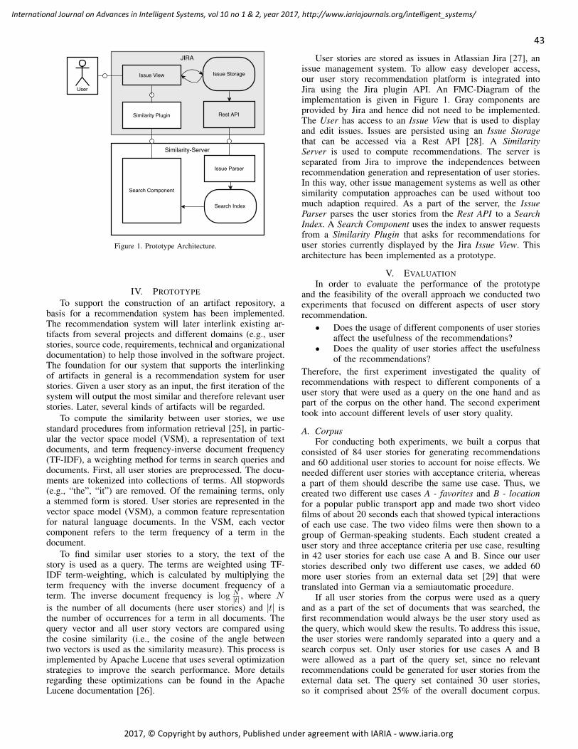
Figure 1. Prototype Architecture.

IV. PROTOTYPE

To support the construction of an artifact repository, abasis for a recommendation system has been implemented.The recommendation system will later interlink existing ar-tifacts from several projects and different domains (e.g., userstories, source code, requirements, technical and organizationaldocumentation) to help those involved in the software project.The foundation for our system that supports the interlinkingof artifacts in general is a recommendation system for userstories. Given a user story as an input, the first iteration of thesystem will output the most similar and therefore relevant userstories. Later, several kinds of artifacts will be regarded.

To compute the similarity between user stories, we usestandard procedures from information retrieval [25], in partic-ular the vector space model (VSM), a representation of textdocuments, and term frequency-inverse document frequency(TF-IDF), a weighting method for terms in search queries anddocuments. First, all user stories are preprocessed. The docu-ments are tokenized into collections of terms. All stopwords(e.g., “the”, “it”) are removed. Of the remaining terms, onlya stemmed form is stored. User stories are represented in thevector space model (VSM), a common feature representationfor natural language documents. In the VSM, each vectorcomponent refers to the term frequency of a term in thedocument.

To find similar user stories to a story, the text of thestory is used as a query. The terms are weighted using TF-IDF term-weighting, which is calculated by multiplying theterm frequency with the inverse document frequency of aterm. The inverse document frequency is log N

∣t∣ , where N

is the number of all documents (here user stories) and ∣t∣ isthe number of occurrences for a term in all documents. Thequery vector and all user story vectors are compared usingthe cosine similarity (i.e., the cosine of the angle betweentwo vectors is used as the similarity measure). This process isimplemented by Apache Lucene that uses several optimizationstrategies to improve the search performance. More detailsregarding these optimizations can be found in the ApacheLucene documentation [26].

User stories are stored as issues in Atlassian Jira [27], anissue management system. To allow easy developer access,our user story recommendation platform is integrated intoJira using the Jira plugin API. An FMC-Diagram of theimplementation is given in Figure 1. Gray components areprovided by Jira and hence did not need to be implemented.The User has access to an Issue View that is used to displayand edit issues. Issues are persisted using an Issue Storagethat can be accessed via a Rest API [28]. A SimilarityServer is used to compute recommendations. The server isseparated from Jira to improve the independences betweenrecommendation generation and representation of user stories.In this way, other issue management systems as well as othersimilarity computation approaches can be used without toomuch adaption required. As a part of the server, the IssueParser parses the user stories from the Rest API to a SearchIndex. A Search Component uses the index to answer requestsfrom a Similarity Plugin that asks for recommendations foruser stories currently displayed by the Jira Issue View. Thisarchitecture has been implemented as a prototype.

V. EVALUATIONIn order to evaluate the performance of the prototype

and the feasibility of the overall approach we conducted twoexperiments that focused on different aspects of user storyrecommendation.● Does the usage of different components of user stories

affect the usefulness of the recommendations?● Does the quality of user stories affect the usefulness

of the recommendations?Therefore, the first experiment investigated the quality ofrecommendations with respect to different components of auser story that were used as a query on the one hand and aspart of the corpus on the other hand. The second experimenttook into account different levels of user story quality.

A. CorpusFor conducting both experiments, we built a corpus that

consisted of 84 user stories for generating recommendationsand 60 additional user stories to account for noise effects. Weneeded different user stories with acceptance criteria, whereasa part of them should describe the same use case. Thus, wecreated two different use cases A - favorites and B - locationfor a popular public transport app and made two short videofilms of about 20 seconds each that showed typical interactionsof each use case. The two video films were then shown to agroup of German-speaking students. Each student created auser story and three acceptance criteria per use case, resultingin 42 user stories for each use case A and B. Since our userstories described only two different use cases, we added 60more user stories from an external data set [29] that weretranslated into German via a semiautomatic procedure.

If all user stories from the corpus were used as a queryand as a part of the set of documents that was searched, thefirst recommendation would always be the user story used asthe query, which would skew the results. To address this issue,the user stories were randomly separated into a query and asearch corpus set. Only user stories for use cases A and Bwere allowed as a part of the query set, since no relevantrecommendations could be generated for user stories from theexternal data set. The query set contained 30 user stories,so it comprised about 25% of the overall document corpus.

43



Recommendations were generated only for user stories in thequery set. Only elements of the search corpus set were usedas recommendations.

B. MetricFor each user story, recommendations are calculated based

on textual similarity. A recommendation is regarded as “cor-rect”, when the recommended user story relates to the sameuse case A or B as the query. In the context of this work weconsider a recommendation system the more useful, the higherthe precision of the result is. Precision and recall are standardmetrics for evaluating these kinds of scenarios [30]. Since arecommendation system will provide the user with only thefirst few recommendations, the usage of overall precision andrecall is not an appropriate metric in this case. A metric thatis more useful regarding recommendation systems in our caseis precision at rank [25, p.161]:

PR =TP

SR

TP is the number of true positives (i.e., recommendationsof the correct use case) and SR a fixed number of searchresults. This metric only evaluates the SR best search results.The two experiments were conducted for each rank from oneto ten. To get an overview of the overall performance, theaverage of the precision for each user story was calculated.We therefore measured the average precision at rank for ranksone to ten.

C. Experiment 1: User Story ComponentsFor the first experiment we defined several variants of our

data sets: user stories along with their associated acceptancecriteria (USAK), user stories only (US) and acceptance criteriaonly (AK). These are the smallest possible variants that aresensible. Separating the user stories into smaller componentswould result in parts of very few words, which would notallow meaningful processing using IR techniques. Each variantcan be used as a query set on the one hand and as a corpusset on the other hand. We combined each variant as a querywith each variant as a corpus and therefore conducted the firstexperiment nine times with all nine combinations of our data.Since no acceptance criteria were available for the external dataset, the same artificial acceptance criteria were added to eachof these user stories. Hence, it is less likely to retrieve userstories as recommendations from the external data set whilethe corpus set consists of user stories with acceptance criteria(USAK) or only acceptance criteria (AK). This would lead toa better average precision at rank for these cases. Effects ofthis shortcoming will be further discussed in Section VII.

D. Experiment 2: User Story QualityA second experiment was conducted to evaluate if user

story quality affects the effectiveness of a text-similarity basedrecommendation system. For this purpose we categorized theuser stories into three quality groups.

First, the quality of all user stories was rated based on afive point scale. We defined five quality criteria and assignedone point to the user story for each criterion that was satisfied:(1) The user story had to have exactly one role. (2) The userstory had to express exactly one desire. (3) The user storyhad to have exactly one benefit. (4) The user story had to bewritten in only one sentence. (5) The user story’s benefit hadto be verifiable, as defined by the INVEST-criteria.

Then the user stories (written by students and from the ex-ternal data source) were categorized into three quality classes:User stories with five points were assigned to quality class1, user stories with four points were assigned to quality class2 and user stories with three or less points were assigned toquality class 3, resulting in class 1 comprising 95 user stories,while classes 2 and 3 contained 26 respectively 23 user stories.

To evaluate the effect of user story quality on recommen-dations, datasets with different user story quality were needed.Using the previously described categories, the data was splitinto three sets: (1) user stories of all quality classes, (2) userstories of quality classes 1 and 2, (3) user stories of only thehigh quality class 1. For each of these sets, the precision atall ranks from one to ten was calculated. For this experiment,only the combination of user story parts from experiment 1with the best results regarding precision was used.

VI. RESULTSWe implemented a small evaluation application that ini-

tiates the recommendation-process, gathers user story rec-ommendations, automatically calculates the average precisionat rank by evaluating class labels (e.g., corresponding usecase) according to the approach presented in Section V andstores results in a CSV file. The results of the experimentsperformed using this application are discussed in the followingsubsections.

A. Experiment 1: User Story ComponentsThe results from the first experiment are shown in Figure

2. Each data series represents one combination of corpus andquery sets, whereas the first part of the data series label denotesthe query set and the second part denotes the corpus type (e.g.,AK/US represents queries that contain only acceptance criteriaand a corpus consisting of user stories without acceptancecriteria).

The data series can be split into two categories: (1) Experi-ments where user story text is used as query and corpus and (2)experiments where either the query or the corpus consists onlyof acceptance criteria. With one exception (USAK/USAK atrank 1), members of the first category in general have a higheraverage precision than members of the second. For readabilitypurposes, only representatives of these categories with highestand lowest average precision at rank in the respective groupare shown in the data series. Note that AK/US and AK/AK arerepresentatives with lowest average precision for their groupat different ranks. Therefore two data series are displayed aslower bounds for the second category. The data series thatare not displayed (USAK/US and US/USAK in the first group;AK/USAK and US/AK in the second group) are always betweenthe upper and lower bounds of their respective groups.

The combination using only user stories (US/US) showsthe highest average precision. The precision for rank 1 is 1.0and drops to 0.88 when considering the first 10 recommen-dations. The data series of the combined user stories alongwith acceptance criteria (USAK/USAK) has a lower precisionthat ranges between 0.71 and 0.79. The data shows that theprecision differs widely between these combinations.

In the category of the experiments where either the query orthe corpus consists of acceptance criteria only, the combinationUSAK/AK showed the highest precision at rank that rangedfrom 0.54 to 0.75. The two combinations of AK/US and AK/AKresulted in the lowest precision varying between 0.58 and 0.63for AK/US and between 0.53 and 0.65 for AK/AK. However, the

44



0.4

0.5

0.6

0.7

0.8

0.9

1

1 2 3 4 5 6 7 8 9 10

Avera

ge P

reci

sion a

t R

ank

Rank

US/USAK/USAK/AK

USAK/AKUSAK/USAK

Figure 2. Evaluation results for combinations of query and corpus data.

0.4

0.5

0.6

0.7

0.8

0.9

1

1 2 3 4 5 6 7 8 9 10

Avera

ge P

reci

sion a

t R

ank

Rank

All ClassesClass 1+2

Class 1

Figure 3. Comparison of results when filtering user story quality.

results show only small differences between all combinationsin this group.

In general, data series that use only user stories either inthe query or the corpus set have a higher average precisionthan the data series applying acceptance criteria only in eitherquery or corpus. The three data series with the lowest averageprecision all use only acceptance criteria as queries. Averageprecision of these data series is between 0.53 and 0.65 varyingin dependence of the rank, while the average precision of thedata series of the other category varies between 0.71 and 1.0.

B. Experiment 2: User Story QualityThe results of the second experiment are shown in Figure

3. The data series Class 1 contains only high quality userstories of class 1, as described in Section V-D. Class 1 +2 are medium- and high-quality user stories, while All Classesrefers to user stories of all quality classes.

Average precision values for all data sets are between 0.8and 1.0. While class 1 user stories show the best results atranks 1, 2 and 3, the precision lowers at the following ranks.The precision with data of all quality classes varies between1.00 and 0.88 and receives the highest values at ranks 5 andfollowing. However, the precision values of quality classes 1and 2 are the lowest at all ranks.

VII. DISCUSSIONThe results we received from our experiments provided us

with information about the precision of text-based recommen-

dations for user stories and acceptance criteria. Based on theseresults we aim to answer our two research questions:● Does the usage of different components of user stories

affect the usefulness of recommendations?● Does the quality of user stories affect the usefulness

of recommendations?

A. Experiment 1The results from experiment 1 showed that the highest pre-

cision is received using the combination US/US. The precisionof the other combinations is not only lower, but by far lower.Also, after a decrease from rank 1 to rank 2, the precisionof the US/US combination remains relatively stable. Out ofall remaining combinations, the ones that use user stories inboth the query and the corpus produced the higher precisionvalues. All combinations that use only acceptance criteria inthe query and/or the corpus show the lowest precision that isby far lower than the highest received precision.

Based on our results we can therefore answer our firstresearch question positively. Different components of userstories do affect the usefulness of recommendations. We dis-covered that the usage of acceptance criteria deteriorates theprecision of the recommendation system, since these combi-nations received the lowest precision values. Correspondingto that, the combination that contained only user stories andno acceptance criteria led to the highest precision values.While it is difficult to define limits for the precision of arecommendation system, we believe the observed precision issufficient for recommendation systems in the context of mobileenterprise application development. We therefore conclude thatusing only user story text as a basis for recommendationcomputation in this context seems to be the most promisingalternative.

B. Experiment 2The results from experiment 2 show that the usage of all

quality classes leads to a higher precision from rank 4 onward.However, at ranks 1, 2 and 3 the usage of only high qualityuser stories received the best precision values. Furthermore, itis especially notable that average precision is lower for userstories of quality classes 1 and 2 combined than for all kindsof user stories.

Based on this data, we can not ascertain any impact of userstory quality on recommendation precision and therefore, oursecond research question is to be answered negatively.

C. Thread to validityOne weakness of our experimental setup may be the small

number of user stories in our corpus. However, the distributionof user stories to primarily two use cases compensates thisshortcoming. Although the quality rating of the user stories didnot follow a common model for user story quality, it is basedon the main and most popular user story models. Furthermore,to our knowledge there is no established model for qualitymeasurement of user stories on an individual level.

As mentioned in Section V-A, we used data from anexternal source that did not contain acceptance criteria. Onecould assume that this would distort the results in favor ofthe combinations that use acceptance criteria. However, thesecombinations gained lower precision than the other combina-tions, despite the lack of acceptance criteria. Therefore, ourconclusion that the usage of user stories has a positive effecton precision still holds.

45



VIII. CONCLUSIONIn this paper we have presented foundation work for an

artifact repository to support the development of MEA. Thefoundation is built on a recommendation system for artifactsbased on user-centered requirement specifications called “UserStories”, in order to allow the user of the artifact repository anefficient navigation. Standard information retrieval techniqueswere used to build the recommendation system. We evaluatedwhich parts of the user stories should be used for recom-mendation computation and how user story quality affects theperformance of the system.

Our experiments have shown that the most valuable partfor requirement computation from a user story is the userstory text. Including acceptance criteria into recommenda-tion computation has a negative impact on recommendationperformance. In our experiment data, we could not find apositive correlation between user story quality and quality ofrecommendations.

As future work, we plan to use our results to extend ourrecommendation system that includes development artifactsfrom several domains. Collecting and evaluating methods forconnecting different artifact types to user stories will be thenext step to reach this goal. In addition, the artifacts will beenriched with further information, such as cost and benefitinformation or process and workflow data.

ACKNOWLEDGMENTSThis work was funded by the German Federal Ministry

of Education and Research, grant no. 03FH032PX5; thePROFRAME project at RheinMain University of AppliedSciences. All responsibility for the content of this paper lieswith the authors.

REFERENCES

[1] M. Jurisch, B. Igler, and S. Bohm, “PROFRAME: A PrototypingFramework for Mobile Enterprise Applications,” in CENTRIC 2016,The Ninth International Conference on Advances in Human-orientedand Personalized Mechanisms, Technologies, and Services, 2016, pp.7–10, 2016.

[2] H. K. Flora, X. Wang, and S. V. Chande, “An investigationon the characteristics of mobile applications: A survey study,”International Journal of Information Technology and ComputerScience, vol. 6, no. 11, pp. 21–27, 2014. [Online]. Available:https://doi.org/10.5815%2Fijitcs.2014.11.03

[3] Inmobi, “State of mobile app developers 2016: Based on a surveyof 1000+ app developers,” http://www.inmobi.com/insights/download/whitepapers/state-of-mobile-app-developers-2016/, accessed: 2017-03-02.

[4] S. J. Andriole, “Managing technology in a 2.0 world,” ITProfessional, vol. 14, no. 1, pp. 50–57, 2012. [Online]. Available:https://doi.org/10.1109%2Fmitp.2012.13

[5] B. Niehaves, S. Koffer, and K. Ortbach, “The effect of private it useon work performance: Towards an it consumerization theory,” in 201311th International Conference on Wirtschaftsinformatik. Institute ofElectrical and Electronics Engineers (IEEE), 2013, pp. 39–53, 2013.[Online]. Available: http://aisel.aisnet.org/wi2013/3/

[6] A. Giessmann, K. Stanoevska-Slabeva, and B. de Visser, “Mobileenterprise applications–current state and future directions,” in 201245th Hawaii International Conference on System Sciences. Instituteof Electrical and Electronics Engineers (IEEE), 2012, 2012. [Online].Available: https://doi.org/10.1109%2Fhicss.2012.435

[7] R. C. Basole, “The emergence of the mobile enterprise: A value-driven perspective,” in International Conference on the Managementof Mobile Business (ICMB 2007). Institute of Electrical andElectronics Engineers (IEEE), 2007, 2007. [Online]. Available:https://doi.org/10.1109%2Ficmb.2007.63

[8] J. O. Borchers, “A pattern approach to interaction design,” AI &Society, vol. 15, no. 4, pp. 359–376, 2001. [Online]. Available:https://doi.org/10.1007%2Fbf01206115

[9] K. Kang, J. Lee, and P. Donohoe, “Feature-oriented product lineengineering,” IEEE Software, vol. 19, no. 4, pp. 58–65, 2002. [Online].Available: https://doi.org/10.1109%2Fms.2002.1020288

[10] A. Cleven, P. Gubler, and K. M. Huner, “Design alternatives forthe evaluation of design science research artifacts,” in Proceedingsof the 4th International Conference on Design Science Research inInformation Systems and Technology - DESRIST '09. Associationfor Computing Machinery (ACM), 2009, 2009. [Online]. Available:https://doi.org/10.1145%2F1555619.1555645

[11] M. Robillard, R. Walker, and T. Zimmermann, “Recommendationsystems for software engineering,” IEEE Software, vol. 27, no. 4, pp.80–86, 2010. [Online]. Available: https://doi.org/10.1109%2Fms.2009.161

[12] M. Cohn, User stories applied: For agile software development.Addison-Wesley Professional, 2004.

[13] B. Wake, “INVEST in good stories, and SMART tasks,” blog post,[retrieved: 2017.05.10], 2003. [Online]. Available: http://xp123.com/articles/invest-in-good-stories-and-smart-tasks

[14] A. Giessmann, K. Stanoevska-Slabeva, and B. de Visser, “Mobileenterprise applications–current state and future directions,” in SystemScience (HICSS), 2012 45th Hawaii International Conference on, Jan2012, pp. 1363–1372, Jan 2012.

[15] Gartner, “Gartner says demand for enterprise mobile apps willoutstrip available development capacity five to one,” website[retrieved: 2017.05.10], 2015. [Online]. Available: https://www.gartner.com/newsroom/id/3076817

[16] P. Dugerdil, “Architecting mobile enterprise app: A modeling approachto adapt enterprise applications to the mobile,” in Proceedings ofthe 2013 ACM Workshop on Mobile Development Lifecycle, ser.MobileDeLi ’13. New York, NY, USA: ACM, 2013, pp. 9–14, 2013.

[17] M. Pistoia and O. Tripp, “Integrating security, analytics and applicationmanagement into the mobile development lifecycle,” in Proceedings ofthe 2Nd International Workshop on Mobile Development Lifecycle, ser.MobileDeLi ’14. New York, NY, USA: ACM, 2014, pp. 17–18, 2014.

[18] S. A. Badami and J. Sathyan, “micE Model for Defining Enterprise Mo-bile Strategy,” Int. J. on Recent Trends in Engineering and Technology,,vol. 10, no. 1, p. 9, Jan 2014.

[19] H. Pirzadeh, A. D. S. Oliveira, and S. Shanian, “ReUse : A Rec-ommendation System for Implementing User Stories,” in InternationalConference on Software Engineering Advances, no. c, 2016, pp. 149–153, 2016.

[20] P. Runeson, M. Alexandersson, and O. Nyholm, “Detection of dupli-cate defect reports using natural language processing,” Proceedings -International Conference on Software Engineering, pp. 499–508, 2007.

[21] X. Wang, L. Zhang, T. Xie, J. Anvik, and J. Sun, “An Approach to De-tecting Duplicate Bug Reports using Natural Language and ExecutionInformation 1 2,” Proceedings of the 30th international conference onSoftware engineering, pp. 461–470, 2008.

[22] J. Anvik and G. C. Murphy, “Reducing the Effort of Bug ReportTriage: Recommenders for Development-Oriented Decisions,” ACMTransactions on Software Engineering and Methodology (TOSEM),vol. 20, no. 3, 2011.

[23] D. Cubranic and G. C. Murphy, “Hipikat: Recommending PertinentSoftware Development Artifacts,” 25th International Conference onSoftware Engineering, no. Section 2, pp. 408–418, 2003. [Online].Available: http://dl.acm.org/citation.cfm?id=776816.776866

[24] D. Oguz, “Similar issues finder,” website, [retrieved: 2017.05.10],2017. [Online]. Available: https://denizoguz.atlassian.net/projects/SIF/summary

[25] C. D. Manning, P. Raghavan, and H. Schutze, Introduction to Infor-mation Retrieval. New York, NY, USA: Cambridge University Press,2008.

[26] Apache Foundation, “TFIDF Similarity (Lucene 4.6.0API),” website, [retrieved: 2017.05.10], 2017. [Online].Available: https://lucene.apache.org/core/4 6 0/core/org/apache/lucene/search/similarities/TFIDFSimilarity.html

46



[27] Atlassian, “JIRA Software - Issue & Project Tracking for SoftwareTeams,” website, [retrieved: 2017.05.10], 2017. [Online]. Available:https://www.atlassian.com/software/jira

[28] Atlassian Developers, “JIRA REST APIS,” website, [retrieved:2017.05.10], 2017. [Online]. Available: https://developer.atlassian.com/jiradev/jira-apis/jira-rest-apis

[29] Open Knowledge International, “Frictionless data: User stories,”website, [retrieved: 2017.05.10], 2016. [Online]. Available: http://frictionlessdata.io/user-stories/

[30] D. M. W. Powers, “Evaluation: From Precision, Recall and F-Factor toROC, Informedness, Markedness & Correlation,” Tech. Rep. December,2007.

47



The DynB Sparse Matrix Format Using Variable Sized 2D Blocksfor Efficient Sparse Matrix Vector Multiplications with General Matrix Structures

Javed Razzaq, Rudolf Berrendorf, Jan P. Ecker,Soenke Hack, Max Weierstall

Computer Science DepartmentBonn-Rhein-Sieg University of Applied Sciences

Sankt Augustin, Germanye-mail:{javed.razzaq, rudolf.berrendorf, jan.ecker,

soenke.hack, max.weierstall}@h-brs.de

Florian MannussEXPEC Advanced Research Center

Saudi Arabian Oil CompanyDhahran, Saudi Arabia


Abstract—The Sparse Matrix Vector Multiplication is an impor-tant operation on sparse matrices. This operation is the mosttime consuming operation in iterative solvers and therefore anefficient execution of that operation is of great importance formany applications. Numerous different storage formats that storesparse matrices efficiently have already been established. Often,these storage formats utilize the sparsity pattern of a matrix in anappropiate manner. For one class of sparse matrices the nonzerovalues occur in small dense blocks and appropriate block storageformats are well suited for such patterns. But on the other side,these formats perform often poor on general matrices withoutan explicit / regular block structure. In this paper, the newlydeveloped sparse matrix format DynB is introduced. The aim is toefficiently use several optimization approaches and vectorizationwith current processors, even for matrices without an explicitblock structure of nonzero elements. The DynB matrix formatuses 2D rectangular blocks of variable size, allowing fill-ins perblock of explicit zero values up to a user controllable threshold.We give a simple and fast heuristic to detect such 2D blocks in asparse matrix. The performance of the Sparse Matrix VectorMultiplication for a selection of different block formats andmatrices with different sparsity structures is compared. Resultsshow that the benefit of blocking formats depend – as to beexpected – on the structure of the matrix and that variable sizedblock formats like DynB can have advantages over fixed sizeformats and deliver good performance results even for generalsparse matrices.

Keywords–Sparse Matrix Vector Multiplication; SpMV; Block-ing; Vector Units; Autotuning

I. INTRODUCTIONSparse matrices arise in many applications of natural sci-

ence and engineering. The characteristic of sparse matricesis that almost all matrix values are zero and only very fewentries (usually less than 1%) have a nonzero value. Thissparseness property is used in special storage formats for suchmatrices to store only / mainly nonzero values along with indexinformation. A performance critical operation on such matricesis the multiplication of a sparse matrix with a dense vector(SpMV) y← Ax that may be executed many times, e.g., ateach iteration step of an iterative solver. The efficiency of theSpMV operation highly depends on the used sparse matrixformat, the matrix structure and how the SpMV operation isimplemented and optimized according to the format. Manytechniques are known to store a sparse matrix and perform theSpMV operation that take advantage of the nonzero structureof the matrix. One class of formats are block formats. Blockstorage formats exploit block structures of nonzero elements

in a matrix and store dense blocks of values [1]. Block formatshave several advantages for efficient SpMV executions. Storingnonzero values together in a block can lead to an improvedspatial data locality and, by addressing more than one nonzerovalue by one index entry, the overall index structure, thememory indirections and the memory bandwidth demand arereduced [2] [3]. Another advantage of block formats is theuse of the processor’s Single Instruction Multi Data (SIMD)extension [4], i.e., the vector units of a processor. Such a blockapproach works for dense nonzero block structures in sparsematrices and increases the performance of the SpMV operationsignificantly, even if explicit zeros are used to fill the blocks[5].

There are two groups of blocking formats: fixed sizeblocking formats that use the same fixed block size for thewhole matrix and variable sized block formats that use thestructure of the matrix to build variable sized blocks. Theadvantages of fixed sized blocking formats are the possibilityof optimizing the SpMV for certain, at compile time known,block sizes and the rather simple building of blocks byallowing and storing explicit zeros. The advantages of variableblocking formats are the exploitation of a non-regular matrixstructure and the ability to store different sized blocks fora matrix. Furthermore, the two types can be combined withdifferent other optimization techniques, like using bitmaps [6][7] or relative indexing [8] [9]. There are also some blockformats that do not fit in either of these categories or use bothtechniques [10].

Sparse matrices with an inherent block structure usuallyarise from a regular 2D / 3D geometry associated with theoriginal problem. Such matrices can certainly benefit fromblocking techniques [11]. A question is whether rather generalmatrices without a clear block structure can also benefit fromblocking techniques.

Additionally, for different block sizes different implemen-tations of the SpMV kernel may be optimal. Selecting animplementation among a set of different implementations fora large amount of different block sizes may be a task thatcan hardly be handled manually, due to the large parameterspace. Thus, using an autotuning approach for this task maybe beneficial.

The paper is structured as follows. In Section II, anoverview on related work is given. In Section III, our ownnewly developed block format DynB is described, includingthe description of a low overhead algorithm for block detec-

48



tion, implementation issues of the specific SpMV operationand optimizations. In Section IV an autotuning approach forselecting optimal SpMV kernel implementations for different2D block sizes is presented for the new format. The fol-lowing Section V describes the experimental setup. SectionVI shows performance results, which compare and evaluaterelevant blocking formats on matrices without an explicit blockstructure. At last, in Section VII a conclusion is given.

II. RELATED WORKIn this section, a comprehensive overview of block formats

is given, including formats where blocks are used aside withother optimization techniques. Then, a short overview onfurther block detection methods is given. At last, autotuningmethods are discussed.

As an introduction we start with a brief discussion of rathergeneral sparse matrix formats. The Coordinate format (COO)[12] is the most simple and basic format to store a sparsematrix. It consists of three arrays. For a nonzero value, thevalue as well as the row and column index is stored explicitlyat the i-th position in the three arrays, respectively. The sizeof each array is equal to the number of nonzeros. The order ofvalues stored is of no concern. The Compressed Sparse Rowformat (CSR) [13] [12] [14] is one of the most used matrixformat for sparse matrices. The index structure in CSR is inrelation to COO reduced by replacing the row index for everynonzero value with a single index for all nonzero values in arow. This row index indicates the start of a new row withinthe other two arrays. As a consequence and in difference toCOO, all values in a row must be stored consecutively.

For blocked formats, the Block Compressed Sparse Rowformat (BCSR) [14] [2] is similar to the CSR format. Butinstead of storing single nonzero values, the BCSR formatstores blocks, i.e., dense submatrices of a fixed size. The matrixis partitioned into blocks of fixed size r× c, where r and crepresent the number of rows and columns of the blocks.Then,only submatrices with at least one nonzero element are stored.The optimal block size differs for different matrices and evendifferent processor platforms. Advantages of the BCSR formatare a possible reduction of the index structure, possible loopunrolling per block, using vector units through automaticcompiler vectorization or using explicit intrinsics [15] andmany other low level optimization techniques [16]. However,it may be necessary to store explicit zero values for blocksthat are not fully filled with nonzero values. In the worst-case,this could lead to the same index structure as with CSR, butwith additional zeros stored for each nonzero value.

The Mapped Blocked Row format (MBR) [6] is similar tothe BCSR format. Like BCSR, MBR uses blocks of a fixed sizer×c. In addition to BCSR, bitmaps are stored that encode thenonzero structure for each block. An advantage of this bitmaparray is, that only actual nonzero values need to be stored inthe values array, even though filled-in zeros exist. In exchangefor the reduced memory use, additional computation time isneeded during the SpMV operation.

The Blocked Compressed Common Coordinate format(BCCOO) [17] uses fixed size blocks. It is based on theBlocked Common Coordinate (BCOO) format, which storesthe matrix coordinates of a fixed sized block to address thevalue. BCCOO relies on a bit_flag to store information aboutthe start of a new row. By using a bit array instead of an integer,a high compression rate of the index information is archived.

One disadvantage of the bit_flag array is, that an additionalarray is needed to execute the SpMV operation in parallel withpartition information.

The Unaligned Block Compressed Sparse Row format(UBCSR) [5] [18] removes the row alignment of the BCSRformat by adding an additional array. However, this optimiza-tion appears to be only applicable to a special set of matriceswhere blocks occur in a recurring pattern in a row and are allshifted.

The Variable Block Row format (VBR) [5] analyses rowsand columns that are next to each other. Their nonzero val-ues are stored in blocks, if they have the identical patternof nonzero values in a row or in a column. Hereby, onlycompletely dense blocks are stored by VBR. It is possibleto relax the analyses of rows and columns by the use of athreshold, which allows VBR to store explicit zeros to buildlarger blocks [18].

The Variable Block Length format (VBL) [3] [19] [11],which is also referred as Blocked Compressed Row Storageformat (BCRS), is likewise similar to the CSR format. But,rather than storing a single value, all consecutive nonzerovalues in a row are stored in 1D blocks. The blocks of theVBL format do not have a fixed size and only nonzero valuesare stored. VBL may reduce the index structure depending onthe stored matrix, but compared to CSR an additional loopinside the SpMV is required to process all blocks in a rowand to proceed all elements in a block.

The aim of the Compressed sparse eXtended format (CSX)[10] is to compress index information by exploiting (arbitrarybut fixed) substructures within matrices. CSX identifies hor-izontal, vertical, diagonal, anti-diagonal and two-dimensionalblock structures in a pre-process. The data structure, whichis used by CSX to store the location information, is basedon the Compressed Sparse Row Delta Unit format (CSR-DU) [20]. The advantages of CSX are the index reductionby using the techniques of CSR-DU and, at the same time,the provision of a special SpMV implementation for eachsubstructure. However, implementing CSX seems to be rathercomplex and to determine appropriate substructures in a matrixmay cause perceptible overhead.

The Pattern-based Representation format (PBR) [7] aims toreduce the index overhead. Instead of adding fill-in or relyingon dense substructures in a matrix, PBR identifies recurringblock structures that are sharing the same nonzero pattern. Foreach pattern that covers more nonzero values than a certainthreshold, PBR stores a submatrix in the BCOO format plusa bitmap, which represents the repeated nonzero pattern. Foreach of these patterns, an optimized SpMV kernel is providedor generated. Belgin et al. state in their work [7] that it ispossible to use prefetching, vectorization and parallelizationto optimize each kernel individually. Advantages of PBR arethe possibility of providing special SpMV kernels for eachoccurring block pattern as well as low level optimization forthese SpMV kernels.

The Recursive Sparse Blocks (RSB) format [21] [22] aimsto reduce the index overhead while keeping locality. By build-ing a quadtree, which represents the sparse matrix, the matrixis recursively divided into four quadrant submatrices, untila certain termination condition is reached. The terminationcondition for the recursive function is defined in detail byMartone et al. in [23] [24]. The submatrix is stored in the leafnode of the quadtree in COO or CSR format. All nodes before

49



the leaf node do not contain matrix data and are pointers, whichbuild the quadtree.

The Compressed Sparse Block format (CSB) [8] [9] aimsto reduce the storage needed to store the location of a valuewithin a matrix by splitting the matrix into huge squareblocks. Further, row and column indices of each value arestored relatively to each block. Due to the relative addressingof the values, it is possible to use smaller data types forthe row and column index arrays, which leads to an indexreduction per nonzero. It is possible to order the values insidethe values array to get better performance of the SpMVoperation. The authors of the original work suggest a recursiveZ-Motion ordering to provide spatial locality. The parallelSpMV implementation of CSB uses a private result vector perthread, but the implementation also provides an optimizationin case the vector is not required for a block row [8].

In [25] it is shown that finding optimal nonoverlappingdense blocks in a sparse matrix is a NP complete problem.Here, the proof is given by using a reduction of the maximumindependent set problem, which is known to be NP complete[26]. Moreover, [25] gives a greedy algorithm for finding 2×2blocks within a sparse matrix. This algorithm is based on adecision tree for finding only dense blocks, allowing no fill-inwithin these blocks.

Other methods that can be used for blockfinding are forexample the kd-tree [27] and r-tree [28] data structure /algorithm known from spatial databases. Both build (search)tree data structures using spatial location of points or objectswithin a search region.

Various other publications [29] [30] [31] [32] [33] discussthe use of autotuning approaches, which can be used for awide range of optimizations. E.g., the selection of formatparameters, specific optimization techniques or the selection ofthe best suited formats. Sophisticated auto-tuning approachesare based on complex models [31] [32] or mathematical andmachine learning concepts [33].

In [29] Byun et al. present an auto-tuning framework foroptimizing the CSR format, e.g., by fixed-sized blocking. Thisframework is used to find the optimal blocking for the resultingBCSR format for a given input matrix and used hardwareplatform.

III. DEVELOPMENT OF A 2D VARIABLE SIZED BLOCKFORMAT

In this section, a newly developed variable sized blockformat, called DynB, is described. The goal of DynB is, tofind rectangular 2D blocks within a matrix to efficiently utilizea processor’s vector units for the SpMV. At first, a simple andfast algorithm for the detection of variable sized 2D blocks isintroduced. Then, the overall structure of the format is given.Afterwards, the SpMV kernel is presented and at last codeoptimization techniques are considered.

A. Finding Variable Sized BlocksAs described in Section II, the CSX format uses a sophis-

ticated but time consuming algorithm to find even complexnonzero substructures within the entire matrix. Although thespeedup of the SpMV operation may be high, many SpMVoperations may be neccessary to compensate the cost of thedetection algorithm. In contrast, the VBL format uses a simpleand fast algorithm to find just 1D blocks within each row of amatrix. However, the speedup of the SpMV may not be as highas for CSX. For the introduced DynB format a fast algorithm

Input: A[ ][ ], T , SmaxOutput: B[ ][ ]

1: for i← 1,nRows2: for j← 1,nColumns3: if A[i][ j] = 0∧A[i][ j] /∈ B4: r← 1, c← 1, rr← 0, cc← 05: added← T RUE6: while added7: added← FALSE8: rr← r−1, cc← c−19: search(next column n with A[i : i+ rr][n] = 0)

10: search(next row m with A[m][ j : j+ cc] = 0)11: if r∗ (n+1− j)≤ Smax∧ t(A[i : i+ rr][ j : n])≥ T12: c← n+1− j13: added← T RUE14: end if15: if (m+1− i)∗c≤ Smax∧t(A[i : m][ j : j+cc])≥ T16: r← m+1− i17: added← T RUE18: end if19: end while20: B← B+A[i : i+ rr][ j : j+ cc]21: end if22: end for23: end for

Figure 1: Fast Heuristic for the Detection of 2D Blocks.

to find rectangular 2D blocks over the entire matrix shouldbe developed. With these 2D blocks, a reasonable runtimeimprovement for the SpMV operation should be achieved, byusing advantages similar to BCSR, while possibly generatingless fill-in.

The algorithm we developed to find 2D block structuresof nonzero elements is a fast greedy heuristic. It tries to findpossible block candidates that should be as large as possible,even if nonzeros are not direct neighbors, i.e., fill-ins ofexplicit zeros are allowed up to a certain amount per block.Consequently, a threshold T is used that indicates how densea block candidate, which has been found by the heuristic,needs to be in order to be stored as a block. That means Tis a measure for how many fill-in is allowed in a block. Thenonzero density t(block) of a block has to satisfy the relation

t(block) = nnzblock/blocksize= nnzblock/(nnzblock + zeros)= nnzblock/(r ∗ c)≥ T

where nnzblock represents the number of nonzero values in theblock and r,c the number of rows, columns of that block.

The algorithm shown in Figure 1 describes a simplifiedversion of the heuristic, which is used to find the blocks in amatrix. The heuristic takes a sparse matrix A[][], the desiredthreshold T (maximum portion of nonzero values in a block)and a maximum blocksize Smax (usually according to the sizeof the vector units) as an input. It gives the converted blockedMatrix B[][] as output. The algorithm iterates rowwise over thenonzero elements of the original matrix. If a nonzero valueof the original matrix is not already assigned to a block, anew 1× 1 block will be created. Then this block will be

50



A =

0 a1 a2 0 0 0 0 0

0 a3 a4 0 0 0 0 0

0 0 a5 0 0 0 a6 a7

0 0 a8 0 0 0 a9 a10

a11 0 0 a12 a13 a14 0 0

a15 0 0 a16 0 a17 0 0

a18 0 0 a19 a20 a21 0 0

0 a22 0 0 0 0 0 0

values = {a1,a2,a3,a4,0,a5,0,a8,

a6,a7,a9,a10,a11,a15,a18,a12,a13,a14,a16,0,a17,a19,a20,a21,a22}

block_start = {0,8,12,15,24}row_index = {0,2,4,4,7}

column_index = {1,6,0,3,1}block_row = {4,2,3,3,1}

block_column = {2,2,1,3,1}

Figure 2: The DynB Format storing Matrix A with a Threshold of 0.75.

expanded successively with new columns and rows in eachiteration of the while loop. Adding a new column or rowmeans adding the column/row with the next nonzero elementand all fill-in columns/rows with zeros that are located betweenthe outermost block column/row and the column/row with thenext nonzero. Column/rows are only added to the block if thenonzero density of the block after adding these columns/rowswould be large enough. If not enough nonzero elements wouldbe added, i.e., the if statements for both column and row fail,the heuristic will finish the block. After all blocks are found,the memory for the DynB data structure is allocated and filledwith the actual values and index structure. This data structureis described in the following section.

B. Structure of the FormatThe DynB format relies on six arrays. In the values array

the nonzero values (plus fill-in zeros) are consecutively storedin block order and rowwise within a block. The block_start

pointer stores the starting position of each block in thevalues array. The row_index and the column_index storethe location of the upper left corner of each block. This issimilar to the COO format for single values, but here, fewerindices are stored explicitly, because the indices are used toaddress a whole block of values. Finally, the block_row andblock_column arrays store the column and row size of eachtwo dimensional block, i.e., the block size is variable. Below,the purpose of the six arrays are described as well as whycertain data types were chosen and how many entries theycontain:• values[nnz+zeros] : double contains the values of

the matrix.• rowIndex[blocks] : int stores the row index in

which a block starts.• columnIndex[blocks] : int stores the column index

in which a block starts.• blockStart[blocks] : int stores the start point of

each block inside the values array.

for (int i = 0; i < nonZeroBlocks; ++i){//general SpMV for any blocksizefor (int ii = 0; ii < blockRow[i]; ++ii){double s = 0.0;int jj = blockStart[i] + (blockColumn[i]*ii) ;for (int j = 0 ; j < blockColumn[i]; ++j, ++jj){

s += values[jj] * x[columnIndex[i]+j];}y[rowIndex[i]+ii]+=s;

}}

Figure 3: SpMV implementation of DynB for general blocks.

• blockRow[blocks] : unsigned char stores the num-ber of rows a block contains. The unsigned char datatype is used because the maximum allowed block sizeis 64, according to the size of vector units, whichmeans that blockRow×blockColumn≤ 64 must hold.

• blockColumn[blocks] : unsigned char stores thenumber of columns a block contains.

• nonZeroBlocks : int stores the quantity of blocks.• threshold : float needs to be set prior to the

conversion of a matrix into the DynB format. Thethreshold needs to be positive and smaller or equalto 1.0 (e.g., 1.0 = 100% nonzero values, 0.5 = 50%nonzero values in a block are allowed).

All data types are choosen as small as possible to reducememory bandwidth demands, which are critical in SpMVoperations. Figure 2 shows in an example how a matrix Ais stored using the DynB format.

C. SpMV KernelThe SpMV implementation of DynB iterates over the

blocks, which have been build before. A general and simplifiedcode version is shown in Figure 3. Initially, beside a genericcode version able to handle arbitrary block sizes, we imple-mented additionally optimized code versions for special andoften found block structures (single nonzero values, horizontaland vertical 1D blocks and the general case of all other 2Dblock sizes). Further block kernels were implemented for theautotuning (see Section IV-A).

D. Code OptimizationIt was already shown in [34] that using vector intrinsics

to address the vector units of a processor can lead to aperformance gain for the SpMV operation. However, with thistechnique the programmer needs to write code on an assemblerlevel, which can be tedious and error prone. Another approach,which showed good results in [34], is to leave the utilizationof vector units solely to the compiler. For the Intel Compilericc/icpc, automatic compiler vectorization is enabled for theoptimization level -O2 and higher levels [15]. The compilercan use various optimization techniques and auto-vectorizecode, where possible. To achieve this, the compiler has tobe provided with appropriate information. E.g., by using the-x compiler option the information on the target processorarchitecture / instruction set can be provided [15]. Withoutthis option, the compiler uses a default (older) instructionset that can not utilize abilities of current vector units. Aprogrammer can give the compiler additional hints, e.g., wheredata can be assumed as aligned, if the compiler is not able to

51



Offline

Kernel

generation

Matrix

generation

Execution

of Benchmarks

Select fastest

kernel for

each block size

Create

optimized

executable

Online

SpMV

execution

Figure 4: Simplified Process of the DynB Autotuning.

detect this automatically [15]. Furthermore, different pragmasexist to force the compiler to execute different actions. With#pragma simd a compiler is requested to vectorize a loopeven if the compiler ascertains that this is not a good idea.There are many other possible optimizations as well for theblocked SpMV. Loop unrolling can be executed manuallyby the programmer, if the blocksizes are known beforehand.With pragma unroll, the compiler can be forced to unroll aloop. Furthermore, special cases of the blocked SpMV canbe considererd, e.g., for 1D blocks, resulting in single loopsinstead of nested loops.

IV. AUTOTUNING FOR 2D BLOCKSBy enabling variable block sizes, many blocks of different

sizes may be found. Due to the design decision (and optimiza-tion) of using unsigned char and therefore 8 Bits to code ablock size, the DynB format supports 280 different block sizes.It would be possible to compute the SpMV operation usingone general kernel code for arbitrary block sizes that iteratesover both dimensions of the blocks (see Figure 3 for such ageneral code version). This very simple implementation is notexpected to deliver the optimal performance, as it containstwo additional loops with unknown iteration counts, whichcan not easily be optimized by a compiler. It is expectedthat the optimal implementation for each block size is at leastslightly different. E.g., the use of vector units may be beneficialfor larger, but not for very small blocks, e.g., single values.Additionally, the optimal strategy to handle specific block sizesis processor specific. Finding the optimal implementation foreach possible block size manually may be time consuming.Thus, an autotuning approach is used for the DynB formatto find offline optimal implementations. The focus of thedeveloped autotuning approach is on the optimization of theSpMV operation for the DynB format, which uses dynamicblock sizes.

A. Description of the Autotuning ApproachThe developed autotuning approach for the DynB format

has similarities to the pOSKI framework [29]. This frameworkis used for finding the optimal blocking for a given inputmatrix and used hardware platform. The autotuning approachdeveloped in this work focuses on the identification of optimalimplementations for all possible block sizes of the DynBformat.

The basic idea of the autotuning approach is to identify theoptimal implementation for each block size individually, using

a large set of possible implementations and synthetic bench-mark matrices with different sparsity pattern. The simplifiedprocess of the autotuning is presented in Figure 4. In a firststep, the possible SpMV kernels and the benchmark matriceshave to be generated. A large set of matrices is thereby created,with each matrix containing only one specific block size.Afterwards, the SpMV is executed using all kernels and thebenchmark matrices, while the execution time is measured. Thegathered information can then be used to identify the fastestimplementation for each specific block size. These implemen-tations are then used to generate an optimized executable,which is used to execute the actual SpMV operation. Thecomplete autotuning is required only once for the specifichardware platform and can be executed offline. This meansthere is no overhead for the the SpMV operation applied onan actual matrix, caused by the autotuning. In the following,the different steps are explained in more detail.

In the first step, the kernel generation, the required SpMVkernel source code for the for all possible block sizes is gen-erated. Many kernels can be generated automatically, becausethey follow a fixed pattern. There are additional kernels ofrelevance, e.g., implementations using intrinsics, that can noteasily be generated automatically and therefore hand-tuning isnecessary is this cases. The following list shows the set ofkernels used for most block sizes:• normal: The default kernel, normally used in the

general case. Consists of two loops with variable loopcount.

• loop: Very similar implementation as the normalkernel. Instead of variable loop counts, the knownblock sizes are used as static loop counts.

• singleLoop: Special kernel for one dimensional blocksonly. Implementation is identical with the loop kernel,but only using one of the loops. The other loop is notrequired, as its iteration count would be 1.

• unroll: Identical loop implementation as the loopkernel. Additionally the #pragma unroll directive isused to generated unrolled code with different unrollfactors.

• novec: Identical loop implementation as the loopkernel. Additionally the #pragma novector directiveis used to prevent a vectorization of the code.

• simd: Identical loop implementation as the loop ker-nel. Additionally the #pragma simd directive is usedto force vectorization of the code.

• plain: The kernel is implemented without any loops.All operations are manually unrolled.

• intrinsic: Similar to the plain kernel, the kernel isimplemented without loops. The calculation is imple-mented using low level intrinsic functions. The kernelshave to be written manually.

In the basic DynB format the elements of every block arestored in row-major order. For the autotuning every kernel isadditionally generated for a column-major order organizationof the blocks. The creation of the format has been changed aswell to allow both block types. This may allow a more efficientvector unit utilization.

Figure 5 shows the usage of vector units with a column-major order and row-major order. In column-major order,vector units are used to process multiple rows at once, whichallows a very efficient calculation. Memory accesses can beeasily aligned and consecutive. Furthermore, after calculating

52



(a) Column-major Order

(b) Row-major Order

Figure 5: Calculation of 2D Blocks using Vector-Units.

the last elements of the rows, the result of the vector unit issimply written to the y vector.

On the other hand, in row-major order, vector units processelements of the same row. This requires an additional reductionoperation at the end of every row, as the partial results of thevector unit lanes have to be combined.

The matrix generation for the benchmark matrices is alsodone in the first autotuning step. For each block size a setof synthetic benchmark matrices is generated. Thereby, thematrices contain one specific block size only. Furthermore, foreach block size three different distributions of the elementsand two different nonzero densities are created. This is done toanalyze, if the matrix structure has an impact on the individualkernel performance.

Figure 6 presents the three used distributions. In everydistribution the blocks are placed with a safety margin aroundthem, to prevent the greedy block finding algorithm of theDynB format to combine multiple blocks into one biggerblock. The first structure is called round robin and it distributesthe elements evenly over the columns of the matrix. Startingin the first row and column, the blocks are placed in increasingcolumns. When the end of the matrix is reached, the columnindex is reset. The resulting patterns resamble squashed diago-nals. The second structure is a simple diagonal pattern, becauseof the safety margin there is not an element in every row. Thelast structure selects the column index of the blocks randomly.The number of entries per row is still fixed, also the safetymargin is still be respected.

The second step of our autotuning uses the generatedkernels and matrices and measures the SpMV execution time.Furthermore, for each kernel multiple versions should be used,using different compilers, optimization levels and inlining ofcode.

In the third step the fastest kernel for each individual blocksize has to be identified. This can simply be achieved by

X

X

X

X

X

X

X

X

X

(a) Round Robin

X

X

X

X

X

(b) Diagonal

X

X

X

X

X

X

X

X

X

(c) Random

Figure 6: Illustration of the three different structures used for the syntheticmatrices of the DynB autotuning. Every red square represents a block in theDynB format.

comparing the measured runtimes of all kernels for one specificblock size. Further complexity is introduced by the differentmatrix structures used, which may require a comparison overa larger data set.

The last step of the offline autotuning is the creation ofan optimized executable for the SpMV execution. The kernelsidentified in the previous step are combined into one largeSpMV kernel, to provide a proper implementation for everypossible kernel. Further analysis may be required to identify ifit is suitable to provide an implementation for every of the 280possible kernels. For each block in a matrix, the proper kernelhas to be selected at runtime. The selection of the kernel hastherefore to be very efficient, to prevent excessive branching.This will be described in more detail in the following SectionIV-B, where the implementation is described.

The developed autotuning potentially can increase theperformance of the DynB format. The default implementationdoes handle most of the block sizes identically. For smallblocks the loop overhead of the general implementation mightbe too high, while for larger blocks the use of vector units maybe beneficial. One possible problem with the use of individualkernels is the introduced branching that is necessary to handlethe different sizes. For every block the correct kernel has to beidentified and executed, which can potentially slow down theSpMV. Furthermore, the amount of program code could resultin problems with the instruction caches. If a large numberof different kernel implementations is used, the required codecould not fit in the available caches.

Another problem may occur because of the developed auto-tuning process itself. The initial assumption of the autotuningis, that the performance result of the individual kernels andsynthetic matrices can be used to determine the proper kernelfor a real matrix. It is also assumed, that the performance

53



numbers of the sequential execution can be used to find theoptimal kernels for a parallel executions. It is possible thatthese assumptions do not hold true, which would result inwrong findings.

B. ImplementationThe autotuning approach can be automated using scripts

(e.g., we used Python) in combination with the SpMV imple-mentation. As described in the previous section, most of thekernels can be generated automatically. These kernels haveone basic pattern, which can be adapted to different blocksizes. This is different for some more specialized kernels,which need to be written by hand. One example for this areimplementations using intrinsics. The kernel creation scriptstake manually written kernels and the general templates tocreate the source code for the kernels for every block size.

The benchmarking script uses the kernel source code tocompile a special version of the DynB SpMV operation. TheSpMV operation is executed using the synthetic matrices andthe execution time is measured. The results can ce stored, e.g.,in a database. This step is repeated several times for everykernel using different compilers and optimization options.Finally, the selection of the fastest kernels and the creation ofthe optimized executable can also be automated using scripts.

An important part of the implementation is the integrationof the optimized block kernels into the SpMV operation of theDynB format. As already discussed in the previous section,280 different block sizes and kernels are possible, whichpotentially introduces a lot of additional branching. To handlethis efficiently a jumper table should be used either by functionpointer arrays generated by a programmer or by a switch casethat is handled by the compiler. Many compilers are able tocreate a jumper table from a switch case if certain limitationsare respected, e.g., the number of states are within a certainlimit. This behavior has been verified for the Intel compiler,by analyzing the generated assembler code. The analysis alsoshowed, that the optimization can be applied in the case thatnot only consecutive numerical values are used. In this case,the missing values are filled with jump directives to the defaultcase of the switch case statement.

V. EXPERIMENTAL SETUPThe experiments to evaluate block formats were run on

a system with an Intel Xeon E5-2697 v3 CPU (Haswellarchitecture) [35] and the Intel C++ Compiler version 2017[15]. A set of 78 large test matrices from the Florida SparseMatrix Collection [36] and SPE reference problems [37] wastaken as test matrices. Most of the chosen matrices do nothave an overall explicit block structure of nonzeros. Compileroptimization and AVX2 instruction set were used, if possi-ble. The following block matrix formats were chosen to becompared in the experiments. They represent a selection of1D and 2D block formats with fixed and variable sizes aswell as more arbitrary pattern (CSX) which have shown to bewell performing, at least on matrices with an explicit blockstructure. In parentheses is shown whether fixed or variablesized blocks can be used.• DynB (variable): own implementation according to

Section III, threshold T varied from 0.55 (slightlymore nonzeros than fill-in) to 1.0 (only nonzeros, nofill-in).

• VBL (variable): own implementation according to [3].

BCSR

10−2

10−1

100

3x3Blocks

Tim

e [s

]

VBL DynB

0.55 0.6 0.65 0.7 0.75 0.8 0.85 0.9 0.95 1Threshold

CSX

Figure 7: SpMV with all Blocking Formats, Best implementation.

TABLE I: Count of minimal SpMV execution times

BCSR VBL DynB CSX

0 4 32 42

• CSX (variable): library taken from the authors of theoriginal work on CSX [10] [38], no influence onimplementation.

• BCSR (fixed): own implementation according to [14],block dimensions: 2×2, 3×3, 4×4

Moreover, the autotuning approach for the DynB formatwas measured for selected block kernels. The other blockkernels were chosen to be optimized by the compiler, giving itin all cases of the switch statement the exact block dimensionsas constants. For all experiments, the SpMV operation wasexecuted 100 times and the median of these execution timeswas taken as the resulting execution time, to exclude uncer-tainty of the measurements. Subsequently, this is referred toas execution time.

VI. RESULTSIn this section we present selected results of the executed

experiments. When boxplots are shown, the quartiles overthe results for all matrices are given, whiskers extend to thelast datapoint within 1.5× interquartile range and outliers aredrawn as points.

A. Comparison of the FormatsFigure 7 shows the execution times of the SpMV for

the formats of interest. Different optimizations were appliedand the on average best implementation was chosen (forDynB optimizations see Section III-D). For BCSR differentblocksizes are possible. In the figure, the results for the 3×3blocks are shown which have shown the best results over allsupported blocksizes.

The base BCSR version showed the weakest performanceof all formats. An explanation is the introduced fill-in of

54



0

5

10

15

20

kkt_

power

G3_cir

cuit

nlpkk

t200

Matrix

Coe

ffitie

nt o

f Var

iatio

n [%

]CV<5 5<=CV<10 10<=CV<20 20<=CV

Figure 8: Coefficient of Variation of SpMV with DynB over all Thresholdsper Matrix.

nonzero values of the format for the fixed 2D block sizes forthe rather general matrices used (i.e., without regular blockstructures). Therefore, a first conclusion is already that theBCSR format should be used only for matrices where anappropriate nonzero pattern exists in the matrix.

Comparing VBL, DynB and CSX shows that these formatsare on a similar SpMV performance level. However, the (one-time) creation times for the VBL format were much shorterthan the complex detection algorithm for the CSX format, dueto the simpler heuristics used in VBL. For the DynB format,there seem to be onyl minor differences dependent on thethreshold T .

Table I summarizes the best ranking of the examinedformats, i.e., when a format with any setting resulted in theminimal execution times of the SpMV operation. It can beseen that the DynB is the second best format for this settingbehind the CSX. However, the algorithm for block detectionin the CSX is much more complicated than the detectionof the rectangular blocks for the DynB format. Additionally,parallelizing the CSX format is difficult, for example as it ispossible that blocks overlap over a row which is circumventedin the creation process of the DynB format. Overlapping blocksin rows computed by different threads requires some form of(costly) synchronization, e.g., atomic operations or reductionson private buffers which can be quite costly.

B. Analysis of the DynB FormatIn this subsection the DynB format is analyzed in more

depth regarding the influence of the threshold T and theautotuning.

1) Influence of the Threshold T : Here, we begin initiallywith the standard / base version of the DynB and used compileroptimization level O3 and the AVX2 instruction set. Figure 8shows the coefficient of variation of the SpMV execution timefor the DynB format for the test matrices, over all thresholdsT for the allowable fill-in of a block. It can be seen that,for some matrices varying the threshold T has a significant

[1x1]

[5x4]

[1x1]

[3x5]

[5x3]

[1x1]

[4x3]

[1x1]

[2x4]

[4x2]

[1x1]

[3x2]

[1x1]

[1x3]

[3x1]

1.352 s

1.391 s

1.503 s

1.373 s

1.608 s 0.949 s

0.0e+00

5.0e+07

1.0e+08

1.5e+08

0.55 0.6 0.65 0.7/0.75 0.8 >=0.85Threshold

Blo

ckco

unt

Blocks

[1x1

]

[1x3

]

[2x1

]

[2x2

]

[2x3

]

[2x4

]

[3x1

]

[3x2

]

[3x3

]

[3x4

]

[3x5

]

[4x2

]

[4x3

]

[4x4

]

[4x5

]

[5x3

]

[5x4

]

Figure 9: Blocks Found for DynB with Different Thresholds, nlpkkt200 Matrix.

0

20

40

60

0.55 0.60 0.65 0.70 0.75 0.80 0.85 0.90 0.95 1.00Threshold

Cou

ntRanking Rank 1 Rank 2 Rank 3

Figure 10: Ranking of DynB Thresholds.

impact on the execution time. This is due to the different blocksthat were found by the heuristic. Figure 9 shows the foundblocks and their execution times according to the thresholdfor the example matrix nlpkkt80. The class of nlpkkt matriceshave shown the highest coefficient of variation. It can be seenthat, for several different thresholds the same block sizes werefound. Consequently, the execution times for the same blocksizes do not differ significantly. Moreover, when blocksize1× 1 is predominant (i.e., such blocks consist of a singlenonzero value), the execution times are highest. Here, a lotof overhead arises due to the indices that have to be storedfor only single values. The best execution times are achieved,when the threshold is higher, i.e., less fill-in occurs, and (for

55



0.0

0.2

0.4

0.6

0.8

1.0

ML_

Geer

nd24

knd

6k

cons

ph

atm

osm

odd

G3_cir

cuit

nlpkk

t240

tors

o1

atm

osm

odl

nlpkk

t160

nlpkk

t200

rajat

31

af_s

hell1

nlpkk

t120

tmt_

sym

af_0

_k10

1

Cube_

Coup_

dt0

nlpkk

t80

pwtk

matrixname

Nor

mal

ized

Tim

e0.55 0.75 1.00

Threshold

Figure 11: Normalized Times for selected Matrices with DynB, DifferentThresholds.

this matrix) a lot of 1D blocks are found.For the G3 circuit matrix the results are similar (not

explicitly shown here), but its coefficient of variation is lower,what can be explained by the lower number of nonzeros,so execution time is primarily lower. The matrix with thelowest coefficient of variance is the kkt power. For this matrix,changing the threshold did not result in different blocks, dueto the structure of the matrix. Hence, the execution time wasthe same for all thresholds.

Figure 10 shows the count of the ranking (rank 1 to rank3, related to time) of the thresholds across all matrices, i.e.,how often a threshold resulted in the fastest, 2nd fastet and3rd fastest time. Overall, it can be seen that higher thresholds(less or no fill-in) could lead mostly to a good ranking. Mediumthreshold did not result in a good ranking for the test matrices.However, in some cases, a low threshold (sufficient amount offill-in) result in better rank counts again.

This is further shown in Figure 11. Here, the normalizedtimes (Time ∈ [0.0,1.0]) for selected matrices with differentstructures is given for different thresholds. It can be seenthat not for all matrices a higher threshold leads to shortexecution times of the SpMV operation. For example, thematrices ML Geer, nd24k and nd6k show the best resultswith a low threshold (thus more fill-in). Figure 12 shows theabsolute results for the matrix ML Geer. With a higher amountof fill-in it is possible to find more larger blocks (8× 8 or4×4). Moreover, when many small blocks are found the useof the AVX2 instruction set is even disadvantegous. With thisinstruction set the vector size of 4 with the Haswell architectureis assumed. Thus the shortest SpMV execution times can beachieved with different settings, dependent on the threshold.

2) Influence of the Autotuning: The results of the autotun-ing approach can be seen in Figure 13. Here, the autotuningdescribed in Section IV-A was used. Four different settings areshown:

1) autotuned transposed

0.0

0.1

0.2

0.6 0.7 0.8 0.9 1.0Treshold

Tim

e[s]

predominantblock 2x2 4x4 8x8

Figure 12: SpMV of ML Geer for different Threshold.

2) autotuned untransposed3) comp. transposed4) comp. untransposed

Items 1 and 2 are partially autotuned kernels, with 30 au-totuned blocks and the rest of the kernels transposed or un-transposed and optimized by the compiler (see Section IV-A).Compiler guided (comp.) denotes that the compiler is providedwith the constant block sizes per kernel (constant propagationis therefore possible at compile time) and the compiler is thusable to optimize these kernels. The compiler guided versionwas also executed with transposed and untransposed blocks.It can be seen that all approaches mostly lead to a reasonablespeedup. However, the compiler guided optimization, i.e., pro-viding the Intel compiler with the information about (constant)blocksizes at compile time, results in the best speedup, evencompared to the code version proposed by autotuning. This isconsistent with the results presented in [34], where differentoptimization setting where examined.

3) Possible Applications: As described in Section I theSpMV is a central operation in iterative solvers, such asConjugate Gradient (CG) or Generalized Minimal Residual(GMRES) [12]. Finding dense subblocks with the algorithmdescribed in Figure 1 can be used in a one time prepro-cessing step before executing the actual solver. Then, theSpMV operation can be executed repeatedly with the samematrix within the iterative solver. Matrices where 1×1 blocksare not the predominant block size found by the algorithmare most suitable for the use with the DynB format. Thereare 44 matrices from our testset for which this is true.These matrices mostly arise from 2D / 3D problems withdifferent origin, e.g., RM07M (CFD problem) [36], Serena(gas reservoir FEM problem) [36], Geo 1438 (geomechanicalproblem) [36], SPE matrices (reservoir simulation problems)[37]. But there are also matrices that arise from other problems,like TSOPF RS b2383 (power network problem) [36], nlpkktmatrices (optimization problems) [36] that are suitable for theDynB format. Spyplots of some of these matrices are given

56



1.0

1.5

2.0

0.55 0.6 0.65 0.7 0.75 0.8 0.85 0.9 0.95 1Threshold

spee

dup

autotuning transposed

autotuning untransposed

comp transposed

comp untransposed

Figure 13: SpMV with DynB Format, Different Optimizations.

(a) Serena (b) TSOPF RS b2383

(c) RM07R (d) nlpkkt80

Figure 14: Example Matrices from the Testset.

in Figure 14. It can be seen that the matrices may have verydifferent structures and they also have different properties, suchas positive definiteness or symmetry. However, they all have alot of densely packed regions, i.e., arbitrary grouped nonzeroentries that can be exploited by the block finding alogorithm.

VII. CONCLUSIONSIn this paper, a new matrix format DynB for storing

variable sized 2D blocks was introduced. The aim of the newformat is to utilize any nonzero block structures in sparsematrices, because dense blocks can be handled efficientlywith current and even more future processor architectures.

For the DynB format, a simple and fast algorithm for findingblocks of different size and a related implementation of theSpMV operation was presented. Furthermore, several codeoptimization techniques, such as using vector intrinsics andusing autotuning, were examined.

The execution of the SpMV operation on a large set ofsparse matrices with different nonzero structures was examinedand compared to other known block formats. Here, the formatswith variable sized blocks had an advantage over the BCSRwith fixed size blocks. For the DynB format, the structure ofthe matrix can have a significant impact on the dimension ofthe found blocks and thus on the execution time of the SpMVoperation. Moreover, the choice of an appropiate thresholdfor DynB is dependent on the matrix structure. Several op-timization approaches were introduced and combined in anautotuning technique for the DynB format. However, resultsshowed that, when constant propagation is used for the blockdimensions for every block kernel, the compiler optimizationsshowed the best results. Future work on the DynB formatwill include improvements in finding variable sized rectangularblocks and examining different parallelization techniques.

ACKNOWLEDGEMENTSSimon Scholl at Bonn-Rhein-Sieg University helped us in

many discussions. We would like to thank the CMT teamat Saudi Aramco EXPEC ARC for their support and input.Especially we want to thank Ali H. Dogru for making thisresearch project possible.

REFERENCES

[1] J. Razzaq, R. Berrendorf, S. Hack, M. Weierstall, and F. Mannuss,“Fixed and variable sized block techniques for sparse matrix vectormultiplication with general matrix structures,” in Proc. Tenth Intl. Con-ference on Advanced Engineering Computing and Applications inSciences (ADVCOMP 2016), pp. 84–90, 2016.

[2] E.-J. Im, K. Yelick, and R. Vuduc, “Sparsity: Optimization frameworkfor sparse matrix kernels,” The International Journal of High Perfor-mance Computing Applications, vol. 18, no. 1, pp. 135–158, 2004.

[3] A. Pinar and M. T. Heath, “Improving performance of sparse matrix-vector multiplication,” in Proc. ACM/IEEE Conference on Supercom-puting (SC’99), pp. 30 – 39. IEEE, Nov. 1999.

[4] S. Williams et al., “Optimization of sparse matrix-vector multiplicationon emerging multicore platforms,” in Proc. ACM/IEEE Supercomputing2007 (SC’07), pp. 1–12. IEEE, 2007.

[5] R. W. Vuduc, “Automatic performance tuning of sparse matrix kernels,”Ph.D. dissertation, University of California, Berkeley, 2003.

[6] R. Kannan, “Efficient sparse matrix multiple-vector multiplication usinga bitmapped format,” in Proc. 20th International Conference on HighPerformance Computing (HiPC), pp. 286–294. IEEE, 2013.

[7] M. Belgin, G. Back, and C. J. Ribbens, “Pattern-based sparse matrixrepresentation for memory-efficient smvm kernels,” in Proc. 23rd In-ternational Conference on Supercomputing (SC’09), ser. ICS ’09, pp.100–109. ACM, 2009.

[8] A. Buluc, J. T. Fineman, M. Frigo, J. R. Gilbert, and C. E. Leiserson,“Parallel sparse matrix-vector and matrix-transpose-vector multiplica-tion using compressed sparse blocks,” in Proc. 21th Annual Symp. onParallelism in Algorithms and Architectures (SPAA’09), pp. 233–244.ACM, 2009.

[9] A. Buluc, S. Williams, L. Oliker, and J. Demmel, “Reduced-bandwidth multithreaded algorithms for sparse matrix-vector multipli-cation,” in Proc. Intl. Parallel and Distributed Processing Symposium(IPDPS’2011), pp. 721–733. IEEE, 2011.

[10] V. Karakasis, T. Gkountouvas, K. Kourtis, G. Goumas, and N. Koziris,“An extended compression format for the optimization of sparse matrix-vector multiplication,” IEEE Transactions on Parallel and DistributedSystems, vol. 24, no. 10, pp. 1930–1940, Oct. 2013.

57



[11] V. Karakasis, G. Goumas, and N. Koziris, “A comparative study ofblocking storage methods for sparse matrices on multicore architec-tures,” in Proc. 12th IEEE Intl. Conference on Computational Scienceand Engineerging (CSE-09), pp. 247–256. IEEE, 2009.

[12] Y. Saad, Iterative Methods for Sparse Linear Systems, 2nd ed. SIAM,2003.

[13] ——, “Sparskit: a basic tool kit for sparse matrix computations,” http://www-users.cs.umn.edu/∼saad/software/SPARSKIT/, 1994, [retrieved:August, 2016].

[14] R. Barrett et al., Templates for the Solution of Linear Systems: BuildingBlocks for Iterative Methods, 2nd ed. SIAM, 1994.

[15] User and Reference Guide for the Intel C++ Compiler 17.0,https://software.intel.com/en-us/intel-cplusplus-compiler-17.0-user-and-reference-guide ed., Intel Corporation, 2017, [retrieved:February, 2017].

[16] R. Berrendorf, M. Weierstall, and F. Mannuss, “SpMV runtime improve-ments with program optimization techniques on different abstractionlevels,” Intl. Journal On Advances in Intelligent Systems, vol. 9, no. 3& 4, pp. 417–429, 2016.

[17] S. Yan, C. Li, Y. Zhang, and H. Zhou, “yaSpMV: yet another SpMVframework on GPUs,” in Proc. 19th ACM SIGPLAN Symposium onPrinciples and Practice of Parallel Programming (PPoPP’14), pp. 107–118. ACM, 2014.

[18] R. W. Vuduc and H.-J. Moon, “Fast sparse matrix-vector multiplicationby exploiting variable block structure,” in Proc. First Intl. Conferenceon High Performance Computing and Communications (HPCC’05), pp.807–816. Springer-Verlag, 2005.

[19] V. Karakasis, G. Goumas, and N. Koziris, “Performance models forblocked sparse matrix-vector multiplication kernels,” in Proc. 38thIntl. Conference on Parallel Processing (ICPP’09), pp. 356 – 364.IEEE, 2009.

[20] K. Kourtis, G. Goumas, and N. Koziris, “Optimizing sparse matrix-vector multiplication using index and value compression,” in Proc. 5thConference on Computing Frontiers (CF’08), pp. 87–96. ACM, 2008.

[21] M. Martone, S. Filippone, S. Tucci, P. Gepner, and M. Paprzycki, “Useof hybrid recursive csr/coo data structures in sparse matrix-vector multi-plication,” in Computer Science and Information Technology (IMCSIT),Proceedings of the 2010 International Multiconference on, pp. 327–335.IEEE, 2010.

[22] M. Martone, S. Filippone, M. Paprzycki, and S. Tucci, “Assemblingrecursively stored sparse matrices.” in IMCSIT, pp. 317–325, 2010.

[23] ——, “On the usage of 16 bit indices in recursively stored sparse ma-trices,” in Symbolic and Numeric Algorithms for Scientific Computing(SYNASC), 2010 12th International Symposium on, pp. 57–64. IEEE,2010.

[24] M. Martone, S. Filippone, S. Tucci, M. Paprzycki, and M. Ganzha,“Utilizing recursive storage in sparse matrix-vector multiplication-preliminary considerations.” in CATA, pp. 300–305, 2010.

[25] A. Pinar and V. Vassilevska, “Finding nonoverlapping dense blocks of asparse matrix,” Electronic Transactions on Numerical Analysis, vol. 21,pp. 107 – 124, 2004.

[26] M. R. Garey and D. S. Johnson, Computers and Intractability: A Guideto the Theory of NP-Completeness. W. H. Freeman & Co., 1979.

[27] J. L. Bentley, “Finding nonoverlapping dense blocks of a sparse matrix,”Commun. ACM, vol. 18, no. 9, pp. 509 – 517, 1979.

[28] A. Guttman, “R-trees: A dynamic index structure for spatial searching,”SIGMOD Rec., vol. 14, no. 2, pp. 47 – 57, 1984.

[29] J.-H. Byun, R. Lin, K. A. Yelick, and J. Demmel, “Autotuning sparsematrix-vector multiplication for multicore,” EECS Department, Univer-sity of California at Berkeley, Tech. Rep. UCB/EECS-2012-215, Nov.2012.

[30] Y. Kubota and D. Takahashi, “Optimization of sparse matrix-vector mul-tiplication by auto selecting storage schemes on GPU,” in Proc. Com-putational Science and Its Applications - ICCSA 2011, vol. 6783, pp.547–561. Springer-Verlag, 2011.

[31] J. W. Choi, A. Singh, and R. W. Vuduc, “Model-driven autotuningof sparse matrix-vector multiply on GPUs,” in Proc. Principles andPractices of Parallel Programming (PPoPP’10), pp. 115–125. ACM,Jan. 2010.

[32] A. Elafrou, G. I. Goumas, and N. Koziris, “A lightweight optimizationselection method for sparse matrix-vector multiplication,” arXiv.org,vol. abs/1511.0249, Dec. 2015.

[33] C. Lehnert, R. Berrendorf, J. P. Ecker, and F. Mannuss, “Performanceprediction and ranking of SpMV kernels on GPU architectures,” inProc. 22th Intl. European Conference on Parallel and DistributedComputing (Euro-Par 2016), ser. LNCS, P. Dutot and D. Trystram, Eds.,no. 9833, pp. 90–102. Springer, 2016.

[34] R. Berrendorf, M. Weierstall, and F. Mannuss, “Program optimizationstrategies to improve the performance of SpMV-operations,” in Proc. 8thIntl. Conference on Future Computational Technologies and Applica-tions (FUTURE COMPUTING 2016), pp. 34–40. IARIA, 2016.

[35] Intel R⃝ Haswell, Intel, http://ark.intel.com/products/codename/42174/Haswell, [retrieved: August, 2016].

[36] T. A. Davis and Y. Hu, “The University of Florida Sparse MatrixCollection,” ACM Trans. Math. Softw., vol. 38, no. 1, pp. 1:1–1:25,Nov. 2010.

[37] SPE Comparative Solution Project, Society of Petroleum Engineers,http://www.spe.org/web/csp/, [retrieved: August, 2016].

[38] V. Karakasis, T. Gkountouvas, and K. Kourtis, CSX library v0.2, https://github.com/cslab-ntua/csx, [retrieved: August, 2016].

58



Data Mining: a Potential Research Approach for Information System Research

A Case Study in Business Intelligence and Corporate Performance Management Research

Karin Hartl, Olaf Jacob Department of Information Management

University of Applied Sciences Neu-Ulm (HNU) Neu-Ulm, Germany

[email protected], [email protected]

Abstract—This paper investigates the opportunities of Data Mining applications for Information System research. Data Mining is a data driven statistical approach for knowledge discovery. Hypotheses and models do not have to be developed at the beginning of the research, which allows the detection of new and otherwise undiscovered patterns in a given dataset. Consequently, current challenges in Information System research can be investigated from a different angle. The Data Mining results may provide additional, surprising and detailed insights to an Information System problem. To prove these assumptions, this study applies Association Rule Discovery and cluster analysis to a questionnaire based data set. This data set has been collected to investigate the relationship between Business Intelligence and Corporate Performance Management. Even though this relationship has been explored at several stages in the Information System research literature, the results are often short on detail. This paper explores, if Data Mining methods can provide additional information to the subject. Both of the applied Data Mining methods provide promising results. Association rules and clusters have been identified, providing a different view on the connection between Business Intelligence and Corporate Performance Management. Therefore, Data Mining techniques offer an option to reuse questionnaire-based data and to gain new insights in Information System research.

Keywords-Information Systems; Data Mining; Association Rule Discovery; Cluster Analysis; Business Intelligence.

I. INTRODUCTION

This research discusses the potentials of explorative Data Mining techniques for Information System (IS) related research and is the extended version of the previously published work of Hartl and Jacob [1] at the Data Analytics Conference 2016 in Venice.

In IS research, Explanatory Factor Analysis (EFA) and Structural Equation Modelling (SEM) are the commonly used research approaches. Before conducting any analysis, research assumptions and hypotheses are developed and afterwards confirmed with data collected for this specific research purpose. This approach has one major limitation, its reliance on human imagination for generating research theories and assumptions [2]. The theories and assumptions are typically based on findings and research results already accomplished in the field. To prove the pre-defined research assumptions, data sets are collected. These data sets may hold even more information regarding a research subject than

anticipated and analysed. Nevertheless, non-logical connections are generally not investigated.

With Data Mining methods, interesting information and patterns can be discovered from various data types [3]. Instead of testing previously defined hypotheses, Data Mining applications are working up from the data [4]. This opens the opportunity to detect non-anticipated connections and hidden information in a given data set.

This research is a first approach in exploring the potentials of Data Mining methods for Information System research subjects [1]. Two descriptive Data Mining techniques are applied to a questionnaire-based data set, exploring the impact of Business Intelligence (BI) on Corporate Performance Management (CPM) [5]. Aim of the questionnaire was to make the business value of BI tangible. CPM is a suitable concept to explore the business value of BI, since a successful CPM requires data and up-to-the-minute information [1][5][6]. In recent researches, the business value of BI for CPM has been explored by extracting assumed connections from the literature and a subsequent testing of these connections with data collected from industry. Several pre-defined connections and interdependencies between BI and CPM have been proven. However, these results are often generic and lack detail.

As a result, the above mentioned research subject presents an interesting case study to investigate, if Data Mining techniques provide more insights to IS research subjects.

Association Rule Discovery and cluster analysis are renowned Data Mining methods and therefore have been identified as a suitable first approach in exploring the value Data Mining has for IS research. Association Rule Discovery searches for structural connections in a data set, formulates If-Then-Statements and can consider all available research criteria. For the presented case study, the results of the association analysis could allow conclusions on the specific BI capabilities accounting for a successful CPM. This may allow researchers and practitioners to focus on the most important BI features in order to improve CPM.

Cluster analysis explores the similarities between cases in a data set. The case study results could facilitate a better understanding of the connection between BI and CPM. Besides analysing the research variables – e.g., BI and CPM characteristics – cluster analysis facilitates the consideration of descriptive items - e.g., annual turnover, company size. This makes conclusions on the actual development of BI and CPM in German companies possible. Furthermore, the results

59



could reveal whether companies with a well-established BI solution likewise have a well-functioning CPM. In addition, the findings may allow conclusions on the impact, the successful use and implementation of BI systems has on a company’s CPM.

The paper is structured as follows. Section II discusses the motivation for this research. It points out, why IS research can profit from Data Mining applications. In Section III, the research approach is discussed. Section IV describes the case study. First, the research background is introduced. The terms BI and CPM are described and the relationship between these two areas is discussed. An investigation of the subject related research highlights the opportunities of the Data Mining approach. Second, the data selection and pre-procession is described for both Data Mining analysis – FP-Growth and k-means clustering. Third, the analysis process is described, before the results are presented. Section IV closes with a discussion on the case study results and on how they can be useful in practice. In Section V, it is discussed if Data Mining presents itself as a suitable research method for IS research topics. Section VI points out the next steps and future research opportunities.

II. MOTIVATION FOR THE DATA MINING APPROACH

In the IS research field regarding the connection between BI and CPM first EFA and second PLS-SEM are the commonly used approaches. The starting point of these two analysis is always an empirically provable theory, which is developed based on assumptions [7]. Afterwards, hypotheses and a theoretical model are developed. To empirical investigate the proposed research model, typically, a questionnaire is developed and real-life data collected. Subsequent, these data are organized by an EFA analysis. The EFA groups correlating items and joins them together in a factor [8]. Data can be structured and reduced this way.

Next, the structured data are analysed with the PLS-SEM method by seeking the optimal predictive linear relationship to assess the previously defined causal relationship [1][9][10]. The characteristics (items) evaluated in the questionnaire built the measurement construct of the PLS model [10]. Mainly reflective PLS models are used in IS research. This means that the measurement model, also called the outer model, is caused by the construct [11]. The measurement items are then interchangeable and generally, a further investigation of the connections between the separate items is missing.

The creation of factors for compacting information might be the right approach for many research subjects, but it must not be the only correct approach to explore connections in IS research. It is assumed that Data Mining can highly contribute to the subject. Data Mining methods can include all available research criteria and has no need for compacting questionnaire data. This may lead to research result that are more detailed.

Data Mining can be understood as an extension of statistical data analysis and statistical approaches [12]. Both approaches aim to discover structure in data, but Data Mining methods are generally robust to non-linear data, complex relationships and non-normal distributions [13]. Data Mining is a data driven approach and supports the discovery of new and sometimes unexpected knowledge [2]. Instead of only

testing assumed hypotheses, with Data Mining otherwise undiscovered data attributes, trends and patterns can be explored [14]. Especially with explanatory Data Mining techniques, a good understanding of connections in the data set can be achieved [15].

Although Data Mining is often only considered suitable for large data sets, Natek and Zwilling [16] illustrate in their research that small data sets are not limiting the use of the tool. They even applied a predictive Data Mining model to a relatively small data set. Prediction needs the division of the data set into a training set and a testing set. For exploratory Data Mining methods, this division is not necessary. All available data cases can be part of the analysis. Therefore, exploratory Data Mining methods should be applicable to small data sets.

III. RESEARCH APPROACH

The Data Mining literature describes various approaches to Data Mining problems [3][15]. The Cross Industry Standard Process for Data Mining (CRISP-DM) is a well-known procedure and the methodology chosen for this research [17]. As the data set is comparatively small, no selection of the appropriate data set was considered necessary. Therefore, the starting point for the data analysis was the pre-processing of the data. Fig. 1 shows the steps followed in the case study.

Each Data Mining analysis is conducted to answer a specific research question. This research question is then the basis for the chosen data and analysis method. In general, this research asks for the information gain in IS research through the application of Data Mining methods.

Exploratory Data Mining methods analyse given data and extract information and patterns from this data. In particular, association analysis allows to take all available items of a data set into account and to identify co-occurrence relationships on item basis. Cluster analysis groups the cases in the data set according to their similarity. The results identify structures in the data, which allow conclusions on dependencies.

In the data selection phase, the questionnaire data has been evaluated and missing values identified. Afterwards, the data has been pre-processed by calculating the missing values and addressing conflicting values. Han et al. [3] and Cleve and Lämmel [15] suggest alternatives for dealing with missing values, depending on the data structure. The important items of the questionnaire used for the case study are formatted as Likert scale items and can be interpreted as metric data. Metric data can be pre-processed by replacing the missing values in the sample by the mean value of all item-based compiled answers. Alternatively, the mean values can be stated by contemplating the data case closest to the data case with the missing value. This idea follows the k-nearest neighbours (kNN) approach. Joenssen and Müllerleite [18] assess the kNN approach as practicable imputation method for missing Likert scale values in small data sets. Therefore, the missing values in the data set were imputed using the kNN approach.

After dealing with the missing values, the data needs to be transformed in the required format for the applicable Data Mining technique. The applied Association Rule Discovery algorithm - FP-Growth - needs binary data [15].

60



Consequently, the Likert scale items have been transformed into binary variables. This has been directly done in the RapidMiner Data Mining tool. The information loss created by transforming the data into binary variables has been accepted at this point of the research. The goal was to apply Data Mining techniques to a questionnaire based data set for the first time in IS research. A wide range of IS researchers should understand the results. Therefore, the results ought to be elementary and understandable.

The results are then evaluated and interpreted. As in every research, not all findings are valuable and of real-life meaning. Accordingly, interpretation and evaluation presuppose a subject knowledge background to ensure that only sensible research results are discussed and interpreted.

Data SelectionData Pre-processing

Data MiningEvaluation and Interpretation

Definition of Data Mining

problem

Figure 1. Research Approach (based on CRISP-DM) [17].

IV. CASE STUDY

The case study focuses on a currend IS research topic which investigates the relationship between BI and CPM. The aim of the initial research was to investigate how the business value of BI can be made tangible [5]. Therefore, a context model has been identified by conducting a in-depth literature study. To pove the context model, data has been collected with the help of a questionairre. This data set and this research study background are used as the basis for the following case study.

A. The Relationship Between BI and CPM

Nowadays, companies have to face a more challenging and continuously changing environment each day. Especially, globalization intensifies the competition and the struggle for success and existence. Additionally, the digitalization confronts companies with immense amounts of data. Transforming these data into information and using these information for the management of a company are assumed to retain a company’s survival in these challenging times. BI is a process including applications for storing data and systems as well as methods for analysing these data and the business environment. The usage of BI promises companies support in their decision making process by acquiring, analysing and disseminating information from data significant to the business activities [4][19][20]. Consequently, BI is a source for data of high quality and actionable information. This indicates that the proper use and application of BI systems supports the successful management of companies [5].

IT investments are necessary, but since there are increasing continuously their return on investment is evaluated critically in companies. Therefore, BI projects and implementations need to be justified. Accordingly, the measurement of the BI business value is an important topic [21]. But capturing the business value of BI is a strategic challenge, due to the diverse nature of BI [22]. Generally, BI systems are not strictly amortized by saving costs after

implementation. Instead, the main BI benefits are of an intangible nature and therefore hard to measure [21]. Williams and Williams [22] see the BI business value in the usage of the system and the contained data within the management processes of a company. Miranda [23] then put BI and CPM into context and identified CPM as the appropriate framework to prove the value proposition and benefits of BI.

CPM is defined by the Gartner Group as “an umbrella term that describes all processes, methodologies, metrics and systems needed to measure and manage the performance of an organization” [24]. Therefore, CPM presents the strategic deployment of the BI solutions and is born out of a company’s need to proactively manage business performance [1][25]. Inferentially, CPM needs BI to work effectively on accurate, timely and high quality data and BI needs CPM for a purposeful commitment [1][24]. As a consequence, it is expected that the effectiveness of CPM increases with the effectiveness of the BI solution and therefore the company success improves as well [1][6].

B. Subject Related Research

The relationship between performance management and BI has been investigated in several studies during the last couple of years.

Williams and Williams [22] are one of the first to expose the necessity to investigate the usage of BI within a company, for the purpose of exploring and measuring the business value of BI. The authors show that the value created through the implementation and usage of BI is to be found particularly within the management processes of a company, which affect the operational processes. Additionally, the research suggest that the return on BI investment can be measured on the increased revenues and reduced costs within a company [1][22]. However, the value created through successful BI solutions is more than just monetary benefits. BI is a complex process and the quest to make the business value of BI tangible needs an in-depth evaluation of the connection between BI and a company’s management processes.

Miranda [23] suggested that CPM is an appropriate framework for BI applications. The authors describe the concept of CPM as a business management approach using business analysis to support the success and management of a company. Accordingly, CPM presents itself as a suitable framework to explore the business value of BI. Although, the research of Miranda [23] does not provide an empirical investigation of the subject, the article can be considered as the foundation for more detailed research in the field, including the following.

The connection between BI and CPM has been of research interest and empirically investigated mainly within the past 10 years. The differences and similarities between BI and CPM have been discussed by Aho [19] in form of a literature study and an action oriented research. The results support the conclusions of Miranda [23] and point out once more that BI and CPM need to be connected for an effective and efficient application. However, the empirical background does not deliver details on the configuration of the relationship between BI and CPM.

61



Yogev et al. [26] explore the business value gained through BI using a process-oriented approach. In the research model, key BI resources and capabilities are identified, which can explain the value created through the implementation and usage of a BI system. A hypotheses based theoretical model has been formulated and tested by the authors using EFA and SEM. The results demonstrate positive effects of BI on the strategic and the operational company level. Nevertheless, the empiricism does not provide any details about the BI related resources creating this positive effect.

Saed [27] investigates the relationship between BI and business success using regression and correlation analysis. First, hypotheses have been developed based on a literature review. Second, data has been collected and descriptively evaluated before correlation and regression analysis have been applied for hypotheses evaluation. Some of the hypotheses could be confirmed, but while these statistical techniques provide room for detailed results, only casual explanations have been provided [1].

Richards et al. [6] explore the connection between BI and CPM using EFA and PLS-SEM. Literature based hypotheses and a research framework have been developed. The framework supposes that BI directly influences and supports measurement, planning and analytics. The effectiveness of planning, measurement and analytics, again, influences the effectiveness of the company’s processes. Through a large-scale survey, sample data has been collected. The number of variables in the questionnaire has then been reduces by applying an EFA. Afterwards, the factors have been converted into latent variables. The connections between these variables have then been evaluated with a Confirmatory Factor Analysis (CFA) using SmartPLS. Three of the seven hypotheses have been confirmed. Consequently, the research identifies a direction on how BI influences CPM, but the specific mechanisms who do so are not discussed or defined.

Hartl et al. [5] also developed a hypotheses based research framework. The framework assumed detailed relationships between BI and CPM. They expected that data quality and provision as well as pre-defined data analysis on the BI side of a company have a positive impact on the existence of closed-loop business processes on the CPM side of a company. Furthermore, technical data and method integration on the BI side of a firm is believed to have a positive impact on organizational alignment within the CPM. Eventually, the usage of extended collaborative and analytical functions is positively influencing CPM process effectiveness and process efficiency. All of these hypotheses have been confirmed, using an EFA first and a PLS-SEM analysis with SmartPLS second. Nevertheless, the detailed characteristics collected in the questionnaire regarding the development of BI and CPM in a company have only been used as the measurement construct of the PLS model. More detailed information contained in the data is not investigated.

This research project complements the subject related work and uses the questionnaire based data of Hartl et al. [5]. Instead of proving a pre-defined construct and compacting information from the collected data, this research considers all the research criteria. The aim is to get detailed insights on the relationship between BI and CPM on questionnaire item basis.

This allows the identification of specific BI characteristics, which support a successful CPM. A first approach has been presented in the research of Hartl and Jacob [1]. The authors present an association rule analysis, which is extended in this research.

The aim of this case study is once more, to identify detailed information on the connection between BI and CPM. Exploratory Data Mining techniques are the used approach. As an alternative to SEM and grouping the questionnaire characteristics and measurement items describing BI and CPM together, all items are considered separately. It is supposed that this identifies patterns and structures that can explain the relationship between BI and CPM in more detail.

C. Defintion of the Data Mining Problem

Two main problems have been identified regarding the research project. Challenge number one is to identify the BI characteristics, which have a strong influence on CPM. Vice versa, it would be interesting to identify the CPM characteristics, which are strongly connected to BI.

The second challenge is to identify if companies with a high BI development also have a high CPM development. Additionally, it would be interesting to identify extra factors – e.g., company size, BI provider used –, which influence the development of CPM and/or BI in German companies.

Therefore, the following two research questions are defined:

Research question 1: Which specific BI characteristics are most influential on CPM and which specific CPM characteristics are most affected by BI? Research question 2: Is a high development of BI related to a high development of CPM and are their certain characteristics that support a high development in both? According to the defined research questions, two Data

Mining methods have been identified for analyses – Association Rule Discovery and cluster analysis.

D. Data Selection

This research is based on the findings of Hartl et al. [5], where a set of criteria that is seen as suitable to represent CPM on one hand, and BI on the other hand, has been identified (Table I). A study has been conducted in Germany, to bring the criteria of both fields together and to clarify the relationship between BI and CPM. Therefore, the identified criteria have been transformed into questionnaire items, which had to be answered on a five-point Likert scale. The anchor points at the ends of the scale have been “does not apply” and “fully applies” and an additional definition “applies half and half” for the mid stage has been defined. The data collection has taken place from December 2014 until March 2015 using telephone interviews and an online questionnaire. Subjects were German companies who use BI for supporting their performance management. For this reason, decision makers from management, controlling and IT were addressed. In total 169 questionnaires were completed resulting in a response rate of 11.3%. The participating companies are mainly mid-sized

62



to large German firms belonging to the manufacturing industry [5].

E. Data Pre-processing and Data Mining

Before applying the analysis, the data has been screened for outliers and missing values. In total, the proportion of missing values is at 12%. As the dataset contains of many items and the missing values are balanced across the data set, it was decided to impute the missing values using the kNN approach. The procedure described in Section 3 has directly been implemented in RapidMiner. Additionally, no severe outliers have been detected and all cases in the data set could be included in the analysis.

1) Association Analysis [1]: Association Rule Discovery is a popular pattern discovery method [2]. With association rules, co-occurrence relationships between data items can be discovered, taking into account as many research items as needed and available [15]. This indeed can lead on

the upside to results that are more detailed and on the downside to an enormous amount of discovered association rules. Unmanageable amounts of association rules easily can be organized by instating measures to evaluate and select rules based on their potential interestingness for the researcher [2]. These interestingness measures include Lift, Support and Confidence [15][28].

To generate association rules, many algorithms are available. The FP-Growth algorithm is the classic procedure used in RapidMiner. The algorithm works in two main steps [3]. In the first step, an FP-tree is generated. The FP-tree has a root node, which is usually marked by Null. Then, a separate node is built for each item. The algorithm calculates the relative frequency of the occurrence of the items in the data set. Afterwards, all cases are viewed and the items are ordered

BI items CPM items BI1_1: Clear roles and responsibilities for operating the BI systems CPM1_1: Business management processes are transparent and traceable for

managers BI1_2: Data consistency (“Single Version of the Truth”) CPM1_2: Business management process are documented throughout the

company BI1_3: 24/7 operation of the BI systems CPM1_3: Business management processes are communicated throughout

the company BI1_4: Only compulsory BI tools are used CPM2_1: Business management processes base on a common database

BI1_5: Data integrity during simultaneous use CPM2_2: Management methods are fully automated and linked without manual support

BI1_6: Clear roles and responsibilities for the BI-development between the company’s departments and the IT throughout the whole enterprise

CPM2_3: Data in business management processes are complete

BI1_7: BI-architecture is documented CPM2_4: Decision makers manual expenditure to edit reports is marginal

BI1_8: Master data changes are traceable CPM3_1: Data in business management processes are relevant

BI1_9: BI relevant master data can be saved in various versions CPM3_2: Data in business management processes are current

BI2_1: Use of feature set for predictive forecasting CPM3_3: Effective use of external data (market data)

BI2_2: Use of feature set for describing data analysis CPM4_1: Alignment of business management processes across all business functions

BI2_3: Use of feature set for information visualization CPM4_2: Alignment of business management processes across all business units

BI3_1: Use of applications for scenario modelling CPM4_3: Alignment of strategic and operational planning

BI3_2: Use of applications for statistical analysis CPM5_1: Use of measurable indicators in all business functions

BI4_1: Each BI project is carried out using a standardized procedure model CPM5_2: Use of measurable indicators in all business units

BI4_2: Each BI project bases on a standardized design method CPM5_3: Use of measurable indicators in all operational business processes

BI4_3: Documentation standards for BI projects are clearly defined CPM5_4: Use of measurable indicators in all strategic business processes

BI4_4: BI projects use agility CPM6_1: Existence of feedback loops in operational business processes (e.g., complaint management)

BI5_1: Use of applications for adding describing comments CPM6_2: Existence of feedback loops in strategy development (adjustment of vision, mission and the company’s strategy to environmental changes)

BI5_2: Use of applications for sharing comments throughout the enterprise CPM6_3: Existence of feedback loops in strategic planning processes

BI5_3: Use of applications for automatic text processing and Text Mining

BI6_1: Denotations and spellings are standardized in the BI databases

BI6_2: BI tools for strategic business management are interoperable

BI6_3: Manual expenditures for ensuring standardized spelling and denotations are marginal

BI7_1: Applications for mobile usage of the BI Systems are available

BI7_2: Applications for the mobile usage of the BI Systems are used

BI8_1: Use of BI applications for implementing alerts linked to automated workflow data in operational business processes

BI8_2: Use of BI applications for implementing alerts linked to automated workflow data in strategic business processes

TABLE I: OVERVIEW OF THE BI AND CPM ITEMS [5]

63



in a tree structure. In the second step, frequent item sets are directly extracted from the FP-tree. For each item a separate FP-tree is generated, which is evaluated from the leaves towards the tree root. Only items meeting the previously defined minimum Support are then recapped as a rule (please refer to Han et al. [3], pp. 257 for a detailed graphical description of the FP-Growth algorithm). After generating the frequent item set, association rules can be generated through a Rapid Miner operator. The overall rule interestingness is measured through the Confidence measure [15].

The FP-Growth algorithm needs binary data. Therefore, the data has to be transformed into binary variables. RapidMiner can do this transformation directly. The questionnaire characteristics “does not apply” to “applies half and half” (1-3) have been transformed to does not apply and “does apply” and “fully applies” (4-5) to does apply.

Furthermore, the minimum levels for the interestingness measures have been defined. Only association rules (X→Y) with a minimum Support≥0.6 have been considered as interesting. This means that in at least 60% of all the cases in the data set the rule has to show [28]. The confidence level has been set at Confidence≥0.7. This determines that in at least 70% of the cases in the data set where the first part of the rule (X) is shown, the second part of the rule (Y) has to show as well [16]. The measure Lift needs to be Lift>1 to indicate a positive correlation between the items of a rule [3]. Regarding the minimum settings of the measures, 103 association rules have been discovered.

Association rules do not imply causality. They find items that imply the presence of other items [2]. As the research focus is on the benefits of BI for CPM, the attention lies on association rules beginning with BI items, leaving 52 association rules for evaluation. The association rules with the highest Support are shown in Table II.

It is conspicuous that especially the CPM items Data in business management processes are relevant and Data in business management processes are current apply in a company, if specific BI items apply too. In more detail, these two CPM items most likely apply in a company, if in addition to the items in Table II the following BI items apply as well:

Data consistency (“Single Version of the Truth”), Only compulsory BI tools are used, Master data changes are traceable, Clear roles and responsibilities for the BI-

development between the company’s departments and the IT throughout the whole enterprise.

In addition, the BI item Use of applications for automatic text processing and Text Mining is found in combination rules with the item Clear roles and responsibilities for operating with the BI system and Data integrity during simultaneous use (Table III). Different from these two, Use of applications for automatic text processing and Text Mining has the characteristic does not apply. Still, the CPM items Data in business management processes are relevant and Data in business management processes are current apply, indicating that data currency and relevance is not influences by the usage of Text Mining and context processing tools.

Furthermore, the association rules illustrate that: Use of BI applications for implementing alerts linked

to automated workflow data in strategic business processes does not apply,

Use of applications for sharing comments throughout the enterprise does not apply,

Use of applications for adding describing comments does not apply,

Use of applications for automatic text processing and Text Mining does not apply

BI items CPM items Interestingness Data integrity during simultaneous use=applies → Data in business management processes are

relevant=applies Support=0.83 Confidence=0.92

Clear roles and responsibilities for operating the BI systems=applies → Data in business management processes are relevant=applies

Support=0.80 Confidence=0.93

Data integrity during simultaneous use=applies → Data in business management processes are current=applies


Data integrity during simultaneous use=applies AND Clear roles and responsibilities for operating the BI systems=applies

→ Data in business management processes are relevant=applies


Data integrity during simultaneous use=applies → Data in business management processes are relevant=applies AND Data in business management processes are current =applies


Clear roles and responsibilities for operating the BI systems=applies → Data in business management processes are current=applies


Clear roles and responsibilities for operating the BI systems=applies → Data in business management processes are relevant=applies AND Data in business management processes are current =applies


24/7 operation of the BI systems=applies → Data in business management processes are relevant=applies


TABLE II: STRONGEST ASSOCIATION RULES (RULE BODY CONTAINS OF BI ITEMS ONLY) [1]

64



the CPM item Management methods are fully automated and linked without manual support does not apply as well (Table III).

2) Cluster Analysis: Clustering attempts to find patterns and groups in research criteria [2]. The data are organized without previous knowledge of potential groups and are arranged by means of their similarity [15]. The objects belonging to one group are as much as possible homogenous [15]. The groups, however, are as heterogeneous as possible [15]. In clustering, all attributes available can be used in parallel. This offers a detailed view of the cluster features and enables a thorough view on the relations between BI and CPM. Clustering can be done by defining a similarity and distance measure, which is also known as proximity measure. Interesting results regarding the research data are believed to be accomplished by using the k-means algorithm as it is a well-known partitioning algorithm [29]. The algorithm works in 5 main steps [3][30].

1. From a data set k ojects are identified as the centre of k clusters. Each k object is one data case (k is the number of clusters to be estracted from a data set).

2. Every other data case from the dataset is then assigned to the k object - also calles cluster centre - it is most similar to. This can be measured based on the Euclidean distance between the data case and the cluster mean (for further details on the Eucledian Distance or alternative proximity measures, please refer to Han et al. [3] or Cleve and Lämmel [15]).

3. After assigning each data case to one cluster, a new cluster centre is calculated.

4. All data cases are then reassignes to one of the new cluster centres and new clusters are built.

5. The above process is continued until there are no more changes in the cluster centres and the compilation of the clusters.

The number of clusters k is to be chosen beforehand by the researcher.

In the case study, the k-means algorithm has been applied using k=2, k=3 and k=4, resulting in the most interesting output using k=3. Regarding, the data set has been divided into 3 clusters – Cluster 1, Cluster 2 and Cluster 3. An extract of the results is visually displayed in Fig. 2. The horizontal axes of the graph shows the items evaluated in the questionnaire. The vertical axes shows the encoded answers to these questions. For the Likert scale formatted BI and CPM items, number 1 is encoded as “does not apply”, 3 as “applies half and half” and 5 as “totally applies”. The numbers in between stand for middle stages. For the supporting questions, each number encodes an answering option. Table IV explains the codes and their meaning in detail.

Cluster 1 contains of 43 cases. The status and development in CPM and BI is assessed as mainly positive. Besides the characteristic Management methods are fully automated and linked without manual support (CPM2_2) CPM is weighed as continuously well developed and only the BI areas

Second Set of Association Rules BI items CPM items Interestingness Use of BI applications for implementing alerts linked to automated workflow data in strategic business processes=does not apply

→ Management methods are fully automated and linked without manual support=does not apply


Use of applications for sharing comments throughout the enterprise=does not apply



Use of applications for adding describing comments=does not apply → Management methods are fully automated and linked without manual support=does not apply


Use of applications for aromatic text processing and Text Mining=does not apply AND Use of applications for sharing comments throughout the enterprise=does not apply



Third Set of Association Rules BI items CPM items Interestingness Clear roles and responsibilities operating the BI system=applies AND Use of applications for automated text processing and Text Mining=does not apply



Clear roles and responsibilities for operating the BI systems=applies AND Data integrity during simultaneous use =applied AND Use of applications for automated text processing and Text Mining=does not apply



Clear roles and responsibilities operating the BI system=applies AND Use of applications for automated text processing and Text Mining=does not apply

→ Data in business management processes are relevant=applies AND Data in business management processes are current =applies


TABLE III: SECOND AND THIRS SET OF STRONG ASSOCIATION RULES (RULE BODY CONTAINS OF BI ITEMS ONLY)

65



Use of applications for adding describing comments (BI5_1),

Use of applications for sharing comments throughout the enterprise (BI5_2) and

Use of applications for automatic text processing and Text Mining (BI5_3)

are evaluated with a critical tendency. Over 55% of the

TABLE IV: CODING OF THE SUPPORTING VARIABLES

Pos Position in the company

1 – Management 2 – Middle Management 3 – Lower Management

Ber Area of work in the company

1 – Company Management 2 – Managerial Accounting 3 – Financial Accounting 4 – Sales and Distribution 5 – Information Technology

Um Company revenue 1 – Below 10 million € 2 – Between 10 and 50 million € 3 – Between 50 and 125 million € 4 – Between 125 and 500 million € 5 – Above 500 million €

Ma Number of full-time Employees

1 – Below 50 Employees 2 – Between 50 and 250 Employees 3 – Between 250 and 1000 Employees 4 – Between 1000 and 5000 Employees 5 – Above 5000 Employees

ERP Throughout the company, ERP software from the same provider

1 – Yes 2 – No

BI Throughout the company, BI software from the same provider

1 – Yes 2 - No

questioned companies in the cluster stated to have above 1000 full-time employees. Almost half of these 55% even have above 5000 full-time employees. The annual turnover is exceeding 125 million Euro. The ERP and BI software used

in the companies is primarily from the same producer and over 70% of the cases only use BI software from the same producer across the whole enterprise.

Cluster 2 can be described as the least developed in both BI and CPM. It contains of 36 cases. The CPM items Data in business management processes are current (CPM3_1) and Data in business management processes are relevant (CPM3_2) have a positive tendency in their development. The other CPM items are rather not distinctive. The same can be found in regards to the BI items. Only the items Clear roles and responsibilities in operating with the BI Systems (BI1_1), 24/7 operation of the BI Systems (BI1_3) and Data integrity during simultaneous use (BI1_5) are positively distinctive in the sample. The cases of this cluster comprise companies of all sizes. The same can be said for the annual revenue:

22% of the cases have an annual revenue below 125 million Euros,

33% of the cases have an annual turnover between 125 million - 500 million Euro,

33% have an annual revenue above 500 million Euro and

11% did not specify their annual turnover. Predominantly, this cluster shows non-uniform BI software throughout the company. The ERP and BI software used throughout the company are mainly from different producers as well.

Cluster 3 consists of 90 cases. The situation and development of BI and CPM in the companies is assessed more critically than in Cluster 1 but more positively than in Cluster 2 (Figure 2). The items are continuously ranked as medium developed, but with a positive tendency. Especially the first couple of BI items (item BI1_1 until BI1_9), which can be grouped under the topic Data Quality and Provision

1

1,5

2

2,5

3

3,5

4

4,5

5

CP

M1_

1C

PM

1_2

CP

M1_

3C

PM

2_1

CP

M2_

2C

PM

2_3

CP

M2_

4C

PM

3_1

CP

M3_

2C

PM

3_3

CP

M4_

1C

PM

4_2

CP

M4_

3C

PM

5_1

CP

M5_

2C

pm5_

3C

PM

5_4

CP

M6_

1C

PM

6_2

CP

M6_

3B

I1_1

BI1

_2B

I1_3

BI1

_4B

I1_5

BI1

_6B

I1_7

BI1

_8B

I1_9

BI2

_1B

I2_2

BI2

_3B

I3_1

BI3

_2B

I3_1

BI4

_2B

I4_3

BI4

_4B

I5_1

BI5

_2B

I5_3

BI6

_1B

I6_2

BI6

_3B

I7_1

BI7

_2B

I8_1

BI8

_2 Pos

Ber

Um

MA

ER

P BI

Cluster1 Cluster2 Cluster3

Figure 2. 3-Cluster solution using k-means clustring in RapidMiner

66



have an obvious positive tendency in their distinction. The BI items measuring Flexible Modelling and Analysis (items BI3_1 and

BI3_2), Rule-based implementation of BI-projects (items

BI4_1 to BI4_4), Information enrichment through unstructured Data

(item BI5_1 till item BI5_3) and Event-driven flow of Information (items BI8_1 and

BI8_2) are weighted below applies half and half. They can be identified as the BI problem areas in Cluster 3. In CPM, an obvious problem area is the item Management methods are fully automated and linked without manual support (CPM2_2). The cluster concentrates together medium-sized and big companies, with more than 70% of them having between 500 and 5000 employees. The enterprises in the cluster mainly use the same BI software throughout the company, but almost 65% specified that their ERP systems and their BI systems are not from the same producer.

F. Result Evaluation and Interpretation

CPM is a management strategy for decision support [31]. This support is achieved by using measures and Key Performance Indicators (KPI’s) from data. Decision makers and managers use the information gained from data to monitor the companies target achievements. If necessary, the strategy, the processes and the goals are adjusted to ensure the company’s survival and success.

1) Association Analysis [1]: Data is the quintessence in CPM but only useful if provided when needed and of high quality. The association rules show that if BI items related to the subject of data quality and data provision (e.g., Data consistency, Data integrity during simultaneous use) are well established in a company the Data in the business management processes are relevant and current. The rules illustrate the connection between data and the business management processes and therefore the connection between BI and CPM. Supported with high quality data, decision makers can act and rely on actionable information to manage the enterprise. The rules underline the function of BI as a decision support tool needed for a successful CPM. The concentration on business management processes as the CPM part of the rule highlights the understanding of CPM as a multiplicity of business management processes connected and integrated into each other [30]. If the processes in a company are managed, based on needed high quality data, it is the initial point for an overall effective CPM.

Nevertheless, a CPM strategy is not implemented in one run. The implementation is a slow process carried out in sub-steps [31]. The focus of the association rules on Data in business management processes is relevant and current supports this. The rules indicate that initially the attention has to lie on each management processes separately. Once a company is working on high quality data when needed, a good connection of the management processes throughout

the enterprise is possible. The lack of association rules containing further CPM items might be an indicator for companies in Germany still working on implementing a thorough performance management.

The second set of association rules discovered that if no opportunity to use and share comments within an enterprise and no opportunities to use unstructured data are given, a full automation and linkage of the company’s management methods without manual support is not given either. Management methods are ideally accepted process descriptions for dealing with certain issues (e.g., Balanced Scorecard) [31]. These methods can only be successful if goal-oriented, understood and used continuously [31]. Consequently, management methods need defined measures and data analysis. For all measures to be useful, a reference magnitude is needed, which can be supplied by adding and sharing comments. Furthermore, the association rules imply that fully automated management and planning methods are dependent on the use of comments for ensuring transparency as well. Only if supported by describing comments, automated management processes and planning methods are understandable throughout a company and the need for manual support is minimalized.

Text Mining enables knowledge discovery from semi-structured or unstructured data. This is a rather advanced analysis method of BI and the rules indicate that if there is no or not much usage of automatic text processing and Text Mining, Data in business management processes are still relevant and current but the Management methods are not fully automated or linked without manual support. Text Mining is an advanced research method used to gain new information from texts. The association rules suggest that this feature of BI is not important for data currency and relevance in business management processes. Therefore, it might to be ignored in the establishment process of CPM. However, it seems to be interesting once an automation of management methods without manual support wants to be achieved.

The association rules discovered only comprise 3 different CPM related items Data in business management processes are current, Data in business management processes are relevant and Management methods are fully automated and linked without manual support. This awakes the awareness that BI is not the only information-technological support in companies. Enterprise Resource Planning Systems (ERP), Customer Relationship Systems (CRM) and Supply-Chain-Management System (SCM) also play an important role for a successful performance management. Before focusing on implementing a BI solution, the predominant step might be to focus on existing software first and afterwards built an effective BI solution on top.

2) Cluster Analysis: The cluster analysis divided the data set into 3 clusters. Cluster 1 contains the companies, which show a high development in both BI and CPM. The companies in this group mainly have above 1000 full-time

67



employees and are considered as big. The BI systems throughout the company are primarily uniform.

Cluster 3 incorporates medium-sized to big companies, but generally with less employees then the ones in Cluster 1. The BI and CPM development is mediocre. The BI systems are uniform but ERP and BI software are mostly from different manufacturers.

Cluster 2 comprises of a mixture of all company sizes but mainly medium-sized enterprises. They have by trend a less developed BI and CPM in common. BI and ERP software as well as the BI software generally are not uniform within the company.

The results imply a connection between BI and CPM. Clusters with a bad development in one discipline also show a low distinction in the other discipline and vice versa. It seems that long established big companies are further in implementing both CPM and BI. Usually, companies with more resources invest earlier in new technologies than other enterprises. As well, they can employ experts to help them implement and use new technologies. This might be an explanation for the high development in both BI and CPM in Cluster 1.

The results further show that medium-sized companies are generally not as experienced in BI. BI characteristics dealing with data quality and data provision are well developed as well, but the medium to low distinction of characteristics including supportive BI techniques and tools indicate no current usage. This is reflected on the CPM side with a low development of the overall connection between the business management processes.

In addition, the patterns in the data set also indicate that in Germany, there are companies of all sizes who struggle with CPM and BI. All clusters discovered differ in the handling of BI and ERP software, which could be a reason for the struggle. Companies in Cluster 2 use different software from various manufacturers for BI and CPM. Additionally, the majority of the cases in this cluster declared that they are not using uniform BI software throughout the company (more than 76%). Instead, the majority of companies in Cluster 1 claimed to use ERP and BI software from the same brand as well as uniform BI software across the whole enterprise. Uniform BI software reduces unnecessary interfaces and ensures that throughout the company the same data and numbers are used for decision support. Inferentially, this facilitates advantages for CPM by providing transparency, which supports the formation of feedback loops in operational and strategic processes.

The results of the Data Mining analysis answer the research questions and can support practitioners in building a successful BI solution. The identified association rules point out the BI characteristics, which are most related to a high development of certain CPM characteristics. The cluster analysis identified three different clusters with a different distinction of BI and CPM development. Therefore, a clear connection between BI and CPM can be recognized as well

as additional items influencing a high development of both – BI and CPM.

V. DISCUSSION

The main goal of the previously published research by Hartl and Jacob [1] and this extended version has been to explore if Data Mining techniques can provide more detailed insights to IS research subjects. Association Rule Discovery and cluster analysis have been applied to the questionnaire based data set collected by Hartl et al. [5]. The aim was to explore, if these Data Mining procedures can extract even more information from the given data set.

In fact, information that is more detailed has been extracted from the data set. While in a PLS analysis all research items seem to matter equally, the association rule analysis showed that there are a handful of characteristics on BI and CPM side, which seem to be most related. For example, the business management processes do profit especially from a well-functioning BI - in detail, the existence of clear roles and responsibilities for operating the BI system and data integrity during simultaneous use. With this background, companies can analyze and improve their regarding BI development to ideally support the organizational alignment of their business processes. The results indicate that this is one of the first steps to a well-functioning CPM supported through BI.

In addition, the cluster analysis offered interesting results contained in the data set. Besides the BI and CPM related characteristics, the questionnaire contained general information about the company too (e.g., company size, software difference and similarities between ERP and BI systems used throughout the company). With cluster analysis, this information can be put into context with the CPM and BI characteristics evaluated. The results showed that a good development in BI and CPM is rather given, if the BI and ERP tools used within a company are from the same software developer.

In comparison to the subject related research, the results of the Data Mining approach show different and more detailed information about the connection of BI and CPM. Besides simply proving a positive relationship, the research outcomes allow conclusions on a path of action for practitioners. Although these inferences still need further investigation in practice, it has been possible to identify the BI and CPM items with the strongest connection. Furthermore, an already collected data set has been re-used and more insights could be gained about a previously investigated subject.

The Data Mining approach presents itself as a suitable addition to exploring the connection between BI and CPM. Inferentially, the results support the assumption that Data Mining methods are in general suitable for IS research subjects. In addition to reanalyze previously collected questionnaire data, Data Mining could support IS research without collecting data especially for the research purpose.

68



Data Mining methods like Text Mining and Web Mining might allow a totally different approach to IS research topics.

VI. CONCLUSION AND FUTURE RESEARCH

The Data Mining approach to the research area of BI and CPM has been successful. Nevertheless, this research still presents an early attempt in exploring the usage of Data Mining in IS research. It might be possible, that different clustering and/or association algorithms are a better fit to explore data in a Likert scale format. Hence, future research should evaluate and compare the results of different algorithms when applying Data Mining to questionnaire based data sets. Additionally, this research only applies Association Rule Discovery and cluster analysis to a relatively small data set. Due to the nature of Data Mining it is well possible that even slightly bigger data sets (200 and more cases) could lead to improved and even more results.

A next step in continuation of this research will be the application of Data Mining to other IS related research topics. It will be interesting to see, if similar results can be obtained. Therefore, given data sets will be evaluated using similar Data Mining applications. If indeed more information can be extracted from each given data sets, many existing researches can benefit.

Another interesting future research will be the application of Data Mining applications as a first approach towards an IS research topic. Text Mining and Web Mining offer the extraction of information from existing sources. In Text Mining the goal is to extract high quality data from texts [3]. In the IS research field the major part of information is available in text form, for example in the form of articles, digital libraries and books. The use of Text Mining could help to gain an overview of a research topic, structure information and detect new research fields. With Web Mining techniques, structured as well as unstructured online data can be analyzed [3]. Existing websites, media data and web usage data can be explored. Both applications offer IS researchers a huge opportunity by providing insights to IS related subjects without relying on test persons and questionnaires. Therefore, Text Mining and Web Mining applications should be tested to search for answers regarding current research questions.

REFERENCES

[1] K. Hartl and O. Jacob, "Using Data Mining Techniques for Information System Research Purposes - An Exemplary Application in the Field of Business Intelligence and Corporate Performance Management," The Fith Conference on Data Analytics (Data Analytics 2016) IARIA, Oct. 2016.

[2] K.-M. Osei-Bryson and O. Ngwenyama, eds. Advances in Research Methods for Information Systems Research. Springer-Verlag: New York, 2014.

[3] J. Han, M. Kamber, and J. Pei, Data Mining: Concepts and Techniques. vol. 3. Waltham, USA: Morgan Kaufmann Publishers, 2012.

[4] S. Rouhani, A. Ashrafi, A. Z. Ravasan, and S. Afshari, "The Impact Model of Business Intelligence on Decision Support

and Organizational Benefits," Enterprise Information Management, vol. 29(1), pp. 19-50, 2016.

[5] K. Hartl, O. Jacob, F.H. Lien Mbep, A. Budree, and L. Fourie, "The Impact of Business Intelligence on Corporate Performance Management," The 49th Hawaii International Conference on System Science (HICSS 2016), Jan. 2016, pp. 5041-5051.

[6] G. Richards, W. Yeoh, A.Y.L. Chong, and A. Popovič, "An Empirical Study of Business Intelligence Impact on Corporate Performance Management," The Pacific Asia Conference on Information Systems (PACIS 2014), 2014, Paper 341.

[7] R. Weiber and D. Mühlhaus, Structural Equation Modelling. 2nd ed., Berlin Heidelberg: Springer-Verlag, 2014.

[8] K. Backhaus, B. Erichson, W. Plinke, and R. Weiber, Multivariate Analysis Methods. An Application-oriented Introduction. vol. 13. Berlin Heidelberg: Springer-Verlag. 2011.

[9] N. Urbach and F. Ahlemann, "Structural Equation Modeling in Information Systems Research Using Partial Least Squares," Journal of Information Technology Theory and Application, vol. 11(2), Article 2, 2010.

[10] E. Vinzi, W. W. Chin, J. Henseler and H. Wang, eds. Handbook of Partial Least Squares: Concepts, Methods and Applications. Berlin: Springer-Verlag, 2010.

[11] J. F. Hair, M. Sarstedt, L. Hopkins, and V.G. Kuppelwieser, "Partial leats squares structurl equation modeling (PLS-SEM)," European Business Review, vol. 26(2), 2014.

[12] J. Jackson, "Data Mining: A Conceptual Overview," Communications of the Association for Information Systems, vol. 8, 2002. 8: pp. 267-296.

[13] A. J. Stolzer and C. Harlford, "Data Mining Methods Applied to Flight Operations Quality Assurance Data: A Comparison to Standard Statistical Methods," Journal of Air Transportation, vol. 12(1), pp. 6-24, 2007.

[14] M. L. Gargano and B.G. Raggad, "Data mining ‐ a powerful information creating tool," OCLC Systems & Services: International digital library perspectives, vol. 15(2), pp. 81-90, 1999.

[15] J. Cleve and U. Lämmel, Data Mining. vol. 2. Berlin: Walter de Gruyter GmbH, 2016.

[16] S. Natek and M. Zwilling, "Data Mining for Small Student Data Set – Knowledge Management Sytem for Higher Education Teachers," The International Conference for Management, Learning and Knowledge, Jun. 2013, pp. 1379-1398.

[17] P. Chapman, J. Clinton, R. Kerber, T. Khabaza, T. Reinartz, C. Shearer, et al., "CRISP-DM 1.0," SPSS Inc., 2000, Available from: https://www.the-modeling-agency.com/crisp-dm.pdf.

[18] D. W. Joenssen and T. Müllerleile, "Missing Data in Data Mining," HMD Praxis der Wirtschaftsinformatik, vol. 51(4), pp. 458-468, 2014.

[19] M. Aho, "The Distinction between Business Intelligence and Corporate Performance Management - A Literature Study Combined with Empirical Findings," The Mini Conference on Scientific Publishing (MCSP 2010), 2010.

[20] M. Hannula and V. Pirttimäki, "Business Intelligence: Empirical Study on Top 50 Finnish Companies," Journal of American Academy of Business, vol. 2(2), pp. 593-599, 2003.

[21] S. Negash, "Business Intelligence," Communications of the Association for Information Systems, vol. 13(1), pp. 177 - 195, 2004.

69



[22] S. Williams and N. Williams, "The Business Value of Business Intelligence," Business Intelligence Journal, vol. 8, pp. 30-39, 2003.

[23] S. Miranda, "Beyond BI: Benefiting from CPM Solutions," Financial Executive, vol. 20(2), 2004.

[24] J. Becker, D. Maßing, and C. Janiesch, "An evolutionary process model for introducing Corporate Performance Management Systems," Data Warehousing, pp. 247-276 2006.

[25] F. H. Lien Mbep, O. Jacob, and L. Fourie, "Critical Success Factors of Corporate Performance Management (CPM): Literature Study and Empirical Findings," The Sixth International Conference on Business Intelligence and Technology (BUSTECH 2015), March 2015.

[26] N. Yogev, L. Fink, and A. Even, "How Business Intelligence Creates Value," The European Conference on Information Sytems (ECIS 2012), Paper 84, 2012.

[27] R. A. Saed, "The Relationship between Business Intelligence and Business Success: An Investigation in Firms in Sharjah Emirate," American Journal of Business and Management, vol. 2(4), pp. 332-339, 2013.

[28] R. M. Müller and H.-J. Lenz, Business Intelligence. Berlin Heidelberg: Springer-Verlag, 2013.

[29] B. Liu, Web Data Mining: Exploring Hyperlinks, Contents, and Usage Data. vol. 2. Berlin Heidelberg: Springer-Verlag, 2011.

[30] M. Lang, ed. Handbook of Business Intelligence: Potentials, Strategies, Best Practices. vol. 1. Düsseldorf: Symposium, 2015.

[31] K. Oehler, Corporate Performance Management with Business Intelligence Tools. Carl Hanser Verlag: München, 2006.

70



Learning Method by Sharing Activity Histories in Multiagent Environment

Keinosuke Matsumoto, Takuya Gohara, and Naoki Mori Department of Computer Science and Intelligent Systems

Graduate School of Engineering, Osaka Prefecture University Sakai, Osaka, Japan

email: {matsu, gohara, mori}@cs.osakafu-u.ac.jp

Abstract—Applications of multiagent systems are expected for parallel and distributed processing. Reinforcement learning is used as an implementation method for learning the actions of the agent. However, when systems must control many agents, the speed of learning becomes slower. Hence, Modular Q-Learning is proposed to solve this problem. Given that it deals with partial states, the number of states is reduced to avoid exponential increases. However, if 𝑛𝑛 agents exist, they need 𝑛𝑛 (𝑛𝑛−1) learning tables, and therefore require a lot of memory. To solve the problem, Centralized Modular Q-Learning is proposed. In this method, the agent has only one learning table. Given that agents do not distinguish other agents, the number of learning tables is reduced. This study improves these methods and proposes a new reinforcement learning method that can learn quickly by using the past actions of its own and other agents. The proposed method can learn good actions in fewer trials. However, if agents continuously learn, the learning efficiency will deteriorate. The method reduces the effects of the actions of other agents in the late stage of learning. Therefore, agents are able to learn suitable actions. In experiments, agents are able to find a good strategy in a small number of trials than the conventional methods. In addition, agents learn actions in hunter games in various environments. The results show that the proposed method is an efficient reinforcement learning method.

Keywords—machine learning; Q-learning; sharing of activity histories; agents; hunter game

I. INTRODUCTION This paper is based on the study [1] presented at the

ADVCOMP 2016. In recent years, information has distributed and increased largely due the rapid development of the Internet and multimedia. Systems also become larger and complicated. It is difficult for centralized systems, which judge by bringing information in one place, to deal with a lot of information and process it. From the viewpoint of parallel and distributed processing, the application of multiagent systems [2] that exchange information between agents [3] is expected.

It is difficult to follow environmental changes that humans could not forecast beforehand, and they do not carry out suitable actions. It is most important for each agent in a multiagent system to learn by itself. Each agent needs to

learn a suitable judgment standard from its experience and information collected from other agents. Reinforcement learning [4][5] attracts attention as an implementation method for multiagent systems. It can be very effective means because it autonomously learns by setting the only reward, if a goal has been given.

A hunter game [6] is widely used as a cooperative problem solving [7][8] under multiagent environment as a benchmark of reinforcement learning. If a hunter game becomes complicated and the number of agents increases, the number of states increases exponentially. The speed of learning slows down. Ono et al. proposed Modular Q-Learning (MQL) [9] to solve this problem, but it had a disadvantage of using a lot of memory. Knowledge sharing methods [10][11][12][13] were also proposed. Reference [12] needs to build a tree structure model and [13] consumes a considerable amount of memory to store auxiliary variables that are used to record the trajectory of states, action, and rewards. With respect to memory, another method that reduced memory [14] was proposed. In this method, each agent has only one Q-value table by not distinguishing each agent with the same purpose.

Based on these methods, this paper proposes a new method that increases learning efficiency by using each agent’s activity history of hunter agents. The method does not need preparation of any special model or communication algorithms between agents, strategies to exchange information [15][16], special exploration agents [17][18][19] and others according to various situations. This method saves only activity histories and updates the Q-value using its own or other hunters’ activity histories. In this manner, the method shares experiences between agents simply by adding other hunters’ activity histories to the Q-value table and picks up learning speed, which makes collective intelligence efficient.

This paper is organized as follows. In Section II, the explosion of the number of states in the reinforcement learning is explained. In Section III, conventional methods are described. In Section IV, the proposed method is explained. In Section V, the results of application experiments confirm the validity of the proposed method. Finally, in Section VI, the conclusion and future work are presented.

71



hunter prey

Figure 1. Hunter game.

II. HUNTER GAME This section describes a hunter game and the explosion of

the number of states.

A. Definition of Hunter Game A hunter game is one of the standard problems in

multiagent systems. It is a game where multiple hunters catch a prey (runaway) by chasing in a two-dimensional field. The definition of a hunter game in this study is shown below.

-A field is a two-dimensional lattice and torus space as shown in Fig. 1. -It is possible for multiple agents to take one lattice space. -Each agent can take five actions of moving, such as right, left, up, down or stop. -A hunter has perfect perception, and it recognizes a prey and other hunters in relative coordinates from itself. -A unit of time that each agent takes one action is called a time step, and a period from an initial state to a goal (i.e., hunters catch a prey) is called an episode.

TABLE I. Number of states m2n.

n\ m 3 5 7 9 1 9 25 49 81 2 81 625 2401 6541 3 729 15025 117649 531441 4 6561 390625 5764801 43046721

B. Explosion of the Number of States Q-Learning [20] is one of the bootstrap-type reinforcement learning. In Markov decision process, which is similar to Q-Learning, if the learning rate is appropriately adjusted, convergence to an optimal solution in infinite time has been proven [21].

In Q-Learning of the hunter game, an action is evaluated on a pair (s, a) considering all observable states S (S ∋ s) and possible actions A (A ∋ a). The evaluated value is utilized for the same pair of state and action. It requires a lot of information on (s, a) to make Q-Learning effective. For example, if the size of the field is m × m and the number of hunters is n, one hunter can see m2n identifiable states (positional combinations of other hunters and prey). Table I shows the number of states for each number of hunters n and field size m. Given that each state has five kinds of actions, the state and action pair is 5m2n.

In the hunter game with multiple hunters, state explosion cannot be avoided because the exponent includes n. The explosion of the number of states results in slower learning speed. Therefore, in Q-Learning in multiagent environment, how the number of states is reduced is an important subject.

III. CONVENTIONAL METHODS This section describes related work of this study.

A. Modular Q-Learning Ono et al. [9] proposed MQL to solve the state explosion

in hunter games. Completely Perceptual Q-Learning (CPQL) [22] is a perfect perception learning, and it uses relative coordinates of all hunters to define states. Moreover, MQL uses a partial state that consists of a hunter and another one. The number of states of field size m × m and n hunters is m4. Given that the exponent is a constant and is not influenced by the number of hunters, it can prevent the state explosion.

Learning accuracy of MQL deteriorates because of imperfect perception by the observing partial states. In addition, if n hunters exist, the number of partial states becomes n-1, and n-1 learning machines are prepared per hunter. A total of n(n-1) learning machines are needed. The size of the Q-value tables tends to increase, and the amount of memory will increase.

B. Centralized Modular Q-Learning Matsumoto et al. [14] proposed a Centralized Modular Q-

Learning (CMQL) to solve the memory problem of MQL. In a hunter game, hunters should just surround a prey. It is not necessary to recognize the kind of hunters that surround the prey. Therefore, CMQL does not distinguish the characteristics of each hunter, and n-1 learning machines that

72



the hunter has in MQL can be reduced to one learning machine. In CMQL, a hunter has only one Q-value table of the partial state. Given that the number of Q-value tables becomes one per hunter, only n Q-value tables are required in all if n hunters exist.

The number of states will increase, and the speed of learning will become slow in the hunter games of three or more hunters. To solve this problem, CMQL is introduced. CMQL improves the degradation of learning by parallel and switching learning [22]. The increase of memory is reduced by one learning machine per hunter.

1) Parallel learning

Imperfect perception learning is used to make learning quicker in the early stage and to accelerate learning processes to some extent. We switch to a perfect perception at a time. Owing to imperfect perception, the learning accuracy of CMQL is lowered, and the action selection will change for the worse in the later stages. A long-term performance is inferior compared with CPQL. The influence of lowered accuracy in early stages does not disappear, and the accuracy of action selection cannot be kept perfect.

Parallel learning is a method of using CMQL that excels in early short-term learning and CPQL that excels in long-term learning simultaneously. A decent action series is found by CMQL, and it is made to converge, where further convergence is expected by switching to CPQL at a suitable time. To obtain the suitable switching time for parallel learning, the mean unlearning entropy is defined. The probability P(s, a), which chooses action a at the time of state s and the unlearning entropy I(s) are shown below. I is an average of I(s), which is averaged for all the states contained in episode E and all agents.

∑ Α∈

=Ρi

isQasQas

),(),(),( (1)

∑ ΡΡ−=Ιaa

asasn

s ),(log),(log

1)( (2)

∑Ε∈

ΙΕ

=Ιsp

sn

)(1 (3)

where Q (s, a) is the Q-value of action a in state s, A is a set of all possible actions, na is the number of actions that can be chosen, np is the number of hunters, and |E| is the number of states contained in episode E. I comes close to 0 when the learning progresses. Moreover, it is 1 if no learning is carried on.

2) Switching learning method If parallel learning of CMQL and CPQL are used at the

same time, the amount of memory will increase because the two learning methods must use a lot of memory. Before switching learning, only the learning machine of CMQL is in the memory; and after switching, only the learning machine of CPQL is in the memory. By this process, learning can

always be carried out under the memory of CPQL before and after switching.

The delivery technique of Q-value at the time of switching is shown: Three hunters (s1, s2, s3) exist with states of sl(x1, yl), s2(x 2, y2), and s3(x 3, y3). Hunter s1’s Q-value of CMQL is Qm (sl, T, a). Moreover, the Q-value of CPQL is Qc (sl, s2, s3, a). Where T is a state of another hunter, and a is one of the actions. The Q-value cannot be copied easily because the expression forms are different. Q-value is delivered in the following formula:

Qc[xl] [yl] [x2] [y2] [x3] [y3] [a]

Qm[xl] [yl] [x2] [y2] [a] + Qm[xl] [yl] [x3] [y3] [a] 2

This formula can deliver the same Q-value to all

combinations from CMQL to CPQL. The difference between both expression forms is absorbed in this manner.

3) Preliminary experiments

Some preliminary experiments have been conducted to investigate the influence of mean unlearning entropy on learning. The problems that the preliminary experiments deal with are shown below. Each hunter carries out Q-learning individually, and a prey acts at random without learning in hunter games. The number of hunters is three, the field size is 7 × 7, and the cost per one-time step is 0.05. Q-value may become zero or less. To prevent this case, δ is defined as follows, and δ is added to Q (s, a).

01.0|),(min| += asQ

aδ (5)

In both CPQL and CMQL, learning and discount rates

are set to 0.5. Thresholds of mean unlearning entropy are set to 0.500, 0.840, and 0.947. These values correspond to switching times at 45,000, 15,000, and 3000 episodes. The resulting graphs are shown in Fig. 2. Every plot shows the average time steps to catch a prey of every 300 episodes. Given that the mean unlearning entropy comes close to 0 as the learning progresses as described in sub-section 1), the larger the thresholds are, the quicker it switches in the early stages of learning.

When it is switched at threshold 0.500, the number of steps to catch a prey has leaped up abruptly at the time of switching. Furthermore, it has also converged on the number of steps worse than that of CPQL. This means that the action patterns learned by CMQL is delivered to CPQL, but the deteriorated action patterns are not corrected. When the threshold is 0.840, it switches earlier than that of the threshold 0.500, but it switches similarly and the number of steps to catch a prey has leaped up abruptly. The convergent number of steps to catch is almost the same as that of CPQL. When it switches at the threshold 0.947, it has switched just before the learning accuracy of CMQL deteriorates. Change of learning machines can be performed, and the number of steps does not leap up abruptly. After the switching, the

= (4)

73



Figure 2. Learning graphs for various thresholds. number of steps converges better than that of CPQL.

These results show that CMQL obtained a fewer steps solution and fewer amount of memory than those of CPQL when it switched at the threshold 0.947. Therefore, the efficiency of reinforcement learning in hunter games can be increased by CMQL. However, if the learning rates and discount rates are changed, the results will change. The inability to determine automatically an optimum switching time is a problem.

IV. PROPOSED METHOD In this section, a method that raises learning efficiency is

described based on MQL and CMQL. Fig. 3 shows the basic concept of the proposed method. The method for defining the partial state of CMQL in a hunter game in a maze environment is examined.

A. Redefinition of the Partial State by the Relative Coordinate Change In MQL and CMQL, the definition of perceptual

information is made by a relative coordinate from the prey. This study uses the relative coordinate from each hunter. If the coordinates of other hunters s1: (x1, y1), s2: (x2, y2), and the prey sp: (xp, yp), the partial state of the method is <sp, s1>, <sp, s2>. Therefore, perceptual information of some hunters can be constituted based on information equal to the partial states of CMQL.

B. Perception Method of Walls Conventional CMQL constitutes partial states based on

hunter and prey coordinates. It is necessary to consider the walls in a hunter game in a maze environment. An effect seems to come out in learning results by way of defining the partial states. Given that the positions of the walls do not change in this study, all walls are grasped by the absolute coordinate system. The partial states that consider the walls using this absolute coordinates are constructed. The walls are blocks where each agent could not go through.

C. Explorative Experiment

Two kinds of partial states are considered in this experiment. In hunter games, one partial state consists of a pair of any hunter and prey, and another pair of a wall and prey (Method 1). Another partial state is considering a hunter, prey, and wall at the same time (Method 2). Figures 4 and 5 show partial states for Methods 1 and 2, respectively. The number of states of Method 2 is larger than that of Method 1, but their memory consumption is equal. Experimental conditions were as follows:

- Size of field: 12 × 12 - Number of walls in the mazy field: 43 - Number of hunters: n = 3 - Action selection strategy: ε-greedy (ε = 0.01) - Prey’s action: random action - Capture state: Four lattices in left, right, top, and bottom of a prey’s position are surrounded by hunters or walls. - Cost per one time step: 0.05 - Learning rate: α = 0.2 - Discount rate: γ = 0.8 - Maximum number of learning episodes: 300000 The comparison results are shown in Fig. 6. The number

of steps of Method 2 to catch the prey decreases when the learning advances. Good learning is possible. Comparing Method 1 with Method 2, the learning speed of Method 1 is rapid, but the number of steps to catch increases. The positions of walls are considered in all partial states of Method 2. Method 2 can choose an action that bypasses walls between the hunter and prey. Some partial states of Method 1 disregard the walls, and Method 1 could not choose a good action that accesses the prey. If an element to be newly considered in the environment increases, each partial state seems to have to consider the new element at the same time.

Figure 3. Architecture of the proposed method.

Tim

e st

eps t

o ca

tch

a pr

ey

Number of episodes (* 300)

74



Method 1 Method 2

Figure 4. Partial states for Method 1.

Tim

e st

eps (

aver

age

ever

y 30

0 ep

isod

es)

Figure 5. Partial states for Method 2.

Figure 6. Results of the proposed method for maze task.


75



D. Learning Method by Sharing Activity Histories In the hunter game, all hunters have the common purpose

of catching the prey. In this environment, the learned actions of other hunters to catch the prey are useful. Appropriate actions can be learned with fewer trials by learning actions of other hunters. In this study, a method of updating the Q-value based on other hunters’ activity histories is proposed. The number of times of updating for every episode increases, but the method raises the learning efficiency for every episode. The algorithm of the proposed method is shown below.

The number of hunters is n and a prey is caught at q steps. Each hunter is observing states s1, s2, ---, sn and actions are a1, a2, ---, an. (1) In each episode, save the hunters’ coordinates and actions

for every step, and for up to t steps. These are activity histories.

(2) Give awards to all hunters’ Q-value Q (s1, a1), Q (s2, a2), ---, Q(sn, an) if the prey is caught.

(3) i = q (4) Q(si-1, ai-1) ← (1-α) Q(si-1, ai-1)+ α [r+γ maxa Q (si, ai)] (5) Replace i by i-1 and repeat (4) until i ≤ q-t or i≤1.

In the algorithm mentioned above, t is t = 1000. Combining this algorithm with CMQL makes a more efficient learning method. Parameter t is determined by the complexity of the applied problems to cover almost all states at the initial setting [23][24][25][26].

Although learning has become early in the proposed method, final learning results tend to deteriorate compared with the conventional methods without sharing activity histories. The learning accuracy of the proposed method becomes worse by learning actions of other hunters at the final learning stage. For this reason, the learning rate using other hunters’ actions is decreased according to the number of episodes. Influence on learning by other hunters’ actions is lessened as learning progresses. This will be an approach that utilizes other hunters’ activity histories at the early learning stages and uses only each hunter’s history at the final learning stage.

E. Control of Learning Rate It is difficult to find an optimal action if a hunter learns

other hunters’ actions in the final stage of learning. The learning rate of learning other hunters’ activity histories should be decreased in proportion to the number of episodes. If other hunters’ activity histories are used at the last stage of learning, learning accuracy will reduce slightly. It does not become bad by learning only for one’s history, and the learning rate at the time of updating for other hunters’ activity histories should be gradually made small.

The influence of other hunters’ activity histories on learning was reduced with the number of times of learning. This method (hereinafter referred to as Turned Experience CMQL (TECMQL)) is a learning approach that utilizes other hunters’ activity histories in the early stage of learning and only its own history in the final stage.

The following formula defines the learning rate at learning other hunters’ activity histories.

)/(1 rateepisodeother +=

aa (6)

where, αother is a learning rate the updates the Q-value using other hunters’ activity histories and rate is a constant that determines reduction rate of the learning rate. The learning rate at learning using other hunters’ actions should be decreased according to the number of episodes. The value of parameter rate is determined to eliminate the effect of other hunters’ actions in proportion to the number of episodes.

V. EXPERIMENTS In this section, the proposed method was applied to

hunter games to confirm its validity.

A. Outline of Experiments Experiments compare learning efficiency of the

following three methods.

- Proposed method: CMQL using other hunters’ activity histories (referred to as Sharing Experience CMQL (SECMQL)). - Compared method: CMQL using only each hunter’s history (referred to as Own Experience CMQL (OECMQL)). - Conventional method: CMQL that does not use activity histories.

These three methods were applied to a hunter game in a maze environment and two-prey hunter game.

B. Experiment 1: Hunter Games in Maze Environment The performances of the three methods mentioned above

were compared in the hunter game in a maze environment. In this case, hunters learn ways of bypassing walls in the maze and leading a prey to the place where it is easy to catch using the walls. The positions of the walls do not change from the beginning of this experiment. Walls are grasped by the absolute coordinate system. In this experiment, a partial state of CMQL consists of a relative coordinate from a hunter to any other hunter, a relative coordinate from the hunter to a prey, and an absolute coordinate of the hunter itself. Actions can be learned considering the positions of walls in each partial state.

Experimental conditions were as follows: - Size of field: 8 × 8 - Number of walls in the mazy field: 21 (cf. Fig. 7) - Number of hunters: n = 3 - Action selection strategy: ε-greedy (ε = 0.01) - Prey’s action: It escapes from hunters. - Capture state: Four lattices in left, right, top, and bottom of a prey’s position are surrounded by hunters or walls. - Cost per one time step: 0.05 - Learning rate: α = 0.2 - Discount rate: γ = 0.8 - Maximum number of learning episodes: 300000

76



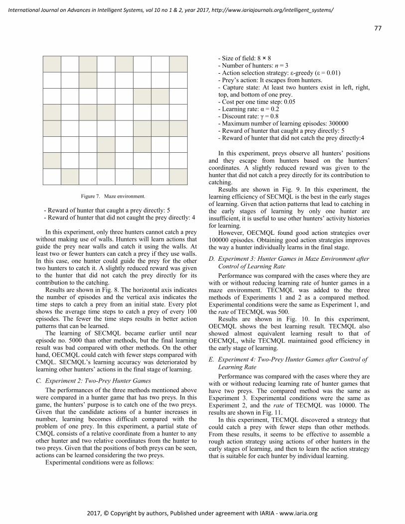
- Reward of hunter that caught a prey directly: 5 - Reward of hunter that did not caught the prey directly: 4

In this experiment, only three hunters cannot catch a prey without making use of walls. Hunters will learn actions that guide the prey near walls and catch it using the walls. At least two or fewer hunters can catch a prey if they use walls. In this case, one hunter could guide the prey for the other two hunters to catch it. A slightly reduced reward was given to the hunter that did not catch the prey directly for its contribution to the catching.

Results are shown in Fig. 8. The horizontal axis indicates the number of episodes and the vertical axis indicates the time steps to catch a prey from an initial state. Every plot shows the average time steps to catch a prey of every 100 episodes. The fewer the time steps results in better action patterns that can be learned.

The learning of SECMQL became earlier until near episode no. 5000 than other methods, but the final learning result was bad compared with other methods. On the other hand, OECMQL could catch with fewer steps compared with CMQL. SECMQL’s learning accuracy was deteriorated by learning other hunters’ actions in the final stage of learning.

C. Experiment 2: Two-Prey Hunter Games The performances of the three methods mentioned above

were compared in a hunter game that has two preys. In this game, the hunters’ purpose is to catch one of the two preys. Given that the candidate actions of a hunter increases in number, learning becomes difficult compared with the problem of one prey. In this experiment, a partial state of CMQL consists of a relative coordinate from a hunter to any other hunter and two relative coordinates from the hunter to two preys. Given that the positions of both preys can be seen, actions can be learned considering the two preys.

Experimental conditions were as follows:

- Size of field: 8 × 8 - Number of hunters: n = 3 - Action selection strategy: ε-greedy (ε = 0.01) - Prey’s action: It escapes from hunters. - Capture state: At least two hunters exist in left, right,

top, and bottom of one prey. - Cost per one time step: 0.05 - Learning rate: α = 0.2 - Discount rate: γ = 0.8 - Maximum number of learning episodes: 300000 - Reward of hunter that caught a prey directly: 5 - Reward of hunter that did not catch the prey directly:4 In this experiment, preys observe all hunters’ positions

and they escape from hunters based on the hunters’ coordinates. A slightly reduced reward was given to the hunter that did not catch a prey directly for its contribution to catching.

Results are shown in Fig. 9. In this experiment, the learning efficiency of SECMQL is the best in the early stages of learning. Given that action patterns that lead to catching in the early stages of learning by only one hunter are insufficient, it is useful to use other hunters’ activity histories for learning.

However, OECMQL found good action strategies over 100000 episodes. Obtaining good action strategies improves the way a hunter individually learns in the final stage.

D. Experiment 3: Hunter Games in Maze Environment after Control of Learning Rate Performance was compared with the cases where they are

with or without reducing learning rate of hunter games in a maze environment. TECMQL was added to the three methods of Experiments 1 and 2 as a compared method. Experimental conditions were the same as Experiment 1, and the rate of TECMQL was 500.

Results are shown in Fig. 10. In this experiment, OECMQL shows the best learning result. TECMQL also showed almost equivalent learning result to that of OECMQL, while TECMQL maintained good efficiency in the early stage of learning.

E. Experiment 4: Two-Prey Hunter Games after Control of Learning Rate Performance was compared with the cases where they are

with or without reducing learning rate of hunter games that have two preys. The compared method was the same as Experiment 3. Experimental conditions were the same as Experiment 2, and the rate of TECMQL was 10000. The results are shown in Fig. 11.

In this experiment, TECMQL discovered a strategy that could catch a prey with fewer steps than other methods. From these results, it seems to be effective to assemble a rough action strategy using actions of other hunters in the early stages of learning, and then to learn the action strategy that is suitable for each hunter by individual learning.

Figure 7. Maze environment.

77



In addition to Experiment 3, TECMQL found actions that were easy to catch a prey rather than the conventional

methods in different environments. However, it is necessary to adjust the learning rate according to the environments.

Figure 11. Results of the proposed method for two-prey game after control of the learning rate.


Figure 9. Results of the proposed method for two-prey game.

Figure 8. Results of the proposed method for maze task. Figure 10. Results of the proposed method for maze task after control of the learning rate.

78



TABLE II. Convergent average steps.

F. Convergent Average Number of Steps for Each Method Table II shows the convergent average steps for each method after each method has finished learning. TECMQL obtained the best average number of steps for the two-prey game. For the maze task game, it obtained nearly the best number of steps.

VI. CONCLUSION In this study, some Q-learning algorithms were applied in the hunter game of maze and two-prey environments. The composition of appropriate partial states was examined. This paper proposed a method that can learn in fewer trials by sharing activity histories among hunters. The method is based on MQL and CMQL, which are methods that prevent an explosion of the number of states. The performance of the proposed method was compared with CMQL. To solve the problem of deteriorating learning performance of the proposed method in the later stage of learning when using other hunters’ activity histories, the learning rate is decreased according to the number of episodes. The proposed method can be generalized to other multiagent environment other than hunter games because it uses a general Q-learning algorithm.

At the present method, the control of learning rate is dependent on the number of episodes, but it is not controlled by the contents of learning. In future study, an index should be established to control the learning rate according to Q-value during learning. In addition, it is considered that the internal states of agents will be optimized by clustering.

ACKNOWLEDGMENT This work was supported in part by JSPS KAKENHI

Grant Number JP16K06424.

REFERENCES [1] K. Matsumoto, T. Gohara, and N. Mori, “Learning method by

sharing activity logs in multiagent environment,” Proc. of the Tenth International Conference on Advanced Engineering Computing and Applications in Sciences (ADVCOMP 2016), IARIA, October 2016, pp. 71-76, ISBN: 978-1-61208-506-7.

[2] G. Weiss, Multiagent Systems: a modern approach to distributed artificial intelligence, MIT Press, 1999.

[3] S. J. Russell and P. Norving, Artificial intelligence: a modern approach, Prentice-Hall, Englewood Cliffs, 1995.

[4] R. S. Sutton and A. G. Barto, Reinforcement learning: an introduction, MIT Press, 1998.

[5] H. Van Hasselt, “Reinforcement learning in continuous state and action spaces,” in Reinforcement Learning, Springer Berlin Heidelberg, pp. 207-251, 2012.

[6] M. Benda, V. Jagannathan, and R. Dodhiawalla, On optimal cooperation of knowledge sources, Technical Report, BCS-G 2010-28, Boeing AI Center, 1985.

[7] I. Nahum-Shani, M. Qian, D. Almirall, W. E. Pelham, B. Gnagy, G. A. Fabiano, and S. A. Murphy, “Q-learning: A data analysis method for constructing adaptive interventions,” Psychological methods, vol. 17, no. 4, p. 478, 2012.

[8] S. Shamshirband, A. Patel, N. B. Anuar, M. L. M. Kiah, and A. Abraham, “Cooperative game theoretic approach using fuzzy Q-learning for detecting and preventing intrusions in wireless sensor networks,” Engineering Applications of Artificial Intelligence, vol. 32, pp. 228-241, 2014.

[9] N. Ono and K. Fukumoto, “Multi-agent reinforcement learning: a modular approach,” Proc. of AAAI ICMAS-96, pp.252-258, 1996.

[10] M.Tan, “Multi-agent reinforcement learning : independent vs. cooperative agents,” Proc. of the 10th International Conference on Machine Learning, pp. 330-337, 1993.

[11] R. M. Kretchmar, “Parallel reinforcement learning,” Proc. of the 6th World Conference on Systemics, Cybernetics, and Informatics, vol. 6, pp. 114-118, 2002.

[12] K. Hwang, W. Jiang, and Y. Chen, “Model learning and knowledge sharing for a multiagent system with Dyna-Q learning,” IEEE Transactions on Cybernetics, vol. 45, no. 5, pp. 978-990, 2015.

[13] Z. Zhang, D. Zhao, J. Gao, D. Wang, and Y. Dai, “FMRQ-A multiagent reinforcement learning algorithm for fully cooperative tasks,” IEEE Transactions on Cybernetics, vol. 47, no. 6, pp. 1367-1379, 2017.

[14] K. Matsumoto, T. Ikimi, and N. Mori, “A switching Q-learning approach focusing on partial states,” Proc. of the 7th IFAC Conference on Manufacturing Modelling, Management, and Control (MIM 2013) IFAC, pp. 982-986, ISBN: 978-3-902823-35-9, June 2013.

[15] H. Iima and Y. Kuroe, “Swarm reinforcement learning algorithm based on exchanging information among agents,” Transactions of the Society of Instrument and Control Engineers, vol. 42, no. 11, pp. 1244-1251, 2006 (in Japanese).

[16] S. Yamawaki, Y. Kuroe, and H. Iima, “Swarm reinforcement learning method for multi-agent tasks,” Transactions of the Society of Instrument and Control Engineers vol. 49, no. 3, pp. 370-377, 2013 (in Japanese).

[17] T. Tateyama, S. Kawata, and Y. Shimomura, “Parallel reinforcement learning systems using exploration agents,” Transactions of the Japan Society of Mechanical Engineers Series C vol. 74, no. 739, pp. 692-701, 2008 (in Japanese).

[18] Y. M. De Hauwere, P. Vrancx, and A. Nowe, “Future sparse interactions: A MARL approach,” Proc. of the 9th European Workshop on Reinforcement Learning, pp. 1-3, 2011.

[19] H. Igarashi, M. Handa, S. Ishihara, and I. Sasano, “Agent control in multiagent systems – Reinforcement learning of weight parameters in particle swarm optimization,” The Research Reports of Shibaura Institute of Technology, Natural Sciences and Engineering vol. 56, pp. 1-8, 2012 (in Japanese).

[20] C. J. C. H. Watkins and P. Dayan, “Technical note Q-learning,” Machine Learning, vol. 8, no. 3, pp. 279-292, 1992.

[21] S. J. Bradtke and M. O. Duff, “Reinforcement learning method for continuous-time Markov decision problems,” Advances in Neural Information Processing Systems, vol. 7, pp. 393-400, 1994.

[22] A. Ito and M. Kanabuchi, “Speeding up multi-agent reinforcement learning by coarse-graining of perception —hunter game as an example—,” IEICE Trans. Information and

Average number of

steps Maze task game Two-prey game

TECMQL 9.6 10.6 SECMQL 11.5 12.1 OECMQL 9.4 11.3

CMQL 10.6 13.6

79



Systems D-I, vol. J84-D-I, no. 3, pp. 285-293, 2001 (in Japanese)

[23] G. Giannakopoulos and P. Themis, “Revisiting the effect of history on learning performance: The problem of the demanding lord,” Knowledge and information systems, vol. 36, no. 3, pp. 653-691, 2013.

[24] I. Koychev and R. Lothian, “Tracking drifting concepts by time window optimisation,” Proc. of the twenty-fifth SGAI

International Conference on Innovative Techniques and Applications of Artificial Intelligence, pp. 46–59, 2005.

[25] I. Koychev and I. Schwab, “Adaptation to drifting user’s interests,” Proc. of ECML2000 Workshop: Machine Learning in New Information Age, pp. 39–45, 2000.

[26] J. Patist, “Optimal window change detection,” Data Mining Workshops, pp. 557–562, 2007.

80



Potential and Evolving Social Intelligent Systems in a Social Responsibility

Perspective in French Universities: Improving Young Unemployed People’s

Motivation by Training for Business Creation Integrating Emotions around

Mediator Artifacts

Christian BOURRET

Research Team DICEN IDF (Information and Communication Devices in the Digital Era)

University of Paris East Marne-la-Vallée (UPEM)

Marne-la-Vallée, France


Abstract - In France, with the economic crisis and the huge rate

of unemployment, the role of Universities has changed in the

recent years with a new challenge of social responsibility. They

try to promote the creation of new economic activities to

attract new people, especially coming from disadvantaged

areas in great town suburbs, particularly unemployed young

people. We present the experiment of Creators of Activities

University Degrees (DUCA) around cooperative devices or

Creators’ Groups (GC). These DUCA / GC correspond to an

individual project, part of a global dynamics in a collective

approach. In a perspective of helping disadvantaged people to

rebuild their life in a project dynamics of creation of economic

activity, information and communication issues are central.

These DUCA / GC areas of interactions and cooperations

constitute socio-technical devices progressively evolving to

potential Social Intelligent Systems. We propose to analyze

these cooperative devices through two Mediator Artifacts

developed in the DUCA / GC areas of cooperations: the

business plan of the activities’ creators and the training serious

game “Solutia”. They help to better master the emotions and

feelings of activities’ creators to develop their self-confidence,

their motivations, their entrepreneurship skills and their

individual and collective knowledge. These areas of projects

constituting potential and evolving Social Intelligent Systems

correspond to a specific way of sustainable development to try

to build “democratic solidarity” on territories.

Keywords – intelligent systems; socio-technical devices;

unemployed people; social responsibility; economic activities

creation; entrepreneurship; mediator artifacts; disadvantaged

areas.

I. INTRODUCTION

In a period of social crisis and of huge unemployment,

particularly for non-graduated young people in disadvantaged areas [1], Serge Paugam pointed the importance of “social links” [2] and of solidarity. These evolutions correspond to the need of repositioning the

Universities in a new perspective of Social Responsibility (RSU) but also other organizations with public service missions, such as Local Missions / Missions Locales (ML) or Centre for Information and Orientation / Centres d’Information et d’Orientation (CIO) in National Education Ministry.

According to Hervé Azoulay [3], “there are talents in the suburbs but they need to be discovered and developed in different manners”. We must give confidence to potential activities’ creators and enable their talents to flourish, and also to promote “innovation in everyday life” according to Norbert Alter [4] and especially social innovations.

The first Creators’ Groups (GC) and Creators of

Activities University Degrees (DUCA) have been created in

2000 by a partnership between the University Institute of

Technology (IUT) of Melun-Sénart belonging to the

University of Paris East Créteil (UPEC) and the Local

Mission (Mission Locale) of Melun-Sénart. A Local

Mission is an intervention space to help young people under

25 years of age. Each young person is given a personalized

follow-up, to help him on employment, on training but also

on housing or health problems.

The University of Paris East Marne-la-Vallée (UPEM,) through its component IUT has managed since 2006 several groups of Creators of Activities University Degrees (DUCA) recently become TPE (Very Small Business) Entrepreneur, supported by training partnerships devices, the Creators’ Groups (GC). These GC (15 in 2016) are federated in a national association: National Association of Creators’ Groups (ANGC).

We first present the global context of the unemployment challenges in France, Social Responsibility of the Universities (RSU) and Social and Solidarity Economy (SSE), particularly for young people in disadvantaged areas. Then we explain our researcher’s position and the methodology used. We show the specificity of the DUCA / GC devices, pointing particularly on their Information and Communication issues and the question of emotions and feelings to improve their motivation. We present two

81



emotions’ Mediator Artifacts: first a training “serious game” (Solutia) and a second, the Business Plan used as the framework of the economic activity project. We explain how DUCA / GC devices may be considered as potential and evolving Social Intelligent Systems. Finally, we show the importance of the DUCA / GC in a Social Solidarity Economy perspective before giving some examples of success stories of activities’ creations and mention some possibilities of evolution of the DUCA / GC.

II. UNEMPLOYMENT CHALLENGES, SOCIAL

RESPONSIBILIY OF UNIVERSITIES IN A SOCIAL AND

SOLIDARITY ECONOMY

The challenge of unemployment is particularly strong in

France. At the end of November 2016, there were 6,238,400

people registered in the Unemployment Office (Pôle

Emploi) in mainland France (without overseas areas),

including 3,447,000 people without any activity. France also

has about 8,000,000 people living below the poverty level.

The situation is particularly worrying for young people.

Nearly 2 million young people are unemployed, without a

diploma or training and, in particular, 19% of young people

under the age of 25: the "neets" (not in education,

employment or training), according to the Anglo-Saxon

expression [5].

The situation has worsened since 2008. For the Minister

of Labor, Myriam El Khomri (DUCAs’ Graduation

Ceremony, Paris, December 12, 2016): "we cannot miss no

skill or talent".

In this context, in the recent years, the role of University

has changed. It is no longer just only to build and transfer

knowledge, but also to welcome new people and promote

their vocational integration, including the creation of new

economic activities. We speak of Social Responsibility of

Universities (RSU). There is also the new position of

“entrepreneur student” [6], concerning all the students and

not only those coming from disadvantaged areas or being

unemployed.

Eric Dacheux defined Social and Solidarity Economy

(SSE) as "seeking to develop links, rather than making

profits" [7]. In the same seminar, Florine Garlot,

highlighting the work of Jean-Louis Laville and Alain

Yvergniaux (2009), stressed the difference between two

types of solidarity: "philanthropic" solidarity and

"democratic" solidarity. With the profound changes of

capitalism over the last thirty years and in particular the

financialization of the economy, Laville and Yvergniaux

propose another project based on “democratic solidarity”.

While for them philanthropic solidarity corresponds to a

liberal political project aimed at calming the tensions of a

system by nature egalitarian, democratic solidarity is

centered on emancipation and the reduction of inequalities

[8].

Our approach to the RSU corresponds to this social and

solidarity economy perspective, thus articulating the notions

of link or interaction (reliance) to promote the sustainable

development of territories through the interactions and

solidarity of all the actors, and especially in disadvantaged

areas (resilience).

III. RESEARCHER’S POSITION AND METHODOLOGY

The author of this paper manages DUCAs in the IUT /

UPEM and is also member of GC Coordination

Committees.

From a methodological perspective, the author of this

article belongs to the French University’s interdisciplinary

field of Information and Communication Sciences,

according to the approach proposed by Françoise Bernard

[9] with the convergence of four aspects: meaning, link

(relationships, interactions), knowledge and action. He

positions in a research action perspective mixing theory and

practice to build knowledge for action. His analysis

corresponds to the research position described by Françoise

Bernard as “engaging communication” [10].

Insisting on the primacy of action, Françoise Bernard

proposed the paradigm of "engaging communication" to

organize communication of societal action and utility, which

is the case of the social and solidarity economy, as defined

by Eric Dacheux. It is a question of apprehending the

change in actions and the complex time of the various

actors. Information corresponds to the time of knowledge,

the urgency of action to the time of change. The articulation

of the four major issues of action, link, knowledge and

meaning, makes it possible to reconcile these different times

to build a new civic responsibility. F. Bernard outlines the

dimensions of “engaging position” and that of projects,

which is the case for DUCA / GC.

According to Nicole D'Almeida [11], organizations move

“between projects and stories.” The projects correspond to

two types of devices: first is the organizational one, and the

second she calls “symbolic narrative” part where “stories”

(symbolic devices) are essential. Organizations or

organizational devices build their own imaginary stories. To

take an example in a presentation’s leaflet of Val de Marne

Creators’ Group: “Creators’ Groups help to switch from

dream to reality.” They are based on two core values:

“everyone is an asset for the territory”, “everyone

expressing the desire to create an activity is heard”.

In this work, we met several concepts. The first concept

met is that of “device” (in French, “dispositif”), that we

consider, according to Michel Foucault [12], with all its

socio-technical dimensions. For him, “What I'm trying to

identify with that name, is first a decidedly mixed space,

with speeches, institutions, architectural arrangements,

regulatory decisions, laws, administrative measures,

scientific statements, philosophical propositions, moral,

82



philanthropic, in short: the words, as well as the unspoken,

are mere elements of the device. The device in itself is the

network that can be established between all these elements.

Secondly, that I would identify in the device, is precisely the

nature of the relationship that may exist between these

heterogeneous elements.” In a socio-constructivist perspective, we also rely on the

concept of “mediator artifact”: “the tools provided by the environment do not only play a role of mediator but also of artifact in that they organize (or reorganize) cognitive functioning” [13] with all the importance of project dynamics as especially developed by Jean-Pierre Boutinet and Gino Gramaccia [14] [15]. We also rely on the concepts of situations and interactions [16], defined by Manuel Zacklad as a logic of “cooperative transactions” [17].

Afterwards we analyze these DUCA / GC socio-technical devices as potential and evolving social Intelligent Systems [18] built by the cooperative knowledge of all their actors.

IV. THE DUCA – GC AS SOCIO-TECHNICAL DEVICES

In this section, we will show how DUCA / GC

correspond to socio-technical devices as interactions’ areas

with important Information and Communication Issues.

A. DUCA and GC as interactions‘ areas

According to ANGC, “The Creators Groups seek

autonomy and professional integration of unemployed people, including school leavers, based on their desires to undertake as a catalyst”. The main goal of the DUCA / GC devices is to restore confidence, especially for young school leavers by leveraging their creativity in a project approach from an individual project based on training (DUCA), developed in training and group work, but also with an individual coaching (GC).

The GCs (Creators’ Groups) aim to transform the desire

for entrepreneurship into catalysts for professional

integration through support and coaching based on

entrepreneurship and project pedagogy. And this coaching is

proposed without judging on the feasibility of the idea of the

potential creator of activity or on the capacity to create or

rescue an activity.

So this is an individual project, part of global dynamics,

in a collective approach.

We have pointed the two key values of the DUCA / GC:

“everyone is an asset for the territory”, “everyone wanting

to develop an economic activity is heard”. These values are

highlighted by the National Association of Creators’ Groups

(ANGC).

The potential creator of activity is in the center of the

DUCA / GC devices, initiator and co-constructor of his

project. Integration and autonomy are the aims of the

coaching. The support or coaching correspond to a public

service approach and the GC services are offered free of

charge [19]. Since 2006, UPEM / IUT proposed several DUCAs in

partnership with different Creators Groups: Val de Marne Department (94), Val Maubuée (Torcy, 77) and, during three years, with the Paris 20

th GC.

We will analyze how a new kind of training (DUCA) is based on cooperative processes and may be regarded as a “device” or an “organizational form” created by all the interactions between all the actors, to develop new opportunities for job seekers coming from disadvantaged areas, especially young school leavers. This process creates a new dynamics among all the actors, combining the individual dimension of each project with a collective dynamics.

A DUCA / GC device brings together partners including: 1) A federative structure (Mission Locale, Local Plan for Economic Insertion (PLIE), House of Employment (Pôle Emploi), other associations, etc.), 2) a University, often through an IUT, 3) a consultancy team in business creation (management shop or boutique de gestion, cooperative, industry and trade chambers, etc.).

B. Importance of Information and Communication Issues

Eric Dacheux, already mentioned [7], characterized

Social and Solidarity Economy (SSE) as "seeking above all to build links". This approach corresponds to the main goals of Communication Sciences, as stressed by both Françoise Bernard [10] and Daniel Bougnoux [20], emphasizing the importance of the links and the relationship. It is the question of "living connected" or "reliance" that, for us, joins that of the "resilience" of territories in difficulty.

In a perspective of helping people to rebuild their life [21] in a project dynamics, information collect and communication issues are central. Their analysis will constitute a main part of our grid to consider awareness and management of emotions and feelings as levers of creating economic activities. And so their management included in these activities’ creation may help people in difficult situations to rebuild their life.

Firstly, candidates to DUCA / GC are searching in leaflets on business and crafts, books and numerous documents offered by the Local Missions and Centre for Information and Orientation (CIO), specialized websites, etc., information to better formalize their projects. They are helped in their information and documentation work by members of ML or of CIO.

The personal reconstruction of the learner / creator is based on an innovative process of creating an activity that is formalized in an oral mid-term and an end-of-year presentation. This process involves many exchanges and a strong research activity for information and documentation with the help of people resources belonging to Local Mission, CIO, or different local associations. It is driven by Mediator Artifact such as Business Plan of each student or meetings around a training “serious game”.

83



This paper corresponds to a complementarity of views. We have met, observed and interviewed: DUCA teachers, GC leaders, trainers, facilitators from Local Missions, members of boutiques de gestion, psychologists, and, of course, students-learners and potential creators of their economic activity.

We propose some ways to analyze emotions and feelings of these actors, especially of young people creating activities around two Mediator Artifacts: a training serious game (Solutia) and the business plan of each activity’s creator. In a first step, these two Mediator Artifacts constitute for us socio-technical devices.

V. TWO EMOTIONS’ MEDIATOR ARTIFACTS

DUCA / GC devices correspond to societal innovative

areas to promote interactions. Two Mediator Artifacts may

act to reveal emotions and feelings and so help to improve

activities creators’ skills and their creativity.

A. A training “Serious Game” (Solutia) as first Mediator

Artifact to develop ludic interactions

The main goal of DUCA / GC is to help increase

creativity spirit and skills of creators of potential economic

activity and especially young people. The DUCA / GC

training teams try to invent new ways to interest the

potential activities’ creators in being involved and so

changing their life. One specific way consists in a training

game: “Solutia”. It is actually a form of “serious game”, but

not developed on Internet interactions but on real exchanges

in face-to-face situations between some creators (five to

eight) with the help (a form of coaching) of a ML member.

This game constitutes a Mediator Artifact to develop ludic interactions to improve interest for cooperation and to create a project dynamics. This training “serious game” may also help converge the representations and develop confidence by creating collective dynamics and some form of pride around a personal project which may be also that of a whole family and, sometimes, of a larger community.

First, this game has been thought and created by Marie Beauvais – Chevalier, member of ML of Marne-la-Vallée / Torcy, coordinator of the GC in Val Maubuée. Solutia’s game corresponds to a sort of Monopoly and Game of the Goose (Jeu de l’Oie) for learning how to manage company’s creation and its traps and opportunities.

In a second step, Solutia has been developed and marketed by a student of UPEM University with the creation of a new company through a new device “Students poles for Innovation, Transfer and Entrepreneurship” (PEPITE) [22].

This business creation by a student around Solutia’s serious game illustrates the important evolution of the French Universities, and especially UPEM University. UPEM University tries to develop a new spirit of entrepreneurship through various devices and especially with times of exchanges and interactions between teachers and students

such as the “All Creative Day, Tous Créatifs” (this year on June 22

th). It also corresponds to interactions between civil

society and local actors and Universities members.

B. A second Mediator Artifact: the Business Plan of the

creators’ projects

We have also observed the emotions and feelings of the

actors of DUCA / GC Devices around another Mediator Artifact, the Business Plan of each creator of potential economic activity. The business plan is the main framework of the entire process of monitoring the development of the economic activity of the potential creator. It is a crystallizer of interactions from the beginning of the process (emergence phase) to the final presentation of the project.

The emergence phase allows the potential activity creators to better define their ideas and formalize them. It includes four steps: 1) better knowing their potentiality as project’s leaders, 2) better defining the main idea of activity to develop, 3) discover the environment of the project, 4) define the suitability of their personality to the project and its environment. After this phase, the future creator formalized a file, which is the basis for presentation and is defending before a jury for admission to the DUCA degree. The interview is always conducted sympathetically to give confidence to the future creator and help to validate his idea.

The training phase (DUCA) allows future creators to receive specific knowledge to develop skills necessary to manage any activity (company, association, etc.): management, information and communication, legal and tax information, sales management, market survey, project management, etc., and to check the feasibility of the proposed project, specifying the business plan (market survey, financing, cost calculations, etc.). The “case” is finalized and presented before a jury. Pedagogy emphasizes the collective dimension and the practical application of the teachings around creative projects.

VI. INTERACTIONS ANALYSIS AROUND MEDIATOR

ARTIFACTS INTEGRATING EMOTIONAL DIMENSIONS

The two presented Mediator Artifacts enable us to

observe the emotions and feelings expressed in particular by young potential entrepreneurs: a phase of interactions between them in a playful position (Solutia Game) and also with interactions with the teaching team: the Business Plan. Both Mediator Artifacts converge to help to build an individual project in a collective dynamics.

Finally, our findings highlight an analysis process with the transition from the initial and spontaneous emotions of the actors, especially young creators of economic activity, to more lasting feelings, attitudes and behaviors over a long period, in relation with their personality.

We promote a dynamic dimension of integration (integrative approach) of changing emotions and feelings in the situation analysis and interactional approach proposed by Alex Mucchielli (Situational and Interactionist Semiotics) [23] for economic activity creativity, apprehended in a grid

84



of informational and communicational integration of actors’ views. Different contexts constituting a situation for the actors are considered: respective positions, goals, references or norms, interactions, values, etc. The set of meanings found provides access to the "global meaning" of the phenomenon, which is therefore the synthesis of the meanings taken in the different contexts and for the different actors.

For us, it is also the challenge of development of a dynamics (process) around control of emotions and feelings on a rather long term process.

Alain Caillé presented the quest for recognition as a new total social phenomenon in the second half of the XX

th

century, notably for minorities or some social groups, but also for populations of sensitive areas. For him, until the 1980s, the emphasis was rather on levels of remuneration, (wages), social protection and working conditions, in particular with the development of trade unions [24]. Recognition by others and the reconstruction of self-esteem are very linked according to Gerard Lefebvre [21].

The DUCA / GC devices are also a space for converging management of project approaches [14], [15], and quality approaches. We propose to consider this convergence through three types of processes that exists in any organization or project: the objective to compliance (control), the desire to implement changes and so the commitment to promote creativity and innovation [25]. For us, DUCA / GC devices constitute interesting areas of cooperation to observe this convergence. The challenge is to promote a culture of change and innovation in the French society based for example on validated and reproducible experiments. It can be first developed betting on the capacity for innovation and creativity in small structures that promote initiatives. But it is also a question of answering the reality of markets and needs of local consumers or funding institutions.

The emotional skills of young creators are the central element of an emotional intelligence, in our opinion, not sufficiently taken into account. The human body is both the mediator from which the individual can sensitize his affects and constitutes a communication support of them, according to Fabienne Martin-Juchat [26].

By helping to set the individual project of business creation in a collective dynamics, the two studied Mediator Artifacts may help to favor a first awareness among activity creators; they are never completely alone and there are levers, networks that they must know how to use to get the right information at the right time and in the right place (informational and communicational skills). This awareness may help activities’ creators to restore their confidence and to overcome their shyness.

The serious game Solutia also promotes situational skills: it allows students to discover a number of problem situations they can find in their creative activity and so help to overpass them. It can give awareness of their personal evolution, especially of their new skills and some pride of their activity’s project: importance of self-esteem, often built through the eyes of others, especially their friends and their families.

The goal of the Mediator Artifacts, particularly Solutia serious game is to (re) give confidence, to raise awareness that everyone has met difficulties in his entrepreneurship’s pathway and that they can be overcome. It is good to know how to go beyond emotions such as fear of failure, withdrawal, frustration, anger, etc. Understanding and better managing emotions by relativizing them may help to recreate a positive dynamics of trust. It is also important to train the activities’ creators to be aware of their emotions and feelings, so they are not paralyzed by them, and, therefore, to better manage them and to succeed in their creation of activity process.

VII. FROM SOCIO-TCHNICAL DEVICES TO POTENTIAL AND

EVOLVING SOCIAL INTELLIGENT SYSTEMS

DUCA / GC constitute spaces for cooperation in order to

develop an individual project in a collective process of building knowledge based on Mediator Artifacts fostering exchanges and cooperation among all their actors, notably creators of economic activity.

As a first step, we proposed to consider them as socio-technical devices based in particular on interactions around two Mediator Artifacts. In a second step, we propose to consider the DUCA / GC as potential and evolving Social Intelligent Systems by placing us notably in the constructivist approach (the social reality is “construct” by the actors) of the complexity analysis proposed by Edgar Morin [27] and Jean-Louis Le Moigne [28]. Particularly, Jean-Louis Le Moigne proposes an approach to the elaboration of a General System, which gradually emerged from the 1950s with the cybernetic, structuralist and structural-functionalist approaches ([18].

J.-L. Le Moigne stresses the importance of modeling: "modeling a complex system is modeling a system of actions". In the formalisms of the systemic modeling, he relies on Edgar Morin, who proposed the concept of organiz-action corresponding to principles of eco - auto - re - organization with information, communication and computational dimensions.

For J.-L. Le Moigne, it is an organizational or informed system: "the information forming the organization that forms it", with all the importance of documentation and information resources, as we have pointed out for the DUCA / GC [28].

From the communicational point of view, Alex Mucchielli proposed [29] a "Systemic and Communicational Approach of Organizations" (2002). He presents an Information and Communication Sciences approach based on the paradigm of complexity in relation with systemism and constructivism, referring to the works of the invisible college at Palo Alto, where "communication is always conceived as a participation in a communicative ensemble or a system of relations (the "orchestra" model). It is a matter of bringing to light the meaning of the different interactions in a global system, in order to create a collective sense of the relational system itself for all actors. It proposes

85



a method leading to model the relations. It begins with an observation of relations, and continues with an effort to diagram the exchanges (including implicit communications) of the actors and to finish with the description of the functioning of the whole system. The final analysis must reveal the emerging "values" of the system, which, implicitly, can be regarded as "leading the game", almost unknown to the actors.

He will confirm and extend these propositions a few years later in his "situational and interactional semiotic" approach (2010) already mentioned in an interactionist analysis of the DUCA / GC [23]. This perspective joins that of the Communication as Constitutive of Organizations proposed by Linda L. Putnam and Anne M. Nicotera [30], considering organizations as organizational systems as Edgar Morin.

After the informational and communicational dimensions of his modeling approach, J.-L. Le Moigne evokes a third "computational" dimension. In this perspective of computational analysis of players’ relations in the case of game situations, such as for the Mediator Artifact Solutia game, we can refer for example to the works of Mossakowski and Mandziuk in the case of the bridge game [31].

At this stage of our analysis, we are at the first two levels of modeling information and communication situations around interactions between DUCA / GC actors in a perspective of social systemic approach in a shared knowledge building perspective.

DUCA / GC considered as potential social Intelligent Systems correspond also to an approach of building collective intelligence in specific situations. We are then in the perspective of management of collective intelligence (CI) proposed by Olivier Zara [32]. According to him, "Collective Intelligence is the intelligence of the link, of the relationship defined by some as a connective intelligence or "global brain"... The heart of the collective intelligence is the harmony in the links... These links induce the cooperation and collective intelligence would ultimately be the consequence of intellectual co-operation, their materialization. He refers to Pierre Lévy, for whom "the best thing that can be done with new technologies is not Artificial Intelligence (AI), but, on the contrary, Collective Intelligence … Computers do not mimic humans, but help them to think and collectively evolve their ideas. CI helps people to think together, while AI seeks to substitute for humans to limit their mistakes ".

All this from a perspective of social systemic that J.C. Lugan proposes to develop in a pragmatic approach "concerned to confront the available systemic tools with concrete social formations" [18], for us DUCA / GC.

VIII. THROUGH AN INDIVIDUAL DYNAMICS IN A

COLLECTIVE APPROACH

To use a formula coming from an ANGC document: "To

dare it is already to move forward". It is a question of helping to "overcome the preconceived ideas that prevent

change": "I have no money", "I am too young", "It is too complicated", "I have no idea", "I feel alone ","I have a disability", "I do not have a diploma", etc. [19].

We think that learning to better manage the emotions can become a collective goal to develop cooperation and improve skills. It is on this aspect that we propose to the other partners of the DUCA / GC to insist with a view of continuous improvement of existing devices.

Social sharing of emotions is also important for encouraging awareness of group membership [16]. This group is essential to promote the personal development of each potential creator. This integration of emotions and feelings can help to better integrate an individual project of creation of activities in a collective dynamics of exchange of experiences and feelings (Group of Creators) to better understand and support in times of doubt and (re) motivate them. We wish to analyze their mechanisms to best promote these periods of interactions and information sharing for improvement of their projects.

Our observations lead us to propose a broadening of perspectives of Situational and Interactionist Semiotics defined by Alex Mucchielli [23] with the integration of the experiences of the actors and their emotions and feelings according to Daniel Goleman [33], particularly for creators of activity.

Another approach to consider is the Sociology of Actor-Network (SAR) proposed by Michel Callon [34], even if the business plan and the serious game Solutia are not full technical devices, but rather social and managerial devices. The idea that the collective activity (“acting elements”) can be considered as a “black box” (“boîte noire”) seems to match our approach of the business plan as the idea of “hybrid reality composed of successive translations” and the fact that the SAR “has been designed to follow the collective in their making process”, which is the case of DUCA / GC devices.

In the perspective developed by Aurélia Dumas and

Fabienne Martin-Juchat [35], through situations of

participatory observations or interviews with young creators

of activities, in particular around the uses of the two

mediating artifacts, we tried to understand their emotional

culture, their emotional language and their mechanisms of

emotional regulation. By privileging the vision of these

actors, in a rather ethnographic approach, we considered the

two mediating artifacts as "communicative objects". We can then consider a dynamic relational semiotics

approach to a certain length: global (approach by the complexity theory in a constructivist way), based on the search for meaning in the interactions’ situations between all the actors (including socio-technical artifacts), and of course also including emotions, feelings, experiences of all the actors in a dynamic approach (convergence of the management of project approaches and the process approaches of quality management) to create a dynamic of change, creativity and innovation, mixing individual and collective dimensions.

86



IX. A SUCCESS TO BETTER SOCIALLY INTEGRATE PEOPLE

BY CREATING NEW ECONOMIC ACTIVITIES FOR THE

SUSTAINABLE DEVELOPMENT OF DISADVANTAGED

TERRITORIES

A very recent study on Creators' Groups [36] clearly

highlights the impact of GCs, corresponding to "an integration program through project pedagogy". DUCA / GC students are both better paid (29 % more than other young unemployed people) and can take back studies in better conditions and with motivation. By enabling young people to rebuild themselves, to regain their confidence and to think about a project, the DUCA / GC are thus two-fold integration mechanisms: both by activity (60% of DUCA graduates) and by training.

Since 2000, the GCs, mostly through Local Missions, have received over than 15,000 people, mainly young people, coached 7,500 people in the project emergence phase and more than 1,300 people in the training phase or DUCA [19]

For the University of Paris East Marne-la-Vallée (UPEM), since 2006, 305 activity creators and, especially, young people, have been trained in the IUT of UPEM and 157 graduated, that is to say more than 50%, which is considered as a very positive result by the Ile-de-France Regional Council (CRIF), the main public collectivity giving funds to the DUCA / GC devices.

More globally, nearly 500 people, especially young people, have been sensitized to business creation and reality of the economic constraints of companies. Nearly 35% of the graduated students have created their business or taken over an existing activity; others have been inserted as employees in existing companies (often trade or food activities). Activities creations successes particularly concern the services sector in very different aspects. First, we have food activities such as free gluten bakeries, food to all tastes and cuisines possible, particularly Afro-Asian. Secondly, we have clothes manufacturing companies corresponding to different countries (Japan and Asia fashion, North Africa, etc.) and shops of different types of clothes. We have also organic cleaning companies, communication companies to organize special events (marriage, etc.), production of video games, jewelry creations, home automation companies, etc. We have also more usual activities such as nurseries, gardening, public writers, different ways of home help, beauticians, hairdressers, sometimes with itinerant projects. But also, with the reform of school times (2013), we have animation’s projects to provide stimulating activities or sports for children after school time, etc.

A great satisfaction during the graduation ceremonies for the DUCAs in December 2015 and 2016 was to see some graduated of previous years come to offer jobs to those who had just come into training.

DUCA / GC can also correspond to an intergenerational perspective that may be part of the Silver Economy (markets linked to ageing and well-ageing). Young retired volunteers could thus help young creators or young rescuers of activities to develop their activity: aids in management but also

according to the different types of jobs (baker, car repair, gardener, etc.) giving a sense of solidarity and transmission in the early years of the often difficult transition from an intense activity to the breaking, not always wanted, to retired new life. These retired people may act as supports or coaches for young and inexperienced creators of activities. This form of intergenerational solidarity on the territories also corresponds to the articulation of the challenges of "reliance" and "resilience".

X. CONCLUSION

Since 2006, DUCA / GC socio-technical devices

developed in UPEM / IUT, in cooperation with federated partners in the DUCA / GC have progressively constituted potential and evolving Social Intelligent Systems. They have trained over than 500 students in the creation of activity, including a majority of young school leavers. The challenge is now finding additional funding to the specific aid the Regional Council of Ile-de-France. We hope in European subsidies.

In the cooperation areas developed around DUCA / GC devices, the position of “committed researcher” has really, for us, taken all its meaning and corresponds to a personal approach to the RSU, revisited as “societal responsibility of the researcher”, in a perspective of “engaging communication” proposed by Françoise Bernard for societal responsibility [10]. We have gradually become convinced that the future can be built from micro actions on the territories and on daily innovative practices.

For us, beyond the figures and examples of activities successes creations in various sectors (gardening, personal computers, clothing, cleaning, food, restaurants, personal services, etc.), the more important part is to have renewed hope through a project dynamics to allow potential creators of economic activities, especially school young leavers, to take charge of their destiny, in taking the risk of action for hope to promote a new business vision, resolutely different from “destructive innovation” discussed by Luc Ferry [37], with the disasters of the financial and speculative capitalism. We insist on a first goal, that people dare to do the first step and also meeting the words of George Mallory starting to climb to Everest Mountain (1924): “Where there is a will, there is always a way.” We also meet Stéphane Hessel and Edgar Morin who proposed new paths towards "the way of hope" in the same perspective of Economic Social and Solidarity where we try also to walk [38].

This approach focuses on the integration and management of emotions and feelings of all the actors of DUCA / GC devices, particularly those of the potential creators of economic activities. It also incorporates the concepts of “resilience” (ability to move again in a crisis situation), both with individual and collective aspects, of “sustainable development” of territories. Territories are then considered as built by a synergy of local projects, both individual and collective, all these projects building new links or interactions and solidarity, especially in disadvantaged areas [39] in order to create a collective

87



dynamics and give capacity for innovation and creativity [40]. For us, they constitute potential and evolving Social Intelligent Systems progressively built by all the knowledge and skills of all their actors and especially the creators of activity.

It is a question of trying to "catalyze" the energies to contribute to a new territorial dynamics, training being an essential element in helping to broaden territorial social capital by relying on projects of motivated young people. It is also in a certain manner an element of the perspective proposed by B. Carayon [41] of the French Economic Intelligence approach insisting on associating competitiveness of companies and social cohesion in a new territorial dynamics linking stakes of economic or competitive intelligence and territorial intelligence.

Potential and Evolving Social Intelligent Systems, DUCA / GC also correspond to new ways of “democratic solidarity” on territories, promoting new links between unemployed people with existing companies, local authorities or retired people acting as supports or coaches to invent new ways of local citizenship. They then contribute to the "relationship economy" proposed by Nicole D'Almeida in a communication perspective [42] and the "economies of conviviality and transactions" defined by Manuel Zacklad [17].

REFERENCES

[1] C. Bourret, “Tracks to Analyze Emotions around Mediator Artifacts to Improve Training and Business Creation for Unemployed People in French Universities,” Proceedings / The Second International Conference on Human and Social Analytics, HUSO 2016 – IARIA, Barcelona November 13 – 16, pp. 9-13, ISBN : 978-1-61208-517-7

[2] S. Paugam, The social link / Le lien social, Paris: PUF, 2010.

[3] H. Azoulay, "Social Intelligence. The case of suburbs : use networks to go gout crisis / L’intelligence sociale. Le cas des banlieues : utiliser les réseaux pour sortir de la crise," in M.-A.Duval dir., New territories of Business Intelligence / Les nouveaux territoires de l’Intelligence Economique, Paris: ACFCI – IFIE Ed., pp. 119-146, 2008.

[4] N. Alter, Ordinary Innovation / L’innovation ordinaire, Paris: PUF, Coll. Quadrige, 2005.

[5] Available on: http://www.lefigaro.fr/social/2015/03/25/09010-20150325ARTFIG00325-pres-de-2-millions-de-jeunes-sont-sans-emploi-ni-diplome-en-france.php. Retrieved 2017, February 5th.

[6] Available on : http://www.enseignementsup-recherche.gouv.fr/cid79926/statut-national-etudiant-entrepreneur.html. Retrieved 2016, June 26th.

[7] Seminar “New forms of cooperation for the Digital Age / New Civic Sociability”, ISCC, Paris, December 1st, 2016.

[8] J.L. Laville and A. Yvergniaux, “Tags for a left project. Democratic solidarity, sustainable development, plural economy / Balises pour un projet de gauche. Solidarité démocratique, développement durable, économie plurielle," Institut Polanyi / France, 2009, Available on: http://institutpolanyi.fr/balises-pour-un-projet-de-gauche-solidarite-democratique-developpement-durable-economie-plurielle/. Retrieved 2017, February 5th.

[9] F. Bernard, "The SIC, a Disciplinary of Openness and Decompartmentalization / Les SIC, une discipline de l’ouverture et du décloisonnement ", in A. Bouzon dir., op. cit., Paris : L’Harmattan, pp. 33 – 46, 2006.

[10] F. Bernard, “Organize communication for societal action and utility. The paradigm of engaging communication / Organiser la communication d’action et d’utilité sociétales. Le paradigme de lacommunication engageante,” Communication and Organization / Communication et organisation , 29 | 2006. Available on http://communicationorganisation.revues.org/3374. Retrieved February 2017, 6th.

[11] N. D’Almeida, "Organizations between projects and stories / Les organisations entre projets et récits", in A. Bouzon dir., Organizational Communication in debates. Fields, Concepts and Prospects / La communication organisationnelle en débats. Champs, concepts et perspectives, " Paris : L’Harmattan, p. 145 – 158, 2006.

[12] "The game of Michel Foucault / Le jeu de Michel Foucault" (interview), Ornicar ?, n° 10, July, pp. 62-93, 1977.

[13] Available on : http://www.edu-tice.org/approche-th%C3%A9orique/glossaire/concepts-5/. Retrieved 2016, June 26th.

[14] J.-P. Boutinet, Psychology of Project Conducts / Psychologie des conduites à projet, Paris: PUF, 1999.

[15] G. Gramaccia, “Quality, Project, Digital : three symbolic variations of Managerial Effectiveness / Qualité, projet, numérique : trois variations symboliques de l’efficacité gestionnaire,” in C. Batazzi dir., Communication, organisation, symboles, Revue MEI, n° 29, Paris : L’Harmattan, pp. 55-67, 2008.

[16] L. Bègue and O. Desrichard dir., Treaty of Social Psychology. Science of Human Interactions / Traité de psychologie sociale. La science des interactions humaines, Bruxelles: De Boeck, 2013.

[17] M. Zacklad, "Economies of Conviviality in Information and Services Societies / Les économies de la convivialité dans les sociétés de l’information et des services," Inaugural Lecture / Leçon inaugurale, Paris: CNAM, 2009 June 17 th.

[18] J.-C. Lugan, Social Systemic / La systémique sociale, Paris : PUF, 2012.

[19] Creators Groupments Network / Le réseau Groupement de Créateurs, Undertake his future / Entreprendre son avenir, Paris, Available on: www.groupement-de-createurs.fr

[20] D. Bougnoux, Introduction to sciences of communication, Paris: La Découverte, 2006.

[21] G. Lefebvre, Identitary Reconstruction and Insertion / Reconstruction identitaire et insertion, Paris: L’Harmattan, 1998.

[22] Available on : http://www.enseignementsup-recherche.gouv.fr/cid79223/pepite-poles-etudiants-pour-innovation-transfert-entrepreneuriat.html. Retrieved 2016, June 26th.

[23] A. Mucchielli, Situation and Communication, Nice : Les éditions Ovadia, 2010.

[24] A. Caillé dir., The quest for recognition new total social phenomenom / La quête de reconnaissance nouveau phénomène social total, Paris : La Découverte, 2007.

[25] J.-P. Caliste and C. Bourret, "Contribution to a Typological Analysis of Processes : From Conformity to Agility / Contribution à une analyse typologique des processus : de la conformité à l’agilité," UTC Quality Notebooks / Les Cahiers de la Qualité de l’UTC, Vol 2, G. Farges and al.., Lexitis éditions, pp. 113-116, 2015.

[26] F. Martin-Juchat, The body and the media. The flesh experienced by the media and social spaces / Le corps et les

88



médias. La chair éprouvée par les médias et les espaces sociaux, Bruxelles: De Boeck, 2008.

[27] E. Morin, Introduction to Complex Thought / Introduction à la pensée complexe, Paris : ESF, 1990, rééd., Points-Seuil, 2005.

[28] J.-L. Le Moigne, Formalisms of Systemic Modelling / Les formalismes de la modélisation systémique, 2005, Available on :www.intelligence-complexite.org/fileadmin/docs/0505formalismesvfr.pdf, Retrieved May 2017, 1st.

[29] A. Mucchielli, Systemic and Communicationnal Approach of Organizations / Approche systémique et communicationnelle des organisations, Paris : Armand Colin, 2002.

[30] L. L. Putnam, A.M. Nicotera, Building Theories of Organization. The Constitutive Role of Communication, New York / London : Routledge, 2009.

[31] K. Mossakowski and J. Mandziuk, “Learning without human expertise. A case study of the Double Dummy Bridge Problem,” Transactions on Neural Networks, IEEE, vol. 20, Issue 2, pp. 1-23, Available on : ieeexplore.ieee.org/iel5/72/4776562/04749256.pdf – Retrieved May 2017, 1st.

[32] O. Zara, Management of Collective Intelligence / Le Management de l’intelligence collective, Paris : M21 Editions, 2008.

[33] D. Goleman, Working with Emotional Intelligence, Bloomsbury: London, 1998.

[34] M. Callon, " Sociology of the Network Actor / Sociologie de l’Acteur Réseau," in M. Akrich, M. Callon and B. Latour., Sociology of the Translation : Founding Texts / Sociologie de la Traduction : Textes fondateurs, Presses de l’Ecole des Mines de Paris, pp. 267-276, 2006.

[35] A. Dumas and F. Martin-Juchat, “Communication approach to emotions in organizations: questions and methodological implications / Approche communicationnelle des émotions dans les organisations : questionnements et implications méthodologiques ,” French Review of Information and Communication Sciences / Revue française des sciences de

l’information et de la communication, 9/ 2016, Available on: http://rfsic.revues.org/2103 ; DOI : 10.4000/rfsic.2103 . Retrieved 2017, February 5th.

[36] Y. Algan, B. Crépon, E. Huillery and W. Parienté, “Impact of Creators' groups: teaching a controlled experiment / Impact des Groupements de Créateurs : enseignement d’une expérience contrôlée”, J-PAL et CREST Laboratories, Paris, 2016. Available on: http://www.lesechos.fr/economie-france/social/0211576808894-jeunes-le-dispositif-groupement-de-createurs-a-fait-ses-preuves-2049670.php. Retrieved 2017, February 5th.

[37] L. Ferry, Destructive Innovation / L’innovation destructrice, Paris: Plon, 2014.

[38] S. Hessel and E. Morin, The Way of Hope / Le Chemin de l’Espérance, Paris :Fayard, 2011.

[39] C. Bourret, "Elements for an Approach of Territorial Intelligence as a Synergy of Local Projects to Develop a Collective Identity / Eléments pour une approche de l’intelligence territoriale comme synergie de projets locaux pour développer une identité collective," International Journal of Projectics, n° 1, Bruxelles: De Boeck, pp. 79-92, 2008.

[40] M. Godet, P. Durance and M. Mousli, Unleashing innovation in the territories / Libérer l’innovation dans les territoires, Paris : Conseil d'Analyse Economique - La documentation Française, 2010.

[41] B. Carayon, Economic Intelligence, Competitiveness and Social Cohesion, / Intelligence économique, compétitivité et cohésion sociale, Paris : La Documentation française, 2003. Available on : http://www.ladocumentationfrancaise.fr/rapports-publics/034000484/index.shtml. Retrieved 2017, May 1st.

[42] N. D’Almeida, The Promises of Communication / Les promesses de la communication, Paris : PUF, 2001.

89



Hierarchical Cooperative Tracking of Vehicles and People Using Laser Scanners Mounted on Multiple Mobile Robots

Yuto Tamura, Ryohei Murabayashi Graduate School of Science and Engineering

Doshisha Unversity Kyotanabe, Kyoto 610-0394 Japan

e-mail: {ytamura915, ryo040978}@gmail.com

Masafumi Hashimoto, Kazuhiko Takahashi Faculty of Science and Engineering

Doshisha Unversity Kyotanabe, Kyoto 610-0394 Japan

e-mail: {mhashimo, katakaha}@mail.doshisha.ac.jp

Abstract—This paper presents a tracking (estimation of the pose and size) of moving objects such as pedestrians, cars, motorcycles, and bicycles, using multiple mobile robots as sensor nodes. In this cooperative-tracking method, nearby sensor nodes share their tracking information, enabling the tracking of objects that are invisible or partially visible to an individual sensor node. The cooperative-tacking method can then make the tracking system more reliable than the conventional individual tracking method by a single robot. We previously presented a centralized architecture of cooperative tracking. Each sensor node detected moving objects in its own laser-scanned images captured by a single-layer laser scanner. It then sent measurement information related to the moving objects to a central server. The central server estimated the objects’ poses (positions and velocities) and sizes from the measurement information using Bayesian filter. However, such a centralized method might have poor dependability and impose a computational burden upon the central server. To address this problem, this paper presents hierarchical architecture of cooperative tracking. Each sensor node locally estimates the poses and sizes of moving objects and then sends these estimates to the central server, which then merges the pose and size estimates. Experimental results using two sensor nodes in outdoor environments show that the proposed hierarchical cooperative-tracking method provides slightly inferior tracking accuracy and has a smaller computational cost in the central server than a previous centralized method.

Keywords—moving-object tracking; cooperative tracking; centralized and hierarchical methods; laser scanner; mobile robot.

I. INTRODUCTION

This paper is an extended version of an earlier paper presented at the IARIA Conference on Intelligent Systems and Applications (INTELLI 2016) [1] in Barcelona. Throughout this paper, the term ‘tracking’ means the estimation of the pose (position and velocity) and size of a moving object.

The tracking of multiple moving objects (such as people, cars, and bicycles) in environments is an important issue in the safe navigation of mobile robots and vehicles. The use of vision, radar or laser scanner (Lidar) in mobile robotics and vehicle automation has attracted considerable interest [2]–[8]. When compared with vision-based tracking, laser-based tracking is insensitive to lighting conditions and requires less data processing time. Furthermore, due to its directionality, laser-based tracking provides better tracking accuracy than radar-based tracking. Therefore, in this paper, we focus on a tracking method for moving objects using laser scanners mounted on mobile robots and vehicles.

Many studies have been conducted on multi-robot coordination and cooperation [9][10]. When multiple robots are located in the same vicinity, they can share their sensing data through a communication network system. Thus, the multi-robot team can be considered to be a multi-sensor system. Even if moving objects are located outside the sensing area of a robot or are occluded in crowded environments, they can be recognized using tracking data from other nearby robots. Hence, multi-robot system can improve the accuracy and reliability with which moving objects are tracked.

Figure 1. Application of cooperative tracking to a vehicle automation field.

90



Such cooperative tracking using multiple robots and vehicles can also be applied to vehicle automation, including intelligent transportation systems (ITS) and systems for personal mobility devices, as shown in Fig. 1. Cooperative tracking enables the detection of moving objects in the blind-spot of each vehicle and can be used to detect sudden changes in a crowded urban environment such as people appearing on roads or vehicles making unsafe lane changes. It can therefore prevent traffic accidents.

In this paper, we present a hierarchical cooperative- tracking method for moving objects using multiple mobile robots as sensor nodes. The sensor nodes locally track moving objects and transmit the tracking information to a central server, which then merges the tracking information.

For simplicity, in this paper, moving-object tracking using multiple mobile sensor nodes is referred to as ‘cooperative tracking,’ whereas that by an individual robot in a team is referred to as ‘individual tracking.’

The rest of the paper is organized as follows. Section II presents an overview of related work. Section III gives our experimental system. In Sections IV to VII, cooperative tracking method is discussed. In Section VIII, we describe experiments of moving-object tracking using two sensor nodes in outdoor environments. We will present our conclusions in Section IX.

II. RELATED WORK We previously presented a cooperative people-tracking

method in which multiple mobile robots and vehicles were used as mobile sensor nodes and equipped with laser scanners [11][12]. The covariance intersection method [13] was applied to operate the tracking system effectively in a decentralized manner without a central server. In cooperative people tracking, each person could be assumed to be a point due to their small size, and mass-point tracking (only pose estimation) was then performed.

However, in the real world, several types of moving objects exist, such as people, cars, bicycles, and motorcycles. Therefore, we should design a cooperative-tracking system for these moving objects. In vehicle (car, motorcycle, and bicycle) tracking, we have to consider moving objects as rigid bodies and estimate both the poses and sizes to avoid collisions in a crowded environment. Tracking of a rigid body is known as extended-object tracking, and many related studies have been conducted [14]–[18]. However, to the best of our knowledge, cooperative tracking using multiple mobile sensor nodes covers only mass-point tracking under the assumption that the tracked object is small. It estimates only the object’s pose but does not estimate its size [19]–[25].

Therefore, we presented a laser-based cooperative-tracking method for rigid bodies that estimates both poses and sizes of people and vehicles using multiple mobile sensor nodes [26]. In a crowded environment, a vehicle can be occluded or only rendered partially visible to each sensor node. To correctly estimate the size of the vehicle, the laser measurements captured by sensor nodes in the team have to be merged. Our previous cooperative-tracking method for

Figure 2. Overview of the mobile sensor nodes.

rigid bodies applied a centralized architecture. Each sensor node detected laser measurements related to the moving objects in its sensing area and transmitted the measurement information to a central server, which then estimated the poses and sizes of the objects. Such a centralized architecture imposes a computational burden upon the central server. Furthermore, the architecture has a weakness against fault in the communication system between sensor nodes and the central server.

To address this problem, in this paper, we present a hierarchical method for cooperative tracking through which the poses and sizes of moving objects are locally estimated by the sensor nodes. Furthermore, these estimates are then merged by a central server. We will treat both vehicles and people as rigid bodies.

III. EXPERIMENTAL SYSTEM Fig. 2 shows the mobile-sensor node system used in our

experiments. Each of the two sensor nodes has two independently driven wheels. A wheel encoder is attached to each drive wheel to measure its velocity. A yaw-rate gyro is attached to the chassis of each robot to sense the turning velocity. These internal sensors calculate the robot’s pose using dead reckoning.

Each sensor node is equipped with a forward-looking laser scanner (SICK LMS100) to capture laser-scanned images that are represented by a sequence of distance samples in a horizontal plane with a field of view of 270°. The angular resolution of the laser scanner is 0.5°, and each scan image comprises 541 distance samples. Each sensor node is also equipped with RTK-GPS (Novatel ProPak-V3 GPS). The sampling frequency of all sensors is 10 Hz.

We use broadcast communication over a wireless local area network to exchange information between the central server and the sensor nodes. The model of the computers used in the sensor nodes and the central server is Iiyama 15X7100-i7-VGB with a 2.8 GHz Intel core i7-4810MQ processor, and the operating system is Microsoft Windows 7 Professional.

91



(a) Centralized method (b) Hierarchical method

Figure 3. System overview of cooperative tracking.

IV. OVERVIEW OF COOPERATIVE-TRACKING SYSTEM In Section VIII, we will evaluate our hierarchical cooperative-tracking method through experiments by comparing it with our previous centralized method. To allow readers to better understand our cooperative-tracking method, we detail both the centralized and hierarchical methods of cooperative tracking. Figs. 3 (a) and (b) show a sequence of centralized and hierarchical cooperative-tracking, respectively, using two sensor nodes and a central server.

A. Centralized Method [26] Each sensor node independently finds moving objects in its own laser-scanned image using an occupancy-grid method [27]. Laser measurements (positions) are mapped onto the grid map represented in the world coordinate frame

w . The mapped measurements are classified into moving and static measurements using the occupancy-grid method. The moving measurements are considered to originate from moving objects, whereas the static measurements are considered to be from static objects. The sensor node uploads moving-measurement information to a central server. This information is detailed in Table I (a). Moving measurements coming from the same moving object have similar positions, whereas those from different moving objects are significantly different. Thus, the central server clusters moving measurements sent from two sensor nodes by checking the gap between two adjacent measurements. Subsequently, the server estimates the poses and sizes of the moving objects using the methods to be presented in Sections V and VI. The estimated information is then fed back to the sensor nodes.

The cell size of the grid map is set at 0.3 × 0.3 m in our

experiments. To map the laser-scanned images onto the grid map, each sensor node accurately identifies its own position and orientation in w based on dead reckoning and GPS information via an extended Kalman filter. Our moving measurement detection using the occupancy-grid method and self-localization using an extended Kalman filter are detailed in references [27] and [12], respectively.

B. Hierarchical Method In the hierarchical method, each sensor node classifies the mapped laser measurements into moving and static TABLE I. INFORMATION AND DATA VOLUME SENT FROM EACH SENSOR NODE TO CENTRAL SERVER

(a) CENTRALIZED METHOD

Information Data volume [bit] Time stamp 2 × 32 Pose of sensor node (x, y, ) 3 × 32 The number of moving objects (n) 32 The number of moving measurements comprising each moving object (m) n × 32

Coordinates of each moving measurement (x, y) n × m × 2 × 32

Total (6 + n + 2nm) × 32

(b) HIERARCHICAL METHOD Information Data volume [bit]

Time stamp 2 × 32 The number of tracked objects (n) 32 Position and velocity estimate of each tracked object ),,,( yyxx n × 4 × 32

Heading of each tracked object ( ) 32 Size (width and lenglth) of each tracked object (W, L) n × 2 × 32

Total (4 + 6n) × 32

92



measurements using the occupancy-grid method and clusters moving measurements by checking the gap between two adjacent measurements. Subsequently, the sensor node locally estimates the poses and sizes of moving objects using the methods shown in Sections V and VI. This means individual tracking. The tracking information of the moving objects, which is detailed in Table I (b), is then uploaded to the central server.

After receiving the information regarding the tracked objects from two sensor nodes, the central server merges the information using the method in Section VII to improve the tracking accuracy. The merged poses and sizes of the moving objects are then fed back to the sensor nodes.

V. POSE AND SIZE ESTIMATION In the hierarchical cooperative-tracking method, the pose

and size are locally estimated by sensor nodes, whereas, in the centralized method, they are estimated by a central server.

We represent the shape of a moving object using a rectangle with width, W and length, L. We detail the size-estimation method in Fig. 4, where red circles indicate laser measurements of the moving object (hereafter referred to as moving measurements), and green lines are the feature lines extracted from these measurements. The green dashed rectangle is the estimated rectangle, and the green star is the centroid of that rectangle. As shown in Fig. 4, an xvyv-coordinate frame is defined, on which the yv-axis aligns with the heading (orange arrow) of a tracked object. From clustered moving measurements, we extract the width, Wmeas and length, Lmeas.

When a moving object is perfectly visible, its size can be estimated from these moving measurements. In contrast, when it is partially occluded by other objects, its size cannot be accurately estimated. Therefore, the size of a partially visible object is estimated using the following equation [14]:

)()(

)1()1()(

)1()1()(

tmeasLtt

tmeasWtt

LLGLLWWGWW

(1)

where W and L are estimates of the width and length, respectively, and t and t-1 are time steps. G is the filter gain, given by t pG )1(1 [14], and p is a parameter. As the value of p increases, the reliabilities of the current measurements of Wmeas and Lmeas increase. We assume that a vehicle passes at 60 km/h in front of the sensor node. After the vehicle enters the surveillance area of the sensor node, we aim to estimate 99% of the size (p = 0.99) within 10 scans (1 s) of the laser scanner. We can then determine G as follows:

369.0)99.01(1)99.01(1

10

tG

10for10for

tt (2)

For a perfectly visible object, we set the gain Gw (GL) as follows: if W(t-1) (L(t-1)) < Wmeas (Lmeas), then Gw (GL) =1, else Gw (GL) = 0.

Figure 4. Size estimation of a vehicle. The estimated size of the tracked object is used to

classify the object as a person or a vehicle (i.e., car, motorcycle, and bicycle). If the estimated length or width is larger than 0.8 m, the object is determined to be a vehicle. If the size is less than 0.8 m, it is determined to be a person.

We then define the centroid position (green star in Fig. 4) of the rectangle estimated from (1) by ),( yx in w . From the centroid position, the pose of the tracked object in

w is estimated using the Kalman filter [28] under the assumption that the object is moving at an almost constant velocity. The rate kinematics is given by:

)1()1(

)1()1()(

02/0

002/

1000100

0010001

2

2

tt

ttt

xx

xGFxx

(3)

where Tyyxx ),,,(x . Tyx ),(x is an unknown acceleration (plant noise). (=0.1 s) is the sampling period of the laser scanner.

The measurement model related to the moving object is then:

)()(

)()()(

01000001

tt

ttt

zx

zHxz (4)

where Tyx zz ),(z is the centroid position represented in wΣ .

z is the measurement noise. From (3), the pose x of the object and its associated

error covariance P can be predicted using the Kalman filter:

Tt

Tttt

ttt

GGQFFPPxFx

)1()1()1/(

)1()1/( ˆˆ (5)

where Q is the covariance of the plant noise x .

93



When the measurement z is obtained from the tracked object, the pose of the tracked object and its associated error covariance are updated using:

)1/()()()1/()(

)1/()()()()1/()( )ˆ(ˆˆttttttt

tttttttt

PHKPPxHzKxx

(6)

where 1)1/()()1/()( tt

Ttttt SHPK , and )1/( ttS

)()()1/()( tT

tttt RHPH . R is the covariance of the measurement noise z .

In our experiment, the covariances of the plant and measurement noises in (3) and (4) are set at Q = diag (1.0 m2/s4, 1.0 m2/s4) and R = diag (0.01 m2, 0.01 m2), respectively, through trial and error.

In this paper, a moving object is assumed to move at an almost constant velocity, and it is tracked using the usual Kalman filter. If it moves with various different motions, such as moving at a constant speed, going or stopping suddenly, or turning suddenly, the use of multi-model-based tracking, such as an interacting-multiple-model estimator, can improve the tracking performance [29] [30].

To extract Wmeas and Lmeas from the moving measurements, the heading information of the tracked object is needed. As shown in Fig. 4, we extract two feature lines (green lines) from the moving measurements using the split-and-merge method [31] and RANSAC [32] and determine the heading of the tracked object from the orientation of the feature lines. When the two feature lines cannot be extracted, we determine the heading from the velocity estimate of the object using arctan ( xy / ).

VI. DATA ASSOCIATION To track objects in crowded environments, we apply

data association (i.e., one-to-one or one-to-many matching of tracked objects and moving measurements). In the hierarchical cooperative-tracking method, data association is performed by sensor nodes, whereas in the centralized method, it is performed by a central server.

As shown in Fig. 5, a validation region (black rectangle) is set around the predicted position (black circle) of a tracked object. The validation region is rectangular, and its length and width are 0.5 m longer than those of the object estimated at the previous time step (green dashed rectangle).

Figure 5. Moving measurements and data association.

Figure 6. Moving measurements, in which two people move near a car.

Figure 7. Data association for Fig. 6. We refer to the representative point of clustered moving

measurements (red circles) as the representative measurement (light blue triangle). The position of the representative measurement is the mean position of clustered moving measurements. Representative measurements inside the validation region are assumed to originate from the tracked object and are used to update the pose of the tracked object using (6), whereas those outside the validation region are identified as false alarms and discarded.

Figs. 6 and 7 illustrate an example of data association, in which two people move close to a car. In these figures, red circles indicate moving measurements, light blue triangles indicate representative measurements, and black circles indicate predicted positions of tracked objects. The right table in Fig. 7 shows the correspondence between tracked objects and representative measurements.

As shown in Fig. 7, multiple representative measurements are often obtained inside a validation region, and multiple validation regions also overlap. To achieve reliable data association (i.e., matching of tracked objects and representative measurements), we introduce the following rules:

1) Person: Because a person is small, he/she usually results in a representative measurement. Therefore, if a tracked object is assumed to be a person, one-to-one matching of a tracked person and a representative measurement is performed.

2) Vehicle (car, motorcycle, and bicycle): Because a vehicle is large, as shown in Fig. 6, it often results in several representative measurements. Thus, if a tracked object is

94



assumed to be a vehicle, one-to-many matching of a tracked vehicle and representative measurements is performed.

As shown in Fig. 6, on urban streets, people often move close to vehicles, whereas vehicles move far away from each other. Thus, when representative measurements of people exist in the validation region of a tracked vehicle, they might be matched to the tracked vehicle. To avoid this situation, we begin data association with people.

We now detail our data association method from Fig. 7, in which the validation regions of a person (T3) and a car (T1) overlap. If tracked objects T2 and T3 are determined to be people from their estimated sizes (less than 0.8 m), the representative measurement M3 is matched with T2 and the representative measurement M4 nearest to T3 is matched with T3, both through one-to-one matching. Subsequently, if a tracked object T1 is determined to be a vehicle from the estimated size (larger than 0.8 m), the two representative measurements M1 and M2 in the validation region are matched with T1 through one-to-many matching. If validation regions of several people overlap, one-to-one matching is performed using the global nearest neighbor (GNN) method [12] [33].

Moving objects appear in and disappear from the sensing area of the sensor node. They are also occluded by each other and other objects in an environment. To maintain reliable tracking under such conditions, we implement following tracking rules.

1) Tracking initiation: If a representative measurement that is not matched with any tracked objects exists, it is assumed to either originate from a new object or to be an outlier. Therefore, we tentatively initiate tracking of the measurement with the Kalman filter. If the representative measurement remains visible in more than N1 scans, it is assumed to originate from a new object and tracking is continued. If the representative measurements disappear within N1 scans, it is assumed to be an outlier, and tentative tracking is terminated.

Because the size of the new tracked object is unknown at the initial time (scan), a rectangular validation region cannot be used for data association. Instead, we use a circular validation region with a constant radius of 2 m at the initial scan, and when the tracked object is matched with a representative measurement at the next scan, we estimate the size and decide whether the object is a vehicle or a person.

2) Tracking termination: When the tracked objects leave the sensing area of the sensor node or they meet occlusion, no representative measurements exist within their validation regions. If no measurements arise from the temporal occlusion, the measurements appear again. We thus predict the positions of the tracked objects using (5). If the representative measurements appear again within N2 scans, we proceed with the tracking. Otherwise, we terminate the tracking.

In our experiments described in Section VIII, we set N1 = 9 scans (0.9 s) and N2 = 30 scans (3 s) through trial and error.

VII. MERGING OF POSE AND SIZE ESTIMATES BY A CENTRAL SERVER In the hierarchical cooperative-tracking method, each sensor node transmits the information of the tracked objects, which is shown in Table I (b), to the central server. When the central server receives this information from sensor nodes, it combines all the information together. It also merges the size, position and velocity of the moving objects locally estimated by the sensor nodes.

To combine the information, we apply data association (matching of tracking information). We present an example of our data association procedure in Figs. 8 and 9, in which two sensor nodes are tracking a car. In Fig. 8, red and blue rectangles indicate the sizes of the tracked objects #A (TA) and #B (TB), estimated by sensor nodes #1 and #2, respectively. Orange arrows indicate the headings of the objects.

If two tracked objects originate from the same object, the position, velocity and heading estimated by both sensor nodes will have similar values. Furthermore, if the tracked object is a vehicle, the size estimated by both sensor nodes will be large. If it is a person, the estimated size will be small. Therefore, we set a validation region with a constant radius of 3 m around the TA position (red star in Fig. 8) and match TB with TA by applying the following rules:

Figure 8. Data association of tracking information related to tracked objects TA and TB.

Figure 9. Merging of tracking information.

95



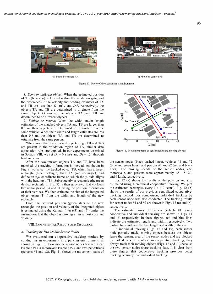
Sensor node #1

Vehicle #2

Person #2

Sensor node #2

Vehicle #1

Person #1

(a) Photo by camera #A (b) Photo by camera #B

Figure 10. Photo of the experimental environment.

1) Same or different object: When the estimated position

of TB (blue star) is located within the validation gate, and the differences in the velocity and heading estimates of TA and TB are less than D1 m/s, and D2°, respectively, the objects TA and TB are determined to originate from the same object. Otherwise, the objects TA and TB are determined to be different objects.

2) Vehicle or person: When the width and/or length estimates of the matched objects TA and TB are larger than 0.8 m, their objects are determined to originate from the same vehicle. When their width and length estimates are less than 0.8 m, the objects TA and TB are determined to originate from the same person. When more than two tracked objects (e.g., TB and TC) are present in the validation region of TA, similar data association rules are applied. In our experiments described in Section VIII, we set D1 = 0.8 m/s and D2 = 15° through trial and error.

After the two tracked objects TA and TB have been matched, the tracking information is merged. As shown in Fig. 9, we select the tracked object TB, which has a larger rectangle (blue rectangle) than TA (red rectangle), and define an xvyv-coordinate frame on which the yv-axis aligns with the heading of TB. Subsequently, a rectangle (the green dashed rectangle in Fig. 9) is then generated that encloses two rectangles of TA and TB using the position information of their vertices. We then estimate the size of the integrated object using (1) from the width and length of the new rectangle.

From the centroid position (green star) of the new rectangle, the position and velocity of the integrated object is estimated using the Kalman filter ((5) and (6)) under the assumption that the object is moving at an almost constant velocity.

VIII. EXPERIMENTAL RESULTS AND DISCUSSION

A. Tracking by Two Mobile Sensor Nodes We evaluated our cooperative-tracking method by

conducting an experiment in a parking environment, as shown in Fig. 10. Two mobile sensor nodes tracked a car (vehicle #1), a motorcycle (vehicle #2), and two pedestrians (persons #1 and #2). Fig. 11 shows the movement paths of

Sensor node #2

Sensor node #1

Person #2

Person #1

Vehicle #1

Vehicle #2

Camera #A

Camera #B

Figure 11. Movement paths of sensor nodes and moving objects.

the sensor nodes (black dashed lines), vehicles #1 and #2 (blue and green lines), and persons #1 and #2 (red and black lines). The moving speeds of the sensor nodes, car, motorcycle, and persons were approximately 1.5, 15, 20, and 6 km/h, respectively.

Fig. 12 (a) shows the results of the position and size estimated using hierarchical cooperative tracking. We plot the estimated rectangles every 1 s (10 scans). Fig. 12 (b) shows the results of our previous centralized cooperative- tracking method. For comparison, individual tracking by each sensor node was also conducted. The tracking results for sensor nodes #1 and #2 are shown in Figs. 13 (a) and (b), respectively.

The estimated sizes of the car (vehicle #1) using cooperative and individual tracking are shown in Figs. 14 and 15, respectively. In these figures, red and blue lines indicate the estimated length and width, respectively. Two dashed lines indicate the true length and width of the car.

In individual tracking (Figs. 13 and 15), each sensor node partially tracks moving objects because the objects leave the sensing area of the sensor nodes and are blocked by parked cars. In contrast, in cooperative tracking, they always track their moving objects (Figs. 12 and 14) because the two sensor nodes share tracking data. It is clear from these figures that cooperative tracking provides better tracking accuracy than individual tracking.

96



(a) Hierarchical method

(b) Centralized method

Figure 12. Estimated track and size of moving objects using cooperative tracking.

As described in Section VI, when new moving objects appear in the sensing area of the sensor node, our tracker uses 9 scans (0.9 s) for the track initiation and begins to track the new objects from the 10th scan (1 s). In the 9 scans for the track initiation, vehicles #1 and #2 (car and motorcycle) have already moved over a long distance. This is the reason why the estimated tracks of vehicles #1 and #2 in Figs. 12 and 13 are shorter than their true movement paths shown in Fig. 11.

As shown in Fig. 14, the car (vehicle #1) size estimated using hierarchical and centralized cooperative-tracking methods are different. In the experiment, sensor node #2 detected vehicle #1 after 3 scans and began to track it from the 13th scan, whereas sensor node #1 detected vehicle #1 after 20 scans and began to track it from the 30th scan. In hierarchical cooperative tracking, each sensor node locally tracks the vehicle. The track initiation for vehicle #1 was executed in 3–13 scans by sensor node #2 and in 20–30 scans by sensor node #1. Therefore, the server received tracking information from sensor node #1 at the 30th scan and merged the information together.

On the other hand, with centralized cooperative tracking, the central server estimates the size based on the moving measurements sent from the sensor nodes. Therefore, the track initiation for vehicle #1 was executed in only 3–13 scans by sensor node #2. When the server received the moving measurements from sensor node #1 at the 20th scan,

(a) Sensor node #1

(b) Sensor node #2

Figure 13. Estimated track and size of moving objects using individual tracking.

(a) Hierarchical method (b) Centralized method

Figure 14. Estimated size of car (vehicle #1) using cooperative tracking.

(a) Sensor node #1 (b) Sensor node #2

Figure 15. Estimated size of car (vehicle #1) using individual tracking.

97





Figure 16. Processing time of sensor nodes and central server.

TABLE II. PROCESSING TIME OF SENSOR NODES AND CENTRAL SERVER

(a) HIERARCHICAL METHOD Max. [ms] Min. [ms] Mean [ms]

Central server 2.3 0.1 0.8 Sensor node #1 47.9 36.8 41.7 Sensor node #2 49.8 39.3 43.0

(b) CENTRALIZED METHOD

Max. [ms] Min. [ms] Mean [ms] Central server 23.8 2.2 7.9

Sensor node #1 41.5 36.1 38.2 Sensor node #2 45.7 36.5 38.8

it quickly merged the measurements with those from sensor node #2 and estimated the car size. As a result, compared to centralized cooperative tracking, hierarchical cooperative tracking causes a slight time lag when merging the information from both sensor nodes. This is why the car (vehicle #1) sizes estimated using hierarchical and centralized cooperative tracking are different.

In our experimental system, the model of the computers used in the sensor nodes and central server is Iiyama 15X7100-i7-VGB with a 2.8 GHz Intel core i7-4810MQ processor, and the operating system used is Microsoft Windows 7 Professional. We examined the processing time of the sensor nodes and the central server in the experiment.

The results for hierarchical and centralized cooperative tracking are shown in Fig.16 and Table II. In centralized cooperative tracking, the central server estimates the poses and sizes of moving objects based on the moving-object



Figure 17. Data volume sent to central server from sensor nodes.

TABLE III. DATA VOLUME SENT TO CENTRAL SERVER FROM SENSOR NODES

(a) HIERARCHICAL METHOD Max. [byte] Min. [byte] Mean [byte]

Sensor node #1 204 24 30 Sensor node #2 240 24 28


Max. [byte] Min. [byte] Mean [byte] Sensor node #1 3628 104 477 Sensor node #2 4952 136 540

measurements sent from the sensor nodes. On the contrary, in hierarchical cooperative tracking, the sensor nodes estimate the poses and sizes of moving objects, and the central server merges their estimates. Therefore, compared with centralized cooperative tracking, hierarchical cooperative tracking reduces the computational burden on the central server.

Fig. 17 and Table III show the data volume sent to the central server from the sensor nodes in the experiment. Fig. 18 and Table IV also show the communication time required from the sensor nodes to the central server. In centralized cooperative tracking, sensor nodes upload the information shown in Table I (a), whereas in hierarchical cooperative tracking, sensor nodes upload the information shown in Table I (b), to the central server. It is clear from these figures and tables that the data volume and communication time for hierarchical cooperative tracking is less than that for centralized cooperative tracking.

98





Figure 18. Communication time required from sensor nodes to central server.

TABLE IV. COMMUNICATION TIME FROM SENSOR NODES TO CENTRAL SERVER

(a) HIERARCHICAL METHOD Max. [ms] Min. [ms] Mean [ms]

Sensor node #1 81.2 17.5 30.1 Sensor node #2 77.9 17.2 28.1


Max. [ms] Min. [ms] Mean [ms] Sensor node #1 175.9 17.7 33.8 Sensor node #2 180.3 18.0 34.0

B. Tracking by Two Static Sensor Nodes We evaluated the accuracy of the pose and size estimates

when using our cooperative-tracking method. For this purpose, we used Zhao’s data set [34]. As shown in Fig. 19 (a), two laser scanners (SICK LMS200) were set at the height of 0.4 m in an intersection environment, and laser measurements were captured every 26 ms. We assumed that their measurements were captured by two sensor nodes and evaluated the tracking performance. The experimental duration was 108 s (4154 scans). Fig. 19 (b) shows the tracking result at 770 scans, where the green rectangles indicate the estimated size, and the light blue lines indicate the estimated heading. Red and blue dots indicate the laser measurements captured by sensors #1 and #2, respectively.

We examined the tracking performance for objects moving in the central area of the intersection (blue area in Fig. 20) where the sensing areas of the two sensor nodes overlapped.

Tables V and VI show the performance of the pose and size estimates when using cooperative and individual tracking, respectively. ‘Actual objects’ in tables were identified from camera images. ‘Correct estimate of pose’ means that the tracking method could always maintain a correct pose estimate of objects moving in the central area of the intersection, whereas ‘incorrect estimate of pose’ means that they failed in estimating the position. As described in Section V, the estimated size of the tracked object is used to classify the object as a person or a vehicle (i.e., car, motorcycle, and bicycle). If the estimated size in length or width is larger than 0.8 m, the object is determined to be a vehicle. If it is less than 0.8 m, the object is determined to be a person. In Tables V and VI, ‘Correct

(a) Experimental environment

(b) Tracking result

Figure 19. Photo of the experimental environment and tracking result after 770 scans.

Figure 20. Overlapping sensing areas of two sensor nodes.

99



TABLE V. THE NUMBER OF OBJECTS WHOSE POSE (OR SIZE) ARE ESTIMATED CORRECTLY AND INCORRECTLY USING COOPERATIVE TRACKING

(a) HIERARCHICAL METHOD

Correct estimate of pose (size)

Incorrect estimate of pose (size)

Person 2 (2) 2 (0) Actual object Bicycle 20 (20) 3 (0) Car 30 (30) 7 (0)




Person 2 (2) 2 (0) Actual object Bicycle 23 (21) 0 (2)

Car 31 (31) 6 (0)

TABLE VI. THE NUMBER OF OBJECTS WHOSE POSE (OR SIZE) ARE ESTIMATED CORRECTLY AND INCORRECTLY USING INDIVIDUAL TRACKING

(a) SENSOR NODE #1



Person 2 (2) 2 (0) Actual object Bicycle 18 (14) 5 (4)

Car 26 (26) 11 (0)

(b) SENSOR NODE #2

Correct estimate of

pose (size) Incorrect estimate of

pose (size)

Actual object Person 2 (2) 2 (0) Bicycle 18 (17) 5 (1)

Car 22 (22) 15 (0)

Figure 21. Movement paths of cars.

estimate of size’ means that the tracking method could always maintain a correct classification of objects moving in the central area of the intersection, whereas ‘Incorrect estimate of size’ means that they failed in the classification.

It is clear from these tables that cooperative tracking provides better tracking accuracy than individual tracking. The performance of the pose and size estimates when using hierarchical cooperative tracking is slightly inferior to that of the centralized method. The pose estimation of cars using cooperative and individual tracking deteriorates when compared with people and bicycles. When cars moved along the paths shown by the dashed lines in Fig. 21, sensor nodes

captured laser measurements related only to the right side of each car. In addition, they only partially captured laser measurements of cars due to occlusions. These cause incorrect pose estimation of cars.

IX. CONCLUSION AND FUTURE WORK This paper presented a laser-based cooperative-tracking

method for moving objects (vehicles and people) using multiple mobile sensor nodes located in the vicinity of the objects. In cooperative tracking, nearby sensor nodes share the tracking information. Hence, they enable the constant tracking of objects that may be invisible or partially visible to an individual sensor node.

We treated people and vehicles as rigid bodies and estimated both the poses and sizes of the objects. In a crowded environment, a vehicle can be occluded or rendered partially visible to each sensor node. To correctly estimate the vehicle’s size, the laser measurements captured by sensor nodes have to be merged well. Therefore, we presented hierarchical cooperative-tracking method. Each sensor node obtained measurements related to the moving objects (moving measurements) and locally estimated the poses and sizes of the moving objects from the moving measurements using a Bayesian filter. It then sent these estimates to the central server, which then merged the pose and size estimates.

The performance of the hierarchical cooperative-tracking method was evaluated from two experimental results in outdoor environments by comparing it with a previous centralized method. The hierarchical method provided slightly inferior tracking accuracy than the centralized method. However, it had a smaller data volume sent to the central server from sensor nodes and a smaller computational cost in the central server than the centralized method. Therefore, the hierarchical method makes the tracking system scalable and robust.

In this paper, single-layer laser scanners were applied to sense the surrounding environment using mobile sensor nodes. Multilayer laser scanners can also capture height information from objects, and thus enable more accurate recognition of the surrounding environment than single-layer laser scanners. Current research is directed to the design of cooperative tracking by multiple sensor nodes equipped with multilayer laser scanners. To achieve cooperative tracking, the sensor nodes should always identify their own poses with a high degree of accuracy in a world coordinate frame. In this paper, we applied localization methods using dead reckoning and RTK-GPS. However, in city-canyon environments, the performance of localization using GPS deteriorates due to GPS multipath errors, diffraction problems and so on. To address this problem, we will embed a cooperative-localization method into our tracking system.

ACKNOWLEDGMENT This study was partially supported by the Scientific

Grants #26420213, the Japan Society for the Promotion of Science (JSPS) and the MEXT-Supported Program for the

100



Strategic Research Foundation at Private Universities, 2014–2018, Ministry of Education, Culture, Sports, Science and Technology, Japan.

We would also like to thank Professor Huijing Zhao of Peking University for providing the laser-scanning and vision data set for experiments in Section VII-B.

REFERENCES [1] Y. Tamura, R Murabayashi, M. Hashimoto, and K. Takahashi,

“Laser-based Cooperative Estimation of Pose and Size of Moving Objects using Multiple Mobile Robots,” Proc. of the Fifth Conf. on Intelligent Systems and Applications (INTELLI 2016), pp. 13–19, 2016.

[2] K. O. Arra and O. M. Mozos, Special issue on: People Detection and Tracking, Int. J. of Social Robotics, vol.2, no.1, pp. 1–107, 2010.

[3] C. Mertz, et al., “Moving Object Detection with Laser Scanners,” J. of Field Robotics, vol.30, pp. 17–43, 2013.

[4] T. Ogawa, H. Sakai, Y. Suzuki, K. Takagi, and K. Morikawa, “Pedestrian Detection and Tracking using In-vehicle Lidar for Automotive Application,” Proc. of IEEE Intelligent Vehicles Symp. (IV2011), pp. 734–739, 2011.

[5] A. Mukhtar, L. Xia, and T.B. Tang, “Vehicle Detection Techniques for Collision Avoidance Systems: A Review,” IEEE Trans. on Intelligent Transportation Systems, vol. 16, pp. 2318–2338, 2015.

[6] H. Cho, Y. W. Seo, B.V.K. V. Kumar, and R. R. Rajkumar, “A Multi-sensor Fusion System for Moving Object Detection and Tracking in Urban Driving Environments,” Proc. of Int. Conf. on IEEE Robotics and Automation (ICRA2014), pp. 1836–1843, 2014.

[7] D. Z. Wang, I. Posner, and P. Newman, “Model-free Detection and Tracking of Dynamic Objects with 2D Lidar,” Int. J. of Robotics Research, vol.34, pp. 1039–1063, 2015.

[8] D. Z. Wang, I. Posner, P. Newman, “What could move? Finding cars, pedestrians and bicyclists in 3D laser data,” Proc. of IEEE Int. Conf. on Robotics and Automation (ICRA2012), pp. 4038–4044, 2012.

[9] Z. Yan, N. Jouandeau, and A. A. Cherif, “A Survey and Analysis of Multi-Robot Coordination,” Int. J. of Advanced Robotic Systems, vol. 10, pp. 1–18, 2013.

[10] S. Nadarajah and K. Sundaraj, “A Survey on Team Strategies in Robot Soccer: Team Strategies and Role Description,” Artificial Intelligence Review, vol. 40, pp. 271–304, 2013.

[11] K. Kakinuma, M. Hashimoto, and K. Takahashi, “Outdoor Pedestrian Tracking by Multiple Mobile Robots based on SLAM and GPS Fusion,” Proc. of IEEE/SICE Int. Symp. on System Integration (SII2012), pp. 422–427, 2012.

[12] M. Ozaki, K. Kakinuma, M. Hashimoto, and K. Takahashi, “Laser-based Pedestrian Tracking in Outdoor Environments by Multiple Mobile Robots,” Sensors, vol. 12, pp. 14489–14507, 2012.

[13] S.J. Julier and J.K. Uhlmann, “A Non-divergent Estimation Algorithm in the Presence of Unknown Correlations,” Proc. of the IEEE American Control Conf., pp. 2369–2373, 1997.

[14] F. Fayad and V. Cherfaoui, “Tracking Objects using a Laser Scanner in Driving Situation based on Modeling Target Shape,” Proc. of the 2007 IEEE Int. Vehicles Symp. (IV2007), pp. 44–49, 2007.

[15] T. Miyata, Y. Ohama, and Y. Ninomiya, “Ego-Motion Estimation and Moving Object Tracking using Multi-layer LIDAR,” Proc. of IEEE Intelligent Vehicles Symp. (IV2009), pp. 151–156, 2009.

[16] K. Granstrom, C. Lundquist, F. Gustafsson, and U. Orguner, “Radom Set Methods, Estimation of Multiple Extended

Objects,” IEEE Robotics & Automation Magazine, pp. 73–82, June 2014.

[17] L. Mihaylova, et al., “Overview of Bayesian Sequential Monte Carlo Methods for Group and Extended Object Tracking,” Digital Signal Processing, vol. 25, pp.1–16, 2014.

[18] J. Lan and X. R. Li, “Tracking of Extended Object or Target Group using Random Matrix Part I: New Model and Approach,” Proc. of 15th Int. Conf. on Information Fusion (FUSION2012), pp.2177–2184, 2012.

[19] Z.Wang and D. Gu, “Cooperative Target Tracking Control of Multiple Robots,” IEEE Trans. on Industrial Electronics, vol. 59, pp. 3232–3240, 2012.

[20] K. Zhou and S. I. Roumeliotis, “Multirobot Active Target Tracking with Combinations of Relative Observations,” IEEE Trans. on Robotics, vol. 27, pp. 678–695, 2011.

[21] A. Ahmad and P. Lima, “Multi-robot Cooperative Spherical-Object Tracking in 3D Space based on Particle Filters,” Robotics and Autonomous Systems, vol. 61, pp. 1084–1093, 2013.

[22] P. U. Limaa, et al., “Formation Control Driven by Cooperative Object Tracking,” Robotics and Autonomous Systems, vol. 63, Part 1, pp. 68–79, 2015.

[23] C. Robin and S. Lacroix, “Multi-robot Target Detection and Tracking: Taxonomy and Survey,” Autonomous Robots, vol. 40, pp. 729–760, 2016.

[24] C. T. Chou, J. Y. Li, M. F. Chang, and L. C. Fu, “Multi-Robot Cooperation Based Human Tracking System Using Laser Range Finder,” Proc. of IEEE Int. Conf. on Robotics and Automation (ICRA2011), pp. 532–537, 2011.

[25] N. A. Tsokas and K. J. Kyriakopoulos, “Multi-robot Multiple Hypothesis Tracking for Pedestrian Tracking,” Autonomous Robot, vol. 32, pp. 63–79, 2012.

[26] M. Hashimoto, R. Izumi, Y. Tamura, and K. Takahashi, “Laser-based Tracking of People and Vehicles by Multiple Mobile Robots,” Proc. of the 11th Int. Conf. on Informatics in Control, Automation and Robotics (ICIT2014), pp. 522–527, 2014.

[27] M. Hashimoto, S. Ogata, F. Oba, and T. Murayama, “A Laser- based Multi-Target Tracking for Mobile Robot,” Intelligent Autonomous Systems 9, pp. 135–144, 2006.

[28] Y. Bar-Shalom and T. E. Fortmann, “Tracking and Data Association,” Academic Press,Inc., 1988.

[29] H.A.P.Blom and Y.Bar-Shalom, “The Interacting Multiple Model Algorithm for Systems with Markovian Switching Coefficient,” IEEE Trans. on Automatic Control, vol.33, pp.780–783, 1988.

[30] E. Mazor, A. Averbuch, Y. Bar-Shalom, and J. Dayan, “Interacting Multiple Model Methods in Target Tracking: A Survey,” IEEE Trans. on Aerospace and Electronic Systems, vol.34, pp.103–123, 1998.

[31] V. Nguyen, A. Martinelli, N. Tomatis, and R. Siegwart, “A Comparison of Line Extraction Algorithms using 2D Laser Rangefinder for Indoor Mobile Robotics,” Proc. of 2005 IEEE/RSJ Int. Conf. on Intelligent Robots and Systems (IROS2009), pp. 1929–1934, 2009.

[32] M. Fischler and R. Bolles, “Random Sample Consensus: A Paradigm for Model Fitting Applications to Image Analysis and Automated Cartography,” Proc. of Image Understanding workshop, pp. 71–88, 1980.

[33] P. Konstantinova, A. Udvarev, and T. Semerdjiev, “A Study of a Target Tracking Algorithm Using Global Nearest Neighbor Approach,” Proc. of Int. Conf. on Systems and Technologies, 2003.

[34] H. Zhao, “Open Resource, Networked horizontal laser scan data at intersection (20071012),” available from <http://www. poss.pku.edu.cn/download.html>, (accessed on 12 December 2014).

101



A Life-cycle Equipment Labeling System for Machine Classification in Smart Factories

Susana Aguiar, Rui Pinto, Joao Reis, Gil Goncalves

Institute for Systems and RoboticsFaculty of Engineering of University of Porto

Rua Dr. Roberto Frias, s/n 4200-465, Porto, PortugalEmail: {saguiar, rpinto, jpcreis, gil}@fe.up.pt

Abstract—Nowadays, due to ever decreasing product life cyclesand high external pressure to cut costs, the ramp-up of productionlines must be significantly shortened and simplified. This isonly possible if a forecast of the impact of modification withinan existing production environment is available, helping duringdecision making of production methods. This type of predictionswill have a direct impact on the cost-effective production process,maintaining concerns regarding the environmental and socialimpacts. These are the ideas behind the project InnovativeReuse of modular knowledge Based devices and technologies forOld, Renewed and New factories (ReBorn). The present paperdescribes the System Assessment Tool, a software applicationdeveloped in ReBorn, which is used for assessing the sustain-ability of highly adaptive production systems through the use ofReliability, Life Cycle Cost and Life Cycle Assessment metrics, inthe form of a equipment labeling scheme. This labeling schemeconsists on classifying the dependability of industrial equipment,based on the collected metrics. To that intent, several simulationprocesses were performed, in order to assess the suitability ofthe labeling system, in comparison to the Quality metric that ishighly preferable among the industrial partners. The simulationresults show that a two-layer equipment labeling system is themost suitable approach to be used for classification.

Keywords–Smart factories; Equipment label; Life-cycle assess-ment; Re-use; Production systems.

I. INTRODUCTION

ReBorn was a European Project funded by the SeventhFramework Programme of the European Commission. The vi-sion of ReBorn was to demonstrate strategies and technologiesthat support a new paradigm for the re-use of productionequipment in factories. This re-use will give new life todecommissioned production systems and equipment, helpingthem to be “reborn” in new production lines. Such newstrategies will contribute to sustainable, resource-friendly andgreen manufacturing and, at the same time, deliver economicand competitive advantages for the manufacturing sector.

The developments made in ReBorn allow production equip-ment to extend its life cycle, contributing to economic andenvironmental sustainability of production systems [1]. Thisconcept of modular production equipment may also be re-used between different production systems, after servicing andupgrading. This new business paradigm will move from anequipment-based business to a value added business, whereequipment servicing and equipment knowledge are main busi-ness drivers.

The proposed paradigm is built on self-aware andknowledge-based equipment, which requires capabilities tocollect and manage information, regarding its functionalities,

evolution over time due to its use and wear, and maintenanceoperations, upgrade and refurbishment over lifetime. For this tobe possible, versatile and modular task-driven plug&producedevices, with built-in capabilities for self-assessment and op-timal re-use were implemented, along with strategies for theirre-use and models for factory layout design and adaptiveconfiguration.

The ReBorn [2] developments demonstrated to be suc-cessful for intelligent machine repair, upgrade and re-use ofequipment, and (re-)design of factory layouts [3]. Most ofthese developments were demonstrated within several indus-trial demonstration scenarios at 2016 AUTOMATICA fair (21-24 June) in Munich, Germany [4].

During its life-cycle, industrial equipment goes throughthree main stages, namely 1) the initial incorporation into theproduction line, 2) the operation and maintenance/upgrade, and3) the end-of-use and disassemble. Throughout these stagesfailures or malfunctions can potentially cause costly machinedowntime or even downtime in the entire production system.Downtime of equipment operation is usually avoided based onengineers and shop-floor operators decision making, which aremost of the times based on the experience of these individuals.Sometimes the individual’s know-how and gained knowledgeby experience is hard to be transferred to other individualsand may be lost [5]. This problem was tackled in ReBorn bydeveloping a software tool named Workbench.

The Workbench is a decision making support tool, whichcombines simulations with the historical process data gath-ered at equipment level. It provides methods and algorithmsfor assessing the various potential possibilities of industrialequipment, regarding change, upgrade, reuse, dismantle anddisposal. These possibilities are evaluated based on the cor-responding reconfiguration effect on the overall system cost,performance and status throughout the life-cycle(s) of themanufacturing system. The analysis and comparison of indus-trial equipment is achieved using a System Assessment Tool(SAT), which performs Life Cycle Cost (LCC) and Life CycleAssessment (LCA) analysis, based on reliability metrics.

In order to have a more generic and simple way ofcomparing industrial equipment, the SAT has a functionality,which main goal is to calculate an equipment Label. This Labelmeasures a dependability factor, as for example the appliancesenergy consumption label, grades equipments from A to F,being A very dependable and F less dependable. This paperpresents three simulations that were defined and executed, inorder to test the usability and correctness of the Label. Thebasic idea behind all the three simulations is to use as much

102



information as possible, from the information available in theSAT, that is, all the metrics that the SAT can calculate. Eachmetric has a weight associated to it, which was defined basedon a questionnaire that was sent to the industrial partners ofthe ReBorn project. The equipment Label simulations indicatethat using all the metrics available in a straight way mightnot give the best results, because this allows the possibility ofhaving equipments with a Label grade that is higher or lower,with a difference of two or more grades, than the quality grade,which is, for the industrial ReBorn partners, the most importantmetric. This lead to a two layer Label scheme that providesgrading results closer to the values of the most importantmetrics.

This paper is organized in five more sections. Section IIdefines the concepts of LCC and LCA and overviews thecurrent state of the art, regarding tools and metrics used toperform this type of equipment analysis. In section III, anoverview of the Workbench tool is presented, along with adescription of its different modules, including the SAT. InSection IV, a detailed analysis and description of the SAT ispresented. Section V explains one of the SAT functionalities,the equipment Label, where several simulations are definedand its results presented and discussed. Finally, Section VIconcludes the paper by exposing some final remarks about thework developed.

II. RELATED WORK

Several models, tools, and standards have been developedto analyze equipment reliability [6], [7], LCC [8]–[12], andLCA [13]–[18]. Although these techniques have usually beentreated as separate analysis tools, defined by their own metricsand standards, some authors attempted to bring them closer[19]–[22] by presenting the relation between different sustain-ability assessment tools, focusing on the life cycle assessmentas central concept for sustainability [23]. For the interestedreader, several surveys of existing methodologies and toolsregarding equipment analysis have been performed over theyears [11], [21], [23]–[25].

A. Life Cycle AssessmentLCA is an approach for assessing industrial systems from

creation to disposal [26]–[30]. This approach begins with thegathering of raw materials of the mother nature to create theproduct, ending when the product is dismantle and the disposalof all materials to the environment [14], [15].

According to Currant [13], LCA had its beginnings in the1960’s due to concerns over the limitations of raw materialsand energy resources. The work published by Harold Smith[31] is considered as one of the firsts in this field. In that workhe reported his calculations of cumulative energy requirementsfor the production of chemical intermediates and products.

In 1969, researchers initiated an internal study for TheCoca-Cola Company (that was not officially published but itis mentioned in most of the LCA works [13], [32], [33]),which laid the foundation for the current methods of life cycleinventory analysis in the United States. In this study, the usedraw materials and fuels, as well as the environmental loadingsfrom the manufacturing processes for each container, werequantified. The comparison between the different beveragecontainers allowed to determine which container had the lowestreleases to the environment and which least affected the supply

of natural resources. The process of quantifying the resourceuse and environmental releases of products became known asa Resource and Environmental Profile Analysis (REPA) in theUnited States, and as Ecobalance in Europe.

From 1975 through the early 1980’s, as influence ofthe oil crisis faded, environmental concerns shifted to issuesof hazardous and household waste management. However,throughout this time, life cycle inventory analysis continued tobe conducted and the methodology improved through a slowstream of about two studies per year, most of which focused onenergy requirements. During this time, European interest grewwith the establishment of an Environment Directorate (DGX1) by the European Commission [34]. European LCA prac-titioners developed approaches parallel to those being used inthe USA. Besides working to standardize pollution regulationsthroughout Europe, DG X1 issued the Liquid Food ContainerDirective in 1985, which charged member companies withmonitoring the energy and raw materials consumption andsolid waste generation of liquid food containers. When solidwaste became a worldwide issue in 1988, LCA emerged againas a tool for environmental problems analysis.

In 1991, concerns over the inappropriate use of LCA tomake broad marketing claims made by product manufacturersresulted in a statement issued by eleven State AttorneysGeneral in the USA, denouncing the use of LCA results topromote products. Such assessments should be conducted byuniform methods, by reaching a consensus on how this type ofenvironmental comparison can be advertised non-deceptively.This action, along with pressure from other environmentalorganizations to standardize LCA methodology, led to the de-velopment of the LCA standards in the International StandardsOrganization (ISO) 14000 series (1997 through 2002) [35].

In 2002, the United Nations Environment Program (UNEP)joined forces with the Society of Environmental Toxicologyand Chemistry (SETAC) to launch the Life Cycle Initiative,an international partnership. This Initiative has characterizedby three programs: (1) the Life Cycle Management (LCM) pro-gram creates awareness and improves skills of decision-makersby producing information materials, establishing forums forsharing best practice, and carrying out training programs in allparts of the world; (2) the Life Cycle Inventory (LCI) programimproves global access to transparent, high quality life cycledata, by hosting and facilitating expert groups work resultsin web-based information systems; (3) the Life Cycle ImpactAssessment (LCIA) program increases the quality and globalreach of life cycle indicators, by promoting the exchange ofviews among experts, whose work results in a set of widelyaccepted recommendations.

Figure 1. Life Cycle Stages (Source: EPA, 1993 [36]).

103



LCA evaluates all stages of a product’s life cycle, fromthe perspective that they are interdependent, meaning that oneoperation leads to the next. Figure 1 presents the possiblelife cycle stages that can be considered in a LCA as wellas the typical inputs and outputs measured. LCA enables theestimation of cumulative environmental impacts that resultedfrom all stages in the product life cycle, often includingimpacts not considered in more traditional analyses (e.g., rawmaterial extraction, material transportation, ultimate productdisposal, etc.). By including these impacts throughout theproduct life cycle, LCA provides a comprehensive view of theenvironmental aspects of the product or process and a moreaccurate picture of the true environmental trade-offs in productand process selection.

The LCA process is a systematic, phased approach andconsists of four components as illustrated in Figure 2: 1)Goal Definition and Scope - Define and describe the product,process or activity, by establishing the context in which theassessment is to be made and identify the boundaries andenvironmental effects to be reviewed for the assessment; 2)Inventory Analysis - Identify and quantify energy, water andmaterials usage and environmental releases, such as air emis-sions, solid waste disposal and waste water discharges; 3) Im-pact Assessment - Assess the potential human and ecologicaleffects of energy, water, material usage and the environmentalreleases identified in the inventory analysis. Inputs and outputsare categorized in different impact categories midpoints, suchas climate change and land use, and endpoints, such as humanhealth and resource depletion; 4) Interpretation - Evaluate theresults of the inventory analysis and impact assessment, inorder to select the preferred product, process or service witha clear understanding of the uncertainty and the assumptionsused to generate the results.

Figure 2. Phases of a LCA Process.

Conducting a LCA study have the main benefit of develop-ing a systematic evaluation of the environmental consequencesassociated with the creation of a given product. This evalua-tion provides means to analyze the environmental trade-offsassociated with one or more specific products/processes, inorder to help the stakeholder gain acceptance for the plannedaction. Moreover, the evaluation allows to quantify environ-mental releases to air, water and land, in relation to eachlife cycle stage and/or major contributing process, assistingin the identification of significant shifts in environmentalimpacts between life cycle stages and environmental media.Also, the assessment of the human and ecological effectsof material consumption and environmental releases to the

local community, region, and world allows to identify impactsto one or more specific environmental areas of concern andcompare the health and ecological impacts between specificproducts/processes.

However, LCA studies may present some limitations, suchas very high resource and time consuming processes. Datagathering can be problematic, due to availability issues, result-ing in inaccuracy of the final results. Also, a LCA study willnot determine which product or process is the most cost ef-fective or works the best. The information provided by a LCAstudy is used as a small component of a more comprehensivedecision process, such as Life Cycle Managements.

B. LCC - Life Cycle CostingLCC is a process used to determine the sum of all the

costs associated with an asset or with part of an asset. Thesecosts include acquisition, installation, operation, maintenance,refurbishment, and disposal. LCC can be carried out duringany or all phases of an asset’s life cycle. LCC processesusually include steps such as [8], [10]–[12], [19]: 1) LifeCost Planning, which concerns the assessment and comparisonof options/alternatives during the design/ acquisition phase;2) Selection and development of the LCC model, namelydesigning cost breakdown structure, identifying data sourcesand uncertainties; 3) Application of LCC model; and 4)Documentation and review of LCC results.

The main goal for carrying out LCC calculations is toaid decision making regarding assessment and control ofcosts, by identifying cost significant items, selection of workand expenditure of planning profiles. Early identification ofacquisition and ownership costs enables the decision-makerto balance performance, reliability, maintenance support andother goals against life cycle costs. Decisions made early inan asset’s life cycle have a greater influence on the Life CycleCosting than those made late, leading to the development ofthe concept of discounted costs. The LCC process can bedivided into several steps, which are represented in Figure3. As it can be seen in this figure, the LCC process has 6stages, that are divided into two groups. The first step is todevelop a plan that addresses the purpose, and scope of theanalysis. The second step is the selection or development ofthe LCC model that will conform with the objectives of theanalysis. Step three is the application of the model defined instep two. In Step four all the results gathered in the analysisare documented, and the Life Cost Planning phase is finished.In Step five, the model defined in step two is applied usingnominal costs, initiating the Life Cost Analysis. Finally, stepsix involves the continuous monitoring in order to identifyareas in which cost savings may be made and to providefeedback for future life cost planning activities. This stepfinishes the Life Cost Analysis phase. All these steps maybe performed iteratively as needed. Assumptions made at eachstep should be rigorously documented to facilitate iterationsand to help in the interpretation of the results of the analysis.

The method used to estimate the cost elements in LCCcalculations will depend on the amount of information neededto establish the usage patterns and operational characteristics,in order to infer the expected remaining life, along with theinformation needed to understand the technology employed.In [12] several methods are presented. The Engineering CostMethod is used when there is detailed and accurate capital and

104



Figure 3. LCC Process.

operational cost data for the study. It involves the direct esti-mation of a particular cost element by examining component-by-component. It uses standard established cost factors, suchas firm engineering and/or manufacturing estimates, in orderto develop the cost of each element and its relationship toother elements (known as Cost Element Relationships - CER).The Analogous Cost Method provides the same level of detailas the Engineering Cost Method, but draws on historical datafrom similar components that have analogous size, technol-ogy, use patterns and operational characteristics. Finally, theParametric Cost Method is employed when actual or historicaldetailed component data is limited to known parameters. Theseavailable data from existing cost analyses is used to developa mathematical regression or progression formula, which canbe solved for the cost estimate required.

The basic deterministic methods are underlying virtuallyall LCC investigations. The process begins with the customerneeds and ultimately ends with the customer selecting apreferred option. In this context, the LCC procedure em-ployed is used to support a decision-making process focusedon customer satisfaction. The deterministic approach assignseach LCC input variable a fixed discrete value. The analystdetermines the most likely input parameters values that occur,usually based on historical evidence or professional judgment.Collectively, these input values are used to compute a sin-gle LCC estimation. Traditionally, applications of LCC havebeen deterministic ones. A deterministic LCC computationis straightforward and can be conducted manually using acalculator or automatically with a spreadsheet. However, it failsto convey the degree of uncertainty associated with the PresentValue (PV) estimate.

The deterministic method of the LCC investigations allowsto have a logical ordering of analytical activities and a meansof ranking [11]. This ranking includes feasible options forthe construction, refurbishment, and on-going managementand support of infrastructures. However, this straightforwarddeterministic approach provides little guidance to the engineeror designer, which attempts to adequately represent the com-plexity and uncertainty inherent to LCC investigations. Forthis reason, the basic method is usually extended. A commonextension to the basic method of LCC involves the use ofsensitivity analysis and risk analysis [37]. Sensitivity analysisinvolves the behavior of model variables over predeterminedbounds to determine their relative effect on model outcome.Through this process, analysts can identify some subset ofmodel variables that exert significant influence on model re-sults and/or determine break-even points that alter the rankingof considered options.

Following an initial deterministic ranking of feasible designoptions, sensitivity analysis is employed to establish the sen-

sitivity of model results and rankings across model variablesof particular concern to analysts and decision makers. Whilesensitivity analysis provides decision-makers insights regard-ing the flexibility of model results across a range of variableestimates and corresponding bounds, it has some shortcomings.First, it may fail to identify a dominant alternative amongconsidered design options. This is certainly the case whereperturbations in model variables disturb the ranking of feasibledesign options. Second, since sensitivity analysis typicallyinvolves the independent perturbation of each model variable,engineers and, therefore, customers do not gain a sense of thecombined and simultaneous influence of several “perturbed”model variables on LCC results and rankings. Finally, in theabsence of defined probability distributions, the likelihood thatparticular values occur is unexplored.

The purpose of risk analysis is to address these shortcom-ings through probabilistic comparison of considered options.Used properly, risk analysis addresses the bulk of limitationsassociated with sensitivity analysis.

C. ToolsCurrently, there are several tools that can perform LCA

and/or LCC calculations. In this subsection, some of the mostcommonly used tool will be briefly described.

The Economic Input-Output Life Cycle Assessment (EIO-LCA) [38] method estimates the materials and energy re-sources required for activities in the economy, and the environ-mental emissions resulting from those activities. Researchersat the Green Design Institute of Carnegie Mellon Universityoperationalized the Leontief’s method in the mid-1990s, sincesufficient computing power was widely available to performthe large-scale matrix manipulations required in real-time.Their work consisted on developing a user-friendly on-linetool that implemented the EIO-LCA method. The websiteperformed fast and easy evaluations to a commodity or service,as well as its supply chain. The EIO-LCA method, models, andresults represent the inventory stage of the LCA. The resultsare used to estimate the environmental emissions or resourceconsumption associated with the life cycle of an industrialsector. However, it fails to estimate the actual environmentalor human health impacts that the emissions or consumptionpatterns cause. The results of the EIO-LCA analysis representthe impacts from a change in demand on an industrial sector.As a LCA tool, the EIO-LCA models applied are incomplete,since the included environmental effects are limited.

EconomyMap [39] is another tool, which uses CEDA 3.0LCA Economic Input/Output (EIO) database [40], to providevisualization of the same economic activity and indirect en-vironmental impacts. It provides an easy way to dynamicallyexplore and understand the sources and flow of goods, services,and environmental impacts among major industrial sectors.EconomyMap is intended to be a free resource for publicinterest lawyers and policymakers, to help them identify andprioritize opportunities to reduce environmental impacts. Italso serves as an educational resource for broader audiences.

openLCA [41] is a professional LCA tool and footprintsoftware created by GreenDelta in 2006, with a broad rangeof features and many available databases. It is an open sourcesoftware and is publicly available to be modified, offeringresources such as professional life cycle modeling, up-to-date

105



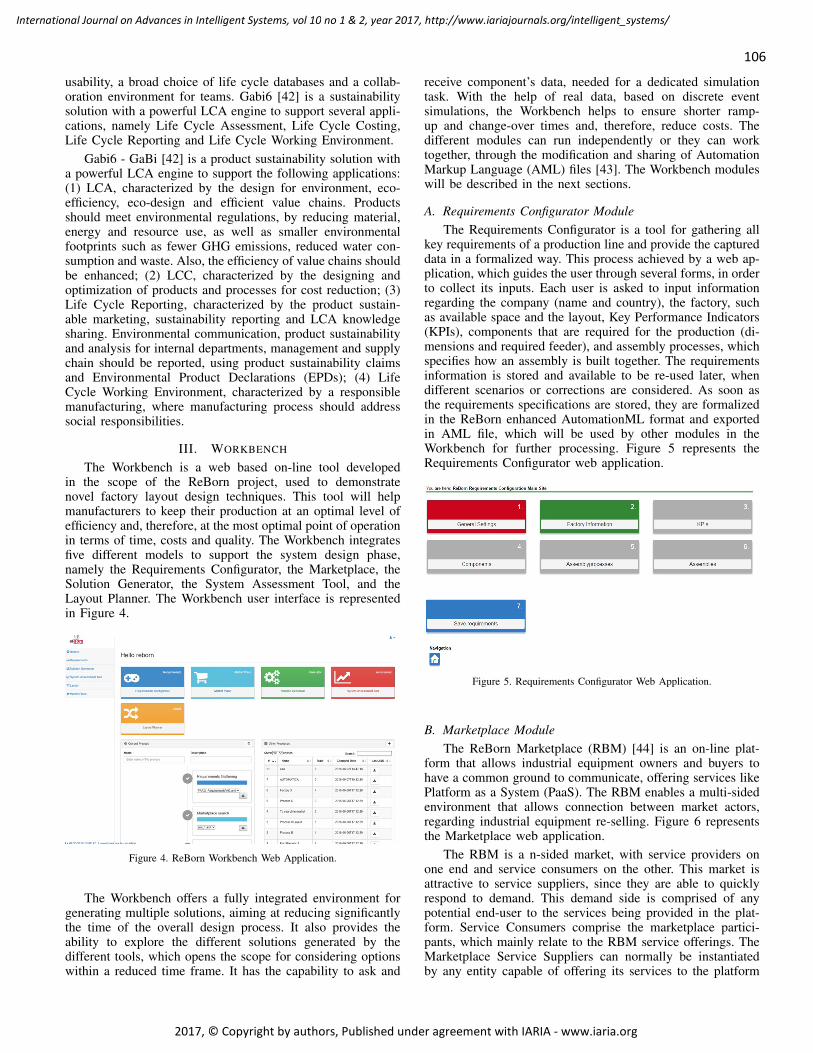
usability, a broad choice of life cycle databases and a collab-oration environment for teams. Gabi6 [42] is a sustainabilitysolution with a powerful LCA engine to support several appli-cations, namely Life Cycle Assessment, Life Cycle Costing,Life Cycle Reporting and Life Cycle Working Environment.

Gabi6 - GaBi [42] is a product sustainability solution witha powerful LCA engine to support the following applications:(1) LCA, characterized by the design for environment, eco-efficiency, eco-design and efficient value chains. Productsshould meet environmental regulations, by reducing material,energy and resource use, as well as smaller environmentalfootprints such as fewer GHG emissions, reduced water con-sumption and waste. Also, the efficiency of value chains shouldbe enhanced; (2) LCC, characterized by the designing andoptimization of products and processes for cost reduction; (3)Life Cycle Reporting, characterized by the product sustain-able marketing, sustainability reporting and LCA knowledgesharing. Environmental communication, product sustainabilityand analysis for internal departments, management and supplychain should be reported, using product sustainability claimsand Environmental Product Declarations (EPDs); (4) LifeCycle Working Environment, characterized by a responsiblemanufacturing, where manufacturing process should addresssocial responsibilities.

III. WORKBENCH

The Workbench is a web based on-line tool developedin the scope of the ReBorn project, used to demonstratenovel factory layout design techniques. This tool will helpmanufacturers to keep their production at an optimal level ofefficiency and, therefore, at the most optimal point of operationin terms of time, costs and quality. The Workbench integratesfive different models to support the system design phase,namely the Requirements Configurator, the Marketplace, theSolution Generator, the System Assessment Tool, and theLayout Planner. The Workbench user interface is representedin Figure 4.

Figure 4. ReBorn Workbench Web Application.

The Workbench offers a fully integrated environment forgenerating multiple solutions, aiming at reducing significantlythe time of the overall design process. It also provides theability to explore the different solutions generated by thedifferent tools, which opens the scope for considering optionswithin a reduced time frame. It has the capability to ask and

receive component’s data, needed for a dedicated simulationtask. With the help of real data, based on discrete eventsimulations, the Workbench helps to ensure shorter ramp-up and change-over times and, therefore, reduce costs. Thedifferent modules can run independently or they can worktogether, through the modification and sharing of AutomationMarkup Language (AML) files [43]. The Workbench moduleswill be described in the next sections.

A. Requirements Configurator ModuleThe Requirements Configurator is a tool for gathering all

key requirements of a production line and provide the captureddata in a formalized way. This process achieved by a web ap-plication, which guides the user through several forms, in orderto collect its inputs. Each user is asked to input informationregarding the company (name and country), the factory, suchas available space and the layout, Key Performance Indicators(KPIs), components that are required for the production (di-mensions and required feeder), and assembly processes, whichspecifies how an assembly is built together. The requirementsinformation is stored and available to be re-used later, whendifferent scenarios or corrections are considered. As soon asthe requirements specifications are stored, they are formalizedin the ReBorn enhanced AutomationML format and exportedin AML file, which will be used by other modules in theWorkbench for further processing. Figure 5 represents theRequirements Configurator web application.

Figure 5. Requirements Configurator Web Application.

B. Marketplace ModuleThe ReBorn Marketplace (RBM) [44] is an on-line plat-

form that allows industrial equipment owners and buyers tohave a common ground to communicate, offering services likePlatform as a System (PaaS). The RBM enables a multi-sidedenvironment that allows connection between market actors,regarding industrial equipment re-selling. Figure 6 representsthe Marketplace web application.

The RBM is a n-sided market, with service providers onone end and service consumers on the other. This market isattractive to service suppliers, since they are able to quicklyrespond to demand. This demand side is comprised of anypotential end-user to the services being provided in the plat-form. Service Consumers comprise the marketplace partici-pants, which mainly relate to the RBM service offerings. TheMarketplace Service Suppliers can normally be instantiatedby any entity capable of offering its services to the platform

106



Figure 6. Marketplace Web Application.

while altogether adding value to the platform’s base propo-sition. Service Suppliers are industrial equipment builderswho provide equipment, as well as equipment information,functionalities (software), and operations. Entities capable ofproviding complementing services to the platform, in orderto co-create value, are labeled as Complementors. These canbe, for instance, independent software developers that provideadditional equipment functionalities.

C. Solution Generator ModuleThe Solution Generator provides configuration solutions,

based on the established requirements gathered by the Require-ments Configurator and the existing equipment modules (bothold and new). This module requires the use of IBM ILOGCPLEX [45], which is a software optimization package. TheSolution Generator uses the information in the AML file tosignificantly reduce the solution space. Then, it generates anAML file for each of the optimized solutions generated. Figure7 represents the Solution Generator module.

Figure 7. Solution Generator Application.

D. Layout Planner ModuleThe Layout Planner is the component of the Workbench

responsible for finding the optimized layout for the factoryshop floor. It delivers an equipment layout solution, takinginto consideration several constraints like space restrictions,equipment to be included and restrictions on material flow.The Layout Planner provides several optimization methods inorder to find a solution that minimizes the total cost of materialhandling associated with the equipment layout considered. Thiscost is calculated by the the sum of the costs of having specificequipment located in a given area of the shop floor layout andthe costs of material handling between equipment. Materialhandling costs are represented by the relationship between flowof material and distance between equipments. Pinto et al. [3]developed an approach based on Genetic Algorithms (GA),which was implemented in the Layout Planner and proved tobe more efficient that other genetic algorithm approaches totackle Facility Layout Problems (FLP). Figure 8 representsthe Layout Planner module.

Figure 8. Layout Planner Web Application.

E. System Assessment Tool ModuleThe SAT integrates reliability and life cycle status informa-

tion during early design and costing of assembly automationprojects. The life-long cost assessment of the system is accom-plished through the data collection of the system performancethroughout its life cycle. Based on this performance data, theSAT performs the life cycle cost assessment and analysis of theeffect on the overall reconfigured system. Figure 9 representsthe SAT module.

The SAT is able to compare machines and productionlines in terms of: 1) Reliability metrics, such as failure rate,Mean Time Between Failure (MTBF), Mean Time To Re-pair (MTTR), reliability, availability, performance, quality andOverall Equipment Effectiveness (OEE); 2) LCC metrics, suchas Future Value (FV), PV, Net Present Cost (NPC) and NetPresent Value (NPV) with initial costs; and 3) LCA metrics,such as life cycle emissions and impact categories, like GlobalWarming Potential or Ozone Depleting Potential. A detailedoverview of the SAT is presented in the next section.

IV. SYSTEM ASSESSMENT TOOL

The SAT has two main objectives, namely providing aneasy and intuitive way for a user to compare machines orproduction lines and providing a web API service, capable ofreceiving requests and share the results with the other modules

107



Figure 9. System Assessment Tool Web Application.

in the Workbench or other future applications. As mentionedbefore, the SAT provides an easy and intuitive way for auser to compare machines or production lines, in terms ofreliability, LCC, LCA, classifying each machine with a label,based on a grading system. Figure 10 represents an overallarchitecture of the SAT, which consists on four main groupsof metric parameters: 1) Reliability; 2) LCC; 3) LCA and 4)Equipment Label. These groups will be further detailed in thenext sections.

Figure 10. System Assessment Tool Overall Architecture.

Regarding communication interfaces, the SAT can interactdirectly with the Marketplace, as represented in Figure 11, orit can interact with other applications, using a web API orthe available web interface. The SAT is prepared to receiverequests for performing analysis of equipment, using theavailable metrics, where both equipment information and theanalysis results are imported/exported to an AML file or storedlocally into a database.

Available machines in the Marketplace can be comparedwith machines available in the SAT scope. The user canselect from a list the machines to be compared and performthe analysis. Figure 12 represents and example of the resultsprovided by a comparison analysis between two industrialmachines. In this case reliability metrics are shown. Each graphshows the percentage of each equipment for each metric.

A. Reliability Metrics FunctionalityRegarding reliability metrics of equipment operation, the

SAT [1] can calculate several parameters, namely the failure

Figure 11. SAT - Marketplace Connection.

Figure 12. Machine comparison - Reliability metrics.

rate, MTBF, MTTR, reliability, availability, performance, qual-ity and OEE.

1) Failure rate: Failure rate, represented by Fr, can bedefined as the frequency that an engineered system or compo-nent fails. Fr is calculated by the ratio between the numberof failures F that occur and the operating time Ot of theequipment, as shown in Equation (1).

Fr =F

Ot(1)

108



2) Mean Time Between Failure: MTBF, represented byMTBF , is defined as the predicted elapsed time betweeninherent failures of a system during operation. It is the inverseof the Failure Rate and is thus calculated from the sameparameters, namely the number of failures F that occur duringthe operating time Ot, as shown in Equation (2).

MTBF =OtF

(2)

3) Mean Time To Repair: MTTR, represented by MTTR,is a basic measurement of the maintainability of repairableitems, which reflects both the severity of breakdowns andthe efficacy of repair activities. It represents the average timerequired to repair a failed component or device and depends onthe number of expected breakdown times Dt and the numberof failures F in a given period of time, as shown in Equation(3).

MTTR =

N∑n=1

Dtn

F(3)

4) Reliability: Reliability, represented by R, is the prob-ability that the equipment will finish successfully a task ofduration t without failures, as shown in Equation (4).

R = e−(Fr×t) (4)

5) Availability: Availability A represents the percentage ofscheduled time that the operation is available to operate. It isdefined as the ratio between the actual operating time Ot andthe scheduled production time of an equipment Pt, as shownin Equation (5).

A =OtPt

(5)

The scheduled production time of an equipment Pt canbe calculated as the sum of the operating time Ot with theexpected down time Dt, as shown in Equation (6).

Pt = Ot +Dt (6)

6) Performance: Performance P represents the speed atwhich the equipment runs as a percentage of its designedspeed. It is the ratio between the actual number of unitsproduced Pt and the number of units that theoretically can beproduced, considering the rate of operation that the equipmentis designed for, represented by the ideal cycle time Ct, asshown in Equation (7).

P =Pt× CtOt

(7)

7) Quality: Quality Q represents the good units producedas a percentage of the total units produced. It is the ratiobetween the number of good units Pg and the total number ofunits Pt that were produced, as shown in Equation (8).

Q =Pg

Pt(8)

8) Overall Equipment Effectiveness: OEE, represented asOEE, quantifies how well a manufacturing unit performsrelative to its designed capacity, during the periods when itis scheduled to run, which can be determined by the theratio between the theoretical maximum good output duringthe production time and the actual good output. Equation(9) represents a practical form to calculate the OEE, whichdepends on the availability A, the performance P and thequality Q.

OEE = A× P ×Q (9)

B. LCC Metrics FunctionalityRegarding LCC metrics, the SAT performs calculations

regarding the Capital Cost Unit Over Service Life, the CapitalAnnualized Cost Unit, the future and present values, NetPresent Cost and Net Present Value.

1) Capital Cost Unit Over Service Life: Capital Cost UnitOver Service Life CC represents the cost of producing a unitover the equipment expected service life. As shown in Equation(10), this cost is calculated by the sum of all costs associatedwith the equipment, namely: 1) acquisition and installationTCi; 2) operation and maintenance TCm, considering also theenergy consumption (where ce is the default annual energyconsumption, re is electricity rate and Esl is the equipmentexpected service life); and 3) disposal TCe.

CC = TCi + TCm + Esl × (ce × re) + TCe (10)

Acquisitions and installation costs include hardware andsoftware acquisitions, service contracts, administrative, set upinstallation and other initial costs. Operation and maintenancecosts include training maintenance support, material costs,equipment upgrade and other maintenance operation. Oper-ation and maintenance costs include the equipment energyconsumption, where the default annual energy consumptionce can be calculated using the power consumption in activePwa and sleep mode Pws, and the time that the equipmentis turned off Toff and in standby Tsleep during workdays, asshown in Equation (11).

ce = 365× (Pwa+Pws)× 24× (1− (Toff + Tsleep)) (11)

2) Capital Annualized Cost Unit: Capital Annualized CostUnit CA is the cost of the equipment producing a unit peryear, which depends on the Capital Cost Unit Over ServiceLife CC and the machine expected service life Esl, as shownin Equation (12).

CA =CC

Esl(12)

3) Future Value: FV, represented as FV in Equation (13),is the economical value of an asset at a specified date inthe future, which is equivalent to the economical value of aspecific sum today. Based on the time value of money, thevalue of an equipment today is not equal to the value of thesame equipment in a future time. In this case, FV growslinearly, since it’s a linear function of the initial investmentCi. Ci is based on the initial acquisitions and installation

109



costs, such as hardware and software acquisitions, servicecontracts, administrative, set up installation and other initialcosts. FV also depends on the interest rate r and the time forthe equipment to be analyzed T .

FV =

N∑n=1

Cin × (1 + r × T ) (13)

4) Present Value: PV, represented as PV in Equation (14),is the economical value in the current day of an equipment thatwill be received in a future date. Costs that occur at differentpoints in the equipment life cycle cannot be compared directlybecause of the varying time value of money. They must bediscounted back to their present value through, e.g., Equation(14), where PV depends on the value in the future FV , theinterest (discount) rate r and the time (number of years) forthe equipment to be analyzed T .

PV =FV

(1 + r)T(14)

5) Net Present Cost: NPC, represented as NPC in Equa-tion (15), is the sum of all costs, such as capital investment,non-fuel operation and maintenance costs, replacement costs,energy costs, such as fuel costs and any other costs, such aslegal fees, etc, after taking into account the interest rate. If anumber of options are being considered, then the option withthe lowest NPC associated will be the most favorable financialoption. NPC depends on the present value PV , the discountrate r and the total cash flow TCf over the reviewed period.

NPC = PV + r × TCf (15)

6) Net Present Value: NPV is used to determine the prof-itability of an investment that is calculated by subtracting thepresent values of cash outflows from the present values of cashinflows over a given period of time. The NPV may consider ornot the initial costs, which are represented as the Net PresentValue without Initial Costs NPVwo and Net Present Valuewith Initial Costs NPVwi, shown in Equations (16) and (17)respectively. They depend on the cash flows Cf during thereviewed period T , the discount rate r and, in the case ofNPVwi, it is considered the initial costs Ci.

NPVwo =

T∑t=1

Cft(1 + r)t

(16)

NPVwi =

T∑t=1

Cft(1 + r)t

− Ci (17)

C. LCA Metrics FunctionalityThe LCA is a “cradle-to-grave” approach for assessing

industrial systems. The realization of an LCA study is acomplex process that needs large amounts of different data,which usually is not commonly available. For that reason, mostof the times, only simpler metrics related to the environmentalimpacts and their characterization are considered, such asglobal warming, stratospheric ozone depletion and humanhealth.

1) Global Warming: Global Warming Potential, repre-sented as GWP in Equation (18), is calculated over a specifictime interval, commonly 20, 100 or 500 years, and is expressedas a factor of carbon dioxide [15]. To calculate this impact,several types of flows must be taken into account, such asCarbon Dioxide CO2, Nitrogen Dioxide NO2, Methane CH4,Chlorofluorocarbons (CFCs) like Sulfur Hexafluoride SF6,Hydrochlorofluorocarbons (HCFCs) like Nitrogen trifluorideNF3 and Methyl Bromide CH3Br.

GWP = CO2 + 25× CH4 + 5× CH3Br + 298×NO2

+ 22800× SF6 + 17200×NF3

(18)

2) Stratospheric Ozone Depletion: StratosphericOzone Depletion, represented as ODP in Equation(19), is characterized by the Ozone Depleting Potential[15]. ODP of a chemical compound is the relativeamount of degradation to the ozone layer it can cause.To calculate this impact, several types of flows mustbe taking into account, such as CFCs, HCFCs andHalons. CFCs include Dichlorodifluoromethane CCl2F ,Trichlorofluoromethane CCl3F , TrichlorotrifluoroethaneC2Cl3F3, Dichlorotetrafluoroethane C2F4Cl andChloropentafluoroethane C2ClF5. HCFCs includeChlorodifluoromethane CHClF2 and TrichloroethaneCH3CCl3. Halons include BromotrifluoromethaneCF3Br, Bromochlorodifluoromethane CF2BrCl andTetrachloromethane CCl4.

ODP = CCl2F + CCl3F + 1.07× C2Cl3F3

+ 0.8× C2F4Cl + 0.5× C2ClF5

+ 0.055× CHClF2 + 0.12× CH3CCl3+ 16× CF3Br + 4× CF2BrCl + 1.08× CCl4

(19)

3) Human Health: Human Health, represented as HH inEquation (20), is characterized by the median lethal concen-tration (LC50) and calculates the amount of toxic materialreleased [15]. To calculate this impact, several types of flowsmust be taking into account, such as Carbon Monoxide CO,Nitrogen Oxide NOx and Sulfur Dioxide SO2.

HH = 0.012× CO + 0.78×NOx+ 1.2× SO2 (20)

Figure 13. Equipment Label Scale.

110



TABLE I. Metrics Weights Used in Simulations 1 and 2.

MetricType Metric

Use /Willing

(%)Import. WV 1 WV 2 WV 3

Reliability

Fr 75% 55% 0.05 0.04 0.04MTBF 100% 91% 0.09 0.09 0.09MTTR 100% 91% 0.09 0.09 0.09R 75% 48% 0.04 0.03 0.03A 100% 90% 0.09 0.09 0.09P 75% 93% 0.09 0.09 0.09Q 100% 98% 0.10 0.20 0.23

OEE 100% 80% 0.08 0.07 0.07

LCC

CC 100% 83% 0.08 0.07 0.07CA 75% 45% 0.04 0.03 0.03

NPVwo 25% 33% 0.03 0.02 0.01NPVwi 25% 28% 0.02 0.01 0.01NPC 50% 43% 0.04 0.03 0.03FV 25% 18% 0.01 0.01 0.00PV 25% 18% 0.01 0.01 0.00

LCAEc 100% 75% 0.08 0.07 0.07Rm 75% 40% 0.04 0.03 0.03Ic 50% 34% 0.02 0.02 0.02

Figure 14. Metrics Questionnaire Results Resume.

D. Equipment Label

The equipment Label is a form of equipment classification,based on the results of the metrics calculated in the SAT,described in sections IV-A, IV-B and IV-C. The classificationconsists on assigning a grade from A to F to the consideredequipment, being A very dependable and F less dependable,as represented in Figure 13, similar to the labeling of theEuropean Union energy [46]. Grades are determined by thesum of the analysis metrics (Reliability, LCC, and LCA), afterattributing weights to each of the metrics.

Aguiar et al. [1] presented a simple grading system that isrepresented in 21 to calculate the label L. This first approachused a few of the possible metrics (along with the corre-sponding weights), such as reliability R, Overall EquipmentEffectiveness OEE, initial Ci, operational Cm and disposalCe costs, energy consumption Ec and percentage reusable Pr.

L =WR ×R+WOEE ×OEE +Cm

W × (Ci+ Ce)

+WEc × Ec+WPr × Pr(21)

V. TESTS AND RESULTS

Although Aguiar et al. [1] presented good labeling resultsbased on the most commonly used metrics calculated by theSAT, some industrial companies may have different prioritiesregarding the metrics used for the analysis. For this reason, inorder to identify the importance of the metrics used, a surveywas carried out among the industrial partners of the ReBornConsortium. This survey consisted on a questionnaire, whereindustrial partners specify the metrics that they usually use andthe importance of each metric. Figure 14 represents a resumeof the results gathered from the survey.

After inspection of the survey results, it is clear that somemetrics are more relevant that others. The most importantmetric is Quality Q, with an importance of 98%, followed byMTTR MTTR, MTBF MTBF and Availability A, which allhave an importance above the 90%.

Based on the information that resulted from the survey, anew labeling system was devised, as shown in Equation (22).In this case, Label L depends on several metrics and the cor-responding weights, namely the Failure Rate Fr, Mean TimeBetween Failures MTBF , Mean Time To Repair MTTR,Reliability R, Availability A, Performance P , Quality Q,Overall Equipment Effectiveness OEE, Capital Cost UnitOver Service Life CC, Capital Annualized Cost Unit CA, NetPresent Value without Initial Costs NPVwo, Net Present Valuewith Initial Costs NPVwi, Net Present Cost NPC, DefaultEnergy Consumption ce, percentage of recyclable material Rmand the sum of the impact categories values Ic.

L =WFr × Fr +WMTBF ×MTBF +WMTTR ×MTTR

+WR ×R+WA ×A+WP × P +WQ ×Q+WOEE ×OEE +WCC × CC +WCA × CA+WNPVwo

×NPVwo +WNPVwi×NPVwi

+WNPC ×NPC +Wce × ce +WRm ×Rm+WIc × Ic

(22)

In order to be widely accepted, the labeling system mustbe simple, clear and generic enough to be used by differentindustrial users, with different metric priorities. To validate theeffectiveness of the labeling system, represented in Equation(22), three different simulations were performed in a Matlabenvironment and are presented in the next sections.

All three simulations have the same principles. It wasassumed that the values for the metrics were normalized andare expressed in percentage. The metrics values were assignedbased on a 1000 uniformly distributed random generatednumbers. For Simulation 1 and 2 the corresponding metricsweights were generated in three different versions (WV 1, WV 2

andWV 3), which are presented in Table I. WV 1 was definedbased on the importance given by each industrial partner of theReBorn Consortium. The other weight versions were definedby increasing the Quality value, because it is the metric withhigher importance, and decreasing the value of the metrics

111



with lower importance, keeping in mind that the sum of allweights is equal to 1. For Simulation 3, the same philosophyis applied, in terms of the weight calculation. The differencebetween Simulation 3 and Simulation 1 and 2, is that theweight calculation for the first layer in Simulation 3 is donein blocks (Reliability, LCC, and LCA).

To be able to compare all the simulations, the mean andstandard deviation are calculated for four different values: 1)number of quality values lower than the Label; 2) number ofquality values lower than the Label by two or more grades; 3)number of quality values higher than the Label; 4) numberof quality values higher than the Label by two or moregrades. Ideally, all the four values, as well as it’s mean andstandard deviation values, should be as small as possible.Having small values for mean and standard deviation meansthat the difference between the metrics used (e.g., Quality) andthe equipment Label is short, and the influence of such metricsis very high regarding the Label being calculated.

A. Simulations 1 and 2Regarding the simulations 1 and 2, the simulations consist

on calculating the equipment Label, based on the metricsand the corresponding weights, as shown in Equation (22).For Simulation 1, Figure 15 presents the relationship of theQuality values and the equipment Label calculated for thethree versions of metrics weights. From the figure and afterobserving the results, several equipment labels were identified,where the most important metrics refereed previously hadvalues much lower or higher than the equipment label, that is,with a difference of two or more grades between the equipmentLabel and the most important metrics.

Figure 15. Simulation 1 - Quality values for the three metrics weightsversions.

In order to have a meaningful labeling system that istruthfully usable by the industry, the label classification mustreflect the most important metrics that are relevant for theusers. Based on the survey performed, Simulation 2 consistedon calculating the equipment Label, considering the most im-portant metrics that resulted from the survey, namely Quality,MTBF, MTTR, and Availability.

In Simulation 2, the equipment Label was calculated usingEquation (22), the same way as used in Simulation 1. Thedifference lays in the importance given for specific metrics.For all the equipment Labels that differ from the Quality value,the Label is recalculated using only the top four metrics, asshown in Equation (23).

L =WMTBF ×MTBF +WMTTR ×MTTR

+WA ×A+WQ ×Q(23)

Figure 16. Simulation 2 - Quality values for the three metrics weightsversions.

The results of Simulation 2 are presented in Figure 16,which consists on the relationship of the Quality values and theequipment Label calculated for the three versions of metricsweights.

The mean µ and standard deviation σ of the number ofequipments that have a Quality value higher or lower thenthe Label, were calculated and are presented in Table II.This allows for a better understanding and comparison of thesimulations results, and to evaluate if the equipment Labelcalculated is more or less accurate when compared with theQuality value of the equipment. The equipments consideredwere those who present a Quality different from the calculatedequipment Label, and that the difference is higher than onegrade from the labeling system.

B. Simulation 3Taking into account the results from the previous Simula-

tions 1 and 2, and based on the fact that the most importantmetrics chosen from the industrial partners belong to theReliability metrics group, a different approach was takenin Simulation 3, where the equipment Label calculation isperformed at two levels, as represented in Figure 17. First,the equipment Label is calculated three times, one from eachmetric group, namely Reliability, LCC and LCA metric groups.These Label results will be used to calculate an overallequipment Label. For each group, the equipment label onlyconsiders the parameters that belong to that group of metrics.

Equation (24) is used to calculate the equipment labelregarding the Reliability group LRel, considering only the

112



TABLE II. Equipments with Quality different from the Label - Simulation 1.

Simulation 1 Simulation 2

WV 1 WV 2 WV 3 WV 1 WV 2 WV 3

Q < Lµ 390.50 375.50 372.00 370.5 351.50 347.50σ 127.71 145.83 150.90 240.92 228.59 230.65

Q < L(2 or more

grades)

µ 386.50 372.75 367.00 379.50 357.00 354.75σ 131.50 148.33 153.26 246.21 236.02 235.75

Q > Lµ 378.50 368.00 362.75 368.75 345.00 343.75σ 142.65 153.83 158.66 256.05 242.73 241.96

Q > L(2 or more

grades)

µ 392.50 378.75 373.25 369.75 340.50 337.50σ 126.75 142.41 148.66 256.92 244.63 245.94

Figure 17. Overall Label - two layer label calculation.

Failure Rate Fr, Mean Time Between Failure MTBF , MeanTime to Repair MTTR, Reliability R, Availability A, Per-formance P , Quality Q, and Overall Equipment EffectivenessOEE, with the corresponding weights.

LRel =WFr × Fr +WMTBF ×MTBF

+WMTTR ×MTTR+WR ×R+WA ×A+WP × P +WQ ×Q+WOEE ×OEE

(24)

Equation (25) is used to calculate the equipment labelregarding the LCC group LLCC , considering only the CapitalCost Unit Over Service Life CC, Capital Annualized CostUnit CA, Net Present Value Without Initial Costs NPVwo,Net Present Value With Initial Costs NPVwi, Net Present CostNPC, Future Value FV , and Present Value PV , with thecorresponding weights.

LLCC =WCC × CC +WCA × CA+WNPVwo

×NPVwo +WNPVwi×NPVwi

+WNPC ×NPC(25)

Equation (26) is used to calculate the equipment labelregarding the LCA group LLCA, considering only the DefaultEnergy Consumption ce, percentage of recyclable materialRm, and the sum of the impact categories values Ic, withthe corresponding weights.

LLCA =Wce × ce +WRm ×Rm+WIc × Ic (26)

Based on the three equipment Label that were determinedfor each metric group, namely the Reliability Label LRel, LCC

Label LLCC , and LCA Label LLCA, the equipment overallLabel can be calculated, as shown in Equation (27).

LOverall =WLRel× LRel +WLLCC

× LLCC+WLLCA

× LLCA(27)

In this case, Step 1 consists on equipment Label calculationfor each metric group, using the same weights assigned inSimulation 1 and 2 (WV 1, WV 2 ND WV 3). Step 2 consists onthe overall equipment Label calculation, considering the Labelsdetermined in Step 1 and assigning the corresponding weights,namely WLRel

, WLLCCand WLLCA

. The weight generationon Step 2 is defined based on the importance of each metrictype and keeping the sum of all weights is equal to 1. TableIII resumes the weights used for the two layer approach inSimulation 3.

The results of Simulation 3 are presented in Figure 18,which presents on the relationship of the Quality values andthe equipment Label calculated for the three metrics weightsWLRel

, WLLCCand WLLCA

.

Figure 18. Quality values with the 3 different weight versions - Simulation 3.

As performed in Simulation 1 and 2, the mean µ andstandard deviation σ of the number of equipments that have aQuality value higher or lower then the Label, were calculatedand are presented in Table IV.

C. SummaryAs previously described, the equipment Label aims at

providing a simple and straightforward way of classifying andcomparing industrial equipments. The idea is to attribute agrade to each equipment, A-F, where A is the best grade andF the worst, based on several metrics than can be collectedfrom the equipment. Three simulations where executed in orderto gain a better understanding of how the grade should becalculated and its usability. From the survey carried out amongthe industrial partners in the ReBorn project, the metric Qualityis the most important metric, but there are others that arealso considered very important, such as MTTR, MTBF, andAvailability. Since Quality was the metric with the highestimportance value, it was used as a baseline for comparing thegrade calculated by the system.

113



TABLE III. Weights Used in Simulation 3.

Step 1 - Single Label Step 2 - Overall LabelMetricType Metric WV 1 WV 2 WV 3 WLRel

WLLCCWLLCA

Reliability

Fr 0.09 0.07 0.06

0.61 0.70 0.75

MTBF 0.14 0.13 0.13MTTR 0.14 0.13 0.13R 0.07 0.05 0.04A 0.14 0.13 0.13P 0.14 0.13 0.13Q 0.15 0.25 0.28

OEE 0.12 0.11 0.10

LCC

CC 0.31 0.35 0.38

0.25 0.20 0.18

CA 0.17 0.17 0.17PVwoCi 0.12 0.11 0.11PVwCi 0.10 0.09 0.09NPC 0.16 0.16 0.15FV 0.07 0.06 0.05PV 0.07 0.06 0.05

LCAEc 0.50 0.60 0.65

0.14 0.10 0.07Rm 0.27 0.22 0.20Ic 0.23 0.18 0.15

TABLE IV. Equipments with Quality different from the Label - Simulation 3.

WLRelWLLCC

WLLCA

WV 1 WV 2 WV 3 WV 1 WV 2 WV 3 WV 1 WV 2 WV 3

Q < Lµ 501.30 504.33 504.44 500.52 504.09 504.16 499.94 503.97 504.21σ 14.55 14.49 14.31 14.80 14.29 14.33 14.72 14.53 14.49

Q < L(2 or more

grades)

µ 301.85 305.51 305.69 301.79 305.22 305.34 301.34 305.08 305.37σ 13.16 13.16 13.03 12.93 13.01 12.91 12.92 12.89 12.97

Q > Lµ 498.70 495.67 495.57 499.49 495.91 495.85 499.49 496.04 495.80σ 14.55 14.49 14.31 14.80 14.29 14.33 14.80 14.53 14.49

Q > L(2 or more

grades)

µ 299.78 296.61 296.77 300.85 296.52 296.61 301.25 296.66 297.03σ 13.04 12.83 12.69 12.89 12.96 13.11 12.92 13.00 13.00

In Simulation 1, a high number of equipments whereidentified where the grade calculated was two or more gradeshigher or lower than the Quality value. In order to try to reducethe number of equipments that have two or more grades ofdifference to the Quality value, Simulation 2 was devised. Inthis second simulation some values were improved, but theresults where not significantly better. These results lead to thedesign of Simulation 3, where a different approach was taken.Simulation 3 uses a two step approach, as show in Figure 17.With this approach there was a significant improvement in theresults, as it can be seen in the Table V.

VI. CONCLUSION AND FUTURE WORK

In the last ten years, there has been a growing desireof industrial companies and equipment integrators, in severaldomains, to achieve higher levels of equipment flexibility tobe re-usable later in different environments. In order to infer ifa given equipment is suitable to be re-use in a different layoutto perform different tasks, the state of the equipment must beevaluated first. This evaluation usually consists on comparingthe considered equipment with others of the same family, usingQuality metrics.

This paper proposes a new approach to classify industrialequipment called labeling system and compares it to the Qual-ity metric, in order to conclude which one performs better at

TABLE V. Resume of the Results of Simulation 1,2 and 3.

Simulation 1 Simulation 2 Simulation 3

Reliability Overall

Q < Lµ 373.00 347.00 496.65 497.08σ 147.20 239.79 15.37 15.95

Q < L(2 or more

grades)

µ 372.00 339.25 299.79 298.09σ 147.81 243.48 14.76 15.16

Q > Lµ 376.50 344.50 503.36 502.92σ 143.34 232.56 15.37 15.95

Q > L(2 or more

grades)

µ 374.00 337.50 306.12 303.25σ 146.16 239.81 15.35 14.66

classifying equipment. This approach was implemented in theSystem Assessment Tool, which is a module of the Workbench,for decision support and production planning, developed withinthe ReBorn project.

As previously mentioned, the Workbench was developedwithin the ReBorn project. This tool is composed of severalmodules that can work together or independently. One ofthese modules is the System Assessment Tool, which aimsat integrating reliability and life cycle status information in

114



one single tool and assigning a label to each equipment. Thislabeling system is an dependability classification system forindustrial equipment, which aims to be similar to the energyefficiency system for appliances.

The labeling system allows the easy comparison of in-dustrial equipment, taking into account several metrics, suchas Reliability, LCC and LCA. The assigned grade for eachequipment may vary from A to F. A first approach of thelabeling system was presented by Aguiar et al. [1], which isthe work that originated this paper, after further research. Thisfirst approach by Aguiar was redefined, based on the resultsof a survey that was filled by the industrial partners in theReBorn Consortium, which stated the most important metricsused by the partners.

Three different simulations were performed, in order toexperiment different approaches to calculate the equipmentLabel and explore different results. In Simulation 1 and 2,different weights were assigned to each metric, according tothe importance stated in the survey. Using this metric weightsresulted in an improvement in the metrics collected and in theequipment Label calculation. However, this improvement wasnot meaningful, since there were a large number of equipmentsthat were classified with a Label that was must lower or higherthan the Quality. Quality is the metric used for comparison andevaluation of the labeling system, because it is the main metricused in industry.

Simulation 3 was based on a different approach, in orderto improve the labeling system in comparison to the Qualitymetric. This approach consisted on a two step labeling clas-sification: 1) Calculate the equipment Label according to thegroup of metrics considered, namely Reliability, LCC and LCALabels; 2) An overall equipment Label is calculated based onthe previously group labels.

Table V is a resume of the simulations results obtained inthe previous section, which presents the mean and standard de-viation of the equipments that had the Quality metric differentform the calculated Label. There is a improvement from theSimulation 1 to the Simulation 2, in a general way in termsof the mean values. However the standard deviation values arelower in the Simulation 1. In Simulation 3, two parameters arepresented, namely the Reliability calculated in the first step andthe overall Label calculated in step.

When comparing Simulation 1 and 2 to Simulation 3,there are two results that are very clear. The first one is thatthe standard deviation values are smaller in the Simulation3, which indicates that the quality values are closer to theequipment Label calculated. The second result is that althoughthere are more equipments with a Quality value lower orhigher than the Label, the number of these values that havemore than one grade of difference are smaller, in comparisonto the results in Simulation 1 and 2. This second result isobviously supported by the standard deviation values. Theseresults validate the decision to use Equation (27), as tested inSimulation 3, as the most suitable for industrial purposes, incomparison to the highly important Quality metric.

As future work, the proposed labeling scheme must bevalidated with real industrial scenarios, instead of simulateddata. Also, further interaction with industrial partners outsidethe ReBorn Consortium must be taken, in order to validate theusability and significance of the labeling system.

ACKNOWLEDGMENT

This research was partially supported by the ReBornproject (FoF.NMP.2013-2) - Innovative Reuse of modularknowledge Based devices and technologies for Old, Renewedand New factories - funded by the European Commissionunder the Seventh Framework Program for Research and Tech-nological Development. We would like to thank all partners fortheir support and discussions that contributed to these results.

REFERENCES

[1] S. Aguiar, R. Pinto, J. Reis, and G. Goncalves, “Life-cycle approachto extend equipment re-use in flexible manufacturing,” in INTELLI2016, The Fifth International Conference on Intelligent Systems andApplications. IARIA, 2016, pp. 148–153.

[2] “ReBorn Project web site,” URL: http://www.reborn-eu-project.org/[accessed: 2015-01-01].

[3] R. Pinto, J. Goncalves, H. L. Cardoso, E. Oliveira, G. Goncalves, andB. Carvalho, “A facility layout planner tool based on genetic algo-rithms,” in 2016 IEEE Symposium Series on Computational Intelligence(SSCI), Dec 2016, pp. 1–8.

[4] “Automatica Fair,” URL: http://automatica-munich.com/ [accessed:2016-07-01].

[5] M. Oppelt, M. Barth, and L. Urbas, “The Role of Simulation withinthe Life-Cycle of a Process Plant. Results of a global online survey,”2014, URL: https://www.researchgate.net/ [accessed: 2016-06-01].

[6] V. Cesarotti, A. Giuiusa, and V. Introna, Using Overall EquipmentEffectiveness for Manufacturing System Design. INTECH OpenAccess Publisher, 2013.

[7] K. Muthiah and S. Huang, “Overall throughput effectiveness (ote) met-ric for factory-level performance monitoring and bottleneck detection,”International Journal of Production Research, vol. 45, no. 20, 2007, pp.4753–4769.

[8] “Standard practice for measuring life-cycle costs of buildings and build-ing systems,” 2002, URL: https://www.astm.org/Standards/E917.htm[accessed: 2016-06-01].

[9] F. Bromilow and M. Pawsey, “Life cycle cost of university buildings,”Construction Management and Economics, vol. 5, no. 4, 1987, pp. S3–S22.

[10] D. Elmakis and A. Lisnianski, “Life cycle cost analysis: actual problemin industrial management,” Journal of Business Economics and Man-agement, vol. 7, no. 1, 2006, pp. 5–8.

[11] D. Langdon, “Literature review of life cyclecosting (lcc) and life cycle assessment (lca),”2006, URL: http://www.tmb.org.tr/arastirma yayinlar/LCC Literature Review Report.pdf [accessed: 2016-06-01].

[12] “Life cycle costing guideline,” 2004, URL:https://www.astm.org/Standards/E917.htm [accessed: 2016-06-01].

[13] M. A. Curran, “Life cycle assessment: Principles and practice,” 2006,URL: http://19-659-fall-2011.wiki.uml.edu/ [accessed: 2016-06-01].

[14] G. Rebitzer, T. Ekvall, R. Frischknecht, D. Hunkeler, G. Norris, T. Ry-dberg, W.-P. Schmidt, S. Suh, B. P. Weidema, and D. W. Pennington,“Life cycle assessment: Part 1: Framework, goal and scope defini-tion, inventory analysis, and applications,” Environment international,vol. 30, no. 5, 2004, pp. 701–720.

[15] D. Pennington, J. Potting, G. Finnveden, E. Lindeijer, O. Jolliet,T. Rydberg, and G. Rebitzer, “Life cycle assessment part 2: Currentimpact assessment practice,” Environment international, vol. 30, no. 5,2004, pp. 721–739.

[16] R. A. Filleti, D. A. Silva, E. J. Silva, and A. R. Ometto, “Dynamicsystem for life cycle inventory and impact assessment of manufacturingprocesses,” Procedia CIRP, vol. 15, 2014, pp. 531–536.

[17] J. Tao, Z. Chen, S. Yu, and Z. Liu, “Integration of life cycle assessmentwith computer-aided product development by a feature-based approach,”Journal of Cleaner Production, vol. 143, 2017, pp. 1144–1164.

[18] J.-P. Schoggl, R. J. Baumgartner, and D. Hofer, “Improvingsustainability performance in early phases of product design:A checklist for sustainable product development tested inthe automotive industry,” Journal of Cleaner Production, vol.

115



140, Part 3, 2017, pp. 1602 – 1617. [Online]. Available:http://www.sciencedirect.com/science/article/pii/S0959652616315360

[19] R. Hoogmartens, S. Van Passel, K. Van Acker, and M. Dubois, “Bridg-ing the gap between lca, lcc and cba as sustainability assessment tools,”Environmental Impact Assessment Review, vol. 48, 2014, pp. 27–33.

[20] R. Heijungs, G. Huppes, and J. B. Guinee, “Life cycle assessment andsustainability analysis of products, materials and technologies. towarda scientific framework for sustainability life cycle analysis,” Polymerdegradation and stability, vol. 95, no. 3, 2010, pp. 422–428.

[21] B. Ness, E. Urbel-Piirsalu, S. Anderberg, and L. Olsson, “Categorisingtools for sustainability assessment,” Ecological economics, vol. 60,no. 3, 2007, pp. 498–508.

[22] D. Cerri, M. Taisch, and S. Terzi, “Proposal of a model for life cycleoptimization of industrial equipment,” Procedia CIRP, vol. 15, 2014,pp. 479–483.

[23] R. K. Singh, H. R. Murty, S. K. Gupta, and A. K. Dikshit, “Anoverview of sustainability assessment methodologies,” Ecological in-dicators, vol. 9, no. 2, 2009, pp. 189–212.

[24] C. Bohringer and P. E. Jochem, “Measuring the immeasurable—asurvey of sustainability indices,” Ecological economics, vol. 63, no. 1,2007, pp. 1–8.

[25] I. T. Cameron and G. Ingram, “A survey of industrial process modellingacross the product and process lifecycle,” Computers & ChemicalEngineering, vol. 32, no. 3, 2008, pp. 420–438.

[26] F. Cucinotta, E. Guglielmino, and F. Sfravara, “Life cycle assessmentin yacht industry: A case study of comparison between hand lay-up andvacuum infusion,” Journal of Cleaner Production, vol. 142, 2017, pp.3822–3833.

[27] F. Iraldo, C. Facheris, and B. Nucci, “Is product durability better forenvironment and for economic efficiency? a comparative assessmentapplying lca and lcc to two energy-intensive products,” Journal ofCleaner Production, vol. 140, 2017, pp. 1353–1364.

[28] J. Auer, N. Bey, and J.-M. Schafer, “Combined life cycle assessmentand life cycle costing in the eco-care-matrix: A case study on the per-formance of a modernized manufacturing system for glass containers,”Journal of Cleaner Production, vol. 141, 2017, pp. 99–109.

[29] S. H. Mousavi-Avval, S. Rafiee, M. Sharifi, S. Hosseinpour, B. No-tarnicola, G. Tassielli, and P. A. Renzulli, “Application of multi-objective genetic algorithms for optimization of energy, economics andenvironmental life cycle assessment in oilseed production,” Journal ofCleaner Production, vol. 140, 2017, pp. 804–815.

[30] J. I. Martınez-Corona, T. Gibon, E. G. Hertwich, and R. Parra-Saldıvar,“Hybrid life cycle assessment of a geothermal plant: From physicalto monetary inventory accounting,” Journal of Cleaner Production, vol.142, 2017, pp. 2509–2523.

[31] H. Smith, “Cumulative energy requirements for the production ofchemical intermediates and products,” in World Energy Conference,1963.

[32] J. Guinee and R. Heijungs, Introduction to life cycle assessment.Springer, 2017.

[33] R. G. Hunt, W. E. Franklin, and R. Hunt, “Lca—how it came about,”The international journal of life cycle assessment, vol. 1, no. 1, 1996,pp. 4–7.

[34] “EU DG,” URL: http://ec.europa.eu/dgs/environment/ [accessed: 2016-07-01].

[35] “ISO 14000,” URL: http://www.iso.org/iso/iso14000 [accessed: 2016-07-01].

[36] B. W. Vigon, B. Vigon, and C. Harrison, “Life-cycle assessment:inventory guidelines and principles,” 1993.

[37] M. A. Ehlen, “Life-cycle costs of new construction materials,” Journalof Infrastructure systems, vol. 3, no. 4, 1997, pp. 129–133.

[38] “Economic Input-Output Life Cycle Assessment (EIO-LCA),” URL:http://www.eiolca.net [accessed: 2016-06-01].

[39] “EconomyMap,” URL: http://www.economymap.org/ [accessed: 2016-06-01].

[40] “CEDA Comprehensive Environmental Data Archive,” URL:http://iersweb.com/services/ceda/ [accessed: 2015-01-01].

[41] “openLCA,” URL: http://www.openlca.org/ [accessed: 2016-06-01].

[42] “Gabi6,” URL: http://www.gabi-software.com/index/ [accessed: 2016-06-01].

[43] “AutomationML,” URL: https://www.automationml.org/o.red.c/home.html[accessed: 2016-06-01].

[44] R. Fonseca, S. Aguiar, M. Peschl, and G. Goncalves, “The rebornmarketplace: an application store for industrial smart components,”in INTELLI 2016, The Fifth International Conference on IntelligentSystems and Applications. IARIA, 2016, pp. 136–141.

[45] “CPLEX,” URL: http://www-03.ibm.com/software/products/en/ibmilogcpleoptistud [accessed: 2016-06-01].

[46] “Energy Efficient,” URL: http://ec.europa.eu/energy/en/topics/energy-efficiency/energy-efficient-products [accessed: 2016-06-01].

116



Design Pattern-based Modeling of Collaborative

Service Chains

Maik Herfurth

Hilti Befestigungstechnik AG

Buchs SG, Switzerland


Thomas Schuster

Pforzheim University of Applied Sciences

Pforzheim, Germany


Abstract—Increased market competition between service

providers has promoted differentiation, currently often based

on offerings of so-called hybrid services. Hybrid services are

complex since service providers and service consumers collabo-

rate and interact in network structures – also called service

chains. Service chains also include collaborative, cross-company

service processes amongst different participants. The effective-

ness of these processes constitutes a major competitive factor

since they possess potential to increase efficiency and reduce

cost. Along with hybrid services, e-procurement becomes stra-

tegically important. While basic service processes are typically

company internal, service chains include cross-company admin-

istration, especially for service e-procurement. If enough do-

main specific data is available, information systems can support

service operations and e-procurement in an integrated mode.

Hence, a precise description, modeling and analysis of service

processes is required for the implementation of process-oriented

information systems is required to unlock these potentials and

optimize network collaboration. To improve the transition from

planning to implementation of collaborative service chains with

incorporated e-procurement, we suggest an integrated and for-

malized modeling approach. Our modeling approach is based

on Petri nets and includes a pattern-based tactic to develop busi-

ness process models. To improve this collaboration systemati-

cally we distinguish hierarchically between service phase pat-

terns and service module patterns. Finally, our approach will be

demonstrated by case studies taken from the domain of indus-

trial service procurement.

Keywords—service processes; service objects; service e-

procurement; hybrid services; integrated modeling approach;

modeling language; design patterns; service phase pattern; service

module pattern

I. INTRODUCTION

This article is an extended version of the recently pub-

lished paper "Integrated Modeling Approach iServMod for

Modeling, Analysis and Execution of Collaborative Service

Processes in Service Chains" [1]. The service sector is a fast-

growing sector in all industrial nations and therefore, it has

gained significant importance for all national economies [2].

Today, the strategic impact of services outruns products.

With shifting the towards services and moving away from a

product centric view, a new paradigm known as service dom-

inant logic is postulated [3]. Current surveys highlight that

services increasingly create value offerings to customers and

thus constitute an integral element of many products [4].

This includes industrial services as one example of hybrid

services. Industrial services contribute a significant share of

companies total spending and ensure required operational

levels and availability of systems and facilities. Therefore, in-

dustrial service e-procurement is gaining importance and an

integrated perspective of goods and services is required

[5],[6]. New business models are arising with cross-company

network structures where service providers and service con-

sumers act in service networks. These cross-company value

chains with incorporated flows of goods, cash and infor-

mation are called service chains [7]-[9]. Progressively com-

panies outsource different areas and reduce the degree of

company-internal value-add. An important example of ser-

vice chains are industrial maintenance services. They are typ-

ically delivered through third-party service providers which

guarantee availability and reliability of industrial facilities

and infrastructures.

With more services sourced externally, the meaning of

service procurement is increasing exponentially. For the pro-

curement of industrial services, several service providers and

service consumers must interact in multilateral service

chains. Capital goods producers, goods and service consum-

ers, as well as specialized service providers interact to pro-

duce, operate and administrate these hybrid services. Hence,

the ability to integrate and share product and service offerings

of external business partners turns out to be a major compet-

itive factor. In consequence, service providers take focus on

supporting consumer processes or even on offering to provide

larger parts of value creation processes. Since service con-

sumers request different service types from different service

providers, new types of flexible collaborations are emerging.

In this case, service e-procurement constitutes an im-

portant segment of e-business activities. It compasses exten-

sive use of Information and Communication Technology

(ICT) to improve productivity and business processes. Elec-

tronic processes support business interactions reducing inter-

faces, process and throughput times and enhance coordina-

tion of activities, procedures and integration of resources.

117



Additionally, e-business standards can help to support a

shared process understanding and increase process transpar-

ency amongst business partners by harmonization and struc-

turing of exchanged business data. As follows, e-business

standards facilitate enhanced interoperability.

Electronic business processes of service chains are in fo-

cus throughout planning (modeling level) and operation (ex-

ecution level). A business process, which defines the control

flows of service procurement, is called service process. A

process object, which represents flow of business data is

called service object. Within the network structures of service

chains, the complexity of service processes is raising. New

requirements on service-oriented procurement result from the

service definition. Characteristics that add further require-

ments are immateriality and integrality. Both determine the

specific characteristics of transactions between service pro-

viders and service consumers. The use of modern information

architectures such as service-oriented architecture (SOA) for

the electronic service processes and service e-procurement is

promising improvements. Nevertheless, there is still a lack of

a precise modeling, analysis and benchmarking approach for

these service processes. The efficiency and performance of

service processes still has to be improved and cost has to be

reduced. Due to the increasing competition and cost pressure

in the domain of service procurement, service processes lev-

erage the improvement potential and come to the fore of com-

panies.

This article is focusing on the development of a system-

atic and structured approach for an integrated analysis and

modeling of service processes in service chains. The ap-

proach is based on patterns leading to a harmonization and

integration of service processes. In consequence, this lever-

ages transparency and structure of service chains. We suggest

a formalized modeling method for collaborative service pro-

cesses in service chains for further improvement. We devel-

oped two new patterns, namely, Service Phase Patterns and

Service Module Patterns. Their application is presented

based on examples and their advantages are outlined. Our

concentration within that is on service e-procurement. The

overall research approach is based and evaluated on case

studies of a research and standardization project [10].

The remainder of this article is structured as follows: in

Section II, the current challenges of service procurement are

outlined and the pattern-based modeling approach of inte-

grated Service Modeling (iServMod) is motivated. An over-

view of the state of the art in service modeling is shown in

Section III. In Section IV, the modeling approach of

iServMod is presented. Design patterns are proposed and we

introduce Petri nets as a formal modeling language. In Sec-

tion V, the modeling of service objects is demonstrated and

Section VI introduces two different design pattern types for

service processes. In Section VII, we present the Service

Phase Pattern (SPP) and continue with the pattern of Service

Module Pattern (SMP) in Section VIII. The modeling of Ser-

vice nets eSN is shown in Section IX, and in Section X, the

modeling of high-level Service nets hSN is described in de-

tail. Based on the modeling of eSN and hSN, Section XI in-

troduces the Evolutionary Procedure Model (EPM) for the

pattern-based integrated modeling approach. Finally, the use

case driven application of iServMod in Section XII and final

remarks, findings and an outlook on future work in Section

XIII conclude this article.

II. CHALLENGES AND MOTIVATION

Service chain collaborations achieve economies of scale,

economies of scope and lower transaction costs. These col-

laborations are confronted with several challenges: missing

harmonization, integration and standardization of cross-com-

pany service processes. Therefore, the creation of new col-

laborations often suffers from low quality of business inter-

actions caused by integration and transaction costs, manual

exception handling, offline communication (media breaks)

and long lead times resulting in less transparency and low

quality of processes and data. Today's service procurement

processes of small and medium-sized companies are mostly

defined by heterogeneous and product-oriented business pro-

cesses [11]. Also, a high amount of manual process tasks and

therefore, missing automation can be observed [12].

In contrast to products, services typically require personal

interaction and are more difficult to describe and to measure.

Therefore, the procurement of services turns out to be partic-

ularly complex due to (1) process descriptions, (2) data de-

scriptions, (3) process iterations, (4) unknown result of a ser-

vice after a service request, and (5) individuality of services.

Cross-company process structures are heterogeneous and the

process and data flow design are influencing each other: an

information asymmetry results out of different proprietary

data formats and inconsistent data. Thus, the electronic pro-

curement of services has still not reached a high level of ma-

turity [13]. Inefficiencies result from internal and especially

cross-company handling und coordination of transactions and

non-harmonized and non-integrated electronic service pro-

cesses. Service processes must support procedural rules and

service logic of required interactions as well as communica-

tion between service providers and service consumers [5].

In turn industrial service e-procurement is still a source of

high costs because underlying service processes are error

prone. Errors and failures occur foremost through the absence

of coherent e-business standards and reference frameworks.

Together, both could offer meta-models for processes, stand-

ardized data objects and interaction patterns for the service

logic. Summarized, we observe the following challenges:

complex collaborative internal and cross-company

service process models lead to high opacity, itera-

tions and adjustment costs

118



heterogeneous service processes, long running pro-

cesses and use of different media lead to error-prone

process execution

heterogeneous data structures, different data formats

and descriptions lead to non-integration and non-

harmonization of data

heterogeneous Information Technology (IT) land-

scapes with different interfaces lead to missing inte-

gration

low maturity level of service process automation

lead to long throughput times, redundancy of tasks

and source of errors

As stated above, the aforementioned shortcomings result

from missing standards in document exchange and lack of in-

formation harmonization. In addition, service processes for

administrative order processing in service chains did not

draw much attention in the past. However, especially these

processes require many resources and incorporate long pro-

cess and throughput times. Existing business process model-

ing methods for modeling, analysis and implementation of

service processes aren`t mature enough and only cover partly

the domain-specific needs for service e-procurement. Thus,

new methods for the harmonization, integration and standard-

ization have to be established and need to include:

best practice based definition for improved under-

standing of service processes and data

harmonization and integration of service processes

and service data

integration of information systems with support of

these service processes and service data

These challenges can be addressed by a formal modeling

approach based on domain-oriented design patterns. In this

article, we present a new domain-oriented analysis and mod-

eling approach based on the formal modeling language Petri

nets. This Petri net based modeling language incorporates de-

sign patterns that build upon best practice knowledge as well

as an integrated modeling approach for process and data

structures. Design patterns provide an immediate benefit (1)

by reducing design and integration efforts, (2) by encourag-

ing best practices, (3) by assisting in analysis, (4) by exposing

inefficiencies, (5) by removing redundancies, (6) by consoli-

dating interfaces and (7) by encouraging modularity and

transparent substitution [14].

A. Research objectives

Within this article, we follow paradigms defined in design

science. Thus, knowledge can be gained by creation and eval-

uation of artifacts in the form of models, methods and sys-

tems. In contrast to empirical research, the goal is not neces-

sarily to evaluate the validity of research results with respect

to their truth, but rather the usefulness of the built artifacts as

a tool to solve certain problems [15]. In this spirit, we will

impose requirements driven by analysis of service and ser-

vice e-procurement literature, interviews with domain ex-

perts as wells as hypotheses. The requirements analysis will

disclose the decisions for the design concept of our planning

approach. In contrast to an approach driven by theory, the ba-

sis for the design has not necessarily to be formulated as hy-

pothesis. Hence, the planning method will be constructed, im-

plemented and tested in a real environment.

In this article, we propose a model-based approach for the

following reasons: information and knowledge must be cap-

tured before it can be part of sound analysis and utilization.

Informal, semi-formal as well as formal models offer an ab-

stract possibility to represent information and knowledge.

Furthermore, graphical representations such as class dia-

grams, data-flow diagrams, state-transition diagrams or Petri

nets ease understanding and exchange between stakeholders,

both for the expert and the non-expert. Overall, this facilitates

the communication between persons of different domains. In

addition, formal languages allow description of certain phe-

nomenon uniquely and precisely, but with a high level of ab-

straction. In addition, they can be evaluated and verified or

be used to automate certain tasks. The goal of this article is

the definition of a modeling method, which improves the

quality of service chains by a domain-specific modeling ap-

proach, linked collaborative, cross-company service pro-

cesses, hierarchical modeling structures, and precise model-

ing of processes and data.

B. Planning and modeling requirements

Due to these challenges, the modeling of service pro-

cesses seeks for an adequate and precise integrated modeling

approach as well as a precise system design for information

systems. So far, no adequate modeling approach based on a

modeling language that focusses the domain-specific context

of service e-procurement is existing. Furthermore, a model-

ing approach for system design should be based on a formal

modeling language to enable the following advantages [16]:

adequate concept for the representation of domain-

specific description of data and control flow,

formal semantics of electronic business processes

due to a formalized syntax,

uniqueness of syntax and graphical descriptions for

an easy understanding,

expressiveness for a precise system modeling,

mathematical foundation for the evaluation and

sound proof of system design,

analysis of information systems for properties like

deadlocks, performance or the correctness of infor-

mation systems,

interoperability and vendor independence of the

modeling language to support different modeling

and analysis tools, and consideration of

static and dynamic elements in service processes to

describe the control flow and data flow.

119



III. STATE OF THE ART

Scientific literature reveals several approaches for service

procurement with different emphasis and granularity.

FlexNet Architect [17] offers reusable modules for the sce-

nario-based modeling of hybrid value creation. For planning

and modeling of hybrid value creation networks, the cooper-

ation definition, actors, areas and information flows can be

modeled. The HyproDesign [18] modeling language was de-

veloped for modeling customer-specific configurations and

calculations of hybrid bundles of services and is based on a

meta-model to describe variants and configurations. Single

modules are described as semantic models via Entity Rela-

tionship diagrams [19]. Winkelmann and Luczak [20] pro-

pose a Petri net-based approach for the cooperative supply of

industrial services by using colored Petri nets (CPN) [21].

Becker and Neumann [22] define central components like

processes and activities, technical objects, contacts and ser-

vice offers based on data models for the order transaction of

technical services. Che et al. [23] are using XML nets [24] for

modeling, execution and monitoring of cross-company busi-

ness processes. Mevius and Pibernik [25] propose XML nets

for the support of business processes for the Supply Chain

Process Management (SCPM). Each of these approaches

considers certain aspects of the description of services and

service processes. However, none of them represents a com-

prehensive model for the description of service objects and

service processes for industrial services based on a formal-

ized approach. For the modeling of collaborative service pro-

cesses and service objects in service transactions of service

e-procurement, none of these approaches takes domain-spe-

cific characteristics of service processes for service e-pro-

curement into account.

IV. INTEGRATED MODELING APPROACH FOR SERVICE

MODELING ISERVMOD

To meet the challenges and requirements described be-

fore, an integrated modeling approach based on a formal

modeling language considering the domain-specific context

of service procurement will be presented in this article. The

integrated modeling approach integrated Service Modeling

(iServMod) is based on Petri nets [26]. We use domain-spe-

cific extensions to Petri nets which will serve as a basis for a

detailed and precise modeling of service processes (design

time) to integrate service processes on the execution level

(run time). In a first step, the modeling of service objects as

static components of data schemas is presented. Service nets

as dynamic components of business processes are developed:

Service nets (eSN) are defined on basis of place/transition

nets. In a second step, high-level service nets (hSN) based on

XML nets are developed. This formal modeling approach

will promote the following advantages:

increased transparency in service chains: service

processes lack transparency due to individual inter-

nal service processes of service providers and ser-

vice providers.

precise modeling of collaborative service processes

and data flow: the precise modeling of service pro-

cesses and service objects serves as a basis for high

quality documentation and analysis. With an ade-

quate modeling approach, internal service processes

can be modeled separately and put together in ser-

vice process models.

analysis of service processes: application of analysis

methods for the quantitative and qualitative evalua-

tion of service process models serve as a basis for

benchmarking.

integration of domain-specific context: integration

of service e-procurement context for its integration

into information systems.

support of modeling and execution layers: the mod-

eling and the execution of service processes rounds

up the comprehensive analysis of service process

models.

Such a modeling approach results in improved efficiency

(performance) and productivity of the service processes due

to (1) the reduction of process costs, (2) reduction of process

times, (3) reduction of process throughput time, (4) the im-

provement of process quantity, (5) improvement of process

transparency, and (6) the increase of process flexibility.

A. Modeling concepts

Based on modeling concepts, service processes and cor-

responding service objects can gradually be modeled in a top-

down approach – thus in detail and on a higher level of ab-

straction. This allows stepwise transformation of service pro-

cesses into different formalization stages and enables hierar-

chical scaling and modularization. For the modeling of dif-

ferent formalized service processes, the screen model [27]

serves as a modeling concept for Petri nets (see Figure 1).

formal modeling level

execution levelsemi-formal modeling level

computer-suported tools (editor)

semi-formal graphical notation

computer-suported tools (editor)

semi-formal graphical notation

net editor

Service nets (eSN)

net editor

Service nets (eSN)

transformation

analysis and simulation tools

high-level Service nets (hSN)

analysis and simulation tools


specification

workflowmanagement system

hSN and WS-BPEL(workflow execution

languages)

workflowmanagement system

hSN and WS-BPEL(workflow execution

languages)

workflow engine


workflow engine


extension

generation and transformation

syntactical distance

Figure 1. Screen model for gradual transformation of abstraction levels

120



This modeling concept supports four different modeling

language types, beginning with informal modeling languages

up to programming modeling language types for an auto-

mated execution (such as XML nets [24]). The screen model

defines a gradual conversion of different formalization level

of Petri net variants. Therefore, modeling languages used in

our approach can be classified into four different groups:

application-oriented, informal modeling languages

support the documentation and visualization of busi-

ness processes. Petri nets can be used to describe the

implicit domain knowledge. The process models are

described colloquially.

application-neutral, semi-formal modeling lan-

guages provide more structure and a higher abstrac-

tion level due to a partial formalization of the busi-

ness process models. Petri nets can be used to de-

scribe more detailed process models.

formal, platform-independent modeling languages

enable to model precise models by their power of

description logic. Process models can be analyzed

for the validation and plausibility checks. High-

level Petri nets with individual tokens enable a pre-

cise and individual description of process and data

concepts.

machine-readable programming languages support

the automated execution of business processes on

the execution level. Service processes with inte-

grated choreography and orchestration of web ser-

vices can be automated. Web Service nets as exten-

sion of XML nets can be used and be transformed

into executable code in WS-BPEL to call web ser-

vices [28],[29].

The hierarchical and modular modeling of service pro-

cesses is supported by the layer model [28]. The layer model

supports the modeling of service processes on four different

abstraction levels. In addition, modelers are guided from spe-

cific process phases to detailed service process descriptions

within a top-down approach to describe a coordinated reali-

zation of service processes on the execution level. Thus, the

overall structure of service processes will be improved by the

hierarchical modeling layers. Software architectures based on

the concept of service-oriented architectures may also be de-

veloped by means of such a hierarchical structure.

Service processes can be gradually refined. On a higher

and abstract modeling level, a choreography is composed by

several service process phases. The choreography resides on

the highest level of abstraction and defines the logic of ser-

vice processes. It is data driven and determines the order of

lower level process phases. While the capsulated service pro-

cesses are modeled by process phases on higher abstraction

levels, distributed capsulated service processes are repre-

sented by process modules on a detailed level. Process mod-

ules incorporate complex electronic processes. These pro-

cesses are implemented based on web service interfaces and

thus can be orchestrated. Overall, from choreography to elec-

tronic processes on the lowest modeling layer, the logic con-

sequence is the implementation of a service-oriented archi-

tecture. While process phases consist of process modules,

they are linked by internal and cross-company process inter-

faces – which can be implemented by web services. Process

modules encapsulate service processes and partial service

processes.

Within service chains, a choreography of process phases

serves as a link between distinct orchestrations of process

modules and service processes. A combination of these coor-

dination patterns process phases and process modules leads

to (1) a choreography of process phases driven by the data

exchange and (2) to the orchestration of their internal service

processes. This results in a global, cross-company service

process. In the domain of service e-procurement, service pro-

viders and service consumers collaborate for the execution of

a procurement transaction. The choreography is being used

to define the overall service process out of several orches-

trated service processes with supervision of different process

participants. Within our approach, the interaction of partners

based on exchanged data can be pre-described and the order

of is pre-defined. This results in valid orders of exchanged

data. This approach defines the basis for agreements and con-

tracts to define the necessary process interfaces in complex

Business-to-Business (B2B) scenarios for the domain of ser-

vice e-procurement.

B. Petri Net based modeling of service processes

Petri nets are a formal modeling language to describe, an-

alyze, simulate and execute distributed, discrete systems. A

Petri net is a based on a mathematical definition. Petri nets

are bipartite graphs (consisting of the node types place and

transition). They allow to capture static and dynamic charac-

teristics of systems (by the concept of tokens). With different

extensions to basic Petri nets, the modeling of different levels

of formalization (precision) can also be accomplished. As a

result, Petri nets may even be used for application-oriented,

informal and semi-formal modeling. Besides the modeling of

static and dynamic aspects, Petri nets offer to model limited

capacities of places and anonymous tokens for modeling pro-

cess objects.

With Petri nets allow to model typical process patterns

such as sequence, iteration, alternative, concurrency, syn-

chronization and further complex patterns as well as their

combination. Dynamic properties like liveness, reachability,

and soundness can be formally analyzed [30]. Petri nets are

graphically represented by tokens (process objects), places

(conditions), transitions (nodes for events) and directed arcs

(arrows). Places are containers for tokens and pre- or post-

conditions for transitions. Places represent local conditions

and are static process components. Transitions are dynamic

121



components and represent local state transitions [31]. For a

formal, platform-independent and machine-readable model-

ing approach and an automated execution of business pro-

cesses (execution level), high-level Petri nets allow a precise

description of individualized tokens as well as the definition

and formalization of further domain-specific process ele-

ments [32].

C. Design pattern

A pattern is a discernible regularity and the elements of a

pattern repeat in a predictable manner. Patterns are an ab-

straction of a concrete form and define a static structure,

which was recognized due to its identical re-appearing [33].

Thus, patterns represent best practice solutions to common

problems and are a result of experiences and behavioral ob-

servation. They represent identical modes of thought, design

fashions, behaviors or courses of action, which can be re-

peated and reproduced. Patterns can be observed in a lot of

domains, maybe at first recognized in the domain of architec-

ture. Software design patterns are introduced in the domain

of software engineering. They are a general solution to solve

a problem in programming. A design pattern provides a reus-

able architectural outline that may speed up the development

of many computer programs [34]. It is considered as a recur-

rent solution template for software architecture and software

development [35].

Design patterns [36] represent solutions to common de-

sign problems in a given context and improve software qual-

ity substantially. This can also help to reduce development

costs. Creational patterns are used for the creation of objects

independent of concrete implementation. Structural patterns

support the design of software by providing templates for re-

lations between classes. Behavioral patterns model the com-

plex behavior of software and are used to increase flexibility.

Nowadays, design patterns are widely used since they capture

and promote best practices in software design like patterns

for software engineering from Gamma et al. [34] and patterns

for the enterprise integration scenarios of software applica-

tions from Hohpe and Woolf [37].

Business process design patterns describe business pro-

cess models in a certain domain being harmonized with best

practices. These patterns are also based on empirical

knowledge how process activities should be executed. Busi-

ness process design patterns are formalizing common struc-

tures of activities of process and data flows [38]. They are

characterized by situations in courses of business and prob-

lems of the realization of modeling languages and implemen-

tation solutions [34]. Barros et al. [39] define bilateral and

multilateral service interaction patterns, which allow emerg-

ing mechanisms such as choreography and orchestration to

be benchmarked. Domain-oriented design patterns offer a

flexible architecture with clear boundaries in terms of well-

defined and highly encapsulated parts being aligned with the

natural constraints of the considered domain [40].

D. Petri net based process patterns

As a well-established modeling language, Petri nets ena-

ble an integrated modeling of process and data structures. Ad-

ditionally, analysis of software-based execution of business

processes can easily be implemented with Petri nets. Van der

Aalst and ter Hofstede [41] define fundamental Workflow

patterns based on Petri nets to formalize requirements of

workflow management and information systems. These pat-

terns are further distinguished into exception handling pat-

terns, control flow patterns, data flow patterns and resource

patterns. Further existing examples for Petri net process pat-

terns are TimeNET [42], a software tool to model, analyze and

control manufacturing systems based on colored Petri nets,

EXSPECT [43], a repository of tool for standardized business

processes in logistics and production or CIMOSA [44], the

modeling and analysis of cross-company value chains. To

formally model supply chains as business processes with an

integrated sense and respond capability, Liu et al. [45] are us-

ing Petri nets to define basic patterns of supply chains. Schus-

ter [33] proposes resource assignment patterns and defines

higher-level resource nets for improved support of these pat-

terns.

V. MODELING OF SERVICE OBJECTS

Service objects describe object-oriented components,

which are being handled within service processes. Service

objects literally are data objects, which describe central ser-

vice master data and transaction data. These data either char-

acterizes a service consumer or service provider, materials,

business documents, a service specification, a service order,

a service invoice or any other service-relevant document

needed for service transactions of service e-procurement.

Hence, service objects represent input, intermediate and out-

put objects of service processes. They convey economically

relevant data, which is transformed, created or simply needed

as execution support in electronic service processes (also

known as service workflows).

As graphical modeling representation, service objects can

be modeled with the XML schema model (XSM) [24]. XSM

can be utilized as modeling construct to describe object struc-

tures in XML nets. XSM serves as a formal object description

method to describe complex object structures in conjunction

with organizational processes. Data structures in XML nets

are associated with places to integrate them in the process

flow. In this fashion, places combine structured service ob-

jects with a common schema (typification of places). The

modeling constructs of XML schema models are element

types represented by type classes and dependencies repre-

sented by association types. As an example, the service object

industrial service description is shown in Figure 2. The ex-

ample reveals a complex data structure, which can be applied

in XML nets to describe typical objects in industrial service

processes.

122



SD-ID[1]

industrial service description

conditions industrial service

SR-ID[1]SP-ID[1]

service consumer

S-ID[1]

service position

SP-ID[1]

external factor

EF-ID[1]

classification system

system name=eCl@sssystem version=7.1

classification attribute

M-ID[1]

classification

C-ID[1]

*

*

*

service provider

SP-ID[1]

SR-SI SP-SISP-SIC-S

material position

MP-ID[1]

* *

Figure 2. Service object industrial service description

VI. SERVICE PROCESS DESIGN PATTERNS

In the domain of service procurement, service providers

and service consumers collaborate in a concrete instance of a

service procurement process model. An instance of a service

process model again is defined as choreography of specific

service phases and comprises internal and cross-company

service processes and service modules. The order of ex-

changed messages is predefined. Choreography is used to de-

fine a cross-company service process out of several inde-

pendently orchestrated service processes (see Figure 3). The

interaction between several partners for the procurement of

services based on the exchanged data is described [46]. Only

valid orders of data between partners may be defined.

123



Based on our review of scientific literature [47] and em-

pirical case studies [49], we derive new patterns for service

e-procurement, which represent best practice of service pro-

curement processes. We introduce the design patterns Service

Phase Patterns (SPP) and Service Module Patterns (SMP)

which support the development of software architectures

based on service-oriented architecture. These patterns define

hierarchic structures and provide a structured concept for the

modeling and implementation phase of service procurement

process models. SPP and SMP ensure and precisely describe

the order of message exchange and interaction in bilateral and

multilateral service chains and constitute required process in-

terfaces.

Service processes between service providers and service

consumers are characterized by highly collaborative service

processes. The collaboration is defined by specific process

and data flows based on specific process interfaces. It can be

observed that typical recurrent service procurement process

models are characterized by a specific order of data flow and

by specific service procurement types. These recurrent orders

of process and data flow defining service procurement types

can be described by patterns.

choreography of service phases

orchestration of service modules

top

do

wn

ap

pro

ach

level E0

level E1

level E2

level E0 service phase

web Service web Servicelevel E3

servicemodule

Figure 3. Choreography of service phases and orchestration of service

modules on different abstraction levels

A sequence of SPP includes data flow, complex service

processes and web services. SPP consist of SMP and are

linked by internal and cross-company process interfaces. The

choreography of SPP serves as a connector between orches-

trations of SMP and their internal service processes. A con-

crete sequence of SMP is pre-defined. The combination of

SPP and SMP results into global, cross-company service pro-

cesses, which define the interaction of internal service pro-

cesses accordantly. The pattern-based application using SPP

and SMP leads to a top-down approach from specific process

phases down to detailed service process descriptions, exe-

cuted by web services. The pattern-based approach enables a

coordinated realization of service processes in information

systems at the execution level. In a first modeling and de-

scription approach of service e-procurement process descrip-

tions, we use Petri nets as modeling language to describe do-

main-specific service phase patterns and service module pat-

terns. Based on this definition, we further develop these pat-

terns based on XML nets [49], a high-level Petri net variant.

VII. SERVICE PHASE PATTERN (SPP) FOR THE

CHOREOGRAPHY OF PROCESS FLOW AND DATA FLOW

The best practice for procurement of services is based on

service procurement types. Service procurement types are

characterized by a specific order of service process phases

and a specific data flow to represent and manage cross-com-

pany interaction. A service procurement type pre-defines a

service process model, which represents a specific process

flow occurrence for service procurement. The following ser-

vice procurement types can be defined:

A planned need of a service is required and a frame

contract doesn’t exist.

A non-planned need of service is required and a

frame contract doesn’t exist.

A planned need of a service is required and a frame

contract exists.

A non-planned need of service is required and a

frame contract exists.

Based on the identified procurement types, we define a

new pattern. Service Phase Pattern (SPP) are further intro-

duced and described, the modeling support is presented, a

definition is given and the composition and syntactical com-

patibility definition and as well as an example provided.

A. Pattern description

A standard pattern-based formal modeling approach

based on best practice for service procurement has not been

provided yet. Recurring service process phases as well as the

validation of the correct order of service processes and ser-

vice data for service process phases are not supported. The

pattern offers the description of service procurement types by

a choreography of service phases based on data flow. The

valid composition of service process phases is ensured by the

syntactical compatibility. The logic of process flow instances

is determined as well. SPP are characterized by capsulated

service procurement processes on a higher abstraction level.

B. Modeling support

This pattern can be modeled by Petri nets and high-level

Petri nets and can be integrated into Petri net-based and high-

level Petri net-based service processes. To support the pat-

tern-based modeling approach, a domain-specific modeling

extension for service process phases is necessary to support

modelers in the design phase.

C. Service Phase Pattern definition

SPP are transition-bounded service processes and are rep-

resented in a Petri net as a single transition, which can be ex-

124



tended to sub nets. Service places are defined by a set of ser-

vice object-specific places, which are classified into service

object places SO, static and dynamic service interface places

SI and service document places SD (see Figure 4).

service object place

service document place

static service interface

place

dynamic service

interface place

Figure 4. Service object specified places SO, SD and SI

SPP represent a self-contained set of cross-company col-

laborative service processes. SPP are connected by cross

company interfaces defined by service object-specific inter-

face places SI and SD. SPP are represented graphically by a

rectangle, which includes the service phase name (see Figure

5).

Figure 5. SPP modeled as Petri net

Domain-specific concepts for a formal modeling ap-

proach of service processes in the context of service e-pro-

curement are also formalized based on high-level Petri nets.

The transfer of the presented formalized concepts further en-

ables communication and information context. SPP are fur-

ther developed into formalized patterns based on high-level

Petri nets with individualized and distinguishable tokens rep-

resenting the service e-procurement-specific data transfer in

information systems. Specific interfaces in collaborative and

cross-company service processes represented by service pro-

cess phases are identified, formalized and defined as patterns

based on high-level Petri nets. The set of service object-spe-

cific places SPS are typified as object containers for service

processes and defined as a coarsened XML net. SPS represent

the complex data flow based on XML service objects to de-

fine the data and document exchange in collaborative cross-

company service processes. The set of typified service object-

specific places SPS is further distinguished into the set of ser-

vice object places SSO, service interface places SSI and ser-

vice document places SSD. The domain specific stereo types

of SPP are proposed. SPP based on XML nets represent

coarsened structures of capsulated service processes and

SMP. SPP are defined based on specific, typified input and

output places and also represent process patterns. SPP are de-

fined based on the process and data flow of collaborative ser-

vice e-procurement processes and consider the specific

phases.

D. Composition and syntactical compatibility

In case of a composition of two service phases 𝑡𝑠𝑝𝑎𝑖 and

𝑡𝑠𝑝𝑏𝑖 , input and output places are melted. The set of TSP is

defined as single transitions of transition bounded sub XML

nets XN'=(S',T',F') and service process modules 𝑡𝑆𝑀𝑖 ∈ 𝑇𝑆𝑀.

The syntactical compatibility is a requirement for the compo-

sition of SPP. The syntactical compatibility postulates that

each interface of SPP is an output place 𝑆𝑆𝑃𝑂𝑈𝑇 of a SPP 𝑡𝑠𝑝𝑖

𝑖

and an input place 𝑆𝑆𝑃𝐼𝑁 of a SPP 𝑡𝑠𝑝𝑗

𝑖 . Syntactically compati-

ble SPP do not necessary have completely overlapped inter-

faces. While the interfaces of two SMP during a composition

are melted, the common non-empty subset of interfaces is

modeled. A mandatory condition for the syntactical compat-

ibility is the partly overlapping of interfaces. The partly over-

lapping of interfaces is also a sufficient condition for SPP.

E. Example

Based on a specific service procurement type, SPP can be

configured to choreograph the data flow and process flow

(see Figure 6).

Figure 6. SPP example Accounting AC modeled as an XML net

Figure 7 shows the example of the pattern of the service phase

Accounting AC. SPP are formally defined as the set TSP

based on single transitions with dedicated service object-

specific places. The sets of input places 𝑆𝑆𝑂𝐼𝑁 and output places

𝑆𝑆𝑂𝑂𝑈𝑇 are assigned and consist of the sets of service object

places SSO, service interface places SSI and service

document places SSD. Each service phase 𝑡𝑠𝑝𝑗𝑖 is defined by

its internal structure, which enables the composition of

service phases.

<phase> service phase

pattern

AC

invoice

credit note

comfirmation

of payment

partial

order

acceptance

protocol

order

bill of

quantities

frame contract

service

specifications

125



Figure 7. Service procurement type as choreography of SPP modeled as Petri net

F. Advantages of SPP

SPP enable a pre-defined data flow. The order of ex-

changed data is prescribed for the definition of domain-spe-

cific standard for the interaction and data exchange for part-

ners [50]. The definition of specific data and process se-

quences provides the basis for required process interfaces in

complex B2B scenarios. Hence, SPP for service processes of

service procurement process models enable the following ad-

vantages:

SPP choreograph service procurement phases and

data flow and therefore, they define recurring pro-

cess flow and data flow orders based on best practice

in service procurement.

SPP are defined patterns for the service procurement

phases specification, request, quotation, order, exe-

cution, measurement, acceptance and accounting.

SPP configure best practice service procurement

types.

SPP enable a pre-defined data flow. The order of ex-

changed data is prescribed for the definition of do-

main-specific standard for the interaction and data

exchange for partners [50]. The definition of spe-

cific data and process sequences provides the basis

for required process interfaces in complex B2B sce-

narios.

VIII. SERVICE MODULE PATTERN (SMP) FOR THE

ORCHESTRATION OF PROCESS FLOW AND DATA FLOW

Service procurement transactions and service processes

are developed in a collaborative way: service providers and

service consumers interact closely. Service processes and sin-

gle service sub processes are characterized by a service pro-

vider or a service consumer. Based on service process phases,

we define a new pattern. Service Module Pattern (SMP) are

further introduced and described, the modeling support is pre-

sented, a definition is given and the composition and syntac-

tical compatibility definition and as well as an example pro-

vided.

A. Pattern description

A standard pattern-based formal modeling approach

based on best practice collaborative service processes in the

domain of service procurement has not been provided yet.

Recurring service processes as well as a collaborative and

modularized modeling approach based on the process partic-

ipants for service processes are not supported. The pattern of-

fers the description of collaborative service processes and

service sub processes by the orchestration of service modules

based on data flow. The valid composition of service process

modules is ensured by the syntactical compatibility. The pre-

defined order of recurring service phases can be further struc-

tured into detailed service modules.

frame contract

partial order

service executed

bill of quantities

remediation of defect

acceptance protocol

AT

AS

AM

AB

AR

order

service specification

invoice

partial invoice

service request

126



These patterns of detailed service modules describe a re-

curring process and data flow characterized by specific pro-

cess interfaces. SMP are characterized by capsulated elec-

tronic service processes. SMP define orchestrations of their

internal capsulated service processes. The process and data

flow is orchestrated. The activities of these service processes

are executed by web services for the horizontal and vertical

integration of different information systems. One of the main

characteristics of SMP is collaboration: the collaborative ser-

vice process of a process participant is further capsulated into

service modules.

B. Modeling support

This pattern can be modeled by Petri nets and high-level

Petri nets and can be integrated into Petri net-based and high-

level Petri net-based service processes. To support the pat-

tern-based modeling approach, a domain-specific modeling

extension for service processes is necessary to support mod-

elers in the design phase.

C. Service Module Pattern definition

Collaborative SMP are transition-bounded service pro-

cesses and are represented in a Petri net as a single transition,

which can be extended to sub nets. SMP are defined as self-

contained collaborative service processes of one collabora-

tion participant (service provider or service consumer). SMP

are represented graphically by a rectangle, which includes the

specific service phase name as well as the participant of the

service process (see Figure 8). The set of SI and SD are input

and output places of SMP.

Figure 8. SMP modeled as Petri net

SMP are defined based on high-level Petri nets. SMP rep-

resent coarsened collaborative service processes of one pro-

cess participant. The collaborative service process consists

out of several SMP representing all process participants and

therefore, the entire service process of a SPP. SMP are con-

nected via a set of input and output places SPS to model bidi-

rectional interaction and communication patterns like send-

ing and receiving. The internal structure of a SMP is built by

a coarsened service net and consists out of a set of internal

input and output places (𝑆𝑆𝑀𝐼𝑁 , 𝑆𝑆𝑀

𝑂𝑈𝑇) and internal transitions.

The set of input and output places is defined as an internal

module interface of a SMP. The internal structure of a SMP

fulfills the requirements of a workflow net [51] and sound-

ness criteria [52]. A SMP interface 𝑆𝑠𝑚1

𝐼𝑁/𝑂𝑈𝑇 of one SMP 𝑡𝑠𝑚

1

can be melted with the SMP interface 𝑆𝑠𝑚2

𝐼𝑁/𝑂𝑈𝑇 of another

SMP 𝑡𝑠𝑚2 . The set of SMP TSM is defined as single transition

of a transition-bounded sub XML net XN'=(S',T',F') as part

of an XML net and dedicated to one SPP of the set of SPP

TSP. The composition of SMP causes the melting of the com-

mon set of interface places.

D. Composition and syntactical compatibility

The syntactical compatibility of SMP enable the compo-

sition of SMP. Syntactically compatible SMP have com-

pletely overlapping process interfaces. The syntactical com-

patibility postulates that each module interface of SPP is an

output place 𝑆𝑆𝑀𝑂𝑈𝑇 of a SPP 𝑡𝑠𝑚𝑖

1 and an input place 𝑆𝑆𝑀𝐼𝑁 of a

SPP 𝑡𝑠𝑚𝑗2 . For every output place, it exists a corresponding

input place. Syntactically compatible SMP have completely

overlapped interfaces. While the interfaces of two SMP are

melted during a composition, the common non-empty subset

of interfaces is modeled. A mandatory condition for the syn-

tactical compatibility is the partly overlapping of interfaces.

The completely overlapping of interfaces is also a sufficient

condition for SMP.

E. Example

Based on a specific SPP, a capsulated service process can

be further detailed into SMP to orchestrate the data flow and

process flow (see Figure 9). The input place 𝑆𝑠𝑚1

𝐼𝑁1 and the out-

put place 𝑆𝑠𝑚1

𝑂𝑈𝑇1 of service process ℎ𝑆𝑁′𝑠𝑚1 and ℎ𝑆𝑁′𝑠𝑚2

of a SMP are melted and create a common internal place

𝑆𝑠𝑚3.

F. Advantages of SMP

SMP for service procurement processes enable the fol-

lowing advantages:

SMP orchestrate the process flow and data flow and

therefore, they define recurring collaborative ser-

vice processes based on best practice in service pro-

curement.

SMP define patterns for the detailed service procure-

ment processes specification, request, quotation, or-

der, execution, measurement, acceptance and ac-

counting.

SMP enable a modularization concept for modeling

and implementing collaborative service processes.

The defined activities can be further modeled and

implemented by web services.

IX. SERVICE NETS ESN

For the modeling of eSN, we utilize place/transition nets

(P/T nets) to support initial modeling phases. Places and to-

kens of these nets represent the current status of a service

chain. In addition, we define domain-specific process inter-

face place types and process transition types to standardize

the modeling approach. Static interface places between ser-

vice processes and dynamic interface places for capsulated

interface processes are defined.

participant

<phase>

service module

pattern

127



execution assessed

acceptance protocol created

execution assessment

remediation of defect

bill of quantities

service specification

acceptance protocol

acceptance protocol creation

acceptance protocol control

bill of quantities

acceptance protocol

acceptance protocol

acceptance protocol

𝑠𝑠𝑚 1𝐼𝑁 𝑠𝑠𝑚 1

𝑂𝑈𝑇

SC AS2

𝑡𝑠𝑚 𝐴𝐺2

𝑠𝑠𝑝1𝐼𝑁 𝑠𝑠𝑝1

𝑂𝑈𝑇

SP AS1


Figure 9. Composition of SMP modeled as an XML net

Therefore, we define the interface place types service ob-

ject places (SO), service interface places (SS) and service

document places (SD). SO places are containers for general

service objects. SS places are internal and cross-company in-

terfaces for the data flow. SD places serve as containers for

service document types. For transition concepts, Service

Phase Patterns are defined to reflect the specific process

phases in service procurement.

Figure 10. Hierarchic structuring of service processes

Service Module Patterns represent service processes of a

collaboration participant (service provider or service con-

sumer). SPP and SMP represent both a black box for sub-

processes, which can be modeled separately in further de-

tailed service processes. A SPP consists out of several SMP.

SPP and SMP represent and apply hierarchical modeling con-

cepts to support the layer model. In an early modeling stage,

SPP and SMP act as a place holder for concrete service pro-

cesses, which can be modeled at a later point of time. These

internal (private) service processes are modeling by using

pools. Specific SMP are assigned to SPP to structure service

processes and organize them into a hierarchy (see Figure 10).

As an example, a single collaborative service process be-

tween a service provider and a service consumer is shown in

Figure 11.

X. HIGH-LEVEL SERVICE NETS HSN

The use of P/T net concepts accompanies a couple of dis-

advantages: the semantic correctness cannot be checked, do-

main-specific modeling constructs are not supported, com-

munication and information concepts are not designed, the

structured hierarchical modeling is not supported and tokens

cannot be specified individually. Thus, we introduce model-

ing extensions of eSN with transfer to high-level Service nets

based on XML nets with individual tokens. High-level Ser-

vice nets (hSN) are based on XML. Operational sequences

and the data flow are based on XML, tokens are represented

by complex structured XML objects. All activities corre-

spond to operations on XML documents. hSN are character-

ized by domain-specific extensions, and individual tokens.

Furthermore, within hSN, the phases of service chains are

standardized.

128



requ-

est phase

offer phase

nego-tiation phase

service consumer

service chain process pool service consumer

service chain process pool service provider

service demand service contract service request service offer

service request

......

SSC1 TDTDTD

TD

requ-est

phase

service consumer

service consumer

service provider

Figure 11. Single collaborative service process with pools of service provider and service consumer

A high-level Service net hSN is defined as follows:

A Service net is defined as a tuple ℎ𝑆𝑁 =

(𝑆, 𝑆𝑆𝑂, 𝑆𝑆𝐼, 𝑆𝑆𝐷, 𝑇, 𝑇𝑆𝑃, 𝑇𝑆𝑀, 𝐹,Φ

, 𝐼𝑆 , 𝐼𝑇 , 𝐼𝐹 , 𝐼𝑆𝑆𝑂, 𝐼𝑆𝑆𝐼 , 𝐼𝑆𝑆𝐷, 𝑀0), where

1. 𝑋𝑁 = (𝑆, 𝑇, 𝐹, Φ, 𝐼𝑆 , 𝐼𝑇 , 𝐼𝐹 , 𝑀0) is an XML net.

2. Φ = (E, FKT, PRE) is a structure consisting of a non-

empty and finite individual set E of Φ, a set of formula

and term functions FKT defined on E, and a set of pred-

icates PRE defined on E.

3. The set of places is structured in the sets process object

places 𝑆𝑃𝑂 and service object specific places 𝑆𝑃𝑆. The

set of 𝑆𝑃𝑆 is further structured in the sets of service ob-

ject places 𝑆𝑆𝑂, service interface places 𝑆𝑆𝐼 and ser-

vice document places 𝑆𝑆𝐷.

4. The set of transitions is structured in the sets of process

activities 𝑇𝑃𝐴 and service process activities 𝑇𝑃𝑆. The

set of 𝑇𝑃𝑆 contains of SPPs 𝑇𝑆𝑃 and SMPs 𝑇𝑆𝑀. The

set of 𝑇𝑃𝑆 is defined as a real set of transitions 𝑇 :

𝑇𝑃𝑆 ⊆ 𝑇.

5. 𝐼𝑆𝑆𝑂 is the function that assigns a valid XML schema as

a place typification to each place 𝑠𝑠𝑜 ∈ 𝑆𝑆𝑂.

6. 𝐼𝑆𝑆𝐼 is the function that assigns a valid XML schema as

a place typification to each place 𝑠𝑠𝑖𝑠∈ 𝑆𝑆𝐼.

7. 𝐼𝑆𝑆𝐷 is the function that assigns a valid XML schema of

a service documents type 𝑗 as a place typification to

each place 𝑠𝑠𝑑𝑗∈ 𝑆𝑆𝐷.

8. 𝐼𝑇 is the function that assigns a predicate logical expres-

sion as inscription to each transition on a given structure

Φ and the set of variables, which are contained on all

adjacent arcs.

9. 𝐼𝐹 is the function that assigns a valid XSLT expression

to each arc, which is conform to the adjacent XML

scheme.

Electronic service processes and their data flow can be

precisely modeled, analyzed, simulated, executed and main-

tained. For the process interface place types, places are typi-

fied based on the domain-specific context. SPP are repre-

sented by coarsened transitions with capsulated service pro-

cesses based on SMP. SMP are also coarsened transitions and

contain capsulated service processes of one process partici-

pant (internal service process). A SMP is defined by an inter-

nal structure and communicates with other modules based on

process interface places. SPP and SMP contains typified in-

put and output places SO, SS and SD. SPP are defined with

specific typified places. The SPP offer (𝑡𝑠𝑝𝐴𝐺) is modularized

by two SMPs (Figure 12).

The service process consists of the service process

ℎ𝑆𝑁′𝑠𝑚1 of the SMP 𝑡𝑠𝑚𝐴𝐺

1 and ℎ𝑆𝑁′𝑠𝑚2 of the SMP

𝑡𝑠𝑚𝐴𝐺2 . ℎ𝑆𝑁′𝑠𝑚1

of the service provider is modeled as an

XML net. The representation of XML filter schemes 𝐹𝑆𝑖 ,

transition inscriptions 𝑇𝐼𝑖 and place type definition 𝑆𝑇𝑖 are

not modeled. The service process of the service requester is

represented by the SMP 𝑡𝑠𝑚𝐴𝐺2 . The place 𝑠𝑠𝑝1

𝐼𝑁1 and the place

𝑠𝑠𝑝1

𝑂𝑈𝑇1 are the in- and output of ℎ𝑆𝑁. The input place 𝑠𝑠𝑚1

𝐼𝑁1

(𝑠𝑠𝑝1

𝐼𝑁1) and the output place 𝑠𝑠𝑚1

𝑂𝑈𝑇1 as the input place 𝑠𝑠𝑚2

𝐼𝑁1 and

the output place 𝑠𝑠𝑚1

𝑂𝑈𝑇1 (𝑠𝑠𝑝2

𝑂𝑈𝑇1) are module interface places of

the SMP.

A. Modeling of distributed service processes based on

SOA

Service processes can be modeled as dynamic interface

processes and be executed by web services in service-ori-

ented architectures (SOA). iServMod supports the modeling

and analysis of distributed service processes based on web

services by Web Service nets (WSN) [53]. A web service is

considered as an implementation of a local service process

(interface process). A distributed service process can be real-

ized by the composition of web services. Input and output

messages represent the data flow in Web Service nets.

129



check requisition

requisition requisition checked

send offer

offer

offer checked

create offer

requisition offer

offeroffer

service process service provider

service processservice consumer

offer phase

𝑠𝑠𝑚 1𝐼𝑁 𝑠𝑠𝑚 1

𝑂𝑈𝑇

𝑠𝑠𝑚 1

𝑠𝑠𝑚 2

service consumer OP2


𝑡𝑠𝑝𝐴𝐺


𝑂𝑈𝑇


𝑂𝑈𝑇

Figure 12. Modularization of a SPP by a SMP

Web Service nets also support the composition concepts

like the orchestration and choreography. The example service

process validation of incorrect orders is models as an abstract

Web Service net with web service selection (Figure 13).

B. Transformation and execution of Web Service Nets

Based on the precise modeling of all aspects of service

processes with Web Service nets, Web Service Business Pro-

cess Execution Language (WS-BPEL) elements can be de-

rived to use standardized web service technologies like inter-

face description (WSDL), protocols (SOAP) and mechanisms

for service discovery.

Web service process models [54] can be modeled and the

transformation of Web Service nets into executable WS-

BPEL code is based on control flow and data flow structures.

An XML-based notation and semantics for the description of

the behavior of service processes enrich Web Service nets

based on web service calls. In this context, the WS-BPEL

model is called web service process model. A web service or

several web services describe the behavior and the interaction

of process instances, process participants and resources using

web service interface places of the Web Service net. Specific

structures and elements can be identified and transformed

into equivalent XML and WS-BPEL structures. A detailed

transformation of Web Service net structures into WS-BPEL

code with a transformation algorithm is defined in [29].

WS: SubmitOrder

confirm incorrect order

orderincorrect order

sorted order

check order for errors

WS: ConfirmInvalidOrder

WS: select WS SubmitOrder

web service repository

web service description ConfirmInvalidOrder

web service description

WSID1:7

FS3

web service

WSID1:7

FS1

WS

𝑡𝑚3 𝑡𝑚4 𝑡𝑚7

𝑠𝑠𝑜1 𝑠𝑠𝑜2

𝑠𝑠𝑜4

𝑡𝑚8

web service description SubmitOrder

WS: select WS ConfirmInvalidOrder

𝑡𝑚9

web service description

WSID2:8

FS4

web service

WSID2:8

FS2

𝑠𝑠𝑜𝐴𝑇4

Figure 13. Web Service net with web service selection

130



XI. EVOLUTIONARY PROCEDURE MODEL FOR THE

INTEGRATED MODELING OF SERVICE PROCESSES

We propose the Evolutionary Procedure Model (EPM)

for the development of process-oriented information systems

based on service processes. EPM is structuring the develop-

ment and the application of the integrated modeling method

iServMod for the domain service e-procurement. EPM incor-

porates the developed methods, models and modeling con-

cepts of the integration service modeling approach. The evo-

lutionary procedure model consists out of several phases,

which can be aggregated to the main phases modeling, model

analysis and implementation. The phases of the EPM are pre-

sented (Figure 14).

A. Project initialization

The phase project initialization defines and plans a project

for the development of an information systems. The scope of

the project is defined, the involved organization and teams

are identified. The project parameters project budget, availa-

ble resources, and temporal frame conditions are defined and

a project plan is created. The project-specific targets are de-

termined and are prioritized. As a first step, a process land-

scape is created, which represents the topmost hierarchical

layer for a service process model for the gradual modeling of

service processes.

Single service processes are graphically represented

amongst their reciprocities. The modeling language group of

application-oriented, informal modeling language is used. On

an abstract level, relevant service processes are represented

by single transitions and their relations based on places,

which represent interfaces.

B. Functional modeling design

The existing service processes are modeled in a semi-for-

mal way. For the adequate modeling of process instances, a

detailed process structure of service process models is devel-

oped. Interfaces and data objects are identified and described.

The description of service processes is based on an informal

modeling level in a first modeling round. As applications-ori-

ented, informal modeling language, Service nets can be used.

The explicit interface description is a central modeling as-

pect. Interfaces are defined as input and output places, which

represent input service objects and output service objects.

Roles and resources are identified and assigned to transitions.

For the functional modeling design, roles and resources are

annotated and modeled by resource places. Resources are

represented as anonymous, non-typified tokens in places.

C. Detailed modeling design

The service processes are modeled top-down on different

abstraction layers based on detailed levels. The layer model

[29] supports the hierarchical modeling. The modeling lan-

guage group of application-neutral, semi-formal modeling

language of Service nets is used. The definition of hierarchies

and a modularized concept is based on process phase patterns

and process module patterns. The target of the modularization

of service processes is the reduction of complexity of service

process modeling by a break down into small process units

[55]. As soon as the process phases are identified, process

modules are modeled successively as refinement. Process

modules build up the corresponding collaborative service

process of a service consumer or service provider. The input

and output of a service process of an abstraction layer is de-

rived from the descriptions of abstraction layer, which is

dominated by it. The hierarchical modeling approach sup-

ports the collaborative modeling since service process mod-

els are modeled in a distributed way and can be integrated in

a structured way. This decentral modeling approach incorpo-

rates several autonomous modelers, which can model partial

service processes independently of each other. The procedure

model supports the consistent, individualized model creation

and the integration of partial service process models. Inter-

faces of service processes are illustrated on each modeling

layer and data objects are identified.

Figure 14. EPM for the development of process-oriented information systems

project initialization continuous improvement

modeling

mod

elin

g an

alys

isimplem

entation

Evolutionary Procedure Model

realization execution monitoring process analysis process simulationprocess

benchmarking

functional modeling design

detailed modeling design

technical modeling design

131



D. Technical modeling design

The technical modeling design is determined and incor-

porated. New requirements decide whether existing infor-

mation systems are still used, or will be changed or replaced.

Existing infrastructures of collaborating service providers

and service consumers are analyzed in detail and relevant sys-

tems are being documented. The analysis data will be used

for the technical modeling design. Modeled hierarchical ser-

vice process models will be enriched by technical modeling

details. Out of the group of formal, platform-independent

modeling languages, high-level Service nets are used.

They support the modeling typified places for the detailed

description of interfaces and data objects. Data objects are

modeled based on XML schemata. Static and dynamic inter-

faces for coupling of collaborative service processes are dif-

ferentiated. The modeling of SPP and SMP detail the typified

places. The detailed service process of a SMP are modeled by

(semi-)automated service processes.

E. Process analysis

For the process analysis, qualitative and quantitative anal-

ysis methods are used. Qualitative process analysis checks for

the logical behavior of service process models to exclude

modeling errors. Quantitative analysis methods define pro-

cess targets to prevent exceptions.

F. Process simulation

The quantitative analysis method of simulation serves as

an efficient method for the validation of potential behavior of

service process models compared to the behavior of the in-

tended service processes. The complex system of service pro-

cess models is analyzed by process simulation.

G. Process benchmarking

The simulation-based process benchmarking can be used

to discover the root causes and potentials of improvements by

a systematic analysis of performance differences [4].

H. Realization

The modeled service process models are implemented

into process-oriented information systems. The modeling

language group of machine-readable programming language

is used. Based on service-oriented architectures, web services

can be modeled and can be related to corresponding WS-

BPEL implementations of service processes. Web services

are implemented and be called and executed with WS-BPEL

after the implementation of service processes [28].

I. Execution

Electronic service processes are executed for the com-

mence operations. Distributed, collaborative service pro-

cesses of all involved parties are integrated to improve the

execution of service processes.

J. Monitoring

The operative service processes must be monitored con-

tinuously. The monitoring serves as a base for a continuous

improvement. As soon as potentials for improvement are

identified, single phases of the procedure models are traced

back and service process models are improved iteratively.

XII. APPLICATION OF ISERVMOD IN USE CASES

The integrated modeling approach integrated Service

Modeling (iServMod) serves as an adequate method for a pre-

cise modeling and analysis of service processes. The ad-

vantages of iServMod increase the value of business process

simulation and business process benchmarking. The simula-

tion of service processes based on key performance indicators

reveals gaps and weaknesses. The execution of a process

benchmarking identifies differences of relevant factors like

throughput times, resource assignments or cost items. The

causes of performance gaps can be analyzed. For the model-

ing and simulation of service process models, the software

tool Horus [56] was enhanced by the new modeling exten-

sions of Service nets and used for a software based simula-

tion. As business process simulation method, a discrete event

driven business process oriented simulation was used [57].

The strengths of the independent simulative analysis are the

possibility of a “playground” by simulating different process

alternatives. Evaluation of simulation results can shed light

on correlations of system parameters at build time and can be

used to develop action strategies [4]. Unlike analytical proce-

dures, the simulation can be used for the analysis of large sys-

tems. Based on benchmarks, performance gaps can be quan-

tified. Redundant service processes and non-value creating

activities as well as automation potentials for service pro-

cesses can be identified and the error data is reduced. Also,

the cost-effectiveness of service processes can be ensured.

The integrated modeling approach iServMod has been

successfully applied in a research projects in the domain of

service procurement [5]. The service process models of 18

use cases between six service suppliers and four service re-

questers were analyzed, modeled, simulated and bench-

marked [4],[10],[58]. Service process models were modeled

with high-level Service nets. The modeling of Service nets

was based on a reference process model [5] to structure and

align the individual service processes. iServMod supported

the precise modeling of service processes and service objects

in a syntactical correct and semantic formal way. The data

flow could be modeled based on XML. Service processes

could be modeled in a hierarchical modeling approach based

on different abstraction levels to support modeling user

groups with different modeling experiences.

Service processes could be modeled top down from high-

level process description to detailed service processes as

132



workflows using web services and representing and support-

ing a further implementation in information systems. SPPs

and SMPs allow for reusability of pre-defined concepts by

assuring the syntactical and semantic compatibility in service

process models. The evaluated uses cases were compared

pairwise for benchmarking by applying EPM.

XIII. CONCLUSION AND OUTLOOK

We presented the integrated modeling approach iServMod. iServMod supports integrated modeling of service processes and service objects based on formalized modeling techniques. Additionally, iServMod offers an adequate mod-eling approach for the precise analysis and implementation of service chains. iServMod is focusing on collaborative service processes, which are modeled independently by different companies and their domain experts (modelers). It further-more supports the domain-specific requirements of service e-procurement in service chains.

The presented modeling concepts enact different formali-zation levels, starting from a semi-formal description of ser-vice process models up to formalized and executable service process models. This includes a hierarchical order of service processes typically modeled in a top down approach. The pat-terns SPP and SMP enable for both the choreography of ser-vice phases and the orchestration of service modules in col-laborative cross-company service chains. These design pat-terns are intended to describe recurring service process se-quences based on observed best practices. SPP and SMP sup-port the modeling and implementation of electronic service processes. SPP and SMP are also defined within our Petri net based modeling approach for service e-procurement. While eSN serve as an initial modeling approach, further analysis is based on hSN, which enable an integrated modeling of service processes and service objects for the design of information systems.

Both the formal modeling language of Petri nets, as well as the service procurement domain-specific patterns lead to improved domain understanding, and support simulation-based analysis and process implementation. The definition of SPP and SMP enables

an integrated, formalized modeling approach of ser-

vice processes and service objects,

the modeling of hierarchic service processes and

modularization of collaborative service processes,

the definition and modeling of service process inter-

faces,

a step-wise transformation of modeling different

formalization levels,

the support of distributed business processes based

on service-oriented architectures (SOA), and

syntactic and semantic correctness to verify service

process models.

The pattern-based modeling approach is concluded by in-

tegrated description of web service calls to implement sound

information systems at execution level. The syntactic do-

main-specific extensions both of service object-specific pro-

cess interface place types and process transition types enable

a precise hierarchical modeling of process participants, mod-

ular service processes, e-procurement service phases, pre-de-

fined process patterns, interfaces and service data objects.

Our pattern-based approach is derived from typical use

cases of service e-procurement of industrial services. Hence,

the integrated modeling and design approach was evaluated

with real-life case studies [5]. The service process models

have been modeled and analyzed. The developed extension

of the software tool Horus supports the overall modeling of

collaborative service chains.

As next steps, we intend to extend the verification of these

patterns. We will evaluate our pattern-based approach by

analysis of further service e-procurement use cases. Further-

more, the adoption and application of iServMod in different

domains and hence different types of service chains are

planned. E-procurement of other service domains will also be

analyzed and validated. We also intend to formulate experi-

ments in other service domains to ensure the general usabil-

ity, the level of detail and completeness of the defined pat-

terns. In addition, the pattern-based modeling approach can

be transferred to further service process types besides pro-

curement. Analog service process types are repair orders, re-

turn orders and warranty service orders. The pattern based

modeling approach will also be used for simulation and

benchmarking of collaborative service processes of different

service provider and service consumer combinations. We

also strive to further evaluate the performance, quality and

efficiency of this approach together with several leading

companies in the domain of industrial services. Thus, we

foresee the evaluation of iServMod by a survey of domain

specific users.

REFERENCES

[1] M. Herfurth and T. Schuster, "Integrated Modeling Approach iServMod for Modeling, Analysis and Execution of Collaborative Service Processes in Service Chains," COLLA 2016, The Sixth International Conference on Advanced Collaborative Networks, Systems and Applications, Spain, pp. 70-77, 2016.

[2] A. Linhart, J. Manderscheid, and M. Roeglinger, “Roadmap to Flexible Service Processes - A Project Portfolio Selection and Scheduling Approach,” ECIS 2015, paper 125, pp. 1-16, 2015.

[3] R. F. Lusch and R. Nambisan, “Service innovation: a service-dominant logic perspective,” MIS Quarterly volume 39 (1), pp. 155-175, 2015.

[4] M. Herfurth, T. Schuster, and P. Weiß, “Simulation-based Service Process Benchmarking in Product-Service Ecosystems,” Proceedings of Collaborative Systems for Reindustrialization: 14th IFIP WG 5.5 Working Conference on Virtual Enterprises, PRO-VE 2013, Germany, pp. 40-47, 2013.

[5] P. Weiß, M. Herfurth, and J. Schumacher, “Leverage Productivity Potentials in Service-oriented Procurement Transactions: E-Standards in Service Procurement,” Proceedings of RESER 2011, pp. 1-20, 2011.

[6] A. Eggert, C. Thiesbrummel, and C. Deutscher, “Heading for new shores: Do service and hybrid innovations outperform

133



product innovations in industrial companies?,” Industrial Marketing Management, volume 45, pp. 173-183, 2015.

[7] O. Kleine and R. Schneider (editors), “Service Chain Management in the industry – an approach for planning of cooperative industrial services,“ VDM Dr. Müller, 2010.

[8] J. Johanson and L. G. Mattsson, “Internationalisation in Industrial Systems — A Network Approach,” in Knowledge, Networks and Power, pp. 111-132, 2015.

[9] T. Baltacioglu, E. Ada, M. Kaplan, O. Yurt, and C. Kaplan, “A New Framework for Service Supply Chains,” Services Industry Journal, volume 27, No. 2, pp. 105-124, 2007.

[10] M. Herfurth, T. Schuster, and P. Weiß, “E-Business for Services: Simulation-based Analysis of E-Business Solution Concepts for Service Procurement Scenarios,” eChallenges e-2012 Conference Proceedings, Paul Cunningham and Miriam Cunningham (editors), IIMC International Information Management Corporation, 2012.

[11] L. R. Smeltzer and J. A. Ogden, “Purchasing Professionals' Perceived Differences between Purchasing materials and Purchasing Services,“ Journal of Supply Chain Management, volume 38 (19), pp. 54-70, 2002.

[12] M. Herfurth and P. Weiß, “Conceptual Design of Service Procurement for collaborative Service Networks,“ Collaborative Networks for a Sustainable World: 11th IFIP WG 5.5 Working Conference on Virtual Enterprises, PRO-VE 2010, France, pp. 435-442, 2010.

[13] P. P. Maglio and J. Spohrer, “Fundamentals of Service Science,“ Journal of the Academy of Marketing Science, volume 36 (1), pp. 18-20, 2008.

[14] R. J. Glushko and T. McGrath, “Designing Business Processes With Patterns,“ The MIT Press Cambridge, Massachusetts, 2005.

[15] A. R. Hevner, S. T. March, J. Park, and S. Ram, “Design Science in Information Systems Research,” MIS Quarterly, 28(1), pp. 75-105, 2004.

[16] W. M. P. van der Aalst, “The Application of Petri Nets to Workflow Management,” The Journal of Circuits, Systems and Computers, volume 8(1), pp. 21-66, 1998.

[17] J. Becker, D. Beverungen, R. Knackstedt, M. Matzner, O. Müller, and J. Pöppelbuß, “Flexible information system architectures for hybrid value creation networks (FlexNet),“ work report of the institute for business informatics no. 130, Westpahlian Wilhelms University Muenster, 2011.

[18] J. Becker, D. Beverungen, R. Knackstedt, and O. Müller, “Conception of a modeling language for the software supported modeling, configuration and evaluation of hybrid bundles of services,“ in: O. Thomas and M. Nüttgens (editors), “Service modeling,“ Physica, pp. 53-70, 2009.

[19] P. P.-S. Chen, “The entity-relationship model - towards a unified view of data,“ ACM Transactions on Database Systems 1 (1976) 1, pp. 9-36, 1976.

[20] K. Winkelmann, “Prospective evaluation of cooperative service delivery of industrial services in manufacturing systems engineering via simulation of Petri nets,“ Dissertation RWTH Aachen, 2007.

[21] K. Jensen, “Coloured Petri Nets: A high-level Language for System Design and Analysis,“ LNCS volume 483, Springer, 1990.

[22] J. Becker and S. Neumann, “Reference models for workflow applications of technical services,“ in: H.-J. Bullinger, and A.-W. Scheer, “Service Engineering“, Springer, pp. 623-647, 2006.

[23] H. Che, M. Mevius, Y. Ju, W. Stucky, and R. Trunko, “A Method for Interorganizational Business Process Management,“ Proceedings of the IEEE International Conference on Automation and Logistics, China, 2007.

[24] K. Lenz and A. Oberweis, “Interorganizational Business Process Management with XML Nets,” in: Petri Net Technology for Communication Based Systems, LNCS 2472, pp. 243-263, 2003.

[25] M. Mevius and R. Pibernik, “Process Management in Supply Chains - A New Petri-Net Based Approach,“ Proceeding of the 37th Hawaii International Conference on System Sciences (HICCS’04), IEEE Computer Society, 2004.

[26] W. Brauer, W. Reisig, and G. Rozenberg, “Petri Nets. Part I and Part II,” Lecture Notes in Computer Science 254 and 255, Springer Verlag, 1987.

[27] J. Desel and A. Oberweis, “Petri nets in applied computer science: introduction, basics and perspectives,” in: Business Informatics, volume 38(4), Vieweg Teubner, pp. 359-367, 1996.

[28] M. Herfurth, T. Karle, and F. Schönthaler, “Reference Model for service oriented Business Software based on Web Service Nets,” Third AIS SIGSAND European Symposium on Analysis, Design, Use and Societal Impact of Information Systems SIGSAND-EUROPE, pp. 55-69, 2008.

[29] M. Herfurth, T. Karle, and R. Trunko, “Model Driven Implementation of Business Processes Based on Web Service Nets,” Proceedings of the 2008 SIWN Congress 2nd International Conference on Adaptive Business Systems (ABS 2008), Glasgow, pp. 32-38, 2008.

[30] W.M.P. van der Aalst and K. van Hee, "Workflow Management: Models, Methods, and Systems," MIT Press, 2004.

[31] W. Reisig, “Petri nets – an Introduction,“ Springer, 1982.

[32] J. Desel and A. Oberweis, “Petri nets in applied informatics: introduction, basics and perspectives,“ Business Informatics, volume 38(4), pp. 359-367, Vieweg + Teubner, 1996.

[33] T. Schuster, “Modeling, integration and analysis of resources in business processes,“ KIT Scientific Publishing, 2012.

[34] E. Gamma, R. Helm, R. Johnson, and J. Vlissides, “Design Patterns: Elements of Reusable Object-Oriented Software,” Addison–Wesley, 2001.

[35] J. Arlow and I. Neustadt, “Enterprise Patterns and MDA,“ Addison-Wesley, 2003.

[36] E. Gamma and K. Beck, “Eclipse to be extended. Principles, Patterns and Plug-Ins,“ Addison-Wesley, 2005.

[37] G. Hohpe and B. Woolf, “Enterprise Integration Patterns: Designing, Building, and Deploying Messaging Solutions,“ Addison-Wesley Longman Publishing Co. Inc., 2004.

[38] O. Barros, “Business process patterns and frameworks: Reusing knowledge in process innovation,“ Business Process Management Journal, volume 13 (1), pp. 47-69, 2007.

[39] A. Barros, M. Dumas, and A.H.M. ter Hofstede, “Service Interaction Patterns,“ Proceedings of the 3rd International Conference on Business Process Management, France, Springer, pp. 302-318, 2005.

[40] D. Port, “Derivation of domain specific desing patterns,“ USC-CSE Annual Reasearch and Technology Week Presentations and Binder Materials, 1998.

[41] N. Russell, A.H.M. ter Hofstede, W.M.P. van der Aalst, and N. Mulyar, “Workflow Control-Flow Patterns: A Revised View,“ BPM Center Report BPM-06-22, BPMcenter.org, 2006.

[42] A. Zimmermann, J. Freiheit, and A. Huck, “A Petri net based design engine for manufacturing systems,“ Journal International Journal of Production Research, volume 39 (2), pp. 225-253, 2001.

[43] W.M.P. van der Aalst and A.W. Waltmans, “Modeling logistic systems with EXPECT,“ in: H.G. Sol, K.M. van Hee, "Dynamic Modeling of Information Systems," pp. 269-288, 1991.

134



[44] M. Dong and F. F. Chen, “Process modeling and analysis of manufacturing supply chain networks using object oriented Petri nets,“ Robotics and Computer Integrated Manufacturing, volume 17, pp. 121-129, 2001.

[45] E. Liu, A. Kumar, and W.M.P. van der Aalst, “Managing Supply Chain Events to Build Sense-and-Response Capability,“ in: D. Straub and S. Klein (editors), Proceedings of International Conference on Information Systems (ICIS 2006), Milwaukee, Wisconsin, pp. 117-134, 2006.

[46] M. Weske, “Business Process Management: Concepts, Languages, Architectures,“ Springer, 2007.

[47] M. Herfurth, A. Meinhardt, J. Schumacher, and P. Weiß, “eProcurement for Industrial Maintenance Services,“ Proceedings of Leveraging Knowledge for Innovation in Collaborative Networks: 10th IFIP WG 5.5 Working Conference on Virtual Enterprises, Greece, pp. 363-370, 2009.

[48] P. Weiss, M. Herfurth, and J. Schumacher, “Leverage Productivity Potentials in Service-oriented Procurement Transactions: E-Standards in Service Procurement,“ RESER Conference, Germany, pp. 1-22, 2011.

[49] K. Lenz, “Modeling and execution of e-business processes with XML nets,“ Dissertation J.W. Goethe University Frankfurt am Main, 2003.

[50] A. Grosskopf, G. Decker, and M. Weske, “The Process. Business Process Modeling Using BPMN,“ Meghan-Kiffer Press, 2009.

[51] W.M.P. van der Aalst, “Modeling and Analyzing Interorganizational Workflows,” in: L. Lavagno and W. Reisig (editors), Proceedings of the International Conference on

Application of Concurrency to System Design (CSD’98), IEEE Computer Society Press, pp. 1-15, 1998.

[52] W.M.P. van der Aalst, “Interorganizational Workflows: An Approach based on Message Sequence Charts and Petri Nets, Systems Analysis - Modeling – Simulation,” volume 34 (3), pp. 335-367, 1999.

[53] A. Koschmider and M. Mevius, “A Petri Net based Approach for Process Model Driven Deduction of BPEL Code,” OTM Confederated International Conferences, Agia Napa, Cyprus, Springer, pp. 495-505, 2005.

[54] A. Martens, “Analyzing Web Service based Business Processes,” Proceedings International Conference on Fundamental Approaches to Software Engineering (FASE), volume 3442 of LNCS, Scotland, pp. 19-33, 2005.

[55] W. Kersten, B. Koeppen, C. Meyer, and E.-M. Kern, "Reduction of process complexity through modularization," Industry Management, volume 21 (4), pp. 11-14, 2005.

[56] Y. Li and A. Oberweis, “A Petri Net-Based Software Process Model for Developing Process-Oriented Information Systems,” Proceedings of the 18th International Conference on Information Systems Development (ISD2009), China, pp. 27-39, 2009.

[57] J. Banks, J. S. Carson, B. L. Nelson, and D. M. Nicol, “Discrete-Event System Simulation,” Pearson Education, 2005.

[58] M. Herfurth, T. Schuster, and P. Weiß, “Decision Support Based on Simulation Analysis of Service Procurement Scenarios,” eChallenges e-2013 Conference Proceedings, Paul Cunningham and Miriam Cunningham (editors), 2013.

135



From Rule Based Expert System to High-Performance Data Analysis for Reduction

of Non-Technical Losses on Power Grids

Juan Ignacio Guerrero, Antonio Parejo, Enrique Personal, Íñigo Monedero, Félix Biscarri, Jesús Biscarri, and

Carlos León

Department of Electronic Technology

EPS

University of Seville

C/ Virgen de África, 7 41011, Seville, Spain

e-mail: [email protected], [email protected], [email protected], [email protected], [email protected], [email protected], [email protected]

Abstract—The Non-Technical Losses represent the non-billed

energy due to faults or illegal manipulations in customer

facilities. The objective of the Midas project is the detection of

Non-Technical Losses through the application of computational

intelligence over the information stored in utility company

databases. This project has several research lines, e.g., pattern

recognition, expert systems, big data and High Performance

Computing. This paper proposes a module which uses statistical

techniques to make patterns of correct consumption. The main

contribution of this module is the detection of cases, which are

usually classified as consumers with Non-Technical Loss

increasing the false positives and decreasing the total success

rate. This module is integrated with a rule based expert system

made up of other modules, such a text mining module and a data

warehousing module. The correct consumption patterns

(consumers without Non-Technical Losses) are generated using

rules, which will be used by a rule based expert system. Two

implementations are proposed. Both of them provided an

Intelligent Information System to reach unapproachable goals

for inspectors. Additionally, some highlighted cases of detected

patterns are described.

Keywords - non-technical losses; pattern recognition; expert

system; big data analytics; high performance computing; high-

performance data analysis.

I. INTRODUCTION

Information systems have provided a new advantage: the

capability to store, manage and analyze great quantities of information without human supervision. This paper proposes

one solution to a very difficult problem: the Non-Technical

Losses (NTLs) reduction in power utility. This paper is an

extended version of a conference paper [1].

NTLs represent the non-billed energy due to the

abnormalities or illegal manipulations in client power

facilities. The objective of this work (called Midas project) is

the detection of NTLs using computational intelligence and

Knowledge Based Systems (KBS) over the information

stored in Endesa databases. The Endesa company is the most

biggest distribution utility in Spain with more than 12 million clients. Initially, this project was tested with information

about low voltage customers. The system used consumer

information with monthly or bimonthly billing. Although the

system can analyze large volume of data, and which poses a

very high cost in time when there are more than four million

consumers. Notwithstanding, this volume of information

would be unfathomable to analyze for an inspector. In order

to reduce this cost, a hybrid architecture based on big data

and high performance computing is currently applied to

create a High-Performance Data Analysis (HPDA). This architecture has been successfully applied in biomedical

topics [2], text data classification [3], and other scientific

datasets [4].

Moreover, Smart Grids have provided a new scope of

technologies, for example, Advanced Metering Infrastructure

(AMI) with smart metering, Advanced Distribution

Automation (ADA), etc. There are several references about

the advantages of Smart Grids, and there are a lot of

initiatives related to Smart Grids in the world (e.g., [5][6][7],

etc.). Additionally, several studies about the utilization of

AMI in Smart Grid (e.g., [8][9][10], etc.) to improve the

power quality (e.g., [11][12], etc.) and demand management (e.g., [13][14], etc.) can be found in the current state of art.

These new infrastructures increase the information about

consumers, taking hourly or even quarterly measurements.

This paper proposes a model which uses statistical

techniques to detect correct consumption patterns. These

patterns are used to generate rules, which are applied in a

Rule Based Expert System (RBES). The RBES is described

in [15][16] and the module of text mining is described in

[17]. In this paper, an improvement on the data mining

module functionality is proposed.

The proposed solution is described as follows. Section II shows a review over the state of the art in NTLs detection.

Following this review, the architecture and technical

characteristics of a new proposed solution is described in

Section III. Section IV provides a brief description of RBES,

and whose text mining module and statistical pattern

generator modules are described in Section V and Section VI

respectively. In Section VII, the consumption

characterization of consumers without NTLs is proposed. In

Section VIII, the improvements of the proposed HPDA

architecture are included. Section IX shows the new

136



parameters for consumption characterization of consumers

without NTLs in the proposed HPDA architecture. In Section

X, a brief description of evaluation and experimental results

are presented. After that, Section XI shows a description of

several highlighted cases, which traditionally are wrongly

classified as an NTL. Finally, Section XII poses the conclusions and future research lines.

II. BIBLIOGRAPHICAL REVIEW

In terms of consumption in utilities, a great spectrum of

techniques can be applied; data mining, time series analysis,

etc. Basically, the use of any type of statistical technique is

essential to detect anomalous patterns. This idea is not new.

Several researchers usually apply statistical or similar

techniques to detect or analyze anomalous consumption

(e.g., [18][19][20][21][22]). Some of these techniques are

based on studies of the historical customer consumptions; for

example, Azadeh et al. [23] made a comparison between the

use of time series, neural network and ANOVA, always with reference of the consumption of the same customer.

However, these techniques have several problems, the main

one being that it is necessary to have large historical data

about customer consumptions. Other researchers use

different studies to make good patterns of consumption,

which compare the consumption of a customer with others

who have similar characteristics. For example, Richardson

[24] compared both neural networks and statistical

techniques; in the performed tests, statistical techniques are

4% more efficient than neural networks. Hand and Blunt [25]

proposed the identification of some characteristics, which make the identification of consumption patterns applying

statistical techniques that use them as anomalous patterns

possible. Other methods propose the use of advanced

techniques to make other profiles or patterns of consumption.

In this sense, Nagi et al. [26] used support vector machines

and [27] applied rough sets, both of them in NTLs detection.

There are other examples, e.g., Aguero [28] proposed a

method to improve the efficiency of the distribution systems

for reducing technical and non-technical losses. They use the

utility information system, which includes computational

models of feeders and advanced modeling software systems

and is based on the implementation smart grid approaches. In the same way, Paruchuri and Dubey [29] proposed the use of

smart metering and advanced communication protocols to

detect NTLs. Iglesias [30] proposed an analysis of energy

losses for activity sectors (domestic, etc.) using a load

balance, by means of consumer information, the distribution

transformers and several measurement points. Alves et al.

[31] suggested an upgrade of the measurement equipment by

means of electronic devices such as alarm systems,

connection systems, remote reconnection, and protections of

drivers.

Nizar et al. [32] described a series of detection rules based on feature selection and clustering techniques, using the

costumer consumption history. Depuru et al. [33] proposed

the use of consumption patterns, which are generated starting

from the consumer history, using a Support Vector Machine

(SVM) and the gathered data from smart meters; the

consumers are classified according to the pattern that they

propose. Ramos et al. [34] proposed the use of an Optimum

Path Forest (OPF) clustering technique based on supervised

learning; so, a dataset with obtained frauds of a power

distribution company is used. These references are based on

the use of learning techniques using available information

about the consumer consumption to model a pattern for anomalous consumption.

Other applications of advanced techniques, mainly

Artificial Neural Network (ANN), which are not typically

used for detection of NTLs, but could be used, are the

applications for demand forecasting. In this sense, the

forecasting can be done in short [35], medium [36], or long

[37] term.

III. ARCHITECTURE AND TECHNICAL CHARACTERISTICS

Initially, the architecture of original RBES is shown in

Figure 1. This architecture is detailed for the Statistical

Pattern Generator, showing the different stages of this

process. The system was run in a single machine, and it has been successfully tested on four million clients. This volume

of analysis forced the system to do partitions in order to

analyze more than four million customers.

Currently, the new architecture applies big data and High

Performance Computing (HPC). The big data architecture is

based on Apache Spark with a database stored in HBase

implemented in Apache Hadoop. The analytics are

implemented in MLlib, GraphX, and library to send jobs to

Graphics Processor Units (GPUs, based on Compute Unified

Device Architecture or CUDA® cores). The architecture is

shown in Figure 2. The proposed system has still not been deployed over a

real cluster of machines. However, a prototype was successfully implemented over a simple cluster of two nodes. The first node had an Intel® CoreTM i7 (3GHz), 16GB RAM and an Nvidia® GeForce® GTX750 graphic adapter (2GB and

Figure 1. Local Expert System Architecture and Details of Statistical

Pattern Generator Module.

137



640 CUDA® cores). The second node had an Intel® Xeon® E5 (2GHz), 64GB RAM and an Nvidia® Quadro® K1200 graphic adapter (4GB and 512 CUDA® cores).

IV. RULE BASED EXPERT SYSTEM (RBES)

This RBES is described in [38]. This system uses the

information extracted from the Endesa staff. The RBES has

several additional modules, which provide dynamic

knowledge using rules. The expert system has additional

modules, which use different techniques: data warehousing

(it is used as a preprocessing step), text mining, and statistical

techniques.

The RBES can be used as additional methods to analyze

the rest of information about the customer. The company

databases store a lot of information, including: contract,

customers’ facilities, inspectors’ commentaries, customers,

etc. All of them are analyzed by RBES using the rules extracted from the Endesa staff and others obtained from the

statistical techniques and text mining modules.

The system can be used alone or with other modules to

provide additional methods to analyze the information. These

modules are described in the following Sections.

V. TEXT MINING MODULE

The text mining module, which is described in [17], uses Natural Language Processing (NLP) and neural networks. This method is used to provide a tool to analyze the inspectors’ commentaries. When an inspection is made in a customer’s location, the inspector should register their observations and commentaries. This data is stored in company databases.

This information is not commonly analyzed because the traditional models are only based on consumption studies. The text mining module complete these studies using additional information because the inspectors’ commentaries provide real information about the client facilities, which may be different from the stored in database.

This technique uses NLP and fuzzy algorithms to extract

concepts from inspectors’ commentaries. This process is implemented and performed in the SPSS Modeler. The NLP

process consists of four engines (as described in Figure 3):

- String matching engine. This engine is based on fuzzy

logic with synonym dictionaries. A fuzzy ratio is

added to each word to identify similar words and

mistakes. The mistake correction can be applied

according to the length of words.

- Syntactic engine. This engine assigns a function to each word, according to its position and the previous

and following words.

- Concept engine. This engine generates several

concepts, the words with the same syntactic function

and meaning in the same sentence are grouped in the

same concept.

- Semantic engine. This engine assigns a semantic function to each concept. The different semantic

categories are defined according to the inspectors’

knowledge.

The different dialects were extracted by means of

synonym dictionaries, these dictionaries allowed this module

to include the different dialects in the extraction process. The

extraction process involves the application of fuzzy

techniques for string matching and correction of mistakes.

This set of categories was used in the second step as a training set:

- CLOSED. This category groups the concepts that

represent consumers who are: closed, uninhabited, on

holiday, demolished, and so on. These scenarios are

usually confused with NTL by the detection of an

algorithm because of the consumption pattern.

- CORRECT. This category identifies consumer installations that are correct or without NTLs. This

category could prevent false positives.

- INCORRECT. This category identifies consumers

whose consumer installation might have an NTL. This

category represents concepts that usually identify a

measurement problem in the consumer facilities.

- LOW CONSUMPTION. This category identifies consumers who usually have a low or very low

consumption, due to their activity. The consumers

classified in this category are filtered because the

correct consumption is irregular or very low. For

example, some consumers with agricultural activities

Figure 3. Diagram flow of Text Mining Module.

Figure 2. Architecture of Expert System in a High-Performance Data Analysis.

138



have water pumps, which have irregular and low

consumption.

- UNUSEFUL. This category has 101 subcategories,

which are not used in the filtering process. These subcategories include the UNKNOWN category,

which contains the concepts that could not be

classified. Additionally, there are several

subcategories that contain information about names,

numbers (currency, telephone numbers, address, etc.)

and dates. These three subcategories represent 23% of

the total number of concepts. This category is

excluded from the set of the most frequent concepts.

These concepts are classified initially according to their

frequency of appearance. The most frequent concepts are

classified manually according to their meaning. Additionally, consumption indicators, date of commentary, number of

measurements (estimated and real), number of proceedings,

source of commentary, frequency of appearance, time

discrimination band and some others are associated to each

concept. Some of these indicators are generated by a

Statistical Pattern Generator and applied in a Semantic

Engine (Figures 4 and 5) This data is used in an ANN, which

is trained with data of the most frequent concepts and is tested

with the less frequent concepts. This ANN can be used to

classify the new concepts, which could appear.

Additionally, the Statistical Pattern Generator is applied

to whole samples when the system is in modelling time (Figure 4). Initially, this modelling process was applied to all

the consumers in the Endesa database (around 12 million

clients). In the analysis time, only limited size samples are

usually analyzed. Thus, the Statistical Pattern Generator

(Figure 5) is applied to generate some indicators, but is only

applied in order to classify the consumer in a previously

defined category. This classification can affect the final

classification of consumer.

VI. STATISTICAL PATTERN GENERATOR

The statistical pattern generator is based on basic

statistical indicators such as: maximum, minimum, average and standard deviation. These indicators are used as patterns

to detect correct consumption. Additionally, the slope of

regression line is used to detect the regular consumption

trend. Each of these calculations is done for different sets of characteristics. These characteristics are: time, contracted

power, measurement frequency, geographic location, postal

code, economic activity and time discrimination band. Using

these characteristics it is possible to determine the patterns of

correct consumption of a customer with a certain contracted

power, geographic location and economic activity.

The creation of these patterns needs to study a lot of

customers. In this study, all customers are not used because

the anomalous consumption of the customers with an NTL is

filtered. This idea allows the system to eliminate the

anomalous consumption getting better results.

Several tables of data are generated as a result of this study. This data is used to create rules, which implement the

detected patterns. If a customer carries out the pattern, this

means that the customer is correct. But if a customer does not

carry out the pattern, this does not mean that the customer is

not correct. These patterns are described in the next Section.

VII. CONSUMPTION CHARACTERIZATION

To find out what characteristics have more influence on

consumption is a very difficult task because there is a lot of

consumption information available. An in-depth analysis

shows that some characteristics have more influence over the

consumption: time, geographic location, postal code, contracted power, measurement frequency, economic

activity and time discrimination band. The importance of

these characteristics has also been analyzed in other utilities

such as gas utility. Moreover, the results of these analysis

have been compared with the knowledge provided by Endesa

inspectors.

Each characteristic by itself is not efficient because the

consumption depends on several characteristics at the same

time. Thus, grouping characteristics can help find patterns of

correct consumption, because these characteristics can

determine the consumption with a low level of error rate

providing, at least, one consumption pattern. These groups have a series of characteristics in common: geographic

location, time, contracted power, and measurement

frequency. These are named Basis Group because these are

the main characteristics. The values for each of these

Figure 4. Role of Statistical Pattern Generator in Semantic Engine in

modelling time

Figure 5. Role of Statistical Pattern Generator in Semantic Engine in analysis time.

139



characteristics are wide; therefore, each of them shows great

variations of consumption. A description of Basis Group and

the other groups are shown in Table I.

Some characteristics have different granularity because

they have continuous values or have a lot of possible values.

The granularity is used because there are some problems

related to the measurements. For example, the proposed

framework performs a discretization of contracted power in

40 ranges. In the graph of Figure 6, the 14th range of contracted power is shown. This range groups the contracted

power between 46,852 kW and 55,924 kW in the North of

Spain. This Figure shows an abnormal level of consumption

at 2002; this fact represents errors in measurements, which

cannot be filtered.

In the graph of Figure 7, the average consumption in

monthly periods for the 14th range is shown. In this case, the

granularity of time is increased; therefore, it is possible to get

another pattern, which is better than the one obtained from

the graph of Figure 6. In this case, the consumption can be

analyzed monthly.

Thus, several time ranges are used: absolute, monthly, yearly and seasonally. For example, the average consumption

calculation provides different results: total average

consumption (absolute), twelve/six average,

monthly/bimonthly consumption, one average yearly

consumption (when the measurements are available), and

four average seasonal consumption. In the same way, the

contracted power should be discretized in equal consumption ranges. In lower contracted power, the ranges are very narrow

because there are a lot of consumers. When the contracted

power is higher, the quantity of consumers is smaller,

although the consumptions are very different. The reason for

adding or aggregating the consumption (of supplies without

NTLs) in different groups is because there are scenarios in

which it is necessary to have other patterns.

These groups provided dynamic patterns, which can be

updated according to the time granularity. Once the

characteristics are identified, it is necessary to design a

process, which finds patterns automatically. Initially, these

studies were made bimonthly and were applied as a part of an integrated expert system to model correct consumption

patterns (Figure 1). Currently, the process can be performed

hourly through the architecture proposed in Figure 2. The

system applies statistical techniques to get consumption

patterns using the process detailed in Figure 1.

When the rules are created, they are used to analyze the

customers in order to determine if there exist any NTLs.

There are defined series of rules in RBES, which use the

information generated by the proposed module. The

antecedents of the rules are generated dynamically using the

patterns generated in the described process and according to the characteristics of the customer who will be analyzed. In

this way, the use of memory resources is minimized because

only the necessary antecedents of the rules are generated.

When the consumption of a customer is analyzed, several

rules can fit with the characteristics of that customer. Initially,

the rules are applied in the most restrictive way; this means,

the customer consumption will be correct if it fits in any

correct consumption pattern. Moreover, the system notifies

us if the pattern fails for each customer. For example, the

correct consumption ranges of active energy for specific

geographic zones, different contracted power ranges, and

different measurement frequency (monthly or bimonthly) are shown in Figure 8. The proposed study includes a geographic

study of consumption could replace the studies related to

TABLE I. GROUPS OF CONSUMPTION CHARACTERISTICS

Consumption

Characteristics Description

Basis Group

This group provides consumption patterns by

general geographic location: north, south, islands,

etc.

Basis Group and

Postal Code

This group provides patterns useful for cities with

coastal and interior zones.

Basis Group and

Economic

activity.

The granularity of geographic location is decreased.

In this way, the economic activity takes more

importance. Nevertheless, the geographic location

cannot be despised because, as for example, a bar

has not the same consumption whether it is in

interior location or coastline location.

Basis Group and

time

discrimination

band.

There are several time discrimination bands. Each

band registers the consumption at a different time

range. This group provides consumption patterns in

different time discrimination bands. These are

useful because there exists customers who make

their consumption in day or night time.

Figure 6. Average yearly consumption graph in power range 14 th.

Figure 7. Average monthly consumption graph in power ranges 14 th.

140



weather conditions, because the consumers in the same zone

have probably the same weather conditions. But, in this case,

the contribution of adding information about weather

probably does not explain the quantity of efforts and time

consumption in analyzing it in front of the increment of

success rate.

VIII. HIGH PERFORMANCE DATA ANALYSIS

The solution proposed in Figure 2 is a novel architecture. This solution is based on big data and HPC. The emergent

technologies related to smart grids provide a great quantity of

data with better temporal resolution. This solution is

proposed to analyze a great quantity of information in an

NRT period.

The main problem in the application of the proposed

solution is the unavailability of data sources. Traditionally,

this type of data sources has a very high security level and are

used by other systems, which requires all resources. In these

cases, it is very difficult to apply the solution, because it is

necessary to load the data onto the proposed solution. Flume and Kafka are used to load the data from relational and non-

relational databases. This load processes in the company

databases are usually performed during the night. However,

if the load of data were performed when a change in database

is made, the system could operate in NRT. But, when the data

is loaded in the proposed solution the operation is in real-

time.

The architecture is based on Apache Hadoop and Spark,

enhanced with a new daemon to take advantage of HPC

architectures. This daemon, named gpulauncher, is invoked

by processes in order to send jobs to GPUs. The processes

can be part of a MapReduce or Analytics. Although the system implemented statistical and regression algorithms, the

new algorithms will also apply multivariable inferences.

The gpulauncher daemon implemented several

algorithms for analytics, functions for streaming the data to

GPUs and functions for synchronization of nodes. These

synchronization functions are in development. The main

objective is the synchronization between GPUs of different

nodes and working in near-real-time (NRT).

The loaded data is stored into HBase. The loading process

includes several preprocessing steps in order to guarantee the

data integrity, coherence, and anonymization. There are

several processes to convert this data into a Resilient

Distributed Dataset (RDD). In these processes, the data is

preprocessed and transformed to the format, which is directly used by analytics algorithms.

The methods, techniques, and algorithms applied on the

proposed solution (Figure 1) to fraud detection in monthly

and bimonthly billing periods were adapted to the new smart

grid scenario (Figure 2).

IX. CONSUMPTION CHARACTERIZATION IN HPDA

SOLUTION

The consumption characterization in the proposed HPDA

solution is increased with more temporal resolution in the

data, adding additional time dimensions: hourly, daily, and

weekly. A calendar is included and updated with working

days and holidays in each geographic zone. In the previous described solution, the generation of each

pattern is updated monthly or bimonthly (according to the

billing period). The solution based on HPDA makes it

possible to update the pattern hourly. This scenario provides

more accurate patterns. It is possible to establish the daily

consumption pattern according to the type of day (working

days or holiday) and the hours where the consumption is

centered.

The solution based on HPDA increased the number of

rules, which can be applied on a consumer. However, the

criteria for applying the pattern is the same (like previously described solution). The consumer is initially selected as

correct if the consumption carries out with any pattern. If the

consumer does not fit any pattern if the consumer is selected

as a possible NTL.

X. EVALUATION AND EXPERIMENTAL RESULTS

The proposed module provides patterns of correct

customer consumption. The analysis made by the mentioned

expert system uses this module to create rules. The customer

consumption analysis applies these rules according to the

contract attributes: contracted power, economic activity,

geographic location, postal code, and time discrimination

band. Traditionally, the systems used to detect frauds or abnormalities in utilities make patterns for NTLs detection.

However, in the proposed system, models of correct

consumption ranges and trends are made. The use of these

patterns increase the efficiency of the RBES. The Statistical

Pattern Generator module is essential to analyze the

customers. The RBES has been applied in real cases getting

better results in zones with a lot of clients. The success of the

RBES (Figure 1) is between 16,67% and 40,66% according

to the quantity of clients and the quality of data, this success

rate is related only to NTL detection. This fact is shown in

Figure 9. But, the proposed solution classifies customers in NTL or CORRECT (without NTLs). Therefore, the success

rate will be the sum of both cases.

Figure 8. Graph of Active Energy Consumption Ranges vs. contracted power ranges without time parameter for a specific geographic zone.

141



The evaluation of these processes is traditionally done

using methods based on sensitivity and specificity

measurements of the performance [39] or confusion matrix:

true positive, true negative, false positive, and false negative.

True and False are related to predicted and non-predicted

values. Positive and Negative are related to correct and

incorrect classifications. In this case, the correct

classification is when the system successfully classifies the

consumers (with and without NTLs). In this case, the consumers classified without NTLs are not usually inspected,

and it is very difficult to get an exact value because it is not

possible to know the results for all classified customers. Thus,

this success rate is estimated because the consumers

classified as CORRECT (without NTLs) are not inspected.

Moreover, the authors check the information of results of

other types of inspections made after the study (until three

months) in order to verify the conclusion provided by RBES.

In this case, the estimation provided a success rate between

82.3% and 91.2%, according to the quantity of clients of the

corresponding location and quality of data.

The RBES was designed to deal with consumers with monthly or bimonthly billing periods. However, the new

architecture based on HPDA makes the application of the

expert system in NRT possible with hourly measurements.

Thus, this system will be useful in the new Smart Grid

infrastructures, based on AMI.

The solution proposed in Figure 1, has been successfully

applied, as can be seen in previous published results [17] and

[38]. The solution proposed in Figure 2, has not been tested

with real inspections, it has been tested with real data

provided by a retailer company but without inspections. The

application of the proposed framework over the data provided several patterns for a determinate geographic location.

XI. HIGHLIGHT CASES

The proposed framework in Figure 1 has been more

efficient in analysis. There are some cases, which

traditionally were very difficult to detect. Specifically, two

cases are treated in this Section.

The first case is a client with an irrigation activity. The

consumption of this type of client is strongly influenced by

climate. The consumption of this client is very irregular, and

difficult to analyze. These clients decrease their consumption

when rainfalls increase. In this system, data about climate are not available, and only use the information about the client.

Sometimes, variations of climate conditions make the data

mining or regression analysis techniques select the client with

irrigation activity. This client is analyzed by expert system,

and normally it is dismissed according to the elapsed time

since the last inspection.

The second case is a client with seasonal consumption. This type of client is very difficult to detect with traditional

methods. The consumption of these clients shows one or two

great peaks, which can be classified as a fraud. This type of

clients can be hotels on the coast weather, which only has

consumption on months with good climate or on holiday

periods. The use of descriptive data mining and expert system

allows the system to detect these cases.

The framework proposed in Figure 2 is useful in this case.

Moreover, it is faster. However, this framework provided the

identification or classification of another very difficult case:

domestic clients. This case showed very high variability in

the consumption, because it depended on a lot of factors: number of residents, age of each of them, housing area, etc.

This information is usually unavailable for retailer and

distribution companies. However, this framework has been

applied over a sample of 20677 customers with a smart meter

data. Thus, several patterns are identified in the groups

previously described:

- High domestic consumption: These clients are

characterized by periodic consumption. Inside this

category there are several subcategories:

o Full working day (only for working days). This

type of clients only has high consumption between two high consumption peaks and the other periods

are low consumption (Figure 10).

o Part-time day (only for working days). The clients

present low consumption several hours, between 4

to 10 hours. In these cases, there are three types

centered in the morning (Figure 11), in the

evening, or at night.

o Holiday with consumption. This pattern usually

models a day or a week consumption. This pattern

is characterized by an irregular consumption,

centering at lunch and dinner time (Figure 12).

Figure 9. Number of customers vs. successful.

Figure 10. Graph of consumer who shows Full work day (only for working

days) pattern.

142



o Holiday without consumption. This pattern

usually models a day or a week consumption. This

pattern is characterized by a constant

consumption.

o Weekend with consumption. This pattern is

equivalent to holiday with consumption, but in

weekend.

o Weekend without consumption. This pattern is equivalent to holiday without consumption, but in

weekend.

- Low domestic consumption. These clients are

characterized by irregular consumption. Although, it is

possible to identify the same subcategories like in high

domestic consumption. In this case, two new

subcategories could be described:

o Irregular. This type of clients shows a very

irregular consumption. Commonly, this pattern is

overlap the other patterns. In this case, the analysis

of consumption should be made for all time resolutions (weekly, monthly, and bimonthly).

o Periodic. This type of clients shows periodic and

low consumption.

Additionally, these patterns are mixed with some other

patterns, which could make the interpretation or application

of patterns very difficult. One of these patterns is the night

shift consumption. This type of pattern modifies the pattern,

increasing the consumption at night time (Figure 13).

Usually, this type of clients has contracted a time discrimination band.

The domestic consumers usually show a weekly pattern

consumption. Usually, the consumption in domestic clients

has three possible patterns: working days (Monday to

Friday), weekend (Saturday and Sunday), and holidays.

However, these different patterns fit in the previously

proposed patterns. In this way, one consumer could carry out

several patterns. Additionally, there are several problems that

make it very useful the proposed solution:

- The domestic consumers are usually the largest sector

in company databases. - The domestic consumers are usually measured remotely

(in Spain). The new smart meters, which support

standards related to Meters&More, IEC 60870-5, IEC

61850, etc. are being installed in the power grid. This

new technology has increased the quantity of

information available about consumption.

- The consumption of domestic consumers has a very

high variability, because it depends on several factors,

which are not registered by distribution or retailer

companies.

- The consumption of domestic consumers is very low if it is compared to other applications like service or

industrial consumers.

XII. CONCLUSION AND FUTURE WORK

The main contribution of the present paper is the

definition of two frameworks for NTL reduction. Both

frameworks are able to analyze great quantities of consumers.

The first framework is applied in traditional power

distribution grid with monthly and bimonthly measurements.

The second framework is applied in Smart Grid scenario,

with smart meter deployment. Both frameworks make

detecting anomalous consumption and identifying consumers

without NTLs possible. The proposed framework in Figure 1 was implemented,

tested and deployed in a real Power Distribution Company.

This framework is part of a RBES. This model establishes a

series of similarities with other utilities. For example, the

utilization of frequency billing, geographic location, and time

Figure 11. Graph of consumer who shows Part-time day (only for working days) centered in morning pattern.

Figure 12. Graph of consumer who shows Holiday with consumption daily

pattern.

Figure 13. Graph of consumer who shows Part-time day (only for working days) with night shift.

143



can be made in all utilities. However, the contracted power

can be replaced by the contracted volume of flow in gas or

water utilities. The different modules of proposed solution, for example

Statistical Pattern Generator or Text Mining module, can be added to other systems of NTLs detection to increase their efficiency by using rules or a translator of the knowledge generated by the module.

The solution based on HPDA was tested with real information from a Retailer Company with hourly consumption data. The test of this solution was focused in Statistical Pattern Generator module, which provides several consumption patterns, discovering some shifting of these patterns in clients. This module has not been tested for NTL detection based on inspections, but it was tested with results of other studies.

Usually, an inspector takes between 5 to 30 minutes to analyze the information about a customer in order to confirm whether an NTL exists. This period depends on the quantity of information to be analyzed; the average time of the analysis process takes 16.3 minutes. This means that the time to analyze four million customers (the maximum number of customers in case proposed in Figure 1) would be 1086666.6 hours of work. In the first case, the proposed system in Figure 1 takes 22 milliseconds per customer in the analysis process (24.4 hours in total). The HPDA provides the possibility of analyzing the information in NRT, without a limit in the number of customers. Notwithstanding, the analysis of the inspector will always be better than the machine analysis because inspectors usually work in the same zone and they have additional knowledge of facilities, which is not stored in the system. However, the analysis of the previously mentioned quantity of consumers is an unapproachable goal for inspectors. Additionally, the new AMI technologies provide information, which improves the efficiency of proposed methods.

The proposed RBES provides a double success rate because it is able to classify customers with and without NTLs. Therefore, the success rate is more difficult to evaluate and compare with because the traditional references deal with NTL detection. They do not deal with detection of customers without NTLs. In addition, there are some other problems:

- The total success rate is estimated according to the inspection results and the manual review of all customers classified without NTLs. Thus, the number of customers with informed inspections from other studies is very limited.

- This manual review takes a lot of time. When the proposed system analyzes great quantities of customers, the number of customers without NTLs is greater than the number of customers with NTL. The manual analysis of all cases classified without NTLs has a very big time period.

- Each zone has different cultural environment. This environment reduces the NTL in each of these zones and traditionally they have a low NTL level. Therefore, the number of customers and the success rate is low in these zones, due to the Statistical Pattern Generator establishes a very general pattern, which could

provoke the increase of true negatives easily. Thus, the total success rate (consumers classified correctly with and without NTL) was estimated between 82.3% and 91.2% according to the location of sample and the quality of data. Notwithstanding, the success rate (only consumers with NTL) is not estimated, and it is calculated according to the results of study between 16.67% and 40.66%. Therefore, in case of the success rate of 82.3% (with and without NTLs), the success rate for customers with NTL is 16.67%. Therefore, in these cases, the proposed solution has more success rate identifying customers without NTLs.

Finally, several research lines for improving the efficiency of the proposed framework will be addressed:

- Application of techniques related to Information Retrieval, to increase the information about consumers.

- Test the new approach in a big scenario, based on AMI and with hourly measurements.

- Application of the proposed framework in other utilities.

- Enhance the analysis with application of multivariable inference.

ACKNOWLEDGMENT

The authors would also like to thank the backing of SIIAM

project (Reference Number: TEC2013-40767-R), which is

funded by the Ministry of Economy and Competitiveness of

Spain.

REFERENCES

[1] J. I. Guerrero, A. Parejo, E. Personal, F. Biscarri, J.

Biscarri, and C. Leon, “Intelligent Information

System as a Tool to Reach Unaproachable Goals for

Inspectors - High-Performance Data Analysis for

Reduction of Non-Technical Losses on Smart Grids,” INTELLI 2016, The Fifth International Conference on Intelligent Systems and Applications,

2016, pp. 83–87.

[2] E. Elsebakhi et al., “Large-scale machine learning

based on functional networks for biomedical big

data with high performance computing platforms,” J. Comput. Sci., vol. 11, pp. 69–81, Nov. 2015.

[3] A. Rauber, P. Tomsich, and D. Merkl, “parSOM: a

parallel implementation of the self-organizing map

exploiting cache effects: making the SOM fit for interactive high-performance data analysis,” IJCNN

2000, Proceedings of the IEEE-INNS-ENNS International Joint Conference on Neural Networks,

2000, 2000, vol. 6, pp. 177–182 vol.6.

[4] J. Liu and Y. Chen, “Improving Data Analysis

Performance for High-Performance Computing

with Integrating Statistical Metadata in Scientific Datasets,” High Performance Computing,

Networking, Storage and Analysis (SCC), 2012 SC

Companion:, 2012, pp. 1292–1295.

144



[5] V. Giordano et al., “Smart Grid projects in Europe:

Lessons learned and current developments,” European Commission, Luxembourg, EUR 25815

EN, 2013.

[6] “The Global Smart Grid Federation Report,” 2012.

[7] P. Lewis, “Smart Grid 2013 Global Impact Report,” Ventix, VaasaETT Global Energy Think Tank,

2013.

[8] M. P. McHenry, “Technical and governance

considerations for advanced metering

infrastructure/smart meters: Technology, security, uncertainty, costs, benefits, and risks,” Energy

Policy, vol. 59, pp. 834–842, Aug. 2013.

[9] C. Selvam, K. Srinivas, G. S. Ayyappan, and M.

Venkatachala Sarma, “Advanced metering

infrastructure for smart grid applications,” 2012 International Conference on Recent Trends In

Information Technology (ICRTIT), 2012, pp. 145–

150.

[10] L. Dan and H. Bo, “Advanced metering standard infrastructure for smart grid,” 2012 China

International Conference on Electricity Distribution

(CICED), 2012, pp. 1–4.

[11] M. Naglic and A. Souvent, “Concept of SmartHome and SmartGrids integration,” 2013 4th International

Youth Conference on Energy (IYCE), 2013, pp. 1–5.

[12] Z. Luhua, Y. Zhonglin, W. Sitong, Y. Ruiming, Z.

Hui, and Y. Qingduo, “Effects of Advanced

Metering Infrastructure (AMI) on relations of Power Supply and Application in smart grid,” 2010 China

International Conference on Electricity Distribution

(CICED), 2010, pp. 1–5.

[13] P. Siano, “Demand response and smart grids—A survey,” Renew. Sustain. Energy Rev., vol. 30, pp.

461–478, Feb. 2014.

[14] E. Valigi and E. Di Marino, “Networks optimization

with advanced meter infrastructure and smart meters,” 20th International Conference and

Exhibition on Electricity Distribution - Part 1, 2009.

CIRED 2009, 2009, pp. 1–4.

[15] C. León, F. Biscarri, I. Monedero, J. I. Guerrero, J. Biscarri, and R. Millán, “Integrated expert system

applied to the analysis of non-technical losses in power utilities,” Expert Syst. Appl., vol. 38, no. 8,

pp. 10274–10285, Agosto 2011.

[16] J. I. G. Alonso, C. L. de Mora, F. B. Triviño, I. M.

Goicoechea, J. B. Triviño, and R. Millán, “EIS for

Consumers Classification and Support Decision Making in a Power Utility Database,” Enterp. Inf.

Syst. Implement. IT Infrastruct. Chall. Issues Chall.

Issues, p. 103, 2010.

[17] J. I. Guerrero, C. León, F. Biscarri, I. Monedero, J. Biscarri, and R. Millán, “Increasing the efficiency in

Non-Technical Losses detection in utility companies,” Melecon 2010 - 2010 15th IEEE

Mediterranean Electrotechnical Conference, 2010,

pp. 136–141.

[18] I. Monedero, F. Biscarri, C. León, J. I. Guerrero, J.

Biscarri, and R. Millán, “Using regression analysis

to identify patterns of non-technical losses on power utilities,” Knowledge-Based and Intelligent Information and Engineering Systems, Springer,

2010, pp. 410–419.

[19] C. C. . Ramos, A. N. de Sousa, J. P. Papa, and A. X.

Falcão, “A New Approach for Nontechnical Losses Detection Based on Optimum-Path Forest,” IEEE

Trans. Power Syst., vol. 26, no. 1, pp. 181–189, Feb.

2011.

[20] M. E. de Oliveira, D. F. . Boson, and A. Padilha-

Feltrin, “A statistical analysis of loss factor to determine the energy losses,” Transmission and

Distribution Conference and Exposition: Latin

America, 2008 IEEE/PES, 2008, pp. 1–6.

[21] M. Gemignani, C. Tahan, C. Oliveira, and F.

Zamora, “Commercial losses estimations through consumers’ behavior analysis,” 20th International

Conference and Exhibition on Electricity

Distribution - Part 1, 2009. CIRED 2009, 2009, pp.

1–4.

[22] A. H. Nizar and Z. Y. Dong, “Identification and

detection of electricity customer behaviour irregularities,” Power Systems Conference and

Exposition, 2009. PSCE ’09. IEEE/PES, 2009, pp.

1–10. [23] A. Azadeh, S. F. Ghaderi, and S. Sohrabkhani,

“Forecasting electrical consumption by integration of Neural Network, time series and ANOVA,” Appl.

Math. Comput., vol. 186, no. 2, pp. 1753–1761,

Mar. 2007.

[24] R. Richardson, “Neural networks compared to statistical techniques,” Computational Intelligence

for Financial Engineering (CIFEr), 1997.

Proceedings of the IEEE/IAFE 1997, 1997, pp. 89–

95.

[25] D. J. Hand and G. Blunt, “Prospecting for gems in credit card data,” IMA J. Manag. Math., vol. 12, no.

2, pp. 173–200, Oct. 2001.

[26] J. Nagi, A. M. Mohammad, K. S. Yap, S. K. Tiong,

and S. K. Ahmed, “Non-Technical Loss analysis for

detection of electricity theft using support vector machines,” Power and Energy Conference, 2008.

PECon 2008. IEEE 2nd International, 2008, pp.

907–912.

[27] J. E. Cabral and E. M. Gontijo, “Fraud detection in electrical energy consumers using rough sets,” 2004

IEEE International Conference on Systems, Man

and Cybernetics, 2004, vol. 4, pp. 3625–3629 vol.4.

[28] J. R. Aguero, “Improving the efficiency of power

distribution systems through technical and non-technical losses reduction,” Transmission and

145



Distribution Conference and Exposition (T D), 2012

IEEE PES, 2012, pp. 1–8.

[29] V. Paruchuri and S. Dubey, “An approach to

determine non-technical energy losses in India,” 2012 14th International Conference on Advanced

Communication Technology (ICACT), 2012, pp.

111–115.

[30] J. M. R. Iglesias, “Follow-up and Preventive Control

of Non-Technical Losses of Energy in C.A. Electricidad de Valencia,” Transmission

Distribution Conference and Exposition: Latin

America, 2006. TDC ’06. IEEE/PES, 2006, pp. 1–5.

[31] R. Alves, P. Casanova, E. Quirogas, O. Ravelo, and

W. Gimenez, “Reduction of Non-Technical Losses

by Modernization and Updating of Measurement Systems,” Transmission Distribution Conference

and Exposition: Latin America, 2006. TDC ’06.

IEEE/PES, 2006, pp. 1–5. [32] A. H. Nizar, Z.-Y. Dong, and P. Zhang, “Detection

rules for Non Technical Losses analysis in power utilities,” 2008 IEEE Power and Energy Society

General Meeting - Conversion and Delivery of

Electrical Energy in the 21st Century, 2008, pp. 1–

8.

[33] S. S. S. R. Depuru, L. Wang, and V. Devabhaktuni,

“Support vector machine based data classification for detection of electricity theft,” Power Systems

Conference and Exposition (PSCE), 2011

IEEE/PES, 2011, pp. 1–8. [34] C. C. O. Ramos, A. N. Souza, R. Y. M. Nakamura,

and J. P. Papa, “Electrical consumers data clustering through Optimum-Path Forest,” 2011 16th

International Conference on Intelligent System

Application to Power Systems (ISAP), 2011, pp. 1–

4.

[35] B. F. Hobbs, U. Helman, S. Jitprapaikulsarn, S.

Konda, and D. Maratukulam, “Artificial neural

networks for short-term energy forecasting: Accuracy and economic value,” Neurocomputing,

vol. 23, no. 1–3, pp. 71–84, Dec. 1998.

[36] M. Gavrilas, I. Ciutea, and C. Tanasa, “Medium-term load forecasting with artificial neural network models,” Electricity Distribution, 2001. Part 1:

Contributions. CIRED. 16th International

Conference and Exhibition on (IEE Conf. Publ No.

482), 2001, vol. 6, p. 5 pp. vol.6-.

[37] K. Padmakumari, K. P. Mohandas, and S.

Thiruvengadam, “Long term distribution demand forecasting using neuro fuzzy computations,” Int. J.

Electr. Power Energy Syst., vol. 21, no. 5, pp. 315–

322, Jun. 1999.

[38] J. I. Guerrero, C. León, I. Monedero, F. Biscarri, and J. Biscarri, “Improving Knowledge-Based Systems

with statistical techniques, text mining, and neural networks for non-technical loss detection,” Knowl.-

Based Syst., vol. 71, pp. 376–388, Nov. 2014.

[39] D. Powers, “Evaluation: From precision, recall and

f-measure to roc., informedness, markedness & correlation,” J. Mach. Learn. Technol., vol. 2, no. 1,

pp. 37–63, 2011.

146



www.iariajournals.org

International Journal On Advances in Intelligent Systems

issn: 1942-2679

International Journal On Advances in Internet Technology

issn: 1942-2652

International Journal On Advances in Life Sciences

issn: 1942-2660

International Journal On Advances in Networks and Services

issn: 1942-2644

International Journal On Advances in Security

issn: 1942-2636

International Journal On Advances in Software

issn: 1942-2628

International Journal On Advances in Systems and Measurements

issn: 1942-261x

International Journal On Advances in Telecommunications

issn: 1942-2601

intsys_v10_n12_2017_paged.pdf - IARIA Journals

Documents

Transcript of intsys_v10_n12_2017_paged.pdf - IARIA Journals