Installation of suction caissons in layered sand - TU Delft ...
211
DELFT UNIVERSITY OF TECHNOLOGY FACULTY OF CIVIL ENGINEERING AND GEOSCIENCES GEO-ENGINEERING MASTER TRACK (GE) MASTER THESIS 2014 Installation of suction caissons in layered sand Assessment of geotechnical aspects Graduation Committee Members: Prof. Ir. A.F. van Tol Professor in Geo-engineering Section Ir. Stefan Buykx Senior Geotechnical Engineer at SPT Offshore Ir. Sebastiaan Frankenmolen Geotechnical Engineer at Shell Global Solutions Ir. Wouter Karreman Geotechnical Engineer at Van Oord Dr. ir. K.J. Bakkker Lecturer of Bored and Immersed Tunnels Ing. H.J. Everts Assistant Professor in Geo-engineering Section Author: Ioannis Giorgiou Chatzivasileiou Student number: 4255259
-
Upload
khangminh22 -
Category
Documents
-
view
2 -
download
0
Transcript of Installation of suction caissons in layered sand - TU Delft ...

DELFT UNIVERSITY OF TECHNOLOGY FACULTY OF CIVIL ENGINEERING AND GEOSCIENCES
GEO-ENGINEERING MASTER TRACK (GE)
MASTER THESIS
2014
Installation of suction caissons in layered sand
Assessment of geotechnical aspects
Graduation Committee Members: Prof. Ir. A.F. van Tol
Professor in Geo-engineering Section Ir. Stefan Buykx
Senior Geotechnical Engineer at SPT Offshore Ir. Sebastiaan Frankenmolen
Geotechnical Engineer at Shell Global Solutions Ir. Wouter Karreman
Geotechnical Engineer at Van Oord Dr. ir. K.J. Bakkker
Lecturer of Bored and Immersed Tunnels Ing. H.J. Everts
Assistant Professor in Geo-engineering Section
Author: Ioannis Giorgiou Chatzivasileiou Student number: 4255259


Master Thesis Installation of suction caissons in layered sand
Administrative Data Professor Frits van Tol Address: Section Geoengineering Delft University of Technology 2600 GA Delft The Netherlands Location: Building CT, room 00.140 Telephone: +31 15 2782092 Appointments via tel: +31 15 2781880 Email: [email protected]
Ir. Stefan Buykx Office Korenmolenlaan 2 3447 GG Woerden The Netherlands Telephone +31 (0)348435264 Email: [email protected] Ir. Sebastiaan Frankenmolen Office Kesslerpark 1 2280 GS Rijswijk The Netherlands Telephone: +31 (0)704476391 Mobile: +31 (0) 619282238 Email: [email protected] Ir.. Wouter Karreman E: [email protected]
Address: Korenmolenlaan 2 3447 GG Woerden
P.O. Box 525 3440 AM Woerden
Ing. H.J. (Bert) Everts Faculty of Civil Engineering and Geosciences
Building 23 Stevinweg 1 / PO-box 5048
2628 CN Delft / 2600 GA Delft Room number: 00.500
Mobile number: Phone: +31 15 27 85478
E-mail address: [email protected]
Dr.ir. Bakker, K.J. (Klaas Jan) Lecturer of Bored and Immersed Tunnels
Office: 3.77.1 Telephone: +31 (0)15 27 85075
E-mail: [email protected]
i

Master Thesis Installation of suction caissons in layered sand
ii

Master Thesis Installation of suction caissons in layered sand
Preface This report is the final result, of ten months of research as a conclusion of the Master program Geotechnical Engineering at Delft University of Technology. The subject investigated in this Master Thesis originates from a theoretical challenge encountered by SPT Offshore. I would like to express my gratitude to the members of my committee, who supported me throughout this entire research project. To my mentor at SPT Offshore, Stefan Buykx, for his patience and guidance. Numerous discussions helped me to get a good understanding of all relevant geotechnical phenomena. I have appreciated the feedback I got, as many of my questions were answered by Sebastiaan Frankenmollen and Wouter Karreman. To Professor Frits van Tol, for giving me the opportunity to do my own, independent research project and for answering my questions whenever needed. Besides my committee, I would like to thank my colleagues at SPT Offshore, for their interest in my research project and their varying contributions to the completion of my thesis. Last but not least, I would like to thank my family and friends, who have supported my throughout my studies. December, 2014 Ioannis Giorgiou Chatzivasileiou
iii

Master Thesis Installation of suction caissons in layered sand
iv

Master Thesis Installation of suction caissons in layered sand
Abstract Suction caissons are used more and more for various in the oil&gas and offshore wind industries. Although, the use of suction caissons is not new, uncertainty still exists regarding their installation, due to the varying soil profiles encountered and the absence of experience within the offshore industry. Prediction methods, regarding the suction requirement, are not always seen to provide accurate estimations, but mostly provide a range of expected values. The general theoretical understanding of the different geotechnical issues arisen during suction caisson installation is known but not defined or quantified sufficiently. The main problem discussed in the thesis is the variation in soil characteristics encountered at offshore sites. Owning to this fact standardization of installation behavior and installation related parameters is challenging. There are a number of uncertainties in the installation prediction of suction caissons. First, the state of stress and soil conditions adjacent to a suction caisson being installed differ from those around typical driven piles or drilled shafts. Dynamic changes are imposed changing the soil state. Second, the soil resistance encountered during the installation of suction caissons depends on the rate of installation, hydraulic conductivity, drainage length, as well as the shear strength properties of the foundation soil material. Finally, during installation, volume characteristics of the surrounding soil change compared to those measured in-situ initially. The existing knowledge related to the prediction of soil resistance and installation of suction caissons is found to be adequately accurate in a relatively short range (homogeneous sand and clay profiles) of soil conditions. The grey area in between permeable and impermeable soils is found to be uncharted. The objective of the present research is to assess the governing mechanisms during installation of a suction caisson in layered sand by investigating the installation behavior and how prediction methods can be modified based on a back-analysis of executed installations. The limitations of existing methods are investigated regarding the soil resistance prediction. The accuracy level associated with the suction requirement in sand and layered sand is evaluated. The monitored installation pressure is assessed in order to verify consistent patterns of installation pressure trends. Typically, in this thesis, installations of suction caissons in homogeneous dense sand profiles have been observed to meet the theoretical predictions regarding the soil resistance encountered during installation. Estimation with adequate accuracy level of the associated suction requirement was observed. Conversely, the installations of suction caissons in layered sand with varying soil characteristics (permeability and relative density) are observed to be inadequately described by the prediction methods regarding the installation suction pressure requirement. Adjustment of predictions’ input parameters was seen to be required based on experience with the particular soil material, in order to return reliable estimations. Parameters such as prediction methods’ 𝑃𝑠𝑢𝑐𝑟𝑖𝑡 were seen to depend on the encountered soil material and its characteristics, determining their loosening rate. Furthermore, the 𝑃𝑠𝑢𝑐𝑟𝑖𝑡 was noticed to be essentially the parameter determining the anticipated soil plug loosening rate based on the analyzed prediction methods. A refinement of the adopted loosening rate by prediction methods for various soil profile characteristics (i.e. initial relative density and permeability) was seen to be required to enhance installation pressure estimation accuracy. The analysis of layered sand profiles interbedded by layers with fine-grained material were seen to behave as virtual sand profiles rather than layered sand profiles (silty sand profiles), when permeability was remained high. Regardless, of the soil profile encountered, the installation pressure was seen to be a function of both the CPT cone resistance integral and the corresponding effective vertical stress at the c depth. DNV standard recommendations have been seen to be conservative, and without adequate specifications on 𝑘𝑓 and 𝑘𝑝 values, which are essential as they relate the CPT cone resistance with the estimation of the friction and tip resistance. Furthermore, a recommended suction-assisted caisson installation phase expression was seen to be required to standardize the suction caisson installation design. Further studies on the variation of the DNV 𝑘𝑓 and 𝑘𝑝 values in regards to the various soil characteristics are required.
5

Master Thesis Installation of suction caissons in layered sand
6

Master Thesis Installation of suction caissons in layered sand
Contents Abstract ........................................................................................................................ 5
Contents ....................................................................................................................... 7
1. Introduction ......................................................................................................... 10
1.1. Background information ................................................................................... 10
1.2. Techno-economic factors .................................................................................. 12
1.3. Engineering challenges ..................................................................................... 13
1.4. Problem definition ........................................................................................... 13
1.5. Reader’s Manual .............................................................................................. 14
2. Literature study .................................................................................................... 16
2.1. The installation principle .................................................................................. 16
2.2. The soil plug behaviour ..................................................................................... 33
2.3. Theoretical evolvement of installation soil resistance ........................................ 41
2.4. Observations from suction caissons installations ............................................... 48
2.5. Existing procedures for predicting penetration resistance .................................. 58
3. Analysis approach ................................................................................................ 61
3.1 Introduction ...................................................................................................... 61
3.2. Methodology ................................................................................................... 61
3.3. Prediction methods used in the analysis ............................................................ 64
3.4. Soil Profile classification, Robertson Index ......................................................... 67
4. Projects installation analysis ................................................................................. 72
4.1 Projects description ........................................................................................... 72
4.2 Comparison of actual installation pressures with predictions .............................. 74
4.3 Conclusions based on the evaluation of predictions versus actual installation pressures ......................................................................................................... 78
5. Project back-analysis ............................................................................................ 82
5.1 DNV values 𝒌𝒇 and 𝒌𝒑 back-analysis ............................................................... 82
5.2 Effective stress comparison with installation pressure ....................................... 88
5.3 Soil resistance reduction back-analysis .............................................................. 90
5.4 Comparison of the installation pressure with the CPT 𝒒𝒄 values ........................ 93
5.5. Back-analysis conclusions ................................................................................. 97
6. Conclusions and recommendations ...................................................................... 100
6.1 General ........................................................................................................... 100
6.2 Conclusions ..................................................................................................... 100
7

Master Thesis Installation of suction caissons in layered sand
6.3 Recommendations .......................................................................................... 103
Appendices ................................................................................................................ 106
Appendix A: Existing procedures for predicting penetration resistance .................... 106
Appendix B: Preliminary analysis ............................................................................ 112
Appendix C: Projects description and site investigation ........................................... 123
Appendix D: Comparison of actual installation pressures with predictions ............... 138
Appendix E: Back-analyses results ........................................................................... 144
Appendix F: Matlab code ........................................................................................ 149
Bibliography .................................................................................................................. 207
8

Master Thesis Installation of suction caissons in layered sand
9

Master Thesis Installation of suction caissons in layered sand
1. Introduction
1.1. Background information This thesis is focused on the research of the suction caissons installation, which may typically be used for offshore oil and gas facilities and windfarms. Currently suction caissons are considered to be the state of the art for offshore foundation applications. The caissons provide the direct connection with the sea floor, transferring any forces applied to them, from the structure, to the seabed. Foundations installed by means of suction, constitutes a relatively young technology, in which there is still much requirement for development and improvement. Emphasis will be given to the installation of suction caissons into sand and layered sand which are encountered at various offshore fields. Various authors presented calculation procedures for the installation of caissons in sand ( (Erbrich, C.T. & Tjelta, T.I, 1999), (Andersen, K. H., Jostad, H. P., & Dyvik, R., 2008), (Houlsby, G. T., & Byrne, B. W., 2005), (Bang, S., Preber, T., Cho, Y., Thomason, J., Karnoski, S. R., & Taylor, R. J. , 2000), (Senders, M., & Randolph, M. F., 2009), (Feld, 2001), (Hogervorst, 1980)). Limited research exists regarding the calculation procedures for the installation of caissons in layered sand (Tran, 2005), (Senders, M., & Randolph, M. F., 2009), (Cotter, 2009), (Romp, 2013)). The industry standards, such as (API, 2000), (DnV, 1992) and ISO (2001) are basically referring to the main researchers mentioned before, having mainly recommendations and references of the main documents published by (Senders, M., & Randolph, M. F., 2009) (DNV) and (Houlsby, G. T., & Byrne, B. W., 2005) (API) (see Table 1 for general information of the existing methods) A sensitivity analysis of the design methods found in literature will be made based on field data of installation projects, in order to check their limitations and to propose recommendations. Table 1: Existing prediction methods
Prediction Methods SWP SAP Soil Conditions Methodology
Houlsby and Byrne (2005) Yes Yes Sand/Clay σ'v
API (2000) Yes No Sand/Clay σ'v
DNV (1992) Yes Yes Sand/Clay CPT
Andersen et al. (NGI) (2008) Yes Yes Sand σ'v and CPT
Senders and Randolph (2009) Yes Yes Layered CPT
Simplified Houlsby and Byrne (2005) Yes Yes Layered σ'v
Bang et al. (2000) Yes Yes Sand/Clay σ'v
Feld (2001) Yes Yes Sand σ'v and CPT
The suction caisson is a form of an open-ended pile, which it could be easier pictured as a hollow cylindrical steel tube, closed on the top and open at the bottom. The range of diameters used in typical applications is of 5-15 meters, whilst skirt height (cylinder’s height) is a matter of the encountered soil conditions in the field. Typically the L/D ratio (skirt height over diameter) for sandy soil is about 1 whereas in clayey soil the L/D ratio is about 2-6 (Cotter, 2009). Another typical sizing categorization is noted relative to the form of loading that the foundations will be subject to. As suction anchors are used to withstand tension and horizontal loads, having relatively high ratios of L/D of 2-5 and bearing suction caissons used to withstand normal compression having relatively low ratios of 1-2 (Houlsby, G. T., & Byrne, B. W., 2005). The installation of the suction caissons requires the open-ended part to have contact with the seabed, whereas over the top-closed part the pump facility is placed. The general installation is divided in two phases (see Figure 1):
Stage 1: The self-weight penetration (SWP): Pump valves are open to allow water to flow out of the caisson. The caisson is allowed to utilize its self-weight, and any ballast attached to it, to penetrate the soil.
Stage 2: suction assisted penetration (SAP): When no longer penetration is observed by the self-weight, valves are closed in order to create the pressure difference, over the top plate allowing further penetration to occur, by reducing the soil resistance (applicable for coarse material, but no in fine material). The soil behavior at stage 2 differs between high-permeable and low-permeable soils. In sandy material, the resistance encountered is substantially higher than in soft clayey material. In sandy material, there is a need for reduction of the tip resistance. This reduction is achieved by seepage flow generated by the applied pressure
Chapter 1: Introduction 10

Master Thesis Installation of suction caissons in layered sand difference. In high-permeable soils (sand), an initiation of seepage flow and subsequent decrease of effective stresses allows both the high skin friction encountered at the skirt inner and outer sides and at the skirt tip to be reduced (Houlsby, G. T., & Byrne, B. W., 2005).
Figure 1: The installation of suction caissons from the lowering stage, to touchdown, to self-weight penetration and to
the final stage of suction-assisted penetration (Romp, 2013)
In low-permeable soils (clay, silt), the installation relies on the net downward pressure created between the caisson’s lowered pressure inside it and the hydrostatic pressures prevailing at this water depth. Due to the pressure difference an effective downward gradient of the pressure is created providing the force (the product of suction pressure applied and the area of the top caisson side) to push the caisson into the clay. In this case, seepage flow is not developed as the low permeability encountered averts any complete flow regime to be created within the layer during the typical installation time. Therefore no substantial changes into the soil resistance will be induced (Houlsby, G. T., & Byrne, B. W., 2005) (see Figure 2).
Figure 2: schematics of suction caissons installation in homogeneous soil conditions ( (Romp, 2013), (Hogervorst, 1980))
Installation in layered soils, for example sand overlain by clay, constitutes a combination of the two soil conditions, having conflicting mechanisms required to be occurred to allow full penetration. Seepage flow within the high-permeable soil layers is restrained by the top layers, and therefore no reduction of the effective stresses is achieved. The lower permeable layer will impact the seepage flow, and therefore higher suction requirement will be required in this case, initiating potential instabilities within the soil plug of the caisson (e.g. risk of plug uplift). Especially at the low-permeable layers, aiming to allow seepage flow to commence underneath them and subsequent reduction of the soil resistance to be obtained. In case of clay overlain by sand, the installation behavior has been observed to be close to homogeneous situations of the soil in respect to where the skirt tip is located (Tran, 2005) (see Figure 3).
Chapter 1: Introduction 11

Master Thesis Installation of suction caissons in layered sand
Figure 3: The schematics of suction caissons installation in layered soil conditions ( (Romp, 2013), (Tran, 2005))
Whilst pile design procedures evolved smoothly from onshore experience and theory, design guidelines for suction caissons have had to be re-examined in light of the intense offshore loading conditions and their excessive cost requirements. The suction installed skirted foundations, have been excessively studied regarding their geotechnical capacity and installation feasibility in homogeneous strata, however inhomogeneous and layered soil conditions are not adequately studied, thus much of uncertainty endues installation in those situations (Cotter, 2009), (Houlsby, G. T., & Byrne, B. W., 2005), (Senders, M., & Randolph, M. F., 2009). However, no standard design methods are currently defined to guide engineers throughout the installation process to ensure successful results with accurately estimations of installation suction requirement. Although, the majority of suction caissons have been installed successfully, the calculation prediction methods are rather conservative (Tran, 2005), (Senders, 2008). Prediction methods for layered sand are not accurate in a satisfactory level, and as a result installation in such soil conditions are conducted by utilising water-flow systems (water jetting system) to ensure installation success (Aas, P. M., Saue, M., & Aarsnes, J., 2009). The conditions for these installations could vary significantly (e.g. soil, size of caisson, water depth, installation equipment, human experience). To permit the technology to be widely employed, robust calculation methods for the caisson installation must be demonstrated, permitting an optimization of the caisson designing resulting to lower costs. Within this thesis fully understanding of the highlighted perceived problematic areas, installation effects and contemporary prediction methods will be made, accompanied with sound recommendations. The outcome of this thesis could be used by the offshore industry, to introduce it into installation design calculations which are essentially determining the caisson diameter which is determined based on the installation requirements encountered (SPT, 2014). Ultimately, the caisson skirt length is determined by the required foundations bearing capacity driven by the in-place loads, whereas the magnitude of the diameter is the governing parameter determining the installation feasibility. Knowing that, if soil resistance prediction accuracy is enhanced, then contingencies will be minimized and thus cost optimization could be achieved.
1.2. Techno-economic factors Suction caissons could lead to cost savings through reduction in materials and in time required for installation, which might be of high importance when numerous caissons are needed to be placed and the project costs are mainly a function of time. The installation time, it is typically around 6-12 hours per foundation, which is much shorter than the installation time of a conventional platform foundation, which can last several days. Their cost effectiveness, which is perhaps the most important factor in their consideration for offshore use ( (Tjelta, 1999), (SPT, 2014)) includes reduction in geotechnical investigation cost (Feld, 2001), increase of steel and fabrication cost which is however offset by the installation cost. No heavy equipment (e.g. lifting barge) or weather specifications are needed to permit caissons installation, contributing to its reliability. The only restriction observed could be the lowering of the caisson at the splash zone, where the wave-height can determine whether lowering is feasible or not, as the vessel-crane lowering the crane will have to compensate the wave-motion. It is generally said, that waves of 2.5 m pose low risks and lowering is possible, however beyond this level lowering is still possible but a crane with particular specifications able to compensate wave motion, or a vessel with alternative positions for the crane (middle point of vessel) will be required (SPT, 2014).
Chapter 1: Introduction 12
Master Thesis Installation of suction caissons in layered sand Another advantage given by the suction pile technology is the minimal noise pollution induced, which in cases of environmental requirements, constitutes the best alternative. Suction caissons have mobility and flexibility advantages as they have the potential to be easily extracted from the seafloor just by applying the reverse suction mechanism and then reused. Owning to this fact, suction caissons are frequently used in case of temporary (and permanent) foundations and mooring systems (i.e. anchors). The ability to position the caissons to high accuracy, together with no embedment uncertainties also make suction caissons advantageous in congested seabeds, compared with, for example, drag anchors (Andersen K. H., Jostad H. P., 1999), (Erbrich, C.T. & Tjelta, T.I, 1999)). In addition, no seabed piling frame is required by which installation time and costs are minimized.
1.3. Engineering challenges Suction installation, whilst an advantageous alternative, leads to changes on the soil properties which initially have been found during soil investigation (e.g. enhancement of skin friction during SWP, reduction of inner skin friction and tip resistance during SAP) (Houlsby, G. T., & Byrne, B. W., 2005). The difference with jacking installation capacity is quite substantial (Tran, 2005). Penetration is achieved by the reduction of soil effective stress in sand, which otherwise could be even impossible, in case of high tip and frictional resistance exerted on the caisson. The soil plug within the skirt compartment is loosening especially at the proximity with the wall to allow seepage to occur (Tran, 2005). The geotechnical capacity of the foundations are changed, a fact that is tolerable by the industry, however, this reduction should be kept small) (Houlsby, G. T., & Byrne, B. W., 2005).
1.4. Problem definition There are a number of uncertainties in the installation prediction of suction caissons. First, the state of stress and soil conditions adjacent to an installing suction caisson differs from those around typical driven piles or drilled shafts (Iskander M., El-Gharbawy S., Olson R., 2002). Second, the soil resistance encountered during the installation of suction caissons depends on the rate of loading, hydraulic conductivity, drainage length, as well as the shearing strength properties of the foundation material ( (Senders, M., & Randolph, M. F., 2009), (Tran, 2005), (Iskander M., El-Gharbawy S., Olson R., 2002)). Finally, during installation, volume change characteristics of the surrounding soil will be changed compared with those measured in-situ (Houlsby, G. T., & Byrne, B. W., 2005). The existing knowledge relating to the prediction of soil resistance and installation of suction caissons is found to be adequately accurate in a relatively short range (homogeneous sand and clay profile) of soil conditions, with the grey area in between permeable and impermeable soils to be uncharted (Tran, 2005), (Houlsby, G. T., & Byrne, B. W., 2005), (Senders, M., & Randolph, M. F., 2009)). Typically, installations of suction caissons in homogeneous sand or clay profiles have been observed to meet the theoretical predictions regarding the soil resistance encountered during installation and the associated suction requirement (Houlsby, G. T., & Byrne, B. W., 2005), (Senders, M., & Randolph, M. F., 2009), (Tran, 2005)), having adequate accuracy. Conversely, the installations of suction caissons in layered sand (meaning that encountered soil profiles are mainly composed of sand (dominant soil content) integrated with intermediate less permeable soil layers of varying thickness, comprising a non-homogeneous sand profile in general) are observed to be inadequately described by the prediction methods regarding the suction requirement, although the suction caissons’ installation were ultimately successful. The problem stems from the existing theoretical background, since prediction methods have been created aiming either for homogeneous sand or clay profiles, leaving layered soil conditions almost untested. Moreover, the majority of the prediction methods are based on experimental modeling results with rare verifications with actual field data from offshore conditions and actual suction caissons’ installations (Tran, 2005). The offshore industry considers that the suction caisson is one viable design alternative, in cases of deepwater (<80m in the majority of the cases) applications, as driving piles installation becomes extremely costly and steel pile jacket platforms, increases exponentially with depth due to the exponential cost increase of their construction (Iskander M., El-Gharbawy S., Olson R., 2002). The accuracy of the predictions methods to better describe the soil resistance during installation in sandy layered soil conditions it is then of pivotal significance. Project feasibility in a deepwater environment could then be better assessed. Prediction methods are tested in offshore soil conditions, parrying any discrepancies stemming by experimental modeling limitations and unavoidable unrealism. The basis of this insight into the prediction methods is gained by back-analyzing of field data gathered from actual suction caisson installation in a range of soil conditions.
Chapter 1: Introduction 13

Master Thesis Installation of suction caissons in layered sand
1.4.1. Research question The main research question of this thesis is to investigate: “How well can prediction methods estimate installation behavior in layered sand and how can these methods be modified based on a back-analysis?”.
1.4.2. Research objectives The main scope of the present research is about the installation of suction caissons in sand/ layered sand. The installation will consider suction application as the placing option of the foundations. Within this framework, the following objectives are formulated:
- Determination of the limitations of the existing prediction methods regarding the soil resistance prediction and the associated suction requirement in sand and layered sand and the accuracy they can provide;
- Determination of the accuracy of the current methods to predict installation effects in sand and layered sand:
Seepage flow; Soil plug loosening and associated soil plug heave; Critical suction pressure.
The research question is to be answered by meeting the objectives, which needs to be done within the available time and budget. The limitations of this research are as follows:
- Silica sand will be considered; - A simplified geometry for the suction caisson is considered (potential effects of ring stiffeners
or pad-eye stiffening will not be investigated; - Effects of the structural integrity by buckling and/or radial expansion/compression will not be
taken into account; - Soil layers are assumed to be horizontally deposited and suction caissons penetrate vertically in
the soil; - The available caisson installation data from SPT Offshore;
Small deviations from these idealized conditions are not considered in this research.
1.4.3. Methodology The grey areas of existing prediction methods for the installation of suction caissons will be investigated. The installation prediction methods will be assessed and evaluated. The evaluation of the design methods will be realized by conducting a sensitivity analysis of the existing prediction methods based on back-analyses using field data of actual installation projects. This approach will give insight of the general soil behaviour and an overview of the dominant soil properties. An improvement of the existing prediction methods could be made based on the knowledge gain from the literature, to include effects that have not been taken into account (4 and 5). Lastly, based on the analyses’ results and the range of the field data assessed, a determination of lower and upper bound estimation of suction will be made for sand and layered sand soil conditions.
1.5. Reader’s Manual This document contains the theoretical background needed to acquire an understanding of the different geotechnical issues arisen due to imposed suction pressure at the soil encountered, in order to allow penetration of a suction caisson (2). The next chapter is focused on the approach, methodology, scenarios and the tools (3) used in combination with the selected prediction methods (Appendix A: Existing procedures for predicting penetration resistance). In the Appendix C: Projects description and site investigation, the selected projects are introduced. The results of the comparison between the predictions conducted and the monitored installation behaviour can be found at (4) of the projects analysed. In the next chapter (5.), the results of the back analysis conducted can be found regarding particular issues of the installation behaviour. At the final chapter (6), the final conclusions and recommendations are presented. At this thesis the main analysis was focused on the observed installation pressure. Two primary sets of investigation were conducted. A comparison of the monitored and predicted installation pressure and a back-analysis of selected engineering parameters and data. The first is presented in paragraph 4.2 Comparison of
Chapter 1: Introduction 14

Master Thesis Installation of suction caissons in layered sand actual installation pressures with predictions, the latter in section Error! Reference source not found.. The cumulative insight throughout this process has led to the final conclusions and the appropriate steps forward that the author recommends to be followed in order to an enhanced insight and precision could be acquired regarding the installation of suction caissons (see Figure 4).
Figure 4: Flowchart describing the process followed to conduct the analysis
Chapter 1: Introduction 15

Master Thesis Installation of suction caissons in layered sand
2. Literature study At this stage of the thesis, the main mechanism which drives the penetration of the suction caisson into the sandy seabed is presented, explaining the ground flow regime during the process, and the associated geotechnical phenomena. The fundamental equations predicting this process are shown, to explain the installation process by suction, the induced changes to the soil stresses, and on its properties. The soil-caisson interaction is introduced to allow understanding of the soil resistance reduction and the limitations of this procedure regarding its failure mechanisms.
2.1. The installation principle The process of the suction caisson installation starts, at the very beginning of lowering the caisson onto the seabed. As the caisson’s inclination is an important factor of its final bearing capacity, a smooth initial contact with seafloor should be made, in order to allow smooth leveled penetration, as the weight of the caisson in combination with the seabed’s inclination should be considered to minimize uneven penetration and subsequent retrieval to restart the installation process. The general principle of the installation method (as illustrated in Figure 5) is divided in two main phases and summarized at the following paragraphs. The main criterions to be fulfilled during the installation of the suction caissons are summarized in the next paragraphs. A more detailed elaboration of the criterion is made in the chapters explaining the design methods used to predict the installation resistance.
2.1.1. The installation principle in homogeneous sand
2.1.1.1. Self-weight penetration (SWP) After initial contact of the caisson with the seafloor, the caisson is allowed to penetrate into the soil profile by means of its self-weight (steel suction pile, pump system on top side) and any additional ballast (attached structure, preloading) provided, to enhance this phase, as the creation of an adequate seal between the caisson’s bottom and the bed is essential to allow successful suction application which will be initiated at the next phase. Otherwise, a risk of allowing piping effects to occur will be high, having as a result the caisson’s penetration to not be possible by suction. In other words, without a closed seal, it is unlikely to generate a pressure difference along the top plate, both with the outer caisson’s side and the lower part of the skirt. From several practical cases it can be found that around 1 m of initial penetration is sufficient (Tjelta, T.I., Guttormsen, T.R. and Hermstad, J., 1986)). The magnitude of the SWP is dependent on the soil properties encountered at the foundation’s location, as even at close proximity with other caissons’ locations quite different resistances could be observed, due to the soil’s spatial variability strength wise (Hicks, 2013). The penetration depth could vary between a couple of centimeters in a very dense sand profile to a few meters for very soft soils. This phase is continued until equilibrium between the total soil resistance mobilized and the total submerged weight and loading induced from the caisson is attained.
Eq 2. 1: 𝑭𝒕𝒐𝒕𝒂𝒍 𝒊𝒏𝒔𝒕𝒂𝒍𝒍𝒂𝒕𝒊𝒐𝒏 𝒇𝒐𝒓𝒄𝒆 = 𝑹𝑺𝑾𝑷 𝒕𝒐𝒕𝒂𝒍 𝒔𝒐𝒊𝒍 𝒓𝒆𝒔𝒊𝒔𝒕𝒂𝒏𝒄𝒆(𝒛)
Eq 2. 2: 𝑭𝑪𝒂𝒊𝒔𝒔𝒐𝒏 𝒔𝒖𝒃𝒎𝒆𝒓𝒈𝒆𝒅 𝒘𝒆𝒊𝒈𝒉𝒕 + 𝑭𝑩𝒂𝒍𝒍𝒂𝒔𝒕 𝒔𝒖𝒃𝒎𝒆𝒓𝒈𝒆𝒅 𝒘𝒆𝒊𝒈𝒉𝒕 = 𝑭𝒕𝒐𝒕𝒂𝒍 𝒊𝒏𝒔𝒕𝒂𝒍𝒍𝒂𝒕𝒊𝒐𝒏 𝒇𝒐𝒓𝒄𝒆
Generally speaking, the soil profile exerts forces as soon as they are mobilized, meaning that the resisting forces will be induced to the caisson having an increase magnitude with depth reached, allowing further penetration until the required equilibrium is reached. The rate of soil resistance increase is not constant, as soil properties are dependent on the geological history of the site, and as in many offshore projects encountered, non linear with depth soil stresses has been observed (SPT, 2014). The resistance force is synthesized by three main components; the mobilized friction generated along the skirt length penetrated into the soil with the soil considering both the inner and outer side of the caisson and the tip bearing of the skirt (see Figure 5): Eq 2. 3: 𝑹𝑺𝑾𝑷 𝒕𝒐𝒕𝒂𝒍 𝒔𝒐𝒊𝒍 𝒓𝒆𝒔𝒊𝒔𝒕𝒂𝒏𝒄𝒆(𝒛) = 𝑭𝒊𝒏𝒏𝒆𝒓 + 𝑭𝒐𝒖𝒕𝒆𝒓 + 𝑸𝒕𝒊𝒑
16 Chapter 2: Literature study

Master Thesis Installation of suction caissons in layered sand
Figure 5: Soil resistance components and installation force (Lembrechts, 2013)
2.1.1.2. Suction assisted penetration (SAP) Once this equilibrium is reached, the additional force required to further penetrate the soil, is provided by means of suction. A differential pressure along the top plate and the hydrostatic conditions at this depth is generated, forcing the remaining part of the skirt to penetrate the soil. As further penetration is required, additional suction is needed to meet equation Eq 2. 4. The reduced pressure within the caisson generates a differential pressure over the top which effectively works like an additional installation force, both in permeable and impermeable soils. In the case of impermeable soils, the suction generated force mentioned is the principle reason that allows further penetration, and owing to the fact that clays in general does not produce high soil resistance, low suction requirements are required (Tran, 2005). In that case the installation force is equal to the total weight of the caisson plus the force generated by the suction: Eq 2. 4: 𝑭𝒕𝒐𝒕𝒂𝒍 𝒊𝒏𝒔𝒕𝒂𝒍𝒍𝒂𝒕𝒊𝒐𝒏 𝒇𝒐𝒓𝒄𝒆 = 𝑭𝑪𝒂𝒊𝒔𝒔𝒐𝒏 𝒔𝒖𝒃𝒎𝒆𝒓𝒈𝒆𝒅 𝒘𝒆𝒊𝒈𝒉𝒕 + 𝑭𝑩𝒂𝒍𝒍𝒂𝒔𝒕 𝒔𝒖𝒃𝒎𝒆𝒓𝒈𝒆𝒅 𝒘𝒆𝒊𝒈𝒉𝒕 + 𝑷𝒔𝒖𝒄𝒕𝒊𝒐𝒏 𝒙 𝑨𝒊𝒏𝒏𝒆𝒓
In the case of sand soil conditions, the suction applied allows additional penetration, mainly not only because of the additional installation force mentioned, but due to the degradation of the initial effective stresses encountered (Erbrich, C.T. & Tjelta, T.I, 1999). Further explanation of the soil effective degradation will be given at the following 2.3.1.2.1. Degradation of inner skirt friction. Eq 2. 5: 𝑹𝑺𝑾𝑷 𝒕𝒐𝒕𝒂𝒍 𝒔𝒐𝒊𝒍 𝒓𝒆𝒔𝒊𝒔𝒕𝒂𝒏𝒄𝒆(𝐳) > 𝑹𝑺𝑨𝑷 𝒕𝒐𝒕𝒂𝒍 𝒔𝒐𝒊𝒍 𝒓𝒆𝒔𝒊𝒔𝒕𝒂𝒏𝒄𝒆(𝐳)
Eq 2. 6: 𝑹𝑺𝑨𝑷 𝒕𝒐𝒕𝒂𝒍 𝒔𝒐𝒊𝒍 𝒓𝒆𝒔𝒊𝒔𝒕𝒂𝒏𝒄𝒆(𝐳) < 𝑭𝒕𝒐𝒕𝒂𝒍 𝒊𝒏𝒔𝒕𝒂𝒍𝒍𝒂𝒕𝒊𝒐𝒏 𝒇𝒐𝒓𝒄𝒆(𝒛)
The 𝑅𝑆𝐴𝑃 𝑡𝑜𝑡𝑎𝑙 𝑠𝑜𝑖𝑙 𝑟𝑒𝑠𝑖𝑠𝑡𝑎𝑛𝑐𝑒 is the resistance that the soil exerts at this stage, has a reduced magnitude compared with the associated 𝑅𝑡𝑜𝑡𝑎𝑙 𝑠𝑜𝑖𝑙 𝑟𝑒𝑠𝑖𝑠𝑡𝑎𝑛𝑐𝑒 at the same depth (z) that would be found normally without the suction application (see Eq 2.5), if the soil has not been induced to suction. As long as the 𝐹𝑡𝑜𝑡𝑎𝑙 𝑖𝑛𝑠𝑡𝑎𝑙𝑙𝑎𝑡𝑖𝑜𝑛 𝑓𝑜𝑟𝑐𝑒 is maintained higher from 𝑅𝑆𝐴𝑃 𝑡𝑜𝑡𝑎𝑙 𝑠𝑜𝑖𝑙 𝑟𝑒𝑠𝑖𝑠𝑡𝑎𝑛𝑐𝑒 ,the skirt continues its penetration, until a new equilibrium is occurred (see Eq 2.2. For a continuous penetration until the required penetration depth is reached, the differential pressure over the top plate should be continuously increased, to meet the Eq 2.6. Eq 2.6 constitute the basic criterion for penetration of the skirt to be achieved. The following chapters additional explanation will be given regarding the term 𝑅𝑆𝐴𝑃 𝑡𝑜𝑡𝑎𝑙 𝑠𝑜𝑖𝑙 𝑟𝑒𝑠𝑖𝑠𝑡𝑎𝑛𝑐𝑒(z) and its elaboration, focusing in the case of permeable soils.
2.1.1.3. General mechanism of suction assisted penetration in sandy soils It is mentioned that when the suction is applied, the pressure differential on the top of the caisson effectively increases the downward force on the foundation. However, in permeable soils (sand) the applied suction also generates flow within the soil, both at the inner side of the caisson and the outer side, at the vicinity of it, as
17 Chapter 2: Literature study

Master Thesis Installation of suction caissons in layered sand water seeps down and around the skirt tip, and then upwards within the skirt compartments through the base plate. An alteration of the pore pressure gradients is generated, which in fact is beneficial to the installation process and must be accounted for in the installation design calculation (Houlsby, G. T., & Byrne, B. W., 2005). Given sufficient time, approximately steady state seepage gradients will form (complete steady state conditions never develop since the skirt continuously penetrates). However, the installation in sand is treated as drained in the sense that an assumed fully developed steady-state seepage pattern is instantaneously set up for any particular set of hydraulic boundary conditions. This is a reasonable approximation for reasonably free-draining sands (Houlsby, G. T., & Byrne, B. W., 2005). Sand is a granular-high permeable material, which allows flow paths to be established almost instantaneously compared with the caisson installation time required typically (Tran, 2005). This flow is a typical seepage flow due to differential pressures across the skirt, which in this case, provokes a two component seepage flow, one upward at the inner caisson side through, firstly, the skirt tip and then the soil plug and one downward at the outer skirt side towards the skirt tip (Tran, 2005).
Figure 6: Effect of seepage gradient on soil effective stress, (Tran, 2005)
The direction of the seepage flow impacts the soil in a different manner. On the outer caisson wall, the downward seepage gradient (pore water pressures along the outer skirt are higher from the reduced pressures at the tip) resulting from the suction application, leading to an enhancement of the effective stress in the adjacent soil, and consequently the external skin friction (𝐹𝑜𝑢𝑡𝑒𝑟). Conversely, the upward flow gradient within the caisson decreases the soil effective stress (in general the associated strength parameters i.e friction angle and lateral earth pressure coefficient) at the caisson tip and along the internal wall, hence reducing the tip resistance (𝑄𝑡𝑖𝑝) and internal skin friction (𝐹𝑖𝑛𝑛𝑒𝑟). This reduction, especially of the tip resistance, is normally large enough to offset the increased outer friction. The net effect of these processes is a substantial reduction of the total penetration resistance and the associated total driving force required, which benefits the installation procedure. Seepage enables installation to occur where it would otherwise be difficult due to the high resistances encountered (See Figure 6) (Erbrich, C.T. & Tjelta, T.I, 1999). However, the upward seepage flow is associated with some soil plug loosening within the caisson, leading to the creation of internal sand heave, thus preventing the caisson penetrating to the intended depth and creates local instability (Tran, 2005). Although, in permeable sands it is unlikely to get contact between the top plate and the soil for suction assisted installations (Lembrechts, 2013). The soil loosening is in fact gradual erosion and transport of fine particles process, due to the seepage flow. The erosion, induces local effects, in terms of increase in the soil volume (expansion of the soil volume due to the water invading into its pores) and variations in the soil mechanical characteristics (increase of sand porosity and decrease of its frictional strength) (Hogervorst, 1980). However, this seepage flow regime creating this beneficial net effect to the installation is created predominantly by the hydraulic gradient produced. This hydraulic gradient is limited since the effective stresses can never be less than zero. The onset of this state occurs at a 'critical gradient', and is quite commonly referred to as a 'quick' condition, which essentially generates liquefaction conditions.
18 Chapter 2: Literature study

Master Thesis Installation of suction caissons in layered sand
Figure 1: General installation procedure (Hogervorst, 1980) Figure 7: General installation procedure (Hogervorst, 1980)
19 Chapter 2: Literature study

Master Thesis Installation of suction caissons in layered sand
2.1.2. The installation principle in layered soil conditions
2.1.2.1. Self-weight penetration (SWP) The prediction of the soil resistance regarding the suction caisson installation in layered soil conditions, it has been suggested that it could be estimated based on the prediction of individual layers as if only permeable or impermeable soil layers were found (Senders, M., Randolph, M., & Gaudin, C., 2007). In a clay layer the SWP of the suction caisson is calculated as the sum of skirt friction and the end bearing on the tip, as it is found for sand (see Figure 6) Eq 2. 7: 𝑭𝒕𝒐𝒕𝒂𝒍 𝒊𝒏𝒔𝒕𝒂𝒍𝒍𝒂𝒕𝒊𝒐𝒏 𝒇𝒐𝒓𝒄𝒆 = 𝑸𝒕𝒐𝒕 = 𝑹𝑺𝑾𝑷 𝒕𝒐𝒕𝒂𝒍 𝒔𝒐𝒊𝒍 𝒓𝒆𝒔𝒊𝒔𝒕𝒂𝒏𝒄𝒆(𝒛)
Figure 8: Installation in layered soils
In the case that the caisson’s submerged weight surpass the soil resistance in the clay layer, the penetration continues in the underlying sand (see Figure 8). Therefore, the criterion Eq 2.4 is not met, and the caisson will penetrate both the impermeable and the permeable layer, meaning that the prediction method should account for both types of layers. In this case, the calculation principle of soil resistance in homogeneous sand is extended by the friction of the upper clay layer, consisting of the inner and outer skirt friction of both layers plus the end bearing at the tip using the sand properties (see Eq 2.8:). However, as it has been mentioned, drained behaviour is considered for the sand material. Eq 2. 8: 𝑹𝑺𝑾𝑷 𝒕𝒐𝒕𝒂𝒍 𝒔𝒐𝒊𝒍 𝒓𝒆𝒔𝒊𝒔𝒕𝒂𝒏𝒄𝒆 (𝒛) = (𝑸𝒊𝒏𝒏𝒆𝒓 + 𝑸𝒐𝒖𝒕𝒆𝒓)𝒄𝒍𝒂𝒚 + (𝑸𝒊𝒏𝒏𝒆𝒓 + 𝑸𝒐𝒖𝒕𝒆𝒓)𝒔𝒂𝒏𝒅 + 𝑸𝒕𝒊𝒑_𝒔𝒂𝒏𝒅
2.1.2.2. Suction assisted penetration (SAP) During the suction assisted penetration phase, the installation principle differs in respect to which layer the caisson is situated. In the case of the caisson being at the impermeable layer, the suction acts as an additional surcharge on top of the caisson pushing it into the ground. Owing to the pressure difference inside the caisson in respect to the outside environment, a pressure is applied over the caisson pushing it downwards. After reaching the sand layer, the soil resistance encountered is greater due to the increase tip resistance imposed by the sand layer at the skirt tip. For this reason, the installation has to overcome the increased tip resistance by reducing it, which is done by inducing seepage flow within the sand layer, in order to allow soil loosening to commence. However, the suction induced over the caisson top (𝑃𝑠𝑢) and especially its effect is subjected to a high reduction, as the main head loss is done within the impermeable layer. This means that the permeable layer is subjected to lower pressure difference (𝑃𝑠𝑢𝑟𝑒𝑑), which eventually affects the soil resistance induced by it to the caisson (𝑃𝑠𝑢𝑟𝑒𝑑 < 𝑃𝑠𝑢). There will be relative negative pore pressures generated within the clay plug due to the applied suction. With regards to the tip reduction due to seepage flow, the initiation of seepage underneath the clay plug is uncertain, and depends on the permeability properties of the impermeable layer on top of the sand layer. It was seen that for permeability of 𝑘 < 10−5 (𝑚
𝑠) the reduction of pore pressure beneath the clay plug during the typical time span of caisson installations,
is negligible (Romp, 2013).
20 Chapter 2: Literature study

Master Thesis Installation of suction caissons in layered sand It was suggested that the clay plug behaves either as a stable or a moving plug during installation in order to permit full penetration with induced seepage flow within the sand layer. However, it has been said that the clay plug in order to permit installation should be cracked, and the percentage of it should be in the range of 15-20% of the�𝐴𝑐𝑙𝑎𝑦
𝐴𝑏𝑎𝑠𝑒� in the case
of thick impermeable layers (>7m) and 1% for thin layers, which is unrealistic in the case of thicker impermeable layers (Romp, 2013). Therefore, it is suggested that in fact caisson installation in layered soil conditions is possible when a plug uplift is observed, allowing water to be displaced underneath it and seepage flow to commence within the sand layer. Within the clay plug, the head pressure drop over its length is constant and almost zero meaning that no seepage flow is observed (negligible). As a consequence, the applied pressure at the top of the caisson (above the plug) will be transferred just below the clay plug as the suction further increases, pushing the plug upwards. When clay plug starts to heave then suction is applied on the interface (𝛥𝑆2) . The plug is heaved when suction applied (𝛥𝑆1) is greater than the critical suction (𝑆𝑐𝑙𝑎𝑦𝑐𝑟𝑖𝑡 ) for the clay layer (see 2.2.2.2. Alteration of the seepage length and associated critical suction) (𝛥𝑆1 > 𝑆𝑐𝑙𝑎𝑦𝑐𝑟𝑖𝑡 ). The pressure difference passed through the clay plug and felt at the interface, is equal to the difference between the applied suction and critical uplift suction (see Figure 9) (𝛥𝑆2 > 𝛥𝑆1 − 𝑆𝑐𝑙𝑎𝑦𝑐𝑟𝑖𝑡 ). A schematization of the corresponding pressures within the caisson during installation is presented at Figure 9.
Figure 9: (Left) Associated pressures within soil plug corresponding at the different layers (Right) Black line represents the hydrostatic pressures when water is extracted within the caisson, the pressure drops with magnitude 𝑺 within the clay plug and has a transition phase as caisson approach the sand layer, with a reduced magnitude 𝑺𝒓𝒆𝒅 beneath the clay plug (Romp, 2013).
2.1.2.3. General mechanism of suction assisted penetration in layered soil conditions The permeability of the impermeable soils is much lower compared with sand and therefore no seepage flow is induced during a typical installation period (see Figure 9. The benefit arising from the seepage flow, is the reduction of the effective stresses across the skirt length and especially at the skirt’s tip. Caissons installation in impermeable soils, is achieved by displacing the trapped water column within the caisson compartment, generating a pushing force to the caisson, due to the differential pressure produced inside the caisson and the external water surrounding it. In layered soil conditions comprising both impermeable and permeable soils, especially regarding the case of sand overlain by clay, the installation becomes problematic in regard of the restriction to the seepage flow generated. The impermeable soil layer works as a hydraulic blockage layer which doesn’t allow seepage to occur and then the corresponding effective stress reduction is minimal therefore the penetration resistance is much higher relatively with the one in a homogeneous sand layer (see Figure 10) (Tran, 2005). However, according to several researchers (Tran, 2005), (Senders, 2008) and (Cotter, 2009)), it has been found that some reduction in underlying sand tip resistance was monitored during installation in layered soils. Experiments of (Watson, P.G., Senders, M., Randolph, M.F., Gaudin, C., 2006) show that installation resistance of suction caissons in layered soil conditions was observed to be lower than predicted if no seepage flow was actually occurring. The test was conducted by inducing only jacking forces to resemble suction caissons installation in clays where no flow is occurring and only the pressure difference constitutes the penetrating force of the caisson into the seabed. As result of this, reduction due to seepage flow was pointed as a possible mechanism that caused the lower installation resistance and consequently seepage flow is generated during installation although impermeable layers reduce this mechanism to a minimum. It is said that the seepage flow occurs due to two possible associated mechanism (plug cracking and plug heave) which are dependent on the impermeable soil layer thickness (Senders, 2008).
21 Chapter 2: Literature study

Master Thesis Installation of suction caissons in layered sand In general, the suction pressures are seen to increase quite linearly with depth, but at a higher gradient when impermeable layers are present. The results also show that the required suction pressures for penetration in sand below an impermeable layer are significantly higher than those in the homogenous sand, on average about 2 to 2.5 times more (see Figure 11) (Tran, 2005). In addition, in the case of intermediate impermeable layers, 𝑃
𝛾′ 𝐷 is observed that tends to
increase quite substantially when caisson approach the impermeable layer. It was suggested that this behavior is probably originated whether by the restrictions imposed to the seepage flow, due to the decreasing available space for the flowlines to be developed between the caisson tip and the impermeable layer, or the increased soil resistance encountered after a point due to the stiffer response provoked by the impermeable layer (see Figure 11) (Tran, 2005).
Figure 10: Example of a normalized suction requirement in the case of intermediate silt layer in between of a homogeneous sand profile. At the beginning the trend is similar to the one observed at the homogeneous sand profile and then a peak suction requirement is needed to overcome the silt layer, and then penetration in sand requires higher suction as soil resistance does not diminish in the same manner as if it was without the silt layer (Tran, 2005).
Figure 11: (Left) Intermediate impermeable layer within a homogeneous sand profile altering the suction requirement as the caisson approach it and beyond it. (Right) Comparison of different soil profiles with intermediate or at the surface impermeable soil layers with homogeneous sand profiles (Tran, 2005).
As the suction below the caisson lid increases, the pressure difference across the soil plug increases. As it is mentioned the limitation of the induced pressure gradient is the ’critical suction’, where the soil effective stress becomes zero. Beyond the critical suction, liquefaction is expected for sandy soils, whilst for clays plug uplift eventually occurs if it remains intact. In other words, critical suction corresponds to the maximum suction without inducing plug instability. For
22 Chapter 2: Literature study

Master Thesis Installation of suction caissons in layered sand homogeneous clays (Houlsby, G. T., & Byrne, B. W., 2005) or sands (Andersen, K. H., Jostad, H. P., & Dyvik, R., 2008); (Senders, 2008)), the critical suction is sufficiently documented, nonetheless not extensively for layered soils. Because of this, the critical suction is determined on the basis of relations for the critical suction for clay and sand. By combining these calculations, an expression for layered soils is obtained (see 2.2.2.2. Alteration of the seepage length and associated critical suction)
2.2.1. The groundwater flow in sand
2.2.1.1. The hydrostatic conditions and the suction induced pressure gradients Normally, at the seabed, where the suctions caissons are going to be installed, fluid pressures in the soil sediments are uniformly increasing with depth (z) according to hydrostatic conditions ( 𝑃𝑊𝑃 = 𝜌𝑤𝑔(𝑧)), where PWP are the pore water pressures at depth z. When those conditions prevail, essentially there is no flow through the soil pores. However, the pressure difference (-ΔP=𝑃𝑠𝑢) (𝑃𝑠𝑢: applied suction by the pump [KPa]) produced within the caisson interrupts this normality, causing a groundwater flow, as a disruption of the hydrostatic regime is observed both at the caisson’s inner and outer side, having a direction from high-to-low pressures (Erbrich et al., 1999). The suction generated within the caisson, is an underpressure, decreasing the normal hydrostatic pressures (relative to depth) along the skirt, having a diminishing profile from top-to-bottom (meaning that the highest decrease is located at top and this effect is reduced at bottom, which is illustrated by the 𝛼 coefficient having a magnitude <1 in general across the skirt and less than 0.5 at the tip) (see Figure 12) used in the (Houlsby, G. T., & Byrne, B. W., 2005)method to describe this decrease in the pressure gradient.
Figure 12: The pressure heads at locations: (1) caisson top plate, (2) skirt tip, (3) at seabed surface
As it is indicated at the Figure 12, the flowlines generated affect both the inside and outside of the caisson, having a predominant direction from outside at the vicinity of the caisson (downward) towards the skirt tip (upward) and then follow the closest path towards the inside surface of the caisson, in order to find an exit, creating a continuous seepage flow. As it mentioned, the flow follows a path from high-to-low pressures which as indicated at the Figure 12, the relationship of the 3 points is 𝑃𝐴𝑏𝑠3 > 𝑃𝐴𝑏𝑠2 > 𝑃𝐴𝑏𝑠1 . In order to define this flow, it is essential to be aware of the pressure gradient inside the soil. The pressure gradient i, according to Darcy, is defined as:
Eq 2. 9: 𝒊 = 𝒅𝒉𝒆𝒂𝒅
𝒅𝑳= 𝒒
𝒌
The hydraulic gradient is essentially a vector gradient between the two hydraulic heads considered over the length of the flow path, determining the quantity of the discharge. The associated pressure considered is defined by the required underpressure needed to overcome the total soil resistance which is a function of depth, causing an increase to the hydraulic gradient too. The hydraulic gradient as measured ( (Houlsby, G. T., & Byrne, B. W., 2005)) (see 2.2.1.2. The prediction of the pressure gradient to the caisson tip), was found to be different in the inside and outside of the caisson as it was expected (see Figure 12):
23 Chapter 2: Literature study

Master Thesis Installation of suction caissons in layered sand Eq 2. 10: (1)->(2) : 𝑷𝑨𝒃𝒔𝟑 > 𝑷𝑨𝒃𝒔𝟐 : 𝒊 = − 𝒂𝑷𝒔𝒖
𝜸𝒘𝒉 (downward flow-Outer caisson side)
Eq 2. 11: (2)-> (1) : 𝑷𝑨𝒃𝒔𝟐 > 𝑷𝑨𝒃𝒔𝟏 : 𝒊 = − (𝟏−𝒂)𝑷𝒔𝒖𝜸𝒘𝒉
(upward seepage flow-Inner caisson side)
Where the 𝛼 is a dimensionless coefficient [-] illustrating the decreased effect of suction to the pressure gradient due to the applied pressure difference at the caisson’s top, and ℎ is the penetration depth at this case in [𝑚].The prediction of seepage flow through the accurate prediction of the hydraulic gradient, it is prerequisite for the reliable estimation of the reduction of the skirt friction inside (𝐹𝑖𝑛𝑛𝑒𝑟) and increase of skirt friction outside (𝐹𝑜𝑢𝑡𝑒𝑟) (Houlsby, G. T., & Byrne, B. W., 2005). This implies that both estimation of the inside and outside hydraulic gradients (close to the skirt) should be made for accurate predictions.
2.2.1.2. The prediction of the pressure gradient to the caisson tip The effect of suction up to the caisson tip is crucial for penetrating the soil matrix. The prediction of the suction effect extension over the caisson tip it is critical to the overall installation process. This is predicted by calculating the 𝛼 coefficient regarding the (Houlsby, G. T., & Byrne, B. W., 2005) method. The calculation of the suction requirement and soil resistance is determined based on the 𝛼 coefficient within this method. The expression of the 𝛼 coefficient is determined based on the 𝐿
𝐷 ratio across the skirt length. An average pressure over the base caisson’s area is used for
these calculations, as it is found that the pressure distribution inside the suction pile is not entirely uniform, having a distribution lower close at the tip and increasing towards the centerline of the caisson. The average pressure across the base is used then for estimating the total inflow of water from outside (Houlsby, G. T., & Byrne, B. W., 2005), (Lembrechts, 2013) (see Figure 13). It is seen for a sheet pile wall case the estimated reduction of PWP at the tip level is around 𝛼 = 50%, but for the suction caisson case, the space inside it is not comparable with the inside of a sheet pile wall area, having different 3D effects which contribute to a smaller magnitude for 𝛼 , which decrease with increasing 𝐿
𝐷 ratio (Verruijt, 2007). This is
happening owning to the fact that smaller pressure gradient exists because the groundwater flow streamlines can spread over a wider cross area. An analysis is made by (Lembrechts, 2013) using PLAXIS to verify the approximation given by (Houlsby, G. T., & Byrne, B. W., 2005) method, which indicated a good agreement between the analytical solution and the numerical modeling software, especially at typical final penetration depths around 8-12 meters (see Figure 14). However, this approximation is seen to overestimate groundwater inflow coming from the outer side, as if only the pressure under the tip is considered then the seepage flow will be higher than the actual. (Lembrechts, 2013) suggested that for shallow depths the average PWP reduction should be used in order to calculate the hydraulic gradient accurately, as at this depths the pressure distribution differs a lot across the horizontal cross section of the caisson’s base (see Figure 13). Based on (Lembrechts, 2013) Matlab code generated to predict the average PWP across the caisson’s base an analytical solution of the 𝛼 is attempted to be expressed to account for the different pressure distribution at shallow penetration depths. The analytical solution of α is the following: Eq 2. 12: 𝜶 = 𝒄𝒐 − 𝒄𝟏[𝟏 − 𝐞𝐱𝐩 �− 𝑳
𝒄𝟐𝑫�]
Where 𝛼 is the dimensionless pore pressure factor [-], 𝑐𝑜 is 0.45, 𝑐1 = 0.36 and 𝑐2 is 0.48. L is the embedded length of the suction pile and 𝐷 the diameter, both in [meters]. The effect of inner and outer permeability can be taken into account, by an adjusted pore pressure factor 𝛼(𝑧) = 𝛼𝐾𝑓𝑎𝑐
(1−𝑎)+ 𝛼𝐾𝑓𝑎𝑐. As it is mentioned, the suction application induces
changes to the mechanical soil properties, which leads to loosening and essentially increase of permeability. A ratio 𝐾𝑓𝑎𝑐 = 𝑘𝑖
𝑘𝑜 (the ratio of inside to the outside permeability is expressed to account for this effect to the actual PWP and
hydraulic gradients. During the suction phase, the inside permeability will increase making the 1 < 𝐾𝑓𝑎𝑐 < 5. This is accounted to the predictions, suggesting that the factor 𝛼(𝑧) should be used instead of α, indicating that with increasing loosening a better value of 𝛼, which comes with higher suction pressures provoking extensive loosening (Houlsby, G. T., & Byrne, B. W., 2005).
Based on the 𝛼 coefficient (Houlsby, G. T., & Byrne, B. W., 2005) apart from predicting the pressure gradients both inside and outside the caisson, they suggested the use of Darcy’s law to estimate groundwater flow (𝑄 =𝑘 𝑃𝑠𝑢(1−𝛼)𝐴𝑛𝑒𝑡
𝐿𝛾𝑤). The 𝛼 coefficient will be seen later on this thesis regarding the estimation of the soil resistances
encountered during penetration of the caisson’s skirt, having a crucial influence to the predictions of the associated suction requirements and penetration depth limitations.
24 Chapter 2: Literature study

Master Thesis Installation of suction caissons in layered sand
Figure 13: (Left) At shallow depths, the pore pressure factor in the centre is much higher (<0.80) compared to the factor at the skirt
tip (≈0.40). (Right) At deeper penetration depths, the absolute difference between the pore pressure factor in the centre (<0.30) and the factor at the skirt tip (<0.15) is much lower (Lembrechts, 2013)
Figure 14: The pore pressure factor (a) at the pile tip according to (C.G. Aywinkle and Junaideen, 1994) verified by the (Lembrechts, 2013) in Plaxis.
2.2.1.3. The prediction of the generated seepage flow due to the induced groundwater flow (Senders, M., & Randolph, M. F., 2009) suggested a method based on volume continuity to measure the seepage flow during installation which actually the same with (Tran, 2005), (Tran, M. N., Airey, D. W., & Randolph, M. F., 2005). (Tran, 2005) having said that seepage flow could not be measured directly from testing, suggested an indirect method based on two basic parameters the result of the subtraction of the displaced volume of water from the total flow and the penetration rate. As the caisson penetrates further into soil, variations in both pressure difference (seepage creator) and embedded caisson length (seepage cut-off: seepage flow lines will be different if the skirt was not obstructing flow through it) make it difficult to model continuously and calculate the amount of seepage at each stage of installation. The expression comprising the total pumped water volume from the caisson (𝑉𝑝𝑢𝑚𝑝) in a time step 𝛥𝑡 is the following: Eq 2. 13: 𝑽𝒑𝒖𝒎𝒑 = 𝑽𝒅𝒊𝒔𝒑 + 𝑽𝒔𝒆𝒆𝒑 + 𝑽𝒔𝒚𝒔
Where 𝑉𝑑𝑖𝑠𝑝 is the volume displaced by the caisson in [𝑚3], 𝑉𝑠𝑒𝑒𝑝 is the seepage volume from the sand plug in [𝑚3] and 𝑉𝑠𝑦𝑠 is the “system” volume due to water compressibility, or pipes volume change between pump and caisson in [𝑚3]. In practice, the 𝑉𝑠𝑦𝑠 will generally be negligible, and the 𝑉𝑝𝑢𝑚𝑝 will be dominated by displacement the sum of 𝑉𝑑𝑖𝑠𝑝 and 𝑉𝑠𝑒𝑒𝑝. These terms are dependent on soil permeability (𝑘𝑠𝑜𝑖𝑙) and the overall pumping rate. Generally speaking, installation starts with a low pumping rate, which then gradually increases giving the most of the 𝑉𝑝𝑢𝑚𝑝 from the 𝑉𝑠𝑒𝑒𝑝 term. In order to retain the required penetration rate, the seepage speed component will gradually increase as the suction increases with a continuously increased pumping rate (seeFigure 15).
25 Chapter 2: Literature study

Master Thesis Installation of suction caissons in layered sand These parameters could be measured continuously both during testing and actual suction caisson installation, making this approach applicable for measurements. The above calculation is important in order to allow prediction of the hydraulic gradient and excess pore water pressures inside the caisson. These values could be used for the estimation of the suction requirement. No suggestion was found on how to use equation Eq 2. 13:, however, it could be said that it should be used in conjunction with other installation aspects or to use its magnitude to correlate soil properties that would describe its behaviour and magnitude. Seepage flow was found to increase with deeper skirt penetration, having a distinguished trend following the hydraulic gradient. It increases very rapidly during the initial stage of installation. However, the rate reduces rapidly with penetration and only very minor increases in seepage occur afterwards when 𝐿
𝐷> 0.6. For deeper caisson penetrations
seepage appears to reach a terminal value (see Figure 16). The increased seepage with higher embedded wall (𝐿𝐷
) , indicates that the increase in cut-off wall length (and thus average seepage length) does not fully compensate for the greater suction pressure that induces more seepage. In other words, the increased length required for flow to come to the surface and cross over the pumping system is not increased enough to indicate lower seepage volumes, because of the increased pressure difference created which is the creator of the seepage (Tran, 2005).It could be said that based on this formula a lower bound of the actual seepage flow it could be predicted, as no change of permeability is included to the theoretical formula. In addition, Tran (2009) suggested that sand loosening will be of the order of 2, meaning that the sand plug permeability (average soil plug permeability) will a have a range 1-2 (see Figure 17). (Tran, 2005) also observed during his investigation that the rate of pumping had an influence on the amount of water coming out. He mentioned that the produced seepage is higher with increasing pumping rate, however the total pumped out water is increased as well indicating that the seepage created (about 8-9%) is less than slow rates (35-40%) where absolute values were lower but with lower total flow too. This was indicative of the reduced time required to penetrate the soil profile if fast installation is preferred, as mostly water from the caisson compartment in between caisson lid and soil plug is generally extracted (see Figure 17). In addition, the requirements of the pumping system which should be capable of extracting water sufficiently quickly to maintain pressure difference could be predicted. Estimating water flow from a caisson would be useful for planning an installation to ensure that suitable equipment is applied.
Figure 15: Predicted speeds of flows during installation in homogeneous sand profile (Senders, M., Randolph, M., & Gaudin, C., 2007)
26 Chapter 2: Literature study

Master Thesis Installation of suction caissons in layered sand
Figure 16: Distinguished trends of seepage flow during installation of suction caissons between initial penetration stage with high increase rate and reaching a limiting value as penetration depth is increased (Tran, 2005)
Figure 17: (Right) seepage flow ratio to total pumping flow relatively to pumping rate. (Left) decreased permeability of soil plug with increased penetration depth (Tran, 2005)
2.2.1.4. Limitations on the disturbance of the groundwater flow
2.2.1.4.1. Critical hydraulic gradient and associated critical suction The creation of the differential pressure regime within the caisson’s top plate and the inner soil plug, has been seen that is beneficial regarding the foundations installation, as it degradates the effective stress condition encountered at the site, which otherwise will result to high soil resistance mobilized as penetration continues. This degradation of the effective stress is predominantly due to the upward seepage gradient, which increases as penetration evolves. The effective stress can be decreased till the threshold value of 0 KPa, as beyond this point liquefaction occurs. This is generally quantified by the measurement of the critical hydraulic gradient (𝑖𝑐) which determines the limitation of the suction assisted penetration process having an associated critical suction (𝑃𝑠𝑢𝑐𝑟𝑖𝑡) (Erbrich, C.T. & Tjelta, T.I, 1999).
Eq 2. 14: 𝒊𝒄 = 𝜟(𝑷𝑾𝑷𝐦𝐚𝐱 )𝒅𝒛
= 𝜸ʹ
𝜸𝒘= 𝑮𝒔−𝟏
𝟏+𝒆
27 Chapter 2: Literature study
Master Thesis Installation of suction caissons in layered sand Where 𝛥(𝑃𝑊𝑃max ) is the maximum change of pore water pressure over depth interval (𝑑𝑧) in [KPa], the 𝛾 ʹ is the submerged unit weight of soil in [𝐾𝑁
𝑚3] and 𝛾𝑤is the unit weight of water in [𝐾𝑁𝑚3], 𝐺𝑠 is the specific gravity of the soil
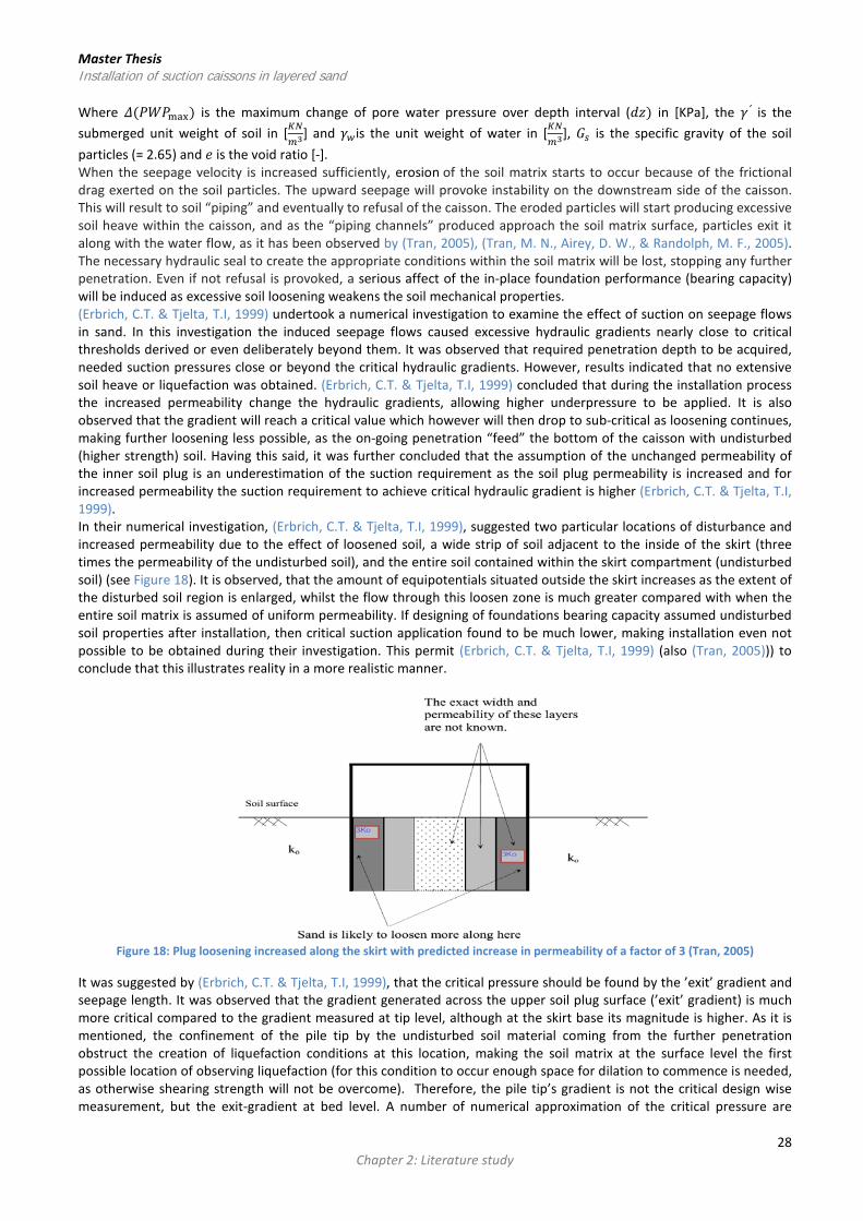
particles (= 2.65) and 𝑒 is the void ratio [-]. When the seepage velocity is increased sufficiently, erosion of the soil matrix starts to occur because of the frictional drag exerted on the soil particles. The upward seepage will provoke instability on the downstream side of the caisson. This will result to soil “piping” and eventually to refusal of the caisson. The eroded particles will start producing excessive soil heave within the caisson, and as the “piping channels” produced approach the soil matrix surface, particles exit it along with the water flow, as it has been observed by (Tran, 2005), (Tran, M. N., Airey, D. W., & Randolph, M. F., 2005). The necessary hydraulic seal to create the appropriate conditions within the soil matrix will be lost, stopping any further penetration. Even if not refusal is provoked, a serious affect of the in-place foundation performance (bearing capacity) will be induced as excessive soil loosening weakens the soil mechanical properties. (Erbrich, C.T. & Tjelta, T.I, 1999) undertook a numerical investigation to examine the effect of suction on seepage flows in sand. In this investigation the induced seepage flows caused excessive hydraulic gradients nearly close to critical thresholds derived or even deliberately beyond them. It was observed that required penetration depth to be acquired, needed suction pressures close or beyond the critical hydraulic gradients. However, results indicated that no extensive soil heave or liquefaction was obtained. (Erbrich, C.T. & Tjelta, T.I, 1999) concluded that during the installation process the increased permeability change the hydraulic gradients, allowing higher underpressure to be applied. It is also observed that the gradient will reach a critical value which however will then drop to sub-critical as loosening continues, making further loosening less possible, as the on-going penetration “feed” the bottom of the caisson with undisturbed (higher strength) soil. Having this said, it was further concluded that the assumption of the unchanged permeability of the inner soil plug is an underestimation of the suction requirement as the soil plug permeability is increased and for increased permeability the suction requirement to achieve critical hydraulic gradient is higher (Erbrich, C.T. & Tjelta, T.I, 1999). In their numerical investigation, (Erbrich, C.T. & Tjelta, T.I, 1999), suggested two particular locations of disturbance and increased permeability due to the effect of loosened soil, a wide strip of soil adjacent to the inside of the skirt (three times the permeability of the undisturbed soil), and the entire soil contained within the skirt compartment (undisturbed soil) (see Figure 18). It is observed, that the amount of equipotentials situated outside the skirt increases as the extent of the disturbed soil region is enlarged, whilst the flow through this loosen zone is much greater compared with when the entire soil matrix is assumed of uniform permeability. If designing of foundations bearing capacity assumed undisturbed soil properties after installation, then critical suction application found to be much lower, making installation even not possible to be obtained during their investigation. This permit (Erbrich, C.T. & Tjelta, T.I, 1999) (also (Tran, 2005))) to conclude that this illustrates reality in a more realistic manner.
Figure 18: Plug loosening increased along the skirt with predicted increase in permeability of a factor of 3 (Tran, 2005)
It was suggested by (Erbrich, C.T. & Tjelta, T.I, 1999), that the critical pressure should be found by the ’exit’ gradient and seepage length. It was observed that the gradient generated across the upper soil plug surface (’exit’ gradient) is much more critical compared to the gradient measured at tip level, although at the skirt base its magnitude is higher. As it is mentioned, the confinement of the pile tip by the undisturbed soil material coming from the further penetration obstruct the creation of liquefaction conditions at this location, making the soil matrix at the surface level the first possible location of observing liquefaction (for this condition to occur enough space for dilation to commence is needed, as otherwise shearing strength will not be overcome). Therefore, the pile tip’s gradient is not the critical design wise measurement, but the exit-gradient at bed level. A number of numerical approximation of the critical pressure are
28 Chapter 2: Literature study

Master Thesis Installation of suction caissons in layered sand introduced based on the effective weight of the soil and empirical relations (Feld, 2001), (Houlsby, G. T., & Byrne, B. W., 2005), (Erbrich, C.T. & Tjelta, T.I, 1999) and (Senders, M., & Randolph, M. F., 2009)) with the seepage length, however since a good agreement is found among them (see Figure 19) only the one suggested by (Senders, M., & Randolph, M. F., 2009) and (Houlsby, G. T., & Byrne, B. W., 2005) are introduced, having no influence of the proposed changed permeability and including the proposed change respectively;
Senders and Randolph method They suggested that the critical suction is generally described by the following expression: Eq 2. 15: 𝑷𝒔𝒖𝒄𝒓𝒊𝒕 = 𝒔𝜸𝒘𝒊𝒄 = 𝒔𝜸ʹ
The boundary conditions used considering an infinitely long suction caisson, have the normalized seepage length (𝑠𝐿) to
tend to unity as essentially all the hydraulic head (𝛥ℎ) loss occurs within the caisson with evenly spaced horizontal equipotential lines, whereas for very small L/D ratio, the theoretical solution for a sheet-pile wall by (Bruggeman, 1999) was suggested equal to π (normalized seepage length). Combining Eq 2.15 and Eq2.16 allows the critical suction to be expressed by:
Eq2.16: 𝒔𝑳
= 𝝅 − 𝐚𝐫𝐜𝐭𝐚𝐧 �𝟓 �𝑳𝑫�𝟎.𝟖𝟓
� (𝟐 − 𝟐𝝅
)
Eq 2. 17: 𝑷𝒔𝒖𝒄𝒓𝒊𝒕
𝜸ʹ𝑫= {𝝅 − 𝐚𝐫𝐜𝐭𝐚𝐧 �𝟓 �𝑳
𝑫�𝟎.𝟖𝟓
� �𝟐 − 𝟐𝝅�} 𝑳
𝑫
Houlsby and Byrne method (Houlsby, G. T., & Byrne, B. W., 2005) used the (C.G. Aywinkle and Junaideen, 1994) study to include the effect of a varying ratio of permeability inside and outside the suction caisson based on the 𝐾𝑓𝑎𝑐 factor. This is due to the fact that sand loosens more adjacent to the caisson wall than towards the middle of the plug due to the shorter hydraulic path (hence higher hydraulic gradient) (see Figure 12 and Figure 18). The prediction of the pressure drop due to suction was used companied with the critical suction conditions prevailing at that instance resulting to the formula Eq 2.18: Eq 2. 18: 𝑷𝒔𝒖
𝒄𝒓𝒊𝒕
𝜸′𝑫= �𝑳
𝑫� (𝟏 + 𝒂 𝑲𝒇𝒂𝒄
𝟏−𝒂)
From Figure 19, it is evident that suggested formulas return similar results regarding suction requirement, even when soil plug loosening is extensive at the areas next to the skirt, having assuming a 𝐾𝑓𝑎𝑐 = 3. Higher differences will be
Figure 19: (left) Different prediction methods of seepage lengths with a good agreement at the specific areas of interest, in particular at penetration depths of 0.1<L/D<1 and (right) associated suction requirement based on the predicted seepage lengths (Senders and Randolph, 2009)
29 Chapter 2: Literature study

Master Thesis Installation of suction caissons in layered sand obtained regarding the normalized seepage length especially either at small 𝐿
𝐷 ratios or very large in magnitude,
nevertheless at 0.1 < 𝐿𝐷
< 1, which is the zone of interest a good agreement is achieved. The concept of predicting the critical suction requirement based on the estimated seepage length is in fact really important regarding the overall prediction of the soil resistances encountered at the field, as it will be seen at Appendix A, that the existing methods use it to predict the decrease of internal friction (𝐹𝑖) and increase of external friction (𝐹𝑜) and hence the overall suction requirement.
2.2.1.4.2. The associated max penetration depth It has been seen that as the penetration of the caisson continues, the suction requirement increases, making the upward hydraulic gradient on the inside of the caisson approaches the value at which a piping failure might be occurred. As this condition is approached the vertical effective stress throughout the depth of the caisson falls to zero. In this case, local piping failures would be induced, with a major inflow of water into the caisson, making the soil to liquefy and make further penetration impossible. In simple mathematical terms, the effective stress function will be the following, including the effect of the upward hydraulic gradient as measured in 2.2.1.2. The prediction of the pressure gradient to the caisson tip (Houlsby, G. T., & Byrne, B. W., 2005): Eq 2. 19: 𝝈𝒗𝒊ʹ = 𝜸ʹ − (𝟏−𝜶)𝑷𝒔𝒖
𝒉= 𝟎 𝑲𝑷𝒂 , where 𝑷𝒔𝒖 = 𝜸ʹ𝒉
(𝟏−𝜶)
By using the (Houlsby, G. T., & Byrne, B. W., 2005) for calculating the soil resistances during SAP (see Appendix A), the max penetration depth could then be derived. In sand the limit on SAP is likely to be of similar magnitude to the diameter. This conclusion can only be applied in sand soil conditions as a first estimation. Eq 2. 20: 𝑳~ 𝑫
𝟐𝑲𝒐𝒕𝒂𝒏𝜹
2.2.2. The groundwater flow in layered soil conditions
2.2.2.1. The mechanisms allowing groundwater flow In the case of layered soil conditions, where the soil resistance in sand is high enough to require seepage flow to occur for continuing penetration, so that soil resistance reduction is required to be induced, then during installation induced groundwater flowlines are altered. In the case of really thin layers, the blockage of seepage flow is negligible, meaning that the typical groundwater flow will be observed within the soil profile. Whereas for very loose sand, reduction of soil resistance is not required, meaning that the penetration will need low suction pressures to be induced to accommodate required penetration, leading to installations without provoking seepage flows (Senders et al., 2007). At the case where seepage flow is required to allow penetration two possible reasons there are which allow such flow to occur in layered soil conditions (i.e sand overlain by clay). 1. (Mechanism 1) Seepage occurs along the sides of the caisson or through cracks in the clay layer (possibly following slight uplift of the plug). At the sides the plug is more likely to form a gap between the skirt and itself due to stiffeners or due to penetration in general, whereas within the soil plug cracking will occur to areas with more silty content or if sand particles are integrated to it (Tran, 2005) (Senders, M., Randolph, M., & Gaudin, C., 2007))(see Figure 20). 2. (Mechanism 2) Seepage at the sand layer occurs once the pressure difference generated above the clay layer exceeds the critical suction pressure in clay (comprised by clay plug’s weight and internal friction (see Eq 2.23)), leading to separation of the soil plug inside the caisson compartment to the clay’s plug which uplifts and the sand’s plug which remains in place and starts to loosen due to the upward seepage (see Figure 20). This results to a water gap at the interface of the two layers. The water gap magnitude developed during caisson installation it is a function of the pumping rate, with observations indicating that plug uplift is minimized by fast suction installation. Slow installation could lead to significant uplift of the clay layer, provided that the clay plug remains intact (Romp, 2013).
30 Chapter 2: Literature study

Master Thesis Installation of suction caissons in layered sand
Figure 20: (Upper figures) Schematization of potential seepage mechanisms in layered soil condition. (Lower figures) Representation of the differential pressures at particular locations across the skirt and outside of the skirt in order for uplift to occur (Senders, M., Randolph, M., & Gaudin, C., 2007)
2.2.2.2. Alteration of the seepage length and associated critical suction In a case of layered soil conditions, at the outer caisson side the soil will remain intact and will act as a seepage flow restriction in the sand both inside and outside. In this way, the net drainage path length is increased, meaning that the critical hydraulic gradient requires a greater pressure to be reached (Senders, M., Randolph, M., & Gaudin, C., 2007). (Senders, M., Randolph, M., & Gaudin, C., 2007) conducted a FEM analysis to assess the head loss in a layered soil conditions installation of a suction caisson. It has been observed that changes in head decay more slowly but surely within the sand compared with the case that a homogeneous sand profile was assessed, owing to the prevention of surface flow outside the caisson (see Figure 21). For long suction caissons the clay layer has relatively little effect on seepage length, but in the typical range of initial penetrations 0.1 < L’/D < 0.5, the seepage length is increased compared with the homogeneous sand case (Romp, 2013). The seepage length for layered soil conditions approximated magnitude could be estimated by the expression Eq 2.21: (see Figure 22 giving that the expression for the critical suction inducing liquefaction within the sand layer could be then estimated by combining the Eq 2.18 and Eq 2.21:
Figure 21: Equi-potential lines for homogeneous sands. (Left) Homogeneous sand profile, (Right) Homogeneous sand profile with a
restriction of surface flow at the outer caisson side due to an impermeable layer (Romp, 2013, Senders et al., 2008).
31 Chapter 2: Literature study

Master Thesis Installation of suction caissons in layered sand
Figure 22: Estimation of seepage length with different prediction methods
Eq 2. 21: 𝒔𝑳𝒂𝒚𝒆𝒓𝒆𝒅
𝑳ʹ= 𝟏 + 𝟎.𝟑(𝑳
ʹ
𝑫)−𝟎.𝟖𝟓
Eq 2. 22: 𝑺𝒍𝒂𝒚𝒆𝒓𝒆𝒅𝒄𝒓𝒊𝒕 = 𝜸ʹ𝑳ʹ[𝟏 + 𝟎.𝟑 �𝑳ʹ
𝑫�−𝟎.𝟖𝟓
]
2.2.2.3. Prediction of the suction inducing seepage flow underneath the impermeable layer In layered soil conditions (i.e sand layer overlain by clay layer), it is mentioned that the desirable seepage flow to allow the degradation of the encountered soil resistance induced by sand, it is restricted by the low permeable layer on top. It is mentioned that to overcome this, the suction induced should overcome the clay plug resistance to uplift, in the case that the clay is relatively thick (>1m) and plug cracking is not possible within the installation time frame (Romp, 2013) (𝛥𝑆1 > 𝑆𝑐𝑙𝑎𝑦𝑐𝑟𝑖𝑡 )(see Figure 23). In the case that clay permeability allows both of the two extremes to commence partly, meaning that both some cracking and simultaneous plug heave will occur to the soil plug, then theoretically some seepage flow could occur within the sand layer. The clay layer, if intact, allows full applied suction to be felt across its thickness as zero head loss is obtained. The clay plug resistance to uplift could then be estimated by the term Sclay
crit , which is composed by the plug effective weight and the internal friction exerted when plug resist uplift (Senders, M., Randolph, M., & Gaudin, C., 2007). Eq 2. 23: 𝜟𝑺 = 𝑺𝒄𝒍𝒂𝒚𝒄𝒓𝒊𝒕 < 𝑾𝒑𝒍𝒖𝒈 + 𝑭𝒊 = �𝜸𝒄𝒍𝒂𝒚′ + 𝟒
𝑫𝒊𝒂𝒔𝒖� 𝒛𝒄𝒍𝒂𝒚
However, it should be mentioned that this prediction of the clay plug uplift is theoretically based, and found experimentally that uplift could commence at a higher suction requirement, meaning that an additional soil resistance component exists resisting uplift (Romp, 2013). The contribution of the reverse end bearing is generally ignored, and it has been assessed by (Mana, D. S., Gourvenec, S., & Randolph, M. F., 2013) to check whether its effect should be accounted or not. (Mana, D. S., Gourvenec, S., & Randolph, M. F., 2013) observed that the reverse end bearing could be maintained equal to the peak undrained compression resistance for a range of embedment ratios as low as d/D = 0.1, and even for uplift displacements between 2% and 5% of the foundation diameter. In the contrary, it was mentioned that reverse end bearing can only be accounted when solid seal is preserved within the caisson plug; otherwise a quick decrease to its magnitude is obtained. (Romp, 2013) conducted experimental modelling in 1g, to assess the contribution of the end bearing to the clay plug’s uplift resistance. It was observed that higher suction requirement was needed, and it was attributed to the reverse end bearing. However, only a part of the end bearing was seen to be required, meaning that the reverse end bearing could not be fully mobilized. Furthermore, it was said that the installation rate and the permeability of the plug mostly determines whether reverse end bearing should be accounted or not (Romp, 2013). Further description of the reverse end bearing capacity is discussed at 2.3.2.2. Reverse end bearing contribution. Subsequently to this point, and without considering the contribution to the uplift resistance, when suction applied is greater than the clay plug uplift resistance, then suction is induced underneath the clay plug. However, as it is
32 Chapter 2: Literature study

Master Thesis Installation of suction caissons in layered sand mentioned the suction felt at the interface of the sand to clay layer is reduced and equal to the difference of the induced suction and the critical suction on clay as stated (see Figure 23) (𝑃𝑠𝑢𝑟𝑒𝑑 = 𝛥𝑆2 = 𝛥𝑆1 − 𝑆𝑐𝑙𝑎𝑦𝑐𝑟𝑖𝑡 < 𝑃𝑠𝑢)
Figure 23: Schematization of the differential pressures induced within the caisson prior to clay plug uplift and when uplift is
initiated by adequate suction greater than the critical suction in clay (Romp, 2013).
2.2. The soil plug behaviour
2.2.1. The soil plug behavior during installation in sand
2.2.1.1. Associated soil plug loosening Plug loosening is the result of suction application beyond the critical point, in which hydraulic gradient have exceed a level, and sand particles have started to move along with the water flow and water flow has reached a level where increase of porosity is needed to accommodate the flow. This could be observed at Figure 24 where the effect of applying a hydraulic gradient beyond the critical value is indicated (𝑖 > 𝑖𝑐) (Lembrechts, 2013).
1. Initial conditions with 𝜌𝜊 (initial density), 𝑉𝑜 (initial volume) at 𝑖 = 0 (initial hydraulic gradient). 2. Almost unchanged conditions 𝜌 ∽ 𝜌𝜊 , 𝑉 ∽ 𝑉𝑜 at 𝑖 < 𝑖𝑐. 3. Soil matrix packing changed 𝜌 < 𝜌𝑜 with increased volume 𝑉 > 𝑉𝑜 and partially liquefaction occurring at 𝑖 > 𝑖𝑐. 4. Removal of induced gradient 𝑖 = 0, but density remains lower than the initial state 𝜌 < 𝜌𝑜 and a permanent
expansion remains 𝑉 > 𝑉𝑜.
These conclusions were supported by (Tran, 2005), who investigated the behavior of sand in 1g conditions, by conducting centrifuge tests and numerical approximations to assess the loosening of the soil plug inside the caisson compartment. Experiments on samples with high relative density (>90%) were used to check whether the discharge through them will be consistent with initial permeability conditions by using Darcy's law at frequent time intervals while gradients were kept constant. He confirmed that the results were inconsistent and the only potential source was the increased permeability of the sample. Modified CPT tests were also used to check initial cone resistances with after installation cone resistances, and jacked piles with suction caissons to assess the soil conditions after the induced processes, indicating that plug loosening is induced within the soil matrix (Tran, 2005) (see Figure 25). In average it was suggested that the end permeability of the soil, induced in suction installation, is increased by a factor of 1.5. This was concluded, as a set of tests were conducted till a good level of agreement with seepage results will be obtained. In addition, considering that in fact soil permeability is increased at this scale, the associated volumetric expansion of the loosened sand resulting to heave should be smaller or equal to the total heave, as heave is comprised by the sand displaced by the caisson wall and the sand inflow too. In this case, (Tran, 2005) concluded that heave will be of the order of 5-6% of the embedment wall depth. In addition, on average the estimated final plug relative density is about 60-70 % when very dense sand was tested (with relative density of >90%), suggesting that the initially dense soil column is likely to loosen to a medium, medium-dense condition during installation.
33 Chapter 2: Literature study

Master Thesis Installation of suction caissons in layered sand
Figure 24: Plug heave below and above the critical gradient, as it will be observed during a test in a permeability apparatus
(Lembrechts, 2013)
The above remarks apply only in the case of the inner side of the caisson, as at the outer side, the opposite occurs. The soil matrix is densified, due to the downward movement of the water. The increase effective stress doesn’t allow the inward soil movement towards the inner side of the caisson, and whilst at tip level the flow is observed to be high, the drag force is not enough to drag the sand particles with the water inside, allowing the densification of the soil at this side.
Figure 25: Comparison of jacked piles with suction caissons to assess the soil conditions after installation (Tran, 2005)
Figure 26: Soil Plug as it is believed to be after installation regarding loosening and associated permeability profile in respect to the
location considered (Tran, 2005)
34 Chapter 2: Literature study

Master Thesis Installation of suction caissons in layered sand (Tran, 2005), supported that there are three main areas of loosening within the caisson’s soil plug. This conclusion was extracted principally from the experimental modeling conducted indicating that an excessive soil loosening commences during the installation. To capture the regions altered because of this process, he conducted numerical modeling approximations to further assess loosening. At Figure 26, it is indicated that the most of the loosening take place at the proximity with the skirt and this effect fades away towards the middle. Sand flow velocities were also approximated and illustrated during the installation process in steps of 𝐿
𝐷= 0.1 and 𝐿
𝐷= 0.3 showing the difference across the regions
within the soil plug (see Figure 27 and Figure 28). The increase permeability illustrated at these figures, are supported by the fact that water flow will follow the shorter hydraulic path, which actually is evident at the case of sand movement as well, as particles movement is alongside with seepage flow, therefore similar flownet should be expected from both when flow velocity is enough to drag particles.
Figure 27: Measured sand movement velocity at 𝑳
𝑫= 𝟎.𝟏 (velocity values shown on the contours are in mm/s) (Tran, 2005)
Figure 28: Measured sand movement velocity at 𝑳
𝑫= 𝟎.𝟑 (velocity values shown on the contours are in mm/s) (Tran, 2005)
The Table 2. summarized the effect of the different installation aspects contributing to the change of the associated plug loosening. Table 2: The effect of the different installation aspects contributing to the change of the associated plug loosening
Installation aspect Plug loosening Reasoning
Increased penetration rate Increased Increased seepage
Increased thickness of caisson wall (t/D) Decreased Confinement effects
Increased penetration depth (L/D) Increased Increased suction requirement
Increased surcharge/Jacking Decreased Reduced suction requirement
35 Chapter 2: Literature study

Master Thesis Installation of suction caissons in layered sand
2.2.1.2. Internal plug heave As it has been illustrated, the main contribution of the suction to the installation of the suction caisson in sand is the generation of groundwater flow within the soil plug (upward). The sand as material stems its strength from its internal friction, which due to the flow is decreased and subsequently the soil plug is loosen-expand and simultaneously heave. The high pressure difference generated makes the plug inside the pile to become less densely packed. The sand volume is effectively increased having then increased permeability too. It has been observed, that the suction application produces irreversible strains, as after suction is terminated the sand arrangement will not return to its original state, having a permanent expansion. This was investigated by (Tran, 2005) doing centrifuge modeling, showing that an approximate plug heave of about 6% of the embedded wall length (𝐿) should be expected, caused mainly both by the volumetric expansion of the loosened sand and the sand inflow coming from the outer caisson side (during suction application 𝜎𝑣𝑜′ > 𝜎𝑣𝑖′ ) . At initial stages of the installation the soil experiences heave of elastic origin when the stress applied to it is less than the critical suction condition (underpressure, removal of loading). The magnitude of the soil heave could be determined by applying Hooke's law (𝛥𝜎 = 𝐸𝛥𝜀). If this is the case, the expected soil heave will be of the order of 0.5% of penetration depth, as no plug loosening is associated (Lembrechts, 2013). (Tran, 2005) investigated the sources of soil heave, using the PIV method (photo analysis method. He initially assumed that the groundwater at the outer side of the caisson generates an inward gradient making more prone that the failure plane beneath the pile tip will be at the inside of the caisson. However, it was observed that the majority of displacements occur in a triangular-shaped zone at the vicinity of the caisson skirt, in particular the inner side. While there is an apparent trend of sand flow around the tip into the caisson, the level of inflow movement compared to the vertical movement along the inner wall is negligible. Another reasoning discussed, came from simulated numerically results showing that at the caisson tip, the flow and velocities are the higher observed and extreme. However, because the seepage provokes upward flow inside the caisson which loosens the soil (volume expansion) and its reduced effective stress allows the particles to move upward as well (piping), at the outside the caisson the movement is downward strengthening the soil and restricting the motion of the particles as well, which could be explain the low inward flow of particles.
Figure 29: (Left) Plug heave at L/D = 0.1. (Right) Plug heave at L/D = 0.2 (Tran, 2005)
For penetration depths 𝐿𝐷
< 0.1, the main part of the soil plug at the central caisson area was mainly unaffected, seeing that almost no movement was occurring away from the skirt. Apart from that, movement at the skirt tip is generally of small extent with almost no movement at the outer side. It was also suggested that the side wedges (see Figure 29) resulted by sand volume expansion rather to inflow. This was explained, mainly owning to the fact that the majority of seepage flow is located there as it constitutes the shortest hydraulic path along the caisson wall, resulting to the initial loosening of the volume, the upcoming expansion and the apparent soil heave. This effect was said to be substantial for cases of very dense sand, as shearing is also occurring at that time which results to shearing and further expansion (dilatation) (Tran, 2005). For penetration depths 𝐿
𝐷< 0.3 the central part of the soil plug was observed to be affected
considerably, with the influence zone to be extended over 30% of the wall embedment below the caisson at the edge wedges which were still expanded (Tran, 2005) (see Figure 30). The tests performed by (Tran, 2005) were conducted at
36 Chapter 2: Literature study

Master Thesis Installation of suction caissons in layered sand worse case conditions inducing high suction pressures to provoke piping failure, indicating that no substantial soil heave is expected in sand even at extreme installation conditions.
Figure 30: Plug heave at L/D = 0.3 (Tran, 2005)
The problem arising with high internal plug heave is that always full aspect ratio L/D=1 regarding penetration depth is not possible to be achieved. Even for installation cases where suction requirements are well below the critical suction pressure threshold, meaning that the soil loosening will be limited, soil heave will be low, as only heave originated by sand volume displaced by penetration will be obtained. However, the main reason of no initial contact between top plate and soil is due to the fact that erosion at the top of the plug takes place, especially as plug approaches the caisson lid. The effect of different dominant installation aspects relatively with the associated soil heave are illustrate to the Table 3. Table 3: The effect of different dominant installation aspects relatively with the associated soil heave
Installation aspect Heave Reasoning
Increased penetration rate Decreased
alteration of seepage regime
Increased thickness of caisson wall (t/D) Increased increased volume displaced
Increased penetration depth (L/D) Increased and then decreased increased volume displaced
Increased surcharge/Jacking Decreased reduced suction requirement
2.2.1.3. The effect of plug’s surface erosion
Figure 31: (Left) The soil without seepage flow. The pore space is filled with almost stationary water (flow is low) and finer soils
grains. (Right) The seepage flow drags soil grains from the pore space in which it travels through (Rosenbrand, 2011).
As plug approaches to the caisson lid, a more pronounced horizontal flow is present on the surface within the caisson compartment. Installation to be achieved is done by pumping water out of the caisson, which is done by an exit opening at the middle of the caisson lid. The cylindrical shape of a suction caisson forces an acceleration pattern of flow velocity
37 Chapter 2: Literature study

Master Thesis Installation of suction caissons in layered sand towards the centre of the caisson, due to the fact that water flows in the direction of decreasing radius. This effect becomes greater towards the end of the installation as the flow accelerates too (Lembrechts, 2013). Erosion depends on the soil structure, the grains’size and the flow velocity. The erosion direction is perpendicular to the soil bed arising problems to the installation. Erosion starts at bed surface and expands downwards. Erosion is amplified by the upward gradient existing within the soil plug picking up soil particles as water flow upwards (see Figure 31) General speaking, the water flow could be visualized as a shearing force within the plug, especially at the surface level eroding the plug’s surface (see Figure 32) (Lembrechts, 2013), (Van Rhee, 2010).
Figure 32: The effect of erosion to the final surface level of the soil plug (Lembrechts, 2013)
In the context of suction caisson installation, erosion exerts a threat at the case when the erosion velocity is greater than the installation velocity. If erosion velocity is kept below this rate then initial contact between top plate and soil will be possible (Lembrechts, 2013).
2.3.2. The soil plug behavior during installation in layered soil conditions
2.3.2.1. Soil plug cracking and plug uplift The restriction imposed to the seepage flow due to the impermeable obstacle of a clay layer, and the structure
of a cohesive layer, does not allow the same mechanisms to arise within the clay layer, as described in the case of sand. However, scouring in silty layers has been observed, which is not so evident in the case of clay (Tran, 2005). (Senders, 2008) described that the imposed seepage flow from below, will generated shear failures along the caisson skirt (piping: applied pressure higher than the reduced shear strength at the edges of the clay plug) or cracking in the middle of the clay, producing flow paths within the clay layer (see Figure 33).
Figure 33: Schematization of plug cracking without the effect of piping (Romp, 2013)
(Romp, 2013) used (Thusyanthan, N. I., Take, W. A., Madabhushi, S. P. G., & Bolton, M. D., 2007) calculation method of bending moment of a clay plug to estimate the cracking mechanism for caisson installation purposes. The main tensile resisting force to bending was considered to be the undrained shear strength for clay. The bandwidth for the relative cracking strength was introduced based on two different fixations (clamped or hinged) of the clay plug with the caisson:
38 Chapter 2: Literature study

Master Thesis Installation of suction caissons in layered sand
Eq 2. 24: 𝑻𝒄𝒍𝒂𝒎𝒑𝒆𝒅𝒎𝒂𝒙 < 𝑷𝒄𝒓𝒂𝒄𝒌𝒊𝒏𝒈 < 𝑻𝒉𝒊𝒏𝒈𝒆𝒅𝒎𝒂𝒙 𝒂𝒏𝒅 𝟔𝟒𝒔𝒖𝒛𝒄𝒍𝒂𝒚
𝟐
𝝅𝑫𝒊𝟑(𝟑+𝝂)< 𝑷𝒄𝒓𝒂𝒄𝒌𝒊𝒏𝒈 <
𝟔𝟒𝒔𝒖𝒛𝒄𝒍𝒂𝒚𝟐
𝝅𝑫𝒊𝟑(𝟏+𝛎)
The cracking mechanism is mainly influence by the increased self-weight and undrained shear strength allowing higher suction pressures to be attained, however, the 𝐷𝑖3 is the major factor determining the cracking failure potential, with a smaller caisson diameter having less cracking probability (Romp, 2013) (see Figure 34). (Romp, 2013) indicated that the major parameter determining whether clay plug will uplift or crack is the caisson geometry, having a transition zone, in which both could occur. Generally speaking, for thin clay layers there is a tendency for cracking whereas for thick layers the uplift failure mechanism will occur. The transition range found to be at the range of 6 < D/z < 10, indicating that for relative high D/z-ratios cracking was the governing failure mechanism (Romp, 2013). However, the rate dependent behavior of the plug was highlighted, since uplift was observed for cases where cracking was supposed to occur, indicating that high pressure difference allow intact plug to uplift prior to cracking to commence. It is interesting to see an example of when cracking will occur; in case of an inner diameter of 10 m, the tendency of cracking will occur for a 1 m < 𝑧𝑐𝑙𝑎𝑦<1.67 m, whereas for thicker layers uplift should be expected. However, D/z < 6 are not really considered as an obstacle in installation practice, meaning that cracking should not be a problem for installation purposes, thus if high probability of plug uplift is predicted, then caisson design should use a higher caisson inner diameter to narrow down this possibility and allow more cracking to occur before uplift being initiated. Another approach to determine the minimum cracking needed to allow installation to be completed without plug uplift was introduced by (Romp, 2013). A fracture requirement ratio ( 𝐶𝑟𝑜𝑠𝑠 𝑎𝑟𝑒𝑎 𝑜𝑓 𝑐𝑙𝑎𝑦 𝑝𝑙𝑢𝑔
𝐶𝑟𝑜𝑠𝑠 𝑎𝑟𝑒𝑎 𝑜𝑓 𝑡ℎ𝑒 𝑐𝑎𝑖𝑠𝑠𝑜𝑛 𝑏𝑎𝑠𝑒= 𝐴𝑐𝑙𝑎𝑦
𝐴𝐶𝑆𝐴) which is increased as clay
layer thickness is increased. For example, it was observed based on experiments that at least 5 - 20 % of cracks was required for the case of 3𝑚 < 𝑧𝑐𝑙𝑎𝑦 < 7𝑚, which practically is not possible, whereas for thin layers (≈ 1𝑚 ) it was only 1%. When uplift is occurred, as described in 2.3.2.1. Soil plug cracking and plug uplift, then it was found that slow installation allow higher total uplift to happen compared with fast installation. The seepage flow of the underlying sand was found to determine the plug speed uplift, which is governed by the sand’s permeability and applied suction.
Figure 34: Suction requirement for different failure mechanisms regarding a clay plug (Romp, 2013)
2.3.2.2. Reverse end bearing contribution Once suction in the caisson is induced, the resultant force on the plug causes an upward motion of the plug. This leads an accumulation of excess negative pore water pressures in the clay plug and reduction in pore water pressures in the seabed beneath the plug relative to the pressures in the surrounding sand. The decrease of pore water pressures in the interface under the clay layer causes a flow of water from the surrounding material outside the caisson towards the low pressure area created. However, the flow rate depends on the soil’s coefficient of permeability and the magnitude of pressure difference induced. In case of homogeneous clay profiles, caisson installation regarding plug stability is advantageous, as clay can inherently resist uplift by generating significant resistance due to the reverse end bearing. This advantage is maintained as long as the negative excess pore pressures (suction) within the confined soil plug are preserved. In this case, a significant uplift resistance is given by reverse end bearing (see Figure 35). Conversely, in the case of layered soil conditions, the contribution of reverse end bearing relies on the underlying sand permeability. Owing to this limitation, it is uncertain whether additional capacity based on the reverse end bearing should be considered. In homogeneous clay conditions
39 Chapter 2: Literature study

Master Thesis Installation of suction caissons in layered sand the reverse end bearing is calculated in accordance to the expression 𝑅𝐸𝐵 = 𝑁𝑐𝑠𝑢 (Verruijt, 2007). Critical stress state conditions are considered neglecting any consolidation effects and soil properties influence is not integrated to this parameter meaning that it can assess different soil layers (Romp, 2013). However, in the case of layered soils the consolidation time should be assessed. Although, for homogeneous clays the dissipation of pore pressures is slow the time-dependency of the dissipation during consolidation in layered soils, depends on the clay’s permeability and drainage path, since suction dissipation will be faster if seepage flow will be faster and at shorter distance (Huang, J., J. Cao, and J. M. Audibert, 2003) (Romp, 2013)). For layered soils, as penetration continues and pass to the sand layer, the generation of negative excess pore pressures will be also developed in the underlying sand, therefore, the sand permeability will mainly affect whether reverse end bearing could be accounted or not and for what duration. It was proposed by (Romp, 2013) that soils with permeability less than 10−5 [𝑚
𝑠] could be considered as capable to maintain
their reverse end bearing capacity, as the time required for dissipation of the negative excess pore pressures (>1 day) was more than a typical installation time (1-6 hours). Therefore, sands with higher permeability than 10−4 − 10−5[𝑚
𝑠]
should not be considered with regards to allow reverse end bearing to actually increase uplift resistance (Romp, 2013).
Figure 35: Schematization of the uplift resistance components of the clay plug (Romp, 2013)
The plug uplift mechanism is based on recommendations made by (DnV, 1992) for clay properties only and hence uplift in layered soils can only be assessed based on theory. For clays, the low permeability allows total stress failure to be accounted regarding installation purposes but for sands, the uplift capacity is matter of time-dependency behavior of the pore pressure dissipation until pressure equalization is occurred after suction (Romp, 2013). However, current shallow foundation design guidelines (e.g., ISO 2003; API 2011), acknowledged the reverse end bearing potential but without specific recommendations (Mana, D. S., Gourvenec, S., & Randolph, M. F., 2013). Generally speaking (Mana, D. S., Gourvenec, S., & Randolph, M. F., 2013) stated that full reverse end bearing should be accounted if no partial drainage around the skirt could be assured, as if not this causes an increase in the compression capacity and decrease in the uplift capacity. Partial drainage was suggested that could be induced either by a vertical gap formed at the outer caisson side at the interface with the soil maybe due to some inclination picked during installation , or at tip level due to a tension crack (see Figure 36). In addition, it was noticed that greater potential for a gap to be formed comes with higher soil undrained strength ratio ( 𝑠𝑢
𝛾ʹ 𝑧> 0.35) (Mana, D. S., Gourvenec, S., & Randolph, M. F., 2013), as soils with low
ratio will self-close the gap.
Figure 36: Schematic of gap mechanisms of a skirted shallow foundation in undrained uplift with (a) intact skirt–soil interface and
(b) gapped skirt–soil interface (Mana, D. S., Gourvenec, S., & Randolph, M. F., 2013)
40 Chapter 2: Literature study

Master Thesis Installation of suction caissons in layered sand
2.3. Theoretical evolvement of installation soil resistance
2.3.1. Installation behaviour in homogeneous sand
2.3.1.1. The self-weight penetration: Enhancement of the inner and outer skirt friction Conventional pile design practice does not take into account the enhancement of vertical stress close to the pile due to the frictional forces further up the caisson generated during skirt penetration (SWP phase). The bearing capacity of a suction caisson is also influenced by the mobilized stress due to penetration of the skirt. It is seen that the skirt friction results in an increase in vertical effective stress alongside with penetration, which if not included to the calculations will result to an underestimation of the soil resistance exerted. (Houlsby, G. T., & Byrne, B. W., 2005) have introduced a method to take this additional vertical effective stress into account. In order to be able to calculate the influence of this extra mobilized soil stress, in (Houlsby, G. T., & Byrne, B. W., 2005) analysis a soil slice inside a caisson with an entirely mobilized soil plug is considered (seeFigure 37). Within this slice of soil that the installation takes place, the increase in vertical stress over its thickness (𝑑𝑧) is the result of the weight of the slice and the stress caused by the friction between the soil and the skirt. The differential equation describing the increase of vertical stress was then simplified at the formula Eq 2.25: considering the inner (subscript i) and outer (subscript o) friction change with a low 𝐿
𝐷< 0.5
(equilibrium of vertical forces as could be observed by the Figure 37). Eq 2. 25: 𝒅𝝈ʹ𝒗
𝒅𝒛= 𝜸ʹ + 𝝈
ʹ𝒗(𝑲𝒐𝒕𝒂𝒏𝜹)𝒊(𝝅𝑫𝒊)
𝝅𝑫𝜾𝟐
𝟒
= 𝜸ʹ + 𝝈ʹ𝒗(𝑲𝒕𝒂𝒏𝜹)𝒊
𝑫𝒊 𝒅𝝈ʹ𝒗
𝒅𝒛− 𝝈ʹ𝒗
𝒁𝒊 𝒐�= 𝜸ʹ
Considering suction piles of typical small L/D-ratio's (bearing caisson), foundations loaded to pressure and not as tension piles, the increase of vertical stress depends on the so called "area of influence", as for this pile the influence area is only a part of the inner soil plug. The spreading region of the extra vertical forces caused by friction is assumed to be contained for both the inner and outer region of the caisson by a 45 degrees plane downwards as resemble in Figure 38, although this area is generally dependent on the soil type.
Figure 37: Equilibrium of a slice of soil inside the suction pile, considering the influence by the skirt friction to the increased
effective stress (Lembrechts, 2013), (Houlsby, G. T., & Byrne, B. W., 2005)
An analysis follows for the stress on the outside and inside of the caisson to account for this area. Simplifying assumptions have been used to define the outer area of influence. A zone of influence contained by 𝐷𝑜 and 𝐷𝑚 = 𝐷𝑜 + 2𝑓𝑜𝑧 in which the vertical stress is enhanced through the action of the downward friction from the caisson was assumed (outer caisson side). Other assumptions used were that within this region the enhanced vertical stress is not dependant on the radial coordinate and no shear stress on vertical planes at diameter 𝐷𝑚 exists. Based on this, the 𝑍𝑜 was derived
( 𝑍𝑜 =𝐷𝑜{�1+�2𝑓𝑜𝑧𝐷𝑜
��2−1}
4(𝛫𝜊𝑡𝑎𝑛𝛿)𝜊). Whilst within the caisson (inner caisson side) at small z/D (z: penetration depth) the stress is
enhanced only in an annulus between 𝐷𝑛 and 𝐷𝑖 , where 𝐷𝑛 = 𝐷𝑖 − 2𝑓𝑖𝑧. For 𝑧 > 𝐷𝑖 2𝑓𝑖
the 𝐷𝑛 = 0, meaning that the
41 Chapter 2: Literature study

Master Thesis Installation of suction caissons in layered sand entire soil plug is mobilized by the increased effective stress (starting point of the influence area is at the point of initial penetration of the skirt as could be seen from Figure 38).
𝑍𝑖 =
⎩⎪⎨
⎪⎧𝐷𝑖�1−�1−�
2𝑓𝑖𝑧𝐷𝑖
��2�
4(𝛫𝜊𝑡𝑎𝑛𝛿)𝑖, 𝑓𝑜𝑟 𝑧 < 𝐷𝑖
2𝑓𝑖
𝐷𝑖4(𝛫𝜊𝑡𝑎𝑛𝛿)𝑖
, 𝑓𝑜𝑟 𝑧 > 𝐷𝑖 2𝑓𝑖
The 45° plane mentioned, containing the area of influence is effectively introduced by the 𝑓𝑖 𝑎𝑛𝑑 𝑓𝑜, which in order to introduce this effect into the formulas shown, should have a value equal to 1, meaning that the area influence is equal to the penetration depth achieved at each moment of the installation. Generally, the inner area of influence is significantly smaller than the outer area, being an annulus for the inner and outer side of the suction caisson (see Figure 39). However for large penetration depths, the inner annulus area tends to capture the whole inner soil plug within the caisson (see Figure 38). The area of the mobilized soil is enhanced with increasing depth. The because of the enhanced effective stress both in and out of the caisson with different areas of influence as penetration depth increases, (Houlsby, G. T., & Byrne, B. W., 2005) deem that higher stresses are generated inside during SWP. The differential equation Eq 2. 25: has no analytical solution, and it should be solved numerically to calculate the vertical effective stress at the inner/outer side of the suction caisson, and subsequently the variation of vertical stress with depth. As the inner (𝜎𝑣𝑖´ ) and outer (𝜎𝑣𝑜´ ) effective stress in relation with the caisson inside and outside regions respectively are altered during installation, the end bearing term (𝑄𝑡𝑖𝑝) change its stress distribution across the tip of the caisson from a triangular to a trapezoidal (see Figure 40). Because of the imbalance of the outer-inner effective stresses, which most probably will be towards the inside area (𝜎𝑣𝑖´ > 𝜎𝑣𝜊´ ) (see Figure 40), it is highlighted that the end bearing term (𝑄𝑡𝑖𝑝) will be lower than if normal effective stress conditions was prevailing during the installation.
Figure 38: Highlighted areas of enhanced effective stress under the 45o plane (Lembrechts, 2013)
42 Chapter 2: Literature study
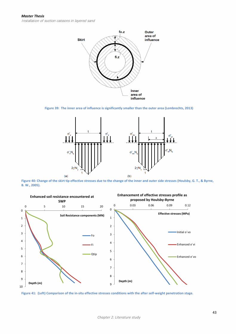
Master Thesis Installation of suction caissons in layered sand
Figure 39: The inner area of influence is significantly smaller than the outer area (Lembrechts, 2013)
Figure 40: Change of the skirt tip effective stresses due to the change of the inner and outer side stresses (Houlsby, G. T., & Byrne, B. W., 2005).
Figure 41: (Left) Comparison of the in-situ effective stresses conditions with the after self-weight penetration stage.
0
1
2
3
4
5
6
7
8
9
10
0 5 10 15 20
Depth (m)
Soil Resistance components (MN)
Enhanced soil resistance encountered at SWP
Fo
Fi
Qtip
0
1
2
3
4
5
6
7
8
9
0 0.03 0.06 0.09 0.12
Depth (m)
Effective stresses (MPa)
Enhancement of effective stresses profile as proposed by Houlsby-Byrne
Initial σ`vo
Enhanced σ`vi
Enhanced σ`vo
43 Chapter 2: Literature study

Master Thesis Installation of suction caissons in layered sand
2.3.1.2. The suction assisted penetration
2.3.1.2.1. Degradation of inner skirt friction The pressure difference produced within the caisson compartment produce the required reduction on the soil resistance encountered during installation of the suction caissons. This is introduced by the induced seepage flow, which is generated due to the hydraulic gradients generated as described at 2.2.1. The groundwater flow in sand. A flow through the porous media of the soil material is initiated, coming from the outer caisson’s side towards the skirt tip and then upward to the caisson’s soil plug surface, allowing penetration to commence. The direction of the seepage flow is the dominant factor of this degradation. The flow coming from outside turns to upward (see reasoning of flow direction shifting at 2.2.1.1. The hydrostatic conditions and the suction induced pressure gradients) as water enters below the skirt tip, and then it flows mainly at a close proximity with the skirt. This is due to the fact that sand loosens more adjacent to the caisson wall than towards the middle of the plug due to the shorter hydraulic path (hence higher hydraulic gradient) (see Figure 17 and Figure 18). The soil loosening is due to the transport of the soil particles, due to the seepage flow. The erosion, induce soil expansion due to the water inventing into its pores, increase of sand porosity and decrease of its frictional strength (Hogervorst, 1980). Generally speaking, the upward flow gradient within the caisson decreases the soil effective along the internal wall, hence reducing the internal skin friction (𝐹𝑖𝑛𝑛𝑒𝑟). The net effect of these processes is a substantial reduction of the total penetration resistance and the associated total driving force required, which benefits the installation procedure. Seepage enables installation to occur where it would otherwise be difficult due to the high resistances encountered (see Figure 6) (Erbrich, C.T. & Tjelta, T.I, 1999). The effect of upward gradient on the mobilized friction force was investigated by (Erbrich, C.T. & Tjelta, T.I, 1999). It was concluded that no linear degradation of friction with gradient is generally obtained. On the contrary, very large hydraulic gradients are essential to considerably degrade the skirt friction. It was suggested that this was due to the fact that the lateral soil stresses do not reduce at a similar rate as the vertical soil stresses. This was indicative regarding the fact that the major principal stress is the horizontal stress whereas the minor principal stress is vertical. In addition, the maximum variation in principal stress magnitude is defined by the passive earth pressure coefficient. No influence of any other soil parameter was observed by (Erbrich, C.T. & Tjelta, T.I, 1999). It was therefore concluded that the degradation of skirt inner friction is a highly non-linear function of the applied upward gradient. (Erbrich, C.T. & Tjelta, T.I, 1999) suggested a theoretical based prediction expression of the degradation of the skirt inner friction, based on 𝐾𝑜 and 𝑂𝐶𝑅 (overconsolidation ratio) suggested by (Mayne P.W. and Kulhaway F.H., 1982).
Figure 42: : Skirt friction degradation with associated pressure gradient (Erbrich, C.T. & Tjelta, T.I, 1999)
Eq 2. 26 : 𝑲𝒐 = 𝑲𝒐 (𝑵𝑪)𝑶𝑪𝑹𝒔𝒊𝒏𝝋ʹ , 𝒘𝒉𝒆𝒓𝒆 𝑲𝒐 (𝑵𝑪) = 𝟏 − 𝒔𝒊𝒏𝝋ʹ 𝒂𝒏𝒅 𝑶𝑪𝑹 = 𝟏
𝟏−𝒊𝒊
By using the above, the degradation of the skirt friction could then be calculated:
44 Chapter 2: Literature study

Master Thesis Installation of suction caissons in layered sand Eq 2. 27: 𝒇𝒔 = 𝑲𝒐𝝈𝒗𝒐ʹ (𝟏 − 𝒊𝒊)𝒕𝒂𝒏𝜹
In addition, the ratio of the initial skirt friction to the degradated friction could be defined as 𝑓𝑠−𝑑𝑒𝑔𝑓𝑠−𝑢𝑛𝑑𝑒𝑔
= 𝑂𝐶𝑅𝑠𝑖𝑛𝜑ʹ(1 −
𝑖𝑖). The comparison with a FE analysis program indicated that a good agreement is achieved with the analytical solution of the skirt friction degradation (see Figure 42). It should be said that (Erbrich, C.T. & Tjelta, T.I, 1999) had not presented any further work regarding the calculation of the soil resistance encountered during the suction assisted penetration of the suction caissons, however, these formulas will be used to check their applicability at chapter for clarification. It has been observed that the existing analytical solutions regarding the soil resistance encountered during suction penetration, try to capture the induced soil behaviour in a simplified manner, as no exact solution exists yet. The proposed solutions regarding the degradation of the skirt friction given by other researchers is given at chapter, in order to present these solutions as a whole. However, it could be said that the effective stress based approaches (i.e. (Houlsby, G. T., & Byrne, B. W., 2005)) follow a similar approach to include this effect to their calculations, whereas CPT-based approaches are generally more simplified considering the 𝑃𝑠𝑢𝑐𝑟𝑖𝑡 to make a prediction of the residual skirt friction, based on a ratio of the applied pressure difference 𝑃𝑠𝑢 to the 𝑃𝑠𝑢𝑐𝑟𝑖𝑡 , having a simple linear reduction in resistance with increasing suction.
2.3.1.2.2. Degradation of Tip Resistance The degradation of tip resistance with applied pressure difference is seen to be more important than the degradation of internal skirt friction (Erbrich, C.T. & Tjelta, T.I, 1999), (Tran, 2005)). Common installation of suction caissons in homogeneous coarse grained soils is based on the principle of tip reduction due to seepage flow, induced by the applied suction. It is seen at 2.2.1.2. The prediction of the pressure gradient to the caisson tip that the induced flow gradient at the skirt’s tip is generally high due to the induced pressure difference producing a flow from the outer side to the inside of the caisson, which is accumulated at the tip, as there the flow path is the shortest towards the surface level of the soil plug within the caisson, generating soil piping effects at this region (Romp, 2013)(see Figure 43). A partially liquefaction (small-scale mechanism) will be initiated at the tip level around the skirt reducing the in-situ effective stresses. As the process of SAP is continued, the induced gradient becomes higher resulting to further liquefaction and reduced stresses, producing an additional flow of soil particles alongside with the water flow as erosion velocity of particles has been exceeded. The degradation of the tip resistance will be increased during this process, being a direct function of the induced inner gradient regime. (Erbrich, C.T. & Tjelta, T.I, 1999) examined the degradation of the tip resistance and concluded that tip resistance will degrade approximately linearly with applied upward gradient, having different behavior compared with the internal skirt friction, indicating that indeed tip resistance reduction will be more severe as for installation purposes the applied pressure difference becomes higher. It was also attempted to assess the coupled process of the degradation of the skirt friction with the tip resistance and it was observed that only some minor non-linearity was introduced. However, the process was largely dominated by the linear tip degradation mechanism (see Figure 44). (Senders, M., & Randolph, M. F., 2009), suggested that the tip resistance will have a residual value even when critical gradient is applied, as part of their investigation indicated that soil resistance was higher than expected if only frictional components were considered.
Figure 43: Induced flow gradient at the skirt’s tip and associated decreased of the tip resistance (Tran, 2005)
45 Chapter 2: Literature study

Master Thesis Installation of suction caissons in layered sand
Figure 44: Linear degradation mechanism at the skirt tip (Erbrich, C.T. & Tjelta, T.I, 1999)
2.3.1.2.3. Enhancement of the outer skirt friction The installation of the suction caisson is seen that creates a seepage flow within the soil plug inside the caisson. However, it is also indicated that the pressure difference created inside the pile, influences the outer skirt area which the caisson is situated, inducing a downward gradient flow, which as a result increase the effective stresses in the soil and consequently increase the external skirt friction (𝐹𝑜) (Erbrich, C.T. & Tjelta, T.I, 1999). This increase is mainly a function of the past stress history of the soil encountered at the site. (Senders, M., & Randolph, M. F., 2009) mentioned that in overconsolidated sands (with high ), this enhancement may be quite low. Following the onset of the suction phase where the magnitude of pressure difference applied approaches (𝑃𝑠𝑢𝑐𝑟𝑖𝑡), then some inward sand grains ‘motion at the caisson tip is possible to occur, resulting in a decrease in the external friction.
2.3.2. Installation behavior in layered soil conditions The installation resistance encountered in layered soil conditions (e.g. sand overlain by clay) is not satisfactory addressed. Full scale installation test are limited (Senders, M., Randolph, M., & Gaudin, C., 2007), having only the recently conducted centrifugal experiments at the UWA, stating that actually installation resistance is reduced significantly compared with jacking installation (push-in resistance) (Watson, P.G., Senders, M., Randolph, M.F., Gaudin, C., 2006). However, the level of this reduction is uncertain, since the hydraulic blockage induced by the upper clay layer to the lower sand layer and the seepage flow that normally is initiated due to suction, resulting to questionable suction caisson feasibility (Watson, P.G., Senders, M., Randolph, M.F., Gaudin, C., 2006). (Senders, M., Randolph, M., & Gaudin, C., 2007), state that the installation resistance could calculated by simply adding the separate soil resistance components from the respective clay and sand layers. As it was stated at 2.3.2. The soil plug behavior during installation in layered soil conditions, the controlling factors (clay layer thickness, sand density) in the case of layered soil profile, is either the impermeable layer’s thickness, as only if the soil plug remain intact, impose a hydraulic blockage to the sand layer, or the sand layer density inducing excessive soil resistance during installation (Senders, M., Randolph, M., & Gaudin, C., 2007). In the case that the impermeable layer thickness is found to be low ( 𝐷𝑖 zclay
< 6) the impermeable layer was found to not really impose problems to the installation (Romp, 2013). In this case
the installation resistance could be predicted as only sand was found at the respective soil profile, assuming seepage flow development as normal. At the case that the sand layer was not dense enough the imposed soil resistance will be low. In this case, the soil resistance could be predicted based on the soil resistance encountered by the respective layers, with the suction though, to be lower than the critical suction (𝑆𝑐𝑙𝑎𝑦𝑐𝑟𝑖𝑡 ) causing the impermeable layer to uplift, meaning that no seepage flow will be imposed to the sand layer (no reduction of the effective stresses) (Senders, M., Randolph, M., & Gaudin, C., 2007). The installation suction requirement needed to penetrate the soil profile is simply calculated by the Eq 2. 28) (Senders, M., Randolph, M., & Gaudin, C., 2007): Eq 2. 28: 𝜟𝑺 = 𝑭𝒊+𝑭𝒐+𝑸𝒕𝒊𝒑−𝑾
𝑨𝒕𝒊𝒑
In the case, where the impermeable layer remain intact during installation and the soil resistance induce by the sand layer is high, the installation will dependent on the impermeable layer plug governing mechanism (Senders, M., Randolph, M., & Gaudin, C., 2007). In Mechanism 1 (cracking) (see 2.3.2.1. Soil plug cracking and plug uplift), the flow barrier is small, and an approximated linear reduction to the internal friction and tip resistance of the sand layers (𝐹𝑖 + 𝑄𝑡𝑖𝑝)𝑠𝑎𝑛𝑑 could be used. This linear reduction could be used to approximate the effect of suction for the
46 Chapter 2: Literature study

Master Thesis Installation of suction caissons in layered sand range0 < 𝛥𝑆 < 𝑆𝑐𝑙𝑎𝑦𝑐𝑟𝑖𝑡 + 𝑃𝑠𝑢𝑐𝑟𝑖𝑡 . The following expression describes the prediction suction requirement, assuming that the self-weight penetration exceeds the clay layer and is located within the sand layer (Senders, M., Randolph, M., & Gaudin, C., 2007): Eq 2. 29: 𝑾 + 𝟎.𝟐𝟓𝝅𝑫𝒊
𝟐𝜟𝑺 = (𝑭𝒐 + 𝑭𝒊)𝒄𝒍𝒂𝒚 + (𝑭𝒐)𝒔𝒂𝒏𝒅 + (𝑭𝒊 + 𝑸𝒕𝒊𝒑)𝒔𝒂𝒏𝒅𝑴𝑨𝑿(𝟏 − 𝜟𝑺𝑺𝒄𝒍𝒂𝒚𝒄𝒓𝒊𝒕 +𝑷𝒔𝒖𝒄𝒓𝒊𝒕
,𝟎)
Where the clay layer’s inner and outer and the sand layer’s outer friction [(𝐹𝑜 + 𝐹𝑖)𝑐𝑙𝑎𝑦 + (𝐹𝑜)𝑠𝑎𝑛𝑑 ] remain unaffected, as the seepage does not influence them during the transitional phase, whereas the sand layer’s inner and tip resistance are reduced as described [ (𝐹𝑖 + 𝑄𝑡𝑖𝑝)𝑠𝑎𝑛𝑑]. If the penetration was still in the clay layer, then for the penetration prediction the expression Eq 2.28 should be used. In Mechanism 2 (plug uplift) the flow barrier is enough to halt any seepage flow, since the clay plug is stationary and no head loss pass through the plug, keeping the sand layer’s hydrostatic conditions. The clay’s permeability is substantial inhibiting any cracking, and so as the suction increases but the plug remains at a standstill, the sand plug’s soil resistance is again assumed to reduce with the induced pressure difference but this reduction is approximated with the factor 𝑓∗. This is because whilst the vertical effective stress is reduced linear with suction increase, the horizontal stress decreases less, in view of the fact that the earth pressure ratio (𝐾𝑜) increase with the vertical stress declining and overconsolidation ratio increase layer (Senders, M., Randolph, M., & Gaudin, C., 2007). The reduction of the internal soil resistance of the sand plug is approximated by the following expression, where the tip resistance is indicated that bears more reduction compared to the internal friction: (𝐹𝑖 + 𝑄𝑡𝑖𝑝)[1 − 𝛥𝑆
𝑆𝑐𝑙𝑎𝑦𝑐𝑟𝑖𝑡 𝑓] 𝑓𝑜𝑟 𝛥𝑆 ≤ 𝑆𝑐𝑙𝑎𝑦𝑐𝑟𝑖𝑡
𝑓 =𝛾𝑐𝑙𝑎𝑦ʹ 𝑧𝑐𝑙𝑎𝑦
𝛾𝑐𝑙𝑎𝑦ʹ 𝑧𝑐𝑙𝑎𝑦+𝛾𝑐𝑙𝑎𝑦
ʹ 𝐿′𝑓∗ Where: 𝑓∗ = 0.25 𝑓𝑜𝑟 (𝐹𝑖) , 𝑓∗ = 1 𝑓𝑜𝑟 (𝑄𝑡𝑖𝑝)
Beyond the suction pressure point capable to provoke uplift to the clay plug (𝛥𝑆 = 𝑆𝑐𝑙𝑎𝑦𝑐𝑟𝑖𝑡 ), the plug will be separated and continue to heave, allowing a water gap to form at the interface of the clay and sand layers, which is sufficient to develop seepage flow. Thereafter, the reduction of the soil resistance is linearly until zero magnitudes are obtained regarding the (𝐹𝑖 + 𝑄𝑡𝑖𝑝)𝑠𝑎𝑛𝑑 components, where suction equals the required suction for both clay plug uplift and sand liquefaction [ 𝛥𝑆 = 𝑆𝑐𝑙𝑎𝑦𝑐𝑟𝑖𝑡 + 𝑃𝑠𝑢𝑐𝑟𝑖𝑡] (Senders, M., Randolph, M., & Gaudin, C., 2007). The vertical equilibrium with depth, assuming that SWP was stopped within the sand layer could be approximated by the following expression:
Eq 2. 30: 𝑾 + 𝟎.𝟐𝟓𝝅𝑫𝒊𝟐𝜟𝑺 = (𝑭𝒐 + 𝑭𝒊)𝒄𝒍𝒂𝒚 + (𝑭𝒐)𝒔𝒂𝒏𝒅 + (𝑭𝒊 + 𝑸𝒕𝒊𝒑)𝒔𝒂𝒏𝒅 �𝟏 − 𝒇 𝑴𝑰𝑵�𝟏, 𝜟𝑺
𝑺𝒄𝒍𝒂𝒚𝒄𝒓𝒊𝒕 ��𝑴𝑨𝑿[𝟎,𝑴𝑰𝑵�𝟏,𝟏 −
𝜟𝑺−𝑺𝒄𝒍𝒂𝒚𝒄𝒓𝒊𝒕
𝑷𝒔𝒖𝒄𝒓𝒊𝒕 �]
It should be mentioned that in both mechanisms, the predictions are based on deliberate simplifications, which are supported by model tests conducted at UWA for similar installations (Senders, M., Randolph, M., & Gaudin, C., 2007). Mechanism 1 is based on assuming some seepage through the clay plug either occurring along the caisson wall and/or through cracks developed in the plug, and involves a linear reduction in penetration resistance with increasing suction. Mechanism 2 suggests that seepage only occurs into a water gap at the interface of the two adjacent layers (sand overlain by clay), resulting to a bilinear decrease in the sand resistance with increasing suction. The water gap extent developed during installation is a function of pumping rate, with fast suction installation minimizing uplift. Whereas slow installation lead to important plug uplift, provided clay layer remains intact (Senders, M., Randolph, M., & Gaudin, C., 2007). The model tests performed at UWA conducted by intact (Senders, M., Randolph, M., & Gaudin, C., 2007), are summarized at . The results indicated that Mechanisms 1 and 2, give similar results, comparable with the measured. Mechanism 1, shows that captures better the initial stage of the installation, as suction is built up faster than it is assumed with the Mechanism 2, whereas later on as suction approaches the 𝑆𝑐𝑙𝑎𝑦𝑐𝑟𝑖𝑡 the Mechanism 2, seems to mimic better this post-uplift behavior. The final caisson penetration was less than the full value (L/D = 0.79), suggesting that the clay plug did indeed move upwards during installation.
47 Chapter 2: Literature study

Master Thesis Installation of suction caissons in layered sand
Figure 45: Measured and predicted (a) total resistance and (b) pressure of suction installation in layered soil (Senders, M., Randolph, M., & Gaudin, C., 2007)
2.4. Observations from suction caissons installations
2.4.1. Review of the general suction pressure trend (Tran, 2005), after conducting both experimental and field tests, it was observed that installation of suction caissons follow a very similar trend, in spite any difference to caissons’ geometrical properties or even in regard of the soil material encountered. Relatively with the suction assisted penetration phase, two distinct stages were observed (see Figure 46):
Figure 46: General suction pressure behaviour (i.e in Sand). Distinct suction phases in regard to the suction requirement slope (Tran, 2005)
1) The transitional stage (1st): the suction requirement are observed to increase with a high rate as pumping is initiated and then to rise quasi-linearly with penetration depth.
2) The stable pressure slope stage (2nd): suction requirement rises with penetration depth with an almost steady gradient till final penetration depth.
48 Chapter 2: Literature study
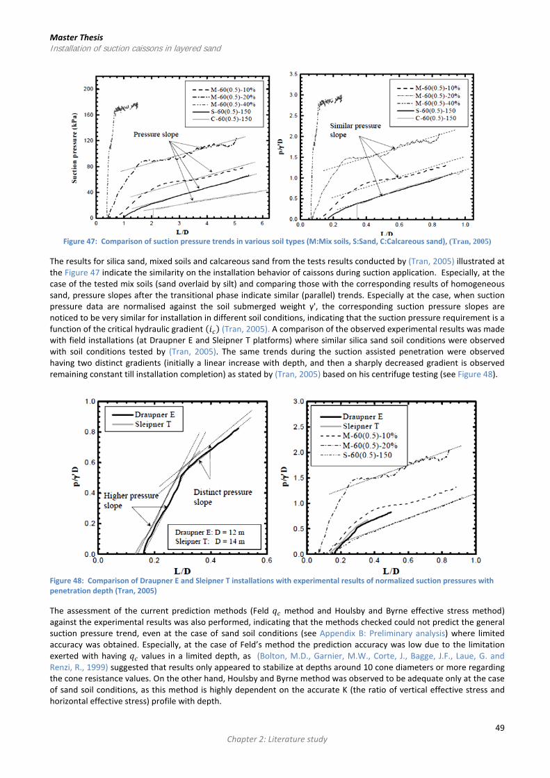
Master Thesis Installation of suction caissons in layered sand
Figure 47: Comparison of suction pressure trends in various soil types (M:Mix soils, S:Sand, C:Calcareous sand), (Tran, 2005)
The results for silica sand, mixed soils and calcareous sand from the tests results conducted by (Tran, 2005) illustrated at the Figure 47 indicate the similarity on the installation behavior of caissons during suction application. Especially, at the case of the tested mix soils (sand overlaid by silt) and comparing those with the corresponding results of homogeneous sand, pressure slopes after the transitional phase indicate similar (parallel) trends. Especially at the case, when suction pressure data are normalised against the soil submerged weight γ', the corresponding suction pressure slopes are noticed to be very similar for installation in different soil conditions, indicating that the suction pressure requirement is a function of the critical hydraulic gradient (𝑖𝑐) (Tran, 2005). A comparison of the observed experimental results was made with field installations (at Draupner E and Sleipner T platforms) where similar silica sand soil conditions were observed with soil conditions tested by (Tran, 2005). The same trends during the suction assisted penetration were observed having two distinct gradients (initially a linear increase with depth, and then a sharply decreased gradient is observed remaining constant till installation completion) as stated by (Tran, 2005) based on his centrifuge testing (see Figure 48).
Figure 48: Comparison of Draupner E and Sleipner T installations with experimental results of normalized suction pressures with penetration depth (Tran, 2005)
The assessment of the current prediction methods (Feld 𝑞𝑐 method and Houlsby and Byrne effective stress method) against the experimental results was also performed, indicating that the methods checked could not predict the general suction pressure trend, even at the case of sand soil conditions (see Appendix B: Preliminary analysis) where limited accuracy was obtained. Especially, at the case of Feld’s method the prediction accuracy was low due to the limitation exerted with having 𝑞𝑐 values in a limited depth, as (Bolton, M.D., Garnier, M.W., Corte, J., Bagge, J.F., Laue, G. and Renzi, R., 1999) suggested that results only appeared to stabilize at depths around 10 cone diameters or more regarding the cone resistance values. On the other hand, Houlsby and Byrne method was observed to be adequate only at the case of sand soil conditions, as this method is highly dependent on the accurate K (the ratio of vertical effective stress and horizontal effective stress) profile with depth.
49 Chapter 2: Literature study
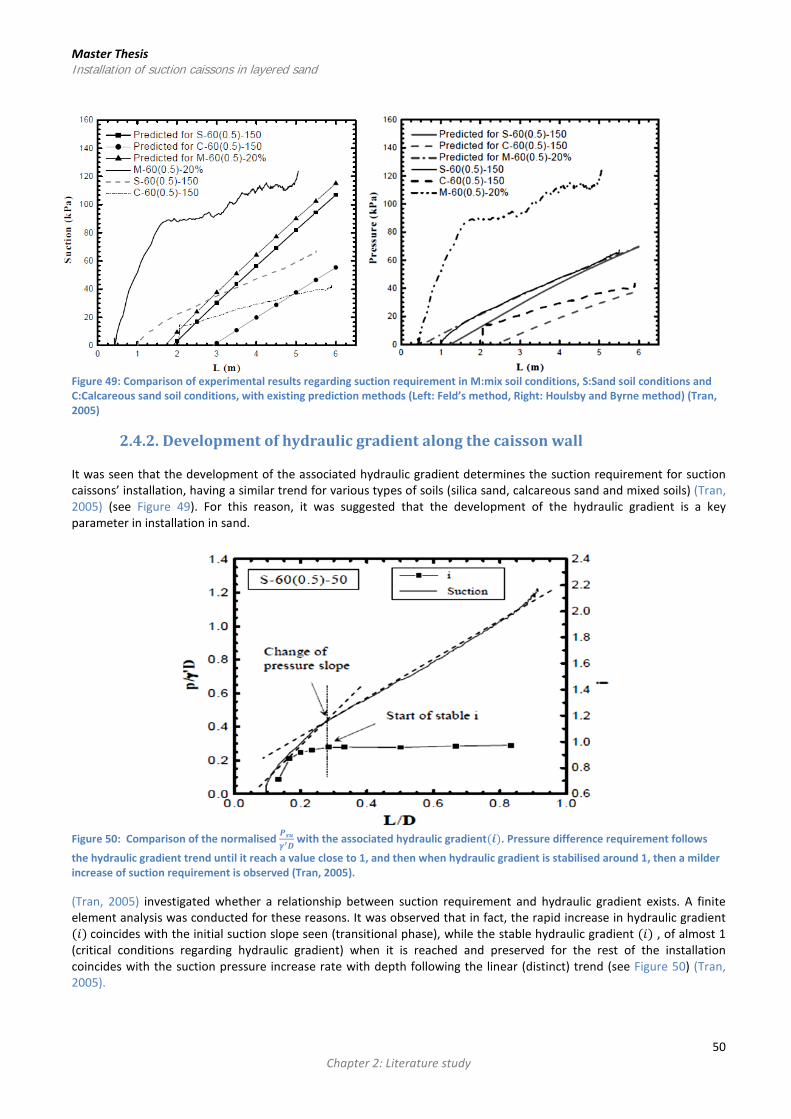
Master Thesis Installation of suction caissons in layered sand
Figure 49: Comparison of experimental results regarding suction requirement in M:mix soil conditions, S:Sand soil conditions and C:Calcareous sand soil conditions, with existing prediction methods (Left: Feld’s method, Right: Houlsby and Byrne method) (Tran, 2005)
2.4.2. Development of hydraulic gradient along the caisson wall It was seen that the development of the associated hydraulic gradient determines the suction requirement for suction caissons’ installation, having a similar trend for various types of soils (silica sand, calcareous sand and mixed soils) (Tran, 2005) (see Figure 49). For this reason, it was suggested that the development of the hydraulic gradient is a key parameter in installation in sand.
Figure 50: Comparison of the normalised 𝑷𝒔𝒖
𝜸′𝑫 with the associated hydraulic gradient(𝒊). Pressure difference requirement follows
the hydraulic gradient trend until it reach a value close to 1, and then when hydraulic gradient is stabilised around 1, then a milder increase of suction requirement is observed (Tran, 2005).
(Tran, 2005) investigated whether a relationship between suction requirement and hydraulic gradient exists. A finite element analysis was conducted for these reasons. It was observed that in fact, the rapid increase in hydraulic gradient (𝑖) coincides with the initial suction slope seen (transitional phase), while the stable hydraulic gradient (𝑖) , of almost 1 (critical conditions regarding hydraulic gradient) when it is reached and preserved for the rest of the installation coincides with the suction pressure increase rate with depth following the linear (distinct) trend (see Figure 50) (Tran, 2005).
50 Chapter 2: Literature study

Master Thesis Installation of suction caissons in layered sand
Figure 51: (Left) Comparison between normalised pressure ( 𝒑
𝜸′𝑳) and (𝒊). Similar response is observed of the normalised to the tip
level suction pressure with the associated hydraulic gradient at the associated penetration depth. (Right) Comparison of field installation data (Draupner E platform) regarding ( 𝒑
𝜸′𝑳) with finite element predicted (𝒊) (Tran, 2005)
It was also suggested that by normalising the suction pressure by the effective overburden stress at tip level, ( 𝑝𝛾′𝐿
), is a
good indicator of the hydraulic gradient along the caisson wall, as effectively 𝑃𝐿 is the average hydraulic gradient
across the skirt length. The hydraulic gradient (𝑖) and normalised pressure ( 𝑝𝛾′𝐿
) indicated similar behaviour with ( 𝑝𝛾′𝐿
) to
follow the increase of (𝑖) when it increases, and reaching its maximum value at the point when (𝑖) reached its critical value equal to 1 following with a stabilize value or a decreasing value afterwards (see Figure 51). This trend where ( 𝑝
𝛾′𝐿)
shows a distinct increase during the transitional installation phase during suction penetration, it is suggested to be used to check which stage of the installation has been reached, as it is helpful to know how early critical hydraulic gradient has been reached and what is the proximity to piping failure (suction response follows the slope corresponding to critical hydraulic gradient along the inner caisson wall) (Tran, 2005). A verification of the suggested normalisation of the suction pressure at tip level, was conducted with field measured data from installations at Draupner E platform (see Figure 51). The comparison indicated that indeed a similar trend exists for the ( 𝑝
𝛾ʹ𝐿) in respect to the (𝑖) following a
similar trend (Tran, 2005), (Erbrich, C.T. & Tjelta, T.I, 1999)).
2.4.3. The effect of pumping rate Fast suction installation implies a greater pressure difference of inner- and outer pressure, which influences the total soil behavior during installation. As it was mentioned at 2.3. Theoretical evolvement of installation soil resistance, the installation of the caisson into the soil matrix generates alterations on the magnitude of the soil resistance encountered, with contrary effects depending on the components of the bearing capacity considered of the soil. In this perspective, especially during the suction assisted penetration of the caisson, the pumping rate used to achieved further penetration has been indicated that plays a dominant role to the whole process (i.e (Senders, M., & Randolph, M. F., 2009), (Houlsby, G. T., & Byrne, B. W., 2005), (Erbrich, C.T. & Tjelta, T.I, 1999)). Furthermore, it is suggested that the penetration resistance encountered at sand is not unique but it depends on the pumping rate as it was indicated by the set of 1g tests conducted (Tran, 2005). This could be visualised if the following is considered. The reduction of the inner pressure regime produce more seepage which though is initiated at the outer wall, as water will flow from outside to the inside, increasing the outer skin friction and then as time passes the generation of increased PWP will commence at the inside reducing the effective stresses at the inner side. Thus, initially the high pumping rate will show a higher sand resistance (outer side), but the on-going transient effect of time to the inner caisson side will allow sand to loosen due to the fully developed seepage flow net which will be appeared afterwards, due to the delay drawn by the soil permeability (in sand this time required is not long but it still poses some effect to the overall process as there is some time requirement to achieve the appropriate loosen state within the sand matrix to allow seepage to flow). This is supported by the fact that sand loosening propagates progressively up, instead of occurring by spontaneous expansion, when a saturated sand column is subjected to upward seepage (Vardoulakis, 2004). Thus, the faster the installation becomes, decreased sand loosening will be observed, but higher sand resistance will be encountered, which will require higher suction pressure
51 Chapter 2: Literature study

Master Thesis Installation of suction caissons in layered sand requirement for a particular penetration depth, which is attributed to that less time is available for the pore pressure generation and any subsequent sand loosening to occur. In this respect, the transient sand loosening also allows higher suction pressures applications as piping formation is less luckily to form as sand loosening is delayed, which means that caisson refusal will be less probable (Tran, 2005). (Vardoulakis, 2004), also observed that no piping channel were developed in fast installations in spite of extremely high suction pressure applications.
Figure 52: Effect of pumping rate to the suction requirement (Tran, 2005)
On the other hand, below particular threshold suction, penetration is unchanged in respect to the penetration rate and as a result in these cases the soil resistance is the same. Probably in these cases the full seepage flow net is already formed and sand loosening is occurring. Probably the time for that full seepage flow net to be formed is related to the soil properties and in particular with the sand consolidation coefficient 𝑐𝑣 (Tran, 2005). Fast installation, show increased absolute seepage volumes, however, the results show that the heave induced in these cases was lower than slow installations. It is seen that suction pressure requirement is strongly dependant on the pumping rate/installation rate (see Figure 52) and the soil properties of the soil matrix allowing transient effects to be generated rather to spontaneous. No matter what, a lower bound suction pressure exists nevertheless the penetration rate induced whereas upper bound can`t be define.
Figure 53: Influence of transition to fast-to-low pumping rate to the suction requirement (Tran, 2005)
It was also observed that the transition to fast-to-low pumping rate (the same applies for the opposite) does not influence the overall behaviour but simply follow the trend that will be evident if only fast or low rate was initially applied (see Figure 53 and Figure 54). The effect of pumping rate is also evident regarding the generation of soil heave within the caisson compartment. (Tran, 2005) observed throughout his experiments that fast installations induce reduced magnitude of plug heave. However, this effect was seen to diminish for cases of thicker caisson’s wall ( 𝑡
𝐷=
2%), indicating that the produced soil heave from the displaced material is far greater from the seepage related component (see Figure 55), making pumping insignificant in this respect.
52 Chapter 2: Literature study

Master Thesis Installation of suction caissons in layered sand
Figure 54: Influence of transition to fast-to-low pumping rate to the suction requirement (Tran, 2005)
In the case of layered soil conditions, numerous researchers found that plug uplift is related to pumping rate (Senders, 2008), (Cotter, 2009), (Tran, 2005). The higher pressure difference (fast pumping) induced between the outer and inner caisson compartment found to change the plug response, although high suction was applied. Even at low suction applications, if low pumping rate was applied, plug heave was always observed (Cotter, 2009), (Tran, 2005). In every case, plug heave was observed to accelerate during the final installation phase (Watson, P.G., Senders, M., Randolph, M.F., Gaudin, C., 2006). From practical experience it is observed that longer installation time may have higher risks regarding refusal of the suction caisson due to plug coming to contact with the caisson lid stopping and influence of the suction to the installation process (SPT, 2014). In addition, piping failure to the impermeable layer, is also more probable, due to the increased suction requirement generally observed for layered soils. Based on experimental tests, piping failure was observed to all cases checked, whereas fast installation led always to successful installation (Tran, 2005). The main reason seems to be that with fast installation, the effective wall-cut off (skirt length embedded to the seabed, displacing soil into the compartment) prevent the development of the piping channels, which normally with the applied suction pressure will have led to piping failure (Tran, 2005) (see Figure 56).
Figure 55: The associated heave with respect to the penetration rate (Tran, 2005)
(Tran, 2005) conducted centrifuge tests to check the validity of the above arguments. It was seen that the suction pressure is not pumping rate dependant but is unique for every depth, as defined at the lower bound value. Seepage results are comparable in spite of the altered pumping rates, which is consistent with the results of the lower bound threshold for suction pressure. It could be attributed to the likely instant generation of the seepage flow net which for the 1g tests time was needed to be fully generated. The soil properties in the centrifuge resemble the actual soil properties, and as soil is a material which stress dependant, the right stresses correspond to the right stiffnesses and compressibility properties for the soil consolidation 𝑐𝑣 , and as a result a stable effective stress condition is generated to every wall embedment depth which will show a similar soil penetration resistance. It was then concluded that the
53 Chapter 2: Literature study

Master Thesis Installation of suction caissons in layered sand suction requirement was unique for every penetration level and independent of the pumping rate induced. However, (Tran, 2005) proposed that additional research should be done based on actual field test to assess whether a transient effect exist in sand soil conditions and in what extent.
Figure 56: Piping failure during penetration of the impermeable layer in slow installation.
2.4.4. The effect of caisson geometry Observations showed that caisson geometry also affected the installation performance. Varying the absolute caisson size did not seem to affect the suction pressure for a given 𝑡
𝐷 ratio. The diameter pose an insignificant influence to the suction
trend compared with other factors, as it continues to have a linear trend with depth. Similar pressure gradient for deep wall embedment ratios (𝐿
𝐷) was seen to be required to allow penetration. The above are true in the case of the
normalised suction ( 𝑝𝛾ʹ𝐿
) , as if absolute suction pressures are observed the required suction for the smaller diameter
caisson is much less (for a given 𝐿𝐷
) compared with larger caissons as shown in (see Figure 57). Although requiring only marginal increase in suction pressure to install due to the increase end bearing resistance created, caissons with thicker walls (higher 𝑡
𝐷 ratio) create substantially higher sand heave during installation. Caisson’s
thickness effect to the suction requirement is more significant compared to diameter’s influence. Its influence is substantial at the SWP phase as increase the tip resistance allowing less self-weight penetration. For the thicker walled caisson ( 𝑡
𝐷= 2%) case the SWP was observed to be almost 25% less compared with ( 𝑡
𝐷= 1%). Given that the wall
roughness was similar for the two caissons, this suggests that the soil resistance is dominated by the wall tip resistance. During SAP its effect is significant smaller although the suction increase is noticeable. This means that the tip resistance is decreased but not eliminated. Generally thicker suction caissons need more suction pressure for the same penetration depth (see Figure 57). For example the required suction pressure for a caisson with 𝑡
𝐷= 2 % is only marginally higher, about 20 % more, compared
with caissons of 𝑡𝐷
= 0.5 %, despite the 4-fold increase in 𝑡𝐷
. Although requiring only marginal increase in suction pressure to install the most significant influence of thicker caissons is the higher created sand heave during installation, as illustrated to Figure 58. It is evident from Figure 58 that the effective heave for all cases is smaller compared with the total observed heave, but in the case of the 𝑡
𝐷= 2% the displaced soil volume within the caisson compartment due to
the caisson volume is substantial and accounts for the a big part of the total heave (Tran, M. N., Randolph, M. F., & Airey, D. W., 2004).
54 Chapter 2: Literature study

Master Thesis Installation of suction caissons in layered sand
Figure 57: The effect of caisson geometry regarding the suction penetration (Tran, 2005)
Figure 58: Sand heave and effective sand heave for various caisson wall thicknesses. (Tran, M. N., Randolph, M. F., & Airey, D. W., 2004)
2.4.5. Effect of additional surcharge and additional penetration depth The significance of surcharge on the overall performance indicated that the increased caisson’s effective weight by using surcharge facilitate installation, although marginally. The added surcharge decrease the necessary differential pressure for a given penetration depth (𝐿
𝐷). It was found that the the total force reduction achieved is quite lower than that
produced by the additional surcharge (Tran, M. N., Randolph, M. F., & Airey, D. W., 2004). In the case that only the suction pressure trend is assessed then almost identical trends have been obtained, suggesting that the use of surcharge does not alter the general suction trend (Tran, M. N., Randolph, M. F., & Airey, D. W., 2004) (see Figure 59). Another important finding relatively with the use of surcharge indicates that installation performance is better in regard to the generated sand heave formation. For instance, at a penetration depth 𝐿
𝐷= 0.8, while the recorded sand heave (with no
surcharge) was measured equal to 6 % of the skirt penetration (𝐿𝐷
), the corresponding sand heave (with surcharge usage)
was reduced by almost 3-fold of the 𝐿𝐷
equal to 2 % (see Figure 60). The additional weight produce increased SWP requiring less suction and this in return generates less heave. For the same reason the soil plug state is seen to remain in a closer state compared to the initial state, meaning that the loosening is less substantial. In other words, the use of higher surcharge (or increase in caisson dead weight) appears to reduce the associated sand loosening (Tran, M. N., Randolph, M. F., & Airey, D. W., 2004). At experimental level, (Tran, 2005) observed that a pressure jump will be
55 Chapter 2: Literature study

Master Thesis Installation of suction caissons in layered sand required in the case of increased surcharge at the starting point of pumping, indicating that large pressure forces is required to mobilize the caisson in this case .The extent of additional SWP by jacking installation (caisson is continuously jacked (pushed) into sand at a rate, equivalent to an extensive self-weight installation phase, where the caisson penetrates under its own weight (the jacking force in this case)) was observed, to determine the effect of additional pressure to the overall installation without inducing suction by (Tran, 2005). The soil resistances exerted, indicated that a rise in a highly non-linear manner will be obtained (see Figure 61), illustrating the significant effect of seepage flow in degrading the tip bearing resistance and the overall difference on the installation approaches. A schematization of the benefits of applying suction instead of jacking is illustrated at the Figure 62, indicating the magnitude of the additional surcharge required to achieve the same penetration depth.
Figure 59: (Left) Effect of surcharge on the required suction pressure. (Right) Comparison of the suction pressure trends for installations with different self-weights (Tran, M. N., Randolph, M. F., & Airey, D. W., 2004)
Figure 60: Effect of surcharge on sand heave formation (Tran, M. N., Randolph, M. F., & Airey, D. W., 2004)
In the case of arbitrarily pushed caisson to a greater penetration depth prior to the SAP, indicates that the suction pressure requirement quickly rises and meet the requirement needed if not additional penetration depth was induced to the caisson. This suggests that inducing additional initial penetration does not effect on the suction pressure trend, given that the rest of the installation conditions are maintained (Tran, 2005) (see Figure 63).
56 Chapter 2: Literature study

Master Thesis Installation of suction caissons in layered sand
Figure 61: Comparison of suction and jacked installation results (Tran, M. N., Randolph, M. F., & Airey, D. W., 2004)
Figure 62: Required suction pressure in comparison with total penetration force at different surcharge levels (Tran, 2005)
57 Chapter 2: Literature study

Master Thesis Installation of suction caissons in layered sand
Figure 63: Effect of initial wall penetration depth on suction pressure (Tran, M. N., Randolph, M. F., & Airey, D. W., 2004)
2.5. Existing procedures for predicting penetration resistance Prediction methods in sand, currently, can be categorized based on the approach and parameter utilized:
• Effective stress or Beta approaches: Constitute the classical approach, using the calculated in-situ effective stress to predict the corresponding tip and frictional resistance with depth.
• CPT approaches: Constitute the most current approach, using the measured cone resistance qc as interpreted by the CPT tests conducted, calculating the corresponding tip and frictional resistance with depth.
The Table 4 contains the current prediction methods, which are mostly used: Table 4: Existing prediction methods
Prediction Methods SWP SAP Soil Conditions Methodology
Houlsby and Byrne (2005) Yes Yes Sand/Clay σ'v
API (2000) Yes No Sand/Clay σ'v
DNV (1992) Yes Yes Sand/Clay CPT
Andersen et al. (NGI) (2008) Yes Yes Sand σ'v and CPT
Senders and Randolph (2009) Yes Yes Layered CPT
Simplified Houlsby and Byrne (2005) Yes Yes Layered σ'v
Bang et al. (2000) Yes Yes Sand/Clay σ'v
Feld (2001) Yes Yes Sand σ'v and CPT
The description of all methods is summarized at the Appendices Appendix A.
2.5.1. Comparison of the prediction methods and suitability The beta methods are theoretically based whereas the CPT methods are empirical methods. This could lead potentially to more confidence in the beta methods. However, theoretical approaches are based on the friction angle, 𝜑′, which in offshore practice is typically deduced from (empirical) correlations with the cone resistance, qc, as the laboratory testing conducted is limited, as it is considered highly expensive and is generally avoided (SPT, 2014). The suitability of the CPT approaches regarding the suction caisson application could be further appraised, if the similarity of the CPT’s cone penetration with the caisson’s skirt penetration is considered. Both the penetrating steel
58 Chapter 2: Literature study

Master Thesis Installation of suction caissons in layered sand objects’ width and the penetration speed are similar, allowing the axi-symmetric failure relevant for the cone may be related to the quasi plane strain failure relevant for skirt penetration (Senders, 2008). Beta approaches especially Houlsby and Byrne method, have been proved to give good predictions, if the appropriate input parameters could be acquired, as otherwise even small deviations could lead to cumulated errors and prediction inaccuracies. As it was mentioned, the friction angle, 𝜑′ and other essential parameters are also correlated based on the 𝑞𝑐 profile, illustrating that implicitly the offshore industry prefers a prediction method with limited accuracy which however comes with limited costs (SPT, 2014), (Senders, 2008). The Table 5 gathers the required parameters for the different prediction methods. Table 5: Required parameters for the used prediction methods
Basic Parameters Empirical factors
DNV 𝑞𝑐 , layer thickness 𝑘𝑝,𝑘𝑓
Senders & Randolph 𝑞𝑐 , layer thickness 𝑘𝑝,𝑘𝑓 ,𝐶𝑜, 𝑃𝑠𝑢𝑐𝑟𝑖𝑡 Feld
𝑞𝑐 ,𝜑′, 𝛾′,layer thickness 𝑃𝑠𝑢𝑐𝑟𝑖𝑡 , 𝑘𝑝,𝑁𝑞, 𝑟𝑜 , 𝑟𝑖 , 𝑟𝑡 , 𝑟
NGI 𝛫𝜊 ,𝜑′, 𝛾′, δ, layer thickness 𝑆𝑁,𝑐𝑟 ,𝑁𝑞 ,𝑁𝛾, 𝑘𝑓 , 𝑘𝑝
API 𝛫𝜊 ,𝜑′, 𝛾′, δ, layer thickness 𝑁𝑞 ,𝑁𝛾
Houlsby & Byrne 𝛫𝜊 ,𝜑′, 𝛾′, δ, layer thickness 𝑁𝑞 ,𝑁𝛾 , 𝑘𝑓𝑎𝑐 ,𝛼
Bang 𝛫𝜊 ,𝜑′, 𝛾′, δ, layer thickness 𝑁𝑞 ,𝑁𝛾 ,𝐹𝑞𝑠,𝐹𝑞𝑑,𝐹𝛾𝑠,𝐹𝛾𝑑
The Table 6 compares the prediction methods upon different criteria, in order to allow a comparison of the methods to be made, and a final selection regarding the methods back-analyzed further up to this thesis to be made. Based on these criteria, a selection of preferred prediction methods to further assess is made, in order to limit the time consumption and increase the effectiveness of the back-analysis further made for the scope of this thesis.
• The simplicity of the Senders & Randolph method and the recommendations attributed to it by the DNV are adequate to consider this method and further evaluate it. In addition, it is easily applied to layered soil conditions, with minimum key parameters required, and has been proved to return sufficient fitting with actual installation data.
• The simplicity of the Feld method, while using both beta and CPT parameters, makes this method potentially more capable to be adjusted to particular soil conditions, preserving its simplicity. In addition, a better documentation to its empirical factors could be made based on the results of this thesis and the soil conditions checked.
• The existing research indicates that the Houlsby & Byrne method can return the most accurate predictions, approaching what in a real installation will be observed and required. This method constitutes the most time consuming method, but it should be used to permit a further analysis of the method and a potential use of it in conjunction with the Feld method. A better fit of the key soil parameters could be acquired through its assessment.
• The DNV standard should also be further assessed, as it is currently the dominant industry’s method to predict suction requirement and soil resistance
59 Chapter 2: Literature study
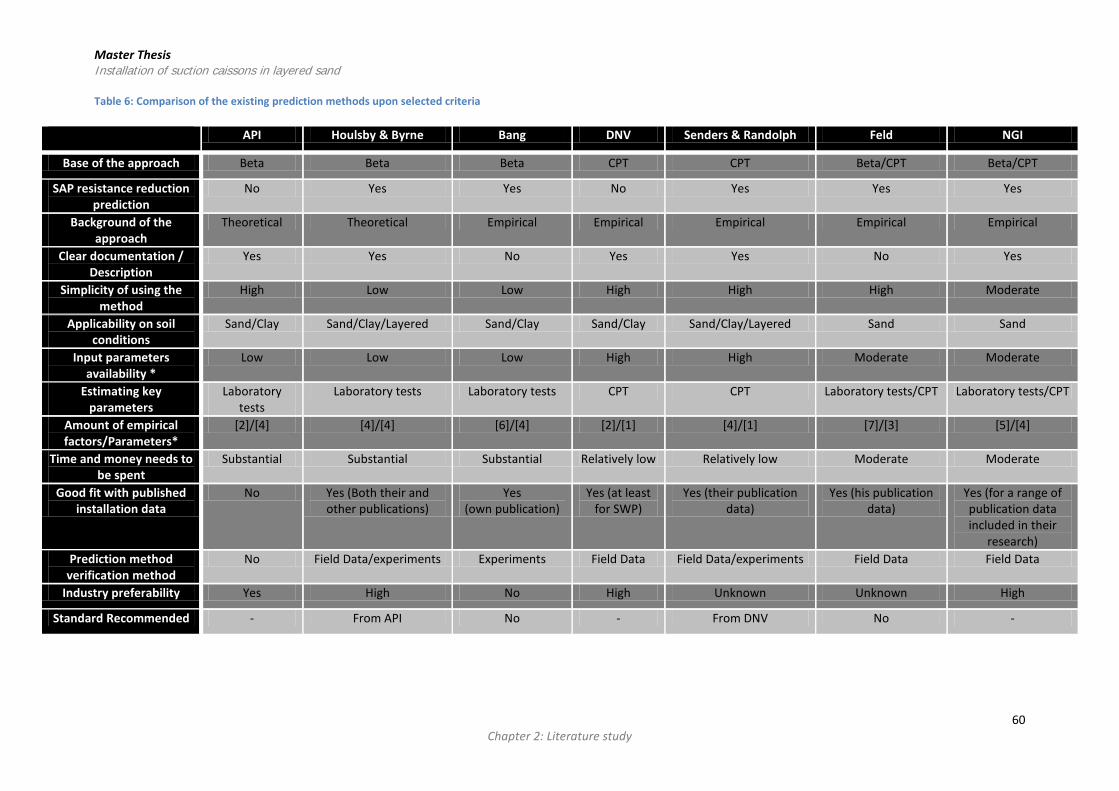
Master Thesis Installation of suction caissons in layered sand Table 6: Comparison of the existing prediction methods upon selected criteria
API Houlsby & Byrne Bang DNV Senders & Randolph Feld NGI
Base of the approach Beta Beta Beta CPT CPT Beta/CPT Beta/CPT
SAP resistance reduction prediction
No Yes Yes No Yes Yes Yes
Background of the approach
Theoretical Theoretical Empirical Empirical Empirical Empirical Empirical
Clear documentation / Description
Yes Yes No Yes Yes No Yes
Simplicity of using the method
High Low Low High High High Moderate
Applicability on soil conditions
Sand/Clay Sand/Clay/Layered Sand/Clay Sand/Clay Sand/Clay/Layered Sand Sand
Input parameters availability *
Low Low Low High High Moderate Moderate
Estimating key parameters
Laboratory tests
Laboratory tests Laboratory tests CPT CPT Laboratory tests/CPT Laboratory tests/CPT
Amount of empirical factors/Parameters*
[2]/[4] [4]/[4] [6]/[4] [2]/[1] [4]/[1] [7]/[3] [5]/[4]
Time and money needs to be spent
Substantial Substantial Substantial Relatively low Relatively low Moderate Moderate
Good fit with published installation data
No Yes (Both their and other publications)
Yes (own publication)
Yes (at least for SWP)
Yes (their publication data)
Yes (his publication data)
Yes (for a range of publication data included in their
research) Prediction method
verification method No Field Data/experiments Experiments Field Data Field Data/experiments Field Data Field Data
Industry preferability Yes High No High Unknown Unknown High
Standard Recommended - From API No - From DNV No -
60 Chapter 2: Literature study

Master Thesis Installation of suction caissons in layered sand
3. Analysis approach
3.1 Introduction The key topic of this thesis is the comparison of field data gathered from actual offshore installation with predicted installation pressures. The focus of this thesis is the installation of caissons in layered sand soils. The Table 10 in section 4.1 Projects description summarises the projects analysed. Both homogeneous dense sand profiles and layered soil conditions were selected to assess the available prediction methods upon their accuracy for predicting the required installation pressure. Primarily, the projects on dense sand profiles were analysed to check the available methods whether they are sufficiently competent to predict required installation pressures on those homogeneous soil conditions or adjustments were necessary to acquire good-fit with the actual results. Methods’ parameters were firstly determined on dense sand conditions, in order to be further used on the layered sand profiles, to assess their suitability on the soil profile recommended and then to check their applicability to others.
3.2. Methodology In the Figure 64, a summary flow chart of the approach followed during the projects‘ analyses is given. A detailed description of the approach followed can be found in the Figure 65, indicating the decisions-path which is followed throughout this analysis in order to enhance its consistency level, highlight and illustrate the expected decisions that should be made during this analysis.
Figure 64: Summary flow chart of the approach followed during the projects‘ analyses
Appraisal of the available field data Prior to the investigation of the available projects, a review process was performed, to appraise which geotechnical aspects could be actually predicted and further compared with the installation data. The existing raw logging data were assessed and processed to determine their reliability and understand their significance. Both visual observations and reading of the prepared as-built reports (including the monitored results, the operational induced changes, the timeline of any reported event influencing the installation) was the base of the reliability assessment. In the case of a malfunction being noticed measurements were disregarded. Identification of the available geotechnical data At this point of the investigation, the geotechnical reports were also screened out to determine the methods possible to be applied for the predictions, as different parameters are needed to be available in order to have direct estimations and not in-direct correlations of parameters and consequently in-direct predictions. In this respect, CPT and Beta methods were considered feasible to be used for the prediction purpose of this thesis. Some correlations nevertheless had to be made, especially at the case of the Beta methods. However, given the results and the conclusions drawn
61 Chapter 3: Analysis approach

Master Thesis Installation of suction caissons in layered sand based on a preliminary analysis of an installation project (see Appendix B), the need for a further soil profile classification was observed. Further analysis of CPTs CPT approaches were concluded to provide the following advantages over Beta approaches (see Appendix B), leading to the decision on assessing further only CPT methods. CPT tests can validate soil profile, soil behaviour (drained or undrained behaviour) and their effect on the predictions (groundwater flow, critical gradient, penetration resistance, loosening rate). Additionally, detailed CPTs were seen to be available to all projects. Therefore a strategy based on this test were used to classify the encountered soil profile. However, as it was found, frequently, the Robertson index is applied to determine soil behaviour and classify soil profile into different categories (Robertson, 2010) (FUGRO, Site investigation results , 2014). It should be mentioned, that many times the soil classification based on the CPTs compared with the soil descriptions obtained based on the laboratory tests were differed substantially. Of course, the most reliable method to determine what sort of drainage behaviour is to be occurred during installation is the laboratory testing. Constrains due to the use of field data Another crucial factor affecting the comparison of the analysis results with the actual installations are the operational contribution, the design simplifications, the reporting or the monitoring of the instrumental measurements, which in every project could contribute to increased subjectivity. The prior mentioned factors could easily affect the judgment made, regarding the reasons change the installation behaviour, which if not documented or determined numerically, can lead to different conclusions. In each project, some uncertainties are present and some design assumptions were necessary to be made, which could be summarised in the following, contributing to discrepancies from the predictions: 1. Caisson dimensions used in predictions may differ from actual dimensions (i.e shell thickness), contributing to
potential overestimations or underestimations of the suction pressures expected, as some minor tolerated differences with the fabricated caisson should be anticipated or due to design simplifications.
2. Surcharge used for the prediction of the self-weight penetration might be different from what was actually used, changing the expected self-weight penetration depth and differential pressure required. Additionally, it was documented that supplementary ballasting after initial set-down of the caisson might be scheduled to reduce applied pressures, but in these cases it was seen that estimation of the new self-weight was difficult, constituting another important reason for substantial discrepancies from the predictions.
3. CPT profiles; Not always continuous CPT graphs were available, decreasing the qc values reliability. The locations of the CPTs available was not always at the exact caisson location. Normally, the CPTs were conducted over the caisson area, however in Q13 project a change of the actual project’s location decided after the site investigation implementation. In addition, the size of the CPT cone (≈ 10 𝑐𝑚2) in respect to the caisson size (≈ 100 𝑚2) (size difference in the order of 105) obviously raise questions about the 𝑞𝑐 spatial variability over the total area where the caisson is to be installed. On the other hand, the skirt wall thickness (30-40 mm) it is comparable, thus, regarding the relation with the penetrability of the caisson similar behaviour with the cone is considered to be existent (Houlsby, G. T., & Byrne, B. W., 2005).
4. Operational variation (see Appendix C: Projects description and site investigation): It was seen from some projects (Q1 and L6-B) that installation speed was altered, and as a result caisson installations were observed to deviate from what was expected quite substantially due to the increased flow and consequently suction rate. In addition, in all projects, caissons should be lifted and re-located or adjusted for design specifications (orientation or allowable tilting limit during installation leading to restarting of the installation process) leading to changes of the installation pressure graph. Change in the inclination or orientation of the caisson was documented as well, changing the actual pressure monitored.
5. Monitoring precision: it is documented that a different level of precision is obtained during monitoring of the different important installation factors (i.e penetration depth, pressure), which depends on the monitoring system used. Another factor influencing the precision obtained is the overburden pressure felt from the sensor. It is reported that this discrepancy increases with increased pressure, which contributes to the extension of the actual pressure bandwidth that it was actually required for the installation. This reduction of the precision has a linear trend with depth and a magnitude of 0.1-0.4 bars depending on the system used (SPT, 2014).
Based on the above issues, it is certain that the analysis is biased, at a different level, in each project. However, this inherent level of uncertainty was used as input to determine the reasons which led to inconsistencies with the available predictions, as obviously the predictions are based on the inputs and the operational changes are not taken into account. As a result, for some cases it will be observed that inconsistencies will be seen between the predicted and actual installation data.
62 Chapter 3: Analysis approach

Master Thesis Installation of suction caissons in layered sand Figure 65: Flowchart of decision making path used in the project analysis
63 Chapter 3: Analysis approach

Master Thesis Installation of suction caissons in layered sand
3.3. Prediction methods used in the analysis Based upon to the preliminary analysis made (see Appendix B: Preliminary analysis), a decision was made to which prediction methods will be further utilised to assess their prediction capacity to the field data available. This decision was essentially based on the preliminary analysis findings, in which the methods indicated whether they have the ability to predict pressures during the course of installation or the ability to be customized for individual cases with different features and characteristics maintaining simplicity. This list of methods is extended with the SPT method. The methods’ equations are available at Appendix A: Existing procedures for predicting penetration resistance.
3.3.1. Prediction methods for sand profiles
Senders & Randolph method (S&R): straight forward, applied to layered soil conditions, with minimum key parameters required, proved to return sufficient fitting with actual installation data both in literature and in Appendix B: Preliminary analysis, particularly at the last part of the installation where the design pressures are mainly determined. For sands, this method is a typical CPT method whereas for layered sand the method turns into a blend of CPT and Beta approach with the use of undrained shear strength ( 𝑆𝑢) as recommended for the clay layers. The main expression describing the installation is the following:
𝑊 + 0.25𝜋𝐷𝑖2𝑃𝑠𝑢 = 𝐹𝑜+ (𝐹𝑖 + 𝑄𝑡𝑖𝑝) �1 −𝑃𝑠𝑢𝑃𝑠𝑢𝑐𝑟𝑖𝑡
�
The prediction was based on the recommendations made for dense sand profiles, when Robertson classification, borehole description and laboratory index tests indicated a sand profile. Taking that into consideration, the predictions were then implemented as having a drained installation. Based on the suggestions made by the S&R method three different scenarios were executed, to include the effect of the soil plug loosening (see Appendix A):
• Assuming 𝑘𝑓𝑎𝑐 = 𝑓𝑖𝑛𝑎𝑙 𝑝𝑒𝑟𝑚𝑒𝑎𝑏𝑖𝑙𝑖𝑡𝑦𝑖𝑛𝑖𝑡𝑖𝑎𝑙 𝑝𝑒𝑟𝑚𝑒𝑎𝑏𝑖𝑙𝑖𝑡𝑦
= 1 corresponding to 𝑃𝑐𝑟𝑖𝑡 = 𝑃𝑐𝑟𝑖𝑡𝑆&𝑅
• Assuming 𝑘𝑓𝑎𝑐 = 3 corresponding to 𝑃𝑐𝑟𝑖𝑡 = 1.5 𝑥 𝑃𝑐𝑟𝑖𝑡𝑆&𝑅 • A 𝑃𝑐𝑟𝑖𝑡 = 4 𝑥 𝑃𝑐𝑟𝑖𝑡𝑆&𝑅 was assumed which for S&R have not been defined a 𝑘𝑓𝑎𝑐. The magnitude of the
parameter corresponding to a high 𝑘𝑓𝑎𝑐(>3) is deemed substantial high as the corresponding loosen state of the plug would be enormous, which is not realistic. However, it was selected to show that recommendations S&R are not appropriate in any case, and other adjustments should be incorporated too.
Feld method: simple, potentially more capable to be adjusted to particular soil conditions, preserving its simplicity, proved to be able to predict actual installation results both in literature and in Appendix B: Preliminary analysis. It can be customized for particular sites where particular soil plug loosening behavior is expected. For layered sand conditions, it is suggested to use the Beta approach with the use of undrained shear strength( 𝑆𝑢). Based on the insight gained from the previous method (S&R), regarding the parameter’s ( 𝑃𝑐𝑟𝑖𝑡) change during the installation, the same was applied in the Feld’s method. Although, this recommendation it is not stated for the Feld’s method, the validity of the above argument was tested. This was also supported during the analysis, when different projects were investigated. Furthermore, it was observed that no single combination of reduction factors for the soil resistance could actually capture the suction requirement during the whole installation, leading to the need of using different scenarios (see Table 7) and check their applicability for the soil profiles tested. The following expression is the main used with Feld’s method:
𝑅𝐹𝑒𝑙𝑑 = 𝐴𝑜𝑟𝑡𝑎𝑛𝜑 ∫ 𝜎𝑣′(𝑧)𝐿0 �1 − 𝑟𝑜
𝑃𝑠𝑢𝑃𝑠𝑢𝑐𝑟𝑖𝑡
� 𝑑𝑧 + 𝐴𝑖𝑟𝑡𝑎𝑛𝜑 ∫ 𝜎𝑣′(𝑧)𝐿0 �1 − 𝑟𝑖
𝑃𝑠𝑢𝑃𝑠𝑢𝑐𝑟𝑖𝑡
� 𝑑𝑧 + 𝐴𝑡𝑖𝑝𝑘𝑝𝑞𝑐(𝐿) �1 − 𝑟𝑡𝑃𝑠𝑢𝑃𝑠𝑢𝑐𝑟𝑖𝑡
�
64 Chapter 3: Analysis approach

Master Thesis Installation of suction caissons in layered sand Table 7: Scenarios applied with Feld method
Scenarios Inner friction 𝑭𝒊
Outer friction 𝑭𝒐
Tip resistance 𝑸𝒕𝒊𝒑 Critical pressure/𝑲𝒇𝒂𝒄
1 -90% +0% -80% 𝑃𝑐𝑟𝑖𝑡 = 𝑃𝑐𝑟𝑖𝑡𝑆&𝑅 (𝐾𝑓𝑎𝑐 = 1)
2 -90% +0% -80% 𝑃𝑐𝑟𝑖𝑡 =1.5 ∗ 𝑃𝑐𝑟𝑖𝑡𝑆&𝑅 (𝐾𝑓𝑎𝑐 = 3)
3 -90% +0% -80% 𝑃𝑐𝑟𝑖𝑡 =1.25 ∗ 𝑃𝑐𝑟𝑖𝑡𝑆&𝑅(𝐾𝑓𝑎𝑐 = 2)
Det Norske Veritas: currently the dominant offshore industry’s standard to predict suction requirement, soil resistance and other designing requirements for offshore applications. However, the method suggested, does not include a suction-assisted penetration phase recommendation, which was addressed by utilizing the DNV values (𝑘𝑓 𝑎𝑛𝑑 𝑘𝑝), accompanied with the Senders & Randolph method when installation was passed into the suction-assisted phase. Substantially, the only difference with applying the S&R method in this case is the DNV values 𝑘𝑓 𝑎𝑛𝑑 𝑘𝑝, which for the DNV standard are constant whereas for the S&R method are different and 𝑘𝑓 change with depth.
SPT method: simple method, using DNV values, able to be applied to layered soil conditions, having minimum parameters, based on experience, it is seen to return good fitting between prediction and actual installation results, especially for dense sand profiles. The method is a typical CPT approach combined with simple coefficients for the different soil-structure resistance components for flow and no-flow conditions, stemming from the experience acquired from actual installations.
3.3.2. Prediction methods for fine-grained layers within sandy soil profiles The soil resistance coming from the cohesive soil identified by the CPTs, was determined based on five different recommendations: 1) Soil resistance is calculated normally as if only granular soil is found. An assumption is made regarding the
groundwater seepage flow possibility within the soil plug. Essentially, the installation is treated such as only sand is found, assuming reduced resistance due to the seepage flow. The typical expressions using qc were used:
• 𝐹𝑖 and 𝐹𝑜 = πD x 𝑘𝑓 x ∫ 𝑞𝑐 (DNV values both for sand and clay) • 𝑄𝑡𝑖𝑝 = 𝐴𝑡𝑖𝑝 x 𝑘𝑝 x 𝑞𝑐
The literature study conducted indicated that in this case an underestimation will be predicted. The cohesive layer, even when it is quite small in thickness, actually change the installation pressure trend (Tran, 2005), and it can lead to underestimations. The soil resistance is deemed reduced due to the seepage flow. 2) The DNV recommendations are used, with the corresponding values found for sand and clay. The calculation in
sand was done as normally, whereas no soil resistance reduction was assumed for the clay layer. The typical expressions using 𝑞𝑐 were used:
• 𝐹𝑖 and 𝐹𝑜 = πD x 𝑘𝑓 x ∫ 𝑞𝑐 (DNV values both for sand and clay) • 𝑄𝑡𝑖𝑝 = 𝐴𝑡𝑖𝑝 x 𝑘𝑝 x 𝑞𝑐
This scenario was checked with the SPT method, as it is the only one using these expressions for layered soil conditions. Generally speaking, it was tested whether the method relying to the 𝑞𝑐 values could estimate accurately the resistance originating by the cohesive layers or not, and if the predicted resistance by the sand layers will be precisely estimated, within the estimations lower and upper bounds or biased by the existence of the clay layer. 3) Instead of using the normal expression found from the DNV standard and the rest CPT approaches, a Beta
determination of the soil resistance was applied, using the undrained shear strength (𝑠𝑢) as recommended by S&R
65 Chapter 3: Analysis approach

Master Thesis Installation of suction caissons in layered sand
and Houlsby and Byrne (Houlsby, G. T., & Byrne, B. W., 2005)( (Watson, P.G., Senders, M., Randolph, M.F., Gaudin, C., 2006). The typical expressions using 𝑠𝑢 were used:
• 𝐹𝑖 and 𝐹𝑜 = πD x 𝑎 x ∫ 𝑠𝑢 • 𝑄𝑡𝑖𝑝 = 𝐴𝑡𝑖𝑝 x ( 𝑠𝑢 𝑥 𝑁𝑐 + 𝜎𝑣𝑜′ )
CPT correlation of undrained strength based on qc values allowing a continuous profile were used to allow the use of this method.
• 𝑠𝑢 = 𝑞𝑐− 𝜎𝑣𝑜𝑁𝑘
• 𝑆𝑡 (𝑠𝑒𝑛𝑠𝑖𝑡𝑖𝑣𝑖𝑡𝑦)= 𝑞𝑐− 𝜎𝑣𝑜𝑁𝑘
∗ 1𝑓𝑠
• 𝑎 = 1𝑆𝑡
Another recommendation of the DNV was used regarding the reduction of the su parameter, in the case it is used for prediction of soil resistance.
• 𝑇ℎ𝑖𝑥𝑜𝑡𝑟𝑜𝑝𝑦 = 𝑠𝑢𝜎𝑣𝑜
𝑖𝑓 𝑡ℎ𝑖𝑥𝑜𝑡𝑟𝑜𝑝𝑦 < 1 𝑎 = 0.5 𝑥 ( 𝑠𝑢
𝜎𝑣𝑜′) ^(−0.5)
𝑖𝑓 𝑡ℎ𝑖𝑥𝑜𝑡𝑟𝑜𝑝𝑦 > 1 𝑎 = 0.5 𝑥 ( 𝑠𝑢
𝜎𝑣𝑜′) ^(−0.25)
• 𝑁𝑐 = 6.2𝑥(1 + 0.34 𝑥 𝑎𝑡𝑎𝑛(𝐿
𝐷))
The DNV standard, also for installation in clay, has made recommendations, regarding the expected penetration resistance (see (DnV, Recommended practise: DNV-RP-E303: Geotechnical design and installation of suction anchors in clay, 2005) paragraph: 4.7.2 Shear strength along skirts penetrated by self-weight). Thus, apart from the frequent used 𝑎 (𝑠𝑖𝑑𝑒 𝑠ℎ𝑒𝑎𝑟 𝑓𝑎𝑐𝑡𝑜𝑟), the DNV standard introduced a more significant reduction factor to 𝑠𝑢 due to the clay’s thixotropic behaviour. Basically this factor is mainly used for self-weight penetrations; however, it was used to check its applicability throughout the installation. This scenario was used with the S&R, as it mainly used there, however an alteration of the Feld’s method for the clay layer using these expressions was done too. The Houlsby and Byrne method is essentially the same for the case of installations in clay (Houlsby, G. T., & Byrne, B. W., 2005). The 𝑠𝑢 , 𝑎 and 𝑆𝑡 clay parameters were calibrated based on the 𝑞𝑐 values found for the clay layer, in accordance to the recommendations made by Robertson, for which it was stated to be highly reliable (Robertson, 2010). 4) Generally it was seen that the sleeve friction is deemed not reliable, in the case it is used for determining the shaft
friction (Senders, M., & Randolph, M. F., 2009). However, it was recommended by Watson, ( (Watson, P.G., Senders, M., Randolph, M.F., Gaudin, C., 2006); (Watson, P.G., and Humpheson, C., 2007) that the sleeve friction, in the case of cohesive soils, should be used, as it was experienced to be promising. In this case, both in sand and clay layers, shaft friction was calculated by using the sleeve friction parameter, to test its precision. The soil resistance expressions using 𝑓𝑠 are the following:
• 𝐹𝑖 and 𝐹𝑜 = 𝜋𝐷 𝑥 ∫ 𝑓𝑠 (𝐵𝑜𝑡ℎ 𝑓𝑜𝑟 𝑠𝑎𝑛𝑑 𝑎𝑛𝑑 𝑐𝑙𝑎𝑦) • 𝑄𝑡𝑖𝑝 = 𝐴𝑡𝑖𝑝 x 𝑘𝑝 x 𝑞𝑐
In literature, the use of the measured sleeve friction for sand was observed to be inappropriate, as the measured friction component of the soil resistance is overestimated. However, this was checked with the SPT method.
5) The use of sleeve friction to determine shaft friction in cohesive layers whereas the use of the qc as normally in
sand was done in this scenario. The soil resistance expressions using 𝑓𝑠 in the clay and qc in sand respectively are the following:
66 Chapter 3: Analysis approach

Master Thesis Installation of suction caissons in layered sand
• 𝐹𝑖 and 𝐹𝑜 = 𝜋𝐷 𝑥 ∫ 𝑓𝑠 (𝐹𝑜𝑟 𝑐𝑙𝑎𝑦) • 𝐹𝑖 and 𝐹𝑜 = πD x 𝑘𝑓 x ∫ 𝑞𝑐 (𝐹𝑜𝑟 𝑠𝑎𝑛𝑑) • 𝑄𝑡𝑖𝑝 = 𝐴𝑡𝑖𝑝 x 𝑘𝑝 x 𝑞𝑐
3.4. Soil Profile classification, Robertson Index During the preliminary analysis (see Appendix B) of a suction caisson (SC) installation case, a question was raised whether CPT is accurate enough to identify soil material within the area of a SC influence area or other measures should be also extend its initial engineering interpretation. This issue was observed to be generally addressed by a relatively great fragment of the offshore industry (i.e FUGRO) and other researchers with the use of the Robertson soil classification approach (Lunne et al., 1997). For the purpose of this thesis, and the amount of the data available to be analysed, the interpretation of the soil profile based on the Robertson soil classification index was coded into a Matlab code to assist to the predictions and increase their precision (see Appendix F: Matlab code). Generally speaking the engineer can make an estimate of the soil profile by observing the basic CPT parameters (𝑞𝑐– 𝑅𝑓) (see Table 8). Table 8: General soil classification based on the magnitude of the basic CPT parameters (Robertson, 2010)
Soil Material 𝒒𝒄 𝑹𝒇 Sand High Low Clay Low High Peat Very low Very high
Sensitive soils Low Low The CPT test, or CPTu test (with pore pressure measurements) as it is commonly known is used as well in offshore applications, has the potential to provide the engineer with a relatively good precision level of the soil profile depending on the complexity of the soil material encountered. It is also suitable to provide correlations, of different range of reliability, for important soil parameters which could be used with caution in predictions (Robertson, 2010). Table 9: Perceived applicability of CPTu for deriving soil parameters (Robertson, 2010)
Soil type
𝑫𝒓 𝜳 𝜥𝝄 𝑶𝑪𝑹 𝑺𝒕 𝒔𝒖 𝝋′ 𝑬,𝑮∗ M 𝑮𝒐∗ 𝒌 𝒄𝒉
Sand 2 − 3 2 − 3 5 5 2 − 3 2 − 3 2 − 3 2 − 3 3 3-4
Clay 2 1 2 1 − 2 4 2 − 4 2 − 3 2 − 4 2 − 3 2 − 3
Where the range 1-5 is a scale of reliability: 1=high, 2=high to moderate, 3=moderate, 4=moderate to low, 5=low, Blank=no applicability, *=Seismic-CPT improves their reliability
Dr: Relative density φ’: Friction angle Ψ: State Parameter Ko: In-situ stress r tio E, G: Young’s and shear modulus Go: Small strain shear modulus OCR: Over conso idation ratio M: Compressibility Su: Undrained shear strength St: Sensitivity ch: Coefficient of consolidation k Permeability
67 Chapter 3: Analysis approach

Master Thesis Installation of suction caissons in layered sand (Robertson, 2010) stated that CPT should be used as a guide to the determination of the mechanical characteristics (strength and stiffness) of the soil, or the soil behaviour type (SBT). CPT tests being continuous, provide data which could be assessed and give a repeatable index of the aggregate behavior of the encountered soil in the vicinity of the probe area. The SBT is based on a chart, which utilises the basic CPT parameters (𝑞𝑡 ,𝑅𝑓). It is also recommended that this chart should always be adjusted to local gained experience (Robertson, 2010). In this chart, a suggestion is made, where results are linked with cementation, age, sensitivity, consolidation-level and soil density. It is also stated that within this soil categorization, some overlapping should be expected (see Figure 66). The full soil classification approach is completed with the use of an additional chart based on a normalized pore pressure parameter (𝐵𝑞) (see Figure 67). The 𝑄𝑡– 𝐵𝑞 chart should be used particularly in the case of a layered soil profile (presence of soft, saturated fine grained soils where the excess pore pressures are expected to be high) where the identification of the exact location and the thickness of each layer are crucial for acquiring precise installation predictions. In soft clayey material and silt layers the probe penetration pore pressures can be high, whereas, in stiff clays (with high OCR ratio), dense silts and silty sand layers, the probe penetration pore pressures can be small or even negative relative to the equilibrium pore pressures (𝑢𝑜). In addition, in sandy soils any excess pore pressures will dissipate in a far higher rate compared from layers with clayey material (Robertson, 2010).
(Robertson, 2010) also recommends that the SBT chart should be used in conjunction with soil samples obtained from the local area, as if no geological data are available for the current geologic environment no clarification of the SBT will be available and predictions will contain high uncertainty about their precision. The SBTN (normalised soil behaviour type) chart soil categorization is essentially founded on the Soil Behavior Type index (𝐼𝑐). This index represents the radius of the concentric circles that represent the boundaries between each SBT zone, which are defined from the 𝑄𝑡– 𝐹𝑟 values obtained for particular soil materials.
68 Chapter 3: Analysis approach

Master Thesis Installation of suction caissons in layered sand
Figure 66: Normalized CPT Soil Behaviour Type (SBTN) chart, 𝑸𝒕𝒏 𝒗𝒔 𝑭𝒓 and description of the displayed zones (Robertson, 2010)
The determination of the Soil Behavior Type index (𝐼𝑐) constitutes an iterative process, which starts with basic CPT parameters obtained from the test. (Robertson, 2010) uses the normalization of the 𝑞𝑐 values generating the 𝑄𝑡𝑛 parameter. Owing to the fact that both the probe penetration resistance and sleeve friction increase with increased penetration depth due to the increase in effective stress, the CPT data requires normalization for overburden stress for shallow and deep readings. The term 𝑄𝑡𝑛 , represents the simple normalization with a stress exponent (𝑛)(typical range 0.7-1). For clay soils this n is equal to 1, whereas for sands this exponent is determined after some iteration. The iterative process is highlighted on Figure 68 , where all the expressions required are indicated at the flow chart (Robertson, 2010) (Robertson, 2010) states that the SBTN chart has the following advantages when it is applied for soil pertaining to the 2-7 zones (see Figure 66):
• Reliability up to 80% is obtained compared with samples • Identification of transition zones throughout the soil profile • Soft material of >100mm (layer thickness) can be detected indicating its full thickness whereas a >750mm layer
is required for stiff materials • Identification of soil behaviour in respect to groundwater flow (drained/undrained behaviour)
Figure 67: Normalized CPT Soil Behaviour Type (SBTN) charts 𝑸𝒕𝒏 𝒗𝒔 𝑩𝒒 (Robertson, 2010)
69 Chapter 3: Analysis approach
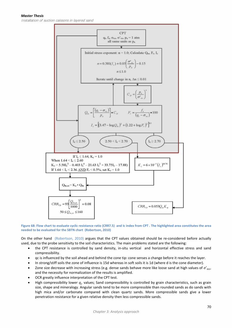
Master Thesis Installation of suction caissons in layered sand
Figure 68: Flow chart to evaluate cyclic resistance ratio (CRR7.5) and Ic index from CPT . The highlighted area constitutes the area needed to be evaluated for the SBTN chart (Robertson, 2010)
On the other hand (Robertson, 2010) argues that the CPT values obtained should be re-considered before actually used, due to the probe sensitivity to the soil characteristics. The main problems stated are the following:
• the CPT resistance is controlled by sand density, in-situ vertical and horizontal effective stress and sand compressibility.
• qc is influenced by the soil ahead and behind the cone tip: cone senses a change before it reaches the layer. • In strong/stiff soils the zone of influence is 15d whereas in soft soils it is 1d (where d is the cone diameter). • Zone size decrease with increasing stress (e.g. dense sands behave more like loose sand at high values of 𝜎’𝑣𝑜,
and the necessity for normalization of the results is amplified. • OCR greatly influence interpretation of the CPT test. • High compressibility lower 𝑞𝑐 values; Sand compressibility is controlled by grain characteristics, such as grain
size, shape and mineralogy. Angular sands tend to be more compressible than rounded sands as do sands with high mica and/or carbonate compared with clean quartz sands. More compressible sands give a lower penetration resistance for a given relative density then less compressible sands.
70 Chapter 3: Analysis approach

Master Thesis Installation of suction caissons in layered sand
• Cementation indicate higher 𝑞𝑐 values. • Grain size (especially if it is comparable with cone size) contributes to increased 𝑞𝑐 values. • Cone diameter influences 𝑞𝑐 and 𝑓𝑠 values especially for soft clays and silts.
Due to these problems ( (Robertson, 2010)recommends the use of CPTu tests, as pore water pressure measurements are done simultaneously with the 𝑞𝑐 measurement. This is advised, as CPTu measures the response of the soil type at the immediate area of the cone and not from its vicinity like in the case of 𝑞𝑐 measurement, indicating the response of the soil at the current depth of the penetration.
71 Chapter 3: Analysis approach

Master Thesis Installation of suction caissons in layered sand
4. Projects installation analysis
4.1 Projects description Herein, a brief project description can be found regarding the available site investigation data used in this thesis (see Table 10), the location of the respective projects (see Figure 69) and the general details of the suction caissons used to each project with an indication of the soil profile at each final penetration depth (see Table 11). Table 10: Analysed projects and general details
Projects Number of
installed caissons
Available Soil investigation Reliability of field data of suction caissons installation
Soil conditions CPTs Boreholes Lab
tests Reports Visual
observation Q1 4 4 1 Yes (3) out of (4) (3) out of (4) Calcareous silica
Sand P6 4 4 1 Yes No logging data only reports
(4) Layered Sand(dense silty fine to medium
Sand) L6-B 3 4 1 Yes 3 3 Fine to medium Sand
Block 12/21 3 3 1 Yes 3 3 Very dense fine Sand
Q13 4 4 1 Yes 4 4 Medium Sand
A more detailed soil profile description can be found in Appendix C containing both the respective CPTs and the description of the profile with depth, as it was done based on the laboratory index tests used. Additionally, Appendix C: Projects description and site investigation comprises short list of the operational changes occurred during the installation which may have affected the overall behaviour. The Table 10 comprises a column which refers to the reliability of the monitored. The reliability of the reports refers to what it was documented that happened during installation stating whether field data gathered should be considered or transformations are required before used. For example, it was seen that soil heave could not be measured due to problems with a reference sensor in two out of the five projects assessed. By means of visual observation it has been assessed that actually no conclusions can be drawn relatively with some geotechnical aspect. For example, as it is referred to the table in Q1 project, although 4 caissons have been installed, a problem occurred with one of them resulting to a problem with the monitored location of it during installation, which does not allow its assessing with the rest in regards to the installation pressure used.
72 Chapter 4: Project analysis
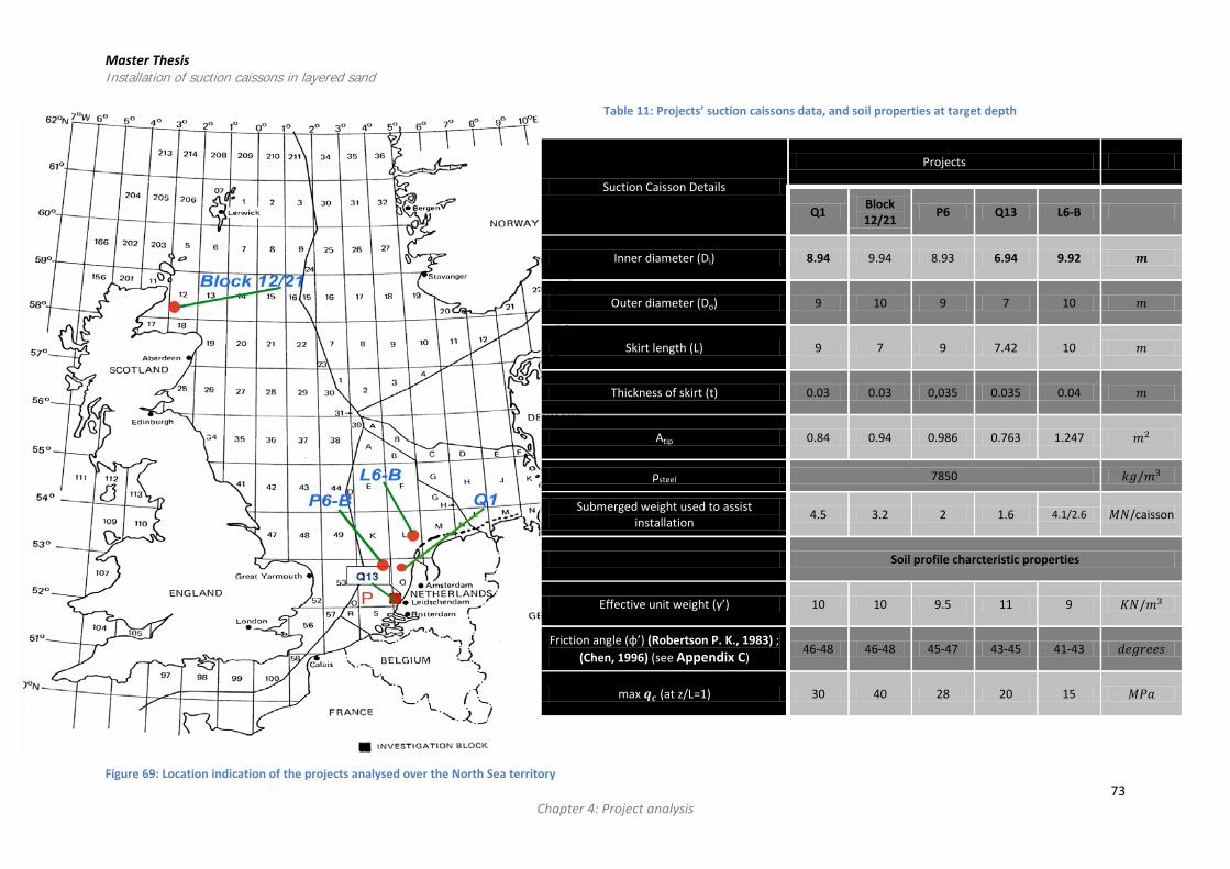
Master Thesis Installation of suction caissons in layered sand
73 Chapter 4: Project analysis
Table 11: Projects’ suction caissons data, and soil properties at target depth
Figure 69: Location indication of the projects analysed over the North Sea territory
Suction Caisson Details
Projects
Q1 Block 12/21 P6 Q13 L6-B
Inner diameter (Di) 8.94 9.94 8.93 6.94 9.92 𝒎
Outer diameter (Do) 9 10 9 7 10 𝑚
Skirt length (L) 9 7 9 7.42 10 𝑚
Thickness of skirt (t) 0.03 0.03 0,035 0.035 0.04 𝑚
Atip 0.84 0.94 0.986 0.763 1.247 𝑚2
ρsteel 7850 𝑘𝑔/𝑚3
Submerged weight used to assist installation 4.5 3.2 2 1.6 4.1/2.6 𝑀𝑁/caisson
Soil profile charcteristic properties
Effective unit weight (γ’) 10 10 9.5 11 9 𝛫𝛮/𝑚3
Friction angle (φ’) (Robertson P. K., 1983) ; (Chen, 1996) (see Appendix C)
46-48 46-48 45-47 43-45 41-43 𝑑𝑒𝑔𝑟𝑒𝑒𝑠
max 𝒒𝒄 (at z/L=1) 30 40 28 20 15 𝑀𝑃𝑎

Master Thesis Installation of suction caissons in layered sand
4.2 Comparison of actual installation pressures with predictions In this chapter, not all estimations of installation pressures are presented (all predictions results can be found at the Appendix D) compared with the observed installation pressure for every project analysed. The methodology followed can be found at 3.2:Methodology, and the prediction methods for sand and layered sand profiles used at 3.3. Prediction methods used in the analysis. A detailed description of the projects’ soil profile and their special features can be found at Appendix C.
Block 12/21 The following observations were obtained:
• 𝐿𝑆𝑘𝑖𝑟𝑡 𝑙𝑒𝑛𝑔𝑡ℎ
= 0 −0.7: Initially, the curve follows the most probable expectation line as predicted by SPT, while
Feld (1st scenario) had analogous prediction.
• 𝐿𝑆𝑘𝑖𝑟𝑡 𝑙𝑒𝑛𝑔𝑡ℎ
=0.7-1: Most probable prediction line by SPT predicts the average behaviour of the Anchors while
the Feld method (2nd scenario) captures this part of the actual curve.
Similar results are obtained using the S&R method, considering both 1st and 2nd scenario as mentioned in 3.3.1. Prediction methods for sand profiles where a shift regarding the fitting of the monitored and predicted installation pressure is observed from the 1st to the 2nd scenario, which was mentioned by the authors for installations in dense sand profiles (see Appendix B). The SWP point was obtained quite accurately (negligible difference of when suction requirement is predicted compared with when it was monitored). The predicted installation pressures were not substantially biased by the uncertainty of the weight imposed or any operational change. The prediction with the DNV values was done only for the 2nd scenario. It was seen that the whole installation could be predicted by the range of pressures obtained by this method (using S&R for the SAP phase). This could be explained by the fact that the S&R method essentially uses the average DNV values. It was observed that the installation pressures curves had two distinct slopes. The physical meaning of the fitting by both scenarios at different 𝐿
𝑆𝑘𝑖𝑟𝑡 𝑙𝑒𝑛𝑔𝑡ℎ, could be described as that the soil
plug was loosen by a factor of 3 after reaching the 𝐿𝑆𝑘𝑖𝑟𝑡 𝑙𝑒𝑛𝑔𝑡ℎ
= 70%. Furthermore, this behaviour indicates that the
soil plug loosening rate reduced during installation, meaning that at the beginning this rate is higher whereas towards the end of the installation this becomes lower, as the soil plug is more difficult to loosen more when from a dense state, it is in a looser state. It should be noted, that the anchors did not have exactly the same suction requirement, having a difference of about 15 KPa, which constitutes an expected range of variance.
Figure 70: Comparison of installation pressures with Feld and SPT prediction (Block 12/21)
Q1 The following results were obtained:
74 Chapter 5: Project back-analysis

Master Thesis Installation of suction caissons in layered sand
Figure 71: Comparison of installation pressures with Feld and SPT prediction (Q1)
• 𝐿𝑆𝑘𝑖𝑟𝑡 𝑙𝑒𝑛𝑔𝑡ℎ
= 0 −1: Throughout the installation the monitored pressures are uniquely identified by the SPT
(max expected )and Feld (most)(1st scenario) methods, meaning that no shifting from 1st2nd scenario was observed.
• No precise estimation of the SWP point was determined (overestimation of the soil resistance) (see red circle at Figure 71)
• 𝐿𝑆𝑘𝑖𝑟𝑡 𝑙𝑒𝑛𝑔𝑡ℎ
= 0.6 −0.7: An underestimation of the required pressure was observed (excluding Anchor 1, as an
operational change [2x pump capacity] was imposed). All methods indicated a reduction due to the obtained 𝑞𝑐 values, showing an underestimation of the soil resistance (see Figure 71). Technically, this may mean that the corresponding CPT values were lower due to the soil properties, in this case calcareous sand, which is more compressible, and this could explain this insufficiency (see 3.4. Soil Profile classification, Robertson Index).
The S&R method (3rd scenario) resulted to the best fitting of the predicted with the monitored installation pressure (see Appendix D: Comparison of actual installation pressures with predictions, Q1). However, this is unrealistic, since this implies that the soil plug was loosen >>3x. As there is no other explanation, the only cause could be the soil resistance underestimation, meaning that DNV values used to link friction (𝑘𝑓) and tip (𝑘𝑝) resistance are substantially lower.
P6 The analysis of this project is not focused on the precision obtained throughout the installation, as the predictions were based not on monitored data but on written reports. The installation behavior at the clay interval and the general behavior after it, constitutes the central focus. The following results were obtained:
• The SWP point predicted was almost the same with actual installation, meaning that self-weight used was as documented and no operational change was imposed, which would have biased the analysis.
• 𝐿𝑆𝑘𝑖𝑟𝑡 𝑙𝑒𝑛𝑔𝑡ℎ
=0.35-0.45: (see Figure 72) it was documented that additional ballasting was allowed, resulting to
additional weight over the caissons, which obviously contributed to a reduction to the final installation pressure, as it could be predicted based on Tran’s observations (see 2.4.5. Effect of additional surcharge and additional penetration depth), where in general surcharge was observed to lead to lower installation pressures requirement (Tran, 2005). By observation the pressure reduction was of the order of 25 KPa or (25*𝐴𝑡𝑜𝑝 =+1.6 MN). Figure 72 also indicates an assumed installation pressure curve in the case of no ballasting was applied, following the actual curve slopes as seen from the graph. If this is considered, then the prediction methods used were actually quite precise (see indicated area at Figure 72). Based on those facts, the monitored actual
75 Chapter 5: Project back-analysis

Master Thesis Installation of suction caissons in layered sand
suction pressures should be higher if not an additional weight is used to the predictions. Therefore, the anticipated suction pressures should be offset in this regard higher by 25 KPa to see the actual pressures (see black line at Figure 72 ).
It was realised that regarding the clay layer the best approximation was obtained with the use of the beta approach (𝑎 𝑥 𝑠𝑢) and especially with Feld’s method and the 5th scenario as presented in 3.3.2. Prediction methods for fine-grained layers within sandy soil profiles. A solely CPT approach as it was the SPT approach was seen to underestimate pressures within this installation interval, indicating that the caisson will have penetrate by its self-weight, which was not observed, although the final penetration was seen to follow the actual behaviour. The SPT method did not succeed to deliver good results regarding the clay layer installation interval. However, the rest of the predicted behaviour agrees well with S&R prediction (see Appendix D: Comparison of actual installation pressures with predictions, P6), indicating similar trends, especially considering the SPT max expected case indicating that the pressure requirement after the cohesive layer it could be captured although having an underestimation there. The SPT method was also used with the 4th and 5th scenarios as described at the paragraph: 3.3.2. Prediction methods for fine-grained layers within sandy soil profiles. The SPT method is the only pure CPT approach both for sand and layered sand soil conditions; therefore, it was selected to implement these scenarios. Initially, the measured sleeve friction was used, observing that a substantial overestimation was acquired for both scenarios. However, when the prediction is focused on the clay layer, an overestimation is obtained, however, the trend is similar with the actual monitored installation pressure. This observation was used with the 5th scenario, in which the sleeve friction measured was decreased by a factor of 40% ( ∫ 𝑓𝑠 (𝑢𝑠𝑒𝑑) = 0.6 𝑥 ∫𝑓𝑠 (𝑚𝑒𝑎𝑠𝑢𝑟𝑒𝑑) ). This was seen to fit well with the actual pressures, without influencing the prediction given for the sand layer. This reduction should be further assessed statistically. In the case of Feld, an assumption was made regarding the magnitude of the ballasting used giving as an input the observed increase of +1.6 MN, which gave good results. Feld prediction captured installation quite precise, considering the above assumptions. In the case of S&R method, the installation behaviour within the clay layer was seen to be better described by the normal reduction factor for the shear friction (see 3.3.2. Prediction methods for fine-grained layers within sandy soil profiles), whereas the thixotropic reduction of the side shear friction was seen to underestimate the corresponding soil resistance, as it was expected, as the installation was in a suction-assisted phase. Again, the shifting from 1st2nd scenario was observed after a 𝐿
𝑆𝑘𝑖𝑟𝑡 𝑙𝑒𝑛𝑔𝑡ℎ= 0.75 to capture the installation pressure trend, in the case the assumed
curve (without additional ballasting) is considered.
Figure 72: Comparison of the actual installation pressure trend with the SPT prediction using the measured sleeve friction (fs) (P6)
Q13 The site investigation of this project was conducted prior to the finalization of the project site. Results indicated that the installation pressure had a variation (two pairs of anchors had similar behavior converging at the end) which indicated that probably a distinct difference of the profile exists for the most of the installation. The following results were obtained:
• The SWP point predicted was not precisely estimated (0.8m off)
76 Chapter 5: Project back-analysis
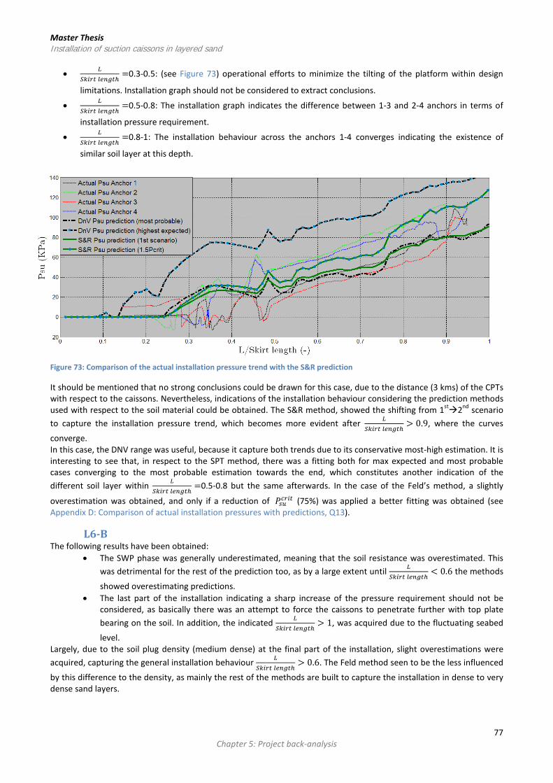
Master Thesis Installation of suction caissons in layered sand
• 𝐿𝑆𝑘𝑖𝑟𝑡 𝑙𝑒𝑛𝑔𝑡ℎ
=0.3-0.5: (see Figure 73) operational efforts to minimize the tilting of the platform within design
limitations. Installation graph should not be considered to extract conclusions.
• 𝐿𝑆𝑘𝑖𝑟𝑡 𝑙𝑒𝑛𝑔𝑡ℎ
=0.5-0.8: The installation graph indicates the difference between 1-3 and 2-4 anchors in terms of
installation pressure requirement.
• 𝐿𝑆𝑘𝑖𝑟𝑡 𝑙𝑒𝑛𝑔𝑡ℎ
=0.8-1: The installation behaviour across the anchors 1-4 converges indicating the existence of
similar soil layer at this depth.
Figure 73: Comparison of the actual installation pressure trend with the S&R prediction
It should be mentioned that no strong conclusions could be drawn for this case, due to the distance (3 kms) of the CPTs with respect to the caissons. Nevertheless, indications of the installation behaviour considering the prediction methods used with respect to the soil material could be obtained. The S&R method, showed the shifting from 1st2nd scenario to capture the installation pressure trend, which becomes more evident after 𝐿
𝑆𝑘𝑖𝑟𝑡 𝑙𝑒𝑛𝑔𝑡ℎ> 0.9, where the curves
converge. In this case, the DNV range was useful, because it capture both trends due to its conservative most-high estimation. It is interesting to see that, in respect to the SPT method, there was a fitting both for max expected and most probable cases converging to the most probable estimation towards the end, which constitutes another indication of the different soil layer within 𝐿
𝑆𝑘𝑖𝑟𝑡 𝑙𝑒𝑛𝑔𝑡ℎ=0.5-0.8 but the same afterwards. In the case of the Feld’s method, a slightly
overestimation was obtained, and only if a reduction of 𝑃𝑠𝑢𝑐𝑟𝑖𝑡 (75%) was applied a better fitting was obtained (see Appendix D: Comparison of actual installation pressures with predictions, Q13).
L6-B The following results have been obtained:
• The SWP phase was generally underestimated, meaning that the soil resistance was overestimated. This was detrimental for the rest of the prediction too, as by a large extent until 𝐿
𝑆𝑘𝑖𝑟𝑡 𝑙𝑒𝑛𝑔𝑡ℎ< 0.6 the methods
showed overestimating predictions. • The last part of the installation indicating a sharp increase of the pressure requirement should not be
considered, as basically there was an attempt to force the caissons to penetrate further with top plate bearing on the soil. In addition, the indicated 𝐿
𝑆𝑘𝑖𝑟𝑡 𝑙𝑒𝑛𝑔𝑡ℎ> 1, was acquired due to the fluctuating seabed
level. Largely, due to the soil plug density (medium dense) at the final part of the installation, slight overestimations were acquired, capturing the general installation behaviour 𝐿
𝑆𝑘𝑖𝑟𝑡 𝑙𝑒𝑛𝑔𝑡ℎ> 0.6. The Feld method seen to be the less influenced
by this difference to the density, as mainly the rest of the methods are built to capture the installation in dense to very dense sand layers.
77 Chapter 5: Project back-analysis

Master Thesis Installation of suction caissons in layered sand The SPT method, had better fitting following the max expected curve, whereas the S&R method, again, indicated that shift of 1st2nd scenario, but earlier than expected, which could be attributed to the sand’s looser state at the final installation stages. Maybe even higher 𝑃𝑠𝑢𝑐𝑟𝑖𝑡 could be used, due to the already loose state of the plug.
Figure 74: Comparison of the actual installation pressure trend with the Feld prediction
4.3 Conclusions based on the evaluation of predictions versus actual installation pressures It has been seen that there are a number of uncertainties in the installation prediction of suction caissons. The soil resistance encountered during the installation of suction caissons depends on several aspects such as; the rate of installation, hydraulic conductivity of the soil, drainage length of the caisson and the shear strength properties of the foundation soil. As a result of installation, volume characteristics of the surrounding soil will be changed compared with those measured in-situ (or prior to installation). The main conclusions are presented below. For each conclusion, the background found from the literature is firstly presented to support it. Then, conclusions are further substantiated by referring to findings made throughout the analysis of this chapter. Finally, in some instances, sub-conclusions are given to support the main conclusion, or a re-statement of the main conclusion is specified. Prediction of required suction pressures in layered soil is less accurate compared with homogeneous sand/clay installations Typically, installations of suction caissons in homogeneous sand or clay profiles have been observed to meet the theoretical predictions with adequate accuracy. Conversely, according to the literature, the installations of suction caissons in layered sand integrated with intermediate less permeable soil layers of varying thickness, relatively density and permeability are observed to be inadequately described by the prediction methods regarding the suction requirement. In this chapter, the evaluation of the installations predictions made in dense sand profiles showed good results. A variation depending on the soil characteristics (size fraction descriptions, relative density) was seen to exist. Based on the different soil characteristics, a change on the fitting of the predicted and the monitored required installation pressure was seen, indicating a change on the associated soil resistance as well (see Q13 and L6-B Prediction analysis results). It was observed that when soil characteristics, such as; permeability, size fraction descriptions and relative density, were altered towards a less dense soil profile, with low permeability, or different sand particle type, methods gave less precise fitting.
78 Chapter 5: Project back-analysis

Master Thesis Installation of suction caissons in layered sand As observed in this study, especially at the case of the Q1 project (calcareous sands), the sand particle type was fundamental on the prediction accuracy. The predictions were found to underestimate the soil profile resistance to installation. The only reliable conclusion that could be drawn is that the soil resistance predicted was lower than the actual resistance. This could be only attributed to the magnitude of the DNV suggested 𝑘𝑓 and the 𝑘𝑝values attributed for sand, as being not representative in the calcareous sand case. Although, the DNV gives a range of a most probable and a highest expected soil resistance based on a lower bound and upper bound 𝑘𝑓 and 𝑘𝑝values, which could explain this high monitored resistance, it poses significant conservatism in designing. A look at Figure 113, where the expected range of required installation pressure was determined to be 110 to 270 kPa, could indicate the magnitude of the adopted conservatism. In this case, the change of the 𝑃𝑠𝑢𝑐𝑟𝑖𝑡magnitude in order to acquire a strong fit was substantial (see Figure 114), as in by the S&R method, meaning that the change of the soil plug state could not happen in reality. As a result the aforementioned conclusion regarding the magnitude of 𝑘𝑓 and the 𝑘𝑝 values for calcareous sand it is considered realistic. This is supported by the fact that the SPT method shows a robust fit with the most probable estimation for dense sand profiles. Whereas for medium dense sand profiles the maximum expected estimation was giving a good fit. In other words, this constitutes an indication that the average of the DNV 𝑘𝑓 and the 𝑘𝑝 values are more representable in case of medium density sand profiles. This is true, as the maximum expected 𝑘𝑓 and the 𝑘𝑝 values used by the SPT, are the mean values as proposed by the DNV suggestions (see Appendix A: Existing procedures for predicting penetration resistance). Yet, no strong conclusions could be drawn, since the investigated profiles shows more than one change at their profiles (see Appendix C: Projects description and site investigation). Despite this, it could be concluded that the soil resistance predicted for sand layers with various characteristics is an underestimation, if based solely on the CPT’s 𝑞𝑐 values. Based on this, it is concluded that higher 𝑘𝑓 and 𝑘𝑝values should be used to meet the desired accuracy for installation in layered soils. Soil resistance is overestimated at shallow depths The DNV standard supported that in shallow depths (0-1.5m), in other words the normal SWP range of depth, the 𝑘𝑓 and the 𝑘𝑝values should be 25-50% lower than those recommended due to local piping. In this chapter this was observed as predictions showed an overestimation of the soil resistance at shallow depths. This mostly could be attributed to uncertainties in the 𝑞𝑐 values provided (discontinuous CPT profiles interrupted for sampling purposes to reduce site investigation costs) and the DNV values recommended. On the other hand, at intermediate installation depths, it was observed the predictions indicated better agreement. Mostly, predictions have been seen to provide good results regarding the final penetration depth, mainly because they have been developed to estimate the critical pressures at the final depth. However, it was seen that underestimations were observed for the SPT and S&R methods at greater depths. This could be caused by overestimating of the final loosening rate. The opposite was seen regarding Feld’s method which demonstrated a slight overestimation. Prediction accuracy is influenced by soil permeability profile In the case of layered soils (sand and clay or silt layers combination), the installation pressure trend for the cases evaluated varies with penetration depth with respect to the location of the impermeable layers. It has been observed in literature that the required suction pressures for penetration in sand below an impermeable layer are on average about 2 to 2.5 times higher than those in homogenous sand,. It was suggested (see 2.2.2. The groundwater flow in layered soil conditions) that this behavior probably originated either from the restrictions imposed to the seepage flow, due to the decreasing available space for the flow-lines to be developed between the caisson tip and the impermeable layer, or the increased soil resistance encountered after a point due to the stiffer response provoked by the impermeable layer. In this chapter, two projects with intermediate impermeable layer were investigated. It was concluded that in layered soils the permeability profile is crucial for determining if soil resistance reduction is anticipated. In the L6-B project (with layered soil conditions (sand-silt-sand sequence of layers)) the installation pressure in the sand was seen to follow the homogeneous dense sand installation behaviour regardless of the presence of less permeable
79 Chapter 5: Project back-analysis

Master Thesis Installation of suction caissons in layered sand material. Whereas, in the case of the P6 project (with layered soil conditions (sand-clay-sand sequence of layers)), the prediction was clearly seen to require to account for the existence of the clay layer, in order to return better fitting. This was concluded to be realistic, owning to the fact that the silt layer and the rest of the sandy layers had similar permeability characteristics. Therefore, the installation behaviour was deduced to be a matter of the soil material permeability characteristics, rather to the existence of the cohesive material. Pragmatically, this is more sensible, as the cause of the soil resistance reduction due to the suction application, is caused by provoked seepage flow, which is a matter of the permeability characteristics of the encountered soil. Permeability comparisons could not be made, between the P6 and the L6-B project, as the P6 project permeability profile was not known. Therefore, it could not be defined on when permeability’s magnitude poses seepage restrictions. Qualitative characteristics (fines content) were seen to require quantitative characteristics (permeability) to support when predictions should be altered to account for seepage restrictions and subsequent absence of soil resistance reduction. This is said, as not always particle size analysis was available at the site investigation reports. An upward offset of the suction pressure required was observed due to the undisturbed soil resistance of the cohesive layer. The potential effect of plug cracking or plug uplift was not applicable since the installation pressure did not exceed the required threshold value. Prediction Accuracy in cohesive soils should be based on undrained shear strength and sleeve friction It has been observed in literature that the installation pressure required in the case of fine-grained low permeability material, is generally estimated based on the undrained shear strength. In addition, it is suggested to use the sleeve friction values obtained by CPTs to determine the associated friction resistance. In this chapter, the applicability of undrained shear strength to predict installation pressure was validated for the P6 (clay layer) project, where the normal reduction factor was used in combination with the undrained shear strength giving significant accuracy level for the prediction of the soil resistance. The use of sleeve friction was seen to give substantial accuracy in the P6 project. However, in the case of L6-B (silt layer) project, there was not sufficient fitting observed. The validation of the use of sleeve friction as accurate friction resistance prediction parameter could be found essential, as there would not be a need for determination of undrained shear strength by laboratory testing. However, as it was seen, in the case of L6-B, this requires the installation to be conducted in an undrained regime. Installation in sandy soils has an increasing critical pressure limit It has been deduced, as part of the literature study, that during installations of suction caissons in sandy soil, the inner soil plug changes. Loosening of the plug occurs, which changes the permeability of the soil and required installation pressure. In particular, the use of the S&R method, suggests changing the magnitude of the parameter 𝑃𝑠𝑢𝑐𝑟𝑖𝑡 due to this change.. Only in the case of such an adjustment, the method results in a prediction capturing the observed? installation’s trend behavior. In this chapter, this was noticed when monitored installation pressures were compared with predictions. The recommendations of S&R method for dense sand were applied changing the 𝑃𝑠𝑢𝑐𝑟𝑖𝑡 magnitude, observing that the increased parameter should be changed towards the end of the installation to give high prediction precision. Not the same consistency was observed with Feld method regarding this parameter change. However, Feld’s 𝑃𝑠𝑢𝑐𝑟𝑖𝑡expression is different, which was seen to give higher values than with S&R’s expression. In this analysis, it was observed that substantial high values of the 𝑃𝑠𝑢𝑐𝑟𝑖𝑡 could be required to acquire sufficient fitting, which however is not realistic. In the case of the Q1 project, which is a case of calcareous sand profile, the increase of the 𝑃𝑠𝑢𝑐𝑟𝑖𝑡 was 400% (3rd scenario). Such change cannot be supported physically, as the 𝑃𝑠𝑢𝑐𝑟𝑖𝑡 is related to a permeability increase. The observed increase would translate to a non-realistic permeability change. The S&R method, suggests a change of the parameter 𝑃𝑠𝑢𝑐𝑟𝑖𝑡 ,
80 Chapter 5: Project back-analysis

Master Thesis Installation of suction caissons in layered sand related to a permeability increase to a factor of 3, whereas others suggest that not more than a permeability change beyond a factor of 3 was measured during experimental modeling (Tran, 2005). On average the estimated final plug relative density was observed to range within 60-70 % when very dense sand was tested (with an in-situ relative density of >90%), suggesting that the initially dense soil column is likely to loosen to a medium, medium-dense condition during installation. In addition, as it found from the literature that the maximum permeability change could not be beyond 4-5 times of the initial, in order to retain a stable soil plug (Tran, 2005). In this analysis, it was observed from the comparisons made that it is more likely that the final permeability will be changed according to the S&R method for dense sand profiles of relative density of >90%. Numerically, this will mean that actually the change of the inner soil plug permeability was reduced by a factor of 3, which could not be validated by the measured data directly. Similar behaviour was observed for medium dense sand profiles of relative density of 60-70 % with the permeability change to be within 2-3 times of the initial. It could be concluded that, as the determination of the magnitude of the parameter 𝑃𝑠𝑢𝑐𝑟𝑖𝑡 is directly linked to the change of the permeability, a loosening threshold should be determined depending on the initial sand plug state. This will give a better prediction of the installation pressure throughout the process and especially at the final penetration depth. Contribution of outer friction to installation pressures could not be determined There is a controversy whether outer friction resistance is enhanced according to (Feld, 2001) and (Houlsby, G. T., & Byrne, B. W., 2005) or not during installations in sand profiles (Senders, M., & Randolph, M. F., 2009) and (SPT, 2014). It has been presented that during installation the outer friction resistance is enhanced due to the downward groundwater flow to the caisson, generated due to the applied suction within the caisson. Such a conclusion could not be drawn by using the prediction methods in this analysis. Many uncertainties are inherently found at the predictions. Primarily, these uncertainties are related with the loosening rate proposed and the relation of the CPT cone resistance with the friction and tip soil resistance, in other words the 𝑘𝑓 and the 𝑘𝑝 values. The comparisons indicated that towards the end of the installation, the soil resistance is not reduced with the same rate as observed previously. This could be attributed to the enhanced outer friction or the reduction of the loosening rate. Owning to this fact, it could be concluded either that the soil plug permeability was increased by some factor or some enhancement of the outer friction was experienced by the soil in combination with the increased permeability.. However, the literature recommendations regarding this enhancement indicate an increase of not more than 13% -15% (Feld, 2001). Certainly this enhancement, as it was seen could not explain the change of the installation pressure requirement towards the end of the installation, indicating that the loosening rate was essentially reduced, as it is the only valid explanation in regards with the monitored soil resistance.
81 Chapter 5: Project back-analysis

Master Thesis Installation of suction caissons in layered sand
5. Project back-analysis At the previous chapter, the use of the prediction methods indicated that the soil resistance estimated was not accurate enough both regarding the soil profile and when compared partially during the installation duration. A number of uncertainties and peculiarities are integrated when relating the measured CPT 𝑞𝑐 value with the friction and tip resistance. This originates from the different soil material characteristics which makes the soil a highly variable resistance wise material. The interpretation of the CPT 𝑞𝑐 index, in respect to the resistance the soil applies to the penetration of the caisson, was seen to differ, indicating that its magnitude it is not the only factor determining the anticipated resistance. Other soil characteristics (i.e. permeability, size fraction, relative density), are seen to influence the suggested DNV values relating the CPT 𝑞𝑐 index with the friction and tip resistance. At this chapter a back-analysis of some parameters of interest (see Figure 4) is done, to get an insight regarding their real magnitude in respect to the different soil profiles encountered at the projects analysed. Strong conclusions are not expected to be drawn rather indications, as the comparison made is of not enough data points. As the analysis done, is based on the monitored data, specifically the suction pressure required, the obtained values contains the error of the loosening rate used to describe the reduction of the inner friction and tip resistance at the specific prediction methods used at this chapter. In this regard, the back-analysis of the DNV values and the reduction of the soil resistance contain this error. On the other hand, two major normalisations were used at this chapter (based on the suction pressure used), namely with the encountered effective stress alongside with the depth (𝜎𝑣𝑜′ ) of the installation and the integral of the CPT 𝑞𝑐 index (∫𝑞𝑐) which is the major parameter determining the friction resistance imposed to the caisson. Based on those normalisations, the relationship of those soil resistance factors is appreciated with the required suction pressure. The results of the normalisations are significant, as essentially they don’t comprise any inherent error by the expressions used to describe the dynamic equilibrium of the resisting soil components with the imposed loads, which is changed during the installation, due to the suction applied to the interchangeable soil state.
5.1 DNV values 𝒌𝒇 and 𝒌𝒑 back-analysis The DNV recommended 𝑘𝑓 and 𝑘𝑝 values for determining the penetration resistance of steel skirts for homogeneous dense sand can be found in a most probable (𝑘𝑓/𝑘𝑝 = 0.001/0.3) and highest expected range (𝑘𝑓/𝑘𝑝 = 0.003/0.6). The back-analysis of these important factors has been done only for the case of the SPT and Senders and Randolph methods, as they are the only methods comprising both 𝑘𝑓 and 𝑘𝑝, both for the installation’s SWP and SAP phase. Based on the expressions determining the equilibrium between suction pressure and soil resistance (as stated in Appendix A: Existing procedures for predicting penetration resistance), the back analysis of the 𝑘𝑓 and 𝑘𝑝 profiles, during the installation, were determined. The expressions giving the corresponding parameters magnitude could be found at Appendix E: Back-analyses results. This analysis has the following uncertainties as inputs: • The PreLoad: As it is mentioned the reported weight used at the design might not be as the one used at the actual
installation. The difference at the magnitude between the design and the actual used is of high importance at this analysis as the equilibrium of the expressions is considerably influenced, thus and the investigated parameters.
• The 𝒒𝒄: The used 𝑞𝑐 value for a particular point of a soil profile contains high uncertainty, as the spatial variability of the soil could change the location of the predicted SWP point. A minor change in depth will have great influence on the calculated 𝑘𝑝 and 𝑘𝑓. Particularly, at the case of shallow SWP points, where the 𝑞𝑐 values are less reliable, this parameter influences dramatically this analysis. This effect and inherent error, is smoothly diminished when the analysis is referred for the whole installation, and a better understanding of its trend could be captured.
• Actual soil plug loosening rate: Reduces during installation. At the beginning this rate is higher whereas towards the end of the installation this becomes lower, as the soil plug is more difficult to loosen more when from a dense state, it is in a looser state.
For both 𝑘𝑝 and 𝑘𝑓 parameters the analysis is based on the assumption that when one is analysed the other is deemed as recommended by the DNV standard. For example, when the 𝑘𝑝 (most probable) is checked then the 𝑘𝑓 is equal to 0.001.
82 Chapter 5: Project back-analysis

Master Thesis Installation of suction caissons in layered sand At this point, it should be mentioned that the back-analysed 𝑘𝑓 and 𝑘𝑝 values are not constant values as recommended by the DNV standard. Back-analysis contains errors of the whole expression’s components. Mainly, the 𝑃𝑟𝑒𝐿𝑜𝑎𝑑, the 𝑞𝑐 value and principally the loosening rate that the method uses to estimate the SAP phase installation behaviour. The SPT method having a constant value (50% see Appendix A: Existing procedures for predicting penetration resistance) as a loosening rate, it was seen that the values obtained had minor fluctuation when prediction and actual installation pressure had minor difference (see 4.2 Comparison of actual installation pressures with predictions, Block 12/21 and 5.1: DNV values kf and kp back-analysis). On the other hand, the S&R method having a
loosening rate of �1 − 𝑃𝑠𝑢𝑃𝑠𝑢𝑐𝑟𝑖𝑡
� was highly influenced, owning to the fact if underestimation or overestimation was
obtained due to the method’s overall behavior.
• S&R method: 𝑊 + 0.25𝜋𝐷𝑖2𝑃𝑠𝑢 = 𝐹𝑜+ (𝐹𝑖 + 𝑄𝑡𝑖𝑝) �1 − 𝑃𝑠𝑢𝑃𝑠𝑢𝑐𝑟𝑖𝑡
�
• SPT method: 𝑊 + 0.25𝜋𝐷𝑖2𝑃𝑠𝑢 = 𝐹𝑜𝑥100% + 𝑄𝑡𝑖𝑝𝑥 50% Owning to this fact, the DNV parameters resulted to profiles rather to constant values having a trend associated to the loosening rate in regards to its magnitude being close to its actual rate or not (at least for the S&R). This was easier demonstrated by the ratio of 𝐿/(𝑆𝑘𝑖𝑟𝑡 𝑙𝑒𝑛𝑔𝑡ℎ). However, it should be mentioned that, the degree of loosening rate is according to the hydraulic gradient reached, which however was not determined precisely, as it was out of the scope of this thesis. Nevertheless, based on the observations made, these profiles support the findings made at prediction analysis regarding having overestimation of the installation pressure requirement at the beginning, and underestimation of the requirement towards the end, especially for the case of the S&R method. The DNV values back-analysis results have been gathered to a single graph, to acquire an understanding of the fluctuation of those values based on the soil profile of the project. In addition, the results have been distinguished between the profiles found in respect to the SPT and S&R methods respectively, as different profiles have been acquired due to the difference to their SAP phase calculation. The S&R profiles were further distinguished according to the used 𝑃𝑠𝑢𝑐𝑟𝑖𝑡 (see scenarios at 3.3.1. Prediction methods for sand profiles). The following observations have been made: SPT 𝒌𝒇 (most probable) and (highest expected) profiles (see
Figure 75 and Figure 76): Generally, the range of values observed was within 0.001-0.003 considering a ratio 𝐿 𝑆𝑘𝑖𝑟𝑡 𝑙𝑒𝑛𝑔𝑡ℎ� > 0.8. The
explanation of the graphs it is done per project to allow better understanding and the relation of the soil profile characteristics with the obtained DNV profiles. • The only project, as it was expected approaching the DNV 𝒌𝒇 (most), was the Block 12/21, as it was the only pure
dense sand soil profile. • The Q13 (Anchors1-3) profile approached the same values, being at a very dense sand profile too with similar
permeability characteristics.
83 Chapter 5: Project back-analysis

Master Thesis Installation of suction caissons in layered sand • The P6 profile, although being at a very dense profile, its permeability was not known but the silt inclusions might
decreased it substantially. • Less permeable profiles, such as L6-B and P6 (probably), medium dense profiles Q13 (Anchors 2-4) and calcareous
sand profiles (Q1) show a range of (2.5 − 3)𝑥 10−3 regarding a 𝐿𝑆𝑘𝑖𝑟𝑡 𝑙𝑒𝑛𝑔𝑡ℎ
> 0.8. Generally, at these graphs, the SPT 𝒌𝒇 (most) profiles of the different projects, actually allow us to gain an insight which soil resistance component (in this case the friction resistance) was mostly underestimated/overestimated. General remarks regarding this relation by observing the graph could be summarised at the following: • The SPT 𝒌𝒇 (most) indicates a positive trend for 𝐿
𝑆𝑘𝑖𝑟𝑡 𝑙𝑒𝑛𝑔𝑡ℎ < 0.4 demonstrating that the friction resistance was
underestimated. Whereas afterwards this fluctuation diminishes, signifying that friction resistance was described better, or that it was less influencing due to the loosening of the inner soil plug.
• The 𝒌𝒇 (most) profile obtained has a direct link to the 𝑞c value of the corresponding soil material. In addition, as the expression used contains the DNV suggested 𝑘𝑝(most), at the beginning the results indicate that the tip resistance is overestimated substantially. Thus, negative values of 𝑘𝑓 are required to compensate and allow equilibrium at shallow depths.
Figure 75: SPT method back-analysed 𝒌𝒇 (most probable) profile
Relatively with the SPT 𝒌𝒇 (high) profile generally a lateral offset towards the left was observed (𝒌𝒑 = 0.3(𝑚𝑜𝑠𝑡) −0.6(ℎ𝑖𝑔ℎ)) giving roughly the half values to the 𝑘𝑓 (high) profile, which is logical as the 𝑘𝑝 was increased by 2 times, meaning that the 𝑘𝑓 (high) profile becomes the lower bound of the parameter. General remarks regarding this relation by observing the graph could be summarised at the following: • It is interesting to observe that the profile becomes inclined, as the parameter moves from large negative values
for 𝐿𝑆𝑘𝑖𝑟𝑡 𝑙𝑒𝑛𝑔𝑡ℎ
< 0.5 to positive values afterwards, although smaller than before. • This argument becomes important, at the case of assessing the relation of the 𝑘𝑝 and 𝑘𝑓, as apparently for the SPT
method the outer friction cannot be negative. The outer friction as it is generally an unchanged if not increased component of the soil resistance, according to (Houlsby, G. T., & Byrne, B. W., 2005), during the SAP phase.
• Only the Q1 and P6 projects indicated a converging trend, showing that only for these cases the used values were at the right magnitude expressing the friction resistance correctly. The converging trend of the profiles, it is certainly significant, as it is an indication that the soil material it is correctly expressed in terms of its friction resistance as correlated by the 𝑞𝑐 index values obtained.
84 Chapter 5: Project back-analysis

Master Thesis Installation of suction caissons in layered sand
Figure 76: SPT method back-analysed 𝒌𝒇 (highest expected) profile
S&R 𝒌𝒇 (most probable) and (highest expected) profiles (1st scenario) and (2nd scenario) (see Figure 77 and Figure 78)
Generally, the range of values observed was within 1 - 5 𝑥10−3 considering a 𝐿 𝑆𝑘𝑖𝑟𝑡 𝑙𝑒𝑛𝑔𝑡ℎ� > 0.8 ratio. General
remarks by observing the graph could be summarised at the following: • There is a clear different trend compared with SPT 𝑘𝑓 (most) profile. The S&R 𝑘𝑓 (most) profile is not directly linked
with the composition of the soil profile rather to the loosening rate. • A distinct increasing trend for the whole range of the 𝐿
𝑆𝑘𝑖𝑟𝑡 𝑙𝑒𝑛𝑔𝑡ℎ is obtained, which moderates towards the end of
the installation. • The same trend is seen for the 2nd scenario, however, the curves seems to converges to a narrower range of
roughly (2 − 4)𝑥10−3. If a lower-upper bound range should be given for both scenarios this would be of (1 − 5)𝑥10−3.
• For shallow depths ( 𝐿𝑆𝑘𝑖𝑟𝑡 𝑙𝑒𝑛𝑔𝑡ℎ
< 0.3), as the expression used contains the corresponding 𝑘𝑝(most), the results
indicated that the tip resistance is overestimated substantially. Thus, negative values of 𝑘𝑓 are required to compensate and allow equilibrium.
Figure 77: S&R 𝒌𝒇 (most probable) profile (2nd scenario)
Relatively with the 𝒌𝒇 (high) profile generally the range of values observed was within 1 - 3 𝑥10−3 considering a ratio 𝐿𝑆𝑘𝑖𝑟𝑡 𝑙𝑒𝑛𝑔𝑡ℎ� > 0.8. General remarks by observing the graph could be summarised at the following:
85 Chapter 5: Project back-analysis

Master Thesis Installation of suction caissons in layered sand
Figure 78: S&R 𝒌𝒇 (highest expected) profile (2nd scenario)
• A lateral offset towards the left was observed (𝑘𝑝 = 0.3(𝑚𝑜𝑠𝑡) − 0.6(ℎ𝑖𝑔ℎ)), as it was seen for SPT profile. • However, a converged range is observed rather to the inclined seen for the SPT. No inclination was acquired, and
the same observations were made as for the ‘’most’’ case. Meaning that initially tip resistance is overestimated, requiring negative friction to compensate the high predicted resistance. The convergence seen was acquired due to the known better presentation of the prediction with the 2nd scenario of the pressure requirement towards the end of the installation.
SPT 𝒌𝒑 (most probable) and (highest expected) profiles (see Figure 79 and Figure 80)
The range of values obtained indicate a big scatter, having more distinct values for each individual project, as it was seen for the 𝑘𝑓 profiles. This is because the SPT method is strongly influenced in the imposed DNV values. The range obtained for the ‘’most’’ case is of 0.35-1.2 and regarding the ‘’high’’ case is of 0-0.5. The following observations were made: • In the SPT 𝑘𝑝 (most) case all projects indicated that they require an increase with depth of the 𝑘𝑝 value to acquire
equilibrium. Only the Block 12/21 project’s profile shown a constant value around 0.37. As the rest of the profiles indicated this increasing trend, it becomes evident that the estimated tip resistance should be increased due to the low friction resistance estimated based on the 𝑘𝑓 (most) used.
Figure 79: SPT method back-analysed 𝒌𝒑 (most probable) profile
86 Chapter 5: Project back-analysis

Master Thesis Installation of suction caissons in layered sand
Figure 80: SPT method back-analysed 𝒌𝒑 (highest expected) profile
• In the ‘’high’’ case the values converged and reduce their fluctuated trend. In other words, the projects’ curves got roughly constant values (ignoring the Block 12/21 project). This means that the used 𝑘𝑓 (high) value was better describing the friction resistance across depth and so the corresponding 𝑘𝑝 (high) did not fluctuate much as seen in the 𝑘𝑝 (most) case. This is supported by the fact that the only project changed its curve behaviour was Block 12/21, which show that a negative trend (with negative values) should be used across the installation.
S&R 𝒌𝒑 (most probable) and (highest expected) profiles (1st scenario) and (2nd scenario) (see Figure 81 and Figure 82)
The range of values obtained, was increasing with depth, having a smaller range for 𝐿𝑆𝑘𝑖𝑟𝑡 𝑙𝑒𝑛𝑔𝑡ℎ
< 0 around 0-0.5,
whereas afterwards a sharp increase was obtained ranging from 1-5. The main observations made are:
Figure 81: S&R 𝒌𝒑 (most probable) profile (2nd scenario)
• Essentially the 𝑘𝑝 (most) profile follows the trend seen in 𝑘𝑓 (most) profile. This is true, apart from the final penetration depth, where there the increase is sharper for 𝑘𝑝. In other words, the 𝑘𝑝 (most) should substantially increase towards the end, as the tip resistance is underestimated.
• Based on the previous fact, it means that the corresponding loosening rate adopted was too high, towards the end of the installation, concerning the tip resistance component. Generally, the same was observed on 𝑘𝑓, but there the trend was almost towards a constant value rather indicating an increase, probably because the inner friction is diminishing towards the end. Based on the theory (see 2.3.1.2. The suction assisted penetration), the inner friction resistance is almost constant towards the end of the installation (residual value close to 0 probably) (only
87 Chapter 5: Project back-analysis

Master Thesis Installation of suction caissons in layered sand
the outer friction resistance remains), meaning that the inner friction resistance converges to roughly the same value close to zero.
Figure 82: S&R 𝒌𝒑 (highest expected) profile (2nd scenario)
On the other hand, the 𝑘𝑝 (high) profile indicates only negative values, meaning that the applied 𝑘𝑓 (high) DNV value, it is too high, resulting to a need of negative tip resistance to obtain equilibrium between resisting and applied forces. In regards to the 1st scenario, the difference observed was only an offset of the values to the left, meaning that lower values obtained, however within the cloud of the rest data points.
5.2 Effective stress comparison with installation pressure
The normalised results are interesting, in the sense that a comparison of the results with other published and analysed cases could be acquired. A number of normalizations were investigated to check their trend and compare the findings with theory. The effective stress either as it was encountered at tip level in the course of installation or at the final penetration depth, was used to compare it with the installation pressure. (Tran, 2005) highlighted particular behaviour depending on the soil material in respect of those normalisations in combination with the hydraulic gradient. The 𝑷𝒔𝒖
𝜸′𝑳 normalisation
The monitored installation pressure was compared with the corresponding effective stress at tip level (see Figure 83). The normalization indicated the same installation pressure trends as it was indicated by (Tran, 2005). Both for the case of the calcareous sand profile (Q1) and the varied density of sand profile projects, a peak value is reached and then the curve flattens to a certain value keeping it until the end of the installation. It is interesting to see the development of the hydraulic gradient (as calculated using the (Houlsby, G. T., & Byrne, B. W., 2005) expression see 2.2.1.2. The prediction of the pressure gradient to the caisson tip) towards the critical value and the corresponding development of the 𝑃𝑠𝑢
𝛾′𝐿 peak value in Figure 85. Essentially, both graphs obtain their peak values
simultaneously, maintaining the same level at the corresponding graphs. The range of values obtained was within 𝑃𝑠𝑢
𝛾′𝐿= (1 − 2.3)𝑥 𝜎𝑣𝑜′ and 𝑖 = (1 − 1.5). The peak values were reached quite
fast after the initiation of the SAP phase for all the projects. However, for the Q13 and L6-B this is not evident, as the pressure was controlled to limit the overall inclination of the platform. Both this normalisation and the hydraulic gradient have a similar behaviour in this regards, reaching a peak value and then keeping it until the end of the installation.
88 Chapter 5: Project back-analysis

Master Thesis Installation of suction caissons in layered sand
Figure 83: Normalised installation pressure with effective stress at tip level over the L/Skirt length
The 𝑷𝒔𝒖𝜸′𝒙 𝑺𝒌𝒊𝒓𝒕𝒍𝒆𝒏𝒈𝒕𝒉
normalisation
Similar to (Tran, 2005) observations regarding the normalisation of the installation pressure over the final penetration depth effective stress were obtained (see Figure 84). The shape of the curves obtained is similar to the installation pressure curves. In both normalisations, the ratio of the normalization does not exceed a range of 1-2.3. Generally, the obtained curves follow two distinct slopes, having the transitional phase before reaching the critical hydraulic gradient and the critical slope stage which is generally parallel for the different projects, as their unit weight it is almost of the same order with minor differences. This is also documented by (Tran, 2005), observing the same behaviour to his experiments and other past projects (e.g. Sleipner T installation).
Figure 84: Normalised installation pressure with effective stress at final penetration depth over the L/Skirt length
89 Chapter 5: Project back-analysis

Master Thesis Installation of suction caissons in layered sand
Figure 85: Development of the hydraulic gradient across the installation L/Skirt length ratio
The installation pressure trend The above observations are getting more apparent, when the installation pressure is plotted with the corresponding effective stress along depth (𝛾’ = 10 𝐾𝑁/𝑚3). The installation pressure generally it could be said that follows the effective stress trend, which independently from the SWP point of each project, the trend is followed as soon as is reach. In other words, as it was seen in Figure 83, as long as the curve reached the peak value the curve was maintained at the same level. The two projects (Block 12/21 and Q1) with a stated relative density range of 80-100% (dense to very dense state as stated by (FUGRO, 2014)) indicated a 𝑃𝑠𝑢
𝛾′𝐿= (2 − 2.5)𝑥 𝜎𝑣𝑜′ whereas the less dense soil profiles (L6-B and
Q13) with a 40-70% the indicated a 𝑃𝑠𝑢𝛾′𝐿
= (1 − 2)𝑥 𝜎𝑣𝑜′ .
Again, it is evident, that a more steep installation pressure slope is monitored at the beginning of the SAP phase, which stabilize to a less steep slope having similar tangent magnitude as the increase of the effective stress with depth.
Figure 86: Effective stress comparison with installation pressure
5.3 Soil resistance reduction back-analysis
A back-analysis regarding the ratio of reduction of the initial soil resistance (unreduced 𝑅𝑐) as predicted by DNV standard and the final soil resistance (reduced 𝑅𝑐) was made. The DNV prediction, it is considered to be essentially accurate to predict unreduced soil resistance as when no groundwater flow is initiated by the induced suction, then the
90 Chapter 5: Project back-analysis

Master Thesis Installation of suction caissons in layered sand corresponding soil resistance is sufficiently estimated. An insight on the anticipated soil resistance reduction is acquired. In addition, a comparison of the inner and outer soil resistance in regards to the installation pressure was made, using the SPT and Feld methods. An investigation of the source of the soil resistance, in respect to the inner and outer side of the caisson was made. It is known, that initially the soil resistance comes mostly by the tip resistance component, which diminishes as the suction applied loosens the inner plug. As a result, the different methods predict a different evolving ratio of the inside and outside soil resistance. The soil resistance (𝑹𝒄) reduction ( 𝐑𝐞𝐝𝐮𝐜𝐞𝐝 𝑹𝒄 (𝐅𝐥𝐨𝐰)
𝐔𝐧𝐫𝐞𝐝𝐮𝐜𝐞𝐝 𝑹𝒄 (𝐍𝐨 𝐟𝐥𝐨𝐰))
The use of the expression 𝑊 + 0.25𝜋𝐷𝑖2𝑃𝑠𝑢= 𝑅𝑐 was made to estimate the reduced 𝑅𝑐. Two uncertainties are incorporated at the expressions used, the magnitude of the DNV values determining the unreduced 𝑅𝑐 and the 𝑊 (total weight on top of the caisson) of the whole structure imposed on the caissons . Rather than that, the expression is deemed to provide with the actual resistance encountered and overpassed during the installation, giving the reduction imposed to the soil resistance. The results were plotted subsequently to the commencing of the SAP phase. The results presented in Figure 87, are representative of each project, giving the mean reduced soil resistance encountered. This graph in order to be developed, it was done based on the best prediction results obtained and then changed manually where needed to fit with monitored installation pressure. This was done as the denominator it is evaluated based on a prediction, and therefore matrices of equal size should be considered to be used in Matlab. For this reason only, one curve per project was developed. Overall, a reduction of the 𝑅𝑐 was within the range of 80-45%. The soil resistance reduction was observed to be a matter of the initial relative density mainly and the soil layers permeability characteristics, rather to the soil strength CPT 𝑞𝑐 index or the effective stress. The projects had the following results (see Figure 87): • The P6, Block 12/21 and Q13 projects indicated an almost identical ratio of Reduced 𝑅𝑐 (Flow)/Initial 𝑅𝑐 (No flow),
having as the only repetitive characteristic their high relative density. The Q13 was documented as medium dense and dense depending on the borehole investigated, with installation showing two different trends. However, as the site investigation being at a distance from the project site (see Appendix C: Projects description and site investigation) this could not be further investigated. Their reduction was at the order of 50-55%, with minor differences among them.
• The L6-B and Q13 having a medium dense sand profile shown an increased reduction ranging to 65-80%. • The sharp less reduced part of the curve of the Q1 project at L/Skirt length=0.6, could be attributed to its reduced
permeability by a factor of 10 compared to all the rest sand soil layers seen to all projects.
Figure 87: Total soil resistance encountered as a fraction of the undisturbed total soil resistance
91 Chapter 5: Project back-analysis

Master Thesis Installation of suction caissons in layered sand
The inner/outer soil resistance (𝑹𝒄) comparison (𝑸𝒕𝒊𝒑+𝑭𝒊
𝑭𝒐)
A comparison of the inner and outer soil resistance in regards to the installation pressure was made, using the SPT and Feld methods. Essentially, the expressions suggested by the particular methods’ authors were used to estimate this ratio (see Appendix A: Existing procedures for predicting penetration resistance). Its method has a different approach to calculate these resistance components, therefore different evolving of this ratio was observed for the same induced installation pressure. Initially, the soil resistance is coming by the tip resistance, as it was expected, especially for shallow depths. Yet again, the ratio follows a distinguish trend for each of the projects depending on the relative density and permeability. Back-analysis based on the SPT’s and Feld’s method The back-analysis based on the SPT method, due to the constant loosening rate, it tends to a constant value. This is not
because of the diminishing tip resistance, but due to the ratio 𝑄𝑡𝑖𝑝𝐹𝑜
= 50% 𝑥 𝐴𝑡𝑖𝑝𝑘𝑝𝑞𝑐(𝐿)
𝐴𝑜𝑘𝑓 ∫ 𝑞𝑐(𝑧)𝑑𝑧 𝐿0
. In this case, the only variation is
originated by the ratio 𝑞𝑐(𝐿)
∫ 𝑞𝑐(𝑧)𝑑𝑧 𝐿0
, which is seen to settle to an asymptote.
The aforementioned fact is diminished after the first 50-60 KPa suction pressure induced, giving a range of 𝑄𝑡𝑖𝑝+𝐹𝑖
𝐹𝑜=
0.6 − 3.5 (see Figure 88). The majority of the projects follow the area within the two power function curves (in orange), expect the Q1 project which due to the calcareous type of sand and the lower permeability, seen to have a higher ratio for the same installation pressure. Considering the back-analysis based on the Feld method, the ratio
𝑄𝑡𝑖𝑝+𝐹𝑖𝐹𝑜
profile, having a varied loosening rate,
indicates a different evolvement, especially towards the end of the installation, with the ratio to tend to zero. The soil resistance coming from the tip resistance, is far lower, however, the diminishing trend continues until the most of the installation, indicating that the method deems that no residual inner soil resistance remains. The difference is coming due to the fact that the SPT method is entirely expressed by the 𝑄𝑡𝑖𝑝 neglecting the 𝐹𝑖 whereas the Feld method
comprises a loosening rate. The ratio is different being 𝑄𝑡𝑖𝑝+𝐹𝑖
𝐹𝑜=
𝐴𝑡𝑖𝑝𝑘𝑝𝑞𝑐(𝐿)�1−𝑟𝑡𝑃𝑠𝑢𝑃𝑠𝑢𝑐𝑟𝑖𝑡�+ 𝐴𝑖𝑟𝑡𝑎𝑛𝜑 ∫ 𝜎𝑣′(𝑧)𝐿
0 �1−𝑟𝑖𝑃𝑠𝑢𝑃𝑠𝑢𝑐𝑟𝑖𝑡�𝑑𝑧
𝐴𝑜𝑟𝑡𝑎𝑛𝜑 ∫ 𝜎𝑣′(𝑧)𝐿0 �1−𝑟𝑜
𝑃𝑠𝑢𝑃𝑠𝑢𝑐𝑟𝑖𝑡�𝑑𝑧
,
indicating that not only the 𝑞𝑐(𝐿) influences it but and the ∫ 𝜎𝑣′(𝑧)𝐿0 with the corresponding loosening rate of the soil
resistance component �1 − 𝑟𝑖𝑃𝑠𝑢𝑃𝑠𝑢𝑐𝑟𝑖𝑡
�.
It should be mentioned, that as it was seen at the previous chapter (see 4.2 Comparison of actual installation pressures with predictions), the predictions based on the Feld method, indicated an overestimation at the initial SAP phase. In other words, this ratio analyzed here, being lower than as seen by the SPT method, it is due to the higher estimated outer friction resistance. It could be said that this is probably because of the overestimated outer friction resistance calculated based on the ∫ 𝜎𝑣′(𝑧)𝐿
0 , especially at the beginning. Both the scatter data are expressed by two power functions (in blue).
Figure 88: Comparison of the inner and outer soil resistance in regards to the installation pressure (SPT method)
92 Chapter 5: Project back-analysis

Master Thesis Installation of suction caissons in layered sand
Figure 89: Comparison of the inner and outer soil resistance in regards to the installation pressure (Feld method)
For both methods, this evolving ratio could be used to determine the sum of the inner soil resistance (𝑄𝑡𝑖𝑝 + 𝐹𝑖) , by using the determined ratio, and link them with the undisturbed reliable 𝐹𝑜. This way a more reliable range would be acquired.
5.4 Comparison of the installation pressure with the CPT 𝒒𝒄 values Three different normalisations have been executed to test the relationship of the installation pressure with the two main soil strength parameters (𝜎𝑣𝑜′ , 𝑞𝑐 ). The expressions used to predict the installation behaviour are essentially based on those parameters. The normalisations have been done in respect to 3 different parameters; 𝐿
𝑆𝑘𝑖𝑟𝑡 𝑙𝑒𝑛𝑔𝑡ℎ,𝜎𝑣𝑜′ , 𝑞𝑐 and the∫ 𝑞𝑐. The
aforementioned parameters have been seen to give different results. The 𝐿𝑆𝑘𝑖𝑟𝑡 𝑙𝑒𝑛𝑔𝑡ℎ
𝑎𝑛𝑑 𝜎𝑣𝑜′ are effectively the same,
however as the skirt length was different for the analysed projects, it was seen that the right parameter to use was the 𝜎𝑣𝑜′ . The CPT 𝑞𝑐 being essentially an index of the soil strength across the penetration depth, was seen to give irregular results, which for different depths odd results were obtained, probably originating from the fact that the different depths can have different 𝜎𝑣𝑜′ but the same 𝑞𝑐 values. Therefore, it was concluded that the normalization will be sensible if a parameter which increase with depth was going to be applied. Consequently, the best normalisations were given by the utilisation of the 𝜎𝑣𝑜′ and the∫ 𝑞𝑐. Essentially, both the parameters mentioned, are intended to estimate the friction resistance, which is crucial, as it is an increasing component with depth. At the first normalisation of the 𝑃𝑠𝑢
𝑞𝑐 in response to the effective stress 𝜎𝑣𝑜′ at Figure 90: a distinct increasing trend with
increasing with depth 𝜎𝑣𝑜′ is being seen having a narrow range of obtained values. This range was (4 − 8) x 𝟏𝟎−𝟑 at 𝜎𝑣𝑜′ = 80 𝑘𝑃𝑎. Considering this normalisation, the effect of the 𝑞𝑐 becomes apparent. In specific, at the case of Q1 project, a different trend was obtained compared with the rest. This could be attributed to the calcareous content of the soil layer encountered there, which as it was mentioned at 3.4. Soil Profile classification, Robertson Index, due to the high compressibility, the actual resistance imposed from this material is higher than it could be predicted based on the obtained 𝑞𝑐 . This is another indication that for the particular soil material higher DNV values should be suggested. In addition, what it is observed in Figure 90 it is quite different from what it was observed in Figure 83 and in Figure 86. Especially regarding the Block 12/21 the relation of the installation pressure with the CPT cone resistance indicates that in this regard this installation requires a lower ratio in terms of this normalization compared with the effective stress normalization. This is another indication showing that the ∫ 𝑞𝑐 should be used to return reasonable results.
93 Chapter 5: Project back-analysis

Master Thesis Installation of suction caissons in layered sand
Figure 90: Normalisation of the installation pressure over the CPT qc values in response to the effective stress at the current penetration depth
At Figure 91, the normalisation in respect to the ratio of the current penetration depth over the design final depth, returns less converged results (2.5 − 8.5) x 𝟏𝟎−𝟑 at a 𝐿
𝑆𝑘𝑖𝑟𝑡 𝑙𝑒𝑛𝑔𝑡ℎ=0.9. This is because; the ratio 𝐿
𝑆𝑘𝑖𝑟𝑡 𝑙𝑒𝑛𝑔𝑡ℎ is not
consistent for all the projects as different caisson’s skirt lengths. At Figure 92, the obtained plot gives less scatter results, (2.5 − 4.5) x 𝟏𝟎−𝟑 at a ∫𝑞𝑐 = 8 𝑥 104 MN/m and even more converged results at ∫ 𝑞𝑐 = 15 𝑥 104 MN/m with a range of (7 − 9) x 𝟏𝟎−𝟑. The only project which did not converge with the rest indicated a quite different total behaviour in regards of this normalisation was the Block 12/21. Again, the Q1 project at the interval having high calcareous content the same peak was observed.
Figure 91: Normalisation of the installation pressure over the CPT qc values in response to the ratio of the current penetration depth over the design final depth
94 Chapter 5: Project back-analysis

Master Thesis Installation of suction caissons in layered sand
Figure 92: Normalisation of the installation pressure over the CPT qc values in response to the integral of the consider qc profile at the current depth of penetration
The most interesting results were obtained with plots at Figure 93. At these plots, it comes apparent that the installation pressure it’s a function of both the∫ 𝑞𝑐 and the corresponding 𝜎𝑣𝑜′ at the current depth. Each of the projects was converging at a single value and all of them were converging to a narrow range of 𝑃𝑠𝑢 = (0.9 − 1.4)x 𝟏𝟎−𝟑𝑥 ∫ 𝑞𝑐 . In these plots, the general sharp peaks and fluctuations observed previously, were smoothen at this normalization. This observation becomes more apparent if not the P6 clay interval is considered which obviously behaves at a different manner compared with sand layers. However, the previous statements should be considered only at the case of sand being the main material. Soil characteristics (density, permeability, soil cohesive inclusions, silica or calcareous sand) which previously were contributing to distinguishable curves, now a more converged behaviour was obtained. It should be mentioned that this can only be supported if more projects are analysed and return similar range of values. At the Figure 94, the reverse view of the Figure 93 it is given. Essentially this figure, represents the same normalisation as it was given at 5.2: Effective stress comparison with installation pressure. However, in this case, the comparison is made in terms of the encountered ∫ 𝑞𝑐, which represents the friction resistance. This normalisation, could be more convenient to be used, as more logical bounds could be placed, based on the 𝜎𝑣𝑜′ . As the trend from both Figure 93 and Figure 94 seems to be stable as a straight line, regardless the magnitude of the ∫ 𝑞𝑐 and the 𝜎𝑣𝑜′ , this behaviour should be tested for other similar sand soil profiles, to check its validity.
95 Chapter 5: Project back-analysis

Master Thesis Installation of suction caissons in layered sand
Figure 93: Normalisation of the installation pressure over the CPT integral qc values in response to the effective stress at the current depth of penetration (lower figure is the zoomed version of the above)
Figure 94: Normalisation of the installation pressure over the effective stress in response to the CPT integral qc values at the current depth of penetration
96 Chapter 5: Project back-analysis

Master Thesis Installation of suction caissons in layered sand
5.5. Back-analysis conclusions The use of the prediction methods indicated that the soil resistance estimated was not accurate for all cases. The relation between the measured CPT 𝑞𝑐 value and the friction and tip resistance was found not to be as suggested by the DNV standard. The different soil material characteristics (i.e. permeability, size fraction, relative density) alters the resistance expected based on the relations of 𝑘𝑓 and the 𝑘𝑝values with the 𝑞𝑐 index regarding the friction and tip resistance. The interpretation of the CPT 𝑞𝑐 index with respect to the resistance the soil applies to the penetration of the caisson, was seen to differ, indicating that its magnitude it is not the only factor determining the anticipated resistance. As the analysis done is based on the monitored data, specifically the suction pressure required, the obtained values contains the error of the loosening rate used to describe the reduction of the inner friction and tip resistance at the specific prediction methods used at this chapter. Two major normalisations were used in this chapter (based on the suction pressure used), namely with the encountered vertical effective stress (𝜎𝑣𝑜′ ) alongside with the installation depth and the integral of the CPT 𝑞𝑐 index (∫ 𝑞𝑐) which is the major parameter determining the friction resistance imposed to the caisson. DNV 𝒌𝒇 and the 𝒌𝒑values should be further distinguished based on different soil materials The DNV standard has suggested the use of a range of values based on a most probable and highest expected estimation for both sand and clay in regards to the relation of the soil material related CPT 𝑞𝑐 values with the friction and tip resistance. In this chapter, it was observed that there is a variation of the relation depending mainly on the sand particle type and the density characteristics. It could be concluded that the soil resistance predicted describing the sand layers with various characteristics is underestimated, having as known solely the CPTs 𝑞𝑐 values. As observed in this study, especially at the case of the Q1 project (calcareous sands), the predictions were found to underestimate the soil profile resistance to installation. This was seen to be due to the magnitude of the DNV suggested 𝑘𝑓 and the 𝑘𝑝values attributed for sand, as being not representative in the calcareous sand case, as the back-analysis conducted presented higher values. In the case of medium dense sand profiles (Q13 and L6-B), the predictions were seen to follow the maximum expected estimations (see paragraph 4.2 Comparison of actual installation pressures with predictions). This was supported by the conducted back-analysis findings. The back-analysis conducted based on the SPT expression (see Appendix E: Back-analyses results)revealed indications of the most likely order of magnitude of the 𝑘𝑓 and the 𝑘𝑝values for the encountered soil profiles. These values are deemed to be presumably a more realistic range of values of these particular soil characteristics, as it was observed that the parameters were stabilised with minor fluctuation. The Table 12 contains the relation of the soil profile and its pair of the DNV values. Table 12: Back-analysis of the DNV values distinguished by the different soil profiles
Projects Soil Profile 𝒌𝒇 𝒌𝒑
Block 12/21 dense silica SAND 1.25 x 10⁻³ 0.35 L6-B clayey medium dense silica SAND 3 x 10⁻³ 0.15 Q13 medium dense silica SAND 3 x 10⁻³ 0.30 P6 silty silica SAND 3 x 10⁻³ 0.42-0.5 Q1 medium dense calcareous silica SAND 3 x 10⁻³ 0.80 Q1 dense calcareous silica SAND 3 x 10⁻³ 0.30
The given values should be considered as a pair, as different solutions could be found based on the back-analysis. This process could be used to determine a right pair of DNV values to directly link friction and tip resistance for the corresponding soil material. Soil profiles with medium to dense sand should use the 𝑘𝑓 (high) value, whereas the 𝑘𝑝 should range within the 0.1-0.3. However, this can only be supported if only more cases are examined.
97 Chapter 5: Project back-analysis

Master Thesis Installation of suction caissons in layered sand Prediction methods used loosening rate predicting friction and tip resistance lead to misestimation For the purpose of predicting soil resistance during installation, as it was seen from the literature (see Appendix A: Existing procedures for predicting penetration resistance), methods have adopted a loosening rate to describe the change induced to inner friction and tip resistance due to underpressure. As it was observed in 4.2 Comparison of actual installation pressures with predictions and concluded in 4.3 Conclusions based on the evaluation of predictions versus actual installation pressures, misestimation of the reduced total soil resistance was acquired based on the used prediction methods (see Appendix A.). This misestimation was better understood whether it is originated by the friction resistance or the tip resistance by the back-analysis conducted in 5.1. In this paragraph, the back-analysis of the 𝑘𝑓 and 𝑘𝑝 values (see expressions inAppendix E: Back-analyses results) contained only the uncertainty of the loosening rate adopted by the analysed methods. Normally, the DNV values should be uniquely determined based on the soil characteristics in order to be related with the friction and tip resistance. However, in this chapter, the back-analysis revealed that this relation is not unique. Different 𝑘𝑓 and 𝑘𝑝 profiles were obtained depending on the prediction method used to estimate the installation pressure. A profile was obtained, which was based on the accuracy level of the prediction made by the method, as the actual installation pressures were used instead as an input. Essentially, the accuracy level obtained was depended on the suitability of the loosening rate used by the methods applied on this back-analysis. Other major sources of error are mainly, the Preload, the 𝑞𝑐 index but principally the loosening rate that the method uses to estimate the SAP phase installation behaviour was seen to be the most influential. This is why the back-analysis results were realized so different from the DNV suggestions. These profiles followed the findings made at prediction analysis regarding having overestimation of the installation pressure requirement at the beginning, and underestimation of the requirement towards the end, especially for the case of the S&R method. On the other hand, the SPT DNV values profiles obtained had a direct link to the 𝑞𝑐 value of the corresponding soil material. It was seen that the SPT method is strongly influenced by the 𝑘𝑝 and 𝑘𝑓values used. When the DNV most probable 𝑘𝑝 was used, low fluctuating 𝑘𝑓 profiles were obtained. However, when the highest expected 𝑘𝑝 was used, this led to severe change of the 𝑘𝑓 profile giving a more shifting shape. The initially small fluctuating values were then seen to give a rather bigger range of 𝑘𝑓 values within the same project. S&R method is far less influenced regarding the used DNV values, as only a shift was seen and no shifting to the graphs (‘’most probable’’ and ‘’highest expected’’ cases) was observed.
On the other hand, the S&R is mostly influence from the suitability of the applied loosening rate. The perceived 𝑘𝑝 (most) was seen to need to be substantially increased towards the end, as the tip resistance was underestimated, and thus the corresponding loosening rate normally adopted is too high, towards the end of the installation. The derived DNV values for each method are different and should be used only for this method. Installation pressure requirement follows the vertical effective stress increase linearly It was observed, both in literature and in this analysis, that the normalizations 𝑃𝑠𝑢
𝛾′𝐿 𝑎𝑛𝑑 𝑃𝑠𝑢
𝛾′𝑆𝑘𝑖𝑟𝑡𝑙𝑒𝑛𝑔𝑡ℎ have a distinctive
installation pressure trend (calcareous and silica sand profiles) where a peak value is reached and then the curve flattens to a certain value keeping it until the end of the installation. The same characteristic development of the hydraulic gradient towards the critical value was detected having alongside the corresponding development of the 𝑃𝑠𝑢𝛾′𝐿
peak value.
It was concluded that the installation pressures generally followed the vertical effective stress increase with depth. Independently from the project’s SWP point, the trend was followed as soon as it was reached. The installation pressure curves reached their peak value corresponding to the soil profile encountered and then these were maintained at the same level.
98 Chapter 5: Project back-analysis

Master Thesis Installation of suction caissons in layered sand The different peak values were perceived to be related with the magnitude of the soil profiles’ relative density. Two projects (Q1 and Block 12/21) with a stated relative density range of 80-100% indicated a 𝑃𝑠𝑢
𝛾′𝐿= (2 − 2.5)𝑥 𝜎𝑣𝑜′ whereas
the less dense soil profiles with a relative density of 40-70% indicated a 𝑃𝑠𝑢𝛾′𝐿
= (1 − 2)𝑥 𝜎𝑣𝑜′ .
Permeability and soil density characteristics are important properties to determine the potential soil resistance reduction In literature, it was seen that the suction pressure technology was introduced due to its capability to reduce anticipated soil resistance in sandy soils, which otherwise will be extremely high and caissons installation will be impossible. The back-analysis of this chapter revealed that overall, a reduction of the 𝑅𝑐 was achieved within the range of 80-45%. Projects with a relative density range of 80-100% shown a reduction of 45-55% whereas projects with a relative density range of 40-70% shown an increased reduction ranging to 65-80%. Permeability characteristics found to influence severely the reduction of the soil resistance (see Q1 results) irrespective of the soil layer’s density, reducing the positive effect of suction. Possibly, seepage restrictions are posed due to the decreased permeability. Inner soil plug resistance has a diminishing trend In literature, it was seen that the inner soil resistance reduces, with a rate dependant on the installation pressure used. On the other hand, the outer friction resistance remains stable or increases to some extent (Houlsby, G. T., & Byrne, B. W., 2005). In this analysis, the prediction methods used, describe the soil resistance differently (see Appendix A: Existing procedures for predicting penetration resistance. Owning to this, when the inner soil resistance was compared with the outer soil resistance (
𝑄𝑡𝑖𝑝+𝐹𝑖𝐹𝑜
), a different evolving rate was obtained.
It was established that for shallow depths, the soil resistance was mostly composed by the tip resistance. Regarding the SPT back analysed ratio profile, this effect is diminished after a suction pressure induced of 40-50 kPa, giving a range of
𝑄𝑡𝑖𝑝+𝐹𝑖𝐹𝑜
= 0.6 − 3. Considering the Feld back analysed 𝑄𝑡𝑖𝑝+𝐹𝑖
𝐹𝑜 ratio profile, its initial magnitude was far
lower, however, the diminishing trend continued throughout the installation trending to 0. This difference was originated due to the assumptions each method apply. Feld, assumes a linear decrease rate of both inner soil resistance components, whereas SPT method, assumes a steady decrease of only the tip resistance as the inner friction is considered zero (see Appendix A: Existing procedures for predicting penetration resistance). Therefore, SPT’s method back-analysis indicates an asymptote and Feld’s method a trend towards to total reduction of inner soil resistance. The
𝑄𝑡𝑖𝑝+𝐹𝑖𝐹𝑜
ratio could be used to determine the sum of the 𝑄𝑡𝑖𝑝 + 𝐹𝑖, by using the back-analysed ratio. The two
components would then be related solely with the undisturbed more reliable 𝐹𝑜. This will tend to minimize the predictions’ uncertainties and enhance their accuracy.
Installation pressure requirement follows the increase of the CPT 𝒒𝒄 integral linearly It was observed that the installation pressure is a linear function of both the ∫ 𝑞𝑐 and the corresponding 𝜎𝑣𝑜′ at the current depth. Each of the projects (at the case of sand being the main material) was converging at a single value and all of them were converging to a narrow range of 𝑃𝑠𝑢
∫𝑞𝑐= (0.9 − 1.4) x 10−3 (1/𝑚) towards the final penetration depth,
although all were highly converged at intermediate depths as well (for greater installation pressures than 50 KPa). In these plots, the general sharp peaks and fluctuations observed previously at the beginning of the installation (for lower installation pressures than 30-40 KPa), were smoothen at this normalization.
99 Chapter 5: Project back-analysis

Master Thesis Installation of suction caissons in layered sand
6. Conclusions and recommendations This chapter presents the conclusions and recommendations regarding the prediction of required suction for the installation of suction caissons in layered sand soil conditions. Section 6.1 presents the conclusions of the research performed. In addition the recommendations for further research are presented in Section 6.2.
6.1 General Although, the use of suction caissons is not new, uncertainty still exists regarding their installation, due to the complex soil profiles encountered and the lack of experience exchanged within the offshore industry. Prediction methods (are not always expected to provide accurate estimations) mostly provide a range of values. The main challenge is the variation in soil conditions encountered at offshore sites, which makes it difficult to standardize installation predictions and installation related parameters. There are a number of uncertainties in the prediction of installation pressure for suction caissons. Firstly, for non-homogeneous (varying density) sand and layered sand (sand overlaid or interlayered by clay) profiles no adequate prediction method exists. The prediction methods’ reliability was seen to be sufficient at the final penetration depths. However, for intermediate to final penetration depths varying accuracy compared to actual installation results is observed. Practical information on skirt penetration resistance is provided by DNV on the estimation of the total soil resistance in sand when CPT-based methods are used. However, the information is for North Sea conditions and does not take into account the effects of suction. API RP 2SK and DNV-RP-E303 present only recommendations regarding suction-assisted penetration in homogeneous clay profiles. Specific guidance on the suction installation process in layered sandy material is not provided. The objective of the research presented was to demonstrate the governing soil behaviour during installation of a suction caisson in layered sand. The objective has been achieved by investigating the installation behavior in these soil profiles. In addition to this, available prediction methods have been assessed and recommendations have been provided based on 17 back- analyses. In this thesis, monitored installation data from actual installations were used to investigate the limitations and the accuracy of selected prediction methods. The sensitivity of the input parameters in the prediction methods for different soil profiles was assessed. It is noted that the conclusions drawn, are formed under the investigation of 17 suction caissons installations. These include various differences in terms of their soil profile and operational changes or monitoring failures.
6.2 Conclusions Limitations and accuracy of the existing prediction methods in sand and layered sand
1. Prediction of required suction pressures in layered soil is less accurate compared with homogeneous sand installations
Confirming the literature study, installations of suction caissons in homogeneous sand profiles are observed to meet the theoretical predictions adequately (see 4.2 Comparison of actual installation pressures with predictions, Block 12/21). However, the installations of suction caissons in layered sandy soils were underpredicted regarding the required installation underpressure. Prediction methods were observed to be less precise when relative density, permeability are varying through the soil profile. The effect of varying relative density was observed at the projects L6-B and Q13. Whereas, the effect of varying permeability was observed at Q1 project. With reference to conclusion 4, the predictions of the analysed projects would be more accurate if a different loosening rate depending on the varying relative density and permeability, would be applied, having indications that lower loosening rate should be used in cases of lower relative density and permeability.
100 Chapter 6 Conclusions and recommendations

Master Thesis Installation of suction caissons in layered sand All analysed projects comprising layered soils indicated that the predicted most probable soil resistance was lower than the actual resistance. With reference to conclusion 2, this is due to the inaccuracy of the DNV 𝑘𝑓 and 𝑘𝑝values for varying soil material properties.
2. DNV 𝒌𝒇 and 𝒌𝒑 values should be further distinguished for different soil materials The widely used DNV classification notes (DNV, 1992) presents a range of values for a most probable and highest expected estimation of friction and tip resistance in both sand and clay. This was seen to give underestimations when soil profiles did not match with the DNV recommendations for dense sand and stiff clay. The DNV only recommends that 𝑘𝑓 and 𝑘𝑝 values should be adjusted if sand/clay mixtures are encountered or when increased tip area or stiffeners are used. DNV suggestions were found to be reliable only for dense silica sand with relative density of >80%. Moreover, there are strong indications that there is a dependency of DNV 𝑘𝑓 and 𝑘𝑝 values mainly on the sand particle type and the density characteristics. For the investigated particle types (silica and calcareous silica sand) and sand of lower density (relative density of <70%) (see Appendix C: Projects description and site investigation) higher 𝑘𝑓 and 𝑘𝑝 are found to be more representative. In the case of high fine-grained material interbedded in the sand, calcareous sand particles or sand of lower density it was observed that 𝑘𝑓 values close to the DNV highest expected (300% of most probable) should be used. In addition, 𝑘𝑝 values were observed to require an increase of 0-60% depending on the relative density whereas almost 300% of most probable increase is required in the case of medium dense calcareous sand particles (see 4.2 Comparison of actual installation pressures with predictions.).
3. Permeability and soil density characteristics are important properties to determine the potential soil resistance reduction
It was concluded that the permeability profile is crucial for determining if soil resistance reduction due to seepage should be anticipated. As, the presence of fine-grained material in a soil profile was proven to not be conclusive in regards to seepage initiation. Qualitative characteristics (fines content) were seen to require quantitative characteristics (permeability) to support when predictions should account for seepage and subsequent soil resistance reduction. In all projects, it was observed that the permeability affected the reduction of soil resistance (see 5.3:Soil resistance reduction back-analysis.). Specifically, the projects (see L6-B and Q13) with higher permeability indicated higher reduction compared to projects with lower permeability (see Block 12/21, P6 and Q1). However, at what point permeability poses restrictions to seepage flow could not be determined. Overall a reduction of the total soil resistance compared to soil resistance without reduction (if installation did not alter the soil state) was found to be within the range of 45-80%. Projects with a relative density range of 80-100% showed a reduction of 45-55% whereas projects with a relative density range of 40-70% showed an increased reduction ranging from 65 to 80%.
4. No prediction method has an accurate estimation of the soil plug state change during installation It was observed that no prediction method has an accurate prediction regarding the soil plug state during installation. Due to imposed underpressure, it is known that the inner soil sand plug changes, as the generated seepage loosens the packing of the soil grains. On the other hand, of the sand around the periphery of the caissons it is unknown whether it is compacted due to the downward seepage or remains unchanged. The rate of this change (loosening rate) was seen to be misestimated by the prediction methods used in this thesis. Installation pressure overestimations were obtained at the beginning and underestimations towards the end, which can only be explained by the inaccurate loosening rate description. This was observed for all analysed projects (see 4.2 Comparison of actual installation pressures with predictions). Nevertheless, predictions were observed to describe the installation pressure trend adequately towards the end of the installation having less precise fitting intermediately. The in-situ soil plug state in terms of its initial permeability and density characteristics were observed to highly influence this rate. In the case of dense sand profiles (Block 12/21), it was seen that no misestimation was obtained
101 Chapter 6 Conclusions and recommendations

Master Thesis Installation of suction caissons in layered sand (see 4.2 Comparison of actual installation pressures with predictions), whereas for less dense sand profiles (L6-B and Q13) or for reduced permeability (Q1), the loosening rate was seen to differ substantially compared with the predicted, having indications that lower loosening rate should be used in cases of lower relative density and permeability.
5. Installation in sandy soils has an increasing critical pressure limit The suction pressure applied is beneficial regarding the foundations installation, as it decreases the in-situ effective stress, which otherwise will constitute the penetration highly demanding in terms of the jacking forces required. This decrease of the effective stress is predominantly due to the upward seepage gradient, which increases as penetration evolves. When the seepage velocity is increased sufficiently, erosion of the soil matrix starts to occur because of the frictional drag exerted on the soil particles. It was observed that in order to reach target penetration depth, suction pressures were applied close to or beyond the critical hydraulic gradients and the corresponding critical pressures. However, results indicated that no extensive soil heave or liquefaction was obtained. This can only be explained by accepting that initial permeability was increased during the installation process. Subsequently, the increased permeability changed the hydraulic gradients, allowing higher underpressure to be applied. It is also observed that the pressure gradient will reach a critical value which however will then drop to sub-critical as loosening continues, making further loosening less possible, as the on-going penetration “feed” the bottom of the caisson with undisturbed (higher strength) soil. This is said, based on the observed increase of the parameter 𝑃𝑠𝑢𝑐𝑟𝑖𝑡 . In this thesis, it was observed, confirming the Senders and Randolph method, that the parameter 𝑃𝑠𝑢𝑐𝑟𝑖𝑡 should be increased towards the end of the installation for 𝐿
𝑆𝑘𝑖𝑟𝑡 𝑙𝑒𝑛𝑔𝑡ℎ> 0.7 (see 4.2 Comparison of actual installation pressures
with predictions), to describe this permeability increase. In addition, as this parameter is related to the loosening of the inner soil plug, this increase also describes the decreasing loosening potential mentioned above. The increase of the parameter 𝑃𝑠𝑢𝑐𝑟𝑖𝑡 during installation is recommended to be in the range of 1.25𝑃𝑠𝑢𝑐𝑟𝑖𝑡(𝑖𝑛𝑖𝑡𝑖𝑎𝑙)<𝑃𝑠𝑢𝑐𝑟𝑖𝑡(𝑓𝑖𝑛𝑎𝑙) < 1.5𝑃𝑠𝑢𝑐𝑟𝑖𝑡(𝑖𝑛𝑖𝑡𝑖𝑎𝑙). The magnitude of the parameter 𝑃𝑠𝑢𝑐𝑟𝑖𝑡 should be determined depending on the initial sand relative density.
Installation suction pressure behaviour
6. Installation suction pressures are correlated linearly with the vertical effective stress with an explicit relation with the soil profiles’ relative density
It was observed that the normalized installation pressure with respect to the vertical effective stress encountered with depth, had a distinctive linear trend. Peak values were reached at the first stages of the installation and then the curves maintained these peak values towards the end of the installation. The different peak values were perceived to be related to the relative density. For profiles with relative density range of 80-100% (see Q1 and Block 12/21) the ratio of 𝑃𝑠𝑢 = (2 − 2.5)𝑥 𝜎𝑣𝑜′ (kPa) whereas for relative density of 40-70% (see Q13 and L6-B) a ratio of 𝑃𝑠𝑢 = (1 − 2)𝑥 𝜎𝑣𝑜′ (kPa) has been observed (see 5.2: Effective stress comparison with installation pressure). The impact of fine-grained material on this correlation was not conclusive. The projects L6-B and P6 with soil profiles of sand mixtures (of high permeability though) and layered sand (sand overlaid by a thin clay layer) respectively (see Appendix C: Projects description and site investigation), did not indicate a different installation pressure trend in respect to the vertical effective stress. However, in L6-B the mentioned trend was seen to require further penetration before converging to a single value as described for the rest of the projects. Based on those findings, the installation pressure trend could be accurately captured by the relative density and effective stress for both sandy and layered sand profiles.
102 Chapter 6 Conclusions and recommendations

Master Thesis Installation of suction caissons in layered sand
7. Installation suction pressures follow linearly the CPT 𝒒𝒄 integral increase It was observed that the installation pressure is a linear function of the integral of CPT cone resistance down to the considered depth. Each of the projects (at the case of sand being the main material) was converging at a single value and all of them were converging to a narrow range of 𝑃𝑠𝑢
∫𝑞𝑐= (0.9 − 1.4) x 10−3 (1/𝑚) towards the final penetration depth, although all
were highly converged at intermediate depths as well (for greater installation pressures than 50 KPa) (see 5.4: Comparison of the installation pressure with the CPT qc values). In these plots, the general sharp peaks and fluctuations observed previously at the beginning of the installation (for lower installation pressures than 30-40 KPa), were smoothen at this normalization. No such an observation was seen to be mentioned in the literature. However, it is considered reasonable, as essentially the integral of the CPT cone resistance constitutes an indication of the expected friction resistance encountered.
6.3 Recommendations The analysed soil profiles in respect to the installation of suction caissons in layered sand, were used to evaluate selected prediction methods. It was seen that adequate knowledge exists for predictions in dense silica sand profiles but prediction methods should be further developed to account for different soil characteristics. The DNV standard 𝑘𝑓 and 𝑘𝑝 values are unchanged since 1992, with limited explanation of the derived magnitudes.
The descriptions of the soils’ type linked to the suggested values are too generalised. A study over the different soil types most frequently encountered in offshore sites should be made in order to determine the corresponding 𝑘𝑓 and
𝑘𝑝 values. In addition, no standard or recommended practice is available for the suction-assisted penetration phase. Where as many uncertainties are still found which are related to the variety of the soil profiles encountered, making the standardization challenging. In this section, a list with recommendations for further research is summarised:
1. DNV users should predict required underpressure during suction-assisted penetration phase with
Senders and Randolph method
Regarding the installation of suction caissons, the relevant recommendations given by the DNV-RP-E303 is the estimation of the in-situ total soil resistance in terms of the associated friction and tip resistance, based on the CPT cone resistance and the 𝑘𝑓 and 𝑘𝑝values, without any reference to effects of applied suction in sand. However, in the case of the suction-assisted penetration phase, even if accurate 𝑘𝑓 and 𝑘𝑝values are determined, a soil resistance misestimation will be acquired due to errors related to the prediction method used. Based on the back-analysis conducted, the Senders and Randolph method was observed to have repetitive good estimations in dense sand profiles (0-13% excluding Q1 project). However, misestimations were observed depending on the soil profile characteristics. Principally, the soil material’s relative density and permeability were seen to lead to different soil resistance reduction and soil state change rate, resulting to under predictions. Based on the back-analyses conducted, a fluctuation of the 𝑘𝑓 and 𝑘𝑝values was observed based on the predictions misestimation (see 5.1:DNV values kf and kp back-analysis). This was depended on the soil material and the associated soil plug state change at the considered depth ( 𝐿
𝑆𝑘𝑖𝑟𝑡 𝑙𝑒𝑛𝑔𝑡ℎ).
103 Chapter 6 Conclusions and recommendations

Master Thesis Installation of suction caissons in layered sand Thus, the misestimation observed by S&R could be reduced by incorporating the back-analysed 𝑘𝑓 and 𝑘𝑝 profiles. The 𝑘𝑓 and 𝑘𝑝 profiles could then play the role of incorporating all uncertainties and errors inherently being at the method’s expression used regarding the suction-assisted penetration phase and uncertainties found related to the specific soil material in-situ characteristics. Thus, based on experience gained from field-data monitoring, the method will be able to introduce a more accurate prediction for specific soils.
2. Field-tests to acquire actual 𝒌𝒇 and 𝒌𝒑 values related to different soil material intended for the CPT-based methods
All methods analysed in this thesis, were CPT-based approaches. All approaches use the DNV 𝑘𝑓 and 𝑘𝑝 values (see
Appendix A: Existing procedures for predicting penetration resistance), to estimate the expected friction and tip resistance. Based on this, it is imperative to ensure that the DNV 𝑘𝑓 and 𝑘𝑝 values are accurately determined. Also in
soils other than homogeneous clay and sand.
It is recommended, that static installations should be performed without the use of underpressures. In this manner, no change to the soil state would be initiated. As it was observed both in 4th and 5th chapter, prediction methods are led to misestimations due to the loosening rate adopted. This effect will be minimised with static penetrations as they would not be influenced by the generated flow developed in a suction-assisted penetration.
Self-weight penetration predictions generally have not been seen to predict accurately the self-weight penetration point. Mainly, the 𝑃𝑟𝑒𝐿𝑜𝑎𝑑 used and a continuous CPT cone resistance profile should be ensured to be provided.
Thus, the determination of the 𝑘𝑓 and 𝑘𝑝 values for particular soil materials could be done based on the DNV’s total
soil resistance expression (see Appendix A: Existing procedures for predicting penetration resistance). This subsequently will allow each method’s loosening rate to be assessed more precisely.
Installations should be performed in such manner to ensure that when 𝑘𝑓 is to be estimated the 𝑘𝑝 can be neglected.
In order to achieve that, steel skirt with thin tip area should be used to allow tip resistance to be neglected. On the
other hand, when 𝑘𝑝 values are to be estimated steel plates of minimum skirt length should be used.
3. Investigation on the sand characteristics influencing suction requirement Experimental modelling study with a base soil profile should be conducted with varying soil characteristics, which will be changed independently. An emphasis should be given on the permeability regarding the expected range that poses restrictions on seepage. Probably, the rate that the inner soil plug loosens is related to this. Furthermore, the study should determine what reduction level should be anticipated in terms of the in-situ relative density. Anticipated residual soil resistance could then be determined.
4. Determination of the evolvement of the 𝑷𝒔𝒖𝒄𝒓𝒊𝒕 parameter
Some of the analysed prediction methods (Senders and Randolph method and Feld’s method) rely on the 𝑃𝑠𝑢𝑐𝑟𝑖𝑡 parameter to determine the inner soil plug loosening rate. The 𝑃𝑠𝑢𝑐𝑟𝑖𝑡 parameters used in the aforementioned methods were independently determined with the aid of finite-element modeling approach. In addition, the parameters were developed for dense sand profiles, which further limit their applicability, as it was observed that the in-situ relative density influences predictions.
As this parameter was seen to be of high importance to the predictions, an adequate determination should be found based on finite element modelling coupled with an experimental modelling study. The study of the parameter should
be in respect to its anticipated variation during installation depth ( 𝐿𝑆𝑘𝑖𝑟𝑡 𝑙𝑒𝑛𝑔𝑡ℎ
). The change of this parameter in terms of
the initial relative density should be defined, in order to allow simple predictions.
104 Chapter 6 Conclusions and recommendations

Master Thesis Installation of suction caissons in layered sand
5. Suction requirement estimation based on vertical effective stress and CPT 𝒒𝒄 integral increase
A linear relation of suction requirement with vertical effective stress increase with depth was observed. Similarly, a linear relation with the CPT cone resistance integral was noticed (see conclusions 6 and 7). The repetition of those observations should be investigated based on other conducted caissons installations.
6. CPT sleeve friction applicability to estimate friction resistance of fine-grained material
Pure fine-grained layers should be further tested to appreciate the validity of using the sleeve friction for clay layers friction resistance estimation. In this thesis, the product of a factor (0.6) with the measured 𝑓𝑠 was seen to give a good fit (𝐹𝑖 𝑜𝑟 𝐹𝑜 = 0.6 𝑥 𝜋𝐷 𝑥 ∫𝑓𝑠) (see 4.2 Comparison of actual installation pressures with predictions, P6). Then its validity to silt layers should be assessed.
7. Calculation of soil resistance during installation based on outer friction resistance
At the back-analysis chapter, Feld’s and SPT’s predictions were manually change to fit with the monitored installation pressure where it was seen to be off. Based on this approach, the methods used presented the actual total soil resistance as encountered during installation.
However, every method uses a different approach to describe the encountered soil resistance during installation of suction caissons. Each method used was seen to describe soil resistance components in a different manner (see Appendix A: Existing procedures for predicting penetration resistance). As the total soil resistance could be
distinguished into inner and outer in respect to the caisson, the ratio of the 𝑖𝑛𝑛𝑒𝑟𝑜𝑢𝑡𝑒𝑟
(𝑟𝑒𝑠𝑖𝑠𝑡𝑎𝑛𝑐𝑒) = 𝑄𝑡𝑖𝑝+𝐹𝑖𝐹𝑜
evolvement
during suction-assisted installation was seen to differ between the used prediction methods (see 5.3:Soil resistance reduction back-analysis).
An expression composed solely by the outer friction (𝐹𝑜) could be developed, extended by the power functions describing the sum of 𝑄𝑡𝑖𝑝 + 𝐹𝑖 for the SPT and Feld methods (see Figure 88 and Figure 89) in respect to the back-
analysed 𝑄𝑡𝑖𝑝+𝐹𝑖
𝐹𝑜 ratio. At the end, an expression solely composed by the undisturbed 𝐹𝑜 could be generated. An
investigation to assess if it would return adequate accuracy should be conducted. The determination of the ratio evolvement should account for the sand varied characteristics.
8. Assessment of the impact of the flow-rate on plug loosening and seepage flow
An estimation of the flow rate impact imposed during installation should be appraised. Flow rate’s effect on the soil plug loosening and the corresponding seepage flow anticipated should be understood. A way towards that direction will be the installation of additional sensors at the pump’s inlet, to measure the total water flow rate and subsequently to allow the estimation of the amount of water originating by seepage flow, based on the caisson’s penetration rate.
105 Chapter 6 Conclusions and recommendations

Master Thesis Installation of suction caissons in layered sand
Appendices
Appendix A: Existing procedures for predicting penetration resistance
Effective stress or Beta approaches
API method (2000) It is only applicable in the case of SWP predictions. There is no a SAP specification included to the guidelines. The push-in resistance is basically based on the pile foundations design codes in cohesionless soils. The API guidelines lead to the following formula (Senders, 2008): Eq 2. 31: 𝑹𝑨𝑷𝑰 = (𝑨𝒐 + 𝑨𝒊)𝐦𝐢𝐧 �𝑲𝒕𝒂𝒏𝜹∫ 𝝈𝒗′ (𝒛)𝒅𝒛𝑳
𝟎 ,𝒇𝒍𝒊𝒎� + 𝑨𝒕𝒊𝒑 𝐦𝐢𝐧�𝝈𝒗′ (𝑳)𝑵𝒒_𝑨𝑷𝑰 ,𝑸𝒍𝒊𝒎�
The (API, 2000) recommends that the soil resistance originating from the skirt friction should not exceed the 𝑓𝑙𝑖𝑚, and a similar check for the tip resistance, it suggests to consider the 𝑄𝑙𝑖𝑚 as the limiting value. In addition, it highlights that the inner friction should not exceed the plug’s end bearing capacity, which however, it is not generally observed in cases 𝑜𝑓 𝐿/𝐷 < 1.5 ratio (Senders, 2008). The (API, 2000) also recommends that the parameters 𝛿, 𝑓𝑙𝑖𝑚,𝑁𝑞 𝑎𝑛𝑑 𝑄𝑙𝑖𝑚 should be selected depending on the sand density found in-situ, whereas 𝐾 it suggests that a value of 0.8 is sufficiently accurate for all cases (see Table 13: Copy of Table 6.4.3-1 of the (API, 2000), (Senders, 2008))). Table 13: Copy of Table 6.4.3-1 of the (API, 2000), (Senders, 2008))
Soil Description Soil-pile friction angle, δ [ο]
Limiting unit skin friction values, flim
[KPa]
Nq_API Limiting unit end bearing values, Qlim
[MPa]
Lateral earth pressure,
K [-] Very loose sand 15 47.8 8 1.9 0.8
Loose sand 20 67.0 12 2.9 0.8
Medium dense sand
25 81.3 20 4.8 0.8
Dense sand 30 95.7 40 9.6 0.8
Very dense sand 35 114.8 50 12.0 0.8
Houlsby and Byrne method (2005) The prediction of penetration resistance at SWP is analogous to the API prediction method, but differs in the calculation manner of inner and outer vertical effective stresses, (𝜎𝑣𝑖′ 𝑎𝑛𝑑 𝜎𝑣𝑜′).
𝑅𝐻&𝐵 = 𝐴𝑜𝐾𝑡𝑎𝑛𝛿 � 𝜎𝑣𝑜′ (𝑧)𝑑𝑧𝐿
0+ 𝐴𝑖𝐾𝑡𝑎𝑛𝛿 � 𝜎𝑣𝑖′ (𝑧)𝑑𝑧
𝐿
0+ 𝐴𝑡𝑖𝑝𝜎𝑒𝑛𝑑′
A distinction to the inner and outer effective stresses at the proximity of the skirt is made, to account the assumed change of the vertical stresses, which are influenced by the frictional forces further up the caisson due to the caisson’s penetration. This was firstly observed by (Erbrich, C.T. & Tjelta, T.I, 1999), after comparison with model tests and data collected during the installation of the Draupner E (Senders, 2008). In their theory, the inside the caisson vertical stress at tip level is typically bigger than the outside one, influencing the effective vertical stress underneath the pile rim. Based on this theory, (Houlsby, G. T., & Byrne, B. W., 2005) suggested a way to predict the associated enhancement of the effective stresses due to the penetration see 2.3.1.2.3. Enhancement of the outer skirt friction for the analytical description of the model. The outline of this model is that the equilibrium of the vertical loads on an infinitely thin disc of soil inside the caisson, requires that the difference in vertical stress over the soil disc to be equivalent to the weight of the disc (depending on the effective unit weight, 𝛾′) plus the sides’ friction (Senders, 2008), (Houlsby, G. T., & Byrne, B. W., 2005)). The internal and outer stress it is then described by the differential equation:
106
Appendix A: Existing procedures for predicting penetration resistance

Master Thesis Installation of suction caissons in layered sand 𝑑𝜎ʹ𝑣𝑑𝑧
− 𝜎ʹ𝑣𝑍𝑖 𝑜�
= 𝛾 ʹ
The parameters, Zi and Zo, are related terms to the side friction on the thin soil disc introduced, to create a more concise expression (2.3.1.2.2. Degradation of Tip Resistance). Due to the inclusive assumption of altered and unequal enhancement of the effective stresses with regards to the side of the caisson, results to alteration of the stress underneath the pile rim too. The stress distribution underneath the tip is therefore not symmetrical but changes from triangular to trapezoidal distribution. Owing to this effect, the end bearing stress is calculated based on the point where both inner and outer stresses are equal (see Figure 40). The following equation was introduced to calculate the stress at the tip:
𝜎𝑒𝑛𝑑′ = 𝜎𝑣𝑜′ 𝑁𝑞 + 𝛾′ �𝑡 −2𝑥2
𝑡�𝑁𝛾
Where:
𝑥 = 𝑡 + (𝜎𝑣𝑜′ −𝜎𝑣𝑖′ )𝑁𝑞
4𝛾′𝑁𝛾
𝑁𝑞 = 𝑡𝑎𝑛2(45 + 𝜑′
2)𝑒𝜋𝑡𝑎𝑛𝜑′
𝑁𝛾 = 2(𝑁𝑞 + 1)𝑡𝑎𝑛𝜑′ In contrast to the API method, there are no limitation over the unit end friction and the unit end bearing capacity encountered as penetration resistance (Senders, 2008). The main limitation of this method is the need to estimate many input parameters (principally 𝜑′, 𝐾𝑜, 𝛾′ and 𝛿) from laboratory tests, with these latter requiring reconstitution of the seabed materials. To make a prediction with the Houlsby and Byrne method, input parameters have to be supplied which describe the caisson, and the soil profile. The input parameters for the soil have to be estimated for 𝐾𝑜 or determined from laboratory tests such as triaxial tests for φ', min/max tests for γ' and interface shear tests for δ. In addition, no scientific method to determine the calculation factors 𝑓𝑖, 𝑓𝑜 𝑎𝑛𝑑 𝑘𝑓𝑎𝑐 of the method has been published. The use of this method, is based on estimates of these values, based upon personal experience or back-calculations of the results for particular soil conditions. An adequate fit attained with the values of 0.8, 1, 1, 1 for 𝐾𝑜 𝑓𝑖, 𝑓𝑜 𝑎𝑛𝑑 𝑘𝑓𝑎𝑐 respectively. The results of this method are highly depending on the different values adopted for the particular case considered resulting to significant influence upon the results (Senders, 2008). The study also introduced a pore pressure factor 𝑎 to take into account the different suction effects (due to different pore pressures generated) on the inside and outside wall friction, and the caisson tip resistance (see 2.2.1.2. The prediction of the pressure gradient to the caisson tip). Seepage flow during suction penetration was also estimated using a flow factor F. These parameters were derived from theoretical analyses, and may need further validation with experimental results (Senders, 2008). The ratio of the permeability of the loosened sand plug 𝑘in and that of the outside sand 𝑘out (i.e. the 𝑘in
𝑘out ratio, of which both factors a and F are a function) should be further validated.
To improve the Houlsby and Byrne method, it is recommended to adjust the method so that input parameters can be directly linked to (in-situ) soil tests. In addition, the assumptions of a fixed 𝐾𝑜 𝑎𝑛𝑑 𝑘𝑓𝑎𝑐 − 𝑟𝑎𝑡𝑖𝑜 should be revisited. A fixed 𝐾𝑜 when vertical stresses on the soil matrix are reduced (due to seepage) means that the 𝐾𝑜 should be increased as the horizontal stresses are reduced with slower rate. The fixed 𝑘𝑓𝑎𝑐 − 𝑟𝑎𝑡𝑖𝑜 implies implicitly that the soil plug has a higher permeability as soon as suction is applied. However, this change can physically only happen gradually. In reality the permeability of the soil matrix will start changing when suction has passed a certain threshold (the differential pressure is so high that the critical hydraulic gradient is reached), and prior to that no significant change should be accounted regarding the soil permeability (Senders, 2008).
Andersen et al. (NGI) method The NGI-method suggests to determine the SWP installation resistance either according to the DNV method or based on to a classical beta approach (i.e Houlsby and Byrne method). In the case of using the DNV method, the suggested values for kp and kf are empirically determined based upon a database of installation data (small scale and full scale) differing from the DNV method.
�0.01 < 𝑘𝑡𝑖𝑝 < 0.55 𝑓𝑜𝑟 𝑘𝑓 = 0.00150.03 < 𝑘𝑡𝑖𝑝 < 0.60 𝑓𝑜𝑟 𝑘𝑓 = 0.0010
107
Appendix A: Existing procedures for predicting penetration resistance

Master Thesis Installation of suction caissons in layered sand During suction installation, the resistance calculated for no flow conditions either by DNV or Beta approach method, has to be combined with an empirical ratio, which depends on the critical pressure, 𝑃𝑐𝑟𝑖𝑡, the suction pressure, 𝑃𝑠𝑢, the self weight, 𝑊, the penetration, 𝑧, and the wall thickness, 𝑤𝑡 . The main influencing parameters on this method are the penetration ratio, 𝑧/𝐷, and the permeability ratio of a thin cylindrical annulus of soil next to the inner caisson wall and outside the caisson, 𝑘fac_thin. This parameter is quite different from the one used in the Houlsby& Byrne method, as the main difference assumed is that the soil permeability will be affected less, and only a thin wall at the vicinity of the wall is affected (Andersen, K. H., Jostad, H. P., & Dyvik, R., 2008). (Andersen, K. H., Jostad, H. P., & Dyvik, R., 2008), adopted the term critical suction number (𝑆𝑁,𝑐𝑟) from Erbrich and Tjelta (Erbrich, C.T. & Tjelta, T.I, 1999), to predict the critical available pressure (𝑃𝑐𝑟𝑖𝑡 = SN,crzγ'). The NGI method, is basically a graphical method, in which the designer should manually determine the ratios between the soil resistances encountered during SWP and SAP phases based on the distinction if there is flow or no flow conditions ( 𝑅𝑐,𝑓𝑙𝑜𝑤
𝑅𝑐,𝑛𝑜 𝑓𝑙𝑜𝑤), and the ratio of the suction number to the critical suction number ( 𝑆𝑁
𝑆𝑁,𝑐𝑟) . Empirically it was
found that these ratios depend on the ratio between the penetration and the wall thickness, � 𝑧𝑤𝑡� (see Figure 95
(Andersen, K. H., Jostad, H. P., & Dyvik, R., 2008).
Figure 95: Illustration of procedure to determine normalized penetration resistance and suction number (Andersen, K. H., Jostad, H. P., & Dyvik, R., 2008).
For each point of the penetration, the critical suction number needs to be determined and it needs to be checked whether the self-weight is higher than the push-in resistance, 𝑅𝑐. When soil resistance is higher than the driving forces used, Figure 95 is used to determine the resistance and the suction pressure require overcoming the resistance encountered. This is done by firstly plotting the ratio of the self-weight and the push in resistance, 𝑊′/𝑅𝑐 (as seen at Figure 95, where it is arbitrarily chosen to be 0.3 in this case) at the graph. Subsequently, using this point the grey dotted line as it is seen on the Figure 95, which has a gradient of 1: 0.25𝜋𝐷2𝑧𝛾′𝑆𝑁,𝑐𝑟/𝑅𝑐 is plotted until the penetration ratio �𝑧
𝑤𝑡� is crossed. From the intersection of the line and the curve the ratios of the resistance and the suction
108
Appendix A: Existing procedures for predicting penetration resistance

Master Thesis Installation of suction caissons in layered sand number are determined, in order to calculate the penetration resistance and necessary suction pressure for every penetration depth (Andersen, K. H., Jostad, H. P., & Dyvik, R., 2008). The proposed curves produced after analyzing field data are quite limited as only a few ratios of �𝑧
𝑤𝑡� were produced,
meaning that after a penetration of �𝑧𝑤𝑡
= 100�the curves are all integrated to one, indicating that the ratio ( 𝑆𝑁𝑆𝑁,𝑐𝑟
) will
be always 0.9, which should be checked for validity.
CPT-based prediction methods
DNV method The DNV method only describes the self-weight penetration phase. The method is based on two dimensionless parameters, 𝑘𝑓 𝑎𝑛𝑑 𝑘𝑝, to relate the unit friction and unit end bearing respectively with the cone penetration resistance, qc measured by the CPT test. As it was described at chapter, regarding the installation principle, the installation resistance is predicted based on the following expression:
𝑅𝐷𝑛𝑉 = 𝐹𝑜 + 𝐹𝑖 + 𝑄𝑡𝑖𝑝
𝑅𝐷𝑛𝑉 = 𝐴𝑜𝑘𝑓 � 𝑞𝑐(𝑧)𝑑𝑧 𝐿
0+ 𝐴𝑖𝑘𝑓 � 𝑞𝑐(𝑧)𝑑𝑧
𝐿
0+ 𝐴𝑡𝑖𝑝𝑘𝑝𝑞𝑐(𝐿)
Table 14: Suggested range for the 𝒌 𝒇 and 𝒌𝒑 coefficient based on probabilistic analysis (DnV, 1992)
Numerical values of coefficients kp and kf for sand and clay, at North Sea conditions
Type of soil Most probable Highest expected
kp kf kp kf
Clay 0.4 0.03 0.6 0.05
Sand 0.3 0.001 0.6 0.003
The range of 𝑘𝑓 𝑎𝑛𝑑 𝑘𝑝 are representative for the encountered North sea conditions as stated by the (DnV, 1992). There the anticipated conditions are dense sand and stiff clay in case of homogeneous soil profile. In addition, the calculation are made by assuming that no plugging occurs during penetration. If this is not true, the DNV suggests that the frictional terms should remain the same, whereas the end bearing should account for this effect by adopting the suggested calculation for the large diameter closed-end (plugging) pile.
𝑄𝑡𝑖𝑝𝑐𝑙𝑎𝑦 = 𝑞𝑝𝐴𝑔𝑟𝑜𝑠𝑠
Where: 𝑞𝑝 = 9𝑐𝑢𝐹𝑐 with 𝐹𝑐 = 1.8, if unconfined compression tests were conducted to samples taken with typical driven samplers. Otherwise, a further description of the suggested values of 𝐹𝑐 are in paragraph (2.2.2.8.) in (DnV, 1992).
𝑄𝑡𝑖𝑝𝑠𝑎𝑛𝑑 = 𝑞𝑝𝐴𝑔𝑟𝑜𝑠𝑠 Where: 𝑞𝑝 = 𝜎𝑣′(𝑧)𝑁𝑞 ≤ 𝑞1, with 𝜎𝑣′ to be the effective overburden at the tip level, the 𝑞1 is the limiting unit end resistance as given at table 2.3 in the (DnV, 1992) report, in respect to the density of the cohesionless soil. Regarding the first penetration meters, the DNV also suggests to take lower values for the coefficients as stated at Table 14, by a factor of 25-50% due to local piping or potential lateral movement of the platform.
Senders and Randolph method Given the difficulties in estimating fundamental soil properties required for the beta approaches to be used, to calculate frictional and end-bearing resistance, Senders and Randolph created an alternative method based on the in situ cone resistance. It is a simple method with introduced modifications to the frictional and end-bearing resistance linked to changes in the effective stress level within the plug, describing both the SWP and SAP phases of the installation. The demonstrated trend of the installation by Tran (Tran, 2005) , which suggested that the installation follows three phases depending on the level of the suction pressure used and the proximity to the critical suction pressure, was integrated to this method to account for the reduction of the soil resistance during the SAP phase (Senders, 2008).
109
Appendix A: Existing procedures for predicting penetration resistance

Master Thesis Installation of suction caissons in layered sand During the SWP phase, the soil resistance is predicted, as proposed by the DNV approach, but with different values for the dimensionless parameters 𝑘𝑓 𝑎𝑛𝑑 𝑘𝑝, as it was seen to fit better in the case of dense sand and shallow penetration depths (Senders, 2008). The values 𝑘𝑓 = 0.002 𝑎𝑛𝑑 𝑘𝑝 = 0.2 are proposed to be used if constant values are to be used, or a varying 𝑘𝑓 with a constant 𝑘𝑝 is otherwise suggested. In theory, this value should be adjusted according to the sand density, with looser sand to require higher values, and lower values for extremely dense sand. For the case of varying 𝑘𝑓, Senders and Randolph adopted (LEHANE, 2005) recommended values for 𝑘𝑓, derived from installation data.
𝑘𝑓 = 𝐶 (1 − �𝐷𝑖𝐷𝑜�2
)0.3 tan 𝛿, where 𝐶 = 0.012 An exact quantitative prediction of the installation is difficult to be established, because of the complexity of the stress state. However, it was noticed that this stress state becomes quite simple once liquefaction occurs due to the critical hydraulic gradient being reached within the soil plug, when a suction pressure beyond the critical pressure is applied. The (near) zero effective stress state created, gives the maximum reduction of resistance in the internal soil plug, which is easier to be determined and so the final installation requirement is easier to be determined (Senders, 2008). In order to approximate the suction required during the transitional phase of installation, the following assumptions and simplifications are taken:
• the internal friction and tip resistance reduce linearly from the values calculated from SWP at zero suction, to zero when the suction reaches 𝑃𝑐𝑟𝑖𝑡.
• the external friction, remains unaffected by the applied suction until the suction reaches 𝑃𝑐𝑟𝑖𝑡.
Seepage measurements reported by Tran et al. (2005) showed that the permeability increases by up to a factor of 2, with an average increase by 50 %. The increased plug permeability will lead to a slight increase in 𝑃𝑐𝑟𝑖𝑡., implying higher suction during the final phase of the installation. The 𝑃𝑐𝑟𝑖𝑡 increases by 30-50 % as 𝑘fac increases from 1 to 3, but only 15 to 25 % for kfac= 2. Both during SWP and SAP phases, the encountered soil resistance and suction requirement are predicted by the following formula:
𝑊 + 0.25𝜋𝐷𝑖2𝑃𝑠𝑢 = 𝐹𝑜+ (𝐹𝑖 + 𝑄𝑡𝑖𝑝) �1 −𝑃𝑠𝑢𝑃𝑠𝑢𝑐𝑟𝑖𝑡
�𝑤𝑖𝑡ℎ 𝑃𝑠𝑢 < 𝑃𝑠𝑢𝑐𝑟𝑖𝑡
The 𝑃𝑠𝑢𝑐𝑟𝑖𝑡 could be calculated as demonstrated at 2.2.1.4.1. Critical hydraulic gradient and associated critical suction.: Senders and Randolph method.
Feld method This method constitutes a combination of a CPT and a beta approach including a reduction in penetration resistance when suction is applied (Senders, 2008), being quite similar in the logical manner treating the installation resistance evolvement during penetration, as it is in the Senders and Randolph method. Regarding the self weight penetration phase the friction resistance is predicted based on the effective vertical stress, σv', while other parameters like a roughness factor, 𝑟 (=0.8) and the friction angle, 𝜑′ are used instead of the normal parameters (𝐾𝑜 , 𝛿) used in the general bearing capacity theory. On the other hand, the tip resistance is calculated based on the cone resistance measured combined with the adopted empirical factor used in the DNV method, the 𝑘𝑝. Regarding the suction penetration phase, the penetration resistance is coupled to the ratio of applied suction to the critical suction ( 𝑃𝑠𝑢
𝑃𝑠𝑢𝑐𝑟𝑖𝑡) and three empirical factors, 𝑟𝑖 , 𝑟𝑜 𝑎𝑛𝑑𝑟𝑡, which describe the maximum change of inside and
outside skin friction and of tip resistance respectively. The determination of their magnitude was not clearly stated, and it was essentially left on the consideration of the designer to select. A recommendation was made though, being 0.2 for the internal friction and the tip resistance, meaning that the loosening of the sand will have a maximum effect to the soil matrix, while the known enhancement of the external friction during suction penetration was recommended to be of the order of 10-15%, concluded after the analysis of the results taken from the Sleipner T platform as reported by (Erbrich, C.T. & Tjelta, T.I, 1999) and (Feld, 2001). The critical suction, 𝑃𝑠𝑢𝑐𝑟𝑖𝑡 , was adopted from the findings of (Clausen, C. J. F. & Tjelta, T. I., 1996) and is defined as:
𝑃𝑠𝑢𝑐𝑟𝑖𝑡 = 𝛾′𝑧
1 − 0.681.46 z
D + 1
The general formula used which describes the total resistance both in SWP and in the SAP phase is the following: 𝑅𝐹𝑒𝑙𝑑 = 𝐹𝑜 + 𝐹𝑖 + 𝑄𝑡𝑖𝑝
Where: 110
Appendix A: Existing procedures for predicting penetration resistance
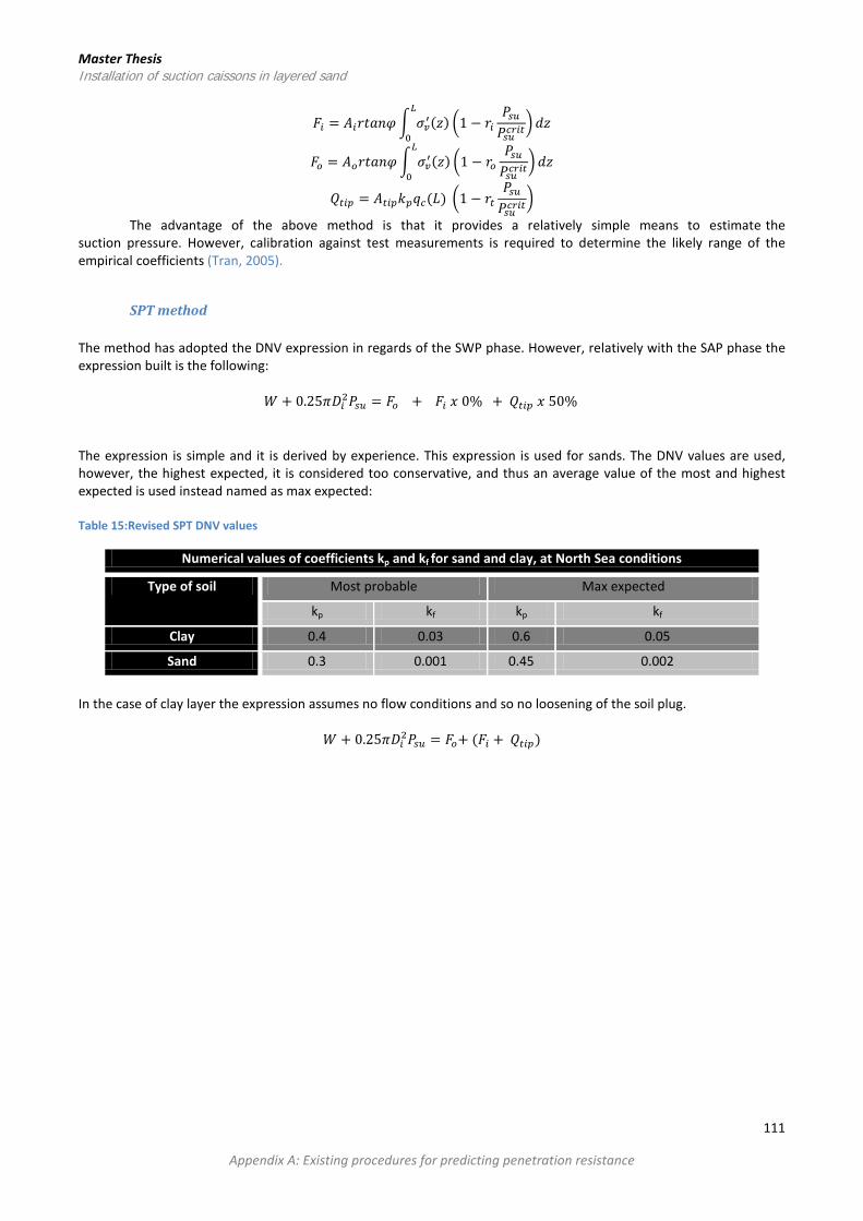
Master Thesis Installation of suction caissons in layered sand
𝐹𝑖 = 𝐴𝑖𝑟𝑡𝑎𝑛𝜑� 𝜎𝑣′(𝑧)𝐿
0�1 − 𝑟𝑖
𝑃𝑠𝑢𝑃𝑠𝑢𝑐𝑟𝑖𝑡
� 𝑑𝑧
𝐹𝑜 = 𝐴𝑜𝑟𝑡𝑎𝑛𝜑� 𝜎𝑣′(𝑧)𝐿
0�1 − 𝑟𝑜
𝑃𝑠𝑢𝑃𝑠𝑢𝑐𝑟𝑖𝑡
� 𝑑𝑧
𝑄𝑡𝑖𝑝 = 𝐴𝑡𝑖𝑝𝑘𝑝𝑞𝑐(𝐿) �1 − 𝑟𝑡𝑃𝑠𝑢𝑃𝑠𝑢𝑐𝑟𝑖𝑡
�
The advantage of the above method is that it provides a relatively simple means to estimate the suction pressure. However, calibration against test measurements is required to determine the likely range of the empirical coefficients (Tran, 2005).
SPT method The method has adopted the DNV expression in regards of the SWP phase. However, relatively with the SAP phase the expression built is the following:
𝑊 + 0.25𝜋𝐷𝑖2𝑃𝑠𝑢 = 𝐹𝑜 + 𝐹𝑖 𝑥 0% + 𝑄𝑡𝑖𝑝 𝑥 50% The expression is simple and it is derived by experience. This expression is used for sands. The DNV values are used, however, the highest expected, it is considered too conservative, and thus an average value of the most and highest expected is used instead named as max expected: Table 15:Revised SPT DNV values
Numerical values of coefficients kp and kf for sand and clay, at North Sea conditions
Type of soil Most probable Max expected
kp kf kp kf
Clay 0.4 0.03 0.6 0.05
Sand 0.3 0.001 0.45 0.002
In the case of clay layer the expression assumes no flow conditions and so no loosening of the soil plug.
𝑊 + 0.25𝜋𝐷𝑖2𝑃𝑠𝑢 = 𝐹𝑜+ (𝐹𝑖 + 𝑄𝑡𝑖𝑝)
111
Appendix A: Existing procedures for predicting penetration resistance

Master Thesis Installation of suction caissons in layered sand
Appendix B: Preliminary analysis
Case background data The analysis was based on the Q1 project. For full detailed description of the project information are available at Appendix C. The Beta methods parameters needed to be evaluated for predicting the encountered soil resistance were based on correlations as a function of the 𝑞𝑐 profile according to (Robertson, 2010) and suggestions made by (Houlsby, G. T., & Byrne, B. W., 2005) and (Andersen, K. H., Jostad, H. P., & Dyvik, R., 2008).
Figure 96: Friction angle, 𝝋ʹ, from CPT for unaged, uncemented, clean quartz to siliceous sand (Mayne, 2006)
For the purpose of the preliminary analysis a less detailed qc profile was used, averaged between the individual soil layers every 1m. For assessing the 𝜑ʹ𝑎𝑛𝑑 𝛿 from the CPT, (Kulhawy, F.H. and Mayne, P.W., 1990) suggested an alternate relationship for clean, rounded, uncemented quartz sands, and evaluated the relationship using high quality field data, see Figure 96. The results of this correlation are given at the Table 16, for the penetration depth needed at this case scenario.
Table 16: Soil properties specific to the offshore site considered for a preliminary analysis
𝑲𝑵/𝒎𝟑
𝑲𝑵/𝒎𝟑
𝑴𝑷𝒂 𝑴𝑷𝒂 𝑴𝑵 𝒅𝒆𝒈𝒓𝒆𝒆𝒔 𝒅𝒆𝒈𝒓𝒆𝒆𝒔
Penetration depth (m)
γ` γ σvo σ`vo qc φ` δ
0 0 0 0 0 0 0 0
0,5 10 20 0,01 0,005 4,9 43,34 28,89
1,5 10 20 0,03 0,015 20,8 47,62 31,75
2,5 10 20 0,05 0,025 21,6 46,58 31,05
3,5 10 20 0,07 0,035 21,2 45,68 30,45
4,5 10 20 0,09 0,045 21,8 45,21 30,14
5,5 10 20 0,11 0,055 8,6 40,25 26,83
6,5 10 20 0,13 0,065 19,8 43,86 29,24
7,5 10 20 0,15 0,075 24,5 44,54 29,69
8,5 10 20 0,17 0,085 21,6 43,63 29,09
9,5 10 20 0,19 0,095 22,6 43,58 29,05
112
Appendix B: Preliminary analysis

Master Thesis Installation of suction caissons in layered sand
Observations and conclusions from the predictions methods
• Anticipated σ’v evolvement during the installation (Beta approach) • The CPT approaches don’t require such an approach, as this enhancement is accounted to the qc while it
penetrates the soil profile.
CPT methods • CPT approaches give a range of values (enhanced safety)
0.000
0.020
0.040
0.060
0.080
0.100
0.120
0.140
0.160
0 2 4 6 8 10
σ' v (MPa)
Penetration Depth (m)
Comparison of σ'v at SWP and SAP ( based on H&B)
Enhanced effective stressinner SC side (SWP)
Enhanced effective stressouter SC side (SWP)
Decreased effective stressinner SC side (SAP)
Increased effective stressouter SC side (SAP)
0
1
2
3
4
5
6
7
8
9
0 5 10 15 20 25 30 35 40 45 50
Pene
trat
ion
Dept
h (m
)
Soil Resistance MN)
Comparison of Beta approaches and CPT approaches
DnV (most probable)
DnV (highest expected)
PrL 6MN
Senders&Randolph estimationwith constant KfFeld estimation (most probable)
Feld estimation (highestexpected)H&B Soil Re
NGI Soil Re
113
Appendix B: Preliminary analysis

Master Thesis Installation of suction caissons in layered sand
• S&R and Feld methods allow a narrower range of results to be expected, (optimistic design rather to the conservative range of results obtained with the DNV standard)
Beta approaches • Soil resistance estimation single line, no lower and upper bound introduced. • A narrow range of values (compared with CPT’s) having the NGI as the lower bound and the Bang method as
the upper bound for shallow jacking penetrations and then Bang method becomes the lower bound and H&B the upper bound
General conclusions • Similar SWP depth for both Beta-CPT methods • At shallow penetrations with small surcharge, prediction coincide more, but as jacking installation is
increased, wider range of potential SWP points are obtained • Increased jacking installation (increased surcharge) leads to wider expected range of results due to the
different estimation processes • S&R method uses DNV equation reduced with the proposed (1- 𝑃𝑠𝑢
𝑃𝑠𝑢𝑐𝑟𝑖𝑡) to account for the loosening effect of the
groundwater flow • S&R gives the mean value of the DNV range
0
2
4
6
8
10
12
14
16
0.00 0.10 0.20 0.30 0.40 0.50 0.60 0.70 0.80 0.90 1.00
Soil
Resi
stan
ce (M
N)
L/D
S&R and S&R (DNV values) soil resistance components
S&R Soil Re
S&R (DnV values)Soil Re (mostprobable)S&R (DnV values)Soil Re (highestexpected)S&R (DnV values)Qtip (highestexpected)S&R (DnV values)Fi (highestexpected)S&R (DnV values)Fo (highestexpected)
114
Appendix B: Preliminary analysis

Master Thesis Installation of suction caissons in layered sand
• Similar soil resistance components magnitude until L/D = 0.7 • Different trend of Fo beyond L/D = 0.7 towards L/D =1 • Both, raise their total SR from Fo after L/D=0.7
0
2
4
6
8
10
12
14
16
18
0.00 0.10 0.20 0.30 0.40 0.50 0.60 0.70 0.80 0.90 1.00
Soil
Resi
stan
ce (M
N)
L/D
Comparison of CPT and H&B method in respect to the SR components
S&R Soil Re
H&B Qtip
H&B Fo
H&B Fi
H&B Soil Re
S&R (DnV values)Soil Re (mostprobable)S&R (DnV values)Soil Re (highestexpected)S&R (DnV values)Qtip (highestexpected)
115
Appendix B: Preliminary analysis

Master Thesis Installation of suction caissons in layered sand
• High similarity on the SR components trend • Feld keeps a minimum level of Fi and Qtip as a residual • Feld’s method, a combination of H&B and S&R (published earlier than both)
0
5
10
15
20
25
0.00 0.10 0.20 0.30 0.40 0.50 0.60 0.70 0.80 0.90 1.00
Soil
Resi
stan
ce (M
N)
L/D
Comparison of Feld and H&B method in respect to the SR components H&B Qtip
H&B Fo
H&B Fi
H&B Soil Re
Feld Fi (mostprobable)
Feld Fo (mostprobable)
Feld Qtip(mostprobable)Feld Soil Re(mostprobable)Feld Fi(highestexpected)Feld Fo(highestexpected)
116
Appendix B: Preliminary analysis

Master Thesis Installation of suction caissons in layered sand
• Feld’s results are comparable with H&B method, but both Feld and H&B are seen to be outside the range of DNV standard estimations after the ratio L/D approaches 0.8.
0
5
10
15
20
25
0.00 0.10 0.20 0.30 0.40 0.50 0.60 0.70 0.80 0.90 1.00
Soil
Resi
stan
ce (M
N)
L/D
Comparison of selected Beta and CPT methods regarding SAP (PrL:6MN)
S&R Soil Re
H&B Qtip
H&B Fo
H&B Fi
H&B Soil Re
DnV Soil Re(mostprobable)DnV Soil Re(highestexpected)DnV Qtip(highestexpected)
0.00
0.50
1.00
1.50
2.00
2.50
3.00
3.50
0.00 0.10 0.20 0.30 0.40 0.50 0.60 0.70 0.80 0.90 1.00
P/γ'L
L/D
Normalized suction requirement prediction
S&R PrL:6MN DnV PrL:6MN (highest expected)DnV PrL:6MN (most probable) Feld PrL:6MN (most probabe)Feld PrL:6MN (highest expected) H&B PrL:6MN
117
Appendix B: Preliminary analysis

Master Thesis Installation of suction caissons in layered sand
• Similar suction behavior until L/D= 0.7 thereafter H&B and Feld methods show a different trend with higher suction
requirement as ratio approaches 1 • S&R method, generally seems to follow the DNV range of values having the mean value alongside with L/D ratio
• Based on the double surcharge option the difference observed between the methods is significantly lower, almost
matching the highest expected range of prediction given by DNV standard • All methods present a suction trend similar to the trend introduced by (Tran, 2005)
• S&R succeed to predict only suction requirement for shallow penetration until L/D <0.5
0.00
0.50
1.00
1.50
2.00
2.50
0.00 0.10 0.20 0.30 0.40 0.50 0.60 0.70 0.80 0.90 1.00
P/γ’
L
L/D
Normalized suction requirement prediction S&R PrL:12MN
DnV PrL:12MN(most probable)
DnV PrL:12MN(highestexpected)Feld PrL:12MN(most probabe)
Feld PrL:12MN(highestexpected)H&B PrL:12MN
0
50
100
150
200
250
0.00 0.10 0.20 0.30 0.40 0.50 0.60 0.70 0.80 0.90 1.00
Suct
ion
Requ
irem
ent (
Kpa)
L/D
Comparison of actual suction required with S&R Pile A1actualsuction req
S&R suctionreq
DnV (byS&R)suction req(mostprobable)
118
Appendix B: Preliminary analysis

Master Thesis Installation of suction caissons in layered sand
• H&B captures final installation requirement after L/D>0.85 • NGI: agreement at L/D<0.4 and 0.75<L/D<0.85
• Agreemenent of actual data with H&B only within 0.85<L/D<1 and Feld within 0.7<L/D<1 and L/D<0.45
0
50
100
150
200
250
300
350
400
0.00 0.10 0.20 0.30 0.40 0.50 0.60 0.70 0.80 0.90 1.00
Suct
ion
Requ
irem
ent (
KPa)
L/D
Comparison of actual suction requirement with Beta approaches Pile A1
actualsuctionreqBangsuctionreq
NGIsuctionreq
H&Bsuctionreq
0
50
100
150
200
250
300
350
0.00 0.10 0.20 0.30 0.40 0.50 0.60 0.70 0.80 0.90 1.00
Suct
ion
requ
irem
ent (
KPa)
L/D
Comparison of actual suction requirement with Feld and H&B method Pile A1 actual
suction req
H&B suctionreq
Feld (20%residual fi andQtip) (mostprobable)
Feld (20%residual fi andQtip) (highestexpected)
119
Appendix B: Preliminary analysis

Master Thesis Installation of suction caissons in layered sand
0
50
100
150
200
250
300
0.00 0.10 0.20 0.30 0.40 0.50 0.60 0.70 0.80 0.90 1.00
Suction requirement (KPa)
L/D
Comparison of actual suction requirement with predictions Pile A1 actual suction req
S&R suction req
DnV (by S&R) suction req (mostprobable)
DnV (by S&R) suction req(highest expected)
H&B suction req
Bang suction req
NGI suction req
Feld (20% residual fi and Qtip)(most probable)
Feld (20% residual fi and Qtip)(highest expected)
Feld (total loosening assumed)(most probable)
Feld (total loosening assumed)(highest expected)
Within the expected range
120
Appendix B: Preliminary analysis

Master Thesis Installation of suction caissons in layered sand
• No agreement obtained within the the 0.5<L/D<0.75 penetration depth (might be due to the spatial variability of the qc and the SC size difference • SWP and SAP prediction quite accurately predicted by Feld’s and DNV range of values
121
Appendix B: Preliminary analysis

Master Thesis Installation of suction caissons in layered sand
• Best fit acquired with Feld (assumed residual 10% of Fi and Qtip) Main conclusions CPT approaches can predict actual data at a bigger L/D range CPT approaches can be modified easier to fit actual data Beta approaches were used after correlations of φ’ with qc and conclusions are biased Range of predictions is better from single lines estimations in terms of safety and feasibility of installation CPT qc profile proved to be insufficient to capture actual soil conditions A more detailed qc profile should be used further to the analysis Selection of qc data points should be done after great care and critical thought
0
50
100
150
200
250
300
0.00 0.10 0.20 0.30 0.40 0.50 0.60 0.70 0.80 0.90 1.00
Suction requirement (KPa)
L/D
Pile A1actualsuctionreqH&Bsuctionreq
Feld(10%)most
feld(10%)highest
122
Appendix B: Preliminary analysis
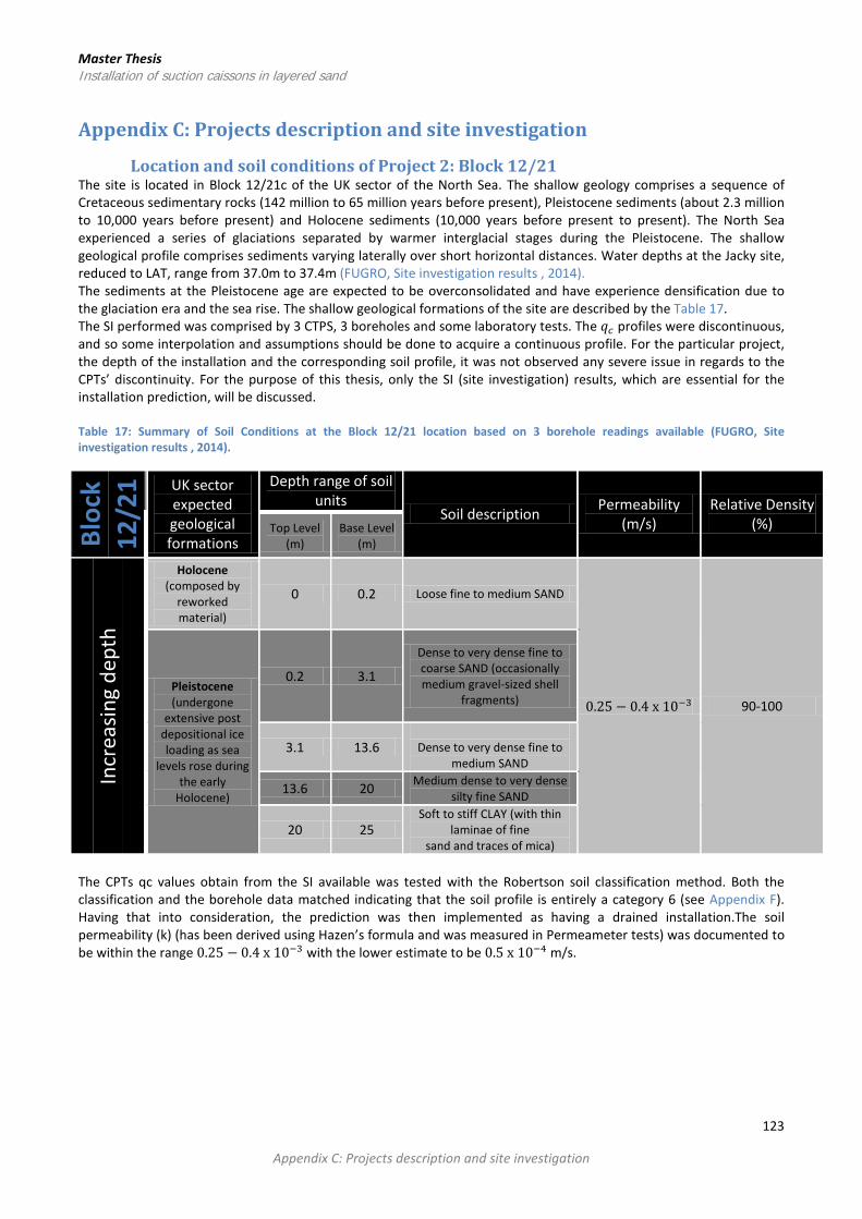
Master Thesis Installation of suction caissons in layered sand
Appendix C: Projects description and site investigation
Location and soil conditions of Project 2: Block 12/21 The site is located in Block 12/21c of the UK sector of the North Sea. The shallow geology comprises a sequence of Cretaceous sedimentary rocks (142 million to 65 million years before present), Pleistocene sediments (about 2.3 million to 10,000 years before present) and Holocene sediments (10,000 years before present to present). The North Sea experienced a series of glaciations separated by warmer interglacial stages during the Pleistocene. The shallow geological profile comprises sediments varying laterally over short horizontal distances. Water depths at the Jacky site, reduced to LAT, range from 37.0m to 37.4m (FUGRO, Site investigation results , 2014). The sediments at the Pleistocene age are expected to be overconsolidated and have experience densification due to the glaciation era and the sea rise. The shallow geological formations of the site are described by the Table 17. The SI performed was comprised by 3 CTPS, 3 boreholes and some laboratory tests. The 𝑞𝑐 profiles were discontinuous, and so some interpolation and assumptions should be done to acquire a continuous profile. For the particular project, the depth of the installation and the corresponding soil profile, it was not observed any severe issue in regards to the CPTs’ discontinuity. For the purpose of this thesis, only the SI (site investigation) results, which are essential for the installation prediction, will be discussed. Table 17: Summary of Soil Conditions at the Block 12/21 location based on 3 borehole readings available (FUGRO, Site investigation results , 2014).
Bloc
k 12
/21 UK sector
expected geological formations
Depth range of soil units
Soil description Permeability (m/s)
Relative Density (%) Top Level
(m) Base Level
(m)
Incr
easin
g de
pth
Holocene (composed by
reworked material)
0 0.2 Loose fine to medium SAND
0.25 − 0.4 x 10⁻³ 90-100 Pleistocene (undergone
extensive post depositional ice loading as sea
levels rose during the early
Holocene)
0.2 3.1
Dense to very dense fine to coarse SAND (occasionally medium gravel-sized shell
fragments)
3.1 13.6
Dense to very dense fine to medium SAND
13.6 20 Medium dense to very dense silty fine SAND
20 25 Soft to stiff CLAY (with thin
laminae of fine sand and traces of mica)
The CPTs qc values obtain from the SI available was tested with the Robertson soil classification method. Both the classification and the borehole data matched indicating that the soil profile is entirely a category 6 (see Appendix F). Having that into consideration, the prediction was then implemented as having a drained installation.The soil permeability (k) (has been derived using Hazen’s formula and was measured in Permeameter tests) was documented to be within the range 0.25 − 0.4 x 10⁻³ with the lower estimate to be 0.5 x 10⁻⁴ m/s.
123
Appendix C: Projects description and site investigation

Master Thesis Installation of suction caissons in layered sand
Figure 97: CPTs qc profile for Block 12/21 site
0
1
2
3
4
5
6
7
8
0 5 10 15 20 25 30 35 40 45 50
Dept
h be
low
seaf
lloor
(m)
Cone resistance, qc (MPa)
Block 12/21 site investigation: CPTs
qc aveqc 1qc 2qc 3
124
Appendix C: Projects description and site investigation

Master Thesis Installation of suction caissons in layered sand
Figure 98: Block 12/21 Platform plan area (triangle) and suction caisson location and respective site investigation
Installation reported events Table 18: Installation reported events
Time Activities
10:15-10:30 (1) SWP (A1-N = 0.5m; A2 = 0.7m; B2 = 0.5m)
10:30-11:00 (2) Closing vent valves; ROV confirmation
11.00 – 11.25 (2) SAP phase initiation: Electromotors 2 started on all 3 suction cans
11:25 – 11:45 (2) Power problem occurred; power supply exchanged, resulting in power problem solved
12:08 (3) Earth fault on electromotor 1 of skid 3; no flow on electromotor 2 of skid 3, reported to CLIENT
12:08 – 15:50 (3) Await instructions
15.50 – 22.10 (4) Suction penetration to 7.0m embedment on all three buckets
Figure 99: Indication of incidents taken place during installation
In this case, no substantial change to the operation was invoked due to project reasons. Thus, fluctuations from the predictions could not be attributed to the operational influence; as a result predictions were expected to be unbiased and high accuracy to be obtained.
125
Appendix C: Projects description and site investigation

Master Thesis Installation of suction caissons in layered sand
Location and soil conditions of Project 1:Q1 This project was situated in the North Sea within the Dutch sector. In this case the site was composed from homogeneous dense calcareous sand with intermediate weaker sand layers. The CPT tests performed indicate that a relatively similar soil material was encountered. In total 4 CTPS, a borehole and some laboratory tests were available. The soil permeability (k) has been derived using Hazen’s formula and was measured in Permeameter tests. Table 19: Soil profile description of Q1
Figure 100: Q1 Platform plan area (rectangular area) and suction caisson location and respective site investigation
Q1
Depth range of soil units
Soil description Permeability (m/s)
Relative Density
(%) Top Level (m)
Base Level (m)
Incr
easi
ng d
epth
0.00 2.50 Very dark calcareous silica fine SAND, with shells and shell fragments
5 − 8 x 10⁻⁴
90-100 ( Very dense)
2.50 3.40 Very dark calcareous silica fine SAND, with shells and shell fragments, with traces of organic matter
3.40 4.85 Very dark calcareous silica fine SAND, with shells and shell fragments
50-60 (medium
dense) 4.85 6.80 Very dark calcareous silica fine SAND, with many shells and shell fragments 1 − 5 x 10⁻⁵
6.80 11.50 Dark grey calcareous silica fine SAND 1 − 5 x 10⁻⁴ 80-90
(dense to very dense)
126
Appendix C: Projects description and site investigation
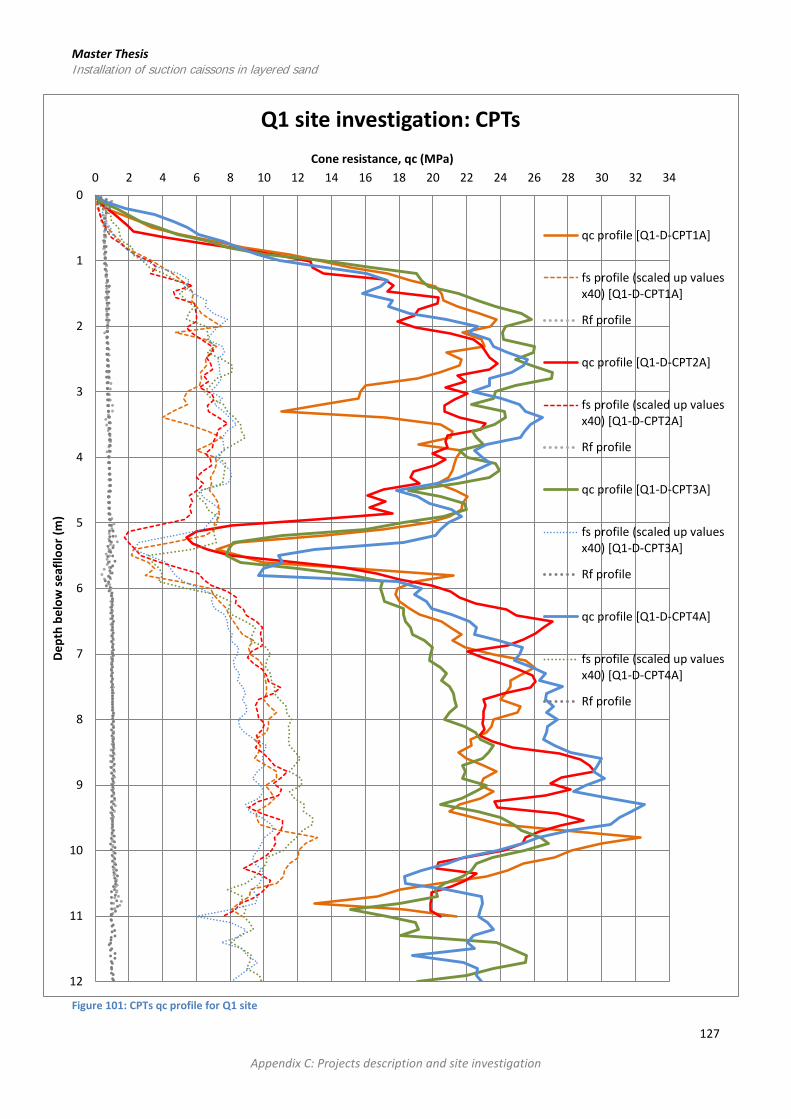
Master Thesis Installation of suction caissons in layered sand
Figure 101: CPTs qc profile for Q1 site
0
1
2
3
4
5
6
7
8
9
10
11
12
0 2 4 6 8 10 12 14 16 18 20 22 24 26 28 30 32 34
Dept
h be
low
seaf
lloor
(m)
Cone resistance, qc (MPa)
Q1 site investigation: CPTs
qc profile [Q1-D-CPT1A]
fs profile (scaled up valuesx40) [Q1-D-CPT1A]
Rf profile
qc profile [Q1-D-CPT2A]
fs profile (scaled up valuesx40) [Q1-D-CPT2A]
Rf profile
qc profile [Q1-D-CPT3A]
fs profile (scaled up valuesx40) [Q1-D-CPT3A]
Rf profile
qc profile [Q1-D-CPT4A]
fs profile (scaled up valuesx40) [Q1-D-CPT4A]
Rf profile
127
Appendix C: Projects description and site investigation

Master Thesis Installation of suction caissons in layered sand
Installation reported events
1. After initial set-down the self-weight penetration was interrupted as the platforms position was found to be incorrect.
2. The operation is paused until the next low current window for repositioning the platform.
3. The platform was repositioned by retrieving 3 suction piles and rotating the platform on the 4th leg.
4. Due to the limited venting capacity the pump system measured an overpressure as the pile penetrated the soil.
5. Due to currents at the installation site the reference sensor could not be used continuously during the installation of the piles.
6. As leg A1 was found to penetrate slower, the 2nd suction pump on the skid was used to speed-up the installation of this caisson, at penetration depths between 5.0 and 7.5 m.
7. The installation stopped before full skirt penetration since peak differential pressures on the suction piles approached the pressure limits of the suction pile buckling strength (250 KPa at 8m and 270 KPa at 9m)
8. Since the platform’s 3rd leg didn’t have measurement of its penetration depth so only 3 caissons were analysis and compared with actual installation data. No comparison could be made for this leg.
Figure 102: Suction caissons installation data and time frame indication of important installation events
128
Appendix C: Projects description and site investigation

Master Thesis Installation of suction caissons in layered sand
Location and soil conditions of Project:P6 The site is located in Block P6 of the Dutch sector of the North Sea. Water depth at the P6 site, reduced to LAT, is about 31.1m (FUGRO, 1996). The shallow geological formations of the site are described by the Table 20. The SI performed was comprised by 2 CPTS, 2 boreholes and some laboratory tests. The 𝑞𝑐 profiles were discontinuous, and so some interpolation and assumptions should be done to acquire a continuous profile. The CPTs reading discontinuity, was detrimental in regard to the precision of the predictions, as the stops made, were at the location of the different soil layers, and as a result the 𝑞𝑐 and 𝑓𝑠 (sleeve friction) used, are certainly prejudiced (Bolton, M.D., Garnier, M.W., Corte, J., Bagge, J.F., Laue, G. and Renzi, R., 1999). No permeability or relative density correlations or indications were available at this case. Table 20: Summary of Soil Conditions at the Block P6 location (FUGRO, 1996)
Bloc
k P6
Depth range of soil units
Soil description Top Level (m) Base Level (m)
Incr
easin
g de
pth
0 1.6 Dense, silty FINE to MEDIUM SAND with shell fragments and locally with gravel and some organic inclusions
1.6 2.4 Firm to very stiff CLAY
2.4 14.5 Dense to very dense, silty, FINE to MEDIUM SAND, with shell fragments, locally silt inclusions, at bottom clay and
silt layers
14.5 21.5 Stiff to hard CLAY, with sand and silt layers
The CPTs 𝑞𝑐 values obtain from the SI available was tested with the Robertson soil classification method. The Robertson classification indicated that the soil layer is certainly of cohesive content, however it was not characterised as clay but as a silty mixture (see Appendix F), in other words as category 4 (see Figure 66). Having that into consideration, the prediction was then implemented as having a drained installation where sand layers are encountered ad undrained were cohesive layers are indicated.
Figure 103: P6 Platform plan area (rectangular area) and suction caisson location and respective site investigation
129
Appendix C: Projects description and site investigation

Master Thesis Installation of suction caissons in layered sand
Figure 104: CPTs qc profile for P6 site
0.00
1.00
2.00
3.00
4.00
5.00
6.00
7.00
8.00
9.00
10.00
0.00 4.00 8.00 12.00 16.00 20.00 24.00 28.00 32.00
Dept
h be
low
seaf
lloor
(m)
Cone resistance, qc (MPa)
P6 site investigation: CPTs
qc1qc2qc avefs 1fs 2fs ave
130
Appendix C: Projects description and site investigation

Master Thesis Installation of suction caissons in layered sand
P6: Installation reported events The analysis of P6 project was based on the reports available from 1996. No monitoring or logging data were available, and the analysis is based on limited data points describing the general installation behavior, as it was extracted by the author, in terms that allowed comparison to be made with predictions. As a result, the precision both of the actual results and the predictions is limited, however, it is deemed reliable and sufficient for the purpose of this thesis. Table 21: Reported events in P6 project
Time Activities
Installation Initiation Installation monitoring was started
3h-4h after initiation
(1) Normal installation process interrupted, as upper structure was allowed to be flooded, as a result the weight over caissons was increased leading to further penetration without suction
application
6h-13h after initiation
(2) Installation was stopped, as it was night
13h-13.5h (3) Installation was stopped and then restarted to allow design penetration to be reached
14.5h after initiation Logging was stopped
Due to uncertainties to water depth monitoring data, heave of the inner soil plug could not be monitored. In this case, a substantial change to the operation was provoked changing the normal installation process. The additional weight due to the ballasting allowed (see Figure 105 (1)), was not documented, and therefore no accurate predictions could be made, however, this was considered during predictions with allowing additional weight at the particular depth to be integrated at the calculations. The predictions were based mainly to the qc profiles of the 2 CPTs, using its CPT for the corresponding SC installation prediction, as the location of both matches. In this case, the numerical average of the CPTs was also used to see its contribution to the prediction precision, as the other two caissons did not have a direct CPT test at their location.
Figure 105: Indication of incidents taken place during installation for P6 project (SPT, 1997)
(1) (2) (3)
131
Appendix C: Projects description and site investigation

Master Thesis Installation of suction caissons in layered sand
Location and soil conditions of Project:Q13 The Block Q13 of the Dutch sector of the North Sea in water of 19.8 m depth with respect to the LAT, was the precise location of this project. The local soil comprises of dense to very dense sand. Seabed conditions are assumed to be generally flat. The soil up to 25 m below the seabed is a dense to very dense dark grey silica medium sand layer. Dense to very dense sand with a relative density of locally 60% to 100% is found. On average the sand is densely packed, i.e. Id= 80% approximately. Because of a change on the location, the site investigation conducted was having a distance of some hundreds of meters from the actual location of the installed caissons. This should be kept in mind, as obviously, some deviation there will be from the encountered soil conditions. The Table 22 presented here, contains the result of only the description of one of the two boreholes, as the other one (considering the same depth), was comprised of only grey dark silica medium SAND.
Table 22: Summary of Soil Conditions at the Block Q13 location (FUGRO, 1996)
The CPTs 𝑞𝑐 values obtain from the SI available was tested with the Robertson soil classification method. The Robertson classification indicated that the soil layers are of sand content (see Appendix F). Having that into consideration, the prediction was then implemented as having a drained installation.
Q13: Installation reported events The analysis of Q13 project was based on interviews with the installation personnel, as no detailed explanation of what happened during the installation have been found. It should be mentioned that some leveling of the platform have been performed during the installation which is generally obvious from the monitored suction. In addition, the encountered soil profile was actually quite different in respect to the platform side, which again could be observed at the installation suction pressure graph, as at pairs the anchors were monitored to show the same requirement, converging towards the end. The installation personnel, described that the anchors probably have been located over a quite different soil profile, which this effect was enhanced by the attempt to level the platform, which do to the tilting the platform was imposing some moment to the other side, constituting as an additional force for the caissons installation.
Q13
Depth range of soil units
Soil description Permeability (m/s)
Relative Density (%) Top Level
(m) Base Level
(m)
Incr
easi
ng d
epth
0.00 1.75
Very dark greylish brown silica medium SAND, with traces of organic
matter and with shells and shell fragments 4.5 · 10−4
80-90 (dense to very dense)
1.75 3.65 Dark grey silica medium SAND with many shells and shell fragments
3.65 5.65 Dark grey silica medium SAND with shell fragments
40-70 ( medium dense)
5.65 10.35 Grey silica medium SAND, with many shells and shell fragments 2.5 · 10−4 80-90
(dense to very dense)
132
Appendix C: Projects description and site investigation

Master Thesis Installation of suction caissons in layered sand
Figure 106: CPTs qc profile for Q13 site
0
1
2
3
4
5
6
7
8
0 5 10 15 20 25 30
Dept
h be
low
seaf
lloor
(m)
Cone resistance, qc (MPa)
Q13 site investigation: CPT
Q13 qc
fs
133
Appendix C: Projects description and site investigation

Master Thesis Installation of suction caissons in layered sand
Location and soil conditions of Project:L6-B The platform is located in the North Sea. The water depth at the project location is approximately 35 m LAT. The local soil comprises of silty sand, clayey sand and calcareous sand layers with varying density. The soil investigation includes 3 CPTs and 1 borehole log to a depth of approximately 20 m below sea bottom level.
Table 23: Summary of Soil Conditions at the Block L6-B location (FUGRO, 1996)
L6-B: Installation reported events Due to the weight distribution of the platform structure on the suction cans, the procedure for self-weight penetration incorporated a pre-defined platform inclination angle for which the vent-valve of the suction can on leg M was closed. Continuation of the self weight penetration resulted in a close to vertical starting position for the suction operation. The suction operation performed maintaining the platform inclination close to vertical by controlling the pump skid outflow on the suction pumps. Due to the platform weight distribution on the suction cans, the structure was expected to settle unevenly on the seabed. Analysis of the self-weight penetration indicated the penetration of the main can was to be stopped when the off vertical platform angle approaches the 0.6°. To stop the main can penetrating the soil, the vent valve on this suction can was closed to allow water pressure to resist the can penetrating the soil. During the installation a crane applied a net. 200 ton lift load on the structure to keep the rigging under tension. This load was maintained for the full suction operation. At a penetration of 2.17 m on the main suction can, the pressure difference changed from negative to positive suction pressure. This would have been the self-weight penetration on this can if it was not interrupted by closing the vent valve. The caissons were having a net load of 4.1 MN (main leg) and 2.6 MN (braced legs), leading to different suction requirements and SWP. The most important operational change was that an increased pumping rate (2x) was applied throughtout the installation, which conservatively means that a downward offset of 10% to monitored installation pressure should be considered based on the observations made by (Tran, 2005) (see 2.4.3. The effect of pumping rate).
Figure 107: L6-B Platform plan area (fading bluish area) and suction caisson location and respective site investigation
L6-B
Depth range of soil units Soil description Permeability
(m/s)
Relative Density
(%) Top Level (m)
Base Level (m)
Incr
easi
ng d
epth
0.00 2.00 Very dark grey slightly clayey fine to medium silica SAND, with shell and shell fragments 9 · 10−6
80-95 (dense to
very dense)
2.00 3.4 Grey fine to fine to medium SAND, at bottom extremely closely spaced thin laminae of silt 2.3 · 10−4
3.4 5.1 Dark grey calcareous silica fine to medium SAND, with traces of shell fragment 4.5 · 10−5
5.1 7.5 dark grey clayey silica fine to medium
SAND, with traces of shell fragments, with traces of mica crystals
2 · 10−4
40-60 (medium
dense) 7.5 10.0
Dark grey clayey silica fine to medium SAND, with few shell fragments, with traces of mica
crystals- occasionally many shell fragment
10.0 11.0 Dark grey clayey silica fine to medium SAND, with few shells and shell fragment 75-80
(dense)
134
Appendix C: Projects description and site investigation

Master Thesis Installation of suction caissons in layered sand
Figure 108: CPTs qc profile for L6-B site
0
1
2
3
4
5
6
7
8
9
10
0 2 4 6 8 10 12 14 16 18 20 22 24 26 28 30
Dept
h be
low
seaf
lloor
(m)
Cone resistance, qc (MPa) L6-B Site investigation: CPTs
fs3
qc3
fs2
qc2
fs1
qc1
fs ave
qc ave
135
Appendix C: Projects description and site investigation

Master Thesis Installation of suction caissons in layered sand
Effective Friction angle (φ’) correlation based on the cone resistance For each project the respective (φ’) was determined at final penetration depth, considering the effective stress at final penetration depth and the given cone resistance as proposed by (Chen, 1996) and (Robertson P. K., 1983). The only uncertainty related to the resulted values were the degree of the compressibility of the sand which was not really determined from the site investigation available, however, knowing the description of the soil material an estimation could be made. The following categorization was made for the projects described at Appendix C.
• Block 12/21: sand of low to medium compressibility • Q1: sand of medium to high compressibility • P6: sand of low to medium compressibility • Q13: sand of low to medium compressibility • L6-B: sand of medium to high compressibility
Figure 109: Correlation of friction angle based on effective stress and qc (coloured lines for sands with low compressibility and black with medium compressibility)
0
50
100
150
200
250
300
350
400
0.00 10.00 20.00 30.00 40.00 50.00
Vert
ical
effe
ctiv
e st
ress
[kPa
]
Cone Resistance [MPa]
38
40
42
44
46
48
50
52
136
Appendix C: Projects description and site investigation

Master Thesis Installation of suction caissons in layered sand
Figure 110: Correlation of friction angle based on effective stress and qc (coloured lines for sands with high compressibility and black with medium compressibility)
0
50
100
150
200
250
300
350
400
0.00 10.00 20.00 30.00 40.00 50.00
Vert
ical
effe
ctiv
e st
ress
[kPa
]
Cone Resistance [MPa]
38
40
42
44
46
48
50
137
Appendix C: Projects description and site investigation

Master Thesis Installation of suction caissons in layered sand
Appendix D: Comparison of actual installation pressures with predictions
Block 12/21
Figure 111: Comparison of installation pressure with the predicted suction pressure by S&R and DNV method (all scenarios)
Figure 112: Comparison of installation pressure with the predicted suction pressure by Feld method (1st-2nd scenario)
138
Appendix D: Comparison of actual installation pressures with predictions

Master Thesis Installation of suction caissons in layered sand
Q1
Figure 113: Comparison of installation pressure with the predicted suction pressure by S&R and DNV method (3rd scenario)
Figure 114: Comparison of installation pressure with the predicted suction pressure by Senders-Randolph method (all scenarios)
139
Appendix D: Comparison of actual installation pressures with predictions

Master Thesis Installation of suction caissons in layered sand
P6
Figure 115:Comparison of installation pressure with the predicted suction pressure by Senders-Randolph method (all scenarios)
Figure 116: Comparison of installation pressure with the predicted pressure by Feld method having additional ballast and without
140
Appendix D: Comparison of actual installation pressures with predictions

Master Thesis Installation of suction caissons in layered sand Figure 117: Comparison of installation pressure with the predicted suction pressure by Feld (having additional ballast) and SPT method
Figure 118: Comparison of installation pressure with the predicted suction pressure by Feld (without having additional ballast) and S&R method
Q13
Figure 119: Comparison of installation pressure with the predicted suction pressure by S&R method (1st-2nd scenarios)
141
Appendix D: Comparison of actual installation pressures with predictions

Master Thesis Installation of suction caissons in layered sand
Figure 120: Comparison of installation pressure with the predicted suction pressure by Feld method
Figure 121: Comparison of installation pressure with the predicted suction pressure by SPT method
L6-B
Figure 122: Comparison of installation pressure with the predicted suction pressure by S&R method
142
Appendix D: Comparison of actual installation pressures with predictions

Master Thesis Installation of suction caissons in layered sand
Figure 123: Comparison of installation pressure with the predicted suction pressure by DNV method
Figure 124: Comparison of installation pressure with the predicted suction pressure by SPT method
143
Appendix D: Comparison of actual installation pressures with predictions

Master Thesis Installation of suction caissons in layered sand
Appendix E: Back-analyses results
DNV values back-analysis expressions This analysis was based on two only prediction methods the SPT and the S&R method, as these are the only
containing both parameters for the SAP phase in sand. Based on the expressions determining the equilibrium between suction pressure and soil resistance as stated in paragraph, the back analysis of the 𝐾𝑓 and 𝐾𝑝 profiles, alongside the installation, were determined. The resulted expressions are the following: Based on the SPT method
𝐾𝑓 = �4𝑃𝑟𝑒𝐿𝑜𝑎𝑑 + 𝜋𝐷𝑖2𝑃𝑠𝑢
2𝜋𝐷𝑖𝑡 − 𝑞𝑐𝐾𝑝�
2∫ 𝑞𝑐𝐿
0
𝑡� , 𝑖𝑓 𝐾𝑝 𝑖𝑠 𝑎𝑠𝑠𝑢𝑚𝑒𝑑 𝑟𝑒𝑙𝑖𝑎𝑏𝑙𝑒
𝐾𝑝 = �4𝑃𝑟𝑒𝐿𝑜𝑎𝑑 + 𝜋𝐷𝑖2𝑃𝑠𝑢
2𝜋𝐷𝑖𝑡 −
2∫ 𝑞𝑐𝐿
0
𝑡𝐾𝑓� 𝑞𝑐� , 𝑖𝑓 𝐾𝑓 𝑖𝑠 𝑎𝑠𝑠𝑢𝑚𝑒𝑑 𝑟𝑒𝑙𝑖𝑎𝑏𝑙𝑒
Based on the S&R method
𝐾𝑓 = �𝑃𝑟𝑒𝐿𝑜𝑎𝑑
𝜋+𝐷𝑖2𝑃𝑠𝑢
4 − 𝐷𝑖𝑡𝑞𝑐 �1 −
𝑃𝑠𝑢𝑃𝑐𝑟𝑖𝑡𝑆𝑒𝑛𝑑𝑒𝑟𝑠�𝐾𝑝� � 𝑞𝑐
𝐿
0 𝑥 𝐷𝑖(2 −
2𝑡𝐷𝑖
� −𝑃𝑠𝑢
𝑃𝑐𝑟𝑖𝑡𝑆𝑒𝑛𝑑𝑒𝑟𝑠)
, 𝑖𝑓 𝐾𝑝 𝑖𝑠 𝑎𝑠𝑠𝑢𝑚𝑒𝑑 𝑟𝑒𝑙𝑖𝑎𝑏𝑙𝑒
𝐾𝑝 = �𝑃𝑟𝑒𝐿𝑜𝑎𝑑
𝜋+𝐷𝑖2𝑃𝑠𝑢
4 −� 𝑞𝑐
𝐿
0 𝑥 𝐷𝑖 �2 −
2𝑡𝐷𝑖−
𝑃𝑠𝑢𝑃𝑐𝑟𝑖𝑡𝑆𝑒𝑛𝑑𝑒𝑟𝑠� 𝑥 𝐾𝑓� � 𝐷𝑖𝑡𝑞𝑐 �1 −
𝑃𝑠𝑢𝑃𝑐𝑟𝑖𝑡𝑆𝑒𝑛𝑑𝑒𝑟𝑠�
, 𝑖𝑓 𝐾𝑓 𝑖𝑠 𝑎𝑠𝑠𝑢𝑚𝑒𝑑 𝑟𝑒𝑙𝑖𝑎𝑏𝑙𝑒
Based on the DNV method to determine soil resistance for an open-ended pile in sand and clay, the expressions will be the following:
𝐾𝑓 = ��2 𝑥 𝑃𝑟𝑒𝐿𝑜𝑎𝑑2𝜋 𝑥 𝐷𝑖 𝑥 𝑡
� − 𝑞𝑐2
𝑥 𝐾𝑝� � � 𝑞𝑐𝐿
0 𝑥 (
1𝐷𝑖
+ 1𝑡
)�� , 𝑖𝑓 𝐾𝑝 𝑖𝑠 𝑎𝑠𝑠𝑢𝑚𝑒𝑑 𝑟𝑒𝑙𝑖𝑎𝑏𝑙𝑒
𝐾𝑝 = ��2 𝑥 𝑃𝑟𝑒𝐿𝑜𝑎𝑑2𝜋 𝑥 𝐷𝑖 𝑥 𝑡
� − � 𝑞𝑐𝐿
0 𝑥 �
1𝐷𝑖
+ 1𝑡� 𝑥 𝐾𝑓 � �
𝑞𝑐2
�� , 𝑖𝑓 𝐾𝑓 𝑖𝑠 𝑎𝑠𝑠𝑢𝑚𝑒𝑑 𝑟𝑒𝑙𝑖𝑎𝑏𝑙𝑒
However, these expressions should be used in order to provide a direct link of the qc values with respect to the friction and tip resistance, at SWP, as DNV has only a SWP phase, where no loosening of the inner soil plug occurs. In order to be done correctly, the exact weight used (comprising all the elements of the structure) should be known, in order to determine the corresponding 𝐾𝑓and 𝐾𝑝 at the SWP point, where no further penetration solely by the weight can be attained. Then the expression will not contain any uncertainty and a direct calculation of those parameters could be acquired and then the same should be used at the SAP phase. When these expressions are statistically determined for particular soil profiles, a better understanding of the loosening rate and its magnitude could be developed, as the back-analysis for these certain profiles will be the only unknown.
144
Appendix E: Back-analyses results

Master Thesis Installation of suction caissons in layered sand
DNV values profile Graphs
Figure 125: S&R 𝒌𝒇 (most) profile (1st scenario) and (2nd scenario)
Figure 126: S&R 𝒌𝒇 (most) profile (1st scenario)
145
Appendix E: Back-analyses results

Master Thesis Installation of suction caissons in layered sand Figure 127: S&R 𝒌𝒇 (high) profile (1st scenario)
Figure 128: S&R 𝒌𝒑 (most) profile (1st scenario)
Figure 129: S&R 𝒌𝒑 (high) profile (1st scenario)
Figure 130: S&R 𝒌𝒑 (most) profile (1st scenario) and (2nd scenario)
146
Appendix E: Back-analyses results

Master Thesis Installation of suction caissons in layered sand
Effective stress comparison with installation pressure
Figure 131: Development of the hydraulic gradient across the installation depth’s effective stress
Soil resistance back-analysis
Figure 132: Q13 initial and reduced total soil resistance
Figure 133: P6 initial and reduced total soil resistance
147
Appendix E: Back-analyses results

Master Thesis Installation of suction caissons in layered sand
Figure 134: Block 12/21 initial and reduced Total soil resistance
Figure 135: L6-B initial and reduced Total soil resistance
Figure 136: Q1 initial and reduced Total soil resistance
148
Appendix E: Back-analyses results

Master Thesis Installation of suction caissons in layered sand
Appendix F: Matlab code
Robertson Index calculation % In this part of the Matlab code prepared for this thesis, the CPT test % related obtained values are used to calculated the Robertson index, which % was used to further assess the associated behaviour of the soil in the % corresponding depth of the installation as it will be if solely this % method was used to determined whether drained/undrained behaviour is % expected. % An automation of the process was implemented. % All the variables in this part, are taken from the Robertson's Flow chart % to evaluate cyclic resistance ratio (CRR7.5) and Ic index from CPT tests. % See paragraph 3.3. Soil Profile classification, Robertson Index % The data points used from the CPT tests given, the number of the CPTs % available is determined intervals=1:81; in=81; CPTs=4; % Soil specific parameters gammaeff=11; gamma=21; % Robertson's method parameters n=ones(in,4); Dn=ones(in,4); % Determination of the total and effective stress for the specific soil % profile encountered at the project for CPT=1:4; tsvo(intervals,CPT)=(intervals/10)*gamma; svo(intervals,CPT)=(intervals/10)*gammaeff; end % Robertson's method parameters Icindex=ones(in,CPTs); Cn=ones(in,CPTs); Qtn=ones(in,CPTs); Ic=ones(in,CPTs); %atmospheric pressure 100 KPa Pa=100; CPT=1:CPTs; % Robertson's method parameters determination for the first soil profile % interval iteration Cn1=ones(in,CPTs); Qtn1=ones(in,CPTs); Fr1=ones(in,CPTs); Ic1=ones(in,CPTs); n1=ones(in,CPTs); n=ones(in,CPTs); Dn=ones(in,CPTs); for CPT=1:CPTs
149
Appendix F: Matlab code

Master Thesis Installation of suction caissons in layered sand for i=1:in Cn1(i,CPT)=(Pa./svo(i,CPT)); Qtn1(i,CPT)=((Amqc(i,CPT)-svo(i,CPT))./Pa).*Cn1(i,CPT); Fr1(i,CPT)=100.*Amfs(i,CPT)./(Amqc(i,CPT)-tsvo(i,CPT)); Ic1(i,CPT)=((3.47-log10(Qtn1(i,CPT))).^2 +(1.22 + log10(Fr1(i,CPT))).^2).^0.5; n1(i,CPT)=real(0.38.*Ic1(i,CPT)+0.05.*(svo(i,CPT)./Pa)-0.15); end end % Robertson's method parameters determination for the rest soil profile % intervals iteration for CPT=1:CPTs for i=1:in while Dn(i,CPT)>0.01 Cn(i,CPT)=(Pa./svo(i,CPT)).^n1(i,CPT); Qtn(i,CPT)=((Amqc(i,CPT)-tsvo(i,CPT))./Pa).*Cn(i,CPT); Ic(i,CPT)=real(((3.47-log10(Qtn(i,CPT))).^2 +(1.22 + log10(Fr1(i,CPT))).^2).^0.5); n(i,CPT)=real(0.38.*Ic(i,CPT)+0.05.*(svo(i,CPT)./Pa)-0.15); Dn(i,CPT)=abs(n(i,CPT)- n1(i,CPT)); n1(i,CPT)=n(i,CPT); Icindex(i,CPT)=Ic(i,CPT); end end end plot(Icindex,intervals) % Soil Profile classification with the use of Robertson method based on % CPTs parameters and an approximation of the Graph in order to be used by % Matlab % The graph of Robertson method is discretized in 1-9 categories. Here % all categories designed. Furthermore, the category 0 was introduced for % cases where the designing was not entirely correct, so the engineer could % spot which interval was not classified and then manually it could be done SoilB=ones(in,CPTs); for CPT=1:CPTs; for i=1:in if Qtn(i,CPT)>60 && 4<Fr1(i,CPT) SoilB(i,CPT)=9; elseif 200<Qtn(i,CPT) && 2<Fr1(i,CPT) && Fr1(i,CPT)<4 SoilB(i,CPT)=8; elseif Qtn(i,CPT)>200 && 0.1<Fr1(i,CPT) && Fr1(i,CPT)<0.6 && Icindex(i,CPT)<1.31 SoilB(i,CPT)=7; elseif 40<Qtn(i,CPT) && Qtn(i,CPT)<200 && 0.1<Fr1(i,CPT) && Fr1(i,CPT)<0.6 && 1.31<Icindex(i,CPT) && Icindex(i,CPT)<2.05
150
Appendix F: Matlab code

Master Thesis Installation of suction caissons in layered sand SoilB(i,CPT)=6; elseif 100<Qtn(i,CPT) && 0.6<Fr1(i,CPT) && Fr1(i,CPT)<2 && 1.31<Icindex(i,CPT) && Icindex(i,CPT)<2.05 SoilB(i,CPT)=6; elseif 7<Qtn(i,CPT) && Qtn(i,CPT)<40 && 0.1<Fr1(i,CPT) && Fr1(i,CPT)<0.6 && 2.05<Icindex(i,CPT) && Icindex(i,CPT)<2.6 SoilB(i,CPT)=5; elseif 20<Qtn(i,CPT) && Qtn(i,CPT)<100 && 0.6<Fr1(i,CPT) && Fr1(i,CPT)<2 && 2.05<Icindex(i,CPT) && Icindex(i,CPT)<2.6 SoilB(i,CPT)=5; elseif 30<Qtn(i,CPT) && Qtn(i,CPT)<200 && 2<Fr1(i,CPT) && Fr1(i,CPT)<4 && 2.05<Icindex(i,CPT) && Icindex(i,CPT)<2.6 SoilB(i,CPT)=5; elseif 2<Qtn(i,CPT) && Qtn(i,CPT)<7 && 0.1<Fr1(i,CPT) && Fr1(i,CPT)<0.2 && 2.6<Icindex(i,CPT) && Icindex(i,CPT)<2.95 SoilB(i,CPT)=4.5; elseif 3<Qtn(i,CPT) && Qtn(i,CPT)<7 && 0.2<Fr1(i,CPT) && Fr1(i,CPT)<0.6 && 2.6<Icindex(i,CPT) && Icindex(i,CPT)<2.95 SoilB(i,CPT)=4.5; elseif 5<Qtn(i,CPT) && Qtn(i,CPT)<20 && 0.6<Fr1(i,CPT) && Fr1(i,CPT)<1.49 && 2.6<Icindex(i,CPT) && Icindex(i,CPT)<2.95 SoilB(i,CPT)=4; elseif 10<Qtn(i,CPT) && Qtn(i,CPT)<20 && 1.49<Fr1(i,CPT) && Fr1(i,CPT)<4 && 2.6<Icindex(i,CPT) && Icindex(i,CPT)<2.95 SoilB(i,CPT)=4; elseif 20<Qtn(i,CPT) && Qtn(i,CPT)<30 && 2<Fr1(i,CPT) && Fr1(i,CPT)<4 && 2.6<Icindex(i,CPT) && Icindex(i,CPT)<2.95 SoilB(i,CPT)=4; elseif 20<Qtn(i,CPT) && Qtn(i,CPT)<60 && 4<Fr1(i,CPT) && 2.6<Icindex(i,CPT) && Icindex(i,CPT)<2.95 SoilB(i,CPT)=4; elseif 1<Qtn(i,CPT) && Qtn(i,CPT)<2 && 0.1<Fr1(i,CPT) && Fr1(i,CPT)<2 && 2.95<Icindex(i,CPT) && Icindex(i,CPT)<3.6 SoilB(i,CPT)=3.5; elseif 2<Qtn(i,CPT) && Qtn(i,CPT)<3 && 0.2<Fr1(i,CPT) && Fr1(i,CPT)<1.49 && 2.95<Icindex(i,CPT) && Icindex(i,CPT)<3.6 SoilB(i,CPT)=3.5; elseif 2<Qtn(i,CPT) && Qtn(i,CPT)<3 && 1.49<Fr1(i,CPT) && Fr1(i,CPT)<5 && 2.95<Icindex(i,CPT) && Icindex(i,CPT)<3.6 SoilB(i,CPT)=3; elseif 3<Qtn(i,CPT) && Qtn(i,CPT)<5 && 0.6<Fr1(i,CPT) && Fr1(i,CPT)<1.49 && 2.95<Icindex(i,CPT) && Icindex(i,CPT)<3.6 SoilB(i,CPT)=3; elseif 3<Qtn(i,CPT) && Qtn(i,CPT)<10 && 1.49<Fr1(i,CPT) && Fr1(i,CPT)<4 && 2.95<Icindex(i,CPT) && Icindex(i,CPT)<3.6 SoilB(i,CPT)=3; elseif 3<Qtn(i,CPT) && Qtn(i,CPT)<20 && 4<Fr1(i,CPT) && 2.95<Icindex(i,CPT) && Icindex(i,CPT)<3.6 SoilB(i,CPT)=3; elseif 1<Qtn(i,CPT) && Qtn(i,CPT)<2 && 2<Fr1(i,CPT) && Fr1(i,CPT)<5 && Icindex(i,CPT)>3.6 SoilB(i,CPT)=2; elseif 1<Qtn(i,CPT) && Qtn(i,CPT)<3 && 5<Fr1(i,CPT) && Icindex(i,CPT)>3.6 SoilB(i,CPT)=2;
151
Appendix F: Matlab code
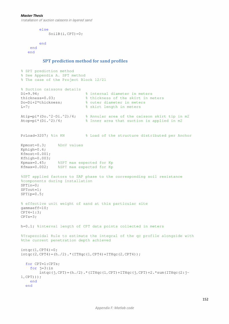
Master Thesis Installation of suction caissons in layered sand else SoilB(i,CPT)=0; end end end
SPT prediction method for sand profiles % SPT prediction method % See Appendix A. SPT method % The case of the Project Block 12/21 % Suction caissons details Di=9.94; % internal diameter in meters thickness=0.03; % thickness of the skirt in meters Do=Di+2*thickness; % outer diameter in meters L=7; % skirt length in meters Atip=pi*(Do.^2-Di.^2)/4; % Annular area of the caisson skirt tip in m2 Atop=pi*(Di.^2)/4; % Inner area that suction is applied in m2 PrLoad=3207; %in KN % Load of the structure distributed per Anchor Kpmost=0.3; %DnV values Kphigh=0.6; Kfmost=0.001; Kfhigh=0.003; Kpmax=0.45; %SPT max expected for Kp Kfmax=0.002; %SPT max expected for Kp %SPT applied factors to SAP phase to the corresponding soil resistance %components during installation SPTin=0; SPTout=1; SPTip=0.5; % effective unit weight of sand at this particular site gammaeff=10; CPT4=1:3; CPTs=3; h=0.1; %interval length of CPT data points collected in meters %Trapezoidal Rule to estimate the integral of the qc profile alongside with %the current penetration depth achieved intqc(1,CPT4)=0; intqc(2,CPT4)=(h./2).*(ITHqc(1,CPT4)+ITHqc(2,CPT4)); for CPT=1:CPTs; for j=3:in intqc(j,CPT)=(h./2).*(ITHqc(1,CPT)+ITHqc(j,CPT)+2.*sum(ITHqc(2:j-1,CPT))); end end
152
Appendix F: Matlab code
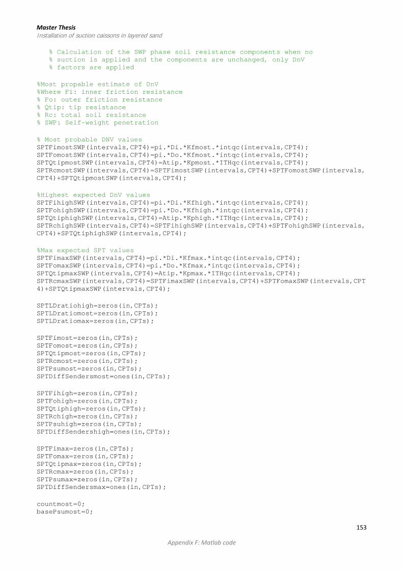
Master Thesis Installation of suction caissons in layered sand % Calculation of the SWP phase soil resistance components when no % suction is applied and the components are unchanged, only DnV % factors are applied %Most propable estimate of DnV %Where Fi: inner friction resistance % Fo: outer friction resistance % Qtip: tip resistance % Rc: total soil resistance % SWP: Self-weight penetration % Most probable DNV values SPTFimostSWP(intervals,CPT4)=pi.*Di.*Kfmost.*intqc(intervals,CPT4); SPTFomostSWP(intervals,CPT4)=pi.*Do.*Kfmost.*intqc(intervals,CPT4); SPTQtipmostSWP(intervals,CPT4)=Atip.*Kpmost.*ITHqc(intervals,CPT4); SPTRcmostSWP(intervals,CPT4)=SPTFimostSWP(intervals,CPT4)+SPTFomostSWP(intervals,CPT4)+SPTQtipmostSWP(intervals,CPT4); %Highest expected DnV values SPTFihighSWP(intervals,CPT4)=pi.*Di.*Kfhigh.*intqc(intervals,CPT4); SPTFohighSWP(intervals,CPT4)=pi.*Do.*Kfhigh.*intqc(intervals,CPT4); SPTQtiphighSWP(intervals,CPT4)=Atip.*Kphigh.*ITHqc(intervals,CPT4); SPTRchighSWP(intervals,CPT4)=SPTFihighSWP(intervals,CPT4)+SPTFohighSWP(intervals,CPT4)+SPTQtiphighSWP(intervals,CPT4); %Max expected SPT values SPTFimaxSWP(intervals,CPT4)=pi.*Di.*Kfmax.*intqc(intervals,CPT4); SPTFomaxSWP(intervals,CPT4)=pi.*Do.*Kfmax.*intqc(intervals,CPT4); SPTQtipmaxSWP(intervals,CPT4)=Atip.*Kpmax.*ITHqc(intervals,CPT4); SPTRcmaxSWP(intervals,CPT4)=SPTFimaxSWP(intervals,CPT4)+SPTFomaxSWP(intervals,CPT4)+SPTQtipmaxSWP(intervals,CPT4); SPTLDratiohigh=zeros(in,CPTs); SPTLDratiomost=zeros(in,CPTs); SPTLDratiomax=zeros(in,CPTs); SPTFimost=zeros(in,CPTs); SPTFomost=zeros(in,CPTs); SPTQtipmost=zeros(in,CPTs); SPTRcmost=zeros(in,CPTs); SPTPsumost=zeros(in,CPTs); SPTDiffSendersmost=ones(in,CPTs); SPTFihigh=zeros(in,CPTs); SPTFohigh=zeros(in,CPTs); SPTQtiphigh=zeros(in,CPTs); SPTRchigh=zeros(in,CPTs); SPTPsuhigh=zeros(in,CPTs); SPTDiffSendershigh=ones(in,CPTs); SPTFimax=zeros(in,CPTs); SPTFomax=zeros(in,CPTs); SPTQtipmax=zeros(in,CPTs); SPTRcmax=zeros(in,CPTs); SPTPsumax=zeros(in,CPTs); SPTDiffSendersmax=ones(in,CPTs); countmost=0; basePsumost=0;
153
Appendix F: Matlab code

Master Thesis Installation of suction caissons in layered sand counthigh=0; basePsuhigh=0; countmax=0; basePsumax=0; % Calculation of the suction pressure needed to overcome the encountered % soil resistance as predicted based on the method's approach % Based on the DNV most probable case for CPT=1:CPTs; for j=1:in if SPTRcmostSWP(j,CPT)<PrLoad % No reduction of the soil resistance components SPTFimost(j,CPT)=pi.*Di.*Kfmost.*intqc(j,CPT); SPTFomost(j,CPT)=pi.*Do.*Kfmost.*intqc(j,CPT); SPTQtipmost(j,CPT)=Atip.*Kpmost.*ITHqc(j,CPT); SPTRcmost(j,CPT)=SPTFimost(j,CPT)+SPTFomost(j,CPT)+SPTQtipmost(j,CPT); SPTPsumost(j,CPT)=0; else countmost=countmost+1; if countmost==1 % The first time found that it is required suction pressure % it is needed to keep this value as a base as otherwise % a negative jump of the pressure will be seen due to the % method's sudden reduction of the soil resistance basePsumost=-(SPTout.*SPTFomostSWP(j,CPT) + SPTip.*SPTQtipmostSWP(j,CPT)+ SPTin.*SPTFimostSWP(j,CPT) - PrLoad)./Atop; end SPTPsumost(j,CPT)=basePsumost + (SPTout.*SPTFomostSWP(j,CPT) + SPTip.*SPTQtipmostSWP(j,CPT)+ SPTin.*SPTFimostSWP(j,CPT) - PrLoad)./Atop; % reduction of the soil resistance components according to the % method's assumptions SPTFimost(j,CPT)=SPTin.*pi.*Di.*Kfmost.*intqc(j,CPT); SPTFomost(j,CPT)=SPTout.*pi.*Do.*Kfmost.*intqc(j,CPT); SPTQtipmost(j,CPT)=SPTip.*Atip.*Kpmost.*ITHqc(j,CPT); SPTRcmost(j,CPT)=SPTFimost(j,CPT)+SPTFomost(j,CPT)+SPTQtipmost(j,CPT); % Checking if the estimated reduced soil resistance is equal % with the applied forces SPTDiffSendersmost(j,CPT)= SPTRcmost(j,CPT)- PrLoad - Atop.*SPTPsumost(j,CPT); SPTLDratiomost(j,CPT)=(0.1.*j)./L; end end end % Calculation of the suction pressure needed to overcome the encountered % soil resistance as predicted based on the method's approach % Based on the DNV highest expected case for CPT=1:CPTs;
154
Appendix F: Matlab code

Master Thesis Installation of suction caissons in layered sand for j=1:in if SPTRchighSWP(j,CPT)<PrLoad SPTFihigh(j,CPT)=pi.*Di.*Kfhigh.*intqc(j,CPT); SPTFohigh(j,CPT)=pi.*Do.*Kfhigh.*intqc(j,CPT); SPTQtiphigh(j,CPT)=Atip.*Kphigh.*ITHqc(j,CPT); SPTRchigh(j,CPT)=SPTFihigh(j,CPT)+SPTFohigh(j,CPT)+SPTQtiphigh(j,CPT); SPTPsuhigh(j,CPT)=0; else counthigh=counthigh+1; if counthigh==1 basePsuhigh=-(SPTout.*SPTFomostSWP(j,CPT) + SPTip.*SPTQtipmostSWP(j,CPT)+ SPTin.*SPTFimostSWP(j,CPT) - PrLoad)./Atop; end SPTPsuhigh(j,CPT)=basePsuhigh + (SPTout.*SPTFohighSWP(j,CPT) + SPTip.*SPTQtiphighSWP(j,CPT) + SPTin.*SPTFihighSWP(j,CPT) - PrLoad )./Atop; SPTFihigh(j,CPT)=SPTin.*pi.*Di.*Kfhigh.*intqc(j,CPT); SPTFohigh(j,CPT)=SPTout.*pi.*Do.*Kfhigh.*intqc(j,CPT); SPTQtiphigh(j,CPT)=SPTip.*Atip.*Kphigh.*ITHqc(j,CPT); SPTRchigh(j,CPT)=SPTFihigh(j,CPT)+SPTFohigh(j,CPT)+SPTQtiphigh(j,CPT); SPTDiffSendershigh(j,CPT)= SPTRchigh(j,CPT)-PrLoad -Atop.*SPTPsuhigh(j,CPT); SPTLDratiohigh(j,CPT)=(0.1.*j)./L; end end end % Calculation of the suction pressure needed to overcome the encountered % soil resistance as predicted based on the method's approach % Based on the SPT max expected case for CPT=1:CPTs; for j=1:in if SPTRcmaxSWP(j,CPT)<PrLoad SPTFimaxSWP(j,CPT)=pi.*Di.*Kfmax.*intqc(j,CPT); SPTFomaxSWP(j,CPT)=pi.*Do.*Kfmax.*intqc(j,CPT); SPTQtipmaxSWP(j,CPT)=Atip.*Kpmax.*ITHqc(j,CPT); SPTRcmaxSWP(j,CPT)=SPTFimaxSWP(j,CPT)+SPTFomaxSWP(j,CPT)+SPTQtipmaxSWP(j,CPT); SPTPsuhigh(j,CPT)=0; else countmax=countmax+1; if countmax==1 basePsumax=-(SPTout.*SPTFomaxSWP(j,CPT) + SPTip.*SPTQtipmaxSWP(j,CPT)+ SPTin.*SPTFimaxSWP(j,CPT) - PrLoad)./Atop;
155
Appendix F: Matlab code

Master Thesis Installation of suction caissons in layered sand end SPTPsumax(j,CPT)= basePsumax + (SPTout.*SPTFomaxSWP(j,CPT) + SPTip.*SPTQtipmaxSWP(j,CPT) + SPTin.*SPTFimaxSWP(j,CPT) - PrLoad )./Atop; SPTFimax(j,CPT)=SPTin.*pi.*Di.*Kfmax.*intqc(j,CPT); SPTFomax(j,CPT)=SPTout.*pi.*Do.*Kfmax.*intqc(j,CPT); SPTQtipmax(j,CPT)=SPTip.*Atip.*Kpmax.*ITHqc(j,CPT); SPTRcmax(j,CPT)=SPTFimax(j,CPT)+SPTFomax(j,CPT)+SPTQtipmax(j,CPT); SPTDiffSendersmax(j,CPT)= SPTRcmax(j,CPT)-PrLoad -Atop.*SPTPsumax(j,CPT); SPTLDratiomax(j,CPT)=(0.1.*j)./L; end end end %Plot of the Psmooth (actual pressure) vs L/D and Psu (predicted) vs L/D %for Block 12/21 site % different time ranges should be taken due to the noise of the data plot(NormLSkirt(1200:5850,1),Psmooth(1200:5850,1)); hold 'all' plot(SPTLDratiomost(1:70,1),SPTPsumost(1:70,1)); hold 'all' plot(SPTLDratiohigh(1:70,1),SPTPsuhigh(1:70,1)); hold 'all' plot(SPTLDratiomax(1:70,1),SPTPsumax(1:70,1)); plot(NormLSkirt(1200:5850,3),Psmooth(1200:5850,3)); hold 'all' plot(SPTLDratiomost(1:70,1),SPTPsumost(1:70,1)); hold 'all' plot(SPTLDratiohigh(1:70,2),SPTPsuhigh(1:70,2)); hold 'all' plot(SPTLDratiomax(1:70,2),SPTPsumax(1:70,2)); plot(NormLSkirt(1200:5850,3),Psmooth(1200:5850,3)); hold 'all' plot(SPTLDratiomost(1:70,3),SPTPsumost(1:70,3)); hold 'all' plot(SPTLDratiohigh(1:70,3),SPTPsuhigh(1:70,3)); hold 'all' plot(SPTLDratiomax(1:70,3),SPTPsumax(1:70,3)); % Predicted P/gL hold 'all' plot(SPTLDratiomost(1:70,3),SPTPsumost(1:70,3)./(gammaeff.*SPTLDratiomost(1:70,3).*L)); hold 'all' plot(SPTLDratiohigh(1:70,3),SPTPsuhigh(1:70,3)./(gammaeff.*SPTLDratiohigh(1:70,3).*L)); hold 'all' plot(SPTLDratiomax(1:70,3),SPTPsumax(1:70,3)./(gammaeff.*SPTLDratiomax(1:70,3).*L)); % Predicted P/gD
156
Appendix F: Matlab code

Master Thesis Installation of suction caissons in layered sand hold 'all' plot(SPTLDratiomost(1:70,3),SPTPsumost(1:70,3)./(gammaeff*L)); hold 'all' plot(SPTLDratiohigh(1:70,3),SPTPsuhigh(1:70,3)./(gammaeff*L)); hold 'all' plot(SPTLDratiomax(1:70,3),SPTPsumax(1:70,3)./(gammaeff*L)); % Predicted P/qc hold 'all' plot(SPTLDratiomost(1:70,3),SPTPsumost(1:70,3)./ITHqc(1:70,3)); hold 'all' plot(SPTLDratiohigh(1:70,3),SPTPsuhigh(1:70,3)./ITHqc(1:70,3)); hold 'all' plot(SPTLDratiomax(1:70,3),SPTPsumax(1:70,3)./ITHqc(1:70,3)); % Predicted Rc hold 'all' plot(SPTPsumost(1:70,3)*Atop + PrLoad, SPTLDratiomost(1:70,3)); hold 'all' plot(SPTPsuhigh(1:70,3)*Atop + PrLoad, SPTLDratiohigh(1:70,3)); hold 'all' plot(SPTPsumax(1:70,3)*Atop + PrLoad, SPTLDratiomax(1:70,3)); % Ratio of reduced Rc/ unreduced Rc SPT_Rc_reduced(1:70,3)=(SPTPsumost(1:70,3)*Atop + PrLoad)./SPTRcmostSWP(1:70,3); SPT_Rc_reduced(1:70,2)=(SPTPsumost(1:70,2)*Atop + PrLoad)./SPTRcmostSWP(1:70,2); hold all plot(SPT_Rc_reduced(1:70,3), SPTLDratiomax(1:70,3)); hold all plot(SPT_Rc_reduced(1:70,2), SPTLDratiomax(1:70,2));
Senders and Radolph prediction method for sand profiles % Senders and Radolph prediction method % Drained installation for sand profiles % See Appendix A. Senders and Randolph method % The case of the Project Block 12/21 % Suction caissons details Di=9.94; % internal diameter in meters thickness=0.03; % thickness of the skirt in meters Do=Di+2*thickness; % outer diameter in meters L=7; % skirt length in meters Atip=pi*(Do.^2-Di.^2)/4; % Annular area of the caisson skirt tip in m2 %Submerged self-weight of the caisson in KN %dsteel=7850; % density of steel in kg/m3 %g=9.806; % accelaration due to gravity in m/s2 %dseawater=1027; % density of seawater in kg/m3 %SW=Atip*L*dsteel*g/1000; % Self-weight of suction caisson in KN %Vskirt=Atip*L; % volume of the actual steel caisson in m3 %SubSW=SW-Vskirt*dseawater*g/1000; PrLoad=3207; % Load of the structure distributed per Anchor % Suggested magnitude of the DNV Kf and Kp values by the S&R method
157
Appendix F: Matlab code

Master Thesis Installation of suction caissons in layered sand C=0.012; % coefficient for the determination of Kf % this value should be adjusted according to the sand density, as indicated % by the normalised cone resistance, with higher values % appropriate in looser sand, and even lower values possible for extremely % dense sand. Kp=0.2; % estimation of phi by Robertson phi(intervals,CPT4)= real(17.6+ 11.*log10(Qtn(intervals,CPT4))); % approximation of delta by Senders delta(intervals,CPT4)=(2/3)*phi(intervals,CPT4); % coefficient reflecting differences in the geometry %(circular for the cone,but strip-like for the caisson skirt) Kf(intervals,CPT4)=(C.*(1-(Di./Do).^2).^0.3).*tan(degtorad(delta(intervals,CPT4))); gammaeff=10; % effective unit weight of sand at site CPT4=1:3; CPTs=3; %Senders Calculation of Critical Pressure KPa PcritSenders=(pi - atan(5*(L./Di).^0.85)*(2-2/pi)).*L*gammaeff; % if it is assumed that kfac=3, as recommended by Senders page 5 at % his paper then the Pcrit should be increased by 50% PcritSendersIncreased=1.5*PcritSenders; %Trapezoidal Rule to estimate the integral of the qc profile alongside with %the current penetration depth achieved h=0.1; %interval length of CPT data points collected in meters intqc(1,CPT4)=0; intqc(2,CPT4)=(h./2).*(ITHqc(1,CPT4)+ITHqc(2,CPT4)); for CPT=1:CPTs; for j=3:in intqc(j,CPT)=(h./2).*(ITHqc(1,CPT)+ITHqc(j,CPT)+2.*sum(ITHqc(2:j-1,CPT))); end end Fi=ones(in,CPTs); Fo=ones(in,CPTs); Qtip=ones(in,CPTs); Rc=ones(in,CPTs); Psu=zeros(in,CPTs); DiffSenders=ones(in,CPTs); LDratio=zeros(in,CPTs); % Calculation of the SWP phase soil resistance components when no % suction is applied and the components are unchanged, only DnV % factors are applied %Most propable estimate of DnV %Where Fi: inner friction resistance % Fo: outer friction resistance % Qtip: tip resistance % Rc: total soil resistance % SWP: Self-weight penetration
158
Appendix F: Matlab code

Master Thesis Installation of suction caissons in layered sand for CPT=1:CPTs; for j=1:in if Rc(j,CPT)<PrLoad % No reduction of the soil resistance components Fi(j,CPT)=pi.*Di.*Kf(j,CPT).*intqc(j,CPT); Fo(j,CPT)=pi.*Do.*Kf(j,CPT).*intqc(j,CPT); Qtip(j,CPT)=Atip.*Kp.*ITHqc(j,CPT); Rc(j,CPT)=Fi(j,CPT)+Fo(j,CPT)+Qtip(j,CPT); Psu(j,CPT)=0; else Psu(j,CPT)=PcritSendersIncreased.*min([((Fo(j,CPT)+Fi(j,CPT)+Qtip(j,CPT)-PrLoad)./(Fi(j,CPT)+Qtip(j,CPT)+0.25*pi*(Di.^2)*PcritSendersIncreased)),1]); end end end for CPT=1:CPTs; for j=1:in % reduction of the soil resistance components according to the % method's assumptions Fi(j,CPT)=(pi.*Di.*Kf(j,CPT).*intqc(j,CPT)).*(1+(-Psu(j,CPT)./PcritSendersIncreased)); Qtip(j,CPT)=Atip.*Kp.*ITHqc(j,CPT).*(1+(-Psu(j,CPT)./PcritSendersIncreased)); Rc(j,CPT)=Fi(j,CPT)+Fo(j,CPT)+Qtip(j,CPT); % Checking if the estimated reduced soil resistance is equal % with the applied forces DiffSenders(j,CPT)= Rc(j,CPT)-PrLoad-0.25.*pi.*(Di.^2).*Psu(j,CPT); LDratio(j,CPT)=(0.1.*j)./L; end end % Plot of the Psmooth (actual pressure) vs L/D and Psu (predicted) vs L/D % for Block 12/21 site % different time ranges should be taken due to the noise of the data plot(NormLSkirt(1200:5850,1),Psmooth(1200:5850,1)); hold 'all' plot(LDratio(1:70,1),Psu(1:70,1)); plot(NormLSkirt(1200:5850,2),Psmooth(1200:5850,2)); hold 'all' plot(LDratio(1:70,2),Psu(1:70,2)); plot(NormLSkirt(1200:5850,3),Psmooth(1200:5850,3)); hold 'all' plot(LDratio(1:70,3),Psu(1:70,3)); % Predicted P/gL hold 'all' plot(LDratio(1:70,3),Psu(1:70,3)./(gammaeff.*LDratio(1:70,3).*L)); % Predicted P/gD
159
Appendix F: Matlab code

Master Thesis Installation of suction caissons in layered sand hold 'all' plot(LDratio(48:70,3),Psu(48:70,3)./(gammaeff*L)); % Predicted Psu/qc hold 'all' plot(LDratio(50:70,3),Psu(50:70,3)./ITHqc(50:70,3)); %Back analysis of reduced total soil resistance hold 'all' plot(Psu(1:70,3)*Atop + PrLoad, LDratio(1:70,3));
Feld prediction method for sand profiles % Feld prediction method % See Appendix A. Feld method % The case of the Project Block 12/21 % Suction caissons details Di=9.94; % internal diameter in meters thickness=0.03; % thickness of the skirt in meters Do=Di+2*thickness; % outer diameter in meters L=7; % skirt length in meters Atip=pi*(Do.^2-Di.^2)/4; % Annular area of the caisson skirt tip in m2 Atop=pi*(Di.^2)/4; % Inner area that suction is applied in m2 PrLoad=3207; %in KN % Load of the structure distributed per Anchor gammaeff=10; % effective unit weight of sand at site CPT4=1:3; intervals=1:81; in=81; CPTs=3; h=0.1; % estimation of phi by Robertson phi(intervals,CPT4)= real(17.6+ 11.*log10(ITHQtn(intervals,CPT4))); % approximation of delta by Senders delta(intervals,CPT4)=(2/3)*phi(intervals,CPT4); %roughness factor, 0.8 for smooth skirts r=0.8; Du=zeros(in,CPTs); % Total soil resistance without suction application during SWP % critical suction as proposed by Clausen and Tjelta (1996) in Feld (2001) % To account the change of permeability as proposed by S&R method, although % such suggestion was not given in this method Du_crit_factor=1.5; Du_crit=Du_crit_factor*(gammaeff*L)/(1-0.68/(1.46*(L/Di)+1)); % Inner Skin friction % max change in inner skin friction, should be given a lower value from 1, % as when vertical stress decrease -> horizontal stress decrease but at a % smaller rate, as Ko increases with increased suction applied. % If r_inner=1 then an overprediction of the reduction in inner skin % friction will be obtained.
160
Appendix F: Matlab code

Master Thesis Installation of suction caissons in layered sand % This value allows a residual 10% of inner skin friction to be maintain % during the installation r_inner=0.9; % change in skin friction due to suction applied SWPalpha_s(intervals,CPT4)=1-r_inner.*(Du(intervals,CPT4)./Du_crit); SWPalpha(intervals,CPT4)=r.*tan(degtorad(phi(intervals,CPT4))).*SWPalpha_s(intervals,CPT4); % unit skin friction calculation SWPtaf_inner(intervals,CPT4)= SWPalpha(intervals,CPT4).*ITHsvo(intervals,CPT4); % Outer Skin friction % This value should allow an increased of 0-13% of outer skin friction % during installation if it is going to be assumed r_outer=0; SWPalpha_out(intervals,CPT4)=1+r_outer.*(Du(intervals,CPT4)./Du_crit); % unit skin friction calculation SWPtaf_outer(intervals,CPT4)= r.*tan(degtorad(phi(intervals,CPT4))).*SWPalpha_out(intervals,CPT4).*ITHsvo(intervals,CPT4); % Tip resistance % This value allows a residual 20% of inner skin friction to be maintain % during the installation r_tip=0.8; % substantially when no suction is applied no reduction is present, whereas % when critical suction is applied, max reduction is present, which is % determined based on experience allowing for a minimum value to be % maintained % DnV proposed values for calculating tip resistance % Friction Kf values are not used in this method as the qc values are not % used for calculating friction resistance Kpmost=0.3; Kphigh=0.6; % change in tip resistance due to suction applied SWPalpha_t(intervals,CPT4)=1-r_tip.*(Du(intervals,CPT4)./Du_crit); SWPsigma_tip_most(intervals,CPT4)=ITHqc(intervals,CPT4).*SWPalpha_t(intervals,CPT4).*Kpmost; SWPsigma_tip_high(intervals,CPT4)=ITHqc(intervals,CPT4).*SWPalpha_t(intervals,CPT4).*Kphigh; % Calculation of the total soil resistance peneintervals=repmat(h.*intervals',1,4); SWPRcFeldmost(intervals,CPT4)= SWPsigma_tip_most(intervals,CPT4).*Atip + SWPtaf_outer(intervals,CPT4).*pi.*Do.*peneintervals(intervals,CPT4) + SWPtaf_inner(intervals,CPT4).*pi.*Di.*peneintervals(intervals,CPT4); SWPRcFeldhigh(intervals,CPT4)= SWPsigma_tip_high(intervals,CPT4).*Atip + SWPtaf_outer(intervals,CPT4).*pi.*Do.*peneintervals(intervals,CPT4) + SWPtaf_inner(intervals,CPT4).*pi.*Di.*peneintervals(intervals,CPT4); % Preallocating the size of the following matrices for the respective % variables in order to reduce running time for Matlab Dumost=zeros(in,CPTs); DiffFeldmost=zeros(in,CPTs); Aout=pi.*Do.*intervals.*h; AAout=repmat(Aout',1,CPTs); Ain=pi.*Di.*intervals.*h; AAin=repmat(Ain',1,CPTs);
161
Appendix F: Matlab code

Master Thesis Installation of suction caissons in layered sand Dumostnumerator=zeros(in,CPTs); Dumostdenominator=zeros(in,CPTs); SAPalpha_s_most=zeros(in,CPTs); SAPalpha_most=zeros(in,CPTs); SAPtaf_inner_most=zeros(in,CPTs); SAPalpha_out_most=zeros(in,CPTs); SAPtaf_outer_most=zeros(in,CPTs); SAPalpha_t_most=zeros(in,CPTs); SAPsigma_tip_most=zeros(in,CPTs); SAPRcFeldmost=zeros(in,CPTs); LDratiomost=zeros(in,CPTs); % Calculation of the SWP phase soil resistance components when no % suction is applied and the components are unchanged, only DnV % factors are applied % Based on the DNV highest expected case % Where Fi: inner friction resistance % Fo: outer friction resistance % Qtip: tip resistance % Rc: total soil resistance % SWP: Self-weight penetration % SAP: suction-assisted penetration for CPT=1:3; for j=1:in if SWPRcFeldmost(j,CPT)>PrLoad %Calculation of the required suction to continue caisson %installation Dumostnumerator(j,CPT)= (PrLoad - (AAout(j,CPT)+ AAin(j,CPT)).*r.*tan(degtorad(phi(j,CPT))).*ITHsvo(j,CPT) - Kpmost.*ITHqc(j,CPT).*Atip).*Du_crit; Dumostdenominator(j,CPT)=-Kpmost.*ITHqc(j,CPT).*Atip.*r_tip + r.*tan(degtorad(phi(j,CPT))).*ITHsvo(j,CPT).*(AAout(j,CPT).*r_outer-AAin(j,CPT).*r_inner) - Du_crit.*Atop; Dumost(j,CPT)=Dumostnumerator(j,CPT)./Dumostdenominator(j,CPT); % change in skin friction due to suction applied SAPalpha_s_most(j,CPT)=1-r_inner.*(Dumost(j,CPT)./Du_crit); SAPalpha_most(j,CPT)=r.*tan(degtorad(phi(j,CPT))).*SAPalpha_s_most(j,CPT); % reduced dinner skin friction calculation SAPtaf_inner_most(j,CPT)= SAPalpha_most(j,CPT).*ITHsvo(j,CPT); % reduced outer skin friction calculation SAPalpha_out_most(j,CPT)=1+r_outer.*(Dumost(j,CPT)./Du_crit); SAPtaf_outer_most(j,CPT)= r.*tan(degtorad(phi(j,CPT))).*SAPalpha_out_most(j,CPT).*ITHsvo(j,CPT); %change in tip resistance due to suction applied SAPalpha_t_most(j,CPT)=1-r_tip.*(Dumost(j,CPT)./Du_crit); SAPsigma_tip_most(j,CPT)=ITHqc(j,CPT).*SAPalpha_t_most(j,CPT).*Kpmost; % Reduced total soil resistance SAPRcFeldmost(j,CPT)= SAPsigma_tip_most(j,CPT).*Atip + SAPtaf_outer_most(j,CPT).*pi.*Do.*peneintervals(j,CPT) + SAPtaf_inner_most(j,CPT).*pi.*Di.*peneintervals(j,CPT);
162
Appendix F: Matlab code

Master Thesis Installation of suction caissons in layered sand % Checking if the estimated reduced soil resistance is equal % with the applied forces DiffFeldmost(j,CPT)= SAPRcFeldmost(j,CPT)-PrLoad -Dumost(j,CPT).*Atop; LDratiomost(j,CPT)=(0.1.*j)./L; end end end % Preallocating the size of the following matrices for the respective % variables in order to reduce running time for Matlab Duhigh=zeros(in,CPTs); Duhighnumerator=zeros(in,CPTs); Duhighdenominator=zeros(in,CPTs); SAPalpha_s_high=zeros(in,CPTs); SAPalpha_high=zeros(in,CPTs); SAPtaf_inner_high=zeros(in,CPTs); SAPalpha_out_high=zeros(in,CPTs); SAPtaf_outer_high=zeros(in,CPTs); SAPalpha_t_high=zeros(in,CPTs); SAPsigma_tip_high=zeros(in,CPTs); SAPRcFeldhigh=zeros(in,CPTs); LDratiohigh=zeros(in,CPTs); DiffFeldhigh=zeros(in,CPTs); % Calculation of the SWP phase soil resistance components when no % suction is applied and the components are unchanged, only DnV % factors are applied % Based on the DNV highest expected case for CPT=1:3; for j=1:in if SWPRcFeldhigh(j,CPT)>PrLoad % Calculation of the required suction to continue caisson % installation Duhighnumerator(j,CPT)= (PrLoad - (AAout(j,CPT)+ AAin(j,CPT)).*r.*tan(degtorad(phi(j,CPT))).*ITHsvo(j,CPT) - Kphigh.*ITHqc(j,CPT).*Atip).*Du_crit; Duhighdenominator(j,CPT)=-Kphigh.*ITHqc(j,CPT).*Atip.*r_tip + r.*tan(degtorad(phi(j,CPT))).*ITHsvo(j,CPT).*(AAout(j,CPT).*r_outer-AAin(j,CPT).*r_inner) - Du_crit.*Atop; Duhigh(j,CPT)=Duhighnumerator(j,CPT)./Duhighdenominator(j,CPT); %change in skin friction due to suction applied SAPalpha_s_most(j,CPT)=1-r_inner.*(Duhigh(j,CPT)./Du_crit); SAPalpha_most(j,CPT)=r.*tan(degtorad(phi(j,CPT))).*SAPalpha_s_most(j,CPT); % reduced inner skin friction calculation SAPtaf_inner_most(j,CPT)= SAPalpha_most(j,CPT).*ITHsvo(j,CPT); % outer skin friction calculation SAPalpha_out_most(j,CPT)=1+r_outer.*(Duhigh(j,CPT)./Du_crit); % reduced outer skin friction calculation SAPtaf_outer_most(j,CPT)= r.*tan(degtorad(phi(j,CPT))).*SAPalpha_out_most(j,CPT).*ITHsvo(j,CPT);
163
Appendix F: Matlab code

Master Thesis Installation of suction caissons in layered sand %change in tip resistance due to suction applied SAPalpha_t_most(j,CPT)=1-r_tip.*(Duhigh(j,CPT)./Du_crit); SAPsigma_tip_high(j,CPT)=ITHqc(j,CPT).*SAPalpha_t_most(j,CPT).*Kphigh; SAPRcFeldhigh(j,CPT)= SAPsigma_tip_high(j,CPT).*Atip + SAPtaf_outer_most(j,CPT).*pi.*Do.*peneintervals(j,CPT) + SAPtaf_inner_most(j,CPT).*pi.*Di.*peneintervals(j,CPT); DiffFeldhigh(j,CPT)= SAPRcFeldmost(j,CPT)-PrLoad -Dumost(j,CPT).*Atop; LDratiohigh(j,CPT)=(0.1.*j)./L; end end end % Plot of the Psmooth (actual pressure) vs L/D and Psu (predicted) vs L/D % for Block 12/21 site % different time ranges should be taken due to the noise of the data plot(NormLSkirt(650:5850,1),Psmooth(650:5850,1)); hold 'all' plot(LDratiomost(1:70,1),Dumost(1:70,1)); hold 'all' plot(LDratiohigh(1:70,1),Duhigh(1:70,1)); plot(NormLSkirt(650:5850,2),Psmooth(650:5850,2)); hold 'all' plot(LDratiomost(1:70,2),Dumost(1:70,2)); hold 'all' plot(LDratiohigh(1:70,2),Duhigh(1:70,2)); plot(NormLSkirt(650:5850,3),Psmooth(650:5850,3)); hold 'all' plot(LDratiomost(55:70,3),Dumost(55:70,3)); hold 'all' plot(LDratiohigh(55:70,3),Duhigh(55:70,3)); % Predicted P/gL hold 'all' plot(LDratiomost(1:70,3),Dumost(1:70,3)./(gammaeff.*LDratiomost(1:70,3).*L)); hold 'all' plot(LDratiohigh(1:70,3),Duhigh(1:70,3)./(gammaeff.*LDratiohigh(1:70,3).*L)); % Predicted P/gD hold 'all' plot(LDratiomost(1:70,3),Dumost(1:70,3)./(gammaeff*L)); hold 'all' plot(LDratiohigh(1:70,3),Duhigh(1:70,3)./(gammaeff*L)); % Predicted P/qc hold 'all' plot(LDratiomost(1:70,3),Dumost(1:70,3)./ITHqc(1:70,3)); hold 'all' plot(LDratiohigh(1:70,3),Duhigh(1:70,3)./ITHqc(1:70,3)); % Back analysis of Rc hold 'all' plot(Dumost(1:70,3)*Atop + PrLoad, LDratiomost(1:70,3));
164
Appendix F: Matlab code

Master Thesis Installation of suction caissons in layered sand hold 'all' plot(Duhigh(1:70,3)*Atop + PrLoad, LDratiohigh(1:70,3));
SPT prediction method for layered sand profiles % SPT prediction method % Undrained installation for layered sand profiles % See 2.4.2. Installation behavior in layered soil conditions and % 3.2.2. Prediction methods scenarios for layered sand profiles % The case of the Project: P6 % Suction caissons details Di=8.93; % internal diameter in meters thickness=0.035; % thickness of the skirt in meters Do=Di+2*thickness; % outer diameter in meters L=9; % skirt length in meters Atip=pi*(Do.^2-Di.^2)/4; % Annular area of the caisson skirt tip in m2 Atop=pi*(Di.^2)/4; % Inner area that suction is applied in m2 PrLoad=2000; %in KN KpmostSand=0.3; %DnV values Sand KphighSand=0.6; KfmostSand=0.001; KfhighSand=0.003; KpmostClay=0.4; %DnV values Clay KphighClay=0.6; KfmostClay=0.03; KfhighClay=0.05; KpmaxSand=0.45; %SPT max expected for Kp KfmaxSand=0.002; %SPT max expected for Kf %SPT applied factors to SAP phase to the corresponding soil resistance % components during installation for CLAY SPTinClay=0.5; SPToutClay=1; SPTipClay=0.75; % SPT applied factors to SAP phase to the corresponding soil resistance % components during installation for SAND SPTinSand=0; SPToutSand=1; SPTipSand=0.5; gammaeff=9.5; % effective unit weight of sand at site CPT4=1:3; CPTs=3; %Trapezoidal Rule to estimate the integral of the qc profile alongside with %the current penetration depth achieved h=0.245; % interval length of CPT data points collected in meters CLqcKfmost=zeros(in,CPTs); CLqcKfhigh=zeros(in,CPTs); CLqcKfmax=zeros(in,CPTs); % The following calculations are based on the criterion whether the soil % interval investigated is described as having drained/undrained behaviour
165
Appendix F: Matlab code

Master Thesis Installation of suction caissons in layered sand % according to the Robertson assification for CPT=1:CPTs; for i=3:in if CLSoilB(i,CPT)==3 || CLSoilB(i,CPT)==4 || CLSoilB(i,CPT)==2 || CLSoilB(i,CPT)==3.5 || CLSoilB(i,CPT)==4.5 || CLSoilB(i,CPT)==9 % Calculating the product of the Kf*qc as it is required to % calculate the integral of them, as both are changed during % the installation, thus both are dependant on the depth CLqcKfmost(i,CPT)=KfmostClay.*CLqc(i,CPT); CLqcKfhigh(i,CPT)=KfhighClay.*CLqc(i,CPT); CLqcKfmax(i,CPT)=KfhighClay.*CLqc(i,CPT); else CLqcKfmost(i,CPT)=KfmostSand.*CLqc(i,CPT); CLqcKfhigh(i,CPT)=KfhighSand.*CLqc(i,CPT); CLqcKfmax(i,CPT)=KfmaxSand.*CLqc(i,CPT); end end end intqcmost(1,CPT4)=0; intqchigh(1,CPT4)=0; intqcmax(1,CPT4)=0; intqcmost(2,CPT4)=(h./2).*(CLqcKfmost(1,CPT4)+CLqcKfmost(2,CPT4)); intqchigh(2,CPT4)=(h./2).*(CLqcKfhigh(1,CPT4)+CLqcKfhigh(2,CPT4)); intqcmax(2,CPT4)=(h./2).*(CLqcKfmax(1,CPT4)+CLqcKfmax(2,CPT4)); intqcwithoutkfkp(1,CPT4)=0; intqcwithoutkfkp(2,CPT4)=(h./2).*(CLqc(1,CPT4)+CLqc(2,CPT4)); % This is done here as it is required to have it separately during % calculations in the Back-analyses done for CPT=1:CPTs; for i=3:in intqcwithoutkfkp(i,CPT)=(h./2).*(CLqc(1,CPT)+CLqc(i,CPT)+2.*sum(CLqc(2:i-1,CPT))); intqcmost(i,CPT)=(h./2).*(CLqcKfmost(1,CPT)+CLqcKfmost(i,CPT)+2.*sum(CLqcKfmost(2:i-1,CPT))); intqchigh(i,CPT)=(h./2).*(CLqcKfhigh(1,CPT)+CLqcKfhigh(i,CPT)+2.*sum(CLqcKfhigh(2:i-1,CPT))); intqcmax(i,CPT)=(h./2).*(CLqcKfmax(1,CPT)+CLqcKfmax(i,CPT)+2.*sum(CLqcKfmax(2:i-1,CPT))); end end % Preallocating the size of the following matrices for the respective % varieables in order to reduce running time for Matlab SPTFimostSWP=zeros(in,CPTs); SPTFomostSWP=zeros(in,CPTs); SPTQtipmostSWP=zeros(in,CPTs); SPTRcmostSWP=zeros(in,CPTs); SPTFihighSWP=zeros(in,CPTs); SPTFohighSWP=zeros(in,CPTs); SPTQtiphighSWP=zeros(in,CPTs); SPTRchighSWP=zeros(in,CPTs);
166
Appendix F: Matlab code

Master Thesis Installation of suction caissons in layered sand SPTFimaxSWP=zeros(in,CPTs); SPTFomaxSWP=zeros(in,CPTs); SPTQtipmaxSWP=zeros(in,CPTs); SPTRcmaxSWP=zeros(in,CPTs); SPTFimost=zeros(in,CPTs); SPTFomost=zeros(in,CPTs); SPTQtipmost=zeros(in,CPTs); SPTRcmost=zeros(in,CPTs); SPTFihigh=zeros(in,CPTs); SPTFohigh=zeros(in,CPTs); SPTQtiphigh=zeros(in,CPTs); SPTRchigh=zeros(in,CPTs); SPTFimax=zeros(in,CPTs); SPTFomax=zeros(in,CPTs); SPTQtipmax=zeros(in,CPTs); SPTRcmax=zeros(in,CPTs); % Calculation of the SWP phase soil resistance components when no % suction is applied and the components are unchanged, only DnV % factors are applied % calculation is branched for the layers which are characterised for % allowing flow or no flow using different DnV values based on the % Robertson classification for CPT=1:CPTs; for i=1:in if CLSoilB(i,CPT)==3 || CLSoilB(i,CPT)==4 || CLSoilB(i,CPT)==2 || CLSoilB(i,CPT)==3.5 || CLSoilB(i,CPT)==4.5 || CLSoilB(i,CPT)==9 % Most propable estimate of DnV if clay layer SPTFimostSWP(i,CPT)=pi.*Di.*intqcmost(i,CPT); SPTFomostSWP(i,CPT)=pi.*Do.*intqcmost(i,CPT); SPTQtipmostSWP(i,CPT)=Atip.*KpmostClay.*CLqc(i,CPT); SPTRcmostSWP(i,CPT)=SPTFimostSWP(i,CPT)+SPTFomostSWP(i,CPT)+SPTQtipmostSWP(i,CPT); % Highest propable estimate of DnV if clay layer SPTFihighSWP(i,CPT)=pi.*Di.*intqchigh(i,CPT); SPTFohighSWP(i,CPT)=pi.*Do.*intqchigh(i,CPT); SPTQtiphighSWP(i,CPT)=Atip.*KphighClay.*CLqc(i,CPT); SPTRchighSWP(i,CPT)=SPTFihighSWP(i,CPT)+SPTFohighSWP(i,CPT)+SPTQtiphighSWP(i,CPT); % Max expected estimate of DnV if clay layer SPTFimaxSWP(i,CPT)=pi.*Di.*intqcmax(i,CPT); SPTFomaxSWP(i,CPT)=pi.*Do.*intqcmax(i,CPT); SPTQtipmaxSWP(i,CPT)=Atip.*KphighClay.*CLqc(i,CPT); SPTRcmaxSWP(i,CPT)=SPTFimaxSWP(i,CPT)+SPTFomaxSWP(i,CPT)+SPTQtipmaxSWP(i,CPT); else SPTFimostSWP(i,CPT)=pi.*Di.*intqcmost(i,CPT); SPTFomostSWP(i,CPT)=pi.*Do.*intqcmost(i,CPT); SPTQtipmostSWP(i,CPT)=Atip.*KpmostSand.*CLqc(i,CPT); SPTRcmostSWP(i,CPT)=SPTFimostSWP(i,CPT)+SPTFomostSWP(i,CPT)+SPTQtipmostSWP(i,CPT);
167
Appendix F: Matlab code

Master Thesis Installation of suction caissons in layered sand %Highest propable estimate of DnV if sand layer SPTFihighSWP(i,CPT)=pi.*Di.*intqchigh(i,CPT); SPTFohighSWP(i,CPT)=pi.*Do.*intqchigh(i,CPT); SPTQtiphighSWP(i,CPT)=Atip.*KphighSand.*CLqc(i,CPT); SPTRchighSWP(i,CPT)=SPTFihighSWP(i,CPT)+SPTFohighSWP(i,CPT)+SPTQtiphighSWP(i,CPT); %Max expected estimate of DnV SPTFimaxSWP(i,CPT)=pi.*Di.*intqcmax(i,CPT); SPTFomaxSWP(i,CPT)=pi.*Do.*intqcmax(i,CPT); SPTQtipmaxSWP(i,CPT)=Atip.*KpmaxSand.*CLqc(i,CPT); SPTRcmaxSWP(i,CPT)=SPTFimaxSWP(i,CPT)+SPTFomaxSWP(i,CPT)+SPTQtipmaxSWP(i,CPT); end end end SPTLDratiohigh=zeros(in,CPTs); SPTLDratiomost=zeros(in,CPTs); SPTLDratiomax=zeros(in,CPTs); SPTPsumost=zeros(in,CPTs); SPTDiffSendersmost=ones(in,CPTs); SPTPsuhigh=zeros(in,CPTs); SPTDiffSendershigh=ones(in,CPTs); SPTPsumax=zeros(in,CPTs); SPTDiffSendersmax=ones(in,CPTs); countmost=0; basePsumost=0; counthigh=0; basePsuhigh=0; countmax=0; basePsumax=0; % Estimation of the installation pressure required during penetration % seperation of the soil layers depending on the robertson classification % to account for reduction of the soil resistance or not after determining % the required Psu % Most probable case of DNV values for CPT=1:CPTs; for i=1:in if SPTRcmostSWP(i,CPT)<PrLoad if CLSoilB(i,CPT)==3 || CLSoilB(i,CPT)==4 || CLSoilB(i,CPT)==2 || CLSoilB(i,CPT)==3.5 || CLSoilB(i,CPT)==4.5 || CLSoilB(i,CPT)==9 SPTFimost(i,CPT)=pi.*Di.*intqcmost(i,CPT); SPTFomost(i,CPT)=pi.*Do.*intqcmost(i,CPT); SPTQtipmost(i,CPT)=Atip.*KpmostClay.*CLqc(i,CPT); SPTRcmost(i,CPT)=SPTFimost(i,CPT)+SPTFomost(i,CPT)+SPTQtipmost(i,CPT); SPTPsumost(i,CPT)=0;
168
Appendix F: Matlab code
Master Thesis Installation of suction caissons in layered sand SPTLDratiomost(i,CPT)=(h.*i)./L; else SPTFimost(i,CPT)=pi.*Di.*intqcmost(i,CPT); SPTFomost(i,CPT)=pi.*Do.*intqcmost(i,CPT); SPTQtipmost(i,CPT)=Atip.*KpmostSand.*CLqc(i,CPT); SPTRcmost(i,CPT)=SPTFimost(i,CPT)+SPTFomost(i,CPT)+SPTQtipmost(i,CPT); SPTPsumost(i,CPT)=0; SPTLDratiomost(i,CPT)=(h.*i)./L; end else countmost=countmost+1; if countmost==1 if CLSoilB(i,CPT)==3 || CLSoilB(i,CPT)==4 || CLSoilB(i,CPT)==2 || CLSoilB(i,CPT)==3.5 || CLSoilB(i,CPT)==4.5 || CLSoilB(i,CPT)==9 basePsumost=-(SPToutClay.*SPTFomostSWP(i,CPT) + SPTipClay.*SPTQtipmostSWP(i,CPT)+ SPTinClay.*SPTFimostSWP(i,CPT) - PrLoad)./Atop; else basePsumost=-(SPToutSand.*SPTFomostSWP(i,CPT) + SPTipSand.*SPTQtipmostSWP(i,CPT)+ SPTinSand.*SPTFimostSWP(i,CPT) - PrLoad)./Atop; end end if CLSoilB(i,CPT)==3 || CLSoilB(i,CPT)==4 || CLSoilB(i,CPT)==2 || CLSoilB(i,CPT)==3.5 || CLSoilB(i,CPT)==4.5 || CLSoilB(i,CPT)==9 SPTPsumost(i,CPT)=basePsumost + (SPToutClay.*SPTFomostSWP(i,CPT) + SPTipClay.*SPTQtipmostSWP(i,CPT)+ SPTinClay.*SPTFimostSWP(i,CPT) - PrLoad)./Atop; % SPTPsumost(i,CPT)=basePsumost + (SPToutClay.*SPTFomost(i,CPT) + SPTipClay.*SPTQtipmostSWP(i,CPT)+ SPTinClay.*SPTFimostSWP(i,CPT) - PrLoad)./Atop; SPTFimost(i,CPT)=SPTinClay.*pi.*Di.*intqcmost(i,CPT); SPTFomost(i,CPT)=SPToutClay.*pi.*Do.*intqcmost(i,CPT); SPTQtipmost(i,CPT)=SPTipClay.*Atip.*KpmostClay.*CLqc(i,CPT); SPTRcmost(i,CPT)=SPTFimost(i,CPT)+SPTFomost(i,CPT)+SPTQtipmost(i,CPT); SPTDiffSendersmost(i,CPT)= SPTRcmost(i,CPT)- PrLoad - Atop.*SPTPsumost(i,CPT) +Atop.*basePsumost; SPTLDratiomost(i,CPT)=(h.*i)./L; else
169
Appendix F: Matlab code
Master Thesis Installation of suction caissons in layered sand SPTPsumost(i,CPT)=basePsumost + (SPToutSand.*SPTFomostSWP(i,CPT) + SPTipSand.*SPTQtipmostSWP(i,CPT)+ SPTinSand.*SPTFimostSWP(i,CPT) - PrLoad)./Atop; SPTFimost(i,CPT)=SPTinSand.*pi.*Di.*intqcmost(i,CPT); SPTFomost(i,CPT)=SPToutSand.*pi.*Do.*intqcmost(i,CPT); SPTQtipmost(i,CPT)=SPTipSand.*Atip.*KpmostSand.*CLqc(i,CPT); SPTRcmost(i,CPT)=SPTFimost(i,CPT)+SPTFomost(i,CPT)+SPTQtipmost(i,CPT); SPTDiffSendersmost(i,CPT)= SPTRcmost(i,CPT)- PrLoad - Atop.*SPTPsumost(i,CPT) +Atop.*basePsumost; SPTLDratiomost(i,CPT)=(h.*i)./L; end end end end % Highest expected case of DNV values for CPT=1:CPTs; for i=1:in if SPTRchighSWP(i,CPT)<PrLoad if CLSoilB(i,CPT)==3 || CLSoilB(i,CPT)==4 || CLSoilB(i,CPT)==2 || CLSoilB(i,CPT)==3.5 || CLSoilB(i,CPT)==4.5 || CLSoilB(i,CPT)==9 SPTFihigh(i,CPT)=pi.*Di.*intqchigh(i,CPT); SPTFohigh(i,CPT)=pi.*Do.*intqchigh(i,CPT); SPTQtiphigh(i,CPT)=Atip.*KphighClay.*CLqc(i,CPT); SPTRchigh(i,CPT)=SPTFihigh(i,CPT)+SPTFohigh(i,CPT)+SPTQtiphigh(i,CPT); SPTPsuhigh(i,CPT)=0; SPTLDratiohigh(i,CPT)=(h.*i)./L; else SPTFihigh(i,CPT)=pi.*Di.*intqchigh(i,CPT); SPTFohigh(i,CPT)=pi.*Do.*intqchigh(i,CPT); SPTQtiphigh(i,CPT)=Atip.*KphighSand.*CLqc(i,CPT); SPTRchigh(i,CPT)=SPTFihigh(i,CPT)+SPTFohigh(i,CPT)+SPTQtiphigh(i,CPT); SPTPsuhigh(i,CPT)=0; SPTLDratiohigh(i,CPT)=(h.*i)./L; end else counthigh=counthigh+1; if counthigh==1 if CLSoilB(i,CPT)==3 || CLSoilB(i,CPT)==4 || CLSoilB(i,CPT)==2 || CLSoilB(i,CPT)==3.5 || CLSoilB(i,CPT)==4.5 || CLSoilB(i,CPT)==9 basePsuhigh=-(SPToutClay.*SPTFohighSWP(i,CPT) + SPTipClay.*SPTQtiphighSWP(i,CPT)+ SPTinClay.*SPTFihighSWP(i,CPT) - PrLoad)./Atop;
170
Appendix F: Matlab code

Master Thesis Installation of suction caissons in layered sand else basePsuhigh=-(SPToutSand.*SPTFohighSWP(i,CPT) + SPTipSand.*SPTQtiphighSWP(i,CPT)+ SPTinSand.*SPTFihighSWP(i,CPT) - PrLoad)./Atop; end end if CLSoilB(i,CPT)==3 || CLSoilB(i,CPT)==4 || CLSoilB(i,CPT)==2 || CLSoilB(i,CPT)==3.5 || CLSoilB(i,CPT)==4.5 || CLSoilB(i,CPT)==9 SPTPsuhigh(i,CPT)=basePsuhigh + (SPToutClay.*SPTFohighSWP(i,CPT) + SPTipClay.*SPTQtiphighSWP(i,CPT)+ SPTinClay.*SPTFihighSWP(i,CPT) - PrLoad)./Atop; SPTFihigh(i,CPT)=SPTinClay.*pi.*Di.*intqchigh(i,CPT); SPTFohigh(i,CPT)=SPToutClay.*pi.*Do.*intqchigh(i,CPT); SPTQtiphigh(i,CPT)=SPTipClay.*Atip.*KphighClay.*CLqc(i,CPT); SPTRchigh(i,CPT)=SPTFihigh(i,CPT)+SPTFohigh(i,CPT)+SPTQtiphigh(i,CPT); SPTDiffSendershigh(i,CPT)= SPTRchigh(i,CPT)- PrLoad - Atop.*SPTPsuhigh(i,CPT) +Atop.*basePsuhigh; SPTLDratiohigh(i,CPT)=(h.*i)./L; else SPTPsuhigh(i,CPT)=basePsuhigh + (SPToutSand.*SPTFohighSWP(i,CPT) + SPTipSand.*SPTQtiphighSWP(i,CPT)+ SPTinSand.*SPTFihighSWP(i,CPT) - PrLoad)./Atop; SPTFihigh(i,CPT)=SPTinSand.*pi.*Di.*intqchigh(i,CPT); SPTFohigh(i,CPT)=SPToutSand.*pi.*Do.*intqchigh(i,CPT); SPTQtiphigh(i,CPT)=SPTipSand.*Atip.*KphighSand.*CLqc(i,CPT); SPTRchigh(i,CPT)=SPTFihigh(i,CPT)+SPTFohigh(i,CPT)+SPTQtiphigh(i,CPT); SPTDiffSendershigh(i,CPT)= SPTRchigh(i,CPT)- PrLoad - Atop.*SPTPsuhigh(i,CPT) +Atop.*basePsuhigh; SPTLDratiohigh(i,CPT)=(h.*i)./L; end end end end % Max expected case of DNV values for CPT=1:CPTs; for i=1:in if SPTRcmaxSWP(i,CPT)<PrLoad if CLSoilB(i,CPT)==3 || CLSoilB(i,CPT)==4 || CLSoilB(i,CPT)==2 || CLSoilB(i,CPT)==3.5 || CLSoilB(i,CPT)==4.5 || CLSoilB(i,CPT)==9 SPTFimax(i,CPT)=pi.*Di.*intqcmax(i,CPT); SPTFomax(i,CPT)=pi.*Do.*intqcmax(i,CPT);
171
Appendix F: Matlab code

Master Thesis Installation of suction caissons in layered sand SPTQtipmax(i,CPT)=Atip.*KphighClay.*CLqc(i,CPT); SPTRcmax(i,CPT)=SPTFimax(i,CPT)+SPTFomax(i,CPT)+SPTQtipmax(i,CPT); SPTPsumax(i,CPT)=0; SPTLDratiomax(i,CPT)=(h.*i)./L; else SPTFimax(i,CPT)=pi.*Di.*intqcmax(i,CPT); SPTFomax(i,CPT)=pi.*Do.*intqcmax(i,CPT); SPTQtipmax(i,CPT)=Atip.*KpmaxSand.*CLqc(i,CPT); SPTRcmax(i,CPT)=SPTFimax(i,CPT)+SPTFomax(i,CPT)+SPTQtipmax(i,CPT); SPTPsumax(i,CPT)=0; SPTLDratiomax(i,CPT)=(h.*i)./L; end else countmax=countmax+1; if countmax==1 if CLSoilB(i,CPT)==3 || CLSoilB(i,CPT)==4 || CLSoilB(i,CPT)==2 || CLSoilB(i,CPT)==3.5 || CLSoilB(i,CPT)==4.5 || CLSoilB(i,CPT)==9 basePsumax=-(SPToutClay.*SPTFomaxSWP(i,CPT) + SPTipClay.*SPTQtipmaxSWP(i,CPT)+ SPTinClay.*SPTFimaxSWP(i,CPT) - PrLoad)./Atop; else basePsumax=-(SPToutSand.*SPTFomaxSWP(i,CPT) + SPTipSand.*SPTQtipmaxSWP(i,CPT)+ SPTinSand.*SPTFimaxSWP(i,CPT) - PrLoad)./Atop; end end if CLSoilB(i,CPT)==3 || CLSoilB(i,CPT)==4 || CLSoilB(i,CPT)==2 || CLSoilB(i,CPT)==3.5 || CLSoilB(i,CPT)==4.5 || CLSoilB(i,CPT)==9 SPTPsumax(i,CPT)=basePsumax + (SPToutClay.*SPTFomaxSWP(i,CPT) + SPTipClay.*SPTQtipmaxSWP(i,CPT)+ SPTinClay.*SPTFimaxSWP(i,CPT) - PrLoad)./Atop; SPTFimax(i,CPT)=SPTinClay.*pi.*Di.*intqcmax(i,CPT); SPTFomax(i,CPT)=SPToutClay.*pi.*Do.*intqcmax(i,CPT); SPTQtipmax(i,CPT)=SPTipClay.*Atip.*KphighClay.*CLqc(i,CPT); SPTRcmax(i,CPT)=SPTFimax(i,CPT)+SPTFomax(i,CPT)+SPTQtipmax(i,CPT); SPTDiffSendersmax(i,CPT)= SPTRcmax(i,CPT)- PrLoad - Atop.*SPTPsumax(i,CPT) +Atop.*basePsumax; SPTLDratiomax(i,CPT)=(h.*i)./L; else SPTPsumax(i,CPT)=basePsumax + (SPToutSand.*SPTFomaxSWP(i,CPT) + SPTipSand.*SPTQtipmaxSWP(i,CPT)+ SPTinSand.*SPTFimaxSWP(i,CPT) - PrLoad)./Atop; SPTFimax(i,CPT)=SPTinSand.*pi.*Di.*intqcmax(i,CPT); SPTFomax(i,CPT)=SPToutSand.*pi.*Do.*intqcmax(i,CPT);
172
Appendix F: Matlab code

Master Thesis Installation of suction caissons in layered sand SPTQtipmax(i,CPT)=SPTipSand.*Atip.*KpmaxSand.*CLqc(i,CPT); SPTRcmax(i,CPT)=SPTFimax(i,CPT)+SPTFomax(i,CPT)+SPTQtipmax(i,CPT); SPTDiffSendersmax(i,CPT)= SPTRcmax(i,CPT)- PrLoad - Atop.*SPTPsumax(i,CPT) +Atop.*basePsumax; SPTLDratiomax(i,CPT)=(h.*i)./L; end end end end %Plot of the Psmooth (actual pressure) vs L/D and Psu (predicted) vs L/D %for P6 platform SPTLDratiomax3(1:42,1)=SPTLDratiomax(1:42,3); c=1; % different time ranges should be taken due to the noise of the data plot(LSkirtratio(1:18,1),PsuKPa(1:18,1)); hold 'all' plot(SPTLDratiomost(1:42,c),SPTPsumost(1:42,c)); hold 'all' plot(SPTLDratiohigh(1:42,c),SPTPsuhigh(1:42,c)); hold 'all' plot(SPTLDratiomax(1:42,c),SPTPsumax(1:42,c)); plot(LSkirtratio(1:18,2),PsuKPa(1:18,2)); hold 'all' plot(SPTLDratiomost(1:42,2),SPTPsumost(1:42,2)); hold 'all' plot(SPTLDratiohigh(1:42,2),SPTPsuhigh(1:42,2)); hold 'all' plot(SPTLDratiomax(1:42,2),SPTPsumax(1:42,2)); plot(LSkirtratio(1:18,3),PsuKPa(1:18,3)); hold 'all' plot(SPTLDratiomost(1:42,3),SPTPsumost(1:42,3)); hold 'all' plot(SPTLDratiohigh(1:42,3),SPTPsuhigh(1:42,3)); hold 'all' plot(SPTLDratiomax(1:42,3),SPTPsumax(1:42,3)); plot(LSkirtratio(1:18,4),PsuKPa(1:18,4)); hold 'all' plot(SPTLDratiomost(1:42,1),SPTPsumost(1:42,1)); hold 'all' plot(SPTLDratiohigh(1:42,1),SPTPsuhigh(1:42,1)); hold 'all' plot(SPTLDratiomax(1:42,1),SPTPsumax(1:42,1)); % Predicted Psu/qc plot(LSkirtratio(1:18,4),PsuKPa(1:18,4)./ CLqc18(1:18,4)); hold 'all' plot(SPTLDratiomost(1:42,1),SPTPsumost(1:42,1)); hold 'all' plot(SPTLDratiohigh(1:42,1),SPTPsuhigh(1:42,1)); hold 'all' plot(SPTLDratiomax(1:42,1),SPTPsumax(1:42,1));
173
Appendix F: Matlab code

Master Thesis Installation of suction caissons in layered sand
Prediction method based on the SPT method and the fs (sleeve friction) % Prediction method based on the SPT method and the fs (sleeve friction) % to calculate friction resistance % Undrained installation for layered sand profiles % See 2.4.2. Installation behavior in layered soil conditions and % 3.2.2. Prediction methods scenarios for layered sand profiles % The case of the Project: P6 % Suction caissons details Di=8.93; % internal diameter in meters thickness=0.035; % thickness of the skirt in meters Do=Di+2*thickness; % outer diameter in meters L=9; % skirt length in meters Atip=pi*(Do.^2-Di.^2)/4; % Annular area of the caisson skirt tip in m2 Atop=pi*(Di.^2)/4; % Inner area that suction is applied in m2 % In this case Load distributed on each anchor was changed during % installation. The load was known at which relative depth was applied as % ballast. PrLoad=zeros(in,CPTs); for CPT=1:CPTs; for i=1:in if i<18 PrLoad(i,CPT)=2000; %in KN elseif i<34 PrLoad(i,CPT)=3200; %in KN else PrLoad(i,CPT)=3200; %in KN end end end KpmostSand=0.3; % DnV values Sand KphighSand=0.6; KfmostSand=0.001; KfhighSand=0.003; KpmostClay=0.4; % DnV values Clay KphighClay=0.6; KfmostClay=0.03; KfhighClay=0.05; KpmaxSand=0.45; % SPT max expected for Kp KfmaxSand=0.002; % SPT max expected for Kf % SPT applied factors to SAP phase to the corresponding soil resistance % components during installation for CLAY SPTinClay=1; SPToutClay=1; SPTipClay=1; %SPT applied factors to SAP phase to the corresponding soil resistance % components during installation for SAND SPTinSand=0; SPToutSand=1; SPTipSand=0.5; gammaeff=9.5; % effective unit weight of sand at site
174
Appendix F: Matlab code

Master Thesis Installation of suction caissons in layered sand CPT4=1:3; CPTs=3; h=0.245; %interval length of CPT data points collected in meters qcKfmost=zeros(in,CPTs); qcKfmax=zeros(in,CPTs); % The following calculations are based on the criterion whether the soil % interval investigated is described as having drained/undrained behaviour % according to the Robertson assification for CPT=1:CPTs; for i=3:in if SoilB(i,CPT)==3 || SoilB(i,CPT)==4 || SoilB(i,CPT)==2 || SoilB(i,CPT)==3.5 || SoilB(i,CPT)==4.5 || SoilB(i,CPT)==9 qcKfmost(i,CPT)=KfmostClay.*qc(i,CPT); qcKfmax(i,CPT)=KfhighClay.*qc(i,CPT); else qcKfmost(i,CPT)=KfmostSand.*qc(i,CPT); qcKfmax(i,CPT)=KfmaxSand.*qc(i,CPT); end end end %Trapezoidal Rule to estimate the integral of the qc and the fs (sleeve % friction) profile alongside with the current penetration depth achieved intqcmost(1,CPT4)=0; intqcmax(1,CPT4)=0; intqcmost(2,CPT4)=(h./2).*(qcKfmost(1,CPT4)+qcKfmost(2,CPT4)); intqcmax(2,CPT4)=(h./2).*(qcKfmax(1,CPT4)+qcKfmax(2,CPT4)); intfs(1,CPT4)=0; intfs(2,CPT4)=(h./2).*(CLfs(1,CPT4)+CLfs(2,CPT4)); fsfactor=0.5; for CPT=1:CPTs; for i=3:in intqcmost(i,CPT)=(h./2).*(qcKfmost(1,CPT)+qcKfmost(i,CPT)+2.*sum(qcKfmost(2:i-1,CPT))); intqcmax(i,CPT)=(h./2).*(qcKfmax(1,CPT)+qcKfmax(i,CPT)+2.*sum(qcKfmax(2:i-1,CPT))); % the fs will be used to estimate the skin friction both to the % sand and the clay intervals to check whether reliable results % could be obtained based on this parameter. intfs(i,CPT)=fsfactor.*(h./2).*(CLfs(1,CPT)+CLfs(i,CPT)+2.*sum(CLfs(2:i-1,CPT))); end end % Preallocating the size of the following matrices for the respective % varieables in order to reduce running time for Matlab SPTFimostSWP=zeros(in,CPTs); SPTFomostSWP=zeros(in,CPTs); SPTQtipmostSWP=zeros(in,CPTs); SPTRcmostSWP=zeros(in,CPTs);
175
Appendix F: Matlab code

Master Thesis Installation of suction caissons in layered sand SPTFimaxSWP=zeros(in,CPTs); SPTFomaxSWP=zeros(in,CPTs); SPTQtipmaxSWP=zeros(in,CPTs); SPTRcmaxSWP=zeros(in,CPTs); SPTFimost=zeros(in,CPTs); SPTFomost=zeros(in,CPTs); SPTQtipmost=zeros(in,CPTs); SPTRcmost=zeros(in,CPTs); SPTFimax=zeros(in,CPTs); SPTFomax=zeros(in,CPTs); SPTQtipmax=zeros(in,CPTs); SPTRcmax=zeros(in,CPTs); SPTFifsSWP=zeros(in,CPTs); SPTFofsSWP=zeros(in,CPTs); SPTRcfsmostSWP=zeros(in,CPTs); SPTRcfsmaxSWP=zeros(in,CPTs); SPTFicombmostSWP=zeros(in,CPTs); SPTFocombmostSWP=zeros(in,CPTs); SPTRccombmostSWP=zeros(in,CPTs); SPTFicombmaxSWP=zeros(in,CPTs); SPTFocombmaxSWP=zeros(in,CPTs); SPTRccombmaxSWP=zeros(in,CPTs); % Calculation of the SWP phase soil resistance components when no % suction is applied and the components are unchanged, only DnV % factors are applied % calculation is branched for the layers which are characterised for % allowing flow or no flow using different DnV values based on the % Robertson classification for CPT=1:CPTs; for i=1:in if SoilB(i,CPT)==3 || SoilB(i,CPT)==4 || SoilB(i,CPT)==2 || SoilB(i,CPT)==3.5 || SoilB(i,CPT)==4.5 || SoilB(i,CPT)==9 %Most propable estimate of DnV if clay layer SPTFimostSWP(i,CPT)=pi.*Di.*intqcmost(i,CPT); SPTFomostSWP(i,CPT)=pi.*Do.*intqcmost(i,CPT); SPTQtipmostSWP(i,CPT)=Atip.*KpmostClay.*qc(i,CPT); SPTRcmostSWP(i,CPT)=SPTFimostSWP(i,CPT)+SPTFomostSWP(i,CPT)+SPTQtipmostSWP(i,CPT); %Max expected estimate of DnV if clay layer SPTFimaxSWP(i,CPT)=pi.*Di.*intqcmax(i,CPT); SPTFomaxSWP(i,CPT)=pi.*Do.*intqcmax(i,CPT); SPTQtipmaxSWP(i,CPT)=Atip.*KphighClay.*qc(i,CPT); SPTRcmaxSWP(i,CPT)=SPTFimaxSWP(i,CPT)+SPTFomaxSWP(i,CPT)+SPTQtipmaxSWP(i,CPT); %Estimation of the shaft resistance based on the sleeve friction % obtained from CPTs tests in combination with the Qtip obtained % from qc expresions of the SPT experience
176
Appendix F: Matlab code

Master Thesis Installation of suction caissons in layered sand SPTFifsSWP(i,CPT)=pi.*Di.*intfs(i,CPT); SPTFofsSWP(i,CPT)=pi.*Do.*intfs(i,CPT); SPTRcfsmostSWP(i,CPT)=SPTFifsSWP(i,CPT)+SPTFofsSWP(i,CPT)+SPTQtipmostSWP(i,CPT); SPTRcfsmaxSWP(i,CPT)=SPTFifsSWP(i,CPT)+SPTFofsSWP(i,CPT)+SPTQtipmaxSWP(i,CPT); %Parameters for predicting soil resistance based on the combination %of the sleeve friction for the clay layers and the qc values for %the sand layers SPTFicombmostSWP(i,CPT)=pi.*Di.*intfs(i,CPT); SPTFocombmostSWP(i,CPT)=pi.*Do.*intfs(i,CPT); SPTRccombmostSWP(i,CPT)=SPTFicombmostSWP(i,CPT)+SPTFocombmostSWP(i,CPT)+SPTQtipmostSWP(i,CPT); SPTFicombmaxSWP(i,CPT)=pi.*Di.*intfs(i,CPT); SPTFocombmaxSWP(i,CPT)=pi.*Do.*intfs(i,CPT); SPTRccombmaxSWP(i,CPT)=SPTFicombmaxSWP(i,CPT)+SPTFocombmaxSWP(i,CPT)+SPTQtipmaxSWP(i,CPT); else %Most propable estimate of DnV if clay layer SPTFimostSWP(i,CPT)=pi.*Di.*intqcmost(i,CPT); SPTFomostSWP(i,CPT)=pi.*Do.*intqcmost(i,CPT); SPTQtipmostSWP(i,CPT)=Atip.*KpmostSand.*qc(i,CPT); SPTRcmostSWP(i,CPT)=SPTFimostSWP(i,CPT)+SPTFomostSWP(i,CPT)+SPTQtipmostSWP(i,CPT); %Max expected estimate of DnV SPTFimaxSWP(i,CPT)=pi.*Di.*intqcmax(i,CPT); SPTFomaxSWP(i,CPT)=pi.*Do.*intqcmax(i,CPT); SPTQtipmaxSWP(i,CPT)=Atip.*KpmaxSand.*qc(i,CPT); SPTRcmaxSWP(i,CPT)=SPTFimaxSWP(i,CPT)+SPTFomaxSWP(i,CPT)+SPTQtipmaxSWP(i,CPT); %Estimation of the shaft resistance based on the sleeve friction % obtained from CPTs tests in combination with the Qtip obtained % from qc expresions of the SPT experience SPTFifsSWP(i,CPT)=pi.*Di.*intfs(i,CPT); SPTFofsSWP(i,CPT)=pi.*Do.*intfs(i,CPT); SPTRcfsmostSWP(i,CPT)=SPTFifsSWP(i,CPT)+SPTFofsSWP(i,CPT)+SPTQtipmostSWP(i,CPT); SPTRcfsmaxSWP(i,CPT)=SPTFifsSWP(i,CPT)+SPTFofsSWP(i,CPT)+SPTQtipmaxSWP(i,CPT); %Parameters for predicting soil resistance based on the combination %of the sleeve friction for the clay layers and the qc values for %the sand layers SPTFicombmostSWP(i,CPT)=pi.*Di.*intqcmost(i,CPT); SPTFocombmostSWP(i,CPT)=pi.*Do.*intqcmost(i,CPT); SPTRccombmostSWP(i,CPT)=SPTFicombmostSWP(i,CPT)+SPTFocombmostSWP(i,CPT)+SPTQtipmostSWP(i,CPT); SPTFicombmaxSWP(i,CPT)=pi.*Di.*intqcmax(i,CPT); SPTFocombmaxSWP(i,CPT)=pi.*Do.*intqcmax(i,CPT);
177
Appendix F: Matlab code

Master Thesis Installation of suction caissons in layered sand SPTRccombmaxSWP(i,CPT)=SPTFicombmaxSWP(i,CPT)+SPTFocombmaxSWP(i,CPT)+SPTQtipmaxSWP(i,CPT); end end end SPTLDratiohigh=zeros(in,CPTs); SPTLDratiomost=zeros(in,CPTs); SPTLDratiomax=zeros(in,CPTs); SPTPsumost=zeros(in,CPTs); SPTDiffSendersmost=ones(in,CPTs); SPTPsumax=zeros(in,CPTs); SPTDiffSendersmax=ones(in,CPTs); countmost=0; basePsumost=0; countmax=0; basePsumax=0; % Prediction with just the normal qc values used from SPT method % Most probable for CPT=1:CPTs; for i=1:in if SPTRcmostSWP(i,CPT)<PrLoad(i,CPT) if SoilB(i,CPT)==3 || SoilB(i,CPT)==4 || SoilB(i,CPT)==2 || SoilB(i,CPT)==3.5 || SoilB(i,CPT)==4.5 || SoilB(i,CPT)==9 SPTFimost(i,CPT)=pi.*Di.*intqcmost(i,CPT); SPTFomost(i,CPT)=pi.*Do.*intqcmost(i,CPT); SPTQtipmost(i,CPT)=Atip.*KpmostClay.*qc(i,CPT); SPTRcmost(i,CPT)=SPTFimost(i,CPT)+SPTFomost(i,CPT)+SPTQtipmost(i,CPT); SPTPsumost(i,CPT)=0; SPTLDratiomost(i,CPT)=(h.*i)./L; else SPTFimost(i,CPT)=pi.*Di.*intqcmost(i,CPT); SPTFomost(i,CPT)=pi.*Do.*intqcmost(i,CPT); SPTQtipmost(i,CPT)=Atip.*KpmostSand.*qc(i,CPT); SPTRcmost(i,CPT)=SPTFimost(i,CPT)+SPTFomost(i,CPT)+SPTQtipmost(i,CPT); SPTPsumost(i,CPT)=0; SPTLDratiomost(i,CPT)=(h.*i)./L; end else countmost=countmost+1;
178
Appendix F: Matlab code

Master Thesis Installation of suction caissons in layered sand if countmost==1 if SoilB(i,CPT)==3 || SoilB(i,CPT)==4 || SoilB(i,CPT)==2 || SoilB(i,CPT)==3.5 || SoilB(i,CPT)==4.5 || SoilB(i,CPT)==9 basePsumost=-(SPToutClay.*SPTFomostSWP(i,CPT) + SPTipClay.*SPTQtipmostSWP(i,CPT)+ SPTinClay.*SPTFimostSWP(i,CPT) - PrLoad(i,CPT))./Atop; else basePsumost=-(SPToutSand.*SPTFomostSWP(i,CPT) + SPTipSand.*SPTQtipmostSWP(i,CPT)+ SPTinSand.*SPTFimostSWP(i,CPT) - PrLoad(i,CPT))./Atop; end end if SoilB(i,CPT)==3 || SoilB(i,CPT)==4 || SoilB(i,CPT)==2 || SoilB(i,CPT)==3.5 || SoilB(i,CPT)==4.5 || SoilB(i,CPT)==9 SPTPsumost(i,CPT)=basePsumost + (SPToutClay.*SPTFomostSWP(i,CPT) + SPTipClay.*SPTQtipmostSWP(i,CPT)+ SPTinClay.*SPTFimostSWP(i,CPT) - PrLoad(i,CPT))./Atop; % SPTPsumost(i,CPT)=basePsumost + (SPToutClay.*SPTFomost(i,CPT) + SPTipClay.*SPTQtipmostSWP(i,CPT)+ SPTinClay.*SPTFimostSWP(i,CPT) - PrLoad)./Atop; SPTFimost(i,CPT)=SPTinClay.*pi.*Di.*intqcmost(i,CPT); SPTFomost(i,CPT)=SPToutClay.*pi.*Do.*intqcmost(i,CPT); SPTQtipmost(i,CPT)=SPTipClay.*Atip.*KpmostClay.*qc(i,CPT); SPTRcmost(i,CPT)=SPTFimost(i,CPT)+SPTFomost(i,CPT)+SPTQtipmost(i,CPT); SPTDiffSendersmost(i,CPT)= SPTRcmost(i,CPT)- PrLoad(i,CPT) - Atop.*SPTPsumost(i,CPT) +Atop.*basePsumost; SPTLDratiomost(i,CPT)=(h.*i)./L; else SPTPsumost(i,CPT)=basePsumost + (SPToutSand.*SPTFomostSWP(i,CPT) + SPTipSand.*SPTQtipmostSWP(i,CPT)+ SPTinSand.*SPTFimostSWP(i,CPT) - PrLoad(i,CPT))./Atop; SPTFimost(i,CPT)=SPTinSand.*pi.*Di.*intqcmost(i,CPT); SPTFomost(i,CPT)=SPToutSand.*pi.*Do.*intqcmost(i,CPT); SPTQtipmost(i,CPT)=SPTipSand.*Atip.*KpmostSand.*qc(i,CPT); SPTRcmost(i,CPT)=SPTFimost(i,CPT)+SPTFomost(i,CPT)+SPTQtipmost(i,CPT); SPTDiffSendersmost(i,CPT)= SPTRcmost(i,CPT)- PrLoad(i,CPT) - Atop.*SPTPsumost(i,CPT) +Atop.*basePsumost; SPTLDratiomost(i,CPT)=(h.*i)./L; end end
179
Appendix F: Matlab code

Master Thesis Installation of suction caissons in layered sand end end SPTFifsmostSAP=zeros(in,CPTs); SPTFofsmostSAP=zeros(in,CPTs); SPTQtipfsmostSAP=zeros(in,CPTs); SPTRcfsmostSAP=zeros(in,CPTs); SPTPsumostfs=zeros(in,CPTs); SPTLDratiomostfs=zeros(in,CPTs); SPTDiffmostfs=zeros(in,CPTs); countmostfs=0; % Calculation of the shaft friction solely based on the sleeve friction % Most probable for CPT=1:CPTs; for i=1:in if SPTRcfsmostSWP(i,CPT)<PrLoad(i,CPT) if SoilB(i,CPT)==3 || SoilB(i,CPT)==4 || SoilB(i,CPT)==2 || SoilB(i,CPT)==3.5 || SoilB(i,CPT)==4.5 || SoilB(i,CPT)==9 SPTFifsmostSAP(i,CPT)=pi.*Di.*intfs(i,CPT); SPTFofsmostSAP(i,CPT)=pi.*Do.*intfs(i,CPT); SPTQtipfsmostSAP(i,CPT)=Atip.*KpmostClay.*qc(i,CPT); SPTRcfsmostSAP(i,CPT)=SPTFifsSWP(i,CPT)+SPTFofsSWP(i,CPT)+SPTQtipmostSWP(i,CPT); SPTPsumostfs(i,CPT)=0; SPTLDratiomostfs(i,CPT)=(h.*i)./L; else SPTFifsmostSAP(i,CPT)=pi.*Di.*intfs(i,CPT); SPTFofsmostSAP(i,CPT)=pi.*Do.*intfs(i,CPT); SPTQtipfsmostSAP(i,CPT)=Atip.*KpmostSand.*qc(i,CPT); SPTRcfsmostSAP(i,CPT)=SPTFifsSWP(i,CPT)+SPTFofsSWP(i,CPT)+SPTQtipmostSWP(i,CPT); SPTPsumostfs(i,CPT)=0; SPTLDratiomostfs(i,CPT)=(h.*i)./L; end else countmostfs=countmostfs+1; if countmostfs==1 if SoilB(i,CPT)==3 || SoilB(i,CPT)==4 || SoilB(i,CPT)==2 || SoilB(i,CPT)==3.5 || SoilB(i,CPT)==4.5 || SoilB(i,CPT)==9 basePsumostfs=-(SPToutClay.*SPTFofsSWP(i,CPT) + SPTipClay.*SPTQtipmostSWP(i,CPT)+ SPTinClay.*SPTFifsSWP(i,CPT) - PrLoad(i,CPT))./Atop; else
180
Appendix F: Matlab code

Master Thesis Installation of suction caissons in layered sand basePsumostfs=-(SPToutSand.*SPTFofsSWP(i,CPT) + SPTipSand.*SPTQtipmostSWP(i,CPT)+ SPTinSand.*SPTFifsSWP(i,CPT) - PrLoad(i,CPT))./Atop; end end if SoilB(i,CPT)==3 || SoilB(i,CPT)==4 || SoilB(i,CPT)==2 || SoilB(i,CPT)==3.5 || SoilB(i,CPT)==4.5 || SoilB(i,CPT)==9 SPTPsumostfs(i,CPT)=basePsumostfs + (SPToutClay.*SPTFofsSWP(i,CPT) + SPTipClay.*SPTQtipmostSWP(i,CPT)+ SPTinClay.*SPTFifsSWP(i,CPT) - PrLoad(i,CPT))./Atop; SPTFifsmostSAP(i,CPT)=SPTinClay.*pi.*Di.*intfs(i,CPT); SPTFofsmostSAP(i,CPT)=SPToutClay.*pi.*Do.*intfs(i,CPT); SPTQtipfsmostSAP(i,CPT)=SPTipClay.*Atip.*KpmostClay.*qc(i,CPT); SPTRcfsmostSAP(i,CPT)=SPTFifsmostSAP(i,CPT)+SPTFofsmostSAP(i,CPT)+SPTQtipfsmostSAP(i,CPT); SPTDiffmostfs(i,CPT)= SPTRcfsmostSAP(i,CPT)- PrLoad(i,CPT) - Atop.*SPTPsumostfs(i,CPT) +Atop.*basePsumostfs; SPTLDratiomostfs(i,CPT)=(h.*i)./L; else SPTPsumostfs(i,CPT)=basePsumostfs + (SPToutSand.*SPTFofsSWP(i,CPT) + SPTipSand.*SPTQtipmostSWP(i,CPT)+ SPTinSand.*SPTFifsSWP(i,CPT) - PrLoad(i,CPT))./Atop; SPTFifsmostSAP(i,CPT)=SPTinSand.*pi.*Di.*intfs(i,CPT); SPTFofsmostSAP(i,CPT)=SPToutSand.*pi.*Do.*intfs(i,CPT); SPTQtipfsmostSAP(i,CPT)=SPTipSand.*Atip.*KpmostSand.*qc(i,CPT); SPTRcfsmostSAP(i,CPT)=SPTFifsmostSAP(i,CPT)+SPTFofsmostSAP(i,CPT)+SPTQtipfsmostSAP(i,CPT); SPTDiffmostfs(i,CPT)= SPTRcfsmostSAP(i,CPT)- PrLoad(i,CPT) - Atop.*SPTPsumostfs(i,CPT) +Atop.*basePsumostfs; SPTLDratiomostfs(i,CPT)=(h.*i)./L; end end end end SPTFicombmostSAP=zeros(in,CPTs); SPTFocombmostSAP=zeros(in,CPTs); SPTQtipcombmostSAP=zeros(in,CPTs); SPTRccombmostSAP=zeros(in,CPTs); SPTPsucombmost=zeros(in,CPTs); SPTLDratiomostcomb=zeros(in,CPTs); SPTDiffmostcomb=zeros(in,CPTs); countmostcomb=0;
181
Appendix F: Matlab code

Master Thesis Installation of suction caissons in layered sand % Combination of shaft friction based on the qc for sand and DnV Kf values % and fs (sleeve friction) for clay intervals % Most probable case for CPT=1:CPTs; for i=1:in if SPTRccombmostSWP(i,CPT)<PrLoad(i,CPT) if SoilB(i,CPT)==3 || SoilB(i,CPT)==4 || SoilB(i,CPT)==2 || SoilB(i,CPT)==3.5 || SoilB(i,CPT)==4.5 || SoilB(i,CPT)==9 SPTFicombmostSAP(i,CPT)=pi.*Di.*intfs(i,CPT); SPTFocombmostSAP(i,CPT)=pi.*Do.*intfs(i,CPT); SPTQtipcombmostSAP(i,CPT)=Atip.*KpmostClay.*qc(i,CPT); SPTRccombmostSAP(i,CPT)=SPTFicombmostSAP(i,CPT)+SPTFocombmostSAP(i,CPT)+SPTQtipcombmostSAP(i,CPT); SPTPsucombmost(i,CPT)=0; SPTLDratiomostcomb(i,CPT)=(h.*i)./L; else SPTFicombmostSAP(i,CPT)=pi.*Di.*intqcmost(i,CPT); SPTFocombmostSAP(i,CPT)=pi.*Do.*intqcmost(i,CPT); SPTQtipcombmostSAP(i,CPT)=Atip.*KpmostSand.*qc(i,CPT); SPTRccombmostSAP(i,CPT)=SPTFicombmostSAP(i,CPT)+SPTFocombmostSAP(i,CPT)+SPTQtipcombmostSAP(i,CPT); SPTPsucombmost(i,CPT)=0; SPTLDratiomostcomb(i,CPT)=(h.*i)./L; end else countmostcomb=countmostcomb+1; if countmostcomb==1 if SoilB(i,CPT)==3 || SoilB(i,CPT)==4 || SoilB(i,CPT)==2 || SoilB(i,CPT)==3.5 || SoilB(i,CPT)==4.5 || SoilB(i,CPT)==9 basePsumostcomb=-(SPToutClay.*SPTFocombmostSWP(i,CPT) + SPTipClay.*SPTQtipmostSWP(i,CPT)+ SPTinClay.*SPTFicombmostSWP(i,CPT) - PrLoad(i,CPT))./Atop; else basePsumostcomb=-(SPToutSand.*SPTFocombmostSWP(i,CPT) + SPTipSand.*SPTQtipmostSWP(i,CPT)+ SPTinSand.*SPTFicombmostSWP(i,CPT) - PrLoad(i,CPT))./Atop; end end if SoilB(i,CPT)==3 || SoilB(i,CPT)==4 || SoilB(i,CPT)==2 || SoilB(i,CPT)==3.5 || SoilB(i,CPT)==4.5 || SoilB(i,CPT)==9 SPTPsucombmost(i,CPT)=basePsumostcomb + (SPToutClay.*SPTFocombmostSWP(i,CPT) + SPTipClay.*SPTQtipmostSWP(i,CPT)+ SPTinClay.*SPTFicombmostSWP(i,CPT) - PrLoad(i,CPT))./Atop;
182
Appendix F: Matlab code

Master Thesis Installation of suction caissons in layered sand % SPTPsumost(i,CPT)=basePsumost + (SPToutClay.*SPTFomost(i,CPT) + SPTipClay.*SPTQtipmostSWP(i,CPT)+ SPTinClay.*SPTFimostSWP(i,CPT) - PrLoad)./Atop; SPTFicombmostSAP(i,CPT)=SPTinClay.*pi.*Di.*intqcmost(i,CPT); SPTFocombmostSAP(i,CPT)=SPToutClay.*pi.*Do.*intqcmost(i,CPT); SPTQtipcombmostSAP(i,CPT)=SPTipClay.*Atip.*KpmostClay.*qc(i,CPT); SPTRccombmostSAP(i,CPT)=SPTFicombmostSAP(i,CPT)+SPTFocombmostSAP(i,CPT)+SPTQtipcombmostSAP(i,CPT); SPTDiffmostcomb(i,CPT)= SPTRccombmostSAP(i,CPT)- PrLoad(i,CPT) - Atop.*SPTPsucombmost(i,CPT) +Atop.*basePsumostcomb; SPTLDratiomostcomb(i,CPT)=(h.*i)./L; else SPTPsucombmost(i,CPT)=basePsumostcomb + (SPToutSand.*SPTFocombmostSWP(i,CPT) + SPTipSand.*SPTQtipmostSWP(i,CPT)+ SPTinSand.*SPTFocombmostSWP(i,CPT) - PrLoad(i,CPT))./Atop; SPTFocombmostSAP(i,CPT)=SPTinSand.*pi.*Di.*intqcmost(i,CPT); SPTFicombmostSAP(i,CPT)=SPToutSand.*pi.*Do.*intqcmost(i,CPT); SPTQtipcombmostSAP(i,CPT)=SPTipSand.*Atip.*KpmostSand.*qc(i,CPT); SPTRccombmostSAP(i,CPT)=SPTFicombmostSAP(i,CPT)+SPTFocombmostSAP(i,CPT)+SPTQtipcombmostSAP(i,CPT); SPTDiffmostcomb(i,CPT)= SPTRccombmostSAP(i,CPT)- PrLoad(i,CPT) - Atop.*SPTPsucombmost(i,CPT) +Atop.*basePsumostcomb; SPTLDratiomostcomb(i,CPT)=(h.*i)./L; end end end end % Max expected normal prediction for CPT=1:CPTs; for i=1:in if SPTRcmaxSWP(i,CPT)<PrLoad(i,CPT) if SoilB(i,CPT)==3 || SoilB(i,CPT)==4 || SoilB(i,CPT)==2 || SoilB(i,CPT)==3.5 || SoilB(i,CPT)==4.5 || SoilB(i,CPT)==9 SPTFimax(i,CPT)=pi.*Di.*intqcmax(i,CPT); SPTFomax(i,CPT)=pi.*Do.*intqcmax(i,CPT); SPTQtipmax(i,CPT)=Atip.*KphighClay.*qc(i,CPT); SPTRcmax(i,CPT)=SPTFimax(i,CPT)+SPTFomax(i,CPT)+SPTQtipmax(i,CPT); SPTPsumax(i,CPT)=0; SPTLDratiomax(i,CPT)=(h.*i)./L; else
183
Appendix F: Matlab code
Master Thesis Installation of suction caissons in layered sand SPTFimax(i,CPT)=pi.*Di.*intqcmax(i,CPT); SPTFomax(i,CPT)=pi.*Do.*intqcmax(i,CPT); SPTQtipmax(i,CPT)=Atip.*KpmaxSand.*qc(i,CPT); SPTRcmax(i,CPT)=SPTFimax(i,CPT)+SPTFomax(i,CPT)+SPTQtipmax(i,CPT); SPTPsumax(i,CPT)=0; SPTLDratiomax(i,CPT)=(h.*i)./L; end else countmax=countmax+1; if countmax==1 if SoilB(i,CPT)==3 || SoilB(i,CPT)==4 || SoilB(i,CPT)==2 || SoilB(i,CPT)==3.5 || SoilB(i,CPT)==4.5 || SoilB(i,CPT)==9 basePsumax=-(SPToutClay.*SPTFomaxSWP(i,CPT) + SPTipClay.*SPTQtipmaxSWP(i,CPT)+ SPTinClay.*SPTFimaxSWP(i,CPT) - PrLoad(i,CPT))./Atop; else basePsumax=-(SPToutSand.*SPTFomaxSWP(i,CPT) + SPTipSand.*SPTQtipmaxSWP(i,CPT)+ SPTinSand.*SPTFimaxSWP(i,CPT) - PrLoad(i,CPT))./Atop; end end if SoilB(i,CPT)==3 || SoilB(i,CPT)==4 || SoilB(i,CPT)==2 || SoilB(i,CPT)==3.5 || SoilB(i,CPT)==4.5 || SoilB(i,CPT)==9 SPTPsumax(i,CPT)=basePsumax + (SPToutClay.*SPTFomaxSWP(i,CPT) + SPTipClay.*SPTQtipmaxSWP(i,CPT)+ SPTinClay.*SPTFimaxSWP(i,CPT) - PrLoad(i,CPT))./Atop; SPTFimax(i,CPT)=SPTinClay.*pi.*Di.*intqcmax(i,CPT); SPTFomax(i,CPT)=SPToutClay.*pi.*Do.*intqcmax(i,CPT); SPTQtipmax(i,CPT)=SPTipClay.*Atip.*KphighClay.*qc(i,CPT); SPTRcmax(i,CPT)=SPTFimax(i,CPT)+SPTFomax(i,CPT)+SPTQtipmax(i,CPT); SPTDiffSendersmax(i,CPT)= SPTRcmax(i,CPT)- PrLoad(i,CPT) - Atop.*SPTPsumax(i,CPT) +Atop.*basePsumax; SPTLDratiomax(i,CPT)=(h.*i)./L; else SPTPsumax(i,CPT)=basePsumax + (SPToutSand.*SPTFomaxSWP(i,CPT) + SPTipSand.*SPTQtipmaxSWP(i,CPT)+ SPTinSand.*SPTFimaxSWP(i,CPT) - PrLoad(i,CPT))./Atop; SPTFimax(i,CPT)=SPTinSand.*pi.*Di.*intqcmax(i,CPT); SPTFomax(i,CPT)=SPToutSand.*pi.*Do.*intqcmax(i,CPT); SPTQtipmax(i,CPT)=SPTipSand.*Atip.*KpmaxSand.*qc(i,CPT); SPTRcmax(i,CPT)=SPTFimax(i,CPT)+SPTFomax(i,CPT)+SPTQtipmax(i,CPT);
184
Appendix F: Matlab code

Master Thesis Installation of suction caissons in layered sand SPTDiffSendersmax(i,CPT)= SPTRcmax(i,CPT)- PrLoad(i,CPT) - Atop.*SPTPsumax(i,CPT) +Atop.*basePsumax; SPTLDratiomax(i,CPT)=(h.*i)./L; end end end end SPTFifsmaxSAP=zeros(in,CPTs); SPTFofsmaxSAP=zeros(in,CPTs); SPTQtipfsmaxSAP=zeros(in,CPTs); SPTRcfsmaxSAP=zeros(in,CPTs); SPTPsumaxfs=zeros(in,CPTs); SPTLDratiomaxfs=zeros(in,CPTs); SPTDiffmaxfs=zeros(in,CPTs); countmaxfs=0; % Calculation of the shaft friction solely based on the sleeve friction % Max expected for CPT=1:CPTs; for i=1:in if SPTRcfsmaxSWP(i,CPT)<PrLoad(i,CPT) if SoilB(i,CPT)==3 || SoilB(i,CPT)==4 || SoilB(i,CPT)==2 || SoilB(i,CPT)==3.5 || SoilB(i,CPT)==4.5 || SoilB(i,CPT)==9 SPTFifsmaxSAP(i,CPT)=pi.*Di.*intfs(i,CPT); SPTFofsmaxSAP(i,CPT)=pi.*Do.*intfs(i,CPT); SPTQtipfsmaxSAP(i,CPT)=Atip.*KphighClay.*qc(i,CPT); SPTRcfsmaxSAP(i,CPT)=SPTFifsmaxSAP(i,CPT)+SPTFofsmaxSAP(i,CPT)+SPTQtipfsmaxSAP(i,CPT); SPTPsumaxfs(i,CPT)=0; SPTLDratiomaxfs(i,CPT)=(h.*i)./L; else SPTFifsmaxSAP(i,CPT)=pi.*Di.*intfs(i,CPT); SPTFofsmaxSAP(i,CPT)=pi.*Do.*intfs(i,CPT); SPTQtipfsmaxSAP(i,CPT)=Atip.*KpmaxSand.*qc(i,CPT); SPTRcfsmaxSAP(i,CPT)=SPTFifsmaxSAP(i,CPT)+SPTFofsmaxSAP(i,CPT)+SPTQtipfsmaxSAP(i,CPT); SPTPsumaxfs(i,CPT)=0; SPTLDratiomaxfs(i,CPT)=(h.*i)./L; end else countmaxfs=countmaxfs+1; if countmaxfs==1
185
Appendix F: Matlab code

Master Thesis Installation of suction caissons in layered sand if SoilB(i,CPT)==3 || SoilB(i,CPT)==4 || SoilB(i,CPT)==2 || SoilB(i,CPT)==3.5 || SoilB(i,CPT)==4.5 || SoilB(i,CPT)==9 basePsumaxfs=-(SPToutClay.*SPTFofsSWP(i,CPT) + SPTipClay.*SPTQtipmaxSWP(i,CPT)+ SPTinClay.*SPTFifsSWP(i,CPT) - PrLoad(i,CPT))./Atop; else basePsumaxfs=-(SPToutSand.*SPTFofsSWP(i,CPT) + SPTipSand.*SPTQtipmaxSWP(i,CPT)+ SPTinSand.*SPTFifsSWP(i,CPT) - PrLoad(i,CPT))./Atop; end end if SoilB(i,CPT)==3 || SoilB(i,CPT)==4 || SoilB(i,CPT)==2 || SoilB(i,CPT)==3.5 || SoilB(i,CPT)==4.5 || SoilB(i,CPT)==9 SPTPsumaxfs(i,CPT)=basePsumaxfs + (SPToutClay.*SPTFofsSWP(i,CPT) + SPTipClay.*SPTQtipmaxSWP(i,CPT)+ SPTinClay.*SPTFifsSWP(i,CPT) - PrLoad(i,CPT))./Atop; SPTFifsmaxSAP(i,CPT)=SPTinClay.*pi.*Di.*intfs(i,CPT); SPTFofsmaxSAP(i,CPT)=SPToutClay.*pi.*Do.*intfs(i,CPT); SPTQtipfsmaxSAP(i,CPT)=SPTipClay.*Atip.*KphighClay.*qc(i,CPT); SPTRcfsmaxSAP(i,CPT)=SPTFifsmaxSAP(i,CPT)+SPTFofsmaxSAP(i,CPT)+SPTQtipfsmaxSAP(i,CPT); SPTDiffmaxfs(i,CPT)= SPTRcfsmaxSAP(i,CPT)- PrLoad(i,CPT) - Atop.*SPTPsumaxfs(i,CPT) +Atop.*basePsumaxfs; SPTLDratiomaxfs(i,CPT)=(h.*i)./L; else SPTPsumaxfs(i,CPT)=basePsumaxfs + (SPToutSand.*SPTFofsSWP(i,CPT) + SPTipSand.*SPTQtipfsmaxSAP(i,CPT)+ SPTinSand.*SPTFifsSWP(i,CPT) - PrLoad(i,CPT))./Atop; SPTFifsmaxSAP(i,CPT)=SPTinSand.*pi.*Di.*intfs(i,CPT); SPTFofsmaxSAP(i,CPT)=SPToutSand.*pi.*Do.*intfs(i,CPT); SPTQtipfsmaxSAP(i,CPT)=SPTipSand.*Atip.*KpmaxSand.*qc(i,CPT); SPTRcfsmaxSAP(i,CPT)=SPTFifsmaxSAP(i,CPT)+SPTFofsmaxSAP(i,CPT)+SPTQtipfsmaxSAP(i,CPT); SPTDiffmaxfs(i,CPT)= SPTRcfsmaxSAP(i,CPT)- PrLoad(i,CPT) - Atop.*SPTPsumaxfs(i,CPT) +Atop.*basePsumaxfs; SPTLDratiomaxfs(i,CPT)=(h.*i)./L; end end end end SPTFicombmaxSAP=zeros(in,CPTs);
186
Appendix F: Matlab code

Master Thesis Installation of suction caissons in layered sand SPTFocombmaxSAP=zeros(in,CPTs); SPTQtipcombmaxSAP=zeros(in,CPTs); SPTRccombmaxSAP=zeros(in,CPTs); SPTPsucombmax=zeros(in,CPTs); SPTLDratiomaxcomb=zeros(in,CPTs); SPTDiffmaxcomb=zeros(in,CPTs); countmaxcomb=0; % Combination of shaft friction based on the qc for sand and DnV Kf values % and fs (sleeve friction) for clay intervals for CPT=1:CPTs; for i=1:in if SPTRccombmaxSWP(i,CPT)<PrLoad(i,CPT) if SoilB(i,CPT)==3 || SoilB(i,CPT)==4 || SoilB(i,CPT)==2 || SoilB(i,CPT)==3.5 || SoilB(i,CPT)==4.5 || SoilB(i,CPT)==9 SPTFicombmaxSAP(i,CPT)=pi.*Di.*intfs(i,CPT); SPTFocombmaxSAP(i,CPT)=pi.*Do.*intfs(i,CPT); SPTQtipcombmaxSAP(i,CPT)=Atip.*KphighClay.*qc(i,CPT); SPTRccombmaxSAP(i,CPT)=SPTFicombmaxSAP(i,CPT)+SPTFocombmaxSAP(i,CPT)+SPTQtipcombmaxSAP(i,CPT); SPTPsucombmax(i,CPT)=0; SPTLDratiomaxcomb(i,CPT)=(h.*i)./L; else SPTFicombmaxSAP(i,CPT)=pi.*Di.*intqcmax(i,CPT); SPTFocombmaxSAP(i,CPT)=pi.*Do.*intqcmax(i,CPT); SPTQtipcombmaxSAP(i,CPT)=Atip.*KpmaxSand.*qc(i,CPT); SPTRccombmaxSAP(i,CPT)=SPTFicombmaxSAP(i,CPT)+SPTFocombmaxSAP(i,CPT)+SPTQtipcombmaxSAP(i,CPT); SPTPsucombmax(i,CPT)=0; SPTLDratiomaxcomb(i,CPT)=(h.*i)./L; end else countmaxcomb=countmaxcomb+1; if countmaxcomb==1 if SoilB(i,CPT)==3 || SoilB(i,CPT)==4 || SoilB(i,CPT)==2 || SoilB(i,CPT)==3.5 || SoilB(i,CPT)==4.5 || SoilB(i,CPT)==9 basePsumaxcomb=-(SPToutClay.*SPTFocombmaxSWP(i,CPT) + SPTipClay.*SPTQtipmaxSWP(i,CPT)+ SPTinClay.*SPTFicombmaxSWP(i,CPT) - PrLoad(i,CPT))./Atop; else basePsumaxcomb=-(SPToutSand.*SPTFocombmaxSWP(i,CPT) + SPTipSand.*SPTQtipmaxSWP(i,CPT)+ SPTinSand.*SPTFicombmaxSWP(i,CPT) - PrLoad(i,CPT))./Atop; end
187
Appendix F: Matlab code

Master Thesis Installation of suction caissons in layered sand end if SoilB(i,CPT)==3 || SoilB(i,CPT)==4 || SoilB(i,CPT)==2 || SoilB(i,CPT)==3.5 || SoilB(i,CPT)==4.5 || SoilB(i,CPT)==9 SPTPsucombmax(i,CPT)=basePsumaxcomb + (SPToutClay.*SPTFocombmaxSWP(i,CPT) + SPTipClay.*SPTQtipmaxSWP(i,CPT)+ SPTinClay.*SPTFicombmaxSWP(i,CPT) - PrLoad(i,CPT))./Atop; % SPTPsumost(i,CPT)=basePsumost + (SPToutClay.*SPTFomost(i,CPT) + SPTipClay.*SPTQtipmostSWP(i,CPT)+ SPTinClay.*SPTFimostSWP(i,CPT) - PrLoad)./Atop; SPTFicombmaxSAP(i,CPT)=SPTinClay.*pi.*Di.*intqcmax(i,CPT); SPTFocombmaxSAP(i,CPT)=SPToutClay.*pi.*Do.*intqcmax(i,CPT); SPTQtipcombmaxSAP(i,CPT)=SPTipClay.*Atip.*KphighClay.*qc(i,CPT); SPTRccombmaxSAP(i,CPT)=SPTFicombmaxSAP(i,CPT)+SPTFocombmaxSAP(i,CPT)+SPTQtipcombmaxSAP(i,CPT); SPTDiffmaxcomb(i,CPT)= SPTRccombmaxSAP(i,CPT)- PrLoad(i,CPT) - Atop.*SPTPsucombmax(i,CPT) +Atop.*basePsumaxcomb; SPTLDratiomaxcomb(i,CPT)=(h.*i)./L; else SPTPsucombmax(i,CPT)=basePsumaxcomb + (SPToutSand.*SPTFocombmaxSWP(i,CPT) + SPTipSand.*SPTQtipmaxSWP(i,CPT)+ SPTinSand.*SPTFocombmaxSWP(i,CPT) - PrLoad(i,CPT))./Atop; SPTFocombmaxSAP(i,CPT)=SPToutSand.*pi.*Do.*intqcmax(i,CPT); SPTFicombmaxSAP(i,CPT)=SPTinSand.*pi.*Di.*intqcmax(i,CPT); SPTQtipcombmaxSAP(i,CPT)=SPTipSand.*Atip.*KpmaxSand.*qc(i,CPT); SPTRccombmaxSAP(i,CPT)=SPTFicombmaxSAP(i,CPT)+SPTFocombmaxSAP(i,CPT)+SPTQtipcombmaxSAP(i,CPT); SPTDiffmaxcomb(i,CPT)= SPTRccombmaxSAP(i,CPT)- PrLoad(i,CPT) - Atop.*SPTPsucombmax(i,CPT) +Atop.*basePsumaxcomb; SPTLDratiomaxcomb(i,CPT)=(h.*i)./L; end end end end %Plot of the Psmooth (actual pressure) vs L/D and Psu (predicted) vs L/D %for P6 platform AnchorCL=3; % Comparison of the normal SPT prediction method results on % Psu of most probable and max-expected DnV values plot(LSkirtratio(1:18,2),PsuKPa(1:18,2)); hold 'all' plot(SPTLDratiomost(1:42,AnchorCL),SPTPsumost(1:42,AnchorCL));
188
Appendix F: Matlab code

Master Thesis Installation of suction caissons in layered sand hold 'all' plot(SPTLDratiohigh(1:42,AnchorCL),SPTPsuhigh(1:42,AnchorCL)); hold 'all' plot(SPTLDratiomax(1:42,AnchorCL),SPTPsumax(1:42,AnchorCL)); % Comparison of the SPT prediction method results on % Psu of most probable DnV values with the use % of fs for the shaft friction(SPTPsumostfs) % and fs for clay and Kf*qc for sand (SPTPsucombmost) plot(LSkirtratio(1:18,AnchorCL),PsuKPa(1:18,AnchorCL)); hold 'all' plot(SPTLDratiomost(1:42,AnchorCL),SPTPsumost(1:42,AnchorCL)); hold 'all' plot(SPTLDratiomostfs(1:42,AnchorCL),SPTPsumostfs(1:42,AnchorCL)); hold 'all' plot(SPTLDratiomostcomb(1:42,AnchorCL),SPTPsucombmost(1:42,AnchorCL)); plot(LSkirtratio(1:18,AnchorCL),PsuKPa(1:18,AnchorCL)); hold 'all' plot(SPTLDratiomost(1:42,AnchorCL),SPTPsumost(1:42,AnchorCL)); hold 'all' plot(SPTLDratiomostcomb(1:42,AnchorCL),SPTPsucombmost(1:42,AnchorCL)); hold 'all' plot(SPTLDratiomaxcomb(1:42,AnchorCL),SPTPsucombmax(1:42,AnchorCL)); % Predicted Psu/g'L hold 'all' plot(SPTLDratiomostcomb(1:42,AnchorCL),SPTPsucombmost(1:42,AnchorCL)./ svo(1:42,CPTnum3)); hold 'all' plot(SPTLDratiomaxcomb(1:42,AnchorCL),SPTPsucombmax(1:42,AnchorCL)./ svo(1:42,CPTnum3)); % Predicted Psu/g'Skirt hold 'all' plot(SPTLDratiomostcomb(1:42,AnchorCL),SPTPsucombmost(1:42,AnchorCL)./(gammaeff*L)); hold 'all' plot(SPTLDratiomaxcomb(1:42,AnchorCL),SPTPsucombmax(1:42,AnchorCL)./(gammaeff*L)); hold 'all' plot(SPTLDratiomostcomb(1:42,AnchorCL),SPTPsucombmost(1:42,AnchorCL)./qc(1:42,AnchorCL)); hold 'all' plot(SPTLDratiomaxcomb(1:42,AnchorCL),SPTPsucombmax(1:42,AnchorCL)./qc(1:42,AnchorCL)); hold 'all' plot(CLintqctimeALL(1:42,:),SPTPsucombmax(1:42,:)./qc(1:42,:)); % Predicted Psu/qc CLPsu_qc_most(1:42,1)= SPTPsucombmost(1:42,AnchorCL)./qc(1:42,AnchorCL); CLPsu_qc_max(1:42,1)= SPTPsucombmax(1:42,AnchorCL)./qc(1:42,AnchorCL); % for curve fitting SPTLDratiomaxcomb1(1:42,1)=SPTLDratiomaxcomb(1:42,AnchorCL); SPTLDratiomostcomb1(1:42,1)=SPTLDratiomostcomb(1:42,AnchorCL); CLPsu_intqc_max(1:42,:)= SPTPsucombmax(1:42,:)./CLintqctimeALL(1:42,:); % Back analysis of soil resistance Back_Rc(1:18,1:4)= PrLoad18(1:18,1:4) + PsuKPa(1:18,1:4)*Atop;
189
Appendix F: Matlab code
Master Thesis Installation of suction caissons in layered sand plot(Back_Rc(1:18,1:4),LSkirtratio(1:18,1:4)); hold 'all' plot(SPTPsucombmax(1:42,AnchorCL)*Atop + PrLoad(1:42,AnchorCL),SPTLDratiomaxcomb(1:42,AnchorCL)); hold all plot(SPTRccombmaxSWP(1:42,AnchorCL),SPTLDratiomaxcomb(1:42,AnchorCL)); % Ratio reduced Rc/ unreduced Rc Rc_ratio_reduced=(SPTPsucombmax(1:42,AnchorCL)*Atop + PrLoad(1:42,AnchorCL))./SPTRccombmaxSWP(1:42,AnchorCL); hold all plot(Rc_ratio_reduced,SPTLDratiomaxcomb(1:42,AnchorCL));
Senders and Radolph prediction method for layered sand profiles % Senders and Radolph prediction method % Undrained installation for layered sand profiles % See 2.4.2. Installation behavior in layered soil conditions and % 3.2.2. Prediction methods scenarios for layered sand profiles % The case of the Project: P6 % Suction caissons details Di=8.93; % internal diameter in meters thickness=0.035; % thickness of the skirt in meters Do=Di+2*thickness; % outer diameter in meters L=9; % skirt length in meters Atip=pi*(Do.^2-Di.^2)/4; % Annular area of the caisson skirt tip in m2 Atop=pi*(Di.^2)/4; % Inner area that suction is applied in m2 % In this case Load distributed on each anchor was changed during % installation. The load was known at which relative depth was applied as % ballast. PrLoad=zeros(in,CPTs); for CPT=1:CPTs; for i=1:in if i<18 PrLoad(i,CPT)=2000; %in KN elseif i<34 PrLoad(i,CPT)=3600; %in KN else PrLoad(i,CPT)=3600; %in KN end end end % Senders Calculation of Critical Pressure KPa PcritSenders=(pi - atan(5*(L./Di).^0.85)*(2-2/pi)).*L*gammaeff; % if it is assumed that kfac=3, as recommended by Senders page 5 at his % paper Senders Calculation of Critical Pressure PcritSendersIncreased=1.5*PcritSenders; % Suggested magnitude of the DNV Kf and Kp values by the S&R method C=0.012; % coefficient for the determination of Kf KpSenders=0.2; % this value should be adjusted according to the sand % density, as indicated by the normalised cone resistance,
190
Appendix F: Matlab code

Master Thesis Installation of suction caissons in layered sand % with higher values appropriate in looser sand, and even % lower values possible for extremely dense sand. %estimation of phi by Robertson phi(intervals,CPT4)= real(17.6+ 11.*log10(Qtn(intervals,CPT4))); % approximation of delta by Senders delta(intervals,CPT4)=(2/3)*phi(intervals,CPT4); % coefficient reflecting differences in the geometry % (circular for the cone,but strip-like for the caisson skirt) Kf(intervals,CPT4)=(C.*(1-(Di./Do).^2).^0.3).*tan(degtorad(delta(intervals,CPT4))); % DNV values Kfmostclay=0.03; CPT4=1:3; h=0.245; gammaeffclay=8.5; Nk=14; su=zeros(in,CPTs); qcKfmostSenders=zeros(in,CPTs); St=zeros(in,CPTs); a=zeros(in,CPTs); % The following calculations are based on the criterion whether the soil % interval investigated is described as having drained/undrained behaviour % according to the Robertson assification for CPT=1:CPTs; for i=1:in if SoilB(i,CPT)==3 || SoilB(i,CPT)==4 || SoilB(i,CPT)==2 || SoilB(i,CPT)==3.5 || SoilB(i,CPT)==4.5 || SoilB(i,CPT)==9 % Calculating the product of the Kf*qc as it is required to % calculate the integral of them, as both are changed during % the installation, thus both are dependant on the depth qcKfmostSenders(i,CPT)=Kfmostclay.*qc(i,CPT); % Calculation of the undrained shear strength of cohesive layer su(i,CPT)=(qc(i,CPT)-tsvo(i,CPT))./Nk; % Calculation of the Sensitivity of clay St(i,CPT)=su(i,CPT)./fs(i,CPT); a(i,CPT)=1./St(i,CPT); else qcKfmostSenders(i,CPT)=Kf(i,CPT).*qc(i,CPT); su(i,CPT)=0; St(i,CPT)=0; a(i,CPT)=0; end end end qcKfmostSenders(isnan(qcKfmostSenders))=0; aREDUCED=zeros(in,CPTs); thixotropyRED=zeros(in,CPTs);
191
Appendix F: Matlab code

Master Thesis Installation of suction caissons in layered sand % reduction of the su parameter due to thixotropy for CPT=1:CPTs; for i=1:in if SoilB(i,CPT)==3 || SoilB(i,CPT)==4 || SoilB(i,CPT)==2 || SoilB(i,CPT)==3.5 || SoilB(i,CPT)==4.5 || SoilB(i,CPT)==9 thixotropyRED(i,CPT)=su(i,CPT)./tsvo(i,CPT); if thixotropyRED(i,CPT) < 1 aREDUCED(i,CPT)=0.5.*(su(i,CPT)./svo(i,CPT)).^(-0.5); else aREDUCED(i,CPT)=0.5.*(su(i,CPT)./svo(i,CPT)).^(-0.25); end end end end % if first value at qcKfmostSenders variable is a Nan value then this % intqcmostSenders will have NaN values as well, run the file and check % whether it has been calculated or not. intqcmostSenders=zeros(in,CPTs); intqcmostSenders(2,CPT4)=(h./2).*(qcKfmostSenders(1,CPT4)+qcKfmostSenders(2,CPT4)); % Trapezoidal Rule to estimate the integral of the Kf*qc profile alongside % with the current penetration depth achieved for CPT=1:CPTs; for i=3:in intqcmostSenders(i,CPT)=(h./2).*(qcKfmostSenders(1,CPT)+qcKfmostSenders(i,CPT)+2.*sum(qcKfmostSenders(2:i-1,CPT))); end end Nc=zeros(in,CPTs); for CPT=1:CPTs; for i=1:in Nc(i,CPT)=6.2*(1 + 0.34*atan(i*h/Do)); end end FocSWP=zeros(in,CPTs); FicSWP=zeros(in,CPTs); CLQtipaySWP=zeros(in,CPTs); FocSWPRED=zeros(in,CPTs); FicSWPRED=zeros(in,CPTs); CLQtipaySWPRED=zeros(in,CPTs); RcSWPRED=zeros(in,CPTs);
192
Appendix F: Matlab code

Master Thesis Installation of suction caissons in layered sand FosSWP=zeros(in,CPTs); FisSWP=zeros(in,CPTs); QtipsandSWP=zeros(in,CPTs); RcSWP=zeros(in,CPTs); RcSWPcumulativeaY=zeros(in,CPTs); RcSWPREDcumulativeaY=zeros(in,CPTs); %Prediction of the soil resistance of the soil profile both for unreduced a %factor for clay and reduced based on DnV due to thixotropy features of %clay when stressed during installation for CPT=1:CPTs; for i=2:in if SoilB(i,CPT)==3 || SoilB(i,CPT)==4 || SoilB(i,CPT)==2 || SoilB(i,CPT)==3.5 || SoilB(i,CPT)==4.5 || SoilB(i,CPT)==9 % Fo for one interval of clay layer at the current penetration depth FocSWP(i,CPT)=pi.*Do.*a(i,CPT).*su(i,CPT)*h; % Fic for one interval of clay layer at the current penetration depth FicSWP(i,CPT)=pi.*Di.*a(i,CPT).*su(i,CPT)*h; % Qtip for one interval of clay layer at the current penetration depth QtipclaySWP(i,CPT)=Atip.*(su(i,CPT).*Nc(i,CPT) + svo(i,CPT)); % total soil resistance from the clay layers from above until this depth RcSWPcumulativeclay(i,CPT)=sum(FocSWP(1:i,CPT))+ sum(FicSWP(1:i,CPT)) + sum(QtipclaySWP(i,CPT)); RcSWP(i,CPT)= RcSWPcumulativeclay(i,CPT) + RcSWP(i-1,CPT) - QtipsandSWP(i-1,CPT); % The same process for the reduced clay resistance FocSWPRED(i,CPT)=pi.*Do.*aREDUCED(i,CPT).*su(i,CPT)*h; FicSWPRED(i,CPT)=pi.*Di.*aREDUCED(i,CPT).*su(i,CPT)*h; QtipclaySWPRED(i,CPT)=Atip.*(su(i,CPT).*Nc(i,CPT) + svo(i,CPT)); RcSWPREDcumulativeclay(i,CPT)=sum(FocSWPRED(1:i,CPT))+ sum(FicSWPRED(1:i,CPT)) + sum(QtipclaySWPRED(i,CPT)); RcSWPRED(i,CPT)= RcSWPREDcumulativeclay(i,CPT) + RcSWPRED(i-1,CPT) - QtipsandSWP(i-1,CPT); % Putting values to the vector of the Fis and Fos for the part % of the installation remaining at the clay layer FisSWP(i,CPT)=FisSWP(i-1,CPT); FosSWP(i,CPT)=FosSWP(i-1,CPT); else RcSWPcumulativeclay(i,CPT)=RcSWPcumulativeclay(i-1,CPT)+0; RcSWPREDcumulativeclay(i,CPT)=RcSWPREDcumulativeclay(i-1,CPT)+0; FisSWP(i,CPT)=pi.*Di.*intqcmostSenders(i,CPT); FosSWP(i,CPT)=pi.*Do.*intqcmostSenders(i,CPT); QtipsandSWP(i,CPT)=Atip.*KpSenders.*qc(i,CPT);
193
Appendix F: Matlab code

Master Thesis Installation of suction caissons in layered sand RcSWP(i,CPT)=FisSWP(i,CPT) + FosSWP(i,CPT) + QtipsandSWP(i,CPT) + RcSWPcumulativeclay(i,CPT) - QtipclaySWP(i,CPT); RcSWPRED(i,CPT)=FisSWP(i,CPT) + FosSWP(i,CPT) + QtipsandSWP(i,CPT) + RcSWPREDcumulativeclay(i,CPT) - QtipclaySWPRED(i,CPT); end end end CLFocSAP=zeros(in,CPTs); CLFicSAP=zeros(in,CPTs); CLQtipclaySAP=zeros(in,CPTs); CLFisSAP=zeros(in,CPTs); CLFosSAP=zeros(in,CPTs); CLQtipsandSAP=zeros(in,CPTs); CLRcSAP=zeros(in,CPTs); PsuSenders=zeros(in,CPTs); LDratioSenders=zeros(in,CPTs); % Prediction of the suction requirement based on the Senders method when % layered soil conditions are encountered during an installation % WITHOUT the thixotropy adjustment factor=1; for CPT=1:CPTs; for i=1:in if RcSWP(i,CPT)>PrLoad(i,CPT) if SoilB(i,CPT)==3 || SoilB(i,CPT)==4 || SoilB(i,CPT)==2 || SoilB(i,CPT)==3.5 || SoilB(i,CPT)==4.5 || SoilB(i,CPT)==9 PsuSenders(i,CPT)= (PcritSendersIncreased*(FisSWP(i,CPT) + FosSWP(i,CPT) + factor.*RcSWPcumulativeclay(i,CPT) - PrLoad(i,CPT)))./(FisSWP(i,CPT)+ Atop*PcritSendersIncreased); else PsuSenders(i,CPT)= (PcritSendersIncreased*(FisSWP(i,CPT) + FosSWP(i,CPT) + QtipsandSWP(i,CPT)+ factor.*(RcSWPcumulativeclay(i,CPT) - QtipclaySWP(i,CPT)) - PrLoad(i,CPT)))./(FisSWP(i,CPT)+ QtipsandSWP(i,CPT) + Atop*PcritSendersIncreased); end CLFocSAP(i,CPT)=FocSWP(i,CPT); CLFicSAP(i,CPT)= FicSWP(i,CPT); CLQtipclaySAP(i,CPT)=QtipclaySWP(i,CPT); CLFosSAP(i,CPT)=FosSWP(i,CPT); CLFisSAP(i,CPT)=FisSWP(i,CPT).*(1+(-PsuSenders(i,CPT)./PcritSendersIncreased)); CLQtipsandSAP(i,CPT)=QtipsandSWP(i,CPT).*(1+(-PsuSenders(i,CPT)./PcritSendersIncreased)); CLRcSAP(i,CPT)=CLFisSAP(i,CPT) + CLFosSAP(i,CPT) + CLQtipsandSAP(i,CPT) + RcSWPcumulativeclay(i,CPT);
194
Appendix F: Matlab code

Master Thesis Installation of suction caissons in layered sand LDratioSenders(i,CPT)=(h.*i)./L; else PsuSenders(i,CPT)=0; CLFocSAP(i,CPT)=FocSWP(i,CPT); CLFicSAP(i,CPT)= FicSWP(i,CPT); CLQtipclaySAP(i,CPT)=QtipclaySWP(i,CPT); CLFisSAP(i,CPT)=FisSWP(i,CPT); CLFosSAP(i,CPT)=FosSWP(i,CPT); CLQtipsandSAP(i,CPT)=QtipsandSWP(i,CPT); CLRcSAP(i,CPT)=RcSWP(i,CPT); LDratioSenders(i,CPT)=(h.*i)./L; end end end CLFocSAPRED=zeros(in,CPTs); CLFicSAPRED=zeros(in,CPTs); CLQtipclaySAPRED=zeros(in,CPTs); CLFisSAPRED=zeros(in,CPTs); CLFosSAPRED=zeros(in,CPTs); CLQtipsandSAPRED=zeros(in,CPTs); CLRcSAPRED=zeros(in,CPTs); PsuSendersRED=zeros(in,CPTs); LDratioSendersRED=zeros(in,CPTs); % Prediction of the suction requirement based on the Senders method when % layered soil conditions are encountered during an installation with % thixotropy adjastment of the a factor for CPT=1:CPTs; for i=1:in if RcSWPRED(i,CPT)>PrLoad(i,CPT) if SoilB(i,CPT)==3 || SoilB(i,CPT)==4 || SoilB(i,CPT)==2 || SoilB(i,CPT)==3.5 || SoilB(i,CPT)==4.5 || SoilB(i,CPT)==9 PsuSendersRED(i,CPT)= (PcritSendersIncreased*(FisSWP(i,CPT) + FosSWP(i,CPT) + factor.*RcSWPREDcumulativeclay(i,CPT) - PrLoad(i,CPT)))./(FisSWP(i,CPT)+ Atop*PcritSendersIncreased); else PsuSendersRED(i,CPT)= (PcritSendersIncreased*(FisSWP(i,CPT) + FosSWP(i,CPT) + QtipsandSWP(i,CPT)+ factor.*(RcSWPREDcumulativeclay(i,CPT) - QtipclaySWPRED(i,CPT)) - PrLoad(i,CPT)))./(FisSWP(i,CPT)+ QtipsandSWP(i,CPT) + Atop*PcritSendersIncreased); end CLFocSAPRED(i,CPT)=FocSWPRED(i,CPT); CLFicSAPRED(i,CPT)= FicSWPRED(i,CPT); CLQtipclaySAPRED(i,CPT)=QtipclaySWPRED(i,CPT); CLFosSAPRED(i,CPT)=FosSWP(i,CPT);
195
Appendix F: Matlab code

Master Thesis Installation of suction caissons in layered sand CLFisSAPRED(i,CPT)=FisSWP(i,CPT).*(1+(-PsuSendersRED(i,CPT)./PcritSendersIncreased)); CLQtipsandSAPRED(i,CPT)=QtipsandSWP(i,CPT).*(1+(-PsuSendersRED(i,CPT)./PcritSendersIncreased)); CLRcSAPRED(i,CPT)=CLFisSAPRED(i,CPT) + CLFosSAPRED(i,CPT) + CLQtipsandSAPRED(i,CPT) + RcSWPREDcumulativeclay(i,CPT); LDratioSendersRED(i,CPT)=(h.*i)./L; else PsuSendersRED(i,CPT)=0; CLFocSAPRED(i,CPT)=FocSWPRED(i,CPT); CLFicSAPRED(i,CPT)= FicSWPRED(i,CPT); CLQtipclaySAPRED(i,CPT)=QtipclaySWPRED(i,CPT); CLFisSAPRED(i,CPT)=FisSWP(i,CPT); CLFosSAPRED(i,CPT)=FosSWP(i,CPT); CLQtipsandSAPRED(i,CPT)=QtipsandSWP(i,CPT); CLRcSAPRED(i,CPT)=RcSWPRED(i,CPT); LDratioSendersRED(i,CPT)=(h.*i)./L; end end end % Plots of the Psu as it was seen from the installation compared with the % predictions based on the Senders method Anchor1=1; CPTbasevalues1=1; Anchor2=2; CPTbasevalues2=2; Anchor3=3; CPTbasevalues3=3; Anchor4=4; Anchor=Anchor1; % different time ranges should be taken due to the noise of the data plot(LSkirtratio(1:18,Anchor),PsuKPa(1:18,Anchor)); hold 'all' % Comparison with the reduced soil resistance taken from the clay layer % corresponding Psu plot(LDratioSendersRED(1:42,CPTbasevalues1),PsuSendersRED(1:42,CPTbasevalues1)); hold 'all' plot(LDratioSendersRED(1:42,CPTbasevalues1),PsuSendersRED(1:42,CPTbasevalues1)); hold 'all' plot(LDratioSendersRED(1:42,CPTbasevalues1),PsuSendersRED(1:42,CPTbasevalues1)); % Comparison with the normal soil resistance taken from the clay layer % corresponding Psu plot(LSkirtratio(1:18,Anchor),PsuKPa(1:18,Anchor)); hold 'all' plot(LDratioSenders(1:42,CPTbasevalues1),PsuSenders(1:42,CPTbasevalues1)); hold 'all' plot(LDratioSenders(1:42,CPTbasevalues1),PsuSenders(1:42,CPTbasevalues1)); hold 'all' plot(LDratioSenders(1:42,CPTbasevalues1),PsuSenders(1:42,CPTbasevalues1));
196
Appendix F: Matlab code

Master Thesis Installation of suction caissons in layered sand % Comparison of the reduced and normal Psu values with the actual % installation pressure plot(LSkirtratio(1:18,Anchor),PsuKPa(1:18,Anchor)); hold 'all' plot(LDratioSenders(1:42,CPTbasevalues1),PsuSenders(1:42,CPTbasevalues1)); hold 'all' plot(LDratioSendersRED(1:42,CPTbasevalues1),PsuSendersRED(1:42,CPTbasevalues1)); hold 'all' plot(LDratioSenders(1:42,CPTbasevalues2),PsuSenders(1:42,CPTbasevalues2)); hold 'all' plot(LDratioSendersRED(1:42,CPTbasevalues2),PsuSendersRED(1:42,CPTbasevalues2)); hold 'all' plot(LDratioSenders(1:42,CPTbasevalues3),PsuSenders(1:42,CPTbasevalues3)); hold 'all' plot(LDratioSendersRED(1:42,CPTbasevalues3),PsuSendersRED(1:42,CPTbasevalues3)); % Predicted Psu/g'L hold 'all' plot(LDratioSenders(1:42,CPTbasevalues3),PsuSenders(1:42,CPTbasevalues3)./ svo(1:42,CPTnum3)); hold 'all' plot(LDratioSendersRED(1:42,CPTbasevalues3),PsuSendersRED(1:42,CPTbasevalues3)./ svo(1:42,CPTnum3)); % Predicted Psu/g'Skirt hold 'all' plot(LDratioSenders(1:42,CPTbasevalues3),PsuSenders(1:42,CPTbasevalues3)./(gammaeff*L)); hold 'all' plot(LDratioSendersRED(1:42,CPTbasevalues3),PsuSendersRED(1:42,CPTbasevalues3)./( gammaeff*L)); % Back analysis of soil resistance hold 'all' plot(PsuSenders(1:42,AnchorCL)*Atop + PrLoad(1:42,AnchorCL),LDratioSenders(1:42,AnchorCL));
Feld prediction method for layered sand profiles % Feld prediction method % Undrained installation for layered sand profiles % See 2.4.2. Installation behavior in layered soil conditions and % 3.2.2. Prediction methods scenarios for layered sand profiles % The case of the Project: P6 % Suction caissons details Di=8.93; % internal diameter in meters thickness=0.035; % thickness of the skirt in meters Do=Di+2*thickness; % outer diameter in meters L=9; % skirt length in meters Atip=pi*(Do.^2-Di.^2)/4; % Annular area of the caisson skirt tip in m2 Atop=pi*(Di.^2)/4; % Inner area that suction is applied in m2 % In this case Load distributed on each anchor was changed during % installation. The load was known at which relative depth was applied as % ballast.
197
Appendix F: Matlab code

Master Thesis Installation of suction caissons in layered sand PrLoad=zeros(in,CPTs); for CPT=1:CPTs; for i=1:in if i<18 PrLoad(i,CPT)=2000; %in KN elseif i<34 PrLoad(i,CPT)=3600; %in KN else PrLoad(i,CPT)=3600; %in KN end end end CPT4=1:3; intervals=1:42; in=42; CPTs=3; h=0.245; %estimation of phi by Robertson phi(intervals,CPT4)= real(17.6+ 11.*log10(CLQtn(intervals,CPT4))); % approximation of delta by Senders delta(intervals,CPT4)=(2/3)*phi(intervals,CPT4); %roughness factor, 0.8 for smooth skirts r=0.8; Du=zeros(in,CPTs); %critical suction as proposed by ausen and Tjelta (1996) in Feld (2001) Du_crit=(gammaeff*L)/(1-0.68/(1.46*(L/Di)+1)); % Total soil resistance without suction application % Inner Skin friction % max change in inner skin friction, should be given a lower value from 1, % as when vertical stress decrease -> horizontal stress decrease but at a % smaller rate, as Ko increases with increased suction applied.If r_inner=1 % then an overprediction of the reduction in inner skin friction will be % obtained. % This value allows a residual 10% of inner skin friction to be maintain % during the installation r_inner=0.9; % change in skin friction due to suction applied SWPalpha_s(intervals,CPT4)=1-r_inner.*(Du(intervals,CPT4)./Du_crit); SWPalpha(intervals,CPT4)=r.*tan(degtorad(phi(intervals,CPT4))).*SWPalpha_s(intervals,CPT4); % unit skin friction calculation SWPtaf_inner(intervals,CPT4)= SWPalpha(intervals,CPT4).*svo(intervals,CPT4); % Outer Skin friction % This value allows an increased of 0-13% of outer skin friction % during installation depending on the assumptions made r_outer=0; SWPalpha_out(intervals,CPT4)=1+r_outer.*(Du(intervals,CPT4)./Du_crit); %unit skin friction calculation SWPtaf_outer(intervals,CPT4)= r.*tan(degtorad(phi(intervals,CPT4))).*SWPalpha_out(intervals,CPT4).*svo(intervals,CPT4);
198
Appendix F: Matlab code

Master Thesis Installation of suction caissons in layered sand % Tip resistance % This value allows a residual 10-30% of inner skin friction to be % maintain during the installation depending on the assumptions made r_tip=0.9; % substantially when no suction is applied no reduction is present, whereas % when critical suction is applied, max reduction is present, which is % determined based on experience allowing for a minimum value to be % maintained % DnV proposed values for calculating tip resistance Kpmost=0.3; Kphigh=0.6; % change in tip resistance due to suction applied SWPalpha_t(intervals,CPT4)=1-r_tip.*(Du(intervals,CPT4)./Du_crit); SWPsigma_tip_most(intervals,CPT4)=qc(intervals,CPT4).*SWPalpha_t(intervals,CPT4).*Kpmost; SWPsigma_tip_high(intervals,CPT4)=qc(intervals,CPT4).*SWPalpha_t(intervals,CPT4).*Kphigh; % The ay and the sand intervals have been filled with the soil % resistances of sand. At this part of the code the ones corresponding to % ay will be re-filled using the appropriate expressions for them. SWPtaf_inner_clay=zeros(in,CPTs); SWPtaf_outer_ay=zeros(in,CPTs); % The following calculations are based on the criterion whether the soil % interval investigated is described as having drained/undrained behaviour % according to the Robertson assification for CPT=1:CPTs; for i=1:in if SoilB(i,CPT)==3 || SoilB(i,CPT)==4 || SoilB(i,CPT)==2 || SoilB(i,CPT)==3.5 || SoilB(i,CPT)==4.5 || SoilB(i,CPT)==9 % The 4 variables here will measure separately the friction % component from the shaft above the ay layer originated % from the sand layer and the ay layer separetely % this way even if before the variables were filled with % the sand corresponding values now these intervals will % have the cumulative frictional resistance from ay and % the sand above SWPtaf_inner(i,CPT)=SWPtaf_inner(i-1,CPT) ; % inner friction is holding the previous measured sand % interval friction for the intervals in the ay layer in % order to be considered at the Rc (total soil resistance % alongside the vertical profile) calculation SWPtaf_inner_clay(i,CPT)=a(i,CPT).*su(i,CPT); SWPtaf_outer(i,CPT)=SWPtaf_outer(i-1,CPT); % the same is done for the outer shaft SWPtaf_outer_ay(i,CPT)=a(i,CPT).*su(i,CPT); % for this part of the soil profile the Qtip should be % taken from the ay corresponding expressions to % predict the tip resistance SWPsigma_tip_most(i,CPT)=(su(i,CPT).*Nc(i,CPT) + svo(i,CPT)); SWPsigma_tip_high(i,CPT)=(su(i,CPT).*Nc(i,CPT) + svo(i,CPT)); end end end
199
Appendix F: Matlab code

Master Thesis Installation of suction caissons in layered sand peneintervals=repmat(h.*intervals'-h,1,4); countclay=zeros(in,CPTs); countsand=zeros(in,CPTs); countsand(1,CPT4)=1; SWPRcFeldmost=zeros(in,CPTs); SWPRcFeldhigh=zeros(in,CPTs); for CPT=1:CPTs; for i=2:in if SoilB(i,CPT)==5 || SoilB(i,CPT)==6 || SoilB(i,CPT)==7 || SoilB(i,CPT)==8 % measure the sand intervals until this depth countsand(i,CPT)=countsand(i-1,CPT)+1; countclay(i,CPT)=countclay(i-1,CPT); % Measure total soil resistance SWPRcFeldmost(i,CPT4)= SWPsigma_tip_most(i,CPT).*Atip + SWPtaf_outer(i,CPT).*pi.*Do.*countsand(i,CPT).*h + SWPtaf_inner(i,CPT).*pi.*Di.*countsand(i,CPT).*h + SWPtaf_inner_clay(i,CPT).*pi.*(Di+Do).*countclay(i,CPT).*h; SWPRcFeldhigh(i,CPT4)= SWPsigma_tip_high(i,CPT).*Atip + SWPtaf_outer(i,CPT).*pi.*Do.*countsand(i,CPT).*h + SWPtaf_inner(i,CPT).*pi.*Di.*countsand(i,CPT).*h + SWPtaf_inner_clay(i,CPT).*pi.*(Di+Do).*countclay(i,CPT).*h; else % measure the ay intervals countclay(i,CPT)=countclay(i-1,CPT)+1; countsand(i,CPT)=countsand(i-1,CPT); % holds the same number of integrals of sand at this depth % as the loop is inside a ay layer SWPRcFeldmost(i,CPT)= SWPsigma_tip_most(i,CPT).*Atip + SWPtaf_outer(i,CPT).*pi.*Do.*countsand(i,CPT).*h + SWPtaf_inner(i,CPT).*pi.*Di.*countsand(i,CPT).*h + SWPtaf_inner_clay(i,CPT).*pi.*(Di+Do).*countclay(i,CPT).*h; SWPRcFeldhigh(i,CPT)= SWPsigma_tip_high(i,CPT).*Atip + SWPtaf_outer(i,CPT).*pi.*Do.*countsand(i,CPT).*h + SWPtaf_inner(i,CPT).*pi.*Di.*countsand(i,CPT).*h + SWPtaf_inner_clay(i,CPT).*pi.*(Di+Do).*countclay(i,CPT).*h; end end end SWPFi_total(intervals,CPT4)=SWPtaf_inner(intervals,CPT4).*pi.*Do.*countsand(intervals,CPT4).*h + SWPtaf_inner_clay(intervals,CPT4).*pi.*Di.*countclay(intervals,CPT4).*h; SWPFo_total(intervals,CPT4)=SWPtaf_outer(intervals,CPT4).*pi.*Do.*countsand(intervals,CPT4).*h + SWPtaf_outer_ay(intervals,CPT4).*pi.*Di.*countclay(intervals,CPT4).*h; Dumost=zeros(in,CPTs); DiffFeldmost=zeros(in,CPTs); % This loop is made to calculate the corresponding shaft area which should % be accounted when calculating the friction resistance alongside the % installation where within the ay layer the area is kept constant and % equal to the last interval in the sand layer % This code should be change if more layers are known to exist at the soil
200
Appendix F: Matlab code

Master Thesis Installation of suction caissons in layered sand % profile Aout_sand=zeros(in,CPTs); Ain_sand=zeros(in,CPTs); Ain_clay=zeros(in,CPTs); Aout_clay=zeros(in,CPTs); for CPT=1:CPTs; for i=1:in if SoilB(i,CPT)==5 || SoilB(i,CPT)==6 || SoilB(i,CPT)==7 || SoilB(i,CPT)==8 Aout_sand(i,CPT)=pi.*Do.*countsand(i,CPT).*h; Ain_sand(i,CPT)=pi.*Di.*countsand(i,CPT).*h; else Aout_clay(i,CPT)= pi.*Do.*countclay(i,CPT).*h; Ain_clay(i,CPT)=pi.*Di.*countclay(i,CPT).*h; end end end % Preallocating the size of the following matrices for the respective % varieables in order to reduce running time for Matlab Dumostnumerator=zeros(in,CPTs); Dumostdenominator=zeros(in,CPTs); SAPalpha_s_most=zeros(in,CPTs); SAPalpha_most=zeros(in,CPTs); SAPtaf_inner_most=zeros(in,CPTs); SAPalpha_out_most=zeros(in,CPTs); SAPtaf_outer_most=zeros(in,CPTs); SAPalpha_t_most=zeros(in,CPTs); SAPsigma_tip_most=zeros(in,CPTs); SAPRcFeldmost=zeros(in,CPTs); LDratiomost=zeros(in,CPTs); SAPFo_total_most=zeros(in,CPTs); SAPFi_total_most=zeros(in,CPTs); for CPT=1:3; for j=1:in if SWPRcFeldmost(j,CPT)>PrLoad(j,CPT) if SoilB(j,CPT)==5 || SoilB(j,CPT)==6 || SoilB(j,CPT)==7 || SoilB(j,CPT)==8 % Calculation of the required suction to continue caisson % installation for the most probable DNV values Dumostnumerator(j,CPT)= (PrLoad(j,CPT) - (Aout_sand(j,CPT)+ Ain_sand(j,CPT)).*r.*tan(degtorad(phi(j,CPT))).*svo(j,CPT) - Kpmost.*qc(j,CPT).*Atip -(SWPtaf_inner_clay(j,CPT).*Ain_clay(j,CPT) + SWPtaf_outer_ay(j,CPT).*Aout_clay(j,CPT))).*Du_crit; Dumostdenominator(j,CPT)=-Kpmost.*qc(j,CPT).*Atip.*r_tip + r.*tan(degtorad(phi(j,CPT))).*svo(j,CPT).*(Aout_sand(j,CPT).*r_outer - Ain_sand(j,CPT).*r_inner) - Du_crit.*Atop; Dumost(j,CPT)=Dumostnumerator(j,CPT)./Dumostdenominator(j,CPT); % Total Fi SAP only the sand resistance is reduced according to % Feld change in skin friction due to suction applied
201
Appendix F: Matlab code

Master Thesis Installation of suction caissons in layered sand SAPalpha_s_most(j,CPT)=1-r_inner.*(Dumost(j,CPT)./Du_crit); SAPalpha_most(j,CPT)=r.*tan(degtorad(phi(j,CPT))).*SAPalpha_s_most(j,CPT); % inner skin friction calculation SAPtaf_inner_most(j,CPT)= SAPalpha_most(j,CPT).*svo(j,CPT); SAPFi_total_most(j,CPT)=SAPtaf_inner_most(j,CPT).*pi.*Do.*countsand(j,CPT).*h + SWPtaf_inner_clay(j,CPT).*pi.*Di.*countclay(j,CPT).*h; % Total Fo SAP only the sand resistance is reduced according to Feld SAPalpha_out_most(j,CPT)=1+r_outer.*(Dumost(j,CPT)./Du_crit); % outer skin friction calculation SAPtaf_outer_most(j,CPT)= r.*tan(degtorad(phi(j,CPT))).*SAPalpha_out_most(j,CPT).*svo(j,CPT); SAPFo_total_most(j,CPT)=SAPtaf_outer_most(j,CPT).*pi.*Do.*countsand(j,CPT).*h + SWPtaf_outer_ay(j,CPT).*pi.*Di.*countclay(j,CPT).*h; %change in tip resistance due to suction applied SAPalpha_t_most(j,CPT)=1-r_tip.*(Dumost(j,CPT)./Du_crit); SAPsigma_tip_most(j,CPT)=qc(j,CPT).*SAPalpha_t_most(j,CPT).*Kpmost; SAPRcFeldmost(j,CPT)= SAPsigma_tip_most(j,CPT).*Atip + SAPtaf_outer_most(j,CPT).*pi.*Do.*countsand(j,CPT).*h + SAPtaf_inner_most(j,CPT).*pi.*Di.*countsand(j,CPT).*h + SWPtaf_inner_clay(i,CPT).*Ain_clay(j,CPT) + SWPtaf_outer_ay(i,CPT).*Aout_clay(j,CPT); DiffFeldmost(j,CPT)= SAPRcFeldmost(j,CPT)-PrLoad(j,CPT) -Dumost(j,CPT).*Atop; LDratiomost(j,CPT)=(h.*j)./L; else Dumostnumerator(j,CPT)= (PrLoad(j,CPT) - (Aout_sand(j,CPT).*SWPtaf_outer(j,CPT)+ Ain_sand(j,CPT).*SWPtaf_inner(j,CPT)) - SWPsigma_tip_most(j,CPT).*Atip -(SWPtaf_inner_clay(j,CPT).*Ain_clay(j,CPT) + SWPtaf_outer_ay(j,CPT).*Aout_clay(j,CPT))).*Du_crit; Dumostdenominator(j,CPT)= + SWPtaf_outer(j,CPT).*Aout_sand(j,CPT).*r_outer - SWPtaf_inner(j,CPT).*Ain_sand(j,CPT).*r_inner - Du_crit.*Atop; Dumost(j,CPT)=Dumostnumerator(j,CPT)./Dumostdenominator(j,CPT); SAPalpha_s_most(j,CPT)=1-r_inner.*(Dumost(j,CPT)./Du_crit); %change in skin friction due to suction applied SAPalpha_most(j,CPT)=r.*tan(degtorad(phi(j,CPT))).*SAPalpha_s_most(j,CPT); SAPtaf_inner_most(j,CPT)= SAPalpha_most(j,CPT).*svo(j,CPT); %inner skin friction calculation SAPalpha_out_most(j,CPT)=1+r_outer.*(Dumost(j,CPT)./Du_crit); SAPtaf_outer_most(j,CPT)= r.*tan(degtorad(phi(j,CPT))).*SAPalpha_out_most(j,CPT).*svo(j,CPT); %outer skin friction calculation %SAPalpha_t_most(j,CPT)=1-r_tip.*(Dumost(j,CPT)./Du_crit); %change in tip resistance due to suction applied
202
Appendix F: Matlab code

Master Thesis Installation of suction caissons in layered sand %SAPsigma_tip_most(j,CPT)=qc(j,CPT).*SAPalpha_t_most(j,CPT).*Kpmost; SAPRcFeldmost(j,CPT)= SAPsigma_tip_most(j,CPT).*Atip + SAPtaf_outer_most(j,CPT).*pi.*Do.*countsand(j,CPT).*h + SAPtaf_inner_most(j,CPT).*pi.*Di.*countsand(j,CPT).*h + SWPtaf_inner_clay(j,CPT).*Ain_clay(j,CPT) + SWPtaf_outer_ay(j,CPT).*Aout_clay(j,CPT); DiffFeldmost(j,CPT)= SAPRcFeldmost(j,CPT)-PrLoad(j,CPT) -Dumost(j,CPT).*Atop; LDratiomost(j,CPT)=(h.*j)./L; end end end end % Preallocating the size of the following matrices for the respective % varieables in order to reduce running time for Matlab Duhigh=zeros(in,CPTs); Duhighnumerator=zeros(in,CPTs); Duhighdenominator=zeros(in,CPTs); SAPalpha_s_high=zeros(in,CPTs); SAPalpha_high=zeros(in,CPTs); SAPtaf_inner_high=zeros(in,CPTs); SAPalpha_out_high=zeros(in,CPTs); SAPtaf_outer_high=zeros(in,CPTs); SAPalpha_t_high=zeros(in,CPTs); SAPsigma_tip_high=zeros(in,CPTs); SAPRcFeldhigh=zeros(in,CPTs); LDratiohigh=zeros(in,CPTs); DiffFeldhigh=zeros(in,CPTs); SAPFo_total_high=zeros(in,CPTs); SAPFi_total_high=zeros(in,CPTs); for CPT=1:3; for j=1:in if SWPRcFeldhigh(j,CPT)>PrLoad(j,CPT) if SoilB(j,CPT)==5 || SoilB(j,CPT)==6 || SoilB(j,CPT)==7 || SoilB(j,CPT)==8 %Calculation of the required suction to continue caisson %installation for the highest expected DNV values Duhighnumerator(j,CPT)= (PrLoad(j,CPT) - (Aout_sand(j,CPT)+ Ain_sand(j,CPT)).*r.*tan(degtorad(phi(j,CPT))).*svo(j,CPT) - Kphigh.*qc(j,CPT).*Atip -(SWPtaf_inner_clay(j,CPT).*Ain_clay(j,CPT) + SWPtaf_outer_ay(j,CPT).*Aout_clay(j,CPT))).*Du_crit; Duhighdenominator(j,CPT)=-Kphigh.*qc(j,CPT).*Atip.*r_tip + r.*tan(degtorad(phi(j,CPT))).*svo(j,CPT).*(Aout_sand(j,CPT).*r_outer - Ain_sand(j,CPT).*r_inner) - Du_crit.*Atop; Duhigh(j,CPT)=Duhighnumerator(j,CPT)./Duhighdenominator(j,CPT); % Total Fi SAP only the sand resistance is reduced according to % Feld change in skin friction due to suction applied SAPalpha_s_high(j,CPT)=1-r_inner.*(Duhigh(j,CPT)./Du_crit); SAPalpha_high(j,CPT)=r.*tan(degtorad(phi(j,CPT))).*SAPalpha_s_high(j,CPT); % inner skin friction calculation SAPtaf_inner_high(j,CPT)= SAPalpha_high(j,CPT).*svo(j,CPT);
203
Appendix F: Matlab code

Master Thesis Installation of suction caissons in layered sand SAPFi_total_high(j,CPT)=SAPtaf_inner_high(j,CPT).*pi.*Do.*countsand(j,CPT).*h + SWPtaf_inner_clay(j,CPT).*pi.*Di.*countclay(j,CPT).*h; % Total Fo SAP only the sand resistance is reduced according to Feld SAPalpha_out_high(j,CPT)=1+r_outer.*(Duhigh(j,CPT)./Du_crit); % outer skin friction calculation SAPtaf_outer_high(j,CPT)= r.*tan(degtorad(phi(j,CPT))).*SAPalpha_out_high(j,CPT).*svo(j,CPT); SAPFo_total_high(j,CPT)=SAPtaf_outer_high(j,CPT).*pi.*Do.*countsand(j,CPT).*h + SWPtaf_outer_ay(j,CPT).*pi.*Di.*countclay(j,CPT).*h; % change in tip resistance due to suction applied SAPalpha_t_high(j,CPT)=1-r_tip.*(Duhigh(j,CPT)./Du_crit); SAPsigma_tip_high(j,CPT)=qc(j,CPT).*SAPalpha_t_high(j,CPT).*Kphigh; SAPRcFeldhigh(j,CPT)= SAPsigma_tip_high(j,CPT).*Atip + SAPtaf_outer_high(j,CPT).*pi.*Do.*countsand(j,CPT).*h + SAPtaf_inner_high(j,CPT).*pi.*Di.*countsand(j,CPT).*h + SWPtaf_inner_clay(i,CPT).*Ain_clay(j,CPT) + SWPtaf_outer_ay(i,CPT).*Aout_clay(j,CPT); DiffFeldhigh(j,CPT)= SAPRcFeldhigh(j,CPT)-PrLoad(j,CPT) -Duhigh(j,CPT).*Atop; LDratiohigh(j,CPT)=(h.*j)./L; else Duhighnumerator(j,CPT)= (PrLoad(j,CPT) - (Aout_sand(j,CPT).*SWPtaf_outer(j,CPT)+ Ain_sand(j,CPT).*SWPtaf_inner(j,CPT)) - SWPsigma_tip_high(j,CPT).*Atip -(SWPtaf_inner_clay(j,CPT).*Ain_clay(j,CPT) + SWPtaf_outer_ay(j,CPT).*Aout_clay(j,CPT))).*Du_crit; Duhighdenominator(j,CPT)= + SWPtaf_outer(j,CPT).*Aout_sand(j,CPT).*r_outer - SWPtaf_inner(j,CPT).*Ain_sand(j,CPT).*r_inner - Du_crit.*Atop; Duhigh(j,CPT)=Duhighnumerator(j,CPT)./Duhighdenominator(j,CPT); % change in skin friction due to suction applied SAPalpha_s_high(j,CPT)=1-r_inner.*(Duhigh(j,CPT)./Du_crit); SAPalpha_high(j,CPT)=r.*tan(degtorad(phi(j,CPT))).*SAPalpha_s_high(j,CPT); % inner skin friction calculation SAPtaf_inner_high(j,CPT)= SAPalpha_high(j,CPT).*svo(j,CPT); % outer skin friction calculation SAPalpha_out_high(j,CPT)=1+r_outer.*(Duhigh(j,CPT)./Du_crit); SAPtaf_outer_high(j,CPT)= r.*tan(degtorad(phi(j,CPT))).*SAPalpha_out_high(j,CPT).*svo(j,CPT); % change in tip resistance due to suction applied SAPalpha_t_high(j,CPT)=1-r_tip.*(Duhigh(j,CPT)./Du_crit); SAPsigma_tip_high(j,CPT)=qc(j,CPT).*SAPalpha_t_high(j,CPT).*Kphigh; SAPRcFeldhigh(j,CPT)= SAPsigma_tip_high(j,CPT).*Atip + SAPtaf_outer_high(j,CPT).*pi.*Do.*countsand(j,CPT).*h + SAPtaf_inner_high(j,CPT).*pi.*Di.*countsand(j,CPT).*h +
204
Appendix F: Matlab code

Master Thesis Installation of suction caissons in layered sand SWPtaf_inner_clay(i,CPT).*Ain_clay(j,CPT) + SWPtaf_outer_ay(i,CPT).*Aout_clay(j,CPT); DiffFeldhigh(j,CPT)= SAPRcFeldhigh(j,CPT)-PrLoad(j,CPT) -Duhigh(j,CPT).*Atop; LDratiohigh(j,CPT)=(h.*j)./L; end end end end %Plot of the Psmooth (actual pressure) vs L/D and Psu (predicted) vs L/D %for P6 platform AnchorCL=1; CPTnum1=1; CPTnum2=2; CPTnum3=3; plot(LSkirtratio(1:18,AnchorCL),PsuKPa(1:18,AnchorCL)); hold 'all' plot(LDratiomost(1:42,CPTnum1),Dumost(1:42,CPTnum1)); hold 'all' plot(LDratiohigh(1:42,CPTnum1),Duhigh(1:42,CPTnum1)); plot(LSkirtratio(1:18,AnchorCL),PsuKPa(1:18,AnchorCL)); hold 'all' plot(LDratiomost(1:42,CPTnum2),Dumost(1:42,CPTnum2)); hold 'all' plot(LDratiohigh(1:42,CPTnum2),Duhigh(1:42,CPTnum2)); plot(LSkirtratio(1:18,AnchorCL),PsuKPa(1:18,AnchorCL)); hold 'all' plot(LDratiomost(1:42,CPTnum3),Dumost(1:42,CPTnum3)); hold 'all' plot(LDratiohigh(1:42,CPTnum3),Duhigh(1:42,CPTnum3)); % Predicted Psu/g'L hold 'all' plot(LDratiomost(1:42,CPTnum3),Dumost(1:42,CPTnum3)./ svo(1:42,CPTnum3)); hold 'all' plot(LDratiohigh(1:42,CPTnum3),Duhigh(1:42,CPTnum3)./ svo(1:42,CPTnum3)); % Predicted Psu/g'Skirt hold 'all' plot(LDratiomost(1:42,CPTnum3),Dumost(1:42,CPTnum3)./(gammaeff*L)); hold 'all' plot(LDratiohigh(1:42,CPTnum3),Duhigh(1:42,CPTnum3)./(gammaeff*L)); % Back analysis of soil resistance hold 'all' plot(Dumost(1:42,AnchorCL)*Atop + PrLoad(1:42,AnchorCL),SPTLDratiomaxcomb(1:42,AnchorCL));
205
Appendix F: Matlab code

Master Thesis Installation of suction caissons in layered sand
206
Appendix F: Matlab code

Master Thesis Installation of suction caissons in layered sand
Bibliography Aas, P. M., Saue, M., & Aarsnes, J. (2009). Design predictions and measurements during installation of suction anchors with and without water-flow system to help installation through layered soil profiles. In Offshore Technology Conference. Houston: Offshore Technology Conference.
Andersen K. H., Jostad H. P. (1999). Foundation Design of Skirted Foundations and Anchors in Clay. Offshore Technology Conference. Houston: Offshore Technology Conference.
Andersen, K. H., Jostad, H. P., & Dyvik, R. (2008). Penetration resistance of offshore skirted foundations and anchors in dense sand. Journal of geotechnical and geoenvironmental engineering, 106-116.
API. (2000). Recommended Practice for Planning, Design and Constructing Fixed Offshore Platforms. American Petroleum Institute.
Bang, S., Preber, T., Cho, Y., Thomason, J., Karnoski, S. R., & Taylor, R. J. . (2000). Suction piles for mooring of mobile offshore bases. Marine structures (pp. 367-382). Elsevier.
Bolton, M.D., Garnier, M.W., Corte, J., Bagge, J.F., Laue, G. and Renzi, R. (1999). Centrifuge cone penetration tests in sand. Géotechnique, 49(4),, 543-552.
Bruggeman, G. A. (1999). Analytical solutions of geohydrological problems. Amsterdam: Elsevier Science B.V.
C.G. Aywinkle and Junaideen. (1994). The installation of offshore plated foundations for oil Rig, PhD Thesis. Department of Engineering Science: Oxford University.
Chen, J. &. (1996). Determination of Drained Friction Angle of Sands from CPT. Journal of Geotechnical Engineering , 374-381.
Clausen, C. J. F. & Tjelta, T. I. (1996). Offshore platforms supported by bucket foundation. Copenhagen: 5th IABSE.
Cotter. (2009). Installation of Suction Caisson Foundations for Offshore Renewable Energy Structures. Oxford: University of Oxford.
DNV. (1992). Det Norske Veritas Classification Guidelines and Classification Notes . Hovic: Det Norske Veritas Classification AS.
DNV. (2005). Recommended practise: DNV-RP-E303: Geotechnical design and installation of suction anchors in clay. Høvik, Norway: DNV.
Erbrich, C.T. & Tjelta, T.I. (1999). Installation of bucket foundations and suction caissons in sand-Geotechnical Performance. Houston: Offshore Technology Conference.
Feld, T. (2001). Suction buckets, a new innovative foundation concept, applied to offshore wind turbines. Aalborg : Aalborg Univeristy.
FUGRO. (1996). Site investigation results.
FUGRO. (2014). Site investigation results .
Hicks. (2013). Offshore Soil Mechanics lefcture notes. Delft: Delft University of Technology .
Hogervorst, J. R. (1980). Field trials with large diameter suction piles. Offshore Technology Conference (pp. 217–224). Houston: Offshore Technology Conference.
207
Bibliography
Master Thesis Installation of suction caissons in layered sand Houlsby, G. T., & Byrne, B. W. (2005). Design procedures for installation of suction caissons in clay and other materials. Proceedings of the ICE-Geotechnical Engineering (pp. 75-82). ICE: Institution of Civil Engineers.
Houlsby, G. T., & Byrne, B. W. (2005). Design procedures for installation of suction caissons in sand. Proceedings of the ICE-Geotechnical Engineering (pp. 135-144). ICE: Institution of Civil Engineers .
Huang, J., J. Cao, and J. M. Audibert. (2003). Geotechnical design of suction caisson in clay. In Proceedings of ISOPE-2003: Thirteenth (2003) International Offshore and Polar Engineering Con-, 770-779.
Iskander M., El-Gharbawy S., Olson R. (2002). Performance of suction caissons in sand and clay. Canadian Geotechnical Journal. Canadian Geotechnical Journal.
Kulhawy, F.H. and Mayne, P.W. (1990). Manual on estimating soil properties for foundation design. Palo Alto: Electric Power Research Institute, Report EL-6800.
LEHANE, B. A. (2005). The UWA-05 method for prediction of axial capacity of driven piles in sand. Proc. International Symposium ‘Frontiers in Offshore Geotechnics’. Perth, Australia: Taylor & Francis Group.
Lembrechts. (2013). Optimization of a suction pile foundation: Initial top plate bearing of a suction pile. Delft: Delft University of Technology.
Lunne et al. (1997). Cone penetration testing in geotechnical practice. 352 p, ISBN 0-7514-0393-8.
Mana, D. S., Gourvenec, S., & Randolph, M. F. (2013). Experimental investigation of reverse end bearing of offshore shallow foundations. Canadian Geotechnical Journal, 50(10), 1022-1033.
Mayne P.W. and Kulhaway F.H. (1982). Ko – OCR Relationships in Soil. Journ. Geo. Eng. Div. (pp. Vol. 108, No. GT6). Proc. ASCE.
Robertson, P. K. (1983). "Interpretation of cone penetration tests. Part I: Sand.". Canadian Geotechnical Journal 20.4 , 718-733.
Robertson, P. K. (2010). Soil behaviour type from the CPT: an update. In 2nd International Symposium on Cone Penetration Testing. California, USA: Gregg Drilling & Testing Inc. .
Romp, R. H. (2013). Installation-effects of suction caissons in non-standard soil conditions. Delft: Delft University of Technology.
Rosenbrand, E. (2011). Investigation into quantitative visualisation of suffusion, MSc Thesis. Delft University of Technology.
Senders. (2008). Suction caissons in sand as tripod foundations for offshore wind turbines. The University of Western Australia.
Senders, M., & Randolph, M. F. (2009). CPT-based method for the installation of suction caissons in sand. Journal of geotechnical and geoenvironmental engineering, 14-25.
Senders, M., Randolph, M., & Gaudin, C. (2007). Theory For The Installation Of Suction Caissons In Sand Overlaid By Clay. London: OFFSHORE SITE INVESTIGATION AND GEOTECHNICS:Confronting New Challenges and Sharing Knowledge.
SPT. (1997). Installation report P6-S project. Rotterdam: SPT.
SPT. (2014). SPT Offshore consultancy discussions. Woerden.
208
Bibliography

Master Thesis Installation of suction caissons in layered sand Thusyanthan, N. I., Take, W. A., Madabhushi, S. P. G., & Bolton, M. D. (2007). Crack initiation in clay observed in beam bending. Geotechnique, 57(7), 581-594.
Tjelta, T. I. (1999). Geotechnical experience from the installation of the Europipe jacket with bucket foundations. In Offshore Technology Conference. Offshore Technology Conference.
Tjelta, T.I., Guttormsen, T.R. and Hermstad, J. (1986). Large-scale penetration test at a deepwater site. Offshore Technology Conference. Houston: Offshore Technology Conference.
Tran, M. N. (2005). Installation of suction caissons in dense sand and the influence of silt and cemented layers. Sydney: University of Sydney School of Civil Engineering.
Tran, M. N., Airey, D. W., & Randolph, M. F. (2005). Study of seepage flow and sand plug loosening in installation of suction caissons in sand. In The Fifteenth International Offshore and Polar Engineering Conference. International Society of Offshore and Polar Engineers.
Tran, M. N., Randolph, M. F., & Airey, D. W. (2004). Experimental study of suction installation of caissons in dense sand. In ASME 2004 23rd International Conference on Offshore Mechanics and Arctic Engineering (pp. 105-112). American Society of Mechanical Engineers.
Van Rhee. (2010). Sediment entrainment at high flow velocity. Journal of hydraulic engineering, 572-582.
Vardoulakis, I. (2004). Fluidisation is artesian flow conditions: Hydromechanically. Géotechnique, 54(2), 117-130.
Verruijt, A. (2007). Soil mechanics. VSSD.
Visser et al. (2012). Self Installing Wind Turbines: A different approach. Hydro International, Volume 16, Number 6.
Watson, P.G., and Humpheson, C. (2007). Foundation design and installation of the Yolla-A platform. In Proceedings of the 6th International Offshore Site Investigation and Geotechnics Conference (pp. pp. 399–412). London, UK,: Society for Underwater Technology.
Watson, P.G., Senders, M., Randolph, M.F., Gaudin, C. (2006). 'Installation of suction caissons in layered soil. Conference on Physical Modelling in Geotechnics (pp. 685-692). London: Conference on Physical Modelling in Geotechnics.
209
Bibliography