Modeling the Relation between Suction, Effective Stress and ...
228
Modeling the Relation between Suction, Effective Stress and Shear Strength in Partially Saturated Granular Media by Nabi Kartal Toker B.S., Civil Engineering (1999) Middle East Technical University, Ankara, TURKEY M.S., Civil and Environmental Engineering (2002) Massachusetts Institute of Technology, Cambridge, MA, USA Submitted to the Department of Civil and Environmental Engineering in Partial Fulfillment of the Requirements for the Degree of Doctor of Philosophy in Civil and Environmental Engineering at the Massachusetts Institute of Technology June 2007 C 2007 Massachusetts Institute of Technology All rights reserved Signature of A uthor................................................... . ......................... Department of Civi fiidEnvironmental Engineering May, 4, 2007 Certified by......................... ........... John T. Germaine Senior Research Associate of Civil and Environmental Engineering Thesis Supervisor Certified by............................................ . Patrcia J. Culligan Professor of Civil and Environmental Engineering Thesis Suppvisor Accepted by.............................. .................................... Professor Daniele Veneziano MASSACHUSETTS INSTITUTE Chairman, Departmental Committee for Graduate Students OF TECHNOLOGY JUN 0 7 2007 BARKER LIBRARIES
-
Upload
khangminh22 -
Category
Documents
-
view
3 -
download
0
Transcript of Modeling the Relation between Suction, Effective Stress and ...

Modeling the Relation between Suction,Effective Stress and Shear Strength inPartially Saturated Granular Media
byNabi Kartal Toker
B.S., Civil Engineering (1999)Middle East Technical University, Ankara, TURKEY
M.S., Civil and Environmental Engineering (2002)Massachusetts Institute of Technology, Cambridge, MA, USA
Submitted to the Department of Civil and Environmental Engineeringin Partial Fulfillment of the Requirements for the Degree of
Doctor of Philosophy in Civil and Environmental Engineeringat the
Massachusetts Institute of Technology
June 2007
C 2007 Massachusetts Institute of TechnologyAll rights reserved
Signature of A uthor................................................... . .........................Department of Civi fiidEnvironmental Engineering
May, 4, 2007
Certified by......................... ...........John T. Germaine
Senior Research Associate of Civil and Environmental EngineeringThesis Supervisor
Certified by............................................ .Patrcia J. Culligan
Professor of Civil and Environmental EngineeringThesis Suppvisor
Accepted by.............................. ....................................Professor Daniele Veneziano
MASSACHUSETTS INSTITUTE Chairman, Departmental Committee for Graduate StudentsOF TECHNOLOGY
JUN 0 7 2007 BARKER
LIBRARIES

MIT LibrariesDocument Services
Room 14-055177 Massachusetts AvenueCambridge, MA 02139Ph: 617.253.2800Email: [email protected]://Iibraries.mit.edu/docs
DISCLAIMER OF QUALITY
Due to the condition of the original material, there are unavoidableflaws in this reproduction. We have made every effort possible toprovide you with the best copy available. If you are dissatisfied withthis product and find it unusable, please contact Document Services assoon as possible.
Thank you.
* Pages 20 - 22 have been ommitted due to pagination error.
* Pages 43 -52 are missing from the Archives copy. This is themost complete version available.

2

Modeling the Relation between Suction,Effective Stress, and Shear Strength in
Partially Saturated Granular Mediaby
Nabi Kartal Toker
Submitted to the Department of Civil and Environmental Engineeringon May 4, 2007
in Partial Fulfillment of the Requirements for the Degree ofDoctor of Philosophy in Civil and Environmental Engineering
ABSTRACT
Decades of geotechnical research firmly established that the mechanical properties (shear strengthand deformation characteristics) of soils are related to soil's "effective stress", i.e. the stress carriedby the solid matrix. The remaining stress is carried by the pore fluid in the form of pore pressure. Inunsaturated soils, the coexistence of water and air results in negative pore pressure, which are termed"soil suction". A clear link between soil suction and effective stress has not yet been established.
This research develops a model for linking effective stress to total stress and soil suction for uniform,spherical particles, at low water contents. The model includes the analytical formulation of watergeometry and forces at the micro-scale. The change in effective stress due to soil suction is estimatedfrom this particle contact scale, taking account of the particle packing. A method for inferring theeffective stress in an unsaturated soil from strength test results is also proposed.
In order to examine the partially saturated mechanical behavior of granular materials, a triaxial testsetup was modified to accommodate an MIT Tensiometer as its pedestal. Materials consisting ofuniform spherical glass beads were tested, under both saturated and unsaturated conditions, atconditions that matched those of the model. In order to accommodate the unique difficulties ofconstituting a specimen made of glass beads, new test preparation procedures were developed. Newdata correction methods, which are applicable to a broad range of triaxial test measurements, werealso proposed.
With the experimental program, new behavioral features unique to the glass beads were observed.Coupling saturated and unsaturated shear strength via the proposed method also enabled the effects ofsuction on effective stress to be inferred. Experimentally obtained increases in effective stress due tosuction were significantly larger than those estimated by the model. However, many observed aspectsof unsaturated behavior were in parallel to those predicted by the model. Therefore, discrepanciesbetween observations and the theory developed here might originate from the method used to linkeffective stress to shear strength, leaving merit to the main model for effective stress in partiallysaturated granular media.
Thesis Supervisor: John T. GermaineTitle: Senior Research Associate
MIT
Thesis Supervisor: Patricia J. CulliganTitle: Professor of Civil and Environmental EngineeringColumbia University
3

4

ACKNOWLEDGEMENTS
The following people contributed to this work in various ways. My infinite thanks to
Dr. John T. Germaine, for never losing the friendly attitude, even throughout my delays,
Prof Patricia J. Culligan, for continuing the supervision despite the hurdles of being inanother city, and clearest and most to-the-point feedback,
Committee members (Professors Herbert H. Einstein, Andrew J. Whittle and John R.Williams), for all the useful feedback,
US Army Research Office, for funding part of the research,
Steven Rudolph, for manufacturing necessary equipment,
Naeem 0. Abdulhadi, for performing part of the triaxial tests,
Cody L. Edwards, for performing the SMC tests,
Antonios Vytiniotis, for acting as liason and printing the thesis,
Cagla Meral, for keeping me sane with her love,
My parents, for their unending patience and support,
All my friends, including the ones mentioned above, for making it bearable with theircompanionship,
And my sister, for being the light at the end of the tunnel.
5

6

CONTENTS
Abstract 3Acknowledgements 5Contents 7List of Figures 13List of Tables 15List of Symbols 19
1. INTRODUCTION 231.1. Problem Statement 251.2. Research Goals 26
1.2.1. Calculation of Effective Stress in Unsaturated Soils 271.2.2. Experimental Verification 271.2.3. Equipment and Procedure Development 27
1.3. Outline of the Thesis 28
2. LITERATURE REVIEW 292.1. Pore Water under Tension 31
2.1.1. Tensile Strength of Water 312.1.2. Total Potential of Soil Water 32
2.1.2.1. Soil Suction 332.1.2.2. Osmotic Suction 332.1.2.3. Matric Suction 332.1.2.4. Suction Measurement 35
2.1.3. Tensiometers 362.1.4. Soil Moisture Characteristic Curve 36
2.2. Previous Research at MIT 382.2.1. MIT Tensiometers 382.2.2. SMC Measurement 39
2.3. Effective Stress 402.4. Shear Strength 41
2.4.1. Effective Stress Approach 422.4.2. Independent State Variables Approach 432.4.3. Comparison of the Two Approaches 44
2.5. Constitutive Modeling 442.6. Micromechanics 46
2.6.1. Particle Contacts 462.6.2. Pendular Rings 462.6.3. Statistical Models for Contacts 482.6.4. Discrete Element Methods 49
2.7. Soil Testing Technology Used on Unsaturated Soils 502.7.1. Saturated Strength Tests 50
2.7.1.1. Triaxial Strength Testing 502.7.1.2. Tests on Idealized Particulate Materials 50
2.7.2. Unsaturated Soil Testing 512.8. Terminology 52
7

2.8.1. Suction2.8.1.1. Units2.8.1.2. Notation and Convention
2.8.2. Quantification of Water2.8.3. Miscellaneous
Appendix
3. THEORETICAL APPROACH3.1. The Pendular Ring
3.1.1. Exact geometry3.1.2. Torus Solution3.1.3. Inner forces
3.2. Defining Effective Stress3.3. Solutions for Ideally Constituted Granular Materials
3.3.1. Cubic packing3.3.2. Body-centered cubic packing3.3.3. Tetrahedral packing3.3.4. Results for Ideal Packings
3.4. Shear Strength3.4.1. Unification of Approaches3.4.2. Hypothesis Linking Effective Stress to Shear Strength
3.5. Solutions by Other SourcesAppendices
4. EQUIPMENT4.1. MIT Tensiometers
4.1.1. Porous Interfaces4.1.1.1. Soil Moisture Corporation Stone4.1.1.2. Kochi University Ceramic4.1.1.3. Vycor@ Porous Glass
4.1.2. Epoxy4.1.3. Metals4.1.4. New Tensiometer Designs
4.1.4.1. Tensiometer Generation 64.1.4.2. Tensiometer Generation 7
4.2. Saturation Setup4.2.1. Pressure Chamber4.2.2. Vacuum Pumps4.2.3. Deaerator4.2.4. Pressure Volume Actuator
4.2.4.1. Ball Screw Actuator4.2.4.2. Servo-Drive Motor4.2.4.3. Motor Controller
4.2.5. Voltage Supply4.2.6. Analog-Analog Feedback System4.2.7. Piping and Connections
4.3. Triaxial Setup
8

4.3.1. Triaxial Cell 894.3.2. Loading Frame 904.3.3. Controller Interface Box 90
4.3.3.1. Control Circuit 914.3.4. Control Computer 91
4.3.4.1. Hardware 914.3.4.2. Software 92
4.3.5. Other Components 924.3.5.1. Cell Fluid 924.3.5.2. Membranes 924.3.5.3. Filter Materials 93
4.4. Modified Triaxial Setup 934.5. Preparation Equipment 94
4.5.1. Specimen Mold 944.5.2. Scoop 954.5.3. Standard Pocket Penetrometer 954.5.4. New O-Ring Stretcher 954.5.5. Step-Cut Brush 954.5.6. Optical Vernier 96
4.6. Electronics 964.6.1. Transducers 96
4.6.1.1. Pressure Transducers 964.6.1.2. Load Cells 974.6.1.3. Displacement Transducers 97
4.6.2. Calibration 974.6.3. Data Acquisition System 98
Appendices 99
5. PROCEDURES 1075.1. Preparations 109
5.1.1. Tensiometer Saturation 1095.1.1.1. Operation of Individual Components 109
5.1.1.1.1. Centrifugal Vacuum Pump 1105.1.1.1.2. Oil Vacuum Pump 1105.1.1.1.3. Deaerator 1105.1.1.1.4. Analog-Analog Feedback Control 1115.1.1.1.5. Pressure-Volume Actuator 1115.1.1.1.6. Target Voltage 1125.1.1.1.7. Tensiometer Placement 113
5.1.1.2. Preliminary Checks and Adjustments 1135.1.1.3. Saturation in the Triaxial Saturation Chamber 114
5.1.2. Sample Preparation 1145.1.3. Cell Preparation 115
5.1.3.1. Maintenance 1155.1.3.1.1. Cleaning 1155.1.3.1.2. 0-ring Maintenance 116
9

5.1.3.1.3. Tensiometer Maintenance 1165.1.3.2. Setting up for Specimen Constitution 116
5.1.4. Specimen Preparation 1205.1.5. Setting up for Triaxial Test 122
5.2. Triaxial Testing Procedures 1255.2.1. Operation of Individual Components 125
5.2.1.1. Controller Interface Box 1265.2.1.2. Affixing Pressure Transducers 1265.2.1.3. Adjusting LVDTs for Linear Range 1275.2.1.4. PVAs of the Triaxial Setup 1275.2.1.5. Loading Mechanism 1285.2.1.6. Computer Control Software 1295.2.1.7. Carbon dioxide Tank 1305.2.1.8. Piston Clamp 130
5.2.2. Saturation 1305.2.2.1. Initial Effective Stress 1305.2.2.2. Carbon dioxide Flushing 1315.2.2.3. Water Flushing 1325.2.2.4. Back-Pressure Saturation 1335.2.2.5. B Value Check 133
5.2.3. Loading 1345.2.3.1. Initial Total Stress 1345.2.3.2. Isotropic Compression 1345.2.3.3. Shearing 135
5.2.4. End of Test 1355.2.4.1. Draining the Pore Water 1355.2.4.2. Emptying and Dismantling the Cell 1365.2.4.3. Specimen Retrieval and Recycling 136
5.2.4.3.1. Opening up the Specimen in the Standard Setup 1375.2.4.3.2. Opening up the Specimen in the Modified Setup 1385.2.4.3.3. Separating Potential Contamination 1395.2.4.3.4. Collect Clean Material 139
5.2.5. Summary of Procedure Differences Among Test Types 1405.2.5.1. Sealed Tests 1405.2.5.2. Unsealed Tests 1405.2.5.3. Tensiometer Tests 140
5.3. Measurement Procedures 1415.3.1. Optical Profiling 1415.3.2. Data Acquisition Software 142
5.4. Data Processing 1435.4.1. Strains 1445.4.2. Corrections 144
5.4.2.1. Standard Area Correction 1445.4.2.2. Modified Area Correction 1455.4.2.3. Standard Membrane Corrections 1455.4.2.4. Axial Modification to Membrane Correction 146
10

5.4.2.5. Radial Modification to Membrane Corrections 1465.4.3. Stress Calculations 147
5.4.3.1. Confining Stress 1485.4.3.2. Smoothening of Deviatoric Stress 148
5.4.4. Locating the Yield Stress and Strain 1485.4.5. Work Calculations 150
Appendices 151
6. EXPERIMENTS and RESULTS 1536.1. Specimen Properties 155
6.1.1. Sample Materials 1556.1.1.1. Type 1 Glass Spheres 1556.1.1.2. Type 2 Glass Spheres 156
6.1.2. Specimen Repeatability 1566.1.3. Estimate for the Effective Stress Increment due to Water Forces 157
6.2. Triaxial Test Results 1586.2.1. Saturated Tests 159
6.2.1.1. Stress Drops 1606.2.1.2. Deformation 162
6.2.2. Unsaturated Tests 1646.2.2.1. Stress Drops 1646.2.2.2. Tensiometer Measurements 1666.2.2.3. Deformation 167
6.2.3. Parametric Sensitivity 1676.2.3.1. Modifications to the Membrane Correction 1676.2.3.2. Modification to the Area Correction 1676.2.3.3. Initial Water Content / Void Ratio 170
Appendices 173
7. INTERPRETATION of RESULTS 1957.1. Stand-Alone Interpretations 197
7.1.1. Stress Drops 1977.1.1.1. Excess Pore Pressure Cycles 199
7.1.2. Effects on Suction 1997.2. Comparison between Saturated and Unsaturated Tests 200
7.2.1. Generalized Comparisons 2007.2.1.1. Axial Strains at Yield and Peak Deviatoric Stress 2007.2.1.2. Work 200
7.2.2. One-to-One Comparisons 2027.3. Stress Space and the Effective Stress Increment due to Water Forces 203
7.3.1. Strength Parameters 2057.4. Parameters Affecting the Effective Stress Increment 206
7.4.1. Effect of Suction 2067.4.2. Effect of Preparation Water Content 2067.4.3. Effect of Void Ratio 2077.4.4. Mechanisms Influencing the Results 207
11
Appendices
8. CONCLUSIONS and RECOMMENDATIONS 2158.1. Achievements 217
8.1.1. Theorethical 2178.1.1.1. Model for Effective Stress Increment due to Suction 2178.1.1.2. Hypothesis to Infer the Effective Stress Increment from Strength 217
8.1.2. Experimental 2188.1.2.1. Developments in Tensiometer 218
8.1.2.2. Triaxial Technology 2188.1.2.3. Improvements on Triaxial Test Calculations 219
8.1.3. Greater Understanding of Spherical Particle Behavior 2198.2. Conclusions 219
8.2.1. Model Assessment 2198.2.1.1. Verification of the Model and Hypothesis 2198.2.1.2. Speculation for the Explanation of the Discrepancy 220
8.2.2. Equipment and Procedures 2208.2.3. Suction Behavior 221
8.3. Recommendations for Future Research 2218.3.1. Analytical Aspects 221
8.3.1.1. Strength 2218.3.1.2. Particle Packing 2228.3.1.3. Water Surface Analysis 222
8.3.2. Narrowing Down the Experimental Factors 2228.3.2.1. Increase Reliability at Large Strains 2228.3.2.2. Compaction Variability 2238.3.2.3. Water Content and Suction 223
8.3.3. Broadening the Experimental Investigation 2238.3.3.1. Testing Different Grain Sizes 2238.3.3.2. Testing Different Materials 2248.3.3.3. Increasing Tensiometer Capacity 2248.3.3.4. Testing at Low Stresses 2248.3.3.5. Testing with Different Loading Schemes 224
REFERENCES 225
12
209

LIST of FIGURES
1.1. Research Flowchart 26
2.1. Tensile strength of water around a bubble 312.2. Components of soil water 322.3. An infinitesimal element of an air-water interface 342.4. Conceptual sketch of tensiometer 362.5. (a) Bulk water at air entry (b) Pendular water (c) SMC curve analysis 372.6. Schematic diagram of the test 402.7. Increase in effective stress and contact forces due to matric suction 412.8. y- S relations from different soils 432.9. Yield surface in mean net stress 452.10. Pendular ring 462.11. Adsorbed transport 47Appendix (1 figure) 54
3.1. Variables to be used in the formulations 573.2. Differences between torus and catenoid solutions for 2K=0 623.3. Variation of curvature of torus with location 623.4. Forces in a pendular ring 633.5. Normalized resultant water force vs suction 633.6. Decomposition of solid stresses and forces over half of a particle 643.7. Decomposition of total stresses and forces over half of a particle 643.8. Decomposition of water stresses and forces over half of a particle 643.9. Cubic packing 663.10. 8-contact packing 673.11. Tetrahedral packing 683.12. Normalized stress increment due to water vs. Matric suction 693.13. Gravimetric water content vs. Normalized stress increment due to water 703.14. Residual parts of normalizes SMC Curves for glass particles 703.15. Model validation through laboratory tests in uoct-q stress space 72Appendices (3 figures) 74
4.1. (a) MIT Tensiometer 6.1 (b) MIT Tensiometer 6.2 (c) Copper seal 824.2. (a) MIT Tensiometer 7.0 (b) MIT Tensiometer 7.1 (c) MIT Tensiometer 7.2 834.3. Saturation setup 844.4. Triaxial saturation chamber 844.5. Pressure-Volume Actuator 854.6. The circuit bridge of the power supply 864.7. Block diagram of the feedback system 874.8. Schematic of the MIT triaxial test setup 884.9. Schematic of the triaxial cell 894.10. MIT triaxial cell 904.11. Simplified block diagram of the controller interface box 914.12. Schmatic of the modified parts of the triaxial cell 94
13

4.13. Preparation equipment 954.14. Schematic of the step-cut brush 954.15 Dimensions of Data Instruments AB/HP pressure transducer 96Apendices (8 figures) 99
5.1. Analog-analog feedback controller 1115.2. Prepared (a) top cap and (b) pedestal 1175.3. The mold without the membrane 1195.4. The mold with the membrane 1195.5. Specimen compaction 1215.6. Tamping sequence used in this research 1215.7. Brushing the top rim 1225.8. Membrane on top cap 1225.9. The mold is about to be removed 1235.10. Upper components of the triaxial cell 1245.11. Front panel of the control interface box 1265.12. Loading mechanism 1285.13. Specimen after the membrane is cut 1385.14. Removing potentially contaminated material 1395.15. Optical vernier 1415.16. Locating yield strain for TX680 149Appendices (2 figures) 151
6.1. Variability in specimen preparation 1576.2. Stress path for TX653 1606.3. (a) Stress-strain curve for TX653 (b) small strain range 1616.4. Stress and pore pressure vs. magnified strain at drops 1626.5. Dilatant behavior (TX653) 1636.6. Deformed TX653 specimen 1636.7. Stress-strain graph of TX681 1646.8. Stress-strain graph of TX676 1656.9. Stress-strain graph of TX688 1656.10. Effect of membrane correction and its modifications on the stresses (TX653) 1686.11. Results with modifications to area correction (a) absolute (b) relative(TX653) 1696.12. Comparison of unsaturated tests with the same a-. 171Appendices (44 figures) 173
7.1. Work done on the specimen of TX653 2017.2 Yield stresses for Type 1 samples 2037.3. (a) Yield stresses for Type 2 samples. (b) Negative apparent cohesion 2047.4. (a) Effective stress (b) increment due to stress (c) increment due to suction 2057.5. Water content's effects on calculated effective stress increment due to suction 208Appendices (8 figures) 210
14

LIST of TABLES
2.1. Techniques of measuring or inducing soil suction 35
3.1. Systematic packings of uniform spheres 65
4.1. MIT Tensiometers 794.2. Preparation and usage of the Kochi silica compacts 804.3. Specifications of Vycor Porous Glass 7930 804.4. Specifications of Loctite E-90 Durabond 814.5. Properties of Copper Alloy 110 and Stainless Steel 304 824.6. Specifications of Duff-Norton 28630 ball screw actuator 864.7. Specifications of Electro-Craft E-series servo-motors 864.8. Properties of the impermeable membrane 924.9. Electrical characteristics of Data Instruments AB/HP pressure transducer 964.10. Electrical characteristics of the Data Instruments JP series load cell 974.11. Electrical characteristics of the Trans-Tek series 240 LVDT 974.12. Usage and electrical characteristics of transducers used in this research 98
5.1. Classification of test types in this research 1095.2. Back-pressure saturation increments 133
6.1. Variability in specimen preparation 1566.2. List of triaxial tests 1586.3. Suction measurements and other relevant data for the tensiometer tests 166Appendices (1 table) 177
7.1. Amplitude ranges and average intervals of stress drops 1987.2. Averages of amplitudes and intervals of the stress drops for groups of tests 1987.3. Averages + standard deviations of axial strains at yield and peak stresses 2007.4. Averages ± standard deviations of work by deviator stress, normalized by ac 2017.5. Magnitude of the differences between effective and total stresses 205Appendices (1 table) 209
15

LIST of
Chapter 2hsn/VRTuwUa
(Ua - uw)
P, r
p, iiK
UST
UST
PvoVnCY
GCi, C2, C3
y, xr7
c'S'SASSrUAE
(cn - Ua)
awAwAtwf,k(0
ne
y,
yxx
Chapter 3cc
SYMBOLS
osmotic suctiontotal ion concentration (molar)universal gas constantabsolute temperature in Kelvinspressure in the liquid phase (water)pressure in the gas phase (air)matric suctionorthogonal radii of curvatureangles on orthogonal planesmean curvatureair-water interfacial tensionuncorrected air-water interfacial tension at current temperatureuncorrected absolute vapor pressure at current temperaturemolar volumenormal total stresseffective stressparameter between 0 and 1coefficients of an ellipsoidvariablesshear strengthcohesionangle of internal frictiondegree of saturationchange in degree of saturationresidual saturationair entry pressurenet normal stressangle of shearing resistancenormalized area of waterarea of pore water at a particular degree of saturationarea of pore water at complete saturationfitting parametersaverage coordination numberporosityvoid ratioeffective stress increment due to suctionpartial derivative of y with respect to x
partial second derivative of y with respect to x
half of the inclusive angle of a pendular ring
16

0 angle of intersectionx, y coordinates
Yrng (x) pendular ring coordinates
Y,, W(x) grain surface coordinates
(xb,yb) coordinates where air-water interface touches grain surfaceR particle radiusa neck radius of exact pendular ringb neck radius of torus approximation to pendular ringr second radius of torus approximation to pendular ringK mean curvature
/c, principal curvature
ICI curvature in the x-y plane
y, partial derivative of y with respect to x
yXX partial second derivative of y with respect to x
c, curvature in y-z plane
K2 second principal curvature
(ua - uw) matric suctionA cross-sectional area at the neckV volume of a rotational (around x-axis) bodyF magnitude of resultant water forceGST air-water interfacial tension(o-'-o-) effective stress increment due to water
Fresutant resultant water forceAeen,t area of a repeatable planar element bisecting one particle.D particle diameterT shear strengthc' cohesion
Xi Bishop's coefficientC' angle of internal friction(n- ua) net normal stress4' angle of unsaturated shearing resistanceaw normalized area of water7r osmotic suction(0 average coordination numbere void ratio
Chapter 4Vref reference voltageVin input voltageR1,R2 resistanceKm axial stiffness of membraneEm elastic modulus of membrane
17

cross sectional area of membraneunstretched perimeter of membranecalibration factoroutput voltage
Chapter 5HOwp
[1][2][3]mdryAo5c
(Tc'AHAVFread
acellu
Ua - Uw
DoVOAf(Vf)aeini
GsEx X
AcAApApfKmFm
amEmxHmo
PmCmvFaxar
ar
initial specimen heightpreparation water contentmass of the scoop + glass beakermass of scoop + beaker + dry samplemass of scoop + beaker + moist sampledry mass of the specimeninitial areaconfinement stresseffective confinement stressaxial displacementvolume change, in saturated tests onlyaxial load readingcell pressurepore pressure, in saturated tests onlymatric suction, in unsaturated tests with tensiometerinitial specimen diameterinitial specimen volumefinal area of the specimenapparent final volume of the specimeninitial void ratiospecific gravity of specimenAxial strainVolumetric strainspecimen area with cylindirical correctionspecimen areaspecimen area with parabolic correctionfinal specimen area with parabolic correctionstiffness of the membraneaxial force carried by the membraneradial pressure applied by the membraneinitial axial strain of the membrane during setupinitial membrane heightunstretched perimeter of the membraneinitial volume strain of the membranecorrected axial forcecorrected axial total stresscorrected radial total stresscorrected axial effective stresscorrected radial effective stress
18
AmPmCFVout

octahedral or mean stressdeviatoric stresscoordinate system for curvature calculations for yield stress determinationpartial derivative of y with respect to x
partial second derivative of y with respect to x
curvature in the x-y plane
smoothened curvaturework done by axial stresswork done by radial stress
Chapter 6Gs2qUc
fvfina1
efinal
(axial
weini
Chapter 72qOc(axial
( O-'-U-)
Goct
Me
specific gravitydeviatoric stressconfinement stressfinal volumetric strainfinal void ratioaxial strainpreparation water content
deviatoric stressconfinement stressaxial strainstress increment due to waterangle of internal frictionoctahedral or mean stresseffective octahedral or mean stressslope of strength envelopevoid ratio
19
aoct
2qx, yy,
yx
KSKsWxWr

MIT LibrariesDocument Services
Room 14-055177 Massachusetts AvenueCambridge, MA 02139Ph: 617.253.2800Email: [email protected]://Iibraries.mit.edu/docs
DISCLAIMER OF QUALITY
Due to the condition of the original material, there are unavoidableflaws in this reproduction. We have made every effort possible toprovide you with the best copy available. If you are dissatisfied withthis product and find it unusable, please contact Document Services assoon as possible.
Thank you.
Pages 20- 22 have been ommitted due topagination error.

INTRODUCTION
23

24

1. INTRODUCTION
Since the early twentieth century, geotechnical engineering has been based on thecharacterization of soil as a two-phase medium (solid+water or solid+air). However, asignificant portion of geotechnical engineering problems involve partially saturated soils,which are three-phase media (solid+water+air) with significant behavioral differences frompurely two-phase systems. Due to the existence of air and water together in the pore space,phenomena that are impossible to observe in two-phase media, such as capillarity due to thesurface tension of water at a water-air interface, affect both the soil parameters and soilbehavior. As a result, partially saturated soils present a variety of engineering challenges thatrequire tools that go beyond those available for saturated soil mechanics. Example challengesinclude problems associated with rainfall induced failures (especially in slopes), expansivesoils, and trafficability in semi-arid regions. The interest in such partially saturated problemsstarted in the late 1950's, and has increased in the last decades (Fredlund & Rahardjo, 1993).
1.1. Problem Statement
The most significant difference between saturated and unsaturated soil mechanics is thenegative water pressures, called soil suction (the exact definition of soil suction is given indetail in Section 2.1.2). This variable replaces the pore pressure, and blurs the concept ofeffective stress (i.e. stress carried by the solid matrix - Section 2.3). The principle ofeffective stress forms the basis of much of modern soil mechanics (Graham et al., 1992), asthis principle governs the strength and deformation properties of dry and saturated soils. Dueto its practicality, the principle of effective stress is a cornerstone of current geotechnicalengineering practice. Although there is no method of measuring the magnitudes of effectivestresses directly, it is possible to calculate effective stress in the case of saturated and drysoils. It the saturated case, water is assumed to act hydrostatically around each particle. In drysoils the pore fluid, air, is assumed to be at atmospheric pressure.
The applicability of the effective stress principle to partially saturated soils (Bishop, 1959) isoften contested (Burland, 1964; Matyas & Radakrishna, 1968; Fredlund & Morgenstern,1977; Alonso et al, 1990; Fredlund, 2006) despite the fact that there has been very littleresearch on the fundamental concept of effective stress or determination of its magnitude inunsaturated media. The majority of partially saturated soil research introduces soil suction asa separate stress variable to provide a practical solution for engineering application. Thisapproach is not as fundamentally sound as use of the effective stress principle of saturatedsoil mechanics. Furthermore, two additional incentives to adopt the use of the effective stressconcept in saturated soil mechanics are discussed in the following paragraphs.
First, effective stress is defineable for partially saturated soils, because the solid matrix ofsuch soils carry stress. There is no proof that the mechanical behavior of a partially saturatedsoil differs from that of the saturated version of the exact same soil with the exact sameeffective stress. On the other hand, there is currently no proven method to compute theeffective stress. Thus, the prevalent denouncement of the effective stress principle forunsaturated soils seems due more to an inability to quantify the effective stress itself, than toa fundemental flaw with the principle.
25

Second, while many ways of analyzing the mechanical behavior of partially saturated soilshave been suggested, none of them unifies the practice the way effective stress does for themechanics of two-phase soils. A framework that is not fundamentally well-defined has tochange itself for every different kind of soil, or even for different states of the same soil. Ifany framework for partially saturated soils is to gain widespread usage, it has to somehow belinked to the well-established foundations of soil mechanics, which primarily mean that it hasto be based upon effective stress.
Building an effective stress principle for partially saturated soils would provide a moreunified framework and a more consistent approach throughout soil mechanics. The fewresearchers (Houlsby, 1997; Li, 2003; Berney, 2004; each discussed in chapter 2), whoexpress effective stress explicitly or implicitly, rely on mathematics and/or physics far tooadvanced for any purpose other than research. Thus, need for practicality is an additionalaspect that needs to be addressed in the development of the unified framework.
1.2. Research Goals
The primary aim of this research is to increase our understanding of the mechanics ofunsaturated particulate materials by defining and formulating a methodology to utilize theeffective stress concept to describe partially saturated soil behavior. The following sectionspresent an overview of this research with the superscripts in the text referring to specificboxes in Figure 1.
Figure 1. Research Flowchart.IMICROMECHANICAL MODELwithout Mctin (see text for the superscripts)
Water content 2 tensiometer
LABORATORY TESTS Iwith (Chapters 4-6)
Solid geometry 3 ''tensiometer
Unsaturated SaturatedI Water geometry 4 Interfacial triaxial tests triaxial tests "1
(Sec. 3.1.1 & 3.1.2) tension
Waerfoce6 SOIL MECHANICS
(Section 3.1.3)
Unsaturated Total Saturated shear6 shear strength 9 stress strength 9 1
Force equilibrium(Section 3.2) L ------- - -----------
Theoretical increment in compare 84 validate Back-calculated increment ineffective stress 7 (Section 3.3) (Chajter 7) effective stress 10 (Section 3.5.2)
I-- - - - - - - ------------ -_-_--
26

1.2.1. Calculation of Effective Stress in Unsaturated Soils
A micromechanical model 1 to compute the increment of effective stress from the saturated tothe unsaturated state will be proposed for particulate systems of uniform (mono-disperse)spheres. For a given water content 2 and void ratio 3, the pore water geometry 4 and stress(suction) 5 will be calculated. Theoretical values of upper and lower limits of effective stressincrement due to suction will be computed (as well as an intermediate geometry) for uniformpackings of uniform granular materials, from the analytical solutions for contact forces 6 onindividual particles. Depending on where the packing of the sample in question lies withrespect to the uniform packings, the increment in effective stress 7 caused by water forces canbe estimated.
1.2.2. Experimental Verification
Although there is no direct method of effective stress determination, it is possible to deduceeffective stresses in unsaturated soils by comparing the measured applied (total) stresses 8 onunsaturated soils with the calculated effective stresses on saturated soils, following similarstress paths (Towner, 1983) (this is discussed in greater detail in section 3.5.2). Followingthis logic, the main focus of the experimental program is to observe the increment instrength 9, associated with suction, and then infer the increment in effective stress . AsTowner suggested, experiments (triaxial strength tests) on both " saturated and unsaturatedspecimen, with similar stress paths, will be performed. These experimental results will thenbe compared 12 to the increment in effective stress range predicted in the hypothetical part ofthe research 7. Note that the lack of success in the experimental program would notautomatically disprove the main model linking suction to effective stress, as the link betweeneffective stress and shear strength for unsaturated materials may also be source ofdiscrepancies. Sample materials that are as close to the assumed ideal case as possible (i.e.uniformly sized, rigid, smooth, inert spheres) will be selected for the experiments. As willbecome apparent in the following chapters, the expected difference between saturated andunsaturated materials is of a similar order of magnitude as some of the measurementcorrections, indicating the difficulty of this comparison.
1.2.3. Equipment and Procedure Development
Incorporation of a suction measurement device into the triaxial test setup will aid accurateunderstanding of mechanisms and phenomena occuring in unsaturated soils. Themeasurement device is a modified version of the MIT tensiometer (sections 2.2.1 and 4.1).Standard triaxial test procedures have to be modified to accommodate both the tensiometerand the extremely low strength of the sample materials. Non-standard corrections tomeasurements will be applied to test measurements, with the aim of achieveing betterprecision.
27

1.3. Outline of the Thesis
The next chapter (2) of this thesis provides detailed background information and a literaturereview pertinent to the research. To improve the reader's understanding, it also includes adescription of the conventions and terminology used throughout the thesis. New ideas andhypotheses that were developed along the course of research are explained in Chapter 3.Details of the equipment and corresponding modifications throughout this research arepresented in Chapter 4. Details of the methodology for the experimental work are presentedin Chapter 5 in the form of step-by-step procedures. In Chapter 6, the experiments performedto verify the hypothesis described in the third chapter are presented. This is followed byChapter 7, which consists of a corresponding discussion and interpretations of the testresults. Chapter 8 concludes the thesis with explanations of how far this research progressedtowards achieving its goals, as well as recommendations for future research.
All related tables and figures are integrated into the text. They, and the equations, arenumbered separately in every chapter. Appendices at the end of some of the chapters provideinformation that are not necessary to understand the text, but may be helpful for thecontinuation of this research in the future.
The figures are in color in the formal copies of this thesis. However, for the sake of black andwhite copies, the descriptions in the text are without color, with the associated color given inparentheses. For example, a red curve in the same coordinate space as a light blue curve maybe referred to as "the darker (red) curve".
28

I T E R IR E
R E VIE W
29

30
2. LITERATURE REVIEW
2.1. Pore Water under Tension
2.1.1. Tensile Strength of Water
The scientific discovery of water's ability to withstand tension dates back to 1730 by the
Bernoulli brothers. In 1754, Euler first described this phenomenon mathematically, showing
that if the velocity of a fluid could be sufficiently increased, its pressure could become
negative. In 1850, Berthelot performed the first experiment in which water sustained a
magnitude of tension (5MPa) greater than the vapor pressure of water (99kPa). He filled a
sealed glass tube with warm distilled water, applied tension thermally by cooling the system
down, and inferred the tension from the sudden increase in the volume of the tube at the
rupture of water. He also postulated that the value he was measuring was the adhesion of
water to the surface of the tube and not the true tensile strength of pure water (Trevana, 1987).In the past decades, scientists (Lewis, 1961; Henderson & Speedy, 1980; Ohde et al., 1989)
used similar techniques to Berthelot's to measure tension in water. The highest tension
measurement using Berthelot setup was 27.7 MPa by Trevana (1987).
Calculating from homogenous nucleation theory (thermodynamical theory on initiating phase
change within pure, uniform substances), Fisher (1948) estimated the tensile strength of pure
water to be 140 MPa. Zheng et al. (1991) extrapolated the same magnitude from their
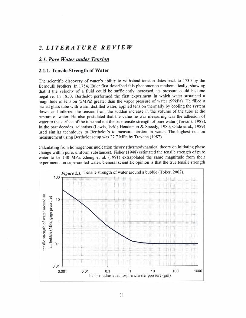
experiments on supercooled water. General scientific opinion is that the true tensile strength
Figure 2.1. Tensile strength of water around a bubble (Toker, 2002).
0)I-
C,)C,)0)I-
0)
0)
-c
100
10
1
0.1
J Ir 1 7
I '1 7 1 1 4 i I-
-- - -- - - - - -
I T
i T I I
I I T T T
-- -- - - - - - - 'T
j - - - - -
0.01 ! I0.001 0.01 0.1 1 10
bubble radius at atmospheric water pressure (gm)
--- F -
100 1000
31
r-
4-4
I - I I - I I

of pure water is not easily observeable because water fails in tension at its interfaces withother materials. Most commonly this phenomenon (termed as cavitation) occurs at air-waterinterfaces. The tensile strength of water with air bubbles can be calculatedthermodynamically in terms of energy (Fisher, 1948), or mechanically in terms of pressure(Toker, 2002) as shown in Fig.2.1. For engineering purposes, almost all observeable waterbodies have impurities (air bubbles) large enough to reduce the tensile strength down to thevapor pressure of water. The vapor pressure of water is approximately -99kPa in gagepressure (17.5 mmHg or 2.33 kPa in absolute pressures) at 20C' and changes geometricallywith temperature (Dalton, 1802).
2.1.2. Total Potential of Soil Water
The term "potential" means the amount of work required to move from a reference state tothe state under consideration. Therefore, total potential of soil water is the amount of usefulwork that must be done per unit quantity of pure water to transfer reversibly and isothermallyan infinitesimal quantity of water from a pool of pure water at the reference elevation andexternal gas pressure to the soil water at the elevation of the soil under consideration(Aitchison 1965).
The general definition of potential above includesstate of the water. To understand and account forseparated into components as shown in Figure 2.2.
various different aspects of changing theeach of these, the total potential can beWith the directions of transfer shown in
this figure, gravitational and pressure potentials are positive (i.e. work must be done on the
Soilelevation
Grav' tional
+
+
Figure 2.2. Components of soil water potential (Toker, 2002).The square water bodies represent pools of water, the curvedones represent pore water. The small black arrows show theexternal (gas) pressure, sizes of small arrows representing themagnitude of pressure. The thick (red) arrow represents thetransfer, on which the potential definition above is based. Thedots in water represent solutes.
Pressure
Matric
Osmotic
32
Soil particle
Soil
To al
Referenceelevation
4-
4-
4-
4-
EReferenceelevation
. . ........ .................. ........... .... ..

water to transfer it in the direction shown in the figure with the thick arrow), although theymay be negative depending on the elevation and pressure values. Matric and osmoticpotential are always less than zero (i.e. when the two water bodies are connected, waternaturally flows as shown in the figure in the figure with the thick arrow).
2.1.2.1. Soil Suction
Among the potential components described above, the first two (gravitational and pressure)lose their existence in the case of soil science, because soil water doesn't change elevation ata certain point under consideration, and the external gas pressure (i.e. barometric pressure)varies negligibly. This leaves only the last two potential components (matric and osmotic) ineffect, as far as soil science is concerned. The total of these two potential components istermed soil suction. It is also called total suction, moisture tension or negative pore pressure.
The exact definition of soil suction, parallel to the potential definitions above, is as follows:Soil suction, i.e. - (matric + osmotic potential) is the amount of useful work that must bedone per unit quantity of pure water to transfer reversibly and isothermally an infinitesimalquantity of water from the soil water to a pool of pure water at the same elevation andatmospheric pressure (Aitchison, 1965). Although thermodynamical aspects of the problemof soil suction (a.k.a. water tension, water potential, or capillarity) have been addressed in atheorethical manner by several scientists over the centuries (Van der Waals, 1893; Einstein,1901; Fisher, 1923; Aitchison, 1965; Coussy & Fleureau, 2002), its mechanical aspects havemostly been studied from a practical point of view.
2.1.2.2. Osmotic Suction
This is the component of suction due to solute concentration differences, and is equal to thepositive of the osmotic potential value. It can be observed in soils with soluble materials.Osmotic suction (h,) can be expressed as
h= n/V-R-T Eq.2.1
where n/V is the total ion concentration (molar), R is the universal gas constant, T is theabsolute temperature in Kelvins (Petrucci, 1989). In most practical problems encountered ingeotechnical engineering, significant changes in osmotic suction do not occur (Nelson &Miller, 1992). For this research, osmotic suction is not a factor because, as the followingsections will describe, this research focuses on physical forces in water.
2.1.2.3. Matric Suction
This is the component of suction due to physics of the water-air interfaces, and is equal topositive of the matric potential value. Any soil may have pores small enough where thesurface forces are large enough to prevent the body forces from draining the pores, i.e. thesoil has a capacity to store water. Some energy (in the form of negative pressure) has to beapplied to withdraw the water, which is held in place by the potential energy of the tensile
33

forces created due to curved air-water interfaces. These forces in the pore water are termedmatric suction. Matric suction is also called capillary potential.
Matric suction (ua - uw) is defined as the negative pressure, or tension, in the pore water. It isthe pressure difference across a curved surface, as illustrated in Fig.2.3, and can beformulated as the following chain of force equilibrium equations:
(ua-uw).p.di.r.dP = 2 .OsT.(p. di.dp/2 - r. dp.dT/2)Eqs.2.2.
(ua - uw).p. r = asT.(P - r)
ua - uw = (1/r - I/p).cysT = 2K . asT Eq.2.3.
where K is the mean curvature, and UsT is theair-water interfacial tension. Underequilibrium conditions, potential differencesare constant, therefore soil suction, and hencethe mean curvature of the interface, isconstant. Eq.2.3 is known as the Young-Laplace Equation (Laplace, 1806).
As noted by Equations 2.4 and 2.5, extremelysmall radii, high values of interface curvatureand matric suction affect even the magnitudesof surface tension and vapor pressure(Adamson, 1960). But their effect issignificant only in the case of radii ofcurvature below 10nm and matric suctionsabove 5 MPa. The suction magnitudesstudied in this thesis never exceed 1 MPa,
drq
r
Fig.2.3. An infinitesimal element of anair-water interface. r7 and pare in orthogonal planes.
and in almost all cases are smaller than the vapor pressure. Therefore surface tension andvapor pressure can be considered constant as long as temperature is constant. These effectshave been taken into account for the small radius / high tension range of Fig 2.1 using thefollowing formulae from Adamson (1960):
01Eq. 2.4.
Eq. 2.5.
where Vn is the molar volume, R is the universal gas constant, T is the temperature inKelvins, ST 0 and PvO are respectively the air-water interfacial tension and the absolute vaporpressure for a flat surface at the temperature T. Equation 2.5 is known as Kelvin Equation II.
34
CST = 0ST ' I + K- 2 x 10 (cm)
2-K-'ST- ,R-TP = PvO .e

Soil suction is important to geotechnical engineers due to the fact that strength, deformationand hydraulic conductivity vary with it. According to Rumpf (1961), suction and interfacialtension combined are one of the five mechanisms that keep particle agglomerations together(the other four are: solid bridges, bonding materials, molecular attraction and interlocking).Similarly, soil suction has an impact on shear strength, which will be discussed in Section 2.4.
2.1.2.4. Suction Measurement
In practice, soil suction is measured by many indirect methods, using correlations throughvarious measurable parameters. Different tension measurement devices are cataloguedfrequently in the literature (Fredlund & Rahardjo, 1993; Lee & Wray, 1995; Ridley & Wray,1996; Toker, 2002; Toker et al., 2004). Among the variety of techniques, only tensiometersmeasure suction directly. All other techniques measure other parameters, which indirectlycorrespond to a suction value through predetermined calibrations.
Table 2.1. Techniques of measuring or inducing soil suction.Technique Suction Parameter Measured Range
(ASTM Code or Reference*) Type (bar)Porous Plate (D2325-68) matric (i) u,= Iatm, ua controlled 0.1 - 1
Pressure Membrane (D3152-72) matric (i) u,= atm, ua controlled 0 - 15Pressure Axis Translation matric positive u, , ua controlled 0 - 15(Southworth, 1980)Filter Paper (D5298-94) matric (w) contacting paper water content 0.3 - 1000Filter Paper (D5298-94) total (r) nearby paper water content 4 - 1000
Time Domain Reflectometry matric (w) dielectric constant of device 0 - 5(Conciani et al., 1996)
Heat Dissipation Sensor matric (w) thermal conductivity of device 0 -7Gypsum Porous Block matric (w) electrical conductivity of device 0.1 - 30
Tensiometer matric water tension 0 - 0.9Tensiometer (IC, MIT, Sasktch.) matric water tension 0 - 15
Squeezing (D4542-95) osmotic ion concentration 0 - 350Humidity Chamber total (i) relative humidity of air 1 - 10000
Psychrometers total (r) temperature at evaporation 0.5 - 700Centrifuge (D425-88) matric (i) capillarity 0 - 30
The letters beside the suction type designate the following: (r) indicates that the measuredparameter correlates to suction through relative humidity of air; (w) indicates that the measuredparameter correlates to suction through the water content of the sensor, which has a unique suction -water content relationship; and (i) means the technique does not measure the suction of the soil -instead, it induces the chosen suction value in the soil specimen.
Table 2.1, presents known techniques of inducing or measuring soil suction. A suctioninducing technique can be incorporated into an interpolation scheme to make suctionmeasurements using multiple sets of equipment and specimen simultaneously (Coleman &Marsh, 1961). However, these are not useable for real-time measurements during a test on asingle specimen.
35
The techniques that are based on translation of the pressure axis rely on the assumption of airand water continuity at all times. If either phase is discontinuous, unifying the pressurethroughout that pore phase will not be possible. In addition, the methods that rely on the axistranslation principle will not simulate the behaviour of a discrete air bubble in the pore space.Under tension, instead of air entry through the surface, cavitation in pores may be initiatedfrom such air bubbles. Under compression, however, a bubble can not cavitate.
Techniques that calculate suction measurements indirectly through relative humidity, such asfilter paper method, do not provide a fine resolution (the suction difference between 99% and100% relative humidity is more than 1 MPa or 10 kgf/cm2
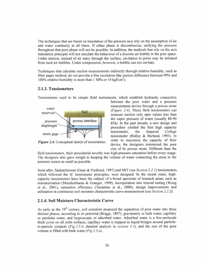
2.1.3. Tensiometers
Tensiometers used to be simple field instruments, which establish hydraulic connectionbetween the pore water and a pressuremeasurement device through a porous stone
water -(Figure 2.4). These field tensiometers canreservoir measure suction only upto values less than
the vapor pressure of water (usually 80-90pressure porous interface kPa). In the past decade, a new design and
diaphragm procedure yielded the first high capacity
strain gage tensiometer, the Imperial Collegetensiometer (Ridley & Burland, 1993). In
Figure 2.4. Conceptual sketch of tensiometer. order to maximize the capacity of theirdevice, the designers minimized the poresize of its porous stone. Different than the
field tensiometers, their procedurial novelty was high-pressure saturation before every usage.The designers also gave weight to keeping the volume of water connecting the stone to thepressure sensor as small as possible.
Soon after, Saskatchewan (Guan & Fredlund, 1997) and MIT (see Section 2.2.1) tensiometers,which followed the IC tensiometer principles, were designed. In the recent years, high-capacity tensiometers have been the subject of a broad spectrum of research areas, such asminiaturization (Muraleetharan & Granger, 1999), incorporation into triaxial testing (Wonget al., 2001), saturation efficiency (Tarantino et al., 2000), design improvements andutilization in continuous soil moisture characteristic curve measurement (see Section 2.2.2).
2.1.4. Soil Moisture Characteristic Curve
As early as the 19h century, soil scientists proposed the separation of pore water into threedistinct phases, according to its potential (Briggs, 1897): gravimetric or bulk water, capillaryor pendular water, and hygroscopic or adsorbed water. Adsorbed water is a few-moleculethick cover on all solid surfaces, capillary water is trapped in liquid bridges around particle-to-particle contacts (Fig.2.5.b; detailed analysis in section 3.1), and the rest of the porevolume is filled with bulk water (Fig. 2.5. a).
36
. ....... ..

All three portions of water are fully present in saturated porous media. Removing the water
causes an increase in matric suction. When the suction exceeds a treshhold termed the Air
Entry Pressure, it starts to lose the bulk water. Once all of the bulk water is drained
(transition from Fig.2.5.a to 2.5.b), the pendular water can be drained gradually if enough
suction is applied. Conditions short of vacuum or very high temperatures, which include
atmospheric conditions of a temperate climate, cannot separate the adsorbed water from the
solids.
Fig.2.5.a. Bulk water at air entry Fig.2.5.b. Pendular water
25
20
5 150
10
5
t
010.001 0.01 0.1
suction (kgf/cm 2)1 10
Fig.2.5.c. SMC curve analysis. Light (blue) curve is calculated for a uniform packing,whereas the dark (red) curve is from a test by MIT technique (section 2.2.2).
The relationship between the amount of water in a soil, and the associated matric suction in
the pore water is described by the Soil Moisture Characteristic (SMC) curve (Fig.2.5.c). This
amount of soil water is expressed as degree of saturation (ratio of water volume to void
37
Air Entry-- -- --- -
Pendular ringformation
--- -----
- - - -L - - - -
------ -------- ------ --- - -

volume), volumetric water content (ratio of water volume to solid volume) or gravimetricwater content (ratio of water mass to solid mass). SMC curves are widely used ingeotechnical engineering for predicting various aspects of mechanical behavior (Fredlund,2006). There is hysterisis in SMC curves between drying and wetting (for a given watercontent, a wetting curve is lower in both suction and water content).
In practice, the SMC curve is obtained in many different ways:- An equation from known soil properties, primarily the grain size distribution, from whichpore size distribution is correlated, can be devised for the SMC curve (Arya & Paris, 1981).- The SMC can be measured at a rate of about one data point per day, each data point beingobtained from a test on a different specimen, by techniques involving use of the porous-plateapparatus, pressure membrane apparatus, or filter paper (ASTM D2325-68, D3152-72 andD5298-94 respectively). To obtain the entire SMC curve takes about 10 - 15 days.- It can be measured on a single specimen by a method proposed by Lu et al. (2006), which isas slow as the conventional methods outlined above, but has the advantage of also obtaininghydraulic conductivity as a function of water content.- It can be fitted onto a few data points using one of the several - Zapata et al. (2000) reports10, Fredlund (2006) reports 12 different - curve-fitting equations. These regressions may ormay not incorporate various soil parameters into their correlations, as they cannot captureevery feature of the SMC with their 2-4 parameters.- A continuous SMC curve on a single specimen can be measured rapidly (in less than 5days), by the syringe pump method (Znidarcic et al., 1991), by a mercury intrusionporosimeter (Kong & Tan, 2000), or by the MIT technique (Toker et al., 2004; Section 2.2.2of this thesis).
2.2. Previous Research at MIT
Research relative to unsaturated soil mechanics has been continuing at MIT for ten years(Sjoblom, 2000; Sjoblom & Germaine, 2001; Toker, 2002; Toker et al., 2003; Toker et al.2004). Until 2003, the main foci of the research had been high capacity tensiometers andmethodology for obtaining drying SMC curves.
2.2.1. MIT Tensiometers
The tensiometer has been the suction measurement instrument of choice of researchers atMIT over the last ten years for its unmatched ability to measure matric suction directly. Overthe course of previous research, nine different tensiometer designs were realized. A full listof these is given by Toker (2002). All versions had the dimensions of a standard triaxial base,because the original intent was incorporation of the tensiometer into triaxial strength tests.Different types of porous stones, strain-gaged pressure diaphragms, and sealing materials thatconnect the two key components to the stainless metal body were tried in different versions.The final design among these, version 6.1, is still in use.
38

In addition to designing the devices, improvements to the performance and reliability of thetensiometers was a research focus. The resulting findings that will be relevant to this researchwere:- Tensiometers are difficult to use on drying cohesive specimen, because cohesive materialsshrink and crack while drying. This often exposes the tensiometer to the atmosphere,affecting the measurements.- Being composed of several different materials (steel, ceramic, epoxy, copper), tensiometersare temperature sensitive. Therefore they should be allowed to come in to thermalequilibrium with the environment before measurements can be considered reliable. Due tothe same reason, the environment should be kept at a constant temperature during the thermalequilibrium and measurement phases.- The pressure-sensing component has strain gage circuitry inside. As with any otherelectrical circuit, the strain gage emits energy in the form of heat. This can cause thetensiometer to be significantly warmer than the surrounding environment unless there issufficient metal-to-metal contact for efficient heat dissipation. Creating such athermodynamic gradient causes water to migrate away from the tensiometer, causing suctionmeasurements to be larger than the actual value.
2.2.2. SMC Measurement
The MIT technique (US patent no 6,234,008) is able to obtain SMC curves using one testspecimen and is faster than almost all of the conventional methods. It is the only SMCmeasurement technique that takes direct suction measurements. Furthermore, it obtainscontinuous curves, which is beyond the capabilities of the traditional ASTM techniques ofthe porous plate, pressure membrane and filter paper. In addition, the technique simulates theway soil suction develops naturally, by evaporation. This eliminates most of the problemsand assumptions required for the application of other techniques, such as those involving axistranslation (i.e., by applying positive pore water pressure and a greater pore air pressure, thismethod assumes the matric suction can be simulated by the difference between the two porefluid pressures, disregarding the fact that it fails to simulate the behavior of isolated airpockets).
For the MIT technique, the tensiometer is pressure-saturated with water in a chamber atpressure values higher than the air entry pressure of the porous ceramic. The specimen maybe pressure saturated with the tensiometer, or may be saturated separately. After a day ofsaturation, the tensiometer and the specimen are placed on a lab balance, as illustrated inFigure 2.6. Both the tensiometer and the balance are connected to a data acquisition system.As the tensiometer reads continuous suction data, the balance measures the total mass of thesystem throughout the test. At the air entry pressure of the porous ceramic stone of thetensiometer, the stone starts drying, and cavitation occurs in the water beneath the stone.After this point, no more measurement is possible without another pressure-saturation of thetensiometer, because the hydraulic connection between the soil and the pressure measuringdiaphragm is broken. The residual water content is determined at the end of each test. Themass decrements (i.e. mass of evaporated water) between the data points are then used toback-calculate the variation of water content throughout the experiment.
39

Styrofoamwalls
DataAcquisition
__________ I_ -I I
Specimen
Thermistor
fixed
Digital Lab Scale
)edj fix
~-1--j.I II II I
I I
Temperature-controlled
environment
fixed
I1DatainAcquisition
r%
Figure 2.6. Schematic diagram of the test
This method was used (Toker, 2002) in investigating;
- the effects of grain size distribution on SMC curves,- the correlation between average grain size and air entry pressure (see Appendix 2.1).
In its current form, the MIT technique is able to obtain drying SMC curves only.
Modification possibilities are being investigated to extend its capabilities to cover wetting
curves as well. Wetting SMC determination is not a part of this thesis, and thus, will not be
discussed any further.
2.3. Effective Stress
The principles of traditional soil mechanics are based on the assumption of two-phase media
(either totally dry or totally wet soil). For most soils, mechanical behavior (strength and
stiffness) is unified by Terzaghi's effective stress principle (Terzaghi, 1925; Terzaghi, 1943),
which divides normal total stress (a) applied to the soil into effective stress (a', the portion of
boundary stress carried by the solid particles) and pore water pressure (uw, the portion of the
stress carried by the soil pore water), as described by Eq.2.6.
a = a' + uW Eq.2.6.
While examining Terzaghi's concept of effective stress more closely, Bishop (1959)
analytically calculated for saturated soils that, for the purposes of solid volume change
calculations, the effective stress can be treated as independent of both the contact areas
between soil particles, and the average number of contacts per particle. He also proposed a
40
.... ..............
|
R V

way to extend the effective stress principle to partially saturated soils by the followingequation:
a' = (a - ua) -X.(uw - ua) Eq.2.7.
where a' is the effective stress, a is the total stress, ua is the pressure in the gas phase (air), uw
is the pressure in the liquid phase (water), and x is a parameter between 0 and 1. Therefore,effective stress is always larger in a partially saturated soil compared to the same soil at fullsaturation. This is valid for both cases of pendular regime at low saturation and bulk waterregime at high, but less than one, saturation levels (Fig 2.7).
Fig.2.7 Increase ineffective stress and ,
contact forces due tomatric suction inunsaturated soilst
(Yoshimura&Kato, 1998)
(a) Meniscus water (b) Bulk water
At lower degrees of saturation where there is a continuous gas phase at atmospheric pressure,when expressed in terms of gage pressure, Eq.2. 7 reduces into
a' = a -X.uw Eq.2.8.
Bishop also asserted that the effective stress equations cannot be used for fine grained soils atlow degrees of saturation. Jennings & Burland (1962) expanded this assertion intodetermination of the degree of saturation below which Bishop's hypothesis is invalid, fordifferent types of soil. Later, Richards (1966) proposed adding an osmotic term to Bishop'sequations. Matyas & Radakrishna (1968) suggested the addition of a surface tension term.They also found the usage of effective stress principle to be unsatisfactory for deformationcalculations of unsaturated clays. Despite all the shortcomings in Bishop's equation, nobodyattempted to calculate the effective stress in unsaturated soils, until recently (Likos & Lu,2004, to be discussed in Section 3.2).
2.4. Shear Strength
In 1989, Escario & Juca proposed using 2 .5th degree ellipsoidal relationships (in the form ofc1x +c2y =c3) to relate shear strength to suction, based on experimental data from threedifferent soils. Since then, there have been two fundamental approaches dominating thedetermination of shear strength of unsaturated soils. These are the effective stress approachand the independent state variables approach (both will be described in the followingsections). Both of these approaches originated from the Coulomb strength equation:
41

t = c' + cy'.tan' Eq. 2.9.
where c is the shear strength, c' is a cohesion term to signify all attraction forces betweenparticles, cy' is the effective stress normal to the shearing plane, and 4' is the angle of internalfriction.
2.4.1. Effective Stress Approach
Following Bishop's idea, the shear strength of unsaturated soils can be calculated via afailure envelope (such as Coulomb strength equation) by substituting Eq.2.7 or 2.8 into thestrength equation of the envelope. Bishop's research group tested the shear strength of avariety of soils in order to examine the relation between the z factor and degree of saturation(Donald, 1960; Bishop & Donald, 1961). Their results showed great variability from soil tosoil (Fig 2.8).
As will be shown, to date, many engineers use x values obtained by correlating from thedegree of saturation (S). These correlations had been developed by comparing strength testson unsaturated soils to the strength predicted by modifying the Coulomb strength equationwith the substitution of Eq.2.7 for the effective stress term. Some correlation examples aregiven below in increasing mathematical complexity:
- Aitchison (1960) derived the following equation, which was used by Donald (1960) in hisresults that are included in Fig 2.8.
X = u, -S + 0.3. u,- AS Eq. 2.10.0
- Oberg & Sallfors (1995) used Fig 2.8 to conclude that x can be considered equal to S forengineering purposes.
- Karube et al. (1996) proposed a linear relationship (Eq 2.11.) in which x is zero at residualsaturation (Sr) and 1 at full saturation:
S - SrX = 'r Eq. 2.11.
1- Sr- Khalili & Khabbaz (1998) examined data from over a dozen different sources and soils.They proposed a general correlation that is not based on the degree of saturation, but on theair entry pressure (uAE):
-0.55
X = .UAE Eq. 2.12.
42

MIT LibrariesDocument Services
Room 14-055177 Massachusetts AvenueCambridge, MA 02139Ph: 617.253.2800Email: [email protected]://Iibraries.mit.edu/docs
DISCLAIMER OF QUALITY
Due to the condition of the original material, there are unavoidableflaws in this reproduction. We have made every effort possible toprovide you with the best copy available. If you are dissatisfied withthis product and find it unusable, please contact Document Services assoon as possible.
Thank you.
Pages 43 - 52 are missing from the Archivalversion of this thesis. This is the most completecopy available.

2.8.3. Miscellaneous
- The difference between effective and total stress (a'-c) in an unsaturated soil will be calledeffective stress increment due to suction. It is the difference between the effective stress atthe specific suction in the porous medium and the effective stress at zero or full saturation inthe same medium.
- The narrowest cross-section of a pendular ring will be called the "neck" of the pendular ring(see Fig.2. 10) for the rest of the thesis.
- The value of air-water interfacial tension will be used as 0.00728 N/m, which is the valuefor pure water at 20'C (Adamson, 1960).
- All comments about void ratio are also valid for relative density, as they are linearlydependant on each other.
- Partial derivatives are expressed in the subscript notation. This means:
X 2 y Eqs.2.26X ax " Y X8 2
53

1001
L -- - L
- -- .. .. . .. .
0 Glass Beads (sjobiom)
Glass Beads(SMC or capfl
MFS(Sjoblom)
Fractionated RBBC
New Jersey Fine Sand
Min-u-sil 40
tion=u 1I+sin( ../2)- 3cos( ./2 ID60 os( /2)- 11
Al
- -- -- - --- - -- -- -- -- -- -
..................... r . .. .. .
Characteristic Particle Diameter, Do (pm)
4'
0
10 ------- -- --- -- -- -- rr q 1 -1. -- -- -- -- r
- - - - - - - - -- -- -- - -- -- -- - - - -
-- -- -- -- - --- - -- - -- -- - - -'-' ' : ------ M atric Su(-------- ------ ----- -- ------- -------
-r - -- ------ - T ----- ---- 1
L 11- -- -- - - - --
- -------------- 71- 6------ --------
------------- --- --------- - --------- '------------ -------
7------------ ------- --- --- I r 4------------- ------- -
------------ ------- j ----- L --- I ---
-------------------------- ----------
---------------------------- *1 :::: :1:: : : : : ::: ---- I ' -- : : j - -
....... ..... ... --- L :- --- 2: L ?7V
- - - - - - - - - --- 7 - - - - - - - - - - - - - - - - - - - - - - - - - - - ---L L
- -- -- -- --r 1-.7 -- ---- -- -- -- -- -W- - - T - - r - I -- -- -- - -- -- -- - -- -- -- - --L -I- L
- -- - - -- -- -- - -- -- --- -- --
- -- -- -- - --L - -- -- I ---- ;- I II I I -- j I
I II
- -- - -- -- --- -- -- - -- -- -- - -- -- -- --
(L10
-15-20-25-30-35-40-45
Ju-55-60
65-70
75-80
0010
0.1
w
0.01 -
0.001
r ---- n ---- r ........ r i----------------
----------------------------------
11 -,r
- - - - - - - I - - - -
r - - -- -- -- --- *-- -4- T
-------- - - -- -- ---- -- r----------- -------- --- - -----
---------------------------
- - - - - - - - - - - - - - - - - - - - --- - - --
------------- I ------- T --- I T I,- -
------------- -------
10

T H E ICALA P P R C H
55

56

3. THEORETICAL APPROACH
The theoretical portion of this research focuses on the micro-scale physics of the particle-fluid interaction. Afterwards, it seeks to upscale the analytical solutions of interparticle forcesto engineering concepts of effective stress and shear strength. For ease in formulations, thesoil will be assumed to consist of uniform, non-reactive, rigid, smooth spheres with smallenough water content to have no bulk water. For the low saturation values (mass watercontents below 5%) that are under consideration, all of the pressures acting on the solidmatrix via the water are the result of forces in pendular ring formations (i.e. all wateraffecting the behavior is in pendular rings at particle contacts). Therefore, the effective stressis expected to be dependent on the mechanics of the pendular rings.
Section 3.1 analyzes a single pendular ring and calculates a single resultant of water forces.Section 3.2 lays out a model framework of calculating the effective stress increment due tosuction using the water force resultants. Section 3.3 follows the framework to calculate theeffective stress increment due to suction, for three idealized isotropic packings. Section 3.4proposes a way to experimentally infer the effective stress increment due to suction. Section3.5 gives the very few examples from the literature comparable to this study.
3.1. The Pendular Ring
3.1.1. Exact geometry
Although Fig.2.8 depicts the pendular ring as a torus section (rotational body of a circle,rotated around an axis outside and coplanar with it) with two distinct radii, closerexamination reveals that a torus section does not have constant curvature, which - as statedin section 2.1.2 - is the case in partially saturated porous media under equilibrium. Thissection compares the actual pendular ring to the torus, in order to check the reliability ofusing the torus geometry in further calculations. In order to further simplify the equations,symmetry around the contact point is introduced by making the two particles identical.
Y (a) Torus. Y (h) General solution.
yFai.1) ygain(a)
Fig. 3. 1. Variab le s to b e us ed in the formul atio ns.
57
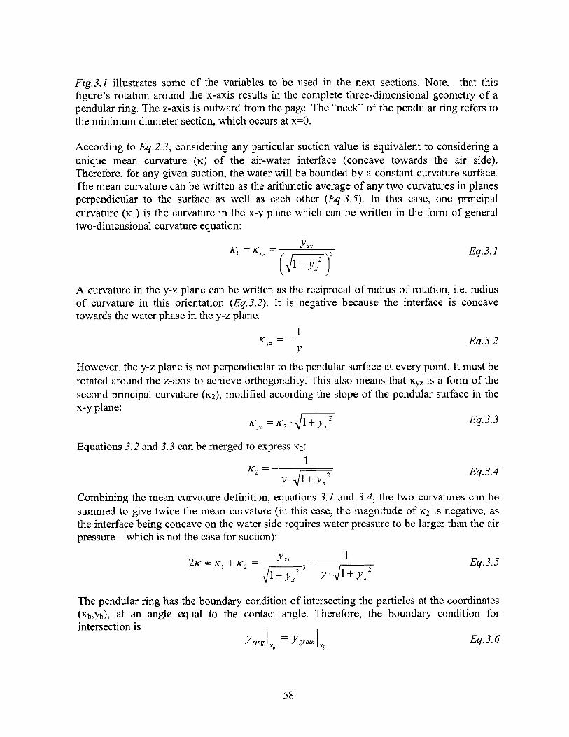
Fig.3.1 illustrates some of the variables to be used in the next sections. Note, that thisfigure's rotation around the x-axis results in the complete three-dimensional geometry of apendular ring. The z-axis is outward from the page. The "neck" of the pendular ring refers tothe minimum diameter section, which occurs at x=O.
According to Eq.2.3, considering any particular suction value is equivalent to considering aunique mean curvature (K) of the air-water interface (concave towards the air side).Therefore, for any given suction, the water will be bounded by a constant-curvature surface.The mean curvature can be written as the arithmetic average of any two curvatures in planesperpendicular to the surface as well as each other (Eq.3.5). In this case, one principalcurvature (Ki) is the curvature in the x-y plane which can be written in the form of generaltwo-dimensional curvature equation:
K1 = Kx, = +; 3 Eq.3.11+ y2
A curvature in the y-z plane can be written as the reciprocal of radius of rotation, i.e. radiusof curvature in this orientation (Eq.3.2). It is negative because the interface is concavetowards the water phase in the y-z plane.
IC = _- Eq.3.2
However, the y-z plane is not perpendicular to the pendular surface at every point. It must berotated around the z-axis to achieve orthogonality. This also means that Kyz is a form of thesecond principal curvature (K2), modified according the slope of the pendular surface in thex-y plane:
K = K2 - 1+ y 2 Eq.3.3
Equations 3.2 and 3.3 can be merged to express K2:
1K 2 = 2 Eq.3.4
Combining the mean curvature definition, equations 3.1 and 3.4, the two curvatures can besummed to give twice the mean curvature (in this case, the magnitude of K2 is negative, asthe interface being concave on the water side requires water pressure to be larger than the airpressure - which is not the case for suction):
2K = K +K 2 =_ _ 1 - Eq.3.5+ y2 y. -1+ y|
The pendular ring has the boundary condition of intersecting the particles at the coordinates(xb,yb), at an angle equal to the contact angle. Therefore, the boundary condition forintersection is
Yring IXb = Ygrain 1 Xb Eq.3.6
58

In terms of the normal vectors at (xb,yb), the boundary condition related to the angle ofintersection can be written as the scalar product of the following vectors
[("r x][(Y '"n" =(" (Yi) )* -cos 0 Eq.3.7
yring - (ygain + 1 = xy + - Ygrain x + 1 - cos 0 Eq.3.8
For spherical grains, Ygmin can be deduced as the equation of a circle from Fig. 3.1 as
Ygrain = k2xR-x 2 Eq.3.9
where the 2xR term is positive for the grain on the right, and negative for the grain on theleft. Because of symmetry, only one of the grains (in this case, the one on the right) needs tobe considered in the formulations. The positive-termed form of Eq.3.9, if substituted intoEq.3.8, results in
(Yring ) R-x 2 +1 yzng + R 2
2xR -x + COS0 Eq.3.1
Regardless of the boundary conditions, the non-homogeneous differential equation of 3.5 isnot solvable analytically (Glasstetter, 1991, attempted to solve this equation - albeit with asmall mistake - but he deemed his final equations to be solvable only by numerical means,too). However, its homogeneous solution, i.e. the solution for the zero curvature and suctioncase, is known and can be compared with the torus. This solution is called a catenoid, whichis the rotational surface created by a catenary curve. The catenary curve is the shape assumedby a uniform rope suspended from the ends. For the symmetrical case, which imposes y,, tobe zero at the mid-point, the catenary curve is described by
y = a -cosh j =a - e/Y - "e Eq.3.11
For the general case of non-zero curvatures, the shape becomes a distorted form of thecatenoid. Only the zero-curvature case is studied here for the purpose of comparison to atorus.
Since the catenary and the circular arc will not match at every point, one variable at a specificlocation (such as the diameter or curvature at the particle face or pendular ring neck) must befixed as the common parameter so that the rest of the curves can be compared. The diameterat the particle face is selected - meaning both catenoid and torus surfaces will touch theparticle at the same loci.
Substituting Eq.3.11 into Eq.3.10:
d x ___-x d ____a -cosh += a -cosh + R cos 0dx a 2xR -xb2 dx a 2 XbR -Xb 2
59

xb
a R-sin 2xb- x 2 Eq.3.12In
R.(l-cosO)-xb
Substituting Eq. 3.11 together with Eq. 3.9 into Eq. 3.6 results in
a -cosh ) = 2xbR-xb2 Eqs.3.13a oha = 2b-X
Equations 3.12 and 3.13 is an equation pair with two unknowns. The values of a and Xb canbe determined numerically. The resulting a value gives a unique catenary equation that fitsthe boundary condition in the form of Eq.3.11. In addition, now that (xb,yb) is known, theinclusive angle (a) can be determined as
a = arctan Yb arctan xbR - Xb2 Eq.3.14
R-xb R-xb
For the torus solution, the equation is
x2 +(y -r -b) 2 = r 2 _ y = r +-b -xr 2 Eqs.3.15
Through trigonometry of the problem, the parameters of the torus can be expressed in termsof angles as the following dimensionless equations:
b- = sin a + (1- cos a)- [tan(O + a)- sec(O + a)]R Eqs.3.16
-r-=(1- cos a)- sec(6+ a)R
When the preceding set of equations are solved numerically for various contact angles, thecurves in Appendix 3.1 are obtained. Contact angle can be affected by solid properties,surface roughness, and dissolved materials in water. For pure water on an absolutely cleanglass surface, the contact angle is supposed to be less than 5' (Mattox, 1998). However, thislevel of cleanness is extremely difficult to achieve and sustain (Bohren, 1987). Thecalculations in this work will be continued for 300, as an average value for water-air-glassboundaries, but the methodology is applicable to any other angle.
For a known pendular ring, its matric suction and volume can be calculated, as well as thecross-sectional area at its neck. For a contact angle of 30', there is 0.17% difference betweenthe radii of the two geometries of penduar rings at their narrowest sections, 0.34% betweenthe corresponding areas, and 0.41% between the volumes (Figure 3.2). The differencebetween the two surfaces is larger in the case of smaller contact angles, but it is less than 5%for all quantities, even for 0 = 0'. For 30', the differences are less than 0.5%. Therefore, thetorus geometry can be used with only negligible errors.
60

3.1.2. Torus Solution
Although the torus is a very close approximation to the exact solution, it is not the exactsolution. Hence, the mean curvature of a torus is not constant along the x-axis (Figure 3.3). Acurvature must be selected as a representative mean curvature for the pendular ring. In thecomparisons presented in Appendix 3.1, for all contact angles, the mean curvatures of the twosurfaces (torus and distorted catenoid) are equal at approximately x = 0.57xb , regardless ofthe contact angle. Using the curvature of the torus at this point will result in a suction valuevery close to the exact solution.
From the definition of matric suction, which leads to Eq. 2.3, and the definitions of principalcurvatures (Eq. 3.1 - Eq. 3.5), matric suction in a torus-shaped pendular ring would be
-u, = 2 K -sT = (KI + K 2) UsT
S jEq.3.17S X U.57x x 0.5 7
xb
If written in terms of angles, Eq. 3.17 becomes
a ~ST cos(+a) cos(0+a)- sec 2(0+a)-0.57 2
u. - u W= C202) Eq. 3.18R 1-cosa sina+(I--cosa)- tan(O+a)- sec 2 (+a)-0.57 2
By simple geometry from Figure 3.1, the cross-sectional area at the neck is
A = z b' 2Eq.3.19
The volume of a rotational (around x-axis) body can be calculated through integration asfollows:
V = . fy 2dx Eq.3.20
Here, the rotational body is the area between the ring surface and the grain surface. Usingsymmetry, Eq.3.20 can be written for twice the half of the pendular ring, eliminating one ofthe grains from the equation:
Xb
V = 27c - J(yyg2 - Ygrain 2 ) dx Eq.3.210
After some integration, Eq. 3.21 can be dimensionlessly expressed in terms of angles as
VR3 2 + - s a - cos a)- r -2
.[sin(20 + 2a)+ ; (20 + 2a)] Eq.3.222zR' R R 22R R2
where the fractions of dimensions are all composed of nothing but trigonometric functions ofangles (see Eqs.3.16).
61

. .. . . .........
Fig. 3.2. D 1 ffem ce s b etw een toru s an d catEn o id so lution s for 2.K =0
----------- ---....I. .. I
------------- -----------------.---- -------- ---- ------------------- ------------------------- -- - - - - - - - - ----
I - - - - r T - - - - - - - - - - --I - --
-r - - - T I - - - - - - - - T I - - - - - - - --1 - - - -:
I --- J --------
- - - - - - - --- - - - - - - i7-
Contact ang I e QO)
Fig. 3.3. V anatlon o f curv ature o f toru s w iffi I o cation
T "11 - - - T r T -1 - - - - - - r .1 - - - r - - -i - - - r T - - I - - - - - - r - - i - - "i - - - r
I I I I I I I I I I I I
-1 - - - T - - - - - --- - - - - - T I - - - - - - r - - - Ir - - I - - - or T - - I - - - - - - Ir - - -1 - - - Ir
V r - - T - - -7 - - - - - - I. Ir - - -1 - - - Ir - - T - - I - - - - - - Ir - - -r.
I I I I I I
- - -- - - - - - - r - - - - - -- - - - - - - - - - - - - - - - - r - - - - - -- - - - r
0.
L
T .1 - - - I - - - I - - - - - -
I Ir- T i - - - - - - r i - - -7 - - -
I- T T -41 - - - rI
IT - - - - - - - - - r T I - - - - - - - - - - - - Ir - - -11- - - Ir - -0 T - - -- - - --- - - I- r
.-- T --- I --- I-- T I--- r--T --- I ------ r--i --- -T--i ------ r--4 ------- r--
12 T I - - -I- r -- -- contact ang I e 0 ------ r--IT - - - - - - - - - - - - - - - - r T I
I I
_0. 1 T I - - - r
20r - P T
I I I
r -I- r I. - - - - - - -I. --- - - - - - - -30 1 1 1 1 ' I I I IT I- r - - - - - - r--. -1 - - -r T I - - - - -
I I IT -1 - - - - - - r - - - - - - r . . . . . . . r N,
-0.2.1 r "I
I I I I I
T catenold "I - - - r -1 - - - r - m -r - T i - - - - - - -- r--
--- - - - - - r - - I - - - - - - Ir - - .11 - - - - - - - - - I
Ir - - 11 - - - Ir - - T - - -11 - - - - - --- - - rI-0.3
0 0.2 0.4 0.6 0.8 1X ly-I e%
5
4
3
2
1
0
I I Ir - - - IT
---- IL --- L----I I
----I -- -
volume
area
diamet
nc
T I - - - - Ir - - -
----------
r - - - TI-----------------
1
---------------------I I I I
- - - --- - - --
0 10 z 0 30 40
62

3.1.3. Inner forces
A pendular ring pulls particles together bytwo types of tensions: matric suctioninside the ring and surface tension aroundthe perimeter. The total effect of apendular ring on a particle can beexamined by taking a cross-section at theneck of the ring (Fig. 3.4). The resultant ofthese forces is:
F = 7-b2 .(u -u )+2.r .b US-
F _ b 2 bF- r*I - 2 -R(ua - u,,)+ 2. c. -- - ST
R R R
Fig.3.4. Forces in a pendular ring (light forces).All forces in a pendular ring can bereplaced by their resultant (dark force)
particle
4'
Eqs.3.23
pendular &ig
Resultant of
water force s
According to Eqs.3.16, 3.18 and 3.23, the relation between F/R and R(ua-uW) is independentof the grain size, R. This unique relationship is graphically represented as the analytical curvein Fig.3.5. The experimental and numerical points in the figure are for the sake ofcomparison. They are from Chateau et al. (2002), who developed a numerical model forpulling two moist spheres apart, and performed experiments to validate their model, asmentioned earlier in section 2.6.2. Their results don't match exactly because the spheres theyused were 8 mm in diameter, at which scale gravity forces are no longer insignificant.
Figure 3.5. Normalized resultant water force vs suction
0.4
Z 0.35
------ An--y-----0
---- --- -- ---- --- --- --- --- - -- --- -- A n a ly tic a l--- --- --- ---- --- -- - ---- -- -- -- --- -- E x p erim e nta l '
-----A Numerical0.25
0.001 0.01 0.1 1 10 100 1000
Suction x radius (Pa.m)
63
- -- -- -------- -- ---- - -- _ - ---____ - - -

According to Fig.3.5, for a given grain size, the resultant force does not change much (lessthan 50%) over many orders of magnitude of matric suction. This is because as matricsuction increases, the pendular ring shrinks, countering the effect from increased suction.
3.2. Defining Effective Stress
Repeating from chapter 2, the effectivestress averaged over an area of aparticulate material is the vector sum ofall of the interparticle forces in a givendirection divided by the total area underconsideration (Mitchell, 1976).
If the area of consideration is selected
Effective Stress
|I L |
I Contact Force
Total StressI . . I
ResultantWater Force Contact Force
Fig.3.7. Decomposition of total stresses andforces over half of a particle
the area of the repeatable element, toobtain effective stress. These forces cannot be measured as yet, so the effectivestress can not be analytically formulated Aby such a direct approach (but they can beinvestigated via DEM simulations).
Following Terzaghi's and Bishop's logic,the effective stress can also be expressedas the total stress minus stress caused bywater. Both total and water stresses andthe contact forces associated to both casescan be assembled, as was done above forthe solid stresses. Total stresses (Fig. 3. 7)
Fig.3.6. Decomposition of solid stresses andforces over half of a particle
such that it is repeatable over a cross-section of the granular material and itcontains the full projection of exactly oneparticle by bisecting it, the effective stresscan be depicted on the free-body diagramof half of a particle as in Fig. 3.6. This is adepiction of the solid stresses andassociated portions of contact forces, but itcan also be considered as all of thestresses and contact forces in the totallydry case. At each particle contact, thecontact forces have normal and shearcomponents, whose vector sum divided by
(Effective - Total) Stress = (a'-a) = f(water)k4 4 4 k 4 14 4 A4
ResultantWater Forc
Fig.3.8. Decomposition of water stressesand forces over half of a particle
64
RZA
I I
. i .

are externally applied, known magnitudes. For small water contents, the only water forces(Fig.3.8) are provided by the pendular rings, which can be reduced to a single calculableresultant normal force at each contact (section 3.1.3). Since water forces in the case ofpartially saturated soils are tensile, effective stress is larger than total stress. Their difference(stress increment due to water) is a function of these water forces - more specifically, thevector sum of all pendular ring water force resultants acting on one half of a particle, dividedby the area of the repeatable element which contains this particle is :
Fresultant (water)
U =-0- f(water) = half-particle Eq.3.24
Aelement
This is not a practically manageable problem for random assemblies of particles, in whichcase there will not be repeatable elements, and pendular rings between non-contactingparticles will be a more frequent occurrence. A system with such complexity will not beanalytically solvable, but it may be possible to simulate through DEM. In order to beanalytically solvable, the particle geometry and coordination geometry are required for theentire particulate matrix. This is the reason for examining idealized packings in the nextsection, where all particles are identically connected and therefore representative of the entirematrix.
3.3. Solutions for Ideally Constituted Granular Materials
Any repetitive particle packing geometry is solvable, as examplified by Graton & Fraser(1935), who discussed cubic, orthorhombic, tetragonal and tetrahedral (rhombohedral)systematic assemblies of equal spheres (Table 3.1). Among these, only isotropic packings,namely cubic and tetrahedral, are considered. Anisotropic packing geometries (orthorhombicor tetragonal) may have anisotropy in the (a'-G) quantity as well, so they will not beexamined in this research. With isotropic packings, (G'-y) will be calculated in differentdirections, to be compared to each other.
Table 3.1. Systematic packings of uniform spheres (the italic entries arefrom this work, the rest are from Graton & Fraser, 1935)
Packing Isotropy Void ratio Co-ordination numberCubic Yes 0.910 6Orthorhombic No 0.654 8Body-centered cubic Yes 0.470 8Tetragonal No 0.433 10Tetrahedral Yes 0.350 12
The description and associated figures of the three packings below follow the same format.In the Figures 3.9 to 3.11, darker arrows indicate forces out of the plane of the page andlighter arrows denote forces into the page. Solid (red) arrows are the forces acting on one half
65

of the central particle, whereas dashed (blue) arrows show the remaining forces at contacts(symmetrical forces acting on the other half and forces in the plane of consideration). Themagnitude of the resultant force of a pendular ring at each contact is F. In the figures, inorder to avoid complicating the view, the particle is not shown. Instead, all F forces aredrawn at a length equal to the particle radius. D is the particle diameter.
3.3.1. Cubic packing
Cubic packing, also called "isometric" packing, is the most basic idealization, constructed byplacing a particle at every corner of an imaginary cube with side length equal to D. It is theloosest stable packing of confined uniform particles. All angles between the 6 contact pointsof each particle are 900. The porous matrix consists of an octahedron-shaped pore for everyparticle, resulting in a porosity of (1-n/6) = 0.476.
Fig.3.9.b presents a plane bisecting four of the neighboring particles. This plane hassymmerical copies in two other orientations. The repeatable area of the plane ofconsideration is a DxD square. There is only one F acting on half of the particle, and it isperpendicular to the plane of consideration. This results in
a _= F D 2 Eq.3.25
A second possible solution is illustrated in Fig.3.9.c, as a plane that bisects two neighboringparticles and separates the remaining foursymmetrically. This plane has symmerical copies infive other orientations. The repeatable area of theplane of consideration is a DxD2 rectangle. Thevector sum of the two F's acting on half of theparticle is F12. This agrees with Eq.3.25 byresulting in
D 2 = D2 Eq.3.26
Fig. 3.9. Cubic packing
F(b)
goo No WO OW
66
........... .....

3.3.2. Body-centered cubic packing
This packing will be called "8-contact packing" for the sake of convenience through the restof this work. Counterintuitively, this packing can not be constructed using an octahedron. Ifthe particles are placed at the corners of an octahedron, the resulting arrangement is a rotatedform of the tetrahedral packing. It is not orthorhombic packing either, it is significantlydenser and isotropic.
The only way to evenly distribute 8 contacts overevery particle in the matrix is by placing theparticles at the centroid and all corners of a cubewith the side length of 2D/N3. In this packing, allangles between the 8 contact points areapproximately 700. The porous matrix consists ofone and a half "short square prism" - shaped poresfor every particle, resulting in a porosity of (1-irl3/8) = 0.320.
Fig.3.10.b demonstrates a plane that does notintersect any of the neighboring particles, dividingthe contacts into symmetric groups of four on eachside. This plane has symmerical copies in two otherorientations. The repeatable area of the plane ofconsideration is a square with sides equal to 2D/I3.The vector sum of the four F's acting on half of theparticle is 4FN3. This results in
-= DFV Eq.3.27
A second possible solution is depicted in Fig. 3.10. c,as a plane that that bisects four neighboring particlesand separates the remaining two symmetrically. Thisplane has symmerical copies in five otherorientations. The repeatable area of the plane ofconsideration is a rhombus with each side D anddiagonals 2D/13 and 2D12/13, respectively. Thevector sum of the two F's acting on half of theparticle is 2F12/N3. This agrees with Eq.3.27 byresulting in
2F4J
0-'-0- = =%3 . F/21 2D 2D /2 V3 V-
Eq.3.28
(c)
Fig. 3.10. 8-contact packing.
67
. .................... .....
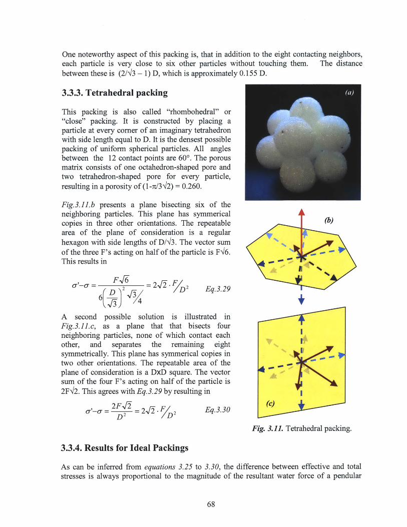
One noteworthyeach particle isbetween these is
aspect of this packing is, that in addition to the eight contacting neighbors,very close to six other particles without touching them. The distance(2/N3 - 1) D, which is approximately 0.155 D.
3.3.3. Tetrahedral packing
This packing is also called "rhombohedral" or"close" packing. It is constructed by placing aparticle at every corner of an imaginary tetrahedronwith side length equal to D. It is the densest possiblepacking of uniform spherical particles. All anglesbetween the 12 contact points are 600. The porousmatrix consists of one octahedron-shaped pore andtwo tetrahedron-shaped pore for every particle,resulting in a porosity of (I-7/3V2) = 0.260.
Fig.3.11.b presents a plane bisecting six of theneighboring particles. This plane has symmericalcopies in three other orientations. The repeatablearea of the plane of consideration is a regularhexagon with side lengths of D/N3. The vector sumof the three F's acting on half of the particle is F'6.This results in
-'-D- = 2.J2 - D2 Eq.3.29
A second possible solution is illustrated inFig.3.11.c, as a plane that that bisects fourneighboring particles, none of which contact eachother, and separates the remaining eightsymmetrically. This plane has symmerical copies intwo other orientations. The repeatable area of theplane of consideration is a DxD square. The vectorsum of the four F's acting on half of the particle is2F12. This agrees with Eq.3.29 by resulting in
---=2F.J = 2-J2 -D22.i Eq.3.30
(b) 4
so4 0 0
4
(C)
Fig. 3.11. Tetrahedral packing.
3.3.4. Results for Ideal Packings
As can be inferred from equations 3.25 to 3.30, the difference between effective and totalstresses is always proportional to the magnitude of the resultant water force of a pendular
68

ring. This would dictate the nature of the relation between matric suction and a'-Y (Fig. 3.12)to be of exactly the same shape as the matric suction versus resultant force curve (Fig.3.5).
In the case of each packing, per each repeatable element (i.e. particle), the number ofpendular rings with calculable volumes is equal to the number of contacts. Therefore, thetotal volume of water per unit soil volume can be calculated for a given pendular ring size,which leads to engineering variables such as water content, suction - and through Fig.3.12and 3.13 - increment in effective stress. Note that these plots are for a contact angle of 300.Equivalent plots for 0 = 0', provided as Appendices 3.2 and 3.3, show a difference of about15% in (&'-a), with the smaller contact angles resulting in larger effective stress increments.
Figure 3.12. Normalized stress increment due to water vs. Matric suction,
both normalized by particle radius.300
25-
1 -I - - I - I - I - I
15- L - - - - - -- - - - - - - -- - -
2 150 IIT I I I I I TT ___
10- -1 I - - 1 1T 1 F1r
1200 9LLLLI __
0 50
0
- - - - T -- ------ - T etra he d ra I- r-- - 11 F -- 7 --- T-1 ___T _ 22 - r
r WI rL W L -T - -- - - 8-contactCubic
T T F T
10 100 1000 10000 100000 1000000matric suction x radius (Pa.mm)
For gravimetric water content calculations, the particles are asumed to have a specific gravityof 2.2 (as given by the manufacturer in section 6.1.1.2). Fig.3.13 shows the stress incrementdue to water not to be significantly affected by changes in water content. Note that thecalculations are for the well-defined geometrical shape of a pendular ring. As the watercontent and the size of pendular rings approach zero, these calculations will no longer holdfor the new form of the problem concerning only a few water molecules. Figure 3.13represents this as a singularity point for pendular water content of zero.
The residual portions of the SMC curves of the three uniform packings is plotted in Fig.3.14.It should be noted that these curves would be for both wetting and drying in the case of cubicand tetrahedral packings (that is, if the wetting and drying contact angles were the same). Incase of the 8-contact packing, the curve represents only the wetting curve at lower suctions,as the drying curve would be higher in water content below a certain suction value. This is
69

because during drying there will be water pendular rings between non-contacting particlesthat are close to each other.
Fig.3.13. Gravimetric water content in pendular rings, for glass materialvs. Normalized stress increment due to water
300
250
200
150
100
50
0 60
gravimetric water content (%)
Fig.3.14. Residual parts of normalized SMC Curves for glass particles
5I_1 -I J 1- - - - --_-_- --F-F F
SII I
F I F F F I I I F I
C -- -------- -- ---- --- L-L -L - -Tetrahedral I-4
-- - - -- -- - 8-contact L>I I11 | i i| t
0 1 F T-1- ~i
------------CIOl - - - - -1-A1 -1 -L-
F I F I F F I II
I----------------I __L__-- -_L_ I F L III
-1--I- -- I F F I-i-II
2>11F F F F I F F I I F I V I
E ----- F--- --------- -
O - -- - - F - 1 - - I I - - -
10 100 1000 10000
matric suction x radius (Pa.mm)
1 2 3
70
4
E-E0.
x
-I
- Tetrahedral-8-contact
Cubic
.1 4 L. I.
-
1
-
5

3.4. Shear Strength
3.4.1. Unification of Approaches
Before taking any step towards estimating the shear strength of partially saturated materials,it is necessary to examine and compare the two approaches that are described in section 2.4.Followers of the effective stress approach calculate strength by substituting Bishop's Eq.2.8into the Mohr-Coulomb strength equation (Eq. 2.9) , which results in
T := c' + [(a - ua) -X.(uw - ua)].tan)'Eqs.3.31
-= c' + (a - ua).tan ' + (ua -u).X.tan '
The shear strength suggested by the independent state variables approach is
T- = c' + (a - ua)tan*' + (ua - uW)tan~b' Eq. 3.32 (Eq. 2.13)
which seems to suggest that this would be a better approach if a unique Ob' could be obtainedfor each soil, i.e. if the failure envelope was planar in (an-ua) - (ua-uw) -- T space. Non-linearity of the failure envelope in the (ua-uw) - T plane was shown by Escario & Juca (1989)and also noted by the founders of the independent state variables approach, Fredlund et al.(1987). This agrees with the model framework proposed in this research, which results in anon-linear relation between suction and effective stress (Fig. 3.12). In order to make Eq. 3.32easier to use, Fredlund introduced a new parameter, aw, such that
tanb' = aw . tan' Eq.3.33 (Eq.2.14)
If Eq. 3.33 is substituted into Eq. 3.32, Eqs. 3.31 are obtained with X=aw . Since in essence theyare both used as empirical fitting parameters, there is no proof of inequality of theseparameters. Over the past decade numerous researchers suggested similar physicaldefinitions for both aw and x, as well as identical correlations and methods to obtain themfrom tests (Section 2.4; compare Eq. 2.11 to 2.16, or 2.12 to 2.17, for example).
Therefore, it is the author's understanding that these two parameters are the same singleparameter. Furthermore, the fact that both approaches use (an-ua) and (ua-uw) as independentstate variables leads to the following result: Bishop's effective stress approach andFredlund's independent state variables approach are two different ways of expressing a singleunified approach.
However, this result does not shadow either one approach, as long as the approaches arestudied in the context of the chronology of their development. Bishop's effective stressapproach was originally suggested in an abstract fashion, whereas Fredlund's independentstate variables approach arose from the need for an empirical and testing-based method thatis able to represent soil behavior better than Bishop's approach. Eventual convergence of theempirical approach to its hypothetical counterpart shows that the effective stress approach
71

was as much on the right track as the independent variables approach, in addition to being thephysically more sensible approach.
3.4.2. Hypothesis Linking Effective Stress to Shear Strength
When the strength gain due to suction is discussed in the literature, it is usually in terms of anadditional cohesion for the same total stress state. Since the line of thought detailed in thisthesis follows the effective stress approach's logic, the effective stress is defined as the statevariable governing behavior. This means that gains in strength are expressed using terms ofgain of effective stress (i.e. a'-a) instead of increasing the cohesion. These areinterchangeable views (just like the two approaches discussed above) through the followingequation
C' = (a'-a).tan<' Eq.3.34
but one has the advantage of making more physical sense than the other. In both views, thesame magnitude of suction is supposed to contribute to the same increase, regardless of thetotal stress, resulting in parallel failure envelopes and a unique angle of internal friction foreach soil. This will be the basis for the experimental validation of the model.
Figure 3.15 illustrates the validation plan using aOU - q stress paths. The strength parametersof the Mohr-Coulomb failure envelope will be determined by running drained triaxialcompression tests on saturated specimens (1). Results of the triaxial tests on unsaturated
Aq
Failure envelope,determined by
(a'-a) interpreted saturated testsTotal stress path, from this test
imposed by 3unsaturatedtriaxial test
Apparentunsaturated
effective stresspath
[cT , GoCt'(a-)from the,
model (sec. 3.3) o ar
Figure 3.15. Graphical representation of the model validation through laboratory tests inaoct - q stress space. The numbered steps are discussed in the text.
72
......................

specimens (2) will be used to back-calculate the actual effective stress at failure by equatingthe horizontal distance between the failure point on the total stress path and the failureenvelope (3). The new hypothesis will provide the theoretical (effective-total) stress based onthe water content, suction and density (4). Comparison between these two effective stressvalues will provide the basis for model evaluation.
From this point onwards, the word model will be used for the framework for analyticallyestimating the effective stress increment due to suction, proposed in sections 3.2 and 3.3. Theword hypothesis will be used for inferring the effective stress increment due to suction, fromthe saturated and unsaturated shear strength envelopes, proposed in section 3.4.2.
3.5. Solutions by Other Sources
From their experiments and numerical calculations, Chateau et al. (2002) report that, themagnitude of the water force resultant varies very little for particles in contact, and is slightlylarger for smaller water contents. For separating particles, the force diminishes much quickerfor systems with less water, which means for a given separation distance, the water force issmaller in most cases with decreasing water content. Simulations by Yang et al. (2003) showlarger forces for increasing water content, which agrees with Chateau's results for the case ofnon-contacting particles.
In 2004, Likos & Lu attempted to analyze the effective stress using a similar logic to the onepresented in section 3.2. In order to avoid geometrical complexity and particle coordinationissues, they simplified the problem by dividing only one resultant pendular force by thecross-sectional area of a single particle. Since both variables (IF and Aeiement) in Eq.3.24were calculated in a fundamentally incorrect way, their solution is not reliable. However,since they erred in similar proportions on the lower side of both the numerator anddenominator of the ratio, their solution can be expected to give values close to thosecalculated in this research.
Sako et al. (2001) derived the following equation for the apparent cohesion due to suction:
c'= _ -F( 1 - 3 -tan#' Eq.3.35;r-2 1+e i-D 2 ).
where o is the number of contact points per particle (i.e. coordination number). In order tocompare with the results from section 3.3, Eq.3.35 can be rewritten, by use of Eq.3.34, as:
3 . co_ F 2 Eq.3.36ir-2 l+e ED
Respectively for cubic, body-centered cubic and tetrahedral packings; when coordinationnumbers of 6, 8 and 12 are plugged into this equation with corresponding void ratios, theresults are 8.26 times larger than the results from section 3.3, for all three cases.
73

0.9
0.8
0.7
0.6
0.5-
0.4-
0.3
0.2 -
0.1 -
F F
F F
T - -1
F F
F F-F
F F
F FV-T
F IF-T
F F-TF |
F F
F F i
---- 1I -F 1--
- -1 - -I-- -i- - -
F I--- 1- -F -- -
F I I I
- - - - -
I F
I I
I I
F I
F I
F I
I I F
I F
- I
I I
0.1
F F F F
F F F F
F F F F
F F F F
F F F F
F F F F
F F F F
F F F F
F F F F
F F F F
F F F F
F F F F
F F F F
- - ~F - - F~ - T - -
F F F F
F F F F
F F F F
F F F F
I I
1 1
I I
F II-- 1 - - - -
T
- T -I I
- - -F
S I I
F--
F--- t -- -F-- - - -
1 - F1 -F- 4- --
S--- - - - - - -F - -L
L I
F - -i- - - i F F F1 - - -
I I
F L - - -4- - - --- F 4 -- F- L- - -
F F F F F F
LJF L - - L- - -L
F F F F F F F F
S I Li F I
F F
--
-- F-- - I
-- F -F - - F ---
F4F
- 4 --- F - - -
- F _ -FL-i1-
F F
- --- - L- _ _4
4--I 4- -4-
- _- _-_1 - L _ l4 -
- I
- - -- L
0.2
-- grain FLF F
F F
- catenoid _____F F
F Ftorus F FF F
F F
F F F F F F
F F F F F
F F F F F
F F F F F
F F F F F F
F F F F F F
F F F F F F
F F F F F F
F F F F F
F F F F F F
F F F F F
F F-- V - -
F F
F
0.3
- F - F ~
-- -F -1
-- -F- - F- - -F - -- -
- -F- - - - 1F - -F-
F - - -F
F F F F
-- -F - -F - -F- -
- -F- - F- -- -- - -F- -
- -F- - F -- FJ - -F- -
- -F- - F- - -- - -F- -
- -F- - L- - J - -F
. -F_- -- F - 4 - -F- -
- -F- - L- _ _ --
- _ F _ L - J - F -
F F F F
-F F - I-F-
-- F- 4--I- F-
- F 1
F F F 'F
0.4
74
Apndices
y
3.1. Catenoid and torus solutions for various contact
angles. Dimensions are in terms of grain radius.
F F
-- F
F1F
F F
0
0
V
0.5
. ............. .
I
1.
I - -I-

Appendix 3.2. Normalized stress increment due to water vs. Matric
suction, both normalized by particle radius. (0= 00)400-
1 LU I I L L- Tetrahedral-1 - - -1-1 -- 4 1- - - - - - -I- -14 -4 -44- - - -I - - 4 4 4- - 1 - - - - -- - 1 - 1
- 8-contact --- - - ----E- T -I -- -t Cub1 ---E 0 -i I I I _ I I I I I I I I I
| | | |II I 11 1 I I 11 1 I lII I I I lii I I I 1
2U 20 I 11 I1Wl- - - - -1 - - - - - - -- - - - , - T 1 - I- - I- - - - - - -
I I 1111 I I I 1 1 I I 11 11I 11111 I I I |
100
I I I 111 ~ I I I II I 1 11 I 11111 I I 11111
UI I I1111 I I I I 11111 I I I ______
I 1 1 1 I I I 1 11 IL 1141 -. 1 .1 I- 11- 1 -114
I - 1I I I 11 I- I 11111 I I 111 I 11 11 1 11
-- T -I-r - - - - - - - I|| r - -1- T -1 -1 7 T I - - T T -r - T1 -1 F T 1- 7 T rI-T
I | l I | l III I 1111 I I I 11 1 I I 11 1 I 11 11 I I I |
0 | ii I 111 I I 111 I I 1111 I 111111 I I I i
10 100 1000 10000 100000 1000000matric suction x radius (Pa.mm)
Appendix 3.3. Normalized stress increment due to water vs. Gravimetric
E~
.-
.01%Uo
water content in pendular rings, for glass material. (0 = 00)A0
- Tetrahedral8-contact
-Cubic300
200 -
100
I. -~ I.U
54210gravimetric water content (%)
75
3
- - - -------

76

77
E UI' P N T

78

4. EQUIPMENT
4.1. MIT Tensiometers
For the research on soil suction at MIT, nine versions of tensiometers were developed by Dr.Kurt Sjoblom (Sjoblom, 2000) and later the author (Toker, 2002). This was an evolutionaryprocess, in which each new design attempted to improve on an aspect of the previoussuccessful version. The last of the line prior to the research associated with this thesis wasVersion 6.1 (section 4.1.4.1).
Four new versions were developed during the course of this research. A summary of thevarious characteristics of these recent tensiometer designs are presented, together with thecharacteristics of Version 6.1, in Table 4.1. As far as the versions detailed here are concerned,the first digit of the version number designates the tensiometer's body geometry, and thesecond digit designates the type of porous interface (0 for Soil Moisture Corporation stone, 1for Kochi University ceramic, 2 for Vycor porous glass). In the rest of the text, TensiometerVersion 6.1 will be abbreviated as T 6.1, Version 7.0 will be abbreviated as T 7.0, and so on.
Table 4.1. MIT Tensiometer history/statistics/performance/advantages and disadvantagesover former models.
Inter Highest Pressure Advantages overface suction Transducer Disadvantages prior versions
T 6.1 2000 Kochi 13.2kgf/cm 2 200 psi Not a triaxial pedestal Replacable transducer
T 6.2 2003 Vycor 24 kgf/cm2 200 psi Saturation difficulty, Highest capacityplate fragile, slow response in MIT
T 7.2 # 2005 Vycor 2 kgf/CM2 1000 psi as T62, low resolution, convenience in therod problematic interface saturation setup
as T7.1,T 7.0 2005 SMCo 0.8 kgf/cm 2 25 psi Low capacity hg TIo
I high resolutionas T7.2,
T 7.1 2006 Kochi 4.3 kgf/cm 2 200 psi None .a Tu.putriaxial setup use
*: versions ordered chronologically, not by number.#: the design was abandoned because it could not fulfill its design purposes.
In addition to the common design properties and materials below, another noteworthy detailof all of these versions is the rounding of the rim of the top face (see Figure 4.1). This isdone to prevent this rim from cutting into o-rings (in case of SMC tests) and impermeablemembranes (in case of triaxial tests).
A tensiometer can take measurements as long as the matric suction remains below a certainvalue (tensiometer capacity). The capacity of a tensiometer depends on the saturationprocedure (applying greater vacuum and saturation pressure) and the porous interface (largestpore size).
79

4.1.1. Porous Interfaces
The working principle of a tensiometer is to establish a hydraulic connection between thepore water and a pressure measurement device through a porous interface that is attached tothe tensiometer body with epoxy.
4.1.1.1. Soil Moisture Corporation Stone
This type of porous interface has widespread usage in suction measurement. Since longbefore the invention of a high capacity tensiometer, this type of material (known as a high airentry ceramic disc) has been used in pressure plate tests. Soil Moisture Corporationmanufactures ceramics with a variety of air entry pressures and pore sizes. The porous stoneof T7.0 was cored out of a 1-bar air entry disc, whose average pore diameter is 2.1 pim(Fredlund & Rahardjo, 1993).
4.1.1.2. Kochi University Ceramic
These porous materials (Table 4.2) were manufactured by Prof. Kazumichi Yanagisawa ofKochi University, Japan, as a part of his research on ceramics (Yanagisawa, 1994). TheKochi Ceramics are manufactured by hydrothermal sintering of silica gels, resulting in fusedceramics of very fine pore distributions (30-80nm average pore diameter, 3-22 kgf/cm2 airentry pressure). Their advantages over the commercially available SMCo. stones can besummarized as providing the possibility of higher capacity, better inter-pore connectivity(easier saturation, without back-pressure) and compatibility with the pressure transducers forsaturation purposes (For a detailed study, refer to Sjoblom, 2000).
Table 4.2. Preparation and usage of the Kochi silica compacts (from Toker, 2002).Production at Kochi University Tensiometer use at MIT
Water (%) T (C) Preload (MPa) Time (min) Sinter (MPa) Time (min) Year Used in AEP (kgf/cm2)4.45 300 20 60 1998 T7.1 4.310.2 300 60 10 2 60 1999 T6.1 3 -15
Previous research (Toker, 2002) observed three drawbacks of Kochi ceramics. Since theresearch in Kochi University was not commercialized or standardized, their ceramicproperties proved to be unpredictable. The second drawback of Kochi ceramics is a durabilityproblem, which is specifically micro-cracking due to sudden changes of water tension uponair entry. Hence, the stones may start to disintegrate after any number of tests. Thirdly, theKochi ceramics are available in very scarce quantities, for they were prototype products ofresearch, that has not been pursued since 2000.
4.1.1.3. Vvcor@ Porous Glass
80

Vycor Porous glass (Table 4.3) wasdeveloped by Corning, Inc. (Coming,NY). For this research, pieces of thematerial were ordered with specifieddimensions, from Advanced Glass &Ceramics (Holden, MA). This materialwas purchased as cylinders withdiameters of 1 cm (20 pieces) and 2cm (1 piece). The 2 cm cylinder wascored out of a glass manufactured as aplate, whereas the 1 cm cylinders were
Table 4.3. Specifications of Vycor Porous Glass7930 (from www.corning.com)
Dry specific gravity:Porosity:Specific surface Area:Avg. pore diameter:Avg. Modulus of Rupture at 25*C:Modulus of Elasticity at 25*C:
1.50.28250 m 2/g4 nm420 kgf/cm 2
175000 kgf/cm 2
slices of a glass rod of the same diameter. An unidentified planar impurity from themanufacturing process is visible within the rod slices. The low suction capacity of the rodslice indicates that (at least part of) this visible impurity is a continuous planar pore, makingthe rod slices unusable in high capacity tensiometers.
It should be noted that the permeability of both types of Vycor glass is observed to beextremely low from the beginning of saturation, as the water front takes more than one hourto pass through the glass with a pressure difference of several atmospheres when filling thetensiometer. Nevertheless, once saturated, the response time of tensiometers with Vycor glassto changes in pressure/suction was less than a minute. Therefore the glass might have somepromise of future use in high capacity tensiometers.
4.1.2. Epoxy
The adhesive used for fixing the porousstones to the tensiometer body is Table 4.4. SpecificationsLoctite@ E-90FL Toughened, flexible, Durabond (froimpervious and impactresistant Durabond@ Epoxy Adhesive Viscosity:(see Table 4.4 for properties). This is a Hardness, Shore D:different adhesive than the epoxy used Shear Strength:in the tensiometers of the prior research Peel Strength:(versions 6.1 and earlier used Stycast Pot Life:2651MM, which is a more rigid epoxy).The Loctite E-90FL epoxy was primarily chosen for its flexibility,bending moments within the porous interface during high tension.
f Loctite E-90.n mymatweb. com)
71500cP6070-211 kgf/cm2
0.9-7 kgf/cm90 min
in order to reduce the
4.1.3. Metals
The tensiometer body is Stainless Steel 304 (see Table 4.5 for properties). A copper gasketprovides the seal between the pressure transducer and the stainless steel body.
Unlike rubber seals, a copper vacuum gasket seals by yielding under compression.Concentrating the stress on the sharp edges of the seal, which are pressed on the surfaces tobe sealed, usually guarantees yielding. Copper Alloy 110 (Table 4.5.), which was the copper
81

alloy available at MIT Civil and Environmental Engineering Department machine workshopat that time, was used for this manufacture.
Table 4.5. Properties of Copper Alloy 110 and Stainless Steel 304(from www.efunda.com) Cul1O S.S.304
Specific Gravity 8.8-8.94 8Poisson's Ratio 0.34 0.27-0.3Young's Modulus (GPa) 117 193Yield Strength (MPa) 69-365 205Ultimate Strength (MPa) 221-455 515Thermal Conductivity (W/m0 K) 390 16.2Thermal Expansion (10~6/oC) 16.9 17.2
4.1.4. New Tensiometer Designs
4.1.4.1. Tensiometer Generation 6
The design purpose of Version 6 tensiometers was to have a device with a replaceablepressure transducer, and to minimize sensitivity to temperature changes (Toker, 2002; Tokeret al., 2004), for usage in SMC curve measurements. It incorporated two essentialcomponents (a copper seal and tightening nut) to achieve these goals (Figure 4.1).
4-
(b)Flexible
__Epoxy*
HardEpoxy
(a)CopperSeal
Steel Body
----Threads
Tightening Nut~hexagonal)
'***Data Acquisition
82
Vycor plate
Koch Ceramic
Pressure
Transducer
.. ............ ........... I..

Figure 4.1.(a) MIT Tensiometer 6.1 (Toker, 2002) (b) MIT Tensiometer 6.2 (c) Copper seal.
Version 6.2 aimed to increase the capacity for suction measurement by replacing the porousinterface (Kochi ceramic) with a material that has finer pores (Vycor glass). Two othermodifications were incorporated with the purpose of countering the brittleness of the glass.First, the glass was installed with a slight recess from the top surface (Figure 4.1. b), becauseit is not machineable (The other porous materials are installed at an equal or higher level tothe top surface, and then the entire top surface of stone, epoxy and steel is machined flat).The second difference is the use of a flexible (and also machineable) epoxy to reducebending moments on the Vycor, as mentioned earlier in section 4.1.2.
4.1.4.2. Tensiometer Generation 7
Although the top face of the generation 6 tensiometers was of triaxial diameter, theirgeometry had some compatibility issues with incorporation into a triaxial setup. Thegeometry of generation 7, i.e. the tensiometer body that would act as triaxial pedestal, had tobe changed to have constant diameter through its length. Its bottommost part is shaped as ahexagon for gripping purposes to hold it in place, while it is fixed to the triaxial base fromthe underside. The lower surface also has a groove for an o-ring, which establishes a sealbetween the base of the triaxial cell and the tensiometer. The tightening nut of generation 6 isreplaced by a threaded pipe with a hexagonal mid-section, in order to fix the pressuretransducer into the device. On the bottom end, a nut fits on the threads of this pipe in order totighten the whole assembly together.
a)Flexible
EpoxySMostn
)per Seal --"Pressure
TransducerBody -------
(b)
[Kochi ceramic 1
7cor ro~
I(Yc)
()-ringBasetriaxia
DataAcquisition
Figure 4.2.(a) MIT Tensiometer 7.0 (b) MIT Tensiometer 7.1 (c) MIT Tensiometer 7.2.
83
Steel
. .................. ...... .......... -- --____ -
Co
SPipeThreads

It is imperative to tighten the threaded pipe into the tensiometer with a much larger force(two large wrenches or a lathe) than that used on the nut to fix the tensiometer to the triaxialsetup (tighten by hand). Otherwise, the copper seal within the tensiometer may break contactand thereby be rendered useless.
4.2. Saturation Setup
Figure 4.3.Saturation setup
air / vacuum- water--- data / signal
pres. transducer
G valve
Arrows show flowdirections.
Deaeration Pressure-Tank Volume ------- <
Device
G-- .- - - -
Voltagesupply
Centrifugal ------------Vacuum GPUp I Pressure
Chamber Oil(tensiometer Vacuum
Water inside) PumpTank_____ _
In order to eliminate the risk of cavitation in thetensiometer, its pores and gaps must be filled with purewater without air bubbles. This is achieved by firstevacuating the air molecules by vacuum, then filling withdeaired distilled water, and then pressurizing the water toabout twice the capacity of the tensiometer. The laboratorysetup for saturation is illustrated Figure 4.3. The processwill be detailed further in Chapter 5.
4.2.1. Pressure Chamber
The standard triaxial pressure chamber is large enough(~700cc) to enclose both the tensiometer and its specimen.This gives the opportunity to pressure - saturate thespecimens, opening the possibility of preparing thespecimen under a variety of conditions. The saturationchamber has multiple in/outlets. A vacuum is appliedthrough top outlet, whereas the distilled deaired watersupply and pressure control is connected to the base.
84
Analog-Analog
FeedbackControl
'------------
I

111 II 'III I 1 1 1 E 111E11111 ~7UL -- -
4.2.2. Vacuum Pumps
As shown in Figure 4.3, two vacuum pumps were used in the saturation setup. The oneconnected to the deaerator is a centrifugal pump driving a water-vacuum aspirator. Itcirculates water in a plexiglass holding tank, which is cooled by tap water. The pump that isused for evacuating all other equipment is an oil vacuum pump, which creates a vacuum withan eccentric cam. The centrifugal pump can draw the pressure down to the vapor pressure ofwater, whereas the oil pump is capable of reducingthe pressure down to the vapor pressure of oil, whichis about 1000 times smaller than that of water.
4.2.3. Deaerator
The Nold Deaerator is a plexiglass cylindrical tank ofabout 4 liters volume. It has a water pipe and an airpipe, connected to the bottom and top of the tank,respectively. It also contains a rotating disc on thebottom inside, for cavitating the water to free the air.
Ball Screw4.2.4. Pressure Volume Actuator altuatr
The Pressure Volume Actuator is standard equipmentthat had been designed (Andersen, 1991) and hasbeen widely used in the MIT GeotechnicalLaboratories. It consists of a 0.75-inch (19mm)diameter steel piston, a ball screw actuator (section Piston4.2.4.1) that moves the piston, and a DC servo-drive Chambermotor (section 4.2.4.2) that drives the worm of theball screw actuator. The combined mechanicaladvantage of the servo-motor and the actuator givesthe PVA the ability to pressurize upto 175 kgf/cm2. itness
TansducerPeripheral equipment can be attached to parts of thispiece of equipment. In the case of the saturation setup,a 1000-psi (70kgf/cm 2) pressure transducer (a.k.a. Figure 4.5. Pressure-Volume
witness transducer) is connected to the PVA's outlet Actuatorto monitor the pressure (Figure 4.5). The two PVAsof the triaxial setup (Figure 4.9) each have a fluid reservoir at their outlets (the cell PVA hasan oil reservoir, the pore PVA has a water reservoir). In addition, the pore PVA has adisplacement transducer installed in parallel to its piston, for the purpose of volumemeasurement.
85

4.2.4.1. Ball Screw Actuator
The rotational movement supplied by theservo-motor is converted into a translationalmovement of the piston by a ball screwactuator. This mechanism is model 28630,manufactured by Duff-Norton, Charlotte, NC(Table 4.6).
4.2.4.2. Servo-Drive Motor
The necessary piston force inall PVAs is exerted bypermanent magnet, brushtype,DC servo-motors, which aremanufactured by Electro-CraftServo Systems, Eden Praire,MN, as model E352 (Table 4.7).The motor powering the triaxialloading frame is Electro-CraftE586. It is likely thatproduction of these modelshave been discontinued.
4.2.4.3. Motor Controller
Table 4.7. Specifications of Electro-Craft E-series servo-motors (from product instruction manual)
Signal input voltage:Input impedance:Maximum speed:Continuous torque:Peak torque:
E352 E586±10 V22 kQ
7500 rpm 5000263 gf.cm. 1500525 gf.cm. 3000
rpmgf.cm.gf.cm.
The MAX-100 DC Servo Amplifier, manufactured by Electro-Craft, is a controllable powersource for brushtype, DC servomotors. Its output regulates the speed of the servo-drive. Thiscorresponds to controlling the strain rate in case of the triaxial loading frame, and, rate ofpressurization/decompression in case of the PVAs of saturation and triaxial setups.
4.2.5. Voltage Supply
In this setup, two input voltages are needed. For this purpose,a Hewlett-Packard 6234A dual output power supply with twodifferently adjustable voltage outlets was used. Alternatively,two separate power supply adapters could have beenemployed. One of the voltages is connected to all pressuretransducers (including the ones in tensiometers) at their inputvoltage (5.5 V). The other outlet connects to a voltage divider(Figure 4.6) for voltage reduction of 100 via Equation 4.1 (4V on the power supply equals 40 mV voltage output). This isused to set the target voltage (section 5.1.1.1.4) for thefeedback control (section 4.2.6). All negative poles aregrounded to earth.
Figure 4.6. The circuitbridge of the power supply:
R 1 R 2
L-Nvv\, Wr
Ref
V~e = Vn R2 *...Eq. 4. 1Ref in + R2
86
Table 4.6. Specifications of Duff-Norton28630 ball screw actuator(from manufacturer's website)
Capacity: 5 kNLifting Screw Diameter: 15.9 mmWorm Gear Ratio: 5:1Travel per Worm Turn: 1.02 mm

4.2.6. Analog-Analog Feedback System
During the saturation process, a constantpressure is maintained on the tensiometer. Thisis accomplished by an analog-analog feedbacksystem that was built by Dr. Kurt Sjoblom(2000). A basic block diagram of the feedbacksystem is presented in Figure 4.7. The feedbackcircuit compares the preset reference voltage tothe witness transducer reading, and a MAX-100controller adjusts the servomotor proportional tothe difference.
The feedback circuit is shown in Appendix 4.2.The circuit is made of three instrumentamplifiers, which are model AD524manufactured by Analog Devices, and arecommon in the laboratory. A gain of x10, whichis wired into the output of the circuit, initiates avery fast response time in the motor.
Transducer Referenceoutput Voltage
PVA TP
Fedback
ManualTach
Figure 4.7.LECi
Block diagram of the feedbacksystem (Sjoblom, 2000).
4.2.7. Piping and Connections
Copper piping is used in the saturation setup for the lines that carry pressurized water. Non-pressurized lines are plastic. Connections are either brass or stainless steel swageloks,whereas the valves are all brass ball valves. Tubing and connections are of various diameters.
4.3. Triaxial SetuD
The MIT Geotechnical Laboratory has been developing, using, and improving automatedversions of conventional testing equipment for almost two decades. For triaxial equipment,this process started with the development of the MIT Automated Stress Path Triaxial Cell(Sheahan, 1991; Sheahan & Germaine, 1992), which was created by incorporatingindependent automation components into each controllable quantity (axial load, radialpressure, pore pressure) and connecting all automation mechanisms to a modified personalcomputer. This automated triaxial test setup has evolved over the years in terms ofperformance (improvement of the control algorithm and circuitry - Andersen, 1991) andapplication (purpose-specific variants). Variants include high-pressure capacity (Andersen,1991), small strain measurement (Santagata, 1998), large diameter specimen, and now, atensiometer. A schematic of the entire setup is presented as Figure 4.8, which also indexessections of the thesis describing individual components.
87
MaxIOO A .4.2.
Controller
*15VDC

TACell P(sectio
Pore PVA(section 4.2.4, Figure 4.5)
PressurizedAir
4.2.4, Figure 4.5)
Loading Frame(section 4.3.2)
Triaxial Cell(sect. 4.3.1,
Fig. 4.9,Fig. 4.10)
VolumeLVDT
Loadingf::::platform
ControllerInterface Box(section 4.3.3)
ControlComputer
(section 4.3.4)
Switchbox
DataAcquisition
System(section 4.8)
88
1J~ Ar.
Figun 4.8. Schematic of theMIT triaxial test setup
Loading frameData signalControl SignalWater pipe
Oil pipe
Nuts and boltsValve*
Servo-motor
*: connects at right angles,not opposite sides
. ... ............. ........... ....... ............
n
F

4.3.1. Triaxial Cell
Loading framecross-bar
Piston
Ball bearings
Vent Valve
Top plate
Superstructure
Top cap
Filter paper
Impermeablemembrane
Specimen
Porous stone-
Base
Cell Valve
Cell PVA
CCell PressureTransducer
Data acquisition
p
ReferenceI bar
Dataacquisition
Axial LVTT
NLVDTcore
Plexiglasscylinder
Rubbersleeve
Pedestal
Tank Valve
Oil Tank
B
Pore PVA
Top ValveBack-pressure junction
Bottom Valve
Transducer Valve
Pore PressureTransducer
89
Figum 4.9. Schematic of
the triaxial cell
O-ring
Loading frame
Data signal
Water pipe
Oil pipe
Valve*
AB,C Free pipe outlets
Bo Nuts and bolts
*: connects at right
angles, not opposite sides
4

The triaxial cells used at MIT are custom-built atthe Institute. Over the years, pieces of these cellshave been modified and customized depending onthe needs of researchers. The version used in thisresearch is illustrated in Figures 4.9 and 4.10.
These cells accommodate a standard triaxialspecimen of 8 cm height and 3.5 cm diameter(approximately), as well as an internal load cell.The plexiglass cylinder can sustain internalpressures of upto 15 kgf/cm2 , but this capacitydeteriorates over time, down to as low as6 kgf/cm 2 . The top cap, load cell and piston sealassembly are all carried by a steel structure ofthree vertical columns. The top plate rests equallyon the o-rings on top of both the superstructureand the plexiglass cylinder, such that it sealsagainst both.
The base was originally manufactured byWykeham Farrance Eng. Ltd., Slough, England.Its geometry is same as the modified base, forwhich the technical drawings are given inAppendix 4.4, except the center part of the base that is shaped to hold a pedestal instead of atensiometer. All valves and swagelok connections are brass. All pipes are made of stainlesssteel or copper, except the plastic water line going into the top cap (for minimizedresistance), and the plastic oil line going into the oil tank.
In unsaturated tests, the pore pressure transducer and pore PVA are not a part of the setup.
4.3.2. Loading Frame
The triaxial cell is axially loaded through the use of a 2000 lbs (~900 kg) capacity, bench-topWykeham Farrance screw-driven loading frame, connected to an Electro-Craft E586 servo-drive motor (section 4.2.4.2). This frame has five adjustable gear ratios, permitting controlledstrain rates when combined with the motor's capabilities.
4.3.3. Controller Interface Box
The servomotors of the triaxial setup can be controlled either manually or by the computer.The interface between the servomotors, the computer, and the operator's manual control isestablished by a control box (Figure 4.11). The box allows the user to switch betweenmanual control through the use of a potentiometer (i.e. knob) and automated control by thecomputer. All three switches have the options of automated, manual, and off. MAX-100cards, which power the servo-motors, are described in section 4.2.4.3.
90
7;-- - - _- - - - : - - _ _ ------------------

-- .- ,,,,,,,,. *.ii. -~
Figure 4.11. Simplified Controlblock diagram of the Gate buffer Computer
controller interface box. Cm tControl circuit Controller
(3) indicates that there are (section 4.3.3.1) interfacethree of the noted box
components, separate for Relay (3)controlling each of axial
displacement, pore and Switches (3) MAX-100 (3) Servomotor (3)cell pressures.
Blue (light) components Potentiometerare the operator interface.
4.3.3.1. Control Circuit
The control circuit recieves computer outputs through a 25-pin connector, and distributesthem to the individual MAX-100 cards. A detailed diagram of the circuit is in Appendix 4.3.The gate buffer is a DM7407N chip, which is manufactured by Fairchild Semiconductor,South Portland, ME. It contains six independent gates, each of which performs a bufferfunction. Relays are W171DIP-21 dual in-line package reed relay chips, manufactured byMagnecraft, Northfield, IL.
4.3.4. Control Computer
4.3.4.1. Hardware
The local data acquisition system is a Pentium-100 PC equipped with a high quality MIT-designed analog-to-digital conversion card and a commercial digital-to-analog output card.
The Multi-channel Analog-to-Digital Conversion card is designed and built by Sheahan(1991) around Analog Devices Inc. model AD1170 high resolution, programmableintegrating converter. The AD 1170 offers independently programmable integration time (1-350 msec) and allows the user to specify the resolution (7-22 bits). For control purposes, theresolution is about 20 bits. For data acquisition, usable resolution is typically limited to 18bits due to measurement and calibration noise error. The fastest usable data acquisition rate isabout 1 second, whereas for control purposes, faster reading rates are used.
Each channel on the MADC is connected to a separate Analog Devices AD524 PrecisionInstrumentation Amplifier chip on the MADC, allowing the user to apply separate gainfactors to individual channel output in order to improve precision. On the MADC used in thisresearch, there is a gain of 10 on all pressure and load channels (all channels with outputs inthe mV-range).
91

In triaxial setups of MIT, the MADC is used only for monitoring the ongoing experimentsand guiding the control system, rather than the actual data acquisition (which is done by theCDAS described in section 4.6.3). Since great precision is not required for its task, the fineadjustments of zeros of the data channels on the MADC are not necessarily maintained.
The output card is manufactured by Strawberry Tree Inc. (now owned by IOtech), as themodel ACAO-8. It is able to acquire and send voltage signals to external devices, as well asdigital output to control relays, through upto 8 independent channels.
4.3.4.2. Software
The software is a QBASIC program written by Dr. John T. Germaine, for the specificpurpose of interfacing the user with all the hardware of the MIT Automated Stress PathTriaxial Setup.
It requires inputs of specimen geometry, and transducer zeros and calibration factors to start.Once started, it displays the outputs of all transducers in both volts and engineering units(kgf/cm2 for pressures, % for strains). An operator must be aware that these readings can bebiased by the zero adjustments on the MADC cards, and are without the proper corrections.The program then allows the user to choose any one of the built-in control schemes, whichare listed in section 5.2.1.6. The operator is able to define necessary specifics for the test,depending on the selected scheme. For example, a target strain rate can be input forconsolidation and shear schemes. The program also shows the target values for eachmeasured quantity, as well as the actual strain rate (which is not always equal to the targetstrain rate).
This program is also under continous modification, and has several more schemes added tothose listed above at the time of this thesis.
4.3.5. Other Components
4.3.5.1. Cell Fluid
The silicone oil that is used as cell fluid is Dow-Corning "200 fluid", 20 centistokes siliconeoil. This particular silicone oil's viscosity exhibits extremely low sensitivity to temperature(relative to other oils), is optically transparent and does not degrade, penetrate, or react withthe o-ring seal or impermeable membrane materials within the duration of testing. Itselectrically insulative nature is essential for the utilization of an internal load cell in thetriaxial setup.
4.3.5.2. Membranes Table 4.8. Properties of the impermeablemembrane
The impermeable membrane is basic, Modulus of Elasticity: 14 kgf/cm 2
unlubricated latex Trojan@ brand condom Perimeter (Pm): 10.6 cmmanufactured by Church & Dwight Co., Inc., Thickness: 88 PmPrinceton, NJ. The axial stiffness of the hIckness:_ 88_pm
92
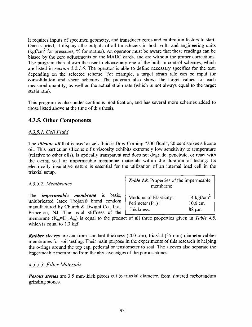
It requires inputs of specimen geometry, and transducer zeros and calibration factors to start.Once started, it displays the outputs of all transducers in both volts and engineering units(kgf/cm 2 for pressures, % for strains). An operator must be aware that these readings can bebiased by the zero adjustments on the MADC cards, and are without the proper corrections.The program then allows the user to choose any one of the built-in control schemes, whichare listed in section 5.2.1.6. The operator is able to define necessary specifics for the test,depending on the selected scheme. For example, a target strain rate can be input forconsolidation and shear schemes. The program also shows the target values for eachmeasured quantity, as well as the actual strain rate (which is not always equal to the targetstrain rate).
This program is also under continous modification, and has several more schemes added tothose listed above at the time of this thesis.
4.3.5. Other Components
4.3.5.1. Cell Fluid
The silicone oil that is used as cell fluid is Dow-Coming "200 fluid", 20 centistokes siliconeoil. This particular silicone oil's viscosity exhibits extremely low sensitivity to temperature(relative to other oils), is optically transparent and does not degrade, penetrate, or react withthe o-ring seal or impermeable membrane materials within the duration of testing. Itselectrically insulative nature is essential for the utilization of an internal load cell in thetriaxial setup.
4.3.5.2. Membranes Table 4.8. Properties of the impermeablemembrane
The impermeable membrane is basic, Modulus of Elasticity: 14 kgf/cm2
unlubricated latex Trojan® brand condom Perimeter (Pm): 10.6 cmmanufactured by Church & Dwight Co., Inc., Thickness: 88 ptmPrinceton, NJ. The axial stiffness of the Imembrane (Km=Em.Am) is equal to the product of all three properties given in Table 4.8,which is equal to 1.3 kgf.
Rubber sleeves are cut from standard thickness (200 ptm), triaxial (35 mm) diameter rubbermembranes for soil testing. Their main purpose in the experiments of this research is helpingthe o-rings around the top cap, pedestal or tensiometer to seal. The sleeves also separate theimpermeable membrane from the abrasive edges of the porous stones.
4.3.5.3. Filter Materials
Porous stones are 3.5 mm-thick pieces cut to triaxial diameter, from sintered carborandumgrinding stones.
93
Nylon filters are cut to triaxial diameter, from 53 pm-thick sheets of Nitex@ nylonmonofilament fabrics, manufactured by Tetko Inc., Elmsford, NY. Compared to the widelyused filter papers, these are extremely durable, reusable, softer, and offer less frictionalresistance. A nylon filter can withstand dozens of tests, and be washed with abrasive lavasoap after each test to remove oil from its surfaces.
4.4. Modified Triaxial Setup
In order to incorporate a 7th generation MIT tensiometer into the MIT triaxial setup, thefollowing changes, which are also shown in Figure 4.12, are made to the setup in Figure 4.9:
- The center of a triaxial base was machined out to accommodate the geometry of thetensiometer. To-scale drawings of the modified triaxial base are given in Appendix 4.4.
- Instead of resting directly on the load frame, the triaxial base is supported by 4 columnson a platform, which is placed on the loading mechanism. This allows one to access tothe tightening nut of the tensiometer, and adds room for the data cables.
- The top cap is connected to a distilled water reservoir through outlet B and the top valve.
- None of the remaining components among those related to pore water in the unmodifiedsetup are needed in the modified setup. They are not physically removed, but the setup isisolated from them by closing the bottom and transducer valves. Hence they are notshown in Figure 4.12. These components are the pore pressure transducer, pore PVA,and pipes that lead to the pedestal in the unmodified setup.
- The data channel for the pore pressure transducer in the unmodified setup is connected tothe tensiometer (which also measures pore pressure), instead.
94

Impermeablemembrane
Porousceramic
Tensiometer
Base
Tank Valve
Oil-- Tank
Tightening nut.--
Cell Valve
Cell PVA
Cell PressureTransducer
Top Valve
Data acquisition
4.5. Preparation Equipment
4.5.1. Specimen Mold
The aluminum mold consists of two half-cylinders held together by two clamps. The moldhas an inner diameter equal to the diameter of a triaxial specimen (3.5 cm), except the bottompart which envelopes the pedestal or tensiometer, as well as the o-rings around them. Theinner surface of the mold is covered with a paper towel to establish air flow from all aroundthe specimen to two outlets (one at the middle of each half), to which a vacuum can beconnected.
The normal procedure for triaxial testing of granular materials involves using a thickmembrane. In order to minimize membrane corrections in this research, a single thinmembrane (section 4.3.5.2) was used instead. To eliminate the risk of puncturing themembrane during setting up, the inner edges of the mold halves were rounded by the author.In order to ease usage, the center of the edges on one surface of one of the clamps are alsorounded. The benefit of this modification will be discussed in section 5.1.5.
95
Figwm 4.12. Schematic of
the modified parts
of the triaxial cell
. O-ring
g Loading frame
-- Data signal
-- Air pipe
-- Oil pipe
Valve*
=Zzi Nuts and bolts
*: connects at right
angles, not opposite sidesI

4.5.2. Scoop
For mixing and placing the samples, a stainless steel scoop with a U-shaped constant crosssection (except a tapered end) was preferred over flat spatulas or spoons. The flat spatulas areunable to hold dry glass beads, and spoons are inaccurate when pouring the material.
4.5.3. Standard Pocket Penetrometer
A standard pocket penetrometer with itsstandard enlarged shoe is used forcompacting specimens in the retaining ringon the tensiometer. The PPT that was used inthis research is model CL-700 manufacturedby Soiltest Inc. and has a capacity of 4.5kg/cm2
4.5.4. New O-Ring Stretcher
Triaxial-diameter o-rings are normallyplaced by first stretching them on a ring-shaped metal stretcher. Given the highstiffness of the o-rings, the commonstretchers are as small as possible. Theregular stretcher is 2.5 cm high and has adiameter of 5 cm, barely larger than thespecimen diameter of 3.6 cm. Figure 4.13. Preparation equipment.
A particular stage of setting up for the c: lower mold clamp d: scoop,experiments in this research (namely, step 13 e: standard pocket penetrometer,in section 5.1.5) requires working on the f: new 0-ring stretcher.inside of the stretcher. Working behind theregular metal stretcher is impossible because of its dimensions. A new 2-piece stainless steelstretcher was built to stretch thinner triaxial-diameter o-rings to larger diameters. The newstretcher is 6.5 cm in diameter, and 1cm high, allowing access between the stretcher and thetop cap.
O-rings being excessively stretched are more likely to snap off the stretcher, especially if itsheight is less. To prevent this, two grooves of semi-circle cross-section circumvent the newstretcher (see left-inset in Figure 4.13). All edges of the stretcher and the grooves arerounded to prevent any damage to the o-rings.
4.5.5. Step-Cut Brush
During the setup procedure, excess particles are brushed offthe upper rim of the specimen mold. Hairs of ordinary brushes Figure 4.14. Schematic ofmay penetrate and disturb the specimen. In order to reduce this the step-cut brush.
96

risk, and brush more efficiently, a flat brush was cut in the shape shown in Figure 4.14 forthis research.
4.5.6. Optical Vernier
This instrument is X-axis Z-axis Measuring A-I Microscope, manufactured by Titan ToolSupply Inc., Buffalo, NY. It has a focal distance adjustable between 9.5 and 10.5 cm. It can
measure horizontal and vertical lengths with resolution of 0.001 inches (25.4 tm). The
eyepiece is equipped with cross-hairs angled at multiples of 300 (see inset in Figure 5.15).See section 5.3.1 for its usage.
4.6. Electronics
4.6.1. Transducers
4.6.1.1. Pressure Transducers
T62 and T71 employed a Data Instruments Table 4.9. Electrical
(Acton, MA) AB/HP 200 psi (14 kgf/cm2) Instrume
pressure transducer, which measures transduc
absolute pressures by the deflection of a Linear Rangesteel diaphragm instrumented with straingages. T72 utilized the 1000 psi (70 kgf/cm2)version of the same model, and T70 used Overloadthe 25 psi (1.8 kgf/cm 2) version. AB/HP(Table 4.9) is the standard transducer type Excitationwidely used in a lot of applications at MIT Span (5Vdc at 25'C)Geotechnical Laboratories, so it is Accuracyincorporated in the MIT tensiometerswhenever applicable for the advantages of familiarity and reliability.
.935-.- E4AX --
(23.Th)
pressuresensitivesurface
MAX (254)(25.4)
.2 to .3 + --
.749 M(19
4 conductorcolor codedshielded cable
Wo7.52) 41. 3 It long(.0) ~ (.91 m)
redAX DIA reen.02) black
In witestrain shieldrA.6)elmef
A =.25 (6.35) xxx = 'nce s
* 2.44 (62) for Option 7
Figure 4.15. Dimensions of Data Instruments AB/HP pressure transducer.
97
characteristics of Datants AB/HP pressurer
±1.8 kgf/cm 2 (25psi)±14 kgf/cm 2 (200psi)±70 kgf/cm 2 (I000psi)2x w/o damage5x w/o bursting5.5 V dc110±1 mV±0.25% of span
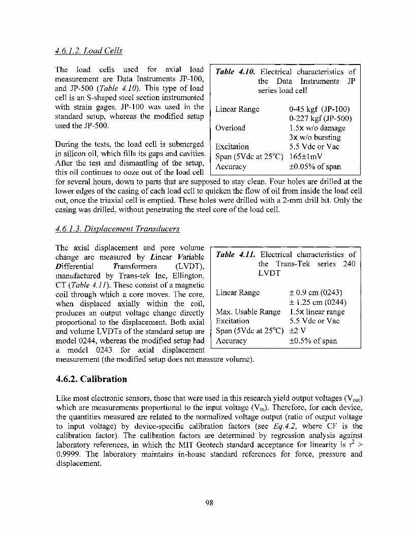
4.6. 1.2. Load Cells
The load cells used for axial loadmeasurement are Data Instruments JP-100,and JP-500 (Table 4.10). This type of loadcell is an S-shaped steel section instrumentedwith strain gages. JP-100 was used in thestandard setup, whereas the modified setupused the JP-500.
Table 4.10. Electrical characteristicsthe Data Instrumentsseries load cell
Linear Range
Overload
ofJP
0-45 kgf (JP-100)0-227 kgf (JP-500)1.5x w/o damage3x w/o bursting
During the tests, the load cell is submerged Excitation 5.5 Vdc or Vacin silicon oil, which fills its gaps and cavities. Span (5Vdc at 25 0C) 165± mVAfter the test and dismantling of the setup, Accuracy ±0.05% of spanthis oil continues to ooze out of the load cellfor several hours, down to parts that are supposed to stay clean. Four holes are drilled at thelower edges of the casing of each load cell to quicken the flow of oil from inside the load cellout, once the triaxial cell is emptied. These holes were drilled with a 2-mm drill bit. Only thecasing was drilled, without penetrating the steel core of the load cell.
4.6.1.3. Displacement Transducers
The axial displacement and pore volumechange are measured by Linear Variable Table 4.11Differential Transformers (LVDT),manufactured by Trans-tek Inc, Ellington,CT (Table 4.11). These consist of a magneticcoil through which a core moves. The core, Linear RanIwhen displaced axially within the coil,produces an output voltage change directly Max. Usablproportional to the displacement. Both axial Excitationand volume LVDTs of the standard setup are Span (5Vdcmodel 0244, whereas the modified setup had Accuracya model 0243 for axial displacementmeasurement (the modified setup does not measure volume).
e
Electrical characteristics ofthe Trans-Tek series 240LVDT
±0.9 cm (0243)1.25 cm (0244)
Range 1.5x linear range5.5 Vdc or Vac
at250C) ±2 V±0.5% of span
4.6.2. Calibration
Like most electronic sensors, those that were used in this research yield output voltages (Vo0 t)which are measurements proportional to the input voltage (Vin). Therefore, for each device,the quantities measured are related to the normalized voltage output (ratio of output voltageto input voltage) by device-specific calibration factors (see Eq.4.2, where CF is thecalibration factor). The calibration factors are determined by regression analysis againstlaboratory references, in which the MIT Geotech standard acceptance for linearity is r2 >
0.9999. The laboratory maintains in-house standard references for force, pressure anddisplacement.
98

Appendices
Appendix 4.1. Metal parts of T 7.1 - 7.2. a) Upper body - Triaxial pedestal.
eq
B
14!iI1k
H
K1--------------e
99
zi
I
IJil
RC413
eq
4-
Sk
H 7"7----------------
............
----------------------
I |
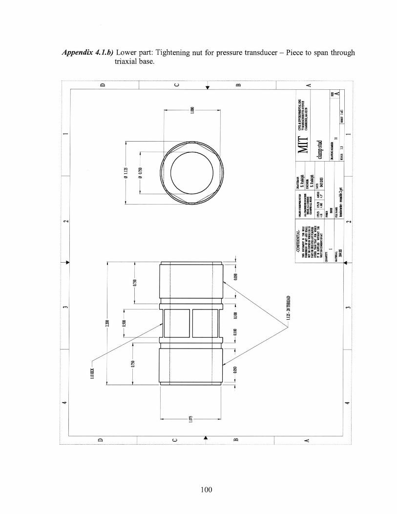
Appendix 4. 1. b) Lower part: Tightening nut for pressure transducer - Piece to span throughtriaxial base.
---------------------------------------------------------------- ------- ----------------------------------- -------------- ------------------------------------------------- --------- ------------------------------------------------
911
Ci
'Imalln
i C=S
C:5
-------------------- ------------------------------------------- --------------------------------------------------------- t -------------------------------------------------------- -------------------------------------------- -------------
100

Appendix 4.1.c) Copper vacuum seal.
--l
101
~I~ujN
I8
I
i!~i~I iii RC4
11
IagIo j
c:i
--------------- ......

Appendix 4. 1. d) Complete image.
11~J~L
iIE
102
I~I~ - - -
IlKIii
III'IL-
IIIi
II
II I 1~~I III III I I
Ii i1 EII I 1~ III -~i 1
II II ill III I I
II I I-i-- 1 I
z1

Appendix 4.2. Analog-analog feedback circuit of the saturation setup. (Sjoblom, 2000)
ADS24
Ref erence voltage
...- 5 Q2 - I1OX Gain
a 9AD524
A0524Output Voltage
Transducer voits".g2 s
13

Appendix 4.3. Control circuit of the triaxial setup.
252423 2 2, 1 18 17 1P 1E 141p 12 11 1PT9 6 5 4 1
--
-I j * 5 S 7
I. *'- - -I
- I
............... .. .. .. .- I
14 - - 14.. % .......... L . .2............ ................. ..
Line Legend- common
..-..-. channel 1 (axial)- - - channel 2 (cell)
- - channel 3 (pore)
.........................2
L .-...-- -.-- -.
. I --- - - - - - - - - - - - -- - - - - -...11 .12 .1 1 11 1 1 1 4 1
10 11 12 13141 1.0 1.1 12 13 14 110 kQResistance
104
I9
Color LegendVin +/-12VVin +6V
ground, limit, Vin-digital signal (sink)amplified digital signal+ analog signal
*. -
I - - - z::,- - - - No -=-- - ..........
iI

Appendix 4.4. Modified triaxial base.
105
- , -.- !, ti 0,11"im -
Nl

Appendix 4.4. continued.
106
----------
---- ----- ---
---- ----- ---
------------------- --
----------------
-------------- -

P R OCE R ES
107

108

5. PROCEDURES
This chapter describes experimental procedures in an instructional manner, as opposed tosimply reporting what has been done. These procedures were exactly followed for almost allof this research, so they indirectly report what has been done as well.
The triaxial tests are categorized into four types as: saturated tests; sealed, unsealed andtensiometer tests. The latter three are unsaturated tests. Only tensiometer tests are run in themodified setup, the remaining three use the standard setup. The important differences amongthe procedures of the test types are summarized in section 5.2.5. All of these labels are usedwithin this, and oncoming, chapters.
Table 5.1. Classification of test types in this research.Test type Saturation Setup
saturatedsealed standard
unsealed unsaturatedtensiometer modified
5.1. Preparations
5.1.1. Tensiometer Saturation
This procedure is followed only for the triaxial tests on unsaturated materials using themodified base (section 4.4).
The saturation setup was previously illustrated in a simplified manner as Figure 4.3.However, the pipes and valves are not necessarily permanent connections. Therefore, theprocedure will be detailed by explaining which component of the saturation setup isconnected to which other component, rather than detailing which valve points which way(i.e. this section gives a functional description of the saturation process).
The necessary saturation procedure before a test is described in sections 5.1.1.2 and 5.1.1.3.Section 5.1.1.1 below focuses on the operation and maintenance of the individualcomponents of the saturation setup.
5.1.1.1. Operation of Individual Components
The components have specific operating tips and rules that should be followed preciselyevery time the particular piece of equipment is put in use. An overarching rule that is validfor all components of the saturation setup is to remember taking the water (or air) that is inthe pipes into account. For example, if a container is to be deaired, the pipes that are going tobe connected to it should be deaired, as well.
109

5.1.1.1.1. Centrifugal Vacuum Pump
- The pump's turbine is the disc-like portion on its side. The water intake pipe goes into thecenter of the turbine, and the outlet pipe is connected tangentially. The vacuum is appliedto the saturation setup through a pipe on the side of the outlet pipe.
- Water in the circulation tank, from which the pump intakes and into which it gives outwater, should always be recycling. That is, it should always have inflow and spillage ofwater, in order to keep the water cool (As noted in section 4.2.2, this pump reduces thepressure to the vapor pressure of water, which is lower for cooler temperatures).
- The outlet pipe of the pump into the water tank should have a small gap, through which airbubbles can join the flow. The air bubbles must be distinctly observable in the tank, as theyfloat up to the water surface without being absorbed into the pump's intake. This isachieved by placing an insulated (to minimize rusting) electrical wire at a connection ofthis pipe. To prevent the pump from intaking bubbles, the ends of these two pipes shouldpoint at different directions in the tank.
- Before operation, all valves on the line to be vacuumed should be closed. After starting thepump, the valves may be opened starting from the one closest to the pump, and proceedingalong the line.
- If the pump fails to start (making bubbles in the tank), the pump's water intake pipe mighthave too much air in it. Bring the pipe through which water fills the tank against the intakepipe to push water into it.
- Rarely, the pump starts but fails to apply the expected vacuum, when some water is trappedwithin the outlet. Pull the pipe through which vacuum is applied to the saturation setup outof the pump. For the saturation setup-side of this separation, point the pipe downward toempty any water within. For the pump-side, close it with a finger. Feel the vacuum build upand then suddenly pull your finger away to let a gush of air into the pipe. Repeat this cyclemany (possibly 50-100) times in a few minutes, until you feel a significant increase in thepull of the vacuum on your finger. Reinsert the pipe to connect the pump to the rest of thesetup.
- Before turning the pump off valves should be closed starting from the farthest andproceeding towards the pump. The pump may be turned off when the valve closest to thepump is closed.
5.1.1.1.2. Oil Vacuum Pump
- The oil should be at the operating level in the observation window. If it is low, oil can beadded from a cap on the top. If it is too high, which can occur when water is mistakenlydrawn into the pump, it can be drained from the tap at the bottom.
- Before turning off, its hose should be disconnected and the pump should be allowed todraw in air. Otherwise, oil vapor will backflow into the system.
5.1.1.1.3. Deaerator
- Take notice of the upper limit for water level, marked on the tank.- If the deaerator is empty, it can be refilled by connecting its water pipe to a distilled water
source, and vacuuming through the air pipe.
110
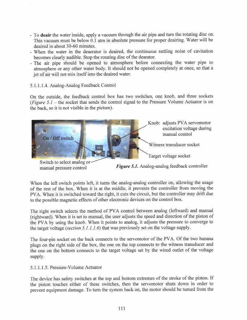
- To deair the water inside, apply a vacuum through the air pipe and turn the rotating disc on.This vacuum must be below 0.1 atm in absolute pressure for proper deairing. Water will be
deaired in about 30-60 minutes.- When the water in the deaerator is deaired, the continuous rattling noise of cavitation
becomes clearly audible. Stop the rotating disc of the dearator.- The air pipe should be opened to atmosphere before connecting the water pipe to
atmosphere or any other water body. It should not be opened completely at once, so that ajet of air will not mix itself into the deaired water.
5.1.1.1.4. Analog-Analog Feedback Control
On the outside, the feedback control box has two switches, one knob, and three sockets(Figure 5.1 - the socket that sends the control signal to the Pressure Volume Actuator is onthe back, so it is not visible in the picture).
Knob: adjusts PVA servomotorexcitation voltage duringmanual control
Witness transducer socket
Target voltage socketSwitch to select analog ormanual pressure control Figure 5.1. Analog-analog feedback controller
When the left switch points left, it turns the analog-analog controller on, allowing the usageof the rest of the box. When it is at the middle, it prevents the controller from moving thePVA. When it is switched toward the right, it cuts the circuit, but the controller may drift dueto the possible magnetic effects of other electronic devices on the control box.
The right switch selects the method of PVA control between analog (leftward) and manual(rightward). When it is set to manual, the user adjusts the speed and direction of the piston ofthe PVA by using the knob. When it points to analog, it adjusts the pressure to converge tothe target voltage (section 5.1.1.1.6) that was previously set on the voltage supply.
The four-pin socket on the back connects to the servomotor of the PVA. Of the two bananaplugs on the right side of the box, the one on the top connects to the witness transducer and
the one on the bottom connects to the target voltage set by the wired outlet of the voltage
supply.
5.1.1.1.5. Pressure-Volume Actuator
The device has safety switches at the top and bottom extremes of the stroke of the piston. Ifthe piston touches either of these switches, then the servomotor shuts down in order to
prevent equipment damage. To turn the system back on, the motor should be turned from the
111

little flag (the topmost point of the PVA, see Figure 4.5) by hand, so that the piston is pulledaway from the safety switch.
After every pressurization, the piston ends up being further inside the cylinder (i.e. the PVAhas less water). If the piston is too close to being completely inside the cylinder (i.e. too closeto the bottom safety switch), it means there is very little water left in the chamber, so thePVA needs filling.
1. To fill the piston, connect it to the deaerator.2. Deair (Section 5.1.1.1.3) the water.3. Connect the deaerator to the atmosphere.4. Connect the deaerator to the PVA.5. Withdraw the piston using the manual setting (Section 5.1.1.1.4).
Normally, the piston moves, at most, a couple of centimeters during pressurization. If itmoves more, it means that there is air in the piston. In this case, the PVA must be evacuatedand refilled.
1. Before refilling, empty the remaining water in the PVA by pushing the piston as far intothe cylinder as possible without triggering off the safety switch,
2. For refilling, the PVA should be connected to both the oil vacuum pump and thedeaerator through a three-way valve.
3. Connect the oil vacuum pump to the PVA and the centrifugal vacuum pump to thedeaerator.
4. Evacuate both the PVA and deaerator for half an hour. The deaerator disc should beoperating throughout this time.
5. Turn off the dearator disc and open the deaerator to the atmosphere. The centrifugalvacuum pump may be shut down.
6. Connect the PVA to the deaerator without turning off the oil pump. The oil vacuum pumpmay be disconnected and shut down.
7. Withdraw the piston.
The operator should keep in mind that with the huge combined mechanical advantage of theball screw actuator and the servomotor, the PVAs are able to generate tremendousmagnitudes of pressure, and are capable of destroying any equipment connected to them ifused improperly.
5.1.1.1.6. Target Voltage
The saturation of the tensiometer approaches 100% with increasing saturation pressure, sothe tensiometer should be saturated at the highest pressure possible. The saturation pressureshould also be greater than the air entry pressure of the porous interface of the tensiometer.However, it may not exceed the yield pressure of the pressure transducer within thetensiometer (which is two times the linear range for the Data Instruments transducers), or thelinear range of the witness transducer on the PVA (the current transducer is 1000 psi = 70kgf/cm2). Thus the saturation pressure should be as high as possible, and also less than thesetwo limits with some safety margin. To impose the selected pressure, follow the procedurebelow:
112

1. Connect the PVA to the atmosphere to obtain zero (gage pressure) of the witnesstransducer.
2. Convert the saturation pressure into a target voltage, using the calibration factor and zeroof the witness transducer (see equation 4.2 in section 4.7.2).
3. Multiply by 100 to account for the voltage divider on the power supply (section 4.2.5).4. Adjust the proper channel of the power supply to set it to 100 times target voltage. For
low-capacity tensiometers (or any other case that requires precision), connect a voltmeterand read from it at much greater resolution than the dial gage of the power supply.
This adjustment is not necessary if the tensiometer is the same as the one that was lastsaturated. So, along the course of a series of tests with a single tensiometer, the target voltageneeds to be set only once before the first test, provided that the saturation setup is not usedfor any other task throughout this period.
5.1.1.1.7. Tensiometer Placement
MIT tensiometers of version 7 and later can be fixed to a triaxial base (which is also the baseof the saturation chamber) by tightening the nut from under the base (Figure 4.2). Thetriaxial base has four legs for support and two male 9-pin electrical sockets for internaltransducers, making it impossible to use a wrench or similar tool to tighten the nut. In orderto tighten it by hand sufficiently, pressure must be applied to the top of the tensiometer withthe other hand at the same time. This compresses the o-ring under the tensiometer and locksstress that is otherwise unachievable by finger-tightening the nut.
5.1.1.2. Preliminary Checks and Adjustments
- Dry the surface of the porous ceramic of the tensiometer.- Check if the water in the tank of the centrifugal pump is recycling.- Check if the deaerator has enough water to fill the pressure chamber.- Check if there is sufficient volume of water in the PVA for pressure saturation. There
should be at least one inch of stroke available into the cylinder.- Check if the oil of the oil pump is at operating level.- Check if all o-rings are clean, in place and not notched, as well as the cleanliness of the
places the o-rings fit into.- Check the magnitudes of voltages (input voltage of 5.5 V and target voltage) from the
power supply.- Check if all pipes are connected as necessary. If they are connected after evacuating the
chambers, air may enter the pipes. To check this, the operator needs to go through thesaturation procedure up to the pressurization beforehand, and must connect the pipes asappropriate. The steps of the procedures below telling the operator to "connect" twocomponents of the setup mean that the pipes are already connected, but the valves on themthat are closed shall be opened.
113

5.1.1.3. Saturation in the Triaxial Saturation Chamber
The PVA, deaerator and the oil vacuum pump start connected to the saturation chamber, withall valves closed. The PVA starts at atmospheric pressure and its control box turned off.
1. Fix the tensiometer into the base of the saturation chamber as described in section5.1.1.1.7. The data acquisition cable passes through the hole in the base (If monitoring isdesired during saturation, it can be done through this connection).
2. Place the upper half of the saturation chamber on top and tighten its bolts.3. Connect the chamber to the oil vacuum pump (section 5.1.1.1.2) and start evacuation.4. Start deairing the water in the deaerator (section 5.1.1.1.3). These two processes will take
about the same amount of time (at least half an hour) with both vacuum pumpsoperational.
5. Stop the deaerator, disconnect it from the centrifugal vacuum pump and open it to theatmosphere. Turn off the disconnected centrifugal vacuum pump (section 5.1.1.1.1).
6. Disconnect the chamber from the vacuum and connect it to the deaerator. Turn off thedisconnected oil vacuum pipe.
7. The chamber will be full of water from the deaerator in less than a minute. After twominutes, check if it is filled successfully by opening the top (ventilation) outlet of thechamber very slowly. If it makes a hissing sound by air flowing either in or out, thechamber did not fill properly, so proceed with steps 15, 16, dry the inside of the chamberand the tensiometer with paper towel, then repeat steps 2 through 7. If water comes out ofthe outlet immediately, the chamber was filled properly, procees to step 8.
8. Disconnect the chamber from the deaerator and connect it to the PVA.9. Turn the PVA control on and to analog. The piston should rapidly compress, bringing the
pressure asymptotically to the saturation pressure.10. Wait for 24 hours.11. Perform other preparatory tasks (material preparation, cell preparation).12. Turn the PVA control to manual and set the rate to decrease at about 0.1 atm/sec.13. Monitor the witness transducer reading. Turn the PVA off when the pressure inside is
close to atmospheric.14. Open the valve of the topmost outlet to the atmosphere (i.e. not the one that connects with
the PVA).15. Place a container under the lowest outlet and drain the chamber through there.16. Unscrew the bolts and take off the upper half of the chamber.17. Take the tensiometer out of the chamber. While it is not in use for short periods (carrying,
installing into the triaxial setup), the top face of the tensiometer should always be fullycovered with water. Putting a plastic sleeve around the tensiometer to act like a containerto store additional water on the surface is also helpful for unattended waiting times longerthan a few hours.
5.1.2. Sample Preparation
There are two types of glass spheres (detailed in section 6.1). Type 1 spheres were obtainedby sieveing mixed-size glass spheres. A Type 1 sample consists of the portion passing #120(125ptm) and retained on #140 (106pm) sieves after one cycle of sieveing. Coarser sieves
114

were stacked above those two sieves, to better distribute the material over the sieves ofinterest, and to prevent overloading of these finer sieves by limiting the rate particles passthrough the sieve system.
The procedure was modified to process the Type 2 spheres. The same sizes of sieves wereused, but the fraction retained on the #140 sieve was repeatedly sieved, until only negligibleamounts of material passed through it. This usually involved 7 to 10 cycles, and resulted in30 grams of sample material. As one cycle took close to 10 minutes, and one test requires120 grams of Type 2 material, several hours of sieveing was necessary for one test. This ledto the development of the retrieval procedure described in section 5.3.3.
5.1.3. Cell Preparation
5.1.3.]. Maintenance
5.1.3.1.1. Cleaning
The primary problem against cleanliness is the cell fluid (oil). An efficient way to clean oil iswith toilet paper. Both before and during the setup procedure, any oily surface (including theoperator's hands) must be wiped with toilet paper, repeatedly if necessary. In unsaturatedtests, any contamination can affect the results by changing interfacial characteristics.
Sample materials themselves create major cleaning problems. It is difficult to clean wet glassbeads, and extremely difficult to clean oily glass beads off any surface. As glass has the samehardness as steel, glass beads can cause damage if they get into metal moving parts.Therefore, it is essential to keep the workspace clean of the glass beads. If possible, designateon the laboratory bench a "clean area", where operators shall put only clean things, and an"unclean area" where items that have glass on the surface are placed (for example after thetest). The latter may also be divided into "oily" and "non-oily" sections.
If sample materials get into the pipes, connections, or transducer sockets, the setup will haveto be cleaned. The procedure is itemized below:
- A pressurized water jet is used for cleaning. For this purpose, a hose that narrows down toan opening of less than a millimeter diameter is fitted to a tap in the laboratory.
- All pipes (including the standpipe for top cap connection) and valves in the lower half ofthe setup are flushed with turbulent water. Valves are flushed a separate time for eachdirrection they can point. All o-ring grooves are also cleaned with the water jet.
- The excess water is dried with a paper towel.
- A pressurized air jet is used to blow away the remaining water, which must be completelyremoved from all oil pipes. If an oil compressor is used then the air jet must be applied tothe water pipes and pedestal surface for a minimum possible duration, because there areairborne oil molecules in the jet. Do not use the air jet on the tensiometer.
115

Another threat to cleanliness is pieces of wire. In time, silicon oil disintegrates the plasticinsulation of the electrical wires. Small pieces of exposed ground wire may break off and fallon the base. These can disrupt a test if they fall on the load cell connector or an o-ring. Theconnector of the load cell inside the triaxial cell must be clean, especially of any wire pieces.
5.1.3.1.2. O-ring Maintenance
Before each test, all o-rings and surfaces contacting them must be clean of grain, wire, hair,or any other tiny object. An o-ring and its contact surfaces can be cleaned by wiping with aclean finger, cloth or paper towel (not cotton or cleenex). Afterwards, grease is applied with afinger. Note the following:- O-rings in grooves don't usually get dirty inside the groove, so cleaning the open surface is
sufficient, unless the setup is being cleaned with pressurized jets.- O-rings lose ductility over time when repeatedly exposed to silicon oil. This can be
prevented by an occasional check involving twisting and bending them while examiningclosely for cracks.
5.1.3.1.3. Tensiometer Maintenance
Pure water in the tensiometer must not be contaminated by any fluid or solute, as these willchange the interfacial tension and introduce unknown inaccuracies to the device,permanently. The only viable way to wash the tensiometer's surface is by holding it underflowing distilled water. If contamination occurs, the tensiometer has to be cleaned piece bypiece after separating it into all of its components (steel body, pressure transducer, copperseal, porous interface), among which the copper seal and porous interface can not be reused.
5.1.3.2. Setting up for Specimen Constitution
1. Check if all pieces of equipment are ready. These are:- All pieces of the triaxial cell setup (section 4.3.1). The load cell and top cap start
attached to the steel structure and the piston. The whole assembly will be called the"superstructure " for the rest of the procedure description. The water line that goes fromthe base to the top cap is a separate piece of metal standpipe. The base starts without thepressure transducers, not connected to either PVA, with all valves closed to all flow, andon a workspace accessible to the operator from different angles (table or laboratorybench).
- The load frame with sufficient stroke (see section 5.2.1.5),- Preparation equipment (section 4.5), calipers, sharp and thin scissors, toilet paper,- Carbon dioxide tank with flow regulator (for saturated tests only),- Oil vacuum pump with regulator and associated tubing (including a double-outlet T-pipe
to connect to the mold). See instructions in section 5.1.1.1.2 for operation of the pump,- 2 thick, 3 thin o-rings and o-ring grease,- 2 porous stones and nylon filters (only one of each for modified setup),- 3 rubber sleeves, one cut to fit the pedestal, one for the top cap, and one 1-1.5 cm long
for the mold,- An impermeable membrane, whose tip has been cut off,
116

- Piston clamp,- Various necessary sizes of wrenches and hexagonal keys,- One 250 ml glass beaker, two 250 ml flasks,- A syringe (for modified setup).
2. Warm the transducers up:- Plug all transducers and input voltage of 5.5 V to their sockets (to which they will be
connected to during the test). This will require a female-to-female 9-pin extension cablefor the load cell, which is a part of the superstructure.
- For the modified setup, install the saturated tensiometer into the triaxial base and plug itin as well. The surface of the tensiometer must have water on it at all times.
3. Prepare the top cap (this can be done anytime between stages 1 and 7 of this procedure,but it was generally done at this point):- In sealed tests, a piece of foil wrap was used to cover the hole on the top cap.- Figure out the best orientation of the superstructure to be placed on the base. Find the
orientation considering the location of the hole that the water pipe from the top cap willconnect, and the orientation of the spiral tubing of the top cap. Rotate the piston relativeto the superstructure if necessary.
- Move the piston to the highest position and clamp it.- Put the shorter rubber sleeve around the top cap with very little grease, such that its
lower end is 3 mm (i.e. the thickness of the porous stone) lower than the rim of the topcap.
- Fold the lowermost portion of the sleeve up onto itself (Figure 5.2. a).
Figure 5.2. Prepared (a) top cap
and (b) pedestal.
117

4. Prepare the pedestal:- In sealed tests, a piece of foil wrap was used to cover the holes on the pedestal.- Put the longer rubber sleeve around the pedestal (or tensiometer for modified setup) with
very little grease, such that its upper end is 3 mm (i.e. the thickness of the porous stone)higher than the rim of the pedestal. For the modified setup the sleeve needs to be only afraction of a millimeter above the tensiometer's upper rim.
- For standard setup only, place a porous stone on the pedestal, into the sleeve.- For standard setup only, place a nylon filter on the stone. If it curls, apply a droplet of
water between the filter and the porous stone.- Hold the impermeable membrane from the inside with two index and two middle fingers
pointing down, hands facing out, cut-end to the bottom, rolling end to the top andoutside. Stretch and put it around the rubber sleeve on the pedestal (or tensiometer).
- Straighten all wrinkles on the membrane by pulling or pushing the cut-end downwards(collecting the wrinkles at the very bottom is acceptable, the aim is having most of theheight of the pedestal or tensiometer wrinkle-free).
- Put the two thick o-rings on a regular stretcher (described in section 4.5.4) after greasingthem. Drop both of them on the membrane. Final state is Figure 5.2. b.
5. Mount the mold:- Roll the membrane up about 5 cm off the top rim of the pedestal assembly. For the
standard setup hold the porous stone and filter down.- Place the two halves of the mold, bottom first, touching the base on both sides of the
pedestal (or tensiometer). The gaps on the bottom of the mold halves must be aligned tothe 9-pin connectors on the base. One of the mold halves has pieces that fit into the otherhalf s holes. The half with holes must be on the side where the top cap water pipeconnects to the base.
- Hold the membrane up and twist it axially. There should be just enough tension on themembrane to keep it as a vertical cone (as held in Figure 5.3 for illustrative purposes),because pulling it too much will displace the o-rings and the sleeve around the pedestal(or tensiometer).
- Slowly close the halves of the mold with care so as not to squeeze any part of themembrane in between. Once closed, keep the two halves pressed together with one handto prevent opening and closing of the gap in between, which could catch the membrane.
- Untwist and stash the membrane into the mold, without releasing the mold halves.- Place the clamps around the mold and tighten, without releasing the mold halves. Both
clamps must be placed on the side opposite to the hole on the base, which connects tothe top cap water pipe. The bottom clamp is the one with edges of one of its facesrounded at the middle section. The rounded face faces downward.
- The fingers holding the mold halves together may be released once one of the clamps istightened. From this point on, whenever a lateral or upwards force, or torsion will beapplied to the mold assembly, it must be pressed down from the diametrically oppositeends of the upper clamp, to prevent its unwanted motion.
6. Cover the inside of the mold with the membrane:- Put the remaining rubber sleeve piece around the top outer rim of the mold, as seen in
Figure 5.3, without grease. Its top part must not go inwards beyond the inner rim, and itonly has to cover the outer rim.
118

- Grease and place a thin o-ring aroundthe mold, on the rubber sleeve, 6-9mm below the top of the mold. If theregular stretcher is large enough, itcan be used. Otherwise, use the newstretcher described in section 4.5.4.The end of this step is illustrated inFigure 5.3.
- Apply some grease on the inner rimof the mold.
- Cover the inner walls of the mold, as
well as the outer o-ring and the partsabove the o-ring with the membrane,by stretching it slightly and placingthe rolled portion lower than the o-ring, as in Figure 5.4. If there are anyaxial wrinkles or twist, the entiremembrane can be moved by holdingit from the rolled part. Propagate themovement to the rest of themembrane by pushing with fingers.The purpose of the o-ring is toprevent the membrane from comingoff the mold.
- Connect the double outlet pipe toboth sides of the mold (as seen inFigure 5.4), finger tight, whilepressing on the mold (as mentioned atthe end of 5th stage of this procedure).
- Connect this pipe to the vacuumregulator. Apply a very slight vacuum(reducing the pressure between themold and the membrane by a few kPashould suffice). If this does not resultin a smooth membrane, vent the pipeto the atmosphere, and move themembrane as described in the stepabove. The end of this step is shownin Figure 5.4.
7. Measure the specimen height (H0 ) fromthe top of the mold to the nylon filterusing the caliper, making care that itsmetal tip and corners do not puncture the
Figure 5.4. The mold with the membrane.
membrane.
119
1. .11 .iu 1 ."" "" '' "" """" '''""""'""""""""""""""""""... .... .......

8. For the modified setup, put enough distilled water into the mold to cover the entirespecimen area.
9. Cover the setup to protect it from spilling grains (the coverings can be seen in Figures 5.5and 5.7):- Cover the setup with the large rubber sheet with the large hole, the mold passing through
the hole.- Stretch the small rubber sheet with the small hole in four directions (this is possible with
only two hands, however an extra pair of hands is an easier option). Place it over themold with the rim of the hole immediately above the o-ring, folding upwards (this isvisible in Figure 5.7).
- Place the plexiglass collar on top of the mold. If the collar rests on the o-ring instead ofthe top surface of the mold, the o-ring was placed too high, and it must be lowered bypushing it down without the collar, and even without the small sheet if necessary.
5.1.4. Specimen Preparation
The method of specimen preparation is important, because the characteristics of the initialfabric of granular materials are determined not only by the shape of the constituting particles,but also by the manner in which they were deposited (Oda, 19722).
1. Measure the mass of the scoop + glass beaker as [1].2. In it, place at least 150 grams of Type 1 sample or 120 grams of Type 2 sample. Record
the mass of scoop + beaker + dry sample as [2].3. Mix with a few grams of water (1-3%) in a beaker, to bring the sample to the consistency
of snow. Keep mixing until it becomes homogeneous (10 to 20 minutes). Record mass ofscoop + beaker + moist sample as [3], immediately before starting to put the sample intothe mold. Then the preparation water content (wp) is
[3]-[2]P = [Eq. 5.1.[2]-[1]
4. For the modified setup, record the input voltage and zero reading of the tensiometer.Then, use the syringe to remove as much water as possible from the tensiometer surface.
There may be different ways of compaction. The important thing here is having a repeatableprocedure for the compaction of all test specimen. The procedure used for this research isdescribed in the next steps. Extreme care must be taken not to spill any material outside thebeaker and the mold in this process, as the remaining mass will be measured later todetermine the specimen mass (step 10). If any material spills on the rubber sheets, it must beretrieved with the scoop or tweezers, and put back into the beaker.
5. Compaction is done in 7 layers, 25 tamps per layer. For the first time this is done with anew material, it may take one or two trials to establish the amount of material to put perlayer.
120
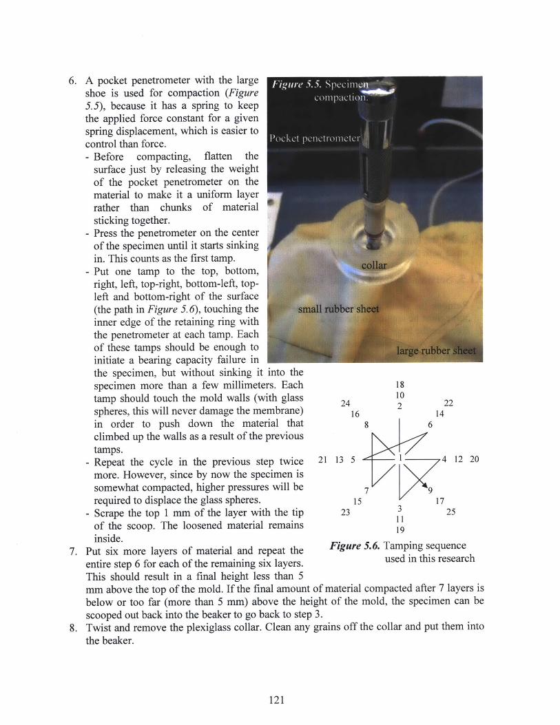
6. A pocket penetrometer with the largeshoe is used for compaction (Figure5.5), because it has a spring to keepthe applied force constant for a givenspring displacement, which is easier tocontrol than force.- Before compacting, flatten the
surface just by releasing the weightof the pocket penetrometer on thematerial to make it a uniform layerrather than chunks of materialsticking together.
- Press the penetrometer on the centerof the specimen until it starts sinkingin. This counts as the first tamp.
- Put one tamp to the top, bottom,right, left, top-right, bottom-left, top-left and bottom-right of the surface(the path in Figure 5.6), touching theinner edge of the retaining ring withthe penetrometer at each tamp. Eachof these tamps should be enough toinitiate a bearing capacity failure inthe specimen, but without sinking it into thespecimen more than a few millimeters. Each 18
tamp should touch the mold walls (with glass 24 2 22spheres, this will never damage the membrane) 16 14in order to push down the material that 8 6climbed up the walls as a result of the previoustamps.
- Repeat the cycle in the previous step twice 21 13 5 1 4 12 20
more. However, since by now the specimen issomewhat compacted, higher pressures will be 7 9required to displace the glass spheres. 15 17
- Scrape the top 1 mm of the layer with the tip 23 3 25
of the scoop. The loosened material remains 19
inside.7. Put six more layers of material and repeat the Figure 5.6. Tamping sequence
entire step 6 for each of the remaining six layers. used in this research
This should result in a final height less than 5mm above the top of the mold. If the final amount of material compacted after 7 layers is
below or too far (more than 5 mm) above the height of the mold, the specimen can be
scooped out back into the beaker to go back to step 3.8. Twist and remove the plexiglass collar. Clean any grains off the collar and put them into
the beaker.
121

9. Use the straight edge of the scoop (or any otherstraight tool) to remove the excess material onthe top of the specimen, a small amount at atime. Put all recovered material into the beaker.
10. Record the weight of scoop + beaker +remaining moist material as [10]. From theamounts advised in step 2, very little material isleft in the beaker. If the water loss from thislittle amount of material due to evaporation isneglected, the dry mass of the specimen is:
_ [3]-[10] Eq.5.2.mdry = Eq 5.2l+w
11. Brush the remaining particles off the top of themold with the step-cut brush (Figure 5.7).
5.1.5. Setting up for Triaxial Test
1. Remove the small rubber sheet by stretching it in 4 directions evenly. Minimal lateralforce must be applied to the mold.
2. Remove the large rubber sheet.3. Place a nylon filter on the top surface of the specimen, convex side down. Place a porous
stone on it. Place a small weight (about 50 grams) on the filter and the stone to minimizespecimen disturbance in steps 4 and 6.
4. For the standard setup, the standpipe that connects to the top cap is affixed to the base atthis stage. Pay attention to the connection orientations on the standpipe and the spiralpipe of the top cap.
5. Record the input and output voltage of the load cell as its zero.6. Disconnect and
remove the vacuumpipes from the sides ofthe mold.
7. Remove the weight onthe specimen. A
8. Place the MP cpsuperstructure on the 7mbr.base (for the standardsetup, top capconnections aligned).Tighten the nuts on thebolts.
9. Stretch two thin o-rings onto the newstretcher. Place itaround the mold as tandpipeshown in Figure 5.8. Figure 5.8. Membrane on top cap.
122
..................

10. Set the top cap height.- Release the piston clamp.- Lower the piston very slowly, by pressing from the top end with one hand while
applying an upward counterforce from under the load cell, until the top cap touches theporous stone. This can be done by watching exactly from the same level as the gapcloses between the top cap and porous stone.
- Clamp the piston.11. Unfold the fold of the sleeve on the top cap to cover the perimeter of the porous stone.
Adjust it by sliding it around the top cap so that it covers the entire lateral area of thestone and digs into the specimen a fraction of a millimeter.
12. Connect the standpipe to the spiral pipe13. Cover the top cap with the membrane:
- Move the entire rolled section of the membrane from below the o-ring to immediatelyabove it.
- Pull the membrane up onto the top cap, symmetrically. This pull must not be too strong,or else grains will come up, stick onto the sleeve, and disrupt sealing.
- Pull the membrane up with radial motions to straighten the wrinkles. Place the rolledportion above the top cap (Figure 5.8.)
14. Drop the two o-rings on the stretcher onto the lateral face of the top cap, to seal. Movethe pieces of the o-ring stretcher out of the setup.
15. For saturated tests, a vacuum much less then the intended confining stress can be appliedto the specimen by connecting the vacuum pump regulator to the specimen through thepore PVA pipe (see Figure 4.9). Use along extension pipe/hose in order notto be limited in measurement whilemoving the cell. Both the top andbottom valves connect the specimen tothe back pressure junction for applyingthe vacuum. For unsaturated specimen,the vacuum can not be applied, as itwould evaporate the water in thespecimen. The confinement providedby the membrane, combined with thestrength increase due to suction, isfound to keep the specimen intactthrough the preparation process.
16. Remove the mold with no movementof the specimen.- Cut the o-ring around the mold with
scissors.- Pull the rubber sleeve section around
the mold down, so that all of it is onthe lateral surface of the mold.
- Cut the rubber sleeve. This is thestage illustrated in Figure 5.9.
- Remove the clamps. Figure 5.9. The mold is about to be removed.
123

- Separate the mold halves carefully and remove them without touching the specimen.17. Plug the load cell to its plug on the base.18. Determine the initial specimen area (A0) by the use of optical vernier (see section 5.3.1
for the optical profiling procedure; photograph in Figure 4.15). Obtain two diametermeasurements at each one of three different levels and average these three cross-sectionalareas to determine A.
19. Place the plexiglass cylinder (make sure both o-ring surfaces are clean) around the cell.20. Place the cell in the loading frame.
- Lift the cell carefully and rest the edge of its base on the loading platform.- Plug the outer cable (not the cable inside the triaxial cell), that connects the load cell to
the data acquisition system, into the socket immediately below the 9-pin socket insidethe cell, where the load cell is already plugged.
- Slide the triaxial cell onthe loading platform and g framealign it. There is a recessof a few millimeters deepunder the base, into whichthe loading platform fits.When everything isaligned, the triaxial cell ewill fall into its place, sokeep the entire weight ofthe triaxial cell supportedin order to prevent a hardfall (as vibrations mayrestructure the specimen).
21. For an unsealed ortensiometer test, put the endof the pore PVA pipe into ahumidity reservoir (acontainer of water that isopen to the atmosphere).Keep as much of the pipe aspossible horizontal (only theend needs to be vertical togo into the reservoir) toavoid gravity effects on thepressure balance betweenthe inside and outside of thepipe. Turn the top valve toconnect the top cap to thisreservoir. For an unsealedtest on standard setup, alsoturn the bottom valve toconnect the pedestal to thehumidity reservoir.
Figure 5.10. Upper components of the triaxial cell.
124
............. . .... .......... ......... ... .... .....

LVDT structure on top in an orientation that will leave enough open space to work withkeys on the front side of the piston (make sure all o-ring surfaces, including those of thebolts, are clean). Tighten the sealed bolts.
23. Put the hole of the LVDT crossbar over the piston. Let the bar rest loosely on the pistonclamp.
24. Fix the top assembly and the loading frame (Figures 4.9 and 5.10) to the piston andtighten its bolts.
25. Insert the LVDT core. Fix the LVDT crossbar to the piston as high as possible, and withproper the orientation so that it carries the LVDT core. The LVDT crossbar may touchthe top assembly.
26. Check if the LVDT is in the proper part of its range; adjust its height if necessary, asdescribed in section 5.2.1.3.
27. Connect the cell PVA and oil tank to the triaxial base in their designated places (Figure4.9).
28. Open the cell PVA valve, to fill the cell pressure transducer socket from the reservoir ofthe cell PVA by gravity (it may take 1-2 minutes).
29. Affix the cell pressure transducer.30. Turn the cell valve to the PVA to fill the pipe between the valve and the triaxial cell from
the cell PVA reservoir by gravity. Then, close the cell valve.31. Fill the cell:
- Open the vent valve to the atmosphere.- Connect the oil tank to the compressed air pipe and pressurize.- Open the tank valve and start filling the cell with oil. Fill upto the mid-level of the
specimen.- Connect the cell pressure transducer to the cell through the cell valve, monitoring its
output voltage reading while tightening it. Record its input and output voltage for itszero reading.
- Close the cell valve, open the tank valve, and continue filling the cell.- Partially close the tank valve when the cell is almost full. Completely close it when oil
outflows through outlet A.- Depressurize the oil tank and disconnect its compressed air pipe.- Close the vent valve.- Open the cell valve to connect the cell to the PVA reservoir.
32. If adjusting the cell PVA's stroke (section 5.1.2.4) before the test is needed, it should bedone at this point.
33. Record the input voltage and output voltages of the LVDTs as their zero readings.
5.2. Triaxial Testing Procedures
5.2.1. Operation of Individual Components
Operation of electrical equipment (voltmeters, switches, plugs) will not be explained in thisthesis, because they differ from laboratory to laboratory, and thus some laboratories will nothave to be the same electrical equipment as that used in the MIT Geotechnical Laboratory.
125

5.2.1.1. Controller Inter face Box
The user interface of the control box is very simple as 4 switches and one knob (Figure 5.11)control all functions. The on-off switch turns the box on/off (the box consumes someelectricity to run its cooling fan).
The remaining 3 identical switches are for axial, cell and pore pressure control, and eachhave options of manual, off or computer that select how each servomotor is controlled. Off isthe default position. Switches should be turned to computer only when the computer controlsoftware is running, otherwise it will send uncontrollable signals to the servomotors. Theknob is a 10-turn potentiometer that controls the speed of the servomotor, whose switchpoints to manual. The numbers, if there are numbers, on the knob may not reflect the controlrate.
At most, one switch may computer
be on manual at any given LOAD mul
time. Before a switch will Massachusettsbe turned to manual for Institute of
the first time by an "hnogoperator in a day, it must CELL off -first be turned to manual manual
for a fraction of a secondand then brought back to m*orcontrolthe off position while computer
watching the corresponding PORE off POWERservomotor. This is donebecause the potentiometer on / offmight have been left at Figure 5.11. Front panel of the control interface box.any rate or directionduring the previous use. If it has been left at a very fast rate, turn it to a slower value. Repeatthe process of briefly switching it to manual and back to off, until the rate is slow. Then, itcan be left on manual and the final adjustment to the rate can be made. To be safe for thenext use, slow the rate down to stationary before turning the switch to off
The back of the controller interface box has sockets for cables from all servomotors, thecontrol computer, and power.
5.2.1.2. Affixing Pressure Transducers
Two issues are important when affixing a pressure transducer to its socket for fluid pressuremeasurement:- Air should not be trapped in the transducer socket. Air can be let out if the transducer is
inserted at a slight angle into a socket full of fluid.- A transducer should not be screwed in or out unless it is open to an air-fluid interface (or it
will be destroyed).
126

- A transducer should be tightened by hand only, not by tools (wrench, etc.). Whiletightening, its voltage reading must be monitored through a voltmeter, because when theother end of the pipe is mistakenly closed (as opposed to the previous step), even tighteningby hand can destroy the transducer.
5.2.1.3. Adjusting L VDTs for Linear Range
Check the LVDT reading; it must be in the linear range (±2 V). For the volumemeasurement, start from about the middle of the range (0 volts) when testing a material forthe first time, preferably from the side of the zero that has the PVA piston more out of itscylinder than in, as, on average, the total flow will be from the specimen to the PVA (due toconsolidation). The materials used in this research don't have large volume deformations inany case.
For the axial measurement, the initial LVDT reading should be close to one end of the range(either 1 to 2 V or -1 to -2 V). Check which way the reading changes when the core is movedinto the LVDT. It should be moving toward the closer boundary of the linear range. If theseconditions are not satisfied, loosen the bolt holding the LVDT and adjust its height. (duringthe test the core will move out of the LVDT, so this check ascertains that the LVDT has mostof its range available for the measurement of axial deformation of the specimen).
If either LVDT runs out of its linear range during the test,- Stop the test- Record the last LVDT reading- Make the necessary adjustment to the LVDT position (the axial LVDT was described in the
previous paragraph, the volume LVDT is described in the next section)- Record the new LVDT reading- When processing the data, subtract {normalized new reading minus normalized old
reading} from all readings after the adjustment.
5.2.1.4. PVAs of the Triaxial Setup
The reservoirs above the PVAs must always have fluid in them. They can be filled using afunnel through the hole on their top surface.
When pressurizing, the PVAs constantly push fluid toward the setup. This eventually resultsin the pore PVA running out of the linear range of the volume LVDT, or more often, the cellPVA running out of the stroke of its piston. To continue operation, the PVA that is close tothe end of its stroke should be adjusted as follows, while the pipe connecting to the triaxialcell is connected only to closed valves (i.e. cell, or top and bottom valves of the triaxial basemust be closed):- Connect the piston to the reservoir by opening the PVA valve.- Use manual control (section 5.2.1.1) to draw the piston to the other end of its stroke.- Turn off the manual control (preferably at zero rate).- Close the PVA valve.
127

If the stroke runs out during a test, the procedure is more complicated for both pore and cellPVAs. For the pore PVA, resetting the piston requires moving the volume LVDT, so thefollowing process written for both PVAs needs to proceed in parallel to the steps for thevolume LVDT in section 5.2.1.3 for pore PVA.- Stop the test by turning all three control switches to off simultaneously.- Record the voltage reading of the cell/pore pressure transducer. In the case of the pore
PVA, the pore pressure transducer must be connected to the back pressure junction throughthe transducer valve. In the case of the pore PVA, also record the volume LVDT reading.
- Close the cell valve for the cell PVA, or top and bottom valves for the pore PVA.- Connect the piston to the reservoir by opening the PVA valve.- Use manual control (section 5.2.1.1) to draw the piston to the other end of its stroke.- Turn off the manual control at zero rate.- Close the PVA valve.- Use manual control to bring the voltage reading of the cell/pore pressure transducer back to
the reading recorded before the adjustment.- Open the cell valve for the cell PVA, or top and bottom valves for the pore PVA. For the
pore PVA, record the new reading from the volume LVDT. When processing the data of atest in which the pore PVA had been reset, subtract {normalized new reading minusnormalized old reading} from all readings after the adjustment..
- Resume a test by turning all three control switches to computer simultaneously.
5.2.1.5. Loading Mechanism
xial
128
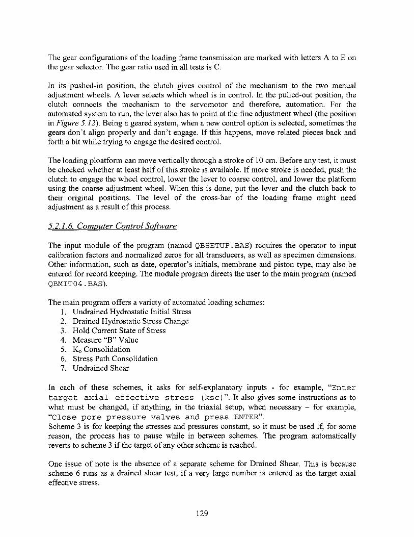
The gear configurations of the loading frame transmission are marked with letters A to E onthe gear selector. The gear ratio used in all tests is C.
In its pushed-in position, the clutch gives control of the mechanism to the two manualadjustment wheels. A lever selects which wheel is in control. In the pulled-out position, theclutch connects the mechanism to the servomotor and therefore, automation. For theautomated system to run, the lever also has to point at the fine adjustment wheel (the positionin Figure 5.12). Being a geared system, when a new control option is selected, sometimes thegears don't align properly and don't engage. If this happens, move related pieces back andforth a bit while trying to engage the desired control.
The loading ploatform can move vertically through a stroke of 10 cm. Before any test, it mustbe checked whether at least half of this stroke is available. If more stroke is needed, push theclutch to engage the wheel control, lower the lever to coarse control, and lower the platformusing the coarse adjustment wheel. When this is done, put the lever and the clutch back totheir original positions. The level of the cross-bar of the loading frame might needadjustment as a result of this process.
5.2.1.6. Computer Control Software
The input module of the program (named QBSETUP . BAS) requires the operator to inputcalibration factors and normalized zeros for all transducers, as well as specimen dimensions.Other information, such as date, operator's initials, membrane and piston type, may also beentered for record keeping. The module program directs the user to the main program (namedQBMITO4.BAS).
The main program offers a variety of automated loading schemes:1. Undrained Hydrostatic Initial Stress2. Drained Hydrostatic Stress Change3. Hold Current State of Stress4. Measure "B" Value5. Ko Consolidation6. Stress Path Consolidation7. Undrained Shear
In each of these schemes, it asks for self-explanatory inputs - for example, "Entertarget axial ef fective stress (ksc)". It also gives some instructions as towhat must be changed, if anything, in the triaxial setup, when necessary - for example,"Close pore pressure valves and press ENTER".Scheme 3 is for keeping the stresses and pressures constant, so it must be used if, for somereason, the process has to pause while in between schemes. The program automaticallyreverts to scheme 3 if the target of any other scheme is reached.
One issue of note is the absence of a separate scheme for Drained Shear. This is becausescheme 6 runs as a drained shear test, if a very large number is entered as the target axialeffective stress.
129

5.2.1.7. Carbon dioxide Tank
The carbon dioxide is kept in a pressurized tank, which can act as a powerful rocket in thecase of an accident. This has important safety directives. The carbon dioxide is needed onlyfor the saturated tests.- The tank must be kept vertical to minimize the risk of an accident.- Except during transportation, the tank must be fixed to an immobile object (laboratory
benches are appropriate) with a belt and clamp.- For transportation, the regulator valves and gages must be removed and the tank's steel cap
must be tightly screwed on the top.- The tank must not be transported by rolling, carrying, pushing or dragging. The only safe
mode of transportation is securing it to a wheeled cart specifically designed for transportingpressurized gas tanks.
5.2.1.8. Piston Clamp
The piston clamp is a two piece doughnut shaped metal component, with two bolts holding ittogether. To clamp the piston, place the pieces around the piston at the lowest possible point,touching the piston guide (the metal cylinder with ball bearings). Then tighten its bolts.
The clamp prevents the piston from moving down into the triaxial cell, but not up. Whentightening or loosening the bolts of the clamp, or axial LVDT crossbar, or the top assembly,the piston should be held down by holding the clamp.
5.2.2. Saturation
The procedure in this section (entire 5.2.2 with all of its subsections) is used only forsaturated tests, and is completely skipped for unsaturated tests. Saturation is achieved by firstdisplacing the pore air with carbon dioxide, then replacing carbon dioxide with water. Anyremaining pockets of CO 2 are dissolved in water (carbon dioxide's solubility in water ismuch higher than air's) through pressurization. This is done using the following procedure:
5.2.2.1. Initial Effective Stress
In order to preserve the integrity of the specimen, the initial effective stress, which wasapplied by lowering the air pressure in the pore space during setup, must be maintainedduring saturation. But this can no longer be done through the pore air. The initial effectivestress will be provided by applying a small magnitude of hydrostatic total stress.- Start the setup module of the computer program.- Input the information except pore pressure zero (pore pressure transducer is not yet
connected to the triaxial cell). The setup module will route the user to the main program.- Remove the vacuum within the specimen by disconnecting the vacuum pump from the pore
PVA pipe. With the piston clamped and the fluid in cell under about 0.04 kgf/cm2 pressurefrom the elevation of the cell PVA reservoir, it is possible to have a stable specimen withzero pore pressure.
130
- Choose option 1 (undrained hydrostatic initial stress) in the main program. Apply a smallinitial stress (0.2 - 0.25 kgf/cm2 was used in all tests of this research).
- Switch the cell pressure control to computer.- Take the piston clamp off.
5.2.2.2. Carbon dioxide Flushing
- In order to judge whether the gas is flowing properly, dip the end of the tub or hoseconnected to the gas tank into a container of water and observe the CO2 outflow as bubbles.Use the valves of the regulator on the tank to adjust the flow to 1-2 gas bubbles per second.
- Connect the CO 2 at this flow rate to the pore PVA pipe on the triaxial base- Fill pore pressure transducer socket with distilled water- Connect outlet B to an open container (a flask works best) with some water inside, through
a flexible tube whose end is submerged in this water.
Carbon dioxide is heavier than air. Therefore the pore space and all connected pipework mustbe flushed upwards from the bottom (this will be called directive 1). One end must open tothe atmosphere through a body of water, in order to prevent the gas pressure from buildingup (directive 2). The next four steps are designed to flush the system while satisfying thesetwo directives. If two valves are to be turned between consecutive steps, they are turnedsimultaneously. Figure 4.9 can be referred to, for tracing the pipes that are being flushed.
1. Turn the transducer valve to connect the back-pressure junction to the pore pressuretransducer socket. Bubbles should start to come out through the socket, satisfyingdirective 2. Wait for a minute to get all air in the transducer socket - back pressurejunction - pore PVA line replaced by CO 2.
2. Read this step and the next step. Turn the transducer valve to connect the pedestal to thepore pressure transducer socket, and turn the top valve to connect the back-pressurejunction to the top cap. This will flush the line between the back-pressure junction and thetop valve, while pushing the excess air downwards through the specimen and out of thetransducer socket. As this will operate against directive 1 once the CO2 reaches the topcap, this step of flushing must not last more than 5 seconds (proceed to step 3 after 5 sec.).
3. Open the bottom valve, and close the top valve to all flow. This flushes the back pressurejunction - pedestal line, the lower porous stone, and pedestal - transducer valve line. Thedispersed flow through the porous stone, and getting the CO2 into all of its pores, may takesome time. So wait for 5 minutes in this step.
4. Close the transducer valve to all flow, and turn the top valve to connect the top cap tooutlet B (i.e. the flask of water). This flushes the specimen, upper porous stone, and thetop cap - top valve line. In order to fill as many specimen pores as possible, leave it at thisstep for 20-30 minutes.
To finish;- seal the CO 2 in the system by closing all three water valves (transducer, top and bottom
valves) on the base,- bend the (copper) pore PVA line upwards,- disconnect it from the CO2 tank, and connect it to the PVA,
131
- close the regulator valves on the CO 2 tank.
5.2.2.3. Water Flushing
- Fill the PVA reservoir with water. This will be the source of water for the flushing stage,and the flow will be by gravity.
- Have an additional empty water container ready with flexible tubing.
For the purpose of flushing the system with water, directive 1 holds because water is heavierthan CO2. Directive 2 holds because most of the CO2 will have to leave the system through avent (the remaining amount will dissolve). As the criteria are same as those for CO 2 flushing,the procedure is very similar to that of CO 2 flushing.
1. Turn the transducer valve to connect the back-pressure junction to the pore pressuretransducer socket. Bubbles should start to come out through the socket, satisfyingdirective 2. Wait until the bubbles stop, which indicates all CO 2 in the transducer socket -back pressure junction - pore PVA line is replaced by water.
2. Read this step and the next step. Turn the transducer valve to connect the pedestal to thepore pressure transducer socket, and turn the top valve to connect the back-pressurejunction to the top cap. This will flush the line between the back-pressure junction and thetop valve, while pushing the excess CO 2 downward through the specimen and out of thetransducer socket. As this will operate against directive 1 once the water reaches the topcap, this step of flushing must not last more than 5 seconds (proceed to step 3 after 5 sec.).Any sign of water at the top of the specimen at this stage will disrupt the procedure, andforce the operator to first drain the pores (section 5.2.4.1) and then go back to section5.2.2.2.
3. Open the bottom valve, and close the top valve to all flow. This flushes the back pressurejunction - pedestal line, the lower porous stone, and pedestal - transducer valve line. Thespecimen, which has seemed translucent until this point, becomes opaque at the lower enddue to wetting. Wait in this step until the bubbles of CO 2 are seen coming out of the porepressure transducer socket stop.
4. Close the transducer valve to all flow, and turn the top valve to connect the top cap tooutlet B (i.e. the flask of water). This flushes the specimen, upper porous stone, and thetop cap - top valve line. The opaqueness of wetting in the specimen will progressupwards. In order to fill as many specimen pores as possible, the specimen is flushed withseveral volumes of water. During this time, the pore PVA reservoir may need refilling,and the flask connected to outlet B may need emptying. The rate of flow can be controlledby changing height of the flask. This step takes about one hour.
At this stage, the only missing component is the pore pressure transducer, which must beaffixed while regarding the rules in section 5.2.1.2, by the following procedure:- Bring the flask to a level so that the water level in the flask is a few centimeters higher than
the pore pressure transducer socket,
132

- Stop the flow of water by closing the bottom valve,- Turn the transducer valve to connect the pore pressure transducer socket to the pedestal.
Water will start to flow slowly from the flask to the socket, through the specimen. Thelevel of water in the socket will start to rise (if the flow is unobservably slow, raise theflask).
- Affix the pore pressure transducer into its socket, monitoring its output voltage.- Raise the flask so that its water level is at the mid-height of the specimen.- Record the input and output voltages of the pore pressure transducer as its zero reading.
5.2.2.4. Back-Pressure Saturation
In order to dissolve the remaining pockets of air or C0 2, the pore pressure will be kept at ahigh value (3 kgf/cm 2) throughout all saturated tests. An equal increment of cell pressuremust be applied to keep the effective stress positive.
- Close the pore PVA valve.- Turn the cell switch on the control box to off- Record the outputs of all transducers.- On the control computer, go back to the setup module and enter the pore pressure zero.- In the main program select scheme 2 (drained hydrostatic stress change).- Enter a pressurization schedule that will elevate the pore pressure (called "back pressure"
in the program) by 1 to 5-minute increments of 0.5 kgf/cm2, while keeping the effective2stress at 0.2 kgf/cm . This results in Table 5.2, which is how the schedule appears on the
computer screen while being input.
Table 5.2. Back-pressure saturation increments.Increment # Cell (ksc) Back (ksc) Time (min)
1 0.7 0.5 52 1.2 1.0 53 1.7 1.5 54 2.2 2.0 55 2.7 2.5 56 3.2 3.0 5
- Turn both the top and bottom valves to connect the specimen to the back-pressure junction.- Turn the transducer valve to connect the pore pressure transducer to the pedestal.- Turn all control switches to computer and wait. (It must be noted that each increment takes
much longer than its specified duration, so the scheme above may take over one hour.)
5.2.2.5. B Value Check
In order to check if saturation was successful, Skempton's B value (Skempton, 1954) ismeasured. The B value is the change in pore pressure in an undrained specimen in responseto a unit increase in isotropic stress, and is close to 1 for completely saturated materials.Scheme 4 of the computer program does this by applying several separate increments of user-defined stress (in the case of this research, 0.25 kgf/cm2 ). The program also prompts the
133

operator to close the top and bottom valves to flow at the beginning, and to open them backto the junction when the increment is reversed. In the end, the program computes the B valueand displays it. B values higher than 0.95 are considered acceptable for a triaxial test, and theprocedure can be continued. If it is lower, Scheme 3 (hold current state of stress) is run for 24hours, and then the B value is checked again.
5.2.3. Loading
After starting each of the phases of loading described in the next three subsections (5.2.3.1 to5.2.3.3) the operator should stay for a few minutes to observe if everything is runningproperly. The unsaturated tests skipped the previous section (5.2.2). Resuming the procedurefor all test types.
5.2.3.1. Initial Total Stress
For unsaturated tests only, this section is to make sure everything is working with lowstresses, before proceeding to higher stresses. Saturated tests already had an equivalentsection in 5.2.2.1.
- Start the setup module of the computer program.- Input the information. The setup module will route the user to the main program.- Take the piston clamp off.- Choose option 1 (undrained hydrostatic initial stress) in the main program. Apply a small
initial stress (0.2 - 0.25 kgf/cm2).- Switch the cell pressure control to computer.
5.2.3.2. Isotropic Compression
- Record the values on the control computer screen onto the datasheet.- Select scheme 6 (stress path consolidation).- Enter the intended confining stress (a, for unsaturated test, or &c' for saturated test), when
prompted for both of the target radial effective stress and the target axial effective stress.This will not exactly be equal to the applied confining stress, as will be explained in section5.4.3.1.
- Enter 0.1 to 0.3 %/hr for axial strain rate. The actual strain rate will not match this, and willnot stay constant.
- Start collecting readings from all 4 to 6 channels (input voltage, axial load, axialdisplacement, cell pressure for sealed and unsealed tests; plus the pore pressure which istensiometer in tensiometer tests; plus volume change LVDT for saturated tests) with theCentral Data Acquisition computer, at a rate of one reading per five seconds, set for 2000readings.
- Start applying the scheme from the control computer, and turn all related control switches(cell pressure and axial load for unsaturated; plus pore pressure for saturated) to computer.
- This scheme lasts less than two hours, and the computer reverts to scheme 3 (hold currentstate of stress).
134

5.2.3.3. Shearing
- Record the values on the control computer screen onto the datasheet. Also record thenumber of data points in the data acquisition computer, or start a new data acquisition task.In order to preserve accuracy in the data, the strain values at this stage will act as the zeroreadings when processing the data (section 5.4.1).
- Select scheme 6 (stress path consolidation).- Enter the intended value of c for unsaturated test, or 7c' for saturated test, when prompted
for the target radial effective stress.- For the target axial effective stress, enter a number larger than the expected strength at this
confining pressure. In this research 20 kgf/cm was entered, whereas no specimenwithstood any axial stress greater than 10 kgf/cm2.
- Enter 1 %/hr for axial strain rate. The actual strain rate will not match this, and will not stayconstant.
- Start the scheme.- Add several thousand readings to the Central Data Acquisiton computer.- After 2 - 3 hours, increase the reading rate to 15 or 20 seconds. Add enough thousands of
readings for the next 24 hours.
5.2.4. End of Test
- Earlier the next day, stop the shearing if the axial strain has exceeded 15%. Turn all controlswitches to off, and stop the data acquisition.
5.2.4.1. Draining the Pore Water
For saturated tests only, follow this procedure before continuing, for unsaturated tests, skip tosection 5.2.4.2;- Close the bottom and transducer valves to all flow.- Turn the top valve to connect the top cap to outlet B.- Open the cell PVA valve.- Detach the pore PVA from the triaxial cell.- Connect both the vacuum pump regulator and pore PVA outlet of the cell, to a watertrap. A
watertrap is a flask that has two holes through its stopper, through which flexible tubesconnect it to other components. The watertrap, in this case, will accommodate the porewater without letting it into the vacuum pump.
- Open the bottom valve and turn on the vacuum pump at a small vacuum. This will drain thespecimen in a few minutes. A Visible color difference will progress throught the specimen.When the bulk pore water is completely drained, water stops flowing into the watertrap andthe hissing sound of air flow through the specimen begins.
- Close the top valve to all flow.- Close the bottom valve. This seals the vacuum in the specimen.- Turn the transducer valve to connect the pore pressure transducer to the back-pressure
junction.- Remove the pore pressure transducer. Water in its socket will be sucked out into the
watertrap immediately.
135
- Disconnect the vacuum from the setup.- Close the cell valve to all flow.
5.2.4.2. Emptving and Dismantling the Cell
- Open the vent valve.- Open the tank valve.- The cell fluid starts to drain very slowly. It can be left as it is, and it will drain completely
by gravity in 20-30 minutes. Or, if faster drainage is desired, the compressed air pipe (notshown in Figure 4.9) that pressurizes the oil tank may be connected to outlet A withpressure, to generate a larger head difference.
Dismantling the cell is mostly the reverse procedure of assembling it (section 5.1.5). Thefollowing steps can be carried out while waiting for the cell to empty:- For the modified setup, unplug the tensiometer.- Disconnect the pipe of the cell PVA from the triaxial cell.- Close the cell PVA valve.- Bend the end of the pipe that was connected to the cell PVA on the triaxial cell, such that
its end is at the same level as the cell pressure transducer.- Remove the cell pressure transducer.- Put the piston clamp on.- If air pressure was used to accelerate the drainage, then disconnect the compressed air pipe
from outlet A.- Release the bolts of the top assembly.- Raise the cross-bar of the loading frame, and the top assembly, off the piston.- Remove the reference bar and the core of the axial LVDT.- Unscrew six bolts of the top plate. Remove the top plate with the LVDT.- Disconnect the pipe that goes to the oil tank.- Lift the triaxial cell and rest it on the edge of the loading platform.- Unplug the load cell cable from underneath the base.- Put the triaxial cell on a workable space with operator access from all directions.- Remove the plexiglass cylinder.- Use toilet paper to dry as much fluid as possible from transducer sockets, outlets and base.- Use the optical vernier (as described in section 5.3.1) to take diameter measurements of the
deformed specimen at various levels, in two directions. In the majority of tests themeasurements were taken at every 0.5 or 1 cm, with an extra measurement at the widestcross-section.
5.2.4.3. Specimen Retrieval and Recycling
As described in section 5.1.2, sample processing procedure is impractically long for Type 2material. Any material that touches oil is deemed unusable, as oil may affect the frictionangle. Moreover, it certainly changes the mechanics by adding oil-water surfaces to all tests,and oil-air surfaces to unsaturated tests. The following procedure was developed to recycleupto three-quarters of each specimen without oil contamination. On average, the missingamount can be replaced by repeating the procedure in section 5.1.2 only once.
136

The equipments for this part of the procedure are:- scoop,- spatula,- sharp, thin scissors,- a glass plate of about 25-30 cm on each side,- a roll of toilet paper,- a container to collect contaminated material,- 3 very clean water content tares, with known weights for unsaturated tests.
Use toilet paper to dry as much oil as possible from the ceiling of the superstructure, loadcell, top cap, and the membrane surface, from top to bottom.
- Wipe the superstructure and the load cell.- Wipe the gap between the top cap and the load cell. Wrap and leave some toilet paper in
the gap, as oil retained within the load cell can continue oozing down for several hours.- Fold the rolled part of the membrane down, over the o-rings. Dry the exposed oily
surfaces (rubber sleeve, inner surface of the membrane) with toilet paper.- Wipe the oil off the outer surface of the membrane around the specimen.- Set a clean glass plate on the laboratory bench or table.
5.2.4.3.1. Opening up the Specimen in the Standard Setup
For the standard setup only;1. Increase the distance between the o-rings around the pedestal by sliding them apart.2. Hold and pull the lower o-ring radially with fingertips to make a gap between the o-ring
and the pedestal. Pull the membrane up out of this gap with the other hand.3. Repeat the step above from several directions until the end of the membrane is free of the
o-ring.4. Slide the upper o-ring on the pedestal downwards. Repeat the previous two steps for this
o-ring as well, to free the lower end of the membrane from both o-rings.5. Turn both top and bottom valves to the back-pressure junction to release the vacuum.6. Place the rolled section of the membrane immediately above both o-rings.7. Push the upper o-ring on the top cap down and slide both o-rings on the top cap down to
a level between the upper porous stone and the surface of the top cap.8. Hold both porous stones from outside the membrane and pull them horizontally while
keeping the specimen intact.9. Lay the specimen on its side onto the glass plate.10. Collect the porous stone and nylon filter at the bottom end (the end without the rolled
section of the membrane).11. Cut the membrane along the length of the specimen, with minimal disturbance to the
specimen. Start the cut from the bottom end, and cut to a little above the top porous stone.12. Peel the membrane from this cut to the sides.13. Collect the remaining porous stone, nylon filter and o-rings (Figure 5.13 is at the end of
this step).
137

Figure 5.13. Specimen after the membrane is cut.
5.2.4.3.2. Opening up the Specimen in the Modified Setup
For the modified setup only;1. Disconnect the connection between the standpipe and the spiral tube of the top cap.2. Slide the o-rings around the tensiometer down, but not off the membrane.3. Place and tighten a second piston clamp at the tip of the piston shaft.4. Turn the entire triaxial cell upside down and balance it on the newly placed piston clamp.
For the steps in which the cell is upside down, the instructions will use "towards thebase" and "away from the base" instead of "up" and "down", to avoid confusion. Thehelp of a second operator will be required for some of the following steps.
5. Remove the toilet paper in the gap between the top cap and the load cell.6. Unfold the rolled portion of the membrane away from the base, over the two o-rings, and
into the gap between the top cap and the load cell.7. Slide the o-ring further from the base into the gap between the top cap and the load cell.
Pass the rolled portion of the membrane through this o-ring toward the base.8. Repeat the process with the second o-ring on the top cap, freeing the top cap - end of the
membrane from both o-rings.9. Unscrew and remove the nuts of the bolts fixing the superstructure to the base.10. Unscrew and remove the nut of the tensiometer.11. One operator holds the tensiometer body with one hand, the top cap with the other. The
other operator lifts the base with one hand while guiding the tensiometer's cable throughthe hole in the base with the other. The result of this step is removal of the base whileeverything else remains in place.
138
linu. ... ........ - -= - -------- ----""--1

12. The second operator holds the superstructure with the hand that was holding the base.The first operator holds the porous stone of the top cap from outside the membrane withthe hand that was holding the top cap.
13. The first operator pulls out the stone, the specimen and the tensiometer while keeping the
specimen intact, and lays them on their side onto the glass plate.14. Collect the porous stone and nylon filter.15. Cut the membrane along the length of the specimen, with minimal disturbance to the
specimen. Start from the rolled portion, and cut all the way to the o-rings around thetensiometer. Then cut it around most of the circumference of the tensiometer, parallel tothe o-rings.
16. Peel the membrane from this cut to the sides.
5.2.4.3.3. Separating Potential Contamination
The potentially contaminated material comprises the parts that have touched the membrane,nylon filters, or the scisors. The scoop and thespatula should be wiped with toilet paper afterevery step in which they are used onpotentially contaminated material.1. Cut off the 5 mm that was closest to the
top cap off the specimen.2. For the standard setup, repeat the previous
step for the bottom end. For modifiedsetup, pull and separate the tensiometerfrom the specimen.
3. Use the scoop to collect the materialimmediately around the trace made by thescissors. Put it into the container ofpotentially contaminated material.
4. Scrape 1-2 mm off the lateral surface ofthe specimen using the spatula or the scoop(Figure 5.14). Do not roll the specimen.For the side it lies on, use the spatula tocarve as much as possible under it.
5.2.4.3.4. Collect Clean Material
1. Slice the remaining part into three using the spatula.2. Place each portion into a tare. For the modified setup, scrape the material that was stuck to
the face of the tensiometer into the same tare as the bottom portion.3. For unsaturated tests, label and determine the mass of each of them.4. Put the tares into the laboratory oven (110 *C). Wait for 24 hours.5. Take the tares out of the oven and into a dessicant jar. Wait for 3 0-60 minutes so that the
tares cool down to room temperature.6. For unsaturated tests, determine the mass of the tares and calculate water contents for the
top, middle, and bottom parts of the specimen.
139
................-------- ---

7. Check each tare for contamination. Using the scoop, shuffle the material in the tare anddestroy any structure caused by oven-drying. Then, shake the tare gently (without spillingout the material). If the material has a planar top surface and particles are freely flowing orrolling around, it is considered clean and can be reused. If the particles stick together andexhibit snow-like behavior as if they are moist, pendular rings of oil are holding themtogether, therefore they are contaminated and should be discarded.
5.2.5. Summary of Procedure Differences Among Test Types
For this section, the saturated tests will be the basis to which the procedures of other testtypes are compared, because the saturated setup has the most complicated procedure and usesalmost all components of the triaxial testing equipment. The setup illustrated in Figures 4.8and 4.9 is the setup for saturated tests.
5.2.5.1. Sealed Tests
This was the procedure for the earliest unsaturated tests. Surfaces of the top cap and pedestalare covered with nylon wrap, sealing the specimen. This also removes all parts of the setupthat are associated with the pore water from the procedure. These parts include: all waterpipes to the top cap and the pedestal; the pore pressure transducer; the pore PVA; andtransducer, top and bottom valves.
A disadvantage of this type was the possibility of inaccuracy with volume deformations. Ifthe specimen dilates, the sealed pore space will have smaller pressure then the initialatmospheric pressure. This pressure difference would be unaccounted for in the calculations,because the unsaturated tests do not have volume measurement. This led to the procedurechange described in the next section.
5.2.5.2. Unsealed Tests
This type of test keeps the pore air of the specimen connected to a water reservoir atatmospheric pressure, through a pipe filled with air. This connection is through both the topcap and the pedestal, as the reservoir is connected to the pipe that connects to the pore PVAin saturated tests. In this type of test, the pore PVA, pore pressure transducer and thetransducer valve are not used at all. The possible disadvantage of the sealed tests was negatedby "sealing" the pore air with a phreatic water reservoir.
5.2.5.3. Tensiometer Tests
These tests use the modified setup, in which a generation 7 MIT tensiometer replaces thepedestal, the bottom porous stone and nylon filter, pore pressure transducer, transducer valve,and bottom valve. These tests use the "sealing" method of the unsealed tests, which meansthat the pore PVA is replaced by an open water reservoir, connected to the top cap through apipe filled with humid air.
140

5.3. Measurement Procedures
5.3.1. Optical Profiling
An optical vernier is used for the cross-section area measurements before and after a test.
Both vertical and horizontal axes have a fixed scale with markings every 0.02 inches (0.5
mm). Across each scale there is a set of 20 markings, which move with the vernier,distributed over the span of 19 markings of the fixed scale. This provides the measurements
on both axes with a resolution of 0.001 inches (25 pm). The number on the fixed scale
immediately before the "0" mark on the moving gradations is the coarse part of the reading.
Whichever of the moving gradations match any marking on the fixed scale is the fine part of
the reading (Fig. 5.15). The resulting measurement is:
measurement coarse +fine Eq. 5.3.
The procedure for mappingthe specimen geometry usingthis instrument is as follows:
1. Set the instrument so thatits objective lens is about10 cm away from thespecimen, aiming at itsedge.
2. Pull the eyepiece to its fulllength. Focus the hairlinesin the view by rotating theeyepiece.
3. Looking through theeyepiece, move the entireinstrument to focus theview (it must be noted that 0 001
the lenses invert the imagein both directions, so up inthe eyepiece view is downon the specimen, and leftin the view is right on thespecimen). First, movesideways to locate sight ofthe side of the specimen.Then, move toward oraway from the specimen tofocus it into view. Withgood lighting, the image Figure 5.15. Optical vernier. Upper inset is the viewcan be focused enough to throught he eyepiece, lower inset is the viewdistinguish the outline of through the monocle on the ruler - readingindividual grains. The very 2.04 + 0.017 = 2.057.
141

edge of the specimen is the target of focusing. If any other point on the specimen istargeted, the edges of the specimen will be fuzzy because the edges are farther away fromthe instrument, compared to the rest of the specimen surface.
4. Bring the instrument to level by adjusting the height of the four screw-legs and watchingthe circular water gauge on the base platform. The weight of the instrument should restequally on all four legs (which is tricky compared to a three-leg setup).
5. Level the optical tube, watching the water gauge on it.6. Looking through the eyepiece, traverse the length of one side of the specimen. Locate the
top and bottom ends of the specimen and note their elevations.7. A point measurement at a given level is taken by aligning the cross-hairs exactly to the
edge of the spcimen and recording the lateral measurement. The diameter measurement ata level is the difference between the point measurements from each side of the specimen atthe same level. The area measurement at a level is taken by the use of two diametermeasurements at the same level, from two different orientations that are perpendicular toeach other on the horizontal plane. From the equation for the area of an ellipse, the areameasurement is:
Area = diameter 1 x diameter 2 x -- Eq.5.4.4
It should be noted that, as opposed to measuring at one level at a time, it is much easier tofirst collect all measurements from one side of the specimen and then the other, and finallymove the vernier to change the orientation.
8. For the measurement before the test, area measurements at three levels are taken: 0.2 to0.4 inches (0.5 to 1 cm) below the top end, 0.2 to 0.4 inches (0.5 to 1 cm) above thebottom end, and the middle. For the profiling of the deformed shape, measurements weretaken at elevation intervals of 0.2 to 0.4 inches (0.5 to 1 cm), possibly with an extrameasurement at the widest section. For measurements at multiple elevations like these, itis more convenient to:- take all measurements from one side of the specimen,- take all measurements of the other side,- rotate the triaxial cell by 900,- refocus the view,- take all measurements from one side of the specimen,- take all measurements of the other side.
5.3.2. Data Acquisition Software
The data acquisition program runs under Microsoft Windows, and is user friendly. Among itscapabilities, the ones that are useful for an ordinary data acquisition task will be explainedhere.
The "Tasks" menu has an option to "Create Task". This brings out an input window in whichtask name, waiting time before starting, number of readings (upto 1000), time intervalbetween readings and data channels to be read (all data sockets in the labs have numbers onthem indicating their number) are entered. Entering this information and clickking OK startsa task of data acquisition from the selected channels.
142

The main screen lists all current tasks. For each task, it displays name, status (running,standing by, or completed), channels, time interval, "missed/read/total" number of datapoints. Double-click on the last column of a task displays upto 1000 readings in tabular formin a new window. Double-click on the "time interval" column brings out an input box askingthe waiting time before starting, number of additional readings and time interval betweenreadings - in case the data collection scheme needs to be changed while the task is running.Double-click on the "channels" column opens a window in which each channel number isdisplayed with its current reading, updated once per second, to act as a voltmeter.
In order to save data while the task is still running, select the task in the main screen, andclick on the "S" button at the lower right corner of the screen. If a task is no longer needed(because the experiment is completed), selecting the task in the main screen, and selecting"Retire Task" form the "Tasks" menu saves the data and closes the task. The data saved byeither means is stored in tabular form in a ".dat" file with the same name as the task, in theprogram's directory. This file can be opened in MS Excel and the data can be processed.
5.4. Data Processin'
Data acquisition and conversion of the acquired data into engineering units was discussed insection 4.6. As mentioned earlier in section 2.8.1.1, lengths are in cm, forces are in kgf;therefore pressure and suction terms are in kgf/cm2 . For each data point, this results in theraw measurement of the following set of quantities:
- Time- Axial displacement (AH).- Volume change (AV), in saturated tests only.- Axial load reading (Fread).
- Cell pressure (Oceii).- Pore pressure (u), in saturated tests only.- Matric suction (ua - u), in unsaturated tests with tensiometer.
Additionally, measurements that were described in prior sections of this chapter are:- Initial specimen height (Ho).- Initial diameter (DO) and area (Ao).- Initial volume (VO).- Dry mass of specimen (mdy)- Final deformed profile of the specimen, in which the height with the maximum cross-
section area is considered as the final area of the specimen (Af).
The apparent final volume of the specimen (Vf)a can be calculated using the final deformedprofile measurements. The specimen is approximately composed of slices in the shape oftruncated cones, each slice being between two levels of optical measurement (see Appendix5.1 for the derivation of relevant equations).
143

The initial void ratio (ej0i) is calculated from the phase relations and using the specific gravityof the specimen (Gs) as:
In -Vei, - Eq. 5.5
G,
5.4.1. Strains
All strains used in the calculations are Eulerian (engineering) strains. These are
Ex, = AH / H, c, = AV/ V, Eqs. 5.6
where Ex is axial strain and F, is the volumetric strain. For consolidation, H0 and V0 are theinitial values; for shear, they are the values at the start of shearing (a.k.a. pre-shear values).
5.4.2. Corrections
For the calculation of stresses from the measurements listed above, area and membranecorrections must be applied. There is no piston correction because the load cell is below thepiston in MIT triaxial setups, as opposed to the commercially widespread external loadsensors.
5.4.2.1. Standard Area Correction
The area of a specimen decreases during isotropic compression. The relevant measuredquantities are axial force, specimen volume and height. Calculation of stress in the axialdirection requires re-computation of the cross-sectional area at each data point because, forisotropic compression (as well as other types of consoidation loading), the specimen isassumed to remain a cylinder. With this assumption, the area of the specimen (Ac forcylindrical) can be calculated through geometry as follows:
AV v0-(i- ,) =AA = H- = AH -( Eq. 5.7
" H HO -- c,) 1-.6During shearing, a triaxial specimen bulges and increases its cross - sectional area. Similar tothe case of isotropic compression, during shearing the area must be re-calculated for everydata point. To approximate the bulging, the specimen is assumed to be the rotational body ofa parabola. By equating the rotational integral of such a parabola to the volume of thespecimen, the maximum cross-sectional area (Ap for parabolic) at any given strain can becalculated as:
A = A- 3O1-6v 5 -1 Eq. 5.8
The derivation of Eq. 5.8 is Appendix 5.2. Changing the area in this manner always results ina significantly larger area and smaller axial stress, compered to the uncorrected case.
144

5.4.2.2. Modified Area Correction
After the first few tests, it became clear that the specimen does not deform as a paraboladuring shearing. As asserted by Oda (19721) and discussed in section 6.2.1.2, the bulgingconcentrates in the center. The parabolic area correction (Eq.5.8) uses the total volume andheight in its calculations, therefore, it underestimates the maximum cross-sectional area bybeing unable to consider the concentration of deformation in the center of the specimen.
The final measurements of an experiment include optical measurement of specimen diameter.The area (A) at each data point is calculated by proportionally increasing the areas calculatedby the parabolic correction, as follows:
A = A f - = area multiplier x A, Eq. 5.9Pf
where Apf is the area calculated with the parabolic correction for the end of the test, and Af isthe maximum cross-sectional area measured after the test. The ratio, which is named "areamultiplier" was between 1.24 and 2.43 through all tests conducted during this research (Table6.2).
5.4.2.3. Standard Membrane Corrections
The impermeable membrane that separates the specimen from the cell fluid adds someresistance to applied forces and pressures. Therefore, all the computed stresses are stressescarried by the specimen plus the membrane. Hence, they must be corrected to account for thecontribution of the membrane, which must be subtracted from them.
In the following equations, Km is the stiffness of the membrane, which is the product of themodulus of elasticity of latex and the area of membrane's cross-section. For a single thinmembrane used in this research, its magnitude is 1.3 kgf, as noted earlier in section 4.3.5. Itis also worth reminding the reader that the strains are positive in compression, negative inextension.
In the axial direction, the membrane is assumed to act as an elastic material, carrying moreforce with increasing strain. The force carried by the membrane (Fm in Eq. 5.10) must besubstracted from the measured axial load.
Fm = Km . (Cx + 2/3 Cy) Eq.5.10
In the radial direction, the membrane provides additional confinement, resisting the radialdisplacement more as the specimen expands. This translates into a radial pressure as anaddition to the cell pressure, which is
a. = K,, -e Eq. 5. 11A 3
145

As volume change is not measured in unsaturated tests, ev is assumed to be zero for thepurpose of membrane correction, in the light of the minuscule volumetric strains measured inthe saturated experiments.
5.4.2.4. Axial Modification to Membrane Correction
While setting up the equipment in preparation for an experiment, the operator is bound tostretch the membrane. This stretching in the axial direction imposes an additional axial stress,unique to the preparation procedure used for this research. The membrane corrections shouldbe modified in accordance.
The initial axial strain of the membrane is measured by the following procedure:
- Follow the setup procedure upto the point of stretching the membrane over the mold.- Mark the membrane from the inside with an inkpen, at the top edge of the mold (top of the
specimen) and the top edge of the bottom porous stone (bottom of specimen).- Take the membrane out of the setup.- Measure the distance between the markings. This is the initial membrane height (Hmo).- For each operator, repeat the process multiple times and take the average for a more
representative assessment.- In the tests by a particular operator, the mebrane is prestressed (in tension) by
H0.= =- Eq. 5.12HMO
which is a negative quantity, as compression is in the positive direction. This is a novelcorrection factor.
Initial axial strain of the membrane during setup (cmx), which depends on the operator, isbetween 3% (for the author) and 7% (for Naeem Abdul-Hadi). 5% was used for the tests withuncertainity of which operator stretched the membrane during a setup. For more discussionon operators and a list of which test was done by which operator, see section 6.1.2.
Finally, the axial strain in Eq 5.10 is replaced by (Fx + cmx) for the calculation of membranecorrection onto the axial force. This is a simplified solution; the exact version would requirecalculating the strains for all data points using Hmo instead of H0, but doing so only whencalculating the membrane correction. Compared to the ±1 mm precision of each pen markingon the membrane, this simplification is sufficiently accurate.
It should be noted that this modification is applicable only to the experiments prepared by theprocedures described in this chapter. Standard clay testing (and some sand testing)procedures roll the membrane over the specimen, rather than stretching it, eliminating 6mx.
5.4.2.5. Radial Modification to Membrane Corrections
The diameter of the membrane is smaller than that of the specimen. This results in a built-inincrease in the confining pressure for all types of triaxial cells. In order to incorporate this in
146

the calculations, the perimeter of the membrane (Pm) is measured (10.6 cm), and the initialvolume strain of the membrane (Cmv) is described by the ratio of the areas of the specimenand a circle bound by the membrane, resulting in the following expression
6MV AO
mM 2 Eq. 5.13
4;r
which is a negative quantity for all experiments conducted in this research. This correctionwas also proposed by Berre (1985).
Similar to the axial modification, the volumetric strain in Eq 5.11 is replaced by (&v + Cmv) forthe consideration of membrane correction in the radial stress calculations. This, too, is asimplified solution in comparison to the more exact alternative of using Pm2/47r instead of AOfor calculating the membrane correction.
Even though &v is deemed negligible in the unsaturated tests, membrane correction due to &mvis still applied because it is a known and significant magnitude.
5.4.3. Stress Calculations
Applying the membrane correction to the axial force, modified as described in the previoussection, results in the following corrected axial force:
2F = Fread - Fm = Fread - Km - {(Ex + mx)+ -3 (Ev +6 mv) Eq. 5.14
where Cmx and &mv are described by the equations 5.12 and 5.13, respectively. In order tocalculate the axial stress, the corrected axial force is divided by the specimen area that is alsocorrected (in accordance to section 5.4.2.2). Cell pressure, which acts hydrostatically oneverything (even the load cell), is added for the axial stress:
= -+ a, Eq. 5.15A
As mentioned in section 5.4.2.3, stress in the radial direction is the cell pressure, with amembrane correction. From Eq.5.11 and section 5.4.2.5, the corrected stress can beexpressed as such:
=~ +o- Km(8v +8 ) Eq.5.1ar cell m cell A K my Eq. 5.16
A 3
In the form expressed above, both axial and radial stresses are total stresses. They are usedfor the results of unsaturated tests. In the case of saturated tests, they are converted intoeffective stresses via Terzaghi's effective stress principle:
Q = o( -u a = , -u Eqs. 5.17
147

In the rest of this chapter, formulae are written in total stresses, but they all can be convertedinto effective stresses by changing all (a)s to (a')s.
The stress space of choice is octahedral or mean stress (cyQct) vs. shear (2q, so that it is notconfused with q of p-q space). These can easily be calculated from the principal stresses ofCx , Cyr , Ur
c - x +2- -r Eq. 5.183
2q = u - Eq. 5.19
5.4.3.1. Confining Stress
The confining stress (ac) is an input to the triaxial control program. However this control isnot as accurate as the measurements, because the computer uses more simplified versions ofcorrection formulas. A more exact value of ac can be inferred at this point in calculations.Once the stress path of the experiment is plotted in aoct - 2q space, the intersection of theloading path (or its extrapolation) with the coct axis is marked as the true cy (Fig.6.2). Forcomparison between tests at different stress levels, acci and 2q are normalized by dividingthem by the true cy.
5.4.3.2. Smoothening of Deviatoric Stress
When sheared, uniform glass spheres tend to undergo cycles of stress relaxation and rebuild-up (Anthony & Marone, 2005) as in Fig.6.3. When this happens, the stress-strain curve is"smoothened" by joining only the top portions of each cycles. This is explained anddiscussed in greater detail in sections 6.2.1.1, 6.2.2.1 and 7.1.
5.4.4. Locating the Yield Stress and Strain
A common comparison between tests is based on the yield stress. The stress strain curves(see next chapter) have more or less elastoplastic overall behavior, without peaking at yieldand with strain hardening upto a peak stress. As with other stress hardening materials, it isdifficult to unambiguously define the yield stress. For this research, the maximum curvaturepoint on the stress-strain curve (smoothened - see Fig. 6.3) was used as a unique definition ofyielding. The relative scale of the axes is recognized as important to the application, so it wasnecessary to unify all stress axes into normalized shear stress to remove the effects of stresslevel. More importantly, all axial strain scales are magnified by a factor of 20, without whichmaximum curvature would occur at the peak stress rather than the yield stress. This numberis chosen to bring the strain axis to similar magnitudes as the normalized shear axis; it givesthe same (or similar) scale on both axes of the stress-strain curves in Chapter 6.
To summarize, in this thesis, the yield stress is defined as the point with maximum curvaturein the plotting of "normalized shear versus twenty times axial strain". For the remainder of
148

this section, the selected horizontal (transformed strain) and vertical (normalized shear) axeswill be denoted by x and y for convenience. This means
x = 20-e, y = 2Y0 Eqs. 5.20
The test results are made up of the discrete points. Curvature calculations will require makingfinite difference approximations of partial derivatives. The approximations of
yx yi+1 - yi-1
xi+1 - xi_1
yi+1 - yi yi - Yi- 1
xi+1 -xi Xi -Xi-1
Xi+1 - Xi-i
2
Eqs. 5.21
will be used in Eq. 3.1, which is repeated here as Eq. 5.22.
Eq.5.22
1+y
Even though the curve is already a smoothened form of the actual data, there are some local
perturbations. At those points, this approximation will give unrealistically high curvatures.
Figure 5.16. Locating yield strain for TX680.
1.5 -
-I --- I --- - -
0 . -1 r - -
0
VI I I-0.5
Z -l - - I - -- Normalized shear t- - -i- I - - -- - AL
-~ I- -~- CurvatureI II I I I
0--- - - -~ - -- - - - - - I T
-1.5
0 1 2 3 4
20 x Axial strain
149

One way of avoiding this problem is basing the aproximation on more points than just theneighboring two points. Let the curvature obtained above be labeled rii,, as it is solved usingthe i-i, i and i+l th data points. For Kia2, only i-2, i and i+2 are used, while i-l and i+l areignored. Averaging multiple such approximations to a single point's curvature should give abetter result. Averaging 4 curvature approximations at each point is deemed enough for thepurposes of this research. The smoothened curvature (14s) is therefore
= Eq.5.23
The lowest (highest but with negative magnitude) curvature in the earlier stages of shearingis at the yield strain. There may be other large curvatures at large strains (Fig.5.16), but thesesignify localized fluctuations. The stress corresponding to the yield strain is the yield stress.
5.4.5. Work Calculations
Work done on the specimen is calculated separately as work done by axial load or deviatoricstress, and work done by radial stress. Both are calculated by numerically integrating axialforce vs. axial displacement, and radial stress vs. volume change. The stress relaxations(sections 5.4.3.2, 6.2.1.1, 6.2.2.1 and 7.1) return energy into the system, therefore they mustbe included in the calculations. For this reason, the work integrations are on the entire data,not the smoothened curve.
W, =z F + Fi+( AI Eq. 5.242
W,.+=a2)'+' JA AVi, -A AV Eq. 5.25
150
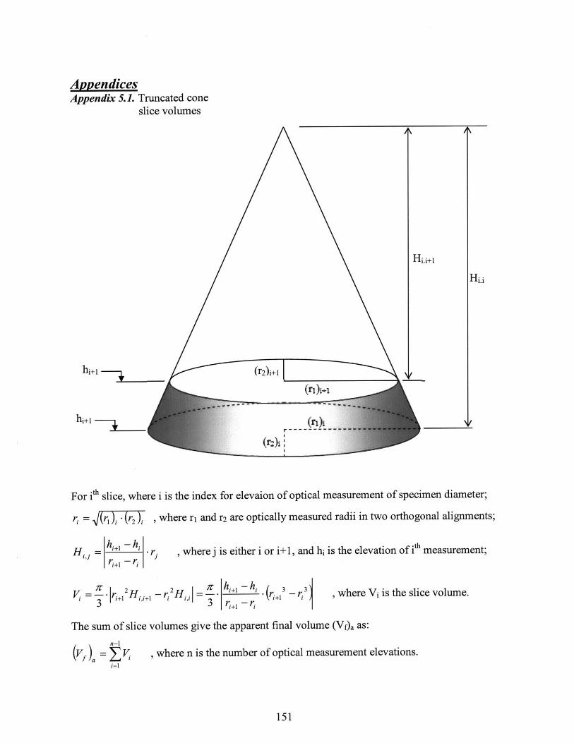
AppendicesAppendix 5.1. Truncated cone
slice volumes
Hiji
(r2)(r1
'V(r()( r - -- - -- -
For i th slice, where i is the index for elevaion of optical measurement of specimen diameter;
r = (r ) (r2, , where r1 and r2 are optically measured radii in two orthogonal alignments;
Hj= ii-r -rj , where j is either i or i+ 1, and hi is the elevation of ith measurement;
A
V = - r' H,+13, where Vi is the slice volume.
The sum of slice volumes give the apparent final volume (Vf)a as:
n
(V -1f) a Vi , where n is the number of optical measurement elevations.
151
-ri Hj' = - l . j - (r, - r 3
3 r,j - r

Appendix 5.2. Parabolic area correction
A (H2 42). j
x=f(y)= A-4y - H 2
2 = (H 2 4y2 )2 . A+8y2 .(H 2 4 2 -A +16y 4 AO
H 4
2 = 1l6 4(A +A,,-2VT A)+48y2 (J A-A)+ AH 4YH2
4y 2 AN /;
Volume expressed in terms of initial dimensions = volume of the rotational body
H/2 2H( Hf MC(A dAy +I) Hy (A. A0 2 )
2
(1AO ,)= - + A(l- . 5 3
+ AO - +Ao(1-6 V
(I - 6)
4 AA4+- A.AO
15
where (= -E)
4 A + 16AO15 225
-32(15K 5
16/15
SA-6 A+3OCA0 -v4/4
4-5+30 -1)
A (30 --5 - l16
D =o (30 -5 -1)4
H H02 2
where 4= (-c)(I - E)
152
O=A- 1 -23
+1 +Ao i
_IA=
= fy)
2
-

E X P IME N TS
RESULT S
153

154

6. EXPERIMENTS and RESULTS
This chapter details results of the experiments and observed effects of various procedurialparameters. There is no attempt to make connections between the results or to provide anyinterpretations with regards to the main ideas of the research. Nevertheless, the chaptercontains essential information for the following chapters of interpretation and conclusion.
The naming convention of the model (for analytically estimating the effective stressincrement due to suction - sections 3.2 and 3.3) and the hypothesis (inferring the effectivestress increment due to suction, from the saturated and unsaturated shear strength envelopes -section 3.4.2) will continue in this chapter.
6.1. Specimen Properties
6.1.1. Sample Materials
In order to have the experiments closer to the calculations with spherical uniform particles inchapter 3, glass spheres were selected as the material to be tested. Two types of glass sphereswere tested. These will be designated as Type 1 and Type 2 for the remainder of this thesis.Through an optical microscope, both materials were observed to contain smooth spheres.Moreover, post-experimental observations show that they preserve their shape andsmoothness through testing, and do not undergo crushing, plastic deformation, or flatteningof contacts (Appendix 6.1).
Drying SMC curves for both materials (Appendix 6.2) were obtained by the MIT technique(section 2.2.2) and fit the normal behavior of uniform glass sphere samples (Toker, 2002). Asany other uniform material, the SMC curves distinctly show saturated, bulk drainage, andpendular regimes. In the low water content range (pengular regime), suction is highlysensitive to variations of water content, as expected of uniform materials. According to themodel, unlike matric suction, effective stress and shear strength shall not have largesensitivity to water content.
6.1.1.]. Type ] Glass Spheres
This material was processed from a mixture of glass spheres of various sizes and origins,found in the MIT Geotechnical lab from past research projects. A specific gravity of 2.43(Sjoblom, 2000) indicate the composition to be a mixture of borosilicate (Gs=2.2) and soda-lime glass (Gs=2.57). The size range of 106-125 prm diameter was separated by sieving in thestandard manner (ASTM-D6913), and was used as Type 1 glass spheres in the tests.
Examination of the microscope photographs (Appendix 6. a and 6. 1b), as well as additionalsieving through 106 pm sieve, showed that the grains are not uniform and that there areparticles smaller than the sieve size in the sample. This is speculated to happen due to the factthat the material was sieved through consecutive sieves (... 180 pm, 150 pim, 125 pim, 106pm,...). All particles that are supposed to be retained on a particular sieve are only slightly
155

larger than the sieve size. Such a particle can easily get stuck in the holes of the sieve, thusblocking the passage of smaller partices. This results in a significant amount of finer particlesretained on every sieve.
6.1.1.2. Type 2 Glass Spheres
As the limited amount of Type 1 material was used up, a new batch of glass beads waspurchased from MO-SCI Corporation. These are borosilicate glass beads with specificgravity of 2.2. The company used sieves of 125 pm and 80 pm size for separation of thepurchased batch. Note that, due to the sieving problem mentioned above, this still did notmean all particles are larger than 80 pm. This material was repetitively sieved as described insection 5.1.2. The resulting 106-125 pm fraction is designated as Type 2 glass spheres in thetests. The microscope photographs of this material (Appendix 6. 1c and 6. 1d) show it to be alot more uniformly sized than the Type 1 spheres.
6.1.2. Specimen Repeatability
The preparation method described in section 5.1.4 results in specimens of similar, but notalways the same initial relative density and void ratio (these are interchangeable as noted insection 2.8.3). Even with a constant number of compaction layers and blows, the initial voidratio depends on both the initial moisture content and the operator. This is documented in
Table 6.1. Variability in specimen preparation.Material Test Type Test compacting wcintMaterial TNo operator (%)
TX653 NKT 1.00 0.593saturated TX654 NKT 1.00 0.568
TX669 NKT 1.00 0.578TX663 NKT 1.00 0.604
Type 1 TX664 NKT 1.20 0.602sealed TX674 NAH 0.98 0.581
TX678 NAH 0.91 0.57unsealed TX676 NAH 1.33 0.599
incomplete TX661 NKT 1.50 0.582TX680 NAH 1.54 0.652
saturated TX685 NAH 1.41 0.654TX692 NAH 3.03 0.628TX684 NKT 1.20 0.691TX686 NKT 2.50 0.688
Type 2 Tensiometer TX687 NAH 1.76 0.656TX688 NKT 3.05 0.669TX690 NKT 3.50 0.632
sealed TX681 NAH 1.16 0.662
unsealed TX682 NAH 1.08 0.653TX683 NAH 1.35 0.666
The two operators who have prepared the specimens are Naeem Abdul-Hadi(NAH) and the author (NKT). Colors and fonts are coded in parallel to Figure 6.1.
156

Table 6.1 and illustrated in Figure 6.1. In all cases, the void ratios are within the boundariesof the densest and loosest possible uniform configuration, which have void ratios of 0.35 and0.91, respectively (Table 3.1).
Table 6.1 lists the triaxial shear tests, including one (namely TX66 1) that did not produce anyuseful shear results, in order to document the variability in specimen preparation. Theprocedures of the four main test types are detailed in section 5.2 (see section 5.2.5 forsummary of differences).
Without any other consideration, void ratios of Type 1 glass spheres has an average of 0.586and standard deviation of 0.014; whereas for Type 2, the average is 0.659 and the standarddeviation is 0.020. Most of the experiments on Type 1 are the early tests when the procedurewas being devised and the operators were learning, so some scatter is expected. Type 2, onthe other hand, shows a clear dependency of the initial void ratio to the operator and a trendof densification with increasing preparation water content (Fig.6.1). Variation in the voidratio can affect the results significantly, by changing both the saturated material strength, andthe contribution of suction to it. The effects of initial void ratio variation will be discussedlater in the thesis.
Fig. 6.1. Variability in specimen preparation
0.7
AA
- A
~. 0.6_ _ __ _ __ _ __ _ __ _
A Type 2 (uniform grain sizes) by NKT
-Type 2 (uniform grain sizes) by NAH
+ Type 1 (non-uniform grain sizes)- - -- - - -- - - -- ---- - - - -- -- -- --
0.5
0 1 2 3 4
initial gravimetric water content (%)
6.1.3. Estimate for the Effective Stress Increment due to Water Forces
For the materials described above, the effect of suction on effective stress can be estimatedbefore the experiments, within the framework discussed in Chapter 3. Comparing the void
157

ratios of the specimens of both types of materials to those listed in table 3.1, the packings areinferred to be between body-centered cubic and cubic, but are much closer to the body-centered cubic. Fromfigures 3.12 and 3.13, this gives a (a'-a).r of about 120 Pamm. Whendivided by the average particle radius of 0.058 mm, the resulting effective stress increment is
22000 Pa, which is approximately equal to 0.02 kgf/cm . Note that this value may be slightlyhigher in Type 1 material (0.02 to 0.025 kgf/cm 2) because of a greater coordination numberdue to variation of sizes of this material's grains.
6.2. Triaxial Test Results
The samples were subjected to CIDC (isotropically consolidated drained) triaxialcompression tests under both saturated and unsaturated conditions. In each test, the specimenwas first isotropically consolidated, and then sheared by increasing axial load (see Appendix6.3 for stress paths). All stress quantities, indicated as "normalized" in the rest of the thesis,denote division by the total radial stress, which is also the total isotropic consolidation stress.Deviatoric stress (2q), sometimes normalized, is used as the measure of shearing,complementing the axial strain axis in the stress-strain curves.
Table 6.2. is a list of all triaxial tests, with corresponding measurements of quantities that arenot observable in the graphs presented throughout this chapter. The tests are divided into fourtypes: saturated, sealed, unsealed, tensiometer. The three latter types are all for unsaturatedtests.
A confining pressure is specified by the operator in every test, as an input to the triaxialcontrol computer program. However, the cell pressure control is not very precise withoutcorrect area and membrane corrections, missing the desired value by upto 0.05 kgf/cm2 . Asan additional effect, this minor imprecision slightly disturbs the isotropy of the initialcompression. The real confining pressure (-c) values are inferred from the extrapolation ofmeasured stress path to the horizontal axis (as in Figure 6.2), rather than direct control (seesection 5.4.3.1 for more detail). Initial void ratios are determined from the solid mass andinitial volume, each of which are determined as described in sections 5.1.4 and 5.3.1.Apparent final volumetric strain is calculated from the apparent final specimen volume,which is obtained (beginning of section 5.4 and Appendix 5.1) by optically profiling the post-shear deformed geometry in two directions (section 5.3.1). The difference between theapparent and measured final volumetric strains is less than 1% in all cases of saturated tests(unsaturated tests don't have volumetric strain measurements). The area multiplier is theratio of maximum cross sectional area of the deformed specimen to the maximum specimenarea estimated by the parabolic approximation at the end of the test (the area multiplier isalways greater than 1, as bulging is concentrated to the center - see sections 5.4.2.2 and6.2.1.2 for details). Area multipliers of tests without reliable post-shear profile measurementswere assigned by averaging within their group of tests (e.g. the area multiplier for TX680 isthe arithmetic average of TX 684, 685 and 692). Final void ratio is computed using the finalmeasured volumetric strain, which is measured by the change in pore water volume insaturated tests.
158

Table 6.2. List of triaxial tests.
MaterialTestType
TestNo
(Gc(kgf/CM2)
Optically measured PVA LVDT
einitial
Fvfinal (%)(apparent)
Areamultiplier
Efnal N
(measured) efinal
final water contents(gravimetric, %)
top middle bottomTX653 0.97 0.593 1.99 1.2796 1.78 0.621
saturated TX654 1.64 0.568 1.58 1.2422 1.85 0.597TX669 2.61 0.578 -0.29 1.7904 0.69 0.589TX663 1.01 0.604 5.36 1.6310 0.28
Type 1 TX664 1.64 0.602 3.57 1.6595 0sealed TX674 2.50 0.581 1.64* 0.46
TX678 0.486 0.57 1.64* 1.43unsealed TX676 1.60 0.599 3.45 1.5942 1.11
incomplete TX661 0.582 0.85TX680 1.01 0.652 1.31* 2.62 0.695TX685 1.74 0.654 2.05 1.2547 2.83 0.701
saturated TX692 2.53 0.628 0.75 1.3739 -0.36 0.622TX684 2.49 0.691 2.57 1.3015 1.98 0.724TX686 1.72 0.688 10.8 # 2.427 # 4.4 2.48 2.62
Type 2 TX687 3.48 0.656 1.77* 1.24 1.32 1.47TensiometerTX6 88 1.73 0.669 2.4 1.3118 2.69 2.69 2.88
TX690 1.73 0.632 4.4 1.5710 3.39 3.38 7.49sealed TX681 0.96 0.662 4.57 1.5047
TX682 0.99 0.653 4.66 1.5884 0.78unsealed TX683 2.47 0.666 1.09 1.2951 1
*: Because the specimen was unintentionally disturbed while dismantling the setup, opticalprofiling at the end of test was not possible. Therefore area multipliers were assigned to beequal to the mean value within the same type of tests on the same material
#: Possibly erroneous optical measurement due to unnoticed specimen disturbance in the end.specimen. Differences in the experimental procedures of these types of tests are summarized insection 5.2.5. There is also a test designated as "incomplete", which did not succeed beyondthe preparation phase due to some electrical problems.
Yield stress and strain are identified as the point of maximum curvature in a plot ofnormalized deviatoric stress vs. 20 times axial strain, as detailed in section 5.4.4. Both yieldand peak values are based on deviatoric stress. Deviatoric stresses and axial strains at bothyield and peak are tabulated in Appendix 6.4.
6.2.1. Saturated Tests
There are some features and aspects of behavior that are common in all saturated tests. Thesewill be examined within the context of the results of one of the tests (TX653), but they occursimilarly in all tests.
As shown in Figure 6.2, first the confining stress of G2= a 3 := ac is applied, sometimes (as isthe case in this example) with slight deviatoric stress. Both types of materials can carry shearstresses upto large fractions (more than half) of their strength without much deformation(Figure 6.3). Yield strains are in the range of 0.56-1.13 % (Appendix 6.4). After yielding, thematerial behaves plasticly and the general stress level does not vary much, except for the
159

cycles of stress drops (see section 6.2.1.1). A little strain-hardening occurs after yielding upto a peak stress, and then continues its plastic behavior with slight softening. The axial strainat which peak stress is observed varies a lot, depending on the material and whether it is asaturated test or not (Appendix 6.4). For saturated tests on Type 1 material it is 5.93 to 7.35 %,whereas in for Type 2 it varies between 2.11 and 5.43 %.
Figure 6.2. Stress path for TX653
2 2- - - - -- -- -- -- --_- -- - -
15 % strain ---- ------ ------- -- ---
L 1.5
- 0.5-
consolidation
0-
0 0.5 1 1.5 2mean stress (kg/cm2)
6.2.1.1. Stress Drops
According to Figure 6.3.a, starting from around - but not necessarily exactly at - the yieldpoint, the specimen undergoes cycles of sudden relief of deviatoric stress every 0.2 to 0.3 %of axial strain (less than two times the particle diameter). From a point of view, such a loss ofstrength at its first occurence could have been assumed as the yielding point. However, sucha definition of yielding would not be consistent through the tests, given that on several teststhe stress drops started after significant plastic deformation.
A closer examination of the stress drops (Fig. 6.4) reveals that they each resemble a miniatureelastoplastic stress-strain curve. The data points corresponding to low stresses during a stressdrop cycle constitute a scatter of points on the left side of the stress path in Figure 6.2. Eachsterss drop causes the stress state to jump from the imposed stress path (solid line with slopeof 3:1 in the Fig. 6.2) to one of the scattered points.
The stress drops are drastic enough for the specimen to emit audible crunching sounds. At thetime of each stress drop, a momentary excess pore pressure of 0.02 to 0.5 kgf/cm 2 wasrecorded (Fig. 6.4), as well as a sudden drop of 0.02 to 0.1 % in volume (Fig. 6.5). It must benoted that the pore pressure measurements at exactly the jump are probably inaccurate,because the data acquisition system was not designed to record such rapid changes.
160
.. ........ ............

Figure 6.3.(a) Stress-strain curve for TX653
-------- ------ -------- -------- -------- ---------y ield -------- ------------------ -------- --------- ----------------- -------- -------- ------- -c- d- d-&A -------------- --------- -------- -------- --------- re d u-------- -------- -------- --------- -------- -------- --------- ------- ---------
---------- ---------- I -------- ---------
H h.
yield----- ---- ----- -------- -- --------------------- -
--- ----------- 7- - - - - - - - -- - -- - - - - - - -T
- - - -- - - - - - - - - - --
- - -- - -- - - - - - - - -
-- - - - - - - --- - - - --- - - - - - -- - - - - - -, -- - -
: -- -- - --- - - - ------------
------
----------- --------------
----- ---------- -----------I I ---- J,
----------- ------------------------- -------: ----------
--------------- ----- I -----------
--- - ---- -------- ---- ----------- ------------------ ------
----------
----------
----------- ---------- ----------
---- ------ - ----- ----------- -- --------- -----
-------------------- - -------- -----------
I
II
2
1.5
> 0.5
COM Iea&
0
0.150.05 0.10
(small strain range).Figure 6.3.(b) Stress-strain curve for TX653
2
/o ,
0
> o
5
1
---------- ---- ------------ --- ---- -----
7
.5
0
0.002 0.004 0.006Axial strain
0.008 0.010
161
- --------------- -- --- ---- -----
Axial strain

It should be noted that these numbers may err on the low side, as the data acquisition andcontrol systems are not designed to record instantaneous changes in data, and do not respondfast enough to monitor sudden discontinuities.
Fig.6.4. Stress and pore pressure vs. magnified strain at drops2 . .3.05
- reduced deviatoric stress 3.05-complete deviatoric stress-pore pressure
1.5 3
S 1 2.95 0----- -------- ------- --------- ---------- - -----
-. 5- - - ---------------- 2.9 -
0 - ------- 2.85
0.02 0.025 0.03Axial strain
In the post-yielding portion of any stress-strain relationship, the stress is (supposed to be) themaximum that the material is able to withstand following its strain history. Immediately aftera stress drop, the material is no longer at its momentary strength. Therefore, only the plasticportion of each cycle belongs to the true stress-strain relationship, while the rest are randomdisturbances in stress. Because of this, as well as to clarify figures, all tests have beenreduced by plotting only one (or a few) high stress data points from each cycle for almost allof the figures throughout the rest of the thesis, as examplified with the light colored line inFigures 6.3 and 6.4. This results in intelligible graphs with data from multiple tests, likethose in Appendix 6.5 as opposed to plots like multiple Figure 6.3s overlapping each other.The reduced graphs of normalized deviatoric stress vs. axial strain and volumetric strain vs.axial strain of all saturated tests are included in Appendix 6.7.
6.2.1.2. Deformation
As expected from compacted granular materials, the glass spheres dilate throughout shearingafter a little compression at the beginning, in all tests but one (except TX692, which did notexhibit dilation - see Appendix 6.7. b), sharing the deformation behavior of most densegranular materials. However, the dilation does not seem to converge to unique critical statevoid ratios for either sample material, as can be seen from the scatter of the final void ratiosreported in Table 6.2 (especially for Type 2 spheres). This is somewhat expected given thenon-uniform deformation of the specimen.
162

During shearing, the specimen'sprofile deforms more like a bellcurve (Fig.6.6; Appendix 6.6 showssimilar profiles from other tests)than a parabola, which is an oftenassumed shape. This means thecenter of the specimen bulges morethan usual for triaxial tests. This isin parallel to the findings of Oda(19721), who had observed volumeexpansion due to dilatancy toconcentrate in the center third of auniform granular specimen.
The irregular geometry heavilyaffects the results at large strains,because the parabolic areacorrection (section 5.4.2.1) is notformulated for the unusual deformedgeometry. The area correction ismodified to accommodate thelocalized bulging in section 5.4.2.2.
163
Figure 6.5. Dilatant behavior (TX653)
-0.02
+ r L - - --
T- - - - -- L -7- - -- - -- - -- - - -
.. 04 -0.015 1 1 1 1 _____
I - -
- - - - - - --- - - - - - - - - - - - - 1
_0.01 5A1
S 0 If_ _I I
0
0 0.05 0.1 0.15Axial strain
Figure 6.6. Deformed TX653 specimen (cm)
8iitialspec men
-7 -- ---
5-- -------7- -6 -
-3 L
F I
- F -
F
-3 - -F 2I3
.. ..... ... ......

6.2.2. Unsaturated Tests
Pores of the specimen in a sealed unsaturated test are completely sealed from the outsidethroughout the test. The pore gas phase of an unsealed specimen is connected only to a waterreservoir at atmospheric pressure through a very narrow pipe, which allows pressureequilibrization but not too much water transfer. In the tests designated "tensiometer", thespecimen is sealed from the outside, but is in physical contact with an MIT tensiometer thatforms the pedestal in the triaxial cell. The reduced graphs of normalized deviatoric stress vs.axial strain and of all unsaturated tests are included in Appendix 6.8.
6.2.2.1. Stress Drops
Stress drops in unsaturated tests are similar to those observed in the saturated tests, as far asthe shape is concerned (i.e. a miniature elastoplastic stress-strain curve shape). The stressdrops in unsaturated tests may
- happen insignificantly or not happen at all. (TX678, TX681, TX686, first half of TX682,first half of TX687. See Figure 6.7 for an example)
- happen infrequently (irregular intervals of upto 1% axial strain), with minuscule stressdrops and oscillations in between. (TX663, TX676, first half of TX664, second half ofTX682, second half of TX687. See Figure 6.8 for an example)
- occur as frequently as in the saturated tests, i.e 0.2-0.3%. (TX674, TX683, TX688,TX690, second half of TX664. See Figure 6.9 for an example)
Figure 6.7. Stress-strain graph of TX681
1.5 -------
-------------------------------------------------------------
0.5
LF -1 J - I - - - - I_ - - I - - - - 1 -1 I - I - - - - L -1 _ - I- -
T IT - - - - - - -I F 7 -I
0
0 0.05 0.1 0.15 0.2
Axial strain
164
. ... . .................. ... ......... --- -- -. ..... ......

. .. ........ . ... .... .............
Figure 6.8. Stress-strain graph of TX676.3
------------------------- ------ ------------ ------ ---------- --- ------ ------ ------
------ ----- ------------------- ------------------- -----------------------
---- ------------------------ -------- ------------
2if------------------- ------
I T - -- - T - - - - - - - - - - - - - - - - - - -- - - - - - - - - - - - - - - - - - - - - - - - - - - - - - - - - - - - - - - - - - -
- - - - - - - - -- - - - - - - -- I -- - -- - - -I - - - - - - -- - - - - - -- - - - - - - - - - -- - - - - J - - - - - -
------------ ------ ------ ------ -- --- ------ --------------------------------
------------ ------ ------ ------------ ------ ------ 7- ------ ------- I ------ ------ ------
------------ ------ ------ ---------- ------------- ------ ------ ------
0
0 0.05 0.1 0.15 0.2
Axial strain
Figure 6.9. Stress-strain graph of TX688
--------
---- f
Axial strain
3
I
0
0.20 0.05 0.1 0.15
165
---------- -- ------ ------ ------ -------- ------
----------- ------ ------
-------- -----
... ..... ...

As can be deduced from the tests listed above for each type of behavior, in some tests thestress-strain curves start with one of the former two (of the three) patterns and continue withone of the latter two (of the three). The stress drops in the unsaturated tests are much smallerthan the saturated tests in magnitude (0-30% of the deviatoric stress in unsaturated tests asopposed to 40-80% in the saturated tests). This is most likely associated with the lack of porepressure generation (reduction in effective stress) in the unsaturated tests. Stress-strain plotsof the rest of the triaxial tests mentioned in this section are given in Appendix 6.5.
6.2.2.2. Tensiometer Measurements
Four tests were carried out in the triaxial cell that is modified to accommodate the MITtensiometer. The progression of matric suction in these tests is plotted in Appendix 6.9,versus time. Values of interest from those plots are summarized in Table 6.3. The high-capacity tensiometer (v.7.1) was utilized in test TX687, instead of the high-resolutiontensiometer (v.7.0) that was employed in the rest of the tests.
The magnitudes of matric suction throughout the tests vary greatly, as expected within thependular regime. The following observations were made from the suction measurementspresented in Appendix 6.9:- The suctions that were measured immediately after setting up the specimen are in
descending order with increasing water contents, as the SMC curves suggest.- At the start of the 24-hour equilibration period, the suction decreased (except in TX687),
but remained in the same descending order.- Suction equilibrium was successfully sustained for one day in tests except TX687, which
sustained it for 6 hours (see footnote in Table 6.3).- Isotropic compression caused the suction to decrease monotonically, except in TX687. In
the case of this exception, the rapid increase of suction with time stopped duringconsolidation, and although not monotonic, it had an overall decrease.
- During secondary compression, the suction increased slightly.- Shearing caused an increase in suction in all of the tests, but by different magnitudes. In
two of the tests, the suction exceeded the capacity of the tensiometer.
Table 6.3. Suction measurements and other relevant data for the tensiometer tests.Initial Final water Initial Equilibrated Matric suction
Test water content at matric matric at the endcontent the bottom suction suction of shearing
(%) (%) (kgf/cm 2) (kgf/cm2) (kgf/cm 2)TX687 1.76 1.47 0.115 0.115 - 3* >4.3TX686 2.5 2.62 0.044 0.029 0.047TX688 3.05 2.88 0.026 0.023 >0.8TX690 3.5 7.49 0.017 <0 ? 0.046
*: Stayed constant at 0.115 kgf/cm2 for 6 hours. Afterwards the suction readingstarted to increase. By the start of consolidation, it was 3 kgf/cm2.
?: possibly error in the transducer zero in this test
166

6.2.2.3. Deformation
There were no volume change measurements in the unsaturated tests. The post-shear opticalmeasurements show the deformed shapes of the unsaturated specimen to be similar to thesaturated case. In parts of tests that did not have stress drops, the volumetric strain - axialstrain curve was smooth as well.
6.2.3. Parametric Sensitivity
Section 5.4.2 proposed two new corrections for the processing of data from triaxial tests. Thenext two sub-sections (6.2.3.1 and 6.2.3.2) show the effects of these corrections on thedeviatoric stess. As earlier, TX653 is selected as an example to demonstrate the differences.
6.2.3.1. Modifications to the Membrane Correction
The conventional way of correcting for membrane stiffness is modified to account for theinitial axial and radial stretching of the membrane, which happens during the process ofsetting up the glass sphere specimen. As was noted in Section 5.4.2.4, and can be seen inFigure 6.10, modifications to the membrane correction in the axial direction result in higheraxial and deviatoric stresses by 0.003-0.004 kgf/cm2 . It must be noted that the modificationon the membrane correction in the axial direction varies with the operator, because it dependson how much the membrane is stretched during the setup process. This effect is taken intoaccount in the results. Modification to the axial correction for TX653 (Fig.6.10) is actuallyone of the smallest in magnitude; some other tests have this modification with more thantwice the magnitude.
The radial modification increases axial stress as well, but the increase in radial stress ishigher, making the overall effect on deviator stress a decrease of 0.005-0.006 kgf/cm2 . Alarge portion of this correction is due to the initial radial stretching of the membrane.Modification to the radial correction is of similar magnitude in all tests, because neithermembrane perimeter nor specimen area vary significantly from one test to another.
These modifications result in measuring more correct and lower deviator stress values, but2the overall difference from the unmodified corrections is within a mere ±0.002 kgf/cm2
6.2.3.2. Modification to the Area Correction
The difference between stresses corrected with respect to the specimen area and uncorrectedstresses increases as the shearing progresses (Figure 6.11), because the area correctiondirectly depends on the strains. For this research, this dependence is dominated by the axialstrain, because volumetric strains are small. It should be noted that the area correction tostress is actually in terms of a fraction of the stress, so in the tests of this research the areacorrection would appear to be directly proportional to the confining pressure as well.
167

(a) 0.0054 standard membrane correction
-- - ---- with axial modificationF -- -V -- T ----- I- - with radial modification% I I I I
4 - I -
0 -000
I T T IL IL|- -ih oh o. obie0
. .0-05005 _.1 .A1
-
- -
i
~I I F -I - - - - -I
I - I4 4 1 - -I -A -I
I I II I I
-0.01 _ _ _ _ _ _
0 0.05 0.1 0.15Axial strain
standard membrane correction---- with axial modification- - with radial modification--- with both mod. combined
L - - - L--
~TI II I
I I
I I I-
---- I F -
I I
-I
--- 4-
- ~I I
I I I
I I ~ II I I
--I---
I I I I- --- 4--- -4---- -I--- - -I- - -- -
I I I I
I I
I I
I I
0.1Axial strain
Figure 6.10. Effect of membrane correction and its modifications on the stresses inexperiment TX653: (a) on deviatoric stress, (b) on octahedral stress.
The modification to the area correction affects only the axial stress. It results in negligibledifference in deviator stress at smaller strains (such as the yield strain). By the time the axialstrain reaches 15%, the modification may diminish the deviator stress by as much as 0.1a ,compared to the usual parabolic correction. In other tests with a specimen more dramatically
168
0.006(b)
0
0
I I
I- t i
L--- 4- A
KT I
~ - -- %- I
-
I I
I I1~~~~~
CNI
r;j~ri~
0
00
0.004-
0.002
0-
- -4----
-
I - -- - -
I
---- A-- --
I V
I.'.
-i --
I --- I-..
I - -
0 -I
- - - - I-- --
I I I 1
-0.002 -'-
0 0.05 0.15
- -- ------------------- ......... . . ... ......

(a) 2. 5 1L -
0 1
- - - - -- no area correction0.5 cylindirical area correction
- -- parabolic area correctione-----------dareacorrection
01
0 0.05 * 0.1 0.15Axial strain
0 0.05Axial strain
0.1 0.15
4 -I-- I
I I I I
I I I I
I I I
I 1K 4I __ I ____ II I I
--- 4-- I
I I - I- - ~1
-- - - I- - I I
I I4- - -- -- -t - ---I-
I -
I I I
I I I
I _ _ I __ _ II I I I
-- -- 4--- I--I ---- 4-----
~~~~1 - -------
I I I
I I I------ II I
I I I I
- -- 4 I- - -I-I I I 4
- -- - - ~ 4
4 I 4
I I
I I I
--L i i I
-t------t-----4----
_____________ .1 i i I
---- 4-----
4---- -
Figure 6.11. Results of TX653 (ac = 0.97 kgf/cm2 ) with modifications to area correction.(a) Absolute deviatoric stress. (b) Deviatoric stress relative to the uncorrected measurement.
169
(b)
C)
0
IN
0
-0.1
-0.2
-0.3
-0.4 -
-0.5 -
-0.6
- cylindirical area correction
parabolic area correction
modified area correction
I

bulged at the center, this difference is observed to be as high as 0.2 7yC. The column named"area multiplier" in Table 6.2 is a direct indicator of the magnitude of the stress change dueto the modification of area correction.
For the final values of axial and radial stress, both membrane and area corrections aremodified. At smaller strains, this results in higher stresses as the membrane correction ismore prevalent. As the shearing progresses, the area correction dominates the magnitude oftotal correction, drawing the stress down. This introduces significant uncertainity to thelarge-strain results collected at the peak stress and 15% strain, compared to the yield stresses.Hence, this research gives precedence to the results obtained from smaller strains, such as theyield strain, for the interpretation of data.
When comparing results of a group of tests, differences in area multipliers betweenindividual tests can result in misleading appearance trends where there were none (ordisappearance of existing trends) at large strains. Because of this, the area correction must beemployed with care, especially if large strain behavior is an area of interest. The effects ofdifferent area corrections on interpreting the results of a group of tests is visible in Figure6.12.
Note that even at 1% axial strain, which is the approximate yield strain in many tests, thetotal of area and membrane corrections to deviatoric stress is -0.03 kgf/cm2 in TX653, whichhas a -cy of 0.97 kgf/cm2 . Compared to the prediction of 0.02 kgf/cm2 for the increment ineffective stress due to suction by the model (section 6.1.3), the corrections are significant,therefore such a detailed study and improvement of standard corrections was necessary.
6.2.3.3. Initial Water Content / Void Ratio
Some of the tests on Type 2 samples (namely TX686, 688 and 690) were repeated at thesame radial stress but different initial water contents. This group of tests was originallyintended as a way to investigate the effects of varying the matric suction on the strength andeffective stress. The matric suction measurements until the start of shear (i.e. through themoisture equilibration and consolidation) are of the order expected from the initial watercontents. As described in section 6.2.2.2, matric suctions generally increase during shearing,but the magnitude and rate of this increase does not exhibit any trends with respect to otherparameters of the test.
However, the direct effects of suction on strength and effective stress were not perceivable inthis set of tests, because the results were under the greater influence of variations in voidratio. As mentioned in section 6.1.2, the void ratio is affected by the initial water content.Within the water content range under consideration, better compaction (i.e. smaller voidratio) is achieved by increasing the initial water content. The shear strength of thesespecimen is greatly affected by the initial void ratio, as illustrated in Figure 6.12. A similarcomparison can be made between the saturated tests of TX684 and TX692, whose results areincluded in Appendix 6.7.b.
170

a) with modified area correction
2
-"0 L I
I I I-- r 1 -4 -- - -- - --
-TX690 (e = 0.632) (A.M.=1.57) -0.5 I
TX688 (e = 0.669) (A.M.=1.31) -----
TX686 (e =0.688) (A.M.=2.43) --- -
0
0 0.05 Axial strain 0.1 0.15
b) with standard area correction2
1.5
01
"0
N
0 0.05 Axial strain 0.1 0.15
Figure 6.12. Comparison of unsaturated tests with the same c and different void ratios anddifferent area multipliers.
171

It should be noted that the behavior at higher strains probably do not match because of thedifferent area correction multipliers (a test with an unrealistically large area multiplier, suchas TX686, has its stress reduced faster than other tests as axial strain increases). Because thearea multipliers are too different in this group of tests, results with parabolic (unmodified)area correction are also included as Figure 6.12.b.
172

Appendices
Appendix 6.1. Photographs of the two specimen materials through optical microscope.
(a) Type 1 spheres before test (200x) (b) Type 1 spheres after test (400x)
(c) Type 2 spheres before test (200x) (d) Type 2 spheres after test (400x)
173

Appendix 6.2. Soil-moisture characteristic curves of the two specimen materials.
Soil moisture characteristic curves
25 -
20 -
5 -
30 ----- -- -Type 1
-- - - - - ---- - - y 2----------- --------------
------ - - - - ---- - - - -
II - I - - I- L L 1
-~~~~~~ ~ ~ --
r - - - - r- - T- - r - r - I -i
-~~~~~~~~i -
- - - - - - - -4 -
- -4 I I I - I- I -
I - - - -
I -4
0-
10010
Matric Suction (kPa)
1
I I- - --- - - - - - - F - - - - - -
- - - - - - - - - - - _: -_ -- -- - - - - - - - - L
- - - - - - - - - - I - - - - - -
_W4 _ F F -I
- - - - - - - - - - - - - - - - -1
- - -- - - - - - - - L L -I- J -
- - - - - - - - - -
- - - - - - - - - - - - - - - -
- - - - - - - - - - F I- - - - - - - - - -
1 -1 -
- - - - - - - - - - - - -
- - - - - - - - - - - - - - - - 1- 4- -4
- - - - - - - - - - [ - - - ]_ '*,- - - - - - - - - - - - - - - - - - - - --
- - -- - - - - - - - - - - - - -
174
4-
I

Appendix 6.3.a. Stress paths for Type 1 material.
Effective stress paths of saturated tests on Type 1 spheres
I I I 4 4 I I I I I I I 4 I 4
5 - ---- I I I I I I I I T . .--~~~I - -~---- TX-6
-4 L- -J L _ -L L LL-I 1II I I I I
T1 J- - -J - - - - LL -
S2-
X6-3-1 I------- 4--------- ------
I L L . _I_ _. L - - L _ -l_ - - - - - - - - - -|- -J -
-I TI I- -I - I -X 4 < --2 ........ I - I I
0
- -- I + - - - - 1 - - - - - - - - - - - - - - - -- - --- -- - -- - - - - -|- - -
'- ~ II II II_ I_ I 4 _I II I I I I I I I I 4 I
- --. F - -l ~ ~ L- - - - - - - - - -- - - - - - - - - - - - - ~ ~
4. _ _ .4 - - - . I- - 4 -- - - - - -- 4 - - - --- - - - - - - -4 - - - - -
Octa hedra sr e I I CMI I
~~~~~~~~~~~~~~~~--- -- -+- -- - - -- -- -- ---------- --- H- - - ----- ---- -H- -- -- ----- t--I--1 lI I I I I
---- a-ed-- a--stress --(kg/---2
_ I_ I 4
I T -I -
- - - - - -I
- -F - -
- - - --- - --
4 I
I I-I
- F --
L I
- I -4----
I I
- - - - - - I - -
-- - - -I -- --F - -
--- 4 - -4-- -
4 - -4 - -4 -
-A I. 1 -1
- - F - I- - - - -
4- - L - - 1 -- -
4 I
- - --
---- - - - -- --
--- 4-- - - - -
-- 4 - - I- - I- - -
- J - -
- -1- - - - - I - - -
I- - J - -
-- - ----I- -- -
I I-I
- -- -- --
- - I- - -- - -
-4- -- 4---
I 4 T
- 1- - -l-- L
-- t- I--- - - - -
- - L - - - -J - L -
I 4 I
F- 4
--- -- - 4- - 4--- -
175
Total stress paths of unsaturated tests on Type 1 spheres5
4
C3
22
0
Octahedral stress (kg/cm 2)
I - -II I -I - J 1
1~~~- 4---1-1 1 t- I

Appendix 6.3.b. Stress paths for Type 2 material.
Effective stress paths of saturated tests on Type 2 spheres5 1 1 I - I I I T T- - - - - I
1-I- I I
I - - - - -- I
IF - - - - I - I - -I-e -
I I - - i ----- t I - - - -~6 I - -
- - 4 -'- - - - - --- 4-- - I 1 -4---- -3 ZIL---L LTIL7_~61~AIJ
-------------- -- -- -- - -- -- -
4 4 2 - - - - -- L----- - -_-L_-_-_-__-_-_-_
-4---I--~-4 - 1 - - - - - - - - - -
L -I- - AL ~ L L--- -LL4
I-l
o' r- 7
Octahedral stress (kg/cm)
Total stress paths of unsaturated tests on Type 2 spheresI I
- A - 1 L -1 -1 1-
I- I I I I I I
+ -
--- -4 --4 - -I- - T
S 4 1 - I 1 1 1 L
--- - - - --- -
1- 4- -4--I-
-I - I--
I
T
-1- - -I4- - 1 - -4 - -
- -I- - 4--- + - H-
-I- LI - 4t1- - 4 - I - -
I I I I
I~- - - -
,I 1--4 -4-
-- L- I 4 i -
1- -L4- - 4 - -
L -4-
- 1 - - - -
1- - 4 -I -I-
I t I
- --- 4- -1 1 II- -4
- ,l - L - 4 - 1
I I I
- -4- -4 - -
0~
5-
4-
3-
2-
1
t~4- -4 -- H-- 11 - 1-I
4-I L -1 A - -
Octahedral stress (kg/cm 2
)
0l
176
i A -- I- -
- - - - - - - - - - - - - - - - -I- - I- -
4- - 4 - 1-- - - I- -
4- 1- 1- -
L -A- -1 1--4
1-- 4I - -
0
4-j
0t
I
I

Appendix 6.4. Axial strains at yield and peak stresses.
177
Test Test Faxial (%) &axial (%)Material Type No at yield at peak
TX653 0.56 7.35saturated TX654 0.77 5.93
TX669 0.69 5.96TX663 0.86 3.48
Type 1 TX664 0.55 3.52sealed TX674 0.76 2.33
TX678 1.06 4.24unsealed TX676 1.09 3.60
TX680 1.13 3.52
saturated TX685 1.06 5.43TX692 0.99 4.14TX684 0.64 2.11TX686 1.00 2.00
Type 2 Tensiometer TX687 0.80 2.50TX688 1.00 4.07TX690 0.95 3.98
sealed TX681 1.20 3.81
unsealed TX682 0.92 2.821 TX683 1.27 4.67

Appendix 6.5. Deviatoric stress - axial strain raw data except TX653. Darker (blue) coloredgraphs belong to saturated tests and light (pink) colored graphs belong to unsaturated tests.
F F FF FF F
-F--' TX654lII1IItllflh1fihIlI1lI~i1flkk1 ~4J4~~ __ F I
IWIIflhIIIIilhIIIIfIIVIIIlIJIIII II(III~I~fl!IfI J~ ~A ~IA~Ad A
-F - - -
-I
I - - ~F -
I_L
-1
1 1 1
''''i VA' k-I I I
I -
I IF I
0.1Axial strain
T ~.
I F F
-I I F I
- - F - - - - - -- -~I I F ii
-F I I I
I I I-- I- - -
I I F
-F -- - -I- - ~ - -I F
- -F - F -
I I IF - - - ~ - --
-
F I
I F I I
4---- -I I I
~ -I -.I I I
F I I I4 -- -- -I-- -- -I- -- --
- - F -~ -
-~ - - --F --
I F I I-F -
I I F I
I I I
__ ~ r4~-- - I-!--iJ ~
F ~F F
I I F
~ F I F
I I I F1~~~ ~ F
I I F F
- ~~1~ ~ F FI I F I
F F - ~---~
I I F I-
F I I
I I I
F - -
I I F
F - ~I I
- -- -- - F F -- -
I I I
T T --- I.
I I I I
0.05
I I I I
- F - 4 - - -
F F I IF-I---
------ I-- -I I
--- 1--i- ~---
I I F-F--
I F
F F
F -~ ~ II I I
F FF- ~F I I I
I -
I I I
--- p--i iI I
F 1i IF I I
F
I I
------iF I F F
-- -F--- ~ F-
- 4-----I I F
- -T----1---I-- -
I I I I
--- F ~F I I I
0.1
TX663
- - - --- -
11 F -
n T
IF FT I I
I F T I
F T
T F - - -
F - - -
I I I I
I F I
1 F 1 - - I
0.15Axial strain
178
3 I A A A . - ,'
-
2
1
-I-F--
V
L.
-I
- - 4 ---
- - I-
U
0 0.05
2-
0.15 0.2
0
0
1.5
1-
0.5
0
0 0.2
-
II
I-
4 -1

Appendix 6.5. continued
3
[__- K V -I-I-
SI I
0.05
- F -4 -- -I - - - I- - -
- F---F -F-
- I F F
0.1
TX664
I I F I
I I
0.15Axial strain
- - -- T - - -- - - - T - - -
-- IT - --I - -- - -
- -- -- --
F F
-- F T - -- -- - - - -
I 1
I1,
ifl~i~1TX669
F FT
M F F I
f I--
I~-
5
4-
3-
2-
0
0.20.150.050
I-, ['I'-I - - - I-
I I
I I
I I
F - --
I- -1
-- -- F-
F F
-- T - - -
__j-
- - -- 1 --
~- I F--- - - ~ - 1
L
I-T-
0.1Axial strain
179
- ~
I I
I I~~~1~*
I I I II I I I
I ~ I
I I I I- I I I I
I I I I
4-----------F I
I F F
I I F II I F FI I F I
I I F F
~~1 ~I I F II I F I
I I I ~
I I I II I I -.I I I IF I I FF F IF
0
ri~ri~
1-4
01~0
2
1 -
0
0 0.2
/01
C13
-T - - F
I
I

Appendix 6.5. continued
5 -
4-
2
F F F F
F F1
0.05
r ------ - - -
-
I I I
F I - -
I I F
-- - I
-TFT
M= MNMIMPIL - - -- -- -- - - "Im
II
Axial strain
-t -- 7 - - - - - - - - - - - - - - - -r - - -T - - -i - - - - - - - - - -T -i - - -
I t I I I
T- - - -T - - I - - - - - - - - - T 11 - - 11 - - - - - - - - - - - - - - -
11 - - -T - - 11 - - - - - - - - - - - - - - - 1 -- 7 - - -
Axial strain
-I, I F-
L
i T
I r -I
r -i - - -
I I
--- r-- T--
I- - - -T -
0
0.1 0.15 0.20
0.5
0-+..0M
0
r -T -I - - - 7 7 - - - 7 7 1 - - -
0.15 0.20 0.05 0.1
180
T
F
I- F'- -1
- 1 ------- T ------ F ------ T-
F -T
I - - -

2T- -T -1 - - - - - - - - - - - - - - - 7 -T -1 - - - - - - - - - T- -T
T 7 -1 - - - - - - - - - -T -1 - - - - - - - - - T 7 -1 - - - - - - - - - r 7
I -T I - - - - - - - - - T- 7 1' - - - - - - T -T - - - - - - ITI I I I I
-i - - - - - - - - -
1.5 -------
--I - - - F I - - - - - - T 7 -1 - - - I - - - - - - T- 7 -1 - - - I
r - - -T - - -i - - - i - - - - - - -r - - -T -- 7 7 - - -T - - -1 - - - - - - - - - r- - 7 - - -i - - - I
T 7 -1 - - - I - - - - - - T- -T -1 - - - - - - - - - T- 7 - - -
I -I - - - I
7" -T -1 - - - I - - - - - - T 7 -1 - - - I - - - - - - T 7 1 T- 7
- - - - - - I - - - - - - I - - - - - - T- 7 TI I I0 ------ I ------+-0 1 - - - - - - 7 1 - - - - - - r- 7
M I I I I I I I Ir - - - - - - -r -T -1 - - - - - - - - - T- 7 1 - - - - - - T-
0.57 - - - - - - - - - 7 'T - - 7 - - - - - - - - r - 7 -1 - - -
I I I I I I I1 -1 - - - I - - - - - - r 7 -1 - - - I - - - - - - -r 7 -1 - - - - - - - - - r 7 -1 - - - II I I I I I I I I I I I I I
r - - 7 - - 7 - - - I - - - - - - r - 7 -1 - - - I - - - - - - T 7 -1 - - - - - - - - - r 7 - - -
T- -T -1 - - - I - - - - - - - I - - - - - - - - - - - - -
o i i I I i I
0 0.05 0.1 0.15 0.2
Axial strain
1.5
-1 - - -
I - - -
I - - -
11
I
I - - -
I
i T
/o- ,Cq
rA
2
1
0.5
00.20 0.05 0.1
Axial strain0.15
181
Appendix 6.5. continued
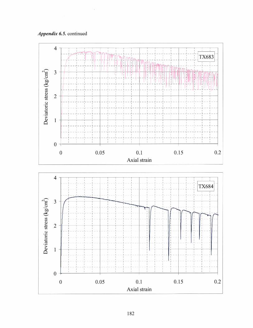
TX683_di -iii t --_ I-) [ -L I4
J 1"i ! if;
I - -I -J - - -L - 1
-1 - -~L -' .1 - -- - - - -i -J 1 -
-I - - - I - J - - - L -
In - --- -r~ -
I - I- -I A- - - L.. iJ - _-_- _ -_ -
4
0
0----------- - I - - -
---------- I - - I - - -I I I I
I I
I I
L j
I I
----- ---
- - L -- -
I - L -
0.1Axial strain
182
Appendix 6.5. continued
I I
I L - - -I - I[ I I ± - - - ~ - - L - - -
1~~~------
I I I I
-i
0 0.05 0.15 0.2
I I-F
1 -F F L TL 1 1 - - -F
~- - -I I I I I
-1 -1 L I - - -
3 t ---- II 4- - -- -I
I L L - - - I - - - J L
0 0.05 0 .... 0.15 l 0.2Axa2sri
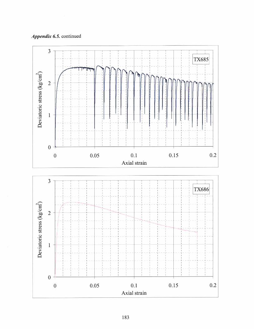
Appendix 6.5. continued
3 1 I 1I I I
I I I-- 4---I--
I I I
I I II ___ I I
I I I
I I I
I I I
I I II I I
- - ~I - - I _ ___ I
I I II I I
I I I I
I I I
I I I4 - - -~ -- - -- I-- - - 4- - -
I I I
I I I
I I II I
I In--v -
I I II I I I
-4 -- I---I----F---
I I II I I
I I I
I I II I I
I I I
I I
II I
I I
I I
I I
I I
0.05
I I
- -
I
0.1
I I -I TX8
L- IL'' ~- - I
I II _ I_
I II I
- -
-r
-- 4--
~1 --
-- 4
0.15Axial strain
1-1- I ~--F-hTI I II I I
4 - -I - - -- I- -- 4--- - --I I II I I
I I _ I
I I I
I I IS--4,---- I
-~I I I I
I' I I I I:4 -
- I I I
I I I I
I I I
I I I-- I II I I I
- I - - I - -- -- I- - 4 -4 F- --
- I I I
I I I-~ - I I I
- I I I I
-- - r - -- -
4----
I I
I I I II I I I
-I -
- - I --
- F- - - 4 -- 4---
I I
I I
I __ I __I I I
I II I
~ 1
I I
-4 I I
I I
I I I
I I
F-- 4- - - --I --- - -
I II I
I II I
- 1- -4 -I - -
I I
I I
I I
I I
I I I
I I
-- --- 4----
I I II I I
I _ I II II I
I I- I
I I
I I
I II I
I I
I I
-,--- I
---
I I I
I I I- - 4- -I- - -I- - -
I I I
I I
I II I
I II I I
~~4~~ -I -I I I
I I I-- 4 - --I- - -I -
I I
I I I
I II I
I I
I -
TX686
I I
I I I
.- -- 1 - - -
~ -AI I-I---4 - -- -~ I-I I II I
I I-I- - - F -- - 4 -- -
I I
I I-I- - - F -- - 4 - - --I I
I II _ I
I I
I I
3
r~i
0a
1
00.20.150.10
Axial strain0.05
183
0
I-cj,
0
0
$
2-
1
0
0 0.2
2 -

Appendix 6.5. continued
6-
5
0
I T I I
1 1 4 I1
-171 - -
II
I - - -
lie- -- - - - ---
1-4
4 4
II
-- -4--- - - -- - - -
r - 4i -1 -
2 TX687
I I I I - - -
-- 4 I- F - - -4 -
I I IF
0.1Axial strain
184
I -I
I - I_
- --
0 0.05 0.15 0.2
3 ~- - m -- - - - - -
Cl lji1jii
I _ I - - -T ---
0
0 0.0 0. 0.1 0.2
Axa strain I

Appendix 6.5. continued
I- T
I F IT
II
I I I I
-II I I I
I I I I
-I-- ~I -
I I I I
I I I
I I I I
I - - I~ ~ - -
I II......
I I
I - - -
-I -
I I
I I- -I-- 1
I I
I I
-I - ~I -- --
I I
--------- F--
F I - - I
I- -- --
I I I F
-- F1~
-I F
I -I
TX692-
I I I
I I
7- - ------- - -
I T
0.1Axial strain
185
5
4
3
.C 2
CI-
0
0 0.05 0.15 0.2

Appendix 6.6. Post-shear deformed shapes. Dash-lines show initial specimen geometry.
-I -
I I
1
7-
6 -
4--
1
ititialspecimen
dfefbmr edl -1specir n
I
A
-3 -2 -l 0 1 2 3
Deformed TX664 specimen (cm)
II L I
4 I
I I
I ~ I I
-3-2 - L 2-3
7--
6--
---- A-
SI
I I I I
- --~ -I -I -I-I- - -
I I ISI
~~~~1
Deformed TX663 specimen (cm)
I I
I
~1 -~ - -
I I
-1-- -
~1
I I I II I
I I
4 -
5--4--
I_
AiI 1 W I |
-3 -2 -1 0 1 2 3
Deformed TX669 specimen (cm)
- - - - - - --
13 -- -
- 2 1 0 I I
-1 I II 1 III I1
I I 2
I I I
-3 -2 - I 2I
186
Deformed TX654 specimen (cm)
8 8I-- -t

Appendix 6.6. continued
Deformed TX676 specimen (cm)R
I I
I
--7 ----------
-I
I I
-I
- ---
- - - -- I
SI
S-1-I-
SI
-i-I- -- ~-~- -
SI
4 -- I
SI
-
-1-
I- -- 1
A)
i I - I w
-3 -2 -1 0 1 2 3
Deformed TX686 specimen (cm)8
I 7I
r I
-1 - - - - -
3--------
__- -- L- -2 --- ----
1 0 1 2
-3 - -1 2I 3
----
5--
4--
3--
2--
I--
7-
-. I
F-
I I I
I I I I
I I I I- - -II- I- I -I -- -
SI I
I I II I I I
I I II I I
I I I- -i------ I- 4 -I-
I II II I I
SI
-- I- F-- -I -i -
I I I II I
I I-I -i -I -
--I- I
-I I~I I ~1I I II I
I I
SI
- -
i - t I . - - T
-3 -2 -1 0 1 2 3
Deformed TX688 specimen (cm)8
I II
I I I
--- - ---- - -----
- -- 52 - -
-3 -2 -1 0 1 2 3
5--
4--
3-
2--
I--
A
187
Deformed TX681 specimen (cm)Q

Appendix 6.6. continued
Deformed TX690 specimen (cm)8
-- 7-------I--
-4 -- -
3 - --- - F -- II-
I I
181
6 I
6 - - - ----
I Ii
- - -2 - I -
ii I I
-3 I-2 -I 4
I ~ I18
Deformed TX692 specimen (cm)
- 7 ------
6
-I -5
5--- F- -- - -
3-- 42 I
-3 -2 -1 0 1 2 3

Appendix 6.7.a. Reduced curves for saturated tests on Type 1 material.
-- TX654 -
-- TTX653I
-- TX669 -
-- 4
I I _ I
4 I I4- - -- -4 - -- 4 I - -
4 I II I I
-- 4- --- 4-----I I
I , I4
-L- - - A -
I 4 I
-I---4 I I -
4 II I
7 ~
4 ~4 I 4
t 4
4 F- t -4
4 I __ II I
F 4- -4
- - 1 I F
- -4
I I I I
I I I I
I I I I
---- I- 4--F- -4---
I I I II I I
--4- - - 4 - - -I I I I
-I - - -
- - - - L - -L, I I
I I
I I.I I I
-~ -I......I I I II I I I
-- F- -4----
S-I I I
- --I- - -I- 4- -
- F -I I I I
I- F- 4- -
I I I I
I I 4 I
I I
I I
I I-- I- - --I-----.
I I I I
II I
I _ _ I
I I
- --I I-I II I
-I - - --I -
I I
I I
I IF- - - F
I I
F--- F--
I I
I I I
4 1
'/1- I I I I
1 - 1,- -1 ---'I- -
Reduced stress-strain curves of Type I spheres2
TX1.(5 058
7- TX664 (e = 0.578)
I I - TX653 (e = 0.568) ---
0
0 0.05 .xa .tai 0.1 0.15
I I I I I
-0.02
-0.015
4- -0.01 -
-0.005
0
0.005
2
4 - -41 1
189
Axial strain

Appendix 6.7.b. Reduced curves for saturated tests on Type 2 material.
I I I I
- - - -
-0-I 0- ' - I -
- - - -1 -- - - - - - - -
I I
- -1-- --
-- ~T - - -~- -~ - -~ ~
--- - - -------4-- --
m-- - - - - -- - L - -
- - - -- - - - - -- TI I I
- - --- - ---
--- 4 -- -- - -~
I I I
-- -------- -- - --
--------- -- -- -- -- ---
- - -- -- - - -
S I I
-4--- -- - -- -- -
S I I I
~ ~~ C ~~I ~ ~ ~ ~
0.1Axial strain
190
2-
S1.5-0
4-4tz 1-
N
0.50
0-
- - -
- - - - - - - - - - - - - -
L I J
I I I I
- - - - -. - -
- - - 4 - -- - - - -
I I I I
- TX692TX685
- - TX684
TX680~- ~ ~I
0 0.05 0.15 0.2
-0.04
TX685 - -- -----------
-0.03 TX680 -
- - TX684 -
-TX692 ----I 73 -- - --- -
-0.02 --t- -- t "-0 - -- - - - - -
- + 1 - - - - - - - - - - -- - 1-- -. -2 - - - -- - H - 1 - -
10 '0 1
0
1-4 - + 41 - - - - - - - 4- - - - - -1-1| | I I I I
4- I 4 -
0 1 1 0.5| 02
Ax4a- sri
Axial strain

Appendix 6.8.a. Reduced stress-strain curves for unsaturated tests on Type 1 material.
2L I
I I II I L
I I I
I I F-
-4 - |
1 1 -
- --7
I I I
I _
I L
- I I I
1- - - I - - 4-1-
S I I I
- I - -L --
0.1Axial strain
0.15 0.2
Appendix 6.8.b. Reduced stress-strain curves for unsaturated tests on Type 2 material.
- I
-- - - - - - - - -
I I
I I
- - - -
I I
- - - -- 4--i-- - -- F- - -
-- -I- - -I -- -
S II
I I
--4-
4 -|- - Il F
- I
- ------ ------ -I- -
I I I I
I -- ~ F-I I
I I ____ I
I I I
- - - l~ - ~ - -
I I I I
-i -
I I T
- _ _ _- - _ _ -
-- I F 4-- --------- 4---I _ _ _ _1
I II II I
*4 - -- - -- _ -- - -
TX683
TX687'-----
- -- 41---- ~
TX681 -- -
0.1Axial strain
191
- t- - -t - - ---- - -L I
I - - - - -
I I
- - - - F - ---
CA2
N
Mz
1.5 -
1-
-- I --------
--- --- - ---- ---I I
I I --
- -TX674
TX678
TX664
TX6630
0 0.05
2
N
z
1.5
0.5 -
0
0 0.05
- - TX682
0.15 0.2

Appendix 6.9. Tensiometer measurements. Time periods marked "c" indicate isotropiccompression, those marked as "2" indicate secondary compression, and those marked "s"indicate shearing.
Tensiometer data for TX687 (wce= 1.76%)5 ----- I I------
--------- -- cpcitycapaiy
09 1 | I| I
- 1 - 1 -1 - - - - - - - - - -- - -1 - - -- - - - - - - + - -- F - - 1-- - -- -
0 1L I I I L I 7
~1 1 ~ - - - - --- - - -- - - T- r - - - - t - - - -1 - I- ---- r- I -
T _ 1 T - F - 1 -
1 T - - - T F T 1 - ~
30 _ L _ _ .-- - L 36 -- -4 L - L -
- - - - - 4 - - -- - - - - -4- 1 1 - - - - - - - - - -- -4 -- -- 4- -- -- - - -- ---
2 ~~ I
2
- 1 -T -- I - F -- -1 - - ----- - - T - -1 ~ ~T
I1 T F_ I I I I -
- ___-- - -----I_ _ 1 1 - - -- - i L - I J _ - -1 _ _ J _ I L 1 .1- - -L 1-- ----- - --- --- 4- --I - - -- - -
- l 1 - t ---I-- - - - t-- -- - -- +- -- - ---- - -t - - - - -
I I I I I I -
0
0 12 24 36 48time (h)
Tensiometer data for TX686 (wes,,=2.5%)0 .0 6 I I 1 -1 1 1 1 11 1
L_ . -- -I -_ - L - - - - - - - J - - - L - -AJ - - -L-
I~~~~ ~ ~ --- I 1 L--j-- -
0 .0 5 -----------
I F _ _- _ 1 _1 _ _I _ _-I T _ _ _- _J1 -
0 .04 i -t- -f ___
0 0 - - -- -- - ----------------- -- ------ ---------- - -- ---1 1 1 1 1 1 1 1 1
S0.02 ---- -- I- - - ~4 -- ~ --
S0.01 s-
0
0 24 time (h) 48 72
192
MIR

Appendix 6.9. continued
Tensiometer data for TX688 (wc1 =3.05%)
--------------------I T - - - - - - - -ii - - - - -
------- ~~~--- ---- --------- I----- L---- --
0 .1 ------- ------
-- ---------- T-------- ----- -----
------ - - - - -- - - - - - - - -
L - - -- - --- -- 0
0.0
0 12 24 36 48time (h)
Tensiometer data for TX690 (wci.=3.5%)
F T
-- t --
I I
I I
L I
-1 - --
-I- - - -I--- -- -
I I
I I
~1-- -I
-I --
-~ - - - ~ -
-- - - ~ -- - --
I I
-I~ -F-
I I
I- -- - - 1---
-r 1-
- - - 1 -
~~1 -
---- 1----
I I
I I
-- 1~
-A
j----
I I
- F - -I I
--- 1 I -I I
----- F- - - -
-+--- -I----
- --- - -- F- - -- - F- - - -
- -I- -- - - F -- - -I I
4
I I
I - -
0.06
0.04 -
0.02 -
0-
-0.02 -
-0.04
0 12 24 time (h) 36 48 60
- --- -- I -I
IIt
193
0
0
0
0
24 time (h) 36
I
0 12 48 60

194

INTERPRETATION
R E SU L T S
195

196

7. INTERPRETATION of RESULTS
This chapter complements Chapter 6 by providing an in-depth analysis of the importantfindings of the test program and detailed comparison of saturated and unsaturated behavior,Finally, the results are assembled in the framework of the hypothesis described in section3.4.2 for comparison between analytical and experimental results for the increment ineffective stress due to suction.
The naming convention of the model (for analytically estimating the effective stressincrement due to suction - sections 3.2 and 3.3) and the hypothesis (inferring the effectivestress increment due to suction, from the saturated and unsaturated shear strength envelopes -section 3.4.2) will continue in this chapter.
7.1. Stand-Alone Inter pretations
7.1.1. Stress Drops
The cycles of stress drops that were observed throughout most of the experiments, wereintroduced in section 6.2.1.1. Seemingly random stress drop cycles in tests on uniform roundparticles have also been measured by other researchers (Ting, 1981; Ovando-Shelley, 1986;Anthony & Marone, 2005). A plausible explanation for the stress drops is a mechanisminvolving a layer of particles suddenly moving outwards from one gap to the other overanother layer of particles, followed by a totally different layer moving in a similar pattern.Such a mechanism would not only exhibit stress drop cycles, but also lead to concentatedstrain in the center of the specimen.
Contrary to the apparent randomness of the stress drop cycles, the local peaks of cycles seemto follow an elastoplastic stress-strain curve, which represents the overall behavior of thematerial, as discussed in section 6.2.1.1. This may be a reflection that continuum responserepresents the aggregate behavior of many force chains - and gives an overall envelope onthe behavior (making and breaking) of individual force chains (apparent stick-slip). Effectsof individual force chains become more apparent in glass spheres due to the uniformity ofparticle size, shape and surface roughness
Occurrence and magnitude of the stress drops show large differences between the tests. Thetable below (7.1) reports the amplitude ranges and average intervals (of axial displacement)of the measured stress drops. For comparison, the average grain size of the materials is about0.11 mm. It is followed by Table 7.2, which shows the average values of amplitudes andintervals over groups of tests, separated by material and saturated/unsaturated distinctions.
From these results, the following observations can be made about stress drops:1. They always occur in saturated tests.2. They are larger in magnitude in the saturated tests, compared to unsaturated tests.3. The interparticle attraction in the form of pendular rings in unsaturated material may
prevent some of the particles from moving away from each other suddenly when they
197

TestType
TestNo
'c(kg/cm 2)
move around other particles. This would remove the discontinuous behavior for some ofthe particles in the specimen, reducing the overall appearance of the stress discontinuitiesin unsaturated tests.
Table 7.1. Amplitude ranges and average intervals of stress drops. Drops that are smallerthan 10% of the deviatoric stress (2q) are ignored for the average interval calculations.
Stress
Amplitude(% of 2q)Material
tx653 0.97 40-70 0.17saturated tx654 1.64 40 -75 0.20
tx669 2.61 30 - 75 0.27
Type 1 tx663 1.01 0-30 0.43
sealed tx664 1.64 0-30 0.37tx674 2.50 10-40 0.33tx678 0.486 None None
unsealed tx676 1.60 0-35 0.47tx680 1.01 35-60 1.56
saturated tx685 1.74 45-75 0.59tx692 2.53 60-90 0.94tx684 2.49 50-85 1.25tx686 1.72 None None
Type 2 Tensiometer tx687 3.48 0-40 0.37tx688 1.73 20-30 0.13tx690 1.73 20-35 0.12
sealed tx681 0.96 None None
unsealed tx682 0.99 15-30 0.50I tx683 2.47 0-30 0.21
Table 7.2. Averages of amplitudes and intervals of the stress drops for groups of tests. Testwithout stress drops aren't included in the averaging.
Material Test type Average amplitude (% of 2q) Average interval (mm)saturated 55 0.22unsaturated 18 0.40
T 2 saturated 64 1.09unsaturated 22 0.27
4. They are more frequent in saturated tests on Type 1 material, compared to unsaturatedtests on the same sample. For Type 2 material, the opposite is true for the frequency ofthe drops. There are a few unsaturated tests whose results were continuous, and thereforewere exceptions to this observation.
5. With the exception of saturated Type 1 samples, larger and more frequent stress dropsoccur at higher stresses. All continuous tests (i.e. tests without stress drops) are tests thatare run under lower confining stresses, among the tests of the same type. A possible
198
drops
Av.lnterval(mm)

explanation for this is microscopic indentations occuring at the contacts between the glassspheres under higher stresses. This may then cause shear behavior to be in the form of astick-slip mechanism.
6. Stress drops appear to be more pronounced in test setups with a smaller load framestiffness. Although the numbers in Table 7.1 do not directly support this speculation, veryclose examination of the drops in some later tests (especially TX692 - see last graph inAppendix 6.5) show that each stress drop is accompanied by a sudden positive strainincrement in the axial strain.
In summary, the materials being poorly graded and with very round particle geometrysomehow allows infinitesimal but widespread plane slips. While the details listed above seemrather random, it is clear that the water forces of the pendular rings act in opposition to thisbrittlely erratic stick-slip phenomenon and reduce the magnitudes of drop in stress. Althoughnot directly relevant to the research, it is an additional revelation about the inner workings ofpendular rings.
7.1.1.1. Excess Pore Pressure Cycles
As seen in Figure 6.4, each stress drop was accompanied by a jump in the pore pressure (forsaturated tests only), hinting at some sort of undrained behavior. This is reasonable, becauseany particulate material reacts to sudden stress changes by temporarily developing excesspore pressures (i.e. undrained behavior). The magnitudes of pore pressure jumpscorresponding to similar magnitudes of stress drops appear to show no trend or similarity toeach other, but this is very likely due to measurement inaccuracy (A system can notaccurately record a change of a few seconds while it is reading a data point every 15 seconds).Theoretically, the jump in the pore pressure would be momentarily equal to the drop in meantotal stress (oct).
7.1.2. Effects on Suction
The observations made by matric suction measurements were listed in section 6.2.2.2. Twoof those are relatively more important and deserve deeper interpretation.
The first observation is that matric suction decreases under isotropic compression. This maybe due to elastic compression of the specimen matrix, probably concentrated at particlecontacts at the micro-scale. When two particles are pressed together in this fashion, thependular ring between them will have to expand (without change in water volume), reducingits surface curvature and matric suction.
Secondly, matric suction was observed to increase during shearing. The process of shearingbreaks many particle contacts, and the engulfing pendular rings as two particles of the matrixmove away from each other. A portion of the water that had been contained in such apendular ring might evaporate and leave the system (to the humidifying reservoir), as it nolonger has the low energy of a stable pendular ring. This would leave less water (moresuction) for a new pendular ring that would be formed at a newly formed contact.
199

7.2. Comparison between Saturated and Unsaturated Tests
The consistency within each set of saturated and unsaturated tests provided the ability toobserve the differences associated with suction (i.e. differences between the results ofsaturated and unsaturated tests). The two materials are observed to have slight differencesregarding the effect of suction on shear behavior. There is no significant behavioraldifference among types of unsaturated tests (i.e. sealed, unsealed, tensiometer).
7.2.1. Generalized Comparisons
7.2.1.1. Axial Strains at Yield and Peak Deviatoric Stress
Unsaturated specimen reach a higher yield stress at similar axial strain in comparison to thesaturated specimen. The axial strains at yield are between 0.55 and 1.27 %. Type 1 sphereshave significantly lower yield strains. Afterwards, the unsaturated tests reach peak deviatoricstresses at lower strains than their saturated counterparts. For Type 1 spheres, this differenceis more pronounced: the strains at peak stresses range from 2.33 to 4.24 %, which isapproximately half of the saturated case on average. In the case of Type 2 spheres, the peakstress occurred between 2 and 4.67% axial strain, which on average is 0.4 % less than thestrains in saturated tests. Table 7.3 demonstrates these results by comparing the average yieldand peak strains of unsaturated versus saturated tests on both materials.
Table 7.3. Averages ± standard deviations of axial strains atyield and peak stresses from all tests.
Material Test type axial strain at yield (%) axial strain at peak stress (%)saturated 0.67 ±0.11 6.42 ±0.81unsaturated 0.81 ± 0.21 3.43 ± 0.69saturated 0.96 ±0.22 3.80± 1.38
Type 2 unsaturated 1.02± 0.16 3.41 ± 0.97
7.2.1.2. Work
Work, as the product of force (or stress) and displacement (or strain), directly depends onboth of these variables. In order to see any trend outside the stress and strain trends, effects ofstress and strain variation from test to test must be eliminated. For the stress aspect, workterms will be normalized by the confining stress for comparison. For the strain aspect, thework quantities calculated with the equations above can only be compared if they are uptothe same strain. For instance, comparing work upto the peak stresses will not be viable, as theaxial strains corresponding to the peak stresses vary between 2 and 7.35 %. Consequently,the comparison will be made for a specific axial strain, namely 1%, 2% and 15%. This meansthe work summations in Eqs. 5.20 and 5.21 will include the data only upto these specificaxial strains.
200

Full listing of the work done on the specimen by deviator stress upto 1%, 2% and 15% axial
strains, and in the case of saturated tests, work done by the confining stress can be found in
Appendix 7.1. Work done by the deviator stress and the total work done in the experimentTX653 are plotted in Figure 7.1. Work done by the confining stress is the difference betweenthe two graphs, and it is negative. Work by the confining stress can not be calculated for the
unsaturated tests due to the absence of volume change measurement. As mentioned insections 6.2.1.2 and 6.2.2.3, the volumetric deformations are low compared to the axial forall kinds of tests performed in this research. Therefore, a comparison of work done by thedeviator stress alone would reflect the majority of the total work.
Figure 7.1. Work done on the specimen of TX653
3
2.5
2
1.5 -
---- ---- -- ------------------- ------
--- I ----------
I ----------- -------------
----------- ----------- -------
------ ------ ------ ------ ------ ------- --- ------ ------ ------ ------ ------
------------- -------------------------
------ ------
------ ------ ------ ------ ------ --------- -- - - - - - - - - -- -
--- --------------------
--------- ------- -----
------ -- --- ------ ------- --------- ------ ------
------ --- - ----------- ------ ------
----- ------ ------- ------ ------------ ------- ------ ----------
----------- -----
------------------- ------ --------------
-------- ----- -----------
------ ------------------------- ------ ------ -- ------
------------------- ------------- - - ------ -----------
1
0.5
0
only
0.20.150.10.050
-- -- --- -- -- -- __ -- - - -- I - by deviatoric stress
total work
Axial strain
Table 7.4. Averages ± standard deviations of work by deviator stress, normalized by ac.Work done on the specimen by deviator stress,
Material Test type normalized by a,, (cm3), upto1% axial strain, 2% axial strain, 15% axial strain,
saturated 0.093 ± 0.004 0.209 ± 0.009 1.946 ± 0.034Type 1 unsaturated* 0.104 0.011 0.241 ± 0.014 2.190 ±0.054
saturated 0.082 ±0.010 0.191 ± 0.018 1.690 ±0.081Type 2 unsaturated 0.084 ± 0.008 0.202 + 0.013 1.863 ± 0.087
*: calculated by ignoring the test TX676, which had less strength, possiblydue to moisture equilibrium problems.
There is no trend within groups of tests (each of the four lines in Table 7.4 are the groups for
this purpose). Between different types of tests, two results are observed:
201
0
------------- ------------ ------
----------- ------

1. In all cases, unsaturated tests require more work than saturated tests to shear. This isspeculated to be because moving and breaking pendular rings require additional energy.
2. In all cases, Type 1 material requires more work than Type 2 to shear. The extra energy isspeculated to be spent ona) the pendular rings, which are more in number for Type 1 specimen,b) overcoming a slightly greater overall shear strength (see section 7.3).
7.2.2. One-to-One Comparisons
As described in section 6.2.3.3, results of both saturated and unsaturated tests are affected byvoid ratio. Therefore, results of a test can not be compared to another test unless their voidratios are close. If a particular test condition was run multiple times at the same stress levelbut with different void ratios (none of which match the rest of the tests), a virtual result canbe interpolated between tests, such that its void ratio would have been acceptably close toother tests. Such an interpolation was deemed necessary in two cases, as described in the nexttwo paragraphs.
In the case of Type 2 material, the unsaturated test, designated as TX683, does not have asaturated counterpart with the same void ratio. Instead there is the pair of TX684 and TX692,which were prepared at different initial water contents, and then tested at the same confiningstress as TX683. The specimen of TX684 is looser and that of TX692 is denser, incomparison to the specimen of TX683. Through linear interpolation of stresses (at yield,peak, or large axial strains) between the two saturated tests, weighted with respect to theirvoid ratios, the stresses at the corresponding strains can be estimated for an imaginarysaturated test on a specimen with the same void ratio of the rest of the tests. This brings thetoo dense or too loose specimen to the relatively more consistent void ratios around 0.653and 0.654, which are the average values for the rest of the saturated and unsaturatedspecimen, respectively.
A similar interpolation, this time between results of the unsaturated tests TX688 and 690 wasnecessary to approximate a counterpart to the saturated test TX685. Results of these twointerpolations are used to generate further results in Section 7.3, rather than the individualresults of the pairs of experiments contributing to each interpolation.
Appendix 7.2 shows comparisons between pairs of saturated and unsaturated tests of similarconfining stress and initial void ratio. According to these plots, axial stresses at yield arehigher in the unsaturated tests. As the shearing progresses, the stress carrying capacities ofthe unsaturated specimen decrease at a faster rate, compared to the saturated tests.
These interpolations are made only for the few quantities (yield stress, peak stress, etc.)necessary for the final plots of the Section 7.3, not the entire stress-strain curve. Thus theinterpolated results are not presented graphically in Appendix 7.2.
202

7.3. Stress Space and the Effective Stress Increment due to Water Forces
The stress increment due to water forces was estimated to be around 0.02 kgf/cm2 in section6.1.3, based on the model for effective stress. This corresponds to the horizontal differencebetween the total stresses from the unsaturated tests and the effective stresses from thesaturated tests, when plotted in mean stress space (section 3.4.2). Figures 7.2 and 7.3.a showsuch plots, created with yield stresses for both materials. Appendix 7.3 contains similar plotsfor peak stresses as well as stresses at large (15%) strain. It should be remembered that withincreasing strain, reliability of the results decreases, mainly because of the area correction.Therefore, the results at high strains have less weight than the results at yielding, which arethe only plots included in the main text.
Figure 7.2. Yield stresses for Type 1 samples.5 -
TX6744-
2; - 110444- +0 0 24-
0 1 2-3X4 5
1D --- --- ---
2 13
aoct or aoct' (kgf/cm2)
All results appear to form linear envelopes. However, there are two unexpected results thatcontradict the normal behavior of granular materials:
- In the two plots for the larger strains (peak and 15%) of Type 1 material (Appendix 7.3), thesaturated envelopes appear stronger than the unsaturated. Given the unreliability of results atlarge strains, this aspect is not detrimental to the research - the main focus will be the mostreliable results, i.e. the yield strength envelopes.
- Almost all of the envelopes seem to intersect the deviatoric stress axis on the negative side,if they are extended linearly. This will be discussed in greater detail in section 7.3.1.
203

Figure 7.3.a. Yield stresses for Type 2 samples.
-+- saturated data point-"-- unsaturated data point TX687
interpolation from 2q =1.0154 a- - 0.0662saturated tests 2 -0- - -62interpolation fromunsaturated tests IX692 (e=0.628)
TX690 (e=0.632)TX688 (e 0.669)
TX686 (e=0 688TX6T5
TXAl2TX 1 - - - 2q
2Goct or
3
------- ------- ------------- --- i ----------- -----------
1.0026c'-0.1904
-------------- -------------------
aoct' (kgf/cm2)4 5 6
unsaturated strengthenvelope
(total stress)saturated
strength envelope(effective stress)
normal stress
Figure 7.4.b Negative apparent cohesion
This result may mean that introducing pendular rings i
As for the main purpose of theseplots in mean stress space, Table7.5 lists the horizontaldifferences between saturatedand unsaturated envelope, whenapplicable. These numbers arefar greater than the 0.02 kgf/cm 2
that was originally predicted bythe model before the experiments(section 6.1.3). Therefore, amechanism that is not accountedfor in this research must havesignificant influence on strengthin partially saturated granularmaterials.
nto the system is not equivalent toapplying additional isotropic effective stress. Pendular rings increase the normal force atparticle contacts without adding shear force, because the water force acts perpendicular to theparticle surface. Therefore, increasing shear resistance of the contact. Increasing the isotropiceffective stress also increases shear strength. These two increases in shear strength need to bedifferent for (a'-a) values in Table 7.5 to be so high.
204
6
5
_4
3
N2
-1
00
4

Table 7.5. Magnitude of the differences between effective and total stresses (i.e.effective stress increment due to water forces. N/A entries occur when the quantity iszero or less, which is not expected as far as unsaturated soil mechanics is concerned.
Ranges of a' - a (kgf/cm 2 ) ,01)Material yield peak stress 15% strain saturated unsaturated
Type 1 0.07 to 0.12 N/A N/A 29.2 28.5
Type 2 0.14 to 0.18 0.16 0.09 to 0.18 27.3 27.6
If applying effective stress on a dry material creates shear forces at some of the particlecontacts, increase in the capacity for extra shear force (i.e. shear strength) would be smallerin comparison to the shear capacity increase due to the pendular rings (Figure 7.4). Since thehypothesis for effective stress increment - shear strength relationship (section 3.4.2) is basedon macroscopic effective stress, it underpredicts the strengthening effect of pendular rings.
(a) Soil under a'
G' strengthf
a7
(b) Soil under a'+Aa'
a'
Ao'
(c) Unsaturated soil undera', with (a'-a) = AC'
a' Aa' strength
a'
Aa'
' strength
Figure 7.4. Possible difference between a regular effective stress increment and theincrement in effective stress due to suction. Oc is the friction angle at the contact,associated to the solid plane - on - solid plane friction, not to be confused withthe internal friction angle, or angle of repose, of the granular matrix.
7.3.1. Strength Parameters
Table 7.5 also reports friction angles, calculated from the slope (M) of the envelopes inFigures 7.2 and 7.3 through the following equation:
# =arcsin tan 3Mfj)(6+ M
Eq. 7.1
The friction angles calculated above are very similar to the experimentally determined angleof repose of 28.60 for glass beads, reported by Jaeger et al. (1989). This is the friction angleof glass as a granular material, and must not be confused with the friction angle between twoglass surfaces.
205
i -- - .- ., - - -- - - - - e-e ! M*N&L MM

As mentioned earlier, the cohesion strangely seems to be negative. However, glass spheresunder zero stress simply roll around with no angle of repose, as opposed to the friction anglesobserved under confining stress (reported in Table 7.5). Since the glass spheres do not sticktogether when dry (they are cohesionless), the envelope for the saturated case must start fromthe origin. These two boundary criteria for the saturated envelope dictate non-linearity atvery low stresses, as illustrated in Figure 7.4.b. Following the hypothesis, unsaturatedstrength envelope in total stress space would still be a copy of the saturated envelope ineffective stress space, shifted by the effective stress increment due to suction along thenormal stress axis.
7.4. Parameters Affecting the Effective Stress Increment
According to the model presented in Chapter 3, the increment in effective stress due tosuction is affected mainly by the grain size and particle packing. Suction and water contentaffect it very little, as shown in section 3.3.4. Grain size distribution of the two materialswere not different enough to create observable differences. Among the remaining threefactors, the effect of suction and that of void ratio are found to be intertwined with the watercontent's effect. The following three sections describe the effects of these three factors,followed by section 7.4.4, which will characterize three mechanisms that affect the effectivestress increment and/or shear strength.
7.4.1. Effect of Suction
The model in section 3.3.4 suggests that no matter how much the suction is varied, its effectson effective stress (and behavior) shouldn't change by more than 30% (Figure 3.12). This issupported by the suction readings from the four tests (TX686, 687, 688 and 690) with anincorporated tensiometer. These suction measurements spread over two orders of magnitude(0.04 or less to 4 kgf/cm2 - see Appendix 6.9), and yet the behavior in the triaxial test resultsare not visibly affected by this variation. Three of the four tests (except TX687) werespecifically aimed to observe effects of suction and water content differences, but did notencounter any trend that can be a result of suction variation. Instead, a reverse trend (morestrength at smaller suction or larger water content) of the results was observed. This is notattributable to the effect of suction, but it is to void ratio (see sections 7.4.2 and 7.4.3).
7.4.2. Effect of Preparation Water Content
In the two groups of tests in which every aspect of preparation and testing other than thewater content was kept constant (saturated tests TX684, 692; and unsaturated tests TX686,688, 690), the results were significantly affected. According to these results, as thepreparation water content increases, the strength increases. This would also indicate greatereffective stress, which clearly is the opposite of not only the calculations presented in thisthesis (section 3.3.4), but also the widely accepted characteristics of partially saturated soils(Fredlund & Rahardjo, 1993).
206

These three unsaturated tests by themselves do not point to any explanation, as theirdifferences are not justifyable solely by the effect of water content. However, furtherinvestigation of the results of these tests show that their initial void ratios are different as aresult of preparation with different water contents.
The saturated pair has the same trend of strength with preparation water content. Ifeverything else was identical, saturated tests shouldn't have been affected by initial watercontent, since the specimen gets saturated at the start of the test. The only other differencebetween TX684 and 692 is the initial void ratio, so it must be the factor affecting the results.Therefore, the preparation water content affects the results indirectly, not through suction orpendular ring size, but through compaction of the specimen (see section 7.4.3).
7.4.3. Effect of Void Ratio
Among the tests prepared with different water contents (listed in the previous section above),another consistent observation was the dependency of void ratio to the water content. As thespecimen are constituted with a standardized method, the energy put into their compaction is(in theory, with the same operator) the same. Similar to compaction of coarse grained soil, itis observed that the material becomes denser (void ratio decreases) with increasing watercontent in preparation. This is observable in Type 2 specimen plotted in Fig. 6.1.
Similar to the behavior of any other granular material, denser glass sphere samples havegreater strength in the triaxial tests, compared to looser packings. This effect on strengthoutweighs the reverse effect of the decreased effective stress due to decreased suction andincreased water content.
7.4.4. Mechanisms Influencing the Results
Within the pendular regime, each of the following mechanisms is caused by, or result in,changes in one or more of suction, water content and void ratio. The first two mechanismsexist only in unsaturated materials, whereas the third takes effect regardless of saturation.Figure 3.13 was redrawn as Fig. 7.5, for the average particle radius of the tested materials, inorder to assist this section.
1- If a pendular ring grows because of decreasing suction and increasing water content, withno change in solid matrix, the effective stress decreases. This effect is very small (watercontent changes by adding or removing water in a given granular matrix are along asingle curve in Fig. 7.5).
2- Increasing the preparation water content results in denser packing of particles (smallervoid ratio), therefore increased number of contacts and pendular rings. This increases theeffective stress. This mechanism has much larger effect than mechanism 1, and itcorresponds to changing from curve to curve in the direction opposite of mechanism 1 inFig. 7.5.
3- Densifying a granular material increases its strength drastically, without increasing theeffective stress. The effect of densification on shear strength is much larger than theeffects of the previous two mechanisms. The hypothesis that links the shear strength to
207

the effective stress increment due to suction does not consider strength changes due tovoid ratio variations. Nevertheless, the hypothesis remains applicable provided the voidratios of all tests are kept constant.
0.05
0.04
1:pendu ar
-e=0.35e=0.47e=0.91
ings grow withate -content
Fig. 7.5. Two mechanisms of water content's effect on the calculated
values of effective stress increment due to suctionn 6
V.V3 Iy
0.02
0.01
- -
V
4210gravimetric water content (%)
208
3
"E
*-.
1-I
---------- ------ ------ ------
/2: co wctibn WRKincreasing
------ _W-atOr cbnttant------- ------ ------ -- I -------47L-'.

Appendices
Appendix 7.1. Table of work done on the specimen by deviator and confining stresses, until 1%, 2% and 15% axial strains.
Work done (j ) on specimenby deviator stress
until the axial strain of1 % 2% 15%
Work done (j ) on specimenby confining stress
until the axial strain of1 % 2% 15%
Total work ( j )until the axial strain of
1 % 2% 15%
Work done by deviator stress,normalized by ac, (cm 3 )
until the axial strain of1 % 2% 1 5%
Type 1 tx653 0.97 0.087 0.196 1.849 -0.009 -0.022 -0.130 0.078 0.174 1.719 0.090 0.202 1.906
Saturated tx654 1.64 0.148 0.337 3.229 -0.010 -0.033 -0.213 0.138 0.304 3.015 0.090 0.205 1.969tx669 2.61 0.255 0.573 5.124 0.001 -0.030 -0.178 0.256 0.543 4.946 0.098 0.220 1.963
tx663 1.01 0.105 0.244 2.167 0.104 0.242 2.145
Sealed tx664 1.64 0.194 0.425 3.622 0.118 0.259 2.209tx674 2.50 0.258 0.596 5.367 0.103 0.239 2.147tx678 0.486 0.045 0.109 1.097 1 0.092 0.225 2.258
Unsealed tx676 1.60 0.085 0.333 1.849 0.053 0.208 2.006
tx680 1.01 0.069 0.169 1.643 0.004 -0.016 -0.182 0.072 0.153 1.461 0.068 0.167 1.627
tx685 1.74 0.156 0.353 3.123 -0.015 -0.059 -0.367 0.140 0.294 2.756 0.089 0.202 1.784Saturated tx692 2.53 0.222 0.527 4.373 0.049 0.030 0.014 0.271 0.557 4.387 0.088 0.208 1.729
tx684 2.49 0.210 0.468 4.031 -0.023 -0.072 -0.356 0.187 0.395 3.674 0.084 0.188 1.619
tx686 1.72 0.132 0.318 2.898 0.077 0.185 1.685
Type Tensiometer tx687 3.48 0.316 0.739 6.496 0.091 0.212 1.867tx688 1.73 0.145 0.347 3.204 0.084 0.200 1.852
tx690 1.73 0.151 0.363 3.390 0.087 0.210 1.959Sealed tx681 0.96 0.067 0.176 1.801 1 1 0.069 0.183 1.876
Unsealed tx682 0.99 0.091 0.211 1.862 0.091 0.213 1.880
Unsea_ _ d tx683 2.47 0.222 0.525 4.752 0.090 0.213 1.924
MaterialTestType
TestNo
(gc(kgf/CM2)

Appendix 7.2.a. Comparisons between saturated and unsaturated tests at ~1 kgf/cm 2
consolidation stress. Type 1 material.
-I -
- T - - - - --
4 I S4 I
I 4 4 I-4 4 I
I I _ 4 _ _ I
I I
- -- -
--
-
-- - I
I _____ I ___ 4I I
-
4 4 I
I I I
I I I I
I I I I
I I I I- - __ - I - --
I II-I I
I I
-- - ---
.)
z
0 0.05 0.1 0.15Axial strain
Appendix 7.2.b. Comparisons between saturated and unsaturated tests at 1.6 kgf/cm2consolidation stress. Type 1 material.
4 I I
--
- -_
4 4 I I
44
I 4 I I
4 ____ __ I I
I I
I~L~ I-----I I I I
1 __ffi~__ ffi -
I I I I
-I - - -- - 4- - - - -4 - - - -I
I I 4
I- 4 -4-----1I I 4 4
4 I I
------ I --- F-- F ~I I I I
I I4 4 I I
4 4 I I
4 I __ I
4 I I I
4 I I
-- I- --- 4--
4 4 I I
I 4 4 I
4- - - - I- ---I I -1I II I
I II I 1~~~~ -]
4 I ,
4 I I ,
TX654 (saturated)
[X664 (unsaturated)
I I I I I
Axial strain
210
2
TX653 (saturated)
TX663 (unsaturated)0
2
Ivl
a.
zi
1.5
0.5
0
0 0.05 0.1 0.15
1.5 -
1
0.5 -

Appendix 7.2.c. Comparisons between saturated and unsaturated tests at -2.5 kgf/cm 2
consolidation stress. Type 1 material.
"0
N
z
- ----- ---- - t - -- -
I I I I I I I
-- -- - - - --------- -
-- -- TX674 (unsaturated)- -- - -- - - - -T - 9 ( a t - t d
I ~ ~ ~ X6 (saturated)___ I
0 0.05 0.1 0.15Axial strain
Appendix 7.2.d. Comparisons between saturated and unsaturated tests at ~1 kgf/cm2
consolidation stress. Type 2 material.
2
N
I T i,2
1.5 . TX8 (unsaturated)
1 --- -------- _I-L----------(unsaturated)
0 _____________-_TX680 (saturated)
S. 0.1 0.15Axial strain
211
2
1.5-
0.5 -
- 4- - - - --- --
I I I
-4----4 --- -
-- I
0 I

Appendix 7.3.a. Peak stresses.
Peak stresses for Type 1 samples.5 1TX619
------- TX-66
----------------- - 2 1j694j' .1 241 _ 67I_
T. 09 a 3+0.O -22-
L J L
-1 - - -]- - - - - - - - - - - I - k I - - - -
IX 65 -- - - -- --
1 T -----saturated- 1 - -U unsaturated
00 1 2 3 4 5
(Yoct or ayoct' (kgf/cm2)
Peak stresses for Type 2 samnples.6 I
* saturated data point -i---TX687
U unsaturated data point 2= 1.0364c-6.0085-5 -interpolation fromn -- __-V---
II I
saturated tests 2interpolation from 4II
unsaturated tests TXI692 (e=0. 28)
C., i 90O (e40.632) TX684 (e=0.6911__ I_
-1-- --- -- -)86 e= .8 TX-
TX6K6 8_ - 2q =-. 432 '-.1815 __
-- - -- - - -4 - -
0-io 1 2 3 4 5 6
aoct or a0oct' (Kgf/CM)
212

Appendix 7.3.b. Stresses at 15% axial strain.
Stresses at 15% axial strain for Type 1 samples.
I - -- -
- I
1.065 8-f
TFX654'
- TX664
T
0943'
TX
X&69-X669
"374-
5-
4-
1-
0
aoct or aoct' (kgf/cm2)
Stresses at 15% axial strain for Type 2 samples.5
+ saturated data pointunsaturated data point X------- Tx68/ interpolation from
4 -_ 4 _ _ -----
4 saturated tests 2q= 0.8984 O. 0 4 2 3interpolation fromunsaturated tests TX6831 TX692 e=O 28
3-D_90 (e=0632)T
T X684- (e -0.691)----TX688 (e=0.66
CN2- - T X-- ---- --
X086 (e=b.688)TX68
1 --TX681 7X680 2q= 0866 a-0.0742
00 1 2 3 4 5
Goct o r oct' (kgf/cm 2)
210 3
2q=
TX653
F 1 I&
213
2q O9%523 )0 0433
- -
+* saturated-u- unsaturated
4 5

214

CONCLUSIONS
RECOM ENoATIONS

216
8. CONCLUSIONS and RECOMMENDATIONS
Among the objectives that were set forth in section 1.2, some were achieved along the courseof this research and some were not. This chapter examines the extent to which each of thetheorethical and experimental research objectives have been achieved. This chapter alsosummarizes the interpretations of the results from Chapters 3, 4, 5 and 7 in an organizedmanner, and provides some recommendations for future research.
The naming convention of the model (for analytically estimating the effective stressincrement due to suction - sections 3.2 and 3.3) and the hypothesis (inferring the effectivestress increment due to suction, from the saturated and unsaturated shear strength envelopes -section 3.4.2) will continue in this chapter.
8.1. Achievements
8.1.1. Theoretical
8.1.1.1. Model for Effective Stress Increment due to Suction
A theoretical model for calculating the effective stress in unsaturated granular media using amicroscopic model of uniform, rigid, inert, spherical grains was developed (Chapter 3). Theprimary elements of the model include analytical formulation of water geometry and forcesat the particle contact scale. The change in effective stress due to soil suction is estimatedfrom this micromechanical scale, involving particle packing in the estimation.
The model applies to the pendular domain where water contents are low. It incorporatessurface tension into the calculations, which is never done in mainstream unsaturated soilmechanics. The model takes grain size, void ratio, and suction or water content into accountas parameters that influence the increment in effective stress due to a material being partiallysaturated. It predicts the influences of grain size and void ratio on the increment in effectivestress to be much larger than the influences of suction and water content (Fig. 3.12 and 3.13).
8.1.1.2. Hypothesis to Infer the Effective Stress Increment from Shear Strength
Since effective stresses can not be measured directly in unsaturated materials, the result ofthe model had to be linked to a measurable quantity - in this case, shear strength. As a meansof testing the theoretical model, a hypothesis for inferring the effective stress increment in anunsaturated soil from strength test results is proposed. Basically the effective stress incrementdue to suction is postulated to be the difference in mean effective stress between the saturatedand partially saturated strength envelopes in mean shear - mean stress space (section 3.4.2).
217
8.1.2. Experimental
8.1.2.1. Developments in Tensiometer
During this research four new versions of the MIT tensiometer were built (section 4.1.4).Precursors to these tensiometer designs had been described by Toker (2002) and Sjoblom(2000). Tensiometer Version 6.2 was used to measure the Soil Moisture CharacteristicCurves of the sample materials.
The utility of Vycor@ porous glass, which has never been used as the porous interface of atensiometer before, was investigated with the purpose of increasing the suction capacity ofMIT Tensiometers. Tensiometer V6.2 recorded a matric suction of 2.4MPa before its Vycorglass cracked under the pressure difference (section 4.1.4.1). This is the highest value by anyMIT Tensiometer, and a close second in the world after 2.5MPa by Tarantino et al. (2000).Glass with a different geometry was used in V7.2 to have higher resistance to cracking, butother problems were encountered (section 4.1.4.2). As the experimental research objectivesfocused on the verification of the effective stress model, this line of research was abandoned.
Versions 7.0 (section 4.1.4.3) and 7.1 (section 4.1.4.4) were designed and built to beimplemented in triaxial tests. These two devices were utilized in some of the unsaturatedtests, and also provide technology for further study. So far, the implementation oftensiometers into triaxial tests provided observations of the changes in matric suction duringisotropic compression and shearing.
8.1.2.2. Triaxial Technology
The geometry of the standard MIT triaxial test setup was modified in order to accommodatethe MIT tensiometer versions 7.0 and later. With this modification, the tensiometer replacedthe pedestal on the triaxial test setup. Continuous measurements of water tension wererecorded throughout some of the triaxial tests. Although other researchers have usedtensiometers in triaxial tests before, this is the first time an MIT tensiometer is used in suchmanner.
A procedure for triaxial testing of cohesionless materials of extreme weakness wasdeveloped. The main procedure was modified into three separate variations in order toperform saturated tests and unsaturated tests in the standard MIT triaxial setup, andunsaturated tests in the modified setup. In the case of unsaturated tests, pore air of thespecimen was either sealed from the outside, or connected to a water reservoir at atmosphericpressure. Each of these procedures are detailed in Chapter 5.
Various pieces of preparation equipment were modified to complement the newly devisedprocedures. These are detailed in section 4.5.
218

8.1.2.3. Improvements on Triaxial Test Calculations
Novel area and membrane corrections for triaxial testing were derived and applied to all data.These are detailed in sections 5.4.2.2 and 5.4.2.4, respectively. The area correction takeslocalized bulging of the specimen into account, whereas the membrane correctionsincorporate initial stretching of the membrane in axial and radial directions while setting upthe specimen. The effects of both unmodified and modified versions of area and membranecorrections on the test results were investigated.
A method to identify the yield stress and strain uniquely and repeatably was devised. Themethod determines the yield point by examining the maximum curvature of a scaled versionof the stress-strain graph.
8.1.3. Greater Understanding of Spherical Particle Behavior
The behavior of materials composed of rigid spheres was examined through experimentation.In some aspects the glass spheres behaved like any other particulate material. Shear strengthis highly affected by void ratio. Unique features that are specific to specimen of sphericalparticles, such as stress drop cycles due to stick-slip type shear deformation behavior, wereobserved. Trends of this behavior with test type and stress level were investigated. Theconcentration of shear deformation in the middle of the specimen was noted. Friction angles(using yield stresses) for the Type 1 and Type 2 glass bead samples were measured as 290and 270, respectively, without observable difference due to suction. Suction is observed toincrease cohesion as expected. The cohesion intercept appears to be negative at first glance,but as discussed in greater detail in section 7.3.1, this is probably due to the curving of thestrength envelope by its boundary conditions at the origin of the stress space.
8.2. Conclusions
8.2.1. Model Assessment
8.2.1.1. Verification of the Model and Hypothesis
The model successfully represented some aspects of effective stress in partially saturatedgranular materials. The trends of the experimental results (section 7.4) with respect to matricsuction fit well into the dependency described in section 3.3.4, and hence support the modelfor the effective stress. Key aspects that are successfully represented are:
- Based on the observation that the shear strength increased equally in tests in whichthe measured suction spanned over two orders of magnitude, the effective stressincrement due to suction is concluded to be independent of the stress level. Thismeans pendular rings do not change the friction angle of a particulate material, butthey shift the strength envelope (in total stress space) in a way that amounts to anapparent cohesion.
219

- Changing matric suction or water content within the pendular regime has very little tono effect on the effective stress increment, and thus strength of granular materials.This implies that any unsaturated model based on suction or water content alone isunrealistic at low water contents of pendular regime.
The test results did not match the predictions of the model with respect to the magnitude ofincrement in effective stress due to suction. The partially saturated tests indicate greaterincrease in shear strength - and therefore effective stress - than predicted by the model. Theincrement in effective stress due to suction that the hypothesis inferred from the experiments(section 7.3) is 4 to 9 times larger than that estimated by the model (section 6.1.3). However,this does not disprove the model for the effective stress, because it is also possible that themisrepresentation causing this discrepancy is in the verification procedure (through thehypothesis for stress-strength relationship) rather than the effective stress model itself.
8.2.1.2. Speculation for the Explanation of the Discrepancv
This discrepancy in measured and predicted increase in shear strength may indicate thatintroducing pendular rings into the system is fundamentally different than applyingadditional isotropic effective stress. If isotropic boundary stress on a dry material createsshear forces in some of the particle contacts, adding pendular rings, which increases normalcontact stresses but not contact shear stresses, would result in heightened shear resistance ofthese contact locations. This would create greater overall shear strength of the specimen, incomparison to the strength of an identical saturated specimen subject to an additionalincrement of effective stress equivalent to the water forces in accordance to the model. (seeFigure 7.4 in Section 7.3)
8.2.2. Equipment and Procedures
The experimental developments within the framework of this research, which weresummarized in section 8.1.2, also results in the following conclusions:- It is possible to employ the MIT tensiometers as the base of a triaxial test setup. Thetensiometer is able to monitor sustained suction in the triaxial specimen.- It is within researchers' capability to perform triaxial tests on absolutely cohesionless andlow strength materials, such as glass spheres. This suggests that it is also possible to performother tests on such materials.- Utilizing Vycor@ porous glass in high capacity tensiometers has potential to measureunprecedented magnitudes of suction directly. However, it also has potential problems ofsaturation difficulty and slower response time.- In unsaturated tests, having the sample sealed or unsealed did not make noticeabledifference as the volumetric deformations are small.- The specimen preparation procedure affects all results, because the idealized material usedfor the tests has a small range of formation conditions. Void ratios of the specimen of any setof strength tests on unsaturated materials must be the same, or else the effect of void ratio onstrength of the material dominates the results, as elaborated in section 7.4.
220

8.2.3. Suction Behavior
Matric suction in the pendular rings is affected by stresses applied on a specimen. Duringisotropic compression, suction is reduced slightly, probably because particles are pressedcloser as they elastically deform at the contacts. During shearing, matric suction increases.This is speculated to happen because the water that is freed from the contacts betweenparticles moving away from each other does not have enough time to move into the newcontacts. In that case it is hypothesized to move out of the system, through pore air, into thehumidifying reservoir.
These variations in the magnitude of matric suction do not appear to affect overall behavior,as mentioned in sections 7.4.1 and 8.2.1.1 above.
For another perspective of interpretation of the unsaturated tests, the work done on specimenwas calculated and found to be more than the work done for the saturated case. This energydifference is probably spent in breaking pendular rings.
8.3. Recommendations for Future Research
The increase in effective stress predicted by the model does not match the difference inferredfrom the experiments. Some aspect may be amiss from either the effective stress model or themethod of verification using the hypothesis. Therefore, improving either with modificationsthat will not change the results drastically (calculating elastic contact deformations,distributing the contacts over the particles statistically, etc.) will result in calculations that arebound to fail in closing the large gap between the results of the model and the interpretationof experiments by the hypothesis. Consequently, attempts at such improvements will not bebeneficial to this research. Instead, future efforts should focus on understanding variousaspects, mechanisms or phenomena in unsaturated soils that haven't been properly describedby the model or the hypothesis.
8.3.1. Analytical Aspects
8.3.1.1. Strength
To investigate whether the speculation for the explanation of the discrepancy (section8.2.1.2) between the model and test results is true, some form of micromechanical modellingthat links the contact forces to macroscopic shear strength better than was done in thisresearch could be implemented. In parallel to the calculations proposed in this thesis, anexisting micromechanical simulation or statistical solution could be run to obtain morerealistic contact forces and represent the effective stress - shear strength relation morerealistically. This would help verify the ideas underlying the model.
221

8.3.1.2. Particle Packing
The model can only be used for repeatable elements in its current form. If the granular matrixis simulated in a realistic manner (i.e. more randomly), a mechanism that is lost in theidealization of the material may be found to exist. A good way to achieve this might be byinvestigating contact forces on individual particles of random particle assemblies. This taskwould require using Discrete Element Methods in conjunction with pendular ring equations.
In such a random assembly of particles, the pore area associated to each grain (sections 3.2and 3.3) would not be identical or repetitive. But since DEM would already be makingcalculations for each individual grain, it could also calculate non-repetitive elements of thepore space by dividing it according to Voronoi separation of the matrix based on particlecenters.
One fact, which is neglected by the model presented in this thesis and various otherapproaches that simulate unsaturated micromechanics in the literature, is that pendular ringsdo not require particle to particle contact to exist. A more detailed simulation, be it analyticalor numerical, would include pendular rings between close but non-contacting particles.
8.3.1.3. Water Surface Analysis
Even though the geometry of the pendular ring is well established, the pendular regimerepresents only the lower end of the saturation scale. Mechanisms of air entry and bulkdrainage, which are valid for the remaining majority of saturation values, are never modelledbeyond a simple capillary tube analysis. More detailed approximations might increase theunderstanding of the phenomenon of air entry, as well as the transition from bulk water topendular water. It is even possible to numerically simulate the exact geometry of air-waterinterface in the pores by utilizing finite difference approximations to curvature and suction.
8.3.2. Narrowing Down the Experimental Factors
The first two subsections (8.3.2.1 and 8.3.2.2.) are suggestions applicable to experimentsregardless of saturation, whereas the third subsection (8.3.2.3) is specific to triaxial tests onunsaturated samples.
8.3.2.1. Increase Reliability at Large Strains
At larger strains (above 5%), results of the triaxial tests are highly affected by changes in thespecimen geometry. Even if the deformed geometry is known, how to compute stressconditions is unclear. Moreover, membrane and area corrections become too large to deemthe results to be reliable. Better understanding of the stress-strain behavior of triaxialspecimen. at large strains would contribute to more accurate representation of the failureenvelope, as well as evolution of suction effects with shearing.
Developing new technology for frictionless ends for the triaxial test would also improve theresults by resisting the specimen's tendency to bulge, and making its geometry more reliablycalculable.
222

8.3.2.2. Compaction Variability
The behavior of granular materials is known to depend on relative density (or void ratio). Theability to constitute a specimen at a desired void ratio would diminish one of the largestcauses of variation in the results.
The void ratio is observed to be significantly affected by the water content at preparation. Astudy of compaction characteristics of the materials before the testing program would ensuremore consistent void ratios, even with different initial water contents (by changing thecompaction energy). Some of the observed effects are possibly unique to, or magnified incase of, uniform glass spheres.
It was also noted that the void ratios resulting from the current preparation procedures aredifferent from one operator to the other even at the same water content. The standardspecimen preparation needs to move away from energy-based compaction to a density-basedmethod. This might be done by developing a more precisely repeatable compactionprocedure, for example, by undercompaction method (Ladd, 1978), or by modifying thecompaction energy applied by each operator according to the efficiency at which theyperform the compaction procedure.
8.3.2.3. Water Content and Suction
When specimen were prepared with different amounts of water to investigate effects of watercontent, void ratio was unavoidably affected as well. In order to observe the direct effects ofchanging the amount of water in the pendular rings, the void ratio must be kept constantamong tests prepared at different water contents. This can be achieved only by changing theenergy put into the compaction for each different water content, perhaps in line with theprevious subsection (8.3.2.2).
Another good way of changing the amount of water is keeping the specimen preparationstandardized, but then controlling the suction. This has the additional (and in fact moreimportant) benefit of an ability to keep suction constant through the tests, and investigatingbehavior under varying suctions and water contents, such as failure induced by loss ofsuction upon wetting. The main drawback of controlling the suction is that the time of testingwill be very long and rate of shear will become important, unless the saturated tests are run atequally slow strain rates. Suction control has been successfully implemented on a fewoccasions using osmotic equilibrium systems (section 2.7.2).
8.3.3. Broadening the Experimental Investigation
8.3.3.1. Testing Different Grain Sizes
Repeating similar testing programs on materials of different particle size, especially smaller,would make the increment in effective stress due to suction more detectable, with betterprecision. However, it is more difficult to obtain a uniform grain size for smaller sizes, bothin the laboratory and commercially.
223

8.3.3.2. Testing Different Materials
Investigation of the effects of particle shape and angularity is possible by experimenting onmaterials with angular and/or non-equidimensional particles (such as real sands). Results oftests on different materials can be compared to the results from the idealized material (i.e.results from this research) to characterize effects like particle geometry on the relationbetween suction and effective stress.
Another aspect that affects unsaturated behavior of granular materials would be particlegradation (a well graded material has significantly more pendular rings than a uniformmaterial of the same average particle size). Tests on well-graded granular materials mightshed some light on the effects of the grain size distribution.
8.3.3.3. Increasing Tensiometer Capacity
Studying unsaturated behavior of finer materials is necessary for the practical implications ofthis work. If the line of research presented in this thesis is to be expanded in that direction,suction measurement methods with higher capacity would be needed. For this purpose, directmeasurement of unprecedented magnitudes of matric suction can be pursued, by merging theadvantages of tensiometer versions 6.2 and 7.2 (detailed in section 4.1.4). This would requirethe porous interface of the device to be a small (< 1 cm) diameter cylinder cored out of aVycor@ plate.
8.3.3.4. Testing at Low Stresses
Although it is not necessary for research in unsaturated soil mechanics, accuratecharacterization of the curve of the strength envelope of glass spheres at low stresses mightbe useful to some other research on mechanics of idealized granular materials. At the veryleast, this would verify the explanation suggested here (in section 7.3.1) for the low-stressportion of the strength envelope.
8.3.3.5. Testing with Different Stress Paths
All triaxial experiments in this research was done under constant confining pressure, whileresults were investigated in the stress space of mean shear vs. octahedral (mean normal)stresses. Testing under, for example, constant octahedral stress may provide some additionalinsight, as octahedral stress is a key element of the theorethical approach.
224

REFERENCES
225

226

REFERENCES
Adamson, N. K. (1960). Physical Chemistry ofSurfaces, Interscience Publishers Inc.
Aitchison, G. D. (1960). "Relationships of moisture stress and effective stress functions inunsaturated soils", Proceedings of Conference on Pore Pressure and Suction in Soils,pp.47-52.
Aitchison, G. D. (1965). "Moisture equilibria and moisture changes in soils", A Symposiumin Print Convened by Soil Mechanics Section Commonwealth Scientific and IndustrialResearch Organization, Butterworths, Australia.
Alonso, E. E., Gens, A. and Josa, A. (1990). "A constitutive model for partially saturatedsoils", Geotechnique, Vol.40, No.3, pp.4 0 5 -4 3 0 .
American Society for Testing and Materials (1997). Annual Book of ASTM Standards,American Society for Testing and Materials, West Conshohocken, PA, volumes 04.08 and04.09.
Anthony, J. L. and Marone, C. (2005). "Influence of particle characteristics on granularfriction", Journal of Geophysical Research, Vol.110, B08409, doi:10.1029/2004JB003399.
Andersen, G.R. (1991). "Physical mechanisms controlling the strength and deformationbehavior of frozen sand", Doctor of Science Dissertation in Civil and EnvironmentalEngineering, Massachusetts Institute of Technology, Cambridge, MA.
Anderson, W. F., Goodwin, A. K., Pyrah, I. C. and Salman, T. H. (1997). "Equipment forone-dimensional compression and triaxial testing of undrained granular soils at low stresslevel", Geotechnical Testing Journal, Vol.20, No.1, pp.7 4 -89 .
Arya, L. M. and Paris, J. F. (1981). "Physicoempirical model to predict the SMC fromparticle size distribution and bulk density data", Soil Science Society of America Journal,Vol.45, pp. 10 2 3 -10 3 0 .
Berney IV, S. E. (2004). "A partially saturated constitutive theory for compacted fills", USArmy Corps of Engineers, ERDC/GSL TR-04-4.
Berre, T. (1985). "Suggested international code of soil engineering practice for triaxialcompression tests", Norwegian Geotechnical Institute, Internal Report 56103-30.
Berthelot, M. (1850). "Sur quelques phenomenes de dilatation forcee des liquides / On somephenomena of tensile force of liquids", Annales de Chimie et Physique, Vol.30, No.3,pp.232-237.
Bishop, A. W. (1959). "The principle of effective stress", Teknisk Ukeblad, Vol.106, No.39,pp.859-863.
227
Bishop, A. W., Alpan, I., Blight, G. H. and Donald, I. B. (1960). "Factors controlling thestrength of partly saturated cohesive soils", Proceedings of the ASCE Research Conferenceon Shear Strength of Cohesive Soils, Boulder, pp.503-532.
Bishop, A. W. and Donald, I. B. (1961). "The experimental study of partly saturated soil inthe triaxial apparatus", 5th International Conference on Soil Mechanics and FoundationEngineering, Paris, Vol.1, pp. 13-21.
Bishop, A. W. and Henkel, D. J. (1962). The Measurement of Soil Properties in the TriaxialTest, 2 Ed., Edward Arnold, London.
Blatz, J. and Graham, J. (2000). "A system for controlled suction in triaxial tests",Geotechnique, Vol.50, No.4, pp.4 6 5 -4 6 9 .
Bohren, C. F. (1987). Clouds in a Glass of Beer: Simple Experiments in AtmosphericPhysics, John Wiley & Sons, New York, pp.51.
Briggs, L. J. (1897). The Mechanics of Soil Moisture, US Department of Agriculture,Division of Soils, Bulletin No.10.
Buckingham, E. (1907). Studies of the Movement of Soil Moisture, US Department ofAgriculture, Bureau of Soils, Bulletin No.3 8.
Buisson, M. S. R. and Wheeler, S. J. (2000). "Inclusion of hydraulic hysteresis in a newelasto-plastic framework for unsaturated soils", Experimental Evidence and TheoreticalApproaches in Unsaturated Soils, Tarantino & Mancuso (eds), Balkema, Rotterdam,pp. 109-120.
Burland, J. B. (1964). "Effective stresses in partly saturated soils", discussion of "Someaspects of effective stress in saturated and partly saturated soils" by A.W. Bishop and G.E.Blight, Geotechnique, Vol.14, No.2, pp.6 5 -6 8 .
Chang, C. S., Misra, A. and Sundaram, S. S. (1990). "Micromechanical modelling ofcemented sands under low amplitude oscillations", Geotechnique, Vol.40, No.2, pp.2 5 1-263.
Chateau, X., Moucheront, P. and Pitois, 0. (2002). "Micromechanics of unsaturated granularmedia", Journal ofEngineering Mechanics, Vol.128, No.8, pp.856-863.
Coleman, J. D. and Marsh, A.D. (1961). "An investigation of the pressure membrane methodfor measuring the suction properties of soil", Journal of Soil Science, Vol.12, No.2,pp.343-362.
Cook, B. K., Noble, D. R. And Wiliams, J. R. (2004). "A direct simulation method forparticle-fluid systems", Engineering Computations: International Journal for Computer-Aided Engineering, Vol.21, No.2/4, pp. 15 1-16 8 .
228

Coussy, 0. (1995). Mechanics ofPorous Continua, John Wiley & Sons, New York.
Coussy, 0. and Fleureau, J. M., (2002). Mecanique des Sols non Satures, Hermes SciencePublications.
Cundall, P. (1971). "A computer method for simulating progressive, large-scale movementsin blocky rock systems, Paper No. 11-8", Proceedings of Symposium of the InternationalSociety for Rock Mechanics, Vol.1.
Dalton, J. (1802). "Experimental Essays", Memoirs & Proceedings of Manchester Literary& Philosophical Society, Vol.5, Part.II, pp.535-602.
Donald, I. B. (1960). "Discussion", Proceedings of Conference on Pore Pressure,Butterworths, London, p.69.
Einstein, A. (1901) "Folgerungen aus den Capillaritiitserscheinungen / Consequences of theobservations of capillarity phenomena", Annalen der Physik, Vol.4, pp.5 1 3 -5 2 3 .
Escario, V. and Juca, J. F. T. (1989). "Strength and deformation of partly saturated soils",Proceedings of the 12th International Conference on Soil Mechanics and FoundationEngineering, Rio de Janerio, Vol.2, pp.4 3 -4 6 .
Faatz, M., Cheng, W. and Wegner, G. (2005). "Mechanical strength of amorphous CaCO3colloidal spheres", Langmuir: The American Chemical Society Journal of Surfaces andColloids, Vol.21, No.15. pp. 6 6 6 6 -6 6 6 8 .
Feng, J. Q. (2000). "Contact behavior of spherical elastic particles: a computational study ofparticle adhesion and deformations", Colloids and surfaces A: Physico-chemical &Engineering Aspects, Vol.172, pp. 175-198.
Field, W. G., (1963). "Towards the statistical definition of a granular mass", Proceedings ofthe 4 th Australian and New Zealand Conference on Soil Mechanics, pp. 14 3 -148.
Fisher, E. A., (1923). "Some factors affecting the evaporation of water from soil", Journal ofAgricultural Science, Vol.13, pp.121-143.
Fisher, J. C., (1948). "The fracture of liquids", Journal ofApplied Physics, Vol.19, pp.1062-1067.
Fleureau, J. M., Bouabdallah, A., Maouchi, D. and Taibi, S. (1998). "Mechanical behaviorof an unsaturated loam under high stresses and high negative pressures", Proceedings ofthe Second International Conference on Unsaturated Soils, Beijing, Vol.1, pp.3 7 -4 3 .
Fredlund, D. G. and Morgenstern, N. R. (1977). "Stress state variables for unsaturated soils",Journal of Geotechnical Division, ASCE, Vol.103, No GT5, pp.447-466.
229

Fredlund, D. G., Rahardjo, H. and Gan, J. K. M. (1987). "Nonlinearity strength envelope forunsaturated soils", Proceeding 6th International Conference on Expansive Soils, NewDelhi, Vol.1, pp.4 9 -54 .
Fredlund, D. G. and Rahardjo, H. (1993). Soil mechanics for unsaturated soils, John Wileyand Sons Inc., New York.
Fredlund, D. G., Vanapalli, S. K., Xing, A. and Pufahl, D. E. (1995)1. "Predicting the shearstrength function for unsaturated soils using the soil-water characteristic curve"Proceedings of First International conference on Unsaturated Soils, Paris, Vol.1, pp.63-69.
Fredlund, D. G., Xing, A., Fredlund, M. D. and Babbour, S. L. (1995)2. "The relationship ofthe unsaturated soil shear strength to the soil - water caharacteristic curve", CanadianGeotechnical Journal, Vol.32, pp.4 4 0 -4 4 8 .
Fredlund, D. G. (2006). "Unsaturated soil mechanics in engineering practice", ASCE Journalof Geotechnical and Geoenvironmental Engineering, Vol.132, No.3, pp.2 8 6 -3 2 1.
Gallipoli, D., Gens, A., Sharma, R. and Vauant, J. (2003). "An elastoplastic model forunsaturated soil incorporating the effects of suction and degree of saturation on mechanicalbehaviour", Geotechnique, Vol.53, No.1, pp. 123-135.
Gardiner, B. S. and Tordesillas, A. (2000). "Micromechanical constitutive modelling ofgranular media: evolution and loss of particle contact in clusters", Journal of EngineeringMathematics, Vol.52, pp.9 3 -1 0 6 .
Gens, A. and Alonso, E. E. (1992). "A framework for the behavior of unsaturated expansiveclays", Canadian Geotechnical Journal, Vol.29, pp. 1013-1032.
Gili, J. A. and Alonso, E. E. (2002). "Microstructural deformation mechanisms ofunsaturated granular soils", International Journal for Numerical and Analytical MethodsIn Geomechanics, pp.433-468.
Glasstetter, R., Rickets, C. I., and Wilhelm, J. G. (1991). "Towards modeling the meniscusgeometry and volume of capillary water between two contacting microspheres in moist air"Journal ofAerosol Science, Vol.22, Supp. 1, pp.S196-S 198.
Graham, J., Oswell, J. M. and Gray, M. N. (1992). "The effective stress concept in saturatedsand-clay buffer ", Canadian Geotechnical Journal, Vol.29, pp. 1033-1043
Graton, L. C. and Fraser, H. J. (1935). "Systematic packing of spheres, with particularrelation to porosity and permeability", Journal of Geology, Vol.43, pp.7 8 5 -9 0 9 .
Gray, W. A. (1968). The Packing of Solid Particles, Chapman and Hall Ltd.
230

Guan, Y. and Fredlund, D. G. (1997). "Use of tensile strength of water for the directmeasurement of high soil suction", Canadian Geotechnical Journal, Vol.34, No.4, pp.604-614.
Hauksbee, F. (1709). Philosophical Transactions.
Head, K. H. (1986). Manual of Soil Laboratory Testing, Vol.3: Effective Stress Tests,Pentech Press, London.
Henderson, S. J. and Speedy, R. J. (1980). "A Berthelot-Bourdon tube method for studyingwater under tension", Journal of Physics e - Scientific Instruments, Vol.13, No.7, pp.778-782.
Hicher, P. Y. and Rahma, A. (1994). "Micro-macro correlations for granular media,application to modeling of sands" European Journal of Mechanics, A:Solids, Vol.13,No.6, pp.7 6 3 -7 8 1.
Houlsby, G. T. (1997). "The work input to an unsaturated granular material", Geotechnique,Vol.47, No.1, pp. 19 3 -1 9 6 .
Hoyos, L. R. and Macari, E. J. (2001). "Development of a stress/suction-controlled truetriaxial testing device for unsaturated soils", Geotechnical Testing Journal, Vol.24, No.1,pp.5 -13 .
Itasca Consulting Group (1999). PFC2D Users' Guide, Command Reference, FISHReference, and Theory and Background, Minneapolis, MN.
Jaeger, H. M., Liu, C. H. and Nagel, S. R. (1989). "Relaxation at the angle of repose",Physical Review Letters, Vol.62, issue 1, pp.4 0 -4 3 .
Jennings, J. E. B. and Burland, J. B. (1962). "Limitations to the use of effective stress inpartly saturated soils", Geotechnique, Vol.12, No.2, pp. 12 5 -14 4 .
Jommi, C. (2000). "Remarks on the constitutive modelling of unsaturated soils"Experimental Evidence and Theoretical Approaches in Unsaturated Soils, Tarantino &Mancuso (eds), Balkema, Rotterdam, pp. 13 9-154.
Jotisankasa, A., Coop, M. and Ridley, A. (2007). "The development of a suction controlsystem for a triaxial apparatus", Geotechnical Testing Journal, Vol.30, No.1, pp.6 9 -7 5 .
Karube, D., Kato, S., Hamada, K. and Honda, M. (1996). "The Relationship between themechanical behavior and the state of pore water in soil", Journal ofJSCE, Vol.535, pp.83-92.
Khalili, N. and Khabbaz, M. H. (1998). "A unique relationship for the determination of theshear strength of unsaturated soils". Geotechnique, Vol.48, No.5, pp.6 8 1-6 8 7 .
231

Kim, H., Suresh, P., Rao, C. and Annable, M. D. (1997). "Determination of effective air-water interfacial area in partially saturated porous media using surfactant adsorption"Water Resources Research, Vol.33, No.12, pp.2 7 0 5 -2 7 1 1.
Kim, T. H. and Hwang, C. (2003). "Modeling of tensile strength on moist granular earthmaterial at low water content", Engineering Geology, Vol.69, pp.233-244.
Kong, L. W. and Tan, L. R. (2000), "A simple method of determining the soil-watercharacteristic curve indirectly", Proceedings of Asian Conference on Unsaturated Soils,Singapore, pp.341-345.
Ladd, R. S. (1978). "Preparing test specimens using undercompaction", GeotechnicalTesting Journal, Vol.1, No.1, pp.16 -2 3 .
Laplace, P. S. (1806). Mdcanique Cdleste, Supplement to the Tenth Edition.
Laudahn, A., Sonsa, K. and Bohac, J. (2005). "A simple method for air volume changemeasurement in triaxial tests", Geotechnical Testing Journal, Vol.28, No.3, pp.3 13-318.
Lee, H. C. and Wray, W. K. (1995). "Techniques to evaluate soil suction - A vitalunsaturated soil water variable", Proceedings of First International Conference onUnsaturated Soils, Paris. Vol.2. pp.6 1 5-6 2 2 .
Lewis, G. M. (1961). "The tensile strength of liquids in Berthelot tubes", Proceedings ofPhysics Society, Vol.78, pp. 13 3- 14 4 .
Li, Y., Wu, D., Zhang, J., Chang, L., Wu, D., Fang, Z. and Shi, Y. (2000). "Extension of amodel for bulk crushing strength of spheres to solid catalysts of different shapes",Industrial Engineering and Chemical Research, Vol.39, pp.8 3 8 -84 2 .
Li, J. and Mason, D. J. (2002). "Application of the discrete element modelling in air dryingof particulate solids", Drying Technology, Vol.20, No.2, pp.2 5 5 -2 8 2 .
Li, X. S. (2003). "Effective stress in unsaturated soil: a microstructures analysis",Geotechnique, Vol.53, No.2, pp. 273-277.
Likos, W. J. and Lu, N. (2004). "Hysterisis of capillary stress in unsaturated granular soil",Journal of Engineering Mechanics, Vol.130, No.6, pp.6 4 6 -6 5 5 .
Liu, S. H., Sun, D. A. and WangY. (2003). "Numerical study of soil collapse behavior bydiscrete element modelling", Computers and Geotechnics, Vol.30, pp.3 9 9 -4 0 8 .
Lu, N., Wayllace, A., Carrera, J. and Likos, W. J. (2006), "Constant Flow Method forConcurrently Measuring Soil-Water Characteristic Curve and Hydraulic ConductivityFunction", Geotechnical Testing Journal, Vol.29, No.3, pp.230-241.
232

Mancuso, C., Vassalo, R. and d'Onofrio, A. (2000). "Soil behavior in suction controlledcyclic and dynamic torsional shear tests", Unsaturated soils for Asia, Rahardjo (ed),pp.539-544.
Mattox, D. M. (1998). Handbook of physical vapor deposition (PVD) processing :filmformation, adhesion, surface preparation and contamination control, Noyes Publications,Westwood, NJ, pp.689.
Matyas, E. L. and Radhakrishna, H. S. (1968). "Volume change characteristics of partiallysaturated soils", Geotechnique, Vol.18, No.4, pp. 4 3 2 -4 4 8 .
Mehrabadi, M. M., Nemat-Nassar, S. and Oda, M. (1982). "On statistical description ofstress and fabric in granular materials", International Journal for Numerical and AnalyticalMethods in Geomechanics, Vol.6, pp.9 5 -10 8 .
Mitchell, J. K. (1976). Fundamentals of Soil Behaviour, John Wiley & Sons, Inc., NewYork, NY.
Molenkamp, F. ,and Nazemi, A. H. (2003). "Interactions between two rough spheres, waterbridge and water vapour", Geotechnique, Vol.53, No.2, pp.2 5 5 -2 6 4 .
Muraleetharan, K. K. and Granger, K. K. (1999). "The use of miniature pore pressuretransducers in measuring matrix suction in unsaturated soils", Geotechnical TestingJournal, Vol.22, No.3, pp.2 2 6 -2 3 4 .
Nelson, J. D. and Miller, D. J. (1992). Expansive Soils, Problems and Practice inFoundation and Pavement Engineering, John Wiley and Sons Inc., New York.
Oda, M. (19721). "Deformation mechanism of sand in triaxial compression tests", Soils andFoundations, Japanese society of Soil Mechanics and Foundation Engineering, Vol.12,No.4, pp.4 5 -6 3 .
Oda, M. (19722). "Initial fabrics and their relations to mechanical properties of granularmaterial", Soils and Foundations, Japanese society of Soil Mechanics and FoundationEngineering, Vol.12, No.1, pp. 1 7 -3 6 .
Oda, M. (1974). "A mechanical and statistical model of granular material", Soils andFoundations, Japanese society of Soil Mechanics and Foundation Engineering, Vol.14,No.1, pp. 13 -2 7 .
Oda, M. (1977). "Co-ordination number and its relation to strength of granular material",Soils and Foundations, Japanese society of Soil Mechanics and Foundation Engineering,Vol. 17, No. 2, pp.2 9 -4 2 .
Oda, M., Mehrabadi, M. M. and Nemat-Nassar, S. (1982). "A statistical study of fabric in arandom assembly of spherical granules", International Journal for Numerical andAnalytical Methods in Geomechanics, Vol.6, pp. 7 7 -94 .
233
Ohde, Y., Ikemizu, M., Okamoto, H., Yokoyama, T. and Shibata, S. (1989). "Cavitationhistory effect of a water-metal Berthelot tube system interpreted by an elaborated gastrapping crevice model", Journal of Physics D-Applied Physics, Vol.22, No.11, pp.1721-1727.
Ovando-Shelley, E. (1986). "Stress-strain behaviour of granular soils tested in the triaxialcell", Doctor of Philosophy Dissertation in Faculty of Engineering, Imperial College ofScience and Technology, London.
Oberg, A. L. and Sillfors, G. (1995). "A rational approach to the determination of the shearstrength parameters of unsaturated soils", Proceedings of First International conference onUnsaturated Soils, Paris, Vol.1, pp. 15 1-1 5 8 .
Papadopoulos, J. M. (1986). "Incremental deformation of an irregular assembly of particlesin compressive contact", Doctor of Philosophy Dissertation in Mechanical Engineering,Massachusetts Institute of Technology, Cambridge, MA.
Petrucci, R.H. (1989). General Chemistry: Principles and Modern Applications, MacmillanPublishing Co., New York.
Princen, H. M. (1968). "Capillary phenomena in assemblies of parallel cylinders", Journal ofColloid and Interface Science, Vol.30, No.1, pp. 6 9 -7 5 .
Restagno, F., Bocquet, L., Crassous, J., Charlaix, E. (2002). "Slow kinetics of capillarycondensation in confined geometry: experiment and theory", Colloids and Surfaces A:Physicochemical Engineering Aspects, Vol.206, pp.6 9 -7 7 .
Richards, B. G. (1966). "The significance of moisture flow and equilibria in unsaturated soilin relation to the design of engineering structures built on shallow foundations inAustralia", Symposium on Permeability and Capillarity, ASTM, Atlantic City, NJ.
Ridley, A. M. and Wray, W. K. (1996). "Suction measurement: a review of current theoryand practices", Proceedings of First International conference on Unsaturated Soils, 1995,Paris, Vol.2, pp. 12 9 3 -13 2 2 .
Ridley, A. M. and Burland, J. B. (1993). "A new instrument for the measurement of soilmoisture suction", Geotechnique, Vol.43, No.2, pp.3 2 1-3 2 4 .
Rifa'i, A., Laloui, L. and Vulliet, L. (2002). "Volume measurement in unsaturated triaxialtest using liquid variation and image processing", Unsaturated Soils, Juci, de Campos andMarinho (eds), Swets and Zellinger, Lisse, pp.441-445.
Roscoe, K. H., and Burland, J. B. (1968). "On the generalised stress-strain behaviour of wetclay", Engineering Plasticity, J. Heyman and F.A. Leckie (eds.), Cambridge.
234

Rumpf, H. (1961). "The strength of granules and agglomerates", Proceedings ofInternational Symposium on Agglomeration, Philedalphia, pp.3 79-418.
Sako, K., Kitamura, R., Yamada, M. (2001). "A consideration on effective cohesion ofunsaturated sandy soil", Powders and Grains, Kishino (ed.), Swets and Zeitlinger, Lisse,pp.39-42.
Santagata, M. C. (1998). "Factors affecting the initial stiffness and stiffness degradation ofcohesive soils", Doctor of Philosophy Dissertation in Civil and EnvironmentalEngineering, Massachusetts Institute of Technology, Cambridge, MA.
Sheahan, T. C. (1991). "An experimental study of the time-dependent undrained shearbehavior of resedimented clay using automated stress-path triaxial equipment", Doctor ofScience Dissertation in Civil and Environmental Engineering, Massachusetts Institute ofTechnology, Cambridge, MA.
Sheahan, T. C. and Germaine, J. T. (1992). "Computer automation of conventional triaxialequipment", Geotechnical Testing Journal, Vol.15, No.4, pp.3 11-322.
Sjoblom, K. J. (2000). "The mechanisms involved during the desaturation process of aporous matrix", Doctor of Philosophy Dissertation in Civil and EnvironmentalEngineering, Massachusetts Institute of Technology, Cambridge, MA.
Sjoblom, K. J. and Germaine, J. T. (2001). "Method and apparatus for the directmeasurement of moisture characteristics of porous samples of soil, wood, concrete and thelike." U.S. Patent No. 6,234,008.
Skempton, A. W. (1954). "The pore pressure coefficient A and B", Geotechnique, Vol.4,pp.143-147.
Smith, W. 0., Foote, P. D. And Busang, P. F. (1929). "Packing of homogeneous spheres",Physical Review, Vol.34, pp. 1271-1274.
Souli6, F., Cherblanc, F., El Youssoufi, M. S. and Saix, C. (2006). "Influence of liquidbridges on the mechanical behaviour of polydisperse granular materials", InternationalJournal for Numerical and Analytical Methods In Geomechanics, Vol.30, pp.4 3 3 -4 6 8 .
Subbash, G., Nemat-Nasser, S., Mehrabadi, M. M., Shodja, H. M. (1991). "Experimentalinvestigation of fabric-stress relation in granular materials", Mechanics of Materials,Vol.11, pp.8 7 -10 6 .
Tamagnini, R. (2004). "An extended Cam-clay model for unsaturated soils with hydraulichysterisis", Geotechnique, Vol.54, No.3, pp.22 3 -2 2 8 .
Tarantino, A. and Mongiovi, L. (2000). "Experimental investigations on the stress governingunsaturated soil behaviour at medium to high degrees of saturation", Experimental
235

Evidence and Theoretical Approaches in Unsaturated Soils, Tarantino & Mancuso (eds),Balkema, Rotterdam, pp.3-20.
Tarantino, A., Bosco, G. and Mongiovi, L. (2000). "Response of the IC tensiometer withrespect to cavitation", Proceedings of Asian Conference on Unsaturated Soils, Singapore,pp. 3 0 9 -3 14.
Terzaghi, K. (1924). "Die theorie der hydrodynamischen Spannungserscheinungen und ihrerdbautechnisches Anwendungsgebiet", Proceedings of the international congress forapplied mechanics, Delft, pp.288-294.
Terzaghi, K. (1943). Theoretical Soil Mechanics, John Wiley and Sons, Inc., New York.
Ting, J. M-M. (1981). "The creep of frozen sands: qualitative and quantitative models",Doctor of Science Dissertation in Civil and Environmental Engineering, MassachusettsInstitute of Technology, Cambridge, MA.
Toker, N. K. (2002). "Improvements and reliability of the MIT tensiometer and studies onsoil moisture characteristic curves", Master of Science Dissertation in Civil andEnvironmental Engineering, Massachusetts Institute of Technology, Cambridge, MA.
Toker, N. K., Germaine, J. T. and Culligan, P. J. (2003). "Comment on 'Cavitation duringdesaturation of porous media under tension' by Dani Or and Markus Tuller", WaterResources Research, Vol.39, No.11.
Toker, N. K., Germaine, J. T., Sjoblom, K. J. and Culligan, P. J. (2004). "A new techniquefor rapid measurement of continuous SMC curves", Geotechnique, Vol.54, No.3, pp.179-186.
Tordesillas, A., Walsh, S. D. C. and Gardiner, B. S. (2004). "Bridging the length scales:micromechanics of granular media", BIT Numerical Mathematics, Vol.44, pp.5 3 9-556.
Towner, G. D. (1983). "Effective stresses in unsaturated soils and their applicability in thetheory of critical state soil mechanics", Journal ofSoil Science, Vol.34, pp.429-435.
Trentadue, F. (2004). "An equilibrium-based approach for the micromechanical modelling ofa non-linear elastic granular material", Mechanics ofMaterials, Vol.36, pp.323-334.
Trevana, D. H. (1987), Cavitation and Tension in Liquids, IOP Publishing Ltd., Philadelphia.
Tuller, M., Or, D. and Dudley, L. M. (1999). "Adsorption and capillary condensation inporous media: Liquid retention and interfacial configurations in angular pores", WaterResources Research, Vol.35, No.7, pp. 19 4 9 -19 64 .
Urso, M.E.D., Lawrence, C.J. and Adams, M.J. (2002). "A two-dimensional study of therupture of funicular liquid bridges", Chemical Engineering Science, Vol.57, pp.677-692.
236

Van der Waals, J. D. (1893). "The thermodynamic theory of capillarity under the hypothesisof a continuous variation of density", Verhandel. Konink Akad. Weten. Amsterdam, Sect. 1,Vol.1, No.8.
Vanapalli, S. K., Ferdlund, D. G., Puhafl, D. E. and Clifton, A. W. (1996). "Model for theprediction of shear strength with respect to soil suction", Canadian Geotechnical Journal,Vol.33, No.3, pp.3 7 9 -3 9 2 .
Vanapalli, S. K. and Ferdlund, D. G. (2000). "Comparison of different procedures to predictunsaturated soil shear strength", Advances in Unsaturated Geotechnics, ASCE 99, pp. 195-209.
Vaunat, J., Romero, E. and Jommi, J. (2000). " An elastoplastic hydromechanical model forunsaturated soils." Experimental Evidence and Theoretical Approaches in UnsaturatedSoils, Tarantino & Mancuso (eds), Balkema, Rotterdam, pp.12 1 -138.
Wapner, P. G. and Hoffman, W. P. (2002). "Partial wetting phenomena on nonplanarsurfaces and in shaped microchannels", Langmuir: the American Chemical Society Journalof Surfaces and Colloids, Vol.18, No.4, pp. 12 2 5 -12 3 0 .
Wheeler, S. J. and Sivakumar, V. (1992). "Critical state concepts for unsaturated soils",Proceedings of 7th International Conference on Expansive Soils, Dallas, Vol.1, pp. 167-172.
Wheeler, S. J. and Sivakumar, V. (1993). "Development and application of a critical statemodel for unsaturated soil", Predictive Soil Mechanics, G.T. Houlsby & A.N. Schofield(eds), pp.709-728.
Wheeler, S. J. and Sivakumar, V. (1995). "An elasto-plastic critical state framework forunsaturated soil", Geotechnique, Vol.45, No.1, pp.3 5 -5 3 .
Williams, J. R. and O'Connor, R. (1995). "A linear complexity intersection algorithm fordiscrete element simulation of arbitrary geometries", Engineering Computations, Vol.12,No.2, pp. 18 5 -2 0 1 .
Wong, J. C., Rahardjo, H., Toll, D. G. and Leong, E. C. (2001). "Modified triaxial apparatusfor shearing-infiltration test", Geotechnical Testing Journal, Vol.24, No.4, pp.3 7 0 -3 8 0 .
Yang, R. Y., Zou, R. P. and Yu, A. B. (2003). "Numerical study of packing of wet coarseuniform spheres" Particle Technology and Fluidization, AIChE Journal, Vol.49, No.7,pp. 1656-1666.
Zapata, E. C., Houston, N. W., Houston, L. S. and Walsh, D. K. (2000). "Soil-watercharacteristic curve variability", Advances in Unsaturated Geotechnics, ASCE, Vol.99,pp.86-87.
237

Zhang, D. Z. (2005). "Evolution of enduring contacts and stress relaxation in dense granularmedium", Physical Review E: Statistical, Nonlinear and Soft Matter Physics, Vol.71, No.4,p.41303-41400.
Zheng, Q., Durben, D. J., Wolf, G. H. and Angell, C. A. (1991). "Liquids at large negativepressures: water at the homogeneous nucleation limit", Science, Vol.254, pp.8 2 9 -8 3 2 .
Zheng, J. and Streator, J. L. (2003). "A micro-scale liquid bridge between two elasticspheres: Deformation and stability", Tribology Letters, Vol.15, No.4, pp.4 5 3 -4 6 4 .
Znidarcic, D., Illangasekare, T. and Manna, M. (1991). "Laboratory testing and parameterestimation for two-phase flow problems", Geotechnical Special Publication 27, ASCE,pp.1089-1099.
238