1 23

Air Quality, Atmosphere & HealthAn International Journal ISSN 1873-9318 Air Qual Atmos HealthDOI 10.1007/s11869-014-0276-5

Influence of local meteorology andNO2 conditions on ground-level ozoneconcentrations in the eastern part of Texas,USA

A. K. Gorai, F. Tuluri, P. B. Tchounwou& S. Ambinakudige

1 23

Your article is protected by copyright and all

rights are held exclusively by Springer Science

+Business Media Dordrecht. This e-offprint

is for personal use only and shall not be self-

archived in electronic repositories. If you wish

to self-archive your article, please use the

accepted manuscript version for posting on

your own website. You may further deposit

the accepted manuscript version in any

repository, provided it is only made publicly

available 12 months after official publication

or later and provided acknowledgement is

given to the original source of publication

and a link is inserted to the published article

on Springer's website. The link must be

accompanied by the following text: "The final

publication is available at link.springer.com”.

Influence of local meteorology and NO2 conditionson ground-level ozone concentrations in the eastern partof Texas, USA

A. K. Gorai & F. Tuluri & P. B. Tchounwou &

S. Ambinakudige

Received: 22 April 2014 /Accepted: 30 June 2014# Springer Science+Business Media Dordrecht 2014

Abstract The influence of local climatic factors on ground-level ozone concentrations is an area of increasing interest toair quality management in regards to future climate change.This study presents an analysis on the role of temperature,wind speed, wind direction, and NO2 level on ground-levelozone concentrations over the region of Eastern Texas, USA.Ozone concentrations at the ground level depend on theformation and dispersion processes. Formation process main-ly depends on the precursor sources, whereas, the dispersionof ozone depends on meteorological factors. Study resultsshowed that the spatial mean of ground-level ozone concen-trations was highly dependent on the spatial mean of NO2

concentrations. However, spatial distributions of NO2 andozone concentrations were not uniformed throughout thestudy period due to uneven wind speeds and wind directions.Wind speed and wind direction also played a significant rolein the dispersion of ozone. Temperature profile in the areararely had any effects on the ozone concentrations due to lowspatial variations.

Keywords Ground-level ozone . NO2.Meteorology .

Kriging .Mapping . Texas

Introduction

Increased air pollutant concentrations in the urban environ-ment do not typically result from sudden increases in emis-sions, but rather from meteorological conditions that impededispersion in the atmosphere or result in increased pollutantgeneration (Cheng et al. 2007). There are many aspects ofvariations in air pollution that are still difficult to understand.One of these aspects is the estimation of the sensitivity of airpollutants to individual meteorological parameters. A combi-nation of meteorological variables important to these condi-tions includes temperature, winds, radiation, atmosphericmoisture, and mixing depth (US EPA 2009). It is well knownthat concentrations of pollutant within local air sheds areaffected by meteorological parameters (Chung 1977; Elminir2005; Ordonez et al. 2005; Cheng et al. 2007; Beaver andPalazoglu 2009). This has proven particularly challenging forseveral reasons. Primarily, meteorological parameters are in-herently linked, resulting in strong interdependencies, forexample, the dependency of atmospheric stability on temper-ature profile or the link between surface temperature and solarradiation. These associations make separating the effects ofindividual parameters a highly complex task. Further, meteo-rological parameters can affect pollutants through direct phys-ical mechanisms such as the relationship with radiation andozone or indirectly through influences on other meteorologi-cal parameters such as the association between high tempera-tures and low wind speed (Ordonez et al. 2005; Jacob andWinner 2009). Thus, multiple approaches are necessary tounderstand the true nature of meteorological pollutant rela-tionships. To further complicate matters, the magnitude andnature of these effects can vary from one geographical regionto the other due to differences in the topographical features.Additionally, the effects also changes across seasons, makingsite-specific assessments necessary for understanding localresponses (Dawson et al. 2007; US EPA 2009).

A. K. GoraiEnvironmental Science and Engineering Group, Birla Institute ofTechnology, Mesra, Ranchi 835215, India

A. K. Gorai (*) : F. TuluriDepartment of Technology, Jackson State University, Jackson,MS 39217, USAe-mail: amit_gorai@yahoo.co.uk

P. B. TchounwouNIMHD RCMI-Center for Environmental Health, Jackson StateUniversity, Jackson, MS 39217, USA

S. AmbinakudigeDepartment of Geosciences, Mississippi State University, Starkville,MS 39762, USA

Air Qual Atmos HealthDOI 10.1007/s11869-014-0276-5

Author's personal copy

One approach that has proven effective in measuring theeffects of meteorological factors on air pollution is statisticalmodeling (Camalier et al. 2007). Statistical models are wellsuited for quantifying and visualizing the nature of pollutantresponse to individual meteorological parameters as they di-rectly fit to the patterns that arise from the observed data(Schlink et al. 2006).

Ground-level ozone is a major component of smog.Photochemical reactions of volatile organic compounds(VOCs) and nitrogen oxides (NOx) under high temperatureslead to ozone formation (Im et al. 2013; Seinfeld and Pandis1998; Chung 1977). Often, NOx alone controls the ozoneformation, but increases with increasing VOC (Sillman et al.1990; Im et al. 2013). The lifetime of the ozone depends onbreaking of ozone and dispersions factors. Moreover, thespatial distribution of ozone concentrations is affected byprecursor concentrations and the atmospheric conditions.Since source apportionment of O3 is difficult as it is a second-ary pollutant, and is not directly emitted from any source, it isimperative to accurately find the sources contributing to O3

concentrations in urban areas in order to take corrective policymeasures and develop cleaner technologies. Previous studies(Darby 2005; Pakalapati et al. 2009) investigated the influenceof wind patterns on ozone concentrations in Houston, Texas,but did not assess the potential correlation between tempera-ture and NO2 which is considered to be a major precursor forozone formation. Thus, a geographic information system(GIS)-based analysis was conducted for understanding theO3 contributing factors (wind patterns, temperature, andNO2 concentrations) in the proposed study area.Additionally, the mapping of ozone in urban areas assists thedecision makers to describe and quantify its concentrations atlocations where no measurement has been done and also toidentify vulnerable areas for epidemiological studies. Thepreparation of maps is feasible if a spatial correlationof the variable of interest is identified (Hopkins et al.1999). The existence of a spatial correlation of air pol-lution is not only a condition for an optimum interpola-tion of the data in space in order to generate a map ofozone, but it also provides very useful insights on theformation and distribution processes. The overall objec-tive of this research was to investigate the nature inwhich daily ozone concentrations respond to measuresof local-scale meteorology and NO2 concentrations in theeastern part of Texas, USA.

Materials and methods

Study area

The eastern part of Texas State (shown in the Fig. 1) wasselected for the distribution analysis of ozone concentrations.

Due to insufficient number of monitoring stations in thewestern part of the state, only the eastern part was consideredfor the study. The State of Texas is located in the west–south–central region of the USA. The longitude and latitude of thestate are 71° 47′ 25″W to 79° 45′ 54″Wand 40° 29′ 40″ N to45° 0′ 42″ N, respectively. It is the second most populous(25,145,561), and the 29th most densely populated (96.3inhabitants per square mile of land area) state of the 50 USStates (U.S. Census Bureau: Resident population data 2010,http://www.census.gov/2010census/). Texas covers 261,797.12 mile2 of land area and ranks as the second largest state bysize (U.S. Census Bureau, State area measurement, http://www.census.gov/geo/reference/state-area.html). In general,the climate in Texas varies widely, from arid in the west tohumid in the east. The topography of Texas is characterized bythe Gulf Coastal Plains of the eastern and southeastern part ofthe state, the North Central Plains of Central Texas, the GreatPlains of the west–central region of Texas that extends to thePanhandle, and the hilly region of the Pecos area of thewestern side. The present study mainly covers the GulfCoastal Plains due to significant variation in thegeography from one region to another. There arecoastal regions, mountains, deserts, and wide openplains. In coastal regions, the weather is neitherparticularly hot in the summer nor particularly coldduring the winter. East Texas has the humid subtropicalclimate typical of the Southeast, occasionally interruptedby intrusions of cold air from the north.

Texas Commission on Environmental Quality (TCEQ)identified three zones for controlling NO2 emissions frommajor combustion sources (source: https://www.tceq.texas.gov/airquality/stationary-rules/nox/major-sources). These areBeaumont/Port Arthur (BPA): Hardin, Jefferson, and OrangeCounties; Dallas/Fort Worth (DFW): Collin, Dallas, Denton,Ellis, Kauffman, Johnson, Parker, Rockwall and TarrantCounties; and Houston/Galveston/Brazoria (HGB): Harris,Galveston, Brazoria, Chambers, Fort Bend, Liberty,Montgomery, and Waller Counties. The three zones aremarked in Fig. 1.

Data sources

As NO2 and temperature play an important role in ozoneformation, data on all three parameters were gathered.Ground-level ozone concentrations (daily maximum 8-h con-centrations), and NO2 concentrations (daily maximum 1-hconcentrations) data monitored by US EPA were used in thestudy. Air pollution data collected by US EPA’s air qualitysystem (AQS) at the various monitoring stations located indifferent counties of the eastern part of Texas for the 7-dayperiod fromMay 1 to 7, 2012 were used for the study. The airpollution data used in this study was taken from the (U.S.EPA) air quality system data mart (Source: http://www.epa.

Air Qual Atmos Health

Author's personal copy

gov/airdata/ad_rep_mon.html). The pollution concentrationsof two criteria air pollutant parameters (NO2 and O3) atvarious monitoring stations located in different countieswere retrieved for a 7-day period from May 1 to 7, 2012.Air pollution concentrations of NO2 and ozone were obtainedfrom 33 and 58 monitoring stations, respectively. The charac-teristics of the raw data collected from the website are dailymaximum 8-h average concentrations of ozone and dailymaximum 1-h average concentrations of NO2. The pollutantswere monitored as per the designated US EPA reference andequivalent methods. The details of the US EPA reference andequivalent methods are available in the website (http://www.epa.gov/ttnamti1/files/ambient/criteria/reference-equivalent-methods-list.pdf). The spatial locations (latitude andlongitude) of each monitoring station were also obtainedfrom the same source (source: http://www.epa.gov/airdata/ad_rep_mon.html). Generally, the highest ozone

concentrations in urban areas were found in summerseasons. Hence, the duration for the present study wasselected arbitrarily for 7 days (May 1 to 7, 2012) duringthe summer time. Temperature data along with the spatiallocations at 49 monitoring stations were obtained fromUS EPA’s offices on personal request. Statistical analyseswere carried out for characterizing the data. Wind speedand wind direction data were obtained from the USDepartment of Agriculture’s website (Source: http://www.wcc.nrcs.usda.gov/nwcc/site?sitenum=2016). Themonitoring station is located in Waller county of Texasas shown in Fig. 1. The latitude and longitude of thelocation are 30° 5″ N and 95° 59″ W, respectively. Sincethe wind speed and wind directions data in multiplestations are not available or accessible in the studyarea, the wind characteristics are assumed to beuniformed in the regions.

Fig. 1 Study area map

Air Qual Atmos Health

Author's personal copy

Geostatistical (kriging) method for mapping

The sources of air pollution data for geographic informationsystem (GIS) analysis were based on the measurements of airpollutant concentrations and temperature data that were rou-tinely collected at 140 US EPA administered monitoring sta-tions (33 for NO2, 58 for ozone, and 49 for temperature)distributed in different counties as shown in Fig. 2. All pointdata (NO2, O3, and temperature) were entered into a GIS usingArcGIS software from Environmental Systems Research Inc.(ESRI). The first stage involved determining the location(latitude and longitude) of air pollution and temperature mon-itoring stations for the each station. The spatial locations ofeach of the selected monitoring stations along with the pollut-ant concentrations or temperature were fed into the GIS sys-tem for applying the kriging method for mapping. Kriging is ageostatistical method involving statistical techniques to

analyze and predict spatial distribution pattern of a variable.It begins with a semivariance analysis, in which the degree ofspatial autocorrelation is displayed as a variogram. Though,there are different types of kriging such as simple, ordinary,indicator, universal, disjunctive, and probability, the choice ofa particular kriging method to use depends on the character-istics of the data and the type of spatial model desired. Themost commonly used method is ordinary kriging, which wasselected for this study because of its versatility and the limitedapplication of other methods. Indicator kriging is used when itis desired to estimate a distribution of values within an arearather than just the mean value of an area whereas universalkriging is used to estimate spatial means when the data have astrong trend and the trend can be modeled by simple func-tions. The method of kriging is briefly explained in this paper(for details see Yuval et al. 2005; Yuval and Broday 2006;Gorai and Kumar 2013). Kriging interpolation involves three

Fig. 2 Air pollution andtemperature monitoring stations

Air Qual Atmos Health

Author's personal copy

steps: (i) exploratory analysis of data, (ii) structural analysisof data, and (iii) prediction and cross validation.Exploratory data analyses were performed to checkdata consistency and identify statistical distribution. Krigingmethods work best for normally distributed data (Goovaerts1997). The normality of the data for each day for threevariables (ozone, NO2, and temperature) was checked by Q–Q plot analyses [shown in Fig. 3a, c]. Transformations can beused to make the data normally distributed and satisfy the

assumption of equal variability for the data. Q–Q plots anal-yses revealed that the data for each day for each variable wereclosely follow normal distribution. Thus, in the present study,no transformation of data was done for geostatistical analyses.

Structural analyses of data needed to determine the spatialcorrelations among data. Spatial correlation or dependencecan be quantified with semivariograms (or simply known asvariograms). Kriging relates the semivariogram, half the ex-pected squared difference between paired data values z(x) and

Fig. 3 Q–Q plots of the three variables during the 7-day period from 1 May 2012 to 7 May 2012. a Ozone; b NO2; c Temperature

Air Qual Atmos Health

Author's personal copy

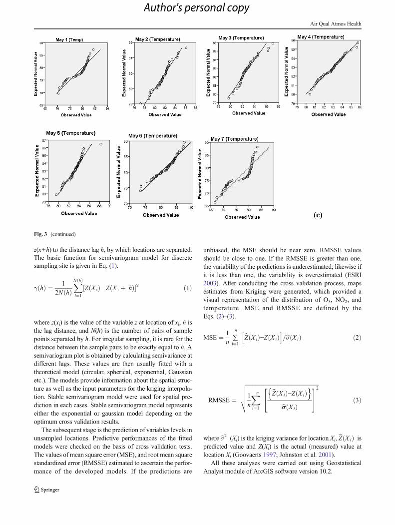
z(x+h) to the distance lag h, by which locations are separated.The basic function for semivariogram model for discretesampling site is given in Eq. (1).

γ hð Þ ¼ 1

2N hð ÞXN hð Þ

i¼1

Z X ið Þ− Z X i þ hð Þ½ �2 ð1Þ

where z(xi) is the value of the variable z at location of xi, h isthe lag distance, and N(h) is the number of pairs of samplepoints separated by h. For irregular sampling, it is rare for thedistance between the sample pairs to be exactly equal to h. Asemivariogram plot is obtained by calculating semivariance atdifferent lags. These values are then usually fitted with atheoretical model (circular, spherical, exponential, Gaussianetc.). The models provide information about the spatial struc-ture as well as the input parameters for the kriging interpola-tion. Stable semivariogram model were used for spatial pre-diction in each cases. Stable semivariogram model representseither the exponential or gaussian model depending on theoptimum cross validation results.

The subsequent stage is the prediction of variables levels inunsampled locations. Predictive performances of the fittedmodels were checked on the basis of cross validation tests.The values of mean square error (MSE), and root mean squarestandardized error (RMSSE) estimated to ascertain the perfor-mance of the developed models. If the predictions are

unbiased, the MSE should be near zero. RMSSE valuesshould be close to one. If the RMSSE is greater than one,the variability of the predictions is underestimated; likewise ifit is less than one, the variability is overestimated (ESRI2003). After conducting the cross validation process, mapsestimates from Kriging were generated, which provided avisual representation of the distribution of O3, NO2, andtemperature. MSE and RMSSE are defined by theEqs. (2)–(3).

MSE ¼ 1

n∑i¼1

n

bZ X ið Þ−Z X ið Þh i

=bσ X ið Þ ð2Þ

RMSSE ¼

ffiffiffiffiffiffiffiffiffiffiffiffiffiffiffiffiffiffiffiffiffiffiffiffiffiffiffiffiffiffiffiffiffiffiffiffiffiffiffiffiffiffiffiffiffiffiffiffiffiffiffiffi

1

n

X

i¼1

n bZ X ið Þ−Z X ið Þn o

bσ X ið Þ

2

4

3

52

vuuut ð3Þ

where bσ2 (Xi) is the kriging variance for location Xi, bZ X ið Þ ispredicted value and Z(Xi) is the actual (measured) value atlocation Xi (Goovaerts 1997; Johnston et al. 2001).

All these analyses were carried out using GeostatisticalAnalyst module of ArcGIS software version 10.2.

Fig. 3 (continued)

Air Qual Atmos Health

Author's personal copy

Results and discussion

Variogram model analysis

To depict the distribution pattern of ozone, NO2 and tem-perature in the study region, experimental semivariogramsand their semivariogram models were first analyzed foreach case. The cross validation results and the characteris-tics parameters of semivariogram models for each case arerepresented in Table 1. MSE for ozone prediction are 0.02,−0.04, 0, −0.01, 0.09, 0, and 0.03, respectively for 7 days(May 1 to 7, 2012). The respective values of RMSSE are0.64, 0.76, 0.92, 0.81, 1.00, 0.64, and 0.83 for 7 days. TheMSE values are close to zero and their correspondingRMSSE values close to one represent a good predictionmodel. The cross validation results indicate that MSEvalues closely followed the rule of thumb whereas theRMSSE values indicate that the predictions wereoverestimated in all the cases except one.

Similarly, MSE for NO2 prediction are 0.07, 0.06, 0.03,0.08, 0.05, 0.03, and 0.05, respectively, for 7 days (May 1 to 7,2012). The respective values of RMSSE are 0.64, 0.76, 0.69,0.81, 0.86, 0.88, and 0.75 for 7 days. In these cases also, the

cross validation results indicate that MSE values closelyfollowed the thumb rule whereas the RMSSE values indicatethat the predictions were overestimated in all the cases.

The MSE for temperature prediction are 0.05, 0.02, −0.01,−0.001, 0.06, 0.07, −0.11, respectively, for 7 days (May 1 to 7,2012). The respective values of RMSSE are 1.20, 1.26, 1.00,1.09, 1.04, 1.32, and 1.28 for 7 days. The results indicate thatMSEs are close to zero except in one case (May 7). OnMay 7,the MSE was relatively high. On the other hand, RMSSEvalues indicate that the predictions were underestimated inall the occasions.

The ratio of nugget variance to sill expressed in percent-ages can be regarded as a criterion for classifying the spatialdependence of ozone, NO2, and temperature. The ratios werecalculated for each case and represented in Table 1. If this ratiois less than 25 %, then the variable has strong spatial depen-dency; if the ratio is between 25 and 75 %, the variable hasmoderate spatial dependency, and if greater than 75 %, thevariables shows only weak spatial dependency (Shi et al.2007; Chien et al. 1997; Chang et al. 1998). The ratio repre-sented in Table 1 clearly indicate that ozone and temperatureshowed strong spatial structure in all cases. NO2 showedstrong spatial structure in four (May 1, May 2, May 5, and

Table 1 Semivariogram modelcharacteristics and cross valida-tion results

Parameter Fittedmodel

Nugget(C0)

Partial sill (C) [C0/(C0 + C)]% Range MSE RMSSE

Ozone

May 1, 2012 Stable 0 169.7 0.0 1.20 0.02 0.64

May 2, 2012 Stable 15.16 52.15 22.5 0.53 −0.04 0.76

May 3, 2012 Stable 6.14 50.58 10.8 4.20 0.00 0.92

May 4, 2012 Stable 0 96.31 0.0 3.05 −0.01 0.81

May 5, 2012 Stable 9.35 159.0 5.6 1.23 0.09 1.00

May 6, 2012 Stable 0 138.8 0.0 0.33 0.00 0.64

May 7, 2012 Stable 0.11 111.1 0.1 0.22 0.03 0.83

NO2

May 1, 2012 Stable 0.12 123.86 0.1 0.23 0.07 0.64

May 2, 2012 Stable 0 70.71 0.0 0.78 0.06 0.76

May 3, 2012 Stable 7.80 5.71 57.7 0.60 0.03 0.69

May 4, 2012 Stable 9.62 21.6 30.8 0.43 0.08 0.81

May 5, 2012 Stable 6.64 37.93 14.9 0.83 0.05 0.86

May 6, 2012 Stable 28.47 33.28 46.1 0.71 0.03 0.88

May 7, 2012 Stable 0 75.63 0.0 0.64 0.05 0.75

Temperature

May 1, 2012 Stable 0.55 3.18 14.7 1.05 0.05 1.20

May 2, 2012 Stable 0.29 1.55 15.8 0.53 0.02 1.26

May 3, 2012 Stable 0 1.82 0.0 1.54 −0.01 1.00

May 4, 2012 Stable 0.27 1.52 15.1 1.54 −0.001 1.09

May 5, 2012 Stable 0 2.61 0.0 1.67 0.06 1.04

May 6, 2012 Stable 0 1.81 0.0 0.35 0.07 1.32

May 7, 2012 Stable 0.90 47.76 1.8 6.22 −0.11 1.28

Air Qual Atmos Health

Author's personal copy

(a) (b) (c)

(d) (e) (f)

(g)

Fig. 4 Spatial distribution of O3 in the eastern part of Texas. aMay 1, 2012; bMay 2, 2012; cMay 3, 2012; dMay 4, 2012; eMay 5, 2012; fMay 6,2012; g May 7, 2012

Air Qual Atmos Health

Author's personal copy

May 7) of the seven cases and moderate spatial structure inremaining cases.

The shape of the semivariogramwas used to understand thespatial structures of ozone concentrations. Sill was used toquantify the variability of the ozone concentration among thesample sites. The sill (i.e., spatial variation) values in eachcase for ozone and NO2 were significantly high. The sillvalues for temperature were found to be consistently low ineach case except one (May 7).

Spatial distribution analysis

The spatial distribution of daily maximum 8-h ozone concen-trations were examined using GIS and geostatistical tech-niques. Figure 4a and g depict the spatial patterns of dailymaximum 8-h O3 concentrations for 1 May 2012 to 7 May2012, respectively. The descriptive statistics of the spatialdistributions maps were determined using ArcGIS. The resultsare represented in Table 2. The mean ozone concentration inthe area ranged from 32.99 ppb (May 3, 2012) to 59.56 ppb(May 1, 2012). The minimum ozone concentrations rangedfrom 17.24 ppb (May 5, 2012) to 26.03 ppb (May 7, 2012)and the maximum ozone concentrations ranged from42.89 ppb (May 3, 2012) to 98.50 ppb (May 1, 2012). This

clearly indicates that the variation in maximum concen-trations is higher than the variations in minimum con-centrations. This is due to the fact that the minimumozone level is dominated by the existence of backgroundozone and the maximum ozone level is influence byformation and dispersion factors. Figure 4a, g indicatethat the average/mean O3 concentrations significantlydeclined from May 1 to 3 and then gradually increaseduntil May 5. The mean concentrations remain at thesame level in the next 2 days. The maximum concentra-tions in the 7-day period (during May 1 to 7, 2012) wereobserved, respectively, in the counties of Harris,Harrison, Grayson, Denton, Tarrant, Harris and Liberty.Figure 4a, g clearly indicate that the spatial trends ofozone concentrations were not uniformed in the studyarea during the period of May 1 to 7. This is due tofrequent changes in the weather conditions in the re-gions. Therefore, the formation and dispersion of ozonehave varied within the regions and thus showed nouniform spatial trend of ozone concentrations. The re-sults of this study clearly illustrate the complex nature ofspatial variation in ozone concentrations, and confirm themarked variation in dispersions and precursor’s emis-sions characteristics.

Table 2 Descriptive statisticsMonths Number of data Minimum Maximum Mean Standard deviation

Ozone (ppb)

May 1, 2012 58 25.97 98.50 59.56 10.48

May 2, 2012 58 22.53 68.66 42.82 10.03

May 3, 2012 58 20.96 42.89 32.99 5.31

May 4, 2012 58 22.09 63.48 39.42 5.77

May 5, 2012 58 23.19 74.10 48.57 11.85

May 6, 2012 58 17.24 74.81 48.60 8.80

May 7, 2012 58 26.03 85.94 47.73 5.58

NO2 (ppb)

May 1, 2012 33 4.73 45.19 13.05 3.29

May 2, 2012 33 3.06 26.15 9.00 2.94

May 3, 2012 33 1.94 8.72 4.24 1.23

May 4, 2012 33 2.23 15.24 6.74 2.25

May 5, 2012 33 3.57 23.32 8.93 3.06

May 6, 2012 33 4.55 21.89 9.40 3.06

May 7, 2012 33 3.04 28.11 9.17 2.64

Temperature (°F)

May 1, 2012 49 70.10 84.09 77.18 3.44

May 2, 2012 49 77.43 85.73 81.49 1.13

May 3, 2012 49 80.08 86.75 82.47 0.82

May 4, 2012 49 80.74 85.34 82.44 0.73

May 5, 2012 49 79.63 87.99 82.77 0.87

May 6, 2012 49 73.60 87.32 81.18 2.19

May 7, 2012 49 64.30 86.48 75.28 5.24

Air Qual Atmos Health

Author's personal copy

(a) (b) (c)

(d) (e) (f)

(g)

Fig. 5 Spatial distribution of NO2 in the eastern part of Texas. aMay 1, 2012; bMay 2, 2012; cMay 3, 2012; dMay 4, 2012; eMay 5, 2012; fMay 6,2012; g May 7, 2012

Air Qual Atmos Health

Author's personal copy

(a) (b) (c)

(d) (e) (f)

(g)

Fig. 6 Temperature profile in the eastern part of Texas. aMay 1, 2012; bMay 2, 2012; cMay 3, 2012; dMay 4, 2012; eMay 5, 2012; fMay 6, 2012; gMay 7, 2012

Air Qual Atmos Health

Author's personal copy

Similarly, Fig. 5a, g show spatial distribution of daily max-imum 1-h NO2 concentrations from May 1 to 7, respectively.Themean NO2 concentrations in the area ranged from 4.24 ppb(May 3, 2012) to 13.05 ppb (May 1, 2012). The minimum andmaximum ozone concentrations ranged from 1.94 ppb (May 3,2012) to 4.73 ppb (May 1, 2012) and 8.72 ppb (May 3, 2012) to45.19 ppb (May 1, 2012), respectively. This clearly indicatesthat the variation in maximum concentrations is higher than thevariations in minimum concentrations. This spatial patternreflects most likely the aggregated density of emission source.Although no counties were exposed to “alert” (1-h maximumNO2 guideline of US EPA, which is 100 ppb) levels during the7 days (May 1 to 7, 2012), many counties in Beaumont/PortArthur (BPA), Dallas/Fort Worth (DFW), and Houston/Galveston/Brazoria (HGB) zones could be of some concern.The significant level of NO2 was observed in the countiessituated close to the three major emission zones (BPA, HGB,and DFW). The maximum NO2 levels were observed in Harriscounty on May 1 to 4 and May 7. On May 5 and 6, themaximum levels were found in Dallas and Tarrantcounties, respectively. Thus, it is clear from the explor-atory data analyses that the major NO2 emission sourcessituated on or near the Harris county.

The daily average temperature profiles for 7 days areshown in Fig. 6a, g. The spatial variation of temperature wasrelatively less. The mean temperatures in the area ranged from75.28 °F (May 7, 2012) to 82.47 °F (May 3, 2012).

The graphical representations of the descriptive statisticsfor the three parameters are shown in Fig. 7a, c. These figuresclearly indicate that the trend of mean ozone concentrations inthe area followed the mean NO2 concentrations during the 7-day period. But, the trends of these two pollutants did notmatch with the temperature variations in the area.

Correlation among ozone, temperature, and NO2

Correlation analysis was done for quantifying the influence oftemperature and NO2 on ozone concentrations. Since themonitoring values of pollutant concentrations or temperatureat common locations were not available, they were extractedfrom the interpolated maps using GIS. The values of ozoneconcentrations, NO2 concentrations, and temperature at thecentroid positions of each county (157 counties) were deter-mined using spatial analyst tool of ArcGIS. The extracted datafor 7 days (May 1 to 7, 2012) were used for correlationanalyses. Pearson two-tailed correlation analyses were con-ducted using SPSS software version 21. Correlation analysesresults of three variables in each day are represented inTable 3.

The results represented in Table 3 clearly indicatethat NO2 concentrations were significantly correlatedwith the ozone concentrations at 1 % significance levelexcept on May 1 and 7, 2012. On May 1, the two

variables were correlated at 5 % significance level.The correlation coefficients between ozone and NO2

are 0.173, 0.683, 0.592, 0.302, 0.641, 0.452, and0.091, respectively, for May 1 through 7. Since, allthe correlation coefficients values are positive, it indi-cates that the higher concentrations of NO2 level in thearea increased the concentration of ozone.

Temperature did not show uniformed correlationswith either NO2 or ozone. The correlation coefficientsbetween ozone and temperature were −0.387, −0.716,0.534, 0.049, 0.406, −0.459, and 0.303, respectively, forMay 1 to 7, 2012. The correlation coefficient resultsclearly indicate that ozone concentration was not influ-enced by temperature level in the area. Similarly, thecorrelation coefficients between NO2 and temperaturewere −0.156, −0.425, 0.581, −0.375, 0.352, −0.569,and −0.120, respectively, for May 1 to 7. Again, thecorrelation coefficient result did not show any trend,that is, the values are negative in five occasions andpositive in two occasions. Thus, the NO2 concentrationsin the study area may not be influenced by temperaturelevel or some other factors playing a role in the ob-served differences in correlation coefficients.

Role of wind speed and wind direction on spatial distribution

Though the maximum NO2 concentrations were ob-served near the emission sources in most instances, thelocations of recorded maximum ozone concentrationsvaried with time. The prime reason behind this is theinfluence of wind speed and direction. The wind rosediagrams for 7-days period are shown in Fig. 8a, g. Thewind rose diagrams were generated using WRPLOTView software version 7.0.0. Wind rose diagrams clearlyindicate the significant fluctuation in wind speed andwind direction.

On May 1, 98.5 ppb of peak hour O3 was observedin Harris county. This is due to maximum NO2 level(45.19 ppb) also observed in the same county and thehorizontal dispersion of NO2 and ozone were relativelyless as there was no particular dominant wind directionsin that day. Easterly and south–easterly wind blowing inthat day transported the ozone slowly in the south–eastdirection. Figure 5a clearly indicates the major sourcesof NO2 are mainly in the regions HGB and DFW. Thecontribution of NO2 from BPA was also significant.

On May 2, the maximum ozone concentration(68.66 ppb) was observed in Harrison county whereasthe maximum NO2 level (26.15 ppb) was observed inHarris county. The highest concentrations of NO2 wereobserved in the counties situated close to the threemajor sources (BPA, HGB, and DFW). The top fivecounties, which showed maximum NO2 levels, were

Air Qual Atmos Health

Author's personal copy

Harris, Tarrant, Newton, Jasper, and Liberty. Three ma-jor sources of NO2 mainly contribute to form high O3

concentrations. The top five counties, where maximumozone concentrations were observed, are Harrison,Marrion, Newton, Jasper, and Panola. Wind rose dia-gram clearly indicates that the prevailing wind direc-tions were S to N and S–S–E to N–N–W. This leadsto the significant transport of emissions from downwindurban and industrial areas, and thus the ozone concen-trations were found to be maximum in the countiessituated in the east and north east regions of the majorpollution sources (Fig. 1).

On May 3, the maximum ozone concentration wasobserved in counties situated in the north–west regionof the NO2 emission sources. The wind rose diagramclearly indicates that the prevailing wind direction wasS–S–E to N–N–W on May 3. Thus, the emissions ofNO2 in the regions HGB and BPA transported to north–west regions either after formation of ozone or in thesame form. This process facilitates increase in the ozoneconcentrations in the counties Grayson, Cooke, Collin,Fannin, and Denton.

On May 4, the prevailing wind direction was same as thaton May 3. But on May 4, the direction was more dominant

(a)

(b)

(c)

Fig. 7 Graphical representations of the trend of NO2, ozone, and temperature

Air Qual Atmos Health

Author's personal copy

and thus, the pollutants were transported to a greater extent incomparison to that on May 3. The spatial distribution map[Fig. 4d] of ozone clearly reveals that the ozone concentra-tions were found maximum in the N–W corner.

On May 5, there was no particular prevailing wind direc-tion and thus the dispersion of NO2 was not very significant.Spatial distribution maps of ozone on May 5 indicate that themaximum concentrations observed were close to the NO2

emission sources.On May 6, though the prevailing wind direction was

S–S–E to N–N–W, the transportation of NO2 was notsignificant due to lower frequency of wind in this di-rection in comparison to that on May 2 and 4. Thus, themaximum NO2 level was observed near to the emissionsources and the secondary ozone dispersed in everydirection of the emission sources.

On May 7, the maximum NO2 concentration was foundmaximum near the emission sources but most of the time windwas blowing from N–E and N–W directions. This facilitatesthe dispersion of the secondary ozone towards the south. NO2

emission in the region DFW dispersed towards the south andbecause of the low level of NO2, no significant level of ozonewas observed in the south of DFW. Higher level of ozoneconcentrations was observed in Liberty, Jefferson, Hardin,Harris, and Fortbend counties due to the transfer of NO2 andozone from the BPA region.

Conclusions

Ground-level ozone prediction and mapping have become anincreasingly important part of air quality public outreachprograms designed to inform the public about air qualityconditions and protect public health. Exposure assessmentsthat are only based on a small number of monitoring sites arelikely to yield inaccurate results during epidemiological stud-ies. Thus, understanding of the spatial distribution of ozoneand identifying the underlying factors that affect its concen-trations within an area of interest, is vital. GIS-based analysiswas done for mapping and understanding the influence ofNO2, and local climatic conditions on ozone concentrationsin Eastern Texas, USA. Study results indicated that ozoneconcentrations were highly correlated with NO2 concentra-tions. Higher concentration levels of NO2 were associatedwith higher concentrations of ozone. The distribution patternof ozone was very much influenced by wind speed and winddirection but rarely showed any correlation with the tempera-ture profile in the studied area. Hence, geospatial mapping ofozone provided a scientific basis for informed decision-making regarding the management of emission sources andcontrol/prevention of ozone-related air pollution. This re-search also provided a basis to formulate new research hy-potheses for further epidemiological studies regarding thehealth effects of air pollution in the studied area.

Table 3 Correlations coefficients among NO2, ozone, and temperature

May 1 May 2

NO2 Ozone Temperature NO2 Ozone Temperature

NO2 1 NO2 1

Ozone 0.173* 1 Ozone 0.683** 1

Temperature −0.156 −0.387** 1 Temperature −0.425** −0.716** 1

May 3 May 4

NO2 Ozone Temperature NO2 Ozone Temperature

NO2 1 NO2 1

Ozone 0.592** 1 Ozone 0.302** 1

Temperature 0.581** 0.534** 1 Temperature −0.375** 0.049 1

May 5 May 6

NO2 Ozone Temperature NO2 Ozone Temperature

NO2 1 NO2 1

Ozone 0.641** 1 Ozone 0.452** 1

Temperature 0.352** 0.406** 1 Temperature −0.569** −0.459** 1

May 7NO2 Ozone Temperature

NO2 1

Ozone 0.091 1

Temperature −0.120 −0.303** 1

*Correlation is significant at the 0.05 level (2-tailed)

**Correlation is significant at the 0.01 level (2-tailed)

Air Qual Atmos Health

Author's personal copy

(a) (b)

(c) (d)

(e) (f)

(g)

Fig. 8 Wind rose diagram. a May 1, 2012; b May 2, 2012; c May 3, 2012; d May 4, 2012; e May 5, 2012; f May 6, 2012; g May 7, 2012

Air Qual Atmos Health

Author's personal copy

Acknowledgments This research work was carried out in part of thecorresponding author’s Raman Postdoctoral Fellowship-2013 awarded byUGC,NewDelhi, India. Authors are also thankful to USEPA formaking airpollution data available on the website for public use. The support from theDST, NewDelhi Grant No. SR/FTP/ES-17/2012, and the National Institutesof Health NIMHDGrant No. G12MD007581 through the RCMI-Center forEnvironmental Health at Jackson State University, are also acknowledged.

References

Beaver S, Palazoglu A (2009) Influence of synoptic and mesoscalemeteorology on ozone pollution potential for San Joaquin Valleyof California. Atmos Environ 43(10):1779–1788

Camalier L, Cox W, Dolwick P (2007) The effects of meteorology onozone in urban areas and their use in assessing ozone trends. AtmosEnviron 41(33):7127–7137

Chang YH, Scrimshaw MD, Emmerson RHC, Lester JN (1998)Geostatistical analysis of sampling uncertainty at the Tollesburymanaged retreat site in Blackwater Estuary, Essex, UK: krigingand cokriging approach to minimise sampling density. Sci TotalEnviron 221:43–57

Cheng CS, Campbell M, Li Q, Li G, Auld H, Day N, Pengelfly D,Gingrich S, Yap D (2007) A synoptic climatological approach toassess climatic impact on air quality in south-central Canada. Part II:future estimates. Water Air Soil Poll 182:117–130

Chien YL, Lee DY, Guo HY, Houng KH (1997) Geostatistical analysis ofsoil properties of mid-west Taiwan soils. Soil Sci 162:291–297

Chung YS (1977) Ground-level ozone and regional transport of airpollutants. J Appl Meteorol 16(11):1127–1136

Darby LS (2005) Cluster analysis of surface winds in Houston, Texas, andthe impact of wind patterns on ozone. J Appl Meteorol 44:1788–1806

Dawson JP, Adams PJ, Pandis SN (2007) Sensitivity of ozone to sum-mertime climate in the Eastern USA: a modeling case study. AtmosEnviron 41:1494–1511

Elminir HK (2005) Dependence of urban air pollutants on meteorology.Sci Total Environ 350:225–237

ESRI (2003) ArcGIS 9. Using ArcGIS Geostatistical Analyst: ONLINE.Available from: http://forums.esri.com/Thread.asp?c=93&f=1727&t=257926, accessed on December 2013.

Goovaerts P (1997) Geostatistics for natural resources evaluation.Applied geostatistics series. Oxford University Press, New York

Gorai AK, Kumar S (2013) Assessment of groundwater quality usingstatistical and geostatistical techniques in Ranchi Municipal

Corporation Area, Jharkhand, India. Geoinfor Geostat: AnOverview 1(2). doi:10.4172/2327-4581.1000105

Hopkins LP, Ensor KB, Rifai HS (1999) Empirical evaluation of ambientozone interpolation procedures to support exposure models. J AirWaste Manage Assoc 49(7):839–846

Im U, Incecik S, Guler M, Tek A, Topcu S, Unal YS, Yenigun O, KindapT, Odman MT, Tayanc M (2013) Analysis of surface ozone andnitrogen oxides at urban, semi-rural and rural sites in Istanbul,Turkey. Sci Total Environ 443:920–931

Jacob DJ, Winner DA (2009) Effect of climate change on air quality.Atmos Environ 43(1):51–63

Johnston K., Ver Hoef JM, Krivoruchko K, Lucas N (2001) UsingArcGIS Geostatistical Analyst.

Ordonez C, Mathis H, Furger M, Henne S, Hoglin C, StaehelinJ, Prevot ASH (2005) Changes of daily surface ozone max-ima in Switzerland in all seasons from 1992 to 2002 anddiscussion of summer 2003. Atmos Chem Phys 5:1187–1203

Pakalapati S, Beaver S, Romagnoli JA, Palazoglu A (2009)Sequencing diurnal airflow patterns for ozone exposure as-sessment around Houston, Texas. Atmos Environ 43:715–723

Schlink U, Herbarth O, Richter M, Dorling S, Nunnari G, CawleyG, Pelikan E (2006) Statistical models to assess the healtheffects and to forecast ground-level ozone. Environ ModelSoftw 21(4):547–558

Seinfeld JH, Pandis SN (1998) Atmospheric chemistry and physic fromair pollution to climate change. Wiley, USA

Shi J, Wang H, Xu J, Wu J, Liu X, Zhu H, Yu C (2007) Spatialdistribution of heavy metals in soils: a case study ofChangxing, China. Environ Geol 52(1):1–10. doi:10.1007/s00254-006-0443-6

Sillman S, Logan JA, Wofry SC (1990) A regional-scale model forozone in the United States with a subgrid representation ofurban and power plant plumes. J Geophys Res 95(D5):5731–5748

US EPA (2009) Assessment of the impacts of global change on regionalU.S. air quality: a synthesis of climate change impacts on ground-level ozone. US EPA, Washington, DC

Yuval, Broday DM (2006) High resolution spatial patterns of long–termmean air pollutants concentrations in Haifa Bay area. AtmosEnviron 40:3653–3664

Yuval, Broday DM, Carmel Y (2005) Mapping spatiotemporal variables:the impact of the time-averaging window width on the spatialaccuracy. Atmos Environ 39:3611–3619

Air Qual Atmos Health

Author's personal copy