100 Years of Progress in Applied Meteorology. Part III

Chapter 24

100 Years of Progress in Applied Meteorology. Part III: Additional Applications

SUE ELLEN HAUPT, BRANKO KOSOVIC, SCOTT W. MCINTOSH, FEI CHEN, AND KATHLEEN MILLER

National Center for Atmospheric Research, Boulder, Colorado

MARSHALL SHEPHERD

University of Georgia, Athens, Georgia

MARCUS WILLIAMS

USDA Forest Service, Athens, Georgia

SHELDON DROBOT

Harris Corporation, Boulder, Colorado

ABSTRACT

Applied meteorology is an important and rapidly growing field. This chapter concludes the three-chapter

series of this monograph describing how meteorological information can be used to serve society’s needs

while at the same time advancing our understanding of the basics of the science. This chapter continues along

the lines of Part II of this series by discussing ways that meteorological and climate information can help to

improve the output of the agriculture and food-security sector. It also discusses how agriculture alters climate

and its long-term implications. It finally pulls together several of the applications discussed by treating the

food–energy–water nexus. The remaining topics of this chapter are those that are advancing rapidly withmore

opportunities for observation and needs for prediction. The study of space weather is advancing our un-

derstanding of how the barrage of particles from other planetary bodies in the solar system impacts Earth’s

atmosphere. Our ability to predict wildland fires by coupling atmospheric and fire-behavior models is be-

ginning to impact decision-support systems for firefighters. Last, we examine how artificial intelligence is

changing the way we predict, emulate, and optimize our meteorological variables and its potential to amplify

our capabilities. Many of these advances are directly due to the rapid increase in observational data and

computer power. The applications reviewed in this series of chapters are not comprehensive, but they will

whet the reader’s appetite for learning more about how meteorology can make a concrete impact on the

world’s population by enhancing access to resources, preserving the environment, and feeding back into a

better understanding how the pieces of the environmental system interact.

1. Introduction

The ancient Greek philosopher Empedocles con-

jectured that the world was composed of four primary

elements—air, fire, water, and earth. He surmised that

these elements were not destructible and unchangeable,

but rather could be superimposed to change structure.

This pre-Socratic theory, originated around 460 BC,

persisted for over 2000 years. Although we now have a

deeper understanding of the nature of the world and

cosmos, one can imagine how ancient humankind de-

veloped this earth–air–fire–water philosophy based on

the observational ability that they had at the time.

This third part of the AMS 100th Anniversary Mono-

graph Series focusing on appliedmeteorology treats some

of the topics that may have led to such philosophy. Per-

haps it became obvious that the fiery sun provided energy

for Earth and its atmosphere. The earth produced food

via agriculture but depended highly on movements of air

to bring weather that could produce rain and provide theCorresponding author: Dr. Sue Ellen Haupt, [email protected]

CHAPTER 24 HAUPT ET AL . 24.1

DOI: 10.1175/AMSMONOGRAPHS-D-18-0012.1

� 2019 American Meteorological Society. For information regarding reuse of this content and general copyright information, consult the AMS CopyrightPolicy (www.ametsoc.org/PUBSReuseLicenses).

mailto:[email protected]

http://www.ametsoc.org/PUBSReuseLicenses



basis for transforming seeds and earth to food. Wildland

fires could change all of that.Of course our understanding

of these issues has greatly evolved, and this chapter treats

how that understanding has progressed over the past 100

years. We now understand that the sun not only provides

Earth’s energy, but also produces space weather that

impacts Earth and its atmosphere.

The rapid increase of available environmental data has

enabled rapid advances in our understanding of processes.

Similarly, advances in computational power have made

possible, and require, new techniques such as artificial-

intelligence (AI)methods, higher-resolution computational

gridded models, and the coupling of complex processes.

Examples include coupling the atmosphere and fire pro-

cesses for wildland fire modeling, atmosphere and ocean

processes for hurricanes simulation, and many other

foundational climatic processes or solar and atmosphere

processes to predict the impact of space weather. As hu-

manity strives to manage the complex Earth processes, it

becomes more important to apply these detailed meteo-

rological modeling capabilities. This coupled modeling

approach is essential to providing accurate simulations and

forecasts for the applications in this chapter: agriculture,

wildland fire modeling, and space weather, as well as for a

plethora of other applications.

Section 2 of this chapter is related to agriculture, food

security, and how meteorological and hydrological

knowledge is used to enhance production in an effort to

help feed the world’s population. In turn, as humans

change land use for agriculture, the environment is im-

pacted, and we must understand these changes to avoid

unintended consequences. This section also continues the

theme of Part II of this series (Haupt et al. 2019b), which

dealt with topics related to growing populations. Section

2 culminates with a discussion of the food–energy–water

nexus and its susceptibility to a changing climate.

Section 3 discusses our current understanding (and

limits to understanding) of space weather. It suggests that

studying the sun’s atmosphere could be accomplished using

similar methods to what has led to better understanding

Earth’s atmosphere. Continuing on the fiery theme, section

4 deals with wildland fire and how modeling this important

and deadly phenomenon can impact how we deal with it.

But because the fire itself generates weather, fully coupled

models are required to capture this important phenomenon.

Section 5 of this chapter is a bit different in that it

discusses the use of AI in the environmental sciences.

Although it is less about how applications of meteo-

rology have changed and served an important human

topic, it looks forward into how programming machines

to think like humans, or even unlike humans, can en-

hance how we make forecasts, or emulate processes in

our models, or optimize some aspect of our models or

workflow, or recognize patterns in our world. It also al-

lows us to interact with our burgeoning data in new ways,

uncovering new insights through clustering and nonlinear

analysis. This section looks to the future, but it also re-

verts to the past when science relied more on finding

patterns in nature. Concluding thoughts and consider-

ation of some prospects for the future appear in section 6.

This chapter is the final one of a three-part series on

applied meteorology. In the first chapter, we considered

some of the most basic and first-addressed application

areas: weather modification, aviation applications, and

security applications. Knowledge of meteorology enabled

each of these applications, and the study required to

progress the applications enriches our understanding of

the meteorological processes involved. In the second chap-

ter, we dealt with using meteorology to find solutions to

problems generatedby a growing population—urbanization,

air pollution, energy, and surface transportation. We saw

not only that meteorology provides useful information for

these applications, but also that each of these issues itself

impacts the environment in ways that must be understood

and carefully managed. Here in the third part of this series

we continue along the lines of understanding the science

behind the applied systems in how we consider space sci-

ence; dealing with the problems, such as in wildland fire

management and agriculture applications; and applying

new techniques such as AI to those problems. As the last

in a series of chapters on applied meteorology, we must

acknowledge the lack of completeness. There are many

additional topics that are not covered in this series, because

of lack of space and time as well as the fact that some are

touched on in other chapters of this monograph. For in-

stance, little attention is paid to hydrological, climatolog-

ical, or social science applications because they are treated

in other chapters of this monograph.

2. Applications in agriculture and food security

a. Introduction

Food is a basic human need. To feed increasing pop-

ulations, global agricultural output has more than tri-

pled in volume in the last 50 years and real prices have

fallen (Fuglie and Wang 2012). In the United States,

even starting from already high levels of productivity,

farm production more than doubled between 1948 and

2011 (Wang and Ball 2014). By 2050 population growth,

mainly in the developing world, will necessitate an in-

crease in food production of 59%–98% (Valin et al.

2014). With limited land available for planting more

crops, technological advances are necessary to improve

practices and efficiencies across the entire food system.

Providing meteorology information is critical to con-

tinuing to optimize productivity.

24.2 METEOROLOG ICAL MONOGRAPHS VOLUME 59

Information on constantly changing weather condi-

tions, such as probability of precipitation, temperature

information, and so on are essential basic information

formodels of crop production. For instance, cropmodels

such as the Parallel version of the Decision Support

System for Agrotechnology Transfer (pDSSAT; Elliott

et al. 2015) use daily weather data (maximum and mini-

mum temperatures, rainfall, solar radiation, winds, and

humidity) and farmmanagement information to examine

the status of agricultural systems, provide a framework to

monitor crop progress, identify problem areas and op-

portunities, and contribute to a multifaceted monitoring

system with machine-based learning incorporating re-

mote sensing and crop model outputs. Meteorological

systems can feed these crop models with weather and

climate information including traditional surface-based

observations as well as satellite-based Earth observa-

tions. In addition, models of weather and climate can

provide useful information for prediction. In turn, the

land use modifications that are part of agriculture can

alter the weather and climate, which should be included

in our models. These aspects are treated here, as well as

the nexus between food, energy, and water.

b. Use of satellite data for agriculture

Remote sensing technologies are poised to play a

larger role in food security, through such practices as

better crop water monitoring (Bastiaanssen and Steduto

2017). Satellite observation systems have the unique

capability to inform critical forecasts and decision-

support tools for the agriculture sector. Currently many

farmers lack access to timely agricultural forecasts and

decision-making tools that could help them make critical

choices throughout the growing season, including what to

plant, when to plant, and when to irrigate, as well as

warning of impending catastrophic weather events and

providing yield forecasts to aid in price negotiations with

intermediaries.

At the end of 2016, 374 Earth observing satellites were

operational (Pixalytics 2017). The main instruments

useful for agriculture and food security are classified

either as multispectral or microwave; however, planned

hyperspectral sensors have the potential to revolution-

ize remote sensing contributions to food security as

many spectral indices focus on narrow bands (e.g.,

Harris Geospatial Solutions 2017).

An important application of remote sensing data is

for monitoring crop conditions, biophysical variables,

and crop yield (e.g., Chen et al. 2016; Gitelson 2016;

Hatfield et al. 2008). Spectral indices, such as normal-

ized difference vegetation index (NDVI), are well-

known and long-standing successful examples of using

remote sensing for crop health identification (e.g., Tucker

1979). The growth in spectral radiances has greatly in-

creased the suite of potential geophysical inversion ca-

pabilities, and numerous crop health conditions can now

bemonitored. For example, alterations toNDVIandother

spectral indices show strong relationships with the fraction

of absorbed photosynthetically active radiation (Viña andGitelson 2005), which is a critical index for inclusion in

production efficiency models (Roujean and Breon 1995).

Remote sensing techniques are also showing considerable

value in identifying crop pests and diseases (e.g., Mahlein

2016), including powdery mildew (Yuan et al. 2016) and

white fly (Nigam et al. 2016), among others. Solar-induced

fluorescence (SIF; Yang et al. 2015) indicates photosyn-

thetic activity with space-based monitoring capabilities

(Guan et al. 2015), and gross primary productivity (GPP;

Running et al. 2000) can indicate biomass and carbon al-

lotment for use in crop modeling. Soil moisture products

from NASA’s Soil Moisture Active Passive (SMAP) and

the European Space Agency’s Soil Moisture and Ocean

salinity instruments could provide much improved global

estimates.

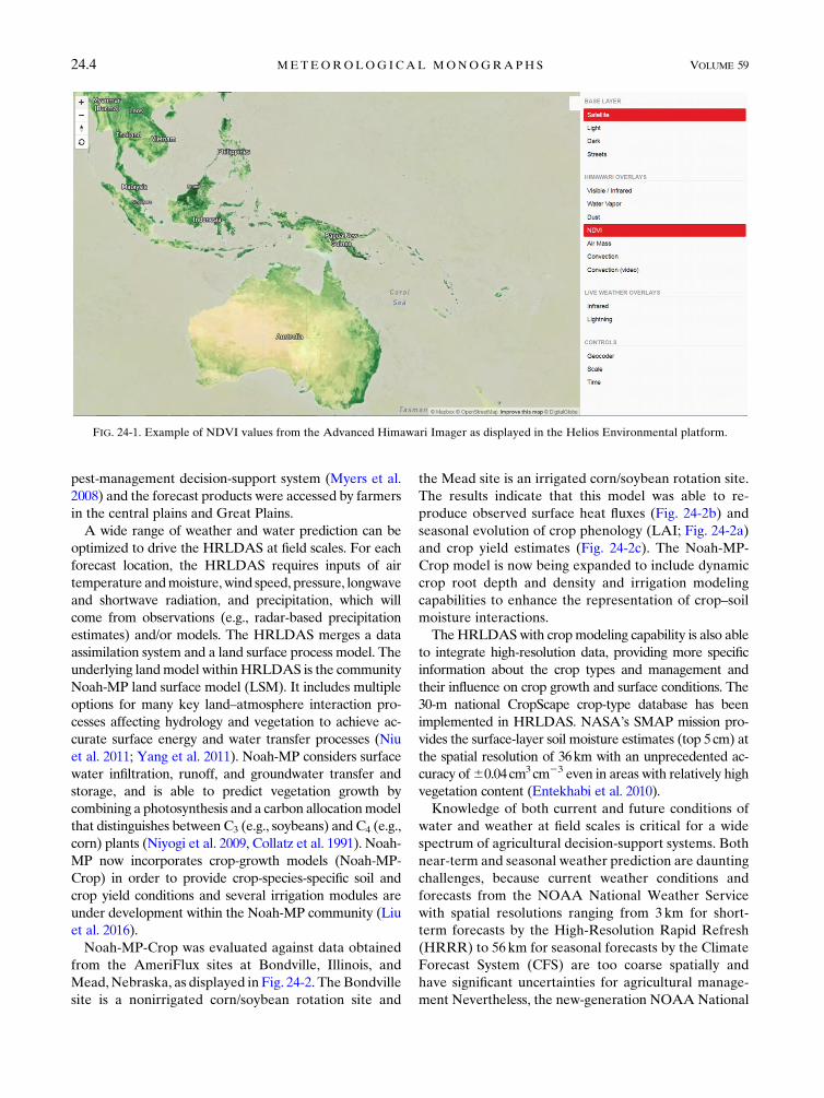
Remote sensing information for agricultural lands

enables improvements to model initializations at the

beginning of the season and helps to constrain a model’s

properties (e.g., biomass, leaf area, soil moisture, and

photosynthetic rate) to avoid the effects of drift over the

course of a season. Figure 24-1 is an example of full-

resolution satellite data (NDVI in the figure), with the

option to select other relevant weather data.

c. Modeling for agriculture applications

Coupled atmosphere–hydrosphere–crop models are

increasingly being used to support agricultural decisions.

The Weather Research and Forecasting (WRF) nu-

merical weather prediction model has been augmented

for interaction with crop models. These WRF-Crop mod-

eling capabilities can be integrated with remote sensing

data, land-data assimilation systems, and prediction sys-

tems to provide short-term and seasonal monitoring and

prediction of crop yield, crop-specific water and irrigation

demand, soil temperature evolution, and impacts of

weather–hydrology–crop interactions on crop growth. Such

information can be utilized as input to various decision-

support systems to include irrigation management, crop

planting dates, and fertilization that would highly impact

income of farmers and food security.

The High Resolution Land Data Assimilation System

(HRLDAS; Chen et al. 2007) performs model-based

data assimilation with remote sensing-derived soil mois-

ture and other land surface parameters to generate

soil and crop phenology conditions at field scales.

The HRLDAS was used to produce real-time soil mois-

ture and temperature in a NASA-funded agricultural


pest-management decision-support system (Myers et al.

2008) and the forecast products were accessed by farmers

in the central plains and Great Plains.

A wide range of weather and water prediction can be

optimized to drive the HRLDAS at field scales. For each

forecast location, the HRLDAS requires inputs of air

temperature andmoisture, wind speed, pressure, longwave

and shortwave radiation, and precipitation, which will

come from observations (e.g., radar-based precipitation

estimates) and/or models. The HRLDAS merges a data

assimilation system and a land surface process model. The

underlying landmodel withinHRLDAS is the community

Noah-MP land surface model (LSM). It includes multiple

options for many key land–atmosphere interaction pro-

cesses affecting hydrology and vegetation to achieve ac-

curate surface energy and water transfer processes (Niu

et al. 2011; Yang et al. 2011). Noah-MP considers surface

water infiltration, runoff, and groundwater transfer and

storage, and is able to predict vegetation growth by

combining a photosynthesis and a carbon allocationmodel

that distinguishes between C3 (e.g., soybeans) and C4 (e.g.,

corn) plants (Niyogi et al. 2009, Collatz et al. 1991). Noah-

MP now incorporates crop-growth models (Noah-MP-

Crop) in order to provide crop-species-specific soil and

crop yield conditions and several irrigation modules are

under development within the Noah-MP community (Liu

et al. 2016).

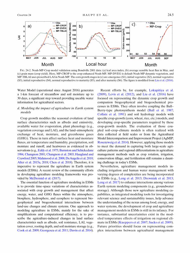
Noah-MP-Crop was evaluated against data obtained

from the AmeriFlux sites at Bondville, Illinois, and

Mead,Nebraska, as displayed in Fig. 24-2. TheBondville

site is a nonirrigated corn/soybean rotation site and

the Mead site is an irrigated corn/soybean rotation site.

The results indicate that this model was able to re-

produce observed surface heat fluxes (Fig. 24-2b) and

seasonal evolution of crop phenology (LAI; Fig. 24-2a)

and crop yield estimates (Fig. 24-2c). The Noah-MP-

Crop model is now being expanded to include dynamic

crop root depth and density and irrigation modeling

capabilities to enhance the representation of crop–soil

moisture interactions.

TheHRLDASwith cropmodeling capability is also able

to integrate high-resolution data, providing more specific

information about the crop types and management and

their influence on crop growth and surface conditions. The

30-m national CropScape crop-type database has been

implemented in HRLDAS. NASA’s SMAP mission pro-

vides the surface-layer soil moisture estimates (top 5cm) at

the spatial resolution of 36km with an unprecedented ac-

curacy of60.04cm3cm23 even in areas with relatively high

vegetation content (Entekhabi et al. 2010).

Knowledge of both current and future conditions of

water and weather at field scales is critical for a wide

spectrum of agricultural decision-support systems. Both

near-term and seasonal weather prediction are daunting

challenges, because current weather conditions and

forecasts from the NOAA National Weather Service

with spatial resolutions ranging from 3km for short-

term forecasts by the High-Resolution Rapid Refresh

(HRRR) to 56km for seasonal forecasts by the Climate

Forecast System (CFS) are too coarse spatially and

have significant uncertainties for agricultural manage-

ment Nevertheless, the new-generation NOAA National

FIG. 24-1. Example of NDVI values from the Advanced Himawari Imager as displayed in the Helios Environmental platform.


Water Model (operational since August 2016) generates

a 1-km forecast of streamflow and soil moisture up to

30 days, a significant step toward providing useable water

information for agricultural sectors.

d. Modeling the impact of agriculture in Earth systemmodels

Crop growth modifies the seasonal evolution of land

surface characteristics such as albedo and emissivity,

available water for evaporation, plant phenology (e.g.,

vegetation coverage and LAI), and the land–atmospheric

exchange of heat, moisture, and greenhouse gases

(GHG). These in turn affect surface heat and moisture

fluxes, air temperature and humidity, precipitation, soil

moisture and runoff, and heatwaves as evidenced in ob-

servations (e.g., Eddy et al. 1975; Barnston and Schickedanz

1984, Changnon 2001; Changnon et al. 2003; Haugland and

Crawford2005;Mahmoodet al. 2008;DeAngelis et al. 2010;

Alter et al. 2015a, 2018; Chen et al. 2018). Therefore, it is

imperative to represent the agriculture in Earth system

models (ESMs). A recent review of the community efforts

in developing agriculture modeling frameworks was pro-

vided by McDermid et al. (2017).

The essential function of agriculture modeling in ESMs

is to provide time–space variations of characteristics as-

sociated with crop growth and management that affect

energy, water, and GHG fluxes within the atmosphere,

biosphere, hydrosphere, and ecosphere to represent bio-

geophysical and biogeochemical interactions between

land-use changes and climate systems. One approach to

modeling agriculture in ESMs, mainly for the sake of

simplifications and computational efficiency, is to pre-

scribe the agriculture-induced changes in land surface

characteristics such as albedo, soil resistance, LAI, vege-

tation cover, rooting depth, and soil moisture storage (e.g.,

Cook et al. 2009; Georgescu et al. 2011; Davin et al. 2014).

Recent efforts by, for example, Lokupitiya et al.

(2009), Levis et al. (2012), and Liu et al. (2016) have

focused on representing the dynamic crop growth and

companion biogeophysical and biogeochemical pro-

cesses in ESMs. They often involve coupling the Ball–

Berry-type photosynthesis model (Ball et al. 1987;

Collatz et al. 1991) and soil hydrology models with

specific crop-growth (corn, wheat, rice, etc.) models, and

developing crop-specific parameters required by these

crop-growth models. The evaluation of those cou-

pled soil–crop–climate models is often realized with

data collected at field scales or from the Agricultural

Model Intercomparison and Improvement Project (AgMIP;

Rosenzweig et al. 2014). However, applying thosemodels

to meet the demand in capturing both large-scale agri-

culture patterns and regional differentiations in agriculture

management methods such as crop rotation, irrigation,

conservation tillage, and fertilization still remains a daunt-

ing challenge in today’s ESMs.

Nevertheless, agriculture management models in-

cluding irrigation and human water management with

varying degrees of complexities are being incorporated

in ESMs (e.g., Leng et al. 2013; Drewniak et al. 2013;

Leng et al. 2017) to enhance interactions among various

Earth system modeling components (e.g., groundwater

storage). Although those new agriculture modeling ca-

pabilities, as integrated modeling tools for investigating

relevant science and sustainability issues, help advance

the understanding of the nexus among food, energy, and

water systems, the development of crop and agriculture

management models in ESMs is still in its infancy. For

instance, substantial uncertainties exist in the mod-

eled temperature effects of irrigation on regional cli-

mate in ESMs (Kueppers et al. 2007; Sacks et al. 2009).

Future priorities should focus on representing com-

plex interactions between agricultural management

FIG. 24-2. Noah-MP-Crop model validation using Bondville 2001 data: (a) leaf area index, (b) average sensible heat flux in May, and

(c) grain mass (crop yield). Here, MP-CROP is the crop-enhanced Noah-MP, MP-DVEG is default Noah-MP dynamic vegetation, and

MP-TBLAI uses prescribed LAI in Noah-MP. The corn growth stages in (c) are emergence (S1), initial vegetative (S2), normal vegetative

(S3), initial reproductive (S4), normal reproductive to maturity (S5), and after maturity (S6). The figure is modified from Liu et al. (2016).


and water-system components at various spatial and

temporal scales.

e. Impact of irrigation on climate

Many areas of the world have seen a recent increase in

agricultural intensity. Agricultural land cover accounts

for roughly 40% of the global land cover (Ramankutty

et al. 2008), and irrigation accounts for 70% of human

consumptive uses of the world’s freshwater resources

(Boucher et al. 2004; Velpuri et al. 2009). It accounts for

approximately 60% of consumptive use of freshwater in

the United States (Minchenkov 2009; Braneon 2014).

Alter et al. (2018) recently showed that intensive agri-

culture over the latter part of the twentieth century was

associated with significant increases in corn and soybean

production in the Midwestern United States. At the same

time, summers had more rainfall and colder conditions,

suggesting a relationship between agricultural practices and

regional climate. Applied climatology and agriculture have

been connected for many decades. A range of agricultural

practices such as farming, irrigation, livestock production,

and land cover change impact hydroclimatic processes and

biogeochemical cycles (Shepherd and Knox 2016).

In the past few decades, increases in irrigated agri-

culture have risen as opposed to rain-fed agriculture

(Fig. 24-3). The average value of production for irrigated

farmland is estimated to be more than 3 times that for

dryland (rain fed) farmland (Schaible and Aillery 2012),

which is one reason for the upward trends in irrigation.

This form of land cover change has the ability to modify

regional climate, with recent studies suggesting that forc-

ing from irrigation is a stronger climate change forcing

than greenhouse gases for some regions (Alter et al. 2018).

The increased amount of water available at the surface

via irrigation has the ability to modify the surface energy

budget (Harding and Snyder 2012). This modification is

primarily due to partitioning the incoming solar radiation

toward latent heating in favor of sensible heating. For a

12-yr average, irrigation decreases summer surface air

temperature by less than 18C and increases surface hu-

midity by 0.52gkg21 (Fig. 24-4; Chen et al. 2018), but the

irrigation cooling effect is more pronounced and longer

lasting for maize than for soybean. These differing tem-

perature effects of irrigation are associated with signifi-

cant reduction in the surface-sensible heat flux for maize,

although the effect over soybean is negligible (Fig. 24-4).

Bothmaize and soybean have increased latent heat fluxes

after irrigation events.

As a first response to the increased sensible heating,

surface temperatures are modified. Changes to temper-

atures in irrigated regions include decreased maximum

temperatures, increased minimum temperatures, and in-

creases in dewpoint temperatures due to the increased

low-level moisture (Geerts 2002; Adegoke et al. 2003;

Boucher et al. 2004; Kueppers et al. 2007; Lobell and

Bonfils 2008; Cook et al. 2015). Recent literature suggests

that irrigation has influenced temperature extremes and

altered precipitation in irrigated areas. The literature also

suggests that precipitation is often enhanced downwind

of irrigated regions (Barnston and Schickedanz 1984;

DeAngelis et al. 2010; Sen Roy et al. 2011; Harding and

Snyder 2012; Alter et al. 2015b; Pei et al. 2016; Williams

2016). It is postulated that irrigation enhances pre-

cipitation downwind due to increased advection of

evapotranspiration and changes in convective available

potential energy (CAPE) (DeAngelis et al. 2010). The

current literature is conclusive that irrigation significantly

modifies the land surface, and it affects surface energy

budgets, the water cycle, and climate (Cook et al. 2015).

With this revelation, futurework needs to focus onhaving

an accurate representation of the impacts of irrigation in

next-generation climate models for historical and future

attribution studies (Alter et al. 2018).

f. Food–energy–water nexus

Beyond irrigation practices, there is an increased focus

on agricultural activities related to the food–energy–water

(FEW) nexus. AWorld Economic Forum report on global

risk clearly articulates the complex and interdependent

relationships among food supply, water availability, and

energy production (World Economic Forum 2011). The

same report projects significant increases in food demand

(50%), water demand (30%), and energy demand (40%)

by 2030. Shepherd et al. (2016) argue that much of the

demand is driven by population changes and urbanization,

which suggests that FEW interactions, agriculture, and

urbanization will challenge scholars for years to come.

The FEWnexus is a conceptualization of themanyways

in which these sectors are interconnected. Inputs of both

energy and water are used in the production, processing,

distribution, and consumption of food. In addition, energy

production depends on the availability of water, while the

provision and use of water require energy. These networks

of interdependencies and feedbacks can be quite compli-

cated. They also differ regionally as a function of differ-

ences in climate, economic activity, population, and land

use. Weather and climate variability affect many of the

activities along the suite of interconnected value chains

that comprise the FEWnexus. Better anticipation of those

impacts is likely to facilitate more efficient coordination of

activities while enhancing the profitability of enterprises

within these sectors.

An understanding of the nature of the FEW nexus, its

regional heterogeneity, and its ongoing evolution in re-

sponse to changing technologies, markets, and policies

will be needed to best meet the applied meteorology


needs of these interconnected sectors. The world’s energy

sector is entering a period of rapid transformation, especially

in the structure of the electric power industry in which dis-

tributed generation by wind, solar and other renewables will

account for a growing share of total electricity output [DOE

2015; IEA 2014; also see Part II of this applied meteorology

series within the monograph (Haupt et al. 2019b)].

In addition to a rapidly evolving electric power sector,

changes also are ongoing in other components of the

nation’s food, energy, and water systems. Globalization

is playing an increasing role in food markets (Brown

et al. 2017); although requiring additional energy costs

for transportation, it helps to alleviate the impacts of

droughts and floods on food security. At the same time,

globalization increases the vulnerability of small-scale

farmers to competition from distant producers and ex-

poses poor consumers to food-price volatility unrelated

to local conditions. Other changes will be driven by the

fact that global climate change is already underway and

is projected to have significant impacts on agricultural

systems and water resources over the foreseeable future

(IPCC 2014).

Most frameworks focused on FEW have ignored

hydroclimate implications and interactions in favor of

FIG. 24-3. Center-pivot irrigation in southwestern Georgia [from Williams et al. (2017), pro-

vided through the courtesy of M. Williams].


FIG. 24-4. The x axis represents days from an irrigation application with amount .7.5mmday21. The y axis

represents the differences in (top) daily air temperature, (top middle) air humidity, (bottom middle) sensible heat

flux, and (bottom) latent heat flux between irrigated and nonirrigated sites with identical maize–soybean rotation.

Samples (represented by black symbols) were taken from all irrigation events from 2001 to 2012, and the red

asterisks represent their averaged values for a given day after irrigation. The figure is adapted from Chen et al.

(2018), copyright under CC BY 3.0 (https://creativecommons.org/licenses/by/3.0/).


https://creativecommons.org/licenses/by/3.0/

land use, greenhouse gas emissions, resource manage-

ment, and other factors (Villamayor-Tomas et al. 2015)

even though hydroclimatic factors are implicitly integral

to each node of the FEW nexus. Organizations like the

World Bank maintain databases of key indicators for

countries related to climate, energy, and agriculture.

They often included metrics like carbon dioxide emis-

sions, cereal yield, improved water source, and percent

of urban population with access. Shepherd et al. (2016),

for example, have explored various precipitation-per-

person metrics (Fig. 24-5). Specific objectives of de-

veloping such metrics are to expose agricultural areas

under cultivation per capita based on water availability,

nourishment needs, and energy constraints, and an as-

sessment of agriculture system vulnerability to hydro-

climatic variability and extremes.

Regional differences in weather and climate vulnera-

bilities are especially striking when considering the food

sector’s connections to energy andwater. Irrigation plays a

significant role is supporting agricultural output in the arid

and semiarid western region of the United States, where it

dwarfs all other water uses. Irrigation also is important in

other major centers of crop production, especially in parts

of the southeastern and south-central states of the United

States where supplemental irrigation allows more reliable

and profitable operations than would be possible with re-

liance on rainfall alone (Fig. 24-6).

In California, which leads the United States in terms

of the value of agricultural output and in irrigation water

use, the USGS reports that irrigators withdrew 25.8 mil-

lion acre-feet (1 acre-foot5 1233.48m3) of water in 2010

(prior to several recent years of extreme drought condi-

tions), while all of public supply and self-supplied in-

dustrial withdrawals amounted to approximately 7.5

million acre-feet. The irrigation share in total water

withdrawals is higher in several other western states: 89%

in Colorado, 81% in Idaho, and 94% in Montana

(Maupin et al. 2014). The region’s heavy reliance on

mountain snowpacks to regulate seasonal water avail-

ability creates vulnerabilities to drought periods aswell as

to climate change. As conditions warm, earlier runoff and

related reductions in late summer streamflows are likely

to be especially disruptive for irrigated agriculture in

those states.

With regard to other aspects of the FEW nexus in the

United States, there are additional striking differences be-

tween thewestern and eastern portions of the country in the

ways that water is used by electric power producers and in

the overall sectoral composition of water use (Fig. 24-7). In

contrast to the eastern states where once-through cooling

for thermoelectric power plants dominates water diver-

sions, water scarcity has forced western electric utilities to

adopt technologies that do not require large volumes of

water such as cooling ponds, recirculating systems, and even

dry cooling towers (Averyt et al. 2011; Cooley et al. 2011;

Fisher and Ackerman 2011; Kenney and Wilkinson 2011).

In addition, much of the West’s hydropower generation

occurs at run-of-the-river facilities, or at dams with limited

FIG. 24-5. Mean precipitation (t yr21) per person from April 2014 to March 2017 in 0.18 3 0.18 boxes (providedthrough the courtesy of J. M. Shepherd and C. Liu).


storage capacity, and thus is also sensitive to droughts and

future changes in seasonal flow patterns (Gleick 2015).

Climate impacts on the electric energy sector occur

on the supply side, for example through the effects of

warmer water on thermoelectric plant cooling and

changes in hydropower, wind, and solar production. On

the demand side, impacts may include increased energy

use for water provision and treatment. As a case study,

FIG. 24-6. (top) Irrigated harvested cropland as percent of all harvested cropland, and

(bottom) acres (1 acre 5 0.4 ha) of irrigated land (1 dot 5 10 000 acres). (Source: U.S. Census

of Agriculture 2012; http://www.agcensus.usda.gov/Publications/2012/Online_Resources/Ag_Atlas_

Maps/Farms/.)


http://www.agcensus.usda.gov/Publications/2012/Online_Resources/Ag_Atlas_Maps/Farms/.)

http://www.agcensus.usda.gov/Publications/2012/Online_Resources/Ag_Atlas_Maps/Farms/.)

in 2014, drought conditions led California’s irrigators who

were facing reduced surface water supplies to increase their

groundwater pumping by approximately 5.1 million acre-

feet, incurring an additional $454million in energy costs for

pumping (Howitt et al. 2014). That surge in energy use by

the agricultural sector came at a time of reduced in-state

hydropower generation and a consequent $1.4 billion in-

crease in ratepayer electrical costs over the course of three

consecutive dry years (Gleick 2015). That drought experi-

ence demonstrates that the coupling between the cost

of electricity and overall electricity use is complicated

and revolves around different ways in which electricity is

used for water supply. Despite the increased groundwater

pumping and probable increased demand for air condi-

tioning during that record-hot summer, statewide retail

sales of electricity in 2014 were slightly lower than during

the previous year (EIA 2015). Possible explanations for the

drop include reduced pumping for long-distance convey-

ance of water from the Sacramento–San Joaquin Delta to

the southern part of the state as a consequence of drought-

related environmental restrictions on that pumping. In ad-

dition, conservation incentives and increased generation by

distributed solar systems may have played a role.

The long-term consequences of California’s recurring

severe droughts will include greater pumping lifts as

increased reliance on groundwater sources contributes

to declining aquifer levels. The substitution of ground-

water for unavailable surface water supplies has done

much to avert economic hardship and long-term damage

to orchards and other perennial crops, but until passage

of the state’s 2014 Sustainable Groundwater Manage-

ment Act (AB 1739, SB 1168, and SB 1319), this activity

was uncoordinated and largely unconstrained.

As climate change progresses, a new generation of

applications is emerging that move beyond physical

connections between agriculture and climate. Chen et al.

(2016) developed an empirical framework for estimating

agricultural yields based on weather. Burke and Emerick

(2016) investigated adaptation practices in U.S. agricul-

tural activities with the goal of understanding future risks

to outcomes. Altieri and Nichols (2017) explore how

traditional agroecological strategies (biodiversification,

soil management, and water harvesting) might be used in

management and design of agroecosystems. The goal is to

improve both resiliency to risk and increase productivity.

Such approaches epitomize how applied climatology is

evolving to address twenty-first-century challenges.

Given the complicated nature of the interlinkages

among the FEW sectors, and their sensitivity to climate

variability, it is important to develop a clear under-

standing of nature and dynamics of the FEW nexus.

Multidisciplinary and multistakeholder collaboration

will be needed to foster that understanding.

3. Applications in space weather

We live in the atmosphere of our star, the sun. ‘‘Space

weather’’ is the term used to describe the relentless

FIG. 24-7. Total water withdrawals showing category of use by state from west to east for 2010 [from Maupin et al. (2014)].


barrage of particles that batheEarth and other planetary

bodies of the solar system that originate in the steady

evolution, and catastrophic breakdown, of magnetic

structures on the sun. In the increasingly technological

society in which we live, the impacts of the sun are being

felt more and more by members of the public—even if

the vast majority do not know it!

Space weather has a range of impacts on our atmo-

sphere that manifest themselves across the scale from

raw natural beauty (through aurorae; e.g., Chapman

1957) to the destruction of critical public infrastructure

(e.g., Boteler 2001). The day-to-day tick tick tick of the

sun on our atmosphere costs the U.S. government and

private sectors upward of $10 billion per year (National

Research Council 2009), and it is one of the only ‘‘nat-

ural disasters’’ that the reinsurance industry will not

cover (e.g., Schrijver et al. 2014). While our planet’s

magnetic field is critical as a shield in protecting us from

the majority of solar variability, the characterization,

monitoring, and modeling of the sun’s magnetic field are

the critical drivers of the sun–Earth system and also pose

the most significant challenge to progress.

Early investigations of solar magnetism and extreme

flavors of solar activity relied heavily on correlated im-

pacts on our atmosphere (e.g., Birkeland 1914). Indeed,

many investigations into what would eventually be dub-

bed space weather were rooted in the practical aspects of

military need during World War II. Both the Axis and

Allied powers deployed observational techniques that

were very advanced at the time to provide forewarning of

ionospheric distortions that would significantly impact

battlefield tactics through local and global radio commu-

nications (see, e.g., Hufbauer 1991; de Jager 2002): em-

pirical connections of the sun andEarth were the norm. In

those days the primary means of identifying solar

‘‘storms’’ was the detection of events on the sun’s east

limb using a device called a coronagraph, a device in-

vented by French astrophysicist Bernard Lyot (Lyot 1939)

to create artificial total eclipses by blocking the light

from the disk of the sun. A coronagraph reveals the Sun’s

corona—a cloud of gas surrounding the sun that is one

million times fainter than the sun’s disk—and chromo-

spheric protuberances called ‘‘prominences.’’

Following World War II, our knowledge of the sun–

Earth system advanced with the dawn of the rocket,

space, and satellite age, much as terrestrial meteorology

did, including V2 rocket-borne spectroscopic measure-

ment of the sun’s corona and its subsequent identification

as being consistent with the presence of a million-kelvin

cloud of highly charged particles (Grotrian 1939; Edlen

1945), the prediction of the ‘‘solar wind’’ (Parker 1958),

and its eventual detection by the Russian Luna 1 sat-

ellite and subsequent Mariner mission measurements

(Neugebauer and Snyder 1962). The observational envi-

ronment outside of the turbulence and (photon) absorp-

tion of our atmosphere provided by the Orbiting Solar

Observatory (OSO) fleet and then Skylab identified a new

relevant feature in the space weather lexicon: the ‘‘coronal

mass ejection’’ (CME; e.g., Hansen et al. 1971; Tousey and

Koomen 1972).

We know now that CMEs are very often intimately

related to flares and prominence eruptions. They flow

into a solar system that has plasma flows dictated by the

sun’s magnetic field, the solar wind structure, and the

energization of the corona. Characterizing, and pre-

dicting that relentlessly evolving environment is the es-

sence of space weather forecasting (SWx).

The challenges of contemporary SWx can be consid-

ered to be of two flavors:

1) Once an eruptive event has occurred (noting that it

takes 8min for the changes from the event to be seen at

Earth because of the 93 million mi (;150 million km)

of light travel time) we are in a race against time to

estimate the path of the disturbance through the solar

system, including the determination of the distur-

bance’s intersection with the orbit of Earth, estimation

of the arrival time at Earth; estimation of the magni-

tude of the interplanetary shock (CMEs can travel

faster than the backgroundmedium); and estimation of

the magnetic polarization of the disturbance–since an

antiparallel magnetic field in the disturbance will cou-

ple directly into Earth’s protective magnetosphere.

This sounds a lot like hurricane forecasting except

with a couple of critical differences—we really do not

know much about the mechanisms driving and popu-

lating the solar wind (the background state on which

the disturbance travels) and we have no observational

baseline to estimate the disturbance polarization, other

than a couple of sentinel spacecraft a few tens of min-

utes upstream of the sun–Earth line at the Lagrange

‘‘L1’’ point of gravitational balance between the sun

and Earth. Since numerical models form the primary

forecasting tool, there is wide acknowledgment of

fundamental limitations in predictive skill on an event-

by-event basis. This ‘‘after thehorse has bolted’’ approach

is the current paradigm of SWx.

2) The alternate, predictive, approach to SWx doesn’t

really exist! To the vast majority of the SWx com-

munity, in addition to the broader solar research

community, solar flares and CMEs are as ‘‘intrinsi-

cally unpredictable’’ as earthquakes. This paradigm

is neither acceptable nor true, as we’ll discuss below.

The future of human exploration of the solar system

and the protection of critical infrastructure in space

and in the troposphere requires the development of


considerable predictive skill in SWx, both for solar

events and terrestrial impacts. (However, such de-

velopment should not be an ‘‘unfunded mandate.’’)

As mentioned earlier, significant predictive skill for

tropospheric weather was accelerated by the dawn of the

satellite age through our ability to study the entire atmo-

sphere from the vantage point of low Earth orbit (e.g.,

Wexler 1962; Lorenz 1973). The identification and char-

acterization of global-scale drivers of local-scale weather

and developing predictability for the former led to more

success in forecasting the latter. SWx research is at the

same status as terrestrial meteorology was at the dawn of

the space age (70 years ago) because the SWx enterprise is

limited by the single ‘‘local time’’ perspective. Our obser-

vational baseline is focused only on the sun–Earth line, and

our knowledge of the global solar atmosphere from where

the bulk of our issues stem is, to be frank, naïve.Solar magnetism is the root cause of space weather. In

fact, solar magnetism drives the bulk of our star’s vari-

ability across scales and so characterizing that evolving

magnetism on time scales from seconds to millennia is

sometimes cast in the similar ‘‘weather’’ and ‘‘climate’’

paradigms as our investigations of Earth’s atmosphere.

The vast scale of the sun and the massive sun–Earth

distance make the SWx problem, or those relating to the

root of the space weather problem at the sun, a profound

remote sensing challenge—a challenge in which we cap-

ture photons and particles 93 million miles away to infer

the physics of the fundamental processes that propelled

them to us (e.g., Schwenn 2006; Schrijver et al. 2015).

Of most critical importance to the SWx enterprise is

the characterization of the sun’s magnetism throughout

the solar atmosphere (e.g., del Toro Iniesta and Ruiz

Cobo 2016). By exploiting quantum mechanical effects

and measuring polarized radiation we can get a bearing

on the sun’s vector magnetic field as it becomes visible

after building up in the sun’s opaque interior, via a

poorly understood process called the ‘‘solar dynamo’’

(e.g., Charbonneau 2010; Hathaway 2015).

Solar magnetism displays a host of variational time

scales of which the enigmatic 11-yr sunspot cycle is most

prominent. Sunspots are a manifestation of intense

magnetic field concentrations and are the hosts to flares,

CMEs, and the most dynamic of prominences—in other

words, the majority of the most dangerous space

weather events. The other, more stealthy, and mysteri-

ous constituent of the space weather zoo is also rooted in

varying magnetism: the coronal hole. Coronal holes

were discovered once systematic, or synoptic, coronal

observations of the solar disk were visible from orbit

(Krieger et al. 1971) where they appeared, literally, as

dark ‘‘holes’’ in the bright corona. It was subsequently

discovered that coronal holes were the outward exten-

sions of spatially extended regions of the unipolar

magnetic field (Timothy et al. 1975) and the source of

the ‘‘fast solar wind’’ (Krieger et al. 1973).

The solar wind has two primary states, ‘‘slow’’ (200–

500 kms21) and ‘‘fast’’ (.500 kms21). The former is

really a continuum of slow states, where differences in

slow wind parcels are most easily quantified through

differences of plasma composition in the parcels (e.g.,

Hundhausen 1970) that result from the different mag-

netically confined regions of the sun’s corona from

which that plasma originates (e.g., Harvey and Sheeley

1979). Slow wind can arise from quiescent and active

regions on the sun. The physical origins of the slow solar

wind, its gradual acceleration, and its compositional

contrast pose challenges to our community. The simpler

state, in principle, is the fast wind, coming from the

relatively simple coronal hole environment, but the

rapid acceleration and starkly different compositional

signature similarly pose physical challenges. A simple

delineation between slow and fast wind, beyond their

measured velocities is that the latter is ‘‘cooler’’ with a

compositional signature consistentwith aplasmaof, 1MK,

and the former with a range of consistent root plasma tem-

peratures that can greatly exceed 1MK (e.g., Zurbuchen

et al. 2002). These two states vary and mix in the three-

dimensional magnetic system that is the heliosphere on

pathways that are themselves set by the magnetic field

configurations at the center of the system.

Establishing the ‘‘solar wind roadmap,’’ the state of

the background plasma environment into which a flare,

CME, or prominence is launched poses as much of a

challenge to our community as the disturbances them-

selves. In a sense though, it is more critical, because any

scientist knows about the impact of poor initial condi-

tions on a mathematical or numerical problem. Can you

imagine the chances of successfully forecasting the

characteristics of a hurricane when you have no more

than 50% accuracy on any of the background environ-

mental variables? That wouldn’t be acceptable, would

it? There are many ‘‘decision points’’ in the contempo-

rary SWx challenge. Operational practice leans heavily

on past experience that results from the analysis of high-

heritage observational tools.

We must rise to these challenges! The SWx capability

required to protect future human explorers in the solar

system, in addition to critical ground- and space-based

infrastructure, is being conceived through the recent

National Space Weather Strategy (https://www.sworm.

gov/). This strategy is devised to reduce and/or eliminate

the shortcomings of the physical challenges and fore-

casting decision points. Observational tools to reduce

risk with regard to the background solar wind, CME


https://www.sworm.gov/

https://www.sworm.gov/

directionality, CME and prominence magnetic polariza-

tion, and so on are all critically wedded to information

technology, data assimilation, and the array of numerical

modeling techniques that have been extensively de-

veloped over past decades in the solar–terrestrial phys-

ics community. A truly critical need for future space

weather understanding (and increased forecast skill) is

the full characterization of the sun’s global magnetic field

distribution—wemust begin to study the sun’s atmosphere

as a weather system, exploiting the observational tools and

methods developed by the meteorological community.

Early investigations of (truly) global solar phenomena

point to strong analogs between our atmosphere and the

sun’s (McIntosh et al. 2017) and offer insight into the gross

predictability of solar activity that belongs to persistent

longitudinal patterns in solar magnetism.

On the terrestrial side of SWx, observational plat-

forms are being deployed to explore themagnetosphere,

radiation belts, and now the ionosphere with theGlobal-

Scale Observations of the Limb and Disk (GOLD;

Eastes et al. 2017) and Ionospheric ConnectionExplorer

(ICON; Immel et al. 2018) missions. Those missions,

their data, and the numerical models derived from them

are going to provide critical insight into the ‘‘top-down’’

(from the sun) and ‘‘bottom-up’’ (from the troposphere)

impacts on the ionospheric interface betweenmagnetically

and thermodynamically controlled environments. As is

often the case, some of the most interesting physical phe-

nomena and challenging measurements to characterize

occur at boundaries of physical domains. Conquering the

physics of the ionosphere will be necessary to improve

forecast skill of that region beyond a few hours. Applica-

tion of high-skill, long-duration ionospheric forecasts has a

reach beyond the academic environment, into commercial

and the military sectors where warfighters critically de-

pend on their field communication devices.

The need for high-skill and accurate space weather

forecasts of the coupled sun–Earth system will not di-

minish. Our societal dependence on technology continues

to increase; it will drive a need to understand our star and

its persistent connection to our planet like never before.

4. Applications in wildland fire management

Wildland fires are a component of the natural envi-

ronment that is essential to maintaining healthy eco-

systems, but they are also often destructive, affecting

natural resources, threatening human life and property,

reducing air quality, leading to soil erosion and flooding,

and potentially affecting weather and climate. The ear-

liest evidence of wildland fire based on plant fossils

preserved as charcoal can be dated to the Silurian period

more than 400 million years ago. Throughout geological

history, wildfire frequency and intensity were related to

the level of oxygen in the atmosphere (Watson et al.

1978) and the availability of fuel sources. Applications

of meteorology in wildland fire management can be

traced back to the development of wildland fire man-

agement. In the United States the event that is often

considered as a turning point in wildland fire manage-

ment is the Great Fire of 1910 also called the ‘‘Big

Blowup,’’ a wildfire in the western states in the summer

of 1910. The resulting burn area spread over parts of

three states: Washington State, Idaho, and Montana,

covering an area of 12 100 km2, similar to the size of the

state of Connecticut. The passage of a cold front on

20 August with hurricane-strength winds resulted in a

large number of smaller wildland fires aggregating into

two large ones. Over two days in August 1910 the fire-

storm killed 87 people, a large number of whom were

firefighters. The devastating effect of this and other wild-

land fires resulted in the U.S. Forest Service policy of

suppressing all wildland fires (Pyne 1982). The Forest

Service officially abandoned this policy in 1978. Initially

better wildland fire suppression and later management

required a better understanding of wildland fire behavior

and, consequently, an improved understanding of in-

teractions and feedbacks between wildland fire and

weather and climate. Advances in climatology, meteorol-

ogy, and weather forecasting over the last 100 years have

resulted in corresponding advancements in the prediction

of wildfire likelihood and spread. Today, development of

coupledwildlandfire andatmospheric environmentmodels

enables predicting extreme fire behavior resulting in rapid

rates of spread. Accurate predictions could provide essen-

tial information for effective wildland fire management.

Fires in general, including wildland fires, require three

components: a heat source, fuel, and oxygen. These three

essential components are all intrinsically connected to en-

vironmental conditions, and therefore, to the atmosphere.

In wildland fires the heat source required to ignite fuels is

often provided by lightning. Regional climate conditions, in

addition to terrain and soil type, determine which fuels are

dominant in a specific area.Weather and climate affect fuel

moisture content. Finally, burning, or combustion, is an

exothermic chemical reaction between a fuel and an oxi-

dant. In wildland fires the oxidant is atmospheric oxygen.

While oxygen is the second largest constituent of Earth’s

atmosphere, accounting for almost 21% of its volume, at-

mospheric circulations, through turbulent mixing, are es-

sential for providing a continuous supply of oxygen for

combustion processes in wildland fires. Atmospheric con-

ditions including winds, relative humidity, precipitation,

cloud cover, solar irradiance, and so on affect the spread of

wildland fires. In turn, wildland fires directly affect at-

mospheric conditions throughmodification of the surface


sensible and latent heat flux, moisture flux, aerosol

loading, and indirectly through modification of convec-

tive updrafts, resulting in modified wind patterns and

smoke dispersion that modifies radiative transfer. Under

favorable conditions, large wildland fires can result in

formation of pyrocumulus clouds. Depending on the

available moisture, pyrocumulus clouds can evolve into

thunderclouds, or pyrocumulonimbus, which can pro-

duce rain, lightning, and potentially strong downdrafts,

sometimes called ‘‘collapsing columns,’’ all of which can

affect wildland fire evolution. Wildland fires and atmo-

spheric conditions therefore form a complex coupled

nonlinear dynamical system with feedbacks that control

wildland fire spread.

The importance of weather phenomena for wildland fire

spread, as well as the effect of large wildland fires on local

weather, has been observed and documented before it was

possible to measure these effects and carry out detailed

quantitative analyses. Some of the first descriptions, pub-

lished in the United States, of the effect of wildland fires

on weather phenomena coincide with the year when the

American Meteorological Society was formed, 1919.

These studies focused on observations of convective

clouds as a consequence of large wildland fires in Cal-

ifornia (Carpenter 1919) and Hawaii (Reichelt 1919), as

well as a number of rain events from cumulus clouds over

wildland fires reported during the mid-1800s (Espy 1919).

Although today the majority of wildland fires may be

ignited by humans, a significant number of wildland fires

are still ignited by lightning. In the western United

States, in particular, a larger number of wildland fires

are ignited by dry lightning (Abatzoglou et al. 2016; also

cf. EcoWest 2013). Dry lightning-ignited wildland fires

in remote, not easily accessible, and sparsely populated

areas often result in the largest burned areas. Dry

lightning is cloud-to-ground lightning that is not ac-

companied by rainfall. The likelihood of dry lightning

occurrence depends on the stability aloft and lower-level

atmospheric moisture content (Rorig and Ferguson

1999). Spatial representation of lightning likelihood af-

ter the passage of a storm can be an important aid for

wildland fire managers. Wildland fire ignition potential

by lightning depends on environmental conditions, in-

cluding live and dead fuel moisture content, andweather

conditions (i.e., wind speed, temperature, and humid-

ity). While dry lightning often ignites wildland fires, re-

cent studies indicate that climate conditions are the

dominant controlling factor of variability in the burned

area throughout the western United States. Forecasting

lightning and lightning ignition potential represents one

of the greatest challenges for modeling and managing

wildland fires due to the inherent spatial and temporal

stochasticity and other associated uncertainties.

The complexity of the coupled wildland fire–atmosphere

system represents a significant challenge to the develop-

ment of effective applications for wildland fire man-

agement. An effective decision-support system combines

observations and observation-derived data products

with predictive models. A decision-support system for

wildland fire management necessarily integrates a wide

range of disparate data sources including data about

lightning strikes, fuel types, and fuel moisture content,

as well as climate and weather conditions (e.g., Wildland

Fire Decision Support System 2018; Calkin et al. 2011;

Wildland Fire Assessment System 2018; Jolly and

Freeborn 2017).

The U.S. Forest Service’s Wildland Fire Assessment

System (WFAS; WFAS 2018; https://www.wfas.net)

provides a range of information related to fire potential

and danger, including Fire Danger Rating, Haines index

(Haines 1988), and dry lightning maps. Fire Danger

Rating is based on preceding weather conditions, fuel

type, and fuel moisture content for dead and live fuels.

Using data from the National Digital Forecast Data-

base, WFAS produces fire danger forecasts. Fuel mois-

ture content for both dead and live fuels depends on

weather and climate conditions.

The Haines index characterizes the lower atmosphere

stability and dryness specifically for fire weather in order

to quantify the likelihood of wildfire growth. The Haines

index is computed using morning atmospheric soundings

provided by the Universal Rawinsonde Observation

Program (RAOB; http://www.raob.com/features.php).

Dry lightning maps are produced by combining daily es-

timates of rainfall produced by the National Weather

Service Advanced Hydrologic Prediction Service (AHPS)

with lightning density grids derived from daily cloud-to-

ground lightning strike data (Cummins et al. 1998). The

dry lightning is calculated using a lightning fuel-type grid

utilizing maps of land cover type (Schmidt et al. 2002).

Last, the potential lightning ignition is calculated by

combining lightning strike data and the lightning efficiency

map. The lightning efficiency depends on the ratio of

positive and negative discharges since positive discharges

result in a higher likelihood of ignition.

Moisture content in wildland fuels represents an im-

portant parameter controlling the ignition and spread of

wildland fires. Accurate estimates of dead and live fuel

moisture content are therefore essential for accurate

assessment of wildland fire risk and spread. Dead fuels

are classified by the time lag, which depends on the

diameter of the fuel. The time lag approximates the

time it takes for the fuel to reach two-thirds of its way

to equilibrium with the environment. Dead fuels are

classified as 1-, 10-, 100-, and 1000-h fuels. Dead fuel

moisture depends only on environmental conditions. In


https://www.wfas.net

http://www.raob.com/features.php

addition to direct estimates of fuel moisture content, the

growing season index (GSI), NDVI, Keetch–Byram

index (Keetch and Byram 1968), and Palmer index

(Palmer 1965) can be used to assess the state of wildland

fuels. GSI is used to quantify physiological limits to

photosynthesis in live fuels. GSI depends on minimum

temperature, vapor pressure deficit, and the duration of

daylight. Biochemical processes in plants are sensitive to

low temperatures: in particular, water uptake by roots is

affected by soil temperatures. The vapor pressure deficit

of the atmosphere is used as a proxy for the soil water

balance, which is difficult to measure. The daylight

corresponds to the period when plant photosynthesis

takes place and is related to the seasonal cycle. NDVI

derived from Advanced Very High Resolution Radi-

ometer satellite data is used to determine vegetation

greenness. The Keetch–Byram index is a drought index

used to assess fire potential. The Palmer index, or the

drought severity index, is based on the water balance

equation taking into account available water content

(AWC) in the soil, precipitation, temperature, and the

concept of supply and demand. As a standardized

measure of drought, this index enables comparison be-

tween different times of year and different locations.

While the assessment of fire danger is largely based

on a wide range of environmental observations, effec-

tive wildland fire management depends on accurate

wildland fire spread prediction. Numerical weather

prediction (NWP) was one of the early applications of

computers and numerical methods for solution of partial

differential equations [see the chapter in this mono-

graph series by Benjamin et al. (2019)]. The increased

computational power led to higher-resolution NWP and

development of the first limited-area models in the early

1970s (e.g., the Mesoscale Model; Anthes and Warner

1974, 1978). These developments coincided with the first

attempts to numerically simulate wildland fire behavior

(Sanderlin and Sunderson 1975; Sanderlin and Van

Gelder 1977). Simulation of wildland fire behavior re-

quired development of mathematical models of wild-

land fire spread. One such model that is still widely used

today was developed by Rothermel (1972). Rothermel

combined theoretical considerations and empirical ob-

servations to derive a wildland fire rate of spread model

linking fuel properties and environmental conditions.

According to the Rothermel model, in addition to the

packing ratio, bulk density of the fuel bed, heat of pre-

ignition, fuel loading, the fuel’s mineral content, and the

fuel’s heat content, which depend on the fuel type, the

rate of spread also depends on the wind speed, terrain

slope, and fuel moisture content. The Rothermel fire

spread model represents a core component of a num-

ber of wildland fire spread simulation models. These

wildland fire spread simulation models combine a fire

spreadmodel with information about the environmental

conditions to provide estimates of wildland fire perim-

eter growth, flame length, crowning, potential for spot-

ting, heat release, and so on. Effective wildland fire

spread simulation models lead to better understanding

and prediction of fire behavior. Such models can be used

to mitigate risk of wildland fires, plan fire suppression

activities, and aid in training firefighters. The effective-

ness of wildland fire spread models depends on the fi-

delity of representing the physical processes that govern

fire behavior, as well as fuel types and fuel moisture

content. Accurate, high spatial resolution characteriza-

tion of fuel types is therefore critical for accurate wildland

fire spread prediction. Fuels characteristic of the United

States are categorized by the fuel models of Anderson

(1982) and Scott and Burgan (2005). Scott and Burgan

expanded the original 13 fuel types of the Anderson

model to 40 fuel types. High-resolution, 30-m gridcell-

size fuel maps are available for both fuel models. Keane

(2015) presented a comprehensive summary of wildland

fuel types and concepts and related applications including

fuel sampling, mapping, and treatments.

Sullivan (2009a,b,c) presented an extensive review of

models for simulation of wildland fire spread developed

since 1990. Sullivan classifies models based on their

complexity and theoretical or empirical underpinnings

as: physical and quasi-physical, empirical and quasi-

empirical, and simulation and mathematical analog

models. An alternative classification of wildland fire

spread simulation models divides them into uncoupled

and coupledmodels. Uncoupledmodels do not include a

dynamic representation of atmospheric conditions, but

rather rely on local measurements, weather forecasts, or

offline atmospheric simulations for wind speed and wind

direction, as well as temperature, moisture, and other

environmental conditions needed to predict fire behav-

ior. Uncoupled models cannot account for the effect of

heat released by combustion processes on the atmo-

spheric flow conditions at the flaming front. The heat

released by combustion induces convective circulations

that, depending on the rate of heat release, can result in

significant modification of local atmospheric flows and

potentially enhance fire spread. Furthermore, convec-

tive plumes raise firebrands that can then be carried long

distances downwind from the flaming front, potentially

resulting in spotting. In addition to plume rise, spotting

efficiency depends on a number of parameters and is

essentially a stochastic process (Albini 1983; Martin and

Hillen 2016). Coupled models that simultaneously re-

solve atmospheric motions and model combustion pro-

cesses account for the feedbacks between the flaming

front and atmospheric conditions, and therefore can


potentially represent and predict fire behavior more ac-

curately. These models are substantially more complex

than uncoupled models and therefore require significant

computational resources. However, coupled models are

required to capture extreme fire behavior such as fire

whirls and tall convection columns that can result in rapid

rates of fire spread. Coupledmodels can be further divided

into those that rely on fire spread models such as the

Rothermel (1972) model to account for the combustion

effects and those that resolve some elements of combus-

tion processes. The latter require much higher resolution

with grid sizes of a few meters or less. Because of com-

putational requirements, such models are most often used

as research tools to study wildland fire spread under ide-

alized conditions. Two representatives of this group of

models are FIRETEC (Linn 1997; Linn et al. 2002) and

the Wildland–Urban Interface Fire Dynamics Simula-

tor (WFDS; Mell et al. 2007) models. The complex com-

bustion reactions of a wildland fire are represented in

FIRETEC using a simplified set of reactions including

pyrolysis of vegetative fuels, solid–gas reactions, and gas–

gas reactions (Linn 1997). This model can be further sim-

plified by reducing the combustion process to a single

solid–gas reaction (Linn et al. 2002). While the FIRETEC

model requires grid cell sizes on the order of a meter or

less, the WFDS model is commonly used for slightly

coarser-resolution simulations with grid cell sizes of a few

meters. The WFDS model is an extension of the Fire

Dynamics Simulator developed by the Building and Fire

Research Laboratory at the National Institute of Stan-

dards and Technology (McGrattan et al. 2018) that ac-

counts for wildland fuel combustion. In the WFDS,

detailed chemical reactions are not represented but com-

bustion is modeled assuming that the time scale of the

chemical reactions is significantly shorter than the time

scale of mixing, so that the combustion is a result of stoi-

chiometric mixing of the fuel gas and oxygen independent

of temperature. The spatial resolution requirement of

coupled models that include combustion models im-

plicitly limits the size of fires that can be simulated. Nev-

ertheless, when combined with observations, validated

high-resolution models represent an indispensable tool

for developing a better understanding of processes gov-

erning wildland fire behavior and development of better

fire spread parameterizations for operational wildland fire

spread simulation models. While these models are com-

putationally intensive they can be used for planning con-

trolled burns and other fuel management strategies.

Coupled models that can be used as a component of

decision-support systems for wildland fire spread pre-

diction usually rely on parameterizations of wildland fire

spread based on the Rothermel or similar models. One

such model is the Coupled Atmosphere Wildland Fire

Environment (CAWFE) model (Clark et al. 1996). The

CAWFEmodel couples a Clark–Hall cloud-scale model

(Clark and Hall 1991) with the Rothermel (1972) rate-

of-fire-spread model and fuel burn rates determined

experimentally by Albini (1976). Following the de-

velopments by Clark et al. (1996), more recently, a rate-

of-fire-spread model implemented in the CAWFE

model was integrated into the WRFModel (Skamarock

and Klemp 2008). The WRF Model is a limited-area

model widely used for both operational weather fore-

casting as well as research studies. It is also used as a

platform for testing and evaluating improvements to

parameterizations of various atmospheric processes.

The WRF Model can be configured as a coupled atmo-

sphere wildland fire model, known asWRF-Fire (Mandel

et al. 2009; Coen et al. 2013; e.g., Fig. 24-8).

While it has been recognized that an effective

decision-support system for wildland fire prediction

needs to include a capability that couples a weather

forecast with fire spread prediction, such a system has

not yet been implemented (Sun et al. 2009). The com-

plexity of the weather–wildland fire system, required

high-resolution data, associated uncertainties, and sig-

nificant computational requirement until recently pre-

cluded development of an effective operational coupled

system. The development of databases needed by cou-

pled operational models, including frequently updated

high-resolution fuel and fuel moisture content maps and

fire perimeters, as well as high-resolution datasets from

prescribed burns (e.g., RxCADRE; Clements et al.

2016) that can be used for their assessment are pre-

requisites for the effective integration of coupledmodels

into decision-support systems. Advances in computa-

tional platforms, including high-performance computing

and cloud computing, will enable transfer of models that

are currently used as research tools to operations.

At present, uncoupled wildland fire spread simulation

models represent the core prediction capability for

decision-support systems for wildland fires. Some of the

more widely used uncoupled wildland fire models are

the Fire Area Simulator (FARSITE; Finney 1998) and

BehavePlus (and its predecessor ‘‘BEHAVE’’; Andrews

1986, 2014) in the United States, Prometheus designed

for Canadian fuel complexes (Tymstra et al. 2009),

Amicus in Australia (Plucinski et al. 2017), ‘‘SYPYDA’’

for Mediterranean pine forests (Mitsopoulos et al. 2016),

and so on. Uncoupled models are able to provide pre-

dictions of wildland fire behavior in real time with limited

computational resources. They utilize weather data ei-

ther from weather forecasts provided by national cen-

ters (e.g., NCEP) or local observations, or rely on wind

fields generated by downscaling weather forecasts us-

ing diagnostic, mass consistent, wind models such as


WindNinja (Forthofer et al. 2014a,b). The capabilities of

the WindNinja model have been recently extended to

include an option for integration of momentum conser-

vation equation (WindNinja 2018).

Both coupled and uncoupled models that rely on

semiempirical models for rate of fire spread require a

flaming-front-tracking algorithm. FARSITE and Pro-

metheus use the Huygens principle of wave propagation

for that purpose (Huygens 1690), and the CAWFE

model includes a Lagrangian particle-tracer algorithm

(Clark et al. 2004). The coupled atmosphere–wildland

fire model based on the Meso-NH mesoscale model

(Filippi et al. 2009) uses the method of markers. Several

models, including WRF-Fire (Mandel et al. 2009), use

the level-set technique for front tracking. The level-set

technique is based on firmmathematical foundations and is

widely used in computational physics for tracking moving

boundaries (Osher and Sethian 1988). Bova et al. (2016)

found minor differences between the marker method and

level-set methods implemented in the same code, and

Muñoz-Esparza et al. (2018) demonstrated that errors in

fire spread can be reduced significantly by using a higher-

order scheme for level-set advection and implementing a

level-set reinitialization algorithm. In addition to front-

tracking algorithms, wildland fire spread simulation

models include crown fire spreadmodels (e.g., Rothermel

1991) and fire-spotting models (e.g., Albini 1983).

Developing an effective decision-support system for

wildland fire represents a significant challenge. In addi-

tion to the large amount of frequently updated high-

resolution data characterizing environmental and fuel

conditions, wildland fire spread prediction requires

high-resolution simulations. For the largest, most de-

structive wildland fires that have the potential to raise

significant fire phenomena, coupled atmosphere–wildland

fire models are required. While significant advances

have been made in understanding and modeling wild-

land fire behavior, in addition to computational limita-

tions, there are still gaps in our understanding of the

underlying processes. Since Finney et al. (2013) identi-

fied the need for a comprehensive theory of wildland fire

spread, advances have been made in elucidating the role

of buoyant flame dynamics in wildfire spread (Finney

et al. 2015). However, a comprehensive theory of wild-

land fire behavior can only be achieved by studying in-

tricate nonlinear feedbacks that characterize coupled

atmosphere–wildland fire environments that lead to the

observed wildland fire behaviors. An effective decision-

support system for wildfire management can be built on

firm foundations by recognizing and quantifying the

uncertainties inherent in this complex coupled system.

To achieve this goal, a concerted effort is needed to

collect high-resolution and high-quality data from both

wildfires and prescribed burns.

5. Applications of AI in applied meteorology

Humans have always noticed patterns in the weather

and sought to understand them. This understanding

advanced in parallel directions. One direction was cat-

egorizing weather events and looking for patterns that

often were repeatable. An example of this approach is

FIG. 24-8. A simulation of a grass fire near Last Chance, Colorado, on 25 Jun 2012, with the

WRF-Fire coupled atmosphere–wildland fire model. Smoke emitted by the fire is represented

as an orange isosurface (provided through the courtesy of D. Muñoz-Esparza).


the old saying ‘‘Red sky at night, sailor’s delight.’’ Peo-

ple did not feel that they needed to understand the

process to be able to use the knowledge to generalize the

likelihood of good versus bad weather for the next day

(Haupt et al. 2009c). This approach is the basis for early

forms of artificial intelligence: break things into gener-

alizable rules based on observations. This heuristic

method is in stark contrast to the reductionist approach,

where scientists sought to understand the processes by

breaking them down into small parts. An example is

using a control volume approach to analyze the various

forces on a parcel of air; this method is typically used to

derive the dynamical equations of motion that describe

the advection of weather patterns. We were not really

able to integrate those equations successfully until the

advent of the digital computer. After the initial suc-

cesses of integrating the Navier–Stokes equations by

Charney et al. (1950), the dynamical/physical approach

based on the reductionist theories advanced alongside

the growth of computational power.

a. The rise of AI

Advances in computing not only spurred advances

in the dynamical/physical approach, but also enabled

modern artificial intelligence (AI) to develop. In 1950,

Alan Turing published a paper exploring whether ma-

chines could be trained to think and proposed a test to

determine whether a suspicious interrogator could dis-

tinguish answers to questions from a machine versus a

human (Smith et al. 2006). Simultaneously, Claude

Shannon was contemplating ways to teach a computer

to play chess (AAAI 2017). In 1956, John McCarthy

convened a conference at Dartmouth University that

brought together the top researchers and coined the

name ‘‘artificial intelligence’’ for the push to advance

the concept of machines emulating human thought

(Smith et al. 2006; AAAI 2017). Although less progress

was made at that meeting than originally hoped, it

prompted a few decades of defense funding to propel the

field forward, particularly in areas of machine trans-

lation of languages. Much of this work was in the more

heuristic field of expert systems, which codifies and

blends the knowledge of experts (Poole and Mackworth

2017). Unfortunately, early hype led to disappointments

for the sponsors: when apparent successes did not lead to

the expected usable products, funding was discontinued.

Thus ensued the ‘‘AI winter’’ beginning in the 1980s in

the United States, leading to two decades of reluctance

to fund work in AI. A host of new names for the field

emerged to mask the real nature of the research, in-

cluding machine learning, informatics, pattern recogni-

tion, knowledge-based systems, and more (Smith et al.

2006). These nomenclatures attempted to distinguish

the more nascent methods that are based more on data

from the earlier, primarily heuristic approaches. In-

dustry, however, continued the work and with IBM’s

success with Deep Blue beating chess champion Gary

Kasparov in 1997, interest in AI resumed (Smith et al.

2006) and U.S. funding agencies began to regain interest

in the field.

During the boom in the more heuristic methods, en-

vironmental scientists began codifying expert systems

as a way to combine information from multiple sources

and make logical inferences. The March 1987 special issue

of Atmospheric and Oceanic Technology (volume 4, num-

ber 1; http://journals.ametsoc.org/toc/atot/4/1) gives a sam-

pling of the types of work being done at that time. It

includes examples of convective storm forecasting (Elio

et al. 1987), recognizing low-level wind shear from radar

observations (Campbell and Olson 1987), and pattern rec-

ognition as applied to forecasting (McArthur et al. 1987).

The environmental sciences possess a host of in-

teresting problems amenable to advancement by in-

telligent techniques. Those advances were occurring in

parallel to the advent of both NWP and AI. They began

as advances using increasingly complex applications of

statistics. NWP forecasts could be improved by using

multivariate linear regression on historical data, pro-

ducing model output statistics (MOS; Glahn and Lowry

1972) that could apply those ‘‘learned’’ corrections to

the current forecast. More could be discerned about

atmospheric modes of oscillation by doing multidimen-

sional correlation analysis (Schlatter et al. 1976) and

principal component analysis, which began to be

dubbed empirical orthogonal functions (Lorenz 1956;

Wilks 2005; Hasselmann 1988). Those correlation tech-

niques could also be applied in time to train predictive

models using canonical correlation analysis and modes

of oscillation (von Storch and Navarra 1995). Re-

searchers began building models using these eigenmodes

as basis functions, both in terms of dynamical model de-

composition (Selten 1997) and in terms of applying

Markov process theory to build stochastic forecast systems,

and using the results to identify the time-dependent prin-

cipal oscillation patterns (Hasselmann 1988; Penland 1989;

Penland and Ghil 1993; von Storch et al. 1995; Branstator

andHaupt 1998). Suchmodels were often shown to predict

as well as physical models (Penland and Magorian 1993;

Penland and Matrosova 1998) or to better respond to im-

posed forcing (Branstator and Haupt 1998).

Some of the blending of statistical methods described

above began to invoke the philosophy of machine

learning. For instance, when making forecasts for a

specific location, human forecasters often study the

output of various models and use their experience and

intuition to blend the information and mentally weight


http://journals.ametsoc.org/toc/atot/4/1

each model depending on the current weather situation.

From experience they know that when a front is

encroaching on the Colorado Front Range, model A

may get the timing better than model B, but model B

may better predict the resulting precipitation. They

mentally correct the model output. In the mid-1990s,

companies such as the Weather Channel decided to

scale up their operations to international, which meant

that the number of locations continually requiring

forecasts would exceed the capability of human fore-

casters. Thus, they initiated a collaboration with the

National Center for Atmospheric Research (NCAR) to

design, test, and deploy a computerized system to ac-

complish this goal. The outcome was the copyrighted

Dynamical Integrated Forecast (DICast) System.DICast

ingests output from multiple models and applies a two-

step process to optimize the blending (Myers et al. 2011;

Mahoney et al. 2012). First, the biases of each model are

removed using a dynamic version of MOS. Second, gra-

dient descent methods are used to optimize the weights

assigned to each of the models for each particular lead

time at each particular location. Thus, the results are very

specific to the relative performance of each input model

at each location for each lead time. As with MOS, this

information is learned by DICast from historical obser-

vations and forecasts and the system is updated dynami-

cally. Although DICast has evolved over the last two

decades, it is still being used as the primary postprocess-

ing engine by some of the best-known forecasting com-

panies. It is one of the first forecasting systems that

crossed over from applications of statistics to AI.

We choose not to dwell on differentiating between the

complexity that evolved in the statistical methods from

AI, but rather take the point of view that we do not need

to. We prefer to consider it as a continuum of statistical/

machine-learning techniques, and practitioners can draw

from that full continuum to apply the right tool for

each problem, which is certainly what has occurred.

Some of the same researchers who were convolving

multiple statistical methods began to look more broadly

at the AI methods to apply to their problems. Many of

the advances began to diverge from the expert-system

approach and toward learning directly from the data.

Neural networks (NNs) became a popular approach.

Krasnopolsky et al. (1995) used a neural network to

retrieve wind speeds from amicrowave imager. Gardner

and Dorling (1998) reviewed NNs and how they could

be used in atmospheric sciences, such as in pattern classi-

fication, prediction, and function approximation. Hsieh

and Tang (1998) described how some perceived difficul-

ties with using neural networks in meteorological and

oceanographic prediction can be overcome. Marzban

and Stumpf (1996) used a neural network to diagnose

circulations likely to lead to tornadoes. Other problems

weremore oriented toward optimization. During the same

time period, Haupt (1996) began exploring using genetic

algorithms to interpret the changes in eigenfunctions used

in Markov models as the dimensionality was changed.

To advance the field, the AMS Committee on Ap-

plications of Artificial Intelligence in the Environmental

Sciences taught a series of short courses, including in

Orlando, Florida, in 2001, Seattle, Washington, in 2004,

Atlanta, Georgia, in 2006, Corpus Christi, Texas, in

2007, Seattle in 2011, and Seattle in 2017. The lectures

were archived in a book in 2009 (Haupt et al. 2009d).

The committee also began to hold regular AI fore-

casting contests including for storm-type classification in

2008, precipitation-type classification in 2009, wind power

forecasting in 2010, daily average solar energy prediction in

2014, and predicting rainfall from radar observations in

2015. These courses and contests encouraged more appli-

cations, and the field continued to grow. When the com-

mittee turned to the kaggle competition website (https://

www.kaggle.com/) to host the contest in 2014, the kaggle

developers won the top three spots, all using forms of

gradient-boosted regression trees. This outcome spurred

the meteorological community to begin employing these

techniques as well.

b. Current applications and methods

As we embark on the 100th anniversary of the

American Meteorological Society, the applications of

AI to the atmospheric sciences are far too numerous to

fully review. Instead, we will highlight a few areas of

applications where AI techniques have facilitated sub-

stantial advances and point the reader to sources of

further information on each of these. This section is

organized by broad application area rather than by

technique. The most successful applications have been

built on a firm understanding of the underlying physics,

allowing the practitioner to draw from the full contin-

uum of methods as well as that knowledge of the physics

to best solve the problem.

1) WEATHER FORECASTING

Forecasting the weather, the ocean state, the ecosys-

tem conditions, and beyond is one of the focal points of

applied environmental science. There has been a huge

jump in data production as models move to higher res-

olution, new instruments are deployed, and more re-

mote sensing methods allow unprecedented levels of

detail. As access to these data grows, it becomes less

possible for a human to absorb and integrate all of the

information that it contains. Thus, it is not surprising

that data-based techniques for forecasting the weather

have been one of the most prevalent uses of AI in


https://www.kaggle.com/

https://www.kaggle.com/

environmental science. MOS and DICast were certainly

successful demonstrations mentioned above that whet

the community’s appetite for more specific applications.

McGovern et al. (2017) review the types of methods that

have been applied to forecasting problems and pro-

vides examples of some recent successful applications to

high-impact weather. Gradient-boosted regression trees

proved the most accurate method for predicting storm

duration, forecasting severe wind (Lagerquist 2016), and

predicting severe hail (Gagne et al. 2017). Another ap-

plication highlighted there is classifying precipitation

using crowd-sourced data together with forecasts from

physical models (Elmore et al. 2014, 2015; Elmore and

Grams 2016). All of these examples incorporate knowl-

edge of the physics into the training design and variable

selection process. There have been a plethora of ways to

smartly use AI in weather prediction, too numerous to

review here.

Applications in sectors with very specific needs have

emerged. As discussed in Part II of this series of chapters

on applied meteorology in the AMS 100 Year Mono-

graph (Haupt et al. 2019b), success in those types of

applications relies on communicating with the end user and

developing methods that the user will trust. Not only is ac-

curacy needed, but also communicating an understanding

of how to use the output. One example presented in

McGovern et al. (2017) is aviation turbulence prediction.

Multiple techniques have come together to meet these

needs at the same time as advancing the underlying science

(Williams 2009; McGovern et al. 2014). Part II (Haupt et al.

2019b) describes some successful aviation systems based on

blending AI with physics. There have also been useful ap-

plications in air pollutionmeteorology.Gardner andDorling

(2000) showed that an NN performed better than either

linear regression or classification and regression trees.

Pelliccioni et al. (2003) coupled NNs and dispersion models

to optimize the important variables of the dispersionmodel,

then Pelliccioni and Tirabassi (2006) used those integrated

models on traditional observational dispersion datasets

and showed improvements upon using the dispersion

models alone.

AI has been a prevalent method to also predict ex-

treme events such as sea level and coastal effects. Hsieh

(2009) describes ways to use nonlinear principal com-

ponent analysis, based on NNs, to better analyze tidal

data. Tissot et al. (2002) and Cox et al. (2002) report

integrating NN and statistical approaches to predict

water levels in the microtidal shallow waters of the Gulf

of Mexico where atmospheric forcings often dominate.

Collins and Tissot (2015) used an NN to predict thun-

derstorms in southern Texas. Roebber et al. (2003) ap-

plied an ensemble of neural networks to the problem of

predicting/diagnosing snow density and the technique

was subsequently implemented at NOAA’s National

Centers for Environmental Prediction as part of their

national snowfall guidance. McCandless et al. (2011)

compared multiple AI methods for predicting snowfall

and found that there are a myriad of ways to improve

such forecasts. Jin et al. (2008) combined an evolution-

ary genetic algorithm with an NN to form a genetic NN

and used it for ensemble prediction of typhoon intensity

and showed that it overcame the overfitting problem.

Part II of this series (Haupt et al. 2019b) also discussed

forecasting for renewable energy and provided some

examples of how making forecasts more accurate en-

ables utilizing higher penetrations of these variable re-

newable resources. It also opens an opportunity to

advance the AI techniques to meet their goals. For in-

stance, short-range forecasting, or nowcasting, allows

the utilities to foresee ramps in the production of re-

newables; both up ramps and down ramps can disrupt

the energy system. To deal with such ramps, the utility

must be able to plan to adjust other power units in

compensation. That chapter reviews the plethora of

methods used for renewable energy and how they have

helped enable deploying more of this variable resource.

2) PROBABILISTIC FORECASTING

Another area of forecasting ripe for advances using

AI is probabilistic forecasting. The current approaches

to probabilistic forecasting involve running ensembles

of NWP simulations with perturbations to the initial

conditions, boundary conditions, physics parameteriza-

tion, or even base model dynamics in an attempt to

quantify the uncertainty. That approach requires a large

computing resource to accomplish those goals, particu-

larly to run a sufficient number of ensemble members

to span the uncertainty space. Once again, statistical

methods have been developed to ‘‘dress’’ an ensemble

to improve its reliability (e.g., Raftery et al. 2005).

However, AI methods have emerged that go beyond

that approach to work with a single NWP run and histor-

ical data. Krasnopolsky (2013) reviews the use of NNs to

form ensembles for various applications. He compares

nonlinear approaches to linear ones and demonstrates

marked improvements using the nonlinear approaches for

several variables.

Another useful technique for generating AI ensembles

is evolutionary programming (EP). Roebber (2015c)

used EP methods to evolve ensembles, demonstrating

that smaller temperature RMSEs and higher Brier skill

scores could be generated than with a 21-member oper-

ational ensemble. Roebber (2015b) then showed that this

method was also successful for minimum temperature

forecasts, and then he demonstrated further improve-

ments for adaptive methods (Roebber 2015a).


Composing analog ensembles (AnEn) has been

shown to be as accurate and reliable as running a sub-

stantial number of ensemble members (Delle Monache

et al. 2011, 2013). This method utilizes a single high-

quality model simulation that has corresponding ob-

servations. For each forecast, a search is made for the

closest historical forecasts. The matching observations to

those analogous forecasts then form an ensemble. This

method has already been applied to forecasting wind

(Alessandrini et al. 2015a; Haupt and Delle Monache

2014), solar power (Alessandrini et al. 2015b; Cervone

et al. 2017), and air quality (Djalalova et al. 2015), among

others. Current research is showing how this method can

also be applied in gridded forecasting (Sperati et al.

2017). This is an example of how novel AI applications

can reduce the need for large computational resources,

which can allow running higher-resolution NWP more

frequently while still producing a probabilistic forecast.

3) CLIMATE APPLICATIONS

In the longer term, understanding, predicting, and

interpreting the stressors for climate is an important

application for AI. AI can accomplish some of the tasks

that have been needed to go the next step in interpreting

the results of global climate models (GCMs). Pasini

(2009) describes how neural networks can be effective at

downscaling data from GCMs to more local scales by

training to appropriate data.

Hsieh (2009) and collaborators began exploring non-

linear principal component analysis (NLPCA), demon-

strating its applicability on chaotic systems and then on

various problems such as simulating sea surface tem-

perature and sea level pressure. This method fits a

nonlinear curve rather than a straight line when forming

the principal components, thus requiring a method such

as an NN to accomplish the fit. It can be used to dem-

onstrate the major modes of climate variability, in-

cluding the Atlantic Oscillation, Pacific–North America

teleconnection, El Niño–Southern Oscillation, quasi-

biennial oscillation, Madden–Julian oscillation, and

more as reviewed by Hsieh (2009) and discussed in de-

tail in the papers referenced therein.

Various AI methods have been used to study pre-

dictability because they more easily generalize to the

nonlinear realm. The Lorenz three-dimensional attrac-

tor (Lorenz 1963) is often the first difficult nonlinear

dynamical system tested, and it has been modeled using

various AI techniques. Monahan (2000) demonstrated

that NLPCA can capture the general map of the Lorenz

attractor. Cannon (2006) showed the efficacy of using

multivariate NNs to capture intersite correlations for

that same Lorenz attractor. Haupt (2006) used a genetic

algorithm to fit a nonlinear matrix of Markov process

coefficients to the Lorenz system and was able to cap-

ture the general shape of the butterfly attractor. Pasini

(2009) tested local predictability of the Lorenz attractor

using NNs by analyzing frequency distributions of dis-

tance errors. As expected, the quasi-bimodal distribu-

tions are sensitive to the closeness to transition from one

wing of the butterfly to the other.

One can also use AI to study long-term climate based

on measured data. Pasini et al. (2017) built a NN model

of climate over the past 160 years using both anthro-

pogenic and natural environmental variables that re-

sulted in a high agreement with observations. This

allowed them to them fix certain variables to determine

changes in the model under differing assumptions.

When anthropogenic forcing was set to preindustrial

levels, the results deviated substantially from those ob-

served, indicating that those anthropogenic forcings

were associated with the changes in temperature that

have been observed. This process also allowed them to

analyze the natural variability, look for associations, and

study the uncertainties in the analysis.

Finally, we note that various applications need smartly

postprocessed climate information and AI methods can

greatly aid that process. For example, the energy industry

wishes to estimate projected changes in the wind and

solar resource under a changing climate. To address this

issue over the United States, Haupt et al. (2016) lever-

aged current reanalysis data as well as model output from

regional climate models and a series of AI and statistical

methods to create resource estimates of current and

projected future climate that contain similar patterns. To

do that, they computed self-organizing maps (SOMs) of

the current climate reanalyses, then projected the future

climate simulations onto those same SOMs. After cor-

recting for changes in temperature and other variables, a

future climate database was generated through Monte

Carlo sampling of the patterns representative of the

specific time of year. That database allows direct com-

parison with the current climate data. Regional and sea-

sonal variability was evident in the projected changes in

the wind and solar resource.

4) OPTIMIZATION

A major class of problems for which AI applications

have demonstrated progress is in optimization. In opti-

mization problems, we often know a final state or a se-

ries of boundary conditions, and want to find a solution

that fits those conditions. Quite a few problems can be

cast in terms of optimization. To do that, one must de-

fine an objective, or cost function, that is to be mini-

mized (or maximized).

Here we focus on genetic algorithms (GAs) as an

example method that is robust at finding global minima


of a cost surface without the necessity of being able to take

derivatives, as required for some of the standard gradient-

based methods. GAs can work with extremely complex

cost surfaces and simultaneously search a wide sample of

the cost surface for the best solution; therefore, they are

less likely to become stuck in local minima. John Holland

first introduced GAs in the 1960s and 1970s (Holland

1975), but they were popularized by his student David

Goldberg (Goldberg 1989). Quite a few flavors of genetic

algorithms have been developed since that time. Although

they were originally coded as binary GAs, the more ver-

satile continuous or real-valued GAs became more

popular. An advantage of the GA is that one can simul-

taneously search for binary, continuous, and integer-

valued parameters in a single problem (Haupt et al. 2011).

The GAmimics a combination of cellular mitosis and

evolution to reach solutions that fit the prescribed con-

ditions. They begin with a randomly constructed pop-

ulation of chromosomes, which are strings of encoded

variables represented in the cost function. Each chro-

mosome is fed to the cost function for evaluation, and

the cost ranked. The best, or ‘‘most fit,’’ chromosomes

survive to the next generation while the rest die off.

Those fit chromosomes form the mating pool. The

operation of mating combines information from two

chromosomes to produce offspring chromosomes. The

mutation operation causes random changes in some

chromosomes. These two operations of mating and

mutation allow exploration and exploitation of the cost

surface in an iterative fashion, allowing evolution to-

ward the global optimum of the cost function. This

process is illustrated in Fig. 24-9. More details can

be found in Haupt and Haupt (2004), among other

references.

GAs have been applied to a wide range of problems.

They have been used to solve inverse problems, to de-

sign optimal solutions, to demonstrate a dynamic as-

similation method (Haupt et al. 2009b, 2013), and even

to solve nonlinear partial differential equations (Haupt

2006). One series of problems involved estimating the

source term of an unspecified pollution source. When

one measures levels of air contamination, it is often

desirable to be able to apportion that contamination to

its sources. When there is insufficient information to

measure percentages of contaminant, one can combine

information on wind direction and speed to estimate

how dispersion may have occurred from various sources

in the region. Genetic algorithms have been shown to be

successful at such estimations (Haupt 2005, 2007; Haupt

et al. 2006, 2009a; Allen et al. 2007a,b; Cervone and

Franzese 2011). Defense agencies use such techniques to

identify the location and release amounts for potentially

unknown releases of hazardous contaminants and the

GA has proven to be competitive with other methods,

including Bayesian and variational methods (Bieringer

et al. 2017; Petrozziello et al. 2016). These methods have

also been used to estimate the amount of volcanic ash

emitted (Schmehl et al. 2012). Kuroki et al. (2010) used

a genetic algorithm combined with an expert system to

determine best paths to guide an unmanned aerial ve-

hicle to sample a contaminant in order to back-calculate

the source parameters.

FIG. 24-9. Flowchart of a typical genetic algorithm.


Other optimization problems have also found evolu-

tionary strategies, such as GAs, to be useful. Mulligan and

Brown (1998) used aGA to calibrate awater qualitymodel

by estimating optimal parameters. They showed that the

GA works better than more traditional techniques plus

that the GA has the added capability to provide in-

formation about the search space, enabling them to de-

velop confidence regions and parameter correlations.

Other water quality studies use GAs to determine flow

routing parameters (Mohan and Loucks 1995), size distri-

bution networks (Simpson et al. 1994), solve groundwater

management problems (McKinney and Lin 1993; Rogers

and Dowla 1994; Ritzel et al. 1994), and calibrate param-

eters for an activated sludge system (Kim et al. 2002).

Peralta and collaborators have combined GAs with

neural networks and simulated annealing techniques to

solve problems with managing groundwater supplies. Aly

and Peralta (1999a) fit parameters of a model to optimize

pumping locations and schedules for groundwater treat-

ment withGAs. In a next step, they combined anNNwith

the GA to model the complex response functions (Aly

and Peralta 1999b). Then, Shieh and Peralta (1997) com-

bined simulated annealing with GAs to maximize effi-

ciency. Fayad (2001) together with Peralta looked at

managing surface and groundwater supplies using a

Pareto GA with a fuzzy-penalty function to sort optimal so-

lutions, while using an NN tomodel the complex aquifer

systems in the groundwater system responses. Chan

Hilton and Culver (2000) used GAs to optimize ground-

water remediation design.

5) EMULATING PROCESSES

Many environmental processes are extremely com-

plex, and our knowledge of precisely how they work is

somewhat limited (e.g., cloud physics). Others can be

modeled but are expensive to implement computation-

ally (e.g., radiative transfer). An alternative is to emu-

late processes with AI models. Krasnopolsky (2009,

2013) has been quite prolific in developing these

methods, which are reviewed in those two overview

works. Most modern forecast models of physical pro-

cesses are based on partial differential equations derived

from first principles plus a series of physics parameter-

izations. Those physics parameterizations typically de-

scribe processes that are only partially understood and

are often a combination of known physics and empirical

coefficients derived from data. So a question is whether

an AI technique can effectively model such processes,

forming a hybrid model. A first problem treated by

Krasnopolsky and collaborators was emulating the

longwave radiation (LWR) component of a GCM, spe-

cifically NCAR’s Community Atmospheric Model

(CAM). They performed this emulation using data

produced by the original LWR scheme in CAM, which

is a computational bottleneck, by training anNNwith 50

hidden nodes. The resulting emulation produced results

that are barely distinguishable from the original CAM

runs. Similar accomplishments were possible for short-

wave radiation (SWR) and in other climate models.

When both LWR and SWR schemes were emulated

with NNs, the run time sped up by a factor of 12 while

preserving the original accuracy.

Similar advances have been accomplished for emu-

lating nonlinear interactions in wind wave models

(Krasnopolsky 2009) and for cloud parameterizations

(Krasnopolsky et al. 2013). A model of the surface layer

of the atmospheric boundary layer was constructed us-

ing NNs by Pelliccioni et al. (1999). Note that this ap-

proach could be very promising for future applications

but does require a series of training data that is suffi-

ciently representative to cover all possible observations.

6) IMAGE PROCESSING

Lakshmanan (2009) reviews methods for automating

spatial analysis. He analyzes the features that make spa-

tial analysis important, such as the inherent correlations

between neighboring points. This work recognizes that

each work flow includes essential processes, or elements

such as filtering, edge finding, segmentation, feature ex-

traction, and classification. Some of these processes, such

as the classification element, are quite amenable to AI

techniques, such as NNs. Putting all of these processes

together constitutes a machine learning application.

Krasnopolsky (2009) describes methods to extract

information from satellite remote sensing in the ocean

environment. He discusses how to use NNs for mapping

processes, then how to applyNNs for both emulating the

forward models as well is for solving the inverse prob-

lems that constitute retrievals. Young (2009) provides a

practical application example. These merely scratch the

surface of using traditional AI for image processing and

the reader is referred to the extensive literature on

the topic.

The rise of deep learning is revolutionizing image

processing. ‘‘Deep learning’’ refers to neural networks

with many more hidden layers than are traditionally

used and to the corresponding techniques to take ad-

vantage of them. This inherently image-based method is

finding its way into atmospheric science problems.

Methods such as convolutional neural networks, gen-

erative adversarial networks, recurrent neural net-

works, andmore are currently being applied to problems

in image processing and identification. Applications

of Deep Learning in the atmospheric sciences have

begun, including identifying, predicting, and interpret-

ing hail processes (Gagne et al. 2018, 2019, manuscript


submitted to Mon. Wea. Rev.), creating radar-like pre-

cipitation analyses for aviation applications (Veillette

et al. 2018), identifying atmospheric rivers in climate

simulations (Mahesh et al. 2018), improving the use of

satellite data for model initialization (Lee et al. 2018),

and climate downscaling (Vandal and Ganguly 2018),

among others.

c. Prospects for future advances

Because AI is a rapidly evolving field, it is difficult to

predict the advances in the next decade and beyond. The

current topics of research are expected to continue to

advance with new techniques emerging. Whole new

paradigms may arise that replace how we think about

artificial intelligence and machine learning. However, let

us look at some of what we might see given the criticisms

of using these techniques as well as recent advances.

One of the primary criticisms of AI in the applications

community is the perception of the physicists that many

of the methods are a ‘‘black box.’’ That is changing as

AI practitioners focus more on interpretability. Some

methods, such as decision trees, can be readily in-

terpreted; for others, including neural networks, one

must be careful not to interpret the weights as having

physical meaning. Now many methods assist the user in

understanding variable importance, which may lead to a

deeper understanding of the physics. But many of the

problems where AI is applied are inherently nonlinear,

and it is difficult to tease out the relationships in

meaningful ways. In these cases, the practitioner may

need to be clever to design numerical experiments to

interpret the results. One recent example of how AI is

being used to test the impact of specific variables on the

outcome and attribute the result to the most important

variables is by Pasini et al. (2017). This work is an ex-

ample of using NNs to determine the most important

variables contributing to the observed patterns of long-

term temperature changes. They argue that using these

methods, they can build in more independence to their

attribution studies than is possible using global climate

models. As interpretability becomes a priority, the AI

community, particularly those who seek applications in

the environmental sciences, are helping to develop and

test methods to learn physics from the applications of AI

methods, including deep learning (Gagne et al. 2019,

manuscript submitted to Mon. Wea. Rev.).

Advancing forecasting has been an important appli-

cation for AI, yet there is much left to be done. There

have been promising results in using regime dependence

to classify conditions and then training AI methods

separately for the regimes. This approach showed po-

tential for temperature forecasts (Greybush et al. 2008),

which used principal component analysis to distinguish

weather regimes. For forecasting solar irradiance

McCandless et al. (2016a,b) used k-means clustering to

separate the cloud regimes, then trained a NN for each

regime separately, showing improvement over a single

NN model when sufficient training data were available.

Regime dependence can be determined either implicitly

by a technique (such as using tree-based methods, which

essentially categorizes in the first splits of the tree) or by

explicitly applying a categorization method (such as a

clustering method) and training each cluster separately

with the preferred AI method. In addition, numerical

weather prediction can be further combined with AI to

emulate processes as discussed above, thus speeding the

calculations and, perhaps, even improving upon empir-

ical models of some of those processes.

Another direction to advance forecasting is likely to

come from embracing gridded methods, which allow

object identification and classification. Such methods

could allow identifying objects and translating, stretch-

ing, or morphing them according to the behavior of

similar objects in historical data. Like many applications

in the atmospheric sciences, this is likely to grow from

the statistical methods. Assessmentmethods to compare

objects that use these techniques have already been

developed and are pushing advances in comparing

model output to observations by including these object-

based methods (Gilleland 2017).

The biggest development in the greater AI commu-

nity in the past decade has been applications of deep

learning. The growth of data stored on digital computers

has allowed sufficient data to train all the weights re-

quired for such deep networks. These approaches could

advance solutions to some of the problems mentioned

above in new ways. They intrinsically will identify re-

gimes and take a fully gridded approach to forecasting.

As we write this monograph, the AI community is in the

‘‘irrational exuberance’’ stage of infatuation with such

methods. Although some level of disappointment in not

meeting all promises currently offered is inevitable, we

expect that these methods have the potential to advance

the field into a new era of being able to interpret and

better utilize the large amounts of data currently being

generated in new ways for new uses.

In 2015, the AI world was astounded whenAlphaGo, a

deep-learning system, beat a world champion human Go

player (Silver et al. 2016, 2017). Go had been considered

one of the hardest problems for AI to solve. However, by

combining supervised learning of value networks using

human experts with reinforcement learning of policy

networks as well as the value networks through playing

games, the AlphaGo system beat other programs 99.8%

of the time as well as the European champion by 5 games

to 0. It is noteworthy that supervised learning leveraging


human knowledge was a key component to its success.

In much the same way, in environmental science, many

of the advances cited above are due to humans with

knowledge of the physical systems cleverly configuring

AI methods to make the most innovative progress.

As wemove toward the next generation of computing,

paradigms may change. It is yet unknown whether

continuing to increase the number of processors (many

core approach) will be the architecture of the future, or

whether graphics processing units (GPUs) will dominate

the next computers. New paradigms are likely to de-

velop that will facilitate new techniques. Deep learning

may overwhelm the methods that have gone before. Or

perhaps those other methods may find a permanent

place in our arsenal of techniques. Moreover, whatever

evolves, it is likely that these methods will enhance our

understanding of the environment, advance our ability

to model and predict it, and motivate many existing and

new applications in the environmental sciences.

6. Summary and concluding thoughts

This series of chapters on 100 Years of Progress in

Applied Meteorology has just scratched the surface

of the many applications accomplished in our field,

let alone those that are possible. The first part of this

series (Haupt et al. 2019a) dealt with some of the oldest

and most basic applications—those in weather modifi-

cation, applications to aviation, and security applica-

tions. We saw that although those applications had

started quite some time ago, they continue to grow. In

addition, research in the applied realm feeds back into

enhancing our understanding of the underlying physics

and dynamics. The second part (Haupt et al. 2019b),

together with the first section of this part, has empha-

sized those applications that directly deal with providing

for a growing population by studying urban meteorol-

ogy, energy applications, air pollution meteorology,

applications to surface transportation, and applications

that enable agriculture and food security. We saw that

decision-support systems can aid these applications.

Although many of these applications have been long-

standing, they also continue to evolve. We need to

provide our knowledge plus weather and climate in-

formation not only to help improve human interaction in

these areas, but also to show how these human-made

problems impact the environment in very visible ways.

Thus, it is critical that we continue to advance the sci-

ence for both points of view so that science can help

provide for the growing population and also help us to

understand how that burgeoning population impacts the

environment that we depend on for the resources to

survive and provide a quality lifestyle for all humankind.

The remainder of this chapter has emphasized some

applications that are evolving very rapidly. Section 3

described the development of space weather models,

which are still in their early stages. The difficulty in

observing these phenomena and integrating those ob-

servations into the models makes it very difficult to ad-

vance the state of the science. However, advances are

coming more rapidly now with increased access to space

observation systems.

In section 4, we saw that although wildland fire mod-

eling in some sense has been ongoing, the use of fully

coupled atmosphere–wildland fire models is relatively

new. It is only in these coupled systems that the heat,

moisture, and other impacts of the fire feed back to the

atmosphere, allowing modeling of some of the impor-

tant phenomena, including whirls, spotting, and other

aspects of fire behavior as well as the development of

pyrocumulus and pyrocumulonimbus.

The final section treats applications of artificial in-

telligence to problems in the environmental sciences.

Although ancient humans codified their observations into

knowledge, it is only with the advent of modern com-

puters that we can learn directly from data. We discussed

the many applications and the movement toward newer

AI methods that could revolutionize science.

The observational abilities of early humans focused on

identifying particular elements, such as the earth–air–

fire–water model of Empedocles in ancient Rome. Our

current approach to science, taking systematic approaches

to building first-principle models that are based on ob-

servations, is also evolving as we learn directly from the

observations and discover the holes in our knowledge.

Many of the applications described in this series of

chapters have resulted in some type of decision-support

system that enables better planning by users of the in-

formation, whether it be better managing wildland fires,

planning how to integrate the variable renewable energy

resources into the electric grid, or planning when to

fertilize and irrigate crops. These decision-support sys-

tems often include both the first-principle models and

AI models, working together to optimize the informa-

tion provided to the decision makers. As we discussed in

Part II (Haupt et al. 2019b), when building those sys-

tems, it is perhaps more effective to use an information

value chain approach in order to hear from the end users

what they really need before building a system to mea-

sure, model, interpret, and provide the weather and

climate information to that user. We have also seen in

this series of chapters that to build such applications

requires more research, which in turn feeds our un-

derstanding of the systems that we model.

In Part I (Haupt et al. 2019a) of this applied meteo-

rology series we began with a quote from Walter Orr


Roberts, first director of NCAR, with which we wish

also to end. He said, ‘‘I have a very strong feeling that

science exists to serve human betterment and improve

human welfare’’ (NCAR 2018). We have certainly made

huge strides in this direction, but there aremanymore to

make. Future generations will have a plethora of op-

portunities to contribute by using meteorology to make

the world a better place.

Acknowledgments.Authors S. E. Haupt, S. McIntosh,

B. Kosovic, F. Chen, and K. Miller were supported, in

part, byNCAR funds.NCAR is sponsored by theNational

Science Foundation. Author Chen also acknowledges

support from USDANIFA Grants 2015-67003-23508 and

2015-67003-23460 and NSF Grant 1739705. The authors

thank two anonymous reviewers, whose thoughtful com-

ments and suggestions led to an improved chapter.

REFERENCES

AAAI, 2017: A brief history of AI. Association for the Advance-

ment of Artificial Intelligence, accessed 8 December 2017,

https://aitopics.org/misc/brief-history.

Abatzoglou, J. T., C. A. Kolden, J. K. Balch, and B. A. Bradley,

2016: Controls on interannual variability in lightning-caused

fire activity in the western US. Environ. Res. Lett., 11, 045005,

https://doi.org/10.1088/1748-9326/11/4/045005.

Adegoke, J. O., R. A. Pielke, J. Eastman, R. Mahmood, and K. G.

Hubbard, 2003: Impact of irrigation on midsummer surface

fluxes and temperature under dry synoptic conditions: A re-

gional atmospheric model study of the U.S. High Plains.Mon.

Wea. Rev., 131, 556–564, https://doi.org/10.1175/1520-0493

(2003)131,0556:IOIOMS.2.0.CO;2.

Albini, F. A., 1976: Estimating wildfire behavior and effects.

USDA Forest Service Intermountain Forest and Range Ex-

periment Station General Tech. Rep. INT-30, 93 pp., https://

www.fs.fed.us/rm/pubs_int/int_gtr030.pdf.

——, 1983: Potential spotting distance from wind-driven surface

fires. USDA Forest Service Intermountain Forest and Range

Experiment Station Res. Paper INT-309, 30 pp., https://www.

frames.gov/documents/behaveplus/publications/Albini_1983_

INT-RP-309_ocr.pdf.

Alessandrini, S., L.DelleMonache, S. Sperati, and J. Nissen, 2015a:

A novel application of an analog ensemble for short-termwind

power forecasting. Renew. Energy, 76, 768–781, https://

doi.org/10.1016/j.renene.2014.11.061.

——, ——, ——, and G. Cervone, 2015b: An analog ensemble for

short-term probabilistic solar power forecast. Appl. Energy,

157, 95–110, https://doi.org/10.1016/j.apenergy.2015.08.011.

Allen, C. T., S. E. Haupt, and G. S. Young, 2007a: Source charac-

terization with a receptor/dispersion model coupled with a

genetic algorithm. J. Appl. Meteor. Climatol., 46, 273–287,

https://doi.org/10.1175/JAM2459.1.

——, G. S. Young, and S. E. Haupt, 2007b: Improving pollutant

source characterization by optimizing meteorological data

with a genetic algorithm. Atmos. Environ., 41, 2283–2289,

https://doi.org/10.1016/j.atmosenv.2006.11.007.

Alter, R. E., E.-S. Im, and E. A. B. Eltahir, 2015a: Rainfall con-

sistently enhanced around the Gezira scheme in East Africa

due to irrigation. Nat. Geosci., 8, 763–767, https://doi.org/

10.1038/ngeo2514.

——, Y. Fan, B. R. Lintner, and C. P. Weaver, 2015b: Observa-

tional evidence that Great Plains irrigation has enhanced

summer precipitation intensity and totals in the midwestern

United States. J. Hydrometeor., 16, 1717–1735, https://doi.org/

10.1175/JHM-D-14-0115.1.

——, H. C. Douglas, J. M. Winter, and E. A. B. Eltahir, 2018:

Twentieth century regional climate change during the summer

in the central United States attributed to agricultural in-

tensification. Geophys. Res. Lett., 45, 1586–1594, https://

doi.org/10.1002/2017GL075604.

Altieri, M., and C. Nicholls, 2017: The adaptation and mitigation

potential of traditional agriculture in a changing climate.Climatic

Change, 140, 33–45, https://doi.org/10.1007/s10584-013-0909-y.

Aly, A. H., and R. C. Peralta, 1999a: Comparison of a genetic al-

gorithm and mathematical programming to the design of

groundwater cleanup systems. Water Resour. Res., 35, 2415–

2425, https://doi.org/10.1029/1998WR900128.

——, and ——, 1999b: Optimal design of aquifer cleanup systems

under uncertainty using a neural network and a genetic algo-

rithm. Water Resour. Res., 35, 2523–2532, https://doi.org/

10.1029/98WR02368.

Anderson,H.E., 1982:Aids to determining fuelmodels for estimating

fire behavior. USDA Forest Service General Tech. Rep. INT-

122, 22 pp., https://www.fs.fed.us/rm/pubs_int/int_gtr122.pdf.

Andrews, P. L., 1986: BEHAVE: Fire behavior prediction and

modeling system – BURN subsystem part 1. USDA Forest

Service Intermountain Forest and Range Experiment Station

General Tech. Rep. INT-194, 130 pp., https://www.fs.fed.us/

rm/pubs_int/int_gtr194.pdf.

——, 2014: Current status and future needs of the BehavePlus fire

modeling system. Int. J. Wildland Fire, 23, 21–33, https://doi.

org/10.1071/WF12167.

Anthes, R., and T. T. Warner, 1974: Prediction of mesoscale flows

over complex terrain. U.S Army Research Development

Tech. Rep. ECOM-5532, White Sands Missile Range, 101 pp.

——, and ——, 1978: Development of hydrodynamic models

suitable for air pollution and other mesometerological stud-

ies. Mon. Wea. Rev., 106, 1045–1078, https://doi.org/10.1175/

1520-0493(1978)106,1045:DOHMSF.2.0.CO;2.

Averyt, K., J. Fisher, A. Huber-Lee, A. Lewis, J. Macknick,

N. Madden, J. Rogers, and S. Tellinghuisen, 2011. Freshwater

use by U.S. power plants: Electricity’s thirst for a precious

resource—A report of the Energy and Water in a Warming

World initiative. Union of Concerned Scientists Rep., 62 pp.,

http://www.ucsusa.org/assets/documents/clean_energy/ew3/

ew3-freshwater-use-by-us-power-plants.pdf.

Ball, J. T., I. E. Woodrow, and J. A. Berry, 1987: A model pre-

dicting stomatal conductance and its contribution to the con-

trol of photosynthesis under different environmental

conditions. Progress in Photosynthesis Research, Vol. 4,

J. Biggins, Ed., Springer, 221–224, https://link.springer.com/

chapter/10.1007/978-94-017-0519-6_48#citeas.

Barnston, A. G., and P. T. Schickedanz, 1984: The effect of irri-

gation on warm season precipitation in the southern Great

Plains. J. Climate Appl. Meteor., 23, 865–888, https://doi.org/

10.1175/1520-0450(1984)023,0865:TEOIOW.2.0.CO;2.

Bastiaanssen, W. G. M., and P. Steduto, 2017: The water pro-

ductivity score (WPS) at global and regional level: Method-

ology and first results from remote sensing measurements of

wheat, rice and maize. Sci. Total Environ., 575, 595–611,

https://doi.org/10.1016/j.scitotenv.2016.09.032.


https://aitopics.org/misc/brief-history

https://doi.org/10.1088/1748-9326/11/4/045005

https://doi.org/10.1175/1520-0493(2003)131<0556:IOIOMS>2.0.CO;2

https://doi.org/10.1175/1520-0493(2003)131<0556:IOIOMS>2.0.CO;2

https://www.fs.fed.us/rm/pubs_int/int_gtr030.pdf


https://www.frames.gov/documents/behaveplus/publications/Albini_1983_INT-RP-309_ocr.pdf



https://doi.org/10.1016/j.renene.2014.11.061


https://doi.org/10.1016/j.apenergy.2015.08.011

https://doi.org/10.1175/JAM2459.1

https://doi.org/10.1016/j.atmosenv.2006.11.007

https://doi.org/10.1038/ngeo2514


https://doi.org/10.1175/JHM-D-14-0115.1


https://doi.org/10.1002/2017GL075604

https://doi.org/10.1002/2017GL075604

https://doi.org/10.1007/s10584-013-0909-y

https://doi.org/10.1029/1998WR900128

https://doi.org/10.1029/98WR02368

https://doi.org/10.1029/98WR02368




https://doi.org/10.1071/WF12167


https://doi.org/10.1175/1520-0493(1978)106<1045:DOHMSF>2.0.CO;2

https://doi.org/10.1175/1520-0493(1978)106<1045:DOHMSF>2.0.CO;2

http://www.ucsusa.org/assets/documents/clean_energy/ew3/ew3-freshwater-use-by-us-power-plants.pdf

http://www.ucsusa.org/assets/documents/clean_energy/ew3/ew3-freshwater-use-by-us-power-plants.pdf

https://link.springer.com/chapter/10.1007/978-94-017-0519-6_48#citeas

https://link.springer.com/chapter/10.1007/978-94-017-0519-6_48#citeas

https://doi.org/10.1175/1520-0450(1984)023<0865:TEOIOW>2.0.CO;2

https://doi.org/10.1175/1520-0450(1984)023<0865:TEOIOW>2.0.CO;2

https://doi.org/10.1016/j.scitotenv.2016.09.032

Benjamin, S. G, J. M. Brown, G. Brunet, P. Lynch, K. Saito, and

T. W. Schlatter, 2019: 100 years of progress in forecasting

andNWPapplications.ACentury of Progress inAtmospheric and

Related Sciences: Celebrating theAmericanMeteorological Society

Centennial,Meteor. Monogr., No. 59, Amer. Meteor. Soc., https://

doi.org/10.1175/AMSMONOGRAPHS- D-18-0020.1.

Bieringer, P. E., G. S. Young, L. M. Rodriguez, A. J. Annunzio,

F. Vandenberghe, and S. E. Haupt, 2017: Paradigms and

commonalities in atmospheric source term estimation

methods.Atmos. Environ., 156, 102–112, https://doi.org/10.1016/

j.atmosenv.2017.02.011.

Birkeland, K., 1914: A possible connection between magnetic and

meteorologic phenomena. Mon. Wea. Rev., 42, 211, https://

doi.org/10.1175/1520-0493(1914)42,211a:APCBMA.2.0.CO;2.

Boteler, D. H., 2001: Space weather effects on power systems.

Space Weather,Geophys. Monogr., Vol. 125, Amer. Geophys.

Union, 347–352, https://doi.org/10.1029/GM125p0347.

Boucher,O.,G.Myhre, andA.Myhre, 2004:Direct human influence

of irrigation on atmospheric water vapour and climate. Climate

Dyn., 22, 597–603, https://doi.org/10.1007/s00382-004-0402-4.

Bova, A. S.,W. E.Mell, and C.M.Hoffman, 2016: A comparison of

level set and marker methods for the simulation of wildland

fire front propagation. Int. J. Wildland Fire, 25, 229–241,

https://doi.org/10.1071/WF13178.

Braneon, C., 2014: Agricultural water demand assessment in the

Southeast U.S. under climate change. Ph.D. dissertation,

Georgia Institute of Technology, 240 pp., https://smartech.

gatech.edu/handle/1853/53409.

Branstator, G., and S. E. Haupt, 1998: An empirical model of

barotropic atmospheric dynamics and its response to tropical

forcing. J. Climate, 11, 2645–2667, https://doi.org/10.1175/

1520-0442(1998)011,2645:AEMOBA.2.0.CO;2.

Brown, M. E., E. R. Carr, K. L. Grace, K. Wiebe, C. C. Funk,

W. Attavanich, P. Backlund, and L. Buja, 2017: Do markets

and trade help or hurt the global food system adapt to climate

change? Food Policy, 68, 154–159, https://doi.org/10.1016/

j.foodpol.2017.02.004.

Burke, M., and K. Emerick, 2016: Adaptation to climate change:

Evidence fromUS agriculture.Amer. Econ. J. Econ. Policy, 8,

106–140, https://doi.org/10.1257/pol.20130025.

Calkin, D. E., M. P. Thompson, M. A. Finney, and K. D. Hyde,

2011:AReal-Time Risk Assessment Tool SupportingWildland

Fire Decisionmaking. USDA Forest Service/UNL Faculty

Publications, 359 pp.

Campbell, S. D., and S. H. Olson, 1987: Recognizing low-altitude wind

shear hazards from Doppler weather radar: An artificial in-

telligence approach. J. Atmos. Oceanic Technol., 4, 5–18, https://

doi.org/10.1175/1520-0426(1987)004,0005:RLAWSH.2.0.CO;2.

Cannon, A. J., 2006: Nonlinear principal predictor analysis: Ap-

plications to the Lorenz system. J. Climate, 19, 579–589,

https://doi.org/10.1175/JCLI3634.1.

Carpenter, F. A., 1919: Convectional clouds induced by forest fire.

Mon. Wea. Rev., 47, 143–144, https://doi.org/10.1175/1520-

0493(1919)47,143:CCIBFF.2.0.CO;2.

Cervone, G., and P. Franzese, 2011: Non-Darwinian evolution for

the source detection of atmospheric releases.Atmos. Environ.,

45, 4497–4506, https://doi.org/10.1016/j.atmosenv.2011.04.054.

——, L. Clemente-Harding, S. Alessandrini, and L. DelleMonache,

2017: Short-term photovoltaic power forecasts using artificial

neural networks and an analog ensemble. Renew. Energy, 108,

274–286, https://doi.org/10.1016/j.renene.2017.02.052.

ChanHilton, A. B., and T. B. Culver, 2000: Constraint handling for

genetic algorithms in optimal remediation design. J. Water

Resour. Plann. Manage., 126, 128–137, https://doi.org/10.1061/

(ASCE)0733-9496(2000)126:3(128).

Changnon, D., M. Sandstrom, and C. Schaffer, 2003: Relating

changes in agricultural practices to increasing dew points in

extreme Chicago heat waves. Climate Res., 24, 243–254, https://

doi.org/10.3354/cr024243.

Changnon, S. A., 2001: Thunderstorm rainfall in the conterminous

United States. Bull. Amer. Meteor. Soc., 82, 1925–1940, https://

doi.org/10.1175/1520-0477(2001)082,1925:TRITCU.2.3.CO;2.

Chapman, S., 1957: The aurora in middle and low latitudes.Nature,

179, 7–11, https://doi.org/10.1038/179007a0.Charbonneau, P., 2010: Dynamo models of the solar cycle. Living

Rev. Sol. Phys., 7, 3, https://doi.org/10.12942/lrsp-2010-3.

Charney, J. G., R. Fjörtoft, and J. von Neumann, 1950: Numerical

integration of the barotropic vorticity equation.Tellus, 2, 237–

254, https://doi.org/10.3402/tellusa.v2i4.8607.

Chen, F., and Coauthors, 2007: Description and evaluation of the

characteristics of the NCAR high-resolution land data as-

similation system. J. Appl. Meteor. Climatol., 46, 694–713,

https://doi.org/10.1175/JAM2463.1.

——, X. Xu, M. Barlage, R. Rasmussen, S. Shen, S. Miao, and

G. Zhou, 2018: Memory of irrigation effects on hydroclimate

and its modeling challenge. Environ. Res. Lett., 13, 064009,

https://doi.org/10.1088/1748-9326/aab9df.

Chen, S., X. Chen, and J. Xu, 2016: Impacts of climate change on

agriculture: Evidence from China. J. Environ. Econ. Manage.,

76, 105–124, https://doi.org/10.1016/j.jeem.2015.01.005.

Clark, T. L., andW. D. Hall, 1991:Multi-domain simulations of the

time dependent Navier–Stokes equation: Benchmark error

analyses of nesting procedures. J. Comput. Phys., 92, 456–481,

https://doi.org/10.1016/0021-9991(91)90218-A.

——, M. A. Jenkins, J. Coen, and D. Packham, 1996: A coupled

atmosphere–fire model: Convective feedback on fire-line dy-

namics. J. Appl. Meteor., 35, 875–901, https://doi.org/10.1175/

1520-0450(1996)035,0875:ACAMCF.2.0.CO;2.

——, J. Coen, and D. Latham, 2004: Description of a coupled

atmosphere–firemodel. Int. J. Wildland Fire, 13, 49–63, https://

doi.org/10.1071/WF03043.

Clements, C. B., and Coauthors, 2016: Fire weather conditions and

fire–atmosphere interactions observed during low-intensity

prescribed fires—RxCADRE 2012. Int. J. Wildland Fire, 25,

90–101, https://doi.org/10.1071/WF14173.

Coen, J., M. Cameron, J. Michalakes, E. G. Patton, P. J. Riggan,

and K. J. Yedinak, 2013: WRF-Fire: Coupled weather–

wildland fire modeling with the Weather Research and Fore-

casting Model. J. Appl. Meteor. Climatol., 52, 16–38, https://

doi.org/10.1175/JAMC-D-12-023.1.

Collatz, G. J., J. T. Ball, C. Grivet, and J.A. Berry, 1991: Physiological

and environmental regulation of stomatal conductance, photo-

synthesis and transpiration: A model that includes a laminar

boundary layer. Agric. For. Meteor., 54, 107–136, https://doi.org/

10.1016/0168-1923(91)90002-8.

Collins, W., and P. Tissot, 2015: An artificial neural network

model to predict thunderstorms within 400 km2 south Texas

domains. Meteor. Appl., 22, 650–655, https://doi.org/10.1002/

met.1499.

Cook, B. I., R. L. Miller, and R. Seager, 2009: Amplification of the

North American ‘‘Dust Bowl’’ drought through human-

induced land degradation. Proc. Natl. Acad. Sci. USA, 106,

4997–5001, https://doi.org/10.1073/pnas.0810200106.

——, S. P. Shukla, M. J. Puma, and L. S. Nazarenko, 2015: Irriga-

tion as an historical climate forcing. Climate Dyn., 44, 1715–

1730, https://doi.org/10.1007/s00382-014-2204-7.


https://doi.org/10.1175/AMSMONOGRAPHS- D-18-0020.1

https://doi.org/10.1175/AMSMONOGRAPHS- D-18-0020.1



https://doi.org/10.1175/1520-0493(1914)42<211a:APCBMA>2.0.CO;2

https://doi.org/10.1175/1520-0493(1914)42<211a:APCBMA>2.0.CO;2

https://doi.org/10.1029/GM125p0347

https://doi.org/10.1007/s00382-004-0402-4


https://smartech.gatech.edu/handle/1853/53409

https://smartech.gatech.edu/handle/1853/53409

https://doi.org/10.1175/1520-0442(1998)011<2645:AEMOBA>2.0.CO;2

https://doi.org/10.1175/1520-0442(1998)011<2645:AEMOBA>2.0.CO;2

https://doi.org/10.1016/j.foodpol.2017.02.004

https://doi.org/10.1016/j.foodpol.2017.02.004

https://doi.org/10.1257/pol.20130025

https://doi.org/10.1175/1520-0426(1987)004<0005:RLAWSH>2.0.CO;2

https://doi.org/10.1175/1520-0426(1987)004<0005:RLAWSH>2.0.CO;2

https://doi.org/10.1175/JCLI3634.1

https://doi.org/10.1175/1520-0493(1919)47<143:CCIBFF>2.0.CO;2

https://doi.org/10.1175/1520-0493(1919)47<143:CCIBFF>2.0.CO;2



https://doi.org/10.1061/(ASCE)0733-9496(2000)126:3(128)


https://doi.org/10.3354/cr024243

https://doi.org/10.3354/cr024243

https://doi.org/10.1175/1520-0477(2001)082<1925:TRITCU>2.3.CO;2

https://doi.org/10.1175/1520-0477(2001)082<1925:TRITCU>2.3.CO;2

https://doi.org/10.1038/179007a0

https://doi.org/10.12942/lrsp-2010-3

https://doi.org/10.3402/tellusa.v2i4.8607


https://doi.org/10.1088/1748-9326/aab9df

https://doi.org/10.1016/j.jeem.2015.01.005

https://doi.org/10.1016/0021-9991(91)90218-A

https://doi.org/10.1175/1520-0450(1996)035<0875:ACAMCF>2.0.CO;2

https://doi.org/10.1175/1520-0450(1996)035<0875:ACAMCF>2.0.CO;2




https://doi.org/10.1175/JAMC-D-12-023.1


https://doi.org/10.1016/0168-1923(91)90002-8

https://doi.org/10.1016/0168-1923(91)90002-8

https://doi.org/10.1002/met.1499

https://doi.org/10.1002/met.1499

https://doi.org/10.1073/pnas.0810200106

https://doi.org/10.1007/s00382-014-2204-7

Cooley, H., J. Fulton, and P. H. Gleick, 2011: Water for energy:

Future water needs for electricity in the Intermountain West.

Pacific Institute Rep., 64 pp., https://pacinst.org/publication/

water-for-energy-future-water-needs-for-electricity-in-the-

intermountain-west/.

Cox, D. T., P. Tissot, and P. Michaud, 2002: Water level observa-

tions and short-term predictions including meteorological

events for entrance of Galveston Bay, Texas. J. Waterway Port

Coastal Ocean Eng., 128, 21–29, https://doi.org/10.1061/

(ASCE)0733-950X(2002)128:1(21).

Cummins, K. L., M. J. Murphy, E. A. Bardo, W. L. Hiscox, R. B.

Pyle, and A. E. Pifer, 1998: A combined TOA/MDF tech-

nology upgrade of the U.S. National Lightning Detection

Network. J. Geophys. Res., 103, 9035–9044, https://doi.org/

10.1029/98JD00153.

Davin, E. L., S. I. Seneviratne, P. Ciais, A. Olioso, and T. Wang,

2014: Preferential cooling of hot extremes from cropland al-

bedo management. Proc. Natl. Acad. Sci. USA, 111, 9757–

9761, https://doi.org/10.1073/pnas.1317323111.

DeAngelis, A., F. Dominguez, Y. Fan, A. Robock, M. D. Kustu, and

D. Robinson, 2010: Evidence of enhanced precipitation due to

irrigation over theGreat Plains of the United States. J. Geophys.

Res., 115, D15115, https://doi.org/10.1029/2010JD013892.

de Jager, C., 2002: Early Solar Space Research. Kluwer Academic,

203 pp.

Delle Monache, L., T. Nipen, Y. Liu, G. Roux, and R. Stull, 2011:

Kalman filter and analog schemes to post-process numerical

weather predictions. Mon. Wea. Rev., 139, 3554–3570, https://

doi.org/10.1175/2011MWR3653.1.

——, F. A. Eckel, D. L. Rife, B. Nagarajan, and K. Searight, 2013:

Probabilistic weather prediction with an analog ensemble.

Mon. Wea. Rev., 141, 3498–3516, https://doi.org/10.1175/

MWR-D-12-00281.1.

del Toro Iniesta, J.-C., and B. Ruiz Cobo, 2016: Inversion of the

radiative transfer equation for polarized light.Living Rev. Sol.

Phys., 13, 4, https://doi.org/10.1007/s41116-016-0005-2.

Djalalova, I., L. DelleMonache, and J.Wilczak, 2015: PM2.5 analog

forecast and Kalman filtering post-processing for the Commu-

nity Multiscale Air Quality (CMAQ) model. Atmos. Environ.,

119, 431–442, https://doi.org/10.1016/j.atmosenv.2015.05.057.

DOE, 2015: Wind vision: A new era for wind power in United

States. U.S. Department of Energy Rep. DOE/GO-102015-

4557, 291 pp., http://www.energy.gov/windvision.

Drewniak, B., J. Song, J. Prell, V. R. Kotamarthi, and R. Jacob, 2013:

Modeling agriculture in the Community Land Model. Geosci.

Model Dev., 6, 495–515, https://doi.org/10.5194/gmd-6-495-2013.

Eastes, R. W., and Coauthors, 2017: The Global-Scale Observa-

tions of the Limb and Disk (GOLD) mission. Space Sci. Rev.,

212, 383–408, https://doi.org/10.1007/s11214-017-0392-2.

EcoWest, 2013: Wildfire ignition trends: Humans vs. lightning.

Accessed 1 August 2018, http://ecowest.org/2013/06/04/

wildfire-ignition-trends-humans-versus-lightning/.

Eddy, J. A., C. K. Stidd, W. B. Fowler, and J. D. Helvey, 1975:

Irrigation increases rainfall? Science, 188, 279–281, https://

doi.org/10.1126/science.188.4185.279.

Edlen, B., 1945: The identification of the coronal lines. Mon. Not.

Roy. Astron. Soc., 105, 323–333, https://doi.org/10.1093/mnras/

105.6.323.

EIA, 2015: Electric powermonthly with data forDecember 2014. U.S.

Energy InformationAssociation, accessed February 2015, https://

www.eia.gov/electricity/monthly/archive/february2015.pdf.

Elio, R., J. de Haan, and G. S. Strong, 1987: METEOR: An arti-

ficial intelligence system for convective storm forecasting.

J. Atmos. Oceanic Technol., 4, 19–28, https://doi.org/10.1175/

1520-0426(1987)004,0019:MAAISF.2.0.CO;2.

Elliott, J., and Coauthors, 2015: The Global Gridded Crop Model

Intercomparison: Data and modeling protocols for phase 1

(v1.0).Geosci. Model Dev., 8, 261–277, https://doi.org/10.5194/

gmd-8-261-2015.

Elmore, K. L., and H. Grams, 2016: Using mPING data to generate

random forests for precipitation type forecasts. 14th Conf. on

Artificial and Computational Intelligence and Its Applications to

the Environmental Sciences, New Orleans, LA, Amer. Meteor.

Soc., 4.2, https://ams.confex.com/ams/96Annual/webprogram/

Paper289684.html.

——, Z. L. Flamig, V. Lakshmanan, B. T. Kaney, V. Farmer, H. D.

Reeves, and L. P. Rothfusz, 2014: MPING: Crowd-sourcing

weather reports for research. Bull. Amer. Meteor. Soc., 95,

1335–1342, https://doi.org/10.1175/BAMS-D-13-00014.1.

——, H. M. Grams, D. Apps, and H. D. Reeves, 2015: Verifying

forecast precipitation type with mPING.Wea. Forecasting, 30,

656–657, https://doi.org/10.1175/WAF-D-14-00068.1.

Entekhabi, D., and Coauthors, 2010: The Soil Moisture Active

Passive (SMAP). Mission. Proc. IEEE, 98, 704–716, https://

doi.org/10.1109/JPROC.2010.2043918.

Espy, J. P., 1919: Rain from cumulus clouds over fires. Mon. Wea.

Rev., 47, 145–147, https://doi.org/10.1175/1520-0493(1919)

47,145:RFCCOF.2.0.CO;2. (Originally published in 1857

in the Fourth Meteorological Report of Prof. James P. Espy.,

34th Cong. 3rd Sess. Senate Ex. Doc. 65, 29–36.)

Fayad, H., 2001: Application of neural networks and genetic al-

gorithms for solving conjunctive water use problems. Ph.D.

dissertation, Utah State University, 152 pp.

Filippi, J. B., and Coauthors, 2009: Coupled atmosphere–wildland

fire modelling. J. Adv. Model. Earth Syst., 1 (11), https://

doi.org/10.3894/JAMES.2009.1.11.

Finney, M. A., 1998: FARSITE: Fire area simulator-model devel-

opment and evaluation. USDA Forest Service Rocky Moun-

tain Research Station Res. Pap. RMRS-RP-4, 47 pp., https://

www.frames.gov/documents/behaveplus/publications/Finney_

1998_RMRS-RP-4.pdf.

——, J. D. Cohen, S. S. McAllister, and W. M. Jolly, 2013: On the

need for a theory of wildland fire spread. Int. J. Wildland Fire,

22, 25–36, https://doi.org/10.1071/WF11117.

——, and Coauthors, 2015: Role of buoyant flame dynamics in

wildfire spread. Proc. Natl. Acad. Sci. USA, 112, 9833–9838,

https://doi.org/10.1073/pnas.1504498112.

Fisher, J., and F. Ackerman, 2011. The water-energy nexus in the

western states: Projections to 2100. Stockholm Environment

Institute Rep., 39 pp., https://www.sei.org/publications/the-

water-energy-nexus-in-the-western-states-projections-to-2100/.

Forthofer, J. M., B. W. Butler, and N. S. Wagenbrenner, 2014a: A

comparison of three approaches for simulating fine-scale sur-

face winds in support of wildland fire management. Part I.

Model formulation and comparison against measurements. Int.

J. Wildland Fire, 23, 969–981, https://doi.org/10.1071/WF12089.

——, ——, C. W. McHugh, M. A. Finney, L. S. Bradshaw, R. D.

Stratton, K. S. Shannon, and N. S. Wagenbrenner, 2014b: A

comparison of three approaches for simulating fine-scale sur-

face winds in support of wildland fire management. Part II. An

exploratory study of the effect of simulated winds on fire

growth simulations. Int. J. Wildland Fire, 23, 982–994, https://

doi.org/10.1071/WF12090.

Fuglie, K., and S. L. Wang, 2012: New evidence points to robust

but uneven productivity growth in global agriculture. Amber

Waves, 20 September 2012, U.S. Department of Agriculture,


https://pacinst.org/publication/water-for-energy-future-water-needs-for-electricity-in-the-intermountain-west/



https://doi.org/10.1061/(ASCE)0733-950X(2002)128:1(21)

https://doi.org/10.1061/(ASCE)0733-950X(2002)128:1(21)

https://doi.org/10.1029/98JD00153

https://doi.org/10.1029/98JD00153


https://doi.org/10.1029/2010JD013892

https://doi.org/10.1175/2011MWR3653.1

https://doi.org/10.1175/2011MWR3653.1

https://doi.org/10.1175/MWR-D-12-00281.1


https://doi.org/10.1007/s41116-016-0005-2


http://www.energy.gov/windvision

https://doi.org/10.5194/gmd-6-495-2013

https://doi.org/10.1007/s11214-017-0392-2

http://ecowest.org/2013/06/04/wildfire-ignition-trends-humans-versus-lightning/

http://ecowest.org/2013/06/04/wildfire-ignition-trends-humans-versus-lightning/

https://doi.org/10.1126/science.188.4185.279

https://doi.org/10.1126/science.188.4185.279

https://doi.org/10.1093/mnras/105.6.323


https://www.eia.gov/electricity/monthly/archive/february2015.pdf

https://www.eia.gov/electricity/monthly/archive/february2015.pdf

https://doi.org/10.1175/1520-0426(1987)004<0019:MAAISF>2.0.CO;2

https://doi.org/10.1175/1520-0426(1987)004<0019:MAAISF>2.0.CO;2

https://doi.org/10.5194/gmd-8-261-2015

https://doi.org/10.5194/gmd-8-261-2015

https://ams.confex.com/ams/96Annual/webprogram/Paper289684.html


https://doi.org/10.1175/BAMS-D-13-00014.1

https://doi.org/10.1175/WAF-D-14-00068.1

https://doi.org/10.1109/JPROC.2010.2043918

https://doi.org/10.1109/JPROC.2010.2043918

https://doi.org/10.1175/1520-0493(1919)47<145:RFCCOF>2.0.CO;2

https://doi.org/10.1175/1520-0493(1919)47<145:RFCCOF>2.0.CO;2

https://doi.org/10.3894/JAMES.2009.1.11

https://doi.org/10.3894/JAMES.2009.1.11

https://www.frames.gov/documents/behaveplus/publications/Finney_1998_RMRS-RP-4.pdf





https://www.sei.org/publications/the-water-energy-nexus-in-the-western-states-projections-to-2100/

https://www.sei.org/publications/the-water-energy-nexus-in-the-western-states-projections-to-2100/




https://www.ers.usda.gov/amber-waves/2012/september/global-

agriculture/.

Gagne, D. J., II, A. McGovern, S. E. Haupt, R. Sobash, J. K.

Williams, and M. Xue, 2017: Storm-based probabilistic hail

forecasting with machine learning applied to convection-

allowing ensembles. Wea. Forecasting, 32, 1819–1840, https://

doi.org/10.1175/WAF-D-17-0010.1.

——, S. E. Haupt, and D. Nychka, 2018: Spatial structure evaluation

of unsupervised deep learning for atmospheric data. 17th Conf.

on Artificial Intelligence and its Application to the Environmental

Sciences, Austin, TX, Amer. Meteor. Soc., TJ4.5, https://ams.

confex.com/ams/98Annual/webprogram/Paper334256.html.

Gardner,M.W., and S. R. Dorling, 1998: Artificial neural networks

(the multilayer perceptron)—A review of applications in the

atmospheric sciences.Atmos. Environ., 32, 2627–2636, https://

doi.org/10.1016/S1352-2310(97)00447-0.

——, and ——, 2000: Statistical surface ozone models: An im-

proved methodology to account for non-linear behavior. At-

mos. Environ., 34, 21–34, https://doi.org/10.1016/S1352-2310

(99)00359-3.

Geerts, B., 2002: On the effects of irrigation and urbanisation on the

annual range of monthly-mean temperatures. Theor. Appl. Cli-

matol., 72, 157–163, https://doi.org/10.1007/s00704-002-0683-7.

Georgescu, M., D. B. Lobell, and C. B. Field, 2011: Direct climate

effects of perennial bioenergy crops in theUnited States.Proc.

Natl. Acad. Sci. USA, 108, 4307–4312, https://doi.org/10.1073/

pnas.1008779108.

Gilleland, E., 2017: A new characterization in the spatial verifica-

tion framework for false alarms, misses, and overall patterns.

Wea. Forecasting, 32, 187–198, https://doi.org/10.1175/WAF-

D-16-0134.1.

Gitelson, A. A., 2016: Remote sensing estimation of crop bio-

physical characteristics at various scales. Hyperspectral Re-

mote Sensing of Vegetation, P. S. Thenkabail, J. G. Lyons, and

A. Huete, Eds., CRC Press, 329–358.

Glahn, H. R., and D. A. Lowry, 1972: The use of model output

statistics (MOS) in objective weather forecasting. J. Appl.

Meteor., 11, 1203–1211, https://doi.org/10.1175/1520-0450

(1972)011,1203:TUOMOS.2.0.CO;2.

Gleick, P. H., 2015. Impacts of California’s ongoing drought: Hy-

droelectricity generation. Pacific Institute Rep., 13 pp., https://

pacinst.org/wp-content/uploads/2015/03/California-Drought-

and-Energy-Final1.pdf.

Goldberg, D. E., 1989:Genetic Algorithms in Search, Optimization,

and Machine Learning. Addison-Wesley, 412 pp.

Greybush, S. J., S. E. Haupt, and G. S. Young, 2008: The regime

dependence of optimally weighted ensemble model consensus

forecasts of surface temperature. Wea. Forecasting, 23, 1146–

1161, https://doi.org/10.1175/2008WAF2007078.1.

Grotrian, W., 1939: Zur Frage der Deutung der Linien im Spek-

trumder Sonnenkorona (On the question of the interpretation

of the lines in the solar corona spectrum).Naturwissenschaften,

27, 214, https://doi.org/10.1007/BF01488890.

Guan, K., and Coauthors, 2015: Photosynthetic seasonality of

global tropical forests constrained by hydroclimate. Nat. Ge-

osci., 8, 284–289, https://doi.org/10.1038/ngeo2382.

Haines, D. A., 1988: A lower atmospheric severity index for wild-

land fire. Natl. Wea. Dig., 13 (2), 23–27.

Hansen, R. T., C. J. Garcia, R. J.-M.Grognard, andK. V. Sheridan,

1971: A coronal disturbance observed simultaneously with a

white-light coronameter and the 80MHz Culgoora radio-

heliograph. Proc. Astron. Soc. Aust., 2, 57–60, https://doi.org/

10.1017/S1323358000012856.

Harding, K. J., and P. K. Snyder, 2012: Modeling the atmo-

spheric response to irrigation in theGreat Plains. Part I: General

impacts on precipitation and the energy budget. J.Hydrometeor.,

13, 1667–1686, https://doi.org/10.1175/JHM-D-11-098.1.

Harris Geospatial Solutions, 2017: Vegetation indices. Ac-

cessed 9 March 2017, http://www.harrisgeospatial.com/docs/

VegetationIndices.html.

Harvey, J. W., and N. R. Sheeley Jr., 1979: Coronal holes and solar

magnetic fields. Space Sci. Rev., 23, 139–158, https://doi.org/

10.1007/BF00173808.

Hasselmann, K., 1988: PIPs and POPs: The reduction of complex

dynamical systems using principal interaction and oscillation

patterns. J. Geophys. Res., 93, 11 015–11 021, https://doi.org/

10.1029/JD093iD09p11015.

Hatfield, J. L., A. A. Gitelson, J. S. Schepers, and C. L. Walthall,

2008: Application of spectral remote sensing for agronomic

decisions. Agron. J., 100 (Suppl. 3), S-117–S-131, https://doi.

org/10.2134/agronj2006.0370c.

Hathaway, D. H., 2015: The solar cycle. Living Rev. Sol. Phys., 12,

4, https://doi.org/10.1007/lrsp-2015-4.

Haugland, M. J., and K. C. Crawford, 2005: The diurnal cycle of

land–atmosphere interactions across Oklahoma’s winter

wheat belt. Mon. Wea. Rev., 133, 120–130, https://doi.org/

10.1175/MWR-2842.1.

Haupt, R. L., and S. E. Haupt, 2004: Practical Genetic Algorithms.

2nd ed. with CD. John Wiley and Sons, 255 pp.

Haupt, S. E., 1996: Eigenvalue matching, a traveling salesman, and

a genetic algorithm. NCAR Climate and Global Dynamics

research report briefing, 29 April 1996, 18 pp., https://opensky.

ucar.edu/islandora/object/conference%3A3392/datastream/

PDF/download/citation.pdf.

——, 2005: A demonstration of coupled receptor/dispersion mod-

eling with a genetic algorithm. Atmos. Environ., 39, 7181–

7189, https://doi.org/10.1016/j.atmosenv.2005.08.027.

——, 2006: Nonlinear empirical models of dynamical systems.

Comput. Math. Appl., 51, 431–440, https://doi.org/10.1016/

j.camwa.2005.10.005.

——, 2007: Genetic algorithms and their applications in environ-

mental sciences. Advanced Methods for Decision Making and

Risk Management in Sustainability Science, J. Kropp and

J. Scheffran, Eds., Nova Science Publishers, 205–220.

——, and L. Delle Monache, 2014: Understanding ensemble pre-

diction: How probabilistic wind power prediction can help in

optimising operations. WindTech, 10, 27–29, https://www.

windtech-international.com/editorial-features/understanding-

ensemble-prediction.

——, G. S. Young, and C. T. Allen, 2006: Validation of a receptor–

dispersion model coupled with a genetic algorithm using

synthetic data. J. Appl. Meteor. Climatol., 45, 476–490, https://

doi.org/10.1175/JAM2359.1.

——, C. T. Allen, and G. S. Young, 2009a: Addressing air quality

problems with genetic algorithms. Artificial Intelligence

Methods in the Environmental Sciences, S. E. Haupt, A. Pasini,

and C. Marzban, Eds., Springer, 269–296.

——, A. Beyer-Lout, K. J. Long, and G. S. Young, 2009b: Assim-

ilating concentration observations for transport and dispersion

modeling in a meandering wind field. Atmos. Environ., 43,

1329–1338, https://doi.org/10.1016/j.atmosenv.2008.11.043.

——, V. Lakshmanan, A. Pasini, C. Marzban, and J. Williams, 2009c:

Environmental science models and artificial intelligence.

Artificial Intelligence Methods in the Environmental Sciences,

S. E. Haupt, A. Pasini, and C. Marzban, Eds., Springer, 1–14.


https://www.ers.usda.gov/amber-waves/2012/september/global-agriculture/

https://www.ers.usda.gov/amber-waves/2012/september/global-agriculture/





https://doi.org/10.1016/S1352-2310(97)00447-0

https://doi.org/10.1016/S1352-2310(97)00447-0

https://doi.org/10.1016/S1352-2310(99)00359-3

https://doi.org/10.1016/S1352-2310(99)00359-3

https://doi.org/10.1007/s00704-002-0683-7





https://doi.org/10.1175/1520-0450(1972)011<1203:TUOMOS>2.0.CO;2

https://doi.org/10.1175/1520-0450(1972)011<1203:TUOMOS>2.0.CO;2

https://pacinst.org/wp-content/uploads/2015/03/California-Drought-and-Energy-Final1.pdf



https://doi.org/10.1175/2008WAF2007078.1

https://doi.org/10.1007/BF01488890


https://doi.org/10.1017/S1323358000012856

https://doi.org/10.1017/S1323358000012856


http://www.harrisgeospatial.com/docs/VegetationIndices.html

http://www.harrisgeospatial.com/docs/VegetationIndices.html

https://doi.org/10.1007/BF00173808

https://doi.org/10.1007/BF00173808

https://doi.org/10.1029/JD093iD09p11015

https://doi.org/10.1029/JD093iD09p11015

https://doi.org/10.2134/agronj2006.0370c

https://doi.org/10.2134/agronj2006.0370c


https://doi.org/10.1175/MWR-2842.1

https://doi.org/10.1175/MWR-2842.1

https://opensky.ucar.edu/islandora/object/conference%3A3392/datastream/PDF/download/citation.pdf




https://doi.org/10.1016/j.camwa.2005.10.005

https://doi.org/10.1016/j.camwa.2005.10.005

https://www.windtech-international.com/editorial-features/understanding-ensemble-prediction






——,A. Pasini, and C. Marzban, Eds., 2009d:Artificial Intelligence

Methods in the Environmental Sciences. Springer, 424 pp.

——, R. L. Haupt, and G. S. Young, 2011: A mixed integer genetic

algorithm used in biological and chemical defense applica-

tions. J. Soft Computing, 15, 51–59, https://doi.org/10.1007/

s00500-009-0516-z.

——,A. J. Annunzio, and K. J. Schmehl, 2013: Evolving dispersion

realizations of atmospheric flow. Bound.-Layer Meteor., 149,

197–217, https://doi.org/10.1007/s10546-013-9845-7.

——, J. Copeland, W. Y. Y. Cheng, Y. Zhang, C. Amman, and

P. Sullivan, 2016: Quantifying the wind and solar power resource

and their inter-annual variability over the United States under

current and projected future climate. J. Appl. Meteor. Climatol.,

55, 345–363, https://doi.org/10.1175/JAMC-D-15-0011.1.

——, R. M. Rauber, B. Carmichael, J. C. Knievel, and J. L. Cogan,

2019a: 100 years of progress in applied meteorology. Part I: Basic

applications. A Century of Progress in Atmospheric and Related

Sciences: Celebrating the American Meteorological Society Cen-

tennial,Meteor. Monogr., No. 59, Amer. Meteor. Soc., 22.1–22.33,

https://doi.org/10.1175/AMSMONOGRAPHS-D-18-0004.1.

——, S. Hanna, M. Askelson, M. Shepherd, M. A. Fragoment,

N. Debbage, and B. Johnson, 2019b: 100 years of progress in

appliedmeteorology. Part II: Applications that address growing

populations.ACentury of Progress in Atmospheric and Related

Sciences: Celebrating the American Meteorological Society

Centennial, Meteor. Monogr., No. 59, Amer. Meteor. Soc.,

https://doi.org/10.1175/AMSMONOGRAPHS-D-18-0007.1.

Holland, J. H., 1975: Adaptation in Natural and Artificial Systems.

The University of Michigan Press, 183 pp.

Howitt, R., J. Medellín-Azuara, D. MacEwan, J. Lund, and

D. Sumner, 2014: Economic analysis of the 2014 drought for

California agriculture. UC Davis Center for Watershed Sci-

ences Rep., 27 pp., https://watershed.ucdavis.edu/files/content/

news/Economic_Impact_of_the_2014_California_Water_

Drought.pdf.

Hsieh, W. W., 2009: Machine Learning Methods in the Environ-

mental Sciences: Neural Networks and Kernels. Cambridge

University Press, 349 pp.

——, and B. Tang, 1998: Applying neural network models to pre-

diction and data analysis in meteorology and oceanography.

Bull. Amer. Meteor. Soc., 79, 1855–1870, https://doi.org/

10.1175/1520-0477(1998)079,1855:ANNMTP.2.0.CO;2.

Hufbauer, K., 1991: Exploring the Sun: Solar Science since Galileo.

Johns Hopkins University Press, 370 pp.

Hundhausen, A. J., 1970: Composition and dynamics of the solar

wind plasma. Rev. Geophys. Space Phys., 8, 729–811, https://

doi.org/10.1029/RG008i004p00729.

Huygens, C., 1690: Traité de la Lumière (Treatise on Light), Van

der Aa, 128 pp. (Translated by Silvanus P. Thompson as

Treatise on Light and published byMacmillan in 1912, 128 pp.)

IEA, 2014: The Power of Transformation: Wind, Sun and the Eco-

nomics of Flexible Power Systems. International EnergyAgency,

238 pp., https://webstore.iea.org/the-power-of-transformation.

Immel, T. J., and Coauthors, 2018: The Ionospheric Connection

Explorer Mission: Mission goals and design. Space Sci. Rev.,

214, 13, https://doi.org/10.1007/s11214-017-0449-2.

IPCC, 2014:Climate Change 2014: Synthesis Report. R. K. Pachauri

and L. A. Meyer, Eds., IPCC, 151 pp.

Jin,L.,C.Yao, andX.-Y.Huang, 2008:Anonlinear artificial intelligence

ensemble predictionmodel for typhoon intensity.Mon.Wea. Rev.,

136, 4541–4554, https://doi.org/10.1175/2008MWR2269.1.

Jolly, W. M., and P. H. Freeborn, 2017: Towards improving wild-

land firefighter situational awareness through daily fire be-

haviour risk assessments in the US Northern Rockies and

Northern Great Basin. Int. J. Wildland Fire, 26, 574–586,

https://doi.org/10.1071/WF16153.

Keane, R. E., 2015:Wildland Fuel Fundamentals and Applications.

Springer, 191 pp., https://doi.org/10.1007/978-3-319-09015-3.

Keetch, J. J., and G. Byram, 1968: A drought index for forest fire

control. USDA Forest Service Southeastern Forest Experi-

ment StationRes. Paper SE-38, 32 pp., https://www.srs.fs.usda.

gov/pubs/rp/rp_se038.pdf.

Kenney, D. S., and R. Wilkinson, Eds., 2011: The Water-Energy

Nexus in the AmericanWest.Edward Elgar Publishing, 253 pp.

Kim, S., H. Lee, J. Kim, C. Kim, J. Ko, H. Woo, and S. Kim, 2002:

Genetic algorithms for the application of Activated Sludge

Model No. 1. Water Sci. Technol., 45, 405–411, https://doi.org/

10.2166/wst.2002.0636.

Krasnopolsky, V. M., 2009: Neural network applications to solve

forward and inverse problems in atmospheric and oceanic

satellite remote sensing. Artificial Intelligence Methods in the

Environmental Sciences, S. E. Haupt, A. Pasini, and C.

Marzban, Eds., Springer, 191–205.

——, 2013:TheApplication of Neural Networks in the Earth System

Sciences. Springer, 189 pp.

——, L. C. Breaker, andW.H. Gemmill, 1995: A neural network as a

nonlinear transfer function model for retrieving surface wind

speeds from the special sensor microwave imager. J. Geophys.

Res., 100, 11 033–11 045, https://doi.org/10.1029/95JC00857.

——, M. S. Fox-Rabinovitz, and A. A. Belochitski, 2013: Using

ensemble of neural networks to learn stochastic convection

parameterization for climate and numerical weather pre-

diction models from data simulated by a cloud resolving

model. Adv. Artif. Neural Syst., 2013, 485913, https://doi.org/

10.1155/2013/485913.

Krieger, A. S., G. S. Vaiana, and L. P. van Speybroeck, 1971: The

X-ray corona and the photospheric magnetic field. Solar

Magnetic Fields, R. Howard, Ed., Springer, 397–412, https://

doi.org/10.1007/978-94-010-3117-2_52.

——, A. F. Timothy, and E. C. Roelof, 1973: A coronal hole and its

identification as the source of a high velocity solar wind stream.

Sol. Phys., 29, 505–525, https://doi.org/10.1007/BF00150828.

Kueppers, L. M., M. A. Snyder, and L. C. Sloan, 2007: Irrigation

cooling effect: Regional climate forcing by land-use change.

Geophys. Res. Lett., 34, L03703, https://doi.org/10.1029/

2006GL028679.

Kuroki, Y., G. S. Young, and S. E.Haupt, 2010:UAVnavigation by

an expert system for contaminant mapping with a genetic al-

gorithm. Expert Syst. Appl., 37, 4687–4697, https://doi.org/

10.1016/j.eswa.2009.12.039.

Lagerquist, R., 2016: Using machine learning to predict damaging

straight-line convective winds. M.S. thesis, School of Meteo-

rology,University ofOklahoma, 251 pp., http://hdl.handle.net/

11244/44921.

Lakshmanan, V., 2009: Automated analysis of spatial grids. Arti-

ficial Intelligence Methods in the Environmental Sciences, S. E.

Haupt, A. Pasini, and C. Marzban, Eds., Springer, 329–346.

Lee, Y. J., C. Bonfanti, L. Trailovic, B. J. Etherton, M. W. Govett,

and J. Q. Stewart, 2018: Using deep learning for targeted data

selection: Improving satellite observation utilization for

model initialization. 17th Conf on Artificial Intelligence and its

Application to the Environmental Sciences, Austin, TX, Amer.

Meteor. Soc., J38.3, https://ams.confex.com/ams/98Annual/

webprogram/Paper333024.html.

Leng, G., M. Huang, Q. Tang,W. J. Sacks, H. Lei, and L. R. Leung,

2013: Modeling the effects of irrigation on land surface fluxes


https://doi.org/10.1007/s00500-009-0516-z

https://doi.org/10.1007/s00500-009-0516-z

https://doi.org/10.1007/s10546-013-9845-7


https://doi.org/10.1175/AMSMONOGRAPHS-D-18-0004.1

https://doi.org/10.1175/AMSMONOGRAPHS-D-18-0007.1

https://watershed.ucdavis.edu/files/content/news/Economic_Impact_of_the_2014_California_Water_Drought.pdf



https://doi.org/10.1175/1520-0477(1998)079<1855:ANNMTP>2.0.CO;2

https://doi.org/10.1175/1520-0477(1998)079<1855:ANNMTP>2.0.CO;2

https://doi.org/10.1029/RG008i004p00729

https://doi.org/10.1029/RG008i004p00729

https://webstore.iea.org/the-power-of-transformation

https://doi.org/10.1007/s11214-017-0449-2

https://doi.org/10.1175/2008MWR2269.1


https://doi.org/10.1007/978-3-319-09015-3

https://www.srs.fs.usda.gov/pubs/rp/rp_se038.pdf

https://www.srs.fs.usda.gov/pubs/rp/rp_se038.pdf

https://doi.org/10.2166/wst.2002.0636

https://doi.org/10.2166/wst.2002.0636

https://doi.org/10.1029/95JC00857

https://doi.org/10.1155/2013/485913

https://doi.org/10.1155/2013/485913

https://doi.org/10.1007/978-94-010-3117-2_52

https://doi.org/10.1007/978-94-010-3117-2_52

https://doi.org/10.1007/BF00150828

https://doi.org/10.1029/2006GL028679

https://doi.org/10.1029/2006GL028679

https://doi.org/10.1016/j.eswa.2009.12.039

https://doi.org/10.1016/j.eswa.2009.12.039

http://hdl.handle.net/11244/44921

http://hdl.handle.net/11244/44921



and states over the conterminous United States: Sensitivity to

input data and model parameters. J. Geophys. Res., 118, 9789–

9803, https://doi.org/10.1002/jgrd.50792.

——, L. R. Leung, and M. Huang, 2017: Significant impacts of ir-

rigation water sources and methods on modeling irrigation

effects in the ACME Land Model. J. Adv. Model. Earth Syst.,

9, 1665–1683, https://doi.org/10.1002/2016MS000885.

Levis, S., B. B. Gordon, E. Kluzek, P. E. Thornton, A. Jones, W. J.

Sacks, and C. J. Kucharik, 2012: Interactive crop management

in the Community Earth System Model (CESM1): Seasonal

influences on land–atmosphere fluxes. J. Climate, 25, 4839–

4859, https://doi.org/10.1175/JCLI-D-11-00446.1.

Linn, R., 1997: A transport model for prediction of wildfire be-

havior. Los Alamos National Laboratory Sci. Rep. LA-13334-

T, 195 pp., https://www.osti.gov/servlets/purl/505313.

——, J. Reisner, J. J. Colman, and J. Winterkamp, 2002: Studying

wildfire behavior using FIRETEC. Int. J. Wildland Fire, 11,

233–246, https://doi.org/10.1071/WF02007.

Liu, X., F. Chen, M. Barlage, G. Zhou, and D. Niyogi, 2016: Noah-

MP-Crop: Introducing dynamic crop growth in the Noah-MP

land surface model. J. Geophys. Res., 121, 13 953–13 972,

https://doi.org/10.1002/2016JD025597.

Lobell, D., and C. Bonfils, 2008: The effect of irrigation on regional

temperatures: A spatial and temporal analysis of trends in

California, 1934–2002. J. Climate, 21, 2063–2071, https://

doi.org/10.1175/2007JCLI1755.1.

Lokupitiya, E., and Coauthors, 2009: Incorporation of crop phe-

nology in Simple Biosphere Model (SiBcrop) to improve

land–atmosphere carbon exchanges from croplands. Bio-

geosciences, 6, 969–986, https://doi.org/10.5194/bg-6-969-2009.

Lorenz, E. N., 1956: Empirical orthogonal functions and statistical

weather prediction. Massachusetts Institute of Technology

Dept. of Meteorology Statistical Forecasting Project Scientific

Rep. 1, 49 pp., https://eapsweb.mit.edu/sites/default/files/

Empirical_Orthogonal_Functions_1956.pdf.

——, 1963: Deterministic nonperiodic flow. J. Atmos. Sci., 20, 130–141,

https://doi.org/10.1175/1520-0469(1963)020,0130:DNF.2.0.CO;2.

——, 1973: On the existence of extended range predictability.

J. Appl. Meteor., 12, 543–546, https://doi.org/10.1175/1520-

0450(1973)012,0543:OTEOER.2.0.CO;2.

Lyot, M. B., 1939: The study of the solar corona and prominences

without eclipses. Mon. Not. Roy. Astron. Soc., 99, 580–594,

https://doi.org/10.1093/mnras/99.8.580.

Mahesh, A., C. A. Cupertino, T. A. O’Brien, M. Prabhat, and

W. Collins, 2018: Assessing uncertainty in deep learning tech-

niques that identify atmospheric rivers in climate simulations. 17th

Conf on Artificial Intelligence and its Application to the Environ-

mental Sciences, Austin, TX, Amer. Meteor. Soc., 2.5, https://ams.

confex.com/ams/98Annual/webprogram/Paper335955.html.

Mahlein, A.-K., 2016: Plant disease detection by imaging sensors—

Parallels and specific demands for precision agriculture and

plant phenotyping. Plant Dis., 100, 241–251, https://doi.org/

10.1094/PDIS-03-15-0340-FE.

Mahmood, R., K. G. Hubbard, R. D. Leeper, and S. A. Foster,

2008: Increase in near-surface atmospheric moisture content

due to land use changes: Evidence from the observed dew-

point temperature data. Mon. Wea. Rev., 136, 1554–1561,

https://doi.org/10.1175/2007MWR2040.1.

Mahoney, W. P., and Coauthors, 2012: A wind power forecasting

system to optimize grid integration. IEEE Trans. Sustainable

Energy, 3, 670–682, https://doi.org/10.1109/TSTE.2012.2201758.

Mandel, J., J. D. Beezley, J. L. Coen, and M. Kim, 2009: Data as-

similation for wildland fires—Ensemble Kalman filters in

coupled atmosphere–surface models. IEEE Contr. Syst. Mag.,

29, 47–65, https://doi.org/10.1109/MCS.2009.932224.

Martin, J., and T. Hillen, 2016: The spotting distribution of wild-

fires. Appl. Sci., 6, 177; https://doi.org/10.3390/app6060177.

Marzban, C., and G. J. Stumpf, 1996: A neural network for tornado

prediction based onDoppler radar-derived attributes. J. Appl.

Meteor., 35, 617–626, https://doi.org/10.1175/1520-0450(1996)

035,0617:ANNFTP.2.0.CO;2.

Maupin, M. A., J. F. Kenny, S. S. Hutson, J. K. Lovelace, N. L.

Barber, and K. S. Linsey, 2014, Estimated use of water in the

United States in 2010. U.S. Geological Survey Circular 1405,

56 pp., https://doi.org/10.3133/cir1405.

McArthur, R. C., J. R. Davis, and D. Reynolds, 1987: Scenario-

driven automatic pattern recognition in nowcasting. J. Atmos.

Oceanic Technol., 4, 29–35, https://doi.org/10.1175/1520-0426

(1987)004,0029:SDAPRI.2.0.CO;2.

McCandless, T. M., S. E. Haupt, and G. S. Young, 2011: Statistical

guidance methods for predicting snowfall accumulation in

the northeast United States. Natl. Wea. Dig., 35, 149–162,

http://nwafiles.nwas.org/digest/papers/2011/Vol35No2/Pg149-

McCandless_etal.pdf.

McCandless, T. C., S. E. Haupt, andG. S. Young, 2016a: A regime-

dependent artificial neural network technique for short-range

solar irradiance forecasting.Appl. Energy, 89, 351–359, https://

doi.org/10.1016/j.renene.2015.12.030.

——, G. S. Young, S. E. Haupt, and L. M. Hinkelman, 2016b:

Regime-dependent short-range solar irradiance forecasting.

J. Appl. Meteor. Climatol., 55, 1599–1613, https://doi.org/

10.1175/JAMC-D-15-0354.1.

McDermid, S. S., L. O. Mearns, and A. C. Ruane, 2017: Repre-

senting agriculture in Earth system models: Approaches and

priorities for development. J. Adv.Model. Earth Syst., 9, 2230–

2265, https://doi.org/10.1002/2016MS000749.

McGovern, A., D. J. Gagne II, J. K. Williams, R. A. Brown, and

J. B. Basara, 2014: Enhancing understanding and improving

prediction of severe weather through spatiotemporal re-

lational learning. Mach. Learn., 95, 27–50, https://doi.org/

10.1007/s10994-013-5343-x.

——, K. Elmore, D. J. Gagne II, S. E. Haupt, C. D. Karstens,

R. Lagerquist, T. Smith, and J. K. Williams, 2017: Using arti-

ficial intelligence to improve real-time decision making for

high-impact weather.Bull. Amer. Meteor. Soc., 98, 2073–2090,

https://doi.org/10.1175/BAMS-D-16-0123.1.

McGrattan, K. B., R. McDermott, S. Hostikka, M. Vanella,

C. Weinschenk, and K. Overholt, 2018: Fire Dynamics Simu-

lator technical reference guide—Volume 1: Mathematical

model. National Institute of Standards and Technology Spe-

cial Pub. 1018-1 (Sixth Edition), 163 pp., https://github.com/

firemodels/fds/releases/download/FDS6.7.0/FDS_Technical_

Reference_Guide.pdf

McIntosh, S. W., W. J. Cramer, M. Pichardo Marcano, and R. J.

Leamon, 2017: The detection of Rossby-likewaves on the Sun.

Nat. Astron., 1, 0086, https://doi.org/10.1038/s41550-017-0086.

McKinney, D. C., and M.-D. Lin, 1993: Genetic algorithm solution

of ground water management models.Water Resour. Res., 30,

1897–1906, https://doi.org/10.1029/94WR00554.

Mell, W., M. A. Jenkins, J. Gould, and P. Cheney, 2007: A physics-

based approach to modelling grassland fires. Int. J. Wildland

Fire, 16, 1–22, https://doi.org/10.1071/WF06002.

Minchenkov, A., 2009: USDA study finds 54.9 million acres of U.S.

farmland now irrigated. USDANewsRelease, U.S. Department

of Agriculture, accessed 1 November 2015, http://www.usda.gov/

wps/portal/usda/usdahome?contentid52009/12/0596.xml.


https://doi.org/10.1002/jgrd.50792

https://doi.org/10.1002/2016MS000885

https://doi.org/10.1175/JCLI-D-11-00446.1

https://www.osti.gov/servlets/purl/505313


https://doi.org/10.1002/2016JD025597

https://doi.org/10.1175/2007JCLI1755.1

https://doi.org/10.1175/2007JCLI1755.1

https://doi.org/10.5194/bg-6-969-2009

https://eapsweb.mit.edu/sites/default/files/Empirical_Orthogonal_Functions_1956.pdf

https://eapsweb.mit.edu/sites/default/files/Empirical_Orthogonal_Functions_1956.pdf

https://doi.org/10.1175/1520-0469(1963)020<0130:DNF>2.0.CO;2

https://doi.org/10.1175/1520-0450(1973)012<0543:OTEOER>2.0.CO;2

https://doi.org/10.1175/1520-0450(1973)012<0543:OTEOER>2.0.CO;2




https://doi.org/10.1094/PDIS-03-15-0340-FE

https://doi.org/10.1094/PDIS-03-15-0340-FE

https://doi.org/10.1175/2007MWR2040.1

https://doi.org/10.1109/TSTE.2012.2201758

https://doi.org/10.1109/MCS.2009.932224

https://doi.org/10.3390/app6060177

https://doi.org/10.1175/1520-0450(1996)035<0617:ANNFTP>2.0.CO;2

https://doi.org/10.1175/1520-0450(1996)035<0617:ANNFTP>2.0.CO;2

https://doi.org/10.3133/cir1405

https://doi.org/10.1175/1520-0426(1987)004<0029:SDAPRI>2.0.CO;2

https://doi.org/10.1175/1520-0426(1987)004<0029:SDAPRI>2.0.CO;2

http://nwafiles.nwas.org/digest/papers/2011/Vol35No2/Pg149-McCandless_etal.pdf

http://nwafiles.nwas.org/digest/papers/2011/Vol35No2/Pg149-McCandless_etal.pdf





https://doi.org/10.1002/2016MS000749

https://doi.org/10.1007/s10994-013-5343-x

https://doi.org/10.1007/s10994-013-5343-x

https://doi.org/10.1175/BAMS-D-16-0123.1

https://github.com/firemodels/fds/releases/download/FDS6.7.0/FDS_Technical_Reference_Guide.pdf



https://doi.org/10.1038/s41550-017-0086

https://doi.org/10.1029/94WR00554


http://www.usda.gov/wps/portal/usda/usdahome?contentid=2009/12/0596.xml

http://www.usda.gov/wps/portal/usda/usdahome?contentid=2009/12/0596.xml

Mitsopoulos, I., P. Trapatsas, and G. Xanthopoulos, 2016: SYPYDA:

A software tool for fire management in Mediterranean pine

forests ofGreece.Comput. Electron.Agric., 121, 195–199, https://

doi.org/10.1016/j.compag.2015.12.011.

Mohan, S., and D. P. Loucks, 1995: Genetic algorithms for estimating

model parameters. 22nd Ann. Conf. on Integrated Water Re-

source Planning for the 21st Century, Cambridge, MA, ASCE,

460–463, https://www.tib.eu/en/search/id/BLCP%3ACN014115169/

Genetic-Alogrithm-for-Estimating-Model-Parameters/.

Monahan, A. H., 2000: Nonlinear principal component analysis by

neural networks: Theory and application to the Lorenz sys-

tem. J. Climate, 13, 821–835, https://doi.org/10.1175/1520-0442

(2000)013,0821:NPCABN.2.0.CO;2.

Mulligan, A. E., and L. C. Brown, 1998: Genetic algorithms for

calibratingwater qualitymodels. J. Environ. Eng., 124, 202–211,

https://doi.org/10.1061/(ASCE)0733-9372(1998)124:3(202).

Muñoz-Esparza, D., B. Kosovic, P.A. Jiménez, and J. L. Coen, 2018:An accurate fire-spread algorithm in theWeatherResearch and

Forecasting model using the level-set method. J. Adv. Model.

Earth Syst., 10, 908–926, https://doi.org/10.1002/2017MS001108.

Myers,W., F. Chen, and J. Block, 2008: Application of atmospheric

and land data assimilation systems to an agricultural decision

support system. Conf. on Agriculture and Forestry, Orlando,

FL, Amer. Meteor. Soc., 9.1, https://ams.confex.com/ams/

28Hurricanes/techprogram/paper_138947.htm.

——, G. Wiener, S. Linden, and S. E. Haupt, 2011: A consensus

forecasting approach for improved turbine hub height wind

speed predictions. Proc. WindPower 2011, Anaheim, CA,

http://opensky.ucar.edu/islandora/object/conference:3296.

National Research Council, 2009: Severe Space Weather Events–

Understanding Societal and Economic Impacts: A Workshop

Report: Extended Summary. The National Academies Press,

32 pp., https://doi.org/10.17226/12643.

NCAR, 2018:Who we are. National Center for Atmospheric Research,

accessed 29 January 2018, https://rap.ucar.edu/who-we-are.

Neugebauer, M., and C. W. Snyder, 1962: Solar Plasma Ex-

periment. Science, 138, 1095–1097, https://doi.org/10.1126/

science.138.3545.1095-a.

Nigam, R., R. Kot, S. S. Sandhu, B. K. Bhattacharya, R. S. Chandi,

M. Singh, J. Singh, and K. R. Manjunath, 2016: Ground-based

hyperspectral remote sensing to discriminate biotic stress in

cotton crop. Proc. SPIE, 9880, 98800H, https://doi.org/10.1117/

12.2228122.

Niu, G.-Y., and Coauthors, 2011: The community Noah land surface

modelwithmulti-physics options (Noah-MP): 1.Model description

and evaluation with local-scale measurements. J. Geophys. Res.,

116, D12109, https://doi.org/10.1029/2010JD015139.

Niyogi, D., K.Alapaty, S. Raman, and F. Chen, 2009: Development

and evaluation of a coupled photosynthesis-based gas ex-

change evapotranspiration model (GEM) for mesoscale

weather forecasting applications. J. Appl. Meteor. Climatol.,

48, 349–368, https://doi.org/10.1175/2008JAMC1662.1.

Osher, S., and J. A. Sethian, 1988: Fronts propagating with curvature-

dependent speed: Algorithms based on Hamilton–Jacobi for-

mulations. J. Comput. Phys., 79, 12–49, https://doi.org/10.1016/

0021-9991(88)90002-2.

Palmer, W. C., 1965: Meteorological drought. U.S. Department of

CommerceWeather BureauRes. Paper 45, 58 pp., https://www.

ncdc.noaa.gov/temp-and-precip/drought/docs/palmer.pdf.

Parker, E. N., 1958: Dynamics of the interplanetary gas and magnetic

fields. Astrophys. J., 128, 664, https://doi.org/10.1086/146579.

Pasini, A., 2009: Neural network modeling in climate change studies.

Artificial Intelligence Methods in the Environmental Sciences,

S. E. Haupt, A. Pasini, and C. Marzban, Eds., Springer, 235–254.

——, P. Racca, S. Amendola, G. Cartocci, and C. Cassardo, 2017:

Attribution of recent temperature behavior reassessed by a

neural-network method.Nat. Sci. Rep., 7, 17681, https://doi.org/

10.1038/s41598-017-18011-8.

Pei, L., N. Moore, S. Zhong, A. D. Kendall, Z. Gao, and D. W.

Hyndman, 2016: Effects of irrigation on summer precipitation

over the United States. J. Climate, 29, 3541–3558, https://doi.org/

10.1175/JCLI-D-15-0337.1.

Pelliccioni, A., and T. Tirabassi, 2006: Air dispersion model and

neural network: A new perspective for integratedmodels in the

simulation of complex situations. Environ. Modell. Software,

21, 539–546, https://doi.org/10.1016/j.envsoft.2004.07.015.——, U. Poli, P. Agnello, and A. Coni, 1999: Application of neural

networks to model the Monin–Obukhov length and the

mixed-layer height from ground-based meteorological data.

Trans. Ecol. Environ., 37, 1055–1064.

——, C. Gariazzo, and T. Tirabassi, 2003: Coupling of neural net-

work and dispersion models: A novel methodology for air

pollution models. Int. J. Environ. Pollut., 20, 136–146, https://

doi.org/10.1504/IJEP.2003.004262.

Penland, C., 1989: Random forcing and forecasting using principal os-

cillation pattern analysis.Mon. Wea. Rev., 117, 2165–2185, https://

doi.org/10.1175/1520-0493(1989)117,2165:RFAFUP.2.0.CO;2.

——, andM.Ghil, 1993: ForecastingNorthernHemisphere 700-mb

geopotential height anomalies using empirical normal modes.

Mon. Wea. Rev., 121, 2355–2372, https://doi.org/10.1175/1520-

0493(1993)121,2355:FNHMGH.2.0.CO;2.

——, and T. Magorian, 1993: Prediction of Niño 3 sea surface

temperatures using linear inverse modeling. J. Climate, 6,

1067–1076, https://doi.org/10.1175/1520-0442(1993)006,1067:

PONSST.2.0.CO;2.

——, and L. Matrosova, 1998: Prediction of tropical Atlantic sea

surface temperatures using linear inverse modeling. J. Climate,

11, 483–496, https://doi.org/10.1175/1520-0442(1998)011,0483:

POTASS.2.0.CO;2.

Petrozziello, A., G. Cervone, P. Franzese, S. E. Haupt, and

R. Cerulli, 2016: Source reconstruction of atmospheric re-

leases with limited meteorological observations using genetic

algorithms. Appl. Artif. Intell., 31, 119–133, https://doi.org/

10.1080/08839514.2017.1300005.

Pixalytics, 2017: Earth observation satellites in space in 2016.

Accessed 10 March 2017, http://www.pixalytics.com/eo-sat-

2016/.

Plucinski, M. P., A. L. Sullivan, C. J. Rucinski, and M. Prakash, 2017:

Improving the reliability and utility of operational bushfire be-

havior predictions in Australian vegetation. Environ. Modell.

Software, 91, 1–12, https://doi.org/10.1016/j.envsoft.2017.01.019.

Poole, D. L., and A. K. Mackworth, 2017: Artificial Intelligence:

Foundations of Computational Agents. 2nd ed., Cambridge Uni-

versity Press, 773 pp., http://artint.info/2e/html/ArtInt2e.html.

Pyne, S. J., 1982: Fire in America: A Cultural History of Wildland

and Rural Fire. University of Washington Press, 680 pp.

Raftery, A. E., T. Gneiting, F. Balabdaoui, and M. Polakowski,

2005: Using Bayesian model averaging to calibrate forecast

ensembles. Mon. Wea. Rev., 133, 1155–1174, https://doi.org/

10.1175/MWR2906.1.

Ramankutty, N., A. Evan, C. Monfreda, and J. Foley, 2008:

Farming the planet: 1. Geographic distribution of global ag-

ricultural lands in the year 2000. Global Biogeochem. Cycles,

22, GB1003, https://doi.org/10.1029/2007GB002952.


https://doi.org/10.1016/j.compag.2015.12.011

https://doi.org/10.1016/j.compag.2015.12.011

https://www.tib.eu/en/search/id/BLCP%3ACN014115169/Genetic-Alogrithm-for-Estimating-Model-Parameters/

https://www.tib.eu/en/search/id/BLCP%3ACN014115169/Genetic-Alogrithm-for-Estimating-Model-Parameters/

https://doi.org/10.1175/1520-0442(2000)013<0821:NPCABN>2.0.CO;2

https://doi.org/10.1175/1520-0442(2000)013<0821:NPCABN>2.0.CO;2


https://doi.org/10.1002/2017MS001108

https://ams.confex.com/ams/28Hurricanes/techprogram/paper_138947.htm

https://ams.confex.com/ams/28Hurricanes/techprogram/paper_138947.htm

http://opensky.ucar.edu/islandora/object/conference:3296

https://doi.org/10.17226/12643

https://rap.ucar.edu/who-we-are

https://doi.org/10.1126/science.138.3545.1095-a

https://doi.org/10.1126/science.138.3545.1095-a

https://doi.org/10.1117/12.2228122

https://doi.org/10.1117/12.2228122

https://doi.org/10.1029/2010JD015139

https://doi.org/10.1175/2008JAMC1662.1

https://doi.org/10.1016/0021-9991(88)90002-2

https://doi.org/10.1016/0021-9991(88)90002-2

https://www.ncdc.noaa.gov/temp-and-precip/drought/docs/palmer.pdf

https://www.ncdc.noaa.gov/temp-and-precip/drought/docs/palmer.pdf

https://doi.org/10.1086/146579

https://doi.org/10.1038/s41598-017-18011-8

https://doi.org/10.1038/s41598-017-18011-8



https://doi.org/10.1016/j.envsoft.2004.07.015

https://doi.org/10.1504/IJEP.2003.004262

https://doi.org/10.1504/IJEP.2003.004262

https://doi.org/10.1175/1520-0493(1989)117<2165:RFAFUP>2.0.CO;2

https://doi.org/10.1175/1520-0493(1989)117<2165:RFAFUP>2.0.CO;2

https://doi.org/10.1175/1520-0493(1993)121<2355:FNHMGH>2.0.CO;2

https://doi.org/10.1175/1520-0493(1993)121<2355:FNHMGH>2.0.CO;2

https://doi.org/10.1175/1520-0442(1993)006<1067:PONSST>2.0.CO;2

https://doi.org/10.1175/1520-0442(1993)006<1067:PONSST>2.0.CO;2

https://doi.org/10.1175/1520-0442(1998)011<0483:POTASS>2.0.CO;2

https://doi.org/10.1175/1520-0442(1998)011<0483:POTASS>2.0.CO;2

https://doi.org/10.1080/08839514.2017.1300005

https://doi.org/10.1080/08839514.2017.1300005

http://www.pixalytics.com/eo-sat-2016/

http://www.pixalytics.com/eo-sat-2016/

https://doi.org/10.1016/j.envsoft.2017.01.019

http://artint.info/2e/html/ArtInt2e.html

https://doi.org/10.1175/MWR2906.1

https://doi.org/10.1175/MWR2906.1

https://doi.org/10.1029/2007GB002952

Reichelt, C. A., 1919: Notes on a cumulus cloud formed over a fire.

Mon. Wea. Rev., 47, 144–145, https://doi.org/10.1175/1520-0493

(1919)47,144:NOACCF.2.0.CO;2.

Ritzel, B. J., J. W. Eheart, and S. Rajithan, 1994: Using genetic

algorithms to solve amultiple objective groundwater pollution

containment problem. Water Resour. Res., 30, 1589–1603,

https://doi.org/10.1029/93WR03511.

Roebber, P. J., 2015a:Adaptive evolutionary programming.Mon.Wea.

Rev., 143, 1497–1505, https://doi.org/10.1175/MWR-D-14-00095.1.

——, 2015b: Ensemble MOS and evolutionary program minimum

temperature forecast skill. Mon. Wea. Rev., 143, 1506–1516,

https://doi.org/10.1175/MWR-D-14-00096.1.

——, 2015c: Evolving ensembles. Mon. Wea. Rev., 143, 471–490,

https://doi.org/10.1175/MWR-D-14-00058.1.

——, S. L. Bruening, D. M. Schultz, and J. V. Cortinas Jr., 2003:

Improving snowfall forecasting by diagnosing snow density.

Wea. Forecasting, 18, 264–287, https://doi.org/10.1175/1520-

0434(2003)018,0264:ISFBDS.2.0.CO;2.

Rogers, L. L. and F. U. Dowla, 1994: Optimization of groundwater

remediation using artificial neural networks with parallel sol-

ute transport modeling. Water Resour. Res., 30, 457–481,

https://doi.org/10.1029/93WR01494.

Rorig,M. L., and S.A. Ferguson, 1999: Characteristics of lightning and

wildland fire ignition in the Pacific Northwest. J. Appl. Meteor.,

38, 1565–1575, https://doi.org/10.1175/1520-0450(1999)038,1565:

COLAWF.2.0.CO;2.

Rosenzweig, C., and Coauthors, 2014: Assessing agricultural risks

of climate change in the 21st century in a global gridded crop

model intercomparison. Proc. Natl. Acad. Sci. USA, 111,

3268–3273, https://doi.org/10.1073/pnas.1222463110.

Rothermel, R. C., 1972: A mathematical model for predicting fire

spread in wildland fires. USDAForest Service Res. Paper INT-

115, 40 pp., https://www.fs.fed.us/rm/pubs_int/int_rp115.pdf.

——, 1991: Predicting behavior and size of crown fires in the northern

Rocky Mountains. USDA Forest Service Intermountain Re-

search Station Res. Paper INT-438, 52 pp., https://www.fs.fed.us/

rm/pubs_int/int_rp438.pdf.

Roujean, J.-L., and F.-M. Breon, 1995: Estimating PAR absorbed

by vegetation from bidirectional reflectance measurements.

Remote Sens. Environ., 51, 375–384, https://doi.org/10.1016/

0034-4257(94)00114-3.

Running, S.W., P. E. Thornton, R. Nemani, and J. M. Glassy, 2000:

Global terrestrial gross and net primary productivity from the

Earth Observing System.Methods in Ecosystem Science, O. E.

Sala et al., Eds., Springer-Verlag, 44–57.

Sacks, W. J., B. I. Cook, N. Buenning, S. Levis, and J. H.

Helkowski, 2009: Effects of global irrigation on the near-

surface climate. Climate Dyn., 33, 159–175, https://doi.org/

10.1007/s00382-008-0445-z.

Sanderlin, J., and J. Sunderson, 1975: A simulation for wildland fire

management planning support (FIREMAN): Volume II. Pro-

totypemodels for FIREMAN(Part II): Campaign fire evaluation.

Mission Research Corp., Contract 231–343, Spec. 222, 249 pp.

——, and R. Van Gelder, 1977: A simulation of fire behavior and

suppression effectiveness for operational support. Wildland

Fire Management: Proceedings of the First International Con-

ference onMathematical Modeling, Vol. 2, X. J. R. Avula, Ed.,

University of Missouri Press, 619–630.

Schaible, G. D., and M. P. Aillery, 2012: Water conservation in

irrigated agriculture: Trends and challenges in the face of

emerging demands. USDA Economic Research Service Eco-

nomic Information Bull. EIB-99, 67 pp., https://www.ers.usda.

gov/webdocs/publications/44696/30956_eib99.pdf?v50.

Schlatter, T. W., G. W. Branstator, and L. G. Thiel, 1976: Testing a

global multivariate statistical objective analysis scheme with

observed data. Mon. Wea. Rev., 104, 765–783, https://doi.org/

10.1175/1520-0493(1976)104,0765:TAGMSO.2.0.CO;2.

Schmehl, K. J., S. E. Haupt, and M. Pavolonis, 2012: A genetic

algorithm variational approach to data assimilation and ap-

plication to volcanic emissions. Pure Appl. Geophys., 169,

519–537, https://doi.org/10.1007/s00024-011-0385-0.

Schmidt, K. M., J. P. Menakis, C. C. Hardy, W. J. Hann, and D. L.

Bunnell, 2002: Development of coarse-scale spatial data for

wildland fire and fuel management. USDA Forest Service

Rocky Mountain Research Station General Tech. Rep.

RMRS-GTR-87, 41 pp. (1 CD), https://www.fs.fed.us/rm/

pubs/rmrs_gtr087.pdf.

Schrijver, C. J., R. Dobbins, W. Murtagh, and S. M. Petrinec, 2014:

Assessing the impact of space weather on the electric power grid

based on insurance claims for industrial electrical equipment.

Space Wea., 12, 487–498, https://doi.org/10.1002/2014SW001066.

——, and Coauthors, 2015: Understanding space weather to shield

society: A global road map for 2015–2025 commissioned by

COSPAR and ILWS. Adv. Space Res., 55, 2745–2807, https://

doi.org/10.1016/j.asr.2015.03.023.

Schwenn, R., 2006: Space weather: The solar perspective. Living

Rev. Sol. Phys., 3, 2, https://doi.org/10.12942/lrsp-2006-2.

Scott, J.H., andR.E.Burgan, 2005: Standard fire behavior fuelmodels:

A comprehensive set for use with Rothermel’s surface fire spread

model. USDA Forest Service General Tech. Rep. RMRS-GTR-

153, 72 pp., https://www.fs.fed.us/rm/pubs/rmrs_gtr153.pdf.

Selten, F. M., 1997: Baroclinic empirical orthogonal functions as

basis functions in an atmospheric model. J. Atmos. Sci., 54,

2099–2114, https://doi.org/10.1175/1520-0469(1997)054,2099:

BEOFAB.2.0.CO;2.

Sen Roy, S., R. Mahmoud, A. Quintanar, and A. Gonzalez, 2010:

Impacts of irrigation on dry season precipitation in India.

Theor. Appl. Climatol., 104, 193–207, https://doi.org/10.1007/

s00704-010-0338-z.

Shepherd, J. M., and P. Knox, 2016: The Paris COP21 Climate

Conference: What does it mean for the Southeast? Southeast.

Geogr., 56, 147–151, https://doi.org/10.1353/sgo.2016.0023.——, S. Burian, C. Liu, and S. Bernardes, 2016: Satellite precipitation

metrics to study the energy-water-food nexus within the back-

drop of an urbanized globe. Earthzine, 31 March 2016, https://

atmos.tamucc.edu/liu/reprints/2016_ieee_shepherd_etal.pdf.

Shieh, H.-J., and R. C. Peralta, 1997: Optimal system design of in-

situ bioremediation using genetic annealing algorithm.Ground

Water: An Endangered Resource—Proceedings of Theme C,

Water for a Changing Global Community, 27th Annual Con-

gress of the International Association of Hydrologic Research,

A. N. Findikakis and F. Stauffer, Eds., ASCE, 95–100.

Silver, D., and Coauthors, 2016: Mastering the game of Go with

deep neural networks and tree search. Nature, 529, 484–489,

https://doi.org/10.1038/nature16961.

——, and Coauthors, 2017: Mastering the game of Go without hu-

man knowledge. Nature, 550, 354–359, https://doi.org/10.1038/

nature24270.

Simpson, A. R., G. C. Dandy, and L. J. Murphy, 1994: Genetic

algorithms compared to other techniques for pipe optimiza-

tion. J. Water Resour. Plann. Manage., 120, 423–443, https://

doi.org/10.1061/(ASCE)0733-9496(1994)120:4(423).

Skamarock, W. C., and J. B. Klemp, 2008: A time-split non-

hydrostatic atmospheric model for weather research and

forecasting applications. J. Comput. Phys., 227, 3465–3485,

https://doi.org/10.1016/j.jcp.2007.01.037.


https://doi.org/10.1175/1520-0493(1919)47<144:NOACCF>2.0.CO;2

https://doi.org/10.1175/1520-0493(1919)47<144:NOACCF>2.0.CO;2

https://doi.org/10.1029/93WR03511




https://doi.org/10.1175/1520-0434(2003)018<0264:ISFBDS>2.0.CO;2

https://doi.org/10.1175/1520-0434(2003)018<0264:ISFBDS>2.0.CO;2

https://doi.org/10.1029/93WR01494

https://doi.org/10.1175/1520-0450(1999)038<1565:COLAWF>2.0.CO;2

https://doi.org/10.1175/1520-0450(1999)038<1565:COLAWF>2.0.CO;2


https://www.fs.fed.us/rm/pubs_int/int_rp115.pdf



https://doi.org/10.1016/0034-4257(94)00114-3

https://doi.org/10.1016/0034-4257(94)00114-3

https://doi.org/10.1007/s00382-008-0445-z

https://doi.org/10.1007/s00382-008-0445-z

https://www.ers.usda.gov/webdocs/publications/44696/30956_eib99.pdf?v=0

https://www.ers.usda.gov/webdocs/publications/44696/30956_eib99.pdf?v=0

https://doi.org/10.1175/1520-0493(1976)104<0765:TAGMSO>2.0.CO;2

https://doi.org/10.1175/1520-0493(1976)104<0765:TAGMSO>2.0.CO;2

https://doi.org/10.1007/s00024-011-0385-0

https://www.fs.fed.us/rm/pubs/rmrs_gtr087.pdf


https://doi.org/10.1002/2014SW001066

https://doi.org/10.1016/j.asr.2015.03.023

https://doi.org/10.1016/j.asr.2015.03.023



https://doi.org/10.1175/1520-0469(1997)054<2099:BEOFAB>2.0.CO;2

https://doi.org/10.1175/1520-0469(1997)054<2099:BEOFAB>2.0.CO;2

https://doi.org/10.1007/s00704-010-0338-z

https://doi.org/10.1007/s00704-010-0338-z

https://doi.org/10.1353/sgo.2016.0023

https://atmos.tamucc.edu/liu/reprints/2016_ieee_shepherd_etal.pdf

https://atmos.tamucc.edu/liu/reprints/2016_ieee_shepherd_etal.pdf

https://doi.org/10.1038/nature16961





https://doi.org/10.1016/j.jcp.2007.01.037

Smith, C., B. McGuire, T. Huang, and G. Yang, 2006: The

history of artificial intelligence. U. Washington Course

Doc., 27 pp., https://courses.cs.washington.edu/courses/

csep590/06au/projects/history-ai.pdf.

Sperati, S., S. Alessandrini, and L. Delle Monache, 2017: Gridded

probabilistic forecasts with an analog ensemble.Quart. J. Roy.

Meteor. Soc., 143, 2874–2885, https://doi.org/10.1002/qj.3137.

Sullivan, A. L., 2009a:Wildland surface fire spreadmodelling, 1990–

2007. 1: Physical and quasi-physical models. Int. J. Wildland


——, 2009b: Wildland surface fire spread modelling, 1990–2007. 2:

Empirical and quasi-empirical models. Int. J. Wildland Fire,

18, 369–386, https://doi.org/10.1071/WF06142.

——, 2009c: Wildland surface fire spread modelling, 1990–2007. 3:

Simulation andmathematical analoguemodels. Int. J. Wildland


Sun, R., S. K. Krueger, M. A. Jenkins, and J. J. Charney, 2009: The

importance of fire–atmosphere coupling and boundary layer

turbulence to wildfire spread. Int. J. Wildland Fire, 18, 50–60,https://doi.org/10.1071/WF07072.

Timothy,A. F., A. S. Krieger, andG. S. Vaiana, 1975: The structure

and evolution of coronal holes. Sol. Phys., 42, 135–156, https://

doi.org/10.1007/BF00153291.

Tissot, P. E., and D. T. Cox, and P. Michaud, 2002: Neural network

forecasting of storm surges along the Gulf of Mexico. Proc.

Fourth Int. Symp. on Ocean Wave Measurement and Analysis

(Waves ’01), San Francisco, CA, ASCE, 1535–1544, https://

doi.org/10.1061/40604(273)155.

Tousey, R., andM. Koomen, 1972: Movement of a bright source in

the white-light corona. Bull. Amer. Astron. Soc., 4, 394.Tucker, C. J., 1979: Red and photographic infrared linear combina-

tions for monitoring vegetation. Remote Sens. Environ., 8, 127–

150, https://doi.org/10.1016/0034-4257(79)90013-0.

Tymstra, C., R.W. Bryce, B.M.Wotton, andO. B. Armitage, 2009:

Development and structure of Prometheus: The Canadian

wildland fire growth simulation model. Canadian Forestry

Service Northern Forestry Centre Rep. NOR-X-417, 102 pp.,

http://www.cfs.nrcan.gc.ca/bookstore_pdfs/31775.pdf.

Valin, H., and Coauthors, 2014: The future of food demand: Un-

derstanding differences in global economic models. Agric.

Econ., 45, 51–67, https://doi.org/10.1111/agec.12089.Vandal, T., and A. R. Ganguly, 2018: Super-resolution and deep

learning for climate downscaling. 17th Conf on Artificial In-

telligence and its Application to the Environmental Sciences,

Austin, TX, Amer. Metor., Soc., TJ7.2, https://ams.confex.

com/ams/98Annual/webprogram/Paper333682.html.

Veillette,M. S., E. P. Hassey, C. J.Mattioli, H. Iskenderian, and P.M.

Lamey, 2018: Using convolutional neural networks to create

radar-like precipitation analyses for aviation. 17th Conf on Ar-

tificial Intelligence and its Application to the Environmental Sci-

ences, Austin, TX, Amer. Meteor. Soc., J2.2, https://ams.confex.

com/ams/97Annual/webprogram/Paper304433.html.

Velpuri, N., P. Thenkabail,M.Gumma, C. Biradar, V.Dheeravath,

P. Noojipady, and L. Yuanjie, 2009: Influence of resolution in

irrigated area mapping and area estimation. Photogramm.

Eng. Remote Sens., 75, 1383–1395.Villamayor-Tomas, S., P. Grundmann, G. Epstein, T. Evans, and

C. Kimmich, 2015: Thewater-energy-food security nexus through

the lenses of the value chain and the Institutional Analysis and

Development frameworks.WaterAltern., 8, 735–755, www.water-alternatives.org/index.php/all-abs/274-a8-1-7/file.

Viña, A., and A. A. Gitelson, 2005: New developments in the re-

mote estimation of the fraction of absorbed photosynthetically

active radiation in crops. Geophys. Res. Lett., 32, L17403,

https://doi.org/10.1029/2005GL023647.

von Storch, H., and A. Navarra, 1995:Analysis of Climate Variability:

Application of Statistical Techniques. Springer-Verlag, 334 pp.

——, G. Bürger, R. Schnur, and J. S. von Storch, 1995: Principal os-

cillation patterns: A review. J. Climate, 8, 377–400, https://doi.org/

10.1175/1520-0442(1995)008,0377:POPAR.2.0.CO;2.

Wang, S. L., and E. Ball, 2014: Agricultural productivity growth in the

United States: 1948–2011. Amber Waves, U.S. Department of

Agriculture Economic Research Service, https://www.ers.usda.

gov/amber-waves/2014/januaryfebruary/agricultural-productivity-

growth-in-the-united-states-1948-2011/.

Watson, A., J. E. Lovelock, and L. Margulis, 1978: Methanogenesis,

fires and the regulation of atmospheric oxygen. Biosystems, 10,

293–298, https://doi.org/10.1016/0303-2647(78)90012-6.

Wexler, H., 1962: TIROS experiment results. Space Sci. Rev., 1,

7–27, https://doi.org/10.1007/BF00174634.

Wildland Fire Assessment System, 2018: Wildland Fire Assessment

System. Accessed 18 November 2018, https://www.wfas.net/.

Wildland Fire Decision Support System, 2018: Wildland Fire Decision

Support System, accessed 1 August 2018, https://wfdss.usgs.gov/

wfdss/WFDSS_Home.shtml.

Wilks, D. S., 2005: Statistical Methods in the Atmospheric Sciences.

2nd ed. Academic Press, 626 pp.

Williams, J. K., 2009: Introduction to fuzzy logic. Artificial In-

telligence Methods in the Environmental Sciences, S. E. Haupt,

A. Pasini, and C. Marzban, Eds., Springer, 127–151.

Williams, M. D., 2016: The spatio-temporal evolution of irrigation

in theGeorgia coastal plain: Empirical andmodeled effects on

the hydroclimate. Ph.D. dissertation, University of Georgia,

Department of Geography, 144 pp., https://getd.libs.uga.edu/

pdfs/williams_marcus_d_201608_phd.pdf.

——, C. M. S. Hawley, M. Madden, and J. M. Shepherd, 2017:

Mapping the spatio-temporal evolution of irrigation in the

Coastal Plain of Georgia, USA. Photogramm. Eng. Remote

Sens., 83, 57–67, https://doi.org/10.14358/PERS.83.1.57.

WindNinja, 2018: Frequently asked questions about WindNinja.

Accessed 1 August 2018, https://github.com/firelab/windninja/

wiki/Frequently-Asked-Questions.

World Economic Forum, 2011: Global risks 2011. 6th ed. 56 pp.,

http://reports.weforum.org/wp-content/blogs.dir/1/mp/uploads/

pages/files/global-risks-2011.pdf.

Yang, X., and Coauthors, 2015: Solar-induced chlorophyll fluores-

cence that correlates with canopyphotosynthesis on diurnal and

seasonal scales in a temperate deciduous forest. Geophys. Res.

Lett., 42, 2977–2987, https://doi.org/10.1002/2015GL063201.

Yang, Z.-L., and Coauthors, 2011: The community Noah land

surface model with multiparameterization options (Noah-

MP): 2. Evaluation over global river basins. J. Geophys. Res.,

116, D12110, https://doi.org/10.1029/2010JD015140.

Young, G. S., 2009: Implementing a neural network emulation of a

satellite retrieval algorithm. Artificial Intelligence Methods in

the Environmental Sciences, S. E. Haupt, A. Pasini, and C.

Marzban, Eds. Springer, 207–216.

Yuan, L., R. Pu, J. Zhang, J. Wang, and H. Yang, 2016: Using high

spatial resolution satellite imagery for mapping powdery

mildew at a regional scale. Precis. Agric., 17, 332–348, https://

doi.org/10.1007/s11119-015-9421-x.

Zurbuchen, T. H., L. A. Fisk, G. Gloeckler, and R. von Steiger,

2002: The solar wind composition throughout the solar cycle:

A continuum of dynamic states.Geophys. Res. Lett., 29, 1352,

https://doi.org/10.1029/2001GL013946.


https://courses.cs.washington.edu/courses/csep590/06au/projects/history-ai.pdf

https://courses.cs.washington.edu/courses/csep590/06au/projects/history-ai.pdf

https://doi.org/10.1002/qj.3137





https://doi.org/10.1007/BF00153291

https://doi.org/10.1007/BF00153291

https://doi.org/10.1061/40604(273)155

https://doi.org/10.1061/40604(273)155

https://doi.org/10.1016/0034-4257(79)90013-0

http://www.cfs.nrcan.gc.ca/bookstore_pdfs/31775.pdf

https://doi.org/10.1111/agec.12089





http://www.water-alternatives.org/index.php/all-abs/274-a8-1-7/file

http://www.water-alternatives.org/index.php/all-abs/274-a8-1-7/file

https://doi.org/10.1029/2005GL023647

https://doi.org/10.1175/1520-0442(1995)008<0377:POPAR>2.0.CO;2

https://doi.org/10.1175/1520-0442(1995)008<0377:POPAR>2.0.CO;2

https://www.ers.usda.gov/amber-waves/2014/januaryfebruary/agricultural-productivity-growth-in-the-united-states-1948-2011/



https://doi.org/10.1016/0303-2647(78)90012-6

https://doi.org/10.1007/BF00174634

https://www.wfas.net/

https://wfdss.usgs.gov/wfdss/WFDSS_Home.shtml

https://wfdss.usgs.gov/wfdss/WFDSS_Home.shtml

https://getd.libs.uga.edu/pdfs/williams_marcus_d_201608_phd.pdf

https://getd.libs.uga.edu/pdfs/williams_marcus_d_201608_phd.pdf

https://doi.org/10.14358/PERS.83.1.57

https://github.com/firelab/windninja/wiki/Frequently-Asked-Questions

https://github.com/firelab/windninja/wiki/Frequently-Asked-Questions

http://reports.weforum.org/wp-content/blogs.dir/1/mp/uploads/pages/files/global-risks-2011.pdf

http://reports.weforum.org/wp-content/blogs.dir/1/mp/uploads/pages/files/global-risks-2011.pdf

https://doi.org/10.1002/2015GL063201

https://doi.org/10.1029/2010JD015140

https://doi.org/10.1007/s11119-015-9421-x

https://doi.org/10.1007/s11119-015-9421-x

https://doi.org/10.1029/2001GL013946

100 Years of Progress in Applied Meteorology. Part III

Documents

Transcript of 100 Years of Progress in Applied Meteorology. Part III