An Introduction to Dynamic Meteorology
524
An Introduction to Dynamic Meteorology Fifth Edition
-
Upload
khangminh22 -
Category
Documents
-
view
1 -
download
0
Transcript of An Introduction to Dynamic Meteorology

To protect the rights of the author(s) and publisher we inform you that this PDF is an uncorrected proof for internal businessuse only by the author(s), editor(s), reviewer(s), Elsevier and typesetter diacriTech. It is not allowed to publish this proofonline or in print. This proof copy is the copyright property of the publisher and is confidential until formal publication.
“Hakim: 01-fm-i-iv-9780123848666” — 2012/7/26 — 9:48 — page 1 — #1
An Introduction to DynamicMeteorology
Fifth Edition
To protect the rights of the author(s) and publisher we inform you that this PDF is an uncorrected proof for internal businessuse only by the author(s), editor(s), reviewer(s), Elsevier and typesetter diacriTech. It is not allowed to publish this proofonline or in print. This proof copy is the copyright property of the publisher and is confidential until formal publication.
“Hakim: FM-9780123848666” — 2012/7/17 — 17:21 — page 3 — #3
An Introduction toDynamic Meteorology
Fifth Edition
James R. HoltonGregory J. Hakim
AMSTERDAM • BOSTON • HEIDELBERG • LONDONNEW YORK • OXFORD • PARIS • SAN DIEGO
SAN FRANCISCO • SINGAPORE • SYDNEY • TOKYO
Academic Press is an imprint of Elsevier

To protect the rights of the author(s) and publisher we inform you that this PDF is an uncorrected proof for internal businessuse only by the author(s), editor(s), reviewer(s), Elsevier and typesetter diacriTech. It is not allowed to publish this proofonline or in print. This proof copy is the copyright property of the publisher and is confidential until formal publication.
“Hakim: FM-9780123848666” — 2012/7/17 — 17:21 — page 4 — #4
Academic Press is an imprint of Elsevier225 Wyman Street, Waltham, MA 02451, USAThe Boulevard, Langford Lane, Kidlington, Oxford, OX5 1GB, UK
© 2013 Elsevier Inc. All rights reserved.
No part of this publication may be reproduced or transmitted in any form or by any means, electronic ormechanical, including photocopying, recording, or any information storage and retrieval system, withoutpermission in writing from the publisher. Details on how to seek permission, further information aboutthe Publisher’s permissions policies and our arrangements with organizations such as the CopyrightClearance Center and the Copyright Licensing Agency, can be found at our website:www.elsevier.com/permissions.
This book and the individual contributions contained in it are protected under copyright by thePublisher (other than as may be noted herein).
NoticesKnowledge and best practice in this field are constantly changing. As new research and experiencebroaden our understanding, changes in research methods, professional practices, or medical treatmentmay become necessary.
Practitioners and researchers must always rely on their own experience and knowledge in evaluatingand using any information, methods, compounds, or experiments described herein. In using suchinformation or methods they should be mindful of their own safety and the safety of others, includingparties for whom they have a professional responsibility.
To the fullest extent of the law, neither the Publisher nor the authors, contributors, or editors, assumeany liability for any injury and/or damage to persons or property as a matter of products liability,negligence or otherwise, or from any use or operation of any methods, products, instructions, or ideascontained in the material herein.
Matlab® is a trademark of The MathWorks, Inc., and is used with permission. The MathWorks does notwarrant the accuracy of the text or exercises in this book. This book’s use or discussion of Matlab®
software or related products does not constitute endorsement or sponsorship by The MathWorks of aparticular pedagogical approach or particular use of the Matlab® software.
Matlab® and Handle Graphics® are registered trademarks of The MathWorks, Inc.
Library of Congress Cataloging-in-Publication DataHolton, James R., and Hakim, Gregory J., authors.An introduction to dynamic meteorology.—Fifth edition / Gregory J. Hakim.
pages cmIncludes bibliographical references and index. Revision of Fourth edition by Holton.ISBN 978-0-12-384866-6 (hardback)
1. Dynamic meteorology. I. Title.QC880.H65 2012551.51’5—dc23 2012022179
British Library Cataloguing-in-Publication DataA catalogue record for this book is available from the British Library.
For information on all Academic Press publicationsvisit our website at http://store.elsevier.com
Printed in the United States12 13 14 15 16 10 9 8 7 6 5 4 3 2 1

To protect the rights of the author(s) and publisher we inform you that this PDF is an uncorrected proof for internal businessuse only by the author(s), editor(s), reviewer(s), Elsevier and typesetter diacriTech. It is not allowed to publish this proofonline or in print. This proof copy is the copyright property of the publisher and is confidential until formal publication.
“Hakim: 02-ded-v-vi-9780123848666” — 2012/7/26 — 10:15 — page v — #1
Dedication
To the memory of James R. Holton (1938–2004)

To protect the rights of the author(s) and publisher we inform you that this PDF is an uncorrected proof for internal businessuse only by the author(s), editor(s), reviewer(s), Elsevier and typesetter diacriTech. It is not allowed to publish this proofonline or in print. This proof copy is the copyright property of the publisher and is confidential until formal publication.
“Hakim: 04-pre-xv-xvi-9780123848666” — 2012/7/26 — 10:31 — page xv — #1
Preface
When Jim Holton was making revisions for the Fourth Edition of this book,I served as a consultant on aspects of the material with which I was mostfamiliar. Toward the end of the revision process, Jim asked whether I would liketo join him as a coauthor for the next edition. Although I agreed to this wonder-ful opportunity and looked forward to the collaboration, it vanished when JimHolton died on March 3, 2004. The shock of his sudden passing lingers in thedynamic meteorology community, where his influence is difficult to exaggerate.That sphere of influence includes this book on dynamic meteorology, which hasserved as the standard text on the subject for generations of students and prac-titioners in the atmospheric and related sciences. It was very difficult to take uprevisions without Jim’s guidance, but the situation also presented an opportu-nity to bring a fresh perspective to aspects of the material that had become dated,tracing their origin to lecture notes from classes taught at MIT during the 1960s.
This book serves three main communities: undergraduate and graduate stu-dents in the atmospheric sciences, practitioners in the field, and those in relatedphysical sciences who want a definitive, and accessible, introduction to thesubject matter. In making revisions, I have tried to draw on my experienceswith the book as both a student and an instructor, to streamline and modernizeaspects of the text to serve these communities. Major structural changes includeChapter 5 (on waves and the perturbation method, formerly Chapter 7),Chapter 7 (on baroclinic development, formerly Chapter 8), and Chapter 8 (onturbulence and the planetary boundary layer, formerly Chapter 5). The mate-rial now flows from the introduction of core concepts (Chapters 1–4) to thedevelopment of methods needed to understand the application of core concepts(Chapter 5) to understanding extratropical weather systems (Chapters 6 and 7),followed by advanced topics in later chapters.
In addition to numerous minor changes, specific substantial revisions includethe following. In Chapter 1, the treatment of viscous effects and noninertialreference frames is streamlined, and a new section on kinematics is introduced.New sections in Chapter 2 are devoted to the Boussinesq approximation andthermodynamics of the moist atmosphere, which are used in several chapterslater in the book. Potential vorticity (PV) is given an expanded treatment inChapter 4, including a derivation of the Ertel PV as a special case of the Kelvincirculation theorem, a discussion of nonconservative effects, and an illustrationof the use of PV to construct maps of the dynamical tropopause. Moreover, PVis used to motivate a derivation of the shallow-water and barotropic equations,
xv

To protect the rights of the author(s) and publisher we inform you that this PDF is an uncorrected proof for internal businessuse only by the author(s), editor(s), reviewer(s), Elsevier and typesetter diacriTech. It is not allowed to publish this proofonline or in print. This proof copy is the copyright property of the publisher and is confidential until formal publication.
“Hakim: 04-pre-xv-xvi-9780123848666” — 2012/7/26 — 10:31 — page xvi — #2
xvi Preface
which are used extensively in later chapters. In Chapter 5, the discussion ofbasic wave properties is extended to three dimensions, and a general strategy forsolving wave problems is outlined. Stationary Rossby wave solutions are nowdiscussed for both shallow-water and stratified atmospheres at rest, providingthe reader with a deeper understanding of the basis for the quasi-geostrophicapproximation that follows in the next chapter.
Chapter 6 is largely rewritten, with a novel, and simple, derivation of thequasi-geostrophic equations starting from the Ertel PV conservation equation.In contrast to previous editions, here standard height coordinates are used, whichliberates the reader from the mental gymnastics associated with pressure coor-dinates. A Matlab code for a quasi-geostrophic model is provided, along witha diagnostic package that allows the reader to simulate and diagnose extratro-pical weather systems; these codes are easily adapted for flow patterns differentfrom those provided. Baroclinic development is covered in Chapter 7; the treat-ment is largely the same as in previous editions but offers a richer discussion of“generalized stability.” Chapter 9 contains updated information on hurricanes,including a full derivation and discussion of potential intensity theory. A newsection in Chapter 10 reviews climate sensitivity and feedbacks, which is a sub-ject of increasing interest in the research community. Finally, Chapter 13 hasbeen revised significantly to include a mathematical treatment of data assimila-tion, building up from simple examples for scalars to many variables. Kalmanfilters, variational techniques (3DVAR and 4DVAR), and ensemble Kalmanfilters are discussed. A new section reviews predictability and ensemble fore-casting, including the Liouville equation and primary results on the theory ofensemble prediction. For other information about, and teaching aids for, thisbook, see booksite.academicpress.com/9780123848666.
I would like to thank Margaret Holton for her friendship and support inundertaking this project. Dale Durran and Cecilia Bitz maintained an excel-lent errata for the Fourth Edition, which was helpful when working on thisrevision. I am grateful to the following individuals for offering comments andsuggestions on early chapter drafts: Hanin Binder, Bonnie Brown, Dale Dur-ran, Luke Madaus, Max Menchaca, Dave Nolan, Ryan Torn, and Mike Wallace.Errors that remain are mine alone, and I would appreciate hearing about them [email protected].
Greg HakimSeattle, WA

To protect the rights of the author(s) and publisher we inform you that this PDF is an uncorrected proof for internal businessuse only by the author(s), editor(s), reviewer(s), Elsevier and typesetter diacriTech. It is not allowed to publish this proofonline or in print. This proof copy is the copyright property of the publisher and is confidential until formal publication.
“Hakim: 05-ch01-001-030-9780123848666” — 2012/7/26 — 11:32 — page 1 — #1
Chapter 1
Introduction
1.1 DYNAMIC METEOROLOGY
Dynamic meteorology is the study of air motion in the Earth’s atmosphere thatis associated with weather and climate. These motions organize into coherentcirculation features that affect human activity primarily through wind, temper-ature, clouds, and precipitation patterns. Short-lived features, lasting from afew minutes to a few days, are related to weather, and some familiar weatherexamples that we will examine in this book include tropical and extratropicalcyclones, organized thunderstorms, and local wind patterns such as those thatoccur near mountains. Figure 1.1 illustrates the mixing effect of larger weatherpatterns in the atmosphere, from large areas of convective cloud in the tropicsto extratropical cyclones in the higher latitudes of the Northern and SouthernHemispheres. These weather elements occur in the troposphere, which is theportion of the atmosphere in contact with the surface. The troposphere normallyexhibits a drop in temperature with elevation and contains most of the watervapor, clouds, and precipitation found in the atmosphere. On average, the tropo-sphere extends vertically about 10 kilometers, where the tropopause is located.Above the tropopause is the stratosphere, where the temperature increases withelevation due to heating of the air by absorption of ultraviolet radiation byozone. Most of the topics addressed in this book concern the dynamics of thetroposphere and stratosphere.
Over longer time periods, the realm of climate, circulation features may per-sist from seasons to years over large regions of Earth. Examples of climatevariability include shifts in the locations where storms occur, oscillations inlarge-scale pressure patterns, and planetary patterns of variability associatedwith the El Nino Southern Oscillation (ENSO) phenomenon of the tropicalPacific Ocean. ENSO reminds us that although dynamic meterology involvesthe study of air motion in the atmosphere, this motion links to other parts ofEarth’s system, including the oceans, biosphere, and cryosphere, and plays anactive role in the transport of chemical species. Moreover, many of the ideas wepresent here also apply to the atmospheres of other planets.
Before we set off to explore the landscape of dynamic meteorology, wedevote this first chapter to introducing fundamental concepts that will guide the
An Introduction to Dynamic Meteorology. DOI: 10.1016/B978-0-12-384866-6.00001-5Copyright © 2013 Elsevier Inc. All rights reserved. 1

To protect the rights of the author(s) and publisher we inform you that this PDF is an uncorrected proof for internal businessuse only by the author(s), editor(s), reviewer(s), Elsevier and typesetter diacriTech. It is not allowed to publish this proofonline or in print. This proof copy is the copyright property of the publisher and is confidential until formal publication.
“Hakim: 05-ch01-001-030-9780123848666” — 2012/7/26 — 11:32 — page 2 — #2
2 CHAPTER | 1 Introduction
FIGURE 1.1 Infrared satellite image near a wavelength of 6.7 µm, which is known as the “watervapor” channel since it captures the distribution of that field in a layer roughly 5 to 10 km aboveEarth’s surface. Because water vapor is continuously distributed, in contrast to clouds, atmosphericmotion is especially well captured. Here we see the convective clouds in the tropics and the mixingeffects of eddies at higher latitude. (Source: NASA.)
journey. First, note that the laws that govern atmospheric motion satisfy the prin-ciple of dimensional homogeneity, which means that all terms in the equationsexpressing these laws must have the same physical dimensions. These dimen-sions can be expressed in terms of multiples and ratios of four dimensionallyindependent properties: length, time, mass, and thermodynamic temperature.To measure and compare the scales of terms in the laws of motion, a set ofunits of measure must be defined for these four fundamental properties. In thistext the international system of units (SI) will be used almost exclusively. Thefour fundamental properties are measured in terms of the SI base units shown inTable 1.1. All other properties are measured in terms of SI derived units, whichare units formed from products or ratios of the base units. For example, velocityhas the derived units of meter per second (m s−1).

To protect the rights of the author(s) and publisher we inform you that this PDF is an uncorrected proof for internal businessuse only by the author(s), editor(s), reviewer(s), Elsevier and typesetter diacriTech. It is not allowed to publish this proofonline or in print. This proof copy is the copyright property of the publisher and is confidential until formal publication.
“Hakim: 05-ch01-001-030-9780123848666” — 2012/7/26 — 11:32 — page 3 — #3
1.1 | Dynamic Meteorology 3
�
�
�
�
TABLE 1.1 SI Base Units
Property Name Symbol
Length Meter (meter) m
Mass Kilogram kg
Time Second s
Temperature Kelvin K
�
�
�
�
TABLE 1.2 SI Derived Units with Special Names
Property Name Symbol
Frequency Hertz Hz(s−1)
Force Newton N(kg m s−2)
Pressure Pascal Pa(N m−2)
Energy Joule J (N m)
Power Watt W(J s−1)
A number of important derived units have special names and symbols. Thosethat are commonly used in dynamic meteorology are indicated in Table 1.2. Inaddition, the supplementary unit designating a plane angle, the radian (rad), isrequired for expressing angular velocity (rad s−1) in the SI system.1 Finally,Table 1.3 lists the symbols frequently used in this book for some of the basicphysical quantities. Note that the full three-dimensional velocity vector, U, isrelated to the horizontal velocity vector, V, by U = (V,w) and U = (V, ω) inheight and pressure vertical coordinates, respectively. We shall use the term“zonal” to refer to the East–West direction and “meridional” to refer to theNorth–South direction.
Dynamic meteorology applies the conservation laws of classical physics formomentum (Newton’s laws of motion), mass, and energy (First law of thermody-namics) to theatmosphere.Anessential aspectof thisapplication involves thecon-tinuum approximation, whereby the properties of discrete molecules are ignoredin favor of a continuous representation involving a local average over a blob ofmolecules. This approximation is common to all fluids, including liquids andgases, and allows atmospheric properties (e.g., pressure, density, temperature), or“field variables,” to be represented as smooth functions taking on unique values
1Note that Hertz measures frequency in cycles per second, not in radians per second.
To protect the rights of the author(s) and publisher we inform you that this PDF is an uncorrected proof for internal businessuse only by the author(s), editor(s), reviewer(s), Elsevier and typesetter diacriTech. It is not allowed to publish this proofonline or in print. This proof copy is the copyright property of the publisher and is confidential until formal publication.
“Hakim: 05-ch01-001-030-9780123848666” — 2012/7/26 — 11:32 — page 4 — #4
4 CHAPTER | 1 Introduction
�
�
�
�
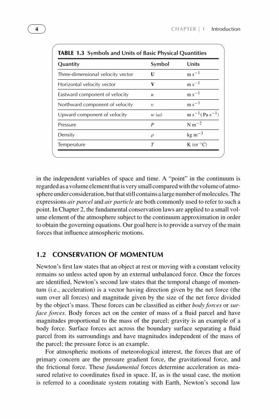
TABLE 1.3 Symbols and Units of Basic Physical Quantities
Quantity Symbol Units
Three-dimensional velocity vector U m s−1
Horizontal velocity vector V m s−1
Eastward component of velocity u m s−1
Northward component of velocity v m s−1
Upward component of velocity w (ω) m s−1(Pa s−1)
Pressure P N m−2
Density ρ kg m−3
Temperature T K (or ◦C)
in the independent variables of space and time. A “point” in the continuum isregardedasavolumeelement that isverysmallcomparedwith thevolumeofatmo-sphereunderconsideration,but that still containsa largenumberofmolecules.Theexpressions air parcel and air particle are both commonly used to refer to such apoint. In Chapter 2, the fundamental conservation laws are applied to a small vol-ume element of the atmosphere subject to the continuum approximation in orderto obtain the governing equations. Our goal here is to provide a survey of the mainforces that influence atmospheric motions.
1.2 CONSERVATION OF MOMENTUM
Newton’s first law states that an object at rest or moving with a constant velocityremains so unless acted upon by an external unbalanced force. Once the forcesare identified, Newton’s second law states that the temporal change of momen-tum (i.e., acceleration) is a vector having direction given by the net force (thesum over all forces) and magnitude given by the size of the net force dividedby the object’s mass. These forces can be classified as either body forces or sur-face forces. Body forces act on the center of mass of a fluid parcel and havemagnitudes proportional to the mass of the parcel; gravity is an example of abody force. Surface forces act across the boundary surface separating a fluidparcel from its surroundings and have magnitudes independent of the mass ofthe parcel; the pressure force is an example.
For atmospheric motions of meteorological interest, the forces that are ofprimary concern are the pressure gradient force, the gravitational force, andthe frictional force. These fundamental forces determine acceleration as mea-sured relative to coordinates fixed in space. If, as is the usual case, the motionis referred to a coordinate system rotating with Earth, Newton’s second law

To protect the rights of the author(s) and publisher we inform you that this PDF is an uncorrected proof for internal businessuse only by the author(s), editor(s), reviewer(s), Elsevier and typesetter diacriTech. It is not allowed to publish this proofonline or in print. This proof copy is the copyright property of the publisher and is confidential until formal publication.
“Hakim: 05-ch01-001-030-9780123848666” — 2012/7/26 — 11:32 — page 5 — #5
1.2 | Conservation of Momentum 5
may still be applied provided that certain apparent forces, the centrifugal forceand the Coriolis force, are included. The fundamental forces are discussedsubsequently, and the apparent forces are introduced in Section 1.3.
1.2.1 Pressure Gradient Force
Pressure is defined as the force per unit area acting normal to a surface. In agas such as the atmosphere, pressure at a point acts equally in all directionsdue to random molecular motion. Therefore, the magnitude of the net force dueto molecules colliding with a surface is independent of the orientation of thesurface; note that the direction of the net force changes with the orientation ofthe surface, but the magnitude does not. Placing a wall in a gas, with the pressureon one side different from that on the other, yields a net force that will acceleratethe wall toward the side having lower pressure; this net force associated withpressure differences is the essence of the pressure gradient force.
Consider now an infinitesimal volume element of air, δV = δxδyδz, centeredat the point x0, y0, z0, as illustrated in Figure 1.2. Due to random molecularmotions, momentum is continually imparted to the walls of the volume elementby the surrounding air. This momentum transfer per unit time per unit area isjust the pressure exerted on the walls of the volume element by the surroundingair. If the pressure at the center of the volume element is designated by p0, thenthe pressure on the wall labeled A in Figure 1.2 can be expressed in a Taylorseries expansion as
p0 +∂p
∂x
δx
2+ higher-order terms
FBx B
(x0, y0, z0)
A
δz
δx
δy
FAx
y
z
x
FIGURE 1.2 The x component of the pressure gradient force acting on a fluid element.

To protect the rights of the author(s) and publisher we inform you that this PDF is an uncorrected proof for internal businessuse only by the author(s), editor(s), reviewer(s), Elsevier and typesetter diacriTech. It is not allowed to publish this proofonline or in print. This proof copy is the copyright property of the publisher and is confidential until formal publication.
“Hakim: 05-ch01-001-030-9780123848666” — 2012/7/26 — 11:32 — page 6 — #6
6 CHAPTER | 1 Introduction
Neglecting the higher-order terms in this expansion, the pressure force actingon the volume element at wall A is
FAx = −
(p0 +
∂p
∂x
δx
2
)δy δz
where δyδz is the area of wall A. Similarly, the pressure force acting on thevolume element at wall B is just
FBx = +
(p0 −
∂p
∂x
δx
2
)δy δz
Therefore, the net x component of this force acting on the volume is
Fx = FAx + FBx = −∂p
∂xδx δy δz
Because the net force is proportional to the derivative of pressure, it is referredto as the pressure gradient force. The mass m of the differential volume elementis simply the density ρ times the volume: m = ρδxδyδz. Thus, the x componentof the pressure gradient force per unit mass is
Fx
m= −
1
ρ
∂p
∂x
Similarly, it can easily be shown that the y and z components of the pressuregradient force per unit mass are
Fy
m= −
1
ρ
∂p
∂yand
Fz
m= −
1
ρ
∂p
∂z
so that the total pressure gradient force per unit mass is the vector given by
Fm= −
1
ρ∇p (1.1)
The gradient operator ∇ =(
i ∂∂x , j ∂
∂y ,k ∂∂z
)acts on functions to its right to yield
vectors that point toward higher values of the function. It is important to notethat (1) the pressure gradient points from low to high pressure, but the pressuregradient force points from high to low pressure, and (2) the pressure gradientforce is proportional to the gradient of the pressure field, not to the pressureitself.
1.2.2 Viscous Force
Any real fluid is subject to internal friction, called viscosity, which causes itto resist the tendency to flow. Viscosity arises when the fluid velocity variesspatially so that random molecular motion accomplishes a net transport ofmomentum from molecules in faster-moving air parcels to molecules in nearby
To protect the rights of the author(s) and publisher we inform you that this PDF is an uncorrected proof for internal businessuse only by the author(s), editor(s), reviewer(s), Elsevier and typesetter diacriTech. It is not allowed to publish this proofonline or in print. This proof copy is the copyright property of the publisher and is confidential until formal publication.
“Hakim: 05-ch01-001-030-9780123848666” — 2012/7/26 — 11:32 — page 7 — #7
1.2 | Conservation of Momentum 7
slower-moving air parcels. This momentum exchange between parcels may beexpressed as a viscous force, F, acting along the face of the air parcel, whichproduces a shear stress, τ , on the parcel per area, A,
τ =F
A(1.2)
Therefore, the viscous force is given by F = τA. For a Newtonian fluid, weassume that the shear stress depends linearly on the fluid speed, which is a verygood approximation for air. In the vertical direction, for example, variation inthe x component of the wind, u, produces the stress
τ ≈ µ∂u
∂z(1.3)
where µ is the viscosity coeficient, which depends on the fluid. As in the pres-sure gradient force discussion, we need the net force acting on the air parcelfrom viscous effects. Following a similar Taylor-approximation approach as forthe pressure gradient derivation, but noting that the force is directed along ratherthan normal to the face of the parcel volume, we find that the viscous force perunit mass due to vertical shear of the component of motion in the x direction is
1
ρ
∂τzx
∂z=
1
ρ
∂
∂z
(µ∂u
∂z
)(1.4)
For constant µ, the right side may be simplified to ν∂2u/∂z2, where ν = µ/ρ isthe kinematic viscosity coefficient. For standard atmosphere2 conditions at sea
level, ν = 1.46 × 10⁻⁵ m2 s−1. Note that (1.4) represents only the contribu-tion from x momentum shear stress in the z direction, and the net force in thex direction, Frx, also includes contributions from the x and y directions. Thenet frictional force components per unit mass in the three Cartesian coordinatedirections are
Frx = ν
[∂2u
∂x2+∂2u
∂y2+∂2u
∂z2
]Fry = ν
[∂2v
∂x2+∂2v
∂y2+∂2v
∂z2
](1.5)
Frz = ν
[∂2w
∂x2+∂2w
∂y2+∂2w
∂z2
]Each component frictional force represents diffusion of momentum in that coor-
dinate direction, since, for example, ∂2u∂x2 +
∂2u∂y2 +
∂2u∂z2 = ∇·∇u = ∇2u. For any
2The U.S. standard atmosphere is a specified vertical profile of atmospheric structure.
To protect the rights of the author(s) and publisher we inform you that this PDF is an uncorrected proof for internal businessuse only by the author(s), editor(s), reviewer(s), Elsevier and typesetter diacriTech. It is not allowed to publish this proofonline or in print. This proof copy is the copyright property of the publisher and is confidential until formal publication.
“Hakim: 05-ch01-001-030-9780123848666” — 2012/7/26 — 11:32 — page 8 — #8
8 CHAPTER | 1 Introduction
vector A, ∇ ·A is a scalar quantity called the divergence of A, since it is pos-itive when vectors diverge away from a point; negative divergence is calledconvergence. At a local maximum in u, ∇u points toward (converges on) themaximum, and therefore ∇2u < 0, resulting in a loss of momentum from themaximum value to the surrounding region. This process is called downgradi-ent diffusion, since momentum diffuses down the gradient, from large to smallvalues.
For the atmosphere below 100 km, ν is so small that molecular viscosityis negligible except in a thin layer within a few centimeters of Earth’s surface,where the vertical shear is very large. Away from this surface molecular bound-ary layer, momentum is transferred primarily by turbulent eddy motions, whichare discussed in Chapter 8.
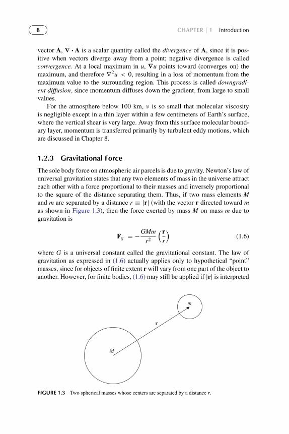
1.2.3 Gravitational Force
The sole body force on atmospheric air parcels is due to gravity. Newton’s law ofuniversal gravitation states that any two elements of mass in the universe attracteach other with a force proportional to their masses and inversely proportionalto the square of the distance separating them. Thus, if two mass elements Mand m are separated by a distance r ≡ |r| (with the vector r directed toward mas shown in Figure 1.3), then the force exerted by mass M on mass m due togravitation is
Fg = −GMm
r2
(rr
)(1.6)
where G is a universal constant called the gravitational constant. The law ofgravitation as expressed in (1.6) actually applies only to hypothetical “point”masses, since for objects of finite extent r will vary from one part of the object toanother. However, for finite bodies, (1.6) may still be applied if |r| is interpreted
M
r
m
FIGURE 1.3 Two spherical masses whose centers are separated by a distance r.

To protect the rights of the author(s) and publisher we inform you that this PDF is an uncorrected proof for internal businessuse only by the author(s), editor(s), reviewer(s), Elsevier and typesetter diacriTech. It is not allowed to publish this proofonline or in print. This proof copy is the copyright property of the publisher and is confidential until formal publication.
“Hakim: 05-ch01-001-030-9780123848666” — 2012/7/26 — 11:32 — page 9 — #9
1.3 | Noninertial Reference Frames and “Apparent” Forces 9
as the distance between the centers of mass of the bodies. Thus, if Earth isdesignated as mass M, and m is a mass element of the atmosphere, then theforce per unit mass exerted on the atmosphere by the gravitational attraction ofEarth is
Fg
m≡ g∗ = −
GM
r2
(rr
)(1.7)
In dynamic meteorology it is customary to use the height above mean sea levelas a vertical coordinate. If the mean radius of Earth is designated by a andthe distance above mean sea level is designated by z, then neglecting the smalldeparture of the shape of Earth from sphericity, r = a+ z. Therefore, Eq. (1.7)can be rewritten as
g∗ =g∗0
(1+ z/a)2(1.8)
where g∗0 = −(GM/a2)(r/r) is the gravitational force at mean sea level. Formeteorological applications, z � a, so that with negligible error we can letg∗ = g∗0 and simply treat the gravitational force as a constant. Note that thistreatment of the gravitational force will be modified in Section 1.3.2 to accountfor centrifugal forces due to Earth’s rotation.
1.3 NONINERTIAL REFERENCE FRAMES AND “APPARENT”FORCES
In formulating the laws of atmospheric dynamics, it is natural to use a geocen-tric reference frame—that is, a frame of reference at rest with respect to rotatingEarth. Newton’s first law of motion states that a mass in uniform motion relativeto a coordinate system fixed in space will remain in uniform motion in theabsence of any forces. Such motion is referred to as inertial motion, and thefixed reference frame is an inertial, or absolute, frame of reference. It is clear,however, that an object at rest or in uniform motion with respect to rotatingEarth is not at rest or in uniform motion relative to a coordinate system fixed inspace.
Therefore, motion that appears to be inertial motion to an observer in ageocentric reference frame is really accelerated motion. Hence, a geocentricreference frame is a noninertial reference frame. Newton’s laws of motion canonly be applied in such a frame if the acceleration of the coordinates is takeninto account. The most satisfactory way of including the effects of coordinateacceleration is to introduce “apparent” forces in the statement of Newton’s sec-ond law. These apparent forces are the inertial reaction terms that arise becauseof the coordinate acceleration. For a coordinate system in uniform rotation, twosuch apparent forces are required: the centrifugal force and the Coriolis force.

To protect the rights of the author(s) and publisher we inform you that this PDF is an uncorrected proof for internal businessuse only by the author(s), editor(s), reviewer(s), Elsevier and typesetter diacriTech. It is not allowed to publish this proofonline or in print. This proof copy is the copyright property of the publisher and is confidential until formal publication.
“Hakim: 05-ch01-001-030-9780123848666” — 2012/7/26 — 11:32 — page 10 — #10
10 CHAPTER | 1 Introduction
1.3.1 Centripetal Acceleration and Centrifugal Force
To illustrate the essential aspects of noninertial frames, we consider a ball ofmass m attached to a string and whirled through a circle of radius r at a constantangular velocity ω. From the point of view of an observer in inertial space thespeed of the ball is constant, but its direction of travel is continuously changingso that its velocity is not constant. To compute the acceleration we consider thechange in velocity δV that occurs for a time increment δt during which the ballrotates through an angle δθ as shown in Figure 1.4. Because δθ is also the anglebetween the vectors V and V+ δV, the magnitude of δV is just |δV| = |V| δθ .If we divide by δt and note that in the limit δt → 0, δV is directed toward theaxis of rotation, we obtain
DVDt= |V|
Dθ
Dt
(−
rr
)However, |V| = ωr and Dθ/Dt = ω, so that
DVDt= −ω2r (1.9)
Therefore, viewed from fixed coordinates, the motion is one of uniformacceleration directed toward the axis of rotation at a rate equal to the squareof the angular velocity times the distance from the axis of rotation. This accel-eration is called centripetal acceleration. It is caused by the force of the stringpulling the ball.
Now suppose that we observe the motion in a coordinate system rotatingwith the ball. In this rotating system the ball is stationary, but there is stilla force acting on the ball—namely, the pull of the string. Therefore, in orderto apply Newton’s second law to describe the motion relative to this rotating
Vr
V
δ V
δθ
δθ
ω
FIGURE 1.4 Centripetal acceleration is given by the rate of change of the direction of the velocityvector, which is directed toward the axis of rotation, as illustrated here by δV.

To protect the rights of the author(s) and publisher we inform you that this PDF is an uncorrected proof for internal businessuse only by the author(s), editor(s), reviewer(s), Elsevier and typesetter diacriTech. It is not allowed to publish this proofonline or in print. This proof copy is the copyright property of the publisher and is confidential until formal publication.
“Hakim: 05-ch01-001-030-9780123848666” — 2012/7/26 — 11:32 — page 11 — #11
1.3 | Noninertial Reference Frames and “Apparent” Forces 11
coordinate system, we must include an additional apparent force, the centrifugalforce, which just balances the force of the string on the ball. Thus, the centrifu-gal force is equivalent to the inertial reaction of the ball on the string and justequal and opposite to the centripetal acceleration.
To summarize, observed from a fixed system, the rotating ball undergoes auniform centripetal acceleration in response to the force exerted by the string.Observed from a system rotating along with it, the ball is stationary and theforce exerted by the string is balanced by a centrifugal force.
1.3.2 Gravity Revisited
An object at rest on the surface of Earth is not at rest or in uniform motionrelative to an inertial reference frame except at the poles. Rather, an objectof unit mass at rest on the surface of Earth is subject to a centripetal accel-eration directed toward the axis of rotation of Earth given by −�2R, whereR is the position vector from the axis of rotation to the object and � =
7.292 × 10⁻⁵ rad s−1 is the angular speed of rotation of Earth.3 Since, exceptat the equator and poles, the centripetal acceleration has a component directedpoleward along the horizontal surface of Earth (i.e., along a surface of constantgeopotential), there must be a net horizontal force directed poleward along thehorizontal to sustain the horizontal component of the centripetal acceleration.
This force arises because rotating Earth is not a sphere but has assumedthe shape of an oblate spheroid in which there is a poleward component ofgravitation along a constant geopotential surface just sufficient to account forthe poleward component of the centripetal acceleration at each latitude for anobject at rest on the surface of Earth. In other words, from the point of view ofan observer in an inertial reference frame, geopotential surfaces slope upwardtoward the equator (Figure 1.5). As a consequence, the equatorial radius of Earthis about 21 km larger than the polar radius.
Viewed from a frame of reference rotating with Earth, however, a geo-potential surface is everywhere normal to the sum of the true force of gravity, g∗,and the centrifugal force �2R (which is just the reaction force of the centripetalacceleration). A geopotential surface is thus experienced as a level surface byan object at rest on rotating Earth. Except at the poles, the weight of an object ofmass m at rest on such a surface, which is just the reaction force of Earth on theobject, will be slightly less than the gravitational force mg∗ because, as illus-trated in Figure 1.5, the centrifugal force partly balances the gravitational force.It is, therefore, convenient to combine the effects of the gravitational force andcentrifugal force by defining gravity g such that
g ≡ −gk ≡ g∗ +�2R (1.10)
3Earth revolves around its axis once every sidereal day, which is equal to 23 h 56 min 4 s (86,164 s).Thus, � = 2π/(86,164 s) = 7.292× 10⁻⁵ rad s−1.

To protect the rights of the author(s) and publisher we inform you that this PDF is an uncorrected proof for internal businessuse only by the author(s), editor(s), reviewer(s), Elsevier and typesetter diacriTech. It is not allowed to publish this proofonline or in print. This proof copy is the copyright property of the publisher and is confidential until formal publication.
“Hakim: 05-ch01-001-030-9780123848666” — 2012/7/26 — 11:32 — page 12 — #12
12 CHAPTER | 1 Introduction
Earth
Sphere
Ω2R
Ω
R
g
g∗
FIGURE 1.5 Relationship between the true gravitation vector g∗ and gravity g. For an idealizedhomogeneous spherical Earth, g∗ would be directed toward the center of Earth. In reality, g∗ doesnot point exactly to the center except at the equator and the poles. Gravity, g, is the vector sum ofg∗ and the centrifugal force and is perpendicular to the level surface of Earth, which approximatesan oblate spheroid.
where k designates a unit vector parallel to the local vertical. Gravity, g,sometimes referred to as “apparent gravity,” will here be taken as a constant(g = 9.81 m s−2). Except at the poles and the equator, g is not directed towardthe center of Earth, but is perpendicular to a geopotential surface as indicated byFigure 1.5. True gravity g∗, however, is not perpendicular to a geopotential sur-face, but has a horizontal component just large enough to balance the horizontalcomponent of �2R.
Gravity can be represented in terms of the gradient of a potential function8, which is just the geopotential referred to before:
∇8 = −g
However, because g=−gk, where g≡|g|, it is clear that8=8(z) and d8/dz=g. Thus, horizontal surfaces on Earth are surfaces of constant geopotential. Ifthe value of dz should be dz’, where dz’ is a dummy variable of integration,geopotential is set to zero at mean sea level, the geopotential 8(z) at height z isjust the work required to raise a unit mass to height z from mean sea level:
8 =
z∫0
gdz (1.11)
Despite the fact that the surface of Earth bulges toward the equator, an objectat rest on the surface of rotating Earth does not slide “downhill” toward thepole because, as indicated previously, the poleward component of gravitationis balanced by the equatorward component of the centrifugal force. However,if the object is put into motion relative to Earth, this balance will be disrupted.Consider a frictionless object located initially at the North Pole. Such an objecthas zero angular momentum about the axis of Earth. If it is displaced away

To protect the rights of the author(s) and publisher we inform you that this PDF is an uncorrected proof for internal businessuse only by the author(s), editor(s), reviewer(s), Elsevier and typesetter diacriTech. It is not allowed to publish this proofonline or in print. This proof copy is the copyright property of the publisher and is confidential until formal publication.
“Hakim: 05-ch01-001-030-9780123848666” — 2012/7/26 — 11:32 — page 13 — #13
1.3 | Noninertial Reference Frames and “Apparent” Forces 13
from the pole in the absence of a zonal torque, it will not acquire rotation andthus will feel a restoring force due to the horizontal component of true gravity,which, as indicated before, is equal and opposite to the horizontal component ofthe centrifugal force for an object at rest on the surface of Earth. Letting R be thedistance from the pole, the horizontal restoring force for a small displacementis thus −�2R, and the object’s acceleration viewed in the inertial coordinatesystem satisfies the equation for a simple harmonic oscillator:
d2R
dt2+�2R = 0 (1.12)
The object will undergo an oscillation of period 2π/� along a path thatwill appear as a straight line passing through the pole to an observer in a fixedcoordinate system, but will appear as a closed circle traversed in 1/2 day to anobserver rotating with Earth (Figure 1.6). From the point of view of an Earth-bound observer, there is an apparent deflection force that causes the object todeviate to the right of its direction of motion at a fixed rate.
0°
3 h
A
0°
6 h
A
B
0°
9 h
A B
C 0°
A
B
C
12 h
FIGURE 1.6 Motion of a frictionless object launched from the North Pole along the 0◦ longitudemeridian at t = 0, as viewed in fixed and rotating reference frames at 3, 6, 9, and 12 h after launch.The horizontal dashed line marks the position that the 0◦ longitude meridian had at t = 0, andthe short dashed lines show its position in the fixed reference frame at subsequent 3-h intervals.The horizontal arrows show 3-h displacement vectors as seen by an observer in the fixed referenceframe. Heavy curved arrows show the trajectory of the object as viewed by an observer in the rotat-ing system. Labels A, B, and C show the position of the object relative to the rotating coordinatesat 3-h intervals. In the fixed coordinate frame, the object oscillates back and forth along a straightline under the influence of the restoring force provided by the horizontal component of gravitation.The period for a complete oscillation is 24 h (only 1/2 period is shown). To an observer in rotatingcoordinates, however, the motion appears to be at constant speed and describes a complete circle ina clockwise direction in 12 h.

To protect the rights of the author(s) and publisher we inform you that this PDF is an uncorrected proof for internal businessuse only by the author(s), editor(s), reviewer(s), Elsevier and typesetter diacriTech. It is not allowed to publish this proofonline or in print. This proof copy is the copyright property of the publisher and is confidential until formal publication.
“Hakim: 05-ch01-001-030-9780123848666” — 2012/7/26 — 11:32 — page 14 — #14
14 CHAPTER | 1 Introduction
1.3.3 The Coriolis Force and the Curvature Effect
Newton’s second law of motion expressed in coordinates rotating with Earthcan be used to describe the force balance for an object at rest on the surface ofEarth, provided that an apparent force, the centrifugal force, is included amongthe forces acting on the object. If, however, the object is in motion along thesurface of Earth, additional apparent forces are required in the statement ofNewton’s second law. The Coriolis force will be given a more formal mathe-matical treatment in Chapter 2, and our purpose here is to deduce the effect bybuilding upon the centrifugal force discussion of the previous section.
Angular momentum, m = r× p, provides a measures of the rotation tracedby the linear momentum vector p with respect to a set of coordinates, the originof which defines the position vector r. We note that the dynamically importantpiece of the angular momentum vector lies parallel to Earth’s rotational axis,m = m cosφ. For now, assume that the linear momentum vector points east-ward, having contributions from eastward air motion, u, and from the planetaryrotation, R�, where R = r cosφ is the distance of the air parcel from the axisof rotation (Figure 1.7). If there is no torque in the east–west direction (i.e., nopressure gradient or viscous forces), then m is conserved following the motion,
Dm
Dt=
DR
Dt(2R�+ u)+ R
Du
Dt= 0 (1.13)
R0
R0 +δR
Earth radius a
δR
Ω
Earth
radiu
s a
FIGURE 1.7 For poleward motion, air parcels move closer to the axis of rotation and, throughangular momentum conservation, the zonal wind accelerates.

To protect the rights of the author(s) and publisher we inform you that this PDF is an uncorrected proof for internal businessuse only by the author(s), editor(s), reviewer(s), Elsevier and typesetter diacriTech. It is not allowed to publish this proofonline or in print. This proof copy is the copyright property of the publisher and is confidential until formal publication.
“Hakim: 05-ch01-001-030-9780123848666” — 2012/7/26 — 11:32 — page 15 — #15
1.3 | Noninertial Reference Frames and “Apparent” Forces 15
so that
Du
Dt= −
(2�R+ u)
R
DR
Dt(1.14)
Figure 1.7 shows that moving an air parcel closer to the axis of rotation, DRDt < 0,
while conserving angular momentum, increases the westerly linear momentum,analagous to an ice skater spinning faster as the person’s arms are drawn inward.
We expand the right side of (1.14) by first noting that
DR
Dt=
Dr
Dtcosφ + r
D
Dtcosφ = w cosφ − v sinφ (1.15)
where v and w are the northward and upward velocity components, respectively.With this relation, (1.14) becomes
Du
Dt= (2� sinφ)v − (2� cosφ)w−
uw
r+
uv
rtanφ (1.16)
The first two terms on the right in (1.16) are the zonal component of the Coriolisforce due to meridional and vertical motion, respectively. The last two terms onthe right are referred to as metric terms or curvature effects because they arisefrom the curvature of Earth’s surface; since r is large, these terms are negligiblysmall except near large u.
Suppose now that the object is set in motion in the eastward direction by animpulsive force. Axial angular momentum is not conserved in this case, but con-sidering again the centrifugal force will help expose the meridional componentof the Coriolis force. Because the object is now rotating faster than Earth, thecentrifugal force on the object will be increased. The excess of the centrifugalforce over that for an object at rest is(
�+u
R
)2R−�2R =
2�uRR+
u2RR2
The terms on the right represent deflecting forces, which act outward alongthe vector R (i.e., perpendicular to the axis of rotation). The meridional and ver-tical components of these forces are obtained by taking meridional and verticalcomponents of R, as shown in Figure 1.8, to yield
Dv
Dt= −2�u sinφ −
u2
atanφ (1.17)
Dw
Dt= 2�u cosφ +
u2
a(1.18)
The first terms on the right are the meridional and vertical components, respec-tively, of the Coriolis forces for zonal motion; the second terms on the right arecurvature effects.

To protect the rights of the author(s) and publisher we inform you that this PDF is an uncorrected proof for internal businessuse only by the author(s), editor(s), reviewer(s), Elsevier and typesetter diacriTech. It is not allowed to publish this proofonline or in print. This proof copy is the copyright property of the publisher and is confidential until formal publication.
“Hakim: 05-ch01-001-030-9780123848666” — 2012/7/26 — 11:32 — page 16 — #16
16 CHAPTER | 1 Introduction
R
2Ωu cos φ
2Ωu (R/R)
2Ωu sin φ
Ω
φ
FIGURE 1.8 Components of the Coriolis force due to relative motion along a latitude circle.
For larger-scale motions, the curvature terms can be neglected as an approxi-mation. Therefore, relative horizontal motion produces a horizontal accelerationperpendicular to the direction of motion given by
Du
Dt= 2�v sinφ= f v (1.19)
Dv
Dt= −2�u sinφ = −fu (1.20)
where f ≡ 2� sinφ is the Coriolis parameter.Thus, for example, an object moving eastward in the horizontal is deflected
equatorward by the Coriolis force, whereas a westward moving object isdeflected poleward. In either case the deflection is to the right of the direction ofmotion in the Northern Hemisphere and to the left in the Southern Hemisphere.The vertical component of the Coriolis force in (1.18) is ordinarily much smallerthan the gravitational force so that its only effect is to cause a very minor changein the apparent weight of an object depending on whether the object is movingeastward or westward.
The Coriolis force is negligible for motions with time scales that are veryshort compared to the period of Earth’s rotation (a point that is illustrated byseveral problems at the end of the chapter). Thus, the Coriolis force is notimportant for the dynamics of individual cumulus clouds but is essential for anunderstanding of longer time scale phenomena such as synoptic scale systems.The Coriolis force must also be taken into account when computing long-rangemissile or artillery trajectories.
As an example, suppose that a ballistic missile is fired due eastward at 43◦Nlatitude ( f = 10−4 s−1 at 43◦N). If the missile travels 1000 km at a horizontalspeed u0 = 1000 m s−1, by how much is the missile deflected from its eastward

To protect the rights of the author(s) and publisher we inform you that this PDF is an uncorrected proof for internal businessuse only by the author(s), editor(s), reviewer(s), Elsevier and typesetter diacriTech. It is not allowed to publish this proofonline or in print. This proof copy is the copyright property of the publisher and is confidential until formal publication.
“Hakim: 05-ch01-001-030-9780123848666” — 2012/7/26 — 11:32 — page 17 — #17
1.3 | Noninertial Reference Frames and “Apparent” Forces 17
path by the Coriolis force? Integrating (1.20) with respect to time, we find that
v = −fu0t (1.21)
where it is assumed that the deflection is sufficiently small so that we may letf and u0 be constants. To find the total displacement, we must integrate (1.13)with respect to time:
t∫0
vdt =
y0+δy∫y0
dy = −fu0
t∫0
tdt
Thus, the total displacement is
δy = −fu0t2/2 = −50 km
Therefore, the missile is deflected southward by 50 km due to the Coriolis effect.Further examples of the deflection of objects by the Coriolis force are given insome of the problems at the end of the chapter.
The x and y components given in (1.19) and (1.20) can be combined in vectorform as (
DVDt
)Co= −f k× V (1.22)
where V ≡ (u, v) is the horizontal velocity, k is a vertical unit vector, and thesubscript Co indicates that the acceleration is due solely to the Coriolis force.Since −k× V is a vector rotated 90◦ to the right of V, (1.22) clearly shows thedeflection character of the Coriolis force. The Coriolis force can only changethe direction of motion, not the speed.
1.3.4 Constant Angular Momentum Oscillations
Suppose an object initially at rest on Earth at the point (x0, y0) is impulsivelypropelled along the x axis with a speed V at time t = 0. Then, from (1.19)and (1.20), the time evolution of the velocity is given by u = V cos ft andv = −V sin ft. However, because u = Dx/Dt and v = Dy/Dt, integration withrespect to time gives the position of the object at time t as
x− x0 =V
fsin ft and y− y0 =
V
f(cos ft − 1) (1.23)
where the variation of f with latitude is neglected. Equations (1.23) show thatin the Northern Hemisphere, where f is positive, the object orbits clockwise(anticyclonically) in a circle of radius R = V/f about the point (x0, y0 − V/f )with a period given by
τ = 2πR/V = 2π/f = π/(� sinφ) (1.24)

To protect the rights of the author(s) and publisher we inform you that this PDF is an uncorrected proof for internal businessuse only by the author(s), editor(s), reviewer(s), Elsevier and typesetter diacriTech. It is not allowed to publish this proofonline or in print. This proof copy is the copyright property of the publisher and is confidential until formal publication.
“Hakim: 05-ch01-001-030-9780123848666” — 2012/7/26 — 11:32 — page 18 — #18
18 CHAPTER | 1 Introduction
Thus, an object displaced horizontally from its equilibrium position on thesurface of Earth under the influence of the force of gravity will oscillate aboutits equilibrium position with a period that depends on latitude and is equalto one sidereal day at 30◦ latitude and 1/2 sidereal day at the pole. Constantangular momentum oscillations (often referred to as “inertial oscillations”) arecommonly observed in the oceans, but are apparently not of importance in theatmosphere.
1.4 STRUCTURE OF THE STATIC ATMOSPHERE
The thermodynamic state of the atmosphere at any point is determined by thevalues of pressure, temperature, and density (or specific volume) at that point.These field variables are related to one an other by the equation of state for anideal gas. Letting p, T, ρ, and α(≡ ρ−1) denote pressure, temperature, density,and specific volume, respectively, we can express the equation of state for dryair as
pα = RT or p = ρRT (1.25)
where R is the gas constant for dry air (R = 287 J kg−1 K−1).
1.4.1 The Hydrostatic Equation
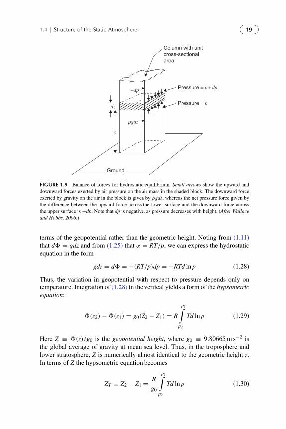
In the absence of atmospheric motions, the gravity force must be exactlybalanced by the vertical component of the pressure gradient force. Thus, asillustrated in Figure 1.9,
dp/dz = −ρg (1.26)
This condition of hydrostatic balance provides an excellent approximation forthe vertical dependence of the pressure field in the real atmosphere. Only forintense small-scale systems, such as squall lines and tornadoes, is it necessary toconsider departures from hydrostatic balance. Integrating (1.26) from a height zto the top of the atmosphere, we find that
p(z) =
∞∫z
ρgdz (1.27)
so that the pressure at any point is simply equal to the weight of the unitcross-section column of air overlying the point. Thus, mean sea level pressurep(0) = 1013.25 hPa is simply the average weight per square meter of the totalatmospheric column.4 It is often useful to express the hydrostatic equation in
4For computational convenience, the mean surface pressure is often assumed to equal 1000 hPa.
To protect the rights of the author(s) and publisher we inform you that this PDF is an uncorrected proof for internal businessuse only by the author(s), editor(s), reviewer(s), Elsevier and typesetter diacriTech. It is not allowed to publish this proofonline or in print. This proof copy is the copyright property of the publisher and is confidential until formal publication.
“Hakim: 05-ch01-001-030-9780123848666” — 2012/7/26 — 11:32 — page 19 — #19
1.4 | Structure of the Static Atmosphere 19
Pressure = p
Ground
dz
ρgdz
−dp Pressure = p + dp
Column with unitcross-sectionalarea
z
FIGURE 1.9 Balance of forces for hydrostatic equilibrium. Small arrows show the upward anddownward forces exerted by air pressure on the air mass in the shaded block. The downward forceexerted by gravity on the air in the block is given by ρgdz, whereas the net pressure force given bythe difference between the upward force across the lower surface and the downward force acrossthe upper surface is −dp. Note that dp is negative, as pressure decreases with height. (After Wallaceand Hobbs, 2006.)
terms of the geopotential rather than the geometric height. Noting from (1.11)that d8 = gdz and from (1.25) that α = RT/p, we can express the hydrostaticequation in the form
gdz = d8 = −(RT/p)dp = −RTd ln p (1.28)
Thus, the variation in geopotential with respect to pressure depends only ontemperature. Integration of (1.28) in the vertical yields a form of the hypsometricequation:
8(z2)−8(z1) = g0(Z2 − Z1) = R
p1∫p2
Td ln p (1.29)
Here Z ≡ 8(z)/g0 is the geopotential height, where g0 ≡ 9.80665 m s−2 isthe global average of gravity at mean sea level. Thus, in the troposphere andlower stratosphere, Z is numerically almost identical to the geometric height z.In terms of Z the hypsometric equation becomes
ZT ≡ Z2 − Z1 =R
g0
p1∫p2
Td ln p (1.30)

To protect the rights of the author(s) and publisher we inform you that this PDF is an uncorrected proof for internal businessuse only by the author(s), editor(s), reviewer(s), Elsevier and typesetter diacriTech. It is not allowed to publish this proofonline or in print. This proof copy is the copyright property of the publisher and is confidential until formal publication.
“Hakim: 05-ch01-001-030-9780123848666” — 2012/7/26 — 11:32 — page 20 — #20
20 CHAPTER | 1 Introduction
where ZT is the thickness of the atmospheric layer between the pressure surfacesp2 and p1. Defining a layer mean temperature
〈T〉 =
p1∫p2
d ln p
−1 p1∫p2
Td ln p
and a layer mean scale height H ≡ R〈T〉/g0, we have from Eq. (1.30)
ZT = H ln( p1/p2) (1.31)
Thus, the thickness of a layer bounded by isobaric surfaces is proportional tothe mean temperature of the layer. Pressure decreases more rapidly with heightin a cold layer than in a warm layer. It also follows immediately from (1.31) thatin an isothermal atmosphere of temperature T, the geopotential height is propor-tional to the natural logarithm of pressure normalized by the surface pressureclearer:
Z = H ln( p0/p) (1.32)
where p0 is the pressure at Z = 0. Thus, in an isothermal atmosphere thepressure decreases exponentially with geopotential height by a factor of e−1
per scale height:
p(Z) = p(0)e−Z/H
1.4.2 Pressure as a Vertical Coordinate
From the hydrostatic equation (1.26), it is clear that a single-valued monotonicrelationship exists between pressure and height in each vertical column of theatmosphere. Thus, we may use pressure as the independent vertical coordinateand height (or geopotential) as a dependent variable. The thermodynamic stateof the atmosphere is then specified by the fields of 8(x, y, p, t) and T(x, y, p, t).
Now the horizontal components of the pressure gradient force given byEq. (1.1) are evaluated by partial differentiation holding z constant. However,when pressure is used as the vertical coordinate, horizontal partial derivativesmust be evaluated holding p constant. Transformation of the horizontal pressuregradient force from height to pressure coordinates may be carried out with theaid of Figure 1.10. Considering only the x, z plane, we see from Figure 1.10 that[
(p0 + δp)− p0
δx
]z=
[(p0 + δp)− p0
δz
]x
(δz
δx
)p

To protect the rights of the author(s) and publisher we inform you that this PDF is an uncorrected proof for internal businessuse only by the author(s), editor(s), reviewer(s), Elsevier and typesetter diacriTech. It is not allowed to publish this proofonline or in print. This proof copy is the copyright property of the publisher and is confidential until formal publication.
“Hakim: 05-ch01-001-030-9780123848666” — 2012/7/26 — 11:32 — page 21 — #21
1.4 | Structure of the Static Atmosphere 21
p0
p0 + δp
δx
δz
z
x
FIGURE 1.10 Slope of pressure surfaces in the x, z plane.
where subscripts indicate variables that remain constant in evaluating thedifferentials. For example, in the limit δz→ 0
[(p0 + δp)− p0
δz
]x→
(−∂p
∂z
)x
where the minus sign is included because δz < 0 for δp > 0.Taking the limits δx, δz→ 0, we obtain5(
∂p
∂x
)z= −
(∂p
∂z
)x
(∂z
∂x
)p
which after substitution from the hydrostatic equation (1.26) yields
−1
ρ
(∂p
∂x
)z= −g
(∂z
∂x
)p= −
(∂8
∂x
)p
(1.33)
Similarly, it is easy to show that
−1
ρ
(∂p
∂y
)z= −
(∂8
∂y
)p
(1.34)
Thus, in the isobaric coordinate system the horizontal pressure gradient force ismeasured by the gradient of geopotential at constant pressure. Density no longerappears explicitly in the pressure gradient force; this is a distinct advantage ofthe isobaric system.
5It is important to note the minus sign on the right in this expression!

To protect the rights of the author(s) and publisher we inform you that this PDF is an uncorrected proof for internal businessuse only by the author(s), editor(s), reviewer(s), Elsevier and typesetter diacriTech. It is not allowed to publish this proofonline or in print. This proof copy is the copyright property of the publisher and is confidential until formal publication.
“Hakim: 05-ch01-001-030-9780123848666” — 2012/7/26 — 11:32 — page 22 — #22
22 CHAPTER | 1 Introduction
1.4.3 A Generalized Vertical Coordinate
Any single-valued monotonic function of pressure or height may be used asthe independent vertical coordinate. For example, in many numerical weatherprediction models, pressure normalized by the pressure at the ground, σ ≡p(x, y, z, t)/ps(x, y, t), is used as a vertical coordinate. This choice guaranteesthat the ground is a coordinate surface (σ ≡ 1) even in the presence of spa-tial and temporal surface pressure variations. Thus, this so-called σ coordinatesystem is particularly useful in regions of strong topographic variations.
We now obtain a general expression for the horizontal pressure gradient,which is applicable to any vertical coordinate s = s(x, y, z, t) that is a single-valued monotonic function of height. Referring to Figure 1.11 we see that fora horizontal distance δx, the pressure difference evaluated along a surface ofconstant s is related to that evaluated at constant z by the relationship
pC − pA
δx=
pC − pB
δz
δz
δx+
pB − pA
δx
Taking the limits as δx, δz→ 0, we obtain(∂p
∂x
)s=∂p
∂z
(∂z
∂x
)s+
(∂p
∂x
)z
(1.35)
Using the identity ∂p/∂z = (∂s/∂z)(∂p/∂s), we can express (1.35) in the alter-nate form (
∂p
∂x
)s=
(∂p
∂x
)z+∂s
∂z
(∂z
∂x
)s
(∂p
∂s
)(1.36)
pApB
pC
s = const
δx
δz
z
x
FIGURE 1.11 Transformation of the pressure gradient force to s coordinates.

To protect the rights of the author(s) and publisher we inform you that this PDF is an uncorrected proof for internal businessuse only by the author(s), editor(s), reviewer(s), Elsevier and typesetter diacriTech. It is not allowed to publish this proofonline or in print. This proof copy is the copyright property of the publisher and is confidential until formal publication.
“Hakim: 05-ch01-001-030-9780123848666” — 2012/7/26 — 11:32 — page 23 — #23
1.5 | Kinematics 23
In later chapters we will apply (1.35) or (1.36) and similar expressions forother fields to transform the dynamical equations to several different verticalcoordinate systems.
1.5 KINEMATICS
Kinematics involves the analysis of motion without reference to forces thatchange the motion in time. It provides a diagnosis of motion at a particularinstant in time, which may in turn prove useful for understanding the dynamicsof the flow as it evolves in time. There are many aspects of kinematics, but usu-ally one is interested in the structure of the flow, and here we will limit attentionto the horizontal flow. One way to quantify flow structure is to examine linearvariations in the flow near an arbitrary point (x0, y0). A leading-order Taylorapproximation to the wind near the point is
u(x0 + dx, y0 + dy) ≈ u(x0, y0)+∂u
∂x
∣∣∣∣(x0,y0)
dx+∂u
∂y
∣∣∣∣(x0,y0)
dy (1.37a)
v(x0 + dx, y0 + dy) ≈ v(x0, y0)+∂v
∂x
∣∣∣∣(x0,y0)
dx+∂v
∂y
∣∣∣∣(x0,y0)
dy (1.37b)
Making the following definitions
∂u
∂x+∂v
∂y= δ (1.38a)
∂v
∂x−∂u
∂y= ζ (1.38b)
∂u
∂x−∂v
∂y= d1 (1.38c)
∂v
∂x+∂u
∂y= d2 (1.38d)
allows the derivatives in (1.37a,b) to be replaced in favor of the elementalquanties δ, ζ, d1, and d2:
u(x0 + dx, y0 + dy) ≈ u(x0, y0)+1
2(δ + d1)dx+
1
2(d2 − ζ )dy (1.39a)
v(x0 + dx, y0 + dy) ≈ v(x0, y0)+1
2(ζ + d2)dx+
1
2(δ − d1)dy (1.39b)
The advantage of this manipulation is that we can now think about the wind neara point as a linear combination of the elemental fluid properties. The vorticity,ζ , represents pure rotation (about the vertical direction); δ represents pure diver-gence; and δ < 0 is called convergence. Pure deformation is represented by d1

To protect the rights of the author(s) and publisher we inform you that this PDF is an uncorrected proof for internal businessuse only by the author(s), editor(s), reviewer(s), Elsevier and typesetter diacriTech. It is not allowed to publish this proofonline or in print. This proof copy is the copyright property of the publisher and is confidential until formal publication.
“Hakim: 05-ch01-001-030-9780123848666” — 2012/7/26 — 11:32 — page 24 — #24
24 CHAPTER | 1 Introduction
and d2, where the wind field contracts, or is confluent in one direction, called theaxis of contraction, and the wind field stretches in the normal direction, calledthe axis of dilatation. d2 represents a 45◦ rotation of d1, and therefore they arenot independent patterns. The leading, constant, terms in (1.39a,b) representuniform translation.
By setting all elemental quantities in (1.39a,b) except one to zero, we visual-ize the spatial distribution of the horizontal wind associated with one elementalquantity (Figure 1.12). Note that the pure deformation pattern represents d1 onlyand that, although the vectors appear to converge and diverge, the divergenceis exactly zero in this field. This is an important example of the fact that con-fluence (difluence) in vector fields is not the same as convergence (divergence).In the lower right panel of Figure 1.12, we see a linear combination of vorticity
(a) (b)
(c) (d)
FIGURE 1.12 Velocity fields associated with pure vorticity (a), pure divergence (b), puredeformation (c), and a mixture of vorticity and convergence (d).

To protect the rights of the author(s) and publisher we inform you that this PDF is an uncorrected proof for internal businessuse only by the author(s), editor(s), reviewer(s), Elsevier and typesetter diacriTech. It is not allowed to publish this proofonline or in print. This proof copy is the copyright property of the publisher and is confidential until formal publication.
“Hakim: 05-ch01-001-030-9780123848666” — 2012/7/26 — 11:32 — page 25 — #25
1.6 | Scale Analysis 25
and divergence, illustrating a more complicated pattern than the elemental fieldsin isolation. By computing the elemental variables at a point, one can visualizethe linear variation of the flow near that point through (1.39a,b).
This taste of kinematics highlights the importance of certain properties of thewind field that will be explored in greater depth in future chapters. Divergenceis connected to vertical motion by mass conservation, as will be discussed inChapter 2. Vorticity is fundamental to understanding dynamic meteorology andwill be explored in detail in Chapter 3. Deformation is important for creatingand destroying boundaries in fluids, such as horizontal temperature contrastsknown as frontal zones, which will be explored in Chapter 9.
1.6 SCALE ANALYSIS
Scale analysis, or scaling, is a convenient technique for estimating the magni-tudes of various terms in the governing equations for a particular type of motion.In scaling, typical expected values of the following quantities are specified:
1. Magnitudes of the field variables2. Amplitudes of fluctuations in the field variables3. Characteristic length, depth, and time scales on which the fluctuations
occur
These typical values are then used to compare the magnitudes of variousterms in the governing equations. For example, in a typical midlatitude syn-optic6 cyclone, the surface pressure might fluctuate by 10 hPa over a horizontaldistance of 1000 km. Designating the amplitude of the horizontal pressure fluc-tuation by δp, the horizontal coordinates by x and y, and the horizontal scaleby L, the magnitude of the horizontal pressure gradient may be estimated bydividing δp by the length L to get(
∂p
∂x,∂p
∂y
)∼δp
L= 10 hpa/103 km
(10−3 Pa m−1
)Pressure fluctuations of similar magnitudes occur in other motion systems
of vastly different scale such as tornadoes, squall lines, and hurricanes. Thus,the horizontal pressure gradient can range over several orders of magnitudefor systems of meteorological interest. Similar considerations are also valid forderivative terms involving other field variables. Therefore, the nature of thedominant terms in the governing equations is crucially dependent on the hor-izontal scale of the motions. In particular, motions with horizontal scales ofonly a few kilometers tend to have short time scales so that terms involvingthe rotation of Earth are negligible, while for larger scales they become very
6The term synoptic designates the branch of meteorology that deals with the analysis of observationstaken over a wide area at or near the same time. This term is commonly used (as here) to designatethe characteristic scale of the disturbances that are depicted on weather maps.

To protect the rights of the author(s) and publisher we inform you that this PDF is an uncorrected proof for internal businessuse only by the author(s), editor(s), reviewer(s), Elsevier and typesetter diacriTech. It is not allowed to publish this proofonline or in print. This proof copy is the copyright property of the publisher and is confidential until formal publication.
“Hakim: 05-ch01-001-030-9780123848666” — 2012/7/26 — 11:32 — page 26 — #26
26 CHAPTER | 1 Introduction
�
�
�
�
TABLE 1.4 Scales of Atmospheric Motions
Type of Motion Horizontal Scale (m)
Molecular mean free path 10−7
Minute turbulent eddies 10−2 to 10−1
Small eddies 10−1 to 1
Dust devils 1 to 10
Gusts 10 to 102
Tornadoes 102
Cumulonimbus clouds 103
Fronts, squall lines 104 to 105
Hurricanes 105
Synoptic cyclones 106
Planetary waves 107
important. Because the character of atmospheric motions depends so stronglyon the horizontal scale, this scale provides a convenient method for the clas-sification of motion systems. Table 1.4 classifies examples of various types ofmotions by horizontal scale for the spectral region from 10−7 to 107 m. In thefollowing chapters, scaling arguments are used extensively in developing sim-plifications of the governing equations for use in modeling various types ofmotion systems.
SUGGESTED REFERENCES
Complete reference information is provided in the Bibliography at the end ofthe book.
Curry and Webster, Thermodynamics of Atmospheres and Oceans, contains a more advanceddiscussion of atmospheric statistics.
Durran (1993) discusses the constant angular momentum oscillation in detail.Wallace and Hobbs, Atmospheric Science: An Introductory Survey, discuss much of the material in
this chapter at an elementary level.
PROBLEMS
1.1. Neglecting the latitudinal variation in the radius of Earth, calculate theangle between the gravitational force and gravity vectors at the surface ofEarth as a function of latitude. What is the maximum value of this angle?

To protect the rights of the author(s) and publisher we inform you that this PDF is an uncorrected proof for internal businessuse only by the author(s), editor(s), reviewer(s), Elsevier and typesetter diacriTech. It is not allowed to publish this proofonline or in print. This proof copy is the copyright property of the publisher and is confidential until formal publication.
“Hakim: 05-ch01-001-030-9780123848666” — 2012/7/26 — 11:32 — page 27 — #27
Problems 27
1.2. Calculate the altitude at which an artificial satellite orbiting in the equa-torial plane can be a synchronous satellite (i.e., can remain above the samespot on the surface of Earth).
1.3. An artificial satellite is placed in a natural synchronous orbit above theequator and is attached to Earth below by a wire. A second satellite isattached to the first by a wire of the same length and is placed in orbitdirectly above the first at the same angular velocity. Assuming that the wireshave zero mass, calculate the tension in the wires per unit mass of satel-lite. Could this tension be used to lift objects into orbit with no additionalexpenditure of energy?
1.4. A train is running smoothly along a curved track at the rate of 50 m s−1.A passenger standing on a set of scales observes that his weight is 10%greater than when the train is at rest. The track is banked so that the forceacting on the passenger is normal to the floor of the train. What is the radiusof curvature of the track?
1.5. If a baseball player throws a ball a horizontal distance of 100 m at 30◦
latitude in 4 s, by how much is the ball deflected laterally as a result of therotation of Earth?
1.6. Two balls 4 cm in diameter are placed 100 m apart on a frictionless hori-zontal plane at 43◦N. If the balls are impulsively propelled directly at eachother with equal speeds, at what speed must they travel so that they justmiss each other?
1.7. A locomotive of mass 2×10⁵ kg travels 50 m s−1 along a straight horizontaltrack at 43◦N. What lateral force is exerted on the rails? Compare the mag-nitudes of the upward reaction force exerted by the rails for cases wherethe locomotive is traveling eastward and westward, respectively.
1.8. Find the horizontal displacement of a body dropped from a fixed platformat a height h at the equator, neglecting the effects of air resistance. What isthe numerical value of the displacement for h = 5 km?
1.9. A bullet is fired directly upward with initial speed w0 at latitude φ. Neglect-ing air resistance, by what distance will it be displaced horizontally whenit returns to the ground? (Neglect 2�u cosφ compared to g in the verticalmomentum equation.)
1.10. A block of mass M = 1 kg is suspended from the end of a weightless string.The other end of the string is passed through a small hole in a horizontalplatform and a ball of mass m = 10 kg is attached. At what angular veloc-ity must the ball rotate on the horizontal platform to balance the weightof the block if the horizontal distance of the ball from the hole is 1 m?While the ball is rotating, the block is pulled down 10 cm. What is the newangular velocity of the ball? How much work is done in pulling down theblock?
1.11. A particle is free to slide on a horizontal frictionless plane located at alatitude φ on Earth. Find the equation governing the path of the particleif it is given an impulsive northward velocity v = V0 at t = 0. Give thesolution for the position of the particle as a function of time. (Assume thatthe latitudinal excursion is sufficiently small that f is constant.)
1.12. Calculate the 1000 to 500 hPa thickness for isothermal conditions withtemperatures of 273 and 250 K, respectively.

To protect the rights of the author(s) and publisher we inform you that this PDF is an uncorrected proof for internal businessuse only by the author(s), editor(s), reviewer(s), Elsevier and typesetter diacriTech. It is not allowed to publish this proofonline or in print. This proof copy is the copyright property of the publisher and is confidential until formal publication.
“Hakim: 05-ch01-001-030-9780123848666” — 2012/7/26 — 11:32 — page 28 — #28
28 CHAPTER | 1 Introduction
1.13. Isolines of 1000 to 500 hPa thickness are drawn on a weather mapusing a contour interval of 60 m. What is the corresponding layer meantemperature interval?
1.14. Show that a homogeneous atmosphere (density independent of height) hasa finite height that depends only on the temperature at the lower boundary.Compute the height of a homogeneous atmosphere with surface tempera-ture T0 = 273 K and surface pressure 1000 hPa. (Use the ideal gas law andhydrostatic balance.)
1.15. For the conditions of the previous problem, compute the variation of thetemperature with respect to height.
1.16. Show that in an atmosphere with uniform lapse rate γ (where γ ≡ −dT/dz)the geopotential height at pressure level p1 is given by
Z =T0
γ
[1−
(p0
p1
)−Rγ /g]
where T0 and p0 are the sea-level temperature and pressure, respectively.1.17. Calculate the 1000 to 500 hPa thickness for a constant lapse rate atmo-
sphere with γ = 6.5 K km−1 and T0 = 273 K. Compare your results withthe results in Problem 1.12.
1.18. Derive an expression for the variation in density with respect to height in aconstant lapse rate atmosphere.
1.19. Derive an expression for the altitude variation in the pressure change δpthat occurs when an atmosphere with a constant lapse rate is subjectedto a height-independent temperature change δT while the surface pressureremains constant. At what height is the magnitude of the pressure change amaximum if the lapse rate is 6.5 K km−1, T0 = 300, and δT = 2 K?
MATLAB ExercisesM1.1. This exercise investigates the role of the curvature terms for high-latitude
constant angular momentum trajectories.(a) Run the coriolis.m script with the following initial conditions: initial
latitude 60◦, initial velocity u = 0, v = 40 m s−1, run time= 5 days. Com-pare the appearance of the trajectories for the case with the curvatureterms included and the case with the curvature terms neglected. Qual-itatively explain the difference that you observe. Why is the trajectorynot a closed circle as described in Eq. (1.15) of the text? [Hint: Considerthe separate effects of the term proportional to tan φ and of the sphericalgeometry.]
(b) Run coriolis.m with latitude 60◦, u = 0, v = 80 m/s. What is differentfrom case (a)? By varying the run time, see if you can determine how longit takes for the particle to make a full circuit in each case, and comparethis to the time given in Eq. (1.24) for φ = 60◦.
M1.2. Using the MATLAB script from Problem M1.1, compare the magnitudes ofthe lateral deflection for ballistic missiles fired eastward and westward at 43◦
latitude. Each missile is launched at a velocity of 1000 m s−1 and travels1000 km. Explain your results. Can the curvature term be neglected in thesecases?

To protect the rights of the author(s) and publisher we inform you that this PDF is an uncorrected proof for internal businessuse only by the author(s), editor(s), reviewer(s), Elsevier and typesetter diacriTech. It is not allowed to publish this proofonline or in print. This proof copy is the copyright property of the publisher and is confidential until formal publication.
“Hakim: 05-ch01-001-030-9780123848666” — 2012/7/26 — 11:32 — page 29 — #29
Problems 29
M1.3. This exercise examines the strange behavior of constant angular momentumtrajectories near the equator. Run the coriolis.m script for the followingcontrasting cases: (a) latitude 0.5◦, u = 20 m s−1, v = 0, run time = 20 daysand (b) latitude 0.5◦, u = −20 m s−1, v = 0, run time = 20 days. Obviously,eastward and westward motion near the equator leads to very differentbehavior. Briefly explain why the trajectories are so different in these twocases. By running different time intervals, determine the approximate periodof oscillation in each case (i.e., the time to return to the original latitude).
M1.4. More strange behavior near the equator. Run the script const ang momtraj1.m by specifying initial conditions of latitude = 0, u = 0, v =
50 m s−1, and a time of about 5 or 10 days. Notice that the motion issymmetric about the equator and that there is a net eastward drift. Why doesproviding a parcel with an initial poleward velocity at the equator lead to aneastward average displacement? By trying different initial meridional veloci-ties in the range of 50 to 250 m s−1, determine the approximate dependenceof the maximum latitude reached by the ball on the initial meridional veloc-ity. Also determine how the net eastward displacement depends on the initialmeridional velocity. Show your results in a table, or plot them using MATLAB.
To protect the rights of the author(s) and publisher we inform you that this PDF is an uncorrected proof for internal businessuse only by the author(s), editor(s), reviewer(s), Elsevier and typesetter diacriTech. It is not allowed to publish this proofonline or in print. This proof copy is the copyright property of the publisher and is confidential until formal publication.
“Hakim: 06-ch02-031-066-9780123848666” — 2012/7/26 — 10:54 — page 31 — #1
Chapter 2
Basic Conservation Laws
Atmospheric motions are governed by three fundamental physical principles:conservation of mass, conservation of momentum, and conservation of energy.The mathematical relations that express these laws may be derived by consid-ering the budgets of mass, momentum, and energy for an infinitesimal controlvolume in the fluid. Two types of control volume are commonly used in fluiddynamics. In the Eulerian frame of reference, the control volume consists of aparallelepiped of sides δx, δy, and δz, whose position is fixed relative to the coor-dinate axes. Mass, momentum, and energy budgets will depend on fluxes causedby the flow of fluid through the boundaries of the control volume. (This type ofcontrol volume was used in Section 1.2.1.) In the Lagrangian frame, however,the control volume consists of an infinitesimal mass of “tagged” fluid particles;thus, the control volume moves about following the motion of the fluid, alwayscontaining the same fluid particles.
The Lagrangian frame is particularly useful for deriving conservation laws,since such laws may be stated most simply in terms of a particular mass elementof the fluid. The Eulerian system is, however, more convenient for solving mostproblems because in that system the field variables are related by a set of partialdifferential equations in which the independent variables are the coordinates x,y, z, and t. In the Lagrangian system, however, it is necessary to follow the timeevolution of the fields for various individual fluid parcels. Thus, the independentvariables are x0, y0, z0, and t, where x0, y0, and z0 designate the position that aparticular parcel passed through at a reference time t0.
2.1 TOTAL DIFFERENTIATION
The conservation laws to be derived in this chapter contain expressions for therates of change of density, momentum, and thermodynamic energy followingthe motion of particular fluid parcels. In order to apply these laws in the Eulerianframe, it is necessary to derive a relationship between the rate of change of afield variable following the motion and its rate of change at a fixed point. Theformer is called the substantial, the total, or the material derivative (it will bedenoted D/Dt). The latter is called the local derivative (it is merely the partialderivative with respect to time).
An Introduction to Dynamic Meteorology. DOI: 10.1016/B978-0-12-384866-6.00002-7Copyright © 2013 Elsevier Inc. All rights reserved. 31

To protect the rights of the author(s) and publisher we inform you that this PDF is an uncorrected proof for internal businessuse only by the author(s), editor(s), reviewer(s), Elsevier and typesetter diacriTech. It is not allowed to publish this proofonline or in print. This proof copy is the copyright property of the publisher and is confidential until formal publication.
“Hakim: 06-ch02-031-066-9780123848666” — 2012/7/26 — 10:54 — page 32 — #2
32 CHAPTER | 2 Basic Conservation Laws
To derive a relationship between the total derivative and the local derivative,it is convenient to refer to a particular field variable (temperature, for example).For a given air parcel the location (x, y, z) is a function of t so that x = x(t), y =y(t), z = z(t). Following the parcel, T may then be considered as truly a functiononly of time, and its rate of change is just the total derivative DT/Dt. To relatethe total derivative to the local rate of change at a fixed point, we consider thetemperature measured on a balloon that moves with the wind. Suppose that thistemperature is T0 at the point x0, y0, z0 and time t0. If the balloon moves to thepoint x0+δx, y0+δy, z0+δz in a time increment δt, then the temperature changerecorded on the balloon, δT , can be expressed in a Taylor series expansion as
δT =
(∂T
∂t
)δt +
(∂T
∂x
)δx+
(∂T
∂y
)δy+
(∂T
∂z
)δz+ (higher-order terms)
Dividing through by δt and noting that δT is the change in temperature followingthe motion so that
DT
Dt≡ limδt→0
δT
δt
we find that in the limit δt→ 0
DT
Dt=∂T
∂t+
(∂T
∂x
)Dx
Dt+
(∂T
∂y
)Dy
Dt+
(∂T
∂z
)Dz
Dt
is the rate of change of T following the motion.If we now let
Dx
Dt≡ u,
Dy
Dt≡ v,
Dz
Dt≡ w
then u, v, w are the velocity components in the x, y, z directions, respectively,and
DT
Dt=∂T
∂t+
(u∂T
∂x+ v
∂T
∂y+ w
∂T
∂z
)(2.1)
Using vector notation, this expression may be rewritten as
∂T
∂t=
DT
Dt− U ·∇T
where U = iu+ jv + kw is the velocity vector. The term −U ·∇T is called thetemperature advection. It gives the contribution to the local temperature changedue to air motion. For example, if the wind is blowing from a cold region towarda warm region, −U ·∇T will be negative (cold advection) and the advectionterm will contribute negatively to the local temperature change. Thus, the localrate of change of temperature equals the rate of change of temperature follow-ing the motion (i.e., the heating or cooling of individual air parcels) plus theadvective rate of change of temperature.

To protect the rights of the author(s) and publisher we inform you that this PDF is an uncorrected proof for internal businessuse only by the author(s), editor(s), reviewer(s), Elsevier and typesetter diacriTech. It is not allowed to publish this proofonline or in print. This proof copy is the copyright property of the publisher and is confidential until formal publication.
“Hakim: 06-ch02-031-066-9780123848666” — 2012/7/26 — 10:54 — page 33 — #3
2.1 | Total Differentiation 33
The relationship between the total derivative and the local derivative givenfor temperature in (2.1) holds for any of the field variables. Furthermore, thetotal derivative can be defined following a motion field other than the actualwind field.
Example
We may wish to relate the pressure change measured by a barometer on a movingship to the local pressure change. The surface pressure decreases by 3 hPa per 180km in the eastward direction. A ship steaming eastward at 10 km/h measures apressure fall of 1 hPa per 3 h.
What is the pressure change on an island that the ship is passing? If we take thex axis oriented eastward, then the local rate of change of pressure on the island is
∂p
∂t=
Dp
Dt− u
∂p
∂x
where Dp/Dt is the pressure change observed by the ship and u is the velocity ofthe ship. Thus,
∂p
∂t=−1 hPa
3 h−
(10
km
h
)(−3 hPa
180 km
)= −
1 hPa
6 h
so that the rate of pressure fall on the island is only half the rate measured on themoving ship.
If the total derivative of a field variable is zero, then that variable is a con-servative quantity following the motion. The local change is then entirely dueto advection. As shown later, field variables that are approximately conservedfollowing the motion play an important role in dynamic meteorology.
2.1.1 Total Differentiation of a Vector in a Rotating System
The conservation law for momentum (Newton’s second law of motion) relatesthe rate of change of the absolute momentum following the motion in aninertial reference frame to the sum of the forces acting on the fluid. For mostapplications in meteorology it is desirable to refer the motion to a referenceframe rotating with Earth. Transformation of the momentum equation to arotating coordinate system requires a relationship between the total derivativeof a vector in an inertial reference frame and the corresponding total derivativein a rotating system.
To derive this relationship, we let A be an arbitrary vector whose Cartesiancomponents in an inertial frame are given by
A = i′A′x + j′A′y + k′A′z
and whose components in a frame rotating with an angular velocity � are
A = iAx + jAy + kAz

To protect the rights of the author(s) and publisher we inform you that this PDF is an uncorrected proof for internal businessuse only by the author(s), editor(s), reviewer(s), Elsevier and typesetter diacriTech. It is not allowed to publish this proofonline or in print. This proof copy is the copyright property of the publisher and is confidential until formal publication.
“Hakim: 06-ch02-031-066-9780123848666” — 2012/7/26 — 10:54 — page 34 — #4
34 CHAPTER | 2 Basic Conservation Laws
Letting DaA/Dt be the total derivative of A in the inertial frame, we can write
DaADt= i′
DA′xDt+ j′
DA′yDt+ k′
DA′zDt
= iDAx
Dt+ j
DAy
Dt+ k
DAz
Dt+
DaiDt
Ax +DajDt
Ay +DakDt
Az
The first three terms on the preceding line can be combined to give
DADt≡ i
DAx
Dt+ j
DAy
Dt+ k
DAz
Dt
which is just the total derivative of A as viewed in the rotating coordinates (i.e.,the rate of change in A following the relative motion).
The last three terms arise because the directions of the unit vectors (i, j,k) change their orientation in space as Earth rotates. These terms have a sim-ple form for a rotating coordinate system. For example, consider the eastwarddirected unit vector:
δi =∂i∂λδλ+
∂i∂φδφ +
∂i∂zδz
For solid-body rotation δλ=�δt, δφ=0, δz=0, so that δi/δt=(∂i/∂λ) (δλ/δt)and taking the limit δt→ 0,
DaiDt= �
∂i∂λ
But from Figures 2.1 and 2.2, the longitudinal derivative of i can be expressed as
∂i∂λ= j sinφ − k cosφ
However, � = (0, � cosφ,� sinφ) so that
DaiDt= �( j sinφ − k cosφ) = �× i
In a similar fashion, it can be shown that Daj/Dt = � × j and Dak/Dt =�× k. Therefore, the total derivative for a vector in an inertial frame is relatedto that in a rotating frame by the expression
DaADt=
DADt+�× A (2.2)

To protect the rights of the author(s) and publisher we inform you that this PDF is an uncorrected proof for internal businessuse only by the author(s), editor(s), reviewer(s), Elsevier and typesetter diacriTech. It is not allowed to publish this proofonline or in print. This proof copy is the copyright property of the publisher and is confidential until formal publication.
“Hakim: 06-ch02-031-066-9780123848666” — 2012/7/26 — 10:54 — page 35 — #5
2.2 | The Vectorial Form of the Momentum Equation 35
ia cos φ
δλ
δλi+ δ i
δ i
δx
FIGURE 2.1 Longitudinal dependence of the unit vector i.
j sin φ
−k cosφφ
φ
a
δ i
Ω
FIGURE 2.2 Resolution of δi in Figure 2.1 into northward and vertical components.
2.2 THE VECTORIAL FORM OF THE MOMENTUMEQUATION IN ROTATING COORDINATES
In an inertial reference frame, Newton’s second law of motion may be writtensymbolically as
DaUa
Dt=
∑F (2.3)

To protect the rights of the author(s) and publisher we inform you that this PDF is an uncorrected proof for internal businessuse only by the author(s), editor(s), reviewer(s), Elsevier and typesetter diacriTech. It is not allowed to publish this proofonline or in print. This proof copy is the copyright property of the publisher and is confidential until formal publication.
“Hakim: 06-ch02-031-066-9780123848666” — 2012/7/26 — 10:54 — page 36 — #6
36 CHAPTER | 2 Basic Conservation Laws
The left side represents the rate of change of the absolute velocity Ua, followingthe motion as viewed in an inertial system. The right side represents the sumof the real forces acting per unit mass. In Section 1.3 we found through sim-ple physical reasoning that when the motion is viewed in a rotating coordinatesystem, certain additional apparent forces must be included if Newton’s secondlaw is to be valid. The same result may be obtained by a formal transformationof coordinates in (2.3).
In order to transform this expression into rotating coordinates, we must firstfind a relationship between Ua and the velocity relative to the rotating system,which we will designate U. This relationship is obtained by applying (2.2) tothe position vector r for an air parcel on rotating Earth:
DarDt=
DrDt+�× r (2.4)
but Dar/Dt ≡ Ua and Dr/Dt ≡ U; therefore, (2.4) may be written as
Ua = U+�× r (2.5)
which states simply that the absolute velocity of an object on rotating Earthis equal to its velocity relative to Earth plus the velocity due to the rotation ofEarth.
Now we apply (2.2) to the velocity vector Ua and obtain
DaUa
Dt=
DUa
Dt+�× Ua (2.6)
Substituting from (2.5) into the right side of (2.6) gives
DaUa
Dt=
D
Dt(U+�× r)+�× (U+�× r)
=DUDt+ 2�× U−�2R
(2.7)
where � is assumed to be constant. Here R is a vector perpendicular to the axisof rotation, with magnitude equal to the distance to the axis of rotation, so thatwith the aid of a vector identity,
�× (�× r) = �× (�× R) = −�2R
Equation (2.7) states that the acceleration following the motion in an iner-tial system equals the rate of change in relative velocity following the relativemotion in the rotating frame plus the Coriolis acceleration due to relative motionin the rotating frame plus the centripetal acceleration caused by the rotation ofthe coordinates.
If we assume that the only real forces acting on the atmosphere are the pres-sure gradient force, gravitation, and friction, we can rewrite Newton’s second

To protect the rights of the author(s) and publisher we inform you that this PDF is an uncorrected proof for internal businessuse only by the author(s), editor(s), reviewer(s), Elsevier and typesetter diacriTech. It is not allowed to publish this proofonline or in print. This proof copy is the copyright property of the publisher and is confidential until formal publication.
“Hakim: 06-ch02-031-066-9780123848666” — 2012/7/26 — 10:54 — page 37 — #7
2.3 | Component Equations in Spherical Coordinates 37
law (2.3) with the aid of (2.7) as
DUDt= −2�× U−
1ρ∇p + g+ Fr (2.8)
where Fr designates the frictional force (see Section 1.2.2), and the centrifugalforce has been combined with gravitation in the gravity term g (see Section1.3.2). Equation (2.8) is the statement of Newton’s second law for motionrelative to a rotating coordinate frame. It states that the acceleration followingthe relative motion in the rotating frame equals the sum of the Coriolis force,the pressure gradient force, effective gravity, and friction. This form of themomentum equation is basic to most work in dynamic meteorology.
2.3 COMPONENT EQUATIONS IN SPHERICALCOORDINATES
For purposes of theoretical analysis and numerical prediction, it is necessaryto expand the vectorial momentum equation (2.8) into its scalar components.Since the departure of the shape of Earth from sphericity is entirely negligiblefor meteorological purposes, it is convenient to expand (2.8) in spherical coor-dinates so that the (level) surface of Earth corresponds to a coordinate surface.The coordinate axes are then (λ, φ, z), where λ is longitude, φ is latitude, and zis the vertical distance above the surface of Earth. If the unit vectors i, j, and kare now taken to be directed eastward, northward, and upward, respectively, therelative velocity becomes
U ≡ iu+ jv + kw
where the components u, v, and w are defined as
u ≡ r cosφDλ
Dt, v ≡ r
Dφ
Dt, w ≡
Dz
Dt(2.9)
Here, r is the distance to the center of Earth, which is related to z by r = a+ z,where a is the radius of Earth. Traditionally, the variable r in (2.9) is replaced bythe constant a. This is a very good approximation, since z � a for the regionsof the atmosphere with which meteorologists are concerned.
For notational simplicity, it is conventional to define x and y as eastwardand northward distance, such that Dx = a cosφ Dλ and Dy = a Dφ. Thus,the horizontal velocity components are u ≡ Dx/Dt and v ≡ Dy/Dt in theeastward and northward directions, respectively. The (x, y, z) coordinate systemdefined in this way is not, however, a Cartesian coordinate system because thedirections of the i, j, k unit vectors are not constant but are functions of positionon spherical Earth. This position dependence of the unit vectors must be takeninto account when the acceleration vector is expanded into its components on

To protect the rights of the author(s) and publisher we inform you that this PDF is an uncorrected proof for internal businessuse only by the author(s), editor(s), reviewer(s), Elsevier and typesetter diacriTech. It is not allowed to publish this proofonline or in print. This proof copy is the copyright property of the publisher and is confidential until formal publication.
“Hakim: 06-ch02-031-066-9780123848666” — 2012/7/26 — 10:54 — page 38 — #8
38 CHAPTER | 2 Basic Conservation Laws
the sphere. Thus, we write
DUDt= i
Du
Dt+ j
Dv
Dt+ k
Dw
Dt+ u
DiDt+ v
DjDt+ w
DkDt
(2.10)
To obtain the component equations, it is necessary first to evaluate the ratesof change of the unit vectors following the motion. We first consider Di/Dt.Expanding the total derivative as in (2.1) and noting that i is a function only ofx (i.e., an eastward-directed vector does not change its orientation if the motionis in the north–south or vertical directions), we get
DiDt= u
∂i∂x
From Figure 2.1 we see by similarity of triangles,
limδx→0
|δi|δx=
∣∣∣∣ ∂i∂x
∣∣∣∣ = 1
a cosφ
and that the vector ∂i/∂x is directed toward the axis of rotation. Thus, as isillustrated in Figure 2.2,
∂i∂x=
1
a cosφ( j sinφ − k cosφ)
Therefore,
DiDt=
u
a cosφ( j sinφ − k cosφ) (2.11)
Considering now Dj/Dt, we note that j is a function only of x and y. Thus,with the aid of Figure 2.3 we see that for eastward motion |δj| = δx/(a/ tanφ).Because the vector ∂j/∂x is directed in the negative x direction, we then have
∂j∂x= −
tanφ
ai
From Figure 2.4 it is clear that for northward motion |δj| = δφ, but δy = aδφ,and δj is directed downward so that
∂j∂y= −
ka
Hence,
DjDt= −
u tanφ
ai−
v
ak (2.12)
Finally, by similar arguments it can be shown that
DkDt= i
u
a+ j
v
a(2.13)

To protect the rights of the author(s) and publisher we inform you that this PDF is an uncorrected proof for internal businessuse only by the author(s), editor(s), reviewer(s), Elsevier and typesetter diacriTech. It is not allowed to publish this proofonline or in print. This proof copy is the copyright property of the publisher and is confidential until formal publication.
“Hakim: 06-ch02-031-066-9780123848666” — 2012/7/26 — 10:54 — page 39 — #9
2.3 | Component Equations in Spherical Coordinates 39
δλ
δx
δ j
φ
Ω
j
a cosφ
a/ tanφ
FIGURE 2.3 Dependence of unit vector j on longitude.
Ω
δ j
j
δφ
aδφ
δφ
a
FIGURE 2.4 Dependence of unit vector j on latitude.
Substituting (2.11), (2.12), and (2.13) into (2.10) and rearranging the terms,we obtain the spherical polar coordinate expansion of the acceleration followingthe relative motion
DUDt=
(Du
Dt−
uv tanφ
a+
uw
a
)i+
(Dv
Dt+
u2 tanφ
a+
vw
a
)j
+
(Dw
Dt−
u2+ v2
a
)k
(2.14)

To protect the rights of the author(s) and publisher we inform you that this PDF is an uncorrected proof for internal businessuse only by the author(s), editor(s), reviewer(s), Elsevier and typesetter diacriTech. It is not allowed to publish this proofonline or in print. This proof copy is the copyright property of the publisher and is confidential until formal publication.
“Hakim: 06-ch02-031-066-9780123848666” — 2012/7/26 — 10:54 — page 40 — #10
40 CHAPTER | 2 Basic Conservation Laws
We next turn to the component expansion of the force terms in (2.8). TheCoriolis force is expanded by noting that � has no component parallel to i andthat its components parallel to j and k are 2� cosφ and 2�sinφ, respectively.Thus, using the definition of the vector cross-product,
−2�× U = −2�
∣∣∣∣∣∣i j k0 cosφ sinφu v w
∣∣∣∣∣∣= −(2�w cosφ − 2�v sinφ) i− 2�u sinφ j+ 2�u cosφ k
(2.15)
The pressure gradient may be expressed as
∇p = i∂p
∂x+ j
∂p
∂y+ k
∂p
∂z(2.16)
and gravity is conveniently represented as
g = −g k (2.17)
where g is a positive scalar (g ∼= 9.8 m s−2 at Earth’s surface). Finally, recallfrom Section 1.2.2 that
Fr = iFrx + jFry + kFrz (2.18)
Substituting (2.14) through (2.18) into the equation of motion (2.8) andequating all terms in the i, j, and k directions, respectively, we obtain
Du
Dt−
uv tanφ
a+
uw
a= −
1
ρ
∂p
∂x+ 2�v sinφ − 2�w cosφ + Frx (2.19)
Dv
Dt+
u2 tanφ
a+
vw
a= −
1
ρ
∂p
∂y− 2�u sinφ + Fry (2.20)
Dw
Dt−
u2+ v2
a= −
1
ρ
∂p
∂z− g+ 2�u cosφ + Frz (2.21)
which are the eastward, northward, and vertical component momentum equa-tions, respectively. The terms proportional to 1/a on the left sides in (2.19),(2.20), and (2.21) are called curvature terms; they are due to the curvature theEarth.1 Because they are nonlinear (i.e., they are quadratic in the dependentvariables), they are difficult to handle in theoretical analyses. Fortunately, asshown in the next section, the curvature terms are unimportant for midlatitudesynoptic-scale motions. However, even when the curvature terms are neglected,
1It can be shown that when r is replaced by a, as here (the traditional approximation) the Coriolisterms proportional to cos φ in (2.19) and (2.21) must be neglected if the equations are to satisfyangular momentum conservation.

To protect the rights of the author(s) and publisher we inform you that this PDF is an uncorrected proof for internal businessuse only by the author(s), editor(s), reviewer(s), Elsevier and typesetter diacriTech. It is not allowed to publish this proofonline or in print. This proof copy is the copyright property of the publisher and is confidential until formal publication.
“Hakim: 06-ch02-031-066-9780123848666” — 2012/7/26 — 10:54 — page 41 — #11
2.4 | Scale Analysis of the Equations of Motion 41
(2.19), (2.20), and (2.21) are still nonlinear partial differential equations, as canbe seen by expanding the total derivatives into their local and advective parts:
Du
Dt=∂u
∂t+ u
∂u
∂x+ v
∂u
∂y+ w
∂u
∂z
with similar expressions for Dv/Dt and Dw/Dt. In general, the advective accel-eration terms are comparable in magnitude to the local acceleration term.The presence of nonlinear advection processes is one reason that dynamicmeteorology is an interesting and challenging subject.
2.4 SCALE ANALYSIS OF THE EQUATIONS OF MOTION
Section 1.6 discussed the basic notion of scaling the equations of motion in orderto determine whether some terms in the equations are negligible for motions ofmeteorological concern. Elimination of terms on scaling considerations havethe advantage of simplifying the mathematics; as shown in later chapters, theelimination of small terms in some cases has the very important property ofcompletely eliminating or filtering an unwanted type of motion. The completeequations of motion—(2.19), (2.20), and (2.21)—describe all types and scalesof atmospheric motions. Sound waves, for example, are a perfectly valid classof solutions to these equations. However, sound waves are of negligible impor-tance in dynamical meteorology. Therefore, it will be a distinct advantage if,as turns out to be true, we can neglect the terms that lead to the production ofsound waves and filter out this unwanted class of motions.
To simplify (2.19), (2.20), and (2.21) for synoptic-scale motions, we definethe following characteristic scales of the field variables based on observedvalues for midlatitude synoptic systems.
U ∼ 10 m s−1 horizontal velocity scale
W ∼ 1 cm s−1 vertical velocity scale
L ∼ 106 m length scale [∼1/(2π) wavelength]
H ∼ 104 m depth scale
δP/ρ ∼ 103 m2 s−2 horizontal pressure fluctuation scale
L /U ∼ 105 s time scale
Horizontal pressure fluctuation δP is normalized by the density ρ in order toproduce a scale estimate that is valid at all heights in the troposphere, despitethe approximate exponential decrease with height of both δP and ρ. Note thatδP/ρ has units of a geopotential. Referring back to (1.31), we see that indeed themagnitude of the fluctuation of δP/ρ on a surface of constant height must equalthe magnitude of the fluctuation of the geopotential on an isobaric surface. Thetime scale here is an advective one, which is appropriate for pressure systems
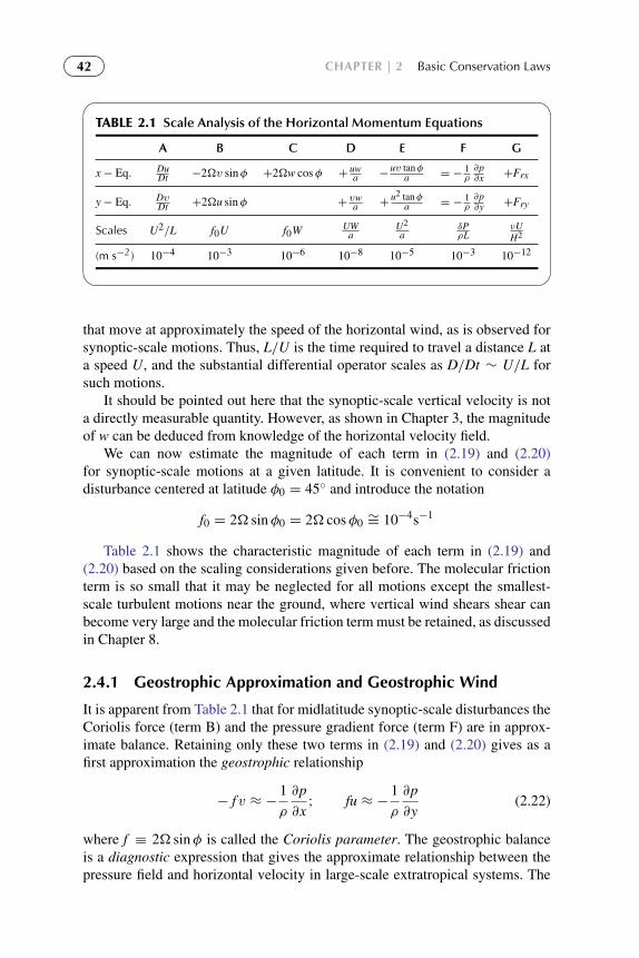
To protect the rights of the author(s) and publisher we inform you that this PDF is an uncorrected proof for internal businessuse only by the author(s), editor(s), reviewer(s), Elsevier and typesetter diacriTech. It is not allowed to publish this proofonline or in print. This proof copy is the copyright property of the publisher and is confidential until formal publication.
“Hakim: 06-ch02-031-066-9780123848666” — 2012/7/26 — 10:54 — page 42 — #12
42 CHAPTER | 2 Basic Conservation Laws
�
�
�
�
TABLE 2.1 Scale Analysis of the Horizontal Momentum Equations
A B C D E F G
x− Eq. DuDt −2�v sinφ +2�w cosφ +
uwa −
uv tanφa = −
1ρ∂p∂x +Frx
y− Eq. DvDt +2�u sinφ +
vwa +
u2 tanφa = −
1ρ∂p∂y +Fry
Scales U2/L f0U f0W UWa
U2
aδPρL
νUH2
(m s−2) 10−4 10−3 10−6 10−8 10−5 10−3 10−12
that move at approximately the speed of the horizontal wind, as is observed forsynoptic-scale motions. Thus, L/U is the time required to travel a distance L ata speed U, and the substantial differential operator scales as D/Dt ∼ U/L forsuch motions.
It should be pointed out here that the synoptic-scale vertical velocity is nota directly measurable quantity. However, as shown in Chapter 3, the magnitudeof w can be deduced from knowledge of the horizontal velocity field.
We can now estimate the magnitude of each term in (2.19) and (2.20)for synoptic-scale motions at a given latitude. It is convenient to consider adisturbance centered at latitude φ0 = 45◦ and introduce the notation
f0 = 2� sinφ0 = 2� cosφ0 ∼= 10−4s−1
Table 2.1 shows the characteristic magnitude of each term in (2.19) and(2.20) based on the scaling considerations given before. The molecular frictionterm is so small that it may be neglected for all motions except the smallest-scale turbulent motions near the ground, where vertical wind shears shear canbecome very large and the molecular friction term must be retained, as discussedin Chapter 8.
2.4.1 Geostrophic Approximation and Geostrophic Wind
It is apparent from Table 2.1 that for midlatitude synoptic-scale disturbances theCoriolis force (term B) and the pressure gradient force (term F) are in approx-imate balance. Retaining only these two terms in (2.19) and (2.20) gives as afirst approximation the geostrophic relationship
− f v ≈ −1
ρ
∂p
∂x; fu ≈ −
1
ρ
∂p
∂y(2.22)
where f ≡ 2� sinφ is called the Coriolis parameter. The geostrophic balanceis a diagnostic expression that gives the approximate relationship between thepressure field and horizontal velocity in large-scale extratropical systems. The

To protect the rights of the author(s) and publisher we inform you that this PDF is an uncorrected proof for internal businessuse only by the author(s), editor(s), reviewer(s), Elsevier and typesetter diacriTech. It is not allowed to publish this proofonline or in print. This proof copy is the copyright property of the publisher and is confidential until formal publication.
“Hakim: 06-ch02-031-066-9780123848666” — 2012/7/26 — 10:54 — page 43 — #13
2.4 | Scale Analysis of the Equations of Motion 43
approximation (2.22) contains no reference to time and therefore cannot beused to predict the evolution of the velocity field. It is for this reason that thegeostrophic relationship is called a diagnostic relationship.
By analogy to the geostrophic approximation (2.22), it is possible to definea horizontal velocity field, Vg ≡ iug + jvg, called the geostrophic wind, thatsatisfies (2.22) identically. In vectorial form,
Vg ≡ k×1
ρf∇p (2.23)
Thus, knowledge of the pressure distribution at any time determines the geo-strophic wind. It should be kept clearly in mind that (2.23) always defines thegeostrophic wind; however, only for large-scale motions away from the equatorshould the geostrophic wind be used as an approximation to the actual horizontalwind field. For the scales used in Table 2.1, the geostrophic wind approximatesthe true horizontal velocity to within 10 to 15% in midlatitudes.
2.4.2 Approximate Prognostic Equations: The Rossby Number
To obtain prediction equations, it is necessary to retain the acceleration (term A)in (2.19) and (2.20). The resulting approximate horizontal momentum equationsare
Du
Dt= f v −
1
ρ
∂p
∂x= f
(v − vg
)= f va (2.24)
Dv
Dt= −fu−
1
ρ
∂p
∂y= −f
(u− ug
)= −f ua (2.25)
where (2.23) is used to rewrite the pressure gradient force in terms of thegeostrophic wind. Because the acceleration terms in (2.24) and (2.25) are pro-portional to the difference between the actual wind and the geostrophic wind,they are about an order of magnitude smaller than the Coriolis force and thepressure gradient force, in agreement with our scale analysis. In the final equal-ities of (2.24) and (2.25) we define the difference between the actual wind andthe geostrophic wind as the ageostrophic wind.
The fact that the horizontal flow is in approximate geostrophic balance ishelpful for diagnostic analysis. However, it makes actual applications of theseequations in weather prognosis difficult because acceleration (which must bemeasured accurately) is given by the small difference between two large terms.Thus, a small error in measurement of either velocity or pressure gradientwill lead to very large errors in estimating the acceleration. This problem ofnumerical weather prediction is discussed in Chapter 13, and the problem ofsimplifying the equations for physical understanding based on the smallnessof the ageostrophic wind will be taken up in Chapter 6.
A convenient measure of the magnitude of the acceleration compared to theCoriolis force may be obtained by forming the ratio of the characteristic scales

To protect the rights of the author(s) and publisher we inform you that this PDF is an uncorrected proof for internal businessuse only by the author(s), editor(s), reviewer(s), Elsevier and typesetter diacriTech. It is not allowed to publish this proofonline or in print. This proof copy is the copyright property of the publisher and is confidential until formal publication.
“Hakim: 06-ch02-031-066-9780123848666” — 2012/7/26 — 10:54 — page 44 — #14
44 CHAPTER | 2 Basic Conservation Laws
for the acceleration and Coriolis force terms: (U2/L)/(f0U). This ratio is a nondi-mensional number called the Rossby number after the Swedish meteorologist C.G. Rossby (1898–1957) and is designated by
Ro ≡ U/( f0L)
Thus, the smallness of the Rossby number is a measure of the validity of the geo-strophic approximation.
2.4.3 The Hydrostatic Approximation
A similar scale analysis can be applied to the vertical component of themomentum equation (2.21). Because pressure decreases by about an order ofmagnitude from the ground to the tropopause, the vertical pressure gradientmay be scaled by P0/H, where P0 is the surface pressure and H is the depth ofthe troposphere. The terms in (2.21) may then be estimated for synoptic-scalemotions and are shown in Table 2.2. As with the horizontal componentequations, we consider motions centered at 45◦ latitude and neglect friction.The scaling indicates that to a high degree of accuracy the pressure field is inhydrostatic equilibrium; that is, the pressure at any point is simply equal to theweight of a unit cross-section column of air above that point.
The preceding analysis of the vertical momentum equation is, however,somewhat misleading. It is not sufficient to show merely that the vertical accel-eration is small compared to g. Because only that part of the pressure field thatvaries horizontally is directly coupled to the horizontal velocity field, it is actu-ally necessary to show that the horizontally varying pressure component is itselfin hydrostatic equilibrium with the horizontally varying density field. To showthis, it is convenient to first define a standard pressure p0(z), which is the hori-zontally averaged pressure at each height, and a corresponding standard densityρ0(z), defined so that p0(z) and ρ0(z) are in exact hydrostatic balance:
1
ρ0
dp0
dz≡ −g (2.26)
�
�
�
�
TABLE 2.2 Scale Analysis of the Vertical Momentum Equation
z− Eq. Dw/Dt −2�u cosφ −(u2+ v2)/a = −ρ−1∂p/∂z −g +Frz
Scales UW/L f0U U2/a P0/(ρH) g νWH−2
m s−2 10−7 10−3 10−5 10 10 10−15

To protect the rights of the author(s) and publisher we inform you that this PDF is an uncorrected proof for internal businessuse only by the author(s), editor(s), reviewer(s), Elsevier and typesetter diacriTech. It is not allowed to publish this proofonline or in print. This proof copy is the copyright property of the publisher and is confidential until formal publication.
“Hakim: 06-ch02-031-066-9780123848666” — 2012/7/26 — 10:54 — page 45 — #15
2.5 | The Continuity Equation 45
We may then write the total pressure and density fields as
p(x, y, z, t) = p0(z)+ p′(x, y, z, t)
ρ(x, y, z, t) = ρ0(z)+ ρ′(x, y, z, t)
(2.27)
where p′ and ρ′ are deviations from the standard values of pressure and density,respectively. For an atmosphere at rest, p′ and ρ′ would thus be zero. Using thedefinitions of (2.26) and (2.27) and assuming that ρ′/ρ0 is much less than unityin magnitude so that (ρ0 + ρ
′)−1 ∼= ρ−10 (1 –ρ′/ρ0), we find that
−1
ρ
∂p
∂z− g = −
1
(ρ0 + ρ′)
∂
∂z
(p0 + p′
)− g
≈1
ρ0
[ρ′
ρ0
dp0
dz−∂p′
∂z
]= −
1
ρ0
[ρ′g+
∂p′
∂z
] (2.28)
For synoptic-scale motions, the terms in (2.28) have the magnitudes
1
ρ0
∂p′
∂z∼[δP
ρ0H
]∼ 10−1m s–2,
ρ′g
ρ0∼ 10−1m s–2
Comparing these with the magnitudes of other terms in the vertical momen-tum equation (refer to Table 2.2), we see that to a very good approximation theperturbation pressure field is in hydrostatic equilibrium with the perturbationdensity field so that
∂p′
∂z+ ρ′g = 0 (2.29)
Therefore, for synoptic-scale motions, vertical accelerations are negligibleand the vertical velocity cannot be determined from the vertical momentumequation. However, we show in Chapter 3 that it is, nevertheless, possible todeduce the vertical motion field indirectly. Moreover, in Chapter 6 we showthat the vertical motion field may be estimated, and physically understood, fromknowledge of the pressure field alone.
2.5 THE CONTINUITY EQUATION
We turn now to the second of the three fundamental conservation principles:conservation of mass. The mathematical relationship that expresses conserva-tion of mass for a fluid is called the continuity equation. This section developsthe continuity equation using two alternative methods. The first method is basedon an Eulerian control volume, whereas the second is based on a Lagrangiancontrol volume.

To protect the rights of the author(s) and publisher we inform you that this PDF is an uncorrected proof for internal businessuse only by the author(s), editor(s), reviewer(s), Elsevier and typesetter diacriTech. It is not allowed to publish this proofonline or in print. This proof copy is the copyright property of the publisher and is confidential until formal publication.
“Hakim: 06-ch02-031-066-9780123848666” — 2012/7/26 — 10:54 — page 46 — #16
46 CHAPTER | 2 Basic Conservation Laws
x
δz
δx
δy
y
z
(x, y, z)
ρu − (ρu) δx2
ρu + (ρu)∂∂x
∂∂x
δx2
FIGURE 2.5 Mass inflow into a fixed (Eulerian) control volume as a result of motion parallel tothe x axis.
2.5.1 A Eulerian Derivation
We consider a volume element δxδyδz that is fixed in a Cartesian coordinateframe as shown in Figure 2.5. For such a fixed control volume, the net rateof mass inflow through the sides must equal the rate of accumulation of masswithin the volume. The rate of inflow of mass through the left face per unitarea is [
ρu−∂
∂x(ρu)
δx
2
]whereas the rate of outflow per unit area through the right face is[
ρu+∂
∂x(ρu)
δx
2
]Because the area of each of these faces is δyδz, the net rate of flow into thevolume due to the x velocity component is
[ρu−
∂
∂x(ρu)
δx
2
]δyδz−
[ρu+
∂
∂x(ρu)
δx
2
]δyδz = −
∂
∂x(ρu)δxδyδz

To protect the rights of the author(s) and publisher we inform you that this PDF is an uncorrected proof for internal businessuse only by the author(s), editor(s), reviewer(s), Elsevier and typesetter diacriTech. It is not allowed to publish this proofonline or in print. This proof copy is the copyright property of the publisher and is confidential until formal publication.
“Hakim: 06-ch02-031-066-9780123848666” — 2012/7/26 — 10:54 — page 47 — #17
2.5 | The Continuity Equation 47
Similar expressions obviously hold for the y and z directions. Thus, the net rateof mass inflow is
−
[∂
∂x(ρu)+
∂
∂y(ρv)+
∂
∂z(ρw)
]δxδyδz
and the mass inflow per unit volume is just −∇ · (ρU), which must equal therate of mass increase per unit volume. Now the increase of mass per unit volumeis just the local density change ∂ρ/∂t. Therefore,
∂ρ
∂t+∇ · (ρU) = 0 (2.30)
Equation (2.30) is the mass divergence form of the continuity equation.An alternative form of the continuity equation is obtained by applying the
vector identity
∇ · (ρU) ≡ ρ∇ ·U+ U ·∇ρ
and the relationship
D
Dt≡∂
∂t+ U ·∇
to get
1
ρ
Dρ
Dt+∇ ·U = 0 (2.31)
Equation (2.31) is the velocity divergence form of the continuity equation. Itstates that the fractional rate of increase of the density following the motion ofan air parcel is equal to minus the velocity divergence (i.e., convergence). Thisshould be clearly distinguished from (2.30), which states that the local rate ofchange of density is equal to minus the mass divergence.
2.5.2 A Lagrangian Derivation
The physical meaning of divergence can be illustrated by the following alter-native derivation of (2.31). Consider a control volume of fixed mass δM thatmoves with the fluid. Letting δV = δxδyδz be the volume, we find that becauseδM = ρδV = ρδxδyδz is conserved following the motion, we can write
1
δM
D
Dt(δM) =
1
ρδV
D
Dt(ρδV) =
1
ρ
Dρ
Dt+
1
δV
D
Dt(δV) = 0 (2.32)
but
1
δV
D
Dt(δV) =
1
δx
D
Dt(δx)+
1
δy
D
Dt(δy)+
1
δz
D
Dt(δz)

To protect the rights of the author(s) and publisher we inform you that this PDF is an uncorrected proof for internal businessuse only by the author(s), editor(s), reviewer(s), Elsevier and typesetter diacriTech. It is not allowed to publish this proofonline or in print. This proof copy is the copyright property of the publisher and is confidential until formal publication.
“Hakim: 06-ch02-031-066-9780123848666” — 2012/7/26 — 10:54 — page 48 — #18
48 CHAPTER | 2 Basic Conservation Laws
uA uB
uAδ t uBδ t
FIGURE 2.6 Change in Lagrangian control volume (shown by shading) as a result of fluid motionparallel to the x axis.
Referring to Figure 2.6, we see that the faces of the control volume in they, z plane (designated A and B) are advected with the flow in the x direction atspeeds uA = Dx/Dt and uB = D(x+ δx)/Dt, respectively. Thus, the differencein speeds of the two faces is δu = uB − uA = D(x + δx)/Dt − Dx/Dt orδu = D(δx)/Dt. Similarly, δv = D(δy)/Dt and δw = D(δz)/Dt. Therefore,
limδx,δy,δz→0
[1
δV
D
Dt(δV)
]=∂u
∂x+∂v
∂y+∂w
∂z= ∇ ·U
so that in the limit δV → 0, (2.32) reduces to the continuity equation (2.31);the divergence of the three-dimensional velocity field is equal to the fractionalrate of change of the volume of a fluid parcel in the limit δV → 0. It is left asa problem for the student to show that the divergence of the horizontal velocityfield is equal to the fractional rate of change of the horizontal area δA of a fluidparcel in the limit δA→ 0.
2.5.3 Scale Analysis of the Continuity Equation
Following the technique developed in Section 2.4.3, and again assuming that∣∣ρ′/ρ0∣∣� 1, we can approximate the continuity (2.31) as
1
ρ0
(∂ρ′
∂t+ U ·∇ρ′
)+
w
ρ0
dρ0
dz+∇ ·U ≈ 0
A B C(2.33)
where ρ′ designates the local deviation of density from its horizontally aver-aged value, ρ0 (z). For synoptic-scale motions, ρ′/ρ0 ∼ 10−2 so that, using thecharacteristic scales given in Section 2.4, we find that term A has magnitude
1
ρ0
(∂ρ′
∂t+ U ·∇ρ′
)∼ρ′
ρ0
U
L≈ 10−7s−1

To protect the rights of the author(s) and publisher we inform you that this PDF is an uncorrected proof for internal businessuse only by the author(s), editor(s), reviewer(s), Elsevier and typesetter diacriTech. It is not allowed to publish this proofonline or in print. This proof copy is the copyright property of the publisher and is confidential until formal publication.
“Hakim: 06-ch02-031-066-9780123848666” — 2012/7/26 — 10:54 — page 49 — #19
2.6 | The Continuity Equation 49
For motions in which the depth scale H is comparable to the density scale height,d ln ρ0/dz ∼ H−1, so that term B scales as
w
ρ0
dρ0
dzv
W
H≈ 10−6s−1
Expanding term C in Cartesian coordinates, we have
∇ ·U =∂u
∂x+∂v
∂y+∂w
∂z
For synoptic-scale motions, the terms ∂u/∂x and ∂v/∂y tend to be of equalmagnitude but opposite sign. Thus, they tend to balance so that(
∂u
∂x+∂v
∂y
)v 10−1 U
L≈ 10−6 s−1
In addition,
∂w
∂z∼
W
H≈ 10−6 s−1
Thus, terms B and C are each an order of magnitude greater than term A, and,to a first approximation, terms B and C balance in the continuity equation. To agood approximation, then
∂u
∂x+∂v
∂y+∂w
∂z+ w
d
dz(ln ρ0) = 0
or, alternatively, in vector form
∇ · (ρ0U) = 0 (2.34)
Thus, for synoptic-scale motions the mass flux computed using the basic statedensity ρ0 is nondivergent. This approximation is similar to the idealizationof incompressibility, which is often used in fluid mechanics. However, anincompressible fluid has a density constant following the motion
Dρ
Dt= 0
Thus, by (2.31) the velocity divergence vanishes (∇ ·U = 0) in an incompress-ible fluid, which is not the same as (2.34). Our approximation (2.34) shows thatfor purely horizontal flow the atmosphere behaves as though it were an incom-pressible fluid. However, when there is vertical motion, the compressibilityassociated with the height dependence of ρ0 must be taken into account.

To protect the rights of the author(s) and publisher we inform you that this PDF is an uncorrected proof for internal businessuse only by the author(s), editor(s), reviewer(s), Elsevier and typesetter diacriTech. It is not allowed to publish this proofonline or in print. This proof copy is the copyright property of the publisher and is confidential until formal publication.
“Hakim: 06-ch02-031-066-9780123848666” — 2012/7/26 — 10:54 — page 50 — #20
50 CHAPTER | 2 Basic Conservation Laws
2.6 THE THERMODYNAMIC ENERGY EQUATION
We now turn to the third fundamental conservation principle: the conservationof energy as applied to a moving fluid element. The first law of thermodynamicsis usually derived by considering a system in thermodynamic equilibrium—thatis, a system that is initially at rest and, after exchanging heat with its surround-ings and doing work on the surroundings, is again at rest. For such a systemthe first law states that the change in internal energy of the system is equal tothe difference between the heat added to the system and the work done by thesystem. A Lagrangian control volume consisting of a specified mass of fluidmay be regarded as a thermodynamic system. However, unless the fluid is atrest, it will not be in thermodynamic equilibrium. Nevertheless, the first law ofthermodynamics still applies.
To show that this is the case, we note that the total thermodynamic energyof the control volume is considered to consist of the sum of the internal energy(due to the kinetic energy of the individual molecules) and the kinetic energydue to the macroscopic motion of the fluid. The rate of change of this totalthermodynamic energy is equal to the rate of diabatic heating plus the rate atwhich work is done on the fluid parcel by external forces.
If we let e designate the internal energy per unit mass, then the total ther-modynamic energy contained in a Lagrangian fluid element of density ρ andvolume δV is ρ [e + (1/2)U · U] δV . The external forces that act on a fluidelement may be divided into surface forces, such as pressure and viscosity, andbody forces, such as gravity or the Coriolis force. The rate at which work isdone on the fluid element by the x component of the pressure force is illustratedin Figure 2.7. Recalling that pressure is a force per unit area and that the rate atwhich a force does work is given by the dot product of the force and velocity
x
δz
δx
δy
y
z
(pu)A (−pu)B
FIGURE 2.7 Rate of working on a fluid element due to the x component of the pressure force.

To protect the rights of the author(s) and publisher we inform you that this PDF is an uncorrected proof for internal businessuse only by the author(s), editor(s), reviewer(s), Elsevier and typesetter diacriTech. It is not allowed to publish this proofonline or in print. This proof copy is the copyright property of the publisher and is confidential until formal publication.
“Hakim: 06-ch02-031-066-9780123848666” — 2012/7/26 — 10:54 — page 51 — #21
2.6 | The Thermodynamic Energy Equation 51
vectors, we see that the rate at which the surrounding fluid does work on theelement due to the pressure force on the two boundary surfaces in the y, z planeis given by
(pu)Aδyδz− (pu)Bδyδz
(The negative sign is needed before the second term because the work done onthe fluid element is positive if u is negative across face B.) Now, by expandingin a Taylor series, we can write
(pu)B = (pu)A +
[∂
∂x(pu)
]Aδx+ · · ·
Thus, the net rate at which the pressure force does work due to the x componentof motion is [
(pu)A − (pu)B]δyδz = −
[∂
∂x(pu)
]AδV
where δV = δxδyδz.Similarly, we can show that the net rates at which the pressure force does
work due to the y and z components of motion are
−
[∂
∂y(pv)
]δV and −
[∂
∂z(pw)
]δV
respectively. Hence, the total rate at which work is done by the pressure force issimply
−∇ · (pU)δV
The only body forces of meteorological significance that act on an element ofmass in the atmosphere are the Coriolis force and gravity. However, because theCoriolis force, −2� × U, is perpendicular to the velocity vector, it can do nowork. Thus, the rate at which body forces do work on the mass element is justρg ·U δV .
Applying the principle of energy conservation to our Lagrangian controlvolume (neglecting effects of molecular viscosity), we thus obtain
D
Dt
[ρ
(e+
1
2U ·U
)δV
]= −∇ · (pU)δV + ρg ·UδV + ρJδV (2.35)
Here J is the rate of heating per unit mass due to radiation, conduction, and latentheat release. With the aid of the chain rule of differentiation, we can rewrite(2.35) as
ρδVD
Dt
(e+
1
2U ·U
)+
(e+
1
2U ·U
)D (ρδV)
Dt
= −U ·∇p δV − p∇ ·U δV − ρgw δV + ρJ δV
(2.36)

To protect the rights of the author(s) and publisher we inform you that this PDF is an uncorrected proof for internal businessuse only by the author(s), editor(s), reviewer(s), Elsevier and typesetter diacriTech. It is not allowed to publish this proofonline or in print. This proof copy is the copyright property of the publisher and is confidential until formal publication.
“Hakim: 06-ch02-031-066-9780123848666” — 2012/7/26 — 10:54 — page 52 — #22
52 CHAPTER | 2 Basic Conservation Laws
where we have used g = −gk. Now, from (2.32), the second term on the left in(2.36) vanishes so that
ρDe
Dt+ ρ
D
Dt
(1
2U ·U
)= −U ·∇p− p∇ ·U− ρgw+ ρJ (2.37)
This equation can be simplified by noting that if we take the dot product of Uwith the momentum equation (2.8), we obtain (neglecting friction)
ρD
Dt
(1
2U ·U
)= −U ·∇p− ρgw (2.38)
Subtracting (2.38) from (2.37), we obtain
ρDe
Dt= −p∇ ·U+ ρJ (2.39)
The terms in (2.37) that were eliminated by subtracting (2.38) represent the bal-ance of mechanical energy due to the motion of the fluid element; the remainingterms represent the thermal energy balance.
Using the definition of geopotential (1.11), we have
gw = gDz
Dt=
D8
Dt
so that (2.38) can be rewritten as
ρD
Dt
(1
2U ·U+8
)= −U ·∇p (2.40)
which is referred to as the mechanical energy equation. The sum of the kineticenergy plus the gravitational potential energy is called the mechanical energy.Thus, (2.40) states that following the motion, the rate of change of mechanicalenergy per unit volume equals the rate at which work is done by the pressuregradient force.
The thermal energy equation (2.39) can be written in more familiar form bynoting from (2.31) that
1
ρ∇ ·U = −
1
ρ2
Dρ
Dt=
Dα
Dt
and that for dry air the internal energy per unit mass is given by e = cvT , wherecv(= 717 J kg−1 K−1) is the specific heat at constant volume. We then obtain
cvDT
Dt+ p
Dα
Dt= J (2.41)
which is the usual form of the thermodynamic energy equation. Thus, the firstlaw of thermodynamics indeed is applicable to a fluid in motion. The secondterm on the left, representing the rate of working by the fluid system (per unit

To protect the rights of the author(s) and publisher we inform you that this PDF is an uncorrected proof for internal businessuse only by the author(s), editor(s), reviewer(s), Elsevier and typesetter diacriTech. It is not allowed to publish this proofonline or in print. This proof copy is the copyright property of the publisher and is confidential until formal publication.
“Hakim: 06-ch02-031-066-9780123848666” — 2012/7/26 — 10:54 — page 53 — #23
2.7 | Thermodynamics of the Dry Atmosphere 53
mass), represents a conversion between thermal and mechanical energy. Thisconversion process enables the solar heat energy to drive the motions of theatmosphere.
2.7 THERMODYNAMICS OF THE DRY ATMOSPHERE
Taking the total derivative of the equation of state (1.25), we obtain
pDα
Dt+ α
Dp
Dt= R
DT
Dt
Substituting for pDα/Dt in (2.41) and using cp = cv + R, where cp(= 1004 Jkg−1 K−1) is the specific heat at constant pressure, we can rewrite the first lawof thermodynamics as
cpDT
Dt− α
Dp
Dt= J (2.42)
Dividing through by T and again using the equation of state, we obtain theentropy form of the first law of thermodynamics:
cpD ln T
Dt− R
D ln p
Dt=
J
T≡
Ds
Dt(2.43)
Equation (2.43) gives the rate of change of entropy per unit mass following themotion for a thermodynamically reversible process. A reversible process is onein which a system changes its thermodynamic state and then returns to the orig-inal state without changing its surroundings. For such a process the entropy sdefined by (2.43) is a field variable that depends only on the state of the fluid.Thus, Ds is a perfect differential, and Ds/Dt is to be regarded as a total deriva-tive. However, “heat” is not a field variable, so the heating rate J is not a totalderivative.2
2.7.1 Potential Temperature
For an ideal gas that is undergoing an adiabatic process (i.e., a reversible pro-cess in which no heat is exchanged with the surroundings), the first law ofthermodynamics can be written in differential form as
cpD ln T − RD ln p = D(cp ln T − R ln p
)= 0
Integrating this expression from a state at pressure p and temperature T to a statein which the pressure is ps and the temperature is θ , we obtain, after taking theantilogarithm,
θ = T (ps/p)R/cp (2.44)
2For a discussion of entropy and its role in the second law of thermodynamics, see Curry andWebster (1999), for example.

To protect the rights of the author(s) and publisher we inform you that this PDF is an uncorrected proof for internal businessuse only by the author(s), editor(s), reviewer(s), Elsevier and typesetter diacriTech. It is not allowed to publish this proofonline or in print. This proof copy is the copyright property of the publisher and is confidential until formal publication.
“Hakim: 06-ch02-031-066-9780123848666” — 2012/7/26 — 10:54 — page 54 — #24
54 CHAPTER | 2 Basic Conservation Laws
This relationship in (2.44) is referred to as Poisson’s equation, and the tem-perature θ defined by (2.44) is called the potential temperature. θ is simplythe temperature that a parcel of dry air at pressure p and temperature T wouldhave if it were expanded or compressed adiabatically to a standard pressureps (usually taken to be 1000 hPa). Thus, every air parcel has a unique valueof potential temperature, and this value is conserved for dry adiabatic motion.Because synoptic-scale motions are approximately adiabatic outside regions ofactive precipitation, θ is a quasi-conserved quantity for such motions.
Taking the logarithm of (2.44) and differentiating, we find that
cpD ln θ
Dt= cp
D ln T
Dt− R
D ln p
Dt(2.45)
Comparing (2.43) and (2.45), we obtain
cpD ln θ
Dt=
J
T=
Ds
Dt(2.46)
Thus, for reversible processes, changes in fractional potential temperature areindeed proportional to entropy changes. A parcel that conserves entropy fol-lowing the motion must move along an isentropic (constant θ ) surface.
2.7.2 The Adiabatic Lapse Rate
A relationship between the lapse rate of temperature (i.e., the rate of decreaseof temperature with respect to height) and the rate of change of potential tem-perature with respect to height can be obtained by taking the logarithm of (2.44)and differentiating with respect to height. Using the hydrostatic equation andthe ideal gas law to simplify the result gives
T
θ
∂θ
∂z=∂T
∂z+
g
cp(2.47)
For an atmosphere in which the potential temperature is constant with respectto height, the lapse rate is thus
−dT
dz=
g
cp≡ 0d (2.48)
Thus, the dry adiabatic lapse rate is approximately constant throughout thelower atmosphere.
2.7.3 Static Stability
If potential temperature is a function of height, the atmospheric lapse rate, 0 ≡−∂T/∂z, will differ from the adiabatic lapse rate and
T
θ
∂θ
∂z= 0d − 0 (2.49)

To protect the rights of the author(s) and publisher we inform you that this PDF is an uncorrected proof for internal businessuse only by the author(s), editor(s), reviewer(s), Elsevier and typesetter diacriTech. It is not allowed to publish this proofonline or in print. This proof copy is the copyright property of the publisher and is confidential until formal publication.
“Hakim: 06-ch02-031-066-9780123848666” — 2012/7/26 — 10:54 — page 55 — #25
2.7 | Thermodynamics of the Dry Atmosphere 55
If 0 < 0d so that θ increases with height, an air parcel that undergoes an adi-abatic displacement from its equilibrium level will be positively buoyant whendisplaced downward and negatively buoyant when displaced upward, so thatit will tend to return to its equilibrium level and the atmosphere is said to bestatically stable or stably stratified.
Adiabatic oscillations of a fluid parcel about its equilibrium level in a stablystratified atmosphere are referred to as buoyancy oscillations. The characteristicfrequency of such oscillations can be derived by considering a parcel that isdisplaced vertically a small distance δz without disturbing its environment. If theenvironment is in hydrostatic balance, ρ0g = −dp0/dz, where p0 and ρ0 are thepressure and density of the environment, respectively. The vertical accelerationof the parcel is
Dw
Dt=
D2
Dt2(δz) = −g−
1
ρ
∂p
∂z(2.50)
where p and ρ are the pressure and density of the parcel, respectively. In the par-cel method it is assumed that the pressure of the parcel adjusts instantaneouslyto the environmental pressure during the displacement: p = p0. This conditionmust be true if the parcel is to leave the environment undisturbed. Thus, with theaid of the hydrostatic relationship, pressure can be eliminated in (2.50) to give
D2
Dt2(δz) = g
(ρ0 − ρ
ρ
)= g
θ
θ0(2.51)
where (2.44) and the ideal gas law have been used to express the buoyancyforce in terms of potential temperature. Here θ designates the deviation of thepotential temperature of the parcel from its basic state (environmental) valueθ0(z). If the parcel is initially at level z = 0 where the potential temperatureis θ0(0), then for a small displacement δz, we can represent the environmentalpotential temperature as
θ0(δz) ≈ θ0(0)+ (dθ0/dz) δz
If the parcel displacement is adiabatic, the potential temperature of the parcel isconserved. Thus, θ(δz) = θ0(0)− θ0(δz) = −(dθ0/dz)δz, and (2.51) becomes
D2
Dt2(δz) = −N2δz (2.52)
where
N2= g
d ln θ0
dz
is a measure of the static stability of the environment. Equation (2.52) has ageneral solution of the form δz = A exp(iNt). Therefore, if N2 > 0, the parcelwill oscillate about its initial level with a period τ = 2π/N. The corresponding

To protect the rights of the author(s) and publisher we inform you that this PDF is an uncorrected proof for internal businessuse only by the author(s), editor(s), reviewer(s), Elsevier and typesetter diacriTech. It is not allowed to publish this proofonline or in print. This proof copy is the copyright property of the publisher and is confidential until formal publication.
“Hakim: 06-ch02-031-066-9780123848666” — 2012/7/26 — 10:54 — page 56 — #26
56 CHAPTER | 2 Basic Conservation Laws
frequency N is the buoyancy frequency.3 For average tropospheric conditions,N ≈ 1.2× 10⁻² s−1 so that the period of a buoyancy oscillation is about 8 min.
In the case of N = 0, examination of (2.52) indicates that no acceleratingforce will exist and the parcel will be in neutral equilibrium at its new level.However, if N2 < 0 (potential temperature decreasing with height), the dis-placement will increase exponentially with time. We thus arrive at the familiargravitational or static stability criteria for dry air:
dθ0/dz > 0 statically stable
dθ0/dz = 0 statically neutral
dθ0/dz < 0 statically unstable
On the synoptic-scale the atmosphere is always stably stratified because anyunstable regions that develop are stabilized quickly by convective overturning.
2.7.4 Scale Analysis of the Thermodynamic Energy Equation
If potential temperature is divided into a basic state θ0(z) and a deviationθ (x, y, z, t) so that the total potential temperature at any point is given byθtot = θ0 (z) + θ (x, y, z, t), the first law of thermodynamics (2.46) can bewritten approximately for synoptic scaling as
1
θ0
(∂θ
∂t+ u
∂θ
∂x+ v
∂θ
∂y
)+ w
d ln θ0
dz=
J
cpT(2.53)
where we have used the facts that for |θ/θ0| � 1, |dθ/dz| � dθ0/dz, and
ln θtot = ln [θ0 (1+ θ/θ0)] ≈ ln θ0 + θ/θ0
Outside regions of active precipitation, diabatic heating is due primarily to netradiative heating. In the troposphere, radiative heating is quite weak so thattypically J/cp ≤ 1◦C d−1 (except near cloud tops, where substantially largercooling can occur due to thermal emission by the cloud particles). The typi-cal amplitude of horizontal potential temperature fluctuations in a midlatitudesynoptic system (above the boundary layer) is θ ∼ 4◦C. Thus,
T
θ0
(∂θ
∂t+ u
∂θ
∂x+ v
∂θ
∂y
)∼θU
L∼ 4◦C d–1
The cooling due to vertical advection of the basic state potential temperature(usually called adiabatic cooling) has a typical magnitude of
w
(T
θ0
dθ0
dz
)= w (0d − 0) ∼ 4◦C d–1
3N is often referred to as the Brunt–Vaisala frequency.

To protect the rights of the author(s) and publisher we inform you that this PDF is an uncorrected proof for internal businessuse only by the author(s), editor(s), reviewer(s), Elsevier and typesetter diacriTech. It is not allowed to publish this proofonline or in print. This proof copy is the copyright property of the publisher and is confidential until formal publication.
“Hakim: 06-ch02-031-066-9780123848666” — 2012/7/26 — 10:54 — page 57 — #27
2.8 | The Boussinesq Approximation 57
where w ∼ 1 cm s−1, and 0d − 0, the difference between dry adiabatic andactual lapse rates, is ∼ 4◦ C km−1.
Thus, in the absence of strong diabatic heating, the rate of change in the per-turbation potential temperature is equal to the adiabatic heating or cooling dueto vertical motion in the statically stable basic state, and (2.54) can be approx-imated as (
∂θ
∂t+ u
∂θ
∂x+ v
∂θ
∂y
)+ w
dθ0
dz≈ 0 (2.54)
Alternatively, if the temperature field is divided into a basic state T0 (z) and adeviation T (x, y, z, t), then, since θ/θ0 ≈ T/T0, (2.54) can be expressed to thesame order of approximation in terms of temperature as(
∂T
∂t+ u
∂T
∂x+ v
∂T
∂y
)+ w (0d − 0) ≈ 0 (2.55)
2.8 THE BOUSSINESQ APPROXIMATION
In some situations, air parcel vertical displacements are relatively small, so thedensity change following the motion is also small. The Boussinesq approxima-tion yields a simplified form of the dynamical equations that are appropriateto this situation. In this approximation, density is replaced by a constant meanvalue, ρ0, everywhere except in the buoyancy term in the vertical momentumequation. The horizontal momentum equations (2.24) and (2.25) can then beexpressed in Cartesian coordinates as
Du
Dt= −
1
ρ0
∂p
∂x+ f v + Frx (2.56)
and
Dv
Dt= −
1
ρ0
∂p
∂y− fu+ Fry (2.57)
while, with the aid of equations (2.28) and (2.51), the vertical momentumequation becomes
Dw
Dt= −
1
ρ0
∂p
∂z+ g
θ
θ0+ Frz (2.58)
Here, as in Section 2.7.3 θ designates the perturbation departure of potentialtemperature from its basic state value θ0(z). Thus, the total potential temperaturefield is given by θtot = θ(x, y, z, t) + θ0(z), and the adiabatic thermodynamic

To protect the rights of the author(s) and publisher we inform you that this PDF is an uncorrected proof for internal businessuse only by the author(s), editor(s), reviewer(s), Elsevier and typesetter diacriTech. It is not allowed to publish this proofonline or in print. This proof copy is the copyright property of the publisher and is confidential until formal publication.
“Hakim: 06-ch02-031-066-9780123848666” — 2012/7/26 — 10:54 — page 58 — #28
58 CHAPTER | 2 Basic Conservation Laws
energy equation has a form similar to (2.54),
Dθ
Dt= −w
dθ0
dz(2.59)
except, from the full material derivative, we see that the vertical advection ofperturbation potential temperature is formally included. Finally, the continuityequation (2.34) under the Boussinesq approximation is
∂u
∂x+∂v
∂y+∂w
∂z= 0 (2.60)
2.9 THERMODYNAMICS OF THE MOIST ATMOSPHERE
Although it is convenient as a first approximation to neglect the role of watervapor in atmospheric dynamics, it sometimes plays an important, if not essen-tial, role. Most often it is the change in phase of water, and the accompanyinglatent heat release, that affects the dynamics, but even just the presence of watervapor can be critical to the buoyancy acceleration. Water vapor is a highly vari-able constituent in the atmosphere and as such presents a challenge to the idealgas law, since the gas constant depends on the molecular composition of air. Fordry air the ideal gas law is
pd = ρdRdT (2.61)
where pd and ρd are the dry air pressure and density, respectively, and Rd is thedry air gas constant. For pure water vapor, the ideal gas law is
e = ρvRvT (2.62)
where e and ρv are the vapor pressure and density, respectively, and Rv is thewater vapor gas constant. For moist air (a mixture of dry air and water vapor)we choose
p = ρRdTv (2.63)
where p and ρ are the pressure and density, respectively, and Tv is the virtualtemperature, which represents the temperature dry air needs to have the samepressure and density as moist air. This formulation allows use of the dry airgas constant everywhere. By adding (2.61) and (2.62), it can be shown that thevirtual temperature is given by
Tv =T
1− ep
(1− Rd
Rv
) (2.64)

To protect the rights of the author(s) and publisher we inform you that this PDF is an uncorrected proof for internal businessuse only by the author(s), editor(s), reviewer(s), Elsevier and typesetter diacriTech. It is not allowed to publish this proofonline or in print. This proof copy is the copyright property of the publisher and is confidential until formal publication.
“Hakim: 06-ch02-031-066-9780123848666” — 2012/7/26 — 10:54 — page 59 — #29
2.9 | Thermodynamics of the Moist Atmosphere 59
We see that Tv ≥ T , and the difference is typically on the order of a few degreesCelsius or less; nevertheless, even these small changes can make the differencebetween an air parcel being stable or unstable.
There are many measures of water vapor in the atmosphere, and we sum-marize here some of the most common. A measure used earlier in the ideal gaslaw is the vapor pressure that by Dalton’s Law is simply the contribution to thetotal pressure from water vapor. Saturation vapor pressure is determined solelyby temperature as given by the Clausius–Clapeyron equation4
1
es
des
dT=
L
RvT2(2.65)
For water vapor over a plane surface of liquid water (ice), L represents the latentheat of condensation (sublimation). Saturation vapor pressure depends approx-imately exponentially on temperature and, for temperatures below freezing, islarger above water surfaces than ice. Relative humidity may be defined as thepercentage
RH = 100×e
es(2.66)
and es may apply to either water or ice saturation; if unspecified, the former maybe assumed with confidence.
The water vapor mixing ratio is given by the ratio of the mass of water vaporto the mass of dry air in a volume of air, which takes units of either kg/kg or,more commonly, g/kg. From (2.61) and (2.62), the mixing ratio is given by
q = 0.622e
p− e(2.67)
where the leading coefficient 0.622 reflects the ratio of the molecular weight ofwater vapor to dry air.
There are several ways to bring moist air to saturation, one of which is bycooling the air at constant pressure without addition or removal of water vapor.Saturation achieved in this manner gives the dew point temperature.
2.9.1 Equivalent Potential Temperature
We previously applied the parcel method to discuss the vertical stability of a dryatmosphere. We found that the stability of a dry parcel with respect to a verticaldisplacement depends on the lapse rate of potential temperature in the environ-ment such that a parcel displacement is stable, provided that ∂θ/∂z > 0 (i.e.,the actual lapse rate is less than the adiabatic lapse rate). The same conditionalso applies to parcels in a moist atmosphere when the relative humidity is lessthan 100%. If, however, a parcel of moist air is forced to rise, it will eventually
4For a derivation see, for example, Curry and Webster (1999, p. 108).

To protect the rights of the author(s) and publisher we inform you that this PDF is an uncorrected proof for internal businessuse only by the author(s), editor(s), reviewer(s), Elsevier and typesetter diacriTech. It is not allowed to publish this proofonline or in print. This proof copy is the copyright property of the publisher and is confidential until formal publication.
“Hakim: 06-ch02-031-066-9780123848666” — 2012/7/26 — 10:54 — page 60 — #30
60 CHAPTER | 2 Basic Conservation Laws
become saturated at a level called the lifting condensation level (LCL). A furtherforced rise will then cause condensation and latent heat release, and the parcelwill then cool at the saturated adiabatic lapse rate. If the environmental lapserate is greater than the saturated adiabatic lapse rate, and the parcel is forcedto continue to rise, it will reach a level at which it becomes buoyant relative toits surroundings. It can then freely accelerate upward. The level at which thisoccurs is called the level of free convection (LFC).
Discussion of parcel dynamics in a moist atmosphere is facilitated bydefining a thermodynamic field called the equivalent potential temperature.Equivalent potential temperature, designated θe, is the potential temperature thata parcel of air would have if all its moisture were condensed and the resultantlatent heat used to warm the parcel. The temperature of an air parcel can bebrought to its equivalent potential value by raising the parcel from its originallevel until all the water vapor in the parcel has condensed and fallen out, andthen compressing the parcel adiabatically to a pressure of 1000 hPa. Becausethe condensed water is assumed to fall out, the temperature increase during thecompression will be at the dry adiabatic rate and the parcel will arrive back atits original level with a temperature that is higher than its original temperature.Thus, the process is irreversible. Ascent of this type, in which all condensationproducts are assumed to fall out, is called pseudoadiabatic ascent. (It is not atruly adiabatic process because the liquid water that falls out carries a smallamount of heat with it.)
A complete derivation of the mathematical expression relating θe to the othervariables of state is rather involved and will be relegated to Appendix D. Formost purposes, however, it is sufficient to use an approximate expression forθe that can be immediately derived from the entropy form of the first law ofthermodynamics (2.46). If we let qs denote the mass of water vapor per unitmass of dry air in a saturated parcel (the saturation mixing ratio), then the rateof diabatic heating per unit mass is
J = −LcDqs
Dt
where Lc is the latent heat of condensation. Therefore, from the first law ofthermodynamics
cpD ln θ
Dt= −
Lc
T
Dqs
Dt(2.68)
For a saturated parcel undergoing pseudoadiabatic ascent, the rate of changein qs following the motion is much larger than the rate of change in T or Lc.Therefore,
d ln θ ≈ −d(Lcqs/cpT
)(2.69)

To protect the rights of the author(s) and publisher we inform you that this PDF is an uncorrected proof for internal businessuse only by the author(s), editor(s), reviewer(s), Elsevier and typesetter diacriTech. It is not allowed to publish this proofonline or in print. This proof copy is the copyright property of the publisher and is confidential until formal publication.
“Hakim: 06-ch02-031-066-9780123848666” — 2012/7/26 — 10:54 — page 61 — #31
2.9 | Thermodynamics of the Moist Atmosphere 61
Integrating (2.69) from the initial state (θ, qs,T) to a state where qs ≈ 0, weobtain
ln (θ/θe) ≈ −Lcqs/cpT
where θe, the potential temperature in the final state, is approximately the equiv-alent potential temperature defined earlier. Thus, θe, for a saturated parcel isgiven by
θe ≈ θ exp(Lcqs/cpT
)(2.70)
The expression in (2.70) may also be used to compute θe for an unsaturatedparcel provided that the temperature used in the formula is the temperature thatthe parcel would have if expanded adiabatically to saturation (i.e., TLCL) and thesaturation mixing ratio were replaced by the actual mixing ratio of the initialstate. Thus, equivalent potential temperature is conserved for a parcel duringboth dry adiabatic and pseudoadiabatic displacements.
An alternative to θe, which is sometimes used in studies of convection, is themoist static energy, defined as h ≡ s+Lcq, where s ≡ cpT + gz is the dry staticenergy. It can be shown (Problem 2.10) that
cpTd ln θe ≈ dh (2.71)
Thus, moist static energy is approximately conserved when θe is conserved.
2.9.2 The Pseudoadiabatic Lapse Rate
The first law of thermodynamics (2.68) can be used to derive a formula forthe rate of change in temperature with respect to height for a saturated parcelundergoing pseudoadiabatic ascent. Using the definition of θ (2.44), we canrewrite (2.68) for vertical ascent as
d ln T
dz−
R
cp
d ln p
dz= −
Lc
cpT
dqs
dz
which, upon noting that qs ≡ qs (T, p) and applying the hydrostatic equationand equation of state, can be expressed as
dT
dz+
g
cp= −
Lc
cp
[(∂qs
∂T
)p
dT
dz−
(∂qs
∂p
)Tρg
]
Thus, as shown in detail in Appendix D, following the ascending saturatedparcel
0s ≡ −dT
dz= 0d
[1+ Lcqs/ (RT)][1+ εL2
cqs/(cpRT2
)] (2.72)

To protect the rights of the author(s) and publisher we inform you that this PDF is an uncorrected proof for internal businessuse only by the author(s), editor(s), reviewer(s), Elsevier and typesetter diacriTech. It is not allowed to publish this proofonline or in print. This proof copy is the copyright property of the publisher and is confidential until formal publication.
“Hakim: 06-ch02-031-066-9780123848666” — 2012/7/26 — 10:54 — page 62 — #32
62 CHAPTER | 2 Basic Conservation Laws
where ε = 0.622 is the ratio of the molecular weight of water to that of dry air,0d ≡ g/cp is the dry adiabatic lapse rate, and 0s is the pseudoadiabatic lapserate, which is always less than 0d. Observed values of 0s range from ∼4 Kkm−1 in warm, humid air masses in the lower troposphere to ∼6–7 K km−1 inthe midtroposphere.
2.9.3 Conditional Instability
Section 2.7.3 showed that for dry adiabatic motions the atmosphere is staticallystable provided that the lapse rate is less than the dry adiabatic lapse rate (i.e., thepotential temperature increases with height). If the lapse rate 0 lies between dryadiabatic and pseudoadiabatic values (0s < 0 < 0d), the atmosphere is stablystratified with respect to dry adiabatic displacements but unstable with respectto pseudoadiabatic displacements. Such a situation is referred to as conditionalinstability (i.e., the instability is conditional to saturation of the air parcel).
The conditional stability criterion can also be expressed in terms of the gra-dient of a field variable θ∗e , defined as the equivalent potential temperature of ahypothetically saturated atmosphere that has the thermal structure of the actualatmosphere.5 Thus,
d ln θ∗e = d ln θ + d(Lcqs/cpT
)(2.73)
where T is the actual temperature, not the temperature after adiabatic expansionto saturation as in (2.70). To derive an expression for conditional instability,we consider the motion of a saturated parcel in an environment in which thepotential temperature is θ0 at the level z0. At the level z0 − δz the undisturbedenvironmental air thus has potential temperature
θ0 − (∂θ/∂z) δz
Suppose that a saturated parcel that has the environmental potential temperatureat z0 − δz is raised to the level z0. When it arrives at z0, the parcel will have thepotential temperature
θ1 =
(θ0 −
∂θ
∂zδz
)+ δθ
where δθ is the change in parcel potential temperature due to condensation dur-ing ascent through vertical distance δz. Assuming a pseudoadiabatic ascent, wesee from (2.69) that
δθ
θ≈ −δ
(Lcqs
cpT
)≈ −
∂
∂z
(Lcqs
cpT
)δz
5Note that θ∗e is not the same as θe except in a saturated atmosphere.

To protect the rights of the author(s) and publisher we inform you that this PDF is an uncorrected proof for internal businessuse only by the author(s), editor(s), reviewer(s), Elsevier and typesetter diacriTech. It is not allowed to publish this proofonline or in print. This proof copy is the copyright property of the publisher and is confidential until formal publication.
“Hakim: 06-ch02-031-066-9780123848666” — 2012/7/26 — 10:54 — page 63 — #33
2.9 | Thermodynamics of the Moist Atmosphere 63
so that the buoyancy of the parcel when it arrives at z0 is proportional to
(θ1 − θ0)
θ0≈ −
[1
θ
∂θ
∂z+∂
∂z
(Lcqs
cpT
)]δz ≈ −
∂ ln θ∗e∂z
δz
where the last expression arises from the application of (2.73).The saturated parcel will be warmer than its environment at z0 provided that
θ1 > θ0. Thus, the conditional stability criterion for a saturated parcel is
∂θ∗e
∂z
< 0 conditionally unstable
= 0 saturated neutral
> 0 conditionally stable
(2.74)
In Figure 2.8 the vertical profiles of θ , θe, and θ∗e for a typical soundingin the vicinity of an extratropical thunderstorm are shown. It is obvious from
LFC
θ
θe
θ e∗
320 340 360 380 400
Temperature (K)
Pre
ssur
e (h
Pa)
200
400
300
500
600
700
800
900
1000
FIGURE 2.8 Schematic sounding for a conditionally unstable environment, characteristic ofmidwestern North American thunderstorm conditions, showing the vertical profiles of potentialtemperature θ , equivalent potential temperature θe, and equivalent temperature θ∗e of a hypothet-ically saturated atmosphere with the same temperature profile. The dotted line shows θe for anonentraining parcel raised from the surface. The arrow denotes the LFC for the parcel.

To protect the rights of the author(s) and publisher we inform you that this PDF is an uncorrected proof for internal businessuse only by the author(s), editor(s), reviewer(s), Elsevier and typesetter diacriTech. It is not allowed to publish this proofonline or in print. This proof copy is the copyright property of the publisher and is confidential until formal publication.
“Hakim: 06-ch02-031-066-9780123848666” — 2012/7/26 — 10:54 — page 64 — #34
64 CHAPTER | 2 Basic Conservation Laws
this figure that the sounding is conditionally unstable in the lower troposphere.However, this observed profile does not imply that convective overturning willoccur spontaneously. The release of conditional instability requires not onlythat ∂θ∗e /∂z < 0, but also parcel saturation at the environmental tempera-ture of the level where the convection begins (i.e., the parcel must reach theLFC). The mean relative humidity in the troposphere is well below 100%, evenin the boundary layer. Thus, low-level convergence with resultant forced layerascent or vigorous vertical turbulent mixing in the boundary layer is required toproduce saturation.
The amount of ascent necessary to raise a parcel to its LFC can be esti-mated simply from Figure 2.8. A parcel rising pseudoadiabatically from a levelz0−δz will conserve the value of θe characteristic of the environment at z0−δz.However, the buoyancy of a parcel depends only on the difference in densitybetween the parcel and its environment. Thus, in order to compute the buoyancyof the parcel at z0, it is not correct simply to compare θe of the environmentat z0 to θe(z0 − δz) because if the environment is unsaturated, the differencein θe between the parcel and the environment may be due primarily to thedifference in mixing ratios, not to any temperature (density) difference. To esti-mate the buoyancy of the parcel, θe(z0 − δz) should instead be compared toθ∗e (z0), which is the equivalent potential temperature that the environment atz0 would have if it were isothermally brought to saturation. The parcel willthus become buoyant when raised to the level z0 if θe(z0 − δz) > θ∗e (z0), forthen the parcel temperature will exceed the temperature of the environmentat z0.
From Figure 2.8, we see that θe for a parcel raised from about 960 hPa willintersect the θ∗e curve near 850 hPa, whereas a parcel raised from any level muchabove 850 hPa will not intersect θ∗e no matter how far it is forced to ascend. It isfor this reason that low-level convergence is usually required to initiate convec-tive overturning over the oceans. Only air near the surface has a sufficiently highvalue of θe to become buoyant when it is forcibly raised. Convection over con-tinental regions, however, can be initiated without significant boundary layerconvergence, as strong surface heating can produce positive parcel buoyancyall the way to the surface. Sustained deep convection, however, requires meanlow-level moisture convergence.
SUGGESTED REFERENCES
Curry and Webster’s Thermodynamics of Atmospheres and Oceans contains an excellent treatmentof atmospheric thermodynamics.
Pedlosky, Geophysical Fluid Dynamics, discusses the equations of motion for a rotating coordinatesystem and has a thorough discussion of scale analysis at a graduate level.
Salby’s Fundamentals of Atmospheric Physics contains a thorough development of the basicconservation laws at the graduate level.

To protect the rights of the author(s) and publisher we inform you that this PDF is an uncorrected proof for internal businessuse only by the author(s), editor(s), reviewer(s), Elsevier and typesetter diacriTech. It is not allowed to publish this proofonline or in print. This proof copy is the copyright property of the publisher and is confidential until formal publication.
“Hakim: 06-ch02-031-066-9780123848666” — 2012/7/26 — 10:54 — page 65 — #35
Problems 65
PROBLEMS
2.1. A ship is steaming northward at a rate of 10 km h−1.The surface pressureincreases toward the northwest at the rate of 5 Pa km−1. What is the pres-sure tendency recorded at a nearby island station if the pressure aboard theship decreases at a rate of 100 Pa/3 h?
2.2. The temperature at a point 50 km north of a station is 3◦C cooler than atthe station. If the wind is blowing from the northeast at 20 m s−1 and theair is being heated by radiation at the rate of 1◦C h−1, what is the localtemperature change at the station?
2.3. Derive the relationship
�× (�× r) = −�2R
which was used in Eq. (2.7).2.4. Derive the expression given in Eq. (2.13) for the rate of change of k
following the motion.2.5. Suppose a 1-kg parcel of dry air is rising at a constant vertical velocity. If
the parcel is being heated by radiation at the rate of 10−1W kg−1, whatmust the speed of rise be to maintain the parcel at a constant temperature?
2.6. Derive an expression for the density ρ that results when an air parcelinitially at pressure ps and density ρs expands adiabatically to pressure p.
2.7. An air parcel that has a temperature of 20◦C at the 1000-hPa level is lifteddry adiabatically. What is its density when it reaches the 500-hPa level?
2.8. Suppose an air parcel starts from rest at the 800-hPa level and rises verti-cally to 500 hPa while maintaining a constant 1◦C temperature excess overthe environment. Assuming that the mean temperature of the 800- to 500-hPa layer is 260 K, compute the energy released due to the work of thebuoyancy force. Assuming that all the released energy is realized as kineticenergy of the parcel, what will the vertical velocity of the parcel be at 500hPa?
2.9. Show that for an atmosphere with an adiabatic lapse rate (i.e., constantpotential temperature) the geopotential height is given by
Z = Hθ[1− (p/p0)
R/cp]
where p0 is the pressure at Z = 0 and Hθ ≡ cp θ/g0 is the total geopotentialheight of the atmosphere.
2.10. The azimuthal velocity component in some hurricanes is observed to havea radial dependence given by vλ = V0(r0/r)2 for distances from the centergiven by r ≥ r0. Letting V0 = 50 m s−1 and r0 = 50 km, find the totalgeopotential difference between the far field (r→∞) and r = r0, assuminggradient wind balance and f0 = 5 × 10⁻⁵ s−1. At what distance from thecenter does the Coriolis force equal the centrifugal force?
2.11. In the isentropic coordinate system (see Section 4.6), potential temperatureis used as the vertical coordinate. Because potential temperature in adi-abatic flow is conserved following the motion, isentropic coordinates areuseful for tracing the actual paths of travel of individual air parcels. Show

To protect the rights of the author(s) and publisher we inform you that this PDF is an uncorrected proof for internal businessuse only by the author(s), editor(s), reviewer(s), Elsevier and typesetter diacriTech. It is not allowed to publish this proofonline or in print. This proof copy is the copyright property of the publisher and is confidential until formal publication.
“Hakim: 06-ch02-031-066-9780123848666” — 2012/7/26 — 10:54 — page 66 — #36
66 CHAPTER | 2 Basic Conservation Laws
that the transformation of the horizontal pressure gradient force from z to θcoordinates is given by
1
ρ∇zp = ∇θM
where M ≡ cp T + 8 is the Montgomery streamfunction.2.12. French scientists have developed a high-altitude balloon that remains at
constant potential temperature as it circles Earth. Suppose such a balloon isin the lower equatorial stratosphere where the temperature is isothermal at200 K. If the balloon were displaced vertically from its equilibrium level bya small distance δz, it would tend to oscillate about the equilibrium level.What would be the period of this oscillation?
2.13. Derive the approximate thermodynamic energy equation (2.55) using thescaling arguments of Sections 2.4 and 2.7.
MATLAB ExercisesM2.1. The MATLAB script standard T p.m defines and plots the temperature and
the lapse rate associated with the U.S. Standard Atmosphere as functions ofheight. Modify this script to compute the pressure and potential tempera-ture, and plot these in the same format used for temperature and lapse rate.[Hint: To compute pressure, integrate the hydrostatic equation from the sur-face upward in increments of δz.] Show that if we define a mean scale heightfor the layer between z and z + δz by letting H = R [T (z)+ T (z+ δz)]/(2g),then p (z+ δz) = p (z) exp [−δz/H]. (Note that as you move upward layer bylayer, you must use the local height-dependent value of H in this formula.)
M2.2. The MATLAB script thermo profile.m is a simple script to read in data givingpressure and temperature for a tropical mean sounding. Run this script toplot temperature versus pressure for data in the file tropical temp.dat. Usethe hypsometric equation to compute the geopotential height correspondingto each pressure level of the data file. Compute the corresponding potentialtemperature and plot graphs of the temperature and potential temperaturevariations with pressure and with geopotential height.

To protect the rights of the author(s) and publisher we inform you that this PDF is an uncorrected proof for internal businessuse only by the author(s), editor(s), reviewer(s), Elsevier and typesetter diacriTech. It is not allowed to publish this proofonline or in print. This proof copy is the copyright property of the publisher and is confidential until formal publication.
“Hakim: 07-ch03-067-094-9780123848666” — 2012/7/26 — 11:01 — page 67 — #1
Chapter 3
Elementary Applicationsof the Basic Equations
In addition to the geostrophic wind, which was discussed in Chapter 2, there areother approximate expressions for the relationships among velocity, pressure,and temperature fields that are useful in the analysis of weather systems. Weconsider estimates of the wind that derive from fundamental force balances,trajectory and streamline analysis, the thermal wind, and estimates for verticalmotion and surface pressure tendency.
3.1 BASIC EQUATIONS IN ISOBARIC COORDINATES
The topics are discussed most conveniently using a coordinate system in whichpressure is the vertical coordinate. Thus, before introducing the elementary app-lications of the present chapter, it is useful to present the dynamical equationsin isobaric coordinates.
3.1.1 The Horizontal Momentum Equation
The approximate horizontal momentum equations (2.24) and (2.25) may bewritten in vectorial form as
DVDt+ f k× V = −
1
ρ∇p (3.1)
where V = iu+ jv is the horizontal velocity vector. In order to express (3.1) inisobaric coordinate form, we transform the pressure gradient force using (1.33)and (1.34) to obtain
DVDt+ f k× V = −∇p8 (3.2)
where∇p is the horizontal gradient operator applied with pressure held constant.
An Introduction to Dynamic Meteorology. DOI: 10.1016/B978-0-12-384866-6.00003-9Copyright © 2013 Elsevier Inc. All rights reserved. 67
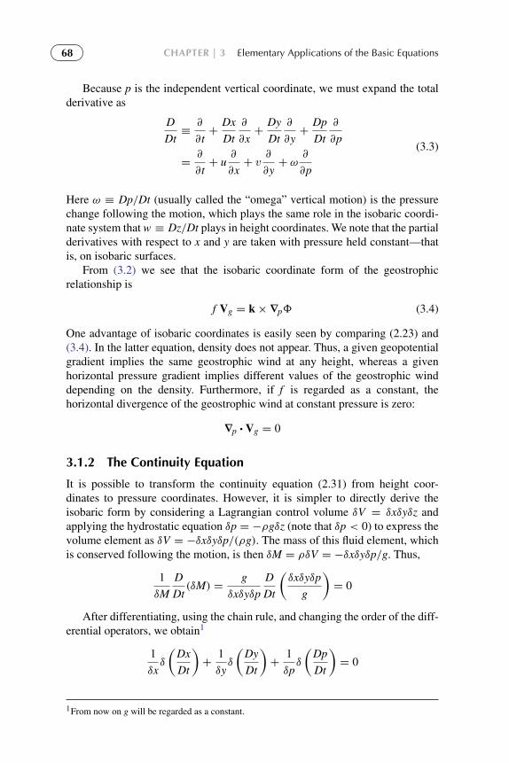
To protect the rights of the author(s) and publisher we inform you that this PDF is an uncorrected proof for internal businessuse only by the author(s), editor(s), reviewer(s), Elsevier and typesetter diacriTech. It is not allowed to publish this proofonline or in print. This proof copy is the copyright property of the publisher and is confidential until formal publication.
“Hakim: 07-ch03-067-094-9780123848666” — 2012/7/26 — 11:01 — page 68 — #2
68 CHAPTER | 3 Elementary Applications of the Basic Equations
Because p is the independent vertical coordinate, we must expand the totalderivative as
D
Dt≡∂
∂t+
Dx
Dt
∂
∂x+
Dy
Dt
∂
∂y+
Dp
Dt
∂
∂p
=∂
∂t+ u
∂
∂x+ v
∂
∂y+ ω
∂
∂p
(3.3)
Here ω ≡ Dp/Dt (usually called the “omega” vertical motion) is the pressurechange following the motion, which plays the same role in the isobaric coordi-nate system that w ≡ Dz/Dt plays in height coordinates. We note that the partialderivatives with respect to x and y are taken with pressure held constant—thatis, on isobaric surfaces.
From (3.2) we see that the isobaric coordinate form of the geostrophicrelationship is
f Vg = k×∇p8 (3.4)
One advantage of isobaric coordinates is easily seen by comparing (2.23) and(3.4). In the latter equation, density does not appear. Thus, a given geopotentialgradient implies the same geostrophic wind at any height, whereas a givenhorizontal pressure gradient implies different values of the geostrophic winddepending on the density. Furthermore, if f is regarded as a constant, thehorizontal divergence of the geostrophic wind at constant pressure is zero:
∇p ·Vg = 0
3.1.2 The Continuity Equation
It is possible to transform the continuity equation (2.31) from height coor-dinates to pressure coordinates. However, it is simpler to directly derive theisobaric form by considering a Lagrangian control volume δV = δxδyδz andapplying the hydrostatic equation δp = −ρgδz (note that δp < 0) to express thevolume element as δV = −δxδyδp/(ρg). The mass of this fluid element, whichis conserved following the motion, is then δM = ρδV = −δxδyδp/g. Thus,
1
δM
D
Dt(δM) =
g
δxδyδp
D
Dt
(δxδyδp
g
)= 0
After differentiating, using the chain rule, and changing the order of the diff-erential operators, we obtain1
1
δxδ
(Dx
Dt
)+
1
δyδ
(Dy
Dt
)+
1
δpδ
(Dp
Dt
)= 0
1From now on g will be regarded as a constant.

To protect the rights of the author(s) and publisher we inform you that this PDF is an uncorrected proof for internal businessuse only by the author(s), editor(s), reviewer(s), Elsevier and typesetter diacriTech. It is not allowed to publish this proofonline or in print. This proof copy is the copyright property of the publisher and is confidential until formal publication.
“Hakim: 07-ch03-067-094-9780123848666” — 2012/7/26 — 11:01 — page 69 — #3
3.2 | Balanced Flow 69
or
δu
δx+δv
δy+δω
δp= 0
Taking the limit δx, δy, δp → 0 and observing that δx and δy are evaluated atconstant pressure, we obtain the continuity equation in the isobaric system:(
∂u
∂x+∂v
∂y
)p+∂ω
∂p= 0 (3.5)
This form of the continuity equation contains no reference to the density fieldand does not involve time derivatives. The simplicity of (3.5) is one of the chiefadvantages of the isobaric coordinate system.
3.1.3 The Thermodynamic Energy Equation
The first law of thermodynamics (2.43) can be expressed in the isobaric systemby letting Dp/Dt = ω and expanding DT/Dt using (3.3):
cp
(∂T
∂t+ u
∂T
∂x+ v
∂T
∂y+ ω
∂T
∂p
)− αω = J
This may be rewritten as(∂T
∂t+ u
∂T
∂x+ v
∂T
∂y
)− Spω =
J
cp(3.6)
where, with the aid of the equation of state and Poisson’s equation (2.44), wehave
Sp ≡RT
cpp−∂T
∂p= −
T
θ
∂θ
∂p(3.7)
which is the static stability parameter for the isobaric system. Using (2.49) andthe hydrostatic equation, (3.7) may be rewritten as
Sp = (0d − 0)/ρg
Thus, Sp is positive provided that the lapse rate is less than dry adiabatic. How-ever, because density decreases approximately exponentially with height, Sp
increases rapidly with height. This strong height dependence of the stabilitymeasure Sp is a minor disadvantage of isobaric coordinates.
3.2 BALANCED FLOW
Despite the apparent complexity of atmospheric motion systems as depictedon synoptic weather charts, the pressure (or geopotential height) and velocitydistributions in meteorological disturbances are actually related by rather sim-ple approximate force balances. In order to gain a qualitative understanding of
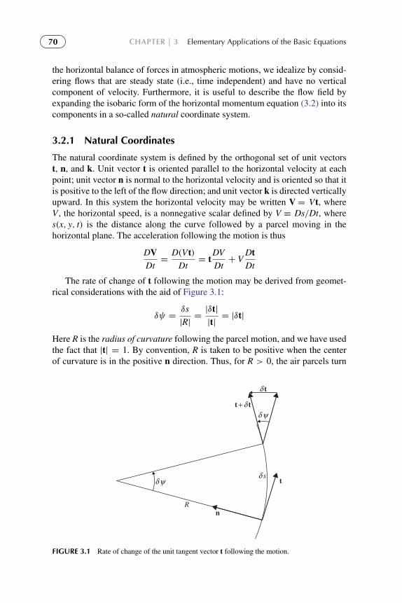
To protect the rights of the author(s) and publisher we inform you that this PDF is an uncorrected proof for internal businessuse only by the author(s), editor(s), reviewer(s), Elsevier and typesetter diacriTech. It is not allowed to publish this proofonline or in print. This proof copy is the copyright property of the publisher and is confidential until formal publication.
“Hakim: 07-ch03-067-094-9780123848666” — 2012/7/26 — 11:01 — page 70 — #4
70 CHAPTER | 3 Elementary Applications of the Basic Equations
the horizontal balance of forces in atmospheric motions, we idealize by consid-ering flows that are steady state (i.e., time independent) and have no verticalcomponent of velocity. Furthermore, it is useful to describe the flow field byexpanding the isobaric form of the horizontal momentum equation (3.2) into itscomponents in a so-called natural coordinate system.
3.2.1 Natural Coordinates
The natural coordinate system is defined by the orthogonal set of unit vectorst, n, and k. Unit vector t is oriented parallel to the horizontal velocity at eachpoint; unit vector n is normal to the horizontal velocity and is oriented so that itis positive to the left of the flow direction; and unit vector k is directed verticallyupward. In this system the horizontal velocity may be written V = Vt, whereV , the horizontal speed, is a nonnegative scalar defined by V ≡ Ds/Dt, wheres(x, y, t) is the distance along the curve followed by a parcel moving in thehorizontal plane. The acceleration following the motion is thus
DVDt=
D(Vt)Dt= t
DV
Dt+ V
DtDt
The rate of change of t following the motion may be derived from geomet-rical considerations with the aid of Figure 3.1:
δψ =δs
|R|=|δt||t|= |δt|
Here R is the radius of curvature following the parcel motion, and we have usedthe fact that |t| = 1. By convention, R is taken to be positive when the centerof curvature is in the positive n direction. Thus, for R > 0, the air parcels turn
δ t
t + δ t
t
δ ψ
δ s
Rn
δ ψ
FIGURE 3.1 Rate of change of the unit tangent vector t following the motion.

To protect the rights of the author(s) and publisher we inform you that this PDF is an uncorrected proof for internal businessuse only by the author(s), editor(s), reviewer(s), Elsevier and typesetter diacriTech. It is not allowed to publish this proofonline or in print. This proof copy is the copyright property of the publisher and is confidential until formal publication.
“Hakim: 07-ch03-067-094-9780123848666” — 2012/7/26 — 11:01 — page 71 — #5
3.2 | Balanced Flow 71
toward the left following the motion, and for R < 0, the air parcels turn towardthe right following the motion.
Noting that in the limit δs → 0, δt is directed parallel to n, the precedingrelationship yields Dt/Ds = n/R. Thus,
DtDt=
DtDs
Ds
Dt=
nR
V
and
DVDt= t
DV
Dt+ n
V2
R(3.8)
Therefore, the acceleration following the motion is the sum of the rate of changeof speed of the air parcel and its centripetal acceleration due to the curvature ofthe trajectory. Because the Coriolis force always acts normal to the direction ofmotion, its natural coordinate form is simply
−f k× V = −f Vn
whereas the pressure gradient force can be expressed as
−∇p8 = −
(t∂8
∂s+ n
∂8
∂n
)The horizontal momentum equation may thus be expanded into the followingcomponent equations in the natural coordinate system:
DV
Dt= −
∂8
∂s(3.9)
V2
R+ f V = −
∂8
∂n(3.10)
Equations (3.9) and (3.10) express the force balances parallel to and normalto the direction of flow, respectively. For motion parallel to the geopotentialheight contours, ∂8/∂s = 0, and the speed is constant following the motion.If, in addition, the geopotential gradient normal to the direction of motion isconstant along a trajectory, (3.10) implies that the radius of curvature of thetrajectory is also constant. In that case the flow can be classified into severalsimple categories depending on the relative contributions of the three terms in(3.10) to the net force balance.
3.2.2 Geostrophic Flow
Flow in a straight line (R → ± ∞) parallel to height contours is referred toas geostrophic motion. In geostrophic motion the horizontal components of theCoriolis force and pressure gradient force are in exact balance so that V = Vg,

To protect the rights of the author(s) and publisher we inform you that this PDF is an uncorrected proof for internal businessuse only by the author(s), editor(s), reviewer(s), Elsevier and typesetter diacriTech. It is not allowed to publish this proofonline or in print. This proof copy is the copyright property of the publisher and is confidential until formal publication.
“Hakim: 07-ch03-067-094-9780123848666” — 2012/7/26 — 11:01 — page 72 — #6
72 CHAPTER | 3 Elementary Applications of the Basic Equations
P
Co
Vg
Φ0 − δ Φ
Φ0
FIGURE 3.2 Balance of forces for geostrophic equilibrium. The pressure gradient force isdesignated by P and the Coriolis force by Co.
where the geostrophic wind Vg is defined by2
f Vg = −∂8/∂n (3.11)
This balance is indicated schematically in Figure 3.2. The actual wind can bein exact geostrophic motion only if the height contours are parallel to latitudecircles. As discussed in Section 2.4.1, the geostrophic wind is generally a goodapproximation to the actual wind in extratropical synoptic-scale disturbances.However, in some of the special cases treated later, this is not true.
3.2.3 Inertial Flow
If the geopotential field is uniform on an isobaric surface so that the horizontalpressure gradient vanishes, (3.10) reduces to a balance between Coriolis forceand centrifugal force:
V2/R+ f V = 0 (3.12)
Equation (3.12) may be solved for the radius of curvature
R = −V/f
Since from (3.9), the speed must be constant in this case, the radius of cur-vature is also constant (neglecting the latitudinal dependence of f ). Thus, theair parcels follow circular paths in an anticyclonic sense.3 The period of this
2Note that although the actual speed V must always be positive in the natural coordinates, Vg,which is proportional to the height gradient normal to the direction of flow, may be negative, as inthe “anomalous” low shown later in Figure 3.5c.3Anticyclonic flow is a clockwise rotation in the Northern Hemisphere and counterclockwise in theSouthern Hemisphere. Cyclonic flow has the opposite sense of rotation in each hemisphere.

To protect the rights of the author(s) and publisher we inform you that this PDF is an uncorrected proof for internal businessuse only by the author(s), editor(s), reviewer(s), Elsevier and typesetter diacriTech. It is not allowed to publish this proofonline or in print. This proof copy is the copyright property of the publisher and is confidential until formal publication.
“Hakim: 07-ch03-067-094-9780123848666” — 2012/7/26 — 11:01 — page 73 — #7
3.2 | Balanced Flow 73
oscillation is
P =
∣∣∣∣2πR
V
∣∣∣∣ = 2π
| f |=
12 day
| sinφ|(3.13)
P is equivalent to the time that is required for a Foucault pendulum to turnthrough an angle of 180◦. Thus, it is often referred to as one-half pendulum day.
Because both the Coriolis force and the centrifugal force due to the rela-tive motion are caused by inertia of the fluid, this type of motion is traditionallyreferred to as an inertial oscillation, and the circle of radius |R| is called the iner-tia circle. It is important to realize that the “inertial flow” governed by (3.12) isnot the same as inertial motion in an absolute reference frame. The flow gov-erned by (3.12) is just the constant angular momentum oscillation referred to inSection 1.3.4. In this flow the force of gravity, acting orthogonal to the plane ofmotion, keeps the oscillation on a horizontal surface. In true inertial motion, allforces vanish and the motion maintains a uniform absolute velocity.
In the atmosphere, motions are nearly always generated and maintained bypressure gradient forces; the conditions of uniform pressure required for pureinertial flow rarely exist. In the oceans, however, currents are often generatedby transient winds blowing across the surface, rather than by internal pressuregradients. As a result, significant amounts of energy occur in currents that oscil-late with near inertial periods. An example recorded by a current meter near theisland of Barbados is shown in Figure 3.3.
3.2.4 Cyclostrophic Flow
If the horizontal scale of a disturbance is small enough, the Coriolis force may beneglected in (3.10) compared to the pressure gradient force and the centrifugalforce. The force balance normal to the direction of flow is then
V2
R= −
∂8
∂n
If this equation is solved for V , we obtain the speed of the cyclostrophic wind
V =
(−R
∂8
∂n
)1/2(3.14)
As indicated in Figure 3.4, cyclostrophic flow may be either cyclonic or anticy-clonic. In both cases the pressure gradient force is directed toward the center ofcurvature and the centrifugal force away from the center of curvature.
The cyclostrophic balance approximation is valid provided that the ratioof the centrifugal force to the Coriolis force is large. This ratio V/( f R) isequivalent to the Rossby number discussed in Section 2.4.2. As an example ofcyclostrophic scale motion, we consider a typical tornado. Suppose that the tan-gential velocity is 30 m s−1 at a distance of 300 m from the center of the vortex.

To protect the rights of the author(s) and publisher we inform you that this PDF is an uncorrected proof for internal businessuse only by the author(s), editor(s), reviewer(s), Elsevier and typesetter diacriTech. It is not allowed to publish this proofonline or in print. This proof copy is the copyright property of the publisher and is confidential until formal publication.
“Hakim: 07-ch03-067-094-9780123848666” — 2012/7/26 — 11:01 — page 74 — #8
74 CHAPTER | 3 Elementary Applications of the Basic Equations
PeriodDays
14
0
10
20
30
Inertial
Semidiurnaltidal
0.001 0.01 0.1
Frequency (cph)
Kin
etic
ene
rgy
dens
ity (
cm2
s−2 cp
h−1)
1.0
40
50
7 3 2 1 12 6 3 1 30Hours Minutes
FIGURE 3.3 Power spectrum of kinetic energy at 30-m depth in the ocean near Barbados (13◦N).Ordinate shows kinetic energy density per unit frequency interval (cph–1 designates cycles perhour). This type of plot indicates the manner in which the total kinetic energy is partitioned amongoscillations of different periods. Note the strong peak at 53 h, which is the period of an inertialoscillation at 13◦ latitude. (After Warsh et al., 1971. Copyright © American Meteorological Society.Reprinted with permission.)
Assuming that f = 10−4 s−1, the Rossby number is just Ro = V/| f R| ≈ 103,
which implies that the Coriolis force can be neglected in computing the bal-ance of forces for a tornado. However, the majority of tornadoes in the NorthernHemisphere are observed to rotate in a cyclonic (counterclockwise) sense. Thisis due to the fact that they are embedded in environments that favor cyclonicrotation (see Section 9.6.1). Smaller-scale vortices, however, such as dust dev-ils and water spouts, do not have a preferred direction of rotation. According todata collected by Sinclair (1965), they are observed to be anticyclonic as oftenas cyclonic.
3.2.5 The Gradient Wind Approximation
Horizontal frictionless flow that is parallel to the height contours so that thetangential acceleration vanishes (DV/Dt = 0) is called gradient flow. Gradientflow is a three-way balance among the Coriolis force, the centrifugal force, andthe horizontal pressure gradient force. Like geostrophic flow, pure gradient flow

To protect the rights of the author(s) and publisher we inform you that this PDF is an uncorrected proof for internal businessuse only by the author(s), editor(s), reviewer(s), Elsevier and typesetter diacriTech. It is not allowed to publish this proofonline or in print. This proof copy is the copyright property of the publisher and is confidential until formal publication.
“Hakim: 07-ch03-067-094-9780123848666” — 2012/7/26 — 11:01 — page 75 — #9
3.2 | Balanced Flow 75
P CeL
P CeL
R > 0, ∂Φ∂n
< 0
R < 0, ∂Φ∂n
> 0
V
V
FIGURE 3.4 Force balance in cyclostrophic flow: P designates the pressure gradient; Ce desig-nates the centrifugal force.
can exist only under very special circumstances. It is always possible, however,to define a gradient wind, which at any point is just the wind component parallelto the height contours that satisfies (3.10). For this reason, (3.10) is commonlyreferred to as the gradient wind equation. Because (3.10) takes into account thecentrifugal force due to the curvature of parcel trajectories, the gradient wind isoften a better approximation to the actual wind than the geostrophic wind.
The gradient wind speed is obtained by solving (3.10) for V to yield
V =−fR
2±
(f 2R2
4− R
∂8
∂n
)1/2
=−fR
2±
(f 2R2
4+ fRVg
)1/2
(3.15)
where in the lower expression (3.11) is used to express ∂8/∂n in terms of thegeostrophic wind. Not all the mathematically possible roots of (3.15) correspondto physically possible solutions, since it is required that V be real and nonnega-tive. In Table 3.1 the various roots of (3.15) are classified according to the signsof R and ∂8/∂n in order to isolate the physically meaningful solutions.
The force balances for the four permitted solutions are illustrated inFigure 3.5. Equation (3.15) shows that in cases of both regular and anomaloushighs the pressure gradient is limited by the requirement that the quantity under

To protect the rights of the author(s) and publisher we inform you that this PDF is an uncorrected proof for internal businessuse only by the author(s), editor(s), reviewer(s), Elsevier and typesetter diacriTech. It is not allowed to publish this proofonline or in print. This proof copy is the copyright property of the publisher and is confidential until formal publication.
“Hakim: 07-ch03-067-094-9780123848666” — 2012/7/26 — 11:01 — page 76 — #10
76 CHAPTER | 3 Elementary Applications of the Basic Equations
�
�
�
�
TABLE 3.1 Classification of Roots of the Gradient Wind Equationin the Northern Hemisphere
Sign ∂8/∂n R > 0 R < 0
Positive (Vg < 0) Positive roota: unphysical Positive root: antibaric flow(anomalous low)
Negative root: unphysical Negative root: unphysical
Negative (Vg > 0) Positive root: cyclonic flow(regular low)
Positive root: (V > −f R/2):anticyclonic flow(anomalous high)
Negative root: unphysical Negative root: (V < −f R/2):anticyclonic flow (regularhigh)
aThe terms “positive root” and “negative root” in columns 2 and 3 refer to the sign taken in thefinal term in Eq. (3.15).
VP Ce
CoL
(a) (b)
P
Ce
CoH
V
(c) (d)
V
P
CeCo
L
V
PCe
CoH
FIGURE 3.5 Force balances in the Northern Hemisphere for the four types of gradient flow:(a) regular low, (b) regular high, (c) anomalous low, and (d) anomalous high.
the radical be nonnegative—that is,
∣∣∣∣ f Vg
∣∣∣∣ = ∣∣∣∣∂8∂n
∣∣∣∣ < |R| f 2
4(3.16)

To protect the rights of the author(s) and publisher we inform you that this PDF is an uncorrected proof for internal businessuse only by the author(s), editor(s), reviewer(s), Elsevier and typesetter diacriTech. It is not allowed to publish this proofonline or in print. This proof copy is the copyright property of the publisher and is confidential until formal publication.
“Hakim: 07-ch03-067-094-9780123848666” — 2012/7/26 — 11:01 — page 77 — #11
3.2 | Balanced Flow 77
Thus, the pressure gradient in a high must approach zero as |R| → 0. It is forthis reason that the pressure field near the center of a high is always flat and thewind gentle compared to the region near the center of a low.
The absolute angular momentum about the axis of rotation for the circularlysymmetric motions shown in Figure 3.5 is given by VR + f R2/2. From (3.15)it is verified readily that regular gradient wind balances have positive abso-lute angular momentum in the Northern Hemisphere, whereas anomalous caseshave negative absolute angular momentum. Because the only source of negativeabsolute angular momentum is the Southern Hemisphere, the anomalous casesare unlikely to occur, except perhaps close to the equator.
In all cases except the anomalous low (Figure 3.5c) the horizontal compo-nents of the Coriolis and pressure gradient forces are oppositely directed. Suchflow is called baric. The anomalous low is antibaric; the geostrophic wind Vg
defined in (3.11) is negative for an anomalous low and is clearly not a use-ful approximation to the actual speed.4 Furthermore, as shown in Figure 3.5,gradient flow is cyclonic only when the centrifugal force and the horizontalcomponent of the Coriolis force have the same sense (Rf > 0); it is anticy-clonic when these forces have the opposite sense (Rf < 0). Since the directionof anticyclonic and cyclonic flow is reversed in the Southern Hemisphere, therequirement that Rf > 0 for cyclonic flow holds regardless of the hemisphereconsidered.
The definition of the geostrophic wind (3.11) can be used to rewrite the forcebalance normal to the direction of flow (3.10) in the form
V2/R+ f V − f Vg = 0
Dividing through by f V shows that the ratio of the geostrophic wind to thegradient wind is
Vg
V= 1+
V
f R(3.17)
For normal cyclonic flow ( f R > 0), Vg is larger than V , whereas for anticy-clonic flow ( f R< 0), Vg is smaller than V . Therefore, the geostrophic wind isan overestimate of the balanced wind in a region of cyclonic curvature and anunderestimate in a region of anticyclonic curvature. For midlatitude synopticsystems, the difference between gradient and geostrophic wind speeds gener-ally does not exceed 10 to 20%. [Note that the magnitude of V/( f R) is justthe Rossby number.] For tropical disturbances, the Rossby number is in therange of 1 to 10, and the gradient wind formula must be applied rather than thegeostrophic wind. Equation (3.17) also shows that the antibaric anomalous low,which has Vg < 0, can exist only when V/( f R) < −1. Thus, antibaric flow isassociated with small-scale intense vortices such as tornadoes.
4 Remember that in the natural coordinate system the speed V is positive definite.

To protect the rights of the author(s) and publisher we inform you that this PDF is an uncorrected proof for internal businessuse only by the author(s), editor(s), reviewer(s), Elsevier and typesetter diacriTech. It is not allowed to publish this proofonline or in print. This proof copy is the copyright property of the publisher and is confidential until formal publication.
“Hakim: 07-ch03-067-094-9780123848666” — 2012/7/26 — 11:01 — page 78 — #12
78 CHAPTER | 3 Elementary Applications of the Basic Equations
3.3 TRAJECTORIES AND STREAMLINES
In the natural coordinate system used in the previous section to discuss balancedflow, s(x, y, t)was defined as the distance along the curve in the horizontal planetraced out by the path of an air parcel. The path followed by a particular airparcel over a finite period of time is called the trajectory of the parcel. Thus, theradius of curvature R of the path s referred to in the gradient wind equation isthe radius of curvature for a parcel trajectory. In practice, R is often estimatedby using the radius of curvature of a geopotential height contour, as this canbe estimated easily from a synoptic chart. However, the height contours areactually streamlines of the gradient wind (i.e., lines that are everywhere parallelto the instantaneous wind velocity).
It is important to distinguish clearly between streamlines, which give a“snapshot” of the velocity field at any instant, and trajectories, which tracethe motion of individual fluid parcels over a finite time interval. In Cartesiancoordinates, horizontal trajectories are determined by the integration of
Ds
Dt= V(x, y, t) (3.18)
over a finite time span for each parcel to be followed, whereas streamlines aredetermined by the integration of
dy
dx=
v(x, y, t0)
u(x, y, t0)(3.19)
with respect to x at time t0. (Note that since a streamline is parallel to the velocityfield, its slope in the horizontal plane is just the ratio of the horizontal velocitycomponents.) Only for steady-state motion fields (i.e., fields in which the localrate of change of velocity vanishes) do the streamlines and trajectories coincide.However, synoptic disturbances are not steady-state motions. They generallymove at speeds of the same order as the winds that circulate about them. Togain an appreciation for the possible errors involved in using the curvature ofthe streamlines instead of the curvature of the trajectories in the gradient windequation, it is necessary to investigate the relationship between the curvatureof the trajectories and the curvature of the streamlines for a moving pressuresystem.
We let β(x, y, t) designate the angular direction of the wind at each pointon an isobaric surface, and Rt and Rs designate the radii of curvature of thetrajectories and streamlines, respectively. Then, from Figure 3.6, δs = R δβ sothat in the limit δs→ 0
Dβ
Ds=
1
Rtand
∂β
∂s=
1
Rs(3.20)
where Dβ/Ds means the rate of change of wind direction along a trajectory(positive for counterclockwise turning) and ∂β/∂s is the rate of change of wind

To protect the rights of the author(s) and publisher we inform you that this PDF is an uncorrected proof for internal businessuse only by the author(s), editor(s), reviewer(s), Elsevier and typesetter diacriTech. It is not allowed to publish this proofonline or in print. This proof copy is the copyright property of the publisher and is confidential until formal publication.
“Hakim: 07-ch03-067-094-9780123848666” — 2012/7/26 — 11:01 — page 79 — #13
3.3 | Trajectories and Streamlines 79
δ β δ s
R
FIGURE 3.6 Relationship between the change in angular direction of the wind δβ and the radiusof curvature R.
direction along a streamline at any instant. Thus, the rate of change of winddirection following the motion is
Dβ
Dt=
Dβ
Ds
Ds
Dt=
V
Rt(3.21)
or, after expanding the total derivative,
Dβ
Dt=∂β
∂t+ V
∂β
∂s=∂β
∂t+
V
Rs(3.22)
Combining (3.21) and (3.22), we obtain a formula for the local turning of thewind:
∂β
∂t= V
(1
Rt−
1
Rs
)(3.23)
Equation (3.23) indicates that the trajectories and streamlines will coincide onlywhen the local rate of change of the wind direction vanishes.
In general, midlatitude synoptic systems move eastward as a result of advec-tion by upper-level westerly winds. In such cases there is a local turning of thewind due to the motion of the system even if the shape of the height contourpattern remains constant as the system moves. The relationship between Rt andRs in such a situation can be determined easily for an idealized circular patternof height contours moving at a constant velocity C. In this case the local turningof the wind is entirely due to the motion of the streamline pattern so that
∂β
∂t= −C·∇β = −C
∂β
∂scos γ = −
C
Rscos γ
where γ is the angle between the streamlines (height contours) and the directionof motion of the system. Substituting the preceding equation into (3.23) and

To protect the rights of the author(s) and publisher we inform you that this PDF is an uncorrected proof for internal businessuse only by the author(s), editor(s), reviewer(s), Elsevier and typesetter diacriTech. It is not allowed to publish this proofonline or in print. This proof copy is the copyright property of the publisher and is confidential until formal publication.
“Hakim: 07-ch03-067-094-9780123848666” — 2012/7/26 — 11:01 — page 80 — #14
80 CHAPTER | 3 Elementary Applications of the Basic Equations
solving for Rt with the aid of (3.20), we obtain the desired relationship betweenthe curvature of the streamlines and the curvature of the trajectories:
Rt = Rs
(1−
C cos γ
V
)−1
(3.24)
Equation (3.24) can be used to compute the curvature of the trajectoryanywhere on a moving pattern of streamlines. In Figure 3.7 the curvatures of thetrajectories for parcels initially located due north, east, south, and west of thecenter of a cyclonic system are shown both for the case of a wind speed greaterthan the speed of movement of the height contours and for the case of a windspeed less than the speed of movement of the height contours. In these examplesthe plotted trajectories are based on a geostrophic balance so that the height
11
1
0
1
2
2
2
2
3
Lt1 t2 t3
C3
3
3
(a)
(b)
1
1
1
1
2
2
2
23
3
3
3
Lt1 t2 t3
C
FIGURE 3.7 Trajectories for moving circular cyclonic circulation systems in the Northern Hemi-sphere with (a) V= 2C and (b) 2V=C. Numbers indicate positions at successive times. L designatesa pressure minimum.

To protect the rights of the author(s) and publisher we inform you that this PDF is an uncorrected proof for internal businessuse only by the author(s), editor(s), reviewer(s), Elsevier and typesetter diacriTech. It is not allowed to publish this proofonline or in print. This proof copy is the copyright property of the publisher and is confidential until formal publication.
“Hakim: 07-ch03-067-094-9780123848666” — 2012/7/26 — 11:01 — page 81 — #15
3.4 | The Thermal Wind 81
contours are equivalent to streamlines. It is also assumed for simplicity that thewind speed does not depend on the distance from the center of the system.
In the case shown in Figure 3.7b, there is a region south of the low cen-ter where the curvature of the trajectories is opposite that of the streamlines.Because synoptic-scale pressure systems usually move at speeds comparable tothe wind speed, the gradient wind speed computed on the basis of the curvatureof the height contours is often no better an approximation to the actual windspeed than the geostrophic wind. In fact, the actual gradient wind speed willvary along a height contour with the variation of the trajectory curvature.
3.4 THE THERMAL WIND
The geostrophic wind must have vertical shear in the presence of a horizontaltemperature gradient, as can be shown easily from simple physical consider-ations based on hydrostatic equilibrium. Since the geostrophic wind (3.4) isproportional to the geopotential gradient on an isobaric surface, a geostrophicwind directed along the positive y axis that increases in magnitude with heightrequires that the slope of the isobaric surfaces with respect to the x axis alsomust increase with height, as shown in Figure 3.8. According to the hypso-metric equation (1.30), the thickness δz corresponding to a (positive) pressureinterval δp is
δz ≈ g−1RTδ ln p (3.25)
z
Vg
yp0 + 2δp
p0 + δp
δz1
p0
x1 x2x
δz2
FIGURE 3.8 Relationship between vertical shear of the geostrophic wind and horizontal thicknessgradients. (Note that δp < 0.)

To protect the rights of the author(s) and publisher we inform you that this PDF is an uncorrected proof for internal businessuse only by the author(s), editor(s), reviewer(s), Elsevier and typesetter diacriTech. It is not allowed to publish this proofonline or in print. This proof copy is the copyright property of the publisher and is confidential until formal publication.
“Hakim: 07-ch03-067-094-9780123848666” — 2012/7/26 — 11:01 — page 82 — #16
82 CHAPTER | 3 Elementary Applications of the Basic Equations
Thus, the thickness of the layer between two isobaric surfaces is proportionalto the mean temperature in the layer, T . In Figure 3.8 the mean temperature T1of the column denoted δz1 must be less than the mean temperature T2 for thecolumn denoted δz2. Thus, an increase with height of a positive x directed pres-sure gradient must be associated with a positive x directed temperature gradient.The air in a vertical column at x2, because it is warmer (less dense), must occupya greater depth for a given pressure drop than the air at x1.
Equations for the rate of change with height of the geostrophic wind compo-nents are derived most easily using the isobaric coordinate system. In isobariccoordinates the geostrophic wind (3.4) has components given by
vg =1
f
∂8
∂xand ug = −
1
f
∂8
∂y(3.26)
where the derivatives are evaluated with pressure held constant. Also, with theaid of the ideal gas law, we can write the hydrostatic equation as
∂8
∂p= −α = −
RT
p(3.27)
Differentiating (3.26) with respect to pressure, and applying (3.27), we obtain
p∂vg
∂p≡
∂vg
∂ ln p= −
R
f
(∂T
∂x
)p
(3.28)
p∂ug
∂p≡
∂ug
∂ ln p=
R
f
(∂T
∂y
)p
(3.29)
or in vectorial form
∂Vg
∂ ln p= −
R
fk×∇pT (3.30)
Equation (3.30) is often referred to as the thermal wind equation. How-ever, it is actually a relationship for the vertical wind shear (i.e., the rate ofchange of the geostrophic wind with respect to ln p). Strictly speaking, the termthermal wind refers to the vector difference between geostrophic winds at twolevels. Designating the thermal wind vector by VT , we may integrate (3.30)from pressure level p0 to level p1 (p1 < p0) to get
VT ≡ Vg(p1)− Vg(p0) = −R
f
p1∫p0
(k×∇pT
)d ln p (3.31)
Letting 〈T〉 denote the mean temperature in the layer between pressure p0and p1, the x and y components of the thermal wind are thus given by
uT = −R
f
(∂〈T〉
∂y
)p
ln
(p0
p1
); vT =
R
f
(∂〈T〉
∂x
)p
ln
(p0
p1
)(3.32)

To protect the rights of the author(s) and publisher we inform you that this PDF is an uncorrected proof for internal businessuse only by the author(s), editor(s), reviewer(s), Elsevier and typesetter diacriTech. It is not allowed to publish this proofonline or in print. This proof copy is the copyright property of the publisher and is confidential until formal publication.
“Hakim: 07-ch03-067-094-9780123848666” — 2012/7/26 — 11:01 — page 83 — #17
3.4 | The Thermal Wind 83
Alternatively, we may express the thermal wind for a given layer in terms ofthe horizontal gradient of the geopotential difference between the top and thebottom of the layer:
uT = −1
f
∂
∂y(81 −80); vT =
1
f
∂
∂x(81 −80) (3.33)
The equivalence of (3.32) and (3.33) can be verified readily by integrating thehydrostatic equation (3.27) vertically from p0 to p1 after replacing T by themean 〈T〉. The result is the hypsometric equation (1.29):
81 −80 ≡ gZT = R〈T〉 ln
(p0
p1
)(3.34)
The quantity ZT is the thickness of the layer between p0 and p1 measured inunits of geopotential meters. From (3.34) we see that the thickness is propor-tional to the mean temperature in the layer. Hence, lines of equal ZT (isolinesof thickness) are equivalent to the isotherms of mean temperature in the layer.It can also be used to estimate the mean horizontal temperature advection in alayer, as shown in Figure 3.9. It is clear from the vector form of the thermal
Cold
Warm
(a)
T0 + δT
T0
T0 − δT
Vg1
VT
Vg0
Warm
Cold
(b)
T0 + δT
T0 − δT
T0
VT
Vg0
Vg1
FIGURE 3.9 Relationship between turning of geostrophic wind and temperature advection:(a) backing of the wind with height and (b) veering of the wind with height.

To protect the rights of the author(s) and publisher we inform you that this PDF is an uncorrected proof for internal businessuse only by the author(s), editor(s), reviewer(s), Elsevier and typesetter diacriTech. It is not allowed to publish this proofonline or in print. This proof copy is the copyright property of the publisher and is confidential until formal publication.
“Hakim: 07-ch03-067-094-9780123848666” — 2012/7/26 — 11:01 — page 84 — #18
84 CHAPTER | 3 Elementary Applications of the Basic Equations
wind relation
VT =1
fk×∇ (81 −80) =
g
fk×∇ZT =
R
fk×∇ 〈T〉 ln
(p0
p1
)(3.35)
that the thermal wind blows parallel to the isotherms (lines of constant thick-ness) with the warm air to the right facing downstream in the NorthernHemisphere. Thus, as is illustrated in Figure 3.9a, a geostrophic wind thatturns counterclockwise with height (backs) is associated with cold-air advec-tion. Conversely, as shown in Figure 3.9b, clockwise turning (veering) of thegeostrophic wind with height implies warm advection by the geostrophic windin the layer.
It is therefore possible to obtain a reasonable estimate of the horizontal tem-perature advection and its vertical dependence at a given location solely fromdata on the vertical profile of the wind given by a single sounding. Alternatively,the geostrophic wind at any level can be estimated from the mean temperaturefield, provided that the geostrophic velocity is known at a single level. Thus, forexample, if the geostrophic wind at 850 hPa is known and the mean horizon-tal temperature gradient in the layer 850 to 500 hPa is also known, the thermalwind equation can be applied to obtain the geostrophic wind at 500 hPa.
3.4.1 Barotropic and Baroclinic Atmospheres
A barotropic atmosphere is one in which the density depends only on the pres-sure, ρ = ρ(p), so that isobaric surfaces are also surfaces of constant density.For an ideal gas, the isobaric surfaces will also be isothermal if the atmosphereis barotropic. Thus, ∇pT = 0 in a barotropic atmosphere, and the thermal windequation (3.30) becomes ∂Vg/∂ln p = 0, which states that the geostrophic windis independent of height in a barotropic atmosphere. Thus, barotropy provides avery strong constraint on the motions in a rotating fluid; the large-scale motioncan depend only on horizontal position and time, not on height.
An atmosphere in which density depends on both the temperature and thepressure, ρ = ρ (p,T), is referred to as a baroclinic atmosphere. In a baro-clinic atmosphere the geostrophic wind generally has vertical shear, and thisshear is related to the horizontal temperature gradient by the thermal windequation (3.30). Obviously, the baroclinic atmosphere is of primary importancein dynamic meteorology. However, as shown in later chapters, much can belearned by study of the simpler barotropic atmosphere.
3.5 VERTICAL MOTION
As mentioned previously, for synoptic-scale motions the vertical velocity com-ponent is typically of the order of a few centimeters per second. Routinemeteorological soundings, however, only give the wind speed to an accuracy of

To protect the rights of the author(s) and publisher we inform you that this PDF is an uncorrected proof for internal businessuse only by the author(s), editor(s), reviewer(s), Elsevier and typesetter diacriTech. It is not allowed to publish this proofonline or in print. This proof copy is the copyright property of the publisher and is confidential until formal publication.
“Hakim: 07-ch03-067-094-9780123848666” — 2012/7/26 — 11:01 — page 85 — #19
3.5 | Vertical Motion 85
about a meter per second. Thus, in general the vertical velocity is not measureddirectly but must be inferred from the fields that are measured directly.
Two methods for inferring the vertical motion field are the kinematicmethod, based on the equation of continuity, and the adiabatic method, basedon the thermodynamic energy equation. Both methods are usually applied usingthe isobaric coordinate system so that ω(p) is inferred rather than w(z). Thesetwo measures of vertical motion can be related to each other with the aid of thehydrostatic approximation.
Expanding Dp/Dt in the (x, y, z) coordinate system yields
ω ≡Dp
Dt=∂p
∂t+ V ·∇p+ w
(∂p
∂z
)(3.36)
Now, for synoptic-scale motions, the horizontal velocity is geostrophic to afirst approximation. Therefore, we can write V = Vg + Va, where Va is theageostrophic wind and |Va| � |Vg|. However, Vg = (ρf )−1k × ∇p, so thatVg ·∇p = 0. Using this result plus the hydrostatic approximation, (3.36) maybe rewritten as
ω =∂p
∂t+ Va ·∇p− gρw (3.37)
Comparing the magnitudes of the three terms on the right in (3.37), we find thatfor synoptic-scale motions
∂p/∂t ∼ 10 hPa d−1
Va ·∇p ∼(
1 m s−1) (
1 Pa km−1)∼ 1 hPa d−1
gρw ∼ 100 hPa d−1
Thus, it is quite a good approximation to let
ω = −ρgw (3.38)
3.5.1 The Kinematic Method
One method of deducing the vertical velocity is based on integrating the conti-nuity equation in the vertical. Integration of (3.5) with respect to pressure froma reference level ps to any level p yields
ω (p) = ω (ps)−
p∫ps
(∂u
∂x+∂v
∂y
)pdp
= ω (ps)+ (ps − p)
(∂ 〈u〉
∂x+∂ 〈v〉
∂y
)p
(3.39)

To protect the rights of the author(s) and publisher we inform you that this PDF is an uncorrected proof for internal businessuse only by the author(s), editor(s), reviewer(s), Elsevier and typesetter diacriTech. It is not allowed to publish this proofonline or in print. This proof copy is the copyright property of the publisher and is confidential until formal publication.
“Hakim: 07-ch03-067-094-9780123848666” — 2012/7/26 — 11:01 — page 86 — #20
86 CHAPTER | 3 Elementary Applications of the Basic Equations
Here the angle brackets denote a pressure-weighted vertical average:
〈 〉 ≡ (p− ps)−1
p∫ps
()dp
With the aid of (3.38), the averaged form of (3.39) can be rewritten as
w(z) =ρ (zs)w (zs)
ρ(z)−
ps − p
ρ(z)g
(∂ 〈u〉
∂x+∂ 〈v〉
∂y
)(3.40)
where z and zs are the heights of pressure levels p and ps, respectively.Application of (3.40) to infer the vertical velocity field requires knowledge
of the horizontal divergence. To determine the horizontal divergence, the par-tial derivatives ∂u/∂x and ∂v/∂y are generally estimated from the fields of uand v by using finite difference approximations (see Section 13.2.1). For exam-ple, to determine the divergence of the horizontal velocity at the point x0, y0 inFigure 3.10, we write
∂u
∂x+∂v
∂y≈
u (x0 + d)− u (x0 − d)
2d+
v (y0 + d)− v (y0 − d)
2d(3.41)
However, for synoptic-scale motions in midlatitudes, the horizontal veloc-ity is nearly in geostrophic equilibrium. Except for the small effect due to thevariation of the Coriolis parameter (see Problem 3.19), the geostrophic windis nondivergent; that is, ∂u/∂x and ∂v/∂y are nearly equal in magnitude butopposite in sign. Thus, the horizontal divergence is due primarily to the smalldepartures of the wind from geostrophic balance (i.e., the ageostrophic wind). A10% error in evaluating one of the wind components in (3.41) can easily causethe estimated divergence to be in error by 100%. For this reason, the continuityequation method is not recommended for estimating the vertical motion fieldfrom observed horizontal winds.
v(y0 + d)
v(y0 − d)
u(x0 − d)(x0, y0)
u(x0 + d)
d
d
FIGURE 3.10 Grid for estimation of the horizontal divergence.

To protect the rights of the author(s) and publisher we inform you that this PDF is an uncorrected proof for internal businessuse only by the author(s), editor(s), reviewer(s), Elsevier and typesetter diacriTech. It is not allowed to publish this proofonline or in print. This proof copy is the copyright property of the publisher and is confidential until formal publication.
“Hakim: 07-ch03-067-094-9780123848666” — 2012/7/26 — 11:01 — page 87 — #21
3.6 | Surface Pressure Tendency 87
3.5.2 The Adiabatic Method
A second method for inferring vertical velocities, which is not so sensitive toerrors in the measured horizontal velocities, is based on the thermodynamicenergy equation. If the diabatic heating J is small compared to the other termsin the heat balance, (3.6) yields
ω = S−1p
(∂T
∂t+ u
∂T
∂x+ v
∂T
∂y
)(3.42)
Because temperature advection can usually be estimated quite accurately inmidlatitudes by using geostrophic winds, the adiabatic method can be appliedwhen only geopotential and temperature data are available. A disadvantage ofthe adiabatic method is that the local rate of change of temperature is required.Unless observations are taken at close intervals in time, it may be difficult toaccurately estimate ∂T/∂t over a wide area. This method is also rather inaccuratein situations where strong diabatic heating is present, such as storms in whichheavy rainfall occurs over a large area. Chapter 6 presents an alternative methodfor estimating ω, based on the so-called omega equation, that does not sufferfrom these difficulties.
3.6 SURFACE PRESSURE TENDENCY
The development of a negative surface pressure tendency is a classic warning ofan approaching cyclonic weather disturbance. A simple expression that relatesthe surface pressure tendency to the wind field, and thus in theory might be usedas the basis for short-range forecasts, can be obtained by taking the limit p→ 0in (3.39) to get
ω (ps) = −
ps∫0
(∇ ·V) dp (3.43)
followed by substituting from (3.37) to yield
∂ps
∂t≈ −
ps∫0
(∇ ·V) dp (3.44)
Here we have assumed that the surface is horizontal so that ws = 0, and haveneglected advection by the ageostrophic surface velocity in accord with thescaling arguments in Section 3.5.1.
According to (3.44), the surface pressure tendency at a given point is deter-mined by the total convergence of mass into the vertical column of atmosphereabove that point. This result is a direct consequence of the hydrostatic assump-tion, which implies that the pressure at a point is determined solely by the weight

To protect the rights of the author(s) and publisher we inform you that this PDF is an uncorrected proof for internal businessuse only by the author(s), editor(s), reviewer(s), Elsevier and typesetter diacriTech. It is not allowed to publish this proofonline or in print. This proof copy is the copyright property of the publisher and is confidential until formal publication.
“Hakim: 07-ch03-067-094-9780123848666” — 2012/7/26 — 11:01 — page 88 — #22
88 CHAPTER | 3 Elementary Applications of the Basic Equations
of the column of air above that point. Temperature changes in the air column willaffect the heights of upper-level pressure surfaces, but not the surface pressure.
Although, as stated earlier, the tendency equation might appear to havepotential as a forecasting aid, its utility is severely limited due to the fact that,as discussed in Section 3.5.1, ∇ · V is difficult to compute accurately fromobservations because it depends on the ageostrophic wind field. In addition,there is a strong tendency for vertical compensation. Thus, when there isconvergence in the lower troposphere, there is divergence aloft, and vice versa.The net integrated convergence or divergence is then a small residual in thevertical integral of a poorly determined quantity.
Nevertheless, (3.44) does have qualitative value as an aid in understandingthe origin of surface pressure changes and the relationship of such changes tothe horizontal divergence. This can be illustrated by considering (as one possibleexample) the development of a thermal cyclone. We suppose that a heat sourcegenerates a local warm anomaly in the midtroposphere (Figure 3.11a). Then,according to the hypsometric equation (3.34), the heights of the upper-levelpressure surfaces are raised above the warm anomaly, resulting in a horizontalpressure gradient force at the upper levels, which drives a divergent upper-level wind. By (3.44) this upper-level divergence will initially cause the surfacepressure to decrease, thus generating a surface low below the warm anomaly(Figure 3.11b). The horizontal pressure gradient associated with the surface lowthen drives a low-level convergence and vertical circulation, which tends tocompensate the upper-level divergence. The degree of compensation betweenupper divergence and lower convergence will determine whether the surfacepressure continues to fall, remains steady, or rises.
The thermally driven circulation of the preceding example is by no meansthe only type of circulation possible (e.g., cold-core cyclones are importantsynoptic-scale features). However, it does provide insight into how dynam-ical processes at upper levels are communicated to the surface and how the
z
High High
LowSea level
(a) (b)
Warm
Warm
FIGURE 3.11 Adjustment of surface pressure to a midtropospheric heat source. Dashed linesindicate isobars. (a) Initial height increase at upper-level pressure surface. (b) Surface response toupper-level divergence.

To protect the rights of the author(s) and publisher we inform you that this PDF is an uncorrected proof for internal businessuse only by the author(s), editor(s), reviewer(s), Elsevier and typesetter diacriTech. It is not allowed to publish this proofonline or in print. This proof copy is the copyright property of the publisher and is confidential until formal publication.
“Hakim: 07-ch03-067-094-9780123848666” — 2012/7/26 — 11:01 — page 89 — #23
Problems 89
surface and upper troposphere are dynamically connected through the divergentcirculation. This subject is considered in detail in Chapter 6.
Equation (3.44) is a lower boundary condition that determines the evolutionof pressure at constant height. If the isobaric coordinate system of dynamicalequations (3.2), (3.5), (3.6), and (3.27) is used as the set of governing equations,the lower boundary condition should be expressed in terms of the evolution ofgeopotential (or geopotential height) at constant pressure. Such an expressioncan be obtained simply by expanding D8/Dt in isobaric coordinates
∂8
∂t= −Va ·∇8− ω
∂8
∂p
and substituting from (3.27) and (3.43) to get
∂8s
∂t≈ −
RTs
ps
ps∫0
(∇ ·V) dp (3.45)
where we have again neglected advection by the ageostrophic wind.In practice, the boundary condition (3.45) is difficult to use because it should
be applied at pressure ps, which is itself changing in time and space. In simplemodels it is usual to assume that ps is constant (usually 1000 hPa) and to letω = 0 at ps, For modern forecast models, an alternative coordinate system isgenerally employed in which the lower boundary is always a coordinate surface.This approach is described in Section 10.3.1.
PROBLEMS
3.1. An aircraft flying a heading of 60◦ (i.e., 60◦ to the east of north) at air speed200 m s−1 moves relative to the ground due east (90◦) at 225 m s−1. If theplane is flying at constant pressure, what is its rate of change in altitude (inmeters per kilometer horizontal distance) assuming a steady pressure field,geostrophic winds, and f = 10−4 s−1?
3.2. The actual wind is directed 30◦ to the right of the geostrophic wind. If thegeostrophic wind is 20 m s−1, what is the rate of change of wind speed? Letf = 10−4 s−1.
3.3. A tornado rotates with constant angular velocity ω. Show that the surfacepressure at the center of the tornado is given by
p = p0 exp
(−ω2r2
0
2RT
)
where p0 is the surface pressure at a distance r0 from the center and T is thetemperature (assumed constant). If the temperature is 288 K and pressureand wind speed at 100 m from the center are 1000 hPa and 100 m s−1,respectively, what is the central pressure?

To protect the rights of the author(s) and publisher we inform you that this PDF is an uncorrected proof for internal businessuse only by the author(s), editor(s), reviewer(s), Elsevier and typesetter diacriTech. It is not allowed to publish this proofonline or in print. This proof copy is the copyright property of the publisher and is confidential until formal publication.
“Hakim: 07-ch03-067-094-9780123848666” — 2012/7/26 — 11:01 — page 90 — #24
90 CHAPTER | 3 Elementary Applications of the Basic Equations
3.4. Calculate the geostrophic wind speed (m s−1) on an isobaric surface fora geopotential height gradient of 100 m per 1000 km, and compare withall possible gradient wind speeds for the same geopotential height gradientand a radius of curvature of ±500 km. Let f = 10−4 s−1.
3.5. Determine the maximum possible ratio of the normal anticyclonic gradientwind speed to the geostrophic wind speed for the same pressure gradient.
3.6. Show that the geostrophic balance in isothermal coordinates may bewritten
f Vg = k×∇T (RT ln p+8)
3.7. Determine the radii of curvature for the trajectories of air parcels located500 km to the east, north, south, and west of the center of a circular low-pressure system, respectively. The system is moving eastward at 15 m s−1.Assume geostrophic flow with a uniform tangential wind speed of 15 m s−1.
3.8. Determine the normal gradient wind speeds for the four air parcels ofProblem 3.7. Using the radii of curvature computed in the previous prob-lem, compare these speeds with the geostrophic speed. (Let f = 10−4 s–1.)Use the gradient wind speeds calculated here to recompute the radii ofcurvature for the four air parcels referred to in Problem 3.7. Use these newestimates of the radii of curvature to recompute the gradient wind speedsfor the four air parcels. What fractional error is made in the radii of curva-ture by using the geostrophic wind approximation in this case? [Note thatfurther iterations could be carried out but would converge rapidly.]
3.9. Show that as the pressure gradient approaches zero, the gradient windreduces to the geostrophic wind for a normal anticyclone and to inertialflow (Section 3.2.3) for an anomalous anticyclone.
3.10. The mean temperature in the layer between 750 and 500 hPa decreaseseastward by 3◦C per 100 km. If the 750-hPa geostrophic wind is from thesoutheast at 20 m s−1, what is the geostrophic wind speed and direction at500 hPa? Let f = 10−4 s−1.
3.11. What is the mean temperature advection in the 750- to 500-hPa layer inProblem 3.10?
3.12. Suppose that a vertical column of the atmosphere at 43◦N is initiallyisothermal from 900 to 500 hPa. The geostrophic wind is 10 m s−1 from thesouth at 900 hPa, 10 m s−1 from the west at 700 hPa, and 20 m s−1 fromthe west at 500 hPa. Calculate the mean horizontal temperature gradientsin the two layers 900 to 700 hPa and 700 to 500 hPa. Compute the rate ofadvective temperature change in each layer. How long would this advec-tion pattern have to persist in order to establish a dry adiabatic lapse ratebetween 600 and 800 hPa? (Assume that the lapse rate is constant between900 and 500 hPa and that the 800- to 600-hPa layer thickness is 2.25 km.)
3.13. An airplane pilot crossing the ocean at 45◦N latitude has both a pressurealtimeter and a radar altimeter, the latter measuring his absolute heightabove the sea. Flying at an air speed of 100 m s−1, he maintains altitude byreferring to his pressure altimeter set for a sea-level pressure of 1013 hPa.He holds an indicated 6000-m altitude. At the beginning of a 1-h period henotes that his radar altimeter reads 5700 m, and at the end of the hour he

To protect the rights of the author(s) and publisher we inform you that this PDF is an uncorrected proof for internal businessuse only by the author(s), editor(s), reviewer(s), Elsevier and typesetter diacriTech. It is not allowed to publish this proofonline or in print. This proof copy is the copyright property of the publisher and is confidential until formal publication.
“Hakim: 07-ch03-067-094-9780123848666” — 2012/7/26 — 11:01 — page 91 — #25
Problems 91
notes that it reads 5950 m. In what direction and approximately how farhas he drifted from his heading?
3.14. Work out a gradient wind classification scheme equivalent to Table 3.1 forthe Southern Hemisphere ( f ¡0) case.
3.15. In the geostrophic momentum approximation (Hoskins, 1975) the gra-dient wind formula for steady circular flow (3.17) is replaced by theapproximation
VVg R−1+ f V = f Vg
Compare the speeds V computed using this approximation with thoseobtained in Problem 3.8 using the gradient wind formula.
3.16. How large can the ratio Vg/( f R) be before the geostrophic momentumapproximation differs from the gradient wind approximation by 10% forcyclonic flow?
3.17. The planet Venus rotates about its axis so slowly that to a reasonableapproximation the Coriolis parameter may be set equal to zero. For steady,frictionless motion parallel to latitude circles, the momentum equation(2.20) then reduces to a type of cyclostrophic balance:
u2 tanφ
a= −
1
ρ
∂p
∂y
By transforming this expression to isobaric coordinates, show that thethermal wind equation in this case can be expressed in the form
ω2r (p1)− ω
2r (p0) =
−R ln (p0/p1)
(a sinφ cosφ)
∂ 〈T〉
∂y
where R is the gas constant, a is the radius of the planet, and ωr ≡ u/(a cosφ)is the relative angular velocity. How must 〈T〉 (the vertically averaged tem-perature) vary with respect to latitude in order for ωr to be a functiononly of pressure? If the zonal velocity at about 60 km above the equator( p1 = 2.9 × 10⁵ Pa) is 100 m s−1 and the zonal velocity vanishes at thesurface of the planet ( p0 = 9.5 × 10⁶ Pa), what is the vertically averagedtemperature difference between the equator and the pole, assuming that ωr
depends only on pressure? The planetary radius is a = 6100 km, and thegas constant is R = 187 J kg−1 K−1.
3.18. Suppose that during the passage of a cyclonic storm the radius of curvatureof the isobars is observed to be 800 km at a station where the wind isveering (turning clockwise) at a rate of 10◦ per hour. What is the radius ofcurvature of the trajectory for an air parcel that is passing over the station?(The wind speed is 20 m s−1.)
3.19. Show that the divergence of the geostrophic wind in isobaric coordinateson the spherical earth is given by
∇ ·Vg = −1
fa
∂8
∂x
(cosφ
sinφ
)= −vg
(cotφ
a
)

To protect the rights of the author(s) and publisher we inform you that this PDF is an uncorrected proof for internal businessuse only by the author(s), editor(s), reviewer(s), Elsevier and typesetter diacriTech. It is not allowed to publish this proofonline or in print. This proof copy is the copyright property of the publisher and is confidential until formal publication.
“Hakim: 07-ch03-067-094-9780123848666” — 2012/7/26 — 11:01 — page 92 — #26
92 CHAPTER | 3 Elementary Applications of the Basic Equations
(Use the spherical coordinate expression for the divergence operator givenin Appendix C.)
3.20. The following wind data were received from 50 km to the east, north, west,and south of a station, respectively: 90◦, 10 m s−1; 120◦, 4 m s−1; 90◦,8 m s−1; and 60◦, 4 m s−1. Calculate the approximate horizontal diver-gence at the station.
3.21. Suppose that the wind speeds given in Problem 3.20 are each in error by±10%. What would be the percentage error in the calculated horizontaldivergence in the worst case?
3.22. The divergence of the horizontal wind at various pressure levels above agiven station is shown in the following table. Compute the vertical velocityat each level assuming an isothermal atmosphere with temperature 260 Kand letting w = 0 at 1000 hPa.
Pressure (hPa) ∇ ·V(×10−5 s−1)
1000 +0.9850 +0.6700 +0.3500 0.0300 −0.6100 −1.0
3.23. Suppose that the lapse rate at the 850-hPa level is 4 K km−1. If the tem-perature at a given location is decreasing at a rate of 2 K h−1, the wind iswesterly at 10 m s−1, and the temperature decreases toward the west at arate of 5 K/100 km, compute the vertical velocity at the 850-hPa level usingthe adiabatic method.
MATLAB ExercisesM3.1. For the situations considered in Problems M2.1 and M2.2, make further modi-
fications in the MATLAB scripts to compute the vertical profiles of density andof the static stability parameter Sp defined in (3.7). Plot these in the intervalfrom z = 0 to z = 15 km. You will need to approximate the vertical derivativein Sp using a finite difference approximation (see Section 13.2.1).
M3.2. The objective of this exercise is to gain an appreciation for the differencebetween trajectories and streamlines in synoptic-scale flows. An idealizedrepresentation of a midlatitude synoptic disturbance in an atmosphere withno zonal mean flow is given by the simple sinusoidal pattern of geopotential,
8(x, y, t) = 80 +8′ sin [k (x− ct)] cos ly
where 80 (p) is the standard atmosphere geopotential dependent only onpressure, 8′ is the magnitude of the geopotential wave disturbance, c is thephase speed of zonal propagation of the wave pattern, and k and l arethe wave numbers in the x and y directions, respectively. If it is assumedthat the flow is in geostrophic balance, then the geopotential is proportionalto the stream function. Let the zonal and meridional wave numbers be equal

To protect the rights of the author(s) and publisher we inform you that this PDF is an uncorrected proof for internal businessuse only by the author(s), editor(s), reviewer(s), Elsevier and typesetter diacriTech. It is not allowed to publish this proofonline or in print. This proof copy is the copyright property of the publisher and is confidential until formal publication.
“Hakim: 07-ch03-067-094-9780123848666” — 2012/7/26 — 11:01 — page 93 — #27
Problems 93
(k = l) and define a perturbation wind amplitude U′ ≡ 8′k/
f0, where f0 is aconstant Coriolis parameter. Trajectories are then given by the paths in (x, y)space obtained by solving the coupled set of ordinary differential equations:
Dx
Dt= u = −f−1
0∂8
∂y= +U′ sin [k (x− ct)] sin ly
Dy
Dt= v = +f−1
0∂8
∂x= +U′ cos [k (x− ct)] cos ly
[Note that U′ (taken to be a positive constant) denotes the amplitude ofboth the x and y components of the disturbance wind.] The MATLAB scripttrajectory 1.m provides an accurate numerical solution to these equationsfor the special case in which the zonal mean wind vanishes. Three separatetrajectories are plotted in the code. Run this script letting U′ = 10 m s−1 forcases with c = 5, 10, and 15 m s−1. Describe the behavior of the three tra-jectories for each of these cases. Why do the trajectories have their observeddependence on the phase speed c at which the geopotential height patternpropagates?
M3.3. The MATLAB script trajectory 2.m generalizes the case of Problem M3.2by adding a mean zonal flow. In this case the geopotential distribu-tion is specified to be 8(x, y, t) = 80 − f0Ul
−1sin ly + 8′ sin [k (x− ct)]
cos ly.
(a) Solve for the latitudinal dependence of the mean zonal wind for this case.(b) Run the script with the initial x position specified as x = −2250 km and
U′ = 15 m s−1. Do two runs, letting U = 10 m s–1, c = 5 m s–1 andU = 5 m s–1, c = 10 m s–1, respectively. Determine the zonal distancethat the ridge originally centered at x = −2250 km has propagated ineach case. Use this information to briefly explain the characteristics (i.e.,the shapes and lengths) of the 4-day trajectories for each of these cases.
(c) Which combination of initial position, U and c, will produce a straight-line trajectory?
M3.4. The MATLAB script trajectory 3.m can be used to examine the dispersion ofa cluster of N parcels initially placed in a circle of small radius for a geopo-tential distribution representing the combination of a zonal mean jet plus apropagating wave with NE to SW tilt of trough and ridge lines. The user mustinput the mean zonal wind amplitude, U, the disturbance horizontal wind,U′, the propagation speed of the waves, c, and the initial y position of thecenter of the cluster.
(a) Run the model for three cases specifying y = 0, U′ = 15 m s−1, and U =10, 12, and 15 m s−1, respectively. Compute 20-day trajectories for allparcel clusters. Give an explanation for the differences in the dispersionof the parcel cluster for these three cases.
(b) For the situation with c = 10 m s−1, U′ = 15 m s−1, and U = 12 m s−1,run three additional cases with the initial y specified to be 250, 500, and750 km.
Describe how the results differ from the case with y = 0 km and U =12 m s−1, and give an explanation for the differences in these runs.

To protect the rights of the author(s) and publisher we inform you that this PDF is an uncorrected proof for internal businessuse only by the author(s), editor(s), reviewer(s), Elsevier and typesetter diacriTech. It is not allowed to publish this proofonline or in print. This proof copy is the copyright property of the publisher and is confidential until formal publication.
“Hakim: 08-ch04-095-126-9780123848666” — 2012/7/26 — 11:07 — page 95 — #1
Chapter 4
Circulation, Vorticity,and Potential Vorticity
In classical mechanics the principle of conservation of angular momentum isoften invoked in the analysis of motions that involve rotation. This principleprovides a powerful constraint on the behavior of rotating objects. Analogousconservation laws also apply to the rotational field of a fluid. However, it shouldbe obvious that in a continuous medium, such as the atmosphere, the definitionof “rotation” is subtler than that for rotation of a solid object.
Circulation and vorticity are the two primary measures of rotation in a fluid.Circulation, which is a scalar integral quantity, is a macroscopic measure of rota-tion for a finite area of the fluid. Vorticity, however, is a vector field that gives amicroscopic measure of the rotation at any point in the fluid. Potential vorticityextends the concept of vorticity to include thermodynamic constraints on themotion, yielding a powerful framework for interpreting atmospheric dynamics.
4.1 THE CIRCULATION THEOREM
The circulation, C, about a closed contour in a fluid is defined as the line inte-gral evaluated along the contour of the component of the velocity vector that islocally tangent to the contour:
C ≡∮
U · dl =∮|U| cos α dl
where l(s) is a position vector extending from the origin to the point s(x, y, z)on the contour C, and dl represents the limit of δl = l(s+ δs)− l(s) as δs→ 0.Hence, as indicated in Figure 4.1, dl is a displacement vector locally tangent tothe contour. By convention the circulation is taken to be positive if C > 0 forcounterclockwise integration around the contour.
That circulation is a measure of rotation is demonstrated readily by consider-ing a circular ring of fluid of radius R in solid-body rotation at angular velocity� about the z axis. In this case, U = � × R, where R is the distance fromthe axis of rotation to the ring of fluid. Thus, the circulation about the ring is
An Introduction to Dynamic Meteorology. DOI: 10.1016/B978-0-12-384866-6.00004-0Copyright © 2013 Elsevier Inc. All rights reserved. 95

To protect the rights of the author(s) and publisher we inform you that this PDF is an uncorrected proof for internal businessuse only by the author(s), editor(s), reviewer(s), Elsevier and typesetter diacriTech. It is not allowed to publish this proofonline or in print. This proof copy is the copyright property of the publisher and is confidential until formal publication.
“Hakim: 08-ch04-095-126-9780123848666” — 2012/7/26 — 11:07 — page 96 — #2
96 CHAPTER | 4 Circulation, Vorticity, and Potential Vorticity
V
d lα
FIGURE 4.1 Circulation about a closed contour.
given by
C ≡∮
U · dl =
2π∫0
�R2dλ = 2�πR2
In this case the circulation is just 2π times the angular momentum of the fluidring about the axis of rotation. Alternatively, note that C/(πR2) = 2�, so thatthe circulation divided by the area enclosed by the loop is just twice the angularspeed of rotation of the ring. Unlike angular momentum or angular velocity,circulation can be computed without reference to an axis of rotation; it can thusbe used to characterize fluid rotation in situations where “angular velocity” isnot easily defined.
The circulation theorem is obtained by taking the line integral of New-ton’s second law for a closed chain of fluid particles. In the absolute coordinatesystem, the result (neglecting viscous forces) is∮
DaUa
Dt· dl = −
∮∇p · dlρ−
∮∇8 · dl (4.1)
where the gravitational force is represented as the gradient of geopotential 8∗,defined in terms of true gravity, so that ∇8∗ = −g∗ = g∗k. The integrand onthe left side can be rewritten as1
DaUa
Dt· dl =
D
Dt(Ua · dl)− Ua ·
Da
Dt(dl)
or after observing that since l is a position vector, Dal/Dt ≡ Ua,
DaUa
Dt· dl =
D
Dt(Ua · dl)− Ua · dUa (4.2)
1Note that for a scalar, Da/Dt = D/Dt (i.e., the rate of change following the motion does not dependon the reference system). For a vector, however, this is not the case, as was shown in Section 2.1.1.

To protect the rights of the author(s) and publisher we inform you that this PDF is an uncorrected proof for internal businessuse only by the author(s), editor(s), reviewer(s), Elsevier and typesetter diacriTech. It is not allowed to publish this proofonline or in print. This proof copy is the copyright property of the publisher and is confidential until formal publication.
“Hakim: 08-ch04-095-126-9780123848666” — 2012/7/26 — 11:07 — page 97 — #3
4.1 | The Circulation Theorem 97
Substituting (4.2) into (4.1) and using the fact that the line integral about aclosed loop of a perfect differential is zero, so that∮
∇8 · dl =∮
d8 = 0
and noting that ∮Ua · dUa =
1
2
∮d(Ua · Ua) = 0
we obtain the circulation theorem:
DCa
Dt=
D
Dt
∮Ua · dl = −
∮ρ−1dp (4.3)
The term that is on the right side in (4.3) is called the solenoidal term, wheredp = ∇p · dl is the pressure increment along an increment of arc length. For abarotropic fluid, the density is a function only of pressure, and the solenoidalterm is zero. Thus, in a barotropic fluid the absolute circulation is conservedfollowing the motion. This result, called Kelvin’s circulation theorem, is a fluidanalog of angular momentum conservation in solid-body mechanics.
For meteorological analysis, it is more convenient to work with the relativecirculation C rather than the absolute circulation; a portion of the absolute cir-culation, Ce, is due to the rotation of Earth about its axis. To compute Ce, weapply Stokes’s theorem to the vector Ue, where Ue = � × r is the velocity ofEarth at position r:
Ce =
∮Ue · dl =
∫A
∫(∇ × Ue) · n dA
where A is the area enclosed by the contour and the unit normal n is defined bythe counterclockwise sense of the line integration using the “right rule.” Thus,for the contour of Figure 4.1, n would be directed out of the page. If the lineintegral is computed in the horizontal plane, n is directed along the local vertical(Figure 4.2). Now, by a vector identity (see Appendix C),
∇ × Ue = ∇ × (�× r) = ∇ × (�× R) = �∇ · R = 2�
so that (∇ × Ue) · n = 2� sinφ ≡ f is just the Coriolis parameter. Hence, thecirculation in the horizontal plane due to the rotation of Earth is
Ce = 2�〈sinφ〉 A = 2�Ae
where 〈sinφ〉 denotes an average over the area element A, and Ae is the projec-tion of A in the equatorial plane, as illustrated in Figure 4.2. Thus, the relativecirculation may be expressed as
C = Ca − Ce = Ca − 2�Ae (4.4)

To protect the rights of the author(s) and publisher we inform you that this PDF is an uncorrected proof for internal businessuse only by the author(s), editor(s), reviewer(s), Elsevier and typesetter diacriTech. It is not allowed to publish this proofonline or in print. This proof copy is the copyright property of the publisher and is confidential until formal publication.
“Hakim: 08-ch04-095-126-9780123848666” — 2012/7/26 — 11:07 — page 98 — #4
98 CHAPTER | 4 Circulation, Vorticity, and Potential Vorticity
Ae
A
n
Ω
φ
FIGURE 4.2 Area Ae subtended on the equatorial plane by horizontal area A centered at latitude φ.
Differentiating (4.4) following the motion and substituting from (4.3), we obtainthe Bjerknes circulation theorem:
DC
Dt= −
∮dp
ρ− 2�
DAe
Dt(4.5)
For a barotropic fluid, (4.5) can be integrated following the motion from an ini-tial state (designated by subscript 1) to a final state (designated by subscript 2),yielding the circulation change
C2 − C1 = −2� (A2 sinφ2 − A1 sinφ1) (4.6)
Equation (4.6) indicates that in a barotropic fluid the relative circulation fora closed chain of fluid particles will be changed if either the horizontal areaenclosed by the loop changes or the latitude changes. Furthermore, a negativeabsolute circulation in the Northern Hemisphere can develop only if a closedchain of fluid particles is advected across the equator from the Southern Hemi-sphere. The anomalous gradient wind balances discussed in Section 3.2.5 areexamples of systems with negative absolute circulations (see Problem 4.6).
Examples
Suppose that the air within a circular region of radius 100 km centered at the equa-tor is initially motionless with respect to Earth. If this circular air mass were movedto the North Pole along an isobaric surface preserving its area, the circulation aboutthe circumference would be
C = −2�πr2 sin(π/2)− sin(0)
Thus, the mean tangential velocity at the radius r = 100 km would be
V = C/(2πr) = −�r ≈ −7 m s−1
The negative sign here indicates that the air has acquired anticyclonic relativecirculation.

To protect the rights of the author(s) and publisher we inform you that this PDF is an uncorrected proof for internal businessuse only by the author(s), editor(s), reviewer(s), Elsevier and typesetter diacriTech. It is not allowed to publish this proofonline or in print. This proof copy is the copyright property of the publisher and is confidential until formal publication.
“Hakim: 08-ch04-095-126-9780123848666” — 2012/7/26 — 11:07 — page 99 — #5
4.1 | The Circulation Theorem 99
In a baroclinic fluid, circulation may be generated by the pressure-densitysolenoid term in (4.3). This process can be illustrated effectively by consideringthe development of a sea breeze circulation, as shown in Figure 4.3. For thesituation depicted, the mean temperature in the air over the ocean is colder thanthe mean temperature over the adjoining land. Thus, if the pressure is uniform atground level, the isobaric surfaces above the ground will slope downward towardthe ocean, while the isopycnic surfaces (surfaces of constant density) will slopedownward toward the land.
To compute the acceleration as a result of the intersection of the pressure-density surfaces, we apply the circulation theorem by integrating around a circuitin a vertical plane perpendicular to the coastline. Substituting the ideal gas lawinto (4.3), we obtain
DCa
Dt= −
∮RTd ln p
For the circuit shown in Figure 4.3, there is a contribution to the line integralonly for the vertical segments of the loop, since the horizontal segments are takenat constant pressure. The resulting rate of increase in the circulation is
DCa
Dt= R ln
(p0
p1
)(T2 − T1) > 0
Letting 〈v〉 be the mean tangential velocity along the circuit, we find that
D〈v〉
Dt=
R ln (p0/p1)
2(h+ L)(T2 − T1) (4.7)
If we let p0 = 1000 hPa, p1 = 900 hPa, T2 − T1 = 10◦ C,L = 20 km, and h = 1 km,(4.7) yields an acceleration of about 7 × 10⁻³ m s−2. In the absence of frictionalretarding forces, this would produce a wind speed of 25 m s−1 in about 1 h. Inreality, as the wind speed increases, the frictional force reduces the accelerationrate, and temperature advection reduces the land–sea temperature contrast so thata balance is obtained between the generation of kinetic energy by the pressure-density solenoids and frictional dissipation.
Land
P0
P1
Ocean
T2T1 h
L
FIGURE 4.3 Application of the circulation theorem to the sea breeze problem. The closed heavysolid line is the loop about which the circulation is to be evaluated. Dashed lines indicate surfacesof constant density.

To protect the rights of the author(s) and publisher we inform you that this PDF is an uncorrected proof for internal businessuse only by the author(s), editor(s), reviewer(s), Elsevier and typesetter diacriTech. It is not allowed to publish this proofonline or in print. This proof copy is the copyright property of the publisher and is confidential until formal publication.
“Hakim: 08-ch04-095-126-9780123848666” — 2012/7/26 — 11:07 — page 100 — #6
100 CHAPTER | 4 Circulation, Vorticity, and Potential Vorticity
4.2 VORTICITY
Vorticity, the microscopic measure of rotation in a fluid, is a vector field definedas the curl of velocity. The absolute vorticity ωa is the curl of the absolutevelocity, whereas the relative vorticity ω is the curl of the relative velocity:
ωa ≡ ∇ × Ua, ω ≡ ∇ × U
so that in Cartesian coordinates,
ω =
(∂w
∂y−∂v
∂z,∂u
∂z−∂w
∂x,∂v
∂x−∂u
∂y
)A scale analysis of the scalar components of the vorticity vector for synoptic-scale motions reveals that the dominant contributions to the horizontal compo-nents, ∂u
∂z and ∂v∂z ,2 scale like U
H , whereas the vertical components, ∂u∂y and ∂v
∂x ,
scale like UL . Therefore, the vertical component of vorticity is of size H
L relativeto the horizontal component, or about 10 km/1000 km = 0.01. We see that thevorticity vector points mainly in the horizontal direction, and this is true evenif we include the planetary contribution, which has size fH
U = Ro−1 HL ∼ 0.1,
where Ro is the Rossby number. For a westerly jet stream with winds increasingupward in the troposphere, the vorticity vector points mostly toward the north.
As a result of this analysis, it may seem strange, but in fact for large-scaledynamic meteorology we are in general concerned only with the vertical com-ponents of absolute and relative vorticity, which are designated by η and ζ ,respectively:
η ≡ k · (∇ × Ua), ζ ≡ k · (∇ × U)
In the remainder of this book, η and ζ are referred to as absolute and relativevorticities, respectively, without adding the explicit modifier “vertical compo-nent of.” We defer a full explanation for why we focus on the relatively smallvertical component of vorticity until after we have discussed potential vortic-ity, but the essential point is that, on synoptic and larger scales, the verticalcomponent of vorticity is tightly coupled to the vertical gradient of potentialtemperature, which is very large compared to the horizontal gradient.
Regions of positive ζ are associated with cyclonic storms in the NorthernHemisphere; regions of negative ζ are associated with cyclonic storms in theSouthern Hemisphere. In both cases ζ has the same sign as f , the local valueof the planetary rotation, so that we may uniformly define cyclonic by f ζ > 0.Thus, the distribution of relative vorticity is an excellent diagnostic for weatheranalysis.
2Terms involving w are negligible by comparison for synoptic-scale weather systems.
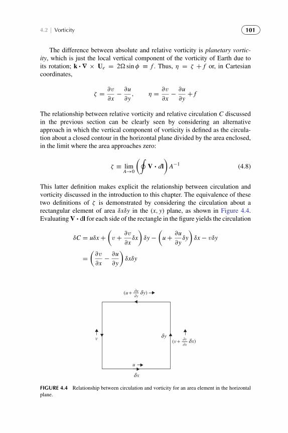
To protect the rights of the author(s) and publisher we inform you that this PDF is an uncorrected proof for internal businessuse only by the author(s), editor(s), reviewer(s), Elsevier and typesetter diacriTech. It is not allowed to publish this proofonline or in print. This proof copy is the copyright property of the publisher and is confidential until formal publication.
“Hakim: 08-ch04-095-126-9780123848666” — 2012/7/26 — 11:07 — page 101 — #7
4.2 | Vorticity 101
The difference between absolute and relative vorticity is planetary vortic-ity, which is just the local vertical component of the vorticity of Earth due toits rotation; k ·∇ × Ue = 2� sinφ ≡ f . Thus, η = ζ + f or, in Cartesiancoordinates,
ζ =∂v
∂x−∂u
∂y, η =
∂v
∂x−∂u
∂y+ f
The relationship between relative vorticity and relative circulation C discussedin the previous section can be clearly seen by considering an alternativeapproach in which the vertical component of vorticity is defined as the circula-tion about a closed contour in the horizontal plane divided by the area enclosed,in the limit where the area approaches zero:
ζ ≡ limA→0
(∮V · dl
)A−1 (4.8)
This latter definition makes explicit the relationship between circulation andvorticity discussed in the introduction to this chapter. The equivalence of thesetwo definitions of ζ is demonstrated by considering the circulation about arectangular element of area δxδy in the (x, y) plane, as shown in Figure 4.4.Evaluating V · dl for each side of the rectangle in the figure yields the circulation
δC = uδx+
(v +
∂v
∂xδx
)δy−
(u+
∂u
∂yδy
)δx− vδy
=
(∂v
∂x−∂u
∂y
)δxδy
v
u
δy
δx
(u + δy)∂u∂y
(v + δx)∂v∂x
FIGURE 4.4 Relationship between circulation and vorticity for an area element in the horizontalplane.

To protect the rights of the author(s) and publisher we inform you that this PDF is an uncorrected proof for internal businessuse only by the author(s), editor(s), reviewer(s), Elsevier and typesetter diacriTech. It is not allowed to publish this proofonline or in print. This proof copy is the copyright property of the publisher and is confidential until formal publication.
“Hakim: 08-ch04-095-126-9780123848666” — 2012/7/26 — 11:07 — page 102 — #8
102 CHAPTER | 4 Circulation, Vorticity, and Potential Vorticity
Dividing through by the area δA = δxδy gives
δC
δA=
(∂v
∂x−∂u
∂y
)≡ ζ
In more general terms the relationship between vorticity and circulation is givensimply by Stokes’s theorem applied to the velocity vector:∮
U · dl =∫∫A
(∇ × U) · nd A
Here A is the area enclosed by the contour and n is a unit normal to the areaelement d A (positive in the right sense). Thus, Stokes’s theorem states that thecirculation about any closed loop is equal to the integral of the normal compo-nent of vorticity over the area enclosed by the contour. Hence, for a finite area,circulation divided by area gives the average normal component of vorticity inthe region. As a consequence, the vorticity of a fluid in solid-body rotation isjust twice the angular velocity of rotation. Vorticity may thus be regarded as ameasure of the local angular velocity of the fluid.
4.2.1 Vorticity in Natural Coordinates
Physical interpretation of vorticity is facilitated by considering the vertical com-ponent of vorticity in the natural coordinate system (see Section 3.2.1). If wecompute the circulation about the infinitesimal contour shown in Figure 4.5, weobtain3
δC = V[δs+ d(δs)
]−
(V +
∂V
∂nδn
)δs
However, from this figure, d(δs) = δβδn, where δβ is the angular change in thewind direction in the distance δs. Hence,
δC =
(−∂V
∂n+ V
δβ
δs
)δn δs
or, in the limit δn, δs→ 0
ζ = limδn,δs→0
δC
(δn δs)= −
∂V
∂n+
V
Rs(4.9)
3Recall that n is a coordinate in the horizontal plane perpendicular to the local flow direction withpositive values to the left of an observer facing downstream.

To protect the rights of the author(s) and publisher we inform you that this PDF is an uncorrected proof for internal businessuse only by the author(s), editor(s), reviewer(s), Elsevier and typesetter diacriTech. It is not allowed to publish this proofonline or in print. This proof copy is the copyright property of the publisher and is confidential until formal publication.
“Hakim: 08-ch04-095-126-9780123848666” — 2012/7/26 — 11:07 — page 103 — #9
4.2 | Vorticity 103
v
v + δn∂v∂n
δn
d (δs)
δβ
n
δs
FIGURE 4.5 Circulation for an infinitesimal loop in the natural coordinate system.
(b)
(a)
FIGURE 4.6 Two types of two-dimensional flow: (a) linear shear flow with vorticity and(b) curved flow with zero vorticity.
where Rs is the radius of curvature of the streamlines [Eq. (3.20)]. It is nowapparent that the net vertical vorticity component is the result of the sum oftwo parts: (1) the rate of change of wind speed normal to the direction of flow–∂V/∂n, called the shear vorticity; and (2) the turning of the wind along astreamline V/Rs, called the curvature vorticity. Thus, even straight-line motionmay have vorticity if the speed changes normal to the flow axis. For example,in the jet stream shown schematically in Figure 4.6a, there will be cyclonic rela-tive vorticity north of the velocity maximum and anticyclonic relative vorticityto the south (Northern Hemisphere conditions), as is recognized easily when the

To protect the rights of the author(s) and publisher we inform you that this PDF is an uncorrected proof for internal businessuse only by the author(s), editor(s), reviewer(s), Elsevier and typesetter diacriTech. It is not allowed to publish this proofonline or in print. This proof copy is the copyright property of the publisher and is confidential until formal publication.
“Hakim: 08-ch04-095-126-9780123848666” — 2012/7/26 — 11:07 — page 104 — #10
104 CHAPTER | 4 Circulation, Vorticity, and Potential Vorticity
turning of a small paddle wheel placed in the flow is considered. The lower ofthe two paddle wheels in Figure 4.6a will turn in a clockwise direction (anticy-clonically) because the wind force on the blades north of its axis of rotationis stronger than the force on the blades to the south of the axis. The upperwheel will, of course, experience a counterclockwise (cyclonic) turning. Thus,the poleward and equatorward sides of a westerly jet stream are referred to asthe cyclonic and anticyclonic shear sides, respectively.
Conversely, curved flow may have zero vorticity provided that the shearvorticity is equal and opposite to the curvature vorticity. This is the case inthe example shown in Figure 4.6b, where a frictionless fluid with zero relativevorticity upstream flows around a bend in a canal. The fluid along the innerboundary on the curve flows faster in just the right proportion so that the paddlewheel does not turn.
4.3 THE VORTICITY EQUATION
The previous section discussed kinematic properties of vorticity. This sec-tion addresses vorticity dynamics using the equations of motion to determinecontributions to the time rate of change of vorticity.
4.3.1 Cartesian Coordinate Form
For motions of synoptic scale, the vorticity equation can be derived using theapproximate horizontal momentum equations (2.24) and (2.25). We differentiatethe zonal component equation with respect to y and the meridional componentequation with respect to x:
∂
∂y
(∂u
∂t+ u
∂u
∂x+ v
∂u
∂y+ w
∂u
∂z− f v = −
1
ρ
∂p
∂x
)(4.10)
∂
∂x
(∂v
∂t+ u
∂v
∂x+ v
∂v
∂y+ w
∂v
∂z+ fu = −
1
ρ
∂p
∂y
)(4.11)
Subtracting (4.10) from (4.11) and recalling that ζ = ∂v/∂x−∂u/∂y, we obtainthe vorticity equation
∂ζ
∂t+ u
∂ζ
∂x+ v
∂ζ
∂y+ w
∂ζ
∂z+ (ζ + f )
(∂u
∂x+∂v
∂y
)
+
(∂w
∂x
∂v
∂z−∂w
∂y
∂u
∂z
)+ v
df
dy=
1
ρ2
(∂ρ
∂x
∂p
∂y−∂ρ
∂y
∂p
∂x
) (4.12)

To protect the rights of the author(s) and publisher we inform you that this PDF is an uncorrected proof for internal businessuse only by the author(s), editor(s), reviewer(s), Elsevier and typesetter diacriTech. It is not allowed to publish this proofonline or in print. This proof copy is the copyright property of the publisher and is confidential until formal publication.
“Hakim: 08-ch04-095-126-9780123848666” — 2012/7/26 — 11:07 — page 105 — #11
4.3 | The Vorticity Equation 105
Using the fact that the Coriolis parameter depends only on y so that Df /Dt =v(df /dy), (4.12) may be rewritten in the form
D
Dt(ζ + f ) =−(ζ + f )
(∂u
∂x+∂v
∂y
)
−
(∂w
∂x
∂v
∂z−∂w
∂y
∂u
∂z
)+
1
ρ2
(∂ρ
∂x
∂p
∂y−∂ρ
∂y
∂p
∂x
) (4.13)
Equation (4.13) states that the rate of change of the absolute vorticity followingthe motion is given by the sum of the three terms on the right, called the diver-gence (or vortex stretching) term, the tilting or twisting term, and the solenoidalterm, respectively.
The concentration or dilution of vorticity by the divergence field—the firstterm on the right in (4.13)—is the fluid analog of the change in angular velocityresulting from a change in the moment of inertia of a solid body when angularmomentum is conserved. If the horizontal flow is divergent, the area enclosedby a chain of fluid parcels will increase with time, and if circulation is to beconserved, the average absolute vorticity of the enclosed fluid must decrease(i.e., the vorticity will be diluted). If, however, the flow is convergent, the areaenclosed by a chain of fluid parcels will decrease with time and the vorticity willbe concentrated. This mechanism for changing vorticity following the motion isvery important in synoptic-scale disturbances.
The second term on the right in (4.13) represents vertical vorticity generatedby the tilting of horizontally oriented components of vorticity into the vertical bya nonuniform vertical motion field. This mechanism is illustrated in Figure 4.7,
z
x
y
w
w
v
v
FIGURE 4.7 Vorticity generation by the tilting of a horizontal vorticity vector (double arrow).
To protect the rights of the author(s) and publisher we inform you that this PDF is an uncorrected proof for internal businessuse only by the author(s), editor(s), reviewer(s), Elsevier and typesetter diacriTech. It is not allowed to publish this proofonline or in print. This proof copy is the copyright property of the publisher and is confidential until formal publication.
“Hakim: 08-ch04-095-126-9780123848666” — 2012/7/26 — 11:07 — page 106 — #12
106 CHAPTER | 4 Circulation, Vorticity, and Potential Vorticity
which shows a region where the y component of velocity is increasing withheight so that there is a component of shear vorticity oriented in the negative xdirection as indicated by the double arrow. If at the same time there is a verticalmotion field in which w decreases with increasing x, advection by the verticalmotion will tend to tilt the vorticity vector initially oriented parallel to x so thatit has a component in the vertical. Thus, if ∂v/∂z > 0 and ∂w/∂x < 0, there willbe a generation of positive vertical vorticity.
Finally, the third term on the right in (4.13) is just the microscopic equivalentof the solenoidal term in the circulation theorem (4.5). To show this equivalence,we may apply Stokes’s theorem to the solenoidal term to get
−
∮αdp ≡ −
∮α∇p · dl = −
∫∫A
∇ × (α∇p) · kd A
where A is the horizontal area bounded by the curve l. Applying the vectoridentity ∇ × (α∇p) ≡ ∇α ×∇p, the equation becomes
−
∮αdp = −
∫∫A(∇α ×∇p) ·kd A
However, the solenoidal term in the vorticity equation can be written
−
(∂α
∂x
∂p
∂y−∂α
∂y
∂p
∂x
)= −(∇α ×∇p) · k
Thus, the solenoidal term in the vorticity equation is just the limit of the sole-noidal term in the circulation theorem divided by the area when the area goes tozero.
4.3.2 The Vorticity Equation in Isobaric Coordinates
A somewhat simpler form of the vorticity equation arises when the motion isreferred to the isobaric coordinate system. This equation can be derived in vectorform by operating on the momentum equation (3.2) with the vector operatork ·∇×, where ∇ now indicates the horizontal gradient on a surface of constantpressure. However, to facilitate this process it is desirable to first use the vectoridentity
(V ·∇)V = ∇(
V ·V2
)+ ζ k× V (4.14)
where ζ = k · (∇ × V), to rewrite (3.2) as
∂V∂t= −∇
(V ·V
2+8
)− (ζ + f )k× V− ω
∂V∂p
(4.15)

To protect the rights of the author(s) and publisher we inform you that this PDF is an uncorrected proof for internal businessuse only by the author(s), editor(s), reviewer(s), Elsevier and typesetter diacriTech. It is not allowed to publish this proofonline or in print. This proof copy is the copyright property of the publisher and is confidential until formal publication.
“Hakim: 08-ch04-095-126-9780123848666” — 2012/7/26 — 11:07 — page 107 — #13
4.3 | The Vorticity Equation 107
We now apply the operator k ·∇× to (4.15). Using the facts that for anyscalar A, ∇ ×∇A = 0 and for any vectors a, b,
∇ × (a× b) = (∇ ·b) a− (a ·∇)b− (∇ · a)b+ (b ·∇) a (4.16)
we can eliminate the first term on the right and simplify the second term so thatthe resulting vorticity equation becomes
∂ζ
∂t= −V ·∇ (ζ + f )− ω
∂ζ
∂p− (ζ + f )∇ ·V+ k ·
(∂V∂p×∇ω
)(4.17)
Comparing (4.13) and (4.17), we see that in the isobaric system there is no vor-ticity generation by pressure-density solenoids. This difference arises becausein the isobaric system, horizontal partial derivatives are computed with p heldconstant so that the vertical component of vorticity is ζ = (∂v/∂x − ∂u/∂y)p,whereas in height coordinates it is ζ = (∂v/∂x − ∂u/∂y)z. In practice the dif-ference is generally unimportant because, as shown in the next section, thesolenoidal term is usually sufficiently small so that it can be neglected forsynoptic-scale motions.
4.3.3 Scale Analysis of the Vorticity Equation
In Section 2.4 the equations of motion were simplified for synoptic-scalemotions by evaluating the order of magnitude of various terms. The same tech-nique can be applied to the vorticity equation. Characteristic scales for the fieldvariables based on typical observed magnitudes for synoptic-scale motions arechosen as follows:
U ∼ 10 m s−1 horizontal scale
W ∼ 1 cm s−1 vertical scale
L ∼ 106 m length scale
H ∼ 104 m depth scale
δp ∼ 10 hPa horizontal pressure scale
ρ ∼ 1 kg m−3 mean density
δρ/ρ ∼ 10−2 fractional density fluctuation
L/U ∼ 105 s time scale
f0 ∼ 10−4 s−1 Coriolis parameter
β ∼ 10−11 m−1 s−1 “beta” parameter
Again we have chosen an advective time scale because the vorticity pattern, likethe pressure pattern, tends to move at a speed comparable to the horizontal windspeed. Using these scales to evaluate the magnitude of the terms in (4.12), we

To protect the rights of the author(s) and publisher we inform you that this PDF is an uncorrected proof for internal businessuse only by the author(s), editor(s), reviewer(s), Elsevier and typesetter diacriTech. It is not allowed to publish this proofonline or in print. This proof copy is the copyright property of the publisher and is confidential until formal publication.
“Hakim: 08-ch04-095-126-9780123848666” — 2012/7/26 — 11:07 — page 108 — #14
108 CHAPTER | 4 Circulation, Vorticity, and Potential Vorticity
first note that
ζ =∂v
∂x−∂u
∂y.
U
L∼ 10−5s−1
where the inequality in this expression means less than or equal to in order ofmagnitude. Thus,
ζ/f0 . U/ (f0 L) ≡ Ro ∼ 10−1
For midlatitude synoptic-scale systems, the relative vorticity is often small(order Rossby number) compared to the planetary vorticity. For such systems, ζmay be neglected compared to f in the divergence term in the vorticity equation
(ζ + f )
(∂u
∂x+∂v
∂y
)≈ f
(∂u
∂x+∂v
∂y
)This approximation does not apply near the center of intense cyclonic storms.In such systems |ζ/f | ∼ 1, and the relative vorticity should be retained.
The magnitudes of the various terms in (4.12) can now be estimated as
∂ζ
∂t, u∂ζ
∂x, v∂ζ
∂y∼
U2
L2∼ 10−10 s−2
w∂ζ
∂z∼
WU
HL∼ 10−11 s−2
vdf
dy∼ Uβ ∼ 10−10 s−2
f
(∂u
∂x+∂v
∂y
).
f0U
L∼ 10−9 s−2
(∂w
∂x
∂v
∂z−∂w
∂y
∂u
∂z
).
WU
HL∼ 10−11 s−2
1
ρ2
(∂ρ
∂x
∂p
∂y−∂ρ
∂y
∂p
∂x
).δρδp
ρ2L2∼ 10−11 s−2
The inequality is used in the last three terms because in each case it is possiblethat the two parts of the expression might partially cancel so that the actualmagnitude would be less than indicated. In fact, this must be the case for thedivergence term (the fourth in the list) because if ∂u/∂x and ∂v/∂y were notnearly equal and opposite, the divergence term would be an order of magnitudegreater than any other term and the equation could not be satisfied. Therefore,scale analysis of the vorticity equation indicates that synoptic-scale motionsmust be quasi-nondivergent. The divergence term will be small enough to be

To protect the rights of the author(s) and publisher we inform you that this PDF is an uncorrected proof for internal businessuse only by the author(s), editor(s), reviewer(s), Elsevier and typesetter diacriTech. It is not allowed to publish this proofonline or in print. This proof copy is the copyright property of the publisher and is confidential until formal publication.
“Hakim: 08-ch04-095-126-9780123848666” — 2012/7/26 — 11:07 — page 109 — #15
4.3 | The Vorticity Equation 109
balanced by the vorticity advection terms only if∣∣∣∣(∂u
∂x+∂v
∂y
)∣∣∣∣ . 10−6 s−1
so that the horizontal divergence must be small compared to the vorticity insynoptic-scale systems. From the aforementioned scalings and the definition ofthe Rossby number, we see that∣∣∣∣(∂u
∂x+∂v
∂y
)/f0
∣∣∣∣ . Ro2
and ∣∣∣∣(∂u
∂x+∂v
∂y
)/ζ
∣∣∣∣ . Ro
Thus, the ratio of the horizontal divergence to the relative vorticity is the samemagnitude as the ratio of relative vorticity to planetary vorticity.
Retaining only the terms of order 10−10 s−2 in the vorticity equation yieldsthe approximate form valid for synoptic-scale motions,
Dh(ζ + f )
Dt= −f
(∂u
∂x+∂v
∂y
)(4.18)
where
Dh
Dt≡∂
∂t+ u
∂
∂x+ v
∂
∂y
As mentioned earlier, (4.18) is not accurate in intense cyclonic storms. For thesethe relative vorticity should be retained in the divergence term:
Dh (ζ + f )
Dt= −(ζ + f )
(∂u
∂x+∂v
∂y
)(4.19)
Equation (4.18) states that the change of absolute vorticity following the hori-zontal motion on the synoptic scale is given approximately by the concentrationor dilution of planetary vorticity caused by the convergence or divergence of thehorizontal flow, respectively. In (4.19), however, it is the concentration or dilu-tion of absolute vorticity that leads to changes in absolute vorticity followingthe motion.
The form of the vorticity equation given in (4.19) also indicates whycyclonic disturbances can be much more intense than anticyclones. For a fixedamplitude of convergence, relative vorticity will increase, and the factor (ζ + f )becomes larger, which leads to even higher rates of increase in the relative vor-ticity. For a fixed rate of divergence, however, relative vorticity will decrease,but when ζ → −f , the divergence term on the right approaches zero andthe relative vorticity cannot become more negative no matter how strong the

To protect the rights of the author(s) and publisher we inform you that this PDF is an uncorrected proof for internal businessuse only by the author(s), editor(s), reviewer(s), Elsevier and typesetter diacriTech. It is not allowed to publish this proofonline or in print. This proof copy is the copyright property of the publisher and is confidential until formal publication.
“Hakim: 08-ch04-095-126-9780123848666” — 2012/7/26 — 11:07 — page 110 — #16
110 CHAPTER | 4 Circulation, Vorticity, and Potential Vorticity
divergence. (This difference in the potential intensity of cyclones and anticy-clones was discussed in Section 3.2.5 in connection with the gradient windapproximation.)
The approximate forms given in (4.18) and (4.19) do not remain valid, how-ever, in the vicinity of atmospheric fronts. The horizontal scale of variation infrontal zones is only ∼100 km, and the vertical velocity scale is ∼10 cm s−1.For these scales, vertical advection, tilting, and solenoidal terms all may becomeas large as the divergence term.
4.4 POTENTIAL VORTICITY
We return now to circulation to show that Kelvin’s theorem applies to baroclinicdynamics for certain integration contours, which has very deep implications fordynamic meteorology. Rather than arbitrary closed contours, we now restrictthe possibilities to those that fall on isentropic surfaces, for which potentialtemperature is constant. We prove that for these contours, the solenoidal term isexactly zero.
With the aid of the ideal gas law (1.25), the definition of potential tempera-ture (2.44) can be expressed as a relationship between pressure and density fora surface of constant θ :
ρ = pcv/cp(Rθ)−1(ps)R/cp
Hence, on an isentropic surface, density is a function of pressure alone, and thesolenoidal term in the circulation theorem (4.3) vanishes;∮
dp
ρ∝
∮dp(1−cv/cp) = 0
For adiabatic and frictionless flow, then, the circulation computed for a closedchain of fluid parcels on a constant θ surface reduces to the same form as in abarotropic fluid; that is, it satisfies Kelvin’s circulation theorem even though thefluid is baroclinic!
From Stokes’s theorem, we may replace the circulation in favor of thecomponent of vorticity normal to the surface
Ca =
∮Ua · dl =
∫∫A
ωa ·n dA (4.20)
where n is a unit vector normal to the surface. Now we replace n and dA infavor of conserved quantities. Consider an infinitesimal cylinder (Figure 4.8)that is bounded above and below by constant potential temperature surfaces;for adiabatic flow, both the potential temperature and the mass of air in thiscylinder, dm, are conserved. A leading-order Taylor approximation across thecylinder gives dθ ≈ |∇θ |dh, where dh is the “height” of the cylinder. The mass

To protect the rights of the author(s) and publisher we inform you that this PDF is an uncorrected proof for internal businessuse only by the author(s), editor(s), reviewer(s), Elsevier and typesetter diacriTech. It is not allowed to publish this proofonline or in print. This proof copy is the copyright property of the publisher and is confidential until formal publication.
“Hakim: 08-ch04-095-126-9780123848666” — 2012/7/26 — 11:07 — page 111 — #17
4.4 | Potential Vorticity 111
δp
θ
θ + δθ
FIGURE 4.8 A cylindrical column of air moving adiabatically, conserving potential vorticity.
of air in the cylinder is given by dm = ρdAdh so that
dA =dm
ρ
|∇θ |
dθ(4.21)
Taking the infinitesimal cylinder to be sufficiently small so that the vorticitynormal to the surface is nearly constant,
DCa
Dt≈
D
Dt[ωa ·n dA] = 0 (4.22)
where
n =∇θ
|∇θ |(4.23)
Using (4.21) and (4.23) in (4.22), and noting that both dm and dθ are conservedfollowing the motion, gives
D
Dt
[ωa ·∇θ
ρ
]= 0 (4.24)
This celebrated equation, the Ertel potential vorticity theorem, is one of themost important theoretical results in dynamic meteorology. It says that thepotential vorticity, or PV,
5 =ωa ·∇θ
ρ(4.25)
is conserved following the motion.What makes this result so profound is that it links all of the basic physi-
cal conservation laws into a single expression. Although it may appear, as onestudies a fluid, that the momentum field fluctuates independently of the ther-modynamic fields, the potential vorticity places a powerful constraint on thosefluctuations: They must evolve in a way that preserves the PV following the
To protect the rights of the author(s) and publisher we inform you that this PDF is an uncorrected proof for internal businessuse only by the author(s), editor(s), reviewer(s), Elsevier and typesetter diacriTech. It is not allowed to publish this proofonline or in print. This proof copy is the copyright property of the publisher and is confidential until formal publication.
“Hakim: 08-ch04-095-126-9780123848666” — 2012/7/26 — 11:07 — page 112 — #18
112 CHAPTER | 4 Circulation, Vorticity, and Potential Vorticity
motion. Take, for example, the situation where the absolute vorticity vector hasno horizontal components so that the PV is given by
1
ρ
(∂v
∂x−∂u
∂y+ f
)∂θ
∂z(4.26)
In this case we see that the PV is the product of the absolute vorticity and thestatic stability so that if one increases, the other must decrease. This is illustratedin Figure 4.8: As the air parcel moves to the right, the static stability decreases,and as a result the vorticity must increase to conserve PV; the connections toangular momentum conservation and to vortex stretching are particularly clear.
The vertical contribution to the PV in (4.25) scales like Uθ∗ρHL +
f θ∗
H , whereθ∗ and ρ∗ are typical potential temperature and density scale values; the sec-ond term represents the contribution from planetary rotation. The horizontalcontribution—that is, from expanding (4.25)—scales like Uθ∗
ρ∗HL (neglectingthe small contribution from w), so that the ratio of vertical to horizontalcontributions is
1 + Ro−1 (4.27)
On synoptic and larger scales, where the Rossby number is small (roughly 0.1),this analysis shows that the dominant contribution to the PV comes from thevertical direction. This serves to explain why we focus on the vertical componentof vorticity in dynamic meteorology: Although the vorticity vector lies primarilyin the horizontal direction, the gradient of potential temperature is mainly in thevertical and this promotes the importance of vertical vorticity. A leading-orderapproximation to the PV is
5 ≈f
ρ
∂θ
∂z(4.28)
Picking typical values for the troposphere, we get an estimate of characteristicPV values of
5trop ∼=
(10−4s−1
1kg m−3
)(5 K km−1
)= 0.5× 10⁻⁶ K m2 s−1 kg−1
≡ 0.5 PVU
(4.29)
The definition “PVU” is a commonly adopted scaling of “PV Units” (1 PVU =10−6 K m2 s−1 kg−1). In the lower stratosphere, where ∂θ
∂z is an order of magni-tude larger, characteristic values of PV are larger as well.
Because there is an abrupt jump in PV values at the troposphere PV providesa useful dynamical definition for that interface. In fact, for adiabatic and friction-less conditions, when both PV and potential temperature are conserved, mapsof potential temperature on the “dynamical” tropopause (defined as a PV sur-face) provide a particularly useful summary of extratropical weather systems,

To protect the rights of the author(s) and publisher we inform you that this PDF is an uncorrected proof for internal businessuse only by the author(s), editor(s), reviewer(s), Elsevier and typesetter diacriTech. It is not allowed to publish this proofonline or in print. This proof copy is the copyright property of the publisher and is confidential until formal publication.
“Hakim: 08-ch04-095-126-9780123848666” — 2012/7/26 — 11:07 — page 113 — #19
4.4 | Potential Vorticity 113
5400300
300
(a) (b)
(c) (d)
FIGURE 4.9 Comparison of 500-hPa geopotential height (a) and tropopause maps of pressure(b) potential temperature (c) and wind speed (d) on January 12, 2012. Geopotential height is shownevery 60 m, potential temperature every 5 K, pressure every 50 hPa, and wind speed every 10 m s−1.Every fourth contour is shown bold except every second contour for wind speed. Gray arrows in(d) illustrate the path of the main branches of jet streams.
because the potential temperature contours are simply advected by the windon the tropopause. Moreover, compared to the alternative of PV contours onpotential temperature surfaces, a single map suffices to describe the state of thetropopause.
An example comparing the structure of the dynamical tropopause with aconventional map of 500-hPa geopotential height is shown in Figure 4.9. Famil-iar features on the 500 hPa chart include a long-wave pattern with a ridge overwestern North America and a trough over the center of the continent, and short-wave troughs near New York and approaching the Pacific coastline near theAlaska panhandle. In addition to the wave-like features, cyclonic vortices arelocated southwest of California, over Hudson Bay, and near Baffin Island.
Tropopause pressure (Figure 4.9b) reveals that troughs are regions where thetropopause is depressed to lower altitudes; in fact, the tropopause is below 500hPa in several of the troughs and vortices. Therefore, troughs are associated withlarge values of stratospheric potential vorticity that have been locally lowered toelevations normally considered tropospheric. In ridges and subtropical latitudes,the tropopause is elevated, with pressure values of 200 to 250 hPa, and thereforethe PV is anomalously low compared to the surroundings.

To protect the rights of the author(s) and publisher we inform you that this PDF is an uncorrected proof for internal businessuse only by the author(s), editor(s), reviewer(s), Elsevier and typesetter diacriTech. It is not allowed to publish this proofonline or in print. This proof copy is the copyright property of the publisher and is confidential until formal publication.
“Hakim: 08-ch04-095-126-9780123848666” — 2012/7/26 — 11:07 — page 114 — #20
114 CHAPTER | 4 Circulation, Vorticity, and Potential Vorticity
Tropopause potential temperature (Figure 4.9c) shows that most of thetroughs apparent in the 500-hPa chart are in fact vortical near their core. We mayinfer this by the appearance of closed potential temperature contours, since, ifpotential temperature and potential vorticity are conserved, air is trapped withinclosed tropopause potential temperature contours. For this reason, these fea-tures are sometimes called material eddies, since the only means of movingthe disturbance is to displace the material comprising it. This stands in con-trasts to waves, which may propagate information without net transport of themedium. In addition to the disturbances, notice the long ribbons where the hor-izontal gradient of tropopause potential temperature is concentrated into fronts,separated by zones that are mixed and filled with small-scale noise. Alongsome of these fronts—for example, the base of the trough in the central UnitedStates—the pressure field reveals that the tropopause is essentially vertical.
Finally, since jet streams are located near the tropopause, this perspective ismuch more useful than isobaric surfaces, which require several maps to depictjet streams located at different elevations. We see that a midlatitude jet reachesthe west coast of Canada before splitting into northern and southern branches;the southern branch also has a subtropical connection that is apparent near thesouthern edge of the domain (Figure 4.9d).
For completeness, we note that a form of the Ertel potential vorticity equa-tion may be derived that includes a source of momentum, F , such as frictionaldissipation, and a source of entropy,H, such as latent heating. The result is
D5
Dt=
ωa
ρ·∇H +
∇θ
ρ·
(∇ ×
Fρ
)(4.30)
where 5 is the Ertel PV defined by (4.25). The first right-side term is positive,where the vorticity vector points in the direction of a local maximum in theentropy source. This often occurs near extratropical cyclones, where clouds andprecipitation are found in the lower and midtroposphere (Figure 4.10a).
L
(a) (b)
> 0
L
∇θωa
−
−
+
FIGURE 4.10 Cartoon illustrating the role of sources of (a) entropy and (b) momentum on chang-ing the potential vorticity. (a) Depicts a precipitating cloud above a surface cyclone, where thevorticity vector, ω, points upward and to the right. Latent heating reaches a maximum in the cloud,which produces a positive (negative) PV tendency below (above) the cloud. (b) Depicts the role ofsurface friction (gray arrow opposite surface circulation). The curl of surface friction points in theopposite direction of the vorticity vector, producing a negative PV tendency.
To protect the rights of the author(s) and publisher we inform you that this PDF is an uncorrected proof for internal businessuse only by the author(s), editor(s), reviewer(s), Elsevier and typesetter diacriTech. It is not allowed to publish this proofonline or in print. This proof copy is the copyright property of the publisher and is confidential until formal publication.
“Hakim: 08-ch04-095-126-9780123848666” — 2012/7/26 — 11:07 — page 115 — #21
4.5 | Shallow Water Equations 115
In this case, near the surface the vertical component of vorticity pointsupward toward a maximum in latent heat release where condensation takesplace; above the maximum in heating, potential vorticity decreases because thevorticity vector and gradient in heating point in opposite directions. The sec-ond right-side term is positive where the curl of the frictional force points inthe same direction as the gradient in entropy. Again, appealing to extratropicalcyclones, assuming that surface friction acts opposite to the motion, the curlof friction is a vector that points in the opposite direction from the gradient inentropy, which produces a negative tendency to the Ertel PV (Figure 4.10b).
4.5 SHALLOW WATER EQUATIONS
In a homogeneous incompressible fluid, potential vorticity conservation takesa somewhat simpler form. To see this, we first derive the shallow water equa-tions, which provide a very useful simplification that we will use later to isolateessential aspects of atmospheric dynamics. Beyond constant density, the shal-low approximation implies that the depth of the fluid is small compared to thethe horizontal scale of the features of interest. As a result of this small aspectratio, we may use the hydrostatic approximation
∂p
∂z= ρ0g (4.31)
where ρ0 is a constant density. Integrating the hydrostatic equation over thedepth of the fluid, h(x, y), gives
p(z) = ρ0g(h− z)+ p(h) (4.32)
where p(h) is the pressure at the top of the layer of shallow water due to thelayer above, which we take to be a constant. Using (4.32) to replace pressure inthe momentum equation gives
DhVDt= −g∇hh − f k× V (4.33)
We assume that V is initially a function of (x, y) only, and since h is a functionof (x, y), (4.33) indicates that V will remain two-dimensional for all time.
Mass conservation for a constant density fluid has the simple form
∇·(u, v,w) = 0 (4.34)
Incompressibility also simplifies the first law of thermodynamics, since the fluidcan no longer do work. Therefore, if no heat is added, the temperature is constantfollowing the motion (see 2.41). Water pressure is a function of density andtemperature, p = f (T, ρ), but following the motion incompressibility implies

To protect the rights of the author(s) and publisher we inform you that this PDF is an uncorrected proof for internal businessuse only by the author(s), editor(s), reviewer(s), Elsevier and typesetter diacriTech. It is not allowed to publish this proofonline or in print. This proof copy is the copyright property of the publisher and is confidential until formal publication.
“Hakim: 08-ch04-095-126-9780123848666” — 2012/7/26 — 11:07 — page 116 — #22
116 CHAPTER | 4 Circulation, Vorticity, and Potential Vorticity
dp = ∂f∂T dT + ∂f
∂ρdρ = 0, so that
Dp
Dt= 0 (4.35)
Applying this fact to (4.32) yields
Dhh
Dt= w(h) (4.36)
where w = DzDt is the vertical motion, which is a function of (x, y, z). Integrating
(4.34) over depth h gives w(h) = −h∇h·V, which may be used to eliminate wfrom (4.36)
Dhh
Dt= −h∇h·V (4.37)
The shallow water equations consist of (4.33) and (4.37), which describe theevolution of three unknowns (u, v, h). Following a derivation similar to that inSection 4.3.1, the shallow water vorticity equation may be derived from (4.33)and yields
Dh
Dt(ζ + f ) = −(ζ + f )
(∂u
∂x+∂v
∂y
)(4.38)
In the shallow water system, absolute vorticity increases following the motionthrough vortex stretching.
Shallow water potential vorticity conservation is obtained by replacingdivergence on the right side of (4.38) using (4.37) to give
Dh
Dt
[ζ + f
h
]= 0 (4.39)
Thus, the shallow water potential vorticity,(ζ + f )/h, is given by the absolutevorticity divided by the fluid depth. Following the motion, if the absolute vor-ticity increases, then the depth of the fluid must as well. One may think of theinverse depth as an analog of static stability in shallow water by noting that thelayer top and bottom surfaces are isentropic surfaces. When the layer depth, h,becomes smaller, the isentropes are closer together.
Since the potential vorticity depends on x and y, only (4.39) provides a dra-matic simplification to the Ertel PV, which is very useful for gaining insightinto large-scale dynamics. For example, consider westerly flow impinging onan infinitely long topographic barrier as shown in Figure 4.11. We suppose thatflow upstream of the mountain barrier is uniform with ζ = 0. Each fluid col-umn of depth h is confined between constant entropy surfaces θ0 and θ0 + δθ
and remains between those surfaces as it crosses the barrier. Air that previouslycrossed the barrier leaves the upper surface higher near the mountain bothupstream and downstream, for reasons that will be explored in Chapter 5.

To protect the rights of the author(s) and publisher we inform you that this PDF is an uncorrected proof for internal businessuse only by the author(s), editor(s), reviewer(s), Elsevier and typesetter diacriTech. It is not allowed to publish this proofonline or in print. This proof copy is the copyright property of the publisher and is confidential until formal publication.
“Hakim: 08-ch04-095-126-9780123848666” — 2012/7/26 — 11:07 — page 117 — #23
4.5 | Shallow Water Equations 117
(b)
x
y
(a)
z
ζ = 0 ζ > 0 ζ > 0 ζ < 0
θ0 + δ0ζ < 0
xθ0
FIGURE 4.11 Schematic view of westerly flow over a topographic barrier: (a) the depth of a fluidcolumn as a function of x and (b) the trajectory of a parcel in the (x, y) plane.
As fluid columns approach the topographic barrier, they stretch vertically,which causes ζ to increase in order to conserve potential vorticity, (ζ + f )/h.Positive cyclonic vorticity is associated with cyclonic curvature in the flow,which causes a poleward drift so that f also increases; this in turn reduces thechange in ζ required for potential vorticity conservation. As the column beginsto cross the barrier, its vertical extent decreases, and the relative vorticity mustthen become negative. Thus, the air column will acquire anticyclonic vorticityand move southward.
When the air column has passed over the barrier and returned to its originaldepth, it will be south of its original latitude so that f will be smaller and therelative vorticity must be positive. Thus, the trajectory must have cyclonic cur-vature and the column will be deflected poleward. When the parcel returns againto its original latitude, it will still have a poleward velocity component and willcontinue poleward gradually, acquiring anticyclonic curvature until its directionis again reversed. The parcel will then move downstream, conserving potentialvorticity by following a wave-like trajectory in the horizontal plane. Therefore,steady westerly flow over a large-scale ridge will result in an anticyclonic flowover the mountain, a cyclonic flow pattern to the east of the barrier, followed bya wavetrain downstream.
The situation for easterly flow impinging on a mountain barrier is quite dif-ferent (Figure 4.12). Upstream stretching leads to a cyclonic turning of the flow,which results in an equatorward component of motion. As the column moveswestward and equatorward over the barrier, its depth contracts and its absolutevorticity must then decrease so that potential vorticity can be conserved. Thisreduction in absolute vorticity arises both from development of anticyclonicrelative vorticity and from a decrease in f due to the equatorward motion. Theanticyclonic relative vorticity gradually turns the column so that when it reaches

To protect the rights of the author(s) and publisher we inform you that this PDF is an uncorrected proof for internal businessuse only by the author(s), editor(s), reviewer(s), Elsevier and typesetter diacriTech. It is not allowed to publish this proofonline or in print. This proof copy is the copyright property of the publisher and is confidential until formal publication.
“Hakim: 08-ch04-095-126-9780123848666” — 2012/7/26 — 11:07 — page 118 — #24
118 CHAPTER | 4 Circulation, Vorticity, and Potential Vorticity
(b)
(a)
z
ζ = 0 ζ > 0 ζ > 0 ζ < 0
θ0 + δ0ζ < 0
x
θ0
x
y
FIGURE 4.12 As in Figure 4.11, but for easterly flow.
the top of the barrier, it is headed westward. As it continues westward down thebarrier, conserving potential vorticity, the process is simply reversed, with theresult that some distance downstream from the mountain barrier, the air columnis again moving westward at its original latitude.
Thus, the dependence of the Coriolis parameter on latitude creates a dramaticdifference between westerly and easterly flow over large-scale topographic bar-riers. In the case of a westerly wind, the barrier generates a wave-like disturbancein the streamlines that extends far downstream. However, in the case of aneasterly wind, the disturbance in the streamlines damps out away from the barrier.
4.5.1 Barotropic Potential Vorticity
Further simplification of potential vorticity is possible beyond the shallow waterequations by making the barotropic assumption. Recall that a barotropic fluid isdefined as one for which pressure depends only on density. For shallow water,(4.32) implies that in this case h and z are constant, so that w = 0 and the fluidis horizontally nondivergent
∂u
∂x+∂v
∂y= 0 (4.40)
Potential vorticity conservation simplifies to
Dh
Dt(ζ + f ) = 0 (4.41)

To protect the rights of the author(s) and publisher we inform you that this PDF is an uncorrected proof for internal businessuse only by the author(s), editor(s), reviewer(s), Elsevier and typesetter diacriTech. It is not allowed to publish this proofonline or in print. This proof copy is the copyright property of the publisher and is confidential until formal publication.
“Hakim: 08-ch04-095-126-9780123848666” — 2012/7/26 — 11:07 — page 119 — #25
4.5 | Shallow Water Equations 119
which states that absolute vorticity is conserved following the motion. Equation(4.41) is called the barotropic vorticity equation and has been widely used intheoretical studies of large-scale dynamical meteorology.
For nondivergent horizontal motion, the flow field can be represented by astreamfunction ψ (x, y) defined so that the velocity components are given asu = −∂ψ/∂y, v = +∂ψ/∂x. The vorticity is then given by
ζ = ∂v/∂x− ∂u/∂y = ∂2ψ/∂x2+ ∂2ψ/∂y2
≡ ∇2hψ
Thus, the velocity field and the vorticity can both be represented in terms ofthe variation of the single scalar field ψ (x, y), and (4.41) can be written as aprognostic equation for vorticity in the form
∂
∂t∇
2ψ = −Vψ ·∇(∇
2ψ + f)
(4.42)
where Vψ ≡ k×∇ψ is a nondivergent horizontal wind. Equation (4.42) statesthat the local tendency of relative vorticity is given by the advection of absolutevorticity. This equation can be solved numerically to predict the evolution ofthe streamfunction and thus of the vorticity and wind fields. Because the flowin the midtroposphere is often nearly nondivergent on the synoptic scale, (4.42)provides a surprisingly good model for short-term forecasts of the synoptic-scale 500-hPa flow field.
Conservation of absolute vorticity following the motion provides a strongconstraint on the flow, as can be shown by a simple example that again illustratesan asymmetry between westerly and easterly flow. Suppose that at a certainpoint (x0, y0) the flow is in the zonal direction and the relative vorticity van-ishes so that η(x0, y0) = f0. Then, if absolute vorticity is conserved, the motionat any point along a parcel trajectory that passes through (x0, y0) must satisfyζ + f = f0. Because f increases toward the north, trajectories that curve north-ward in the downstream direction must have ζ = f0−f < 0, whereas trajectoriesthat curve southward must have ζ = f0 − f > 0. However, as indicated inFigure 4.13, if the flow is westerly, northward curvature downstream impliesζ > 0, whereas southward curvature implies ζ < 0. Thus, westerly zonal flowmust remain purely zonal if absolute vorticity is to be conserved following themotion. The easterly flow case, also shown in Figure 4.13, is just the opposite.Northward and southward curvatures are associated with negative and positive
Easterly flowη conservedx
Westerly flowη not conserved
ζ > 0
ζ < 0ζ > 0
ζ < 0
FIGURE 4.13 Absolute vorticity conservation for curved flow trajectories.

To protect the rights of the author(s) and publisher we inform you that this PDF is an uncorrected proof for internal businessuse only by the author(s), editor(s), reviewer(s), Elsevier and typesetter diacriTech. It is not allowed to publish this proofonline or in print. This proof copy is the copyright property of the publisher and is confidential until formal publication.
“Hakim: 08-ch04-095-126-9780123848666” — 2012/7/26 — 11:07 — page 120 — #26
120 CHAPTER | 4 Circulation, Vorticity, and Potential Vorticity
relative vorticities, respectively. Hence, an easterly current can curve either tothe north or to the south and still conserve absolute vorticity.
4.6 ERTEL POTENTIAL VORTICITY IN ISENTROPICCOORDINATES
We consider here a more detailed treatment of the Ertel potential vorticityin isentropic coordinates, including nonconservative effects due to sources ofmomentum and entropy. We begin with a description of the basic conservationlaws in isentropic coordinates.
4.6.1 Equations of Motion in Isentropic Coordinates
If the atmosphere is stably stratified so that potential temperature θ is a mono-tonically increasing function of height, θ may be used as an independent verticalcoordinate. The vertical “velocity” in this coordinate system is just θ ≡ Dθ/Dt.Thus, adiabatic motions are two-dimensional when viewed in an isentropiccoordinate frame. An infinitesimal control volume in isentropic coordinates withcross-sectional area δA and vertical extent δθ has a mass
δM = ρδAδz = δA
(−δp
g
)=δA
g
(−∂p
∂θ
)δθ = σδAδθ (4.43)
Here the “density” in (x, y, θ) space is defined as
σ ≡ −g−1∂p/∂θ (4.44)
The horizontal momentum equation in isentropic coordinates may be obtainedby transforming the isobaric form (4.15) to yield
∂V∂t+∇θ
(V · V
2+9
)+ (ζθ + f )k× V = −θ
∂V∂θ+ Fr (4.45)
where ∇θ is the gradient on an isentropic surface, ζθ ≡ k ·∇θ × V is the isen-tropic relative vorticity, and 9 ≡ cpT + 8 is the Montgomery streamfunction(see Problem 2.11 in Chapter 2). We have included a frictional term Fr on theright side, along with the diabatic vertical advection term. The continuity equa-tion can be derived with the aid of (4.43) in a manner analogous to that used forthe isobaric system in Section 3.1.2. The result is
∂σ
∂t+∇θ · (σV) = −
∂
∂θ
(σ θ)
(4.46)
The 9 and σ fields are linked through the pressure field by the hydrostaticequation, which in the isentropic system takes the form
∂9
∂θ= 5(p) ≡ cp
(p
ps
)R/cp
= cpT
θ(4.47)

To protect the rights of the author(s) and publisher we inform you that this PDF is an uncorrected proof for internal businessuse only by the author(s), editor(s), reviewer(s), Elsevier and typesetter diacriTech. It is not allowed to publish this proofonline or in print. This proof copy is the copyright property of the publisher and is confidential until formal publication.
“Hakim: 08-ch04-095-126-9780123848666” — 2012/7/26 — 11:07 — page 121 — #27
4.6 | Ertel Potential Vorticity in Isentropic Coordinates 121
where 5 is called the Exner function. Equations (4.44) through (4.47) form aclosed set for prediction of V, σ , 9, and p, provided that θ and Fr are known.
4.6.2 The Potential Vorticity Equation
If we take k ·∇θ×(4.45) and rearrange the resulting terms, we obtain thisisentropic vorticity equation:
D
Dt(ζθ + f )+ (ζθ + f )∇θ ·V = k ·∇θ ×
(Fr − θ
∂V∂θ
)(4.48)
where
D
Dt=∂
∂t+ V ·∇θ
is the total derivative following the horizontal motion on an isentropic surface.Noting that σ−2∂σ/∂t = −∂σ−1/∂t, we can rewrite (4.46) in the form
D
Dt
(σ−1
)−
(σ−1
)∇θ ·V = σ−2 ∂
∂θ
(σ θ)
(4.49)
Multiplying each term in (4.48) by σ−1 and in (4.49) by (ζθ + f ) and adding,we obtain the desired conservation law:
D5
Dt=∂5
∂t+ V ·∇θ5 =
5
σ
∂
∂θ
(σ θ)+ σ−1k ·∇θ ×
(Fr − θ
∂V∂θ
)(4.50)
where 5 ≡ (ζθ + f )/σ is the Ertel potential vorticity. If the diabatic andfrictional terms on the right side of (4.50) can be evaluated, it is possible todetermine the evolution of 5 following the horizontal motion on an isentropicsurface. When the diabatic and frictional terms are small, potential vorticity isapproximately conserved following the motion on isentropic surfaces.
Weather disturbances that have sharp gradients in dynamical fields, such asjets and fronts, are associated with large anomalies in the Ertel potential vortic-ity. In the upper troposphere such anomalies tend to be advected rapidly undernearly adiabatic conditions. Thus, the potential vorticity anomaly patterns areconserved materially on isentropic surfaces. This material conservation prop-erty makes potential vorticity anomalies particularly useful in identifying andtracing the evolution of meteorological disturbances.
4.6.3 Integral Constraints on Isentropic Vorticity
The isentropic vorticity equation (4.48) can be written in the form
∂ζθ
∂t= −∇θ ·
[(ζθ + f
)V]+ k ·∇θ ×
(Fr − θ
∂V∂θ
)(4.51)

To protect the rights of the author(s) and publisher we inform you that this PDF is an uncorrected proof for internal businessuse only by the author(s), editor(s), reviewer(s), Elsevier and typesetter diacriTech. It is not allowed to publish this proofonline or in print. This proof copy is the copyright property of the publisher and is confidential until formal publication.
“Hakim: 08-ch04-095-126-9780123848666” — 2012/7/26 — 11:07 — page 122 — #28
122 CHAPTER | 4 Circulation, Vorticity, and Potential Vorticity
Using the fact that any vector A satisfies the relationship
k · (∇θ × A) = ∇θ · (A× k)
we can rewrite (4.51) in the form
∂ζθ
∂t= −∇θ ·
[(ζθ + f
)V−
(Fr − θ
∂V∂θ
)× k
](4.52)
Equation (4.52) expresses the remarkable fact that isentropic vorticity can onlybe changed by the divergence or convergence of the horizontal flux vector inbrackets on the right side. The vorticity cannot be changed by vertical trans-fer across the isentropes. Furthermore, integration of (4.52) over the area of anisentropic surface and application of the divergence theorem (Appendix C.2)show that for an isentrope that does not intersect the surface of Earth, the globalaverage of ζθ is constant. Furthermore, integration of ζθ over the sphere showsthat the global average ζθ is exactly zero. Vorticity on such an isentrope is nei-ther created nor destroyed; it is merely concentrated or diluted by horizontalfluxes along the isentropes.
SUGGESTED REFERENCES
Acheson, Elementary Fluid Dynamics, provides a good introduction to vorticity at a graduate level.Hoskins et al. provide an advanced discussion of Ertel potential vorticity and its uses in diagnosis
and prediction of synoptic-scale disturbances.Pedlosky, Geophysical Fluid Dynamics, provides a thorough treatment of circulation, vorticity, and
potential vorticity in Chapter 2.Vallis, Atmospheric and Oceanic Fluid Dynamics, discusses vorticity and potential vorticity in
Chapter 4.Williams and Elder, Fluid Physics for Oceanographers and Physicists, provides an introduction to
vorticity dynamics at an elementary level. This book also provides a good general introductionto fluid dynamics.
PROBLEMS
4.1. What is the circulation about a square of 1000 km on a side for an easterly(i.e., westward flowing) wind that decreases in magnitude toward the northat a rate of 10 m s−1 per 500 km? What is the mean relative vorticity in thesquare?
4.2. A cylindrical column of air at 30◦N with radius 100 km expands to twiceits original radius. If the air is initially at rest, what is the mean tangentialvelocity at the perimeter after expansion?
4.3. An air parcel at 30◦N moves northward, conserving absolute vorticity. If itsinitial relative vorticity is 5 × 10⁻⁵ s−1, what is its relative vorticity uponreaching 90◦N?
4.4. An air column at 60◦N with ζ = 0 initially stretches from the surface toa fixed tropopause at 10 km height. If the air column moves until it is

To protect the rights of the author(s) and publisher we inform you that this PDF is an uncorrected proof for internal businessuse only by the author(s), editor(s), reviewer(s), Elsevier and typesetter diacriTech. It is not allowed to publish this proofonline or in print. This proof copy is the copyright property of the publisher and is confidential until formal publication.
“Hakim: 08-ch04-095-126-9780123848666” — 2012/7/26 — 11:07 — page 123 — #29
Problems 123
over a mountain barrier 2.5 km high at 45◦N, what is its absolute vorticityand relative vorticity as it passes the mountain top, assuming that the flowsatisfies the barotropic potential vorticity equation?
4.5. Find the average vorticity within a cylindrical annulus of inner radius200 km and outer radius 400 km if the tangential velocity distribution isgiven by V = A/r, where A = 106 m2 s−1 and r is in meters. What is theaverage vorticity within the inner circle of radius 200 km?
4.6. Show that the anomalous gradient wind cases discussed in Section 3.2.5have negative absolute circulation in the Northern Hemisphere and thushave negative average absolute vorticity.
4.7. Compute the rate of change of circulation about a square in the (x, y) planewith corners at (0, 0), (0,L), (L,L), and (L, 0) if temperature increases east-ward at a rate of 1◦C per 200 km and presure increases northward at a rateof 1 hPa per 200 km. Let L = 1000 km and the pressure at the point (0, 0)be 1000 hPa.
4.8. Verify the identity (4.14) by expanding the vectors in Cartesian compo-nents.
4.9. Derive a formula for the dependence of depth on radius for an incom-pressible fluid in solid-body rotation in a cylindrical tank with a flat bottomand free surface at the upper boundary. Let H be the depth at the centerof the tank, � be the angular velocity of rotation of the tank, and a be theradius of the tank.
4.10. By how much does the relative vorticity change for a column of fluidin a rotating cylinder if the column is moved from the center of the tankto a distance 50 cm from the center? The tank is rotating at the rate of20 revolutions per minute, the depth of the fluid at the center is 10 cm, andthe fluid is initially in solid-body rotation.
4.11. A cyclonic vortex is in cyclostrophic balance with a tangential velocityprofile given by the expression V = V0(r/r0)
n, where V0 is the tangentialvelocity component at the distance r0 from the vortex center. Compute thecirculation about a streamline at radius r, the vorticity at radius r, and thepressure at radius r. (Let p0 be the pressure at r0 and assume that density isa constant.)
4.12. A westerly zonal flow at 45◦ is forced to rise adiabatically over a north–south-oriented mountain barrier. Before striking the mountain, the westerlywind increases linearly toward the south at a rate of 10 m s−1 per 1000 km.The crest of the mountain range is at 800 hPa and the tropopause, locatedat 300 hPa, remains undisturbed. What is the initial relative vorticity of theair? What is its relative vorticity when it reaches the crest if it is deflected5◦ latitude toward the south during the forced ascent? If the current assumesa uniform speed of 20 m s−1 during its ascent to the crest, what is the radiusof curvature of the streamlines at the crest?
4.13. A cylindrical vessel of radius a and constant depth H rotating at an angularvelocity � about its vertical axis of symmetry is filled with a homoge-neous, incompressible fluid that is initially at rest with respect to the vessel.A volume of fluid V is then withdrawn through a point sink at the cen-ter of the cylinder, thus creating a vortex. Neglecting friction, derive anexpression for the resulting relative azimuthal velocity as a function of

To protect the rights of the author(s) and publisher we inform you that this PDF is an uncorrected proof for internal businessuse only by the author(s), editor(s), reviewer(s), Elsevier and typesetter diacriTech. It is not allowed to publish this proofonline or in print. This proof copy is the copyright property of the publisher and is confidential until formal publication.
“Hakim: 08-ch04-095-126-9780123848666” — 2012/7/26 — 11:07 — page 124 — #30
124 CHAPTER | 4 Circulation, Vorticity, and Potential Vorticity
radius (i.e., the velocity in a coordinate system rotating with the tank).Assume that the motion is independent of depth and that V � πa2H. Alsocompute the relative vorticity and the relative circulation.
4.14. (a) How far must a zonal ring of air initially at rest with respect to Earth’ssurface at 60◦ latitude and 100-km height be displaced latitudinally toacquire an easterly (east to west) component of 10 m s−1 with respectto Earth’s surface?
(b) To what height must it be displaced vertically in order to acquire thesame velocity? Assume a frictionless atmosphere.
4.15. The horizontal motion within a cylindrical annulus with permeable wallsof inner radius 10 cm, outer radius 20 cm, and 10-cm depth is inde-pendent of height and azimuth and is represented by the expressionsu = 7 − 0.2r, v = 40 + 2r, where u and v are the radial and tangentialvelocity components in cm s−1, positive outward and counterclockwise,respectively, and r is distance from the center of the annulus in centimeters.Assuming an incompressible fluid, find(a) Circulation about the annular ring(b) Average vorticity within the annular ring(c) Average divergence within the annular ring(d) Average vertical velocity at the top of the annulus if it is zero at the
base4.16. Prove that, as stated in Eq. (4.52), the globally averaged isentropic vorticity
on an isentropic surface that does not intersect the ground must be zero.Show that the same result holds for the isobaric vorticity on an isobaricsurface.
MATLAB ExercisesM4.1. Equation 4.41 showed that for nondivergent horizontal motion, the flow field
can be represented by a streamfunction ψ (x, y), and the vorticity is then givenby ζ = ∂2ψ/∂x2
+ ∂2ψ/∂y2≡ ∇2ψ . Thus, if the vorticity is represented
by a single sinusoidal wave distribution in both x and y, the streamfunctionhas the same spatial distribution as the vorticity and the opposite sign, ascan be verified easily from the fact that the second derivative of a sine isproportional to minus the same sine function. An example is shown in theMATLAB script vorticity 1.m. However, when the vorticity pattern is localizedin space, the space scales of the streamfunction and vorticity are much differ-ent. This latter situation is illustrated in the MATLAB script vorticity demo.m,which shows the streamfunction corresponding to a point source of vorticityat (x, y) = (0, 0). For this problem you must modify the code in vorticity 1.mby specifying ζ (x, y) = exp
[−b
(x2+ y2
)]where b is a constant. Run the
model for several values of b from b = 1×10⁻⁴ km−2 to 4×10⁻⁷ km−2. Showin a table or line plot the dependence of the ratio of the horizontal scales onwhich vorticity and the streamfunction decay to one-half of their maximumvalues as a function of the parameter b. Note that for geostrophic motions(with constant Coriolis parameter), the streamfunction defined here is pro-portional to geopotential height. What can you conclude from this exerciseabout the information content of a 500-hPa height map versus that of a mapof the 500-hPa vorticity field?

To protect the rights of the author(s) and publisher we inform you that this PDF is an uncorrected proof for internal businessuse only by the author(s), editor(s), reviewer(s), Elsevier and typesetter diacriTech. It is not allowed to publish this proofonline or in print. This proof copy is the copyright property of the publisher and is confidential until formal publication.
“Hakim: 08-ch04-095-126-9780123848666” — 2012/7/26 — 11:07 — page 125 — #31
Problems 125
M4.2. The MATLAB scripts geowinds 1.m (to be used when the mapping toolbox isavailable) and geowinds 2.m (to be used if no mapping toolbox is available)contain contour plots showing the observed 500-hPa height and horizon-tal wind fields for November 10, 1998, in the North American sector. Alsoshown is a color plot of the magnitude of the 500-hPa wind with height con-tours superposed. Using centered difference formulas (see Section 13.2.1),compute the geostrophic wind components, the magnitude of the geostrophicwind, the relative vorticity, the vorticity of the geostrophic wind, and the vor-ticity minus the vorticity of the geostrophic wind. Following the models ofFigures 4.1 and 4.2, superpose these fields on the maps of the 500-hPa heightfield. Explain the distribution and the sign of regions with large differencesbetween vorticity and geostrophic vorticity in terms of the force balances thatwere studied in Chapter 3.

To protect the rights of the author(s) and publisher we inform you that this PDF is an uncorrected proof for internal businessuse only by the author(s), editor(s), reviewer(s), Elsevier and typesetter diacriTech. It is not allowed to publish this proofonline or in print. This proof copy is the copyright property of the publisher and is confidential until formal publication.
“Hakim: 09-ch05-127-170-9780123848666” — 2012/7/26 — 11:27 — page 127 — #1
Chapter 5
Atmospheric OscillationsLinear Perturbation Theory
If one is interested in producing an accurate forecast of the circulation at somefuture time, a detailed numerical model based on the primitive equations andincluding processes such as latent heating, radiative transfer, and boundary layerdrag should produce the best results. However, the inherent complexity of sucha model generally precludes any simple interpretation of the physical processesthat produce the predicted circulation. If we wish to gain physical insight intothe fundamental nature of atmospheric motions, it is helpful to employ simpli-fied models in which certain processes are omitted and compare the results withthose of more complete models. It is difficult to gain an appreciation for theprocesses that produce the wave-like character observed in many meteorolog-ical disturbances through the study of numerical integrations alone. Therefore,analytical treatment of idealized representations of the atmosphere are valuableand are the main topic of this chapter.
First, we discuss the perturbation method, a simple technique that is use-ful for qualitative analysis of atmospheric waves. We then use this method toexamine several types of waves in the atmosphere. In Chapters 6 and 7, theperturbation method is used to develop the quasi-geostrophic equations and tostudy the development of synoptic-wave disturbances, respectively.
5.1 THE PERTURBATION METHOD
In the perturbation method, all field variables are divided into two parts: a basicstate portion, which is usually assumed to be independent of time and longitude,and a perturbation portion, which is the local deviation of the field from thebasic state. Thus, for example, if u designates a time and longitude-averagedzonal velocity, and u′ is the deviation from that average, then the complete zonalvelocity field is u(x, t) = u + u′(x, t). In that case, for example, the inertialacceleration u∂u/∂x can be written
u∂u
∂x=(u+ u′
) ∂∂x
(u+ u′
)= u
∂u′
∂x+ u′
∂u′
∂x
An Introduction to Dynamic Meteorology. DOI: 10.1016/B978-0-12-384866-6.00005-2Copyright © 2013 Elsevier Inc. All rights reserved. 127

To protect the rights of the author(s) and publisher we inform you that this PDF is an uncorrected proof for internal businessuse only by the author(s), editor(s), reviewer(s), Elsevier and typesetter diacriTech. It is not allowed to publish this proofonline or in print. This proof copy is the copyright property of the publisher and is confidential until formal publication.
“Hakim: 09-ch05-127-170-9780123848666” — 2012/7/26 — 11:27 — page 128 — #2
128 CHAPTER | 5 Atmospheric Oscillations
The basic assumptions of perturbation theory are that the basic state vari-ables must themselves satisfy the governing equations when the perturbationsare set to zero, and the perturbation fields must be small enough so that allterms in the governing equations that involve products of the perturbations canbe neglected. Terms that depend linearly on perturbation fields drop by halfwhen the perturbation amplitude is cut in half, but terms that are quadratic inthe perturbation field become smaller by a factor of four. Therefore, the nonlin-ear terms become smaller faster than the linear terms and can be neglected inthe small-amplitude limit. If |u′/u| � 1, then∣∣u∂u′/∂x
∣∣� ∣∣u′∂u′/∂x∣∣
If terms that are products of the perturbation variables are neglected, thenonlinear governing equations are reduced to linear differential equations inthe perturbation variables in which the basic state variables are specified coeffi-cients. These equations can then be solved by standard methods to determine thecharacter and structure of the perturbations in terms of the known basic state.For equations with constant coefficients, the solutions are sinusoidal or expo-nential in character. Solution of perturbation equations then determines suchcharacteristics as the propagation speed, vertical structure, and conditions forgrowth or decay of the waves. The perturbation technique is especially useful instudying the stability of a given basic state flow with respect to small superposedperturbations. This application is the subject of Chapter 7.
5.2 PROPERTIES OF WAVES
Wave motions are oscillations in field variables (e.g., velocity and pressure)that propagate in space and time. In this chapter we are concerned with linearsinusoidal wave motions. Many of the mechanical properties of such waves arealso features of a familiar system, the linear harmonic oscillator. An importantproperty of the harmonic oscillator is that the period, or time required to exe-cute a single oscillation, is independent of the amplitude of the oscillation. Formost natural vibratory systems, this condition holds only for oscillations of suf-ficiently small amplitude. The classical example of such a system is the simplependulum (Figure 5.1) consisting of a mass M suspended by a massless stringof length l, free to perform small oscillations about the equilibrium positionθ = 0. The component of the gravity force parallel to the direction of motion is−Mg sin θ . Thus, the equation of motion for the mass M is
Mld2θ
dt2= −Mg sin θ
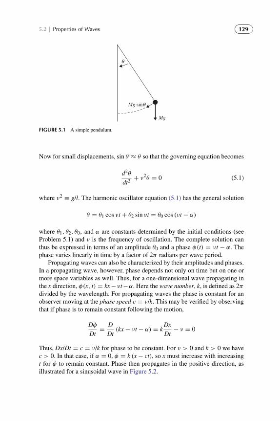
To protect the rights of the author(s) and publisher we inform you that this PDF is an uncorrected proof for internal businessuse only by the author(s), editor(s), reviewer(s), Elsevier and typesetter diacriTech. It is not allowed to publish this proofonline or in print. This proof copy is the copyright property of the publisher and is confidential until formal publication.
“Hakim: 09-ch05-127-170-9780123848666” — 2012/7/26 — 11:27 — page 129 — #3
5.2 | Properties of Waves 129
Mg
Mg sinθ
θ
FIGURE 5.1 A simple pendulum.
Now for small displacements, sin θ ≈ θ so that the governing equation becomes
d2θ
dt2+ ν2θ = 0 (5.1)
where ν2≡ g/l. The harmonic oscillator equation (5.1) has the general solution
θ = θ1 cos νt + θ2 sin νt = θ0 cos (νt − α)
where θ1, θ2, θ0, and α are constants determined by the initial conditions (seeProblem 5.1) and ν is the frequency of oscillation. The complete solution canthus be expressed in terms of an amplitude θ0 and a phase φ(t) = νt − α. Thephase varies linearly in time by a factor of 2π radians per wave period.
Propagating waves can also be characterized by their amplitudes and phases.In a propagating wave, however, phase depends not only on time but on one ormore space variables as well. Thus, for a one-dimensional wave propagating inthe x direction, φ(x, t) = kx−νt−α. Here the wave number, k, is defined as 2πdivided by the wavelength. For propagating waves the phase is constant for anobserver moving at the phase speed c ≡ ν/k. This may be verified by observingthat if phase is to remain constant following the motion,
Dφ
Dt=
D
Dt(kx− νt − α) = k
Dx
Dt− ν = 0
Thus, Dx/Dt = c = ν/k for phase to be constant. For ν > 0 and k > 0 we havec > 0. In that case, if α = 0, φ = k (x− ct), so x must increase with increasingt for φ to remain constant. Phase then propagates in the positive direction, asillustrated for a sinusoidal wave in Figure 5.2.

To protect the rights of the author(s) and publisher we inform you that this PDF is an uncorrected proof for internal businessuse only by the author(s), editor(s), reviewer(s), Elsevier and typesetter diacriTech. It is not allowed to publish this proofonline or in print. This proof copy is the copyright property of the publisher and is confidential until formal publication.
“Hakim: 09-ch05-127-170-9780123848666” — 2012/7/26 — 11:27 — page 130 — #4
130 CHAPTER | 5 Atmospheric Oscillations
π
−π
2π
0x
t = 0 ct = πct = π2
FIGURE 5.2 A sinusoidal wave traveling in the positive x direction at speed c. (Wave number isassumed to be unity.)
5.2.1 Fourier Series
The representation of a perturbation as a simple sinusoidal wave might seeman oversimplification, since disturbances in the atmosphere are never purelysinusoidal. It can be shown, however, that any reasonably well-behaved functionof longitude can be represented in terms of a zonal mean plus a Fourier seriesof sinusoidal components:
f (x) =∞∑
s=1
(As sin ksx+ Bs cos ksx) (5.2)
where ks = 2πs/L is the zonal wave number (units m−1), L is the distancearound a latitude circle, and s, the planetary wave number, is an integer des-ignating the number of waves around a latitude circle. The coefficients As arecalculated by multiplying both sides of (5.2) by sin(2πnx/L), where n is aninteger, and integrating around a latitude circle. Applying the orthogonalityrelationships
L∫0
sin2πsx
Lsin
2πnx
Ldx =
{0, s 6= nL/2, s = n
}
we obtain
As =2
L
L∫0
f (x) sin2πsx
Ldx
In a similar fashion, multiplying both sides in (5.2) by cos(2πnx/L) andintegrating gives
Bs =2
L
L∫0
f (x) cos2πsx
Ldx

To protect the rights of the author(s) and publisher we inform you that this PDF is an uncorrected proof for internal businessuse only by the author(s), editor(s), reviewer(s), Elsevier and typesetter diacriTech. It is not allowed to publish this proofonline or in print. This proof copy is the copyright property of the publisher and is confidential until formal publication.
“Hakim: 09-ch05-127-170-9780123848666” — 2012/7/26 — 11:27 — page 131 — #5
5.2 | Properties of Waves 131
As and Bs are called the Fourier coefficients, and
fs (x) = As sin ksx+ Bs cos ksx (5.3)
is called the sth Fourier component or sth harmonic of the function f (x). If theFourier coefficients are computed for, say, the longitudinal dependence of the(observed) geopotential perturbation, the largest-amplitude Fourier componentswill be those for which s is close to the observed number of troughs or ridgesaround a latitude circle. When only qualitative information is desired, it is usu-ally sufficient to limit the analysis to a single typical Fourier component andassume that the behavior of the actual field will be similar to that of the compo-nent. The expression for a Fourier component may be written more compactlyusing complex exponential notation. According to the Euler formula,
exp (iφ) = cosφ + i sinφ
where i ≡ (−1)1/2 is the imaginary unit. Thus, we can write
fs (x) = Re[Cs exp (iksx)]
= Re[Cs cos ksx+ iCs sin ksx](5.4)
where Re[ ] denotes “real part of” and Cs is a complex coefficient. Compar-ing (5.3) and (5.4), we see that the two representations of fs(x) are identical,provided that
Bs = Re[Cs] and As = −Im[Cs]
where Im[ ] stands for “imaginary part of.” This exponential notation will gen-erally be used for applications of the perturbation theory that follows and alsoin Chapter 7.
5.2.2 Dispersion and Group Velocity
A fundamental property of linear oscillators is that the frequency of oscillation νdepends only on the physical characteristics of the oscillator, not on the motionitself. For propagating waves, however, ν generally depends on the wave num-ber of the perturbation as well as the physical properties of the medium. Thus,because c = ν/k, the phase speed also depends on the wave number except in thespecial case where ν ∝ k. For waves in which the phase speed varies with k, thevarious sinusoidal components of a disturbance originating at a given locationare at a later time found in different places—that is, they are dispersed. Suchwaves are referred to as dispersive, and the formula that relates ν and k is calleda dispersion relationship. Some types of waves, such as acoustic waves, havephase speeds that are independent of the wave number. In such nondispersivewaves a spatially localized disturbance consisting of a number of Fourier wavecomponents (a wave group) will preserve its shape as it propagates in space atthe phase speed of the wave.

To protect the rights of the author(s) and publisher we inform you that this PDF is an uncorrected proof for internal businessuse only by the author(s), editor(s), reviewer(s), Elsevier and typesetter diacriTech. It is not allowed to publish this proofonline or in print. This proof copy is the copyright property of the publisher and is confidential until formal publication.
“Hakim: 09-ch05-127-170-9780123848666” — 2012/7/26 — 11:27 — page 132 — #6
132 CHAPTER | 5 Atmospheric Oscillations
For dispersive waves, however, the shape of a wave group will not remainconstant as the group propagates. Because the individual Fourier componentsof a wave group may either reinforce or cancel each other, depending on therelative phases of the components, the energy of the group will be concentratedin limited regions as illustrated in Figure 5.3. Furthermore, the group generallybroadens in the course of time—that is, the energy is dispersed.
When waves are dispersive, the speed of the wave group is generally differ-ent from the average phase speed of the individual Fourier components. Hence,as shown in Figure 5.4, individual wave components may move either morerapidly or more slowly than the wave group as the group propagates along.Surface waves in deep water (such as a ship wake) are characterized by disper-sion in which individual wave crests move twice as fast as the wave group. Insynoptic-scale atmospheric disturbances, however, the group velocity exceedsthe phase velocity. The resulting downstream development of new disturbanceswill be discussed later.
An expression for group velocity, which is the velocity at which theobservable disturbance (and thus the energy) propagates, can be derived asfollows: We consider the superposition of two horizontally propagating waves
FIGURE 5.3 Wave groups formed from two sinusoidal components of slightly different wave-lengths. For nondispersive waves, the pattern in the lower part of the diagram propagates withoutchange of shape. For dispersive waves, the shape of the pattern changes in time.
(a)
ct =0
ct =2π
ct =4π
ct =6π
(b)
ct =0
ct = π
ct =2π
ct =3π
FIGURE 5.4 Schematic showing propagation of wave groups: (a) group velocity less than phasespeed and (b) group velocity greater than phase speed. Heavy lines show group velocity, and lightlines show phase speed.
To protect the rights of the author(s) and publisher we inform you that this PDF is an uncorrected proof for internal businessuse only by the author(s), editor(s), reviewer(s), Elsevier and typesetter diacriTech. It is not allowed to publish this proofonline or in print. This proof copy is the copyright property of the publisher and is confidential until formal publication.
“Hakim: 09-ch05-127-170-9780123848666” — 2012/7/26 — 11:27 — page 133 — #7
5.2 | Properties of Waves 133
of equal amplitude but slightly different wavelengths, with wave numbers andfrequencies differing by 2δk and 2δν, respectively. The total disturbance is thus
9 (x, t) = exp {i [(k + δk) x− (ν + δν) t]} + exp {i [(k − δk) x− (ν − δν) t]}
where for brevity the Re[ ] notation in (5.4) is omitted and it is understood thatonly the real part of the right side has physical meaning. Rearranging terms andapplying the Euler formula gives
9 =[ei(δkx−δνt)
+ e−i(δkx−δνt)]
ei(kx−νt)
= 2 cos (δkx− δνt) ei(kx−νt)(5.5)
The disturbance (5.5) is the product of a high-frequency carrier wave ofwavelength 2π /k whose phase speed, ν/k, is the average for the two Fouriercomponents, and a low-frequency envelope of wavelength 2π /δk that travels atthe speed δν/δk. Thus, in the limit as δk → 0, the horizontal velocity of theenvelope, or group velocity, is just
cgx = ∂ν/∂k
The wave energy thus propagates at the group velocity. This result applies gen-erally to arbitrary wave envelopes provided that the wavelength of the wavegroup, 2π /δk, is large compared to the wavelength of the dominant component,2π /k.
5.2.3 Wave Properties in Two and Three Dimensions
Developing a complete understanding of wave properties in two and threedimensions is sufficiently important to the remainder of this chapter and aspectsof later chapters that we devote this section to a vector-oriented description ofwave properties. We discuss two dimensions for ease of presentation, but thenotation is sufficiently general that properties for three dimensions should beclear.
A two-dimensional plane wave in a scalar field, f , may be expressed as
f (x, y, t) = Re{
A ei(kx+ly−νt)}= Re
{A eiφ} (5.6)
Independent variables (x, y) and t represent space and time, respectively. k andl are the x and y wave numbers (m−1), and ν is the frequency (s−1). The waveis determined by amplitude, A (units of f ), and phase angle, φ. Note that φ is alinear function of the independent variables, and it proves useful to consider thespace and time properties of φ separately.
At any instant in time, φ = kx + ly + C, C constant, so φ is uniform alonglines of constant kx + ly. This implies dφ = ∂φ
∂x δx +∂φ∂y δy = 0 for φ constant.

To protect the rights of the author(s) and publisher we inform you that this PDF is an uncorrected proof for internal businessuse only by the author(s), editor(s), reviewer(s), Elsevier and typesetter diacriTech. It is not allowed to publish this proofonline or in print. This proof copy is the copyright property of the publisher and is confidential until formal publication.
“Hakim: 09-ch05-127-170-9780123848666” — 2012/7/26 — 11:27 — page 134 — #8
134 CHAPTER | 5 Atmospheric Oscillations
∇φ
0
(a) (b)
π2π
3π
x
y
L
LH
H1−1
−11
λ
x
y
FIGURE 5.5 Two-dimensional plane wave at a fixed time: (a) phase angle, φ, and (b) phase,eiφ . Wavelength is denoted λ. Note that if ν > 0, the wave travels in the direction of the wavevector, ∇φ.
Therefore, the slope of these lines is δyδx
∣∣φ= −k/l. Constant values of
eiφ= ei(φ+2πn) (5.7)
where n is an integer, define lines of constant phase, such as lows and highs(Figure 5.5). The wave vector is defined by
K = ∇φ (5.8)
K = |K| is the total wave number, and therefore λ = 2πK is the wavelength—that
is, the distance between lines of constant phase.At any fixed point in space, φ = C− νt, C constant, so φ is a linear function
of time. Therefore, frequency is defined as
ν = −∂φ
∂t(5.9)
which is the rate at which lines of constant phase pass a fixed point in space.The wave period is 2π
|ν|, which is the length of time between points of constant
phase (units: seconds). The wave phase speed (m s−1) is determined by howfast lines of constant phase move along the wave vector
c =ν
K= −
1
|∇φ|
∂φ
∂t(5.10)
This definition represents a generalization of phase speed from the one-dimensional example given in the previous section. In particular, for two andthree dimensions, the phase speed is not the same as cx =
νk and cy =
νl , which
define the rate at which phase lines travel along the x and y coordinate axes,respectively. Furthermore, c, cx, and cy do not satisfy rules of vector addition,so c2
6= c2x + c2
y .Note that, in general, φ and A may be complex numbers. If φ has an
imaginary part, φ = φr + iφi, then eiφ= ei(φr+iφi) = eiφr e−φi ≡ A∗eiφr . φr
is the wave phase angle as interpreted in the preceding, and A∗ = Ae−φi is

To protect the rights of the author(s) and publisher we inform you that this PDF is an uncorrected proof for internal businessuse only by the author(s), editor(s), reviewer(s), Elsevier and typesetter diacriTech. It is not allowed to publish this proofonline or in print. This proof copy is the copyright property of the publisher and is confidential until formal publication.
“Hakim: 09-ch05-127-170-9780123848666” — 2012/7/26 — 11:27 — page 135 — #9
5.2 | Properties of Waves 135
a modified amplitude that depends on time and/or space. For example, if thefrequency, ν, contributes the imaginary part, then the wave has time-dependentamplitude that grows or decays with time. Such waves are referred to asunstable to distinguish them from the neutral waves with fixed A. In Chapter 7we seek waves that grow in time, and therefore will study conditions thatcontribute to imaginary frequency.
We return now to group velocity, which provides the speed and direction inwhich an observer must travel in order to follow waves of a certain wavelengthand frequency. Rather than a pure plane wave, which exists over all space, wetake the phase angle, φ in (5.6), to be a slowly varying function of space andtime due to variable ν and K. Equations (5.8) and (5.9) define the wave vectorand frequency respectively, even when these quantities vary in space and time.Together, (5.8) and (5.9) imply
∂K∂t+∇ν = 0 (5.11)
Frequency is defined by a dispersion relationship, so that ν is a function of K.As such, ∇ν may be evaluated using the chain rule
∇ν = (∇kν ·∇)K (5.12)
where ∇kν =(∂ν∂k ,
∂ν∂l
)is the group velocity, Cg. Therefore, (5.11) can be
written as
∂K∂t+ (Cg·∇)K = 0 (5.13)
Consequently, in a frame of reference moving with the group velocity, the wavevector is conserved; that is, we follow a group of waves with fixed wavelengthand frequency.
5.2.4 A Wave Solution Strategy
Approximations to the full equations governing atmospheric dynamics will besolved for wave motions many times. Even though aspects of each individualcase are different, a guide to the general approach to solving these problems isas follows:
1. Choose a basic state The basic state is a simplified representation of theatmosphere. Typically we wish to eliminate all complications except thoseessential to the motions of interest. For example, in this chapter we will oftenmake use of basic states that are at rest and in hydrostatic balance. The basicstate is like a musical instrument, and we wish to know what tones naturallyemerge.
2. Linearize the governing equations Given a basic state, the governingequations can be linearized using the perturbation method of Section 5.1

To protect the rights of the author(s) and publisher we inform you that this PDF is an uncorrected proof for internal businessuse only by the author(s), editor(s), reviewer(s), Elsevier and typesetter diacriTech. It is not allowed to publish this proofonline or in print. This proof copy is the copyright property of the publisher and is confidential until formal publication.
“Hakim: 09-ch05-127-170-9780123848666” — 2012/7/26 — 11:27 — page 136 — #10
136 CHAPTER | 5 Atmospheric Oscillations
3. Assume wave solutions of the form in equation (5.6) If the coefficientsof the linearized equations do not depend on an independent variable, thenthe functions that depend on the independent variable may be representedas waves, eiφ , as in equation (5.6), provided that the independent variableis periodic. If, for example, the domain of interest is not periodic in the ydirection, or the basic state varies in y, then we cannot assume wave solu-tions in that direction. Instead, a general functional form must be assumedin that direction, such as F(y)ei(kx−νt), which typically leads to an ordinarydifferential equation that must be solved for the structure function F(y).
4. Solve for the dispersion and polarization relationships Substituting thewave form into the linearized governing equations typically results in asimpler closed set of algebraic equations or, in cases having nonconstantcoefficients, with a set of ordinary differential equations. Normally the wavenumber is taken as the independent variable, and the frequency is determinedas a function of the wave number; this gives the dispersion relationship. Thewave amplitude is unconstrained, but the relationships between variables,the polarization relations, must be determined. Variables are in phase if theyshare the same form and sign (e.g., sin(x)) and out of phase if they have thesame form and opposite sign (e.g., sin(x) and −sin(x)). If the variables are90◦ out of phase, they are in quadrature (e.g., sin(x) and cos(x)).
5.3 SIMPLE WAVE TYPES
Waves in fluids result from the action of restoring forces on fluid parcels thathave been displaced from their equilibrium positions. The restoring forces maybe due to compressibility, gravity, rotation, or electromagnetic effects. This sec-tion considers the two simplest examples of linear waves in fluids: acousticwaves and shallow water gravity waves.
5.3.1 Acoustic or Sound Waves
Sound waves, or acoustic waves, are longitudinal waves. That is, they are wavesin which the particle oscillations are parallel to the direction of propagation.Sound is propagated by the alternating adiabatic compression and expansion ofthe medium. As an example, Figure 5.6 shows a schematic section along a tubethat has a diaphragm at its left end. If the diaphragm is set into vibration, theair adjacent to it will be alternately compressed and expanded as the diaphragmmoves inward and outward. The resulting oscillating pressure gradient forcewill be balanced by an oscillating acceleration of the air in the adjoining region,which will cause an oscillating pressure oscillation further into the tube, andso on. The result of this continual adiabatic increase and decrease of pressurethrough alternating compression and rarefaction is, as shown in Figure 5.6, asinusoidal pattern of pressure and velocity perturbations that propagates to theright down the tube. Individual air parcels do not, however, have a net rightward
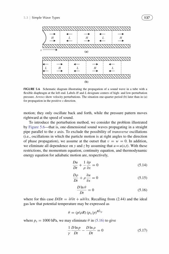
To protect the rights of the author(s) and publisher we inform you that this PDF is an uncorrected proof for internal businessuse only by the author(s), editor(s), reviewer(s), Elsevier and typesetter diacriTech. It is not allowed to publish this proofonline or in print. This proof copy is the copyright property of the publisher and is confidential until formal publication.
“Hakim: 09-ch05-127-170-9780123848666” — 2012/7/26 — 11:27 — page 137 — #11
5.3 | Simple Wave Types 137
x (a)
(b)
H L H HL
L H HL L
FIGURE 5.6 Schematic diagram illustrating the propagation of a sound wave in a tube with aflexible diaphragm at the left end. Labels H and L designate centers of high- and low-perturbationpressure. Arrows show velocity perturbations. The situation one-quarter period (b) later than in (a)for propagation in the positive x direction.
motion; they only oscillate back and forth, while the pressure pattern movesrightward at the speed of sound.
To introduce the perturbation method, we consider the problem illustratedby Figure 5.6—that is, one-dimensional sound waves propagating in a straightpipe parallel to the x axis. To exclude the possibility of transverse oscillations(i.e., oscillations in which the particle motion is at right angles to the directionof phase propagation), we assume at the outset that v = w = 0. In addition,we eliminate all dependence on y and z by assuming that u=u(x,t). With theserestrictions, the momentum equation, continuity equation, and thermodynamicenergy equation for adiabatic motion are, respectively,
Du
Dt+
1
ρ
∂p
∂x= 0 (5.14)
Dρ
Dt+ ρ
∂u
∂x= 0 (5.15)
D ln θ
Dt= 0 (5.16)
where for this case D/Dt = ∂/∂t + u∂/∂x. Recalling from (2.44) and the idealgas law that potential temperature may be expressed as
θ = (p/ρR) (ps/p)R/cp
where ps = 1000 hPa, we may eliminate θ in (5.16) to give
1
γ
D ln p
Dt−
D ln ρ
Dt= 0 (5.17)

To protect the rights of the author(s) and publisher we inform you that this PDF is an uncorrected proof for internal businessuse only by the author(s), editor(s), reviewer(s), Elsevier and typesetter diacriTech. It is not allowed to publish this proofonline or in print. This proof copy is the copyright property of the publisher and is confidential until formal publication.
“Hakim: 09-ch05-127-170-9780123848666” — 2012/7/26 — 11:27 — page 138 — #12
138 CHAPTER | 5 Atmospheric Oscillations
where γ = cp/cv . Eliminating ρ between (5.15) and (5.17) gives
1
γ
D ln p
Dt+∂u
∂x= 0 (5.18)
The dependent variables are now divided into constant basic state portions(denoted by overbars) and perturbation portions (denoted by primes):
u(x, t) = u+ u′(x, t)
p(x, t) = p+ p′(x, t)
ρ(x, t) = ρ + ρ′(x, t)
(5.19)
Substituting (5.19) into (5.14) and (5.18) we obtain
∂
∂t
(u+ u′
)+(u+ u′
) ∂∂x
(u+ u′
)+
1
(ρ + ρ′)
∂
∂x
(p+ p′
)= 0
∂
∂t
(p+ p′
)+(u+ u′
) ∂∂x
(p+ p′
)+ γ
(p+ p′
) ∂∂x
(u+ u′
)= 0
We next observe that provided∣∣ρ′/ ρ∣∣ � 1, we can use the binomial expansion
to approximate the density term as
1
(ρ + ρ′)=
1
ρ
(1+
ρ′
ρ
)−1
≈1
ρ
(1−
ρ′
ρ
)Neglecting products of the perturbation quantities and noting that the basic statefields are constants, we obtain the linear perturbation equations1(
∂
∂t+ u
∂
∂x
)u′ +
1
ρ
∂p′
∂x= 0 (5.20)
(∂
∂t+ u
∂
∂x
)p′ + γ p
∂u′
∂x= 0 (5.21)
Eliminating u′ by operating on (5.21) with (∂/∂t + u∂/∂x) and substitutingfrom (5.20), we get2 (
∂
∂t+ u
∂
∂x
)2
p′ −γ p
ρ
∂2p′
∂x2= 0 (5.22)
1It is not necessary that the perturbation velocity be small compared to the mean velocity for lin-earization to be valid. It is only required that quadratic terms in the perturbation variables be smallcompared to the dominant linear terms in (5.20) and (5.21).2Note that the squared differential operator in the first term expands in the usual way as(
∂
∂t+ u
∂
∂x
)2=∂2
∂t2+ 2u
∂2
∂t∂x+ u2 ∂
2
∂x2

To protect the rights of the author(s) and publisher we inform you that this PDF is an uncorrected proof for internal businessuse only by the author(s), editor(s), reviewer(s), Elsevier and typesetter diacriTech. It is not allowed to publish this proofonline or in print. This proof copy is the copyright property of the publisher and is confidential until formal publication.
“Hakim: 09-ch05-127-170-9780123848666” — 2012/7/26 — 11:27 — page 139 — #13
5.3 | Simple Wave Types 139
which is a form of the standard wave equation familiar from electromagnetictheory. A simple solution representing a plane sinusoidal wave propagating inx is
p′ = A exp [ik (x− ct)] (5.23)
where for brevity we omit the Re{ } notation, but it is to be understood thatonly the real part of (5.23) has physical significance. Substituting the assumedsolution (5.23) into (5.22), we find that the phase speed c must satisfy
(−ikc+ iku)2 − (γ p/ ρ) (ik)2 = 0
where we have canceled out the factor A exp [ik (x− ct)], which is common toboth terms. Solving for c gives
c = u± (γ p/ ρ)1/2 = u±(γRT
)1/2(5.24)
Therefore, (5.23) is a solution of (5.22), provided that the phase speed satisfies(5.24). According to (5.24), the speed of wave propagation relative to the zonal
current is c − u = ±cs, where cs ≡(γRT
)1/2is called the adiabatic speed of
sound.The mean zonal velocity here plays only a role of Doppler shifting the sound
wave so that the frequency relative to the ground corresponding to a given wavenumber k is
ν = kc = k (u± cs)
Thus, in the presence of a wind, the frequency as heard by a fixed observerdepends on the location of the observer relative to the source. If u > 0, thefrequency of a stationary source will appear to be higher for an observer to theeast (downstream) of the source (c = u + cs) than for an observer to the west(upstream) of the source c = u− cs.
5.3.2 Shallow Water Waves
The second example of pure wave motion concerns the horizontally propagat-ing oscillations known as shallow water waves. This analysis provides a clearintroduction to the primary wave motions in the extratropical latitudes: Rossbywaves and gravity waves.
We linearize the shallow water equations (derived in Section 4.5) for aresting basic state having water depth h and fixed ambient rotation given bya constant Coriolis parameter f . The linearized momentum (4.33) and mass

To protect the rights of the author(s) and publisher we inform you that this PDF is an uncorrected proof for internal businessuse only by the author(s), editor(s), reviewer(s), Elsevier and typesetter diacriTech. It is not allowed to publish this proofonline or in print. This proof copy is the copyright property of the publisher and is confidential until formal publication.
“Hakim: 09-ch05-127-170-9780123848666” — 2012/7/26 — 11:27 — page 140 — #14
140 CHAPTER | 5 Atmospheric Oscillations
continuity (4.37) equations are
∂u′
∂t= −g
∂h′
∂x+ f v′
∂v′
∂t= −g
∂h′
∂y− fu′
∂h′
∂t= −h
(∂u′
∂x+∂v′
∂y
)(5.25)
Primes denote perturbation values—that is, departures from the state of rest.(5.25) represent a set of three coupled first-order partial differential equations inthe unknowns, u′, v′, h′. One approach to solving these equations is to form andsolve a single third-order partial differential equation. This is accomplished bytaking ∂/∂t of the third equation in (5.25), which gives
∂2h′
∂t2= −h
(∂2u′
∂t∂x+∂2v′
∂t∂y
)(5.26)
The terms on the right side of (5.26) may be replaced using the first twoequations of (5.25):
∂2h′
∂t2= h
(g∇2
hh′ − f ζ ′)
(5.27)
Again take ∂/∂t, which gives the third-order equation
∂3h′
∂t3+
(f 2− gh∇2
h
) ∂h′
∂t= 0 (5.28)
where ∂ζ ′/∂t is replaced using the linearized version of (4.38) (noting that f istaken constant here):
∂ζ ′
∂t= −f
(∂u′
∂x+∂v′
∂y
)(5.29)
Assuming that the lateral boundaries are periodic and, since the coefficients fand gh are constant, we may assume wave solutions of the form
h′ = Re{
Aei(kx+ly−νt)} (5.30)
Using (5.30) in (5.28) gives a cubic polynomial for the frequency
ν3− ν
[f 2+ gh
(k2+ l2
)]= 0 (5.31)

To protect the rights of the author(s) and publisher we inform you that this PDF is an uncorrected proof for internal businessuse only by the author(s), editor(s), reviewer(s), Elsevier and typesetter diacriTech. It is not allowed to publish this proofonline or in print. This proof copy is the copyright property of the publisher and is confidential until formal publication.
“Hakim: 09-ch05-127-170-9780123848666” — 2012/7/26 — 11:27 — page 141 — #15
5.3 | Simple Wave Types 141
This is the dispersion relationship for shallow water waves. Clearly ν = 0 is asolution, and if ν 6= 0, then
ν2= f 2+ gh
(k2+ l2
)(5.32)
For readers familiar with linear algebra, we note an alternative solutionmethod. Taking solutions of the form (5.30) for h′, u′, and v′, and substitutingdirectly into (5.25), converts the set of partial differential equations to algebraicequations that may be written as
Ax = 0 (5.33)
where x is the column vector of the unknowns [u′v′h′]T, and
A =
−iν −f ikg
f −iν ilg
hk −hl −ν
(5.34)
A nontrivial solution to (5.33) is obtained only if A is not invertible. This isenforced by setting the determinant of A to zero, which gives (5.31).
Turning now to the structure of the waves, consider first the case whereν = 0. Appealing to (5.25), we see that since the waves are stationary, the leftsides are zero. Clearly, these waves depend on rotation, since when f = 0, thewave amplitude, A, must also be zero. For non zero f , (5.25) implies
v′ =g
f
∂h
∂x
u′ = −g
f
∂h
∂y
(5.35)
The stationary waves are in a state of geostrophic balance and are an exampleof Rossby waves in the limit of constant Coriolis parameter. The case of propa-gating Rossby waves, with nonconstant Coriolis parameter, will be explored inSection 5.7.
Solutions for ν 6= 0 are called inertia–gravity waves, since particle oscilla-tions depend on both gravitational and inertial forces. The inertial aspect will bediscussed in Section 5.7 so that we may focus here on the gravitational aspect.In the limiting case f = 0, we have simply gravity waves, and from (5.32) thewave speed becomes
c =√
gh (5.36)
Since the waves all move at the same speed, they are nondispersive. For afluid h = 4 km deep, the shallow water gravity wave speed is approximately200 m s−1. Thus, long waves on the ocean surface travel very rapidly. It shouldbe emphasized again that this theory applies only to waves of wavelength
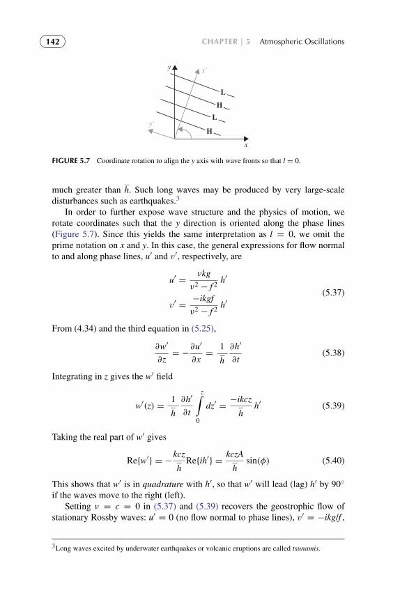
To protect the rights of the author(s) and publisher we inform you that this PDF is an uncorrected proof for internal businessuse only by the author(s), editor(s), reviewer(s), Elsevier and typesetter diacriTech. It is not allowed to publish this proofonline or in print. This proof copy is the copyright property of the publisher and is confidential until formal publication.
“Hakim: 09-ch05-127-170-9780123848666” — 2012/7/26 — 11:27 — page 142 — #16
142 CHAPTER | 5 Atmospheric Oscillations
L
L
H
H
x
y x'
y'
FIGURE 5.7 Coordinate rotation to align the y axis with wave fronts so that l = 0.
much greater than h. Such long waves may be produced by very large-scaledisturbances such as earthquakes.3
In order to further expose wave structure and the physics of motion, werotate coordinates such that the y direction is oriented along the phase lines(Figure 5.7). Since this yields the same interpretation as l = 0, we omit theprime notation on x and y. In this case, the general expressions for flow normalto and along phase lines, u′ and v′, respectively, are
u′ =νkg
ν2 − f 2h′
v′ =−ikgf
ν2 − f 2h′
(5.37)
From (4.34) and the third equation in (5.25),
∂w′
∂z= −
∂u′
∂x=
1
h
∂h′
∂t(5.38)
Integrating in z gives the w′ field
w′(z) =1
h
∂h′
∂t
z∫0
dz′ =−ikcz
hh′ (5.39)
Taking the real part of w′ gives
Re{w′} = −kcz
hRe{ih′} =
kczA
hsin(φ) (5.40)
This shows that w′ is in quadrature with h′, so that w′ will lead (lag) h′ by 90◦
if the waves move to the right (left).Setting ν = c = 0 in (5.37) and (5.39) recovers the geostrophic flow of
stationary Rossby waves: u′ = 0 (no flow normal to phase lines), v′ = −ikg/f ,
3Long waves excited by underwater earthquakes or volcanic eruptions are called tsunamis.

To protect the rights of the author(s) and publisher we inform you that this PDF is an uncorrected proof for internal businessuse only by the author(s), editor(s), reviewer(s), Elsevier and typesetter diacriTech. It is not allowed to publish this proofonline or in print. This proof copy is the copyright property of the publisher and is confidential until formal publication.
“Hakim: 09-ch05-127-170-9780123848666” — 2012/7/26 — 11:27 — page 143 — #17
5.3 | Simple Wave Types 143
Wavemotion
FIGURE 5.8 Depiction of shallow water gravity wave height and velocity fields for the case wherethe coordinates have been rotated as shown in Figure 5.7.
and w = 0. For the inertia gravity waves (ν 6= 0), notice that the flow alongphase lines is zero in the absence of ambient rotation. In that case, the physicsof wave propagation is particularly clear. From (5.32) we see that ν2
− f 2 isstrictly positive, and in the rotated coordinates, u′ = c/h. This shows that the u′
field is either in phase, or out of phase, with the h′ field depending on the sign ofc. Waves that move to the right (c > 0) are shown in Figure 5.8. Convergenceand divergence of the u field raise and lower the height of the fluid, respectively,moving the wave to the right in Figure 5.8. As expected from mass conservation,the w field exhibits rising motion near convergence, which increases linearlywith height from zero at the bottom boundary. Changing the sign of c has noeffect on h′, but reverses the u and w fields so that the wave moves to the left.
Finally, consider the vorticity and potential vorticity (PV) of the waves inthe rotated coordinates. Since there is no variation in the y direction, the relativevorticity is simply
ζ ′ =∂v′
∂x=
k2g f
ν2 − f 2h′ (5.41)
A linearized version of the shallow water potential vorticity equation (4.39) isobtained from (5.29) and the third equation in (5.25), which yields
∂
∂t
[ζ ′ −
f
hh′]= 0 (5.42)
Linearization has removed all advection terms from the PV conservationequation, so that (5.42) states that the linearized PV
Q′ = ζ ′ −f
hh′ (5.43)
is conserved locally, at every point in space. This is an extremely powerfulconstraint on the linear dynamics, which we will exploit in Section 5.6 whensolving initial-vale problems for (5.25).
For shallow water Rossby waves, vorticity in the rotated coordinates becomes
ζ ′RW = −k2g
fh′ (5.44)

To protect the rights of the author(s) and publisher we inform you that this PDF is an uncorrected proof for internal businessuse only by the author(s), editor(s), reviewer(s), Elsevier and typesetter diacriTech. It is not allowed to publish this proofonline or in print. This proof copy is the copyright property of the publisher and is confidential until formal publication.
“Hakim: 09-ch05-127-170-9780123848666” — 2012/7/26 — 11:27 — page 144 — #18
144 CHAPTER | 5 Atmospheric Oscillations
which is out of phase with the height field and larger for shorter waves. Rossbywave PV is given by ζ reduced by f
hh′, which has the same sign as ζ except for
unrealistically long waves.For shallow water inertia–gravity waves, vorticity in the rotated coordinates
becomes
ζ ′GW =f
hh′ (5.45)
which is in phase with the height field, and nonzero provided there exists ambi-ent rotation. From (5.45) and (5.43), it is clear that inertia–gravity wave PV isidentically zero.
A summary of the essential differences between Rossby and inertia–gravitywaves for rotating shallow water follows:
l Rossby waves are stationary for f constant, whereas inertia–gravity wavesmove very fast.
l Inertia–gravity waves have small relative vorticity but are strongly diver-gent, whereas Rossby waves have geostrophic winds with zero divergenceand large relative vorticity.
l Inertia–gravity waves have zero potential vorticity, whereas Rossby wavesgenerally have nonzero potential vorticity.
These properties generalize to waves in a stratified atmosphere, considered inthe next two sections. They provide a useful framework for eliminating inertia–gravity waves from the full nonlinear equations, yielding the quasi-geostrophicequations, which we use to understand the dynamics of extratropical weathersystems in Chapters 6 and 7.
5.4 INTERNAL GRAVITY (BUOYANCY) WAVES
The nature of gravity wave propagation in the stratified atmosphere is con-sidered now in the absence of ambient rotation. Atmospheric gravity wavescan only exist when the atmosphere is stably stratified so that a fluid par-cel displaced vertically will undergo buoyancy oscillations (see Section 2.7.3).Because the buoyancy force is the restoring force responsible for gravity waves,the term buoyancy wave is actually more appropriate as a name for these waves.However, in this text we will generally use the traditional name gravity wave.
In a fluid, such as the ocean, which is bounded both above and below, grav-ity waves propagate primarily in the horizontal plane, since vertically travelingwaves are reflected from the boundaries to form standing waves. However,in a fluid that has no upper boundary, such as the atmosphere, gravity wavesmay propagate vertically as well as horizontally. In vertically propagatingwaves the phase is a function of height. Such waves are referred to as internalwaves. Although internal gravity waves are not generally of great importance

To protect the rights of the author(s) and publisher we inform you that this PDF is an uncorrected proof for internal businessuse only by the author(s), editor(s), reviewer(s), Elsevier and typesetter diacriTech. It is not allowed to publish this proofonline or in print. This proof copy is the copyright property of the publisher and is confidential until formal publication.
“Hakim: 09-ch05-127-170-9780123848666” — 2012/7/26 — 11:27 — page 145 — #19
5.4 | Internal Gravity (Buoyancy) Waves 145
for synoptic-scale weather forecasting (and indeed are nonexistent in the fil-tered quasi-geostrophic models), they can be important in mesoscale motions.For example, they are responsible for the occurrence of mountain lee waves.They also are believed to be an important mechanism for transporting energyand momentum into the middle atmosphere, and are often associated with theformation of clear air turbulence (CAT).
5.4.1 Pure Internal Gravity Waves
For simplicity we neglect the Coriolis force and limit our discussion to two-dimensional internal gravity waves propagating in the x, z plane. An expressionfor the frequency of such waves can be obtained by modifying the parcel theorydeveloped in Section 2.7.3.
Internal gravity waves are transverse waves in which the parcel oscillationsare parallel to the phase lines as indicated in Figure 5.9. A parcel displaced adistance δs along a line tilted at an angle α to the vertical as shown in Figure 5.8will undergo a vertical displacement δz = δs cosα . For such a parcel the verti-cal buoyancy force per unit mass is just −N2δz, as was shown in (2.52). Thus,the component of the buoyancy force parallel to the tilted path along which theparcel oscillates is just
−N2δz cosα = −N2 (δs cosα) cosα = −(N cosα)2 δs
The momentum equation for the parcel oscillation is then
d2 (δs)
dt2= −(N cosα)2 δs (5.46)
which has the general solution δs = exp [±i (N cosα) t] . Thus, the parcels exe-cute a simple harmonic oscillation at the frequency ν = N cosα. This frequencydepends only on the static stability (measured by the buoyancy frequency N) andthe angle of the phase lines to the vertical.
The preceding heuristic derivation can be verified by considering the lin-earized equations for two-dimensional internal gravity waves. For simplicity, we
z0 +δz
αδs
φ= const
z0
dθ0
dzθ0 + δz
θ0
FIGURE 5.9 Parcel oscillation path (heavy arrow) for pure gravity waves with phase lines tiltedat an angle α to the vertical.

To protect the rights of the author(s) and publisher we inform you that this PDF is an uncorrected proof for internal businessuse only by the author(s), editor(s), reviewer(s), Elsevier and typesetter diacriTech. It is not allowed to publish this proofonline or in print. This proof copy is the copyright property of the publisher and is confidential until formal publication.
“Hakim: 09-ch05-127-170-9780123848666” — 2012/7/26 — 11:27 — page 146 — #20
146 CHAPTER | 5 Atmospheric Oscillations
employ the Boussinesq approximation of Section 2.8, in which density is treatedas a constant except where it is coupled with gravity in the buoyancy term ofthe vertical momentum equation. Thus, in this approximation the atmosphere isconsidered to be incompressible, and local density variations are assumed to besmall perturbations of the constant basic state density field. Because the verticalvariation of the basic state density is neglected except where coupled with grav-ity, the Boussinesq approximation is only valid for motions in which the verticalscale is less than the atmospheric scale height H(≈ 8 km).
Neglecting the effects of rotation, the basic equations for two-dimensionalmotion of an incompressible atmosphere may be written as
∂u
∂t+ u
∂u
∂x+ w
∂u
∂z+
1
ρ
∂p
∂x= 0 (5.47)
∂w
∂t+ u
∂w
∂x+ w
∂w
∂z+
1
ρ
∂p
∂z+ g = 0 (5.48)
∂u
∂x+∂w
∂z= 0 (5.49)
∂θ
∂t+ u
∂θ
∂x+ w
∂θ
∂z= 0 (5.50)
where the potential temperature θ is related to pressure and density by
θ =p
ρR
(ps
p
)κwhich, after taking logarithms on both sides, yields
ln θ = γ−1 ln p− ln ρ + constant (5.51)
We now linearize (5.47) through (5.51) by letting
ρ= ρ0 + ρ′ u= u+ u′
p= p (z)+ p′ w= w′ (5.52)
θ = θ (z)+ θ ′
where the basic state zonal flow u and the density ρ0 are both assumed to beconstant. The basic state pressure field must satisfy the hydrostatic equation
d p/dz = −ρ0g (5.53)
while the basic state potential temperature must satisfy (5.51) so that
ln θ = γ−1 ln p− ln ρ0 + constant (5.54)

To protect the rights of the author(s) and publisher we inform you that this PDF is an uncorrected proof for internal businessuse only by the author(s), editor(s), reviewer(s), Elsevier and typesetter diacriTech. It is not allowed to publish this proofonline or in print. This proof copy is the copyright property of the publisher and is confidential until formal publication.
“Hakim: 09-ch05-127-170-9780123848666” — 2012/7/26 — 11:27 — page 147 — #21
5.4 | Internal Gravity (Buoyancy) Waves 147
The linearized equations are obtained by substituting from (5.52) into(5.47) through (5.51) and neglecting all terms that are products of the pertur-bation variables. Thus, for example, the last two terms in (5.48) are approxi-mated as
1
ρ
∂p
∂z+ g =
1
ρ0 + ρ′
(d p
dz+∂p′
∂z
)+ g
≈1
ρ0
d p
dz
(1−
ρ′
ρ0
)+
1
ρ0
∂p′
∂z+ g =
1
ρ0
∂p′
∂z+ρ′
ρ0g
(5.55)
where (5.53) has been used to eliminate p. The perturbation form of (5.51) isobtained by noting that
ln
[θ
(1+
θ ′
θ
)]= γ−1 ln
[p
(1+
p′
p
)]− ln
[ρ0
(1+
ρ′
ρ0
)]+ const.
(5.56)
Now, recalling that ln(ab) = ln (a)+ ln (b) and that ln (1+ ε) ≈ ε for any ε �1, we find with the aid of (5.54) that (5.56) may be approximated by
θ ′
θ≈
1
γ
p′
p−ρ′
ρ0
Solving for ρ′ yields
ρ′ ≈ −ρ0θ ′
θ+
p′
c2s
(5.57)
where c2s ≡ pγ /ρ0 is the square of the speed of sound. For buoyancy wave
motions∣∣ρ0θ
′/θ∣∣� ∣∣p′/c2
s
∣∣; that is, density fluctuations due to pressure changesare small compared with those due to temperature changes. Therefore, to a firstapproximation,
θ ′/θ = −ρ′/ρ0 (5.58)
Using (5.55) and (5.58), the linearized version of the equation set (5.47)through (5.50), we can write as(
∂
∂t+ u
∂
∂x
)u′ +
1
ρ0
∂p′
∂x= 0 (5.59)
(∂
∂t+ u
∂
∂x
)w′ +
1
ρ0
∂p′
∂z−θ ′
θg = 0 (5.60)
∂u′
∂x+∂w′
∂z= 0 (5.61)
(∂
∂t+ u
∂
∂x
)θ ′ + w′
d θ
dz= 0 (5.62)

To protect the rights of the author(s) and publisher we inform you that this PDF is an uncorrected proof for internal businessuse only by the author(s), editor(s), reviewer(s), Elsevier and typesetter diacriTech. It is not allowed to publish this proofonline or in print. This proof copy is the copyright property of the publisher and is confidential until formal publication.
“Hakim: 09-ch05-127-170-9780123848666” — 2012/7/26 — 11:27 — page 148 — #22
148 CHAPTER | 5 Atmospheric Oscillations
Subtracting ∂(5.59)/∂z from ∂(5.60)/∂x, we can eliminate p′ to obtain(∂
∂t+ u
∂
∂x
)(∂w′
∂x−∂u′
∂z
)−
g
θ
∂θ ′
∂x= 0 (5.63)
which is just the y component of the vorticity equation. With the aid of (5.61)and (5.62), u′ and θ ′ can be eliminated from (5.63) to yield a single equation forw′: (
∂
∂t+ u
∂
∂x
)2 (∂2w′
∂x2+∂2w′
∂z2
)+ N2 ∂
2w′
∂x2= 0 (5.64)
where N2≡ g d ln θ /dz is the square of the buoyancy frequency, which is
assumed to be constant.4
Equation (5.64) has harmonic wave solutions of the form
w′ = Re[w exp(iφ)
]= wr cosφ − wi sinφ (5.65)
where w = wr + iwi is a complex amplitude with real part wr and imaginarypart wi, and φ = kx+mz− νt is the phase, which is assumed to depend linearlyon z as well as on x and t. Here the horizontal wave number k is real becausethe solution is always sinusoidal in x. The vertical wave number m = mr + imi
may, however, be complex, in which case mr describes sinusoidal variation inz and mi describes exponential decay or growth in z, depending on whether mi
is positive or negative. When m is real, the total wave number may be regardedas a vector κ ≡ (k,m), directed perpendicular to lines of constant phase, and inthe direction of phase increase, whose components, k = 2π /Lx and m = 2π /Lz,are inversely proportional to the horizontal and vertical wavelengths, respec-tively. Substitution of the assumed solution into (5.64) yields the dispersionrelationship
(ν − uk)2(
k2+ m2
)− N2k2
= 0
so that
ν ≡ ν − uk = ±Nk/(
k2+ m2
)1/2= ±Nk/ |κ | (5.66)
where ν, the intrinsic frequency, is the frequency relative to the mean wind.Here, the plus sign is to be taken for eastward phase propagation and the minussign for westward phase propagation, relative to the mean wind.
4Strictly speaking, N2 cannot be exactly constant if ρ0 is constant. However, for shallow distur-bances the variation of N2 with height is unimportant.

To protect the rights of the author(s) and publisher we inform you that this PDF is an uncorrected proof for internal businessuse only by the author(s), editor(s), reviewer(s), Elsevier and typesetter diacriTech. It is not allowed to publish this proofonline or in print. This proof copy is the copyright property of the publisher and is confidential until formal publication.
“Hakim: 09-ch05-127-170-9780123848666” — 2012/7/26 — 11:27 — page 149 — #23
5.4 | Internal Gravity (Buoyancy) Waves 149
Warm
Cold
Cold High
Warm
Warm
Low
Cold
Horizontal distance
Hei
ght
FIGURE 5.10 Idealized cross-section showing phases of pressure, temperature, and velocity per-turbations for an internal gravity wave. Thin arrows indicate the perturbation velocity field; bluntsolid arrows, the phase velocity. Shading shows regions of upward motion.
If we let k > 0 and m < 0, then lines of constant phase tilt eastward withincreasing height as shown in Figure 5.10 (i.e., for φ = kx + mz to remainconstant as x increases, z must also increase when k > 0 and m < 0). The choiceof the positive root in (5.66) then corresponds to eastward and downward phasepropagation relative to the mean flow, with horizontal and vertical phase speeds(relative to the mean flow) given by cx = ν/k and cz = ν/m, respectively.5 Thecomponents of the group velocity, cgxand cgz, however, are given by
cgx =∂ν
∂k= u±
Nm2(k2 + m2
)3/2(5.67)
cgz =∂ν
∂m= ±
(−Nkm)(k2 + m2
)3/2(5.68)
where the upper or lower signs are chosen in the same way as in (5.66). Thus,the vertical component of group velocity has a sign opposite to that of the verti-cal phase speed relative to the mean flow (downward phase propagation impliesupward energy propagation). Furthermore, it is easily shown from (5.45) thatthe group velocity vector is parallel to lines of constant phase. Internal gravitywaves thus have the remarkable property that group velocity is perpendicular
5Note that phase speed is not a vector. The phase speed in the direction perpendicular to constantphase lines (i.e., the blunt arrows in Figure 5.10) is given by ν/(k2
+ m2)1/2, which is not equal to(c2
x + c2z
)1/2.

To protect the rights of the author(s) and publisher we inform you that this PDF is an uncorrected proof for internal businessuse only by the author(s), editor(s), reviewer(s), Elsevier and typesetter diacriTech. It is not allowed to publish this proofonline or in print. This proof copy is the copyright property of the publisher and is confidential until formal publication.
“Hakim: 09-ch05-127-170-9780123848666” — 2012/7/26 — 11:27 — page 150 — #24
150 CHAPTER | 5 Atmospheric Oscillations
to the direction of phase propagation. Because energy propagates at the groupvelocity, this implies that energy propagates parallel to the wave crests andtroughs, rather than perpendicular to them as in acoustic waves or shallowwater gravity waves. In the atmosphere, internal gravity waves generated in thetroposphere by cumulus convection, by flow over topography, and by other pro-cesses may propagate upward many scale heights into the middle atmosphere,even though individual fluid parcel oscillations may be confined to verticaldistances much less than a kilometer.
Referring again to Figure 5.10, it is evident that the angle of the phase linesto the local vertical is given by
cosα = Lz/(L2x + L2
z )1/2= ±k/(k2
+ m2)1/2= ±k/ |κ |
Thus, ν = ±N cosα (i.e., gravity wave frequencies must be less than the buoy-ancy frequency) in agreement with the heuristic parcel oscillation model (5.46).The tilt of phase lines for internal gravity waves depends only on the ratio ofthe intrinsic wave frequency to the buoyancy frequency and is independent ofwavelength.
5.5 LINEAR WAVES OF A ROTATING STRATIFIEDATMOSPHERE
Rotation is now considered by extending the analysis of linear waves in a strat-ified atmosphere. As in the shallow water analysis of Section 5.3.2, rotationpermits the existence of stationary Rossby waves. Gravity waves with horizon-tal scales greater than a few hundred kilometers and periods greater than a fewhours are hydrostatic, but they are influenced by the Coriolis effect and are char-acterized by parcel oscillations that are elliptical rather than straight lines asin the pure gravity wave case. This elliptical polarization can be understoodqualitatively by observing that the Coriolis effect resists horizontal parcel dis-placements in a rotating fluid, but in a manner somewhat different from thatin which the buoyancy force resists vertical parcel displacements in a staticallystable atmosphere. In the latter case the resistive force is opposite to the direc-tion of parcel displacement, whereas in the former it is at right angles to thehorizontal parcel velocity.
5.5.1 Pure Inertial Oscillations
Section 3.2.3 showed that a parcel put into horizontal motion in a resting atmo-sphere with a constant Coriolis parameter executes a circular trajectory in ananticyclonic sense. A generalization of this type of inertial motion to the casewith a geostrophic mean zonal flow can be derived using a parcel argumentsimilar to that used for the buoyancy oscillation in Section 2.7.3.
If the basic state flow is assumed to be a zonally directed geostrophic windug, and it is assumed that the parcel displacement does not perturb the pressure

To protect the rights of the author(s) and publisher we inform you that this PDF is an uncorrected proof for internal businessuse only by the author(s), editor(s), reviewer(s), Elsevier and typesetter diacriTech. It is not allowed to publish this proofonline or in print. This proof copy is the copyright property of the publisher and is confidential until formal publication.
“Hakim: 09-ch05-127-170-9780123848666” — 2012/7/26 — 11:27 — page 151 — #25
5.5 | Linear Waves of a Rotating Stratified Atmosphere 151
field, the approximate equations of motion become
Du
Dt= f v = f
Dy
Dt(5.69)
Dv
Dt= f
(ug − u
)(5.70)
We consider a parcel that is moving with the geostrophic basic state motion ata position y = y0. If the parcel is displaced across stream by a distance δy, wecan obtain its new zonal velocity from the integrated form of (5.49):
u (y0 + δy) = ug (y0)+ f δy (5.71)
The geostrophic wind at y0 + δy can be approximated as
ug (y0 + δy) = ug (y0)+∂ug
∂yδy (5.72)
Using (5.71) and (5.72) to evaluate (5.50) at y0 + δy yields
Dv
Dt=
D2δy
Dt2= −f
(f −
∂ug
∂y
)δy = −f
∂M
∂yδy (5.73)
where we have defined the absolute momentum, M ≡ fy− ug.This equation is mathematically of the same form as (2.52), the equation for
the motion of a vertically displaced particle in a stratified atmosphere. Depend-ing on the sign of the coefficient on the right side in (5.73), the parcel will eitherbe forced to return to its original position or will accelerate further from thatposition. This coefficient thus determines the condition for inertial instability:
f∂M
∂y= f
(f −
∂ug
∂y
)> 0 stable= 0 neutral< 0 unstable
(5.74)
Viewed in an inertial reference frame, instability results from an imbalancebetween the pressure gradient and inertial forces for a parcel displaced radiallyin an axisymmetric vortex. In the Northern Hemisphere, where f is positive,the flow is inertially stable provided that the absolute vorticity of the basicflow, ∂M/∂y, is positive. In the Southern Hemisphere, however, inertial sta-bility requires that the absolute vorticity be negative. Observations show thatfor extratropical synoptic-scale systems the flow is always inertially stable,although near neutrality often occurs on the anticyclonic shear side of upper-level jet streaks. The occurrence of inertial instability over a large area wouldimmediately trigger inertially unstable motions, which would mix the fluid later-ally just as convection mixes it vertically, and reduce the shear until the absolutevorticity times f was again positive. (This explains why anticyclonic shearscannot become arbitrarily large.)

To protect the rights of the author(s) and publisher we inform you that this PDF is an uncorrected proof for internal businessuse only by the author(s), editor(s), reviewer(s), Elsevier and typesetter diacriTech. It is not allowed to publish this proofonline or in print. This proof copy is the copyright property of the publisher and is confidential until formal publication.
“Hakim: 09-ch05-127-170-9780123848666” — 2012/7/26 — 11:27 — page 152 — #26
152 CHAPTER | 5 Atmospheric Oscillations
5.5.2 Rossby and Inertia–Gravity Waves
When the flow is both inertially and gravitationally stable, parcel displacementsare resisted by both rotation and buoyancy. The resulting oscillations are calledinertia–gravity waves. The dispersion relation for such waves can be analyzedusing a variant of the parcel method applied in Section 5.4 We consider parceloscillations along a slantwise path in the (y, z) plane as shown in Figure 5.11.For a vertical displacement δz, the buoyancy force component parallel to theslope of the parcel oscillation is−N2δz cosα, and for a meridional displacementδy the Coriolis (inertial) force component parallel to the slope of the parcelpath is −f 2 δy sinα, where we have assumed that the geostrophic basic flow isconstant in latitude. Thus, the harmonic oscillator equation for the parcel (5.46)is modified to the form
D2δs
Dt2= −( f sinα)2 δs− (N cosα)2 δs (5.75)
where δs is again the perturbation parcel displacement.The frequency now satisfies the dispersion relationship
ν2= N2 cos2 α + f 2 sin2 α (5.76)
Since in general N2 > f 2, (5.76) indicates that inertia–gravity wave frequen-cies must lie in the range f ≤ |ν| ≤ N. The frequency approaches N as thetrajectory slope approaches the vertical, and approaches f as the trajectoryslope approaches the horizontal. For typical midlatitude tropospheric condi-tions, inertia–gravity wave periods are in the approximate range of 12 min to15 h. Rotational effects become important, however, only when the second term
z0 + δz
y0 +δyy0
M0
αδs
z0
dθdz
θ0 + δz
θ0
dMdy
M0 + δy∧
FIGURE 5.11 Parcel oscillation path in the meridional plane for an inertia–gravity wave. (Seetext for definition of symbols.)

To protect the rights of the author(s) and publisher we inform you that this PDF is an uncorrected proof for internal businessuse only by the author(s), editor(s), reviewer(s), Elsevier and typesetter diacriTech. It is not allowed to publish this proofonline or in print. This proof copy is the copyright property of the publisher and is confidential until formal publication.
“Hakim: 09-ch05-127-170-9780123848666” — 2012/7/26 — 11:27 — page 153 — #27
5.5 | Linear Waves of a Rotating Stratified Atmosphere 153
on the right in (5.76) is similar in magnitude to the first term. This requires thattan2 α ∼ N2/f 2
= 104, in which case it is clear from (5.76) that ν � N. Thus,only low-frequency gravity waves are modified significantly by Earth’s rotation,and these have very small parcel trajectory slopes.
The heuristic parcel derivation can again be verified using the linearizeddynamical equations. In this case, however, it is necessary to include rotation.The small parcel trajectory slopes of the relatively long period waves that arealtered significantly by rotation imply that the horizontal scales are much greaterthan the vertical scales for these waves. Therefore, we may assume that themotions are in hydrostatic balance. If in addition we assume a motionless basicstate, the linearized equations (5.59) through (5.62) are replaced by the set
∂u′
∂t− f v′ +
1
ρ0
∂p′
∂x= 0 (5.77)
∂v′
∂t+ fu′ +
1
ρ0
∂p′
∂y= 0 (5.78)
1
ρ0
∂p′
∂z−θ ′
θg = 0 (5.79)
∂u′
∂x+∂v′
∂y+∂w′
∂z= 0 (5.80)
∂θ ′
∂t+ w′
d θ
dz= 0 (5.81)
The hydrostatic relationship in (5.79) may be used to eliminate θ ′ in (5.81) toyield
∂
∂t
(1
ρ0
∂p′
∂z
)+ N2w′ = 0 (5.82)
Letting
u′ = Re[u exp i (kx+ ly+ mz− νt)
]v′ = Re
[v exp i (kx+ ly+ mz− νt)
]w′ = Re
[w exp i (kx+ ly+ mz− νt)
]p′/ρ0 = Re
[p exp i (kx+ ly+ mz− νt)
]
To protect the rights of the author(s) and publisher we inform you that this PDF is an uncorrected proof for internal businessuse only by the author(s), editor(s), reviewer(s), Elsevier and typesetter diacriTech. It is not allowed to publish this proofonline or in print. This proof copy is the copyright property of the publisher and is confidential until formal publication.
“Hakim: 09-ch05-127-170-9780123848666” — 2012/7/26 — 11:27 — page 154 — #28
154 CHAPTER | 5 Atmospheric Oscillations
and substituting into (5.77), (5.78), and (5.82), we obtain
u =(ν2− f 2
)−1(νk + ilf ) p (5.83)
v =(ν2− f 2
)−1(νl− ikf ) p (5.84)
w = −(νm/N2
)p (5.85)
which with the aid of (5.80) yields the dispersion relation
m2ν3−
[N2(k2
+ l2)+ f 2m2]ν = 0 (5.86)
As in the shallow water dispersion relationship (5.31), there exists a zeroroot corresponding to stationary Rossby waves. Time independence impliesgeostrophic flow from (5.77) and (5.78), and from (5.81) that w′ = 0.
For ν 6= 0, we have the classic dispersion relationship for hydrostaticinertia–gravity waves,
ν2= f 2+ N2
(k2+ l2
)m−2 (5.87)
Because hydrostatic waves must have (k2+ l2)/m2
� 1, (5.87) indicates thatfor vertical propagation to be possible (m real) the frequency must satisfy theinequality |f | < |ν| � N. Equation (5.87) is just the limit of (5.76) when we let
sin2 α→ 1, cos2α =(
k2+ l2
)/m2
which is consistent with the hydrostatic approximation. Note also that (5.87)may be approximated exactly by the shallow water dispersion relationship
(5.32) if one uses the “equivalent depth” of h = N2
gm2 for the water depth.
If axes are chosen to make l = 0 (Figure 5.7), it may be shown (see Problem5.14) that the ratio of the vertical to the horizontal components of group velocityis given by
∣∣cgz/cgx∣∣ = |k/m| = (ν2
− f 2)1/2
/N (5.88)
Thus, for fixed v, inertia–gravity waves propagate more closely to the horizon-tal than pure internal gravity waves. However, as in the latter case the groupvelocity vector is again parallel to lines of constant phase.
Eliminating p between (5.83) and (5.84) for the case l = 0 yields the rela-tionship v = −if u/ν, from which it is easily verified that if u is real, theperturbation horizontal motions satisfy the relations
u′ = u cos (kx+ mz− νt) , v′ = u (f /ν) sin (kx+ mz− νt) (5.89)
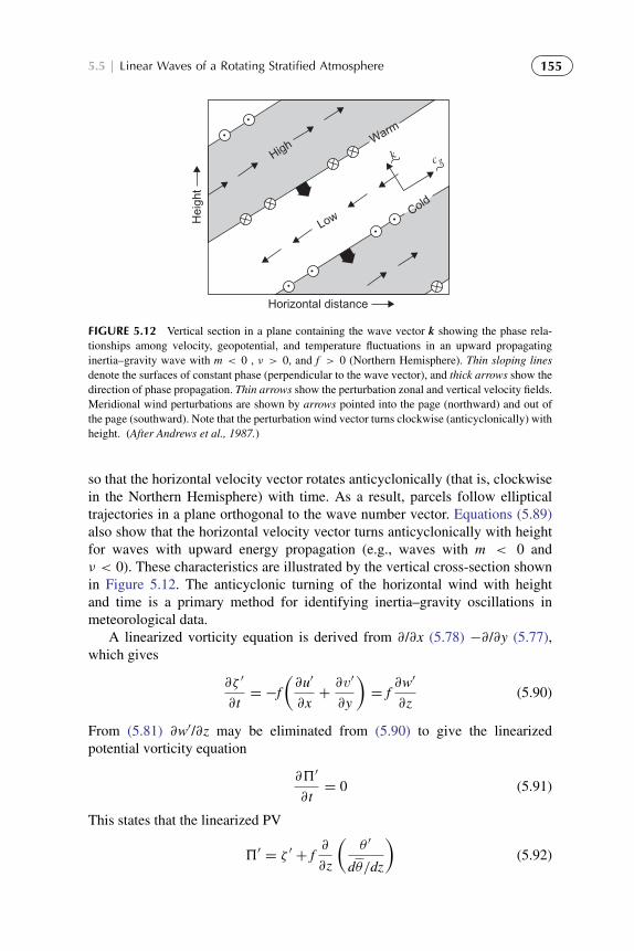
To protect the rights of the author(s) and publisher we inform you that this PDF is an uncorrected proof for internal businessuse only by the author(s), editor(s), reviewer(s), Elsevier and typesetter diacriTech. It is not allowed to publish this proofonline or in print. This proof copy is the copyright property of the publisher and is confidential until formal publication.
“Hakim: 09-ch05-127-170-9780123848666” — 2012/7/26 — 11:27 — page 155 — #29
5.5 | Linear Waves of a Rotating Stratified Atmosphere 155
Horizontal distance
Low
Highc g
Hei
ght
kWarm
Cold
FIGURE 5.12 Vertical section in a plane containing the wave vector k showing the phase rela-tionships among velocity, geopotential, and temperature fluctuations in an upward propagatinginertia–gravity wave with m < 0 , ν > 0, and f > 0 (Northern Hemisphere). Thin sloping linesdenote the surfaces of constant phase (perpendicular to the wave vector), and thick arrows show thedirection of phase propagation. Thin arrows show the perturbation zonal and vertical velocity fields.Meridional wind perturbations are shown by arrows pointed into the page (northward) and out ofthe page (southward). Note that the perturbation wind vector turns clockwise (anticyclonically) withheight. (After Andrews et al., 1987.)
so that the horizontal velocity vector rotates anticyclonically (that is, clockwisein the Northern Hemisphere) with time. As a result, parcels follow ellipticaltrajectories in a plane orthogonal to the wave number vector. Equations (5.89)also show that the horizontal velocity vector turns anticyclonically with heightfor waves with upward energy propagation (e.g., waves with m < 0 andν < 0). These characteristics are illustrated by the vertical cross-section shownin Figure 5.12. The anticyclonic turning of the horizontal wind with heightand time is a primary method for identifying inertia–gravity oscillations inmeteorological data.
A linearized vorticity equation is derived from ∂/∂x (5.78) −∂/∂y (5.77),which gives
∂ζ ′
∂t= −f
(∂u′
∂x+∂v′
∂y
)= f
∂w′
∂z(5.90)
From (5.81) ∂w′/∂z may be eliminated from (5.90) to give the linearizedpotential vorticity equation
∂5′
∂t= 0 (5.91)
This states that the linearized PV
5′ = ζ ′ + f∂
∂z
(θ ′
dθ/dz
)(5.92)
To protect the rights of the author(s) and publisher we inform you that this PDF is an uncorrected proof for internal businessuse only by the author(s), editor(s), reviewer(s), Elsevier and typesetter diacriTech. It is not allowed to publish this proofonline or in print. This proof copy is the copyright property of the publisher and is confidential until formal publication.
“Hakim: 09-ch05-127-170-9780123848666” — 2012/7/26 — 11:27 — page 156 — #30
156 CHAPTER | 5 Atmospheric Oscillations
is conserved at every point in space, as was the case for linear shallow waterwaves. Polarization relationships (5.83) and (5.84) for the l = 0 case can beused to show that for Rossby waves
ζ ′ = −k2
fp (5.93)
and for inertia–gravity waves
ζ ′ =fm2
N2p (5.94)
This result may be used to show (see Problem 5.16) that if the buoyancyfrequency, N, is constant, inertia-gravity waves have zero linearized potentialvorticity (5.92). Therefore, as in linearized shallow water, the linearized poten-tial vorticity equation (5.91) effectively filters gravity waves from the dynamics.We will exploit this fact in the next section, where we show that geostrophic bal-ance emerges in the long-time limit for arbitrary initial states. This result alsomotivates the derivation of the quasi-geostrophic equations in Chapter 6, whichessentially generalizes (5.91) to include nonlinear advection of linearized PV(5.92).
5.6 ADJUSTMENT TO GEOSTROPHIC BALANCE
This section investigates the process by which geostrophic balance is achievedfrom an unbalanced initial condition—that is, the adjustment process. Forsimplicity we utilize the linearized shallow water equations of Section 5.3.2;similar considerations apply to a continuously stratified atmosphere. The prob-lem addressed here is the solution of the full linearized equations (5.25) in thelimit of large time, starting from an arbitrary initial condition.
The key to solving this problem comes from (5.42), the linearized shallowwater potential vorticity equation,
∂Q′
∂t= 0 (5.95)
where Q′ designates the perturbation potential vorticity. This implies theconservation relationship
Q′(x, y, t) = ζ ′/f − h′/h = Const. (5.96)
Thus, if we know the distribution of Q′ at the initial time, we know Q′ for alltime
Q′ (x, y, t) = Q′(x, y, 0)

To protect the rights of the author(s) and publisher we inform you that this PDF is an uncorrected proof for internal businessuse only by the author(s), editor(s), reviewer(s), Elsevier and typesetter diacriTech. It is not allowed to publish this proofonline or in print. This proof copy is the copyright property of the publisher and is confidential until formal publication.
“Hakim: 09-ch05-127-170-9780123848666” — 2012/7/26 — 11:27 — page 157 — #31
5.6 | Adjustment to Geostrophic Balance 157
and the final adjusted state can be determined without solving the time-dependent problem. Note that, in general, u′, v′, and h′ evolve in time, but onlyin such a way that Q′ is constant at every point in space.
This problem was first solved by Rossby in the 1930s and is often referredto as the Rossby adjustment problem. As a simplified, albeit somewhat unrealis-tic, example of the adjustment process, we consider an idealized shallow watersystem on a rotating plane with initial conditions
u′, v′ = 0; h′ = −h0sgn (x) (5.97)
where sgn(x) = 1 for x > 0 and sgn(x) = −1 for x < 0. This corresponds to aninitial step function in h′ at x = 0, with the fluid motionless. Thus, from (5.96)(
ζ ′/f)−(h′/h
)=(h0/h
)sgn (x) (5.98)
Using (5.98) to eliminate ζ ′ in (5.27) yields
∂2h′
∂t2− c2
(∂2h′
∂x2+∂2h′
∂y2
)+ f 2h′ = −f 2h0sgn (x) (5.99)
where c2= gh.
Because initially h′ is independent of y, it will remain so for all time. Thus,in the final steady state (5.99) becomes
− c2 d2h′
dx2+ f 2h′ = −f 2h0 sgn (x) (5.100)
which has the solution
h′
h0=
{−1+ exp (−x/λR) for x > 0+1− exp (+x/λR) for x < 0
}(5.101)
where λR ≡ f−10
√gh is the Rossby radius of deformation. Hence, the radius
of deformation may be interpreted as the horizontal length scale over whichthe height field adjusts during the approach to geostrophic equilibrium. For|x| � λR the original h′ remains unchanged. Substituting from (5.101) into(5.25) shows that the steady velocity field is geostrophic and nondivergent:
u′ = 0, and v′ =g
f
∂h′
∂x= −
gh0
fλRexp (− |x| /λR) (5.102)
The steady-state solution (5.102) is shown in Figure 5.13.Note that (5.102) could not be derived merely by setting ∂/∂t = 0 in (5.25).
That would yield geostrophic balance, and any distribution of h′ would satisfy

To protect the rights of the author(s) and publisher we inform you that this PDF is an uncorrected proof for internal businessuse only by the author(s), editor(s), reviewer(s), Elsevier and typesetter diacriTech. It is not allowed to publish this proofonline or in print. This proof copy is the copyright property of the publisher and is confidential until formal publication.
“Hakim: 09-ch05-127-170-9780123848666” — 2012/7/26 — 11:27 — page 158 — #32
158 CHAPTER | 5 Atmospheric Oscillations
−3
(b)
3
x/λRv
−3 −2 −1 0
(a)
1 2 3
x/λR
h'
FIGURE 5.13 The geostrophic equilibrium solution corresponding to adjustment from the initialstate defined in (5.97). (a) Final surface elevation profiles and (b) the geostrophic velocity profile inthe final state. (After Gill, 1982.)
the equations:
fu′ = −g∂h′
∂y, f v′ = g
∂h′
∂x,
∂u′
∂x+∂v′
∂y= 0
Only by combining (5.25) to obtain the potential vorticity equation, andrequiring the flow to satisfy potential vorticity conservation at all intermediatetimes, can the degeneracy of the geostrophic final state be eliminated. In otherwords, although any height field can satisfy the steady-state versions of (5.25),there is only one field that is consistent with a given initial state; this field canbe found readily because it can be computed from the distribution of potentialvorticity, which is conserved.
Although the final state can be computed without solving the time-dependentequation, if the evolution of the adjustment process is required, it is necessaryto solve (5.99) subject to the initial conditions (5.97), which is beyond the scopeof this discussion. We can, however, compute the amount of energy that isdispersed by gravity waves during the adjustment process. This only requirescomputing the energy change between initial and final states.
The potential energy per unit horizontal area is given by
h′∫0
ρgzdz = ρgh′2/2

To protect the rights of the author(s) and publisher we inform you that this PDF is an uncorrected proof for internal businessuse only by the author(s), editor(s), reviewer(s), Elsevier and typesetter diacriTech. It is not allowed to publish this proofonline or in print. This proof copy is the copyright property of the publisher and is confidential until formal publication.
“Hakim: 09-ch05-127-170-9780123848666” — 2012/7/26 — 11:27 — page 159 — #33
5.7 | Rossby Waves 159
Thus, the potential energy released per unit length in y during adjustment is
+∞∫−∞
ρgh20
2dx−
+∞∫−∞
ρgh′2
2dx
= 2
+∞∫0
ρgh20
2
[1−
(1− e−x/λR
)2]
dx
=3
2ρgh2
0λR
(5.103)
In the nonrotating case (λR → ∞) all potential energy available initially isreleased (converted to kinetic energy) so that there is an infinite energy release.(Energy is radiated away in the form of gravity waves, leaving a flat free surfaceextending to |x| → ∞ as t→∞.)
In the rotating case only the finite amount given in (5.103) is converted tokinetic energy, and only a portion of this kinetic energy is radiated away. Therest remains in the steady geostrophic circulation. The kinetic energy in thesteady-state per unit length is
2
+∞∫0
ρhv′2
2dx = ρh
(gh0
fλR
)2 +∞∫0
e−2x/λRdx =1
2ρgh2
0λR (5.104)
Thus, in the rotating case a finite amount of potential energy is released, butonly one-third of the potential energy released goes into the steady geostrophicflow. The remaining two-thirds is radiated away in the form of inertia–gravitywaves. This simple analysis illustrates the following points
l It is difficult to extract the potential energy of a rotating fluid. Although thereis an infinite reservoir of potential energy in this example (because h′ is finiteas |x| → ∞), only a finite amount is converted before geostrophic balanceis achieved.
l Conservation of potential vorticity allows one to determine the steady-stategeostrophically adjusted velocity and height fields without carrying out atime integration.
l The length scale for the steady solution is the Rossby radius λR.
5.7 ROSSBY WAVES
The wave type that is of most importance for large-scale meteorological pro-cesses is the Rossby wave, or planetary wave. In an inviscid barotropic fluid ofconstant depth (where the divergence of the horizontal velocity must vanish),

To protect the rights of the author(s) and publisher we inform you that this PDF is an uncorrected proof for internal businessuse only by the author(s), editor(s), reviewer(s), Elsevier and typesetter diacriTech. It is not allowed to publish this proofonline or in print. This proof copy is the copyright property of the publisher and is confidential until formal publication.
“Hakim: 09-ch05-127-170-9780123848666” — 2012/7/26 — 11:27 — page 160 — #34
160 CHAPTER | 5 Atmospheric Oscillations
the Rossby wave is an absolute vorticity-conserving motion that owes its exis-tence to the variation of the Coriolis parameter with latitude. More generally,in a baroclinic atmosphere, the Rossby wave is a potential vorticity-conservingmotion that owes its existence to the gradient of potential vorticity.
The variation of the Coriolis parameter with latitude can be approximated byexpanding the latitudinal dependence of f in a Taylor series about a referencelatitude φ0 and retaining only the first two terms to yield
f = f0 + βy (5.105)
where β ≡ (df /dy)φ0= 2� cosφ0/a and y = 0 atφ0. This approximation is
usually referred to as the midlatitude β-plane approximation. Rossby wavepropagation can be understood in a qualitative fashion by considering a closedchain of fluid parcels initially aligned along a circle of latitude. Recall that theabsolute vorticity η is given by η = ζ + f , where ζ is the relative vorticity andf is the Coriolis parameter. Assume that ζ = 0 at time t0. Now suppose that att1, δy is the meridional displacement of a fluid parcel from the original latitude.Then at t1 we have
(ζ + f )t1 = ft0
or
ζt1 = ft0 − ft1 = −βδy (5.106)
where β ≡ df /dy is the planetary vorticity gradient at the original latitude.From (5.106) it is evident that if the chain of parcels is subject to a
sinusoidal meridional displacement under absolute vorticity conservation, theresulting perturbation vorticity will be positive for a southward displacementand negative for a northward displacement.
This perturbation vorticity field will induce a meridional velocity field,which advects the chain of fluid parcels southward west of the vorticity maxi-mum and northward west of the vorticity minimum, as indicated in Figure 5.14.
Ω
−+
FIGURE 5.14 Perturbation vorticity field and induced velocity field (dashed arrows) for a merid-ionally displaced chain of fluid parcels. The heavy wavy line shows original perturbation position;the light line shows westward displacement of the pattern due to advection by the induced velocity.

To protect the rights of the author(s) and publisher we inform you that this PDF is an uncorrected proof for internal businessuse only by the author(s), editor(s), reviewer(s), Elsevier and typesetter diacriTech. It is not allowed to publish this proofonline or in print. This proof copy is the copyright property of the publisher and is confidential until formal publication.
“Hakim: 09-ch05-127-170-9780123848666” — 2012/7/26 — 11:27 — page 161 — #35
5.7 | Rossby Waves 161
Thus, the fluid parcels oscillate back and forth about their equilibrium latitude,and the pattern of vorticity maxima and minima propagates to the west. Thiswestward propagating vorticity field constitutes a Rossby wave. Just as a posi-tive vertical gradient of potential temperature resists vertical fluid displacementsand provides the restoring force for gravity waves, the meridional gradient ofabsolute vorticity resists meridional displacements and provides the restoringmechanism for Rossby waves.
The speed of westward propagation, c, can be computed for this simpleexample by letting δy = a sin [k (x− ct)], where a is the maximum northwarddisplacement. Then v = D (δy)/Dt = −kca cos [k (x− ct)], and
ζ = ∂v/∂x = k2ca sin [k (x− ct)]
Substitution for δy and ζ in (5.106) then yields
k2ca sin [k (x− ct)] = −βa sin [k (x− ct)]
or
c = −β/k2 (5.107)
Thus, the phase speed is westward relative to the mean flow and is inverselyproportional to the square of the zonal wave number.
5.7.1 Free Barotropic Rossby Waves
The dispersion relationship for barotropic Rossby waves may be derived for-mally by finding wave-type solutions of the linearized barotropic vorticityequation. The barotropic vorticity equation (4.41) states that the vertical com-ponent of absolute vorticity is conserved following the horizontal motion. For amidlatitude β-plane this equation has the form(
∂
∂t+ u
∂
∂x+ v
∂
∂y
)ζ + βv = 0 (5.108)
We now assume that the motion consists of a constant basic state zonalvelocity plus a small horizontal perturbation:
u = u+ u′, v = v′, ζ = ∂v′/∂x− ∂u′/∂y = ζ ′
We define a perturbation streamfunction ψ ′ according to
u′ = −∂ψ ′/∂y, v′ = ∂ψ ′/∂x
from which ζ ′ = ∇2ψ ′. The perturbation form of (5.108) is then(∂
∂t+ u
∂
∂x
)∇
2ψ ′ + β∂ψ ′
∂x= 0 (5.109)

To protect the rights of the author(s) and publisher we inform you that this PDF is an uncorrected proof for internal businessuse only by the author(s), editor(s), reviewer(s), Elsevier and typesetter diacriTech. It is not allowed to publish this proofonline or in print. This proof copy is the copyright property of the publisher and is confidential until formal publication.
“Hakim: 09-ch05-127-170-9780123848666” — 2012/7/26 — 11:27 — page 162 — #36
162 CHAPTER | 5 Atmospheric Oscillations
where as usual we have neglected terms involving the products of perturbationquantities. We seek a solution of the form
ψ ′ = Re [9 exp(iφ)]
where φ = kx + ly− νt. Here k and l are wave numbers in the zonal andmeridional directions, respectively. Substituting for ψ ′ in (5.109) gives
(−ν + ku)(−k2− l2
)+ kβ = 0
which may immediately be solved for ν:
ν = uk − βk/K2 (5.110)
where K2≡ k2+ l2 is the total horizontal wave number squared.
Recalling that c= ν/k, we find that the zonal phase speed relative to themean wind is
c− u = −β/K2 (5.111)
which reduces to (5.109) when the mean wind vanishes and l → 0. Thus, theRossby wave zonal phase propagation is always westward relative to the meanzonal flow. Furthermore, the Rossby wave phase speed depends inversely on thesquare of the horizontal wave number. Therefore, Rossby waves are dispersivewaves whose phase speeds increase rapidly with increasing wavelength.
For a typical midlatitude synoptic-scale disturbance, with similar meridionaland zonal scales (l ≈ k) and zonal wavelength of order 6000 km, the Rossbywave speed relative to the zonal flow calculated from (5.111) is approximately−8 m s−1. Because the mean zonal wind is generally westerly and greater than8 m s−1, synoptic-scale Rossby waves usually move eastward, but at a phasespeed relative to the ground that is somewhat less than the mean zonal windspeed. For longer wavelengths the westward Rossby wave phase speed may belarge enough to balance the eastward advection by the mean zonal wind so thatthe resulting disturbance is stationary relative to Earth’s surface. From (5.111)it is clear that the free Rossby wave solution becomes stationary when
K2= β/u ≡ K2
s (5.112)
The significance of this condition is discussed in the next subsection.Unlike the phase speed, which is always westward relative to the mean flow,
the zonal group velocity for a Rossby wave may be either eastward or westwardrelative to the mean flow, depending on the ratio of the zonal and meridionalwave numbers (see Problem 5.20). Stationary Rossby modes (i.e., modes withc = 0) have zonal group velocities that are eastward relative to the ground.Synoptic-scale Rossby waves also tend to have zonal group velocities that areeastward relative to the ground. For synoptic waves, advection by the meanzonal wind is generally larger than the Rossby phase speed so that the phasespeed is also eastward relative to the ground, but is slower than the zonal group
To protect the rights of the author(s) and publisher we inform you that this PDF is an uncorrected proof for internal businessuse only by the author(s), editor(s), reviewer(s), Elsevier and typesetter diacriTech. It is not allowed to publish this proofonline or in print. This proof copy is the copyright property of the publisher and is confidential until formal publication.
“Hakim: 09-ch05-127-170-9780123848666” — 2012/7/26 — 11:27 — page 163 — #37
5.7 | Rossby Waves 163
velocity. As shown earlier in Figure 5.4b, this implies that new disturbancestend to develop downstream of existing disturbances, which is an importantconsideration for forecasting.
It is possible to carry out a less restrictive analysis of free planetary wavesusing the perturbation form of the full primitive equations. In that case thestructure of the free modes depends critically on the boundary conditions atthe surface and the upper boundary. The results of such an analysis are mathe-matically complicated, but qualitatively yield waves with horizontal dispersionproperties similar to those in the shallow water model. It turns out that the freeoscillations allowed in a hydrostatic gravitationally stable atmosphere consistof eastward- and westward-moving gravity waves that are slightly modified byEarth’s rotation and westward-moving Rossby waves that are slightly modifiedby gravitational stability. These free oscillations are the normal modes of oscil-lation of the atmosphere. As such, they are continually excited by the variousforces acting on the atmosphere. Planetary scale-free oscillations, although theycan be detected by careful observational studies, generally have rather weakamplitudes. Presumably this is because the forcing is quite weak at the largephase speeds characteristic of most such waves. An exception is the 16-dayperiod zonal wave number 1 normal mode, which can be quite strong in thewinter stratosphere.
5.7.2 Forced Topographic Rossby Waves
Although free propagating Rossby modes are only rather weakly excited inthe atmosphere, forced stationary Rossby modes are of primary importancefor understanding the planetary-scale circulation pattern. Such modes maybe forced by longitudinally dependent diabatic heating patterns or by flowover topography. Of particular importance for the Northern Hemisphere extra-tropical circulation are stationary Rossby modes forced by flow over theRockies and the Himalayas. It is just the topographic Rossby wave that wasdescribed qualitatively in the discussion of streamline deflections in potentialvorticity-conserving flows crossing mountain ranges in Section 4.3.
As the simplest possible dynamical model of topographic Rossby waves, weuse a modified version of the the shallow potential vorticity equation (4.39). Weassume that the upper boundary is at a fixed height H, and the lower boundaryis at the variable height hT(x, y) where |hT | � H. We also approximate ζ bythe geostrophic value, ζg, and assume that |ζg| � f0. We can then approximate(4.39) by
H
(∂
∂t+ V · ∇
) (ζg + f
)= −f0
DhT
Dt(5.113)
Linearizing and applying the midlatitude β-plane approximation yields(∂
∂t+ u
∂
∂x
)ζ ′g + βv′g = −
f0H
u∂hT
∂x(5.114)

To protect the rights of the author(s) and publisher we inform you that this PDF is an uncorrected proof for internal businessuse only by the author(s), editor(s), reviewer(s), Elsevier and typesetter diacriTech. It is not allowed to publish this proofonline or in print. This proof copy is the copyright property of the publisher and is confidential until formal publication.
“Hakim: 09-ch05-127-170-9780123848666” — 2012/7/26 — 11:27 — page 164 — #38
164 CHAPTER | 5 Atmospheric Oscillations
We now examine solutions of (5.114) for the special case of a sinusoidallower boundary. We specify the topography to have the form
hT(x, y) = Re [h0 exp (ikx)] cos ly (5.115)
and represent the geostrophic wind and vorticity by the perturbation stream-function
ψ(x, y) = Re [ψ0 exp (ikx)] cos ly (5.116)
Then (5.114) has a steady-state solution with complex amplitude given by
ψ0 = f0h0/[H(
K2− K2
s
)](5.117)
The streamfunction is either exactly in phase (ridges over the mountains) orexactly out of phase (troughs over the mountains), with the topography depend-ing on the sign of K2
− K2s . For long waves (K < Ks) the topographic vorticity
source in (5.114) is balanced primarily by the meridional advection of plane-tary vorticity (the β effect). For short waves (K > Ks) the source is balancedprimarily by the zonal advection of relative vorticity.
The topographic wave solution (5.117) has the unrealistic characteristic thatwhen the wave number exactly equals the critical wave number Ks, the ampli-tude goes to infinity. From (5.112) it is clear that this singularity occurs at thezonal wind speed for which the free Rossby mode becomes stationary. Thus, itmay be thought of as a resonant response of the barotropic system.
Charney and Eliassen (1949) used the topographic Rossby wave model toexplain the winter mean longitudinal distribution of 500-hPa heights in NorthernHemisphere midlatitudes. They removed the resonant singularity by includingboundary layer drag in the form of Ekman pumping, which for the barotropicvorticity equation is simply a linear damping of the relative vorticity (seeSection 8.3.4). The vorticity equation thus takes the form(
∂
∂t+ u
∂
∂x
)ζ ′g + βv′g + rζ ′g = −
f0H
u∂hT
∂x(5.118)
where r ≡ τ−1e is the inverse of the spin-down time defined in (8.37).
For steady flow, (5.118) has a solution with complex amplitude
ψ0 = f0h0/ [
H(
K2− K2
s − iε)]
(5.119)
where ε ≡ rK2 (ku)−1. Thus, boundary layer drag shifts the response’s phaseand removes the singularity at resonance. However, the amplitude is still a max-imum for K=Ks and the trough in the streamfunction occurs one-quarter cycleeast of the mountain crest, in approximate agreement with observations.

To protect the rights of the author(s) and publisher we inform you that this PDF is an uncorrected proof for internal businessuse only by the author(s), editor(s), reviewer(s), Elsevier and typesetter diacriTech. It is not allowed to publish this proofonline or in print. This proof copy is the copyright property of the publisher and is confidential until formal publication.
“Hakim: 09-ch05-127-170-9780123848666” — 2012/7/26 — 11:27 — page 165 — #39
5.7 | Rossby Waves 165
2 km
1 km
Longitude
0
−200
−100
0
(a)
(b)
100
200
90°E 180°
Hei
ght (
m)
90°W 0
ObservedModel
FIGURE 5.15 (a) Longitudinal variation of the disturbance in geopotential height (≡ f09/g) inthe Charney–Eliassen model for the parameters given in the text (solid line) compared with theobserved 500-hPa height perturbations at 45◦N in January (dashed line). (b) Smoothed profile oftopography at 45◦N used in the computation. (After Held, 1983.)
By use of a Fourier expansion, (5.118) can be solved for realistic distribu-tions of topography. The results for an x-dependence of hT given by a smoothedversion of Earth’s topography at 45◦N, a meridional wave number correspond-ing to a latitudinal half-wavelength of 35◦, τe = 5 days, u = 17 m s−1, f0 =10−4 s−1, and H = 8 km are shown in Figure 5.15. Despite its simplicity, theCharney–Eliassen model does a remarkable job of reproducing the observed500-hPa stationary wave pattern in Northern Hemisphere midlatitudes.
SUGGESTED REFERENCES
Chapman and Lindzen, Atmospheric Tides: Thermal and Gravitational, is the classic reference onboth observational and theoretical aspects of tides, a class of atmospheric motions for whichthe linear perturbations method has proved to be particularly successful.
Gill, Atmosphere-Ocean Dynamics, has a very complete treatment of gravity, inertia–gravity, andRossby waves, with particular emphasis on observed oscillations in the oceans.

To protect the rights of the author(s) and publisher we inform you that this PDF is an uncorrected proof for internal businessuse only by the author(s), editor(s), reviewer(s), Elsevier and typesetter diacriTech. It is not allowed to publish this proofonline or in print. This proof copy is the copyright property of the publisher and is confidential until formal publication.
“Hakim: 09-ch05-127-170-9780123848666” — 2012/7/26 — 11:27 — page 166 — #40
166 CHAPTER | 5 Atmospheric Oscillations
Hildebrand, Advanced Calculus for Applications, is one of many standard textbooks that discussthe mathematical techniques used in this chapter, including the representation of functions inFourier series and the general properties of the wave equation.
Nappo, An Introduction to Atmospheric Gravity Waves, is an excellent introduction to the theoryand observation of gravity waves in the atmosphere.
Scorer, Natural Aerodynamics, contains an excellent qualitative discussion on many aspects ofwaves generated by barriers such as lee waves.
PROBLEMS
5.1. Show that the Fourier component F (x) = Re [C exp (imx)] can be written as
F (x) = |C| cos m (x+ x0)
where x0 = m−1 sin−1 (Ci/|C|) and Ci stands for the imaginary part of C.5.2. In the study of atmospheric wave motions, it is often necessary to consider
the possibility of amplifying or decaying waves. In such a case we mightassume that a solution has the form
ψ = A cos (kx− νt − kx0) exp (αt)
where A is the initial amplitude, α the amplification factor, and x0 the initialphase. Show that this expression can be written more concisely as
ψ = Re[Beik(x−ct)
]where both B and c are complex constants. Determine the real andimaginary parts of B and c in terms of A, α, k, ν, and x0.
5.3. Several of the wave types discussed in this chapter are governed byequations that are generalizations of the wave equation
∂2ψ
∂t2= c2 ∂
2ψ
∂x2
This equation can be shown to have solutions corresponding to waves ofarbitrary profile moving at the speed c in both positive and negative x direc-tions. We consider an arbitrary initial profile of the field ψ ; ψ = f (x) att = 0. If the profile is translated in the positive x direction at speed c with-out change of shape, then ψ = f (x′), where x′ is a coordinate moving atspeed c so that x = x′ + ct. Thus, in terms of the fixed coordinate x we canwrite ψ = f (x− ct), corresponding to a profile that moves in the positive xdirection at speed c without change of shape. Verify that ψ = f (x− ct) is asolution for any arbitrary continuous profile f (x− ct). [Hint: Let x− ct = x′
and differentiate f using the chain rule.]5.4. Assuming that the pressure perturbation for a one-dimensional acoustic
wave is given by (5.23), find the corresponding solutions of the zonal windand density perturbations. Express the amplitude and phase for u′ and ρ′ interms of the amplitude and phase of p′.
5.5. Show that for isothermal motion (DT/Dt = 0) the acoustic wave speed isgiven by (gH)1/2, where H = RT/g is the scale height.
To protect the rights of the author(s) and publisher we inform you that this PDF is an uncorrected proof for internal businessuse only by the author(s), editor(s), reviewer(s), Elsevier and typesetter diacriTech. It is not allowed to publish this proofonline or in print. This proof copy is the copyright property of the publisher and is confidential until formal publication.
“Hakim: 09-ch05-127-170-9780123848666” — 2012/7/26 — 11:27 — page 167 — #41
Problems 167
5.6. In Section 5.3.1 the linearized equations for acoustic waves were devel-oped for the special situation of one-dimensional propagation in a horizon-tal tube. Although this situation does not appear to be directly applicableto the atmosphere, there is a special atmospheric mode, the Lamb wave,which is a horizontally propagating acoustic mode with no vertical velocityperturbation (w′ = 0). Such oscillations have been observed following vio-lent explosions such as volcanic eruptions and atmospheric nuclear tests.Using (5.20) and (5.21), plus the linearized forms of the hydrostatic equa-tion, and the continuity equation (5.15), derive the height dependenceof the perturbation fields for the Lamb mode in an isothermal basic stateatmosphere, assuming that the pressure perturbation at the lower bound-ary (z = 0) has the form (5.23). Determine the vertically integrated kineticenergy density per unit horizontal area for this mode.
5.7. If the surface height perturbation in a shallow water gravity wave is givenby
h′ = Re[Aeik(x−ct)
]find the corresponding velocity perturbation u′(x, t). Sketch the phaserelationship between h′ and u′ for an eastward propagating wave.
5.8. Assuming that the vertical velocity perturbation for a two-dimensional inter-nal gravity wave is given by (5.65), obtain the corresponding solution forthe u′, p′, and θ ′ fields. Use these results to verify the approximation∣∣ρ0θ
′/θ∣∣� ∣∣∣p′/c2
s
∣∣∣which was used in (5.58).
5.9. For the situation in the preceding problem, express the vertical flux ofhorizontal momentum, ρ0u′w′, in terms of the amplitude A of the verti-cal velocity perturbation. Hence, show that the momentum flux is positivefor waves in which phase speed propagates eastward and downward.
5.10. Show that if (5.60) is replaced by the hydrostatic equation (i.e., the termsin w′ are neglected), the resulting frequency equation for internal gravitywaves is just the asymptotic limit of (5.66) for waves in which |k| � |m|.
5.11. (a) Show that the intrinsic group velocity vector in two-dimensionalinternal gravity waves is parallel to lines of constant phase.
(b) Show that in the long-wave limit (|k| � |m|) the magnitude of thezonal component of the group velocity equals the magnitude of thezonal phase speed so that energy propagates one wavelength per waveperiod.
5.12. Determine the perturbation horizontal and vertical velocity fields for sta-tionary gravity waves forced by flow over sinusoidally varying topographygiven the following conditions: The height of the ground is h = h0 cos kx,where h0 = 50 m is a constant; N = 2 × 10⁻² s−1; u = 5 m s−1; andk = 3× 10⁻³ m−1. Hint: For small-amplitude topography (h0k� 1) we canapproximate the lower boundary condition by
w′ = Dh/Dt = u∂h/∂x at z = 0

To protect the rights of the author(s) and publisher we inform you that this PDF is an uncorrected proof for internal businessuse only by the author(s), editor(s), reviewer(s), Elsevier and typesetter diacriTech. It is not allowed to publish this proofonline or in print. This proof copy is the copyright property of the publisher and is confidential until formal publication.
“Hakim: 09-ch05-127-170-9780123848666” — 2012/7/26 — 11:27 — page 168 — #42
168 CHAPTER | 5 Atmospheric Oscillations
5.13. Verify the group velocity relationship for inertia–gravity waves that are givenin (5.88).
5.14. Show that when u = 0 the wave number vector κ for an internal inertia–gravity wave is perpendicular to the group velocity vector.
5.15. Derive an expression for the group velocity of a barotropic Rossby wavewith dispersion relation (5.110). Show that for stationary waves the groupvelocity always has an eastward zonal component relative to Earth. Hence,Rossby wave energy propagation must be downstream of topographicsources.
5.16. Prove that the internal gravity waves of Section 5.5.2 have zero linearizedpotential vorticity in the case of constant buoyancy frequency, N.
MATLAB ExercisesM5.1. (a) The MATLAB script phase demo.m shows that the Fourier series F(x) =
A sin(kx)+B cos(kx) is equivalent to the form F(x) = Re C exp(ikx) whereA and B are real coefficients and C is a complex coefficient. Modifythe MATLAB script to confirm that the expression F(x) = |C| cos k(x +x0) = |C| cos(kx + α) represents the same Fourier series where kx0 ≡
α = sin−1(Ci/|C|), Ci stands for the imaginary part of C, α is the “phase”defined in the MATLAB script. Plot your results as the third subplot in thescript.
(b) By running the script for several input phase angles (e.g., 0, 30, 60,and 90◦), determine the relationship between α and the location of themaximum of F(x).
M5.2. In this problem you will examine the formation of a “wave envelope” for acombination of dispersive waves. The example is that of a deep water wavein which the group velocity is half of the phase velocity. The MATLAB scriptgrp vel 3.m has code to show the wave height field at four different times fora group composed of various numbers of waves with differing wave numbersand frequencies. Study the code and determine the period and wavelengthof the carrier wave. Then run the script several times, varying the numberof wave modes from 4 to 32. Determine the half-width of the envelope attime t = 0 (top line on the graph) as a function of the number of modes in thegroup. The half-width is here defined as two times the distance from the pointof maximum amplitude (x = 0) to the point along the envelope where theamplitude is half the maximum. You can estimate this from the graph usingthe ginput command to determine the distance. Use MATLAB to plot a curveof the half-width versus number of wave modes.
M5.3. The script geost adjust 1.m together with the function yprim adj 1.m illus-trates one-dimensional geostrophic adjustment of the velocity field in abarotropic model for a sinusoidally varying initial height field. The equationsare a simplification of (5.25) in the text for the case of no y dependence. Ini-tially u′ = v′ = 0, φ′ ≡ gh′ = 9.8 cos(kx). The final balanced wind in this casewill have only a meridional component. Run the program geost adjust 1.mfor the cases of latitude 30 and 60◦, choosing a time value of at least 10 days.For each of these cases choose values of wavelength of 2000, 4000, 6000,and 8000 km (a total of eight runs). Construct a table showing the initial andfinal values of the fields u′, v′, φ′ and the ratio of the final energy to the initial

To protect the rights of the author(s) and publisher we inform you that this PDF is an uncorrected proof for internal businessuse only by the author(s), editor(s), reviewer(s), Elsevier and typesetter diacriTech. It is not allowed to publish this proofonline or in print. This proof copy is the copyright property of the publisher and is confidential until formal publication.
“Hakim: 09-ch05-127-170-9780123848666” — 2012/7/26 — 11:27 — page 169 — #43
Problems 169
energy. You can read the values from the MATLAB graphs by using the gin-put command or, for greater accuracy, add lines in the MATLAB code to printout the values needed. Modify the MATLAB script to determine the partitionof final state energy per unit mass between the kinetic energy (v
′2/2) andthe potential energy φ
′2/(2gH). Compute the ratio of final kinetic energy topotential energy for each of your eight cases and show this in a table.
M5.4. The script geost adjust 2.m together with the function yprim adj 2.mextends Problem M5.3 by using Fourier expansion to examine thegeostrophic adjustment for an isolated initial height disturbance of the form
h0 (x) = −hm/[
1+ (x/L)2]. The version given here uses 64 Fourier modes
and employs a fast Fourier transform algorithm (FFT). (There are 128 modesin the FFT, but only one-half of them provide real information.) In this caseyou may run the model for only 5 days of integration time (it requires a lot ofcomputation compared to the previous case). Choose an initial zonal scale ofthe disturbance of 500 km and run the model for latitudes (in degrees) of 15,30, 45, 60, 75, and 90 (six runs). Study the animations for each case. Notethat the zonal flow is entirely in a gravity wave mode that propagates awayfrom the initial disturbance. The meridional flow has a propagating gravitywave component, but also a geostrophic part (cyclonic flow). Use the ginputcommand to estimate the zonal scale of the final geostrophic flow (v com-ponent) by measuring the distance from the negative velocity maximum justwest of the center to the positive maximum just east of the center. Plot a curveshowing the zonal scale as a function of latitude. Compare this scale with theRossby radius of deformation defined in the text. (Note that gH = 400 m2 s–2
in this example.)M5.5. This problem examines the variation of phase velocity for Rossby waves as
the zonal wavelength is varied. Run the MATLAB program rossby 1.m withzonal wavelengths specified as 5000, 10,000 and 20,000 km. For each ofthese cases try different values of the mean zonal wind until you find themean wind for which the Rossby wave is approximately stationary.
M5.6. The MATLAB script rossby 2.m shows an animation of the Rossby wavesgenerated by a vorticity disturbance initially localized in the center of thedomain, with mean wind zero. Run the script and note that the waves excitedhave westward phase speeds, but that disturbances develop on the eastwardside of the original disturbance. By following the development of these dis-turbances, make a crude estimate of the characteristic wavelength and thegroup velocity for the disturbances appearing to the east of the original dis-turbance at time t = 7.5 days. (Wavelength can be estimated by using ginputto measure the distance between adjacent troughs.) Compare your estimatewith the group velocity formula derived from (5.108). Can you think of a rea-son why your estimate for group velocity may differ from that given in theformula?
M5.7. The MATLAB script rossby 3.m gives the surface height and meridional veloc-ity disturbances for topographic Rossby waves generated by flow over anisolated ridge. The program uses a Fourier series approach to the solution.Ekman damping with a 2-day damping time is included to minimize the effectof waves propagating into the mountain from upstream (but this cannot beentirely avoided). Run this program for input zonal mean winds from 10 to

To protect the rights of the author(s) and publisher we inform you that this PDF is an uncorrected proof for internal businessuse only by the author(s), editor(s), reviewer(s), Elsevier and typesetter diacriTech. It is not allowed to publish this proofonline or in print. This proof copy is the copyright property of the publisher and is confidential until formal publication.
“Hakim: 09-ch05-127-170-9780123848666” — 2012/7/26 — 11:27 — page 170 — #44
170 CHAPTER | 5 Atmospheric Oscillations
100 m/s at 10-m/s intervals. For each run use ginput to estimate the scale ofthe leeside trough by measuring the zonal distance between the minimumand maximum in the meridional velocity. (This should be equal approxi-mately to one-half the wavelength of the dominant disturbance.) Compareyour results in each case with the zonal wavelength for resonance given bysolving (5.112) to determine the resonant Lx = 2π /k, where K2
= k2+ l2
and l = π /8× 106 in units of 1/m. (Do not expect exact agreement becausethe actual disturbance corresponds to the sum over many separate zonalwavelengths.)

To protect the rights of the author(s) and publisher we inform you that this PDF is an uncorrected proof for internal businessuse only by the author(s), editor(s), reviewer(s), Elsevier and typesetter diacriTech. It is not allowed to publish this proofonline or in print. This proof copy is the copyright property of the publisher and is confidential until formal publication.
“Hakim: 10-ch06-171-212-9780123848666” — 2012/7/26 — 11:35 — page 171 — #1
Chapter 6
Quasi-geostrophic Analysis
A primary goal of dynamic meteorology is to interpret the observed structureof large-scale atmospheric motions in terms of the physical laws governing themotions. These laws, which express the conservation of momentum, mass, andenergy, completely determine the relationships among the pressure, tempera-ture, and velocity fields. As we saw in Chapter 2, these governing laws are quitecomplicated even when the hydrostatic approximation (which is valid for alllarge-scale meteorological systems) is applied. For extratropical synoptic-scalemotions, however, the horizontal velocities are approximately geostrophic (seeSection 2.4). Such motions, which are usually referred to as quasi-geostrophic,are often simpler to analyze than are tropical disturbances or planetary-scaledisturbances. They are also the major systems of interest in traditional short-range weather forecasting, and are thus a reasonable starting point for dynamicalanalysis.
In addition to the observation that extratropical weather systems are nearlygeostrophic and hydrostatic, we found in the linear wave analyses of Chapter 5that the properties of Rossby waves resemble these weather systems, whereasthose of inertia–gravity waves do not. Specifically, Rossby waves have relativelyslow phase speeds and nonzero potential vorticity, whereas the inertia–gravitywaves are fast moving and have little or no potential vorticity. We will exploitthese properties here in order to filter the full equations to a simpler set, the quasi-geostrophic (QG) equations. Before developing this system of equations, it isuseful to briefly summarize the observed structure of midlatitude synoptic sys-tems and the mean circulations in which they are embedded. We then developthe QG equations using potential vorticity and potential temperature, which pro-vides one framework (“PV Thinking”) for understanding. A second frameworkfor dynamics (“w Thinking”) is based on the diagnosis of vertical motion throughan “omega equation,” and will also be thoroughly explored.
6.1 THE OBSERVED STRUCTURE OF EXTRATROPICALCIRCULATIONS
Atmospheric circulation systems depicted on a synoptic chart rarely resemblethe simple circular vortices discussed in Chapter 3. Rather, they are generally
An Introduction to Dynamic Meteorology. DOI: 10.1016/B978-0-12-384866-6.00006-4Copyright © 2013 Elsevier Inc. All rights reserved. 171

To protect the rights of the author(s) and publisher we inform you that this PDF is an uncorrected proof for internal businessuse only by the author(s), editor(s), reviewer(s), Elsevier and typesetter diacriTech. It is not allowed to publish this proofonline or in print. This proof copy is the copyright property of the publisher and is confidential until formal publication.
“Hakim: 10-ch06-171-212-9780123848666” — 2012/7/26 — 11:35 — page 172 — #2
172 CHAPTER | 6 Quasi-geostrophic Analysis
highly asymmetric in form, with the strongest winds and largest temperaturegradients concentrated along narrow bands called fronts. Also, such systemsgenerally are highly baroclinic; the amplitudes and phases of the geopotentialand velocity perturbations both change substantially with height. Part of thiscomplexity is due to the fact that these synoptic systems are not superposedon a uniform mean flow, but are embedded in a slowly varying planetary scaleflow that is itself highly baroclinic. Furthermore, this planetary scale flow isinfluenced by orography (i.e., by large-scale terrain variations) and continent-ocean heating contrasts so that it is highly longitude dependent. Therefore, whileviewing synoptic systems as disturbances superposed on a zonal flow that variesonly with latitude and height is a useful first approximation in theoretical analy-ses (see, e.g., Chapter 7), more complete descriptions require the observed zonalasymmetry.
Zonally averaged cross-sections do provide some useful information on thegross structure of the planetary scale circulation in which synoptic-scale eddiesare embedded. Figure 6.1 shows meridional cross-sections of the longitudinallyaveraged zonal wind and temperature for the solstice seasons of (a) December,January, and February (DJF) and (b) June, July, and August (JJA). These sec-tions extend from approximately sea level (1000 hPa) to about 32 km altitude(10 hPa). Thus, the troposphere and lower stratosphere are shown. This chap-ter is concerned with the structure of the wind and temperature fields in thetroposphere, and the stratosphere is discussed in Chapter 12.
The average pole to equator temperature gradient in the Northern Hemi-sphere troposphere is much larger in winter than in summer. In the SouthernHemisphere the difference between summer and winter temperature distribu-tions is smaller, due mainly to the large thermal inertia of the oceans, togetherwith the greater fraction of the surface that is covered by oceans in the South-ern Hemisphere. Since the mean zonal wind and temperature fields satisfy thethermal wind relationship to a high degree of accuracy, the seasonal cycle inzonal wind speeds is similar to that of the meridional temperature gradient.In the Northern Hemisphere the maximum zonal wind speed in the winteris twice as large as in the summer, whereas in the Southern Hemisphere thedifference between winter and summer zonal wind maxima is much smaller.Furthermore, in both seasons the core of maximum zonal wind speed (calledthe mean jet stream axis) is located just below the tropopause (the boundarybetween the troposphere and stratosphere) at the latitude where the thermalwind integrated through the troposphere is a maximum. In both hemispheres,this is about 30◦ latitude during winter, but moves poleward to about 45◦ duringsummer.
The zonally averaged meridional cross-sections of Figure 6.1 are not repre-sentative of the mean wind structure at all longitudes, which can be seen in thedistribution of the time-averaged zonal wind component for DJF on the 200-hPasurface in the Northern Hemisphere (Figure 6.2). It is clear that at some lon-gitudes there are very large deviations of the time-mean zonal flow from itslongitudinally averaged distribution. In particular, there are strong zonal wind
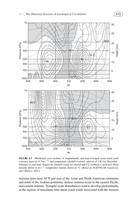
To protect the rights of the author(s) and publisher we inform you that this PDF is an uncorrected proof for internal businessuse only by the author(s), editor(s), reviewer(s), Elsevier and typesetter diacriTech. It is not allowed to publish this proofonline or in print. This proof copy is the copyright property of the publisher and is confidential until formal publication.
“Hakim: 10-ch06-171-212-9780123848666” — 2012/7/26 — 11:35 — page 173 — #3
6.1 | The Observed Structure of Extratropical Circulations 173
100
200
Pre
ssur
e (h
Pa)
300
500
700
100090S 60S 30S EQ 30N 60N 90N
−54.242
30
−79.7
−88.2
−76.6
41 21
−7.4
−7.5
−69.6
1030
25
20
15
Hei
ght (
km)
10
5
100
200
Pre
ssur
e (h
Pa)
300
500
700
100090S 60S 30S EQ 30N 60N 90N
1030
(a)
(b)
25
20
15H
eigh
t (km
)
10
5
FIGURE 6.1 Meridional cross-sections of longitudinally and time-averaged zonal wind (solidcontours, interval of 5 m s−1) and temperature (dashed contours, interval of 5 K) for December–February (a) and June–August (b). Easterly winds are shaded and 0◦C isotherm is darkened. Windmaxima shown in m s−1, temperature minima shown in ◦C. (Based on NCEP/NCAR reanalyses;after Wallace, 2003.)
maxima (jets) near 30◦N just east of the Asian and North American continentsand north of the Arabian peninsula; distinct minima occur in the eastern Pacificand eastern Atlantic. Synoptic-scale disturbances tend to develop preferentiallyin the regions of maximum time-mean zonal winds associated with the western

To protect the rights of the author(s) and publisher we inform you that this PDF is an uncorrected proof for internal businessuse only by the author(s), editor(s), reviewer(s), Elsevier and typesetter diacriTech. It is not allowed to publish this proofonline or in print. This proof copy is the copyright property of the publisher and is confidential until formal publication.
“Hakim: 10-ch06-171-212-9780123848666” — 2012/7/26 — 11:35 — page 174 — #4
174 CHAPTER | 6 Quasi-geostrophic Analysis
FIGURE 6.2 Mean zonal wind at the 200-hPa level for December through February, averaged foryears 1958–1997. Contour interval 10 m s−1 (heavy contour, 20 m s−1). (Based on NCEP/NCARreanalyses; after Wallace, 2003.)
Pacific and western Atlantic jets and to propagate downstream along stormtracks that approximately follow the jet axes.
The large departure of the northern winter climatological jet stream fromzonal symmetry can also be readily inferred from examination of Figure 6.3,which shows the mean 500-hPa geopotential contours for January and July inthe Northern Hemisphere. Striking departures from zonal symmetry are appar-ent, which are linked to the distributions of continents and oceans. The mostprominent asymmetries are the troughs in January to the east of the Americanand Asian continents. Referring to Figure 6.2, we see that the intense jet at35◦N and 140◦E is a result of the semipermanent trough in that region. Thus, itis apparent that the mean flow in which synoptic systems are embedded shouldreally be regarded as a longitude-dependent time-averaged flow. In northernsummer, 500-hPa geopotential height increases much more over high latitudesas compared to the tropics due to warming in the polar region. As a result,the pole–equator temperature contrast is smaller than in winter, and the heightcontrast and jet stream are weaker and located at higher latitude.
In addition to its longitudinal dependence, the planetary scale flow alsovaries from day to day due to its interactions with transient synoptic-scale dis-turbances. In fact, observations show that the transient planetary scale flowamplitude is comparable to that of the time-mean. As a result, monthly mean

To protect the rights of the author(s) and publisher we inform you that this PDF is an uncorrected proof for internal businessuse only by the author(s), editor(s), reviewer(s), Elsevier and typesetter diacriTech. It is not allowed to publish this proofonline or in print. This proof copy is the copyright property of the publisher and is confidential until formal publication.
“Hakim: 10-ch06-171-212-9780123848666” — 2012/7/26 — 11:35 — page 175 — #5
6.1 | The Observed Structure of Extratropical Circulations 175
584
572
560
548
July500 hPa
January500 hPa
572
512
584
560
548536
524
FIGURE 6.3 Mean 500-hPa geopotential height contours in January (left) and July (right) in theNorthern Hemisphere (30-year average). Geopotential height contours are shown every 60 meters.(Adapted from NOAA/ESRL http://www.esrl.noaa.gov/psd/.)
charts tend to smooth out the actual structure of the instantaneous jet streamsince the position and intensity of the jet vary. Thus, at any time the plane-tary scale flow in the region of the jet stream has much greater baroclinicitythan indicated on time-averaged charts. This point is illustrated schematically inFigure 6.4, which shows a latitude–height cross-section through an observed jetstream over North America. Figure 6.4a shows the zonal wind and potentialtemperature, whereas Figure 6.4b shows the potential temperature and Ertelpotential vorticity. The 2-PVU contour of potential vorticity approximatelymarks the tropopause. As illustrated in Figure 6.4a, the axis of the jet streamtends to be located above a narrow sloping zone of strong potential temperaturegradients called the polar-frontal zone. This is the zone that in general separatesthe cold air of polar origin from warm tropical air. The occurrence of an intensejet core above this zone of large-magnitude potential temperature gradientsis, of course, not mere coincidence but rather a consequence of thermal windbalance.
The potential temperature contours in Figure 6.4 illustrate the strong staticstability in the stratosphere. They also illustrate the fact that isentropes (constantθ surfaces) cross the tropopause in the vicinity of the jet so that air can movebetween the troposphere and the stratosphere without diabatic heating or cool-ing. The strong gradient of Ertel potential vorticity at the tropopause, however,provides a strong resistance to cross-tropopause flow along the isentropes. Note,however, that in the frontal region the potential vorticity surfaces are displacedsubstantially downward so that the frontal zone is characterized by a strong pos-itive anomaly in potential vorticity associated with the strong relative vorticityon the poleward side of the jet and the strong static stability on the cold air sideof the frontal zone.

To protect the rights of the author(s) and publisher we inform you that this PDF is an uncorrected proof for internal businessuse only by the author(s), editor(s), reviewer(s), Elsevier and typesetter diacriTech. It is not allowed to publish this proofonline or in print. This proof copy is the copyright property of the publisher and is confidential until formal publication.
“Hakim: 10-ch06-171-212-9780123848666” — 2012/7/26 — 11:35 — page 176 — #6
176 CHAPTER | 6 Quasi-geostrophic Analysis
Latitude70 60 50 40 30
1000
850
700
500
300
150P
ress
ure
(hP
a)P
ress
ure
(hP
a)
70 60 50 40 301000
850
700
500
300
150
Latitude
250
260
270
280290
330
340350 360
300
310
320
1
2
3
456
(a)
(b)
260
270
280
290
300310
320330
340350
360
250
10
0
10
20
30
40
5040
10
FIGURE 6.4 Latitude–height cross-sections through a cold front at 80W longitude on 2000 UTCJanuary 14, 1999. (a) Potential temperature contours (thin solid lines, K) and zonal wind isotachs(dashed lines, m s−1). (b) Thin solid contours as in (a), heavy dashed contours, Ertel potentialvorticity labeled in PVU(1-PVU= 10−6 K kg−1 m2 s−1).

To protect the rights of the author(s) and publisher we inform you that this PDF is an uncorrected proof for internal businessuse only by the author(s), editor(s), reviewer(s), Elsevier and typesetter diacriTech. It is not allowed to publish this proofonline or in print. This proof copy is the copyright property of the publisher and is confidential until formal publication.
“Hakim: 10-ch06-171-212-9780123848666” — 2012/7/26 — 11:35 — page 177 — #7
6.1 | The Observed Structure of Extratropical Circulations 177
It is a common observation in fluid dynamics that jets in which strong veloc-ity shears occur may be unstable with respect to small perturbations. Any smalldisturbance introduced into an unstable jet will tend to amplify, drawing energyfrom the jet as it grows. For synoptic-scale systems in midlatitudes, the primaryinstability is called baroclinic instability because it depends on the meridionaltemperature gradient or, equivalently, from thermal-wind balance, on verticalwind shear. Athough horizontal temperature gradients maximize near frontalzones, baroclinic instability is not identical to frontal instability, as most baro-clinic instability models describe only geostrophically scaled motions, whereasdisturbances in the vicinity of strong frontal zones must be highly ageostrophic.As shown in Chapter 7, baroclinic disturbances may themselves act to intensifypre-existing temperature gradients and thus generate frontal zones.
Disturbances in the midlatitude storm tracks take the form of baroclinicwaves and smaller-scale vortices. A statistical analysis of the meridional windreveals that the baroclinic waves have a dominant wavelength of about 4000 km,and travel eastward at approximately 10 to 15 m s−1(Figure 6.5). The verticalstructure of the waves indicates a westward tilt with height in the geopotentialheight field and, consistent with hydrostatic balance, an eastward tilt with heightin the temperature field (Figure 6.6). Vertical motion peaks in the middle tropo-sphere, with rising motion between the trough and ridge and sinking motionwest of the trough. It is these organized patterns of vertical motion that arelargely responsible for clouds and precipitation in middle latitudes, and under-standing the dynamical source for these circulations is a major subject of thischapter. Key aspects of an idealized developing baroclinic system are capturedin the schematic vertical cross-section illustrated in Figure 6.7. Throughout thetroposphere the trough and ridge axes tilt westward (or upstream) with height,1
whereas the axes of warmest and coldest air are observed to have the oppositetilt. As will be shown later, the westward tilt of the troughs and ridges is nec-essary in order that the mean flow transfers potential energy to the developingwave. In the mature stage (not shown in Figure 6.7) the troughs at 500 and 1000hPa are nearly in phase and, as a consequence, thermal advection and energyconversion are quite weak.
This statistical description of baroclinic waves is manifest in individualrealizations of weather disturbances in the form of extratropical cyclones. Thestages in the development of a typical extratropical cyclone are shown schemat-ically in Figure 6.8. In the stage of rapid development there is a cooperativeinteraction between the upper-level and surface flows; strong cold advection isseen to occur west of the trough at the surface, with weaker warm advection tothe east. This pattern of thermal advection is a direct consequence of the factthat the trough at 500 hPa lags (lies to the west of) the surface trough so thatthe mean geostrophic wind in the 1000- to 500-hPa layer is directed across the
1As Figure 6.6 reveals, in reality, the phase tilts tend to be concentrated below the 700-hPa level.

To protect the rights of the author(s) and publisher we inform you that this PDF is an uncorrected proof for internal businessuse only by the author(s), editor(s), reviewer(s), Elsevier and typesetter diacriTech. It is not allowed to publish this proofonline or in print. This proof copy is the copyright property of the publisher and is confidential until formal publication.
“Hakim: 10-ch06-171-212-9780123848666” — 2012/7/26 — 11:35 — page 178 — #8
178 CHAPTER | 6 Quasi-geostrophic Analysis
Latit
ude
90N
60N
30N
00 60E 120E 180 120W 60W 0
Day −1La
titud
e
90N
60N
30N
00 60E 120E 180 120W 60W 0
Day 0
Latit
ude
90N
60N
30N
00 60E 120E
Longitude
180 120W 60W 0
Day +1
FIGURE 6.5 Linear regression of the meridional wind relative to the base point at 40◦N, 180◦W.Contours are shown every 2 m s−1 with negative values dashed. The top, middle, and bottom panelsshow lags of −1, 0, and +1 days, respectively, relative to the base point, which reveals the motionof the baroclinic waves across the North Pacific ocean. (After Chang, 1993. Copyright © AmericanMeteorological Society. Reprinted with permission.)
1000- to 500-hPa thickness lines toward larger thickness west of the surfacetrough and toward smaller thickness east of the surface trough.
6.2 DERIVATION OF THE QUASI-GEOSTROPHICEQUATIONS
The main goal of this chapter is to show how the observed structure of midlati-tude synoptic systems can be interpreted in terms of the constraints imposed onsynoptic-scale motions by the dynamical equations. Specifically, we show thatfor motions that are nearly hydrostatic and geostrophic, the three-dimensionalflow field is determined approximately by the pressure field. Given the smallmagnitude of vertical motion on these scales, this is a remarkable result. Here weuse height, z, as the vertical coordinate, and make the Boussinesq approximation

To protect the rights of the author(s) and publisher we inform you that this PDF is an uncorrected proof for internal businessuse only by the author(s), editor(s), reviewer(s), Elsevier and typesetter diacriTech. It is not allowed to publish this proofonline or in print. This proof copy is the copyright property of the publisher and is confidential until formal publication.
“Hakim: 10-ch06-171-212-9780123848666” — 2012/7/26 — 11:35 — page 179 — #9
6.2 | Derivation of the Quasi-Geostrophic Equations 179
Pre
ssur
e (h
Pa)
100
400
700
100080E 80W180
Pre
ssur
e (h
Pa)
100
400
700
100080E 80W180
(a)
(b)
(c)
Longitude
Pre
ssur
e (h
Pa)
100
400
700
100080E 80W180
FIGURE 6.6 Linear regression is shown on the longitude–height plane of (a) geopotential height(b) temperature, and (c) vertical motion (ω) relative to the meridional wind at the base point locatedat 300 hPa, 40◦N, and 180◦W. Contours are shown every 20 m for geopotential height, 0.5 K fortemperature, and 0.02 Pa s−1 for vertical motion, with negative values dashed. (After Chang, 1993.Copyright © American Meteorological Society. Reprinted with permission.) The vertical structure ofbaroclinic waves is revealed: westward tilt with height for geopotential height anomalies, eastwardtilt with height for temperature, and rising motion eastward of the geopotential height trough axis.
so that density is treated as a constant everywhere except for the buoyancyforce. This approach has the advantage of simplicity and clarity compared tousing pressure as a vertical coordinate, which involves a left-handed coordinatesystem and reverses the sign of vertical motion (negative is rising). Neverthe-less, most weather and climate data are contained in pressure coordinates, so inSection 6.7 we present the isobaric-coordinate form of the equations. For com-pleteness, the isobaric equations also allow for a linear variation of the Coriolisparameter (β-plane approximation), whereas the rest of this chapter employsthe f -plane approximation (constant value); this simplifies the analysis and is agood approximation in midlatitudes, since ambient potential vorticity gradientsnear jet streams are much larger than those of f .

To protect the rights of the author(s) and publisher we inform you that this PDF is an uncorrected proof for internal businessuse only by the author(s), editor(s), reviewer(s), Elsevier and typesetter diacriTech. It is not allowed to publish this proofonline or in print. This proof copy is the copyright property of the publisher and is confidential until formal publication.
“Hakim: 10-ch06-171-212-9780123848666” — 2012/7/26 — 11:35 — page 180 — #10
180 CHAPTER | 6 Quasi-geostrophic Analysis
Tropopause W
arm
Col
d
Col
dRidge
Trough War
m
Ridge
1000
750
500
250
0
W E
Pre
ssur
e (h
Pa)
FIGURE 6.7 West–east cross-section through a developing baroclinic wave. Solid lines are troughand ridge axes; dashed lines are axes of temperature extrema; the chain of open circles denotes thetropopause.
(a) (b) (c)
FIGURE 6.8 Schematic 500-hPa contours (heavy solid lines), 1000-hPa contours (thin lines), and1000–500-hPa thickness (dashed lines) for a developing extratropical cyclone at three stages ofdevelopment: (a) incipient development stage, (b) rapid development stage, and (c) occlusion stage.(After Palmen and Newton, 1969.)
To protect the rights of the author(s) and publisher we inform you that this PDF is an uncorrected proof for internal businessuse only by the author(s), editor(s), reviewer(s), Elsevier and typesetter diacriTech. It is not allowed to publish this proofonline or in print. This proof copy is the copyright property of the publisher and is confidential until formal publication.
“Hakim: 10-ch06-171-212-9780123848666” — 2012/7/26 — 11:35 — page 181 — #11
6.2 | Derivation of the Quasi-Geostrophic Equations 181
6.2.1 Preliminaries
The geostrophic wind, Vg = (ug, vg) is given by
Vg =1
ρ0 fk×∇hp =
1
ρ0 f
(−∂p
∂y,∂p
∂x
)(6.1)
where ρ0 and f are constants as a result of the Boussinesq and f -plane approxi-mations, respectively. Recall that∇h is the horizontal gradient operator ( ∂
∂x ,∂∂y ).
The geostrophic relative vorticity, ζg, measures the rotational component of thegeostrophic wind about the vertical axis,
ζg =∂vg
∂x−∂ug
∂y=
1
ρ0f∇
2h p (6.2)
where the second relationship derives from (6.1); the geostrophic relativevorticity is determined completely by the pressure field.
We will assume that the wind in all but one of the advection terms of theequations may be approximated by the geostrophic wind. The basis for thisassumption derives from the following scaling arguments. The Eulerian timetendency and horizontal advection scale like
∂
∂t+ u
∂
∂x+ v
∂
∂y∼
U
L(6.3)
and, for w ∼ Ro HL U, vertical advection scales like
w∂
∂z∼
U
LRo (6.4)
where Ro is the Rossby number, U/fL, discussed in Section 2.4.2. Verticaladvection may be neglected for small Rossby number, provided the verticalgradient of the advected quantity is not on the order of Ro−1 or larger. More-over, since the Lagrangian tendency of horizontal momentum scales with theRossby number, the ageostrophic wind does as well—see (2.24) and (2.25); as aresult, the ageostrophic wind is small compared to the geostrophic wind. There-fore, for a small Rossby number, to good approximation we can we make thereplacement
D
Dt→
D
Dtg=
∂
∂t+ Vg·∇h =
∂
∂t+ ug
∂
∂x+ vg
∂
∂y(6.5)
which is simply the material derivative following the geostrophic wind.In addition to a nearly geostrophic horizontal wind (“quasi-geostrophic”),
we assume that the vertical distribution of pressure is nearly hydrostatic (“quasi-hydrostatic”). Recall that although we do not have a prognostic (forecast)equation for w, this does not mean that w is zero, but rather that it must bededuced diagnostically from the other variables. As was done in Section 2.4.3,

To protect the rights of the author(s) and publisher we inform you that this PDF is an uncorrected proof for internal businessuse only by the author(s), editor(s), reviewer(s), Elsevier and typesetter diacriTech. It is not allowed to publish this proofonline or in print. This proof copy is the copyright property of the publisher and is confidential until formal publication.
“Hakim: 10-ch06-171-212-9780123848666” — 2012/7/26 — 11:35 — page 182 — #12
182 CHAPTER | 6 Quasi-geostrophic Analysis
we assume a reference atmosphere (denoted here by overbars) that is at rest andin exact hydrostatic balance:
∂p
∂z= −ρg
Perturbations from the reference state are also in hydrostatic balance,
∂p
∂z=ρ0
θθg (6.6)
where p and θ are the disturbance pressure and potential temperature, respec-tively, ρ0 is a constant density (a result of the Boussinesq approximation), andθ is a function of z only. The full value of potential temperature will be denotedby θtot.
Together, the assumptions of geostrophic and hydrostatic balance producethe thermal wind relation (see Section 3.4):
VT =∂Vg
∂z=
g
f θk×∇hθ (6.7)
We notice that the disturbance potential temperature plays the same role as pres-sure does for the geostrophic wind: Wind flows along the contours with greatestmagnitude near the largest gradients.
From equation (2.54), in the absence of strong diabatic heating, and for asmall Rossby number, the first law of thermodynamics can be expressed as
Dθ
Dtg= −w
dθ
dz(6.8)
which is the quasi-geostrophic thermodynamic energy equation. Equation(6.8) says that the perturbation potential temperature following the geostrophicmotion changes due to vertical advection of the reference potential temperature.Note that the appearance of vertical advection in (6.8) reflects the large staticstability of the reference atmosphere (on the order of 1/Ro). To simplify thesubsequent discussion, we take the static stability to be constant, which is areasonable leading-order approximation for the troposphere. This implies thatthe buoyancy frequency (see Section 2.7.3),
N =
[g
θ
dθ
dz
]1/2
(6.9)
is also constant.Finally, since many results that follow assume a familiarity with the gradient
and Laplacian operations on scalar fields, we provide a brief review of theseterms and their interpretation. Given a two-dimensional scalar function, φ, thegradient of φ, ∇hφ, is a vector quantity that is directed toward larger values and

To protect the rights of the author(s) and publisher we inform you that this PDF is an uncorrected proof for internal businessuse only by the author(s), editor(s), reviewer(s), Elsevier and typesetter diacriTech. It is not allowed to publish this proofonline or in print. This proof copy is the copyright property of the publisher and is confidential until formal publication.
“Hakim: 10-ch06-171-212-9780123848666” — 2012/7/26 — 11:35 — page 183 — #13
6.3 | Potential Vorticity Derivation of the QG Equations 183
0
2
4
FIGURE 6.9 Illustration of the gradient operator for a scalar function, φ. The gradient of φ, avector field, is illustrated by arrows that are directed toward larger values and orthogonal to linesof constant φ. The Laplacian is given by the divergence of the gradient, which is a local maximumnear the local minimum in φ.
orthogonal to lines of constant φ (Figure 6.9). The Laplacian is given by thedivergence of the gradient of φ, ∇2
h φ=∇h·(∇hφ), which is a scalar quantity.Since the gradient points toward larger values, the Laplacian is positive and alocal maximum near local minima in φ; conversely, the Laplacian is negativeand a local minimum near local maxima in φ.
6.3 POTENTIAL VORTICITY DERIVATION OF THE QGEQUATIONS
Consider now conservation of potential vorticity, which will provide the basisfor one perspective of quasi-geostrophic dynamics. In Sections 5.3.2 and 5.5.2,we discovered that fast gravity-wave motions have zero potential vorticity.The dynamics of extratropical weather systems are more closely related toRossby waves, which are geostrophically balanced and have nonzero PV, soit proves useful to filter the gravity waves from the governing equations. Thisis accomplished by the linearized PV equation (5.91), but the linear dynamicsare deficient in many aspects needed to understand weather systems, includinginteractions between these systems and the jet stream. These interactions comefrom advection terms in the PV equation, which are lacking in (5.91) and mustbe reintroduced. It turns out that this is easily accomplished. First, we use theperturbation method of Section 5.1 to linearize the Ertel PV around the referenceatmosphere described in Section 6.2.1, while retaining the nonlinear advectionterms. Second, we replace the wind by the geostrophic wind in both the PV andthe advection terms by the reasoning leading to (6.5).

To protect the rights of the author(s) and publisher we inform you that this PDF is an uncorrected proof for internal businessuse only by the author(s), editor(s), reviewer(s), Elsevier and typesetter diacriTech. It is not allowed to publish this proofonline or in print. This proof copy is the copyright property of the publisher and is confidential until formal publication.
“Hakim: 10-ch06-171-212-9780123848666” — 2012/7/26 — 11:35 — page 184 — #14
184 CHAPTER | 6 Quasi-geostrophic Analysis
For the Boussinesq approximation, the Ertel PV conservation law (4.24) canbe expressed as
D5
Dt=
D
Dt
[ωa·∇θtot
ρo
]= 0 (6.10)
where
ωa = (η, ξ, ζ + f ) (6.11)
is the three-dimensional vorticity vector. Since ∇θtot =
(∂θ∂x ,
∂θ∂y ,
∂θ∂z +
dθdz
), we
immediately notice that the x and y contributions to the dot product in (6.10)involve nonlinear terms2 and must be discarded, leaving
D
Dt
[1
ρo(ζ + f )
∂θtot
∂z
]= 0 (6.12)
Substituting θtot = θ + θ , and again discarding nonlinear terms gives
D
Dt
1
ρo
[(ζ + f )
dθ
dz+ f
∂θ
∂z
]= 0 (6.13)
Factoring the constant dθdz yields
D
Dt
1
ρo
dθ
dz
[ζ + f + f
∂
∂z
(dθ
dz
−1
θ
)]= 0 (6.14)
Although dθdz is assumed constant, we introduce it within the vertical derivative
since this general form holds even in the case where dθdz is a function of z. Finally,
approximating the wind geostrophically gives
D
Dtg
1
ρo
dθ
dz
[ζg + f + f
∂
∂z
(dθ
dz
−1
θ
)]= 0 (6.15)
or
D
Dtg
1
ρo
dθ
dzq = 0 (6.16)
where
q = ζg + f + f∂
∂z
(dθ
dz
−1
θ
)(6.17)
is the quasi-geostrophic potential vorticity (QG PV).
2Products of the functions of the dependent variables—in this case, disturbance vorticity and poten-tial temperature.

To protect the rights of the author(s) and publisher we inform you that this PDF is an uncorrected proof for internal businessuse only by the author(s), editor(s), reviewer(s), Elsevier and typesetter diacriTech. It is not allowed to publish this proofonline or in print. This proof copy is the copyright property of the publisher and is confidential until formal publication.
“Hakim: 10-ch06-171-212-9780123848666” — 2012/7/26 — 11:35 — page 185 — #15
6.3 | Potential Vorticity Derivation of the QG Equations 185
Equation (6.16) says that the QG PV is conserved following the geostrophicmotion, analogous to Ertel PV conservation following the full flow. We note
that the leading factor, 1ρo
dθdz , is independent of time and merely scales the QG
PV by a constant function of z. It is customary to discard this factor; however,in doing so the units change to those of vorticity (s−1). Although, as a result oflinearization, the QG PV involves a sum of vorticity and static stability com-pared to a product for the Ertel PV, the dynamical interpretation following anair parcel is qualitatively similar: Increases in vorticity must be accompanied bydecreases in static stability in order to conserve PV.
Taking the vertical derivative of the quasi-geostrophic thermodynamicenergy equation (6.8) and using the result to replace the static stability termin (6.15) gives
D
Dtg
(ζg + f
)= f
∂w
∂z(6.18)
which is the quasi-geostrophic vorticity equation. Following the geostrophicmotion, the geostrophic absolute vorticity, ζg + f , changes due to stretchingof planetary rotation by vertical motion. The fact that the contribution fromstretching of relative vorticity is absent indicates that the quasi-geostrophicapproximation is only formally valid when the relative vorticity is small com-pared to f . This is consistent with the small Rossby number approximation,since the ratio of the scaling for vorticity, U/L, to f is U/( f L). Fortunately,it turns out that quasi-geostrophic equations remain qualitatively useful forobserved disturbance amplitudes despite this restrictive condition. The verticalmotion in the quasi-geostrophic vorticity equation is linked to horizontal motionby the quasi-geostrophic mass continuity equation,
∂ua
∂x+∂va
∂y+∂w
∂z= 0 (6.19)
where Va= (ua, va) is the ageostrophic wind. This result derives directly fromthe Boussinesq approximation (see 2.60) and the fact that the geostrophic windis horizontally nondivergent on the f -plane.
We return now to the question of momentum conservation for the quasi-geostrophic approximation. If we approximate the momentum geostrophicallyin the momentum equations (e.g., 2.24 and 2.25), steady-state expressions resultand there are no dynamics. Therefore, ageostrophic effects must be present inthe momentum equation (hence, quasi-geostrophy), and this is one reason whywe did not begin our analysis with momentum conservation. Approximating thematerial derivative geostrophically, the momentum equation can be written ingeneral as
DVg
Dtg= −
1
ρo∇h(pg + pa) − f k×(Vg + Va) (6.20)

To protect the rights of the author(s) and publisher we inform you that this PDF is an uncorrected proof for internal businessuse only by the author(s), editor(s), reviewer(s), Elsevier and typesetter diacriTech. It is not allowed to publish this proofonline or in print. This proof copy is the copyright property of the publisher and is confidential until formal publication.
“Hakim: 10-ch06-171-212-9780123848666” — 2012/7/26 — 11:35 — page 186 — #16
186 CHAPTER | 6 Quasi-geostrophic Analysis
which allows for ageostrophic effects in both the pressure and wind fields.Forming a vorticity equation as in Chapter 4, by taking ∂
∂x of the vg-momentumequation minus ∂
∂y of the ug-momentum equation, gives
Dζg
Dtg= −f
(∂ua
∂x+∂va
∂y
)= f
∂w
∂z(6.21)
where the last equality is accomplished by the quasi-geostrophic mass continu-ity equation. Noting that f is a constant allows it to be added to the materialderivative, which recovers the quasi-geostrophic vorticity equation (6.18). Thisshows that (6.20) is consistent with the previously derived equations, but for rea-sons described subsequently, there is ambiguity in the individual terms in (6.20).
Ambiguity in the momentum equation involves two effects. First, since thecurl of a gradient is zero, we may add an arbitrary field, pa, to pa in (6.20) andarrive at the same vorticity equation, (6.18). Second, we may add an arbitraryvector field, Va, to the ageostrophic wind in the momentum equation and arriveat the same vorticity equation, provided that ∇h·Va= 0. Thus, pa and Va arearbitrary fields, but they are related through the quasi-geostrophic divergenceequation,
∇2h pa = ρ0 f ζa + 2J(ug, vg) (6.22)
which is obtained from equation (6.20) by taking ∂∂x of the ug-momentum equa-
tion plus ∂∂y of the vg-momentum equation. Here, J(ug, vg)=
∂ug∂x
∂vg∂y −
∂vg∂x
∂ug∂y
is a Jacobian, and ζa=∂va∂x −
∂ua∂y is the ageostrophic vertical vorticity. Although
(6.22) provides a diagnostic equation relating the ageostrophic pressure andthe rotational part of the ageostrophic wind to the geostrophic wind, lackingadditional information, one of the ageostrophic quantities must be eliminatedin order to close the system. This choice is arbitrary, and therefore so arethe terms on the right side of (6.20). The most common choice, pa= 0, putsall ageostrophic effects into Va, giving the quasi-geostrophic momentumequation
DVg
Dtg= −f k× Va (6.23)
We emphasize that this arbitrary choice has no effect on the dynamics of vor-ticity or potential vorticity. The divergent part of the ageostrophic wind is wellconstrained through the continuity equation and will play an essential role in“w-Thinking.” First we explore the “PV Thinking” view of quasi-geostrophicdynamics, which has no role for ageostrophic motion.

To protect the rights of the author(s) and publisher we inform you that this PDF is an uncorrected proof for internal businessuse only by the author(s), editor(s), reviewer(s), Elsevier and typesetter diacriTech. It is not allowed to publish this proofonline or in print. This proof copy is the copyright property of the publisher and is confidential until formal publication.
“Hakim: 10-ch06-171-212-9780123848666” — 2012/7/26 — 11:35 — page 187 — #17
6.4 | Potential Vorticity Thinking 187
Section’s Key Points
l The QG equations are defined by a small Rossby number and for a referenceatmosphere that has strong stratification.
l The QG PV is a linearization of the Ertel PV consisting of a sum of contri-butions from the vertical component of vorticity and the disturbance staticstability.
l Following the geostrophic motion, geostrophic vorticity changes due tostretching of ambient planetary rotation.
l Neglecting ageostrophic effects on pressure, following the geostrophic motion,geostrophic momentum changes due to Coriolis turning of the ageostrophicwind. The divergent ageostrophic wind links to vertical motion by the masscontinuity equation, and the rotational ageostrophic wind is approximatedfrom the geostrophic wind by the QG divergence equation.
6.4 POTENTIAL VORTICITY THINKING
The fact that potential vorticity conservation represents all of the fundamentalphysical conservation laws in a single equation provides the basis for a verypowerful and simple interpretation of the dynamics of weather systems. Beforereviewing the two essential elements comprising “PV Thinking,” inversion andconservation, we examine the scaling properties of the QG PV.
Using the geostrophic and hydrostatic relationships to replace the vortic-ity and potential temperature in the QG PV (6.17), and recalling that N is thebuoyancy frequency, gives
q− f =1
ρof∇
2h p +
1
ρo
∂
∂z
f
N2
∂p
∂z(6.24)
so that the QG PV is determined completely by the pressure field. This remark-able fact will allow us to make forecasts knowing only the pressure at the initialtime, and to understand why and how the system evolves. Nondimensionalizing(6.24) using length scales L and H in the horizontal and vertical, respectively,and a geostrophic scaling3 for the pressure field, p ∼ ρo U f L gives
q− f ∼U
L
(∇
2h p +
1
B2
∂2p
∂ z2
)(6.25)
where we have assumed that the buoyancy frequency, N, is a constant, hatsdenote nondimensional variables that are assumed to have values on the orderof one, and B is the nondimensional Burger number. In analogy with vorticity,q − f may be thought of as the “relative” QG PV, and we see that the naturalscaling for this quantity is the same as for vertical vorticity, U/L. Including the
3The nondimensional geostrophic wind is then given in terms of the nondimensional pressure byVg = −k × p.

To protect the rights of the author(s) and publisher we inform you that this PDF is an uncorrected proof for internal businessuse only by the author(s), editor(s), reviewer(s), Elsevier and typesetter diacriTech. It is not allowed to publish this proofonline or in print. This proof copy is the copyright property of the publisher and is confidential until formal publication.
“Hakim: 10-ch06-171-212-9780123848666” — 2012/7/26 — 11:35 — page 188 — #18
188 CHAPTER | 6 Quasi-geostrophic Analysis
scaling factor from (6.16) gives a scaling for QG PV, UρoL
dθdz , in the same units
as the Ertel PV.The Burger number is a fundamental measure of the importance of stratifi-
cation relative to rotation, and can be expressed in at least four useful forms:
B =NH
fL=
LR
L=
H
HR=
Ro
Fr(6.26)
The second equality shows that the Burger number is given by the ratio of theRossby radius, LR =
NHf , to the scaling length of the motion, L. Disturbances
that are large compared to the Rossby radius have a small Burger number, whichpromotes the importance of vortex stretching. The third equality shows that theBurger number is also given by the ratio of the scaling depth, H, to the Rossbydepth, HR =
fLN . Rossby depth measures the vertical influence of disturbances,
which increases with disturbance length scale and rotation, and for smaller staticstability. Finally, the Burger number is also given by the ratio of the Rossbynumber, Ro = U
fL , to the Froude number, Fr = UNH , both of which are non-
dimensional. As we have seen, the Rossby number measures the importance ofdisturbance vorticity, U
L , relative to the ambient vorticity, f , and, in the presentcontext, the Froude number4 measures the importance of disturbance verticalshear, U
H , relative to the buoyancy frequency, N. In deriving the QG equations
we have assumed strong ambient rotation (ζ � f ) and stratification (large dθdz ),
so that both Ro and Fr are small (much less than one), which implies a Burgernumber close to unity and equal importance for the two terms in the QG PV. Thisin turn implies that the natural disturbance length scales are L ∼ LR and H ∼HR, which provide useful guides in discussing the dynamics of weather features.
Section’s Key Points
l The QG PV is determined completely by the pressure field.l The relative importance of the vorticity and static stability contributions to the
QG PV is measured by the Burger number.
6.4.1 PV Inversion, Induced Flow, and PiecewisePV Inversion
PV inversion is a kinematic diagnostic technique involving the recovery of otherfields from the PV. For unity B, (6.25) can be written as
q− Ro−1= ∇
2p (6.27)
4By the thermal-wind relationship, vertical shear of the geostrophic wind is proportional to thehorizontal temperature gradient, so the Froude number measures the slope of the isentropes.

To protect the rights of the author(s) and publisher we inform you that this PDF is an uncorrected proof for internal businessuse only by the author(s), editor(s), reviewer(s), Elsevier and typesetter diacriTech. It is not allowed to publish this proofonline or in print. This proof copy is the copyright property of the publisher and is confidential until formal publication.
“Hakim: 10-ch06-171-212-9780123848666” — 2012/7/26 — 11:35 — page 189 — #19
6.4 | Potential Vorticity Thinking 189
The constant Ro−1 is due to the ambient rotation and stratification and, althoughlarge, has no dynamical significance since it merely changes the value of the PVeverywhere. Therefore, features of interest in the nondimensional QG PV, q, aredetermined by the Laplacian of the nondimensional pressure field. Areas of rela-tively low pressure are associated with large values of QG PV, and areas of highpressure with relatively small QG PV. QG PV inversion involves recovering thepressure from QG PV by solving
p = ∇−2q (6.28)
Since ∇2 involves taking derivatives, we expect that ∇−2 will involve takingantiderivatives, integrals, to recover the pressure field from the QG PV.
Returning to the full-dimensional form of the QG PV, multiplying (6.24) byf we find
f (q− f ) =1
ρo∇
2h p +
1
ρo
∂
∂z
f 2
N2
∂p
∂z= Lp (6.29)
where
L =1
ρo∇
2h +
1
ρo
∂
∂z
f 2
N2
∂
∂z(6.30)
is an operator that is approximately a three-dimensional Laplacian, “stretched”
in the z direction relative to x and y by f 2
N2 ; the nondimensionalized version dis-cussed in (6.28) removes this stretching. The product fq is a useful combinationbecause it is positive (negative) for cyclones (anticyclones) in both Northern andSouthern hemispheres, providing a “hemispherically neutral” interpretation forPV Thinking.5 Since L acts like a Laplacian, f (q− f ) will be a maximum wherep is a minimum, which for cyclones implies q > 0 in the Northern Hemisphereand q < 0 in the Southern Hemisphere; the reverse applies to anticyclones.
As for the nondimensional case, symbolically we may define QG PVinversion by the operator that reverses the action of L,
p = L−1(fq) (6.31)
which recovers the pressure field from the QG PV field (the constant fromL−1 f 2 is taken to be zero). Given the pressure field, the geostrophic wind andthe disturbance potential temperature are recovered from (6.1) and (6.6), respec-tively. From this point of view, the wind and potential temperature field are“induced,” or caused, by the QG PV.
5This relation derives from relative vorticity, so that cyclones have the same sign as the localplanetary rotation, f .

To protect the rights of the author(s) and publisher we inform you that this PDF is an uncorrected proof for internal businessuse only by the author(s), editor(s), reviewer(s), Elsevier and typesetter diacriTech. It is not allowed to publish this proofonline or in print. This proof copy is the copyright property of the publisher and is confidential until formal publication.
“Hakim: 10-ch06-171-212-9780123848666” — 2012/7/26 — 11:35 — page 190 — #20
190 CHAPTER | 6 Quasi-geostrophic Analysis
Boundary conditions must be supplied when inverting the potential vorticity.Assuming periodic conditions in the horizontal, boundary conditions on hor-izontal boundaries such as the surface include a specification of the pressure(Dirichlet condition), the vertical derivative of pressure (Neumann condition),or a linear combination of the pressure and its vertical derivative (Robin con-dition); “free-space” solutions apply in the absence of boundary conditions.From the hydrostatic equation (6.6), Neumann conditions involve a specifica-tion of the potential temperature field at the boundary. Assuming that the surfacepotential temperature field is independent of the potential vorticity providesa powerful approach to atmospheric dynamics because both the QG PV andθ are conserved following the motion. Since the conservation law for surfacepotential temperature (6.8 with w= 0) resembles that for QG PV (6.16), surfacepotential temperature may be thought of as QG PV at the surface. Mathemat-ically, one can make this association precise by replacing the inhomogeneousNeumann boundary condition with a homogeneous one (setting θ = 0 at z= 0),provided the QG PV is augmented by a “spike” contribution at z= 0 that isdirectly proportional to surface θ . This “PV-θ” perspective is particularly usefulfor understanding how PV anomalies in the troposphere, such as those associ-ated with tropopause undulations, interact with surface features, such as surfacecyclones.
To illustrate the concepts associated with PV inversion, we consider twocanonical disturbances in this chapter. The first disturbance is modeled after a“short-wave” trough, which appears on upper-tropospheric weather maps as anisolated trough of low pressure (low geopotential height on pressure surfaces).This disturbance is associated with a localized blob of cyclonic QG PV, takenhere to be in the middle troposphere with Gaussian structure and a maximumvalue of 2 PVU (Figure 6.10). The flow induced by the PV blob is largest nearthe “edge” of the disturbance, and decays with distance (Figure 6.10a), whichillustrates the important nonlocal aspect of the inversion: The wind is nonzeromore than 1000 km from the region having QG PV. This leads to the notionof “action at a distance,” where a dynamical process may depend on the flowinduced by a remote PV anomaly.
The disturbance in Figure 6.10 is embedded within the simplest possiblejet stream, with a zonal wind that is constant in x and y and if the zonal windincreases linearly upward from zero at the ground. Despite its simplicity, it isapparent from Figure 6.10b that this configuration is a rather good model for ashort-wave trough in a westerly jet stream. The “stretched”-Laplacian solutionis evident in the vertical cross-sections, which reveal that the nonlocal influenceextends to the surface, with an area of low pressure due to the QG PV aloft(Figure 6.10c). Finally, in Figure 6.10d we see that the PV blob is associatedwith a local maximum in cyclonic vorticity, cyclonic wind flow around the PVblob, and a local maximum in static stability, with “warm” air above the PVblob and “cold” air below.

To protect the rights of the author(s) and publisher we inform you that this PDF is an uncorrected proof for internal businessuse only by the author(s), editor(s), reviewer(s), Elsevier and typesetter diacriTech. It is not allowed to publish this proofonline or in print. This proof copy is the copyright property of the publisher and is confidential until formal publication.
“Hakim: 10-ch06-171-212-9780123848666” — 2012/7/26 — 11:35 — page 191 — #21
6.4 | Potential Vorticity Thinking 191
(a)
2000
−2000
y (k
m)
1000
−1000
0
−2000 2000−1000 10000x (km)
+
(b)
2000
−2000
−2000 2000−1000 10000x (km)
1000
−1000
0
(c)
8
6
4
2
−2000 2000−1000 1000
L
0x (km)
z (k
m)
y (k
m)
z (k
m)
(d)
8
6
4
2
W
C
−2000 2000−1000 10000x (km)
+−
FIGURE 6.10 Inversion of an idealized localized blob of QG PV having a magnitude of 2 PVUembedded in a jet stream consisting of a westerly wind increasing linearly with height. (a) PVcontours at altitude of 5 km are shown every 0.5 PVU; wind induced by the PV anomaly is shownby arrows, with a maximum wind speed of 22 m s−1; (b) pressure contours every 42 hPa (equivalentto 60-m height contours on an isobaric surface) and full wind vectors (wind due to the PV anomalyplus the westerly jet), with a maximum wind speed of 36 m s−1; (c) anomaly pressure every 21hPa (equivalent to 30-m height contours) with bold zero contour; and (d) meridional wind every6 m s−1and potential-temperature anomalies every 2 K (“W” and “C” imply “warm” and “cold”values). In (a) through (c), the 1-PVU QG PV contour is denoted by the thick gray line.
As mentioned previously, surface potential temperature plays the role ofPV. Warm (cold) air at the surface is associated with low (high) pressureand, by thermal wind reasoning, cyclonic circulation that decays upwardfrom the surface into the troposphere (Figure 6.11). This may be under-stood from the hydrostatic equation and the fact that, with zero QG PV,solutions to Laplace problems have extrema on the boundaries. A leading-order approximation to the tropopause is a rigid boundary similar to thesurface, in which case cold (warm) air is associated with low (high) pres-sure and cyclonic (anticyclonic) circulation that decays downward from thetropopause.

To protect the rights of the author(s) and publisher we inform you that this PDF is an uncorrected proof for internal businessuse only by the author(s), editor(s), reviewer(s), Elsevier and typesetter diacriTech. It is not allowed to publish this proofonline or in print. This proof copy is the copyright property of the publisher and is confidential until formal publication.
“Hakim: 10-ch06-171-212-9780123848666” — 2012/7/26 — 11:35 — page 192 — #22
192 CHAPTER | 6 Quasi-geostrophic Analysis
Warm−2000
2
4z (k
m)
z (k
m)6
8
−1000 1000x (km)
L2000
(a)
2
4
6
8
L
0−2000 −1000 1000x (km)
2000
(b)
FIGURE 6.11 Pressure contours associated with (a) surface warm anomaly and (b) tropopausecold anomaly. Pressure is contoured every 21 hPa (equivalent to 30-m height contours) withbold zero contour. The potential temperature anomalies have an amplitude of 10 K and the samehorizontal shape as the PV anomaly in Figure 6.10.
The notion of induced flow is most powerful when considering discrete por-tions of the atmosphere, and their interaction (i.e., dynamics). Since the QGPV operator, L, is linear, the atmosphere may be broken into components, thesum of which gives the full fields. This “piecewise PV inversion” framework isexpressed mathematically as
p =N∑
i=1
pi =
N∑i=1
L−1 ( fqi) (6.32)
To each PV element, qi, one associates a pressure field, pi, from which the windand temperature may be recovered; adding up the pieces gives the full fieldfor each variable (because geostrophic and hydrostatic balance are also linearoperations).
To illustrate the concept of piecewise PV inversion we introduce the secondcanonical disturbance: a straight localized wind maximum within the westerlyjet stream known as a “jet streak” (Figure 6.12). An elliptical dipole is usedto model the jet streak, with a cyclonic QG PV anomaly poleward of an anticy-clonic QG PV anomaly. The flow induced by this dipole produces a jet of strongwind between them (Figure 6.12a) and, adding in the simple linear westerly jetas in the previous example, we see a spatially localized burst of stronger windwithin the broader westerlies (Figure 6.12b). Considering now the flow inducedby only the positive and negative ellipses of QG PV, we see that the jet is presentbetween the vortices because the contribution from each ellipse reinforces thatfrom the other in this location. Moreover, the flow from each ellipse extends tothe other vortex in a symmetrical fashion (Figure 6.12c, d). The dynamics ofthis system are simply understood by the component of flow from each ellipse

To protect the rights of the author(s) and publisher we inform you that this PDF is an uncorrected proof for internal businessuse only by the author(s), editor(s), reviewer(s), Elsevier and typesetter diacriTech. It is not allowed to publish this proofonline or in print. This proof copy is the copyright property of the publisher and is confidential until formal publication.
“Hakim: 10-ch06-171-212-9780123848666” — 2012/7/26 — 11:35 — page 193 — #23
6.4 | Potential Vorticity Thinking 193
(c)
x (km)
2000
−2000
y (k
m)
y (k
m)
1000
−1000
0
−2000 2000−1000 10000
2000
−2000
y (k
m)
y (k
m)
1000
−1000
0
−2000 2000−1000 10000
(a)
2000
−2000
1000
−1000
0
−2000 2000−1000 10000
(b)
(d)
x (km)
x (km) x (km)
2000
−2000
1000
−1000
0
−2000 2000−1000 10000
FIGURE 6.12 Idealized model of a “jet streak” as a dipole of QG PV having a magnitude of2 PVU embedded in a jet stream consisting of a westerly wind increasing linearly with height.(a) PV contours at a height of 5 km are shown every 0.5 PVU; wind induced by the PV anomaly isshown by arrows, with a maximum wind speed of 22 m s−1; (b) pressure contours at 5 km every42 hPa (equivalent to 60-m geopotential height contours on an isobaric surface), full wind vectors(wind due to the PV dipole plus the westerly jet), and isotachs (20, 30, and 40 m s−1) in thick lines;(c) wind induced by the positive anomaly; (d) wind induced by the negative PV anomaly. In (c) and(d) the −1- and 1-PVU QG PV contours are denoted by the thick gray and black lines, respectively.
advecting the QG PV, which reveals that (1) there is very little dynamics asso-ciated with each ellipses’ “self” advection; and (2) the dynamics focus aroundthe advection of the QG PV by the opposing ellipse, which advects the ellipsessymmetrically downstream (the system moves in a straight line) at a speed muchslower than the wind in the jet streak itself.
Section’s Key Points
l The pressure field is determined completely by the QG PV through aninversion relationship. Through the geostrophic and hydrostatic relations, the

To protect the rights of the author(s) and publisher we inform you that this PDF is an uncorrected proof for internal businessuse only by the author(s), editor(s), reviewer(s), Elsevier and typesetter diacriTech. It is not allowed to publish this proofonline or in print. This proof copy is the copyright property of the publisher and is confidential until formal publication.
“Hakim: 10-ch06-171-212-9780123848666” — 2012/7/26 — 11:35 — page 194 — #24
194 CHAPTER | 6 Quasi-geostrophic Analysis
geostrophic wind and potential temperature fields are recovered from the QGPV as well.
l Warm air at the surface is analogous to cyclonic QG PV; cold air at thetropopause is analogous to cyclonic QG PV.
l QG PV inversion is defined by a Laplacian-like operator, so that local maximain cyclonic QG PV yield local minima in pressure.
l Piecewise QG PV inversion involves breaking the QG PV field into com-ponents and associating with each component a pressure field by QG PVinversion; the sum of the pieces is equal to the total pressure field.
6.4.2 PV Conservation and the QG “Height Tendency”Equation
Given the ability to recover the geostrophic wind from the QG PV, QG predic-tion may now be explored from the PV Thinking perspective. Expanding theQG material derivative in (6.16) gives
∂q
∂t= −Vg·∇hq (6.33)
which says that the time rate of change of QG PV at a point in space is deter-mined entirely by the advection of the QG PV by the geostrophic wind. Thisprovides the basis for a dynamical forecast model. Given an initial distributionof QG PV, one inverts this field for the pressure using (6.31), which then givesthe geostrophic wind. Knowledge of the QG PV and geostrophic wind allowsfor a prediction of the future configuration of the QG PV from (6.33). At thefuture time, the QG PV can be inverted for the wind, and the process repeatedindefinitely into the future.
To complete the picture, however, we need to specify boundary conditionsfor (6.33). At Earth’s surface, which we approximate as a rigid horizontal sur-face, there is no vertical motion, and therefore the QG thermodynamic energyequation takes the form
∂θ
∂t= −Vg·∇hθ (6.34)
Notice that this equation is identical to (6.33), where θ plays the role of q. There-fore, in addition to advancing q by (6.33), we also advance θ by (6.34), whichprovides boundary conditions for the QG PV inversion at the future time. Forthe upper boundary condition, another rigid horizontal boundary may be usedto represent either a crude approximation to the tropopause or a higher level inthe stratosphere.
This approach is an extremely powerful approximation to the evolutionof extratropical weather systems, where one needs to evaluate the horizontaladvection of only a single quantity to predict the future, compared to solv-ing complicated equations for five variables in the full system (u, v,w, p, θ).

To protect the rights of the author(s) and publisher we inform you that this PDF is an uncorrected proof for internal businessuse only by the author(s), editor(s), reviewer(s), Elsevier and typesetter diacriTech. It is not allowed to publish this proofonline or in print. This proof copy is the copyright property of the publisher and is confidential until formal publication.
“Hakim: 10-ch06-171-212-9780123848666” — 2012/7/26 — 11:35 — page 195 — #25
6.4 | Potential Vorticity Thinking 195
Nevertheless, we do not measure QG PV directly, and a forecast of pressure isoften more intuitive. We may obtain a pressure forecast equation from (6.33) bynoting that ∂
∂t f (q− f ) = ∂∂t (fq) = L ∂p
∂t , so that
L∂p
∂t= −Vg·∇h( fq) (6.35)
Here, L is the quasi-Laplacian operator (6.30). Therefore, in order to obtain thepressure tendency, ∂p
∂t , we apply the inversion operator L−1 to the QG PVadvection term. We expect that near local maxima in QG PV advection, suchas downwind of a QG PV maximum, the pressure tendency will be a localminimum (that is, the pressure will fall).
Boundary conditions for the pressure tendency are obtained using the hydro-static equation (6.6) in (6.34) to yield
∂
∂z
∂p
∂t=ρ0g
θ
(−Vg·∇hθ
)(6.36)
Warm-air advection at the surface implies that the pressure tendency increasesupward from the surface so that, if the tendency is negative (pressure falls), itwill be most negative on the boundary.
Replacing q on the right side of (6.35) using (6.17) gives
L∂p
∂t= −Vg·∇hζg − Vg·∇h
(f∂
∂z
dθ
dz
−1
θ
)(6.37)
Using the thermal-wind equation (6.7) on the last term leaves
L∂p
∂t= −Vg·∇h( f ζg) + f 2 ∂
∂z
[dθ
dz
−1 (−Vg·∇hθ
)](6.38)
which is known as the quasi-geostrophic pressure tendency equation, or theheight tendency equation since, in pressure coordinates, geopotential heightplays the role of pressure (see Section 6.7). Recalling the rough rule of thumbthat L reverses the sign of the quantity it operates upon, we see that pressure willdecrease in time where there is (1) cyclonic geostrophic vorticity advection bythe geostrophic wind, and (2) an upward increase in the geostrophic advectionof potential temperature. An example of the first situation occurs downwind ofupper-level troughs, since cyclonic vorticity is a local maximum in troughs. Anexample of the second situation occurs where cold air advection in the lower tro-posphere decreases with height, such as behind a surface cold front. Notice that
if the atmosphere is very stable(
large dθdz
), the pressure tendency is dominated
by vorticity advection and, from (6.30), the response is local in the vertical, sothat the dynamics become a set of nearly horizontal uncoupled layers.

To protect the rights of the author(s) and publisher we inform you that this PDF is an uncorrected proof for internal businessuse only by the author(s), editor(s), reviewer(s), Elsevier and typesetter diacriTech. It is not allowed to publish this proofonline or in print. This proof copy is the copyright property of the publisher and is confidential until formal publication.
“Hakim: 10-ch06-171-212-9780123848666” — 2012/7/26 — 11:35 — page 196 — #26
196 CHAPTER | 6 Quasi-geostrophic Analysis
(a)
2000
−2000
y (k
m)
1000
−1000
0
−2000 2000−1000 10000 −2000 2000−1000 10000
(b)
z (k
m)
z (k
m)
8
6
4
2
(d)
8
6
4
2
−2000 2000−1000 10000x (km)
(c)
−2000 2000−1000 10000x (km)
x (km)x (km)
z (k
m)
8
6
4
2
FIGURE 6.13 Pressure tendency associated with the PV blob in vertical shear shown inFigure 6.10. Pressure tendency: (a) plan view at 5-km altitude; (b) cross-section along y= 0;(c) cross-section along y= 0 of vorticity advection contribution; and (d) cross-section along y= 0 oftemperature advection contribution. The sum of (c) and (d) equals (b). Pressure tendency contoursare shown every 5 hPa (day)−1, and the 1-PVU QG PV contour by a thick gray line.
For the PV blob in westerly shear (refer to Figure 6.10), solution of the pres-sure tendency equation shows, as expected, that the pressure falls downwind ofthe PV blob (Figure 6.13a). In the vertical, the pressure falls over a deep layerdownwind of the upper-level feature, including at the surface (Figure 6.13b).The response is asymmetric in the vertical direction due to the boundary condi-tion (6.36): Warm air advection to the right of the PV blob implies an upwardincrease in ∂p
∂t at the boundaries, so that pressure falls are a local minimum at thesurface. From the PV perspective, recall that warm air on the surface acts likecyclonic QG PV, whereas warm air on the tropopause acts like anticyclonic PV;therefore, temperature advection on the surface reinforces the tendency from thePV blob, whereas there is cancellation on the tropopause.
Examining the individual contributions from advection of vorticity andpotential temperature, we see that, due to the increase of westerly winds withheight, the magnitude of the pressure tendency from vorticity advection is
To protect the rights of the author(s) and publisher we inform you that this PDF is an uncorrected proof for internal businessuse only by the author(s), editor(s), reviewer(s), Elsevier and typesetter diacriTech. It is not allowed to publish this proofonline or in print. This proof copy is the copyright property of the publisher and is confidential until formal publication.
“Hakim: 10-ch06-171-212-9780123848666” — 2012/7/26 — 11:35 — page 197 — #27
6.5 | Vertical Motion (w) Thinking 197
largest above the PV blob and the pressure tendency from potential temperatureadvection changes sign between the surface and tropopause (Figure 6.13c, d)due in part to the boundary condition effect described previously.
Section’s Key Points
l Pressure falls near local maxima of cyclonic QG PV advection.l Pressure falls near local maxima of cyclonic geostrophic vorticity PV advec-
tion.l Pressure falls near locations having an increase with height of the geostrophic
advection of potential temperature (cold-air advection decreasing with heightor warm-air advection increasing with height).
l At the surface, geostrophic advection of potential temperature determines thesign of the vertical gradient of the pressure tendency (warm-air advectionimplies the pressure tendency increases with height).
6.5 VERTICAL MOTION (w) THINKING
Vertical motion plays no role in PV Thinking because advection of potentialvorticity is determined entirely by the geostrophic wind. Although temperatureand momentum adjustments are implicit in the material conservation of QG PV,it is often helpful for understanding the dynamics of weather systems to con-sider these changes explicitly. In this framework the QG dynamics are expressedthrough the thermodynamic energy and vorticity equations
∂θ
∂t= −Vg·∇hθ − w
dθ
dz(6.39)
and
∂
∂t
(ζg + f
)= −Vg·∇h(ζ + f ) + f
∂w
∂z(6.40)
respectively. Vertical motion controls the evolution of both θ and ζg. Therefore,we need an equation for w, which will not only mathematically close this frame-work but will also provide useful information on locations where clouds mightform and conditional instability might be released.
To obtain the w equation we eliminate the time derivative between (6.39) and(6.40). First, we use (6.2) and (6.6) to express vorticity and potential temperaturein terms of pressure:
∂θ
∂t=
θ
ρ0g
∂
∂z
∂p
∂t
∂ζ
∂t=
1
ρ0f∇
2h∂p
∂t(6.41)

To protect the rights of the author(s) and publisher we inform you that this PDF is an uncorrected proof for internal businessuse only by the author(s), editor(s), reviewer(s), Elsevier and typesetter diacriTech. It is not allowed to publish this proofonline or in print. This proof copy is the copyright property of the publisher and is confidential until formal publication.
“Hakim: 10-ch06-171-212-9780123848666” — 2012/7/26 — 11:35 — page 198 — #28
198 CHAPTER | 6 Quasi-geostrophic Analysis
Time tendencies of pressure can then be eliminated by taking gf θ∇
2 ∂θ∂t and ∂
∂z∂ζ∂t ,
and subtracting the resulting equations, which gives
∇2h w+
f 2
N2
∂2w
∂z2=
g
θN2∇
2h
(−Vg·∇hθ
)−
f
N2
∂
∂z
(−Vg·∇hζ
)(6.42)
This equation is more commonly known as the “traditional form” of the quasi-geostrophic vertical motion equation (or “omega” equation, where omega (ω)is the symbol for vertical motion in pressure coordinates). The left side involvesagain a quasi-Laplacian operator,
L = ∇2h +
f 2
N2
∂2
∂z2(6.43)
and its interpretation is similar to that for L in QG PV inversion (6.30). Specif-ically, we see that, for a given forcing, the response in w will be mainly in the
horizontal when f 2
N2 is small—that is, for small planetary rotation and large staticstability.
From (6.42) we see that upward motion (w > 0) is associated with localmaxima in warm-air advection and an upward increase in the advection ofgeostrophic vorticity by the geostrophic wind. In both cases, the term on theright side of (6.42) is negative, which becomes positive when we “flip the sign”for the quasi-Laplacian, L.
A problem with the traditional form of the omega equation is that there existssignificant cancellation between the two right-side terms. To expose this can-cellation and develop two different forms of the omega equation, we need toexpand the right side of (6.42). This involves taking the gradient of vector prod-ucts, for which vector notation is not well suited. Just as we use vector notationto simplify mathematical manipulations when scalar notation becomes cumber-some, it is often prudent to move to indicial notation for situations where vectornotation becomes awkward. In many ways, indicial notation is simpler and lessambiguous than vector notation; we introduce only the basic elements neededhere.
Indicial notation uses a subscript index to represent the components of avector. For example, the vector wind U= (u, v,w) in vector notation may bewritten as ui, where u1= u, u2= v, and u3=w in indicial notation. Similarly,the vector coordinate directions (x, y, z) may be written simply as xi. The keysimplification of indicial notation is that repeated indices represent sums. Forexample, aibi= a1b1 + a2b2 in two dimensions. Indices left over after summa-tion, called dummy indices, are free to be changed if done so consistently. Thedot product between two vectors can in general be written as
c = a ·b = ai bjδij = ai bi = aj bj (6.44)
where δij is the Kronecker delta, which takes the value one when i = j and zerootherwise, leaving the familiar sum of products of vector components. There-fore, when expressing dot products it is convenient to match the subscripts of

To protect the rights of the author(s) and publisher we inform you that this PDF is an uncorrected proof for internal businessuse only by the author(s), editor(s), reviewer(s), Elsevier and typesetter diacriTech. It is not allowed to publish this proofonline or in print. This proof copy is the copyright property of the publisher and is confidential until formal publication.
“Hakim: 10-ch06-171-212-9780123848666” — 2012/7/26 — 11:35 — page 199 — #29
6.5 | Vertical Motion (w) Thinking 199
the effected quantities, which obviates the need for δij. The gradient operator,∇ in vector notation, takes the form ei
∂∂xi
for indicial notation, where ei is aunit vector. This turns out to be useful for our purposes because all of the tradi-tional rules of differential calculus, such as the product and chain rules, apply asusual. Advection combines the gradient operator and dot product, and appearsfor indicial notation as, for example,
U·∇θ = ui∂θ
∂xi(6.45)
We may now write the traditional form of the omega equation using indicialnotation as
Lw =g
θN2
∂
∂xi
∂
∂xi
(−vj
∂θ
∂xj
)−
f
N2
∂
∂x3
(−vj
∂ζ
∂xj
)(6.46)
where we have dropped the subscript g on the wind and vorticity, and indices iand j take values 1 and 2 (x and y directions). Taking the innermost derivativesgives
Lw =g
θN2
∂
∂xi
(−∂vj
∂xi
∂θ
∂xj− vj
∂2θ
∂xi∂xj
)−
f
N2
(−∂vj
∂x3
∂ζ
∂xj− vj
∂
∂j
∂ζ
∂x3
)(6.47)
From the definition of vorticity, ζg=1ρof
∂2p∂x2
i, and the hydrostatic balance,
1ρo
∂p∂x3=
gθθ , we find ∂ζ
∂x3=
gf θ∂2θ
∂x2i. Using this identity in (6.47), and taking the
remaining derivative on the first term, gives
Lw =g
θN2
(−∂2vj
∂x2i
∂θ
∂xj− 2
∂vj
∂xi
∂2θ
∂xi∂xj− vj
∂
∂xj
∂2θ
∂x2i
)
+f
N2
(∂vj
∂x3
∂ζ
∂xj+ vj
∂
∂xj
g
f θ
∂2θ
∂x2i
)(6.48)
Cancellation is now apparent between the last term of each bracketed quantity.Moreover, it may be shown that (see Problem 6.3)
g
θN2
∂2vj
∂x2i
∂θ
∂xj=
f
N2
∂vj
∂x3
∂ζ
∂xj(6.49)
Two other forms of the omega equation are now immediately recovered.Using (6.49) to replace the term involving vorticity in (6.48) gives the compactform
Lw = −2g
N2θ
∂
∂xi
(∂vj
∂xi
∂θ
∂xj
)(6.50)
To protect the rights of the author(s) and publisher we inform you that this PDF is an uncorrected proof for internal businessuse only by the author(s), editor(s), reviewer(s), Elsevier and typesetter diacriTech. It is not allowed to publish this proofonline or in print. This proof copy is the copyright property of the publisher and is confidential until formal publication.
“Hakim: 10-ch06-171-212-9780123848666” — 2012/7/26 — 11:35 — page 200 — #30
200 CHAPTER | 6 Quasi-geostrophic Analysis
In vector notation this may be written as
Lw = 2∇h ·Q (6.51)
where Q ≡ − gN2θ
∂vj∂xi
∂θ∂xj
is the “Q-vector.” Writing the Q-vector in componentform,
Q = −g
N2θ(Q1,Q2)
= −g
N2θ
(∂ug
∂x
∂θ
∂x+∂vg
∂x
∂θ
∂y,∂ug
∂y
∂θ
∂x+∂vg
∂y
∂θ
∂y
)(6.52)
we see that vertical motion is associated with products of horizontal wind gra-dients and horizontal potential temperature gradients. These effects involvechanges in horizontal potential temperature gradients, which we shall exploremore thoroughly in Chapter 9. Rising air is found in regions where the Q-vectorconverges, so that the righthand side of (6.51) is negative, and L flips the sign.
The direction and magnitude of the Q-vector at a given point on a weathermap can be estimated as follows. First note that the Q-vector can be written as
Q = −g
N2θ
(∂Vg
∂x·∇hθ,
∂Vg
∂y·∇hθ
)(6.53)
By referring the motion to a Cartesian coordinate system in which the x axis isparallel to the local isotherm with cold air on the left, (6.53) can be simplifiedto give
Q = −g
N2θ
∣∣∣∣∂θ∂y
∣∣∣∣k×∂Vg
∂x(6.54)
where we have used the fact that ∂ug/∂x = −∂vg/∂y and ∂θ∂y < 0 in the speci-
fied coordinates. Thus, the Q-vector can be obtained by evaluating the vectorialchange of Vg along the isotherm (with cold air on the left), rotating this changevector by 90◦ clockwise, and multiplying the resulting vector by g
N2θ|∂θ∂y |. An
example is shown in Figure 6.14, which shows an idealized pattern of cyclonesand anticyclones in a slightly perturbed westerly thermal wind. Near the centerof the low, the geostrophic wind change moving eastward along the isothermis from northerly to southerly. Thus the geostrophic wind change vector pointsnorthward, and a 90◦ clockwise rotation produces a Q-vector parallel to thethermal wind. In the highs, by the same reasoning, the Q-vectors are antiparal-lel to the thermal wind. The pattern of ∇ ·Q thus yields descent in the regionof cold-air advection west of the trough, and ascent in the warm-air advectionregion east of the trough.

To protect the rights of the author(s) and publisher we inform you that this PDF is an uncorrected proof for internal businessuse only by the author(s), editor(s), reviewer(s), Elsevier and typesetter diacriTech. It is not allowed to publish this proofonline or in print. This proof copy is the copyright property of the publisher and is confidential until formal publication.
“Hakim: 10-ch06-171-212-9780123848666” — 2012/7/26 — 11:35 — page 201 — #31
6.5 | Vertical Motion (w) Thinking 201
Cold
Warm
DescentAscent
H HL
FIGURE 6.14 Q vectors (bold arrows) for an idealized pattern of isobars (solid lines) and isothe-rms (dashed lines) for a family of cyclones and anticyclones. (After Sanders and Hoskins, 1990.)
Yet another form of the omega equation is obtained using (6.49) to replacethe first term in (6.48) to yield
Lw = 2f
N2
∂vi
∂x3
∂ζ
∂xi+ D (6.55)
where D = −2 gθN2
∂vj∂xi
∂2θ∂xi∂xj
is the “deformation term.” Noting that ∂vi ∂x3
is the thermal wind, VT , then (6.55) becomes, in vector notation, the defor-mation term is one of two terms in the divergence of the Q-vector. In vectornotation,
Lw = −2
N2
[−VT ·∇h( f ζg)
]+ D (6.56)
is called the Sutcliffe form of the QG omega equation. Neglecting the defor-mation term, we see that rising air is located near regions of cyclonic vorticityadvection by the thermal wind. Although this approximation neglects a poten-tially important source of vertical motion from the deformation term, advectionof vorticity by the thermal wind is easily visualized on upper-level weathermaps.
The vertical motion field for the PV blob in westerly shear is shown inFigure 6.15. Notice that Q-vectors converge (diverge) in the region of rising(sinking) motion downwind (upwind) of the PV blob. An east–west cross-section through the PV-blob reveals the ageostrophic circulation that links risingand sinking motion by mass continuity. Consider the local time tendency ofpotential temperature at the level of maximum QG PV. Since disturbance poten-tial temperature is zero at this level, there is no advection of this quantity (seeFigure 6.10d), whereas the disturbance advection of the basic-state potentialtemperature gradient (linear decrease with y) implies increasing (decreasing)values to the right (left) of the PV blob. Geostrophic and hydrostatic balanceare “disrupted” by this geostrophic advection pattern, but they are “restored”by the ageostrophic circulation. Notice that the vertical motion pattern cools

To protect the rights of the author(s) and publisher we inform you that this PDF is an uncorrected proof for internal businessuse only by the author(s), editor(s), reviewer(s), Elsevier and typesetter diacriTech. It is not allowed to publish this proofonline or in print. This proof copy is the copyright property of the publisher and is confidential until formal publication.
“Hakim: 10-ch06-171-212-9780123848666” — 2012/7/26 — 11:35 — page 202 — #32
202 CHAPTER | 6 Quasi-geostrophic Analysis
(a)
−2000 2000−1000 10000x (km)
y (k
m)
1000
2000
0
−1000
−2000
(b)
−2000 2000−1000 10000x (km)
z (k
m)
8
6
4
2
FIGURE 6.15 Vertical motion associated with the PV blob in vertical shear shown in Figure 6.10.(a) Q-vectors and contours of w every 2 cm s−1, with rising air where Q-vectors converge;(b) vertical cross-section along y= 0 of the ageostrophic circulation (ua, w). The 1-PVU QG PVcontour is shown by a thick gray line.
(warms) the atmosphere in the region of rising (sinking) motion, which opposesthe tendency from geostrophic advection discussed previously. Moreover, Cori-olis turning of the horizontal ageostrophic wind acts to increase (decrease)the vg component of the wind above (below) the PV blob, which restoresthermal wind balance with the new potential temperature distribution. In thequasi-geostrophic equations, this adjustment “process” is instantaneous, so thatthe atmosphere is always in quasi-geostrophic and quasi-hydrostatic balance.Linking back to the PV view of dynamics, one can say that the ageostrophic cir-culations that maintain geostrophic and hydrostatic balance are required if theQG PV is to be conserved following the geostrophic motion.
Note that, in the absence of Q-vectors, one may still easily estimate the ver-tical motion pattern using the Sutcliffe form of the QG omega equation. Thethermal wind, dominated by the westerly shear jet, points mostly toward pos-itive x, so that the advection of geostrophic vorticity by the thermal wind ispositive (negative) to the right (left) of the PV blob. As a result, one expectsrising (sinking) motion to the right (left) of the blob. This technique can beextremely useful for quickly estimating regions of rising and sinking air fromweather maps.
For the jet streak example, a four-cell pattern of vertical motion is appar-ent, with rising motion in the “right entrance” and “left exit” regions of thejet (Figure 6.16). Vertical cross sections through the jet entrance (Figure 6.17,left panel) and exit (Figure 6.17b) regions reveal transverse (across flow)ageostrophic circulations, which increase (decrease) zonal momentum in upperlevels. These circulation patterns accelerate (decelerate) the wind into (out of)the jet, as well as increasing (decreasing) the vertical shear of the zonal wind inthe jet entrance (exit) regions. Notice that, in the jet entrance region, relatively
To protect the rights of the author(s) and publisher we inform you that this PDF is an uncorrected proof for internal businessuse only by the author(s), editor(s), reviewer(s), Elsevier and typesetter diacriTech. It is not allowed to publish this proofonline or in print. This proof copy is the copyright property of the publisher and is confidential until formal publication.
“Hakim: 10-ch06-171-212-9780123848666” — 2012/7/26 — 11:35 — page 203 — #33
6.5 | Vertical Motion (w) Thinking 203
2000
1000
0
0 1000 2000
−1000
−2000
−2000 −1000
FIGURE 6.16 Vertical motion associated with the jet streak shown in Figure 6.12. Contoursshow vertical motion (w) at 5-km altitude every 1 cm s−1, and arrows show the divergentageostrophic wind. The −1- and 1-PVU QG PV contours are denoted by the thick gray and blacklines, respectively.
8
6
4z (k
m)
x (km)−2000 −1000 0 1000 2000
2
8
6
4
x (km)(a) (b)
−2000 −1000 0 1000 2000
2
FIGURE 6.17 Vertical cross-section of ageostrophic circulation (ua, w) near the (a) jet entrance(x=−700 km) and (b) jet exit (x= 700 km) regions. Contours show the acceleration of thegeostrophic zonal wind, Du
Dt , every 5 m s−1 per hour.
warm air rises while relatively cold air sinks, which converts potential energy tokinetic energy of the stronger winds in the jet streak; the reverse process occursin the jet exit region.
To protect the rights of the author(s) and publisher we inform you that this PDF is an uncorrected proof for internal businessuse only by the author(s), editor(s), reviewer(s), Elsevier and typesetter diacriTech. It is not allowed to publish this proofonline or in print. This proof copy is the copyright property of the publisher and is confidential until formal publication.
“Hakim: 10-ch06-171-212-9780123848666” — 2012/7/26 — 11:35 — page 204 — #34
204 CHAPTER | 6 Quasi-geostrophic Analysis
Section’s Key Points
l The QG equations have a diagnostic equation for vertical motion.l Air rises near local maxima in warm-air advection and an upward increase in
the advection of geostrophic vorticity by the geostrophic wind.l Air rises near local maxima of Q-vector convergence.l Air rises near local maxima of cyclonic vorticity advection by the thermal
wind.
6.6 IDEALIZED MODEL OF A BAROCLINIC DISTURBANCE
We have developed two dynamically consistent frameworks for interpretingquasi-geostrophic dynamics. Here we apply these frameworks to understandintensifying extratropical cyclones, which is a process referred to as cyclo-genesis (see Figures 6.7, 6.8, and accompanying text). Figure 6.18 illustratesthe main elements involved in the development process. Nearly all developingcyclones are preceded by an upper-level disturbance that is due to a downwardundulation of the tropopause. This downward undulation is associated with ablob of anomalous cyclonic PV, represented by the “+” sign in Figure 6.18. Asdiscussed in connection with Figure 6.10, such a PV blob is associated with low-pressure, cyclonic winds, and warm (cold) air above (below) the blob. At thesurface, a developing cyclone appears downshear of the PV blob as a region ofrelatively warm air at the surface. As discussed in connection with Figure 6.11,anomalously warm air at the surface behaves like cyclonic PV and is associatedwith low pressure and cyclonic winds that weaken upward. Taken together, thesePV anomalies yield pressure fields that tilt westward with height and potentialtemperature fields that tilt eastward with height. A final important ingredient isthe ambient flow, which takes the form of westerly winds that increase upwardto a maximum at the tropopause.
From the PV-θ (kinematic) perspective, low pressure develops east of theupper-level PV blob because the induced flow from the blob acts to increasethe amplitude of the surface warm anomaly through warm air advection(Figure 6.18b, heavy dashed line). Note that this mechanism requires a pole-ward decrease in the ambient potential temperature field and, by thermal wind,an upward increase in westerly winds as assumed before. Similarly, given apoleward increase of PV at the level of the upper-level PV blob, the amplitudeof the anomaly will increase due to equatorward advection of PV by the flowinduced from the surface warm anomaly (Figure 6.18b, thin solid line).
From a height tendency (dynamic) perspective, we know from Figure 6.13that pressure falls east of the upper PV blob due to advection of cyclonic QGPV by the ambient westerly shear. Moreover, an upward decrease in the cold-airadvection to the west of the developing surface low pressure results in intensi-fication of the upper-level low pressure. One may understand the developmentof surface high pressure upshear from the PV blob by similar reasoning.

To protect the rights of the author(s) and publisher we inform you that this PDF is an uncorrected proof for internal businessuse only by the author(s), editor(s), reviewer(s), Elsevier and typesetter diacriTech. It is not allowed to publish this proofonline or in print. This proof copy is the copyright property of the publisher and is confidential until formal publication.
“Hakim: 10-ch06-171-212-9780123848666” — 2012/7/26 — 11:35 — page 205 — #35
6.6 | Idealized Model of a Baroclinic Disturbance 205
LHET
T + δ T
Pole
(a)
(b)
LC
WH
C
H L
W
StratosphereE
Up W
FIGURE 6.18 Schematic of quasi-geostrophic reasoning applied to extratropical cyclone devel-opment. (a) East–West vertical section showing the tropopause (thick solid line), the surface(cross-hatched line), a lower-tropospheric isentropic surface (dashed line), and the air circulationsrequired to conserve potential vorticity for the typical case where westerly winds are increasingfrom the surface to the tropopause. Regions of relatively warm and cold air are given by “W” and“C,” respectively, and regions of relatively low and high pressure are given by “L” and “H,” respec-tively. (b) Horizontal plan view showing the surface isotherms (solid lines), surface wind associatedwith the upper-level PV disturbance (thick dashed lines with arrows), and surface wind associatedwith the surface cyclone (thin solid lines with arrows). In both (a) and (b), “+” shows the locationof the PV disturbance due to the lowered tropopause. (From Hakim, 2002.)
From the w perspective, low-level vorticity increases east of the upper-levelPV blob because of vortex stretching associated with rising air in the troposhpereabove this location (Figure 6.18a, arrows). From Figure 6.15, we know that PVblobs in westerly shear produce ageostrophic circulations associated with thisrising air and convergence near the surface, which increases the vorticity. Fromthe thermodynamic energy equation, rising air tends to cool the column, par-tially canceling warming due to warm-air advection. By thickness reasoning, thewarming over the surface low pressure is associated with an increase in the spac-ing between pressure surfaces so that, given a fixed upper surface in the lowerstratosphere, the increased thickness is realized as a drop in the surface pressure.Again, one may understand the development of surface high pressure upshearfrom the PV blob by vortex squashing associated with sinking air.
We may now add the contributions of clouds and precipitation to this drydescription of cyclogenesis. In the region of rising motion we expect clouds toform due to latent heat release. From the w perspective, this added heat helps
To protect the rights of the author(s) and publisher we inform you that this PDF is an uncorrected proof for internal businessuse only by the author(s), editor(s), reviewer(s), Elsevier and typesetter diacriTech. It is not allowed to publish this proofonline or in print. This proof copy is the copyright property of the publisher and is confidential until formal publication.
“Hakim: 10-ch06-171-212-9780123848666” — 2012/7/26 — 11:35 — page 206 — #36
206 CHAPTER | 6 Quasi-geostrophic Analysis
to intensify the developing cyclone by warming the column. From the PV-θperspective, we must recognize that latent heating implies that PV is not con-served following air parcels, and from Section 4.4, we note that cyclonic PV iscreated below the level of maximum heating (see Figure 6.10a). This “new” PVis located above the surface cyclone, and as a result, produces a decrease in pres-sure and an increase in cyclonic circulation by PV inversion and superpositionreasoning.
Finally, we note that the cyclogensis process is accelerated when the ambi-ent static stability is reduced. This may be understood from the PV-θ perspectivethrough an increase in the Rossby depth, which increases flow induced by theupper-level PV blob at the surface. From the w perspective, weaker static sta-bility is also associated with a stronger and deeper ageostrophic circulation.Conversely, the cyclogenesis process is slowed for increasing ambient static sta-bility. This is one reason why the main storm tracks for extratropical cyclonesare found over the western margins of the Atlantic and Pacific oceans; thehigh heat capacity of the upper ocean allows relatively warm water in winterto heat the overlying lower atmosphere, weakening the static stability of thetroposphere.
6.7 ISOBARIC FORM OF THE QG EQUATIONS
Gridded weather data and weather maps are typically available in isobaric,rather than constant height, surfaces. The reasons for this are partly historical,but also that density becomes implicit in the governing equations when pressureis used as a vertical coordinate. Nevertheless, using pressure as the vertical coor-dinate yields a “left-handed” coordinate system, since pressure increases downrather than up, which results in a more cumbersome interpretation of the equa-tions. Upward vertical motion is negative in the isobaric system (ω = Dp/Dtis the vertical motion). Following is a summary of the QG equations in iso-baric coordinates presented without proof. Interpretation of these equations isthe same as for the height-coordinate counterparts presented earlier in the chap-ter, except here additional terms appear due to the inclusion of the β effect(the Coriolis parameter varies linearly with latitude); these are often small inmagnitude, but are included here for completeness.
Hydrostatic balance is given by
∂8
∂p= −α = −RT
/p (6.57)
The geostrophic wind is defined by
Vg ≡ f−10 k×∇h8 (6.58)
where 8 is the geopotential, and the β-plane approximation applies to theCoriolis parameter,
f = f0 + βy (6.59)

To protect the rights of the author(s) and publisher we inform you that this PDF is an uncorrected proof for internal businessuse only by the author(s), editor(s), reviewer(s), Elsevier and typesetter diacriTech. It is not allowed to publish this proofonline or in print. This proof copy is the copyright property of the publisher and is confidential until formal publication.
“Hakim: 10-ch06-171-212-9780123848666” — 2012/7/26 — 11:35 — page 207 — #37
6.7 | Isobaric Form of the QG Equations 207
where f0 is a constant, and β ≡ (df /dy)φ0= 2� cosφ0
/a and y = 0 at φ0. The
QG momentum equation takes the form
DgVg
Dt= −f0k× Va − βyk× Vg (6.60)
and the QG mass continuity equation is
∂ua
∂x+∂va
∂y+∂ω
∂p= 0 (6.61)
The adiabatic QG thermodynamic energy equation is(∂
∂t+ Vg ·∇h
)T −
(σp
R
)ω = 0 (6.62)
where σ ≡−RT0p−1d lnθ0/dp measures the static stability of the referenceatmosphere. The QG vorticity equation is unchanged aside from the β term,
Dgζg
Dt= −f0
(∂ua
∂x+∂va
∂y
)− βvg (6.63)
The vorticity–temperature-advection form of the QG height tendency equation(χ ≡ ∂8/∂t),[
∇2+∂
∂p
(f 20
σ
∂
∂p
)]χ =− f0Vg ·∇h
(1
f0∇
28+ f
)
−∂
∂p
[−
f 20
σVg ·∇h
(−∂8
∂p
)](6.64)
includes advection of the planetary vorticity, as does the QG PV equation,(∂
∂t+ Vg ·∇h
)q =
Dgq
Dt= 0 (6.65)
where the QG PV is given by
q ≡1
f0∇
28+ f +∂
∂p
(f0σ
∂8
∂p
)(6.66)
The Sutcliffe form of the QG omega (vertical motion) equation includesadvection of the planetary vorticity(
∇2+
f 20
σ
∂2
∂p2
)ω ≈
f0σ
[∂Vg
∂p·∇h
(1
f0∇
28+ f
)](6.67)
Finally, the Q-vector form of the QG omega (vertical motion) equation is
σ ∇2ω + f 20∂2ω
∂p2= −2∇ ·Q+ f0β
∂vg
∂p(6.68)
To protect the rights of the author(s) and publisher we inform you that this PDF is an uncorrected proof for internal businessuse only by the author(s), editor(s), reviewer(s), Elsevier and typesetter diacriTech. It is not allowed to publish this proofonline or in print. This proof copy is the copyright property of the publisher and is confidential until formal publication.
“Hakim: 10-ch06-171-212-9780123848666” — 2012/7/26 — 11:35 — page 208 — #38
208 CHAPTER | 6 Quasi-geostrophic Analysis
where the Q-vector is given by
Q ≡ (Q1,Q2) =
(−
R
p
∂Vg
∂x·∇T,−
R
p
∂Vg
∂y·∇T
)(6.69)
SUGGESTED REFERENCES
Blackburn, Interpretation of Ageostrophic Winds and Implications for Jetstream Maintenance,discusses the differences between variable f (VF) and constant f (CF) ageostrophic motion.
Bluestein, Synoptic-Dynamic Meteorology in Midlatitudes, Vol. II, has a comprehensive treatmentof midlatitude synoptic disturbances at the graduate level.
Cunningham and Keyser (2006) provide the theoretical basis for understanding jet streaks from aPV perspective.
Durran and Snellman (1987) illustrate the application of both traditional and Q-vector forms of theomega equation in diagnosing the vertical motion of an observed system.
Hakim, Cyclogenesis in Encyclopedia of Atmospheric Sciences.Lackmann, Midlatitude Synoptic Meteorology: Dynamics, Analysis, and Forecasting, applies the
quasi-geostrophic equations to the problem of weather analysis and forecasting.Martin, Mid-Latitude Atmospheric Dynamics: A First Course, covers similar material as in this
chapter, with an emphasis on the development of extratropical cyclones.Pedlosky, Geophysical Fluid Dynamics, 2nd Edition, presents a detailed formal derivation of the
quasi-geostrophic system with applications to both the atmosphere and the oceans.Vallis, Atmospheric and Oceanic Fluid Dynamics: Fundamentals and Large-Scale Circulation,
presents a comprehensive treatment of the dynamics of both the atmosphere and ocean,including the quasi-geostrophic equations.
Wallace and Hobbs, Atmospheric Science: An Introductory Survey, has an excellent introductory-level description of the observed structure and evolution of midlatitude synoptic-scaledisturbances.
PROBLEMS
6.1. Show that for a basic-state having linear shear, U= λz, λ constant, the basic-state QG PV depends only on z, and that the disturbance QG PV obeys(
∂
∂t+ U
∂
∂x
)q′ = 0
6.2. Show that the Boussinesq continuity equation,
∂u
∂x+∂v
∂y+∂w
∂z= 0
can be written as
∂ua
∂x+∂va
∂y+∂w
∂z= 0
where the subscript a indicates ageostrophic wind.6.3. Prove identity (6.49).

To protect the rights of the author(s) and publisher we inform you that this PDF is an uncorrected proof for internal businessuse only by the author(s), editor(s), reviewer(s), Elsevier and typesetter diacriTech. It is not allowed to publish this proofonline or in print. This proof copy is the copyright property of the publisher and is confidential until formal publication.
“Hakim: 10-ch06-171-212-9780123848666” — 2012/7/26 — 11:35 — page 209 — #39
Problems 209
6.4. In this problem you will derive an equation for the QG streamfunctionof the ageostrophic secondary circulation. You should assume constant f
and dθdz , and that the geostrophic flow is two-dimensional (y–z); specifically:
ug= ug(z, t) only and vg= vg(y, t) only.(a) Starting with geostrophic and hydrostatic balance,
Vg =1
ρ0fk×∇hp
∂p
∂z=ρ0g
θθ
show that the maintenance of thermal wind balance requires
D
Dtg
∂ug
∂z= −
g
θ f
D
Dtg
∂θ
∂y
(b) Determine the left side of the result in (a) from the ug momentumequation.
Dug
Dtg= f va
Interpret the result physically.(c) Determine the right side of the result in (a) from the thermodynamic
energy equation. Interpret the result physically.(d) Now use your results from (b) and (c) in (a), using a streamfunction for
the ageostrophic wind: va=∂ψ∂z and w= − ∂ψ
∂y . Express your result withall streamfunction terms on the left side of the equation.
(e) Assume that the right side of your result in (d) reaches a local minimumin the midtroposphere. Sketch the ageostrophic circulation streamlinesin a y–z cross-section along with arrows showing va and w.
6.5. Consider two spherical, cyclonic QG PV anomalies. One anomaly islocated at the origin and has unity radius. The second anomaly is located at(x, y, z)= (2, 0, 0) and has radius and amplitude one-half the correspondingvalues of the other anomaly. Draw an (x, y) sketch estimating the trajectorytraced out by these two anomalies assuming that their shape is preserved.Draw a second sketch showing the w field at a level above the anomalies.
6.6. (a) Derive the dispersion relationship for 3D QG Rossby waves on theβ-plane. Assume plane waves in the absence of mean flow and bound-aries. The governing (disturbance PV) equation is modified by anadditional term
Dq
Dtg+ vβ = 0
(b) Derive the group velocity vector. Explain the result.6.7. Derive the QG kinetic energy equation
∂K
∂tg+ ∇·ES =
g
θ0wθ
starting with the QG momentum equation
DVg
Dtg= −f k× EVa

To protect the rights of the author(s) and publisher we inform you that this PDF is an uncorrected proof for internal businessuse only by the author(s), editor(s), reviewer(s), Elsevier and typesetter diacriTech. It is not allowed to publish this proofonline or in print. This proof copy is the copyright property of the publisher and is confidential until formal publication.
“Hakim: 10-ch06-171-212-9780123848666” — 2012/7/26 — 11:35 — page 210 — #40
210 CHAPTER | 6 Quasi-geostrophic Analysis
6.8. We have considered simple PV distributions associated with points andspheres. Now consider an extremely complicated PV structure, which iscompletely contained within a cube having sides of length L. Withoutknowing the detailed structure of the PV, derive a formula relating the cir-culation on the lateral sides of the cube, and the mean θ on the top andbottom of the cube, to the mean PV in the cube. [Hint: First show that theQG PV can be expressed as the divergence of a vector field.]
MATLAB ExercisesM6.1. Examine the impact of disturbance horizontal scale using the idealized QG
PV inversion routine QG PV inversion.m. Use the parallelpiped initial condi-tion (ipv= 1) with an amplitude of 2 PVU. Make a plot of how the disturbanceminimum pressure changes as a function of the size of the disturbance (con-trolled by the parameter iw in the routine QG initial value.m). Repeat theexercise using a Dirichlet boundary condition (zero surface pressure; setidn=−1) and compare your results to the Neumann case. Repeat the exerciseagain by moving the boundaries very far apart (set ZH to 10 in grid setup.m).Compare the pressure of all three solutions at a fixed distance below the PVanomaly (e.g., 5.5 km below the anomaly). What can you conclude aboutthe sensitivity to boundary conditions for the Neumann and Dirichlet cases?
M6.2. Set the disturbance in the idealized QG PV inversion routine QG PVinversion.m to a jet streak (ipv= 5) with an amplitude of 2 PVU. Computethe wind speed and make a plot of the wind speed and wind vectors (usingquiver). Make a blocking pattern by changing the sign on the QG PV ampli-tude variable pvmag so that the dipole pattern reverses. Make a plot of windspeed and wind vectors including a constant zonal wind so that the totalzonal wind speed between the vortices is zero. Perform piecewise QG PVinversion on the cyclonic and anticyclone vortices in isolation and, includ-ing the constant zonal wind, use PV Thinking to explain why the blockingpattern does not move.
M6.3. The code QG model.m is a numerical solver of the quasi-geostrophic equa-tions in PV−θ form. Initialize the model with a “blob” of PV (ipv= 4) in asimple linear-shear jet (ijet= 1). Run the model for 96 hours. Use the plottingcode plot QG model.m to create figures for the solution at various times.Diagnose the solution using QG diagnostics.m. From the solutions of theheight tendency equation, describe the evolution of the surface pressure field.From the diagnosed vertical motion field, diagnose the vortex stretching termin the vorticity equation, and use the result to describe the evolution of thesurface geostrophic vorticity field. Finally, one might expect the PV blob totilt over in the linear shear. Check to see if this happens, and explain whatyou find.
M6.4. For the solution in problem M6.3, solve for the rotational ageostrophic winddefined by (6.22) with pa= 0. Since this component of the wind has nodivergence, we may express it in terms of a streamfuntion
Va = k×∇ψa (6.70)

To protect the rights of the author(s) and publisher we inform you that this PDF is an uncorrected proof for internal businessuse only by the author(s), editor(s), reviewer(s), Elsevier and typesetter diacriTech. It is not allowed to publish this proofonline or in print. This proof copy is the copyright property of the publisher and is confidential until formal publication.
“Hakim: 10-ch06-171-212-9780123848666” — 2012/7/26 — 11:35 — page 211 — #41
Problems 211
Derive an expression for the ageostrophic vorticity from (6.70) that can beused in (6.22). Plot the rotational ageostrophic wind using quiver at the levelof the blob along with the pressure field. The sum of the geostrophic and thetotal ageostrophic wind (rotational plus divergent) provides the QG estimateof the gradient wind. How do the results compare with your expectationsbased on Section 3.2.5?
M6.5. Initialize QG model.m with a blocking configuration (dipole with high PVover low PV) for the PV described in Problem M6.2. Use QG diagnostics.mto determine favored locations for cloud and precipitation. How does thew pattern compare with a jet streak? Add a constant wind to the linearshear using parameter Unot, and note that your value should be non-dimensionalized using the scaling parameter, U. Pick a value for Unot thatmakes the block stationary. Next, average the QG PV and boundary potentialtemperature fields for the last few output times, and use the result as the initialcondition for a new experiment with the value of Unot that makes the patternstationary. How does the result differ from the first experiment? Repeat theexperiment by adding a small-amplitude random field to the initial condi-tion. What does the result tell you about why blocks are so persistent in theatmosphere?

To protect the rights of the author(s) and publisher we inform you that this PDF is an uncorrected proof for internal businessuse only by the author(s), editor(s), reviewer(s), Elsevier and typesetter diacriTech. It is not allowed to publish this proofonline or in print. This proof copy is the copyright property of the publisher and is confidential until formal publication.
“Hakim: 11-ch07-213-254-9780123848666” — 2012/7/28 — 12:35 — page 213 — #1
Chapter 7
Baroclinic Development
Chapter 6 showed that the quasi-geostrophic equations can qualitatively accountfor the observed relationships among the vorticity, temperature, and verticalvelocity fields in midlatitude synoptic-scale systems. The diagnostic approachused in that chapter provided useful insights into the structure of synoptic-scalesystems; it also demonstrated the key role of potential vorticity in dynamicalanalysis. It did not, however, provide quantitative information on the origins,growth rates, and propagation speeds of such disturbances. This chapter showshow the linear perturbation analysis of Chapter 5 can be used to obtain suchinformation from the quasi-geostrophic equations.
The development of synoptic-scale weather disturbances is often referred toas cyclogenesis, a term that emphasizes the role of relative vorticity in devel-oping synoptic-scale systems. This chapter analyzes the processes that leadto cyclogenesis. Specifically, we discuss the role of dynamical instability ofthe mean flow in accounting for the growth of synoptic-scale disturbances.Moreover, even in the absence of such instability, we show that baroclinic dis-turbances may still amplify over finite periods of time if properly configured.Thus the quasi-geostrophic equations can, indeed, provide a reasonable theoret-ical basis for understanding the development of synoptic-scale storms, althoughas discussed in Section 9.2, ageostrophic effects must be included to model thedevelopment of fronts and subsynoptic-scale storms.
7.1 HYDRODYNAMIC INSTABILITY
A zonal-mean flow field is said to be hydrodynamically unstable if a small dis-turbance introduced into the flow grows spontaneously, drawing energy from themean flow. It is useful to divide fluid instabilities into two types: parcel insta-bility and wave instability. The simplest example of a parcel instability is theconvective overturning that occurs when a fluid parcel is displaced verticallyin a statically unstable fluid (see Section 2.7.3). Another example is inertialinstability, which occurs when a parcel is displaced radially in an axisymmetricvortex with negative absolute vorticity in the Northern Hemisphere or posi-tive absolute vorticity in the Southern Hemisphere. This instability in discussedin Section 5.5.1. A more general type of parcel instability, called symmetric
An Introduction to Dynamic Meteorology. DOI: 10.1016/B978-0-12-384866-6.00007-6Copyright © 2013 Elsevier Inc. All rights reserved. 213

To protect the rights of the author(s) and publisher we inform you that this PDF is an uncorrected proof for internal businessuse only by the author(s), editor(s), reviewer(s), Elsevier and typesetter diacriTech. It is not allowed to publish this proofonline or in print. This proof copy is the copyright property of the publisher and is confidential until formal publication.
“Hakim: 11-ch07-213-254-9780123848666” — 2012/7/28 — 12:35 — page 214 — #2
214 CHAPTER | 7 Baroclinic Development
instability, may also be significant in weather disturbances; this is discussed inSection 9.3.
Most of the instabilities of importance in meteorology, however, are associ-ated with wave propagation The wave instabilities important for synoptic-scalemeteorology generally occur in the form of zonally asymmetric perturbations toa zonally symmetric basic flow field. In general the basic flow is a jet streamthat has both horizontal and vertical mean-flow shears. Barotropic instabilityis a wave instability associated with the horizontal shear in a jet-like current.Barotropic instabilities grow by extracting kinetic energy from the mean-flowfield. Baroclinic instability, however, is associated with vertical shear of themean flow. Baroclinic instabilities grow by converting potential energy associ-ated with the mean horizontal temperature gradient that must exist to providethermal wind balance for the vertical shear in the basic state flow. In neitherof these instability types does the parcel method provide a satisfactory stabilitycriterion. A more rigorous approach is required in which a linearized version ofthe governing equations is analyzed to determine the structure and amplificationrate for the various wave modes supported by the system.
As indicated in Problem 5.2 of Chapter 5, the traditional approach to instabil-ity analysis is to assume that a small perturbation consisting of a single Fourierwave mode of the form exp[ik(x – ct)] is introduced into the flow, and to deter-mine the conditions for which the phase velocity c has an imaginary part. Thistechnique, which is called the normal modes method, is applied in the nextsection to analyze the stability of a baroclinic current.
An alternative method of instability analysis is the initial value approach.This method is motivated by the recognition that in general the perturba-tions from which storms develop cannot be described as single normal modedisturbances, but may have a complex structure. The initial growth of suchdisturbances may strongly depend on the potential vorticity distribution in theinitial disturbance. On the time scale of a day or two, such growth can be quitedifferent from that of a normal mode of similar scale, although in the absenceof nonlinear interactions the fastest-growing normal mode disturbance musteventually dominate.
A strong dependence of cyclogenesis on initial conditions occurs when alarge-amplitude upper-level potential vorticity anomaly is advected into a regionwhere there is a preexisting meridional temperature gradient at the surface. Inthat case, as shown schematically in Figure 7.1, the circulation induced by theupper-level anomaly (which extends downward, as discussed in Section 6.6)leads to temperature advection at the surface; this induces a potential vorticityanomaly near the surface, which in turn reinforces the upper-level anomaly.Under some conditions the surface and upper-level potential vorticity anomaliescan become locked in phase so that the induced circulations produce a very rapidamplification of the anomaly pattern. Detailed discussion of the initial valueapproach to cyclogenesis is beyond the scope of this text. Here we concentrateprimarily on the simplest normal mode instability models.

To protect the rights of the author(s) and publisher we inform you that this PDF is an uncorrected proof for internal businessuse only by the author(s), editor(s), reviewer(s), Elsevier and typesetter diacriTech. It is not allowed to publish this proofonline or in print. This proof copy is the copyright property of the publisher and is confidential until formal publication.
“Hakim: 11-ch07-213-254-9780123848666” — 2012/7/28 — 12:35 — page 215 — #3
7.2 | Normal Mode Baroclinic Instability: A Two-Layer Model 215
Cold
+ +
Warm
(a) (b)
FIGURE 7.1 A schematic picture of cyclogenesis associated with the arrival of an upper-levelpotential vorticity perturbation over a lower-level baroclinic region. (a) Lower-level cyclonic vortic-ity induced by the upper-level potential vorticity anomaly. The circulation induced by the potentialvorticity anomaly is shown by the solid arrows, and potential temperature contours are shown atthe lower boundary. The advection of potential temperature by the induced lower-level circulationleads to a warm anomaly slightly east of the upper-level vorticity anomaly. This in turn will inducea cyclonic circulation as shown by the open arrows in (b). The induced upper-level circulation willreinforce the original upper-level anomaly and can lead to amplification of the disturbance. (AfterHoskins et al., 1985.)
7.2 NORMAL MODE BAROCLINIC INSTABILITY:A TWO-LAYER MODEL
Even for a highly idealized mean-flow profile, the mathematical treatment ofbaroclinic instability in a continuously stratified atmosphere is rather compli-cated. Before considering such a model, we first focus on the simplest modelthat can incorporate baroclinic processes. The atmosphere is represented by twodiscrete layers bounded by surfaces numbered 0, 2, and 4 (generally taken tobe the 0-, 500-, and 1000-hPa surfaces, respectively) as shown in Figure 7.2.The quasi-geostrophic vorticity equation for the midlatitude β plane is appliedat the 250- and 750-hPa levels, designated by 1 and 3 in Figure 7.2, whereas thethermodynamic energy equation is applied at the 500-hPa level, designated by2 in Figure 7.2.
Before writing out the specific equations of the two-layer model, it is conve-nient to define a geostrophic streamfunction, ψ ≡ 8/f0, for the isobaric form ofthe quasi-geostrophic equations. Then the geostrophic wind and the geostrophicvorticity can be expressed respectively as
Vψ = k×∇hψ, ζg = ∇2hψ (7.1)
The quasi-geostrophic vorticity equation and the hydrostatic thermodynamicenergy equation can then be written in terms of ψ and ω as
∂
∂t∇
2hψ + Vψ ·∇h
(∇
2hψ)+ β
∂ψ
∂x= f0
∂ω
∂p(7.2)

To protect the rights of the author(s) and publisher we inform you that this PDF is an uncorrected proof for internal businessuse only by the author(s), editor(s), reviewer(s), Elsevier and typesetter diacriTech. It is not allowed to publish this proofonline or in print. This proof copy is the copyright property of the publisher and is confidential until formal publication.
“Hakim: 11-ch07-213-254-9780123848666” — 2012/7/28 — 12:35 — page 216 — #4
216 CHAPTER | 7 Baroclinic Development
0
1
2
3
4
p = 0
p = 250
p = 500
p = 750
p = 1000
ω0 = 0
ψ1
ω2
ψ3
ω4
(hPa)
FIGURE 7.2 Arrangement of variables in the vertical for the two-level baroclinic model.
∂
∂t
(∂ψ
∂p
)= −Vψ ·∇h
(∂ψ
∂p
)−σ
f0ω (7.3)
We now apply the vorticity equation (7.2) at the two levels designated as 1and 3, which are at the middle of the two layers. To do this we must estimate thedivergence term ∂ω/∂p at these levels using finite difference approximations tothe vertical derivatives:(
∂ω
∂p
)1≈ω 2 − ω 0
δp,
(∂ω
∂p
)3≈ω 4 − ω 2
δp(7.4)
where δp = 500 hPa is the pressure interval between levels 0 to 2 and 2 to 4,and subscript notation is used to designate the vertical level for each dependentvariable. The resulting vorticity equations are
∂
∂t∇
2hψ1 + V1 ·∇
(∇
2hψ1
)+ β
∂ψ1
∂x=
f0δpω2 (7.5)
∂
∂t∇
2hψ3 + V3 ·∇h
(∇
2hψ3
)+ β
∂ψ3
∂x= −
f0δpω2 (7.6)
where we have used the fact that ω 0 = 0, and assumed that ω 4 = 0, which isapproximately true for a level-lower boundary surface.
We next write the thermodynamic energy equation (7.3) at level 2. Here wemust evaluate ∂ψ/∂p using the difference formula
(∂ψ/∂p)2 ≈ (ψ3 − ψ1) /δp
The result is
∂
∂t(ψ1 − ψ3) = −V2 ·∇h(ψ1 − ψ3)+
σδp
f0ω 2 (7.7)

To protect the rights of the author(s) and publisher we inform you that this PDF is an uncorrected proof for internal businessuse only by the author(s), editor(s), reviewer(s), Elsevier and typesetter diacriTech. It is not allowed to publish this proofonline or in print. This proof copy is the copyright property of the publisher and is confidential until formal publication.
“Hakim: 11-ch07-213-254-9780123848666” — 2012/7/28 — 12:35 — page 217 — #5
7.2 | Normal Mode Baroclinic Instability: A Two-Layer Model 217
The first term on the right-hand side in (7.7) is the advection of the 250- to750-hPa thickness by the wind at 500 hPa. However, ψ2, the 500-hPa stream-function, is not a predicted field in this model. Therefore, ψ2 must be obtainedby linearly interpolating between the 250- and 750-hPa levels:
ψ2 = (ψ1 + ψ3)/2
If this interpolation formula is used, (7.5), (7.6), and (7.7) become a closed setof prediction equations in the variables ψ1, ψ3, and ω2.
7.2.1 Linear Perturbation Analysis
To keep the analysis as simple as possible, we assume that the streamfunctionsψ1 and ψ3 consist of basic state parts that depend linearly on y alone, plusperturbations that depend only on x and t. Thus, we let
ψ1 = −U1y+ ψ ′1 (x, t)
ψ3 = −U3y+ ψ ′3 (x, t) (7.8)
ω2 = ω′
2 (x, t)
The zonal velocities at levels 1 and 3 are then constants with the values U1and U3, respectively. Hence, the perturbation field has meridional and verticalvelocity components only.
Substituting from (7.8) into (7.5), (7.6), and (7.7) and linearizing yields theperturbation equations(
∂
∂t+ U1
∂
∂x
)∂2ψ ′1
∂x2+ β
∂ψ ′1
∂x=
f0δpω′2 (7.9)
(∂
∂t+ U3
∂
∂x
)∂2ψ ′3
∂x2+ β
∂ψ ′3
∂x= −
f0δpω′2 (7.10)
(∂
∂t+ Um
∂
∂x
) (ψ ′1 − ψ
′
3
)− UT
∂
∂x
(ψ ′1 + ψ
′
3
)=σδp
f0ω′2 (7.11)
where we have linearly interpolated to express V2 in terms of ψ1 and ψ3, andhave defined
Um ≡ (U1 + U3)/2, UT ≡ (U1 − U3)/2
Thus, Um and UT are, respectively, the vertically averaged mean zonal wind andthe mean thermal wind.
The dynamical properties of this system are more clearly expressed if (7.9),(7.10), and (7.11) are combined to eliminate ω′2. We first note that (7.9) and

To protect the rights of the author(s) and publisher we inform you that this PDF is an uncorrected proof for internal businessuse only by the author(s), editor(s), reviewer(s), Elsevier and typesetter diacriTech. It is not allowed to publish this proofonline or in print. This proof copy is the copyright property of the publisher and is confidential until formal publication.
“Hakim: 11-ch07-213-254-9780123848666” — 2012/7/28 — 12:35 — page 218 — #6
218 CHAPTER | 7 Baroclinic Development
(7.10) can be rewritten as[∂
∂t+(Um + UT
) ∂∂x
]∂2ψ ′1
∂x2+ β
∂ψ ′1
∂x=
f0δpω′2 (7.12)
[∂
∂t+(Um − UT
) ∂∂x
]∂2ψ ′3
∂x2+ β
∂ψ ′3
∂x= −
f0δpω′2 (7.13)
We now define the barotropic and baroclinic perturbations as
ψm ≡(ψ ′1 + ψ
′
3
)/2; ψT ≡
(ψ ′1 − ψ
′
3
)/2 (7.14)
Adding (7.12) and (7.13) and using the definitions in (7.14) yield[∂
∂t+ Um
∂
∂x
]∂2ψm
∂x2+ β
∂ψm
∂x+ UT
∂
∂x
(∂2ψT
∂x2
)= 0 (7.15)
while subtracting (7.13) from (7.12) and combining with (7.11) to eliminate ω′2yield [
∂
∂t+ Um
∂
∂x
](∂2ψT
∂x2− 2λ2ψT
)+ β
∂ψT
∂x
+ UT∂
∂x
(∂2ψm
∂x2+ 2λ2ψm
)= 0
(7.16)
where λ2≡ f 2
0 /[σ(δp)2]. Equations (7.15) and (7.16) govern the evolution
of the barotropic (vertically averaged) and baroclinic (thermal) perturbationvorticities, respectively.
As in Chapter 5, we assume that wave-like solutions exist of the form
ψm = Aeik(x−ct), ψT = Beik(x−ct) (7.17)
Substituting these assumed solutions into (7.15) and (7.16) and dividing throughby the common exponential factor, we obtain a pair of simultaneous linearalgebraic equations for the coefficients A, B:
ik[(
c− Um)k2+ β
]A− ik3UTB = 0 (7.18)
ik[(
c− Um) (
k2+ 2λ2
)+ β
]B− ikUT
(k2− 2λ2
)A = 0 (7.19)
Because this set is homogeneous, nontrivial solutions will exist only if the deter-minant of the coefficients of A and B is zero. Thus, the phase speed c must satisfythe condition ∣∣∣∣(c− Um) k2
+ β −k2UT
−UT(k2− 2λ2
)(c− Um)
(k2+ 2λ2
)+ β
∣∣∣∣ = 0

To protect the rights of the author(s) and publisher we inform you that this PDF is an uncorrected proof for internal businessuse only by the author(s), editor(s), reviewer(s), Elsevier and typesetter diacriTech. It is not allowed to publish this proofonline or in print. This proof copy is the copyright property of the publisher and is confidential until formal publication.
“Hakim: 11-ch07-213-254-9780123848666” — 2012/7/28 — 12:35 — page 219 — #7
7.2 | Normal Mode Baroclinic Instability: A Two-Layer Model 219
which gives a quadratic dispersion equation in c:(c− Um
)2k2(
k2+ 2λ2
)+ 2
(c− Um
)β(
k2+ λ2
)+
[β2+ U2
Tk2(
2λ2− k2
)]= 0
(7.20)
which is analogous to the linear wave dispersion equations developed inChapter 5. The dispersion relationship in (7.20) yields for the phase speed
c = Um −β(k2+ λ2
)k2(k2 + 2λ2
) ± δ1/2 (7.21)
where
δ ≡β2λ4
k4(k2 + 2λ2
)2 − U2T
(2λ2− k2
)(k2 + 2λ2
)We have now shown that (7.17) is a solution for the system (7.15) and (7.16)
only if the phase speed satisfies (7.21). Although (7.21) appears to be rathercomplicated, it is immediately apparent that if δ < 0, the phase speed will havean imaginary part and the perturbations will amplify exponentially. Before dis-cussing the general physical conditions required for exponential growth, it isuseful to consider two special cases.
As the first special case we let UT = 0 so that the basic state thermal windvanishes and the mean flow is barotropic. The phase speeds in this case are
c1 = Um − βk−2 (7.22)
and
c2 = Um − β(
k2+ 2λ2
)−1(7.23)
These are real quantities that correspond to the free (normal mode) oscillationsfor the two-level model with a barotropic basic state current. The phase speedc1 is simply the dispersion relationship for a barotropic Rossby wave with no ydependence (see Section 5.7). Substituting from (7.22) for c in (7.18) and (7.19),we see that in this case B = 0 so that the perturbation is barotropic in structure.The expression of (7.23), however, may be interpreted as the phase speed for aninternal baroclinic Rossby wave. Note that c2 is a dispersion relationship anal-ogous to the Rossby wave speed for a homogeneous ocean with a free surface,which was given in Problem 7.16. However, in the two-level model, the factor2λ2 appears in the denominator in place of the f 2
0 /gH for the oceanic case.In each of these cases there is vertical motion associated with the Rossby
wave so that static stability modifies the wave speed. It is left as a problem forthe reader to show that if c2 is substituted into (7.18) and (7.19), the resultingfields of ψ1 and ψ3 are 180◦ out of phase so that the perturbation is baroclinic,
To protect the rights of the author(s) and publisher we inform you that this PDF is an uncorrected proof for internal businessuse only by the author(s), editor(s), reviewer(s), Elsevier and typesetter diacriTech. It is not allowed to publish this proofonline or in print. This proof copy is the copyright property of the publisher and is confidential until formal publication.
“Hakim: 11-ch07-213-254-9780123848666” — 2012/7/28 — 12:35 — page 220 — #8
220 CHAPTER | 7 Baroclinic Development
although the basic state is barotropic. Furthermore, the ω′2 field is 1/4 cycle outof phase with the 250-hPa geopotential field, with the maximum upward motionoccurring west of the 250-hPa trough.
This vertical motion pattern may be understood if we note that c2 – Um < 0,so that the disturbance pattern moves westward relative to the mean wind. Now,viewed in a coordinate system moving with the mean wind, the vorticity changesare due only to the planetary vorticity advection and the convergence terms,while the thickness changes must be caused solely by the adiabatic heatingor cooling due to vertical motion. Thus, there must be rising motion west ofthe 250-hPa trough to produce the thickness changes required by the westwardmotion of the system.
Comparing (7.22) and (7.23), we see that the phase speed of the baro-clinic mode is generally much less than that of the barotropic mode since foraverage midlatitude tropospheric conditions λ2
≈ 2 × 10⁻¹² m−2, which isapproximately equal to k2 for a zonal wavelength of 4300 km.1
As the second special case, we assume that β = 0. This case corresponds,for example, to a laboratory situation in which the fluid is bounded above andbelow by rotating horizontal planes so that the gravity and rotation vectors areeverywhere parallel. In such a situation
c = Um ± UT
(k2− 2λ2
k2 + 2λ2
)1/2
(7.24)
For waves with zonal wave numbers satisfying k2 < 2λ2, (7.24) has an imagi-nary part. Thus, all waves longer than the critical wavelength Lc =
√2π/λ will
amplify. From the definition of λ we can write
Lc = δpπ(2σ)1/2/f0
For typical tropospheric conditions (2σ)1/2≈ 2 × 10⁻³ N−1 m3 s−1. Thus,with δp= 500 hPa and f0= 10−4 s−1, we find that Lc≈ 3000 km. It is alsoclear from this formula that the critical wavelength for baroclinic instabil-ity increases with static stability. The role of static stability in stabilizing theshorter waves can be understood qualitatively as follows: For a sinusoidal per-turbation, the relative vorticity, and thus the differential vorticity advection,increases with the square of the wave number. However, as shown in Chapter 6,a secondary vertical circulation is required to maintain hydrostatic temperaturechanges and geostrophic vorticity changes in the presence of differential vor-ticity advection. Thus, for a geopotential perturbation of fixed amplitude, the
1The presence of the free internal Rossby wave should actually be regarded as a weakness of thetwo-level model. Lindzen et al. (1968) have shown that this mode does not correspond to any freeoscillation of the real atmosphere. Rather, it is a spurious mode resulting from the use of the upperboundary condition ω = 0 at p = 0, which formally turns out to be equivalent to putting a lid at thetop of the atmosphere.

To protect the rights of the author(s) and publisher we inform you that this PDF is an uncorrected proof for internal businessuse only by the author(s), editor(s), reviewer(s), Elsevier and typesetter diacriTech. It is not allowed to publish this proofonline or in print. This proof copy is the copyright property of the publisher and is confidential until formal publication.
“Hakim: 11-ch07-213-254-9780123848666” — 2012/7/28 — 12:35 — page 221 — #9
7.2 | Normal Mode Baroclinic Instability: A Two-Layer Model 221
relative strength of the accompanying vertical circulation must increase as thewavelength of the disturbance decreases. Because static stability tends to resistvertical displacements, the shortest wavelengths will thus be stabilized.
It is also of interest that with β = 0 the critical wavelength for instabilitydoes not depend on the magnitude of the basic state thermal wind UT . Thegrowth rate, however, does depend on UT . According to (7.17) the timedependence of the disturbance solution has the form exp(–ikct). Thus, theexponential growth rate is α= kci, where ci designates the imaginary part ofthe phase speed. In the present case
α = kUT
(2λ2− k2
2λ2 + k2
)1/2
(7.25)
so that the growth rate increases linearly with the mean thermal wind.Returning to the general case where all terms are retained in (7.21), the sta-
bility criterion is understood most easily by computing the neutral curve, whichconnects all values of UT and k for which δ = 0 so that the flow is marginallystable. From (7.21), the condition δ = 0 implies that
β2λ4
k4(2λ2 + k2
) = U2T
(2λ2− k2
)(7.26)
This complicated relationship between UT and k can best be displayed bysolving (7.26) for k4/2λ4, yielding
k4/(
2λ4)= 1±
[1− β2
/(4λ4U2
T
)]1/2
In Figure 7.3 the nondimensional quantity k2/2λ2, which is proportionalto the square of the zonal wave number, is plotted against the nondimensionalparameter 2λ2UT/β, which is proportional to the thermal wind. As indicatedin Figure 7.3, the neutral curve separates the unstable region of the UT , kplane from the stable region. It is clear that the inclusion of the β effect servesto stabilize the flow, since now unstable roots exist only for |UT |>β/(2λ2).In addition, the minimum value of UT required for unstable growth dependsstrongly on k. Thus, the β effect strongly stabilizes the long wave end of thewave spectrum (k→ 0). Again, the flow is always stable for waves shorter thanthe critical wavelength Lc =
√2π/λ.
This long-wave stabilization associated with the β effect is caused by therapid westward propagation of long waves (i.e., Rossby wave propagation),which occurs only when the β effect is included in the model. It can be shownthat baroclinically unstable waves always propagate at a speed that lies betweenmaximum and minimum mean zonal wind speeds. Thus, for the two-level modelin the usual midlatitude case where U1>U3> 0, the real part of the phase speedsatisfies the inequality U3 < cr < U1 for unstable waves. In a continuous atmo-sphere, this would imply that there must be a level where U = cr. Such a

To protect the rights of the author(s) and publisher we inform you that this PDF is an uncorrected proof for internal businessuse only by the author(s), editor(s), reviewer(s), Elsevier and typesetter diacriTech. It is not allowed to publish this proofonline or in print. This proof copy is the copyright property of the publisher and is confidential until formal publication.
“Hakim: 11-ch07-213-254-9780123848666” — 2012/7/28 — 12:35 — page 222 — #10
222 CHAPTER | 7 Baroclinic Development
4
Stable (δ > 0)
Unstable (δ < 0)
2
3
1
0 0.5 1.0
2λ2 U
T
β
k2/2λ2
FIGURE 7.3 Neutral stability curve for the two-level baroclinic model.
level is called a critical level by theoreticians and a steering level by synopti-cians. For long waves and weak basic state wind shear, the solution given by(7.21) will have cr < U3, there is no steering level, and unstable growth cannotoccur.
Differentiating (7.26) with respect to k and setting dUT/dk = 0, we findthat the minimum value of UT for which unstable waves may exist occurs whenk2=√
2λ2. This wave number corresponds to the wave of maximum instability.Wave numbers of observed disturbances should be close to the wave number ofmaximum instability, because if UT were gradually raised from zero, the flowwould first become unstable for perturbations of wave number k = 21/4λ. Thoseperturbations would then amplify and in the process remove energy from themean thermal wind, thereby decreasing UT and stabilizing the flow.
Under normal conditions of static stability the wavelength of maximuminstability is about 4000 km, which is close to the average wavelength for mid-latitude synoptic systems. Furthermore, the thermal wind required for marginalstability at this wavelength is only about UT ≈ 4 m s−1, which implies a shearof 8 m s−1 between 250 and 750 hPa. Shears greater than this are certainly com-mon in middle latitudes for the zonally averaged flow. Therefore, the observedbehavior of midlatitude synoptic systems is consistent with the hypothesis thatsuch systems can originate from infinitesimal perturbations of a baroclinicallyunstable basic current. Of course, in the real atmosphere many other factorsmay influence the development of synoptic systems—for example, due to lateralshear in the jet stream, nonlinear interactions of finite-amplitude perturbations,

To protect the rights of the author(s) and publisher we inform you that this PDF is an uncorrected proof for internal businessuse only by the author(s), editor(s), reviewer(s), Elsevier and typesetter diacriTech. It is not allowed to publish this proofonline or in print. This proof copy is the copyright property of the publisher and is confidential until formal publication.
“Hakim: 11-ch07-213-254-9780123848666” — 2012/7/28 — 12:35 — page 223 — #11
7.2 | Normal Mode Baroclinic Instability: A Two-Layer Model 223
and the release of latent heat in precipitating systems. However, observationalstudies, laboratory simulations, and numerical models all suggest that baro-clinic instability is a primary mechanism for synoptic-scale wave developmentin middle latitudes.
7.2.2 Vertical Motion in Baroclinic Waves
Since the two-level model is a special case of the quasi-geostrophic system, thephysical mechanisms responsible for forcing vertical motion should be thosediscussed in Section 6.5. Thus, the forcing of vertical motion can be expressedin terms of the sum of the forcing by thermal advection (evaluated at level 2)plus the differential vorticity advection (evaluated as the difference between thevorticity advection at level 1 and that at level 3). Alternatively, the forcing ofvertical motion can be expressed in terms of the divergence of the Q vector.
The Q-vector form of the omega equation for the two-level model can bederived simply from (6.68). We first estimate the second term on the left-handside by finite differencing in p. Using (7.4) and again letting ω0 = ω4 = 0, weobtain
∂2ω
∂p2≈(∂ω/∂p)3 − (∂ω/∂p)1
δp≈ −
2ω2
(δp)2
and observe that temperature in the two-level model is represented as
RT
p= −
∂8
∂p≈
f0δp(ψ1 − ψ3)
Thus, (6.68) becomes
σ(∇
2h − 2λ2
)ω2 = −2∇h ·Q (7.27)
where
Q =f0δp
[−∂V2
∂x·∇h (ψ1 − ψ3) , −
∂V2
∂y·∇h (ψ1 − ψ3)
]In order to examine the forcing of vertical motion in baroclinically unstablewaves, we linearize (7.27) by specifying the same basic state and perturbationvariables as in (7.8). For this situation, in which the mean zonal wind and theperturbation streamfunctions are independent of y, the Q vector has only an xcomponent:
Q1 =f0δp
[∂2ψ ′2
∂x2 (U1 − U3)
]=
2f0δp
UTζ′
2
The pattern of the Q vector in this case is similar to that of Figure 6.14, witheastward-pointing Q centered at the trough and westward-pointing Q centered

To protect the rights of the author(s) and publisher we inform you that this PDF is an uncorrected proof for internal businessuse only by the author(s), editor(s), reviewer(s), Elsevier and typesetter diacriTech. It is not allowed to publish this proofonline or in print. This proof copy is the copyright property of the publisher and is confidential until formal publication.
“Hakim: 11-ch07-213-254-9780123848666” — 2012/7/28 — 12:35 — page 224 — #12
224 CHAPTER | 7 Baroclinic Development
at the ridge. This is consistent with the fact that Q represents the change oftemperature gradient forced by geostrophic motion alone. In this simple modelthe temperature gradient is entirely due to the vertical shear of the mean zonalwind [UT ∝ −∂T/∂y], and the shear of the perturbation meridional velocitytends to advect warm air poleward east of the 500-hPa trough and cold air equa-torward west of the 500-hPa trough so that there is a tendency to produce acomponent of temperature gradient directed eastward at the trough.
The forcing of vertical motion by the Q vector in the linearized model is,from (7.27), (
∂2
∂x2− 2λ2
)ω′2 = −
4f0σδp
UT∂ζ ′2
∂x(7.28)
Observing that (∂2
∂x2− 2λ2
)ω′2 ∝ −ω
′
2
we may interpret (7.28) physically by noting that
w′2 ∝ −ω′
2 ∝ −UT∂ζ ′2
∂x∝ −v′2
∂T
∂y
Thus, sinking motion is forced by negative advection of disturbance vorticityby the basic state thermal wind (or, alternatively, cold advection of the basicstate thermal field by the perturbation meridional wind), while rising motion isforced by advection of the opposite sign.
We now have the information required to diagram the structure of a baroclin-ically unstable disturbance in the two-level model. The lower part of Figure 7.4shows schematically the phase relationship between the geopotential field andthe divergent secondary motion field for the usual midlatitude situation whereUT > 0. Linear interpolation has been used between levels so that the troughand ridge axes are straight lines tilted back toward the west with height. In thisexample the ψ1 field lags the ψ3 field by about 65◦ in phase so that the troughat 250 hPa lies 65◦ in phase west of the 750-hPa trough. At 500 hPa the per-turbation thickness field lags the geopotential field by one-quarter wavelengthas shown in the top part of Figure 7.4, and the thickness and vertical motionfields are in phase. Note that the temperature advection by the perturbation meri-dional wind is in phase with the 500-hPa thickness field so that the advection ofthe basic state temperature by the perturbation wind acts to intensify the pertur-bation thickness field. This tendency is also illustrated by the zonally orientedQ vectors shown at the 500-hPa level in Figure 7.4.
The pattern of vertical motion forced by the divergence of the Q vector, asshown in Figure 7.4, is associated with a divergence–convergence pattern thatcontributes a positive vorticity tendency nearthe 250-hPa trough and a negative
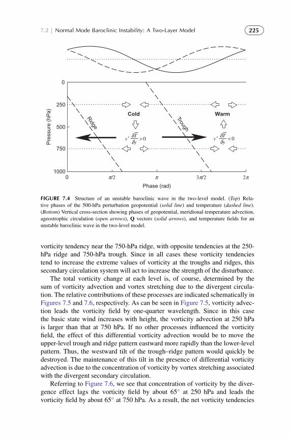
To protect the rights of the author(s) and publisher we inform you that this PDF is an uncorrected proof for internal businessuse only by the author(s), editor(s), reviewer(s), Elsevier and typesetter diacriTech. It is not allowed to publish this proofonline or in print. This proof copy is the copyright property of the publisher and is confidential until formal publication.
“Hakim: 11-ch07-213-254-9780123848666” — 2012/7/28 — 12:35 — page 225 — #13
7.2 | Normal Mode Baroclinic Instability: A Two-Layer Model 225
0
250
500
750
10000 π/2 π 3π/2 2π
Ridge
Trough
WarmCold
Pre
ssur
e (h
Pa)
δTδy
> 0v ′ δTδy
< 0v ′
Phase (rad)
FIGURE 7.4 Structure of an unstable baroclinic wave in the two-level model. (Top) Rela-tive phases of the 500-hPa perturbation geopotential (solid line) and temperature (dashed line).(Bottom) Vertical cross-section showing phases of geopotential, meridional temperature advection,ageostrophic circulation (open arrows), Q vectors (solid arrows), and temperature fields for anunstable baroclinic wave in the two-level model.
vorticity tendency near the 750-hPa ridge, with opposite tendencies at the 250-hPa ridge and 750-hPa trough. Since in all cases these vorticity tendenciestend to increase the extreme values of vorticity at the troughs and ridges, thissecondary circulation system will act to increase the strength of the disturbance.
The total vorticity change at each level is, of course, determined by thesum of vorticity advection and vortex stretching due to the divergent circula-tion. The relative contributions of these processes are indicated schematically inFigures 7.5 and 7.6, respectively. As can be seen in Figure 7.5, vorticity advec-tion leads the vorticity field by one-quarter wavelength. Since in this casethe basic state wind increases with height, the vorticity advection at 250 hPais larger than that at 750 hPa. If no other processes influenced the vorticityfield, the effect of this differential vorticity advection would be to move theupper-level trough and ridge pattern eastward more rapidly than the lower-levelpattern. Thus, the westward tilt of the trough–ridge pattern would quickly bedestroyed. The maintenance of this tilt in the presence of differential vorticityadvection is due to the concentration of vorticity by vortex stretching associatedwith the divergent secondary circulation.
Referring to Figure 7.6, we see that concentration of vorticity by the diver-gence effect lags the vorticity field by about 65◦ at 250 hPa and leads thevorticity field by about 65◦ at 750 hPa. As a result, the net vorticity tendencies

To protect the rights of the author(s) and publisher we inform you that this PDF is an uncorrected proof for internal businessuse only by the author(s), editor(s), reviewer(s), Elsevier and typesetter diacriTech. It is not allowed to publish this proofonline or in print. This proof copy is the copyright property of the publisher and is confidential until formal publication.
“Hakim: 11-ch07-213-254-9780123848666” — 2012/7/28 — 12:35 — page 226 — #14
226 CHAPTER | 7 Baroclinic Development
0
250
500
750
10000 π/2 π 3π/2 2π
Ridge
Trough
Pre
ssur
e (h
Pa)
Phase (rad)
δζδt
<< 0adv
δζδt
>> 0adv
δζδt < 0
adv
δζδt
> 0adv
FIGURE 7.5 Vertical cross-section showing the phase of vorticity change due to vorticityadvection for an unstable baroclinic wave in the two-level model.
0
250
500
750
10000 π/2 π 3π/2 2π
Ridge
Trough
Pre
ssur
e (h
Pa)
Phase (rad)
δζδt
> 0div
δζδt
> 0div
δζδt
< 0div
δζδt
< 0div
FIGURE 7.6 Vertical cross-section showing the phase of vorticity change due to divergence–convergence for an unstable baroclinic wave in the two-level model.
ahead of the vorticity maxima and minima are less than the advective tendenciesat the upper level and greater than the advective tendencies at the lower level:
∣∣∣∣∂ζ ′1∂t
∣∣∣∣ < ∣∣∣∣∂ζ ′1∂t
∣∣∣∣adv,
∣∣∣∣∂ζ ′3∂t
∣∣∣∣ > ∣∣∣∣∂ζ ′3∂t
∣∣∣∣adv
Furthermore, vorticity concentration by the divergence effect will tend toamplify the vorticity perturbations in the troughs and ridges at both the 250- and750-hPa levels as required for a growing disturbance.

To protect the rights of the author(s) and publisher we inform you that this PDF is an uncorrected proof for internal businessuse only by the author(s), editor(s), reviewer(s), Elsevier and typesetter diacriTech. It is not allowed to publish this proofonline or in print. This proof copy is the copyright property of the publisher and is confidential until formal publication.
“Hakim: 11-ch07-213-254-9780123848666” — 2012/7/28 — 12:35 — page 227 — #15
7.3 | The Energetics of Baroclinic Waves 227
7.3 THE ENERGETICS OF BAROCLINIC WAVES
The previous section showed that under suitable conditions a vertically shearedgeostrophically balanced basic state flow is unstable to small wave-like per-turbations with horizontal wavelengths in the range of observed synoptic-scalesystems. Such baroclinically unstable perturbations will amplify exponentiallyby drawing energy from the mean flow. This section considers the energeticsof linearized baroclinic disturbances and shows that the potential energy of themean flow is the energy source for baroclinically unstable perturbations.
7.3.1 Available Potential Energy
Before discussing the energetics of baroclinic waves, it is necessary to con-sider the energy of the atmosphere from a more general point of view. Forall practical purposes, the total energy of the atmosphere is the sum of inter-nal energy, gravitational potential energy, and kinetic energy. However, it isnot necessary to consider separately the variations of internal and gravitationalpotential energy because in a hydrostatic atmosphere these two forms of energyare proportional and may be combined into a single term called the total poten-tial energy. The proportionality of internal and gravitational potential energycan be demonstrated by considering these forms of energy for a column of airof unit horizontal cross-section extending from the surface to the top of theatmosphere.
If we let dEI be the internal energy in a vertical section of the column ofheight dz, then from the definition of internal energy—see Section (2.6):
dEI = ρcvTdz
so that the internal energy for the entire column is
EI = cv
∞∫0
ρTdz (7.29)
However, the gravitational potential energy for a slab of thickness dz at a heightz is just
dEP = ρgzdz
so that the gravitational potential energy in the entire column is
EP =
∞∫0
ρgzdz = −
0∫p0
zdp (7.30)
where we have substituted from the hydrostatic equation to obtain the lastintegral in (7.30). Integrating (7.30) by parts and using the ideal gas law,

To protect the rights of the author(s) and publisher we inform you that this PDF is an uncorrected proof for internal businessuse only by the author(s), editor(s), reviewer(s), Elsevier and typesetter diacriTech. It is not allowed to publish this proofonline or in print. This proof copy is the copyright property of the publisher and is confidential until formal publication.
“Hakim: 11-ch07-213-254-9780123848666” — 2012/7/28 — 12:35 — page 228 — #16
228 CHAPTER | 7 Baroclinic Development
we obtain
EP =
∞∫0
pdz = R
∞∫0
ρTdz (7.31)
Comparing (7.29) and (7.31), we see that cvEP = REI . Thus, the total potentialenergy may be expressed as
EP + EI =(cp/cv
)EI =
(cp/R
)EP (7.32)
Therefore, in a hydrostatic atmosphere the total potential energy can be obtainedby computing either EI or EP alone.
The total potential energy is not a very useful measure of energy in theatmosphere because only a very small fraction of the total potential energyis available for conversion to kinetic energy in storms. To demonstrate qual-itatively why most of the total potential energy is unavailable, we consider asimple model atmosphere that initially consists of two equal masses of dry airseparated by a vertical partition as shown in Figure 7.7. The two air massesare at uniform potential temperatures θ1 and θ2, respectively, with θ1<θ2. Theground-level pressure on each side of the partition is taken to be 1000 hPa.We wish to compute the maximum kinetic energy that can be realized by anadiabatic rearrangement of mass within the same volume when the partition isremoved.
Now for an adiabatic process, total energy is conserved:
EK + EP + EI = constant
where EK denotes the kinetic energy. If the air masses are initially at rest,EK = 0. Thus, if we let primed quantities denote the final state
E′K + E′P + E′I = EP + EI
zθ1
θ2
1000
750
500
250
(hPa)
FIGURE 7.7 Two air masses of differing potential temperature separated by a vertical partition.Dashed lines indicate isobaric surfaces. Arrows show direction of motion when the partition isremoved.

To protect the rights of the author(s) and publisher we inform you that this PDF is an uncorrected proof for internal businessuse only by the author(s), editor(s), reviewer(s), Elsevier and typesetter diacriTech. It is not allowed to publish this proofonline or in print. This proof copy is the copyright property of the publisher and is confidential until formal publication.
“Hakim: 11-ch07-213-254-9780123848666” — 2012/7/28 — 12:35 — page 229 — #17
7.3 | The Energetics of Baroclinic Waves 229
so that with the aid of (7.32) the kinetic energy realized by removal of thepartition may be expressed as
E′K =(cp/cv
) (EI − E′I
)Because θ is conserved for an adiabatic process, the two air masses cannot mix.It is clear that E′I will be a minimum (designated by E′′I ) when the masses arerearranged so that the air at potential temperature θ1 lies entirely beneath the airat potential temperature θ2, with the 500-hPa surface as the horizontal boundarybetween the two masses. In that case the total potential energy (cp/cv)E′′I isnot available for conversion to kinetic energy because no adiabatic process canfurther reduce E′′I .
The available potential energy (APE) can now be defined as the differencebetween the total potential energy of a closed system and the minimum totalpotential energy that could result from an adiabatic redistribution of mass.Thus, for the idealized model given earlier, the APE, which is designated bythe symbol P, is
P =(cp/cv
) (EI − E′′I
)(7.33)
which is equivalent to the maximum kinetic energy that can be realized by anadiabatic process.
Lorenz (1960) showed that available potential energy is given approximatelyby the volume integral over the entire atmosphere of the variance of potentialtemperature on isobaric surfaces. Thus, letting θ designate the average potentialtemperature for a given pressure surface and θ ′ the local deviation from theaverage, the average available potential energy per unit volume satisfies theproportionality
P ∝ V−1∫ (
θ ′2/θ2)
dV
where V designates the total volume. For the quasi-geostrophic model, this pro-portionality is an exact measure of the available potential energy, as shown inthe following subsection.
Observations indicate that for the atmosphere as a whole,
P/[(
cp/cv)
EI]∼ 5× 10⁻³, K/P ∼ 10−1
Thus, only about 0.5% of the total potential energy of the atmosphere is avail-able, and of the available portion only about 10% is actually converted to kineticenergy. From this point of view the atmosphere is a rather inefficient heat engine.
7.3.2 Energy Equations for the Two-Layer Model
In the two-layer model of Section 7.2, the perturbation temperature field isproportional to ψ ′1−ψ
′
3, the 250- to 750-hPa thickness. Thus, in view of the dis-cussion in the previous section, we anticipate that the available potential energy

To protect the rights of the author(s) and publisher we inform you that this PDF is an uncorrected proof for internal businessuse only by the author(s), editor(s), reviewer(s), Elsevier and typesetter diacriTech. It is not allowed to publish this proofonline or in print. This proof copy is the copyright property of the publisher and is confidential until formal publication.
“Hakim: 11-ch07-213-254-9780123848666” — 2012/7/28 — 12:35 — page 230 — #18
230 CHAPTER | 7 Baroclinic Development
in this case will be proportional to (ψ ′1−ψ′
3)2. To show that this in fact must be
the case, we derive the energy equations for the system in the following manner:We first multiply (7.9) by −ψ1, (7.10) by −ψ3, and (7.11) by (ψ ′1 − ψ
′
3). Wethen integrate the resulting equations over one wavelength of the perturbationin the zonal direction.
The resulting zonally averaged2 terms are denoted by overbars as donepreviously in Chapter 5:
( ) = L−1
L∫0
( ) dx
where L is the wavelength of the perturbation. Thus, for the first term in (7.9)we have, after multiplying by −ψ1, averaging and differentiating by parts:
−ψ ′1∂
∂t
(∂2ψ ′1
∂x2
)= −
∂
∂x
[ψ ′1
∂
∂x
(∂ψ ′1
∂t
)]+∂ψ ′1
∂x
∂
∂t
(∂ψ ′1
∂x
)The first term on the right side vanishes because it is the integral of a perfectdifferential in x over a complete cycle. The second term on the right can berewritten in the form
1
2
∂
∂t
(∂ψ ′1
∂x
)2
which is just the rate of change of the perturbation kinetic energy per unit massaveraged over a wavelength. Similarly,−ψ ′1 times the advection term on the leftin (7.9) can be written after integration in x as
−U1ψ′
1∂2
∂x2
(∂ψ ′1
∂x
)= −U1
∂
∂x
[ψ ′1
∂
∂x
(∂ψ ′1
∂x
)]+ U1
∂ψ ′1
∂x
∂2ψ ′1
∂x2
=U1
2
∂
∂x
(∂ψ ′1
∂x
)2
= 0
Thus, the advection of kinetic energy vanishes when integrated over a wave-length. Evaluating the various terms in (7.10) and (7.11) in the same mannerafter multiplying through by −ψ ′3 and (ψ ′1 − ψ
′
3), respectively, we obtain thefollowing set of perturbation energy equations:
1
2
∂
∂t
(∂ψ ′1
∂x
)2
= −f0δpω′2ψ
′
1 (7.34)
2A zonal average generally designates the average around an entire circle of latitude. However, fora disturbance consisting of a single sinusoidal wave of wave number k = m/(a cosφ), where m isan integer, the average over a wavelength is identical to a zonal average.

To protect the rights of the author(s) and publisher we inform you that this PDF is an uncorrected proof for internal businessuse only by the author(s), editor(s), reviewer(s), Elsevier and typesetter diacriTech. It is not allowed to publish this proofonline or in print. This proof copy is the copyright property of the publisher and is confidential until formal publication.
“Hakim: 11-ch07-213-254-9780123848666” — 2012/7/28 — 12:35 — page 231 — #19
7.3 | The Energetics of Baroclinic Waves 231
1
2
∂
∂t
(∂ψ ′3
∂x
)2
= +f0δpω′2ψ
′
3 (7.35)
1
2
∂
∂t
(ψ ′1 − ψ
′
3
)2= UT
(ψ ′1 − ψ
′
3
) ∂∂x
(ψ ′1 + ψ
′
3
)+σδp
f0ω′2
(ψ ′1 − ψ
′
3
)(7.36)
where as before UT ≡ (U1 – U3)/2.Defining the perturbation kinetic energy to be the sum of the kinetic energies
of the 250- and 750-hPa levels,
K′ ≡ (1/2)
[(∂ψ ′1/∂x
)2+(∂ψ ′3/∂x
)2]we find by adding (7.34) and (7.35) that
dK′/dt = − (f0/δp) ω′2(ψ ′1 − ψ
′
3
)= − (2f0/δp) ω′2ψT (7.37)
Thus, the rate of change of perturbation kinetic energy is proportional to thecorrelation between perturbation thickness and vertical motion.
If we now define the perturbation available potential energy as
P′ ≡ λ2(ψ ′1 − ψ ′3)2/2we obtain from (7.36)
dP′/dt = λ2UT(ψ ′1 − ψ
′
3
)∂(ψ ′1 + ψ
′
3
)/∂x+ ( f0/δp) ω′2
(ψ ′1 − ψ
′
3
)= 4λ2UTψT∂ψm/∂x+ (2f0/δp) ω′2ψT (7.38)
The last term in (7.38) is just equal and opposite to the kinetic energy sourceterm in (7.37). This term clearly must represent a conversion between potentialand kinetic energy. If on average the vertical motion is positive (ω′2 < 0) wherethe thickness is greater than average (ψ ′1 − ψ
′
3 > 0) and vertical motion isnegative where thickness is less than average, then
ω′2
(ψ ′1 − ψ
′
3
)= 2ω′2ψT < 0
and the perturbation potential energy is being converted to kinetic energy.Physically, this correlation represents an overturning in which cold air aloft isreplaced by warm air from below, a situation that clearly tends to lower thecenter of mass and thus the potential energy of the perturbation. However, theavailable potential energy and kinetic energy of a disturbance can still growsimultaneously, provided that the potential energy generation due to the firstterm in (7.38) exceeds the rate of potential energy conversion to kinetic energy.
The potential energy generation term in (7.38) depends on the correlationbetween the perturbation thickness ψT and the meridional velocity at 500 hPa,

To protect the rights of the author(s) and publisher we inform you that this PDF is an uncorrected proof for internal businessuse only by the author(s), editor(s), reviewer(s), Elsevier and typesetter diacriTech. It is not allowed to publish this proofonline or in print. This proof copy is the copyright property of the publisher and is confidential until formal publication.
“Hakim: 11-ch07-213-254-9780123848666” — 2012/7/28 — 12:35 — page 232 — #20
232 CHAPTER | 7 Baroclinic Development
∂ψm/∂x. In order to understand the role of this term, it is helpful to con-sider a particular sinusoidal wave disturbance. Suppose that the barotropic andbaroclinic parts of the disturbance can be written, respectively, as
ψm = Am cos k (x− ct) and ψT = AT cos k (x+ x0 − ct) (7.39)
where x0 designates the phase difference. Because ψm is proportional to the500-hPa geopotential and ψT is proportional to the 500-hPa temperature (or250- to 750-hPa thickness), the phase angle kx0 gives the phase differencebetween geopotential and temperature fields at 500 hPa. Furthermore, Am andAT are measures of the amplitudes of the 500-hPa disturbance geopotential andthickness fields, respectively. Using the expressions in (7.39), we obtain
ψT∂ψm
∂x= −
k
L
L∫0
ATAm cos k (x+ x0 − ct) sin k (x− ct) dx
=kATAm sin kx0
L
L∫0
[sin k (x− ct)]2 dx
= (ATAmk sin kx0) /2
(7.40)
Substituting from (7.40) into (7.38), we see that for the usual midlatitude caseof a westerly thermal wind (UT > 0) the correlation in (7.40) must be positiveif the perturbation potential energy is to increase. Thus, kx0 must satisfy theinequality 0 < kx0 < π . Furthermore, the correlation will be a positive maxi-mum for kx0 = π /2—that is, when the temperature wave lags the geopotentialwave by 90◦ in phase at 500 hPa.
This case was shown schematically earlier in Figure 7.4. Clearly, when thetemperature wave lags the geopotential by one-quarter cycle, the northwardadvection of warm air by the geostrophic wind east of the 500-hPa trough andthe southward advection of cold air west of the 500-hPa trough are both max-imized. As a result, cold advection is strong below the 250-hPa trough, andwarm advection is strong below the 250-hPa ridge. In that case, as discussedpreviously in Section 6.4.2, the upper-level disturbance will intensify. It shouldalso be noted here that if the temperature wave lags the geopotential wave,the trough and ridge axes will tilt westward with height, which, as mentionedin Section 6.1, is observed to be the case for amplifying midlatitude synopticsystems.
Referring again to Figure 7.4 and recalling the vertical motion patternimplied by the omega equation (7.28), we see that the signs of the two termson the right in (7.38) cannot be the same. In the westward-tilting perturbationof Figure 7.4, the vertical motion must be downward in the cold air behindthe trough at 500 hPa. Hence, the correlation between temperature and verticalvelocity must be positive in this situation; that is,
ω′2ψT < 0

To protect the rights of the author(s) and publisher we inform you that this PDF is an uncorrected proof for internal businessuse only by the author(s), editor(s), reviewer(s), Elsevier and typesetter diacriTech. It is not allowed to publish this proofonline or in print. This proof copy is the copyright property of the publisher and is confidential until formal publication.
“Hakim: 11-ch07-213-254-9780123848666” — 2012/7/28 — 12:35 — page 233 — #21
7.3 | The Energetics of Baroclinic Waves 233
Thus, for quasi-geostrophic perturbations, a westward tilt of the perturbationwith height implies both that the horizontal temperature advection will increasethe available potential energy of the perturbation and that the vertical circula-tion will convert perturbation available potential energy to perturbation kineticenergy. Conversely, an eastward tilt of the system with height would change thesigns of both terms on the right in (7.38).
Although the signs of the potential energy generation term and the potentialenergy conversion term in (7.38) are always opposite for a developing baroclinicwave, it is only the potential energy generation rate that determines the growthof the total energy P′ + K′ of the disturbance. This may be proved by adding(7.37) and (7.38) to obtain
d(P′ + K′
)/dt = 4λ2UTψT∂ψm/∂x
Provided the correlation between the meridional velocity and temperature ispositive and UT > 0, the total energy of the perturbation will increase. Notethat the vertical circulation merely converts disturbance energy between theavailable potential and kinetic forms without affecting the total energy of theperturbation.
The rate of increase of the total energy of the perturbation depends on themagnitude of the basic state thermal wind UT . This is, of course, proportional tothe zonally averaged meridional temperature gradient. Because the generationof perturbation energy requires systematic poleward transport of warm air andequatorward transport of cold air, it is clear that baroclinically unstable distur-bances tend to reduce the meridional temperature gradient and thus the availablepotential energy of the mean flow. This latter process cannot be described math-ematically in terms of the linearized equations. However, from Figure 7.8 we
θ0 + 3δθ
θ0 + 2δθ
y
θ0 +δθ
θ0
FIGURE 7.8 Slopes of parcel trajectories relative to the zonal-mean potential temperature surfacesfor a baroclinically unstable disturbance (solid arrows) and for a baroclinically stable disturbance(dashed arrows).

To protect the rights of the author(s) and publisher we inform you that this PDF is an uncorrected proof for internal businessuse only by the author(s), editor(s), reviewer(s), Elsevier and typesetter diacriTech. It is not allowed to publish this proofonline or in print. This proof copy is the copyright property of the publisher and is confidential until formal publication.
“Hakim: 11-ch07-213-254-9780123848666” — 2012/7/28 — 12:35 — page 234 — #22
234 CHAPTER | 7 Baroclinic Development
can see qualitatively that parcels that move poleward and upward with slopesless than the slope of the zonal-mean potential temperature surface will becomewarmer than their surroundings, and vice versa for parcels moving downwardand equatorward.
For such parcels the correlations between disturbance meridional velocityand temperature and between disturbance vertical velocity and temperature willboth be positive as required for baroclinically unstable disturbances. For parcelsthat have trajectory slopes greater than the mean potential temperature slope,however, both of these correlations will be negative. Such parcels must thenconvert disturbance kinetic energy to disturbance available potential energy,which is in turn converted to zonal-mean available potential energy. There-fore, in order that perturbations are able to extract potential energy from themean flow, the perturbation parcel trajectories in the meridional plane must haveslopes less than the slopes of the potential temperature surfaces, and a permanentrearrangement of air must take place for there to be a net heat transfer.
Since we have previously seen that poleward-moving air must rise andequatorward-moving air must sink, it is clear that the rate of energy generationcan be greater for an atmosphere in which the meridional slope of the poten-tial temperature surfaces is large. We can also see more clearly why baroclinicinstability has a short-wave cutoff. As mentioned previously, the intensity ofthe vertical circulation must increase as the wavelength decreases. Thus, theslopes of the parcel trajectories must increase with decreasing wavelength, andfor some critical wavelength the trajectory slopes will become greater thanthe slopes of the potential temperature surfaces. Unlike convective instabil-ity, where the most rapid amplification occurs for the smallest possible scales,baroclinic instability is most effective at an intermediate range of scales.
The energy flow for quasi-geostrophic perturbations is summarized inFigure 7.9 by means of a block diagram. In this type of energy diagram eachblock represents a reservoir of a particular type of energy, and arrows desig-nate the direction of energy flow. The complete energy cycle cannot be derivedin terms of linear perturbation theory but will be discussed qualitatively inChapter 10.
7.4 BAROCLINIC INSTABILITY OF A CONTINUOUSLYSTRATIFIED ATMOSPHERE
In the two previous sections some basic aspects of baroclinic instability wereelucidated in the context of a simple two-layer model. The dependence ofgrowth rate on vertical shear and the existence of a short-wave cutoff wereclearly demonstrated. The two-layer model, however, does have one severe con-straint: It assumes that the altitude dependence of large-scale systems can beadequately represented with only two degrees of freedom in the vertical (i.e.,the streamfunctions at the 250- and 750-hPa levels). Although most synoptic-scale systems in midlatitudes are observed to have vertical scales comparable

To protect the rights of the author(s) and publisher we inform you that this PDF is an uncorrected proof for internal businessuse only by the author(s), editor(s), reviewer(s), Elsevier and typesetter diacriTech. It is not allowed to publish this proofonline or in print. This proof copy is the copyright property of the publisher and is confidential until formal publication.
“Hakim: 11-ch07-213-254-9780123848666” — 2012/7/28 — 12:35 — page 235 — #23
7.4 | Baroclinic Instability of a Continuously Stratified Atmosphere 235
P ′Perturbation
availablepotential energy
K ′Perturbation
kinetic energy
PMean flowavailable
potential energy
⟨(ψ ′1 − ψ ′3) ∂ (ψ ′1 + ψ ′3)⟩∂x
⟨ω ′2 (ψ ′1 − ψ ′3)⟩
FIGURE 7.9 Energy flow in an amplifying baroclinic wave.
to the depth of the troposphere, observed vertical structures do differ. Distur-bances that are concentrated near the ground or near the tropopause can hardlybe represented accurately in the two-layer model.
An analysis of the structure of baroclinic modes for realistic mean zonalwind profiles is quite complex, and indeed can only be done by numerical meth-ods. However, without obtaining specific normal mode solutions, it is possibleto obtain necessary conditions for baroclinic or barotropic instability from anintegral theorem first developed by Rayleigh. This theorem, which is discussedin Section 7.4.2, also shows how baroclinic instability is intimately related tothe mean meridional gradient of potential vorticity and the mean meridionaltemperature gradient at the surface.
If a number of simplifying assumptions are made, it is possible to posethe stability problem for a continuously stratified atmosphere in a fashion thatleads to a second-order differential equation for the vertical structure that canbe solved by standard methods. This problem was originally studied by theBritish meteorologist Eady (1949) and, although mathematically similar to thetwo-layer model, provides additional insights. It is developed in Section 7.4.3.
7.4.1 Log-Pressure Coordinates
Derivation of the Rayleigh theorem and the Eady stability model is facilitatedif we transform from the standard isobaric coordinates to a vertical coordinatebased on the logarithm of pressure. In the log-pressure coordinates, the vertical
To protect the rights of the author(s) and publisher we inform you that this PDF is an uncorrected proof for internal businessuse only by the author(s), editor(s), reviewer(s), Elsevier and typesetter diacriTech. It is not allowed to publish this proofonline or in print. This proof copy is the copyright property of the publisher and is confidential until formal publication.
“Hakim: 11-ch07-213-254-9780123848666” — 2012/7/28 — 12:35 — page 236 — #24
236 CHAPTER | 7 Baroclinic Development
coordinate is defined as
z∗ ≡ −H ln (p/ps) (7.41)
where ps is a standard reference pressure (usually taken to be 1000 hPa) andH is a standard scale height, H ≡ RTs/g, with Ts a global average temper-ature. For the special case of an isothermal atmosphere at temperature Ts, z∗
is exactly equal to geometric height, and the density profile is given by thereference density
ρ0(z∗)= ρs exp
(−z∗/H
)where ρs is the density at z∗ = 0.
For an atmosphere with a realistic temperature profile, z∗ is only approxi-mately equivalent to the height, but in the troposphere the difference is usuallyquite small. The vertical velocity in this coordinate system is
w∗ ≡ Dz∗/dt
The horizontal momentum equation in the log-pressure system is the same asthat in the isobaric system:
DV/Dt + f k× V = −∇h8 (7.42)
However, the operator D/Dt is now defined as
D/Dt = ∂/∂t + V ·∇h + w∗∂/∂z∗
The hydrostatic equation ∂8/∂p = −α can be transformed to the log-pressuresystem by multiplying through by p and using the ideal gas law to get
∂8/∂ ln p = −RT
which after dividing through by –H and using (7.41) gives
∂8/∂z∗ = RT/H (7.43)
The log-pressure form of the continuity equation can be obtained by transform-ing from the isobaric coordinate form (3.5). We first note that
w∗ ≡ −(H/p)Dp/Dt = −Hω/p
so that
∂ω
∂p= −
∂
∂p
(pw∗
H
)=∂w∗
∂z∗−
w∗
H=
1
ρ0
∂(ρ0w∗)
∂z∗
Thus, in log-pressure coordinates the continuity equation becomes simply
∂u
∂x+∂v
∂y+
1
ρ0
∂(ρ0w∗)
∂z∗= 0 (7.44)

To protect the rights of the author(s) and publisher we inform you that this PDF is an uncorrected proof for internal businessuse only by the author(s), editor(s), reviewer(s), Elsevier and typesetter diacriTech. It is not allowed to publish this proofonline or in print. This proof copy is the copyright property of the publisher and is confidential until formal publication.
“Hakim: 11-ch07-213-254-9780123848666” — 2012/7/28 — 12:35 — page 237 — #25
7.4 | Baroclinic Instability of a Continuously Stratified Atmosphere 237
It is left as a problem for the reader to show that the first law of thermody-namics (3.6) can be expressed in log-pressure form as(
∂
∂t+ V ·∇h
)∂8
∂z∗+ w∗N2
=κJ
H(7.45)
where
N2≡ (R/H)
(∂T/∂z∗ + κT/H
)is the buoyancy frequency squared (see Section 2.7.3) and κ ≡ R/cp. Unlike thestatic stability parameter, Sp, in the isobaric form of the thermodynamic equation(3.6), the parameter N2 varies only weakly with height in the troposphere; it canbe assumed to be constant without serious error. This is a major advantage ofthe log-pressure formulation.
The quasi-geostrophic potential vorticity equation has the same form as inthe isobaric system, but with q defined as
q ≡ ∇2hψ + f +
1
ρ0
∂
∂z∗
(ερ0
∂ψ
∂z∗
)(7.46)
where ε ≡ f 20 /N
2.
7.4.2 Baroclinic Instability: The Rayleigh Theorem
We now examine the stability problem for a continuously stratified atmo-sphere on the midlatitude β plane. The linearized form of the quasi-geostrophicpotential vorticity equation can be expressed in log-pressure coordinates as(
∂
∂t+ u
∂
∂x
)q′ +
∂q
∂y
∂ψ ′
∂x= 0 (7.47)
where
q′ ≡ ∇2hψ′+
1
ρ0
∂
∂z∗
(ερ0
∂ψ ′
∂z∗
)(7.48)
and
∂q
∂y= β −
∂2u
∂y2−
1
ρ0
∂
∂z∗
(ερ0
∂u
∂z∗
)(7.49)
As in the two-layer model, boundary conditions are required at lower- andupper-boundary pressure surfaces. Assuming that the flow is adiabatic and thatthe vertical motion w∗ vanishes at these boundaries, the linearized form of thethermodynamic energy equation (7.45) valid at horizontal boundary surfaces issimply (
∂
∂t+ u
∂
∂x
)∂ψ ′
∂z∗−∂ψ ′
∂x
∂u
∂z∗= 0 (7.50)

To protect the rights of the author(s) and publisher we inform you that this PDF is an uncorrected proof for internal businessuse only by the author(s), editor(s), reviewer(s), Elsevier and typesetter diacriTech. It is not allowed to publish this proofonline or in print. This proof copy is the copyright property of the publisher and is confidential until formal publication.
“Hakim: 11-ch07-213-254-9780123848666” — 2012/7/28 — 12:35 — page 238 — #26
238 CHAPTER | 7 Baroclinic Development
The sidewall boundary conditions are
∂ψ ′/∂x = 0, hence, ψ ′ = 0 at y = ±L (7.51)
We now assume that the perturbation consists of a single zonal Fouriercomponent propagating in the x direction:
ψ ′(x, y, z, t) = Re{9(y, z)
exp[ik(x− ct
)]}(7.52)
where 9(y, z) = 9r + i9i is a complex amplitude, k is the zonal wave number,and c = cr + ici is a complex phase speed. Note that (7.52) can alternatively beexpressed as
ψ ′(x, y, z, t
)= ekcit
[9r cos k
(x− crt
)−9i sin k
(x− crt
)]Thus, the relative magnitudes of 9r and 9i determine the phase of the wave forany y, z∗.
Substituting from (7.52) into (7.47) and (7.50) yields
(u− c)
[∂29
∂y2− k29 +
1
ρ0
∂
∂z∗
(ερ0
∂9
∂z∗
)]+∂q
∂y9 = 0 (7.53)
and
(u− c)∂9
∂z∗−∂u
∂z∗9 = 0 at z∗ = 0 (7.54)
If the upper boundary is taken to be a rigid lid at a finite height, as is sometimesdone in theoretical studies, the condition (7.54) is appropriate at that bound-ary as well. Alternatively the upper boundary condition can be specified byrequiring 9 to remain finite as z∗→∞.
Equation (7.53), together with its boundary conditions, constitutes a linearboundary value problem for 9(y, z∗). It is generally not simple to obtain solu-tions to (7.53) for realistic mean zonal wind profiles. Nevertheless, we canobtain some useful information on stability properties simply by analyzing theenergetics of the system.
Dividing (7.53) by (u−c) and separating the resulting equation into real andimaginary parts, we obtain
∂29r
∂y2+
1
ρ0
∂
∂z∗
(ερ0
∂9r
∂z∗
)−
[k2− δr (∂q/∂y)
]9r
− δi∂q/∂y9i = 0
(7.55)
∂29i
∂y2+
1
ρ0
∂
∂z∗
(ερ0
∂9i
∂z∗
)−
[k2− δr (∂q/∂y)
]9i
+ δi∂q/∂y9r = 0
(7.56)

To protect the rights of the author(s) and publisher we inform you that this PDF is an uncorrected proof for internal businessuse only by the author(s), editor(s), reviewer(s), Elsevier and typesetter diacriTech. It is not allowed to publish this proofonline or in print. This proof copy is the copyright property of the publisher and is confidential until formal publication.
“Hakim: 11-ch07-213-254-9780123848666” — 2012/7/28 — 12:35 — page 239 — #27
7.4 | Baroclinic Instability of a Continuously Stratified Atmosphere 239
where
δr =u− cr
(u− cr)2+ c2
i
, and δi =ci
(u− cr)2+ c2
i
Similarly, dividing (7.54) through by (u − c) and separating into real andimaginary parts gives, for the boundary condition at z∗ = 0,
∂9r
∂z∗+∂u
∂z∗(δi9i − δr9r) = 0;
∂9i
∂z∗−∂u
∂z∗(δr9i + δi9r) = 0 (7.57)
Multiplying (7.55) by 9i, (7.56) by 9r, and subtracting the latter from theformer yields
ρ0
[9i∂29r
∂y2−9r
∂29i
∂y2
]+
[9i
∂
∂z∗
(ερ0
∂9r
∂z∗
)−9r
∂
∂z∗
(ερ0
∂9i
∂z∗
)]− ρ0δi(∂q/∂y)
(92
i +92r
)= 0
(7.58)
Using the chain rule of differentiation, (7.58) can be expressed in the form
ρ0∂
∂y
[9i∂9r
∂y−9r
∂9i
∂y
]+
∂
∂z∗
[ερ0
(9i∂9r
∂z∗−9r
∂9i
∂z∗
)]− ρ0δi(∂q/∂y)
(92
i +92r
)= 0
(7.59)
The first term in brackets in (7.59) is a perfect differential in y; the secondterm is a perfect differential in z∗. Thus, if (7.59) is integrated over the y, z∗
domain, the result can be expressed as
∞∫0
[9i∂9r
∂y−9r
∂9i
∂y
]+L
−Lρ0dz∗ +
+L∫−L
[ερ0
(9i∂9r
∂z∗−9r
∂9i
∂z∗
)]∞0
dy
=
+L∫−L
∞∫0
ρ0δi∂q
∂y
(92
i +92r
)dydz∗ (7.60)
However, from (7.51)9i = 9r = 0 at y = ±L so that the first integral in (7.60)vanishes. Furthermore, if 9 remains finite as z∗ → ∞, the contribution to thesecond integral of (7.60) at the upper boundary vanishes. If we then use (7.57) toeliminate the vertical derivatives in this term at the lower boundary, (7.60) can

To protect the rights of the author(s) and publisher we inform you that this PDF is an uncorrected proof for internal businessuse only by the author(s), editor(s), reviewer(s), Elsevier and typesetter diacriTech. It is not allowed to publish this proofonline or in print. This proof copy is the copyright property of the publisher and is confidential until formal publication.
“Hakim: 11-ch07-213-254-9780123848666” — 2012/7/28 — 12:35 — page 240 — #28
240 CHAPTER | 7 Baroclinic Development
be expressed as
ci
+L∫−L
∞∫0
∂q
∂y
ρ0 |9|2
|u− c|2dydz∗ −
+L∫−L
ε∂u
∂z∗ρ0 |9|
2
|u− c|2
∣∣∣∣∣z∗=0
dy
= 0 (7.61)
where |9|2 = 92r +9
2i is the disturbance amplitude squared.
Equation (7.61) has important implications for the stability of quasi-geostrophic perturbations. For unstable modes, ci must be nonzero, and thusthe quantity in square brackets in (7.61) must vanish. Because |9|2/|u − c|2 isnonnegative, instability is possible only when ∂u/∂z∗ at the lower boundary and(∂q/∂y) in the whole domain satisfy certain constraints:
1. If ∂u/∂z∗ at z∗ = 0 (which by thermal wind balance implies that the meri-dional temperature gradient vanishes at the boundary), the second integralin (7.61) vanishes. Thus, the first integral must also vanish for instability tooccur. This can occur only if ∂q/∂y changes sign within the domain (i.e.,∂q/∂y = 0 somewhere). This is referred to as the Rayleigh necessary condi-tion and is another demonstration of the fundamental role played by potentialvorticity. Because ∂q/∂y is normally positive, it is clear that in the absenceof temperature gradients at the lower boundary, a region of negative meridi-onal potential vorticity gradients must exist in the interior for instability tobe possible.
2. If ∂q/∂y ≥ 0 everywhere, then it is necessary that ∂u/∂z∗> 0 somewhere atthe lower boundary for ci > 0.
3. If ∂u/∂z∗< 0 everywhere at z∗= 0, then it is necessary that ∂q/∂y< 0 some-where for instability to occur. Thus, there is an asymmetry between westerlyand easterly shear at the lower boundary, with the former more favorable forbaroclinic instability.
The basic state potential vorticity gradient in (7.49) can be written in theform
∂q
∂y= β −
∂2u
∂y2+ε
H
∂u
∂z∗− ε
∂2u
∂z∗2−∂ε
∂z∗∂u
∂z∗
Because β is positive everywhere, if ε is constant a negative basic state poten-tial vorticity gradient can occur only for strong positive mean flow curvature(i.e., ∂2u/∂y2 or ∂2u/∂z∗
2� 0 ) or strong negative vertical shear (∂u/∂z∗ � 0).
Strong positive meridional curvature can occur at the core of an easterly jet oron the flanks of a westerly jet. Instability associated with such horizontal curva-ture is referred to as barotropic instability. The normal baroclinic instability inmidlatitudes is associated with mean flows in which ∂q/∂y > 0 and ∂u/∂z∗ > 0at the ground. Hence, a mean meridional temperature gradient at the ground isessential for the existence of such instability. Baroclinic instability can also beexcited at the tropopause because of the rapid decrease of ε with height if there

To protect the rights of the author(s) and publisher we inform you that this PDF is an uncorrected proof for internal businessuse only by the author(s), editor(s), reviewer(s), Elsevier and typesetter diacriTech. It is not allowed to publish this proofonline or in print. This proof copy is the copyright property of the publisher and is confidential until formal publication.
“Hakim: 11-ch07-213-254-9780123848666” — 2012/7/28 — 12:35 — page 241 — #29
7.4 | Baroclinic Instability of a Continuously Stratified Atmosphere 241
is a sufficiently strong easterly mean wind shear to cause a local reversal in themean potential vorticity gradient.
7.4.3 The Eady Stability Problem
This section analyzes the structures (eigenfunctions) and growth rates (eigen-values) for unstable modes in the simplest possible model that satisfies thenecessary conditions for instability in a continuous atmosphere given in theprevious subsection. For simplicity, we make the following assumptions:
l Basic state density constant (Boussinesq approximation).l f -plane geometry (β = 0).l ∂u/∂z∗ = 3 = constant.l Rigid lids at z∗ = 0 and H.
These conditions are only a crude model of the atmosphere, but provide a firstapproximation for study of the dependence of vertical structure on horizontalscale and stability. Despite the zero mean potential vorticity in the domain,the Eady model satisfies the necessary conditions for instability discussed in theprevious subsection because vertical shear of the basic state mean flow at theupper boundary provides an additional term in (7.61) that is equal and oppositeto the lower boundary integral.
Using the aforementioned approximations, the quasi-geostrophic potentialvorticity equation is (
∂
∂t+ u
∂
∂x
)q′ = 0 (7.62)
where the perturbation potential vorticity is given by
q′ = ∇hψ′+ ε
∂2ψ
∂z∗2(7.63)
and ε≡ f 20 /N
2. The thermodynamic energy equation at the horizontal bound-aries (z∗= 0,H) is (
∂
∂t+ u
∂
∂x
)T ′ = 0 (7.64)
Letting
ψ ′(x, y, z∗, t
)= 9
(z∗)
cos ly exp [ik (x− ct)]
u(z∗)= 3z∗
(7.65)
where as in the previous subsection 9(z∗) is a complex amplitude and c acomplex phase speed, and substituting from (7.65) into (7.62) we find that
(u− c) q′ = 0 (7.66)

To protect the rights of the author(s) and publisher we inform you that this PDF is an uncorrected proof for internal businessuse only by the author(s), editor(s), reviewer(s), Elsevier and typesetter diacriTech. It is not allowed to publish this proofonline or in print. This proof copy is the copyright property of the publisher and is confidential until formal publication.
“Hakim: 11-ch07-213-254-9780123848666” — 2012/7/28 — 12:35 — page 242 — #30
242 CHAPTER | 7 Baroclinic Development
From (7.66) we see that either q′= 0 or u− c= 0. Since u=3z∗,u− c = 0 allows for nonzero q′ only at the level where the wave speed matchesthe flow speed. Moreover, since u is strictly real, the wave speed in this casemust be as well, so this particular solution branch describes singular neutralmodes (spikes of PV at the steering level of the wave). They are useful fordescribing the evolution of potential vorticity disturbances in the Eady model,but they do not describe instability. Therefore, unstable modes must have q′= 0,which from (7.63) implies that the vertical structure is given by the solution ofthe second-order differential equation
d29
dz∗2− α29 = 0 (7.67)
where α2=(k2+ l2
)/ε. A similar substitution into (7.64) yields the boundary
conditions (3z∗ − c
)d9/dz∗ −93 = 0, at z∗ = 0,H (7.68)
valid for rigid horizontal boundaries (w∗= 0) at the surface (z∗= 0) and thetropopause (z∗=H).
The general solution of (7.67) can be written in the form
9(z∗)= A sinhαz∗ + B coshαz∗ (7.69)
Substituting from (7.69) into the boundary conditions (7.68) for z∗= 0 and Hyields a set of two linear homogeneous equations in the amplitude coefficientsA and B:
−cαA− B3 = 0
α(3H − c) (A coshαH + B sinhαH)−3(A sinhαH + B coshαH) = 0
As in the two-layer model, a nontrivial solution exists only if the determinant ofthe coefficients of A and B vanishes. Again, this leads to a quadratic equation inthe phase speed c. The solution (see Problem 7.12) has the form
c =3H
2±3H
2
[1−
4 coshαH
αH sinhαH+
4
α2H2
]1/2
(7.70)
Thus
ci 6= 0 if 1−4 coshαH
αH sinhαH+
4
α2H2< 0
and the flow is then baroclinically unstable. When the quantity in square brack-ets in (7.70) is equal to zero, the flow is said to be neutrally stable. Thiscondition occurs for α = αc where
α2c H2/4− αcH (tanhαcH)−1
+ 1 = 0 (7.71)

To protect the rights of the author(s) and publisher we inform you that this PDF is an uncorrected proof for internal businessuse only by the author(s), editor(s), reviewer(s), Elsevier and typesetter diacriTech. It is not allowed to publish this proofonline or in print. This proof copy is the copyright property of the publisher and is confidential until formal publication.
“Hakim: 11-ch07-213-254-9780123848666” — 2012/7/28 — 12:35 — page 243 — #31
7.4 | Baroclinic Instability of a Continuously Stratified Atmosphere 243
Using the identity
tanhαcH = 2 tanh
(αcH
2
)/[1+ tanh2
(αcH
2
)]we can factor (7.71) to yield[
αcH
2− tanh
(αcH
2
)][αcH
2− coth
(αcH
2
)]= 0 (7.72)
Thus, the critical value of α is given by αcH/2 = /coth(αcH/2), which impliesαcH ∼= 2.4. Hence, instability requires α < αc or(
k2+ l2
)<(α2
c f 20 /N
2)≈ 5.76/L2
R
where LR≡NH/f0≈ 1000 km is the Rossby radius of deformation for a contin-uously stratified fluid—compare to λ−1 defined just below equation (7.16). Forwaves with equal zonal and meridional wave numbers (k = l), the wavelength AQ:1of maximum growth rate turns out to be
Lm = 2√
2πLR/(Hαm) ∼= 5500 km
where αm is the value of α for which kci is a maximum.Substituting this value of α into the solution for the vertical structure of the
streamfunction (7.69) and using the lower boundary condition to express thecoefficient B in terms of A, we can determine the vertical structure of the mostunstable mode. As shown in Figure 7.10, trough and ridge axes slope westwardwith height, in agreement with the requirements for extraction of availablepotential energy from the mean flow. The axes of the warmest and coldestair, however, tilt eastward with height, a result that could not be determinedfrom the two-layer model where temperature was given at a single level.Furthermore, Figures 7.10a and 7.10b show that east of the upper-level troughaxis, where the perturbation meridional velocity is positive, the vertical velocityis also positive. Thus, parcel motion is poleward and upward in the regionwhere θ ′> 0. Conversely, west of the upper-level trough axis parcel motion isequatorward and downward where θ ′< 0. Both cases are thus consistent withthe energy-converting parcel trajectory slopes shown earlier in Figure 7.8.
Although the Eady model yields unstable solutions that resemble the baro-clinic waves that dominate the statistics of midlatitude eddy fields, individualcyclone events are highly localized and often develop at a faster rate thandescribed by the growth rate of the most unstable mode. Both issues are resolvedby considering initial value problems for finite-amplitude, localized, upper-levelinitial disturbances, as are often observed to precede the development of sur-face cyclones. Figure 7.11 shows the development of a surface cyclone from a

To protect the rights of the author(s) and publisher we inform you that this PDF is an uncorrected proof for internal businessuse only by the author(s), editor(s), reviewer(s), Elsevier and typesetter diacriTech. It is not allowed to publish this proofonline or in print. This proof copy is the copyright property of the publisher and is confidential until formal publication.
“Hakim: 11-ch07-213-254-9780123848666” — 2012/7/28 — 12:35 — page 244 — #32
244 CHAPTER | 7 Baroclinic Development
(a)
1.0
H L0.5
0.0
(c)
W C W
1.0
0.5
0 2ππ0.0
kx
(b)
1.0
0.5
0.0
Hz∗
FIGURE 7.10 Properties of the most unstable Eady wave. (a) Contours of perturbation geopoten-tial height; “H” and “L” designate ridge and trough axes, respectively. (b) Contours of vertical veloc-ity; up and down arrows designate axes of maximum upward and downward motion, respectively.(c) Contours of perturbation temperature; “W” and “C” designate axes of warmest and coldesttemperatures, respectively. In all panels 1 and 1/4 wavelengths are shown for clarity.
localized initial disturbance. Note that, after 48 hours, the full nonlinear solu-tion resembles a mature extratropical cyclone, with warm air moving polewardand cold air moving equatorward around an area of low pressure. The linearsolution for only the unstable growing modes approximates the full nonlinearsolution and shows that the development may be explained by the projection ofthe initial disturbance onto only the unstable modes. Nonlinear effects relate tothe poleward drift of the surface cyclone because of the interaction of the sur-face and upper-level PV anomalies and details of the development of the surfacecold and warm fronts. Although the unstable modes are sufficient to explain thedevelopment of surface cyclones, it turns out that transient development is alsopossible, even when all the modes are neutral.

To protect the rights of the author(s) and publisher we inform you that this PDF is an uncorrected proof for internal businessuse only by the author(s), editor(s), reviewer(s), Elsevier and typesetter diacriTech. It is not allowed to publish this proofonline or in print. This proof copy is the copyright property of the publisher and is confidential until formal publication.
“Hakim: 11-ch07-213-254-9780123848666” — 2012/7/28 — 12:35 — page 245 — #33
7.5 | Growth and Propagation of Neutral Modes 245
ψ,z = 0 θ
FIGURE 7.11 Development of a spatially localized disturbance in an idealized westerly jet stream.Dashed lines show pressure every 4 hPa and solid lines show potential temperature every 5 K.An initial surface disturbance (top panel) associated with an upper-level PV anomaly evolves intoa well-developed extratropical cyclone 48 h later (middle panel). The linear solution for only theprojection of the initial disturbance onto the unstable normal modes (bottom panel) captures most ofthe development of the full nonlinear solution. (Adapted from Hakim, 2000. Copyright © AmericanMeteorological Society. Reprinted with permission.)
7.5 GROWTH AND PROPAGATION OF NEUTRAL MODES
As suggested earlier, baroclinic wave disturbances with certain favorable initialconfigurations may amplify rapidly even in the absence of baroclinic instability.Although the theory for the optimal initial perturbations that give rise to rapidtransient growth is beyond the scope of this book, the main ideas can be exposedmathematically and illustrated with an example from the two-layer model.
A central concept for growth involves a metric, which is needed to mea-sure the amplitude of disturbances; we call this measure a norm. A familiarexample is the magnitude of a scalar z, |z|, which gives the absolute value for
To protect the rights of the author(s) and publisher we inform you that this PDF is an uncorrected proof for internal businessuse only by the author(s), editor(s), reviewer(s), Elsevier and typesetter diacriTech. It is not allowed to publish this proofonline or in print. This proof copy is the copyright property of the publisher and is confidential until formal publication.
“Hakim: 11-ch07-213-254-9780123848666” — 2012/7/28 — 12:35 — page 246 — #34
246 CHAPTER | 7 Baroclinic Development
real-valued z. For complex-valued z = a+ib, the magnitude gives the length of avector on the complex plane, as defined by |z| = (z∗z)1/2 = (a2
+b2)1/2, wherethe asterisk denotes a complex conjugate. For functions, we adopt a naturalextension of this definition:
| f | = [〈 f , f 〉]1/2 (7.73)
where, for functions of a single independent variable, x,
〈 f , g〉 =∫
f ∗g dx (7.74)
is an inner product that gives a scalar result. In particular, for g= f , (7.74)reveals that | f |2 gives the integral over f ∗f , which is a continuous analog ofthe sum of squared scalar components for complex numbers discussed previ-ously. We define amplification over a time interval as the ratio of the norm atthe time of interest, t, to the norm at the initial time, t0:
A =| f |t| f |t0
(7.75)
Consider the normal modes of the Eady model, which have the form(dropping the prime)
ψ = 9(z∗) eiφ ekcit (7.76)
where φ = k(x− crt) and cr and ci are the real and imaginary parts of the phasespeed, respectively. The amplification of a single normal mode, as defined by(7.75), for t0 = 0 is given by[∫∫
9∗e−iφekcit 9eiφekcit dxdz∫∫9∗e−ikx9eikx dxdz
]1/2
=
[e2kcit
∫∫9∗9 dxdz∫∫9∗9 dxdz
]1/2
= ekcit (7.77)
For neutral modes ci= 0 and A= 1; otherwise, amplitude grows or decays expo-nentially depending on the sign of ci. Note that, because of the space and timeseparation in (7.76), any function of the spatial structure of the normal modes(e.g., potential vorticity) amplifies at the same rate given by (7.77). This meansthat, for a single mode, the exponential growth found in (7.77) is independentof the norm.
Consider now the sum of two neutral modes, ψ1 + ψ2. In this case, ampli-fication is given by[〈ψ1 + ψ2, ψ1 + ψ2〉t
〈ψ1 + ψ2, ψ1 + ψ2〉t0
]1/2
=
[〈ψ1, ψ1〉t + 〈ψ2, ψ2〉t + 2〈ψ1, ψ2〉t
〈ψ1, ψ1〉t0 + 〈ψ2, ψ2〉t0 + 2〈ψ1, ψ2〉t0
]1/2
(7.78)

To protect the rights of the author(s) and publisher we inform you that this PDF is an uncorrected proof for internal businessuse only by the author(s), editor(s), reviewer(s), Elsevier and typesetter diacriTech. It is not allowed to publish this proofonline or in print. This proof copy is the copyright property of the publisher and is confidential until formal publication.
“Hakim: 11-ch07-213-254-9780123848666” — 2012/7/28 — 12:35 — page 247 — #35
7.5 | Growth and Propagation of Neutral Modes 247
where we have used the fact that 〈 f , g〉 = 〈g, f 〉∗. Since the modes are neutral,〈ψ1, ψ1〉 and 〈ψ2, ψ2〉 are constants, and amplification is determined by the term
〈ψ1, ψ2〉t = eik(c1−c2)t∫∫
9∗192 dxdz (7.79)
This shows that if the modes are orthogonal in the chosen norm—that is,∫∫9∗192 dxdz = 0 (7.80)
then there is no amplification. On the other hand, if the modes are not orthog-onal, then the amplitude fluctuates periodically proportional to the differencein the phase speeds of the modes. A physical interpretation is that, because themodes move relative to one another, there are times when the sum gives anupshear-tilted disturbance3 and the amplitude of the sum increases. Eventually,the relationship changes so that the modes tilt downshear and the amplitude ofthe sum decreases. Therefore, the amplification effect is transient and dependson the chosen norm. In contrast, the unstable normal modes grow exponentiallyfor all time, and measures of amplification do not depend on the norm.
7.5.1 Transient Growth of Neutral Waves
Consider now a specific example for the two-layer model of Section 7.2. If weneglect the β effect, let Um= 0, and assume that k2> 2λ2, the two-layer modelhas two oppositely propagating neutral solutions given by (7.24) with zonalphase speeds
c1 = +UTµ; c2 = −UTµ (7.81)
where
µ =
[k2− 2λ2
k2 + 2λ2
]1/2
Then from (7.17) a disturbance consisting of these two modes can be expres-sed as
ψm = A1 exp [ik (x− c1t)]+ A2 exp [ik (x− c2t)] (7.82a)
ψT = B1 exp [ik (x− c1t)]+ B2 exp [ik (x− c2t)] (7.82b)
but from (7.18)
c1A1 − UTB1 = 0; c2A2 − UTB2 = 0
3This interpretation is based on energy, which, as shown in Section 7.3.2, is proportional to ψ2.
To protect the rights of the author(s) and publisher we inform you that this PDF is an uncorrected proof for internal businessuse only by the author(s), editor(s), reviewer(s), Elsevier and typesetter diacriTech. It is not allowed to publish this proofonline or in print. This proof copy is the copyright property of the publisher and is confidential until formal publication.
“Hakim: 11-ch07-213-254-9780123848666” — 2012/7/28 — 12:35 — page 248 — #36
248 CHAPTER | 7 Baroclinic Development
So that with the aid of (7.81)
B1 = µA1; B2 = −µA2 (7.83)
For an initial disturbance confined entirely to the upper level, it is easily ver-ified that ψm=ψT (ψ1= 2ψm and ψ3= 0). Thus, initially A1+A2=B1+B2,and substituting from (7.83) gives
A2 = −A1 [(1− µ) / (1+ µ)]
Hence, if A1 is real, the streamfunctions of (7.82a,b) can be expressed as
ψm (x, t) = A1
[cos [k (x− µUT t)]−
(1− µ)
(1+ µ)cos [k (x+ µUT t)]
]=
2µA1
(1+ µ)
[cos kx cos (kµUT t)+
1
µsin kx sin (kµUT t)
] (7.84a)
ψT (x, t) = µA1
[cos [k (x− µUT t)]+
(1− µ)
(1+ µ)cos [k (x+ µUT t)]
]=
2µA1
(1+ µ)
[cos kx cos (kµUT t)+ µ sin kx sin (kµUT t)
] (7.84b)
The first forms on the right side in (7.84a,b) show that for small µ thebarotropic mode initially consists of two waves of nearly equal amplitude thatare 180◦ out of phase so that they nearly cancel, whereas the baroclinic modeinitially consists of two very weak waves that are in phase.
As time advances, the two oppositely propagating barotropic modes beginto reinforce each other, leading to a maximum-amplitude trough 90◦ to the eastof the initial trough at time tm = π/(2kµUT). From (7.84) the baroclinic andbarotropic modes at time tm are then
(ψm)max = 2A1 (1+ µ)−1 sin kx
(ψT)max = 2A1µ2 (1+ µ)−1 sin kx
(7.85a,b)
from which it is shown easily that
(ψ1)max = 2A1
(1+ µ2
)(1+ µ)−1 sin kx; (ψ3)max = 2A1 (1− µ) sin kx
so that for smallµ the resulting disturbance is nearly barotropic. Thus, the initialdisturbance not only amplifies but spreads in the vertical. The time for growth tomaximum amplitude is inversely proportional to the basic state thermal wind;the maximum amplitude, however, depends only on the initial amplitude andthe parameter µ.

To protect the rights of the author(s) and publisher we inform you that this PDF is an uncorrected proof for internal businessuse only by the author(s), editor(s), reviewer(s), Elsevier and typesetter diacriTech. It is not allowed to publish this proofonline or in print. This proof copy is the copyright property of the publisher and is confidential until formal publication.
“Hakim: 11-ch07-213-254-9780123848666” — 2012/7/28 — 12:35 — page 249 — #37
7.5 | Growth and Propagation of Neutral Modes 249
0 500 1000 1500 2000 2500 3000−2
−1
0
1
2
x (km)
Bar
otro
pic
mod
e am
plitu
de
0 500 1000 1500 2000 2500 3000−2
−1
0
1
2
x (km)
Bar
oclin
ic m
ode
ampl
itude
FIGURE 7.12 Zonal distribution of the amplitude of a transient neutral disturbance initially con-fined entirely to the upper layer in the two-layer model. Dashed lines show the initial distributionof the baroclinic and barotropic modes; solid lines show the distribution at the time of maximumamplification.
Figure 7.12 shows the initial and maximum amplitudes of the barotropic andbaroclinic streamfunctions for f0 = 10−4 s−1, σ = 2×10⁻⁶ m2 Pa−2 s−2,UT =
35 m s−1, and a zonal wavelength of 3000 km. In this case, the amplitude of thebarotropic disturbance increases by a factor of 8 in about 48 h. Although themost unstable normal mode for these conditions amplifies by a similar amountin less than 1 day, if the initial upper-level neutral disturbance has a velocityamplitude of a few meters per second, its growth on the time scale of a few daysmay dominate over a normal mode instability that grows exponentially from amuch smaller initial perturbation.
As with normal mode baroclinic instability, the energy source for the tran-sient amplification of the neutral modes is conversion of the available potentialenergy of the mean flow into disturbance potential energy by meridional tem-perature advection, followed immediately by conversion to disturbance kineticenergy by the secondary vertical circulation. This secondary circulation hasa vertical velocity field that lags the upper-level streamfunction field by 90◦
phase. Maximum upward motion and lower-level convergence thus occur tothe west of the initial upper-level ridge, and maximum downward motion andlower-level divergence occur west of the initial upper-level trough. Vorticity

To protect the rights of the author(s) and publisher we inform you that this PDF is an uncorrected proof for internal businessuse only by the author(s), editor(s), reviewer(s), Elsevier and typesetter diacriTech. It is not allowed to publish this proofonline or in print. This proof copy is the copyright property of the publisher and is confidential until formal publication.
“Hakim: 11-ch07-213-254-9780123848666” — 2012/7/28 — 12:35 — page 250 — #38
250 CHAPTER | 7 Baroclinic Development
tendencies associated with this convergence and divergence pattern partly bal-ance the eastward vorticity advection at the upper level and also act to producea lower-level trough to the east of the initial upper-level trough and lower-levelridge to the east of the initial upper-level ridge. The result is that a pattern ofnearly barotropic troughs and ridges develops 90◦ to the east of the initial troughand ridge pattern. Unlike normal mode instability, the growth in this case doesnot continue indefinitely. Rather, for a given value of µ the maximum growthoccurs at the time for which tm=π/(2kUTµ). As the zonal wave numberapproaches the short-wave instability cutoff, the total amplification increases,but the amplification time also increases.
7.5.2 Downstream Development
It was noted in Section 7.2.2 that under some circumstances the zonal groupvelocity may exceed the zonal phase speed so that the energy of a wave grouppropagates faster than the individual wave disturbances. This dispersion effect isdemonstrated for barotropic Rossby waves in Problem 5.15. The β effect is notnecessary, however, for the development of new disturbances to occur down-stream of the original wave disturbances on the synoptic scale. The two-layerchannel model with constant Coriolis parameter can be used to demonstrate theprocess of dispersion and downstream development of neutral waves in a simplecontext.
Expressed in terms of wave frequency, the dispersion relation of (7.24)becomes
ν = kUm ± kµUT (7.86)
where µ is defined below (7.81). The corresponding group velocity is then
cgx =∂ν
∂k= Um ± UTµ
(1+
4k2λ2
k4 − 4λ4
)(7.87)
Comparison of (7.87) with (7.81) shows that relative to the mean zonal flowthe group velocity exceeds the phase velocity by the factor in parentheses onthe right side of (7.87) for both eastward- and westward-directed neutral modes.For example, if k2
= 2λ2(1+√
2), the group velocity equals twice the phase
speed, which is the situation shown schematically earlier in Figure 7.4.Observations of baroclinic waves in the midlatitude storm tracks show
clearly the downstream development of wave energy. For example, over theNorth Pacific ocean, the baroclinic wave phase speed is about 10 m s−1, whilethe group speed is about 30−1 (Figure 7.13). As a result, the impact of extratrop-ical cyclones that develop near the Asian coastline may be felt along the WestCoast of North America in three days, even though the initial disturbance maytake five days to reach the middle Pacific during its decay phase.

To protect the rights of the author(s) and publisher we inform you that this PDF is an uncorrected proof for internal businessuse only by the author(s), editor(s), reviewer(s), Elsevier and typesetter diacriTech. It is not allowed to publish this proofonline or in print. This proof copy is the copyright property of the publisher and is confidential until formal publication.
“Hakim: 11-ch07-213-254-9780123848666” — 2012/7/28 — 12:35 — page 251 — #39
Problems 251
−5
0
+5
180120E 60W60E 120W0 0
Longitude
Lag
(day
s)
Cg
Cp
FIGURE 7.13 Time-series correlation of meridional wind as a function of longitude and time lag.Correlation is shown every 0.1 unit (i.e., a unitless number between −1 and 1), with the referencetime series at 180. Results are averaged over 30 to 60◦N latitude during winter. (From Chang, 1993.Copyright © American Meteorological Society. Reprinted with permission.)
SUGGESTED REFERENCES
Charney (1947) is the classic paper on baroclinic instability. The mathematical level is advanced,but Charney’s paper contains an excellent qualitative summary of the main results that is veryreadable.
Hoskins, McIntyre, and Robertson (1985) discuss cyclogenesis and baroclinic instability from apotential vorticity perspective.
Pedlosky, Geophysical Fluid Dynamics (2nd ed.), contains a thorough treatment of normal modebaroclinic instability at a mathematically advanced level.
Pierrehumbert and Swanson (1995) review numerous aspects of baroclinic instability, includingspatiotemporal development.
Vallis, Atmospheric and Oceanic Fluid Dynamics: Fundamentals and Large-Scale Circulation,covers topics in baroclinic instability similar to those considered here.
PROBLEMS
7.1. Show using (7.25) that the maximum growth rate for baroclinic instabilitywhen β = 0 occurs for
k2= 2λ2
(√2− 1
)How long does it take the most rapidly growing wave to amplify by a factorof e1 if λ2
= 2× 10⁻¹² m−1 and UT = 20 m s−1?7.2. Solve for ψ ′3 and ω′2 in terms of ψ ′1 for a baroclinic Rossby wave
whose phase speed satisfies (7.23). Explain the phase relationship amongψ ′1, ψ
′
3, ω′
2 and in terms of the quasi-geostrophic theory. (Note that UT = 0in this case.)

To protect the rights of the author(s) and publisher we inform you that this PDF is an uncorrected proof for internal businessuse only by the author(s), editor(s), reviewer(s), Elsevier and typesetter diacriTech. It is not allowed to publish this proofonline or in print. This proof copy is the copyright property of the publisher and is confidential until formal publication.
“Hakim: 11-ch07-213-254-9780123848666” — 2012/7/28 — 12:35 — page 252 — #40
252 CHAPTER | 7 Baroclinic Development
7.3. For the case U1 = −U3 and k2= λ2, solve for ψ ′3 and ω′2 in terms of ψ ′1 for
marginally stable waves—that is, δ = 0 in (7.21).7.4. For the case β = 0, k2
= λ2, and Um = UT , solve for ψ ′3 and ω′2 in terms ofψ ′1. Explain the phase relationships among ω′2, ψ
′
1, and ψ ′3 in terms of theenergetics of quasi-geostrophic waves for the amplifying wave.
7.5. Suppose that a baroclinic fluid is confined between two rigid horizontallids in a rotating tank in which β = 0, but friction is present in the formof linear drag proportional to the velocity (i.e., Fr = −µV). Show that thetwo-level model perturbation vorticity equations in Cartesian coordinatescan be written as (
∂
∂t+ U1
∂
∂x+ µ
)∂2ψ ′1
∂x2−
f
δpω′2 = 0
(∂
∂t+ U3
∂
∂x+ µ
)∂2ψ ′3
∂x2+
f
δpω′2 = 0
where perturbations are assumed in the form given in (7.8). Assuming solu-tions of the form (7.17), show that the phase speed satisfies a relationshipsimilar to (7.21) with β replaced everywhere by iµk, and that as a result thecondition for baroclinic instability becomes
UT > µ(
2λ2− k2
)−1/2
7.6. For the case β = 0 determine the phase difference between the 250- and750-hPa geopotential fields for the most unstable baroclinic wave (seeProblem 7.1). Show that the 500-hPa geopotential and thickness fields(ψm, ψT ) are 90◦ out of phase.
7.7. For the conditions of Problem 7.6, given that the amplitude of ψm is A =107 m2 s−1, solve the system (7.18) and (7.19) to obtain B. Let λ2
= 2.0 ×10⁻¹² m−2 and UT = 15 m s−1. Use your results to obtain expressions for ψ ′1and ψ ′3.
7.8. For the situation of Problem 7.7, compute ω′2 using (7.28).7.9. Compute the total potential energy per unit cross-sectional area for an
atmosphere with an adiabatic lapse rate given that the temperature andpressure at the ground are p = 105 Pa and T = 300 K, respectively.
7.10. Consider two air masses at the uniform potential temperatures θ1 = 320 Kand θ2= 340 K that are separated by a vertical partition as shown inFigure 7.7. Each air mass occupies a horizontal area of 104 m2 and ex-tends from the surface (p0= 105 Pa) to the top of the atmosphere. What isthe available potential energy for this system? What fraction of the totalpotential energy is available in this case?
7.11. For the unstable baroclinic wave that satisfies the conditions given inProblems 7.7 and 7.8, compute the energy conversion terms in (7.37) and(7.38) and thus obtain the instantaneous rates of change of the perturbationkinetic and available potential energies.
7.12. Starting with (7.62) and (7.64), derive the phase speed c for the Eady wavegiven in (7.70).

To protect the rights of the author(s) and publisher we inform you that this PDF is an uncorrected proof for internal businessuse only by the author(s), editor(s), reviewer(s), Elsevier and typesetter diacriTech. It is not allowed to publish this proofonline or in print. This proof copy is the copyright property of the publisher and is confidential until formal publication.
“Hakim: 11-ch07-213-254-9780123848666” — 2012/7/28 — 12:35 — page 253 — #41
Problems 253
7.13. Unstable baroclinic waves play an important role in the global heat budgetby transferring heat poleward. Show that for the Eady wave solution thepoleward heat flux averaged over a wavelength,
v′T ′ =1
L
L∫0
v′T ′dx
is independent of height and is positive for a growing wave. How does themagnitude of the heat flux at a given instant change if the mean wind shearis doubled?
7.14. Assuming that the coefficient A in (7.69) is real, obtain an expression forthe geostrophic streamfunction ψ ′ (x, y, z∗, t) for the most unstable mode inthe Eady stability problem for the case k = l. Use this result to derive anexpression for the corresponding vertical velocity w* in terms of A.
7.15. For the neutral baroclinic wave disturbance in the two-layer model given by(7.85a,b), derive the corresponding ω′2 field. Describe how the convergenceand divergence fields associated with this secondary circulation influencethe evolution of the disturbance.
7.16. For the situation of Problem 7.15, derive expressions for the conversion ofzonal available potential energy to eddy available potential energy and theconversion of eddy available potential energy to eddy kinetic energy.
MATLAB ExercisesM7.1. By varying the input zonal wavelength in the MATLAB script twolayer
model 1A.m, find the shortest zonal wavelength for which the two-layermodel is baroclinically unstable and the wavelength of maximum instabil-ity (i.e., most rapid growth rate) in the case where the basic state thermalwind is 15 m s−1. The case given corresponds to the situation given inSection 7.2.1. The code of twolayer model 1B.m differs only in that afinite meridional width is assumed with meridional wave number m =π/(3000 km). Compare the zonal wavelengths for short-wave cutoff and formaximum growth rate for these two cases.
M7.2. Use the MATLAB script twolayer model 2A.m to examine the transient growthassociated with a disturbance that is initially entirely confined to the 250-hPa level. Let the basic state thermal wind be 25 m s−1. By examining zonalwavelengths shorter than the instability cutoff determined in Exercise M7.1,find the zonal wavelength that gives the largest amplification of the distur-bance. Repeat this exercise using the script twolayer model 2B.m, which in-cludes a meridional dependence with wave number m=π/(3000 km). Notethat the program will terminate if you choose a wavelength that is longenough to be baroclinically unstable. Discuss the vertical structure ofthe transiently growing stable modes. What sort of situation in the real atmos-phere does this solution crudely model?
M7.3. The MATLAB script twolayer model 3b.m shows the propagation of a wavepacket composed of the sum of nine eastward propagating neutral wavesof the two-layer model, ranging in wave number from 0.6 to 1.6 k, wherek = 2π/L and L = 1850 km. Run the script and estimate from the animation

To protect the rights of the author(s) and publisher we inform you that this PDF is an uncorrected proof for internal businessuse only by the author(s), editor(s), reviewer(s), Elsevier and typesetter diacriTech. It is not allowed to publish this proofonline or in print. This proof copy is the copyright property of the publisher and is confidential until formal publication.
“Hakim: 11-ch07-213-254-9780123848666” — 2012/7/28 — 12:35 — page 254 — #42
254 CHAPTER | 7 Baroclinic Development
the characteristic phase velocity and the characteristic group velocity for thecases of UT = 15 and 30 m s−1.
M7.4. Suppose that a meridional dependence is included in the eddy fields in thetwo-layer model so that (7.17) becomes
ψm = A cos (my) eik(x−ct); ψT = B cos (my) eik(x−ct)
where m = 2π/Ly and Ly = 3000 km. Determine the zonal wavelength ofthe most unstable wave. Solve for the fields ψm, ψT, and ω′2 and plot (x, y)cross-sections of these fields using the MATLAB script contour sample.m as atemplate. Hint: The solutions in this case are similar to those of Problems 7.6through 7.8 but with k2 replaced by k2
+ m2 everywhere.M7.5. The MATLAB script eady model 1.m shows vertical and meridional cross-
sections of the solution for the Eady model (Section 7.4.3) for the mostunstable wave mode at time t = 0. Modify this script to plot the solutionfor the Eady wave corresponding to the neutral stability condition given in(7.71). Explain the vertical structure in this case in terms of quasi-geostrophictheory.

To protect the rights of the author(s) and publisher we inform you that this PDF is an uncorrected proof for internal businessuse only by the author(s), editor(s), reviewer(s), Elsevier and typesetter diacriTech. It is not allowed to publish this proofonline or in print. This proof copy is the copyright property of the publisher and is confidential until formal publication.
“Hakim: 12-ch08-255-278-9780123848666” — 2012/7/26 — 11:57 — page 255 — #1
Chapter 8
The PlanetaryBoundary Layer
The planetary boundary layer is that portion of the atmosphere in which theflow field is strongly influenced directly by interaction with Earth’s surface.Ultimately this interaction depends on molecular viscosity. It is, however, onlywithin a few millimeters of the surface, where vertical shears are very intense,that molecular diffusion is comparable to other terms in the momentum equa-tion. Outside this viscous sublayer molecular diffusion is not important in theboundary layer equations for the mean wind, although it is still important forsmall-scale turbulent eddies. However, viscosity still has an important indirectrole; it causes the velocity to vanish at the surface. As a consequence of thisno-slip boundary condition, even a fairly weak wind will cause a large-velocityshear near the surface, which continually leads to the development of turbulenteddies.
These turbulent motions have spatial and temporal variations at scales muchsmaller than those resolved by the meteorological observing network. Suchshear-induced eddies, together with convective eddies caused by surface heat-ing, are very effective in transferring momentum to the surface and transferringheat (latent and sensible) away from the surface at rates many orders of magni-tude faster than can be done by molecular processes. The depth of the planetaryboundary layer produced by this turbulent transport may range from as little as30 m in conditions of large static stability to more than 3 km in highly convec-tive conditions. For average midlatitude conditions the planetary boundary layerextends through the lowest kilometer of the atmosphere and thus contains about10% of the mass of the atmosphere. Given the modest vertical displacement ofair parcels, we apply the Boussinesq approximation of Section 2.8 in subsequentanalysis.
The dynamical structure of the flow in the planetary boundary layer is notproduced directly by viscosity. Rather, it is largely determined by the fact thatthe atmospheric flow is turbulent. In the free atmosphere (i.e., the region abovethe planetary boundary layer), this turbulence can be ignored in an approxi-mate treatment of synoptic-scale motions, except perhaps in the vicinity of jet
An Introduction to Dynamic Meteorology. DOI: 10.1016/B978-0-12-384866-6.00008-8Copyright © 2013 Elsevier Inc. All rights reserved. 255
To protect the rights of the author(s) and publisher we inform you that this PDF is an uncorrected proof for internal businessuse only by the author(s), editor(s), reviewer(s), Elsevier and typesetter diacriTech. It is not allowed to publish this proofonline or in print. This proof copy is the copyright property of the publisher and is confidential until formal publication.
“Hakim: 12-ch08-255-278-9780123848666” — 2012/7/26 — 11:57 — page 256 — #2
256 CHAPTER | 8 The Planetary Boundary Layer
streams, fronts, and convective clouds. However, in the boundary layer thedynamical equations of the previous chapters must be modified to properlyrepresent the effects of turbulence.
8.1 ATMOSPHERIC TURBULENCE
Turbulent flow contains irregular quasi-random motions spanning a continuousspectrum of spatial and temporal scales. Such eddies cause nearby air parcels todrift apart and thus mix properties such as momentum and potential temperatureacross the boundary layer. Unlike the large-scale rotational flows discussed inearlier chapters, which have depth scales that are small compared to their hori-zontal scales, the turbulent eddies of concern in the planetary boundary layertend to have similar scales in the horizontal and vertical. The maximum eddylength scale is thus limited by the boundary layer depth to be about 103 m. Theminimum length scale (10−3 m) is that of the smallest eddies that can exist inthe presence of diffusion by molecular friction.
Even when observations are taken with very short temporal and spatial sep-arations, a turbulent flow will always have scales that are unresolvable becausethey have frequencies greater than the observation frequency and spatial scalessmaller than the scale of separation of the observations. Outside the bound-ary layer, in the free atmosphere, the problem of unresolved scales of motion isusually not a serious one for the diagnosis or forecasting of synoptic- and larger-scale circulations (although it is crucial for the mesoscale circulations discussedin Chapter 9). The eddies that contain the bulk of the energy in the free atmo-sphere are resolved by the synoptic network. However, in the boundary layer,unresolved turbulent eddies are of critical importance. Through their transportof heat and moisture away from the surface, they maintain the surface energybalance, and through their transport of momentum to the surface, they maintainthe momentum balance. The latter process dramatically alters the momentumbalance of the large-scale flow in the boundary layer so that geostrophic balanceis no longer an adequate approximation to the large-scale wind field. It is thisaspect of boundary layer dynamics that is of primary importance for dynamicalmeteorology.
8.1.1 Reynolds Averaging
In a turbulent fluid, a field variable such as velocity measured at a point gen-erally fluctuates rapidly in time as eddies of various scales pass the point. Inorder that measurements be truly representative of the large-scale flow, it is nec-essary to average the flow over an interval of time long enough to average outsmall-scale eddy fluctuations, but still short enough to preserve the trends inthe large-scale flow field. To do this we assume that the field variables can beseparated into slowly varying mean fields and rapidly varying turbulent compo-nents. Following the scheme introduced by Reynolds, we then assume that for

To protect the rights of the author(s) and publisher we inform you that this PDF is an uncorrected proof for internal businessuse only by the author(s), editor(s), reviewer(s), Elsevier and typesetter diacriTech. It is not allowed to publish this proofonline or in print. This proof copy is the copyright property of the publisher and is confidential until formal publication.
“Hakim: 12-ch08-255-278-9780123848666” — 2012/7/26 — 11:57 — page 257 — #3
8.1 | Atmospheric Turbulence 257
any field variables, w and θ , for example, the corresponding means are indicatedby overbars and the fluctuating components by primes. Thus, w = w + w′ andθ = θ + θ ′.
By definition, the means of the fluctuating components vanish; the productof a deviation with a mean also vanishes when the time average is applied. Thus,
w′θ = w′ θ = 0
where we have used the fact that a mean variable is constant over the periodof averaging. The average of the product of deviation components (called thecovariance) does not generally vanish. Thus, for example, if on average theturbulent vertical velocity is upward where the potential temperature deviationis positive, and downward where it is negative, the product w′θ ′ is positive andthe variables are said to be correlated positively.
These averaging rules imply that the average of the product of two variableswill be the product of the average of the means plus the product of the averageof the deviations:
wθ = (w+ w′)(θ + θ ′) = wθ + w′θ ′
Before applying the Reynolds decomposition to the Boussinesq equations (2.56)through (2.59), it is convenient to rewrite the total derivatives in each equationin flux form. For example, the term on the left in (2.56) may be manipulated withthe aid of the continuity equation (2.60) and the chain rule of differentiation toyield
Du
Dt=∂u
∂t+ u
∂u
∂x+ v
∂u
∂y+ w
∂u
∂z+ u
(∂u
∂x+∂v
∂y+∂w
∂z
)
=∂u
∂t+∂u2
∂x+∂uv
∂y+∂uw
∂z(8.1)
Separating each dependent variable into mean and fluctuating parts, substitutinginto (8.1), and averaging then yields
Du
Dt=∂ u
∂t+∂
∂x
(uu+ u′u′
)+∂
∂y
(uv + u′v′
)+∂
∂z
(uw+ u′w′
)(8.2)
Noting that the mean velocity fields satisfy the continuity equation (2.60), wecan rewrite (8.2) as
Du
Dt=
Du
Dt+∂
∂x
(u′u′
)+∂
∂y
(u′v′
)+∂
∂z
(u′w′
)(8.3)

To protect the rights of the author(s) and publisher we inform you that this PDF is an uncorrected proof for internal businessuse only by the author(s), editor(s), reviewer(s), Elsevier and typesetter diacriTech. It is not allowed to publish this proofonline or in print. This proof copy is the copyright property of the publisher and is confidential until formal publication.
“Hakim: 12-ch08-255-278-9780123848666” — 2012/7/26 — 11:57 — page 258 — #4
258 CHAPTER | 8 The Planetary Boundary Layer
where
D
Dt=∂
∂t+ u
∂
∂x+ v
∂
∂y+ w
∂
∂z
is the rate of change following the mean motion. The mean equations thus havethe form
Du
Dt= −
1
ρ0
∂ p
∂x+ f v −
[∂u′u′
∂x+∂u′v′
∂y+∂u′w′
∂z
]+ Frx (8.4)
Dv
Dt= −
1
ρ0
∂ p
∂y− f u−
[∂u′v′
∂x+∂v′v′
∂y+∂v′w′
∂z
]+ Fry (8.5)
Dw
Dt= −
1
ρ0
∂ p
∂z+ g
θ
θ0−
[∂u′w′
∂x+∂v′w′
∂y+∂w′w′
∂z
]+ Frz (8.6)
Dθ
Dt= −w
dθ0
dz−
[∂u′θ ′
∂x+∂v′θ ′
∂y+∂w′θ ′
∂z
](8.7)
∂ u
∂x+∂ v
∂y+∂w
∂z= 0 (8.8)
The various covariance terms in square brackets in (8.4) through (8.7)represent turbulent fluxes. For example, w′θ ′ is a vertical turbulent heat fluxin kinematic form. Similarly w′u′= u′w′ is a vertical turbulent flux of zonalmomentum. For many boundary layers the magnitudes of the turbulent fluxdivergence terms are of the same order as the other terms in (8.4) through (8.7).In such cases, it is not possible to neglect the turbulent flux terms even whenonly the mean flow is of direct interest. Outside the boundary layer the turbu-lent fluxes are often sufficiently weak so that the terms in square brackets in(8.4) through (8.7) can be neglected in the analysis of large-scale flows. Thisassumption was implicitly made in Chapters 3 and 4.
The complete equations for the mean flow (8.4) through (8.8), unlike theequations for the total flow (2.56) through (2.60), and the approximate equa-tions of Chapters 3 and 4, are not a closed set since in addition to the fiveunknown mean variables u, v,w, θ, p, there are unknown turbulent fluxes. Tosolve these equations, closure assumptions must be made to approximate theunknown fluxes in terms of the five known mean state variables. Away fromregions with horizontal inhomogeneities (e.g., shorelines, towns, forest edges),we can simplify by assuming that the turbulent fluxes are horizontally homoge-neous so that it is possible to neglect the horizontal derivative terms in squarebrackets in comparison to the terms involving vertical differentiation.

To protect the rights of the author(s) and publisher we inform you that this PDF is an uncorrected proof for internal businessuse only by the author(s), editor(s), reviewer(s), Elsevier and typesetter diacriTech. It is not allowed to publish this proofonline or in print. This proof copy is the copyright property of the publisher and is confidential until formal publication.
“Hakim: 12-ch08-255-278-9780123848666” — 2012/7/26 — 11:57 — page 259 — #5
8.2 | Turbulent Kinetic Energy 259
8.2 TURBULENT KINETIC ENERGY
Vortex stretching and twisting associated with turbulent eddies always tend tocause turbulent energy to flow toward the smallest scales, where it is dissipatedby viscous diffusion. Thus, there must be continuing production of turbulence ifthe turbulent kinetic energy is to remain statistically steady. The primary sourceof boundary layer turbulence depends critically on the structure of the windand temperature profiles near the surface. If the lapse rate is unstable, bound-ary layer turbulence is convectively generated. If it is stable, then instabilityassociated with wind shear must be responsible for generating turbulence in theboundary layer. The comparative roles of these processes can best be understoodby examining the budget for turbulent kinetic energy.
To investigate the production of turbulence, we subtract the component meanmomentum equations (8.4) through (8.6) from the corresponding unaveragedequations (2.56), (2.57), and (2.58). We then multiply the results by u′, v′, w′,respectively; add the resulting three equations; and average to obtain the turbu-lent kinetic energy equation. The complete statement of this equation is quitecomplicated, but its essence can be expressed symbolically as
D (TKE)
Dt= MP+ BPL+ TR− ε (8.9)
where TKE ≡ (u′2 + v′2 + w′2)/2 is the turbulent kinetic energy per unit mass,MP is the mechanical production, BPL is the buoyant production or loss, TRdesignates redistribution by transport and pressure forces, and ε designates fric-tional dissipation. ε is always positive, reflecting the dissipation of the smallestscales of turbulence by molecular viscosity.
The buoyancy term in (8.9) represents a conversion of energy between meanflow potential energy and turbulent kinetic energy. It is positive for motions thatlower the center of mass of the atmosphere and negative for motions that raiseit. The buoyancy term has the form1
BPL ≡ w′θ ′ (g/θ0)
Positive buoyancy production occurs when there is heating at the surfaceso that an unstable temperature lapse rate (see Section 2.7.2) develops near theground and spontaneous convective overturning can occur. As shown in theschematic of Figure 8.1, convective eddies have positively correlated verticalvelocity and potential temperature fluctuations and hence provide a source ofturbulent kinetic energy and positive heat flux. This is the dominant source in
1In practice, buoyancy in the boundary layer is modified by the presence of water vapor, which hasa density significantly lower than that of dry air. The potential temperature should be replaced byvirtual potential temperature in (8.9) in order to include this effect. (See, for example, Curry andWebster, 1999, p. 67.)

To protect the rights of the author(s) and publisher we inform you that this PDF is an uncorrected proof for internal businessuse only by the author(s), editor(s), reviewer(s), Elsevier and typesetter diacriTech. It is not allowed to publish this proofonline or in print. This proof copy is the copyright property of the publisher and is confidential until formal publication.
“Hakim: 12-ch08-255-278-9780123848666” — 2012/7/26 — 11:57 — page 260 — #6
260 CHAPTER | 8 The Planetary Boundary Layer
z
θ0
θ ′ < 0w ′ < 0
w ′ > 0θ ′ > 0
FIGURE 8.1 Correlation between vertical velocity and potential temperature perturbations forupward or downward parcel displacements when the mean potential temperature θ0(z) decreaseswith height.
a convectively unstable boundary layer. For a statically stable atmosphere, BPLis negative, which tends to reduce or eliminate turbulence.
For both statically stable and unstable boundary layers, turbulence can begenerated mechanically by dynamical instability due to wind shear. This processis represented by the mechanical production term in (8.9), which represents aconversion of energy between mean flow and turbulent fluctuations. This termis proportional to the shear in the mean flow and has the form
MP ≡ −u′w′∂ u
∂z−v′w′
∂ v
∂z(8.10)
MP is positive when the momentum flux is directed down the gradient of themean momentum. Thus, if the mean vertical shear near the surface is westerly(∂ u/∂z> 0), then u′w′< 0 for MP> 0.
In a statically stable layer, turbulence can exist only if mechanical produc-tion is large enough to overcome the damping effects of stability and viscousdissipation. This condition is measured by a quantity called the flux Richardsonnumber. It is defined as
Rf ≡ −BPL/MP
If the boundary layer is statically unstable, then Rf< 0 and turbulence issustained by convection. For stable conditions, Rf will be greater than zero.Observations suggest that only when Rf is less than about 0.25 (i.e., mechanical

To protect the rights of the author(s) and publisher we inform you that this PDF is an uncorrected proof for internal businessuse only by the author(s), editor(s), reviewer(s), Elsevier and typesetter diacriTech. It is not allowed to publish this proofonline or in print. This proof copy is the copyright property of the publisher and is confidential until formal publication.
“Hakim: 12-ch08-255-278-9780123848666” — 2012/7/26 — 11:57 — page 261 — #7
8.3 | Planetary Boundary Layer Momentum Equations 261
production exceeds buoyancy damping by a factor of 4) is the mechanical pro-duction intense enough to sustain turbulence in a stable layer. Since MP dependson the shear, it always becomes large close enough to the surface. However, asthe static stability increases, the depth of the layer in which there is net produc-tion of turbulence shrinks. Thus, when there is a strong temperature inversion,such as produced by nocturnal radiative cooling, the boundary layer depth maybe only a few decameters and vertical mixing is strongly suppressed.
8.3 PLANETARY BOUNDARY LAYER MOMENTUMEQUATIONS
For the special case of horizontally homogeneous turbulence above the viscoussublayer, molecular viscosity and horizontal turbulent momentum flux diver-gence terms can be neglected. The mean flow horizontal momentum equations(8.4) and (8.5) then become
Du
Dt= −
1
ρ0
∂ p
∂x+ f v −
∂u′w′
∂z(8.11)
Dv
Dt= −
1
ρ0
∂ p
∂y− f u−
∂v′w′
∂z(8.12)
In general, (8.11) and (8.12) can only be solved for u and v if the vertical distri-bution of the turbulent momentum flux is known. Because this depends on thestructure of the turbulence, no general solution is possible. Rather, a number ofapproximate semiempirical methods are used.
For midlatitude synoptic-scale motions, Section 2.4 showed that to a firstapproximation the inertial acceleration terms—the terms on the left in (8.11) and(8.12)—can be neglected compared to the Coriolis force and pressure gradientforce terms. Outside the boundary layer, the resulting approximation is thensimply geostrophic balance. In the boundary layer the inertial terms are stillsmall compared to the Coriolis force and pressure gradient force terms, but theturbulent flux terms must be included. Thus, to a first approximation, planetaryboundary layer equations express a three-way balance among the Coriolis force,the pressure gradient force, and the turbulent momentum flux divergence:
f(v − vg
)−∂u′w′
∂z= 0 (8.13)
−f(u− ug
)−∂v′w′
∂z= 0 (8.14)
where (2.23) is used to express the pressure gradient force in terms of geo-strophic velocity.

To protect the rights of the author(s) and publisher we inform you that this PDF is an uncorrected proof for internal businessuse only by the author(s), editor(s), reviewer(s), Elsevier and typesetter diacriTech. It is not allowed to publish this proofonline or in print. This proof copy is the copyright property of the publisher and is confidential until formal publication.
“Hakim: 12-ch08-255-278-9780123848666” — 2012/7/26 — 11:57 — page 262 — #8
262 CHAPTER | 8 The Planetary Boundary Layer
8.3.1 Well-Mixed Boundary Layer
If a convective boundary layer is topped by a stable layer, turbulent mixing canlead to formation of a well-mixed layer. Such boundary layers occur commonlyover land during the day when surface heating is strong and over oceans whenthe air near the sea surface is colder than the surface water temperature. Thetropical oceans typically have boundary layers of this type.
In a well-mixed boundary layer, the wind speed and potential temperatureare nearly independent of height, as shown schematically in Figure 8.2, and to afirst approximation it is possible to treat the layer as a slab in which the velocityand potential temperature profiles are constant with height and turbulent fluxesvary linearly with height. For simplicity, we assume that the turbulence van-ishes at the top of the boundary layer. Observations indicate that the surfacemomentum flux can be represented by a bulk aerodynamic formula2:(
u′w′)
s= −Cd
∣∣V∣∣ u, and(v′w′
)s= −Cd
∣∣V∣∣ vwhere Cd is a nondimensional drag coefficient, |V| = h(u2
+ v2)1/2, and thesubscript s denotes surface values (referred to the standard anemometer height).Observations show that Cd is of order 1.5× 10⁻³ over oceans, but may beseveral times as large over rough ground.
The approximate planetary boundary layer equations (8.13) and (8.14) canthen be integrated from the surface to the top of the boundary layer at z= h
z
θ0
z
U
Mixedlayer
Freeatmosphere
Entrainmentzone
Surface layer
(a) (b)
FIGURE 8.2 (a) Mean potential temperature, θ0, and (b) mean zonal wind, U, profiles in a well-mixed boundary layer. (Adapted from Stull, 1988.)
2The turbulent momentum flux is often represented in terms of an “eddy stress” by defining, forexample, τex= ρou′w′. We prefer to avoid this terminology to eliminate possible confusion withmolecular friction.

To protect the rights of the author(s) and publisher we inform you that this PDF is an uncorrected proof for internal businessuse only by the author(s), editor(s), reviewer(s), Elsevier and typesetter diacriTech. It is not allowed to publish this proofonline or in print. This proof copy is the copyright property of the publisher and is confidential until formal publication.
“Hakim: 12-ch08-255-278-9780123848666” — 2012/7/26 — 11:57 — page 263 — #9
8.3 | Planetary Boundary Layer Momentum Equations 263
to give
f(v − vg
)= −
(u′w′
)s
/h = Cd
∣∣V∣∣ u/
h (8.15)
−f(u− ug
)= −
(v′w′
)s
/h = Cd
∣∣V∣∣ v /h (8.16)
Without loss of generality we can choose axes such that vg = 0. Then (8.15)and (8.16) can be rewritten as
v = κs∣∣V∣∣ u; u = ug − κs
∣∣V∣∣ v (8.17)
where κs≡Cd/(fh) . Thus, in the mixed layer the wind speed is less than the
geostrophic speed and there is a component of motion directed toward lowerpressure (i.e., to the left of the geostrophic wind in the Northern Hemisphere andto the right in the Southern Hemisphere) whose magnitude depends on κs. Forexample, if ug= 10 m s–1 and κs= 0.05 m–1 s, then u= 8.28 m s–1, v= 3.77m s–1, and
∣∣V∣∣ = 9.10 m s–1 at all heights within this idealized slab mixed layer.It is the work done by the flow toward lower pressure that balances the fric-
tional dissipation at the surface. Because boundary layer turbulence tends toreduce wind speeds, the turbulent momentum flux terms are often referred toas boundary layer friction. It should be kept in mind, however, that the forcesinvolved are due to turbulence, not molecular viscosity.
Qualitatively, the cross-isobar flow in the boundary layer can be understoodas a direct result of the three-way balance among the pressure gradient force,the Coriolis force, and turbulent drag:
f k× V = −1
ρ0∇p−
Cd
h
∣∣V∣∣V (8.18)
This balance is illustrated in Figure 8.3. Because the Coriolis force is alwaysnormal to the velocity and the turbulent drag is a retarding force, their sum canexactly balance the pressure gradient force only if the wind is directed towardlower pressure. Furthermore, it is easy to see that as the turbulent drag becomesincreasingly dominant, the cross-isobar angle must increase.
P
V
p
p−δp
p−2δp
FT
Co
FIGURE 8.3 Balance of forces in the well-mixed planetary boundary layer: P designates thepressure gradient force; Co, the Coriolis force; and FT, the turbulent drag.

To protect the rights of the author(s) and publisher we inform you that this PDF is an uncorrected proof for internal businessuse only by the author(s), editor(s), reviewer(s), Elsevier and typesetter diacriTech. It is not allowed to publish this proofonline or in print. This proof copy is the copyright property of the publisher and is confidential until formal publication.
“Hakim: 12-ch08-255-278-9780123848666” — 2012/7/26 — 11:57 — page 264 — #10
264 CHAPTER | 8 The Planetary Boundary Layer
8.3.2 The Flux–Gradient Theory
In neutrally or stably stratified boundary layers, the wind speed and directionvary significantly with height. The simple slab model is no longer appropriate;some means is needed to determine the vertical dependence of the turbulentmomentum flux divergence in terms of mean variables in order to obtain closedequations for the boundary layer variables. The traditional approach to this clo-sure problem is to assume that turbulent eddies act in a manner analogous tomolecular diffusion so that the flux of a given field is proportional to the localgradient of the mean. In this case the turbulent flux terms in (8.13) and (8.14)are written as
u′w′ = −Km
(∂ u
∂z
); v′w′ = −Km
(∂ v
∂z
)and the potential temperature flux can be written as
θ ′w′ = −Kh
(∂θ
∂z
)where Km(m2 s−1) is the eddy viscosity coefficient and Kh is the eddy diffusivityof heat. This closure scheme is often referred to as the K theory.
The K theory has many limitations. Unlike the molecular viscosity coeffi-cient, eddy viscosities depend on the flow rather than the physical properties ofthe fluid and must be determined empirically for each situation. The simplestmodels have assumed that the eddy exchange coefficient is constant throughoutthe flow. This approximation may be adequate for estimating the small-scalediffusion of passive tracers in the free atmosphere. However, it is a very poorapproximation in the boundary layer where the scales and intensities of typicalturbulent eddies are strongly dependent on the distance to the surface as well asthe static stability. Furthermore, in many cases the most energetic eddies havedimensions comparable to the boundary layer depth, and neither the momen-tum flux nor the heat flux is proportional to the local gradient of the mean. Forexample, in much of the mixed layer, heat fluxes are positive even though themean stratification may be very close to neutral.
8.3.3 The Mixing Length Hypothesis
The simplest approach to determining a suitable model for the eddy diffusioncoefficient in the boundary layer is based on the mixing length hypothesis intro-duced by the famous fluid dynamicist Ludwig Prandtl. This hypothesis assumesthat a parcel of fluid displaced vertically will carry the mean properties of itsoriginal level for a characteristic distance ξ ′ and then will mix with its sur-roundings just as an average molecule travels a mean free path before collidingand exchanging momentum with another molecule. By further analogy to the

To protect the rights of the author(s) and publisher we inform you that this PDF is an uncorrected proof for internal businessuse only by the author(s), editor(s), reviewer(s), Elsevier and typesetter diacriTech. It is not allowed to publish this proofonline or in print. This proof copy is the copyright property of the publisher and is confidential until formal publication.
“Hakim: 12-ch08-255-278-9780123848666” — 2012/7/26 — 11:57 — page 265 — #11
8.3 | Planetary Boundary Layer Momentum Equations 265
molecular mechanism, this displacement is postulated to create a turbulent fluc-tuation whose magnitude depends on ξ ′ and the gradient of the mean property.For example,
θ ′ = −ξ ′∂θ
∂z; u′ = −ξ ′
∂ u
∂z; v′ = −ξ ′
∂ v
∂z
where it must be understood that ξ ′> 0 for upward parcel displacement andξ ′< 0 for downward parcel displacement. For a conservative property, suchas potential temperature, this hypothesis is reasonable provided that the eddyscales are small compared to the mean flow scale or that the mean gradientis constant with height. However, the hypothesis is less justified in the caseof velocity, as pressure gradient forces may cause substantial changes in thevelocity during an eddy displacement.
Nevertheless, if we use the mixing length hypothesis, the vertical turbulentflux of zonal momentum can be written as
− u′w′ = w′ξ ′∂ u
∂z(8.19)
with analogous expressions for the momentum flux in the meridional directionand the potential temperature flux. In order to estimate w′ in terms of meanfields, we assume that the vertical stability of the atmosphere is nearly neutralso that buoyancy effects are small. The horizontal scale of the eddies shouldthen be comparable to the vertical scale so that |w′| ∼ |V′| and we can set
w′ ≈ ξ ′∣∣∣∣∣∂V∂z
∣∣∣∣∣where V′ and V designate the turbulent and mean parts of the horizontal veloc-ity field, respectively. Here the absolute value of the mean velocity gradientis needed because if ξ ′> 0, then w> 0 (i.e., upward parcel displacements areassociated with upward eddy velocities). Thus, the momentum flux can bewritten
− u′w′ = ξ ′2
∣∣∣∣∣∂V∂z
∣∣∣∣∣ ∂ u
∂z= Km
∂ u
∂z(8.20)
where the eddy viscosity is now defined as Km = ξ ′2∣∣∂V
/∂z∣∣ = `2
∣∣∂V/∂z∣∣
and the mixing length,
` ≡(ξ ′2)1/2

To protect the rights of the author(s) and publisher we inform you that this PDF is an uncorrected proof for internal businessuse only by the author(s), editor(s), reviewer(s), Elsevier and typesetter diacriTech. It is not allowed to publish this proofonline or in print. This proof copy is the copyright property of the publisher and is confidential until formal publication.
“Hakim: 12-ch08-255-278-9780123848666” — 2012/7/26 — 11:57 — page 266 — #12
266 CHAPTER | 8 The Planetary Boundary Layer
is the root mean square parcel displacement, which is a measure of average eddysize. This result suggests that larger eddies and greater shears induce greaterturbulent mixing.
8.3.4 The Ekman Layer
If the flux–gradient approximation is used to represent the turbulent momentumflux divergence terms in (8.13) and (8.14), and the value of Km is taken to beconstant, we obtain the equations of the classical Ekman layer:
Km∂2u
∂z2+ f
(v − vg
)= 0 (8.21)
Km∂2v
∂z2− f
(u− ug
)= 0 (8.22)
where we have omitted the overbars because all fields are Reynolds-averaged.The Ekman layer equations (8.21) and (8.22) can be solved to determine
the height dependence of the departure of the wind field in the boundary layerfrom geostrophic balance. In order to keep the analysis as simple as possible, weassume that these equations apply throughout the depth of the boundary layer.The boundary conditions on u and v then require that both horizontal velocitycomponents vanish at the ground and approach their geostrophic values far fromthe ground:
u = 0, v = 0 at z = 0
u→ ug, v→ vg as z→∞(8.23)
To solve (8.21) and (8.22), we combine them into a single equation by firstmultiplying (8.22) by i = (−1)1/2 and then adding the result to (8.21) to obtaina second-order equation in the complex velocity, (u+ iv):
Km∂2 (u+ iv)
∂z2− if (u+ iv) = −if
(ug + ivg
)(8.24)
For simplicity, we assume that the geostrophic wind is independent of heightand that the flow is oriented so that the geostrophic wind is in the zonal direction(vg = 0). Then the general solution of (8.24) is
(u+ iv) = A exp[(if /Km)
1/2 z]+ B exp
[−(if /Km)
1/2 z]+ ug (8.25)
It can be shown that√
i = (1+ i) /√
2. Using this relationship and applyingthe boundary conditions of (8.23), we find that for the Northern Hemisphere(f > 0), A = 0 and B = −ug. Thus,
u+ iv = −ug exp [−γ (1+ i) z]+ ug
where γ = (f /2Km)1/2.

To protect the rights of the author(s) and publisher we inform you that this PDF is an uncorrected proof for internal businessuse only by the author(s), editor(s), reviewer(s), Elsevier and typesetter diacriTech. It is not allowed to publish this proofonline or in print. This proof copy is the copyright property of the publisher and is confidential until formal publication.
“Hakim: 12-ch08-255-278-9780123848666” — 2012/7/26 — 11:57 — page 267 — #13
8.3 | Planetary Boundary Layer Momentum Equations 267
Applying the Euler formula exp(−iθ) = cos θ − i sin θ and separating thereal from the imaginary part, we obtain for the Northern Hemisphere
u = ug(1− e−γ z cos γ z
), v = uge−γ z sin γ z (8.26)
This solution is the famous Ekman spiral named for the Swedish oceanographerVagn Walfrid Ekman, who first derived an analogous solution for the surfacewind drift current in the ocean. The structure of the solution (8.26) is best illus-trated by a hodograph as shown in Figure 8.4, where the zonal and meridionalcomponents of the wind are plotted as functions of height. The heavy solidcurve traced out in Figure 8.4 connects all the points corresponding to values ofu and v in (8.26) for values of γ z increasing as one moves away from the originalong the spiral. Arrows show the velocities for various values of γ z marked atthe arrow points. When z=π/γ , the wind is parallel to and nearly equal to thegeostrophic value. It is conventional to designate this level as the top of theEkman layer and to define the layer depth as De ≡ π/γ .
Observations indicate that the wind approaches its geostrophic value at about1 km above the surface. Letting De = 1 km and f = 10−4 s−1, the definition ofγ implies that Km ≈ 5 m2 s−1. Referring back to (8.20), we see that for a char-acteristic boundary layer velocity shear of |δV/δz| ∼ 5×10⁻³ s−1, this value ofKm implies a mixing length of about 30 m, which is small compared to the depthof the boundary layer, as it should be if the mixing length concept is to be useful.
Qualitatively, the most striking feature of the Ekman layer solution is that,like the mixed layer solution of Section 8.3.1, it has a boundary layer windcomponent directed toward lower pressure. As in the mixed layer case, this isa direct result of the three-way balance among the pressure gradient force, theCoriolis force, and the turbulent drag.
The ideal Ekman layer discussed here is rarely, if ever, observed in the atmo-spheric boundary layer. Partly this is because turbulent momentum fluxes areusually not simply proportional to the gradient of the mean momentum. How-ever, even if the flux–gradient model were correct, it still would not be properto assume a constant eddy viscosity coefficient, since in reality Km must vary
0.4
0.2
0.2 0.4 0.6 0.8 1.0
π /6 π /3
π /2
2π /3
v/u g
u/ug
FIGURE 8.4 Hodograph of wind components in the Ekman spiral solution. Arrows show velocityvectors for several levels in the Ekman layer; the spiral curve traces out the velocity variation as afunction of height. Points labeled on the spiral show the values of γ z, which is a nondimensionalmeasure of height.

To protect the rights of the author(s) and publisher we inform you that this PDF is an uncorrected proof for internal businessuse only by the author(s), editor(s), reviewer(s), Elsevier and typesetter diacriTech. It is not allowed to publish this proofonline or in print. This proof copy is the copyright property of the publisher and is confidential until formal publication.
“Hakim: 12-ch08-255-278-9780123848666” — 2012/7/26 — 11:57 — page 268 — #14
268 CHAPTER | 8 The Planetary Boundary Layer
rapidly with height near the ground. Thus, the Ekman layer solution should notbe carried all the way to the surface.
8.3.5 The Surface Layer
Some of the inadequacies of the Ekman layer model can be overcome if wedistinguish a surface layer from the remainder of the planetary boundary layer.The surface layer, whose depth depends on stability, but is usually less than 10%of the total boundary layer depth, is maintained entirely by vertical momen-tum transfer by the turbulent eddies; it is not directly dependent on the Coriolisor pressure gradient forces. Analysis is facilitated by supposing that the windclose to the surface is directed parallel to the x axis. The kinematic turbulentmomentum flux can then be expressed in terms of a friction velocity, u∗, whichis defined as3
u2∗ ≡
∣∣∣(u′w′)s∣∣∣Measurements indicate that the magnitude of the surface momentum flux isof the order 0.1 m2 s−2. Thus, the friction velocity is typically of the order0.3 m s−1.
According to the scale analysis in Section 2.4, the Coriolis and pressuregradient force terms in (8.11) have magnitudes of about 10−3 m s−2 in midlat-itudes. The momentum flux divergence in the surface layer cannot exceed thismagnitude or it would be unbalanced. Thus, it is necessary that
δ(u2∗
)δz≤ 10−3 m s−2
For δz = 10 m, this implies that δ(u2∗) ≤ 10−2 m2 s−2 so that the change in the
vertical momentum flux in the lowest 10 m of the atmosphere is less than 10%of the surface flux.
To a first approximation it is then permissible to assume that in the low-est several meters of the atmosphere the turbulent flux remains constant at itssurface value, so with the aid of (8.20),
Km∂ u
∂z= u2∗ (8.27)
where we have parameterized the surface momentum flux in terms of the eddyviscosity coefficient. In applying Km in the Ekman layer solution, we assumeda constant value throughout the boundary layer. Near the surface, however,the vertical eddy scale is limited by the distance to the surface. Thus, a logi-cal choice for the mixing length is `= kz, where k is a constant. In that case
3Thus, the surface eddy stress (see footnote 3) is equal to ρ0u2∗.

To protect the rights of the author(s) and publisher we inform you that this PDF is an uncorrected proof for internal businessuse only by the author(s), editor(s), reviewer(s), Elsevier and typesetter diacriTech. It is not allowed to publish this proofonline or in print. This proof copy is the copyright property of the publisher and is confidential until formal publication.
“Hakim: 12-ch08-255-278-9780123848666” — 2012/7/26 — 11:57 — page 269 — #15
8.3 | Planetary Boundary Layer Momentum Equations 269
Km= (kz)2∣∣∂ u
/∂z∣∣. Substituting this expression into (8.27) and taking the
square root of the result gives
∂ u/∂z = u∗/(kz) (8.28)
Integrating with respect to z yields the logarithmic wind profile:
u =(u∗/
k)
ln(z/
z0)
(8.29)
where z0, the roughness length, is a constant of integration chosen so that u = 0at z = z0. The constant k in (8.29) is a universal constant called von Karman’sconstant, which has an experimentally determined value of k ≈ 0.4. The rough-ness length z0 varies widely depending on the physical characteristics of thesurface. For grassy fields, typical values are in the range of 1 to 4 cm. Althougha number of assumptions are required in the derivation of (8.29), many exper-imental programs have shown that the logarithmic profile provides a generallysatisfactory fit to observed wind profiles in the surface layer.
8.3.6 The Modified Ekman Layer
As pointed out earlier, the Ekman layer solution is not applicable in the surfacelayer. A more satisfactory representation for the planetary boundary layer can beobtained by combining the logarithmic surface layer profile with the Ekman spi-ral. In this approach the eddy viscosity coefficient is again treated as a constant,but (8.24) is applied only to the region above the surface layer and the veloc-ity and shear at the bottom of the Ekman layer are matched to those at the topof the surface layer. The resulting modified Ekman spiral provides a somewhatbetter fit to observations than the classical Ekman spiral. However, observedwinds in the planetary boundary layer generally deviate substantially from thespiral pattern. Both transience and baroclinic effects (i.e., vertical shear of thegeostrophic wind in the boundary layer) may cause deviations from the Ekmansolution. However, even in steady-state barotropic situations with near neutralstatic stability, the Ekman spiral is seldom observed.
It turns out that the Ekman layer wind profile is generally unstable fora neutrally buoyant atmosphere. The circulations that develop as a result ofthis instability have horizontal and vertical scales comparable to the depth ofthe boundary layer. Thus, it is not possible to parameterize them by a simpleflux–gradient relationship. However, these circulations do in general transportconsiderable momentum vertically. The net result is usually to decrease theangle between the boundary layer wind and the geostrophic wind from that char-acteristic of the Ekman spiral. A typical observed-wind hodograph is shown inFigure 8.5. Although the detailed structure is rather different from the Ekmanspiral, the vertically integrated horizontal mass transport in the boundary layeris still directed toward lower pressure. As shown in the next section, this fact isof primary importance for synoptic- and larger-scale motions.

To protect the rights of the author(s) and publisher we inform you that this PDF is an uncorrected proof for internal businessuse only by the author(s), editor(s), reviewer(s), Elsevier and typesetter diacriTech. It is not allowed to publish this proofonline or in print. This proof copy is the copyright property of the publisher and is confidential until formal publication.
“Hakim: 12-ch08-255-278-9780123848666” — 2012/7/26 — 11:57 — page 270 — #16
270 CHAPTER | 8 The Planetary Boundary Layer
4
2
0 2 4 6
u (m s−1)
v(m
s−1)
8
100100
100
300
300
600700
500
600
100010 12
300
FIGURE 8.5 Mean wind hodograph for Jacksonville, Florida (∼=30◦N), April 4, 1968 (solid line)compared with the Ekman spiral (dashed line) and the modified Ekman spiral (dash-dot line) com-puted with De ∼= 1200 m. Heights are shown in meters. (Adapted from Brown, 1970. Copyright ©American Meteorological Society. Reprinted with permission.)
8.4 SECONDARY CIRCULATIONS AND SPIN DOWN
Both the mixed layer solution (8.17) and the Ekman spiral solution (8.26) indi-cate that in the planetary boundary layer the horizontal wind has a componentdirected toward lower pressure. As suggested by Figure 8.6, this implies massconvergence in a cyclonic circulation and mass divergence in an anticycloniccirculation, which by mass continuity requires vertical motion out of and intothe boundary layer, respectively. To estimate the magnitude of this induced ver-tical motion, we note that if vg = 0, the cross-isobaric mass transport per unitarea at any level in the boundary layer is given by ρ0v. The net mass trans-port for a column of unit width extending vertically through the entire layer issimply the vertical integral of ρ0v. For the mixed layer, this integral is sim-ply ρ0vh (kg m−1 s−1), where h is the layer depth. For the Ekman spiral, it isgiven by
M =
De∫0
ρ0vdz =
De∫0
ρ0ug exp (−πz/De) sin (πz/De) dz (8.30)
where De = π/γ is the Ekman layer depth defined in Section 8.3.4.Integrating the mean continuity equation (8.8) through the depth of the
boundary layer gives
w(De) = −
De∫0
(∂u
∂x+∂v
∂y
)dz (8.31)
where we have assumed that w(0) = 0. Assuming again that vg = 0 so thatug is independent of x, we find after substituting from (8.26) into (8.31) andcomparing with (8.30) that the mass transport at the top of the Ekman layer is

To protect the rights of the author(s) and publisher we inform you that this PDF is an uncorrected proof for internal businessuse only by the author(s), editor(s), reviewer(s), Elsevier and typesetter diacriTech. It is not allowed to publish this proofonline or in print. This proof copy is the copyright property of the publisher and is confidential until formal publication.
“Hakim: 12-ch08-255-278-9780123848666” — 2012/7/26 — 11:57 — page 271 — #17
8.4 | Secondary Circulations and Spin Down 271
L H
FIGURE 8.6 Schematic surface wind pattern (arrows) associated with high- and low-pressurecenters in the Northern Hemisphere. Isobars are shown by thin lines, and “L” and “H” designatehigh- and low-pressure centers, respectively. (After Stull, 1988.)
given by
ρ0w(De) = −∂M
∂y(8.32)
Thus, the mass flux out of the boundary layer is equal to the convergence ofthe cross-isobar mass transport in the layer. Noting that −∂ug/∂y = ζg isjust the geostrophic vorticity in this case, we find after integrating (8.30) andsubstituting into (8.32) that4
w(De) = ζg
(1
2γ
)= ζg
∣∣∣∣Km
2f
∣∣∣∣1/2 ( f
|f |
)(8.33)
where we have neglected the variation of density with height in the boundarylayer and have assumed that 1+ e−π ≈ 1. Thus, we obtain the important resultthat the vertical velocity at the top of the boundary layer is proportional to thegeostrophic vorticity. In this way the effect of boundary layer fluxes is commu-nicated directly to the free atmosphere through a forced secondary circulationthat usually dominates over turbulent mixing. This process is often referred toas boundary layer pumping. It only occurs in rotating fluids and is one of thefundamental distinctions between rotating and nonrotating flow. For a typicalsynoptic-scale system with ζg ∼ 10−5 s−1, f ∼ 10−4 s−1, and De ∼ 1 km,the vertical velocity given by (8.33) is of the order of a few millimeters persecond.
An analogous boundary layer pumping is responsible for the decay of thecirculation created when a cup of tea is stirred. Away from the bottom andsides of the cup there is an approximate balance between the radial pressuregradient and the centrifugal force of the spinning fluid. However, near the bot-tom, viscosity slows the motion and the centrifugal force is not sufficient to
4The ratio of the Coriolis parameter to its absolute value is included so that the formula will be validin both hemispheres.

To protect the rights of the author(s) and publisher we inform you that this PDF is an uncorrected proof for internal businessuse only by the author(s), editor(s), reviewer(s), Elsevier and typesetter diacriTech. It is not allowed to publish this proofonline or in print. This proof copy is the copyright property of the publisher and is confidential until formal publication.
“Hakim: 12-ch08-255-278-9780123848666” — 2012/7/26 — 11:57 — page 272 — #18
272 CHAPTER | 8 The Planetary Boundary Layer
balance the radial pressure gradient. (Note that the radial pressure gradient isindependent of depth, since water is an incompressible fluid.) Therefore, radialinflow takes place near the bottom of the cup. Because of this inflow, the tealeaves are always observed to cluster near the center at the bottom of the cupif the tea has been stirred. By continuity of mass, the radial inflow in the bot-tom boundary layer requires upward motion and a slow compensating outwardradial flow throughout the remaining depth of the tea. This slow outward radialflow approximately conserves angular momentum, and by replacing high angu-lar momentum fluid with low angular momentum fluid, it makes the vorticity inthe cup spin down far more rapidly than could mere diffusion.
The characteristic time for the secondary circulation to spin down an atmo-spheric vortex is illustrated most easily in the case of a barotropic atmosphere.For synoptic-scale motions, equation (4.38) can be written approximately as
Dζg
Dt= −f
(∂u
∂x+∂v
∂y
)= f
∂w
∂z(8.34)
where we have neglected ζg compared to f in the divergence term and have alsoneglected the latitudinal variation of f . Recalling that the geostrophic vorticityis independent of height in a barotropic atmosphere, (8.34) can be integratedeasily from the top of the Ekman layer (z = De) to the tropopause (z = H) togive
Dζg
Dt= +f
[w(H)− w(De)
(H − De)
](8.35)
Substituting for w(De) from (8.33), assuming that w(H) = 0 and that H � De,(8.35) may be written as
Dζg
Dt= −
∣∣∣∣ fKm
2H2
∣∣∣∣1/2 ζg (8.36)
This equation may be integrated in time to give
ζg (t) = ζg (0) exp (−t/τe) (8.37)
where ζg(0) is the value of the geostrophic vorticity at time t = 0, and τe ≡
H |2/(fKm)|1/2 is the time that it takes the vorticity to decrease to e−1 of its
original value.This e-folding time scale is referred to as the barotropic spin-down time.
Taking typical values of the parameters as follows: H ≡ 10 km, f = 10−4 s−1,and Km = 10 m2 s−1, we find that τe ≈ 4 days. Thus, for midlatitude synoptic-scale disturbances in a barotropic atmosphere, the characteristic spin-down timeis a few days. This decay time scale should be compared to the time scale forordinary viscous diffusion. For viscous diffusion the time scale can be estimated

To protect the rights of the author(s) and publisher we inform you that this PDF is an uncorrected proof for internal businessuse only by the author(s), editor(s), reviewer(s), Elsevier and typesetter diacriTech. It is not allowed to publish this proofonline or in print. This proof copy is the copyright property of the publisher and is confidential until formal publication.
“Hakim: 12-ch08-255-278-9780123848666” — 2012/7/26 — 11:57 — page 273 — #19
8.4 | Secondary Circulations and Spin Down 273
from scale analysis of the diffusion equation
∂u
∂t= Km
∂2u
∂z2(8.38)
If τd is the diffusive time scale and H is a characteristic vertical scale fordiffusion, then from the diffusion equation
U/τd ∼ KmU
/H2
so that τd ∼ H2/Km. For the preceding values of H and Km, the diffusion timescale is thus about 100 days. Thus, in the absence of convective clouds thespin-down process is a far more effective mechanism than eddy diffusion fordestroying vorticity in a rotating atmosphere. Cumulonimbus convection canproduce rapid turbulent transports of heat and momentum through the entiredepth of the troposphere. These must be considered together with boundarylayer pumping for intense systems such as hurricanes.
Physically the spin-down process in the atmospheric case is similar to thatdescribed for the teacup, except that in synoptic-scale systems it is primarily theCoriolis force that balances the pressure gradient force away from the boundary,not the centrifugal force. Again, the role of the secondary circulation driven byforces resulting from boundary layer drag is to provide a slow radial flow inthe interior that is superposed on the azimuthal circulation of the vortex abovethe boundary layer. This secondary circulation is directed outward in a cycloneso that the horizontal area enclosed by any chain of fluid particles graduallyincreases. Since the circulation is conserved, the azimuthal velocity at any dis-tance from the vortex center must decrease in time or, from another point ofview, the Coriolis force for the outward-flowing fluid is directed clockwise, andthis force thus exerts a torque opposite to the direction of the circulation of thevortex. Figure 8.7 shows a qualitative sketch of the streamlines of this secondaryflow.
It should now be obvious exactly what is meant by the term secondary cir-culation. It is simply a circulation superposed on the primary circulation (inthis case the azimuthal circulation of the vortex) by the physical constraints ofthe system. In the case of the boundary layer, viscosity is responsible for thepresence of the secondary circulation. However, other processes, such as tem-perature advection and diabatic heating, may also lead to secondary circulations,as shown later.
The preceding discussion has concerned only the neutrally stratifiedbarotropic atmosphere. An analysis for the more realistic case of a stably strat-ified baroclinic atmosphere is more complicated. However, qualitatively theeffects of stratification may be easily understood. The buoyancy force (seeSection 2.7.3) will act to suppress vertical motion, since air lifted vertically ina stable environment will be denser than the environmental air. As a result, the

To protect the rights of the author(s) and publisher we inform you that this PDF is an uncorrected proof for internal businessuse only by the author(s), editor(s), reviewer(s), Elsevier and typesetter diacriTech. It is not allowed to publish this proofonline or in print. This proof copy is the copyright property of the publisher and is confidential until formal publication.
“Hakim: 12-ch08-255-278-9780123848666” — 2012/7/26 — 11:57 — page 274 — #20
274 CHAPTER | 8 The Planetary Boundary Layer
De
ζg
FIGURE 8.7 Streamlines of the secondary circulation forced by frictional convergence in theplanetary boundary layer for a cyclonic vortex in a barotropic atmosphere. The circulation extendsthroughout the full depth of the vortex.
De
ζg
FIGURE 8.8 Streamlines of the secondary circulation forced by frictional convergence in theplanetary boundary layer for a cyclonic vortex in a stably stratified baroclinic atmosphere. Thecirculation decays with height in the interior.
interior secondary circulation will decrease with altitude at a rate proportionalto the static stability.
This vertically varying secondary flow, shown in Figure 8.8, will ratherquickly spin down the vorticity at the top of the Ekman layer without appre-ciably affecting the higher levels. When the geostrophic vorticity at the topof the boundary layer is reduced to zero, the pumping action of the Ekman

To protect the rights of the author(s) and publisher we inform you that this PDF is an uncorrected proof for internal businessuse only by the author(s), editor(s), reviewer(s), Elsevier and typesetter diacriTech. It is not allowed to publish this proofonline or in print. This proof copy is the copyright property of the publisher and is confidential until formal publication.
“Hakim: 12-ch08-255-278-9780123848666” — 2012/7/26 — 11:57 — page 275 — #21
Problems 275
layer is eliminated. The result is a baroclinic vortex with a vertical shear of theazimuthal velocity that is just strong enough to bring ζg to zero at the top ofthe boundary layer. This vertical shear of the geostrophic wind requires a radialtemperature gradient that is in fact produced during the spin-down phase byadiabatic cooling of the air forced out of the Ekman layer. Thus, the secondarycirculation in the baroclinic atmosphere serves two purposes: (1) it changes theazimuthal velocity field of the vortex through the action of the Coriolis force,and (2) it changes the temperature distribution so that a thermal wind balance isalways maintained between the vertical shear of the azimuthal velocity and theradial temperature gradient.
SUGGESTED REFERENCES
Arya, Introduction to Micrometeorology, gives an excellent introduction to boundary layer dynamicsand turbulence at the beginning undergraduate level.
Garratt, The Atmospheric Boundary Layer, is an excellent graduate-level introduction to the physicsof the atmospheric boundary layer.
Stull, An Introduction to Boundary Layer Meteorology, provides a comprehensive and very nicelyillustrated treatment of all aspects of the subject at the beginning graduate level.
PROBLEMS
8.1. Verify by direct substitution that the Ekman spiral expression (8.26) isindeed a solution of the boundary layer equations (8.21) and (8.22) forthe case vg = 0.
8.2. Derive the Ekman spiral solution for the more general case where thegeostrophic wind has both x and y components (ug and vg, respectively),which are independent of height.
8.3. Letting the Coriolis parameter and density be constants, show that (8.33) iscorrect for the more general Ekman spiral solution obtained in Problem 8.2.
8.4. For laminar flow in a rotating cylindrical vessel filled with water (molecu-lar kinematic viscosity ν= 0.01 cm2 s−1), compute the depth of the Ekmanlayer and the spin-down time if the depth of the fluid is 30 cm and therotation rate of the tank is 10 revolutions per minute. How small wouldthe radius of the tank have to be in order for the time scale for vis-cous diffusion from the side walls to be comparable to the spin-downtime?
8.5. Suppose that at 43◦N the geostrophic wind is westerly at 15 m s−1. Com-pute the net cross-isobaric transport in the planetary boundary layer usingboth the mixed layer solution (8.17) and the Ekman layer solution (8.26).You may let |V| = ug in equation (8.17), h = De = 1 km, κs = 0.015 m−1 s,and ρ = 1 kg m−3.
8.6. Derive an expression for the wind-driven surface Ekman layer in the ocean.Assume that the wind stress τw is constant and directed along the x axis.The continuity of turbulent momentum flux at the air–sea interface (z = 0)

To protect the rights of the author(s) and publisher we inform you that this PDF is an uncorrected proof for internal businessuse only by the author(s), editor(s), reviewer(s), Elsevier and typesetter diacriTech. It is not allowed to publish this proofonline or in print. This proof copy is the copyright property of the publisher and is confidential until formal publication.
“Hakim: 12-ch08-255-278-9780123848666” — 2012/7/26 — 11:57 — page 276 — #22
276 CHAPTER | 8 The Planetary Boundary Layer
requires that the wind stress divided by air density must equal the oceanicturbulent momentum flux at z = 0. Thus, if the flux–gradient theory is used,the boundary condition at the surface becomes
ρ0K∂u
∂z= τw, ρ0K
∂v
∂z= 0, at z = 0
where K is the eddy viscosity in the ocean (assumed constant). For a lowerboundary condition, assume that u, v→ 0 as z→−∞. If K = 10−3 m2 s−1,what is the depth of the surface Ekman layer at 43◦N latitude?
8.7. Show that the vertically integrated mass transport in the wind-drivenoceanic surface Ekman layer is directed 90◦ to the right of the surface windstress in the Northern Hemisphere. Explain this result physically.
8.8. A homogeneous barotropic ocean of depth H= 3 km has a zonally symmet-ric geostrophic jet whose profile is given by the expression
ug = U exp[−(y/L)2
]where U= 1 m s−1 and L= 200 km are constants. Compute the verticalvelocity produced by convergence in the Ekman layer at the ocean bottomand show that the meridional profile of the secondary cross-stream motionforced in the interior is the same as the meridional profile of ug. What arethe maximum values of v in the interior and w if K = 10−3 m2 s−1 andf = 10−4 s−1 (assume that w and the eddy stress vanish at the surface).
8.9. Using the approximate zonally averaged momentum equation
∂ u
∂t∼= f v
compute the spin-down time for the zonal jet in Problem 8.8.8.10. Derive a formula for the vertical velocity at the top of the planetary bound-
ary layer using the mixed layer expression (8.17). Assume that |V| = 5 m s−1
is independent of x and y and that ug = ug(y). If h = 1 km and κs = 0.05,what value must Km have if this result is to agree with the vertical velocityderived from the Ekman layer solution at 43◦ latitude with De = 1 km?
8.11. Show that Km = kzu∗ in the surface layer.
MATLAB ExercisesM8.1. The MATLAB script mixed layer wind1.m uses a simple iterative technique to
solve for u and v in (8.17) with ug in the range 1–20 m s−1 for the case vg = 0and κs = 0.05 m−1 s. If you run the script, you will observe that this iterativetechnique fails for ug greater than 19 m s−1. An alternative method, whichworks for a wide range of specified geostrophic winds, utilizes the naturalcoordinate system introduced in Section 3.2.1.(a) Show that in the natural coordinate system the force balances parallel
and perpendicular to the velocity vector in the mixed layer model (seeFigure 8.3) can be expressed respectively as
fκsV2= fug cosβ and f V = fug sinβ
To protect the rights of the author(s) and publisher we inform you that this PDF is an uncorrected proof for internal businessuse only by the author(s), editor(s), reviewer(s), Elsevier and typesetter diacriTech. It is not allowed to publish this proofonline or in print. This proof copy is the copyright property of the publisher and is confidential until formal publication.
“Hakim: 12-ch08-255-278-9780123848666” — 2012/7/26 — 11:57 — page 277 — #23
Problems 277
where it is assumed that the pressure gradient force is directed northward
so that fug=
∣∣∣ρ−10 ∇p
∣∣∣, and β designates the angle between the pressure
gradient force vector and the mixed layer velocity, V. (Other notation isas defined in Section 8.3.1.)
(b) Use MATLAB to solve for V and β given ug in the range of 1 to 50 m s−1,and plot V and β versus ug. Hint: Solve for V in the two equations in (a),and for each value of ug, vary β until the two solutions for V agree.
M8.2. Suppose that the geopotential distribution at the top of the mixed layer canbe expressed in the form 8(x, y) = 80− f0U0y+A sin kx sin ly, where 80 =
9800 m2 s−2, f0 = 10−4 s−1, U0 = 5 m s−1, A = 1500 m2 s−2, k = πL−1, and,l = πL−1, where L = 6000 km.(a) Use the technique given in the demonstration script mixed layer
wind1.m to determine the wind distribution in the mixed layer for thissituation for the case where κs = 0.05.
(b) Using the formula obtained in Problem 8.10, compute the vertical veloc-ity distribution at the top of the mixed layer for this distribution ofgeopotential when the depth of the mixed layer is 1 km. (The MATLAB
script mixed layer wind 2.m has a template that you can use to contourthe vertical velocity and the vorticity fields.)
M8.3. For the geopotential distribution of Exercise M8.2, use the Ekman layer theoryto derive the pattern of vertical velocity at the top of the boundary layer.Assume that Km= 10 m2 s−1 and again use MATLAB to contour the fieldsof vorticity and vertical velocity. Explain why the vertical velocity patternsderived from the mixed layer and Ekman theories differ for this situation.
To protect the rights of the author(s) and publisher we inform you that this PDF is an uncorrected proof for internal businessuse only by the author(s), editor(s), reviewer(s), Elsevier and typesetter diacriTech. It is not allowed to publish this proofonline or in print. This proof copy is the copyright property of the publisher and is confidential until formal publication.
“Hakim: 13-ch09-279-324-9780123848666” — 2012/7/26 — 12:04 — page 279 — #1
Chapter 9
Mesoscale Circulations
Earlier chapters focused primarily on the dynamics of synoptic- and planetary-scale circulations. Such large-scale motions are strongly influenced by therotation of Earth so that outside the equatorial zone the Coriolis force domi-nates over inertia (i.e., the Rossby number is small). To first approximation,large-scale motions can be modeled by quasi-geostrophic theory (as shown inChapter 6).
The study of quasi-geostrophic motions has been a central theme of dynamicmeteorology for many years. Not all important circulations fit into the quasi-geostrophic classification, however. Some have Rossby numbers of order unity,and some are hardly influenced by Earth’s rotation at all. Such circulationsinclude a wide variety of phenomena. They all, however, are characterized byhorizontal scales that are smaller than the synoptic scale (i.e., the macroscaleof motion) but larger than the scale of an individual fair-weather cumulus cloud(i.e., the microscale). Hence, they can be classified conveniently as mesoscalecirculations. Most severe weather is associated with mesoscale motion sys-tems. Thus, understanding of the mesoscale is of both scientific and practicalimportance.
9.1 ENERGY SOURCES FOR MESOSCALE CIRCULATIONS
Mesoscale dynamics is generally defined to include the study of motion systemsthat have horizontal scales in the range of about 10 to 1000 km. It includes cir-culations ranging from thunderstorms and internal gravity waves at the smallend of the scale to fronts and hurricanes at the large end. Given the diversenature of mesoscale systems, it is not surprising that there is no single concep-tual framework equivalent to the quasi-geostrophic theory that can provide aunified model for the dynamics of the mesoscale. Indeed, the dominant dynam-ical processes vary enormously depending on the type of mesoscale circulationsystem involved.
Possible sources of mesoscale disturbances include instabilities that occurintrinsically on the mesoscale, forcing by mesoscale thermal or topographicsources, nonlinear transfer of energy from either macroscale or microscalemotions, and interaction of cloud physical and dynamical processes.
An Introduction to Dynamic Meteorology. DOI: 10.1016/B978-0-12-384866-6.00009-XCopyright © 2013 Elsevier Inc. All rights reserved. 279

To protect the rights of the author(s) and publisher we inform you that this PDF is an uncorrected proof for internal businessuse only by the author(s), editor(s), reviewer(s), Elsevier and typesetter diacriTech. It is not allowed to publish this proofonline or in print. This proof copy is the copyright property of the publisher and is confidential until formal publication.
“Hakim: 13-ch09-279-324-9780123848666” — 2012/7/26 — 12:04 — page 280 — #2
280 CHAPTER | 9 Mesoscale Circulations
Although instabilities associated with the mean velocity or thermal struc-ture of the atmosphere are a rich source of atmospheric disturbances, mostinstabilities have their maximum growth rates either on the large scale (baro-clinic and most barotropic instability) or on the small scale (convection andKelvin–Helmholtz instability). Only symmetric instability (to be discussed inSection 9.3) appears to be an intrinsically mesoscale instability.
Mountain waves created by flow over the individual peaks are generallyregarded as small-scale phenomena. However, flow over large mountain rangescan produce orographic disturbances in the 10- to 100-km mesoscale range,whose characteristics depend on the mean wind and static stability profiles andthe scale of the orography. Flow over mountain ranges, such as the Front Rangeof the Colorado Rockies, can under some conditions of mean flow and staticstability lead to strong downslope wind storms.
Energy transfer from small scales to the mesoscale is a primary energysource for mesoscale convective systems. These may start as individual con-vective cells, which grow and combine to form thunderstorms; convective com-plexes such as squall lines and mesocyclones; and even hurricanes. Conversely,energy transfer from the large scale associated with temperature and vorticityadvection in synoptic-scale circulations is responsible for the development offrontal circulations.
9.2 FRONTS AND FRONTOGENESIS
In the discussion of baroclinic instability in Chapter 7, the mean thermal windUT was taken to be a constant independent of the y coordinate. That assump-tion was necessary to obtain a mathematically simple model that retained thebasic instability mechanism. It was pointed out in Section 6.1, however, thatbaroclinicity is not distributed uniformly in the atmosphere. Rather, horizon-tal temperature gradients tend to be concentrated in baroclinic zones associatedwith tropospheric jet streams. Not surprisingly, the development of baroclinicwaves is also concentrated in such regions.
We showed in Chapter 7 that the energetics of baroclinic waves require thatthey remove available potential energy from the mean flow. Thus, on averagebaroclinic wave development tends to weaken the meridional temperature gradi-ent (i.e., reduce the mean thermal wind). The mean pole-to-equator temperaturegradient is of course restored continually by differential solar heating, whichmaintains the time-averaged temperature gradient pattern. In addition, there aretransient dynamical processes that produce zones with greatly enhanced tem-perature gradients within individual baroclinic eddies. Such zones, which areparticularly intense at the surface, are referred to as fronts.
Processes that generate fronts are called frontogenetic. Frontogenesis usu-ally occurs in association with developing baroclinic waves, which in turn areconcentrated in the storm tracks associated with the time-mean jetstreams. Thus,
To protect the rights of the author(s) and publisher we inform you that this PDF is an uncorrected proof for internal businessuse only by the author(s), editor(s), reviewer(s), Elsevier and typesetter diacriTech. It is not allowed to publish this proofonline or in print. This proof copy is the copyright property of the publisher and is confidential until formal publication.
“Hakim: 13-ch09-279-324-9780123848666” — 2012/7/26 — 12:04 — page 281 — #3
9.2 | Fronts and Frontogenesis 281
even though on average baroclinic disturbances transport heat down the meantemperature gradient and tend to weaken the temperature difference betweenthe polar and tropical regions, locally the flow associated with baroclinicdisturbances may actually enhance the temperature gradient.
9.2.1 The Kinematics of Frontogenesis
A complete discussion of the dynamics of frontogenesis is beyond the scope ofthis text. A qualitative description of frontogenesis can be obtained, however,by considering the evolution of the temperature gradient when temperature istreated as a passive tracer in a specified horizontal flow field. Such an approachis referred to as kinematic; it considers the effects of advection on a field variablewithout reference to the underlying physical forces or to any influence of theadvected tracer on the flow field.
The influence of a purely geostrophic flow on the temperature gradient wasgiven in terms of the Q vector in (6.51). If for simplicity we focus on themeridional temperature gradient, then from (6.46) neglecting ageostrophic anddiabatic effects gives
Dg
Dt
(∂T
∂y
)= −
[∂ug
∂y
∂T
∂x−∂ug
∂x
∂T
∂y
](9.1)
where we have used the fact that the geostrophic wind is nondivergent so that∂vg/∂y = −∂ug/∂x. The two terms within the brackets on the right in (9.1)can be interpreted as the forcing of the meridional temperature gradient byhorizontal shear deformation and stretching deformation, respectively.
Horizontal shear has two effects on a fluid parcel: It tends to rotate theparcel (due to shear vorticity) and to deform the parcel through stretchingparallel to the shear vector (i.e., along the x axis in Figure 9.1a) and shrink-ing along the horizontal direction perpendicular to the shear vector. Thus, thex-directed temperature gradient in Figure 9.1a is both rotated into the positive ydirection and intensified by the shear. Horizontal shear is an important fronto-genetic mechanism in both cold and warm fronts. For example, in the schematicsurface pressure chart of Figure 9.2, the geostrophic wind has a northerly com-ponent west of point B and a southerly component east of point B. The resultingcyclonic shear will tend to rotate the isotherms and to concentrate them alongthe line of maximum shear passing through B. (Note the strong cold advectionnorthwest of B and the weak thermal advection southeast of B.)
Horizontal stretching deformation tends to advect the temperature field sothat the isotherms become concentrated along the axis of dilation (the x axisin Figure 9.1b), provided that the initial temperature field has a finite gradientalong the axis of contraction (the y axis in Figure 9.1b). That this effect is rep-resented by the second term on the right in (9.1) can be verified by noting fromFigure 9.1b that ∂T/∂y < 0 and ∂ug/∂x > 0.

To protect the rights of the author(s) and publisher we inform you that this PDF is an uncorrected proof for internal businessuse only by the author(s), editor(s), reviewer(s), Elsevier and typesetter diacriTech. It is not allowed to publish this proofonline or in print. This proof copy is the copyright property of the publisher and is confidential until formal publication.
“Hakim: 13-ch09-279-324-9780123848666” — 2012/7/26 — 12:04 — page 282 — #4
282 CHAPTER | 9 Mesoscale Circulations
x
(a)
WC
y
(b)
W
C
y
x
FIGURE 9.1 Frontogenetic flow configurations: (a) shows horizontal shearing deformation and(b) shows horizontal stretching deformation.
B
A
H H
L
FIGURE 9.2 Schematic surface isobars (solid lines) and isotherms (dashed lines) for a baroclinicwave disturbance. Arrows show direction of geostrophic wind. Horizontal stretching deformationintensifies the temperature gradient at A, and horizontal shear deformation intensifies the gradientat B. (After Hoskins and Bretherton, 1972. Copyright © American Meteorological Society. Reprintedwith permission.)
The velocity field shown in Figure 9.1b is a pure stretching deformationfield. A pure deformation field is both irrotational and nondivergent. Thus, aparcel advected by a pure deformation field will merely have its shape changedin time, without any rotation or change in horizontal area. The deformation fieldof Figure 9.1b has a streamfunction given by ψ = −Kxy, where K is a constant.Such a field is characterized by the rate at which advection changes the shape ofa horizontal area element. This can be illustrated by considering the rectangularelement with sides δx and δy. The shape can be represented by the ratio δx/δy,
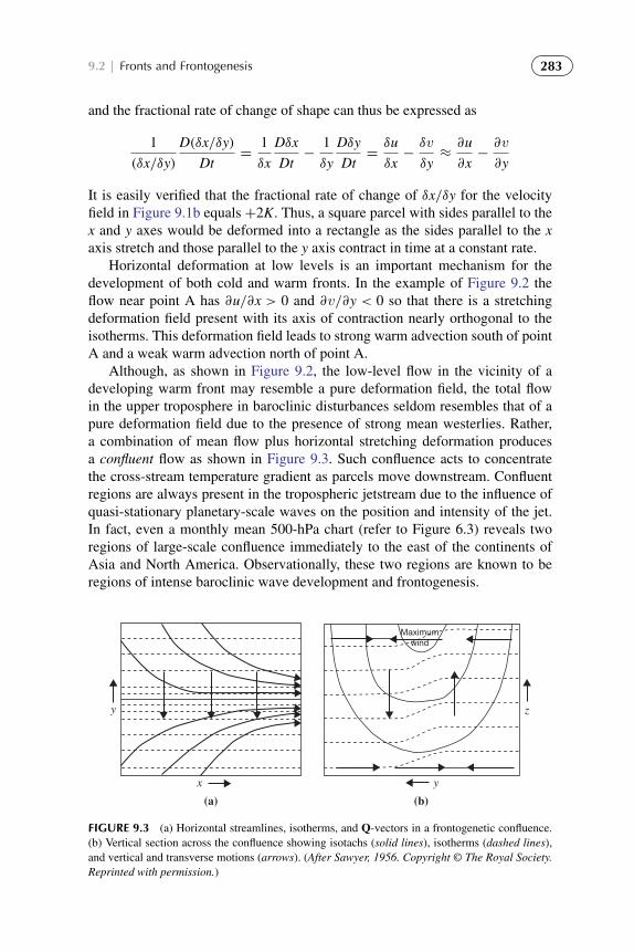
To protect the rights of the author(s) and publisher we inform you that this PDF is an uncorrected proof for internal businessuse only by the author(s), editor(s), reviewer(s), Elsevier and typesetter diacriTech. It is not allowed to publish this proofonline or in print. This proof copy is the copyright property of the publisher and is confidential until formal publication.
“Hakim: 13-ch09-279-324-9780123848666” — 2012/7/26 — 12:04 — page 283 — #5
9.2 | Fronts and Frontogenesis 283
and the fractional rate of change of shape can thus be expressed as
1
(δx/δy)
D(δx/δy)
Dt=
1
δx
Dδx
Dt−
1
δy
Dδy
Dt=δu
δx−δv
δy≈∂u
∂x−∂v
∂y
It is easily verified that the fractional rate of change of δx/δy for the velocityfield in Figure 9.1b equals +2K. Thus, a square parcel with sides parallel to thex and y axes would be deformed into a rectangle as the sides parallel to the xaxis stretch and those parallel to the y axis contract in time at a constant rate.
Horizontal deformation at low levels is an important mechanism for thedevelopment of both cold and warm fronts. In the example of Figure 9.2 theflow near point A has ∂u/∂x > 0 and ∂v/∂y < 0 so that there is a stretchingdeformation field present with its axis of contraction nearly orthogonal to theisotherms. This deformation field leads to strong warm advection south of pointA and a weak warm advection north of point A.
Although, as shown in Figure 9.2, the low-level flow in the vicinity of adeveloping warm front may resemble a pure deformation field, the total flowin the upper troposphere in baroclinic disturbances seldom resembles that of apure deformation field due to the presence of strong mean westerlies. Rather,a combination of mean flow plus horizontal stretching deformation producesa confluent flow as shown in Figure 9.3. Such confluence acts to concentratethe cross-stream temperature gradient as parcels move downstream. Confluentregions are always present in the tropospheric jetstream due to the influence ofquasi-stationary planetary-scale waves on the position and intensity of the jet.In fact, even a monthly mean 500-hPa chart (refer to Figure 6.3) reveals tworegions of large-scale confluence immediately to the east of the continents ofAsia and North America. Observationally, these two regions are known to beregions of intense baroclinic wave development and frontogenesis.
(a)
y
x
(b)
Maximumwind
y
z
FIGURE 9.3 (a) Horizontal streamlines, isotherms, and Q-vectors in a frontogenetic confluence.(b) Vertical section across the confluence showing isotachs (solid lines), isotherms (dashed lines),and vertical and transverse motions (arrows). (After Sawyer, 1956. Copyright © The Royal Society.Reprinted with permission.)

To protect the rights of the author(s) and publisher we inform you that this PDF is an uncorrected proof for internal businessuse only by the author(s), editor(s), reviewer(s), Elsevier and typesetter diacriTech. It is not allowed to publish this proofonline or in print. This proof copy is the copyright property of the publisher and is confidential until formal publication.
“Hakim: 13-ch09-279-324-9780123848666” — 2012/7/26 — 12:04 — page 284 — #6
284 CHAPTER | 9 Mesoscale Circulations
The mechanisms of horizontal shear and horizontal stretching deformationdiscussed previously operate to concentrate the pole–equator temperature gradi-ent on the synoptic scale (∼1000 km). The time scale on which these processesoperate can be estimated with the aid of (9.1). Suppose that the geostrophic windconsists of a pure deformation field so that ug = Kx, and vg = −Ky, and let Tbe a function of y only. Then (9.1) simplifies to
Dg
Dt
(∂T
∂y
)= K
∂T
∂y
so that following the geostrophic motion
∂T
∂y= eKt
(∂T
∂y
)t=0
Typically, K∼ 10−5 s−1 so that the temperature gradient amplifies by a factor of10 in about 3 days. This is much slower than observed rates of atmosphericfrontogenesis.
Thus, geostrophic deformation fields alone cannot cause the rapid fronto-genesis often observed in extratropical systems, in which the temperature gradi-ent can become concentrated in a zone of ∼50 km width on a time scale of lessthan a day. This rapid reduction in scale is caused primarily by the frontogeneticcharacter of the secondary circulation driven by the quasi-geostrophic synoptic-scale flow (moist processes may also be important in rapid frontogenesis).
The nature of the secondary flow may be deduced from the pattern of Qvectors illustrated in Figure 9.3a. As discussed in Section 6.5, the divergence ofQ forces a secondary ageostrophic circulation. For the situation of Figure 9.3,this circulation is in the cross-frontal plane as illustrated in Figure 9.3b. Advec-tion of the temperature field by this ageostrophic circulation tends to increasethe horizontal temperature gradient at the surface on the warm side of the jetaxis. Temperature advection by the upper-level secondary circulation, however,tends to concentrate the temperature gradient on the cold side of the jet axis. Asa result, the frontal zone tends to slope toward the cold air side with height. Thedifferential vertical motion associated with the ageostrophic circulation tends toweaken the front in the midtroposphere due to adiabatic temperature changes(adiabatic warming on the cold side of the front and adiabatic cooling on thewarm side). For this reason fronts are most intense in the lower troposphere andnear the tropopause.
The secondary circulation associated with frontogenesis is required to main-tain the thermal wind balance between the along-front flow and the cross-fronttemperature gradient in the presence of advective processes that tend to destroythis balance. The concentration of the isotherms by the horizontal advectionincreases the cross-stream pressure gradient at upper levels, and thus requiresan increase in the vertical shear of the along-jet flow in order to maintain ther-mal wind balance. The required upper-level acceleration of the jet is producedby the Coriolis force caused by the cross-jet ageostrophic wind, which develops

To protect the rights of the author(s) and publisher we inform you that this PDF is an uncorrected proof for internal businessuse only by the author(s), editor(s), reviewer(s), Elsevier and typesetter diacriTech. It is not allowed to publish this proofonline or in print. This proof copy is the copyright property of the publisher and is confidential until formal publication.
“Hakim: 13-ch09-279-324-9780123848666” — 2012/7/26 — 12:04 — page 285 — #7
9.2 | Fronts and Frontogenesis 285
in response to the increased cross-stream pressure gradient in the jetstream core.As the jet accelerates, cyclonic vorticity must be generated on the cold side ofthe jet axis and anticyclonic vorticity on the warm side. These vorticity changesrequire that the horizontal flow at the jetstream level be convergent on the coldside of the jet axis and divergent on the warm side of the jet axis. The resultingvertical circulation and low-level secondary ageostrophic motion required bymass continuity are indicated in Figure 9.3b.
9.2.2 Semigeostrophic Theory
To analyze the dynamics of the frontogenetic motion fields discussed in theprevious subsection, it is convenient to use the Boussinesq approximation intro-duced in Section 2.8, in which density is replaced by a constant reference valueρ0 except where it appears in the buoyancy force. This approximation simplifiesthe equations of motion without affecting the main features of the results. It isalso useful to replace the total pressure and density fields with deviations fromtheir standard atmosphere values. Thus, we let8(x, y, z, t) = (p− p0)/ρ0 desig-nate the pressure deviation normalized by density and2 = θ−θ0 designate thepotential temperature deviation, where p0(z) and θ0(z) are the height-dependentstandard atmosphere values of pressure and potential temperature, respectively.
With the preceding definitions, the horizontal momentum equations, thermo-dynamic energy equation, hydrostatic approximation, and continuity equationbecome
Du
Dt− f v +
∂8
∂x= 0 (9.2)
Dv
Dt+ fu+
∂8
∂y= 0 (9.3)
D2
Dt+ w
dθ0
dz= 0 (9.4)
b ≡g2
θ00=∂8
∂z(9.5)
∂u
∂x+∂v
∂y+∂w
∂z= 0 (9.6)
where b is the buoyancy, θ00 is a constant reference value of potential tempera-ture, and
D
Dt≡∂
∂t+ u
∂
∂x+ v
∂
∂y+ w
∂
∂z
From the discussion of the previous subsection it should be clear thatthe horizontal scale of variations parallel to a front is much larger than thecross-frontal scale. This scale separation suggests that to a first approximationwe can model fronts as two-dimensional structures. For convenience we choose

To protect the rights of the author(s) and publisher we inform you that this PDF is an uncorrected proof for internal businessuse only by the author(s), editor(s), reviewer(s), Elsevier and typesetter diacriTech. It is not allowed to publish this proofonline or in print. This proof copy is the copyright property of the publisher and is confidential until formal publication.
“Hakim: 13-ch09-279-324-9780123848666” — 2012/7/26 — 12:04 — page 286 — #8
286 CHAPTER | 9 Mesoscale Circulations
Lx
ug
Ly
v
FIGURE 9.4 Velocity and length scales relative to a front parallel to the x axis.
a coordinate system in which the front is stationary and take the cross-frontaldirection to be parallel to the y axis. Then Lx � Ly, where Lx and Ly desig-nate the along-front and cross-front length scales. Similarly, U � V , where Uand V , respectively, designate the along-front and cross-front velocity scales.Figure 9.4 shows these scales relative to the front.
Letting U ∼ 10 m s−1, V ∼ 1 m s−1, Lx ∼ 1000 km, and Ly ∼ 100 km, wefind that it is possible to use the differing scales of the along-front and cross-front motion to simplify the dynamics. Assuming that D/Dt ∼ V/Ly (the cross-front advection time scale) and defining a Rossby number, Ro ≡ V/fLy � 1,the magnitude of the ratios of the inertial and Coriolis terms in the x and ycomponents of the momentum equation can be expressed as
|Du/Dt|
| f v|∼
UV/Ly
f V∼ Ro
(U
V
)∼ 1
|Dv/Dt|
| fu|∼
V2/Ly
f U∼ Ro
(V
U
)∼ 10−2
The along-front velocity is in geostrophic balance with the cross-front pres-sure gradient with error of order 1%, but geostrophy does not hold evenapproximately for the cross-front velocity. Therefore, if the geostrophic windcomponents are defined by
fug = −∂8/∂y, f vg = ∂8/∂x
and we separate the horizontal velocity field into geostrophic and ageostrophicparts, to a good approximation u = ug, but v = vg+ va, where vg and va are thesame order of magnitude.
The x component of the horizontal momentum equation (9.2), the thermody-namic energy equation (9.4), and the continuity equation (9.6) for frontal scalingcan thus be expressed as
Dug
Dt− f va = 0 (9.7)
Db
Dt+ wN2
= 0 (9.8)
∂va
∂y+∂w
∂z= 0 (9.9)

To protect the rights of the author(s) and publisher we inform you that this PDF is an uncorrected proof for internal businessuse only by the author(s), editor(s), reviewer(s), Elsevier and typesetter diacriTech. It is not allowed to publish this proofonline or in print. This proof copy is the copyright property of the publisher and is confidential until formal publication.
“Hakim: 13-ch09-279-324-9780123848666” — 2012/7/26 — 12:04 — page 287 — #9
9.2 | Fronts and Frontogenesis 287
Here, (9.8) is obtained by using (9.5) to replace 2 by b in (9.4), and N is thebuoyancy frequency defined in terms of potential temperature as
N2≡
g
θ00
∂θ0
∂z
Because the along-front velocity is in geostrophic balance, ug and b are relatedby the thermal wind relationship:
f∂ug
∂z= −
∂b
∂y(9.10)
Note that (9.7) and (9.8) differ from their quasi-geostrophic analogs; althoughzonal momentum is still approximated geostrophically, and advection parallelto the front is geostrophic, the advection of momentum and temperature acrossthe front is due not only to the geostrophic wind but to the ageostrophic (va,w)circulation:
D
Dt=
Dg
Dt+
(va∂
∂y+ w
∂
∂z
)where Dg/Dt was defined in equation (6.5). Replacement of momentum byits geostrophic value in (9.7) is referred to as the geostrophic momentumapproximation, and the set of prediction equations that result are called thesemigeostrophic equations.1
9.2.3 Cross-Frontal Circulation
Equations (9.7) through (9.10) form a closed set that can be used to determinethe cross-frontal ageostrophic circulation in terms of the distribution of zonalwind or temperature. Suppose that the large-scale geostrophic flow is acting tointensify the north–south temperature gradient through deformation as shownin Figure 9.3. As the temperature gradient increases, the vertical shear of thezonal wind must also increase to maintain geostrophic balance. This requires anincrease of ug in the upper troposphere, which must be produced by the Coriolisforce associated with a cross-frontal ageostrophic circulation—see (9.7). Thestructure of this secondary circulation can be computed by deriving an equationanalogous to the omega equation discussed in Section 6.5.
We first differentiate (9.8) with respect to y and use the chain rule to expressthe result as
D
Dt
(∂b
∂y
)= Q2 −
∂va
∂y
∂b
∂y−∂w
∂y
(N2+∂b
∂z
)(9.11)
1Some authors reserve this name for a version of the equations written in a transformed set ofcoordinates called geostrophic coordinates (e.g., Hoskins, 1975).

To protect the rights of the author(s) and publisher we inform you that this PDF is an uncorrected proof for internal businessuse only by the author(s), editor(s), reviewer(s), Elsevier and typesetter diacriTech. It is not allowed to publish this proofonline or in print. This proof copy is the copyright property of the publisher and is confidential until formal publication.
“Hakim: 13-ch09-279-324-9780123848666” — 2012/7/26 — 12:04 — page 288 — #10
288 CHAPTER | 9 Mesoscale Circulations
where
Q2 = −∂ug
∂y
∂b
∂x−∂vg
∂y
∂b
∂y(9.12)
is just the y component of the Q vector discussed in Section 6.5, but expressedin the Boussinesq approximation.
Next we differentiate equation (9.7) with respect to z, again use the chainrule to rearrange terms, and use the thermal wind equation (9.10) to replace∂ug/∂z by ∂b/∂y on the right side. The result can then be written as
D
Dt
(f∂ug
∂z
)= Q2 +
∂va
∂zf
(f −
∂ug
∂y
)+∂w
∂z
∂b
∂y(9.13)
Again, as shown in Section 6.5, the geostrophic forcing (given by Q2) tends todestroy thermal wind balance by changing the temperature gradient and verticalshear parts of the thermal wind equation in equal but opposite senses. This ten-dency of geostrophic advection to destroy geostrophic balance is counteractedby the cross-frontal secondary circulation.
In this case the secondary circulation is a two-dimensional transverse cir-culation in the y, z plane. It can thus be represented in terms of a meridionalstreamfunction ψM defined so that
va = −∂ψM/∂z, w = ∂ψM/∂y (9.14)
which identically satisfies the continuity equation (9.9). Adding (9.11) and(9.13), and using the thermal wind balance (9.10) to eliminate the timederivative and (9.14) to eliminate va and w, we obtain the Sawyer–Eliassenequation:
N2s∂2ψM
∂y2+ F2 ∂
2ψM
∂z2+ 2S2 ∂
2ψM
∂y∂z= 2Q2 (9.15)
where
N2s ≡ N2
+∂b
∂z, F2
≡ f
(f −
∂ug
∂y
)= f
∂M
∂y, S2
≡ −∂b
∂y(9.16)
where M is the absolute momentum defined as
M = fy− ug
Equation (9.15) can be compared with the quasi-geostrophic version obtai-ned by neglecting advection by the ageostrophic circulation in (9.7) and (9.8).This has the form
N2 ∂2ψM
∂y2+ f 2 ∂
2ψM
∂z2= 2Q2 (9.17)

To protect the rights of the author(s) and publisher we inform you that this PDF is an uncorrected proof for internal businessuse only by the author(s), editor(s), reviewer(s), Elsevier and typesetter diacriTech. It is not allowed to publish this proofonline or in print. This proof copy is the copyright property of the publisher and is confidential until formal publication.
“Hakim: 13-ch09-279-324-9780123848666” — 2012/7/26 — 12:04 — page 289 — #11
9.2 | Fronts and Frontogenesis 289
Thus, in the quasi-geostrophic case the coefficients in the differential operatoron the left depend only on the standard atmosphere static stability, N, and theplanetary vorticity, f , whereas in the semigeostrophic case they depend on thedeviation of potential temperature from its standard profile through the Ns andS terms and the absolute vorticity through the F term.
An equation of the form (9.17), in which the coefficients of the derivatives onthe left are positive, is referred to as an elliptic boundary value problem. It hasa solution ψM that is uniquely determined by Q2 plus the boundary conditions.For a situation such as that of Figure 9.1b, with both ∂vg/∂y and ∂b/∂y negative,the forcing term Q2 is negative in the frontal region. The streamfunction in thatcase describes a circulation symmetric about the y axis, with rising on the warmside and sinking on the cold side. The semigeostrophic case (9.15) is also anelliptic boundary value problem provided that N2
s F2− S4 > 0. It can be shown
(see Problem 9.1) that this condition requires that the Ertel potential vorticity bepositive in the Northern Hemisphere and negative in the Southern Hemisphere,which is nearly always the case in the extratropics for an unsaturated atmosphere.
The spatial variation of the coefficients in (9.16) and the presence of thecross-derivative term produce a distortion of the secondary circulation, as shownin Figure 9.5. The frontal zone slopes toward the cold air side with height; thereis an intensification of the cross-frontal flow near the surface in the region oflarge absolute vorticity on the warm air side of the front and a tilting of thecirculation with height.
The influence of the ageostrophic circulation on the time scale for frontogen-esis can be illustrated by comparing the processes included in quasi-geostrophicand semigeostrophic frontogenesis. For semigeostrophic advection there is apositive feedback that greatly reduces the time scale of frontogenesis compared
yy
z
FIGURE 9.5 Relationship of the ageostrophic circulation (heavy curve with arrows) in two-dimensional frontogenesis to the potential temperature field (long dashes) and absolute momentumfield (short dashes). Cold air is on the right and warm air is on the left. Note the tilt of the circu-lation toward the cold air side and the enhanced gradients of the absolute momentum and potentialtemperature fields in the frontal zone.

To protect the rights of the author(s) and publisher we inform you that this PDF is an uncorrected proof for internal businessuse only by the author(s), editor(s), reviewer(s), Elsevier and typesetter diacriTech. It is not allowed to publish this proofonline or in print. This proof copy is the copyright property of the publisher and is confidential until formal publication.
“Hakim: 13-ch09-279-324-9780123848666” — 2012/7/26 — 12:04 — page 290 — #12
290 CHAPTER | 9 Mesoscale Circulations
to that in the quasi-geostrophic case. As the temperature contrast increases,Q2 increases, and the secondary circulation must also increase so that theamplification rate of |∂T/∂y| increases with |∂T/∂y| rather than remainingconstant as in the quasi-geostrophic case. Because of this feedback, in theabsence of frictional effects, the semigeostrophic model can produce an infinitetemperature gradient at the surface in less than half a day.
9.3 SYMMETRIC BAROCLINIC INSTABILITY
Observations indicate that mesoscale bands of cloud and precipitation com-monly occur in association with synoptic-scale systems. These are often alignedwith fronts but are separate entities. In common with fronts, such features aregenerally associated with strong baroclinicity and have length scales parallelto the mean wind shear that are much larger than the scales across the windshear. A plausible source for such features is a two-dimensional form of baro-clinic instability known as symmetric instability (also referred to as slantwiseconvection).
For typical atmospheric conditions, buoyancy tends to stabilize air parcelsagainst vertical displacements, and rotation tends to stabilize parcels with respectto horizontal displacements. Instability with respect to vertical displacementsis referred to as hydrostatic (or, simply, static) instability (see Section 2.7.3).For an unsaturated atmosphere, static stability requires that the local buoyancyfrequency squared be positive (N2
s > 0). Instability with respect to horizontaldisplacements, however, is referred to as inertial instability (see Section 5.5.1).The condition for inertial stability equation (5.74) requires that F2 as defined in(9.16) be positive.
If parcels are displaced along slantwise paths rather than vertical or hori-zontal paths, it is possible under certain conditions for the displacements to beunstable even when the conditions for ordinary static and inertial stability areseparately satisfied. Such instability can occur only in the presence of verticalshear of the mean horizontal wind and may be regarded as a special form ofbaroclinic instability in which the perturbations are independent of the coor-dinate parallel to the mean flow. Alternatively, as will be shown, symmetricinstability may be regarded as isentropic inertial instability.
For convenience in deriving the conditions for symmetric instability, we usethe Boussinesq equations of Section 2.8 and assume that the flow is independentof the x coordinate. The mean wind is directed along the x axis and is in thermalwind balance with the meridional temperature gradient:
f ∂ug/∂z = −∂b/∂y = −(g/θ00) ∂2/∂y (9.18)
where, as before, θ00 is a constant reference value of potential temperature.Following Sections 2.7.3 and 5.5.1, we measure the stability with respect
to vertical displacements by the distribution of total potential temperature θ =θ0 + 2 and that with respect to horizontal displacements by the distribution of

To protect the rights of the author(s) and publisher we inform you that this PDF is an uncorrected proof for internal businessuse only by the author(s), editor(s), reviewer(s), Elsevier and typesetter diacriTech. It is not allowed to publish this proofonline or in print. This proof copy is the copyright property of the publisher and is confidential until formal publication.
“Hakim: 13-ch09-279-324-9780123848666” — 2012/7/26 — 12:04 — page 291 — #13
9.3 | Symmetric Baroclinic Instability 291
the absolute zonal momentum, M ≡ fy− ug (where ∂M/∂y = f − ∂ug/∂y is thezonal mean absolute vorticity).
For a barotropic flow, potential temperature surfaces are oriented horizon-tally and absolute momentum surfaces are oriented vertically in the meridionalplane. When the mean flow is westerly and increases with height, however,the potential temperature and absolute momentum surfaces both slope upwardtoward the pole. The comparative strengths of the vertical and horizontal restor-ing forces in the midlatitude troposphere are given by the ratio N2
s/(f ∂M/∂y).For typical tropospheric conditions, this ratio is ∼ 104. Thus, parcel motion inthe plane orthogonal to the mean flow will remain much closer to θ surfacesthan to M surfaces. It is thus natural to utilize isentropic coordinates to ana-lyze parcel displacements. The arguments of Section 5.5.1 still apply, providedthat derivatives with respect to y are taken at constant θ . The stability of suchmotions thus depends on the relative slope of the θ and M surfaces. Ordinarilythe M surfaces will slope more than the θ surfaces (see Figure 9.5), and parceldisplacements are stable. However, when the θ surfaces slope more than the Msurfaces so that
f (∂M/∂y)θ < 0 (9.19)
the flow is unstable with respect to displacements along the θ surfaces. Thissituation may occur in regions of a very strong horizontal temperature gradientand weak vertical stability. The condition in (9.19) is similar to the criterion of(5.74) for inertial instability, except that the derivative of M is here taken alonga sloping θ surface.
If (9.19) is multiplied by −g(∂θ/∂p), the criterion for symmetric instabilitycan be expressed in terms of the distribution of Ertel potential vorticity (4.12)in the simple form
f P < 0 (9.20)
where P is the potential vorticity of the basic state geostrophic flow. Thus, ifthe initial state potential vorticity in the Northern Hemisphere is everywherepositive, then symmetric instability cannot develop through adiabatic motions,as potential vorticity is conserved following the motion and will always remainpositive.
To demonstrate that (9.19) is the condition for symmetric instability, we con-sider the change in mean kinetic energy required for exchange of the tubesof fluid labeled 1 and 2 in Figure 9.6. (These tubes are located at y1 andy2 = y1 + δy, respectively, and are assumed to extend infinitely along the xaxis so that the problem is two-dimensional.) Because the tubes lie on the samepotential temperature surface, they have the same available potential energy.Thus, a spontaneous exchange of parcels is possible if δ(KE), the kinetic energyof the zonal flow after exchange minus that in the initial state, is negative. Other-wise some external source of energy is required to furnish the kinetic energy ofthe meridional and vertical motions required for the exchange.

To protect the rights of the author(s) and publisher we inform you that this PDF is an uncorrected proof for internal businessuse only by the author(s), editor(s), reviewer(s), Elsevier and typesetter diacriTech. It is not allowed to publish this proofonline or in print. This proof copy is the copyright property of the publisher and is confidential until formal publication.
“Hakim: 13-ch09-279-324-9780123848666” — 2012/7/26 — 12:04 — page 292 — #14
292 CHAPTER | 9 Mesoscale Circulations
zθ +2δ θ
M − 2δ M
M − δ M
M + δ M
θ +δ θ
θ − δθ
θ − 2δθ
θ
M
y
2
1
FIGURE 9.6 Cross-section showing isolines of absolute momentum and potential temperature fora symmetrically unstable basic state. Motion along the isentropic path between points labeled 1 and2 is unstable, as M decreases with latitude along the path. See text for details.
Initially the motion of the tubes is parallel to the x axis and in geostrophicbalance so that the absolute momentum for the two tubes is
M1 = fy1 − u1 = fy1 − ug(y1, z)M2 = fy2 − u2 = fy1 + f δy− ug (y1 + δy, z+ δz)
(9.21)
Absolute momentum is conserved by the tubes so that after exchange theperturbation zonal velocities are given by
M′1 = fy1 + f δy− u′1 = M1, M′2 = fy1 − u′2 = M2 (9.22)
Eliminating M1 and M2 between (9.21) and (9.22) and solving for the distur-bance zonal wind, we obtain
u′1 = f δy+ u1, u′2 = −f δy+ u2
The difference in zonal kinetic energy between the final state and the initial stateis given by
δ(KE) = 12
(u′1
2+ u′2
2)−
12
(u2
1 + u22
)= f δy (u1 − u2 + f δy) = f δy (M2 −M1)
(9.23)

To protect the rights of the author(s) and publisher we inform you that this PDF is an uncorrected proof for internal businessuse only by the author(s), editor(s), reviewer(s), Elsevier and typesetter diacriTech. It is not allowed to publish this proofonline or in print. This proof copy is the copyright property of the publisher and is confidential until formal publication.
“Hakim: 13-ch09-279-324-9780123848666” — 2012/7/26 — 12:04 — page 293 — #15
9.3 | Symmetric Baroclinic Instability 293
Thus, δ(KE) is negative, and unforced meridional motion may occur, providedthat f (M2 −M1) < 0. This is equivalent to the condition (9.19), as the tubes liealong the same θ surface.
To estimate the likelihood that conditions for symmetric instability may besatisfied, it is useful to express the stability criterion in terms of a mean-flowRichardson number. To do this we first note that the slope of an M surface canbe estimated from noting that on an M surface
δM =∂M
∂yδy+
∂M
∂zδz = 0
so that the ratio of δz to δy at constant M is(δz
δy
)M=
(−∂M
∂y
)/(∂M
∂z
)=
(f −
∂ug
∂y
)/(∂ug
∂z
)(9.24)
Similarly, the slope of a potential temperature surface is(δz
δy
)θ
=
(−∂θ
∂y
)/(∂θ
∂z
)=
(f∂ug
∂z
)/(g
θ00
∂θ
∂z
)(9.25)
where we have used the thermal wind relationship to express the meridionaltemperature gradient in terms of the vertical shear of the zonal wind. The ratioof (9.24) to (9.25) is simply(
δz
δy
)M
/(δz
δy
)θ
= f
(f −
∂ug
∂y
)(g
θ00
∂θ
∂z
)/[f 2(∂ug
∂z
)2]=
F2N2s
S4
where the notation in the last term is defined in (9.16).Recalling that symmetric instability requires that the slopes of the θ sur-
faces exceed those of the M surfaces, the necessary condition for instability ofgeostrophic flow parallel to the x axis becomes(
δz
δy
)M
/(δz
δy
)θ
= f
(f −
∂ug
∂y
)Ri/
f 2=
F2N2s
S4< 1 (9.26)
where the mean-flow Richardson number Ri is defined as
Ri ≡
(g
θ00
∂θ
∂z
)/(∂ug
∂z
)2
Thus, if the relative vorticity of the mean flow vanishes (∂ug/∂y = 0), Ri < 1is required for instability.
The condition (9.26) can be related to (9.20) by observing that (9.26)requires that F2N2
s − S4 < 0 for symmetric instability. As is to be shown inProblem 9.1,
F2N2s − S4
=(ρfg
/θ00)
P (9.27)

To protect the rights of the author(s) and publisher we inform you that this PDF is an uncorrected proof for internal businessuse only by the author(s), editor(s), reviewer(s), Elsevier and typesetter diacriTech. It is not allowed to publish this proofonline or in print. This proof copy is the copyright property of the publisher and is confidential until formal publication.
“Hakim: 13-ch09-279-324-9780123848666” — 2012/7/26 — 12:04 — page 294 — #16
294 CHAPTER | 9 Mesoscale Circulations
Because the large-scale potential vorticity, P, is normally positive in the North-ern Hemisphere and negative in the Southern Hemisphere, (9.27) is ordinarilypositive in both hemispheres; thus, the condition for symmetric instability israrely satisfied. If the atmosphere is saturated, however, the relevant static sta-bility condition involves the lapse rate of the equivalent potential temperature,and neutral conditions with respect to symmetric instability may easily occur(see Section 9.5).
Finally, it is worth noting that the condition for stability with respect to sym-metric displacements, F2N2
s − S4 > 0, is identical to the condition that theSawyer–Eliassen equation (9.15) be an elliptic boundary value problem. Thus,when the flow is stable with respect to symmetric baroclinic perturbations, anonzero forced transverse circulation governed by (9.15) will exist when thereis nonzero forcing, Q2—see (9.12). Free transverse oscillations, however, mayoccur in the absence of forcing. These require including the horizontal accelera-tion term in the y component of the momentum equation. The resulting equationfor the transverse circulation has the form (see Appendix F):
∂2
∂t2
(∂2ψM
∂z2
)+ N2
s∂2ψM
∂y2+ F2 ∂
2ψM
∂z2+ 2S2 ∂
2ψM
∂y∂z= 0 (9.28)
which should be compared with (9.15). When F2N2s − S4 > 0, solutions of
(9.28) correspond to stable oscillations, while for F2N2s − S4 < 0, solutions are
exponentially growing, corresponding to symmetric baroclinic instability.
9.4 MOUNTAIN WAVES
When stably stratified air is forced to flow over varying surface topography,buoyancy oscillations are created. First, consider the case with constant windand stratification for sinusoidally varying topography, and then allow forlocalized mountain barriers and vertical variations in static stability and wind.
9.4.1 Waves over Sinusoidal Topography
When air with mean wind speed u is forced to flow over a sinusoidal patternof ridges under statically stable conditions, individual air parcels are alternatelydisplaced upward and downward from their equilibrium levels and will thusundergo buoyancy oscillations as they move across the ridges, as shown inFigure 9.7. In this case there are solutions in the form of waves that are sta-tionary relative to the ground. For such stationary waves, w′ depends only on(x, z) and the equation governing their motion, (5.64), simplifies to(
∂2w′
∂x2+∂2w′
∂z2
)+
N2
u2w′ = 0 (9.29)

To protect the rights of the author(s) and publisher we inform you that this PDF is an uncorrected proof for internal businessuse only by the author(s), editor(s), reviewer(s), Elsevier and typesetter diacriTech. It is not allowed to publish this proofonline or in print. This proof copy is the copyright property of the publisher and is confidential until formal publication.
“Hakim: 13-ch09-279-324-9780123848666” — 2012/7/26 — 12:04 — page 295 — #17
9.4 | Mountain Waves 295
(a)
(b)
FIGURE 9.7 Streamlines in steady flow over an infinite series of sinusoidal ridges for the narrowridge case (a) and broad ridge case (b). The dashed line in (b) shows the phase of maximum upwarddisplacement. (From Durran, 1990. Copyright © American Meteorological Society. Reprinted withpermission.)
Substituting
w′ = Re w expi(kx+mz) (9.30)
into (9.29) yields
m2=
N2
u2− k2 (9.31)
For given values of N, k, and u, (9.31) determines the vertical structure. Thenif |u| < N/k, (9.31) shows that m2 > 0 (i.e., m must be real) and solutions of(9.29) have the form of vertically propagating waves. When m2 < 0,m = imi
To protect the rights of the author(s) and publisher we inform you that this PDF is an uncorrected proof for internal businessuse only by the author(s), editor(s), reviewer(s), Elsevier and typesetter diacriTech. It is not allowed to publish this proofonline or in print. This proof copy is the copyright property of the publisher and is confidential until formal publication.
“Hakim: 13-ch09-279-324-9780123848666” — 2012/7/26 — 12:04 — page 296 — #18
296 CHAPTER | 9 Mesoscale Circulations
is imaginary and the solution to (9.29) will have the form of vertically trappedwaves:
w′ = w exp (ikx) exp (−miz)
Thus, vertical propagation is possible only when |uk|, the magnitude of thefrequency relative to the mean flow, is less than the buoyancy frequency.
Stable stratification, wide ridges, and comparatively weak zonal flow pro-vide favorable conditions for the formation of vertically propagating topo-graphic waves (m real). Because the energy source for these waves is at theground, they must transport energy upward. Hence, the phase speed relative tothe mean zonal flow must have a downward component. Thus, if u > 0, lines ofconstant phase must tilt westward with height. When m is imaginary, however,the solution (9.30) has exponential behavior in the vertical with an exponentialdecay height of µ−1, where µ = |m|. Boundedness as z→∞ requires that wechoose the solution with exponential decay away from the lower boundary.
To contrast the character of the solutions for real and imaginary m, we con-sider a specific example in which there is westerly mean flow over topographywith a height profile given by
h (x) = hM cos kx
where hM is the amplitude of the topography. Then, because the flow at thelower boundary must be parallel to the boundary, the vertical velocity perturba-tion at the boundary is given by the rate at which the boundary height changesfollowing the motion:
w′ (x, 0) =(Dh/
Dt)
z=0 ≈ u∂h/∂x = −ukhM sin kx
and the solution of (9.29) that satisfies this condition can be written
w (x, z) =
{−uhMke−µz sin kx, uk > N−uhMk sin (kx+ mz) , uk < N
}(9.32)
For fixed mean wind and buoyancy frequency, the character of the solutiondepends only on the horizontal scale of the topography. The two cases of (9.32)may be regarded as narrow ridge and wide ridge cases, respectively, since forspecified values of u and N, the character of the solution is determined by thezonal wave number k. The streamline patterns corresponding to these cases forwesterly flow are illustrated in Figure 9.7. In the narrow ridge case (Figure 9.7a),the maximum upward displacement occurs at the ridge tops, and the amplitudeof the disturbance decays with height. In the wide ridge case (Figure 9.7b), theline of maximum upward displacement tilts back toward the west (m > 0),and amplitude is independent of height consistent with an internal gravity wavepropagating westward relative to the mean flow.
Alternatively, for fixed zonal wave number and buoyancy frequency, thesolution depends only on the speed of the mean zonal wind. As indicated in

To protect the rights of the author(s) and publisher we inform you that this PDF is an uncorrected proof for internal businessuse only by the author(s), editor(s), reviewer(s), Elsevier and typesetter diacriTech. It is not allowed to publish this proofonline or in print. This proof copy is the copyright property of the publisher and is confidential until formal publication.
“Hakim: 13-ch09-279-324-9780123848666” — 2012/7/26 — 12:04 — page 297 — #19
9.4 | Mountain Waves 297
(9.32), only for mean zonal wind magnitudes less than the critical value N/kwill vertical wave propagation occur.
Equation (9.29) was obtained for conditions of constant basic state flow. Inreality, both the zonal wind u and the stability parameter N generally vary withheight, and ridges are usually isolated rather than periodic. A wide variety ofresponses are possible depending on the shape of the terrain and on wind and sta-bility profiles. Under certain conditions, large-amplitude waves can be formed,which may generate severe downslope surface winds and zones of strong clearair turbulence. Such circulations are discussed further in Section 9.4.4.
9.4.2 Flow over Isolated Ridges
Just as flow over a periodic series of sinusoidal ridges can be represented by asingle sinusoidal function flow—that is, by a single Fourier harmonic flow—over an isolated ridge can be approximated by the sum of a number of Fouriercomponents (see Section 5.2.1). Thus, any zonally varying topography can berepresented by a Fourier series of the form
hM (x) =∞∑
s=1
Re [hs exp (iksx)] (9.33)
where hs is the amplitude of the sth Fourier component of the topography. Wecan then express the solution to the wave equation (9.29) as the sum of Fouriercomponents:
w (x, z) =∞∑
s=1
Re{
Ws exp[i (ksx+ msz)
]}(9.34)
where Ws = iksuhs, and m2s = N2/u2
− k2s .
Individual Fourier modes will yield vertically propagating or verticallydecaying contributions to the total solution (9.34) depending on whether ms isreal or imaginary. This in turn depends on whether k2
s is less than or greater thanN2/u2. Thus, each Fourier mode behaves just as the solution (9.30) for periodicsinusoidal topography behaves. For a narrow ridge, Fourier components withwave numbers greater than N/u dominate in (9.33), and the resulting distur-bance decays with height. For a broad ridge, components with wave numbersless than N/u dominate, and the disturbance propagates vertically. In the widemountain limit where m2
s ≈ N2/u2, the flow is periodic in the vertical witha vertical wavelength of 2πm−1
s , and phase lines tilt upstream with height asshown in Figure 9.8.
Vertically propagating gravity waves generated by flow over broad topog-raphy can produce clouds both upstream and downstream of the topographydepending on variations of the moisture distribution with altitude. In the exam-ple shown in Figure 9.7, the positions labeled A and B indicate regions where

To protect the rights of the author(s) and publisher we inform you that this PDF is an uncorrected proof for internal businessuse only by the author(s), editor(s), reviewer(s), Elsevier and typesetter diacriTech. It is not allowed to publish this proofonline or in print. This proof copy is the copyright property of the publisher and is confidential until formal publication.
“Hakim: 13-ch09-279-324-9780123848666” — 2012/7/26 — 12:04 — page 298 — #20
298 CHAPTER | 9 Mesoscale Circulations
1.0
0.75
0.5
18012060
Cross-mountain distance (km)
0
A
B
0.25
0
Hei
ght (
vert
ical
wav
elen
gths
)
−180 −120 − 60
FIGURE 9.8 Streamlines of flow over a broad isolated ridge showing upstream phase tilt withheight. The pattern is periodic in height, and one vertical wavelength is shown. Orographicclouds may form in the shaded areas where streamlines are displaced upward from equilibriumeither upstream or downstream of the ridge if sufficient moisture is present. (After Durran, 1990.Copyright © American Meteorological Society. Reprinted with permission.)
streamlines are displaced upward downstream and upstream of the ridge, respec-tively. If sufficient moisture is present, orographic clouds may then form inregion A or B as suggested by the shading in Figure 9.8.
9.4.3 Lee Waves
If u and N are allowed to vary in height, then (9.29) must be replaced by(∂2w′
∂x2+∂2w′
∂z2
)+ l2w′ = 0 (9.35)
where the Scorer parameter, l, is defined as
l2 = N2/
u2− u−1d2u
/dz2
and the condition for vertical propagation becomes k2s < l2.
If the mean cross-mountain wind speed increases strongly with height, orif there is a low-level stable layer so that N decreases strongly with height,there may be a layer near the surface in which vertically propagating wavesare permitted, which is topped by a layer in which the disturbance decays inthe vertical. In that case vertically propagating waves in the lower layer arereflected when they reach the upper layer. Under some circumstances the wavesmay be repeatedly reflected from the upper layer and the surface downstream ofthe mountain, leading to a series of “trapped” lee waves as shown in Figure 9.9.

To protect the rights of the author(s) and publisher we inform you that this PDF is an uncorrected proof for internal businessuse only by the author(s), editor(s), reviewer(s), Elsevier and typesetter diacriTech. It is not allowed to publish this proofonline or in print. This proof copy is the copyright property of the publisher and is confidential until formal publication.
“Hakim: 13-ch09-279-324-9780123848666” — 2012/7/26 — 12:04 — page 299 — #21
9.4 | Mountain Waves 299
7
6
5
4
3
1
00−12
Hei
ght (
km)
12 24
Cross-mountain distance (km)
36
2
FIGURE 9.9 Streamlines for trapped lee waves generated by flow over topography with verticalvariation of the Scorer parameter. Shading shows locations where lee wave clouds may form. (AfterDurran, 1990. Copyright © American Meteorological Society. Reprinted with permission.)
Vertical variations in the Scorer parameter can also modify the amplitudeof waves that are sufficiently long to propagate vertically through the entiretroposphere. Amplitude enhancement leading to wave breaking and turbulentmixing can occur if there is a critical level where the mean flow goes to zero(l→∞).
9.4.4 Downslope Windstorms
Strong downslope surface winds are occasionally observed along the lee slopesof mountain ranges. Although partial reflection of vertically propagating lin-ear gravity waves may produce enhanced surface winds under some condi-tions, it appears that nonlinear processes are essential to account for observedwindstorms associated with stable flow over topography.
To demonstrate the role of nonlinearity, we assume that the troposphere has astable lower layer of undisturbed depth h topped by a weakly stable upper layer,and assume that the lower layer behaves as a barotropic fluid with a free sur-face h(x,t). We assume that disturbances have zonal wavelengths much greaterthan the layer depth. The motion of the lower layer may then be describedby the shallow water equations of Section 4.5, but with the lower boundary

To protect the rights of the author(s) and publisher we inform you that this PDF is an uncorrected proof for internal businessuse only by the author(s), editor(s), reviewer(s), Elsevier and typesetter diacriTech. It is not allowed to publish this proofonline or in print. This proof copy is the copyright property of the publisher and is confidential until formal publication.
“Hakim: 13-ch09-279-324-9780123848666” — 2012/7/26 — 12:04 — page 300 — #22
300 CHAPTER | 9 Mesoscale Circulations
condition replaced by
w(x, hM) = DhM/
Dt = u∂hM/∂x
where hM again denotes the height of the topography.We first examine the linear behavior of this model by considering steady
flow over small-amplitude topography. Neglecting ambient rotation, the lin-earized shallow water equations in steady state become
u∂u′
∂x+ g
∂h′
∂x= 0 (9.36)
u∂(h′ − hM
)∂x
+ H∂u′
∂x= 0 (9.37)
Here, h′ = h − H, where H is the mean height of the interface and h′ − hM isthe deviation from H of the thickness of the layer.
The solutions for (9.36) and (9.37) can be expressed as
h′ = −hM(u2/
c2)(
1− u2/
c2) , u′ =
hM
H
(u
1− u2/
c2
)(9.38)
where c2≡ gH is the shallow water gravity wave speed. The characteristics
of the disturbance fields h′ and u′ depend on the magnitude of the mean-flowFroude number, defined by the relation Fr2
= u2/
c2 . When Fr < 1, the flowis referred to as subcritical. In subcritical flow, the shallow water gravity wavespeed is greater than the mean-flow speed, and the disturbance height andwind fields are out of phase. The interface height disturbance is negative, andthe velocity disturbance is positive over the topographic barrier as shown inFigure 9.10a. When Fr > 1, the flow is referred to as supercritical. In supercrit-ical flow the mean flow exceeds the shallow water gravity wave speed. Gravitywaves cannot play a role in establishing the steady-state adjustment betweenheight and velocity disturbances because such waves are swept downstreamfrom the ridge by the mean flow. In this case the fluid thickens and slows as itascends over the barrier (Figure 9.10b). It is also clear from (9.38) that for Fr∼1 the perturbations are no longer small and the linear solution breaks down.
The nonlinear equations corresponding to (9.36) and (9.37) can be expressedas
u∂u
∂x+ g
∂h
∂x= 0 (9.39)
∂
∂x
[u(h− hM
)]= 0 (9.40)
Equation (9.39) may be integrated immediately to show that the sum of kineticand potential energy, u2/2+ gh, is constant following the motion. Thus, energy

To protect the rights of the author(s) and publisher we inform you that this PDF is an uncorrected proof for internal businessuse only by the author(s), editor(s), reviewer(s), Elsevier and typesetter diacriTech. It is not allowed to publish this proofonline or in print. This proof copy is the copyright property of the publisher and is confidential until formal publication.
“Hakim: 13-ch09-279-324-9780123848666” — 2012/7/26 — 12:04 — page 301 — #23
9.4 | Mountain Waves 301
PE KE PE
(a)
PE
KEKE
(b)
PEKE
(c)
FIGURE 9.10 Flow over an obstacle for a barotropic fluid with free surface. (a) Subcritical flow(Fr > 1 everywhere). (b) Supercritical flow (Fr < 1 everywhere). (c) Supercritical flow on lee slopewith adjustment to subcritical flow at hydraulic jump near base of obstacle. (After Durran, 1990.Copyright © American Meteorological Society. Reprinted with permission.)
conservation requires that if u increases, h must decrease, and vice versa. Inaddition, (9.40) shows that the mass flux, u(h − hM), must also be conserved.The direction of the exchange between kinetic and potential energy in flow overa ridge is determined by the necessity that both (9.39) and (9.40) be satisfied.
Multiplying (9.39) by u and eliminating ∂h/∂x with the aid of (9.40) gives(1− Fr2
) ∂u
∂x=
ug
c2
∂hM
∂x(9.41)
where the shallow water gravity wave speed, c, and the Froude number are nowdefined using the local thickness and velocity of the fluid:
c2≡ g (h− hM) ; Fr2
≡ u2/c2
From (9.41) it is clear that the flow will accelerate on the upslope side of theridge (∂u/∂x > 0, where ∂hM/∂x > 0) if the Froude number is less than unity,but will decelerate if the Froude number is greater than unity.
As a subcritical flow ascends the upslope side of a topographic barrier, Frwill tend to increase both from the increase in u and the decrease in c. If Fr = 1

To protect the rights of the author(s) and publisher we inform you that this PDF is an uncorrected proof for internal businessuse only by the author(s), editor(s), reviewer(s), Elsevier and typesetter diacriTech. It is not allowed to publish this proofonline or in print. This proof copy is the copyright property of the publisher and is confidential until formal publication.
“Hakim: 13-ch09-279-324-9780123848666” — 2012/7/26 — 12:04 — page 302 — #24
302 CHAPTER | 9 Mesoscale Circulations
at the crest, then from (9.41) the flow will become supercritical and continue toaccelerate as it descends the lee side until it adjusts back to the ambient subcrit-ical conditions in a turbulent hydraulic jump as illustrated in Figure 9.10c. Inthis case very high velocities can occur along the lee slope, as potential energyis converted into kinetic energy during the entire period that a fluid columntraverses the barrier. Although conditions in the continuously stratified atmo-sphere are clearly more complex than in the shallow water hydraulic model,numerical simulations have demonstrated that the hydraulic model provides areasonable conceptual model for the primary processes occurring in downslopewindstorms.
9.5 CUMULUS CONVECTION
Mesoscale storms associated with cumulus convection represent a large frac-tion of all of the meteorologically important mesoscale circulations. Beforeconsidering such systems, it is necessary to examine a few of the essential ther-modynamic and dynamical aspects of individual cumulus clouds. The subject ofcumulus convection is extremely complex to address theoretically. Much of thisdifficulty stems from the fact that the cumulus clouds have a complex internalstructure. They are generally composed of a number of short-lived individualrising towers, which are produced by elements of ascending buoyant air calledthermals. Rising thermals entrain environmental air and thus modify the cloudair through mixing.
Thermals are nonhydrostatic, nonsteady, and highly turbulent. The buoyancyof an individual thermal (i.e., the difference between its density and the densityof the environment) depends on a number of factors, including the environmen-tal lapse rate, the rate of dilution by entrainment, and the drag by the weight ofliquid water in cloud droplets. A detailed discussion of the dynamics of thermalconvection is beyond the scope of this text. This section utilizes a simple one-dimensional cloud model and focuses primarily on the thermodynamic aspectsof moist convection. Convective storm dynamics is considered in Section 9.6.
9.5.1 Convective Available Potential Energy
Development of convective storms depends on the presence of environmen-tal conditions favorable for the occurrence of deep convection. Several indiceshave been developed to measure the susceptibility of a given temperature andmoisture profile to the occurrence of deep convection. A particularly use-ful measure is the convective available potential energy. Convective availablepotential energy (CAPE) provides a measure of the maximum possible kineticenergy that a statically unstable parcel can acquire (neglecting effects of watervapor and condensed water on the buoyancy), assuming that the parcel ascends

To protect the rights of the author(s) and publisher we inform you that this PDF is an uncorrected proof for internal businessuse only by the author(s), editor(s), reviewer(s), Elsevier and typesetter diacriTech. It is not allowed to publish this proofonline or in print. This proof copy is the copyright property of the publisher and is confidential until formal publication.
“Hakim: 13-ch09-279-324-9780123848666” — 2012/7/26 — 12:04 — page 303 — #25
9.5 | Cumulus Convection 303
without mixing with the environment and adjusts instantaneously to the localenvironmental pressure.
The momentum equation for such a parcel is (2.51), which can be rewrittenfollowing the vertical motion of the parcel as
Dw
Dt=
Dz
Dt
Dw
Dz= w
Dw
Dz= b′ (9.42)
where b′(z) is again the buoyancy given by
b′ = g
(ρenv − ρparcel
)ρparcel
= g
(Tparcel − Tenv
)Tenv
(9.43)
and Tenv designates the temperature of the environment. If (9.42) is inte-grated vertically from the level of free convection, zLFC, to the level of neutralbuoyancy, zLNB, following the motion of the parcel the result is
w2max
2=
zLNB∫zLFC
g
(Tparcel − Tenv
Tenv
)dz ≡ B (9.44)
Here, B is the maximum kinetic energy per unit mass that a buoyant parcel canobtain by ascending from a state of rest at the level of free convection to thelevel of neutral buoyancy near the tropopause (see Figure 2.8). This is an over-estimate of the actual kinetic energy realized by a nonentraining parcel, as thenegative buoyancy contribution of liquid water reduces the effective buoyancy,especially in the tropics.
In a typical tropical oceanic sounding, parcel temperature excesses of 1 to2 K may occur over a depth of 10 to 12 km. A typical value of CAPE is thenB ≈ 500 m2 s−2. In severe storm conditions in the Midwest of North America,however, parcel temperature excesses can be 7 to 10 K (refer to Figure 2.8) andB ≈ 2000 to 3000 m2 s−2. Observed updrafts in the latter case (up to 50 m s−1)
are much stronger than in the former case (5–10 m s−1). The small value ofCAPE in the mean tropical environment is the major reason that updraft veloc-ities in tropical cumulonimbus are observed to be much smaller than those inmidlatitude thunderstorms.
9.5.2 Entrainment
In the previous subsection it was assumed that convective cells rise without mix-ing with environmental air so that they maintain constant θe during their rise.In reality, however, rising saturated air parcels tend to be diluted by entrain-ing, or mixing in, some of the relatively dry environmental air. If the air inthe environment is unsaturated, some of the liquid water in the rising parcel

To protect the rights of the author(s) and publisher we inform you that this PDF is an uncorrected proof for internal businessuse only by the author(s), editor(s), reviewer(s), Elsevier and typesetter diacriTech. It is not allowed to publish this proofonline or in print. This proof copy is the copyright property of the publisher and is confidential until formal publication.
“Hakim: 13-ch09-279-324-9780123848666” — 2012/7/26 — 12:04 — page 304 — #26
304 CHAPTER | 9 Mesoscale Circulations
must be evaporated to maintain saturation in the convective cell as air from theenvironment is entrained. The evaporative cooling caused by entrainment willreduce the buoyancy of the convective parcel (i.e., lower its θe). Thus, the equiv-alent potential temperature in an entraining convection cell will decrease withheight rather than remaining constant. Similar considerations hold for any otherconservable variable2 in which environmental values differ from cloud values;entrainment will modify the in-cloud vertical profiles.
Denoting as A the amount of an arbitrary conservable variable per unit massof air, the vertical dependence of A in an entraining convective cell can be esti-mated by assuming that to a first approximation the cell can be modeled as asteady-state jet as shown in Figure 9.11. Thus, in a time increment δt, a mass mof saturated cloud air with an amount of the arbitrary variable given by mAcld
mixes with a mass δm of entrained environmental air, which has an amount ofthe arbitrary variable given by δmAenv . The change in the value of A within thecloud, δAcld, is then given by the mass balance relationship
(m+ δm) (Acld + δAcld) = mAcld + δmAenv +(DAcld
/Dt)
S mδt (9.45)
where(DAcld
/Dt)
S designates the rate of change of Acld due to sources andsinks unrelated to entrainment. Dividing through by δt in (9.45), neglecting the
m + δ m
δ m
m
δ z
FIGURE 9.11 An entraining jet model of cumulus convection. See text for an explanation.
2A conservable variable is one that is conserved following the motion in the absence of sources andsinks (e.g., a chemical trace constituent).

To protect the rights of the author(s) and publisher we inform you that this PDF is an uncorrected proof for internal businessuse only by the author(s), editor(s), reviewer(s), Elsevier and typesetter diacriTech. It is not allowed to publish this proofonline or in print. This proof copy is the copyright property of the publisher and is confidential until formal publication.
“Hakim: 13-ch09-279-324-9780123848666” — 2012/7/26 — 12:04 — page 305 — #27
9.5 | Cumulus Convection 305
second-order term, and rearranging yields
δAcld
δt=
(DAcld
Dt
)S−
1
m
δm
δt(Acld − Aenv) (9.46)
Noting that in the time increment δt an ascending parcel rises a distanceδz = wδt, where w is the speed of ascent of the parcel, we can eliminate δt in(9.46) to obtain an equation for the vertical dependence of Acld in a continuouslyentraining convective cell:
wdAcld
dz=
(DAcld
Dt
)S− wλ (Acld − Aenv) (9.47)
where we have defined the entrainment rate; λ ≡ d ln m/dz.Letting Acld = ln θe and noting that θe is conserved in the absence of
entrainment, (9.47) yields(d ln θe
dz
)cld= −λ [(ln θe)cld − (ln θe)env]
≈ −λ
[Lc
cpT(qs − qenv)+ ln
(Tcld
Tenv
)] (9.48)
where (2.70) is used to obtain the latter form of the right side. Thus, an entrain-ing convective cell is less buoyant than a nonentraining cell. Letting Acld = win (9.47), applying (9.42), and neglecting the pressure contribution to buoyancy,we find that the height dependence of kinetic energy per unit mass is given by
d
dz
(w2
2
)= g
(Tcld − Tenv
Tenv
)− λw2 (9.49)
An entraining cell will undergo less acceleration than a nonentraining cell notonly because the buoyancy is reduced, but also because of the drag exerted bymass entrainment.
Equations (9.48) and (9.49), together with suitable relations for the cloudmoisture variables, can be used to determine the vertical profile of cloud vari-ables. Such one-dimensional cloud models have been very popular in the past.Unfortunately, observed cloud properties, such as maximum cloud depth andcloud water concentration, cannot simultaneously be satisfactorily predicted bythis type of model. In reality, pressure perturbations generated by the convectivecells are important in the momentum budget, and entrainment does not occurinstantaneously but in a sporadic manner that allows some cells to rise throughmost of the troposphere with very little dilution. Although more sophisticatedone-dimensional models can partly overcome these deficiencies, some of themost important aspects of thunderstorm dynamics (e.g., the influence of verti-cal shear of the environmental wind) can only be included in multidimensionalmodels.

To protect the rights of the author(s) and publisher we inform you that this PDF is an uncorrected proof for internal businessuse only by the author(s), editor(s), reviewer(s), Elsevier and typesetter diacriTech. It is not allowed to publish this proofonline or in print. This proof copy is the copyright property of the publisher and is confidential until formal publication.
“Hakim: 13-ch09-279-324-9780123848666” — 2012/7/26 — 12:04 — page 306 — #28
306 CHAPTER | 9 Mesoscale Circulations
9.6 CONVECTIVE STORMS
Convective storms can take a large variety of forms. These range in scalefrom isolated thunderstorms involving a single convective cloud (or cell)to mesoscale convective complexes consisting of ensembles of multicelledthunderstorms. Here we distinguish three primary types: the single-cell, the mul-ticell, and the supercell storm. As shown in the previous section, convectiveavailable potential energy measures whether thermodynamical conditions arefavorable for the development of cumulus convection. CAPE, therefore, pro-vides a guide to the strength of convection. It does not, however, provide anynotion of the most likely type of mesoscale organization. It turns out, as sug-gested earlier, that storm type also depends on the vertical shear of the lowertropospheric environment.
When vertical shear is weak (<10 m s−1 below 4 km), single cell stormsoccur. These tend to be short-lived (∼30 min) and move with the mean wind inthe lowest 8 km. When there is moderate vertical shear (∼10–20 m s−1 below4 km), multicell storms arise in which individual cells have lifetimes of∼30 min,but the storm lifetime may be many hours. In multicell storms the downdraftsinduced by the evaporation of precipitation form a dome of cold outflowingair at the surface. New cells tend to develop along the gust front where thecold outflow lifts conditionally unstable surface air. When vertical shear is large(>20 m s−1 below 4 km), the strong tilting of convective cells tends to delaystorm development, even in a thermodynamically favorable environment, sothat an hour or more may be required for the initial cell to completely develop.This development may be followed by a split into two storms, which moveto the left and right of the mean wind. Usually the left-moving storm diesrapidly, while the right-moving storm slowly evolves into a rotating circula-tion with a single updraft core and trailing downdrafts, as discussed in the nextsection. Such supercell storms often produce heavy rain, hail, and damagingtornadoes. Ensembles of multicell or supercell storms are often organized alonglines referred to as squall lines, which may move in a different direction thanthe individual thunderstorms.
9.6.1 Development of Rotation in Supercell Thunderstorms
The supercell thunderstorm is of particular dynamical interest because of itstendency to develop a rotating mesocyclone from an initially nonrotating envi-ronment. The dominance of cyclonic rotation in such systems might suggest thatthe Coriolis force plays a role in supercell dynamics. However, it can be shownreadily that the rotation of Earth is not relevant to the development of rotationin supercell storms.
Although a quantitative treatment of supercell dynamics requires that thedensity stratification of the atmosphere be taken into account, for purposes ofunderstanding the processes that lead to the development of rotation in such
To protect the rights of the author(s) and publisher we inform you that this PDF is an uncorrected proof for internal businessuse only by the author(s), editor(s), reviewer(s), Elsevier and typesetter diacriTech. It is not allowed to publish this proofonline or in print. This proof copy is the copyright property of the publisher and is confidential until formal publication.
“Hakim: 13-ch09-279-324-9780123848666” — 2012/7/26 — 12:04 — page 307 — #29
9.6 | Convective Storms 307
systems and to the dominance of the right-moving cell, it is sufficient to usethe Boussinesq approximation. The Euler momentum equation and continuityequation may then be expressed as
DUDt=∂U∂t+ (U · ∇)U = −
1
ρ0∇p+ bk
∇ · U = 0
Here, U ≡ V+kw is the three-dimensional velocity,∇ is the three-dimensionaldel operator, ρ0 is the constant basic state density, p is the deviation of pressurefrom its horizontal mean, and b ≡ −gρ′/ρ0 is the total buoyancy.
It is convenient to rewrite the momentum equation using the vector identity
(U · ∇)U = ∇(
U · U2
)− U× (∇ × U)
to obtain
∂U∂t= −∇
(p
ρ0+
U · U2
)+ U× ω + bk (9.50)
Taking∇ × (9.50) and recalling that the curl of the gradient vanishes, we obtainthe three-dimensional vorticity equation
∂ω
∂t= ∇ × (U× ω)+∇ × (bk) (9.51)
Letting ζ = k · ω be the vertical component of vorticity and taking k· (9.51),we obtain an equation for the tendency of ζ in a nonrotating reference frame:
∂ζ
∂t= k · ∇ × (U× ω) (9.52)
Note that buoyancy only affects the horizontal vorticity components.We now consider a flow consisting of a single convective updraft embedded
in a basic state westerly flow that depends on z alone. Linearizing about thisbasic state by letting
ω = jd u/
dz + ω′ (x, y, z, t), U = i u+ U′ (x, y, z, t)
and noting that the linearized form of the right side in (9.52) becomes
k · ∇ × (U× ω) = −k · ∇ ×(iw′d u
/dz + j uζ ′
)we find that the linearized vorticity tendency is
∂ζ ′
∂t= −u
∂ζ ′
∂x+∂w′
∂y
d u
dz(9.53)

To protect the rights of the author(s) and publisher we inform you that this PDF is an uncorrected proof for internal businessuse only by the author(s), editor(s), reviewer(s), Elsevier and typesetter diacriTech. It is not allowed to publish this proofonline or in print. This proof copy is the copyright property of the publisher and is confidential until formal publication.
“Hakim: 13-ch09-279-324-9780123848666” — 2012/7/26 — 12:04 — page 308 — #30
308 CHAPTER | 9 Mesoscale Circulations
The first term on the right in (9.53) is just the advection by the basic state flow.The second term represents tilting of horizontal shear vorticity into the verticalby differential vertical motion.
Because d u/dz is positive, the vorticity tendency due to this tilting will bepositive to the south of the updraft core and negative to the north of the updraftcore. As a result, a counterrotating vortex pair is established with cyclonic rota-tion to the south and anticyclonic rotation to the north of the initial updraft, asshown in Figure 9.12a. Eventually, the development of negative buoyancy dueto precipitation loading generates an upper-level downdraft at the position ofthe initial updraft, and the storm splits as shown in Figure 9.12b. New updraftcores are established centered on the counterrotating vortex pair.
To understand the generation of updrafts in the vortices on the flanks of thestorm, we examine the perturbation pressure field. A diagnostic equation for thedisturbance pressure is obtained by taking ∇ · (9.53) to yield
∇2(
p
ρ0
)= −∇
2(
U · U2
)+∇ · (U× ω)+
∂b
∂z(9.54)
The first two terms on the right in (9.54) represent dynamical forcing, whereasthe last term represents buoyancy forcing. Observations and numerical modelssuggest that the buoyancy forcing in (9.54) produces pressure perturbations thattend partly to compensate for the buoyancy force in the vertical momentumequation. Dynamically forced pressure perturbations, however, may generatesubstantial vertical accelerations.
To compute the dynamical contribution to the disturbance pressure gradi-ent force in either the right or left vortex, we use cylindrical coordinates (r, λ,z) centered on the axis of rotation of either vortex, and assume that to a firstapproximation the azimuthal velocity vλ (positive for cyclonic flow) is inde-pendent of λ. In this system the storm relative horizontal motion and verticalcomponent of vorticity are given approximately by
U′ ≈ jλvλ, k · ω′ = ζ ′ ≈ r−1∂ (rvλ)/∂r
where jλ is the unit vector in the azimuthal direction (positive counterclockwise)and r is the distance from the axis of the vortex. Letting iλ be the unit vector inthe radial direction, we then have
U× ω ≈ iλvλ
r
∂
∂r(rvλ)
Assuming that the vertical scale is much larger than the radial scale, theLaplacian in cylindrical coordinates can be approximated by
∇2≈
1
r
∂
∂r
(r∂
∂r
)

To protect the rights of the author(s) and publisher we inform you that this PDF is an uncorrected proof for internal businessuse only by the author(s), editor(s), reviewer(s), Elsevier and typesetter diacriTech. It is not allowed to publish this proofonline or in print. This proof copy is the copyright property of the publisher and is confidential until formal publication.
“Hakim: 13-ch09-279-324-9780123848666” — 2012/7/26 — 12:04 — page 309 — #31
9.6 | Convective Storms 309
(a)
SN
W
W
E
SN
E
(b)
FIGURE 9.12 Development of rotation and splitting in a supercell storm with westerly meanwind shear (shown by storm relative wind arrows in the upper left corner of each panel). Cylindri-cal arrows show the direction of cloud relative air flow. Heavy solid lines show vortex lines with asense of rotation shown by circular arrows. Plus and minus signs indicate cyclonic and anticyclonicrotation caused by vortex tube tilting. Shaded arrows represent updraft and downdraft growth. Ver-tical dashed lines denote regions of precipitation. (a) In the initial stage, the environmental shearvorticity is tilted and stretched into the vertical as it is swept into the updraft. (b) In the splittingstage, downdraft forms between the new updraft cells. The arced line with triangles in the lowermiddle of (b) at the surface indicates downdraft outflow at the surface. (After Klemp, 1987. Usedwith permission from Annual Reviews.)

To protect the rights of the author(s) and publisher we inform you that this PDF is an uncorrected proof for internal businessuse only by the author(s), editor(s), reviewer(s), Elsevier and typesetter diacriTech. It is not allowed to publish this proofonline or in print. This proof copy is the copyright property of the publisher and is confidential until formal publication.
“Hakim: 13-ch09-279-324-9780123848666” — 2012/7/26 — 12:04 — page 310 — #32
310 CHAPTER | 9 Mesoscale Circulations
Thus, from (9.54) the dynamical component of the pressure perturbation in thevortices (designated pdyn) can be expressed as
1
r
∂
∂r
(r
ρ0
∂pdyn
∂r
)≈ −
1
r
∂
∂r
[r∂(v2λ
/2)
∂r
]+
1
r
∂
∂r
[vλ∂ (rvλ)
∂r
]=
1
r
∂v2λ
∂r(9.55)
Integrating (9.55) with respect to r, we obtain the equation of cyclostrophicbalance (see Section 3.2.4):
ρ−10 ∂pdyn
/∂r ≈ v2
λ /r (9.56)
Hence, there is a pressure minimum at the vortex center irrespective of whetherthe rotation is cyclonic or anticyclonic. The strong midtropospheric rotationinduced by vortex tube twisting and stretching creates a “centrifugal pump”effect, which causes a negative dynamical pressure perturbation centered inthe vortices in the midtroposphere. This in turn produces an upward-directeddynamical contribution to the vertical component of the pressure gradient force,and thus provides an upward acceleration, which produces updrafts in the coresof the counterrotating vortices as depicted in Figure 9.12. These updrafts areseparated by a downdraft that leads to a splitting of the storm and the devel-opment of two new centers of convection that move to the right and left of theoriginal storm (Figure 9.12b).
As discussed in this section, the tilting and stretching of horizontal vorticityassociated with the vertical shear of the basic state wind can account for thedevelopment of mesoscale rotating supercells. This process does not, however,appear to be able to produce the large vorticities observed in the tornadoes thatoften accompany supercell thunderstorms. Numerical simulations suggest thatthese tend to involve tilting and stretching of especially strong horizontal vor-ticity produced by horizontal gradients in buoyancy that occur near the surfacealong the gust front where negatively buoyant outdrafts produced by convectivedowndrafts meet moist, warm boundary layer air.
9.6.2 The Right-Moving Storm
When the environmental wind shear is unidirectional, as in the case discussedpreviously (see also Figure 9.13a), the anticyclonic (left-moving) and cyclonic(right-moving) updraft cores are equally favored. In most severe storms inthe central United States, however, the mean flow turns anticyclonically withheight; this directional shear in the environment favors the right-moving stormcenter, while inhibiting the left-moving center. Thus, right-moving storms areobserved far more than left-moving storms.
The dominance of the right-moving storm can be understood qualitativelyby again considering the dynamical pressure perturbations. We define the basicstate wind shear vector S ≡ ∂V
/∂z , which is assumed to turn clockwise with

To protect the rights of the author(s) and publisher we inform you that this PDF is an uncorrected proof for internal businessuse only by the author(s), editor(s), reviewer(s), Elsevier and typesetter diacriTech. It is not allowed to publish this proofonline or in print. This proof copy is the copyright property of the publisher and is confidential until formal publication.
“Hakim: 13-ch09-279-324-9780123848666” — 2012/7/26 — 12:04 — page 311 — #33
9.6 | Convective Storms 311
(a)
(b)
SN
W
H
HL
H
H
L
L
E
S NW
E
L
L
H−
+
+
+ −
−
−
+
FIGURE 9.13 Pressure and vertical vorticity perturbations produced by interaction of the updraftwith environmental wind shear in a supercell storm. (a) Wind shear does not change directionwith height. (b) Wind shear turns clockwise with height. Broad open arrows designate the shearvectors. H and L designate high and low dynamical pressure perturbations, respectively. Shadedarrows show resulting disturbance vertical pressure gradients. (After Klemp, 1987. Used withpermission from Annual Reviews.)
To protect the rights of the author(s) and publisher we inform you that this PDF is an uncorrected proof for internal businessuse only by the author(s), editor(s), reviewer(s), Elsevier and typesetter diacriTech. It is not allowed to publish this proofonline or in print. This proof copy is the copyright property of the publisher and is confidential until formal publication.
“Hakim: 13-ch09-279-324-9780123848666” — 2012/7/26 — 12:04 — page 312 — #34
312 CHAPTER | 9 Mesoscale Circulations
height. Noting that the basic state horizontal vorticity in this case is
ω = k× S = −i∂v/∂z + j∂u
/∂z
we see that there is a contribution to the dynamic pressure in (9.54) of the form
∇ ·(U′ × ω
)≈ −∇ ·
(w′S
)From (9.54) the sign of the pressure perturbation due to this effect may bedetermined by noting that
∇2pdyn ∼ −pdyn ∼ −
∂
∂x
(w′Sx
)−∂
∂y
(w′Sy
)(9.57)
which shows that there is a positive dynamical pressure perturbation upshear ofthe cell and a negative perturbation pressure downshear (analogous to the pos-itive pressure perturbation upwind and negative perturbation downwind of anobstacle). The resulting pattern of dynamical pressure perturbations is shownin Figure 9.13. In the case of unidirectional shear (Figure 9.13a), the inducedpressure pattern favors updraft growth on the leading edge of the storm. How-ever, when the shear vector rotates clockwise with height as in Figure 9.13b,(9.57) shows that a dynamical pressure disturbance pattern is induced in whichthere is an upward-directed vertical pressure gradient force on the flank of thecyclonically rotating cell and a downward-directed pressure gradient force onthe flank of the anticyclonic cell. Thus, in the presence of clockwise rotationof the environmental shear, stronger updrafts are favored in the right-movingcyclonic vortex to the south of the initial updraft.
9.7 HURRICANES
Hurricanes, which are also referred to as tropical cyclones and typhoons insome parts of the world, are intense vortical storms that develop over the trop-ical oceans in regions of very warm surface water. Although the winds andconvective clouds observed in hurricanes are not truly axisymmetric about thevortex center, the fundamental aspects of hurricane dynamics can be modeled byidealizing the hurricane as an axisymmetric vortex. Typically hurricanes haveradial scales of several hundred kilometers, similar to those of some midlatitudesynoptic systems. However, the horizontal scale of the region of intense convec-tion and strong winds in a hurricane is typically only about 100 km in radius.Thus, it is reasonable to classify hurricanes as mesoscale systems.
Unlike the rotating convective storms treated in the previous section, thehurricane vortex cannot be understood without including the rotation of Earthin the vorticity balance. The rapid rotation observed in hurricanes is produced byconcentration of the vertical component of absolute vorticity by vortex stretch-ing, not by tilting horizontal vorticity into the vertical. Maximum tangential

To protect the rights of the author(s) and publisher we inform you that this PDF is an uncorrected proof for internal businessuse only by the author(s), editor(s), reviewer(s), Elsevier and typesetter diacriTech. It is not allowed to publish this proofonline or in print. This proof copy is the copyright property of the publisher and is confidential until formal publication.
“Hakim: 13-ch09-279-324-9780123848666” — 2012/7/26 — 12:04 — page 313 — #35
9.7 | Hurricanes 313
wind speeds in these storms range typically from 50 to 100 m s−1. For suchhigh velocities and relatively small scales, the centrifugal force term cannot beneglected compared to the Coriolis force. Thus, to a first approximation, theazimuthal velocity in a steady-state hurricane is in gradient wind balance withthe radial pressure gradient force. Hydrostatic balance also holds on the hurri-cane scale, which implies that the vertical shear of the azimuthal velocity is afunction of the radial temperature gradient.
The hurricane primary circulation consists of cyclonic flow around a centerof low pressure, with the maximum wind located roughly 15 to 50 km fromthe center and about 1 to 1.5 km altitude, near the top of the boundary layer(Figure 9.14). The hurricane secondary circulation consists of radial inflow atlow levels, which rises in the eyewall while conserving equivalent potentialtemperature, and then moves radially away from the storm at upper levels inthe outflow layer before gradually subsiding in the surrounding environment.This secondary circulation is driven by radial gradients of latent heating in theeyewall and vertical gradients of momentum dissipation in the boundary layer;it may be understood through a generalization of (9.15) to include these effects.Within the eyewall the θe and angular momentum surfaces coincide, so parcelascent in the eyewall is neutral with respect to conditional symmetric instabilityand thus does not require external forcing. The eyewall surrounds a central eye
150
200
300
400
500
700
850
50 50
Radius
00
150
10
20
3050 40
10
−20°
−30°
−40°
−50°
−60°
−10°
+10°
+20°
0° 5
Hei
ght (
km)
150
Pre
ssur
e (h
Pa)
100 100 150
342
354
Maxwind
FIGURE 9.14 Schematic illustration of hurricane structure. Thin solid curves show the azimuthalwind speeds, which peak in the lower troposphere. Mainly horizontal dashed lines give the temper-ature field, which reflects the decrease with height in the troposphere. Mainly vertical thin dashedlines show equivalent potential temperature, which is well mixed in the eyewall. Arrows denote thesecondary circulation, with radial inflow at low levels, ascent in the eyewall, and subsidence in theenvironment and inside the eye. (Adapted from Wallace and Hobbs, 2006.)

To protect the rights of the author(s) and publisher we inform you that this PDF is an uncorrected proof for internal businessuse only by the author(s), editor(s), reviewer(s), Elsevier and typesetter diacriTech. It is not allowed to publish this proofonline or in print. This proof copy is the copyright property of the publisher and is confidential until formal publication.
“Hakim: 13-ch09-279-324-9780123848666” — 2012/7/26 — 12:04 — page 314 — #36
314 CHAPTER | 9 Mesoscale Circulations
of radius 15 to 50 km where subsidence occurs, resulting in relatively warm airthat is cloud-free above the boundary layer.
9.7.1 Dynamics of Mature Hurricanes
Because of the fact that tropical cyclones are primarily axisymmetric and havewell-defined centers, angular momentum is a useful measure of storm intensity.Angular momentum about the vertical axis is defined by
m = rv + fr2 (9.58)
The azimuthal gradient wind, V , in pressure coordinates is determined by
∂8
∂r=
V2
r+ f V (9.59)
and hydrostatic balance in terms of the specific volume, α, is determined by
∂8
∂p= −α (9.60)
A thermal wind equation is obtained by equating ∂/∂p (9.59) and ∂/∂r (9.60),giving
−∂α
∂r=
2m
r3
∂m
∂p(9.61)
Although this form of the thermal wind equation is different than the onediscussed in Chapter 3, the general interpretation is similar: Radial gradients indensity are linked to vertical gradients in angular momentum. Specific volumemay be eliminated from (9.61) in favor of entropy using so-called Maxwellrelations3:
∂α
∂r
∣∣∣∣p
=∂α
∂s
∂s
∂r
∂α
∂s
∣∣∣∣p
=∂T
∂p
∣∣∣∣s
(9.62)
Since entropy and angular momentum contours are, to good approximation,congruent in the eyewall, we take entropy to be a function of angular momen-tum alone. This implies that radial entropy gradients are proportional to radial
3Wikipedia has a particularly good description of these relationships among thermodynamic vari-ables, which result from constraints in the First Law of Thermodynamics and commutation of partialderivatives.

To protect the rights of the author(s) and publisher we inform you that this PDF is an uncorrected proof for internal businessuse only by the author(s), editor(s), reviewer(s), Elsevier and typesetter diacriTech. It is not allowed to publish this proofonline or in print. This proof copy is the copyright property of the publisher and is confidential until formal publication.
“Hakim: 13-ch09-279-324-9780123848666” — 2012/7/26 — 12:04 — page 315 — #37
9.7 | Hurricanes 315
angular momentum gradients:
∂s
∂r
∣∣∣∣p
=∂s
∂m
∂m
∂r(9.63)
so that (9.61) becomes
2m
r3
∂m
∂p= −
∂T
∂p
∣∣∣∣s
∂s
∂m
∂m
∂r(9.64)
Alternatively, noting that
∂m/∂p
∂m/∂r= −
∂r
∂p
∣∣∣∣m
(9.65)
thermal wind can be expressed in terms of the slope of angular momentum (andentropy) surfaces
2m
r3
∂r
∂p
∣∣∣∣m
= −∂T
∂p
∣∣∣∣s
∂s
∂m(9.66)
Although (9.66) applies at each level in the eyewall, it proves useful to integratethis equation along the angular momentum surface that extends from the pointof maximum wind above the boundary layer, b, to a point in the outflow, t,(Figure 9.15). Integration over the interval yields
1
r2b
−1
r2t=
1
m
∂s
∂m(Tt − Tb) (9.67)
Assuming that the outflow radius is much larger than the radius of maximumwind, the second left-side term may be neglected, which reveals that angularmomentum depends on the radius of maximum wind, rb, as anticipated by (9.58),the temperature difference between point of maximum wind and the outflow, andthe relationship between entropy and angular momentum. This last relationshipis determined by the following closure scheme for the boundary layer. If the dom-inant balance in the entropy and angular momentum equations in the boundarylayer is between radial advection and turbulent mixing, then
−u∂m
∂r≈∂τm
∂z
−u∂s
∂r≈∂τs
∂z
(9.68)

To protect the rights of the author(s) and publisher we inform you that this PDF is an uncorrected proof for internal businessuse only by the author(s), editor(s), reviewer(s), Elsevier and typesetter diacriTech. It is not allowed to publish this proofonline or in print. This proof copy is the copyright property of the publisher and is confidential until formal publication.
“Hakim: 13-ch09-279-324-9780123848666” — 2012/7/26 — 12:04 — page 316 — #38
316 CHAPTER | 9 Mesoscale Circulations
b
t
m,s constant
so
Tt
Tb,V
ss,vs
s, m
FIGURE 9.15 Essential elements of the potential intensity theory. The bold curve with endpointsb and t denotes the constant entropy and angular momentum surface along which the thermal windequation is integrated. The curve originates at the top of the boundary layer, which is denoted by thesloping gray curve. Within the boundary layer, radial advection of entropy and angular momentum,denoted by the bold arrow (positive for angular momentum and negative for entropy) is balanced byvertical flux divergence due to turbulence, denoted by the curved arrows. At the sea surface, thereexists an entropy difference between values in the atmosphere, ss and ocean, so. The surface windspeed is given by vs.
where τm and τs are the vertical turbulent fluxes (see Section 8.3) of angularmomentum and entropy, respectively. Dividing these equations indicates
∂s
∂m
∣∣∣∣r
=∂τs
∂τm
∣∣∣∣z
(9.69)
which indicates that the relationship between entropy and angular momentumis controlled by the relationship between the turbulent fluxes. We now assumethat these turbulent fluxes are independent of depth in the boundary layer, sothey may be determined from surface fluxes, which are given by aerodynamicformulae (Section 8.3.1):
τs0 = CS|V|0(ss − so)
τm0 = CD|V|0(ms − mo) = CD|V|0rvs(9.70)
Here, |V|0 is the surface wind speed, and CS and CD are the surface exchange co-efficients for entropy and angular momentum, respectively. The surface value ofentropy (angular momentum) for the atmosphere is given by ss (ms), and analo-gously, for the surface of the ocean, we have so and mo. In the last equality forthe angular momentum flux we assumed that the azimuthal speed of the ocean issmall compared to the atmosphere, vs. Note that no assumption has been madeabout the azimuthal wind in the boundary layer; in particular, the wind is not

To protect the rights of the author(s) and publisher we inform you that this PDF is an uncorrected proof for internal businessuse only by the author(s), editor(s), reviewer(s), Elsevier and typesetter diacriTech. It is not allowed to publish this proofonline or in print. This proof copy is the copyright property of the publisher and is confidential until formal publication.
“Hakim: 13-ch09-279-324-9780123848666” — 2012/7/26 — 12:04 — page 317 — #39
9.7 | Hurricanes 317
assumed to be in gradient wind balance. Combining equations (9.70) gives
τs0 =
[CS(ss − so)
CDrvs
]τm0 (9.71)
which from (9.69) immediately recovers
∂s
∂m
∣∣∣∣r
=CS(ss − so)
CDrvs(9.72)
Armed with the relationship between entropy and angular momentum, wereturn to (9.67) and use (9.72) assuming large rt to yield
mvs
rb=
CS
CD(so − ss)(Tb − Tt) (9.73)
Using (9.58) indicates that the left side of (9.73) is equal to
Vvs + 0.5frbvs (9.74)
For typical hurricane parameters the second term may be neglected withinapproximately 5% error. Finally, we use a “surface wind reduction factor” torelate the gradient wind at the point of maximum wind, V , to the windspeed atthe ocean surface (not a gradient wind), vs = aV; observations indicate that thevalue of a is often around 0.8 to 0.9. These substitutions yield the “potentialintensity” formula for a steady-state storm (Emanuel, 1988)
V2= a−1 CS
CD(so − ss)(Tb − Tt) (9.75)
Aside from the factor a, which has about a 5% effect, we see that steady-state hurricane intensity depends on the square root of the ratio of the surfaceexchange coefficients, the surface entropy difference between ocean and atmo-sphere, and the temperature difference between the top of the boundary layerand the outflow. The ratio of surface exchange coefficients is not known exactly,but is thought to be around 0.7. The surface entropy difference is due to a com-bination of moisture and thermal effects, with a net flux of both quantities fromthe ocean to the atmosphere. Therefore, although it may seem counterintuitive,(9.75) indicates that the potential intensity in steady state is higher when theatmosphere is colder and drier; the physical reason is that such situations pro-mote the development of larger radial gradients of entropy. Although Tb appliesat the top of the boundary layer, it is commonly approximated by the sea-surfacetemperature, which allows one to create global maps estimating the potentialintensity of storms that form in these areas.
Since (9.75) estimates steady-state intensity, it does not apply to short-termintensity fluctuations. As such, one may expect to find storms that occasionallyexceed (9.75), even when all assumptions are well satisfied; nevertheless, thetime average over these transient periods should be limited by (9.75). Of course,

To protect the rights of the author(s) and publisher we inform you that this PDF is an uncorrected proof for internal businessuse only by the author(s), editor(s), reviewer(s), Elsevier and typesetter diacriTech. It is not allowed to publish this proofonline or in print. This proof copy is the copyright property of the publisher and is confidential until formal publication.
“Hakim: 13-ch09-279-324-9780123848666” — 2012/7/26 — 12:04 — page 318 — #40
318 CHAPTER | 9 Mesoscale Circulations
55
L
PGF
W
Ce
Co
60
FIGURE 9.16 Illustration of unbalanced contributions to the azimuthal wind following an airparcel from the boundary layer into the free atmosphere (thick arrow) near the radius of maximumwind (isotachs of azimuthal wind speed given by gray contours in m/s). A large pressure gradientforce is directed inward toward low pressure in the eye (“L”). If vertical motion is small, then thevertical advection of horizontal azimuthal momentum (“W”) may be neglected, which results ina balance between the pressure gradient force and the sum of the Coriolis (“Co”) and centrifugal(“Ce”) forces—that is, gradient wind balance. If vertical advection is large, a stronger azimuthalwind is required to achieve balance, which yields winds stronger than that for gradient balance. Inthis situation, when parcels approach the level maximum wind, vertical advection approaches zero,resulting in a net outward force that decelerates the wind.
if the assumptions behind (9.75) fail, then the estimate will as well. One aspectwhere this may occur fairly often is in the gradient wind assumption at the pointof maximum wind. Specifically, vertical advection of azimuthal momentum inthe boundary layer introduces an extra term in the momentum equation notconsidered by gradient wind balance. Below the level of maximum wind, thecontribution from this term is of the same sign as the pressure gradient force(Figure 9.16). In steady state, the centrifugal and Coriolis forces required tobalance these effects are larger than in the absence of vertical advection. As aresult, the azimuthal wind tends to be supergradient near the top of the boundarylayer, and this effect can become large if vertical advection is also large, whichhappens when the radial gradient of radial wind is large. As air parcels approachthe level of maximum wind, vertical advection approaches zero, resulting in anet outward force that decelerates the air parcel. As a result, air tends to flowradially outward just above the boundary layer, particularly in cases when thesupergradient effect is large.
9.7.2 Hurricane Development
The origin of tropical cyclones is still a matter of active research. Althoughthere are many tropical disturbances each year, only rarely does one developinto a hurricane. Thus, the development of a hurricane requires rather specialconditions. As shown in Chapter 7, linear stability theory is quite successfulin accounting for the development of extratropical baroclinic disturbances. As

To protect the rights of the author(s) and publisher we inform you that this PDF is an uncorrected proof for internal businessuse only by the author(s), editor(s), reviewer(s), Elsevier and typesetter diacriTech. It is not allowed to publish this proofonline or in print. This proof copy is the copyright property of the publisher and is confidential until formal publication.
“Hakim: 13-ch09-279-324-9780123848666” — 2012/7/26 — 12:04 — page 319 — #41
9.7 | Hurricanes 319
such, this approach provides a reasonable starting point for theoretical investi-gations of hurricane development, where one seeks the conditions under whichunstable amplification of an initial disturbance can occur.
In the tropics, however, the only well-documented linear instability is condi-tional instability. This instability has its maximum growth rate on the scale of anindividual cumulus cloud. Therefore, it cannot explain the synoptic-scale orga-nization of the motion. Observations indicate, moreover, that the mean tropicalatmosphere is not saturated, even in the planetary boundary layer. Thus, a parcelmust undergo a considerable amount of forced ascent before it reaches its LFCand becomes positively buoyant. Such forced parcel ascent can only be causedby small-scale motions, such as turbulent plumes in the boundary layer. The effi-cacy of boundary layer turbulence in producing parcel ascent to the LFC clearlydepends on the temperature and humidity of the boundary layer environment. Inthe tropics it is difficult to initialize deep convection unless the boundary layeris brought toward saturation and destabilized, which may occur if there is large-scale (or mesoscale) ascent in the boundary layer. Thus, convection tends tobe concentrated in regions of large-scale low-level convergence. This concen-tration does not arise because the large-scale convergence directly “forces” theconvection, but rather because it preconditions the environment to be favorableto parcel ascent to the LFC.
Cumulus convection and the large-scale environmental motion are thus oftenviewed as cooperatively interacting. In this viewpoint, diabatic heating due tolatent heat released by cumulus clouds produces a large-scale (or mesoscale)cyclonic disturbance; this disturbance, in turn, through boundary layer pumping,drives the low-level moisture convergence necessary to maintain an environ-ment favorable to the development of cumulus convection. There have beenattempts to formalize these ideas into a linear stability theory; this is oftenreferred to as conditional instability of the second kind (CISK), which attributeshurricane growth to the organized interaction between the cumulus-scale andthe large-scale moisture convergence. This interaction process is indicatedschematically in Figure 9.17a. The CISK model for hurricane development hasnot been successful because there is little evidence that such interaction leads toa growth rate maximum on the observed scale of hurricanes.
A different view of the stability of the tropical atmosphere, referred to aswind-induced surface heat exchange (WISHE), is based on air–sea interactions.According to the WISHE view, illustrated schematically in Figure 9.17b, thepotential energy for hurricanes arises from the thermodynamic disequilibriumbetween the atmosphere and the underlying ocean, which is quantified throughthe entropy difference in (9.75). The efficacy of air–sea interaction in provid-ing potential energy to balance frictional dissipation depends on the rate oftransfer of latent heat from the ocean to the atmosphere. This is a function of sur-face wind speed; strong surface winds, which produce a rough sea surface, canincrease the evaporation rate greatly. Thus, hurricane development is enhancedby the presence of a finite-amplitude initiating disturbance, such as an equato-rial wave, to provide the winds required to produce strong evaporation. Given
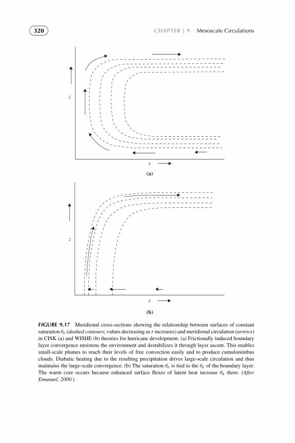
To protect the rights of the author(s) and publisher we inform you that this PDF is an uncorrected proof for internal businessuse only by the author(s), editor(s), reviewer(s), Elsevier and typesetter diacriTech. It is not allowed to publish this proofonline or in print. This proof copy is the copyright property of the publisher and is confidential until formal publication.
“Hakim: 13-ch09-279-324-9780123848666” — 2012/7/26 — 12:04 — page 320 — #42
320 CHAPTER | 9 Mesoscale Circulations
z
(a)
r
z
(b)
r
FIGURE 9.17 Meridional cross-sections showing the relationship between surfaces of constantsaturation θe (dashed contours; values decreasing as r increases) and meridional circulation (arrows)in CISK (a) and WISHE (b) theories for hurricane development. (a) Frictionally induced boundarylayer convergence moistens the environment and destabilizes it through layer ascent. This enablessmall-scale plumes to reach their levels of free convection easily and to produce cumulonimbusclouds. Diabatic heating due to the resulting precipitation drives large-scale circulation and thusmaintains the large-scale convergence. (b) The saturation θe is tied to the θe of the boundary layer.The warm core occurs because enhanced surface fluxes of latent heat increase θe there. (AfterEmanuel, 2000.)

To protect the rights of the author(s) and publisher we inform you that this PDF is an uncorrected proof for internal businessuse only by the author(s), editor(s), reviewer(s), Elsevier and typesetter diacriTech. It is not allowed to publish this proofonline or in print. This proof copy is the copyright property of the publisher and is confidential until formal publication.
“Hakim: 13-ch09-279-324-9780123848666” — 2012/7/26 — 12:04 — page 321 — #43
Problems 321
a suitable initial disturbance, a feedback may occur in which an increase ininward-spiraling surface winds increases the rate of moisture transfer from theocean, which increases the intensity of the convection, which further increasesthe secondary circulation. While it appears that observed cases of tropical cyclo-genesis require finite-amplitude initial disturbances, the reason is likely thatsuch disturbances require a shorter period of time to reach maturity. As initialdisturbance amplitude decreases, the time required to reach maturity increases,as does the probability of adverse environmental factors disrupting the process.
Many environmental factors may slow or hinder the development process,but the most important are vertical wind shear and dry air. Vertical shear “tilts”the convection so that the heating is not vertically aligned. Moreover, shear pro-duces a dipole of vertical motion about the nascent disturbance, which disturbsthe circulation from axisymmetry and results in dry air in the midtroposphereon the upshear side of the storm. Dry air may be entrained into the convec-tion, resulting in strong downdrafts that transport low-entropy air to the surface,reducing conditional instability. Thus, storm development can be substantiallyinhibited if dry air is continually transported into the midtroposphere above thedeveloping storm. As a result, developing systems that have a deep layer withclosed streamlines in a framework moving with the disturbance are favored,since the air is trapped within the disturbance, and convection may moisten thetroposphere through detrainment without being replaced by drier environmentalair.
SUGGESTED REFERENCES
Durran (1990) reviews the dynamics of mountain waves and downslope windstorms.Eliassen (1990) discusses the secondary circulation within frontal zones.Emanuel’s Atmospheric Convection is a graduate-level text covering the subject of convection,
including symmetric instability, in great detail.Emanuel (2000) provides a qualitative explanation of the WISHE theory for hurricane development.Keppert and Wang (2001) discuss the importance of vertical advection in generating supergradient
winds in tropical cyclone boundary layers.Hoskins (1982) discusses the semigeostrophic theory of frontogenesis and summarizes results from
numerical models.Houze’s Cloud Dynamics discusses convective storms at the graduate level.Klemp (1987) describes the dynamics of tornadic thunderstorms.
PROBLEMS
9.1. Show by transforming from θ coordinates to height coordinates that theErtel potential vorticity P is proportional to F2N2
s − S4. See (9.27).9.2. Starting with the linearized Boussinesq equations for a basic state zonal
flow that is a function of height, derive (9.35) and verify the form given forthe Scorer parameter.

To protect the rights of the author(s) and publisher we inform you that this PDF is an uncorrected proof for internal businessuse only by the author(s), editor(s), reviewer(s), Elsevier and typesetter diacriTech. It is not allowed to publish this proofonline or in print. This proof copy is the copyright property of the publisher and is confidential until formal publication.
“Hakim: 13-ch09-279-324-9780123848666” — 2012/7/26 — 12:04 — page 322 — #44
322 CHAPTER | 9 Mesoscale Circulations
9.3. Show that for stationary flow over an isolated ridge in the broad ridge limit(ks�ms), the group velocity vector is directed upward so that energy cannotpropagate upstream or downstream of the ridge.
9.4. An air parcel at 920 hPa with temperature 20◦C is saturated (mixing ratio16 g kg−1). Compute θe for the parcel.
9.5. Suppose that the mass of air in an entraining cumulus updraft increasesexponentially with height so that m = m0ez/H , where H = 8 km and m0 isthe mass at a reference level. If the updraft speed is 3 m s−1 at 2-km height,what is its value at a height of 8 km, assuming that the updraft has zero netbuoyancy?
9.6. Verify the approximate relationship between moist static energy and θe
given by equation (2.71).9.7. The azimuthal velocity component in some hurricanes is observed to have
a radial dependence given by vλ = V0(r0/r)2 for distances from the centergiven by r ≥ r0. Letting V0 = 50 m s−1 and r0 = 50 km, find the totalgeopotential difference between the far field (r→∞) and r = r0, assuminggradient wind balance and f0 = 5 × 10⁻⁵ s−1. At what distance from thecenter does the Coriolis force equal the centrifugal force?
9.8. Starting with equation (9.59), derive the angular momentum form of thegradient wind balance for an axisymmetric vortex given by equation (9.61).
MATLAB ExercisesM9.1. The MATLAB script surface front 1.m demonstrates the concentration of an
initial temperature gradient by an imposed deformation field. The tempera-ture field is initially taken to have a linear decrease in y: T (y) = 300− 10−2y,where y is in kilometers. The horizontal wind is given by the streamfunctionψ (x, y) = −15k−1 sin (kx) sin (my), where k = 2π/3× 106 and m = π/3× 106.Evaluate and contour-plot the deformation field for this streamfunction,where deformation is defined as ∂u/∂x− ∂v/∂y. Run the model and observewhere the temperature gradient increases. Modify the code to plot the max-imum temperature gradient as a function of time. For how long does thegradient increase approximately exponentially? What is the e-folding timefor increase of the temperature gradient at the origin?
M9.2. The MATLAB script profile 1.m and the function Tmoist.m use pressure, tem-perature, and humidity data in the file sounding.dat to calculate and graphvertical profiles of temperature, dewpoint, and the temperature correspond-ing to pseudoadiabatic ascent from the lifting condensation level for a parcellifted from the lowest level of the sounding. Modify this script to plot pro-files of the potential temperature, the equivalent potential temperature, andthe saturated potential temperature. Hint: Temperature at saturation can becalculated by inverting the expression for saturation vapor pressure, which isobtainable by integrating equation (D.4):
es = es,tr exp
[Lv
Rv
(1
Ttr−
1
T
)]
where es,tr = 6.11 hPa, Ttr = 273.16 K, and Lv = 2.5 × 10⁶ J kg−1 are thesaturation vapor pressure at the triple point temperature, the triple pointtemperature, and the latent heat of vaporization, respectively.

To protect the rights of the author(s) and publisher we inform you that this PDF is an uncorrected proof for internal businessuse only by the author(s), editor(s), reviewer(s), Elsevier and typesetter diacriTech. It is not allowed to publish this proofonline or in print. This proof copy is the copyright property of the publisher and is confidential until formal publication.
“Hakim: 13-ch09-279-324-9780123848666” — 2012/7/26 — 12:04 — page 323 — #45
Problems 323
M9.3. For the thermodynamic sounding of Problem M9.2, compute the CAPE andthe profile of vertical velocity for a parcel lifted from the lowest layer in theabsence of entrainment. What is the maximum vertical velocity, and what isthe distance that the parcel overshoots its level of neutral buoyancy?
M9.4. The MATLAB script lee wave 1.m uses the Fourier series approach to solvefor flow over an isolated ridge for the case of constant N and constant meanzonal flow. For the case of u = 50 m s−1, run the script for various ridgewidths to determine the width is required for significant vertical propagation(i.e., at what ridge width do phase lines of vertical velocity begin to tilt withheight)?
M9.5. The script lee wave 2.m plots an approximate analytic solution for flow overa mountain in the wide ridge limit. The height profile is given by
h(x) = h0L2/(
L2+ x2
)where L is the width scale of the ridge and h0 is the ridge height. For afixed ridge height of 2 km, vary the input zonal mean wind and commenton the dependence of the contoured solutions. (Note that the vertical scale isgiven in vertical wavelengths as in Figure 9.7.) Modify the script to vary themountain height and determine what fraction of the vertical wavelength themountain height must have in order for wave breaking to occur. (The onset ofwave breaking occurs when the streamlines become vertical.)
M9.6. Consider stationary gravity waves forced by flow over a sinusoidal lowerboundary for a case in which the static stability decreases rapidly with heightat about the 6-km level. Thus, the buoyancy frequency is altitude dependentand the simple analytic solution (9.32) no longer applies. The MATLAB scriptnamed linear grav wave 1.m gives a highly accurate numerical solution forthis situation.(a) Describe the qualitative change in the wave behavior as the zonal wave-
length is changed over the range of 10 to 100 km. Be sure to commenton momentum flux as well as on vertical velocity.
(b) Determine as accurately as you can what the minimum zonal wavelengthis for vertical propagation to occur in the upper part of the domain (abovethe 6-km level).
(c) Determine how the amplitudes of the momentum flux and momen-tum flux convergence at z = 6 km change as the zonal wavelength isincreased from 20 to 100 km. Do several different wavelengths so youcan plot graphs of the dependence of the magnitudes of the momentumflux and zonal force on the wavelength of the sinusoidal topography. UseMATLAB to plot these two graphs.

To protect the rights of the author(s) and publisher we inform you that this PDF is an uncorrected proof for internal businessuse only by the author(s), editor(s), reviewer(s), Elsevier and typesetter diacriTech. It is not allowed to publish this proofonline or in print. This proof copy is the copyright property of the publisher and is confidential until formal publication.
“Hakim: 14-ch10-325-376-9780123848666” — 2012/7/26 — 12:09 — page 325 — #1
Chapter 10
The General Circulation
In its broadest sense, the general circulation of the atmosphere is usually con-sidered to include the totality of motions that characterizes the global-scaleatmospheric flow. Specifically, the study of the general circulation is concernedwith the dynamics of climate—that is, with the temporally averaged structuresof the fields of wind, temperature, humidity, precipitation, and other meteoro-logical variables. The general circulation may thus be considered to consist ofthe flow averaged in time over a period sufficiently long to remove the randomvariations associated with individual weather systems but short enough to retainmonthly and seasonal variations.
In the past, both observational and theoretical studies of the general cir-culation concentrated on the dynamics of the zonally averaged flow. Thetime-averaged circulation is, however, highly dependent on longitude due tolongitudinally asymmetric forcing by orography and land–sea heating con-trasts. The longitudinally dependent components of the general circulationmay be separated into quasi-stationary circulations, which vary little in time;monsoonal circulations, which are seasonally reversing; and various subsea-sonal and interannual components, which together account for low-frequencyvariability. A complete understanding of the physical basis for the general cir-culation requires an explanation not only for the zonally averaged circulationbut for the longitudinally and time-varying components as well.
Nevertheless, to introduce the study of the general circulation, it provesuseful to isolate those processes that maintain the zonal-mean flow (i.e., theflow averaged around latitude circles). This approach follows naturally fromthe linear wave studies of previous chapters in which flow fields were splitinto zonal-mean and longitudinally dependent eddy components. In this chap-ter, however, we concentrate not on the development and motion of the eddiesbut on the influence of the eddies on the structure of the zonal-mean circu-lation. Focusing on the zonal mean allows us to isolate those features of thecirculation that are not dependent on continentality and should thus be com-mon to all thermally driven rotating fluid systems. In particular, we discuss theangular momentum and energy budgets of the zonally averaged flow. We alsoshow that the mean meridional circulation (i.e., the circulation consisting of the
An Introduction to Dynamic Meteorology. DOI: 10.1016/B978-0-12-384866-6.00010-6Copyright © 2013 Elsevier Inc. All rights reserved. 325

To protect the rights of the author(s) and publisher we inform you that this PDF is an uncorrected proof for internal businessuse only by the author(s), editor(s), reviewer(s), Elsevier and typesetter diacriTech. It is not allowed to publish this proofonline or in print. This proof copy is the copyright property of the publisher and is confidential until formal publication.
“Hakim: 14-ch10-325-376-9780123848666” — 2012/7/26 — 12:09 — page 326 — #2
326 CHAPTER | 10 The General Circulation
zonal-mean vertical and meridional velocity components) satisfies a diagnosticequation analogous to the vertical motion equation of Section 6.5, but with theforcing determined by the distributions of diabatic heating and eddy heat andmomentum fluxes.
Following our discussion of the zonal-mean circulation, we consider thelongitudinally varying time-averaged circulation. In this chapter the primaryemphasis is on extratropical aspects of the circulation; these can be discussedwithin the framework of quasi-geostrophic theory. The general circulation ofthe tropics is considered in Chapter 11.
10.1 THE NATURE OF THE PROBLEM
Theoretical speculation on the nature of the general circulation has quite a longhistory. Perhaps the most important early work on the subject was that of an18th-century Englishman, George Hadley. Hadley, in seeking a cause for thetrade wind circulation, realized that this circulation must be a form of thermalconvection driven by the difference in solar heating between equatorial andpolar regions. He visualized the general circulation as consisting of a zonallysymmetric overturning in which the heated equatorial air rises and flows pole-ward, where it cools, sinks, and flows equatorward again. At the same time, theCoriolis force deflects the poleward moving air at the upper levels to the eastand the equatorward-moving air near the surface to the west. The latter is, ofcourse, consistent with the observed surface winds in the trade wind zone, whichare northeasterly in the Northern Hemisphere and southeasterly in the South-ern Hemisphere. This type of circulation is now called a Hadley circulation orHadley cell.
Although a circulation consisting of Hadley cells extending from equatorto pole in each hemisphere is mathematically possible in the sense that such acirculation would not violate the laws of physics, the observed Hadley circu-lation is confined to the tropics. Evidence from a number of studies indicatesthat for conditions existing in Earth’s atmosphere, a symmetric hemispheric-wide Hadley circulation would be baroclinically unstable. If such a circulationwere to become established by some mechanism, it would quickly break downoutside the tropics as baroclinic eddies developed and modified the zonal-meancirculation through their heat and momentum fluxes.
The observed general circulation thus cannot be understood purely in termsof zonally symmetric processes. Rather, it can be thought of qualitatively asdeveloping through three-dimensional interactions among radiative and dynam-ical processes. In the mean, the net solar energy absorbed by the atmosphereand Earth must equal the infrared energy radiated back to space by the planet.The annually averaged solar heating is, however, strongly dependent on lati-tude, with a maximum at the equator and a minimum at the poles. The outgoinginfrared radiation, however, is only weakly latitude dependent. Thus, there is anet radiation surplus in the equatorial region and a deficit in the polar region.

To protect the rights of the author(s) and publisher we inform you that this PDF is an uncorrected proof for internal businessuse only by the author(s), editor(s), reviewer(s), Elsevier and typesetter diacriTech. It is not allowed to publish this proofonline or in print. This proof copy is the copyright property of the publisher and is confidential until formal publication.
“Hakim: 14-ch10-325-376-9780123848666” — 2012/7/26 — 12:09 — page 327 — #3
10.1 | The Nature of the Problem 327
This differential heating warms the equatorial atmosphere relative to higherlatitudes and creates a pole-to-equator temperature gradient. Therefore, it pro-duces a growing store of zonal-mean available potential energy. At some pointthe westerly thermal wind (which must develop if the motion is to be balancedgeostrophically in the presence of the pole-to-equator temperature gradient)becomes baroclinically unstable. As shown in Chapter 8, the resulting baro-clinic waves transport heat poleward. These waves will intensify until theirheat transport (together with the heat transported by planetary waves and oceancurrents) is sufficient to balance the radiation deficit in the polar regions sothat the pole-to-equator temperature gradient ceases to grow. At the same time,these perturbations convert potential energy into kinetic energy, thereby main-taining the kinetic energy of the atmosphere against the effects of frictionaldissipation.
From a thermodynamic point of view, the atmosphere may be regarded as a“heat engine” that absorbs net heat at relatively warm temperatures in the trop-ics (primarily in the form of latent heat due to evaporation from the sea surface)and gives up heat at relatively cool temperatures in the extratropics. In this man-ner, net radiation generates available potential energy, which is in turn partiallyconverted to kinetic energy, which does work to maintain the circulation againstfrictional dissipation. Only a small fraction of the solar energy input is actuallyconverted to kinetic energy. Thus, from an engineer’s viewpoint, the atmo-sphere is a rather inefficient heat engine. However, if due account is taken of themany constraints operating on atmospheric motions, it appears that the atmo-sphere may in fact generate kinetic energy about as efficiently as dynamicallypossible.
The preceding qualitative discussion suggests that the gross features ofthe general circulation outside the tropics can be understood on the basis ofquasi-geostrophic theory, since, as we have seen, baroclinic instability is con-tained within the quasi-geostrophic framework. In view of this fact, and to keepthe equations as simple as possible, our discussion of the zonally averagedand longitudinally varying components of the circulation outside the tropicswill concentrate on those aspects that can be qualitatively represented by thequasi-geostrophic equations on the midlatitude β plane.
It should be recognized that a quasi-geostrophic model cannot provide acomplete theory of the general circulation because in the quasi-geostrophic the-ory a number of assumptions are made concerning scales of motion that restrictin advance the possible types of solutions. Quantitative modeling of the gen-eral circulation requires complicated numerical models based on the primitiveequations in spherical coordinates. The ultimate objective of these modelingefforts is to simulate the general circulation so faithfully that the climatologicalconsequences of any change in the external parameters (e.g., the atmosphericconcentration of carbon dioxide) can be predicted accurately. Present modelscan provide fairly accurate simulations of the current climate and plausible pre-dictions of the response of the climate system to changes in external conditions.

To protect the rights of the author(s) and publisher we inform you that this PDF is an uncorrected proof for internal businessuse only by the author(s), editor(s), reviewer(s), Elsevier and typesetter diacriTech. It is not allowed to publish this proofonline or in print. This proof copy is the copyright property of the publisher and is confidential until formal publication.
“Hakim: 14-ch10-325-376-9780123848666” — 2012/7/26 — 12:09 — page 328 — #4
328 CHAPTER | 10 The General Circulation
However, uncertainties in the representations of a number of physical processes,particularly clouds and precipitation, limit the confidence that can be placed inquantitative climate change predictions based on such models.
10.2 THE ZONALLY AVERAGED CIRCULATION
The observed global distribution of the longitudinally averaged zonal wind forthe two solstice seasons was shown in Figure 6.1. Although there are importantinterhemispheric differences, the flow in both hemispheres is characterized bywesterly jets with maximum zonal velocities at about 30◦ to 35◦ latitude nearthe tropopause. These westerlies vary in longitude, especially in the NorthernHemisphere (refer to Figure 6.2), but there is a significant zonally symmetriccomponent, which we will refer to as the mean zonal wind.
Although departures of the time-averaged flow from zonal symmetry areimportant aspects of the general circulation, especially in the Northern Hemi-sphere, it is useful to first obtain an understanding of the dynamics of the zonallysymmetric component before investigating the three-dimensional time-meancirculation. This section examines the dynamics of zonally symmetric motionsusing quasi-geostrophic theory and the log-pressure coordinate system intro-duced in Chapter 7, and shows that the meridional circulation associated with anaxially symmetric vortex is dynamically analogous to the secondary divergentcirculation in a baroclinic wave.
In the log-pressure coordinate system, the x and y components of themomentum equation, the hydrostatic approximation, the continuity equation,and the thermodynamic energy equation can be written as
Du/Dt − f v + ∂8/∂x = X (10.1)
Dv/Dt + fu+ ∂8/∂y = Y (10.2)
∂8/∂z = H−1RT (10.3)
∂u/∂x+ ∂v/∂y+ ρ−10 ∂ (ρ0w) /∂z = 0 (10.4)
DT/Dt + (κT/H)w = J/cp (10.5)
where
D
Dt≡∂
∂t+ u
∂
∂x+ v
∂
∂y+ w
∂
∂z
and X and Y designate the zonal and meridional components of drag due tosmall-scale eddies.

To protect the rights of the author(s) and publisher we inform you that this PDF is an uncorrected proof for internal businessuse only by the author(s), editor(s), reviewer(s), Elsevier and typesetter diacriTech. It is not allowed to publish this proofonline or in print. This proof copy is the copyright property of the publisher and is confidential until formal publication.
“Hakim: 14-ch10-325-376-9780123848666” — 2012/7/26 — 12:09 — page 329 — #5
10.2 | The Zonally Averaged Circulation 329
For convenience in this and the following chapters, we have dropped theasterisk notation used in Chapter 7 to distinguish the log-pressure coordinatefrom geometric height. Thus, z here designates the log-pressure variable definedin Section 7.4.1.
Analysis of the zonally averaged circulation involves study of the interac-tion of longitudinally varying disturbances (referred to as eddies and denotedby primed variables) with the longitudinally averaged flow (referred to as themean flow and denoted by overbars). Thus, any variable A is expanded in theform A = A + A′. This sort of average is a Eulerian mean, as it is evaluated atfixed latitude, height, and time. Eulerian mean equations are obtained by tak-ing zonal averages of (10.1) through (10.5). Such averaging is facilitated byusing (10.4) to expand the material derivative for any variable A in flux form asfollows:
ρ0DA
Dt= ρ0
(∂
∂t+ V ·∇ + w
∂
∂z
)A+ A
[∇ · (ρ0V)+
∂
∂z(ρ0w)
]
=∂
∂t(ρ0A)+
∂
∂x(ρ0Au)+
∂
∂y(ρ0Av)+
∂
∂z(ρ0Aw)
(10.6)
where we recall that ρ0 = ρ0(z).Applying the zonal averaging operator then gives
ρ0DA
Dt=∂
∂t
(ρ0A
)+∂
∂y
[ρ0
(Av + A′v′
)]+∂
∂z
[ρ0
(Aw+ A′w′
)](10.7)
Here we have used the fact that ∂ ( )/∂x = 0, since quantities with the overbarare independent of x. We have also used the fact that for any variables a and b
ab = (a+ a′)(b+ b′
)= ab+ ab′ + a′b+ a′b′ = ab+ a′b′
which follows from that fact that a and b are independent of x and a′ = b′ = 0so that, for example, ab′ = ab′ = 0.
The terms involving (v,w) on the right in (10.7) can be rewritten inadvective form with the aid of the zonal mean of (10.4):
∂v/∂y+ ρ−10 ∂(ρ0w)/∂z = 0 (10.8)
Applying the chain rule of differentiation to the mean terms on the right in (10.7)and substituting from (10.8), we can rewrite (10.7) as
ρ0DA
Dt= ρ0
D
Dt
(A)+∂
∂y
[ρ0
(A′v′
)]+∂
∂z
[ρ0
(A′w′
)](10.9)

To protect the rights of the author(s) and publisher we inform you that this PDF is an uncorrected proof for internal businessuse only by the author(s), editor(s), reviewer(s), Elsevier and typesetter diacriTech. It is not allowed to publish this proofonline or in print. This proof copy is the copyright property of the publisher and is confidential until formal publication.
“Hakim: 14-ch10-325-376-9780123848666” — 2012/7/26 — 12:09 — page 330 — #6
330 CHAPTER | 10 The General Circulation
where
D
Dt≡∂
∂t+ v
∂
∂y+ w
∂
∂z(10.10)
is the rate of change following the mean meridional motion (v,w).
10.2.1 The Conventional Eulerian Mean
Applying the averaging scheme of (10.9) to (10.1) and (10.5), we obtain thezonal-mean zonal momentum and thermodynamic energy equations for quasi-geostrophic motions on the midlatitude β plane:
∂u/∂t − f0v = −∂(
u′v′)/∂y+ X (10.11)
∂T/∂t + N2HR−1w = −∂(v′T ′
)/∂y+ J/cp (10.12)
where N is the buoyancy frequency defined by
N2≡
R
H
(κT0
H+
dT0
dz
)In (10.11) and (10.12), consistent with quasi-geostrophic scaling, we haveneglected advection by the ageostrophic mean meridional circulation and ver-tical eddy flux divergences. It is easily confirmed that for quasi-geostrophicscales, these terms are small compared to the retained terms (see Problem10.4). We have included the zonally averaged turbulent drag in (10.11) becausestresses due to unresolved eddies (such as gravity waves) may be important notonly in the boundary layer but also in the upper troposphere and in the middleatmosphere.
Similar scaling shows that the zonal average of the meridional momentumequation (10.2) can be approximated accurately by geostrophic balance:
f0u = −∂8/∂y
This can be combined with the hydrostatic approximation (10.3) to give thethermal wind relation
f0∂u/∂z+ RH−1∂T/∂y = 0 (10.13)
This relationship between zonal-mean wind and potential temperature dis-tributions imposes a strong constraint on the ageostrophic mean meridionalcirculation (v,w). In the absence of a mean meridional circulation, the eddymomentum flux divergence in (10.11) and eddy heat flux divergence in (10.12)would tend separately to change the mean zonal wind and temperature fields,and thus would destroy thermal wind balance. The pressure gradient force that

To protect the rights of the author(s) and publisher we inform you that this PDF is an uncorrected proof for internal businessuse only by the author(s), editor(s), reviewer(s), Elsevier and typesetter diacriTech. It is not allowed to publish this proofonline or in print. This proof copy is the copyright property of the publisher and is confidential until formal publication.
“Hakim: 14-ch10-325-376-9780123848666” — 2012/7/26 — 12:09 — page 331 — #7
10.2 | The Zonally Averaged Circulation 331
results from any small departure of the mean zonal wind from geostrophicbalance will, however, drive a mean meridional circulation, which adjusts themean zonal wind and temperature fields so that (10.13) remains valid. In manysituations this compensation allows the mean zonal wind to remain unchangedeven in the presence of large eddy heat and momentum fluxes. The meanmeridional circulation thus plays exactly the same role in the zonal-mean cir-culation that the secondary divergent circulation plays in the synoptic-scalequasi-geostrophic system. In fact, for steady-state mean flow conditions, the(v,w) circulation must just balance the eddy forcing plus diabatic heating sothat the balances in (10.11) and (10.12) are as follows:
l Coriolis force ( f0v) ≈ divergence of eddy momentum fluxesl Adiabatic cooling ≈ diabatic heating plus convergence of eddy heat fluxes
Analysis of observations shows that outside the tropics these balances appearto be approximately true above the boundary layer. Thus, changes in the zonal-mean flow arise from small imbalances between the forcing terms and the meanmeridional circulation.
The Eulerian mean meridional circulation can be determined in terms of theforcing from an equation similar to the omega equation of Section 6.4. Beforederiving this equation, it is useful to observe that the mean meridional mass cir-culation is nondivergent in the meridional plane. Thus, it can be represented interms of a meridional mass transport streamfunction, which identically satisfiesthe continuity equation (10.8) by letting
ρ0v = −∂χ
∂z; ρ0w =
∂χ
∂y(10.14)
The relationship of the sign of the streamfunction χ to the sense of the meanmeridional circulation is shown schematically in Figure 10.1.
1000
750
500
250
(hPa)
Equator N
ρ
χ = 0
χ > 0 χ < 0
FIGURE 10.1 Relationship of the Eulerian mean meridional streamfunction to vertical andmeridional motion.

To protect the rights of the author(s) and publisher we inform you that this PDF is an uncorrected proof for internal businessuse only by the author(s), editor(s), reviewer(s), Elsevier and typesetter diacriTech. It is not allowed to publish this proofonline or in print. This proof copy is the copyright property of the publisher and is confidential until formal publication.
“Hakim: 14-ch10-325-376-9780123848666” — 2012/7/26 — 12:09 — page 332 — #8
332 CHAPTER | 10 The General Circulation
The diagnostic equation for χ is derived by first taking
f0∂
∂z(10.11)+
R
H
∂
∂y(10.12)
and then using (10.13) to eliminate the time derivatives and (10.14) to expressthe mean meridional circulation in terms of χ . The resulting elliptic equationhas the form
∂2χ
∂y2+
f 20
N2ρ0∂
∂z
(1
ρ0
∂χ
∂z
)=ρ0
N2
[∂
∂y
(κJ
H−
R
H
∂
∂y
(v′T ′
))
− f0
(∂2
∂z∂y
(u′v′
)−∂X
∂z
)] (10.15)
Equation (10.15) can be used to qualitatively diagnose the mean meridionalcirculation. Because χ must vanish on the boundaries, it can be represented bya double Fourier series in y and z. Hence, the elliptic operator on the left sideof (10.15) is approximately proportional to −χ , and (10.15) states qualitativelythat
χ ∝−∂
∂y(diabatic heating)+
∂2
∂y2 (large-scale eddy heat flux)
+∂2
∂y∂z(large-scale eddy momentum flux)+
∂
∂z(zonal drag force)
Now, diabatic heating in the Northern Hemisphere decreases for increasing y.Thus, the first term on the right is positive and tends to force a mean meridionalcell with χ > 0. This is referred to as a thermally direct cell, as warm air is risingand cool air is sinking. It is this process that primarily accounts for the Hadleycirculation of the tropics as illustrated in Figure 10.2. For an idealized Hadleycell in the absence of eddy sources, the differential diabatic heating would bebalanced only by adiabatic cooling near the equator and adiabatic warming athigher latitudes.
In the extratropical Northern Hemisphere, poleward eddy heat fluxes dueto both transient synoptic-scale eddies and stationary planetary waves tend totransfer heat poleward, producing a maximum poleward heat flux v′T ′ in thelower troposphere at about 50◦ latitude as shown in Figure 10.3. Because χ isproportional to the second derivative of v′T ′, which should be negative wherev′T ′ > 0, the term should tend to produce a mean meridional cell with χ < 0centered in the lower troposphere at midlatitudes. Thus, the eddy heat flux tendsto drive an indirect meridional circulation.
The existence of this indirect meridional circulation can be understood interms of the need to maintain geostrophic and hydrostatic balance. North of thelatitude where v′T ′ is a maximum, there is a convergence of eddy heat flux,

To protect the rights of the author(s) and publisher we inform you that this PDF is an uncorrected proof for internal businessuse only by the author(s), editor(s), reviewer(s), Elsevier and typesetter diacriTech. It is not allowed to publish this proofonline or in print. This proof copy is the copyright property of the publisher and is confidential until formal publication.
“Hakim: 14-ch10-325-376-9780123848666” — 2012/7/26 — 12:09 — page 333 — #9
10.2 | The Zonally Averaged Circulation 333
Latentheating
Radiativecoolingχ > 0
J > 0 J < 0
Equator 30°
FIGURE 10.2 Schematic Eulerian mean meridional circulation showing the streamfunction for athermally direct Hadley cell.
100
200
0.0
0.0
0.0
0.0
0.0
0.0
0.0
16.0
16.0
300
500
700
100090S 60S 30S EQ 30N 60N 90N
FIGURE 10.3 Observed northward eddy heat flux distribution (◦C m s−1) for Northern Hemi-sphere winter. (Adapted from Schubert et al., 1990.)
while equatorward of that latitude, there is a divergence. Thus, eddy heat trans-port tends to reduce the pole-to-equator mean temperature gradient. If the meanzonal flow is to remain geostrophic, the thermal wind must then also decrease.In the absence of eddy momentum transport, this decrease in the thermal windcan only be produced by the Coriolis torque due to a mean meridional circula-tion with the sense of that in Figure 10.4. At the same time, it is not surprisingto find that the vertical mean motions required by continuity oppose the tem-perature tendency associated with the eddy heat flux by producing adiabaticwarming in the region of eddy heat flux divergence and adiabatic cooling in theregion of eddy heat flux convergence.

To protect the rights of the author(s) and publisher we inform you that this PDF is an uncorrected proof for internal businessuse only by the author(s), editor(s), reviewer(s), Elsevier and typesetter diacriTech. It is not allowed to publish this proofonline or in print. This proof copy is the copyright property of the publisher and is confidential until formal publication.
“Hakim: 14-ch10-325-376-9780123848666” — 2012/7/26 — 12:09 — page 334 — #10
334 CHAPTER | 10 The General Circulation
f v > 0–
f v > 0–
(v ′T′)max∂ (v′T′)
∂y0
S N
>∂ (v ′T ′)
∂y0<
FIGURE 10.4 Schematic Eulerian mean meridional circulation forced by poleward heat fluxes.
S N
Adiabaticcooling
Adiabaticwarming
∂ (u′v′)∂y
0<
∂ (u′v′)∂y
0<<
f v < 0–
f v > 0–
FIGURE 10.5 Schematic Eulerian mean meridional circulation forced by a vertical gradient ineddy momentum flux convergence.
The next to last forcing term in (10.15) is proportional to the vertical gradientof the horizontal eddy momentum flux convergence. However, it can be shown(see Problem 10.5) that
−∂2
∂z∂y
(u′v′
)= +
∂
∂z
(v′ζ ′
)Thus, this term is proportional to the vertical derivative of the meridionalvorticity flux. To interpret this eddy forcing physically, we suppose as shown inFigure 10.5 that the momentum flux convergence (or the vorticity flux) is pos-itive and increasing with height. This will be true in the Northern Hemisphere
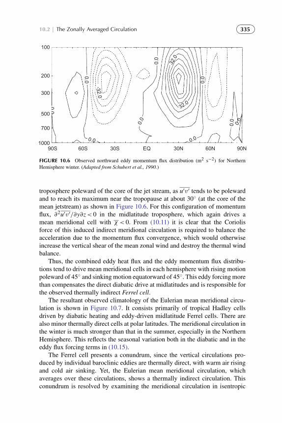
To protect the rights of the author(s) and publisher we inform you that this PDF is an uncorrected proof for internal businessuse only by the author(s), editor(s), reviewer(s), Elsevier and typesetter diacriTech. It is not allowed to publish this proofonline or in print. This proof copy is the copyright property of the publisher and is confidential until formal publication.
“Hakim: 14-ch10-325-376-9780123848666” — 2012/7/26 — 12:09 — page 335 — #11
10.2 | The Zonally Averaged Circulation 335
0.0
100
200
300
700
100090S 60S 30S 30NEQ 60N
0.00.0
0.0
0.0
0.0
0.0
32.0
32.0
32.0
0.0
0.0
90N
500
FIGURE 10.6 Observed northward eddy momentum flux distribution (m2 s−2) for NorthernHemisphere winter. (Adapted from Schubert et al., 1990.)
troposphere poleward of the core of the jet stream, as u′v′ tends to be polewardand to reach its maximum near the tropopause at about 30◦ (at the core of themean jetstream) as shown in Figure 10.6. For this configuration of momentumflux, ∂2u′v′/∂y∂z< 0 in the midlatitude troposphere, which again drives amean meridional cell with χ < 0. From (10.11) it is clear that the Coriolisforce of this induced indirect meridional circulation is required to balance theacceleration due to the momentum flux convergence, which would otherwiseincrease the vertical shear of the mean zonal wind and destroy the thermal windbalance.
Thus, the combined eddy heat flux and the eddy momentum flux distribu-tions tend to drive mean meridional cells in each hemisphere with rising motionpoleward of 45◦ and sinking motion equatorward of 45◦. This eddy forcing morethan compensates the direct diabatic drive at midlatitudes and is responsible forthe observed thermally indirect Ferrel cell.
The resultant observed climatology of the Eulerian mean meridional circu-lation is shown in Figure 10.7. It consists primarily of tropical Hadley cellsdriven by diabatic heating and eddy-driven midlatitude Ferrel cells. There arealso minor thermally direct cells at polar latitudes. The meridional circulation inthe winter is much stronger than that in the summer, especially in the NorthernHemisphere. This reflects the seasonal variation both in the diabatic and in theeddy flux forcing terms in (10.15).
The Ferrel cell presents a conundrum, since the vertical circulations pro-duced by individual baroclinic eddies are thermally direct, with warm air risingand cold air sinking. Yet, the Eulerian mean meridional circulation, whichaverages over these circulations, shows a thermally indirect circulation. Thisconundrum is resolved by examining the meridional circulation in isentropic

To protect the rights of the author(s) and publisher we inform you that this PDF is an uncorrected proof for internal businessuse only by the author(s), editor(s), reviewer(s), Elsevier and typesetter diacriTech. It is not allowed to publish this proofonline or in print. This proof copy is the copyright property of the publisher and is confidential until formal publication.
“Hakim: 14-ch10-325-376-9780123848666” — 2012/7/26 — 12:09 — page 336 — #12
336 CHAPTER | 10 The General Circulation
100
200
300
700
100090S 60S 30S 30NEQ 60N
0.0
0.016.016.0
16.00.
0
0.0
0.0
0.0 0.
0
0.0
0.0
32.0
90N
500
FIGURE 10.7 Streamfunction (units: 102 kg m−1s−1) for the observed Eulerian mean meridionalcirculation for Northern Hemisphere winter. (Based on the data of Schubert et al., 1990).
Latitude
Pot
entia
l tem
pera
ture
(K
)
250 220
500
750
20
60
20
120
−50° 0° +50°250
300
350
Hadley cells
FIGURE 10.8 January time and zonal-mean isentropic mass flux streamfunction determined fromERA-40 reanalysis data 1980–2001). Streamfunction contours are shown every 20 × 109 kg s−1,with implied clockwise circulation around negative values. Dotted lines show pressure surfaces andthe solid lower curve is the median surface potential temperature. (Adapted from Schneider, 2006.Used with permission of Annual Reviews.)
coordinates (Figure 10.8), which reveals a thermally direct circulation in boththe Hadley cells and in the extratropics. This shows that the Ferrel cell is anartifact of the Eulerian averaging process and that eddy fluxes of entropy arelarge compared to those of the mean circulation.
The zonal momentum balance in the upper troposphere in tropical and mid-latitude cells is maintained by the balance between the Coriolis force caused

To protect the rights of the author(s) and publisher we inform you that this PDF is an uncorrected proof for internal businessuse only by the author(s), editor(s), reviewer(s), Elsevier and typesetter diacriTech. It is not allowed to publish this proofonline or in print. This proof copy is the copyright property of the publisher and is confidential until formal publication.
“Hakim: 14-ch10-325-376-9780123848666” — 2012/7/26 — 12:09 — page 337 — #13
10.2 | The Zonally Averaged Circulation 337
by the mean meridional drift and the eddy momentum flux convergence. Theheat balance is maintained by rising motion (adiabatic cooling) balancing thediabatic heating in the tropics and by the eddy heat flux convergence at highlatitudes and subsidence (adiabatic warming) balancing the eddy heat fluxdivergence in the subtropics.
Because of the appearance of eddy flux terms in both mean momentum andthermodynamic energy equations, and the near cancellation of eddy and meanflow processes, it is rather inefficient to attempt to diagnose the net eddy forcingof the mean flow from the conventional Eulerian mean. It can be shown thatsimilar eddy and mean flow compensation occurs in the Eulerian mean continu-ity equation for a long-lived tracer so that tracer transport calculations are alsoinefficient in this formulation.
10.2.2 The Transformed Eulerian Mean
An alternative approach to analysis of the zonal-mean circulation, which pro-vides a clearer diagnosis of eddy forcing and also provides a more direct view oftransport processes in the meridional plane, is the transformed Eulerian mean(TEM) formulation introduced by Andrews and McIntyre (1976). This trans-formation takes account of the fact that in (10.12) there tends to be a strongcancellation between the eddy heat flux convergence and adiabatic cooling,while the diabatic heating term is a small residual. Since in the mean an airparcel will rise to a higher equilibrium altitude only if its potential temperatureis increased by diabatic heating, it is the residual meridional circulation associ-ated with diabatic processes that is directly related to the mean meridional massflow.
The TEM equations can be obtained from (10.11) and (10.12) by definingthe residual circulation
(v∗,w∗
)as follows:
v∗ = v − ρ−10 RH−1∂(ρ0v′T ′/N
2)/∂z (10.16a)
w∗ = w+ RH−1∂(v′T ′/N2)/∂y (10.16b)
The residual vertical velocity defined in this manner clearly represents that partof the mean vertical velocity with a contribution to adiabatic temperature changethat is not canceled by the eddy heat flux divergence.
Substituting from (10.16a) into (10.11) and (10.12) to eliminate (v,w) yieldsthe TEM equations
∂u/∂t − f0v∗= +ρ−1
0 ∇ ·F+ X ≡ G (10.17)
∂T/∂t + N2HR−1w∗ = J/cp (10.18)
∂v∗/∂y+ ρ−10 ∂
(ρ0w∗
)/∂z = 0 (10.19)

To protect the rights of the author(s) and publisher we inform you that this PDF is an uncorrected proof for internal businessuse only by the author(s), editor(s), reviewer(s), Elsevier and typesetter diacriTech. It is not allowed to publish this proofonline or in print. This proof copy is the copyright property of the publisher and is confidential until formal publication.
“Hakim: 14-ch10-325-376-9780123848666” — 2012/7/26 — 12:09 — page 338 — #14
338 CHAPTER | 10 The General Circulation
where F ≡ jFy + kFz, the Eliassen–Palm flux (EP flux), is a vector in themeridional (y, z) plane, which for large-scale quasi-geostrophic eddies has thecomponents
Fy = −ρ0u′v′, Fz = ρ0f0Rv′T ′/(N2H) (10.20)
and G in (10.17) designates the total zonal force due to both large- and small-scale eddies.
The TEM formulation clearly shows that the eddy heat and momentumfluxes do not act separately to drive changes in the zonal-mean circulation, butonly in the combination given by the divergence of the EP flux. The funda-mental role of the eddies is thus to exert a zonal force. This eddy forcing ofthe zonal-mean flow can be displayed conveniently by mapping the field of Fand contouring the isolines of its divergence. When properly scaled by the basicstate density, these contours give the zonal force per unit mass exerted by quasi-geostrophic eddies. The mean global EP flux divergence pattern for a NorthernHemisphere winter is shown in Figure 10.9. Note that in most of the extratrop-ical troposphere, the EP flux is convergent so that the eddies exert a westwardzonal force on the atmosphere. On the seasonal time scale the zonal force dueto the EP flux divergence in (10.17) is nearly balanced by the eastward Coriolisforce of the residual mean meridional circulation. Conditions for this balanceare discussed in the next subsection.
The structure of the residual mean meridional circulation can be determinedby defining a residual streamfunction:
χ∗ ≡ χ + ρ0R
H
v′T ′
N2
0.0
100
300
700
100090S 60S 30S 30NEQ 60N
−8.0
0
0.00.0
0.0 0.0
0.0 0.0
0.0
0.0
90N
500
200
FIGURE 10.9 Eliassen–Palm flux divergence divided by the standard density ρ0 for NorthernHemisphere winter. (Units: m s−1 day−1.) (Based on the data of Schubert et al., 1990.)

To protect the rights of the author(s) and publisher we inform you that this PDF is an uncorrected proof for internal businessuse only by the author(s), editor(s), reviewer(s), Elsevier and typesetter diacriTech. It is not allowed to publish this proofonline or in print. This proof copy is the copyright property of the publisher and is confidential until formal publication.
“Hakim: 14-ch10-325-376-9780123848666” — 2012/7/26 — 12:09 — page 339 — #15
10.2 | The Zonally Averaged Circulation 339
It can then be shown by direct substitution into (10.14) and (10.15) that
ρ0v∗= −
∂χ∗
∂z; ρ0w∗ =
∂χ∗
∂y
and
∂2χ∗
∂y2+ ρ0
f 20
N2
∂
∂z
(1
ρ0
∂χ∗
∂z
)=ρ0
N2
[∂
∂y
(κJ
H
)+ f0
∂G
∂z
](10.21)
The magnitudes of the diabatic and EP flux contributions to the source term onthe right in (10.21) are generally larger in the winter hemisphere than in thesummer hemisphere. In the Northern Hemisphere troposphere, the source termsare generally negative, whereas in the Southern Hemisphere, they are generallypositive. This implies that χ∗ itself is positive in the Northern Hemisphere andnegative in the Southern Hemisphere so that the residual meridional circulationconsists of a single thermally direct overturning in each hemisphere, with thestrongest cell in the winter hemisphere as shown in Figure 10.10.
Unlike the conventional Eulerian mean, the residual mean vertical motionfor time-averaged conditions is proportional to the rate of diabatic heating. Itapproximately represents the diabatic circulation in the meridional plane—thatis, the circulation in which parcels that rise are diabatically heated and thosethat sink are diabatically cooled in order that their potential temperatures adjustto the local environment. The time-averaged residual mean meridional circu-lation thus approximates the mean motion of air parcels and thus, unlike theconventional Eulerian mean, provides an approximation to the mean advectivetransport of trace substances.
100
200
300
500
700
90S 60S 30S 30N
16.0
16.0
0.00.0
0.0
0.0
60N 90NEQ
32.0
16.0
32.0
1000
FIGURE 10.10 Residual mean meridional streamfunction (units: 102 kg m−1 s−1) for NorthernHemisphere winter. (Based on the data of Schubert et al., 1990.)
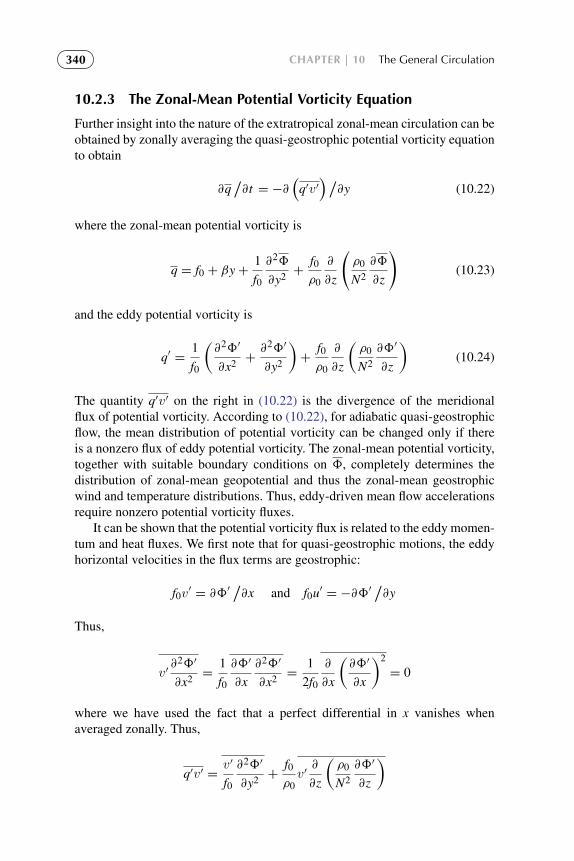
To protect the rights of the author(s) and publisher we inform you that this PDF is an uncorrected proof for internal businessuse only by the author(s), editor(s), reviewer(s), Elsevier and typesetter diacriTech. It is not allowed to publish this proofonline or in print. This proof copy is the copyright property of the publisher and is confidential until formal publication.
“Hakim: 14-ch10-325-376-9780123848666” — 2012/7/26 — 12:09 — page 340 — #16
340 CHAPTER | 10 The General Circulation
10.2.3 The Zonal-Mean Potential Vorticity Equation
Further insight into the nature of the extratropical zonal-mean circulation can beobtained by zonally averaging the quasi-geostrophic potential vorticity equationto obtain
∂q/∂t = −∂
(q′v′
)/∂y (10.22)
where the zonal-mean potential vorticity is
q = f0 + βy+1
f0
∂28
∂y2+
f0ρ0
∂
∂z
(ρ0
N2
∂8
∂z
)(10.23)
and the eddy potential vorticity is
q′ =1
f0
(∂28′
∂x2+∂28′
∂y2
)+
f0ρ0
∂
∂z
(ρ0
N2
∂8′
∂z
)(10.24)
The quantity q′v′ on the right in (10.22) is the divergence of the meridionalflux of potential vorticity. According to (10.22), for adiabatic quasi-geostrophicflow, the mean distribution of potential vorticity can be changed only if thereis a nonzero flux of eddy potential vorticity. The zonal-mean potential vorticity,together with suitable boundary conditions on 8, completely determines thedistribution of zonal-mean geopotential and thus the zonal-mean geostrophicwind and temperature distributions. Thus, eddy-driven mean flow accelerationsrequire nonzero potential vorticity fluxes.
It can be shown that the potential vorticity flux is related to the eddy momen-tum and heat fluxes. We first note that for quasi-geostrophic motions, the eddyhorizontal velocities in the flux terms are geostrophic:
f0v′= ∂8′
/∂x and f0u′ = −∂8′
/∂y
Thus,
v′∂28′
∂x2=
1
f0
∂8′
∂x
∂28′
∂x2=
1
2f0
∂
∂x
(∂8′
∂x
)2
= 0
where we have used the fact that a perfect differential in x vanishes whenaveraged zonally. Thus,
q′v′ =v′
f0
∂28′
∂y2+
f0ρ0
v′∂
∂z
(ρ0
N2
∂8′
∂z
)
To protect the rights of the author(s) and publisher we inform you that this PDF is an uncorrected proof for internal businessuse only by the author(s), editor(s), reviewer(s), Elsevier and typesetter diacriTech. It is not allowed to publish this proofonline or in print. This proof copy is the copyright property of the publisher and is confidential until formal publication.
“Hakim: 14-ch10-325-376-9780123848666” — 2012/7/26 — 12:09 — page 341 — #17
10.3 | The Angular Momentum Budget 341
We can use the chain rule of differentiation to rewrite the terms on the rightin this expression as
v′
f0
∂28′
∂y2=
1
f 20
(∂8′
∂x
∂28′
∂y2
)
=1
f 20
∂
∂y
(∂8′
∂x
∂8′
∂y
)−
1
2
∂
∂x
(∂8′
∂y
)2 = − ∂
∂y
(u′v′
)and
f0ρ0
v′∂
∂z
(ρ0
N2
∂8′
∂z
)=
1
ρ0
∂∂z
(ρ0
N2
∂8′
∂x
∂8′
∂z
)−
ρ0
2N2
∂
∂x
(∂8′
∂z
)2
=f0ρ0
∂
∂z
(ρ0
N2v′∂8′
∂z
)Thus,
q′v′ = −∂u′v′
∂y+
f0ρ0
∂
∂z
(ρ0
N2v′∂8′
∂z
)(10.25)
so that it is not the momentum flux u′v′ or heat flux v′∂8′/∂z that drives net
changes in the mean flow distribution, but rather the combination given by thepotential vorticity flux. Under some circumstances the eddy momentum fluxand eddy heat flux may individually be large, but the combination in (10.25)actually vanishes. This cancellation effect makes the traditional Eulerian meanformulation a poor framework for analysis of mean flow forcing by eddies.
Comparing (10.25) and (10.20), we see that the potential vorticity flux isproportional to the divergence of the EP flux vector:
q′v′ = ρ−10 ∇ ·F (10.26)
Thus, the contribution of large-scale motions to the zonal force in (10.17) equalsthe meridional flux of quasi-geostrophic potential vorticity. If the motion is adi-abatic and the potential vorticity flux is nonzero, equation (10.22) shows thatthe mean flow distribution must change with time. For this reason, there can-not be complete compensation between Coriolis torque and zonal force terms in(10.17).
10.3 THE ANGULAR MOMENTUM BUDGET
The previous section used the quasi-geostrophic version of the zonal-meanequations to show that large-scale eddies play an essential part in the main-tenance of the zonal-mean circulation in the extratropics. In particular, we

To protect the rights of the author(s) and publisher we inform you that this PDF is an uncorrected proof for internal businessuse only by the author(s), editor(s), reviewer(s), Elsevier and typesetter diacriTech. It is not allowed to publish this proofonline or in print. This proof copy is the copyright property of the publisher and is confidential until formal publication.
“Hakim: 14-ch10-325-376-9780123848666” — 2012/7/26 — 12:09 — page 342 — #18
342 CHAPTER | 10 The General Circulation
contrasted the mean flow forcing as represented by the conventional Eulerianmean and TEM formulations. This section expands our consideration of themomentum budget by considering the overall balance of angular momentumfor the atmosphere and Earth combined. Thus, rather than simply consideringthe balance of momentum for a given latitude and height in the atmosphere,we must consider the transfer of angular momentum between Earth and theatmosphere, and the flow of angular momentum in the atmosphere.
It would be possible to utilize the complete spherical coordinate version ofthe TEM equations for this analysis, but we are concerned primarily with theangular momentum balance for a zonal ring of air extending from the surface tothe top of the atmosphere. In that case it proves simpler to use the conventionalEulerian mean formulation. It also proves convenient to use a special verticalcoordinate, called the sigma coordinate, in which Earth’s surface is a coordinatesurface.
Because the average rotation rate of Earth is itself observed to be veryclose to constant, the atmosphere must also on the average conserve its angularmomentum. The atmosphere gains angular momentum from Earth in the tropicswhere the surface winds are easterly (i.e., where the angular momentum of theatmosphere is less than that of Earth) and gives up angular momentum to Earthin middle latitudes where the surface winds are westerly. Thus, there must be anet poleward transport of angular momentum within the atmosphere; otherwise,the torque due to surface friction would decelerate both easterlies and wester-lies. Furthermore, the angular momentum given by Earth to the atmosphere inthe belt of easterlies must just balance the angular momentum given up to Earthin the westerlies if the global angular momentum of the atmosphere is to remainconstant.
In the equatorial regions the poleward angular momentum transport isdivided between the advection of absolute angular momentum by the polewardflow in the axially symmetric Hadley circulation and transport by eddies. Inmidlatitudes, however, it is primarily the eddy motions that transport momen-tum poleward, and the angular momentum budget of the atmosphere must bequalitatively as shown in Figure 10.11.
As this figure suggests, there is a maximum poleward flux of angularmomentum at about 30◦ latitude and a maximum horizontal flux convergence atabout 45◦. This maximum in the flux convergence is a reflection of the strongenergy conversion in upper-level westerlies and is the mechanism whereby theatmosphere can maintain a positive zonal wind in the middle latitudes despitethe momentum lost to the surface.
It is convenient to analyze the momentum budget in terms of absolute angu-lar momentum. The absolute angular momentum per unit mass of atmosphere is
M = (�a cosφ + u) a cosφ
where as before a is the radius of Earth. The crucial role of zonal eddy dragin maintaining the observed latitudinal profile of the mean zonal wind can be

To protect the rights of the author(s) and publisher we inform you that this PDF is an uncorrected proof for internal businessuse only by the author(s), editor(s), reviewer(s), Elsevier and typesetter diacriTech. It is not allowed to publish this proofonline or in print. This proof copy is the copyright property of the publisher and is confidential until formal publication.
“Hakim: 14-ch10-325-376-9780123848666” — 2012/7/26 — 12:09 — page 343 — #19
10.3 | The Angular Momentum Budget 343
Eddy flux
(Divergence) (Convergence)
Easterlies Westerlies
0 15 30 45 601000
600
200ρ
(hP
a)
Latitude
FIGURE 10.11 Schematic mean angular momentum budget for the atmosphere–Earth system.
seen by evaluating the mean zonal velocity that would arise if a zonal ringof air at rest on the equator were to be displaced poleward, conserving M. Inthat case u(φ) = �a sin2 φ/cosφ, so that in an angular momentum–conservingHadley circulation, u ≈ 130 m s−1 at 30◦ latitude, which is far greater than isobserved.
Clearly, the absolute angular momentum must decrease as air parcels areadvected poleward in the Hadley circulation. The absolute angular momentumof an individual air parcel can be changed only by torques caused by the zonalpressure gradient and eddy stresses. In isobaric coordinates, Newton’s secondlaw in its angular momentum form is thus
DM
Dt= −a cosφ
[∂8
∂x+ g
∂τ xE
∂p
](10.27)
where τ xE is the zonal component of the vertical eddy stress, and it is assumed
that horizontal eddy stresses are negligible compared to the vertical eddy stress.
10.3.1 Sigma Coordinates
In neither the isobaric nor the log-pressure coordinate system does the lowerboundary exactly coincide with a coordinate surface. In analytical studies it isusual to assume that the lower boundary can be approximated as a constantpressure surface and to apply the approximate condition
ω(ps) ≈ −ρ0gw(z0)
as the lower boundary condition. Here we have assumed that the height of theground z0 is coincident with the pressure surface ps–that is, where ps is usu-ally set equal to 1000 hPa. These assumptions are of course not strictly valideven when the ground is level. Pressure does change at the ground, but, more

To protect the rights of the author(s) and publisher we inform you that this PDF is an uncorrected proof for internal businessuse only by the author(s), editor(s), reviewer(s), Elsevier and typesetter diacriTech. It is not allowed to publish this proofonline or in print. This proof copy is the copyright property of the publisher and is confidential until formal publication.
“Hakim: 14-ch10-325-376-9780123848666” — 2012/7/26 — 12:09 — page 344 — #20
344 CHAPTER | 10 The General Circulation
important, the height of the ground generally varies so that even if the pres-sure tendency were zero everywhere, the lower boundary condition should notbe applied at a constant ps. Rather, we should set ps = ps(x, y). It is veryinconvenient for mathematical analysis, however, to have a boundary con-dition that must be applied at a surface that is a function of the horizontalvariables.
This problem can be overcome by defining a vertical coordinate that isproportional to pressure normalized by the surface pressure. The most com-mon form of this coordinate is the sigma coordinate, defined as σ ≡ p/ps,where ps(x, y, t) is the pressure at the surface. Thus, σ is a nondimensional-independent vertical coordinate that decreases upward from a value of σ = 1at the ground to σ = 0 at the top of the atmosphere. In sigma coordinates thelower boundary condition will always apply exactly at σ = 1. Furthermore, thevertical σ velocity defined by
σ ≡ Dσ/Dt
will always be zero at the ground even in the presence of sloping terrain. Thus,the lower boundary condition in the σ system is merely
σ = 0 at σ = 1
To transform the dynamical equations from the isobaric system to the σsystem, we first transform the pressure gradient force in a manner analogous tothat shown in Section 1.4.3. Applying (1.36) with p replaced by 8, s replacedby σ , and z replaced by p, we find that
(∂8/∂x)σ = (∂8/∂x)p + σ(∂ ln ps/∂x)(∂8/∂σ) (10.28)
Because any other variable will transform in an analogous way, we can writethe general transformation as
∇p( ) = ∇σ ( )− σ∇ ln ps∂( )/∂σ (10.29)
Applying the transformation (10.29) to the momentum equation (3.2), we get
DVDt+ f k× V = −∇8+ σ∇ ln ps
∂8
∂σ(10.30)
where ∇ is now applied holding σ constant, and the total differential is
D
Dt=∂
∂t+ V ·∇ + σ
∂
∂σ(10.31)
The equation of continuity can be transformed to the σ system by first using(10.29) to express the divergence of the horizontal wind as
∇p ·V = ∇σ ·V− σ(∇ ln ps) · ∂V/∂σ (10.32)

To protect the rights of the author(s) and publisher we inform you that this PDF is an uncorrected proof for internal businessuse only by the author(s), editor(s), reviewer(s), Elsevier and typesetter diacriTech. It is not allowed to publish this proofonline or in print. This proof copy is the copyright property of the publisher and is confidential until formal publication.
“Hakim: 14-ch10-325-376-9780123848666” — 2012/7/26 — 12:09 — page 345 — #21
10.3 | The Angular Momentum Budget 345
To transform the term ∂ω/∂p, we first note that since ps does not depend on σ
∂
∂p=
∂
∂(σps)=
1
ps
∂
∂σ
Thus, the continuity equation (3.5) can be written as
ps(∇p ·V
)+ ∂ω/∂σ = 0 (10.33)
Now the sigma vertical velocity can be written as
σ =
(∂σ
∂t+ V ·∇σ
)p+ ω
∂σ
∂p= −
σ
ps
(∂ps
∂t+ V ·∇ps
)+ω
ps
Differentiating the preceding with respect to σ , eliminating ∂ω/∂σ with (10.33),and rearranging yields the transformed continuity equation
∂ps
∂t+∇ · (psV)+ ps
∂σ
∂σ= 0 (10.34)
With the aid of the equation of state and Poisson’s equation–that is, (2.44)—the hydrostatic approximation can be written in the sigma system as
∂8
∂σ= −
RT
σ= −
Rθ
σ
(p/
p0)κ (10.35)
where p0 = 1000 hPa.Expanding the total derivative in (2.46), we may write the thermodynamic
energy equation for sigma coordinates as
∂θ
∂t+ V ·∇θ + σ
∂θ
∂σ=
J
cp
θ
T(10.36)
10.3.2 The Zonal-Mean Angular Momentum
We now transform the angular momentum equation (10.27) into sigma coordi-nates with the aid of (10.28) and (10.35) to yield(
∂
∂t+ V ·∇ + σ
∂
∂σ
)M = −a cosφ
(∂8
∂x+
RT
ps
∂ps
∂x+
g
ps
∂τ xE
∂σ
)(10.37)
Multiplying the continuity equation (10.34) by M and adding the result to(10.37) multiplied by ps, we obtain the flux form of the angular momentum
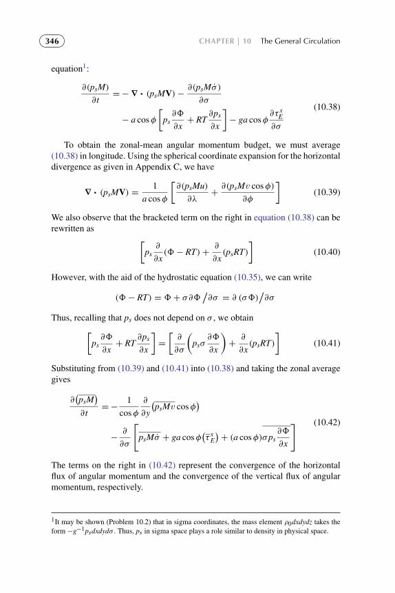
To protect the rights of the author(s) and publisher we inform you that this PDF is an uncorrected proof for internal businessuse only by the author(s), editor(s), reviewer(s), Elsevier and typesetter diacriTech. It is not allowed to publish this proofonline or in print. This proof copy is the copyright property of the publisher and is confidential until formal publication.
“Hakim: 14-ch10-325-376-9780123848666” — 2012/7/26 — 12:09 — page 346 — #22
346 CHAPTER | 10 The General Circulation
equation1:
∂(psM)
∂t=−∇ · (psMV)−
∂(psMσ )
∂σ
− a cosφ
[ps∂8
∂x+ RT
∂ps
∂x
]− ga cosφ
∂τ xE
∂σ
(10.38)
To obtain the zonal-mean angular momentum budget, we must average(10.38) in longitude. Using the spherical coordinate expansion for the horizontaldivergence as given in Appendix C, we have
∇ · (psMV) =1
a cosφ
[∂(psMu)
∂λ+∂(psMv cosφ)
∂φ
](10.39)
We also observe that the bracketed term on the right in equation (10.38) can berewritten as [
ps∂
∂x(8− RT)+
∂
∂x(psRT)
](10.40)
However, with the aid of the hydrostatic equation (10.35), we can write
(8− RT) = 8+ σ∂8/∂σ = ∂ (σ8)
/∂σ
Thus, recalling that ps does not depend on σ , we obtain[ps∂8
∂x+ RT
∂ps
∂x
]=
[∂
∂σ
(psσ
∂8
∂x
)+∂
∂x(psRT)
](10.41)
Substituting from (10.39) and (10.41) into (10.38) and taking the zonal averagegives
∂(psM
)∂t
=−1
cosφ
∂
∂y
(psMv cosφ
)−∂
∂σ
[psMσ + ga cosφ
(τ x
E
)+ (a cosφ)σps
∂8
∂x
] (10.42)
The terms on the right in (10.42) represent the convergence of the horizontalflux of angular momentum and the convergence of the vertical flux of angularmomentum, respectively.
1It may be shown (Problem 10.2) that in sigma coordinates, the mass element ρ0dxdydz takes theform −g−1psdxdydσ . Thus, ps in sigma space plays a role similar to density in physical space.

To protect the rights of the author(s) and publisher we inform you that this PDF is an uncorrected proof for internal businessuse only by the author(s), editor(s), reviewer(s), Elsevier and typesetter diacriTech. It is not allowed to publish this proofonline or in print. This proof copy is the copyright property of the publisher and is confidential until formal publication.
“Hakim: 14-ch10-325-376-9780123848666” — 2012/7/26 — 12:09 — page 347 — #23
10.3 | The Angular Momentum Budget 347
Integrating (10.42) vertically from Earth’s surface (σ = 1) to the top of theatmosphere (σ = 0), and recalling that σ = 0 for σ = 0, 1, we have
1∫0
g−1 ∂
∂tpsMdσ =− (g cosφ)−1
1∫0
∂
∂y
(psMv cosφ
)dσ
−a cosφ[(τ x
E
)σ=1+ ps∂h/∂x
] (10.43)
where h(x, y) = g−18(x, y, 1) is the height of the lower boundary (σ = 1), andwe have assumed that the eddy stress vanishes at σ = 0.
Equation (10.43) expresses the angular momentum budget for a zonal ringof air of unit meridional width, extending from the ground to the top of theatmosphere. In the long-term mean the three terms on the right, representingthe convergence of the meridional flux of angular momentum, the torque dueto small-scale turbulent fluxes at the surface, and the surface pressure torque,must balance. In the sigma coordinate system the surface pressure torque takesthe particularly simple form −ps∂h/∂x. Thus, the pressure torque acts to trans-fer angular momentum from the atmosphere to the ground, provided that thesurface pressure and the slope of the ground (∂h/∂x) are correlated positively.Observations indicate that this is generally the case in middle latitudes becausethere is a slight tendency for the surface pressure to be higher on the westernsides of mountains than on the eastern sides (refer to Figure 4.11). In midlati-tudes of the Northern Hemisphere the surface pressure torque provides nearlyone-half of the total atmosphere–surface momentum exchange, but in the trop-ics and the Southern Hemisphere the exchange is dominated by turbulent eddystresses.
The role of eddy motions in providing the meridional angular momentumtransport necessary to balance the surface angular momentum sinks can be elu-cidated best if we divide the flow into zonal-mean and eddy components byletting
M = M +M′ =(�a cosφ + u+ u′
)a cosφ
ps v = ( ps v)+ ( ps v)′
where primes indicate deviations from the zonal-mean. Thus, the meridionalflux becomes
(ps Mv) =[�a cosφps v + ups v + u′(ps v)
′]
a cosφ (10.44)
The three meridional flux terms on the right in this expression are called themeridional �–momentum flux, the meridional drift, and the meridional eddymomentum flux, respectively.

To protect the rights of the author(s) and publisher we inform you that this PDF is an uncorrected proof for internal businessuse only by the author(s), editor(s), reviewer(s), Elsevier and typesetter diacriTech. It is not allowed to publish this proofonline or in print. This proof copy is the copyright property of the publisher and is confidential until formal publication.
“Hakim: 14-ch10-325-376-9780123848666” — 2012/7/26 — 12:09 — page 348 — #24
348 CHAPTER | 10 The General Circulation
The drift term is important in the tropics, but in midlatitudes it is smallcompared to the eddy flux and can be neglected in an approximate treatment.Furthermore, we can show that the meridional �–momentum flux does notcontribute to the vertically integrated flux. Averaging the continuity equation(10.34) zonally and integrating vertically, we obtain
∂ps
∂t= −(cosφ)−1 ∂
∂y
1∫0
psv cosφdσ (10.45)
Thus, for time-averaged flow—where the left side of (10.45) vanishes—thereis no net mass flow across latitude circles. The vertically integrated meridionalangular momentum flux is therefore given approximately by
1∫0
psMvdσ ≈
1∫0
u′( psv)′a cosφdσ ≈
1∫0
a cosφpsu′v′dσ (10.46)
where we have assumed that the fractional change in ps is small compared tothe change in v′ so that (psv)
′≈ psv
′. The angular momentum flux is thusproportional to the negative of the meridional component of the EP flux givenin (10.20).
In the Northern Hemisphere, as shown in Figure 10.6, the eddy momen-tum flux in midlatitudes is positive and decreases in magnitude with latitudepoleward of 30◦. For quasi-geostrophic flow, positive eddy momentum fluxrequires that the eddies be asymmetric in the horizontal plane, with the troughand ridge axes tilting as indicated in Figure 10.12. When the troughs and ridgeson the average have southwest to northeast phase tilt, the zonal flow will belarger than average (u′ > 0) where the meridional flow is poleward (v′ > 0)and less than average (u′ < 0) where the flow is equatorward. Thus, u′v′ > 0,and the eddies will systematically transport positive zonal momentum poleward.
As shown in (10.42), the total vertical momentum flux consists of the fluxdue to large-scale motions psMσ ≈ �a cosφpsσ ; the flux due to the pressure
Trou
gh
Rid
ge
y
x
FIGURE 10.12 Schematic streamlines for a positive eddy momentum flux.

To protect the rights of the author(s) and publisher we inform you that this PDF is an uncorrected proof for internal businessuse only by the author(s), editor(s), reviewer(s), Elsevier and typesetter diacriTech. It is not allowed to publish this proofonline or in print. This proof copy is the copyright property of the publisher and is confidential until formal publication.
“Hakim: 14-ch10-325-376-9780123848666” — 2012/7/26 — 12:09 — page 349 — #25
10.4 | The Lorenz Energy Cycle 349
8
4
0
–4
–8
80°S 60 40 20 0 20 40 60 80°N
FIGURE 10.13 Latitudinal profile of the annual mean eastward torque (surface friction plusmountain torque) exerted on the atmosphere in units of 1018 m2 kg s−2. (Adapted from Oort andPeixoto, 1983.)
torque, (a cosφ)σps∂8/∂x ; and the flux due to small-scale turbulent stresses,
ga cosφτ xE. As mentioned previously, the last two are responsible for the trans-
fer of momentum from Earth to the atmosphere in the tropics and from theatmosphere to Earth in midlatitudes. Outside the planetary boundary layer, how-ever, the vertical momentum transport in the troposphere is due primarily to thevertical �–momentum flux, �a cosφpsσ .
An estimate of the annual average of the zonal-mean total surface torque isshown in Figure 10.13. The total surface torque must be balanced by polewardfluxes of angular momentum in the atmosphere. Except for the belt within 10◦
of the equator, almost all of the poleward flux is accounted for by the eddy fluxterm given on the right side of (10.46). Thus, the momentum budget and theenergy cycle both depend critically on the transports by the eddies.
10.4 THE LORENZ ENERGY CYCLE
The previous section discussed the interaction between zonally averaged flowand longitudinally varying eddy motions in terms of the angular momen-tum balance. It is also useful to examine the exchange of energy betweenthe eddies and the mean flow. As in Section 10.2, we limit the analysis toquasi-geostrophic flow on a midlatitude β plane. Eulerian mean equations inlog-pressure coordinates can then be written as
∂u/∂t − f0v = −∂(
u′v′)/∂y+ X (10.47)
f0u = −∂8/∂y (10.48)

To protect the rights of the author(s) and publisher we inform you that this PDF is an uncorrected proof for internal businessuse only by the author(s), editor(s), reviewer(s), Elsevier and typesetter diacriTech. It is not allowed to publish this proofonline or in print. This proof copy is the copyright property of the publisher and is confidential until formal publication.
“Hakim: 14-ch10-325-376-9780123848666” — 2012/7/26 — 12:09 — page 350 — #26
350 CHAPTER | 10 The General Circulation
∂
∂t
(∂8
∂z
)+ wN2
=κ
HJ −
∂
∂y
(v′∂8′
∂z
)(10.49)
∂v/∂y+ ρ−10 ∂(ρ0w)/∂z = 0 (10.50)
Here we have used the hydrostatic approximation in (10.3) to express the tem-perature in (10.49) in terms of the differential geopotential thickness, and wehave again neglected vertical eddy fluxes and advection by the mean meridionalcirculation in (10.47) and (10.49). We have, however, included a turbulent dragforce, X, in (10.47), as dissipation by unresolved turbulent eddies is an essentialelement in the energy balance.
To analyze the exchange of energy between mean flow and eddies, werequire a similar set of dynamical equations for the eddy motion. For simplicity,assume that the eddies satisfy the following linearized set of equations2:(
∂
∂t+ u
∂
∂x
)u′ −
(f0 −
∂u
∂y
)v′ = −
∂8′
∂x+ X′ (10.51)
(∂
∂t+ u
∂
∂x
)v′ + f0u′ = −
∂8′
∂y+ Y ′ (10.52)
(∂
∂t+ u
∂
∂x
)∂8′
∂z+ v′
∂
∂y
(∂8
∂z
)+ N2w′ =
κJ′
H(10.53)
∂u′
∂x+∂v′
∂y+
1
ρ0
∂(ρ0w′
)∂z
= 0 (10.54)
where X′ and Y ′ are the zonally varying components of drag as a result ofunresolved turbulent motions.
We now define a global average:
〈 〉 ≡ A−1
∞∫0
D∫0
L∫0
( )dxdydz
where L is the distance around a latitude circle, D is the meridional extent of themidlatitude β plane, and A designates the total horizontal area of the β plane.
2A similar analysis can be carried out for the nonlinear case.

To protect the rights of the author(s) and publisher we inform you that this PDF is an uncorrected proof for internal businessuse only by the author(s), editor(s), reviewer(s), Elsevier and typesetter diacriTech. It is not allowed to publish this proofonline or in print. This proof copy is the copyright property of the publisher and is confidential until formal publication.
“Hakim: 14-ch10-325-376-9780123848666” — 2012/7/26 — 12:09 — page 351 — #27
10.4 | The Lorenz Energy Cycle 351
Then for any quantity 9
〈∂9/∂x〉 = 0
〈∂9/∂y〉 = 0, if 9 vanishes at y = ±D
〈∂9/∂z〉 = 0, if 9 vanishes at z = 0 and z→∞
An equation for the evolution of the mean flow kinetic energy can thenbe obtained by multiplying (10.47) by ρ0u and (10.48) by ρ0ν and adding theresults to get
ρ0∂
∂t
(u2
2
)= −ρ0v
∂8
∂y− ρ0u
∂
∂y
(u′v′
)+ ρ0uX
= −∂
∂y
(ρ0v8
)+ ρ08
∂v
∂y−∂
∂y
(ρ0uu′v′
)+ ρ0u′v′
∂u
∂y+ ρ0uX
Integrating over the entire volume, we get
d
dt
⟨ρ0u2
2
⟩= +
⟨ρ08
∂v
∂y
⟩+
⟨ρ0u′v′
∂u
∂y
⟩+⟨ρ0uX
⟩(10.55)
where we have assumed that v = 0 and u′v′ = 0 for y = ±D. Terms on the rightside in (10.55) can be interpreted as the work done by the zonal-mean pressureforce, the conversion of eddy kinetic energy to zonal-mean kinetic energy, anddissipation by the zonal-mean eddy stress. Alternatively, the first term on theright can be rewritten with the aid of the continuity equation to yield⟨
ρ08∂v
∂y
⟩= −
⟨8∂ρ0w
∂z
⟩=
⟨ρ0w
∂8
∂z
⟩=
R
H
⟨ρ0wT
⟩where we have assumed that ρ0w = 0 at z = 0, and z → ∞. Thus, averagedover the whole domain the pressure work term is proportional to the correlationbetween the zonal-mean vertical mass flux ρ0w and the zonal-mean temperature(or thickness). This term will be positive if on the average warm air is risingand cold air is sinking—that is, if there is a conversion from potential to kineticenergy.
Section 7.3.1 showed that in the quasi-geostrophic system the availablepotential energy is proportional to the square of the deviation of temperaturefrom a standard atmosphere profile divided by the static stability. In terms ofdifferential thickness the zonal-mean available potential energy is defined as
P ≡1
2
⟨ρ0
N2
(∂8
∂z
)2⟩

To protect the rights of the author(s) and publisher we inform you that this PDF is an uncorrected proof for internal businessuse only by the author(s), editor(s), reviewer(s), Elsevier and typesetter diacriTech. It is not allowed to publish this proofonline or in print. This proof copy is the copyright property of the publisher and is confidential until formal publication.
“Hakim: 14-ch10-325-376-9780123848666” — 2012/7/26 — 12:09 — page 352 — #28
352 CHAPTER | 10 The General Circulation
Multiplying (10.49) through by ρ0(∂8/∂z)/N2 and averaging over space gives
d
dt
⟨ρ0
2N2
(∂8
∂z
)2⟩=−
⟨ρ0w
∂8
∂z
⟩+
⟨ρ0κ J
N2H
(∂8
∂z
)⟩
−
⟨ρ0
N2
∂8
∂z
∂
∂y
(v′∂8′
∂z
)⟩ (10.56)
The first term on the right is just equal and opposite to the first term on the rightin (10.55), which confirms that this term represents a conversion between zonal-mean kinetic and potential energies. The second term involves the correlationbetween temperature and diabatic heating; it expresses the generation of zonal-mean potential energy by diabatic processes. The final term, which involves themeridional eddy heat flux, expresses the conversion between zonal-mean andeddy potential energy.
That the second term on the right in (10.55) and the final term in (10.56)represent conversion between zonal-mean and eddy energies can be confirmedby performing analogous operations on the eddy equations (10.51), (10.52),and (10.53) to obtain equations for the eddy kinetic and available potentialenergies:
d
dt
⟨ρ0
u′2 + v′2
2
⟩=+
⟨ρ08′
(∂u′
∂x+∂v′
∂y
)⟩
−
⟨ρ0u′v′
∂u
∂y
⟩+
⟨ρ0
(u′X′ + v′Y ′
)⟩ (10.57)
d
dt
⟨ρ0
2N2
(∂8′
∂z
)2⟩=−
⟨ρ0w′
∂8′
∂z
⟩+
⟨ρ0κJ′∂8′
/∂z
N2H
⟩
−
⟨ρ0
N2
(∂28
∂z∂y
)(v′∂8′
∂z
)⟩ (10.58)
If we set w′ = 0 at z = 0, the first term on the right in (10.57) can be rewrittenusing the continuity equation (10.54) as⟨
ρ08′(∂u′
∂x+∂v′
∂y
)⟩= −
⟨8′∂(ρ0w′)
∂z
⟩=
⟨ρ0w′
(∂8′
∂z
)⟩
which is equal to minus the first term on the right in (10.58). Thus, this termexpresses the conversion between eddy kinetic and eddy potential energy forthe Eulerian mean formulation. Similarly, the last term in (10.58) is equal to

To protect the rights of the author(s) and publisher we inform you that this PDF is an uncorrected proof for internal businessuse only by the author(s), editor(s), reviewer(s), Elsevier and typesetter diacriTech. It is not allowed to publish this proofonline or in print. This proof copy is the copyright property of the publisher and is confidential until formal publication.
“Hakim: 14-ch10-325-376-9780123848666” — 2012/7/26 — 12:09 — page 353 — #29
10.4 | The Lorenz Energy Cycle 353
minus the last term in (10.56) and thus represents conversion between eddy andzonal-mean available potential energy.
The Lorenz energy cycle can be expressed compactly by defining zonal-mean and eddy kinetic and available potential energies:
K ≡
⟨ρ0
u2
2
⟩, K′ ≡
⟨ρ0
u′2 + v′2
2
⟩
P ≡1
2
⟨ρ0
N2
(∂8
∂z
)2⟩, P′ ≡
1
2
⟨ρ0
N2
(∂8′
∂z
)2⟩
the energy transformations
[P ·K
]≡
⟨ρ0w
∂8
∂z
⟩,
[P′ ·K′
]≡
⟨ρ0w′
∂8′
∂z
⟩
[K′ ·K
]≡
⟨ρ0u′v′
∂u
∂y
⟩,
[P′ ·P
]≡
⟨ρ0
N2v′∂8′
∂z
∂28
∂y∂z
⟩and the sources and sinks
R ≡
⟨ρ0
N2
κJ
H
∂8
∂z
⟩, R′ ≡
⟨ρ0
N2
κJ′
H
∂8′
∂z
⟩
ε ≡⟨ρ0uX
⟩, ε′ ≡
⟨ρ0
(u′X′ + v′Y ′
)⟩Equations (10.55) through (10.58) can then be expressed in the simple form
dK/dt =[P ·K
]+[K′ ·K
]+ ε (10.59)
dP/dt = −[P ·K
]+[P′ ·P
]+ R (10.60)
dK′/dt =[P′ ·K′
]−[K′ ·K
]+ ε′ (10.61)
dP′/dt = −[P′ ·K′
]−[P′ ·P
]+ R′ (10.62)
Here [A ·B] designates conversion from energy form A to form B.Adding (10.59) through (10.62), we obtain an equation for the rate of change
of total energy (kinetic plus available potential):
d(K + K′ + P+ P′
)/dt = R+ R′ + ε + ε′ (10.63)
For adiabatic inviscid flow, the right side vanishes and the total energy K +K′ + P + P′ is conserved. In this system the zonal-mean kinetic energy doesnot include a contribution from the mean meridional flow because the zon-ally averaged meridional momentum equation was replaced by the geostrophic
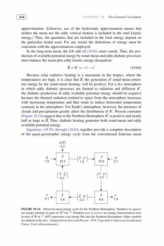
To protect the rights of the author(s) and publisher we inform you that this PDF is an uncorrected proof for internal businessuse only by the author(s), editor(s), reviewer(s), Elsevier and typesetter diacriTech. It is not allowed to publish this proofonline or in print. This proof copy is the copyright property of the publisher and is confidential until formal publication.
“Hakim: 14-ch10-325-376-9780123848666” — 2012/7/26 — 12:09 — page 354 — #30
354 CHAPTER | 10 The General Circulation
approximation. (Likewise, use of the hydrostatic approximation means thatneither the mean nor the eddy vertical motion is included in the total kineticenergy.) Thus, the quantities that are included in the total energy depend onthe particular model used. For any model the definitions of energy must beconsistent with the approximations employed.
In the long-term mean, the left side of (10.63) must vanish. Thus, the pro-duction of available potential energy by zonal-mean and eddy diabatic processesmust balance the mean plus eddy kinetic energy dissipation:
R+ R′ = −ε − ε′ (10.64)
Because solar radiative heating is a maximum in the tropics, where thetemperatures are high, it is clear that R, the generation of zonal-mean poten-tial energy by the zonal-mean heating, will be positive. For a dry atmospherein which eddy diabatic processes are limited to radiation and diffusion R′,the diabatic production of eddy available potential energy should be negativebecause the thermal radiation emitted to space from the atmosphere increaseswith increasing temperature and thus tends to reduce horizontal temperaturecontrasts in the atmosphere. For Earth’s atmosphere, however, the presence ofclouds and precipitation greatly alters the distribution of R′. Present estimates(Figure 10.14) suggest that in the Northern Hemisphere R′ is positive and nearlyhalf as large as R. Thus, diabatic heating generates both zonal-mean and eddyavailable potential energy.
Equations (10.59) through (10.62) together provide a complete descriptionof the quasi-geostrophic energy cycle from the conventional Eulerian mean
1.5
−0.2
−0.3
0.2B (P)
1.5R P · P ′
2.2P ′· K′
8.8
K′
15.6
P ′0.7R′
1.9′
0.1
P · K
K · K′
33.5
P
3.6
K
}}
}}}}
}}ε ε
FIGURE 10.14 Observed mean energy cycle for the Northern Hemisphere. Numbers in squaresare energy amounts in units of 105 J m−2. Numbers next to arrows are energy transformation ratesin units of W m−2. B(P) represents a net energy flux into the Southern Hemisphere. Other symbolsare defined in the text. (Adapted from Oort and Peixoto, 1974. Copyright © American GeophysicalUnion. Used with permission.)

To protect the rights of the author(s) and publisher we inform you that this PDF is an uncorrected proof for internal businessuse only by the author(s), editor(s), reviewer(s), Elsevier and typesetter diacriTech. It is not allowed to publish this proofonline or in print. This proof copy is the copyright property of the publisher and is confidential until formal publication.
“Hakim: 14-ch10-325-376-9780123848666” — 2012/7/26 — 12:09 — page 355 — #31
10.4 | The Lorenz Energy Cycle 355
point of view. The content of these equations is summarized by means of thefour-box diagram in Figure 10.14. In this diagram the squares represent reser-voirs of energy, and the arrows indicate sources, sinks, and conversions. Theobserved direction of the conversion terms in the troposphere for the North-ern Hemisphere annual mean is indicated by arrows. It should be emphasizedthat the direction of the various conversions cannot be theoretically deduced byreference to the energy equations alone. It also should be emphasized that theconversion terms given here are a result of the particular type of zonal averagemodel used. The analogous energy equations for the TEM equations have ratherdifferent conversions. Thus, the energy transformations given in the presentanalysis should not be regarded as fundamental properties of the atmospherebut rather as properties of the Eulerian mean system.
Nevertheless, because the conventional Eulerian mean model is generallyused as a basis for the study of baroclinic waves, the four-box energy diagrampresented here does provide a useful framework for considering the role ofweather disturbances in maintenance of the general circulation. The observedenergy cycle as summarized in Figure 10.14 suggests the following qualitativepicture:
1. The zonal-mean diabatic heating generates mean zonal available potentialenergy through a net heating of the tropics and cooling of the polar regions.
2. Baroclinic eddies transport warm air poleward and cold air equatorward, andtransform the mean available potential energy to eddy available potentialenergy.
3. At the same time, eddy available potential energy is transformed into eddykinetic energy by the vertical motions in the eddies.
4. The zonal kinetic energy is maintained primarily by the conversions fromeddy kinetic energy due to the correlation u′v′. This is discussed further inthe next section.
5. The energy is dissipated by surface and internal friction in the eddies andmean flow.
In summary, the observed atmospheric energy cycle as given by the Eule-rian mean formulation is consistent with the notion that baroclinically unstableeddies are the primary disturbances responsible for the energy exchange in mid-latitudes. It is through the eddy motions that the kinetic energy lost throughturbulent stresses is replaced, and it is the eddies that are primarily responsi-ble for the poleward heat transport to balance the radiation deficit in the polarregions. In addition to transient baroclinic eddies, forced stationary orographicwaves and free Rossby waves may also contribute substantially to the polewardheat flux. The direct conversion of mean available potential energy to meankinetic energy by symmetric overturning is, however, small and negative in themiddle latitudes but positive in the tropics, where it plays an important role inthe maintenance of the mean Hadley circulation.

To protect the rights of the author(s) and publisher we inform you that this PDF is an uncorrected proof for internal businessuse only by the author(s), editor(s), reviewer(s), Elsevier and typesetter diacriTech. It is not allowed to publish this proofonline or in print. This proof copy is the copyright property of the publisher and is confidential until formal publication.
“Hakim: 14-ch10-325-376-9780123848666” — 2012/7/26 — 12:09 — page 356 — #32
356 CHAPTER | 10 The General Circulation
10.5 LONGITUDINALLY DEPENDENT TIME-AVERAGEDFLOW
So far in this chapter we have concentrated on the zonally averaged componentof the general circulation. For a planet with a longitudinally uniform surface,the flow averaged over a season should be completely characterized by the zon-ally averaged component of the circulation, since for such a hypothetical planetthe statistics of zonally asymmetric transient eddies (i.e., weather disturbances)should be independent of longitude. On Earth, however, large-scale topographyand continent–ocean heating contrasts provide strong forcing for longitudinallyasymmetric planetary-scale time mean motions. Such motions, usually referredto as stationary waves, are especially strong in the Northern Hemisphere duringthe winter season.
Observations indicate that tropospheric stationary waves generally tendto have an equivalent barotropic structure; that is, wave amplitude generallyincreases with height, but phase lines tend to be vertical. Although nonlinearprocesses may be significant in the formation and maintenance of stationarywaves, the climatological stationary wave pattern can to a first approximationbe described in terms of forced barotropic Rossby waves. When superposedon zonal-mean circulation, such waves produce local regions of enhanced anddiminished time mean westerly winds, which strongly influence the develop-ment and propagation of transient weather disturbances. They thus representessential features of the climatological flow.
10.5.1 Stationary Rossby Waves
The most significant of the time mean zonally asymmetric circulation featuresis the pattern of stationary planetary waves excited in the Northern Hemisphereby the flow over the Himalayas and the Rockies. It was shown in Section 5.7.2that the quasi-stationary wave pattern along 45◦ latitude could be accountedfor to a first approximation as the forced wave response when mean westerliesimpinge on the large-scale topography. More detailed analysis suggests that zon-ally asymmetric heat sources also contribute to the forcing of the climatologicalstationary wave pattern. Some controversy remains, however, concerning therelative importance of heating and orography in forcing the observed stationarywave pattern. The two processes are difficult to separate because the pattern ofdiabatic heating is influenced by orography.
The discussion of topographic Rossby waves in Section 5.7.2 used a β-planechannel model in which it was assumed that wave propagation was parallel tolatitude circles. In reality, however, large-scale topographic features and heatsources are confined in latitude as well as longitude, and the stationary wavesexcited by such forcing may propagate energy meridionally as well as zonally.For a quantitatively accurate analysis of the barotropic Rossby wave responseto a local source, it is necessary to use the barotropic vorticity equation in

To protect the rights of the author(s) and publisher we inform you that this PDF is an uncorrected proof for internal businessuse only by the author(s), editor(s), reviewer(s), Elsevier and typesetter diacriTech. It is not allowed to publish this proofonline or in print. This proof copy is the copyright property of the publisher and is confidential until formal publication.
“Hakim: 14-ch10-325-376-9780123848666” — 2012/7/26 — 12:09 — page 357 — #33
10.5 | Longitudinally Dependent Time-Averaged Flow 357
spherical coordinates and to include the latitudinal dependence of the meanzonal wind. The mathematical analysis for such a situation is beyond the scopeof this book. It is possible, however, to obtain a qualitative notion of the natureof the wave propagation for this case by generalizing the β-plane analysis ofSection 5.7. Thus, rather than assuming that propagation is limited to a chan-nel of specified width, we assume that the β plane extends to plus and minusinfinity in the meridional direction and that Rossby waves can propagate bothnorthward and southward without reflection from artificial walls.
The free barotropic Rossby wave solution then has the form of (5.109) andsatisfies the dispersion relation of (5.110), where l is the meridional wave num-ber, which is now allowed to vary. From (5.112) it is clear that for a specifiedzonal wave number, k, the free solution is stationary for l given by
l2 = β/u− k2 (10.65)
Thus, for example, westerly flow over an isolated mountain that primarilyexcites a response at a given k will produce stationary waves with both positiveand negative l satisfying (10.65). As remarked in Section 5.7.1, although Rossbywave phase propagation relative to the mean wind is always westward, this isnot true of the group velocity. From (5.110) we readily find that the x and ycomponents of group velocity are
cgx =∂ν
∂k= u+ β
(k2− l2
)(k2 + l2
)2 (10.66)
cgy =∂ν
∂l=
2βkl(k2 + l2
)2 (10.67)
For stationary waves, these may be expressed alternatively with the aid ofequation (10.65) as
cgx =2uk2(
k2 + l2) , cgy =
2ukl(k2 + l2
) (10.68)
The group velocity vector for stationary Rossby waves is perpendicular tothe wave crests. It always has an eastward zonal component and a northwardor southward meridional component depending on whether l is positive ornegative. The magnitude is given by∣∣cg
∣∣ = 2u cosα (10.69)
(see Problem 10.9). Here, as shown in Figure 10.15 for the case of positive l, αis the angle between lines of constant phase and the y axis.
Because energy propagates at the group velocity, (10.68) indicates that thestationary wave response to a localized topographic feature should consist oftwo wave trains, one with l > 0 extending eastward and northward and the other

To protect the rights of the author(s) and publisher we inform you that this PDF is an uncorrected proof for internal businessuse only by the author(s), editor(s), reviewer(s), Elsevier and typesetter diacriTech. It is not allowed to publish this proofonline or in print. This proof copy is the copyright property of the publisher and is confidential until formal publication.
“Hakim: 14-ch10-325-376-9780123848666” — 2012/7/26 — 12:09 — page 358 — #34
358 CHAPTER | 10 The General Circulation
cg
x
y
2π /K s
α
FIGURE 10.15 Stationary plane Rossby wave in a westerly flow. Ridges (solid lines) and troughs(dashed lines) are oriented at an angle α to the y axis; the group velocity relative to the ground, cg,is oriented at an angle α to the x axis. The wavelength is 2 π/Ks. (Adapted from Hoskins, 1983.)
FIGURE 10.16 Vorticity pattern generated on a sphere when a constant angular velocity westerlyflow impinges on a circular forcing centered at 30◦N and 45◦W of the central point. Left to right,the response at 2, 4, and 6 days after the forcing is switched on. Five contour intervals correspondto the maximum vorticity response that would occur in 1 day if there were no wave propagation.Heavy lines correspond to zero contours. The pattern is drawn on a projection in which the sphereis viewed from infinity. (After Hoskins, 1983.)
with l< 0 extending eastward and southward. An example computed usingspherical geometry is given in Figure 10.16. Although the positions of indi-vidual troughs and ridges remain fixed for stationary waves, the wave trains inthis example do not decay in time, as the effects of dissipation are counteractedby energy propagation from the source at the Rossby wave group velocity.
For the climatological stationary wave distribution in the atmosphere, theexcitation comes from a number of sources, both topographic and thermal, dis-tributed around the globe. Thus, it is not easy to trace out distinct paths ofwave propagation. Nevertheless, detailed calculations using spherical geome-try suggest that two-dimensional barotropic Rossby wave propagation providesa reasonable first approximation for the observed departure of the extratropicaltime mean flow from zonal symmetry.
Rossby waves excited by isolated orographic features also play a significantrole in the momentum budget. Letting the amplitude coefficient 9 be real in

To protect the rights of the author(s) and publisher we inform you that this PDF is an uncorrected proof for internal businessuse only by the author(s), editor(s), reviewer(s), Elsevier and typesetter diacriTech. It is not allowed to publish this proofonline or in print. This proof copy is the copyright property of the publisher and is confidential until formal publication.
“Hakim: 14-ch10-325-376-9780123848666” — 2012/7/26 — 12:09 — page 359 — #35
10.5 | Longitudinally Dependent Time-Averaged Flow 359
(5.109), the meridional momentum flux can be expressed as
u′v′ = −(∂ψ ′/∂x) (∂ψ ′/∂y) = −92kl/2
From (10.68) it is then verified readily that if u > 0,
cgy > 0 implies u′v′ < 0
cgy < 0 implies u′v′ > 0
Thus, westerly momentum converges into the wave source region (where theenergy flux is divergent). This eddy momentum flux convergence is neces-sary to balance the momentum lost to the surface through the pressure torquemechanism discussed in Section 10.3.
10.5.2 Jet Stream and Storm Tracks
When the longitudinally asymmetric geopotential anomalies associated withstationary waves are added to the zonal-mean geopotential distribution, theresulting time mean field includes local regions of enhanced meridional geopo-tential gradient that are manifested in the wind field of the Northern Hemisphereby the Asian and North American jetstreams. The existence of these two jets canbe inferred from the January mean 500-hPa geopotential height field shown inFigure 6.3. Note the strong meridional gradients in height associated with thetroughs centered just east of the Asian and North American continents (the samefeatures can be seen in annual mean charts, although with somewhat reducedintensity). The zonal flow associated with these semipermanent troughs is illus-trated in Figure 6.2. In addition to the two intense jet cores in the western Pacificand western Atlantic, there is a third weaker jet centered over North Africa andthe Middle East. Figure 6.2 shows dramatically the large deviations from zonalsymmetry in the jet stream structure. In midlatitudes the zonal wind speed variesby nearly a factor of three between the core of the Asian jet and the area of lowwind speed in western North America.
Although, as was argued earlier, the climatological stationary wave distribu-tion on which the Asian and North American jets are superposed is apparentlyforced primarily by orography, the structure of the jets also appears to be influ-enced by continent–ocean heating contrasts. Thus, the strong vertical shear inAsian and North American jets reflects a thermal wind balance consistent withthe very strong meridional temperature gradients that occur in winter near theeastern edges of the Asian and North American continents due to the con-trast between warm water to the southeast and cold land to the northwest.A satisfactory description of the jet streams must account, however, not onlyfor their thermal structure but for the westerly acceleration that air parcels mustexperience as they enter the jet and the deceleration as they leave the jet core.
To understand the quasi-geostrophic momentum budget in the jet streamsand its relationship to the observed distribution of weather, we consider the

To protect the rights of the author(s) and publisher we inform you that this PDF is an uncorrected proof for internal businessuse only by the author(s), editor(s), reviewer(s), Elsevier and typesetter diacriTech. It is not allowed to publish this proofonline or in print. This proof copy is the copyright property of the publisher and is confidential until formal publication.
“Hakim: 14-ch10-325-376-9780123848666” — 2012/7/26 — 12:09 — page 360 — #36
360 CHAPTER | 10 The General Circulation
zonal component of the momentum equation, which (if we neglect the β effect)may be written in the form of
Dgug
Dt= f0
(v − vg
)≡ f0va (10.70)
where va is the meridional component of the ageostrophic wind. This equationindicates that the westerly acceleration (Dug/Dt)> 0) that air parcels experi-ence as they enter the jet can only be provided by a poleward ageostrophicwind component (va>0); conversely, the easterly acceleration that air parcelsexperience as they leave the jet requires an equatorward ageostrophic motion.This meridional flow, together with its accompanying vertical circulation, isillustrated in Figure 10.17. Note that this secondary circulation is thermallydirect upstream of the jet core. A magnitude of va ∼ 2−3 m s−1 is required
Pre
ssur
e (h
Pa)
Pre
ssur
e (h
Pa)
Lowersea-level pressure Weak surface winds
Cold
Highersea-level pressure
300
500
1000
J
(a)
300
500
1000
(b)
Strong eddyheat flux
Subtropical highs Strong westerly surface winds Oceanic
lows
30 40 50 60
Latitude
Strong convergenceof eddy flux of
westerly momentum
J
Cool
FIGURE 10.17 Meridional cross-sections showing the relationship between the time mean sec-ondary meridional circulation (continuous thin lines with arrows) and the jet stream (“J”) atlocations (a) upstream and (b) downstream from the jet stream cores. (After Blackmon et al., 1977.Copyright © American Meteorological Society. Reprinted with permission.)

To protect the rights of the author(s) and publisher we inform you that this PDF is an uncorrected proof for internal businessuse only by the author(s), editor(s), reviewer(s), Elsevier and typesetter diacriTech. It is not allowed to publish this proofonline or in print. This proof copy is the copyright property of the publisher and is confidential until formal publication.
“Hakim: 14-ch10-325-376-9780123848666” — 2012/7/26 — 12:09 — page 361 — #37
10.6 | Low-Frequency Variability 361
to account for the observed zonal wind acceleration. This is an order of mag-nitude stronger than the zonal-mean indirect cell (Ferrel cell) that prevails inmidlatitudes. Downstream of the jet core, however, the secondary circulation isthermally indirect but much stronger than the zonally averaged Ferrel cell. Itis interesting to note that the vertical motion pattern on the poleward (cyclonicshear) side of the jet is similar to that associated with deep transient barocliniceddies in the sense that subsidence occurs to the west of the stationary troughassociated with the jet, and ascent occurs east of the trough (e.g., Figure 6.18).
Because the growth rate of baroclinically unstable synoptic-scale distur-bances is proportional to the strength of the basic state thermal wind, it is notsurprising that the Pacific and Atlantic jet streams are important source regionsfor storm development. Typically, transient baroclinic waves develop in the jetentrance region, grow as they are advected downstream, and decay in the jetexit region. The role of these transient eddies in maintenance of the jet streamstructure is rather complex. Transient eddy heat fluxes, which are strong andpoleward in the storm tracks, appear to act to weaken the climatological jets.The transient eddy vorticity flux in the upper troposphere, however, appears toact to maintain the jet structure. In both cases the secondary ageostrophic circu-lation associated with the jet tends to partly balance the influence of the transienteddy fluxes in order to maintain the mean thermal and momentum balances.
10.6 LOW-FREQUENCY VARIABILITY
An understanding of the general circulation requires consideration not only ofthe zonal-mean and stationary wave components and their variations with theannual cycle, but also of irregular variability on time scales longer than that ofindividual transient eddies. The term low-frequency variability is generally usedto describe such components of the general circulation. The observed spectrumof low-frequency variability ranges from weather anomalies lasting only 7 to 10days to interannual variability on the scale of several years (see Section 11.1.6).
One possible cause of atmospheric low-frequency variability is forcing dueto anomalies in sea surface temperature (SST), which themselves arise fromcoherent air–sea interaction. Because of the large thermal inertia of the oceanicsurface mixed layer, such anomalies tend to have time scales much longer thanthose associated with subseasonal variations in the atmosphere; they are thoughtto be of greatest significance on the seasonal and interannual time scales.
It is believed, however, that substantial variability on subseasonal timescales can arise in midlatitudes in the absence of anomalous SST forcing asa result of internal nonlinear atmospheric dynamics, although SST anomaliesmay tend to favor the occurrence of certain types of variations. One exampleof internally generated low-frequency variability is the forcing of large-scaleanomalies by potential vorticity fluxes of high-frequency transient waves. Thisprocess appears to be important in the maintenance of high-amplitude quasi-

To protect the rights of the author(s) and publisher we inform you that this PDF is an uncorrected proof for internal businessuse only by the author(s), editor(s), reviewer(s), Elsevier and typesetter diacriTech. It is not allowed to publish this proofonline or in print. This proof copy is the copyright property of the publisher and is confidential until formal publication.
“Hakim: 14-ch10-325-376-9780123848666” — 2012/7/26 — 12:09 — page 362 — #38
362 CHAPTER | 10 The General Circulation
stationary wave disturbances called blocking patterns. Some types of blockingmay also be related to special nonlinear wave patterns called solitary waves, inwhich damping by Rossby wave dispersion is balanced by intensification due tononlinear advection. Although most internal mechanisms involve nonlinearity,there is some evidence that the longitudinally dependent time mean flow maybe unstable to linear barotropic normal modes that are stationary in space butoscillate in time at low frequencies. Such modes, which are global in scale, maybe responsible for some observed teleconnection patterns.
10.6.1 Climate Regimes
It has long been observed that extratropical circulation appears to alternatebetween a so-called high-index state, corresponding to a circulation with strongzonal flow and weak waves, and a “low-index” state, with weak zonal flowand high-amplitude waves. This behavior suggests that more than one climateregime exists consistent with a given external forcing and that the observed cli-mate may switch back and forth between regimes in a chaotic fashion. Whetherthe high-index and low-index states actually correspond to distinct quasi-stableatmospheric climate regimes is a matter of controversy.
The concept of climate regimes can also be demonstrated in a highly simpli-fied model of the atmosphere developed by Charney and DeVore (1979). Theyexamined the equilibrium mean states that can result when a damped topo-graphic Rossby wave interacts with the zonal-mean flow. Their model is anextension of the topographic Rossby wave analysis given in Section 5.7.2. Inthis model the wave disturbance is governed by (5.118), which is the linearizedform of the barotropic vorticity equation (5.113) with weak damping added. Thezonal-mean flow is governed by the barotropic momentum equation:
∂u
∂t= −D(u)− κ(u− Ue) (10.71)
where the first term on the right designates forcing by interaction between thewaves and the mean flow, and the second term represents a linear relaxationtoward an externally determined basic state flow, Ue.
The zonal mean equation (10.71) can be obtained from (5.113) by dividingthe flow into zonal-mean and eddy parts and taking the zonal average to get
∂
∂t
(−∂u
∂y
)= −
∂
∂y
(v′gζ′g
)−
f0H
∂
∂y
(v′ghT
)which, after integrating in y and adding the external forcing term, yields (10.71)with
D(u) = −v′gζ′g −
(f0/
H)v′ghT (10.72)
As shown in Problem 10.5, the eddy vorticity flux, that is, the first term onthe right in (10.72), is proportional to the divergence of the eddy momentum

To protect the rights of the author(s) and publisher we inform you that this PDF is an uncorrected proof for internal businessuse only by the author(s), editor(s), reviewer(s), Elsevier and typesetter diacriTech. It is not allowed to publish this proofonline or in print. This proof copy is the copyright property of the publisher and is confidential until formal publication.
“Hakim: 14-ch10-325-376-9780123848666” — 2012/7/26 — 12:09 — page 363 — #39
10.6 | Low-Frequency Variability 363
flux. The second term, which is sometimes referred to as the form drag, is theequivalent in the barotropic model of the surface pressure torque term in theangular momentum balance equation (10.43).
If hT and the eddy geostrophic streamfunction are assumed to consist ofsingle harmonic wave components in x and y, as given by (5.115) and (5.116),respectively, the vorticity flux vanishes, and with the aid of (5.119) the formdrag can be expressed as
D(u) = −
(f0H
)v′ghT =
(rK2f 2
0
2uH2
)h2
0 cos2 ly[(K2 − K2
s
)2+ ε2
] (10.73)
where r is the spin-down rate due to boundary layer dissipation, ε is as defined inequation (5.119), and Ks is the resonant stationary Rossby wave number definedin (5.112).
It is clear from (10.73) that the form drag will have a strong maximum whenu = β/K2, as shown schematically in Figure 10.18. The last term on the rightin (10.71), however, will decrease linearly as u increases. Thus, for suitableparameters there will be three values of u (labeled A, B, and C in Figure 10.18)for which the wave drag just balances the external forcing so that steady-statesolutions may exist. By perturbing the solution about the points A, B, and C, itis shown easily (Problem 10.12) that point B corresponds to an unstable equilib-rium, whereas the equilibria at points A and C are stable. Solution A corresponds
A
B
Ue
κUe
C
−κ (u − Ue)
D(u)
u
FIGURE 10.18 Schematic graphical solution for steady-state solutions of the Charney–DeVoremodel. (Adapted from Held, 1983.)

To protect the rights of the author(s) and publisher we inform you that this PDF is an uncorrected proof for internal businessuse only by the author(s), editor(s), reviewer(s), Elsevier and typesetter diacriTech. It is not allowed to publish this proofonline or in print. This proof copy is the copyright property of the publisher and is confidential until formal publication.
“Hakim: 14-ch10-325-376-9780123848666” — 2012/7/26 — 12:09 — page 364 — #40
364 CHAPTER | 10 The General Circulation
to a low-index equilibrium, with high-amplitude waves analogous to a blockingregime. Solution C corresponds to a high-index equilibrium with strong zonalflow and weak waves. Thus, for this very simple model there are two possible“climates” associated with the same forcing.
The Charney–DeVore model is a highly oversimplified model of the atmo-sphere. Models that contain more degrees of freedom do not generally have mul-tiple steady solutions. Rather, there is a tendency for the (unsteady) solutions tocluster about certain climate regimes and to shift between regimes in an unpre-dictable fashion. Such behavior is characteristic of a wide range of nonlineardynamical systems and is popularly known as chaos (see Section 13.7).
10.6.2 Annular Modes
If a second meridional mode is added to the Charney–DeVore model (seeExercise M10.2), oscillatory solutions can be obtained that bear a qualitativeresemblance to the observed leading modes of variability in the extratropicalatmospheric circulation in both hemispheres. These observed modes, referred toas annular modes, are characterized by geopotential anomalies of opposite signsin the polar and midlatitude regions and by corresponding mean zonal windanomalies with opposite signs equatorward and poleward of about 45◦ latitude(Figure 10.19). The annular modes exist year-round in the troposphere, but arestrongest in the winter when they extend well into the stratosphere, especiallyin the Northern Hemisphere. The zonally symmetric mean flow anomalies asso-ciated with the annular modes are apparently maintained by anomalous eddymomentum fluxes, which are themselves influenced by the zonally symmetricflow anomalies.
There is some evidence for downward propagation of the wintertime annu-lar modes, suggesting that circulation changes in the stratosphere may precedeannular mode changes in the troposphere. Dynamical linkages between thestratosphere and the troposphere are discussed further in Chapter 12.
10.6.3 Sea Surface Temperature Anomalies
Sea surface temperature anomalies influence the atmosphere by altering the fluxof latent and sensible heat from the ocean, and thus providing anomalous heat-ing patterns. The efficacy of such anomalies in exciting global-scale responsesdepends on their ability to generate Rossby waves. A thermal anomaly cangenerate a Rossby wave response only by perturbing the vorticity field. Thisrequires that the thermal anomaly produce an anomalous vertical motion field,which in turn produces anomalous vortex tube stretching.
For low-frequency disturbances the thermodynamic energy equation (10.5)may be approximated as
V · ∇T + wN2HR−1≈ J/cp (10.74)
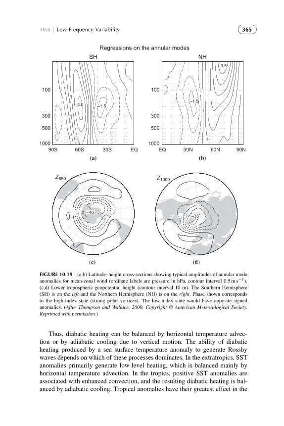
To protect the rights of the author(s) and publisher we inform you that this PDF is an uncorrected proof for internal businessuse only by the author(s), editor(s), reviewer(s), Elsevier and typesetter diacriTech. It is not allowed to publish this proofonline or in print. This proof copy is the copyright property of the publisher and is confidential until formal publication.
“Hakim: 14-ch10-325-376-9780123848666” — 2012/7/26 — 12:09 — page 365 — #41
10.6 | Low-Frequency Variability 365
Regressions on the annular modes
–40
Z850
(c)
–35
Z1000
(d)
SH
–1.53.0
100
500
1000
300
EQ30S60S90S
(a)
NH
3.5
–1.5
100
500
1000
300
EQ 30N 60N 90N
(b)
FIGURE 10.19 (a,b) Latitude–height cross-sections showing typical amplitudes of annular modeanomalies for mean-zonal wind (ordinate labels are pressure in hPa, contour interval 0.5 m s−1).(c,d) Lower tropospheric geopotential height (contour interval 10 m). The Southern Hemisphere(SH) is on the left and the Northern Hemisphere (NH) is on the right. Phase shown correspondsto the high-index state (strong polar vortices). The low-index state would have opposite signedanomalies. (After Thompson and Wallace, 2000. Copyright © American Meteorological Society.Reprinted with permission.)
Thus, diabatic heating can be balanced by horizontal temperature advec-tion or by adiabatic cooling due to vertical motion. The ability of diabaticheating produced by a sea surface temperature anomaly to generate Rossbywaves depends on which of these processes dominates. In the extratropics, SSTanomalies primarily generate low-level heating, which is balanced mainly byhorizontal temperature advection. In the tropics, positive SST anomalies areassociated with enhanced convection, and the resulting diabatic heating is bal-anced by adiabatic cooling. Tropical anomalies have their greatest effect in the

To protect the rights of the author(s) and publisher we inform you that this PDF is an uncorrected proof for internal businessuse only by the author(s), editor(s), reviewer(s), Elsevier and typesetter diacriTech. It is not allowed to publish this proofonline or in print. This proof copy is the copyright property of the publisher and is confidential until formal publication.
“Hakim: 14-ch10-325-376-9780123848666” — 2012/7/26 — 12:09 — page 366 — #42
366 CHAPTER | 10 The General Circulation
Western Pacific, where the average sea surface temperature is very high so thateven a small positive anomaly can generate large increases in evaporation dueto the exponential increase of saturation vapor pressure with temperature. Bycontinuity of mass, the upward motion in cumulonimbus convection requiresconvergence at low levels and divergence in the upper troposphere.
The low-level convergence acts to sustain the convection by moistening anddestabilizing the environment, whereas the upper-level divergence generates avorticity anomaly. If the mean flow is westerly in the region of upper-leveldivergence, the forced vorticity anomaly will form a stationary Rossby wavetrain. The observed upper tropospheric height anomalies during the NorthernHemisphere winter associated with such an anomaly are shown schematicallyin Figure 10.20. The pattern strongly suggests a train of stationary Rossby wavesthat emanates from the equatorial source region and follows a great circle path,as predicted by barotropic Rossby wave theory (see Section 10.5.1). In thismanner, tropical SST anomalies may generate low-frequency variability in theextratropics. It is possible that the effects of SST anomalies and of internal vari-ability are not completely independent. In particular, it is more likely that theatmosphere will tend to preferentially reside in those regimes whose anomalousflow is correlated with the pattern in Figure 10.20 than would be the case in theabsence of SST anomalies.
H 0
EQUATOR
0
H
H
L
L
160°w 100°w10°N
30°N
140° 120°
180°
L
NP
0
FIGURE 10.20 Pattern of middle and upper tropospheric height anomalies for Northern Hemi-sphere winter during an ENSO event in the tropical Pacific. The region of enhanced tropicalprecipitation is shown by shading. Arrows depict a 200-hPa streamline for the anomaly condi-tions. “H” and “L” designate anomaly highs and lows, respectively. The anomaly pattern propagatesalong a great circle path with an eastward component of group velocity, as predicted by station-ary Rossby wave theory. (After Horel and Wallace, 1981. Copyright © American MeteorologicalSociety. Reprinted with permission.)

To protect the rights of the author(s) and publisher we inform you that this PDF is an uncorrected proof for internal businessuse only by the author(s), editor(s), reviewer(s), Elsevier and typesetter diacriTech. It is not allowed to publish this proofonline or in print. This proof copy is the copyright property of the publisher and is confidential until formal publication.
“Hakim: 14-ch10-325-376-9780123848666” — 2012/7/26 — 12:09 — page 367 — #43
10.7 | Numerical Simulation of the General Circulation 367
10.7 NUMERICAL SIMULATION OF THE GENERALCIRCULATION
The only practical manner in which to quantitatively simulate the presentclimate, or to predict possible climate modifications resulting from intentionalor unintentional human intervention, is by numerical simulation with the aidof computers. Atmospheric general circulation models (AGCMs) are similar tolarge-scale numerical weather prediction models (see Chapter 13) in that theyattempt to explicitly simulate synoptic-scale weather disturbances. However,whereas weather prediction is an initial value problem, which requires that theevolution of the flow be computed from a specified initial state, general circula-tion modeling is usually performed as a boundary value problem in which theaverage circulation is computed for specified external forcing conditions.
In many AGCMs the sea surface temperature is treated as a specified forcing.In reality, of course, there are strong interactions between the atmosphere andthe ocean: The winds drive currents, which influence the sea surface tempera-ture distribution, which in turn influences the atmosphere. Such interaction maybe simulated using coupled climate models, also known as Earth system models(ESMs), which include flux couplers that link the atmosphere with other con-stituent components of the climate system, including the ocean, land surface,biosphere, and cryosphere. Unlike the dynamical cores of AGCMs, whichinvolve numerical solution of the equations of dynamic meteorology and maybe compared against known analytical nonlinear solutions on the sphere, thereare no known solutions of the full coupled system. Therefore, for ESMs, valida-tion typically comprises a comparison of simulated statistics with observationsduring the instrumental record.
Atmospheric model intercomparison projects (AMIPs) provide a standard-ized experimental design that is meant to facilitate comparing the performanceof different models by fixing many aspects of the simulation. Experimentsare configured with prescribed sea surface temperature and sea–ice bound-ary conditions, along with the concentration and distribution of radiativelyimportant gases such as ozone and carbon dioxide. Similarly, the coupledmodel intercomparison project (CMIP) provides a standardized protocol forcomparing ESMs. The collected datasets for AMIPs and CMIPs provide alarge sample of information that has proven useful for climate studies andmodel comparisons; data from these experiments are freely available onthe Web.
Interest in the development of AGCMs and ESMs derives not only fromthe pursuit of basic research but also from societal interest in predicting futureclimate. Periodic reports from the Intergovernmental Panel on Climate Change(IPCC) provide a comprehensive summary of the results from these model pro-jections, and also a thorough review of the latest results in climate research.Forecasts described in these reports have been consistent in projecting, relativeto preindustrial times, about 2.0 to 4.5◦C warming of the global-mean surface

To protect the rights of the author(s) and publisher we inform you that this PDF is an uncorrected proof for internal businessuse only by the author(s), editor(s), reviewer(s), Elsevier and typesetter diacriTech. It is not allowed to publish this proofonline or in print. This proof copy is the copyright property of the publisher and is confidential until formal publication.
“Hakim: 14-ch10-325-376-9780123848666” — 2012/7/26 — 12:09 — page 368 — #44
368 CHAPTER | 10 The General Circulation
temperature due to a presumed doubling of carbon dioxide. Projections alsoshow a small, but nontrivial, probability that the warming may be much larger.An introduction to climate sensitivity analysis in Section 10.8 will serve to pro-vide a quantitative basis for understanding the source of this disturbingly widerange of uncertainty.
Because of its enormous complexity and many important applications,general circulation modeling has become a complicated activity that cannot pos-sibly be covered adequately in a short space. Here we can only give a summaryof the primary physical processes represented and present an example of anapplication in climate modeling. A brief discussion of the technical aspects ofthe formulation of numerical prediction models is given in Chapter 13.
10.7.1 Dynamical Formulation
Most general circulation models are based on the primitive equations in theσ -coordinate form introduced in Section 10.3.1. As was pointed out in thatsection, σ coordinates make it possible to retain the dynamical advantages ofpressure coordinates but simplify the specification of boundary conditions at thesurface.
The minimum prediction equations for a σ -coordinate GCM are the hori-zontal momentum equation (10.30), the mass continuity equation (10.34), thethermodynamic energy equation (10.36), and a moisture continuity equation,which can be expressed as
D
Dt(qv) = Pv (10.75)
where qv is the water vapor mixing ratio and Pv is the sum of all sources andsinks. In addition, we require the hydrostatic equation (10.35) to provide a diag-nostic relationship between the geopotential and temperature fields. Finally,a relationship is needed to determine the evolution of the surface pressureps(x, y, t). This is given by integrating (10.34) vertically and using the boundaryconditions σ = 0 at σ = 0 and 1 to obtain
∂ps
∂t= −
1∫0
∇ · (psV)dσ (10.76)
Vertical variations are generally represented by dividing the atmosphereinto a number of levels and utilizing a finite difference grid. AGCMs typicallyhave prediction levels at 1- to 3-km intervals extending from the surface toabout a 30-km altitude. Some models, however, have many more levels extend-ing nearly to the mesopause. Horizontal resolution of global models varieswidely, from an effective grid size of several hundred kilometers to less than100 km.

To protect the rights of the author(s) and publisher we inform you that this PDF is an uncorrected proof for internal businessuse only by the author(s), editor(s), reviewer(s), Elsevier and typesetter diacriTech. It is not allowed to publish this proofonline or in print. This proof copy is the copyright property of the publisher and is confidential until formal publication.
“Hakim: 14-ch10-325-376-9780123848666” — 2012/7/26 — 12:09 — page 369 — #45
10.7 | Numerical Simulation of the General Circulation 369
10.7.2 Physical Processes and Parameterizations
The various types of surface and atmospheric processes represented in a typicalAGCM and the interactions among these processes are shown schematically inFigure 10.21. The most important classes of physical processes are (1) radiative,(2) cloud and precipitation, and (3) turbulent mixing and exchange.
As pointed out in Section 10.1, the fundamental process that drives the circu-lation of the atmosphere is the differential radiative heating that results in a netgain in heat at low latitudes relative to high latitudes. The general circulation of
Adiabaticprocesses
Winds
PrecipitationReevaporationCondensationRadiationDiffusion
Sensibleheat flux
Friction
Snow
Melting
Groundtemperature
Groundhumidity
Groundroughness
Evaporation
Temperature HumidityClouds
FIGURE 10.21 Schematic of processes commonly included in AGCMs and their interactions. Thethickness of each arrow gives a rough indication of the importance of the interaction that a particulararrow represents. (After Simmons and Bengtsson, 1984. Copyright © Cambridge University Press.Used with permission.)

To protect the rights of the author(s) and publisher we inform you that this PDF is an uncorrected proof for internal businessuse only by the author(s), editor(s), reviewer(s), Elsevier and typesetter diacriTech. It is not allowed to publish this proofonline or in print. This proof copy is the copyright property of the publisher and is confidential until formal publication.
“Hakim: 14-ch10-325-376-9780123848666” — 2012/7/26 — 12:09 — page 370 — #46
370 CHAPTER | 10 The General Circulation
the atmosphere and the oceans provides the meridional and vertical heat transferrequired for balance.
Half of the solar radiation absorbed at the surface is used to evaporate waterand thus to moisten the atmosphere. Solar heating is realized in the atmosphereprimarily in the form of latent heat release associated with convective clouds.The global distribution of evaporation clearly depends on the sea surface tem-perature, which is itself dependent on the general circulation of the oceans as wellas on interactions with the atmosphere. That is why, for detailed understanding ofthe influence of large-scale air–sea interactions on climate, it is important to runcoupled atmosphere–ocean GCMs in which the sea surface temperature is pre-dicted. At present, however, most AGCMs use externally specified monthly orseasonal mean sea surface temperatures. Over land, however, the surface temper-ature adjusts very quickly to changes in the fluxes of solar and infrared radiationand is determined from a surface energy–balance equation.
Atmospheric radiative heating by solar radiation and heating and coolingby long-wave thermal radiation are computed using radiative transfer modelsof varying sophistication. Zonally averaged distributions of radiatively impor-tant constituents such as carbon dioxide, ozone, and even cloudiness are oftenemployed, but the more complete models do utilize model-predicted zonallyand time-varying cloudiness in their radiation codes.
Boundary layer fluxes of momentum, heat, and moisture are parameterizedin most AGCMs by the use of bulk aerodynamic formulas (see Section 8.3.1).Typically the fluxes are specified to be proportional to the magnitude of the hor-izontal velocity at the lowest atmospheric level times the difference between thefield variable at the boundary and its value at the lowest atmospheric level. Insome models the boundary layer is explicitly resolved by locating several pre-diction levels within the lowest 2 km and utilizing the model-predicted boundarylayer static stability in the parameterization of turbulent fluxes.
The hydrological cycle is usually represented by a combination of param-eterization and explicit prediction. The water vapor mixing ratio is generallyone of the explicitly predicted fields. The distributions of layer clouds andlarge-scale precipitation are then determined from the predicted distribution ofhumidity by requiring that when the predicted humidity exceeds 100%, enoughvapor is condensed to reduce the mixing ratio to saturation or less. Parameteri-zations in terms of the mean state thermal and humidity structure must be usedto represent the distributions of convective clouds and precipitation.
10.8 CLIMATE SENSITIVITY, FEEDBACKS,AND UNCERTAINTY
As discussed previously, ESMs predict warming of about 3◦C under a sce-nario of doubling carbon dioxide concentration over preindustrial values, but theprobability distribution of forecasts is skewed, with a long tale extending towardmuch larger warming. To understand the source of this uncertainty, we briefly

To protect the rights of the author(s) and publisher we inform you that this PDF is an uncorrected proof for internal businessuse only by the author(s), editor(s), reviewer(s), Elsevier and typesetter diacriTech. It is not allowed to publish this proofonline or in print. This proof copy is the copyright property of the publisher and is confidential until formal publication.
“Hakim: 14-ch10-325-376-9780123848666” — 2012/7/26 — 12:09 — page 371 — #47
10.8 | Climate Sensitivity, Feedbacks, and Uncertainty 371
review climate sensitivity analysis, which is typically defined as the change inthe global-mean temperature, from one equilibrium state to another, due to animposed forcing that changes the heat budget of the Earth system. Assumingthat the change is small, we may estimate it by the leading-order Taylor seriesapproximation
T(R0 + δR) = T(R0)+∂T
∂R
∣∣∣∣R0
δR (10.77)
Here, the global-mean surface temperature, T , in equilibrium, is assumed todepend only on the parameter R, which may be taken as the net radiative heat-ing of the surface, and R0 is the value for the unperturbed climate. The linearresponse to perturbing the radiative heating by δR is then given by
δT =∂T
∂R
∣∣∣∣R0
δR = λ δR (10.78)
where λ is the climate sensitivity parameter, which determines the change intemperature for a given amount of forcing. A common experiment with climatemodels used to determine λ involves perturbing the carbon dioxide field byinstantaneously doubling the concentration and then integrating the model toa new equilibrium state (when the global-mean surface temperature reaches anew time-averaged value). Results show an initial, relatively fast, response dueto strong greenhouse forcing, with about half of the warming occurring in about50 years, followed by a slower asymptotic approach to the new equilibriumvalue, which may take over 1000 years.
The evolution to a new equilibrium state involves an interaction betweenvarious aspects of the Earth system, including feedback processes, which willbe discussed next. In the absence of feedbacks, the experiments describedpreviously produce a warming of about δT0= 1.2◦C due to δR0 of roughly4 W m−2, yielding a “control” climate sensitivity of 0.3 K(W m−2)−1. Feed-backs may increase or decrease this control value by an amount proportional tothe “output,” δT:
δT = δT0 + f δT (10.79)
where “feedback factor” f controls the amplification. Feedbacks are due to phys-ical processes that depend on temperature, such as clouds, which affect theradiative forcing. Therefore, we take R(αi(T)), where αi represents the physicalprocess, so that application of the chain rule in (10.78) gives
δT = λ δR0 + λ∑
i
∂R
∂αi
∂αi
∂TδT (10.80)

To protect the rights of the author(s) and publisher we inform you that this PDF is an uncorrected proof for internal businessuse only by the author(s), editor(s), reviewer(s), Elsevier and typesetter diacriTech. It is not allowed to publish this proofonline or in print. This proof copy is the copyright property of the publisher and is confidential until formal publication.
“Hakim: 14-ch10-325-376-9780123848666” — 2012/7/26 — 12:09 — page 372 — #48
372 CHAPTER | 10 The General Circulation
14
12
10
8
6
4
2
0 0.2 0.4 0.6
Feedback factor
0.8 1.2
hf ( f )
hT (δT )δT (
°C)
f1
1 − f
δT0δT =
FIGURE 10.22 How (10.82) (solid curve) maps uncertainty in the feedback factor, f (abscissa)onto uncertainty in the temperature equilibrium change, δT (ordinate). Gray shading gives the prob-ability density function, with a Gaussian distribution assumed for the feedback factor for purpose ofillustration. The control equilibrium temperature change is taken to be 3◦C. Dotted (dashed) linesshow the mean (95% confidence interval) for the feedback factor. (Adapted with permission fromRoe and Baker, 2007.)
This result is the same as (10.79) provided that the feedback factor is defined by
f = λ∑
i
∂R
∂αi
∂αi
∂T(10.81)
Solving (10.79) for δT gives
δT =δT0
1− f(10.82)
If the feedback parameter is positive, the feedbacks amplify the control responseto a given forcing; f ≥ 1 represents unphysical solutions. Note that since1/(1− f ) is a nonlinear function,3 small changes in f may lead to large changesin δT . This fact is graphically depicted in Figure 10.22 and reveals the essenceof the uncertainty in climate forecasts. Climate models approximate the natu-ral system, with many sources of uncertainty, which implies uncertainty in thefeedback factor (assumed Gaussian in Figure 10.22). This feedback uncertainty
3In the limit of the small feedback factor, 1/(1 − f ) ≈ 1 + f . This is linear feedback, which isconsistent with (10.79) when the feedback is proportional to the control value, δT = δT0 + f δT0,and with (10.80) when the processes, αi, do not depend on temperature.
To protect the rights of the author(s) and publisher we inform you that this PDF is an uncorrected proof for internal businessuse only by the author(s), editor(s), reviewer(s), Elsevier and typesetter diacriTech. It is not allowed to publish this proofonline or in print. This proof copy is the copyright property of the publisher and is confidential until formal publication.
“Hakim: 14-ch10-325-376-9780123848666” — 2012/7/26 — 12:09 — page 373 — #49
10.8 | Climate Sensitivity, Feedbacks, and Uncertainty 373
maps into a non-Gaussian distribution in δT with a “long tail” of large warm-ing (8–12◦C) relative to the peak of the distribution (3◦C). Reducing the longtail requires narrowing the distribution for the feedback factor. Since the totalfeedback factor is a sum of many feedback processes (see 10.80), this presentsa daunting task in complex Earth System models, but may be more tractable insimpler models that are properly calibrated.
Of the many feedbacks in ESMs, the following are currently thought to bethe most important:
1. The water vapor feedback results from the fact that, through the Clausius-Clapeyron equation, the saturation vapor pressure of water vapor increasewith temperature. Water vapor is the most important greenhouse gas inEarth’s atmosphere, so unless the relative humidity changes, a positive feed-back results when the temperature increases because of, for example, CO2forcing, since the amount of water vapor in the atmosphere increases, pro-ducing more warming. Conversely, forcing that produces cooling reducesthe saturation vapor pressure, leading to more cooling.
2. The ice–albedo feedback is due to the fact that ice strongly reflects solarradiation so that decreasing the amount of ice reduces the planetary albedo,thereby increasing the temperature and producing more ice loss. Con-versely, increasing the amount of ice increases the planetary albedo, therebydecreasing the temperature, which further increases the amount of ice.
3. Cloud feedback comes in a wide variety, but one particularly simple oneinvolves the areal coverage of low clouds. Low clouds emit radiation nearthe surface temperature, so they have little effect on outgoing long-waveradiation, but since they are highly reflective, they can reduce the net incom-ing solar radiation. Therefore, if warming results in substantially less lowcloud, a positive feedback occurs since the planetary albedo decreases, pro-ducing more warming. Conversely, if warming results in more low cloud, anegative feedback results.
4. The lapse-rate feedback derives from the fact that, especially in the tropics,the lapse rate tends to follow a saturated adiabat. Since saturated adiabatsbecome less steep with increasing temperature (more latent heat is availableto offset adiabatic cooling for lifted parcels), a negative feedback resultsbecause smaller lapse rates result in less warming. Conversely, decreasingthe temperature increases the lapse rate, resulting in more cooling.
SUGGESTED REFERENCES
James, Introduction to Circulating Atmospheres, provides an excellent introduction to observationaland theoretical aspects of the global general circulation.
Lorenz, The Nature and Theory of the General Circulation of the Atmosphere, although somewhatout of date, contains an excellent survey of the subject, including observational and theoreticalaspects.
Randall (ed.), General Circulation Model Development, contains articles describing all aspects ofgeneral circulation modeling.
To protect the rights of the author(s) and publisher we inform you that this PDF is an uncorrected proof for internal businessuse only by the author(s), editor(s), reviewer(s), Elsevier and typesetter diacriTech. It is not allowed to publish this proofonline or in print. This proof copy is the copyright property of the publisher and is confidential until formal publication.
“Hakim: 14-ch10-325-376-9780123848666” — 2012/7/26 — 12:09 — page 374 — #50
374 CHAPTER | 10 The General Circulation
Schneider (2006) provides a modern review of the general circulation.Washington and Parkinson, An Introduction to Three-Dimensional Climate Modeling, provide an
excellent text, which covers the physical basis and computational aspects of general circulationmodeling.
PROBLEMS
10.1. Starting with the isobaric version of the thermodynamic energy equation(2.42), derive the log-pressure version (10.5).
10.2. Show that in the σ -coordinate system a mass element ρ0dxdydz takes theform −g−1psdxdydσ .
10.3. Compute the mean zonal wind u at the 200-hPa level at 30◦N underthe assumption that u = 0 at the equator and that the absolute angu-lar momentum is independent of latitude. What is the implication of thisresult for the role of eddy motions?
10.4. Show by scale analysis that advection by the mean meridional circulationcan be neglected in the zonally averaged equations (10.11) and (10.12)for quasi-geostrophic motions.
10.5. Show that for quasi-geostrophic eddies the next to last term in squarebrackets on the right side in (10.15) is proportional to the verticalderivative of the eddy meridional relative vorticity flux.
10.6. From equations (10.16) through (10.19), derive the governing equation forthe residual streamfunction (10.21).
10.7. Using the observed data given in Figure 10.13, compute the time requiredfor each possible energy transformation or loss to restore or deplete theobserved energy stores. (A watt equals 1 J s−1.)
10.8. Compute the surface torque per unit horizontal area exerted on the atmo-sphere by topography for the following distribution of surface pressure andsurface height:
ps = p0 + p sin kx, h = h sin (kx− γ )
where p0 = 1000 hPa, p = 10 hPa, h = 2.5 × 10³ m, γ = π/6 rad, andk = 1/(a cosφ), where φ = π/4 radians is the latitude, and a is Earth’sradius. Express the answer in kg s−2.
10.9. Starting from (10.66) and (10.67), show that the group velocity relative tothe ground for stationary Rossby waves is perpendicular to the wave crestsand has a magnitude given by (10.69).
10.10. Consider a thermally stratified liquid contained in a rotating annulus ofinner radius 0.8 m, outer radius 1.0 m, and depth 0.1 m. The temperatureat the bottom boundary is held constant at T0. The fluid is assumed tosatisfy the equation of state (10.76) with ρ0 = 103 kg m−3 and ε = 2 ×10⁻⁴ K−1. If the temperature increases linearly with height along the outerradial boundary at a rate of 1◦C cm−1 and is constant with height alongthe inner radial boundary, determine the geostrophic velocity at the upperboundary for a rotation rate of� = 1 rad s−1. (Assume that the temperaturedepends linearly on radius at each level.)

To protect the rights of the author(s) and publisher we inform you that this PDF is an uncorrected proof for internal businessuse only by the author(s), editor(s), reviewer(s), Elsevier and typesetter diacriTech. It is not allowed to publish this proofonline or in print. This proof copy is the copyright property of the publisher and is confidential until formal publication.
“Hakim: 14-ch10-325-376-9780123848666” — 2012/7/26 — 12:09 — page 375 — #51
Problems 375
10.11. Show by considering ∂u/∂t for small perturbations about the equilibriumpoints in Figure 10.18 that point B is an unstable equilibrium point whilepoints A and C are stable.
MATLAB ExercisesM10.1. The MATLAB script topo wave 1.m uses finite differencing to solve the lin-
earized vorticity equation (5.118) on a midlatitude β plane for the case of aconstant mean zonal wind and forcing by a circular mountain with moun-
tain height given by hT (x, y) = h0L2(L2+ x2+ y2
)−1, where h0 and L areconstants characterizing the mountain height and horizontal scale, respec-tively. Run the script for mean zonal winds of 5, 10, 15, and 20 m s−1.In each case estimate the horizontal wavelength and group velocity of thenorthward and southward Rossby wave trains that form in the lee of themountain. Compare your results with the corresponding expressions givenin Section 10.5.1.
M10.2. The two-meridional-mode version of the Charney and Devore (1979) modeldescribed in Section 10.6.1 is given in the MATLAB script C D model.m. Solu-tions for thismodelmaybesteadystate,periodic in time,or irregularlyvarying,dependingon the forcingof thefirstmodezonal-meanstreamfunction (zf(1)in the script) and the initial amplitude of this mode (zinit(1) in the script).Run this script for forcing values of zf(1)=0.1,0.2,0.3,0.4,0.5.In each case do two runs with initial conditions zinit(1)=zf(1) andzinit(1)=0.1, respectively. For each of the 10 cases, note whether thesolution is steady,periodic, or irregular. Compute the timeaverageof thezonalmean zonal wind for nondimensional time interval 2000< t< 3000 for eachof these cases. Are your results consistent with Figure 10.18? Note for eachcase whether the streamfunction tends to be in phase or out of phase withthe topography and whether the results are qualitatively consistent with thesolution for topographic Rossby waves given in Section 5.7.2.
M10.3. The MATLAB script baroclinic model 1.m provides a simple illustration of theeffect of baroclinic eddies on the mean flow. The script extends the two-levelbaroclinic instability model discussed in Section 7.2 by calculating the evo-lution of the mean zonal flow components Um and UT caused by meridionalvorticity and heat fluxes associated with unstable baroclinic waves. The cal-culation is done for a midlatitude β plane with weak Ekman layer damping.The eddies are governed by the linearized model of Section 7.2 (with fixedzonal wavelength of 6000 km), but the zonal-mean flow is affected by eddy–mean flow interactions and evolves as a result of eddy heat and momentumfluxes. In this model the mean thermal wind is relaxed toward a baroclini-cally unstable radiative equilibrium state (designated by U0rad in the code),which has a sinusoidal distribution in the meridional direction, and the meanwind components Um and UT are assumed to vanish at the northern andsouthern boundaries. Run the model for four cases with U0rad=10, 20,30, and 40 ms−1, respectively. In each case run the model long enoughso that the eddy kinetic energy equilibrates. Show in a table the maximumvalues for Um and UT for each of these cases. Explain these results in termsof the baroclinic instability theory of Section 7.2.

To protect the rights of the author(s) and publisher we inform you that this PDF is an uncorrected proof for internal businessuse only by the author(s), editor(s), reviewer(s), Elsevier and typesetter diacriTech. It is not allowed to publish this proofonline or in print. This proof copy is the copyright property of the publisher and is confidential until formal publication.
“Hakim: 15-ch11-377-412-9780123848666” — 2012/7/26 — 12:15 — page 377 — #1
Chapter 11
Tropical Dynamics
Throughout the previous chapters of this book, we have emphasized circula-tion systems of the extratropical regions (i.e., the regions poleward of about30◦ latitude). This emphasis should not be regarded as an indication of a lackof interesting motion systems in the tropics, but is a result, rather, of the rel-ative complexity of the dynamics of tropical circulations. There is no simpletheoretical framework analogous to quasi-geostrophic theory that can be usedto provide an overall understanding of large-scale tropical motions.
Outside the tropics, the primary energy source for synoptic-scale distur-bances is the zonal available potential energy associated with the latitudinaltemperature gradient. Observations indicate that latent heat release and radia-tive heating are usually secondary contributors to the energetics of extratropicalsynoptic-scale systems. In the tropics, however, the storage of available poten-tial energy is small due to the very small temperature gradients in the tropicalatmosphere. Latent heat release appears to be the primary energy source, atleast for those disturbances that originate within the equatorial zone. Most latentheat release in the tropics occurs in association with convective cloud systems,although much of the actual precipitation falls from mesoscale regions of strati-form clouds within such systems; the cloud systems are themselves generallyembedded in large-scale circulations.
The diabatic heating associated with tropical precipitation not only drives alocal response in the atmospheric circulation, but through excitation of equato-rial waves may also induce a remote response. Thus, there is a strong interactionamong cumulus convection, mesoscale, and large-scale circulations, which isof primary importance for understanding tropical motion systems. Furthermore,the distribution of diabatic heating in the tropics is strongly influenced by seasurface temperature (SST) variations, and these in turn are strongly influencedby the motion of the atmosphere.
An understanding of tropical circulations thus requires consideration ofequatorial wave dynamics, interactions of cumulus convection and mesoscalecirculations with large-scale motions, and air–sea interactions. Detailed treat-ment of all these topics is beyond the scope of an introductory text. Neverthe-less, because the tropics play a fundamental role in the general circulation of theatmosphere, and coupling between tropical and middle latitudes is an important
An Introduction to Dynamic Meteorology. DOI: 10.1016/B978-0-12-384866-6.00011-8Copyright © 2013 Elsevier Inc. All rights reserved. 377

To protect the rights of the author(s) and publisher we inform you that this PDF is an uncorrected proof for internal businessuse only by the author(s), editor(s), reviewer(s), Elsevier and typesetter diacriTech. It is not allowed to publish this proofonline or in print. This proof copy is the copyright property of the publisher and is confidential until formal publication.
“Hakim: 15-ch11-377-412-9780123848666” — 2012/7/26 — 12:15 — page 378 — #2
378 CHAPTER | 11 Tropical Dynamics
consideration in extratropical extended-range forecasting, some discussion ofthe tropics is required even in a text with an extratropical emphasis.
Of course, it is not always possible to distinguish clearly between tropicaland extratropical systems. In subtropical regions (∼30◦ latitude), circula-tion systems characteristic of both tropical and extratropical regions may beobserved depending on the season and geographical location. To keep the dis-cussion in this chapter as simple as possible, we focus primarily on the zonewell equatorward of 30◦ latitude where the influence of middle-latitude systemsshould be minimum.
11.1 THE OBSERVED STRUCTURE OF LARGE-SCALETROPICAL CIRCULATIONS
Because of the nature of their energy sources, as well as the smallness ofthe Coriolis parameter, large-scale equatorial motion systems have several dis-tinctive characteristic structural features that are quite different from those ofmidlatitude systems. Many of these can be understood in terms of the equato-rial wave modes discussed in Section 11.3. Before discussing equatorial wavetheory, however, it is useful to review some of the major observed circulationfeatures of the tropical atmosphere.
11.1.1 The Intertropical Convergence Zone
Traditionally, the tropical general circulation was thought to consist of a ther-mally direct Hadley circulation in which air in the lower troposphere in bothhemispheres moved equatorward toward the intertropical convergence zone(ITCZ), where by continuity considerations it was forced to rise uniformly andmove poleward, thus transporting heat away from the equator in the upper tro-posphere in both hemispheres. This simple model of large-scale overturning isnot, however, consistent with the observed vertical profile of equivalent poten-tial temperature (θe). As indicated in Figure 11.1, the mean tropical atmosphereis conditionally stable above about 600 hPa. Thus, a large-scale upward massflow, were it to exist, would be up the gradient of θe in the upper troposphereand would actually cool the upper troposphere in the region of the ITCZ. Such acirculation could not generate potential energy and would not, therefore, satisfythe heat balance in the equatorial zone.
It appears that the only way in which heat can effectively be brought fromthe surface to the upper troposphere in the ITCZ is through pseudoadiabaticascent in the cores of large cumulonimbus clouds (often referred to as “hot tow-ers”). For such motions, cloud parcels approximately conserve θe. They can,therefore, arrive in the upper troposphere with moderate temperature excesses.Thus, the heat balance of the equatorial zone can be accounted for, at least qual-itatively, provided that the vertical motion in the ITCZ is confined primarily to

To protect the rights of the author(s) and publisher we inform you that this PDF is an uncorrected proof for internal businessuse only by the author(s), editor(s), reviewer(s), Elsevier and typesetter diacriTech. It is not allowed to publish this proofonline or in print. This proof copy is the copyright property of the publisher and is confidential until formal publication.
“Hakim: 15-ch11-377-412-9780123848666” — 2012/7/26 — 12:15 — page 379 — #3
11.1 | The Observed Structure of Large-Scale Tropical Circulations 379
500
Pre
ssur
e (h
Pa)
300 320 340
θε∗
360 3801000
900
150
0
θeθ
Temperature (K)
FIGURE 11.1 Typical sounding in the tropical atmosphere showing the vertical profiles of poten-tial temperature θ , equivalent potential temperature θe, and equivalent potential temperature θ∗ε ofa hypothetically saturated atmosphere with the same temperature at each level. This figure shouldbe compared with Figure 2.8, which shows similar profiles for a midlatitude squall line sounding.(After Ooyama, 1969. Copyright © American Meteorological Society. Reprinted with permission.)
the updrafts of individual convective cells. Riehl and Malkus (1958) estimatedthat only 1500–5000 individual hot towers would need to exist simultaneouslyaround the globe to account for the required vertical heat transport in the ITCZ.
This view of the ITCZ as a narrow zonal band of vigorous cumulus convec-tion has been confirmed beyond a doubt by observations, particularly satellitecloud photos. An example is given in Figure 11.2, which shows infrared cloudbrightness temperatures in the tropics for the period August 14 to December17, 1983. Low brightness temperatures signal the presence of deep anvil cloudscharacteristic of convective storms. The ITCZ appears as a line of deep convec-tive cloud extending across the Atlantic and Pacific oceans between about 5◦
and 10◦N.Observations indicate that within the ITCZ, precipitation greatly exceeds
the moisture supplied by evaporation from the ocean surface below. Thus,much of the vapor necessary to maintain the convection in the ITCZ must besupplied by the converging trade wind flow in the lower troposphere. In thismanner the large-scale flow provides the latent heat supply required to sustainthe convection. The convective heating in turn produces large-scale midtropo-spheric temperature perturbations and (through hydrostatic adjustment) surfaceand upper-level pressure perturbations, which maintain the low-level inflow.
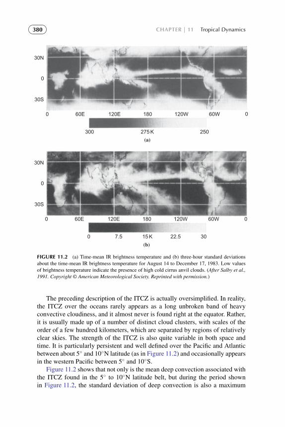
To protect the rights of the author(s) and publisher we inform you that this PDF is an uncorrected proof for internal businessuse only by the author(s), editor(s), reviewer(s), Elsevier and typesetter diacriTech. It is not allowed to publish this proofonline or in print. This proof copy is the copyright property of the publisher and is confidential until formal publication.
“Hakim: 15-ch11-377-412-9780123848666” — 2012/7/26 — 12:15 — page 380 — #4
380 CHAPTER | 11 Tropical Dynamics
275 K
(a)
250
120W180120E
300
60E0
0
30S
30N
60W 0
(b)
15 K7.5 22.5 30
120W180120E
0
60E0
0
30S
30N
60W 0
FIGURE 11.2 (a) Time-mean IR brightness temperature and (b) three-hour standard deviationsabout the time-mean IR brightness temperature for August 14 to December 17, 1983. Low valuesof brightness temperature indicate the presence of high cold cirrus anvil clouds. (After Salby et al.,1991. Copyright © American Meteorological Society. Reprinted with permission.)
The preceding description of the ITCZ is actually oversimplified. In reality,the ITCZ over the oceans rarely appears as a long unbroken band of heavyconvective cloudiness, and it almost never is found right at the equator. Rather,it is usually made up of a number of distinct cloud clusters, with scales of theorder of a few hundred kilometers, which are separated by regions of relativelyclear skies. The strength of the ITCZ is also quite variable in both space andtime. It is particularly persistent and well defined over the Pacific and Atlanticbetween about 5◦ and 10◦N latitude (as in Figure 11.2) and occasionally appearsin the western Pacific between 5◦ and 10◦S.
Figure 11.2 shows that not only is the mean deep convection associated withthe ITCZ found in the 5◦ to 10◦N latitude belt, but during the period shownin Figure 11.2, the standard deviation of deep convection is also a maximum

To protect the rights of the author(s) and publisher we inform you that this PDF is an uncorrected proof for internal businessuse only by the author(s), editor(s), reviewer(s), Elsevier and typesetter diacriTech. It is not allowed to publish this proofonline or in print. This proof copy is the copyright property of the publisher and is confidential until formal publication.
“Hakim: 15-ch11-377-412-9780123848666” — 2012/7/26 — 12:15 — page 381 — #5
11.1 | The Observed Structure of Large-Scale Tropical Circulations 381
there. This is consistent with the idea that the ITCZ is the locus of transientcloud clusters, rather than simply a region of steady-state precipitation and meanuplift. The dry zones along the equator in the oceanic regions are a particularlystriking feature in Figure 11.2.
As the preceding discussion suggests, the vertical mass flux associated withthe ITCZ has important regional variations. Nevertheless, there is a significantzonal mean component, which constitutes the upward mass flux of the meanHadley circulation. This Hadley circulation consists of overturning thermallydirect cells in the low latitudes of both hemispheres, as shown in Figure 10.7.The center of the Hadley circulation is located at the mean latitude of theITCZ. As Figure 10.7 shows, the winter hemisphere branch of the Hadley cellis much stronger than the summer hemisphere branch. Observations indicatethat two Hadley cells, symmetric about the equator, are rarely observed evenin the equinoctial seasons. Rather, the northern cell dominates from Novem-ber to March, the southern cell dominates from May to September, and rapidtransitions occur in April and October (see Oort, 1983).
11.1.2 Equatorial Wave Disturbances
The variance observed in the cloudiness associated with the ITCZ, as illustratedin Figure 11.2b, is generally caused by transient precipitation zones associ-ated with weak equatorial wave disturbances that propagate westward along theITCZ. That such westward-propagating disturbances exist and are responsiblefor a large part of the cloudiness in the ITCZ can be seen easily by viewing time-longitude sections constructed from daily satellite pictures cut into thin zonalstrips. An example is shown in Figure 11.3. The well-defined bands of cloudi-ness that slope from right to left down the page define the locations of the cloudclusters as functions of longitude and time. Clearly much of the cloudiness inthe 5 to 10◦N latitude zone of the Pacific is associated with westward-movingdisturbances. The slope of the cloud lines in Figure 11.3 implies a westwardpropagation speed of about 8 to 10 m s−1. The longitudinal separation of thecloud bands is about 3000 to 4000 km, corresponding to a period range of about4 to 5 days for this type of disturbance.
Diagnostic studies suggest that these westward-propagating wave distur-bances are generally driven by the release of latent heat in their accompanyingconvective precipitation areas. The vertical structure of a typical equatorialwave disturbance is shown in schematic form in Figure 11.4. Vertical motionin such disturbances is proportional to the diabatic heating rate; thus, the maxi-mum vertical velocities occur in the convective zone. By mass continuity theremust be convergence at low levels in the convective zone and divergence in theupper levels. Hence, provided that the absolute vorticity has the sign of f , thedivergence term in the vorticity equation will induce cyclonic vorticity tenden-cies in the lower troposphere and anticyclonic vorticity tendencies in the upper

To protect the rights of the author(s) and publisher we inform you that this PDF is an uncorrected proof for internal businessuse only by the author(s), editor(s), reviewer(s), Elsevier and typesetter diacriTech. It is not allowed to publish this proofonline or in print. This proof copy is the copyright property of the publisher and is confidential until formal publication.
“Hakim: 15-ch11-377-412-9780123848666” — 2012/7/26 — 12:15 — page 382 — #6
382 CHAPTER | 11 Tropical Dynamics
10
August
5 1 301 25 20 15 10 5 1 150E160E
170E180W
170W160W
150W140W
130W120W
110W100W
90W80W
July
14
FIGURE 11.3 Time-longitude sections of satellite photographs for the period July 1 to August 14,1967, in the 5 to 10◦N latitude band of the Pacific. The westward progression of the cloud clustersis indicated by the bands of cloudiness sloping down the page from right to left. (After Chang, 1970.Copyright © American Meteorological Society. Reprinted with permission.)
W W
C C
S
S
S
S
S
S
N
N
SW
C
W
C
Rid
ge
Pre
ssur
e (h
Pa)
100
200
400
600
800
10000.25 0.25 0.500
Phase (cycles)W E(Time or longitude)
S
N
N
N
N
N
N
FIGURE 11.4 Schematic model for equatorial wave disturbances showing trough axis (solid line),ridge axis (dashed lines), and axes of northerly and southerly wind components (dotted lines).Regions of warm and cold air are designated by W and C, respectively. The axes shown are fornortherly (N) and southerly (S) wind components. (After Wallace, 1971. Copyright © AmericanGeophysical Union. Used with permission.)

To protect the rights of the author(s) and publisher we inform you that this PDF is an uncorrected proof for internal businessuse only by the author(s), editor(s), reviewer(s), Elsevier and typesetter diacriTech. It is not allowed to publish this proofonline or in print. This proof copy is the copyright property of the publisher and is confidential until formal publication.
“Hakim: 15-ch11-377-412-9780123848666” — 2012/7/26 — 12:15 — page 383 — #7
11.1 | The Observed Structure of Large-Scale Tropical Circulations 383
troposphere. The process of adjustment between mass and velocity fields willthen generate a low-level trough and an upper-level ridge.1 Thus, the thickness(or layer mean temperature) in the convective zone must be greater than in thesurrounding environment.
In the convectively active areas of equatorial waves there is net upwardmotion, and midtropospheric temperatures are warmer than average (althoughgenerally by less than 1◦C). The correlations between temperature and verticalmotion, and between temperature and diabatic heating, are thus both positive,and the potential energy generated by the diabatic heating is immediately con-verted to kinetic energy—that is, the P′ ·K′ conversion balances R′ in (10.62).There is, in this approximation, no storage in the form of available potentialenergy. The energy cycle of these disturbances, therefore, differs remarkablyfrom that of midlatitude baroclinic systems in which the available potentialenergy greatly exceeds the kinetic energy.
For latent heat release by cumulonimbus clouds to be an effective energysource for large-scale disturbances, there must be an interaction between theconvective scale and the large scale, as mentioned in Section 9.7.2. In suchinteraction large-scale convergence at low levels moistens and destabilizes theenvironment so that small-scale thermals can easily reach the level of free con-vection and produce deep cumulus convection. The cumulus cells, in turn, actcooperatively to provide the large-scale heat source that drives the secondarycirculation responsible for the low-level convergence.
A typical vertical profile of divergence in the precipitation zone of asynoptic-scale equatorial wave disturbance in the western Pacific is shown inFigure 11.5. Convergence is not limited to low-level frictional inflow in theplanetary boundary layer, but extends up to nearly 400 hPa, which is the heightwhere the hot towers achieve their maximum buoyancy. The deep convergenceimplies that there must be substantial entrainment of midtropospheric air into theconvective cells. Because the midtropospheric air is relatively dry, this entrain-ment will require considerable evaporation of liquid water to bring the mixtureof cloud and environment air to saturation. It will thus reduce the buoyancy ofthe cloud air and may in fact produce negatively buoyant convective downdraftsif there is sufficient evaporative cooling. However, in the large cumulonimbusclouds present in equatorial waves, the central core updrafts are protected fromentrainment by the surrounding cloud air so that they can penetrate nearly to thetropopause without dilution by environmental air. These undiluted cores consti-tute the “hot towers” referred to in Section 11.1.1. Because the hot towers areresponsible for much of the vertical heat and mass transport above the boundary
1The terms trough and ridge as used by tropical meteorologists designate pressure minima andmaxima, respectively, just as in midlatitudes. In the easterlies of the Northern Hemisphere tropics,however, the zonal-mean pressure increases with latitude so that the pattern of isobars depicting atropical trough will resemble the pattern associated with a ridge in middle latitudes (i.e., there is apoleward deflection of the isobars).

To protect the rights of the author(s) and publisher we inform you that this PDF is an uncorrected proof for internal businessuse only by the author(s), editor(s), reviewer(s), Elsevier and typesetter diacriTech. It is not allowed to publish this proofonline or in print. This proof copy is the copyright property of the publisher and is confidential until formal publication.
“Hakim: 15-ch11-377-412-9780123848666” — 2012/7/26 — 12:15 — page 384 — #8
384 CHAPTER | 11 Tropical Dynamics
−10 −5 0 +5 +10 +151000
900
800
700
600
500
400
300
200
100
Divergence (10−6 s−1)
Pre
ssur
e (h
Pa)
FIGURE 11.5 Vertical profile of 4◦-square area average divergence based on composites of manyequatorial disturbances. (Adapted with permission from Williams, 1971.)
layer in the ITCZ, and the wave disturbances contain most of the active convec-tive precipitation areas along the ITCZ, it is obvious that equatorial waves playan essential role in the general circulation of the atmosphere.
11.1.3 African Wave Disturbances
The considerations of the previous subsection are valid for ITCZ disturbancesover most regions of the tropical oceans. In the region of the North Africancontinent, however, local effects due to surface conditions create a uniquesituation that requires separate discussion. During the Northern Hemispheresummer, intense surface heating over the Sahara generates a strong positivemeridional temperature gradient in the lower troposphere between the equatorand about 25◦N. The resulting easterly thermal wind is responsible for the exis-tence of a strong easterly jet core near 650 hPa centered near 16◦N as shownin Figure 11.6. Synoptic-scale disturbances are observed to form and propagatewestward in the cyclonic shear zone to the south of this jet core.
Occasionally, such disturbances are progenitors of tropical storms and hur-ricanes in the western Atlantic. The average wavelength of observed Africanwave disturbances is about 2500 km, and the westward propagation speed isabout 8 ms−1, implying a period of about 3.5 days. The disturbances have hor-izontal velocity perturbations that reach maximum amplitude at the 650-hPa

To protect the rights of the author(s) and publisher we inform you that this PDF is an uncorrected proof for internal businessuse only by the author(s), editor(s), reviewer(s), Elsevier and typesetter diacriTech. It is not allowed to publish this proofonline or in print. This proof copy is the copyright property of the publisher and is confidential until formal publication.
“Hakim: 15-ch11-377-412-9780123848666” — 2012/7/26 — 12:15 — page 385 — #9
11.1 | The Observed Structure of Large-Scale Tropical Circulations 385
+12 +8 +4 0 −4 −8 −12
850
700
500
400
300
250
200
150
100
Pre
ssur
e (h
Pa)
Δ Latitude
Hei
ght (
km)
2
4
6
8
10
12
14
16−5
0
0
5W
−5
–5
−10
−10
E
E
−5
−10
5W0
00
FIGURE 11.6 Mean-zonal wind distribution in the North African region (30◦W to 10◦E longi-tude) for the period August 23 to September 19, 1974. Latitude is shown relative to latitude ofmaximum disturbance amplitude at 700 hPa (about 12◦N). The contour interval is 2.5 m s−1. (AfterReed et al., 1977. Copyright © American Meteorological Society. Reprinted with permission.)
level, as indicated in Figure 11.7. Although there is considerable organizedconvection associated with these waves, they do not appear to be driven pri-marily by latent heat release, but depend, rather, on barotropic and baroclinicconversions of energy from the easterly jet.
In Figure 11.8 the absolute vorticity profile for the African easterly jet shownin Figure 11.6 is plotted. The shaded region indicates the area in which thevorticity gradient is negative. Thus, it is clear that the African jet satisfies thenecessary condition for barotropic instability discussed in Section 7.4.2.2 Baro-clinic instability due to the strong easterly shear in the lower troposphere alsoappears to play a role in these disturbances. Thus, both barotropic and baro-clinic conversions from the mean flow energy appear to be important for thegeneration of African wave disturbances.
Because such disturbances continue to exist in the absence of strong meanwind shears after they have propagated westward into the Atlantic, it is unlikelythat either baroclinic or barotropic instability continues to be the primary energysource for their maintenance. Rather, diabatic heating through precipitating
2It should be noted here that the profile shown in Figure 11.6 is not a zonal mean. Rather, it is atime mean for a limited longitudinal domain. Provided that the longitudinal scale of variation of thistime-mean zonal flow is large compared to the scale of the disturbance, the time-mean flow may beregarded as a locally valid basic state for linear stability calculations.

To protect the rights of the author(s) and publisher we inform you that this PDF is an uncorrected proof for internal businessuse only by the author(s), editor(s), reviewer(s), Elsevier and typesetter diacriTech. It is not allowed to publish this proofonline or in print. This proof copy is the copyright property of the publisher and is confidential until formal publication.
“Hakim: 15-ch11-377-412-9780123848666” — 2012/7/26 — 12:15 — page 386 — #10
386 CHAPTER | 11 Tropical Dynamics
850
R N T S R0
5
10
15
18
0
0
−2
−2
−4
−2
00
−22
0
SN
−2
S
0
4
20
N 700
500
400
300
250
200
150
100
Hei
ght (
km)
Pre
ssur
e (h
Pa)
FIGURE 11.7 Vertical cross-section along the reference latitude of Figure 11.6 showing perturba-tion meridional velocities in m s−1. R, N, T, and S refer to ridge, northwind, trough, and southwindsectors of the wave, respectively. (After Reed et al., 1977. Copyright © American MeteorologicalSociety. Reprinted with permission.)
convective systems appears to be the main energy source for such waves overthe ocean.
11.1.4 Tropical Monsoons
The term monsoon is commonly used in a rather general sense to designate anyseasonally reversing circulation system. The basic drive for a monsoon circu-lation is provided by the contrast in the thermal properties of the land and seasurfaces. Because the thin layer of soil that responds to seasonal changes in sur-face temperature has a small heat capacity compared to the heat capacity of theupper layer of the ocean that responds on a similar timescale, the absorptionof solar radiation raises the surface temperature over land much more rapidlythan over the ocean. The warming of the land relative to the ocean leads toenhanced cumulus convection and thus to latent heat release, which produceswarm temperatures throughout the troposphere.
Much of the tropics is influenced by monsoons. The most extensive monsooncirculation by far is the Asian monsoon. This monsoon completely dominates

To protect the rights of the author(s) and publisher we inform you that this PDF is an uncorrected proof for internal businessuse only by the author(s), editor(s), reviewer(s), Elsevier and typesetter diacriTech. It is not allowed to publish this proofonline or in print. This proof copy is the copyright property of the publisher and is confidential until formal publication.
“Hakim: 15-ch11-377-412-9780123848666” — 2012/7/26 — 12:15 — page 387 — #11
11.1 | The Observed Structure of Large-Scale Tropical Circulations 387
+12 +8 +4 0 –4 –8 –12
2
4
6
8
10
12
14
16
Hei
ght (
km)
Pre
ssur
e (h
Pa)
850
700
500
400
300
250
200
150
100
6
5
5
4
4
4
4 3
3 2
2 1
1
0
0
Δ Latitude
FIGURE 11.8 Absolute vorticity (units 10−5s−1) corresponding to the mean wind field ofFigure 11.6. Shading shows region where β − ∂2u/∂y2 is negative. (After Reed et al., 1977.Copyright © American Meteorological Society. Reprinted with permission.)
the climate of the Indian subcontinent, producing warm wet summers and cooldry winters. An idealized model of the structure of the Asian summer monsoonis indicated in Figure 11.9. As indicated in Figure 11.9, the 1000 to 200-hPathickness is larger over the land than over the ocean. As a result there is apressure gradient force at the upper levels directed from the land to the ocean.
The divergent wind that develops in response to this pressure gradient(shown by the arrows in Figure 11.9) causes a net mass transport out of theair column above the continent and thereby generates a surface low over thecontinent (often called a thermal low). A compensating convergent wind thendevelops at low levels. This low-level flow produces a convergence of mois-ture, which by increasing the equivalent potential temperature in the boundarylayer makes the environment more favorable for development of the cumulusconvection, which is the primary energy source for the monsoon circulation.
The low-level convergence and upper-level divergence over the continentconstitute a secondary circulation that concentrates cyclonic vorticity at thelower levels and anticyclonic vorticity at the upper levels. Thus, the vorticityadjusts toward geostrophic balance. From Figure 11.9 it is clear that a positivecorrelation exists between the vertical motion and the temperature field. There-fore, the monsoon circulation converts eddy potential energy to eddy kineticenergy, just as midlatitude baroclinic eddies do.
Unlike the case of baroclinic eddies, however, the primary energy cycleof the monsoons does not involve the zonal-mean potential or kinetic energy.Rather, eddy potential energy is generated directly by diabatic heating (latentand radiative heating); the eddy potential energy is converted to eddy kinetic

To protect the rights of the author(s) and publisher we inform you that this PDF is an uncorrected proof for internal businessuse only by the author(s), editor(s), reviewer(s), Elsevier and typesetter diacriTech. It is not allowed to publish this proofonline or in print. This proof copy is the copyright property of the publisher and is confidential until formal publication.
“Hakim: 15-ch11-377-412-9780123848666” — 2012/7/26 — 12:15 — page 388 — #12
388 CHAPTER | 11 Tropical Dynamics
(b)
C2 W2 C2
C1
W2
Strongpressuregradient
Weaksurfacepressuregradient
C1 W1 W1
Temperature Cold Warm Log (pressure)
(c) (d)
Hei
ght (
km)
Moi
st
15
10
5
15
10
5
15
(a) Moist monsoon
Constant pressure surface
10
5
Hei
ght (
km)
0
40° S 50° N30° 40°30°20° 20°10° 10°0°Latitude
C1
C2
W2
W1
FIGURE 11.9 Schematic representation of the moist phase of the Asian monsoon. (a) Arrowsshow the meridional circulation, dashed lines the isobars. (b) Temperature profiles for columnsC1 to C2 and W1 to W2, respectively. (c) Schematic of the mass distribution in the cold and warmsectors. (d) Horizontal pressure difference as a function of height. (After Webster and Fasullo, 2003.)
energy by a thermally direct secondary circulation; and the eddy kinetic energyis frictionally dissipated. (A portion of the eddy kinetic energy may be con-verted to zonal kinetic energy.) In a dry atmosphere, monsoon circulationswould still exist; however, because the diabatic heating would then be con-fined to a shallow layer near the surface, they would be much weaker than theobserved monsoons. The presence of cumulus convection and its concomitantlatent heat release greatly amplifies the eddy potential energy generation andmakes the summer monsoons among the most important features of the globalcirculation.

To protect the rights of the author(s) and publisher we inform you that this PDF is an uncorrected proof for internal businessuse only by the author(s), editor(s), reviewer(s), Elsevier and typesetter diacriTech. It is not allowed to publish this proofonline or in print. This proof copy is the copyright property of the publisher and is confidential until formal publication.
“Hakim: 15-ch11-377-412-9780123848666” — 2012/7/26 — 12:15 — page 389 — #13
11.1 | The Observed Structure of Large-Scale Tropical Circulations 389
In the winter season the thermal contrast between the land and the seareverses so that the circulation is just opposite to that shown in Figure 11.9.As a result the continents are cool and dry and the precipitation is found overthe relatively warm oceans.
11.1.5 The Walker Circulation
The pattern of diabatic heating in the equatorial regions exhibits strong depar-tures from zonal symmetry. These are caused by longitudinal variations in seasurface temperature due mainly to the effects of wind-driven ocean currents.Such SST variations produce zonally asymmetric atmospheric circulations,which in some regions dominate over the Hadley circulation. Of particularsignificance is the east–west overturning along the equator, which is shownschematically in Figure 11.10. Several overturning cells are indicated, whichare associated with diabatic heating over equatorial Africa, Central and SouthAmerica, and the Maritime Continent (i.e., the Indonesian region). The domi-nant cell in both zonal scale and amplitude, however, is that in the equatorialPacific. This cell is referred to as Walker circulation after G. T. Walker, who firstdocumented the surface pressure pattern associated with it.
As suggested by Figure 11.10, this pressure pattern consists of low surfacepressure in the western Pacific and high surface pressure in the eastern Pacific.
200-hPapressure
Surfacepressure
200-hPapressure
Surfacepressure
L
L
L
L
L
H
H
H
H
0
Indian
90E 180
Pacific
90W
Atlantic
Indian Pacific Atlantic
0
0 90E 180 90W 0
(a)
(b)
FIGURE 11.10 Schematic diagrams of the Walker circulations along the equator for (a) nor-mal conditions and (b) El Nino conditions. (From Webster, 1983, and Webster and Chang, 1988.Copyright © American Meteorological Society. Reprinted with permission.)
To protect the rights of the author(s) and publisher we inform you that this PDF is an uncorrected proof for internal businessuse only by the author(s), editor(s), reviewer(s), Elsevier and typesetter diacriTech. It is not allowed to publish this proofonline or in print. This proof copy is the copyright property of the publisher and is confidential until formal publication.
“Hakim: 15-ch11-377-412-9780123848666” — 2012/7/26 — 12:15 — page 390 — #14
390 CHAPTER | 11 Tropical Dynamics
The resulting westward-directed pressure gradient force drives mean surfaceeasterlies in the equatorial Pacific, which are much stronger than the zonal-meansurface easterlies, and by horizontal vapor transport provides a moisture sourcefor convection in the western Pacific, in addition to that provided by the highevaporation rates caused by the high sea surface temperatures in that region.
The wind stress due to the time-mean equatorial easterly surface winds overthe Pacific has a strong influence on the heat balance of the ocean surface layer.It advects warm surface waters into the western Pacific and produces pole-ward drifts in the oceanic Ekman layer which by continuity drive an equatorialupwelling. This upwelling accounts for the cold tongue of water along the equa-tor, which in turn is a major reason for the equatorial dry zone exhibited earlierin Figure 11.2.
11.1.6 El Nino and the Southern Oscillation
The east–west pressure gradient associated with the Walker circulation under-goes an irregular interannual variation. This global-scale “see-saw” in pressure,and its associated changes in patterns of wind, temperature, and precipitation,was named the southern oscillation by Walker. This oscillation can be clearlyseen by comparing time series of surface pressure anomalies (i.e., departuresfrom the long-term mean) for locations on the western and eastern sides of theequatorial Pacific. As shown in the upper portion of Figure 11.11, surface pres-sure anomalies at Darwin, Australia, and Tahiti are negatively correlated andhave strong variations in the period range of 2 to 5 years. During periods of largepressure difference between these stations, the Walker circulation is unusuallystrong and has the same general structure as its time-mean pattern. In periodsof weak pressure difference the Walker circulation weakens and the region ofmaximum rainfall shifts eastward (see Figure 11.10b).
The weakening of trade winds during periods of small Darwin–Tahiti pres-sure difference reduces wind-driven oceanic upwelling and deepens the oceanicthermocline in the eastern Pacific. This in turn, as shown in the lower portion ofFigure 11.11, leads to an increase in the sea surface temperature that is referredto as El Nino (Spanish for “the child”). This term was originally applied to awarming of the coastal waters of Peru and Ecuador that occurs annually nearChristmas time (hence, El Nino refers to the Christ child), but is now usedin a more general sense for the large-scale oceanic anomalies associated withthe weak wind phase of the Southern Oscillation. In the opposite phase, thestrengthening of trade winds associated with large Darwin–Tahiti pressure dif-ferences enhances oceanic upwelling and deepens the oceanic thermocline. Thiscauses a cooling of the sea surface temperatures in the equatorial Pacific that isnow referred to as La Nina.
The ocean anomalies associated with weakening in the trade winds maybegin near the coast, but over the course of several months spread westwardalong the equator to produce large-scale positive SST anomalies over much of

To protect the rights of the author(s) and publisher we inform you that this PDF is an uncorrected proof for internal businessuse only by the author(s), editor(s), reviewer(s), Elsevier and typesetter diacriTech. It is not allowed to publish this proofonline or in print. This proof copy is the copyright property of the publisher and is confidential until formal publication.
“Hakim: 15-ch11-377-412-9780123848666” — 2012/7/26 — 12:15 — page 391 — #15
11.1 | The Observed Structure of Large-Scale Tropical Circulations 391
2.5
1.5
0.5
2.0
1.0
−0.5
−1.5−1.0
0.0
−2.0−2.5
Ano
mal
ies
1950 1955 1960 1965 1970 1975 1980 1985 1990 1995 2000
Year
2.5
1.5
0.5
2.0
1.0
−0.5
−1.5−1.0
0.0
−2.0
FIGURE 11.11 Time series showing SST anomalies (◦C) in the eastern Pacific (lower curve)and anomalies in sea-level pressures (hPa) at Darwin (upper solid curve) and Tahiti (upper dashedcurve). Data are smoothed to eliminate fluctuations with periods less than a year. (Figure courtesyof Dr. Todd Mitchell, University of Washington.)
the equatorial Pacific. These SST anomalies in turn cause a further weakeningof the trade winds. This entire complex of atmospheric and oceanic variations isnow referred to as ENSO (for El Nino—Southern Oscillation). It is a dramaticexample of interannual climate variability associated with atmosphere–oceancoupling.
The leading theoretical model for ENSO is the “delayed oscillator” model.In this model the sea surface temperature anomaly, T , in the eastern Pacificsatisfies an equation of the form
dT
dt= bT(t)− cT(t − τ)
where b and c are positive constants and τ is a time delay determined by theadjustment time for the equatorial ocean. The first term on the right representsa positive feedback associated with changes in the Darwin–Tahiti pressure dif-ference. This term represents the atmosphere–ocean coupling through which aninitial weakening of the wind causes an increase of the SST, which induces afurther weakening of the wind and thus a further increase in the SST. The sec-ond term provides a negative feedback due to the adjustment in the thermoclinedepth (and thus the ocean temperature) caused by propagating equatorial waves(see Section 11.4) in the ocean that are excited by the SST changes. The timedelay in the negative feedback term is determined by the time that it takes forwave energy excited by air–sea interaction in the eastern Pacific to propagate tothe western boundary of the ocean, undergo reflection, and propagate back tothe region of origin. For realistic parameters the delayed oscillator model leads

To protect the rights of the author(s) and publisher we inform you that this PDF is an uncorrected proof for internal businessuse only by the author(s), editor(s), reviewer(s), Elsevier and typesetter diacriTech. It is not allowed to publish this proofonline or in print. This proof copy is the copyright property of the publisher and is confidential until formal publication.
“Hakim: 15-ch11-377-412-9780123848666” — 2012/7/26 — 12:15 — page 392 — #16
392 CHAPTER | 11 Tropical Dynamics
to ENSO oscillations in the period range of 3 to 4 years. This highly simplifiedmodel qualitatively accounts for the average characteristics of an ENSO cycle,but cannot, however, account for the observed irregularity of ENSO.
In addition to its profound effects in the equatorial region, ENSO is asso-ciated with a wide range of interannual climate anomalies in the extratropics.Thus, the development of models that show skill in predicting ENSO severalmonths in advance is of considerable practical importance.
11.1.7 Equatorial Intraseasonal Oscillation
In addition to the interannual variability associated with El Nino, the equato-rial circulation has an important intraseasonal oscillation, which occurs on atimescale of 30 to 60 days and is often referred to as the Madden–Julian oscilla-tion (MJO) in honor of the meteorologists who first described it. The structure ofthe equatorial intraseasonal oscillation is shown schematically in Figure 11.12,which shows the time development of the oscillation in the form of longitude–height sections along the equator, with time increasing at an interval of about10 days for each panel from top to bottom. The circulations in Figure 11.12 areintended to represent anomalies from the time-mean equatorial circulation.
The oscillation originates with the development of a surface low-pressureanomaly over the Indian Ocean, accompanied by enhanced boundary layermoisture convergence, increased convection, warming of the troposphere, andraising of the tropopause height. The anomaly pattern gradually moves eastwardat about 5 m s−1 and reaches maximum intensity over the western Pacific. As theanomaly moves over the cooler waters of the central Pacific, the anomalous con-vection gradually weakens, although a circulation disturbance continues east-ward and can sometimes be traced completely around the globe. The observedintraseasonal oscillation is known to be associated with equatorial Rossby andKelvin waves (see Section 11.4). However, a completely satisfactory theory forthe oscillation has not yet been developed.
11.2 SCALE ANALYSIS OF LARGE-SCALE TROPICALMOTIONS
Despite the uncertainties involved in the interaction between convective andsynoptic scales, some information on the character of synoptic-scale motions inthe tropics can be obtained through the methods of scale analysis. The scalingarguments can be carried out most conveniently if the governing equations arewritten in the log-pressure coordinate system introduced in Section 7.4.1:(
∂
∂t+ V ·∇ + w∗
∂
∂z∗
)V+ f k× V = −∇8 (11.1)
∂8/∂z∗ = RT/H (11.2)

To protect the rights of the author(s) and publisher we inform you that this PDF is an uncorrected proof for internal businessuse only by the author(s), editor(s), reviewer(s), Elsevier and typesetter diacriTech. It is not allowed to publish this proofonline or in print. This proof copy is the copyright property of the publisher and is confidential until formal publication.
“Hakim: 15-ch11-377-412-9780123848666” — 2012/7/26 — 12:15 — page 393 — #17
11.2 | Scale Analysis of Large-Scale Tropical Motions 393
Tropopause
East longitude
Africa Indonesia South America
West longitude
20° 20°60° 60°100° 100°140° 140°180°
Sea-level pressure
FIGURE 11.12 Longitude-height section of the anomaly pattern associated with the tropicalintraseasonal oscillation (MJO). Reading downward, the panels represent a time sequence withintervals of about 10 days. Streamlines show the west–east circulation, the wavy top line repre-sents the tropopause height, and the bottom line represents surface pressure (with shading showingbelow-normal surface pressure). (After Madden, 2003; adapted from Madden and Julian, 1972.)
∂u/∂x+ ∂v/∂y+ ∂w∗/∂z∗ − w∗/H = 0 (11.3)
(∂
∂t+ V ·∇
)T + w∗N2H/R = J/cp (11.4)
We wish to compare the magnitudes of the various terms in (11.1) through(11.4) for synoptic-scale motions in the tropics. We first note that an upper limiton the vertical velocity scale W is imposed by the continuity equation (11.3).

To protect the rights of the author(s) and publisher we inform you that this PDF is an uncorrected proof for internal businessuse only by the author(s), editor(s), reviewer(s), Elsevier and typesetter diacriTech. It is not allowed to publish this proofonline or in print. This proof copy is the copyright property of the publisher and is confidential until formal publication.
“Hakim: 15-ch11-377-412-9780123848666” — 2012/7/26 — 12:15 — page 394 — #18
394 CHAPTER | 11 Tropical Dynamics
Thus, following the discussion of Section 4.5,
∂u/∂x+ ∂v/∂y ≤ U/L
However, for motions with vertical scales comparable to the density scaleheight H,
∂w∗/∂z∗ − w∗/H ∼ W/H
so that the vertical velocity scale must satisfy the constraint W ≤ HU/L if thehorizontal divergence and the vertical stretching terms are to balance in the con-tinuity equation. We next define characteristic scales for the various field vari-ables as follows:
H ∼ 104 m vertical length scale
L ∼ 106 m horizontal length scale
U ∼ 10 m s−1 horizontal velocity scale
W ≤ HU/L vertical velocity scale
δ8 geopotential fluctuation scale
L/U ∼ 105 s timescale for advection
The magnitudes chosen for the horizontal length and velocity scales are typ-ical for observed values in synoptic-scale systems both in the tropics and atmidlatitudes. We now wish to show how the corresponding characteristic scalesfor vertical velocity and geopotential fluctuations are limited by the dynamicconstraints imposed by conservation of mass, momentum, and thermodynamicenergy.
We can estimate the magnitude of the geopotential fluctuation δ8 by scalingthe terms in the momentum equation (11.1). For this purpose it is convenient tocompare the magnitude of the horizontal inertial acceleration,
(V ·∇)V ∼ U2/L
with each of the other terms in (11.1) as follows:
|∂V/∂t| / |(V ·∇)V| ∼ 1 (11.5)
|w∗∂V/∂z∗|/ |(V ·∇)V| ∼ WL/UH ≤ 1 (11.6)
| f k× V| / |(V ·∇)V| ∼ fL/U = Ro−1≤ 1 (11.7)
|∇8| / |(V ·∇)V| ∼ δ8/U2 (11.8)

To protect the rights of the author(s) and publisher we inform you that this PDF is an uncorrected proof for internal businessuse only by the author(s), editor(s), reviewer(s), Elsevier and typesetter diacriTech. It is not allowed to publish this proofonline or in print. This proof copy is the copyright property of the publisher and is confidential until formal publication.
“Hakim: 15-ch11-377-412-9780123848666” — 2012/7/26 — 12:15 — page 395 — #19
11.2 | Scale Analysis of Large-Scale Tropical Motions 395
We have shown previously that in middle latitudes where f ∼ 10−4 s−1, theRossby number Ro is small so that to first approximation the Coriolis force andpressure gradient force terms balance. In that case, δ 8 ∼ fUL. In the equato-rial region, however, f ≤ 10−5 s−1 and the Rossby number is of order unity orgreater. Therefore, it is not appropriate to assume that the Coriolis force bal-ances the pressure gradient force. In fact, (11.5) through (11.8) show that if thepressure gradient force is to be balanced in (11.1), the geopotential perturbationmust scale as δ+8 ∼U2
∼ 100 m2 s−2, and geopotential perturbations associ-ated with equatorial synoptic-scale disturbances will be an order of magnitudesmaller than those for midlatitude systems of similar scale.
This constraint on the amplitude of geopotential fluctuations in the tropicshas profound consequences for the structure of synoptic-scale tropical motionsystems. These consequences can be understood easily by applying scalingarguments to the thermodynamic energy equation. It is first necessary to obtainan estimate of the temperature fluctuations. The hydrostatic approximation(11.2) implies that for systems whose vertical scale is comparable to the scaleheight,
T = (H/R)∂8/∂z∗ ∼ (δ8/R) ∼ U2/R ∼ 0.3 K (11.9)
Therefore, deep tropical systems are characterized by practically negligiblesynoptic-scale temperature fluctuations. Referring to the thermodynamic energyequation, we find that for such systems(
∂
∂t+ V ·∇
)T ∼ 0.3 K d−1
In the absence of precipitation, the diabatic heating is caused primarily bythe emission of long wave radiation, which tends to cool the troposphere at arate of J/cp ∼ 1 K d−1. Because the actual temperature fluctuations are small,this radiative cooling must be approximately balanced by adiabatic warmingdue to subsidence. Thus, to a first approximation, (11.4) becomes a diagnosticrelationship for w∗:
w∗(N2H/R) = J/cp (11.10)
For the tropical troposphere, N2H/R∼ 3 K km−1, so the vertical motion scalemust satisfy W ∼ 0.3 cm s−1 and WL/UH∼ 0.03 in (11.6). Therefore, in theabsence of precipitation, the vertical motion is constrained to be even smallerthan in extratropical synoptic systems of a similar scale. Not only can the ver-tical advection term be neglected in (11.1), but from the continuity equation(11.3), the divergence of the horizontal wind is ∼ 3× 10⁻⁷ s−1. Thus, the flowis nearly nondivergent.
The quasi-nondivergent nature of the flow in the absence of convective dis-turbances in the tropics makes it possible to simplify the governing equations

To protect the rights of the author(s) and publisher we inform you that this PDF is an uncorrected proof for internal businessuse only by the author(s), editor(s), reviewer(s), Elsevier and typesetter diacriTech. It is not allowed to publish this proofonline or in print. This proof copy is the copyright property of the publisher and is confidential until formal publication.
“Hakim: 15-ch11-377-412-9780123848666” — 2012/7/26 — 12:15 — page 396 — #20
396 CHAPTER | 11 Tropical Dynamics
for that situation. A theorem of Helmholtz3 states that any velocity field can bedivided into a nondivergent part Vψ and an irrotational part Ve such that
V = Vψ + Ve
where ∇ · Vψ = 0 and ∇ × Ve = 0.For a two-dimensional velocity field the nondivergent part can be expressed
in terms of a streamfunction ψ defined by letting
Vψ = k×∇ψ (11.11)
or in Cartesian components:
uψ = −∂ψ/∂y, vψ = ∂ψ/∂x
from which it is verified easily that ∇ ·Vψ = 0 and ζ = k ·∇ × Vψ = ∇2ψ .Because the isolines of ψ correspond to streamlines for the nondivergent veloc-ity and the distance separating the isolines of ψ is inversely proportional to themagnitude of the nondivergent velocity, the spatial distribution of Vψ can bepictured easily by plotting lines of constant ψ on a synoptic chart.
We now approximate V by its nondivergent part Vψ in (11.1) and neglectthe small vertical advection term to obtain an approximate momentum equationvalid for synoptic-scale motions in the tropics outside regions of precipitation:
∂Vψ∂t+(Vψ ·∇
)Vψ + f k× Vψ = −∇8 (11.12)
Using the vector identity
(V ·∇)V = ∇(
V ·V2
)+ k× Vζ
we can rewrite (11.12) as
∂Vψ∂t= −∇
(8+
Vψ ·Vψ2
)− k× Vψ (ζ + f ) (11.13)
We next take k ·∇ × (11.13) to obtain the vorticity equation valid fornondivergent flow: (
∂
∂t+ Vψ ·∇
)(ζ + f ) = 0 (11.14)
This equation shows that in the absence of condensation heating, synoptic-scalecirculations in the tropics in which the vertical scale is comparable to the scaleheight of the atmosphere must be barotropic; absolute vorticity is conservedfollowing the nondivergent horizontal wind. Such disturbances cannot convert
3See, for example, Bourne and Kendall (1968, p. 190).

To protect the rights of the author(s) and publisher we inform you that this PDF is an uncorrected proof for internal businessuse only by the author(s), editor(s), reviewer(s), Elsevier and typesetter diacriTech. It is not allowed to publish this proofonline or in print. This proof copy is the copyright property of the publisher and is confidential until formal publication.
“Hakim: 15-ch11-377-412-9780123848666” — 2012/7/26 — 12:15 — page 397 — #21
11.2 | Scale Analysis of Large-Scale Tropical Motions 397
potential energy to kinetic energy. They must be driven by barotropic conversionof mean-flow kinetic energy or by lateral coupling either to midlatitude systemsor to precipitating tropical disturbances.
Because both the nondivergent velocity and the vorticity can be expressedin terms of the streamfunction, (11.14) requires only the field of ψ at any levelin order to make a prediction. The pressure distribution is neither required norpredicted. Rather, it must be determined diagnostically. The relationship of thepressure and streamfunction fields can be obtained by taking ∇ · (11.13). Thisyields a diagnostic relationship between the geopotential and streamfunctionfields, which is usually referred to as the nonlinear balance equation:
∇2[8+
1
2(∇ψ)2
]= ∇·
[(f +∇2ψ
)∇ψ
](11.15)
For the special case of stationary circularly symmetric flow, (11.15) is equiva-lent to the gradient wind approximation. Unlike the gradient wind, however, thebalance in (11.15) does not require information on trajectory curvature and thuscan be solved for 8 from knowledge of the instantaneous distribution of ψ onan isobaric surface. Alternatively, if the 8 distribution is known, (11.15) can besolved for ψ . In this case the equation is quadratic so that there are generallytwo possible solutions, which correspond to the normal and anomalous gradientwind cases.
Such a balance condition is valid only when the previous scaling argumentsapply. These, however, have been based on the assumptions that the depth scaleis comparable to the scale height of the atmosphere and that the horizontal scaleis of order 1000 km. There is a special class of planetary-scale motions forwhich the divergence term in the vorticity equation is important even outside ofregions of active precipitation (see Section 11.4). For such motions the pressurefield cannot be diagnosed from a balance relationship. Rather, the pressure dis-tribution must be predicted from the primitive equation form of the dynamicsequations.
For precipitating synoptic-scale systems in the tropics, the preceding scal-ing considerations require extensive modification. Precipitation rates in suchsystems are typically of the order 2 cm d−1. This implies condensation ofmw = 20 kg water for an atmospheric column of 1 m2 cross-section. Becausethe latent heat of condensation is Lc ≈ 2.5 × 10⁶ J kg−1, this precipitation rateimplies an addition of heat energy to the atmospheric column of
mwLc ∼ 5× 10⁷ J m−2 d−1
If this heat is distributed uniformly over the entire atmospheric column of massp0/g ≈ 104 kg m−2, then the average heating rate per unit mass of air is
J/cp ≈[Lcmw/cp (p0/g)
]∼ 5 K d−1
In reality the condensation heating due to deep convective clouds is notdistributed evenly over the entire vertical column, but is a maximum between

To protect the rights of the author(s) and publisher we inform you that this PDF is an uncorrected proof for internal businessuse only by the author(s), editor(s), reviewer(s), Elsevier and typesetter diacriTech. It is not allowed to publish this proofonline or in print. This proof copy is the copyright property of the publisher and is confidential until formal publication.
“Hakim: 15-ch11-377-412-9780123848666” — 2012/7/26 — 12:15 — page 398 — #22
398 CHAPTER | 11 Tropical Dynamics
300 and 400 hPa, where the heating rate can be as high as 10 K d−1. In thiscase the approximate thermodynamic energy equation (11.10) implies that thevertical motion on the synoptic scale in precipitating systems must have a mag-nitude of order W ∼ 3 cm s−1 in order that the adiabatic cooling can balancethe condensation heating in the 300- to 400-hPa layer. Therefore, the averagevertical motion in precipitating disturbances in the tropics is an order of mag-nitude larger than the vertical motion outside the disturbances. As a result theflow in these disturbances has a relatively large divergent component so that thebarotropic vorticity equation (11.14) is no longer a reasonable approximation,and the full primitive equations must be used to analyze the flow.
11.3 CONDENSATION HEATING
The manner in which the atmosphere is heated by condensation of water vapordepends crucially on the nature of the condensation process. In particular, it isnecessary to differentiate between latent heat release through large-scale ver-tical motion (i.e., synoptic-scale forced uplift) and the latent heat release dueto deep cumulus convection. The former process, which is generally associatedwith midlatitude synoptic systems, can be incorporated easily into the thermo-dynamic energy equation in terms of the synoptic-scale field variables. Thelarge-scale heating field resulting from the cooperative action of many cumu-lonimbus cells, however, requires representation of this type of latent heating interms of the synoptic-scale field variables, which is much more difficult.
Before considering the problem of condensation heating by cumulus convec-tion, it is worth indicating briefly how the condensation heating by large-scaleforced uplift can be included in a prediction model. The approximate thermo-dynamic energy equation for a pseudoadiabatic process given in Section 2.9.1states that
D ln θ
Dt≈ −
(Lc
cpT
)Dqs
Dt(11.16)
It may be shown that an equivalent static stability, 0e, may be defined so that(11.16) can be written as (
∂
∂t+ V ·∇
)θ + w0e ≈ 0 (11.17)
where
0e ≈
{(0s/0d) ∂θe/∂z for q ≥ qs and w > 0
∂θ/∂z for q < qs or w < 0
Here, 0s and 0d are the lapse rates for pseudoadiabatic and dry ascent, respec-tively. Thus, in the case of condensation due to large-scale forced ascent(0e > 0), the thermodynamic energy equation has essentially the same form

To protect the rights of the author(s) and publisher we inform you that this PDF is an uncorrected proof for internal businessuse only by the author(s), editor(s), reviewer(s), Elsevier and typesetter diacriTech. It is not allowed to publish this proofonline or in print. This proof copy is the copyright property of the publisher and is confidential until formal publication.
“Hakim: 15-ch11-377-412-9780123848666” — 2012/7/26 — 12:15 — page 399 — #23
11.3 | Condensation Heating 399
as for adiabatic motions except that the static stability is replaced by the equiv-alent static stability. As a consequence, the local temperature changes inducedby the forced ascent will be smaller than for the case of forced dry ascent withthe same lapse rate.
If, however, 0e < 0, the atmosphere is conditionally unstable and condensa-tion will occur primarily through cumulus convection. In that case, the verticalvelocity must be that of the individual cumulus updrafts, not the synoptic-scale w. Thus, a simple formulation of the thermodynamic energy equation interms of only the synoptic-scale variables is not possible. We can still, how-ever, simplify the thermodynamic energy equation to some extent. We recallfrom Section 11.2—see Eq. (11.10)—that due to the smallness of temperaturefluctuations in the tropics, the adiabatic cooling and diabatic heating terms mustapproximately balance. Thus, (11.16) becomes approximately
w∂ ln θ
∂z≈ −
Lc
cpT
Dqs
Dt(11.18)
The synoptic-scale vertical velocity w that appears in (11.18) is the averageof very large vertical motions in the active convection cells and small verticalmotions in the environment. Thus, if we let w′ be the vertical velocity in theconvective cells and the w be vertical velocity in the environment, we have
w = aw′ + (1− a)w (11.19)
where a is the fractional area occupied by the convection. Approximating thechange in qs following the motion by w ∂qs
∂z , we can then write (11.18) in theform
w∂ ln θ
∂z≈ −
Lc
cpTaw′
∂qs
∂z(11.20)
The problem now is to express the condensation heating term on the right in(11.20) in terms of synoptic-scale field variables.
This problem of parameterizing the cumulus convective heating is one ofthe most challenging areas in tropical meteorology. A simple approach that hasbeen used successfully in some theoretical studies4 is based on the fact that,because the storage of water in the clouds is rather small, the total verticallyintegrated heating rate due to condensation must be approximately proportionalto the net precipitation rate:
−
zT∫zc
(ρaw′∂qs/∂z
)dz = P (11.21)
where zc and zT represent the cloud base and cloud top heights, respectively,and P is the precipitation rate (kg m−2 s−1).
4See, for example, Stevens and Lindzen (1978).

To protect the rights of the author(s) and publisher we inform you that this PDF is an uncorrected proof for internal businessuse only by the author(s), editor(s), reviewer(s), Elsevier and typesetter diacriTech. It is not allowed to publish this proofonline or in print. This proof copy is the copyright property of the publisher and is confidential until formal publication.
“Hakim: 15-ch11-377-412-9780123848666” — 2012/7/26 — 12:15 — page 400 — #24
400 CHAPTER | 11 Tropical Dynamics
Because relatively little moisture goes into changing the atmospheric vapormixing ratio, the net precipitation rate must approximately equal the moistureconvergence into an atmospheric column plus surface evaporation:
P = −
zm∫0
∇ ·(ρqV
)dz+ E (11.22)
where E is the evaporation rate (kg m−2 s−1) and zm is the top of the moist layer(zm ≈ 2 km over much of the equatorial oceans). Substituting into (11.22) fromthe approximate continuity equation for q,
∇· (ρqV)+ ∂ (ρqw) /∂z ≈ 0 (11.23)
we obtain
P = (ρwq)zm+ E (11.24)
Using (11.24) we can relate the vertically averaged heating rate to the synoptic-scale variables w(zm) and q(zm).
We still, however, need to determine distribution of the heating in the ver-tical. The most common approach is to use an empirically determined verticaldistribution based on observations. In that case, equation (11.16) can be written as(
∂
∂t+ V ·∇
)ln θ + w
∂ ln θ
∂z=
Lc
ρcpTη (z)
[(ρwq)zm
+ E]
(11.25)
where η(z) = 0 for z < zc and z > zT and η(z) for zc ≤ z ≤ zT is a weightingfunction that must satisfy
zT∫zc
η(z)dz = 1
Recalling that the diabatic heating must be approximately balanced by adia-batic cooling as indicated in (11.20), we see from (11.25) that η(z) will have avertical structure similar to that of the large-scale vertical mass flux, ρw. Obser-vations indicate that for many tropical synoptic-scale disturbances, η(z) reachesits maximum at about the 400-hPa level, consistent with the divergence patternshown earlier in Figure 11.5.
The preceding formulation is designed to model average tropical condi-tions. In reality, the vertical distribution of diabatic heating is determined bythe local distribution of cloud heights. Thus, the cloud height distribution isapparently a key parameter in cumulus parameterization. A cumulus parameteri-zation scheme in which this distribution is determined in terms of the large-scalevariables was developed by Arakawa and Schubert (1974). A number of otherschemes have been suggested in the past decade. Discussion of these is beyondthe scope of this text.
To protect the rights of the author(s) and publisher we inform you that this PDF is an uncorrected proof for internal businessuse only by the author(s), editor(s), reviewer(s), Elsevier and typesetter diacriTech. It is not allowed to publish this proofonline or in print. This proof copy is the copyright property of the publisher and is confidential until formal publication.
“Hakim: 15-ch11-377-412-9780123848666” — 2012/7/26 — 12:15 — page 401 — #25
11.4 | Equatorial Wave Theory 401
11.4 EQUATORIAL WAVE THEORY
Equatorial waves are an important class of eastward- and westward-propa-gating disturbances in the atmosphere and in the ocean that are trapped about theequator (i.e., they decay away from the equatorial region). Diabatic heating byorganized tropical convection can excite atmospheric equatorial waves, whereaswind stresses can excite oceanic equatorial waves. Atmospheric equatorial wavepropagation can cause the effects of convective storms to be communicatedover large longitudinal distances, thus producing remote responses to localizedheat sources. Furthermore, by influencing the pattern of low-level moisture con-vergence, atmospheric equatorial waves can partly control the spatial and thetemporal distribution of convective heating. Oceanic equatorial wave propa-gation, however, can cause local wind stress anomalies to remotely influencethe thermocline depth and the sea surface temperature, as was discussed inSection 11.1.6.
11.4.1 Equatorial Rossby and Rossby–Gravity Modes
A complete development of equatorial wave theory would be rather compli-cated. In order to introduce equatorial waves in the simplest possible context,we here use a shallow water model, analogous to that introduced in Section 4.5,and concentrate on the horizontal structure. Vertical propagation in a stratifiedatmosphere is discussed in Chapter 12. For simplicity, we consider the linearizedmomentum and continuity equations for a fluid system of mean depth he in amotionless basic state. Because we are interested only in the tropics, we utilizeCartesian geometry on an equatorial β plane Section 5.7. In this approxima-tion, terms proportional to cos φ are replaced by unity, and terms proportionalto sin φ are replaced by y/a, where y is the distance from the equator and ais the radius of Earth. The Coriolis parameter in this approximation is givenby
f ≈ βy (11.26)
where β ≡ 2�/a, and � is the angular velocity of Earth. The resulting lin-earized shallow water equations (Section 4.5) for perturbations on a motionlessbasic state of mean depth he may be written as
∂u′/∂t − βyv′ = −∂8′∂x (11.27)
∂v′/∂t + βyu′ = −∂8′∂y (11.28)
∂8′/∂t + ghe(∂u′/∂x+ ∂v′/∂y
)= 0 (11.29)
where 8′ = gh′ is the geopotential disturbance, and primed variables designateperturbation fields.

To protect the rights of the author(s) and publisher we inform you that this PDF is an uncorrected proof for internal businessuse only by the author(s), editor(s), reviewer(s), Elsevier and typesetter diacriTech. It is not allowed to publish this proofonline or in print. This proof copy is the copyright property of the publisher and is confidential until formal publication.
“Hakim: 15-ch11-377-412-9780123848666” — 2012/7/26 — 12:15 — page 402 — #26
402 CHAPTER | 11 Tropical Dynamics
The x and t dependence may be separated by specifying solutions in the formof zonally propagating waves:u′
v′
8′
= u (y)
v (y)8 (y)
exp [i (kx− νt)] (11.30)
Substitution of (11.30) into (11.27), (11.28), and (11.29) then yields a set ofordinary differential equations in y for the meridional structure functions u, v, 8:
−iνu− βyv = −ik8 (11.31)
−iνv + βyu = −∂8/∂y (11.32)
−iν8+ ghe(iku+ ∂ v/∂y
)= 0 (11.33)
If (11.31) is solved for u and the result substituted into (11.32) and (11.33), weobtain (
β2y2− ν2
)v = ikβy8+ iν∂8/∂y (11.34)
(ν2− ghek2
)8+ iνghe
(∂ v
∂y−
k
νβyv
)= 0 (11.35)
Finally, (11.35) can be substituted into (11.34) to eliminate 8, yielding a second-order differential equation in the single unknown, v:
∂2v
∂y2+
[(ν2
ghe− k2−
k
νβ
)−β2y2
ghe
]v = 0 (11.36)
Because (11.36) is homogeneous, we expect that nontrivial solutions satisfyingthe requirement of decay at large |y| will exist only for certain values of ν,corresponding to frequencies of the normal mode disturbances.
Before discussing this equation in detail, it is worth considering the asymp-totic limits that occur when either he →∞ or β = 0. In the former case, whichis equivalent to assuming that the motion is nondivergent, (11.36) reduces to
∂2v
∂y2+
[−k2−
k
νβ
]v = 0
Solutions exist of the form v ∼ exp (ily), provided that ν satisfies the Rossbywave dispersion relationship, ν = −βk/(k2
+ l2). This illustrates that for non-divergent barotropic flow, equatorial dynamics is in no way special. Earth’srotation enters only in the form of the β effect; it is not dependent on f . However,if β = 0, all influence of rotation is eliminated and (11.36) reduces to the shallowwater gravity wave model, which has nontrivial solutions for
ν = ±[ghe
(k2+ l2
)]1/2

To protect the rights of the author(s) and publisher we inform you that this PDF is an uncorrected proof for internal businessuse only by the author(s), editor(s), reviewer(s), Elsevier and typesetter diacriTech. It is not allowed to publish this proofonline or in print. This proof copy is the copyright property of the publisher and is confidential until formal publication.
“Hakim: 15-ch11-377-412-9780123848666” — 2012/7/26 — 12:15 — page 403 — #27
11.4 | Equatorial Wave Theory 403
Returning to (11.36), we seek solutions for the meridional distribution of v,subject to the boundary condition that the disturbance fields vanish for |y| → ∞.This boundary condition is necessary because the approximation f ≈ βy isnot valid for latitudes much beyond ±30◦, so that solutions must be trappedequatorially if they are to be good approximations to the exact solutions onthe sphere. Equation (11.36) differs from the classic equation for a harmonicoscillator in y because the coefficient in square brackets is not a constant but isa function of y. For sufficiently small y, this coefficient is positive and solutionsoscillate in y, whereas for large y, solutions either grow or decay in y. Only thedecaying solutions, however, can satisfy the boundary conditions.
It turns out5 that solutions to (11.36), which satisfy the condition of decay farfrom the equator, exist only when the constant part of the coefficient in squarebrackets satisfies the relationship
√ghe
β
(−
k
νβ − k2
+ν2
ghe
)= 2n+ 1; n = 0,1,2, . . . (11.37)
which is a cubic dispersion equation determining the frequencies of permittedequatorially trapped free oscillations for zonal wave number k and meridionalmode number n. These solutions can be expressed most conveniently if y isreplaced by the nondimensional meridional coordinate
ξ ≡(β/√
ghe
)1/2y
Then the solution has the form
v (ξ) = v0Hn (ξ) exp(−ξ2/2
)(11.38)
where v0 is a constant with velocity units, and Hn(ξ ) designates the nth Hermitepolynomial. The first few of these polynomials have the values
H0 = 1, H1 (ξ) = 2ξ, H2 (ξ) = 4ξ2− 2
Thus, the index n corresponds to the number of nodes in the meridional velocityprofile in the domain |y| <∞.
In general the three solutions of (11.37) can be interpreted as eastward- andwestward-moving equatorially trapped gravity waves, and westward-movingequatorial Rossby waves. The case n = 0 (for which the meridional velocityperturbation has a Gaussian distribution centered at the equator) must be treatedseparately. In this case the dispersion relationship (11.37) factors as(
ν√
ghe−β
ν− k
)(ν√
ghe+ k
)= 0 (11.39)
5See Matsuno (1966).
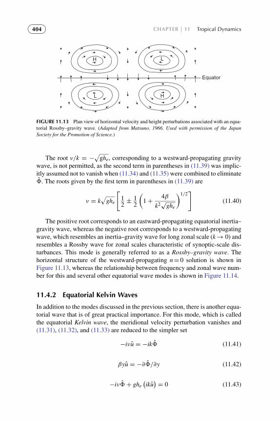
To protect the rights of the author(s) and publisher we inform you that this PDF is an uncorrected proof for internal businessuse only by the author(s), editor(s), reviewer(s), Elsevier and typesetter diacriTech. It is not allowed to publish this proofonline or in print. This proof copy is the copyright property of the publisher and is confidential until formal publication.
“Hakim: 15-ch11-377-412-9780123848666” — 2012/7/26 — 12:15 — page 404 — #28
404 CHAPTER | 11 Tropical Dynamics
Equator
L
L H
H
FIGURE 11.13 Plan view of horizontal velocity and height perturbations associated with an equa-torial Rossby–gravity wave. (Adapted from Matsuno, 1966. Used with permission of the JapanSociety for the Promotion of Science.)
The root ν/k = −√
ghe, corresponding to a westward-propagating gravitywave, is not permitted, as the second term in parentheses in (11.39) was implic-itly assumed not to vanish when (11.34) and (11.35) were combined to eliminate8. The roots given by the first term in parentheses in (11.39) are
ν = k√
ghe
[12±
12
(1+
4β
k2√
ghe
)1/2]
(11.40)
The positive root corresponds to an eastward-propagating equatorial inertia–gravity wave, whereas the negative root corresponds to a westward-propagatingwave, which resembles an inertia–gravity wave for long zonal scale (k→ 0) andresembles a Rossby wave for zonal scales characteristic of synoptic-scale dis-turbances. This mode is generally referred to as a Rossby–gravity wave. Thehorizontal structure of the westward-propagating n= 0 solution is shown inFigure 11.13, whereas the relationship between frequency and zonal wave num-ber for this and several other equatorial wave modes is shown in Figure 11.14.
11.4.2 Equatorial Kelvin Waves
In addition to the modes discussed in the previous section, there is another equa-torial wave that is of great practical importance. For this mode, which is calledthe equatorial Kelvin wave, the meridional velocity perturbation vanishes and(11.31), (11.32), and (11.33) are reduced to the simpler set
−iνu = −ik8 (11.41)
βyu = −∂8/∂y (11.42)
−iν8+ ghe(iku)= 0 (11.43)

To protect the rights of the author(s) and publisher we inform you that this PDF is an uncorrected proof for internal businessuse only by the author(s), editor(s), reviewer(s), Elsevier and typesetter diacriTech. It is not allowed to publish this proofonline or in print. This proof copy is the copyright property of the publisher and is confidential until formal publication.
“Hakim: 15-ch11-377-412-9780123848666” — 2012/7/26 — 12:15 — page 405 — #29
11.4 | Equatorial Wave Theory 405
Rossby
k*
v*
n=0
n=0
n=1
n=1n=2
n=1
n=2
n=2
n=3
Eastwardgravity
Westwardgravity
3
2
1
0
−1
−2
−3
Kelvin
wave
FIGURE 11.14 Dispersion diagram for free equatorial waves. Frequency and zonal wave numbers
have been nondimensionalized by defining ν∗≡ ν/(β√
ghe)1/2 k∗≡ k
(√ghe/β
)1/2. Curves showdependence of frequency on zonal wave number for eastward and westward gravity modes and forRossby and Kelvin modes. (k∗ axis tic marks at unit interval with 0 on left.)
Combining (11.41) and (11.43) to eliminate 8, we see that the Kelvin wavedispersion equation is identical to that for ordinary shallow water gravity waves:
c2≡ (ν/k)2 = ghe (11.44)
According to (11.44), the phase speed c can be either positive or negative. How-ever, if (11.41) and (11.42) are combined to eliminate 8, we obtain a first-orderequation for determining the meridional structure:
βyu = −c∂ u/∂y (11.45)
which may be integrated immediately to yield
u = uo exp(−βy2/2c
)(11.46)

To protect the rights of the author(s) and publisher we inform you that this PDF is an uncorrected proof for internal businessuse only by the author(s), editor(s), reviewer(s), Elsevier and typesetter diacriTech. It is not allowed to publish this proofonline or in print. This proof copy is the copyright property of the publisher and is confidential until formal publication.
“Hakim: 15-ch11-377-412-9780123848666” — 2012/7/26 — 12:15 — page 406 — #30
406 CHAPTER | 11 Tropical Dynamics
L H Equator
FIGURE 11.15 Plan view of horizontal velocity and height perturbations that are associated withan equatorial Kelvin wave. (Adapted from Matsuno, 1966.)
where u0 is the amplitude of the perturbation zonal velocity at the equator.Equation (11.46) shows that if solutions decaying away from the equator areto exist, the phase speed must be positive (c> 0). Thus, Kelvin waves are east-ward propagating and have zonal velocity and geopotential perturbations thatvary in latitude as Gaussian functions centered on the equator. The e-foldingdecay width is given by
YK = |2c/β|1/2
which for a phase speed c = 30 m s−1 gives YK ≈ 1600 km.The perturbation wind and geopotential structure for the Kelvin wave are
shown in plan view in Figure 11.15. In the zonal direction the force balance isexactly that of an eastward-propagating shallow water gravity wave. A verticalsection along the equator would thus be the same as that shown in Figure 5.10.The meridional force balance for the Kelvin mode is an exact geostrophic bal-ance between the zonal velocity and the meridional pressure gradient. It is thechange in sign of the Coriolis parameter at the equator that permits this specialtype of equatorial mode to exist.
11.5 STEADY FORCED EQUATORIAL MOTIONS
Not all zonally asymmetric circulations in the tropics can be explained on thebasis of inviscid equatorial wave theory. For quasi-steady circulations the zonalpressure gradient force must be balanced by turbulent drag rather than by inertia.The Walker circulation may be regarded as a quasi-steady equatorially trappedcirculation that is generated by diabatic heating. The simplest models of suchcirculations specify the diabatic heating and use the equations of equatorialwave theory to compute the atmospheric response. These models, however,neglect the fact that the distribution of diabatic heating is highly dependenton the mean wind and equivalent potential temperature distributions in theboundary layer. These in turn depend on the surface pressure and the mois-ture distribution, which are themselves dependent on the motion field. Thus,

To protect the rights of the author(s) and publisher we inform you that this PDF is an uncorrected proof for internal businessuse only by the author(s), editor(s), reviewer(s), Elsevier and typesetter diacriTech. It is not allowed to publish this proofonline or in print. This proof copy is the copyright property of the publisher and is confidential until formal publication.
“Hakim: 15-ch11-377-412-9780123848666” — 2012/7/26 — 12:15 — page 407 — #31
11.5 | Steady Forced Equatorial Motions 407
in a consistent model the diabatic heating cannot be regarded as an externallyspecified quantity, but must be obtained as part of the solution by, for example,using the cumulus parameterization scheme illustrated in Section 11.3.
As indicated in (11.25), this scheme requires information on the vertical dis-tribution of convective heating in order to solve for the temperature perturbationthroughout the troposphere. There is, however, evidence that the essential fea-tures of stationary equatorial circulations can be partly explained on the basisof a model that involves only the boundary layer. This is perhaps not surprisingsince the maintenance of a convective system depends on evaporation and mois-ture convergence in the boundary layer. Over the tropical oceans the boundarylayer can be approximated as a mixed layer of about 2-km depth. This is cappedby an inversion across which there is a density discontinuity δρ (see Figure 8.2).The virtual temperature in the mixed layer is strongly correlated with the seasurface temperature. If we assume that the pressure field is uniform at the topof the mixed layer, the surface pressure will be determined by hydrostatic massadjustment within the mixed layer. The resulting pressure perturbation in thelayer depends on the density discontinuity at the top of the layer and the devi-ation, h, of the layer depth from its mean depth Hb. In addition, there will bea contribution from the perturbation virtual potential temperature, θv , withinthe mixed layer. Thus, the perturbation geopotential in the mixed layer can beexpressed as
8 = g (δρ/ρ0) h− 0θv (11.47)
where 0≡ (gHb/θ0) is a constant and ρ0 and θ0 are constant mixed layerreference values of density and potential temperature, respectively.
According to (11.47), positive sea surface temperature anomalies and neg-ative boundary layer height anomalies will produce low surface pressures andvice versa. If the boundary layer depth does not vary too much, the surfacepressure gradient will thus tend to be proportional to the sea surface tempera-ture gradient. The dynamics of steady circulations in such a mixed layer can beapproximated by a set of linear equations analogous to the equatorial wave equa-tions (11.27), (11.28), and (11.29), but with the time derivative terms replacedby linear damping terms.
Thus, in the momentum equations the surface eddy stress is taken to be pro-portional to the mean velocity in the mixed layer. In the continuity equation theperturbation in the mixed layer height is proportional to the mass convergencein the layer, with a coefficient that is smaller in the presence of convection thanin its absence because of ventilation of the boundary layer by convection. Thex and y components of the vertically averaged momentum equation for steadymotions in the mixed layer can then be written as
αu− βyv + ∂8/∂x = 0 (11.48)
αv + βyu+ ∂8/∂y = 0 (11.49)

To protect the rights of the author(s) and publisher we inform you that this PDF is an uncorrected proof for internal businessuse only by the author(s), editor(s), reviewer(s), Elsevier and typesetter diacriTech. It is not allowed to publish this proofonline or in print. This proof copy is the copyright property of the publisher and is confidential until formal publication.
“Hakim: 15-ch11-377-412-9780123848666” — 2012/7/26 — 12:15 — page 408 — #32
408 CHAPTER | 11 Tropical Dynamics
whereas the continuity equation can be expressed as
αh+ Hb (1− ε) (∂u/∂x+ ∂v/∂y) = 0 (11.50)
where ε is a coefficient that is zero in the absence of convection and of order3/4 when convection occurs. Substituting from (11.47) into (11.50) yields
α8+ c2b (1− ε) (∂u/∂x+ ∂v/∂y) = −α0θv (11.51)
where c2b ≡ g (δρ/ρ0)Hb is the square of the phase speed for gravity waves
propagating along the inversion at the top of the mixed layer. See Battisti et al.(1999) for a more complete discussion.
Equations (11.48), (11.49), and (11.51) are a closed set for prediction of theboundary layer variables u, v,8 for a specified boundary layer perturbation vir-tual temperature θv . However, because the parameter ε depends on the presenceor absence of convection, the system can only be solved by iteration throughusing (11.22) to test for the presence of convection. This model can be used tocompute the steady surface circulation. A sample calculation of the anomalouscirculation for temperature anomalies corresponding to a typical ENSO event isshown in Figure 11.16. Note that the region of convergence is narrower than the
Divergence
20N0
0
EQ
20S
20N
EQ
20S
140E 160E 180 160W 140W 120W 100W 80W
Wind velocity
20N
EQ
20S
20N
EQ
20S
140E 160E 180 160W 140W 120W 100W 80W
0 −1
−1
−2
−2−2
−1
0
0
0
0
FIGURE 11.16 Steady surface circulation forced by sea surface temperature anomalies character-istic of El Nino in the equatorial Pacific. (Courtesy of D. Battisti.)

To protect the rights of the author(s) and publisher we inform you that this PDF is an uncorrected proof for internal businessuse only by the author(s), editor(s), reviewer(s), Elsevier and typesetter diacriTech. It is not allowed to publish this proofonline or in print. This proof copy is the copyright property of the publisher and is confidential until formal publication.
“Hakim: 15-ch11-377-412-9780123848666” — 2012/7/26 — 12:15 — page 409 — #33
Problems 409
region of warm SST anomalies due to the convective feedback in the boundarylayer model.
SUGGESTED REFERENCES
Philander, El Nino, La Nina, and the Southern Oscillation, is a well-written text that covers thedynamics of both atmospheric and oceanographic aspects of ENSO at an advanced level.
Trenberth (1991) is an excellent review article on ENSO.Wallace (1971) is a detailed review of the structure of synoptic-scale tropospheric wave disturbances
in the equatorial Pacific.Webster and Fasullo (2003) present an excellent review of the structure and dynamics of tropical
monsoons.
PROBLEMS
11.1. Suppose that the relative vorticity at the top of an Ekman layer at 15◦N isζ = 2×10⁻⁵ s−1. Let the eddy viscosity coefficient be Km = 10 m2 s−1 andthe water vapor mixing ratio at the top of the Ekman layer be 12 g kg−1.Use the method of Section 11.3 to estimate the precipitation rate due tomoisture convergence in the Ekman layer.
11.2. As mentioned in Section 11.1.3, barotropic instability is a possible energysource for some equatorial disturbances. Consider the following profilefor an easterly jet near the equator:
u (y) = −u0 sin2 [l (y− y0)]
where u0, y0, and l are constants and y is the distance from the equator.Determine the necessary conditions for this profile to be barotropicallyunstable.
11.3. Show that the nonlinear terms in the balance equation (11.15)
G (x, y) ≡ −∇2(
1
2∇ψ ·∇ψ
)+∇ ·
(∇ψ∇2ψ
)may be written in Cartesian coordinates as
G (x, y) = 2
[(∂2ψ/∂x2
) (∂2ψ/∂y2
)−
(∂2ψ/∂x∂y
)2]
11.4. With the aid of the results of Problem 11.3, show that if f is assumed to beconstant the balance equation (11.15) is equivalent to the gradient windequation (3.15) for a circularly symmetric regular low with geopotentialperturbation given by
8 = 80
(x2+ y2
)/L2
where 80 is a constant geopotential and L a constant length scale. Hint:Assume that ψ(x, y) has the same functional dependence on (x, y) asdoes 8.
To protect the rights of the author(s) and publisher we inform you that this PDF is an uncorrected proof for internal businessuse only by the author(s), editor(s), reviewer(s), Elsevier and typesetter diacriTech. It is not allowed to publish this proofonline or in print. This proof copy is the copyright property of the publisher and is confidential until formal publication.
“Hakim: 15-ch11-377-412-9780123848666” — 2012/7/26 — 12:15 — page 410 — #34
410 CHAPTER | 11 Tropical Dynamics
11.5. Starting from the perturbation equations (11.27), (11.28), and (11.29),show that the sum of kinetic plus available potential energy is conservedfor equatorial waves. Hence, show that for the Kelvin wave there is anequipartition of energy between kinetic and available potential energy.
11.6. Solve for the meridional dependence of the zonal wind and geopoten-tial perturbations for a Rossby–gravity mode in terms of the meridionalvelocity distribution (11.38).
11.7. Use the linearized model (11.48) and (11.49) to compute the meridionaldistribution of divergence in the mixed layer for a situation in which thegeostrophic wind is given by ug = uo exp
(−βy2/2c
), vg = 0, where u0
and c are constants.11.8. Show that the frequency of the n = 1 equatorial Rossby mode is given
approximately by ν = −kβ(k2+ 3β/
√ghe
)−1 and use this result to solvefor the u (y) and 8(y) fields in terms of v(y). Hint: Use the fact that theRossby wave phase speed is much less than
√ghe.
MATLAB ExercisesM11.1. The MATLAB script profile 2.m and the function Tmoist.m use Decem-
ber through March seasonal mean pressure and temperature data forSamoa (14◦S, 171◦W) in the file tropical temp.dat, together with anassumed constant relative humidity of 80%, to calculate and graph verti-cal profiles of temperature, dewpoint, and the temperature correspondingto pseudoadiabatic ascent from the lifting condensation level for a parcellifted from the lowest level of the sounding. Modify this script to plot pro-files of the potential temperature, the equivalent potential temperature, andthe saturation equivalent potential temperature. Hint: See Problem M9.2.
M11.2. For the thermodynamic sounding of Exercise M11.1, compute the CAPEand the profile of vertical velocity for a parcel lifted from the lowest layerin the absence of entrainment. What is the maximum vertical velocity andwhat is the distance that the parcel overshoots its level of neutral buoy-ancy? What can you conclude about convection associated with this meantropical sounding?
M11.3. Consider a simple nondivergent flow given by the streamfunction ψ =
A sin kx sin ly. The MATLAB script nonlinear balance.m solves the nonlinearbalance equation (11.15) for the corresponding geopotential 8, assum-ing that the Coriolis parameter is a constant corresponding to its value at30◦N. Run this script for several values of the amplitude, A, in the range0.4 × 107 to 4.0 × 10⁷ m2 s−1. Note how the geopotential field depends onA. For the case A = 4.0 × 10⁷m2 s−1 use the gradient function in MATLAB
to compute the geostrophic wind and thus find the ageostrophic wind.Plot these as quiver plots and explain why the ageostrophic wind has thestructure seen in your plot.
M11.4. A simple model for the horizontal flow in the mixed layer on an equato-rial β plane forced by an equatorial wave mode is given by the followingequations:
∂u
∂t= −αu+ βyv −
∂8
∂x

To protect the rights of the author(s) and publisher we inform you that this PDF is an uncorrected proof for internal businessuse only by the author(s), editor(s), reviewer(s), Elsevier and typesetter diacriTech. It is not allowed to publish this proofonline or in print. This proof copy is the copyright property of the publisher and is confidential until formal publication.
“Hakim: 15-ch11-377-412-9780123848666” — 2012/7/26 — 12:15 — page 411 — #35
Problems 411
∂v
∂t= −αv − βyu−
∂8
∂y
where 8(x, y, t) is given by (11.30) for the appropriate mode. The MATLAB
script equatorial mixed layer.m solves these equations numerically for thehorizontal velocity components and divergence field in the mixed layerforced by a specified Rossby–gravity wave (n = 0 mode) geopotential per-turbation corresponding to a westward-propagating disturbance of zonalwavelength 4000 km and
√ghe = 18 m s−1. Run the code for a long enough
time so that the solution becomes periodic in time. Rerun the model forzonal wavelength 10,000 km and
√ghe = 36 m s−1. In each case compare
the frequency of the oscillation with the Coriolis parameter at the latitude ofmaximum convergence forced by the wave. What can you conclude fromthese results?
M11.5. Modify the MATLAB script of M11.4 to compute the mixed layer velocity anddivergence pattern for the n = 1 Rossby mode for zonal wavelength 4000km and
√ghe = 18 m s−1 using the formulas for frequency and geopotential
derived in Problem 11.8.M11.6. The MATLAB script forced equatorial mode2.m shows the time develop-
ment of the velocity and height perturbations produced by a transientlocalized mass source for shallow water waves on an equatorial β plane.The model is based on equations (11.48), (11.49), and (11.51), but with timetendency terms included (ε = 0 is set here, but you can experiment with dif-ferent values if you wish). The source is located at the equator at x = 0. Itrises smoothly in amplitude for the first 2.5 days and then decreases to 0at day 5. Modify the script to contour the divergence and the vorticity. Runthe script for a 10-day period and interpret the results in terms of equatorialwave theory by noting the structure and speeds of energy propagation forthe disturbances to the east and west of the source.

To protect the rights of the author(s) and publisher we inform you that this PDF is an uncorrected proof for internal businessuse only by the author(s), editor(s), reviewer(s), Elsevier and typesetter diacriTech. It is not allowed to publish this proofonline or in print. This proof copy is the copyright property of the publisher and is confidential until formal publication.
“Hakim: 16-ch12-413-452-9780123848666” — 2012/7/26 — 12:29 — page 413 — #1
Chapter 12
Middle Atmosphere Dynamics
The middle atmosphere is generally regarded as the region extending from thetropopause (about 10–16 km altitude, depending on latitude) to about 100 km.The bulk of the middle atmosphere consists of two main layers, the stratosphereand the mesosphere, which are distinguished on the basis of temperature stratifi-cation (Figure 12.1). The stratosphere, which has large static stability associatedwith an overall increase of temperature with height, extends from the tropopauseto the stratopause at about 50 km. The mesosphere, which has a lapse rate simi-lar to that in the troposphere, extends from the stratopause to the mesopause atabout 80 to 90 km.
Previous chapters of this text have focused almost exclusively on the dynam-ics of the troposphere. The troposphere accounts for about 85% of the totalmass of the atmosphere and virtually all atmospheric water. There can be lit-tle doubt that processes occurring in the troposphere are primarily responsiblefor weather disturbances and climate variability. Nevertheless the middle atmo-sphere cannot be neglected. The troposphere and the middle atmosphere arelinked through radiative and dynamical processes that must be represented inglobal forecast and climate models. They are also linked through the exchangeof trace substances that are important in the photochemistry of the ozone layer.This chapter focuses primarily on dynamical processes in the lower part of themiddle atmosphere and their links to the troposphere.
12.1 STRUCTURE AND CIRCULATION OF THE MIDDLEATMOSPHERE
Zonal-mean temperature cross-sections for January and July in the lower andmiddle atmosphere are shown in the upper panels of Figures 12.2 and 12.3,respectively. Because very little solar radiation is absorbed in the troposphere,the thermal structure of the troposphere is maintained by an approximate bal-ance among infrared radiative cooling, vertical transport of sensible and latentheat away from the surface by small-scale eddies, and large-scale heat transportby synoptic-scale eddies. The net result is a mean temperature structure in whichthe surface temperature has its maximum in the equatorial region and decreases
An Introduction to Dynamic Meteorology. DOI: 10.1016/B978-0-12-384866-6.00012-XCopyright © 2013 Elsevier Inc. All rights reserved. 413

To protect the rights of the author(s) and publisher we inform you that this PDF is an uncorrected proof for internal businessuse only by the author(s), editor(s), reviewer(s), Elsevier and typesetter diacriTech. It is not allowed to publish this proofonline or in print. This proof copy is the copyright property of the publisher and is confidential until formal publication.
“Hakim: 16-ch12-413-452-9780123848666” — 2012/7/26 — 12:29 — page 414 — #2
414 CHAPTER | 12 Middle Atmosphere Dynamics
Thermosphere
Mesopause
Mesosphere
Stratopause
Stratosphere
TropopauseTroposphere
1000
500
200
100
50
20
10
5
2
1
0.5
0.2
0.1
0.05
0.020.01
0.005
0.0020.001
0
10
20
30
40
50
60
70
80
90
100
Hei
ght (
km)
Pre
ssur
e (h
Pa)
Temperature (K)
180 200 220 240 260 280
FIGURE 12.1 Midlatitude mean temperature profile. (Based on the U.S. Standard Atmosphere,1976.)
toward both the winter and the summer poles. There is also a rapid decrease inaltitude, with a lapse rate of about 6◦C km−1.
In the stratosphere, however, infrared radiative cooling is in the mean bal-anced primarily by radiative heating due to the absorption of solar ultravioletradiation by ozone. As a result of the solar heating in the ozone layer, themean temperature in the stratosphere increases with height to a maximum atthe stratopause near 50 km. Above the stratopause, temperature decreases withheight due to the reduced solar heating of ozone.
The meridional temperature structure in the middle atmosphere is also quitedifferent from that in the troposphere. In the lower stratosphere, where thetemperature is strongly influenced by upper tropospheric processes, there isa temperature minimum at the equator and maxima at the summer pole andin midlatitudes of the winter hemisphere. Above about 30 hPa the temperaturedecreases uniformly from summer pole to winter pole, in qualitative accord withradiative equilibrium conditions.

To protect the rights of the author(s) and publisher we inform you that this PDF is an uncorrected proof for internal businessuse only by the author(s), editor(s), reviewer(s), Elsevier and typesetter diacriTech. It is not allowed to publish this proofonline or in print. This proof copy is the copyright property of the publisher and is confidential until formal publication.
“Hakim: 16-ch12-413-452-9780123848666” — 2012/7/26 — 12:29 — page 415 — #3
12.1 | Structure and Circulation of the Middle Atmosphere 415
Temperature: January80
180
240
240
240
240240
240
−60−70
−50
240
220
220220
220 220
280260
220
260
260
260240 260
280280
260
260
260
200200
240220
220200
60
70
50
Hei
ght (
km)
30
20
10
0Latitude
Zonal wind: January
−20 20 40 60 80−40
−30
−10 −50−40
−20−30
−50−60
−10
−20
−30−10
−20
−40
−10 10
20
30
0
00
10
2010
0
0
30
30 20
30
4050
5060
40
0
20
20
2010
10
10
0
30
−60
0Latitude
−20 20 40 60 80−40−60
−80
40
80
60
70
50
Hei
ght (
km)
−80
40
30
20
10
−40
FIGURE 12.2 Observed monthly and zonally averaged temperature (K) and zonal wind (m s−1)
for January. (Based on Fleming et al., 1990.)
Mean zonal wind climatologies for the middle atmosphere are usuallyderived from the satellite-observed temperature field. This is done using thegeostrophic winds on an isobaric surface in the lower stratosphere (obtainedfrom conventional meteorological analyses) as a lower boundary condition andintegrating the thermal wind equation vertically. January and July mean zonalwind cross-sections are shown in the lower panels of Figures 12.2 and 12.3,respectively. The main features are an easterly jet in the summer hemisphereand a westerly jet in the winter hemisphere, with maxima in the wind speedsoccurring near the 60-km level. Of particular significance are the high-latitudewesterly jets in the winter hemispheres. These polar night jets provide wave
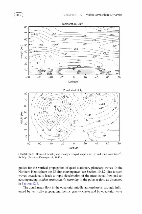
To protect the rights of the author(s) and publisher we inform you that this PDF is an uncorrected proof for internal businessuse only by the author(s), editor(s), reviewer(s), Elsevier and typesetter diacriTech. It is not allowed to publish this proofonline or in print. This proof copy is the copyright property of the publisher and is confidential until formal publication.
“Hakim: 16-ch12-413-452-9780123848666” — 2012/7/26 — 12:29 — page 416 — #4
416 CHAPTER | 12 Middle Atmosphere Dynamics
80
70
60
50
30
20
10
40
80
70
60
50
30
20
10
40
0
Latitude
−20 20 40 60 80−40−60−80
0
Latitude
−20 20 40 60 80−40−60−80
Hei
ght (
km)
Hei
ght (
km)
180
240
240
240
220
240 240
280
240
240
220
200220 220
280260 260
220
260
260
240
260
260
260
260 260280280
240
220
220
200
220
20040
−20 −30
−10
−30
−30
−20
−20
−40
−50
−50
−40
20
−10
1020
3040 50
60
50
30
60
20
10
70
80
7040
20
30
10
0
30
0
10
−30
−60
−70
40
−10
10
0
0
Temperature: July
Zonal wind: July
FIGURE 12.3 Observed monthly and zonally averaged temperature (K) and zonal wind (m s−1)for July. (Based on Fleming et al., 1990.)
guides for the vertical propagation of quasi-stationary planetary waves. In theNorthern Hemisphere the EP flux convergence (see Section 10.2.2) due to suchwaves occasionally leads to rapid deceleration of the mean zonal flow and anaccompanying sudden stratospheric warming in the polar region, as discussedin Section 12.4.
The zonal mean flow in the equatorial middle atmosphere is strongly influ-enced by vertically propagating inertia–gravity waves and by equatorial wave

To protect the rights of the author(s) and publisher we inform you that this PDF is an uncorrected proof for internal businessuse only by the author(s), editor(s), reviewer(s), Elsevier and typesetter diacriTech. It is not allowed to publish this proofonline or in print. This proof copy is the copyright property of the publisher and is confidential until formal publication.
“Hakim: 16-ch12-413-452-9780123848666” — 2012/7/26 — 12:29 — page 417 — #5
12.2 | The Zonal-Mean Circulation of the Middle Atmosphere 417
modes, especially the Kelvin and Rossby–gravity modes. These waves interactwith the mean flow to produce a long-period oscillation called quasi-biennialoscillation. This oscillation produces large year-to-year variability in the meanzonal wind in the equatorial middle atmosphere, which is not shown in thelong-term means of Figure 12.3.
12.2 THE ZONAL-MEAN CIRCULATION OF THE MIDDLEATMOSPHERE
As discussed in Section 10.1, the general circulation of the atmosphere con-sidered as a whole can be regarded to a first approximation as the atmosphericresponse to the diabatic heating caused by absorption of solar radiation at thesurface. Thus, it is reasonable to say that the atmosphere is driven by differentialdiabatic heating. For an open subregion of the atmosphere, such as the middleatmosphere, it is not correct, however, to assume that the circulation is drivenby diabatic heating. It is, rather, necessary to consider the transfer of momentumand energy between that subregion and the rest of the atmosphere.
In the absence of eddy motions, the zonal-mean temperature of the middleatmosphere would relax to a radiatively determined state in which, except for asmall lag due to thermal inertia, the temperature would correspond to an annu-ally varying radiative equilibrium following the annual cycle in solar heating.The circulation in such a situation would consist only of a zonal-mean zonalflow in thermal wind balance with the meridional temperature gradient. Neglect-ing small effects of the annual cycle, there would be no meridional or verticalcirculation and no stratosphere–troposphere exchange for such a hypotheticalstate.
A cross-section of the radiatively determined temperature during a NorthernHemisphere winter is shown in Figure 12.4. It should be compared to theobserved temperature profile for the same season that was shown in Figure 12.2.Although the rather uniform increase of temperature from winter pole to sum-mer pole in the region of 30- to 60-km altitude is qualitatively consistentwith the radiatively determined distribution, the actual temperature differencebetween the two poles is much smaller than in the radiatively determined state.Above 60 km even the sign of the gradient is opposite to that in the radiativesolution; the observed temperatures near the summer polar mesopause are muchcolder than those near the winter polar mesopause.
Departures from this radiatively determined state must be maintained byeddy transports. Thus, rather than causing the mean circulation, the radiativeheating and cooling patterns observed in the middle atmosphere are a result ofthe eddies driving the flow away from a state of radiative balance. This eddy-driven circulation has meridional and vertical wind components that inducesubstantial local departures from radiative equilibrium, especially in the winterstratosphere and in the mesosphere in both winter and summer.

To protect the rights of the author(s) and publisher we inform you that this PDF is an uncorrected proof for internal businessuse only by the author(s), editor(s), reviewer(s), Elsevier and typesetter diacriTech. It is not allowed to publish this proofonline or in print. This proof copy is the copyright property of the publisher and is confidential until formal publication.
“Hakim: 16-ch12-413-452-9780123848666” — 2012/7/26 — 12:29 — page 418 — #6
418 CHAPTER | 12 Middle Atmosphere Dynamics
80
60
70
Hei
ght (
km)
50
30
20
40
0Latitude
−20 20 40 60 80−40−60−80
210
230230
230
190
270270
250
210
190 150
150
170
170
170
210
190
230
210
250250
250
230
250
270
290270
230
January radiatively determined temperature
FIGURE 12.4 Radiatively determined middle atmosphere temperature distribution (K) for north-ern winter soltice from a radiative model that is time-marched through an annual cycle. Realistictropospheric temperatures and cloudiness are used to determine the upward radiative flux at thetropopause. (Based on Shine, 1987.)
12.2.1 Lagrangian Motion of Air Parcels
Viewed in the conventional Eulerian mean framework (Section 10.2.1), thetime-averaged zonal-mean temperature distribution in the middle atmosphereis determined by the net balance among net radiative heating or cooling, eddyheat transport, and adiabatic heating or cooling by the mean meridional circula-tion (v,w). That this framework does not provide a useful model for transportin the meridional plane can be seen easily by considering steady-state adiabaticmotion in the presence of large-scale waves. According to (10.12), in such asituation waves that have a positive poleward heat flux must drive a nonzero w,with upwelling at high latitudes and downwelling at low latitudes correspondingto the regions of heat flux convergence and divergence, respectively. However,if the flow is adiabatic, there can be no motion across the isentropes, and thusin steady state there can be no net vertical transport even though w is nonzero.Thus, w clearly does not provide an approximation to the vertical motion of airparcels (i.e., the vertical transport) in such a situation.
But how can vertical transport vanish when the Eulerian mean verticalmotion is finite? The resolution of this “nontransport” paradox can be illustratedby considering the kinematics of adiabatic flow in the presence of a stationary

To protect the rights of the author(s) and publisher we inform you that this PDF is an uncorrected proof for internal businessuse only by the author(s), editor(s), reviewer(s), Elsevier and typesetter diacriTech. It is not allowed to publish this proofonline or in print. This proof copy is the copyright property of the publisher and is confidential until formal publication.
“Hakim: 16-ch12-413-452-9780123848666” — 2012/7/26 — 12:29 — page 419 — #7
12.2 | The Zonal-Mean Circulation of the Middle Atmosphere 419
Up
Down
S3
S2
S1
3
2
1
S1 S2 S3
Latitude
(a)
(b)
Hei
ght
FIGURE 12.5 Parcel motions for an adiabatic planetary wave in a westerly zonal flow. (a) Solidlines labeled S1, S2, and S3 are parcel trajectories, heavy dashed lines are latitude circles, and lightdashed lines are contours of the vertical velocity field. (b) Projection of parcel oscillations on themeridional plane.
large-scale wave superposed on a background westerly flow as shown inFigure 12.5a. Parcels moving along the streamlines labeled S1, S2, and S3 willoscillate about their mean latitudes, moving equatorward and upward, then pole-ward and downward following the up and down displacements of the isentropicsurfaces associated with the wave. However, over a full wave period there canbe no net vertical motion following the parcels, as the parcels must remain on thesame isentropic surface. Hence there can be no vertical transport. If, however,an average vertical velocity is computed by taking the mean along a constantlatitude circle, then as clearly shown in Figure 12.5a, on the latitude circle φ3poleward of the maximum in wave amplitude, the Eulerian mean is upward,w(φ3)> 0, as regions of upward motion dominate over regions of downwardmotion at that latitude.
Conversely, on the latitude circle φ1 equatorward of the maximum in waveamplitude, the Eulerian mean is downward w(φ1)< 0. The conventional Eule-rian mean circulation thus suggests misleadingly that a trace constituent wouldbe transported upward poleward of the latitude of maximum wave ampli-tude and downward equatorward of that latitude. In reality, air parcels in thisidealized example of adiabatic wave motion are not undergoing net vertical

To protect the rights of the author(s) and publisher we inform you that this PDF is an uncorrected proof for internal businessuse only by the author(s), editor(s), reviewer(s), Elsevier and typesetter diacriTech. It is not allowed to publish this proofonline or in print. This proof copy is the copyright property of the publisher and is confidential until formal publication.
“Hakim: 16-ch12-413-452-9780123848666” — 2012/7/26 — 12:29 — page 420 — #8
420 CHAPTER | 12 Middle Atmosphere Dynamics
S1S3
Latitude
Hei
ght
S2
χ
χ − δ χ
χ + δ χ
FIGURE 12.6 Projections of parcel motions on the meridional plane for planetary waves in west-erlies with diabatic heating at low latitudes and diabatic cooling at high latitudes. Thin dashed linesshow tilting of isosurfaces of tracer mixing ratio due to transport by the diabatic circulation.
displacements, but are simply oscillating back and forth along the same isen-tropic surface with trajectories whose meridional projections are closed ellipsesas shown in Figure 12.5b. In such a situation there is no net vertical parcelmotion, and thus no net vertical transport.
Only if there is net diabatic heating or cooling can there be mean trans-port across the isentropes. In the winter stratosphere, where stationary planetarywave amplitudes tend to be large and there is diabatic heating at low latitudesand diabatic cooling at high latitudes, the meridional projection of actual par-cel motions is a combination of the elliptical orbits of Figure 12.5b and meanvertical drift as indicated in Figure 12.6, which clearly shows that a verticallystratified long-lived trace constituent is transported upward at low latitudes anddownward at high latitudes because of vertical transport of fluid parcels associ-ated with diabatic heating and cooling. Thus, in order to represent net transporteffects efficiently, a zonal averaging process should yield an average verticalcirculation that mimics the net cross-isentropic parcel motion.
12.2.2 The Transformed Eulerian Mean
In many circumstances the transformed Eulerian mean (TEM) equations intro-duced in Section 10.2.2 provide a useful model for the study of global-scalemiddle atmospheric transport. Recall that in this formulation the zonal-meanmomentum, mass continuity, thermodynamic energy, and thermal wind equa-tions have the form1
∂u/∂t − f0v∗= ρ−1
0 ∇·F+ X ≡ G (12.1)
1As in Chapter 10, we express the log-pressure coordinate simply as z rather than z ∗.

To protect the rights of the author(s) and publisher we inform you that this PDF is an uncorrected proof for internal businessuse only by the author(s), editor(s), reviewer(s), Elsevier and typesetter diacriTech. It is not allowed to publish this proofonline or in print. This proof copy is the copyright property of the publisher and is confidential until formal publication.
“Hakim: 16-ch12-413-452-9780123848666” — 2012/7/26 — 12:29 — page 421 — #9
12.2 | The Zonal-Mean Circulation of the Middle Atmosphere 421
∂T/∂t + N2HR−1w ∗ = −αr[T − Tr (y, z, t)
](12.2)
∂v ∗/∂y+ ρ−10 ∂
(ρ0w ∗
)/∂z = 0 (12.3)
f0∂u/∂z+ RH−1∂T/∂y = 0 (12.4)
Here the residual circulation (v ∗,w ∗) is as defined in (10.16a,b), F designatesthe EP flux due to large-scale eddies, X is the zonal force due to small-scaleeddies (e.g., gravity wave drag), and G designates the total zonal force. In (12.2)the diabatic heating is approximated in terms of a Newtonian relaxation propor-tional to the departure of the zonal mean temperature T(y, z, t) from its radiativeequilibrium value Tr(y, z, t), where αr is the Newtonian cooling rate.
To understand how eddies can lead to departures of the zonal-mean tem-perature distribution in the middle atmosphere from its radiatively determinedstate, we use the TEM system of equations to consider an idealized model ofextratropical forcing. The dependence of the circulation on forcing frequencycan be examined in an idealized model in which Tr is taken to be a function ofheight alone, and the forcing has a simple harmonic dependence in time withfrequency σ . Then w ∗ and G are of the form[
w ∗
G
]= Re
[w (φ, z)G (φ, z)
]eiσ t (12.5)
where w and G are complex latitude- and height-dependent amplitudes. Com-bining (12.1) and (12.3) to eliminate v ∗ and combining the resulting equationwith (12.2) and (12.4) to eliminate T yields a partial differential equation for w:
∂
∂z
(1
ρ0
∂(ρ0w
)∂z
)+
(iσ
iσ + αr
)(N2
f 20
)∂2w
∂y2=
1
f0
∂
∂y
(∂G
∂z
)(12.6)
The structure of w in the meridional plane depends on the latitudinal and verticaldistribution of the forcing G. The differential equation (12.6) is elliptic in form.Such a form implies that a forcing applied locally in any region will producea nonlocal response in the form of a large-scale circulation that acts to main-tain the zonal flow in thermal wind balance with the meridional temperaturegradient.
As suggested by the coefficients of (12.6), the character of the nonlocalresponse depends on the ratio of the frequency of the forcing to the Newtonianrelaxation rate. We consider three cases:
1. High-frequency variations σ�αr: The motions are approximately adiabatic(as is true in sudden stratospheric warmings)—that is,
iσ
iσ + αr→ 1

To protect the rights of the author(s) and publisher we inform you that this PDF is an uncorrected proof for internal businessuse only by the author(s), editor(s), reviewer(s), Elsevier and typesetter diacriTech. It is not allowed to publish this proofonline or in print. This proof copy is the copyright property of the publisher and is confidential until formal publication.
“Hakim: 16-ch12-413-452-9780123848666” — 2012/7/26 — 12:29 — page 422 — #10
422 CHAPTER | 12 Middle Atmosphere Dynamics
Away from the forcing region, the right side of (12.6) vanishes so that thetwo terms on the left must balance each other. For this balance to hold, asimple scaling argument indicates that in midlatitudes the vertical scale δzof the response must be related to the horizontal scale as δz ∼ (f0/N) δy ∼10−2δy.
2. Low-frequency variations (e.g., the annual cycle): The Newtonian relaxationcoefficient has a magnitude of order αr ≈ 1/(20 days) in the lower strato-sphere, increasing to αr ≈ 1/(5 days) near the stratopause. Thus αr > σ andthe coefficient multiplying the second term on the left in (12.6) is reducedfrom its value in case (1) so that the vertical penetration scale is increased.
3. Steady-state regime σ/αr→ 0: In this limit ∂u/∂t= 0, and rather than using(12.6), it is simpler to note that (12.1) in this case reduces to a simple balancebetween the Coriolis force and the zonal drag force:
− f0v∗= G (12.7)
Combining this equation with the continuity equation (12.3) and requiring that
ρ0w ∗→ 0 as z→∞
it follows that
ρow ∗ = −∂
∂y
1
f0
∞∫z
ρ0Gdz′
(12.8)
According to (12.8), w ∗ is zero in the regions above a localized forcing region,whereas it is constant for regions directly below it; hence the term downwardcontrol is sometimes used to refer to this steady-state situation.
Substitution of (12.8) into the first law of thermodynamics (12.2) andneglecting the time-dependent term yield an expression that explicitly showsthe dependence on the zonal force distribution of the departure of the time andzonally averaged temperature from radiative equilibrium:
(T − Tr
)=
N2H
αrρ0R
∂
∂y
1
f0
∞∫z
ρ0Gdz′
(12.9)
Thus, in steady state the departure of temperature from radiative equilibrium ata given level depends on the meridional gradient of the zonal force distributionin the column above that level.
For mathematical simplicity, the variation of the Coriolis parameter with lat-itude and other effects of spherical geometry have been neglected in deriving theequations of this section. It is straightforward to extend this model to sphericalcoordinates. Figure 12.7 shows streamlines of the meridional mass circulation

To protect the rights of the author(s) and publisher we inform you that this PDF is an uncorrected proof for internal businessuse only by the author(s), editor(s), reviewer(s), Elsevier and typesetter diacriTech. It is not allowed to publish this proofonline or in print. This proof copy is the copyright property of the publisher and is confidential until formal publication.
“Hakim: 16-ch12-413-452-9780123848666” — 2012/7/26 — 12:29 — page 423 — #11
60
50
40
30H
eigh
t (km
)
20
10
0
60
50
40
30
Hei
ght (
km)
20
10
0
60
50
40
30
Hei
ght (
km)
20
10
0
−80 −60 −40 −20 0
Latitude
(a)
20 40 60 80
−80 −60 −40 −20 0
Latitude
(b)
(c)
20 40 60 80
−80 −60 −40 −20 0
Latitude
20 40 60 80
FIGURE 12.7 Response of the zonally symmetric circulation to a westward force applied in theshaded region. Contours are streamlines of the TEM meridional circulation, with the same contourinterval used in each panel. (a) Adiabatic response for high-frequency forcing. (b) Response forannual frequency forcing and 20-day radiative damping timescale; solid and dashed contours showthe response that is in phase and 90◦ out of phase, respectively, with the forcing. (c) Responseto steady-state forcing. (After Holton et al., 1995. Used with permission of American GeophysicalUnion.)

To protect the rights of the author(s) and publisher we inform you that this PDF is an uncorrected proof for internal businessuse only by the author(s), editor(s), reviewer(s), Elsevier and typesetter diacriTech. It is not allowed to publish this proofonline or in print. This proof copy is the copyright property of the publisher and is confidential until formal publication.
“Hakim: 16-ch12-413-452-9780123848666” — 2012/7/26 — 12:29 — page 424 — #12
424 CHAPTER | 12 Middle Atmosphere Dynamics
in response to isolated extratropical forcing for three cases corresponding tothe differing frequency regimes discussed earlier, but with spherical geometryretained.
A comparison of Figures 12.2 and 12.4 shows that the largest departuresfrom radiative equilibrium occur in the summer and winter mesosphere and inthe polar winter stratosphere. According to (12.9), these are the locations andseasons when zonal forcing must be strongest. The zonal force in the meso-sphere is believed to be caused primarily by vertically propagating internalgravity waves. These transfer momentum from the troposphere into the meso-sphere, where wave breaking produces strong zonal forcing. The zonal force inthe winter stratosphere is due primarily to stationary planetary Rossby waves.These, as discussed in Section 12.3, can propagate vertically provided that themean zonal wind is westerly and less than a critical value that depends stronglyon the wavelength of the waves. Thus, in the extratropical stratosphere weexpect a strong annual cycle in δT , with large values (i.e., strong departure fromradiative equilibrium) in winter and small values in summer.
This is indeed observed (see Figures 12.2 and 12.4). Furthermore, becauseeddy forcing maintains the observed temperature above its radiative equilib-rium in the extratropical stratosphere, there is radiative cooling, and from (12.3)the residual vertical motion must be downward. By mass continuity it is thenrequired that the residual vertical motion be upward in the tropics, implying thatthe temperature must be below radiative equilibrium in that region. Note that itis the dynamical driving by extratropical eddies, rather than local forcing, thatis responsible for the upward residual motion and net radiative heating in thetropical stratosphere.
12.2.3 Zonal-Mean Transport
Viewed from the TEM perspective, the overall meridional circulation in thewinter stratosphere is qualitatively as pictured in Figure 12.8. The residualcirculation transfers mass and trace chemicals upward across the tropopausein the tropics and downward in the extratropics. This vertical circulation isclosed in the lower stratosphere by a poleward meridional drift balanced byEP flux convergence. That this schematic picture gives a qualitatively correctview can be ascertained by examining the zonal-mean mixing ratio distributionof any long-lived vertically stratified trace species. As an example, the distri-bution of N2O is shown in Figure 12.9. N2O is produced at the surface andis mixed uniformly in the troposphere, but then it decays with height in thestratosphere due to photochemical dissociation. Thus, as shown in Figure 12.9,the mixing ratio decreases upward in the stratosphere. Note, however, thatsurfaces of constant mixing ratio are displaced upward in the tropics and down-ward at higher latitudes, suggesting that the mean meridional mass transportis upward in the tropics and downward in the extratropics as suggested inFigure 12.9.

To protect the rights of the author(s) and publisher we inform you that this PDF is an uncorrected proof for internal businessuse only by the author(s), editor(s), reviewer(s), Elsevier and typesetter diacriTech. It is not allowed to publish this proofonline or in print. This proof copy is the copyright property of the publisher and is confidential until formal publication.
“Hakim: 16-ch12-413-452-9780123848666” — 2012/7/26 — 12:29 — page 425 — #13
12.2 | The Zonal-Mean Circulation of the Middle Atmosphere 425
5
10
15
20
25
30
35
Wave-driven
“Pump”
30
100
300
10000 30 60 90
Latitude
Pre
ssur
e (h
Pa)
10
Alti
tude
(km
)
Tropopause
FIGURE 12.8 Schematic cross-section of the wave-driven circulation in the middle atmosphereand its role in transport. Thin dashed lines denote potential temperature surfaces. Dotted line is thetropopause. Solid lines are contours of the TEM meridional circulation driven by the wave-inducedforcing (shaded region). Wavy double-headed arrows denote meridional transport and mixing byeddy motions. Heavy dashed line shows an isopleth of mixing ratio for a long-lived tracer.
In addition to the slow meridional drift by the residual meridional veloc-ity shown in Figure 12.8, tracers in the winter stratosphere are also subject torapid quasi-isentropic transport and mixing by breaking planetary waves. Sucheddy transport, which is highly variable in space and time, must be included forquantitatively accurate modeling of transport within the stratosphere.
In the mesosphere the residual circulation is dominated by a single circu-lation cell with upward motion in the summer polar region, meridional driftfrom the summer to the winter hemisphere, and subsidence in the winter polarregion. This circulation, like the residual circulation in the stratosphere, iseddy driven. However, in the mesosphere it appears that the dominant eddiesare vertically propagating internal gravity waves, which have shorter scales inspace and time than the planetary waves that dominate the eddy activity in thestratosphere.

To protect the rights of the author(s) and publisher we inform you that this PDF is an uncorrected proof for internal businessuse only by the author(s), editor(s), reviewer(s), Elsevier and typesetter diacriTech. It is not allowed to publish this proofonline or in print. This proof copy is the copyright property of the publisher and is confidential until formal publication.
“Hakim: 16-ch12-413-452-9780123848666” — 2012/7/26 — 12:29 — page 426 — #14
426 CHAPTER | 12 Middle Atmosphere Dynamics
Latitude
20
1.20
1.00
0.800.
600.
40
1.40
1.60
0.40
0.60
0.80
1.00
1.201.40
0.20
30
Hei
ght (
km)
40
50
90°S 60°S 30°S 30°N 60°N 90°N0°
FIGURE 12.9 October zonal mean cross-section of methane (ppmv) from observations by theHALOE on the UARS. Note the strong vertical stratification due to photochemical destruction inthe stratosphere. The upward-bulging mixing ratio isopleths in the equatorial region are evidence ofupward mass flow in the equatorial region, whereas the downward-sloping isopleths in high latitudesare evidence of subsidence in the polar regions. The region of flattened isopleths in the midlati-tudes of the Southern Hemisphere is evidence for quasi-adiabatic wave transport due to wintertimeplanetary wave activity. (After Norton, 2003.)
12.3 VERTICALLY PROPAGATING PLANETARY WAVES
In Section 12.1 we pointed out that the predominant eddy motions in the strato-sphere are vertically propagating quasi-stationary planetary waves (Rossbywaves) and that these waves are confined to the winter hemisphere. To under-stand the absence of synoptic-scale motions and the confinement of stationaryplanetary waves to the winter hemisphere, it is necessary to examine theconditions under which planetary waves can propagate vertically.
12.3.1 Linear Rossby Waves
To analyze planetary wave propagation in the stratosphere, it is convenient towrite the equations of motion in the log-pressure coordinate system introduced

To protect the rights of the author(s) and publisher we inform you that this PDF is an uncorrected proof for internal businessuse only by the author(s), editor(s), reviewer(s), Elsevier and typesetter diacriTech. It is not allowed to publish this proofonline or in print. This proof copy is the copyright property of the publisher and is confidential until formal publication.
“Hakim: 16-ch12-413-452-9780123848666” — 2012/7/26 — 12:29 — page 427 — #15
12.3 | Vertically Propagating Planetary Waves 427
in Section 7.4.1. For analysis of extratropical planetary wave motions in themiddle atmosphere, we may refer the motions to the midlatitude β plane anduse the quasi-geostrophic potential vorticity equation, which in log-pressurecoordinates can be written as(
∂
∂t+ Vg·∇
)q = 0 (12.10)
where
q ≡ ∇2ψ + f +f 20
ρ0N2
∂
∂z
(ρ0∂ψ
∂z
)Here ψ =8/f0 is the geostrophic streamfunction and f0 is a constant midlati-tude reference value of the Coriolis parameter. We now assume that the motionconsists of a small-amplitude disturbance superposed on a constant zonal-meanflow. Thus, letting ψ = −uy + ψ ′, q = q + q′ and linearizing (12.10), we findthat the perturbation q′ field must satisfy(
∂
∂t+ u
∂
∂x
)q′ + β
∂ψ ′
∂x= 0 (12.11)
where
q′ ≡ ∇2ψ ′ +f 20
ρ0N2
∂
∂z
(ρ0∂ψ ′
∂z
)(12.12)
Equation (12.11) has solutions in the form of harmonic waves with zonaland meridional wave numbers k and l and zonal phase speed cx:
ψ ′ (x, y, z, t) = 9 (z) ei(kx+ly−kcxt)+z/2H (12.13)
Here the factor ez/2H (which is proportional to ρ−1/20 ) is included to simplify the
equation for the vertical dependence. Substituting (12.13) into (12.11) yields
d29/dz2+ m29 = 0 (12.14)
where
m2≡
N2
f 20
[β
(u− cx)−
(k2+ l2
)]−
1
4H2(12.15)
Referring back to Section 7.4, we recall that m2> 0 is required for verticalpropagation, and in that case, m is the vertical wave number; that is, solutionsof (12.14) have the form 9(z)=Aeimz, where A is a constant amplitude and

To protect the rights of the author(s) and publisher we inform you that this PDF is an uncorrected proof for internal businessuse only by the author(s), editor(s), reviewer(s), Elsevier and typesetter diacriTech. It is not allowed to publish this proofonline or in print. This proof copy is the copyright property of the publisher and is confidential until formal publication.
“Hakim: 16-ch12-413-452-9780123848666” — 2012/7/26 — 12:29 — page 428 — #16
428 CHAPTER | 12 Middle Atmosphere Dynamics
the sign of m is determined by requiring that the vertical component of groupvelocity be positive. For stationary waves (cx= 0), we see from (12.15) thatvertically propagating modes can exist only for mean zonal flows that satisfy thecondition
0 < u < β[(
k2+ l2
)+ f 2
0 /(
4N2H2)]−1
≡ Uc (12.16)
where Uc is called the Rossby critical velocity. Thus, vertical propagation ofstationary waves can occur only in the presence of westerly winds weaker thana critical value that depends on the horizontal scale of the waves. In the summerhemisphere the stratospheric mean zonal winds are easterly so that stationaryplanetary waves are all trapped vertically.
In the real atmosphere the mean zonal wind is not constant, but depends onlatitude and height. However, both observational and theoretical studies suggestthat (12.16) still provides a qualitative guide for estimating vertical propagationof planetary waves, even though the actual critical velocity may be larger thanindicated by the β-plane theory.
12.3.2 Rossby Wavebreaking
The term wavebreaking for Rossby waves simply refers to a rapid, irreversibledeformation of material contours. Since by (12.10) potential vorticity is approx-imately conserved in Rossby waves, isolines of potential vorticity on isentropicsurfaces approximate material contours, and wavebreaking can best be illus-trated by considering the field of potential vorticity. Wavebreaking may occurwhen the disturbance fields reach amplitudes for which nonlinear effects canno longer be neglected in the dynamical equations. For example, if the flowis divided into mean and disturbance parts, and nonlinear terms are included,the equation for conservation of quasi-geostrophic potential vorticity (12.10)becomes (
∂
∂t+ u
∂
∂x
)q′ + v′
∂q
∂y= −u′
∂q′
∂x− v′
∂q′
∂y(12.17)
For steady waves propagating relative to the ground at zonal-phase speed cx,the variation of phase in time and space is given by φ= k (x− cxt), where k isthe zonal wave number, and it is readily verified that
∂
∂t= −cx
∂
∂x
so that in the linearized version of (12.17) there is a balance between advectionof the disturbance potential vorticity q′ by the Doppler-shifted mean wind and
To protect the rights of the author(s) and publisher we inform you that this PDF is an uncorrected proof for internal businessuse only by the author(s), editor(s), reviewer(s), Elsevier and typesetter diacriTech. It is not allowed to publish this proofonline or in print. This proof copy is the copyright property of the publisher and is confidential until formal publication.
“Hakim: 16-ch12-413-452-9780123848666” — 2012/7/26 — 12:29 — page 429 — #17
12.3 | Vertically Propagating Planetary Waves 429
the advection of mean potential vorticity by the disturbance meridional wind:
(u− cx)∂q′
∂x= −v′
∂q
∂y(12.18)
The validity of the linear approximation can thus be assessed by comparingthe sizes of the two terms on the right side of (12.17) with either term in (12.18).Linearity holds provided that ∣∣u− cx
∣∣� ∣∣u′∣∣ (12.19a)
and
∂q/∂y�∣∣∂q′/∂y
∣∣ (12.19b)
Basically these criteria require that the slope of the material contours in the x, yplane must be small.
As indicated in (12.13), in an atmosphere with constant mean zonal wind,vertically propagating linear Rossby waves have amplitudes increasing expo-nentially in height. Thus, at some altitude the disturbance amplitude will becomesufficiently large so that wavebreaking must occur. In the real atmosphere, how-ever, the mean-zonal flow varies in both latitude and height, and this variationis crucial for understanding the distribution and mean-flow forcing provided byRossby wavebreaking. The simplest example of Rossby wavebreaking occurs inthe presence of a critical surface along which the Doppler-shifted phase speedof the wave vanishes (u− cx= 0). In that case (12.19a) cannot be satisfied evenfor small-amplitude waves.
For understanding wave behavior near critical lines it is helpful to generalizethe Rossby wave analysis of Section 12.3.1 to a situation such as that shownin the seasonal mean cross-sections of Figure 12.2 in which the zonal winddepends on latitude and height, u= u (y, z). The x and t dependence in (12.11)can then be separated by seeking solutions of the form
ψ ′ = ez/2HRe[9 (y, z) eik(x−cxt)
](12.20)
We obtain
∂29
∂y2+
f 20
N2
∂29
∂z2+ n2
k9 = 0 (12.21)
where the small vertical variation of N2 is neglected, and
n2k (y, z) = (u− cx)
−1 ∂q/∂y− k2− f 2
0
/(4H2N2
)(12.22)

To protect the rights of the author(s) and publisher we inform you that this PDF is an uncorrected proof for internal businessuse only by the author(s), editor(s), reviewer(s), Elsevier and typesetter diacriTech. It is not allowed to publish this proofonline or in print. This proof copy is the copyright property of the publisher and is confidential until formal publication.
“Hakim: 16-ch12-413-452-9780123848666” — 2012/7/26 — 12:29 — page 430 — #18
430 CHAPTER | 12 Middle Atmosphere Dynamics
Equation (12.21) has a form similar to that of the equation governing thetwo-dimensional propagation of light waves in a medium with variable refrac-tive index, nk. The propagation of linear Rossby wave EP flux in that case can beshown to be along rays that behave somewhat like light rays. Thus, wave activ-ity will tend to propagate along rays that bend toward regions of large positiven2
k and avoid regions of negative n2k . For stationary Rossby waves (cx= 0) of
low zonal wave number, n2k is positive in a region with westerly winds that are
not too strong, and increases to infinity along a critical surface where the meanflow vanishes. Thus, the index of refraction for wave activity is positive in thewinter hemisphere, but increases rapidly toward the equatorial zero wind line.As a result, Rossby wave activity tends to propagate upward and equatorward,and wavebreaking occurs in the vicinity of the equatorial critical line.
12.4 SUDDEN STRATOSPHERIC WARMINGS
In the lower stratosphere the temperature is a minimum at the equator and hasmaxima at the summer pole and at about 45◦ latitude in the winter hemisphere(see Figure 12.2). From thermal wind considerations the rapid decrease of tem-perature poleward of 45◦ in winter requires a zonal vortex with strong westerlyshear with height.
In the Northern Hemisphere, every other year or so, this normal winterpattern of a cold polar stratosphere with a westerly vortex is interrupted in aspectacular manner in midwinter. Within the space of a few days the polar vortexbecomes highly distorted and breaks down (see Figure 12.10) with an accompa-nying large-scale warming of the polar stratosphere, which can quickly reversethe meridional temperature gradient and (through thermal wind balance) createa circumpolar easterly current. Warmings of 40 K in a few days have occurredat the 50-hPa level.
Numerous observational studies of sudden warmings confirm that enhancedpropagation of planetary waves from the troposphere, primarily zonal wavenumbers 1 and 2, is essential for the development of the warmings. Since majorwarmings are observed primarily in the Northern Hemisphere, it is logical toconclude that enhanced wave propagation into the stratosphere is due to topo-graphically forced waves, which are much stronger in the Northern Hemispherethan in the Southern Hemisphere. Even in the Northern Hemisphere, however, itis apparently only in certain winters that conditions are right to produce suddenwarmings.
It is generally accepted that sudden warmings are an example of transientmean-flow forcing due to planetary wave driving. Section 10.2.3 showed that inorder for planetary waves to decelerate the zonal-mean circulation, there mustbe a nonzero equatorward eddy potential vorticity flux (i.e., a net EP flux conver-gence). We further showed that for steady nondissipative waves, the divergenceof the EP flux vanishes. For normal stationary planetary waves in the strato-spheric polar night jet, this constraint should be at least approximately satisfied,

To protect the rights of the author(s) and publisher we inform you that this PDF is an uncorrected proof for internal businessuse only by the author(s), editor(s), reviewer(s), Elsevier and typesetter diacriTech. It is not allowed to publish this proofonline or in print. This proof copy is the copyright property of the publisher and is confidential until formal publication.
“Hakim: 16-ch12-413-452-9780123848666” — 2012/7/26 — 12:29 — page 431 — #19
H
H
HL
2880
3008
30723072
3072
3072
3072
Analysis 12 UTC February 11
H
3072
3072
Analysis 12 UTC February 16
(a)
(b)
3008
3072
L
FIGURE 12.10 10-hPa geopotential height analyses for days in 1979: February 11 (a), February16 (b), and February 21 (c) at 12 UTC, showing breakdown of the polar vortex associated with awave number 2’s sudden stratospheric warming. Contour interval: 16 dam. (Analysis from ERA-40reanalysis courtesy of the European Centre for Medium-Range Weather Forecasts.)
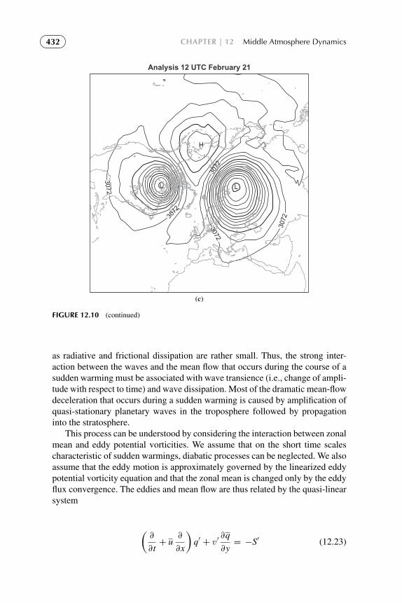
To protect the rights of the author(s) and publisher we inform you that this PDF is an uncorrected proof for internal businessuse only by the author(s), editor(s), reviewer(s), Elsevier and typesetter diacriTech. It is not allowed to publish this proofonline or in print. This proof copy is the copyright property of the publisher and is confidential until formal publication.
“Hakim: 16-ch12-413-452-9780123848666” — 2012/7/26 — 12:29 — page 432 — #20
432 CHAPTER | 12 Middle Atmosphere Dynamics
L
3072
Analysis 12 UTC February 21
(c)
3072
3072
3072
3072
H
L
FIGURE 12.10 (continued)
as radiative and frictional dissipation are rather small. Thus, the strong inter-action between the waves and the mean flow that occurs during the course of asudden warming must be associated with wave transience (i.e., change of ampli-tude with respect to time) and wave dissipation. Most of the dramatic mean-flowdeceleration that occurs during a sudden warming is caused by amplification ofquasi-stationary planetary waves in the troposphere followed by propagationinto the stratosphere.
This process can be understood by considering the interaction between zonalmean and eddy potential vorticities. We assume that on the short time scalescharacteristic of sudden warmings, diabatic processes can be neglected. We alsoassume that the eddy motion is approximately governed by the linearized eddypotential vorticity equation and that the zonal mean is changed only by the eddyflux convergence. The eddies and mean flow are thus related by the quasi-linearsystem
(∂
∂t+ u
∂
∂x
)q′ + v′
∂q
∂y= −S′ (12.23)

To protect the rights of the author(s) and publisher we inform you that this PDF is an uncorrected proof for internal businessuse only by the author(s), editor(s), reviewer(s), Elsevier and typesetter diacriTech. It is not allowed to publish this proofonline or in print. This proof copy is the copyright property of the publisher and is confidential until formal publication.
“Hakim: 16-ch12-413-452-9780123848666” — 2012/7/26 — 12:29 — page 433 — #21
12.4 | Sudden Stratospheric Warmings 433
where again
q′ ≡ ∇2ψ ′ +f 20
ρ0
∂
∂z
(ρ0
N2
∂ψ ′
∂z
)(12.24)
and an eddy damping term, –S′, has been added to represent the effects of bothmechanical and thermal dissipation. (For constant and equal Rayleigh frictionand Newtonian cooling, S′=αq′, where α is the dissipation rate coefficient.)Multiplying (12.23) by q′ and averaging zonally after noting that
u q′∂q′
∂x=
u
2
∂q′2
∂x= 0
yields with the aid of (10.26)
∂A
∂t+∇·F = D (12.25)
where wave activity, A, and dissipation, D, are defined, respectively, as
A ≡ρ0(q′)
2
2∂q/∂y, and D ≡ −
ρ0S′q′
∂q/∂y(12.26)
For linear planetary waves satisfying the quasi-geostrophic equations, it canbe shown that
F =(0, cgy, cgz
)A (12.27)
so that the EP flux is given by the wave activity times the group velocity inthe meridional (y, z) plane. It is the flux of wave activity—not the flux of waveenergy—that is fundamental for wave–mean-flow interaction.
Equation (12.25) shows that if dissipation and transience vanish, the EP fluxdivergence must vanish. Substitution into (12.1) then gives the nonaccelera-tion theorem, which states that there is no wave-driven mean-flow accelerationfor steady (∂A/∂t= 0) and conservative (D= 0) waves. The EP flux diver-gence, which must be nonzero for wave-induced forcing, is dependent on wavetransience and dissipation.
In sudden stratospheric warmings the planetary wave amplitudes increaserapidly in time. During the Northern Hemisphere winter, quasi-stationary plan-etary waves of zonal wave numbers 1 and 2 are produced in the troposphereby orographic forcing. These waves propagate vertically into the stratosphere,implying a local increase in the wave activity. Thus, ∂A/∂t > 0, implying from(12.25) that, for quasi-conservative flow, the flux of quasi-geostrophic potential

To protect the rights of the author(s) and publisher we inform you that this PDF is an uncorrected proof for internal businessuse only by the author(s), editor(s), reviewer(s), Elsevier and typesetter diacriTech. It is not allowed to publish this proofonline or in print. This proof copy is the copyright property of the publisher and is confidential until formal publication.
“Hakim: 16-ch12-413-452-9780123848666” — 2012/7/26 — 12:29 — page 434 — #22
434 CHAPTER | 12 Middle Atmosphere Dynamics
vorticity is negative and that the Eliassen–Palm flux field is convergent:
ρ0v′q′ = ∇ ·F < 0 (12.28)
Usually D < 0 also, so dissipation and wave growth both produce a convergentEP flux (i.e., an equatorward potential vorticity flux).
According to the transformed-Eulerian-mean zonal-momentum equation(12.1), EP flux convergence leads to a deceleration of the zonal-mean zonalwind, partially offset by the Coriolis torque f v ∗. As a result, the polar nightjet weakens, allowing even more waves to propagate into the stratosphere. Atsome point, the mean zonal wind changes sign so that a critical layer is formed.Stationary linear waves can no longer propagate beyond the level where thisoccurs, and strong EP flux convergence and even faster easterly accelerationthen occurs below the critical layer.
Figure 12.11a illustrates the deceleration of the zonal-mean wind due tothe Eliassen–Palm flux convergence caused by upward propagation of tran-sient planetary wave activity. Note that the deceleration is spread out over abroader range in height than the eddy forcing. This reflects the elliptical nature
(a)
z
z0
W
(b)
y
W
C
C
z
North South
FIGURE 12.11 Schematic of transient wave, mean–flow interactions occurring during a strato-spheric warming. (a) Height profiles of EP flux (dashed line), EP flux divergence (heavy line), andmean zonal flow acceleration (thin line); z0 is the height reached by the leading edge of the wavepacket at the time pictured. (b) Latitude–height cross-section showing region where the EP flux isconvergent (hatching), contours of induced zonal acceleration (lines), and induced residual circu-lation (arrows). Regions of warming (W) and cooling (C) are also shown. (From Andrews et al.,1987.)

To protect the rights of the author(s) and publisher we inform you that this PDF is an uncorrected proof for internal businessuse only by the author(s), editor(s), reviewer(s), Elsevier and typesetter diacriTech. It is not allowed to publish this proofonline or in print. This proof copy is the copyright property of the publisher and is confidential until formal publication.
“Hakim: 16-ch12-413-452-9780123848666” — 2012/7/26 — 12:29 — page 435 — #23
12.5 | Waves in the Equatorial Stratosphere 435
of the equation for mean zonal-wind acceleration that can be derived from thetransformed Eulerian mean equations. Figure 12.11b shows the TEM residualmeridional circulation and the pattern of temperature perturbation associatedwith the zonal wind deceleration. The thermal wind relation implies that a decel-eration of the polar night jet leads to a warming in the polar stratosphere and acooling in the equatorial stratosphere, with a compensating warming in the polarmesosphere and cooling in the equatorial mesosphere. Eventually, as more ofthe flow becomes easterly, waves can no longer propagate vertically. The wave-induced residual circulation then decreases, and radiative cooling processes areable to slowly reestablish the normal cold polar temperatures. Thermal windbalance then implies that the normal westerly polar vortex is also reestablished.
In some cases the wave amplification may be large enough to produce apolar warming but insufficient to lead to reversal of the mean zonal wind inthe polar region. Such “minor warmings” occur every winter and are generallyfollowed by a quick return to normal winter circulation. A “major warming” inwhich the mean zonal flow reverses at least as low as the 30-hPa level in thepolar region seems to occur only about once every couple of years. If the majorwarming occurs sufficiently late in the winter, the westerly polar vortex may notbe restored at all before the normal seasonal circulation reversal.
12.5 WAVES IN THE EQUATORIAL STRATOSPHERE
Section 11.4 discussed equatorially trapped waves in the context of shallowwater theory. Under some conditions, however, equatorial waves (both gravityand Rossby types) may propagate vertically, and the shallow water model mustbe replaced by a continuously stratified atmosphere examine the vertical struc-ture. It turns out that vertically propagating equatorial waves share a numberof physical properties with ordinary gravity modes. Section 5.6 discussed verti-cally propagating gravity waves in the presence of rotation for a simple situationin which the Coriolis parameter was assumed to be constant and the waves wereassumed to be sinusoidal in both x and y.
We found that such inertia–gravity waves can propagate vertically onlywhen the wave frequency satisfies the inequality f <ν <N. Thus, at the middlelatitudes, waves with periods that are in the range of several days are gener-ally vertically trapped—that is, they are not able to propagate significantly intothe stratosphere. As the equator is approached, however, the decreasing Cori-olis frequency should allow vertical propagation to occur for lower-frequencywaves. Therefore, in the equatorial region there is a possibility for the existenceof long-period, vertically propagating internal gravity waves.
As in Section 11.4, we consider linearized perturbations on an equatorial βplane. The linearized equations of motion, continuity equation, and first law of

To protect the rights of the author(s) and publisher we inform you that this PDF is an uncorrected proof for internal businessuse only by the author(s), editor(s), reviewer(s), Elsevier and typesetter diacriTech. It is not allowed to publish this proofonline or in print. This proof copy is the copyright property of the publisher and is confidential until formal publication.
“Hakim: 16-ch12-413-452-9780123848666” — 2012/7/26 — 12:29 — page 436 — #24
436 CHAPTER | 12 Middle Atmosphere Dynamics
thermodynamics can then be expressed in log-pressure coordinates as
∂u′/∂t − βyv′ = −∂8′/∂x (12.29)
∂v′/∂t + βyu′ = −∂8′/∂y (12.30)
∂u′/∂x+ ∂v′/∂y+ ρ−10 ∂
(ρ0w′
)/∂z = 0 (12.31)
∂28′/∂t∂z+ w′N2= 0 (12.32)
We again assume that the perturbations are zonally propagating waves, but wenow assume that they also propagate vertically with vertical wave number m.Due to the basic state density stratification, there will also be an amplitudegrowth in height proportional to ρ−1/2
0 . Thus, the x, y, z, and t dependenciescan be separated as
u′
v′
w′
8′
= ez/2H
u (y)v (y)w (y)8 (y)
exp [i (kx+ mz− νt)] (12.33)
Substituting from (12.33) into (12.29) through (12.32) yields a set of ordinarydifferential equations for the meridional structure:
−iνu− βyv = −ik8 (12.34)
−iνv + βyu = −∂8/∂y (12.35)
(iku+ ∂ v/∂y
)+ i (m+ i/2H) w = 0 (12.36)
ν (m− i/2H) 8+ wN2= 0 (12.37)
12.5.1 Vertically Propagating Kelvin Waves
For Kelvin waves the aforementioned perturbation equations can be simplifiedconsiderably. Setting v= 0 and eliminating w between (12.36) and (12.37), weobtain
−iνu = −ik8 (12.38)
βyu = −∂8/∂y (12.39)
−ν(
m2+ 1/4H2
)8+ ukN2
= 0 (12.40)

To protect the rights of the author(s) and publisher we inform you that this PDF is an uncorrected proof for internal businessuse only by the author(s), editor(s), reviewer(s), Elsevier and typesetter diacriTech. It is not allowed to publish this proofonline or in print. This proof copy is the copyright property of the publisher and is confidential until formal publication.
“Hakim: 16-ch12-413-452-9780123848666” — 2012/7/26 — 12:29 — page 437 — #25
12.5 | Waves in the Equatorial Stratosphere 437
LongitudeW E
Col
d
Low
Low
Low
Hig
h
Hig
h
Hig
h
War
m
War
m
War
m
Hei
ght
Col
d
Col
d
FIGURE 12.12 Longitude–height section along the equator showing pressure, temperature, andwind perturbations for a thermally damped Kelvin wave. Heavy wavy lines indicate material lines;short black arrows show phase propagation. Areas of high pressure are shaded. Length of the smallthin arrows is proportional to the wave amplitude, which decreases with height due to damping. Thelarge shaded arrow indicates the net mean flow acceleration due to the wave stress divergence.
Equation (12.38) can be used to eliminate 8 in (12.39) and (12.40). Thisyields two independent equations that the field of u must satisfy. The first ofthese determines the meridional distribution of u and is identical to (11.47). Thesecond is simply the dispersion equation
c2(
m2+ 1/4H2
)− N2
= 0 (12.41)
where, as in Section 11.4, c2= (ν2/k2).
If we assume that m2� 1/4H2, as is true for most observed stratospheric
Kelvin waves, (12.41) reduces to the dispersion relationship for internal gravitywaves (5.66) in the hydrostatic limit (|k| � |m|). For waves in the stratospherethat are forced by disturbances in the troposphere, the energy propagation (i.e.,the group velocity) must have an upward component. Therefore, according tothe arguments of Section 5.4, the phase velocity must have a downward com-ponent. We showed in Section 11.4 that Kelvin waves must propagate eastward(c > 0) if they are to be trapped equatorially. However, eastward phase prop-agation requires m < 0 for downward phase propagation. Thus, the verticallypropagating Kelvin wave has phase lines that tilt eastward with height as shownin Figure 12.12.
12.5.2 Vertically Propagating Rossby–Gravity Waves
For all other equatorial modes, (12.34) through (12.37) can be combined ina manner exactly analogous to that described for the shallow water equations
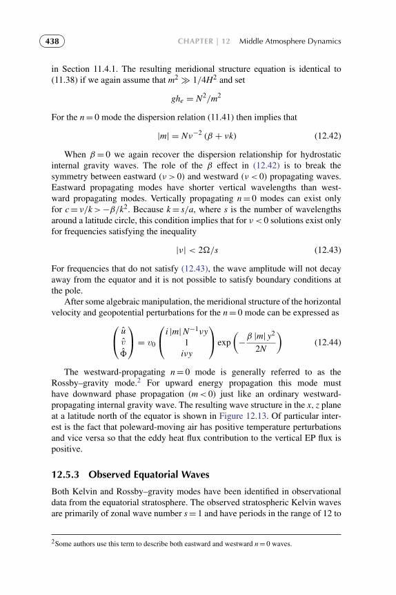
To protect the rights of the author(s) and publisher we inform you that this PDF is an uncorrected proof for internal businessuse only by the author(s), editor(s), reviewer(s), Elsevier and typesetter diacriTech. It is not allowed to publish this proofonline or in print. This proof copy is the copyright property of the publisher and is confidential until formal publication.
“Hakim: 16-ch12-413-452-9780123848666” — 2012/7/26 — 12:29 — page 438 — #26
438 CHAPTER | 12 Middle Atmosphere Dynamics
in Section 11.4.1. The resulting meridional structure equation is identical to(11.38) if we again assume that m2
� 1/4H2 and set
ghe = N2/m2
For the n= 0 mode the dispersion relation (11.41) then implies that
|m| = Nν−2 (β + νk) (12.42)
When β = 0 we again recover the dispersion relationship for hydrostaticinternal gravity waves. The role of the β effect in (12.42) is to break thesymmetry between eastward (ν > 0) and westward (ν < 0) propagating waves.Eastward propagating modes have shorter vertical wavelengths than west-ward propagating modes. Vertically propagating n= 0 modes can exist onlyfor c= ν/k>−β/k2. Because k= s/a, where s is the number of wavelengthsaround a latitude circle, this condition implies that for ν < 0 solutions exist onlyfor frequencies satisfying the inequality
|ν| < 2�/s (12.43)
For frequencies that do not satisfy (12.43), the wave amplitude will not decayaway from the equator and it is not possible to satisfy boundary conditions atthe pole.
After some algebraic manipulation, the meridional structure of the horizontalvelocity and geopotential perturbations for the n= 0 mode can be expressed as u
v
8
= v0
i |m|N−1νy1
iνy
exp
(−β |m| y2
2N
)(12.44)
The westward-propagating n= 0 mode is generally referred to as theRossby–gravity mode.2 For upward energy propagation this mode musthave downward phase propagation (m< 0) just like an ordinary westward-propagating internal gravity wave. The resulting wave structure in the x, z planeat a latitude north of the equator is shown in Figure 12.13. Of particular inter-est is the fact that poleward-moving air has positive temperature perturbationsand vice versa so that the eddy heat flux contribution to the vertical EP flux ispositive.
12.5.3 Observed Equatorial Waves
Both Kelvin and Rossby–gravity modes have been identified in observationaldata from the equatorial stratosphere. The observed stratospheric Kelvin wavesare primarily of zonal wave number s= 1 and have periods in the range of 12 to
2Some authors use this term to describe both eastward and westward n= 0 waves.

To protect the rights of the author(s) and publisher we inform you that this PDF is an uncorrected proof for internal businessuse only by the author(s), editor(s), reviewer(s), Elsevier and typesetter diacriTech. It is not allowed to publish this proofonline or in print. This proof copy is the copyright property of the publisher and is confidential until formal publication.
“Hakim: 16-ch12-413-452-9780123848666” — 2012/7/26 — 12:29 — page 439 — #27
12.5 | Waves in the Equatorial Stratosphere 439
LongitudeW E
Low
Low
Low
High
High
High
Hei
ght
Warm
Warm
Cold
Cold
Warm
Warm
Cold
FIGURE 12.13 Longitude–height section along a latitude circle north of the equator showingpressure, temperature, and wind perturbations for a thermally damped Rossby–gravity wave. Areasof high pressure are shaded. Small arrows indicate zonal and vertical wind perturbations with lengthproportional to the wave amplitude. Meridional wind perturbations are shown by arrows pointedinto the page (northward) and out of the page (southward). The large shaded arrow indicates the netmean flow acceleration due to the wave stress divergence.
20 days. An example of zonal wind oscillations caused by the passage of Kelvinwaves at a station near the equator is shown in the form of a time–height sectionin Figure 12.14. During the observational period shown in Figure 12.14, thewesterly phase of the quasi-biennial oscillation (see Section 12.6) is descendingso that at each level there is a general increase in the mean zonal wind withincreasing time. However, superposed on this secular trend is a large fluctuatingcomponent with a period between speed maxima of about 12 days and a verticalwavelength (computed from the tilt of the oscillations with height) of about 10to 12 km.
Observations of the temperature field for the same period reveal that thetemperature oscillation leads the zonal wind oscillation by 1/4 cycle (i.e., maxi-mum temperature occurs prior to maximum westerlies), which is just the phaserelationship required for upward-propagating Kelvin waves (see Figure 12.12).Additional observations from other stations indicate that these oscillations dopropagate eastward at the theoretically predicted speed. Therefore, there can belittle doubt that the observed oscillations are Kelvin waves.
The existence of the Rossby–gravity mode has been confirmed in observa-tional data from the stratosphere in the equatorial Pacific. This mode is identifiedmost easily in the meridional wind component, as v′ is a maximum at the equatorfor the Rossby–gravity mode. The observed Rossby–gravity waves have s= 4,vertical wavelengths in the range of 6 to 12 km, and a period range of 4 to 5 days.Kelvin and Rossby–gravity waves each have significant amplitude only withinabout 20◦ latitude of the equator.

To protect the rights of the author(s) and publisher we inform you that this PDF is an uncorrected proof for internal businessuse only by the author(s), editor(s), reviewer(s), Elsevier and typesetter diacriTech. It is not allowed to publish this proofonline or in print. This proof copy is the copyright property of the publisher and is confidential until formal publication.
“Hakim: 16-ch12-413-452-9780123848666” — 2012/7/26 — 12:29 — page 440 — #28
440 CHAPTER | 12 Middle Atmosphere Dynamics
10
15
202530
40
50607080
100125
Pre
ssur
e (h
Pa)
30
25
20
1531 10 31 1020 20 31 3110 20101 20
May June July August1963
Hei
ght (
km)
E
EEE
E
E
W
W
WW
WW
FIGURE 12.14 Time–height section of zonal wind at Canton Island (3◦S). Isotachs at intervals of5 m s−1. Westerlies are shaded. (Courtesy of J. M. Wallace and V. E. Kousky.)
A more complete comparison of observed and theoretical properties of theKelvin and Rossby–gravity modes is presented in Table 12.1. In comparing the-ory and observation, it must be recalled that it is the frequency relative to themean flow, not relative to the ground, that is dynamically relevant.
It appears that Kelvin and Rossby–gravity waves are excited by oscilla-tions in the large-scale convective heating pattern in the equatorial troposphere.Although these waves do not contain much energy compared to typical tro-pospheric weather disturbances, they are the predominant disturbances of theequatorial stratosphere and, through their vertical energy and momentum trans-port, play a crucial role in the general circulation of the stratosphere. In additionto the stratospheric modes considered here, there are higher-speed Kelvin andRossby–gravity modes, which are important in the upper stratosphere and meso-sphere. There is also a broad spectrum of equatorial gravity waves, whichappears to be important for the momentum balance of the equatorial middleatmosphere.
12.6 THE QUASI-BIENNIAL OSCILLATION
The search for periodic oscillations in the atmosphere has a long history. Aside,however, from the externally forced diurnal and annual components and theirharmonics, no compelling evidence exists for truly periodic atmospheric oscil-lations. The phenomenon that perhaps comes closest to exhibiting periodicbehavior not associated with a periodic forcing function is the quasi-biennialoscillation (QBO) in the mean zonal winds of the equatorial stratosphere. Thisoscillation has the following observed features.

To protect the rights of the author(s) and publisher we inform you that this PDF is an uncorrected proof for internal businessuse only by the author(s), editor(s), reviewer(s), Elsevier and typesetter diacriTech. It is not allowed to publish this proofonline or in print. This proof copy is the copyright property of the publisher and is confidential until formal publication.
“Hakim: 16-ch12-413-452-9780123848666” — 2012/7/26 — 12:29 — page 441 — #29
12.6 | The Quasi-Biennial Oscillation 441
�
�
�
�
TABLE 12.1 Characteristics of the Dominant Observed Planetary-ScaleWaves in the Equatorial Lower Stratosphere
Theoretical description Kelvin wave Rossby–gravity wave
Discovered by Wallace and Kousky Yanai and Maruyama(1968) (1966)
Period (ground-based)2πω−1
15 days 4–5 days
Zonal wave numbers = ka cosφ
1–2 4
Vertical wavelength2 πm−1
6–10 km 4–8 km
Average phase speedrelative to ground
+25 m s−1 –23 m s−1
Observed when mean Easterly Westerlyzonal flow is (maximum ≈ −25 m s−1) (maximum ≈ +7 m s−1)
Average phase speedrelative to maximumzonal flow +50 m s−1 –30 m s−1
Approximate observedamplitudesu′ 8 m s−1 2–3 m s−1
v′ 0 2–3 m s−1
T ′ 2–3 K 1 K
Approximate inferredamplitudes8′/g 30 m 4 mw′ 1.5 × 10⁻³m s−1 1.5 × 10⁻³m s−1
Approximate meridionalscales(2N/β|m|
)1/2 1300–1700 km 1000–1500 km
From Andrews et al., 1987.
1. Zonally symmetric easterly and westerly wind regimes alternate regularlywith periods varying from about 24 to 30 months.
2. Successive regimes first appear above 30 km but propagate downward at arate of 1 km mo−1.
3. Downward propagation occurs without loss of amplitude between 30 and23 km, but there is rapid attenuation below 23 km.
4. Oscillation is symmetric about the equator with a maximum amplitude ofabout 20 m s−1 and an approximately Gaussian distribution in latitude witha half-width of about 12◦.

To protect the rights of the author(s) and publisher we inform you that this PDF is an uncorrected proof for internal businessuse only by the author(s), editor(s), reviewer(s), Elsevier and typesetter diacriTech. It is not allowed to publish this proofonline or in print. This proof copy is the copyright property of the publisher and is confidential until formal publication.
“Hakim: 16-ch12-413-452-9780123848666” — 2012/7/26 — 12:29 — page 442 — #30
442 CHAPTER | 12 Middle Atmosphere Dynamics
This oscillation is best depicted by means of a time–height section of thezonal wind speed at the equator as shown in Figure 12.15. It is apparent fromthis figure that the vertical shear of the wind is quite strong at the level whereone regime is replacing the other. Because the QBO is zonally symmetric andcauses only very small mean meridional and vertical motions, the QBO meanzonal wind and temperature fields satisfy the thermal wind balance equation.For the equatorial β plane this has the form—compare with (10.13):
βy∂u/∂z = −RH−1∂T/∂y
For equatorial symmetry ∂T/∂y= 0 at y= 0, and by L’Hopital’s rule thermalwind balance at the equator has the form
∂u/∂z = −R(Hβ)−1∂2T/∂y2 (12.45)
Equation (12.45) can be used to estimate the magnitude of the QBO temper-ature perturbation at the equator. The observed magnitude of vertical shear ofthe mean zonal wind at the equator is ∼5 m s−1 km−1, and the meridional scaleis ∼1200 km, from which (12.45) shows that the temperature perturbation hasan amplitude ∼3 K at the equator. Because the second derivative of tempera-ture has the opposite sign to that of the temperature at the equator, the westerlyand easterly shear zones have warm and cold equatorial temperature anomalies,respectively.
The main factors that a theoretical model of the QBO must explain are theapproximate biennial periodicity, the downward propagation without loss ofamplitude, and the occurrence of zonally symmetric westerlies at the equator.Because a zonal ring of air in westerly motion at the equator has an angularmomentum per unit mass greater than that of Earth, no plausible zonally sym-metric advection process could account for the westerly phase of the oscillation.Therefore, there must be a vertical transfer of momentum by eddies to producethe westerly accelerations in the downward-propagating shear zone of the QBO.
Observational and theoretical studies have confirmed that vertically prop-agating equatorial Kelvin and Rossby–gravity waves provide a significantfraction of the zonal momentum sources necessary to drive the QBO. FromFigure 12.12 it is clear that Kelvin waves with upward energy propagation trans-fer westerly momentum upward (i.e., u′ and w′ are positively correlated so thatu′w′ > 0). Thus, the Kelvin waves can provide a source of westerly momentumfor the QBO.
Vertical momentum transfer by the Rossby–gravity mode requires specialconsideration. Examination of Figure 12.13 shows that u′w′> 0 also for theRossby–gravity mode. The total effect of this wave on the mean flow cannotbe ascertained from the vertical momentum flux alone, but rather the com-plete vertical EP flux must be considered. This mode has a strong polewardheat flux (v′T ′ > 0), which provides an upward-directed EP flux contribution.This dominates over the vertical momentum flux, and the net result is that the
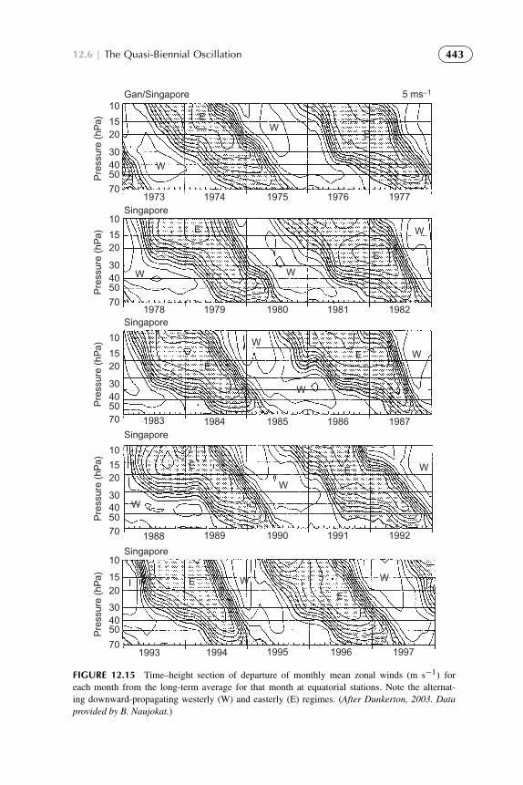
To protect the rights of the author(s) and publisher we inform you that this PDF is an uncorrected proof for internal businessuse only by the author(s), editor(s), reviewer(s), Elsevier and typesetter diacriTech. It is not allowed to publish this proofonline or in print. This proof copy is the copyright property of the publisher and is confidential until formal publication.
“Hakim: 16-ch12-413-452-9780123848666” — 2012/7/26 — 12:29 — page 443 — #31
12.6 | The Quasi-Biennial Oscillation 443
1983
10
1520
30
5040
70
Gan/Singapore
1973
W
WE
E
1974 1975 1976 1977
10
1520
30
5040
70
Singapore
1978
W W
WE
E
1979 1980 1981 1982
10
1520
30
5040
70
Singapore
W
W
WE
E
1984 1985 1986 1987
1988
10
1520
30
5040
70
Singapore
W
W
WE E
1989 1990 1991 1992
1993
10
1520
Pre
ssur
e (h
Pa)
Pre
ssur
e (h
Pa)
Pre
ssur
e (h
Pa)
Pre
ssur
e (h
Pa)
Pre
ssur
e (h
Pa)
30
5040
70
Singapore
W WE
E
1994 1995 1996 1997
5 ms−1
FIGURE 12.15 Time–height section of departure of monthly mean zonal winds (m s−1) foreach month from the long-term average for that month at equatorial stations. Note the alternat-ing downward-propagating westerly (W) and easterly (E) regimes. (After Dunkerton, 2003. Dataprovided by B. Naujokat.)

To protect the rights of the author(s) and publisher we inform you that this PDF is an uncorrected proof for internal businessuse only by the author(s), editor(s), reviewer(s), Elsevier and typesetter diacriTech. It is not allowed to publish this proofonline or in print. This proof copy is the copyright property of the publisher and is confidential until formal publication.
“Hakim: 16-ch12-413-452-9780123848666” — 2012/7/26 — 12:29 — page 444 — #32
444 CHAPTER | 12 Middle Atmosphere Dynamics
Rossby–gravity mode transfers easterly momentum upward and can provide amomentum source for the easterly phase of the QBO. Observed Kelvin andRossby–gravity wave momentum fluxes are not, however, sufficient to accountfor the observed zonal accelerations of the QBO. Additional wave sources, suchas gravity waves generated by convective storms, must also contribute to theforcing of the QBO.
It was pointed out in Section 12.4 that quasi-geostrophic wave modes donot produce any net mean flow acceleration unless the waves are transient orare damped mechanically or thermally. Similar considerations apply to gravitywaves and to the equatorial Kelvin and Rossby–gravity modes. Stratosphericwaves are subject to thermal damping by infrared radiation, and to both thermaland mechanical damping by small-scale turbulent motions. Such damping isstrongly dependent on the Doppler-shifted frequency of the waves.
As the Doppler-shifted frequency decreases, the vertical component of groupvelocity also decreases, and there is a longer time available for the wave energyto be damped as it propagates through a given vertical distance. Thus, eastward-propagating gravity waves and Kelvin waves tend to be damped preferentiallyin westerly shear zones, where their Doppler-shifted frequencies decrease withheight. The momentum flux convergence associated with this damping pro-vides a westerly acceleration of the mean flow, and thus causes the westerlyshear zone to descend. Similarly, the westward-propagating gravity waves andRossby–gravity waves are damped in easterly shear zones, thereby causing aneasterly acceleration and descent of the easterly shear zone. We conclude thatthe QBO is indeed excited primarily by vertically propagating waves throughwave transience and damping, which causes westerly accelerations in westerlyshear zones and easterly accelerations in easterly shear zones.
This process of wave, mean-flow interaction can be elucidated by consid-ering the heavy wavy lines shown earlier in Figures 12.12 and 12.13. Theselines indicate the vertical displacement of horizontal surfaces of fluid parcels(material surfaces) by the velocity field associated with the waves. (For suffi-ciently weak thermal damping they are approximately the same as isentropicsurfaces.) The wavy lines show that the maximum upward displacement occurs1/4 cycle after the maximum upward perturbation velocity. In the Kelvin wavecase (Figure 12.12), positive pressure perturbations coincide with negativematerial surface slopes. Thus, the fluid below a wavy material line exerts aneastward-directed pressure force on the fluid above. Because the wave ampli-tude decreases with height, this force is larger for the lower of the two materiallines in Figure 12.12. There will thus be a net westerly acceleration of the blockof fluid contained between the two wavy material lines shown in Figure 12.12.
For the Rossby–gravity wave, however, positive pressure perturbations coin-cide with positive slopes of the material lines. There is thus a westward-directedforce exerted by the fluid below the lines on the fluid above as shown inFigure 12.13. In this case the result is a net easterly acceleration of the fluidcontained between the two wavy material lines shown in Figure 12.13. Thus,

To protect the rights of the author(s) and publisher we inform you that this PDF is an uncorrected proof for internal businessuse only by the author(s), editor(s), reviewer(s), Elsevier and typesetter diacriTech. It is not allowed to publish this proofonline or in print. This proof copy is the copyright property of the publisher and is confidential until formal publication.
“Hakim: 16-ch12-413-452-9780123848666” — 2012/7/26 — 12:29 — page 445 — #33
12.6 | The Quasi-Biennial Oscillation 445
by considering the stresses acting across a material surface corrugated by thewaves, it is possible to deduce the mean-flow acceleration caused by the waveswithout explicit reference to the EP fluxes of the waves.
How such a mechanism can cause a mean zonal flow oscillation when equalamounts of easterly and westerly momentum are transferred upward across thetropopause by the waves can be seen qualitatively by considering Figure 12.16.If initially, as shown in Figure 12.16a, the mean zonal wind is weak and west-erly, the eastward-propagating waves will be preferentially damped at loweraltitude and produce a westerly acceleration, which will move downward intime as the mean westerlies intensify and the wave-driven acceleration is con-centrated at ever lower altitudes. The westward-propagating waves, however,initially penetrate to higher altitudes, where they produce easterlies, which alsomove downward in time. Eventually the westerlies are damped out as theyapproach the tropopause, and the stratosphere is dominated by easterlies so thatthe eastward-propagating waves can penetrate to high altitude and produce anew westerly phase. In this manner the mean zonal wind is forced to oscillateback and forth between westerlies and easterlies with a period that depends pri-marily on the vertical momentum transport and other properties of the waves,not on an oscillating external forcing.
0−c +c 0
(b)(a)
3
2
1
z
z
−c +c
u– u–
FIGURE 12.16 Schematic representation of wave-driven accelerations that lead to the zonal windQBO. Eastward- and westward-propagating gravity waves of phase speeds+c and−c, respectively,propagate upward and are dissipated at rates dependent on the Doppler-shifted frequency. (a) Ini-tial weak westerly current selectively damps the eastward-propagating wave and leads to westerlyacceleration at lower levels and easterly acceleration at higher levels. (b) Descending westerly shearzones block penetration of eastward-propagating waves, whereas westward-propagating waves pro-duce descending easterlies aloft. Broad arrows show locations and direction of maxima in meanwind acceleration. Wavy lines indicate relative penetration of waves. (After Plumb, 1982.)

To protect the rights of the author(s) and publisher we inform you that this PDF is an uncorrected proof for internal businessuse only by the author(s), editor(s), reviewer(s), Elsevier and typesetter diacriTech. It is not allowed to publish this proofonline or in print. This proof copy is the copyright property of the publisher and is confidential until formal publication.
“Hakim: 16-ch12-413-452-9780123848666” — 2012/7/26 — 12:29 — page 446 — #34
446 CHAPTER | 12 Middle Atmosphere Dynamics
12.7 TRACE CONSTITUENT TRANSPORT
The study of global transport involves the motion of atmospheric tracers, whichare defined as chemical or dynamical quantities that label fluid parcels. Chem-ical tracers consist of minor atmospheric species that have significant spatialvariability in the atmosphere. Dynamical tracers (potential temperature andpotential vorticity) are properties of the flow field that are conserved followingthe motion under certain conditions. These also can be useful for interpretationof transport.
12.7.1 Dynamical Tracers
Potential temperature, defined in (2.44), can be thought of as a label for thevertical position of an air parcel. Because the atmosphere is stably stratified,potential temperature increases monotonically with height (slowly in the tropo-sphere and rapidly in the stratosphere as shown in Figure 12.17) and thus canbe used as an independent vertical coordinate: the isentropic coordinates intro-duced in Section 4.6.1. A parcel moving adiabatically remains on a surface ofconstant potential temperature and can be “tagged” by its value of potential tem-perature. Thus the motion of such a parcel is two-dimensional when viewed inisentropic coordinates.
Potential temperature surfaces are quasi-horizontal, but they do move up anddown in physical space with adiabatic changes in temperature. Thus, it is usefulto reference trace constituent data to potential temperature, rather than pressure
10
100
710
590
200
25
20
15
10
5250
2901000
−90 −90−60 −60−30 300
Equator North poleSouth pole
Pre
ssur
e (h
Pa)
Alti
tude
(km
)
500
380
FIGURE 12.17 Latitude–height section showing January mean potential temperature surfaces(solid contours) and temperature (dashed contours). Heavy line shows the 380-K θ surface, abovewhich all θ surfaces lie completely in the middle atmosphere. The light shaded region below the380 K surface is the lowermost stratosphere, where 2 surfaces span the tropopause (shown by theline bounding the lower side of the shaded region). (Courtesy of C. Appenzeller.)

To protect the rights of the author(s) and publisher we inform you that this PDF is an uncorrected proof for internal businessuse only by the author(s), editor(s), reviewer(s), Elsevier and typesetter diacriTech. It is not allowed to publish this proofonline or in print. This proof copy is the copyright property of the publisher and is confidential until formal publication.
“Hakim: 16-ch12-413-452-9780123848666” — 2012/7/26 — 12:29 — page 447 — #35
12.7 | Trace Constituent Transport 447
or altitude, as reversible variations at local altitudes or pressures caused by adi-abatic vertical displacements associated with transient motions (e.g., gravitywaves) are then accounted for.
The other commonly used dynamical tracer, potential vorticity (PV), isconserved for adiabatic, frictionless flow. As defined in equation (4.25), PVnormally has a positive gradient in the meridional direction on an isentropic sur-face; it is negative in the Southern Hemisphere, zero at (or near) the equator, andpositive in the Northern Hemisphere. PV has strong gradients in both height andlatitude. Because a parcel moving in adiabatic frictionless flow conserves PV aswell as potential temperature, its motion must lie parallel to isocontours of PVon isentropic surfaces. Rapid meridional transport implies production of strongPV anomalies as high polar values of PV are advected equatorward or lowequatorial values are advected poleward. As discussed earlier, the meridionalgradient of the background PV field resists meridional displacements throughthe production of Rossby waves. Thus, regions of strong PV gradients on isen-tropic surfaces can act as semipermeable “barriers” to transport. This PV barriereffect is one of the reasons that eddy diffusion is often not a good model formeridional transport.
Because PV depends only on the distribution of horizontal winds andtemperatures on isentropic surfaces, its distribution can be determined fromconventional meteorological observations. Thus, the evolution of PV on anisentropic surface can be used as a surrogate for the study of trace constituenttransport on isentropic surfaces in circumstances in which there are inadequateobservations of relevant chemical tracers. In addition, for dynamical studies,PV has the important property, not shared by other tracers, that it not only isadvected by the flow, but actually determines the flow field. Thus, the distri-bution of PV on isentropic surfaces can be “inverted” to yield the wind andtemperature fields. Changes in the PV distribution are then said to “induce”changes in the wind and temperature fields. In the quasi-geostrophic case theinduced changes are required to maintain geostrophic and hydrostatic bal-ance. More generally, such changes preserve a higher-order balance among thedynamical fields.
12.7.2 Chemical Tracers
Much can be learned about the nature of large-scale transport by consider-ing the climatological distribution of quasi-conservative chemical tracers in theatmosphere. The distribution of such trace substances is dependent on the com-petition between dynamical and chemical processes. This competition can beapproximately measured by comparing the characteristic dynamical and chem-ical timescales. Chemical timescale is the average time for replacement orremoval of a tracer due to chemical sources and sinks. Dynamical timescaleis the average time for advective and diffusive processes to transport the tracerfrom equator to pole or across a scale height in the vertical. The role of transport

To protect the rights of the author(s) and publisher we inform you that this PDF is an uncorrected proof for internal businessuse only by the author(s), editor(s), reviewer(s), Elsevier and typesetter diacriTech. It is not allowed to publish this proofonline or in print. This proof copy is the copyright property of the publisher and is confidential until formal publication.
“Hakim: 16-ch12-413-452-9780123848666” — 2012/7/26 — 12:29 — page 448 — #36
448 CHAPTER | 12 Middle Atmosphere Dynamics
in determining tracer climatology depends on the nature and distribution oftracer sources and sinks, and on the relative magnitudes of the timescales fordynamical and chemical processes.
If the chemical timescale is much shorter than the dynamical timescale, thetracer will be in photochemical equilibrium and transport does not directly influ-ence its distribution. Transport can, however, play an important indirect role bypartly determining the concentrations of other species that participate in thephotochemical production or loss of the tracer in question.
If the chemical timescale is much longer than the dynamical timescale, thetracer will be passively advected by the flow field. In the absence of localizedsources and sinks, such a tracer would eventually become well mixed due to thedispersive effects of transport. It is for this reason that species such as nitrousoxide (N2O) tend to have uniform concentrations in the troposphere and are thusnot useful for tropospheric transport studies.
When the chemical and dynamical timescales are comparable, the observedspecies concentration depends on the net effects of chemical sources and sinksand of transport. In many cases of interest, the ratio of chemical and dynami-cal timescales changes drastically between the troposphere and the stratosphere,and with altitude in the stratosphere. Tracers that have long lifetimes in the tro-posphere and the lower stratosphere are referred to as long-lived tracers, as thebulk of the tracer mass is contained in the troposphere and lower stratosphere,and the lifetime is determined mainly by the (slow) flux of the tracer to altitudeswhere the chemical timescales become comparable to or shorter than dynamicaltimescales.
12.7.3 Transport in the Stratosphere
Transport processes are conveniently divided between those that involve meanmotions of the atmosphere, or advection, and those that may be characterized asturbulent, or diffusive in nature. In the case of point sources, such as volcaniceruptions, the distinction is quite clear; advection moves the center of mass ofthe plume along the direction of the average wind, whereas turbulent diffusiondisperses the plume in the plane orthogonal to the average wind. On a globalscale, however, the distinction between advective and diffusive processes is notalways clear. Because the atmosphere is characterized by spatially and tempo-rally varying motions with a wide range of scales, there is no obvious physicalseparation between “mean” and “turbulent” motions.
In practice, those transport processes that are explicitly resolved by theparticular observational network or transport model being utilized are oftenregarded as the advective motions, whereas the remaining unresolved motionsare assumed to be diffusive. The effects of the unresolved motions must thenbe parameterized in terms of the mean motions in some fashion. Usually thisinvolves assuming that tracer fluxes by the unresolved motions are proportionalto the gradient of the resolved tracer distribution. However, this approach is not

To protect the rights of the author(s) and publisher we inform you that this PDF is an uncorrected proof for internal businessuse only by the author(s), editor(s), reviewer(s), Elsevier and typesetter diacriTech. It is not allowed to publish this proofonline or in print. This proof copy is the copyright property of the publisher and is confidential until formal publication.
“Hakim: 16-ch12-413-452-9780123848666” — 2012/7/26 — 12:29 — page 449 — #37
12.7 | Trace Constituent Transport 449
always physically justified. A major problem in the modeling of global transportis accurate representation of the contribution of the unresolved eddy motions tothe total transport.
As discussed in Section 12.2, the global-scale residual meridional circulationin the middle atmosphere is driven by wave-induced zonal forces associatedwith Rossby waves and gravity waves. Not surprisingly, the residual circulationplays an essential role in the meridional and vertical transport of trace chemicalconstituents in the middle atmosphere. Additionally, the waves responsible forthe zonal force that drives the residual circulation are also responsible for thequasi-isentropic stirring and mixing that is associated with wavebreaking. Thus,understanding of transport involves both eddy and mean-flow transport effects.
In dynamical studies it is usual to characterize a chemical constituent by thevolume mixing ratio (or mole fraction), defined as χ ≡ nT/nA, where nT and nA
designate the number densities (molecules m−3) for the trace constituent and air,respectively. The mixing ratio is conserved following the motion in the absenceof sources and sinks and thus satisfies the simple tracer continuity equation
Dχ
Dt= S (12.46)
where S designates the sum of all chemical sources and sinks.As in the case of the dynamical variables discussed in Section 12.2, it is
useful to define a longitudinally averaged mixing ratio χ and a disturbance oreddy ratio χ ′ such that χ =χ + χ ′. Again, it proves useful to use the residualmean meridional circulation
(v ∗,w ∗
)defined in (10.16a,b). The zonal mean
tracer continuity equation in the TEM framework can then be written as
∂χ
∂t+ v ∗
∂χ
∂y+ w ∗
∂χ
∂z= S+
1
ρ0∇·M (12.47)
Here, M represents the diffusive effects of the eddies, plus advective effects notrepresented by the residual meridional circulation. In models the term involv-ing M is often represented by meridional and vertical eddy diffusion, withempirically determined diffusion coefficients.
To appreciate the role of the wave-induced global circulation in deter-mining the distribution of long-lived tracers in the middle atmosphere, it isuseful to consider a hypothetical atmosphere in which there are no wavemotions and thus no wave-induced zonal force. In that case, as argued in Sec-tion 12.2, the middle atmosphere would relax to radiative equilibrium, theresidual circulation would vanish, and the distribution of the tracer wouldbe determined at each altitude by a balance between slow upward diffusionand photochemical destruction. Thus, tracer mixing ratio surfaces would, inan annual mean, tend to be close to horizontal. This is to be contrasted toobserved distributions, which are characterized by mixing ratio surfaces thatbow upward in the tropics and slope downward toward both poles (e.g.,Figure 12.9).

To protect the rights of the author(s) and publisher we inform you that this PDF is an uncorrected proof for internal businessuse only by the author(s), editor(s), reviewer(s), Elsevier and typesetter diacriTech. It is not allowed to publish this proofonline or in print. This proof copy is the copyright property of the publisher and is confidential until formal publication.
“Hakim: 16-ch12-413-452-9780123848666” — 2012/7/26 — 12:29 — page 450 — #38
450 CHAPTER | 12 Middle Atmosphere Dynamics
As discussed in Section 12.2, the wave-induced global-scale circulationconsists of upward and poleward motion across the isentropes in low lat-itudes, accompanied by diabatic heating, and downward motion across theisentropes at high latitudes, accompanied by diabatic cooling. Actual parceltrajectories, of course, do not follow the zonally averaged motion, but areinfluenced by the three-dimensional wave motion. Nevertheless the diabatic cir-culation defined by the mean diabatic heating and cooling closely approximatesthe global transport circulation. For seasonal and longer timescales the TEMresidual circulation generally provides a good approximation to the diabaticcirculation and is generally simpler to compute from standard meteorologicalanalyses. For shorter-period phenomena in which the temperature tendency islarge, the residual circulation is no longer a good approximation to the diabaticcirculation.
The previous conceptual model of global transport is clearly supportedby long-lived tracer observations as shown earlier in Figure 12.9. In middlelatitudes there are regions in which tracer mixing ratio isopleths are nearly hor-izontal, reflecting the horizontal homogenizing role of meridional dispersionby planetary wavebreaking in the surf zone. The same processes also tend tohomogenize the PV distribution on isentropes in the so-called surf zone in mid-latitudes where Rossby wavebreaking tends to occur. The surf zone is boundedat both low and high latitudes by regions of strong meridional gradients of long-lived tracers and of PV. The existence of such gradients is evidence that there isonly weak mixing into and out of the tropics and into and out of the polar wintervortex. Thus, these locations are sometimes referred to as “transport barriers.”The strong PV gradients, strong winds, and strong wind shears that occur alongthe transport barriers at the subtropical and polar edges of the surf zone all actto suppress wavebreaking, and thus to minimize mixing and sustain the stronggradients at those locations.
SUGGESTED REFERENCES
Andrews, Holton, and Leovy, Middle Atmosphere Dynamics present a graduate-level treatment ofthe dynamics of the stratosphere and mesosphere.
Brasseur and Solomon’s Aeronomy of the Middle Atmosphere has an excellent discussion of thechemistry of the stratosphere at an advanced level.
PROBLEMS
12.1. Suppose that temperature increases linearly with height in the layerbetween 20 and 50 km at a rate of 2 K km−1. If the temperature is 200K at 20 km, find the value of the scale height H for which the log-pressureheight z coincides with actual height at 50 km. (Assume that z coincideswith the actual height at 20 km and let g= 9.81 m s−2 be a constant.)
12.2. Find the Rossby critical velocities for zonal wave numbers 1, 2, and 3 (i.e.,for 1, 2, and 3 wavelengths around a latitude circle). Let the motion be

To protect the rights of the author(s) and publisher we inform you that this PDF is an uncorrected proof for internal businessuse only by the author(s), editor(s), reviewer(s), Elsevier and typesetter diacriTech. It is not allowed to publish this proofonline or in print. This proof copy is the copyright property of the publisher and is confidential until formal publication.
“Hakim: 16-ch12-413-452-9780123848666” — 2012/7/26 — 12:29 — page 451 — #39
Problems 451
referred to a β plane centered at 45◦N, scale height H= 7 km, buoyancyfrequency N= 2× 10⁻² s−1, and infinite meridional scale (l= 0).
12.3. Suppose that a stationary linear Rossby wave is forced by flow over sinu-soidal topography with height h (x)= h0 cos(kx), where h0 is a constantand k is the zonal wave number. Show that the lower boundary conditionon the streamfunction ψ can be expressed in this case as
(∂ψ/∂z) = −hN2/f0
Using this boundary condition and an appropriate upper boundary con-dition, solve for ψ (x, z) in the case |m| � (1/2H) using the equationsof Section 12.3.1. How does the position of the trough relative to themountain ridge depend on the sign of m2 for the limit |m| � (1/2H).
12.4. Consider a very simple model of a steady-state mean meridional circu-lation for zonally symmetric flow in a midlatitude channel bounded bywalls at y= 0, π/l and z= 0, π/m. We assume that the zonal mean zonalflow u is in thermal wind balance and that the eddy momentum andheat fluxes vanish. For simplicity, we let ρ0= 1 (Boussinesq approxima-tion) and let the zonal force due to small-scale motions be representedby a linear drag: X=−γ u. We assume that the diabatic heating hasthe form J/cp= (H/R)J0 cos ly sin mz, and we let N and f be constants.Equations (12.1) through (12.4) then yield the following:
−f0v∗= −γ u
+N2HR−1w ∗ = +J/cp
v ∗ = −∂χ ∗
∂z; w ∗ =
∂χ ∗
∂y
f0∂u/∂z+ RH−1∂T/∂y = 0
Assuming that there is no flow through the walls, solve for the residualcirculation defined by χ ∗, v ∗, and w ∗ .
12.5. For the situation of Problem 12.4, solve for the steady-state zonal windand temperature fields u and T.
12.6. Find the geopotential and vertical velocity fluctuations for a Kelvin waveof zonal wave number 1, phase speed 40 m s−1, and zonal velocityperturbation amplitude 5 m s−1. Let N2
= 4× 10⁻⁴ s−2.12.7. For the situation of Problem 12.6 compute the vertical momentum flux
M ≡ ρ0u′w′. Show that M is constant with height.12.8. Determine the form for the vertical velocity perturbation for the Rossby–
gravity wave corresponding to the u′, v′, and 8′ perturbations given in(12.44).
12.9. For a Rossby–gravity wave of zonal wave number 4 and phase speed−20 m s−1, determine the latitude at which the vertical momentum fluxM ≡ ρ0u′w′ is a maximum.
12.10. Suppose that the mean zonal wind shear in the descending westerliesof the equatorial QBO can be represented analytically on the equa-torial β plane in the form ∂u/∂z=3 exp
(−y2/L2
)where L= 1200 km.

To protect the rights of the author(s) and publisher we inform you that this PDF is an uncorrected proof for internal businessuse only by the author(s), editor(s), reviewer(s), Elsevier and typesetter diacriTech. It is not allowed to publish this proofonline or in print. This proof copy is the copyright property of the publisher and is confidential until formal publication.
“Hakim: 16-ch12-413-452-9780123848666” — 2012/7/26 — 12:29 — page 452 — #40
452 CHAPTER | 12 Middle Atmosphere Dynamics
Determine the approximate meridional dependence of the correspondingtemperature anomaly for |y| � L.
12.11. Estimate the TEM residual vertical velocity in the westerly shear zone ofthe equatorial QBO assuming that radiative cooling can be approximatedby Newtonian cooling with a 20-day relaxation time, that the verticalshear is 20 m s−1 per 5 km, and that the meridional half-width is 12◦
latitude.
MATLAB ExercisesM12.1. The MATLAB script topo Rossby wave.m plots solutions for various fields for
a stationary linear Rossby wave forced by flow over an isolated ridge. Aβ–plane channel model is used following the discussion in Section 12.3.1.Run the script for mean wind values of 5, 10, 15, 20, and 25 m s−1. Describehow the geopotential and potential temperature perturbations change withchanging mean wind speed. Explain these results based on the argumentsgiven in Section 12.3.1.
M12.2. For the situation of Problem 12.4 let J0= 10−6 s−3, N = 10−2 s−1, f = 10−4
s−1, l = 10−6 m−1, m=π/H, where H = 104 m, and γ 10−5 s−1. Makecontour plots of the fields u, v ∗,w ∗,T and discuss the relationship of thesefields to the imposed diabatic heating.
M12.3. The MATLAB script sudden warming model.m provides an analog to thesudden stratospheric warmings on an extratropical β plane centered at60◦N. The amplitude of a single planetary wave of zonal wave number s= 1or s= 2 is specified at the bottom boundary (taken to be the 16-km level),and a time integration is carried out to determine the evolution of the zonalmean wind in the stratosphere forced by the EP flux of the specified wave.For the cases s= 1 and 2, run the model for geopotential heights between100 and 400 m at a 50-m interval. For each case note whether the flow tendstoward steady state or repeated sudden warmings. Modify the code to plotthe time–height evolution of the EP flux divergence for the case s= 2 andforcing of 200 m.
M12.4. The MATLAB script qbo model.m is a simplified one-dimensional model ofthe equatorial QBO originally introduced by Plumb (1977). In this modelthe mean zonal flow is forced by two waves of equal amplitude at thelower boundary and equal and opposite phase speeds. The initial meanwind profile has a weak westerly shear. If the model is run for sufficientlyweak forcing, the mean wind approaches a steady state, but for forcinggreater than a critical amplitude, a downward-propagating oscillatory solu-tion occurs, with period dependent on the amplitude of forcing. Run thescript for a range of forcing between 0.04 and 0.40 and determine theapproximate minimum forcing for a large-amplitude oscillatory motion tooccur, and the dependence of period on the forcing amplitude. Modify thescript to compute the time mean of the zonal wind over the course of sev-eral oscillations. Try a case in which the eastward forcing is 0.15 and thewestward forcing is 0.075. How does the time mean wind change in thiscase?

To protect the rights of the author(s) and publisher we inform you that this PDF is an uncorrected proof for internal businessuse only by the author(s), editor(s), reviewer(s), Elsevier and typesetter diacriTech. It is not allowed to publish this proofonline or in print. This proof copy is the copyright property of the publisher and is confidential until formal publication.
“Hakim: 17-ch13-453-490-9780123848666” — 2012/7/26 — 12:35 — page 453 — #1
Chapter 13
Numerical Modelingand Prediction
Dynamical meteorology provides the theoretical basis and methodology formodern weather forecasting. Stated simply, the objective of dynamical forecast-ing is to predict the future state of the atmospheric circulation from knowledgeof its present state by use of numerical approximations to the dynamical equa-tions. Fulfilling this objective requires observations of the initial state of the fieldvariables, a closed set of prediction equations relating the field variables, and amethod of integrating the equations in time to obtain the future distribution ofthe field variables.
Numerical prediction is a highly specialized field, which is continuallyevolving. Operational forecast centers utilize complex prediction models thatrequire the largest available supercomputers to obtain a solution. It is difficultto provide more than a superficial introduction to such models in an introduc-tory text. Fortunately, however, many aspects of numerical prediction can beillustrated using a simple model, such as the barotropic vorticity equation. Infact, this equation was the basis of the earliest operational numerical predictionmodels.
13.1 HISTORICAL BACKGROUND
The British scientist L. F. Richardson made the first attempt to predict theweather numerically. His book, Weather Prediction by Numerical Process, pub-lished in 1922, is the classic treatise in this field. In his work Richardson showedhow the differential equations governing atmospheric motions could be writtenapproximately as a set of algebraic difference equations for values of the ten-dencies of various field variables at a finite number of points in space. Given theobserved values of the field variables at these grid points, the tendencies couldbe calculated numerically by solving the algebraic difference equations.
By extrapolating the computed tendencies ahead a small increment in time,an estimate of the fields at a short time in the future could be obtained. The newvalues of the field variables could then be used to recompute the tendencies,which could in turn be used to extrapolate further ahead in time, and so on. Even
An Introduction to Dynamic Meteorology. DOI: 10.1016/B978-0-12-384866-6.00013-1Copyright © 2013 Elsevier Inc. All rights reserved. 453

To protect the rights of the author(s) and publisher we inform you that this PDF is an uncorrected proof for internal businessuse only by the author(s), editor(s), reviewer(s), Elsevier and typesetter diacriTech. It is not allowed to publish this proofonline or in print. This proof copy is the copyright property of the publisher and is confidential until formal publication.
“Hakim: 17-ch13-453-490-9780123848666” — 2012/7/26 — 12:35 — page 454 — #2
454 CHAPTER | 13 Numerical Modeling and Prediction
for short-range forecasting over a small area of Earth, this procedure requiresan enormous number of arithmetic operations. Richardson did not foresee thedevelopment of high-speed digital computers. He estimated that a workforce of64,000 people would be required just to keep up with the weather on a globalbasis!
Despite the tedious labor involved, Richardson worked out one exampleforecast for surface pressure tendencies at two grid points. Unfortunately, theresults were very poor. Predicted pressure changes were an order of magni-tude larger than those observed. At the time this failure was thought to be dueprimarily to the poor initial data available, especially the absence of upper-airsoundings. However, it is now known that there were other, even more seriousproblems with Richardson’s scheme.
After Richardson’s failure to obtain a reasonable forecast, numerical pre-diction was not again attempted for many years. Finally, after World War IIinterest in numerical prediction revived partly because of the vast expansion ofthe meteorological observation network, which provided much improved initialdata. Even more important was the development of digital computers, whichmade the enormous volume of arithmetic operations required in a numericalforecast feasible. At the same time it was realized that Richardson’s schemewas not the simplest possible scheme for numerical prediction. His equationsnot only governed the slow-moving meteorologically important motions, butalso included high-speed sound and gravity waves as solutions. Such wavesare in nature usually very weak in amplitude. However, for reasons that willbe explained later, if Richardson had carried his numerical calculation beyondthe initial time step, these oscillations would have amplified spuriously, therebyintroducing so much “noise” in the solution that the meteorologically relevantdisturbances would have been obscured.
The American meteorologist J. G. Charney showed in 1948 how the dynam-ical equations could be simplified by systematic introduction of the geostrophicand hydrostatic approximations so that sound and gravity oscillations werefiltered out. The equations that resulted from Charney’s filtering approxima-tions were essentially those of the quasi-geostrophic model. Thus, Charney’sapproach utilized the conservative properties of potential vorticity. A specialcase of this model, the equivalent barotropic model, was used in 1950 to makethe first successful numerical forecast.
This model provided forecasts of the geopotential near 500 hPa. Thus, itdid not forecast “weather” in the usual sense. It could, however, be used byforecasters as an aid in predicting the local weather associated with large-scalecirculations. Later multilevel versions of the quasi-geostrophic model providedexplicit predictions of surface pressure and temperature distributions, but theaccuracy of such predictions was limited because of the approximations inherentin the quasi-geostrophic model.
With the development of vastly more powerful computers and more sophis-ticated modeling techniques, numerical forecasting has now returned to models

To protect the rights of the author(s) and publisher we inform you that this PDF is an uncorrected proof for internal businessuse only by the author(s), editor(s), reviewer(s), Elsevier and typesetter diacriTech. It is not allowed to publish this proofonline or in print. This proof copy is the copyright property of the publisher and is confidential until formal publication.
“Hakim: 17-ch13-453-490-9780123848666” — 2012/7/26 — 12:35 — page 455 — #3
13.2 | Numerical Approximation of the Equations of Motion 455
that are quite similar to Richardson’s formulation and are far more accuratethan quasi-geostrophic models. Nevertheless, it is still worth considering thesimplest filtered model, the barotropic vorticity equation, to illustrate some ofthe technical aspects of numerical prediction in a simple context.
13.2 NUMERICAL APPROXIMATION OF THE EQUATIONSOF MOTION
The equations of motion are an example of a general class of systems known asinitial value problems. A system of differential equations is referred to as an ini-tial value problem when the solution depends not only on boundary conditionsbut also on the values of the unknown fields or their derivatives at some initialtime. Clearly, weather forecasting is a primary example of a nonlinear initialvalue problem. Due to its nonlinearity, even the simplest forecast equation, thebarotropic vorticity equation, is rather complicated to analyze. Fortunately, gen-eral aspects of the numerical solution of initial value problems can be illustratedusing linearized prototype equations that are much simpler than the barotropicvorticity equation.
13.2.1 Finite Differences
The equations of motion involve terms that are quadratic in the dependentvariables (the advection terms). Such equations generally cannot be solved ana-lytically. Rather, they must be approximated by some suitable discretization andsolved numerically. The simplest form of discretization is the finite differencemethod.
To introduce the concept of finite differencing, we consider a field variableψ(x), which is a solution to some differential equation in the interval 0 ≤ x ≤ L.If this interval is divided into J subintervals of length δx, then ψ(x) can beapproximated by a set of J + 1 values as 9j=ψ(jδx), which are the values ofthe field at the J + 1 grid points given by x = jδx, j = 0, 1, 2, . . . , J, whereδx = L/J. Provided that δx is sufficiently small compared to the scale on whichψ varies, the J + 1 grid point values should provide good approximations toψ(x) and its derivatives.
The limits of accuracy of a finite difference representation of a continuousvariable can be assessed by noting that the field can also be approximated by afinite Fourier series expansion:
ψ(x) =a0
2+
J/2∑m=1
[am cos
2πmx
L+ bm sin
2πmx
L
](13.1)
The available J+ 1 values of 9j are just sufficient to determine the J+ 1 coef-ficients in (13.1). That is, it is possible to determine a0 plus am and bm for wavenumbers m= 1, 2, 3, . . . , J/2. The shortest wavelength component in (13.1)

To protect the rights of the author(s) and publisher we inform you that this PDF is an uncorrected proof for internal businessuse only by the author(s), editor(s), reviewer(s), Elsevier and typesetter diacriTech. It is not allowed to publish this proofonline or in print. This proof copy is the copyright property of the publisher and is confidential until formal publication.
“Hakim: 17-ch13-453-490-9780123848666” — 2012/7/26 — 12:35 — page 456 — #4
456 CHAPTER | 13 Numerical Modeling and Prediction
has wavelength L/m= 2L/J= 2δx. Thus, the shortest wave that can be resolvedby finite differencing has a wavelength twice that of the grid increment. Accu-rate representation of derivatives is only possible, however, for wavelengthsmuch greater than 2δx.
We now consider how the grid point variable 9j can be used to constructa finite difference approximation to a differential equation. That is, we wish torepresent derivatives such as dψ/dx and d2ψ/dx2 in terms of the finite differ-ence fields. We first consider the Taylor series expansions about the point x0:
ψ(x0 + δx) = ψ(x0)+ ψ′(x0)δx+ ψ
′′(x0)(δx)2
2
+ ψ ′′′(x0)(δx)3
6+ O
[(δx)4
](13.2)
ψ(x0 − δx) = ψ(x0)− ψ′(x0)δx+ ψ
′′(x0)(δx)2
2
− ψ ′′′(x0)(δx)3
6+ O
[(δx)4
](13.3)
where the primes indicate differentiation with respect to x, and O[(δx)4] meansthat terms with order of magnitude (δx)4 or less are neglected.
Subtracting (13.3) from (13.2) and solving for ψ ′(x) give a finite differenceexpression for the first derivative of the form
ψ ′(x0) = [ψ(x0 + δx)− ψ(x0 − δx)]/(2δx)+ O[(δx)2
](13.4)
while adding the same two expressions and solving for ψ ′′(x) give a finitedifference expression for the second derivative of the form
ψ ′′(x0) = [ψ(x0 + δx)− 2ψ(x0)+ ψ(x0 − δx)]/(δx)2+ O
[(δx)2
](13.5)
Because the difference approximations in (13.4) and (13.5) involve points atequal distances on either side of x0, they are called centered differences. Theseapproximations neglect terms of order (δx)2. We thus say that the truncationerror is order (δx)2. Higher accuracy can be obtained by decreasing the gridinterval, but at the cost of increasing the density of grid points. Alternatively,it is possible to obtain higher-order accuracy without decreasing the grid spac-ing by writing formulas analogous to (13.2) and (13.3) for the interval 2δx andusing these together with (13.2) and (13.3) to eliminate error terms less thanorder (δx)4. This approach, however, has the disadvantage of producing morecomplicated expressions and can be difficult to implement near boundary points.

To protect the rights of the author(s) and publisher we inform you that this PDF is an uncorrected proof for internal businessuse only by the author(s), editor(s), reviewer(s), Elsevier and typesetter diacriTech. It is not allowed to publish this proofonline or in print. This proof copy is the copyright property of the publisher and is confidential until formal publication.
“Hakim: 17-ch13-453-490-9780123848666” — 2012/7/26 — 12:35 — page 457 — #5
13.2 | Numerical Approximation of the Equations of Motion 457
13.2.2 Centered Differences: Explicit Time Differencing
As a prototype model, consider the linear one-dimensional advection equation
∂q/∂t + c∂q/∂x = 0 (13.6)
with c a specified speed and q(x, 0) a known initial condition. This equation canbe approximated to second-order accuracy in x and t by the centered differenceequation
[q(x, t + δt)− q(x, t − δt)] /(2δt) = −c [q (x+ δx, t)− q (x− δx, t)] /(2δx)
(13.7)
The original differential equation (13.6) is thus replaced by a set of algebraicequations (13.7), which can be solved to determine solutions for a finite setof points that define a grid mesh in x and t (see Figure 13.1). For notationalconvenience it is useful to identify points on the grid mesh by indices m, s.These are defined by letting x = mδx, where m = 0, 1, 2, 3, . . . , M, and t =sδt; s = 0, 1, 2, 3, . . . , S. Writing qm,s≡ q(mδx, sδt), the difference equation(13.7) can then be expressed as
qm,s+1 − qm,s−1 = −σ(qm+1,s − qm−1,s) (13.8)
4
3
2s A
+
x− ct=0
1
00 543
m21
δt
δx
FIGURE 13.1 Grid in x − t space showing the domain of dependence of the explicit finite-difference solution at m= 3 and s= 2 for the one-dimensional linear advection equation. Solidcircles show grid points. The sloping line is a characteristic curve along which q(x, t) = q(0, 0), andthe “+” shows an interpolated point for the semi-Lagrangian differencing scheme. In this examplethe leapfrog scheme is unstable because the finite difference solution at point A does not depend onq(0, 0).

To protect the rights of the author(s) and publisher we inform you that this PDF is an uncorrected proof for internal businessuse only by the author(s), editor(s), reviewer(s), Elsevier and typesetter diacriTech. It is not allowed to publish this proofonline or in print. This proof copy is the copyright property of the publisher and is confidential until formal publication.
“Hakim: 17-ch13-453-490-9780123848666” — 2012/7/26 — 12:35 — page 458 — #6
458 CHAPTER | 13 Numerical Modeling and Prediction
where σ ≡ cδt/δx is the Courant number. This form of time differencing isreferred to as the leapfrog method, as the tendency at time step s is given bythe difference in values computed for time steps s+ 1 and s− 1 (i.e., by leapingacross point s).
Leapfrog differencing cannot be used for the initial time t = 0 (s = 0), asqm,−1 is not known. For the first time step, an alternative method is requiredsuch as the forward difference approximation
qm,1 − qm,0 ≡ −(σ/2)(qm+1,0 − qm−1,0) (13.9)
The centered difference scheme for the advection equation (13.8) is an exampleof an explicit time differencing scheme. In an explicit difference scheme, thevalue of the predicted field at a given grid point for time step s + 1 dependsonly on the known values of the field at previous time steps. (In the case of theleapfrog method the fields at time step s and s − 1 are used.) The differenceequation can then be solved simply by marching through the grid and obtainingthe solution for each point in turn. The explicit leapfrog scheme is thus simpleto solve. However, as shown in the next section, it has disadvantages in that itintroduces a spurious “computational” mode and has stringent requirements onthe maximum value permitted for the Courant number. There are a number ofalternative explicit schemes that do not introduce a computational mode (e.g.,see Problem 13.3), but these still require that the Courant number be sufficientlysmall.
13.2.3 Computational Stability
Experience shows that solutions to finite difference approximations such as(13.8) will not always resemble solutions to the original differential equationseven when the finite difference increments in space and time are very small. Itturns out that the character of the solutions depends critically on the computa-tional stability of the difference equations. If the difference equations are notstable, numerical solutions will exhibit exponential growth even when, as in thecase of the linear advection equation, the original differential equation systemhas solutions whose amplitudes remain constant in time.
In the example (13.8), stability considerations place stringent limitationson the value of the parameter σ , as we show later. If the initial condition isspecified as
q (x, 0) =Re [exp(ikx)] = cos (kx)
The analytic solution of (13.6) that satisfies this initial condition is
q(x, t) = Re {exp [ik (x− ct)]} = cos (kx− ct) (13.10)

To protect the rights of the author(s) and publisher we inform you that this PDF is an uncorrected proof for internal businessuse only by the author(s), editor(s), reviewer(s), Elsevier and typesetter diacriTech. It is not allowed to publish this proofonline or in print. This proof copy is the copyright property of the publisher and is confidential until formal publication.
“Hakim: 17-ch13-453-490-9780123848666” — 2012/7/26 — 12:35 — page 459 — #7
13.2 | Numerical Approximation of the Equations of Motion 459
We now compare (13.10) with the solution of the finite difference system(13.8) and (13.9). In finite difference form the initial condition is
qm,0 = exp (ikmδx) = exp (ipm) (13.11)
where p ≡ kδx. Noting that the analytic solution (13.10) is separable in x and t,we consider solutions of (13.8) and (13.9) of the form
qm,s = Bs exp (ipm) (13.12)
where B is a complex constant. Substituting into (13.8) and dividing through bythe common factor Bs−1, we obtain a quadratic equation in B:
B2+ (2i sin θP)B− 1 = 0 (13.13)
where sin θp ≡ σ sin p. Equation (13.13) has two roots, which may be expressedin the form
B1 = exp (−iθp), B2 = −exp (+iθp)
The general solution of the finite difference equation is thus
qm,s =[CBs
1 + DBs2
]exp (ipm) = Cei(pm−θps) + D (−1)s ei(pm+θps) (13.14)
where C and D are constants to be determined by the initial conditions (13.11)and the first time step (13.9). The former gives C + D = 1, whereas the lattergives
Ce−iθp − De+iθp = 1− i sin θp (13.15)
Thus,
C =
(1+ cos θp
)2 cos θp
, D = −
(1− cos θp
)2 cos θp
(13.16)
From inspection of (13.14) it is clear that the solution will remain finite fors→∞ provided that θp is real. If θp is imaginary, then one term in (13.14) willgrow exponentially and the solution will be unbounded for s→∞. This sort ofbehavior is referred to as computational instability. Now because
θp = sin−1(σ sin p) (13.17)
θp will be real only for |σ sin p| ≤ 1, which can only be valid for all waves (i.e.,for all p) if σ ≤ 1. Thus, computational stability of the difference equation (13.8)requires that
σ = cδt/δx ≤ 1 (13.18)
which is referred to as the Courant–Friedrichs–Levy (CFL) stability criterion.
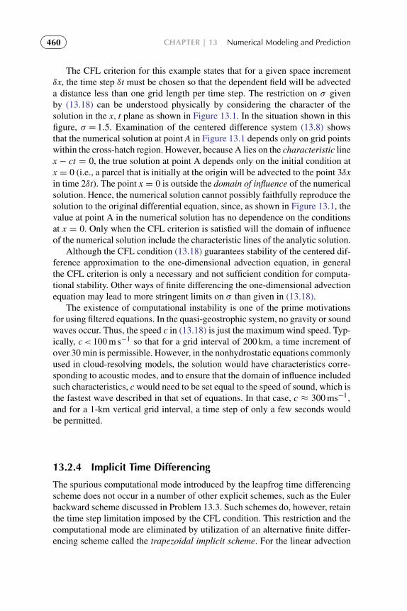
To protect the rights of the author(s) and publisher we inform you that this PDF is an uncorrected proof for internal businessuse only by the author(s), editor(s), reviewer(s), Elsevier and typesetter diacriTech. It is not allowed to publish this proofonline or in print. This proof copy is the copyright property of the publisher and is confidential until formal publication.
“Hakim: 17-ch13-453-490-9780123848666” — 2012/7/26 — 12:35 — page 460 — #8
460 CHAPTER | 13 Numerical Modeling and Prediction
The CFL criterion for this example states that for a given space incrementδx, the time step δt must be chosen so that the dependent field will be advecteda distance less than one grid length per time step. The restriction on σ givenby (13.18) can be understood physically by considering the character of thesolution in the x, t plane as shown in Figure 13.1. In the situation shown in thisfigure, σ = 1.5. Examination of the centered difference system (13.8) showsthat the numerical solution at point A in Figure 13.1 depends only on grid pointswithin the cross-hatch region. However, because A lies on the characteristic linex − ct = 0, the true solution at point A depends only on the initial condition atx = 0 (i.e., a parcel that is initially at the origin will be advected to the point 3δxin time 2δt). The point x = 0 is outside the domain of influence of the numericalsolution. Hence, the numerical solution cannot possibly faithfully reproduce thesolution to the original differential equation, since, as shown in Figure 13.1, thevalue at point A in the numerical solution has no dependence on the conditionsat x = 0. Only when the CFL criterion is satisfied will the domain of influenceof the numerical solution include the characteristic lines of the analytic solution.
Although the CFL condition (13.18) guarantees stability of the centered dif-ference approximation to the one-dimensional advection equation, in generalthe CFL criterion is only a necessary and not sufficient condition for computa-tional stability. Other ways of finite differencing the one-dimensional advectionequation may lead to more stringent limits on σ than given in (13.18).
The existence of computational instability is one of the prime motivationsfor using filtered equations. In the quasi-geostrophic system, no gravity or soundwaves occur. Thus, the speed c in (13.18) is just the maximum wind speed. Typ-ically, c< 100 m s−1 so that for a grid interval of 200 km, a time increment ofover 30 min is permissible. However, in the nonhydrostatic equations commonlyused in cloud-resolving models, the solution would have characteristics corre-sponding to acoustic modes, and to ensure that the domain of influence includedsuch characteristics, c would need to be set equal to the speed of sound, which isthe fastest wave described in that set of equations. In that case, c ≈ 300 ms−1,
and for a 1-km vertical grid interval, a time step of only a few seconds wouldbe permitted.
13.2.4 Implicit Time Differencing
The spurious computational mode introduced by the leapfrog time differencingscheme does not occur in a number of other explicit schemes, such as the Eulerbackward scheme discussed in Problem 13.3. Such schemes do, however, retainthe time step limitation imposed by the CFL condition. This restriction and thecomputational mode are eliminated by utilization of an alternative finite differ-encing scheme called the trapezoidal implicit scheme. For the linear advection
To protect the rights of the author(s) and publisher we inform you that this PDF is an uncorrected proof for internal businessuse only by the author(s), editor(s), reviewer(s), Elsevier and typesetter diacriTech. It is not allowed to publish this proofonline or in print. This proof copy is the copyright property of the publisher and is confidential until formal publication.
“Hakim: 17-ch13-453-490-9780123848666” — 2012/7/26 — 12:35 — page 461 — #9
13.2 | Numerical Approximation of the Equations of Motion 461
equation (13.6), this scheme can be written in the form(qm,s+1 − qm,s
)δt
= −c
2
[(qm+1,s+1 − qm−1,s+1
)2δx
+
(qm+1,s − qm−1,s
)2δx
](13.19)
Substituting the trial solution (13.12) into (13.19) yields
Bs+1=
[1− i (σ/2) sin p
1+ i (σ/2) sin p
]Bs (13.20)
where as before σ = cδt/δx and p = kδx. Defining
tan θp ≡ (σ/2) sin p (13.21)
and eliminating the common term Bs in (13.20), it can be shown that
B =
(1− i tan θp
1+ i tan θp
)= exp (−2iθp) (13.22)
so that the solution may be expressed simply as
qm,s = A exp[ik(mδx− 2θps/k)
](13.23)
Equation (13.19) involves only two time levels. Hence, unlike (13.14), thesolution yields only a single mode, which has phase speed c′= 2θp/(kδt).According to (13.21), θp remains real for all values of δt. (This should becontrasted to the situation for the explicit scheme given by (13.17).) Thus,the implicit scheme is absolutely stable. The truncation errors, however, canbecome large if θp is not kept sufficiently small (see Problem 13.9). A disadvan-tage of the implicit scheme is that the integration cannot proceed by marchingthrough the grid, as in the explicit case. In (13.19) there are terms involvingthe s + 1 time level on both sides of the equal sign, and these involve thevalues at a total of three grid points. Thus, the system (13.19) must be solvedsimultaneously for all points on the grid. If the grid is large, this may involveinverting a very large matrix, and so is computationally intensive. Furthermore,it is usually not feasible to utilize the implicit approach for nonlinear terms, suchas the advection terms in the momentum equations. Semi-implicit schemes inwhich the linear terms are treated implicitly and the nonlinear terms explicitlyare discussed briefly in Section 13.5.

To protect the rights of the author(s) and publisher we inform you that this PDF is an uncorrected proof for internal businessuse only by the author(s), editor(s), reviewer(s), Elsevier and typesetter diacriTech. It is not allowed to publish this proofonline or in print. This proof copy is the copyright property of the publisher and is confidential until formal publication.
“Hakim: 17-ch13-453-490-9780123848666” — 2012/7/26 — 12:35 — page 462 — #10
462 CHAPTER | 13 Numerical Modeling and Prediction
13.2.5 The Semi-Lagrangian Integration Method
The differencing schemes discussed previously are Eulerian schemes in whichthe time integration is carried out by computing the tendencies of the predictedfields at a set of grid points fixed in space. Although it would be possiblein theory to carry out predictions in a Lagrangian framework by following aset of marked fluid parcels, in practice this is not a viable alternative, sinceshear and stretching deformations tend to concentrate marked parcels in afew regions. Thus, it is difficult to maintain uniform resolution over the fore-cast region. It is possible to take advantage of the conservative properties ofLagrangian schemes, while maintaining uniform resolution, by employing asemi-Lagrangian technique. This approach permits relatively long time stepswhile retaining numerical stability and high accuracy.
The semi-Lagrangian method can be illustrated in a very simple fashion withthe one-dimensional advection equation (13.6). According to this equation, thefield q is conserved following the zonal flow at speed c. Thus, for any grid point,xm = mδx, and time ts = sδt:
q(xm, ts + δt) = q(xsm, ts) (13.24)
Here, xsm is the location at time ts for the air parcel that is located at point xm at
time ts + δt. This position in general does not lie on a grid point (see the “plus”marked on Figure 13.1), so evaluation of the right-hand side of (13.24) requiresinterpolating from the grid point values at time t. For c > 0 the position xs
mlies between the grid points xm−p and xm−p−1, where p is the integer part of theexpression cδt/δx (a measure of the number of grid points traversed in a timestep). If linear interpolation is used,
q(xsm, ts) = αq(xm−p−1, ts)+ (1− α)q(xm−p, ts)
where α = (xm−p − xsm)/δx. Thus, in Figure 13.1, p = 1, and to predict q at
point A, data are interpolated between the points m = 1 and m = 2 to the pointshown by the “+”.
In an actual prediction model the velocity field is predicted rather thanknown, as in this simple example. Thus, for a two-dimensional field
q (x, y, t + δt) = q (x− uδt, y− vδt, t) (13.25)
where the velocity components at time t can be used to estimate the fieldsat t+ δt; once these are obtained they can be used to provide more accurateapproximations to the velocities on the right in (13.25). The right side in (13.25)is again estimated by interpolation, which now must be carried out in twodimensions.
As shown in Figure 13.1, the semi-Lagrangian scheme guarantees that thedomain of influence in the numerical solution corresponds to that of the physi-cal problem. Thus, the scheme is computational stability for time steps much

To protect the rights of the author(s) and publisher we inform you that this PDF is an uncorrected proof for internal businessuse only by the author(s), editor(s), reviewer(s), Elsevier and typesetter diacriTech. It is not allowed to publish this proofonline or in print. This proof copy is the copyright property of the publisher and is confidential until formal publication.
“Hakim: 17-ch13-453-490-9780123848666” — 2012/7/26 — 12:35 — page 463 — #11
13.2 | Numerical Approximation of the Equations of Motion 463
longer than possible with an explicit Eulerian scheme. The semi-Lagrangianscheme also preserves the values of conservative properties quite accurately andis particularly useful for accurately advecting trace constituents such as watervapor.
13.2.6 Truncation Error
To be useful it is necessary not only that a numerical solution be stable but thatit also provide an accurate approximation to the true solution. The differencebetween the numerical solution to a finite difference equation and the solutionto the corresponding differential equation is called the discretization error. Ifthis error approaches zero with δt and δx, the solution is called convergent. Thedifference between a differential equation and the finite difference analog to itis referred to as a truncation error because it arises from truncating the Taylorseries approximation to the derivatives. If this error approaches zero as δt andδx go to zero, the scheme is called consistent. According to the Lax equivalencetheorem,1 if the finite difference formulation satisfies the consistency condition,then stability is the necessary and sufficient condition for convergence. Thus, ifa finite difference approximation is consistent and stable, one can be certain thatthe discretization error will decrease as the difference intervals are decreased,even if it is not possible to determine the error exactly.
Because numerical solutions are as a rule sought only when analytic solu-tions are unavailable, it is usually not possible to determine the accuracy ofa solution directly. For the linear advection equation with constant advectionspeed considered in Section 13.2.3, it is possible, however, to compare the solu-tions of the finite difference equation (13.8) and the original differential equation(13.6). We can then use this example to investigate the accuracy of the differencemethod introduced earlier.
From the preceding discussion we can already conclude that the magnitudeof the truncation error in the present case will be of order δx2 and δt2. It is pos-sible to obtain more precise information on accuracy from examination of thesolution (13.14). Note that for θp→ 0,C→ 1 and D→ 0. The part of the solu-tion proportional to C is the physical mode. The part proportional to D is calledthe computational mode because it has no counterpart in the analytic solutionto the original differential equation. It arises because centered time differencinghas turned a differential equation that is first order in time into a second-orderfinite difference equation. The accuracy of the finite difference solution dependsnot only on the smallness of D and the closeness of C to unity but on thematch between the phase speed of the physical mode and the phase speed inthe analytic solution. The phase of the physical mode is given in (13.14) by
pm− θps = (p/δx)(mδx− θpsδx/p
)= k
(x− c′t
)1See Richtmyer and Morton (1967).

To protect the rights of the author(s) and publisher we inform you that this PDF is an uncorrected proof for internal businessuse only by the author(s), editor(s), reviewer(s), Elsevier and typesetter diacriTech. It is not allowed to publish this proofonline or in print. This proof copy is the copyright property of the publisher and is confidential until formal publication.
“Hakim: 17-ch13-453-490-9780123848666” — 2012/7/26 — 12:35 — page 464 — #12
464 CHAPTER | 13 Numerical Modeling and Prediction
�
�
�
�
TABLE 13.1 Centered Finite Difference Accuracy
L/δx p θp c′/c |D|/|C|
2 π π – ∞
4 π/2 0.848 0.720 0.204
8 π/4 0.559 0.949 0.082
16 π/8 0.291 0.988 0.021
32 π/16 0.147 0.997 0.005
Note: Results apply to the advection equation as a function ofresolution for σ = 0.75.
where c′ = θpδx/(pδt) is the phase speed of the physical mode. Its ratio to thetrue phase speed is
c′/c = θpδx/(pcδt) = sin−1(σ sin p)/(σp)
so that c′/c→ 1 as σp→ 0. The dependence of c′/c and |D|/|C| on wavelengthis shown in Table 13.1 for the particular case where σ = 0.75.
It is clear from Table 13.1 that phase speed and amplitude errors bothincrease as the wavelength decreases. Short waves move slower than long wavesin the finite difference solution, even though in the original equation all wavesmove at speed c. This dependence of phase speed on wavelength in the dif-ference solution is called numerical dispersion. It is a serious problem fornumerical modeling of any advected field that has sharp gradients (and thuslarge-amplitude short-wave components).
Short waves also suffer from having significant amplitude in the computa-tional mode. This mode, which has no counterpart in the solution to the originaldifferential equation, propagates opposite to the direction of the physical modeand changes sign from one time step to the next. This behavior makes it easy torecognize when the computational mode has significant amplitude.
13.3 THE BAROTROPIC VORTICITY EQUATIONIN FINITE DIFFERENCES
The simplest example of a dynamical forecast model is the barotropic vorticityequation (11.14), which for a Cartesian β plane can be written in the form
∂ζ
∂t= −F(x, y, t) (13.26)

To protect the rights of the author(s) and publisher we inform you that this PDF is an uncorrected proof for internal businessuse only by the author(s), editor(s), reviewer(s), Elsevier and typesetter diacriTech. It is not allowed to publish this proofonline or in print. This proof copy is the copyright property of the publisher and is confidential until formal publication.
“Hakim: 17-ch13-453-490-9780123848666” — 2012/7/26 — 12:35 — page 465 — #13
13.3 | The Barotropic Vorticity Equation in Finite Differences 465
where
F(x, y, t) = Vψ ·∇ (ζ + f ) =∂
∂x
(uψζ
)+∂
∂y
(vψζ
)+ βvψ (13.27)
and uψ = −∂ψ/∂y, vψ = ∂ψ/∂x, and ζ = ∇2ψ . We have here used the factthat the horizontal velocity is nondivergent (∂uψ/∂x+∂vψ/∂y = 0) to write theadvection term in flux form. The advection of absolute vorticity F(x, y, t) maybe calculated provided that we know the field of ψ(x, y, t). Equation (13.26) canthen be integrated forward in time to yield a prediction for ζ . It is then necessaryto solve the Poisson equation ζ = ∇2ψ to predict the streamfunction.
A straightforward solution method is the leapfrog scheme discussed inSection 13.2.2. This requires writing (13.27) in finite difference form. Supposethat the horizontal x,y space is divided into a grid of (M + 1)× (N + 1) pointsseparated by distance increments δx and δy. Then we can write the coordinateposition of a given grid point as xm = mδx, yn = nδy,where m = 0, 1, 2, . . . ,Mand n = 0, 1, 2, . . . ,N. Thus, any point on the grid is uniquely identified by theindices (m, n). A portion of such a grid space is shown in Figure 13.2.
Centered difference formulas of the type (13.4) can then be used to approxi-mate derivatives in the expression F(x, y, t). For example, if we assume thatδx = δy ≡ d,
uψ ≈ um,n = −(ψm,n+1 − ψm,n−1)/2d
vψ ≈ vm,n = +(ψm+1,n − ψm−1,n)/2d(13.28)
(m − 1, n + 1) (m, n + 1)
δy δx
(m + 1, n + 1)
(m − 1, n ) (m, n ) (m + 1, n )
(m − 1, n − 1) (m, n − 1) (m + 1, n − 1)
FIGURE 13.2 Portion of a two-dimensional (x, y) grid mesh for solution of the barotropic vorticityequation.

To protect the rights of the author(s) and publisher we inform you that this PDF is an uncorrected proof for internal businessuse only by the author(s), editor(s), reviewer(s), Elsevier and typesetter diacriTech. It is not allowed to publish this proofonline or in print. This proof copy is the copyright property of the publisher and is confidential until formal publication.
“Hakim: 17-ch13-453-490-9780123848666” — 2012/7/26 — 12:35 — page 466 — #14
466 CHAPTER | 13 Numerical Modeling and Prediction
Similarly, with the aid of (13.5) we find that the horizontal Laplacian can beapproximated as
∇2ψ ≈ (ψm+1,n+ψm−1,n+ψm,n+1+ψm,n−1−4ψm,n)/d
2= ζm,n (13.29)
The finite difference form of the Laplacian is proportional to the differencebetween the value of the function at the central point and the average valueat the four surrounding grid points. If there are (M − 1)× (N − 1) interiorgrid points, then (13.29) yields a set of (M − 1)× (N − 1) simultaneous equa-tions, which together with suitable boundary conditions determine ψm,n fora given array ζm,n. This set can be solved by standard methods of matrixinversion.
Before expressing the advection term F(x, y, t) in finite difference form, itis worth noting that if ψ is taken to be constant on the northern and southernboundaries of the β-plane channel, it is easily shown by integration over thearea of the channel that the average value of F is zero. This implies that themean vorticity is conserved for the channel. It is also possible, with a little morealgebra, to show that the mean kinetic energy and the mean square vorticity(called the enstrophy) are conserved.
For accuracy of long-term integrations, it is desirable that any finite differ-ence approximation to F satisfy the same conservation constraints as the originaldifferential form; otherwise, the finite difference solution would not be conser-vative. The mean vorticity, for example, might then drift systematically in timepurely because of the nature of the finite difference solution. Finite differenceschemes that simultaneously conserve vorticity, kinetic energy, and enstrophyhave been designed. They are, however, rather complex. For our purposes itis sufficient to note that by writing the advection in the flux form (13.27) andusing centered space differences we can conserve both mean vorticity and meankinetic energy:
Fm,n =1
2d
[(um+1,nζm+1,n − um−1,nζm−1,n
)+(vm,n+1ζm,n+1 − vm,n−1ζm,n−1
)]+ βvm,n (13.30)
It is verified readily that if ψ satisfies periodic boundary conditions, there is acancellation of terms when (13.30) is summed over the domain. Thus,
M∑m=1
N∑n=1
Fm,n = 0 (13.31)
Therefore, mean vorticity is conserved (except for errors introduced by timedifferencing) when (13.30) is used as the finite difference form of the advec-tion term. This form also conserves mean kinetic energy (see Problem 13.2).

To protect the rights of the author(s) and publisher we inform you that this PDF is an uncorrected proof for internal businessuse only by the author(s), editor(s), reviewer(s), Elsevier and typesetter diacriTech. It is not allowed to publish this proofonline or in print. This proof copy is the copyright property of the publisher and is confidential until formal publication.
“Hakim: 17-ch13-453-490-9780123848666” — 2012/7/26 — 12:35 — page 467 — #15
13.4 | The Spectral Method 467
Enstrophy is not conserved in this difference formulation, and it is conventionalto add a small diffusion term in order to control any numerically generatedincrease in enstrophy.
The procedure for preparing a numerical forecast with the barotropicvorticity equation can now be summarized as follows:
1. The observed geopotential field at the initial time is used to compute theinitial streamfunction ψm,n(t = 0) at all grid points.
2. Fm,n is evaluated at all grid points.3. ζm,n(t+ δt) is determined using centered differencing except at the first time
step when a forward difference must be used.4. The simultaneous set (13.29) is solved for ψm,n(t + δt).5. The predicted array of ψm,n is used as data, and steps 2 through 4 are
repeated until the desired forecast period is reached. For example, a 24-hforecast with 30-min time increments would require 48 cycles.
13.4 THE SPECTRAL METHOD
In the finite difference method, the dependent variables are specified on a set ofgrid points in space and time, and derivatives are approximated using finite dif-ferences. An alternative approach, referred to as the spectral method, involvesrepresenting the spatial variations of the dependent variables in terms of finiteseries of orthogonal functions called basis functions. For the Cartesian geome-try of a midlatitude β-plane channel, the appropriate set of basis functions is adouble Fourier series in x and y. For spherical Earth, however, the appropriatebasis functions are the spherical harmonics.
A finite difference approximation is local in the sense that the finite differ-ence variable 9m,n represents the value of ψ(x, y) at a particular point in space,and the finite difference equations determine the evolution of the 9m,n for allgrid points. The spectral approach, however, is based on global functions—that is, the individual components of the appropriate series of basis functions.In the case of Cartesian geometry, for example, these components determinethe amplitudes and phases of the sinusoidal waves that when summed deter-mine the spatial distribution of the dependent variable. The solution proceedsby determining the evolution of a finite number of Fourier coefficients. Becausethe distribution in wave number space of the Fourier coefficients for a givenfunction is referred to as its spectrum, it is appropriate to call this approach thespectral method.
At low resolution the spectral method is generally more accurate than thegrid point method, partly because, for linear advection, the numerical dispersiondiscussed in Section 13.2.4 can be severe in a grid point model but does notoccur in a properly formulated spectral model. For the range of resolutions usedcommonly in forecast models the two approaches are comparable in accuracy,and each has its advocates.

To protect the rights of the author(s) and publisher we inform you that this PDF is an uncorrected proof for internal businessuse only by the author(s), editor(s), reviewer(s), Elsevier and typesetter diacriTech. It is not allowed to publish this proofonline or in print. This proof copy is the copyright property of the publisher and is confidential until formal publication.
“Hakim: 17-ch13-453-490-9780123848666” — 2012/7/26 — 12:35 — page 468 — #16
468 CHAPTER | 13 Numerical Modeling and Prediction
13.4.1 The Barotropic Vorticity Equation in SphericalCoordinates
The spectral method is particularly advantageous for solution of the vortic-ity equation. When the proper set of basis functions is chosen, it is trivialto solve the Poisson equation for the streamfunction. This property of thespectral method not only saves computer time but eliminates the truncation errorassociated with finite differencing the Laplacian operator.
In practice the spectral method is applied most frequently to global mod-els. This requires use of spherical harmonics, which are more complicated thanFourier series. To keep the discussion as simple as possible, it is again useful toconsider the barotropic vorticity equation as a prototype forecast model in orderto illustrate the spectral method on the sphere.
The barotropic vorticity equation in spherical coordinates may be exp-ressed as
D
Dt(ζ + 2� sinφ) = 0 (13.32)
where, as usual, ζ = ∇2ψ , with ψ a streamfunction, and
D
Dt≡∂
∂t+
u
a cosφ
∂
∂λ+
v
a
∂
∂φ(13.33)
It turns out to be convenient to use µ ≡ sinφ as the latitudinal coordinate, inwhich case the continuity equation can be written
1
a
∂
∂λ
(u
cosφ
)+
1
a
∂
∂µ(v cosφ) = 0 (13.34)
so that the streamfunction is related to the zonal and meridional velocitiesaccording to
u
cosφ= −
1
a
∂ψ
∂µ; v cosφ =
1
a
∂ψ
∂λ(13.35)
The vorticity equation can then be expressed as
∂∇2ψ
∂t=
1
a2
[∂ψ
∂µ
∂∇2ψ
∂λ−∂ψ
∂λ
∂∇2ψ
∂µ
]−
2�
a2
∂ψ
∂λ(13.36)
where
∇2ψ =
1
a2
{∂
∂µ
[(1− µ2
) ∂ψ∂µ
]+
1
1− µ2
∂2ψ
∂λ2
}(13.37)
The appropriate orthogonal basis functions are the spherical harmonics,which are defined as
Yγ (µ, λ) ≡ Pγ (µ) eimλ (13.38)

To protect the rights of the author(s) and publisher we inform you that this PDF is an uncorrected proof for internal businessuse only by the author(s), editor(s), reviewer(s), Elsevier and typesetter diacriTech. It is not allowed to publish this proofonline or in print. This proof copy is the copyright property of the publisher and is confidential until formal publication.
“Hakim: 17-ch13-453-490-9780123848666” — 2012/7/26 — 12:35 — page 469 — #17
13.4 | The Spectral Method 469
where γ ≡ (n,m) is a vector containing the integer indices for the sphericalharmonics. These are given by m = 0,±1,±2,±3, . . . , n = 1, 2, 3, . . . , whereit is required that |m| ≤ n. Here, Pγ designates an associated Legendre functionof the first kind of degree n. From (13.38) it is clear that m designates the zonalwave number. It can be shown2 that n − |m| designates the number of nodesof Pγ in the interval −1 < µ < 1 (i.e., between the poles), and thus measuresthe meridional scale of the spherical harmonic. The structures of a few sphericalharmonics are shown in Figure 13.3.
An important property of the spherical harmonics is that they satisfy therelationship
∇2Yγ = −
n (n+ 1)
a2Yγ (13.39)
so that the Laplacian of a spherical harmonic is proportional to the functionitself, which implies that the vorticity associated with a particular spherical har-monic component is simply proportional to the streamfunction for the samecomponent.
Antisymmetricm = 0 m = 1
m = 2 m = 3
m = 4 m = 5
Symmetric
FIGURE 13.3 Patterns of positive and negative regions for the spherical harmonic functionswith n = 5 and m = 0, 1, 2, 3, 4, 5. (After Washington and Parkinson, 1986; adapted from Baer,1972. Copyright © American Meteorological Society. Reprinted with permission.)
2See Washington and Parkinson (1986) for a discussion of the properties of the Legendre function.
To protect the rights of the author(s) and publisher we inform you that this PDF is an uncorrected proof for internal businessuse only by the author(s), editor(s), reviewer(s), Elsevier and typesetter diacriTech. It is not allowed to publish this proofonline or in print. This proof copy is the copyright property of the publisher and is confidential until formal publication.
“Hakim: 17-ch13-453-490-9780123848666” — 2012/7/26 — 12:35 — page 470 — #18
470 CHAPTER | 13 Numerical Modeling and Prediction
In the spectral method on the sphere, the streamfunction is expanded in afinite series of spherical harmonics by letting
ψ(λ,µ, t) =∑γ
ψγ (t)Yγ (µ, λ) (13.40)
where ψγ is the complex amplitude for the Yγ spherical harmonic and the sum-mation is over both n and m. The individual spherical harmonic coefficients ψγare related to the streamfunction ψ(λ,µ) through the inverse transform
ψγ (t) =1
4π
∫S
Y∗γψ(λ,µ, t)dS (13.41)
where dS = dµdλ and Y∗γ designates the complex conjugate of Yγ .
13.4.2 Rossby–Haurwitz Waves
Before considering numerical solution of the barotropic vorticity equation, itis worth noting that an exact analytic solution of the nonlinear equation canbe obtained in the special case where the streamfunction is equal to a singlespherical harmonic mode. Thus, we let
ψ(λ,µ, t) = ψγ (t) eimλPγ (µ) (13.42)
Substituting from (13.42) into (13.36) and applying (13.39), we find that thenonlinear advection term is identically zero so that the amplitude coefficientsatisfies the ordinary linear equation
−n (n+ 1) dψγ /dt = −2�imψγ (13.43)
which has the solution ψγ (t) = ψγ (0) exp (iνγ t), where
νγ = 2�m/ [n (n+ 1)] (13.44)
is the dispersion relationship for Rossby–Haurwitz waves, which is the namegiven to planetary waves on a sphere. (This should be compared to (5.110) withu = 0, which is the equivalent expression for a midlatitude β-plane.) Becausethe horizontal scale of a spherical harmonic mode is proportional to n−1, (13.44)shows that a single mode propagates westward on a sphere at a speed that isapproximately proportional to the square of the horizontal scale. This solutionalso suggests why for some problems the spectral method is superior to thefinite difference method at coarse resolution. A model containing even a singleFourier component can represent a realistic meteorological field (the Rossbywave), while many grid points are required for an equivalent representation infinite differences.

To protect the rights of the author(s) and publisher we inform you that this PDF is an uncorrected proof for internal businessuse only by the author(s), editor(s), reviewer(s), Elsevier and typesetter diacriTech. It is not allowed to publish this proofonline or in print. This proof copy is the copyright property of the publisher and is confidential until formal publication.
“Hakim: 17-ch13-453-490-9780123848666” — 2012/7/26 — 12:35 — page 471 — #19
13.4 | The Spectral Method 471
13.4.3 The Spectral Transform Method
When many spherical harmonic modes are present, the solution of (13.36)by a purely spectral method requires evaluation of the nonlinear interactionsamong various modes due to the advection term. It turns out that the numberof interaction terms increases as the square of the number of modes retainedin the series (13.40) so that this approach becomes computationally ineffi-cient for models with the sort of spatial resolution required for prediction ofsynoptic-scale weather disturbances. The spectral transform method overcomesthis problem by transforming between spherical harmonic wave number spaceand a latitude–longitude grid at every time step and carrying out the multipli-cations in the advection term in grid space. Thus, that it is never necessary tocompute products of spectral functions.
To illustrate this method it is useful to rewrite the barotropic vorticityequation in the form
∂∇2ψ
∂t= −
1
a2
[2�∂ψ
∂λ+ A (λ, µ)
](13.45)
where
A(λ, µ) ≡
[−∂ψ
∂µ
∂∇2ψ
∂λ+∂ψ
∂λ
∂∇2ψ
∂µ
](13.46)
Substituting from (13.40) into (13.45) then yields for the spherical harmoniccoefficients
dψγ /dt = iνγψγ + Aγ [n (n+ 1)]−1 (13.47)
where Aγ is the γ component of the transform of A(λ, µ):
Aγ =1
4π
2π∫0
+1∫−1
A (λ, µ)Y∗γ dλdµ (13.48)
The transform method utilizes the fact that if the sum γ = (n,m) is takenover a finite number of modes, the integral in the transform (13.48) can beevaluated exactly by numerical quadrature—that is, by summing appropri-ately weighted values of A(λ, µ) evaluated at the grid points (λj, µk) of alatitude–longitude grid mesh. Computation of the distribution of A(λ, µ) forall grid points can be carried out without need to introduce finite differences forderivatives by noting that we can express the advection term in the form
A(λj, µk
)=(1− µ2)−1 [F1F2 + F3F4] (13.49)

To protect the rights of the author(s) and publisher we inform you that this PDF is an uncorrected proof for internal businessuse only by the author(s), editor(s), reviewer(s), Elsevier and typesetter diacriTech. It is not allowed to publish this proofonline or in print. This proof copy is the copyright property of the publisher and is confidential until formal publication.
“Hakim: 17-ch13-453-490-9780123848666” — 2012/7/26 — 12:35 — page 472 — #20
472 CHAPTER | 13 Numerical Modeling and Prediction
1
3
4 2
ψ (λj, μk)
ζ (λj, μk)
ψγ (t + δt)
ζγ (t + δt)
A(λj, μk)
Aγ
FIGURE 13.4 Steps in the prediction cycle for the spectral transform method of solution of thebarotropic vorticity equation.
where
F1 = −(1− µ2)∂ψ/∂µ, F2 = ∂∇
2ψ/∂λ
F3 =(1− µ2)∂∇2ψ/∂µ, F4 = ∂ψ/∂λ
The quantities F1 − F4 can be computed exactly for each grid point using thespectral coefficients ψγ and the known differential properties of the sphericalharmonics. For example,
F4 = ∂ψ/∂λ =∑γ
imψγ Yγ(λj, µk
)Once these terms have been computed for all grid points, A(λ, µ) can be
computed at the grid points by forming the products F1F2 and F3F4; no finitedifference approximations to the derivatives are required in this procedure. Thetransform (13.48) is then evaluated by numerical quadrature to compute thespherical harmonic components Aγ . Finally, (13.47) can be stepped ahead bya time increment δt to obtain new estimates of the spherical harmonic compo-nents of the streamfunction. The whole process is then repeated until the desiredforecast period is reached. The steps in forecasting with the barotropic vortic-ity equation using the spectral transform method are summarized in schematicform in Figure 13.4.
13.5 PRIMITIVE EQUATION MODELS
Modern numerical forecast models are based on a formulation of the dynam-ical equations, referred to as the primitive equations, which is essentially theformulation proposed by Richardson. The primitive equations differ from the

To protect the rights of the author(s) and publisher we inform you that this PDF is an uncorrected proof for internal businessuse only by the author(s), editor(s), reviewer(s), Elsevier and typesetter diacriTech. It is not allowed to publish this proofonline or in print. This proof copy is the copyright property of the publisher and is confidential until formal publication.
“Hakim: 17-ch13-453-490-9780123848666” — 2012/7/26 — 12:35 — page 473 — #21
13.5 | Primitive Equation Models 473
+ +T, p
(a) (b)
T, p
u
v
v
u
u
u
v v
FIGURE 13.5 Horizontal grid staggering schemes for the Arakawa-C (a) and Arakawa-D (b)grids. Thermodynamic (T, p) and other scalar fields are located at the center of the grid cell;horizontal velocity components u and v are located along the grid edge.
complete momentum equations (2.19), (2.20), and (2.21) in that the verticalmomentum equation is replaced by the hydrostatic approximation, and the smallterms in the horizontal momentum equations given in columns C and D inTable 2.1 are neglected. In most models some version of the σ -coordinatesystem introduced in Section 10.3.1 is used, and the vertical dependence isrepresented by dividing the atmosphere into a number of levels and utilizingfinite difference expressions for vertical derivatives. Both finite differencing andthe spectral method have been used for horizontal discretization in operationalprimitive equation forecast models.
Grid point models utilize the finite difference method described inSection 13.2.1. Most grid point models utilize a grid-staggering approach toimprove the accuracy of certain fields. Two examples of where the momen-tum field is staggered relative to the thermodynamic variables are shown inFigure 13.5. The Arakawa-C grid (a) is staggered so that the horizontal diver-gence (∂u/∂x + ∂v/∂y) is located in the center of the grid cell, whereas theArakawa-D grid (b) is staggered so that the vertical vorticity ∂v/∂x − ∂u/∂yis located in the center of the grid cell.
13.5.1 Spectral Models
Most operational forecast centers utilize spectral models as their primary globalforecast models, whereas grid point models are generally employed for fine-scale limited area models. Operational spectral models employ a primitive equa-tion version of the spectral transform method described in Section 13.4.3. In thismethod the values of all meteorological fields are available in both spectral andgrid point domains at each time step. Vorticity and divergence are employedas predictive variables rather than u and v. Physical computations involvingsuch processes as radiative heating and cooling, condensation and precipita-tion, and convective overturning are calculated in physical space on the gridmesh, whereas differential dynamical quantities, such as pressure gradients andvelocity gradients, are evaluated exactly in spectral space. This combination

To protect the rights of the author(s) and publisher we inform you that this PDF is an uncorrected proof for internal businessuse only by the author(s), editor(s), reviewer(s), Elsevier and typesetter diacriTech. It is not allowed to publish this proofonline or in print. This proof copy is the copyright property of the publisher and is confidential until formal publication.
“Hakim: 17-ch13-453-490-9780123848666” — 2012/7/26 — 12:35 — page 474 — #22
474 CHAPTER | 13 Numerical Modeling and Prediction
n
M
|m|
n
M
|m|
(a) (b)
FIGURE 13.6 Regions of wave number space (n,m) in which spectral components are retainedfor the rhomboidal truncation (a) and triangular truncation (b). (After Simmons and Bengtsson, 1984.Used with permission.)
preserves the simplicity of the grid point representation for physical processesthat are “local” in nature, while retaining the superior accuracy of the spectralmethod for dynamical calculations.
Two spectral truncations are typically employed in global spectral modes.The first, triangular truncation, refers to the fact that on a plot of m versus n(see 13.38) the retained modes occupy a triangular area. The second spectraltruncation is rhomboidal truncation, which has N= |m| + M. Both of thesetruncations are shown schematically in Figure 13.6. In triangular truncation,the horizontal resolution in the zonal and meridional directions is nearly equal.In rhomboidal truncation, however, the latitudinal resolution is the same forevery zonal wave number. Rhomboidal truncation has some advantages for low-resolution models, but at high resolution the triangular truncation appears to besuperior.
13.5.2 Physical Parameterizations
The physical processes included in modern operational forecast models are gen-erally the same as those included in general circulation models and were shownschematically in Figure 10.21. Inclusion of such processes as boundary layer

To protect the rights of the author(s) and publisher we inform you that this PDF is an uncorrected proof for internal businessuse only by the author(s), editor(s), reviewer(s), Elsevier and typesetter diacriTech. It is not allowed to publish this proofonline or in print. This proof copy is the copyright property of the publisher and is confidential until formal publication.
“Hakim: 17-ch13-453-490-9780123848666” — 2012/7/26 — 12:35 — page 475 — #23
13.6 | Data Assimilation 475
fluxes, vertical mixing by dry and moist convection, formation of clouds andprecipitation, and the interaction of cloud and radiation fields requires that therelevant subgrid-scale processes be represented in terms of model-predictedfields. The approximation of unresolved processes in terms of resolved vari-ables is referred to as parameterization; it is probably the most difficult andcontroversial area of weather and climate modeling.
Perhaps the most important physical process that must be parameterized isconvection. Vertical heat transfer by convection is essential in maintaining theobserved tropospheric lapse rate and moisture distribution. The simplest wayto mimic this effect of unresolved convective motions is through convectiveadjustment. In a simple version of this method, the relative humidity and lapserate in each grid column are examined at the end of each time step. If the lapserate is super-adiabatic, the temperature profile is adjusted to dry static neutralityin a manner that conserves energy; if the column is conditionally unstable, andthe humidity exceeds a specified value, the column is adjusted to moist staticneutrality. More sophisticated schemes utilize the fact that moist convectionis dependent on low-level moisture convergence, and they include a moisturebudget as part of the parameterization.
Various methods are used to relate clouds to the resolved humidity, tem-perature, and wind fields. None is completely satisfactory. In some models themodel-predicted cloud fields are used only in the portion of the model con-cerned with precipitation, and cloud–radiation interactions are parameterizedusing specified cloud climatologies.
13.6 DATA ASSIMILATION
Since forecasting is an initial value problem, observations are needed toestablish the initial condition, which is called an analysis. Observations are dis-tributed inhomogeneously in space and time, in contrast to numerical models,which have regularly spaced grids and forecasts that begin at specific times.Data assimilation is a technique that maps the inhomogeneous observationsonto a regular grid, and also accounts for the errors in observations. As thename suggests, observations are assimilated into the numerical model, and themodel is used to transmit the information from observations to a future timewhen observations are again available.
For this reason, data assimilation involves blending observations with esti-mates of the observations from short-range forecasts. Since the short-rangeforecasts start from relatively accurate initial conditions, the error in the model-estimated observations is so small that, for operational forecast systems, onlyabout 15% of the analysis comes from millions of observations; the other 85%derives from the model, which has accumulated the information from all obser-vations before that time. An essential aspect of data assimilation is that nothingis known exactly and the problem must be treated probabilistically.

To protect the rights of the author(s) and publisher we inform you that this PDF is an uncorrected proof for internal businessuse only by the author(s), editor(s), reviewer(s), Elsevier and typesetter diacriTech. It is not allowed to publish this proofonline or in print. This proof copy is the copyright property of the publisher and is confidential until formal publication.
“Hakim: 17-ch13-453-490-9780123848666” — 2012/7/26 — 12:35 — page 476 — #24
476 CHAPTER | 13 Numerical Modeling and Prediction
13.6.1 Data Assimilation for a Single Variable
To define the data assimilation problem, and different techniques used to solveit, we begin with a single scalar before moving on to multiple variables. Given ascalar variable x, assume that there are two estimates of its true value: an obser-vation, y, and a prior estimate, or background, xb. The background may comefrom different sources, but mainly it comes from a short-range forecast. Wewish to estimate the true value of x given the background and observation. Themathematical transcription of this statement involves a conditional probability
p(xa) = p(x|y) (13.50)
In words, the probability density of the analysis, xa, is equal to the con-ditional probability density of the true state, x, given observation y (seeAppendix G for background on conditional probability). The background infor-mation comes in through Bayes’ Rule, which allows the conditional probabilitydensity to be “inverted” so that
p(x|y) =p(y|x)p(x)
p(y)(13.51)
where, in this case, p(y) is just a scaling constant that may be neglected.3 Sincep(y|x) is a function of the second argument, x, it is a likelihood function for theobservation, given x. A more complete description is given in Appendix G, butthe basic idea can be illustrated by flipping a coin to determine the likelihoodthat the coin is fair (e.g., determine the likelihood that the coin is fair fromobserving three consecutive tosses that all yield heads). This problem is thereverse of knowing that the coin is fair and determining the probability of anoutcome conditioned on that knowledge (e.g., the probability of three heads ina row for a fair coin).
At this point the probability density functions are general, but for problemswith many variables, a simplification is needed. The main simplification is thatthe variables are distributed normally (or Gaussian), which for a scalar reducesthe probability density description to the mean and variance,
p(y|x) = c1e−
12
(y−xσy
)2
p(x) = c2e−
12
(x−xbσb
)2
(13.52)
where c1 and c2 are constants. The error variances of the observation and back-ground are σ 2
y and σ 2b , respectively. Using (13.52) and (13.51) in (13.50) gives
the analysis probability density
p(xa) = Ce−
12
(x−xbσb
)2
e−
12
(y−xσy
)2
(13.53)
3The integral over p(xa), like all probability density functions, must be unity.

To protect the rights of the author(s) and publisher we inform you that this PDF is an uncorrected proof for internal businessuse only by the author(s), editor(s), reviewer(s), Elsevier and typesetter diacriTech. It is not allowed to publish this proofonline or in print. This proof copy is the copyright property of the publisher and is confidential until formal publication.
“Hakim: 17-ch13-453-490-9780123848666” — 2012/7/26 — 12:35 — page 477 — #25
13.6 | Data Assimilation 477
This result involves a product of Gaussians, which may be simplified to a newGaussian distribution. To do so it proves useful to consider the following metric,J, of the probability density:
J(x) ≡ −log [p(x)] = 12(x− xb)
2
σ 2b
+12(y− x)2
σ 2y− log(C) (13.54)
Metric J, the “cost function,” is a quadratic measure of the misfit betweenthe true value of the scalar and the two estimates we have, with smaller valuesof J indicating a better fit. Finding the best fit involves solving for the minimumvalue of J by taking ∂J/∂x and setting the result to zero. Solving for x at thispoint yields the analysis value, xa,
xa =
(σ 2
y
σ 2y + σ
2b
)xb +
(σ 2
b
σ 2y + σ
2b
)y (13.55)
This result reveals that the best estimate of the true state is given by a linearcombination4 of the prior estimate and the observation, with weights determinedby the errors in these quantities. In the limit of vanishing error in the observation(σ 2
y → 0) the weight on the prior estimate approaches zero and the weight onthe observation approaches one. The error variance for xa is given by
σ 2a =
σ 2b
1+(σbσy
)2=
σ 2y
1+(σyσb
)2< σ 2
b , σ2y (13.56)
which shows that the error in the analysis is always less than the error in boththe prior estimate and the observation. Thus the analysis is Gaussian distributedwith mean xa and variance σ 2
a .The generalization from a scalar to vectors in the case of many analysis
variables and many observations is facilitated by rewriting (13.55) as
xa = xb + K(y− xb) (13.57)
and (13.56) as
σ 2a = (1− K) σ 2
b (13.58)
where
K =σ 2
b
σ 2b + σ
2y
(13.59)
From (13.57) we see that the analysis may be viewed as a linear combinationof the prior estimate and the innovation, or new information, contained in the
4The result is identical to the solution obtained using the method of linear least squares.

To protect the rights of the author(s) and publisher we inform you that this PDF is an uncorrected proof for internal businessuse only by the author(s), editor(s), reviewer(s), Elsevier and typesetter diacriTech. It is not allowed to publish this proofonline or in print. This proof copy is the copyright property of the publisher and is confidential until formal publication.
“Hakim: 17-ch13-453-490-9780123848666” — 2012/7/26 — 12:35 — page 478 — #26
478 CHAPTER | 13 Numerical Modeling and Prediction
observation. If the observation gives the same value as our prior estimate, noth-ing has been learned, and there is no need to adjust the prior estimate. Whenthere is new information, its weight relative to the background is controlled bythe gain weighting factor, K, which is given by the ratio of the variance in theprior to the variance in the innovation.5 K has an upper limit of one for σ 2
y → 0
and a lower limit of zero for σ 2b → 0. Notice in (13.58) that, in the case of a
perfect observation, the error in the prior is reduced to zero in the analysis.A graphical illustration of these results is shown in Figure 13.7. Notice that,
by assumption, the distribution in the observation (thin solid line) has less errorthan the prior (dashed line) and, as a result, the analysis (thick solid line) isweighted closer to the observation than the prior. Similarly, the distribution forthe analysis has higher probability density than either the prior or the observa-tion, because the analysis error variance is smaller as well. The thick gray curveshows the cost function, J, which reaches a minimum at the mean value of xa.
−2 −1.5 −1 −0.5 0 0.5 1 1.5 2 2.5 3x
FIGURE 13.7 Data assimilation for scalar variable x assuming Gaussian error statistics. Priorestimate xb, given by the dashed line, has mean −0.25 and variance 0.5. Observation y, given bythe thin solid line, has mean 1.0 and variance 0.25. The analysis, xa, given by the thick solid line,has mean 0.58 and variance 0.17. The parabolic gray curve denotes the cost function, J, which takesa minimum at the mean value of xa.
5The variance of the innovation is given by the sum of variances σ 2b + σ
2y provided that errors in
the prior and observation are uncorrelated.

To protect the rights of the author(s) and publisher we inform you that this PDF is an uncorrected proof for internal businessuse only by the author(s), editor(s), reviewer(s), Elsevier and typesetter diacriTech. It is not allowed to publish this proofonline or in print. This proof copy is the copyright property of the publisher and is confidential until formal publication.
“Hakim: 17-ch13-453-490-9780123848666” — 2012/7/26 — 12:35 — page 479 — #27
13.6 | Data Assimilation 479
13.6.2 Data Assimilation for Many Variables
The generalization to many variables involves a straightforward extension ofthe scalar case provided that matrix notation is used. Because the form of theequations is so similar to the scalar case, readers unfamiliar with matrix algebrashould still be able to follow the discussion, if not the main points of the mathas well.
The system is described by a state vector, x, which is a column vector con-taining all of the grid point (or spectral) variables. For many variables, the costfunction (13.54) becomes
J(x) = 12(x− xb)
T B−1(x− xb)+12(y−H x)T R−1(y−Hx) (13.60)
As before, J is a scalar measuring the misfit between the true state and boththe prior estimate and the observations. The weight on each term is no longerdetermined by the variances, σ 2
b and σ 2y , but rather by the covariance matrices,
B and R, for the prior and the observations, respectively. The diagonal elementsof B contain the error variance of each variable in x, whereas the off-diagonalelements contain the covariance between the variables, which measure the linearrelationships between the variables (e.g., the relationship between pressure andwind may obey gradient wind balance).
Similarly, the diagonal elements of R contain the error variance of eachobservation; the off-diagonal elements, the covariance between the observa-tions. Superscript T denotes a transpose, turning column vectors into rowvectors, so that the (inner) products in both terms yield scalars. Matrix H isthe “observation operator,” which maps the state variables to the observations.Simple examples of H involve linear interpolation of grid point values of, forexample, temperature, to the observation location where a measurement wasmade. A more complicated example involves radiative transfer calculationsthrough the entire model atmosphere to yield an estimate of a satellite radiance.
The minimum value of J again determines the analysis, although this timecareful application of matrix calculus and algebra are required to yield themultivariate analog of (13.57):
xa = xb +K(y−Hxb) (13.61)
The interpretation of (13.61) is identical to that of (13.57), except that now theweight is given by the Kalman gain matrix
K = BHT[HBHT
+ R]−1
(13.62)
Although seemingly more complicated than (13.59), K may be interpreted simi-larly as the ratio of a prior covariance to an innovation covariance. The quantityHBHT measures the error covariance in the prior estimate of the observations,a direct analog of R.

To protect the rights of the author(s) and publisher we inform you that this PDF is an uncorrected proof for internal businessuse only by the author(s), editor(s), reviewer(s), Elsevier and typesetter diacriTech. It is not allowed to publish this proofonline or in print. This proof copy is the copyright property of the publisher and is confidential until formal publication.
“Hakim: 17-ch13-453-490-9780123848666” — 2012/7/26 — 12:35 — page 480 — #28
480 CHAPTER | 13 Numerical Modeling and Prediction
The multivariate version of (13.58) involves the analysis error covariance, A,given by
A = (I−KH)B (13.63)
where I is the identity matrix, and we see that the prior covariance is “reduced”by I−KH.
Analysis equations (13.61) and (13.63) represent one part of the Kalmanfilter, which is a recursive algorithm for estimating the state of a system sequen-tially in time. The second part of the Kalman filter includes a forecast from theanalysis to a future time when observations are again available. In addition to aforecast of the prior estimate, (13.61) and (13.63) require a forecast of the errorcovariance B. Since the size of B is square in the number of variables, whichcan be on the order of 100 million for operational forecast systems, this calcu-lation is prohibitively expensive. There are two leading approximations to dealwith this problem: One gives variational assimilation, and the other gives theEnsemble Kalman filter (EnKF).
Rather than solving (13.61), which involves operations on enormous matri-ces including matrix inversion, in variational data assimilation (13.60) is solvedby a direct search. Starting from the background, a descent strategy is pursuedtoward smaller J until changes become small within a tolerance. These strate-gies normally involve both J and its gradient, ∂J/∂x, which must be updatedduring the search. A common approximation in the variational approach is toassume a fixed covariance matrix for the prior, B, which eliminates the need topropagate a large matrix.
When the variational approach is performed at a single time, it is calledthree-dimensional variational assimilation (3DVAR). Augmenting the costfunction (13.60) to include the misfit to observations over a window of timeyields four-dimensional data assimilation (4DVAR). A discussion of the detailsis beyond the scope of this book, but 4DVAR requires substantially moreresources than 3DVAR because the gradient descent involves an iteration overa period of time and specialized models (so-called “adjoints” of the forecastmodel), or ensembles, to accomplish this task. An example of a 4DVAR pro-cedure, as used at the European Centre for Medium Range Weather Forecasts(ECMWF), is shown schematically in Figure 13.8. The ECMWF scheme uti-lizes a 12-h assimilation window extending from 9 h prior to 3 h after theanalysis times, which are 00Z and 12Z. An assimilation cycle is begun by usinga forecast from the initial state at the previous analysis time as the prior estimate.All available observations within the assimilation window are used to update theanalysis.
The EnKF approach deals directly with (13.61) and renders the calculationmanageable either by processing the observations one at a time or by breakingthe domain into smaller subdomains where the matrix operations are tractable.Furthermore, rather than propagate the large matrix B, the EnKF employs asampling strategy, where the nonlinear forecast model is used to evolve each of

To protect the rights of the author(s) and publisher we inform you that this PDF is an uncorrected proof for internal businessuse only by the author(s), editor(s), reviewer(s), Elsevier and typesetter diacriTech. It is not allowed to publish this proofonline or in print. This proof copy is the copyright property of the publisher and is confidential until formal publication.
“Hakim: 17-ch13-453-490-9780123848666” — 2012/7/26 — 12:35 — page 481 — #29
13.7 | Predictability and Ensemble Forecasting 481
x
J0
J0
J0
obs
obs
obs
Analysis
Correctedforecast
J0
Jb
xa
3Z 6Z 9Z 12Z 15Z Time
Previousforecast
Assimilation window
obs
xb
FIGURE 13.8 ECMWF data assimilation process. The vertical axis indicates the value of an atmo-spheric field variable. The curve labeled xb is the first guess or “background” field, and xa is theanalysis field. Jb indicates the misfit between the background and analysis fields. Stars indicate theobservations, and J0 designates the “cost function,” a measure of the misfit between the observa-tions and the analysis, which along with Jb is minimized to produce the best estimate of the state ofthe atmosphere at the analysis time (Courtesy ECMWF.)
a chosen number of ensemble members. This sample provides the basis to esti-mate B, taking care to deal with sampling error. There are two main strategiesto updating the forecast ensemble with observations to produce an ensembleanalysis. The first strategy, called “perturbed observations” adds random errorconsistent with the error covariance matrix, R, to the observations, so that everyensemble member assimilates slightly different observations. The second strat-egy, called “square root filters,” uses the observations to update the ensemblemean forecast to an ensemble mean analysis, and then uses a modified versionof (13.61) to update the deviations of each ensemble member from the mean.There are several, statistically equivalent, techniques that accomplish the squareroot update. In addition to the benefits of using state-dependent estimates of theprior covariance, B, the EnKF also has the attractive property that an ensembleanalysis is immediately available for ensemble forecasting.
13.7 PREDICTABILITY AND ENSEMBLE FORECASTING
Atmospheric prediction is a fundamentally probabilistic problem. Errors in theobservations and prior are nonzero and, as a result, errors in the analysis are aswell. The problem of atmospheric prediction is to determine how these errors,

To protect the rights of the author(s) and publisher we inform you that this PDF is an uncorrected proof for internal businessuse only by the author(s), editor(s), reviewer(s), Elsevier and typesetter diacriTech. It is not allowed to publish this proofonline or in print. This proof copy is the copyright property of the publisher and is confidential until formal publication.
“Hakim: 17-ch13-453-490-9780123848666” — 2012/7/26 — 12:35 — page 482 — #30
482 CHAPTER | 13 Numerical Modeling and Prediction
as defined by a probability density function, evolve toward a future time. Thisprobability density, p, obeys the Liouville equation,
Dp
Dt= −p∇ ·F(x) (13.64)
which expresses the conservation of total probability in direct analogy withmass conservation. The material derivative in this equation applies followingthe motion in state-space coordinates. The state-space velocity vector describesthe change of the state vector, x, in time through a set of coordinates defined bya particular basis (e.g., spectral or grid point variables):
DxDt= F(x) (13.65)
The velocity, F, is a vector-valued function that defines the dynamics of thesystem—for example, conservation of momentum, mass, and energy.
Having thus far made no approximations, it is a remarkable fact that, sincethe Liouville equation is a linear first-order PDE in p, there is an exact solutionto the atmospheric predictability problem:
p[x(t), t] = p[x(t0), t0]e−∫ t
t0∇ ·F(x) dt′
(13.66)
Given an initial probability density function, p [x(t0), t0], the probability densityat a future time, p [x(t), t], is determined by the divergence of state-space tra-jectories. When state-space trajectories diverge, ∇ ·F > 0, probability densitydecreases exponentially fast. A chaotic system is characterized by a sensitiv-ity to initial conditions, which is realized by diverging state-space trajectories(solutions become different exponentially fast). As a result, for chaotic systemssuch as the atmosphere, probability density approaches zero over the attractor,while the probability over state space remains unity.
The evolution of a probability density function with time is clearly illustratedfor the scalar differential equation (Ehrendorfer, 2006)
dx
dt= x− x3 (13.67)
An initially Gaussian distribution with a slightly positive mean shows thatprobability density quickly decreases and spreads in x as the solution divergestoward stable fixed points located at x=−1 and x= 1 (Figure 13.9a). State-spacevelocity (13.67) is positive (negative) for x positive (negative), so state-spacetrajectory divergence is maximized at x = 0, and becomes negative (conver-gence) for |x|> 1/
√3. The solution ultimately converges at the fixed points
with increasing probability density.Unfortunately, numerical solution of (13.66) for any realistic problem is
completely intractable. Consider discretizing the probability density by 100 bins

To protect the rights of the author(s) and publisher we inform you that this PDF is an uncorrected proof for internal businessuse only by the author(s), editor(s), reviewer(s), Elsevier and typesetter diacriTech. It is not allowed to publish this proofonline or in print. This proof copy is the copyright property of the publisher and is confidential until formal publication.
“Hakim: 17-ch13-453-490-9780123848666” — 2012/7/26 — 12:35 — page 483 — #31
13.7 | Predictability and Ensemble Forecasting 483
−1 −0.8 −0.6 −0.4 −0.2 0 0.2 0.4 0.6 0.8 10
0.5
1
1.5
2
2.5
3
3.5
4
Pro
babi
lity
dens
ity
t = 0
t = 1
t = 2
t = 3
x(a)
(b)
FIGURE 13.9 Time evolution of an initially Gaussian probability density function subject to thedynamics in (13.67) from numerically solving the Liouville equation (a). Populating a 100-memberensemble by randomly sampling from the initial probability density function, and solving (13.67)for the state at t = 3—summarized by a histogram in (b)—provides an estimate of the solution ofthe Liouville equation (solid line).
for each state-space variable, as was done for Figure 13.9. For a three-variablesystem, we have a formidable calculation involving 1 million degrees of free-dom, which becomes an intractable 10 billion for a five-variable system;obviously, solutions for a modern NWP system having 100 million variablesis out of the question. This motivates a sampling strategy using an ensembleapproach, whereby only a random selection of states from the initial distri-bution are integrated in time. An example is shown in the lower panel ofFigure 13.9, where a 100-member ensemble is randomly drawn from the ini-tial distribution, and then integrated in time. The ensemble-based histogram attime t = 3 provides a coarse, but useful, approximation to the Liouville solution(solid line).
Forecast accuracy is ultimately limited by sensitivity to the initial state,which is an essential characteristic of chaotic systems. A simple illustrationof sensitivity to initial errors is given by the three-variable model of Lorenz(1963) (see Exercise M13.9). The sensitivity of forecasts in this system is

To protect the rights of the author(s) and publisher we inform you that this PDF is an uncorrected proof for internal businessuse only by the author(s), editor(s), reviewer(s), Elsevier and typesetter diacriTech. It is not allowed to publish this proofonline or in print. This proof copy is the copyright property of the publisher and is confidential until formal publication.
“Hakim: 17-ch13-453-490-9780123848666” — 2012/7/26 — 12:35 — page 484 — #32
484 CHAPTER | 13 Numerical Modeling and Prediction
−20 −15 −10 −5 0 5 10 15 200
5
10
15
20
25
30
35
40
45
50
−10
−5
0
5
FIGURE 13.10 Sensitivity of forecasts to initial condition errors for the Lorenz (1963) attractor(forecasts are one time unit long). The natural logarithm of the errors is depicted in gray-scale, withdarker gray indicating points that yield forecasts with larger errors. Solutions for the most sensitivelocation are given by lines.
illustrated in Figure 13.10, which shows the squared error in forecasts of fixedlength (one nondimensional time unit) over the attractor. Errors are plotted ona logarithmic scale, so a wide range of errors is evident, with regions of largeerrors (darker areas) wrapping around the two fixed points toward the midpoint.Forecasts starting from a sensitive location are shown by the solid curves, whichreveal that initially small differences grow suddenly as the two dynamical tra-jectories split in opposite directions. Such behavior is characteristic of a widevariety of systems governed by deterministic equations, including atmosphericflows.
Estimates of how this sort of error growth limits the inherent predictability ofthe atmosphere can be made using primitive equation forecast models. In thesepredictability experiments a “control” run is made using initial data correspond-ing to the observed flow at a given time. The initial data are then perturbed byintroducing small random errors, as in Figure 13.10, and the model is run again.The growth of inherent error can then be estimated by comparing the second“forecast” run with the control. Results from a number of such studies indi-cate that the doubling time for the root mean square geopotential height error is

To protect the rights of the author(s) and publisher we inform you that this PDF is an uncorrected proof for internal businessuse only by the author(s), editor(s), reviewer(s), Elsevier and typesetter diacriTech. It is not allowed to publish this proofonline or in print. This proof copy is the copyright property of the publisher and is confidential until formal publication.
“Hakim: 17-ch13-453-490-9780123848666” — 2012/7/26 — 12:35 — page 485 — #33
13.7 | Predictability and Ensemble Forecasting 485
about 2 to 3 days for small errors and somewhat greater for large errors. Thus,the theoretical limit for predictability on the synoptic scale is probably about2 weeks.
Actual predictive skill with present deterministic models is, however, lessthan the theoretical limit imposed by inherent error growth. A number of factorsare probably responsible for the failure of current models to reach the theoreti-cal forecast skill limits. These include observational and analysis errors in initialdata, inadequate model resolution, and unsatisfactory representation of physicalprocesses involving radiation, clouds, precipitation, and boundary layer fluxes.An indication of the skill of the present generation of global forecast mod-els is given in Figure 13.11, in which forecast skill is plotted in terms of theanomaly correlation of the 500-hPa geopotential height field, defined as thecorrelation between observed and predicted deviations from climatology. Sub-jective evaluations suggest that useful forecasts are obtained when the anomalycorrelation is greater than 0.6. Thus, over the past 20 years the range for whichECMWF forecasts show useful skill has increased from 5 days to more than7 days. There can, of course, be quite wide variations in skill from one situ-ation to another reflecting variations in the degree of predictability from oneatmospheric flow regime to another.
Ensembles provide the main technique for estimating the evolution of errorin initial value problems. A few basic statistical results are available to evaluatethe performance of ensemble forecast systems. For an ensemble of size M, the
81 82 83 84 85 86 87 88 89 90 91 92 93 94 95 96 97 98 99 00 01 02 03 04 05 06 07
Year
98
95
90
80
70
60
50
40
30
Day 3
Day 5
Day 7
Day 10
FIGURE 13.11 Anomaly correlation of 500-hPa height for 3-, 5-, 7-, and 10-day forecasts for theECMWF operational model as a function of year. Thick and thin lines correspond to Northern andSouthern Hemispheres, respectively. Note that the difference in skill between the two hemisphereshas nearly disappeared in the last decade, a result of the successful assimilation of satellite data.(Courtesy ECMWF.)

To protect the rights of the author(s) and publisher we inform you that this PDF is an uncorrected proof for internal businessuse only by the author(s), editor(s), reviewer(s), Elsevier and typesetter diacriTech. It is not allowed to publish this proofonline or in print. This proof copy is the copyright property of the publisher and is confidential until formal publication.
“Hakim: 17-ch13-453-490-9780123848666” — 2012/7/26 — 12:35 — page 486 — #34
486 CHAPTER | 13 Numerical Modeling and Prediction
ensemble spread, S, about the ensemble mean is defined as
S =1
M − 1
M∑j=1
(uj − u
)2 (13.68)
where u is the ensemble mean and uj is an ensemble member. This describesthe variance about the ensemble mean. Averaging S over an infinite number ofprobability density functions, and over all states on the attractor (the “climate”)gives
〈S〉 ≡ D (13.69)
The error in ensemble mean is defined by
eM = (u− ut)2 (13.70)
where ut is the true (unknown) state. Again, averaging as above, it can be shownthat (Murphy, 1989)
〈eM〉 =M + 1
MD (13.71)
As a result, we see immediately that, for a deterministic forecast (M = 1),〈e1〉 = 2D.
Two main results derive from (13.69) and (13.71). The first is that the ratioof the error in the ensemble mean to a single deterministic forecast is
〈eM〉
〈e1〉=
M + 1
2M(13.72)
This clearly shows the benefit of averaging over errors with an ensemble: Inthe limit of large ensembles, the error in the ensemble mean is, on average,half of that for a single deterministic forecast (i.e., a randomly drawn ensemblemember). The second main result involves the ratio of the error in the ensemblemean to the ensemble spread:
〈eM〉
〈S〉=
M + 1
M(13.73)
This shows that, except for small ensembles, the error in the ensemble meanshould equal the spread in the ensemble. A common problem with ensembleforecast systems is that they have too little spread, so that (13.73) is larger thanit would be for a well-calibrated system.
SUGGESTED REFERENCES
Durran, Numerical Methods for Wave Equations in Geophysical Fluid Dynamics, is an excellentgraduate-level textbook covering the numerical methods used in the atmospheric sciences.

To protect the rights of the author(s) and publisher we inform you that this PDF is an uncorrected proof for internal businessuse only by the author(s), editor(s), reviewer(s), Elsevier and typesetter diacriTech. It is not allowed to publish this proofonline or in print. This proof copy is the copyright property of the publisher and is confidential until formal publication.
“Hakim: 17-ch13-453-490-9780123848666” — 2012/7/26 — 12:35 — page 487 — #35
Problems 487
Kalnay, Atmospheric Modeling, Data Assimilation and Predictability, is an excellent graduate-leveltext on all aspects of modern numerical weather forecasting.
PROBLEMS
13.1. Show that for the barotropic vorticity equation on the Cartesian β plane(13.26) enstrophy and kinetic energy are conserved when averaged overthe whole domain—that is, that the following integral constraints aresatisfied:
d
dt
∫∫ζ 2
2dxdy = 0,
d
dt
∫∫∇ψ ·∇ψ
2dxdy = 0
Hint: To prove energy conservation, multiply (13.26) through by −ψ anduse the chain rule of differentiation.
13.2. Verify expression (13.31). Use periodic boundary conditions in both xand y.
13.3. The Euler backward method of finite differencing the advection equationis a two-step method consisting of a forward prediction step followed bya backward corrector step. In the notation of Section 13.2.2 the completecycle is thus defined by
q∗m − qm,s = −σ
2
(qm+1,s − qm−1,s
)qm,s+1 − qm,s = −
σ
2
(q∗m+1 − q∗m−1
)where q∗m is the first guess for time step s + 1. Use the method ofSection 13.2.3 to determine the necessary condition for stability of thismethod.
13.4. Carry out truncation error analyses analogous to that of Table 13.1 for thecentered difference approximation to the advection equation but for thecases σ = 0.95 and σ = 0.25.
13.5. Suppose that the streamfunction ψ is given by a single sinusoidal waveψ(x) = A sin(kx). Find an expression for the error of the finite differenceapproximation
∂2ψ
∂x2≈ψm+1 − 2ψm + ψm−1
δx2
for kδx = π/8, π/4, π/2, and π . Here x = mδx with m = 0, 1, 2, . . . .13.6. Using the method given in Section 13.2.3, evaluate the computational
stability of the following two finite difference approximations to the one-dimensional advection equation:
(a) ζm,s+1 − ζm,s = −σ(ζm,s − ζm−1,s
)(b) ζm,s+1 − ζm,s = −σ
(ζm+1,s − ζm,s
)

To protect the rights of the author(s) and publisher we inform you that this PDF is an uncorrected proof for internal businessuse only by the author(s), editor(s), reviewer(s), Elsevier and typesetter diacriTech. It is not allowed to publish this proofonline or in print. This proof copy is the copyright property of the publisher and is confidential until formal publication.
“Hakim: 17-ch13-453-490-9780123848666” — 2012/7/26 — 12:35 — page 488 — #36
488 CHAPTER | 13 Numerical Modeling and Prediction
where σ = cδt/δx > 0. (The schemes labeled (a) and (b) are referred to asupstream and downstream differencing, respectively.) Show that scheme(a) damps the advected field and compute the fractional damping rate pertime step for σ = 0.25 and kδx = π/8 for a field with the initial formζ = exp (ikx).
13.7. Using a staggered horizontal grid analogous to that shown in the left panelof Figure 13.5 (but for an equatorial β-plane geometry), express the lin-earized shallow water equations (11.27), (11.28), and (11.29) in finitedifference form.
13.8. Verify the equality (1− i tan θp
1+ i tan θp
)= exp
(−2iθp
)given in (13.22).
13.9. Compute the ratio of the numerical phase speed to the true phase speed,c′/c, for the implicit differencing scheme of (13.19) for p=π , π/2, π/4,π/8, and π/16. Let σ = 0.75 and σ = 1.25. Compare your results to thoseof Table 13.1.
13.10. Using the technique of Section 13.2.1, show that the following four-pointdifference formula for the first derivative is of fourth-order accuracy:
ψ ′(x0) ≈4
3
(ψ (x0 + δx)− ψ (x0 − δx)
2δx
)−
1
3
(ψ (x0 + 2δx)− ψ (x0 − 2δx)
4δx
) (13.74)
13.11. The Dufort–Frankel method for approximating the one-dimensional diffu-sion equation
∂q
∂t= K
∂2q
∂x2
can be expressed in the notation of Section 13.2.2 as
qm,s+1 = qm,s−1 + r[qm+1,s −
(qm,s+1 + qm,s−1
)+ qm−1,s
]where r ≡ 2Kδt/ (δx)2. Show that this scheme is an explicit differencingscheme and that it is computationally stable for all values of δt.
13.12. Starting from (13.54), derive (13.55).
MATLAB ExercisesM13.1. The MATLAB script finite diff1.m can be used to compare the centered
difference first derivative formula (13.4) for the function ψ (x) = sin (πx/4)to the analytic expression dψ/dx = (π/4) cos (πx/4) for various numbersof grid intervals in the domain −4 ≤ x ≤ 4. Graph the maximum erroras a function of number of grid intervals, ngrid, in the range of 4 to 64.Carry out a similar analysis for the second derivative. (Note that first-orderdifferencing is used next to the boundaries.)

To protect the rights of the author(s) and publisher we inform you that this PDF is an uncorrected proof for internal businessuse only by the author(s), editor(s), reviewer(s), Elsevier and typesetter diacriTech. It is not allowed to publish this proofonline or in print. This proof copy is the copyright property of the publisher and is confidential until formal publication.
“Hakim: 17-ch13-453-490-9780123848666” — 2012/7/26 — 12:35 — page 489 — #37
Problems 489
M13.2. Modify the script of M13.1 to evaluate the error in the first derivative ofthe function tanh (x) using the same domain in x.
M13.3. The MATLAB script advect 1.m demonstrates the leapfrog differencingscheme for the one-dimensional advection equation as given in (13.8).By running the script for various grid intervals, find the dependence ofphase error (degrees per wave period) on the number of grid intervals perwavelength for the range 4 to 64. Compare your results with Table 13.1.
M13.4. Modify the script advect 1.m by substituting the upstream differenc-ing scheme described in Problem 13.6 and the Euler backward schemedescribed in Problem 13.3. Compare the accuracy in phase and amplitudeof these two schemes with the leapfrog scheme of M13.3.
M13.5. The MATLAB script advect 2.m is similar to the script of M13.3 except thatthe initial tracer distribution is a localized positive definite pulse of width0.25. Run the script for 100, 200, and 400 grid intervals. Explain why thepulse changes shape as it is advected. Using the results of Problem 13.10,modify the script to provide a fourth-order accurate approximation to theadvection term and compare the accuracy of the fourth-order version to thatof the second-order accurate system for the case with 400 grid intervals.
M13.6. The MATLAB script advect 3.m is a variant of the second-order accuratescript of M13.5 in which the implicit differencing of (13.19) is utilized.Run this script with σ = 1 and 1.25 and 400 grid intervals and then tryrunning advect 2.m with these values of σ . Give a qualitative explanationof these results referring to Problem 13.9.
M13.7. The MATLAB script barotropic model.m can be used to solve a finitedifference approximation to the barotropic vorticity equation, usingthe flux form of the nonlinear terms given in (13.30) and leapfrog timedifferencing. In this example the initial flow consists of a localized vortexand a constant zonal-mean flow. Run the model for a 10-day simulationusing different values of the time step to determine the maximum timestep permitted to maintain numerical stability. How does this comparewith the CFL criterion (13.18)?
M13.8. The MATLAB script Lorenz model.m gives an accurate numerical solutionto the famous three-component Lorenz equations, which are often used todemonstrate sensitive dependence on initial conditions in chaotic systems(e.g., the atmosphere). The equations for the Lorenz model can be written as
dX/dt = −σX + σY (13.75)
dY/dt = −XZ + rX − Y (13.76)
dZ/dt = XY − bZ (13.77)
Here (X,Y,Z) may be regarded as a vector defining the “climate” and σ ,r, and b are constants. Run the script, letting the initial value of X = 10and verify that in the X− Z plane the resulting trajectory of solution pointshas the well-known “butterfly wings” shape. Modify the code to save andplot the time histories of the variables and compare solutions in which theinitial condition on X is increased and decreased by 0.1%. How long (innondimensional time units) do the three solutions remain within 10% ofeach other?

To protect the rights of the author(s) and publisher we inform you that this PDF is an uncorrected proof for internal businessuse only by the author(s), editor(s), reviewer(s), Elsevier and typesetter diacriTech. It is not allowed to publish this proofonline or in print. This proof copy is the copyright property of the publisher and is confidential until formal publication.
“Hakim: 17-ch13-453-490-9780123848666” — 2012/7/26 — 12:35 — page 490 — #38
490 CHAPTER | 13 Numerical Modeling and Prediction
M13.9. Modify the code in Lorenz model.m to include a constant forcing F = 10on the right side of the equation governing dX/dt. Describe how thecharacter of the solution changes in this case. (See Palmer, 1993.)
M13.10. Use the results of Problem 13.7 to write a staggered grid version of theMATLAB script forced equatorial mode2.m (see Problem M11.6) for theshallow water model on the equatorial β plane. Set the staggered gridsuch that u and 8 are defined at the equator and v is defined at pointsδy/2 north and south of the equator. Compare the results of the staggeredgrid model with those of forced equatorial mode2.m when the latter hasa grid spacing half that of the former.
M13.11. The MATLAB script nonlinear advect diffuse.m provides a numericalapproximation to the one-dimensional nonlinear advection–diffusionequation
∂u
∂t= −u
∂u
∂x+ K
∂2u
∂x2
with initial condition u(x, 0)= sin (2πx/Lx). The script uses leapfrogdifferencing for the advective term and forward differencing for thediffusion term. In the absence of diffusion, the flow would quickly evolveto a shock, but diffusion prevents this from occurring. Run the script andby varying δt determine the maximum time step for a stable solution.Modify the code by expressing the diffusion term in the Dufort–Frankeldifferencing scheme given in Problem 13.11. Determine the maximumtime step allowed for stability in this case. How does the accuracy of thesolution change as the time step is increased?

To protect the rights of the author(s) and publisher we inform you that this PDF is an uncorrected proof for internal businessuse only by the author(s), editor(s), reviewer(s), Elsevier and typesetter diacriTech. It is not allowed to publish this proofonline or in print. This proof copy is the copyright property of the publisher and is confidential until formal publication.
“Hakim: 18-appa-491-492-9780123848666” — 2012/7/26 — 12:41 — page 491 — #1
Appendix A
Useful Constantsand Parameters
Gravitational constant G = 6.673× 10⁻¹¹ N m2 kg−2
Gravity at sea level g0 = 9.81 m s−2
Mean radius of Earth a = 6.37× 10⁶ m
Earth’s angular speed of rotation � = 7.292× 10⁻⁵ rad s−1
Universal gas constant R∗ = 8.314× 10³ J K−1 kmol−1
Gas constant for dry air R = 287 J K−1 kg−1
Specific heat of dry air atconstant pressure cp = 1004 J K−1 kg−1
Specific heat of dry air atconstant volume cv = 717 J K−1 kg−1
Ratio of specific heats γ = cp/cv = 1.4
Molecular weight of water mv = 18.016 kg kmol−1
Latent heat of condensation at 0˚C Lc = 2.5× 10⁶ J kg−1
Mass of Earth M = 5.988× 1024 kg
Standard sea-level pressure p0 = 1013.25 hPa
Standard sea-level temperature T0 = 288.15 K
Standard sea-level density ρ0 = 1.225 kg m−3
491

To protect the rights of the author(s) and publisher we inform you that this PDF is an uncorrected proof for internal businessuse only by the author(s), editor(s), reviewer(s), Elsevier and typesetter diacriTech. It is not allowed to publish this proofonline or in print. This proof copy is the copyright property of the publisher and is confidential until formal publication.
“Hakim: 19-appb-493-498-9780123848666” — 2012/7/26 — 12:46 — page 493 — #1
Appendix B
List of Symbols
Only the principal symbols are listed. Symbols formed by adding primes, over-bars, or subscripted indices are not listed separately. Boldface type indicatesvector quantities. Where symbols have more than one meaning, the sectionwhere the second meaning is first used is indicated in the list.
a Radius of Earth
b Buoyancy
c Phase speed of a wave
cp Specific heat of dry air at constant pressure
cpv Specific heat of water vapor at constant pressure
cv Specific heat of dry air at constant volume
cw Specific heat of liquid water
d Grid distance
e Internal energy per unit mass
f Coriolis parameter (≡ 2� sinφ)
g Magnitude of gravity
g Gravity
g* Gravitational acceleration
h Depth of fluid layer; moist static energy (Section 2.9.1)
i Square root of −1
i Unit vector along the x axis
j Unit vector along the y axis
k Unit vector along the z axis
k Zonal wave number
493

To protect the rights of the author(s) and publisher we inform you that this PDF is an uncorrected proof for internal businessuse only by the author(s), editor(s), reviewer(s), Elsevier and typesetter diacriTech. It is not allowed to publish this proofonline or in print. This proof copy is the copyright property of the publisher and is confidential until formal publication.
“Hakim: 19-appb-493-498-9780123848666” — 2012/7/26 — 12:46 — page 494 — #2
494 APPENDIX | B
l Mixing length; meridional wave number
m Mass element; vertical wave number; planetary wave number(Section 13.4)
mv Molecular weight of water
n Distance in direction normal to a parcel trajectory; meridional indexfor equatorial waves (Section 11.4)
n Unit vector normal to a parcel trajectory
p Pressure
ps Standard constant pressure; surface pressure in σ coordinates(Section 10.3.1)
q Quasi-geostrophic potential vorticity; water vapor mixing ratio
qs Saturation mixing ratio
r Radial distance in spherical coordinates
r Position vector
s Generalized vertical coordinate; distance along a parcel trajectory(Section 3.2); entropy (Section 2.7); dry static energy (Section 2.9.1)
t Time
t Unit vector parallel to a parcel trajectory
u∗ Friction velocity
u x component of velocity (eastward)
v y component of velocity (northward)
w z component of velocity (upward)
w∗ Vertical motion in log-pressure system
x, y, z Eastward, northward, and upward distance, respectively
z∗ Vertical coordinate in log-pressure system
A Arbitrary vector
A Area
B Convective available potential energy
Cd Surface drag coefficient
De Depth of Ekman layer

To protect the rights of the author(s) and publisher we inform you that this PDF is an uncorrected proof for internal businessuse only by the author(s), editor(s), reviewer(s), Elsevier and typesetter diacriTech. It is not allowed to publish this proofonline or in print. This proof copy is the copyright property of the publisher and is confidential until formal publication.
“Hakim: 19-appb-493-498-9780123848666” — 2012/7/26 — 12:46 — page 495 — #3
List of Symbols 495
E Evaporation rate
EI Internal energy
F Force; EP flux (Section 10.2)
Fr Frictional force
G Universal gravitational constant; zonal force (Section 10.2)
H Scale height
J Diabatic heating rate
K Total horizontal wavenumber; kinetic energy (Section 9.3)
Km Eddy viscosity coefficient
L A length scale
Lc Latent heat of condensation
M Mass; mass convergence in Ekman layer (Section 8.4); absolutezonal momentum (Section 9.3); angular momentum (Section 10.3)
N Buoyancy frequency
P Available potential energy (Section 7.3); precipitation rate(Section 11.3)
Q Q vector
R Gas constant for dry air; distance from the axis of rotation of Earthto a point on the surface of Earth (Section 1.3); diabatic energygeneration rate (Section 10.4)
R Vector in the equatorial plane directed from the axis of rotation to apoint on the surface of Earth
R∗ Universal gas constant
Sp ≡−T∂ ln θ/∂p, stability parameter in pressure coordinates
T Temperature
U Horizontal velocity scale
V Speed in natural coordinates
δV Volume increment
U Three-dimensional velocity vector
V Horizontal velocity vector
W Vertical motion scale

To protect the rights of the author(s) and publisher we inform you that this PDF is an uncorrected proof for internal businessuse only by the author(s), editor(s), reviewer(s), Elsevier and typesetter diacriTech. It is not allowed to publish this proofonline or in print. This proof copy is the copyright property of the publisher and is confidential until formal publication.
“Hakim: 19-appb-493-498-9780123848666” — 2012/7/26 — 12:46 — page 496 — #4
496 APPENDIX | B
X Zonal turbulent drag force
Z Geopotential height
α Specific volume
β ≡ df /dy, variation of the Coriolis parameter with latitude; angulardirection of the wind (Section 3.3)
γ ≡ cp/cv , ratio of specific heats
ε Rate of frictional energy dissipation
ζ Vertical component of relative vorticity
η Vertical component of absolute vorticity; weighting function forheating profile (Section 11.3)
θ Potential temperature
θ ≡ Dθ/Dt, vertical motion in isentropic coordinates
θe Equivalent potential temperature
κ ≡ R/cp, ratio of gas constant to specific heat at constant pressure;Rayleigh friction coefficient (Section 10.6)
λ Longitude, positive eastward
µ Dynamic viscosity coefficient
ν Angular frequency; kinematic viscosity (Section 1.2.2)
ρ Density
σ ≡−RT0p−1d ln θ0/dp, standard atmosphere static stabilityparameter in isobaric coordinates
≡−p/ps, vertical coordinate in σ system (Section 10.3); “density”in isentropic coordinates (Section 4.6)
τd Diffusive time scale
τE Eddy stress
φ Latitude
χ Geopotential tendency; meridional streamfunction; tracer mixingratio
ψ Horizontal streamfunction
ω Vertical velocity (≡ dp/dt) in isobaric coordinates
ω Vorticity vector
To protect the rights of the author(s) and publisher we inform you that this PDF is an uncorrected proof for internal businessuse only by the author(s), editor(s), reviewer(s), Elsevier and typesetter diacriTech. It is not allowed to publish this proofonline or in print. This proof copy is the copyright property of the publisher and is confidential until formal publication.
“Hakim: 19-appb-493-498-9780123848666” — 2012/7/26 — 12:46 — page 497 — #5
List of Symbols 497
0 ≡−dT/dz, lapse rate of temperature
0d Dry adiabatic lapse rate
8 Geopotential
5 Ertel potential vorticity; Exner function
2 Potential temperature deviation
� Angular speed of rotation of Earth
� Angular velocity of Earth

To protect the rights of the author(s) and publisher we inform you that this PDF is an uncorrected proof for internal businessuse only by the author(s), editor(s), reviewer(s), Elsevier and typesetter diacriTech. It is not allowed to publish this proofonline or in print. This proof copy is the copyright property of the publisher and is confidential until formal publication.
“Hakim: 20-appc-499-502-9780123848666” — 2012/7/26 — 12:49 — page 499 — #1
Appendix C
Vector Analysis
C.1 VECTOR IDENTITIES
The following formulas may be shown to hold where 8 is an arbitrary scalarand A and B are arbitrary vectors.
∇ ×∇8 = 0
∇ · (8A) = 8∇ · (A)+ A · ∇8
∇ × (8A) = ∇8× A+8(∇ × A)
∇ · (∇ × A) = 0
(A · ∇)A = 12∇ (A ·A)− A× (∇ × A)
∇ × (A× B) = A (∇ ·B)− B (∇ ·A)− (A · ∇)B+ (B · ∇)A
A× (B× C) = (A ·C)B− (A ·B)C
C.2 INTEGRAL THEOREMS
(a) Divergence theorem:∫A
B ·ndA =∫
VV ·BdV
where V is a volume enclosed by surface A and n is a unitnormal on A.
(b) Stokes’s theorem:∮B · dl =
∫A(V× B) · ndA
where A is a surface bounded by the line traced by the position vectorl and n is a unit normal of A.
499

To protect the rights of the author(s) and publisher we inform you that this PDF is an uncorrected proof for internal businessuse only by the author(s), editor(s), reviewer(s), Elsevier and typesetter diacriTech. It is not allowed to publish this proofonline or in print. This proof copy is the copyright property of the publisher and is confidential until formal publication.
“Hakim: 20-appc-499-502-9780123848666” — 2012/7/26 — 12:49 — page 500 — #2
500 APPENDIX | C
C.3 VECTOR OPERATIONS IN VARIOUS COORDINATESYSTEMS
(a) Cartesian coordinates: (x, y, z)
Coordinate Symbol Velocity component Unit vector
Eastward x u i
Northward y v j
Upward z w k
∇8 = i∂8
∂x+ j
∂8
∂y+ k
∂8
∂z
∇ ·V =∂u
∂x+∂v
∂y
k · (∇ × V) =∂v
∂x−∂u
∂y
∇2h8 =
∂28
∂x2+∂28
∂y2
(b) Cylindrical coordinates: (r, λ, z)
Coordinate Symbol Velocity component Unit vector
Radial r u i
Azimuthal λ v j
Upward z w k
∇8 = i∂8
∂r+ j
1
r
∂8
∂λ+ k
∂8
∂z
∇ ·V =1
r
∂ (ru)
∂r+
1
r
∂v
∂λ
k · (∇ × V) =1
r
∂ (rv)
∂r−
1
r
∂u
∂λ
∇2h8 =
1
r
∂
∂r
(r∂8
∂r
)+
1
r2
∂28
∂λ2

To protect the rights of the author(s) and publisher we inform you that this PDF is an uncorrected proof for internal businessuse only by the author(s), editor(s), reviewer(s), Elsevier and typesetter diacriTech. It is not allowed to publish this proofonline or in print. This proof copy is the copyright property of the publisher and is confidential until formal publication.
“Hakim: 20-appc-499-502-9780123848666” — 2012/7/26 — 12:49 — page 501 — #3
Vector Analysis 501
(c) Spherical coordinates: (λ, φ, r)
Coordinate Symbol Velocity component Unit vector
Longitude λ u i
Latitude φ v j
Height r w k
∇8 =i
r cosφ
∂8
∂λ+ j
1
r
∂8
∂φ+ k
∂8
∂r
∇ ·V =1
r cosφ
[∂u
∂λ+∂ (v cosφ)
∂φ
]
k · (∇ × V) =1
r cosφ
[∂v
∂λ−∂ (u cosφ)
∂φ
]
∇2h8 =
1
r2 cos2 φ
[∂28
∂λ2+ cosφ
∂
∂φ
(cosφ
∂8
∂φ
)]
To protect the rights of the author(s) and publisher we inform you that this PDF is an uncorrected proof for internal businessuse only by the author(s), editor(s), reviewer(s), Elsevier and typesetter diacriTech. It is not allowed to publish this proofonline or in print. This proof copy is the copyright property of the publisher and is confidential until formal publication.
“Hakim: 21-appd-503-506-9780123848666” — 2012/7/26 — 12:53 — page 503 — #1
Appendix D
Moisture Variables
D.1 EQUIVALENT POTENTIAL TEMPERATURE
A mathematical expression for θe can be derived by applying the first law ofthermodynamics to a mixture of 1 kg dry air plus q kg of water vapor (q, calledthe mixing ratio, is usually expressed as grams of vapor per kilogram of dry air).If the parcel is not saturated, the dry air satisfies the energy equation
cpdT −d (p− e)
p− eRT = 0 (D.1)
and the water vapor satisfies
cpvdT −de
e
R∗
mvT = 0 (D.2)
where the motion is assumed to be adiabatic. Here, e is the partial pressure ofthe water vapor, cpv is the specific heat at constant pressure for the vapor, R∗ isthe universal gas constant, and mv is the molecular weight of water. If the parcelis saturated, then condensation of −dqs kg vapor per kilogram dry air will heatthe mixture of air and vapor by an amount of heat that goes into the liquid water,and the saturated parcel must satisfy the energy equation
cpdT + qscpvdT −d (p− es)
p− esRT − qs
des
es
R∗
mvT = −Lcdqs (D.3)
where qs and es are the saturation mixing ratio and vapor pressure, respec-tively. The quantity des/es may be expressed in terms of temperature using theClausius–Clapeyron equation1
des
dT=
mvLces
R∗T2(D.4)
1For a derivation, see Curry and Webster (1999, p. 108).
503

To protect the rights of the author(s) and publisher we inform you that this PDF is an uncorrected proof for internal businessuse only by the author(s), editor(s), reviewer(s), Elsevier and typesetter diacriTech. It is not allowed to publish this proofonline or in print. This proof copy is the copyright property of the publisher and is confidential until formal publication.
“Hakim: 21-appd-503-506-9780123848666” — 2012/7/26 — 12:53 — page 504 — #2
504 APPENDIX | D
Substituting from (D.4) into (D.3) and rearranging terms, we obtain
−Lcd(qs
T
)= cp
dT
T−
Rd (p− es)
p− es+ qscpv
dT
T(D.5)
If we now define the potential temperature of the dry air θd, according to
cpd ln θd = cpd ln T − Rd ln (p− es)
we can rewrite (D.5) as
−Lcd(qs
T
)= cpd ln θd + qscpvd ln T (D.6)
However, it may be shown that
dLc/dT = cpv − cw (D.7)
where cw is the specific heat of liquid water. Combining (D.7) and (D.6) toeliminate cpv yields
−d
(Lcqs
T
)= cpd ln θd + qscwd ln T (D.8)
Neglecting the last term in (D.8), we may integrate from the originial state(p, T , qs, es , θd) to a state where qs → 0. Therefore, the equivalent potentialtemperature of a saturated parcel is given by
θe = θd exp(Lcqs/cpT
)≈ θ exp
(Lcqs/cpT
)(D.9)
Equation (D.9) may also be applied to an unsaturated parcel provided that thetemperature used is the temperature that the parcel would have if brought tosaturation by an adiabatic expansion.
D.2 PSEUDOADIABATIC LAPSE RATE
Section 2.9.2 showed that from the first law of thermodynamics the lapse ratefor a saturated parcel undergoing pseudoadiabatic ascent can be obtained fromthe formula
dT
dz+
g
cp= −
Lc
cp
[(∂qs
∂T
)p
dT
dz−
(∂qs
∂p
)Tρg
](D.10)

To protect the rights of the author(s) and publisher we inform you that this PDF is an uncorrected proof for internal businessuse only by the author(s), editor(s), reviewer(s), Elsevier and typesetter diacriTech. It is not allowed to publish this proofonline or in print. This proof copy is the copyright property of the publisher and is confidential until formal publication.
“Hakim: 21-appd-503-506-9780123848666” — 2012/7/26 — 12:53 — page 505 — #3
Moisture Variables 505
Noting that qs ∼= εes/p, where ε = 0.622 is the ratio of the molecular weight ofwater to that of dry air and utilizing (D.4), we can express the partial derivativesin (D.10) as(
∂qs
∂p
)T≈ −
qs
pand
(∂qs
∂T
)p≈ε
p
∂es
∂T=ε2Lces
pRT2=εLcqs
RT2
Substitution into (D.10), and noting that g/cp = 0d, then yields the desiredresult:
0s ≡ −dT
dz= 0d
[1+ Lcqs/ (RT)][1+ εL2
cqs/(cpRT2
)]

To protect the rights of the author(s) and publisher we inform you that this PDF is an uncorrected proof for internal businessuse only by the author(s), editor(s), reviewer(s), Elsevier and typesetter diacriTech. It is not allowed to publish this proofonline or in print. This proof copy is the copyright property of the publisher and is confidential until formal publication.
“Hakim: 22-appe-507-508-9780123848666” — 2012/7/26 — 14:21 — page 507 — #1
Appendix E
Standard Atmosphere Data
�
�
�
�
TABLE E.1 Geopotential Heightversus Pressure
Pressure (hPa) Z (km)
1000 0.111
900 0.988
850 1.457
700 3.012
600 4.206
500 5.574
400 7.185
300 9.164
250 10.363
200 11.784
150 13.608
100 16.180
50 20.576
30 23.849
20 26.481
10 31.055
507

To protect the rights of the author(s) and publisher we inform you that this PDF is an uncorrected proof for internal businessuse only by the author(s), editor(s), reviewer(s), Elsevier and typesetter diacriTech. It is not allowed to publish this proofonline or in print. This proof copy is the copyright property of the publisher and is confidential until formal publication.
“Hakim: 22-appe-507-508-9780123848666” — 2012/7/26 — 14:21 — page 508 — #2
508 APPENDIX | E
�
�
�
�
TABLE E.2 Standard Atmosphere Temperature, Pressure,and Density as a Function of Geopotential Height
Z (km) Temperature (K) Pressure (hPa) Density (kg m−3)
0 288.15 1013.25 1.225
1 281.65 898.74 1.112
2 275.15 794.95 1.007
3 268.65 701.08 0.909
4 262.15 616.40 0.819
5 255.65 540.19 0.736
6 249.15 471.81 0.660
7 242.65 410.60 0.590
8 236.15 355.99 0.525
9 229.65 307.42 0.466
10 223.15 264.36 0.412
12 216.65 193.30 0.311
14 216.65 141.01 0.227
16 216.65 102.87 0.165
18 216.65 75.05 0.121
20 216.65 54.75 0.088
24 220.65 29.30 0.046
28 224.65 15.86 0.025
32 228.65 08.68 0.013

To protect the rights of the author(s) and publisher we inform you that this PDF is an uncorrected proof for internal businessuse only by the author(s), editor(s), reviewer(s), Elsevier and typesetter diacriTech. It is not allowed to publish this proofonline or in print. This proof copy is the copyright property of the publisher and is confidential until formal publication.
“Hakim: 23-appf-509-510-9780123848666” — 2012/7/26 — 13:02 — page 509 — #1
Appendix F
Symmetric BaroclinicOscillations
A variant of the derivation of the Sawyer–Eliassen equation for forced trans-verse circulations in baroclinic zones (9.15) can be used to obtain an equa-tion for free symmetric transverse oscillations, which can be used to derivean expression for the growth rate of unstable symmetric oscillations or thefrequency of stable symmetric oscillations.
Suppose that the flow field is zonally symmetric so that ug = ug (y, z) andb = b (y, z). The ageostrophic (transverse) flow is given by the streamfunc-tion ψ (y, z) so that va = −∂ψ
/∂z; wa = ∂ψ
/∂y. Then from (9.12) Q2 = 0
so that any transverse circulation is unforced and must arise from a departurefrom exact geostrophic balance. This can be simply represented by adding anacceleration term in the y-momentum equation so that (9.10) becomes
∂
∂t
(−∂2ψ
∂z2
)+ f
∂ug
∂z+∂b
∂y= 0 (F.1)
Then, combining (9.11) and (9.13) as before and applying (F.1), we obtain
D
Dt
[∂
∂t
(∂2ψ
∂z2
)]+ N2
s∂2ψ
∂y2+ F2 ∂
2ψ
∂z2+ 2S2 ∂
2ψ
∂y∂z= 0 (F.2)
Neglecting terms quadratic in the streamfunction,
D
Dt=∂
∂t+ va
∂
∂y+ wa
∂
∂z≈∂
∂t
then yields the desired result:
∂2
∂t2
(∂2ψ
∂z2
)+ N2
s∂2ψ
∂y2+ F2 ∂
2ψ
∂z2+ 2S2 ∂
2ψ
∂y∂z= 0 (F.3)
509

To protect the rights of the author(s) and publisher we inform you that this PDF is an uncorrected proof for internal businessuse only by the author(s), editor(s), reviewer(s), Elsevier and typesetter diacriTech. It is not allowed to publish this proofonline or in print. This proof copy is the copyright property of the publisher and is confidential until formal publication.
“Hakim: 24-appg-511-512-9780123848666” — 2012/7/26 — 13:06 — page 511 — #1
Appendix G
Conditional Probabilityand Likelihood
A random variable is defined by the result of a rule (e.g., a function) that asso-ciates a real number with each outcome in a sample space, S. Consider twodiscrete random variables, A and B, that are associated with events in the sam-ple space. The probabilities of A and B, denoted by P(A) and P(B), respectively,take values between zero and one and, by definition, P(S) = 1. Conditionalprobability is denoted by P(A | B) and read as “the probability of A given B.”Given that B has occurred, the sample space shrinks from S to B.
We expect that P(A | B) is proportional to P(A ∩ B), which is the intersectionprobability that both A and B occur. Since P(B | B)must be unity and P(B ∩ B) =
P(B), the constant of proportionality must be 1/P(B):
P(A | B) =P(A ∩ B)
P(B)(G.1)
Similarly,
P(B | A) =P(A ∩ B)
P(A)(G.2)
Using (G.2) to replace P(A ∩ B) in (G.1) gives Bayes’s Theorem,
P(A | B) =P(B | A) P(A)
P(B)(G.3)
Likelihood
With conditional probability, we are given specific information about an eventthat affects the probability of another event. For example, knowing that B = ballows us to “update” the probability of A by P(A | B = b) through (G.3).Conversely, if we view the conditional probability as a function of the secondargument, B, we get a likelihood function
L(b | A) = αP(A | B = b) (G.4)
511

To protect the rights of the author(s) and publisher we inform you that this PDF is an uncorrected proof for internal businessuse only by the author(s), editor(s), reviewer(s), Elsevier and typesetter diacriTech. It is not allowed to publish this proofonline or in print. This proof copy is the copyright property of the publisher and is confidential until formal publication.
“Hakim: 24-appg-511-512-9780123848666” — 2012/7/26 — 13:06 — page 512 — #2
512 APPENDIX | G
0 0.2 0.4 0.6 0.8 10
0.1
0.2
0.3
0.4
0.5
0.6
0.7
0.8
0.9
1
P(H)
Like
lihoo
dHHTHHT
FIGURE G.1 Likelihood as a function of the probability of “H” on a two-sided coin givenobservations of heads “H” and tails “T.”
where α is a constant parameter. For example, consider a sequence of observa-tions of a two-sided coin with outcomes “H” and “T.” If we flip the coin onceand observe “H,” we can ask, “What is the likelihood that the true probabil-ity P(H) is 0.5?” Figure G.1 shows that L = 0.5, and in fact the most likelyvalue is P(H) = 1; note that L(0) = 0 since “H” has been observed and there-fore must have a nonzero probability. Suppose flipping the coin again also gives“H.” Maximum likelihood is still located at P(H) = 1, and the likelihood ofsmaller P(H) is diminished. Remember that we can turn this around and ask,“If we know that P(H) = 0.5 (i.e., the coin is fair), what is the probability ofobserving ‘HH’?” This is conditional probability, which in this case is 0.25 (thesame as L(0.5 | HH). If, on the other hand, one of the observations is also “T,”then both L(0) and L(1)must be zero (Figure G.1). Note that, unlike conditionalprobability likelihood is not a probability since it may take values larger thanunity and it does not integrate to one.

To protect the rights of the author(s) and publisher we inform you that this PDF is an uncorrected proof for internal businessuse only by the author(s), editor(s), reviewer(s), Elsevier and typesetter diacriTech. It is not allowed to publish this proofonline or in print. This proof copy is the copyright property of the publisher and is confidential until formal publication.
“Hakim: 25-bib-513-518-9780123848666” — 2012/7/26 — 14:13 — page 513 — #1
Bibliography
Acheson, D.J., 1990. Elementary Fluid Dynamics. Oxford University Press, New York.Andrews, D.G., Holton, J.R., Leovy, C.B., 1987. Middle Atmosphere Dynamics. Academic Press,
Orlando.Andrews, D.G., McIntyre, M.E., 1976. Planetary waves in horizontal and vertical shear: the general-
ized Eliassen–Palm relation and the mean zonal acceleration. J. Atmos. Sci. 33, 2031–2048.Arakawa, A., Schubert, W., 1974. Interaction of a cumulus cloud ensemble with the large-scale
environment. Part I. J. Atmos. Sci. 31, 674–701.Arya, S.P., 2001. Introduction to Micrometeorology, second ed. Academic Press, Orlando.Baer, F., 1972. An alternate scale representation of atmospheric energy spectra. J. Atmos. Sci. 29,
649–664.Battisti, D.S., Sarachik, E.S., Hirst, A.C., 1992. A consistent model for the large-scale steady surface
atmospheric circulation in the tropics. J. Climate 12, 2956–2964.Blackburn, M., 1985. Interpretation of ageostrophic winds and implications for jet stream mainte-
nance. J. Atmos. Sci. 42, 2604–2620.Blackmon, M.L., Wallace, J.M., Lau, N.-C., Mullen, S.L., 1977. An observational study of the
northern hemisphere wintertime circulation. J. Atmos. Sci. 34, 1040–1053.Bluestein, H., 1993. Synoptic-Dynamic Meteorology in Midlatitudes, Vol. II. Oxford University
Press, New York.Bourne, D.E., Kendall, P.C., 1968. Vector Analysis. Allyn & Bacon, Boston.Brasseur, G., Solomon, S., 1986. Aeronomy of the Middle Atmosphere: Chemistry and Physics of
the Stratosphere and Mesosphere, second ed. Reidel, Norwell, MA.Brown, R.A., 1970. A secondary flow model for the planetary boundary layer. J. Atmos. Sci. 27,
742–757.Brown, R.A., 1991. Fluid Mechanics of the Atmosphere. Academic Press, Orlando.Chang, C.P., 1970. Westward propagating cloud patterns in the Tropical Pacific as seen from time-
composite satellite photographs. J. Atmos. Sci. 27, 133–138.Chang, E.K.M., 1993. Downstream development of baroclinic waves as inferred from regression
analysis. J. Atmos. Sci. 50, 2038–2053.Chapman, S., Lindzen, R.S., 1970. Atmospheric Tides: Thermal and Gravitational. Reidel, Dor-
drecht, Holland.Charney, J.G., 1947. The dynamics of long waves in a baroclinic westerly current. J. Meteor. 4,
135–163.Charney, J.G., 1948. On the scale of atmospheric motions. Geofys. Publ. 17 (2), 1–17.Charney, J.G., DeVore, J.G., 1979. Multiple flow equilibria in the atmosphere and blocking.
J. Atmos. Sci. 36, 1205–1216.Charney, J.G., Eliassen, A., 1949. A numerical method for predicting the perturbations of the middle
latitude westerlies. Tellus 1 (2), 38–54.Cunningham, P., Keyser, D., 2006. Dynamics of jet streaks in a stratified quasi-geostrophic
atmosphere: steady-state representations. Quart. J. Roy. Meteor. Soc. 130A, 1579–1609.
513

To protect the rights of the author(s) and publisher we inform you that this PDF is an uncorrected proof for internal businessuse only by the author(s), editor(s), reviewer(s), Elsevier and typesetter diacriTech. It is not allowed to publish this proofonline or in print. This proof copy is the copyright property of the publisher and is confidential until formal publication.
“Hakim: 25-bib-513-518-9780123848666” — 2012/7/26 — 14:13 — page 514 — #2
514 Bibliography
Curry, J.A., Webster, P.J., 1999. Thermodynamics of Atmospheres and Oceans. Academic Press,San Diego.
Dai, A., Wigley, T.M.L., Boville, B.A., Kiehl, J.T., Buja, L.E., 2001. Climates of the twentieth andtwenty-first centuries simulated by the NCAR climate system model. Climate 14, 485–519.
Dunkerton, T.J., 2003. Middle atmosphere: quasi-biennial oscillation. In: Holton, J.R., Curry, J.A.,Pyle, J.A. (Eds.), Encyclopedia of Atmospheric Sciences. Academic Press, London.
Durran, D.R., 1990. Mountain waves and downslope winds. In: Blumen, W. (Ed.), AtmosphericProcesses over Complex Terrain. American Meteorological Society, pp. 59–82.
Durran, D.R., 1993. Is the Coriolis force really responsible for the inertial oscillation? Bull. Am.Meteorol. Soc. 74 (11), 2179–2184.
Durran, D.R., 1999. Numerical Methods for Wave Equations in Geophysical Fluid Dynamics.Springer, New York.
Durran, D.R., Snellman, L.W., 1987. The diagnosis of synoptic-scale vertical motion in an opera-tional environment. Weather Forecasting 1, 17–31.
Eady, E.T., 1949. Long waves and cyclone waves. Tellus 1 (3), 33–52.Eliassen, A., 1990. Transverse circulations in frontal zones. In: Newton, C.W., Holopainen, E.O.
(Eds.), Extratropical Cyclones, The Erik Palmen Memorial Volume. American MeteorologicalSociety, Boston, pp. 155–164.
Emanuel, K.A., 1988. Toward a general theory of hurricanes. Am. Sci. 76, 370–379.Emanuel, K.A., 1994. Atmospheric Convection. Oxford University Press, New York.Emanuel, K.A., 2000. Quasi-equilibrium thinking. In: Randall, D.A. (Ed.), General Circulation
Model Development. Academic Press, New York, pp. 225–255.Fleming, E.L., Chandra, S., Barnett, J.J., Corey, M., 1990. Zonal mean temperature, pressure, zonal
wind and geopotential height as functions of latitude. Adv. Space Res. 10 (12), 11–59.Garratt, J.R., 1992. The Atmospheric Boundary Layer. Cambridge University Press, Cambridge.Gill, A.E., 1982. Atmosphere-Ocean Dynamics. Academic Press, New York.Hakim, G.J., 2000. Role of nonmodal growth and nonlinearity in cyclogenesis initial-value prob-
lems. J. Atmos. Sci. 57, 2951–2967.Hakim, G.J., 2002. Cyclogenesis. In: Encyclopedia of the Atmospheric Sciences. Elsevier, Boston.Hamill, T.M., 2006. Ensemble-based atmospheric data assimilation. In: Palmer, T., Hagedorn,
R. (Eds.), Predictability of Weather and Climate. Cambridge University, Cambridge, UK,pp. 124–156.
Held, I.M., 1983. Stationary and quasi-stationary eddies in the extratropical troposphere: theory.In: Hoskins, B.J., Pearce, R. (Eds.), Large-Scale Dynamical Processes in the Atmosphere.Academic Press, New York, pp. 127–168.
Hess, S.L., 1959. Introduction to Theoretical Meteorology. Holt, New York.Hide, R., 1966. On the dynamics of rotating fluids and related topics in geophysical fluid mechanics.
Bull. Am. Meteorol. Soc. 47, 873–885.Hildebrand, F.B., 1976. Advanced Calculus for Applications, second ed. Prentice Hall, New York.Holton, J.R., 1986. Meridional distribution of stratospheric trace constituents. J. Atmos. Sci. 43,
1238–1242.Holton, J.R., Haynes, P.H., McIntyre, M.E., Douglass, A.R., Rood, R.B., Pfister, L., 1995.
Stratosphere-troposphere exchange. Rev. Geophys. 33, 403–439.Horel, J.D., Wallace, J.M., 1981. Planetary scale atmospheric phenomena associated with the
southern oscillation. Mon. Wea. Rev. 109, 813–829.Hoskins, B.J., 1975. The geostrophic momentum approximation and the semi-geostrophic equa-
tions. J. Atmos. Sci. 32, 233–242.
To protect the rights of the author(s) and publisher we inform you that this PDF is an uncorrected proof for internal businessuse only by the author(s), editor(s), reviewer(s), Elsevier and typesetter diacriTech. It is not allowed to publish this proofonline or in print. This proof copy is the copyright property of the publisher and is confidential until formal publication.
“Hakim: 25-bib-513-518-9780123848666” — 2012/7/26 — 14:13 — page 515 — #3
Bibliography 515
Hoskins, B.J., 1982. The mathematical theory of frontogenesis. Annu. Rev. Fluid Mech. 14,131–151.
Hoskins, B.J., 1983. Dynamical processes in the atmosphere and the use of models. Quart. J. Roy.Meteor. Soc. 109, 1–21.
Hoskins, B.J., Bretherton, F.P., 1972. Atmospheric frontogenesis models: mathematical formulationand solution. J. Atmos. Sci. 29, 11–37.
Hoskins, B.J., McIntyre, M.E., Robertson, A.W., 1985. On the use and significance of isentropicpotential vorticity maps. Quart. J. Roy. Meteorol. Soc. 111, 877–946.
Houze Jr., R.A., 1993. Cloud Dynamics. Academic Press, San Diego.James, I.N., 1994. Introduction to Circulating Atmospheres. Cambridge University Press, Cam-
bridge, UK.Kalnay, E., 2003. Atmospheric Modeling, Data Assimilation and Predictability. Cambridge Univer-
sity Press, Cambridge, UK.Kepert, J.D., Wang, Y., 2001. The dynamics of boundary layer jets within the tropical cyclone core.
Part II: Nonlinear enhancement. J. Atmos. Sci. 58, 2485–2501.Klemp, J.B., 1987. Dynamics of tornadic thunderstorms. Annu. Rev. Fluid Mech. 19, 369–402.Lackmann, G., 2012. Midlatitude Synoptic Meteorology: Dynamics, Analysis, and Forecasting.
American Meteorological Society, Boston.Lim, G.H., Holton, J.R., Wallace, J.M., 1991. The structure of the ageostrophic wind field in
baroclinic waves. J. Atmos. Sci. 48, 1733–1745.Lindzen, R.S., Batten, E.S., Kim, J.W., 1968. Oscillations in atmospheres with tops. Mon. Wea.
Rev. 96, 133–140.Lorenz, E.N., 1960. Energy and numerical weather prediction. Tellus 12, 364–373.Lorenz, E.N., 1967. The Nature and Theory of the General Circulation of the Atmosphere. World
Meteorological Organization, Geneva.Lorenz, E.N., 1984. Some aspects of atmospheric predictability. In: Burridge, D.M., Kallen, E.
(Eds.), Problems and Prospects in Long and Medium Range Weather Forecasting. Springer-Verlag, New York, pp. 1–20.
Madden, R.A., 2003. Intraseasonal oscillation (Madden–Julian oscillation). In: Holton, J.R., Curry,J.A., Pyle, J.A. (Eds.), Encyclopedia of Atmospheric Sciences. Academic Press, London, pp.2334–2338.
Madden, R.A., Julian, P.R., 1972. Description of global-scale circulation cells in the tropics with a40–50 day period. Atmos. Sci. 29, 1109–1123.
Martin, J.E., 2006. Mid-Latitude Atmospheric Dynamics. John Wiley & Sons, New York.Matsuno, T., 1966. Quasi-geostrophic motions in the equatorial area. J. Meteorol. Soc. Japan 44,
25–43.Nappo, C.J., 2002. An Introduction to Atmospheric Gravity Waves. Academic Press, San Diego.Naujokat, B., 1986. An update of the observed quasi-biennial oscillation of the stratospheric winds
over the tropics. J. Atmos. Sci. 43, 1873–1877.Norton, W.A., 2003. Middle atmosphere: transport circulation. In: Holton, J.R., Curry, J.A., Pyle,
J.A. (Eds.), Encyclopedia of Atmospheric Sciences. Academic Press, London, pp. 1353–1358.Oort, A.H., 1983. Global atmospheric circulation statistics, 1958–1973. NOAA Professional Paper
14, U. S. Government Printing Office, Washington, DC.Oort, A.H., Peixoto, J.P., 1974. The annual cycle of the of the atmosphere on a planetary scale.
J. Geophys. Res. 79, 2705–2719.Oort, A.H., Peixoto, J.P., 1983. Global angular momentum and energy balance requirements from
observations. Adv. Geophys. 25, 355–490.

To protect the rights of the author(s) and publisher we inform you that this PDF is an uncorrected proof for internal businessuse only by the author(s), editor(s), reviewer(s), Elsevier and typesetter diacriTech. It is not allowed to publish this proofonline or in print. This proof copy is the copyright property of the publisher and is confidential until formal publication.
“Hakim: 25-bib-513-518-9780123848666” — 2012/7/26 — 14:13 — page 516 — #4
516 Bibliography
Ooyama, K., 1969. Numerical simulation of the life cycle of tropical cyclones. J. Atmos. Sci. 26,3–40.
Palmen, E., Newton, C.W., 1969. Atmospheric Circulation Systems. Academic Press, London.Palmer, T.N., 1993. Extended-range atmospheric prediction and the Lorenz model. Bull. Am.
Meteor. Soc. 74, 49–65.Panofsky, H.A., Dutton, J.A., 1984. Atmospheric Turbulence. Wiley, New York.Pedlosky, J., 1987. Geophysical Fluid Dynamics, second ed. Springer-Verlag, New York.Philander, S. G., 1990. El Nino, La Nina, and the Southern Oscillation. Academic Press, New York.Phillips, N.A., 1956. The general circulation of the atmosphere: a numerical experiment. Quart. J.
Roy. Meteorol. Soc. 82, 123–164.Phillips, N.A., 1963. Geostrophic motion. Rev. Geophys. 1, 123–176.Pierrehumbert, R.T., Swanson, K.L., 1995. Baroclinic instability. Annu. Rev. Fluid Mech. 27, 419–
467.Plumb, R.A., 1982. The circulation of the middle atmosphere. Aust. Meteorol. Mag. 30, 107–121.Randall, D.A., 2000. General Circulation Model Development. Academic Press, San Diego.Reed, R.J., Norquist, D.C., Recker, E.E., 1977. The structure and properties of African wave
disturbances as observed during Phase III of GATE. Mon. Wea. Rev. 105, 317–333.Richardson, L.F., 1922. Weather Prediction by Numerical Process. Cambridge University Press
(reprinted by Dover, 1965).Richtmyer, R.D., Morton, K.W., 1967. Difference Methods for Initial Value Problems, second ed.
Wiley (Interscience), New York.Riehl, H., Malkus, J.S., 1958. On the heat balance of the equatorial trough zone. Geophysica 6,
503–538.Roe, G.H., Baker, M.B., 2007. Why is climate sensitivity so unpredictable? Science 318, 629–632.Salby, M.L., 1996. Fundamentals of Atmospheric Physics. Academic Press, San Diego.Salby, M.L., Hendon, H.H., Woodberry, K., Tanaka, K., 1991. Analysis of global cloud imagery
from multiple satellites. Bull. Am. Meteorol. Soc. 72, 467–480.Sanders, F., Hoskins, B.J., 1990. An easy method for estimation of Q-vectors from weather maps.
Wea. Forecasting 5, 346–353.Sawyer, J.S., 1956. The vertical circulation at meteorological fronts and its relation to frontogenesis.
Proc. Roy. Soc. A 234, 346–362.Schneider, T., 2006. The general circulation of the atmosphere. Annu. Rev. Earth Planet. Sci. 34,
655–688.Schubert, S., Park, C.-K., Higgins, W., Moorthi, S., Suarez, M., 1990. An atlas of ECMWF analyses
(1980–1987) Part I — First moment quantities. NASA Technical Memorandum 100747.Scorer, R.S., 1958. Natural Aerodynamics. Pergamon Press, New York.Shine, K.P., 1987. The middle atmosphere in the absence of dynamical heat fluxes. Quart. J. Roy.
Meteor. Soc. 113, 603–633.Simmons, A.J., Bengtsson, L., 1984. Atmospheric general circulation models: their design and use
for climate studies. In: Houghton, J.T. (Ed.), The Global Climate. Cambridge University Press,Cambridge, UK, pp. 37–62.
Simmons, A.J., Burridge, D.M., Jarraud, M., Girard, C., Wergen, W., 1989. The ECMWF medium-range prediction models: Development of the numerical formulations and the impact ofincreased resolution. Meteorol. Atmos. Phys. 40, 28–60.
Simmons, A.J., Hollingsworth, A., 2002. Some aspects of the improvement in skill of numericalweather prediction. Quart. J. Roy. Meteorol. Soc. 128, 647–678.
Sinclair, P.C., 1965. On the rotation of dust devils. Bull. Am. Meteorol. Soc. 46, 388–391.Smagorinsky, J., 1967. The role of numerical modeling. Bull. Am. Meteorol. Soc. 46, 89–93.

To protect the rights of the author(s) and publisher we inform you that this PDF is an uncorrected proof for internal businessuse only by the author(s), editor(s), reviewer(s), Elsevier and typesetter diacriTech. It is not allowed to publish this proofonline or in print. This proof copy is the copyright property of the publisher and is confidential until formal publication.
“Hakim: 25-bib-513-518-9780123848666” — 2012/7/26 — 14:13 — page 517 — #5
Bibliography 517
Smith, R.B., 1979. The influence of mountains on the atmosphere. Adv. Geophys. 21, 87–230.Stevens, D.E., Lindzen, R.S., 1978. Tropical wave–CISK with a moisture budget and cumulus
friction. J. Atmos. Sci. 35, 940–961.Stull, R.B., 1988. An Introduction to Boundary Layer Meteorology. Kluwer Academic Publishers,
Boston.Thompson. D.W.J., Wallace, J. M., Hegerl, G.C., 2000. Annular modes in the extratropical
circulation. Part II: Trends. J. Climate. 13, 1018–1036.Thorpe, A.J., Bishop, C.H., 1995. Potential vorticity and the electrostatics analogy: Ertel-Rossby
formulation. Quarti. J. Ref. Meteorol. Soc. 121, 1477–1495.Trenberth, K.E., 1991. General characteristics of El Nino–Southern Oscillation. In: Glantz, M.,
Katz, R., Nichols, N. (Eds.), ENSO Teleconnections Linking Worldwide Climate Anomalies:Scientific Basis and Societal Impact. Cambridge University Press, Cambridge, UK, pp. 13–42.
Turner, J.S., 1973. Buoyancy Effects in Fluids. Cambridge University Press, Cambridge.U.S. Government Printing Office, 1976. U. S. Standard Atmosphere, 1976. U. S. Government
Printing Office, Washington, DC.Vallis, G.K., 2006. Atmospheric and Oceanic Fluid Dynamics: Fundamentals and Large-Scale
Circulation. Cambridge University Press, Cambridge, UK.Wallace, J.M., 1971. Spectral studies of tropospheric wave disturbances in the tropical Western
Pacific. Rev. Geophys. 9, 557–612.Wallace, J.M., 2003. General circulation: overview. In: Holton, J.R., Curry, J.A., Pyle, J.A. (Eds.),
Encyclopedia of Atmospheric Sciences. Academic Press, London, pp. 821–829.Wallace, J.M., Hobbs, P.V., 2006. Atmospheric Science: An Introductory Survey, second ed.
Academic Press, New York.Wallace, J.M., Kousky, V.E., 1968. Observational evidence of Kelvin waves in the tropical
stratosphere. J. Atmos. Sci. 25, 900–907.Warsh, K.L., Echternacht, K.L., Garstang, M., 1971. Structure of near-surface currents east of
Barbados. J. Phys. Oceanog. 1, 123–129.Washington, W.M., Parkinson, C.L., 1986. An Introduction to Three-Dimensional Climate Model-
ing. University Science Books, Mill Valley, CA.Webster P.J., 1983. The large-scale structure of the tropical atmosphere. In: Hoskins, B.J., Pearc,
R. (Eds.), Large-Scale Dynamical Processes in the Atmosphere. Academic Press, New York,pp. 235–275.
Webster, P.J., Chang, H.R., 1988, Equatorial energy accumulation and emanation regions: impactsof a zonally varying basic state. J. Atmos. Sci. 45, 803–829.
Webster, P.J., Fasullo, J., 2003. Monsoon: dynamical theory. In: Holton J.R., Curry, J.A., Pyle, J.A.(Eds.), Encyclopedia of Atmospheric Sciences. Academic Press, London, pp. 1370–1386.
Williams, J., Elder, S.A., 1989. Fluid Physics for Oceanographers and Physicists. Pergamon Press,New York.
Williams, K.T., 1971: A statistical analysis of satellite-observed trade wind cloud clusters in thewestern North Pacific. Atmospheric Science Paper No. 161, Dept. of Atmospheric Science,Colorado State University, Fort Collins, CO.
Yanai, M., Maruyama, T., 1966. Stratospheric wave disturbances propagating over the equatorialPacific. J. Meteor. Soc. Jpn. 44, 291–294.

To protect the rights of the author(s) and publisher we inform you that this PDF is an uncorrected proof for internal businessuse only by the author(s), editor(s), reviewer(s), Elsevier and typesetter diacriTech. It is not allowed to publish this proofonline or in print. This proof copy is the copyright property of the publisher and is confidential until formal publication.
“Hakim: 26-ind-519-536-9780123848666” — 2012/7/26 — 14:16 — page 519 — #1
Index
AAbsolute angular momentum, 342, 343Absolute coordinate system, 96Absolute momentum, 151, 292Absolute vorticity, 100, 101, 109, 112, 116,
119f, 213advection of, 465conservation of, 119, 396of flow, 151geostrophic, 185
Accelerationcentripetal, 10–11, 10feddy-driven mean flow, 340gradient tangential, 74inertial, 127, 261net mean flow, 439f, 444wave-driven mean-flow, 433
Acoustic waves, 131, 136–139Adiabatic cooling, 56, 331, 337, 365,
398–400Adiabatic lapse rate, dry, 54Adiabatic method, 53, 85, 87, 228Adiabatic speed of sound, 139Advection, temperature, 32, 196, 284
vorticity, 183Aerodynamic formula, 316African wave disturbances, 384–386AGCMs. See Atmospheric general
circulation modelsAgeostrophic circulation, 201–203, 203f,
289fcross-frontal, 287–290
Ageostrophic wind, 43, 85, 181–185Air parcel and particle, 4
Lagrangian motion of, 418–420Air-sea interaction, 319Along-front velocity in geostrophic
balance, 286, 287Amplification, 246Angular momentum
absolute, 342, 343
Note: Page numbers followed by “f ” indicate figures, “t” indicate tables and “n” indicatefootnotes.
circulation, 341–349oscillations, 17–18zonal mean, 345–349
Annular modes, 364Anomaly correlation, 485, 485fAntibaric flow, 77Anticyclonic flow, 73, 74APE. See Available potential energyArbitrary vector, 33Asian monsoon, 386–387, 388fAsymmetric atmospheric circulations,
389Atmosphere. See also Middle atmosphere
barotropic and baroclinic, 84data, standard, 507–508structure of static, 18–23turbulence, 256–258
Atmosphere–ocean coupling, 391Atmospheric equatorial wave propagation,
401Atmospheric general circulation models
(AGCMs)development of, 367formulation of, 368physical processes and
parameterizations, 369–370Atmospheric motions, principles of, 31Atmospheric tracers, motion of, 446Available potential energy (APE), 227–229
BBacking wind, 83, 83fBalanced flow, 69–77Balance equation, nonlinear, 397Baric flow, 77Baroclinic atmospheres, 84Baroclinic disturbance, model of, 100f, 177,
204–206Baroclinic instability, 177, 213–251
continuous stratified atmosphere and,234–245
519
To protect the rights of the author(s) and publisher we inform you that this PDF is an uncorrected proof for internal businessuse only by the author(s), editor(s), reviewer(s), Elsevier and typesetter diacriTech. It is not allowed to publish this proofonline or in print. This proof copy is the copyright property of the publisher and is confidential until formal publication.
“Hakim: 26-ind-519-536-9780123848666” — 2012/7/26 — 14:16 — page 520 — #2
520 Index
Baroclinic instability (continued)neutral modes, growth and propagation
of, 245–251normal mode, 215–226Rayleigh theorem, 237–241symmetric, 290–294
Baroclinic (Ertel) potential vorticityequation, 120–122
Baroclinic Rossby wave, 180f, 219Baroclinic waves, 177, 328, 355, 361
energetics of, 227–234energy equations for two-layer model,
229–234potential energy, 227–229vertical motion in, 223–226, 225f
Barometer, 33Barotropic atmospheres, 84Barotropic fluids, vorticity and, 118–120Barotropic instability, 214, 240Barotropic potential vorticity, 118–120Barotropic Rossby waves, 161–163Barotropic vorticity equation, 119
in finite difference, 455, 464–467in spherical coordinates, 468–470
Bayes’s theorem, 511Bjerknes circulation theorem, 98Blocking patterns, 361–362Body forces, 4Boundary condition, 89, 403
Dirichlet, 190Neumann, 190no-slip, 255for pressure tendency, 195Robin, 190in two-layer model, 237
Boundary value problem, 367Boussinesq approximation, 57–58,
146, 178, 181, 184, 255,285, 288
β-plane, 160, 179, 206, 401, 464Brunt–Vaisala frequency, 56nBulk aerodynamic formula, 262Buoyancy frequency, 56Buoyancy oscillations, 55, 144, 294Buoyancy waves. See Gravity wavesBurger number, 187, 188
CCAPE. See Convective available potential
energyCartesian coordinate
directions, 7form and vorticity equation, 104–106
frame, 46system, 37, 200
Cartesian geometry, 401CAT. See Clear air turbulenceCentered differences, 456, 457–458Centrifugal force, 10–11, 14, 15, 318
Coriolis force and, 72–73, 313Centripetal acceleration, 10–11, 10fCFL stability criterion. See Courant-
Friedrichs-Levy stability criterionChaos, 364Chaotic system, 482Charney–DeVore model, 363f, 364Charney, J. G., 454Chemical timescale, 447–448Chemical tracers, 447–448Circulation. See also Mesoscale circulation;
Tropical circulationageostrophic, 201–203, 289fcross-frontal, 287–290diabatic, 325extratropical, structure of, 171–178Hadley, 326, 332secondary, 270–275, 284, 313theorem, 95–99Walker, 389–390zonal-mean circulation of middle
atmosphere, 417–426Circulation, general, 325
angular momentum, 341–349climate regimes, 362–364conventional Eulerian mean, 330–337dynamical formulation, 368jet stream and storm tracks, 359–361Lorenz energy cycle, 349–355low-frequency variability, 325, 361–366monsoonal, 325nature of, 326–328numerical simulation of, 367–370quasi-stationary, 325stationary waves, 356–359transformed Eulerian mean, 337–339zonally averaged, 328–341
Clausius–Clapeyron equation, 59, 503Clear air turbulence (CAT), 145Climate feedbacks, 370–373Climate models, 368, 371, 372Climate variability, 1Component equations in spherical
coordinates, 37–41Computational instability, 459, 460Computational mode, 463Computational stability, 458–460

To protect the rights of the author(s) and publisher we inform you that this PDF is an uncorrected proof for internal businessuse only by the author(s), editor(s), reviewer(s), Elsevier and typesetter diacriTech. It is not allowed to publish this proofonline or in print. This proof copy is the copyright property of the publisher and is confidential until formal publication.
“Hakim: 26-ind-519-536-9780123848666” — 2012/7/26 — 14:16 — page 521 — #3
Index 521
Condensation heating, 398–400vorticity equation in, 396
Conditional instability, 62–64, 319, 321Conditional instability of the second kind
(CISK), 319Conditional probability, 511–512Confluent flow, 283Conservation laws
Boussinesq approximation, 57–58component equations in spherical
coordinates, 37–41continuity equation, 45–49control volume, 31momentum equation in rotating
coordinates, 35–37scale analysis of momentum equations,
41–42thermodynamic energy equation, 50–53thermodynamics of dry atmosphere,
53–57thermodynamics of moist atmosphere,
58–64total differentiation, 31–35
Conservation of energy, 50–53Conservation of mass, 45–49Continuity equation, 407
Eulerian derivation, 46–47in isobaric coordinate system, 68–69,
207Lagrangian derivation, 47–48scale analysis of, 48–49
Continuum, approximation, 3–4Control volume, 31Convection, cumulus, 302–305, 319Convective adjustment, 475Convective available potential energy
(CAPE), 302–303Convective heating, 379Convective storms, 306–312Conventional Eulerian mean, 330–337,
418–420Coordinates
Cartesian, 500cylindrical, 500generalized, 22–23geostrophic, 287ninertial, 13isentropic, 120–121isobaric, 21, 206log-pressure, 235–237natural, 70–71sigma, 343–345spherical, 37–41, 501
Coriolis acceleration, 36Coriolis force, 5, 9, 14–17, 16f, 43–44, 284,
318, 326, 331, 333, 335, 338causes of, 336–337and centrifugal force, 72–73, 313role in supercell dynamics, 306
Coriolis parameter, 16, 42, 105, 118, 160,179, 206, 401, 406
β-plane approximation, 160f -plane approximation, 179variation of, 422
Cost function, 477, 481fCoupled climate models, 367Coupled model intercomparison project
(CMIP), 367Courant–Friedrichs–Levy (CFL) stability
criterion, 459–460Courant number, 458Covariance, 257, 479Critical level, 222, 299Critical surface, 429Cross-frontal circulation, 287–290Cumulus cells, 383Cumulus convection, 302–305, 319Curvature
effect, 14–17radius of, 70, 72–73of streamlines and trajectories, 78, 80terms, 40vorticity, 103, 104
Cyclogenesis, 205–206, 213, 214, 215fCyclones
extratropical, 177, 180f, 250surface, development of, 177, 180f,
243–244tropical, 312–321
Cyclonic flow, 73, 74Cyclostrophic flow, 73–74
force balance in, 75fCyclostrophic wind, 73–74
DDalton’s Law, 59Darwin–Tahiti pressure difference, 390, 391Data assimilation, 478–481
for many variables, 479–481for single variable, 476–478
Deflecting forces, 15Deformation, radius of, 157, 243Delayed oscillator model, 391Derivative, total and local, 31–33Diabatic circulation, 339Diabatic cooling, 420, 450

To protect the rights of the author(s) and publisher we inform you that this PDF is an uncorrected proof for internal businessuse only by the author(s), editor(s), reviewer(s), Elsevier and typesetter diacriTech. It is not allowed to publish this proofonline or in print. This proof copy is the copyright property of the publisher and is confidential until formal publication.
“Hakim: 26-ind-519-536-9780123848666” — 2012/7/26 — 14:16 — page 522 — #4
522 Index
Diabatic heating, 56, 57, 401, 417, 420, 450in equatorial regions, 389monsoons, 388in tropics, 377
Diagnostic relationship, 42–43Dimensional homogeneity, 2Dirichlet condition, 190Discretization error, 463Dispersion, 131–132Disturbance vorticity, 224Divergence, 8, 24f, 25
equation, quasi-geostrophic, 186theorem, 499
Doppler shifting, 139, 429, 444Downgradient diffusion, 8Downslope windstorms, 299–302Downward control, 422Drag coefficient, 262Dry air, 321Dry static energy, 61Dynamical instability, role of, 213Dynamical timescale, 447–448Dynamical tracers, 446–447Dynamic meteorology, 1–4
EEady stability model, 235, 242, 243Eady stability problem, 241–245Eady wave, properties of, 244fEarth system models (ESMs), 367Eastward-propagating waves, 445ECMWF. See European Centre for
Medium-Range Weather ForecastsEddies, 328, 329
diabatic process, 354geostrophic streamfunction, 363stress, 343viscosity, 264vorticity, 114
Eddy flux, 333fheat, 330, 335–336momentum, 330, 334f, 335–337, 335f,
336fpotential vorticity, 329
Eddy kinetic energy, 352, 353, 388Eddy motions, 347, 417Eddy potential energy, 387–388Eddy stress, 262nEddy transport, 425Eddy viscosity coefficient, 264e-folding time scale, 272Ekman layer, 266–268, 267n, 390
modified, 269–270
Ekman, V.W., 267Eliassen-Palm (EP) flux, 338, 338f, 339
convergence, 416, 424in wave activity, 433
Elliptical polarization, 150Elliptic boundary value problem, 289, 294El Nino-Southern Oscillation (ENSO),
390–392Energetics of baroclinic waves, 227–234Energy
CAPE, 302–303conservation of, 50–53equations for two-layer model, 229–234equation, thermodynamic, 215, 216, 241flow in amplifying baroclinic wave, 235fLorenz energy cycle, 349–355potential, 227–229transfer, 280turbulent kinetic, 259–261
EnKF. See Ensemble Kalman filterEnsemble forecasting, 481–486Ensemble Kalman filter (EnKF), 480Ensemble spread, 486Enstrophy, 466, 467Entrainment, 303–305Entropy form of first law of
thermodynamics, 53, 54EP flux. See Eliassen-Palm fluxEquations of motion, scale analysis of,
41–45Equatorial β-plane, 401Equatorial intraseasonal oscillation, 392Equatorial Kelvin waves, 404–406, 405f,
406fEquatorial motions, steady forced, 406–409Equatorial stratosphere, waves in, 435–440Equatorial wave disturbances, 381–384
observed, 438–440schematic model for, 381, 382ftheory, 401–406
Equivalent barotropic model, 454Equivalent potential temperature, 59–61,
294, 304, 503–504Equivalent static stability, 398Ertel potential vorticity, 120–122, 175,
289conservation law, 184theorem, 111, 112, 114
Eulerian control volume, 31continuity equation, 45, 46f
Eulerian derivation, 46–47Eulerian mean
conventional, 330–337, 418–420

To protect the rights of the author(s) and publisher we inform you that this PDF is an uncorrected proof for internal businessuse only by the author(s), editor(s), reviewer(s), Elsevier and typesetter diacriTech. It is not allowed to publish this proofonline or in print. This proof copy is the copyright property of the publisher and is confidential until formal publication.
“Hakim: 26-ind-519-536-9780123848666” — 2012/7/26 — 14:16 — page 523 — #5
Index 523
in log-pressure coordinates, 349meridional streamfunction, 331f, 333fmodel, 355by poleward heat fluxes, 334transformed, 337–339, 420–424
European Centre for Medium-RangeWeather Forecasts (ECMWF), 480
Exner function, 121Explicit time differencing, 457–458Extratropical circulation, structure of,
171–178Extratropical cyclones, 250Eyewall, 313
FFerrel cell, 335, 336Field variables, 3–4Finite difference approximations, horizontal
divergence using, 86Finite difference method, 455–456
barotropic vorticity equation, 455,464–467, 465f
centered, 456, 457–458computational stability, 458–460explicit time differencing, 457–458implicit time differencing, 460–461
Finite Fourier series expansion, 455First law of thermodynamics. See
Thermodynamic energy equationFlow
balanced, 69–77baric, 77cyclostrophic, 73–74geostrophic, 71–72gradient, 74–77inertial, 72–73time-averaged, 356–361
Fluid instabilities, 213Flux. See also Eddy flux
gradient theory, 264Richardson number, 260–261turbulent momentum, 261, 262n
Forcesbalance, 75, 76fbody, 4centrifugal, 11Coriolis. See Coriolis forcedeflecting, 15gravity, 8–9, 11–13, 12fhydrostatic equilibrium, 19fpressure gradient, 5–7, 7fsurface, 4viscous, 6–8
Forecasting. See Numerical modeling andprediction
Form drag, 363Four-dimensional data assimilation
(4DVAR), 480Fourier
coefficients, 131component, 131modes, 297series, 130–131
f -plane approximation, 179Free atmosphere, 255Free transverse oscillations, 294Frequency, intrinsic, 148Friction, planetary boundary layer,
263Friction velocity, 268Frontal circulation, 280Frontogenesis, 280–290Fronts, 172, 280–290
gust, 306, 310Froude number, 300, 301
GGas constant, 18Gaussian functions, 406Geocentric reference frame, 9Geopotential
constant, 11–12height, 19, 507t, 508tperturbation, 220–221tendency equation, 200
Geostrophic approximation, 42–44Geostrophic balance, 42, 43
adjustment to, 156–159along-front velocity in, 286, 287
Geostrophic coordinates, 287nGeostrophic equilibrium, balance of forces
for, 72, 72fGeostrophic flow, 71–72Geostrophic momentum approximation,
287Geostrophic motion, 71, 284Geostrophic streamfunction, 215Geostrophic vorticity, 215, 220Geostrophic wind, 42–43, 181, 206, 215,
286vertical shear of, 81, 81f
Gradient flow, 74–77Gradient tangential acceleration, 74Gradient wind approximation, 74–77Gravitational constant, 8Gravitational force, 8–9
To protect the rights of the author(s) and publisher we inform you that this PDF is an uncorrected proof for internal businessuse only by the author(s), editor(s), reviewer(s), Elsevier and typesetter diacriTech. It is not allowed to publish this proofonline or in print. This proof copy is the copyright property of the publisher and is confidential until formal publication.
“Hakim: 26-ind-519-536-9780123848666” — 2012/7/26 — 14:16 — page 524 — #6
524 Index
Gravitational potential energy, 227Gravity, 11–13, 12fGravity waves
inertia, 152–156internal, 145–150modified by rotation, 150–156shallow water, 139–144topographic, 163–165
Grid point models, 473Group velocity, 132–133, 132fGust front, 306, 310
HHadley circulation (cell), 326, 332, 333f,
343, 378, 381Hadley, George, 326Heat
latent, 313, 319specific, 52, 53
Heating, condensation, 398–400Height tendency equation, 194–197, 207Helmholtz theorem, 396Hermite polynomial, 403High-index state, 362Horizontal divergence, using finite
difference approximations, 86Horizontal momentum equation, 67–68,
236, 286approximate, 43in natural coordinate system, 71scale analysis of, 42, 42t
Horizontal shearing deformation, 281, 282fHorizontal stretching deformation, 281, 282fHorizontal velocity
field, 43, 44, 48vector, 67
Hot towers, 378–379, 383–384Hurricanes, 312
development, 318–321dynamics of, 314–318
Hydrodynamic instability, 213–215Hydrostatic approximation, 44–45Hydrostatic balance, 18, 44, 55, 182, 206,
313Hydrostatic equation, 18–20, 21, 115, 120,
236Hydrostatic equilibrium, 19f, 44–45Hydrostatic thermodynamic energy
equation, 215
IIdeal gas law, 54, 55, 58–59, 82Implicit time differencing, 460–461
Incompressible fluid, 49Induced flow, 188–193Inertia circle, 73Inertia gravity waves, 141, 152–156, 152f,
171Inertial flow, 72–73Inertial instability, 151, 213Inertial motion, 9, 73Inertial oscillation, 73, 150–151Inertial reference frame, 33, 34
law of motion (second) in, 35–37Inflow of mass, 46, 47Initial value approach, 214Initial value problems, 367, 455Instability
baroclinic, 177, 213–251, 290–294barotropic, 214, 240computational, 459, 460conditional, 62–64, 321conditional of the second kind (CISK),
319dynamical, 213fluid, 213hydrodynamic, 213–215inertial, 151, 213Kelvin–Helmholtz, 280parcel, 213symmetric, 213–214wave, 214
Intergovernmental Panel on ClimateChange (IPCC), 367
Internal gravity waves, 144–150, 425Intertropical convergence zone (ITCZ),
378–381Intrinsic frequency, 148Inversion, potential vorticity, 188–189Isentropic coordinates
momentum equation in, 120system, 65
Isentropic vorticity, 121–122Isobaric coordinates, 67–69
QG equations in, 206Isobaric coordinate system, 21, 106–107
continuity equation in, 207equations of motion in, 120–121hydrostatic equation, 18–20, 21potential vorticity equation, 121scale analysis and, 179vorticity and, 106–107
Isobaric coordinate system, basicequations
continuity equation, 68–69geostrophic wind using, 67–68

To protect the rights of the author(s) and publisher we inform you that this PDF is an uncorrected proof for internal businessuse only by the author(s), editor(s), reviewer(s), Elsevier and typesetter diacriTech. It is not allowed to publish this proofonline or in print. This proof copy is the copyright property of the publisher and is confidential until formal publication.
“Hakim: 26-ind-519-536-9780123848666” — 2012/7/26 — 14:16 — page 525 — #7
Index 525
horizontal momentum equation, 67–68thermodynamic energy equation, 69
Isolated ridges, flow over, 297–298
JJet streak, 192, 193f, 202Jet stream, 172, 175, 359–361
KKalman gain matrix, 479Kelvin–Helmholtz instability, 280Kelvin’s circulation theorem, 97, 110Kelvin’s theorem, 110Kelvin waves, 404–406, 405f, 406f
in observational data, 438–440vertically propagating, 436–437
Kinematics, 23–25of frontogenesis, 281–285method, 85–86
Kinematic viscosity coefficient, 7Kinetic energy, 159, 228–229, 291, 303,
327, 355See also Potential energyeddy, 352, 353, 388perturbation, 231, 233power spectrum of, 74fin thermodynamic energy, 50turbulent, 259–261
Kronecker delta, 198K theory, 264
LLagrangian control volume, 31, 50
as result of fluid motion, 48, 48fin thermodynamic system, 50
Lagrangian derivation, 47–48Lagrangian motion of air parcels, 418–420La Nina, 390Lapse rate of temperature, 54
pseudoadiabatic, 504–505Latitude dependence of unit vector, 38, 39fLaw of gravitation, 8Law of motion
Newton’s first, 14Newton’s second, 14, 33, 35–37
Lax equivalence theorem, 463Leapfrog differencing method, 458Lee wave, 298–299Level of free convection (LFC), 60Lifting condensation level (LCL), 60Likelihood, 511–512Linear interpolation, 224
Linearized equations, 136Linear perturbation analysis, 217–223Linear stability theory, 318Liouville equation, 482, 483fLocal derivative, 31–33Logarithmic wind profile, 269Log-pressure coordinates, 235–237,
328–329Longitudinal dependence of unit vector,
35f, 38, 39fLongitudinally dependent time-averaged
flow, 356–361Longitudinal waves, 136–139Long-lived tracers, 448, 449Long-wave stabilization, 221Lorenz energy cycle, 349–355Lower-level cyclonic vorticity, 215fLow-frequency variability, 325, 361–366
MMadden–Julian oscillation (MJO), 392,
393fMarginal stability, 222Mass, conservation of, 45–49, 115Mass flux, 49Material derivative, 31Maxwell relations, 314Mean energy cycle, 354fMean zonal wind, 328Measurements, SI (Systeme International)
units of, 2–3Mechanical energy, 52Mechanical energy equation, 52Meridional circulation
Eulerian mean, 330–337residual, 337transformed Eulerian mean, 337–339
Meridional force balance for Kelvin mode,406
Meridional wind, statistical analysis of,177, 178f
Mesopause, 413Mesoscale circulation
convective storms, 306–312cross-frontal circulation, 287–290cumulus convection, 302–305, 319energy sources for, 279–280fronts and frontogenesis, 280–290hurricanes, 312–321mountain waves, 294–302symmetric baroclinic instability,
290–294

To protect the rights of the author(s) and publisher we inform you that this PDF is an uncorrected proof for internal businessuse only by the author(s), editor(s), reviewer(s), Elsevier and typesetter diacriTech. It is not allowed to publish this proofonline or in print. This proof copy is the copyright property of the publisher and is confidential until formal publication.
“Hakim: 26-ind-519-536-9780123848666” — 2012/7/26 — 14:16 — page 526 — #8
526 Index
Mesosphere, 413. See also Middleatmosphere
Meteorologyapplications of, 33instabilities in, 214
Metric terms, 15Middle atmosphere, 413
conventional Eulerian mean, 418–420layers of, 413quasi-biennial oscillation, 440–445structure and circulation of, 413–417trace constituent transport, 446–450transformed Eulerian mean, 420–424vertically propagating planetary waves,
426–430warmings, sudden stratospheric,
430–435waves in equatorial stratosphere,
435–440zonal-mean circulation of, 417–426zonal-mean transport, 424–426
Midlatitude β-plane approximation, 160,179
Mixing length hypothesis, 264–266Mixing ratio, 59, 61, 503MJO. See Madden–Julian oscillationMoist static energy, 61Moisture convergence, low-level, 401Moisture variables, 503–505Molecular diffusion, 255Momentum equations, 407
horizontal, 67–68isentropic coordinates and, 120planetary boundary layer, 261–270quasi-geostrophic, 186, 207in rotating coordinates, 35–37scale analysis of, 41–42in spherical coordinates, 37–41transformation of, 33
Monsoons, 325, 386–389Montgomery streamfunction, 120Motion
and the Coriolis force, 16fequations of, 455–464geostrophic, 71inertial, 9Newton’s first law of, 9scales of, 26ttropical, 392–398vertical, 84–87
Mountain lee waves, 145, 298–299Mountain waves, 294–302Multicell storms, 306
NNatural coordinate system, 70–71
vorticity in, 102–104Neumann boundary condition, 190Neutral curve, 221, 222fNeutral modes
downstream development, 250–251growth and propagation of, 245–250
Neutral stability, 242curve, 222f
Neutral waves, transient growth of,247–250
Newtonian relaxation rate, 421Newton’s laws
of gravitation, 8of motion (first), 4of motion (second), 4, 9, 10, 14, 33,
35–37Nonacceleration theorem, 433Nondimensional geostrophic wind, 187nNonlinear balance equation, 397Nonlinearity, 455Nonlinear partial differential equations,
41Normal mode method, 214
baroclinic instability, 215–226Northern Hemisphere, 430Northern Hemisphere troposphere, 172No-slip boundary condition, 255Numerical dispersion, 464Numerical modeling and prediction
approximation of motion equations,455–464
barotropic vorticity equation in finitedifference, 455, 464–467
barotropic vorticity equation inspherical coordinates, 468–470
data assimilation, 475–481finite differences, 455–456historical background, 453–455primitive equation models, 472–475purpose of, 453spectral method, 467–472
Numerical simulation of generalcirculation, 367–370
OObservation operator, 479Observed equatorial waves, 438–440Oceanic equatorial wave propagation,
401Omega equation, 87, 171, 198–200
two-level model, 223

To protect the rights of the author(s) and publisher we inform you that this PDF is an uncorrected proof for internal businessuse only by the author(s), editor(s), reviewer(s), Elsevier and typesetter diacriTech. It is not allowed to publish this proofonline or in print. This proof copy is the copyright property of the publisher and is confidential until formal publication.
“Hakim: 26-ind-519-536-9780123848666” — 2012/7/26 — 14:16 — page 527 — #9
Index 527
Operational forecast centers, 453Orography, 172Oscillations
angular momentum, 17–18buoyancy, 55equatorial intraseasonal, 392quasi-biennial, 440–445southern, 390–392transverse, 137
PParameterization, 399, 475Parcel dynamics in moist atmosphere, 60Parcel instability, 213Parcel method, 55, 59–60Parcel motions
for adiabatic planetary, 419, 419fon meridional plane, 420, 420f
Pendulum day, 73Perturbation method
geostrophic balance, adjustment to,156–159
linear, 217–223purpose of, 127–128waves, gravity, 145–150waves, properties of, 128–136waves, types of, 136–144
Perturbed observations, 481Phase speed, 129, 132f, 219Piecewise potential vorticity inversion,
188–193Planetary boundary layer, 255
atmospheric turbulence, 256–258depth of, 255–256Ekman layer, 266–268, 269–270flux gradient theory, 264friction, 263mixing length hypothesis, 264–266momentum equations, 261–270pumping, 271–272secondary circulation and spin down,
270–275surface layer, 268–269turbulent kinetic energy, 259–261well-mixed, 262–263
Planetary vorticity, 101, 109, 207entropy and momentum, 114f
Planetary wave. See Rossby wavesPlanetary wave number, 130Poisson’s equation, 54, 69, 345Polar-frontal zone, 175Polar stratosphere, warming of, 430,
431–432f
Positive cyclonic vorticity, 117Positive eddy momentum flux, 348fPotential energy, 158–159
available, 227–229, 231, 233, 234, 291,302–303
eddy, 387–388gravitational, 227for hurricanes, 319of mean flow, 227perturbation, 232total, 227
Potential intensity, 317Potential temperature, 53–54, 446
advection of, 215fdefinition of, 110equivalent, 294, 304, 503–504
Potential vorticity (PV), 110–115, 143,160f, 241
anomaly, 214, 215fbarotropic, 118–120conservation, 194–197equation, 121Ertel, 111, 175, 289evolution of, 242gradient, 235, 240inversion, 188–189piecewise inversion, 192quasi-geostrophic, 171, 183–186thinking, 187–197as a tracer, 447zonal mean, 340–341
Prandtl, L., 264Predictability, 481–486Predicting. See Numerical modeling and
predictionPressure, as a vertical coordinates, 20–21Pressure change, measuring, 33Pressure gradient, 40Pressure gradient force, 5–7, 5f, 22fPressure tendency
equation, quasi-geostrophic, 195surface, 87–89
Primary circulation, 313Primitive equation models, 472–475
grid point models, 473physical parameterizations, 474–475spectral models, 473–474
Prognostic equations, approximate, 43–44Propagating waves, 445Pseudoadiabatic ascent, 60, 61, 378, 504Pseudoadiabatic lapse rate, 61–62,
504–505PV. See Potential vorticity

To protect the rights of the author(s) and publisher we inform you that this PDF is an uncorrected proof for internal businessuse only by the author(s), editor(s), reviewer(s), Elsevier and typesetter diacriTech. It is not allowed to publish this proofonline or in print. This proof copy is the copyright property of the publisher and is confidential until formal publication.
“Hakim: 26-ind-519-536-9780123848666” — 2012/7/26 — 14:16 — page 528 — #10
528 Index
QQuadratic dispersion equation, 219Quasi-biennial oscillation (QBO), 417,
440–445Quasi-geostrophic approximation, 185Quasi-geostrophic divergence equation, 186Quasi-geostrophic energy cycle, 354Quasi-geostrophic (QG) equations, 171
derivation of, 178–183, 186isobaric form, 206–208potential vorticity derivation of,
183–186PV conservation, 194–197
Quasi-geostrophic height tendencyequation, 194–197, 207
Quasi-geostrophic mass continuityequation, 185
Quasi-geostrophic model, 327, 454Quasi-geostrophic momentum, 359
equation, 186Quasi-geostrophic perturbations, 233, 234Quasi-geostrophic potential vorticity
(QG PV), 171, 183–186inversion, 189scaling properties of, 187
Quasi-geostrophic pressure tendencyequation, 195
Quasi-geostrophic scaling, 330Quasi-geostrophic thermodynamic energy
equation, 182, 185, 207Quasi-geostrophic vertical motion equation,
198Quasi-geostrophic vorticity equation,
183–186, 207, 213, 215Quasi-Laplacian operator, 195, 198Quasi-stationary circulation, 325Quasi-stationary planetary waves in
troposphere, 432Q vector, 200–201, 202f, 207–208,
223–225in frontogenetic confluence, 283f
RRadiative cooling, 417, 418Radiative heating, 56, 414, 417, 418
in tropical stratosphere, 424Radius of curvature, 70, 72–73Radius of deformation, 157, 243Rayleigh theorem, 235, 237–241Reference frames
geocentric, 9–10inertial (absolute), 9noninertial, 9–18
Relative vorticity, 23, 100, 101, 109, 185,187
Residual mean meridional streamfunction,339
Residual meridional circulation, 337, 338Residual vertical velocity, 337Reversible process in thermodynamic, 53,
54Reynolds averaging, 256–258Rhomboidal truncation, 474Richardson, L. F., 453, 454, 455, 472Richardson number
flux, 260–261mean-flow, 293
Right-moving storm, 310–312Rossby adjustment problem, 157Rossby critical velocity, 428Rossby–gravity waves, 401–404, 442,
444in observational data, 438–440vertically propagating, 437–438
Rossby–Haurwitz waves, 470Rossby number, 43–44, 74, 77, 112, 181,
188, 286, 395Rossby radius of deformation, 157, 243Rossby waves, 141, 159–161, 171, 220n
baroclinic, 219barotropic, 161–163equatorial, 401–404, 404flinear, 426–428propagation, 221stationary, 356–359, 358ftheory, 366, 366ftopographic, 163–165vertical propagation, 426–430wavebreaking, 428–430zonal-mean flow, 362
Rotating coordinatesmomentum equation in, 35–37total differentiation of vector in, 33–35
Rotationcirculation theorem, 95–99macroscopic measure of, 95in supercell thunderstorms, 306–310vorticity, 99–112
Roughness length, 269
SSatellite cloud photos, 379, 380f
longitude sections of, 381, 382fSaturation mixing ratio, 61, 503Saturation vapor pressure, 59Sawyer–Eliassen equation, 288, 294

To protect the rights of the author(s) and publisher we inform you that this PDF is an uncorrected proof for internal businessuse only by the author(s), editor(s), reviewer(s), Elsevier and typesetter diacriTech. It is not allowed to publish this proofonline or in print. This proof copy is the copyright property of the publisher and is confidential until formal publication.
“Hakim: 26-ind-519-536-9780123848666” — 2012/7/26 — 14:16 — page 529 — #11
Index 529
Scale analysis, 25–26of continuity equation, 48–49of momentum equations, 41–42isobaric coordinates and, 179of thermodynamic energy equation,
56–57of tropical motion, 392–398of vorticity equation, 107–110
Scorer parameter, 298, 299fSea breeze, 99Sea surface temperature (SST), 361,
364–366, 377, 390–391Secondary circulation, 270–275, 313
associated with frontogenesis, 284Semigeostrophic equations, 287Semigeostrophic theory, 285–287Semi-Lagrangian integration method,
462–463Shallow water
equations, 115–118gravity waves, 139–144
Shallow water theory, 435Shearing stress, 7Shear, vertical wind, 82Shear vorticity, 103, 106Sigma coordinates, 342, 343–345, 347Single cell storms, 306Sinking motion, 224Sinusoidal topography, 294–297SI (Systeme International) units of
measurement, 2–3Slantwise convection, 290Solar heating in ozone layer, 414Solenoidal term
in circulation theorem, 97, 106, 107synoptic-scale motions, 107in vorticity equation, 106
Solid curves, 484Solitary waves, 362Sound waves, 136–139
in equations of motion, 41Southern oscillation, 390–392Specific heat, 52, 53
of water vapor, 504Spectral method, 467–472Spectral models, 473–474Spectral transform method, 471–472, 472fSpherical coordinates
barotropic equation in, 468–470momentum equations in, 37–41
Spherical harmonics functions, 468, 469,469f
Spin-down, Ekman, 272–275
Squall lines, 306Square root filters, 481SST. See Sea surface temperatureStability
computational, 458–460Eady problem, 241–245marginal, 222neutral, 242
Stably stratified, 55Standard atmosphere data, 507–508Standard density, 44Standard pressure, 44State potential vorticity gradient, 240State vector, 479Statically stable, 55Static atmosphere, structure of, 18–23Static stability, 54–56
equivalent, 398normal conditions of, 222role of, 220
Stationary waves, 356–359Steady circulations, dynamics of, 407Steady forced equatorial motions,
406–409Steady-state motions, 78Steady-state storm, potential intensity
formula for, 317Steering level, 222Stokes’s theorem, 499
relationship between vorticity andcirculation, 102
to solenoidal term, 106vorticity and circulation, 102
Storm tracks, 174, 359–361Stratopause, 413Stratosphere, 413, 414. See also Middle
atmosphereStreamfunction, 119
geostrophic, 215Streamlines, 78–81
of meridional mass circulation, 422,423f
Stretching deformation, 281, 282fStretching vorticity, 185Subcritical flow, 300Substantial derivative, 31Sudden stratosperic warming, 430–435Supercell thunderstorms, 306–310Supercritical flow, 300Surface cyclone, development of, 243–244Surface forces, 4Surface layer, 268–269Surface pressure tendency, 87–89

To protect the rights of the author(s) and publisher we inform you that this PDF is an uncorrected proof for internal businessuse only by the author(s), editor(s), reviewer(s), Elsevier and typesetter diacriTech. It is not allowed to publish this proofonline or in print. This proof copy is the copyright property of the publisher and is confidential until formal publication.
“Hakim: 26-ind-519-536-9780123848666” — 2012/7/26 — 14:16 — page 530 — #12
530 Index
Surf zone, 450Symmetric baroclinic instability, 290–294Symmetric instability, 213–214Synoptic-scale motion, 41, 85, 86
baroclinic disturbance, model of,204–206
baroclinic instability, continuousstratified atmosphere and, 234–245
baroclinic instability, normal mode,215–226
continuity equation for, 48–49energetics of baroclinic waves, 227–234extratropical circulation, 171–178hydrodynamic instability, 213–215hydrostatic approximation for, 44neutral modes, growth and propagation
of, 245–251potential vorticity thinking, 187–197quasi-geostrophic approximation,
178–183quasi-geostrophic vorticity equation,
183–186solenoidal term in, 107, 108vertical motion analysis, 197–204
Synoptic-scale pressure systems, 81
TTaylor approximation, 7, 23Taylor series, 5, 456TEM. See Transformed Eulerian meanTemperature
advection, 32, 196, 284equivalent potential, 294, 304, 503–504lapse rate of, 54oscillation, 439potential, 53–54, 446pseudoadiabatic lapse rate, 504–505sea surface, 361, 364–366, 377
Thermal low, 387Thermally direct cell, 332Thermals, 302Thermal wind, 33, 81–84, 280, 327, 330,
435equation, 82, 314
Thermocline, 390, 391Thermodynamic energy equation, 50–53,
216, 241in condensation heating, 399hydrostatic, 215in isobaric coordinate system, 69, 207in log-pressure coordinates, 237quasi-geostrophic, 182, 185scale analysis of, 56–57
Thermodynamics of dry atmosphere, 53–57adiabatic lapse rate, 54potential temperature, 53–54static stability, 54–56
Thermodynamics of moist atmosphere,58–64
conditional instability, 62–64equivalent potential temperature, 58–64pseudoadiabatic lapse rate, 61–62
Three-dimensional variational assimilation(3DVAR), 480
Three dimensions, wave properties in,133–135
Thunderstorms, 306–310Timescale, dynamical and chemical,
447–448Topographically forced waves, 430Topographic waves, 163–165
Rossby waves, 159–161Total derivative, 31–33Total differentiation, 31–33
of vector in rotating system, 33–35Tracers
chemical, 447–448dynamical, 446–447long-lived, 448, 449
Trajectories, 78–81Transformed Eulerian mean (TEM),
337–339, 342, 355, 420–424Transient growth of neutral waves, 247–250Transient wave, schematic of, 434, 434fTransport barriers, 450Transport process in stratosphere, 448–450Transverse oscillations, 137Trapezoidal implicit scheme, 460–461Triangular truncation, 474Tropical circulation
African wave disturbances, 384–386condensation heating, 398–400El Nino and southern oscillation,
390–392equatorial intraseasonal oscillation, 392equatorial wave disturbances, 381–384equatorial wave theory, 401–406intertropical convergence zone, 378–381monsoons, 325, 386–389Walker circulation, 389–390
Tropical cyclones, 312–321Tropical motion
scale analysis of, 392–398steady forced equatorial, 406–409
Tropopause, 1, 113, 114, 172maps, 112–113

To protect the rights of the author(s) and publisher we inform you that this PDF is an uncorrected proof for internal businessuse only by the author(s), editor(s), reviewer(s), Elsevier and typesetter diacriTech. It is not allowed to publish this proofonline or in print. This proof copy is the copyright property of the publisher and is confidential until formal publication.
“Hakim: 26-ind-519-536-9780123848666” — 2012/7/26 — 14:16 — page 531 — #13
Index 531
Troposphere, 1, 172, 413, 414Truncation
error, 463–464rhomboidal, 474triangular, 474
Turbulence, atmospheric, 256–258Turbulent kinetic energy, 259–261Two-layer model
energy equations for, 229–234normal mode baroclinic instability,
215–226Typhoons, 312–321
UUpper-level anomaly, 214
VVapor pressure, 503Vector analysis, 499–501Vectorial momentum equation, 37Velocity, 24f
absolute, 36dispersion and group, 131–133friction, 268Rossby critical, 428vector, 32, 36
Vertical coordinatesgeneralized, 22–23isentropic, 120isobaric, 21, 206log-pressure, 235–236pressure, 20–21sigma, 343–345
Vertically propagating wavesKelvin waves, 436–437planetary waves, 426–430Rossby–gravity waves, 437–438
Vertical momentum equation, 45in Boussinesq approximation, 57scale analysis of, 44, 44t
Vertical motion, 84–87, 197ageostrophic circulation, 201–203,
203fbaroclinic waves and, 223–226, 225fomega equation, 198–200Q-vector, 200–201, 202f
Virtual temperature, 58Viscosity coefficient, kinematic, 7Viscosity, eddy, 264Viscous force, 6–8Von Karman’s constant, 269Vorticity, 23, 24f, 25. See also under type of
absolute, 100, 101, 119f, 213
advection, 220, 223, 224, 225barotropic fluids and, 118–120barotropic potential, 118–120changes of, 220concentration of, 225, 226curvature, 103, 104definition of, 100generation, 105fgeostrophic, 215lower-level cyclonic, 215fnatural coordinates and, 102–104planetary, 207potential. See Potential vorticityrelative, 100, 101, 185, 187shear, 103stretching, 185tendencies, 224–225, 250
Vorticity equation, 207, 216baroclinic (Ertel) potential, 120–122barotropic, 464–467barotropic potential, 118–120Cartesian coordinate form, 104–106isentropic, 121–122in isobaric coordinates, 106–107quasi-geostrophic, 213, 215scale analysis of, 107–110zonal mean potential, 340–341
WWalker circulation, 389–390, 406Walker, G. T, 389Warm-air advection, 195Warm core systems, 320fWarming, sudden stratospheric, 430–435Water vapor in atmospheric dynamics, 58Wavebreaking, 428–430Wave equation, 139Wave instabilities, 214Wave number, 129
planetary, 130zonal, 130
Wavesacoustic, 136–139African wave disturbances, 384–386baroclinic, 223–234, 328, 355, 361dispersive and group, 131–133eddy heat fluxes, 332equatorial Kelvin, 404–406, 405f, 406fin equatorial stratosphere, 435–440equatorial wave disturbances, 381–384equatorial wave theory, 401–406gravity, inertia, 152–156gravity, internal, 145–150

To protect the rights of the author(s) and publisher we inform you that this PDF is an uncorrected proof for internal businessuse only by the author(s), editor(s), reviewer(s), Elsevier and typesetter diacriTech. It is not allowed to publish this proofonline or in print. This proof copy is the copyright property of the publisher and is confidential until formal publication.
“Hakim: 26-ind-519-536-9780123848666” — 2012/7/26 — 14:16 — page 532 — #14
532 Index
Waves (continued)gravity, shallow water, 139–144Kelvin, 404–406, 405f, 406f, 436–437longitudinal, 136–139mountain, 294–302mountain lee, 145, 298–299neutral, transient growth of, 247–250properties of, 128–136Rossby, 159–165, 356–359, 426–430Rossby–gravity, 401–404, 437–438Rossby–Haurwitz, 470solitary, 362sound, 136–139stationary, 356–359strategy, 135–136topographic, 163–165types of, 136–144
Wave speedRossby, 162shallow water, 141two-layer, 219
Wave vector, 134, 134fWeather forecasting, 455Weather Prediction by Numerical Process
(Richardson), 449Well-mixed planetary boundary layer,
262–263, 263fWind
ageostrophic, 85, 181, 185cyclostrophic, 73–74geostrophic, 42–43, 181, 215
gradient approximation, 74–77irrotational, 396mean zonal, 328nondivergent, 396thermal, 81–84, 327, 330, 333, 335, 359,
361Wind-induced surface heat exchange
(WISHE), 319Wind profile, logarithmic, 269Windstorms
downslope, 299–302hurricanes, 312–321
ZZonal force, 421
in mesosphere, 424Zonally averaged circulation, 328–341Zonal mean angular momentum,
345–349Zonal-mean circulation
analysis of, 339maintenance of, 341of middle atmosphere, 417–426structure of, 325
Zonal-mean flow, 213, 325–326Rossby waves, 362
Zonal mean potential vorticity equation,340–341
Zonal-mean transport, 424–426zonal wave number, 130
Zonal wind oscillations, 439