Inferring the concentration of anthropogenic carbon in the

ocean from tracers

Timothy M. HallNASA Goddard Institute for Space Studies, New York, New York, USA

Thomas W. N. Haine and Darryn W. WaughEarth and Planetary Sciences, Johns Hopkins University, Baltimore, Maryland, USA

Received 19 November 2001; revised 8 February 2002; accepted 14 September 2002; published 14 December 2002.

[1] We present a technique to infer concentrations of anthropogenic carbon in the oceanfrom observable tracers and illustrate the technique using synthetic data from a simplemodel. In contrast to several recent studies, the technique makes no assumptionsabout transport being dominated by bulk advection and does not require separation of thesmall anthropogenic signal from the large and variable natural carbon cycle. Mixing isincluded naturally and implicitly by using observable tracers in combination to estimatethe distributions of transit times from the surface to interior points. The time-varyingsignal of anthropogenic carbon in surface waters is propagated directly into the interiorby the transit time distributions (TTDs) without having to consider background naturalcarbon. The TTD technique provides estimates of anthropogenic carbon, as simulateddirectly in the model, that are more accurate than techniques relying on single tracer‘‘ages’’ (e.g., CFC age) to represent transport. In general, the TTD technique works bestwhen at least two tracers are used in combination, and the tracers have significantlydifferent timescales in either their surface temporal variation or radioactive decay.Possibilities are a CFC or CCl4 in combination with natural D14C or 39Ar. However,even for a CFC alone the TTD technique results in less bias for anthropogenic carbonestimates than use of a CFC age. INDEX TERMS: 1615 Global Change: Biogeochemical processes

(4805); 1635 Global Change: Oceans (4203); 4568 Oceanography: Physical: Turbulence, diffusion, and

mixing processes; 4806 Oceanography: Biological and Chemical: Carbon cycling; 4808 Oceanography:

Biological and Chemical: Chemical tracers; KEYWORDS: carbon cycle, ocean carbon uptake, ocean tracers,

ocean transport, transit-time distribution

Citation: Hall, T. M., T. W. N. Haine, and D. W. Waugh, Inferring the concentration of anthropogenic carbon in the ocean from

tracers, Global Biogeochem. Cycles, 16(4), 1131, doi:10.1029/2001GB001835, 2002.

1. Introduction

[2] The ocean is a major buffer to the increasing levels ofatmospheric CO2 caused by anthropogenic emissions.According to the Intergovernmental Panel on Climate Con-trol (IPCC), best estimates indicate that roughly one third ofthe carbon from these emissions is sequestered by theocean. However, there remains great uncertainty in the rateof uptake and the amount of anthropogenic carbon thatpresently resides in the ocean. Better quantification of theocean’s role in the perturbed carbon cycle is one of themajor challenges for carbon cycle science [Sarmiento andWofsy, 2000].[3] There has been considerable effort to estimate the

ocean inventory of anthropogenic carbon from measure-ments of total carbon [see Wallace, 2001, and referencestherein]. A major difficulty is separating the small anthro-

pogenic signal (order 1%) from the much larger naturalsignal, which is variable due to biogeochemical sources andsinks. Gruber et al. [1996] have developed one of the mostdetailed techniques to perform such separation, and appli-cation of the method has resulted in estimates of anthro-pogenic carbon inventories accumulated since preindustrialtimes in several ocean regions [Gruber, 1998; Sabine et al.,1999]. These analyses represent an important contributionto the interpretation of ocean carbon measurements, butthere are several sources of uncertainty and possible bias.For example, to separate DDIC (the anthropogenic compo-nent of total dissolved inorganic carbon) from the DIC dueto remineralization of organic material a stoichiometriccarbon to oxygen ratio R is assumed (Redfield ratio).Wanninkhof et al. [1999] have shown that realistic uncer-tainty in R can lead to large fractional errors at moderatelevels of DDIC (e.g., 30% to 50% error for DDIC of30 mmole/kg).[4] Additionally, the approaches of Gruber et al. [1996]

and others [e.g., Thomas and Ittekkot, 2001] rely on knowl-

GLOBAL BIOGEOCHEMICAL CYCLES, VOL. 16, NO. 4, 1131, doi:10.1029/2001GB001835, 2002

Copyright 2002 by the American Geophysical Union.0886-6236/02/2001GB001835$12.00

78 - 1

edge of ‘‘age,’’ construed as the time since the water underanalysis last made surface contact. Ages derived fromchlorofluorocarbons (CFCs) and tritium helium combina-tions (3H/3He) have commonly been used. Recently, Wal-lace [2001] has pointed out the need for an improvedapproach for water masses having negligible CFCs butsignificant DDIC, which is expected because anthropogenicCO2 has been present in the atmosphere much longer thanCFCs (�250 years compared to �50 years). More funda-mentally, the age approach suffers from a basic flaw: It restson the assumption that a water mass has a single transit timesince last surface contact, equivalent to an assumption ofpure bulk advection. While the impact of mixing on tracerages has been a subject of considerable study [e.g., Thieleand Sarmiento, 1990], recent theoretical work has madeexplicit the fact that in any flow involving mixing there is acontinuous distribution of transit times from one region toanother [Beining and Roether, 1996; Khatiwala et al., 2001;Deleersnijder et al., 2001; Haine and Hall, 2002]. No singleage, whether a CFC age or otherwise, can completelysummarize the transport.[5] It is the transit time distribution (also called the ‘‘age

spectrum’’), rather than any single age, that is a fundamentaldescriptor of the transport from one region to another. Thetransit time distribution (TTD) implicitly includes theeffects of bulk advection and mixing. Indeed, the integratedeffects of all transport mechanisms are included, althoughnone need be represented explicitly. If the TTDs from allsurface source regions were fully known in the ocean, thenthe distribution and evolution of any passive and conserva-tive constituent could be determined solely from knowledgeof the constituent’s space and time variation in surfacewaters [Haine and Hall, 2002]. Alternatively, if the TTDfrom the outcrops of an isopycnal surface were known, thenthe distribution and evolution of a passive and conservativeconstituent on the surface could be determined solely fromknowledge of its variation at the outcrops, to the extent thatdiapycnal mixing is negligible. Finally, if a constituent isapproximately uniform over the ocean surface, varying onlyin time, then that time variation and the TTD from the fullsurface would be sufficient to determine interior concen-trations of the tracer. This last approach is taken by Thomaset al. [2001], who used model-generated TTDs from the fullsurface to determine anthropogenic carbon inventories froma reconstruction of DDIC in surface waters. Their analysis,however, is subject to the error of the model transport.[6] Here we explore the possibility of extending the

Thomas et al. [2001] approach by using TTDs derived fromcombinations of observable tracers, rather than from mod-els, to estimate DDIC. Because all tracer signals are propa-gated from the surface to the interior by TTDs, observationsof these tracers provide information on TTDs. If sufficientinformation can be gleaned, TTDs can be estimated andused to propagate anthropogenic carbon, given knowledgeof its surface time variation. This technique does not dependon model transport, and because direct measurements ofDIC are not required, it avoids the inherent uncertainties ofthe separation of anthropogenic and natural carbon. It isimportant to note that most DDIC inference techniques,including the TTD technique, share common assumptions.

Anthropogenic carbon is assumed to be a linear perturbationto the ocean carbon cycle (that is, rising carbon levels havenot caused significant changes in biogeochemical cycles),and neither the spatial distribution of surface air-sea fluxesnor the ocean circulation itself have changed significantlysince preindustrial times. The TTD technique has the benefitof relaxing an additional and highly questionable assump-tion made in many previous studies; namely, that oceantransport is purely bulk advective.[7] This paper constitutes a ‘‘test-of-concept’’ study using

a simple model as a laboratory ocean. In subsequent workwe plan to use more sophisticated models to explore thelimits of the approximations made and to apply the techni-que to tracer measurements. The paper is organized asfollows: In section 2 we review briefly the theory of theTTD. In section 3 we describe the simple model that servesas our laboratory ocean. Section 4 introduces the tracers tobe used, and section 5 contains our analysis. In section 6 wemake some comparisons to the approach of Gruber et al.[1996]. We summarize in section 7.

2. Transit Time Distribution

[8] Our analysis exploits the conceptual framework of the‘‘transit time distribution,’’ (TTD) variously known as theage spectrum, the age distribution, the transit-time proba-bility density function, the boundary propagator, and theGreen’s function for boundary conditions. The TTD andrelated quantities have a long history in a variety ofdisciplines (see the review by Waugh and Hall [2002]). Inan atmospheric context, it has been developed formally byHall and Plumb [1994] and Holzer and Hall [2000]. In anocean context the TTD and related quantities have beendiscussed in several studies [Beining and Roether, 1996;Delhez et al., 1999; Khatiwala et al., 2001; Deleersnijder etal., 2001; Haine and Hall, 2002]. We review the TTD onlybriefly here.[9] The TTD, G(r, x), is the distribution of transit times x

since a water parcel at point r last had contact with aspecified surface region S (which could be the full oceansurface); that is, the quantity G(r, x) dx is the mass fractionof the parcel that made last contact with S a time x to x + dxago. The TTD for pure bulk advection from S to r at rate u isd(x � |r|/u), where d(x) is the Dirac delta function. Gen-erally, however, a broad distribution of transit time exists,due in part to the fact that various subregions of S havingdifferent proximities to r contribute to the water at r. Even ifS represents a single surface source region, however, there isa wide distribution of times, because shear flows and eddiescause transport pathways to diverge and become convo-luted. Haine and Hall [2001] have extended the TTDframework to encompass distributions with respect to sur-face sources regions (i.e., components of S), thereby includ-ing the classical concept of water mass composition bysurface region. Here, however, we restrict attention to asingle surface region, which is assumed to have uniform(but time varying) tracer concentrations.[10] The TTD is a type of Green’s function that prop-

agates a boundary condition (BC) on tracer mole fraction insurface waters into the interior. For a tracer of mole fraction

78 - 2 HALL ET AL.: OCEAN CARBON FROM TRACERS

q with a known surface layer time history q(rS, t) interiorvalues can be written

q r; tð Þ ¼Z 1

0

q rS ; t � xð ÞG r; xð Þ dx ð1Þ

(assuming stationary transport and uniform q over thesurface region). For a tracer that is decaying radioactively orundergoing uniform chemical loss at rate l, a similarexpression holds, but with an additional factor e�lx in theintegral. The TTD is always positive, and

R01Gdx = 1

everywhere (for a finite domain with nonzero diffusion),which is simply the statement that all the water in a parcelmust have at some past time made surface contact. Withoutany knowledge of the circulation, there is little additionalrestriction on G. The task is to deconvolve expression (1)from measurements of q to obtain information on G that canbe applied to DDIC.[11] While it is possible to approach the deconvolution

without any assumptions on the form of G [e.g., Johnson etal., 1999], we use a parametric technique based on ourexpectation that G often has a relatively simple shape. In thenumerical ocean studies of Khatiwala et al. [2001], Haineand Hall [2002] and Thomas et al. [2001] the TTD arebroad and asymmetric, with an early peak and long tail.Other advective-diffusive systems display similar TTDshapes, for example numerical models of the stratosphere[e.g., Hall et al., 1999]. The TTDs may have this shapebecause direct pathways from the surface to interior pointsdominate the transport, causing short transit times to be themost common, while along-flow and lateral mixing result inthe additional presence of widely varied longer transit times.Whatever the reason, the relative simplicity of shape sug-gests that only a few parameters can go a long way tocharacterize the TTD. Therefore, we write the TTD with asimple functional form having this shape and estimate thefree parameters of the function from tracer observations.[12] The functional form we employ, sometimes called an

‘‘inverse Gaussian’’ (IG) distribution [Seshadri, 1999], is asolution to the one-dimensional advection-diffusion equa-tion. However, we make no dynamical arguments for therelevance of one-dimensional transport, and the solution ismerely a convenient form whose parameters are variedfreely at each location to best match the tracer observations.In terms of the ‘‘mean transit time’’ � (the first temporalmoment of G, also referred to as the ‘‘mean age’’) and ameasure D of the spread of transit times (the centeredsecond temporal moment)

G tð Þ ¼ 1

2Dffiffiffiffiffiffiffipt3

p exp ��2 t � 1ð Þ2

4D2t

!ð2Þ

where t = x/� is a dimensionless time [Waugh and Hall,2002].[13] The simple IG form cannot fully represent the

complexity of real ocean transport, nor even fully thetransport in simple ocean models (see below). It would bepossible, of course, to describe the TTD with more flexiblefunctional forms having additional free parameters; thiswould necessitate additional observational constraints. Wenote, however, that in previous observational analyses of

anthropogenic carbon a single age has been used to repre-sent transport, equivalent to assuming a delta function forthe TTD. (Note that limD!0G(t) = d(t � G) in (2) above.) Bypermitting nonzero D our approach constitutes, in effect, anext level of approximation of the TTD.

3. Model

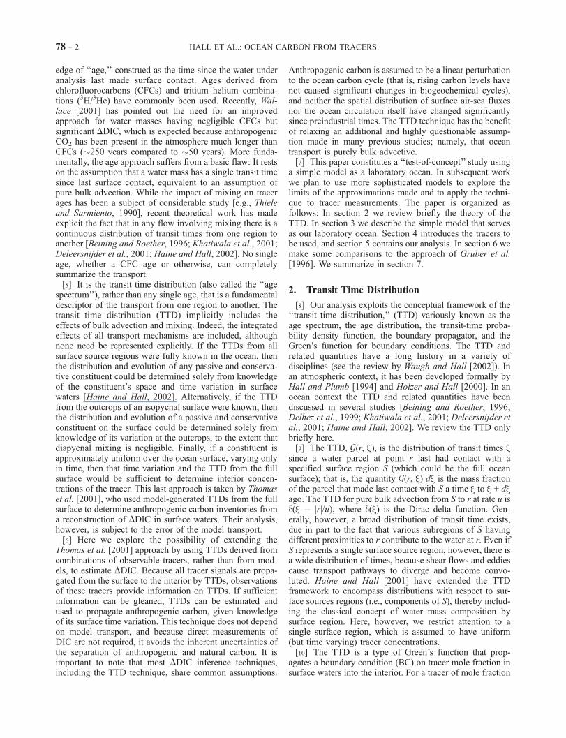
[14] To illustrate the TTD approach to DDIC estimation,we employ the nine box model described by Haine and Hall[2002], and summarized schematically in Figure 1. Themodel has diffusive and advective fluxes coupling theinterior boxes. The upper left box is coupled diffusivelyto a mixed layer on which time-dependent boundary con-ditions (BCs) on tracer mole fraction are applied.[15] Physically, the model may be thought of as represent-

ing a hemispheric meridional overturning cell whose pen-etration of tracer from the mixed layer to the interior isrestricted to high latitudes. Alternatively, it can be consid-ered a circulation on an isopycnal surface with the mixedlayer exchange representing a single outcrop. No attempthas been made to ‘‘tune’’ the model to any particular oceancirculation, and we do not defend its realism in detail. Ourgoal is to generate examples of TTDs that are similar tothose of more sophisticated numerical models. Our guide inselecting the magnitude of fluxes is to have significantamounts of DDIC throughout the domain, thereby allowingthe best comparison to the analysis on the ‘‘fully contami-nated’’ isopycnal surfaces of Gruber et al. [1996]. In section5.4 we examine sensitivity to the circulation.[16] The TTD for the nine box model, shown in Figure 2,

can be computed from an eigenvalue analysis or as the time-dependent response to a d(t) BC on the mixed layer [Haineand Hall, 2002]. The model captures important features ofTTDs seen in ocean GCM studies [Khatiwala et al., 2001;

Figure 1. Schematic of nine-box model. One-sided arrowsindicate advective fluxes. Two-sided arrows indicatediffusive fluxes. Arrow lengths are proportional to fluxmagnitudes.

HALL ET AL.: OCEAN CARBON FROM TRACERS 78 - 3

Thomas et al., 2001; Haine and Hall, 2002]. The TTD arebroadly distributed with early peaks and long tails. Withincreasing distance from the mixed layer along the domi-nant advective pathway, the TTDs broaden and shift tolonger transit times. The TTD of box 1, which receivesdirect input from the mixed layer, is bimodal, reflecting theearly peak of the adjacent source water, and the secondarybroad, low peak due to recirculated waters from below.(Similar weak bimodality was seen in the North Atlanticgyre of the Haine and Hall [2002] numerical study.) Whilethe nine box model TTDs do not have high frequencystructure, such structure is largely irrelevant to this study,since the tracer fields represent integrations over manydecades of transit time (see section 5.4). For the sake ofthis test-of-concept analysis, we take the nine box TTD andits tracer fields, including DDIC, as ‘‘truth.’’ The tracerfields are considered ‘‘observations’’ to be used to estimateDDIC, and the estimates are compared to the ‘‘true’’ DDIC.

4. Tracers and Tracer Ages

[17] In our analysis we use the tracers CFC11, CCl4,natural D

14C, 39Ar, and DDIC. For the transient tracers(CFC11, CCl4, DDIC) a time-dependent BC is applied onthe model’s mixed layer and the interior response iscalculated. For the radioisotopes (39Ar, D14C) the BC isconstant, and radioactive decay applies in the interior withthe e-folding times of 390 years for 39Ar and 8270 years forD14C. Although not exhaustive, the tracers we select cover a

wide range of timescales. Other observable tracers areavailable, particularly CFC12, bomb-radiocarbon andbomb-3H and 3He. CFC12 has a surface history very similarto CFC11, and would work as well as CFC11 in ouranalysis. But once either CFC11 or CFC12 is selected theother tracer provides little additional constraint on DDIC. Inour simple model 3H/3He in combination with CFC11provides only marginal improvement in DDIC estimationover CFC11 alone. However, Waugh et al. [2002], who

discuss relationships among tracer ages in more detail(including CFCs, CCl4,

3H/3He and their ability to constrainage spectra) find circumstances in which 3H/3He and a CFCare useful in combination.

4.1. CFC11 and CCl4[18] A number of studies in recent years have made use of

CFCs (CFC11, CFC12, CFC113) and CCl4 as tracers toestimate pathways and rates of ocean circulation and toevaluate general circulation models [e.g., Wallace et al.,1994; Haine et al., 1998; England and Maier-Reimer,2001]. CFC11 and CFC12 are passive and inert in sea-water and have no interior sources. There is evidence fortemperature-dependent chemical loss of CCl4 [Meredith etal., 1996; Huhn et al., 2001], which we include in a simplefashion here (see below). Until the 1990s, the concentra-tions of CFCs and CCl4 had increased steadily in theatmosphere since the beginning of industrial sources inthe 1940s for CFCs and 1920s for CCl4. The atmosphericsignals have penetrated the ocean. Plotted in Figure 3 arethe boundary layer time series used in the model for CFC11and CCl4. These series were converted from the atmos-pheric histories of Walker et al. [2000] using publishedsolubility factors [Hunter-Smith et al., 1983; Warner andWeiss, 1985] for T = 6�C and S = 35pss (typical of water inthe North Atlantic subpolar gyre) and assuming 100%saturation. Other choices for solubility (T, S) and surface

Figure 2. TTD for the box model (solid line) and the best-fit two-parameter TTD (dashed line). Panels corresponds tomodel boxes, as displayed in Figure 1. Also shown assymbols are tCFC (triangle), tCCl4 (cross) tDIC (asterisk),t39Ar (plus), t14C (square), and � (diamond).

Figure 3. Surface layer time-dependent boundary condi-tions for (a) CFC11, (b) CCl4, and (c) DDIC.

78 - 4 HALL ET AL.: OCEAN CARBON FROM TRACERS

saturation would serve equally well in this test-of-conceptanalysis.[19] Our analysis requires a figure for the uncertainty of

the tracers as constraints on transport. Sources of thisuncertainty are measurement error, uncertainty in the BCin surface waters, and, for CCl4, chemical loss. The boun-dary uncertainty is comprised of uncertainty in the solubil-ity, saturation, and atmospheric history. Based on theseconsiderations, Doney et al. [1997] estimate uncertaintiesfor CFCs in terms of their ages (the lag times of a CFC atinterior ocean points from the surface layer evolution) of±0.5 years for present day values, increasing to ±5 years forvalues before 1950. We convert the ages to mole fractions toobtain an effective uncertainty for CFC11. The 5-yearuncertainty is based in part on an assumed 10% uncertaintyin the early atmospheric CFC abundance, which is largerthan the uncertainty in abundance estimated by Walker et al.[2000]. We have chosen to use the larger uncertainty of ±0.5to ±5.0 years, because it encompasses better the error inassuming 100% saturation, and in general provides a moreconservative assessment of the TTD technique.[20] We have less guidance for CCl4. The CCl4 solubil-

ity factor is thought to be less well established than forCFCs [e.g., Wallace et al., 1994], and the atmospherichistory has greater uncertainty [Walker et al., 2000]. Inaddition the nature and rate of chemical loss of CCl4 isuncertain. For T = 6�C used in these model experimentsHuhn et al. [2001] estimate a loss rate of about 1.5%/year(see their Figure 13), with a range from 0.0% (conserva-tive) to about 3%/year. Thus, in our simulations of CCl4we apply a uniform 1.5%/year loss, while in the subse-quent TTD analysis we try a range of loss rates from 0.0to 3%/year to mimic realistic uncertainty. At each assumedloss rate, we use the CFC age uncertainty increaseduniformly by 50% (to account for higher uncertainty insolubility and atmospheric history) and converted to CCl4mole fractions. The total uncertainty is the union of theuncertainties for each assumed loss rate. The loss rateincreases rapidly with temperature. A similar analysis incolder waters would incur less uncertainty, while the lossin much warmer waters (up to 25%/year above 14�C)would negate the tracer utility of CCl4.

4.2. 39Ar and #14C

[21] Many studies have exploited the radioisotope 14C todiagnose transport [e.g., Broecker et al., 1988], and severalhave analyzed the sparse measurements of 39Ar [e.g.,Schlitzer et al., 1985]. These radioisotopes have atmos-pheric sources and, upon entering the ocean by gasexchange, decay with e-folding times of 390 years for39Ar and 8270 years for 14C. There are advantages toconsidering the ratio D

14C = 14C/12C, instead of 14C alone.The two carbon isotopes undergo similar biochemical trans-formations, so that to a good approximation the ratio acts asa radioactive tracer with no interior chemical sources orsinks [Fiadiero, 1982]. We adopt this approach here.[22] 39Ar is an attractive tracer. Its concentration in sur-

face waters equilibrates rapidly enough with the atmospherethat the surface saturation is near 100%. Its 390-year time-scale is complementary to the shorter timescales of CFCs

and the longer timescale of D14C. In addition, the dominantsource of 39Ar, natural upper atmospheric cosmogenesis, issteady. Unfortunately, the extremely small isotopic abun-dance of 39Ar makes its measurement challenging andexpensive. Thus, effective uncertainty in 39Ar is dominatedby the measurement uncertainty, which is significantbecause large sample volumes and long decay counts arerequired. We choose an uncertainty of ±5%, correspondingroughly to 39Ar uncertainties quoted by Broecker and Peng[2000]. The inclusion of 39Ar in this study might reasonablybe questioned, given the paucity of measurements and thefact that the TTD method has merit independent ofthe use of 39Ar as a constraint. We include it in part toexplore the extent to which 39Ar data could be useful forDDIC estimation if less expensive measurement techniqueswere developed. Additionally, the few present data mayprovide a useful check on TTD estimates from othertracers.[23] D

14C equilibrates with the atmosphere much moreslowly, resulting in surface water depletions ofD14C by morethan 4%, equivalent to D

14C ages of more than 300 years.Moreover, in addition to the steady cosmogenic source,present day D

14C is a response to the small source fromfossil CO2 via the Suess effect, and, importantly, the largeinput from the 1960s atmospheric bomb tests. We areinterested here in the long timescale of the decay of naturalD14C. (In our simple model, bomb D14C in combination with

CFC11 offers only marginal gain in DDIC estimation overCFC11 alone.) Thus, the effective uncertainty on naturalD14C is largely set by the ability to separate natural and

bomb radiocarbon at the surface (for the BC) and in theinterior. Broecker et al. [1995] show latitudinal profiles ofbomb D

14C separated from natural D14C along various

isopycnal surfaces with a scatter of ±10 to ±20 permil,corresponding to an equivalent uncertainty in the remainingnatural D14C; i.e., ±1 to ±2%. This turns out to be near thethreshold of what is useful in our study of DDIC estimation.We employ the figure ±1%, keeping in mind that doublingthe uncertainty would result in D

14C that is a less usefulconstraint. Of course, even with larger uncertainty, deepdepletion of D14C (e.g., D14C ages of 500 to 1000 years inthe deep tropical Pacific [Broecker and Peng, 2000]) repre-sents an important constraint, by indicating negligible levelsof DDIC.

4.3. #DIC

[24] DIC in the equilibrium marine carbonate system canbe determined from the partial pressure of atmospheric CO2

( pCO2), total alkalinity, temperature (T ) and salinity (S ).We take the basic approach of Thomas et al. [2001] andThomas and Ittekkot [2001] and use the ‘‘CO2sys’’ program[Lewis and Wallace, 1998] (available at http://cdiac.es-d.ornl.gov/oceans/co2rprt.html) to solve for DIC, given Tand S typical of the North Atlantic subpolar gyre (T = 6�Cand S = 35pss) and pCO2 from 1750 to the present day(pCO2 data at http://www.giss.nasa.gov/data/si2000/ghgases). Alkalinity is set to 2300 mmole/kg, also typicalof the North Atlantic [Millero et al., 1998]. From each valueof DIC we subtract the value for the year 1750, thusproviding a time series of DDIC. This serves as our time

HALL ET AL.: OCEAN CARBON FROM TRACERS 78 - 5

dependent BC. Note that compared to Thomas et al. [2001]no linearization of DDIC in T and S is required or performed.[25] The Thomas et al. [2001] approach of propagating a

DDIC BC has the advantage that anthropogenic carbon,rather than total carbon, is considered from inception, sothat no separation of the small anthropogenic signal fromthe large and variable natural signal is required. Further-more, when one makes the approximation, as has been donein most other methods, that the disequilibrium across theair-sea interface has changed little since preindustrial times,then the Thomas et al. [2001] method also has the advant-age of not requiring any knowledge of that disequilibrium.The disequilibrium term vanishes upon forming the differ-ence DDIC = DIC(t) � DICpre, where DICpre is thepreindustrial level.[26] There are several sources of uncertainty in the BC for

DDIC that, in principle, impact the inference of interiorDDIC concentrations. Among these is the lack of a univer-sally agreed upon best set of dissociation coefficients for theequilibrium carbonate system. A full exploration of thesensitivity of inferred DDIC to this and other uncertaintiesin the BC is beyond the scope of this study, although suchan exploration should be performed before applying the agespectral technique to observations. However, two points canbe made here: (1) The impact of these uncertainties onDDIC will be significantly smaller than the impact on DIC.For example, we use the carbonate dissociation coefficientsof Roy et al. [1993]. A preliminary investigation usingCO2sys suggests that the impact on DDIC (as opposed toDIC) of using the dissociation constants of Goyet andPoissonn [1989] or Mehrbach et al. [1973], as refit byDickson and Millero [1987], is only about 1 mmole/kg. (2)Uncertainties in the DDIC BC also affect most other DDICinference techniques, including Gruber et al. [1996] (seeSection 6). Thus, for the purpose here of testing relativeadvantages of the TTD technique, the sensitivity to uncer-tainty in the DDIC BC is not included.[27] Finally, we emphasize that the ‘‘true’’ DDIC (that

simulated directly in the model) is a strictly passive andconservative tracer. Carbon chemistry largely determinesthe DDIC concentration in surface waters, but we assume theresults of this process to be known, thus establishing the BC.No subsequent biochemical transformations are included.We are in effect testing the ability to infer one tracer with aknown time-dependent BC from other tracers with differentknown time-dependent BCs. DDIC in the real ocean is apassive and conservative tracer only to the extent thatincreasing DIC levels have not caused changes in rates ofbiochemical processes in the interior ocean. Modelingevidence suggests this is a reasonable approximation[Maier-Reimer et al., 1996; Plattner et al., 2001], althoughit warrants further study. It is also the same approximationmade in other DDIC inference techniques, including Gruberet al. [1996].

4.4. Tracer Ages

[28] Transient tracer ages, sometimes called concentrationor partial pressure ages, have been exploited extensively todiagnose transport [e.g., Doney et al., 1997]. They aredefined as the lag times of the tracer evolution at interior

points with respect to the surface layer. Radioactive tracerages have also been used extensively for this purpose [e.g.,Jenkins, 1987; Broecker et al., 1988], and are defined as�l�1 ln (qobs/q(0)), where l is the relevant radioactive e-folding decay rate, qobs the observed isotopic abundanceand q(0) the abundance at the surface.[29] To illustrate the behavior of these tracer ages, we plot

as symbols in Figure 2 tracer ages obtained from CFC11,CCl4, DDIC (assuming it were known), D14C, and 39Ar, aswell as the mean transit time. These are denoted tCFC,tCCl4, tDIC, t14C, t39Ar and �, respectively. The ages allstrictly differ from one another, with tCFC < tCCl4 < tDIC <t39Ar < t14C < �. (Note that all the ages are equal for purebulk advection.) In general, the tracer with the shortesthistory or most rapid radioactive decay will weight mostheavily the early components of the TTD, resulting in thesmallest tracer age [Waugh et al., 2002]. CFC11 is onlysensitive to the first �50 years of the spectrum and CCl4 tothe first �80 years (the times they have been present in theatmosphere), resulting in smaller timescales. The radio-isotopes have longer timescales, while DDIC is intermedi-ate. Note that Coatanoan et al. [2001], as part of acomparison of carbon inventory techniques, observe thattDIC (using the DDIC obtained from the ‘‘MIX’’ techniqueof Goyet et al. [1999]) is larger than tCFC and speculate asto the cause. Part of the difference they observe is afundamental consequence of tracers having different time-dependent surface variations in the presence of a wide TTD.[30] For the age spectra of Figure 2, t14C and � are

indistinguishable. When a tracer’s time variation, eitherbecause of transience or radioactive decay, is roughly linearover the width of the TTD its age approximates the meantransit time [Hall and Plumb, 1994]. Compared to these agespectra, D14C decays very slowly, and therefore approxi-mately linearly, and so t14C �. This is true for 39Ar onlyto a lesser degree, and t39Ar can be distinguished from � formost of the age spectra in Figure 2.

5. Analysis

[31] Our procedure to test the use of the TTD in estimat-ing DDIC proceeds as follows: We use the model tosimulate the TTD, CFC11, CCl4, natural D

14C, 39Ar, andDDIC. Our goal is to estimate DDIC using the tracer‘‘observations,’’ that is values of CFC11, CCl4, D

14C, and39Ar simulated directly by the model. We check first howaccurately the IG TTD estimates DDIC, given perfectknowledge of the mean transit time � and spectral D fromthe true age spectra (i.e., the model generated age spectra).We then use various tracers observations singly and incombination, allowing for measurement uncertainty, toestimate � and D. These estimates of � and D provide arange of IG age spectra, which in turn are used to constructestimates of DDIC. The estimated DDIC are then comparedto the true values (the values simulated directly by themodel) to evaluate the procedure.[32] It is possible to bypass the TTD completely in this

analysis. Because DDIC is estimated as a function of �and D, and � and D are estimated from tracers, we couldexpress DDIC directly as a function of tracer concentra-

78 - 6 HALL ET AL.: OCEAN CARBON FROM TRACERS

tions. We prefer to maintain the TTD as an intermediatestep for two reasons: (1) The TTD has a physical inter-pretation; (2) The TTD approach is more general, becauseother constituents in addition to DDIC could, in principle,be estimated.

5.1. Impact of Assumed TTDFunctional Form

[33] In addition to the true (model) TTD, the IG TTD,with � and D set equal to the values of the true TTDs, areplotted superposed in Figure 2 as dashed lines. These are the‘‘best-fit’’ IG TTD. The IG functional form does not permitbimodality, and so the comparison to the true TTDs ispoorest in boxes 1 and 4. In other boxes the IG TTDs mimicthe true TTDs more closely.[34] The best-fit IG age spectra are used to construct

DDIC by convolution with the DDIC BC, according toexpression (1). In Figure 4 these DDIC values are plottedas diamonds for each model box. Also plotted for com-parison is DDIC inferred by lagging the DDIC surfacehistory by tCFC, the approach taken by Thomas andIttekkot [2001]; DDIC inferred by using � as a lag; andDDIC employing the transport component of the Gruber etal. [1996] technique, which uses tCFC in a more restrictivefashion (see section 6). The true DDIC concentrations areindicated in Figure 4 by the horizontal lines. In all boxes(except box 1) the best-fit IG TTD DDIC is the bestestimate of the ‘‘true’’ DDIC. The tCFC-lagged DDIC iseverywhere an overestimate. The value of tCFC is onlysensitive to components of the TTD less then �50 years,whereas much DDIC has older surface origins (see Figure3). In contrast, the �-lagged DDIC is everywhere anunderestimate: � is strongly influenced by very longtransit times, which correspond to water with little or noDDIC, since significant anthropogenic CO2 was notpresent in the atmosphere before 1750. (It is possible,for example, in a slower circulation to have � > 250 years,thereby predicting DDIC = 0 according to the �-lagmethod, even though there are still significant watercomponents at younger ages having nonzero DDIC.)[35] The only single age that could be used to infer DDIC

accurately by lagging the surface DDIC history is the age of ahypothetical tracer whose surface BC was similar to that ofDDIC. (A hypothetical radioactive tracer with constantatmospheric abundance and decaying in the ocean with ane-folding time of 40 years, roughlymatching the approximateexponential growth in anthropogenic CO2, would also work.)No such tracer is known. Instead, we aim to use observabletracers in combination to estimate the age spectrum, a morecomplete transport descriptor than any single age, and use theTTD to estimate DDIC.

5.2. TTD Moments From Tracers

[36] The results shown in Figure 4 suggest that knowl-edge of just two moments of the TTD could help improveDDIC inferences. Unfortunately, in reality we do not know� and D for water masses. Can � and D be determined fromobservable tracers with sufficient accuracy to allow usefulDDIC estimates? This is the question we address next.[37] We aim to find the (�, D) pairs that result in a match

to the observations. We sweep through ranges of � and D,

constructing an IG TTD for each (�, D) pair. These TTDare used to estimate concentrations for CFC11, CCl4,D14C, and 39Ar by convolution with the tracers’ BCs and

radioactive decay. We then record the range of (�, D) thatmatch each tracer observation (i.e., model simulated con-centrations) within a tolerance equal to the tracer’s uncer-tainty. Figure 5 shows examples of this procedure.Contours of CFC11, CCl4, D

14C, and 39Ar constructed fromthe IG TTD as functions of � and D are repeated for modelboxes 1, 5, and 9. The loci of (�, D) that result in the‘‘observed’’ concentrations are plotted as dashed lines; theselines are surrounded by shaded regions representing thetracer uncertainty.[38] No single tracer can fix both � and D simultane-

ously, even given zero uncertainty. Instead, for each tracerthere is a locus of (�, D) points that result in a match tothe true value, generally sweeping up to the right fromsmall to large � and D. To understand the shape of thelocus, consider first CFC11. The smallest (�, D) pairintersects the x-axis, corresponding to a delta functionTTD (zero width) peaked at � = tCFC. These purelyadvective age spectra are not ruled out by CFC11 alone.However, higher � are also not ruled out, if the corre-sponding TTD are wider (increasing D). Now, IG TTDbecome increasingly asymmetric with increasing D. There-fore, these larger (�, D) values represent the possibilitythat the water mass under consideration has young com-ponents (early TTD peaks) containing high concentrationsof CFC11 mixed with old components (long TTD tails)containing little or no CFC11, such that the observedCFC11 is matched. Water in box 9 is old enough thatthe observed CFC11 value is not different than zero withinthe uncertainty, and so the allowed (�, D) range coversmuch of the lower right half of the parameter space. This

Figure 4. DDIC for each model box as estimated by thebest-fit two-parameter spectra (diamond); lagging by �(triangle); lagging by tCFC (asterisk); and by employing thetransport component of the Gruber et al. [1996] technique(cross), which uses tCFC in a more restrictive fashion (called‘‘CFC diseq’’ above; see text). The true DDIC (computeddirectly by the model) is indicated by the horizontal line.

HALL ET AL.: OCEAN CARBON FROM TRACERS 78 - 7

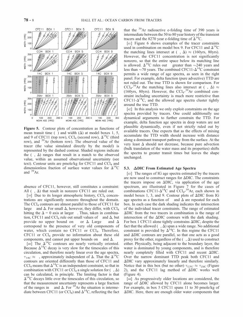
absence of CFC11, however, still constitutes a constraint:All (�, D) that result in nonzero CFC11 are ruled out.[39] Due to its longer atmospheric history, CCl4 concen-

trations are significantly nonzero throughout the domain.The CCl4 contours are almost parallel to those of CFC11 forlarge � and D. For small D, however, they differ, with CCl4hitting the D = 0 axis at larger �. Thus, taken in combina-tion, CFC11 and CCl4 rule out small values of � and D, butprovide no upper bound on � or D. Large � and D

correspond to the presence of very old components ofwater, which contain no CFC11 or CCl4. Therefore,CFC11 or CCl4 provide no information about these oldcomponents, and cannot put upper bounds on � and D.[40] The D

14C contours are nearly vertically oriented.Because D

14C decay is very slow for the timescales of thiscirculation, and therefore nearly linear over the age spectra,t14C �, approximately independent of D. That the D

14Ccontours are oriented differently than those of CFC11 andCCl4 means that D14C is an independent constraint, so that incombination with CFC11 or CCl4 a single solution for (�, D)can be calculated, in principle. The limiting factor is thatD14C decays little over the timescales of this circulation, so

that the measurement uncertainty represents a large fractionof the ranges in � and D. For 39Ar the situation is interme-diate between CFC11 (or CCl4) and D

14C, reflecting the fact

that the 39Ar radioactive e-folding time of 390 years isintermediate between the 50 to 80 year history of the transienttracers and the 8270 year e-folding time of D14C.[41] Figure 6 shows examples of the tracer constraints

used in combination on model box 9. For CFC11 and D14C

the matching lines intersect at (�, D) (160yrs, 80yrs).However, the CFC11 concentration is not significantlynonzero, so that the entire space below its matching lineis allowed. D14C rules out � greater than �240 years andless than �70 years. The combined CFC11-D14C constraintpermits a wide range of age spectra, as seen in the rightpanel. For example, delta function (pure advective) TTD arenot ruled out. The true TTD is shown for comparison. ForCCl4-

39Ar the matching lines also intersect at (�, D) (160yrs, 80yrs). However, the CCl4-

39Ar combined con-straint including uncertainty is much more restrictive thanCFC11-D14C, and the allowed age spectra cluster tightlyaround the true TTD.[42] In this analysis we only exploit constraints on the age

spectra provided by tracers. One could additionally usedynamical arguments to further constrain the TTD. Forexample, delta function age spectra in deep waters are notplausible dynamically, even if not strictly ruled out byavailable tracers. One expects that as the effects of mixingaccumulate the TTD width should increase with distancealong a dominant transport pathway from the surface. At thevery least D should not decrease, because pure advection(bulk translation of the water mass and its properties) shiftsthe spectra to greater transit times but leaves the shapeunchanged.

5.3. #DIC From Estimated Age Spectra

[43] The ranges of IG age spectra estimated by the tracersare now used to construct ranges for DDIC. The constraintsthe tracers impose on DDIC, via application of the agespectrum, are illustrated in Figure 7 for the cases ofcombinations CFC11-D14C and CCl4-

39Ar, each shown inmodel boxes 1, 3, and 9. Contour plots of DDIC from IGage spectra as a function of � and D are repeated for eachbox. In each case the dark shading indicates the intersectionof the individual tracer constraints. The range of estimatedDDIC from the two tracers in combination is the range ofintersection of the DDIC contours with the dark shading.For box 1 CFC11 alone tightly constrains DDIC, despite thefact that the allowed (�, D) span a wide range. No additionalconstraint is provided by D14C. In this regime the CFC11and DDIC contours are parallel, so that one acts as a goodproxy for the other, regardless of the (�, D) used to constructeither. Physically, being adjacent to the boundary layer, thewater is dominated by young components, and is thereforenearly completely filled with CFC11 and recent DDIC.Over the narrow dominant TTD peak both CFC11 andDDIC vary approximately linearly and therefore similarly.Notice that in this box (but no other) tCFC tDIC (Figure2), and the CFC11 lag method of DDIC works well(Figure 4).[44] As progressively older locations are considered, the

range of DDIC allowed by CFC11 alone becomes larger.For example, in box 5 CFC11 spans 11 to 30 pmole/kg ofDDIC. Here, there are enough older water components that

Figure 5. Contour plots of concentration as functions ofmean transit time (�) and width (D) at model boxes 1, 5,and 9 of CFC11 (top row), CCl4 (second row), D14C (thirdrow), and 39Ar (bottom row). The observed value of thetracer (the value simulated directly by the model) isrepresented by the dashed contour. Shaded regions indicatethe (�, D) ranges that result in a match to the observedvalue, within an assumed observational uncertainty (seetext). Contour units are pmole/kg for CFC11 and CCl4 anddimensionless fraction of surface water values for D

14Cand 39Ar.

78 - 8 HALL ET AL.: OCEAN CARBON FROM TRACERS

the surface history of CFC11 and DDIC look very differentover the TTD. The D

14C constraint rules out large (�, D)allowed by CFC11, but these (�, D) correspond to littleadditional range in DDIC. Ruling out lower values of (�, D)would offer more leverage on DDIC, but the D14C on box 5is too uncertain to provide a lower bound. Thus, the CFC11intersection with D

14C constitutes only a marginally tighterbound on DDIC (12 to 30 pmole/kg) than CFC11 alone. Inbox 9 CFC11 is not significantly different than zero, anddelta function age spectra cannot be ruled out by CFC11and D

14C (see Figure 6). Nonetheless, the addition of D14Cto CFC11 in box 9 offers more advantage for DDIC than itdoes in box 5. The delta function TTD at highest �permitted by D

14C still yield marginally nonzero DDICestimates, because these � are all less than 250 years, thetime DDIC has been present in surface waters. (A slowercirculation, however, could have a CFC11–D14C constraintallowing delta function TTD at � greater than 250 years,which would predict zero DDIC, even though the true DDICcould be nonzero; see section 5.4.) More importantly, box 9D14C rules out � < 70 years, which is permitted by CFC11

at small D, thereby prohibiting the DDIC > 16 mmol/kgallowed by CFC11.[45] The combination CCl4 and

39Ar behave similarly, butthe constraints on DDIC are tighter. Because the atmospheric

history of CCl4 is longer than CFC11, it exists in significantamounts in older waters. For this circulation, it is nonzerothroughout the domain. Because 39Ar decays more rapidlythan D

14C its uncertainty covers a smaller range of � and D.

Figure 6. (a) Loci of (�, D) resulting in matches to box nine D14C (solid line, labeled in fraction of

surface layer concentration) and CFC11 (dashed line, labeled in pmole/kg). The light shaded (mediumshaded) region indicates the allowed (�, D) from the CFC11 observational uncertainty (D14Cuncertainty). The dark shade is the intersection, the combined CFC11-D14C constraint. (b) Sample TTDscorresponding to representative (�, D) pairs through the intersection region. The heavy dashed curve isthe true TTD in box nine. (c, d) As in Figures 6a and 6b, respectively, but for 39Ar (medium shade), CCL4

(light shade) and the intersection (dark shade).

Figure 7. Contours of DDIC versus � and D (solid lines,labeled in mmole/kg), repeated for boxes 1, 5, and 9.Superposed on the top row are ranges allowed by CFC11(light shade), D14C (medium shade), and their intersection(dark shade), aswell as the best estimate curves (dashed lines).On the bottom row are ranges allowed by CCl4 (light shade),39Ar (medium shade), and their intersection (dark shade).

HALL ET AL.: OCEAN CARBON FROM TRACERS 78 - 9

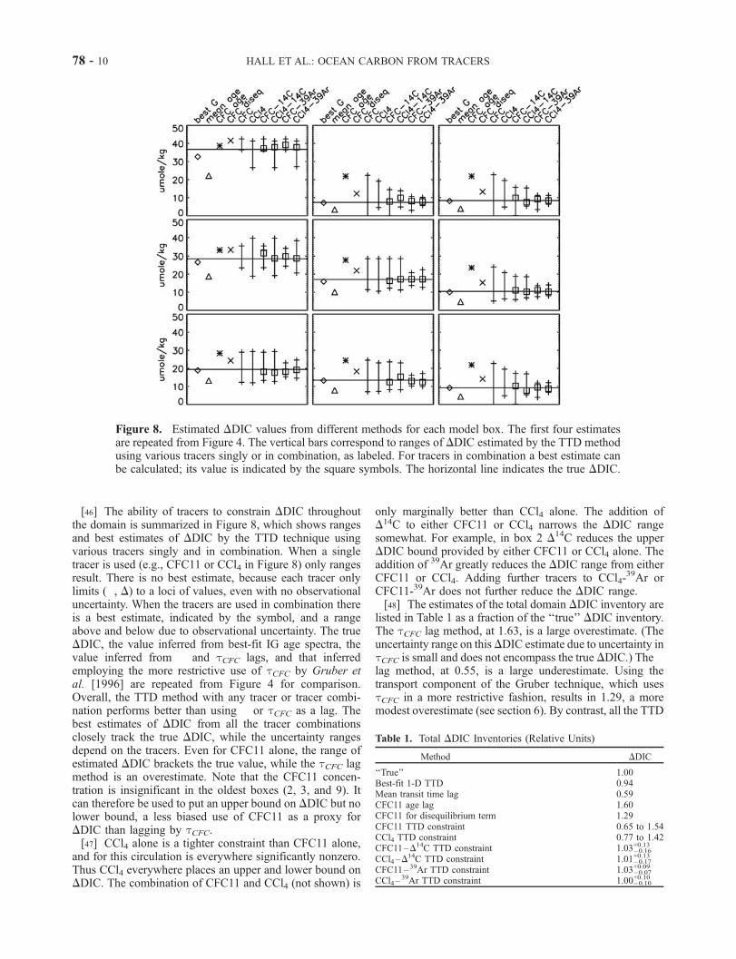
[46] The ability of tracers to constrain DDIC throughoutthe domain is summarized in Figure 8, which shows rangesand best estimates of DDIC by the TTD technique usingvarious tracers singly and in combination. When a singletracer is used (e.g., CFC11 or CCl4 in Figure 8) only rangesresult. There is no best estimate, because each tracer onlylimits (�, D) to a loci of values, even with no observationaluncertainty. When the tracers are used in combination thereis a best estimate, indicated by the symbol, and a rangeabove and below due to observational uncertainty. The trueDDIC, the value inferred from best-fit IG age spectra, thevalue inferred from � and tCFC lags, and that inferredemploying the more restrictive use of tCFC by Gruber etal. [1996] are repeated from Figure 4 for comparison.Overall, the TTD method with any tracer or tracer combi-nation performs better than using � or tCFC as a lag. Thebest estimates of DDIC from all the tracer combinationsclosely track the true DDIC, while the uncertainty rangesdepend on the tracers. Even for CFC11 alone, the range ofestimated DDIC brackets the true value, while the tCFC lagmethod is an overestimate. Note that the CFC11 concen-tration is insignificant in the oldest boxes (2, 3, and 9). Itcan therefore be used to put an upper bound on DDIC but nolower bound, a less biased use of CFC11 as a proxy forDDIC than lagging by tCFC.[47] CCl4 alone is a tighter constraint than CFC11 alone,

and for this circulation is everywhere significantly nonzero.Thus CCl4 everywhere places an upper and lower bound onDDIC. The combination of CFC11 and CCl4 (not shown) is

only marginally better than CCl4 alone. The addition ofD14C to either CFC11 or CCl4 narrows the DDIC rangesomewhat. For example, in box 2 D

14C reduces the upperDDIC bound provided by either CFC11 or CCl4 alone. Theaddition of 39Ar greatly reduces the DDIC range from eitherCFC11 or CCl4. Adding further tracers to CCl4-

39Ar orCFC11-39Ar does not further reduce the DDIC range.[48] The estimates of the total domain DDIC inventory are

listed in Table 1 as a fraction of the ‘‘true’’ DDIC inventory.The tCFC lag method, at 1.63, is a large overestimate. (Theuncertainty range on thisDDIC estimate due to uncertainty intCFC is small and does not encompass the true DDIC.) The �lag method, at 0.55, is a large underestimate. Using thetransport component of the Gruber technique, which usestCFC in a more restrictive fashion, results in 1.29, a moremodest overestimate (see section 6). By contrast, all the TTD

Figure 8. Estimated DDIC values from different methods for each model box. The first four estimatesare repeated from Figure 4. The vertical bars correspond to ranges of DDIC estimated by the TTD methodusing various tracers singly or in combination, as labeled. For tracers in combination a best estimate canbe calculated; its value is indicated by the square symbols. The horizontal line indicates the true DDIC.

Table 1. Total DDIC Inventories (Relative Units)

Method DDIC

‘‘True’’ 1.00Best-fit 1-D TTD 0.94Mean transit time lag 0.59CFC11 age lag 1.60CFC11 for disequilibrium term 1.29CFC11 TTD constraint 0.65 to 1.54CCl4 TTD constraint 0.77 to 1.42CFC11–D14C TTD constraint 1.03�0.16

+0.13

CCl4–D14C TTD constraint 1.01�0.17

+0.13

CFC11–39Ar TTD constraint 1.03�0.07+0.09

CCl4–39Ar TTD constraint 1.00�0.10

+0.10

78 - 10 HALL ET AL.: OCEAN CARBON FROM TRACERS

methods give constraints bracketing the true value. The useof CFC11 alone gives an upper bound of 1.54, close to thetCFC method, but has a lower bound (0.65) well below the‘‘true’’ value. The TTD technique thus uses CFC11 in a lessbiased way. When tracer combinations are considered theinventory constraints are tighter. The combination CFC11-D14C gives 1.03�0.16

+0.13. CFC11-39Ar, the tightest constrainingpair, gives 1.03�0.07

+0.09. Note that domain summing can result incanceling errors. For example, on a domain scale CCl4 aloneis more accurate than CFC11 alone, because it is everywherenonzero. However, in young regions CFC11 is more accu-rate, because it has a smaller uncertainty.

5.4. Sensitivity to Circulation

[49] In order to check that the apparent merit of the TTDapproach is not just a consequence of the particular circu-

lation selected for our simple model (termed ‘‘MEDIUM’’),we repeat the analysis for a circulation in which advectivefluxes are everywhere halved (‘‘SLOW’’) and everywheredoubled (‘‘FAST’’). We also test a circulation (‘‘CYCLES’’)for which the advective fluxes connecting the upper six boxesvary sinusoidally with six frequency components rangingfrom 2p/350 years�1 to 2p/50 years�1, all having amplitude0.25 times the steady MEDIUM circulation fluxes andrandomly selected phases. The results on box 5 are shownin Figure 9. Increasing the circulation results in youngerwater, higher DDIC and higher estimates of DDIC for alltechniques. Decreasing the circulation results in older water,lowerDDIC and lowerDDIC estimates. The relative perform-ance of the techniques is little changed, however. Periodicvariations in the circulation cause ‘‘wiggles’’ in the TTD, buthave little impact on the accuracy of the DDIC inferences.

Figure 9. Box 5 TTD (left), allowed parameter ranges (center) and DDIC estimates (right) for fourcirculations. (a) ‘‘FAST’’ circulation, for which all advective fluxes are doubled compared to previousfigures; (b) ‘‘MEDIUM’’ circulation, identical to previous figures; (c) ‘‘SLOW’’ circulation, for which alladvective fluxes are halved; (d) circulation with ‘‘CYCLES,’’ for which the advective fluxes connectingthe upper six boxes vary sinusoidally with six frequency components ranging from 2p/350 years�1 to2p/50 years�1, all having amplitude 0.25 times the steady MEDIUM circulation fluxes and randomlyselected phases.

HALL ET AL.: OCEAN CARBON FROM TRACERS 78 - 11

[50] Age spectra in the real ocean could be very differentthan the age spectra for any of the circulations of our simplemodel. Two points can be made, however: (1) As notedpreviously, the simple model’s age spectra are similar inoverall shape to those seen in several GCM studies [Kha-tiwala et al., 2001; Thomas et al., 2001; Haine and Hall,2002]. (2) Differences among observed tracer ages indicatethat age spectra in the real ocean must have significantwidth; that is, they cannot be the delta functions of purebulk advection. In the deep ocean this is illustrated by thetypical 50% differences between 39Ar and D

14C ages[Broecker and Peng [2000]. For younger water Waugh etal. [2002] argue that differences in CFC and 3H/3He ages,noted by Doney et al. [1997], are consistent with TTDwidths that are a large fraction of the mean transit time.Thus, even if real ocean age spectra are different than theage spectra of our simple model or the IG form, theseobservations suggest that the estimation of two temporalmoments (mean and width) is an important step beyondusing single tracer ages as lags for DDIC, which implicitlyassumes delta function age spectra.

6. Comparison to Technique ofGruber et al. [1996]

[51] Gruber et al. [1996] developed and applied a techni-que (hereafter called the Gruber technique) to infer DDICfrom measurements of total DIC. Their technique, appliedin several subsequent analyses [Gruber, 1998; Sabine et al.,1999] represents an important advance in quantifyinganthropogenic carbon in the ocean. Several recent studieshave compared the Gruber technique to other techniques[e.g., Coatanoan et al., 2001; Sabine and Feely, 2001].Here, we are address the limits of the representation oftransport in the Gruber technique. We begin with a briefreview.[52] Gruber et al. [1996] construct a quasiconserved

tracer C* by adding other constituents to total DIC thatcompensate for carbon conversions due to natural biogeo-chemical processes; i.e., the ‘‘soft-tissue pump’’ and ‘‘car-bonate pump.’’ At the sea surface C* = DIC. As waterpenetrates the interior, carbon cycles among its biochem-ical reservoirs, but C* is approximately conserved. Theanthropogenic component is DDIC = C*obs � C*pre, whereC*obs is the total observed concentration and C*pre is thepreindustrial concentration. Unfortunately, C*pre is notdirectly known. Gruber et al. [1996] express it for eachoutcrop of an isopycnal surface as C*pre = C*eq, pre � C*diseq,where C*eq, pre is the concentration in saturated equilibriumwith the preindustrial atmosphere for the outcrop (deter-mined by solving the equilibrium carbonate system givenknowledge of preindustrial atmospheric CO2) and C*diseq (the‘‘disequilibrium term’’) is the degree to which the oceancirculation prevents air-sea equilibrium from being achievedat the outcrop. The Gruber technique estimates C*diseq in twodifferent ways, depending on the isopycnal surface underconsideration. If somewhere on the surface there is waterold enough to be uncontaminated by anthropogenic carbon,then C*diseq = C*eq, pre � C*obs(old), where C*obs(old) is theobserved concentration in these old waters. In other words,

C*pre = C*obs(old). In the Gruber [1998] Atlantic Oceananalysis, C*diseq for these deep isopycnal surfaces is computedfor two outcrops, in high northern and southern latitudes,using PO*4 as a discriminator of surface origin [Broecker etal., 1991]. An average C*diseq weighted by the relative out-crop contributions is then applied to all water on theisopycnal surface, including contaminated water.[53] For more rapidly ventilated isopycnal surfaces no

such uncontaminated water exists to determine C*diseq. Bythe Gruber technique one obtains C*diseq for these surfaces inthe following manner: Tracer ‘‘ages’’ t (e.g., tCFC) are usedto estimate the date that a water mass was last at the surface.The saturated equilibrium C*eq appropriate for atmosphericCO2 levels at this past date, C*eq(t � t), is computed fromknowledge of atmospheric CO2, and C*diseq = C*eq(t � t) �C*obs. Upon substitution, one then has

DDIC ¼ Ceq* t � tð Þ � Ceq; pre* ð3Þ

which is the statement of the approximation (shown to bepoor in our analysis) that interior DDIC can be determinedfrom the DDIC surface time series with a single age, forexample tCFC. Expression (3) amounts to applying a d(t� t)TTD to the BC C*eq(t) � C*eq, pre, which is the same BC weuse. Our approach generalizes (3) by allowing a morerealistic TTD; that is, by applying expression (1) to the BCwe have, instead of (3),

DDIC r; tð Þ ¼Z 1

0

Ceq* t � xð ÞG r; xð Þdx � Ceq; pre* ð4Þ

Recognizing the potential for error Gruber et al. [1996] andGruber [1998] do not use (3) directly. Instead, Gruber[1998] calculates C*diseq, using CFC11 on each outcrop onlyfor waters with tCFC � 30 years and water masscontribution from the outcrop greater than 80%. Averagingthe resulting C*diseq estimates provides an effective C*diseq forthe isopycnal surface.[54] If this analysis over/underestimates C*diseq then it

over/underestimates DDIC by an equal amount. Shown inFigures 4 and 8 are DDIC estimates of the Gruber C*diseqapproach applied to our simple model (called ‘‘CFC diseq’’in the figure). In this application of the model we consider itto represent a single isopycnal surface that has one outcropand that is ‘‘fully contaminated’’ with DDIC. We obtainedthe Gruber DDIC by adding to the ‘‘true’’ DDIC (the valuesimulated directly in the model) the Gruber error in C*diseq,which is just the difference in the DDIC BC evaluated at t �tCFC and t � tDIC (t is the present time) averaged over allmodel boxes having tCFC � 30 years. (The value tDIC, notknown in advance, would be the only correct single ‘‘age’’to use for C*diseq, as it is by definition the elapsed time sincethe surface displayed the C* of the water mass.) EverywheretCFC < tDIC, as seen in Figure 2. Thus, when comparing thesurface C*eq(t) to C*obs to get C*diseq, one does not look farenough back in time. The C*diseq and DDIC are thereforeoverestimated, in this case by 4.9 mmole/kg. Note that thiserror is caused solely by the representation of transport inthe Gruber technique. No analysis of the representation ofcarbon biochemistry is made here; that is, the constructionof the conservative tracer C* is assumed to be perfect.

78 - 12 HALL ET AL.: OCEAN CARBON FROM TRACERS

[55] The 4.9 mmole/kg overestimate is a significantlysmaller error than using tCFC as a lag time throughout thehypothetical isopycnal surface, as is seen in Figures 4 and 8.The error in the Gruber analysis is smaller because it arisesfrom biases in tCFC only over the young regions of theisopycnal surface where tCFC � 30 years (boxes 1, 4, and7). In these regions CFCs are better proxies of DDIC than inolder regions. However, because the resulting C*diseq esti-mate applies over the whole isopycnal surface, its error is alarge fraction of the smaller DDIC levels of older regions(boxes 2, 3, 4, and 5 in Figures 4 and 8). Gruber [1998]quotes a DDIC uncertainty due to tCFC of 3 mmole/kg,based on the observation that ages derived from CFC11 and3H/3He are within eight years of each other for tCFC � 30years [Doney et al., 1997]. However, for DDIC estimationthe more relevant comparison is between tCFC and tDIC,which differ by 20 years for tCFC = 30 years in our simplemodel, by 30 to 60 years in an analysis of DDIC inferencetechniques by Coatanoan et al. [2001], and even more forsome combinations of advection and diffusion in the studyof Waugh et al. [2002]. Moreover, the error in C*diseq (andtherefore DDIC) from use of tCFC is systematic, so that itaccumulates in domain inventories. The inventory over thehypothetical isopycnal surface represented by our simplemodel is overestimated by 29% using the Gruber C*diseqtechnique (Table 1). (Other circulations for the model yielddifferent fractional errors.)[56] Errors in the DDIC inventory of deep isopycnal

surfaces could also arise if regions that were believed tobe uncontaminated instead had small but nonzero DDIC.Application of the Gruber technique to such an isopycnalsurface would result in an underestimate of DDIC over thewhole surface, as C*diseq would be underestimated (C*preoverestimated). As Gruber [1998] notes, a 2 mmol/kgsystematic error in deep North Atlantic C*dis leads to anapproximate 20% error in total water column inventory. Thepossibility of this systematic error, in fact, largely deter-mines the inventory uncertainties quoted by Gruber [1998].Are 2 mmol/kg DDIC concentrations in the deep Atlanticplausible? Broecker and Peng [2000] analyze D

14C and39Ar observations in Atlantic regions deep enough that theywould be treated as uncontaminated in the Gruber analysis.For example, at 18�N, 54�W and 2.8 km depth Broeckerand Peng [2000] report D14C = 0.97 and 39Ar = 0.57 (statedas fractions of North Atlantic surface water concentrations),giving t14C = 252 years and t39Ar = 219 years. Neglectingobservational uncertainties for the moment, these dataconstrain the IG TTD form to � = 254 years and D = 136years. Convolving this IG TTD with the DDIC surface BCyields DDIC = 4.5 mmol/kg.[57] Now, the 4.5 mmol/kg value is not likely to be

accurate, nor have we even demonstrated it to be statisti-cally different than zero. There is considerable uncertaintyon t14C and t39Ar. In addition, the IG TTD form workspoorly when applied to a tracer that, because of its shorthistory, is only sensitive to the leading fraction of the TTD,as is the case for DDIC in these old waters. An erroneousshape of the leading edge of the TTD may cause onlyrelatively small errors in � and D, but the effect on the traceris greatly magnified. Finally, we are neglecting contribu-

tions to the water mass from southern hemisphere sources.Nonetheless, the magnitude of this DDIC estimate fromt14C and t39Ar suggests that 2 mmole/kg errors in C*diseq forthe deep Atlantic cannot be ruled out and raises thepossibility of significant inventory errors. The key featureis that t14C is significantly larger than t39Ar throughout thedeep Atlantic [Broecker and Peng, 2000], implying broadlydistributed TTDs. This is true even if the details of the TTDdo not match the IG form. Therefore, even though � may begreater than 250 years (the history of DDIC in surfacewaters) there is still a significant fraction of water withtransit time less than 250 years, and this fraction containsnonzero DDIC.[58] It is important to note that, assuming other uncer-

tainties to be neutral, the neglect of mixing in the Grubertechnique leads to overestimates of DDIC on fully contami-nated isopycnal surfaces and underestimates on ‘‘unconta-minated’’ surfaces. These errors will tend to cancel indomain-wide inventories. In addition, we have onlyaddressed the representation of transport in the Grubertechnique. Biogeochemical issues related to the compensa-tion of natural sources and sinks by the inclusion of addi-tional constituents are beyond the scope of this study.Finally, we note that the TTD could be used in the contextof the Gruber technique. Instead of C*diseq = C*eq(t � t) �C*obs one could compute

Cdiseq* ¼

Z 1

0

Ceq* t � t0ð ÞG r; t0ð Þdt0 � Cobs* r; tð Þ ð5Þ

where the TTD G is estimated as best as possible fromavailable tracers. Compared to using the TTD directly (5)has the advantage of not requiring tracer observations overthe entire isopycnal surface under analysis, although C*measurements are required. The TTD need only beestimated over a limited region to determine C*diseq, whichis then applied to the entire surface. The use of G, evenconstrained solely by CFCs, would be an improvement overthe tCFC approach. The TTD-estimated C*diseq would havecomparable uncertainty but would be less biased.

7. Summary and Discussion

[59] We have described a technique (the ‘‘transit timedistribution,’’ or TTD, technique) for estimating concen-trations of anthropogenic carbon from observable tracers,and have illustrated the technique with an idealized model.Unlike techniques that rely on single tracer ages, whicheffectively assume the transport to be purely bulk advective,the TTD technique naturally includes the effects of mixing.Following Thomas et al. [2001], transport from the surfaceto interior points is represented by distributions of transittimes (age spectra). However, while Thomas et al.[2001] use GCMs to generate TTDs, we describe a wayto estimate TTDs directly from tracer observations. We usetracers in combination to constrain two temporal momentsof a TTD, equivalent to the mean ventilation time and thespread of ventilation times. From inception the TTD tech-nique considers only the anthropogenic carbon componentDDIC. The tracer-estimated TTDs propagate into the inte-

HALL ET AL.: OCEAN CARBON FROM TRACERS 78 - 13

rior a time series of DDIC in surface waters, which isconstructed from marine carbonate system analysis. Thus,no separation of the small anthropogenic component fromthe large and variable natural ocean carbon cycle isrequired.[60] In a comparison using synthetic data from a simple

model the TTD technique provides a more accurate estimateof DDIC and a more natural assessment of uncertainty thanseveral other approaches. Using CFC age to propagate thesurface DDIC evolution into the interior results in a largeoverestimate of DDIC through much of the domain. Asmaller but still significant overestimate results from limit-ing the use of CFC to water having tCFC � 30 years, as isdone for ‘‘fully contaminated’’ isopycnal surfaces byGruber [1998]. Because of mixing, a range of ages ispresent in any water mass. CFCs only provide informationabout components that are younger than �50 years, whileanthropogenic carbon is present in components up to �250years. In the TTD technique the effects of mixing areincluded implicitly, because continuous distributions of agesare considered. In addition, the technique provides a naturaltranslation of the uncertainties in individual tracers to anuncertainty in inferred DDIC. In contrast to approachesusing a single tracer age, the uncertainty in DDIC inferredby the TTD technique bounds the true DDIC.[61] The tightest DDIC constraint in the TTD technique is

provided by using two tracers in combination. The tracersshould be significantly different in their temporal variation(for transient tracers) or radioactive decay (for naturalradioisotopes), and at least one should have a timescalecomparable to or greater than the history of anthropogeniccarbon (�250 years). CFCs or CCl4 or 3H/3He in combi-nation with 39Ar or natural D14C are possible combinations,although D

14C is limited by uncertainty in the surface waterBC for these timescales, which are short compared to D

14Cdecay. The combination of 39Ar with either a CFC or CCl4provides tight upper and lower bounds on DDIC. Unfortu-nately, 39Ar is expensive to measure, and there are only theorder of 100 measurements globally. However, the TTDapproach has benefits even using a CFC alone as a con-straint. The resulting DDIC estimates have uncertaintycomparable to using CFC age as a lag time, but they areless biased. In fact, using only CFCs the TTD approachcould be applied in the context of the Gruber et al. [1996]technique to provide less biased estimates of C*diseq, the air-sea ‘‘disequilibrium’’ term.[62] This study demonstrates promise for the TTD

approach to DDIC estimation. Important testing remainsto be done, however. We have considered only one surfacesource region for tracers in our analysis. We plan to repeatthe analysis with three-dimensional numerical models togenerate more realistic TTDs, having multiple sourceregions. Among other things, this will allow us to test morethoroughly the applicability of the IG TTD form. Moregenerally, it would be valuable to perform systematiccomparisons and evaluations of various DDIC inferencetechniques in the context of an ocean GCM with carbonbiochemistry, where the true answer is known. Such testingwill allow the relative advantages and disadvantages ofdifferent DDIC inference techniques be assessed in detail.

[63] Acknowledgments. We thank the ‘‘age group’’ at the Lamont-Doherty Earth Observatory for lively discussions and Mick Follows andHelmuth Thomas for assistance with the equilibrium carbonate system.Comments from an anonymous reviewer led to an improved manuscript.This work was supported in part by a grant from the Physical Ocean-ography Program of the National Science Foundation (OCE-9911598).

ReferencesBeining, P., and W. Roether, Temporal evolution of CFC11 and CFC–12concentrations in the ocean interior, J. Geophys. Res., 101, 16,455–16,464, 1996.

Broecker, W. S., and T.-H. Peng, Comparison of 39Ar and D14C ages for

waters in the deep ocean, Nucl. Instrum. Methods Phys. Res., Sect. B,172, 473–478, 2000.

Broecker, W. S., et al., Preliminary estimates for the radiocarbon age ofdeep water in the glacial ocean, Paleoceanography, 3, 659–669, 1988.

Broecker, W. S., et al., Radiocarbon decay and oxygen utilization in thedeep Atlantic Ocean, Global Biogeochem. Cycles, 5, 87–117, 1991.

Broecker, W. S., et al., Oceanic radiocarbon: Separation of the natural andbomb components, Global Biogeochem. Cycles, 9, 263–288, 1995.

Coatanoan, C., et al., Comparison of two approaches to quantify anthro-pogenic CO2 in the ocean: Results from the northern Indian Ocean,Global Biogeochem. Cycles, 15, 11–25, 2001.

Deleersnijder, E., et al., The concept of age in marine modelling, 1, Theoryand preliminary model results, J. Mar. Syst., 28, 229–267, 2001.

Delhez, E., et al., Toward a general theory of age in ocean modelling,Ocean Modell., 1, pp. 17–27, Hooke Inst. Oxford Univ., Oxford, Eng-land, 1999.

Dickson, A. G., and F. J. Millero, A comparison of the equilibrium con-stants for the dissociation of carbonic acid in seawater media, Deep SeaRes., 34, 1733–1743, 1987.

Doney, S. C., et al., A comparison of ocean tracer dating techniques on ameridional section in the eastern North Atlantic, Deep Sea Res., Part 1,44, 603–626, 1997.

England, M. H., and E. Maier-Reimer, Using chemical tracers to assessocean models, Rev. Geophys., 39, 29–70, 2001.

Fiadiero, M. E., Three-dimensional modeling of tracers in the deep PacificOcean, 2, Radiocarbon and the circulation, J. Mar. Res., 40, 537–550,1982.

Goyet, C., and P. G. Poissonn, New determination of carbonic acid disso-ciation constants in seawater as a function of temperature and salinity,Deep Sea Res., 36, 2635–2654, 1989.

Goyet, C., et al., Spatial variation of total CO2 and total alkalinity in thenorthern Indian Ocean: A novel approach for the quantification of anthro-pogenic CO2 in seawater, J. Mar. Res., 57, 135–163, 1999.

Gruber, N., Anthropogenic CO2 in the Atlantic Ocean, Global Biogeochem.Cycles, 12, 165–191, 1998.

Gruber, N., J. L. Sarmiento, and T. F. Stocker, An improved method fordetecting anthropogenic CO2 in the oceans, Global Biogeochem. Cycles,10, 809–837, 1996.

Haine, T. W. N., and T. M. Hall, A generalized transport theory: Water masscomposition and age, J. Phys. Oceanogr., 32, 1932–1946, 2002.

Haine, T. W. N., et al., The flow of Antarctic bottom water to the southwestIndian Ocean estimated using CFCs, J. Geophys. Res., 103, 27,637–27,653, 1998.

Hall, T. M., and R. A. Plumb, Age as a diagnostic of stratospheric transport,J. Geophys. Res., 99, 1059–1070, 1994.

Hall, T. M., et al., Evaluation of transport in stratospheric models, J. Geo-phys. Res., 104, 18,815–18,839, 1999.

Holzer, M., and T. M. Hall, Transit-time and tracer-age distributions ingeophysical flows, J. Atmos. Sci., 57, 3539–3558, 2000.

Huhn, O., W. Roether, P. Beining, and H. Rose, Validity limits of carbontetrachloride as an ocean tracer, Deep Sea Res., Part I, 48, 2025–2049,2001.

Hunter-Smith, R. J., et al., Henry’s law constants and the air-sea exchangeof various low molecular weight halocarbon gases, Tellus, Ser. B, 35,170–176, 1983.

Jenkins, W. J., 3H and 4He in the Beta Triangle: Observations of gyreventilation and oxygen utilization rates, J. Phys. Oceaogr., 17, 763–783, 1987.

Johnson, D. G., et al., Stratospheric age spectra derived from observations ofwater vapor and methane, J. Geophys. Res., 104, 21,595–21,602, 1999.

Khatiwala, S., M. Visbeck, and P. Schlosser, Age tracers in an ocean GCM,Deep Sea Res., Part A, 48, 1423–1441, 2001.

Lewis, E. and D. W. R. Wallace, Program developed for CO2 systemcalculations, ORNL/CDIAC-105, Carbon Dioxide Inf. Anal. Cent., OakRidge Natl. Lab., U. S. Dep. of Energy, Oak Ridge, Tenn, 1988.

78 - 14 HALL ET AL.: OCEAN CARBON FROM TRACERS

Maier-Reimer, E., et al., Future ocean uptake of CO2: Interaction betweenocean circulation and biology, Clim. Dyn., 12, 711–721, 1996.

Mehrbach, C., C. H. Culberson, J. E. Hawley, and R. M. Pytkowicz,Measurement of the apparent dissociation constants of carbonic acid inseawater at atmospheric pressure, Limnol. Oceanogr., 18, 897–907,1973.

Meredith, M. R., et al., On the use of carbon tetrachloride as a transienttracer of Weddell Sea deep and bottom waters, Geophys. Res. Lett., 23,2943–2946, 1996.

Millero, F. J., P. Roche, and K. Lee, The total alkalinity of Atlantic andPacific waters, J. Mar. Chem., 60, 111–130, 1998.

Plattner, G.-K., et al., Feedback mechanisms and sensitivities of oceancarbon uptake under global warming, Tellus, Ser. B, 53, 564–592,2001.

Roy, R. N., et al., The dissociation constants of carbonic acid in seawater atsalinities 5 to 45 and temperatures 0 to 45 deg C, J. Mar. Chem., 44,249–267, 1993.

Sabine, C. L., and R. A. Feeley, Comparison of recent Indian Ocean anthro-pogenic CO2 estimates with a historical approach, Global Biogeochem.Cycles, 15, 33–42, 2001.

Sabine, C. L., et al., Anthropogenic CO2 inventories in the Indian Ocean,Global Biogeochem. Cycles, 13, 179–198, 1999.

Sarmiento, J. L., and S. C. Wofsy, A U. S. carbon cycle science plan:Report of the Carbon and Climate Working Group, report, U. S. GlobalChange Res. Program, Washington, D. C., 2000.

Schlitzer, R., et al., A meridional 14C and 39Ar section in Northeast AtlanticDeep Water, J. Geophys. Res., 90, 6945–6952, 1985.

Seshadri, V., The Inverse Gaussian Distribution: Statistical Theory andApplications, Springer-Verlag, New York, 1999.

Thiele, G., and J. L. Sarmiento, Tracer dating and ocean ventilation,J. Geophys. Res., 95, 9377–9391, 1990.

Thomas, H., and V. Ittekkot, Determination of anthropogenic CO2 in theNorth Atlantic Ocean using water mass age and CO2 equilibrium chem-istry, J. Mar. Syst., 27, 325–336, 2001.

Thomas, H., M. H. England, and V. Ittekkot, An off-line 3D model ofanthropogenic CO2 uptake by the oceans, Geophys. Res. Lett, 28,547–550, 2001.

Walker, S. J., et al., Reconstructed histories of the annual mean atmosphericmole fractions for the halocarbons CFC11, CFC–12, CFC113 and carbontetrachloride, J. Geophys. Res., 105, 14,285–14,296, 2000.

Wallace, W. R. D., Introduction to special section: Ocean measurementsand models of carbon sources and sinks, Global Biogeochem. Cycles, 15,3–10, 2001.

Wallace, W. R. D., et al., Carbon tetrachloride and chlorofluorocarbons inthe South Atlantic Ocean, 19�S, J. Geophys. Res., 99, 7803–7819, 1994.

Wanninkhof, R., S. C. Doney, T.-H. Peng, J. L. Bullister, K. Lee, and R. A.Feely, Comparison of methods to determine the anthropogenic CO2 in-vasion into the Atlantic Ocean, Tellus, Ser. B, 51, 511–530, 1999.

Warner, M. J., and R. F. Weiss, Solubilities of chlorofluorocarbons 11 and12 in water and sea water, Deep Sea Res., Part A, 32, 1485–1497, 1985.

Waugh, D.W., and T.M. Hall, Age of stratospheric air: Theory, observations,and models, Rev. Geophys., doi:10.1029/2000RG000101, in press, 2002.

Waugh, D. W., T. M. Hall, and T. W. N. Haine, Relationships among tracerages, J. Geophys. Res., doi:10.1029/2002JC001325, (in press), 2002.

�������������������������T. M. Hall, NASA Goddard Institute for Space Studies, 2880 Broadway,

New York, NY 10025, USA. (thall@giss.nasa.gov)T. W. N. Haine and D. W. Waugh, Department of Earth and Planetary

Sciences, Johns Hopkins University, Baltimore, MD 21218, USA. (Thomas.Haine@jhu.edu; waugh@jhu.edu)

HALL ET AL.: OCEAN CARBON FROM TRACERS 78 - 15