Income distribution and the fulfillment of basic needs: Theory and empirical evidence
28
Income Distribution and the Fulfillment of Basic Needs: Theory and Empirical Evidence Nice Heerink and Henk Folmer, Wageningerl Agricultuml University, The Netherlands The main purpose of this paper is to argue that a nonlinear, micro-based macroe- conomic relationship should not only include the average of the explanatory variable but also a term reflecting the nonlinearity bias. In the case of a continuous and strictly convex function the nonlinearity bias satisfies tt.e basic properties of an inequality measure. This result is used for examking ihe &tionsh:,n ‘betweeu income inequaiity and basic needs fultilment. It is argued ihat the impact of house- hold income on basic needs satisfaction follows a strictly concave function. As a result, an equalization of household incomes results in a hig”ler average level of basic needs satisfaction. This theoretical result is empirically confirmed by a regression analysis based on a cross-section data set of 54 countries. king the same sample, it is further shown that the puzzling and sometimes contradictory results obtained in previous empirical studies are mainly caused by the fact that the specifications of the regression equations do not adequately represent the theory. 1. INTRODUCTION In recent years a number of studies has analyzed the impacts of average income and income inequality on the fulfilment of basic needs. The level of basic needs fulfilment is postulated to be posi- tively related to average income, because richer countries have more resources available to meet the basic needs (see Sheehan and Hopkins, 1978). As the income levels of the poor are of crucial importance in meeting basic needs, it is assumed that there also exists a negative relationship between income inequality and basic needs fulfilment (see Stewart, 1979). The empirical literature on per capita income, income inequality, and basic needs fulfilment is highly diverse and contradictory as the following examples show. Sheehan and Hopkins ( 1978) made an exploratory analysis of the factors that explain intercountry differ- Address cwrrespmdet~ce to Nicw Heerittk. Departtttettt of De~eloptt~et~t Ecotwtnics, Wagenin- get1 Agricultural Utliversity. P.O. Bm 8l.30, 6700 EW Wagettingen. The Netherlatrds. Received January 1994; final draft accepted May 1994. Jourtlal ctf Poiicy Moticlitlg I6(6):625-652 ( 1993) 625 0 Society for Policy Modeling. 1994 016 i -S938/94/$7.O0
-
Upload
independent -
Category
Documents
-
view
1 -
download
0
Transcript of Income distribution and the fulfillment of basic needs: Theory and empirical evidence

Income Distribution and the Fulfillment of Basic Needs: Theory and Empirical Evidence
Nice Heerink and Henk Folmer, Wageningerl Agricultuml University, The Netherlands
The main purpose of this paper is to argue that a nonlinear, micro-based macroe- conomic relationship should not only include the average of the explanatory variable but also a term reflecting the nonlinearity bias. In the case of a continuous and strictly convex function the nonlinearity bias satisfies tt.e basic properties of an inequality measure. This result is used for examking ihe &tionsh:,n ‘betweeu income inequaiity and basic needs fultilment. It is argued ihat the impact of house- hold income on basic needs satisfaction follows a strictly concave function. As a result, an equalization of household incomes results in a hig”ler average level of basic needs satisfaction. This theoretical result is empirically confirmed by a regression analysis based on a cross-section data set of 54 countries. king the same sample, it is further shown that the puzzling and sometimes contradictory results obtained in previous empirical studies are mainly caused by the fact that the specifications of the regression equations do not adequately represent the theory.
1. INTRODUCTION
In recent years a number of studies has analyzed the impacts of average income and income inequality on the fulfilment of basic needs. The level of basic needs fulfilment is postulated to be posi- tively related to average income, because richer countries have more resources available to meet the basic needs (see Sheehan and Hopkins, 1978). As the income levels of the poor are of crucial importance in meeting basic needs, it is assumed that there also exists a negative relationship between income inequality and basic needs fulfilment (see Stewart, 1979).
The empirical literature on per capita income, income inequality, and basic needs fulfilment is highly diverse and contradictory as the following examples show. Sheehan and Hopkins ( 1978) made an exploratory analysis of the factors that explain intercountry differ-
Address cwrrespmdet~ce to Nicw Heerittk. Departtttettt of De~eloptt~et~t Ecotwtnics, Wagenin-
get1 Agricultural Utliversity. P.O. Bm 8l.30, 6700 EW Wagettingen. The Netherlatrds.
Received January 1994; final draft accepted May 1994.
Jourtlal ctf Poiicy Moticlitlg I6(6):625-652 ( 1993) 625
0 Society for Policy Modeling. 1994 016 i -S938/94/$7.O0

626 Ia:. Hecrink and I-L Fdi?ltX
ences in basic needs fultilment in 1970 and the improvements be- tween 1960 and 1970. Eleven basic needs indicators were chosen as dependent variables in the regressions. Trying various different speci- fications of the regression equations, they concluded that GNP per head is the most important explanatory variable of the average level of basic needs satisfaction .I In one of their specifications, income in- equality (as measured by the income share of the poorest 40 percent of the population) and income growth were used as explanatory variables in addition to average income. For most of the basic needs indicators that were examined, the estimated coefficient of the income inequality variable did not differ significantly from zero. Hence, they tentatively concluded that income distribution is not an important determinant of average levels of basic needs performa71ce; -y -“-.
A different conclusion was reached by Stewart (1979), who ana- lyzed the results of a series of country studies on basic needs perfor- mance carried out by the World Bank. She concluded that both the average income level and the skewness of the income distribution are important in explaining achievements in meeting basic needs.
Leipziger and Lewis ( 1980) argued that a distinction should be made between low income and middle income less developed coun- tries. At low income levels, growth of income per head is necessary for progress in basic needs satisfaction. At higher income levels, once a critical level of development has been reached, distributional factors are of crucial importance in further raising levels of basic needs satisfaction. The statistical tests in their study were based on a sample of 38 developing countries for which observations during the period 1960-65 are available. The level of GNP per head of 550 dollars in 1975 was used as the division line between middle income and low income countries. Using simple correlation coefficients between basic needs indicators and GNP per head and income inequality (as mea- sured by the Gini-coefficient), respectively, the authors concluded that sta.tistical evidence provides additional support for the view that the level of GNP is important in low income countries onlv, whereas _ income inequality matters for the group of middle income countries.
%am (1985) reexamined the conclusions reached by Leipziger and Lewis by using multiple regression instead of simple correlation coefficients. Furthermore, he tried to reduce the measurement errors in the data set by using more recent data (centered around 1970), and by using an average income measure based on purchasing power parities
‘As observed by Love11 (10143). extensive specification search (data mining) may seriously
damage the quality of inferences. See also Folmcr ( 1986).

INCOME DISTRIBUTION AND BASIC NEEDS 627
instead of exchange rate conversions. The results deviated substan- tially from those obtained by Leipziger and Lewis. Average income was found to be an important explanatory variable in low income as well as middle income sountries, although its impact was found to be larger in the subgroup of low income countries. The impact of income inequality (measured by the income share of the poorest 40 percent), on the other hand, was found to be quite limited in both groups of countries. Only the two measures of nutrition (calorie and protein intake per capita), were found to be significantly affected by the degree of inequality in the income distribution.
After reviewing the empirical evidence, Van der Hoeven ( 1987, p. 6) concludes that a more equal distribution does not guarantee in- creased satisfaction of basic needs. Hopkins and Van der Hoeven ( 1983, ch. 4) draw a similar conclusion from the empirical results of Sheehan and Hopkins (1978). They argue that there is no reason, a priori, to believe that changes in the size distribution of income will affect the avetuge level of basic needs satisfaction. What presumably happens, in their opinion, is that the losses of the rich that result from income equalization cancel out the gains of the poor (Hopkins and Van der Hoeven, 1983, p. 101).
The purpose of this paper is to show that the macro-level empirical studies of the relationship between basic needs fulfilment, income per head or household, and income inequality thus far are based on misspecified regression models. In particular, the nonlinear (concave) relationship between basic needs fulfilment and income at the micro- level is not adequately reflected in the macro-level relationship. Because such a concave micro relationship implies that income equal- ization causes the gains of the poor to exceed the losses of the rich, the net effect of income equalization will be an increase of the average level of basic needs satisfaction. Hence, a theoretical justification for the impact of income inequality on basic needs fulfilment will be provided. Moreover, a model of basic needs satisfaction based on the nonlinearity argument will be tested, and the deviant conclusions obtained by previous studies will be investigated.
In Section 2 the nonlinearity argument is formalized. It is shown in general terms that when a macro-level relationship is derived from the behavior of micro-level units (as in the case of basic needs fulfilment) and the micro-level relationship is strictly convex (concave), then the average value of the dependent variable does not only depend on the mean value of the explanatory variable but also on a term reflecting the (in)equality in the distribution of the explanatory variable. h Section 3 a basic needs fulfilment model based on the specifications

628 N. Heerink and H. Folmer
derived in Section 2 and relevant existing theory is estimated on the basis of a sample of 54 countries. In the transition from theory to empirical application, several problems arise and a number of com- promises have to be made. We will detail the choices and accomoda- tions that are made. ln Section 4 some alternative specifications based on models that have been used in the literature are tested. It is found that the puzzling results of previous empirical studies are mainly caused by inadequate specifications of the model. Conclusions follow in Section 5.
2. AGGREGATION OF STRICTLY CONCAVE MICRO RELATIONSHIPS
The purpose of this section is to show that when a micro-level relationship between two variables is strictly convex or strictly con- cave (as in the case of basic needs fulfilment and income) the average value of the dependent variable not only depends on the mean of the explanatory variable but also on a term that reflects the (in)equality in. the distribution of that variable.
Assume that a population consists of n micro-level units (individu- als, households, and so on). Let the relationship between the depen- dent variable 2 and explanatory variable X be
Zi = f(Xi) + E; i = 1, 2 ,......, n (1)
E(Ei) = 0, E(E~) = Uf,E(EiEj) = 0 for i # j.
where Ei is a random disturbance term. Equation 1 expresses that the micro-level relationship between the
variables X and 2 is identical for all micro units, except for an additive random disturbance term2 Averaging of Equation 1 over the total population (i = 1,. . . . ,n) gives
I n 1 n =f(k) + _C (f(Xi) - f(X) ) + -x E;q
t1 i=l n i=l
or
z = f(X) + V/cX, -I- E, (2)
‘When the relationship is not identical for all micro-units (that is, the function f depends on i),
a different aggregation problem arises (see e.g., Theil, 1971, ch. II; Van Daal and Merkies,
1984).

lNCOMEDlISTRIBUTION ANDBASICNEEDS
with
1 n vr (X) = -
c (f(X,) - f(X) ).
n i=l
629
1 n 1 n 1 n 1 ” z=-
c Ziq x = -
c Xi, Z = -
c Eiq E(E)= 0, E(EZ) =- a,?.
n i=l n i=l n i=l c n2 i=l
x = (X,*X? ,......, X,).
So, when a micro-level relationship between two variables is identical for all micro units except for a random disturbance term, then the macro-level variable z is equal to the value of x under the same function f plus the value of a bias term V,(X) (and a disturbance term Z with zero expectation). I+(X) will be termed the “nonlinearity bias.” When f is a linear function, the value of V&X) equals zero. For nonlinear functions, however, its value will generally differ from zero.
Next it will be shown that the nonlinearity bias VXX) that corre- sponds to continuous and strictly convex functions satisfies the four basic properties that, according to Shot-rocks (1988), an inequality measure should satisfy. These properties are:
2A. Principles of Transfers
Let M(X) = M(X,, . . . ,X,) be the inequality measure, and let X* = (X * ]9***9 XE) be derived from X by
Xr = Xi for all i # j, k (i = l,...,n), XJ = Xj + d, X; = XL - d
With Xk > X,9 0 < d < 0.5IXk - XjJi
then the measure M satisfies the principle of transfers, if M(X*) < M(X).
2B. Normalization
If x, = x2 = . . . . = X, = k, then M(X) = 0
2C. Symmetry
If W = n(X), ?r being any permutation of X, then M(W) = M(X)
2D. Continuity
M(X) is continuous.
The principle of transfers captures the most fundamental defining characteristic of an inequality measure. According to this principle,

630 N. Heerink and H. Folmer
any progressive transfer d must lessen the degree of inequality.’
THEOREM. For every continuous and strictly convex function f, VXX) as defined in Equation 3 satisfies the principle of transfers, and the normalization, symmetry and continuity conditions.
PROOF. A. Principle of transfers.” Let X and X* be as specified under a. above. Then x* = x. Define
r_Lj respectively pk by
d Pj = 1 - & _ x,’ pk =
d
J XX; - Xj’
It can easily be seen thit 0.5 < r_Lj < 1, 0 < Fk < 0.5, and pj + kk = 1. Since f is a strictly convex function, it follows that
f(XJ) + f(X,‘) = f{ /LjXj + (I-pj)X,) + f{ /.LX; Xj + (I-p.A_)X/i}
< i_Li f<XjJ + (l-pj) f(Xk) + pk f(Xj> + (l-/J,k) f(xk)
= f(Xj) + fXk)
Therefore
1 n V/(X”) = -
c n i=]
( w:, -.fR*, )
1 n
c
1 ‘I = - fcXiJ +JrXi*) + f(Xi) - - c f(X)
n i=l n i=l i+j,k
I n
<- c
iftxi) -f(x)} = VAX>
n i=j
B. Normalization. Follows directly from the definition of V,(X). C. Symmetry. Let ilv = (W,,. . . . ,W,) be obtained from X = (X,,. . . . ,X,) by WY = Xi for all i # j,k (i = 1, . . . , n), Wj = Xk, Wk = Xj.
?S~,rue of the inequality measures that have been proposed iri the literature do not even s&s!) these four basic conditions. For example, the relative mean deviation and the variance of the logarithms of the Xi’s violate the principle of transfers. Moreover, the standard deviation of logarithms increases as a result of progressive transfers at levels of X,>G, where G, is the geometric average of the X,‘s and e is the base of the natural logarithm (see e.g., Kakwani, 1980, pp. 79-80, 87-88).
4.4n alternative proof of the principle of transfers may be derived by following the proof of Lemma 5.2 in Kakwani ( 1980, pp. 67-68) or the proof of Theorem 3 in Shorrocks ( 1980, p. 619).

INCOME DISTRIBUTION AND BASIC NEEDS
Then
631
2 fCW,, = 2 fcX,,, urtd w = x. 1=l /=I
By (3), it follows that VAW) = V,-(X). The notion that any permuta- tion n of X can be obtained from X by interchanging two elements of X a finite number of times, completes the proof of the symmetry condition. D. Corztinuitv. Follows directly from the continuity of function f.0
COROLLARY. For every continuous and strictly concave function f, WfJX) = -V&X) satisfies the principle of transfers, and the normaliza- tion, symmetry, and continuity conditions,
The nonlinearity bias VAX) that corresponds to continuous and strictly convex functions f will be referred to as an inequality men- sure. For continuous and strictly concave functions f. on the other hand, WAX) = -VAX) may be called VAX) an equcrlifi ilzensure).
In the next section, an application will a semilogarithmic function at the micro that corresponds to this function will be
be discussed that starts from level. The nonlinearity bias written as V,,,,(X). From the I
definition of VAX) in Equation 3 it follows that
an inequality measure (and
1 I?
V,,,,(X) = - {log (X,1 - log (!C,)= - 1 (fog (fi X,) - log CF,} 12 c
I=1 II /=I
G = llog G,) - tog IX, = log jf-
where G, is the geometric average of XI, . . . , X,.”
‘Observe that W,,,,(X) = -V,,,,(X) is equal to Theil’s second or population-weighted entropy
index (Theil. 1967. pp. 126-I 27). In addition to the properties already discussed. it can be easill
shown that W1,,,(X) has a number of additional properties which are usually considered to be
desirable for inequality measures. These are the properties of population size invariance. sign
preservation. additikfe decomposability. and scale invariance and the principle of equal additions
(see e.g.. Kakwani. 1980. ch. 5: Eichhom and Gehrig. 1982. pp. 68 I-683; Shorrocks. 198X. pp.
333435 for definitions). Of these. the first three conditions are met by all inequality measures
W,(X) = -V&X) that correspond to continuous and strictly concave functions (see Heerink.
1994, ch. 2 for details).

632 N. heerink and H. Folmer
3. EMI’IRICAL RESULTS FOR BASIC NEEDS SATISFACTION
The theoretical results obtained in the previous section will now be used for estimating the impact of income inequality and average income on basic needs satisfaction. Decisions taken at the household level determine to a large extent the degree to which the basic needs of household members are satisfied. The “basic” nature of these needs implies that poor households will spend a larger proportion of their (additional) incomes on these needs than rich households will. So, the relationship between satisfaction of basic needs and household income is expected to be concave. Empirical studies of the macro-level relationship between basic needs fulfilment, average income, and income inequality should therefore base their analyses on the specifi- cations derived in the foregoing section.
In this study a cross-national data set is used for estimating the relationship. The sample consists of 54 countries for which nation- wide income distribution estimates based on the same income concept (total available household income) are available. The year of observa- tion differs from country to country, because the surveys providing information on income distributions were held in different years. Data on the other variables have been gathered for the same year as the year of observation on income distribution. The sample contains 15 low-income countries (per capita real income < US$l,OOO of 1975), 2 1 middle-income countries, and 17 high-income countries (per capita real income > US$4,000 of 1975). Seven countries are located in Africa (six in sub-Saharan Africa), 11 countries in Latin-America, and 15 in Asia. The remaining countries are located in Europe ( 16 countries), Oceania (three countries), and North America (two coun- tries). All but four OECD-countries are included, but there is only one centrally planned Eastern European country in the sample. More information on. the composition of the sample and data sources can be found in the Appendix.
The sample contains countries at all levels of development. Inclu- sion of high income countries in the sample increases the variance of the explanatory variables in the analysis. If high income countries were excluded, as is often done in cross-national regressions, then the smaller variance and the smaller sample size would result in less reliable estimates. Moreover, the inconsistency of the coefficient estimators caused by measurement errors would be larger because the ratio between the variance of measurement error and the variance of the explanatory variable would increase (see Heerink, 19W, ch. 3). Finally, exclusion of high income countries would lead to problems in

INCOME IMSTRIBUTION AND BASIC NEEDS 633
interpretation of the regression coefficients? For these reasons high income countries are included into the sample.
A first problem that has to be faced in an empirical analysis of basic needs fulfilment is the choice of appropriate basic needs indica- tors. In this regard it may be useful to recall that basic needs fulfilment is usually defined as the elimination of deprivation in the following two major respects: First, the physical deprivation due to inadequate means of subsistence; and second, the associated depriva- tion of basic human rights (Sir,ha et al., 1979, p. 23). Many authors have tried to define a “core” set of basic needs. For example, Hopkins and Van der Hoeven ( 1983, pp. 9-l 1) select the following compo- nents for their core set:
l food and nutrition (including drinking water) l shelter l clothing l health l education (ability to read and write; knowledge of basic health
and contraceptive services) l nonmaterial needs (participation of the people in the decisions
that affect them).
For empirical applications, a set of indicators that measure the degree of satisfaction of each component is needed. There are at least three problems involved (see Sheehan and Hopkins, 1978, p. 523). First, for some components of basic needs there exist no generally accepted indicators. This is true, for example, for clothing and for nonmaterial basic needs. Second, when suitable indicators are available, data on these indicators may either be lacking or of a poor quality in many countries. And third, most of the available data is in the form of averages for a whole country (or region), without any indication of the distribution over the population. Such average data obscure the basic needs situation of the poorest segment of the population.
‘ross-section regression estimates are commonly interpreted as long-run responses. whereas
estimates from time-series data are interpreted as short-run responses (see e.g. Kuh. 1959;
Houthakker. 1965; Griffin and Gregory. 1976). Heerink I 19W. ch, 3 I shows. however. that
cross-section regression estimates will represent biased estimates of the long-run responses
when the standard deviation of the explanatory variables is not (approximately) constant over
time. ,4s regards the variables in the present analysis, Heerink ( 1994. ch. 3) demonstrates that
when both low and high income countries are included in the sample the regression coefficients
of the explanatory variables may be interpreted as long-term impacts. When high income
cotmtries are excluded from the samp!+. the L 4timated cocticicnts will show large deviations
from the true long-term impact.

634 N. Heerink and H. Folmer
The remainder of this paper will consider only material basic needs, because no suitable indicators of sufficient quality are available for nonmaterial basic needs. Moreover, the relationship with economic variables is probably weakest for nonmaterial basic needs (see Shee- han and Hopkins, 1978, p. 536).
A useful distinction between material basic needs indicators that is often made in the literature is that between input and output measures (see Streeten 198 1, pp. 78-79: Hopkins and Van der Hoeven, 1983, pp. 12-l 3). Input indicators measure the supply of basic goods and services. Examples are the number of doctors or hospital beds per thousand inhabitants or the number of schools per thousand children of school-going age. The values of these indicators depend to a large extent on the public expenditure on basic goods and services. Output or performance indicators measure the actual performance in the field of basic needs. In other words, they measure the state of the popula- tion instead of how this state is arrived at. Examples are the adult literacy rate, life expectancy at birth, or calorie consumption per capita. In this study we distinguish a third class of so-called semi-out- put measures. These indicators measure specific aspects of the use of basic goods and services, but they do not measure the actual satisfac- tion of the basic need in question (as output indicators do). Examples are the primary school enrollment ratio or the number of days spent in the hospital. Input indicators will not be used as dependent variables in our analysis because they are not (directly) affected by household decisions. The present study differs in this respect from the empirical studies mentioned in the introduction that use both input and (semi-)output indicators.
Which (semi-)output indicators should be used in the analysis? Using the availability and quality of the data and the suitability of the indicators as criteria, the following indicators have been selected:’
0
0
0
For
Health: life expectancy at birth, infant mortality rate. Food and nutrition: calorie supply per capita, protein supply per capita. Education: adult literacy rate, primary school enrollment ratio, combined primary and secondary school enrollment ratio.
two other basic needs, clothing and shelter, no suitable indicators of sufficient quality are available. The following remarks apply. First, life expectancy at birth and infant mortality are indicators of mortality rather than health. Typical indicators of health require measurement of
7Stx Hccrink ( Ic)W) Ibr more &tails on the choice ot’ the indicators.

INCOME DISTRIBUTION AND BASIC NEEDS 635
the average length or weight of demographic groups. Such data is usually not available, as opposed to data on life expectancy at birth and infant mortality. As health and mortality are closely related and their indicators are usually highly correlated, infant mortality rate and life expectancy at birth are used in the empirical analysis. Second, calorie and protein supply per capita are used as proxies for calorie and protein consumption per capita. Data on calorie and protein supply are based on FAO-estimates of food available for human consumption, i.e. tota; food supply minus food used for other pur- poses (seeds, animal feed, losses in distribution, etc.). These estimates relate to the amounts of food reaching the consumer but not necessar- ily to the amounts of food actually consumed, as losses of edible food and nutrients in the household are not taken into account. However, the correlation between supply of calories and proteins and actual consumption is likely to be high, so the bias resulting from using supply indicators will usually be small. Third, the choice of two different school enrollment ratios may seem a bit strange. From a theoretical point of view, the primary school enrollment ratio is the best of these two indicators, as primary schooling is much more a basic need than secondary schooling. But for a comparison over countries, this indicator has two basic weaknesses (see McGranahan et al., 1985, pp. 67-70). First, the length of schooling differs from country to country as it depends on the schooling system in each country. And second, many of the enrolled children are older or younger than the official age range. As a result, enrollment ratios can be larger than 100 percent. When secondary schooling becomes generally available in low income countries and educational systems develop, this source of error usually becomes smaller. According to McGranahan et al. (1985, p. 70), these weaknesses are less marked when the combined primary and secondary school enrollment ratio is used.
A second problem in empirical analyses of basic needs satisfaction is the choice of the functional form. At given levels of government expenditure on health, education, food subsidies and other relevant items, household expenditure on goods that provide basic needs satisfaction (food, medicines, tuition fees, books and school uniforms, etc.) is expected to have an income elasticity between zero and one. In other words, these goods can be classified as “necessities” or ‘“basic goods.“X Studies of health care, housing, or clothing may find these
nThis does not imply, of’ course, that all necessities contribute to better basic needs t’ultilnwnt.
Cigarettes and alcolwl provide uxamplcs 01’ basic goods that may cvcn have an ~dv~rsc impact
on basic needs fullilmcnt.

636 N. Heerink and H. Folmer
have elasticities greater than one when no distinction is made .
mvnanrlltrrre nn hncir. wAy~~AuacuI CI w11 UU31b types (primary health care, elementary and clothing, etc.) and more luxurious types (specialized
/
hospitals, villas, fashion clothes, etc.) of these goods. In our opinion, only the former kind of expenditure is relevant for studying basic needs satisfaction. The functional form f of basic needs indicators (measures of basic goods consumption or social indicators such as the literacy rate, infant mortality rate, etc.) and their explanatory variables should reflect that at low levels a substantial part of income is spent on basic types. At higher income levels this proportion still grows, although at a steadily decreasing rate. The continuing growth is caused by further completion and quality improvement of the set of necessities. The steady decrease of the growth rate is a consequence of the rivalry of nonbasic types and the boundedness of indicators.
Empirical studies of consumption patterns. based on the so-called Engel-curve approach, have found that a semi-logarithmic or double- logarithmic specification generally provides an adequate representa- tion of the impact of household income on the consumption of food and other necessities (see Prais and Houthakker, 1955, ch. 7; Houth- akker, 1957; Iyengar, 1964; Phlips, 1983, ch. IV). For our purpose, the double-logarithmic specification is not a feasible option, because aggregation of this function results in a macro-level equation that contains not only measures of the inequality in the explanatory variables but also a measure of the inequality in the dependent variable. Unfortunately micro-level data that allow an assessment of the degree of inequality in the distribution of health, education, food, or nutrition are scarce. More importantly, however, because of the decline of the growth rate of the proportion of income spent on necessities for growing income and the nonconstant income elasticity, the double-logarithmic specification is not appropriate. Instead, the semi-logarithmic form will be applied as it better reflects the theoreti- cal features outlined earlier.9
On the basis of these considerations the following macro-level specification has been chosen for the regression models:
BNIi = Cl + CzlOg(YHi) + C,V,,,(YH)i + C,ISi + Uiq for i = I,..,54 (or 52) (4)
where BNI stands for the basic need indicators EO, IMR, CAL, PRT, LIT, ENRl, ENR12.
‘The semi-log form can generally be improved upon in demand studies. However, this is more relevant to micro studies with detailed data sets on expenditure patterns than to macro studies of the present kind.

INCOME DISTRIBUTION AND BASIC NEEDS 637
EO = Life expectancy at birth; IMR = Infant mortality rate; CAL = Supply of calories per capita per day (x 100); PRT = Supply of proteins (in grams) per capita per day; LIT = Adult literacy rate (as a percentage of the population aged I5
and over); ENRl = Primary school enrollment ratio (as a percentage of the
primary school age population); ENRl2 = Combined primary and secondary school enrollment ratio
(as a percentage of the primary and secondary school age popula- tion);
YH = Real gross domestic product (in $1000 of 1975) per household; V,,,(YH) = Measure of equality of total (available) household income,
as measured by V,,,(X); IS = Percentage of the population with Islamic religion; u = Disturbance term with standard properties; cl, . . ,c4 = Unknown parameters.
The chosen model requires some further explanations. First of all, the dependent variables are defined per head of the population whereas the explanatory variables average income and income equality are at the household level. Households are usually defined as groups of persons residing in the same housing unit, pooling the individual incomes, and making common provisions for food and other essen- tials of living (see ILO, 1976: pp. 85-86; Kuznets, 1976, p. 85). Hence, explanatory variables at the household level are appropriate as explanatory variables for basic needs indicators at the individual level. Ideally one would like to take the number of persons or consumer equivalents in a household into account, but the limited availability of data on the distribution of such incomes makes this approach not feasible. The concept of total household income is therefore used for defining the average income and income equality variablesJO
As regards the depends% variables, the chosen basic needs indica- tors represent approximations of household food consumption, health, and education per household member. When the correlation between f, 3d consumption (or health, education) per household member and the number of household members is zero, then food consumption per
head of the population is precisely equal to the average level of household food consumption per household member (see Heerink, 1993, Section 22.6).
!“Notice that the same income concept should be used for these two variables (see Section 2).
Average household income should therefore not bc replaced by per capita income.

638 N. Heerink and H. Folrner
Next, it should be noted that household incomes do not only have direct effects on basic needs fulfilment (through expenditures on relevant basic goods), but have indirect effects as well. Assuming that tax rates and patterns of government expenditure do not change, higher household incomes mean more government expenditure on health and education services, cheap food programs, and so on. What we are interested in here is the total, direct plus indirect, effect of income changes on basic needs fulfilment. There are two ways in which the total income effect can be estimated.” One is to add a variable representing the relevant share of government expenditure to the regression Equation 4 and enlarge the model with an equation relating household incomes to these government expenditures. Lim- ited data availability on government expenditure precludes the appli- cation of this approach. The other approach, adopted here, is to specify basic need satisfaction as a function of household income and other truly exogenous variables only, with the purpose of estimating the total income effect at once. Econometric analysis of the effects of omitted variables on regression estimates (see Dhrymes, 1978, pp. 225-226) shows that the coefficient estimate of the incorporated variable, say X, is equal to the sum of the direct effect of that variable on the dependent variable Y and an “omission bias” that can be interpreted as the indirect effect of X on Y running through the omitted variables. l2 A disadvantiige of the chosen approach is that it is not possible to control for the effects on basic needs fulfilment of variations in government expenditures that are not related to changes in household incomes. It will be assumed that these variations satisfy the standard properties of the disturbance term.
As described in the appendix, average household income is ob- tained by multiplying real gross domestic product per capita by average household size. Because the focus of the analysis is on estimating the total, direct and indirect, income effect, total GDP is used instead of its private consumption component. Ideally, one would like to use survey estimates of average household income, but unfortunately the sources of our income distribution data (see Appen- dix) do not give such information.
Estimates of average household income are likely to contain some further measurement errors, because the concept of household varies across countries and the measurement of average household size is
“See also Mueller ar,rf Short (1983, p, 607) for a discussion on estimating direct and indirect
income effects on fertility.
?3ee also Heerink ( I?‘,??, Section 3.2) for a more extensive discussion.

INCCME DiZ’iXBUTIBN AND BASIC NEEDS 639
complicated. However, the bias as a consequence of these errors will be mitigated by the large variation of average household size (10 countries in the sample have values 5 3 and seven have values 2 5.8). As shown by Judge et al. (1985, pp. 708-9) and Kmenta (1986, p. 349), the bias resulting from measurement error is negatively affected by the variance of the explanatory variable.
The degree of (in)equality in the income distribution is measured by applying V,,,(X), as defined in Section 2, to the distribution of household incomes. The resulting measure is called V,,,,(YH). For some countries the data concern household incomes before tax, but for most countries the income concept is that of available household income. The exclusion of direct taxes is not likely to influence the income distribution very much, because, particularly in developing countries, personal income taxes are only a small proportion of total income (Van Ginneken and Park, 1984, p. 9).
As c,q.n be seen from Equations 2 and 3, the coefficients for log(YH) and V,,,(YH) should in principle be equal. In the present application, however, the coefficients might differ from each other for the following reasons:
l The income definitions underlying YH and V,,(YH) deviate from each other. Differences exist for example in the treatment of foreign earnings, taxes, and government services in the two income definitions.
. Measurement errors are likely to differ between these variables, because the data come from different sources. Moreover, the purchasing power parities used for estimating YH may contain measurement errors.
l There may exist additional explanatory variables that have been omitted from the regression equation. When these variables are correlated with log(YH) and/or Vi,,(YH), this will affect the estimates.
l The semi-logarithmic form is used as an approximation of the true nonlinear relationship. The coefficients of log(YH) and V,,,(YH) may be affected differently by such an approximation.
I’he Wald test will be used for testing the null hypothesis that cZ and c+ the coefficients of log(YH) and VI,,,(YH), are equal (see Judge et al., 1985, pp. 184-7 for details).
The percentage of the population having Islamic religion (IS) has been added as an explanatory variable to the equations. The subordi- nate position of women in traditional Moslem society and their limited participation in public life restricts female access to education

640 N. Heerink and H. Folmer
and retards mortality declines in these countries (see Kirk, 1967; Caldwell, 1986). It should be noted, however, that the position of
women is changing rapidly in the more progressive Moslem states, but earlier attitudes may still be reflected in present levels of educa- tion and health and possibly also nutrition. In order to facilitate comparison with results based on model specifications used in previous studies, additional regressions have been made with the IS variable excluded.
What are the expected signs of the unknown parameters? As discussed earlier, the impact of average income and income equality on basic needs fulfilment is expected to be positive. For infant mortality (IMR), this means that the coefficients of the two income variables should be negative. For the other basic need indicators, positive signs are expected. Islamic religion is associated with lower levels of education and health, and possibly also nutrition. The coefficient of IS is therefore expected to have a negative sign in all the equations except the equation for infant mortality. In the latter equa- tion, a positive sign is expected.
Only 52 observations are available for ENRl and ENR12. No data on primary and secondary school enrollment ratios are available for Switzerland 1978 and Germany 1974.13
The main results are given in Table 1; regression results for the intercepts are omitted for simplicity. With one exception, the esti- mated coefficients for the two income variables, Iog(YH) and V,,,(YH), have the expected signs and differ significantly from zero in all equations. The only exception is the coefficient for V,,,(YH) in the equations for primary school cnrollmcnt. In the equation for the combined primary and secondary school enrollment ratio (which is a better indicator of education), the estimated coefficient does have the expected sign and differs significantly from zero. It seems therefore justified to conclude that the results are in agreement with the hypoth- esis that an equalization of household incomes leads to a higher average level of basic needs satisfaction in a population.
The results of the Wald test for testing the equality of the coeffi- cients for log( YH) and V,,,(YH) indicate that the null hypothesis (c, = ~3) should be rejected for ENRl at the 5-percent significance level (critical value from the F-distribution: 4.03, whereas the results are inconclusive in the equations for CAL. The equality of c2 and c3
“For Switzeriand no comparable data are available because of the lack of a uniform
edecztion strtxture: for Germany the enrollment ratios are distorted because of an overlap of
durations of primary and secondary education levels between states (UNESCO, 1985, p. lII-69).
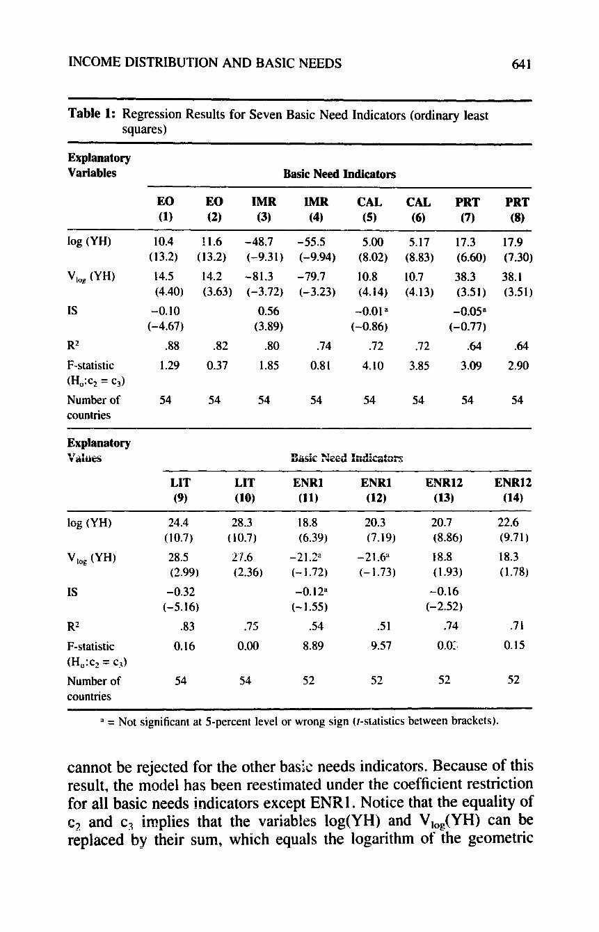
INCOME DISTRIBUTION AND BASIC NEEDS 641
Table 1: Regression Results for Seven Basic Need Indicators (ordinary least squares)
Explanatory Variables Basic Need Indicators
EO EO IMR IMR CAL CAL PRT PRT (1) (2) (3) (4) (5) (6) (7) (8)
log W-0
V,, W-U
IS
R2
F-statistic (H,:c, = c3)
Number of countries
10.4 t-1.6 -48.7 -55.5 5.00 5.17 17.3 17.9 (13.2) (13.2) (-9.3 1) (-9.94) (8.02) (8.83) (6.60) (7.30)
14.5 14.2 -81.3 -79.7 10.8 10.7 38.3 38.1 (4.40) (3.63) (-3.72) (-3.23) (4.14) (4.13) (3.51) (3.51)
-0.10 0.56 -0.01 a -0.05” (-4.67) (3.89) (-0.86) (-0.77)
.88 .82 .80 .74 .72 .72 .64 .64
1.29 0.37 1.85 0.81 4.10 3.85 3.09 2.90
54 54 54 54 54 54 54 54
LIT LIT ENRl ENRI ENR12 ENR12 (9) (10) (11) (12) (13) (14)
log O’H)
hg W-0
IS
R’
F-statistic
(H,:q = q)
Number of
countries
24.4 28.3 18.8 20.3 20.7 22.6 (10.7) (10.7) (6.39) (7.19) (8.86) (9.7 1)
28.5 27.6 -21.2” -21.6” 18.8 18.3 (2.99) (2.36) (- 1.72) (- 1.73) ( 1.93) (1.78)
-0.32 -0.12” -0.16 (-5.16) (- 1.55) (-2.52)
.83 .75 .54 .51 .74 .71
0.16 0.00 8.89 9.57 0.01 0.15
54 54 52 52 52 52
a = Not significant at 5-percent level or wrong sign (t-stdstics between brackets).
cannot be rejected for the other basic needs indicators. Because of this result, the model has been reestimated under the coefficient restriction for all basic needs indicators except ENR 1. Notice that the equality of c2 and c3 implies that the variables log(YH) and V,,,(YM) can be replaced by their sum, which equals the logarithm of the geometric

642 N. Heerink and H. Folmer
T&le 2: Regression Results Under the Coefficient Restriction (ordinary least squares)
Explanatory Variables Basic Need Indicators
EO EO IMR IMR CAL CAL
(I) (2) (3) (4) (5) (6)
log GYH)
IS
R’
Number of countries
10.9 11.9 -52.2 -57.9 5.61 5.73 ( 15.7) (15.5) (-11.3) (- I 1.9) ( 10.0) f 10.9)
-0.10 0.54 -0.01 ;1 (-4.58) (3.75) (-0.66)
.87 .82 .79 .73 .70 .70
54 54 54 54 54 54
Explanatory Values Basic Need Indicators
PRT (7)
PRT (8)
LIT LIT ENRl2 ENRl2
(9) (10) (11) (12)
log (GYH) 19.5 20.0 24.8 28.2 20.5 22.2 (8.39) (9.13) ( 12.6) (12.4) (10.1) ( 10.9)
:s -0.04” -0.32 -0.16 (-0.60) (-5.18) (-2.58)
R’ .rr, ‘3 .62 .83 .75 .74 .70
Number of 54 54 54 54 52 52 countries
p = Not significant at 5-percent level or wrong sign (f-statistics between brackets).
average of household incomes (see Section 2). The latter variable is denoted by log(GYH). The regression results are presented in Table 2.
Assuming the restrictions hold, the coefficient estimates shown in Table 2 have an improved efficiency. All the coefficient estimates for log(GYH) are highly significant. The fit of the equations has hardly changed as compared with the unrestricted regressions. The regression results further indicate that Islamic religion has a negative impact on the satisfaction of two of the three basic needs that are examined, namely health and education. These findings are consistent with those of Caldwell (1986). The third basic need, nutrition, is not significantly affected, as indicated by the low values of t-statistics for IS in the equations for CAL and PRT. When the variable IS is deleted from these two equations, the results for the other two variables are only marginally affected (see columns (6) and (8) in Table 2).

INCOME DISTRIBUTION AND BASIC NEEDS 643
The estimated coefficients for log(GYH) suggest that when house- hold incomes are equalized such that V,,,(YH) increases by 0.17 (the standard deviation across the sample), the life expectancy at birth increases by 1.85 years and the number of infant deaths per thousand decreases by nine, whereas the daily supply of calories increases by 98 and the daily supply of proteins by 3.4 grams.t4 For education, the effect would be an increase of 4.2 percentage points in the adult literacy rate, and an increase of 3.5 percentage points in the combined primary and secondary school enrollment ratio. When, on the other hand, average household income increases by $2,127 (the antilog of the standard deviation of log(YH)), then the life expectancy would go up by 8.2 years, the number of infant deaths per thousand infants would decrease by 39, the calories supply would increase by 433, and proteins supply would increase by 15.1 grams. As regards education, the effect would be an increase of the adult literacy rate by 18.8 percentage points, and an increase of the combined primary and secondary school enrollment ratio by 15.5 percentage points.
4. PITFALLS OF PREVIOUS STUDIES
The regression results presented in the last section raise the ques- tion why previous empirical studies have reached such deviating conclusions with regard to the impact of income (in)equality on basic needs fulfilment. The main reason is an inadequate specification of the regression equations that are inconsistent with the theory as described in Section 2 and 3. In particular, the specifications used in the studies mentioned in the introktction show the following short- comings:
The income concepts (household or personal income) used within the same equation are often inconsistent. The specifications used for average income and income (in)equal- ity are inconsistent with each other. Besides (semi-)output indicators, input indicators (e.g. population per physician) are used as dependent variables as well.
In order to examine the impact of these shortcomings, two alternative specifications have been tried for the regression equations. In the first specification, the logarithm of income per household has been re- placed by (untransformed) per capita income and population per
‘“It should be observed that calories are x 100 and average household income in $1000 (see
Appendix ).

644 N. Heerink and H. Folmer
Table 3: Regression Results for First Alternative Specification (ordinary least squares)
Explanatory Variables Basic Need Indicators
EO (1)
IMR CAL PRT LIT ENRl ENR12 DOC (2) (3) (4) (5) (6) (7) (8)
YPC
V,, WI)
R2
Numbers of countries
0.39 -1.86 0.20 0.72 0.94 0.59 0.77 -0.26 (8.38) (-7.03) (8.53) (7.88) (7.33) (4.38) (6.77) (-4.97)
3.93” - 30.9” 4.54” 14.3” 2.93” -33. la -1.14” 12.1” (0.66) (-0.92) (1.53) (1.23) (0.18) (- 1.97) (-0.08) (1.81)
.67 .61 .71 .67 .60 .28 55 .33
54 54 54 54 54 52 52 54
a = Not significant at 5-percent level or wrong sign (t-statistics between brackets).
physician has been added to the set of explanatory variables. This gives the following specificatiorQ5
BNIi = c’l + C’2 YPCi + C’jV,,g(YH)i + U’i, for i = I,...,54 (or 52)
where BNI stands for the basic need indicators EO, IMR, CAL, PRT, LIT, ENRl, ENR12, DOC.
DOC = Population per physician (in thousands); YPC = Real gross domestic product (in $1,000 of 1975) per capita; u’i = Disturbance term with standard properties. c’ 1,c’*,c’s = Unknown parameters.
The specification resembles the one used by Sheehan and Hopkins (1978). As before, average income and income equality are expected to have a positive impact on basic needs fulfilment, This means that the coefficients of YPC and VI,,(YH) should be negative in the equations for IMR and DOC, and should be positive in the other equations. The regression results are given in Table 3.
The regression results lead to a totally different conclusion. In all the equations, the estimated coefficient for V,,,(YH) is either not significantly different from zero or has the wrong sign. The fit of the equations, as indicated by the values of the R*, is lower than the fit of the equa&ns based on the original specification except for the equa-
The variable IS is omitted from the regression because it has not been used in the studies under comparison.

INCOME DISTRIBUTION AND BASIC NEEDS 645
tion for proteins supply per capita (see Table 1). In other words, if a specification similar to the one used by Sheehan and Hopkins (1978) had been used for the regressions instead of Equation 4, the results would have suggested to reject the hypothesis that an equalization of incomes leads to a higher average level of basic needs satisfaction.
The second alternative specification that is tested here is based on the suggestion made by Leipziger and Lewis (1980) and Ram (1985) to distinguish between low income and middle income subgroups. As before, average income is represented by per capita real income and population per physician is added to the set of explanatory variables. Following Ram ( 1985), the sample is confined to less developed countries (so high income countries are excluded), and the intercepts and slopes are allowed to differ between the two subgroups. This gives the following “piecewise linear” specification:
BNIi = C” 1 + c”zDUMRi + C”xYPCi + c”aYPCi.DUMRi
+ C”5Vlog(YH)i + C”hV,q(YH)imDUMRi + U”i
for i=l,..., 32
where BNI stands for the basic need indicators EO, IMR, CAL, PRT, LIT, ENRl, ENR12, DOC.
DUMR = Dummy variable (one for countries with per capita real income < $1,000, zero otherwise)?
U”i = Disturbance term with standard properties. c”, , . . . ,C”(j = Unknown parameters.
The purpose of this specification is to test the hypothesis that average income is important for low-income countries only, whereas income equality matters for the satisfaction of basic needs in middle income countries only (see Ram, 1985). So, positive signs are expected for the coefficients of YPC, YPCDUMR and V,O,(YH), whereas the coeffi- cient of Vi,,(YH).DUMR is expected to be negative. In the equations for IMR and DOC, the coefficients are again expected t3 have the reverse signs.
The results are giver in Table 4. The estimated coefficients for YPC and V,,,(YH). DUMR do not differ significantly from zero in all equations. On the other hand, the coefficients for YPCDUMR are found to differ significantly from zero in all equations except the ones for CAL and PRT whereas the coefficients for V,,,(YH) significantly differ from zero in three out of eight equations. For the three educa-
T’he criterion that is used in Ram’s study for dividing developing countries into low income
and middle income countries is the level of $400 of conventional GDP per capita in 1970.

646 N. Heerink and H. Folmer
TabPe 4: Regression Results for Second Alternative Specification (ordinary least squares)
Explanatory Variables Basic Need Indicators
EO IMR CAL PRT LIT ENRl ENR12 DOC
(1) (2) (3) (4) (5) (6) (7) (8)
YPC 0.22” (1.24)
YPC.DUMR 1.87 (3.05)
V,,( YH) 15.4 ( 1.76)
V,,,(YH).DUMR -7.63” (-0.60)
R’ .72
-0.69” (-0.56)
- 10.3 (-2.46)
-113 (- 1.90)
107” (1.23)
.55
-0.00” (-0.03)
0.30” (1.22)
6.7 1 ( 1.93)
-5.23” (- I .04)
.66
0.51” ( 1.29)
0.18” (0.14)
25.8” ( 1.35)
- 34.6” (- 1.25)
.42
0.38” (0.66)
5.65 (2.88)
32.2” (1.15)
-20.3” (-0.50)
.60
-0.12”
(-0.2 1)
4.00 (2.00)
17.1” (0.60)
- 56.0” (- 1.35)
.52
-0.04” (-0.08)
4.59 (2.77)
32.2” ( 1.36)
-40.1 a (-1.17)
.55
-0.05” (-0.23)
-3.36 (-4.87)
0.94” (0.10)
6.16” (0.43)
.68
Sample size is 32 (low and middle income countries only). a = Not significant at 5-percent testing level or wrong sign (t-statistics between brackets).
tion indicators, the values of the t-statistics for VI,,(YH) are below the critical values at the 5-percent level. On the basis of these results, one would be tempted to conclude that income equality has a positive impact of health and possibly on nutrition but not on education, whereas average income is important only for education and health in low income countries. Again, these conclusions differ substantially from the conclusions that were reached on the basis of Equation 4.
In conclusion, these two exercises have shown that the specification of the explanatory variables is of crucial importance for testing the impact of income equality on basic needs satisfaction. In particular, when a linear or piecewise linear specification (instead of strictly concave function) is used for average income, and average income is expressed per capita instead of per household, the results of the regressions suggest incorrectly that income redistributions either have no impact on basic needs satisfaction or have an impact on a few components only.

INCOME DISTRIBUTION AND BASIC NEEDS 647
5. CONCLLJSIONS
It has been shown in this paper that a nonlinear micro-based macroeconomic relationships should not only include the average of the explanatory variable but also a term reflecting the nonlinearity bias. In the case of a continuous and strictly convex function the nonlinearity bias satisfies the basic characteristics of an inequality measure.
From these theoretical results it follows that an equalization of household incomes leads to a higher average level of basic needs satisfaction in a population. This proposition is primarily based on the strict concave form that is usually found for Engel curves of necessi- ties. When household incomes are equalized, low income households will consume more and high income households less goods and services that satisfy their basic needs. But the strict concavity of the Engel curve implies that the gains of the poor households exceed the losses of the rich households. As a resuli, the average leve! of basic need satisfaction increases.
The empirical results of this paper support the hypothesis. This raises the question why most previous empirical studies have reached different conclusions. It is shown that the main reason lies in the fact that the specification of the regression equations in previous studies does not adequately represent the theory. In particular, a (piecewise) linear specification is used for average income instead of a nonlinear specification and different income concepts are used for income inequality and average income. These specifications are not based on consistent aggregation of (nonlinear) micro relationships and therefore are not consistent with the underlying theory. When similar specifka- tions are used in the present analysis, the regression results do not confirm the hypothesis either. This result shows that consistent aggre- gation of the underlying micro-level relationships is of fundamental importance for the derivation of the regression equations to be used in studies of the impact of income (in)equality on basic needs fulfilment or other macro-level variables.

648 N. Heerink and H. Folmer
APPENDIX: DATA SOURCES The sample that is used for the regression analyses consist of the
following 54 countries and years:
1. Kenya 1976 20. Taiwan 1971 37. Italy 1977 2. Tanzania 1969 21. Hong Kong 1980 38. Ireland 1973 3. Malawi 1967-68 22. Mexico 1968 39. United Kingdom 1979 4. Zambia 1076 23. Honduras 1.967 48. Nelherial& i977 5. Sierra Leone 1967-69 24. El Salvador 1976-77 41. Germany, Fed. Rep. 1974 6. Sudan 1967-68 25. Costa Rica 197 1 42. Belgium 1978-79 7. Egypt 1974 26. Panama 1970 43. France 1975 8. Turkey 1973 27. Trinidad and 44. Switzerland 1978 9. Iran 1973-74 Tobago 1975-76 45. Denmark 1976
10. India 1975-76 28. Venezuela 1970 46. Sweden 1979 11. Nepal 1976-77 29. Peru 1972 47. Norway 1970 12. Bangladesh 1973-74 30. Brazil 1972 48. Finland 1977 13. Sri Lanka 1969-70 31. Chile 1968 49. Japan 1979 14. Thailand 1975-76 32. Argentina 1970 50. New Zealand 1981-82 15. Malaysia 1973 33. Israel 1979-80 5 1. Australia 1975-76 16. Indonesia 1976 34. Yugoslavia 1978 52. Canada 1977 17. Philippines 1970-7 1 35. Portugal 1973-74 53. United States 197 1
18. Fiji 1977 36. Spain 1973-74 54. Hungary 1982 19. Rep. of Korea 1976
The data come from the following sources (variables ranked alphabet- ically):
CAL = Supply of calories per capita per day (x 100).
Sources: a F.A.O. Production yearbook (various years). l Taiwan 197 1: Estimated from data for 1970 and 1974 in World
Bank, World development report (various years) and World Bank (1980). Data refer to 3-year averages.
DOC = Population per physician (x 1000).
Sources: 0 World Bank (1984, Volume II). l Taiwan 197 1: Estimated from data for 1970 and 1976 in World
Bank, World development report (various years).
DUMB = -1, for countries with per capita real income C $1000; -0, for other countries in the sample.
Equals one for countries nos. l-7, lo- 14, 16, 17 and 23; the variable YPC serves as the criterium.

INCOME DISTRIBUTION AND BASIC NEEDS 649
ENRI = Primary school enrollment ratio (as a percentage of the primary school age population).
Sources: l UNESCO, Statistical yearbook (various years): Table 3.2. l Taiwan 197 1: World Bank, World development report (various
years).
ENR12 = Combined primary and secondary school enrollment ratio (as a percentage of the primar;! and secondary school age population). Sources: See ENRl .
EO = Life expectancy at birth.
Sources: l IJnited Nations ( 1982). l Bangladesh 1973-74: United Nations, Demographic yearbook
(various years). l Taiwan 197 1: DGBAS (1983, Table 19).
GYH = Geometric average of household incomes. Calculated by taking the antilog of the sum of log(YH) and V,, g (YH).
IMR = Infant mortality rate (= number of deaths to infants under one year of age per thousand live births).
Sources: l United Nations Secretariat ( 1982) l United Nations, Demographic yearbook (various years). l Taiwan: DGBAS (1983, Table 19).
IS = Percentage of the population with Islamic religion. Source: Kurian ( 1979, p. 48). The data refer to the early 1970s.
LIT = Adult literacy rate (population aged 15 and over).
c\ources: l World Bank (1984, Volume II). l Taiwan 197 I : Estimated from data for 1960 and 1974 in World
Bank ( 1980) and World Bank, World development report (various years).
PRT = Supply of proteins (in grams) per capita per day.
Sources: e World Bank ( 1984, Volume 11).

650 N. Heerink and H. Folmer
l Taiwan i97 1: Kurian ( 1979, p. 306). Data refer to 3-year averages.
VLOGYH = Equality of total available household income, as mea- sured by V,,,(X).
Estimates of the distribution of total available household income come from Van Ginneken and Park (1984, Table 1 and Table A 1) for 33 countries. These are countries nos. l-2, 4-7, 9- 13, 17- 19, 22-23, 25-32, 34, 36, 38-39, 41, 43, 45-46, and 53. In order to enlarge the sample, income distribution estimates were taken from the World Bank, World Development Report (various years) for another 21 countries. The income concept in this series is the same as the one used by Van Ginneken and Park.
When income distribution estimates have been published for more than year in the World Development Reports, the most recent year (but not later than 1980) for a country has been chosen. The value of the equality measure V,,(X) has been estimated by fitting the Lorenz- curve that corresponds to the lognormal distribution to these income distribution estimates (see Heerink 1994, ch. 2, for a description of this method).
YH = Average household income (= real gross domestic product per household), in $1,000 of 1975. Calculated by multiplying YPC and average household size. Sources for estimates of average household size:
l United Nations, Compendium of housing statistics 1975-77. l Ta%an 197 1: Own estimate, based on data for 1966 in United
Nations, Demographic yearbook 1968 and trend in average household size in the Rep. of Korea.
YPC = Income per capita (= real gross domestic product per capita), in $1,000 of 1975.
Sources: l Summers and Heston (1984). l New Zealand 1981-82 and Hungary 1982: Own estimates, based
on estimates for 1980 in Summers and Heston (1984) and growth rate of per capita GDP in constant prices in IMF, International financial statistics (various years).
Purchasing power parities are used for converting incomes in local currencies to U.S. dollars. The estimates are results of the United Nations Income Comparison Project (ICP).

INCOME DISTRIBUTION AND BASIC NEEDS 651
REFERENCES
Caldwell, J.C. ( 1986) Routes to Low Mortality in Poor Countries, Population and De1*elopmerzt Reiiebv 12: 17 l-220.
Dhrymes, P.J. ( 1978) lutroductory Econometrics. New York: Springer. Directorate-General of Budget, Accounting & Statistics (DGBAS). ( 1983) Statistical Yearbook
of the Republic of China, 1983. Taipei: DGBAS. Eichhom, W. and Ge’luig, W. ( 1982) Measurement of Inequality in Economics. In Modern
Applied Mathematics: Optimization and Operations Research CE. Korte, Ed. ). Amster- dam: North-Holland.
Folmer, H. ( 1986) Regional Economic Policy Measurement of Its Eficts. Boston: Kluwer. Griffin. J.M., and Gregory. P.R. ( 1976) An Intercountry Translog Model of Energy Substitution
Responses, American Ecorlomic Review* 66: 845-857.
Heerink, N. ( 1994) Lopulation Grorvth, Income Distribution and Economic Development: TheoF, Methodology and Empirical Renrlts. Berlin and New York: Springer-Verlag.
Hopkins. M.. and van der Hoeven. R. ( 1983) Basic Needy in Development Planning. Aldershot, U.K.: Gower.
Houthakker, H.S. (1957) An International Comparison of Household Expenditure Patterns Commemorating the Centenary of Engel’s Law, Econometrica 25: 532-55 1.
Houthakker, H.S. ( 1965) New Evidence on Demand Elasticities, Econometrica 33: 277-288. International Labour Office (ILO). ( 1976) International Recon:r?le~ldatiorls on Labour Statistics.
Geneva: ILO. Iyengar, N.S. ( 1964) A Consistent Method of Estimating the Engel Curve from Grouped Survey
Data, Econometrica 32: 59 1-6 18. Judge. G.G., Griffiths, W.E., Hill, R.C.. Lutkepohl, H. and Lee, T.-C. (1985) The TheoF and
Practice of Econometrics. 2nd ed. New York: John Wiley & Sons. Kakwani. NC. (1980) lrlcorlre InequaliQ and Poverty: Methods of Estimation and Policy
Applications. Oxford, U.K.: Oxford University Press. Kirk, D. (1967) Factors Affecting Moslem Natality. In United Nations, World Population
Conference, Belgrade 1965. New York: United Nations. Kmenta, J. ( 1986) Elements of Econometrics, 2nd ed. New York: Macmillan. Kuh, E. ( 1959) The Validity of Cross Sectionally Estimated Behavior Equations in Time Series
Applications, Econometrica 27: 197-2 14.
Kurian, G.T. ( 1979) The Book of World Rankings. London: Macmillan. Kuznets, S. (1976) Demographic Aspects of the Size Distribution of Income: An Exploratory
Essay, Economic Development and Cultliral Change 25: 1-94. Leipziger, D.M., and Lewis, M.A. (1980) Social Indicators, Growth and Distribution, World
Development 8 : 299-302. Lovell, M.C. ( 1983) Data Mining, Reviebv of Economics and Statistics 65: l-12. McGranahan, D., Pizarro, E. and Richard, C. (1985) Measurement and Analysis of Socio-eco-
nomic Development, Report No. 85.5, Geneva: United Nations Research Institute for Social Development.
Mueller, E.. and Short, K. (1983) Effects of Income and Wealth on the Demand for Children. In Determinants of Fertility in Deryeloping Countries (R.A. Bulatao and R.D. Lee, Eds.). New York: Academic Press.
Phlips, L. ( 1983) Applied Consun~ptiort Analysis. Amsterdam: North-Holland. Prais, S..J., and HouthakKer, H.S. (1955) The Analysis of Family Budgets. Cambridge, U.K.:
Cambridge University Press. Ram, R. ( 1985) The Role of Real Income Level and Income Distribution in Fulfillment of Basic
Needs, World Development 13: 589-594.

652 N. Heerink and H. Folmer
Sheehan, G., and Hopkins, M. (1978) Meeting Basic Needs: An Examination of the World Situation in 1970, International Labour Review 117: 523-541.
Shonocks, A.F. (1980) The Class of Additively Decomposable Inequality Measures, hnome- trica 48: 6 13-625.
Shorrocks, A.%. (1988) Aggregation Issues in Inequality Measurement. In Measurement in Economics (W. Eichhom, Ed.). Heidelberg: Physica-Verlag.
Sinha, R., Pearson, P., Kadekodi, G., and Gregory, M (1979) Income Distribu?ion, Growth and Basic Needs in India. London: Croom Helm.
Stewart, F. (1979) Country Experience in Providing for Basic Needs, Finance & Development 16(4): 23-26.
Streeten, P. (1981) First Things First: Meeting Basic Human Needs in Developing Countries. Oxford, U.K.: Oxford University Press.
Summers, R., and Heston, A. (1984) Improved International Comparisons of Real Product and its Composition: 1950-1980, Review of fncome and Wealth 30: 207-262.
Theil, H. (1967) Economics and Information Theory Amsterdam: North-Holland. Theil, H. (1971) Principles of Econometrics. New York: John Wiley & Sons. United Nations. (1982) Demographic Indicators of Countries: Estimates and Projections as
Assessed in 1980. New York: U.N. United Nations Secretariat. (1982) Infant Mortality: World Estimates and Projections, 1950-
2025, Population Bulletin of the United Nations 14: 31-53. UNESCO. (1985) Statistical Yearbook 1985 Paris: UNESCO. Van ihal, 3.. and Merkies, A.H.Q.M. (1984) Aggregation in Economic Research: From
Individual to Macro Relations Dordrecht, The Netherlands: D. Reidel. Van der Hoeven, R. (1987) Planning for Basic Needs: A Basic Needs Simulation Model Applied
to Kenya Doctorate dissertation. Amsterdam: Free University Press. Van Ginneken, W., and Park, J.-G., eds. (1984) Generating lntemationally Comparable Income
Distributi’on Estimates Geneva: ILO. World Bank. (1980) World Tables; The Second Edition. B&imore: Johns Hopkins University
Press. World Bank. (1984) World Tables: The Third Edition. Baltimore: Johns Hopkins University
Press.