Allocation Planning for Demand Fulfillment in Make-to-Stock ...
190
Allocation Planning for Demand Fulfillment in Make-to-Stock Industries – A Stochastic Linear Programming Approach genehmigte Dissertation zur Erlangung des akademischen Grades eines Doctor rerum politicarum (Dr. rer. pol.) der Technischen Universit¨ at Darmstadt Fachbereich Rechts- und Wirtschaftswissenschaften Hochschulkennziffer D17 vorgelegt von Dipl.-Wi.-Ing. Stephanie Eppler Geburtsort: Albstadt Referent: Prof. Dr. Herbert Meyr Korreferent: Prof. Dr. Michael Schneider Tag der Einreichung: 04.11.2014 Tag der Disputation: 28.01.2015 Darmstadt 2015
-
Upload
khangminh22 -
Category
Documents
-
view
0 -
download
0
Transcript of Allocation Planning for Demand Fulfillment in Make-to-Stock ...

Allocation Planning for Demand Fulfillmentin Make-to-Stock Industries
– A Stochastic Linear Programming Approach
genehmigte Dissertation
zur Erlangung des akademischen Grades
eines Doctor rerum politicarum (Dr. rer. pol.)
der Technischen Universitat Darmstadt
Fachbereich Rechts- und Wirtschaftswissenschaften
Hochschulkennziffer D17
vorgelegt von
Dipl.-Wi.-Ing. Stephanie Eppler
Geburtsort: Albstadt
Referent: Prof. Dr. Herbert Meyr
Korreferent: Prof. Dr. Michael Schneider
Tag der Einreichung: 04.11.2014
Tag der Disputation: 28.01.2015
Darmstadt 2015

Acknowledgments
First and foremost, I would like to express my gratitude to my PhD advisor Prof. Dr. Herbert
Meyr for all his support and for providing guidance during the last years. Throughout the
entire project and despite your busy schedule, you always found time for fruitful discussions,
valuable comments and questions. You provided the opportunity to learn a lot by sharing
your great experience.
Furthermore, I would like to thank Prof. Dr. Michael Schneider for acting as second
reviewer of my PhD thesis. Also thanks to Prof. Dr. Anne Lange, Prof. Dr. Volker Nitsch
and Prof. Dr. Reiner Quick for being members of my PhD committee.
Thanks also to my colleagues at the Chair of Supply Chain Management at the University
of Hohenheim: In particular, I want to thank Mirko Kiel and Martin Worbelauer for their
support and for the great atmosphere at the chair.
Moreover, I am sincerely grateful to my family who has always believed in me and has
always supported me in achieving my goals. Thank you also for showing so much under-
standing throughout the last years.
Most of all, however, I am grateful to Volker. You have always been there for me, being
an invaluable source of motivation and confidence. Thank you so much for your love and
your support.
Stephanie Eppler, Stuttgart, November 2014

Contents
Acknowledgements ii
List of Figures vi
List of Tables viii
List of Abbreviations ix
1 Introduction 1
1.1 Motivation . . . . . . . . . . . . . . . . . . . . . . . . . . . . . . . . . . . . . 1
1.2 Research Goals and Methodology . . . . . . . . . . . . . . . . . . . . . . . . 3
1.3 Outline of the Thesis . . . . . . . . . . . . . . . . . . . . . . . . . . . . . . . 5
2 Conceptual and Methodological Basics 6
2.1 Quantity-based Revenue Management . . . . . . . . . . . . . . . . . . . . . . 6
2.1.1 Origins of Revenue Management . . . . . . . . . . . . . . . . . . . . . 7
2.1.2 Revenue Management – Definitions and Implementation Approaches . 8
2.1.3 Conditions for Revenue Management to Be Beneficial . . . . . . . . . 10
2.1.4 Capacity Control . . . . . . . . . . . . . . . . . . . . . . . . . . . . . 11
2.1.5 Littlewood’s Model . . . . . . . . . . . . . . . . . . . . . . . . . . . . 17
2.1.6 Randomized Linear Programming . . . . . . . . . . . . . . . . . . . . 20
2.1.7 Flexible Products . . . . . . . . . . . . . . . . . . . . . . . . . . . . . 21
2.2 Demand Fulfillment & Available-to-Promise . . . . . . . . . . . . . . . . . . 23
2.2.1 Classification of Demand Fulfillment as a Planning Task of Supply
Chain Planning . . . . . . . . . . . . . . . . . . . . . . . . . . . . . . 23
2.2.2 Customer Order Decoupling Point . . . . . . . . . . . . . . . . . . . . 28
2.2.3 Definition of the Terms Demand Fulfillment and Available-to-Promise 31
2.2.4 Planning Tasks of Demand Fulfillment . . . . . . . . . . . . . . . . . 34
2.2.5 Transfer of Revenue Management ideas to Demand Fulfillment in Make-
to-Stock – Allocation Planning . . . . . . . . . . . . . . . . . . . . . 38
2.2.6 Demand Fulfillment in Advanced Planning Systems . . . . . . . . . . 42
2.2.7 State-of-the-Art Models for Allocation Planning in Make-to-Stock En-
vironments . . . . . . . . . . . . . . . . . . . . . . . . . . . . . . . . 44

Contents
2.3 Two-Stage Stochastic Linear Programming with Recourse . . . . . . . . . . . 50
2.3.1 General Model Formulation . . . . . . . . . . . . . . . . . . . . . . . 50
2.3.2 Measuring the Value of the Stochastic Solution . . . . . . . . . . . . 52
2.3.3 Literature Review of two-stage SLP and SMIP applications . . . . . . 53
3 Two-Stage Stochastic Linear Programming Formulations of Littlewood’s
Model 57
3.1 Model Formulations . . . . . . . . . . . . . . . . . . . . . . . . . . . . . . . . 57
3.1.1 Marginal Analysis of Littlewood’s Rule – SLW-MA . . . . . . . . . . 57
3.1.2 Littlewood’s Model with Partitioned Allocations – SLW-PAR . . . . 60
3.1.3 Littlewood’s Model with Nested Allocations – SLW-NES . . . . . . . 62
3.1.4 Dual Model of SLW-MA . . . . . . . . . . . . . . . . . . . . . . . . . 64
3.1.5 Dual Model of SLW-PAR . . . . . . . . . . . . . . . . . . . . . . . . 65
3.1.6 Dual Model of SLW-NES . . . . . . . . . . . . . . . . . . . . . . . . 66
3.2 Numerical Study . . . . . . . . . . . . . . . . . . . . . . . . . . . . . . . . . 67
3.2.1 Verification Tests of the Primal Models . . . . . . . . . . . . . . . . . 67
3.2.1.1 SLW-MA . . . . . . . . . . . . . . . . . . . . . . . . . . . . 69
3.2.1.2 SLW-PAR . . . . . . . . . . . . . . . . . . . . . . . . . . . . 69
3.2.1.3 SLW-NES . . . . . . . . . . . . . . . . . . . . . . . . . . . . 69
3.2.2 Tests of the Dual Models . . . . . . . . . . . . . . . . . . . . . . . . . 71
3.3 Conclusions . . . . . . . . . . . . . . . . . . . . . . . . . . . . . . . . . . . . 73
4 Single-Period Models for Allocation Planning in Make-to-Stock Environ-
ments 75
4.1 Conditions for Allocation Planning to Be Beneficial . . . . . . . . . . . . . . 76
4.1.1 Order Arrival Sequence . . . . . . . . . . . . . . . . . . . . . . . . . . 80
4.1.2 Customer Segmentation and Heterogeneity . . . . . . . . . . . . . . . 82
4.1.3 Load Factor . . . . . . . . . . . . . . . . . . . . . . . . . . . . . . . . 85
4.1.4 Demand Uncertainty . . . . . . . . . . . . . . . . . . . . . . . . . . . 86
4.1.5 Decision Tree . . . . . . . . . . . . . . . . . . . . . . . . . . . . . . . 88
4.2 Model Formulations . . . . . . . . . . . . . . . . . . . . . . . . . . . . . . . . 89
4.2.1 Allocation Planning Model Anticipating a Partitioned Consumption
Rule . . . . . . . . . . . . . . . . . . . . . . . . . . . . . . . . . . . . 90
4.2.2 Allocation Planning Model Anticipating a Nested Consumption Rule 92
4.3 Numerical Study . . . . . . . . . . . . . . . . . . . . . . . . . . . . . . . . . 96
4.3.1 Simulation Environment . . . . . . . . . . . . . . . . . . . . . . . . . 96
4.3.2 Analysis of the Base Case . . . . . . . . . . . . . . . . . . . . . . . . 98
4.3.3 Choice of Steering Profits . . . . . . . . . . . . . . . . . . . . . . . . 100
4.3.3.1 Choice of the Steering Profits for the Unallocated Quantities 101
4.3.3.2 Choice of the Steering Profits for the Nesting Quantities . . 104
iv

Contents
4.3.4 Benefit of the Anticipation . . . . . . . . . . . . . . . . . . . . . . . . 107
4.3.4.1 Benefit of Anticipating a Standard Nesting Consumption Rule109
4.3.4.2 Benefit of Anticipating a Partitioned Consumption Rule . . 111
4.3.5 Benefit of Accounting for Uncertainty . . . . . . . . . . . . . . . . . . 112
4.3.5.1 Influence of Demand Uncertainty . . . . . . . . . . . . . . . 113
4.3.5.2 Influence of Customer Heterogeneity . . . . . . . . . . . . . 116
4.3.6 Benefit of Nesting . . . . . . . . . . . . . . . . . . . . . . . . . . . . . 118
4.4 Conclusions . . . . . . . . . . . . . . . . . . . . . . . . . . . . . . . . . . . . 121
5 A Multi-Period Model for Allocation Planning in Make-to-Stock Environ-
ments 123
5.1 Model Formulation . . . . . . . . . . . . . . . . . . . . . . . . . . . . . . . . 123
5.2 Numerical Study . . . . . . . . . . . . . . . . . . . . . . . . . . . . . . . . . 127
5.2.1 Simulation Environment . . . . . . . . . . . . . . . . . . . . . . . . . 128
5.2.2 Analysis of the Base Case . . . . . . . . . . . . . . . . . . . . . . . . 132
5.2.3 Benefit of Accounting for Uncertainty by Means of an SLP . . . . . . 134
5.2.4 Influence of the Replanning Frequency . . . . . . . . . . . . . . . . . 137
5.2.5 Influence of the Replenishment Frequency . . . . . . . . . . . . . . . 139
5.2.6 Influence of the Holding and Backlogging Costs . . . . . . . . . . . . 142
5.2.7 Comparison with APS Rules . . . . . . . . . . . . . . . . . . . . . . . 144
5.3 Conclusions . . . . . . . . . . . . . . . . . . . . . . . . . . . . . . . . . . . . 146
6 Conclusions and Further Research 149
6.1 Results . . . . . . . . . . . . . . . . . . . . . . . . . . . . . . . . . . . . . . . 149
6.2 Further Research . . . . . . . . . . . . . . . . . . . . . . . . . . . . . . . . . 152
Appendix 155
Bibliography 162
Curriculum Vitae 179
v

List of Figures
2.1 Illustration of partitioned protection levels and booking limits . . . . . . . . 13
2.2 Illustration of nested protection levels and booking limits . . . . . . . . . . . 13
2.3 Illustration of the relationship between booking limits and bid prices . . . . 15
2.4 Decision tree when CR units of capacity are remaining . . . . . . . . . . . . 19
2.5 SCP matrix . . . . . . . . . . . . . . . . . . . . . . . . . . . . . . . . . . . . 25
2.6 SCP matrix with module structure . . . . . . . . . . . . . . . . . . . . . . . 26
2.7 Decoupling points in MTO, ATO and MTS . . . . . . . . . . . . . . . . . . . 29
2.8 Modeling environment without customer segmentation . . . . . . . . . . . . 37
2.9 Modeling environment with customer segmentation . . . . . . . . . . . . . . 42
3.1 Bid prices bLW and bm3 of the SLP models m3 = {SLW-MAD, SLW-PARD,
SLW-NESD} for different load factors lf and a different number S of scenarios 72
4.1 Visualization of an order sequence . . . . . . . . . . . . . . . . . . . . . . . . 78
4.2 Illustration of the benefit of allocation planning . . . . . . . . . . . . . . . . 78
4.3 Illustration of order arrival sequences and the related potential benefit of
allocation planning . . . . . . . . . . . . . . . . . . . . . . . . . . . . . . . . 81
4.4 Order sequences with different heterogeneities . . . . . . . . . . . . . . . . . 83
4.5 Alternatives of customer segmentation . . . . . . . . . . . . . . . . . . . . . 84
4.6 Variation of the ATP quantity . . . . . . . . . . . . . . . . . . . . . . . . . . 85
4.7 Illustration of two customer classes’ uncertain demand . . . . . . . . . . . . 87
4.8 Benefit of accounting for uncertainty – resulting profits for order sequence 3
when applying a DLP and an SLP . . . . . . . . . . . . . . . . . . . . . . . 88
4.9 Decision tree for allocation planning . . . . . . . . . . . . . . . . . . . . . . . 89
4.10 Representation of an lbh order arrival sequence and a standard nesting rule
in the AP-NES model . . . . . . . . . . . . . . . . . . . . . . . . . . . . . . 94
4.11 Representation of an lbh order arrival sequence and the nesting rule described
by Vogel (2013) in the AP-NES model . . . . . . . . . . . . . . . . . . . . . 95
4.12 Percentage of ATP allocated to the different classes or remaining unallocated 99
4.13 Fill rates of the different classes for different allocation planning models and
FCFS . . . . . . . . . . . . . . . . . . . . . . . . . . . . . . . . . . . . . . . 100
4.14 Percentage of ATP remaining unallocated . . . . . . . . . . . . . . . . . . . 102
4.15 Impact of steering profits pus depending on cov . . . . . . . . . . . . . . . . . 103

List of Figures
4.16 Impact of steering profits pus on the profit deviation from the GOP depending
on lf . . . . . . . . . . . . . . . . . . . . . . . . . . . . . . . . . . . . . . . . 103
4.17 Representation of a mixed order arrival sequence and a standard nesting rule
in the AP-NES model . . . . . . . . . . . . . . . . . . . . . . . . . . . . . . 105
4.18 Allocated and unallocated ATP quantity for different steering profits . . . . 106
4.19 Impact of steering profits pnk′k and pus on the profit deviation from the GOP
depending on cov . . . . . . . . . . . . . . . . . . . . . . . . . . . . . . . . . 107
4.20 ATP quantity allocated by the SLP models AP-PAR and AP-NES depending
on cov . . . . . . . . . . . . . . . . . . . . . . . . . . . . . . . . . . . . . . . 108
4.21 Absolute profits and the benefit of anticipating a nested consumption rule . . 109
4.22 Fill rates when a nested consumption rule is applied . . . . . . . . . . . . . . 110
4.23 Absolute profits and the benefit of anticipating a partitioned consumption rule 111
4.24 Fill rates when a partitioned consumption rule is applied . . . . . . . . . . . 112
4.25 Influence of demand uncertainty on the absolute profits and on the percentage
profit deviation from the GOP . . . . . . . . . . . . . . . . . . . . . . . . . . 113
4.26 Allocations and fill rates of classes 1 – 3 for different values of cov . . . . . . 115
4.27 Influence of customer heterogeneity on the total profit and the percentage
profit deviation from the GOP . . . . . . . . . . . . . . . . . . . . . . . . . . 117
4.28 Profits of different allocation planning models in combination with different
consumption rules . . . . . . . . . . . . . . . . . . . . . . . . . . . . . . . . . 118
4.29 Benefit of allowing for standard nesting . . . . . . . . . . . . . . . . . . . . . 119
4.30 Comparison of the capacity utilization when applying standard nesting or a
partitioned consumption rule . . . . . . . . . . . . . . . . . . . . . . . . . . . 120
5.1 Illustration of simulation horizon, allocation planning horizon, and frozen hori-
zon . . . . . . . . . . . . . . . . . . . . . . . . . . . . . . . . . . . . . . . . . 128
5.2 Base case related results: lost sales, quantities backlogged, fulfilled from ATP
which becomes available at or prior to the due date . . . . . . . . . . . . . . 133
5.3 Absolute profits and relative profit deviations from the GOP for different policies135
5.4 Costs and lost sales for different policies and values of cov . . . . . . . . . . 136
5.5 Absolute profits for different lengths of the frozen horizon . . . . . . . . . . . 138
5.6 Backlogging costs and lost sales for different lengths of the frozen horizon . . 139
5.7 Absolute profits for different replenishment frequencies . . . . . . . . . . . . 140
5.8 Lost sales, quantities backlogged, fulfilled from ATP which becomes available
at or prior to the due date for different replenishment frequencies . . . . . . 141
5.9 Absolute profits for different values of backlogging and inventory holding costs 142
5.10 Inventory holding and backlogging costs and related quantities for different
cost parameters . . . . . . . . . . . . . . . . . . . . . . . . . . . . . . . . . . 143
5.11 Absolute profits and relative profit deviations of different APS rules . . . . . 144
5.12 Lost sales of different allocation planning rules and TPAR . . . . . . . . . . 146
5.13 Lost sales of different allocation planning rules and TNES . . . . . . . . . . 147
vii

List of Tables
2.1 Indices, data and variables of the SOPA model (Meyr (2009)) . . . . . . . . 46
2.2 Additional index, modified data and variables of the RLP model by Quante
(2009), pp. 61 . . . . . . . . . . . . . . . . . . . . . . . . . . . . . . . . . . . 48
2.3 Allocation planning models for MTS environments . . . . . . . . . . . . . . . 49
3.1 Indices, parameters and variables of the SLW-MA model . . . . . . . . . . . 58
3.2 Additional parameters and variables of the SLW-PAR model . . . . . . . . . 61
3.3 Additional parameter and variables of the SLW-NES model . . . . . . . . . 62
3.4 Variables of the SLW-MAD model . . . . . . . . . . . . . . . . . . . . . . . . 64
3.5 Additional variables of the SLW-PARD model . . . . . . . . . . . . . . . . . 66
3.6 Absolute percentage deviations ∆zm1,m2 of the SLP protection levels zm1 from
their analytical equivalents zm2 for S = 100 scenarios (S = 10 scenarios),
computed as averages over all parameter combinations . . . . . . . . . . . . 68
3.7 Average allocation deviations ∆zSLW−NES,LW
and the corresponding shortage
probabilities P (D1 +D2 > C) (both measured in %) for different load factors
lf and S = 100 scenarios . . . . . . . . . . . . . . . . . . . . . . . . . . . . . 70
3.8 Average absolute optimality gaps ∆ESLW−NES,LW
(measured in %) for the
revenue obtained in the consumption process for different load factors and
S = 100 scenarios . . . . . . . . . . . . . . . . . . . . . . . . . . . . . . . . . 71
4.1 Exemplary order sequence . . . . . . . . . . . . . . . . . . . . . . . . . . . . 77
4.2 Exemplary order sequence with low heterogeneity . . . . . . . . . . . . . . . 82
4.3 Indices, data and variables of AP-PAR . . . . . . . . . . . . . . . . . . . . . 91
4.4 Additional data and variables of AP-NES . . . . . . . . . . . . . . . . . . . 93
4.5 Absolute profits and relative profit deviations for the base case data . . . . . 99
4.6 Values of γ and impact on the relation of the per-unit profit for unallocated
quantities pus to the classes’ profits in case of deterministic demand . . . . . . 101
5.1 Indices, data and variables of the consumption LP for order o . . . . . . . . 125
5.2 Additional and modified indices, data and variables of AP-TIME . . . . . . 126
5.3 Absolute profits and relative profit deviations for the base case data . . . . . 133
5.4 Average computation times (in seconds) of an iteration n of the base case for
different allocation planning models . . . . . . . . . . . . . . . . . . . . . . . 137

List of Abbreviations
AATP Advanced available-to-promise
aATP Allocated available-to-promise
acc. According
analyt. Analytical
AP Allocation planning
AP-NES Single-period, multi-class allocation planning model anticipating a nested
consumption rule
AP-PAR Single-period, multi-class allocation planning model anticipating a parti-
tioned consumption rule
AP-TIME Multi-period, multi-class allocation planning model anticipating a time-
based consumption rule
APICS American Production & Inventory Control Society
APO Advanced Planner & Optimizer
APS Advanced planning system
ATO Assemble-to-order
ATP Available-to-promise
B Backlog
BOP Batch order processing
cATP Cumulated available-to-promise
CODP Customer order decoupling point
CR Consumption rule
CTO Configure-to-order
CTP Capable-to-promise
DD Discrete distribution
Dem. Demand
det. Deterministic
DLP Deterministic linear program
DND Discretised normal distribution
EEV Expected result of using the expected value solution
EMSR Expected Marginal Seat Revenue
end. Endogenous
ERP Enterprise resource planning
EV Expected value

List of Abbreviations
EVP Expected value problem
EVPI Expected value of perfect information
ex. Exogenous
FCFS First-come, first-serve
GLPK GNU Linear Programming Kit
GOP Global optimum
GSL GNU Scientific Library
hbl High-before-low
HN Here-and-now
KPI Key performance indicators
lbh Low-before-high
LP Linear program(ming)
LW Littlewood’s model
LW-PAR Littlewood’s partitioned model
MIP Mixed integer program
MRP Material requirements planning
MTO Make-to-order
MTS Make-to-stock
n.a. Not applicable
n.s. Not specified
NES Nested (rule)
NLKP Non-linear knapsack problem
NLSP Non-linear stochastic program
O&D Origin-destination
OP Order processing
PAR Partitioned (rule)
repl. Replenishment
RLP Randomized linear program
SAA Sample average approximation
SCM Supply chain management
SCP Supply chain planning
SDP Stochastic dynamic program
Seq. Sequence
SLP Stochastic linear program
SLW-MA Stochastic linear programming formulation of Littlewood’s rule derived
from the marginal analysis
SLW-MAD Dual stochastic linear programming formulation of Littlewood’s rule de-
rived from the marginal analysis
SLW-NES Stochastic linear programming formulation of Littlewood’s model
SLW-NESD Dual stochastic linear programming formulation of Littlewood’s model
x

List of Abbreviations
SLW-PAR Stochastic linear programming formulation of the partitioned version of
Littlewood’s model
SLW-PARD Dual stochastic linear programming formulation of the partitioned version
of Littlewood’s model
SMIP Stochastic mixed integer program
SOP Single order processing
SOPA Single order processing after allocation planning
Sp Sample
St Store
stoch. Stochastic
TNES Time-based, nested consumption rule of an APS
TPAR Time-based, partitioned consumption rule of an APS
VSS Value of the stochastic solution
WS Wait-and-see
xi

1 Introduction
1.1 Motivation
Demand fulfillment has gained increasing interest in research during the last years (see, e.g.,
Geier (2014), pp. 85). Demand fulfillment is a planning process which is concerned with the
processing of customer orders (see, e.g., Fleischmann and Meyr (2003b)). It comprises several
planning tasks, such as due date setting or the commitment of orders (see, e.g., Fleischmann
and Meyr (2003a)). Their importance can differ considerably depending on the particular
industry. In make-to-stock industries, such as the consumer goods industry, production
quantities are usually determined based on forecasts and not on actual customer requests
(see, e.g., Hoekstra and Romme (1992), p. 7, Meyr (2003), Fleischmann et al. (2008)). As
a consequence, the main planning tasks of demand fulfillment in make-to-stock entail two
decisions: whether an order should be accepted or rejected and whether an accepted order
is fulfilled from stock or from future production quantities (see, e.g., Fleischmann and Meyr
(2003a), Fleischmann and Meyr (2003b), Kilger and Meyr (2008), Fleischmann (2008)).
As customers assume make-to-stock products to be always on stock, they usually place
their orders only a few days before the due date. Consequently, they expect an immediate
order commitment from the firm (see, e.g., Meyr (2003), Fleischmann and Meyr (2003b)).
A firm could, e.g., accept and commit orders according to their arrival sequence, i.e. on a
first-come, first-serve basis. However, customers are usually heterogeneous regarding their
profitability, i.e. they differ w.r.t. revenues, costs (taxes, shipping, or backlogging costs),
or their strategic importance for the firm (see, e.g., Fleischmann and Meyr (2003b), Meyr
(2009)). Furthermore, as production quantities are determined when demand is still uncer-
tain, the firm is sometimes faced with scarce capacity when orders are finally placed (see,
e.g., Meyr (2009)). If the firm accepts orders on a first-come, first-serve basis, less prof-
itable orders may be fulfilled, while more profitable orders, which arrive later, have to be
declined as there is no more capacity available (see, e.g., Fleischmann and Meyr (2003b),
Meyr (2009)).
The situation of having scarce capacities in the short-run, heterogeneous customers, and
uncertain demand leads to the idea of transferring revenue management ideas to the context
of demand fulfillment in manufacturing (see, e.g., Quante et al. (2009a)). Revenue manage-
ment arises from service industries, in particular the airline industry, and is concerned with
managing uncertain demand of heterogeneous customers when capacity is scarce (see, e.g.,
Kimes (1989a), Talluri and van Ryzin (2004), pp. 6).

1 Introduction
Within the context of revenue management, several demand management instruments
have been developed in the past. One of these instruments is called allocation planning.
The basic idea of allocation planning is (1) to group customers with the same or a similar
profitability to customer classes and (2) to use information about the uncertain demand and
the classes’ profitability in order to reserve capacity for more profitable classes, i.e. to protect
this capacity from being consumed by less profitable classes (see, e.g., Kimes (1989b), Talluri
and van Ryzin (2004), pp. 27). Then, customer orders can be fulfilled from the allocation
reserved for the respective customer class. This is called the consumption process.
In order to further improve revenues and the customer service for more valuable classes,
nesting rules can be applied in the consumption process. If a more valuable customer class’
demand exceeds the class’ allocation and if nesting is applied, the class’ demand can also be
fulfilled from the allocations reserved for less profitable classes. Consequently, nesting is a
class-based consumption rule. In contrast, customers are only allowed to consume their own
class’ allocations under a partitioned policy (see, e.g., Kimes (1989b), Lee and Hersh (1993),
Talluri and van Ryzin (2004), pp. 28).
Make-to-stock differs from the setting in service industries regarding several issues. First,
customer orders often arrive in a so-called low-before-high arrival sequence in service in-
dustries. Customers with a low profitability, such as leisure travelers, order earlier than
customers with a high profitability, such as business travelers. This is due to several order or
booking conditions. An example for a booking condition linked with a low-fare ticket for a
flight is a required booking at least two weeks in advance which induces that price-sensitive
leisure travelers book earlier than business travelers (see, e.g., Talluri and van Ryzin (2004),
p. 33, Klein and Steinhardt (2008), p. 135). In make-to-stock environments, however, the
orders arrive in a mixed sequence. Second, customers usually order a single unit of capacity
(e.g., a single seat on a flight) in service industries, while an order in make-to-stock usually
consists of multiple units. Third, services are perishable. A seat on a flight, e.g., cannot be
sold after the flight date (see, e.g., Kimes (1989b), Weatherford and Bodily (1992)). Make-
to-stock products, however, can usually be stored and orders can in principal be backlogged,
i.e. they can be delivered after the customer’s due date (see, e.g., Meyr (2009), Quante et al.
(2009a), Quante et al. (2009b)). This implies that an order cannot only be fulfilled by the
allocations of several classes but also by allocations reserved for different periods in the past
or in the future. Consequently, time-based consumption rules as well as costs for holding and
backlogging have to be considered additionally. These differences made the transfer of rev-
enue management ideas to the context of demand fulfillment in make-to-stock a challenging
task.
Simple rules for allocation planning already exist in commercial demand fulfillment soft-
ware modules, which are usually parts of advanced planning systems (see, e.g., Kilger and
Meyr (2008)). However, to the best of our knowledge, the question whether these rules can
be beneficial has never been examined in literature. Besides these rules, several models for
allocation planning in make-to-stock environments have been developed. The correspond-
2

1 Introduction
ing numerical studies show that allocation planning is beneficial in make-to-stock industries
(see, e.g., Meyr (2009), Quante (2009), pp. 61, Quante et al. (2009a)). However, the existing
models show two main drawbacks: they either do not consider information about demand
uncertainty appropriately or they are not scalable and, thus, not applicable to problems of
practical sizes. However, numerical studies show that the consideration of information about
the demand uncertainty is beneficial (see, e.g., Quante et al. (2009a)). Therefore, there is a
need for developing models which compensate the drawbacks of existing approaches.
Subsequently, we formulate the research questions in Section 1.2 and state the outline of
the thesis in Section 1.3.
1.2 Research Goals and Methodology
Existing allocation planning models for demand fulfillment in make-to-stock industries show
two main drawbacks. They either neglect information about the uncertain demand or they
are not scalable, i.e. they cannot be applied to problems of practical sizes. This leads to the
first research question.
Research Question 1: How can allocation planning for make-to-stock be performed by
simultaneously accounting for information about uncertain demand and obtaining scalable
models, such that problems of practical sizes are still solvable in a reasonable amount of
time?
We identify the concept of two-stage stochastic linear programming (SLP) as a promising
approach in order to fulfill both requirements and therefore to compensate the drawbacks
related to the existing models. If the uncertain demand can be described by means of a
probability distribution, two-stage SLPs provide the opportunity of accounting for demand
uncertainty by means of a sample of scenarios generated from this demand distribution. At
the same time, SLPs retain the characteristic of an linear programming model and are thus
scalable. The term two-stage arises from the fact that two-stage SLP models divide the
decision process into two stages – a stage with decisions made prior to the realization of the
uncertain parameter and a stage with decisions made afterwards. For demand fulfillment
in make-to-stock, the first stage can be interpreted as the allocation planning stage and the
second stage as the process of fulfilling orders by means of the allocations, i.e. the consump-
tion process. Due to this two-stage setting, two-stage SLPs might provide the opportunity
of integrating the consumption rule, which is applied in the subsequent consumption pro-
cess, as well as the arrival sequence of incoming orders in the allocation planning model by
means of variables of the second stage. The integration might yield allocations which match
better to the consumption policy applied and, therefore, entail higher service levels for more
profitable classes as well as higher profits. This leads to Research Question 2.
3

1 Introduction
Research Question 2: How can consumption policies and order arrival sequences be in-
tegrated into the allocation planning model in order to improve the profits realized during the
consumption process?
As shown in literature (see, e.g., Meyr (2009), Quante (2009), pp. 76, Quante et al.
(2009a)), the benefit of allocation planning depends on different characteristics of the input
data such as the extent of customer heterogeneity. Furthermore, these aspects determine
whether the application of a certain allocation planning instrument and its related effort
and costs are justified or not. In some cases, the high effort for applying a two-stage SLP
model for allocation planning can be justified, while in other cases, simple rules for alloca-
tion planning, as typically implemented in commercial advanced planning systems, can be
sufficient. Moreover, in some cases allocation planning might not be beneficial at all. Then,
one can achieve the optimal profit by just accepting customers’ orders according to their
arrival sequence, i.e. accepting them on a first-come, first-serve basis. As a consequence, we
derive the following Research Questions 3 and 4.
Research Question 3: In which situations is allocation planning in make-to-stock indus-
tries likely to be beneficial?
Research Question 4: If allocation planning is beneficial, in which situations does the
application of more sophisticated instruments considering information about demand uncer-
tainty pay off?
To answer Research Question 1, we discuss the existing allocation planning models for
make-to-stock and outline their respective drawbacks. Subsequently, we explain how the
concept of two-stage SLP compensates these drawbacks and, therefore, two-stage SLP mod-
els represent a promising alternative for allocation planning in make-to-stock. To answer
Research Question 2, we formulate several single-period SLP models for allocation planning
in both the traditional revenue management context and in make-to-stock industries as well
as a multi-period SLP model for allocation planning in make-to-stock. The models differ in
the anticipated consumption rules (e.g., nesting, partitioned, or a time-based consumption
rule) and the anticipated order arrival sequence. To answer Research Questions 3 and 4,
we discuss the characteristics of the input data, which influence the benefit of allocation
planning or of the particular allocation planning instrument, and present a decision tree
which can be applied in order to evaluate a priori whether allocation planning is likely to
be beneficial regarding the current setting and, if it is, which allocation planning instrument
should be applied. Furthermore, the results of our numerical studies related to the SLPs
presented within this thesis further contribute to answer Research Questions 1 – 4.
4

1 Introduction
1.3 Outline of the Thesis
This thesis is organized in six chapters. After this introductory chapter, we state conceptual
and methodological basics of revenue management and demand fulfillment in Chapter 2.
We further give an overview of existing allocation planning models for make-to-stock and
outline their respective drawbacks. By the conceptual basics of two-stage SLPs we illustrate
why the concept of two-stage SLPs may compensate the drawbacks of the existing allocation
planning models and, therefore, seem to represent a suitable approach.
As an initial step regarding the design of an SLP formulation for allocation planning, we
formulate the most simple stochastic allocation planning problem known from revenue man-
agement literature, which is the two-class, single-period model given by Littlewood (1972),
as two-stage SLP in Chapter 3. We present three different SLP formulations which differ
w.r.t. the number of customer classes’ demand distributions considered. The formulations
further allow for evaluating how different consumption policies (nesting and partitioned) and
a low-before-high order arrival sequence can be integrated into the SLP model.
In Chapter 4, we turn our focus from revenue management to demand fulfillment in
make-to-stock. Therefore, assumptions on the low-before-high order arrival sequence and
on the fixed order quantity of a single capacity unit are not valid anymore. Furthermore,
it is possible to keep a share of the total capacity unallocated. The unallocated share is
subsequently available for all customer classes and hence serves as a safety stock. We keep
the single-period assumption of Chapter 3, however, we allow for the consideration of more
than two customer classes. First, we present a decision tree referring to the input data
such as customer heterogeneity and demand uncertainty. Depending on the input data, it
indicates whether allocation planning can be beneficial and, if it is, which allocation planning
instrument fits best. Therefore, the decision tree supports the decision on the implementation
of allocation planning and the selection of an appropriate allocation planning instrument.
Second, we state two different SLP formulations for allocation planning for the single-period
case. Both models are based on formulations of Chapter 3. The two models differ w.r.t
the consumption policy which is integrated into the model. Within the numerical study, we
investigate how a mixed order arrival sequence can be anticipated in the allocation planning
model. Furthermore, we quantify the benefit of implementing allocation planning and of
applying different allocation planning instruments depending on the input data.
In Chapter 5, we skip the single-period assumption. As a consequence, holding and back-
logging costs have to be considered. We state a multi-period SLP for allocation planning in
make-to-stock which anticipates a time-based consumption policy. We quantify the benefit
of implementing allocation planning for the multi-period case. We compare the performance
of the SLP with a deterministic linear program and with simple rules which are implemented
in current commercial advanced planning systems. Furthermore, we evaluate the model’s
performance for different holding and backlogging costs.
In Chapter 6, we summarize our findings and provide directions for further research.
5

2 Conceptual and Methodological
Basics
As this thesis focuses on the transfer of revenue management ideas to the context of demand
fulfillment in make-to-stock environments, we first discuss different revenue management
concepts, their origins as well as different conditions for revenue management to be beneficial
in Section 2.1. We explicitly state the basic two-class capacity control model by Littlewood
(1972) as it serves as a basis for our approach of applying stochastic linear programming
models to allocation planning (see Chapter 3). Furthermore, we describe the concept of
randomized linear programming as it represents the basis for a benchmark model for the
stochastic linear programming model in Chapter 5. We also discuss the concept of flexible
products due to its similarities to fulfillment options of customer orders in manufacturing
contexts.
In Section 2.2, we give a conceptual framework of demand fulfillment which has gained
increasing interest in research in the last years (see, e.g., Geier (2014), pp. 85). After
classifying demand fulfillment as a planning task of supply chain planning and introducing
the concept of customer order decoupling points, the terms demand fulfillment and available-
to-promise are defined. Planning tasks of demand fulfillment are discussed and the transfer of
revenue management ideas to demand fulfillment resulting in an additional planning task is
motivated and explained. Furthermore, the implementation of demand fulfillment planning
tasks in advanced planning systems is described and a literature review of several models
designed for compensating the implementations’ deficiencies is given.
Based on the drawbacks of three models which are most appropriate for our setting, the
concept of two-stage stochastic linear programming with recourse is introduced in Section
2.3. Possible measures in order to evaluate the benefit of applying stochastic linear program-
ming are outlined. The concept of two-stage stochastic linear programming has widely been
applied in literature. Therefore, we give a literature overview of applications of stochastic
linear programming models (Section 2.3.3).
2.1 Quantity-based Revenue Management
After outlining the origins of revenue management (Section 2.1.1), a definition as well as two
key approaches for the implementation of revenue management are given (Section 2.1.2).
Furthermore, conditions for revenue management to be beneficial are explained in Section

2 Conceptual and Methodological Basics
2.1.3 in order to evaluate their relevance in the context of demand fulfillment in make-to-
stock environments later on. Afterwards, three well-established capacity control methods
are described in Section 2.1.4. Two of them have built the basis for allocation planning for
demand fulfillment in make-to-stock environments which is within the focus of this thesis. A
basic capacity control problem, the static two-class model for single-resource capacity control
by Littlewood (1972), is explained in Section 2.1.5. It serves as a basis for the formulation
of allocation planning models by means of two-stage stochastic linear programming later on.
In Section 2.1.6, we describe the concept of randomized linear programming which has been
developed in the context of capacity control for multiple resources. The concept serves as
a basis for a model formulation which is intended for allocation planning in make-to-stock
environments and which represents a benchmark for the allocation planning model presented
in Chapter 5. Finally, we discuss the concept of flexible products in Section 2.1.7 as it shows
remarkable similarities to demand fulfillment concepts in manufacturing contexts.
2.1.1 Origins of Revenue Management
Revenue management is a concept originating from the deregulation of the U.S. airline indus-
try in 1978 (see, e.g., Talluri and van Ryzin (2004), pp. 6, Phillips (2005), pp. 121, Klein and
Steinhardt (2008), pp. 2). Based on the so-called Airline Deregulation Act, flight schedules
and prices formerly controlled by the U.S. Civil Aviation Board could now be freely chosen
by the airlines themselves.1 As a consequence, new low-budget carriers like, e.g., People-
Express entered the market with the intention to acquire price-sensitive travelers, which
were at most leisure travelers. The low-budget carriers’ strategy was to serve itineraries,
which had at most been served by buses before, at low prices. Subsequently, many bus and
car travelers, but also (price-sensitive) customers of the established airlines changed to the
low-budget carriers. Therefore, the established airlines lost market shares. As a reaction,
American Airlines, one of the established airlines on the U.S. market, developed a new strat-
egy to regain these customers. As the cost structure of the established airlines differed from
the one of the low-cost carriers, American Airlines could not just enter a price war without
becoming unprofitable. However, based on the insight that the high fixed costs of a flight
were faced by marginal costs of nearly zero for a single seat, American Airlines decided to
offer two different types of fares. The normal fare, which it had already offered before, and a
low fare providing the opportunity to improve capacity utilization. The low-fare tickets were
associated with several conditions being unattractive for business travelers but acceptable
for price-sensitive leisure travelers. Examples for these conditions are a required stay over
a weekend or a booking at least two weeks in advance (see, e.g., Phillips (2005), p. 122).
These conditions prevented business travelers switching to the low-fare tickets. Furthermore,
the number of low-fare tickets was restricted in order to avoid that a seat which could have
been sold to a customer buying a normal-fare ticket shortly before the flight was sold to a
1 Detailed information about the deregulation of the U.S. airline industry can be found in Doganis (2002),pp. 48.
7

2 Conceptual and Methodological Basics
customer buying a low-fare ticket some weeks in advance. Consequently, this strategy led to
a segmentation of the market in a business traveler and a leisure traveler segment which were
both served at different prices.2 American Airlines’ strategy was so successful that the low-
budget competitor PeopleExpress had to leave the market. Moreover, the strategy brought
American Airlines a benefit of 1.4 billion dollars within 3 years starting in 1988 (Smith et al.
(1992)). Afterwards, other airlines copied this strategy and also achieved considerable profit
gains. Today, the revenue management concept is seen to be essential for every airline in
order to be profitable and it is considered to provide the opportunity of increasing profits by
2 – 8% (see, e.g., Hanks et al. (1992), Boyd (1998), Talluri and van Ryzin (2004), p. 10).
According to Phillips (2005), p. 120, revenue management methods are applicable to every
company aiming at selling a fixed capacity to customer segments with different willingness’ to
pay. Consequently, other industries such as car rental (Carroll and Grimes (1995), Geraghty
and Johnson (1997), Steinhardt and Gonsch (2012)), railway (Ciancimino et al. (1999)),
hotels (Bitran and Mondschein (1995), Bitran and Gilbert (1996), Badinelli (2000), Vinod
(2004)), air cargo (Kasilingam (1997), Amaruchkul et al. (2007)), e-commerce (Boyd and
Bilegan (2003)), or media, broadcasting and entertainment (Kimms and Muller-Bungart
(2007), Drake et al. (2008)) adopted the new concept which had been so successful within
the airline industry.3 Beyond these service industries, the ideas of revenue management were
also transferred to the context of manufacturing (see Section 2.2.5).
2.1.2 Revenue Management – Definitions and Implementation
Approaches
Since its origins, numerous terms which are used synonymously to the term revenue man-
agement have been established. Examples are: pricing and revenue optimization, demand
management or yield management (see Talluri and van Ryzin (2004), p. 2). Furthermore,
several definitions for revenue management (and its synonyms) have been given in literature.
Kimes (2000), e.g., defines yield management as “the application of information systems and
pricing strategies to allocate the right capacity to the right customer at the right place at
the right time”.4 Talluri and van Ryzin (2004), p. 2, compress this definition to “demand-
management decisions and the methodology and systems required to make them”. They
further add the purpose of applying revenue management which is to increase revenues.
These definitions reflect the most important elements of American Airlines’ successful
strategy. Information systems are not only used for real-time ticket sale but also for collecting
information, e.g., about demand levels at different points in time. Segmenting customers
and setting different fares according to the segment’s price-sensitivity is another important
aspect. The data needed for this is also gathered by the information systems. Associating the
2 Market segmentation is defined as the process of dividing the complete market into distinct segments orgroups of customers each having similar needs (see, e.g., Capon (2011), p. 194, Zhang (2011)).
3 Overviews of different areas of application of revenue management can be found in Talluri and van Ryzin(2004), pp. 515, Chiang et al. (2007), Klein and Steinhardt (2008), pp. 35, and Cleophas et al. (2011).
4 For similar definitions see Kimes (1989b) or Weatherford and Bodily (1992).
8

2 Conceptual and Methodological Basics
low-fare tickets with, e.g., early booking conditions on the one hand, and limiting the number
of low-fare tickets on the other hand, corresponds to the act of allocating capacity to different
customers within Kimes’ definition. Due to the booking conditions, business travelers hardly
have an incentive to buy low-fare tickets and, at the same time, the limitation of low-fare
tickets mitigates the risk that a booking request of a more profitable business traveler has
to be rejected (see, e.g., Kimes (2000), Talluri and van Ryzin (2004), pp. 6).
Within the context of revenue management, various mechanisms have been developed in
the past. They all deal with prices or capacity in order to raise revenues. Talluri and van
Ryzin (2004), pp. 3, classify these mechanisms into two key approaches for the implementa-
tion of revenue management: price-based revenue management comprising dynamic pricing
and auctions on the one hand, as well as quantity-based revenue management covering ca-
pacity control and overbooking mechanisms on the other hand.
In dynamic pricing problems, the price of a product is taken as decision variable in order
to manage demand. During a selling (or booking) horizon, the price is adapted several times
depending on demand information which has been gained in the meantime. Dynamic pricing
especially applies to contexts in which prices can flexibly be changed. Retailers, e.g., rather
manage demand by adapting prices during the sales period than by changing quantities as
their contracts with manufacturers often include fixed order quantity commitments (see,
e.g., Talluri and van Ryzin (2004), p. 3 and pp. 175). In auctions, prices are also adjusted
dynamically. The main difference to the dynamic pricing method is the fact that in auctions,
customers first reveal their willingness to pay directly by offering a price to the seller, i.e.
by placing a bid and the seller can choose afterwards which of the bids he accepts (see, e.g.,
Talluri and van Ryzin (2004), pp. 241).
In contrast to the price-based approach, the quantity-based approach is suitable for con-
texts with high quantity flexibility. As an example, American Airlines’ low- and high-fare
tickets for a single flight draw on a joint capacity, i.e. the limited seats of the same air-
craft. The high flexibility arises from the possibility of allocating more or less quantity to
the respective customer segments. The capacity control – or alternatively booking control
– method concerns the allocation of scarce capacity or products to different customer seg-
ments, the decision on whether products should be kept back in order to sell them at a later
point in time and the decision on accepting or rejecting booking requests (see, e.g., Talluri
and van Ryzin (2004), p. 3, Phillips (2005), p. 126). By means of overbooking the firm aims
at managing uncertain cancellations by accepting more bookings than products available in
order to improve capacity utilization (see, e.g., Talluri and van Ryzin (2004), pp. 129).
As this thesis deals with allocation planning, i.e. capacity control mechanisms, in the con-
text of demand fulfillment in make-to-stock environments, we do neither discuss price-based
revenue management nor overbooking in more detail. For price-based revenue management,
we refer to the overviews given by Elmaghraby and Keskinocak (2003), Bitran and Caldentey
(2003) as well as Chiang et al. (2007), who additionally discuss auctions. A general overview
of overbooking is provided by Weatherford and Bodily (1992) as well as by Chiang et al.
9

2 Conceptual and Methodological Basics
(2007). Capacity control mechanisms are presented in more detail in Section 2.1.4 of this
thesis.
2.1.3 Conditions for Revenue Management to Be Beneficial
The benefit which can be gained by applying revenue management methods strongly depends
on different conditions, which are in principal customer heterogeneity, demand uncertainty
and variability, production inflexibility (i.e. high marginal capacity adjustment costs in com-
bination with low marginal sales costs), products sold in advance and perishable inventory
(see, e.g., Kimes (1989a), Weatherford (1997), Talluri and van Ryzin (2004), pp. 13). In the
following, we give a short overview of these conditions and explain why they contribute to
the success of revenue management.
Customers usually differ in their willingness to pay for a certain product. Furthermore,
they have different preferences regarding purchase conditions (possibility of cancellation etc.).
These differences make up customer heterogeneity. Due to their heterogeneity, a firm is able
to segment its customers and to offer its product to different prices combined with different
conditions to each customer segment. Thus, the firm increases its revenues by exploiting its
customers’ heterogeneity. Obviously, the potential benefit of revenue management is firmly
related to the degree of customer heterogeneity. The more heterogeneous the segments are,
the more benefit can be expected by applying revenue management methods. If customers
are completely homogeneous, revenue management aspects like the allocation of capacity
or the setting of different prices would be useless. One could just accept customers’ orders
according to their arrival sequence, i.e. accepting them on a first-come, first-serve basis
(FCFS) (see, e.g., Talluri and van Ryzin (2004), p. 13, Weatherford (1997)).
According to Kimms and Klein (2005), demand variability and uncertainty do not repre-
sent a strict prerequisite for applying revenue management methods. However, they highly
influence how particular revenue management methods (especially capacity control) are im-
plemented. Talluri and van Ryzin (2004), p. 13, emphasize that the risk of making poor
demand-management decisions especially arises if demand is uncertain and fluctuating. For
this reason, they recommend applying elaborate mechanisms in order to anticipate possible
consequences of the demand-management decision alternatives.
Production inflexibility is mostly characterized by high costs which occur when capacity
is adjusted at short notice in order to react to demand fluctuations. In addition, capacity
often cannot be adjusted in the short run, due to technical aspects or long lead-times. A car
rental, which has currently rent out all its cars, cannot just buy another car only because an
additional customer wants to rent one immediately. The same holds for hotels, airlines etc.
However, if the marginal sales costs for a product5 are low, fluctuating demand can be tack-
led by allocating capacity to the different customer segments instead of adjusting capacity.
5 Marginal sales costs are costs occasioned by selling another capacity unit, e.g., costs for the vehiclehandover, for the subsequent cleaning of the car, or costs for the catering during a flight (see, e.g., Kleinand Steinhardt (2008), p. 14).
10

2 Conceptual and Methodological Basics
Therefore, applying revenue management methods offers high benefits when production is
inflexible (see, e.g., Talluri and van Ryzin (2004), p. 14, Kimes (1989b)).
If products are sold in advance, i.e. before the service is provided, the firm is again faced
with uncertainty. If a customer from a segment with a low willingness to pay places an order
at an early point in time, the firm can of course accept this order. However, there is a certain
probability that a customer from a segment with a higher willingness to pay will also place
an order, but at a later point in time. Consequently, the firm also has an incentive to reject
the current order, due to the risk of selling the unit of capacity too cheap. Nevertheless,
services are seen to be perishable products. This condition is based on the fact that if a car
is not rent out to anybody on a certain day, the combination of that car and that day is
lost. It cannot be stored so that the car can be rent out twice on another day in the future
where demand is higher. As products are perishable, the firm has an incentive to accept
the low-fare order. As there is also a certain probability that the customer from a high-fare
segment will not place an order, the firm might prefer selling the unit of capacity now to
not selling it at all. Revenue management methods, especially capacity allocation methods,
support firms in weighing up the two risks and making the right acceptance and rejection
decision (see, e.g., Kimes (1989b), Weatherford and Bodily (1992)).
2.1.4 Capacity Control
Based on the short overview of general revenue management approaches (Section 2.1.2) and
the previously discussed conditions for revenue management to be beneficial, we discuss
capacity control mechanisms in more detail within this section. We introduce three different
mechanisms of capacity control. In particular, we discuss a booking limit, a protection
level and a bid price control policy. We distinguish between partitioned and nested booking
limits and protection levels. Furthermore, we introduce three different nesting policies.
Afterwards, we discuss a bid price control policy and outline its benefits and drawbacks
compared to protection levels and booking limits. Finally, we address different models for
capacity control problems with one or multiple resources.
In general, capacity control deals with the management of capacity in order to maximize
revenues. The main challenges of capacity control are to optimally allocate capacity of either
a single or multiple resources to different customer segments. Based on these allocations,
the firm can subsequently determine whether a request should be accepted or rejected. In
this context, it is necessary to consider the trade-off between allocating too much or too
little capacity to a certain segment. In the following sections and chapters, we assume that
customer segments are ordered according to their willingness to pay, with class 1 having the
highest and class K the lowest. If too much capacity is allocated to a low-fare segment, the
firm runs the risk of being forced to reject a booking request from a high-fare segment, which
is often placed later in the booking horizon. However, allocating more capacity to the low-
fare segment provides the opportunity of improving capacity utilization. The complexity of
this problem increases significantly if the products sold are not only, e.g., seats of one single
11

2 Conceptual and Methodological Basics
flight, but also seats of connecting flights using the capacity of different resources. While the
problem considering only a single flight is called single-resource capacity control, the more
complex problem considering multiple resources (and products) is called network capacity
control (see, e.g., Kimes (1989b), Talluri and van Ryzin (2004), p. 20 and p. 27, Klein and
Steinhardt (2008), pp. 69).
Since its advent, in the literature several terms have been used synonymously to the term
capacity control like, e.g., seat inventory control (Belobaba (1989), Williamson (1992), Lee
and Hersh (1993)) or seat allocation (Curry (1990), Brumelle and McGill (1993), Lee and
Hersh (1993)). In the following, we use the term capacity control within the context of the
traditional revenue management.
Within capacity control mechanisms, a distinction is drawn between the booking limit
control policy and the closely related protection level control policy on the one hand, and
the bid price control policy on the other hand. Booking limits as well as protection levels
restrict the number of units of capacity that can be sold to each customer segment. Both
mechanisms can be partitioned or nested.
If a firm segments its customers into K segments – or customer classes – and chooses
partitioned booking limits, it divides the total capacity into K disjunct subsets. Then, each
customer class k only has access to the partitioned booking limit BLk which is intended for
this class. If all units of a certain booking limit are already sold, the booking limit is closed
and all subsequent orders from this class are rejected, independently of how many units of
capacity remain in the other booking limits. As this policy might lead to situations where
high-fare requests are rejected, while capacity in other booking limits remains unused due to
low demand in other classes, nested booking limits are usually preferred (see, e.g., Lee and
Hersh (1993), Talluri and van Ryzin (2004), pp. 28).
In contrast to the partitioned case, nested booking limits are not disjunct. Here, more
valuable customer segments, i.e. classes with a higher willingness to pay, have access to their
own booking limit and, beyond this, to the booking limits of all less valuable segments.
Therefore, the booking limits reflect the hierarchy of the customer classes. Class 1 gets
access to all booking limits and, thus, to the total capacity. Class K gets only access to the
units of capacity within its own booking limit – like in the partitioned case. Consequently,
booking limits determine the maximum amount of capacity which can be sold to a certain
segment (see, e.g., Kimes (1989b), Lee and Hersh (1993), Talluri and van Ryzin (2004), pp.
28). The nesting policy compensates for the disadvantage of partitioned booking limits and
diminishes the risk of having capacity left over at the end of the booking horizon (see, e.g.,
Phillips (2005), p. 126). Several studies illustrate that the application of a nesting policy
results in higher expected revenues than the application of a partitioned policy (see, e.g.,
Williamson (1992), p. 46 and pp. 213, Ball and Queyranne (2009)).
A protection level defines how much capacity has to be reserved (protected) for a certain
segment. Partitioned protection levels and partitioned booking limits are equivalent by their
definition (see Figure 2.1). A reserved quantity of q units of capacity for a customer class k
12

2 Conceptual and Methodological Basics
BL1 = PL1 BL2 = PL2 BL3 = PL3 BLK-1 = PLK-1 BLK = PLK …
0 C
Capacity
Figure 2.1: Illustration of partitioned protection levels and booking limits (see Lee and Hersh(1993))
is identical to a maximum number of q units which can be sold to this particular class (see,
e.g., Talluri and van Ryzin (2004), p. 30).
In accordance with nested booking limits, nested protection levels have a hierarchical order.
A protection level PLk specifies the units of capacity to reserve for customer class k and
all higher (i.e. more valuable) classes. Therefore, PLk determines the amount of capacity
reserved for classes 1, . . . , k − 1, k. Consequently, the relation between booking limits and
the protection levels can be described as follows: The protection level for a class k is equal
to the total capacity minus the booking limit for class k+ 1 (see, e.g., Talluri and van Ryzin
(2004), p. 30, Phillips (2005), p. 128). The relation of nested booking limits and protection
levels is illustrated in Figure 2.2.
BL1 = C BL2 BL3 BLK-1 BLK
…
0
Capacity
PL1 PL2
PLK-2 PLK-1
Figure 2.2: Illustration of nested protection levels and booking limits (see Lee and Hersh(1993))
The nesting policy can basically be divided into two different processes: standard nesting
and theft nesting. For a better understanding of their differences, we introduce the term
allocations (see, e.g., Klein and Steinhardt (2008), pp. 77). For the nesting case, an allocation
zk for class k is defined by the difference between the booking limit of class k and the booking
limit of class k+1: zk := BLk−BLk+1 or, equivalently, zk := PLk−PLk−1. The allocation for
class 1 is equal to its protection level PL1. For the partitioned case, we define the allocation
as equivalent to the protection level and the booking limit, i.e. zk := PLk (= BLk).
When applying standard nesting, an order from class k is only accepted if the remaining
capacity is greater than the protection level for class k − 1. Respectively, a class 1 order
is accepted if there is any capacity remaining. If an order with an order quantity of one
13

2 Conceptual and Methodological Basics
unit of capacity from class k is accepted, the protection level PLk is reduced by one. The
quantity sold hence diminishes the allocation of the particular class k as long as zk > 0. If
zk is depleted, the allocation of class k + 1 is reduced to fulfill an order from class k and
afterwards the allocations from classes k + 2, k + 3, . . . , K (see, e.g., Talluri and van Ryzin
(2004), pp. 30, Bertsimas and de Boer (2005), Klein and Steinhardt (2008), pp. 132).
Under theft nesting, the order of allocations effected is different. If there is more capacity
available than PLk, the protection level of class k remains preliminarily unused, but the
protection level PLK is reduced by one if PLK > 0. Hence, the allocation of the lowest class
zK is reduced first. After zK is depleted, orders are fulfilled from zK−1 etc. Therefore, class k
first steals units of capacity from the allocations of lower classes without diminishing its own
protection level. As a consequence, theft nesting often leads to an overprotection of higher
classes resulting in potentially lower capacity utilization. For this reason, theft nesting is
rather seldom used in practice. Only for the special case that customers’ orders arrive in a
so-called low-before-high (lbh) order sequence, i.e. first the orders from class K arrive, then
from class K − 1 etc., both nesting policies perform equivalently (see, e.g., Talluri and van
Ryzin (2004), pp. 30, Bertsimas and de Boer (2005), Klein and Steinhardt (2008), pp. 134).
A further nesting policy is proposed by Vogel (2013). He combines the processes of stan-
dard and theft nesting. According to the standard nesting policy, an order from class k is
first fulfilled from its own allocation zk. If this allocation is exhausted, the process follows
the theft nesting logic, i.e. the allocation of the lowest class is consumed next and afterwards
the allocations of all other lower classes k′ > k in increasing order of their willingness to
pay. This mechanism offers the advantage of not overprotecting higher classes, which theft
nesting does, while it still depletes allocations of less valuable classes rather than allocations
of higher classes (see Vogel (2013), p. 271).
The third capacity control mechanism, the bid price control, was first introduced by Smith
and Penn (1988) and Simpson (1989). Subsequently, variations of bid price controls were
further developed and examined by Williamson (1992) and Phillips (1994). Bid price control
is, according to Talluri and van Ryzin (2004), pp. 31, rather a revenue-based policy than
an allocation or class-based mechanism like the previous booking limit or protection level
mechanisms. Depending on the remaining time within the booking horizon or the remaining
capacity, it represents a threshold price. If the revenue rk of an incoming order from class k
exceeds or is equal to this threshold price, the order is accepted. Otherwise, it is rejected (see,
e.g., Talluri and van Ryzin (2004), pp. 31). The bid price for a particular resource reflects the
resource’s opportunity costs (see, e.g., Phillips (2005), p. 164). Opportunity, or displacement,
costs are defined as “the expected loss in future revenue from using the capacity now rather
than reserving it for future use” (Talluri and van Ryzin (2004), p. 33). However, bid prices
do not necessarily have to be identical to the opportunity costs. According to Talluri and
van Ryzin (2004), pp. 91, examples can be generated where bid prices differ widely from the
opportunity costs but still lead to optimal acceptance and rejection decisions.
Due to its dependence on the remaining time or capacity, the bid price policy requires
14

2 Conceptual and Methodological Basics
BL1 = C BL2 BL3 BLK-1 BLK
…
0
Capacity
Bid price
rK
rK-1
r1 r2 r3
Figure 2.3: Illustration of relationship between booking limits and bid prices (see Talluri andvan Ryzin (2004), p. 29)
being updated regularly, i.e. after each booking or cancellation or after each time slot, i.e. a
predefined number of periods (see, e.g., de Boer et al. (2002), Talluri and van Ryzin (2004),
pp. 31). The bid price’s behavior can be described as increasing when an order has been
accepted, and decreasing if an accepted order has been canceled by the customer again.
Applying a bid price control depending on the remaining capacity leads to the same results
like a nested class-based policy (see, e.g., Talluri and van Ryzin (2004), p. 32). Figure 2.3
illustrates this relationship between booking limits and the bid price.
Under this revenue-based policy, only a single number (the bid price) has to be (re-)cal-
culated, while in the two previous class-based control mechanisms a separate booking limit/
protection level is required for every single class. This seems to make the bid price control
being a more simple mechanism. Moreover, if customers’ revenues are not identical within
a customer segment and if their revenues are known at the time of booking, a bid price
control leads to higher total revenues than class-based approaches, which lose information
on customers’ individual revenues at the time of customer segmentation. Nevertheless, in
practice, class-based policies are rather applied than the bid price policy (see, e.g., Phillips
(2005), pp. 164). This is not only the case because customers’ individual revenues are not
known exactly. Phillips (2005), pp. 164, states three main reasons for this fact. First, the
bid price only serves as threshold price for the next single unit of capacity to sell. If order
quantities are greater than one single unit of capacity, the bid price cannot just be taken
as decision criteria for accepting or rejecting the whole order. Second, taking into account
all booking requests and cancellations that occur in practice during a booking horizon,
the recalculation of the bid price would be computationally too demanding. Finally, the
first reservation systems made for airlines included booking limits and, thus, favored the
application of nested class-based control policies.
In the context of single-resource capacity control, both static and dynamic models as
well as methods supporting capacity allocation decisions exist. Static models fix a capacity
control policy based on the classes’ total future demands typically at the beginning of the
booking horizon. In contrast to this, dynamic models allow for adjustments of the policy
(e.g., the booking limits) during the booking horizon depending on the current state (remain-
15

2 Conceptual and Methodological Basics
ing periods, remaining capacity, number of orders placed by each class etc.) of the booking
process (see, e.g., McGill and van Ryzin (1999), Pak (2005), pp. 23, Klein and Steinhardt
(2008), pp. 82). A well-known static two-class model (Littlewood’s model) is discussed in
Section 2.1.5 of this thesis (see also Littlewood (1972)). The model is extended by the
assumption of stochastically dependent demands by Brumelle et al. (1990). A dynamic pro-
gramming formulation6 and optimal policy for static K-class models (K > 2) can be found
in Talluri and van Ryzin (2004), pp. 36. The popular Expected Marginal Seat Revenue
heuristics (EMSR-a and EMSR-b) for K-class models have been developed by Belobaba (see
Belobaba (1987a), Belobaba (1987b) and Belobaba (1989)). Further static models were pro-
vided by Curry (1990), Wollmer (1992), Brumelle and McGill (1993) and Robinson (1995).
For a dynamic model formulation for K classes we refer to Lee and Hersh (1993).
Network capacity control problems arise when more than only one resource is affected by
a customer order. Examples are a booking of several connecting flights or a booking of a
hotel room for more than one night. Accordingly, the network control is also called origin-
destination (O&D) control (see, e.g., Curry (1990)), passenger-mix problem (see, e.g., Glover
et al. (1982)) or length-of-stay control (see, e.g., Vinod (2004)). In the network case, the
firm has to account for the interdependencies between the different products it offers and for
the effect of an order acceptance on future availability of other products (see, e.g., Phillips
(2005), p. 176). Consequently, network capacity control problems are more complex than
single-resource problems. Nevertheless, they are often treated like a set of single-resource
problems and thus solved by the corresponding methods (see, e.g., Talluri and van Ryzin
(2004), p. 27). Despite this simplification, several network model formulations exist and
various methods have been developed in order to consider all resources of a network problem
simultaneously and solve the capacity control problem. Based on the results of, e.g., Feldman
(1990), Weatherford (1991), Smith et al. (1992), or Belobaba and Wilson (1997), Boyd and
Bilegan (2003) summarize that applying methods especially created for the network case can
increase revenues by up to 2 % compared to the alternative of decomposing the problem into
several single-resource problems.
Basically, the three control mechanisms discussed previously are all appropriate for the
network case. Nevertheless, they are not applied to the same degree in research. Albeit
the model of Ciancimino et al. (1999) for partitioned allocations in the context of railways
performs well, the partitioned policy’s disadvantage of risking lost sales by simultaneously
having capacity left over prevents others from using partitioned control mechanisms. Class-
based nesting policies for networks, so-called virtual nesting controls, are much more complex
than single-resource nesting policies. They are described by Belobaba (1987a), Smith and
Penn (1988), Vinod (1995) and Williamson (1992). As they pose several difficulties due to
the underlying network complexity (such as collection and forecast of much data is required,
the methods themselves tend to distort the forecasts and data gained etc.), bid price con-
6 Dynamic programming is an optimization method which is closely related to Bellman’s functional equation(see, e.g., Bellman (1957), p. 7 and p. 39, Puterman (2009), p. 3). It can be applied to both static anddynamic decision models.
16

2 Conceptual and Methodological Basics
trols, which are seen to be much more easy and intuitive, are the prevailing methods for
network capacity control. Bid price controls for networks have been studied by Talluri and
van Ryzin (1998). As the calculation of bid prices by means of the value function is often
computationally too demanding, approximation methods have been developed. Determin-
istic formulations in order to approximate the value function of the network problem were
first studied by Glover et al. (1982), Dror et al. (1988), and Wong et al. (1993). Probabilistic
formulations are given and compared to further approaches by Talluri and van Ryzin (1998),
Williamson (1992) and de Boer et al. (2002). A randomized linear programming (RLP)
approach is given by Talluri and van Ryzin (1999). RLP serves as a basis for a model ap-
plied to demand fulfillment in make-to-stock by Quante (2009), pp. 61, which is introduced
in Section 2.2.7. We use this model as a benchmark in Chapter 5. Therefore, the RLP
approach by Talluri and van Ryzin (1999) is explained in Section 2.1.6.
A common approach for a bid price control in networks is to accept an order if the corre-
sponding revenue exceeds the sum of the bid prices of those resources which are affected by
this order (see, e.g., Phillips (2005), p. 195). Such additive bid price approaches are presented
and discussed by Simpson (1989), Williamson (1992), Talluri and van Ryzin (1999), de Boer
et al. (2002) and Bertsimas and Popescu (2003). Further approaches given by Adelman
(2007) and Topaloglu (2009) additionally consider the dynamics of the order arrivals. Their
modeling approaches are further examined and compared by Talluri (2008). In addition, a
concept to dynamically update bid prices by self-adjustment is presented by Klein (2007).
McGill and van Ryzin (1999) as well as Pak and Piersma (2002) provide an overview
of most of the previously mentioned models in the context of single-resource and network
capacity control.
2.1.5 Littlewood’s Model
In this section, we describe the well-known static two-class model for single-resource capacity
control by Littlewood (1972). The model serves as basis for an linear programming (LP)
formulation accounting for the stochasticity of demand (see Chapter 3).
Littlewood’s model (1972) considers customer heterogeneity by dealing with two customer
classes with class 1 being more profitable than class 2. Both classes compete for a limited
capacity C, which is available during a pre-defined planning horizon. The revenue obtained
from selling one unit of capacity to class k (k = 1, 2) is rk, with r1 > r2. Demands Dk of
both classes are uncertain, i.e. there is only information on their (independent) cumulative
probability distributions Fk. The planning period’s realized demand dk per class k constitutes
of distinct customer orders of size one, arriving one after the other. Furthermore, it is
assumed that the orders of class 2 arrive prior to the orders of class 1 (i.e. lbh) and that
a (standard) nesting policy is applied.7 The objective is to maximize the expected total
revenue.
7 For lbh order sequences, standard nesting and theft nesting policies are equivalent (see Section 2.1.4).
17

2 Conceptual and Methodological Basics
In order to achieve this, a protection level z out of the total capacity C is reserved for
class 1 (see, e.g., Talluri and van Ryzin (2004), pp. 35). The remaining quantity (C − z)
which can at most be consumed by class 2 represents the booking limit for class 2. If once
the protection level is fixed, arriving orders from customer class 2 are accepted until the
booking limit for class 2 is depleted. Afterwards, additional orders of class 2 are rejected.
If the realized class 2 demand is less than the booking limit for this class (d2 < C − z), the
quantity left over by class 2 is – due to the nesting policy – additionally available for class
1. Therefore, class 1 can in total consume C − d2 in this case.
The optimal protection level z can be determined by the following marginal analysis (see,
e.g., Talluri and van Ryzin (2004), pp. 35): Let rc = 1, ..., C denote the sequence of accepted
orders, rc = 0 denote the initial state at the beginning of planning and Crc := C− rc denote
the remaining capacity after the rc-th order has been fulfilled. Assume that rc orders of
class 2 have already arrived and been accepted. Now order rc + 1 from class 2 for another
unit of capacity is placed. If this order is accepted, the revenue obtained from selling this
capacity unit to class 2 is r2. However, if this order is rejected, there is a probability that
this unit of capacity can be sold to class 1 at a later date, in other words, that demand of
class 1 exceeds the current remaining capacity Crc. This probability is P (D1 ≥ Crc) and
the expected marginal revenue which could be achieved from not selling this capacity unit
to class 2 but reserving it for class 1 would accordingly be r1 · P (D1 ≥ Crc). Hence, the
marginal analysis accounts for the trade-off between the revenue r2, which can certainly be
collected from class 2 at this point in time, and the uncertain expected marginal revenue
r1 · P (D1 ≥ Crc) from class 1 in the future. This is also illustrated in Figure 2.4. The
optimal decision is to accept the order of class 2 if the revenue r2 exceeds the uncertain
future revenue r1 · P (D1 ≥ Crc) and to reject the order of class 2, otherwise. As Crc is
decreasing and P (D1 ≥ Crc) is increasing for rc increasing, there is an optimal protection
level zLW for which the following holds: a class 2 order would be accepted if the remaining
capacity exceeds this protection level and it would be rejected if the remaining capacity is
less than or equal to zLW . Thus, zLW is the quantity that satisfies the following equation,
also called Littlewood’s rule:
r2 = r1 · P (D1 > zLW ). (2.1.1)
Solving for zLW yields:
zLW := F−11 (1− r2
r1
). (2.1.2)
The solution is independent of the class 2 demand distribution.
Alternatively, the protection level can be calculated by setting the first order derivative of
the expected revenue w.r.t. the protection level equal to zero (see, e.g., Bhatia and Parekh
(1973), Curry (1990), Maragos (1994), pp. 43). In the following, we denote the revenue
gained when reserving a protection level z for class 1 as rLW (z). The expected revenue
E[rLW (z)] can, due to its relation to the Newsvendor model, be expressed as (see, e.g.,
18

2 Conceptual and Methodological Basics
Accept order of class 2?
no
yes
Sell unit of capacity later?
no
yes
Figure 2.4: Decision tree when CR units of capacity are remaining (see Bodily and Weath-erford (1995))
Phillips (2005), pp. 157, Kocabiykoglu et al. (2011)):
E[rLW (z)] = r2 · E[min{D2, C − z}]
+ r1 · E[min{D1,max{z, C −D2}}].(2.1.3)
If the decision on order acceptance or rejection is not supposed to be taken quantity-based,
i.e. by comparing the current remaining quantity Crc with the protection level zLW , it can
also be taken based on the opportunity costs of capacity by comparing the revenue of the
order from class 2 (r2) with the bid price brc+1 which is the revenue of the possible future
order from class 1 (see, e.g., Talluri and van Ryzin (2004), p. 36):
brc+1 := r1 · P (D1 > Crc). (2.1.4)
Here the class 2 order rc+ 1 is only accepted if r2 ≥ brc+1 holds.
In the following, we denote the protection level obtained by Littlewood’s rule as zLW and
the related expected optimal revenue E[rLW (zLW )].
Littlewood’s model can be modified in order to obtain partitioned allocations, i.e. class
1 cannot consume the quantity which has been left over by class 2 as any nesting policy
is forbidden. In the remainder, we call this model LW-PAR. The expected revenue for the
partitioned case can be expressed as (see Kocabiykoglu et al. (2011)):
E[rLW−PAR(z)] = r2 · E[min{D2, C − z}] + r1 · E[min{D1, z}]. (2.1.5)
Differentiating the expected revenue with respect to the protection level yields the first order
condition for the optimal protection level zLW−PAR (see, e.g., Kocabiykoglu et al. (2011)):
r2
r1
=1− F1(zLW−PAR)
1− F2(C − zLW−PAR). (2.1.6)
The allocation for class 1 cannot be expressed by a formula which is as simple as Equation
(2.1.2) for zLW , but, intuitively, the following holds: zLW−PAR ≥ zLW . Hence, more capacity
should be reserved for class 1 in order to compensate the lost sales caused by the restriction
of partitioned allocations.
19

2 Conceptual and Methodological Basics
We also use Littlewood’s partitioned model for an SLP formulation in Section 3.1 in order
to reveal how different consumption policies (nesting vs. partitioned) can be anticipated in
the allocation planning model.
2.1.6 Randomized Linear Programming
The concept of RLP was first developed by Talluri and van Ryzin (1999). It serves as a
basis for a model by Quante (2009), pp. 61, which is intended for the context of demand
fulfillment in make-to-stock and which represents a benchmark for the model presented in
Chapter 5. Therefore, we describe the RLP concept within this section by means of the
original RLP model formulation of Talluri and van Ryzin (1999).
The RLP model given by Talluri and van Ryzin (1999) bases on the following LP formula-
tion used to determine allocations for different products j which could be imagined as flights
consisting of one or several flight legs l and which are offered at a price rj:
max∑j
rjzj (2.1.7)
s. t. aljzj ≤ Cl ∀l (2.1.8)
0 ≤ zj ≤ E[Dj] ∀j (2.1.9)
In the objective function (2.1.7), the allocations zj for products j are weighted with their
revenues rj and the overall revenue is maximized. Parameters alj define whether resource
l (e.g., a flight leg) is used by product j or not. Constraints (2.1.8) therefore assure that
the capacities Cl of the flight legs l, i.e. the resources, are not exceeded by the product
allocations. Constraints (2.1.9) limit the product allocations to the expected demand value
for each product E[Dj]. Assuming that the uncertain demand always equals the expected
value of its probability distribution turns the model (2.1.7) – (2.1.9) to a deterministic linear
programming (DLP) model.
The basic idea of an RLP is to incorporate the uncertainty of data (in this case of demand
for products j) by substituting the deterministic data value (E[Dj]) by a random value
out of the probability distribution of the data. Thus, in a first step, a sample of scenarios
s = 1, . . . , S is generated from the demand distribution. Each scenario consists of a demand
value dsj for each product j. Afterwards, the corresponding LP (2.1.10) – (2.1.12) is solved
for each scenario s separately and the dual values bsl of the capacity constraints (2.1.11) are
saved.
max∑j
rjzsj (2.1.10)
s. t. aljzsj ≤ Cl ∀l (2.1.11)
0 ≤ zsj ≤ dsj ∀j (2.1.12)
Talluri and van Ryzin (1999) then use these dual values for determining the bid price for
20

2 Conceptual and Methodological Basics
each resource l by calculating the mean over all scenarios s:
bl =1
S
S∑s=1
bsl . (2.1.13)
For the decision on order acceptance or rejection, they apply an additive bid price ap-
proach, i.e. an order for product j is accepted if the corresponding revenue rj exceeds∑
l aljbl,
i.e. the sum of the bid prices bl of those resources l which are used by product j, and it is
rejected otherwise.
2.1.7 Flexible Products
Within the literature on revenue management, the field of flexible products shows remarkable
conceptual similarities to demand fulfillment in make-to-stock. Therefore, in this section,
we introduce the term of flexible products, describe the opportunities that arise for a firm
offering flexible products and give a short overview of related revenue management literature.
Gallego and Phillips (2004), define a flexible product as a set of at least two alternative
products. As an example, if a customer wants to book a hotel room for one night from
January, 1st to January, 2nd, the hotel offers him a room for the required date, which
represents a so-called specific product. If the customer wants to book a room for some night
between January, 1st and January, 8th, the hotel can offer him a room for each of the nights
in this period. As he is indifferent between these products, he just books the product “a
night between January, 1st and January, 8th”. The hotel confirms the booking and assigns
him to a room-night later, when it has more information about other customers’ bookings.
For this reason, the product is seen as a flexible product.
Offering flexible products provides the firm two essential benefits. First, as the assignment
of customers to products does not need to be done at the time the order is placed, the
firm can postpone it until customers buying specific products placed their orders. At that
time, the uncertain demand has been revealed and the firm can make the assignments with
the objective of improving capacity utilization. Consequently, flexible products allow risk
pooling. Second, as flexible products’ prices are usually lower than specific products’ prices, a
firm can acquire new customers who are not willing to pay a specific product’s price (demand
induction) (see, e.g., Gallego and Phillips (2004) and Gallego et al. (2004)). Besides the
hospitality industry, flexible products are offered in several industries like air cargo, Internet
advertising, and tour operators. Opaque fares can also be seen as flexible products. Here, a
customer buys, e.g., a ticket for a flight from one city to another. When the booking is made
by the customer, he has no information about several flight details, like departure or arrival
time, airline, itinerary etc. Despite the accordance of opaque fares with flexible products,
Gallego and Phillips (2004) indicate that opaque fares differ from flexible products in their
provider. While flexible products are offered by the respecting firms themselves, opaque
products are mostly offered by Internet booking platforms.
21

2 Conceptual and Methodological Basics
Flexible and specific products share the same capacity. Therefore, the firm’s main chal-
lenge is to successively manage them (see, e.g., Gallego and Phillips (2004)). In particular,
the firm must determine how many flexible products and how many specific products to
offer. Gallego and Phillips (2004) consider a two-period model. A flexible product with two
alternatives can be ordered in the first period and two specific products can be ordered in
both periods. Optimal booking limits for all product types in both periods are determined
for the case when overbooking is allowed and for the case when it is forbidden. Their numeri-
cal results confirm the two benefits of flexible products (risk pooling and demand induction).
They conclude that flexible products increase profitability significantly.
Gallego et al. (2004) extend the model of Gallego and Phillips (2004) to networks. They
examine a case of independent demand and a case where demand depends on the products
offered (customer choice).
Kimms and Muller-Bungart (2007) consider the case of a broadcasting company. They
state an optimization model maximizing revenues for orders placed by advertisers. The
broadcasting company decides on accepting or rejecting an advertiser’s order for a spot.
Furthermore, the broadcasting company schedules the accepted spots to commercial breaks.
As advertisers are indifferent to the various spot schedules, the flexible product is defined
as a spot in one of the commercial breaks. Several heuristics for this problem are developed
and tested. The paper serves as basis for subsequent research on more complex approaches
for the problem considered.
Petrick et al. (2012) provide such more complex approaches by extending standard revenue
management models (a stochastic dynamic programming (SDP) model as well as some linear
approximations of it) by incorporating flexible products. They further modify common
control policies such as bid prices and booking limits that allow to take advantage of the
flexibility. Results of their simulation study show that flexible products can mitigate negative
effects of forecast errors.
Petrick et al. (2010) develop and compare several dynamic capacity control policies. Re-
quests are accepted or rejected by means of bid prices. Accepted orders are subsequently
assigned to resources. The policies differ in their degree of flexibility which is characterized
by the extent to which both reassignment of requests to resources and re-optimization of
bid prices are allowed. Reassignment can be done either after each customer order, after a
certain period, or not at all. Re-optimization can be done after each customer order or after
a certain period. If a request for a flexible product is accepted and reassignment is allowed,
the assignment of the request to a certain resource is not immediately irrevocably fixed. It
may change again during each reassignment step until the end of the booking horizon. Com-
putational experiments show that revenues can be increased by using more flexible policies.
However, the revenue increase depends on both the proportion of flexible products on the
whole network and the forecast quality.
22

2 Conceptual and Methodological Basics
2.2 Demand Fulfillment & Available-to-Promise
Based on an overview of supply chain planning tasks, we classify demand fulfillment as
one of these planning tasks in Section 2.2.1. In principal, demand fulfillment considers the
fulfillment of customer orders. However, the importance of its underlying planning tasks
strictly depends on the supply chain’s customer order decoupling point. The customer order
decoupling point divides supply chain planning tasks according to whether they have to
be performed before or after a customer order is placed. Its concept is discussed in Section
2.2.2. Afterwards, the terms demand fulfillment and available-to-promise are defined (Section
2.2.3) and demand fulfillment planning tasks are outlined (Section 2.2.4), each w.r.t. different
customer order decoupling points. Motivated by the shortcomings of the way some demand
fulfillment planning tasks are accomplished, we explain the idea of transferring revenue
management ideas to the context of demand fulfillment in make-to-stock environments in
terms of allocation planning (Section 2.2.5). We briefly compare allocation planning and
the subsequent order processing to the concepts of inventory rationing and flexible products.
Allocation planning and order processing are implemented in advanced planning systems in
terms of simple rules. We describe them and discuss their drawbacks in Section 2.2.6. Due
to the rules’ drawbacks, several models have been developed by means of, e.g., operations
research methods in order to enhance the allocation planning process. A literature review
of allocation planning models for make-to-stock environments is given in Section 2.2.7.
2.2.1 Classification of Demand Fulfillment as a Planning Task of
Supply Chain Planning
A supply chain is a network of several players (suppliers, manufacturers, distributors etc.)
who are involved in different activities and processes in order to produce final products or
services requested by final customers (see, e.g., Stevens (1989), Chopra and Meindl (2012), p.
13, Christopher (2012), pp. 12). Activities and processes comprise the development, produc-
tion and distribution of products, but also tasks like, e.g., marketing, customer relationship
management, and finance (see, e.g., Chopra and Meindl (2012), p. 13). The involved players
are linked by a down-stream flow of material, an up-stream flow of funds, and both up-
and down-stream flows of information (see, e.g., Stevens (1989), Lee and Billington (1993),
Ganeshan et al. (1999), Christopher (2012), pp. 12).
Supply chain management (SCM) is concerned with the integration of all involved players
and with the coordination of all flows of material, information and funds (see, e.g., Stadtler
(2008c), Chopra and Meindl (2012), p. 16).
Many definitions exist for the terms supply chain and SCM. Nevertheless, they all imply
the unique intention of any supply chain and, thus, of SCM which entails generating profit
by satisfying customers’ requirements (see, e.g., Stadtler (2008c), Chopra and Meindl (2012),
p. 14, Christopher (2012), p. 27).
23

2 Conceptual and Methodological Basics
As supply chains are usually large networks with many players and even much more ac-
tivities and processes, their coordination is quite complex. Especially the high number of
interrelations between the decisions to be made within a supply chain makes planning being
a challenging task. It is intuitively clear, that it is impossible to solve all decision problems
simultaneously (see, e.g., Fleischmann and Meyr (2003b), Fleischmann et al. (2008)). In-
stead, it is better to tackle the different planning tasks in a predefined order. According
to Stadtler and Fleischmann (2011), a first proposal for bringing this idea into practice has
been made by Hax and Meal (1975). Their proposal entails decomposing the plenty of a
supply chain’s or a firm’s planning tasks hierarchically into separated, solvable sub-problems
of different planning levels (see, e.g., Stadtler (2008c), Stadtler and Fleischmann (2011)).
Furthermore, their proposal accounts for the coordination of the planning tasks’ mutual
dependencies (see, e.g., Fleischmann and Meyr (2003b)).
Within such a hierarchical planning approach two or more planning levels are defined based
on different planning horizons (e.g., long-term, mid-term, short-term). In accordance to the
framework of Anthony (1965), pp. 15, each of the levels extends across the entire supply chain
(see, e.g., Miller (2002), p. 9 and pp. 23, Fleischmann and Meyr (2003b), Stadtler (2008c)).
For each level, planning modules are defined. A planning module comprises planning tasks
which are processed by the same planning unit (e.g., production). All decisions within a
planning module are made simultaneously (see, e.g., Miller (2002), pp. 23, Fleischmann and
Meyr (2003b), Fleischmann et al. (2008)).
The most complex and important decisions are strategic decisions. In order to cope with
the complexity of these planning tasks, strategic decisions are made on a highly aggregated
level (regarding input data and solutions) (see, e.g., Hax and Candea (1984), p. 395, Stadtler
(2008c)). Aggregation enables solving complex decision problems primarily by reducing
uncertainty of data (see, e.g., Hax and Candea (1984), p. 395, Stadtler (2008c)). The degree
of aggregation primarily concerns the product, the geographical, and the time dimension8.
Planning problems of lower levels have a minor impact. They are taken more often, refer
to a shorter planning horizon, and are therefore less aggregated (see, e.g., Hax and Candea
(1984), p. 395, Fleischmann and Meyr (2003b), Fleischmann et al. (2008)).
Mutual dependencies of planning tasks are accounted for by hierarchical planning as fol-
lows: On the one hand, decisions of higher levels provide a framework of directives for lower
levels’ decisions (top down). On the other hand, information from lower levels again influence
higher level decisions (bottom up) and allow the anticipation of decisions’ consequences on
lower level processes. As an example: A strategic decision on capacity expansion determines
how much products can be produced in the midterm. At the same time, information about
utilization of production capacity or of the matching of orders or forecast with capacity
again influences the strategic capacity decision (see, e.g., Fleischmann and Meyr (2003b),
8 Examples are: Data related to final products can be aggregated to data related to product groups (productdimension), data related to individual machines can be aggregated to data related to groups of machinesof the same type (resource dimension), and data available on a daily basis can be aggregated to weeks(time dimension).
24

2 Conceptual and Methodological Basics
long-term
mid-term
short-term
• master production scheduling
• capacity planning
• personnel planning • material requirements
planning • contracts
• distribution planning
• mid-term sales planning
• personnel planning • ordering materials
• lot-sizing • machine scheduling • shop floor control
• warehouse replenishment
• transport planning
• short-term sales planning
• materials program • supplier selection • cooperations
• plant location • production system
• physical distribution structure
• product program • strategic
sales planning
flow of goods information flows
production distribution sales procurement
Figure 2.5: SCP matrix (Fleischmann et al. (2008))
Fleischmann et al. (2008), Stadtler (2008c)). This mutual coordination of different planning
levels makes up a hierarchical planning system (see, e.g., Fleischmann et al. (2008), Stadtler
(2008c)).
Hierarchical supply chain planning can be visualized by means of the Supply Chain Plan-
ning (SCP) Matrix (see Figure 2.5). Within this matrix, planning tasks are grouped by
means of the two dimensions supply chain processes and planning horizon (see, e.g., Fleisch-
mann et al. (2008)). The supply chain processes are procurement, production, distribution
and sales, the planning horizon is (according to Anthony (1965), pp. 15) split up into the
three levels long-term, mid-term and short-term. Albeit these three levels are often equated
with strategic (long-term), tactical (mid-term) and operational (short-term) (see, e.g., An-
thony (1965), pp. 15, Silver et al. (1998), p. 537), Fleischmann et al. (2008) define both the
mid-term and the short-term level as operational, due to different definitions of the term
tactical that exist in literature (see, e.g., also Fleischmann and Meyr (2003b)). Besides the
vertical exchange of information across the different levels, Figure 2.5 additionally illustrates
a horizontal, i.e. up- and down-stream, exchange of information representing the influence
of information on decisions of other units. Examples are: Demand forecasts are used to fix
procurement quantities, or production quantities specified for a mid-term horizon determine
how much quantity can be sold in a certain timeframe (see, e.g., Fleischmann and Meyr
(2003b), Fleischmann et al. (2008)).
The planning tasks shown in Figure 2.5 are exemplary for typical planning tasks that can
be found in most supply chains. However, depending on the particular industry, they differ
in their importance (see, e.g., Fleischmann and Meyr (2003b), Fleischmann et al. (2008)).
Advanced planning systems (APS) are software systems representing an implementation of
the hierarchical planning concept (see, e.g., Fleischmann et al. (2008)). They are extensions
of enterprise resource planning (ERP) systems which are transactional software systems
25

2 Conceptual and Methodological Basics
Production Planning
Distribution Planning
Purchasing &
Material Requirements
Planning Scheduling Transport Planning
Demand Fulfillment
& ATP
production distribution sales
Strategic Network Design
procurement
long-term
mid-term
short-term
Master Planning Demand Planning
Figure 2.6: SCP matrix with module structure (Rohde et al. (2000), Meyr et al. (2008c))
providing a comprehensive database for all major business units and processing most common
business workflows (see, e.g., Fleischmann and Meyr (2003b), Stadtler (2008c)). APS have
been created as ERP systems are only partly suitable for planning due to their transactional
character. APS dispose of different instruments for decision making like forecasting methods
or operations research methods. Data used for the decision making is gained from the ERP
system to where the decisions are returned to in order to put them into practice (see, e.g.,
Fleischmann and Meyr (2003b)). Besides the representation of the hierarchical planning
concept, APS comprise both an integrated planning of the complete supply chain and the
optimization of planning problems (see, e.g., Fleischmann et al. (2008)).
Figure 2.6 illustrates typical modules and a typical structure of an APS which correspond
to the planning tasks and the structure of the SCP matrix (see, e.g., Fleischmann and Meyr
(2003b)). In order to improve planning, the APS implementation can entail a consolidation
of different planning tasks to a single module, or a split of particular planning tasks into
multiple modules (see, e.g., Fleischmann et al. (2008)).
All long-term planning tasks are consolidated in a single module, the strategic network
design module. This consolidation reflects the importance of the decisions made on this
level, whose impact on a firm’s success stretches over several years (see, e.g., Fleischmann
and Meyr (2003b), Fleischmann et al. (2008), Stadtler (2008c)). Planning tasks belonging
to the scope of strategic network design are, e.g., the determination of number, location, and
size of plants and distribution centers, the selection of suppliers, the launch of products in
particular markets, and the planning of the basic material flows from the suppliers to the
final customers (see, e.g., Fleischmann and Meyr (2003b), Fleischmann et al. (2008), Meyr
et al. (2008c)). Not every APS provides a module for strategic network design (see Kilger
and Wetterauer (2008)). The reason is that input data needed for strategic decisions (e.g.,
data related to new locations, markets, suppliers, or products as well as political aspects etc.)
is usually not gathered by ERP systems (see, e.g., Goetschalckx and Fleischmann (2008)).
26

2 Conceptual and Methodological Basics
The planning horizon of mid-term planning tasks is typically restricted to six months or
at most two years (see, e.g., Silver et al. (1998), p. 537). While the demand planning module
falls within the scope of the sales section, master planning extends across the remaining
sections. However, demand planning covers both mid-term and short-term planning tasks.
In some industries like consumer goods industries (more general: in make-to-stock situations
– see Section 2.2.2 for a definition), the main planning task of demand planning entails
forecasting demand for final products or product groups at a point in time where the actual
demand has not yet been unveiled. Depending on the planning level (mid- or short-term),
forecasts are more or less aggregated regarding the three dimensions time, product, and
region (see, e.g., Fleischmann and Meyr (2003b), Kilger and Wagner (2008)). Based on the
demand forecasts from the demand planning, a production plan as well as a distribution
plan, both aggregated according to the mid-term planning level, are generated within the
master planning (see, e.g., Fleischmann and Meyr (2003b), Rohde and Wagner (2008)). The
generation of the plans, which together with the procurement plan represent the master plan,
especially comprises the planning of the usage of available production and transport capacity,
the personnel planning including overtime as well as the fixing of necessary inventory levels,
and aggregated production and procurement quantities (see, e.g., Fleischmann et al. (2008),
Meyr et al. (2008c)). Within the master planning, seasonal demand fluctuations and mid-
term shortages are considered (see, e.g., Fleischmann and Meyr (2003b), Fleischmann et al.
(2008)).
As literature on short-term planning modules in APS rather focuses on the consumer
goods industry, the following description also refers to this setting. The short-term planning
horizon usually ranges from a few weeks to a few months. Its decisions are put into practice
immediately (see, e.g., Fleischmann and Meyr (2003b)). The framework for the short-term
planning is given by the master planning decisions and can be influenced9 by short-term
demand forecasts from the demand planning. Based on the mid-term production plan and
the forecasts, detailed schedules for the production are generated within the production
planning and scheduling modules (see, e.g., Stadtler (2008a)). The schedules define, e.g.,
lot-sizes and lot-sequences. A further short-term planning task is the machine assignment
(see, e.g., Fleischmann and Meyr (2003b), Meyr et al. (2008c)). As the final products
have to be distributed to the final customers via distribution centers or warehouses and by
different transport modes, the transport planning and distribution planning are the modules
following the production planning and scheduling. Within these modules the replenishments
of warehouses, the release of shipments, and the employment of external service providers
are fixed (see, e.g., Fleischmann (2008), Fleischmann et al. (2008), Meyr et al. (2008c)).
In the procurement section, material requirements planning (MRP) determines the quan-
tities of components and raw materials to be ordered from the suppliers. Due to the inter-
face with the ERP system, orders are released based on the module’s decisions (see, e.g.,
9 The influence by short-term demand forecasts holds if the customer order decoupling point is locateddownstream in the supply chain, i.e. for make-to-stock (see Section 2.2.2 for definitions of the terms).
27

2 Conceptual and Methodological Basics
Fleischmann and Meyr (2003b), Meyr et al. (2008c), Stadtler (2008b)). The calculation of
the respective quantities can be performed according to the established MRP concept (see,
e.g., Orlicky (1975)). The demand fulfillment module finally is concerned with incoming
customer orders. It uses data from the master planning module, more precisely information
about quantities and dates of future production quantities and supplies from external suppli-
ers, as well as short-term sales forecasts from the demand planning as input for the decisions
to be made. Its planning tasks comprise the availability check of products, components, and
capacity, the due date setting – both in order to quote customers’ orders reliably – and also
the handling of short-term situations in which capacity is scarce (shortage planning) (see,
e.g., Fleischmann and Meyr (2003b), Kilger and Meyr (2008)). As the key topics of this
thesis refer to the part of demand fulfillment, its planning tasks are discussed in more detail
in Section 2.2.4.
The importance of each planning task can differ considerably depending on the specific
industry or supply chain (see, e.g., Meyr et al. (2008c)). For this reason, in the following
section, the concept of the customer order decoupling point as a means of classifying supply
chains is introduced.
2.2.2 Customer Order Decoupling Point
The customer order decoupling point (CODP) (see, e.g., Hoekstra and Romme (1992), p.
4) is also called inventory/order interface (see, e.g., Hopp and Spearman (2011), p. 377),
order penetration point (see, e.g., Sharman (1984)), or push/pull point (see, e.g., Silver et al.
(1998), p. 541, Chopra and Meindl (2012), p. 22). According to Fleischmann and Meyr
(2003a), its concept can be ascribed to Sharman (1984) and to Hoekstra and Romme (1992).
It enables the classification of supply chains with regard to customer orders.
The CODP is the point in the supply chain that separates the supply chain processes into
forecast-driven and order-driven driven processes (see, e.g., Hoekstra and Romme (1992),
p. 6 and pp. 65, Fleischmann and Meyr (2003a)). Usually, it is identical to the point
in the supply chain where the specification of the products according to the customers’
requirements are fixed (see, e.g., Sharman (1984)). Forecast-driven processes are upstream
from the CODP. When planning these processes, a customer order has not yet been placed.
Therefore, forecasts from the demand planning module are needed. In contrast, order-
driven processes are based on received customer orders. The receipt of an order triggers the
execution of these processes downstream of the CODP (see, e.g., Sharman (1984), Fleisch-
mann and Meyr (2003a), Simchi-Levi and E. (2009), pp. 188, Hopp and Spearman (2011), pp.
377). As demand forecasts may contain forecast errors and as lead times for replenishments
may alter, a safety stock should be installed at the CODP (see, e.g., Fleischmann and Meyr
(2003a), Meyr (2003)). Due to this stocking point, forecast-driven processes are also called to
stock processes, while order-driven processes are called to order processes (see, e.g., Fleisch-
mann and Meyr (2003a)). If a customer order is placed, it takes a certain amount of time
to complete all order-driven processes so that the final customer receives the goods ordered.
28

2 Conceptual and Methodological Basics
production 1st stage final assembly distribution procurement …
forecast-driven order-driven safety stock
MTO
ATO
MTS
order lead time
order lead time
order lead time
raw material
components
final products
Figure 2.7: Decoupling points in MTO, ATO and MTS (see Fleischmann and Meyr (2003a))
This interval is called service time or customer order lead time. Its duration is closely related
to the particular position of the CODP as shown in Figure 2.7 (see, e.g., Surie and Wagner
(2008), Fleischmann and Meyr (2003a)).
Figure 2.7 shows three supply chains which differ w.r.t. the position of the CODP: make-
to-order (MTO), assemble-to-order (ATO) and make-to-stock (MTS). Depending on the
CODP’s position, the safety stock held at the stocking point can be either raw materials,
components and intermediate products, or final products. Figure 2.7 illustrates that basically
all four major processes of the SCP matrix can be both “to stock” and “to order”. The more
downstream the CODP is located, the shorter is the customer order lead time while the
holding costs for necessary safety stocks increase (see, e.g., Fleischmann and Meyr (2003a),
Kilger and Meyr (2008)).
In MTO situations, all production processes as well as all following processes are triggered
by customer orders (see, e.g., Fleischmann and Meyr (2003a), Meyr (2003)). The stock
mainly consists of raw materials. The procurement of the raw materials is based on forecasts
(see, e.g., Hoekstra and Romme (1992), p. 7, Meyr (2003)). The bottleneck in an MTO
supply chain usually is the production capacity (see, e.g., Fleischmann and Meyr (2003a)).
Products produced within MTO supply chains are usually products of high value and with
a high degree of specifications made by the customer. Often, the production of such a
product represents an entire project like, e.g., the manufacturing of production facilities or
of airplanes (see, e.g., Hoekstra and Romme (1992), p. 7).
Order driven processes of ATO systems are the assembly and distribution of final prod-
ucts. The final products’ components are produced and raw materials are procured based
on forecasts (see, e.g., Hoekstra and Romme (1992), p. 7, Fleischmann and Meyr (2003a)).
29

2 Conceptual and Methodological Basics
The components are held as stock (see, e.g., Hoekstra and Romme (1992), p. 7). Compared
to MTO, ATO supply chains have shorter customer order lead times while still allowing
customers to specify products within certain bounds.10 In ATO supply chains, the bottle-
necks can be both the amount of components stocked as well as the capacity for the final
assembly (see, e.g., Fleischmann and Meyr (2003a)). ATO systems are suitable for products
characterized by few types of components which can be assembled to a multitude of final
products, like, e.g., personal computers (see, e.g., Meyr (2003)).
In contrast to MTO settings, all processes upstream of the production of final products
(including the production process itself) are carried out forecast-driven, i.e. without any
knowledge of actual customer orders, in MTS environments. Final products are stocked at
the CODP and customers expect the products to be ready for shipment when they place
their order (see, e.g., Hoekstra and Romme (1992), p. 7, Meyr (2003), Fleischmann et al.
(2008)). Therefore, final products represent the unique bottleneck in MTS environments
(see, e.g., Fleischmann and Meyr (2003a)). Consequently, customer orders only trigger the
distribution processes in the supply chain. The customer order lead time hence corresponds
to the time the distribution of goods takes (see, e.g., Fleischmann and Meyr (2003a)). Due to
these relatively short order lead times and due to the stock consisting of relatively valuable
final products, stock-outs, backlogs as well as high inventory levels have to be avoided as
they result in high costs (either lost sales or backlogging/holding costs). As a consequence,
safety stock planning and forecasting are decisive planning tasks in MTS environments (see,
e.g., Fleischmann et al. (2008)). MTS environments are suited for standard products like,
e.g., consumer goods (food, beverages, books, pharmaceuticals etc.) which have relatively
stable demand and quite long production lead times and product life cycles (see, e.g., Ball
et al. (2004)).
Besides the three supply chain types discussed above, several other supply chain types can
be distinguished depending on the position of the CODP. Sharman (1984) defines engineer-
to-order as a supply chain where products are not only made, but also designed or developed
to order. Similarly, Hoekstra and Romme (1992), p. 7, define CODPs where production and
procurement is based on orders and thus no stocking point is provided at all as purchase-
and-make-to-order. Furthermore, they define the situation where not only the production
but also the shipment of final products to regional warehouses is forecast-based as make-
and-ship-to-stock.
To summarize, the impact of the CODP’s position is manifold: The more downstream the
CODP is, the more standardized products are, the higher holding costs at the CODP are and
the shorter customer order lead times are. The latter characteristic entails a special focus
on all forecast-driven processes, especially on the demand planning itself. On the other
hand, CODPs which are more upstream are related to more customer-specific products,
lower holding costs at the CODP and longer customer order lead times. Here, order-driven
10 If the product’s specification is fixed at the time where the order is placed, the CODP is called configure-to-order (CTO) (see, e.g., Kilger and Meyr (2008)).
30

2 Conceptual and Methodological Basics
processes like the promising and tracking of orders are considered to be very important (see,
e.g., Fleischmann and Meyr (2003a)).
In practice, CODPs rarely appear in a pure form as described above. Therefore, it can
be quite difficult to determine the CODP of a particular supply chain. Furthermore, there
is no strict assignment of certain industries or product characteristics to certain positions of
the CODP. The position of the CODP can be influenced by market conditions, technological
constraints and also by the lead time accepted by the different customer segments. As a
consequence, it may happen that a certain product is both made to stock and made to order
– each for a particular market (see, e.g., Sharman (1984), Hoekstra and Romme (1992), p.
69, Fleischmann and Meyr (2003a), Meyr (2003)).
The CODP’s location has a fundamental impact on the importance of planning tasks to
be processed when a customer order is placed. These tasks can be subsumed under the term
demand fulfillment. Therefore, this term as well as the closely related term of available-to-
promise are defined and discussed in detail in the next section.
2.2.3 Definition of the Terms Demand Fulfillment and
Available-to-Promise
Customer orders represent the essential aspect of demand fulfillment (see, e.g., Fleischmann
and Meyr (2003b)). A customer’s order usually contains – besides details of the customer
himself – information about the types and quantities of products required and also the desired
due date (see, e.g., Framinan and Leisten (2010)). The general task of demand fulfillment
is to deal with incoming customer orders (see, e.g., Fleischmann and Meyr (2003a), Fleisch-
mann and Meyr (2003b), Fleischmann and Geier (2011)). Demand fulfillment starts with
receiving a customer order at the CODP and ends with its fulfillment (i.e. the delivery
of the products ordered) (see, e.g., Lin and Shaw (1998), Framinan and Leisten (2010)).
It represents the interface between a company and its customers (see, e.g., Fleischmann
and Meyr (2003a), Ball et al. (2004), Kilger and Meyr (2008)). As demand fulfillment is
concerned with the processes downstream of the CODP (see, e.g., Fleischmann and Meyr
(2003a), Fleischmann and Geier (2011)), it is closely related to the customer order lead time
(see, e.g., Lin and Shaw (1998), Kilger and Meyr (2008)).
Demand fulfillment decides on accepting or rejecting an incoming order and determines
how much of an accepted order can be fulfilled. Furthermore, it determines the first promise
date (the date the order ought to be delivered) which is communicated to the customer (see,
e.g., Fleischmann and Meyr (2003b), Fleischmann et al. (2008), Kilger and Meyr (2008),
Framinan and Leisten (2010)). While doing this, demand fulfillment considers both incoming
orders and orders that have been placed in the past but have not yet been delivered (see,
e.g., Fleischmann and Meyr (2003a), Kilger and Meyr (2008)). Kilger and Meyr (2008)
define demand fulfillment as “the planning process that determines how the actual customer
demand is fulfilled”. It is sometimes equivalently called “order fulfillment” (see, e.g., Lin and
31

2 Conceptual and Methodological Basics
Shaw (1998), Framinan and Leisten (2010)). Its central intention is, according to Lin and
Shaw (1998), to deliver “qualified products to fulfill customer orders at the right time and
right place” and to become more flexible in order to hedge against uncertainties like demand
or production uncertainty. This intention demonstrates many common features with the
definition of revenue management by Kimes (2000) (see Section 2.1.2).
In order to decide on the fulfillment of incoming orders, information about the availability
of resources is needed. The quantity of products available to fulfill incoming orders, i.e. both
the company’s on-hand inventory and the projected supply, is called available-to-promise
(ATP) (see, e.g., Fogarty and Barringer (1985), Fleischmann and Meyr (2003a), Ball et al.
(2004)). Furthermore, already committed orders are considered in terms of diminishing the
on-hand inventory and future supplies (see, e.g., Fleischmann and Meyr (2003b), Fleisch-
mann et al. (2008)). The term ATP is said to be first mentioned by Schwendinger (1979)
(see, e.g., Fischer (2001), p. 11, Kilger and Meyr (2008)).
The information on future production quantities, i.e. on projected supplies, is obtained
from the results of the decisions made within the master planning. As a consequence, the
time granularity, i.e. the time buckets of the master plan and of ATP are identical (see,
e.g., Schwendinger (1979), Kilger and Meyr (2008)). Moreover, also the aggregation level
regarding product/product groups or sales region is the same like in the master plan (see,
e.g., Kilger and Meyr (2008)).
According to the previously described characteristics, ATP is defined by the American
Production & Inventory Control Society (APICS) as “the uncommitted portion of a com-
pany’s inventory and planned production maintained in the master schedule to support
customer order promising” (Blackstone (2013), p. 10). While the ATP quantity corresponds
to components (intermediate products) in ATO settings, it corresponds to final products in
MTS situations (see, e.g., Kilger and Meyr (2008)).
The ATP-related term capable-to-promise (CTP) denotes (production) capacity which is
available to fulfill customer orders. It is principally applied in MTO and ATO environments.
In ATO environments, CTP is combined with ATP as both capacity and components are
bottlenecks (see, e.g., Stadtler (2005), Gunther and Tempelmeier (2012), p. 343, Oracle
Corporation (2014)). As the usage of production capacity is already fixed mid-term in MTS
environments and thus order confirmations can only be made based on final products stock
(see, e.g., Meyr (2009)), CTP is not relevant for MTS. As this thesis’ focus is on MTS, we
refer to Fleischmann and Meyr (2003a), Kilger and Meyr (2008), Dickersbach (2009), pp.
325, as well as Bixby et al. (2006) and Cederborg and Rudberg (2009) for further information
about CTP.
ATP-based order commitments provide important advantages in comparison to myopic
order commitment policies like the traditional MRP logic (see, e.g., Orlicky (1975)). If orders
with a due date (e.g., in 6 weeks) lying beyond the scope of the standard lead time (e.g., 4
weeks) arrive, the MRP logic would first of all fulfill the orders until the planned supplies
within the next standard lead time (i.e. the next 4 weeks) are depleted. However, if there
32

2 Conceptual and Methodological Basics
are any orders left, the MRP logic would confirm these orders for the period which follows
on the standard lead time (i.e. week 5), independently of whether a supply is projected for
this period and how many units are projected. As a consequence of this policy, unreliable
commitments are made (see, e.g., Kilger and Meyr (2008)). In contrast, the ATP logic is
based on data obtained from the master plan and thus accounts for the actual projected
supply quantities and the periods in which these supplies arrive. An order is then compared
with the ATP quantities and committed in correspondence to them (see, e.g., Ball et al.
(2004), Kilger and Meyr (2008), Fleischmann and Geier (2011)). Hence, ATP can help to
enhance customer service by supporting the creation of feasible order confirmations with
reliable first promise dates (see, e.g., Schwendinger (1979), Fleischmann and Meyr (2003a),
Framinan and Leisten (2010)).
According to Fleischmann and Meyr (2003b), the calculation of ATP quantities is rarely
explained in literature. Moreover, calculations given in literature often differ from each other.
Numerical examples of the ATP calculation are, e.g., given by Fischer (2001), pp. 75 (based
on Fogarty and Barringer (1985) and Fogarty et al. (1991)), Vollmann et al. (2005), pp. 157,
Fleischmann and Geier (2011), and Gunther and Tempelmeier (2012), p. 344. The ATP
calculation for single products presented in the following refers to Fleischmann and Meyr
(2003a), Fleischmann and Meyr (2003b), and Fleischmann and Geier (2011).11 We denote
the following data:
I0 initial inventory on handSUt projected supply in period t, t = 0, . . . , TCOt aggregate promised customer orders in t, t = 0, . . . , T
(t is the shipping date in MTS settings)
Based on this data, the net inventory It can be determined according to:
It := I0 +t∑t=0
(SUt − COt), t = 1, . . . , T. (2.2.1)
Subsequently, the so-called cumulated ATP (cATP) quantities are calculated. They represent
the overall ATP quantity available in period t:
cATPt := mint{It : t ≤ t ≤ T}, t = 0, . . . , T. (2.2.2)
With the information on cATP, the quantities which become available in period t and which
have not yet been committed (i.e. the ATP quantities) can be determined by:
ATPt := cATPt − cATPt−1, t = 1, . . . , T. (2.2.3)
The procedure of the ATP calculation is also illustrated by the following example:
11 Further ATP related models, algorithms, and applications are given by Ball et al. (2004) and Pibernik(2005).
33

2 Conceptual and Methodological Basics
t 0 1 2 3 4 5
I0 4SUt 2 4 0 6 2COt 3 0 3 4 3
It 3 7 4 6 5cATPt 3 4 4 5 5ATPt 3 1 0 1 0
With the information of ATP and cATP, one is able to track the uncommitted portion of
on-hand inventory and projected supply and thus to immediately decide on order fulfillment
by the knowledge on when and how much finished goods are available (see, e.g., Fleischmann
and Meyr (2003b), Ball et al. (2004), Pibernik (2005)). If a new order with a due date in
period t and an order quantity of q is placed by a customer, the order can be accepted if the
following holds:
cATPt ≥ q. (2.2.4)
If partial deliveries are allowed, the inequality changes to:
cATPt > 0. (2.2.5)
In order to ensure the reliability of the ATP information, the ATP and cATP quantities
have to be updated after each supply and each accepted order. Furthermore, the aggregation
of the data needed to commit customer orders has to be on a daily basis (see, e.g., Fleisch-
mann and Geier (2011), Surie (2011)). As the ATP granularity corresponds to the granularity
of the master plan, a disaggregation of ATP is needed (see, e.g., Kilger and Meyr (2008)).
Different ATP dimensions (product, time, and customer) and ways to disaggregate ATP
along these dimensions are discussed in detail by Kilger and Meyr (2008). We refer to
the disaggregation by the customer dimension in the context of demand fulfillment in APS
discussed in Section 2.2.6.
Being familiar with the definitions of demand fulfillment and ATP, we describe the different
planning tasks of demand fulfillment and their individual CODP-dependent importance in
the following section.
2.2.4 Planning Tasks of Demand Fulfillment
In literature, the demand fulfillment process is basically subdivided into three main steps:
order promising, demand-supply matching, and shortage planning (see, e.g., Fleischmann
and Meyr (2003a)). Framinan and Leisten (2010) alternatively denote the demand-supply
matching step as order scheduling and control. The importance and the extent of the planning
steps for a particular company strongly depend on the underlying CODP.
The demand fulfillment step which is performed first is the order promising step (see, e.g.,
Fleischmann and Meyr (2003a)). After a customer order arrives, the firm’s primary tasks are
the decision on order acceptance/rejection (also called order acceptance/selection decision)
34

2 Conceptual and Methodological Basics
and the due date setting (or due date assignment). These decisions are based on information
about ATP (and CTP in case of ATO), the customer’s due date and order quantity, and
also the customer’s tolerance towards delayed deliveries (see, e.g., Fleischmann and Meyr
(2003a), Framinan and Leisten (2010)).
In case an order has been accepted, a confirmation is sent to the customer including the
promised due date (see, e.g., Fleischmann and Meyr (2003a), Fleischmann and Meyr (2003b),
Ball et al. (2004)).
Basically, due date setting is said to be more important for ATO settings than for MTS
(see, e.g., Fleischmann and Meyr (2003b), Meyr (2003)). As customers have an influence
on the particular configuration of their products ordered, the decision on order acceptance
together with the due date setting in ATO starts with a check of the technical feasibility
of the requested configuration, followed by an ATP/CTP check and resulting in either a
rejection or an acceptance including a first promise date (see, e.g., Fleischmann and Meyr
(2003a)). This date might be updated later, either if the order can be fulfilled earlier or if
it has to be postponed due to unforeseen events (see, e.g., Fleischmann and Meyr (2003a)).
In contrast, customers in MTS settings expect products to be ready for shipment. As a
consequence, they expect very short lead times which at best correspond to the delivery
times (see, e.g., Fleischmann and Meyr (2003b), Meyr (2003)). Therefore, deciding about
accepting or rejecting an order rather is a yes-or-no decision for immediate fulfillment, which
can be taken by means of a simple ATP check (see, e.g., Fleischmann and Meyr (2003a),
Fleischmann and Meyr (2003b), Fleischmann (2008), Kilger and Meyr (2008)). Nevertheless,
also in MTS environments one could imagine of a customer’s tolerance of at least a few days,
especially if, e.g., the company holds the monopoly on its products, the prospects of getting
the desired products earlier from a competitor are not particularly good, or if ordering from
a competitor would first mean working out contracts which would last longer than waiting
for the delayed shipment. Therefore, due date setting can play a substantial role in MTS.
Order promising essentially pursues four goals: (1) Keeping the response time, i.e. the time
between order receipt and confirmation/rejection short (see, e.g., Ball et al. (2004), Kilger
and Meyr (2008)). This is obviously most important in MTS environments as lead times
are short and customers therefore expect an almost immediate note on order acceptance or
rejection (see, e.g., Fleischmann and Meyr (2003b)). (2) Keeping service times (lead times)
short, which is again of high importance for MTS situations (see, e.g., Fleischmann and
Meyr (2003a), Fleischmann et al. (2008)). (3) Promising reliable due dates to the customer.
In this context, reliability is defined as delivering the right quantity of the ordered product
to the promised due date. On a long-term basis, promising reliable due dates leads to an
improvement of a supply chain’s competitiveness (see, e.g., Fleischmann and Meyr (2003a),
Fleischmann et al. (2008), Kilger and Meyr (2008)). (4) Achieving a high revenue from
the incoming orders, which is particularly relevant if demand exceeds the supply (see, e.g.,
Fleischmann and Meyr (2003a), Ball et al. (2004)).
Apparently, there is a trade-off between some of the goals: the earlier promised due dates
35

2 Conceptual and Methodological Basics
are, the shorter service times are. However, the earlier promised due dates are, the less reli-
able they become (see, e.g., Fleischmann and Meyr (2003a), Fleischmann and Meyr (2003b)).
Furthermore, if customers are heterogeneous w.r.t. revenues or costs (taxes, shipping or back-
logging costs), short response (and also service) times limit the opportunities of gaining high
profits (see, e.g., Fleischmann and Meyr (2003b), Meyr (2009)). If, e.g., a less profitable
customer asks for the last ten units available and an immediate response is given, the firm
loses the difference to the profit which it could have gained from a more profitable customer
demanding the same ten units, but two hours later. This trade-off is also reflected by the
different order processing (OP) modes single order processing (or on-line order processing),
batch order processing and hybrid order processing.
In a single order processing mode, an ATP check (and, if necessary, a CTP check) is
performed for each incoming customer request separately in order to provide an immediate,
i.e. real-time response to the customer (see, e.g., Chen et al. (2002), Ball et al. (2004),
Fleischmann and Geier (2011)). If a customer order is placed, the ordered quantity is just
compared to the cATP of the customer’s due date. If there is sufficient cATP to fulfill the
order, it is confirmed to the customer. Otherwise, ATP quantities of the following periods
are checked under consideration of the customer’s tolerance towards delays. Single order
processing is often applied in e-commerce, but, evidently, importance also grows in other
areas as customers have an increasing interest in immediate responses (see, e.g., Fleischmann
and Meyr (2003a), Fleischmann and Meyr (2003b)). Therefore, single order processing has
a positive effect on a firm’s responsiveness and hence on the customers’ perception of the
firm’s customer service (see, e.g., Pibernik (2005), Kilger and Meyr (2008)). However, single
order processing with its short response times corresponds to a myopic FCFS logic leading
to lower profits as explained above (see, e.g., Fleischmann and Meyr (2003b), Ball et al.
(2004), Pibernik (2005)).
Consequently, collecting several orders over a predefined period and promising them si-
multaneously seems to be a better alternative in order to increase profits in situations with
scarce supply. In this batch order processing mode, the ATP check is not triggered by each
order. It is done once in a predefined time interval, e.g., a day (see, e.g., Pibernik (2005),
Fleischmann and Geier (2011)). During the ATP check, the orders’ profitability and also
the customers’ importance for the firm can be accounted for (see, e.g., Chen et al. (2001),
Meyr (2009)). Furthermore, the firm gains more flexibility in terms of setting due dates
(see, e.g., Fleischmann and Meyr (2003a)). However, the possible increase of profit is ac-
companied by a decrease of responsiveness, which is an important aspect of customer service
(see, e.g., Chen et al. (2001), Chen et al. (2002), Pibernik (2005)). The general procedure of
single/batch order processing is also illustrated in Figure 2.8: based on the ATP information
derived from the master plan once in a planning horizon, the order acceptance or rejection
decision is either made in real-time (single) or once a day (batch).
Another alternative, balancing the (dis-)advantages of single and batch order processing is
hybrid order processing. This mode consists of two steps. First, incoming orders are promised
36

2 Conceptual and Methodological Basics
master planning (e.g. production planning)
ATP consumption (“order promising”)
“customer”
ATP
order(s) commitment(s)
once for planning horizon T
real-time / several times in T
SOP, BOP
SOP: Single Order Processing, BOP: Batch Order Processing
Figure 2.8: Modeling environment without customer segmentation (see Meyr (2009))
immediately, but the promised due date is aggregated (e.g., a certain week) (see, e.g., Kilger
and Meyr (2008), Fleischmann and Geier (2011)). The concrete due date (i.e. the exact day)
is determined in a second step which is performed after a certain time interval, according
to the batch order promising (see, e.g., Chen et al. (2002), Ball et al. (2004)). Nevertheless,
customers would prefer to obtain the exact first promised due date immediately.
In MTO and ATO situations, production does normally not start immediately after the
order has been confirmed. When the production of a confirmed order finally starts, the
order is assigned to the ATP and CTP quantities. This assignment is called demand-supply
matching (see, e.g., Fleischmann and Meyr (2001), Meyr (2003)). It enables the tracking
of a customer order’s fulfillment at each point in time (see, e.g., Fleischmann and Meyr
(2003a), Kilger (2008)). The importance of the demand-supply matching diminishes the
more downstream the CODP is. For MTS environments, the assignment of orders to ATP
usually occurs simultaneously with the OP. The shipment to the customer is therefore the
only downstream process to be tracked (see, e.g., Fleischmann and Meyr (2003a), Meyr
(2003)).
Especially in MTS (and also in ATO) environments, it often occurs that demand exceeds
ATP (and CTP, respectively). Thus orders cannot be fulfilled to the customers’ preferred
due dates (see, e.g., Fleischmann and Meyr (2003a), Fleischmann et al. (2008)). Reasons
for such unforeseen shortage situations can be, e.g., unreliable forecasts but also unexpected
shortfalls in production (see, e.g., Fleischmann and Meyr (2003a), Fleischmann and Geier
(2011)). As a consequence, alternative supply options have to be searched in order to fulfill
the customer requests. This procedure is called shortage planning. It starts with the selection
of orders which can be postponed best. These are usually less profitable orders or orders
from customers which have a low strategic importance for the firm. The shortage planning
procedure then proceeds with the search for alternative supply options which comprises the
search for substitute products, alternative delivery dates according to the ATP, products
37

2 Conceptual and Methodological Basics
in alternative distribution centers, and also the split of orders (see, e.g., Fleischmann et al.
(2008), Kilger and Meyr (2008), Framinan and Leisten (2010)). Shortage planning is seen
to be the most crucial planning task in demand fulfillment (see, e.g., Fleischmann and Meyr
(2003b)). Its intention is to keep reliability and, subsequently, customer satisfaction high
and to enable a still profitable fulfillment of the committed orders despite the shortage (see,
e.g., Fleischmann and Meyr (2003a)).
Numerous models for the three planning tasks order promising, demand-supply matching,
and shortage planning can be found in literature. Most of them are LP or mixed integer
programming (MIP) models tailored for a particular CODP. Although being frequently de-
noted as, e.g., order promising model or shortage planning model, the proposed models are
usually not restricted to just one of these planning tasks. Order promising models can often
be applied to shortage planning, too. Sometimes a stated model can be used for performing
all the planning tasks described previously.
Fleischmann and Meyr (2003a) state an MTS, an ATO and an MTO model, which can
principally (i.e. under consideration of the characteristics of the practical application) be
applied to all three planning tasks. Models, initially dedicated to order promising (i.e. for
due date setting and deciding on order acceptance or rejection) are, e.g., given by Pibernik
and Yadav (2008) for MTO, by Chen et al. (2001), Chen et al. (2002), Zhao et al. (2005),
Tsai and Wang (2009), Volling (2009), Chen-Ritzo et al. (2010), and Chen-Ritzo et al. (2011)
for ATO/CTO and by Fogarty and Barringer (1985), Schwendinger (1979), Pibernik (2005),
Meyr (2009), Pibernik and Yadav (2009), Gunther and Tempelmeier (2012), Alemany et al.
(2013), and Nguyen et al. (2013) for MTS. Overviews of models explicitly dedicated to
due date setting are reviewed by Gordon et al. (2002) and Keskinocak and Tayur (2004).
Only few papers are explicitly dedicated to demand-supply matching (e.g., Klein (2009) and
Geier (2014) for ATO/CTO). Shortage planning models finally are given by, e.g., Ervolina
et al. (2009), Klein (2009), and Geier (2014) for ATO/CTO and by Fischer (2001) for MTS.
Detailed reviews of models for the demand fulfillment planning tasks are given by Chen et al.
(2001), Fleischmann and Meyr (2003a), Ball et al. (2004), Quante et al. (2009b), Framinan
and Leisten (2010), and Geier (2014).
2.2.5 Transfer of Revenue Management ideas to Demand
Fulfillment in Make-to-Stock – Allocation Planning
In contrast to the airline industry where revenue management ideas came up due to a particu-
lar event in the market (see Section 2.1.1), the approach of transferring revenue management
ideas to the context of demand fulfillment in MTS environments arose from the general aim
of increasing competitiveness (see, e.g., Kilger and Meyr (2008)).
A firm pursues two primary goals when committing incoming orders: keeping customer
satisfaction high and gaining high profits. Reliable order promises and short response times
increase customer satisfaction (see, e.g., Fleischmann and Meyr (2003a), Ball et al. (2004),
38

2 Conceptual and Methodological Basics
Pibernik (2005)). The firm increases its profits by increasing capacity utilization and by
exploiting customer heterogeneity (see, e.g., Ball et al. (2004)). As discussed in Section
2.2.4, single order processing provides the opportunity of short response times. However,
due to its similarities to an FCFS policy, it leads to lower profits compared to batch order
promising in case of scarce capacity (see, e.g., Fleischmann and Meyr (2003b)). Batch order
promising compensates the disadvantage of low profits by comparing all orders received
within a certain time interval, but increases response times as the impact on profitability
increases when the batching interval increases (see, e.g., Chen et al. (2002), Pibernik (2005),
Meyr (2009)). At first glance, hybrid order promising seems to be a good compromise, but
also does not meet customers’ expectations of an immediate, definite promise date.
As each alternative contradicts one of the objectives pursued by the firm, the need of
advanced mechanisms has been identified in literature (see, e.g., Fleischmann and Meyr
(2003a), Ball et al. (2004), Framinan and Leisten (2010)). The basic idea of the advanced
mechanisms is to achieve both goals simultaneously by not only accounting for the ATP
information derived from the master plan once in the planning horizon, but also accounting
for the demand forecasts and the customers’ strategic importance as well as their orders’
profitability (see, e.g., Kilger and Meyr (2008), Fleischmann and Geier (2011)). Therefore,
quantity-based revenue management ideas have been transferred to demand fulfillment in
terms of customer differentiation and the reservation of capacity (ATP) for certain customers
(see, e.g., Quante et al. (2009a)).
In MTO environments, the whole production process is triggered by the customer request.
Therefore, if only production capacity represents the bottleneck in MTO, this situation can
be transformed to the traditional revenue management setting in service industries without
much effort by defining the process of production equivalent to the service (e.g., a flight)
and the production capacity equivalent to the scarce, perishable capacity (e.g. the seats of
an aircraft). The same is principally done for ATO settings (see, e.g., Quante et al. (2009a),
Quante et al. (2009b)). As a consequence, the conditions for revenue management ideas to
be beneficial defined in Section 2.1.3 hold. Revenue management mechanisms have been
transferred to MTO by, e.g., Rehkopf and Spengler (2005), Spengler and Rehkopf (2005),
Gupta and Wang (2007), Spengler et al. (2007), Hintsches et al. (2010), Hintsches (2012),
and Volling et al. (2012) and to ATO by Harris and Pinder (1995) and Guhlich et al. (2014).12
In MTS settings, however, not all of the above conditions hold. As stock of final products
represents the bottleneck, production capacity can usually not be considered being perishable
(see, e.g., Ball et al. (2004), Talluri and van Ryzin (2004), pp. 574, Quante et al. (2009a)).
Most consumer goods, e.g., can be stored for a certain time (see, e.g., Meyr (2009), Quante
et al. (2009a), Quante et al. (2009b)). Thus, in contrast to services or production capacity,
a final product can be sold in a later period if a lower-class order has been rejected and
if the product is not subsequently requested by a higher customer class. Furthermore, as
12 For overviews of revenue management applications in manufacturing contexts, we refer to Swann (1999),Kimms and Klein (2005), Chiang et al. (2007), and Quante et al. (2009b).
39

2 Conceptual and Methodological Basics
customers have a – at least low – tolerance towards delayed deliveries, future replenishments
can additionally be accounted for when promising orders in MTS (see, e.g., Talluri and van
Ryzin (2004), pp. 574, Quante et al. (2009a), Quante et al. (2009b)). This contradicts the
two revenue management conditions of perishable inventory and products sold in advance.
However, customers are regarded as heterogeneous (because of their locations, strategic
importance etc.) and their demand as uncertain (see, e.g., Talluri and van Ryzin (2004), pp.
574). Furthermore, as production quantities are fixed within the master planning horizon,
capacity in terms of ATP is inflexible in the short term (see, e.g., Meyr (2009)).
Although the MTS setting obviously does not satisfy two of the revenue management con-
ditions, quantity-based revenue management mechanisms can still be applied. However, the
complexity of the problem increases as additionally costs for storing capacity and backlog-
ging orders as well as transportation costs, taxes, and the customers’ strategic importance
have to be taken into account (see, e.g., Meyr (2009), Quante et al. (2009a), Quante et al.
(2009b)). Apart from the cost aspect, order quantities in MTS environments are usually
much bigger than in basic revenue management settings where each customer is assumed
to request exactly one unit of capacity. According to Talluri and van Ryzin (2004), pp. 56,
order quantities of more than a single unit of capacity can be compared to group bookings.13
Therefore, they do not represent an obstacle for applying revenue management methods.
Nevertheless, the basic question in revenue management of accepting or declining an incom-
ing request has to be extended for demand fulfillment in MTS. The additional question for
this context is: If an order is accepted, how much of the order quantity should
be fulfilled from stock and how much from future ATP quantities?
Besides the analogy to revenue management settings, demand fulfillment in MTS also
shows similarities to the field of inventory rationing (see, e.g., Ha (1997), de Vericourt et al.
(2002)), which represents the extension of stochastic inventory control by customer segmen-
tation (see, e.g., Quante et al. (2009b)). However, inventory rationing models build on the
essential assumption that future replenishments of stocks can be influenced which contradicts
the ATP’s characteristic of being exogenously given. Therefore, inventory rationing models
do not qualify for the situation considered within this thesis (see, e.g., Meyr (2009), Quante
et al. (2009a), Quante et al. (2009b)). We refer to Kleijn and Dekker (1999), Teunter and
Klein Haneveld (2008) and Quante (2009), pp. 35, for general reviews on inventory rationing
models and to Quante et al. (2009b) and Nguyen et al. (2013) for an in-depth discussion of
the link between the concepts of inventory rationing and demand fulfillment.
Like in traditional quantity-based revenue management, the corresponding approach in
demand fulfillment comprises the definition of customer classes and the reservation of capac-
ity (see, e.g., Fleischmann and Meyr (2003a), Fleischmann and Geier (2011)). Due to the
additional consideration of different cost factors, segmentation in MTS is profit-related and
not just revenue-related (see, e.g., Kilger and Meyr (2008), Quante et al. (2009b)). As it is
13 For revenue management models with group bookings we refer to, e.g., Kleywegt and Papastavrou (1998),Van Slyke and Young (2000), Brumelle and Walczak (2003).
40

2 Conceptual and Methodological Basics
often desired to have only few customer classes, e.g., clustering methods are needed for the
segmentation (see, e.g., Meyr (2008), Meyr (2009)).
Based on the segmentation and on the segments’ forecasts, shares of the ATP quanti-
ties are reserved for the customer classes (see, e.g., Fleischmann and Meyr (2003b), Meyr
(2009)). In MTS environments, this planning step is often called allocation planning14 and
the resulting capacity shares for the customer classes are denoted as allocations or allocated
ATP (aATP) (see, e.g., Kilger and Meyr (2008), Meyr (2009), Quante et al. (2009a), Quante
et al. (2009b))15. Allocation planning in MTS corresponds to network capacity control in
service industries described in Section 2.1.4. The resulting allocations correspond to the
definition of allocations in revenue management (see also Section 2.1.4). According to Kilger
and Meyr (2008), these allocations indicate “the right to consume ATP”.
Due to the preceding allocation planning step, incoming requests can be processed in
a single order processing mode, i.e. an order quantity is compared to the allocation that
corresponds to the particular class and due date (see, e.g., Meyr (2009), Quante et al.
(2009b)). However, the processing of an order is not restricted to its corresponding allocation.
The application of different consumption rules like the nesting rules described in Section 2.1.4
or time-based consumption rules exploiting the opportunity of backlogs or inventories is also
possible (see, e.g., Fleischmann and Meyr (2003b), Quante (2009), pp. 47). The combined
procedure of allocation planning and single order processing is illustrated in Figure 2.9:
At the beginning of each planning horizon T , demand forecasts obtained from the demand
planning and information on customer classes are used to perform the allocation planning
step, i.e. to assign the planned ATP quantities derived from the master plan to allocations
– one for each customer class and period. Based on these allocations, the order promising,
i.e. the order acceptance or rejection decision, is made in real-time (single order processing).
The fulfillment of orders by applying consumption rules is comparable to the concept of
flexible products (see Section 2.1.7). Nevertheless, customers who ask for a flexible product
already know about the characteristics of and conditions related to the flexible product in
advance. This means in particular, they are willing to accept a late delivery date when they
request the flexible product. Furthermore, they request for it being aware of its lower price.
In classical MTS situations, customers ask for specific products to their normal price not
expecting to be delivered late when they place their order. As a consequence, if the order is
not fulfilled as expected, they often claim a price discount (see, e.g., Cachon and Terwiesch
(2012), pp. 304, Chopra and Meindl (2012), p. 380). Thus, the firm cannot regard the
different allocations as equivalent fulfillment alternatives. As a consequence, the firm either
has to define consumption rules or it must determine the relevant allocations by LP order
promising models, both based on the costs that arise when the allocation corresponding to
a particular order is not sufficient (i.e. backlogging costs, penalties, or loss of goodwill) (see,
e.g., Meyr (2009), Quante (2009), pp. 47).
14 Allocation planning is called pre-allocation by Pibernik (2006).15 Note that other authors (e.g., Pibernik (2005)) use the abbreviation aATP for advanced ATP (methods)
(called AATP in this thesis) which do not include allocation planning.
41

2 Conceptual and Methodological Basics
supply planning
ATP consumption (“order promising”)
“customer”
ATP
single order
single commitment
once for planning horizon T
real-time
demand planning
forecasts
allocation planning
allocated ATP / allocations
once for planning horizon T
clustering
customer classes / segments
Figure 2.9: Modeling environment with customer segmentation (see Meyr et al. (2008a),Meyr (2009))
To summarize, introducing allocation planning in the context of demand fulfillment opened
up new opportunities to increase both profits and customer service levels for customers with
high priorities in situations with scarce resources (see, e.g., Kilger and Meyr (2008), Fleisch-
mann and Geier (2011)). Furthermore, the preceding allocation planning step allows for a
real-time order processing. Thus, response times can still be kept short and order promises
are still reliable. As a result, inserting an allocation planning step prior to the single order
processing step helps to overcome the drawbacks of the order processing models described
in Section 2.2.4.
2.2.6 Demand Fulfillment in Advanced Planning Systems
Demand fulfillment planning tasks as characterized in Sections 2.2.4 and 2.2.5 are supported
by many commercial APS (see, e.g., Kilger and Wetterauer (2008), Meyr (2009)). However,
these tasks are usually processed by means of simple rules (see, e.g., Fischer (2001), pp. 44
and pp. 83, Fleischmann and Meyr (2003b), Ball et al. (2004), Kilger and Meyr (2008)),
although APS principally provide LP or MIP solvers in order to tackle (mainly long-term
and mid-term) SCP planning tasks (see, e.g., Bartsch and Bickenbach (2001), p. 56, Fleisch-
mann and Meyr (2003b)). In the following, some of these simple rules used to allocate or to
consume ATP are outlined. More detailed overviews of different APS functionalities (ATP
and beyond) are given by, e.g., Ball et al. (2004), Meyr et al. (2008b) and more recently by
Knolmayer et al. (2009), Fleischmann and Geier (2011) and Drewer et al. (2012) for SAP’s
Advanced Planner & Optimizer (APO) and by Gerald et al. (2001) and Siddiqui (2010) for
Oracle’s Value Chain Planning.
The idea of transferring revenue management ideas to demand fulfillment in order to raise
profits and customer service also found its way into APS (see, e.g., Kilger and Meyr (2008)).
Often, allocation planning is integrated in APS as part of the demand planning module (see,
e.g., Dickersbach (2009), pp. 120). According to the planning tasks’ description in Section
42

2 Conceptual and Methodological Basics
2.2.4, information on ATP (quantity and date) is derived from the master plan. Therefore,
the information’s granularity also corresponds to the master plan’s granularity. Furthermore,
ATP can be structured by different dimensions like, e.g., time, product, and supply location
(see, e.g., Kilger and Meyr (2008), Fleischmann and Geier (2011)). Customers are often
clustered according to their location which results in a kind of geographic hierarchy. By
applying predefined rules, ATP is split up and allocated to the different customer segments.
This is usually done immediately after the creation of a new master plan, e.g., once a week.
The resulting allocations extend over the whole planning horizon in which ATP information
is available, i.e. the master planning horizon (Kilger and Meyr (2008), Knolmayer et al.
(2009), pp. 108, Drewer et al. (2012), pp. 160).
Kilger and Meyr (2008), describe three different rules applied in APS to create allocations:
rank based, per committed, and fixed split. When applying a rank based rule, customers are
initially ranked, e.g., according to their profitability or their strategic importance. After-
wards, ATP is allocated to the customer segments in decreasing rank order according to
their forecasts until the ATP quantity is depleted. The per committed rule assigns ATP
according to a segment’s percentage of the total forecast, while the fixed split rule allocates
ATP according to a predefined, forecast-independent proportion.
All of these rules have their drawbacks: the rank based rule and the fixed split rule both
ignore the forecasts of the relevant segments which can lead to allocating too much ATP
to one segment and too little to another. Per committed, however, provides an incentive
to the segments to communicate higher demand forecasts than actually determined in the
demand planning process with the intention to receive higher allocations. This behavior is
called shortage gaming and can lead to a bullwhip effect (see, e.g., Lee et al. (1997), Stadtler
(2008c)). While the description of the rules by Kilger and Meyr (2008) mainly refers to
software products of i2 (see Meyr (2009)), the allocation planning procedure of SAP APO
can be found in Dickersbach (2009), pp. 114, Meyr (2011), Pradhan and Verma (2011), pp.
147 and Drewer et al. (2012), pp. 338. Oracle’s Global Order Promising (a part of the Value
Chain Planning) is discussed by Murray and Maclean (2014a). Most authors concentrate
rather on the implementation of the software (i.e. the selection of transactions) than on the
descriptive explanation of the underlying rules.
Order promising is also done by simple rules in APS. If an order is placed, first, the
allocation which corresponds to the related customer class and due date is checked. If
this allocation is sufficient, the order can be confirmed and fulfilled (see, e.g., Kilger and
Meyr (2008), Fleischmann and Geier (2011)). If not, different search rules can be defined
depending on how allocations have been structured (time, class, location etc.). They are used
in order to find alternatives for the order fulfillment. Examples for alternatives are allocations
of previous or subsequent periods, of other customer classes, of substitute products, or
allocations at other locations (see, e.g., Fleischmann and Meyr (2003a), Kilger and Meyr
(2008)). Search rules can be combined to search sequences. An exemplary search sequence
within allocations structured by the dimensions location, delivery date, and product could
43

2 Conceptual and Methodological Basics
be: (1) search in the allocation which corresponds to the order, (2) search in allocations of
previous or subsequent periods, (3) search in allocations of substitute products at the due
date, (4) repeat step (3) for substitute products, (5) repeat steps (1) – (4) within allocations
of other locations.16 Allocations used to fulfill the order are reduced accordingly. If the order
cannot be fulfilled completely despite the search through the allocations, a partial fulfillment
can be offered to the customer. Otherwise, the order has to be rejected (see, e.g., Kilger and
Meyr (2008), Fleischmann and Geier (2011)). For more general information on options and
the implementation of order promising in SAP APO we refer to Bartsch and Bickenbach
(2001), Dickersbach (2009), pp. 122, Knolmayer et al. (2009), pp. 107, Pradhan and Verma
(2011), pp. 119 and Drewer et al. (2012). For related information of Oracle’s Global Order
Promising we refer to Murray and Maclean (2014b) and Murray and Maclean (2014c).
As the rules for allocation planning in APS either ignore information about demand fore-
casts or use the information but evoke a shortage gaming behavior, the application of the
discussed myopic allocation planning rules is not recommended. Meyr (2009) further men-
tions that APS vendors even do not advice which rule to apply in which situation and
therefore concludes that the performance of the APS rules seems to be rather debatable.
Consequently, supporting the allocation planning process by operations research methods
seems to be a promising approach. In the following section, a literature review of allocation
planning models is given.
2.2.7 State-of-the-Art Models for Allocation Planning in
Make-to-Stock Environments
Only few models meant for a mid-term allocation planning preceding the short-term OP step
in MTS environments exist. The first suggestion is made by Fischer (2001). After providing
an extensive overview of ATP, its dimensions as well as related tasks, search procedures, and
key performance indicators, he suggests an allocation planning procedure which still rests
upon the allocation rules implemented in APS (see Section 2.2.6). In shortage situations,
he allocates ATP quantities to customer classes by a fixed split rule and allows a nesting
policy in the subsequent OP step. By means of order data from the lighting industry, the
procedure’s performance is compared to the performance of a batch order processing DLP
model which accounts for all actual upcoming customer requests.
Besides the discussion of different consumption rules in stock-out situations at a phar-
maceutical company, Pibernik (2006) suggests a simple scheme to allocate ATP to several
customer classes. Information about demand uncertainty is not considered. The allocation
of the class with the highest priority corresponds to the minimum of the class’ forecast and
the ATP quantity. The other classes’ allocations are determined successively according to
decreasing priorities as the maximum of their forecasts and the remaining ATP.
16 Further examples for search rules and sequences are given by Kilger and Meyr (2008) and Fleischmannand Geier (2011).
44

2 Conceptual and Methodological Basics
A first LP-based approach intended for MTS settings is given by Ball et al. (2004). They
state a deterministic LP taking the demand forecast per customer class, product, and period
into account. In contrast to the setting outlined in Section 2.2.5, they do not consider
final products as exogenously given ATP quantity. Instead, they allocate scarce material
(raw material or components) and limited production or assembly capacity to final products
which in fact rather represents the ATO case as defined in Section 2.2.2 with ATP being on
a component level (see also Meyr (2009)).
Chen (2006) presents a constrained non-linear stochastic programming (NLSP) model in
order to maximize a combination of profit and customer service in a single-product, single-
period case. Besides a set of already committed (and thus deterministic) orders, he accounts
for uncertain future orders which are represented by pseudo orders. The already committed
orders and the pseudo orders represent two distinct classes. The model’s intention is to
reserve a certain quantity for the pseudo orders. The model is assigned to MTS in some
literature (see, e.g., Geier (2014), p. 92). However, similarly to Ball et al. (2004), Chen
(2006) decides on the assignment of raw materials and production capacity used to create
the final products. Therefore, we classify the setting as ATO (compare Section 2.2.2).
Different profit-based allocation schemes for heterogeneous, multi-stage customer hierar-
chies in MTS are discussed by Vogel (2013), pp. 185. The schemes refer to situations which
can be distinguished by their degree of data transparency and the position of the decision
maker (central/decentral). Vogel (2013), pp. 208, introduces a novel scheme based on the
Theil index leading to a non-linear knapsack problem (NLKP) and outperforming the alter-
native schemes. The main contrast to our setting consists in the consideration of customer
hierarchies with multiple stages, whereas we focus on the case of having a single stage of
customer segments for which the allocation planning is performed.
An MTS setting with two customer classes is considered by Pibernik and Yadav (2009).
They propose a model used to allocate current and future inventory to the high priority
customer class. Demand is considered as uncertain. In contrast to the models following in
Chapters 4 and 5, they do not extend their model to more than two classes and they allocate
inventory with respect to a desired service level and not to the classes’ profits. Furthermore,
backlogging is not allowed in their model.
The first profit optimization model for allocation planning in a single-product, single-
location (stocking point) MTS environment that accounts for ATP as exogenously given
data and is applicable to multiple classes is stated by Meyr (2009). His DLP model, called
single order processing after allocation planning (SOPA), serves as benchmark for the models
in Chapters 4 and 5. Therefore, it is stated and explained in the following ((2.2.6) – (2.2.8)).
Related indices, data and variables are summarized in Table 2.1. The DLP is formulated as
follows:
45

2 Conceptual and Methodological Basics
Table 2.1: Indices, data and variables of the SOPA model (Meyr (2009))
Indices:
t, τ = 1, . . . , T Periodst = T + 1 Dummy period T + 1 with infinite supplyk = 1, . . . ,K Customer classes
Data:
ATPt ATP quantity that becomes available in period tdminkτ (≥ 0) Lower bound to demand of class k in period τdmaxkτ (≥ dminkτ ) Estimated maximum demand of class k in period τpktτ Per-unit profit if ATP of period t is sold to class k in period τ= Per-unit revenue rk
- supply costs- holding costs if t < τ- backlogging costs if τ < t ≤ T
= 0 if t = T + 1
Variables:
zktτ ≥ 0 Part of demand of class k in period τ which is fulfilled by ATPfrom period t (allocation for class k in period τ from ATP ofperiod t)
zut ≥ 0 Unallocated part of ATP in period t
maxT+1∑k,t=1
T∑τ=1
pktτ · zktτ (2.2.6)
s. t. dminkτ ≤T+1∑t=1
zktτ ≤ dmaxkτ ∀k, τ = 1, . . . , T (2.2.7)
T∑k,τ=1
zktτ + zut = ATPt ∀t = 1, . . . , T (2.2.8)
In Constraints (2.2.8), the ATP quantity becoming available in period t is split up into
allocations zktτ for each customer class k and period of demand τ and into an unallocated part
zut . The unallocated part zut is not class-specific, i.e. during the order processing step, which
follows the allocation planning step (see Section 2.2.5), it can be consumed by all customer
classes in a FCFS manner. An allocation zktτ can consist of a part of an ATP quantity on
hand (t < τ) or of a part of an ATP quantity which becomes available in the future (τ < t).
In both cases relevant costs have to be considered: holding costs in the first case as ATP has
become available in the past, and backlogging costs in the latter case as the customer wants
to be reimbursed for not receiving the requested quantity at the customer’s due date τ , but
in period period t > τ . Constraints (2.2.7) assure that the allocations for each customer
class k and demand period τ lie between the lower bound on demand of the related class and
period and the respective maximum demand. A dummy period T + 1 with infinite supply is
introduced in order to ensure the model’s feasibility in case that demand exceeds supply. In
46

2 Conceptual and Methodological Basics
the objective function (2.2.6), the overall profit is maximized. The allocation planning step
is followed by a single order processing step which is again performed by an LP (see Meyr
(2009)).
In the numerical study, the profits obtained from the application of the SOPA are compared
to the profits gained by an ex post batch order processing taking all orders of the planning
horizon simultaneously into account. In this context, Meyr (2009) sets the lower bounds dminkτ
equal to zero. Furthermore, in order to omit the influence of forecast errors, the maximum
demands are set equal to the sum of all actually incoming order quantities of the related
classes and in the respective periods. Thus, he assumes demand to be known in advance
which is usually not the case in practice.
Nevertheless, the results of Meyr (2009) verify that the transfer of revenue management
ideas to demand fulfillment in MTS environments can be beneficial. Customer segmentation
and allocation planning does not only yield higher profits in service industries or MTO/ATO
settings, but also in forecast-driven manufacturing. He shows that this success depends on
the degree of customer heterogeneity (analogously to the customer heterogeneity condition in
traditional revenue management settings – see Section 2.1.3) and on the number of customer
classes. Furthermore, Meyr (2009) generally stresses the importance of forecast reliability
regarding the benefit of allocation planning in MTS.
Another approach for the same context like the SOPA model (single-product, single-
location, multiple periods and classes, MTS environment) is given by Quante et al. (2009a).
They formulate an SDP model which accounts for stochasticity of demand in an appropriate
way. In their numerical study, they compare their model with an FCFS policy as well as
with the SOPA model.
Similarly like Meyr (2009), Quante et al. (2009a) show that the transfer of revenue man-
agement ideas leads to a profit increase in MTS contexts and that this benefit increases with
increasing customer heterogeneity. Furthermore, they reveal that accounting for demand un-
certainty is beneficial and its effect raises with increasing demand uncertainty or decreasing
forecast accuracy.
However, the SDP model’s appropriate consideration of demand uncertainty is accompa-
nied by a limited scalability. Computational effort increases significantly with increasing
problem instances. Consequently, problems of practical sizes can hardly be tackled by this
formulation. Besides this, some assumptions do not match actual facts in practical settings.
First, customers’ due dates are assumed to be identical to the order entry date. Of course,
customers in MTS situations expect a quick or even immediate availability of goods. Nev-
ertheless, the alternative of customers placing orders with a due date within the next few
days cannot be completely excluded in practice. Second, the probability of receiving more
than a single order per period is assumed to be negligible. However, in practice, a firm
receives many orders from different customers in each period. Finally, backlogging costs are
considered as equal for all customer classes although one would expect that “important”
customers (e.g., paying a high price for a product, ordering high quantities for many years)
47

2 Conceptual and Methodological Basics
Table 2.2: Additional index, modified data and variables of the RLP model by Quante(2009), pp. 61
Index:
s = 1, . . . , S Scenarios
Data:
dskτ (≥ dminkτ ) Demand of class k in scenario s in period τ
Variables:
zsktτ ≥ 0 Part of demand of class k in period τ and scenario s which isfulfilled by ATP from period t
claim higher discounts than “less important” customers (e.g., ordering a small quantity only
once).
In order to combine the advantage of scalability and short computation times of LP models
and the benefit of increasing profits by considering information about demand uncertainty,
Quante (2009), pp. 61, states another model formulation for the MTS setting of Meyr (2009)
and of Quante et al. (2009a) ((2.2.9) – (2.2.11)). His formulation represents an extension of
the SOPA model in the form of an RLP (see Section 2.1.6). As we also use this model as a
benchmark in Chapter 5, the model is explained in the following.
Based on the assumption that uncertain demand can be described by means of a proba-
bility distribution, a sample of S independent scenarios s of this distribution is generated,
before solving the model. Afterwards, the RLP is sequentially solved for each single scenario
s. The model’s additional index s as well as the modified data and variables are given in
Table 2.2. The model is formulated as follows:
max Ht(dskτ ) =
T+1∑k,t=1
T∑τ=1
pktτ · zsktτ (2.2.9)
s. t. dminkτ ≤T+1∑t=1
zsktτ ≤ dskτ ∀k, τ (2.2.10)
T∑k,τ=1
zsktτ + zut = ATPt ∀t (2.2.11)
Compared to the SOPA model, the deterministic upper bound for demand of class k
in period τ is replaced by a scenario value dskτ of the sample in the demand constraints
(2.2.10). Accordingly, the allocations zktτ of the SOPA model are replaced by zsktτ . After
solving the RLP for a single scenario s, the corresponding optimal allocations zs ∗ktτ as well
as the optimal value H∗t (dskτ ) are saved. After S iterations, the allocation for a class k in
period τ is calculated by the weighted average as follows:
zktτ :=
∑Ss=1 H
∗t (dskτ ) · zs ∗ktτ∑S
s=1H∗t (dskτ )
. (2.2.12)
48

2 Conceptual and Methodological Basics
Table 2.3: Allocation planning models for MTS environments
Article AP by CODP Demand No. of ATP/ Objective Back-classes repl. function logging
Fischer (2001) rule(fixed split)
MTS neglected K ex. n.a. yes
Pibernik (2006) rule(acc. to
priorities)
MTS deterministic K ex. n.a. no
Ball et al.(2004)
DLP ATO(MTS)
deterministic K end. profits no
Chen (2006) NLSP ATO(MTS)
deterministic 2 end. profit &service levelcombined
no
Vogel (2013) NLKP MTS deterministic K ex. profit no
Pibernik andYadav (2009)
analyt. MTS stochastic 2 ex. service level no
Meyr (2009) DLP MTS deterministic K ex. profits yes
Quante et al.(2009a)
SDP MTS stochastic K ex. profits yes
Quante (2009) RLP MTS stochastic K ex. profits yes
acc.: according; analyt.: analytical; AP: allocation planning; end.: endogenous;ex.: exogenous; n.a.: not applicable; repl.: replenishment
The SOPA model also serves as benchmark for the RLP formulation by Quante (2009),
pp. 61. However, although the RLP approach accounts for the stochasticity of demand by
means of the scenarios, the numerical study by Quante (2009) shows that the results of the
RLP model are (nearly) identical to the results of the SOPA model (see Quante (2009), pp.
89). The reason for this effect probably is the usage of the primal RLP solutions, i.e. the
allocations, instead of the dual values of the capacity constraint (i.e. the bid price) as it is
usually done in literature (see, e.g., Talluri and van Ryzin (1999), Kunnumkal and Topaloglu
(2011) or Kunnumkal et al. (2012)).
As the RLP approach fails in coping with the disadvantages of both the DLP and the SDP
formulation, another modeling approach is evaluated within this thesis. In our approach,
we also build on the idea of generating a sample of scenarios from the demand distributions
of the classes. However, we solve the allocation problem by means of stochastic linear
programming. Its concept is illustrated in Section 2.3.
The models outlined within this section are summarized in Table 2.3. It states information
on how the allocation planning (AP) is done (e.g., by a DLP model or by rules), where the
CODP is located, if demand is considered as deterministic or stochastic, and on the number of
customer classes taken into account. Additionally, information is provided about whether the
replenishments of final products, i.e. ATP quantities, are regarded as (endogenous) decision
variables (end.) or as exogenously given data (ex.), about the model’s objective (e.g., to
maximize profits) and about whether backlogging is allowed.
49

2 Conceptual and Methodological Basics
2.3 Two-Stage Stochastic Linear Programming with
Recourse
According to Research Question 1 outlined in Section 1.2, our intention is to find a mod-
eling approach for allocation planning in MTS environments that is able to cope with the
drawbacks of existing models. The modeling approach should provide the following two
properties: (1) to account for uncertainty in an appropriate way and (2) to be scalable, i.e.
problems of practical sizes should still be solvable in a reasonable amount of time. Stochastic
linear programming models seem to be a promising approach. Therefore, we introduce the
concept of two-stage SLP models in Section 2.3.1. We state a general model formulation and
explain different characteristics of the second stage. We further briefly outline the difference
between SLP and RLP models as well as the correspondence between the two-stage con-
cept and the processes of demand fulfillment in MTS environments. As SLPs are supposed
to outperform expected value problems (EVP), which are models taking only the expected
value of the uncertain parameter into account, some measures have been defined in literature
in order to evaluate the benefit of using SLPs. The measures are discussed in Section 2.3.2.
Finally, we give a literature review of SLPs which we classify into four different fields of
applications (Section 2.3.3).
2.3.1 General Model Formulation
Two-stage stochastic linear programming (SLP) models divide the decision process into two
stages. The first stage comprises initial decisions that have to be made prior to the real-
ization of the uncertain input parameter and, hence, without complete information. These
first-stage decisions thus have to be feasible for all possible realizations of the uncertain pa-
rameter. After the first stage, uncertainty is resolved. Then one has complete information
on the concrete realization of the input parameter. Therefore, decisions in the second stage
depend both on the first-stage decisions and the knowledge of the input parameter’s realiza-
tions, and thereby provide the possibility to take corrective actions called recourse actions.
Consequently, these kinds of models are called two-stage SLP models with recourse (see,
e.g., Birge and Louveaux (2011), pp. 103). The important requirement of taking a decision
before the uncertain parameter is revealed is called the nonanticipativity requirement (see,
e.g., Kall and Wallace (1994), p. 103, Sen and Higle (1999), Birge and Louveaux (2011), p.
118). It is discussed comprehensively by Rockafellar and Wets (1976).
Originating from the formulation of Dantzig (1955), a two-stage stochastic linear program-
ming model with recourse can in general be formulated as follows:
50

2 Conceptual and Methodological Basics
max f = rT · z + Eω[max q(ω)Ty(ω)] (2.3.1)
s. t. Az = b , (2.3.2)
T (ω)z +W (ω)y(ω) = h(ω) , (2.3.3)
z ≥ 0, y(ω) ≥ 0 , (2.3.4)
where z is the vector of the first-stage decision variables, y is the vector of the second-stage
decision variables and ω is a set of possible realizations of the uncertain input parameter.
The vectors of the first-, respectively the second-stage objective coefficients (e.g., profits or
revenues) are represented by r and q. Eω is the mathematical expectation with respect to
ω. A and b indicate the matrix and the vector of the first-stage constraints (2.3.2). The
matrices and the vector of the constraints that connect first- and second-stage decisions
(2.3.3) are represented by T, W and h. The objective of this two-stage SLP with recourse
is to maximize the first-stage profits and the expected second-stage profits simultaneously
(2.3.1).
The recourse action can be characterized as fixed, simple, complete, relatively complete,
or incomplete. A fixed recourse means that the necessary recourse actions are not random
(see, e.g., Kall and Wallace (1994), pp. 34 and pp. 160, Scholl (2001), p. 76). For the
model formulation (2.3.1) – (2.3.4), this definition means that if the elements of matrix W in
Constraint (2.3.3) are independent of the scenarios ω, the recourse is fixed (see, e.g., Sen and
Higle (1999)). A complete recourse is given if there are feasible recourse actions for every
possible first-stage solution. If there is exactly one feasible recourse action for each possible
first-stage solution, the recourse is called simple (see, e.g., Scholl (2001), p. 76). According to
its definition, a complete recourse comprises simple recourse, i.e. simple recourse represents
a special case of complete recourse. If there is only a recourse action for those first-stage
solutions which are feasible for the pure first-stage constraints, it is called relatively complete.
Otherwise, the recourse is incomplete (see, e.g., Sen and Higle (1999), Scholl (2001), p. 75).17
Like in RLP models (see Section 2.1.6), the set of possible realizations of the uncertain
input parameter ω can be represented by a sample drawn from the parameter’s probability
distribution. However, in SLPs, all scenarios are considered simultaneously. Thus, calcu-
lating averages of the (first-stage) solution becomes redundant. Furthermore, in contrast to
RLPs, which are used to calculate the dual values of constraints, two-stage SLPs allow for
using of the primal solution (see, e.g., Talluri and van Ryzin (1999), de Boer et al. (2002),
Chen and Homem-de-Mello (2010)).
Besides two-stage SLPs, also multi-stage SLPs exist. They represent an extension of the
two-stage concept to M stages (M > 2). Both, two-stage and multi-stage SLPs’ complexity
increases strongly with an increasing number of scenarios and, for multi-stage models, with
an increasing number of stages M . For this reason, solution algorithms have been designed
for SLPs (see, e.g., Kall (1979), Ruszczynski (1986), Birge and Louveaux (1988), Higle and
17 For more details about mathematical characteristics of the different recourse types see also Birge andLouveaux (2011), pp. 109.
51

2 Conceptual and Methodological Basics
Sen (1991), Infanger (1994), Kall and Wallace (1994), pp. 161, Birge and Louveaux (2011),
pp. 181, Kall and Mayer (2011), pp. 285, Ziegler (2012), pp. 109). A model management
system designed for SLPs is described by Kall and Mayer (1996). However, as we do not
make use of the multi-stage concept for our models and as our two-stage SLP models in
Chapters 3, 4 and 5 can still be solved by standard solvers in an adequate amount of time,
we refer to the aforementioned literature for further information on solution algorithms and
to, e.g., Prekopa (1995), Bertsekas and Tsitsiklis (1996), Zimmermann (1996), Ruszczynski
and Shapiro (2003), or Birge and Louveaux (2011) for more information about multi-stage
(and also two-stage) SLPs in general.
The two-stage concept can be transferred to the context of demand fulfillment in MTS
as the relevant planning tasks described in Section 2.2.5 (allocation planning and order
processing) also represent two subsequent stages. Therefore, the allocation planning decision
taken once in the planning horizon, in particular prior to the realization of uncertain demand,
corresponds to the first-stage decision. The decisions during the consumption process, i.e.
which allocations to use for the fulfillment of an incoming order, are based both on the
allocations fixed in the first stage and the demand realizations. They correspond to the
aforementioned recourse actions.
To summarize, due to its two-stage concept and the consideration of demand uncertainty
by simultaneously accounting for all scenarios out of a sample, two-stage SLPs seem to be
a promising approach in order to compensate the drawbacks related to the models of Meyr
(2009), Quante (2009), pp. 61, and Quante et al. (2009a) (see Section 2.2.7).
2.3.2 Measuring the Value of the Stochastic Solution
SLPs or stochastic mixed integer programming (SMIP) models are assumed to outper-
form EVPs (see, e.g., Birge and Louveaux (2011), p. 168). Nevertheless, the application
of SLP/SMIP models also entails collecting and storing much more information about the
uncertain parameter than in the case of applying EVPs. Thus, there is a trade-off between
the benefit of better solutions and the effort for gaining the additional data (see, e.g., Scholl
(2001), p. 79). One way of evaluating the SLP’s benefit is to take the EVP’s and the SLP’s
(first-stage) solution (which are the allocations in our case) as input data for a simulation
of the second-stage process (i.e. the consumption process) with actual realizations of the
uncertain parameter (actual orders). After the simulation, realized profits can be compared.
The models stated in Chapters 3, 4 and 5 are evaluated in this manner. However, alternative
means applied in order to decide whether the expense justifies the resulting benefit have been
stated in literature (see, e.g., Scholl (2001), pp. 79, Birge and Louveaux (2011), pp. 163).
The two most important key performance indicators (KPI) are outlined in the following.
For both KPIs, first the optimal value of the SLP’s objective function has to be calculated.
As the decision has to be taken before uncertainty is resolved, the situation is called a here-
and-now situation. Accordingly, the optimal value of the objective function is called the
here-and-now (HN) solution (see, e.g., Madansky (1960), Birge and Louveaux (2011), p.
52

2 Conceptual and Methodological Basics
164).
For the first KPI, the SLP is converted to an EVP by replacing each random variable by its
expected value. After solving the EVP, its solution, which is called the expected value (EV)
solution, is saved. Afterwards, the SLP’s first-stage variables are fixed to the EV solution
and the corresponding optimal second-stage solution (related to the random variables) is
determined. The result of this optimization is called the expected value solution (EEV). The
first KPI, the value of the stochastic solution (VSS) is then defined by:
V SS := HN − EEV ≥ 0. (2.3.5)
It quantifies the contribution made by explicitly considering uncertainty of data (see, e.g.,
Scholl (2001), p. 80, Birge and Louveaux (2011), p. 165).
The second KPI originating from the field of decision analysis is the expected value of
perfect information (EVPI) (see, e.g., Raiffa and Schlaifer (1961), p. 88, Birge and Louveaux
(2011), p. 163). It quantifies the potential additional value which can be gained when
“determining which outcomes might actually occur” (Birge (1995)). The EVPI is defined
as:
EV PI := WS −HN ≥ 0, (2.3.6)
where WS denotes the wait-and-see solution. For obtaining WS, the problem is solved for
each single scenario sequentially. This represents the case of waiting until the uncertain
parameter has been realized and then making a decision. It corresponds to the procedure
related to RLPs (see Section 2.1.6). Afterwards, the expected value over all objective function
values is calculated (see, e.g., Madansky (1960), Birge and Louveaux (2011), p. 164). The
EVPI therefore represents the contribution which perfect information could make (see, e.g.,
Kall and Wallace (1994), pp. 154, Birge and Louveaux (2011), p. 164).
Structural properties of the relationships between the EVPI, VSS, WS and HN as well as
upper and lower bounds related to these measures can be found in, e.g., Madansky (1960),
Avriel and Williams (1970), Birge (1982) as well as Kall and Mayer (2011).
2.3.3 Literature Review of two-stage SLP and SMIP applications
Two-stage stochastic models have been applied to various planning problems in different in-
dustries like semiconductor manufacturing, energy markets, airlines, or the financial industry
as well as different scopes like network configuration, postponement strategies, disaster relief
management, or freight transportation. Some of the first (both two-stage and multi-stage)
SLP applications are the assignment of aircrafts to routes (see Ferguson and Dantzig (1956))
and the determination of production plans in agriculture (see Tintner (1960)). Dantzig and
Infanger (1993) present an SLP for portfolio optimization in financial industries, which is
one of the first fields where multi-stage stochastic programming has been applied. In the
following, we give a brief overview of several applications of two-stage stochastic programs.
For further models in the context of applications of (multi-stage) stochastic models we refer
53

2 Conceptual and Methodological Basics
to Sahinidis (2004).
In several papers, two-stage SLPs are applied to settings where strategic decisions on
capacity acquisition or expansion have to be taken in the first stage and where decisions of the
second stage represent mid-term planning tasks like the determination of capacity utilization
or of production or sales quantities (see, e.g., Modiano (1987), Wagner and Berman (1995),
Krukanont and Tezuka (2007), Francas and Minner (2009)). In other papers, first-stage
decisions comprise the opening of new locations or the assignment of products to production
sites which gives rise to formulate the decision problem as a two-stage SMIP instead of a
two-stage SLP (see, e.g., Bienstock and Shapiro (1988), MirHassani et al. (2000), Bozorgi-
Amiri et al. (2013), Chien et al. (2013), Klibi and Martel (2013) and also Guericke et al.
(2012) for postponement strategies in the apparel industry, and Schoneberg et al. (2013) for
the decision on delivery profiles in logistics networks).
Besides these applications, where first-stage decisions represent strategic (respectively
long-term) decisions and mid-term decisions are taken in the second stage, there are several
papers applying SLPs to depict mid-term planning tasks like, e.g., determining purchase
quantities as first-stage decisions and short-term planning tasks like, e.g., short-term ad-
justments of purchase quantities or the assignment of purchased components to production
orders as second-stage decisions (see, e.g., Al-Othman et al. (2008), Yucel et al. (2009),
Chen-Ritzo et al. (2010), Chen-Ritzo et al. (2011), Koberstein et al. (2011)).
In a further stream, only (mid-term) first-stage decisions represent real decisions, but
second-stage variables reflect rather short-term consequences instead of corrective actions.
Examples are inventory levels, sales or lost sales quantities resulting from the discrepancies
between the first-stage solution and the subsequent realization of the uncertain parameter
(see, e.g., Escudero et al. (1993), Kira et al. (1997), Hsu and Bassok (1999), Chen and
Pangarad (2005), Luo et al. (2005), Maqsood et al. (2005), Alem and Morabito (2013)).
A third scope of application of two-stage stochastic models are planning tasks in the field
of transportation and logistics. Here, SLPs or SMIPs are used to formulate, e.g., resource
allocation problems in freight transportation on railways (see Powell and Topaloglu (2003)),
distribution problems faced by manufacturers or retailers (see Cheung and Powell (1996)),
transportation planning problems for disaster response (see Barbarosoglu and Arda (2004)),
vehicle routing problems (VRP) with stochastic travel times (see Laporte et al. (1992)) or
airline fleet assignment problems (see Pilla et al. (2008)).
There are also some papers using two-stage SLPs or SMIPs to formulate problems in
the field of revenue management (see, e.g., de Boer et al. (2002), Lai and Ng (2005), Higle
(2007), Buke et al. (2008), Chen and Homem-de-Mello (2010), Haensel et al. (2012)). Most
of them focus on network revenue management and incorporate flexible capacities or cus-
tomer choice18, such as buy-up or buy-down. Furthermore, most of them apply SLPs for
18 The term customer choice defines the setting that customers need not distinctly be assigned to a customerclass, e.g., to the class of leisure travelers buying low-fare tickets or to the class of business travelers buyinghigh-fare tickets (see Section 2.1.1). Instead, customers are assumed to have preferences for the differentproducts. If a customer’s favorite product is out of stock, he can substitute it. Consequently, the affiliation
54

2 Conceptual and Methodological Basics
computing bid prices. Chen and Homem-de-Mello (2010) describe a case of network revenue
management with customer choice and formulate a two-stage SMIP with integer recourse.
Lai and Ng (2005) introduce an SLP for hotel revenue optimization including cancellations,
no-shows, early check-outs, and over-booking. An SMIP model for network capacity con-
trol in the car rental industry is presented by Haensel et al. (2012). The authors further
incorporate flexible capacities. Buke et al. (2008) state three two-stage SLPs for network
revenue management with buy-ups. In one of the models, theft nesting is incorporated via a
constraint which ensures that a quantity consumed by a customer class reduces the available
booking limit for less profitable customer classes. The nested quantity is assumed to be a
percentage of the booking limits of the less profitable classes. Similarly, Higle (2007) states
network revenue management models without and with a nesting-constraint which she uses
for a bid-price control.
The model without nesting constraint as well as the model stated in de Boer et al. (2002)
are similar to our SLP formulation of Littlewood’s partitioned model in Section 3.1.2. How-
ever, Higle (2007) concentrates on networks and multiple classes and not on single resource
capacity control for two customer classes. Furthermore, she focuses on the bid price calcu-
lation by means of the model’s dual solutions and does not explicitly consider allocations.
De Boer et al. (2002) consider both single resource capacity control for two customer classes
and network capacity control for multiple customer classes. In contrast to our SLP model
in Section 3.1.2, the intention of de Boer et al. (2002) is to compare the performance of
deterministic and stochastic approaches depending on demand uncertainty and customer
heterogeneity. Nevertheless, for the two-class case, they evaluate the protection levels in or-
der to compare their SLP with a DLP formulation and the analytical solution – similarly to
our verification tests for the partitioned model in Section 3.2.1. Due to overprotection of the
more profitable class, de Boer et al. (2002) infer that nesting is not considered in their model
formulation. Both de Boer et al. (2002) and Higle (2007) conclude that more sophisticated
representations of capacity control in two-stage models should be developed by, e.g., focusing
on integrating nesting rules in the allocation planning models. These findings support our
intention to anticipate nesting rules in the allocation planning step like it is done in Sections
3.1.3 (for the two-class case) and 4.2.2.
Due to the relationship of the two-class SLP formulations in Chapter 3 and the multi-class
SLP formulations in Chapter 4, the models of de Boer et al. (2002) and Higle (2007) also
show some similarities to our partitioned SLP formulation for multiple classes in Section
4.2.1. However, besides the differences mentioned above, the allocation planning models
of Chapter 4 form a basis for multi-period models (see Chapter 5) which are intended for
allocation planning in the context of demand fulfillment in MTS and not for (traditional)
revenue management in service industries19. As a consequence, our models explicitly account
of a customer to a customer class can only be expressed by means of conditional probabilities (see, e.g.,Talluri and van Ryzin (2004), pp. 62 and pp. 301, van Ryzin and Vulcano (2008)).
19 For the general differences of allocation planning in the context of revenue management and demandfulfillment in MTS, see Section 2.2.5.
55

2 Conceptual and Methodological Basics
for the part of the total capacity which is not assigned to the classes’ allocations, i.e. they
include an additional variable for the unallocated quantities, which is quite common in the
context of allocation planning models in MTS (see, e.g., Meyr (2009), Quante (2009), p. 62).
The two-stage SLP models discussed within this section are also listed in the appendix.
The table contains further information on industries, applications, first- and second-stage
decisions, and the uncertain parameters of the models. Furthermore, it provides information
on the number of periods considered, the distribution of the uncertain parameter (for dis-
crete distributions the intervals’ probabilities are considered in the objective function, while
for continuous distributions a sample is generated and the objective function is averaged)
the type of the models (SLP/SMIP), the models’ objectives, and the possibility of holding
inventory or backlogging orders.
56

3 Two-Stage Stochastic Linear
Programming Formulations of
Littlewood’s Model
As an initial step regarding the design of an SLP formulation for allocation planning in
MTS environments, we formulate the most simple stochastic allocation planning problem
known from literature, which is Littlewood’s model (see Section 2.1.5) as two-stage SLP
with recourse. We therefore state three different model formulations for both nested and
partitioned allocations as well as the corresponding dual formulations for the determination
of the bid prices (Section 3.1).
Numerical tests of all six models are given in Section 3.2. Finally, we summarize the
insights gained from the consideration of the model formulations and the corresponding test
(Section 3.3).
3.1 Model Formulations
In the following, we present three different two-stage SLP formulations of Littlewood’s model
(described in Section 2.1.5) for both nested and partitioned allocations. The models are also
part of Eppler and Meyr (2014). In Section 3.1.1, we start with an SLP formulation resem-
bling the marginal analysis of Littlewood’s rule (see Equations (2.1.1) and (2.1.2)) which
allows for neglecting the class 2 demand distribution F2. In Section 3.1.2, we state an SLP
formulation of the partitioned version LW-PAR of Littlewood’s model (see Equations (2.1.5)
and (2.1.6)) which is similar to the formulations of de Boer et al. (2002) and Higle (2007).
In Section 3.1.3, this model is subsequently extended to another SLP which represents Lit-
tlewood’s (nested) model LW and explicitly includes the demand distribution of class 2 (see
Equation (2.1.3)). Finally, we state the dual formulations of the three models (Sections
3.1.4 – 3.1.6). The dual formulations allow to retrace how the probability components of the
analytical solutions zLW and zLW−PAR are integrated in the models.
3.1.1 Marginal Analysis of Littlewood’s Rule – SLW-MA
In order to evolve the two-stage SLP, we first state models illustrating the decision problems
of the first stage and the second stage separately. Afterwards, both models are merged to a

3 Two-Stage Stochastic Linear Programming Formulations of Littlewood’s Model
Table 3.1: Indices, parameters and variables of the SLW-MA model
Indices:
k = 1, 2 Customer classess = 1, . . . , S Scenarios
Parameters:
Crc Remaining capacityd1s Demand of class 1 in scenario sr1 Per-unit revenue of class 1r2 Per-unit revenue of class 2; r2 < r1
Variables:
y1s ≥ 0 Quantity sold to class 1 in scenario sz ≥ 0 Protection levelz ≥ 0 Booking limit for class 2
two-stage SLP with recourse. The notation used in the SLP formulation is stated in Table
3.1.
According to Section 2.1.5, for the marginal analysis it is assumed that rc orders of class
2 have already arrived and been accepted. We therefore consider the arrival of the class 2
order rc+ 1. The current remaining capacity is again denoted by Crc.
Since the class 2 order rc + 1 is on hand, only class 1 demand is considered as uncer-
tain. Thus, information about the demand distribution of class 2 is neglected. Following
the transfer of the two-stage concept to demand fulfillment in MTS (see Section 2.3.1), the
determination of the protection level (i.e. the allocation planning) represents the task that
has to be accomplished prior to the realization of the class 1 demand. Although being sub-
stitutable by z := Crc− z, we explicitly include the determination of the booking limit z for
class 2 as a first-stage decision in order to incorporate the per-unit revenue r2 of class 2. We
end in the following
LP formulation of the first-stage decision of Littlewood’s rule derived from marginal anal-
ysis:
max r2 · z (3.1.1)
s. t. z + z = Crc (3.1.2)
In Constraint (3.1.2), the capacity Crc is split into the protection level z and the booking
limit z. The objective function (3.1.1) maximizes the revenue that can be achieved by selling
the booking limit to the less profitable class 2, i.e. it is assumed that the total quantity which
is not reserved for class 1 can certainly be sold for a per-unit revenue r2. This reflects the
marginal analysis’ assumption that rc + 1 class 2 orders have already been placed. The
current class 2 order rc + 1 thus represents the certain alternative (i.e. with probability 1)
when deciding on how much capacity to allocate to class 1. Consequently, only information
58

3 Two-Stage Stochastic Linear Programming Formulations of Littlewood’s Model
about the class 1 demand distribution has to be included in the second stage of the SLP.
For the second-stage problem, a sample of scenarios s = 1, . . . , S, each comprising a class
1 demand realization d1s, is drawn from the probability distribution F1. As the protection
level has already been been fixed in the first-stage, for each scenario s a second-stage decision
can be taken on how many units of capacity are actually sold to class 1 depending on the
scenario’s demand realization. The model formulation which solely describes the second-
stage problem and which uses the solution z of the first-stage problem as input parameter
can be stated as follows:
SLP formulation of the second-stage decision of Littlewood’s rule derived from marginal
analysis:
max1
S
∑s
r1 · y1s (3.1.3)
s. t. y1s ≤ d1s ∀s (3.1.4)
y1s ≤ z ∀s (3.1.5)
The objective function (3.1.3) maximizes the expected revenue over all scenarios s gained
from selling y1s to class 1 with a per-unit revenue of r1. Constraints (3.1.4) ensure that the
quantity sold to class 1 in a scenario s does not exceed the demand of class 1 in this scenario,
while Constraints (3.1.5) limit the quantity sold to the protection level.
Combining the model formulations of the first-stage and the second-stage problem yields
the following two-stage SLP formulation denoted as SLW-MA in the remainder:
SLW-MA – two-stage SLP formulation of Littlewood’s rule derived from marginal analysis:
max r2 · z +1
S
∑s
r1 · y1s (3.1.6)
s. t. z + z = Crc (3.1.7)
y1s ≤ d1s ∀s (3.1.8)
y1s ≤ z ∀s (3.1.9)
The objective function (3.1.6) maximizes the first-stage revenue that can be achieved by
selling the booking limit z to class 2 plus the expected second-stage revenue which can be
obtained by selling y1s to class 1. As the capacity constraint (3.1.7) is independent from
a particular demand realization, it represents a pure first-stage constraint. In contrast,
Constraints (3.1.8) are pure second-stage constraints as the quantity sold to class 1 in a
scenario s is limited by the class’ demand in this scenario. In Constraints (3.1.9), finally, the
protection level z is compared with the quantity sold to class 1 after demand has already
been realized, i.e. for each scenario s. Therefore, these constraints combine the first-stage
and second-stage decisions.
59

3 Two-Stage Stochastic Linear Programming Formulations of Littlewood’s Model
While the first stage of the model consists of deciding on the protection level z and the
booking limit z, the variables of the second stage determine how much of the protection
level is sold to class 1. Therefore, the second-stage variables actually do not represent
real decisions or corrective actions. The recourse rather aims at capturing the discrepancy
between first-stage decisions and the realization of the uncertain demand.
According to the definitions given in Section 2.3.1, the recourse of the SLW-MA model is
not simple because a possible first-stage solution can imply several different feasible second-
stage solutions. As the second-stage variables do not provide the opportunity to correct
violations caused by the fist-stage solutions, the recourse is not complete, but relatively
complete. Furthermore, the recourse is fixed because the weights of the second-stage variables
in Constraints (3.1.8) – (3.1.9) equal to 1 and, thus, are independent of the scenarios s.
Like Littlewood’s rule, SLW-MA does not account for the class 2 demand distribution, but
only considers information about the demand distribution of class 1. It also incorporates
the per-unit revenues of class 1 and 2. However, the SLP formulation includes the booking
limit z for class 2 as well as the capacity Crc as mentioned before. This is requisite to enable
the integration of the per-unit revenue of class 2 into the model. The booking limit z is
weighted by r2 in the objective function (3.1.6). The capacity restriction (3.1.7) links z with
the protection level z.
3.1.2 Littlewood’s Model with Partitioned Allocations –
SLW-PAR
As the protection level in the partitioned case (see Equation (2.1.6)) does not only depend
on the demand distribution of class 1, but also on the class 2 demand distribution, the SLP
formulation of Littlewood’s partitioned model, in the following denoted as SLW-PAR and
stated in (3.1.10) – (3.1.15), additionally accounts for the class 2 demand distribution F2.
For this reason, parameters d2s are introduced representing the class 2 demand realization in
scenario s drawn from F2. Furthermore, the quantity sold to class 2 in scenario s is captured
by y2s.
In contrast to Section 3.1.1, we do not consider the marginal analysis with its assumption
of a class 2 order being on hand any longer. Instead, we focus on allocation decisions to be
taken at the beginning of the planning period (rc = 0). Therefore, the available capacity is
denoted by C (= C0) again (see Table 3.2).
60

3 Two-Stage Stochastic Linear Programming Formulations of Littlewood’s Model
Table 3.2: Additional parameters and variables of the SLW-PAR model
Parameters:
C (= C0) Capacity at the beginning of the planning period, i.e. before thefirst order arrives
d2s Demand of class 2 in scenario s
Variables:
y2s ≥ 0 Quantity sold to class 2 in scenario s
SLW-PAR – SLP formulation of Littlewood’s model with partitioned allocations:
max1
S
∑s
(r1 · y1s + r2 · y2s) (3.1.10)
s. t. z + z = C (3.1.11)
y1s ≤ d1s ∀s (3.1.12)
y2s ≤ d2s ∀s (3.1.13)
y1s ≤ z ∀s (3.1.14)
y2s ≤ z ∀s (3.1.15)
Unlike the basic SLP formulation in Section 3.1.1, the objective function (3.1.10) does
no longer include any first-stage variable. It maximizes the scenario-dependent expected
revenue which can be achieved by selling y1s and y2s to classes 1 and 2. Thus, the first-stage
revenue which can be achieved by selling z to class 2 in the SLW-MA model is replaced
by the expected second-stage revenue of class 2. Constraint (3.1.11) corresponds to the
pure first-stage constraint (3.1.7) in the SLW-MA model. It splits the total capacity into
the two allocations z and z. Constraints (3.1.12) and (3.1.13) ensure that the quantities
sold to class 1 and 2 in a scenario s do not exceed the classes’ demands in this scenario.
Finally, Constraints (3.1.14) and (3.1.15) link the first and the second stage of the model
by determining which shares of the protection level and the booking limit are sold to class
1 and 2, respectively, in a scenario s. Like the recourse of the SLW-MA model, the recourse
of SLW-PAR is fixed and relatively complete.
SLW-PAR corresponds to the two-class model of de Boer et al. (2002) who find out that
this model cannot represent Littlewood’s (nested) model properly as too much capacity is
reserved for class 1. They trace this insight back to the fact that nesting is not incorporated
in the model. Moreover, we can see that the assumption on the order arrival sequence to be
lbh, which is a prerequisite of Littlewood’s conclusions, is completely ignored by this model.
61

3 Two-Stage Stochastic Linear Programming Formulations of Littlewood’s Model
3.1.3 Littlewood’s Model with Nested Allocations – SLW-NES
As a consequence of the finding of de Boer et al. (2002), we state an extension of SLW-PAR
which represents Littlewood’s model like the SLW-MA formulation. However, in comparison
to the models SLW-MA and SLW-PAR, the extended model offers the opportunity of both
accounting for the class 2 demand and of determining the quantity nested by class 1 in each
scenario s. As a consequence, nesting (as an example for a particular consumption rule) is
explicitly considered in this SLP formulation.
Table 3.3: Additional parameter and variables of the SLW-NES model
Parameter:
rn21 Per-unit steering revenue for the quantity sold to class 1 afterhaving been left over by class 2(Implementing the lbh order arrival sequence)
Variables:
x21s ≥ 0 Quantity which has been left over by class 2 and is subsequentlyconsumed by class 1(This quantity is sold additionally to the protection level in sce-nario s; x21s > 0 if d1s > z ∧ d2s < z, x21s = 0 otherwise.)
The extension consists of tracking the quantity which has been left over by class 2 and is
subsequently consumed by class 1 in each scenario s and integrating this quantity into the
allocation planning SLP. Therefore, further recourse variables are needed. We denote these
variables x21s (see Table 3.3) as in each scenario s the quantity is available for class 2 first
and afterwards if class 2 demand is less than z, it can be consumed by class 1. We denote the
model (3.1.16) – (3.1.21), which results from the previous thoughts, the SLW-NES model.
SLW-NES – SLP formulation of Littlewood’s model:
max1
S
∑s
(r1 · y1s + r2 · y2s + rn21 · x21s) (3.1.16)
s. t. z + z = C (3.1.17)
y1s + x21s ≤ d1s ∀s (3.1.18)
y2s ≤ d2s ∀s (3.1.19)
y1s ≤ z ∀s (3.1.20)
y2s + x21s ≤ z ∀s (3.1.21)
Due to the additional variables, the objective function (3.1.16) of this model as well as
the demand constraints of class 1 (3.1.18) and the booking limit constraints (3.1.21) are
modified compared to SLW-PAR. Constraints (3.1.18) still ensure that the quantity sold
62

3 Two-Stage Stochastic Linear Programming Formulations of Littlewood’s Model
to class 1 does not exceed the class 1 demand in a scenario s. However, in this case, this
quantity consists of the two parts y1s and x21s. Constraints (3.1.21) ensure that class 1
demand cannot only be fulfilled by the protection level but also by the booking limit z.
Under certain assumptions, which we explain at the end of this section, the corresponding
recourse variable x21s equals 0 if class 1 demand is less than the protection level z in a certain
scenario s. Furthermore, it becomes positive if class 1 demand exceeds the protection level
and if class 2 demand is less than z in a scenario s. Consequently, the value of x21s in a
scenario s depends on two aspects. On the one hand, it depends on the extent to which the
demand of class 1 exceeds the protection level. On the other hand, it depends on how many
units of capacity of z have been left over by class 2 in this scenario. Accordingly, Constraints
(3.1.18) – (3.1.21) ensure that x21s := max{0;min{z − d2s; d1s − z}} holds for all scenarios
s. According to the recourse of the previously stated SLP models, the recourse of SLW-NES
can be characterized as fixed and relatively complete.
In a stochastic dynamic model, each unit of capacity, and thus each order, can be tracked
individually. Hence, the sequence of order arrivals is explicitly considered. In contrast, an
SLP model has an aggregate, simultaneous view on a class’ overall demand of the whole
planning period. Therefore, the order arrival sequence is ignored in principle — as it is done
by the partitioned consumption policy of the SLW-PAR model’s second stage. The SLW-MA
model considers the marginal case where the overall class 1 demand only arrives when all
orders of class 2 have already been placed. In this case, nesting is implicitly assumed.
In order to anticipate a nested consumption policy correctly within SLW-NES, the lbh
arrival sequence has to be explicitly enforced. If this lbh arrival sequence was not integrated
in the model, the optimal solution of SLW-NES could deviate considerably from the corre-
sponding analytical protection level zLW . The reason for this deviation is that, in case of
considering both demand quantities simultaneously, the (actually future) demand of class
1 would no longer be considered as uncertain. Thus, there would be no need for any pro-
tection level anymore. The optimal solution of the model would just consist of selling as
many capacity units as possible to the more profitable class 1 in each scenario and of selling
the remaining capacity units, if any, to class 2. Therefore, z would take the value of the
minimal class 1 demand over all scenarios s, i.e. dmin1 := mins{d1s}. For all other scenarios,
the demand of class 1 exceeding z would then be satisfied by x21s as long as this demand
does not exceed the total capacity. The booking limit would still be z = C − z = C − dmin1 .
However, in each scenario where the class 1 demand exceeds z, class 2 would receive less
than the booking limit as the order arrival sequence would not only be ignored but even
reversed to a high-before-low (hbl) order arrival sequence due to the order of the revenues
(r1 > r2). In fact, class 2 only receives capacity if the demand of class 1 is less than the total
capacity. Otherwise, the total class 2 demand is rejected.
In order to prevent this, the order arrival sequence has to be explicitly incorporated into
the SLW-NES model. For this reason, we introduce a steering revenue rn21 for the quantity
which can be sold to class 1 after having been left over by class 2. The variables x21s are
63
3 Two-Stage Stochastic Linear Programming Formulations of Littlewood’s Model
then weighted by this steering revenue in the second-stage part of the objective function
(3.1.16). The value of rn21 has to be chosen such that selling capacity units out of z to class
2 is more beneficial than selling these capacity units to class 1 via x21s, i.e. 0 < rn21 < r2.
If this inequality holds, the lbh order arrival sequence is represented properly in the SLP.
Then, class 2 demand is satisfied as long as it is less than z, class 1 demand is satisfied by the
protection level z first and then by the quantity left over by class 2. The optimal solution
zSLW−NES of SLW-NES then approximates zLW for a sufficiently large number of scenarios
S.
3.1.4 Dual Model of SLW-MA
Like the primal models, the dual formulations comprise scenario-dependent variables and
a first-stage variable being independent of any demand scenario s. We first consider the
dual version of the SLW-MA model of Section 3.1.1. This dual model (3.1.22) – (3.1.25) is
denoted as SLW-MAD in the following. The variables used in the SLW-MAD model are
given in Table 3.4.
Table 3.4: Variables of the SLW-MAD model
Variables:
brc+1 ∈ R Bid price of the next capacity unit after rc orders have been ac-cepted, i.e. dual variable of the capacity constraint (3.1.7) in theSLW-MA model
λ1s ≥ 0 Dual variables of the demand constraints of class 1 (3.1.8) in theSLW-MA model
ν1s ≥ 0 Dual variables of the protection level constraints (3.1.9) in theSLW-MA model
SLW-MAD – dual SLP formulation of Littlewood’s rule derived from marginal analysis:
min Crc · brc+1 +∑s
d1s · λ1s (3.1.22)
s. t. brc+1 ≥S∑s=1
ν1s (3.1.23)
brc+1 ≥ r2 (3.1.24)
ν1s + λ1s ≥1
S· r1 ∀s (3.1.25)
The first-stage variable brc+1 is the dual variable of the capacity constraint (3.1.7) in the
primal SLW-MA model. It represents the bid price of the current remaining capacity (see
Section 2.1.4 as well as Equation (2.1.4)). This is analogous to the interpretation of the
64

3 Two-Stage Stochastic Linear Programming Formulations of Littlewood’s Model
capacity constraint’s dual variable in the RLP model stated by Talluri and van Ryzin (1999)
(see Section 2.1.6). The second-stage variables λ1s correspond to the demand constraints
(3.1.8) of SLW-MA. Being dual variables, brc+1 and λ1s represent the change of the optimal
value of SLW-MA’s objective function when capacity, respectively, the class 1 demand in
a scenario s is marginally changed. In the objective function (3.1.22), brc+1 and λ1s are
weighted by the capacity and the class 1 demand in scenario s. The objective is to minimize
the total costs of changes that incur if capacity or demand changes are made in order to
further improve the revenues of the optimal solution of SLW-MA.
In contrast to the analytical bid price, the value of the dual variable brc+1 cannot fall
below r2 due to Constraint (3.1.24). If brc+1 exceeds r2, it can be traced back to the shares
ν1s which the individual scenarios s contribute (3.1.23). The overall contribution of each
scenario s to the value of the capacity (by ν1s) and the class 1 demand changes (by λ1s) has
at least to be 1Sr1 (3.1.25).
The probability P (D1 > C) is integrated by the second-stage variables as follows: In a
scenario s, where d1s ≥ Crc holds, λ1s is set equal to zero. Consequently, the corresponding
second-stage variable ν1s has to be increased in order to satisfy Constraint (3.1.25). This
induces an increase of the bid price brc+1 by 1Sr1. As this holds for all scenarios s = 1, . . . , S
with d1s ≥ Crc, the number of the marginal bid price increases corresponds to the absolute
frequency of the event d1s ≥ Crc. The factor 1S
turns the absolute to a relative frequency,
which represents the probability P (D1 > C).
3.1.5 Dual Model of SLW-PAR
Table 3.5 introduces the additional second-stage variables λ2s and ν2s, which extend the
dual marginal model SLW-MAD to SLW-PARD (3.1.26) – (3.1.30) – the dual model of the
partitioned SLP model SLW-PAR. They are necessary to take the class 2 demand distribution
into account as we now consider the situation of deciding at the beginning of the planning
period (rc = 0).
SLW-PARD – dual SLP formulation of Littlewood’s model with partitioned allocations:
min C · b+∑s
(d1s · λ1s + d2s · λ2s) (3.1.26)
s. t. b ≥∑s
ν1s (3.1.27)
b ≥∑s
ν2s (3.1.28)
λ1s + ν1s ≥1
S· r1 ∀s (3.1.29)
λ2s + ν2s ≥1
S· r2 ∀s (3.1.30)
65

3 Two-Stage Stochastic Linear Programming Formulations of Littlewood’s Model
Table 3.5: Additional variables of the SLW-PARD model
Variables:
λ2s ≥ 0 Dual variables of the demand constraints of class 2 (3.1.13) in theSLW-PAR model
ν2s ≥ 0 Dual variables of the booking limit constraints (3.1.15) in theSLW-PAR model
Analogously to the weights of λ1s, variables λ2s related to the class 2 demand constraints
(3.1.13) in the SLW-PAR model are weighted by the class 2 demand realizations in the ob-
jective function (3.1.26) of SLW-PARD. For each scenario s, λ2s is simultaneously compared
with the capacity C via the new constraint (3.1.30) and its scenario-specific contribution
ν2s to the bid price. As a class 2 order does not represent a certain alternative any longer
(like in Constraints (3.1.24) of the SLW-MAD model), the demand distribution of class 2
is now considered (3.1.28) analogously to the class 1 demand demand distribution in the
SLW-MAD model.
3.1.6 Dual Model of SLW-NES
Finally, we state the dual model of the SLW-NES model which is denoted as SLW-NESD.
Compared to the partitioned model SLW-PARD, the nested model SLW-NESD contains fur-
ther constraints (3.1.36), which correspond to the variables representing the nested quantities
in the primal SLW-NES model.
SLW-NESD – dual SLP formulation of Littlewood’s model:
min C · b+S∑s=1
(d1s · λ1s + d2s · λ2s) (3.1.31)
s. t. b ≥∑s
ν1s (3.1.32)
b ≥∑s
ν2s (3.1.33)
λ1s + ν1s ≥1
S· r1 ∀s (3.1.34)
λ2s + ν2s ≥1
S· r2 ∀s (3.1.35)
λ1s + ν2s ≥1
S· rn21 ∀s (3.1.36)
For each scenarios s, the class 1 demand is compared with the capacity C (3.1.31). Imag-
ine again that ν1s contributes to the bid price by 1Sr1 if d1s ≥ C (Constraints (3.1.32) and
66

3 Two-Stage Stochastic Linear Programming Formulations of Littlewood’s Model
(3.1.34)) for each scenario s. However, now the new Constraints (3.1.36) also compare the
class 1 demand with the capacity C and additionally increase the class 2 contributions ν2s to
the bid price by 1Srn21 if d1s ≥ C. Note that this can only show effect if d2s < C holds simul-
taneously. Otherwise, ν2 would anyway be set to the higher value 1Sr2 because of (3.1.33)
and (3.1.35). This is complementary to the primal condition x21s > 0 if d1s > z ∧ d2s < z.
Therefore, as compared to model SLW-PARD, the nested model SLW-NESD increases
the bid price contribution of scenario s when class 2 demand allows left overs and the class
1 demand simultaneously exceeds capacity. Constraint (3.1.36) provides the opportunity to
consider the corresponding probability by tying together the individual probability distribu-
tions F1 and F2 to a combined distribution.
3.2 Numerical Study
In the following, we present test results of the previously introduced models. In Section
3.2.1, we verify that the three primal SLP models represent both Littlewood’s nested and
partitioned model properly. Tests of the dual formulations are given in Section 3.2.2.
All experiments have been coded in C++. For the solution of the SLPs as well as the
analytical calculations the standard linear programming solver GLPK and the GSL library of
the GNU Project were used. The computational tests were executed on a personal computer
with an Intel Xenon W3550 3.06GHz processor and 24GB RAM, operated by the Microsoft
Windows 7 Professional system.
3.2.1 Verification Tests of the Primal Models
The protection levels obtained from the three primal models are denoted zSLW−MA, zSLW−PAR
and zSLW−NES. In order to verify that the three primal SLP models represent Littlewood’s
(partitioned) model properly, we compare the protection levels resulting from the SLP mod-
els with the analytical solutions zLW and zLW−PAR (see Equations (2.1.2) and (2.1.6)).
The tests are performed according to the sample average approximation (SAA) scheme,
which is often applied in the context of SLPs (see, e.g., Norkin et al. (1998), Shapiro and
Homem-de-Mello (1998), Mak et al. (1999), Shapiro (2003), Verweij et al. (2003), Santoso
et al. (2005), or Linderoth et al. (2006)). First, a sample of S demand scenarios, each
consisting of a class 1 (and, if applicable, a class 2) demand realization d1s (d2s), is generated.
Afterwards, the SLP model is solved and the solution for the protection level is saved. To
mitigate the risk that the generated scenario sample is, by chance, not significant for the
probability distribution it was generated from, these three steps (generating scenarios, solving
SLP, saving solution) are repeated over n = 1, . . . , N iterations, generating a new scenario
sample in each iteration. Consequently, the solution for the protection level of an iteration
n is called zSLW−MAn , zSLW−PARn , or zSLW−NESn . After N = 100 iterations, we determine the
absolute percentage deviation ∆zm1,m2 of the average SLP protection level zm1 := 1N
∑n z
m1n
67

3 Two-Stage Stochastic Linear Programming Formulations of Littlewood’s Model
from the analytical protection level zm2 according to
∆zm1,m2 := 100
∣∣∣∣zm1 − zm2
zm2
∣∣∣∣ (3.2.1)
for m1 ∈ {SLW-MA, SLW-PAR, SLW-NES} and m2 ∈ {LW, LW-PAR}.The three primal SLP models are all solved with the same parameter values for D1, r1, r2
and the capacity C, or Crc, respectively, for SLW-MA: For the class 1 demand D1, a normal
distribution with expected values E[D1] = {100, 200} and coefficients of variations cov1 =
{0.1, 0.3, 0.5} is assumed. Scenarios d1s are then generated out of the normal distribution
functions specified by combinations of E[D1] and cov1. With the aforementioned values for
the parameters of the demand distribution, the probability of a negative demand is less than
2.27%. If a scenario with a negative demand value is generated by chance, it is abolished
and replaced by a newly drawn scenario. The capacity C (Crc) is set to 300 and the revenues
are increased by 100, for class 1 from 200 to 600 and for class 2 from 100 to 300, such that
the inequality r1 > r2 always holds.
For the SLW-PAR and the SLW-NES model, a normal distribution is assumed for the
class 2 demand with coefficients of variations of cov2 = {0.1, 0.3, 0.5}, but, in contrast to
class 1, with expected values of E[D2] = {200, 300, 400}. Scenarios d2s are then generated
according to the scenarios d1s. While the SLW-MA model is solved for sample sizes of
S = {10, 100, 1000} scenarios, the other two formulations are only solved for a sample size
of 10 and 100. As the discussion below shows, a further extension of S would not gain an
additional benefit. The steering profit parameter rn21, which is only relevant in the SLW-
NES model, is set to r2− 1, as for this value, the SLP solution zSLW−NES gets closest to its
analytical equivalent zLW . In total, we consider 2 · 3 · (5 · 3 − 3) · 3 = 216 combinations of
parameter values for the SLW-MA model and 2 · 3 · (5 · 3− 3) · 3 · 3 · 2 = 1296 combinations
of parameter values for the SLW-PAR and the SLW-NES model. Table 3.6 summarizes the
average absolute percentage deviations ∆zm1,m2 of the SLP protection levels zm1 from their
analytical equivalents zm2 . The values ∆zm1,m2 are computed as averages over all parameter
combinations and are shown for S = 100 and for S = 10 (in brackets) scenarios, respectively.
Table 3.6: Absolute percentage deviations ∆zm1,m2 of the SLP protection levels zm1 from
their analytical equivalents zm2 for S = 100 scenarios (S = 10 scenarios), com-puted as averages over all parameter combinations
∆zm1,m2 m2 = LW m2 = LW-PAR
m1 = SLW-MA 0.51 (2.60) -m1 = SLW-PAR 4.51 (5.79) 0.56 (1.84)m1 = SLW-NES 3.01 (4.56) -
68

3 Two-Stage Stochastic Linear Programming Formulations of Littlewood’s Model
3.2.1.1 SLW-MA
For S = 10 scenarios, the absolute percentage deviation of zSLW−MA from the Littlewood
quantity zLW is 2.60% on average. For S = 100 scenarios, the deviation decreases to 0.51%
on average. A further increase of the sample size to S = 1000, however, only yields a
negligible further change of the average deviation, but rather increases computation time.
Therefore, we conclude that sample sizes of S = 100 scenarios are sufficient to represent
the demand distribution. The small average deviations show that the SLP solutions are
very close to the analytical solutions and thus confirm that the SLW-MA model represents
Littlewood’s model properly. As the optimal solution zSLW−MAn in an iteration n always
takes a value which is equal to the value d1s of one of the demand scenarios of class 1, we
can further conclude that the quality of the SLP solution strongly depends on the quality of
the scenario sample, i.e. on the extent to which the sample is consistent with the probability
distribution.
3.2.1.2 SLW-PAR
The average deviation of the allocation zSLW−PAR from zLW−PAR over all parameter sets is
about 1.84% for 10 scenarios and about 0.56% for 100 scenarios which confirms the correct
representation of the partitioned case by the SLP model.
Comparing the average partitioned allocation zSLW−PAR with the analytical (nested) Lit-
tlewood protection level zLW shows an average absolute deviation of about 5.79% for 10
scenarios and 4.51% for 100 scenarios. When looking at the individual values zSLW−PARn one
can see that most allocations zSLW−PARn reach higher values than the analytical solution.
This result confirms the finding of de Boer et al. (2002) who detect an overprotection of
class 1 and trace this back to the fact that nesting is not included in their model.
3.2.1.3 SLW-NES
The average absolute deviation of the allocation zSLW−NES from zLW over all parameter sets
is 4.56% for 10 scenarios and about 3.01% for 100 scenarios. On the one hand, zSLW−NES
is on average closer to zLW than the solutions obtained from the SLW-PAR model. On the
other hand, zSLW−MA yields even lower deviations on average.
The main reason for the observed performance difference between the SLW-NES model and
the SLW-MA model is revealed when having a closer look at the load factor lf = E[D1]+E[D2]C
and the resulting probability P (D1 +D2 > C) of shortages. Table 3.7 shows the percentage
deviations ∆zSLW−NES,LW
and the corresponding shortage probabilities P (D1 + D2 > C)
for the load factors lf ∈ {1.00, 1.33, 1.66, 2.00} for S = 100 scenarios. As can be seen,
the average deviation of the allocation decreases with lf increasing. In other words, the
protection levels of the nested model SLW-NES are very close to the analytic protection
levels zLW if the shortage probability is high.
However, there can be substantial differences when the probability of shortages P (D1 +
69

3 Two-Stage Stochastic Linear Programming Formulations of Littlewood’s Model
Table 3.7: Average allocation deviations ∆zSLW−NES,LW
and the corresponding shortageprobabilities P (D1 + D2 > C) (both measured in %) for different load factorslf and S = 100 scenarios
lf 1.00 1.33 1.66 2.00
∆zSLW−NES,LW
9.22 2.37 1.51 1.07P (D1 +D2 > C) 50.00 81.74 90.49 94.03
D2 > C) is low. The reason for these high deviations is that in these cases the probability
of not having scarce capacity can reach up to 50.00%. In these scenarios, the opportunity
costs of reserving an additional capacity unit for class 1 and thus protecting it from being
consumed by class 2 would be 0, as there is enough capacity for both classes’ demand anyway.
Therefore, reserving more capacity for class 1 compared to Littlewood’s rule does not have
an impact on the total revenue achieved, i.e. there can be several solutions zSLW−NES which
yield the same optimal value of the objective function.
To demonstrate this, we repeat our tests and extend the evaluation process by a simulation
of the consumption process which follows the allocation planning process: After solving the
SLP for a set of S demand scenarios s, another sample of S demand scenarios s′, also each
consisting of a class 1 and a class 2 demand (d1s′n, d2s′n), is generated in each iteration
n. The consumption is simulated for each demand scenario s′ separately assuming an lbh
order arrival sequence and using the value of zSLW−NESn to set the protection level. For
each scenario s′ the corresponding revenue (rSLW−NESs′n ) is calculated and then averaged over
all consumption scenarios according to rSLW−NESn := 1S
∑s′ r
SLW−NESs′n . After N iterations,
not only the mean zSLW−NES of all allocations for class 1 is determined, but also the mean
rSLW−NES(zSLW−NES) := 1N
∑n r
SLW−NESn (zSLW−NESn ) of the revenues over all iterations.
Finally, in analogy to Equation (3.2.1), the absolute percentage deviation ∆ESLW−NES,LW
of this revenue from its analytical equivalent, which is the expected revenue of Littlewood’s
model E[rLW (zLW )] according to Equation (2.1.3), and its average ∆ESLW−NES,LW
over the
different parameter combinations are calculated.
The average absolute optimality gaps ∆ESLW−NES,LW
for the revenue obtained in the
consumption process are given in Table 3.8. The overall optimality gap obtained for 100
scenarios is on average 0.88%. This means that the optimality gap is low in general and that
– although the deviation of the protection levels grows – the revenues gained by using the
SLP protection levels get even closer to the analytically expected ones when the load factor
decreases. This confirms our assumption that, due to the high amount of scenarios in which
capacity is not scarce, more capacity than zLW can be reserved for class 1 without running
the risk of lost sales regarding class 2.
Due to the small deviations of the protection levels from their analytical equivalents and
due to the small optimality gaps for the revenues, we conclude that the three primal SLP
models represent both Littlewood’s nested and partitioned model adequately.
70

3 Two-Stage Stochastic Linear Programming Formulations of Littlewood’s Model
Table 3.8: Average absolute optimality gaps ∆ESLW−NES,LW
(measured in %) for the rev-enue obtained in the consumption process for different load factors and S = 100scenarios
lf 1.00 1.33 1.66 2.00
∆ESLW−NES,LW
0.74 0.87 0.91 1.00
3.2.2 Tests of the Dual Models
While the protection level of Littlewood’s model is obviously independent of the total capa-
city or the current remaining capacity (see Equation (2.1.2)), bid prices are always related
to the current remaining capacity (see Equation (2.1.4)). They are used in order to compare
whether accepting an order from class 2 for the next single capacity unit leads to a higher
revenue than rejecting it and waiting for an uncertain future order from class 1 instead.
For this reason, there is a bid price for every single capacity unit. As a consequence, it
is sufficient to solve the primal SLP once, i.e. for the total capacity, in order to obtain the
optimal protection level. However, the dual SLP has to be solved for each remaining capacity
Crc = C, . . . , 0. Therefore, for the numerical tests, we replace the capacity C in the objective
functions (3.1.26) and (3.1.31) of the dual models by the remaining capacity Crc, solve all
three models subsequently for each Crc = C, . . . , 0 and finally obtain a bid price vector
bm3n := (bm3
n (C), . . . , bm3n (0)) with m3 := {SLW-MAD, SLW-PARD, SLW-NESD}. After N
iterations, we calculate the mean of each component of the three bid price vectors and finally
get the SLP bid price vector bm3 := (bm3(C), . . . , bm3(0)).
Assuming a capacity C of 300, Figure 3.1 shows the analytical bid prices bLW (c) for
300 ≥ c ≥ 0 and the SLP models’ bid price vectors bm3 = (bm3(Crc = 300), . . . , bm3(Crc = 0))
where Crc has been decreased with a step size 1. S = 10 scenarios have been used for part
(a) of the figure and S = 100 scenarios for parts (b) and (c), respectively. The graphs (a)
and (b) have been calculated using the exemplary parameters E[D1] = 100, cov1 = 0.5,
r1 = 400, r2 = 300, and if applicable, E[D2] = 300 and cov2 = 0.1. In contrast, the expected
value of the class 2 demand in part (c) is 200 which results in a lower load factor lf = 1.00
in comparison to the load factor of part (a) and (b), which is lf = 1.33.
The analytical bid price function is a continuous function, which is strictly monotone in the
remaining capacity c, with limc→∞bLW (c) = 0 and bLW (0) = r1. According to Littlewood’s
rule (see Equation (2.1.1)), it reaches the revenue r2 of class 2 for c = zLW ≈ 66.28.
The comparison of the curves for S = 10 and for S = 100 scenarios (parts (a) and (b) of
Figure 3.1) shows the degree to which the size of the scenario sample improves the quality
of the dual SLP solution: The value of Crc, where the bid price vectors of the SLP models
exceed the less profitable class’ revenue r2, converges to the value where the analytical bid
price equals r2, i.e. to the optimal protection level zLW . Again, a sample size of S = 100
scenarios appears sufficient.
71

3 Two-Stage Stochastic Linear Programming Formulations of Littlewood’s Model
bLW
bSLW-MAD
bSLW-PARD
bSLW-NESD
zLW r1
r2
(a) S = 10 and lf = 1.33(bSLW-MAD, bSLW-PAR, and bSLW-NES overlap)
bLW
bSLW-MAD
bSLW-PARD
bSLW-NESD
zLW r1
r2
(b) S = 100 and lf = 1.33(bSLW-MAD, bSLW-PAR, and bSLW-NES overlap)
bLW
bSLW-MAD
bSLW-PARD
bSLW-NESD
zLW r1
r2
(c) S = 100 and lf = 1.00
Figure 3.1: Bid prices bLW and bm3 of the SLP models m3 = {SLW-MAD, SLW-PARD,SLW-NESD} for different load factors lf and a different number S of scenarios
In contrast to the analytical bid price function, the bid price values of the SLP model SLW-
MAD do not fall below the value of the class 2 revenue (see part (a) – (c) of Figure 3.1). They
equal r2 = 300 if there is still a lot of residual capacity. The reason for this is that the dual
SLP model SLW-MAD sets r2 as a lower bound for the bid price (see Constraint (3.1.24))
because its corresponding primal model SLW-MA assumes a class 2 order with revenue r2 as
a certain alternative. However, this assumption is only necessary for the determination of
the protection level. For calculating the bid prices, the information about r2 is not required.
Consequently, if r2 was set equal to zero, the bid price vector bSLW−MAD would approximate
the analytical bid price function bLW .
In contrast to the SLW-MA model, the models SLW-PAR and SLW-NES focus on the
determination of the protection level at the beginning of the planning period. Therefore,
they as well as their corresponding dual model formulations account for information about
the class 2 demand.
When looking at the bid price vectors of the two models SLW-PARD and SLW-NESD
in parts (b) and (c) of Figure 3.1, two effects are striking. First, the bid prices of SLW-
PARD and SLW-NESD are almost identical although the protection levels of their primal
equivalents may differ substantially. The vector bSLW−NESD seems to be slightly above
bSLW−PARD if the load factor is low (part (c)) and the remaining capacity is high, but both
72

3 Two-Stage Stochastic Linear Programming Formulations of Littlewood’s Model
price vectors assimilate when the load factor increases (part (b)). When looking at Section
3.1.6, this effect can easily be explained: the only difference between SLW-PARD and SLW-
NESD are the additional Constraints (3.1.36). These constraints can lead to an increase of
the bid price if class 2 is not likely to exploit its booking limit z and class 1 demand is likely
to exceed the protection level, i.e. d2s < Crc ≤ d1s holds. In part (c), the bid price’s decrease
happens if the capacity is in a range between 250 and 300. In part (b), however, the overall
expected demand of class 2 has increased substantially from E[D2] = 200 to E[D2] = 300.
Therefore, the number of scenarios with d2s < Crc decreases which leads to an assimilation
between the bid prices obtained by SLW-PARD and SLW-NESD.
Secondly, the bid prices bSLW−PARD and bSLW−NESD fall below r2 in Figure 3.1(c), where
the load factor is low, but show the same behavior like the marginal model SLW-MAD in
Figure 3.1(b), where the load factor is rather high. If the load factor is low, the higher the
remaining capacity is, the lower is the probability of being able to sell every unit of capacity
to class 2. In contrast to the marginal model SLW-MAD, the models SLW-PARD and SLW-
NESD know about the demand distribution of class 2 and can react on such excess capacity
by lowering the bid price. If the load factor is high, however, the probability that capacity
is left unexploited is negligible. Thus, SLW-PARD and SLW-NESD react like SLW-MAD,
which assumes a class 2 order, as an alternative selling opportunity, to be on hand for sure.
3.3 Conclusions
In this chapter, three different primal SLP models called SLW-MA, SLW-PAR and SLW-
NES have been introduced. The models SLW-MA and SLW-NES represent Littlewood’s
well-known two-class model (see Section 2.1.5), while the SLW-PAR model represents a
partitioned version of it. All three primal models allow for calculating the protection level
of the more profitable class 1. The marginal model SLW-MA assumes – like the marginal
analysis of Littlewood’s model – that there is a class 2 order on hand and that the future
demand of class 1 is uncertain. Therefore, one has to account for the trade-off between the
certain revenue of class 2 and the uncertain expected marginal revenue from class 1 in the
future. Consequently, for calculating the protection level, the model does not need further
information about the class 2 demand. In contrast, the models SLW-PAR and SLW-NES
explicitly account for information about the class 2 demand distribution, which represents
the situation of determining the protection level at the beginning of the planning period.
This is a prerequisite to extend the model to more than two customer classes (see Chapter
4).
The two models SLW-PAR and SLW-NES enable to explicitly anticipate the consumption
rule, which is later on applied during order acceptance, in the earlier allocation step. The
model SLW-PAR is similar to other SLPs known from the literature. It implicitly assumes
a partitioned consumption policy. On the contrary, like SLW-MA, the model SLW-NES
is a new contribution as it anticipates standard nesting in combination with an lbh order
73

3 Two-Stage Stochastic Linear Programming Formulations of Littlewood’s Model
arrival sequence. The anticipation is implemented by introducing an additional second-stage
variable. The incorporation of steering revenues enables the integration of the assumption
regarding an lbh order arrival sequence. The SLW-NES model corrects and explains a
deficiency that has been observed for the partitioned model before: the partitioned model
tends to overprotect the more profitable class 1 as compared to Littlewood’s analytical
results.
The numerical tests of the primal SLP models in Section 3.2.1 illustrate that SLW-MA,
SLW-PAR and SLW-NES are able to approximate the analytical protection levels and the
corresponding analytically determined expected revenues of both Littlewood’s model and the
partitioned case sufficiently precisely. If deviations occur, these can be explained compre-
hensibly and do not leave doubts concerning the models’ validity. However, the analyses also
show that the quality of the SLP solutions strongly depends on the quality of the scenario
samples.
The dual formulations SLW-MAD, SLW-PARD and SLW-NESD of the three primal SLP
models have been introduced in Sections 3.1.4 – 3.1.6. They illustrate how Littlewood’s bid
prices, which are used for a revenue-based order acceptance, can explicitly be derived and
interpreted as dual decisions.
The dual marginal model SLW-MAD of Section 3.1.4 illustrates how the probability com-
ponents of the analytical solutions are integrated in the SLPs. The other two dual SLP
models SLW-PARD and SLW-NESD show how bid prices can be optimized if the demand
distributions of both customer classes are considered at the beginning of the planning period.
In the nested case, actual sales quantities of both customer classes are not independent of
each other because the class 1 demand can also be fulfilled by capacity units out of the book-
ing limit which have been left over by class 2. Consequently, the bid prices of SLW-PARD
and SLW-NESD can differ. However, the differences only occur in scenarios where the class
2 demand is less than the booking limit and at the same time the class 1 demand exceeds
the protection level. The tests of the SLW-PARD and the SLW-NESD model in Section
3.2.2 indicate that these situations occur rather seldom and therefore the differences between
the bid prices generated by SLW-PARD and SLW-NESD are small. As mentioned above,
in contrast to the small bid price deviations, the protection levels obtained by the primal
formulations SLW-PAR and SLW-NES can deviate noticeably.
As the primal models SLW-PAR and SLW-NES focus on the determination of the pro-
tection level at the beginning of the planning period and therefore account for information
about both customer classes’ demand, they provide a good basis for formulating SLP models
for multiple customer classes and more than a single period which can be applied to the de-
mand fulfillment in MTS environments. Consequently, we first extend both formulations to
multi-class, single-period models (Chapter 4) and subsequently to multi-class, multi-period
models (Chapter 5).
74

4 Single-Period Models for Allocation
Planning in Make-to-Stock
Environments
In Chapter 3, we have presented both primal and dual SLP models. The primal SLP models
yield allocations, while the dual SLP models yield bid prices. If a firm decides for the
implementation of capacity control (see Section 2.1.4), it has to decide for one of these
instruments. As already indicated in Section 2.1.4, this can be a challenging task.
On the one hand, bid price controls can outperform allocation planning if customers’
revenues are not identical within a customer segment (see Section 2.1.4). On the other
hand, bid prices have to be calculated for each single capacity unit, which entails a very
high computational effort. This is especially true in manufacturing contexts, where the total
available capacity may be a large multiple of the capacity of, e.g., an aircraft. In contrast to
bid price controls, it is sufficient to determine allocations only once in the planning horizon
and to simply update them after each order fulfillment.
If a firm decides to implement a bid price policy, it should evaluate whether solving an
RLP model for each single scenario (see Section 2.1.6) or solving a single SLP model for all
scenarios needs less computation time. In principal, there is more computation time needed
for solving an SLP model than for solving an RLP model. However, loading data and saving
the solution is done only once when an SLP is used, while for an RLP both tasks have to be
repeated for each scenario s = 1, . . . , S. For small problem instances, the time for loading
data and saving the corresponding solution S-times when applying an RLP could exceed the
solution time regarding the RLP and even regarding the SLP. Thus, an SLP would rather
be appropriate. For large problem instances, however, solution times related to an SLP can
increase disproportionately. Consequently, RLPs are preferable to SLPs in this case.
Besides these computational aspects, the bid price policy is closely related to the assump-
tion of single-unit order quantities. In settings where this assumption does not hold, such
as in manufacturing, one has to decide which bid price to choose for the comparison with an
order’s profit: the average over the bid prices for all units of capacity affected by this order,
e.g., or the highest bid price for all units of capacity affected. There are several approaches
to this issue in the context of group bookings in service industries (see Section 2.2.5) as well
as in manufacturing contexts (see, e.g., Guhlich et al. (2014)). However, demand fulfillment
modules in commercial APS usually refer to the concept of ATP. They are designed for few

4 Single-Period Models for Allocation Planning in Make-to-Stock Environments
ATP calculations within a certain number of periods and not for a bid price calculation for
each single unit of capacity. Accordingly, they provide the opportunity to determine alloca-
tions at most once a day (which is mostly done overnight) or at least once in the planning
horizon. Therefore, with regard to the high amount of capacity in MTS and the prerequisites
created by APS, we consider allocations more suitable than bid price controls for demand
fulfillment in MTS environments.
In this chapter, we therefore extend two of the primal two-class models from Chapter 3 in
order to obtain single-period allocation planning models for multiple customer classes. As
we consider MTS environments instead of service industries, not only the assumption on the
fixed order quantity of a single capacity unit is not valid anymore but also the assumption
on the lbh order arrival sequence. Furthermore, it is possible to keep a share of the total
capacity unallocated. The unallocated share is subsequently available for all customer classes
and, hence, serves as a kind of safety stock. However, we keep the single-period assumption.
As shown by, e.g., Meyr (2009) and Quante et al. (2009a), the benefit of allocation plan-
ning in MTS environments depends on several characteristics of the underlying input data.
Therefore, before deciding on the implementation of allocation planning, the input data
should be evaluated carefully in order to assess whether allocation planning is likely to be
advantageous or not. We illustrate how the benefit of allocation planning can be evalu-
ated and discuss conditions for allocation planning to be beneficial in MTS environments
in Section 4.1. The multi-class, single-period SLP formulations for allocation planning in
MTS environments are presented in Section 4.2. The numerical study in Section 4.3 illus-
trates, e.g., the benefit of accounting for uncertainty and of anticipating the consumption
rule applied. Section 4.4 summarizes the results of this chapter.
4.1 Conditions for Allocation Planning to Be Beneficial
In principal, the transfer of revenue management ideas to MTS environments in terms of
allocation planning can be beneficial (see, e.g., Meyr (2009), Quante et al. (2009a)). Nev-
ertheless, applying allocation planning also entails effort and costs incurred by, e.g., the
collection of data, the implementation of an additional module of the planning system, or
by high computation times for solving large-scale LPs. Consequently, the firm should care-
fully consider the trade-off between potential benefits and the related additional costs before
deciding upon the implementation of an allocation planning process. As investment costs
related to the implementation represent the main part of the costs, the costs can be consid-
ered to incur on a strategic level. The benefit of allocation planning, however, results from
the operational side in terms of higher profits in the short-run. Therefore, the trade-off is
between strategic cost considerations and operational benefits of allocation planning. The
evaluation of the strategic aspects should be done by means of typical investment valuation
methods. However, we do not consider this issue in more detail but refer to, e.g., Damodaran
(2012) for further information about these methods. Instead, we focus on the operational
76

4 Single-Period Models for Allocation Planning in Make-to-Stock Environments
side, i.e. on how the benefit of allocation planning can be evaluated.
For the evaluation of the benefit of allocation planning, the firm should consider its histori-
cal data. If the firm intends to perform the allocation planning step every day, i.e. a planning
period equals one day, order sequences of a single day should be taken into account. Then,
the benefit of allocation planning can be measured by an ex post evaluation of the historical
order sequences.
In the following, we illustrate how the benefit of allocation planning can be visualized and
evaluated by means of an ex post consideration of an exemplary order sequence. Consider the
sequence of 10 orders stated in Table 4.1. The orders arrive according to their order number.
For each order, the respective order quantity, the per-unit profit, and the order profit are
given. The order quantities range from 4 units to 25 units while the related per-unit profits
range from 8.00 to 150.00, resulting in order profits between 200 and 1000. Furthermore,
the table shows the cumulated total and relative demand as well as the cumulated total and
relative profit. The total demand of the exemplary order sequence is 100 units related to a
total profit of 6000.
Table 4.1: Exemplary order sequence
Ordernumber
Orderquantity
Per-unitprofit
Orderprofit
Cumulateddemand
Cumulatedprofit
Cumulatedrelativedemand
Cumulatedrelativeprofit
1 4 75.00 300 4 300 4% 5%2 6 150.00 900 10 1200 10% 20%3 10 30.00 300 20 1500 20% 25%4 5 140.00 700 25 2200 25% 37%5 17 58.82 1000 42 3200 42% 53%6 8 125.00 1000 50 4200 50% 70%7 25 8.00 200 75 4400 75% 73%8 5 100.00 500 80 4900 80% 82%9 15 33.33 500 95 5400 95% 90%10 5 120.00 600 100 6000 100% 100%
For illustrating the benefit of allocation planning, the information about the cumulated
demand and the cumulated profit are relevant. In a first step, we illustrate the cumulated
profit of the exemplary order sequence as a function of the cumulated demand in Figure
4.1(a). The curve is a piecewise linear function where each order is represented by one of
the curve’s segments. In order to be independent of any units, both the cumulated demand
and the cumulated profits can be scaled such that the sum over all order quantities and
orders’ profits equals 100%. As a consequence, we obtain the information about an order’s
relative total demand and profit. The resulting curve is depicted in Figure 4.1(b). The
representation of order sequences in terms of relative demand and profit represents a good
basis for illustrating the benefit of allocation planning in the following sections.
In the following, we assume a total ATP quantity of 75 units, which becomes available at
the beginning of the planning period and which can be used in order to fulfill the demand of
77

4 Single-Period Models for Allocation Planning in Make-to-Stock Environments
(a) Cumulated absolute demand and profit (b) Cumulated relative demand and profit
Figure 4.1: Visualization of an order sequence
the exemplary order sequence. As the total demand exceeds the ATP quantity, 25% of the
incoming demand cannot be fulfilled.
First, we assume that the firm applies a FCFS policy. Consequently, the firm would accept
the first seven orders comprising 75% of the sequence’s total demand and reject the last three
orders. This is illustrated by Figure 4.2(a). The curve representing the cumulated relative
profit realized by fulfilling the orders FCFS increases for orders 1 – 7 up to 73.33% of the
sequence’s total profit. Afterwards, the curve stagnates as no more ATP is available.
ATP
(a) Cumulated relative profit achieved by FCFS
ATP
(b) Cumulated relative profit achieved by alloca-tion planning
Figure 4.2: Illustration of the benefit of allocation planning
Now, we consider the maximum cumulated relative profit which can be realized by applying
allocation planning. In contrast to FCFS, where simply the last orders are rejected, allocation
planning provides the opportunity to reject the “most suitable” orders. These are the orders
with the least per-unit profit, which we denote as the least profitable orders in the following.
If allocation planning is applied, shares of the ATP quantity are reserved for the more
profitable orders and, subsequently, the orders are fulfilled by means of these allocations.
In the relative profit curve, the profitability of a single order determines the slope of its
respective segment. An order with a low profitability has a low slope, while an order with a
high profitability has a high slope. As a consequence, the firm should allocate ATP to the
78

4 Single-Period Models for Allocation Planning in Make-to-Stock Environments
orders according to a decreasing order of the respective segments’ slopes.
Order 2 is the most profitable order within the exemplary order sequence as its segment
is the one with the highest slope (see Figure 4.1(b)). As the corresponding order quantity
equals 6% of the total demand, the firm should allocate the respective quantity out of the
total ATP to this order. The second most profitable order is order 4. According to its order
quantity, the firm should allocate ATP in the amount of 5% of the total demand quantity
to this order. After allocating the total ATP quantity in this way, only order 7 remains, i.e.
no ATP can be allocated to it. As this order is the least profitable order, its segment’s slope
is the lowest of all segments.
After the allocation planning, the consumption of the allocations can be evaluated. The
orders are processed in a single order processing mode (see Section 2.2.4) under consideration
of the allocations determined before. According to this ex post order processing, orders 1 –
6 would be accepted and the relative profit realized would increase to 70% of the sequence’s
total profit (see Figure 4.2(b)). Order 7, however, would be rejected and the relative profit
curve would stagnate until order 8 arrives. Afterwards, orders 8 – 10 would be accepted
again and the corresponding profit curve would increase again. Finally, the relative profit
curve would reach 96.67% of the order sequence’s total profit.
The comparison of Figures 4.2(a) and 4.2(b) shows the effect of allocation planning. FCFS
just leads to a rejection of the orders at the end of a sequence. Therefore, the cumulated profit
curve always stagnates between the position where the cumulated demand equals the ATP
quantity and 100%. In contrast, the ideal, i.e. the ex post, allocation planning determines
which orders to reject independently of their position within the sequence and, in case that
more than a single order is rejected, independently of whether the rejected orders arrive
consecutively or not. Consequently, allocation planning can split up the segments where
the profit curve stagnates and shift them within the order sequence. Nevertheless, the total
length of the segments where the cumulated profit curve stagnates is identical for both FCFS
and allocation planning.
After determining the relative profits realized by means of an FCFS policy and by perform-
ing an allocation planning step prior to the consumption, we can now quantify the benefit
of allocation planning for the exemplary order sequence. By the FCFS policy, 73.33% of
the order sequence’s total profit can be achieved. However, if an ideal allocation planning
step would be performed before any order has been placed, the relative profit realized would
reach 96.67% of the order sequence’s total profit. Therefore, the ideal allocation planning
would yield a relative profit increase of 96.67%−73.33%73.33%
= 31.82% compared to FCFS.
Obviously, the quantified benefit of allocation planning, which is determined by means
of an ex post consideration of a historical order sequence, only refers to this single order
sequence. Thus, any value determined by this consideration can only serve as a hint for the
decision on implementing allocation planning. This is especially true if the firm is faced with
uncertain demand. In order to improve the reliability of the results, the consideration should
be repeated for a reasonable amount of order sequences and the potential benefit should be
79

4 Single-Period Models for Allocation Planning in Make-to-Stock Environments
expressed as the average of the single results.
When the firm decides about the implementation of allocation planning, it should con-
sider that different allocation planning instruments, such as SLPs, DLPs, or simple rules,
differ w.r.t. to their complexity and the amount of data needed, but also w.r.t. the benefit
generated. It is intuitive that, independent of the allocation planning instrument applied,
the actual benefit generated by an (ex ante) allocation planning step, hardly yields the
maximum benefit, which can be easily determined by the ex post consideration described
previously. However, the selection of the particular allocation planning instrument can have
a considerable influence on how much the actual benefit deviates from the maximum. As a
consequence, the firm should also evaluate the relevant historical data by means of different
allocation planning instruments for both deciding about the implementation of allocation
planning and, in case that the firm decides for allocation planning, for selecting the most
appropriate allocation planning instrument.
As shown by the numerical studies of, e.g., Meyr (2009), Quante (2009), pp. 76, and
Vogel (2013), pp. 238, several characteristics of the input data are crucial for the benefit of
allocation planning in general and the benefit of different allocation planning instruments in
particular. The characteristics identified mainly refer to the load factor or the shortage rate,
respectively, the customer segmentation and heterogeneity as well as the extent of demand
uncertainty. Besides, the order arrival sequence can affect the benefit of allocation planning.
We therefore discuss these aspects in the following and illustrate their relation to the benefit
of both allocation planning and accounting for uncertainty.
First, we consider the order arrival sequence in Section 4.1.1. Second, we analyze the
influence of customer segmentation and customer heterogeneity in Section 4.1.2. Afterwards,
we discuss the load factor (Section 4.1.3) and demand uncertainty (Section 4.1.4). Based on
the insights gained, we present a decision tree, which supports both the decision on whether
to implement an allocation planning process and the selection of an appropriate allocation
planning instrument (Section 4.1.5).
4.1.1 Order Arrival Sequence
In principle, order sequences can be classified in lbh, mixed, and hbl. An lbh sequence
is obtained from a mixed sequence if all orders within a sequence are sorted according to
increasing per-unit profits, while sorting them according to decreasing per-unit profits yields
an hbl sequence. Figure 4.3(a) shows the cumulated relative profit curves for the orders of
Table 4.1 according to their actual arrival sequence as well as sorted hbl and lbh.
In practical MTS settings, usually neither a strict lbh arrival sequence as, e.g., assumed
in Littlewood’s model nor an hbl arrival sequence can be observed. Service companies try
to induce lbh arrival sequences by time-oriented fencing-structures, i.e. low-fare tickets are
associated with conditions such as a booking date of at least one month before the flight (see,
e.g., Talluri and van Ryzin (2004), p. 33, Klein and Steinhardt (2008), p. 135). However,
in MTS contexts, customer heterogeneity principally does not arise from the customers’
80

4 Single-Period Models for Allocation Planning in Make-to-Stock Environments
(a) Different arrival sequences of the orders
ATP
Benefit of AP arising from the arrival sequence
(b) Illustration of the benefit of allocation plan-ning arising from the arrival sequence
Figure 4.3: Illustration of order arrival sequences and the related potential benefit of alloca-tion planning
different willingness’ to pay, but from different variable costs (see Section 2.2.5). Therefore,
fencing-structures as applied in service industries are not appropriate in MTS contexts and
order arrival sequences can be principally regarded as mixed. Nevertheless, the consideration
of the hbl and lbh sequences allows for evaluating the lower and upper bounds of the benefit
of allocation planning.
Changing an order sequence to an hbl sequence and fulfilling the sequence by an FCFS
policy corresponds to the ideal (ex post) procedure of allocation planning described previ-
ously. Therefore, for any ATP quantity, the value of the cumulated (relative) profit curve of
the hbl sequence represents an upper bound, i.e. the maximum relative profit which can be
achieved by fulfilling the sequence’s orders. In contrast, a lower bound can be determined by
sorting the order sequence according to lbh and determining the corresponding cumulated
(relative) profit.
The potential benefit of allocation planning arising from the arrival sequence can be eval-
uated by determining the difference of the cumulated relative profits of the hbl sequence
and the actual (mixed) sequence at the position where the cumulated relative demand is
equal to the ATP quantity. This represents the difference of the relative profits achieved by
allocation planning and by an FCFS policy. To illustrate this, we indicated the relative ATP
quantity of 75% of the total demand by a vertical line in Figure 4.3(b). The potential benefit
of allocation planning regarding this sequence equals the difference between the cumulated
relative profit of the hbl sequence at the vertical line, i.e. 96.67%, and the corresponding
value of the mixed sequence, i.e. 73.33%.
The more the actual order sequence approaches the lbh sequence, the more increases the
relative profit difference between the hbl sequence and the actual sequence. Consequently, the
potential benefit of allocation planning increases (see, e.g., Talluri and van Ryzin (2004), p.
33). In contrast, if the actual sequence approaches the hbl sequence, the benefit of allocation
planning decreases. If orders would actually arrive in an hbl sequence, no additional profit
could be gained when previously performing an allocation planning step. Hence, an FCFS
policy would absolutely be sufficient.
81

4 Single-Period Models for Allocation Planning in Make-to-Stock Environments
4.1.2 Customer Segmentation and Heterogeneity
In principal, customer heterogeneity arises from the fact that each customer has its own
willingness to pay for a product (see, e.g., Talluri and van Ryzin (2004), p. 13, Klein and
Steinhardt (2008), p. 9). In manufacturing contexts, order-related variable costs like ship-
ping costs, taxes, or backlogging costs are also taken into account (see, e.g., Meyr (2009)).
Furthermore, virtual costs can be integrated representing a customer’s strategic importance.
The simultaneous consideration of all customer-specific aspects leads to an individual per-
unit profit for every single order. If we additionally assume that different orders placed by
the same customer do not differ from each other significantly w.r.t. these costs (see, e.g.,
Meyr (2009)), we obtain an individual per-unit profit for each single customer.
The heterogeneity of the orders within a single sequence can be visualized by the cumulated
relative profit when sorting all orders according to lbh or hbl. The resulting curve corresponds
to a Lorenz curve (see, e.g., Lorenz (1905), Iyengar (1960) for general information and Vogel
and Meyr (2014) for the context of customer orders). If all customers’ individual profits
were equal, i.e. if all customers were homogeneous, the curve would equal the unit square’s
diagonal. The more heterogeneous customers are, the greater the area between the diagonal
and the curve and, concurrently, the greater the area between the curves of the hbl and the
lbh sequence.
We illustrate this by comparing the exemplary order sequence introduced at the beginning
of Section 4.1 with another exemplary order sequence, which is characterized by a lower
heterogeneity. The order sequence with the lower heterogeneity also comprises 10 orders
with order quantities being identical to those in Table 4.1. The new order sequence stated
in Table 4.2 only differs from the original sequence with the high heterogeneity w.r.t. the
per-unit profits.
Table 4.2: Exemplary order sequence with low heterogeneity
Ordernumber
Orderquantity
Per-unitprofit
Orderprofit
Cumulateddemand
Cumulatedprofit
Cumulatedrelativedemand
Cumulatedrelativeprofit
1 4 48.50 194 4 194 4% 3%2 6 45.00 270 10 464 10% 8%3 10 77.50 775 20 1239 20% 21%4 5 45.00 225 25 1464 25% 24%5 17 58.00 986 42 2450 42% 41%6 8 35.50 284 50 2734 50% 46%7 25 64.00 1600 75 4334 75% 72%8 5 53.00 265 80 4599 80% 77%9 15 77.00 1155 95 5754 95% 96%10 5 45.00 225 100 5979 100% 100%
Figure 4.4 shows the actual sequences as well as the lbh and the hbl sequences of both
examples. The order sequence with the higher heterogeneity is depicted in part (a) of Figure
4.4, while the order sequence with the lower heterogeneity is depicted in part (b). Obviously,
82

4 Single-Period Models for Allocation Planning in Make-to-Stock Environments
the area between the hbl and lbh sequence is significantly greater in part (a) than in part
(b). As a consequence, the benefit from allocation planning is higher in part (a). This
benefit is not influenced by the actual arrival sequence. It only arises from the orders’
heterogeneity. For this reason, the allocation planning potential of an order set which arises
from its heterogeneity can be illustrated by the gap between the cumulated relative profit
curves of the lbh and the hbl sequence as indicated in Figure 4.4.
ATP
Potential arising from the
heterogeneity
(a) Order sequences with a high heterogeneity
ATP
Potential arising from the
heterogeneity
(b) Order sequences with a low heterogeneity
Figure 4.4: Order sequences with different heterogeneities
The consideration of each order’s individual profit corresponds to a first-degree (or perfect)
price discrimination (see, e.g., Pigou (1962), pp. 278, Talluri and van Ryzin (2004), pp. 352).
Due to the high effort for gleaning the necessary customer-specific information and also due
to legal reasons, first-degree price discrimination is not implementable in practice (see, e.g.,
Klein and Steinhardt (2008), pp. 43). As a result, customers are aggregated to customer
segments. This corresponds to a segment-oriented price discrimination (see, e.g., Klein and
Steinhardt (2008), p. 45).
For segment-oriented price discrimination, all customers within a single class are regarded
as homogeneous. A class is related to a unique per-unit profit which equals, e.g., the average
of the per-unit profits of all customers within this class (see, e.g., Talluri and van Ryzin
(2004), p. 353, Meyr (2009)). The cumulated profit curve resulting from this segmentation
also consists of linear segments, now each referring to a customer class. In parts (a) and (b)
of Figure 4.5, two different exemplary segmentations of the initial exemplary order sequence
(see Table 4.1) are displayed as black curves. In both cases, customers are aggregated to
two classes. While the more profitable class comprises 19% of the total demand and the
less profitable class 81% in part (a), both classes comprise 50% of the total demand in part
(b). As a consequence, the per-unit profit of both classes is higher in part (a), in particular
136.84 and 41.98, than in part (b), where the profits are 100.00 and 20.00. Furthermore, the
shaded area between the individual relative profits’ curve and the segments’ curve is smaller
in part (b). The area illustrates the profit loss which occurs due to customer segmentation.
This aggregation error becomes smaller the better the segmentation is. The segmentation
in part (b) of Figure 4.5 results in a smaller aggregation error and is therefore better than
83

4 Single-Period Models for Allocation Planning in Make-to-Stock Environments
(a) Segmentation alternative 1 (b) Segmentation alternative 2
Figure 4.5: Alternatives of customer segmentation
the segmentation in part (a).
Several methods exist for customer segmentation. Meyr (2008), e.g., presents a MIP
formulation as well as several solution heuristics which are based on local neighborhood
search. A comprehensive overview of further segmentation methods can, e.g., be found in
Wedel and Kamakura (2000).
Besides the assignment of customers to classes, also the number of classes influences the
aggregation error. It it intuitively clear that an increasing number of classes reduces the
aggregation error. This also affects the benefit of allocation planning. According to the
numerical studies of Meyr (2009) and Quante (2009), p. 78, profits can be enhanced when
specifying more customer classes for the allocation planning. However, an increasing number
of customer classes implies a decreasing size of each class (which at last ends up in a first-
degree price discrimination) entailing a lower forecast accuracy for each class (see, e.g., Meyr
(2009)). As a consequence, when segmenting customers, a firm should focus on the trade-off
between the opportunities and drawbacks related to the number of classes and the assignment
of individual customers to the classes.
Customer heterogeneity can be measured in different ways. Most of them have their origins
in economics or, more precisely, in measuring income inequalities. Well-known examples are
the Gini coefficient, which is closely related to the Lorenz curve, and the Theil coefficient
(see, e.g., Dalton (1920), Cowell (2000), Vogel and Meyr (2014)).20 However, referring to
the heterogeneity as considered in Quante et al. (2009a), we define a measure different from
those in economics literature. We denote this measure as Het.
For the test data of the numerical studies in Sections 4.3 and 5.2, we define the profits of
the less profitable classes k > 1 as a linear function of the most profitable customer class’
profit p1:
pk = p1 − (k − 1) ·Het · p1 ∀k = 2, . . . , K. (4.1.1)
Therefore, if we assume a class 1 profit of 400 and Het = 0.10, the profits of the less profitable
classes are p2 = 360, p3 = 320, p4 = 280, etc. This definition entails the drawback that the
20 Overviews of heterogeneity or inequality measures are, e.g., given by Coulter (1989) and Cowell (2000).
84

4 Single-Period Models for Allocation Planning in Make-to-Stock Environments
number of classes is restricted by the value of Het. Nevertheless, as this definition refers
to numerical studies performed previously in the context of allocation planning in MTS, its
usage provides the opportunity of comparing results. By rearranging Equation (4.1.1), we
finally obtain the following expression for customer heterogeneity:
Het =p1 − pK
(K − 1) · p1
. (4.1.2)
As a consequence, for segmentation alternative 1, illustrated in Figure 4.5(a), we obtain a
heterogeneity value of Het = 136.84−41.98(2−1)·136.84
= 0.69. Segmentation alternative 2 (see Figure
4.5(b)), however, yields a higher heterogeneity of Het = 100.00−20.00(2−1)·100.00
= 0.8.
4.1.3 Load Factor
Besides the order arrival sequence and the customer heterogeneity and segmentation, the
load factor lf also plays an important role regarding the benefit of allocation planning. It
is defined as the expected total demand divided by the total available capacity. For a single
order arrival sequence, the load factor represents the sequence’s total demand divided by the
ATP quantity. The load factor is closely related to the shortage rate sr:
lf =1
1− sr. (4.1.3)
We visualize the influence of the load factor by means of the order sequence given by
Table 4.1. Figure 4.6 shows the cumulated relative profit of the orders both according to
their actual sequence and in an hbl sequence. Furthermore, the ATP quantity is mapped. As
75% of the total demand can be fulfilled by the ATP quantity, the corresponding shortage
rate equals 25% and the load factor equals 1.33, i.e. lf = 1relative ATP
.
ATP
Figure 4.6: Variation of the ATP quantity
As described in Section 4.1.1, the benefit of allocation planning can be determined by
the difference between the hbl sequence and the mixed sequence at the position where the
cumulated relative demand is equal to the relative ATP quantity. If the ATP quantity is
varied, the vertical line is shifted horizontally. This is indicated by the to arrows in Figure
4.6. If the ATP quantity becomes smaller than 75% of the total demand, both the load factor
85

4 Single-Period Models for Allocation Planning in Make-to-Stock Environments
and the shortage rate increase. The more the ATP quantity approaches 0%, i.e. lf → ∞and sr → 100%, the more decreases the difference between the two cumulated relative profit
curves. Thus, the benefit of allocation planning decreases. If the ATP quantity increases
and approaches 100%, i.e. lf → 1 and sr → 0%, the benefit of allocation planning also
decreases. For lf < 1 and sr < 0%, respectively, allocation planning is not beneficial at all.
In case of deterministic demand, the firm should consider the trade-off between the benefit
of allocation planning for 0% < sr < 100%21, i.e. 1 < lf < ∞, and the costs related to the
implementation of the allocation planning step. For sr < 0% (lf < 1), however, an FCFS
policy is obviously sufficient.
In contrast, if demand is uncertain, allocation planning can on average also be beneficial
for lf < 1. In this case, the variability of demand has to be considered. As the load
factor only accounts for the expected value of the total demand, another measure has to
be used. Allocation planning can only be beneficial if there is a probability that demand
exceeds the total capacity, i.e. ATP. Therefore, P (Dtotal > ATP ) is an appropriate measure.
The higher P (Dtotal > ATP ), the more benefit can be obtained by applying allocation
planning. P (Dtotal > ATP ) increases with an increasing expected value but also with an
increasing standard deviation of the total demand. However, P (Dtotal > ATP ) has to be
considered along with customer heterogeneity – especially for low values of P (Dtotal > ATP ).
If P (Dtotal > ATP ) is low, allocation planning can still achieve a considerable benefit through
a very high customer heterogeneity.
In case of uncertain demand and 1 < lf < ∞, the benefit of allocation planning can
deviate from the benefit of the corresponding deterministic case. Consequently, the firm
should repeat the evaluation of the benefit of allocation planning for a representative number
of order sequences and average the respective results.
4.1.4 Demand Uncertainty
Demand uncertainty is not seen to be a strict prerequisite for a successful application of
revenue management instruments, as allocation planning can be beneficial independently
on how uncertain demand is (see, Kimms and Klein (2005) and Section 2.1.3). However, if
demand is uncertain, the uncertainty affects the benefit of allocation planning. Therefore,
it is an important characteristic, which has to be considered additionally to the conditions
described in Sections 4.1.1 – 4.1.3.
Besides this influence, demand uncertainty further supports the decision on which instru-
ment to use for the allocation planning. If demand is deterministic, models which, e.g.,
need much information (such as scenarios) about the demand entail high computation times
and are therefore not justified. Instead, DLPs (see, e.g., Meyr (2009)) or simple rules (see,
e.g., Pibernik (2006)) are rather appropriate. Nevertheless, if demand is uncertain, more
21 While in case of deterministic demand, the shortage rate is rather appropriate for measuring the relationbetween demand and capacity (see, e.g., Vogel and Meyr (2014)), the load factor is more suitable for thecase of uncertain demand.
86

4 Single-Period Models for Allocation Planning in Make-to-Stock Environments
sophisticated instruments, which account for demand uncertainty, can significantly improve
the benefit of allocation planning. In the following, we illustrate this by an example.
We consider the demand of two customer classes. The less profitable class is related
to a per-unit profit of 21. Its demand is assumed to follow a normal distribution with
E[Dless] = 70 units and a standard deviation of σ[Dless] = 12 units. The more profitable
class is related to a per-unit profit of 210. Its demand is also assumed to follow a normal
distribution. However, E[Dmore] = 15 units and σ[Dmore] = 4 units is assumed. Part (a)
and (b) of Figure 4.7 show the cumulated profits as a function of the cumulated demand of
both classes. The demand uncertainty of each class is indicated by the corresponding density
functions (dotted lines).
(a) Less profitable class 2 (b) More profitable class 1
(c) Possible lbh order sequences when demand isuncertain
Figure 4.7: Illustration of two customer classes’ uncertain demand
Figure 4.7(c) illustrates three possible realizations of the classes’ total demand, both or-
dered according to lbh: sequence 1 represents the case where a low demand quantity of class
2 and a medium quantity of class 1 is realized. Sequence 2 is an example for a medium class
2 demand and a low class 1 demand, while demand quantities of both classes are high within
sequence 3.
Now, we assume a total ATP of 75 units. We perform an allocation planning step by
both a DLP and an SLP. For the DLP, we choose the SOPA model by Meyr (2009). For
the SLP, we choose the SLW-NES model of Section 3.1.3. For the classes’ demand the
expected values are used for the SOPA model and a sample of 100 scenarios out of the
87

4 Single-Period Models for Allocation Planning in Make-to-Stock Environments
classes’ demand distributions is generated for SLW-NES. Each scenario comprises a class 1
and a class 2 demand quantity. After solving both models, we obtain a class 1 allocation
of 15 units as well as a class 2 allocation of 60 units from the SOPA solution. SLW-NES,
however, determines a class 1 allocation of 20 units and a class 2 allocation of 55 units.
We assume that demand realizes in terms of the orders of sequence 3. We perform the
consumption process by means of the allocations determined by the SOPA model and by
SLW-NES. Figure 4.8 shows the cumulated relative profits gained. If the allocations are
determined by the SOPA model, a cumulated relative profit of 51% of the sequence’s total
profit is achieved. The SLP, however, accounts for the high uncertainty regarding both
classes’ demands. The cumulated relative profit achieved in the consumption is 62% and,
thus, significantly higher compared to the DLP.
Benefit of AP by SLP
vs. AP by DLP
Figure 4.8: Benefit of accounting for uncertainty – resulting profits for order sequence 3 whenapplying a DLP and an SLP
However, these results only refer to a single order sequence. As demand is uncertain, the
results of a single ex post consideration cannot be seen representative. Therefore we repeat
the ex post consideration for 100 different order sequences and average the resulting profits.
We obtain an average relative profit of 49% of the sequence’s total profit if the allocations are
determined by means of SLW-NES and an average relative profit of 47% if the allocations
are determined by means of the SOPA model. These results show that, in case of uncertain
demand, the selection of an allocation planning instrument which accounts for information
on demand uncertainty can significantly improve the profits gained. Consequently, for the
consideration of the trade-off between implementation costs and the operational benefit, the
firm should evaluate the benefit of allocation planning by means of different instruments if
demand is uncertain.
4.1.5 Decision Tree
In Sections 4.1.1 – 4.1.4, we described four different conditions related to the input data,
which can be used in order to evaluate whether the application of allocation planning seems
to be promising or not and also to select an appropriate instrument for allocation planning.
In the following, we summarize these conditions in order to derive a decision tree for the
88

4 Single-Period Models for Allocation Planning in Make-to-Stock Environments
FCFS
Allocation planning can be beneficial, i.e. consideration of the trade-off between the benefit of allocation planning and the related costs is justified
Evaluate deterministic allocation planning approaches (DLP, rules)
Allocation planning by means of an SLP can be beneficial, i.e. evaluate the additional benefit of the consideration of uncertainty
Figure 4.9: Decision tree for allocation planning
implementation of allocation planning and the selection of potential allocation planning
instruments.
The decision tree is shown in Figure 4.9. If the historical data indicates that (1) the
load factor is usually less than or equal to 1.00, i.e. the shortage rate is negative or equals
to zero, and demand is deterministic, i.e. the forecasts made by the demand planning are
accurate and, thus, the forecast error equals zero, or (2) the order arrival sequence for some
reason tends to be mostly an hbl sequence, or (3) customers are nearly homogeneous, the
benefit of allocation planning seems to be negligible. In these cases, a simple FCFS policy
can be applied. Otherwise, allocation planning can be beneficial, i.e. the consideration of
the trade-off between the benefit of allocation planning and the related costs is justified. In
this case, an appropriate instrument has to be selected. If demand is deterministic (and
the load factor is greater than 1.00 and 0% < sr < 100%, respectively), the benefit of
allocation planning can be evaluated by means of a DLP or simple rules. Depending on the
corresponding results and computation times, the firm can decide which approach to choose.
If demand is stochastic, i.e. the forecast error is positive, the effort of gathering information
about the uncertain demand and the effort of solving an SLP can pay off. Therefore, the
firm should evaluate the benefit of allocation planning by means of an SLP and also by a
DLP in order to find the appropriate instrument.
4.2 Model Formulations
In the following, we state two SLP models for allocation planning in a single-product, single-
location (i.e. stocking point) MTS environment. Both models are applicable to a single
period and multiple customer classes. Moreover, ATP quantities are assumed to be exoge-
nously given. In Section 4.2.1, we state a two-stage SLP formulation which anticipates a
partitioned consumption rule and is therefore called AP-PAR. The model formulation pre-
sented in Section 4.2.2, denoted as AP-NES, anticipates a nested consumption rule. Both
89

4 Single-Period Models for Allocation Planning in Make-to-Stock Environments
models are two-stage SLP formulations with fixed and relatively complete recourse.
As described in Section 2.2.5, allocation planning in the context of demand fulfillment
in MTS is done once within the mid-term planning horizon, after the master planning step
and before any order has been placed. On the one hand, research results show that this
planning frequency is not enough (see, e.g., Quante et al. (2009a)). Profits increase signif-
icantly if allocation planning is done more often, i.e. at least every day or even after each
order. This is due to the updated information. On the other hand, performing an allocation
planning step after each order is not realizable in practice. Consequently, performing the al-
location planning step every day, i.e. overnight, seems to be a reasonable compromise which
regularly accounts for the quantity recently sold and the new information on future ATP re-
plenishments and is still acceptable regarding computation times. However, if the allocation
planning step is performed once a day, there can still be several hundreds of orders between
two allocation planning runs. This still represents the situation of performing allocation
planning prior to the demand realization of the next period. The two SLP formulations
stated in the following sections therefore represent extensions of the two models SLW-PAR
and SLW-NES of Sections 3.1.2 and 3.1.3, i.e. they account for the demand distributions of
all customer classes.
4.2.1 Allocation Planning Model Anticipating a Partitioned
Consumption Rule
The single-period, multi-class SLP formulation which anticipates a partitioned consumption
rule, called AP-PAR, is given by (4.2.1) – (4.2.5). It accounts for demand uncertainty by
a sample of S scenarios s each comprising an aggregated demand quantity dks for each
customer class k.
As we turn our focus from traditional revenue management (Chapter 3) to MTS environ-
ments, we do not only determine an allocation zk for each customer class k. The AP-PAR
model additionally allows for keeping a share zu of the ATP quantity unallocated. This
is quite common in the context of allocation planning in manufacturing. The unallocated
quantity serves as a virtual safety stock which is available for each customer class on top of
its own allocation. Therefore, it additionally supports the mitigation of forecast errors (see,
e.g., Kilger and Meyr (2008), p. 193).
AP-PAR accounts for customer heterogeneity by the classes’ profits pk consisting of the
actual class-specific revenue less class-specific costs. For the unallocated share, we introduce
virtual steering profits pus for each scenario s, which are explained later-on.
Indices, data and variables related to the AP-PAR model are given in Table 4.3.
90

4 Single-Period Models for Allocation Planning in Make-to-Stock Environments
Table 4.3: Indices, data and variables of AP-PAR
Indices:
k = 1, . . . ,K Customer classess = 1, . . . , S Scenarios
Data:
ATP ATP quantitydks Demand of class k in scenario spk Per-unit profit of class k, pk > pk′ , for k < k′
= Per-unit revenue rk- class-specific costs (shipping costs, taxes, virtual costs
representing the strategic importance)pus Per-unit profit for unallocated quantities sold in scenario s
Variables:
yks ≥ 0 Share of allocation zk which is sold to class k in scenario syuks ≥ 0 Share of unallocated quantity zu which is sold to class k in sce-
nario szk ≥ 0 Allocation for class kzu ≥ 0 Unallocated quantity
AP-PAR:
max1
S
S∑s=1
K∑k=1
(pk · yks + pus · yuks) (4.2.1)
s. t.K∑k=1
zk + zu = ATP (4.2.2)
yks + yuks ≤ dks ∀k, s (4.2.3)
yks ≤ zk ∀k, s (4.2.4)
K∑k=1
yuks ≤ zu ∀s (4.2.5)
In Constraint (4.2.2), the ATP quantity is split into allocations zk for each customer class
k and an unallocated share zu available for all customer classes. Both zk and zu are first-
stage variables. The total quantity sold to customer class k in scenario s consists of a share
of the allocation for this class and a share of the unallocated quantity. Both shares are
represented by second-stage variables, the first by yks and the latter by yuks. Constraints
(4.2.3) ensure that the total quantity sold to customer class k in scenario s does not exceed
the class’ demand dks in this scenario. Constraints (4.2.4) restrict yks to the allocation zk
and Constraints (4.2.5) limit the sum over all shares of the unallocated quantity to zu. In
the objective function (4.2.1), the expected profit from selling the ATP quantity to classes k
is maximized. The shares of the allocations are weighted by the per-unit profits pk of each
91

4 Single-Period Models for Allocation Planning in Make-to-Stock Environments
class. The weight of the unallocated quantities’ shares are the virtual steering profits pus .
The unallocated share is intended to be equally available for each customer class. Thus,
the steering profits pus are not class-specific. However, they can support the unallocated
share’s function as a safety stock if information about demand uncertainty is integrated into
the steering profits. Since the information on demand uncertainty is represented by the
scenarios s, each with an aggregated demand value dks for each customer class k, pus are
defined to be scenario-specific. Then, the steering profit in a certain scenario s can, e.g.,
be chosen as the average over all classes’ profits pk weighted by the classes’ demand value
dks in this particular scenario. We consider the impact of different values of pus within our
numerical study in Section 4.3.3.1.
4.2.2 Allocation Planning Model Anticipating a Nested
Consumption Rule
Analogously to the relation between the models SLW-PAR and SLW-NES in Section 3.1,
the subsequent multi-class SLP model anticipating a nested consumption rule is based on
the partitioned model AP-PAR (see Section 4.2.1). We call this model given by (4.2.6) –
(4.2.10) the AP-NES model. The additional data and variables for the AP-NES model are
given in Table 4.4.
AP-NES:
max1
S
S∑s=1
(K∑k=1
(pk · yks + pus · yuks) +K∑k′=2
k′−1∑k=1
pnk′k · xk′ks) (4.2.6)
s. t.K∑k=1
zk + zu = ATP (4.2.7)
yks + yuks +K∑
k′=k+1
xk′ks ≤ dks ∀k, s (4.2.8)
yks +k−1∑k′=1
xkk′s ≤ zk ∀k, s (4.2.9)
K∑k=1
yuks ≤ zu ∀s (4.2.10)
Constraints (4.2.7) and (4.2.10) are identical to Constraints (4.2.2) and (4.2.5) in the
AP-PAR model. However, due to the anticipation of nesting, the model comprises an addi-
tional second-stage variable xk′ks for the nesting quantities. As a consequence, the objective
function (4.2.6) as well as Constraints (4.2.8) and (4.2.9) are modified and differ from the
AP-PAR model.
Constraints (4.2.8) account for the fact that the demand of a class k < K cannot only be
92

4 Single-Period Models for Allocation Planning in Make-to-Stock Environments
Table 4.4: Additional data and variables of AP-NES
Data:
0 < pnk′k < pk Per-unit steering profit for the quantity sold to class k taken fromthe allocation of class k′ (nesting-quantity), k < k′
Variables:
xk′ks ≥ 0 Quantity sold to class k taken from the allocation of class k′ inscenario s (nesting-quantity), k < k′
satisfied by the class’ own allocation and the unallocated quantity zu, but also by shares of
less profitable classes’ allocations, i.e. by the nesting quantities xk′ks (with k′ > k). Again,
the total quantity sold to a customer class k in a scenario s must not exceed the class’
demand in this scenario. Constraints (4.2.9) ensure that the sum of the quantity which is
sold to a class k directly and the quantity which is sold to classes k′ < k via nesting does
not exceed the allocation zk of class k.
As compared to the objective function of AP-PAR, the objective function of AP-NES
(4.2.6) is extended by the expected profit from selling the nesting quantities xk′ks. Similarly
to the shares of the unallocated quantity, the nesting quantities are weighted by virtual
steering profits pnk′k.
As described in Section 3.1.3, the demand of each customer class k is not considered in
terms of a sequence of single orders. Instead, the parameter dks represents the simultaneous,
aggregate view on the overall demand of class k in scenario s within the planning period.
However, according to the SLW-NES model (see Section 3.1.3), the steering profit pnk′k allows
for anticipating both the consumption rule and the order arrival sequence. Therefore, in order
to specify the search sequence through the allocations of less profitable classes as well as the
order arrival sequence, the steering profits pnk′k must be carefully chosen. In accordance to
Section 3.1.3, a standard nesting policy in combination with an lbh order arrival sequence is
implemented if the following inequalities hold:
p1 > . . . > pK > pnK,K−1 > pnK−1,K−2 > pnK,K−2 > . . . > pn21 > . . . > pnK1. (4.2.11)
Figure 4.10 illustrates the representation of a standard nesting rule and an lbh arrival
sequence in the SLP formulation of the AP-NES model. The arrows in this matrix replace
the > relation in Inequalities (4.2.11). Accordingly, the inequality p1 > p2, e.g., is represented
by an arrow pointing from p1 to p2. The columns of the matrix represent the classes k whose
demand is fulfilled. The per-unit profits pk of classes k are stated in the matrix’ first line,
below the classes’ index k. According to our assumption of classes k being ordered according
to decreasing per-unit profits, the solid arrows show that p1 > p1 > . . . pK−2 > pK−1 > pK
holds. The steering profits pnk′k referring to the quantities sold to class k and taken from the
allocation of class k′ are stated in the lines below the classes’ per-unit profits. Here, each
line refers to a class k′ of whose allocation the nested quantity is taken from.
93

4 Single-Period Models for Allocation Planning in Make-to-Stock Environments
…
…
…
…
… …
p1 p2 pK-2 pK-1 pK
k = 1 k = 2 k = K - 2 k = K - 1 k = K
k‘ = 2
k‘ = 4
k‘ = K - 1
k‘ = K
k‘ = 3
n p21
n p31
n p41
n pK-1,1
n pK1
…
n p32
n p42
n pK2
n pK-1,2
n pK,K-2
n pK-1,K-2
n pK,K-1
(1)
(3) (2)
: “>“ relation related to per-unit profits pk : “>” relation representing the nesting policy : “>“ relation representing the arrival sequence
Figure 4.10: Representation of an lbh order arrival sequence and a standard nesting rule inthe AP-NES model
As an lbh arrival sequence is assumed, the demand of class K arrives first. It is fulfilled
by the class’ own allocation since class K is the least profitable class. Consequently, there
is no steering profit in the column of class K.
After the class K demand, the demand of class K − 1 arrives. This demand is fulfilled
by the class’ allocation zK−1 first and, afterwards, if zK−1 is not sufficient and if class K
has not depleted its allocation before, by zK . Therefore, pK−1 > (pK >) pnK,K−1 must hold.
This is indicated by the horizontal black arrow between pK−1 and pK and the dashed arrow
between pK and pnK,K−1, which is marked by a (1).
Subsequently, the demand of class K− 2 arrives. The fact that the demand of class K− 2
arrives after the demand of class K − 1 is visualized by the dashed arrow which is marked
with a (2) and points from pnK,K−1 to pnK−1,K−2. According to the standard nesting policy,
the demand of class K − 2 is fulfilled by zK−2 first. In case that the demand exceeds zK−2,
the allocation zK−1 related to the steering profit pnK−1,K−2 and, subsequently, zK related to
pnK,K−2 are searched. Therefore, (pK−2 >) pnK−1,K−2 > pnK,K−2 must hold. The last part of
these inequalities is illustrated by the vertical dotted arrow, which points from pnK−1,K−2 to
pnK,K−2 and which is marked by a (3).
After the search related to the demand of class K − 2 is finished, the procedure continues
for all other classes k < K − 2 until, finally, the class 1 demand arrives. It is fulfilled by z1
first and, afterwards, by z1, . . . , zK , i.e. pn21 > . . . > pnK1 holds which is represented by the
vertical dotted arrows in the left column.
To summarize, the standard nesting policy is represented in the illustration by two facts:
first, following the arrows according to their direction and starting with p1, the per-unit profit
94

4 Single-Period Models for Allocation Planning in Make-to-Stock Environments
…
…
…
…
… …
p1 p2 pK-2 pK-1 pK
k = 1 k = 2 k = K - 2 k = K - 1 k = K
k‘ = 2
k‘ = 4
k‘ = K - 1
k‘ = K
k‘ = 3
n p21
n p31
n p41
n pK-1,1
n pK1
…
n p32
n p42
n pK2
n pK-1,2
n pK,K-2
n pK-1,K-2
n pK,K-1
(1)
(3) (2)
: “>“ relation related to per-unit profits pk : “>” relation representing the nesting policy : “>“ relation representing the arrival sequence
Figure 4.11: Representation of an lbh order arrival sequence and the nesting rule describedby Vogel (2013) in the AP-NES model
pk of a class k is reached before any steering profit pnk′k (∀k′ > k) related to the quantity
nested by class k is reached, i.e. the class’ own allocation is always searched first (pk > pnk′k).
Second, the dotted arrows between the steering profits pnk′k and pnk′′k ∀k′′ > k′ > k point
downwards, i.e. the allocations of the less profitable classes are searched in decreasing order
(pnk′k > pnk′′k). The lbh arrival assumption, however, entails that following the dashed arrows
between the steering profits according to their direction represents a successive move from
the right of the matrix to the left.
In contrast to a standard nesting policy, the nesting policy as described by Vogel (2013) in
combination with an lbh order arrival sequence is implemented if the following inequalities
hold:
p1 > . . . > pK > pnK,K−1 > pnK,K−2 > pnK−1,K−2 > . . . > pnK1 > . . . > pn21. (4.2.12)
The nesting policy represents a modified version of the theft nesting policy. If this nesting
policy is applied, a the demand of a class k is also fulfilled by its own allocation zk first. If
this allocation is not sufficient, the allocation zK of the least profitable class is consumed.
Afterwards, the allocations are searched in increasing order of the classes’ per-unit profits,
i.e. zK−1, zK−2 etc. until the allocation zk+1 is reached (see Section 2.1.4 and Vogel (2013),
p. 271).
Figure 4.11 illustrates the representation of an lbh arrival sequence in combination with
the nesting policy described by Vogel (2013) in the SLP formulation. The matrix depicted
in this figure corresponds to the matrix in Figure 4.10. Furthermore, the arrows in Figure
95

4 Single-Period Models for Allocation Planning in Make-to-Stock Environments
4.11 also represent the > relation. However, the dashed arrows and the dotted arrows in
Figure 4.11 are arranged differently from those in Figure 4.10.
As we again assume an lbh arrival sequence, the dashed arrows still point to the (top)
left. In contrast to Figure 4.10, however, the dotted arrows point upwards. Together with
the fact that any per-unit profit is greater than any steering profit this reflects the nesting
policy as described above.
4.3 Numerical Study
In this section, we present the results of the numerical study of the two single-period models
of Section 4.2. First, we describe the simulation environment and define a base case for
the test data (Section 4.3.1). The analysis of the base case is stated in Section 4.3.2. The
subsequent part of the numerical study focuses on the influence of the steering profits on
the models’ performance (Section 4.3.3). In Section 4.3.4, we illustrate the benefit arising
from anticipating the consumption rule applied. The benefit of accounting for uncertainty
is outlined in Section 4.3.5. Finally, we show the benefit of applying a standard nesting rule
instead of a partitioned rule in the consumption process (Section 4.3.6). To the best of our
knowledge, this benefit has not yet been quantified in literature.
4.3.1 Simulation Environment
The SLPs presented in Section 4.2 can be interpreted as network flow problems. Thus,
standard LP software or specialized network flow solvers can be applied (see, e.g., Ahuja et al.
(1993)). Accordingly, the SLPs have again been solved by the standard linear programming
solver GLPK. Further computational specifications (such as programming language and
hardware) have been chosen according to the numerical study in Section 3.2.
Like the tests in Section 3.2.1, the following tests are performed according to the SAA
scheme. Therefore, the two steps allocation planning and consumption are are repeated over
n = 1, . . . , N iterations.
Each iteration n starts with an allocation planning step. We create a sample of S demand
scenarios s with an aggregated demand realization dks for each customer class k out of the
class’ probability distribution. The SLP is solved for this sample of demand realizations and
the allocations as well as the unallocated quantity are saved.
After the allocation planning, the consumption process is simulated. Therefore, a single
consumption scenario s′ is created. In contrast to the allocation planning scenarios s, a
consumption scenario s′ does not consist of an aggregated demand quantity for each customer
class. Instead, is consists of a sequence of single orders from the different classes. Each order
of the sequence comprises information about the ordering class and the order quantity.
As we consider MTS environments, we drop the typical revenue management assumptions
on single-unit order quantities and on lbh order arrivals. Consequently, we consider mixed
96

4 Single-Period Models for Allocation Planning in Make-to-Stock Environments
order arrivals within the subsequent numerical study. The consumption process is performed
according to the predefined consumption rule, i.e. standard nesting as described in Section
4.2.2 (see, e.g., Figure 4.10) or a partitioned rule where first the class’ own allocation is
depleted and afterwards, if necessary, the unallocated quantity is used to fulfill the orders.
Furthermore, partial order fulfillment is allowed. At the end of each iteration n, the profit
resulting from the consumption process as well as the classes’ fill rates are determined.
After N iterations, the mean of the resulting profits as well as the average fill rates are
determined. Referring to, e.g., Silver et al. (1998), p. 243, we define a class’ fill rate as the
share of the class’ demand within the order sequence which can be fulfilled by the ATP.
The parameter values used for our tests are chosen according to our considerations of the
conditions for allocation planning to be beneficial described in Section 4.1. At the same time,
the parameter values refer to the data used within the numerical study of Quante (2009),
pp. 75, and Quante et al. (2009a) in order to provide the opportunity of comparing results.
In the following, we define a base case for our numerical study, which we use as a starting
point in order to vary different parameters within the tests in the subsequent sections. We
start with assumptions and data relevant for both the allocation planning and the consump-
tion process:
� The number of iterations n is set to N = 100.
� We assume customers to be segmented previously into three customer classes (K = 3).
� The aggregated demand of a class k follows a negative binomial distribution22 with
E[Dk] = 200 and σ[Dk] = 133.33 ∀k = 1, . . . K such that cov = covk = 0.67 holds.
� The ATP quantity available at the beginning of the period is 375, i.e. lf = 1.60 (and
the corresponding shortage rate sr = 37.5%).
� The classes’ profits are p1 = 400, p2 = 280, and p3 = 160, i.e. Het = 0.30.23
For the allocation planning step we assume the following:
� The number of scenarios s for the allocation planning is set to S = 100 which follows
from our finding in Section 3.2 that a sample size of 100 scenarios for the SLP appears
sufficient.
Furthermore, we define assumptions and data which are only relevant for the consumption
process as follows:
� The classes’ aggregated demand quantities dks′ of the consumption scenario s′ are split
up into single orders. The number of orders Ok of a class k are assumed to be Poisson
distributed with E[Ok] = 20 (and σ[Ok] =√
20) ∀k = 1, . . . K.
22 The negative binomial distribution fits customer demand better than a Poisson or normal distribution(see, e.g., Ehrenberg (1959), Lawless (1987), Agrawal and Smith (1996)).
23 Quante (2009), pp. 75, chooses a heterogeneity of 0.10 as a base case. However, the deviation of the simpleFCFS policy to the global optimum is only 3.88% in this case. Therefore, we choose a case providing ahigher potential for allocation planning.
97

4 Single-Period Models for Allocation Planning in Make-to-Stock Environments
� The sequence of the incoming orders is mixed; the probability that the next incoming
order is from class k is 1K
= 13.
In the tables and figures of the following sections, the base case is always marked with a *.
Within the numerical study, the results obtained by the SLP models are compared to
several benchmarks like FCFS, or the SOPA model of Meyr (2009) (see Section 2.2.7).
According to the numerical studies of Quante (2009) and Quante et al. (2009a), we set the
lower bounds dminkτ of the SOPA model (Equation (2.2.7)) equal to zero and the upper bounds
equal to the expected value E[Dk] of the classes’ demands. We furthermore compare our
results to the maximal profit which can be gained from an order sequence of a single period.
The maximum can be easily determined by changing the mixed sequence of the orders to an
hbl sequence and performing an FCFS policy under consideration of the ATP quantity. We
call the resulting profit the global optimum (GOP).24
4.3.2 Analysis of the Base Case
As a first step, we apply AP-NES and AP-PAR as well as the SOPA model and a simple
FCFS policy to the base case data. Furthermore, we determine the GOP of the base case.
For both SLP models, we choose pus = 0.00. Although the actual order arrival sequence
is mixed, we choose the steering profits pnkk′ of the AP-NES model according to Inequalities
(4.2.11), i.e. we anticipate an lbh arrival sequence in combination with a standard nesting
rule.
In the consumption process, we apply both a partitioned (PAR) consumption rule (CR)
and a standard nesting rule (NES ) if the allocation planning is done by the SOPA model.
For the SLP models, we apply the particular consumption rule which is anticipated in the
model. Therefore, PAR is applied if the allocation planning is performed by AP-PAR and
NES if the allocation planning is performed by AP-NES.
The absolute profits of the base case and for the different policies are given in Table 4.5.
Furthermore, the relative profit deviation from the GOP is given. The absolute profit related
to AP-PAR is 93,853.20, while the respective profit for AP-NES is 98,010.00. AP-NES
outperforms SOPA, independent of which consumption rule is applied when the allocations
are determined by the SOPA model. In contrast, AP-PAR performs worse than SOPA.
However, none of the allocation planning models outperforms the simple FCFS policy.
The poor performance of the allocation planning models indicates that allocation plan-
ning might not be beneficial in the base case. However, the performance of the SLP models
might be increased by selecting values for the steering profits, which differ from those stated
above. In particular, as cov > 0 holds, it can be beneficial to increase pus in order to raise
the unallocated quantity, which serves as a safety stock. Furthermore, different values for
pnkk′ could be found which anticipate a mixed arrival instead of lbh. Therefore, we evaluate
the influence of the selection of steering profits in the subsequent section.
24 This corresponds to the consideration of hbl as best-case benchmark (see Section 4.1.1).
98

4 Single-Period Models for Allocation Planning in Make-to-Stock Environments
Table 4.5: Absolute profits and relative profit deviations for the base case data
GOP FCFS SOPA,CR: PAR
SOPA,CR: NES
AP-PAR AP-NES
Absolute profit 116,293.20 101,160.00 94,800.00 97,520.80 93,853.20 98,010.00Relative profit deviationfrom the GOP
- 13.01% 18.48% 16.14% 19.30% 15.72%
Figure 4.12 shows the percentage of ATP allocated to the three classes as well as the
percentage of ATP remaining unallocated for the three allocation planning models. Further-
more, Figure 4.12 shows that no quantity is allocated at all when an FCFS policy is applied.
Figure 4.12: Percentage of ATP allocated to the different classes or remaining unallocated
All three allocation planning models allocate the total ATP quantity to the different
classes. Therefore, no ATP remains unallocated. Furthermore, SOPA and the SLP models
allocate more than 50% of the ATP to class 1 and between 40.51% and 46.67% to class 2.
SOPA allocates no ATP to class 3, while AP-NES and AP-PAR allocate 3.91% and 4.92%,
respectively, to class 3. This is due to the consideration of uncertainty by the SLP models.
As demand is not considered as deterministic, a share of the ATP is allocated to the least
profitable class in order to compensate the risk that quantity is left over at the end of the
consumption period. The effect of accounting for uncertainty is discussed in more detail in
Section 4.3.5.
Compared to AP-NES, AP-PAR allocates more ATP to class 1. This reflects the overpro-
tection which has already been observed in literature (see Section 3.1.2 and de Boer et al.
(2002)).
Figure 4.13 shows how the different allocation planning policies in combination with the
consumption policies affect the classes’ fill rates. When an FCFS policy is applied, orders
are accepted independently of the corresponding class. This results in almost equal fill rates
of about 70%. However, applying an allocation planning model yields high class 1 fill rates
of about 90% and lower class 2 fill rates (about 72% to 78%). For the SOPA model, the
99

4 Single-Period Models for Allocation Planning in Make-to-Stock Environments
class 3 fill rate equals zero as no ATP is allocated to this class. In contrast, the SLP models
allocate ATP to class 3. Consequently, the class 3 fill rates are positive.
Although the allocation planning models account for customer heterogeneity and, thus,
result in higher class 1 and 2 fill rates, the profit gained by applying FCFS is higher. Despite
the high customer heterogeneity, the higher class 1 fill rates of the allocation planning models
seem not to compensate the significantly lower class 3 fill rates. This could be due to the
input data or, as already indicated, due to the values of the steering profits. Therefore,
in Section 4.3.5, we do not only evaluate in which situations it is beneficial to account for
uncertainty but also for which settings allocation planning pays off.
Figure 4.13: Fill rates of the different classes for different allocation planning models andFCFS
The effect of applying a standard nesting rule in the consumption process can be observed
by comparing the fill rates related to SOPA in combination with NES and PAR. NES entails
a higher class 1 fill rate and lowers the class 2 fill rate as quantity which is reserved for class 2
is also available for class 1. In contrast, the difference between the fill rates of AP-NES and
AP-PAR can be referred to both the results of the allocation planning and the particular
consumption rule. We examine the difference in the allocations resulting from the different
SLP models in Section 4.3.4 and the effect of nesting in Section 4.3.6.
4.3.3 Choice of Steering Profits
The steering profits of the models presented in Section 4.2 affect the amount of ATP which
is allocated to the classes or remains unallocated, respectively. As a consequence, they
determine the performance of the SLP models and therefore have to be carefully chosen. The
influence of the steering profits pus related to the unallocated share of the ATP is illustrated in
Section 4.3.3.1 by means of the AP-PAR model. Subsequently, we focus on the performance
of the AP-NES model for two alternatives for the steering profits pnk′k in Section 4.3.3.2.
100

4 Single-Period Models for Allocation Planning in Make-to-Stock Environments
4.3.3.1 Choice of the Steering Profits for the Unallocated Quantities
The steering profits pus represent the per-unit profits for unallocated quantities yuks sold to
class k in a scenario s and thus have an influence on the amount of the unallocated quantity
zu. The unallocated quantity zu serves as a virtual safety stock (see Section 4.2.1) which
supports managing demand uncertainty. As a consequence, we choose pus in a way that
allows for incorporating demand uncertainty. We define pus as average class profits weighted
by the classes’ demands, multiplied with a constant factor γ ≥ 0:
pus := γ ·∑
k dks · pk∑k dks
. (4.3.1)
For determining appropriate values for γ, we make the following consideration. If demand
is deterministic, dks = E[Dk] holds for each scenario s. As we assume E[Dk] = E[Dk′ ]
∀k, k′ = 1, . . . K (see Section 4.3.1), Equation (4.3.1) simplifies to pus = γ ·∑
k pkK
. For γ = 0,
there is no incentive to leave any ATP unallocated. If γ is increased until it exceeds a certain
threshold such that pus > p3 holds, there is an incentive to allocate less quantity to class 3
and to raise the amount of zu. For the heterogeneity value of our base case, i.e. Het = 0.30,
the corresponding threshold value is γ = 0.57. Obviously, for γ = 1.00, pus equal the class
2 profit p2 due to the symmetry of the profits pk. Hence, choosing a value γ > 1 leads to
a decreasing class 2 allocation and a further increased unallocated share. If γ exceeds a
threshold of 1.43 (for Het = 0.30), it holds that pus > p1, i.e. we expect the total ATP to
remain unallocated. This corresponds to a simple FCFS policy.
Following the previous consideration, we test the AP-PAR model for the values of γ =
{0.00, 0.75, 1.25, 1.50} inducing steering profits pus being higher/lower than the classes’ profits
as shown in Table 4.6. For the evaluation, we vary the demand uncertainty by means of the
standard deviation and obtain coefficients of variation of cov = {0.00, 0.33, 0.67, 1.00, 1.33}.We apply a partitioned consumption rule in the consumption process.
Table 4.6: Values of γ and impact on the relation of the per-unit profit for unallocatedquantities pus to the classes’ profits in case of deterministic demand
γ 0.00 0.75 1.25 1.50
Relation of profitsfor cov = 0
pus < p3 p3 < pus < p2 p2 < pus < p1 p1 < pus
First, we analyze how γ affects the actual percentage of ATP remaining unallocated.
Figure 4.14 shows the percentage of ATP remaining unallocated for increasing demand un-
certainty. As expected, the higher γ and hence the steering profits pus , the more ATP remains
unallocated, i.e. the more the model’s results approach an FCFS policy.
In the deterministic case, no ATP remains unallocated at all for pus < p2 (i.e. for γ =
{0.00, 0.75}) – although pus > p3 holds. This is due to the high load factor which causes
101

4 Single-Period Models for Allocation Planning in Make-to-Stock Environments
Figure 4.14: Percentage of ATP remaining unallocated
that, independently of pus , no ATP is allocated to class 3. For γ = 1.25, pus exceed the class
2 profit. While for γ = {0.00, 0.75}, a share of the ATP quantity is allocated to class 2,
this share remains unallocated in case of γ = 1.25, i.e. no quantity is reserved for class 2.
Thus, zu comprises 46.67% of the ATP quantity. For γ = 1.50, 100% of the ATP remains
unallocated.
For increasing demand uncertainty, the unallocated quantity’s role as safety stock is in-
creasingly important. For γ = {0.75, 1.25}, zu continuously increases for increasing cov. The
percentage of ATP remaining unallocated rises up to 43.58% for γ = 0.75 and to 93.27% for
γ = 1.25. While for γ = 1.50, zu cannot be further increased, for γ = 0.00, the expected
lost sales incurring when ATP is allocated to the “wrong” class cannot be compensated by
the expected profit of an increasing unallocated share zu. Therefore, zu stagnates for both
values of γ.
The influence of the amount of ATP remaining unallocated on the profit gained is de-
picted in Figure 4.15(a). It illustrates the percentage profit deviation from the GOP de-
pending on cov for different values of γ as well as for the FCFS policy. If uncertainty is
low, i.e. for cov ≤ 0.33, low values of γ (i.e. γ = {0.00, 0.75}) perform better than high
values (i.e. γ = {1.25, 1.50}). For cov = 0.33, we obtain a percentage deviation of 9.07% for
γ = 0.00, respectively, 10.33% for γ = 0.75. In contrast, the corresponding deviations for
γ = {1.25, 1.50} are higher (14.54% and 16.34%). If uncertainty increases, the performance
of the low values for γ decreases (e.g., the percentage profit deviation increases up to 27.11%
for γ = 0), while the performance of high values of γ, which lead to an approach of the
FCFS policy, improves significantly (e.g., the percentage profit deviation decreases to 9.23%
for γ = 1.25).
The explanation of these observations is quite intuitive. If uncertainty is low, a safety
stock is hardly necessary. Instead, it even weakens the protection effect of the allocations.
Hence, if the unallocated quantity is high, class 3 obtains more and class 1 less compared
to the case where no ATP quantity remains unallocated. This results in lower total profits.
However, if uncertainty increases, the importance of the safety stock also increases. In this
case, the probability of reserving too much ATP for a certain class and simultaneously having
102

4 Single-Period Models for Allocation Planning in Make-to-Stock Environments
(a) Percentage profit deviation from the GOP (b) Capacity utilization
Figure 4.15: Impact of steering profits pus depending on cov
unfulfilled demand of another class is quite high – especially when applying a partitioned
consumption rule. This effect decreases the capacity utilization, as shown in Figure 4.15(b).
The capacity utilization is defined as the total quantity sold divided by the total capacity.
The capacity utilization decreases for all values of γ for increasing cov. The lower γ, the
greater this decrease. For an FCFS policy (respectively for γ = 1.50), the capacity utiliza-
tion decreases to 83.00% for cov = 1.33. In contrast, for γ = 0.00, the capacity utilization
decreases to 56.99%.
From the above results it seems that, in case of high demand uncertainty, FCFS always
performs better than allocation planning in combination with a partitioned consumption rule.
However, this is not generally the case. Figure 4.16 shows the percentage profit deviation
from the GOP for cov = 0.67 depending on the load factor for different values of γ as well
as for the FCFS policy. If the load factor exceeds 1.80, the probability of a low capacity
utilization decreases and the AP-PAR model followed by a partitioned consumption rule
outperforms FCFS.
Figure 4.16: Impact of steering profits pus on the profit deviation from the GOP dependingon lf
Consequently, we conclude that allocation planning in combination with a partitioned
consumption rule is not beneficial for moderate load factors (i.e. lf = 1.60) and a high
demand uncertainty (i.e. cov ≥ 0.66). Instead, the firm can fulfill orders by a simple FCFS
103

4 Single-Period Models for Allocation Planning in Make-to-Stock Environments
policy. If demand uncertainty decreases (in our case cov < 0.66) or if the load factor
increases (in our case lf > 1.80), AP-PAR in combination with a partitioned consumption
rule is beneficial. In these cases, a low value for γ should be selected.
4.3.3.2 Choice of the Steering Profits for the Nesting Quantities
As mentioned in Section 4.2.2, the steering profits pnk′k determine the search sequence which
is anticipated in the AP-NES model. Simultaneously, pnk′k incorporate the order arrival
sequence in the SLP. For K customer classes, an lbh order arrival sequence in combination
with a standard nesting rule is induced by Inequalities (4.2.11). This is visualized by Figure
4.10 (see Section 4.2.2). For three customer classes, the corresponding inequalities are:
p1 > p2 > p3 > pn32 > pn21 > pn31. (4.3.2)
These inequalities represent the first of two alternatives considered in our numerical study.
We denote this alternative as R1.
Although the allocations determined by using R1 for the AP-NES model are particularly
matched to an lbh order arrival sequence, they can still be used for orders arriving in a
mixed sequence, which we assume in our numerical study. Titze and Griesshaber (1983),
e.g., show that for two classes, a slight deviation from the lbh arrival sequence has not a
significant influence on the optimality of Littlewood’s rule. Furthermore, Robinson (1995)
analyzes the optimality conditions for arbitrary order arrivals for K > 2 customer classes.
Based on numerical tests, he compares the optimal policy and the EMSR heuristics assuming
lbh order arrivals (see Belobaba (1987a), Belobaba (1987b) and Belobaba (1989)). He states
that the optimality gap of EMSR is rather small, i.e. the effort for determining the optimal
policy for mixed arrivals analytically is unlikely to pay off.
Besides R1, we define a second alternative for the steering profits pnk′k, which tries to
anticipate a mixed arrival sequence and a standard nesting rule. Thus, in contrast to R1,
we only change one of the two options (arrival sequence and consumption rule) which are
anticipated by the steering profits pnk′k. We change the anticipated arrival sequence, but
keep the anticipated nesting rule as we want to apply this nesting rule in the consumption
process.
The second alternative is denoted as R2 and sorts the profits pnk′k related to the nesting
quantities consumed by class k between the class’ own profit pk and the profit pk+1 of class
k + 1:
p1 > pn21 > pn31 > p2 > pn32 > p3. (4.3.3)
Figure 4.17 illustrates the representation of R2 in the SLP formulation of the AP-NES
model. According to the illustrations in Section 4.2.2, the arrows in this matrix replace the
> relation in Inequalities (4.3.3). The columns of the matrix represent the classes k whose
demand is fulfilled. The per-unit profits pk are stated in the matrix’ first line, below the
classes’ index k. In the second and the third line of the matrix, the steering profits pnk′k are
104

4 Single-Period Models for Allocation Planning in Make-to-Stock Environments
given, i.e. each line refers to a class k′ > 1 of whose allocation the nested quantity is taken
from.
The standard nesting rule is represented by the dotted arrows pointing downwards. How-
ever, the dashed arrows rather refer to the arrival sequence. In Figure 4.10, where standard
nesting in combination with an lbh arrival is illustrated, the lbh arrival is represented by
dashed arrows pointing from the (bottom) right to the (top) left. In contrast, in Figure
4.17, the dashed arrows point from the (bottom) left to the (top) right. Although one could
assume that this represents an hbl arrival sequence, it actually does not. For an hbl arrival
sequence, no ATP has to be reserved for classes 1 and 2 at all. Thus, allocation planning is
not appropriate for this setting. However, according to our two-class considerations in Sec-
tion 3.1.3, an hbl arrival sequence could be anticipated in the model by setting each pnk′k = pk,
i.e. assuming that each nested unit of capacity can be sold to a class k at the same profit as a
unit of capacity out of the class’ own allocation. For the two-class case, this implicates that
the class 1 allocation z1 resulting from the SLP equals the minimal class 1 demand over all
scenarios s, i.e. dmin1 := mins{d1s}. For all other scenarios, the demand of class 1 exceeding
z1 would be satisfied by nesting as long as d1s < ATP holds. The quantity sold to class 2
in a scenario s depends on the class 1 demand of this scenario. If d1s < ATP holds, class
2 consumes the minimum of its demand d2s and ATP − d1s. However, if d1s > ATP holds,
class 2 gets no ATP at all.
Selecting pnk′k according to Inequalities (4.3.3) for AP-NES, however, yields allocations
which differ from the policy described previously which leads to the assumption that they
rather refer to a mixed sequence. In our numerical study, we evaluate whether Inequalities
(4.3.3) fit better to a mixed arrival than Inequalities (4.3.2).
p1 p2 p3
k = 1 k = 2 k = 3
k‘ = 2
k‘ = 3
n p21
n p31 n p32
: “>” relation representing the nesting policy : “>“ relation related to the arrival sequence
Figure 4.17: Representation of a mixed order arrival sequence and a standard nesting rulein the AP-NES model
Figure 4.18 ((a) – (d)) shows how the two alternatives R1 and R2 affect the quantities
allocated to the three classes as well as the unallocated share depending on cov. Besides
pnk′k, also the steering profits for the unallocated quantity are varied. According to Section
4.3.3.1, we choose γ = {0.00, 0.75, 1.25}. However, we do not test γ = 1.50 as this leads to
a simple FCFS policy.
105

4 Single-Period Models for Allocation Planning in Make-to-Stock Environments
For deterministic demand, the two alternatives for pnk′k do not affect the allocations. For
increasing demand uncertainty however, pnk′k obviously has an influence on how the ATP
quantity is split up. Compared to alternative R1 (solid lines), alternative R2 (dashed lines)
entails higher class 2 and 3 allocations on the one hand, and lower class 1 allocations as well
as less unallocated quantity on the other hand. This is intuitive as R2 assumes relatively
high profits for the quantity sold to class 1 via nesting. Consequently, R2 relies more on
the nesting opportunity, i.e. the incentive to reserve ATP exclusively for class 1 is lower.
The difference of the allocations determined by means of R1 and R2 declines if pus rises, i.e.
the anticipated consumption rule and arrival sequence becomes less important the more the
unallocated quantity is weighted.
(a) Percentage of ATP allocated to class 1(γ = 0.00 R2 and γ = 0.75 R2 as well asγ = 1.25 R2 and γ = 1.25 R1 overlap)
(b) Percentage of ATP allocated to class 2(γ = 0.00 R2 and γ = 0.75 R2 overlap)
(c) Percentage of ATP allocated to class 3(γ = 0.75 R1, γ = 1.25 R1 and γ = 1.25 R2overlap)
(d) Percentage of ATP remaining unallocated(γ = 0.00 R1 and γ = 0.00 R2 overlap)
Figure 4.18: Allocated and unallocated ATP quantity for different steering profits
The class 1 allocation declines for increasing demand uncertainty. For γ < 1.25, the
quantity out of the class 1 allocation is not only shifted to the unallocated share, but also to
the class 3 allocation. Hence, due to the integration of the nesting opportunity, the allocation
of class 3 serves as additional safety stock.
In the following, we consider the impact of the alternatives R1 and R2 on the profits
gained. According to the anticipation of nesting, we apply a standard nesting rule in the
106

4 Single-Period Models for Allocation Planning in Make-to-Stock Environments
Figure 4.19: Impact of steering profits pnk′k and pus on the profit deviation from the GOPdepending on cov (γ = 1.25 R1 and γ = 1.25 R2 overlap)
consumption process. Figure 4.19 illustrates the profit impact by the percentage profit
deviation from the GOP for different values of cov. In case of deterministic demand, the
choice of pnk′k has no influence on the profit gained. This is not surprising as in this case the
allocations are identical for both alternatives.
R1 and R2 perform almost identically if demand uncertainty is low, i.e. cov = 0.33,
even though the class 1 and 3 allocations deviate considerably. However, the lower class 1
allocation determined by means of R2 reduces the class 1 fill rate only slightly more compared
to R1, as in this case, more of the class 1 demand is fulfilled via nesting. Furthermore, a
higher class 3 fill rate resulting from R2 compensates the small difference of the class 1 fill
rate. For increasing cov, R2 performs distinctly better than R1 as the class 3 allocation
rises and progressively serves as an additional safety stock. However, this effect diminishes
with increasing weights γ. For γ = 1.25, R1 and R2 perform identically.
Again, a high amount of unallocated ATP, i.e. a high value for γ, seems to be unfavorable
if uncertainty is low. For cov ≤ 1.00, γ ≤ 0.75 in combination with R2 performs best.
For cov = 1.33, however, the safety stock again gains in importance. Therefore, choosing a
higher value for γ further improves the model’s performance.
4.3.4 Benefit of the Anticipation
In the following, we quantify the benefit of anticipating the consumption rule which is ac-
tually applied in the consumption process. We first solve both SLP formulations, AP-NES
and AP-PAR. Afterwards, we simulate the consumption process by applying a particular
consumption rule – the standard nesting rule in Section 4.3.4.1 and the partitioned rule in
Section 4.3.4.2. We determine the profit Profit(mCR,CR) which results when using the
allocations determined by the SLP model mCR = {AP-NES ,AP-PAR} and by applying a
consumption rule CR = {NES ,PAR}. Afterwards, we calculate the percentage deviation of
the profit resulting when anticipating the actually applied consumption rule CR from the
profit resulting when anticipating the consumption rule CR which is not applied. Hence,
107

4 Single-Period Models for Allocation Planning in Make-to-Stock Environments
the benefit of the anticipation is defined as:
Benefit =Profit(mCR,CR)− Profit(mCR,CR)
Profit(mCR,CR). (4.3.4)
In order to achieve comparability of both models, the value of γ related to the steering
profits pus should be chosen identically for both SLP models as different values of γ would
affect the results. The results in Section 4.3.3.1 show that in the base case, AP-PAR with
γ = 1.50, which is identical to a FCFS policy, performs best. However, this would not
be reasonable for the purpose of comparing two allocation planning models. However, the
results of Section 4.3.3.2 show that for AP-NES, γ = 0.00 and alternative R2 (Equation
(4.3.3)) for pnk′k lead to the lowest profit deviation from the GOP in the base case. As
this represents a real allocation planning policy (γ < 1.50), we follow the results of Section
4.3.3.2 for the selection of the value of γ. Therefore, we also choose γ = 0.00 for the tests of
AP-PAR in the following.
(a) Percentage of ATP allocated to class 1 (b) Percentage of ATP allocated to class 2
(c) Percentage of ATP allocated to class 3
Figure 4.20: ATP quantity allocated by the SLP models AP-PAR and AP-NES dependingon cov
As the underlying allocations determined by the AP-PAR model and the AP-NES model
are the same for both evaluations, we first state them in Figure 4.20 depending on the cov.
For the case of deterministic demand, the allocations obtained from both models are identical.
53.33% of the ATP is allocated to class 1 and 46.67% to class 2. Due to the high load factor,
108

4 Single-Period Models for Allocation Planning in Make-to-Stock Environments
no ATP is allocated to class 3. If uncertainty increases, the class 1 allocation of AP-NES
decreases to 12.46%, while the class 3 allocation rises significantly (up to 36.35%). The class
2 allocation increases only slightly. Due to the anticipation of nesting, the less profitable
classes’ allocations are seen as a kind of safety stock for more profitable classes. AP-NES
therefore copes with uncertain demand by shifting ATP to the less profitable classes.
The class 1 allocation obtained when a partitioned rule is anticipated stay high and even
slightly increase for increasing cov. This is in line with the findings of de Boer et al. (2002)
that class 1 is overprotected by a partitioned model (see Section 3.1.2). Furthermore, it
reflects the relation of the partitioned and the nested protection level of Littlewood’s model
(see Section 2.1.5). The class 1 allocation’s slight increase for increasing demand uncertainty
is referable to the high customer heterogeneity and hence to the high opportunity costs
related to lost sales of class 1. While the class 3 allocation determined by AP-PAR also
tends to rise (up to 7.04%), the class 2 allocation decreases for increasing cov.
4.3.4.1 Benefit of Anticipating a Standard Nesting Consumption Rule
In the following, we quantify the benefit of anticipating a nesting consumption rule. There-
fore, we apply standard nesting (i.e. CR = NES ) during the consumption process and
evaluate the benefit according to Equation (4.3.4).
The total profits realized when applying AP-PAR or AP-NES for determining the alloca-
tions and a standard nesting rule in the consumption are illustrated in Figure 4.21(a). The
profits of both SLP models equal 129,000.00 for cov = 0.00. For cov increasing, both profits
decrease. However, the profits related to AP-PAR decrease more. For cov = 1.33, the profit
obtained by applying AP-PAR equals 80,352.80, while for AP-NES, it equals 86,943.6.
(a) Profits of AP-PAR and AP-NES for CR: NES (b) Benefit of the anticipation when a nested con-sumption rule is applied
Figure 4.21: Absolute profits and the benefit of anticipating a nested consumption rule
Figure 4.21(b) shows the benefit of anticipating standard nesting for different values of
cov. While the benefit is negligibly small and even negative for cov ≤ 0.33, it amounts to
6.33% for the base case and further increases to 8.20% for cov = 1.33.
109

4 Single-Period Models for Allocation Planning in Make-to-Stock Environments
As the allocations obtained from the two models are identical in case of deterministic
demand, it is intuitive that the anticipation is not beneficial. The low but negative value
for cov = 0.33 can be explained by means of the classes’ fill rates as depicted in parts (a)
– (c) of Figure 4.22. Compared to the case of cov = 0.00, the fill rate of class 1 decreases
for both models. However, it is lower for AP-NES than for AP-PAR as class 1 allocations
are lower when anticipating nesting. Class 2 fill rates are again equal for both models. In
contrast, the class 3 fill rate is significantly higher for AP-NES than for AP-PAR as AP-NES
allocates more to class 3. Due to the high heterogeneity, the higher class 3 fill rate does not
completely compensate the lower class 1 fill rate obtained by applying AP-NES. Thus, the
benefit converges to zero or even becomes slightly negative for low demand uncertainty.
(a) Fill rate of class 1 (b) Fill rate of class 2
(c) Fill rate of class 3
Figure 4.22: Fill rates when a nested consumption rule is applied
For increasing demand uncertainty (cov > 0.33), the difference between the class 3 fill
rates of AP-PAR and AP-NES gets positive and even increases. Furthermore, the class 2 fill
rate of AP-NES also exceeds the class 2 fill rate of AP-PAR, while the difference between
the class 1 fill rates of AP-PAR and AP-NES stagnate. Consequently, the higher class 2 and
3 fill rates overcompensate the lower class 1 fill rate which leads to a better performance of
AP-NES.
110

4 Single-Period Models for Allocation Planning in Make-to-Stock Environments
4.3.4.2 Benefit of Anticipating a Partitioned Consumption Rule
The evaluation of the benefit of anticipating a partitioned consumption rule is performed
analogously to the evaluation of the previous chapter except for applying a partitioned
consumption rule (i.e. CR = PAR) instead of standard nesting.
Figure 4.23(a) shows the profits obtained by applying AP-PAR or AP-NES for the allo-
cation planning and a partitioned rule in the consumption process. In case of deterministic
demand, both models yield a profit of 129,000.00. Both profits decrease for increasing de-
mand uncertainty. However, AP-PAR only decreases to 71,345.60 for cov = 1.33, while
AP-NES decreases to 53,283.60.
(a) Profits of AP-PAR and AP-NES for CR: PAR (b) Benefit of the anticipation when a partitionedconsumption rule is applied
Figure 4.23: Absolute profits and the benefit of anticipating a partitioned consumption rule
The percentage benefit of anticipating a partitioned consumption rule is illustrated in
Figure 4.23(b). Starting from the deterministic case where the benefit is again zero due to
the identical allocations of both models, the benefit increases for increasing cov. It reaches
a value of 4.55% for the base case and increases significantly to 33.90% for cov = 1.33.
According to the classes’ fill rates depicted in parts (a) – (c) of Figure 4.24, the class 1
fill rate’s decrease for increasing cov is much more significant for AP-NES than for AP-PAR
when a partitioned rule is applied. For cov = 1.33, the class 1 fill rate decreases down to
50.65% for AP-NES and only down to 83.18% for AP-PAR. The high difference is referable
to the fact that less ATP is allocated to class 1 by AP-NES and the demand exceeding
the class 1 allocation cannot be fulfilled by nesting anymore. In contrast, the class 3 fill
rate’s increase is higher for AP-NES when applying a partitioned rule (up to 78.07% for
cov = 1.33) than when applying standard nesting (69.94%, see Figure 4.22(c)) because in
the partitioned case the class 3 allocation is exclusively consumed by class 3. However, the
higher class 3 fill rate is not sufficient to compensate the high loss of the class 1 fill rate
when compared to the AP-PAR model. Consequently, the profits gained by anticipating a
partitioned rule are distinctly higher.
To summarize, for deterministic demand, the anticipation of the consumption rule applied
has no effect on the profit gained. However, if demand is uncertain, the anticipation is ben-
111

4 Single-Period Models for Allocation Planning in Make-to-Stock Environments
(a) Fill rate of class 1 (b) Fill rate of class 2
(c) Fill rate of class 3
Figure 4.24: Fill rates when a partitioned consumption rule is applied
eficial – except for the case of applying standard nesting when demand uncertainty is low.
The more uncertain demand, the more the anticipation pays off. Comparing Section 4.3.4.1
with Section 4.3.4.2 shows that applying a standard nesting rule in the consumption process
and anticipating this rule in the allocation planning by AP-NES significantly outperforms
AP-PAR in combination with a partitioned rule. This can be led back to both the anticipa-
tion and the application of nesting. The effect which solely arises from the application of a
consumption rule is evaluated in Section 4.3.6.
4.3.5 Benefit of Accounting for Uncertainty
In the following, we determine the benefit of accounting for uncertainty by comparing the
results obtained from an SLP model with the results obtained from the SOPA model. Fur-
thermore, we use the FCFS policy as a benchmark.
In Section 4.3.3.1, we explained the possible drawbacks of a partitioned consumption rule.
As for our test data lf = 1.60 holds, these drawbacks take effect. Moreover, the results of the
previous section show that a nesting rule in the consumption in combination with AP-NES
outperforms AP-PAR together with a partitioned consumption rule. As a consequence, we
limit our consideration to the case of applying a standard nesting rule in the consumption
process and applying AP-NES for determining allocations. For the steering profits, we
112

4 Single-Period Models for Allocation Planning in Make-to-Stock Environments
choose γ = 0.00 and alternative R2 for pnk′k (see Inequalities (4.3.3)). We evaluate the benefit
depending on cov in Section 4.3.5.1 and subsequently depending on customer heterogeneity
in Section 4.3.5.2.
4.3.5.1 Influence of Demand Uncertainty
The total profits achieved by applying an FCFS policy, or by determining allocations by
means of SOPA or AP-NES as well as the profits related to the GOP are illustrated in
Figure 4.25(a). While both SOPA and AP-NES equal the GOP profit, which is 129,000.00,
in case of deterministic demand, FCFS only yields 105,572.40. If demand uncertainty in-
creases, all policies’ profits decrease. For cov = 1.33, the profit related to the GOP equals
97,876.00. While the two allocation planning models’ profits decrease to 86.943.60 (AP-NES )
and 80,915.20 (SOPA), the profit obtained by applying an FCFS policy only decreases to
89,002.00.
(a) Absolute profits resulting from the application ofSOPA, AP-NES, FCFS and GOP
(b) Influence of demand uncertainty on the percent-age profit deviation from the GOP
Figure 4.25: Influence of demand uncertainty on the absolute profits and on the percentageprofit deviation from the GOP
Figure 4.25(b) shows the percentage profit deviations from the GOP depending on cov
for SOPA, AP-NES and the FCFS policy. If demand is deterministic, both SOPA and AP-
NES are optimal. In contrast, the FCFS policy performs significantly worse (18.16% profit
deviation from the GOP). For cov = 0.33, the deviations of SOPA and AP-NES increase
almost identically although SOPA seems to perform even slightly better. For a further
increase of cov, the profit deviations of both models also increase further until cov = 1.00.
In this case, the profit deviation of SOPA reaches 18.06% and the deviation of AP-NES
12.62%. For cov = 1.33, the deviations slightly decrease again. The difference between
the deviations of SOPA and AP-NES and hence the benefit of accounting for uncertainty
increases for increasing cov. Nevertheless, the profit deviation of the FCFS policy decreases
for increasing cov. For cov = 1.33, it is even lower (9.07%) than the deviation of AP-
NES. This result contradicts our assumption within Section 4.1.5 that allocation planning
is beneficial as soon as demand is uncertain.
113

4 Single-Period Models for Allocation Planning in Make-to-Stock Environments
As already shown in Section 4.3.3.2, the SLP’s performance can be improved for cov = 1.33
by increasing the steering profits for the unallocated quantities. If, e.g., γ = 1.25, the profit
deviation from the GOP decreases to 9.32% (see Figure 4.19). However, AP-NES is not
able to outperform the FCFS policy for cov = 1.33 for any value of γ. The reason for this
observation and for the increasing performance of FCFS for cov increasing is referable to
the number of consumption scenarios in which capacity is not scarce. While for cov = 0.00
capacity is scarce in 100.00% of the scenarios, the share decreases to 58.00% for cov = 1.33.
As a consequence, for cov = 1.33, allocation planning is not beneficial in 42.00% of the
scenarios. Moreover, for the scenarios in which capacity is not scarce, allocation planning
can even reduce profits compared to FCFS. This is the case when demand of less profitable
classes exceeds the classes’ own allocations while more profitable classes do not exploit their
corresponding allocations. Thus, allocation planning entails that orders are rejected although
there is enough capacity for fulfilling all customers’ orders.
For the comparison of the two allocation planning models, SOPA and AP-NES, we consider
the allocations determined by the models as well as the classes’ fill rates. Figure 4.26 shows
the percentage of ATP allocated to classes 1 – 3 (parts (a), (c), and (e)) for both SOPA
and AP-NES as well as the corresponding fill rates of the three classes (parts (b), (d), and
(f)). As the allocations determined by SOPA are independent of demand uncertainty, the
class 1 allocation corresponds to the class’ expected demand. The remaining ATP quantity
is allocated to class 2. As the class 2 allocation is lower than the expected class 2 demand,
no ATP is reserved for class 3. The SOPA model overprotects class 1 and hence behaves
similarly to the AP-PAR model (see Section 4.3.4). As described in Section 4.3.4, the class 1
allocation determined by AP-NES decreases and the class 3 allocation increases for increasing
cov. Nevertheless, the corresponding class 1 fill rate only decreases little more than the one
related to SOPA. In contrast, the class 3 fill rate related to AP-NES increases significantly
(up to 69.94% for cov = 1.33), while all class 3 orders are declined when applying SOPA.
This leads to the better performance of AP-NES for cov > 0.33. However, for cov = 0.33,
the slightly higher class 1 fill rate of the SOPA model is not completely compensated by the
higher fill rate of the less profitable class 3 when applying AP-NES. As a consequence, both
models perform almost identically.
To conclude, from our tests we can identify a corridor 0.33 < cov < 1.33 where both
allocation planning and accounting for demand uncertainty is likely to pay off. This is
in line with the findings of, e.g., Quante et al. (2009a). If uncertainty is too low, i.e. for
cov ≤ 0.33, the benefit of allocation planning is high, but the benefit of accounting for
uncertainty is negligible. Therefore, the effort related to an SLP does not pay off. The more
uncertainty increases, the more beneficial it is to incorporate uncertainty into the allocation
planning model, but the benefit of allocation planning declines. If uncertainty is too high,
i.e. for cov = 1.33, an FCFS policy even performs best.
In the following section, we show that this corridor also depends on customer heterogeneity.
114

4 Single-Period Models for Allocation Planning in Make-to-Stock Environments
(a) Percentage of ATP allocated to class 1 (b) Fill rate of class 1
(c) Percentage of ATP allocated to class 2 (d) Fill rate of class 2
(e) Percentage of ATP allocated to class 3 (f) Fill rate of class 3
Figure 4.26: Allocations and fill rates of classes 1 – 3 for different values of cov
115

4 Single-Period Models for Allocation Planning in Make-to-Stock Environments
4.3.5.2 Influence of Customer Heterogeneity
In the following, we illustrate the influence of customer heterogeneity on the benefit of the
consideration of demand uncertainty. Figure 4.27 shows the absolute profits for SOPA, AP-
NES, FCFS, and the GOP (parts (a), (c), (e), and (g)) as well as the percentage profit
deviations from the GOP again for AP-NES, SOPA, and the FCFS policy (parts (b), (d),
(f), and (h)) depending on cov for different values of Het.
As customer heterogeneity is increased by lowering the less profitable classes’ profits while
keeping the class 1 profit (p1 = 400), the absolute profits decrease when Het is increasing
(parts (a), (c), (e), and (g) of Figure 4.27). For Het = 0.1, the GOP profit decreases from
143,000.00 for deterministic demand to 116,857.60 for cov = 1.33. For Het = 0.4, however,
the GOP profit in case of cov = 0.00 only yields 122,000.00 and decreases to 86,844.80 for
cov = 1.33. For increasing customer heterogeneity and cov > 0.00, the difference between
FCFS and AP-NES on the one hand and the GOP on the other hand increases. In contrast,
the gap between SOPA and GOP decreases. Furthermore, we observe that while the profit
curves of the GOP and AP-NES become steeper the more the heterogeneity increases, the
FCFS profit curve becomes flatter. This can again be explained by the probability that
capacity is scarce depending on cov (see Section 4.3.5.1). For deterministic demand, capacity
is scarce for 100.00% of the consumption scenarios. Thus, the increasing heterogeneity affects
each order of a more profitable class which is rejected due to FCFS. In case of cov = 1.33,
however, capacity is scarce in only 58.00% of the scenarios. In 42.00% of the scenarios, all
orders are accepted and, thus, the corresponding profits obtained by applying FCFS just
increase for Het increasing. However, as the gap between FCFS and GOP increases for Het
increasing, FCFS finally performs worse than the allocation planning models for Het = 0.40
and cov = 1.33.
In the following, we consider the relative profit deviations from the GOP (parts (b),
(d), (f), and (h) of Figure 4.27). On the one hand, the performance difference between
SOPA and AP-NES and, hence, the benefit of accounting for uncertainty, decreases for
increasingHet. While the profit deviations differ considerably forHet = 0.10 and cov > 0.00,
both models even perform almost identically for Het = 0.40. On the other hand, the
performance difference between FCFS and AP-NES increases for increasing Het. While for
cov ≥ 0.33 and Het = 0.10, the profit deviations of both policies hardly deviate and FCFS
even outperforms the SLP if demand uncertainty is high, FCFS performs much worse than
AP-NES for Het = 0.40.
As a consequence, the previously identified corridor (see Section 4.3.5.1), in which both
allocation planning and accounting for uncertainty are beneficial, shifts and enlarges for
increasing Het. While for Het = 0.10 and Het = 0.20, the SLP’s performance exceeds
both FCFS and SOPA for 0 < cov < 0.66, the corridor shifts to 0.33 < cov < 1.33 for
Het = 0.30. For Het = 0.40, AP-NES outperforms both alternatives for all cov > 0.00.
However, the results of SOPA and AP-NES converge. Thus, the trade-off between the benefit
of accounting for uncertainty and the effort related to an SLP has to be carefully considered.
116

4 Single-Period Models for Allocation Planning in Make-to-Stock Environments
(a) Absolute profits for Het = 0.10 (b) Profit deviation from the GOP for Het = 0.10
(c) Absolute profits for Het = 0.20 (d) Profit deviation from the GOP for Het = 0.20
(e) Absolute profits for Het = 0.30 (f) Profit deviation from the GOP for Het = 0.30
(g) Absolute profits for Het = 0.40 (h) Profit deviation from the GOP for Het = 0.40
Figure 4.27: Influence of customer heterogeneity on the total profit and the percentage profitdeviation from the GOP
117

4 Single-Period Models for Allocation Planning in Make-to-Stock Environments
4.3.6 Benefit of Nesting
As indicated in Section 4.3.3.1, a partitioned consumption rule is quite limiting compared to
standard nesting as it tends to lower capacity utilization. For this reason, we quantify the
benefit of nesting in the following by applying both the partitioned (PAR) and the standard
nesting (NES) rule in the consumption process. The allocations are determined by means
of AP-NES, AP-PAR, and SOPA. According to the previous sections, we choose γ = 0.00
as well as alternative R2 for pnk′k (see Inequalities (4.3.3)).
Figure 4.28 shows the total profits obtained when applying AP-NES, AP-PAR (part (a)),
and SOPA (part (b)) in the allocation planning process and PAR or NES in the consumption
process. Independent of the allocation planning model, standard nesting does not improve
profits in case of deterministic demand. However, nesting is beneficial in case of uncertain
demand. Independently of the allocation planning model, the benefit of applying standard
nesting increases for cov increasing.
(a) Profits of AP-PAR and AP-NES in combinationwith different consumption rules
(b) Profits of SOPA in combination with different con-sumption rules
Figure 4.28: Profits of different allocation planning models in combination with differentconsumption rules
Nevertheless, the difference between NES and PAR is higher for AP-NES than for AP-
PAR or SOPA. While for cov = 1.33 the profit of AP-NES in combination with NES equals
86,943.60, it decreases significantly to 53,283.60 when PAR is applied. In contrast, the
difference between AP-PAR in combination with NES (80,352.80) or PAR (71,345.60) as
well as the difference between the corresponding profits related to SOPA (80,915.20 (NES),
70,102.80 (PAR)) are much lower.
Figure 4.29 illustrates the percentage benefit for the three allocation planning models and
for different values of cov. The benefit of nesting is expressed by the relative profit difference
between applying standard nesting and a partitioned consumption rule. Figure 4.29 shows
that the benefit of applying standard nesting only increases to 12.62% for cov = 1.33 when
AP-PAR is applied and to 15.42%when SOPA is applied. In contrast, the benefit regarding
AP-NES increases up to 63.17%.
118

4 Single-Period Models for Allocation Planning in Make-to-Stock Environments
Figure 4.29: Benefit of allowing for standard nesting
Independently of demand uncertainty, the SOPA model allocates little ATP to class 3 and
much to class 1, i.e. SOPA overprotects class 1 (compare parts ((a), (c) and (e)) of Figure
4.26). As a consequence of the overprotection, class 1 demand hardly exceeds the class’
allocation and hence, nesting rarely happens. Therefore, the capacity utilization hardly
differs when applying a partitioned rule or standard nesting as illustrated in Figure 4.30(a).
In principal, the same holds for AP-PAR (see Figure 4.30(b)). However, the effect is even
greater as the overprotection resulting from AP-PAR is even more distinct than for SOPA
(compare Figure 4.20).
In contrast, for AP-NES, the class 1 allocation declines and the class 3 allocation rises
significantly for cov increasing (compare parts (a), (c), and (e) of Figure 4.26). Accordingly,
class 1 demand is more likely to exceed its allocation. Therefore, applying standard nesting
or a partitioned rule has a significant impact. The capacity utilization (see Figure 4.30(c))
is distinctly higher for standard nesting (76.42% for cov = 1.33) than for a partitioned rule
(56.00% for cov = 1.33). As a consequence, profits increase significantly when applying
standard nesting.
119

4 Single-Period Models for Allocation Planning in Make-to-Stock Environments
(a) Capacity utilization for the SOPA model (b) Capacity utilization for AP-PAR
(c) Capacity utilization for AP-NES
Figure 4.30: Comparison of the capacity utilization when applying standard nesting or apartitioned consumption rule
120

4 Single-Period Models for Allocation Planning in Make-to-Stock Environments
4.4 Conclusions
In this chapter, different characteristics regarding the input data, which affect the benefit
of allocation planning as well as the benefit of accounting for demand uncertainty within
allocation planning, have been analyzed. The characteristics considered are the order arrival
sequence, the customer heterogeneity, the load factor, and the demand uncertainty. Their
consideration enables a pre-evaluation of the input data in order to support the decision
about the implementation of allocation planning as well as the selection of an appropriate
allocation planning instrument. The pre-evaluation is meaningful as the implementation of
allocation planning can incur high costs and different allocation planning instruments differ
w.r.t. the related effort (i.e. computation times and the amount of data to be gleaned). While
the order arrival sequence, the customer heterogeneity, and the load factor mainly support
the decision on the implementation of allocation planning, demand uncertainty also affects
the decision on the particular allocation planning instrument. As a result of our analysis, we
present a decision tree which supports both decisions: allocation planning can be beneficial
if (1) orders arrive in a lbh or mixed sequence, (2) customers are not homogeneous regarding
their profits, (3) demand is uncertain, or (4) if demand is deterministic but the load factor is
greater than 1.00, i.e. the shortage rate is positive. In the latter case, the firm should evaluate
whether a DLP or simple rules are rather appropriate for allocation planning. However, if
demand is not deterministic, the firm should evaluate whether accounting for uncertainty by
means of an SLP compared to solving a DLP pays off.
Subsequently, we state two SLP formulations for allocation planning in MTS environments.
Both models are applicable to a single period and multiple customer classes. Moreover,
ATP quantities are assumed to be exogenously given. Due to the consideration of MTS
environments, the models allow for keeping a share of the ATP quantity unallocated. This
unallocated share serves as a virtual safety stock and hence supports managing demand
uncertainty. According to the models in Sections 3.1.2 and 3.1.3, the two formulations
anticipate a partitioned and a nested consumption policy by means of steering profits. While
the steering profits pus affect the unallocated share of the ATP quantity, the steering profits
pnk′k enable the anticipation of the nested consumption policy and the order arrival sequence.
We explain in detail how the values of the steering profits pnk′k have to be selected in order
to represent different nesting policies and order arrival sequences appropriately.
In our numerical study, we illustrate how the steering profits pus and pnk′k affect the classes’
allocations as well as the unallocated share of the ATP and, consequently, the models’ per-
formance. For a low demand uncertainty, a low value for pus should be selected. The same
holds if demand uncertainty as well as the load factor is high. However, if the load factor
decreases and demand uncertainty is high, allocation planning in combination with a parti-
tioned consumption rule is not beneficial. This can be referred to the fact that the probability
of having scarce capacity decreases when demand uncertainty increases. Therefore, the risk
that orders of a class whose allocation is already depleted have to be rejected, while another
121

4 Single-Period Models for Allocation Planning in Make-to-Stock Environments
class’ allocation is not completely sold within a planning period increases. The simple FCFS
policy, however, avoids this risk. For the steering profits pnk′k, which are related to the nesting
quantities, we test two different alternatives. The choice of pnk′k has no significant influence
if demand uncertainty is low. For increasing cov, alternative R2, anticipating a mixed order
arrival sequence, should be chosen.
After selecting appropriate values for the steering profits, we evaluate the benefit of an-
ticipating the consumption rule applied. The test results show that in case of uncertain
demand, the anticipation is generally beneficial. The benefit increases for increasing cov.
However, if uncertainty is low and standard nesting is applied, the anticipation seems not
to be advantageous. This is referable to the fact that the model, which anticipates nesting,
allocates less ATP to the most profitable class and more to the least profitable class as com-
pared to the model which anticipates a partitioned rule. This entails a lower fill rate for the
most profitable class and a higher fill rate for the least profitable class. However, due to the
high heterogeneity, the higher fill rate of the least profitable class cannot compensate the
lower fill rate of the most profitable class.
Furthermore, we quantify the benefit of both allocation planning and accounting for un-
certainty by means of applying an SLP instead of a DLP or FCFS. In contrast to our
expectations of allocation planning to be beneficial as soon as demand is uncertain, FCFS
outperforms the SLP model in case of high demand uncertainty if the customer heterogene-
ity is low. This can again be led back to the fact that the probability of having scarce
capacity decreases with increasing demand uncertainty. Therefore, we identify a corridor
regarding demand uncertainty within which allocation planning and the consideration of
demand uncertainty are beneficial. This confirms the results of, e.g., Quante et al. (2009a).
Additionally, we illustrate that this corridor depends on the customer heterogeneity. For
increasing Het, the corridor shifts to higher values of cov and, simultaneously, enlarges. Fur-
thermore, for Het increasing, the gap between the FCFS policy and GOP increases more
than the gap between SOPA or the SLP model and the GOP. Thus, for Het = 0.40 the SLP
outperforms the DLP and FCFS independently of demand uncertainty.
Finally, we quantify the benefit of applying a nesting rule in the consumption process
compared to applying a partitioned rule. For deterministic demand, the choice of the con-
sumption rule has no influence on the profits gained. If demand is uncertain, nesting is
beneficial and the benefit increases for increasing cov. However, the benefit depends on the
allocation planning model. While for the SOPA model or AP-PAR, which allocate more
ATP to higher classes and less to lower classes, the choice of the consumption rule has a
moderate impact on the overall performance, the impact is significantly higher for AP-NES.
122

5 A Multi-Period Model for
Allocation Planning in
Make-to-Stock Environments
In this chapter, we formulate a multi-class, multi-period SLP model for allocation planning
in MTS. As it is possible to hold inventories and to backlog orders in the multi-period case,
a time-based consumption policy is anticipated in the allocation planning model. Although
nesting outperforms a partitioned policy due to the higher capacity utilization (see, e.g.,
Section 4.3.6), we anticipate partitioned allocations instead of nesting in the multi-period
model, i.e. allocations are only available for the classes they are reserved for. The anticipation
of partitioned allocations enables us to demonstrate the effect which solely arises from the
anticipation of the time-based consumption rule.
The model is presented in Section 5.1. In our numerical study in Section 5.2, the results of
the SLP are compared to the GOP, the SOPA model of Meyr (2009), the RLP model given
by Quante (2009), pp. 61, and the simple FCFS policy. Furthermore, we compare the SLP
to three allocation planning rules which represent typical rules implemented in commercial
APS (see Section 2.2.6). The results of this chapter are summarized in Section 5.3.
5.1 Model Formulation
In the following, we consider a multi-period model with partitioned allocations. In addition
to the partitioned consumption policy, a time-based consumption is anticipated. A time-
based consumption policy differs from nesting rules in a particular aspect: Nesting rules are
pre-defined search sequences, which can be expressed as, e.g., search in increasing/decreasing
order of the classes’ per-unit profits (theft/standard nesting, see Section 2.1.4). Nesting rules
can be incorporated in the allocation planning model by virtual steering profits (see Chapters
3 and 4). In contrast, for time-based consumption rules, holding and backlogging costs, can
be assigned to the consumption out of different allocations. If, e.g., an order o from a class
k with order quantity q and due date τ is fulfilled by the allocation zktτ , i.e. a share of the
ATP quantity that becomes available in period t and is reserved for class k and due date τ ,
the fulfillment is related to holding costs if t < τ holds, and it is related to backlogging costs
if t > τ holds. As a consequence, the search through the different allocations by means of a
simple time-based search sequence, as it is often done in APS, does not necessarily lead to

5 A Multi-Period Model for Allocation Planning in Make-to-Stock Environments
an optimal fulfillment of orders.
In the following, we illustrate the drawbacks of time-based search rules as implemented
in APS by means of a simple example. A simple time-based search rule within APS can be
defined as follows:
1. Start the search with the allocation out of the ATP quantity which becomes available
at the order’s due date, i.e. t = τ .
2. If the order is not yet fulfilled, search through allocations out of the ATP quantities
which become available prior to the order’s due date, i.e. t < τ , as long as t > τ − 4
holds.
3. If the order is not yet fulfilled, search through allocations out of the ATP quantities
which become available after the order’s due date, i.e. t > τ , as long as t < τ +4 holds.
If we assume per-unit holding costs h = 5, per-unit backlogging costs b = 8, and q > zkτ τ , i.e.
the order quantity exceeds the share of the ATP quantity becoming available at the order’s
due date τ which is reserved for class k and due date τ , the search rule described previously
would first cause per-unit costs of h = 5 when searching in zkτ−1,τ and, subsequently, if the
order can still not be fulfilled, per-unit costs of 2 ·h = 10 when searching in zkτ−2,τ . However,
it would be optimal to search in allocation zkτ−1,τ first, incurring per-unit costs of h = 5
and, subsequently, in zkτ+1,τ , incurring per-unit costs of only b = 8.
In contrast to this simple example, in practice, the optimum regarding an order’s time-
based fulfillment can hardly be determined by means of a simple rule or comparison of
costs. Instead, an LP model should be applied. Therefore, in the following, we state a
consumption LP model in order to integrate it into the allocation planning SLP analogously
to the integration of the nesting rule in the single-period case (see Section 4.2.2).
For the consumption, we consider each single order separately. Thus, we assume that an
order o from customer class k with due date τ and an order quantity q is placed. As the al-
location planning has already been performed, both the allocations zktτ and the unallocated
shares zut are known. Indices, data and variables of the consumption LP (5.1.1) – (5.1.4) are
given in Table 5.1.
Consumption LP:
maxT∑t=1
(pktτ · qt + puktτ · qut ) (5.1.1)
s. t.T∑t=1
(qt + qut ) ≤ q (5.1.2)
qt ≤ zktτ ∀t (5.1.3)
qut ≤ zut ∀t (5.1.4)
124

5 A Multi-Period Model for Allocation Planning in Make-to-Stock Environments
Table 5.1: Indices, data and variables of the consumption LP for order o
Indices:
k ∈ {1, . . . ,K} Ordering customer classt = 1, . . . , T Periods in which ATP becomes availableτ ∈ {1, . . . , T} Due date of order
Data:
pktτ Per-unit profit if ATP that becomes available in period t is usedto fulfill order o of class k with due date τ
= Per-unit revenue rk- class-specific costs (shipping costs, taxes, virtual costs
representing the strategic importance)- holding costs (τ − t) · h if τ > t- class-specific backlogging costs (t− τ) · bk if τ < t
puktτ
Per-unit profit for unallocated quantities out of ATPt sold to classk in period τ
= Per-unit profit for unallocated quantities pu
- holding costs (τ − t) · h if τ > t- class-specific backlogging costs (t− τ) · bk if τ < t
q Quantity of order ozktτ Share of ATP quantity that becomes available in period t and is
allocated to class k and period τzut Share of ATP quantity that becomes available in period t and
remains unallocated
Variables:
qt ≥ 0 Share of allocation zktτ used in order to fulfill order oqut ≥ 0 Share of unallocated quantity zut used in order to fulfill order o
The order can be fulfilled by shares qt of the allocations zktτ and by shares qut of the
unallocated quantities zut . The total quantity sold must not exceed the order quantity q
(Constraint (5.1.2)). Constraints (5.1.3) and (5.1.4) ensure that the shares used to fulfill
order o do not exceed the corresponding allocations and the unallocated quantities. In the
objective function, the profit gained by fulfilling order o is maximized. The allocations’
shares are weighted with the per-unit profit pktτ , which includes, besides the class-specific
revenue, transportation costs, and virtual costs representing the class’ strategic importance,
holding costs as well as class-specific backlogging costs dependent on when the ATP becomes
available. Similarly, the unallocated quantities’ shares are also weighted by per-unit profits
including holding and backlogging costs. However, they are still based on a virtual per-unit
profit pu.
After having introduced the consumption LP, we integrate this model into the allocation
planning formulation. The relevant additional and modified indices, data and variables are
given in Table 5.2.
We denote the resulting multi-class, multi-period SLP formulation for allocation planning
given by (5.1.5) – (5.1.9) as AP-TIME.
125

5 A Multi-Period Model for Allocation Planning in Make-to-Stock Environments
Table 5.2: Additional and modified indices, data and variables of AP-TIME
Indices:
k = 1, . . . ,K Customer classess = 1, . . . , S Scenariosτ = 1, . . . , T Periods / due dates
Data:
ATPt ATP quantity that becomes available in period tdkτs Demand of class k with due date τ in scenario spktτ Per-unit profit if ATP that becomes available in period t is used
to fulfill the demand of class k with due date τ , pktτ > pk′tτ , fork < k′
= Per-unit revenue rk- class-specific costs (shipping costs, taxes, virtual costs
representing the strategic importance)- holding costs (τ − t) · h if τ > t- class-specific backlogging costs (t− τ) · bk if τ < t
puktτs Per-unit profit for unallocated quantities out of ATPt sold to classk in period τ in scenario s
= Per-unit profit for unallocated quantities pus in scenario s- holding costs (τ − t) · h if τ > t- class-specific backlogging costs (t− τ) · bk if τ < t
Variables:
yktτs ≥ 0 Share of allocation zktτ used to fulfill the demand of class k withdue date τ in scenario s
yuktτs ≥ 0 Share of unallocated quantity zut used to fulfill the demand ofclass k with due date τ in scenario s
zktτ Share of ATP quantity that becomes available in period t and isallocated to class k and period τ
zut Share of ATP quantity that becomes available in period t andremains unallocated
AP-TIME:
max1
S
∑s
∑k,t,τ
(pktτ · yktτs + puktτs · yuktτs) (5.1.5)
s. t.∑k,τ
zktτ + zut = ATPt ∀t (5.1.6)∑t
(yktτs + yuktτs) ≤ dkτs ∀k, τ, s (5.1.7)
yktτs ≤ zktτ ∀k, t, τ, s (5.1.8)∑k,τ
yuktτs ≤ zut ∀t, s (5.1.9)
In Constraints (5.1.6), the ATP quantity becoming available in period t is split into both
126

5 A Multi-Period Model for Allocation Planning in Make-to-Stock Environments
allocations zktτ for each customer class k and due date τ and unallocated shares zut . Both
zktτ and zut are first-stage variables. Constraints (5.1.7) ensure that the total quantity sold to
customer class k for due date τ in scenario s does not exceed the class’ demand dkτs for this
due date in this scenario. The quantity sold is composed of shares yktτs out of the allocations
zktτ and shares yuktτs out of the unallocated quantities zut . Both shares are represented by
second-stage variables. Constraints (5.1.8) and (5.1.9) ensure that these shares do not exceed
the corresponding allocations and unallocated quantities.
In the objective function (5.1.5), the expected profit from selling the ATP quantities,
which become available in periods t, to classes k in periods τ is maximized. The shares of
the allocations are weighted by the per-unit profits pktτ consisting of the actual revenue less
inventory holding costs, class-specific costs for, e.g., the shipping or representing the customer
class’ strategic importance and less class-specific backlogging costs. The profits puktτs related
to the unallocated shares are supposed to support the unallocated share’s function as a safety
stock. Therefore, we again integrate information about demand uncertainty into the per-
unit profits pus . As the information on demand uncertainty is represented by the scenarios
s each with an aggregated demand value dkτs for each customer class k and due date τ , pus
are also defined to be scenario-specific. This coincides with our considerations related to
the single-period models (see Section 4.2.1 and 4.3.3.1). Consequently, pus can, according to
Equation (4.3.1), be chosen as the average over all classes’ per-unit profits pk (consisting
of the revenue rk less class-specific costs like the virtual costs representing the customers’
strategic importance) weighted by the classes’ demand value dkτs in this particular scenario
multiplied with a constant factor γ ≥ 0:
pus := γ ·∑
k,τ dkτs · pk∑k,τ dkτs
. (5.1.10)
In the allocation planning model, the consumption LP (5.1.1) – (5.1.4) is represented
by the second stage. However, the second stage of the allocation planning model neglects
information about the order arrival sequence. In contrast to the original consumption LP,
which is solved for each single order, aggregated demand quantities each related to a customer
class k and a due date τ are considered in AP-TIME.
5.2 Numerical Study
In this section, we present the results of the numerical study of the multi-class, multi-period
SLP model of Section 5.1. We describe the simulation environment and define a base case
for the test data in Section 5.2.1. The analysis of the base case is presented in Section 5.2.2.
We consider the benefit of accounting for uncertainty by means of an SLP model in Section
5.2.3. Subsequently, we illustrate the influence of the replanning frequency (Section 5.2.4),
the influence of the frequency in which ATP becomes available (Section 5.2.5) as well as the
influence of inventory holding and backlogging costs (Section 5.2.6). Finally, we compare
127

5 A Multi-Period Model for Allocation Planning in Make-to-Stock Environments
the SLP model with typical rules implemented in commercial APS (Section 5.2.7).
5.2.1 Simulation Environment
The computational specifications (such as programming language, solver, and hardware) of
the following numerical study are identical to the specifications of the numerical studies in
Sections 3.2 and 4.3. For the simulation, we initially create a single consumption scenario s′,
which consists of a sequence of single orders placed by the different customer classes within
the simulation horizon. Each order comprises information about the ordering class, the order
quantity, the order entry date, and the due date.
After having created a consumption scenario, we start the simulation run. Figure 5.1
illustrates the time structure of our simulation. We perform a rolling horizon planning, i.e.
during the simulation horizon, the allocation planning is performed several times, each time
for an allocation planning horizon which is significantly smaller than the simulation horizon.
For each allocation planning run, a sample of S demand scenarios s is generated. In
contrast to the consumption scenario s′, a demand scenario s does not comprise information
about single orders. Furthermore, it does not consider the total simulation horizon. Instead,
a demand scenario s consists of an aggregated demand quantity dkτs for each customer class
k out of the class’ probability distribution with a due date τ within the allocation planning
horizon. After solving the SLP model for the sample of demand scenarios, the allocations
zktτ and the unallocated shares zut are saved.
Frozen horizon
Measurement period
Time t
Allocation planning horizon
…
Frozen horizon
Warm-up phase Ending phase
Allocation planning horizon
Allocation planning horizon
Simulation horizon
Single orders
Single orders
(= Consumption per order) ∧
Figure 5.1: Illustration of simulation horizon, allocation planning horizon, and frozen horizon
Between two allocation planning runs, i.e. during the frozen horizon, the consumption
is simulated. Therefore, orders placed within this time frame are processed. Partial order
128

5 A Multi-Period Model for Allocation Planning in Make-to-Stock Environments
fulfillment is allowed.
ATP quantities which become available but are not consumed within the frozen horizon are
considered as initial inventory in the next allocation planning step. Orders which are fulfilled
from ATP quantities becoming available within the allocation planning horizon but after the
frozen period are committed and assigned to the respective ATP quantities immediately after
the order entry. For the subsequent allocation planning run, the related ATP quantities are
reduced by the order quantity’s shares in order to avoid that the quantity is committed
twice.25
As we perform a steady-state simulation, we add a time frame at the beginning of the
simulation horizon for the warm-up phase and also a time frame at the end of the simulation
horizon. After the simulation run, the profit gained through the consumption, lost sales,
quantities backlogged or stored as well as related costs etc. of the measurement period are
determined and saved.
In order to obtain representative results, we repeat the process described previously, i.e.
the creation of a consumption scenario, the rolling horizon planning over the simulation
horizon and the determination of profits, costs etc., over n = 1, . . . N iterations. Besides, we
determine the GOP of each iteration by solving an ex post LP considering all orders placed
within the simulation horizon. After N iterations, we calculate the mean of the resulting
(relative) profits, costs, quantities and lost sales. Consequently, the procedure of the tests
corresponds to the SAA procedure described in Section 4.3 (see also Section 3.2).
Alternatively, we could perform a single simulation run with a long simulation horizon.
On the one hand, this alternative would decrease the total computation time as not N but
only a single warm-up and ending phase had to be passed. On the other hand, if only a
single simulation run is performed, the results related to the different measurement periods
would be autocorrelated. Furthermore, the probability that the ex post LP, which is needed
in order to determine the GOP, can be solved decreases with an increasing length of the
simulation horizon. As a consequence, we have decided for the SAA scheme.
We define a base case for the multi-period setting by expanding the base case defined
for the single-period case (Section 4.3). We use this base case as a starting point in order
to vary several parameters within the numerical tests in the subsequent sections. In the
following, we state the assumptions and data related to both the allocation planning and
the consumption process in the multi-period base case:
� The number of iterations n is set to N = 100.
� We assume customers to be segmented previously into three customer classes (K = 3).
25 If the ATP quantity or its availability date was stochastic, the backlogged order quantity could not besubtracted from the future ATP quantity. Instead, the firm has to treat the assignment of the backloggedorder to a future ATP quantity as a temporary assignment, which cannot be converted into a final assign-ment until the firm knows with certainty when and how much ATP becomes available. In case that theactual ATP quantity is less than the backlogged order quantity, the firm has to perform a repromisingstep, i.e. at least a share of the order quantity has to be reassigned and the customer has to be informedabout the new delivery date(s).
129

5 A Multi-Period Model for Allocation Planning in Make-to-Stock Environments
� The aggregated demand of a class k per period τ follows a negative binomial distri-
bution with E[Dkτ ] = 200 and σ[Dkτ ] = 133.33 ∀k, τ such that cov = covkτ = 0.67
holds.
� We assume that ATP becomes available every second period. The respective quantity
is 750 units, i.e. lf = 1.60 and the corresponding shortage rate sr = 37.5% still hold.
� Uncertainties regarding the quantity or availability date of ATP are excluded.
� If no holding or backlogging costs incur, i.e. for t = τ , the classes’ per-unit profits are
assumed as p1ττ = 400, p2ττ = 280, and p3ττ = 160. Thus, Het = 0.30. However, for
t < τ , we assume per-unit holding costs of h = 5. Furthermore, we assume class-specific
per-unit backlogging costs for t > τ . In accordance to Quante (2009) and Quante et al.
(2009a), we choose b3 = 8. Moreover, b2 = 17 and b1 = 26. The selection of bk reflects
the assumption that an order of a less profitable class can rather be backlogged than
an order from a more profitable class.
For the allocation planning with AP-TIME, we further assume the following:
� The number of scenarios s for the allocation planning is set to S = 100. This is in
line with our finding in Section 3.2 that a sample size of 100 scenarios for the SLP is
sufficient.
� We choose γ = 0.50 for the parameter related to the per-unit profit for the unallocated
quantities of AP-TIME.
The assumptions and data relevant for the consumption process are:
� The sequence of the incoming orders is mixed; the probability that the next incoming
order is from class k is 1K
= 13.
� The time interval between an order entry τ and its due date τ is assumed to follow a
Poisson distribution with E[τ − τ ] = 2.
� The number of orders Okτ of a class k with due date τ follows a Poisson distribution
with E[Okτ ] = 20 ∀k, τ .
We define a simulation horizon of 24 periods and an allocation planning horizon of six
periods (see Figure 5.1). The warm-up phase and the ending phase are set to six periods
each, as results indicate that a steady state is reached after this frame. Although the research
results of Quante et al. (2009a) indicate that results improve with a decreasing length of the
frozen horizon, we choose a frozen horizon of three periods. This is due to the computation
time which increases with a decreasing length of the frozen horizon. On the one hand, the
additional computation time is almost not an issue for a single allocation planning step and,
thus, in practical settings, the frozen horizon can be set equal to a single period. On the
other hand, for the high number of test data evaluated within the following numerical study,
130

5 A Multi-Period Model for Allocation Planning in Make-to-Stock Environments
the additional computation time is not acceptable anymore. In the tables and figures of the
following sections, the base case is always marked with a *.
Within the numerical study, the results obtained by the SLP models are compared to
several benchmarks like the GOP, the FCFS policy, the SOPA model of Meyr (2009), and
the RLP model of Quante (2009), pp. 61 (see Section 2.2.7). For the SOPA model, we set
the lower bounds dminkτ (Equation (2.2.7)) equal to zero and the upper bounds equal to the
expected value E[Dkτ ] of the classes’ demands, like in the numerical studies of Quante (2009)
and Quante et al. (2009a). For the RLP model, we also use S demand scenarios s. However,
in contrast to the SLP, the RLP model is solved sequentially for each single demand scenario
s. After the allocation planning is (according to Figure 5.1) performed for the allocation
planning horizon by means of SOPA, AP-TIME, or the RLP model, the consumption LP as
stated by (5.1.1) – (5.1.4) is applied in the consumption for each single order.
We furthermore compare our results to three allocation planning rules, which represent
typical rules implemented in commercial APS: fixed split, rank based and per committed (see
Section 2.2.6). Like the LP models, the allocation planning rules determine allocations for
the allocation planning horizon (see Figure 5.1). When applying the fixed split rule, ATP is
allocated to the different classes according to a predefined, forecast-independent ratio. As
the three classes’ demand distributions are assumed to be identical, we choose the ratio as
1 : 1 : 1 for our numerical study, i.e. 33.33% of the ATP quantity are allocated to each
customer class. If the rank based rule is chosen, ATP is allocated to the customer classes
according to decreasing profitability and according to their forecasts until the ATP quantity
is depleted, while the per committed rule assigns ATP according to a class’ percentage of
the total demand forecast. If after the assignment of the ATP quantities to the allocations
any ATP quantity is left over, it is assigned to the respective unallocated share. For the
deterministic case, the shares of ATP allocated to the different classes by fixed split and per
committed are identical. However, if demand uncertainty increases, fixed split still allocates
33.33% of the ATP quantity to each customer class, while per committed follows the forecast
which is drawn from the probability distributions.
After the rule-based allocation planning, the consumption of the orders being placed within
the frozen horizon is also performed by means of two typical APS consumption rules (CR).
For an arbitrary order o from class k with due date τ and order quantity q, the first con-
sumption rule is defined as follows:
1. Start the search with the allocation zkτ τ , i.e. the share of the ATP quantity becoming
available at the due date (t = τ) which is reserved for class k and due date τ .
2. If the quantity found is not sufficient, search within the class’ allocations derived from
ATP quantities which have become available prior to the due date, i.e. t < τ . Stop
this search step when the first period of the allocation planning horizon T is reached.
3. If the quantity found is not sufficient, search within the class’ allocations derived from
ATP quantities which become available after the due date, i.e. t > τ . Stop this search
131

5 A Multi-Period Model for Allocation Planning in Make-to-Stock Environments
step when the end of the allocation planning horizon T is reached.
4. If the quantity found is not sufficient, apply steps (2) and (3) to the allocations of the
next less profitable class (k + 1) and afterwards, if necessary, to the allocations of the
next less profitable class (k+ 2) etc. until the allocations of the least profitable class K
are reached.
5. If the quantity found is not sufficient, search within the unallocated share arising from
the ATP quantity becoming available at the due date, i.e. zuτ .
6. If the quantity found is not sufficient, search within the unallocated shares arising from
ATP quantities which have become available prior to the due date, i.e. t < τ . Stop
this search step when the first period of the allocation planning horizon T is reached.
7. If the quantity found is not sufficient, search within the unallocated shares arising from
ATP quantities which become available after the due date, i.e. t > τ . Stop this search
step when the end of the allocation planning horizon T is reached.
8. Stop the search.
The second rule corresponds to the first rule, but it excludes step 4, which is printed in
italics. We call the first consumption rule TNES as it is both time-based and nested and
the second rule TPAR as it is time-based and partitioned.
5.2.2 Analysis of the Base Case
First, we apply AP-TIME, the SOPA model, the RLP model as well as a simple FCFS policy
to the base case. Furthermore, we determine the GOP of the base case.
The absolute profits of the base case for the different policies are given in Table 5.3.
Furthermore, the relative profit deviation from the GOP is given. The absolute profit related
to AP-TIME is 1,301,572.00. It outperforms the other allocation planning models, i.e. SOPA
and the RLP model, as well as the simple FCFS policy. Therefore, performing an allocation
step and accounting for uncertainty by means of an SLP model is beneficial in the base case.
SOPA and the RLP model yield similar results. Their deviation from the GOP (14.52% and
14.81%, respectively) is slightly higher than the deviation of AP-TIME. The FCFS policy,
however, performs much worse than the three allocation planning models. Its deviation from
the GOP equals almost 30%.
Figure 5.2 shows the class-specific percentage lost sales (part (a)) as well as the class-
specific percentage of order quantities which are backlogged (part (b)), fulfilled from ATP
quantities which become available prior to the due date (part (c)), or at the due date (part
(d)). These parameters help to explain the performances of the different policies. When
FCFS is applied, orders are rejected independently of the corresponding class. Therefore,
the lost sales of each class is about 33.33%. Furthermore, almost all accepted orders are
backlogged. Consequently, the bad performance of FCFS is referable to a high amount of
132

5 A Multi-Period Model for Allocation Planning in Make-to-Stock Environments
Table 5.3: Absolute profits and relative profit deviations for the base case data
GOP FCFS SOPA RLP AP-TIME
Absolute profit 1,505,625.13 1,067,010.38 1,286,936.21 1,282,664.22 1,301,572.00Relative profit deviationfrom the GOP
- 29.13% 14.52% 14.81% 13.55%
rejected orders from more profitable classes and to high backlogging costs related to all
accepted orders.
When an allocation planning step is performed, the lost sales of the three classes differ
from each other. While more than 61% of the class 3 orders are rejected, only 25.47% –
29.30% of the class 2 orders and 16.78% – 22.22% of the class 1 orders are rejected. The lost
sales related to SOPA and the RLP model are nearly identical. In contrast, the lost sales of
class 1 are lower and the lost sales of class 2 are higher when AP-TIME is applied.
(a) Percentage lost sales (b) Percentage of order quantities backlogged
(c) Percentage of order quantities fulfilled from ATPwhich becomes available prior to the due date
(d) Percentage of order quantities fulfilled from ATPwhich becomes available at the due date
Figure 5.2: Base case related results: lost sales, quantities backlogged, fulfilled from ATPwhich becomes available at or prior to the due date
In contrast to the FCFS policy, almost no quantity is backlogged when allocation planning
is performed (part (b)). While no quantity is backlogged at all when SOPA is applied, the
backlogged quantities increase, when an RLP or an SLP is used. Similar to the lost sales,
133

5 A Multi-Period Model for Allocation Planning in Make-to-Stock Environments
the percentage of quantities backlogged increases with decreasing backlogging costs (and
profits) of the classes, i.e. almost no quantity ordered by class 1 is backlogged, but up to
7.90% of the quantity ordered by class 3. In contrast, the percentage of quantities fulfilled
by ATP becoming available at or prior to the due date, which arise when allocation planning
is performed, decreases with decreasing profits of the classes (parts (c) and (d)). Thus, if
allocation planning is performed, the orders of the more profitable classes are preferably
fulfilled and each order is rather tried to be fulfilled from stock than from ATP quantities
which become available in the near future.
The SLP model entails higher backlogging and inventory holding costs as more quantity
is delivered too late or by ATP becoming available prior to the due date than when the
RLP or SOPA is applied (parts (b) and (c)). Nevertheless, in total, AP-TIME achieves
higher profits as the additional costs are compensated by lower lost sales related to the most
profitable class 1 (part (a)).
5.2.3 Benefit of Accounting for Uncertainty by Means of an SLP
In the following, we determine the benefit of accounting for uncertainty by comparing the
results obtained from AP-TIME with the results obtained from SOPA and the RLP model
depending on the cov. Furthermore, we use the FCFS policy as a benchmark. According to
the numerical study of the single-period models (see Section 4.3), we vary demand uncer-
tainty by means of the standard deviation resulting in different values of the coefficient of
variation cov = {0.00, 0.33, 0.67, 1.00, 1.33}.The total profits achieved by applying an FCFS policy, or by performing allocation plan-
ning by means of SOPA, AP-TIME, and the RLP model are illustrated in Figure 5.3(a).
It further comprises the profits related to the GOP. In case of deterministic demand, the
allocation planning models almost reach the GOP profit of 1,537,500.00. FCFS, however,
only yields 1,040,150.31. The profits related to the allocation planning models as well as
the GOP decrease for increasing demand uncertainty. Only the profit obtained by FCFS
increases to 1,169,669.61 for cov = 1.33. The allocation planning models’ profits decrease
to 1,195,983.98 (AP-TIME ), 1,114,849.52 (RLP), and 1,036,054.00 (SOPA) for cov = 1.33,
while the corresponding GOP profit equals 1,484,623.13.
Figure 5.3(b) shows the percentage profit deviations from the GOP depending on the cov
for SOPA, AP-TIME, the RLP model and the FCFS policy. As for cov = 0.00, the allocation
planning models almost reach the GOP profit, their deviation is negligibly small (less than
1%). Up to cov = 0.67, the deviations of SOPA, AP-TIME, and the RLP model increase
almost identically. For a further increase of the cov, the profit deviations of the three models
also increase further. However, they deviate from each other. As in the numerical study of
Quante (2009), pp. 90, the results related to SOPA and the RLP model are nearly identical,
the deviation of the models’ results in our numerical study is quite surprising at first glance.
Nevertheless, the difference between our results and those of Quante (2009), pp. 90, might
be due to the different assumptions made. Quante (2009) assumes that only a single order
134
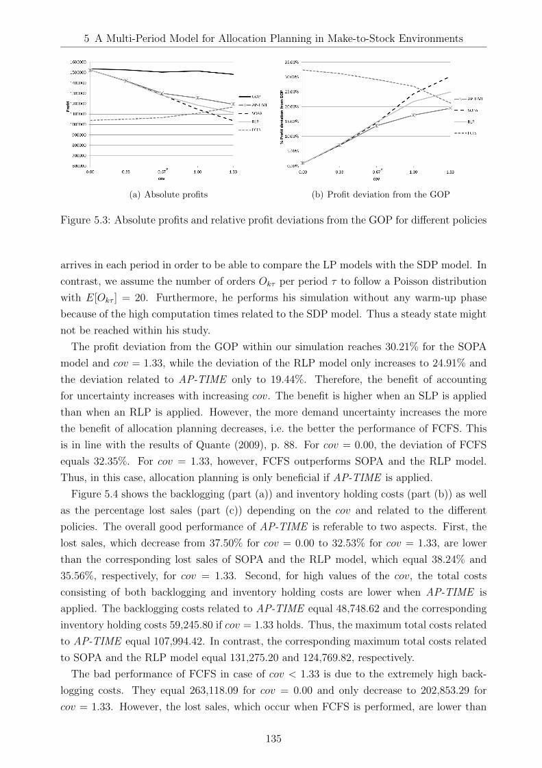
5 A Multi-Period Model for Allocation Planning in Make-to-Stock Environments
(a) Absolute profits (b) Profit deviation from the GOP
Figure 5.3: Absolute profits and relative profit deviations from the GOP for different policies
arrives in each period in order to be able to compare the LP models with the SDP model. In
contrast, we assume the number of orders Okτ per period τ to follow a Poisson distribution
with E[Okτ ] = 20. Furthermore, he performs his simulation without any warm-up phase
because of the high computation times related to the SDP model. Thus a steady state might
not be reached within his study.
The profit deviation from the GOP within our simulation reaches 30.21% for the SOPA
model and cov = 1.33, while the deviation of the RLP model only increases to 24.91% and
the deviation related to AP-TIME only to 19.44%. Therefore, the benefit of accounting
for uncertainty increases with increasing cov. The benefit is higher when an SLP is applied
than when an RLP is applied. However, the more demand uncertainty increases the more
the benefit of allocation planning decreases, i.e. the better the performance of FCFS. This
is in line with the results of Quante (2009), p. 88. For cov = 0.00, the deviation of FCFS
equals 32.35%. For cov = 1.33, however, FCFS outperforms SOPA and the RLP model.
Thus, in this case, allocation planning is only beneficial if AP-TIME is applied.
Figure 5.4 shows the backlogging (part (a)) and inventory holding costs (part (b)) as well
as the percentage lost sales (part (c)) depending on the cov and related to the different
policies. The overall good performance of AP-TIME is referable to two aspects. First, the
lost sales, which decrease from 37.50% for cov = 0.00 to 32.53% for cov = 1.33, are lower
than the corresponding lost sales of SOPA and the RLP model, which equal 38.24% and
35.56%, respectively, for cov = 1.33. Second, for high values of the cov, the total costs
consisting of both backlogging and inventory holding costs are lower when AP-TIME is
applied. The backlogging costs related to AP-TIME equal 48,748.62 and the corresponding
inventory holding costs 59,245.80 if cov = 1.33 holds. Thus, the maximum total costs related
to AP-TIME equal 107,994.42. In contrast, the corresponding maximum total costs related
to SOPA and the RLP model equal 131,275.20 and 124,769.82, respectively.
The bad performance of FCFS in case of cov < 1.33 is due to the extremely high back-
logging costs. They equal 263,118.09 for cov = 0.00 and only decrease to 202,853.29 for
cov = 1.33. However, the lost sales, which occur when FCFS is performed, are lower than
135

5 A Multi-Period Model for Allocation Planning in Make-to-Stock Environments
(a) Backlogging costs (b) Inventory holding costs
(c) Percentage lost sales
Figure 5.4: Costs and lost sales for different policies and values of cov
the allocation planning models’ lost sales. For increasing cov the lost sales of FCFS even
decrease to 26.53%. This effect compensates the higher costs related to FCFS and improves
the policy’s performance.
The decreasing lost sales can be explained according to the single-period case in Section
4.3. If demand uncertainty increases, the probability that the total demand of a scenario
exceeds the total ATP quantity also decreases. Consequently, the probability that quantity
is allocated to the “wrong” customer class, i.e. an allocation of, e.g., the most profitable class
is not depleted, while simultaneously orders of other classes have to be rejected, increases.
This leads to a lower capacity utilization and can make allocation planning unfavorable as
compared to FCFS.
To summarize, accounting for uncertainty is beneficial. The benefit increases for increasing
demand uncertainty. The benefit is higher when an SLP is applied than when an RLP is
applied. However, the benefit of allocation planning itself decreases with increasing demand
uncertainty. For cov = 1.33, allocation planning is only beneficial if it is performed by means
of an SLP model. However, the performance of the allocation planning models is likely to be
further improved if nesting would also be allowed in the consumption process (see Section
4.3.6). Consequently, FCFS could even be outperformed by the SOPA model.
136

5 A Multi-Period Model for Allocation Planning in Make-to-Stock Environments
5.2.4 Influence of the Replanning Frequency
As already indicated in Section 5.2.1, the research results of Quante et al. (2009a) indicate
that the replanning frequency of the allocation planning or the length of the frozen horizon,
respectively, has an influence on the profits gained by allocation planning. While the frozen
horizon represents the time frame between two consecutive planning runs, the replanning
frequency represents the number of planning runs made within a certain time frame. The
numerical study of Quante et al. (2009a) states that profits increase with a decreasing length
of the frozen horizon. Nevertheless, the associated increasing replanning frequency increases
computation times significantly, which is especially relevant for the computationally intensive
SLP model. We therefore evaluate how profits and computation times change depending on
this parameter. We test two alternatives for the length of the frozen horizon: a single period
and three periods.
Table 5.4 shows the average computation times of an iteration n (see Section 5.2.1) of
the base case for the three different allocation planning models AP-TIME, the RLP model,
and SOPA and the two different lengths of the frozen horizon. Independent of the length
of the frozen horizon, the computation time related to AP-TIME is much higher than the
computation times of SOPA or the RLP model. For a frozen horizon of a single period, the
computation time related to AP-TIME is 7.18 times as high as the computation time of the
RLP model and about 26.33 times as high as the corresponding time for SOPA.
Table 5.4: Average computation times (in seconds) of an iteration n of the base case fordifferent allocation planning models
AP-TIME RLP SOPA
Frozen horizon: 1 period 199.61 27.82 7.58Frozen horizon: 3 periods 77.94 19.29 4.03
For all three models, the average computation time decreases significantly if the frozen
horizon is increased. However, the decrease of the computation time related to AP-TIME is
higher (60.95%) than the decrease regarding the other two models (30.66% and 46.83% for
the RLP model and SOPA, respectively).
As indicated in Section 5.2.1, the average computation times are still relatively low. Thus,
if a firm would perform allocation planning by, e.g., AP-TIME and for parameter values
being similar to those in our numerical study, the computation time of a single allocation
planning step related to a frozen horizon of a single period, which is usually done overnight,
is still very low. However, due to the high number of test data, which we consider in our
numerical study, and due to the N = 100 iterations for each test data set, the computation
time related to a frozen horizon of a single period is not acceptable anymore.
Nevertheless, in the following, we consider the profit impact of the frozen horizon. Figure
5.5 illustrates the absolute profits of the three allocation planning models and the GOP for
137

5 A Multi-Period Model for Allocation Planning in Make-to-Stock Environments
(a) Absolute profits for a frozen horizon of a singleperiod
(b) Absolute profits for a frozen horizon of three pe-riods
Figure 5.5: Absolute profits for different lengths of the frozen horizon
different values of the cov and for a frozen horizon of a single period (part (a)) and of three
periods (part (b)).
Although the research results of Quante et al. (2009a) suggest that profits increase when
the frozen horizon decreases, this is in principal not the case for our test results. In contrast,
for all values of the cov, the profits of AP-TIME increase if the frozen horizon is increased to
three periods. The values of SOPA hardly change for 0.00 < cov < 1.33, but they increase
for cov = 0.00 and cov = 1.33 from 1,511,100.00 to 1,523,150.00 and from 1,014,904.60 to
1,036,054.00, respectively. Only for the RLP model, the profits decrease for an increasing
length of the frozen horizon if cov > 0.33 holds. While for cov = 1.33, the profit related to
the RLP model equals 1,133,654.70 for a frozen horizon of a single period, it decreases to
1,114,849.52 for a frozen horizon of three periods. In contrast, the profit related to AP-TIME
for a single period is 1,175,411.70 and it increases to 1,195,983.98 for three periods.
The profit changes can in principal be explained by means of the backlogging costs and
the lost sales which are displayed in Figure 5.6. The backlogging costs of both AP-TIME
and the RLP model decrease for an increasing frozen horizon (compare parts (a) and (b)).
Simultaneously, the lost sales increase, i.e. if the frozen horizon is enlarged, more orders are
rejected and less orders are delivered too late (compare parts (c) and (d)). This can be
referred to the fact that if the replanning frequency is increased, i.e. the frozen horizon is
shortened, new information on future ATP quantities is considered earlier. This increases
the percentage of order quantities which are backlogged. If the frozen horizon is enlarged,
the ATP information is updated more seldom. Consequently, the probability that the ATP
quantity of the allocation planning horizon is exploited and orders have to be rejected in-
creases. For the SOPA model, the backlogging costs for cov = 0.00 also decrease and lost
sales increase for an increasing frozen horizon. For cov = 1.33 the backlogging costs related
to SOPA do not change, but lost sales even decrease and thus entail higher profits.
Although the backlogging costs and lost sales of the RLP model and AP-TIME behave
similarly, their corresponding profits deviate, i.e. the profit of AP-TIME increases and the
138

5 A Multi-Period Model for Allocation Planning in Make-to-Stock Environments
(a) Backlogging costs for a frozen horizon of a singleperiod
(b) Backlogging costs for a frozen horizon of threeperiods
(c) Lost sales for a frozen horizon of a single period (d) Lost sales for a frozen horizon of three periods
Figure 5.6: Backlogging costs and lost sales for different lengths of the frozen horizon
profit of the RLP model decreases for an increasing length of the frozen horizon. This is
due to the extent of the changes regarding the backlogging costs and the lost sales. While
the backlogging costs of AP-TIME decrease significantly (for cov = 1.33, they decrease
from 85,246.90 to 48,748.62), the backlogging costs of the RLP model decrease less (from
27,418.79 to 17,041.99 for cov = 1.33). The change of the lost sales, however, is lower for
AP-TIME (from 31.95% to 32.52% for cov = 1.33) than for the RLP model (from 34.31%
to 35.56% for cov = 1.33).
To summarize, the high decrease of the backlogging costs of AP-TIME compensates the
almost negligible increase of the lost sales and thus increases the profits of AP-TIME. The
lower decrease of the backlogging cost related to the RLP however is not able to compensate
the increasing lost sales. Thus, the profits of the RLP model decrease.
5.2.5 Influence of the Replenishment Frequency
In the base case, we assume that an ATP quantity becomes available every second period.
However, the frequency of the ATP replenishments can also affect the allocations. In order
to evaluate this effect, we vary the replenishment frequency but ensure that lf = 1.60 as well
as the assumptions on ATP quantities and availability dates being deterministic still hold.
We choose a high replenishment frequency, the base case frequency, and a low frequency.
139

5 A Multi-Period Model for Allocation Planning in Make-to-Stock Environments
For the high frequency, the time frame between two ATP replenishments equals a single
period. The ATP quantity becoming available in each period equals 375. For the base case
frequency, the time frame between two ATP replenishments equals two periods with an ATP
quantity of 750 each. Finally, the low frequency corresponds to a time frame of four periods
between two replenishments with an ATP quantity of 1,500 each.
Figure 5.7 shows the absolute profits related to the three allocation planning models AP-
TIME, SOPA and the RLP model for the three different alternatives of the replenishment
frequency. Furthermore, it shows the GOP profit.
Figure 5.7: Absolute profits for different replenishment frequencies
For all values of the replenishment frequency, AP-TIME performs better than the other
two allocation planning models. The GOP profit first slightly decreases from 1,530,147.60
to 1,505,625.10 and then increases again to 1,511,462.70 when the frequency decreases, i.e.
the time frame between two replenishments increases. The profits related to the allocation
planning models, however, decrease slightly with a decreasing replenishment frequency, e.g.,
AP-TIME decreases from 1,306,465.60 to 1,274,738.91. Thus, in total the decrease of the
replenishment frequency from a single period to four periods hardly affects the models’
performance.
Nevertheless, the replenishment frequency affects each model’s allocation policy in a dif-
ferent way. Figure 5.8 illustrates the lost sales (part (a)), the percentage of order quantities
backlogged (part (b)), and the percentage of order quantities which are fulfilled from ATP
becoming available prior to or at the due date (part (c) and (d)), respectively.
The replenishment frequency’s effect on the lost sales (part (a)) is negligible. The per-
centage of order quantities fulfilled from ATP which becomes available at the due date (part
(d)) decreases significantly for all three models (e.g., from 56.91% to 27.25% for AP-TIME ).
This is intuitive, as the number of availability dates of the ATP decreases.
The percentage of backlogged quantities (part (b)), i.e. the fulfillments from ATP be-
coming available in the future, increases for all models. Nevertheless, while the decrease of
the replenishment frequency hardly changes the backlogged quantities caused by the SOPA
model (0.00% to 1.55%), the change is much more significant for AP-TIME (from 0.05% to
11.76%). This entails higher backlogging costs for AP-TIME.
140

5 A Multi-Period Model for Allocation Planning in Make-to-Stock Environments
(a) Percentage lost sales (b) Percentage of order quantities backlogged
(c) Percentage of order quantities fulfilled from ATPwhich becomes available prior to the due date
(d) Percentage of order quantities fulfilled from ATPwhich becomes available at the due date
Figure 5.8: Lost sales, quantities backlogged, fulfilled from ATP which becomes available ator prior to the due date for different replenishment frequencies
The percentage of order quantities fulfilled from ATP which becomes available prior to the
due date (part (c)) also increases for all allocation planning models. The increase related to
SOPA, however, is more significant (from 6.53% to 28.50%) than the one of AP-TIME or
the RLP model. For all replenishment frequencies, AP-TIME shows the lowest percentage
of order quantities fulfilled by former ATP quantities, which entails lower inventory holding
costs than for the other two models.
To summarize, the decrease of the replenishment frequency or the increase of the time
frame between two replenishments, respectively, affects the allocations of the three models
differently. Much more orders are fulfilled from former ATP quantities and almost the
same percentage of order quantities is backlogged when the SOPA model is applied. In
contrast, both the percentage of order quantities fulfilled from former and from future ATP
increase regarding AP-TIME. However, the increase regarding the former ATP quantities
is less than for SOPA, while the percentage of backlogged quantities is significantly higher.
The corresponding values of the RLP model are always in between. However, the RLP
model shows the smallest decrease of order fulfillments from ATP becoming available at the
due date. The increase of the related costs, i.e. inventory holding and backlogging costs,
finally, explains the models’ profit decrease. Nevertheless, although allocations are affected
141

5 A Multi-Period Model for Allocation Planning in Make-to-Stock Environments
significantly by the change of the replenishment frequency, the total profit decrease is very
low.
5.2.6 Influence of the Holding and Backlogging Costs
In the multi-period case, the differences related to the allocations’ profits do not only arise
from customer heterogeneity but also from the inventory holding and backlogging costs.
Therefore, we evaluate to which extent the relation of inventory holding and backlogging
costs to customer heterogeneity influences the allocations determined by the different models.
For this purpose, we keep the customer heterogeneity value of the base case (Het = 0.30),
but vary the inventory holding and backlogging costs. Additionally to the base case values
of these costs (b1 = 26, b2 = 17, b3 = 8, and h = 5), which we denote in the following as low,
we define two further cost alternatives, medium and high. While for the medium alternative,
costs are twice as high as in the low case, i.e. b1 = 52, b2 = 34, b3 = 16, and h = 10, they
are four times as high in the high case, b1 = 104, b2 = 68, b3 = 32, and h = 20.
First, we consider the influence of the cost variation on the profits gained. Figure 5.9
shows the absolute profits of the three allocation planning models AP-TIME, SOPA, and
the RLP model as well as the profits related to the GOP and FCFS. The base case as defined
in Section 5.2.1 is again marked by a *.
Figure 5.9: Absolute profits for different values of backlogging and inventory holding costs
All profits decrease for increasing costs. While the GOP only decreases from 1,505,625.13
to 1,456,869.64, which corresponds to a relative decrease of 3.24%, the decrease of the allo-
cation planning models is higher, e.g., from 1,301,572.00 to 1,127,200.12 for AP-TIME. The
allocation planning models’ relative decrease is 13.40% for AP-TIME, 14.42% for SOPA, and
14.90% for the RLP model. AP-TIME still performs best, but all three allocation planning
models’ profits are very similar. In contrast, the FCFS policy decreases from 1,067,010.38
to 324,626.72 which corresponds to a relative decrease of 69.85%.
In the following, we determine whether the profit changes are only due to the rising costs
or also due to variances regarding the allocations. We state the inventory holding and the
backlogging costs in Figure 5.10(a) and 5.10(c), respectively. Furthermore, we illustrate the
142

5 A Multi-Period Model for Allocation Planning in Make-to-Stock Environments
(a) Inventory holding costs for different cost param-eters
(b) Percentage of order quantities fulfilled from ATPwhich becomes available prior to the due date
(c) Backlogging costs for different cost parameters (d) Percentage of order quantities backlogged
Figure 5.10: Inventory holding and backlogging costs and related quantities for different costparameters
percentage of order quantities fulfilled by means of ATP quantities which become available
prior to or after an order’s due date (Figure 5.10(b) and 5.10(d), respectively).
Both the inventory holding and the backlogging costs increase for the three allocation
planning models and for FCFS. However, as almost no quantity is backlogged for cov = 0.67
when allocation planning is performed (see, e.g., Section 5.2.2), the backlogging costs of the
three models only increase slightly (up to 36,137.08 for AP-TIME ). The inventory holding
costs of the three models increase by 185,593.75 (SOPA), 180,353.63 (RLP) and only by
147,229.45 for AP-TIME. In contrast, the costs related to FCFS behave different. As due
to the high load factor almost no order is fulfilled by means of ATP which is on stock, the
inventory holding costs only rise from 182.70 to 730.80. However, the backlogging costs rise
from 251,246.90 to 993,082.50.
Nevertheless, the increase of the cost parameters hardly influences the allocations (see
parts (b) and (d) of Figure 5.10). Neither the percentage of quantities backlogged or fulfilled
by ATP becoming available prior to an order’s due date changes for SOPA or the RLP
model. Only for AP-TIME, the quantities fulfilled by ATP becoming available prior to an
order’s due date decrease from 21.32% to 19.19%. Instead, these orders are fulfilled by ATP
becoming available at the due date.
143

5 A Multi-Period Model for Allocation Planning in Make-to-Stock Environments
Therefore, the variation of inventory holding costs and backlogging costs in the considered
range does not affect the allocations determined by SOPA or the RLP model and affects the
allocations obtained by AP-TIME only slightly. The profit decrease thus basically arises
directly from the cost increase.
5.2.7 Comparison with APS Rules
In the following, we discuss the results obtained by applying the allocation planning rules
fixed split (1 : 1 : 1), rank based, and per committed as described in Section 2.2.6 in combi-
nation with the two consumption rules TPAR and TNES presented in Section 5.2.1. The
results are compared to the results of AP-TIME, which is followed by the consumption LP
(5.1.1) – (5.1.4), the FCFS policy, and the GOP. Figure 5.11 shows the absolute profits as
well as the profit deviations from the GOP. Parts (a) and (c) illustrate the results referring
to consumption rule (CR) TPAR and parts (b) and (d) refer to consumption rule TNES.
(a) Absolute profits of different allocation planningrules and CR: TPAR
(b) Absolute profits of different allocation planningrules and CR: TNES
(c) Relative profit deviations from the GOP of differ-ent allocation planning rules and CR: TPAR
(d) Relative profit deviations from the GOP of dif-ferent allocation planning rules and CR: TNES
Figure 5.11: Absolute profits and relative profit deviations of different APS rules
The comparison of parts (a) and (b) of Figure 5.11 shows that, in principal, the application
of consumption rule TNES improves the APS rules’ performance. Nevertheless, independent
of whether consumption rule TPAR or TNES is applied and independent of whether demand
is uncertain or not, the rules’ performance is worse than the performance of AP-TIME as the
144

5 A Multi-Period Model for Allocation Planning in Make-to-Stock Environments
rules do neither consider information on demand uncertainty nor on customer heterogeneity,
nor on inventory holding or backlogging costs, nor on costs at all. Consequently, the deviation
from the GOP can rise up to 59.62% for TPAR and up to 31.96% for TNES, while AP-TIME
does not deviate more than 19.44%.
If demand is deterministic, the rank based rule performs significantly better than fixed split
or per committed. For increasing demand uncertainty, its performance declines. However,
rank based is still the best performing rule if TPAR is applied. If TNES is applied, per com-
mitted outperforms the rank based rule for cov > 0.33. Nevertheless, if demand uncertainty
is very high, FCFS outperforms all APS rules.
The performance impact of allowing for nesting in the consumption, i.e. applying TNES
instead of TPAR, is significantly higher for per committed as compared to the other two
rules. This indicates that the allocations of the less profitable classes are higher when per
committed is applied than when fixed split or rank based is applied. Therefore, if TPAR is
applied, rank based and fixed split perform better for increasing demand uncertainty than per
committed as they reserve more for the most profitable class 1 and less for class 3. However,
if nesting is applied, the drawback of per committed is compensated by the consumption
rule.
Figure 5.12 shows the percentage lost sales of the three classes related to the different
policies for TPAR. In principal, the lost sales of class 1 are higher when a rule is applied
than when AP-TIME is applied. If demand uncertainty is low, the lost sales of class 3
related to AP-TIME are higher than the class 3 lost sales of the two rules fixed split and
per committed. This indicates that the two rules allocate too little ATP to class 1 and 2
and too much ATP to class 3 for low values of the cov. Thus, the lost sales of the two
rules rather behave like the FCFS policy when demand uncertainty is low. Due to the high
heterogeneity, the high class 1 lost sales of the fixed split and the per committed rules cannot
be compensated by lower class 3 lost sales. Therefore, applying one of the two APS rules
yields much lower profits as compared to the SLP model.
If demand uncertainty increases, the lost sales of the rules fixed split and per committed
rather approach the lost sales of AP-TIME. However, in contrast to the lost sales of FCFS,
the lost sales increase and, thus, the performances of fixed split and per committed further
decrease.
Different from these two rules, the lost sales related to the rank based rule show a similar
behavior to the lost sales related to AP-TIME. This is due to the high class 1 and the low
class 3 allocation caused by the rank based rule. Therefore, especially for low values of
the cov, the allocations determined by the SLP and the rule are similar. This explains the
relatively good performance of the rule in case of low demand uncertainty.
However, the more uncertain demand becomes, the more deviate the class 1 and 2 lost sales
values of the rank based rule from those of AP-TIME. As a consequence, the performance
of the rank based rule decreases.
Nevertheless, the decreasing profits of the three rules in combination with TPAR are not
145

5 A Multi-Period Model for Allocation Planning in Make-to-Stock Environments
(a) Class 1 lost sales for CR: TPAR (b) Class 2 lost sales for CR: TPAR
(c) Class 3 lost sales for CR: TPAR
Figure 5.12: Lost sales of different allocation planning rules and TPAR
only due to the lost sales. The evaluation of further KPIs shows that the decreasing profits
are also due to increasing inventory holding costs which are, e.g., for cov = 1.33 up to four
times as high as the inventory holding costs of AP-TIME.
Figure 5.13 illustrates the lost sales values of the three classes for the consumption rule
TNES. As the class 1 and 2 lost sales are lower and the class 3 lost sales higher for TNES
than for TPAR, the profits of the APS rules are higher in combination with TNES.
The lost sales values of the rank based rule in combination with TNES are even closer
to the lost sales of AP-TIME than for TPAR. Consequently, the profits of the rank based
rule improve. In principal, the lost sales of all rules approach the corresponding values
of AP-TIME for high values of the cov, i.e. the possibility of nesting in the consumption
significantly improves the rules’ performance. The remaining profit gap between the rules
and AP-TIME is again due to the higher inventory holding costs of the rules, which are,
e.g., for cov = 1.33 still up to three times as high as the inventory holding costs which occur
when allocation planning is performed by AP-TIME.
5.3 Conclusions
In this chapter, a multi-class, multi-period SLP model for allocation planning in MTS has
been presented. ATP quantities are assumed to be exogenously given. Both the ATP
146

5 A Multi-Period Model for Allocation Planning in Make-to-Stock Environments
(a) Class 1 lost sales for CR: TNES (b) Class 2 lost sales for CR: TNES
(c) Class 3 lost sales for CR: TNES
Figure 5.13: Lost sales of different allocation planning rules and TNES
quantities and their availability dates are assumed to be deterministic. The model allows
for keeping a share of each ATP quantity unallocated. These shares serve as a safety stock.
The model anticipates a time-based consumption policy. Furthermore, regarding the class-
based consumption policies, it assumes a partitioned consumption. In contrast to nesting
as a class-based consumption policy, a time-based consumption should not be performed by
means of simple rules. We show by a simple example how simple time-based rules can be
outperformed by LP models. Therefore, we perform the time-based consumption by means
of a consumption LP considering both the possibility of holding inventories and backlogging
orders. In order to anticipate the time-based consumption in the allocation planning SLP
model, we integrate the consumption LP into the SLP by means of the second-stage variables.
In our numerical study, we perform a rolling horizon planning. First, we compare our
results to the results of SOPA, the RLP model by Quante (2009), the simple FCFS policy,
and the GOP. We evaluate the benefit of allocation planning and accounting for uncertainty
by means of an SLP. The benefit of accounting for uncertainty by means of an SLP increases
with increasing demand uncertainty. Also the benefit of accounting for uncertainty by means
of an RLP increases, but less as compared to an SLP. However, the benefit of allocation
planning decreases for cov increasing. In contrast to the results of Quante (2009), pp. 89,
the RLP outperforms the SOPA model. We refer this to the different assumptions made in
our numerical study.
147

5 A Multi-Period Model for Allocation Planning in Make-to-Stock Environments
We evaluate the influence of the replanning frequency on the allocation planning mod-
els’ performance and computation times. The computation times increase for an increasing
replanning frequency. This affects especially the SLP model as its computation times are
generally higher than those of the other two models. Although the research results of Quante
et al. (2009a) indicate that an increasing replanning frequency improves the models’ perfor-
mance, this only holds for the results obtained when applying the RLP model. The results
of the SOPA model hardly change, while the SLP model’s results even improve when the
replanning frequency is decreased.
Subsequently, we determine the influence of the ATP replenishment frequency on the
performance of the allocation planning models. A change of the replanning frequency hardly
affects the profits gained, but, it affects the allocation planning policies of the different
models. For a decreasing replenishment frequency, even more orders are fulfilled from former
ATP quantities and the percentage of orders backlogged hardly changes when the SOPA
model is applied. In contrast, for the SLP and the RLP model, both the percentage of order
quantities fulfilled from former ATP and the percentage of order quantities fulfilled from
future ATP increase.
Besides the frequencies of replanning and replenishing ATP, we consider how profits are
affected when inventory holding and backlogging costs increase as compared to the difference
between the classes’ base profits. The cost increase entails lower profits. However, it hardly
affects the models’ allocation policies.
Finally, we compare the performance of the SLP in combination with the consumption
LP with typical allocation and consumption rules of commercial APS. The results show
that the rules’ performance depends on demand uncertainty. Nevertheless, the SLP model
outperforms all APS rules independently of demand uncertainty.
148

6 Conclusions and Further Research
This thesis deals with the transfer of revenue management ideas to demand fulfillment in
make-to-stock (MTS) in terms of allocation planning. Allocation planning aims at exploiting
customer heterogeneity in situations in which capacity is scarce and demand is uncertain.
Within this thesis, we have shown how two-stage stochastic linear programming can improve
allocation planning in make-to-stock industries by simultaneously considering information
about the uncertain demand and providing models which can be solved in a reasonable
amount of time even if applied to problems of practical sizes. In the following, we summarize
the key results of our research in Section 6.1 and and provide directions for further research
in Section 6.2.
6.1 Results
For summarizing the key results of this thesis, we return to the research questions formulated
in Section 1.2.
Research Question 1: How can allocation planning for make-to-stock be performed by
simultaneously accounting for information about uncertain demand and obtaining scalable
models, such that problems of practical sizes are still solvable in a reasonable amount of
time?
In the literature review of allocation planning models for make-to-stock environments in
Chapter 2, we have outlined their respective drawbacks which, in principal, are an insufficient
consideration of demand uncertainty and a limited scalability. Thus, problems of practical
sizes cannot be solved in a reasonable amount of time. Based on this review, the concept
of two-stage stochastic linear programming (SLP) with recourse has been introduced. If
the uncertain demand can be described by means of a probability distribution, two-stage
SLPs provide the opportunity of accounting for demand uncertainty by means of a sample
of scenarios generated from this demand distribution. At the same time, SLPs retain the
characteristic of a linear programming (LP) model and are thus scalable. We have justi-
fied that two-stage SLPs represent a promising approach for allocation planning in MTS
environments, which is able to cope with the drawbacks of existing models.
Furthermore, we have outlined how the two-stage concept corresponds to the processes
of demand fulfillment in MTS environments. The first stage of an SLP model considers
decisions made prior to the realization of the uncertain parameter, while the second stage

6 Conclusions and Further Research
considers decisions made afterwards. Regarding the demand fulfillment process in make-to-
stock, the first stage represents the allocation planning stage and the second stage the process
of fulfilling orders by means of the allocations, i.e. the consumption process. The fact that
an SLP’s second-stage decisions depend on both the first-stage decisions and the realization
of the uncertain parameter gave rise to the assumption that two-stage SLPs provide the
opportunity of integrating the consumption rule, which is applied in the consumption process,
and the order arrival sequence in the allocation planning model by means of the second-stage
variables.
Research Question 2: How can consumption policies and order arrival sequences be
integrated into the allocation planning model in order to improve the profits realized during
the consumption process?
In Chapter 3, we have formulated the most simple stochastic allocation planning problem
known from literature, which is Littlewood’s (analytical) two-class model (see Littlewood
(1972)), as a two-stage SLP. Besides a formulation representing Littlewood’s marginal rule,
two further SLP models have been presented. They differ in the class-based consumption
rule which is anticipated: partitioned, i.e. each allocation is only available for the class it is
reserved for, and nested, i.e. more profitable classes can also consume quantities out of the
less profitable classes’ allocations. Furthermore, the nested model anticipates a low-before-
high order arrival sequence by means of steering profits related to the second-stage variables.
While the partitioned model is similar to other SLPs known from literature, the nested model
is a new contribution. In contrast to the model representing Littlewood’s marginal rule, the
other two models account for the information on both classes’ demands and represent the
situation of determining allocations at the beginning of the planning period. For this reason
and as they allow for the integration of the consumption rule and the arrival sequence, they
represent the basis for models dedicated for more than two customer classes and more than
a single period in the context of MTS.
The numerical tests show that the SLP models are able to approximate the analytically
determined protection levels and the corresponding expected revenues of both Littlewood’s
model and the partitioned case sufficiently precisely. This confirms the proper integration
of the consumption rules and the arrival sequence into the allocation planning SLP.
In Chapter 4, we have extended the two models of Chapter 3, which account for infor-
mation on both classes’ demands, to single-period, multi-class models intended for MTS. In
order to represent the MTS setting properly, a mixed order arrival sequence is anticipated.
Furthermore, the multi-class models allow for keeping a share of the total capacity unallo-
cated. This unallocated share serves as a virtual safety stock and, therefore, further supports
managing demand uncertainty.
In the corresponding numerical study, we have quantified the benefit of anticipating the
consumption rule, which is applied in the consumption process, already in the allocation
planning model. The results show that in case of uncertain demand, the anticipation is
150

6 Conclusions and Further Research
generally beneficial and the benefit increases for increasing demand uncertainty.
Finally, in Chapter 5, we have introduced a multi-period, multi-class SLP model for allo-
cation planning in MTS. As compared to the single-period models, the multi-period setting
additionally allows for a time-based consumption policy. In contrast to the class-based con-
sumption rules, the time-based consumption in Chapter 5 is not represented by a rule but
by a consumption LP model. We have shown how this consumption LP can again be inte-
grated into the allocation planning SLP. Besides the time-based consumption, a partitioned
(class-based) consumption is anticipated in the model.
Based on research results by, e.g., Meyr (2009), Quante (2009), pp. 76, and Quante et al.
(2009a), which indicate that both the benefit of allocation planning and the benefit of ac-
counting for information on the uncertain demand depends on different characteristics of
the input data such as the extent of customer heterogeneity, we have identified Research
Questions 3 and 4.
Research Question 3: In which situations is allocation planning in make-to-stock indus-
tries likely to be beneficial?
Research Question 4: If allocation planning is beneficial, in which situations does the
application of more sophisticated instruments considering information about demand uncer-
tainty pay off?
By a theoretical analysis of different characteristics of the input data stated at the be-
ginning of Chapter 4, we have shown how the firm’s decision about the implementation of
allocation planning as well as the selection of an appropriate allocation planning instru-
ment can be supported by a pre-evaluation of the firm’s input data. The pre-evaluation is
summarized by means of a decision tree.
Within the numerical studies of Chapters 4 and 5, we have quantified the benefit of both
allocation planning and accounting for uncertainty by means of applying an SLP instead of
a deterministic linear programming (DLP) model or first-come, first-serve (FCFS). Depend-
ing on the load factor, both in the single-period and in the multi-period case, a corridor
regarding demand uncertainty can be identified in which the application of an SLP is rea-
sonable. If demand uncertainty is too low, a DLP can be applied, i.e. the consideration of
demand uncertainty is not beneficial. If uncertainty becomes too high, allocation planning
can be outperformed by the simple FCFS policy. However, the more customer heterogeneity
increases, the more the corridor in which the application of an SLP is reasonable enlarges.
The multi-period model of Chapter 5 has also been compared to simple rules which are typi-
cally implemented in commercial advanced planning systems (APS). The corresponding test
results show that, except for the case of deterministic demand, the SLP model significantly
outperforms the rules.
Besides the results related to Research Questions 1 – 4, we have illustrated the relationship
between the primal SLP models, which determine the allocations, and the dual SLP models,
151

6 Conclusions and Further Research
which determine the bid prices (Chapter 3). We have shown how the probability components
of the analytical two-class solutions are integrated in the corresponding SLPs. Furthermore,
we have illustrated how bid prices differ depending on whether information about the less
profitable class’ demand is considered, which consumption rule is anticipated, and depending
on the load factor.
Furthermore, we have quantified the benefit of applying a nesting rule in the consumption
process compared to applying a partitioned rule (Chapter 4). To the best of our knowledge,
this benefit has not yet been quantified in literature. The related results show that if demand
is uncertain, nesting is beneficial and the benefit increases for increasing demand uncertainty.
However, the benefit depends on the allocation planning model applied. It is significantly
higher, if nesting is already anticipated in the allocation planning model.
6.2 Further Research
Based on the results of our numerical studies, we identify several opportunities for further
research. The numerical study of the multi-period model (Chapter 5) has shown that for
a high demand uncertainty, allocation planning is only beneficial when it is performed by
means of an SLP model and not by a DLP or a randomized linear programming (RLP)
model. However, in reference to the test results related to the benefit of allowing for nesting
in Chapter 4, we assume that the performance of the DLP model or the RLP model could
be improved if nesting was allowed in the consumption process. As a consequence, the tests
could be repeated by additionally allowing for nesting in the consumption process.
However, according to the research results of Chapter 4, which illustrate that the antici-
pation of the consumption rule applied is beneficial, nesting should be integrated into the
multi-period SLP model if a nesting policy is applied in the consumption process. Otherwise,
the SLP’s performance could even become worse than those of a DLP or an RLP model.
While the time-based consumption is represented by an LP model, nesting is represented
by a rule. Integrating both policies into an SLP formulation gives rise to an evaluation
regarding how steering profits have to be ideally set as compared to inventory holding and
backlogging costs for representing the combination of both policies adequately.
In principal, we compare the results of the different models with the global optimum
(GOP), but only regarding the profits. Besides, also the lost sales of the GOP, or the
percentage of quantities backlogged or fulfilled from former replenishments in the GOP
could be determined in order to compare them with the respective figures of the allocation
planning models. The comparison might imply ideas regarding how the steering profits could
be adapted for a further improvement of the SLP models.
In the numerical study related to the multi-period model, we have also evaluated how the
performance and the allocation policy of the allocation planning models change if inventory
holding and backlogging costs are increased in comparison to the profit difference between
the customer classes. Besides this, the ratio between backlogging costs and inventory holding
152
6 Conclusions and Further Research
costs could be varied as well as the ratio of the backlogging costs related to the different
classes. Based on these variations not only the behavior of sophisticated allocation planning
models could be evaluated, but they could also be compared to the simple APS rules.
An assumption of our numerical study is that the available-to-promise (ATP) quantities
and their availability date are deterministic. It would be interesting to consider how the
allocation planning models perform if at least one of the two parameters or both would be
considered as stochastic, e.g., due to fluctuations in the production process. Moreover, the
possibility of integrating this supply uncertainty into the allocation planning SLP could be
investigated according to the integration of the demand uncertainty as it has been done
within this thesis.
A further assumption within this thesis states that profits of less profitable classes can
be expressed by a linear function of the most profitable customer class’ profit and the het-
erogeneity of the classes. The assumption is made as the numerical studies of this thesis
refer to further numerical studies performed previously in the context of allocation planning
in MTS. Nevertheless, additional numerical tests could be performed by defining customer
heterogeneity in a different way (see, e.g., Vogel and Meyr (2014)).
Moreover, we assume that partial order fulfillment is allowed. However, depending on the
firm considered, customers might not accept partial order fulfillments. As for assemble-to-
order (ATO) situations, the possibility of splitting orders has a significant influence on the
firm’s order acceptance policy (see Geier (2014), pp. 172), this could also be an interesting
aspect regarding the allocation planning process in MTS industries.
Based on the results of, e.g., Quante (2009), pp. 75, and Quante et al. (2009a), we assume
customers to be segmented previously into three customer classes. On the one hand, this
assumption could be skipped in order to evaluate the influence of the number of customer
classes on the SLP’s allocation planning policy according to the numerical studies of, e.g.,
Meyr (2009) and Quante (2009), pp. 78. On the other hand, it would be even more interesting
to consider the research question of how to segment customers at all and how to determine
the classes’ profit and costs (see also Meyr (2008)).
Besides further numerical tests related to the assumptions made in our study, the multi-
period, multi-class SLP model for a single location stated in Chapter 5 as well as its extension
mentioned above, which anticipates both a class- and a time-based consumption policy,
should be tested by means of real-world data.
Finally, besides the research directions stated above which are all related to the single-
location (i.e. stocking point) case considered within this thesis, the idea of accounting for
demand uncertainty by means of two-stage SLP models with recourse could also be applied
to related research fields. There are already deterministic approaches for allocation planning
in MTS in both the multi-location case (see, e.g., Nguyen et al. (2013)) and the field of
multi-dimensional customer hierarchies (see Vogel (2013), Vogel and Meyr (2014)). Both
approaches might be improved if demand (and supply) uncertainty would be integrated by
means of SLP models.
153

Appendix

Appendix
The table following on the next pages provides an alphabetical overview of the two-stage
SLP applications discussed within Section 2.3.3. The table contains further information
on industries, the fields of application, first- and second-stage decisions, and the uncertain
parameters of the models. Furthermore, it provides information on the number of periods
considered and the distribution of the uncertain parameter. For discrete distributions the
intervals’ probabilities are considered in the objective function, while for continuous distribu-
tions a sample is generated and the objective function is averaged. The numbers in brackets
indicate the number of intervals in case of discrete distributions or the number of scenarios
in case of continuous distributions. Finally, the table provides information about the type
of the models (SLP/SMIP), the models’ objectives, and the possibility of holding inventory
or backlogging.
155

Appendix
Ap
plica
tion
sof
two-s
tage
SL
Ps
Article
Field
/Application
First-S
tage
Second-S
tage
Uncerta
inPeri-
Sam
ple/
SLP/
Objec-
St/
Annot.
Industry
Decision
Decision
Param
ete
rods
DD
(*)
SM
IPtive
B
Ale
man
d
Mora
bit
o
(2013)
Fu
rnit
ure
Ind
ust
ry
Pro
du
ctio
n
Pla
nn
ing
Pro
du
ctio
n
Qu
anti
ties
,
Fre
qu
ency
of
Cu
ttin
gP
att
ern
s
Inven
tory
,B
ack
log,
Over
tim
e
Dem
an
d,
Set
up
Tim
es
TD
D
(27),
Sp
(125)
SM
IPM
in
Cost
s
both
-
Al-
Oth
man
etal.
(2008)
Oil
Ind
ust
ry
Pro
du
ctio
n
Pla
nn
ing
Cru
de
Oil
Pro
du
ctio
nP
rofi
le
Pro
du
ctio
n
Qu
an
titi
es,
Alloca
ted
Qu
an
titi
esfo
r
furt
her
Pro
cess
ing,
Qu
anti
ties
Sh
ipp
ed,
Sto
red
,L
ost
Dem
an
d,
Back
log
Dem
an
d,
Mark
etP
rice
TD
D(3
)S
LP
Min
Neg
ati
ve
Pro
fita
-
bilit
y
St
+
B
-
Barb
aro
soglu
an
dA
rda
(2004)
Dis
ast
er
Rel
ief
Mu
ltim
od
al
Dis
trib
uti
on
of
Fir
st-A
id
Com
mod
itie
s
Am
ou
nt
of
Com
mod
itie
sto
Tra
nsp
ort
Am
ou
nt
of
Com
modit
ies
to
Tra
nsp
ort
,E
xce
ss/
Sh
ort
age
Am
ou
nts
Dem
an
d1
DD
SL
PM
in
Cost
s
no
Mu
lti-
Mod
al
Bie
nst
ock
an
d
Sh
ap
iro
(1988)
En
ergy
Sec
tor
Inves
tmen
t
Dec
isio
ns/
Cap
aci
ty
Acq
uis
itio
n&
Uti
liza
tion
Pla
nt
Con
stru
ctio
n/
Net
work
Pla
nn
ing/
Fu
elC
ontr
act
s
Res
ou
rce
Uti
liza
tion
Dem
an
d,
Em
issi
on
Lim
it,
Pri
ces,
Com
ple
tion
tim
eof
Pip
elin
es
TD
D(6
)S
MIP
Min
Cost
s
no
-
Bozo
rgi-
Am
iri
etal.
(2013)
Dis
ast
er
Rel
ief
Dis
trib
uti
on
of
Com
mod
itie
s
Loca
tion
Pla
nn
ing,
Pro
cure
men
t
Qu
anti
ties
Flo
wof
Good
s,
Inven
tory
,
Sh
ort
ages
Dem
an
d,
Su
pp
ly,
Cost
1D
D(4
)S
MIP
Min
Cost
s
St
-
Bu
ke
etal.
(2008)
Air
lin
e&
Hote
l
Net
work
Cap
aci
ty
Contr
ol
Alloca
tion
sfo
r
Ori
gin
-Des
tin
ati
on
Itin
erari
es
Sale
san
dL
ost
Sale
s
Bu
y-u
ps
1D
DS
LP
Max
Rev
enu
e
no
Bu
y-u
ps
an
dT
hef
t
Nes
tin
g
Conti
nu
edon
Nex
tP
age.
..
156

Appendix
Ap
plica
tion
sof
two-s
tage
SL
Ps
–C
onti
nu
ed
Article
Field
/Application
First-S
tage
Second-S
tage
Uncerta
inPeri-
Sam
ple/
SLP/
Objec-
St/
Annot.
Industry
Decision
Decision
Param
ete
rods
DD
(*)
SM
IPtive
B
Ch
enan
d
Hom
em-d
e-
Mel
lo
(2010)
Air
lin
esN
etw
ork
Rev
enu
e
Man
agem
ent
Alloca
tion
sS
ale
san
dL
ost
Sale
s
Dem
an
d&
Ord
er
Pre
fere
nce
s
1D
DS
MIP
Max
Rev
enu
e
no
Cu
stom
er
Ch
oic
e
Ch
enan
d
Pan
gara
d
(2005)
AT
O/
MT
O
AT
PR
esou
rce
Alloca
tion
Sale
san
dL
ost
Sale
s,In
ven
tori
es
Dem
an
d4
DD
SL
PM
ax
Pro
fit
no
-
Ch
en-R
itzo
etal.
(2010)
CT
O/
Com
pu
ter
Manu
fac-
ture
r
Su
pp
ly
Pla
nn
ing/
Dem
an
d-
Su
pp
ly-
Matc
hin
g
(1)
Ord
er
Qu
anti
ties
of
Com
pon
ents
/(2
)
Com
mit
men
t-to
-
Sale
s-Q
uanti
ties
(1)
Ass
ign
men
tof
Com
pon
ents
to
Fin
ish
edP
rod
uct
s/
(2)
Ass
ign
men
tof
CT
Sto
Ord
ers
Ord
erC
on
-
figu
rati
on
s
TS
p
(100/
50)
SL
PM
ax
Pro
fit
St
+
B
2se
para
te
Pla
nn
ing
Pro
ble
ms
Ch
en-R
itzo
etal.
(2011)
CT
O/
Com
pu
ter
Manu
fac-
ture
r
Com
pon
ent
Rati
on
ing
Rati
on
ing
Th
resh
old
s
Dem
an
d-S
up
ply
-
Matc
hin
g
Ord
erC
on
-
figu
rati
on
s
1D
DS
MIP
Max
Rev
enu
e
St
-
Ch
eun
gan
d
Pow
ell
(1996)
Ret
ailer
/
MT
S
Dis
trib
uti
on
Pla
nn
ing
Dis
trib
uti
on
from
Pro
du
ctio
nS
ites
to
Ware
hou
ses
Dis
trib
uti
on
from
Ware
hou
ses
to
Cu
stom
ers
Dem
an
d1
DD
SL
PM
in
Cost
s
BB
ack
log
Cost
sas
Ap
pro
xi-
mati
on
for
Lost
Sale
s
Ch
ien
etal.
(2013)
Wafe
r
Ind
ust
ry
Dem
an
d
Fu
lfill
men
t
Pro
du
ct-P
lant
ass
ign
men
t
Dem
an
d-S
up
ply
-
Matc
hin
g
Dem
an
dT
DD
SM
IPM
in
Cost
s
no
-
Dantz
igan
d
Infa
nger
(1993)
Fin
an
cial
Ind
ust
ry
Port
folio
Op
tim
izati
on
Port
folio-S
elec
tion
Ch
an
ges
wit
hin
Port
folio
Ret
urn
sT
DD
SL
PM
in
Cost
s
no
-
de
Boer
etal.
(2002)
Air
lin
eN
etw
ork
Rev
enu
e
Man
agem
ent
Alloca
tion
sfo
r
Ori
gin
-Des
tin
ati
on
Itin
erari
es
Alloca
tion
s
Acc
om
mod
ati
ng
Part
sof
the
Dem
an
d
Dem
an
d1
n.s
.S
MIP
Max
Rev
enu
e
no
-
Conti
nu
edon
Nex
tP
age.
..
157

Appendix
Ap
plica
tion
sof
two-s
tage
SL
Ps
–C
onti
nu
ed
Article
Field
/Application
First-S
tage
Second-S
tage
Uncerta
inPeri-
Sam
ple/
SLP/
Objec-
St/
Annot.
Industry
Decision
Decision
Param
ete
rods
DD
(*)
SM
IPtive
B
Esc
ud
ero
etal.
(1993)
Manu
fac-
turi
ng
Pro
du
ctio
n/
Cap
aci
ty
Pla
nn
ing
Pro
du
ctio
n&
Ad
dit
ion
al
Pu
rch
ase
Qu
anti
ties
Pro
du
ctio
n&
Ad
dit
ion
al
Pu
rchase
Qu
anti
ties
,L
ost
Sale
s,In
ven
tory
Dem
an
dT
DD
(9
–25)
SL
P,
SM
IP
Min
Cost
s
St
-
Fer
gu
son
an
d
Dantz
ig(1
956)
Air
lin
esA
ssig
nm
ent
of
Air
craft
to
Rou
tes
Air
craft
Ass
ign
men
t
Cap
aci
ty
Uti
liza
tion
Dem
an
d1
DD
(2
–5)
SL
PM
ax
Rev
enu
e
no
-
Fra
nca
san
d
Min
ner
(2009)
Manu
fac-
turi
ng
Net
work
Con
figu
rati
on
for
Pro
du
ctio
n
an
dP
rod
uct
Rec
over
y
Cap
aci
tyP
lan
nin
gP
rod
uct
ion
&
Rec
over
y
Qu
anti
ties
Dem
an
d&
Ret
urn
s
1S
p
(5000)
SL
PM
ax
Pro
fit
no
-
Gu
eric
ke
etal.
(2012)
Dis
trib
uti
on
Net
work
s
inA
pp
are
l
Ind
ust
ry
Post
pon
emen
t
Str
ate
gie
s
Ass
ign
men
tof
Pro
du
ctio
n
Act
ivit
ies
to
Sta
ges
,P
rod
uct
ion
an
dD
istr
ibu
tion
Qu
anti
ties
of
Sta
ge
1
Pro
du
ctio
n
Qu
anti
ties
for
Su
bse
qu
ent
Sta
ges
/
Tra
nsp
ort
ati
on
Qu
anti
ties
bet
wee
n
Sit
es
Dem
an
d1
DD
(DN
D)
SM
IPM
ax
Pro
fit
no
-
Haen
sel
etal.
(2012)
Car
Ren
tal
Fle
et
Dis
trib
uti
on
Car
Dis
trib
uti
on
bet
wee
nR
enta
l
Sta
tion
/B
ookin
g
Lim
its
Bookin
gs
Dem
an
d1
Sp
(300)
SM
IPM
ax
Rev
enu
e
no
-
Hig
le(2
007)
Air
lin
eN
etw
ork
Rev
enu
e
Man
agem
ent
Alloca
tion
of
Flight
Leg
s
Sale
sD
eman
d1
DD
SL
PM
ax
Rev
enu
e
no
Nes
tin
g
Con
stra
int
-
Hsu
an
dB
ass
ok
(1999)
Sem
icon
-
du
ctor
Manu
fac-
turi
ng
Pro
du
ctio
nan
d
Alloca
tion
Pla
nn
ing
wit
h
Pro
du
ct
Su
bst
itu
tion
Inp
ut
Qu
anti
tyfo
r
Pro
du
ctio
n
Alloca
tion
s,
Sh
ort
age
an
d
Exce
ssQ
uanti
ties
Yie
ld,
Dem
an
d
1S
p
(100,
300,
1000,
3000)
SL
PM
ax
Pro
fit
both
Su
bst
itu
tion
Conti
nu
edon
Nex
tP
age.
..
158

Appendix
Ap
plica
tion
sof
two-s
tage
SL
Ps
–C
onti
nu
ed
Article
Field
/Application
First-S
tage
Second-S
tage
Uncerta
inPeri-
Sam
ple/
SLP/
Objec-
St/
Annot.
Industry
Decision
Decision
Param
ete
rods
DD
(*)
SM
IPtive
B
Kir
aet
al.
(1997)
n.s
.H
iera
rch
ical
Pro
du
ctio
n
Pla
nn
ing
Pro
du
ctio
nan
d
Ad
dit
ion
al
Pu
rch
ase
Qu
anti
ties
,
Inven
tori
es,
Pro
du
ctio
nT
imes
,
Over
tim
es
Qu
anti
ties
Over
-
/U
nd
erp
rod
uce
d
Dem
an
dT
DD
SL
PM
in
Cost
s
no
-
Klib
ian
d
Mart
el(2
013)
n.s
.S
up
ply
Ch
ain
Net
work
Des
ign
Sel
ecti
on
of
Faci
liti
es,
Sou
rcin
g/
Tra
nsp
ort
ati
on
Contr
act
s,D
eman
d
Sh
ap
ing
Polici
es
Pro
du
ctF
low
s,
Inven
tory
Lev
els
Dem
an
d,
Cap
aci
ty
TS
p(3
0)
SM
IPM
ax
Valu
e
Cre
ati
on
St
-
Kob
erst
ein
etal.
(2011)
Gas
Dis
tri-
bu
tion
Pu
rchase
Port
folio
of
Loca
l
Dis
trib
uto
rs
Pu
rch
ase
Qu
anti
ties
(Base
load
Contr
act
s)
Ad
dit
ion
al
Pu
rchase
s,S
tora
ge
Inje
ctio
nan
d
Extr
act
ion
Dem
an
dT
DD
SL
PM
ax
Pro
fit
no
-
Kru
kan
ont
an
d
Tez
uka
(2007)
En
ergy
Sec
tor
Inves
tmen
t
Dec
isio
ns
Cap
aci
tyP
lan
nin
gC
ap
aci
ty
Uti
liza
tion
Dem
an
d,
Taxes
TD
V(3
–6.1
77
x1014)
SL
PM
in
Cost
s
no
-
Lai
an
dN
g
(2005)
Hote
lN
etw
ork
Rev
enu
e
Man
agem
ent
Acc
epte
dB
ookin
gs
Un
sold
Qu
anti
ties
Dem
an
d&
Pri
ces
TD
DS
LP
Max
Rev
enu
e
no
-
Lap
ort
eet
al.
(1992)
n.s
.V
ehic
leR
ou
tin
g
Pro
ble
m
No.
of
Veh
icle
s,
Rou
tes
Exce
ssD
ura
tion
sS
ervic
ean
d
Tra
vel
Tim
es
n.s
.S
p(2
–
5)
SM
IPM
in
Cost
s
no
-
Lu
oet
al.
(2005)
Agri
cult
ure
,
Eco
logy
Cro
pA
rea,
Effl
uen
ts
Siz
eof
Cro
pA
rea
Exce
ssE
fflu
ent
Effl
uen
t
Dis
charg
e&
Pre
cip
itati
on
1D
D(3
)S
LP
Max
Pro
fit
no
Fu
zzy
Maqso
od
etal.
(2005)
Wate
r
Su
pp
lier
Alloca
tion
sof
Wate
r
Alloca
tion
sof
Wate
r
Sh
ort
fall
Qu
anti
ties
Wate
rF
low
1D
D(3
)S
LP
Max
Pro
fit
no
Fu
zzy
Conti
nu
edon
Nex
tP
age.
..
159

Appendix
Ap
plica
tion
sof
two-s
tage
SL
Ps
–C
onti
nu
ed
Article
Field
/Application
First-S
tage
Second-S
tage
Uncerta
inPeri-
Sam
ple/
SLP/
Objec-
St/
Annot.
Industry
Decision
Decision
Param
ete
rods
DD
(*)
SM
IPtive
B
Mir
Hass
an
i
etal.
(2000)
n.s
.F
aci
lity
Loca
tion
&
Cap
aci
ty
Pla
nn
ing
Faci
lity
Loca
tion
&
Cap
aci
tyP
lan
nin
g
of
Pla
nts
an
d
Dis
trib
uti
on
Cen
ters
Pro
du
ctio
nan
d
Tra
nsp
ort
ati
on
Qu
anti
ties
Dem
an
dn
.s.
DD
(100)
SM
IPM
in
Cost
s
no
-
Mod
ian
o(1
987)
En
ergy
Sec
tor
Cap
aci
ty
Pla
nn
ing
Cap
aci
tyP
lan
nin
gC
ap
aci
ty
Uti
liza
tion
Dem
an
d1
DD
(DN
D)
SL
PM
in
Cost
s
no
-
Pilla
etal.
(2008)
Air
lin
eF
leet
Ass
ign
men
t
Ass
ign
men
tof
Cre
wco
mp
ati
ble
Fam
ilie
s
Ass
ign
men
tof
Sp
ecifi
cA
ircr
aft
wit
hin
Cre
wco
mp
ati
ble
Fam
ily
toF
light
Leg
s
Dem
an
d1
Sp
(30)
SM
IPM
ax
Pro
fit
no
-
Pow
ell
an
d
Top
alo
glu
(2003)
Fre
ight
Tra
ns-
port
ati
on
on
Railw
ays
Res
ou
rce
Alloca
tion
Cars
Sen
tto
Cu
stom
ers
Ass
ign
men
tof
Cars
toO
rder
s
Dem
an
dT
no
case
stu
dy
SL
PM
in
Cost
s
no
-
Sch
on
eber
g
etal.
(2013)
Forw
ard
ing
Inb
ou
nd
Logis
tics
Net
work
s
Pla
nin
gof
Del
iver
y
Pro
file
s
Del
iver
yP
rofi
les
Am
ou
nt
of
Load
Un
its,
Volu
me
&
Wei
ght
Usa
ge,
Reb
ate
Lev
els
Dem
an
dT
DD
SM
IPM
in
Cost
s
St
-
Tin
tner
(1960)
Agri
cult
ure
Pla
nn
ing
of
Cu
ltiv
ati
on
Qu
anti
ties
Cu
ltiv
ate
d
Pro
port
ion
of
Res
ou
rces
dev
ote
d
toC
ult
ivati
ng
Act
ivit
y
Inp
ut
Fact
ors
1D
D(2
)S
LP
Max
Pro
fit
no
-
Wagn
eran
d
Ber
man
(1995)
Conven
ien
ce
Sto
res
Cap
aci
ty
Exp
an
sion
Cap
aci
ty
Exp
an
sion
Sale
sQ
uanti
ties
Dem
an
dT
DD
(3,
243)
SL
PM
ax
Pro
fit
no
-
Conti
nu
edon
Nex
tP
age.
..
160

Appendix
Ap
plica
tion
sof
two-s
tage
SL
Ps
–C
onti
nu
ed
Article
Field
/Application
First-S
tage
Second-S
tage
Uncerta
inPeri-
Sam
ple/
SLP/
Objec-
St/
Annot.
Industry
Decision
Decision
Param
ete
rods
DD
(*)
SM
IPtive
B
Yu
cel
etal.
(2009)
Ret
ailer
Pro
du
ct
ass
ort
men
tan
d
Inven
tory
Pla
nn
ing
Ass
ort
men
t,O
rder
Qu
anti
ties
Inven
tory
,S
ale
s,
Su
bst
itu
tion
Qu
anti
ties
Dem
an
d1
DD
(1,
2)
an
d
Sp
(100)
SM
IPM
ax
Pro
fit
St
Su
bst
itu
tion
yB
:B
acklo
gy
DD
:D
iscr
ete
Dis
trib
uti
ony
DN
D:
Dis
cret
ized
Nor
mal
Dis
trib
uti
ony
n.s
.:N
otS
pec
ified
yS
p:
Sam
ple
yS
t:S
tore
y*:
No.
ofS
cen
ario
sor
Inte
rval
s
161

Bibliography
Adelman, D. (2007). Dynamic bid prices in revenue management. Operations Research,
55(4):647–661.
Agrawal, N. and Smith, S. A. (1996). Estimating negative binomial demand for retail inven-
tory management with unobservable lost sales. Naval Research Logistics, 43(6):839–861.
Ahuja, R. K., Magnanti, T. L., and Orlin, J. B. (1993). Network flows: Theory, Algorithms
and Applications. Prentice Hall, Upper Saddle River.
Al-Othman, W. B., Lababidi, H. M., Alatiqi, I. M., and Al-Shayji, K. (2008). Supply chain
optimization of petroleum organization under uncertainty in market demands and prices.
European Journal of Operational Research, 189(3):822–840.
Alem, D. and Morabito, R. (2013). Risk-averse two-stage stochastic programs in furniture
plants. OR Spectrum, 35(4):773–806.
Alemany, M., Lario, F.-C., Ortiz, A., and Gomez, F. (2013). Available-to-promise modeling
for multi-plant manufacturing characterized by lack of homogeneity in the product: An
illustration of a ceramic case. Applied Mathematical Modelling, 37(5):3380–3398.
Amaruchkul, K., Cooper, W. L., and Gupta, D. (2007). Single-leg air-cargo revenue man-
agement. Transportation Science, 41(4):457–469.
Anthony, R. (1965). Planning and Control Systems: A Framework for Analysis. Harvard
University, Boston, MA, Boston.
Avriel, M. and Williams, A. C. (1970). The value of information and stochastic programming.
Operations Research, 18(5):947–954.
Badinelli, R. D. (2000). An optimal, dynamic policy for hotel yield management. European
Journal of Operational Research, 121(3):476–503.
Ball, M. O., Chen, C.-Y., and Zhao, Z.-Y. (2004). Available-to-promise. In Simchi-Levi,
D., Wu, D., and Shen, M., editors, Handbook of Quantitative Supply Chain Analysis:
Modeling in the E-Business Era, number 74 in International series in operations research
& management science, pages 447–484. Kluwer Academic Publishers, New York.
Ball, M. O. and Queyranne, M. (2009). Toward robust revenue management: Competitive
analysis of online booking. Operations Research, 57(4):950–963.
Barbarosoglu, G. and Arda, Y. (2004). A two-stage stochastic programming framework for
transportation planning in disaster response. The Journal of the Operational Research
Society, 55(1):43–53.
Bartsch, H. and Bickenbach, P. (2001). Supply Chain Management mit SAP APO. Galileo
Press, Bonn, 2nd edition.

Bibliography
Bellman, R. E. (1957). Dynamic Programming. Princeton University Press, Princeton.
Belobaba, P. P. (1987a). Air Travel Demand and Airline Seat Inventory Management. PhD
thesis, Massachusetts Institute of Technology.
Belobaba, P. P. (1987b). Airline yield management an overview of seat inventory control.
Transportation Science, 21(2):63–73.
Belobaba, P. P. (1989). Application of a probabilistic decision model to airline seat inventory
control. Operations Research, 37(2):183–197.
Belobaba, P. P. and Wilson, J. L. (1997). Impacts of yield management in competitive airline
markets. Journal of Air Transport Management, 3(1):3–9.
Bertsekas, D. P. and Tsitsiklis, J. N. (1996). Neuro-Dynamic Programming. Optimization
and neural computation series; 3. Athena Scientific, Belmont.
Bertsimas, D. and de Boer, S. V. (2005). Simulation-based booking limits for airline revenue
management. Operations Research, 53(1):90–106.
Bertsimas, D. and Popescu, I. (2003). Revenue management in a dynamic network environ-
ment. Transportation Science, 37(3):257–277.
Bhatia, A. and Parekh, S. (1973). Optimal allocation of seats by fare. Presentation by Trans
World Airlines to AGIFORS Reservations Study Group.
Bienstock, D. and Shapiro, J. F. (1988). Optimizing resource acquisition decisions by stochas-
tic programming. Management Science, 34(2):215–229.
Birge, J. R. (1982). The value of the stochastic solution in stochastic linear programs with
fixed recourse. Mathematical Programming, 24(1):314–325.
Birge, J. R. (1995). Models and model value in stochastic programming. Annals of Operations
Research, 59(1):1–18.
Birge, J. R. and Louveaux, F. (1988). A multicut algorithm for two-stage stochastic linear
programs. European Journal of Operational Research, 34(3):384–392.
Birge, J. R. and Louveaux, F. (2011). Introduction to Stochastic Programming. Springer,
New York, Dordrecht, Heidelberg, London, 2nd edition.
Bitran, G. R. and Caldentey, R. (2003). An overview of pricing models for revenue manage-
ment. Manufacturing & Service Operations Management, 5(3):203–229.
Bitran, G. R. and Gilbert, S. M. (1996). Managing hotel reservations with uncertain arrivals.
Operations Research, 44(1):35–49.
Bitran, G. R. and Mondschein, S. V. (1995). An application of yield management to the
hotel industry considering multiple day stays. Operations Research, 43(3):427–443.
Bixby, A., Downs, B., and Self, M. (2006). A scheduling and capable-to-promise application
for swift & company. Interfaces, 36(1):69–86.
Buke, B., Yildirim, U., and Kuyumcu, H. A. (2008). New stochastic linear programming
approximations for network capacity control problem with buy-ups. Journal of Revenue
and Pricing Management, 7(1):61–84.
Blackstone, J., editor (2013). APICS Dictionary. American Production & Inventory Control
Society, 14 edition.
163

Bibliography
Bodily, S. E. and Weatherford, L. R. (1995). Perishable-asset revenue management: Generic
and multiple-price yield management with diversion. Omega, 23(2):173–185.
Boyd, E. A. (1998). Airline alliance revenue management. OR/MS Today, 25(5):28–31.
Boyd, E. A. and Bilegan, I. C. (2003). Revenue management and e-commerce. Management
Science, 49(10):1363–1386.
Bozorgi-Amiri, A., Jabalameli, M., and Mirzapour Al-e Hashem, S. (2013). A multi-objective
robust stochastic programming model for disaster relief logistics under uncertainty. OR
Spectrum, 35(4):905–933.
Brumelle, S. L. and McGill, J. I. (1993). Airline seat allocation with multiple nested fare
classes. Operations Research, 41(1):127–137.
Brumelle, S. L., McGill, J. I., Oum, T. H., Sawaki, K., and Tretheway, M. W. (1990).
Allocation of airline seats between stochastically dependent demands. Transportation
Science, 24(3):183–192.
Brumelle, S. L. and Walczak, D. (2003). Dynamic airline revenue management with multiple
semi-markov demand. Operations Research, 51(1):137–148.
Cachon, G. and Terwiesch, C. (2012). Matching Supply with Demand: An Introduction to
Operations Management. McGraw-Hill Education, New York.
Capon, N. (2011). Managing Marketing in the 21st Century: Developing and Implementing
the Market Strategy. Wessex Incorporated, New York, 3rd edition.
Carroll, W. J. and Grimes, R. C. (1995). Evolutionary change in product management:
Experiences in the car rental industry. Interfaces, 25(5):84–104.
Cederborg, O. and Rudberg, M. (2009). Customer segmentation and capable-to-promise in a
capacity constrained manufacturing environment. In 16th International Annual EurOMA
Conference, Goteborg, Sweden, pages 1–10, Goteburg.
Chen, C.-Y. and Pangarad, A. (2005). A dynamic resource reservation policy for multi-class
available-to-promise problems. In Proceedings of the 10th Annual Conference of Asia-
Pacific Decision Sciences Institute. Yuan Ze University and Chinese Decision Sciences
Institute Taiwan.
Chen, C.-Y., Zhao, Z.-Y., and Ball, M. O. (2001). Quantity and due date quoting available
to promise. Information Systems Frontiers, 3(4):477–488.
Chen, C.-Y., Zhao, Z.-Y., and Ball, M. O. (2002). A model for batch advanced available-to-
promise. Production and Operations Management, 11(4):424–440.
Chen, L. and Homem-de-Mello, T. (2010). Mathematical programming models for rev-
enue management under customer choice. European Journal of Operational Research,
203(2):294–305.
Chen, M. (2006). Coordinating Demand Fulfillment with Supply Across a Dynamic Supply
Chain. PhD thesis, University of Maryland.
Chen-Ritzo, C.-H., Ervolina, T., Harrison, T. P., and Gupta, B. (2010). Sales and operations
planning in systems with order configuration uncertainty. European Journal of Operational
Research, 205(3):604–614.
164

Bibliography
Chen-Ritzo, C.-H., Ervolina, T., Harrison, T. P., and Gupta, B. (2011). Component rationing
for available-to-promise scheduling in configure-to-order systems. European Journal of
Operational Research, 211(1):57–65.
Cheung, R. K.-M. and Powell, W. B. (1996). Models and algorithms for distribution problems
with uncertain demands. Transportation Science, 30(1):43–59.
Chiang, W.-C., Chen, J. C., and Xu, X. (2007). An overview of research on revenue manage-
ment: Current issues and future research. International Journal of Revenue Management,
1(1):97–128.
Chien, C.-F., Wu, J.-Z., and Wu, C.-C. (2013). A two-stage stochastic programming ap-
proach for new tape-out allocation decisions for demand fulfillment planning in semicon-
ductor manufacturing. Flexible Services and Manufacturing Journal, 25(3):286–309.
Chopra, S. and Meindl, P. (2012). Supply Chain Management: Strategy, Planning, and
Operation. Pearson international edition. Pearson Education, Harlow, 5th edition.
Christopher, M. (2012). Logistics and Supply Chain Management. Financial Times Series.
Pearson Education, London, 4th edition.
Ciancimino, A., Inzerillo, G., Lucidi, S., and Palagi, L. (1999). A mathematical program-
ming approach for the solution of the railway yield management problem. Transportation
Science, 33(2):168–181.
Cleophas, C., Yeoman, I., McMahon-Beattie, U., and Veral, E. (2011). The applications
of revenue management and pricing. In Yeoman, I. and McMahon-Beattie, U., editors,
Revenue Management: A Practical Pricing Perspective, pages 9–16. Palgrave Macmillan,
London.
Coulter, P. B. (1989). Measuring Inequality: A Methodological Handbook. Westview Press,
Boulder, 2nd edition.
Cowell, F. (2000). Measurement of inequality. In Atkinson, A. B. and Bourguignon, F.,
editors, Handbook of Income Distribution, volume 1, chapter 2, pages 87 – 166. Elsevier,
Amsterdam.
Curry, R. E. (1990). Optimal airline seat allocation with fare classes nested by origins and
destinations. Transportation Science, 24(3):193–204.
Dalton, H. (1920). The measurement of the inequality of incomes. The Economic Journal,
30(119):348–361.
Damodaran, A. (2012). Investment Valuation: Tools and Techniques for Determining the
Value of Any Asset. Wiley Finance Series. John Wiley & Sons.
Dantzig, G. B. (1955). Linear programming under uncertainty. Management Science,
1(3/4):197–206.
Dantzig, G. B. and Infanger, G. (1993). Multi-stage stochastic linear programs for portfolio
optimization. Annals of Operations Research, 45(1):59–76.
de Boer, S. V., Freling, R., and Piersma, N. (2002). Mathematical programming for network
revenue management revisited. European Journal of Operational Research, 137(1):72–92.
165

Bibliography
de Vericourt, F., Karaesmen, F., and Dallery, Y. (2002). Optimal stock allocation for a
capacitated supply system. Management Science, 48(11):1486–1501.
Dickersbach, J. T. (2009). Supply Chain Management with SAP APO�: Structures, Mod-
elling Approaches and Implementation of SAP SCM�2008. Springer, Berlin, Heidelberg,
3rd edition.
Doganis, R. (2002). Flying off Course: The Economics of International Airlines. Routledge,
London, 3rd edition.
Drake, M. J., Duran, S., Griffin, P. M., and Swann, J. L. (2008). Optimal timing of switches
between product sales for sports and entertainment tickets. Naval Research Logistics,
55(1):59–75.
Drewer, J., Honert, D., and Kappauf, J. (2012). Verfugbarkeitsprufung mit SAP. SAP Press.
Galileo Press, Bonn.
Dror, M., Trudeau, P., and Ladany, S. P. (1988). Network models for seat allocation on
flights. Transportation Research Part B: Methodological, 22(4):239–250.
Ehrenberg, A. S. (1959). The pattern of consumer purchases. Journal of the Royal Statistical
Society. Series C (Applied Statistics), 8(1):26–41.
Elmaghraby, W. and Keskinocak, P. (2003). Dynamic pricing in the presence of inventory
considerations: Research overview, current practices, and future directions. Management
Science, 49(10):1287–1309.
Eppler, S. and Meyr, H. (2014). Explaining littlewood’s model by two-stage stochastic linear
programming. Working Paper.
Ervolina, T., Ettl, M., Lee, Y., and Peters, D. (2009). Managing product availability in an
assemble-to-order supply chain with multiple customer segments. OR Spectrum, 31(1):257–
280.
Escudero, L. F., Kamesam, P. V., King, A. J., and Wets, R. J.-B. (1993). Production
planning via scenario modelling. Annals of Operations Research, 43(6):309–335.
Feldman, J. M. (1990). Fares: To raise or not to raise. Air Transport World, 27(6):58–59.
Ferguson, A. R. and Dantzig, G. B. (1956). The allocation of aircraft to routes - an example
of linear programming under uncertain demand. Management Science, 3(1):45–73.
Fischer, M. E. (2001). Available-to-Promise: Aufgaben und Verfahren im Rahmen des Supply
Chain Management. S. Roderer Verlag, Regensburg.
Fleischmann, B. (2008). Distribution and transport planning. In Stadtler, H.; Kilger, C.,
editor, Supply Chain Management and Advanced Planning, chapter 12, pages 231–246.
Springer, Berlin, Heidelberg, 4 edition.
Fleischmann, B. and Geier, S. (2011). Global available-to-promise (global atp). In Stadtler,
H., Fleischmann, B., Grunow, M., Meyr, H., and Surie, C., editors, Advanced Planning
in Supply Chains: Illustrating the Concepts Using an SAP® APO Case Study, chapter 7,
pages 195–216. Springer, Berlin, Heidelberg.
166

Bibliography
Fleischmann, B. and Meyr, H. (2001). Supply chain planning. In Sebastian, H.-J. and
Grunert, T., editors, Logistik Management - Supply Chain Management und e-Business,
pages 13–29. Teubner, Stuttgart, Leipzig, Wiesbaden.
Fleischmann, B. and Meyr, H. (2003a). Customer orientation in advanced planning systems.
In Dyckhoff, H., Lackes, R., and Reese, J., editors, Supply Chain Management and Reverse
Logistics, pages 297–321. Springer, Berlin, Heidelberg.
Fleischmann, B. and Meyr, H. (2003b). Planning hierarchy, modeling and advanced planning
systems. In de Kok, A. G.; Graves, S. C., editor, Supply Chain Management: Design,
Coordination, Operation., Handbooks in Operations Research and Management Science,
chapter 9, pages 457–523. Elsevier, Amsterdam.
Fleischmann, B., Meyr, H., and Wagner, M. (2008). Advanced planning. In Stadtler,
H.; Kilger, C., editor, Supply Chain Management and Advanced Planning, chapter 4, pages
81–106. Springer, Berlin, Heidelberg, 4 edition.
Fogarty, D. W. and Barringer, P. R. (1985). The available-to-promise quantity. In Readings
in Production & Inventory Control and Planning, pages 153–156, Falls Church. American
Production & Inventory Control Society.
Fogarty, D. W., Blackstone, J., and Hoffmann, T. (1991). Production & Inventory Manage-
ment. South-Western Publishing Co., Cincinnati, 2 edition.
Framinan, J. M. and Leisten, R. (2010). Available-to-promise (ATP) systems: A clas-
sification and framework for analysis. International Journal of Production Research,
48(11):3079–3103.
Francas, D. and Minner, S. (2009). Manufacturing network configuration in supply chains
with product recovery. Omega, 37(4):757–769.
Gallego, G., Iyengar, G., Phillips, R. L., and Dubey, A. (2004). Managing flexible products
on a network. Technical Report TR-2004-01, Columbia University, New York.
Gallego, G. and Phillips, R. L. (2004). Revenue management of flexible products. Manufac-
turing & Service Operations Management, 6(4):321–337.
Ganeshan, R., Jack, E., Magazine, M. J., and Stephens, P. (1999). A taxonomic review of
supply chain management research. In Quantitative models for supply chain management,
pages 839–879. Springer, Norwell.
Geier, S. (2014). Demand Fulfillment bei Assemble-to-Order-Fertigung. Analyse, Opti-
mierung und Anwendung in der Computerindustrie. Produktion und Logistik. Springer,
Wiesbaden.
Geraghty, M. K. and Johnson, E. (1997). Revenue management saves national car rental.
Interfaces, 27(1):107–127.
Gerald, B., King, N., and Natchek, D. (2001). Oracle E-Business Suite Manufacturing &
Supply Chain Management. Oracle Press. McGraw-Hill Education, Osborne.
Glover, F., Glover, R., Lorenzo, J., and McMillan, C. (1982). The passenger-mix problem
in the scheduled airlines. Interfaces, 12(3):73–80.
167

Bibliography
Gunther, H.-O. and Tempelmeier, H. (2012). Produktion und Logistik. Springer, Berlin,
Heidelberg, New York, 9 edition.
Goetschalckx, M. and Fleischmann, B. (2008). Strategic network design. In Stadtler, H.; Kil-
ger, C., editor, Supply Chain Management and Advanced Planning, chapter 6, pages 117–
132. Springer, Berlin, Heidelberg, 4 edition.
Gordon, V., Proth, J.-M., and Chu, C. (2002). A survey of the state-of-the-art of common
due date assignment and scheduling research. European Journal of Operational Research,
139(1):1–25.
Guericke, S., Koberstein, A., Schwartz, F., and Voß, S. (2012). A stochastic model for
the implementation of postponement strategies in global distribution networks. Decision
Support Systems, 53(2):294–305.
Guhlich, H., Fleischmann, M., and Stolletz, R. (2014). Revenue management in an assemble-
to-order production system. Available at SSRN 2378950. Working Paper.
Gupta, D. and Wang, L. (2007). Capacity management for contract manufacturing. Opera-
tions Research, 55(2):367–377.
Ha, A. Y. (1997). Inventory rationing in a make-to-stock production system with several
demand classes and lost sales. Management Science, 43(8):1093–1103.
Haensel, A., Mederer, M., and Schmidt, H. (2012). Revenue management in the car rental
industry: A stochastic programming approach. Journal of Revenue and Pricing Manage-
ment, 11(1):99–108.
Hanks, R. D., Cross, R. G., and Noland, R. P. (1992). Discounting in the hotel industry: A
new approach. The Cornell Hotel and Restaurant Administration Quarterly, 33(1):15–23.
Harris, F. H. and Pinder, J. P. (1995). A revenue management approach to demand man-
agement and order booking in assemble-to-order manufacturing. Journal of Operations
Management, 13(4):299–309.
Hax, A. and Candea, D. (1984). Production and Inventory Management. Prentice Hall
College Division, Engelwood Cliffs.
Hax, A. and Meal, H. (1975). Hierarchical integration of production planning and scheduling.
In Geisler, M., editor, Logistics: TIMS Studies in Management Sciences Vol. 1, pages 53–
69. North–Holland, Amsterdam.
Higle, J. L. (2007). Bid-price control with origin-destination demand: A stochastic program-
ming approach. Journal of Revenue and Pricing Management, 5(4):291–304.
Higle, J. L. and Sen, S. (1991). Stochastic decomposition: An algorithm for two-stage linear
programs with recourse. Mathematics of Operations Research, 16(3):650–669.
Hintsches, A. (2012). Dynamische Kapazitatssteuerung bei kundenindividueller Auftragspro-
duktion in der stahlverarbeitenden Industrie. Springer, Wiesbanden.
Hintsches, A., Spengler, T., Volling, T., Wittek, K., and Priegnitz, G. (2010). Revenue man-
agement in make-to-order manufacturing: Case study of capacity control at thyssenkrupp
vdm. BuR Business Research Journal, 3(2):173–190.
168

Bibliography
Hoekstra, S. and Romme, J., editors (1992). Integral Logistic Structures: Developing
Customer-oriented Goods Flow. Industrial Press.
Hopp, W. and Spearman, M. (2011). Factory Physics. Waveland Press, Long Growe, 3rd
edition.
Hsu, A. and Bassok, Y. (1999). Random yield and random demand in a production system
with downward substitution. Operations Research, 47(2):277–290.
Infanger, G. (1994). Planning Under Uncertainty: Solving Large-Scale Stochastic Linear
Programs. The scientific press series. Boyd & Fraser, Danvers.
Iyengar, N. S. (1960). On a method of computing engel elasticities from concentration curves.
Econometrica, 28(4):882–891.
Kall, P. (1979). Computational methods for solving two-stage stochastic linear programming
problems. Journal of Applied Mathematics and Physics (ZAMP), 30(2):261–271.
Kall, P. and Mayer, J. (1996). SLP-IOR: An interactive model management system for
stochastic linear programs. Mathematical Programming, 75(2):221–240.
Kall, P. and Mayer, J. (2011). Stochastic Linear Programming: Models, Theory, and Compu-
tation, volume 156 of International Series in Operations Research & Management Science.
Springer, New York, Dordrecht, Heidelberg, London, 2nd edition.
Kall, P. and Wallace, S. W. (1994). Stochastic Programming. Wiley Interscience Series in
Systems and Optimization. John Wiley & Sons, New York, 2nd edition.
Kasilingam, R. G. (1997). Air cargo revenue management: Characteristics and complexities.
European Journal of Operational Research, 96(1):36–44.
Keskinocak, P. and Tayur, S. (2004). Due-date management policies. In Simchi-Levi, D.,
Wu, S., and Z.-J., S., editors, Handbook of quantitative supply chain Analysis - Modeling
in the E-Business era, chapter 12, pages 485–547. Kluwer Academic Publishers, Boston,
DDordrecht, London.
Kilger, C. (2008). Computer assembly. In Stadtler, H.; Kilger, C., editor, Supply Chain Man-
agement and Advanced Planning, chapter 20, pages 381–398. Springer, Berlin, Heidelberg,
4 edition.
Kilger, C. and Meyr, H. (2008). Demand fulfillment and ATP. In Stadtler, H.; Kilger,
C., editor, Supply Chain Management and Advanced Planning, chapter 9, pages 181–198.
Springer, Berlin, Heidelberg, 4 edition.
Kilger, C. and Wagner, M. (2008). Demand planning. In Stadtler, H.; Kilger, C., editor,
Supply Chain Management and Advanced Planning, chapter 7, pages 133–160. Springer,
Berlin, Heidelberg, 4 edition.
Kilger, C. and Wetterauer, U. (2008). The selection process. In Stadtler, H.; Kilger, C.,
editor, Supply Chain Management and Advanced Planning, chapter 16, pages 309–323.
Springer, Berlin, Heidelberg, 4 edition.
Kimes, S. E. (1989a). The basics of yield management. The Cornell Hotel and Restaurant
Administration Quarterly, 30(3):14–19.
169

Bibliography
Kimes, S. E. (1989b). Yield management: A tool for capacity-constrained service firms.
Journal of Operations Management, 8(4):348–363.
Kimes, S. E. (2000). A strategic approach to yield management. In Ingold, A., Yeoman, I.,
and McMahon-Beattie, U., editors, Yield Management, pages 3–14. Continuum, London,
New York.
Kimms, A. and Klein, R. (2005). Revenue Management im Branchenvergleich. Zeitschrift
fur Betriebswirtschaft: Special Issue 1, pages 1–30.
Kimms, A. and Muller-Bungart, M. (2007). Revenue management for broadcasting commer-
cials: The channel’s problem of selecting and scheduling the advertisements to be aired.
International Journal of Revenue Management, 1(1):28–44.
Kira, D., Kusy, M., and Rakita, I. (1997). A stochastic linear programming approach to hier-
archical production planning. The Journal of the Operational Research Society, 48(2):207–
211.
Kleijn, M. and Dekker, R. (1999). An overview of inventory systems with several demand
classes. In Speranza, M. and StA¤hly, P., editors, New Trends in Distribution Logistics,
volume 480 of Lecture Notes in Economics and Mathematical Systems, pages 253–265.
Springer, Berlin, Heidelberg.
Klein, O. (2009). Fehlmengenverteilung im Demand Fulfillment. PhD thesis, Universitat
Duisburg-Essen.
Klein, R. (2007). Network capacity control using self-adjusting bid-prices. OR Spectrum,
29(1):39–60.
Klein, R. and Steinhardt, C. (2008). Revenue Management: Grundlagen und mathematische
Methoden. Springer, Berlin, Heidelberg.
Kleywegt, A. J. and Papastavrou, J. D. (1998). The dynamic and stochastic knapsack
problem. Operations Research, 46(1):17–35.
Klibi, W. and Martel, A. (2013). The design of robust value-creating supply chain networks.
OR Spectrum, 35(4):867–903.
Knolmayer, G., Mertens, P., Zeier, A., and Dickersbach, J. T. (2009). Supply Chain Man-
agement Based on SAP Systems: Achitecture and Planning Processes. SAP Excellence.
Springer, Berlin, Heidelberg, New York.
Koberstein, A., Lucas, C., Wolf, C., and Konig, D. (2011). Modelling and optimizing risk in
the strategic gas-purchase planning problem of local distribution companies. Journal of
Energy Markets, 4(3):47–68.
Kocabiykoglu, A., Popescu, I., and Stefanescu, C. (2011). Pricing and revenue management:
The value of coordination. INSEAD Working Paper No. 2011/109/DS.
Krukanont, P. and Tezuka, T. (2007). Implications of capacity expansion under uncertainty
and value of information: The near-term energy planning of japan. Energy, 32(10):1809–
1824.
170
Bibliography
Kunnumkal, S., Talluri, K. T., and Topaloglu, H. (2012). A randomized linear programming
method for network revenue management with product-specific no-shows. Transportation
Science, 46(1):90–108.
Kunnumkal, S. and Topaloglu, H. (2011). A randomized linear program for the network
revenue management problem with customer choice behavior. Journal of Revenue and
Pricing Management, 10(5):455–470.
Lai, K.-K. and Ng, W.-L. (2005). A stochastic approach to hotel revenue optimization.
Computers & Operations Research, 32(5):1059–1072.
Laporte, G., Louveaux, F., and Mercure, H. (1992). The vehicle routing problem with
stochastic travel times. Transportation Science, 26(3):161–170.
Lawless, J. F. (1987). Negative binomial and mixed poisson regression. Canadian Journal
of Statistics, 15(3):209–225.
Lee, H. L. and Billington, C. (1993). Material management in decentralized supply chains.
Operations Research, 41(5):835–847.
Lee, H. L., Padmanabhan, V., and Whang, S. (1997). The bullwhip effect in supply chains.
Sloan management review, 38(3):93–102.
Lee, T. C. and Hersh, M. (1993). A model for dynamic airline seat inventory control with
multiple seat bookings. Transportation Science, 27(3):252–265.
Lin, F.-R. and Shaw, M. J. (1998). Reengineering the order fulfillment process in supply
chain networks. International Journal of Flexible Manufacturing Systems, 10(3):197–229.
Linderoth, J., Shapiro, A., and Wright, S. (2006). The empirical behavior of sampling
methods for stochastic programming. Annals of Operations Research, 142(1):215–241.
Littlewood, K. (1972). Forecasting and control of passenger bookings. volume 12 of AGI-
FORS Symposium Proceedings, pages 95–117.
Lorenz, M. O. (1905). Methods of measuring the concentration of wealth. Publications of
the American Statistical Association, 9(70):209–219.
Luo, B., Maqsood, I., Huang, G. H., Yin, Y., and Han, D. (2005). An inexact fuzzy two-stage
stochastic model for quantifying the efficiency of nonpoint source effluent trading under
uncertainty. Science of The Total Environment, 347(1-3):21–34.
Madansky, A. (1960). Inequalities for stochastic linear programming problems. Management
Science, 6(2):197–204.
Mak, W.-K., Morton, D. P., and Wood, R. (1999). Monte carlo bounding techniques for
determining solution quality in stochastic programs. Operations Research Letters, 24(1-
2):47–56.
Maqsood, I., Huang, G. H., and Yeomans, J. S. (2005). An interval-parameter fuzzy two-
stage stochastic program for water resources management under uncertainty. European
Journal of Operational Research, 167(1):208–225.
Maragos, S. A. (1994). Revenue management for ocean carriers: optimal capacity alloca-
tion with multiple nested freight rate classes. Master’s thesis, Massachusetts Institute of
Technology.
171

Bibliography
McGill, J. I. and van Ryzin, G. J. (1999). Revenue management: Research overview and
prospects. Transportation Science, 33(2):233–256.
Meyr, H. (2003). Die Bedeutung von Entkopplungspunkten fur die operative Planung von
Supply Chains. Zeitschrift fur Betriebswirtschaft, 73(9):941–962.
Meyr, H. (2008). Clustering methods for rationing limited resources. In Monch, L. and
Pankratz, G., editors, Intelligente Systeme zur Entscheidungsunterstutzung, Multikon-
ferenz Wirtschaftsinformatik, Munchen, 26th February 2008 - 28th February 2008, pages
19–31, San Diego. SCS Publishing House e.V.
Meyr, H. (2009). Customer segmentation, allocation planning and order promising in make-
to-stock production. OR Spectrum, 31(1):229–256.
Meyr, H. (2011). Demand planning. In Stadtler, H., Fleischmann, B., Grunow, M., Meyr,
H., and Surie, C., editors, Advanced Planning in Supply Chains: Illustrating the Concepts
Using an SAP® APO Case Study, chapter 4, pages 67–108. Springer, Berlin, Heidelberg.
Meyr, H., Quante, R., and Fleischmann, M. (2008a). A comparison of demand fulfillment
models for make-to-stock production. Research Symposium New Ideas in Order Fulfilment,
University of Nottingham, Business School, 17th September 2008.
Meyr, H., Rosic, H., Seipl, C., Wagner, M., and Wetterauer, U. (2008b). Architecture of
selected APS. In Stadtler, H.; Kilger, C., editor, Supply Chain Management and Advanced
Planning, chapter 18, pages 349–366. Springer, Berlin, Heidelberg, 4 edition.
Meyr, H., Wagner, M., and Rohde, J. (2008c). Structure of advanced planning systems.
In Stadtler, H.; Kilger, C., editor, Supply Chain Management and Advanced Planning,
chapter 5, pages 109–116. Springer, Berlin, Heidelberg, 4 edition.
Miller, T. (2002). Hierarchical Operations and Supply Chain Planning. Advanced manufac-
turing series. Springer, London.
MirHassani, S., Lucas, C., Mitra, G., Messina, E., and Poojari, C. (2000). Computational
solution of capacity planning models under uncertainty. Parallel Computing, 26(5):511–
538.
Modiano, E. M. (1987). Derived demand and capacity planning under uncertainty. Opera-
tions Research, 35(2):185–197.
Murray, M. and Maclean, K. (2014a). Oracle global order promising implementation and
user’s guide: ATP based on planning output: Part I, Release 12.2, Part Number E48770-
01. http://docs.oracle.com/cd/E26401 01/doc.122/e48770/T474179T474185.htm,
(18.02.2014).
Murray, M. and Maclean, K. (2014b). Oracle global order promising implementation and
user’s guide: ATP inquiry and order scheduling, Release 12.2, Part Number E48770-
01. http://docs.oracle.com/cd/E26401 01/doc.122/e48770/T474179T474187.htm,
(05.03.2014).
172

Bibliography
Murray, M. and Maclean, K. (2014c). Oracle global order promising implementation
and user’s guide: Order backlog workbench, Release 12.2, Part Number E48770-
01. http://docs.oracle.com/cd/E26401 01/doc.122/e48770/T474179T474188.htm,
(05.03.2014).
Nguyen, T.-H., Vogel, S., and Meyr, H. (2013). Demand fulfillment in networks. In Reiner,
G., Fichtinger, J., Poiger, M., and Schodl, R., editors, Trendberichte zum Operations
Management, pages 55–102. Peter Lang, Frankfurt am Main.
Norkin, V. I., Ermoliev, Y. M., and Ruszczynski, A. (1998). On optimal allocation of
indivisibles under uncertainty. Operations Research, 46(3):381–395.
Oracle Corporation (2014). Capable to Promise (CTP).
http://docs.oracle.com/cd/A60725 05/html/comnls/us/mrp/atp02.htm, (24.01.2014).
Orlicky, J. (1975). Material Requirements Planning: The New Way of Life in Production
and Inventory Management. McGraw-Hill, Hamburg, New York, London, Paris, Tokio.
Pak, K. (2005). Revenue Management: New Features and Models. PhD thesis, Erasmus
University Rotterdam.
Pak, K. and Piersma, N. (2002). Overview of or techniques for airline revenue management.
Statistica Neerlandica, 56(4):479–495.
Petrick, A., Gonsch, J., Steinhardt, C., and Klein, R. (2010). Dynamic control mecha-
nisms for revenue management with flexible products. Computers & Operations Research,
37(11):2027–2039.
Petrick, A., Steinhardt, C., Gonsch, J., and Klein, R. (2012). Using flexible products to cope
with demand uncertainty in revenue management. OR Spectrum, 34(1):215–242.
Phillips, R. L. (1994). A marginal-value approach to airline origin & destination revenue
management. In Henry, J. and Yvon, P., editors, Proceedings of the Sixteenth Conference
on System Modeling and Optimization, pages 907–917, New York. Springer.
Phillips, R. L. (2005). Pricing and Revenue Optimization. Stanford Business Books. Stanford
University Press, Standford.
Pibernik, R. (2005). Advanced available-to-promise: Classification, selected methods and re-
quirements for operations and inventory management. International Journal of Production
Economics, 93-94:239–252.
Pibernik, R. (2006). Managing stock-outs effectively with order fulfillment systems. Journal
of Manufacturing Technology Management, 17(6):721–736.
Pibernik, R. and Yadav, P. (2008). Dynamic capacity reservation and due date quoting in a
make-to-order system. Naval Research Logistics, 55(7):593–611.
Pibernik, R. and Yadav, P. (2009). Inventory reservation and real-time order promising in
a make-to-stock system. OR Spectrum, 31(1):281–307.
Pigou, A. C. (1962). The Economics of Welfare. Macmillan, London, 4th edition.
Pilla, V. L., Rosenberger, J. M., Chen, V. C. P., and Smith, B. C. (2008). A statistical
computer experiments approach to airline fleet assignment. IIE Transactions, 40(5):524–
537.
173

Bibliography
Powell, W. B. and Topaloglu, H. (2003). Stochastic programming in transportation and
logistics. In Ruszczynski, A. and Shapiro, A., editors, Stochastic Programming, volume 10
of Handbooks in Operations Research and Management Science, pages 555–635. Elsevier,
Amsterdam.
Pradhan, S. and Verma, P. (2011). Global Available-to-Promise with SAP: Functionality and
Configuration. SAP Press. Galileo Press, Bonn.
Prekopa, A. (1995). Stochastic Programming. Kluwer Academic Publishers, Dordrecht,
Boston, London.
Puterman, M. (2009). Markov Decision Processes: Discrete Stochastic Dynamic Program-
ming. Wiley Series in Probability and Statistics. John Wiley & Sons, Hoboken.
Quante, R. (2009). Management of Stochastic Demand in Make-to-Stock Manufacturing.
Research Results of the Wirtschaftsuniversitat Vienna. Peter Lang, Frankfurt am Main.
Quante, R., Fleischmann, M., and Meyr, H. (2009a). A stochastic dynamic programming
approach to revenue management in a make-to-stock production system. Available at
SSRN 1365058. Working Paper.
Quante, R., Meyr, H., and Fleischmann, M. (2009b). Revenue management and demand
fulfillment: Matching applications, models, and software. OR Spectrum, 31(1):31–62.
Raiffa, H. and Schlaifer, R. (1961). Applied Statistical Decision Theory. Harvard University,
Boston, MA, Boston.
Rehkopf, S. and Spengler, T. (2005). Revenue management in a make-to-order environ-
ment. In Fleuren, H., Hertog, D., and Kort, P., editors, Operations Research Proceedings
2004, volume 2004 of Operations Research Proceedings, pages 470–478, Berlin, Heidelberg.
Springer.
Robinson, L. W. (1995). Optimal and approximate control policies for airline booking with
sequential nonmonotonic fare classes. Operations Research, 43(2):252–263.
Rockafellar, R. and Wets, R. J.-B. (1976). Nonanticipativity and L1-martingales in stochastic
optimization problems. In Wets, R. J.-B., editor, Stochastic Systems: Modeling, Identifica-
tion and Optimization, II, volume 6 of Mathematical Programming Studies, pages 170–187.
Springer, Berlin, Heidelberg.
Rohde, J., Meyr, H., and Wagner, M. (2000). Die Supply Chain Planning Matrix. PPS
Management, 5(1):10–15.
Rohde, J. and Wagner, M. (2008). Master planning. In Stadtler, H.; Kilger, C., editor,
Supply Chain Management and Advanced Planning, chapter 8, pages 161–180. Springer,
Berlin, Heidelberg, 4 edition.
Ruszczynski, A. (1986). A regularized decomposition method for minimizing a sum of poly-
hedral functions. Mathematical Programming, 35(3):309–333.
Ruszczynski, A. and Shapiro, A. (2003). Stochastic programming models. In Ruszczynski, A.
and Shapiro, A., editors, Stochastic Programming, volume 10 of Handbooks in Operations
Research and Management Science, pages 1–64. Elsevier, Amsterdam.
174

Bibliography
Sahinidis, N. V. (2004). Optimization under uncertainty: State-of-the-art and opportunities.
Computers & Chemical Engineering, 28(6-7):971–983.
Santoso, T., Ahmed, S., Goetschalckx, M., and Shapiro, A. (2005). A stochastic program-
ming approach for supply chain network design under uncertainty. European Journal of
Operational Research, 167(1):96–115.
Scholl, A. (2001). Robuste Planung und Optimierung: Grundlagen - Konzepte und Methoden
- Experimentelle Untersuchungen. Physica Verlag, Heidelberg.
Schoneberg, T., Koberstein, A., and Suhl, L. (2013). A stochastic programming approach
to determine robust delivery profiles in area forwarding inbound logistics networks. OR
Spectrum, 35(4):807–834.
Schwendinger, J. (1979). Master production scheduling’s available-to-promise. In APICS
conference proceedings, pages 316–330.
Sen, S. and Higle, J. L. (1999). An introductory tutorial on stochastic linear programming
models. Interfaces, 29(2):33–61.
Shapiro, A. (2003). Monte carlo sampling methods. In Ruszczynski, A. and Shapiro, A.,
editors, Stochastic Programming, volume 10 of Handbooks in Operations Research and
Management Science, pages 353–426. Elsevier, Amsterdam.
Shapiro, A. and Homem-de-Mello, T. (1998). A simulation-based approach to two-stage
stochastic programming with recourse. Mathematical Programming, 81(3):301–325.
Sharman, G. (1984). The rediscovery of logistics. Harvard Business Review, 62(5):71–79.
Siddiqui, M. (2010). Oracle E-Business Suite R12 Supply Chain Management. IT Pro. Packt
Publishing, Olton.
Silver, E. A., Pyke, D. F., and Peterson, R. (1998). Inventory Management and Production
Planning and Scheduling. John Wiley & Sons, New York, Chichester, Brisbane, Toronto,
3rd edition.
Simchi-Levi, D., K. P. and E., S.-L. (2009). Designing and Managing the Supply Chain: Con-
cepts, Strategies and Case Studies. The McGrawHill/Irwin series operations and decision
sciences. McGraw-Hill, New York, 3rd edition.
Simpson, R. W. (1989). Using Network Flow Techniques to Find Shadow Prices for Market
Demands and Seat Inventory Control. Massachusetts Institute of Technology, Department
of Aeronautics and Astronautics, Flight Transportation Laboratory, Boston.
Smith, B. C., Leimkuhler, J. F., and Darrow, R. M. (1992). Yield management at american
airlines. Interfaces, 22(1):8–31.
Smith, B. C. and Penn, C. (1988). Analysis of alternate origin-destination control strategies.
In AGIFORS PROCEEDINGS, pages 123–144, Miami.
Spengler, T. and Rehkopf, S. (2005). Revenue Management Konzepte zur Entscheidung-
sunterstutzung bei der Annahme von Kundenauftragen. Zeitschrift fur Planung & Un-
ternehmenssteuerung, 16(2):123–146.
Spengler, T., Rehkopf, S., and Volling, T. (2007). Revenue management in make-to-order
manufacturing - an application to the iron and steel industry. OR Spectrum, 29(1):157–171.
175

Bibliography
Stadtler, H. (2005). Supply chain management and advanced planning – basics, overview
and challenges. European Journal of Operational Research, 163(3):575–588.
Stadtler, H. (2008a). Production planning and scheduling. In Stadtler, H.; Kilger, C., editor,
Supply Chain Management and Advanced Planning, chapter 10, pages 199–216. Springer,
Berlin, Heidelberg, 4 edition.
Stadtler, H. (2008b). Purchasing and material requirements planning. In Stadtler, H.; Kilger,
C., editor, Supply Chain Management and Advanced Planning, chapter 10, pages 217–229.
Springer, Berlin, Heidelberg, 4 edition.
Stadtler, H. (2008c). Supply chain management - an overview. In Stadtler, H.; Kilger,
C., editor, Supply Chain Management and Advanced Planning, chapter 1, pages 9–36.
Springer, Berlin, Heidelberg, 4 edition.
Stadtler, H. and Fleischmann, B. (2011). Hierarchical planning and the supply chain planning
matrix. In Stadtler, H., Fleischmann, B., Grunow, M., Meyr, H., and Surie, C., editors,
Advanced Planning in Supply Chains: Illustrating the Concepts Using an SAP® APO
Case Study, chapter 2, pages 21–34. Springer, Berlin, Heidelberg.
Steinhardt, C. and Gonsch, J. (2012). Integrated revenue management approaches for capac-
ity control with planned upgrades. European Journal of Operational Research, 223(2):380–
391.
Stevens, G. C. (1989). Integrating the supply chain. International Journal of Physical
Distribution & Logistics Management, 19(8):3–8.
Surie, C. (2011). Sap® APO - module matrix and general principles. In Stadtler, H., Fleisch-
mann, B., Grunow, M., Meyr, H., and Surie, C., editors, Advanced Planning in Supply
Chains: Illustrating the Concepts Using an SAP® APO Case Study, chapter 3, pages
35–63. Springer, Berlin, Heidelberg.
Surie, C. and Wagner, M. (2008). Supply chain analysis. In Stadtler, H.; Kilger, C., editor,
Supply Chain Management and Advanced Planning, chapter 2, pages 37–63. Springer,
Berlin, Heidelberg, 4 edition.
Swann, J. L. (1999). Flexible pricing policies: Introduction and a survey of implementation
in various industries. Contract Report# CR-99/04/ESL, General Motors Corporation.
Talluri, K. T. (2008). On bounds for network revenue management. Available at SSRN
1107171. Universitat Pompeu Fabra Working Paper No. 1066.
Talluri, K. T. and van Ryzin, G. J. (1998). An analysis of bid-price controls for network
revenue management. Management Science, 44(11-part-1):1577–1593.
Talluri, K. T. and van Ryzin, G. J. (1999). A randomized linear programming method for
computing network bid prices. Transportation Science, 33(2):207–216.
Talluri, K. T. and van Ryzin, G. J. (2004). The Theory and Practice of Revenue Management.
International Series in Operations Research & Management Science, Vol. 68. Springer,
Berlin.
176

Bibliography
Teunter, R. H. and Klein Haneveld, W. K. (2008). Dynamic inventory rationing strategies for
inventory systems with two demand classes, poisson demand and backordering. European
Journal of Operational Research, 190(1):156–178.
Tintner, G. (1960). A note on stochastic linear programming. Econometrica, 28(2):490–495.
Titze, B. and Griesshaber, R. (1983). Realistic passenger booking behaviour and the simple
low-fare high-fare seat allotment model. In AGIFORS PROCEEDINGS, Miami.
Topaloglu, H. (2009). Using lagrangian relaxation to compute capacity-dependent bid prices
in network revenue management. Operations Research, 57(3):637–649.
Tsai, K. and Wang, S. (2009). Multi-site available-to-promise modeling for assemble-to-
order manufacturing: An illustration on TFT-LCD manufacturing. International Journal
of Production Economics, 117(1):174–184.
van Ryzin, G. J. and Vulcano, G. (2008). Computing virtual nesting controls for network rev-
enue management under customer choice behavior. Manufacturing & Service Operations
Management, 10(3):448–467.
Van Slyke, R. and Young, Y. (2000). Finite horizon stochastic knapsacks with applications
to yield management. Operations Research, 48(1):155–172.
Verweij, B., Ahmed, S., Kleywegt, A. J., Nemhauser, G., and Shapiro, A. (2003). The sample
average approximation method applied to stochastic routing problems: A computational
study. Computational Optimization and Applications, 24(2-3):289–333.
Vinod, B. (1995). Origin-and-destination yield management. In Jenkins, D., editor, The
Handbook of Airline Economics: A Global Approach, pages 459–468. McGraw-Hill, Wash-
ington D. C.
Vinod, B. (2004). Unlocking the value of revenue management in the hotel industry. Journal
of Revenue and Pricing Management, 3(2):178–190.
Vogel, S. (2013). Demand Fulfillment in Multi-Stage Customer Hierarchies. Springer, Wies-
baden.
Vogel, S. and Meyr, H. (2014). Decentral allocation planning in multi-stage customer hier-
archies. Working Paper.
Volling, T. (2009). Auftragsbezogene Planung bei variantenreicher Serienproduktion: Eine
Untersuchung mit Fallstudien aus der Automobilindustrie. Gabler, Wiesbaden.
Volling, T., Eren Akyol, D., Wittek, K., and Spengler, T. (2012). A two-stage bid-
price control for make-to-order revenue management. Computers & Operations Research,
39(5):1021–1032.
Vollmann, T., Berry, W., Whybark, D. C., and Jacobs, F. R. (2005). Manufacturing Plan-
ning and Control Systems for Supply Chain Management: The Definitive Guide for Pro-
fessionals. The McGraw-Hill/Irwin series in operations and decision sciences. McGraw-Hill
Education, New York, 5th edition.
Wagner, J. and Berman, O. (1995). Models for planning capacity expansion of convenience
stores under uncertain demand and the value of information. Annals of Operations Re-
search, 59(1):19–44.
177

Bibliography
Weatherford, L. R. (1991). Perishable Asset Revenue Management in General Business
Situations. PhD thesis, University of Virginia.
Weatherford, L. R. (1997). A tutorial on optimization in the context of perishable-asset
revenue management problems for the airline industry. In Yu, G., editor, Operations
Research in the Airline Industry, International series in operations research & management
science, pages 68–100. Kluwer Academic Publishers, Norwell.
Weatherford, L. R. and Bodily, S. E. (1992). A taxonomy and research overview of perishable-
asset revenue management: Yield management, overbooking, and pricing. Operations
Research, 40(5):831–844.
Wedel, M. and Kamakura, W. A. (2000). Market Segmentation: Conceptual and Method-
ological Foundations. International Series in Quantitative Marketing. Kluwer Academic
Publishers, Norwell.
Williamson, E. L. (1992). Airline Network Seat Inventory Control: Methodologies and Rev-
enue Impacts. PhD thesis, Massachusetts Institute of Technology, Dept. of Aeronautics
and Astronautics.
Wollmer, R. D. (1992). An airline seat management model for a single leg route when lower
fare classes book first. Operations Research, 40(1):26–37.
Wong, J.-T., Koppelman, F. S., and Daskin, M. S. (1993). Flexible assignment approach to
itinerary seat allocation. Transportation Research Part B: Methodological, 27(1):33–48.
Yucel, E., Karaesmen, F., Salman, F. S., and Turkay, M. (2009). Optimizing product
assortment under customer-driven demand substitution. European Journal of Operational
Research, 199(3):759–768.
Zhang, M. (2011). Fencing in the practice of revenue management. In Yeoman, I. and
McMahon-Beattie, U., editors, Revenue Management: A Practical Pricing Perspective,
pages 136–149. Palgrave Macmillan, London.
Zhao, Z.-Y., Ball, M. O., and Kotake, M. (2005). Optimization-based available-to-promise
with multi-stage resource availability. Annals of Operations Research, 135(1):65–85.
Ziegler, H.-P. (2012). Algorithms for Linear Stochastic Programs and their Application in
Supply Chain Network Design Problems. Number 30 in QM - Quantitative Methoden in
Forschung und Praxis. Verlag Dr. Kovac, Hamburg.
Zimmermann, H.-J. (1996). Fuzzy Set Theory and its Applications. Kluwer Academic Pub-
lishers, Boston, 3rd edition.
178

Curriculum Vitae
Stephanie Eppler
Personliche AngabenGeburtsort Albstadt, Baden-Wurttemberg, DeutschlandStaatsangehorigkeit Deutsch
Akademische Ausbildung06/2010 - 01/2015 Doktorandin
Fachbereich Rechts- und WirtschaftswissenschaftenProf. Dr. Herbert MeyrTechnische Universitat Darmstadt, Darmstadt, Deutschland
10/2002 - 01/2009 Diplomstudiengang WirtschaftsingenieurwesenUniversitat Karlsruhe (TH), Karlsruhe, Deutschland
07/2002 AbiturGymnasium Ebingen, Albstadt, Deutschland