Assignment of e-commerce orders to fulfillment warehouses
60
New Jersey Institute of Technology New Jersey Institute of Technology Digital Commons @ NJIT Digital Commons @ NJIT Theses Electronic Theses and Dissertations Summer 2019 Assignment of e-commerce orders to fulfillment warehouses Assignment of e-commerce orders to fulfillment warehouses Ahmad Basem Zamka New Jersey Institute of Technology Follow this and additional works at: https://digitalcommons.njit.edu/theses Part of the E-Commerce Commons, Industrial Engineering Commons, and the Operations and Supply Chain Management Commons Recommended Citation Recommended Citation Zamka, Ahmad Basem, "Assignment of e-commerce orders to fulfillment warehouses" (2019). Theses. 1687. https://digitalcommons.njit.edu/theses/1687 This Thesis is brought to you for free and open access by the Electronic Theses and Dissertations at Digital Commons @ NJIT. It has been accepted for inclusion in Theses by an authorized administrator of Digital Commons @ NJIT. For more information, please contact [email protected].
-
Upload
khangminh22 -
Category
Documents
-
view
0 -
download
0
Transcript of Assignment of e-commerce orders to fulfillment warehouses
New Jersey Institute of Technology New Jersey Institute of Technology
Digital Commons @ NJIT Digital Commons @ NJIT
Theses Electronic Theses and Dissertations
Summer 2019
Assignment of e-commerce orders to fulfillment warehouses Assignment of e-commerce orders to fulfillment warehouses
Ahmad Basem Zamka New Jersey Institute of Technology
Follow this and additional works at: https://digitalcommons.njit.edu/theses
Part of the E-Commerce Commons, Industrial Engineering Commons, and the Operations and Supply
Chain Management Commons
Recommended Citation Recommended Citation Zamka, Ahmad Basem, "Assignment of e-commerce orders to fulfillment warehouses" (2019). Theses. 1687. https://digitalcommons.njit.edu/theses/1687
This Thesis is brought to you for free and open access by the Electronic Theses and Dissertations at Digital Commons @ NJIT. It has been accepted for inclusion in Theses by an authorized administrator of Digital Commons @ NJIT. For more information, please contact [email protected].

Copyright Warning & Restrictions
The copyright law of the United States (Title 17, United States Code) governs the making of photocopies or other
reproductions of copyrighted material.
Under certain conditions specified in the law, libraries and archives are authorized to furnish a photocopy or other
reproduction. One of these specified conditions is that the photocopy or reproduction is not to be “used for any
purpose other than private study, scholarship, or research.” If a, user makes a request for, or later uses, a photocopy or reproduction for purposes in excess of “fair use” that user
may be liable for copyright infringement,
This institution reserves the right to refuse to accept a copying order if, in its judgment, fulfillment of the order
would involve violation of copyright law.
Please Note: The author retains the copyright while the New Jersey Institute of Technology reserves the right to
distribute this thesis or dissertation
Printing note: If you do not wish to print this page, then select “Pages from: first page # to: last page #” on the print dialog screen

The Van Houten library has removed some of the personal information and all signatures from the approval page and biographical sketches of theses and dissertations in order to protect the identity of NJIT graduates and faculty.

ABSTRACT
ASSIGNMENT OF E-COMMERCE ORDERS TO FULFILLMENT WAREHOUSES
by
Ahmad Basem Zamka
For large e-commerce companies such as Amazon, when an order comes, this order might
be available at more than one fulfillment centers. Therefore, the question of which
fulfillment center this order should be fulfilled from would arise.
In a typical situation, customer demand is fulfilled from the closest fulfillment
center. However, this approach does not always provide the optimal solution since there
are so many factors that could be involved in making such a decision. These factors might
include inventory balance, product correlations, and future demand.
Our decision model focuses on putting future orders in consideration while
assigning orders to fulfillment centers. In order to get insights about future demand and
orders, using historical data to forecast future orders is used. Different forecasting methods
are used for different demand behaviors and different types of products. The objective of
this thesis is to showcase the importance of considering future demand while assigning
current demand to fulfillment centers and its effect on the total shipping cost.
We propose that for a singular product, when demand is uniformly distributed, and
the total inventory level is higher than the current and expected demand, including future
orders in consideration while allocating current orders would result in changing the
allocation and reduce the total shipping costs when the right forecasting method is used.

ASSIGNMENT OF E-COMMERCE ORDERS TO FULFILLMENT WAREHOUSES
by Ahmad Basem Zamka
A Thesis Submitted to the Faculty of
New Jersey Institute of Technology in Partial Fulfillment of the Requirements for the Degree of
Master of Science in Industrial Engineering
Department of Mechanical and Industrial Engineering
August 2019


APPROVAL PAGE
ASSIGNMENT OF E-COMMERCE ORDERS TO FULFILLMENT WAREHOUSES
Ahmad Basem Zamka
Dr. Sanchoy K.Das, Thesis Advisor Date Professor of Mechanical and Industrial Engineering, NJIT Dr. Athanassios Bladikas, Committee Member Date Associate Professor of Mechanical and Industrial Engineering, NJIT Dr. Sevilay Onal, Committee Member Date Assistant Professor of Mechanical and Industrial Engineering, University of Illinois
BIOGRAPHICAL SKETCH
Author: Ahmad Basem Zamka
Degree: Master of Science
Date: August 2019
Undergraduate and Graduate Education:
• Master of Science in Industrial Engineering, New Jersey Institute of Technology, Newark, NJ, 2019
• Bachelor of Science in Industrial Engineering, King Abdulaziz University, Jeddah, Saudi Arabia, 2014
Major: Industrial Engineering
iv
v
This thesis is dedicated to my parents for their endless love, support, and encouragement.
My father, Basem Ahmad Zamka. My mother, Najwa Abduljawwad.

vi
ACKNOWLEDGMENT
I would like to thank Prof. Sanchoy Das my thesis advisor for giving me this great
opportunity to be working with him and opening the door for me to the academic field. I
have learned a lot from him. Since our first meeting, Prof. Das has been always there for
all my questions and concerns and made this entire journey less stressful and more
enjoyable. Additionally, I would also like to thank Dr. Sevilay Onal for all her help and
support. She has inspired me by her work ethic and always made sure that my thesis is
going in the right direction. I would love to work with both of them again in the future.
Last but not least, I would love to thank my family for their endless love and support. They
have always been there for me since the beginning.
vii
TABLE OF CONTENTS
Chapter Page
1 INTRODUCTION……............................………………..…………………………. 1
1.1 Background Information.…….........................….…………………………….... 1
1.2 Problem Definition …………….………..………………………………….…... 2
1.3 Research Objective ………….……….…………………………………….….... 3
2 LITERATURE REVIEW……………………………….…………………………... 5
2.1 E-Commerce and Fulfillment Strategies………………………………………... 5
2.2 Cost Based Fulfillment …………………………………………………………. 6
2.3 Customers and Fulfillment ……..………………………………………………. 7
2.4 Transshipment and Fulfillment ……………………………………………...…. 7
2.5 Decision Models in E-Commerce Fulfillment …………………………………. 8
2.6 Forecasting and E-Commerce ….………………………………………………. 9
3 MODEL ………………..…………………………………………………………… 10
3.1 Problem Definition ………………………...…….…………………………...… 10
3.2 Base Model ……………..……………………………………………………....
11
3.2.1 Base Model Assumption …………………………………………..….… 11
3.2.2 Heuristic Solution for the Base Model ……………………………..…… 12
3.2.3 Base Model Example …………………………………..…………..…… 12
3.3 Optimal Model ……………..…………………………………………………...
15
3.3.1 Optimal Model Assumption ………………………………………..…… 15
3.3.2 Heuristic Solution for the Optimal Model …………..……………..…… 16

viii
TABLE OF CONTENTS (Continued)
Chapter Page
3.3.3 Optimal Model Example …………………………………………..……. 16
3.4 Suboptimal Model ……………..……..………………………………………....
18
3.4.1 Suboptimal Model Assumption …………………………………..…...… 19
3.4.2 Heuristic Solution for the Suboptimal Model ……………………...…… 20
3.4.3 Suboptimal Model Example ………………………………………..…… 20
3.5 Models Comparison ……………..………………………...…………………....
23
4 EXPERIMENATION ……………………………………………….……………... 26
4.1 Generation of Test Problems ………………………………………………...… 26
4.2 Experimentation Results and Explanations ………………………...……….….. 27
4.3 Experimentation Results Analysis …………………….…………...……….….. 28
4.4 Sensitivity Analysis ………………………………………………...……….….. 37
5 SUMMARY.…………….…….………………………..…………………………... 41
5.1 Conclusion and Remarks …………...………………………………………...… 41
5.2 Future Work ……………………………………………….............................… 42
REFERENCES ………………………………………………………………………... 44

ix
LIST OF TABLES
Table Page
3.1 Weekly Demand, Inventory Level, and Shipping Costs for Period One ……...… 13
3.2 Allocated Quantities, Shipping Costs, and Total Cost for Period One …...…...… 13
3.3 Five Weeks Demand …………...…....…………….….…………………………. 14
3.4 Allocated Quantities, Shipping Costs, and Total Cost for Base Model….………. 14
3.5 Weekly Demand, Inventory Level, and Shipping Costs for Five Periods...……... 16
3.6 Allocated Quantities, Shipping Costs, and Total Cost for Optimal Model …...… 17
3.7 Weekly and Historical Demand, Inventory Level, and Shipping Costs ...…...….. 21
3.8 Forecasted Table for the Optimal Model……………………….........……….….. 21
3.9 Allocated Quantities, Shipping and Total Costs for Suboptimal Period One……. 22
3.10 Allocated Quantities, Shipping Costs, and Total Cost for Suboptimal Model .…. 22
4.1 Models Comparison and Experimentations Results ………………………….…. 27
4.2 Testing Balanced Inventory for Uniformly Distributed Demand (1, 500) …...…. 37
x
LIST OF FIGURES
Figure Page
3.1 Comparison between shipping costs for the base and optimal models ..…..…….. 18
3.2 Comparison between shipping costs for the base, optimal, and suboptimal models per destinations…………………………………………………………...
23
3.3 Comparison between shipping costs for the base, optimal, and suboptimal models per fulfillment centers. …..…………….………………………………...
24
4.1 Comparison between shipping costs for the base, optimal, and suboptimal models for random distributed demand between (1, 50). …………………...…...
29
4.2 Comparison between shipping costs for the base, optimal, and suboptimal models for random distributed demand between (1, 100). ………………….…...
29
4.3 Comparison between shipping costs for the base, optimal, and suboptimal models for random distributed demand between (1, 500). ………………….…...
30
4.4 Comparison between shipping costs for the base, optimal, and suboptimal models for random distributed demand between (1, 1000). …………………......
30
4.5 Opportunity cost in the base and in the suboptimal model for random distributed demand between (1, 50) …………………………………………..……………...
32
4.6 Opportunity cost optimization for random distributed demand between (1, 50) ... 32
4.7 Opportunity cost in the base and in the suboptimal model for random distributed demand between (1, 100) ………………………………………………………...
33
4.8 Opportunity cost optimization for random distributed demand between (1, 100).. 33
4.9 Opportunity cost in the base and in the suboptimal model for random distributed demand between (1, 500) ………………………………………..…………..…...
34
4.10 Opportunity cost optimization for random distributed demand between (1, 500).. 34
4.11 Opportunity cost in the base and in the suboptimal model for random distributed demand between (1, 1000) ………………………………………..……………...
35
4.12 Opportunity cost optimization for random distributed demand between (1, 1000) 35

xi
LIST OF FIGURES (CONTINUED)
Figure Page
4.13 Total shipping cost comparison between stable and unstable demand…………... 38
4.14 Total shipping cost comparison between stable and unstable demand per fulfillment center.………………………………………………..……………....
39
4.15 Total shipping cost comparison between stable and unstable demand per destinations.……………………………………………………..…………...…...
40

1
CHAPTER 1
INTRODUCTION
1.1 Background Information
Internet retailing and e-commerce is the process of selling product directly to the customers
without having physical stores. The actual physical process of delivering these products
called fulfillment (Onal, Zhang, & Das, 2017). Warehouses that are designed particularly
for online retailing are different than warehouses that are designed for brick and mortar.
Products usually spend less time and stored in less quantities. The average e-commerce
demand is 1.6 items per order (Boysen, Schwerdfeger, & Weidinger, 2018). For large e-
commerce companies, products might be available in more than one fulfillment center in
order to satisfy demand in different geographical areas.
Consumers usually have access to websites that show all the products that are
available at the fulfillment centers. One of the advantages that e-commerce has over brick
and mortar is product variety, companies are able to offer more products without having
these products in stores (Brynjolfsson, Hu, & Smith, 2003). However, consumers do not
know which fulfillment center that these products will be delivered from, if the company
has more than one. After the consumer chooses the product, they can be involved in picking
one delivery option such as next day delivery, two days delivery, or no rush delivery. E-
commerce companies are targeting next-day or even same-day delivery in order to stay
competitive (Yaman, Karasan, & Kara, 2012). The sooner the customer wants the product,
the most likely they will pay more.

2
After the consumer picks a delivery option, now all the work and decisions are
transferred to the e-commerce company. The process of picking the right carrier, the
process of picking the right fulfillment center to deliver from, and all the delivery options
and decisions associated with this delivery. For large companies these decisions are made
automatically by intelligent decision models. The main goal of these decision models is to
minimize all the logistical costs such as transportation, inventory, and stockout costs.
Once the product is delivered to the customer, the customer checks if the product
is not defective. If the product is defective or does not satisfy the consumer, the consumer
can return the product, and this process called reverse logistics which is more complicated
and more costly than forward logistics. These products that are returned will be checked in
order to be remanufactured, or reused after assessment (Kokkinaki, Dekker, van Nunen, &
Pappis, 2015). This research only considers the forward logistics.
1.2 Problem Description
Once the consumer chooses a product and a delivery option, based on how big the e-
commerce company is, the product might be available at more than one fulfillment center.
The first thing that comes to mind is to fulfill this order from the closest fulfillment center
to where the product has to be delivered. The bigger the distance is, the higher the
transportation cost will be. However, the distance is not the only factor that is involved in
making such a decision. For small companies, it could be, but the bigger the e-commerce
company, the more complex the process will get. For a company as big as Amazon, it is
very likely to have a similar shipping cost from two different warehouses to the same
3
destination. Therefore, other factors should be involved in the fulfillment process. For
instance, a company might be expecting a lot of orders from a particular area, and they
want to preserve that inventory at that location until the orders come. They do not wish to
use this inventory for other orders. Another factor is inventory imbalance which means
having a lot of inventory in one fulfillment center and a few in another. Then, an e-
commerce company can think of transshipment which is moving the products between
fulfillment centers or fulfilling the order from either of the fulfillment centers.
Additionally, some products might be ordered together. Therefore, you want the inventory
level of these products to be close to each other in order to minimize the order picking
costs, packaging, and order consolidation time.
As we can see that there are so many factors that could be included in the process
of picking which fulfillment center to fulfill orders from. Some of these factors could be
more important than others based on the companies’ strategies and their competitive
advantage over other companies.
1.3 Research Objective
Among all the factors that could influence the process of picking the right fulfillment center
to fulfill orders from, the one we would like to focus on is including the future orders while
allocating received orders to fulfillment centers. The problem is that the future orders are
unknown, and the only way to get insights about the future orders is the historical data.
Using the historical data to forecast future orders would help us make better decisions and
minimize costs. The main goal is to have the right inventory level in each fulfillment center
4
so that the total shipping cost is minimized. We investigated if the future orders are
included into the decision model, would the allocation be any different and what its effect
would be on the total shipping costs. Varying scenarios with different inventory levels are
tested for the objective of proving that including future orders into the current allocation
process would change the allocation and minimize the total shipping cost.

5
CHAPTER 2
LITERATURE REVIEW
2.1 E-Commerce and Fulfillment Strategies
E-commerce market and online shopping have been growing over the last years. During
the last three years, the online retail market has increased from 11.3% in 2016 to hit 15.2%
in 2018 (Young, 2019). One of the main reasons for this growth of the online market is
logistics. Online retailing is shifting from marketing to fulfillment logistics which is having
the logistical abilities to deliver the products when the customer wants, the way they want
it, and in low costs. In order to provide superior service and lower costs, online companies
need to seek cost optimization in all the aspects of their supply chain. The success of
consumer direct fulfillment can be related to the integration of four elements which are
order-fulfillment planning, production execution, distribution management and cross-
application integration (Ricker & Kalakota, 1999).
Choosing a fulfillment strategy would influence all the logistical decision that
companies make. All companies seek to minimizing costs that are associated with their
strength so that they can stay competitive and unique. For companies with dedicated
fulfillment centers strategy, their major strength is fast delivery and reducing long-term
costs of logistical operations which make them keen to reduce all the costs that are related
to warehousing and shipping in order to compete with brick-and-mortar and stay
competitive with companies that have similar strategies. Therefore, picking a fulfillment
strategy is an important decision that every e-commerce company needs to make.
6
2.2 Cost Based Fulfilment
There are different factors that play a role in selecting which fulfillment center to fulfill an
order from. The first and most important factor that comes to mind is the shipping cost,
and shipping cost must be included all the decision models for picking which fulfillment
center to fulfill an order from. One of the approaches that only considers the cost is the
“greedy approach”. The greedy approach as fulfilling an order from the closest fulfilment
center to the order’s destination. The concept behind the greedy approach is that the
shipping cost from the nearest fulfillment center to an order would minimize the shipping
cost. The expected cost is calculated for each delivery based on the inventory level that
would result from fulfilling this order and the shipping cost (Raff & Li, 2013). This
approach does not include any future factors such as upcoming demand. However, in some
cases the expected cost from two fulfillment centers could be the same which forces the
merchant to look at other factors that influence this decision or just select one of them
randomly due to the limitation of the greedy approach. The greedy approach tries to
minimize the current expected costs that are associated with current orders only.
For some e-commerce companies, the greedy approach could be the best choice.
On the other hand, for companies who have multiple fulfillment centers in one region, other
factors might be included beside the distance. For instance, customers might be presented
multiple delivery dates based on future fulfillment plans that are made by system to
minimize the total costs, a fulfillment plan usually considers future costs and future orders
for a certain period of time (Braumoeller, Brinkerhoff, Holden, & Lee, 2007).

7
2.3 Customers and Fulfillment
Customers are getting more involved in businesses’ decisions which helps achieving higher
rate of customer satisfaction. However, listening to customers’ needs would always create
more challenges regarding availability, quality, and delivery (Field-Darragh, Olson, &
Shiner, 2014). Customers can influence the process of choosing which fulfillment center
to fulfill an order from. When a customer chooses a product, the customer is given more
than one delivery dates. Each delivery date is associated with shipping and handling costs.
The sooner the delivery date is, the more the shipping cost will be. Each one of these costs
is associated with a fulfillment center. However, in all this the customer is not aware that
this product is available at more than one fulfillment center. For example, a customer
orders an order that is available at three fulfillment centers. Different costs are associated
with different fulfillment centers such as next day delivery, two days delivery, or ground
delivery. Therefore, in this scenario there are nine different costs, three for each fulfillment
center. The customer will only see three costs, one cost for each date. After the customer
selects a cost, the fulfillment center is assigned. E-commerce companies could recommend
a delivery option or a delivery date to the customers which would decrease the total
shipping cost for them and then the customer is rewarded by points or gifts (Albright,
2003).
2.4 Transshipment and Fulfillment
Another aspect that could influence and minimize the total logistic costs is transshipment.
Transshipment is moving products between fulfillment centers. (Torabi, Hassini, &
8
Jeihoonian, 2015) Discusses how transshipment would influence the total logistic costs,
when a customer places an order, the order goes to the nearest fulfilment center. However,
in some cases, the order is not available at the fulfillment center or only part of it is
available. Consequently, the order is moved to another fulfillment center, or transshipment
is optimized with the objective of minimizing the total shipping costs while fulfilling the
order from one location.
In some cases, transshipment is not possible or not allowed. Therefore, having more
than one fulfillment center would reduce the risk of demand instability while serving each
market by the nearest fulfillment center. Demand allocation and inventory problem should
be solved together since inventory level is affected by the demand allocation. (Benjaafar,
Li, Xu, & Elhedhli, 2008) explains how to find an optimal solution by balancing two trade-
offs. First, assigning demand from sources to fulfillment centers by looking at the lowest
transportation cost. Second, consolidate demand in fewest number of fulfillment centers.
Demand is becoming more uncertain and companies are trying to balance holding costs
and stockout costs by using transshipment within the same companies or between other
companies (He, Zhang, & Yao, 2014).
2.5 Decision Models in E-Commerce Fulfillment
(Onal, Zhang, & Das, 2018) Discussed some decision models that are associated with
internet fulfillment warehouses. They also have discussed the use of explosive storage and
its effect on fast fulfillment. Additionally, they categorized the process flow into three
categories which starts with receiving and stocking, followed by order picking and

9
consolidation, and ending with truck assignment and loading.
They have also introduced some decision problems for the internet fulfilment
control. One of the problems introduced is that fulfilling an order from the closest location
is considered as simple and more factors could be involved in such a decision. Big data
analytics could be used to make more effective and efficient allocations. Other problems
that have been introduced are:
• Creating stocking lists and assign bins
• Creating order picking lists
• Assigning picking list totes to consolidators
• Creating truck docking schedule
Creating decision models would help online retailers to improve their fulfillment processes
and minimize their logistical costs.
2.6 Forecasting and E-Commerce
For e-commerce companies to be competitive, they might consider some key performance
indicators while forecasting. These KPI’s are the number of website’s visits, transactions,
revenue, media spend. All these factors could be included in the forecast decision models
for e-commerce companies in order to forecast demand accurately (Wan, 2017). Wan’s
base model uses the simple linear regression to forecast the KPI’s. Additionally, introduces
different forecasting models and compare them with each other to showcase the importance
of these KPI’s in e-commerce forecasting.

10
CHAPTER 3
MODEL
3.1 Problem Definition
If we consider an e-commerce company that has i fulfillment centers, each one of these
fulfillment centers has an inventory level of Si. Additionally, there are j destinations which
represent the customers, and for each j there is a weekly demand Dj. There is a cost of
shipping the product from i to j which is represented as Cij. This company has only a
singular product. Mainly, we would like to answer this question:
How much to allocate from each fulfillment center i to destinations j in order to minimize
the total shipping cost?
Such a problem is very common in operation research and it is known as
transportation problem. This could be solved by linear programming formulation that is
represented below:
Minimize∑ ∑ 𝐶$%𝑋$%'%()
*$() (1)
Subject to:
∑ 𝑋$%*$() ≥ 𝐷%∀𝑖𝑗 (2)
∑ 𝑋$%'
%() ≤ 𝑆$∀𝑖𝑗 (3) 𝑋$% ≥ 0∀𝑖𝑗 (4)
The transportation model is very common and popular in solving transportation
and inventory allocation problems. Let us assume the future demand is known, then, new
questions will arise: would the allocation be any different if the future demand is known?

11
would we be able to minimize the total shipping cost; and if yes by how much?
In order to be able to answer these questions, we created three models which represent
three cases. The first case, when demand is fulfilled on a weekly basis without looking at
future or expected demand. The second, when future demand is known, and demand is
fulfilled on a weekly basis. The final model, when future demand is unknown but
forecasted, and demand is fulfilled on a weekly basis. After creating these models, we were
able to see changes in order allocation to fulfillment center in these three models, and
changes in the total shipping cost and compare between them.
3.2 Base Model
Let us assume that the demand Dj is fulfilled on a weekly basis. At the end of every week,
you will have all the orders that are needed to be fulfilled in the upcoming week by
destinations, also the inventory levels Si for each fulfillment center is given. Additionally,
the shipping costs Cij from every fulfillment center to every destination is provided.
We solved the problem for every week demand separately and allocated the orders
to the distribution centers at the end of each week for the upcoming week.
3.2.1 Base Model Assumptions
• There is only one type product.
• Demand Dj is uniformly distributed between predefined range.
• Demand is fulfilled on a weekly basis.
• Demand is known on a weekly basis.

12
• The total inventory level in all the fulfillment centers exceeds the total demand for all the destinations.
• The shipping costs are generated based on the assumption that each fulfillment center ships to at least one destination with a low cost since that they are in close proximity to each other. The further the destinations from the fulfillment centers, the higher the shipping cost would be.
• All fulfillment centers have the ability to send the products to all destinations.
3.2.2 Heuristic Solution Steps for the Base Model
1. For weekly orders of a singular product, Identify the inventory level Si at every fulfillment center.
2. Identify the shipping cost Cij from every fulfillment center i to every destinations
j.
3. Allocate the demand Dj to the fulfillment center i with the minimum shipping cost Cij to destination j.
4. Check if the demand Dj for the product is less than or equal to the inventory level
Si.
5. If yes, allocate the required quantity from the fulfilment center i to destination j and update the inventory level Si at the fulfillment center.
6. If no, allocate what is available at the fulfillment center i with the lowest cost and
look for the next fulfillment center with the lowest shipping cost for the remaining quantity.
7. Repeat the process every week for the orders that need to be fulfilled the upcoming
week.
3.2.3 Base Model Example
The demand Dj is uniformly distributed between one and fifty, the inventory level Si is
generated randomly with assumption that it will always be higher than the demand. Finally,
shipping costs are generated with the assumption that it would be cheaper to ship from

13
some fulfillment centers to the closest destinations j. The same set of data are used for the
other models in order to compare the results at the end. The data that are available for
period one is as follow.
Table 3.1 Weekly Demand, Inventory Level, and Shipping Costs for Period One
We used excel solver to solve this problem as a linear programming problem with
the formulation presented earlier. This transportation model is used to allocate orders to
fulfillment centers. The allocated quantities and shipping costs for period one are as follow.
Table 3.2 Allocated Quantities, Shipping Costs, and Total Cost for Period One
After every week, the demand for the upcoming week is given, and is allocated for
the upcoming week by doing the same thing for period one. The demand for the entire five
periods is as follow.
Destinations 1 2 3 4 5 6 7 8 9 10 TotalWeek One Demand 50 29 14 24 10 3 20 18 44 48 260Fulfillment Centers 1 2 3 4 5
Inventory Level 385 150 390 387 140Shipping Costs 1 2 3 4 5 6 7 8 9 10
1 $2 $10 $15 $20 $25 $10 $15 $20 $10 $252 $10 $15 $20 $25 $10 $15 $20 $10 $25 $23 $15 $20 $25 $10 $15 $20 $10 $25 $2 $104 $20 $25 $10 $15 $20 $10 $25 $2 $10 $155 $25 $10 $15 $20 $10 $25 $2 $10 $15 $20
Fulfillment Centers 1 2 3 4 5 6 7 8 9 10 TOTALS1 50 29 0 0 0 0 0 0 0 0 792 0 0 0 0 0 0 0 0 0 48 483 0 0 0 24 0 0 0 0 44 0 684 0 0 14 0 0 3 0 18 0 0 355 0 0 0 0 10 0 20 0 0 0 30
Totals 50 29 14 24 10 3 20 18 44 48 260Allocated Shipping Costs 1 2 3 4 5 6 7 8 9 10
1 $100 $290 $0 $0 $0 $0 $0 $0 $0 $02 $0 $0 $0 $0 $0 $0 $0 $0 $0 $963 $0 $0 $0 $240 $0 $0 $0 $0 $88 $04 $0 $0 $140 $0 $0 $30 $0 $36 $0 $05 $0 $0 $0 $0 $100 $0 $40 $0 $0 $0
Total Cost $1,160

14
Table 3.3 Five Weeks Demand
At the end of each week, we solved for the upcoming week, we calculated the total
cost for all the five weeks at the end of week five, and we looked at the total allocated
quantity from every fulfillment center to every destination. Then, compared these results
with the second and third models which are presented next.
Table 3.4 Allocated Quantities, Shipping Costs, and Total Cost for Base Model
After optimizing each period solely, we were able to get the total allocated quantity
for the entire five periods per fulfillment center. Additionally, the total shipping cost per
destination and per fulfillment center which are used later to compare the three models
which each other. Inventory levels are updated after every week, and the shipping costs for
all the periods are added up to get the final total cost.
Weeks 1 2 3 4 5 6 7 8 9 10 Total1 50 29 14 24 10 3 20 18 44 48 2602 30 29 21 27 50 27 3 7 45 41 2803 39 44 22 9 32 31 25 24 47 13 2864 21 45 44 10 25 45 14 21 27 2 2545 50 8 37 11 39 9 4 3 4 26 191
Total 190 155 138 81 156 115 66 73 167 130 1271
Fulfillment Centers 1 2 3 4 5 6 7 8 9 101 140 147 0 0 0 98 0 0 0 0 3852 0 0 0 0 25 0 0 0 0 125 1503 50 8 0 81 39 0 18 0 167 5 3684 0 0 138 0 0 17 0 73 0 0 2285 0 0 0 0 92 0 48 0 0 0 140
Totals 190 155 138 81 156 115 66 73 167 130 1271Fulfillment Centers 1 2 3 4 5
Inventory Level 0 0 22 159 0Allocated Shipping Costs 1 2 3 4 5 6 7 8 9 10
1 $280 $1,470 $0 $0 $0 $980 $0 $0 $0 $02 $0 $0 $0 $0 $250 $0 $0 $0 $0 $2503 $750 $160 $0 $810 $585 $0 $180 $0 $334 $504 $0 $0 $1,380 $0 $0 $170 $0 $146 $0 $05 $0 $0 $0 $0 $920 $0 $96 $0 $0 $0
Total Cost $8,811

15
3.3 Optimal Model
Our objective in this model is to show that when the demand for the entire five periods is
known at the beginning of period one, we would be able to reduce the total shipping costs,
and the allocation might be different from the base model. In the base model, we did not
consider future demand in the optimization process which what we did for this model.
Let us assume that the demand Dj is fulfilled on a weekly basis. However, the
demand for the entire five weeks is known at the beginning of period one. The inventory
levels Si for each fulfillment center is given. Additionally, the shipping costs from every
fulfillment center to every destinations Cij. We solved the problem and allocated the entire
orders for the five weeks to the fulfillment centers. However, the fulfillment is weekly.
3.3.1 Optimal Model Assumptions
• There is only one type product.
• Demand Dj is uniformly distributed between predefined range.
• Demand is fulfilled on a weekly basis.
• Future demand is known for the entire period which is five weeks.
• The total inventory level in all the fulfillment centers exceeds the total demand for all the destinations.
• The shipping costs are generated randomly based on the assumption that each fulfillment center ships to at least one destination with low cost since that they are in close proximity to each other. The farther the destinations from the fulfillment centers, the higher the shipping cost would be.
• All fulfillment centers have the ability to send the products to all the destinations.

16
3.3.2 Heuristic Solution Steps for the Optimal Model
1. For the total demand for the current and future periods of a singular product, Identify the inventory level Si at every fulfillment center.
2. Identify the shipping cost Cij from every fulfillment center to every destinations.
3. Allocate the total demand Dj for the entire periods to the fulfillment center with the
minimum shipping cost Cij.
4. Check if the Demand Dj for the product is less than or equal to the inventory level Si.
5. If yes, allocate the required quantity from the fulfilment center i to destination j and
update the inventory level Si at the fulfillment center.
6. If no, allocate what is available at the fulfillment center with the lowest cost and check the next fulfillment center with the lowest shipping cost for the remaining quantity.
7. This allocated quantity is for the entire period and fulfilling demand is on a weekly
basis according to the allocated quantity.
3.3.3 Optimal Model Example
For the same set of data that was used for the base model. We solved the same problem
with the same way. The only difference is that we allocated the inventory for the entire five
periods under the assumption that the demand is known.
Table 3.5 Weekly Demand, Inventory Level, and Shipping Costs for Five Periods
Destinations 1 2 3 4 5 6 7 8 9 10 TotalWeek One Demand 50 29 14 24 10 3 20 18 44 48 260Week Two Demand 30 29 21 27 50 27 3 7 45 41 280
Week Three Demand 39 44 22 9 32 31 25 24 47 13 286Week Four Demand 21 45 44 10 25 45 14 21 27 2 254Week Five Demand 50 8 37 11 39 9 4 3 4 26 191
Total 190 155 138 81 156 115 66 73 167 130 1271Fulfillment Centers 1 2 3 4 5
Inventory Level 385 150 390 387 140Shipping Costs 1 2 3 4 5 6 7 8 9 10
1 $2 $10 $15 $20 $25 $10 $15 $20 $10 $252 $10 $15 $20 $25 $10 $15 $20 $10 $25 $23 $15 $20 $25 $10 $15 $20 $10 $25 $2 $104 $20 $25 $10 $15 $20 $10 $25 $2 $10 $155 $25 $10 $15 $20 $10 $25 $2 $10 $15 $20
17
Using excel solver to solve this problem as a linear programming problem with the
formulation presented earlier for a typical transportation model, we allocated the demand
for the entire five periods as follow.
Table 3.6 Allocated Quantities, Shipping Costs, and Total Cost for Optimal Model
After allocating quantities for the entire period, we can see that the total shipping
cost has decreased from $8,8011 on the base model to $8,012 on the optimal model. In this
case the total shipping cost has decreased by 9.4%, we discussed this further in the
experimentation chapter. The next graph shows the total shipping cost per destination for
the base and optimal models.
Fulfillment Centers 1 2 3 4 5 6 7 8 9 101 190 155 0 0 0 40 0 0 0 0 3852 0 0 0 0 20 0 0 0 0 130 1503 0 0 0 81 62 0 0 0 167 0 3104 0 0 138 0 0 75 0 73 0 0 2865 0 0 0 0 74 0 66 0 0 0 140
Totals 190 155 138 81 156 115 66 73 167 130 1271Fulfillment Centers 1 2 3 4 5
Inventory Level 0 0 80 101 0Allocated Shipping Costs 1 2 3 4 5 6 7 8 9 10
1 $380 $1,550 $0 $0 $0 $400 $0 $0 $0 $02 $0 $0 $0 $0 $200 $0 $0 $0 $0 $2603 $0 $0 $0 $810 $930 $0 $0 $0 $334 $04 $0 $0 $1,380 $0 $0 $750 $0 $146 $0 $05 $0 $0 $0 $0 $740 $0 $132 $0 $0 $0
Total Cost $8,012

18
Figure 3.1 Comparison between shipping costs for the base and optimal models
Figure 3.1 shows that by including future demand in the optimization, we would be
able to make better decisions which means different allocations. We can see that out of ten
destinations, nine of which were less or equal than the base model. Every case is different
based on the demand and shipping costs. What we tried to do in our next recommended
model is to come up with a line that lies as close as possible to the optimal line. However,
not lower than the base model through using historical data which will be discussed in the
next section.
3.4 Suboptimal Model
In the last section, we were able to indicate that knowing future demand could influence
our inventory allocation process. It could also help us make better decisions and reduce our
total shipping costs. In business-to-business relations, customers might give you an
estimation about how much they are going to need during the next period. This information
$1,030
$1,630
$1,380
$810
$1,755
$1,150
$276
$146
$334 $300 $380
$1,550
$1,380
$810
$1,870
$1,150
$132 $146
$334 $260
$0
$200
$400
$600
$800
$1,000
$1,200
$1,400
$1,600
$1,800
$2,000
1 2 3 4 5 6 7 8 9 10
Shipping Cost Per DestinationsBase Model Optimal Model

19
would help organizations optimize and improve their inventory decisions. Conversely, in
business-to-consumer relations. The best way to estimate future demand is by forecasting.
Looking at historical data and trying to see patterns that would improve your demand
estimations.
In the base model, we needed to wait for the orders to come and then do the
allocation without looking at future orders at all. On the other hand, on our optimal model,
the future demand was known which does not exist in business-to-consumer e-commerce
market. Therefore, our objective is to find a suboptimal solution that uses historical data to
predict future demand and orders, then, preserve inventory for expected orders in order to
achieve better allocation and minimize the total shipping cost.
3.4.1 Suboptimal Model Assumptions
• There is only one type product.
• Demand Dj is uniformly distributed between a predefined range.
• Historical demand is uniformly distributed between the same predefined range.
• The total inventory level for all the fulfillment centers exceeds the total demand for all the destinations.
• The shipping costs are generated randomly based on the assumption that each fulfillment center ships to at least one destination with low cost since that they are in close proximity to it. The farther the destinations from the fulfillment centers, the higher the shipping cost would be.
• All fulfillment centers have the ability to send the products to all the destinations
The assumptions for the base and recommended model are the same except that we
needed to create a historical data for our recommended model to be used in the forecasting
20
process. In our recommended suboptimal model, we used weighted moving average to
forecast the demand. We gave higher weights to the most recent periods, these weights are
40%, 30%, 20%, and 10% respectively to the most recent period.
3.4.2 Heuristic Solution Steps for the Suboptimal Model
1. For weekly orders of a singular product plus the forecasted orders for the upcoming period, Identify the inventory level Si at every fulfillment center.
2. Identify the shipping cost Cij from every fulfillment center to every destination.
3. Allocate the actual demand in addition to the forecasted demand for the upcoming
period to the fulfillment center with the minimum shipping cost Cij.
4. Check if the actual and forecasted demand Dj for the product is less than or equal to the inventory level Si.
5. If yes, allocate the required quantity from the fulfilment center to the destination,
and update the inventory level Si at the fulfillment center by only the actual demand.
6. If no, allocate the actual demand to what is available at the fulfillment center with the lowest shipping cost and look for the next fulfillment center with the lowest shipping cost for the remaining quantity.
7. The first allocation is for the actual demand plus the forecasted demand. However,
updating the inventory is only for the actual demand.
8. Repeat the process for the upcoming orders and update the forecasted demand.
3.4.3 Suboptimal Model Example
On our recommended model the demand is coming on a weekly basis, and the demand for
the upcoming week is forecasted by a weighted moving average using historical data. We
solved the model for one period only. However, we will be keeping the forecasted quantity
for the upcoming week reserved. Moreover, when new demand comes, the forecast is
updated, and the same allocation process happens again.

21
Table 3.7 Weekly and Historical Demand, Inventory Level, and Shipping Costs
In the suboptimal model we used weighted moving average forecast method in
order to predict the future demand. Yet, we allocated the quantity that is expected to be
used only for one upcoming forecasted period. We also gave higher weights to the most
recent periods. As mentioned earlier we used 40%, 30%, 20%, and 10% respectively to the
most recent period. Using the historical data presented earlier, future demand is forecasted
and presented in the next table.
Table 3.8 Forecasted Table for the Optimal Model
We solved the problem with the formulation presented earlier as a transportation
problem using excel solver. The demand Dj is used as the summation of the current actual
demand and the expected forecasted demand for the next period that is presented in table
3.8. This method allows us to minimize the total shipping costs for two periods by
Destinations 1 2 3 4 5 6 7 8 9 10Previous Demand 50 29 14 24 10 3 20 18 44 48Previous Demand 30 29 21 27 50 27 3 7 45 41Previous Demand 39 44 22 9 32 31 25 24 47 13Previous Demand 21 45 44 10 25 45 14 21 27 2
Week One Demand 50 29 14 24 10 3 20 18 44 48Fulfillment Centers 1 2 3 4 5
Inventory Level 385 150 390 387 140Shipping Costs 1 2 3 4 5 6 7 8 9 10
1 $2 $10 $15 $20 $25 $10 $15 $20 $10 $252 $10 $15 $20 $25 $10 $15 $20 $10 $25 $23 $15 $20 $25 $10 $15 $20 $10 $25 $2 $104 $20 $25 $10 $15 $20 $10 $25 $2 $10 $155 $25 $10 $15 $20 $10 $25 $2 $10 $15 $20
Weight% Period/Demand 1 2 3 4 5 6 7 8 9 100.1 Previous Demand 10 44 17 40 26 40 22 32 30 190.2 Previous Demand 41 46 2 35 1 37 25 5 7 90.3 Previous Demand 9 11 28 7 13 6 44 13 3 150.4 Previous Demand 37 10 30 8 50 20 7 40 17 37
Week One Demand 27 21 23 16 27 21 23 24 12 23Week Two Forecast 28 18 24 14 29 19 23 25 11 24
Week Three Forecast 28 17 25 13 31 19 22 27 12 25Week Four Forecast 29 17 25 13 32 20 21 27 12 26Week Five Forecast 28 18 25 14 31 20 22 26 12 25Week Six Forecast 28 18 25 14 31 20 22 26 12 25

22
preserving the expected demand in the fulfillment centers that would make the minimal
shipping costs. The more accurate the forecast, the closer we would get to our optimal
solution. As we did on our base model, tracking and updating the inventory level after
every week and calculating the total shipping costs. Additionally, allocating the quantities
in every fulfillment center to be sent to every destination.
Table 3.9 Allocated Quantities, Shipping and Total Costs for Suboptimal Period One
We allocated the demand for every week and preserved the demand for the
upcoming week based on the forecast. After every period ends, the forecast will be updated,
inventory levels are updated, and orders are allocated. After five period the total allocations
and total shipping costs will be as follow.
Table 3.10 Allocated Quantities, Shipping Costs, and Total Cost for Suboptimal Model
Fulfillment Centers 1 2 3 4 5 6 7 8 9 10 TOTALS1 50 0 0 0 0 0 0 0 0 0 502 0 0 0 0 0 0 0 0 0 48 483 0 0 0 24 0 0 0 0 44 0 684 0 0 14 0 0 3 0 18 0 0 355 0 29 0 0 10 0 20 0 0 0 59
Totals 50 29 14 24 10 3 20 18 44 48 260Allocated Shipping Costs 1 2 3 4 5 6 7 8 9 10
1 $100 $0 $0 $0 $0 $0 $0 $0 $0 $02 $0 $0 $0 $0 $0 $0 $0 $0 $0 $963 $0 $0 $0 $240 $0 $0 $0 $0 $88 $04 $0 $0 $140 $0 $0 $30 $0 $36 $0 $05 $0 $290 $0 $0 $100 $0 $40 $0 $0 $0
Total Cost $1,160
Fulfillment Centers 1 2 3 4 5 6 7 8 9 101 190 126 0 0 0 36 0 0 0 0 3522 0 0 0 0 46 0 0 0 0 104 1503 0 0 0 81 58 0 7 0 167 26 3394 0 0 138 0 0 79 0 73 0 0 2905 0 29 0 0 52 0 59 0 0 0 140
Totals 190 155 138 81 156 115 66 73 167 130 1271Fulfillment Centers 1 2 3 4 5
Inventory Level 33 0 51 97 0Allocated Shipping Costs 1 2 3 4 5 6 7 8 9 10
1 $380 $1,260 $0 $0 $0 $360 $0 $0 $0 $02 $0 $0 $0 $0 $460 $0 $0 $0 $0 $2083 $0 $0 $0 $810 $870 $0 $70 $0 $334 $2604 $0 $0 $1,380 $0 $0 $790 $0 $146 $0 $05 $0 $290 $0 $0 $520 $0 $118 $0 $0 $0
Total Cost $8,256

23
We can see that using the weighted moving average forecast method and put future
orders in consideration while allocating current orders helped us finding a suboptimal
solution that is between our base and optimal models’ costs.
3.5 Models Comparison
We can see that the total shipping cost for the suboptimal model comes between our
optimal and base models. The total shipping cost for the suboptimal model is $8,256 less
than the base model by 6.3% and higher than the optimal model by 3.05%.
The next graph shows the total shipping cost per destination for the base, optimal,
and suboptimal models.
Figure 3.2 Comparison between shipping costs for the base, optimal, and suboptimal models per destinations.
$0
$200
$400
$600
$800
$1,000
$1,200
$1,400
$1,600
$1,800
$2,000
1 2 3 4 5 6 7 8 9 10
Shipping Cost per Destinations
Base Model Optimal Model Subopimal Model
24
It can be seen from figure 3.2 that the behavior of the suboptimal model is similar
to the behavior of the optimal model in most of the destinations. In some cases, it came
between the base and optimal model which is also good. However, the shipping cost for
the suboptimal model can be higher than the base and optimal model as we can see for
destination ten. The main objective is to have a total shipping cost that is close to the
optimal cost for the entire period. We can also look at the shipping cost per fulfillment
centers as follow.
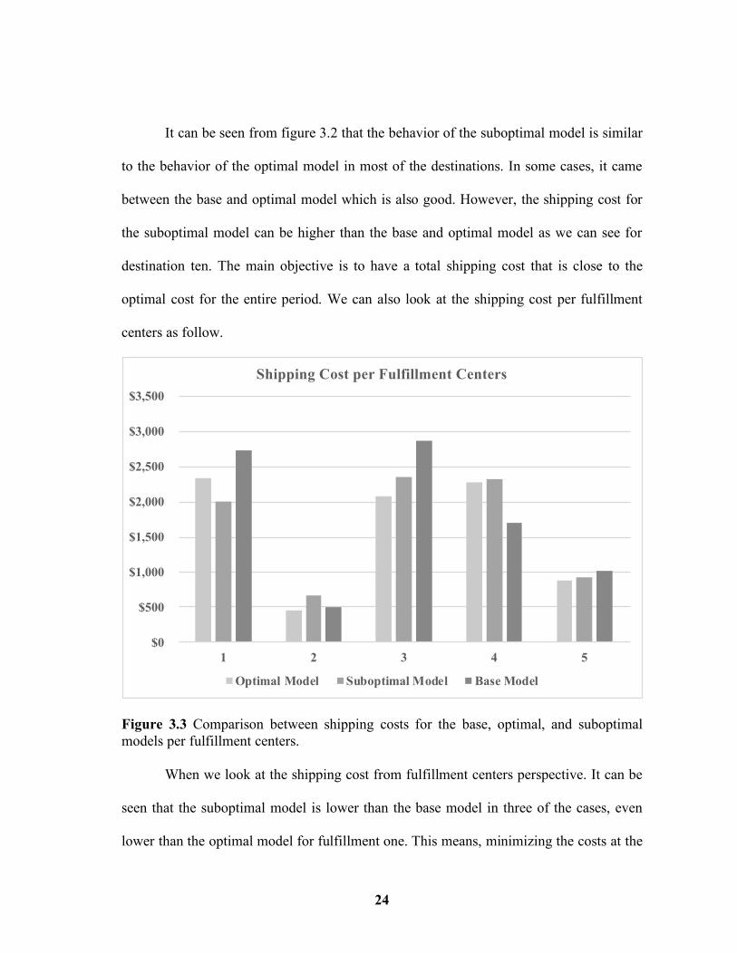
Figure 3.3 Comparison between shipping costs for the base, optimal, and suboptimal models per fulfillment centers. When we look at the shipping cost from fulfillment centers perspective. It can be
seen that the suboptimal model is lower than the base model in three of the cases, even
lower than the optimal model for fulfillment one. This means, minimizing the costs at the
$0
$500
$1,000
$1,500
$2,000
$2,500
$3,000
$3,500
1 2 3 4 5
Shipping Cost per Fulfillment Centers
Optimal Model Suboptimal Model Base Model
25
current period to its minimal level might affect the shipping cost in the future, if future
demand is not considered. Using the right forecasting method is very important too. For
our case, when demand is uniformly distributed, a weighted moving average forecast
method is used to predict future demand. In order to be able to validate this model, we did
more experiments with different set of data for the variables that are demand, inventory
levels, and historical data which is presented next in the upcoming experiment chapter.

26
CHAPTER 4
EXPERIMENTATION
4.1 Generation of Test Problems
In chapter two, we presented our recommended decision model which we call the
suboptimal model. In the example presented earlier, our suboptimal model comes between
our base and optimal model. In order to validate our suboptimal model, we need to create
more examples by changing our variables which are the demand Dj, the inventory level Si
for every fulfillment center, and the historical demand while keep the shipping costs
constant throughout all the models. Additionally, as mentioned earlier, the total inventory
level is always higher than the total demand for the entire period.
We tested different demand, and different inventory levels, to validate our model,
and to get insights about which inventory levels could reduce the total shipping costs.
Additionally, we did sensitivity analysis and created some special cases.
We categorized our test table into four categories based on the demand, and each
category have five classes which present different inventory levels. In every case also the
demand is changing. The values of the demand Dj are uniformly distributed for every
category between (1, 50), (1, 100), (1, 500), and (1, 1000). Additionally, different inventory
levels are presented with the assumption that inventory levels are controllable not like the
demand. It is important to note that in our decision model transshipment is not allowed.
The main goal of our model is to predict future demand and preserve required inventory
for expected demand in order to minimize the total shipping cost and reduce costly

27
assignments and allocations. As a concept, such a decision model would reduce the need
of transshipment which will be very interesting to look at and will be recommended on this
thesis for future research and expansion of the current model.
4.2 Experimentation Results and Explanations
As mentioned in chapter two, all the models are solved using excel solver as a linear
programming problem. Our main comparison and experimentation table is presented as
follow.
Table 4.1 Models Comparison and Experimentations Results
Table 4.1 shows four different categories, each category represents a different
demand range, and within each category there are five classes and scenarios that follow the
same demand with different inventory levels for each one of them. As mentioned earlier
demand is uncontrollable, but inventory level is. Therefore, different inventory levels were
presented to measure its effect on the total shipping costs. The first three columns present
our optimal, suboptimal, and base models’ total shipping costs. We always want to make
Optimal Model Suboptimal Model Base Model Opportunity Cost New Opportunity Cost Opportunity Cost Reduction %1 $8,437 $9,691 $9,857 $1,420 $1,254 11.69%2 $6,210 $6,505 $6,723 $513 $295 42.50%3 $9,900 $10,080 $10,166 $266 $180 32.33%4 $8,012 $8,256 $8,811 $799 $244 69.46%5 $8,970 $9,656 $9,828 $858 $686 20.05%1 $16,754 $17,195 $18,439 $1,685 $441 73.83%2 $12,819 $13,976 $14,156 $1,337 $1,157 13.46%3 $16,044 $17,505 $17,652 $1,608 $1,461 9.14%4 $16,765 $17,239 $17,767 $1,002 $474 52.69%5 $17,489 $17,983 $18,613 $1,124 $494 56.05%1 $83,831 $89,236 $90,823 $6,992 $5,405 22.70%2 $74,323 $75,813 $80,250 $5,927 $1,490 74.86%3 $87,551 $91,370 $92,416 $4,865 $3,819 21.50%4 $112,244 $117,289 $119,874 $7,630 $5,045 33.88%5 $97,284 $105,317 $109,809 $12,525 $8,033 35.86%1 $175,092 $184,285 $184,520 $9,428 $9,193 2.49%2 $174,718 $191,198 $195,738 $21,020 $16,480 21.60%3 $144,922 $146,212 $149,587 $4,665 $1,290 72.35%4 $193,822 $201,268 $208,623 $14,801 $7,446 49.69%5 $241,332 $244,206 $248,495 $7,163 $2,874 59.88%
RAND(1,50)
RAND(1,100)
RAND(1,500)
RAND(1,1k)
28
sure that our suboptimal model total shipping cost is as close as possible to the optimal
model. The fourth column is the opportunity cost. The opportunity cost is the difference
between the optimal and base models. Our objective is to minimize the opportunity cost as
much as possible and to make it match the optimal cost. In order to measure how much our
decision model is getting us closer to the optimal model, we added two more columns at
the end which show the difference between the suboptimal model and the base model
which should be lower than the difference in the opportunity cost. Lastly, how much we
decreased the opportunity costs as a percentage. For example, in the first case it was
11.69% which means we were able to get closer to the optimal solution by 11.69% and
there is 88.31% that could have been minimized more. This column is important if we want
to test out other forecasting methods and see if we could get closer to the optimal solution.
Table 4.1 looks complicated, we will break it down and analyze it in order to validate our
recommended decision model.
4.3 Experimentation Results Analysis
In order to analyze this table, let us break it down and analyze each set of demand alone.
The first thing we want to look at is the total shipping cost for each scenario for the three
models.

29
Figure 4.1 Comparison between shipping costs for the base, optimal, and suboptimal models for random distributed demand between (1, 50).
Figure 4.2 Comparison between shipping costs for the base, optimal, and suboptimal models for random distributed demand between (1, 100).
$0
$2,000
$4,000
$6,000
$8,000
$10,000
$12,000
1 2 3 4 5
RAND(1,50)
Total Shipping Cost
OPTIMAL SUBOPTIMAL BASE
$0
$2,000
$4,000
$6,000
$8,000
$10,000
$12,000
$14,000
$16,000
$18,000
$20,000
1 2 3 4 5
RAND(1,100)
Total Shipping Cost
OPTIMAL SUBOPTIMAL BASE

30
Figure 4.3 Comparison between shipping costs for the base, optimal, and suboptimal models for random distributed demand between (1, 500).
Figure 4.4 Comparison between shipping costs for the base, optimal, and suboptimal models for random distributed demand between (1, 1000).
$0
$20,000
$40,000
$60,000
$80,000
$100,000
$120,000
$140,000
1 2 3 4 5
RAND(1,500)
Total Shipping Cost
OPTIMAL SUBOPTIMAL BASE
$0
$50,000
$100,000
$150,000
$200,000
$250,000
$300,000
1 2 3 4 5
RAND(1,1k)
Total Shipping Cost
OPTIMAL SUBOPTIMAL BASE

31
In the previous figures, it can be seen that the total shipping cost for the suboptimal
model is always coming lower than the base model which what we wanted to see here. The
question of could our suboptimal model be worse than our base model, the answer to this
question is yes, when the demand is not stable, or the forecasting method is not appropriate,
we could end up making bad allocation even worse than optimizing every single period
alone. It can be observed that the level of optimization is different in every case or scenario.
In some cases, the optimization is minimal, and it could also equal to the base model.
However, we can conclude that when demand is stable, and the right forecasting method
is used, including future demand in the optimization process would reduce the total
shipping cost.
By looking at some cases such as in 4.1 scenario 1, it can be observed that there is
a large opportunity to minimize our shipping costs. Even though our suboptimal model
minimized the total shipping cost, but still an additional minimization is possible. Of
course, having a cost that is equal to the optimal cost is difficult, but we want to get as
close as possible to the optimal model shipping cost. Conversely, by looking at figure 4.4
scenario 3, it can be observed that the opportunity cost is not big, and there is not a big area
for improvement, and our suboptimal solution is very close to the base model. It can be
concluded that every case is different, but we want to make sure that in some cases we
might not minimize the cost a lot, but in most cases, we are.
Let us look at the opportunity costs and how much we were able to minimize it in
terms of costs and percentages.
32
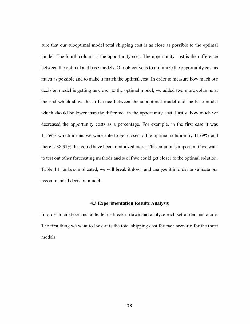
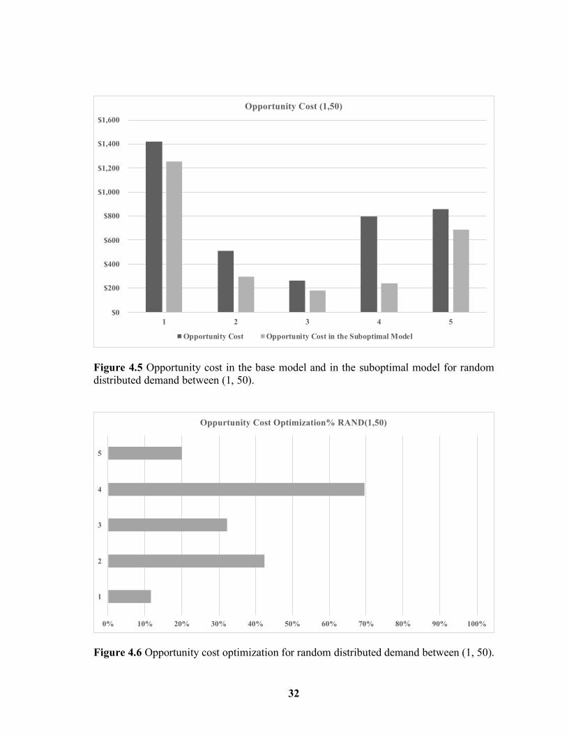
Figure 4.5 Opportunity cost in the base model and in the suboptimal model for random distributed demand between (1, 50).
Figure 4.6 Opportunity cost optimization for random distributed demand between (1, 50).
$0
$200
$400
$600
$800
$1,000
$1,200
$1,400
$1,600
1 2 3 4 5
Opportunity Cost (1,50)
Opportunity Cost Opportunity Cost in the Suboptimal Model
0% 10% 20% 30% 40% 50% 60% 70% 80% 90% 100%
1
2
3
4
5
Oppurtunity Cost Optimization% RAND(1,50)

33
Figure 4.7 Opportunity cost in the base model and in the suboptimal model for random distributed demand between (1, 100).
Figure 4.8 Opportunity cost optimization for random distributed demand between (1, 100).
$0
$200
$400
$600
$800
$1,000
$1,200
$1,400
$1,600
$1,800
1 2 3 4 5
Opportunity Cost (1,100)
Opportunity Cost Opportunity Cost in the Suboptimal Model
0% 10% 20% 30% 40% 50% 60% 70% 80% 90% 100%
1
2
3
4
5
Oppurtunity Cost Optimization% RAND(1,100)
34
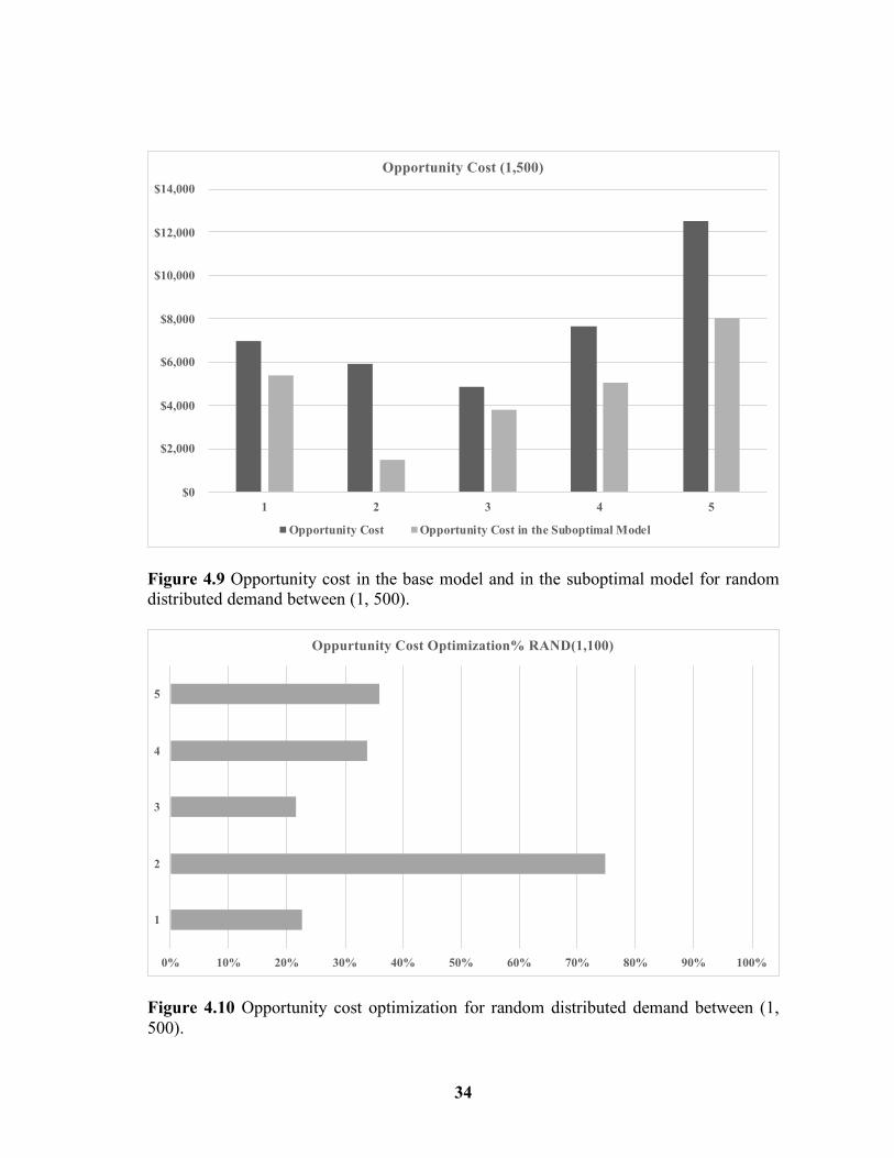
Figure 4.9 Opportunity cost in the base model and in the suboptimal model for random distributed demand between (1, 500).
Figure 4.10 Opportunity cost optimization for random distributed demand between (1, 500).
$0
$2,000
$4,000
$6,000
$8,000
$10,000
$12,000
$14,000
1 2 3 4 5
Opportunity Cost (1,500)
Opportunity Cost Opportunity Cost in the Suboptimal Model
0% 10% 20% 30% 40% 50% 60% 70% 80% 90% 100%
1
2
3
4
5
Oppurtunity Cost Optimization% RAND(1,100)

35
Figure 4.11 Opportunity cost in the base model and in the suboptimal model for random distributed demand between (1, 1000).
Figure 4.12 Opportunity cost optimization for random distributed demand between (1, 1000).
$0
$5,000
$10,000
$15,000
$20,000
$25,000
1 2 3 4 5
Opportunity Cost (1,1000)
Opportunity Cost Opportunity Cost in the Suboptimal Model
0% 10% 20% 30% 40% 50% 60% 70% 80% 90% 100%
1
2
3
4
5
Oppurtunity Cost Optimization% RAND(1,1000)

36
By looking at the previous figures, it can be seen that in every set of data and in
every scenario, the opportunity cost is decreasing in different rates. When the opportunity
cost is equal to zero, this means that the suboptimal solution is equal to the optimal solution
which is difficult to achieve. However, we want to get closer to the optimal solution as
much as possible. These set of graphs help us to see if there is a good chance for further
improvement. Our main objective of our decision model is to make sure that in all scenarios
we were able to minimize the total shipping cost compared to the base model. Furthermore,
we are looking to see how far we are from the optimal solution. For instance, in figure 4.7
scenario one, it can be observed that the opportunity cost has decreased from around $1,700
to around $500. By looking at figure 4.10, it can be seen that this reduction has got us closer
to 70% of the optimal solution which is very satisfactory. Conversely, by looking at figure
4.11 scenario one, it can be seen that the opportunity cost has not decreased a lot and it is
almost the same, and by looking at figure 4.12, it can be observed that we only have got
closer to our optimal solution by 2%. This result is not satisfactory and there is a big chance
of further improvement. The reason behind this is that sometimes the historical data that
are randomly generated is too optimistic or too pessimistic and conversely the real demand
is. This causes different optimization rates.
To conclude this part, we can say that the suboptimal model is minimizing the total
shipping costs in different rates. The forecasting method used has a big impact on the
model. In our case, weighted moving average is used for a uniformly distributed demand,
and we were able to minimize the total shipping costs in most of the scenario as presented
in table 4.1.

37
4.4 Sensitivity Analysis
Sensitivity analysis is changing controllable factors and see its effect on the output. On our
model the controllable factors are the inventory level and the forecasting method that is
being used to predict future demand. Additionally, the shipping costs from fulfillment
centers to destinations. When a company has more than one fulfillment center and they
know the expected demand. They would be able to keep the right inventory level in every
fulfillment center based on the geographical demand. However, in the e-commerce industry
predicting demand and forecasting could be more challenging, and in order to minimize
costly allocations and stockouts e-commerce companies always want to carry safety stock
inventory. Therefore, in our model, when demand is uniformly distributed, we wanted to
see the effect of balancing the inventory in all the fulfillment centers as a barrier for
unexpected demand or too optimistic or too pessimistic forecast. What we tested was when
the demand is uniformly distributed between (1, 500) for the same set of data that was used
before, we kept the inventory balanced in all the fulfillment centers and looked to see if we
were able to minimize the total shipping costs while using our recommended model. The
results are as follow.
Table 4.2 Testing Balanced Inventory for Uniformly Distributed Demand (1, 500)
It can be seen from table 4.1 that we were able to minimize our total shipping costs
for the same set of data by keeping the inventory balanced. For case two, there is no
SHIPPING COST SUBOPTIMAL BALANCED INVENTORY % DECREASED1 $89,236 $83,661 6%2 $75,813 $75,813 0%3 $91,370 $84,247 8%4 $117,289 $88,783 24%5 $105,317 $80,143 24%
RAND(1,500)

38
improvement because it was balanced in the main example. Keeping the inventory
balanced is a good idea if the demand is unknown, and there is no or few historical data.
Once historical data is available, and the right forecasting method is used. The right amount
of inventory should be kept in each fulfillment center.
Another concept that we have tested is when the demand is unstable. For example,
let us assume that the demand for the last previous periods was uniformly distributed
between (1, 20), and for some reason the demand has increased from (1, 20) to be (1, 50).
This change would influence the forecasted demand. Consequently, the allocated quantities
for destinations. We created two models and compared them to each other and looked at
the effect of unstable demand on our model.
Figure 4.13 Total shipping cost comparison between stable and unstable demand.
Figure 4.13 shows the total shipping costs is different when the demand is unstable.
The actual demand is uniformly distributed between (1, 50) in all models. However, what
$9,177
$9,562
$9,969 $9,946
OPTIMAL SUBOPTIMAL (STABLEDEMAND)
SUBOPTIMAL (UNSTABLEDEMAND)
BASE
TOTAL SHIPPING COST

39
is different between the suboptimal models is that the historical data. When demand is
stable, the historical data were uniformly distributed between (1, 50). On the other hand,
when demand is unstable, the historical data were uniformly distributed between (1, 20)
which means that the increase in demand has influenced the total shipping cost which
showcase the importance of using the right forecasting method, for the right set of data.
Like presented earlier, when historical data is not available or is not accurate different
models might be used to forecast future demand, and different inventory levels might be
used. The next figures show the total shipping cost per destinations and per fulfillment
centers for unstable demand.
Figure 4.14 Total shipping cost comparison between stable and unstable demand per fulfillment center.
$-
$500
$1,000
$1,500
$2,000
$2,500
$3,000
$3,500
$4,000
1 2 3 4 5
TOTAL SHIPPING COST PER FULFILLMENT CENTER
OPTIMAL SUBOPTIMAL (STABLE DEMAND) SUBOPTIMAL (UNSTABLE DEMAND) BASE
40
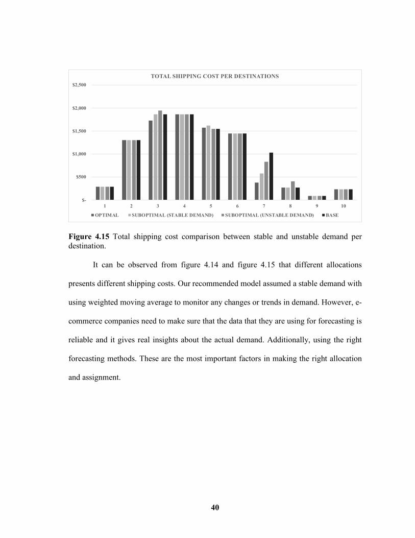
Figure 4.15 Total shipping cost comparison between stable and unstable demand per destination.
It can be observed from figure 4.14 and figure 4.15 that different allocations
presents different shipping costs. Our recommended model assumed a stable demand with
using weighted moving average to monitor any changes or trends in demand. However, e-
commerce companies need to make sure that the data that they are using for forecasting is
reliable and it gives real insights about the actual demand. Additionally, using the right
forecasting methods. These are the most important factors in making the right allocation
and assignment.
$-
$500
$1,000
$1,500
$2,000
$2,500
1 2 3 4 5 6 7 8 9 10
TOTAL SHIPPING COST PER DESTINATIONS
OPTIMAL SUBOPTIMAL (STABLE DEMAND) SUBOPTIMAL (UNSTABLE DEMAND) BASE

41
CHAPTER 5
SUMMARY
5.1 Conclusion and Remarks
In order for e-commerce to be competitive with brick and mortar, it has to be effective and
efficient in all its logistics operations. Big e-commerce companies such as Amazon have
different decision models for different operations and functions. The process of decision
making is automated, and it is done in seconds. Once an e-commerce customer picks a
product, and picks a delivery option, then it is the e-commerce company responsibility to
deliver the product in the expected delivery date.
For companies such as Amazon, when an order comes there is a big probability that
this order is available at more than one fulfillment center. Delivering the product from the
closest fulfillment center to the order might be the first thing to come in mind. However, it
is not always the right and optimal decision. There are different variables that are included
in such a decision besides the distance such as future order and product correlations.
Our model shows that including future demand during the process of allocating
received demand would change the allocation and minimize the total shipping costs. We
presented three models, the first model which was called the base model. The base model
allocates orders to fulfillment centers after they are received without considering future
orders. The second model was to show that when the future demand is known the allocation
is different and the total shipping cost is minimized, and we called this model the optimal
model. However, in real life the future demand is unknown, but we could have insights

42
about future demand by looking at historical data. For our recommended decision model,
we were trying to find a solution that is better than the base model and as close as possible
to the optimal model. For a uniformly distributed demand, we used weighted moving
average to forecast future orders and including expected orders in our optimization process,
we called this model, the suboptimal model. All the models were solved as a linear
programming problem using excel solver. Different shipping costs, inventory levels and
demands were presented to validate the model.
Additionally, once the model is developed, we tried to see the effect of balancing
the inventory in all fulfillment centers. By testing that we were able to minimize the total
shipping costs to be lower than other random inventory levels. Therefore, we think that
balancing the inventory is a good idea when historical data is not available, or it is not
reliable or when the demand is unpredictable and instable.
5.2 Future Work
Future research should consider including other factors to the model and looking at their
effects on the total shipping cost. For example, assuming that two products are always
ordered together, and there is a correlation between these two products and we want the
quantity of these two products to be somewhat equal in the fulfillment centers. Would
product correlation affect the allocation process or minimize the total shipping costs.
Keeping two products that are usually ordered together would reduce the order picking
time and also the packaging. One of the big challenges in e-commerce is order
consolidation which mean objective is to minimize the shipped boxes for orders that have

43
more than one product. Additionally, future research might test other forecasting methods,
for different demand behaviors, different inventory levels and shipping costs knowing that
each product is different, and one forecasting method might work well with certain type of
products and work bad with others, and as we discussed earlier that bad forecasting would
make companies make costly allocation.
In our model, the total inventory level is always higher than the demand, future
studies could also look at when the demand is higher than the inventory level, what is the
effect on the allocation and what how to involve and calculate stockout costs. Finally,
testing how such a model would reduce transshipment between fulfillment centers. As
mentioned earlier, transshipment is the process of moving products between fulfillment
centers. Transshipment should be minimized as much as possible. Knowing the right
amount of inventory needed in every fulfillment center would minimize transshipment.
(Albright, 2003; Benjaafar et al., 2008; Boysen, de Koster, & Weidinger, 2018; Boysen,
Schwerdfeger, et al., 2018; Braumoeller et al., 2007; Brynjolfsson et al., 2003; Ferreira,
Lee, & Simchi-Levi, 2015; Field-Darragh et al., 2014; He et al., 2014; Kok, 2016;
Kokkinaki et al., 2015; Lynch, 2014; Nau, 2016; Nicholson, 2017; Onal et al., 2017, 2018;
Raff & Li, 2013; Ricker & Kalakota, 1999; Torabi et al., 2015; Wan, 2017; Yaman et al.,
2012; Young, 2019)

44
REFERENCES
Albright, B. (2003). Automated product sourcing from multiple fulfillment centers: Google Patents.
Benjaafar, S., Li, Y., Xu, D., & Elhedhli, S. (2008). Demand allocation in systems with
multiple inventory locations and multiple demand sources. Manufacturing & Service Operations Management, 10(1), 43-60.
Boysen, N., de Koster, R., & Weidinger, F. (2018). Warehousing in the e-commerce era:
A survey. European Journal of Operational Research. Boysen, N., Schwerdfeger, S., & Weidinger, F. (2018). Scheduling last-mile deliveries
with truck-based autonomous robots. European Journal of Operational Research, 271(3), 1085-1099. doi:10.1016/j.ejor.2018.05.058
Braumoeller, R., Brinkerhoff, R., Holden, J., & Lee, D. (2007). Generating current order
fulfillment plans based on expected future orders: Google Patents. Brynjolfsson, E., Hu, Y. J., & Smith, M. D. (2003). Consumer Surplus in the Digital
Economy: Estimating the Value of Increased Product Variety at Online Booksellers.
Ferreira, K. J., Lee, B. H. A., & Simchi-Levi, D. (2015). Analytics for an online retailer:
Demand forecasting and price optimization. Manufacturing & Service Operations Management, 18(1), 69-88.
Field-Darragh, K. D., Olson, E. J., & Shiner, B. M. (2014). System and methods for order
fulfillment, inventory management, and providing personalized services to customers: Google Patents.
He, Y., Zhang, P., & Yao, Y. (2014). Unidirectional transshipment policies in a dual-
channel supply chain. Economic Modelling, 40, 259-268. doi:10.1016/j.econmod.2014.04.016
Kok, S. (2016). Should You Forecast Monthly or Weekly? Retrieved from
https://www.linkedin.com/pulse/should-you-forecast-monthly-weekly-stefan-de-kok/
Kokkinaki, A. I., Dekker, R., van Nunen, J., & Pappis, C. (2015). An Exploratory Study
on Electronic Commerce for Reverse Logistics. Supply Chain Forum: An International Journal, 1(1), 10-17. doi:10.1080/16258312.2000.11517067

45
Lynch, N. J. (2014). Fulfillment of requests for computing capacity: Google Patents. Nau, R. (2016). Statistical Forecasting: Notes on Regression and Time Series Analysis.
Fuqua School of Business, Duke University. Nicholson, J. R. (2017). New Insights on Retail E-Commerce: US Department of
Commerce, Economics and Statistics Administration, Office …. Onal, S., Zhang, J., & Das, S. (2017). Modelling and performance evaluation of explosive
storage policies in internet fulfilment warehouses. International Journal of Production Research, 55(20), 5902-5915.
Onal, S., Zhang, J., & Das, S. (2018). Product flows and decision models in Internet
fulfillment warehouses. Production Planning & Control, 29(10), 791-801. Raff, P., & Li, X. Y. (2013). Cost-based fulfillment tie-breaking: Google Patents. Ricker, F., & Kalakota, R. (1999). Order fulfillment: the hidden key to e-commerce
success. Supply chain management review, 11(3), 60-70. Torabi, S. A., Hassini, E., & Jeihoonian, M. (2015). Fulfillment source allocation,
inventory transshipment, and customer order transfer in e-tailing. Transportation Research Part E: Logistics and Transportation Review, 79, 128-144. doi:10.1016/j.tre.2015.04.004
Wan, C. (2017). Forecasting E-commerce Key Performance Indicators. Yaman, H., Karasan, O. E., & Kara, B. Y. (2012). Release Time Scheduling and Hub
Location for Next-Day Delivery. Operations Research, 60(4), 906-917. doi:10.1287/opre.1120.1065
Young, J. (2019). Global ecommerce sales grow 18% in 2018. Retrieved from
https://www.digitalcommerce360.com/article/global-ecommerce-sales/