Automatic Detection of Structural Changes inData Warehouses

Johann Eder∗ and Christian Koncilia∗ and Dieter Mitsche§

University of KlagenfurtDep. of Informatics-Systems

∗ {eder,koncilia}@isys.uni-klu.ac.at§ dmitsche@edu.uni-klu.ac.at

Abstract. Data Warehouses provide sophisticated tools for analyzingcomplex data online, in particular by aggregating data along dimensionsspanned by master data. Changes to these master data are a frequentthreat to the correctness of OLAP results, in particular for multi-perioddata analysis, trend calculations, etc. As dimension data might changein underlying data sources without notifying the data warehouse we areexploring the application of data mining techniques for detecting suchchanges and contribute to avoiding incorrect results of OLAP queries.

1 Introduction and Motivation

A data warehouse is a collection of data stemming from different frequentlyheterogeneous data sources and is optimized for complex data analysis opera-tion rather than for transaction processing. The most popular architectures aremultidimensional data warehouses (data cubes) where facts (transaction data)are ”indexed” by several orthogonal dimensions representing a hierarchical or-ganization of master data. OLAP (on-line analytical processing) tools allow theanalysis of this data, in particular by aggregating data along the dimensionswith different consolidation functions.

Although data warehouses are typically deployed to analyse data from alonger time period than transactional databases, they are not well preparedfor changes in the structure of the dimension data. This surprising observationoriginates in the (implicit) assumption that the dimensions of data warehousesought to be orthogonal, which, in the case of the dimension time means that allother dimensions ought to be time-invariant.

When analysts place their queries they have to know which dimension datachanged. Consider the following example: Diagnoses for patients were repre-sented in a data warehouse using the “International Statistical Classification ofDiseases and Related Health Problems” (ICD) code. However, codes for diag-noses changed from ICD Version 9 to ICD Version 10. For instance the code for“malignant neoplasm of stomach” has changed from 151 in ICD-9 to C16 in ICD-10. Other diagnoses were regrouped, e.g. “transient cerebral ischaemic attacks”has moved from “Diseases of the circulatory system” to “Diseases of the nervous

system”. Even worse, the same code described different diagnoses in ICD-9 andICD-10. Other ICD-9 codes are a subset of ICD-10 codes, i.e. the granularity ofcodes changed (in fact ICD-10 comprises about 8, 000 unique codes, over 3, 000more than ICD-9). It is obvious, that for questions like “did liver cancer in-crease over the last 5 years” correct results can only be obtained, if the analystis aware of these changes. A data warehouse should therefore provide means forrepresenting such changes to proactively assist analysts [EK01, EKM02].

In this paper we address another important issue: how can such structuralchanges be recognized, even if the sources do not notify the data warehouse aboutthe changes. This defensive strategy, of course, can only be an aid to avoid someproblems, it is not a replacement for adequate means for managing knowledgeabout changes. Nevertheless, in several practical situations we trace erroneousresults of OLAP queries back to structural changes not known by the analystsand the data warehouse operators. Erroneous in the sense that the resulting datadid not correctly represent the state of affairs in the real world.

As means for detecting such changes we propose the use of data miningtechniques. In a nutshell, the problem can be described as a multidimensionaloutlier detection problem.

In this paper we report on some experiments we were conducting to analyse

– which data mining techniques might be applied for the detection of structuralchanges

– how these techniques are best applied– whether these techniques effectively detect structural changes– whether these techniques scale up to large data warehouses.

To the best of our knowledge it is the first time that the problem of changesin dimensions of data warehouses is addressed with data mining techniques.The problems related to the effects of structural changes in data warehouses andapproaches to overcome the problems they cause were subject of several projects[Yan01, BSH99, Vai01, CS99] including our own efforts [EK01, EKM02] to builda temporal data warehouse structure with means to transform data betweenstructural versions such that OLAP tools work on data cleaned of the effects ofstructural changes.

The remainder of this paper is organized as follows: in section 2 we bring basicdefinitions and discuss the notion of structural changes in data warehouses. Insection 3 we briefly introduce the data mining techniques we analysed for thedetection of structural changes and we introduce a procedure for applying thesetechniques. In section 4 we briefly discuss the experiments we conducted as proofof concept. Finally in section 5 we draw some conclusions.

2 Structural Changes

Basically, a multidimensional view on data consists of a set of dimensions. Typ-ical examples of dimensions frequently found in multidimensional databases areTime, Facts or Products. The structure of each dimension is defined by a set of

2

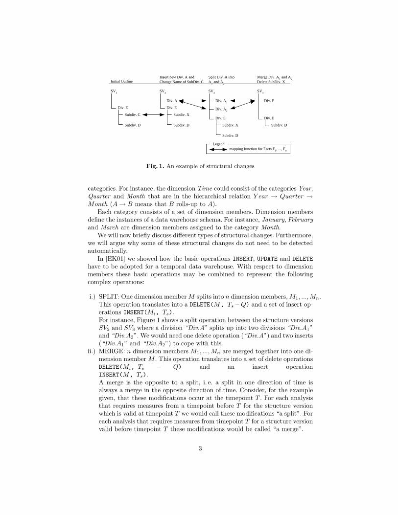
mapping function for Facts F1, ..., Fn

Legend

Div. E

SV1

Subdiv. C

Subdiv. D

Div. E

SV2

Subdiv. X

Subdiv. D

Div. A

Div. E

SV3

Subdiv. X

Subdiv. D

Div. A1

Div. A2

Div. E

SV4

Subdiv. D

Div. F

Insert new Div. A andChange Name of SubDiv. C

Split Div. A intoA1 and A2

Initial OutlineMerge Div. A1 and A2Delete SubDiv. X

Fig. 1. An example of structural changes

categories. For instance, the dimension Time could consist of the categories Year,Quarter and Month that are in the hierarchical relation Y ear → Quarter →Month (A → B means that B rolls-up to A).

Each category consists of a set of dimension members. Dimension membersdefine the instances of a data warehouse schema. For instance, January, Februaryand March are dimension members assigned to the category Month.

We will now briefly discuss different types of structural changes. Furthermore,we will argue why some of these structural changes do not need to be detectedautomatically.

In [EK01] we showed how the basic operations INSERT, UPDATE and DELETEhave to be adopted for a temporal data warehouse. With respect to dimensionmembers these basic operations may be combined to represent the followingcomplex operations:

i.) SPLIT: One dimension member M splits into n dimension members, M1, ..., Mn.This operation translates into a DELETE(M, Ts−Q) and a set of insert op-erations INSERT(Mi, Ts).For instance, Figure 1 shows a split operation between the structure versionsSV2 and SV3 where a division “Div.A” splits up into two divisions “Div.A1”and “Div.A2”. We would need one delete operation (“Div.A”) and two inserts(“Div.A1” and “Div.A2”) to cope with this.

ii.) MERGE: n dimension members M1, ..., Mn are merged together into one di-mension member M . This operation translates into a set of delete operationsDELETE(Mi, Ts − Q) and an insert operationINSERT(M, Ts).A merge is the opposite to a split, i. e. a split in one direction of time isalways a merge in the opposite direction of time. Consider, for the examplegiven, that these modifications occur at the timepoint T . For each analysisthat requires measures from a timepoint before T for the structure versionwhich is valid at timepoint T we would call these modifications “a split”. Foreach analysis that requires measures from timepoint T for a structure versionvalid before timepoint T these modifications would be called “a merge”.

3

iii.) CHANGE: An attribute of a dimension member changes, for example, ifthe product number (Key) or the name of a department (user defined at-tribute) changes. Such a modification can be carried out by using the updateoperation defined above.With respect to dimension members representing measures, CHANGE couldmean that the way how to compute the measure changes (for example, theway how to compute the unemployment rate changed in Austria becausethey joined the European Union in 1995) or that the unit of facts changes(for instance, from Austrian Schillings to EURO).

iv.) MOVE: A dimension member moves from one parent to another, i.e., wemodify the hierarchical position of a dimension member. For instance, if aproduct P no longer belongs to product group GA but to product group GB .This can be done by changing the DMP

id (parent ID) of the correspondingdimension member with an update operation.

v.) NEW-MEMBER: A new dimension member is inserted. For example, if anew product becomes part of the product spectrum. This modification canbe done by using an insert operation.

vi.) DELETE-MEMBER: A dimension member is deleted. For instance, if abranch disbands. Just as a merge and a split are related depending on thedirection of time, this is also applicable for the operations NEW-MEMBERand DELETE-MEMBER. In opposite to a NEW-MEMBER operation thereis a relation between the deleted dimension member and the following struc-ture version. Consider, for example, that we delete a dimension member“Subdivision B” at timepoint T . If for the structure version valid at time-point T we would request measures from a timepoint before T , we still couldget valid results by simply subtracting the measures for “Subdivision B”from its parent.

For two of these operations, namely NEW-MEMBER and DELETE-MEMBER,there is no need to use data mining techniques to automatically detect these mod-ifications. When loading data from data sources for a dimension member whichis new in the data source but does not exist in the warehouse yet, the NEW-MEMBER operation is detected automatically by the ETL-Tool (extraction,transformation and loading tool). On the other hand, the ETL-Tool automat-ically detects when no fact values are available in the data source for deleteddimension members.

3 Data Mining Techniques

In this chapter a selection of different data mining techniques for automaticdetection of structural changes is issued. Whereas the first section deals gives anoverview over some possible data mining techniques, the second section focusseson multidimensional extensions of the methods. Finally, a stepwise approach todetect structural changes at different layers is proposed.

4

3.1 Possible data mining methods

The simplest method for detecting structural changes is the calculation of de-viation matrices. Absolute and relative differences between consecutive values,and differences in the shares of each dimension member between two chrononscan be easily computed - the runtime of this approach is clearly linear in thenumber of analysed values. Since this method is very fast, it should be used asa first sieve.

A second approach whose runtime complexity is in the same order as thecalculation of traditional deviation matrices is the attempt to model a givendata set with a stepwise constant differential equation (perhaps with a simplefunctional equation). This model, however, only makes sense if there exists somerudimentary, basic knowledge about factors that could have caused the develop-ment of certain members (but not exact knowledge, since in this case no datamining would have to be done anymore). After having solved the equation (forsolution techniques of stepwise differential equations refer to [Dia00]), the rela-tive and absolute differences between the predicted value and the actual valuecan be considered to detect structural changes.

Other techniques that can be used for detecting structural changes are mostlytechniques that are also used for time-series analysis:

– autoregression - a significantly high absolute and relative difference betweena dimension member’s actual value and its value predicted via a simpleARMA (AutoRegression Moving Average)(p,q)-model (or, if necessary, anARIMA (AutoRegression Integrated Moving Average)(p,d,q)-model, per-haps even with extensions for seasonal periods) is an indicator for a structuralchange of that dimension member.

– autocorrelation - the usage of this method is similar to the method of au-toregression. The results of this method, however, can be easily visualizedwith the help of correlograms.

– crosscorrelation and regression - these methods can be used to detect sig-nificant dependencies between two different members. Especially a very lowcorrelation coefficient (a very inaccurate prediction with a simple regressionmodel, respectively) could lead to the roots of a structural change.

– discrete fourier transform (DFT), discrete cosine transform (DCT), differenttypes of discrete wavelet transforms - the maximum difference (scaled bymean of the vector) as well as the overall difference (scaled by mean andlength of the vector) of the coefficients of the transforms of two dimensionmembers can be used to detect structural changes.

– singular value decomposition (SVD) - unusually high differences in singularvalues can be used for detecting changes in the measure dimension whenanalyzing the whole data matrix. If single dimension members are compared,the differences of the eigenvalues of the covariance matrices of the dimensionmembers (= principal component analysis) can be used in the same way.

In this paper, due to lack of space no detailed explanation of these methods isgiven. For details we refer to [Atk89] (fourier transform), [Vid99] (wavelet trans-

5

forms), [BD02] (autoregression and -correlation), [Hol02] (SVD and principalcomponent analysis), [Wei85] (linear regression and crosscorrelation).

3.2 Multidimensional Structures

Since in data warehouses there is usually a multidimensional view on the data,the techniques shown in the previous chapter have to be applied carefully. Ifall structure dimensions are considered simultaneously and a structural changeoccurred in one structure dimension, it is impossible to detect the dimension thatwas responsible for this change. Therefore the values of the data warehouse haveto be grouped along one structure dimension (we considered only fully-additivemeasures that can be summed along each structure dimension. It is one aspect offurther work to check the approach for semi-additive and non-additive measures).On this two-dimensional view the methods of the previous chapter can then beapplied to detect the changed structure dimension. If, however, a change happensin two or more structure dimensions at the same time, the analysis of the valuesgrouped along one structure dimension will not be successful - either a few (oreven all) structure dimensions will show big volatilities in their data, or not asingle structure dimension will show significant changes. Hence, if a change inthe structure dimensions is assumed, and none can be detected with the methodsdescribed above, the values have to be grouped along two structure dimensions.The methods can be applied on this view, if changes still cannot be detected,the values are grouped by three structure dimensions, a.s.o. The approach toanalyse structural changes in data warehouses by grouping values by just onestructure dimension in the initial step was chosen for two reasons:

1.) In the vast majority of all structure changes in structure dimensions onlyone structure dimension will be affected.

2.) The runtime and memory complexity of the analysis is much smaller whenvalues are grouped by just one structure dimension: let D1, D2, . . . , Dn

denote the number of elements in the i-th structure dimension (i = 1 . . . n;D1 ≥ D2 ≥ . . .≥ Dn); then in the first step only D1 + D2 + . . . + Dn =O(D1) different values have to be analysed, in the second step already D1D2

+ . . . + D1Dn + . . .+ Dn−1Dn = O(D21), in the i-th step therefore O(Di

1),i = 1 . . . n.

3.3 Stepwise Approach

As a conclusion of the previous sections we propose a stepwise approach to detectdifferent types of structure changes at different layers:

1.) In the first step the whole data matrix of each measure in the data ware-house is analysed to detect changes in the measure dimension (change of thecalculation formula of a measure, change of the metric unit of a measure).Primarily a simple deviation matrix that calculates the differences of thesums of all absolute values between two consecutive chronons can be applied

6

here. If these differences between two chronons are substantially bigger thanthose between other chronons, then this is an indicator for a change in themeasure dimension. If the runtime performance is not too critical, SVD andDCT can also be carried out to detect changes. Changes at this level thatare detected must be either corrected or eliminated - otherwise the resultsin the following steps will be biased by these errors.

2.) In the next step the data are grouped by one structure dimension. Thedeviation matrices that were described above can be applied here to detectdimension members that were affected by structural changes.

3.) If the data grouped by one structure dimension can be adequately mod-elled with a stepwise constant differential equation (or a simple functionalequation) then also the deviation matrices that calculate the absolute andrelative difference between the model-estimated value and the actual valueshould be used.

4.) In each structure dimension where one dimension member is known thatdefinitely remained unchanged throughout all chronons (fairly stable so thatit can be considered as a dimension member with an average development,mostly a dimension member with rather big absolute values), other datamining techniques such as autocorrelation, autoregression, discrete fouriertransform, discrete wavelet transform, principal component analysis, cross-correlation and linear regression can be used to compare this ’average’ di-mension member with any other dimension member detected in steps 2 and3. If one of the methods shows big differences between the average dimen-sion member and the previously detected dimension member, then this is anindicator for a structural change of the latter one. Hence, these methods onthe one hand are used to make the selection of detected dimension memberssmaller, on the other hand they are also used to ’prove’ the results of the pre-vious steps. However, all these methods should not be applied to a dimensionmember that is lacking values, whose data are too volatile or whose valuesare often zero. If no ’average’ dimension member is known, the dimensionmembers that were detected in previous steps can also be compared withthe sum of the absolute values of all dimension members. In any case, it isfor performance reasons recommended to use the method of autocorrelationat first; among all wavelet transforms the Haar method is the fastest.

5.) If in steps 2, 3 and 4 no (or not all) structural changes are detected and onestill assumes structural changes, then the values are grouped by i+1 structuredimensions, where i (i = 1 . . .n − 1, n = number of structure dimensions)is the number of structure dimensions that were used for grouping values inthe current step. Again, steps 2, 3 and 4 can be applied.

4 Experiments

The stepwise approach proposed in the previous chapter was tested on manysmall data sets and one larger sample data set. Here one small example is givento show the usefulness of the stepwise approach.

7

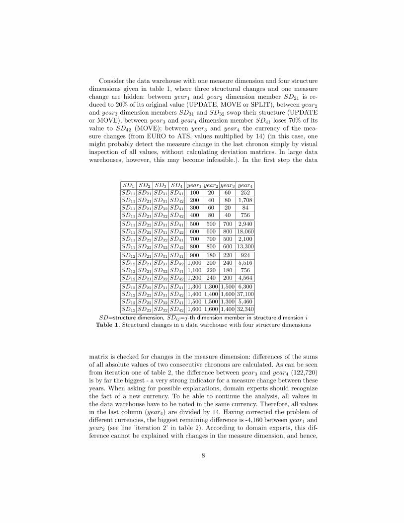
Consider the data warehouse with one measure dimension and four structuredimensions given in table 1, where three structural changes and one measurechange are hidden: between year1 and year2 dimension member SD21 is re-duced to 20% of its original value (UPDATE, MOVE or SPLIT), between year2

and year3 dimension members SD31 and SD32 swap their structure (UPDATEor MOVE), between year3 and year4 dimension member SD41 loses 70% of itsvalue to SD42 (MOVE); between year3 and year4 the currency of the mea-sure changes (from EURO to ATS, values multiplied by 14) (in this case, onemight probably detect the measure change in the last chronon simply by visualinspection of all values, without calculating deviation matrices. In large datawarehouses, however, this may become infeasible.). In the first step the data

SD1 SD2 SD3 SD4 year1 year2 year3 year4

SD11 SD21 SD31 SD41 100 20 60 252

SD11 SD21 SD31 SD42 200 40 80 1,708

SD11 SD21 SD32 SD41 300 60 20 84

SD11 SD21 SD32 SD42 400 80 40 756

SD11 SD22 SD31 SD41 500 500 700 2,940

SD11 SD22 SD31 SD42 600 600 800 18,060

SD11 SD22 SD32 SD41 700 700 500 2,100

SD11 SD22 SD32 SD42 800 800 600 13,300

SD12 SD21 SD31 SD41 900 180 220 924

SD12 SD21 SD31 SD42 1,000 200 240 5,516

SD12 SD21 SD32 SD41 1,100 220 180 756

SD12 SD21 SD32 SD42 1,200 240 200 4,564

SD12 SD22 SD31 SD41 1,300 1,300 1,500 6,300

SD12 SD22 SD31 SD42 1,400 1,400 1,600 37,100

SD12 SD22 SD32 SD41 1,500 1,500 1,300 5,460

SD12 SD22 SD32 SD42 1,600 1,600 1,400 32,340

SD=structure dimension, SDij=j-th dimension member in structure dimension iTable 1. Structural changes in a data warehouse with four structure dimensions

matrix is checked for changes in the measure dimension: differences of the sumsof all absolute values of two consecutive chronons are calculated. As can be seenfrom iteration one of table 2, the difference between year3 and year4 (122,720)is by far the biggest - a very strong indicator for a measure change between theseyears. When asking for possible explanations, domain experts should recognizethe fact of a new currency. To be able to continue the analysis, all values inthe data warehouse have to be noted in the same currency. Therefore, all valuesin the last column (year4) are divided by 14. Having corrected the problem ofdifferent currencies, the biggest remaining difference is -4,160 between year1 andyear2 (see line ’iteration 2’ in table 2). According to domain experts, this dif-ference cannot be explained with changes in the measure dimension, and hence,

8

Diff year12 year23 year34

iteration 1 -4,160 0 122,720

iteration 2 -4,160 0 0Diff=absolute difference, yearmn=comparison of year m with year n

Table 2. Detection of changes in the measure dimension

the approach can be continued with the analysis of changes in the structuredimensions.

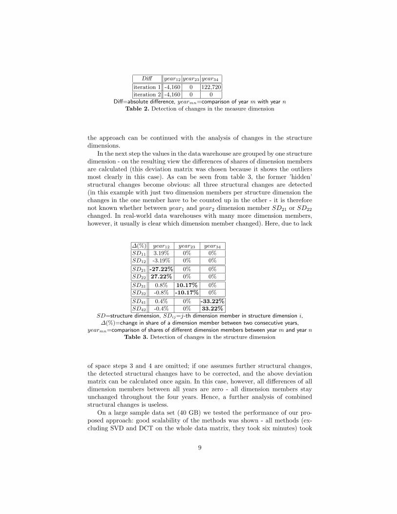
In the next step the values in the data warehouse are grouped by one structuredimension - on the resulting view the differences of shares of dimension membersare calculated (this deviation matrix was chosen because it shows the outliersmost clearly in this case). As can be seen from table 3, the former ’hidden’structural changes become obvious: all three structural changes are detected(in this example with just two dimension members per structure dimension thechanges in the one member have to be counted up in the other - it is thereforenot known whether between year1 and year2 dimension member SD21 or SD22

changed. In real-world data warehouses with many more dimension members,however, it usually is clear which dimension member changed). Here, due to lack

∆(%) year12 year23 year34

SD11 3.19% 0% 0%

SD12 -3.19% 0% 0%

SD21 -27.22% 0% 0%

SD22 27.22% 0% 0%

SD31 0.8% 10.17% 0%

SD32 -0.8% -10.17% 0%

SD41 0.4% 0% -33.22%

SD42 -0.4% 0% 33.22%SD=structure dimension, SDij=j-th dimension member in structure dimension i,

∆(%)=change in share of a dimension member between two consecutive years,yearmn=comparison of shares of different dimension members between year m and year n

Table 3. Detection of changes in the structure dimension

of space steps 3 and 4 are omitted; if one assumes further structural changes,the detected structural changes have to be corrected, and the above deviationmatrix can be calculated once again. In this case, however, all differences of alldimension members between all years are zero - all dimension members stayunchanged throughout the four years. Hence, a further analysis of combinedstructural changes is useless.

On a large sample data set (40 GB) we tested the performance of our pro-posed approach: good scalability of the methods was shown - all methods (ex-cluding SVD and DCT on the whole data matrix, they took six minutes) took

9

less than six seconds (Pentium III, 866 MHz, 128 MB SDRAM). This example,however, also showed that the quality of the results of the different methods verymuch depends on the quality and the volatility of the original data.

5 Conclusions

Unknown structural changes lead to incorrect results of OLAP queries, to analy-sis reports with wrong data and probably to suboptimal decisions based on thesedata. Since analysts need not see such changes in the data, the changes might behidden in the lower levels of the dimension hierarchies which are typically onlylooked at in drill down operations, but of course influence the data derived inhigher levels. Pro-active steps are necessary to avoid that incorrect results dueto neglecting of structural changes.

Some changes might be detected when data is loaded into the database, orwhen change-logs of the sources are forwarded to the data warehouse. Neverthe-less, such changes stemming from different sources might appear unnoticed indata warehouses. Therefore, we are proposing to apply data mining techniquesfor detecting such changes, or more precisely detecting suspicious unexpecteddata characteristics which might originate from unknown structural changes. Itis clear that any such technique will face the problem, that it might not be ableto detect all such changes, in particular, when the data looks perfectly feasible.On the other hand, the techniques might indicate a change due to character-istics of data which is however correctly representing reality, i.e. no change indimension data took place.

We showed that several data mining techniques might be used for this anal-ysis. We propose a procedure which uses several techniques in turn and in ouropinion is a good combination of efficiency and effectiveness. We were able toshow that the techniques we propose actually detect structural changes in datawarehouses and that these techniques also scale up for large data warehouses.The application of the data mining techniques, however, requires good qualityof the data in the data warehouse, because otherwise errors of first and seconddegree rise. It is also necessary to fine-tune the parameters for the data miningtechniques, in particular to take the volatility of the data in the data warehouseinto account. Here, further research is expected lead to self adaptive methods.

References

[Atk89] K. E. Atkinson. An Introduction to Numerical Analysis. John Wiley, NewYork, USA, 1989.

[BD02] P. J. Brockwell and R. A. Davis. Introduction to Time Series Forecasting.Springer Verlag, New York, USA, 2002.

[BSH99] M. Blaschka, C. Sapia, and G. Hofling. On Schema Evolution in Multidi-mensional Databases. In Proceedings of the DaWak99 Conference, Florence,Italy, 1999.

10

[CS99] P. Chamoni and S. Stock. Temporal Structures in Data Warehousing. InProceedings of the 1st International Conference on Data Warehousing andKnowledge Discovery (DaWaK’99), pages 353–358, Florence, Italy, 1999.

[Dia00] F. Diacu. An Introduction to Differential Equations - Order and Chaos. W.H. Freeman, New York, USA, 2000.

[EK01] J. Eder and C. Koncilia. Changes of Dimension Data in Temporal DataWarehouses. In Proceedings of 3rd International Conference on Data Ware-housing and Knowledge Discovery (DaWaK’01), Munich, Germany, 2001.Springer Verlag (LNCS 2114).

[EKM02] J. Eder, C. Koncilia, and T. Morzy. The COMET Metamodel for TemporalData Warehouses. In Proceedings of the 14th International Conference onAdvanced Information Systems Engineering (CAISE’02), Toronto, Canada,2002. Springer Verlag (LNCS 2348).

[Hol02] J. Hollmen. Principal component analysis, 2002.URL: http://www.cis.hut.fi/ jhollmen/dippa/node30.html.

[Vai01] A. Vaisman. Updates, View Maintenance and Time Management in Multi-dimensional Databases. Universidad de Buenos Aires, 2001. Ph.D. Thesis.

[Vid99] B. Vidakovic. Statistical Modeling by Wavelets. John Wiley, New York,USA, 1999.

[Wei85] S. Weisberg. Applied Linear Regression. John Wiley, New York, USA, 1985.[Yan01] J. Yang. Temporal Data Warehousing. Stanford University, June 2001.

Ph.D. Thesis.

11