In-flight comparison of Brewer-Mast and electrochemical

concentration cell ozonesondes

Rene Stubi,1 Gilbert Levrat,1 Bruno Hoegger,1 Pierre Viatte,1

Johannes Staehelin,2 and F. J. Schmidlin3

Received 22 June 2007; revised 4 March 2008; accepted 10 April 2008; published 8 July 2008.

[1] The analysis of 140 dual flights between two types of ozonesondes, namely, theBrewer-Mast (BM) and the electrochemical concentration cell (ECC), is presented in thisstudy. These dual flights were performed before the transition from BM to ECC as theoperational ozonesonde for the Payerne Aerological Station, Switzerland. Thedifferent factors of the ozonesonde data processing are considered and their influences onthe profile of the difference are evaluated. The analysis of the ozone differencebetween the BM and the ECC ozonesonde data shows good agreement between the twosonde types. The profile of the ozone difference is limited to ±5% (±0.3 mPa) fromthe ground to 32 km. The analysis confirms the appropriateness of the standard BM dataprocessing method and the usefulness of the normalization of the ozonesonde data.The conclusions of the extended dual flight campaigns are corroborated by the analysis ofthe time series of the Payerne soundings for the periods of 5 years before and after thechange from BM to ECC which occurred in September 2002. No significantdiscontinuity can be identified in 2002 attributable to the change of sonde.

Citation: Stubi, R., G. Levrat, B. Hoegger, P. Viatte, J. Staehelin, and F. J. Schmidlin (2008), In-flight comparison of Brewer-Mast

and electrochemical concentration cell ozonesondes, J. Geophys. Res., 113, D13302, doi:10.1029/2007JD009091.

1. Introduction

[2] Reliable ozone profile information and its changeover time are crucial for describing the effect of man-maderelease of ozone depleting substances, such as chlorofluor-ocarbons which lead to stratospheric ozone depletion. In thetroposphere, the profile information is also important be-cause ozone is a strong greenhouse gas and its increasesince preindustrial time significantly contributed to theincrease of radiative forcing. The present concern aboutthe future of the Earth’s climate is generating extendedclimate modeling activities as well as new developments ofinstruments on board spacecraft. Both disciplines requirereference systems for comparison, to verify the ability of themodels to reproduce the state of the atmosphere and itsevolution over time [e.g., Stevenson et al., 2006] and tovalidate and maintain the calibration of the present andfuture remote sensing instruments in space [e.g., Liu et al.,2006]. For this purpose, the ground based instruments needperiodical review concerning their capabilities to fulfill theirrole as reference systems.[3] Sondes have proved to be reliable instruments for in

situ atmospheric ozone measurements. Attached to anaerological balloon, they record the ozone partial pressure

from the ground to more than 30 km. The sonde profiles arecharacterized by their high vertical resolution (�150 m)which permits measurements of the high ozone gradientspresent above the tropopause as well as the layered struc-tures of the ozone profile which often occur in the winter-spring period [Krizan and Lastovicka, 2005]. However, thelow ozone concentration below the tropopause is a chal-lenging issue for in situ measurements. Careful preparationof the sondes is necessary to avoid contamination that mayproduce a bias in the profile.[4] Ozonesonde data are extensively used for process

studies [Streibel et al., 2006], satellite validations [Meijeret al., 2004] and ozone trend studies [Logan, 1985; WorldMeteorological Organization (WMO), 1998; Logan et al.,1999; Staehelin et al., 2001; Jeannet et al., 2007]. In thesepublications, questions about the methods used to preparethe sondes and to process the data are repeatedly raised.[5] Two main designs for the ozonesondes have been

used in the last 40 years: the BM type [Brewer and Milford,1960; Claude et al., 1987] and the ECC type [Komhyr,1969]; ECC sondes dominate the global network. Thecoexistence of these instruments in different monitoringnetworks and during measurement campaigns requires adetailed comparison of their characteristics to avoid reduc-ing the data quality by instrumental effects.[6] In the early years, data recording on paper charts

and simplified procedures in the preparation of the sondeswere the major limitations to measurement precision andaccuracy. The introduction of digital recording and stan-dardized and computer controlled operations in the preflightpreparation of the ozonesondes have reduced the uncertain-

JOURNAL OF GEOPHYSICAL RESEARCH, VOL. 113, D13302, doi:10.1029/2007JD009091, 2008

1Payerne Aerological Station, MeteoSwiss, Payerne, Switzerland.2Institute for Atmospheric and Climate Science, ETH Zurich, Zurich,

Switzerland.3Wallops Flight Facility, NASA Goddard Space Flight Center, Wallops

Island, Virginia, USA.

Copyright 2008 by the American Geophysical Union.0148-0227/08/2007JD009091

D13302 1 of 11

ties of the measurements. The accuracy limitations appear tocome now from manufacturing aspects of the ozonesondes(material used, specifications, sonde provider, etc.) as wellas from details of the preparation procedures. The BMsondes are more sensitive to these factors than the ECCsondes and they show a larger variability from sonde tosonde in the simulation chamber [Smit and Kley, 1998] andin atmospheric conditions (see section 4.1).[7] Over the last 40 years, studies comparing different

ozonesonde types were conducted and can be grouped intofour classes: (1) large balloon experiment with multipleinstrument gondola to characterize the accuracy and preci-sion of the sondes [Attmannspacher and Dutsch, 1970,1981; Hilsenrath et al., 1986; Beekmann et al., 1994,1995; Kerr et al., 1994; Komhyr et al., 1995a, 1995b;Margitan et al., 1995; Deshler et al., 2008]; (2) dual flightcampaign [De Backer et al., 1998b; Boyd et al., 1998];(3) comparison with other instrument types, generallyground based remote sensing instruments [Beekmann et al.,1994, 1995; Steinbrecht et al., 1998; Calisesi et al., 2003];and (4) laboratory and environmental simulation chamberexperiments [De Backer et al., 1998a; Smit and Kley, 1998;Steinbrecht et al., 1998].[8] In the large balloon and laboratory experiments, the

presence of a reference instrument (e.g., UV photometer[Proffitt and McLaughlin, 1983]) allows conclusions to bedrawn about the accuracy and precision of the ozonesondes,whereas for the other experiments the relative differencesbetween ozonesondes are only inferred. Over the 40 yearperiod that has elapsed since these experiments occurred,ozonesondes have evolved which implies that some of theearlier conclusions could be out of date.[9] A review of the experiments conducted up to 1998 is

presented in the SPARC/IO3/GAW report published in 1998[Harris et al., 1998, Table 2.9]. This report describes themost relevant problems and uncertainties regarding theozonesonde measurements. Since this review, further prog-ress has been made with the successive Julich simulationchamber campaigns JOSIE in 1996, 1998 and 2000 [Smitand Strater, 2004a, 2004b; Smit et al., 2007] and the recentlarge balloon experiment BESOS [Deshler et al., 2008].[10] Among the long-term ozone sounding series avail-

able for trend analysis, several stations originally used theBM ozonesondes and later changed to ECC. However thetransition from one system to the other generated significantbreaks in the data series. Different studies have beenpublished concerning the revision of old BM series tohomogenize data sets or to explain the break induced bythe transition from BM to ECC sondes. These includethe series from Australia [Lehmann and Easson, 2003;Lehmann, 2005], Canada [Tarasick et al., 1995, 2002;Fioletov et al., 2006], Uccle (Belgium) [Lemoine andDe Backer, 2001; De Backer et al., 1998a, 1998b] and theObservatoire de Haute-Provence (France) [Guirlet et al., 2000].[11] The Payerne series were measured with BM sondes

until August 2002 and ECC sondes since September 2002.Many aspects of the data quality of the BM series werediscussed by Stubi et al. [1998], Calisesi et al. [2003] andJeannet et al. [2007]. Prior to the transition to ECC sonde,series of dual flights were launched to compare BM andECC sondes in real atmospheric conditions and to evaluatethe impact of the change on the Payerne series. The analysis

of this dual flight data set is presented here. The sensitivityanalysis of the data processing methods is presented insections 2.2 and 2.3. Section 3 provides details on the dualflights performed in Payerne. Section 4 presents the analysisof the dual flights and an evaluation of the consequences ofthe transition on the Payerne series. The analysis of thecontinuity of the Payerne series following 5 years of ECCoperation is also discussed.

2. Method Used to Process BM and ECCOzonesondes Measurements

2.1. Ozonesondes Principles

[12] Ozonesondes were developed in the 1960s [Komhyr,1969; Brewer and Milford, 1960]. They are based on thechemical reaction of potassium iodide in aqueous solutionwith atmospheric ozone molecules sampled outside theozonesonde box by a small pump. Each single reaction,due to oxidation of the KI by ozone contained in the airsample, gives two electric charges producing a currentbetween the two immersed electrodes. Assuming a 100%yield of reaction, the general form of the equation relatingthe measured current i( p) (mA) to the ozone partial pressureO3(p) (mPa) in the atmosphere is:

O3 pð Þ ¼ cst � i pð Þ � ioð Þ � P pð Þ � Tp pð Þ � F ð1Þ

where the constant cst (units mPa/K C ) is:

cst ¼ R

2 � e � NAð Þ ¼ 0:043085 ð2Þ

R is the universal gas constant, e the elementary charge, NA

Avogadro’s number, F is the flow rate expressed as the time(s) needed to pump 100 cm3 of air, Tp( p) is the temperature(K) of the air when passing through the pump, P( p) is thepump efficiency correction and io is the background current.Besides the constant and the current, this formula containsterms characterizing the air flow entering the cathode cell.The pump temperature Tp( p) converts from volume to massflow rate and the pressure dependant efficiency correctionP( p) adjusts the pumping rate F measured in the laboratoryat ambient pressure.[13] Equation (1) applies to both BM and ECC ozone-

sondes but the methods of processing the data are slightlydifferent between the two systems and this has an impact onthe observed differences. The parameters of equation (1) arebased on physics and chemistry concepts but their use interms of measured quantities is subject to interpretation (seesections 2.2 and 2.3).[14] To illustrate the different terms of equation (1),

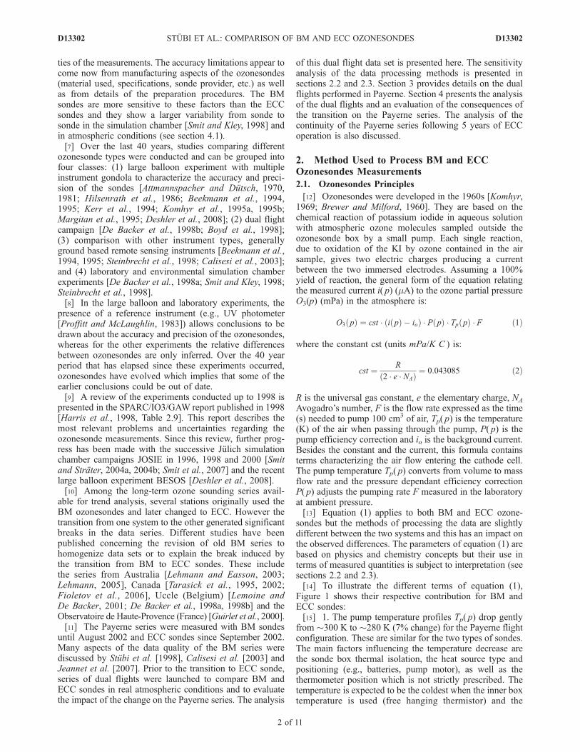
Figure 1 shows their respective contribution for BM andECC sondes:[15] 1. The pump temperature profiles Tp( p) drop gently

from �300 K to �280 K (7% change) for the Payerne flightconfiguration. These are similar for the two types of sondes.The main factors influencing the temperature decrease arethe sonde box thermal isolation, the heat source type andpositioning (e.g., batteries, pump motor), as well as thethermometer position which is not strictly prescribed. Thetemperature is expected to be the coldest when the inner boxtemperature is used (free hanging thermistor) and the

D13302 STUBI ET AL.: COMPARISON OF BM AND ECC OZONESONDES

2 of 11

D13302

warmest when the sensor is inserted in a hole drilled in thepump body. Some stations measure the inlet tube walltemperature assumed to be the same as the entering airtemperature.[16] 2. The background current io measured during the

laboratory preparation procedure is �0.03 mA (equivalent to��0.1 mPa in equation (1)) for the ECC sondes. Values of�0.1 mPa and �0.2 mPa were reported in Figure 1 (dia-monds) as percentage deviation of the mean ozone profileshown in Figure 1 (right). Contrary to the smooth pumptemperature curves, the background current produces thelargest deviation just below the tropopause where ozoneconcentration is low.[17] 3. The pump efficiency correction profiles P( p)

smoothly increase with decreasing pressure and predomi-nantly affect the upper part of the ozone profile. Thecorrection profiles are 2 to 3 times larger for BM sondesthan for ECC sondes.[18] After the calculation of the ozone profile with

equation (1), the sonde integrated profile is comparedto independent total ozone column measurements (e.g.,Dobson, Brewer) and a normalization factor is calculated.Applying this factor (Dobson/sonde) to the ozonesonde dataguarantees that the column calculated from the profile isconsistent with the other ozone column measurements.However, the partial ozone column above the balloon burstaltitude has to be evaluated and therefore a hypothesis onthe ozone distribution above burst altitude is needed.

2.2. Method Used to Process the BM Data

[19] The standardized operating procedures for the BMozonesonde, in particular the data processing, are defined inthe WMO Standard Operating Procedures (SOP) [Claude et

al., 1987]. Taking into account that neither the pumptemperature nor the background current were accuratelymeasured in the past, equation (1) was simplified by (1)setting the background current to zero, i0 = 0, and (2)assuming the pump temperature profile constant, Tp( p) =280 K. Assumption 1 implies that the calculated ozone maybe overestimated and a larger relative error is expected inthe troposphere where the ozone level is low. Assumption 2creates an imbalance of the tropospheric part of the profilecompared to the stratospheric part due to Tp( p) change of�7%. The two effects 1 and 2 tend to compensate eachother from the ground up to about 50 hPa as seen in Figure1 where the negative contribution of i0 (diamonds) cancelsthe positive contribution of Tp (circles). However, thebackground current depends strongly on the preparationprocedure and assumption 1 may have had a larger vari-ability than assumption 2 during the 40 years of ozonesounding activity.[20] A third assumption (assumption 3) concerns the

pump correction factor P. The metal/plastic assembly thatconstitutes the BM pumps leads to reduced efficiency at lowpressure. The BM pump requires that the piston be lubri-cated and this affects the pump leakage and possibly leadsto some ozone destruction. In the SOP, it is recommended touse the correction measured by Komhyr and Harris [1965]reproduced in Figure 1 which shows that this correction islarger than 20% below 8 hPa.[21] Figure 2 gives different pump efficiency correction

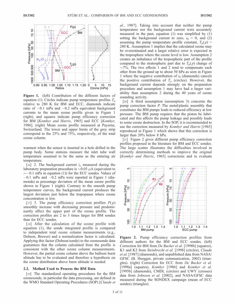
profiles proposed in the literature for BM and ECC sondes.The large scatter illustrates the difficulties involved incorrectly determining methods to improve the original[Komhyr and Harris, 1965] corrections and to evaluate

Figure 1. (left) Contribution of the different factors ofequation (1). Circles indicate pump temperature profiles Tprelative to 280 K for BM and ECC, diamonds indicateratio of �0.1 mPa and �0.2 mPa equivalent backgroundcurrents to the mean ozone profile given in Figure 1(right), and squares indicate pump efficiency correctionfor BM [Komhyr and Harris, 1965] and ECC [Komhyr,1986]. (right) Mean ozone profile measured at Payerne,Switzerland. The lower and upper limits of the grey stripcorrespond to the 25% and 75%, respectively, of the totalozone column.

Figure 2. Pump efficiency correction profiles fromdifferent authors for the BM and ECC sondes. (left)Correction for BM from De Backer et al. [1998b] (squares),K1 and K2 from Steinbrecht et al. [1998] (circles), Claudeet al. [1987] (diamonds), and unpublished data from NASA/GFSC (B. Hoegger, private communication, 2002) (trian-gles). (right) Correction for ECC from De Backer et al.[1998a] (squares), Komhyr [1986] and Komhyr et al.[1995b] (diamonds), CMDL (circles) and UWY (crosses)data from Johnson et al. [2002], and NASA/GFSC datameasured during the SONDEX campaign (mean of ECCsondes) (triangles).

D13302 STUBI ET AL.: COMPARISON OF BM AND ECC OZONESONDES

3 of 11

D13302

possible changes in the performance of the sondes over thelast four decades. Steinbrecht et al. [1998] proposed twoalternatives (see Figure 2, left): the first (K1) is based onlaboratory measurements and the second (K2) is an empir-ical correction deduced from the comparisons of measuredozone profiles by BM sondes and a colocated LIDAR. DeBacker et al. [1998a] derived a parametric correction profilebased on laboratory experiments. The curve (squares)presented in Figure 2 corresponds to the mean BM correc-tion profile given by De Backer et al. [1998b] (theirequation 1 with b = 1.56). Measurements (triangles) fromthe NASA/GFSC laboratory [Torres, 1981; B. Hoegger,unpublished data, 2002] show BM pump efficiency correc-tions very close to the original Komhyr and Harris [1965](diamonds) results. An additional temperature sensitivity ofthe pump efficiency correction P(Tp) was reported by DeBacker et al. [1998b]. However, the pump temperaturedecrease compensates for the increase of pump efficiencyassociated with this temperature change. The net effectcould be low sensitivity of the BM sondes to the pumptemperature.[22] The SOPs for BM sondes call for the normalization

of the profiles which reduces the sonde to sonde variabilityand correct the �10% low bias of the ozone columnevaluated from the BM profile. The largest contribution tothe column comes from the ozone layer. This is emphasizedin Figure 1 (right) by the grey strip that encompasses 50%of the total column. The residual column above the burstaltitude represents 10–20% of the whole column and it isevaluated by assuming a constant mixing ratio (CMR). TheCMR method was tested for the BM sondes by comparisonwith an ozone microwave radiometer [Calisesi et al., 2003].The error associated with the CMR method to evaluate theresidual column was estimated to be �3%.[23] The contribution of the background current to the

total column can be evaluated directly and it amounts toabout 5.4 DU/0.1 mPa (integration from 1000 hPa to 1 hPa).For a column of 300 DU, this corresponds to a contributionof 1.8%/0.1 mPa of background signal.[24] Table 1 summarizes the method and the parameters

of equation (1) used in the standard BM data processing andthe reference to other methods published in the literature hasbeen listed.

2.3. Method Used to Process ECC Ozonesonde Data

[25] Referring to equation (1), in ECC sondes the back-ground current i0 is measured at ground level prior to thelaunch and the pump temperature profile Tp( p) is recordedduring the flight. Therefore, the open questions regardingthe ECC sondes data processing are the hypothesis of analtitude-independent background current, the pump efficiency

correction profile and the normalization of the ozoneprofile.[26] Reid et al. [1996] compared ECC sondes with a

chemiluminescent analyzer in the troposphere and foundthat the measurements agree within 4% if a constantbackground current correction is applied. This was con-firmed in a dual flight at Payerne with ozone eliminatingcharcoal filters connected to the inlet tube of the two sondesduring the flight. Both BM and ECC signals gave a constantresidual signal within ±0.1 mPa. Therefore in this analysis,the background current is assumed to be constant during theascent.[27] ECC pumps are made of Teflon and their efficiency

is better than BM pumps at low pressure as seen in Figure 2(right). However there is a difference by a factor of 2between the different measurements reported in the literature.The recent JOSIE [Smit et al., 2007] and BESOS [Deshleret al., 2008] experiments show that the smaller pumpcorrections give better results compared to the UV photo-meter reference available in these two experiments. In thepresent study, the pump efficiency correction was selectedaccording to the manufacturer recommendation [Komhyr,1986].[28] The normalization was systematically applied to the

ECC data with the CMR method for the residual column tobe consistent with the BM data processing.

3. Measurements Used in This Study

3.1. Ozonesondes Measurements at Payerne

[29] Payerne is a small city located on the Swiss plateaubetween the Jura Mountains in the northwest and the Alpsin the southeast. The regular ozonesonde measurements,started in 1968, were done every Monday-Wednesday-Friday using the BM ozonesondes. The history of the BMseries and the methods to minimize inhomogeneities aredescribed by Jeannet et al. [2007]. The SOP for BM sondeswas applied for the preparation of all the BM sondes in hisstudy. The constant pump temperature was set to 280 Kinstead of 300 K specified in the SOP document [Claude etal., 1987] because it better reflected the Payerne flightconditions. This change does not affect the ozone profilebut the normalization factor increases by 7%.[30] The ECC sondes are provided by two manufacturers,

ENSCI and SPC companies. Recent experiments haveshown that the ECC sondes from the two providers produceslightly different results [Smit et al., 2007; Deshler et al.,2008]. Moreover, today they recommend using differentsensing solution concentration with their sondes.[31] The preparation procedure for ECC sondes follows

the recommendations of the manufacturer [Komhyr, 1986]

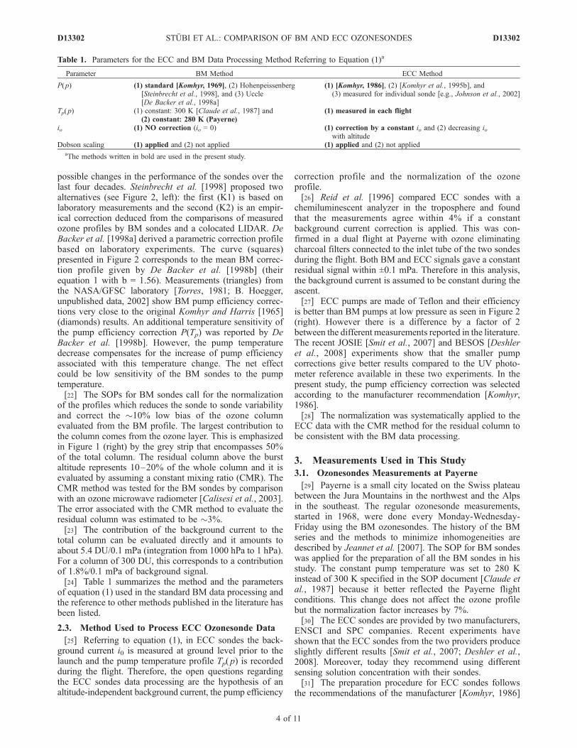
Table 1. Parameters for the ECC and BM Data Processing Method Referring to Equation (1)a

Parameter BM Method ECC Method

P(p) (1) standard [Komhyr, 1969], (2) Hohenpeissenberg[Steinbrecht et al., 1998], and (3) Uccle[De Backer et al., 1998a]

(1) [Komhyr, 1986], (2) [Komhyr et al., 1995b], and(3) measured for individual sonde [e.g., Johnson et al., 2002]

Tp(p) (1) constant: 300 K [Claude et al., 1987] and(2) constant: 280 K (Payerne)

(1) measured in each flight

io (1) NO correction (io = 0) (1) correction by a constant io and (2) decreasing iowith altitude

Dobson scaling (1) applied and (2) not applied (1) applied and (2) not appliedaThe methods written in bold are used in the present study.

D13302 STUBI ET AL.: COMPARISON OF BM AND ECC OZONESONDES

4 of 11

D13302

and the general practices of the ECC user community. Oneweek in advance of the flight, the sonde cell is cleaned witha high level of ozone air flow and then filled with thesensing solution. After this, the sonde is operated for asequence of three periods of 10 min: the first and thirdperiods with ‘‘clean air’’ and the second period with amixture of ‘‘clean air’’ and 0.2 ppm of ozone (�20 hPa).Then the cathode cell is completely filled with solution andthe sonde is stored for a week. On the day of flight after achange of the sensing solution, the conditioning cycle isrepeated about 3 h before the launch. The backgroundcurrent is measured at the end of the last sequence. Theseoperations are computer controlled in Payerne (except forthe change of solution) and therefore the preparation isreproducible from instrument to instrument. The pumptemperature is measured during the ascent with a thermom-eter placed in a hole drilled in the pump block.[32] The total ozone column from the Dobson located at

Arosa (210 km East of Payerne) is used for the normaliza-tion of both profiles. Under cloudy conditions, satellite dataare used instead.

3.2. Dual Flight Campaigns

[33] As already mentioned, since September 2002 theECC ozonesondes have been the operational instrumentsfor Payerne. To prepare the transition from BM to ECC, alarge number of dual flights were launched to compare thetwo sonde types in operational conditions. Dual flightsconsist of attaching two independent sondes under theaerological balloon assuring the sampling of the sameatmospheric environment, the two sondes being separatedby only a 2 m boom. The data acquisition systems of eachsonde are synchronized at the start which assures a timedifference smaller than 1 s. The actual sampling of the datais about 7 s, representing the time needed for a completecycle of measurements of temperature, pressure, humidityand two ozone parameters (current and pump temperature).The time elapsed since the launch is the more accuratecoordinate to compare the sondes’ data.

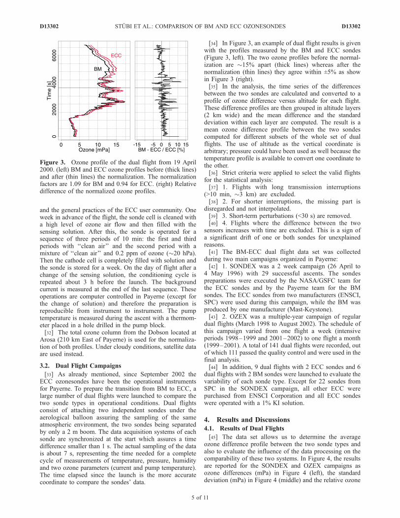
[34] In Figure 3, an example of dual flight results is givenwith the profiles measured by the BM and ECC sondes(Figure 3, left). The two ozone profiles before the normal-ization are �15% apart (thick lines) whereas after thenormalization (thin lines) they agree within ±5% as showin Figure 3 (right).[35] In the analysis, the time series of the differences

between the two sondes are calculated and converted to aprofile of ozone difference versus altitude for each flight.These difference profiles are then grouped in altitude layers(2 km wide) and the mean difference and the standarddeviation within each layer are computed. The result is amean ozone difference profile between the two sondescomputed for different subsets of the whole set of dualflights. The use of altitude as the vertical coordinate isarbitrary; pressure could have been used as well because thetemperature profile is available to convert one coordinate tothe other.[36] Strict criteria were applied to select the valid flights

for the statistical analysis:[37] 1. Flights with long transmission interruptions

(>10 min, �3 km) are excluded.[38] 2. For shorter interruptions, the missing part is

disregarded and not interpolated.[39] 3. Short-term perturbations (<30 s) are removed.[40] 4. Flights where the difference between the two

sensors increases with time are excluded. This is a sign ofa significant drift of one or both sondes for unexplainedreasons.[41] The BM-ECC dual flight data set was collected

during two main campaigns organized in Payerne:[42] 1. SONDEX was a 2 week campaign (26 April to

4 May 1996) with 29 successful ascents. The sondespreparations were executed by the NASA/GSFC team forthe ECC sondes and by the Payerne team for the BMsondes. The ECC sondes from two manufacturers (ENSCI,SPC) were used during this campaign, while the BM wasproduced by one manufacturer (Mast-Keystone).[43] 2. OZEX was a multiple-year campaign of regular

dual flights (March 1998 to August 2002). The schedule ofthis campaign varied from one flight a week (intensiveperiods 1998–1999 and 2001–2002) to one flight a month(1999–2001). A total of 141 dual flights were recorded, outof which 111 passed the quality control and were used in thefinal analysis.[44] In addition, 9 dual flights with 2 ECC sondes and 6

dual flights with 2 BM sondes were launched to evaluate thevariability of each sonde type. Except for 22 sondes fromSPC in the SONDEX campaign, all other ECC werepurchased from ENSCI Corporation and all ECC sondeswere operated with a 1% KI solution.

4. Results and Discussions

4.1. Results of Dual Flights

[45] The data set allows us to determine the averageozone difference profile between the two sonde types andalso to evaluate the influence of the data processing on thecomparability of these two systems. In Figure 4, the resultsare reported for the SONDEX and OZEX campaigns asozone differences (mPa) in Figure 4 (left), the standarddeviation (mPa) in Figure 4 (middle) and the relative ozone

Figure 3. Ozone profile of the dual flight from 19 April2000. (left) BM and ECC ozone profiles before (thick lines)and after (thin lines) the normalization. The normalizationfactors are 1.09 for BM and 0.94 for ECC. (right) Relativedifference of the normalized ozone profiles.

D13302 STUBI ET AL.: COMPARISON OF BM AND ECC OZONESONDES

5 of 11

D13302

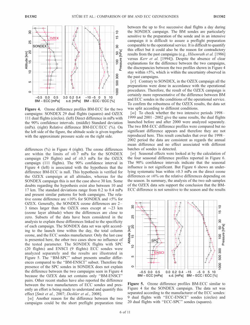
differences (%) in Figure 4 (right). The ozone differencesare within the limits of ±0.7 mPa for the SONDEXcampaign (29 flights) and of ±0.3 mPa for the OZEXcampaign (111 flights). The 90% confidence interval inFigure 4 (left) is associated with the hypothesis that thedifference BM-ECC is null. This hypothesis is verified forthe OZEX campaign at all altitudes, whereas for theSONDEX campaign this is not the case above 30 km. Somedoubts regarding the hypothesis exist also between 10 and17 km. The standard deviations range from 0.2 to 0.4 mPaand present similar patterns for both campaigns. The rela-tive ozone difference are ±10% for SONDEX and ±5% forOZEX. Generally, the SONDEX ozone differences are 2–3 times larger than the OZEX ones except at �23 km(ozone layer altitude) where the differences are close tozero. Subsets of the data have been considered in theanalysis to explain these differences linked to the specificityof each campaign. The SONDEX data set was split accord-ing to the launch time within the day, the total columnozone, and the ECC sondes manufacturer. Only the last caseis presented here, the other two cases show no influence ofthe tested parameter. The SONDEX flights with SPC(20 flights) and ENSCI (9 flights) ECC sondes wereanalyzed separately and the results are illustrated inFigure 5. The ‘‘BM-SPC’’ subset presents smaller differ-ences compared to the ‘‘BM-ENSCI’’ subset. Therefore thepresence of the SPC sondes in SONDEX does not explainthe difference between the two campaigns seen in Figure 4because the OZEX data set contains only ‘‘BM-ENSCI’’pairs. Other recent studies have also reported the differencebetween the two manufacturers of ECC sondes and pres-ently an effort is being made to understand and quantify thiseffect [Smit et al., 2007; Deshler et al., 2008].[46] Another reason for the difference between the two

campaigns could be the short preflight preparation time

between the up to five successive dual flights a day duringthe SONDEX campaign. The BM sondes are particularlysensitive to the preparation of the sonde and in an intensivecampaign it is difficult to assure a preflight preparationcomparable to the operational service. It is difficult to quantifythis effect but it could also be the reason for contradictoryresults from the past campaigns (e.g., Hilsenrath et al. [1986]versus Kerr et al. [1994]). Despite the absence of clearexplanations for the difference between the two campaigns,the discrepancies between the two profiles shown in Figure 4stay within ±5%, which is within the uncertainty observed inthe past campaigns.[47] Contrary to SONDEX, in the OZEX campaign all the

preparations were done in accordance with the operationalprocedures. Therefore, the result of the OZEX campaign iscertainly more representative of the difference between BMand ECC sondes in the conditions of the operational service.To confirm the robustness of the OZEX results, the data setwas split according to different conditions.[48] To check whether the two intensive periods 1998–

1999 and 2001–2002 give the same results, the dual flightslaunched before and after 2000 were analyzed separately.The two BM-ECC difference profiles were compared but nosignificant difference appears and therefore they are notreproduced here. This result concludes that over the 1998–2002 period the data are consistent as regards the annualmean difference and no effect associated with differentbatches of sondes is detected.[49] Seasonal effects were looked at by the calculation of

the four seasonal difference profiles reported in Figure 6.The 90% confidence intervals indicate that the seasonalinfluence is not significant. But Figure 6 shows an under-lying systematic bias within ±0.3 mPa on the direct ozonedifferences or ±6% on the relative differences depending onthe season. In summary, the analysis of the two sub samplesof the OZEX data sets support the conclusion that the BM-ECC difference is not sensitive to the season and the results

Figure 4. Ozone difference profiles BM-ECC for the twocampaigns: SONDEX 29 dual flights (squares) and OZEX111 dual flights (circles). (left) Direct difference in mPa withthe 90% confidence intervals. (middle) Standard deviation(mPa). (right) Relative difference BM-ECC/ECC (%). Onthe left side of the figure, the altitude scale is given togetherwith the approximate pressure scale on the right side.

Figure 5. Ozone difference profiles BM-ECC similar toFigure 4 for the SONDEX campaign. The data set wasseparated according to the manufacturer of the ECC sondes:9 dual flights with ‘‘ECC-ENSCI’’ sondes (circles) and20 dual flights with ‘‘ECC-SPC’’ sondes (squares).

D13302 STUBI ET AL.: COMPARISON OF BM AND ECC OZONESONDES

6 of 11

D13302

remained stable over the period 1998–2002 of the OZEXcampaign.[50] The confidence intervals are determined by the

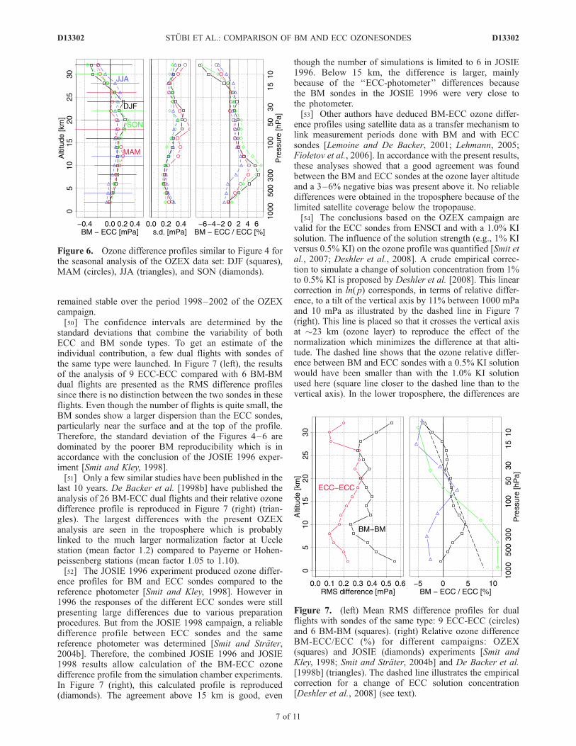
standard deviations that combine the variability of bothECC and BM sonde types. To get an estimate of theindividual contribution, a few dual flights with sondes ofthe same type were launched. In Figure 7 (left), the resultsof the analysis of 9 ECC-ECC compared with 6 BM-BMdual flights are presented as the RMS difference profilessince there is no distinction between the two sondes in theseflights. Even though the number of flights is quite small, theBM sondes show a larger dispersion than the ECC sondes,particularly near the surface and at the top of the profile.Therefore, the standard deviation of the Figures 4–6 aredominated by the poorer BM reproducibility which is inaccordance with the conclusion of the JOSIE 1996 exper-iment [Smit and Kley, 1998].[51] Only a few similar studies have been published in the

last 10 years. De Backer et al. [1998b] have published theanalysis of 26 BM-ECC dual flights and their relative ozonedifference profile is reproduced in Figure 7 (right) (trian-gles). The largest differences with the present OZEXanalysis are seen in the troposphere which is probablylinked to the much larger normalization factor at Ucclestation (mean factor 1.2) compared to Payerne or Hohen-peissenberg stations (mean factor 1.05 to 1.10).[52] The JOSIE 1996 experiment produced ozone differ-

ence profiles for BM and ECC sondes compared to thereference photometer [Smit and Kley, 1998]. However in1996 the responses of the different ECC sondes were stillpresenting large differences due to various preparationprocedures. But from the JOSIE 1998 campaign, a reliabledifference profile between ECC sondes and the samereference photometer was determined [Smit and Strater,2004b]. Therefore, the combined JOSIE 1996 and JOSIE1998 results allow calculation of the BM-ECC ozonedifference profile from the simulation chamber experiments.In Figure 7 (right), this calculated profile is reproduced(diamonds). The agreement above 15 km is good, even

though the number of simulations is limited to 6 in JOSIE1996. Below 15 km, the difference is larger, mainlybecause of the ‘‘ECC-photometer’’ differences becausethe BM sondes in the JOSIE 1996 were very close tothe photometer.[53] Other authors have deduced BM-ECC ozone differ-

ence profiles using satellite data as a transfer mechanism tolink measurement periods done with BM and with ECCsondes [Lemoine and De Backer, 2001; Lehmann, 2005;Fioletov et al., 2006]. In accordance with the present results,these analyses showed that a good agreement was foundbetween the BM and ECC sondes at the ozone layer altitudeand a 3–6% negative bias was present above it. No reliabledifferences were obtained in the troposphere because of thelimited satellite coverage below the tropopause.[54] The conclusions based on the OZEX campaign are

valid for the ECC sondes from ENSCI and with a 1.0% KIsolution. The influence of the solution strength (e.g., 1% KIversus 0.5% KI) on the ozone profile was quantified [Smit etal., 2007; Deshler et al., 2008]. A crude empirical correc-tion to simulate a change of solution concentration from 1%to 0.5% KI is proposed by Deshler et al. [2008]. This linearcorrection in ln(p) corresponds, in terms of relative differ-ence, to a tilt of the vertical axis by 11% between 1000 mPaand 10 mPa as illustrated by the dashed line in Figure 7(right). This line is placed so that it crosses the vertical axisat �23 km (ozone layer) to reproduce the effect of thenormalization which minimizes the difference at that alti-tude. The dashed line shows that the ozone relative differ-ence between BM and ECC sondes with a 0.5% KI solutionwould have been smaller than with the 1.0% KI solutionused here (square line closer to the dashed line than to thevertical axis). In the lower troposphere, the differences are

Figure 6. Ozone difference profiles similar to Figure 4 forthe seasonal analysis of the OZEX data set: DJF (squares),MAM (circles), JJA (triangles), and SON (diamonds).

Figure 7. (left) Mean RMS difference profiles for dualflights with sondes of the same type: 9 ECC-ECC (circles)and 6 BM-BM (squares). (right) Relative ozone differenceBM-ECC/ECC (%) for different campaigns: OZEX(squares) and JOSIE (diamonds) experiments [Smit andKley, 1998; Smit and Strater, 2004b] and De Backer et al.[1998b] (triangles). The dashed line illustrates the empiricalcorrection for a change of ECC solution concentration[Deshler et al., 2008] (see text).

D13302 STUBI ET AL.: COMPARISON OF BM AND ECC OZONESONDES

7 of 11

D13302

larger but the crude correction from Deshler et al. [2008] isnot better than ±5% in the troposphere.[55] The overestimation of the ozone of the 1.0% KI

solution compared to 0.5% KI solution was also confirmedat different ozone sounding stations where dual flight‘‘ECC-0.5%’’–‘‘ECC-1.0%’’ campaigns were organized.The results of these campaigns have been analyzed and aseparate publication is under preparation.[56] The results of the analysis presented in this para-

graph are based on the data processing discussed in sections2.2 and 2.3. It is necessary to quantify the influence of theprocessing by doing a sensitivity analysis that will bepresented in the next section.

4.2. Sensitivity Analysis of the Method Used toProcess BM Data

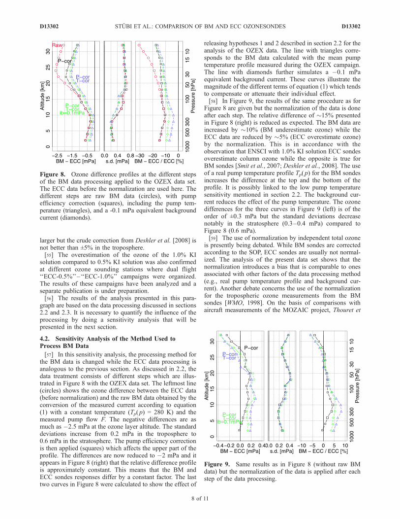
[57] In this sensitivity analysis, the processing method forthe BM data is changed while the ECC data processing isanalogous to the previous section. As discussed in 2.2, thedata treatment consists of different steps which are illus-trated in Figure 8 with the OZEX data set. The leftmost line(circles) shows the ozone difference between the ECC data(before normalization) and the raw BM data obtained by theconversion of the measured current according to equation(1) with a constant temperature (Tp(p) = 280 K) and themeasured pump flow F. The negative differences are asmuch as �2.5 mPa at the ozone layer altitude. The standarddeviations increase from 0.2 mPa in the troposphere to0.6 mPa in the stratosphere. The pump efficiency correctionis then applied (squares) which affects the upper part of theprofile. The differences are now reduced to �2 mPa and itappears in Figure 8 (right) that the relative difference profileis approximately constant. This means that the BM andECC sondes responses differ by a constant factor. The lasttwo curves in Figure 8 were calculated to show the effect of

releasing hypotheses 1 and 2 described in section 2.2 for theanalysis of the OZEX data. The line with triangles corre-sponds to the BM data calculated with the mean pumptemperature profile measured during the OZEX campaign.The line with diamonds further simulates a �0.1 mPaequivalent background current. These curves illustrate themagnitude of the different terms of equation (1) which tendsto compensate or attenuate their individual effect.[58] In Figure 9, the results of the same procedure as for

Figure 8 are given but the normalization of the data is doneafter each step. The relative difference of �15% presentedin Figure 8 (right) is reduced as expected. The BM data areincreased by �10% (BM underestimate ozone) while theECC data are reduced by �5% (ECC overestimate ozone)by the normalization. This is in accordance with theobservation that ENSCI with 1.0% KI solution ECC sondesoverestimate column ozone while the opposite is true forBM sondes [Smit et al., 2007; Deshler et al., 2008]. The useof a real pump temperature profile Tp(p) for the BM sondesincreases the difference at the top and the bottom of theprofile. It is possibly linked to the low pump temperaturesensitivity mentioned in section 2.2. The background cur-rent reduces the effect of the pump temperature. The ozonedifferences for the three curves in Figure 9 (left) is of theorder of ±0.3 mPa but the standard deviations decreasenotably in the stratosphere (0.3–0.4 mPa) compared toFigure 8 (0.6 mPa).[59] The use of normalization by independent total ozone

is presently being debated. While BM sondes are correctedaccording to the SOP, ECC sondes are usually not normal-ized. The analysis of the present data set shows that thenormalization introduces a bias that is comparable to onesassociated with other factors of the data processing method(e.g., real pump temperature profile and background cur-rent). Another debate concerns the use of the normalizationfor the tropospheric ozone measurements from the BMsondes [WMO, 1998]. On the basis of comparisons withaircraft measurements of the MOZAIC project, Thouret et

Figure 8. Ozone difference profiles at the different stepsof the BM data processing applied to the OZEX data set.The ECC data before the normalization are used here. Thedifferent steps are raw BM data (circles), with pumpefficiency correction (squares), including the pump tem-perature (triangles), and a -0.1 mPa equivalent backgroundcurrent (diamonds).

Figure 9. Same results as in Figure 8 (without raw BMdata) but the normalization of the data is applied after eachstep of the data processing.

D13302 STUBI ET AL.: COMPARISON OF BM AND ECC OZONESONDES

8 of 11

D13302

al. [1998] questioned the use of normalization for tropo-spheric ozone. Another recent comparison between aircraftdata and BM data from Payerne and Hohenpeissenbergprovides evidence that the response time of the BM sensorsneeds to be taken into account and that agreement is betterwhen using normalized ozonesonde measurements [SchnadtPoberaj et al., 2007].[60] From the discussion of sections 2.2 and 2.3, it follows

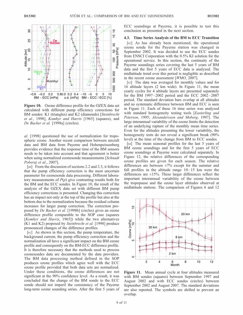
that the pump efficiency correction is the most uncertainparameter for ozonesonde data processing. Different labora-tory measurements of P(p) give contrasting results both forthe BM and the ECC sondes. In Figure 10, the result of theanalysis of the OZEX data set with different BM pumpefficiency corrections is presented. Changing this correctionhas an impact not only at the top of the profile but also at thebottom due to the normalization because the residual columnincreases for larger pump correction. The correction pro-posed by De Backer et al. [1998b] (circles) gives an ozonedifference profile comparable to the SOP case (squares[Komhyr and Harris, 1965]) while the two alternatives(K1 and K2) proposed by Steinbrecht et al. [1998] producepronounced changes of the difference profiles.[61] As shown in this section, the pump temperature, the

background current, the pump efficiency correction and thenormalization all have a significant impact on the BM ozoneprofile and consequently on the BM-ECC difference profile.It is therefore necessary that the methods used to processozonesondes data are documented by the data providers.The BM data processing method defined in the SOPproduces ozone profiles which agree well with the ECCozone profile provided that both data sets are normalized.Under these conditions, the ozone differences are notsignificant at the 90% confidence level. As a result, it wasconcluded that the change of the BM sonde to the ECCsonde should not imperil the consistency of the Payernelong-term ozone sounding series. After the first 5 years of

ECC soundings at Payerne, it is possible to test thisconclusion as presented in the next section.

4.3. Time Series Analysis of the BM to ECC Transition

[62] As has already been mentioned, the operationalozone sonde for the Payerne station was changed inSeptember 2002. It was decided to use the ECC sondesfrom ENSCI Corporation with the 0.5% KI solution for theoperational service. In this section, the continuity of thePayerne soundings series covering the last 5 years of BMdata and the first 5 years of ECC data is analyzed. Themidlatitude trend over this period is negligible as describedin the recent ozone assessment [WMO, 2007].[63] The data was averaged for monthly values and for

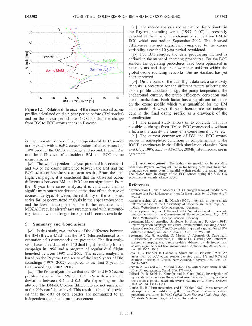
16 altitude layers (2 km wide). In Figure 11, the meanyearly cycles for 4 altitude layers are presented separatelyfor the BM 1997–2002 period and the ECC 2002–2007period. The standard deviation bars overlap at all altitudesand no systematic difference between BM and ECC is seenin Figure 11. Each of these 16 time series was analyzedwith standard homogeneity testing tools [Easterling andPeterson, 1995; Alexandersson and Moberg, 1997]. Thelarge interannual variability of the ozone limits the detectionof an underlying rupture of the monthly mean time series.Even for the altitudes presenting the lower variability, thehomogeneity tests do not reveal a significant break (90%level) at the time of the change from BM to ECC sondes.[64] The mean seasonal profiles for the last 5 years of

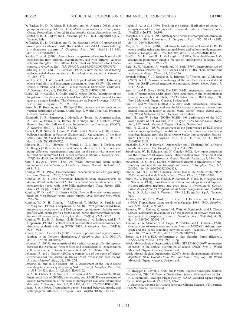
BM ozone soundings and for the first 5 years of ECCozone soundings at Payerne were calculated separately. InFigure 12, the relative differences of the correspondingozone profiles are given for each season. The relativedifferences are between ±7% except for the summer andfall profiles in the altitude range 10–15 km were thedifferences are ±15%. These larger differences reflect theimportant interannual variability of the ozone betweenthe tropopause and the ozone layer altitudes observed atmidlatitude stations. The comparison of Figures 6 and 12

Figure 10. Ozone difference profile for the OZEX data setcalculated with different pump efficiency corrections forBM sondes: K1 (triangles) and K2 (diamonds) [Steinbrechtet al., 1998], Komhyr and Harris [1965] (squares), andDe Backer et al. [1998a] (circles).

Figure 11. Mean annual cycle at four altitudes measuredwith BM sondes (squares) between September 1997 andAugust 2002 and with ECC sondes (circles) betweenSeptember 2002 and August 2007. The standard deviationsare also reported. The symbols are shifted to prevent anoverlap.

D13302 STUBI ET AL.: COMPARISON OF BM AND ECC OZONESONDES

9 of 11

D13302

is inappropriate because first, the operational ECC sondesare operated with a 0.5% concentration solution instead of1.0% used for the OZEX campaign and second, Figure 12 isnot the difference of coincident BM and ECC ozonemeasurements.[65] The two independent analyses presented in sections 4.1

and 4.3 of the ozone difference between the BM and theECC ozonesondes show consistent results. From the dualflight campaigns, it is concluded that the observed ozonedifferences between BM and ECC are not significant. Fromthe 10 year time series analysis, it is concluded that nosignificant ruptures are detected at the time of the change ofozonesonde type. However, the reliability of the combinedseries for long-term trend analysis in the upper troposphereand the lower stratosphere will be further evaluated withMOZAIC regular aircraft measurements and with surround-ing stations when a longer time period becomes available.

5. Summary and Conclusions

[66] In this study, two analyses of the difference betweenthe BM (Brewer-Mast) and the ECC (electrochemical con-centration cell) ozonesondes are presented. The first analy-sis is based on a data set of 140 dual flights resulting from acampaign in 1996 and a program of regular dual flightslaunched between 1998 and 2002. The second analysis isbased on the Payerne time series of the last 5 years of BMsoundings (1997–2002) compared to the first 5 years ofECC soundings (2002–2007).[67] The first analysis shows that the BM and ECC ozone

profiles agree within ±5% or ±0.3 mPa with a standarddeviation between 0.2 and 0.5 mPa depending on thealtitude. The BM-ECC ozone differences are not significantat the 90% confidence level. This result is obtained provid-ed that the data of both sondes are normalized to anindependent ozone column measurement.

[68] The second analysis shows that no discontinuity inthe Payerne sounding series (1997–2007) is presentlydetected at the time of the change of sonde from BM toECC which occurred in September 2002. The observeddifferences are not significant compared to the ozonevariability over the 10 year period considered.[69] For BM sondes, the data processing method is

defined in the standard operating procedures. For the ECCsondes, the operating procedures have been optimized inrecent years and they are now rather uniform within theglobal ozone sounding networks. But no standard has yetbeen approved.[70] On the basis of the dual flight data set, a sensitivity

analysis is presented for the different factors affecting theozone profile calculation, e.g., the pump temperature, thebackground current, the pump efficiency correction andthe normalization. Each factor has a significant influenceon the ozone profile which was quantified for the BMozonesondes. However, these influences are not indepen-dent in the final ozone profile as a drawback of thenormalization.[71] The present study allows us to conclude that it is

possible to change from BM to ECC ozonesondes withoutaffecting the quality the long-term ozone sounding series.[72] The current comparison of BM and ECC ozone-

sondes in atmospheric conditions is complementary to theJOSIE experiments in the Julich simulation chamber [Smitand Kley, 1998; Smit and Strater, 2004b]. Both results are inagreement.

[73] Acknowledgments. The authors are grateful to the soundingteam from Payerne Aerological Station for having performed these dualsoundings over many years in parallel to their regular operational duties.The NASA team in charge of the ECC sondes during the SONDEXexperiment is warmly acknowledged.

ReferencesAlexandersson, H., and A. Moberg (1997), Homogenization of Swedish tem-perature data. Part I: Homogeneity test for linear trends, Int. J. Climatol., 17,25–34.

Attmannspacher, W., and H. Dutsch (1970), International ozone sondeintercomparison at the Observatory of Hohenpeissenberg, Rep. 120,Dtsch. Wetterdienste, Hohenpeissenberg, Germany.

Attmannspacher, W., and H. Dutsch (1981), 2nd international ozone sondeintercomparison at the Observatory of Hohenpeissenberg, Rep. 157,Dtsch. Wetterdienste, Hohenpeissenberg, Germany.

Beekmann, M., G. Ancellet, G. Megie, H. Smit, and D. Kley (1994),Intercomparison campaign for vertical ozone profiles including electro-chemical sondes of ECC and Brewer-Mast type and a ground based UV-differential absorption lidar, J. Atmos. Chem., 19, 259–288.

Beekmann, M., G. Ancellet, D. Martin, C. Abonnel, G. Duverneuil,F. Eidelimen, P. Bessemoulin, N. Fritz, and E. Gizard (1995), Intercom-parison of tropospheric ozone profiles obtained by electrochemicalsondes, a ground based lidar and airborne UV-photometer, Atmos. Envir-on., 29, 1027–1042.

Boyd, I., G. Bodeker, B. Connor, D. Swart, and E. Brinksma (1998), Anassessment of ECC ozone sondes operated using 1% and 0.5% KIcathode solutions at Lauder, New Zealand, Geophys. Res. Lett., 25,2409–2412.

Brewer, A. W., and J. R. Milford (1960), The Oxford-Kew ozone sonde,Proc. R. Soc. London, Ser. A, 256, 470–495.

Calisesi, Y., R. Stubi, N. Kampfer, and P. Viatte (2003), Investigation ofsystematic uncertainty in Brewer-Mast ozone soundings using observa-tions from a ground-based microwave radiometer, J. Atmos. OceanicTechnol., 20, 1543–1551.

Claude, H., R. Hartmannsgruber, and U. Kohler (1987), Measurement ofatmospheric ozone profiles using the Brewer/Mast sonde—Preparation,procedure, evaluation, inWMO Global Ozone Res. and Monit. Proj., Rep.17, World Meteorol. Organ., Geneva, Switzerland.

Figure 12. Relative difference of the mean seasonal ozoneprofiles calculated on the 5 year period before (BM sondes)and on the 5 year period after (ECC sondes) the changefrom BM to ECC ozonesondes in Payerne.

D13302 STUBI ET AL.: COMPARISON OF BM AND ECC OZONESONDES

10 of 11

D13302

De Backer, H., D. De Muer, E. Schoubs, and M. Allaart (1998a), A newpump correction profile for Brewer-Mast ozonesondes, in AtmosphericOzone, Proceedings of the XVIII Quadrennial Ozone Symposium, vol. 2,edited by R. D. Bojkov and G. Visconti, pp. 891–894, Edigrafital S.p.A.,Teramo, Italy.

De Backer, H., D. De Muer, and G. De Sadelaer (1998b), Comparison ofozone profiles obtained with Brewer-Mast and Z-ECC sensors duringsimultaneous ascents, J. Geophys. Res., 103, 19,641 – 19,648,doi:10.1029/98JD01711.

Deshler, T., et al. (2008), Atmospheric comparison of electrochemical cellozonesondes from different manufacturers, and with different cathodesolution strengths: The Balloon Experiment on Standards for Ozone-sondes, J. Geophys. Res., 113, D04307, doi:10.1029/2007JD008975.

Easterling, D. R., and T. C. Peterson (1995), A new method for detectingundocumented discontinuities in climatological series, Int. J. Climatol.,15, 368–377.

Fioletov, V. E., D. W. Tarasick, and I. Petropavlovskikh (2006), Estimatingozone variability and instrument uncertainties from SBUV (/2), ozone-sonde, Umkehr, and SAGE II measurements: Short-term variations,J. Geophys. Res., 111, D02305, doi:10.1029/2005JD006340.

Guirlet, M., P. Keckhut, S. Godin, and G. Megie (2000), Description of thelong-term ozone data series obtained from different instrumental techni-ques at a single location: The Observatory de Haute-Provence (43.9�N,5.7�E), Ann. Geophys., 18, 1325–1339.

Harris, N., R. Hudson, and C. Phillips (1998), Assessment of trends in thevertical distribution of ozone, SPARC Rep. 1, World Clim. Res. Program,Geneva, Switzerland.

Hilsenrath, E., R. Hagemeyer, J. Mentall, A. Torres, W. Attmannspacher,A. Bass, W. Evans, R. A. Barnes, W. Komhyr, and D. Robbins (1986),Results from the Balloon Ozone Intercomparison Campaign (BOIC),J. Geophys. Res., 91, 13,137–13,152.

Jeannet, P., R. Stubi, G. Levrat, P. Viatte, and J. Staehelin (2007), Ozoneballoon soundings at Payerne (Switzerland): Reevaluation of the timeseries 1967-2002 and trend analysis, J. Geophys. Res., 112, D11302,doi:10.1029/2005JD006862.

Johnson, B. J., S. J. Oltmans, H. Vomel, H. G. J. Smit, T. Deshler, andC. Kroger (2002), Electrochemical concentration cell (ECC) ozonesondepump efficiency measurements and tests on the sensitivity to ozone ofbuffered and unbuffered ECC sensor cathode solutions, J. Geophys. Res.,107(D19), 4393, doi:10.1029/2001JD000557.

Kerr, J. B., et al. (1994), The 1991 WMO international ozone sondesintercomparison at Vanscoy, Canada, J. Atmos. Oceanic Technol., 32,685–716.

Komhyr, W. D. (1969), Electrochemical concentration cells for gas analy-sis, Ann. Geophys., 25(1), 203–210.

Komhyr, W. D. (1986), Operations handbook-ozone measurements to40-km altitude with model 4A electrochemical concentration cell (ECC)ozonesondes (used with 1680-MHz radiosondes), Tech. Memo. ERLARL-149, 49 pp., NOAA, Boulder, Colo.

Komhyr, W. D., and T. B. Harris (1965), Note on flow rate measurementsmade on Mast-Brewer ozone sensor pumps, Mon. Weather Rev., 93(4),267–268.

Komhyr, W. D., B. Connor, I. McDermid, T. McGee, A. Parrish, andJ. Margitan (1995a), Comparison of STOIC 1989 ground-based lidar,microwave spectrometer, and Dobson spectrophotometer Umkehr ozoneprofiles with ozone profiles from balloon-borne electrochemical concen-tration cell ozonesondes, J. Geophys. Res., 100(D5), 9273–9282.

Komhyr, W. D., R. A. Barnes, G. B. Brothers, J. A. Lathrop, and D. P.Opperman (1995b), Electrochemical concentration cell ozonesondes per-formance evaluation during STOIC 1989, J. Geophys. Res., 100(D5),9231–9244.

Krizan, P., and J. Lastovicka (2005), Trends in positive and negative ozonelaminae in the Northern Hemisphere, J. Geophys. Res., 110, D10107,doi:10.1029/2004JD005477.

Lehmann, P. (2005), An estimate of the vertical ozone profile discrepancybetween the Australian Brewer-Mast and electrochemical concentrationcell ozonesondes, J. Atmos. Oceanic Technol., 22, 1864–1874.

Lehmann, P., and J. Easson (2003), A comparison of the pump efficiencycorrections for the Australian Brewer-Mast ozonesonde data record,J. Aust. Meteorol. Mag., 52, 259–264.

Lemoine, R., and H. De Backer (2001), Assessment of the Uccle ozonesounding time series quality using SAGE II dat, J. Geophys. Res., 106,14,515–14,524, doi:10.1029/2001JD900122.

Liu, X., K. Chance, C. E. Sioris, T. P. Kurosu, and M. J. Newchurch (2006),Intercomparison of GOME, ozonesonde, and SAGE II measurements ofozone: Demonstration of the need to homogenize available ozonesondedata sets, J. Geophys. Res., 111, D14305, doi:10.1029/2005JD006718.

Logan, J. A. (1985), Tropospheric ozone: Seasonal behavior, trends, andanthropogenic influence, J. Geophys. Res., 90(D6), 10,463–10,482.

Logan, J. A., et al. (1999), Trends in the vertical distribution of ozone: Acomparison of two analyses of ozonesonde data, J. Geophys. Res.,104(D21), 26,373–26,399.

Margitan, J. J., et al. (1995), Stratospheric ozone intercomparison campaign(STOIC) 1989: Overview, J. Geophys. Res., 100, 9193 – 9208,doi:10.1029/95JD00509.

Meijer, Y. J., et al. (2004), Pole-to-pole validation of Envisat GOMOSozone profiles using data from ground-based and balloon sonde measure-ments, J. Geophys. Res., 109, D23305, doi:10.1029/2004JD004834.

Proffitt, M. H., and R. J. McLaughlin (1983), Fast dual-beam UV-absorption photometer suitable for use on stratospheric balloons, Rev.Sci. Instrum., 54, 1719–1728.

Reid, S., G. Vaughan, A. Marsh, and H. Smit (1996), Intercomparison ofozone measurements by ECC sondes and BENDIX chemiluminescentanalyser, J. Atmos. Chem., 25, 215–226.

Schnadt Poberaj, C., J. Staehelin, D. Brunner, V. Thouret, and V. Mohnen(2007), A UT/LS ozone climatology of the nineteen seventies deducedfrom the GASP aircraft measurement program, Atmos. Chem. Phys., 7,5917–5936.

Smit, H., and D. Kley (1998), The 1996 WMO international intercompar-ison of ozonesondes under quasi flight conditions in the environmentalsimulation chamber at Julich, WMO Global Atmos. Watch Rep., 130,World Meteorol. Organ., Geneva, Switzerland.

Smit, H., and W. Strater (2004a), The 2000 WMO international intercom-parison of operating procedures for ECC-ozone sondes at the environ-mental simulation facility at Julich, WMO Global Atmos. Watch Rep.,158, World Meteorol. Organ., Geneva, Switzerland.

Smit, H., and W. Strater (2004b), JOSIE-1998 performance of the ECCozone sondes of SPC-6A and ENSCI-Z type, WMO Global Atmos. WatchRep., 157, World Meteorol. Organ., Geneva, Switzerland.

Smit, H. G., et al. (2007), Assessment of the performance of ECC-ozonesondes under quasi-flight conditions in the environmental simulationchamber: Insights from the Julich Ozone Sonde Intercomparison Experi-ment (JOSIE), J. Geophys. Res., 112, D19306, doi:10.1029/2006JD007308.

Staehelin, J., N. R. P. Harris, C. Appenzeller, and J. Eberhard (2001), Ozonetrends: A review, Rev. Geophys., 32(2), 231–290.

Steinbrecht, W., R. Schwarz, and H. Claude (1998), New pump correctionfor the Brewer-Mast ozone sonde: Determination from experiment andinstrument intercomparisons, J. Atmos. Oceanic Technol., 15, 144–156.

Stevenson, D. S., et al. (2006), Multimodel ensemble simulations of pre-sent-day and near-future tropospheric ozone, J. Geophys. Res., 111,D08301, doi:10.1029/2005JD006338.

Streibel, M., et al. (2006), Chemical ozone loss in the Arctic winter 2002/2003 determined with Match, Atmos. Chem. Phys., 6, 2783–2792.

Stubi, R., V. Bugnion, M. Giroud, P. Jeannet, P. Viatte, B. Hoegger, andJ. Staehelin (1998), Long term ozone balloon soundings series at Payerne:Homogenization methods and problems, in Atmospheric Ozone,Proceedings of the XVIII Quadrennial Ozone Symposium, vol. 2, editedby R. D. Bojkov and G. Visconti, 179–182, Edigrafital S.p.A., Teramo,Italy.

Tarasick, D. W., D. I. Wardle, J. B. Kerr, J. J. Bellefieur, and J. Davies(1995), Tropospheric ozone trends over Canada: 1980–1993, Geophys.Res. Lett., 22(4), 409–412.

Tarasick, W., J. Davies, K. Anlauf, M. Watt, W. Steinbrecht, and J. Claude(2002), Laboratory investigations of the response of Brewer-Mast ozo-nesondes to tropospheric ozone, J. Geophys. Res., 107(D16), 4308,doi:10.1029/2001JD001167.

Thouret, V., A. Marenco, J. A. Logan, P. Nedelec, and C. Grouhel (1998),Comparisons of ozone measurements from the MOZAIC airborne pro-gram and the ozone sounding network at eight locations, J. Geophys.Res., 103, 25,695–25,720, doi:10.1029/98JD02243.

Torres, A. (1981), ECC performance at high altitudes: Pump efficiency,NASA Tech. Memo., TM93290, 10 pp.

World Meteorological Organization (1998), SPARC-IOC-GAW assessmentof trends in the vertical distribution of ozone, SPARC Rep. 1, WorldMeteorol. Organ., Geneva, Switzerland.

World Meteorological Organization (2007), Scientific assessment of ozonedepletion: 2006, Global Ozone Res. and Monit. Proj. Rep. 50, WorldMeteorol. Organ., Geneva, Switzerland.

�����������������������B.Hoegger, G. Levrat, R. Stubi, and P. Viatte, PayerneAerological Station,

MeteoSwiss, CH-1530 Payerne, Switzerland. (rene.stubi@meteoswiss.ch)F. J. Schmidlin, Wallops Flight Facility, NASA Goddard Space Flight

Center, Wallops Island, VA 23337, USA.J. Staehelin, Institute for Atmospheric and Climate Science, ETH Zurich,

CH-8092 Zurich, Switzerland.

D13302 STUBI ET AL.: COMPARISON OF BM AND ECC OZONESONDES

11 of 11

D13302