Improving the Estimation of Above Ground Biomass Using Dual Polarimetric PALSAR and ETM+ Data in the...
23
Remote Sens. 2014, 6, 3693-3715; doi:10.3390/rs6053693 remote sensing ISSN 2072-4292 www.mdpi.com/journal/remotesensing Article Improving the Estimation of Above Ground Biomass Using Dual Polarimetric PALSAR and ETM+ Data in the Hyrcanian Mountain Forest (Iran) Sara Attarchi 1, * and Richard Gloaguen 1,2 1 Remote Sensing Group, Institute of Geology, TU Bergakademie Freiberg (TUBAF), Bernhard-von-Cotta-Str. 2, D-09599 Freiberg, Germany 2 Remote Sensing Group, Helmholtz Institute Freiberg of Resource Technology, Halsbruecker Str. 34, D-09599 Freiberg, Germany; E-Mail: [email protected] * Author to whom correspondence should be addressed; E-Mail: [email protected]; Tel.: +49-373-139-2806; Fax: +49-373-139-3599. Received: 16 December 2013; in revised form: 17 April 2014 / Accepted: 18 April 2014 / Published: 28 April 2014 Abstract: The objective of this study is to develop models based on both optical and L-band Synthetic Aperture Radar (SAR) data for above ground dry biomass (hereafter AGB) estimation in mountain forests. We chose the site of the Loveh forest, a part of the Hyrcanian forest for which previous attempts to estimate AGB have proven difficult. Uncorrected ETM+ data allow a relatively poor AGB estimation, because topography can hinder AGB estimation in mountain terrain. Therefore, we focused on the use of atmospherically and topographically corrected multispectral Landsat ETM+ and Advanced Land-Observing Satellite/Phased Array L-band Synthetic Aperture Radar (ALOS/PALSAR) to estimate forest AGB. We then evaluated 11 different multiple linear regression models using different combinations of corrected spectral and PolSAR bands and their derived features. The use of corrected ETM+ spectral bands and GLCM textures improves AGB estimation significantly (adjusted R 2 = 0.59; RMSE = 31.5 Mg/ha). Adding SAR backscattering coefficients as well as PolSAR features and textures increase substantially the accuracy of AGB estimation (adjusted R 2 = 0.76; RMSE = 25.04 Mg/ha). Our results confirm that topographically and atmospherically corrected data are indispensable for the estimation of mountain forest’s physical properties. We also demonstrate that only the joint use of PolSAR and multispectral data allows a good estimation of AGB in those regions. OPEN ACCESS
Transcript of Improving the Estimation of Above Ground Biomass Using Dual Polarimetric PALSAR and ETM+ Data in the...

Remote Sens. 2014, 6, 3693-3715; doi:10.3390/rs6053693
remote sensing ISSN 2072-4292
www.mdpi.com/journal/remotesensing
Article
Improving the Estimation of Above Ground Biomass Using Dual
Polarimetric PALSAR and ETM+ Data in the Hyrcanian
Mountain Forest (Iran)
Sara Attarchi 1,
* and Richard Gloaguen 1,2
1 Remote Sensing Group, Institute of Geology, TU Bergakademie Freiberg (TUBAF),
Bernhard-von-Cotta-Str. 2, D-09599 Freiberg, Germany 2
Remote Sensing Group, Helmholtz Institute Freiberg of Resource Technology, Halsbruecker Str. 34,
D-09599 Freiberg, Germany; E-Mail: [email protected]
* Author to whom correspondence should be addressed; E-Mail: [email protected];
Tel.: +49-373-139-2806; Fax: +49-373-139-3599.
Received: 16 December 2013; in revised form: 17 April 2014 / Accepted: 18 April 2014 /
Published: 28 April 2014
Abstract: The objective of this study is to develop models based on both optical and L-band
Synthetic Aperture Radar (SAR) data for above ground dry biomass (hereafter AGB)
estimation in mountain forests. We chose the site of the Loveh forest, a part of the
Hyrcanian forest for which previous attempts to estimate AGB have proven difficult.
Uncorrected ETM+ data allow a relatively poor AGB estimation, because topography can
hinder AGB estimation in mountain terrain. Therefore, we focused on the use of
atmospherically and topographically corrected multispectral Landsat ETM+ and Advanced
Land-Observing Satellite/Phased Array L-band Synthetic Aperture Radar (ALOS/PALSAR)
to estimate forest AGB. We then evaluated 11 different multiple linear regression models
using different combinations of corrected spectral and PolSAR bands and their derived
features. The use of corrected ETM+ spectral bands and GLCM textures improves AGB
estimation significantly (adjusted R2 = 0.59; RMSE = 31.5 Mg/ha). Adding SAR
backscattering coefficients as well as PolSAR features and textures increase substantially
the accuracy of AGB estimation (adjusted R2 = 0.76; RMSE = 25.04 Mg/ha). Our results
confirm that topographically and atmospherically corrected data are indispensable for the
estimation of mountain forest’s physical properties. We also demonstrate that only the joint
use of PolSAR and multispectral data allows a good estimation of AGB in those regions.
OPEN ACCESS

Remote Sens. 2014, 6 3694
Keywords: Landsat7/ETM+; ALOS/PALSAR; L-band; above ground biomass (AGB);
DBH; linear multiple regression; topographic effects; Hyrcanian mountainous forest; Iran
1. Introduction
In this study, we developed forest AGB models based on ETM+ and ALOS/PALSAR data in the
Loveh forest, a mountainous and high biomass forest located in northern Iran. This forest is of interest
because it is increasingly fragmented, degraded and converted to other forms of land use [1]. As many
other forests in Western and Central Asia it is located in a rugged terrain. To our knowledge, limited
studies used remote sensing approaches to investigate the biodiversity, species richness and forest
structure in this forest [1,2]. Because of its complexity, no attempt on biomass estimation was performed
before. Therefore, the retrieval of biophysical properties over the Loveh forest remains challenging.
Information about forest stand structure and the quantification of AGB are of great importance to
assess forest ecosystem productivity, determine carbon budget and support studies of the role of forests
in the global carbon cycle [3–8]. The existing biomass estimation methods that rely on forest inventory
data and allometric equations are accurate. However, they have two main disadvantages. First, they are
expensive, time-consuming and they cannot provide the spatial distribution of biomass in large areas.
Second, forest inventory data and allometric models are rarely available for specific forested
environments [9,10].
Optical remote sensing data have proven to be a powerful means for biomass estimation [4,11].
However, the use of these data has some limitations such as model dependency on in situ data as well
as low spectral saturation levels [9,12]. Estimation of forest biomass by means of optical remote
sensing still remains challenging especially in a forest with dense canopy or complex structure as well
as in high relief areas [9,12]. Active remote sensing data like SAR overcome some limitations of
optical data. They have the advantage to be weather and daylight independent [9,13]. SAR backscatter
correlates with forest biomass, particularly in low-medium biomass forest at lower frequencies like P
and L-bands [14–17].
Polarized SAR at L-bands (e.g., ALOS/PALSAR) have been successfully used for estimating AGB
due to the high sensitivity of the backscattered signal at L-bands to forest structure, probably because
of strong interactions with tree trunks and branches [18–21]. Usually, L-bands fail for high amounts of
biomass (i.e., ca. >100 Mg/ha), because of saturation problems i.e., loss of sensitivity to forest
biophysical parameters [19,21–23].
Previous studies show that L-band backscattering tends to increase with increasing canopy cover,
density and size of the tree [19,24–26]. Both co-polarized (HH and VV) and cross-polarized (HV and
VH) of L-bands are sensitive to forest biomass [19,27,28]. Usually, cross-polarized backscatter data
display a larger dynamic range compared to co-polarized bands [19,25,29].
Several studies investigated the integration of SAR and multispectral remote sensing data for the
estimation of forest biophysical properties [6,17,30]. Ahmed et al. [31] observed promising
correlations among high AGB values (>100 Mg/ha) and radar backscatter of ALOS/PALSAR and
NASA JPL’s Uninhabited Aerial Vehicle Synthetic Aperture Radar (UAVSAR) over the Harvard
Remote Sens. 2014, 6 3695
forest in the United States, despite the fact that saturation of L-band occurs at high AGB. Thus, the
joint usage of SAR and optical data for estimating AGB appears promising but still needs more
investigation [6]. All of the mentioned studies were not in mountain forests probably because the
estimation of forest structure parameters is strongly affected by the relief [5,32–35]. Heterogeneous
topography causes changes in backscattering mechanisms and induced large surface reflectance
variations [5,36]; hence, topographic corrections are necessary for the minimization of such effects [6].
The main objective of this study is to improve the estimation of biomass in rugged terrain forests.
We first evaluate the predictive power of ETM+ reflectance and ALOS/PALSAR backscattering
intensity. We then show the effect of the terrain corrections and finally develop an approach based on
multiple linear regressions in order to jointly use PolSAR and multispectral data and some pertinent
derived features such as textures and PolSAR decompositions.
First, we describe the study area as well as field and remote sensing data. Then, we detail the
preprocessing procedures and the extraction of specific metrics allowing a better description of forest
structures. We then develop the calculation of forest AGB based on the allometric equation and the
multiple linear regressions used in this study.
2. Study Area and Data
2.1. Study Area and Field Data
The study area is the Loveh forest, a subset of the Hyrcanian forest that stretches over the northern
slopes of the Alborz mountains and the southern coast of the Caspian sea. The natural vegetation is a
temperate deciduous broadleaved forest [37,38]. The Loveh forest extends from 37°14′ to 37°24′N and
55°33′ to 55°47′E (comprises ca. 10,683 ha) in the north east of Iran (Figure 1). Based on SRTM data,
elevation ranges from 190–1900 m above mean sea level, while slopes vary between 6° and 16° based on
shuttle radar topography mission (SRTM) data. Annual mean temperature and precipitation are 12.2 °C and
524 mm [39]. Its main tree species are Quercus castaneafolia, Carpinus betulus, Acer cappadocicum,
Cerasus avium, Tilia begonifolia, Diospyros lotus, and Parrotia persica [1,39].
Figure 1. Location of the study area (red rectangle) in northern Iran. The land cover map is
reclassified from 500 m MODIS land cover map.
Remote Sens. 2014, 6 3696
This forest has been treated by the shelter-wood method since 1963. In 2003, the treatment method
was replaced by a selective logging method. As a result, the vertical structure of the forest has been
modified. Three different stand age classes are found due to these logging activities (Table 1).
Preparatory and establishment cuts provided more light and space for new seedlings to grow in
managed forest [40]. Therefore, tree densities increase in managed forest compared to natural
forest [39]. The maximum tree density belongs to MF2, where the long treatment allows for more
seedlings to establish. Because of the existence of some mature trees in MF1 class [41], the tree diameter
at breast height (measured at 1.3 m; DBH) and basal area values are higher than MF2 class [39].
However, the largest DBH and basal areas are observed in natural forest (NF) (Figure 2) [39].
Table 1. Characteristics of three selected forest types.
Forest Stand Age Characteristics
Natural forest (NF)
The forest has not been affected by any treatment. Trees have closed crown cover.
This forest has more developed vertical stratification, and fewer trees per ha
compared to managed forests. It is also composed of trees with larger DBH [39].
Managed forest1 (MF1)
(5–25 years)
Forest area, which is managed by shelter-wood method. Preparatory cut, seed
cut, and establishment cut were done according to a 25-year time plan. The
removal cut still is not done, so some trees with large DBH can be found [39].
Managed forest2 (MF2)
(25–45 years)
Forest area which is also managed by shelter-wood method for 45 years.
Preparatory cut, seed cut as well as establishment and removal cut were done.
In average, density of trees (number per ha) is higher, and trees’ DBH are
smaller compared to other classes [39].
Field inventory was carried out in 99 square plots (60 × 60 m) during the summer of 2004 [1].
Handheld GPS measurements were used to register the geographic center of each sample plot. DBH as
well as the number of trees were measured and tree species were recorded in each plot. Trees with
DBH below 7.5 cm were not included in the survey.
Figure 2. The distribution of (a) mean DBH and (b) number of trees per ha for the field
plots located in three different forest stand age classes.
2.2. Remote Sensing Data
The Landsat ETM+ scene used in this study was acquired on 10 September 2007. Six reflective
bands consisting of visible and shortwave infrared wavelengths with 30 m spatial resolution were used
(Table 2). Thermal and panchromatic bands were not included in this investigation.

Remote Sens. 2014, 6 3697
ALOS/PALSAR fine beam double polarization (FBD) at HH and HV was acquired on
27 September 2007 (Table 2). The scene was delivered in slant range single look complex (SLC)
format (level 1.1). Our first concern was SAR data availability; therefore, there is inevitable time shift
between field data and remote sensing data. We accepted this time shift as one of the limitation for
developing AGB estimation model. Given our knowledge of forest growth in this area, the delay
between remote sensing data acquisition and field survey will not affect biomass prediction.
Table 2. Remote sensing data used in this study.
Satellite Sensor Image Acquisition Date Spatial Resolution
Landsat7/ETM+ 10 September 2007 Six visible and shortwave infrared bands with 30 m
spatial resolution
ALOS/PALSAR 27 September 2007
L-band HH and HV With 12.5 m pixel spacing (resample to 30 m)
DEM 90 m spatial resolution (resample to 30 m)
Digital elevation model (DEM) from SRTM with 3 arc-second spatial resolution (90 m) from U.S.
Geological Survey (USGS) was obtained. We then resampled the DEM to 30 m resolution using cubic
convolution interpolation (Table 2).
3. Methodology
3.1. Above Ground Biomass Calculation
We used diameter-based allometric equations to calculate forest AGB from DBH data measured in
the field (Equation (1), [42]). There is no specific allometric equation for the Hyrcanian forest;
therefore, we used a general and not-site specific allometric equation which is adjusted for all tree
species based on DBH data [43,44].
AGB = 𝑎 (DBH)𝑏 (1)
𝑎 = 0.0566, 𝑏 = 2.663 [42], AGB = the total above ground tree dry biomass (kg/tree), DBH (cm). DBH:
ranges from 3.8–63 cm [42].
Once forest AGB was calculated using the DBH of all trees in each plot, we summed up all the
values and converted them to Mg/ha. We chose the above formula, which is applicable to various DBH
values as in the study area. According to West [45], the scaling coefficient 𝑎 is not necessarily species
and site dependent [43,46]. We chose the value of 0.0566, adopted for all tree species according
to [42]. A universal value of around 2.66 has been suggested for the scaling exponent 𝑏 [43,45]. As the
AGB estimation is dependent on allometric equations, we also tested the modeling of DBH.
Table 3. Summary of field forest AGB (Mg/ha).
Forest Stand Age Mean STD Range
Natural forest 254.27 29.9 176.34–343.38
Managed forest 1 195.93 44.74 88.22–297.44
Managed forest 2 142.14 32.73 64.45–267.84
Remote Sens. 2014, 6 3698
Table 3 summarizes calculated forest AGB based on field data by using the allometric equation in
different forest stand age classes. Plots of natural forest have high AGB. Average values of AGB in these
plots are 254.27 Mg/ha. Plots of managed forests have lower value compared to natural forest. Minimum
AGB values belong to the MF2, and the AGB values of MF1 remain between these two classes.
3.2. Landsat Processing
First we corrected Landsat scene ETM+ for scan line corrector (SLC) error using one successive
scene. The filled scene should be selected in the way that both scenes have the highest possible
spectral, temporal and radiometric consistency [47]. The number of needed filled scenes is determined
based on the gaps overlapping between scenes [48]. We selected the image acquired on 12 October
2007 as the filled scene, because its acquisition date is close to that of the base image and it is mostly
free of clouds. As the corresponding pixels of the base image are scanned on the filled scene, there was
no need to use more filled scenes [49]. The correction was done in two steps. First, the two scenes
have been aligned to a common frame, then the gaps caused by SLC-off were replaced with the filled
scene [50]. After removing the SLC-off error, we calculated at sensor radiance from digital number
(DN), taking into account the gain and bias of the sensor. In the next step, radiance was converted to
surface reflectance using ATCOR-3 [51] and SRTM. We also evaluated the ATCOR-2 [51] without a
DEM, in order to verify the impact of relief on the surface reflectance. In mountainous forests, relief
can considerably affect forest reflectance, resulting in spurious relationships between AGB and
reflectance [6].
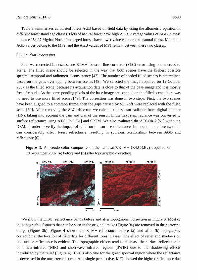
Figure 3. A pseudo-color composite of the Landsat-7/ETM+ (R4:G3:B2) acquired on
10 September 2007 (a) before and (b) after topographic correction.
We show the ETM+ reflectance bands before and after topographic correction in Figure 3. Most of
the topographic features that can be seen in the original image (Figure 3a) are removed in the corrected
image (Figure 3b). Figure 4 shows the ETM+ reflectance before (a) and after (b) topographic
correction at the location of field data for different forest classes. The effect of relief and shadows on
the surface reflectance is evident. The topographic effects tend to decrease the surface reflectance in
both near-infrared (NIR) and shortwave infrared regions (SWIR) due to the shadowing effects
introduced by the relief (Figure 4). This is also true for the green spectral region where the reflectance
is decreased in the uncorrected scene. At a single perspective, MF2 showed the highest reflectance due

Remote Sens. 2014, 6 3699
to the regeneration effects after logging. The logging has led to the more homogeneous canopy
structure in MF2; therefore, it has higher reflectance of red and NIR. On the other hand, shadows of
emergent trees from MF1 and NF brought more shadowing effects in the canopy structure; therefore,
the signal of red and NIR towards the sensor is decreased [52].
Figure 4. Landsat surface reflectance based on the location of field data (a) before and
(b) after topographic correction.
After preprocessing of the ETM+ scene, we calculated the normalized difference vegetation index
(NDVI) [53], the principal component analysis (PCA) [54], a tasseled cap transformation
(TCT) [55,56] and the gray level co-occurrence matrix (GLCM) [57]. NDVI has been in use for many
years to measure and monitor plant growth, vegetation cover and biomass production from
multispectral satellite data [53]. However, NDVI loses its sensitivity to dense vegetation because of the
saturation in red and near infrared wavelength [11,58–60]. PCA allows redundant data to be
compacted into fewer bands. The bands of PCA data (components) are non-correlated and
independent, and often can be interpreted better than the source data [54]. However, the first few bands
account for a high proportion of the variance in the data [61]. TCT brightness, greenness, and wetness
define the vegetation information content [55,56] and are calculated by the linear combination of
ETM+ bands. GLCM textures describe the spatial variation of the spectral information in the
image [57,62]. As many images contain regions characterized by variation in brightness rather than a
unique value, textures can improve image classification [57]. In this study, we used texture filters
based on co-occurrence measures by the window size of 11 × 11 pixels with horizontal and vertical
offset of one. These metrics have been widely used to predict stand forest structure and biomass from
remote sensing data [8,59,63].
3.3. ALOS/PALSAR Processing
In order to enhance radiometric resolution and to square the pixels in ground range geometry at
similar spatial resolution (i.e., 30 m for Landsat), the amplitude images were multi-looked eight times
(i.e., four looks in azimuth and two looks in range) for the dual-polarization scene [64]. After
multi-looking, we performed refined Lee filter using a window size of 7 × 7 in order to minimize
speckle [65,66]. The performance of the filter and selection of the optimal window size was evaluated
with the speckle suppression and mean preservation index (SMPI; [67]).

Remote Sens. 2014, 6 3700
The intensity scenes were converted in their corresponding backscattering coefficients (Sigma
nought (dB); σ°) values (Equation (2), [68,69]). The study area is mountainous, and a strong relief
effect is observed. Heterogeneous topography changes the dominant ground-trunk double-bounce
scattering mechanism, subsequently the backscatter from forest will be changed [70]. Therefore, we
performed radiometric terrain correction to compensate for the ground-topography influence on
backscattering coefficient. The corrected backscatter in gamma-nought 𝛾° format can be obtained from
the sigma-nought 𝜎° value according to Equation (3) [71,72].
σ° = 10 × log10(I2 + Q2) + CF− 32.0 (2)
CF (calibration factor)= −83 dB, I and Q = the real and imaginary parts of the complex SAR image
pixel values
𝛾° = 𝜎°𝐴𝑓𝑙𝑎𝑡
𝐴𝑠𝑙𝑜𝑝𝑒 𝑐𝑜𝑠𝜃𝑟𝑒𝑓
𝑐𝑜𝑠𝜃𝑙𝑜𝑐 𝑛
(3)
𝛾° = topographic normalized backscattering coefficient, 𝜎° = radar backscattering coefficient,
Aflat = PALSAR pixel size for a theoretical flat terrain, Aslope = true local PALSAR pixel size for the
mountain terrain, 𝜃𝑙𝑜𝑐 = local incidence angle, 𝜃𝑟𝑒𝑓 = radar incidence angle at the image center.
The exponent n is the optical canopy depth and ranges between 0 and 1. It is a site-specific factor
and difficult to obtain in practice, therefore it is set to 1 [19,32,33,73].
We calculated alpha angle (α), entropy (H) and anisotropy (A) according to the decomposition
proposed by Cloude and Pottier [74]. This method is based on the extraction of mean diffusion based
on eigenvalues/eigenvectors decomposition of the coherence matrix in order to characterize scattering
interactions of the beams with the targets [74]. We extracted GLCM SAR textures using a window size
of 11 × 11 pixels with horizontal and vertical offset of one. Mean, variance, homogeneity, contrast,
dissimilarity, second moment and correlation from both HH and HV polarization bands were extracted.
Figure 5. (a) HH-HV backscattering (b) alpha-entropy of Cloude-Pottier decomposition on
the location of field data for different forest classes. (Z6 and Z9 are dominated by surface
scattering, Z2, Z5 and Z8 by volume scattering and Z1, Z4 and Z7 by multiple scattering
mechanisms. Z3 is non-feasible region).
Figure 5a shows the backscattering in HH and HV polarized bands, and Figure 5b shows the
distribution of alpha angle and entropy on the Cloude-Pottier diagram. The results may be affected by

Remote Sens. 2014, 6 3701
the use of dual-polarization data rather than quad-polarization data [13] that were not available for the
area. The backscattering values in both HH and HV polarized bands (Figure 5a) tend to decrease from
NF to the both managed forest classes due to a more clear forest floor. Less density of trees per ha might
enhance forest backscattering (Figure 5a). In general, there is no substantial difference among different
forest classes. This backscattering similarity could be resulted from saturation effect in backscattering
value, which is known for forest with high AGB value (i.e., ca. > 100 Mg/ha) [19,22,75]. Alpha angle
values are below 40 degrees, indicating predominantly surface scattering mechanism [74,76,77].
3.4. Modeling of Forest AGB
Figure 6 illustrates the whole procedure starting from preprocessing of data in order to develop a
forest AGB estimation model from multi-source remote sensing data. Various correlations between
forest AGB and the reflectance or vegetation indices were found [63,78–80]. Also, many studies made
use of the relation between SAR backscatter/texture and forest AGB [14,24,30,31,81,82].
Figure 6. Flowchart of mountain forest AGB estimation model.
We divided the sample plots into training and validation parts. We used the training plots to develop
forest AGB estimation models and validation plots to validate the models and calculate RMSE. In each
class, around 30% of plots are used as validation data. All models are generated at 95% confidence
level (α = 0.05), which means that there is a statistically significant relationship between the variables
at 95% confidence interval. In each model, only the parameters with P value ≤ 0.05 are included.
These parameters are statistically significant parameters to the model. We developed AGB estimation

Remote Sens. 2014, 6 3702
model with SAR data and uncorrected ETM+ to verify the effect of topography on mountain forest
AGB estimation. We also tested the relation of remote sensing dataset and original DBH
measurements to overcome the bias induced by introducing empirical allometric equations. Based on
the positive results, we then focused on developing AGB estimation models based on corrected remote
sensing data. Table 4 summarizes the datasets and significant parameters to AGB models. Models L1–L5
stand for the forest AGB estimation models, which use the corrected ETM+ reflectance, NDVI and
GLCM texture. In models P1–P5, PALSAR backscattering and their textures as well as polarimetric
features are used. Final model is the forest AGB estimation model based on ETM+, PALSAR and their
derivatives’ metrics (Table 4). As we have a large number of independent variables in each model,
multicollinearity (a high degree of correlation) may occur among variables. Therefore, we
implemented variance inflation factor (VIF) test to detect and remove multicollinearity among
variables [83].
Table 4. Datasets and significant parameters for different AGB estimation models.
Model Datasets Significant Parameters * (P ≤ 0.05)
Landsat
L1 ETM+ bands b3, b4, b7
L2 ETM+ bands, NDVI b4, b7, NDVI
L3 ETM+ bands, NDVI, PCA b7, PCA-1, PCA-2
L4 ETM+ bands, NDVI, PCA, TCT b7, PCA-1, PCA-2
L5 ETM+ bands, NDVI, PCA, TCT, GLCM
textures
b7, b4, PCA-1, variance b4, variance b5,
correlation b2, correlation b4
PALSAR
P1 HH, HV HH, HV
P2 HH, HV, polarimetric features HH, HV, entropy
P3 HH, HV, polarimetric features, texture HH HH, HV, entropy, contrast HH, mean HH
P4 HH, HV, polarimetric features, texture HV HH, HV, entropy, mean HV
P5 HH, HV, polarimetric features, texture HH,
texture HV
HH, HV, entropy, contrast HH, mean HH,
second moment HV
Landsat
&
PALSAR
Final ETM+ bands, PALSAR polarized bands, their
derived features b3, b4, b7, PCA-1, HH, HV, contrast HH
Note: * Significant parameters; parameters with P values ≤ 0.05. There are statistically significant relationships between
these parameters and AGB at 95% confidence interval.
Adjusted R2 and P value of each model were calculated. For validation purposes, we calculated
RMSE of each model based on validation dataset. RMSE (Equation (4)) is a frequently used measure
of differences between values predicted by the model and the observed values.
𝑅𝑀𝑆𝐸 = 1
𝑛 (𝑝𝑟𝑒𝑑𝑖𝑐𝑡𝑒𝑑 𝑣𝑎𝑙𝑢𝑒 − 𝑜𝑏𝑠𝑒𝑟𝑣𝑒𝑑 𝑣𝑎𝑙𝑢𝑒)2
𝑛
𝑗 = 1
(4)
Normally, a model with high adjusted R2 and low RMSE values implies a good fit between the
predicted values (calculated from developed models) and observed value in the field. For all models,
one-way ANOVA analysis was done at 0.05 significance level [84].

Remote Sens. 2014, 6 3703
4. Results and Discussion
4.1. Effect of Topographic Correction on Forest AGB Estimation
In Figures 3 and 4, we show the effect of topographic correction on reflectance in ETM+ Landsat
bands. Reflectance in green, NIR, and SWIR is remarkably decreased because of relief effects. This
will affect the relationship between AGB and reflectance. We evaluated final forest AGB model with
uncorrected ETM+ data. Table 5 summarizes the model. Low adjusted 𝑅2 (i.e., 0.51), and high RMSE
stand for unreliable model. In Figure 7, we plotted the difference between predicted and observed
biomass versus the slope for each plot before and after topographic correction. In steeper slope (>10°),
the differences are higher compared to gentler slope. The averages of the absolute values of difference
between the predicted and observed AGB values for different slope class are reported in Table 6. In all
slope groups, the difference is higher for the uncorrected data compared to corrected data. The highest
contrast is found in very steep slope (>15°). We concluded that the topographic component has a high
influence on AGB estimation in the mountain forest (Table 5). Therefore, we focus on developing
AGB estimation model with topographically corrected data.
Table 5. Statistics summary of forest AGB estimation model based on uncorrected
ETM+ data.
Model Dataset Significant Parameters *
(P ≤ 0.05) RMSE Adj. 𝑹𝟐 P Value **
AGB model (Before
topographic correction)
Landsat bands, Landsat textures,
PALSAR bands and their textures
b4, mean b5, contrast b5, HH, HV,
alpha, mean HH
37.53
(Mg/ha) 0.51 0.0000
Note: * Significant parameters; parameters with P values ≤ 0.05. There are statistically significant relationships between
theses parameters and AGB at 95% confidence interval. ** When the P value is ≤ 0.05, there is a statistically significant
relationship between the variables at 95% confidence level.
Figure 7. Distribution of difference between predicted and observed forest AGB values
versus slopes of each plot (a) before (b) and after topographic correction.
4.2. Forest AGB Estimation from DBH Data
We developed AGB estimation model with DBH data (Table 7). The high adjusted 𝑅2 (i.e., 0.74)
and low RMSE (i.e., 3.61 cm) indicate that in case the only DBH data are available, they can be
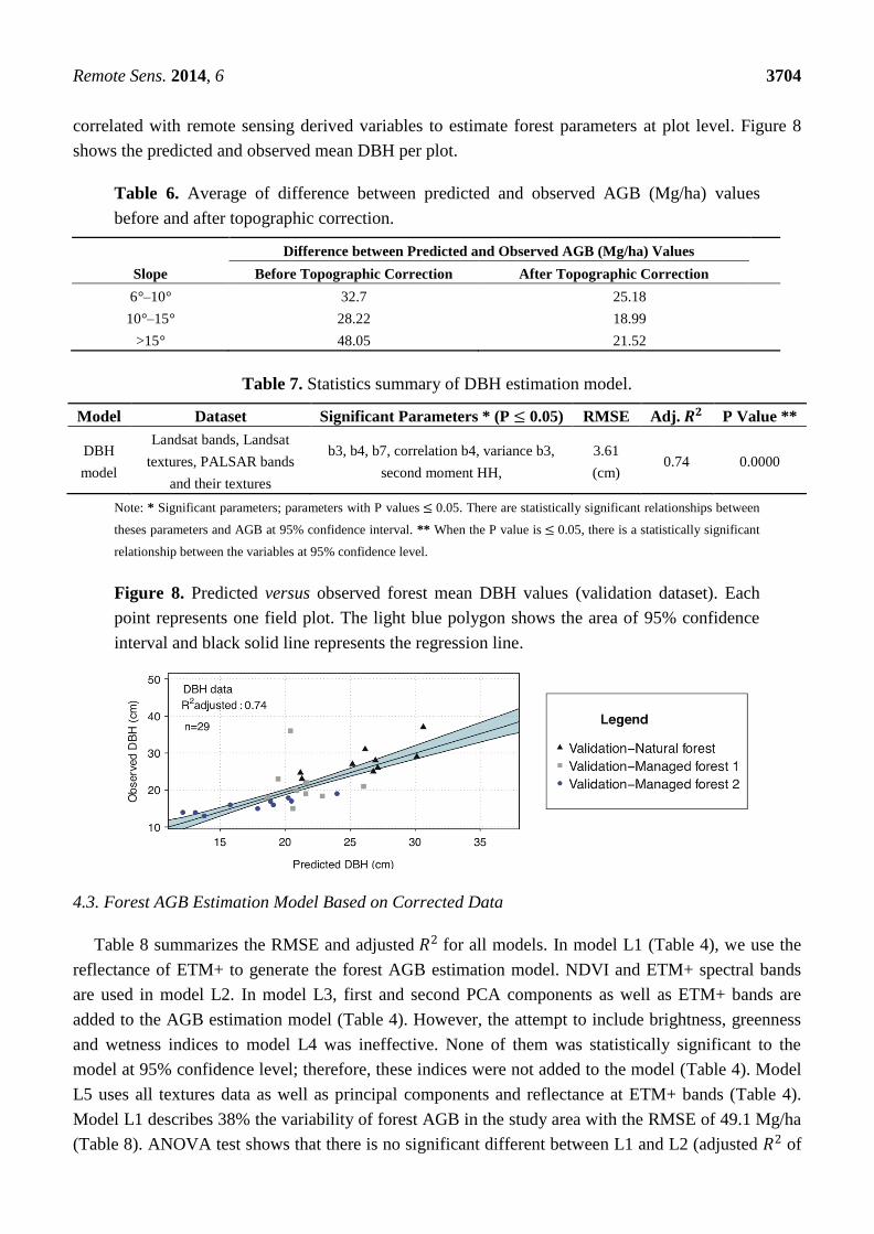
Remote Sens. 2014, 6 3704
correlated with remote sensing derived variables to estimate forest parameters at plot level. Figure 8
shows the predicted and observed mean DBH per plot.
Table 6. Average of difference between predicted and observed AGB (Mg/ha) values
before and after topographic correction.
Difference between Predicted and Observed AGB (Mg/ha) Values
Slope Before Topographic Correction After Topographic Correction
6°–10° 32.7 25.18
10°–15° 28.22 18.99
>15° 48.05 21.52
Table 7. Statistics summary of DBH estimation model.
Model Dataset Significant Parameters * (P ≤ 0.05) RMSE Adj. 𝑹𝟐 P Value **
DBH
model
Landsat bands, Landsat
textures, PALSAR bands
and their textures
b3, b4, b7, correlation b4, variance b3,
second moment HH,
3.61
(cm) 0.74 0.0000
Note: * Significant parameters; parameters with P values ≤ 0.05. There are statistically significant relationships between
theses parameters and AGB at 95% confidence interval. ** When the P value is ≤ 0.05, there is a statistically significant
relationship between the variables at 95% confidence level.
Figure 8. Predicted versus observed forest mean DBH values (validation dataset). Each
point represents one field plot. The light blue polygon shows the area of 95% confidence
interval and black solid line represents the regression line.
4.3. Forest AGB Estimation Model Based on Corrected Data
Table 8 summarizes the RMSE and adjusted 𝑅2 for all models. In model L1 (Table 4), we use the
reflectance of ETM+ to generate the forest AGB estimation model. NDVI and ETM+ spectral bands
are used in model L2. In model L3, first and second PCA components as well as ETM+ bands are
added to the AGB estimation model (Table 4). However, the attempt to include brightness, greenness
and wetness indices to model L4 was ineffective. None of them was statistically significant to the
model at 95% confidence level; therefore, these indices were not added to the model (Table 4). Model
L5 uses all textures data as well as principal components and reflectance at ETM+ bands (Table 4).
Model L1 describes 38% the variability of forest AGB in the study area with the RMSE of 49.1 Mg/ha
(Table 8). ANOVA test shows that there is no significant different between L1 and L2 (adjusted 𝑅2 of
Remote Sens. 2014, 6 3705
0.39, RMSE of 49.1 Mg/ha) at 5% significance level (Table 8). This could be because of the saturation
of vegetation indices in high biomass forest due to high reflectance [11,58,59,85]. Adding PCA
components to the model L3 increases the adjusted 𝑅2 to 0.47 and decreases RMSE to 44.0 Mg/ha
(Table 8). The result is the same for model L4 (Table 8). Because of the inclusion of GLCM textures,
Model L5 shows the best result (adjusted 𝑅2 = 0.59; RMSE = 31.5 Mg/ha; Table 8). In heterogeneous
forests, texture measures are more sensitive to the canopy structure than spectral reflectance, therefore
they correlate better with forest AGB [11,85,86]. Band 4 (NIR) and band 7 (MIR), first principal
components as well as variance band 4, variance band 5, correlation band 2 and correlation band 4 are
the significant parameters (at 95% interval level) that contribute to the models based on ETM+ data.
ANOVA test of models against one another reveals that models L3 and L5 are significantly (at 0.05
significance level) different from model L1.
Results of forest AGB estimation models based on PALSAR backscattering intensity, polarimetric
features, and PALSAR texture are as follows. In model P1, we used the backscatter intensity of HH
and HV polarization bands (Table 4). In model P2, we also add polarimetric features to the model.
SAR textures from HH polarized band are additional input to model P3 compared to model P2. We use
HH and HV and SAR textures from HV in model P4. In model P5, we use HH, HV, and polarimetric
features as well as the textures of HH and HV (Table 4). The adjusted 𝑅2 and RMSE of model P1 are
0.16 and 58.01 Mg/ha, respectively (Table 8). The week correlation between SAR backscattering
coefficients and forest AGB is also reported in previous studies [25,81,87]. In model P2, the adjusted
𝑅2 is increased to 0.25 and RMSE decrease to 47.0 Mg/ha (Table 8). Model P3 describes 41% the
variability of forest AGB in the study area (RMSE = 47.08 Mg/ha). Contrast and mean of HH are the
statistically significant HH-texture at 95% confidence level (Table 4). In model P4 (adjusted 𝑅2 = 0.25;
RMSE = 52.01 Mg/ha), second moment and mean are the statistically significant texture from HV
polarized band (Table 4). HH and HV backscattering and entropy as well as contrast HH, mean HH,
and second moment HV are the most correlated parameters derived from ALOS/PALSAR data (Table 4)
in model P5. This model can describe the 45% variability of the data. RMSE decreases to 43.25 Mg/ha
in this model (Table 8). Saturation of L-band that occurs at high AGB can explain the moderate
correlation [15,19,22,88,89]. Results from ANOVA test (at 5% confidence interval) among P1–P5
models confirm that all of the models are significantly different from one another. Higher correlation
of model P5 compared to the other models based on PALSAR data could be explained by the
sensitivity of SAR textures to forest canopy [90]. Our results are in agreement with the finding of
previous studies [90–93].
In the final model, ETM+ and PALSAR data, NDVI and GLCM textures are used (Table 4). The
adjusted 𝑅2 of the final model is 0.76 and RMSE is 25.04 Mg/ha (Table 8). Bands 3, 4, 7, PCA-1 as
well as HH, HV, and contrast HH significantly correlate with AGB values (Table 9). Many references
choose 5 as a threshold for VIF, also the other recommend 10 for each independent variable [94] or
average VIF of 6 for the all selected variables in the model [95,96]. We preferred to keep HH—despite
the fact that it is highly correlated with HV—because the average VIF of all selected variables is less
than 6. Comparison among this model and the other 10 models shows that the joint process of optical
and SAR data increase the reliability of model significantly (at 5% significance level). This model
benefits from the complementary nature of the spectral information from ETM+ data and volume

Remote Sens. 2014, 6 3706
information from SAR backscattering. The AGB estimation improvement from the inclusion of optical
and SAR data is comparable to those reported previously [6,17,30].
Table 8. Forest AGB estimation model parameters.
Model RMSE Adj. 𝑹𝟐 P Value * ANOVA **
Landsat L1 49.1 0.38 0.0000 -
L2 49.1 0.39 0.0000 -
L3 44.0 0.47 0.0000 **
L4 44.0 0.47 0.0000 **
L5 31.5 0.59 0.0000 **
PALSAR P1 58.01 0.16 0.0002 **
P2 47.0 0.25 0.0000 **
P3 47.08 0.41 0.0000 **
P4 52.1 0.25 0.0010 **
P5 43.25 0.45 0.0000 **
Landsat & PALSAR Final 25.04 0.76 0.0000 **
Note: * When the P value is ≤0.05, there is a statistically significant relationship between the variables at 95%
confidence level. ** Represents the results of ANOVA test; it shows the models that are statistically different at 95%
confidence level.
Table 9. Statistics summary of final forest AGB model.
Significant Parameters Coefficient P Value VIF
Band 3 21.39 0.00 1.66
Band 4 4.85 0.04 3.13
Band 7 −18.1 0.00 2.34
PCA-1 14.8 0.02 1.29
HH −6.67 0.02 11.99
HV 2.87 0.05 9.5
Contrast HH −6.63 0.01 2.39
4.4. Validation of Forest AGB Models
Predicted versus observed AGB values are plotted in Figure 9 for the selected models. Figure 10
shows the bar plot of adjusted 𝑅2 for all models. Model L5 (Figure 9a; Tables 4 and 6) yields
moderate results; AGB values between 150 and 210 Mg/ha are modeled better compare to values out of
this range. Underestimations are also observed for very high AGB values (>280 Mg/ha). In Figure 9b
(model P5; Tables 4 and 6), we observe more overestimating and underestimating compared to model L5.
Relatively low adjusted 𝑅2 and high RMSE show that dual polarimetric SAR cannot properly predict
forest AGB. Final model (Figure 9c) based on multisource data is a well-balanced model. The joint
processing of ETM+ and ALOS/PALSAR has two significant effects on the biomass estimation. First,
it substantially reduces the RMSE error. Second, it leads to the better prediction of medium AGB
values ranges from 80–250 Mg/ha. High ABG values are mostly underestimated.

Remote Sens. 2014, 6 3707
Figure 9. Predicted versus observed forest AGB (validation dataset); (a) Model L5: based
on spectral reflectance and textures of ETM+ scene; (b) Model P5: based on backscattering
and derived parameters of ALOS/PALSAR; and (c) Final model: based on ETM+ and
ALOS/PALSAR data. Each point represents one field plot. The light blue polygon shows
the area of 95% confidence interval and black solid line represents the fitted line.
Figure 10. Bar plot of 𝑅2 (refer to Table 4).
Note: *Final: AGB estimation model based on uncorrected data (Section 4.1).
4.5. Limitation and Sources of Errors
We found a reasonable relationship among ETM+ reflectances, SAR backscattering and field
measured AGB. However, there are some limitations and sources of errors to our AGB estimation.
These include limitation of field measurements and errors introduced by allometric equation and soil
and vegetation moisture.
We used the latest inventory data conducted in the study area and the closest remotely sensed data
available. Although differences in time acquisitions may bring additional sources of errors in the
retrieval of biomass, the inevitable difference of three years between the in-situ measurements and the
remote sensing data used was neglected. The AGB estimations would be improved in case they were
coincident. Real AGB can only be measured by destructive sampling that is not available for the study.

Remote Sens. 2014, 6 3708
The calculated AGB values from allometric equations are accounted for as reference value.
Calculations based on allometric equations are the best method when destructive sampling is not
performed [21], despite introducing errors by using empirical equations [44]. The other deficiency in
observed AGB is that trees with DBH <7.5 cm were excluded from field measurement. They
contribute slightly to forest AGB and may impact the SAR backscattering [21].
Soil and vegetation moisture related to the precipitation events impact the SAR backscattering and
could be a confounding factor in AGB estimation [89]. L-band SAR can penetrate more through
vegetation; thus, the soil backscattering is involved in the total backscattering [21,97]. However, in
low biomass densities, soil moisture has more effect on SAR backscattering, since radar signal can
penetrate through the trees and hit the surface [15,21].
5. Recommendations and Conclusions
This research was the first attempt to apply synthetic aperture radar (SAR) data for above ground
dry biomass (AGB) estimation in the Hyrcanian forest. The multiple linear regression procedure
clearly demonstrates the feasibility of the joint usage of ETM+ and Advanced Land-Observing
Satellite/Phased Array L-band Synthetic Aperture Radar (ALOS/PALSAR) data for the AGB
estimation in mountainous and high biomass forests. We conclude that relief influences the forest
reflectance and backscatter in mountainous areas; therefore, topographic correction is essential for
modeling forest AGB in those regions. Using non-topographically corrected data, the AGB prediction
model captured only 51% of the biomass variability (RMSE = 37.53 Mg/ha). Adding topographic
corrections improved the AGB estimation by up to 25%. Biomass estimation based on ETM+ data
shows that gray level co-occurrence matrix (GLCM) textures correlate more with AGB than NDVI and
principal component analysis (PCA). Our results showed that the coefficient of correlation could be
increased by 0.12 when including texture information. Polarized L-band SAR features alone correlate
weakly with AGB (adjusted 𝑅2 = 0.45, RMSE= 43.25 Mg/ha). However, SAR data can be used
alternatively when optical data is not available or if the region is covered by clouds. Forest AGB can
be modeled more accurately with the joint usage of optical and SAR data (adjusted 𝑅2 = 0.76,
RMSE = 25.04 Mg/ha) rather than independently (adjusted 𝑅2 ≤ 0.59)
The methodology can be used to produce forest AGB maps in mountainous terrain that can be
difficult to obtain with more traditional techniques. Biomass estimations can help managers to measure
forest productivity and give them a better vision for further activities. Additional research will explore
the influence of full polarimetric L-band SAR data. Although no spaceborne L-band SAR is currently
active, some missions such as ALOS/PALSAR-2, Multi-Application Purpose SAR (MAPSAR) and
Deformation, Ecosystem Structure and Dynamics of Ice (DESDynI) are planned [20]. Our further
research will also focus on the performance of other regression models (e.g., robust regression) for
estimating forest AGB based on multisource remote sensing data.
Acknowledgments
The first author was supported from the German Academic Exchange Service (DAAD) and the
International Association of Mathematical Geosciences (IAMG). SAR data was provided under
Cat.1-Proposal 6242 through the European Space Agency (ESA) Third Party Mission. The
Remote Sens. 2014, 6 3709
Landsat/ETM+, SRTM data and MODIS global land cover product (MOD12) were obtained from USGS.
For the correction of SLC-off error, a frame and fill tool—programmed by Richard Irish from NASA
Goddard Space Flight Center—was used. We also wish to thank Veraldo Liesenberg (Unicamp/FAPESP)
for his contributory feedback on the manuscript. We would like to thank Shaban Shataee
from the forestry department, Gorgan University of Agriculture and Natural Science in Iran for providing
us with in-situ datasets; without his aid this research would not have been possible.
Author Contributions
Sara Attarchi prepared and accomplished the study. She also wrote the manuscript. Richard Gloaguen
outlined the research, and supported the analysis and discussion. He also supervised the writing of the
manuscript at all stages.
Conflicts of Interest
The authors declare no conflict of interest.
References
1. Mohammadi, J.; Shataee, S. Possibility investigation of tree diversity mapping using Landsat
ETM+ data in the Hyrcanian forests of Iran. Remote Sens. Environ. 2010, 114, 1504–1512.
2. Mohammadi, J.; Shataee, S.; Habashi, H.; Amiri, M. Effect of shelterwood logging on diversity of
tree species in the Loveh Forest, Gorgan. Iran. J. For. Poplar Res. 2008, 16, 241–250.
3. Department of Environment, Iran. Forth National Report to the Convention on Biological
Diversity; Department of Environment, Iran, 2010; Available online: https://www.cbd.int/doc/
world/ir/ir-nr-04-en.pdf (accessed on 18 April 2014).
4. Main-Knorn, M.; Moisen, G.G.; Healey, S.P.; Keeton, W.S.; Freeman, E.A.; Hostert, P.
Evaluating the remote sensing and inventory-based estimation of biomass in the western
Carpathians. Remote Sens. 2011, 3, 1427–1446.
5. Soenen, S.A.; Peddle, D.R.; Hall, R.J.; Coburn, C.A.; Hall, F.G. Estimating aboveground forest
biomass from canopy reflectance model inversion in mountainous terrain. Remote Sens. Environ.
2010, 114, 1325–1337.
6. Lu, D. The potential and challenge of remote sensing‐based biomass estimation. Int. J. Remote
Sens. 2006, 27, 1297–1328.
7. Palacios-Orueta, A.; Chuvieco, E.; Parra, A.; Carmona-Moreno, C. Biomass burning emissions:
A review of models using remote-sensing data. Environ. Monit. Assess. 2005, 104, 189–209.
8. Zheng, D.; Rademacher, J.; Chen, J.; Crow, T.; Bresee, M.; Le Moine, J.; Ryu, S.-R. Estimating
aboveground biomass using Landsat 7 ETM+ data across a managed landscape in northern
Wisconsin, USA. Remote Sens. Environ. 2004, 93, 402–411.
9. Kronseder, K.; Ballhorn, U.; Böhm, V.; Siegert, F. Above ground biomass estimation across
forest types at different degradation levels in Central Kalimantan using LiDAR data. Int. J. Appl.
Earth Obs. Geoinf. 2012, 18, 37–48.
Remote Sens. 2014, 6 3710
10. Amini, J.; Sumantyo, J.T.S. SAR and Optical Images for Forest Biomass Estimation;
In Biomass—Detection, Production and Usage; Matovic, D., Ed.; InTech: Rijeca, Croatia, 2011;
pp. 53–74.
11. Eckert, S. Improved forest biomass and carbon estimations using texture measures from
WorldView-2 satellite data. Remote Sens. 2012, 4, 810–829.
12. Gibbs, H.K.; Brown, S.; Niles, J.O.; Foley, J.A. Monitoring and estimating tropical forest carbon
stocks: Making REDD a reality. Environ. Res. Lett. 2007, doi:10.1088/1748-9326/2/4/045023.
13. Liesenberg, V.; Gloaguen, R. Evaluating SAR polarization modes at L-band for forest
classification purposes in Eastern Amazon, Brazil. Int. J. Appl. Earth Obs. Geoinf. 2013, 21,
122–135.
14. Le Toan, T.; Beaudoin, A.; Riom, J.; Guyon, D. Relating forest biomass to SAR data. IEEE Trans.
Geosci. Remote Sens. 1992, 30, 403–411.
15. Luckman, A.; Baker, J.; Kuplich, T.M.; da Costa Freitas Yanasse, C.; Frery, A.C. A study of the
relationship between radar backscatter and regenerating tropical forest biomass for spaceborne
SAR instruments. Remote Sens. Environ. 1997, 60, 1–13.
16. Castel, T.; Guerra, F.; Caraglio, Y.; Houllier, F. Retrieval biomass of a large Venezuelan pine
plantation using JERS-1 SAR data. Analysis of forest structure impact on radar signature.
Remote Sens. Environ. 2002, 79, 30–41.
17. Cutler, M.; Boyd, D.; Foody, G.; Vetrivel, A. Estimating tropical forest biomass with a
combination of SAR image texture and Landsat TM data: An assessment of predictions between
regions. ISPRS J. Photogramm. Remote Sens. 2012, 70, 66–77.
18. Wolter, P.T.; Townsend, P.A. Multi-sensor data fusion for estimating forest species composition
and abundance in northern Minnesota. Remote Sens. Environ. 2011, 115, 671–691.
19. Santoro, M.; Fransson, J.E.; Eriksson, L.E.; Magnusson, M.; Ulander, L.M.; Olsson, H. Signatures
of ALOS PALSAR L-band backscatter in Swedish forest. IEEE Trans. Geosci. Remote Sens.
2009, 47, 4001–4019.
20. Cartus, O.; Kellndorfer, J.; Rombach, M.; Walker, W. Mapping canopy height and growing stock
volume using Airborne Lidar, ALOS PALSAR and Landsat ETM+. Remote Sens. 2012, 4,
3320–3345.
21. Robinson, C.; Saatchi, S.; Neumann, M.; Gillespie, T. Impacts of spatial variability on
aboveground biomass estimation from L-band radar in a temperate forest. Remote Sens. 2013, 5,
1001–1023.
22. Imhoff, M.L. Radar backscatter and biomass saturation: Ramifications for global biomass
inventory. IEEE Trans. Geosci. Remote Sens. 1995, 33, 511–518.
23. Saatchi, S.; Marlier, M.; Chazdon, R.L.; Clark, D.B.; Russell, A.E. Impact of spatial variability of
tropical forest structure on radar estimation of aboveground biomass. Remote Sens. Environ. 2011,
115, 2836–2849.
24. Ranson, K.; Sun, G. Mapping biomass of a northern forest using multifrequency SAR data.
IEEE Trans. Geosci. Remote Sens. 1994, 32, 388–396.
25. Rignot, E.; Way, J.; Williams, C.; Viereck, L. Radar estimates of aboveground biomass in boreal
forests of interior Alaska. IEEE Trans. Geosci. Remote Sens. 1994, 32, 1117–1124.

Remote Sens. 2014, 6 3711
26. Harrell, P.; Bourgeau-Chavez, L.; Kasischke, E.; French, N.; Christensen, N, Jr. Sensitivity of
ERS-1 and JERS-1 radar data to biomass and stand structure in Alaskan boreal forest.
Remote Sens. Environ. 1995, 54, 247–260.
27. Richards, J.A.; Sun, G.-Q.; Simonett, D.S. L-band radar backscatter modeling of forest stands.
IEEE Trans. Geosci. Remote Sens. 1987, 487–498.
28. Craig Dobson, M.; Ulaby, F.T.; Pierce, L.E. Land-cover classification and estimation of terrain
attributes using synthetic aperture radar. Remote Sens. Environ. 1995, 51, 199–214.
29. Wang, Y.; Davis, F.; Melack, J.; Kasischke, E.; Christensen, N., Jr. The effects of changes in
forest biomass on radar backscatter from tree canopies. Int. J. Remote Sens. 1995, 16, 503–513.
30. Rauste, Y. Multi-temporal JERS SAR data in boreal forest biomass mapping. Remote Sens.
Environ. 2005, 97, 263–275.
31. Ahmed, R.; Siqueira, P.; Bergen, K.; Chapman, B.; Hensley, S. A Biomass Estimate Over the
Harvard Forest Using Field Measurements with Radar and Lidar Data. In Proceedings of 2010
IEEE International Geoscience and Remote Sensing Symposium (IGARSS), Honolulu, HI, USA,
25–30 July 2010; pp. 4768–4771.
32. Thiel, C.J.; Thiel, C.; Schmullius, C.C. Operational large-area forest monitoring in Siberia using
ALOS PALSAR summer intensities and winter coherence. IEEE Trans. Geosci. Remote Sens.
2009, 47, 3993–4000.
33. Kim, C. Quantataive analysis of relationship between ALOS PALSAR backscatter and forest
stand volume. J. Mar. Sci. Technol. 2012, 20, 624–628.
34. He, Q.-S.; Cao, C.-X.; Chen, E.-X.; Sun, G.-Q.; Ling, F.-L.; Pang, Y.; Zhang, H.; Ni, W.-J.; Xu, M.;
Li, Z.-Y.; et al. Forest stand biomass estimation using ALOS PALSAR data based on LiDAR-derived
prior knowledge in the Qilian Mountain, western China. Int. J. Remote Sens. 2011, 33, 710–729.
35. Sun, G.; Ranson, K.J.; Kharuk, V.I. Radiometric slope correction for forest biomass estimation
from SAR data in the Western Sayani Mountains, Siberia. Remote Sens. Environ. 2002, 79, 279–287.
36. Liu, W.; Song, C.; Schroeder, T.A.; Cohen, W.B. Predicting forest successional stages using
multitemporal Landsat imagery with forest inventory and analysis data. Int. J. Remote Sens. 2008,
29, 3855–3872.
37. Mosadegh, A. Silviculture; Tehran University Publications: Tehran, Iran, 1996.
38. Marvie Mohadjer, M. Silviculture; Tehran University Publications: Karaj, Iran, 2005.
39. Amiri, M.; Dargahi, D.; Azadfar, D.; Habashi, H. Comparison of structure of the natural and
managed Oak (Quercus castaneifolia) stand (shelter wood system) in Forest of Loveh, Gorgan.
J. Agric. Sci. Nat. Resour. 2009, 15, 45–56.
40. Amiri, M.; Habashi, H.; Azadfar, D.; Soleymani, N. Comparison of regeneration density and
species diversity in managed and natural stands of Loveh Oak forest. J. Agric. Sci. Nat. Resour.
2008, 28, 44–53.
41. Mohammadi, J.; Shataei, S.; Yaghmaei, F.; Salman Mahini, A. Forest stand age classification
using Landsat ETM+ data. J. Wood For. Sci. Technol. 2009, 16, 43–59.
42. Martin, J.G.; Kloeppel, B.D.; Schaefer, T.L.; Kimbler, D.L.; McNulty, S.G. Aboveground
biomass and nitrogen allocation of ten deciduous southern Appalachian tree species. Can. J. For.
Res. 1998, 28, 1648–1659.
Remote Sens. 2014, 6 3712
43. Zianis, D.; Mencuccini, M. On simplifying allometric analyses of forest biomass. For. Ecol.
Manag. 2004, 187, 311–332.
44. Ahmed, R.; Siqueira, P.; Hensley, S.; Bergen, K. Uncertainty of forest biomass estimates in north
temperate forests due to allometry: Implications for remote sensing. Remote Sens. 2013, 5,
3007–3036.
45. West, G.B.; Brown, J.H.; Enquist, B.J. A general model for the structure and allometry of plant
vascular systems. Nature 1999, 400, 664–667.
46. Niklas, K.J.; Midgley, J.J.; Enquist, B.J. A general model for mass-growth-density relations
across tree-dominated communities. Evol. Ecol. Res. 2003, 5, 459–468.
47. Boloorani, A.D.; Erasmi, S.; Kappas, M. Multi-source remotely sensed data combination:
Projection transformation gap-fill procedure. Senors 2008, 8, 4429–4440.
48. Gap Phase Statistic Calculator. Available online: https://landsat.usgs.gov/gap_phase_tool.php
(accessed on 4 April 2014),
49. Chen, J.; Zhu, X.; Vogelmann, J.E.; Gao, F.; Jin, S. A simple and effective method for filling gaps
in Landsat ETM+ SLC-off images. Remote Sens. Environ. 2011, 115, 1053–1064.
50. Tutorial for Using the NASA Gap Filling Software. Available online:
biodiversityinformatics.amnh.org/file.php?file_id=619 (accessed on 4 April 2014),
51. Richter, R.; Schläpfer, D. Atmospheric/Topographic Correction for Satellite Imagery; 565-02/11;
DLR-German Aerospace Center: Wessling, Germany, 2011; p. 202.
52. Liesenberg, V.; Boehm, H.-D.V.; Gloaguen, R. Spectral variability and discrimination assessment
in a tropical peat swamp landscape using CHRIS/PROBA data. GISci. Remote Sens. 2010, 47,
541–565.
53. Tucker, C.J. Red and photographic infrared linear combinations for monitoring vegetation.
Remote Sens. Environ. 1979, 8, 127–150.
54. Jensen, J.R. Introductory Digital Image Processing: A Remote Sensing Perspective; Prentice-Hall Inc.:
Upper Saddle River, NJ, USA, 1996.
55. Crist, E.P.; Kauth, R. The tasseled cap de-mystified. Photogramm. Eng. Remote Sens. 1986, 52,
81–86.
56. Crist, E.P.; Laurin, R.; Cicone, R.C. Vegetation and Soils Information Contained in Transformed
Thematic Mapper Data. In Proceedings of IGRASS’86 Symposium, Zurich, Switzerland, 8–11
September 1986; ESA Publ. Division: Noordwijk, The Netherlands, 1986; pp. 1465–1470..
57. Haralick, R.M.; Shanmugam, K.; Dinstein, I.H. Textural features for image classification.
IEEE Trans. Syst. Man Cybern. 1973, 3, 610–621.
58. Huete, A.R.; Liu, H.; van Leeuwen, W.J. The Use of Vegetation Indices in Forested Regions:
Issues of Linearity and Saturation. In Proceedings of 1997 IEEE International Geoscience and
Remote Sensing Symposium, Singapore, 3–8 August 1997; European Space Agency Publications
Division: Noordwijk, The Netherlands, 1997; pp. 1966–1968.
59. Lu, D.; Mausel, P.; Brondızio, E.; Moran, E. Relationships between forest stand parameters and
Landsat TM spectral responses in the Brazilian Amazon Basin. For. Ecol. Manag. 2004, 198,
149–167.
60. Mutanga, O.; Skidmore, A.K. Narrow band vegetation indices overcome the saturation problem in
biomass estimation. Int. J. Remote Sens. 2004, 25, 3999–4014.

Remote Sens. 2014, 6 3713
61. Taylor, P.J. Quantitative Methods in Geography: An Introduction to Spatial Analysis;
Houghton Mifflin Boston: Boston, MA, USA, 1977.
62. Holden, J. An Introduction to Physical Geography and the Environment; Pearson Education:
Upper Saddle River, NJ, USA, 2005.
63. Sader, S.A.; Waide, R.B.; Lawrence, W.T.; Joyce, A.T. Tropical forest biomass and successional
age class relationships to a vegetation index derived from Landsat TM data. Remote Sens. Environ.
1989, 28, 143–198.
64. Lee, J.-S.; Hoppel, K.W.; Mango, S.A.; Miller, A.R. Intensity and phase statistics of multilook
polarimetric and interferometric SAR imagery. IEEE Trans. Geosci. Remote Sens. 1994, 32,
1017–1028.
65. Lee, J.-S. Refined filtering of image noise using local statistics. Comput. Graph. Image Process.
1981, 15, 380–389.
66. Cantalloube, H.; Nahum, C. How to Compute a Multi-look SAR Image? In Proceedings of SAR
Workshop: CEOS Committee on Earth Observation Satellites Working Group on Calibration and
Validation, Toulouse, France, 26–29 October 1999; Harris, R.A., Ouwehand, L., Eds.; European
Space Agency: Paris, France, 2000; pp. 635–640.
67. Shamsoddini, A.; Trinder, J.; Wagner, W.; Székely, B. Image texture preservation in speckle
noise suppression. Int. Arch. Photogramm. Remote Sens. Spat. Inf. Sci. 2010, 38, 239–244.
68. Shimada, M.; Isoguchi, O.; Tadono, T.; Isono, K. PALSAR radiometric and geometric calibration.
IEEE Trans. Geosci. Remote Sens. 2009, 47, 3915–3932.
69. Lavalle, M.; Wright, T. Absolute radiometric and polarimetric calibration of ALOS PALSAR products.
Available online: http://earth.eo.esa.int/pcs/alos/palsar/articles/Calibration_palsar_products_v13.pdf
(accessed on 23 April 2014)
70. Folkesson, K.; Smith-Jonforsen, G.; Ulander, L.M. Model-based compensation of topographic
effects for improved stem-volume retrieval from CARABAS-II VHF-band SAR images.
IEEE Trans. Geosci. Remote Sens. 2009, 47, 1045–1055.
71. Ulander, L.M. Radiometric slope correction of synthetic-aperture radar images. IEEE Trans.
Geosci. Remote Sens. 1996, 34, 1115–1122.
72. Castel, T.; Beaudoin, A.; Stach, N.; Stussi, N.; Le Toan, T.; Durand, P. Sensitivity of space-borne
SAR data to forest parameters over sloping terrain. Theory and experiment. Int. J. Remote Sens.
2001, 22, 2351–2376.
73. Lucas, R.; Armston, J.; Fairfax, R.; Fensham, R.; Accad, A.; Carreiras, J.; Kelley, J.; Bunting, P.;
Clewley, D.; Bray, S. An evaluation of the ALOS PALSAR L-band backscatter—Above ground
biomass relationship Queensland, Australia: Impacts of surface moisture condition and vegetation
structure. IEEE J. Sel. Top. Appl. Earth Obs. Remote Sens. 2010, 3, 576–593.
74. Cloude, S.R.; Pottier, E. An entropy based classification scheme for land applications of
polarimetric SAR. IEEE Trans. Geosci. Remote Sens. 1997, 35, 68–78.
75. Watanabe, M.; Shimada, M.; Rosenqvist, A.; Tadono, T.; Matsuoka, M.; Romshoo, S.A.; Ohta, K.;
Furuta, R.; Nakamura, K.; Moriyama, T. Forest structure dependency of the relation between
L-band and biophysical parameters. IEEE Trans. Geosci. Remote Sens. 2006, 44, 3154–3165.
Remote Sens. 2014, 6 3714
76. Ouarzeddine, M.; Belhdj Aissa, A.; Souissi, B.; Belkhider, M.; Boulahbal, S. Polarimetric
Classification Using the Cloude/Pottier Decomposition. In Proceedings of the 2nd International
Workshop POLINSAR 2005, Frascati, Italy, 17–21 January 2005; Lacoste, H., Ed.;
ESA Publications Division: Noordwijk, The Netherlands, 2005.
77. Lonnqvist, A.; Rauste, Y.; Molinier, M.; Hame, T. Polarimetric SAR data in land cover mapping
in boreal zone. IEEE Trans. Geosci. Remote Sens. 2010, 48, 3652–3662.
78. Roy, P.; Ravan, S.A. Biomass estimation using satellite remote sensing data—An investigation on
possible approaches for natural forest. J. Biosci. 1996, 21, 535–561.
79. Steininger, M. Satellite estimation of tropical secondary forest above-ground biomass: Data from
Brazil and Bolivia. Int. J. Remote Sens. 2000, 21, 1139–1157.
80. Hall, R.; Skakun, R.; Arsenault, E.; Case, B. Modeling forest stand structure attributes using
Landsat ETM+ data: Application to mapping of aboveground biomass and stand volume.
For. Ecol. Manag. 2006, 225, 378–390.
81. Dobson, M.C.; Ulaby, F.T.; LeToan, T.; Beaudoin, A.; Kasischke, E.S.; Christensen, N.
Dependence of radar backscatter on coniferous forest biomass. IEEE Trans. Geosci. Remote Sens.
1992, 30, 412–415.
82. Kuplich, T.; Salvatori, V.; Curran, P. JERS-1/SAR backscatter and its relationship with biomass
of regenerating forests. Int. J. Remote Sens. 2000, 21, 2513–2518.
83. Belsley, D.; Kuh, E.; Welsch, R. Regression Diagnostics: Identifying Influential Data and
Sources of Collinearity; Wiley & Sons, Inc.: Hoboken, NJ, USA, 1980.
84. Chambers, J.M.; Hastie, T. Statistical models in S; Chapman & Hall/CRC: Pacific Grove, CA,
USA, 1992.
85. Lu, D. Aboveground biomass estimation using Landsat TM data in the Brazilian Amazon. Int. J.
Remote Sens. 2005, 26, 2509–2525.
86. Sarker, L.R.; Nichol, J.E. Improved forest biomass estimates using ALOS AVNIR-2 texture
indices. Remote Sens. Environ. 2011, 115, 968–977.
87. Foody, G.M.; Green, R.; Lucas, R.; Curran, P.; Honzak, M.; Do Amaral, I. Observations on the
relationship between SIR-C radar backscatter and the biomass of regenerating tropical forests.
Int. J. Remote Sens. 1997, 18, 687–694.
88. Lucas, R.M.; Mitchell, A.L.; Rosenqvist, A.; Proisy, C.; Melius, A.; Ticehurst, C. The potential of
L‐band SAR for quantifying mangrove characteristics and change: case studies from the tropics.
Aquat. Conserv.: Mar. Freshw. Ecosys. 2007, 17, 245–264.
89. Morel, A.C.; Saatchi, S.S.; Malhi, Y.; Berry, N.J.; Banin, L.; Burslem, D.; Nilus, R.; Ong, R.C.
Estimating aboveground biomass in forest and oil palm plantation in Sabah, Malaysian Borneo
using ALOS PALSAR data. For. Ecol. Manag. 2011, 262, 1786–1798.
90. Sarker, M.L.R.; Nichol, J.; Ahmad, B.; Busu, I.; Rahman, A.A. Potential of texture measurements
of two-date dual polarization PALSAR data for the improvement of forest biomass estimation.
ISPRS J. Photogramm. Remote Sens. 2012, 69, 146–166.
91. Kuplich, T.; Curran, P.; Atkinson, P. Relating SAR image texture to the biomass of regenerating
tropical forests. Int. J. Remote Sens. 2005, 26, 4829–4854.
92. Luckman, A.; Frery, A.; Yanasse, C.; Groom, G. Texture in airborne SAR imagery of tropical
forest and its relationship to forest regeneration stage. Int. J. Remote Sens. 1997, 18, 1333–1349.
Remote Sens. 2014, 6 3715
93. Champion, I.; Dubois‐Fernandez, P.; Guyon, D.; Cottrel, M. Radar image texture as a function of
forest stand age. Int. J. Remote Sens. 2008, 29, 1795–1800.
94. Kutner, M.H.; Nachtsheim, C.J.; Neter, J.; Li, W. Applied Linear Statistical Models;
McGraw-Hill/Irwin: New York, NY, USA, 2004.
95. Pedhazur, E.J. Multiple Regression in Behavioral Research: Explanation and Prediction;
Harcourt Brace College Publishers: San Diego, CA, USA, 1997.
96. Ender, P.B. Applied Categorical & Nonnormal Data Analysis. Available online:
http://www.philender.com/courses/categorical/notes2/collin.html (accessed on 1 April 2014).
97. Wang, X.; Ge, L.; Li, X. Pasture monitoring using SAR with COSMO-SkyMed, ENVISAT
ASAR, and ALOS PALSAR in Otway, Australia. Remote Sens. 2013, 5, 3611–3636.
© 2014 by the authors; licensee MDPI, Basel, Switzerland. This article is an open access article
distributed under the terms and conditions of the Creative Commons Attribution license
(http://creativecommons.org/licenses/by/3.0/).