Determining Spatial and Temporal Patterns of Submergence in Rice with MODIS Satellite Data
Upload
independentCategory
view
0download
0
COMPARING MODIS AND ETM+ IMAGE DATA FOR INLAND WATER STUDIES SPATIAL RESOLUTION CONSTRAINTS
Comparaccedilatildeo de Imagens MODIS e ETM para Estudo de Aacuteguas Interiores
Imposiccedilotildees da Resoluccedilatildeo Espacial
Evlyn Maacutercia Leatildeo de Moraes Novo 1
Claudio Clemente Faria Barbosa1
John MMelack 2Ramon Moraes de Freitas1
Fernanda Titonelli1
Yosio Shimabukuro1
1 Instituto Nacional de Pesquisas Espaciais Coordenaccedilatildeo de Observaccedilatildeo da Terra 12 201970 ndash Satildeo Joseacute dos Campos ndash SP CP 515
evlynltidinpebr
2 University of California Santa Barbara USA Bren School of Environmental Science and Management
Santa Barbara CA 93106 USA melacklifescilscfucsbedu
RESUMO O objetivo desse artigo eacute apresentar os resultados de um estudo voltado agrave comparaccedilatildeo do desempenho das imagens MODIS de resoluccedilatildeo moderada (250 m e 500 m) com o de imagens com maior resoluccedilatildeo espacial como as imagens do sensor ETM+ no tocante a sua capacidade para o mapeamento de feiccedilotildees relevantes para o estudo dos sistemas aquaacuteticos Para realizar essa comparaccedilatildeo foram obtidas simultaneamente imagens ETM+ e MODIS sobre a regiatildeo da planiacutecie do Lago Grande de Curuai Para que se tornassem comparaacuteveis ambos os conjuntos de imagens foram georreferenciados e reamostrados para um tamanho de pixel de 100 m x 100m com o auxiacutelio do interpolador pelo vizinho mais proacuteximo de modo a compatibilizar o tamanho da grade sobre a qual se aplicariam os processamentos subsequumlentes Esse procedimento foi adotado com base na suposiccedilatildeo de que a resoluccedilatildeo efetiva dos sensores seria pouco afetada devido ao maior poder de resoluccedilatildeo radiomeacutetrica dos dados MODIS Apoacutes a organizaccedilatildeo da base de dados as imagens foram submetidas a testes visando identificar o melhor procedimento para gerar um mapa com a distribuiccedilatildeo de ilhas rios e canais da regiatildeo de estudo Os testes indicaram que a melhor abordagem foi a de segmentaccedilatildeo e classificaccedilatildeo natildeo supervisionada da fraccedilatildeo sombra derivada da aplicaccedilatildeo do modelo linear de mistura as imagens ETM+ e MODIS Os mapas resultantes da segmentaccedilatildeo e classificaccedilatildeo foram transformados em vetores e gerados poliacutegonos representativos das feiccedilotildees classificadas genericamente em lagos (aacutegua) e ilhas (terra) Procedeu-se entatildeo a anaacutelise da distribuiccedilatildeo dos poliacutegonos em termos da frequumlecircncia de tamanho de ilhas e lagos mapeaacuteveis Os resultados permitiram verificar que em termos de aacuterea total mapeada pelos sensores ETM+ e MODIS as diferenccedilas chegam a 11 Entretanto a anaacutelise da distribuiccedilatildeo de poliacutegonos mapeados indica que haacute um grande nuacutemero de poliacutegonos detectados pelas imagens MODIS que natildeo puderam ser recuperados pela imagem ETM+ Esses resultados sugerem que as melhorias apresentadas pelo sensor MODIS no tocante agrave resoluccedilatildeo espectral e radiomeacutetrica podem compensar em algumas situaccedilotildees especiacuteficas a degradaccedilatildeo da resoluccedilatildeo espacial Na realidade os resultados mostram que nas condiccedilotildees em que foi realizado este experimento as imagens MODIS podem ter um desempenho melhor do que o de imagens do sensor ETM+ reamostradas para 100m x 100m Isto explicaria a pequena diferenccedila de desempenho no tocante ao computo final da aacuterea ocupada por superfiacutecies liacutequidas Palavras chaves Imagens MODIS Imagens ETM+ Sistemas Aquaacuteticos Resoluccedilatildeo Espacial
Revista Brasileira de Cartografia No 5802 Agosto 2006 (ISSN 1808-0936)
109
ABSTRACT The objective of this paper is to compare the performance of medium spatial resolution (250 m and 500 m) Terra MODIS images to finer resolution Landsat ETM+ images MODIS Terra images have high frequency of acquisition (1 day revisit at high latitudes) and that makes them more useful for inland water studies Assessing the performance of ETM and MODIS to map relevant features for the functioning of aquatic systems is very important for fostering water resource remote sensing To carry out the comparison concurrent ETM+ and MODIS images were acquired over the Lago Grande de Curaui Lake The images were georeferenced and resample to the 100 x 100 m ground resolution using a next neighbor algorithm to make the data comparable The resampling rationale was making the digital processing easier without changing the effective resolution properties of the original data It was assumed that the improved MODIS radiometric resolution as compared to the ETM+would make both data set comparable at a 100m x 100m resolution In the next step a series of tests were carry out in order to define the best approach to map aquatic system features such as lakes islands and levees in the study area The tests indicated that the best approach was the segmentation of the shadow fraction derived from the application of the linear unmixing model to both ETM+ and MODIS images The segmentation was then followed by the application of a non-supervised region classifier The final classes were mapped into two categories lakes (water) and island (land) The polygon distribution generated by the classification procedure was then statistically analyzed to assess the polygon size frequency of features mapped by each data set The results showed that ETM+ and MODIS were able to recover the water surface area in the studied region with a difference of 11 The analyses of polygon distribution however showed that there were many polygons which were detected in MODIS image data but not in ETM+ image data This result suggests that the spectral and radiometric resolution improvements presented by MODIS image tend to compensate for the losses in spatial resolution That is to say that under the boundary conditions adopted in this study MODIS images performed better than degraded ETM+ images of 100m x 100m This explains the small difference in performance presented by comparing two sensors with such large differences in nominal spatial resolution Keywords MODIS Images EMT+ images Aquatic Systems Spatial Resolution
1 INTRODUCTION
This paper reports an experiment performed to assess the suitability of MODIS spatial resolution for studying Amazon aquatic systems compared to that of LandsatETM+ images degraded to 100 m x 100 m The assumption is that the spatial resolution will not be a major constraint for the retrieval of ground information because it is compensated by the improved radiometric and spectral resolution
The remote sensing of inland waters was always behind of Ocean Atmospheric and Land applications because the sensors available did not meet the requirements needed to cope with a target that displays a huge variability in space and time The water color sensors developed for ocean applications (Kampel and Novo 2005) have poor spatial resolution and the radiometric resolution is not tuned to deal with scenes undergoing sharp changes in the reflected signal Land sensors such as the Thematic Mapper on board of Landsat satellite series do not have the radiometric sensitivity to account for subtle changes in water reflectance (Kirk 1994)
MODIS is the principal high temporal frequency global mapping sensor on-board NASArsquos Earth Observation System (EOS) (httpmodarchgsfcnasagovMODIS) Terra
(February 2000 - present) and Aqua (June 2002 - present) satellites Terra and Aqua are at near-polar Sun-synchronous orbits and are crossing the Equator three hours apart Terra at 1030AM descending while Aqua at 130PM ascending Thus near global coverage is achieved by MODIS in a single day at spatial resolutions spanning from 250 m to 1000 m according to various application requirements These features suggest that MODIS data might be useful for studying large inland aquatic systems such as those comprised by the Amazon River Basin
MODIS is an optical scanner that measures Earth radiance in 36 bands ranging from 04 to 14 μm and presents substantial improvements in bandwidths and radiometric resolution which are fundamental for inland water studies In addition to these new features continuous global data sets and corresponding science products with improved quality have been produced with constant on-orbit calibration Table 1 summarizes the main MODIS features Table 2 summarizes the information derived from MODIS products designed for both land and ocean applications
Revista Brasileira de Cartografia No 5802 Agosto 2006 (ISSN 1808-0936)
110
TABLE 1 ndash MODIS SPECIFICATIONS (httpmodisgsfcnasagovaboutspecshtml)
1 Bands 1 to 19 are in nm Bands 20 to 36 are in microm Quantization= 12 bits Spatial Resolution 250m (bands 12) 500m (bands 3-7) 1000 m (8-36)
Primary Use 1 Band Bandwidth
1 620 ndash 670 LandCloudAerosols Boundaries 2 841 ndash 876
3 459 ndash 479 4 545 ndash 565 5 1230 ndash 1250 6 1628 ndash 1652
LandCloudAerosols Properties
7 2105 ndash 2155 8 405 ndash 420 9 438 ndash 448
10 483 ndash 493 11 526 ndash 536 12 546 ndash 556 13 662 ndash 672 14 673 ndash 683 15 743 ndash 753
Ocean Color Phytoplankton
Biogeochemistry
16 862 ndash 877 17 890 ndash 920 18 931 ndash 941
Atmospheric Water Vapor
19 915 ndash 965 20 3660 - 3840 21 3929 - 3989 22 3929 - 3989
SurfaceCloud Temperature
23 4020 - 4080 24 4433 - 4498 Atmospheric
Temperature 25 4482 - 4549 26 1360 - 1390 27 6535 - 6895
Cirrus Clouds Water Vapor
28 7175 - 7475 Cloud Properties 29 8400 - 8700
Ozone 30 9580 - 9880 31 10780 - 11280SurfaceCloud
Temperature 32 11770 - 1227033 13185 - 1348534 13485 - 13785
Cloud Top Altitude
35 13785 - 14085
Broadly speaking MODIS applications were
gathered into Land Ocean and Atmosphere From Table
1 it is clear that Land Application requirements for spatial resolution are more rigorous than those for Ocean Applications This fact prevents the use of Ocean Products for studying inland water Moreover inadequate sensor calibration problematic atmospheric correction and bio-optical inversion procedures (Hu et al 2004) also limits their application
On the other hand recent work shows that MODIS Land bands have sufficient sensitivity to be useful in various aquatic applications and have been successfully applied for water studies (Li et al 2003) TABLE 2 ndash BANDS AND APPLICATIONS OF MOD
09 (LAND) AND MOD 18 (OCEAN) PRODUCTS
MOD 09
Band width (nm)
MOD 18
Band width (nm)
Application
1 620-670 (50)
Sediments
13 672-672 (10)
Sediments
14 673-683 (10)
Phytoplanckton
Fluorescence 15 743-753
(10) Phytoplanckto
n Fluorescence
16 862-877 (15)
Aerosol properties
2 841-876 (35)
8 405-420 (15)
Dissolved organic matter
9 438-448 (10)
Chlorophyll
3 459-479 (20)
Dissolved organic matter
10 483-493 (10)
Chlorophyll
11 526-536 (10)
Chlorophyll
4 545-565 (20)
12 546-556 (10)
Phytoplankton scattering
bands 5 to 7 are not particularly useful for water optical property assessment
The information content in lower spatial
resolution data is determined not only by the pixel size but by the ability of distinguishing between subtle signal intensities The improved radiometric resolution provided by the 12 bit MODIS image may compensate for the losses in spatial resolution compared to the finer yielded by ETM+-like sensors
The information content however is not only a function of the sensor properties but it is also dependent on the landscape variability The relationship between sensor spatial resolution and the size distribution of ground objects is crucial for assessing its utility Lake size in the Amazon floodplain for instance can span from less than 01 km2 to more than 3000 km2
(Melack 1984) Lake shape also affects the information content for a given spatial resolution At Amazon
Revista Brasileira de Cartografia No 5802 Agosto 2006 (ISSN 1808-0936)
111
floodplain lake shape varies enormously from channel lakes encroached between levees and sandbars to round lakes oxbow lakes crescent lakes (Melack 1984)
If a coarser spatial resolution can be compensated by an improved radiometric and spectral resolution as available in MODIS image data then it may provide a vital tool for studying water movement from river channel to floodplain lakes of the major drainage basin of the world such as GangesBrahmaputra Huangho (Yellow) Amazon Yangtze Irrawaddy Magdalena Orinoco Hungho (Red) Mekong Indus Mackenzie Godavari La Plata Haiho Purari Niger and Mekong 2 THE STUDY AREA AND DATA SET
Curuai lake floodplain region (Figure 1) was selected due to the presence of lakes of various sizes (from 300 km2 to less than 01 km2) shapes and water types which spans a wide range of landscape variability
SolimotildeesAmazonasSolimotildeesAmazonas
SolimotildeesAmazonasSolimotildeesAmazonas
Fig1 ndash Curuai lake floodplain test site The test site area is located between the towns
of Oacutebidos and Santareacutem (Paraacute State) 900 km from the Amazon River mouth and is subject to seasonal fluctuations in water level of around 54 m
The following data set were available for this study LandsatETM + image (path 228row 61) and MOD 09 Level 2 G Validated Version 3 (tile h12v09) both acquired in July 8 2002 LandsatETM + images were provided by the Image Generation Division at the National Institute for Space Research (INPE) in Geotiff format MOD 09 product was distributed by the Land Processes Distributed Active Archive Center (LP DAAC) located at the US Geological Surveys EROS Data Center (httpLPDAACusgsgov)
MOD 09 products are available in two sets for Version 3 MODIS GQK set is the MODISTerra Surface Reflectance Daily (L2G) Global 250m resolution and projected according to an integerized
sinusoidal (ISIN) grid MODIS 250 m Surface Reflectance is a two-band product computed from the MODIS Level 1B land bands 1 and 2 (centered at 648 nm and 858 nm respectively) MOD09GHK set is the MODISTerra Surface Reflectance (L2G) Global 500 m resolution It is a seven-band product computed from the MODIS Level 1B land bands 1-7
Both sets are estimates of the surface spectral reflectance for each band as it would have been measured at ground level if there were no atmospheric scattering or absorption The correction scheme includes corrections for the effect of atmospheric gases aerosols and thin cirrus clouds (httplpdaac2usgsgovmodismod09ghkasp) Table 3 summarizes the main features of each set of MOD 09 product
TABLE 3 ndash MOD 09 DATA SE CHARACTERISTICS
MOD09 GQK Data Set Characteristics
Area = ~ 10deg x 10deg latlong Image Dimensions = 4800 x 4800 rowscolumns Resolution = ~250 meters Projection = Integerized Sinusoidal Data Format = HDF-EOS 16-bit signed int
MOD09GHK Data Set Characteristics
Area = ~ 10deg x 10deg latlong Image Dimensions = 2400 x 2400 rowscolumnsResolution = ~500 meters Projection = Integerized Sinusoidal Data Format = HDF-EOS 16-bit signed int
3 DATA PROCESSING The first step in this study consisted in
establishing a data base composed of 250 m x 250 m spatial resolution bands In this step MOD 09 was transformed from the ISIN projection to LatLong projection
This transformation was accomplished by using the MODIS Reprojection Tool (RTM) made available at (httplpdaac2usgsgovlanddaactoolsmodisaboutasp) RTM enables to read data files in HDF-EOS format select the geographic subset and science data sets as input to processing and performing the geographic transformation to a different coordinate systemcartographic projection The software also allows defining the pixel size of the output image and writes it in formats other than HDF-EOS
Bands 3 to 7 of MOD09GHK data set were resample for 250 m using a nearest neighbor algorithm The output image was saved in Geotiff format The MOD09 GQK set was only reprojected to LatLong and
Revista Brasileira de Cartografia No 5802 Agosto 2006 (ISSN 1808-0936)
112
exported as Geotiff The final data comprised the seven bands with a 250 m x 250 m pixel size
MODIS data is provided as 16 bit data in spite of its inherent 12 bit radiometric resolution In order to reduce image size a 16 bit to 8 bit compression was carried out using a tool (Arai et al 2005) which accommodates the reflectance distribution from the 16 bit image into an 8 bit image by tuning the look up table to users defined reflectance range
MODIS and ETM+ Image analyses were carried out using SPRING (Sistema de Processamento de Informaccedilotildees Georeferenciadas) a freeware Geographical Information and Image Processing System which provides for the integration of raster and vector data format in a single environment (httpwwwdpiinpebrspring) MODIS images were registred to ETM+ data and further resampled to 100 m x 100 m (Schowengerdt 1997)
In order to compare the ability of MODIS images to retrieve landwater boundary with that of ETM+ resampled images two approaches were tested The first approach was based on a single band thresholding The 250 nominal resolution MOD09 B2 (841 ndash 876 nm) resampled to 100 m x 100m image was selected to build a water surface mask A mask is a binary image that consists of values of 0 and 1
This band was selected because of its inherent higher spatial resolution In the ETM+ data set infrared band 5 (1550- 1750nm) was selected instated of band 4 (0775- 0900nm) Preliminary tests showed that the wider sensitivity of band ETM+4 towards the red edge increased its sensitivity to water turbidity resulting in an overlaping of highly turbid water and bare soil
The second approach to build a water mask was the application of the linear unmixing model to MOD 09 and ETM+ data sets (Shimabukuro et al 1998) so as to determine the relative abundances of shadewater soil and vegetation cover within a given pixel based on their spectral features The reflectance at each pixel of the image is assumed to be a linear combination of the reflectance of each material (or endmember) present within the pixel So given the resulting spectrum (the input data) and the endmember spectra the linear unmixing solves for the abundance values of each endmember for every pixel Figure 2 shows the selected endmembers used to run the unmixing algorithm
In the linear unmixing model the pixel reflectance (R) at any of the n bands can be modeled as the linear combination of the spectral response of k pure endmembers The model can be expressed by (the) a set of linear equations
Ri = Σ (aij xj ) + ei (1)
j=1
where
j = 1 k (endmembers)
i = 1 n (bands)
Ri Pixel reflectance in the ith spectral band
aij spectral reflectance of the jth endmember at the ith spectral band
xj estimated fraction of the jth endmember within the pixel
The following constraints apply
11
=sum=
k
jix (2)
and
0 lt= xj lt= 1 (3)
ei estimated error
B1B2B3B4 B5 B7
ETM+ BANDS
Spe
ctra
lree
spon
se
B1B2B3B4 B5 B7
ETM+ BANDS
Spe
ctra
lree
spon
se
B3B4B1 B2 B5 B7
MODIS BANDS
VEGETATION SOIL SHADE
Fig 2 - Endmember spectral responses (shade vegetation and soil)
Usually kltn which makes the system (1) overdetermined A constrained least squares adjustment approach can be applied here
The shade fraction was then submitted to image segmentation In this process individual image pixels are grouped into partitions according to some intrinsic properties of the image eg gray levels contrast spectral values or textural properties (Le Moigne and Tilton 1995) In the segmentation a series
Spe
ctra
lree
spon
se
B1B2B3B4 B5 B7
ETM+ BANDS
Spe
ctra
lree
spon
se
B1B2B3B4 B5 B7
ETM+ BANDS
Spe
ctra
lree
spon
seS
pect
ralr
eesp
onse
B3B4B1 B2 B5 B7
MODIS BANDS
VEGETATION SOIL SHADE
Spe
ctra
lree
spon
se
B3B4B1 B2 B5 B7
MODIS BANDS
VEGETATION SOIL SHADE
Spe
ctra
lree
spon
se
B3B4B1 B2 B5 B7
MODIS BANDS
VEGETATION SOIL SHADE
Revista Brasileira de Cartografia No 5802 Agosto 2006 (ISSN 1808-0936)
113
of similarity and minimum area thresholds were tested and evaluated against the image color composites in order to select the results fitting both lake and island distribution in the scene The similarity threshold sets the minimum diference between a given pixel digital number and the average digital number in its neighbourhood so as it can be addressed to that region or image segment The minimum area threshold defines the minimum number of pixels to make up a segment Similarity and minimum area thresholds were set constant in both images
The rationale for segmenting the fraction image is that if spatial resolution does not affect the discrimination of lakes and island the number shape and size of the segments generated in both data sets would be identical In order to limit the study to the floodplain lakes a mask was applied to the segmented image to eliminate the Terra Firme rivers and lakes from the analysis This mask was produced by Hess et al (2004) based on dual date SAR images acquired by JERS1 satellite The segmented image was then submitted to an unsupervised classification using the Isoseg algorithm available at the SPRING image processing system It is a region classifier which allows the clustering of segments based on the Mahalanobis distance The Isoseg is a region classifier The regions are characterized by the average covariance matrix and area The regions are clustered according to a similarity measurement (Mahalanobis distance) between the classes and the candidate regions The algorithm runs according to three steps in the first step the user defines an acceptance threshold which will define the distance beyond which the region can not be included in a given cluster In the second step the algorithm organizes the segments according to their size The larger segments are assumed to be classes (clusters) for which the statistical parameters are computed Smaller segments (regions) are then assigned to each cluster according to an acceptance threshold In the third step the algorithm assigns the segments (regions) to new clusters The process is repeated up to moment that the clusters statistics did not change from one algorithm run to another The clusters were then assigned manually to two classes lakes and islandsland (Schowengerdt 1997)
Polygon statistics were produced and analysed in order to quantify the effects of MODIS spatial resolution on the detection of lakes and island In order to investigate the effect of shape variability on the ability to map island and lakes the Polygon Shape Factor (PSF) was adapted from Wetzel (1976) The PSF is a dimensionless number that expresses the irregularity of the shoreline (perimeter) and the polygon shape departure from a perfect circle A perfectly circular polygon would have PSF = 1 The PSF can be determined as follows
PSF = p [2 radicπ a] (4) where PSF= Polygon Shape Factor p= polygon perimeter
a= polygon area
4 RESULTS
The results are analyzed according to two approaches In the first approach the focus is to compare the ability of MODIS and ETM+ image data to retrieve area information
The second approach consists of comparing ETM+ and MODIS images in relation to their ability to retrieve lake and island shapes
41 Water masks
In this section the results of using a single band versus the shade fraction to create the water mask are compared The shade fraction image data provided a more accurate rendition of the water surface in the scene than the ETM+ band 5 as shown in the water masks displayed on Figure 3 The advantage of the fraction image lies on its ability for separating water from cloud shadow It is clear that when ETM+ band 5 is used the water mask includes cloud shadows (red circle on Figure 3) As the unmixing model takes into account the spectral signature of each pure endmenber the shade fraction does not include cloud shadow providing a water mask free from this undesirable effect The shade fraction used to unmix the images shows a very low reflectance in bands 4 5 and 7 The cloud shadow spectra however shows a consistent increase in reflectance towards longer infrared wavelengths It must be pointed out that those are experimental results applicable to the scene characteristics
ETM band 5
MOD 09 band 2 MOD 09 shade fraction
ETM shade fraction
Fig 3 ndash The effect of using single bands and the shade fractions on the generation of the Water-Land Mask
Red circle shows the inclusion of cloud shadow in the single ETM+ band 5 mask This effect is removed when
using the ETM+ shade fraction
As it can be observed in Figure 4 the open water masks derived from the shade fraction did not include the abundant cloud shadow observed in both
Revista Brasileira de Cartografia No 5802 Agosto 2006 (ISSN 1808-0936)
114
ETM+ and MOD 09 data set Total water surface computed from ETM+ and MOD 09 masks are very similar The total area mapped as water surface is 4731 km2 and 4205 km2 respectively which corresponds to 11 difference MOD09 image underestimated the area covered by water because it failed to recover most of the lakes smaller than 01 km2
Fig 4 ndash Open water shade mask overlaid on ETM+ true color composite and MOD 09 true color composite
The segmentation of ETM + shade fraction resulted into 2498 polygons whereas the MOD 09 shade fraction resulted in only 1413 polygons If the polygon size distribution (Figure 5) is analyzed however one can observe that there is a close agreement between ETM+ and MOD 09 for class intervals larger than 01- 10 km2 Looking into detail within the 01 ndash 10 km2 class intervals it was observed that only in the interval 010 to 025 km2 there are 486 ETM+ polygons This class interval corresponds to polygons with area equivalent to 1 to 4 MODIS pixels Looking into the polygon size distribution for MODIS data it is observed that there are 585 polygons in this size interval It means that it is not only the size which is responsible for the polygon definition but other variables might explain differences in the detection threshold
ETM 1 (B)ETM 2 (G)ETM 3 (R)
MOD 3 (B)MOD 4 (G)MOD 1 (R)
Fig 5 ndash ETM+ and MODIS polygon distribution as a function of the area
42 Polygon shape and size distribution This section explores how the shape of the
polygon affects the retrieval of information from both sets of image data
The more irregular the shape of the polygon the longer the shoreline will be and the larger the PSF A rectangular polygon has a Polygon Shape Factor (PSF) around 2 whereas dendritic shaped polygons may have PSF larger than 3 Figure 6 shows the PSF distribution against polygon size for ETM+ (a) and MODIS (b) It is clearly shown that due to the spatial constraints imposed by the MODIS coarse resolution there is a tighter relationship between PSF and polygon area (Figure 6b) The PSF explains around 68 (r2= 068) of the detectable lakes and islands when MODIS images are considered whereas for ETM+ images its explanation power drops to 46 (r2= 046) for the same polygon size interval (Figure 6a)
Revista Brasileira de Cartografia No 5802 Agosto 2006 (ISSN 1808-0936)
115
Figure 7 exemplifies this fact In this figure island and lake polygons extracted from MODIS (Blue) and from ETM+ images (Red) are overlaid on a MOD 09 true color composite It is clear in A1 that MOD 09 images missed small long islands with one of the dimensions smaller than 2 pixels MOD 09 images recovered the general shape and format of the large island in A2 but it was unable to depict the fine detail of channels and small lakes within the island In B one can observe that it is not only the size and shape that affects the recovering of the ground information The contrast between the water and its surroundings is also an important variable In A the island is within a white water lake where there is a high contrast between the vegetation cover and the water The island is clearly distinguished against the white background In B however the islands are located in a clear water lake which represents a dark background against which the island does not produce a detectable signal In B1 the channel is 12 km wide but was not detected due to the low contrast between water and the surrounding vegetation Another factor affecting the detection is the spatial frequency of the feature In C1 there is an almost perfect correspondence between ETM+ and MOD 09 In C2 however the irregular set of levees is not registered by MOD 09 as a continuous surface D1 and D2 shows that beyond a given size contrast between lakes and islands are no longer important
Fig 6 ndash Polygon shape factor and polygon area distribution for (a) ETM+ and (b) MODIS image data
The analysis of figure 6 shows that as the polygon shape departs from a near perfect circle (PSF=1) the polygon size becomes critical Rectangular polygons (the shape which corresponds to levees scroll bars and elongated lakes) can only be detected when their surfaces are larger than 06 km2 This restriction is not observed for ETM+ image due to the finer nominal resolution
Figure 6 also highlights that there are other factors other than the shape affecting sensor ability to detect lakes and islands Lakes of equal size and shape can be detected or not as a function of target contrast to the background
165 km
97
km 20 km
03
kmA1
A2
A B
DCC
B1
C1C2
D1D2
165 km
97
km 20 km
03
kmA1
A2
A B
DCC
B1
C1C2
D1D2
Revista Brasileira de Cartografia No 5802 Agosto 2006 (ISSN 1808-0936)
116
Figure 7 ndash Effect of local features on the retrieval of lakes and islands from ETM+ and MOD 09 images
At a regional scale (Figure 8) the results rendered by the segmentation of both ETM+ and MODIS shade fraction are very similar The main floodplain features such as river channels islands lakes sand bars and levees were mapped by both products The differences are focused on the detection of local features The finer nominal resolution in ETM image data renders detailed lake shores which are detected by the coarser spatial resolution MODIS data as straight lines But in spite of the finer spatial resolution there features which are not detected by ETM+ and yet are rendered by MODIS This is observed at the polygon difference images The cyan polygons identified on ETM+ shade fraction image were missed by the segmentation of MODIS shade fraction image The statistical analysis showed that most of them (99 )
represent features with sizes smaller than four MODIS pixels MODIS polygons subtracted from ETM+
polygons overlaid on MODIS true color composite (pink line are polygons which were identified on MODIS shade fraction and not in ETM+ shade fraction) suggests that there are features which can be detected by the MODIS data and overlooked by ETM+ data suggesting that the improved radiometric and spectral resolution compensates for the coarser spatial resolution It is important however to stress the fact that in the experiment the ETM+ were degraded to a pixel size of 100m x 100m The detailed analyses of the polygon difference distribution shows that 74 of them were in the class size between one and three pixels (006 km2 ndash 0125 km2)
ETM+ Image lake and island polygons MODIS Image lake and island polygons
ETM+ MODIS polygon difference MODISETM + difference
ETM+ Image lake and island polygons MODIS Image lake and island polygons
ETM+ MODIS polygon difference MODISETM + difference
Figure 8 - Polygons resulting from the segmentation and classification of the ndash ETM+ and MODIS shade fraction images The red line corresponds to ETM+ polygons overlaid on ETM+ image data The blue line corresponds to the MODIS polygons overlaid on MODIS image data Cyan lines are polygons which were identified only on ETM+ images (ETM+MODIS polygon difference) Pink lines are polygons which were identified only on MODIS image data (MODISETM difference) Actually 99 of the polygons missed by ETM+ segmented shade fraction are smaller then 1 km2 Those differences can be explained by the increased MODIS radiometric sensitivity which sometimes compensates for the better ETM+ spatial resolution The analyses of the ETM+- MODIS statistics showed that MODIS shade fraction image failed to identify around 93 of the polygons with area smaller than four pixels 5 CONCLUSIONS
The results show that MODIS images underestimated the open water surface in around 11 in relation to that of ETM+ image Taking into account that both images were acquired with 05 minutes between takes those differences are only related to sensor performance in relation to scene features Although ETM+ was used as reference it does not mean it renders the correct portrait of the scene The results presented here show that there are many features identified by MODIS images which were not detected by ETM+ images and the other way around Batimetric
Revista Brasileira de Cartografia No 5802 Agosto 2006 (ISSN 1808-0936)
117
data available for the Curuai lake area will be useful in the future to get a better assessment of the real shape and area of the several lakes and islands Those studies will help to answer questions such as why in some circumstances the identification limit is 025 km2 (4 MODIS pixels) and in others the system is able to detect features smaller than 0125 km2 (3 MODIS pixels) Features beyond this limit (1 MODIS pixel) were recovered in very special circumstances as shown in this study but what are those circumstances Are they constant features in the landscape which would make it easier to forecast MODIS applicability or restrict to very specific cases characterized by a sharp contrast in the intensity of their spectral response and the neighborhood
The main conclusion at the end of this research is that there are still a lot to be learned about the interactions between sensor specifications and scene response to them AKNOWLEDGEMENTS The authors acknowledge FAPESP for financial support (Grant 200300785-3) and Fernanda Titonelli PCI CNPq fellowship which were vital for carrying on this research BIBLIOGRAPHICAL REFERENCES ARAI E FREITAS R M ANDERSON L O S Y E Anaacutelise Radiomeacutetrica de Imagens MOD09 em 16bits e 8bits Simpoacutesio Brasileiro de Sensoriamento Remoto 12 (SBSR) Goiacircnia Anais p3983-3990 2005 HESS L L MELACK J M NOVO EMLM BARBOSA C C F GASTIL M Dual-Season Mapping of Wetland Inundation and Vegetation for the Central Amazon Basin Remote Sensing of Environment 87(4)404-428 2004 HU C CHEN Z CLAYTON TD SWARZENSKI P BROCK JC MULLER-KARGER FE Assessment of estuarine water-quality indicators using MODIS medium-resolution bands Initial results from Tampa Bay Florida Remote Sensing of Environment Volume 93(3) 423-441 2004 JUNK W J The central Amazon floodplain Ecology of a pulsing system Springer Ecological Studies 126 525 pp1997 KAMPEL M NOVO EMLM O sensoriamento remoto da cor da aacutegua In Oceanografia por sateacutelites pp 179-196 Ed RB Souza Oficina de Texto 336 pp 2005 KIRK JTO Light and photosynthesis in aquatic ecosystems New York 2 Ed Cambridge Univ Press 509 p 1994
LE MOIGNE J TILTON JC Refining Image segmentation by integration of edge and region data IEEE Transactions on Geoscience and Remote Sensing 33 (3) 605-615 1995 LI R R KAUFMAN YF GAO BC DAVIS CO Remote sensing of suspended sediments and shallow coastal waters IEEE Transections on Geoscience and Remote Sensing 41 559-566 2003 MELACK J M Amazon floodplain lakes Shape fetch and stratification Verh Internat Verein Limnol v 22 p 1278-1282 1984 SCHOWENGERDT RA Remote sensing models and methods for image processing 2nd edition Academic Press New York 1997 517 p SHIMABUKURO YE NOVO EM PONZONI FJ Iacutendice de vegetaccedilatildeo e modelo linear de mistura espectral no monitoramento da regiatildeo do Pantanal Pesquisa Agropecuaacuteria Brasileira 331729-1737 1998
WETZEL R G Limnology Philadelphia London Toronto W B Saunders Company 1976 742 p
Revista Brasileira de Cartografia No 5802 Agosto 2006 (ISSN 1808-0936)
118
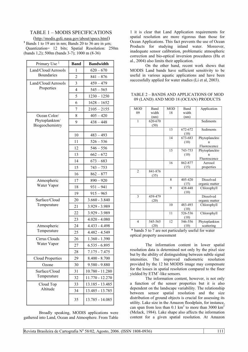
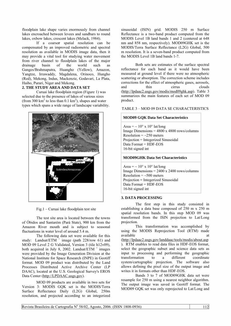
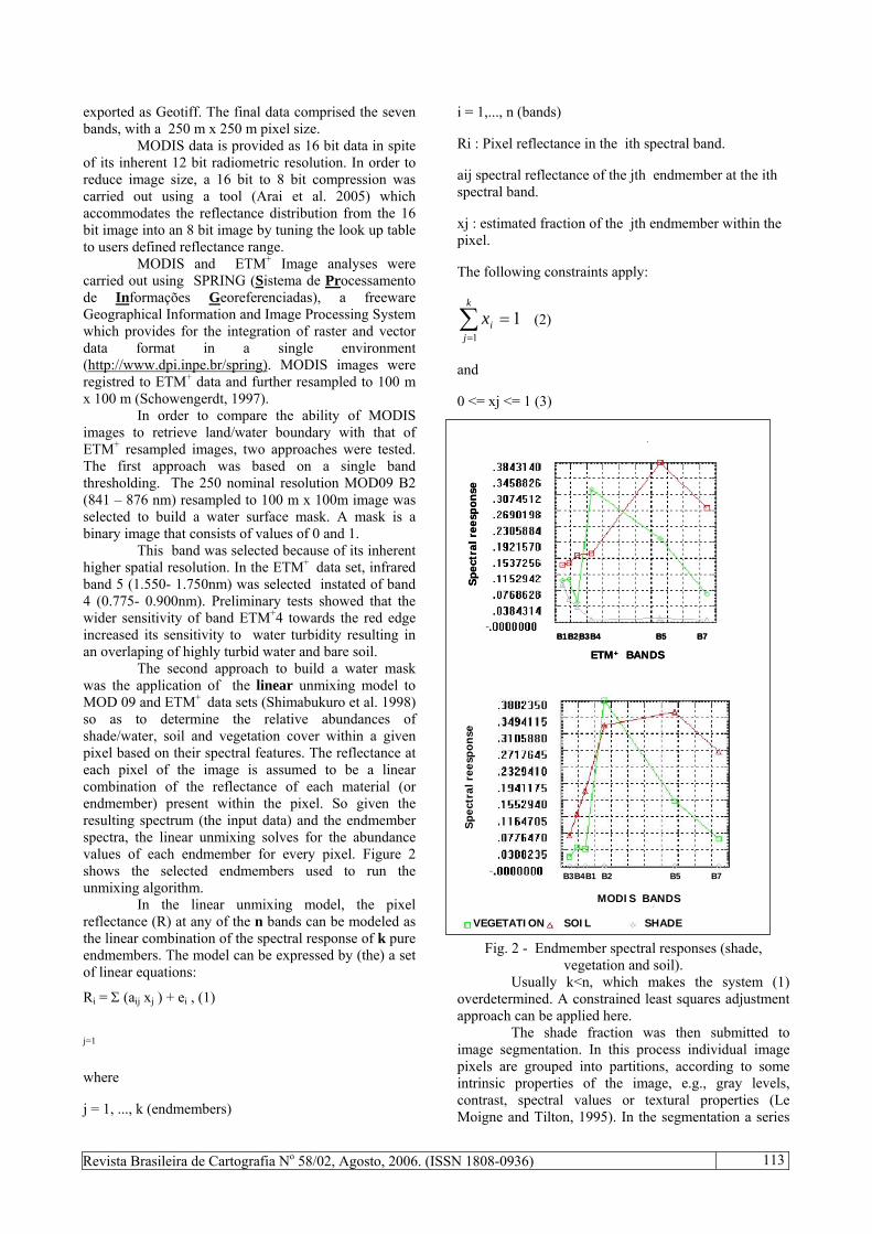
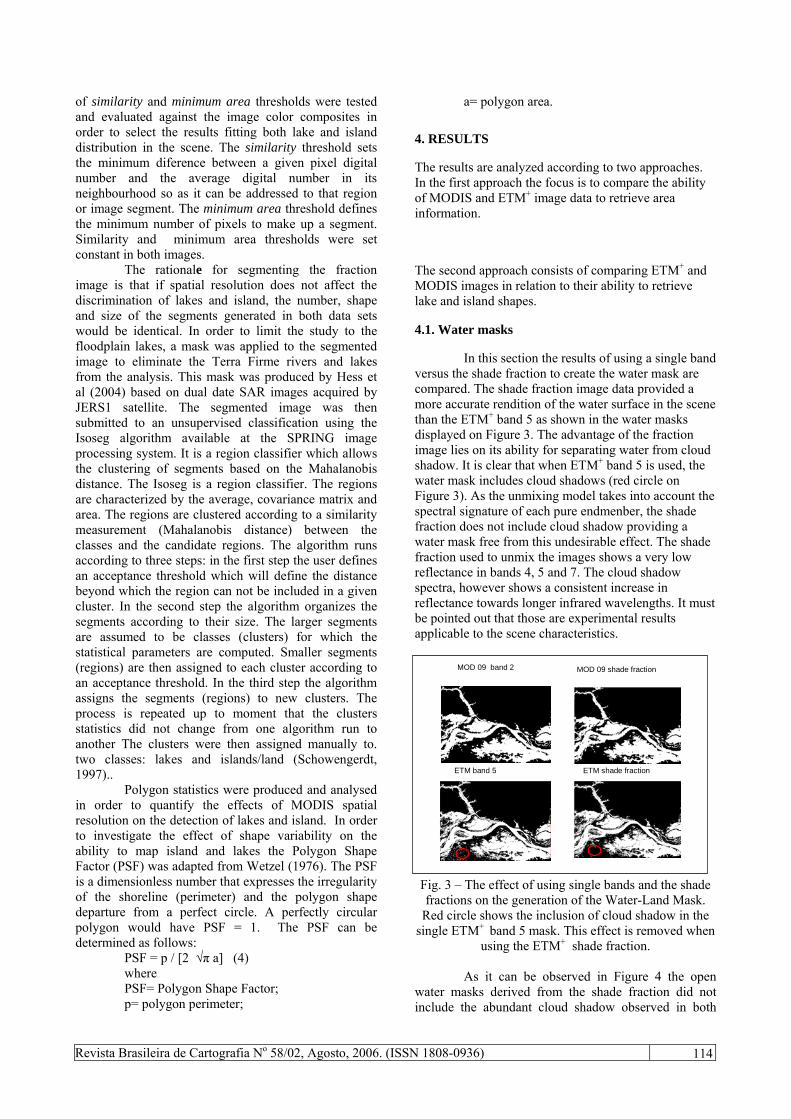
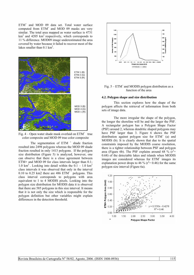
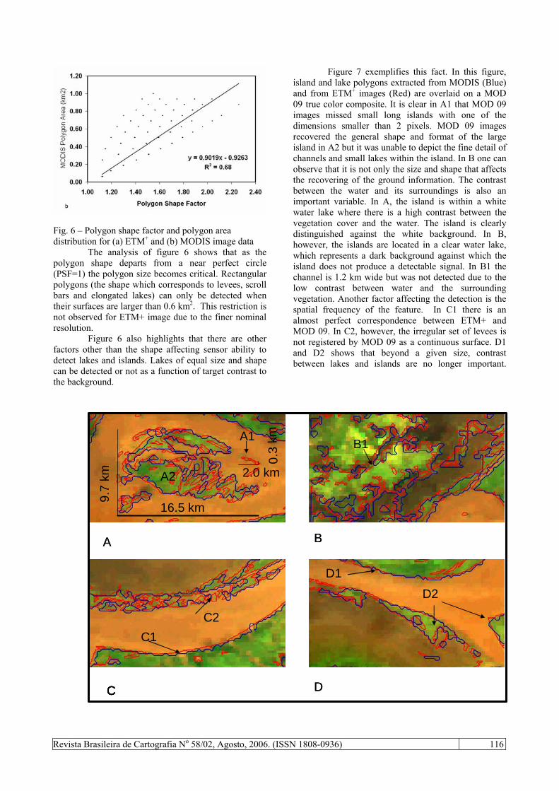
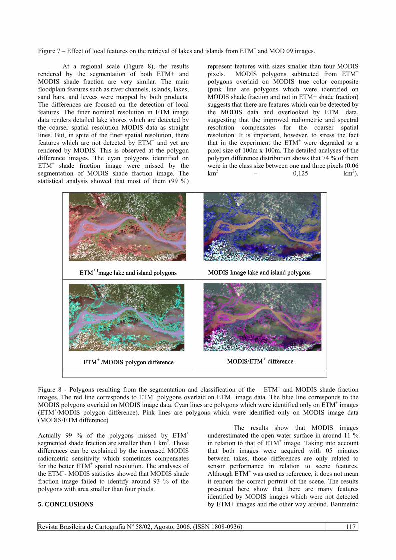
Copyright © 2022 FDOKUMEN