Simultaneous Observations and Analysis of Severe Storms Using Polarimetric X-Band SAR and...

3622 IEEE TRANSACTIONS ON GEOSCIENCE AND REMOTE SENSING, VOL. 48, NO. 10, OCTOBER 2010

Simultaneous Observations and Analysis of SevereStorms Using Polarimetric X-Band SAR and

Ground-Based Weather RadarJason P. Fritz, Senior Member, IEEE, and V. Chandrasekar, Fellow, IEEE

Abstract—Recent advances in synthetic aperture radar (SAR)technology have revived meteorological applications with thistype of radar. SARs are designed for surface imaging, but nowthat several X-band multipolarization SAR satellites are in orbit,the attenuation and backscatter caused by precipitation can bebetter studied. The results presented here demonstrate some ofthe possibilities by analyzing observations from dual-polarization(HH, VV) TerraSAR-X (TSX) acquisitions over central Floridasurrounding severe storms in August 2008. Simultaneous to theSAR acquisitions, WSR-88D ground weather radars in Melbourneand Tampa Bay, FL, collected reflectivity and radial velocity data;the observed strong precipitation cells from convective stormsare colocated with severe attenuation in the corresponding SARimages. The observations from SAR measurements are explainedquantitatively by converting ground radar reflectivity into space-borne radar attenuation via a theoretical model. In addition,polarization analysis comparing the SAR image to two additionalTSX acquisitions 11 days apart and without rain provides anindication of storm-induced propagation effects on X-band SAR.Specifically, the copolar ratio Zdr and the copolar correlationdifferences exhibit behavior that is better explained by the precip-itation impact versus surface changes. Multiple regions with vary-ing ground cover, including urban, and storm characteristics areanalyzed to highlight the complexity of meteorological researchusing SAR while revealing a potential use of the technology toinvestigate the storm structure.

Index Terms—Attenuation, meteorological radar, polarimetricsynthetic aperture radar, propagation losses, spaceborne radar,TerraSAR-X.

I. INTRODUCTION

THE GLOBAL hydrological cycle has a profound influ-ence on life on earth, and apprehension of its effects is

a major scientific pursuit by researchers around the world.Understanding the variability and surface impact of rainfall iscrucial to understanding our dynamic planet, and spacebornesensors can provide valuable information to meet this goal,particularly in regions with sparse or nonexistent ground radarcoverage. This need led to the highly successful Tropical Rain-fall Measurement Mission (TRMM), a joint project launched

Manuscript received August 26, 2009; revised December 24, 2009 andMarch 11, 2010. Date of publication July 23, 2010; date of current versionSeptember 24, 2010. This work was supported by the NASA Earth and SpaceScience Fellowship Program under Grant NNX07AO55H and the NASA PMMProgram.

The authors are with the Department of Electrical and Computer Engineer-ing, Colorado State University, Fort Collins, CO 80523-1373 USA (e-mail:[email protected]; [email protected]).

Color versions of one or more of the figures in this paper are available onlineat http://ieeexplore.ieee.org.

Digital Object Identifier 10.1109/TGRS.2010.2048920

in 1997 between the National Aeronautics and Space Ad-ministration (NASA) and the Japanese Aerospace ExplorationAgency (JAXA) [1], [2]. The success of the TRMM has inturn prompted the follow-on Global Precipitation Measure-ment (GPM) mission [3] scheduled to be launched in 2013.In addition to microwave radiometers, a dual-frequency (Ku-/Ka-band) nadir scanning radar will provide the core satel-lite of GPM with a more detailed precipitation measurementinstrument.

Observations of meteorology from spaceborne radar, how-ever, began with early synthetic aperture radar (SAR) missions.Atlas and Black [4] analyzed storms over the ocean as observedby the Seasat satellite [5]. Atlas and Moore [6] also developedtheoretical expressions to measure precipitation using SAR,whereas Pichugin and Spiridonov [7] presented a geometricmodel from a real aperture side-looking radar. In 1994, theNASA Space Shuttle Radar Laboratory missions provided thefirst multipolarization and multifrequency radar observationsof precipitation [8]–[10] from space. Observations of stormswere made both at traditional SAR look angles (oblique andside looking) and at nadir in preparation for TRMM. However,the X-band SAR that was part of the SIR-C/X-SAR missionshad only one polarization: vertical. These studies showed thepotential of SAR for precipitation measurement, particularly atX-band, where the signal is attenuated the most. C-band SARobservations of storms over the ocean have also been comparedwith ground-based weather radar using the European SpaceAgency’s ERS platform [11], [12].

Since the turn of the century, several X-band SAR(X-SAR) missions have been successfully launched or areplanned for the near future, providing an opportunity to investi-gate global precipitation with high-resolution spaceborne radar.In 2007, the Deutches Zentrum für Luft und Raumfahrt (DLR)launched the multipolarization X-SAR TerraSAR-X (TSX) [13]and is planning the follow-on mission TanDEM-X. The firsttwo of four satellites in the COnstellation of small Satellitesfor the Mediterranean basin Observation (COSMO)-SkyMedmultipolarization X-SAR constellation by the Agenzia SpazialeItaliana (ASI) were also propelled into orbit in 2007. As ofAugust 2009, three COSMO-SkyMed systems are orbitingthe planet. Within the next several years, more X-SARs willbe launched by Korea (KOMPSat-5), Russia (Severjanin onMETEOR-M), and others. As a result of these new sensors,and the fact that precipitation has more of an impact onX-band wavelengths, renewed interest in SAR precipitationmeasurement has surfaced. Danklmayer et al. [14] reportedthe first images of storms observed by TSX during the

0196-2892/$26.00 © 2010 IEEE

FRITZ AND CHANDRASEKAR: OBSERVATION AND ANALYSIS OF STORMS USING X-BAND SAR AND WEATHER RADAR 3623

TABLE IRADAR SPECIFICATIONS AND OPERATING PARAMETERS DURING

ACQUISITIONS OF DATA PRESENTED IN THIS PAPER

commissioning phase and have explored the effects of precipi-tation on SAR [15], whereas the first polarimetric storm obser-vations at X-band were described in [16] and [17]. Meanwhile,Marzano and Weinman [19] have made progress on model-based inversion algorithms.

The focus of this paper is to analyze and characterizedual-polarimetric (HH and VV) TSX observations of stormsover heterogeneous land. By using data from two NationalWeather Service (NWS) weather surveillance radar, 1988,Doppler (WSR-88D) S-band systems, also known as the NEXtgeneration RADar (NEXRAD) system, in conjunction withmicrophysical and spatial distribution models, the observedbackscatter and attenuation in the X-SAR images can be ex-plained. The two NWS radars used were KMLB in Melbourne,FL, and KTBW in Tampa Bay, FL. In addition, multiple TSXacquisitions were scheduled at the same location, allowingtemporal analysis of surface backscatter through different at-mospheric conditions. One of the consequences of using strip-map dual-polarization TSX data is a reduction in swath width toonly 15 km. However, the very high resolution may still providesome insight into the storm structure. Various parameter speci-fications for the two radar systems during the data acquisitionsanalyzed in this paper are given in Table I.

This paper is organized as follows: Section II providesbackground theory for the models used in the analysis. Next,Section III describes the TSX data acquisitions and qualitativeanalysis, followed by quantitative analysis with ground-basedradar in Section IV. The polarimetric effects of precipitationcells are discussed in Section V, and Section VI wraps up witha summary and conclusions.

II. THEORETICAL MODEL

A theoretical model is used to convert from the nearly hori-zontal pointing S-band ground radar reflectivity Zh to the spe-cific attenuation and polarimetric parameters of a slant-lookingX-band spaceborne SAR. Two components are required: 1) aspatial distribution model and 2) a microphysical model of rain.These are described in more detail below. A model describingthe effect of rain drop parameters on radar observations basedon scattering and propagation physics allows for comparisonbetween the ground and space radars within different spatialregions.

A. Fundamentals

A number of fundamental relationships for weather radarapplications are applied here [21]. The two basic phenomenaof electromagnetic (EM) wave interaction with precipitationare backscatter and attenuation, which are described by theradar backscatter cross section per unit volume η (m2m−3)and the extinction cross section σext (m2). The radar reflec-tivity factor Z is related to the precipitation backscatter crosssection as

Z =λ4

π0|Kw|2η

=λ4

π5|Kw|2∫

σpN(D) dD (mm6m−3) (1)

where λ is the wavelength, |Kw|2 is the dielectric factor ofhydrometeors, σp is the radar cross section for precipitation,and N(D) is hydrometeor size distribution (HSD), i.e., thenumber of particles per unit volume with sizes in the interval(D,D + ΔD). Similarly, the specific coefficient of attenuationk as a function of σext and N(D) is expressed by

k=4.343 × 103

∫σextN(D) dD (dB km−1). (2)

Over a given range from r1 to r2, the signal attenuation iscalculated using

A(r) = exp

⎛⎝−0.2 ln 10

r2∫r1

k(ξ) dξ

⎞⎠ (3)

which is also known as the path integrated attenuation (PIA).The observed reflectivity is then Zobs(r) = Z(r)A(r). A powerlaw relationship describes the association between the specificattenuation and the reflectivity factor, which is known as thek–Z relation and written as

k = αZβ . (4)

Because SAR is a surface imaging radar, the backscattercross section is normalized by area (normalized radar crosssection or NRCS) and typically expressed as σ0. However,the true NRCS is a function of the local surface incidenceangle and is not always precisely known without a highly accu-rate digital elevation model. Therefore, complex focused SARdata are most often provided as radar brightness or β0 [22].


The relationship between the two parameters is given by σ0 =β0 sin θ, where θ is the local incidence angle. Analyzing thepropagation impact of precipitation on SAR is the primaryfocus here, and the SAR products used are obtained in this form(i.e., the Level 1b single-look slant-range complex product),so the results are expressed in terms of β0 unless otherwiseindicated.

Due to the nonspherical nature of precipitation particles, apolarimetric radar can have differential observations betweenhorizontal and vertical channels. This effect is often more pro-nounced at near horizontal elevation angles but is still presentat SAR look angles. The specific differential phase observedbetween the two channels is [21]

Kdp =180λ

π

∫� [fh(D) − fv(D)] N(D) dD (deg km−1)

(5)

where fh and fv are the forward scattering amplitudes forthe horizontal and vertical polarization states, and � refersto the real part of a complex number. Similarly, the specificdifferential attenuation is defined by

Adp = (8.686 × 103)∫

� [fh(D) − fv(D)] N(D) dD

(dB km−1) (6)

where � refers to the imaginary part of a complex number.Ideally, a fully polarimetric radar observes three scat-

tering components expressed in vector form as Ω =[Shh

√2Shv Svv]T , where the subscripts represent receive

and transmit polarizations, respectively, and reciprocity is as-sumed. The resulting 3 × 3 covariance matrix from C = ΩΩ∗T

contains the relationships among the observations.Similarly, under the reciprocity assumption, the Pauli scat-

tering vector k = (1/√

2)[Shh + Svv Shh − Svv 2Shv]T isused to generate the coherency matrix via kk∗T [23]. In thispaper, only the second diagonal element is used, i.e.,

T22 = |Shh − Svv|2. (7)

The transform to the coherency matrix is used because thediagonal elements have a physical interpretation, where T22 isinterpreted as double bounce or dihedral scattering (maximumwhen the copolar phase difference, φco is 180◦). At the time ofdata acquisition, TSX only provided any two elements of Ω, andthe two copolar terms were selected, thus allowing the analysisof copolar relationships. Among these parameters, the copolarcorrelation coefficient is calculated as

ρco =〈ShhS∗

vv〉√〈|Shh|2〉〈|Svv|2〉

= |ρco|ejφco . (8)

The magnitude and phase of ρco provide information about notonly surface scattering mechanisms but also propagation effectswhen the radar wave passes through a volume of distributedparticles. Another parameter that is available with just thesetwo terms is the copolar ratio or differential reflectivity Zdr

determined from

Zdr = 10 log10

(⟨|Shh|2

⟩〈|Svv|2〉

)(dB). (9)

Fig. 1. Schematic of SAR planar wavefronts through a rain cell. x is thecross-track ground range, with various transition points between attenuation,backscatter, or both indicated. rx is the radial vector, whereas px is theperpendicular (ideal wavefront) vector. Thus, r(x) is the range through theprecipitation cell to the surface location x, p(x) represents the backscattercomponent of the precipitation affecting the observation at x, and r(px) is theattenuation of the precipitation backscatter as it is integrated along px.

The term Zdr will be used to refer to this copolar ratio, althoughSAR observations are not technically reflectivity because thecalculation is the same. Therefore, although the entire co-variance matrix is not known, the two copolar signals con-tain clues about the environment not available with a singlepolarization.

B. SAR Propagation Through Precipitation Model

The spatial distribution model for SAR through precipitationhas been presented by several previous works [7], [8], [19], [20]and is described with the aid of Fig. 1. This cross track verticalslice depicts a precipitation cell (gray region), the direction ofthe incident radar beam, and the plane wave approximationsto the range-time samples (δr = cτ/2, where τ is the com-pressed pulse width) and c is the speed of light. The cell couldcontain frozen, melting, and liquid layers; however, frozenparticles cause minimal attenuation, and melting layers are notas prevalent in the convective cells analyzed [21]. Therefore, theinvestigation begins by only considering liquid particles (i.e.,rain) to determine the adequacy of this model.

When the SAR beam passes through a precipitation cell, theobserved NRCS can be expressed as the sum of volume andsurface cross sections (see Fig. 1) [7], [8], [10], [20], i.e.,

σobs = σsp + σvp

σ0obsαsrf = σ0

spαsrf + ηvpVeff (10)

where αsrf = δaδr is the surface area within the SAR resolutioncell, ηvp is the volumetric backscatter cross section (m2m−3),and Veff is the effective volume of precipitation backscatter[8] that incorporates the turbulent velocity-dependent azimuthresolution described in [6]. Dividing through by this surfacearea leaves σ0

obs = σ0sp + ηvpaeff , where aeff is the remaining

effective area. In general, the volume and surface componentsare scaled based on how much of the sampled beam volumetravels through (r(x) in Fig. 1) or resides in the precipitationvolume in the transverse dimension (p(x)). At the cross-trackrange where the beam reflects the surface x with a no-rainNRCS σ0

NR

σ0sp = σ0

NRAr(x)(r) (11)


where Ar(x)(r) is defined by (3) integrated over r(x) and

ηvpaeff = sin θ

∫p(x)

η(px)Ar(px)(r) dpx (12)

where Ar(px)(r) is defined by (3) integrated over r(px). Sim-ilarly, the differential reflectivity contains surface and volumecomponents expressed as

Zobsdr = Zsrf

dr + Zvoldr − 2

R∫0

Adp(r) dr (13)

where Adp is defined in (6), and the superscripts of Zdr aredefined as follows: obs is the observation, srf is the surfacecomponent, and vol is the contribution of the hydrometeorvolume. The last term reveals the differential attenuation fora target at range R.

If the precipitation cell were a perfect rectangle, then basictrigonometry can be used to precisely calculate the integrationparameters r(x), p(x), and r(px) [7], [19]. However, realisticvalues are not so easy to determine, particularly when theedges are not well defined. The ground-based radar reflectivitiescorresponding to visible artifacts in the SAR images are mostlikely convective cells due to the high reflectivity values andthe sharp gradients [24]; this is discussed further in Sections IIIand IV. Over regions that would be classified as stratiform, theeffects on SAR observations are negligible. Despite the ambi-guity, however, the ground radar reflectivity volume providesestimates for comparison.

The second part of the model involves microphysical repre-sentation. Similar to [25], the HSD is represented by a normal-ized gamma distribution [26], [27], i.e.,

N(D) = Nwf(μ)(

D

D0

)μ

exp[−(3.67 + μ)

D

D0

](14)

where

f(μ) =6

3.674

(3.67 + μ)μ+4

Γ(μ + 4). (15)

In (14) and (15), D0 is the volume-weighted median dropdiameter equivalent (mm), Nw is the slope intercept parameter(mm−1mm−3), μ is a shape parameter, and Γ represents thegamma function.

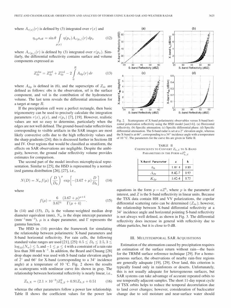
The HSD in (14) provides the framework for simulatingthe relationship between polarimetric X-band parameters andS-band horizontal reflectivity. For rain cells, the followingstandard value ranges are used [21], [25]: 0.5 ≤ D0 ≤ 2.5, 3 ≤log10(Nw) ≤ 5, and −1 ≤ μ ≤ 4 with a constraint of a rain rateless than 300 mm h−1. In addition, the Beard and Chuang [28]drop shape model was used with S-band radar elevation anglesof 2◦ and 66◦ for X-band (corresponding to a 34◦ incidenceangle) at a temperature of 10 ◦C. Fig. 2 shows the resultsas scattergrams with nonlinear curve fits shown in gray. Therelationship between horizontal reflectivity is nearly linear, i.e.,

Zh,X = (2.1 × 10−3)Z2h,S + 0.91Zh,S + 0.51 (16)

whereas the other parameters follow a power law relationship.Table II shows the coefficient values for the power law

Fig. 2. Scattergrams of X-band polarimetric observables versus S-band hori-zontal polarization reflectivity using the HSD model [see(14)]. (a) Horizontalreflectivity. (b) Specific attenuation. (c) Specific differential phase. (d) Specificdifferential attenuation. The S-band radar is set at a 2◦ elevation angle, whereasthe X-band is at 66◦, corresponding to a 34◦ incidence angle with a temperatureof 10 ◦C. The parameters for the curve fits are given in Table II.

TABLE IICOEFFICIENTS TO CONVERT Zh,S TO X-BAND

PARAMETERS IN THE FORM aZbh,S

equations in the form p = aZb, where p is the parameter ofinterest, and Z is the S-band reflectivity in linear units. Becausethe TSX data contain HH and VV polarizations, the copolardifferential scattering ratio can be determined (Zdr); however,the relationship between X-band differential reflectivity at a34◦ incidence angle and horizontal pointing S-band reflectivityis not always well defined, as shown in Fig. 3. The differentialreflectivity does increase in general with reflectivity due tooblate particles, but it is close to 0 dB.

III. MULTITEMPORAL SAR ACQUISITIONS

Estimation of the attenuation caused by precipitation requiresan estimation of the surface return without rain—the basisfor the TRMM surface reference technique [29]. For a homo-geneous surface, the observations of nearby rain-free regionsare generally adequate [19], [29]. Over land, this criterion istypically found only in rainforests or deserts. Unfortunately,this is not usually adequate for heterogeneous surfaces, butSAR systems can take advantage of accurate repeated orbits touse temporally adjacent samples. The short 11-day repeat cycleof TSX orbits helps to reduce the temporal decorrelation dueto land cover changes; however, consideration of backscatterchange due to soil moisture and near-surface water should


Fig. 3. Scattergram from the theoretical model showing (a) the differencebetween X- and S-band reflectivity versus X-band differential reflectivityZdr,X and (b) Zdr,X versus Zh,S , with the same radar alignment as in Fig. 2.When the X-band minus S-band reflectivity difference drops below 0 dBZ,the a 1 : 1 correspondence with Zdr,X no longer exists due primarily to Miescattering. There is also high variability in the differential reflectivity whenonly knowing Zh,S , but at an elevation angle of 66◦, Zdr,X is close to 0 dB.

Fig. 4. WSR-88D reflectivity scans over Google Earth image of Florida.(a) Convective storm front reflectivity from the KTBW radar on 080808 at anelevation of 1.5◦. (b) TS Fay reflectivity on 080819 from the KMLB radarat an elevation of 0.5◦. The SAR image frames are outlined in (a) white and(b) black with the NEXRAD locations indicated.

be considered, particularly in a region such as Florida withnumerous lakes and easily saturated soil [30], [31].

In August 2008, several TSX acquisitions over the Floridapeninsula were requested by the authors with the express goalof capturing precipitation signatures in the data. By requestingacquisitions suitable for interferometry, better temporal com-parisons can be made without concern for fluctuations dueto different viewing geometries or beam modes. Success wasachieved on multiple overpasses using the same operationalmode. Specifically, data acquired in dual-polarimetric strip-map mode over the Orlando and Kissimmee regions captureda strong storm on August 8, 2008 (080808), as shown in theNEXRAD KTBW radar in Fig. 4(a). Given the sharp reflectivitygradients and high values, this storm is mostly convective [24]and may even be classified as a squall line. In mid-August,Tropical Storm Fay (TS Fay) swirled over the state for severaldays, dumping up to 700 mm of rain near Melbourne, FL,with sustained winds of over 100 km h−1 [32]. During thistime, the TSX satellite acquired dual-polarization data justsouth of Orlando, FL, on August 19, 2008 (080819), as shownover the NEXRAD KMLB radar reflectivity in Fig. 4(b). Thethird acquisition was captured during a virtually rain-free timeperiod 11 days later on August 30, 2008 (080830). Each SARswath is broken into multiple products known as frames, and

the two southernmost are analyzed in this paper (i.e., sixproducts/images were purchased from DLR under the TSXscience program).

Fig. 5 depicts color composite multilooked β0 images of allthree acquisitions, where the two frames have been mosaickedtogether. The first three images consist of the |HH| and |VV|channels assigned to red and green, whereas the blue coloris 2−.5|HH − VV| [i.e.,

√T22 in (7)]. For qualitative compar-

ison and visualization, the histogram tails are clipped at thesame values (±0.5% with respect to the 080830 data) afterconversion to decibels. The fourth image [Fig. 5(d)] consists of√

T11 from 080808 (red), 080819 (green), and 080830 (blue).This provides a clear indication of the different power fromeach acquisition even with only an 11-day separation. Forexample, cyan indicates attenuation from the 080808 storm, redmarks backscatter from that storm, whereas magenta and greenidentify where TS Fay increased attenuation and VV reflectivityover water surfaces.

There are several interesting features to point out that arerelative to the investigation of storms. Obviously, the stormsduring the first two acquisitions caused severe attenuation andappear like black clouds. Without further knowledge, a con-clusion might be reached that these storm cells were isolated,but the analysis in Section IV shows that is not the case. Theseimages do give an indication, however, that the storm cells on080808 were more severe than on 080819 because they appearto have higher attenuation. In Fig. 5(a), a higher (reddish) HHreturn is visible on the near-range side, indicating that theprecipitation backscatter is stronger than the attenuated surfacereturns (i.e., the volume term in (10) dominates). As shown inSection IV, this region corresponds to high reflectivity gradienton the western side of the convective cell. Figs. 6–8 show thestorm regions in more detail and indicate zones that will be usedfor a more detailed analysis and comparison with the weatherradar data in Section IV and the polarimetric investigationsin Section V. The colors shown in these images are createdby using |HH|, |VV|, and

√T22 from 080808, 080819, and

080830, respectively, only to indicate the attenuation regionwhile still revealing surface features that would otherwise beobscured by the precipitation.

Two other storm-related effects visible in the TSX imagesare related to surface water. One is the higher VV return fromthe water bodies due to wind and rain, resulting in a significantincrease in Bragg scattering at the TSX incidence angle, whichis typically stronger in VV polarization [33]. In the 080808image, rain is more likely the cause, but the pattern on thewater surfaces in the 080819 image suggests that the high windsmight be more dominant. The other effect is due to near surfacewater and soil saturation. Some of these regions become visiblein the composite image of Fig. 5(d) and are discussed brieflyin the next two sections. There is significant agriculture in thisregion, and the sandy soil is easily saturated.

IV. COMPARISON TO GROUND RADAR

Weather data from ground-based radar are used to quantifythe observations from TSX acquisitions. The goal is to demon-strate that features in the reflectivity data align with featuresin the SAR data, followed by a more quantitative analysis inthe regions indicated in Figs. 6–8. Considerable overlap exists


Fig. 5. Three TSX HH, VV acquisitions on (a) 080808, (b) 080819, and (c) 080830. The true color composite images consist of two β0 frames of |HH| (red),|VV| (green), and

√T22 (blue) in decibels and are coregistered with respect to each other. (d)

√T11, where the RGB consists of 080808, 080819, and 080830,

respectively (see text). The flight direction is bottom to top looking right.

between the two NEXRAD radars, i.e., KMLB in Melbourne,FL, and KTBW in Tampa Bay, FL, and provides the capabilityto estimate the reflectivity volume by combining observations.KMLB is the closest radar to the TSX acquisition frames atroughly 78 and 92 km to the center of each frame, whereasKTBW is approximately 105 and 119 km.

The merging process is complicated by the fact that the tworadars are not synchronized and sometimes have very differentvolume coverage patterns (VCPs). For example, during TS Fay,KMLB scanned a volume in 4.5 min, whereas KTBW tookabout 6 min, with different pulse repetition frequencies (PRFs),

scan rates, and elevation angles (see Table I). Fortunately, thesedifferences are addressed in the Warning Decision SsupportSystem–Integrated Information (WDSS-II) and the mergingalgorithms contained within [34] and [35]. The 3-D grid fromWDSS-II is georeferenced, allowing for spatial comparisonswith the SAR acquisitions. A Gaussian-weighted 3-D low-pass filter is then applied for additional smoothing. WDSS-IIcan also estimate advection, which is particularly importantwhen the precipitation cores of the TS Fay were moving over22 m s−1; however, there is still a fair amount of uncertainty,and selection of the best algorithm is not straightforward. Prior


Fig. 6. Close-up of the 080808 storm region over Orlando with the analysiszones marked. The RGB image is formed by using |HH| from 080808,|VV| from 080819, and

√T22 from 080830, respectively, only to indicate

the attenuation region while still revealing surface features. The attenuationhere is indicated by the cyan color (green + blue), whereas the backscatteris red.

Fig. 7. Close-up of the 080808 storm region near Kissimmee with the analysiszones marked. The RGB channels are the same as in Fig. 6. Again, theattenuation from the 080808 storm shows up as cyan.

to experimenting with advection estimation, adjusting the timeperiod of the output volumes can provide a reasonable snapshotof the storm during TSX acquisition within the limitations ofthe radar VCPs. The grid resolution is 0.0015◦ latitude andlongitude (approximately 150 × 150 m2) by 250 m vertically.After the 3-D volume of reflectivity is gridded, it can be slicedat any angle to reveal what the SAR beam would pass throughand illuminate. The path-integrated reflectivity at S-band canthen be used to estimate the attenuation seen by the X-bandSAR at each resolution cell using the model presented inSection II-B. Coregistration and orthorectification of the TSXdata were accomplished using the Doris SAR interferometrysoftware [36].

Fig. 8. Close-up of the 080819 storm region with the analysis zones marked.The RGB channels are the same as in Fig. 6. In this case, the attenuation causedby the 080819 tropical storm is magenta (red + blue) with higher backscatterin bright green.

Fig. 9. (a) Orthorectified 080808 TSX RGB composite compared with(b) the same region in the vertical maximum of the merged WSR-88D reflec-tivity. Contours of this maximum field are drawn on the TSX image at 29, 36,and 43 dBZ. This clearly shows correspondence between the high reflectivityregion and the high attenuation in the SAR image and provides a visualindication of the horizontal displacement due to viewing geometry described inSection IV-B. Portions of the two SAR image frame boundaries are shownin (b).

A. Case 1: 080808

Fig. 9 clearly shows a strong relationship between the groundradar reflectivity and the precipitation signature in the orthorec-tified SAR image. To get a better sense of the 3-D volume in a2-D image, the reflectivity plot is the maximum value within thevertical column at each grid location to capture the most intenseportions within the storm (also known as vertical maximumintensity). Smoothed contours of this maximum reflectivityfield at 29, 36, and 43 dBZ are drawn over the SAR image.With an incidence angle of about 35◦, it appears that the visiblebackscatter and attenuation in the TSX data is around 45 dBZin this case. Selection of this threshold will be explored inthe subsequent quantitative analysis below, and it is likely thatthe threshold level depends on many variables. Several factors


contribute to the challenge of accurately aligning ground-basedweather radar observations to SAR images. A major factor isthe 4 to 6 min volume update time of the NEXRAD radars ver-sus the nearly instantaneous SAR acquisition. Another factoris the horizontal cross-track storm motion, which can induce aDoppler shift resulting in along-track displacement. It is alsoclear from Fig. 9(a) that it was raining over the lakes to thewest of the convective cell, causing stronger backscatter in thevertical polarization. Although it is not visible at the scale ofthe images in this paper, a small amount of attenuation is alsopresent in the data around 28.6◦ latitude and −81.45◦ longitude,corresponding to the small region that is close to 40 dBZin Fig. 9(b). Around 28.2◦ latitude, the cell with reflectivity> 55 dBZ to the west of the TSX swath results in nearly com-plete signal loss from the SAR. This is described in Fig. 11(b)and the accompanying text and is also shown Fig. 18(c), wherethe copolar phase is almost uniformly distributed. The outlineof the TSX images in Fig. 9(b) also indicates the overlap of theframes.

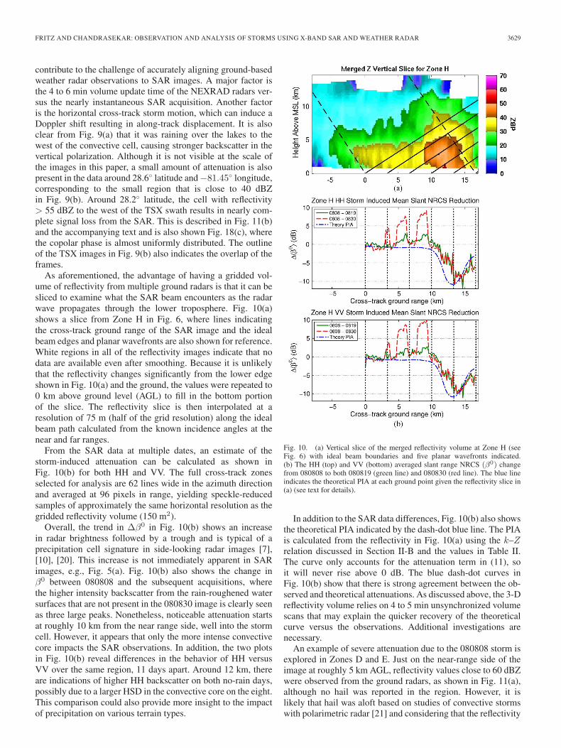
As aforementioned, the advantage of having a gridded vol-ume of reflectivity from multiple ground radars is that it can besliced to examine what the SAR beam encounters as the radarwave propagates through the lower troposphere. Fig. 10(a)shows a slice from Zone H in Fig. 6, where lines indicatingthe cross-track ground range of the SAR image and the idealbeam edges and planar wavefronts are also shown for reference.White regions in all of the reflectivity images indicate that nodata are available even after smoothing. Because it is unlikelythat the reflectivity changes significantly from the lower edgeshown in Fig. 10(a) and the ground, the values were repeated to0 km above ground level (AGL) to fill in the bottom portionof the slice. The reflectivity slice is then interpolated at aresolution of 75 m (half of the grid resolution) along the idealbeam path calculated from the known incidence angles at thenear and far ranges.

From the SAR data at multiple dates, an estimate of thestorm-induced attenuation can be calculated as shown inFig. 10(b) for both HH and VV. The full cross-track zonesselected for analysis are 62 lines wide in the azimuth directionand averaged at 96 pixels in range, yielding speckle-reducedsamples of approximately the same horizontal resolution as thegridded reflectivity volume (150 m2).

Overall, the trend in Δβ0 in Fig. 10(b) shows an increasein radar brightness followed by a trough and is typical of aprecipitation cell signature in side-looking radar images [7],[10], [20]. This increase is not immediately apparent in SARimages, e.g., Fig. 5(a). Fig. 10(b) also shows the change inβ0 between 080808 and the subsequent acquisitions, wherethe higher intensity backscatter from the rain-roughened watersurfaces that are not present in the 080830 image is clearly seenas three large peaks. Nonetheless, noticeable attenuation startsat roughly 10 km from the near range side, well into the stormcell. However, it appears that only the more intense convectivecore impacts the SAR observations. In addition, the two plotsin Fig. 10(b) reveal differences in the behavior of HH versusVV over the same region, 11 days apart. Around 12 km, thereare indications of higher HH backscatter on both no-rain days,possibly due to a larger HSD in the convective core on the eight.This comparison could also provide more insight to the impactof precipitation on various terrain types.

Fig. 10. (a) Vertical slice of the merged reflectivity volume at Zone H (seeFig. 6) with ideal beam boundaries and five planar wavefronts indicated.(b) The HH (top) and VV (bottom) averaged slant range NRCS (β0) changefrom 080808 to both 080819 (green line) and 080830 (red line). The blue lineindicates the theoretical PIA at each ground point given the reflectivity slice in(a) (see text for details).

In addition to the SAR data differences, Fig. 10(b) also showsthe theoretical PIA indicated by the dash-dot blue line. The PIAis calculated from the reflectivity in Fig. 10(a) using the k–Zrelation discussed in Section II-B and the values in Table II.The curve only accounts for the attenuation term in (11), soit will never rise above 0 dB. The blue dash-dot curves inFig. 10(b) show that there is strong agreement between the ob-served and theoretical attenuations. As discussed above, the 3-Dreflectivity volume relies on 4 to 5 min unsynchronized volumescans that may explain the quicker recovery of the theoreticalcurve versus the observations. Additional investigations arenecessary.

An example of severe attenuation due to the 080808 storm isexplored in Zones D and E. Just on the near-range side of theimage at roughly 5 km AGL, reflectivity values close to 60 dBZwere observed from the ground radars, as shown in Fig. 11(a),although no hail was reported in the region. However, it islikely that hail was aloft based on studies of convective stormswith polarimetric radar [21] and considering that the reflectivity


Fig. 11. (a) Vertical slice of the merged reflectivity volume at Zone D (seeFig. 7) with ideal beam boundaries and five planar wavefronts indicated. (b) HH(top)- and VV (bottom)-averaged slant range NRCS (β0) change from 080808to both 080819 (green line) and 080830 (red line). The blue line indicates thetheoretical PIA at each ground point given the reflectivity slice in (a) (see textfor details).

is higher above 4 km (this could indicate a melting layerof approximately 4 km). This induces a signal loss from thesurface of nearly 15 dB relative to the two other acquisitions,as shown in Fig. 11(b). The absolute values in this regionwere close to −20 dB, which is lower than the semispecularreflections observed from smooth water surfaces, indicatingthat many observations are likely to be close to the system noisefloor before averaging. Near to far range pixels are farthestfrom the beam center, meaning the system noise floor is higherin these regions. Theoretically, however, the attenuation inthis region should go down to −22 dB if the system weresensitive enough and the hydrometeors were all liquid water.The theoretical PIA plotted in Fig. 11(b) does match fairly wellwith the signal recovery after passing beyond the storm cell atapproximately 5 km. Because there is no precipitation beyondabout 5-km cross-track ground range, the differences observedfrom 080808 to 080819 and 080830 can be attributed to surfacebackscatter changes and some precipitation effects caused byTS Fay discussed in Section IV-B.

Fig. 12. (a) Orthorectified 080819 TSX RGB composite compared with(b) the same region in the vertical maximum of the merged WSR-88D reflec-tivity. Contours of this maximum field are drawn on the TSX image at 29, 36,and 43 dBZ.

B. Case 2: 080819–TS Fay

TS Fay provides another case to explore the impact of precip-itation on X-band SAR. Fig. 12 depicts the spatial relationshipbetween ground radar reflectivity and TSX signal attenuationon 080819, similar to Fig. 9. In this case, however, it is evidentthat rain is falling over the entire region, but mostly at ratestoo low to noticeably attenuate the TSX data. The thresholdfor attenuation appears to be closer to the 43 dBZ contour lineshown in Fig. 12(a), but there are numerous differences betweenthis tropical storm and the convective storm on 080808. Asidefrom physical differences, the KTBW radar was operating witha 6-min VCP. With estimated storm motion in this region of22 m s−1, even the shorter 4-min VCP for KMLB will havedifficulty capturing the horizontal storm structure.

Using the same analysis and processing discussed inSection IV-A, comparisons between the ground-based reflec-tivity from two NEXRAD radars are compared with the TSXdata during TS Fay. Cross-track vertical slices of the WSR-88Dreflectivity at Zones A and B along-track ranges shown in Fig. 8correlate spatially with the SAR parameters in those regions.The vertical slice of the S-band reflectivity volume shown inFig. 13(a) verifies that attenuation should be apparent from thenear-range edge. The observed disparity between TSX radarbrightness on this date relative to 080808 and 080830 resultsin a decrease of about 3 dB to begin with, dropping to about−7 dB at both polarizations, as shown in Fig. 13(b). A largerdiscrepancy between the acquisitions is also more apparent inHH polarization mode; however, surface changes resulting fromthe tropical storm may play a considerable role in this naturalground cover region. Fig. 13(b) also shows a fairly close matchwith the theoretical PIA, although features do not line up inrange as well, most likely due to a temporal gap in the lowerelevation NEXRAD coverage. Close examination of the sharpchanges with respect to 080830 reveals flooded regions andother water surfaces that exhibit low backscatter.

Analysis of Zone B, which is depicted in Fig. 14, showsa slightly different behavior of the observations relative toZone A. However, these are more similar to the 080808 case,where the attenuation is preceded by backscatter despite the factthat it is not visually noticeable. Compared with the theoretical


Fig. 13. (a) Vertical slice of the merged reflectivity volume at Zone A (seeFig. 8) with ideal beam boundaries and five planar wavefronts indicated.(b) Reduction in slant range NRCS (β0) from both 080808 and 080830 inZone A (see Fig. 8 for zone indications) with ΔHH on the top and ΔVV onthe bottom. This shows the total NRCS change from each of the two adjacentpasses, indicating that potentially significant surface change resulted from thestorm.

PIA curve in Fig. 14(b), the backscatter term in (10) appearsto dominate the attenuation, plus the wet surface may haveenhanced reflectivity. Again, the trend in the theoretical curvedoes not quite line up with the observations, but they arewithin a few decibels. The SAR data, however, appears topick up a sharper gradient that is beyond the resolution of theWSR-88Ds. Similar to the Zone A response, the HH returnrelative to 080808 is larger, but storm-induced surface alterationis suspected because no rain was present in this area on either ofthe adjacent acquisition dates. The drastic spike at the far rangeis caused by SAR interaction with the lake surface.

C. Summary of Ground Radar Comparison

The overall relationship between the path-integrated slantrange reflectivity and the change in radar brightness comparedwith the no-rain cases for all cross-track zones is displayed inFig. 15. Drastic changes due to the roughened water surfaces

Fig. 14. (a) Vertical slice of the merged reflectivity volume at Zone B(see Fig. 8) with ideal beam boundaries and six planar wavefronts indicated.(b) Reduction in radar brightness (β0) from both 080808 and 080830 in Zone Bwith HH on the top and VV on the bottom. This shows the total β0 change fromeach of the two adjacent passes, indicating that potentially significant surfacechange resulted from the storm.

Fig. 15. Differential radar brightness from rain cases versus path-integratedS-band reflectivity for all cross-track zones (A, B, D, F, and H) at bothpolarizations. Observations from roughened water are removed, and differencesbetween no-rain values are averaged. The solid line is an exponential least-square fit.

were removed, and differences between the no-rain data wereaveraged. Accumulating reflectivity with range is unconven-tional, but it is analogous to PIA using a directly observableparameter. Significant backscatter can still be present up to anaccumulated 55 dBZ, but at that point it drops sharply. Accu-mulated values above 68 dBZ, which did not decrease the signal


beyond the noise floor, were also removed. An exponentialrecursive least-square fit of the form y = aebx (in linear units),where a = 1.144, and b = −7.065 × 10−7, is plotted as theblack line in Fig. 15. In general, this is similar to the expressionfor PIA in (3).

V. POLARIMETRIC EFFECT

The previous section analyzed the attenuation and backscat-ter caused by the storms. Now, we investigate the effect ofprecipitation on signal polarization. There are three parameterswe can investigate with the two available copolar channels.Two of these parameters are represented by (8): 1) the copolarcorrelation coefficient magnitude |ρco| and 2) the copolar phaseφco. The third parameter is the copolar ratio Zdr (differentialreflectivity) from (9). While weather radars measure theseparameters directly, in the absence of ground clutter, SAR mustrely on detecting the deviation from the polarimetric propertiesof surface scattering. Unfortunately, this may not be conclusivebecause polarimetric SAR is also valuable as a surface propertychange analyzer. Despite this uncertainty, however, pure attenu-ation of the surface reflections will not change the polarimetricproperties. Given a constant return from the surface, this changecan only occur due to propagation effects that are polarizationdependent, such as nonspherical oriented hydrometeors [21].

Several observations about the polarimetric effects of pre-cipitation can be made from the scatter plots in Section II-Band literature on the subject [21]. Differential reflectivity andattenuation will be 0 dB for perfectly spherical hydrometeorsand increase as liquid drops increase in size and becomeoblate. Lighter rain and most hail tend to be very correlatedbetween polarizations, decreasing as the raindrop size, and thecorresponding oblateness increases. The oblateness increase isusually associated with an increase in horizontal reflectivitycoupled with a higher attenuation in this polarization. However,Figs. 2(d) and 3(b) indicate that the impacts on Zdr and Adp areminimal at a surface incidence angle of 34◦. Likewise, the copo-lar phase change will be close to zero until the particles becomemore nonspherical and oriented. As the EM wave propagatesthrough a volume with nonspherical oriented hydrometeors,the phase change accumulates as shown in (5), and Fig. 2(c)conveys the level of propagation phase shift relative to S-bandZh at the viewing geometries analyzed.

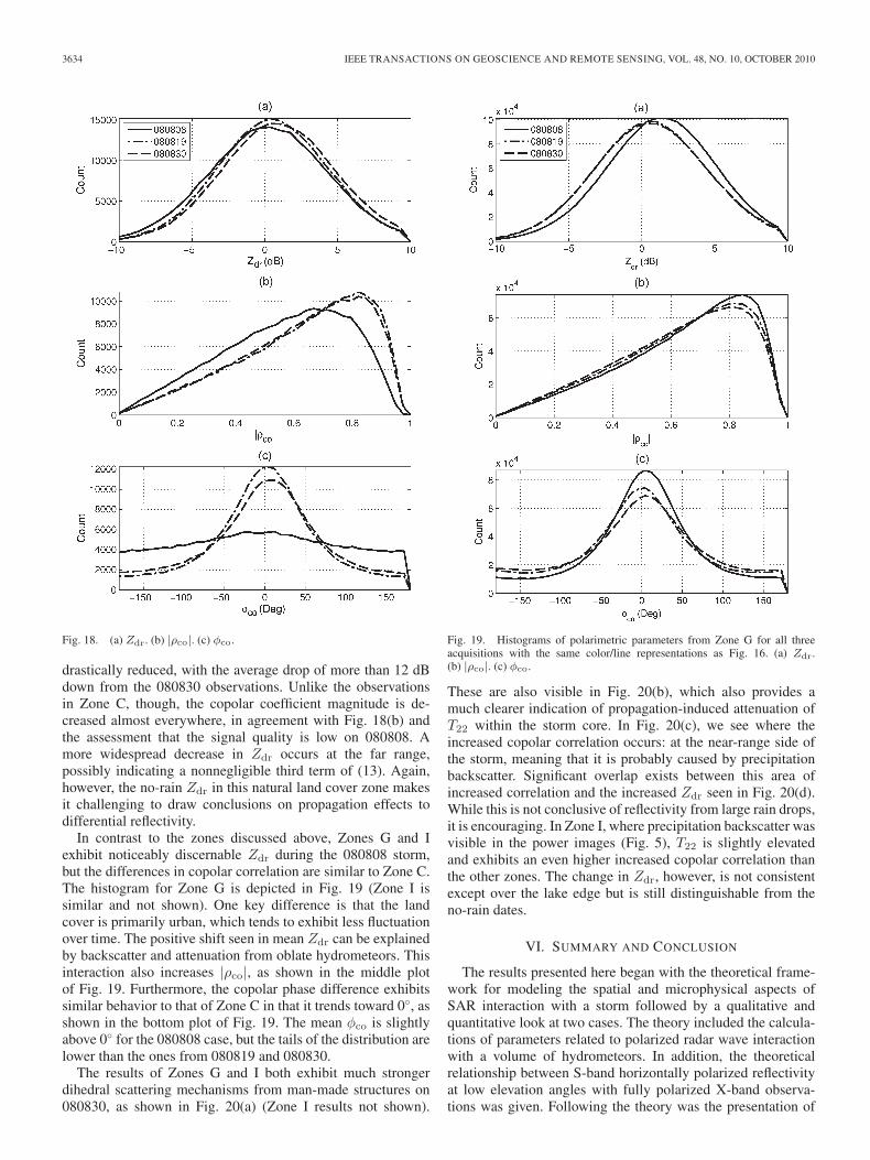
Histograms of the three polarimetric parameters for Zone C(Fig. 6) are shown in Fig. 16 for all three acquisitions. The solidgreen line is 080808, the dash-dot blue line is 080819, and thedashed red line is 080830. The parameters from 080819 duringTS Fay clearly stand out from the others. For Zdr, however,the difference is not statistically significant because over thisnatural cover area, the mean copolar ratio is approximately0 dB. On the other hand, the 080819 |ρco| histogram shownin the middle panel indicates higher copolar correlation with anincrease in the mean of 0.04 and 0.06 from the other two. Thisis indicative of the precipitation affecting the observed signals.A more significant divergence of the TS Fay data is seen in thebottom panel for φco. The mean phase difference decreases by14.4◦ and 11.1◦ from the other dates with a 14◦–20◦ decreasein standard deviation. Additional discussion of copolar phasechange due to TS Fay, including pooling surface water, can befound in [17].

Fig. 16. Histograms of polarimetric parameters from Zone C for all threeacquisitions. 080808 is the green solid line, 080819 is the blue dash-dot line,and 080830 is the red dashed line. (a) Copolar ratio (Zdr) histograms inZone C. (b) Copolar correlation coefficient (|ρco|) histograms. (c) Copolarphase difference (φco) histograms.

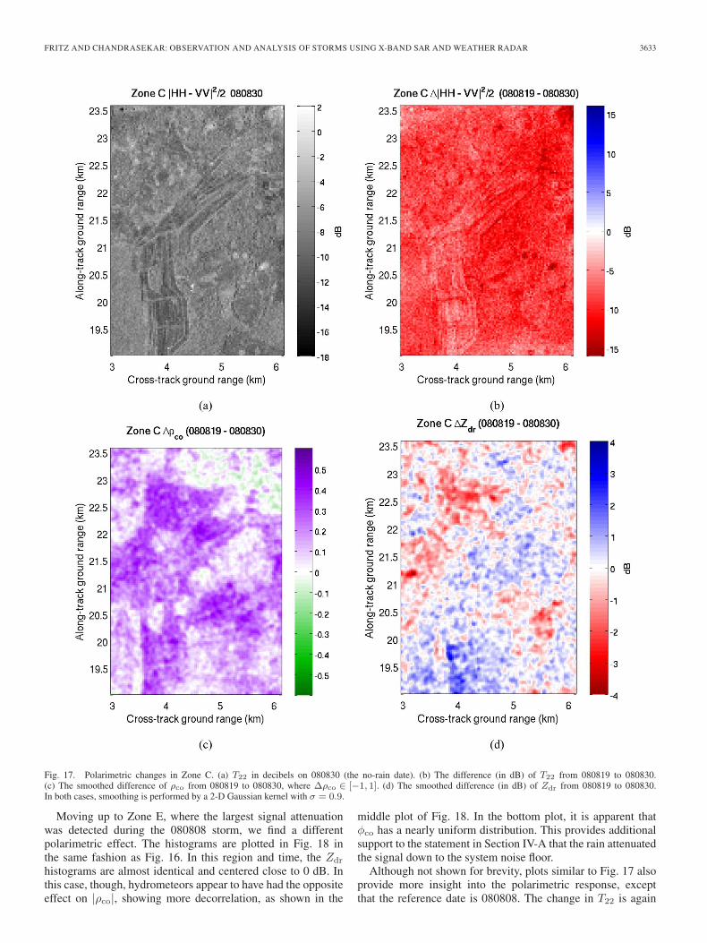
Fig. 17 provides some insight into the polarimetric changesthat occurred in Zone C due to the storm. For these images,data from 080830 were selected as the no-rain estimate ofsurface returns considering the fact that changes occur evenwithout rain. The complex copolar difference power [see (7)]on 080830 is depicted in Fig. 17(a). Limited dihedral scatteringresults in relatively low power. TS Fay, however, caused adrastic decrease in this parameter of about 10 dB, as shownin Fig. 17(b), where the linear power ratio between 080819and 080830 determines the change prior to dB conversion. Adrop of this magnitude is not likely from pure surface changein 11 days. Fig. 17(c) displays the increase in copolar corre-lation (|ρ080819

co | − |ρ080830co |) seen in the Fig. 16(b) histogram.

Comparing this to Fig. 17(a) does reveal some correspondencewith ground features, but the increase over most of the regionpoints to propagation effects. The change in Zdr from 1080819to 080830 is shown in Fig. 17(d) (again, the linear power ratiowas calculated prior to decibel conversion). Here, we can seethat while shifts on the order of ±3 dB have occurred in thiszone, the balance does not drastically change the histogram inFig. 16(a). Unfortunately, the impact of the last two terms of(13) is inconclusive here without better ground truth. Due tothe inherent noise of Zdr and |ρco|, a 2-D Gaussian filter kernelwith σ = 0.9 was applied to better reveal the spatial trend.


Fig. 17. Polarimetric changes in Zone C. (a) T22 in decibels on 080830 (the no-rain date). (b) The difference (in dB) of T22 from 080819 to 080830.(c) The smoothed difference of ρco from 080819 to 080830, where Δρco ∈ [−1, 1]. (d) The smoothed difference (in dB) of Zdr from 080819 to 080830.In both cases, smoothing is performed by a 2-D Gaussian kernel with σ = 0.9.

Moving up to Zone E, where the largest signal attenuationwas detected during the 080808 storm, we find a differentpolarimetric effect. The histograms are plotted in Fig. 18 inthe same fashion as Fig. 16. In this region and time, the Zdr

histograms are almost identical and centered close to 0 dB. Inthis case, though, hydrometeors appear to have had the oppositeeffect on |ρco|, showing more decorrelation, as shown in the

middle plot of Fig. 18. In the bottom plot, it is apparent thatφco has a nearly uniform distribution. This provides additionalsupport to the statement in Section IV-A that the rain attenuatedthe signal down to the system noise floor.

Although not shown for brevity, plots similar to Fig. 17 alsoprovide more insight into the polarimetric response, exceptthat the reference date is 080808. The change in T22 is again


Fig. 18. (a) Zdr. (b) |ρco|. (c) φco.

drastically reduced, with the average drop of more than 12 dBdown from the 080830 observations. Unlike the observationsin Zone C, though, the copolar coefficient magnitude is de-creased almost everywhere, in agreement with Fig. 18(b) andthe assessment that the signal quality is low on 080808. Amore widespread decrease in Zdr occurs at the far range,possibly indicating a nonnegligible third term of (13). Again,however, the no-rain Zdr in this natural land cover zone makesit challenging to draw conclusions on propagation effects todifferential reflectivity.

In contrast to the zones discussed above, Zones G and Iexhibit noticeably discernable Zdr during the 080808 storm,but the differences in copolar correlation are similar to Zone C.The histogram for Zone G is depicted in Fig. 19 (Zone I issimilar and not shown). One key difference is that the landcover is primarily urban, which tends to exhibit less fluctuationover time. The positive shift seen in mean Zdr can be explainedby backscatter and attenuation from oblate hydrometeors. Thisinteraction also increases |ρco|, as shown in the middle plotof Fig. 19. Furthermore, the copolar phase difference exhibitssimilar behavior to that of Zone C in that it trends toward 0◦, asshown in the bottom plot of Fig. 19. The mean φco is slightlyabove 0◦ for the 080808 case, but the tails of the distribution arelower than the ones from 080819 and 080830.

The results of Zones G and I both exhibit much strongerdihedral scattering mechanisms from man-made structures on080830, as shown in Fig. 20(a) (Zone I results not shown).

Fig. 19. Histograms of polarimetric parameters from Zone G for all threeacquisitions with the same color/line representations as Fig. 16. (a) Zdr.(b) |ρco|. (c) φco.

These are also visible in Fig. 20(b), which also provides amuch clearer indication of propagation-induced attenuation ofT22 within the storm core. In Fig. 20(c), we see where theincreased copolar correlation occurs: at the near-range side ofthe storm, meaning that it is probably caused by precipitationbackscatter. Significant overlap exists between this area ofincreased correlation and the increased Zdr seen in Fig. 20(d).While this is not conclusive of reflectivity from large rain drops,it is encouraging. In Zone I, where precipitation backscatter wasvisible in the power images (Fig. 5), T22 is slightly elevatedand exhibits an even higher increased copolar correlation thanthe other zones. The change in Zdr, however, is not consistentexcept over the lake edge but is still distinguishable from theno-rain dates.

VI. SUMMARY AND CONCLUSION

The results presented here began with the theoretical frame-work for modeling the spatial and microphysical aspects ofSAR interaction with a storm followed by a qualitative andquantitative look at two cases. The theory included the calcula-tions of parameters related to polarized radar wave interactionwith a volume of hydrometeors. In addition, the theoreticalrelationship between S-band horizontally polarized reflectivityat low elevation angles with fully polarized X-band observa-tions was given. Following the theory was the presentation of


Fig. 20. Polarimetric changes in Zone G. (a) 2−.5|HH − VV| in decibels on 080830 (the no-rain date). (b) The difference (in dB) of 2−.5|HH − VV| from080808 to 080830. (c) The smoothed difference of ρco from 080808 to 080830, where Δρco ∈ [−1, 1]. (d) The smoothed difference (in dB) of Zdr from 080808to 080830. In both cases, smoothing is performed by a 2-D Gaussian kernel with σ = 0.9.

two cases, i.e., 080808 and 080819, where the TSX observedstorms over central Florida using HH- and VV-polarized signalsin the same operating mode. These two acquisitions, and thesubsequent one 11 days later, were coregistered for temporalcomparisons between rain and no-rain states. The resultingimages were shown to exhibit strong attenuation and evensome noticeable backscatter, which was occasionally strongerin the HH channel. By comparing the georeferenced TSX datawith a gridded 3-D volume of ground-based S-band weatherradar reflectivity, associations between precipitation levels andSAR observations were made. Attenuation was only apparentat reflectivity values above 40 dBZ. Meanwhile, backscatter isnot consistently visible, but it exists along the near-range sideclose to values reaching 50 dBZ. At other near-range locations,backscatter may go unnoticed without comparison to additionalacquisitions in the same region.

A quantitative analysis of the TSX radar brightness andNEXRAD radar reflectivity provided more detailed evidenceof the effect of rain on X-SAR images. Several cross-track

zones and three larger rectangular zones were identified forfurther analysis. By slicing the 3-D reflectivity volume at thesame location as the cross-track zones, it becomes clearerwhat the SAR wave travels through en route to and from thesurface. In slant range space, observations from adjacent TSXacquisitions without severe rainfall were subtracted from thatof the storm to provide a better indication of backscatter andattenuation, although they also include surface changes. Whenthe near-range side of a convective cell was within the SARswath, the backscatter most likely from the precipitation waspresent as predicted by the spatial model, although in somecases backscatter is observed well into the highly reflective coreas opposed to near the probably ice to water transition zone.In addition, the theoretical PIA based on the reflectivity sliceshowed reasonable similarity to the actual attenuation in mostcases, although the entire reflectivity volume was modeled asrain without frozen particles.

In cases where the differences between observations andtheoretical PIA were more pronounced, possible explanations


include the presence of backscatter, inaccuracies in the reflec-tivity corresponding to the precise SAR acquisition time, sur-face changes, modeling frozen/melting hydrometeors as rain,and possible displacement of attenuation due to the hydrome-teor Doppler velocity in the cross-track direction. Polarization-related parameters were also quantitatively analyzed for furtherevidence of precipitation effects on the TSX observations.The convective squall line on 080808 in particular exhibitedpolarization-dependent backscatter and attenuation. Beyond thehistogram analysis, direct spatial comparison between rain andno-rain acquisitions reveals effects than cannot be attributedto surface change alone, although there exists some spatialcorrelation with surface features. The higher HH backscatterseen in Zones F and H near the high ground-based radar reflec-tivity is also indicative of oblate hydrometeors. All rectangularzones, except for D, also show an increase in copolar correlationmagnitude and a reduction in extreme (close to 180◦ copo-lar phase shifts, which also reduce T22 observations). Thesetrends are both consistent with radar wave propagation throughprecipitation. Zone D, however, showed a reduction in |ρco|and a nearly uniform distribution of phase difference betweenchannels in addition to drastic attenuation, all signs that thesignal is in or near the noise floor. Certainly, alterations in thesurface will exhibit polarimetric and backscatter fluctuations,as demonstrated by using more than one “no-rain” referencecase. However, with the aid of simultaneous ground-basedweather radar observations, the results presented here showstrong evidence of both propagation and backscatter effectsfrom severe storms. This evidence provides further motivationfor investigating meteorological phenomena using space-basedX-band SAR systems, particularly if they are polarimetric.The results presented here also highlight the challenges inextracting precipitation effects and parameters over heteroge-neous land with highly variable natural cover and high dynamicrange.

ACKNOWLEDGMENT

TSX data were purchased from DLR under their science pro-gram. WSR-88D data were provided by the National Oceanicand Atmospheric Administration (NOAA) National ClimaticData Center. Vexcel, a Microsoft Company, provided softwarefor polarimetric visualization and analysis. TSX processingin Doris advice was provided by Batuhan Osmanoglu at theUniversity of Miami’s Space Geodesy Laboratory.

REFERENCES

[1] C. Kummerow, W. B. T. Kozu, J. Shiue, and J. Simpson, “The TropicalRainfall Measuring Mission (TRMM) sensor package,” J. Atmos. Ocean.Technol., vol. 15, no. 3, pp. 809–817, Jun. 1998.

[2] C. Liu, E. Zipser, D. Cecil, S. Nesbitt, and S. Sherwood, “A cloud andprecipitation feature database from nine years of TRMM observations,”J. Appl. Meteorol. Clim., vol. 47, no. 10, pp. 2712–2728, Oct. 2008.

[3] D. Bundas, “Global precipitation measurement mission—Architectureand mission concept,” in Proc. IEEE Aerosp. Conf., 2006.

[4] D. Atlas and P. Black, “The evolution of convective storms from theirfootprints on the sea as viewed by synthetic aperture radar from space,”Bull. Amer. Meteorol. Soc., vol. 75, no. 7, pp. 1183–1190, Jul. 1994.

[5] G. Born, J. Dunne, and D. Lame, “Seasat mission overview,” Science,vol. 204, no. 4400, pp. 1405–1406, Jun. 1979.

[6] D. Atlas and R. K. Moore, “The measurement of precipitation withsynthetic aperture radar,” J. Atmos. Ocean. Technol., vol. 4, no. 3, pp. 368–376, Sep. 1987.

[7] A. P. Pichugin and Y. G. Spiridonov, “Spatial structure of precipitationzones on space radar images,” Issled. Zemli iz Kosmosa, vol. 5, no. 2,pp. 20–28, 1985.

[8] R. K. Moore, A. Mogili, Y. Fang, B. Beh, and A. Ahamad, “Rain mea-surement with SIR-C/X-SAR,” Remote Sens. Environ., vol. 59, no. 2,pp. 280–293, Feb. 1997.

[9] A. R. Jameson, F. K. Li, S. L. Durden, Z. S. Haddad, B. Holt, T. Fogarty,E. Im, and R. K. Moore, “SIR-C/X-SAR observations of rain storms,”Remote Sens. Environ., vol. 59, no. 2, pp. 267–279, Feb. 1997.

[10] C. Melsheimer, W. Alpers, and M. Gade, “Investigation ofmultifrequency/multipolarization radar signatures of rain cells overthe ocean using SIR-C/X-SAR data,” J. Geophys. Res., vol. 103, no. C9,pp. 18 867–18 884, Aug. 1998.

[11] I.-I. Lin, W. Alpers, V. Khoo, H. Lim, T. K. Lim, and D. Kasilingam, “AnERS-1 synthetic aperture radar image of a tropical squall line comparedwith weather radar data,” IEEE Trans. Geosci. Remote Sens., vol. 39,no. 5, pp. 937–945, May 2001.

[12] C. Melsheimer, W. Alpers, and M. Gade, “Simultaneous observations ofrain cells over the ocean by the synthetic aperture radar aboard the ERSsatellites and by surface-based weather radars,” J. Geophys. Res., vol. 106,no. C3, pp. 4665–4677, Mar. 2001.

[13] S. Buckreuss, W. Balzer, P. Mühlbauer, R. Werninghaus, and W. Pitz, “TheTerraSAR-X satellite project,” in Proc. IEEE IGARSS, Jul. 2003, vol. 5,pp. 3096–3098.

[14] A. Danklmayer, B. Doring, M. Schwerdt, and M. Chandra, “Analysis ofatmospheric propagation effects in TerraSAR-X images,” in Proc. IEEEIGARSS, 2008, pp. II-533–II-536.

[15] A. Danklmayer, B. Döring, M. Schwerdt, and M. Chandra, “Assessmentof atmospheric propagation effects in SAR images,” IEEE Trans. Geosci.Remote Sens., vol. 47, no. 10, pp. 3507–3518, Oct. 2009.

[16] J. Fritz and V. Chandrasekar, “Simultaneous observations of X-band po-larimetric SAR and ground-based weather radar during a tropical stormto characterize the propagation effects,” in Proc. Eur. Conf. AntennasPropag., Berlin, Germany, Mar. 2009.

[17] J. Fritz and V. Chandrasekar, “Simultaneous observations of a tropicalcyclone from dual-pol TerraSAR-X and ground-based weather radar,” inProc. IEEE Radar Conf., Pasadena, CA, May 2009, pp. 1–6.

[18] F. Marzano, J. Weinman, A. Mugnai, and N. Pierdicca, “Rain retrievalover land from X-band spaceborne synthetic aperture radar: A modelstudy,” in Proc. ERAD, 2006.

[19] F. Marzano and J. Weinman, “Inversion of spaceborne X-band syntheticaperture radar measurements for precipitation remote sensing over land,”IEEE Trans. Geosci. Remote Sens., vol. 46, no. 11, pp. 3472–3487,Nov. 2008.

[20] J. Weinman and F. Marzano, “An exploratory study to derive precipitationover land from X-band synthetic aperture radar measurements,” J. Appl.Meteorol. Clim., vol. 47, no. 2, pp. 562–575, Feb. 2008.

[21] V. N. Bringi and V. Chandrasekar, Polarimetric Doppler Weather Radar:Principles and Applications. Cambridge, U.K.: Cambridge Univ. Press,2001.

[22] R. K. Raney, A. Freeman, R. W. Hawkins, and R. Bamler, “A plea forradar brightness,” in Proc. IEEE IGARSS, 1994, pp. 1090–1092.

[23] S. R. Cloude and E. Pottier, “A review of target decomposition theoremsin radar polarimetry,” IEEE Trans. Geosci. Remote Sens., vol. 34, no. 2,pp. 498–518, Mar. 1996.

[24] M. Steiner, R. A. Houze, and S. E. Yuter, “Climatological characterizationof three-dimensional storm structures from operational radar and raingauge data,” J. Appl. Meteorol., vol. 34, no. 9, pp. 1978–2007, Sep. 1995.

[25] S. Bolen and V. Chandrasekar, “Quantitative estimation of tropical rainfallmapping mission precipitation radar signals from ground-based polari-metric radar observations,” Radio Sci., vol. 38, no. 3, p. 8056, May 2003.

[26] P. T. Willis, “Functional fits to some observed drop size distributions andparameterization of rain,” J. Atmos. Sci., vol. 41, no. 9, pp. 1648–1661,May 1984.

[27] V. N. Bringi, T. Tang, and V. Chandrasekar, “Evaluation of a new polari-metrically based Z–R relation,” J. Atmos. Ocean. Technol., vol. 21, no. 4,pp. 612–623, Apr. 2004.

[28] K. V. Beard and C. Chuang, “A new model for the equilibrium shape ofraindrops,” J. Atmos. Sci., vol. 44, no. 11, pp. 1509–1524, Jun. 1987.

[29] R. Meneghini, T. Iguchi, T. Kozu, L. Liao, K. Okamoto, J. A. Jones, andJ. Kwiatkowski, “Use of the surface reference technique for path attenu-ation estimates from the TRMM precipitation radar,” J. Appl. Meteorol.,vol. 39, no. 12, pp. 2053–2070, Dec. 2000.

[30] F. T. Ulaby, R. K. Moore, and A. K. Fung, Microwave Remote SensingActive and Passive, Volume II: Radar Remote Sensing and SurfaceScattering and Emission Theory. Norwell, MA: Artech House, 1986,ser. Remote Sensing.


[31] J. Fritz and V. Chandrasekar, “Analyzing radar backscatter of land withinthe TRMM footprint using high resolution SAR,” in Proc. IGARSS,Cape Town, South Africa, Jul. 2009, pp. II-829–II-832.

[32] S. Stewart and J. Beven, “Tropical cyclone report: Tropical storm fay,”Nat. Hurricane Center, Miami, FL, Tech. Rep. AL062008, Feb. 2009.

[33] R. Contreras, W. Plant, W. Keller, K. Hayes, and J. Nystuen, “Effects ofrain on Ku-band backscatter from the ocean,” J. Geophys. Res., vol. 108,no. C5, p. 3165, May 2003.

[34] V. Lakshmanan, T. Smith, K. Hondl, G. J. Stumpf, and A. Witt, “Areal-time, three dimensional, rapidly updating, heterogeneous radarmerger technique for reflectivity, velocity and derived products,” WeatherForecast., vol. 21, no. 5, pp. 802–823, 2006.

[35] V. Lakshmanan, T. Smith, G. J. Stumpf, and K. Hondl, “The warningdecision support system–integrated information (WDSS-II),” WeatherForecast., vol. 22, no. 3, pp. 592–608, 2007.

[36] B. Kampes and S. Usai, “Doris: The Delft object-oriented radar interfero-metric software,” in Proc. ITC 2nd ORS Symp., Aug. 1999.

Jason P. Fritz (S’89–M’97–SM’10) received theB.S. degree in electrical engineering from the Uni-versity of Dayton, Dayton, OH, in 1994 and the M.S.degree in electrical engineering from the Universityof Delaware, Newark, DE, in 1997, where he con-ducted research with haptic interface systems. He iscurrently working toward the Ph.D. degree in elec-trical engineering with Colorado State University,Fort Collins.

From 1997 to 1999, he was with Imetrix, Inc.,Cataumet, MA, where he developed 3-D visual-

ization environments for underwater remotely operated vehicles and dataanalysis/visualization of an automated ship hull inspection system. From 1999to 2005, he was with Raytheon Company, where he designed FPGAs for com-munications systems and a postinstallation optimization program for RaytheonDigital Airport Surveillance Radar systems. His current research interests are inradar signal processing, modeling of electromagnetic propagation effects, andremote sensing systems.

Mr. Fritz is a member of Eta Kapp Nu, the Electrical Engineering HonorSociety, the American Geophysical Union, and The International Society forOptical Engineers. In 2007, he became Chair of the IEEE Signal ProcessingSociety Denver chapter.

V. Chandrasekar (S’83–M’87–F’03) received theundergraduate degree from the Indian institute ofTechnology, Kharagpur, India, and the Ph.D. degreefrom Colorado State University, Fort Collins.

He is currently a Professor with Colorado StateUniversity (CSU). He has been actively involvedwith research and development of weather radarsystems for over 25 years. He has played a key role indeveloping the CSU-CHILL National Radar Facilityas one of the most advanced meteorological radarsystems available for research and continues to work

actively with the CSU-CHILL radar, supporting its research and educationmission and is a Co-PI and the engineering leader of the facility. He has alsobeen the Director of the “Research Experiences for Undergraduate Program”for over 15 years, promoting research in undergraduate curriculum. He servesas the Deputy Director of the NSF-ERC, Center for Collaborative AdaptiveSensing of the Atmosphere. He is an avid experimentalist conducting specialexperiments to collect in situ observations to verify the new techniques andtechnologies. He served as the college leader for promoting internationalresearch collaboration. He is a coauthor of two test books and five generalbooks. He has served as academic advisor for over 50 graduate students.

Dr. Chandrasekar is a Fellow of the American Meteorological Society andthe National Oceanic and Atmospheric Administration/Cooperative Institutefor Research in the Atmosphere (NOAA/CIRA). He has served as a member ofthe National Academy of Sciences Committee that wrote the books, “WeatherRadar Technology beyond NEXRAD” and “Flash Flood Forecasting in Com-plex Terrain.” He served as the General Co-Chair for the 2006 InternationalGeoscience and Remote Sensing Symposium (IGARSS’06) and serves as theEditor of the Journal of Atmospheric and Oceanic Technology. He has been aVisiting Professor of the National Research Council of Italy, currently servesas the Distinguished Professor of Finland, and an affiliate scientist of theNational Center For Atmospheric Research. He has received numerous awards,including the Halliburton Foundation Research Award, the Abell FoundationOutstanding Researcher Award, the NASA Technical Contribution Award,the University Outstanding Advisor Award, the Abell Foundational Awardfor International Contributions, and the National Oceanic and AtmosphericAdministration/National Weather Service (NOAA/NWS) Director’s Medal ofExcellence.

Simultaneous Observations and Analysis of Severe Storms Using Polarimetric X-Band SAR and...

Documents

Transcript of Simultaneous Observations and Analysis of Severe Storms Using Polarimetric X-Band SAR and...