A contribution to rainfall observation in Africa from polarimetric ...
269
HAL Id: tel-02955598 https://tel.archives-ouvertes.fr/tel-02955598 Submitted on 2 Oct 2020 HAL is a multi-disciplinary open access archive for the deposit and dissemination of sci- entific research documents, whether they are pub- lished or not. The documents may come from teaching and research institutions in France or abroad, or from public or private research centers. L’archive ouverte pluridisciplinaire HAL, est destinée au dépôt et à la diffusion de documents scientifiques de niveau recherche, publiés ou non, émanant des établissements d’enseignement et de recherche français ou étrangers, des laboratoires publics ou privés. A contribution to rainfall observation in Africa from polarimetric weather radar and commercial micro-wave links Matias Alcoba Kait To cite this version: Matias Alcoba Kait. A contribution to rainfall observation in Africa from polarimetric weather radar and commercial micro-wave links. Climatology. Université Paul Sabatier - Toulouse III, 2019. English. NNT : 2019TOU30238. tel-02955598
-
Upload
khangminh22 -
Category
Documents
-
view
2 -
download
0
Transcript of A contribution to rainfall observation in Africa from polarimetric ...
HAL Id: tel-02955598https://tel.archives-ouvertes.fr/tel-02955598
Submitted on 2 Oct 2020
HAL is a multi-disciplinary open accessarchive for the deposit and dissemination of sci-entific research documents, whether they are pub-lished or not. The documents may come fromteaching and research institutions in France orabroad, or from public or private research centers.
L’archive ouverte pluridisciplinaire HAL, estdestinée au dépôt et à la diffusion de documentsscientifiques de niveau recherche, publiés ou non,émanant des établissements d’enseignement et derecherche français ou étrangers, des laboratoirespublics ou privés.
A contribution to rainfall observation in Africa frompolarimetric weather radar and commercial micro-wave
linksMatias Alcoba Kait
To cite this version:Matias Alcoba Kait. A contribution to rainfall observation in Africa from polarimetric weather radarand commercial micro-wave links. Climatology. Université Paul Sabatier - Toulouse III, 2019. English.�NNT : 2019TOU30238�. �tel-02955598�


2
Contribution à l’observation des précipitations en Afrique avec un radar polarimétrique et des liens microondes commerciaux – Matias Alcoba
iii
RÉSUMÉ
Le climat ouest africain est gouverné par un régime de mousson, les précipitations, souvent
intenses, y sont principalement associées à des systèmes convectifs de méso-échelle. Dans
un contexte de risques hydrométéorologiques, caractériser ces précipitations jusqu’aux plus
fines échelles est important. Deux types d’observation des précipitations par télédétection
active, au sol, dans le domaine des micro-ondes, sont explorés : un radar météorologique
polarimétrique et des liens micro-ondes commerciaux.
La première partie de la thèse est dédiée à la caractérisation des hydrométéores à partir d’un
radar polarimétrique opérant en bande X. Le lien entre les observations et les
caractéristiques des hydrométéores peut se faire à partir de modèles physiques. L’inversion
de ces modèles permet de retrouver les caractéristiques des hydrométéores à partir des
observations. On présente une première méthode d’inversion permettant d’obtenir la
densité des hydrométéores au-dessus de la couche de fusion grâce à la modélisation simple
du profil vertical de réflectivité radar. La deuxième méthode d’inversion vise à créer des
cartes horizontales de la distribution de taille de gouttes de pluie à partir des mesurables
radar polarimétrique. La méthode exploite toute l’information d’une radiale pour estimer
la distribution de taille de gouttes tout en corrigeant de l’atténuation par la pluie.
La deuxième partie est consacrée à la mesure des précipitations à partir de liens micro-
ondes commerciaux, issus des réseaux de téléphonie mobile. Cette méthode prometteuse
pour les régions mal couvertes par les mesures météorologiques opérationnelles exploite
l’atténuation par la pluie des signaux transmis entre les antennes relais. Les principes de la
méthode, les sources d’incertitudes et la validation quantitative sur un jeu de données
acquis au Niger sont présentés. Enfin, on analyse différentes méthodes d’interpolation des
données de liens pour créer des cartes de pluie.
Mots clefs : Télédétection, microondes, radar polarimétrique, liens microondes commerciaux, précipitations, inversions
Contribution à l’observation des précipitations en Afrique avec un radar polarimétrique et des liens microondes commerciaux – Matias Alcoba
iv
ABSTRACT
West Africa climate is driven by a monsoon regime: the precipitations are characterized by
heavy rain rates which are organized into mesoscale convective systems. In a context of
hydro-meteorological risks, the characterization of such systems at fine scales is important.
Two type of ground precipitation observation by active microwave remote sensing are
explored: a meteorological polarimetric radar and commercial microwave links.
The first part is dedicated to the characterization of hydrometeors with X-band polarimetric
radar data. The link between the observations and the hydrometeor characteristics can be
made with physical models. The physical characteristics of hydrometeors can be retrieved
with inversion of these physical models. We present a first inversion method permitting the
retrieval of the hydrometeors density above the 0°C isotherm, with the simple modelization
of the vertical profile of reflectivity. The second inversion method aims to produce maps
of rainfall drop size distribution with polarimetric radar observables. In the proposed
method we use all the information of a radar radial to estimate the size distribution of drops
and, at the same time, correcting the attenuation.
The second part is focused on the precipitation estimation with commercial
microwave links from telecommunication companies. This promising method for ill-
equipped regions, uses the rain induced attenuation between a pair of antennas composing
a link to estimate rainfall. The principle of the method, the sources of uncertainties and the
quantitative evaluation of a dataset in Niger are presented. Finally, we analyse different
interpolation methods to create rainfall maps from commercial microwave links data.
Keywords: Remote Sensing, Microwaves, Polarimetric Radar, Microwave links, Precipitation, Inversion
v
ACKNOWLEDGEMENTS
Je voudrais remercier tous ceux qui ont rendu possible ce travail, en France, au Burkina-
Faso, au Niger, au Mali et au Cameroun.
Un grand merci à Hervé Andrieu pour ses conseils et son regard sur la méthode
d’inversion polarimétrique, mais aussi pour ses commentaires et réflexions sur le reste de
mon travail qui m’ont aidé à prendre du recul.
Un grand merci aussi à Fréderic Cazenave pour m’avoir appris à me débrouiller en
Afrique de l’Ouest, à faire du terrain et à opérer le radar.
Je voudrais aussi remercier les techniciens de terrain et ingénieurs qui créent des données
d’une grande qualité, merci à Guillaume Quantin, Marc Arjounin, Nogmana Soumaguel,
Salomon Bouda parmi tant d’autres.
Merci à mes partenaires, collègues et amis africains, Modeste Kacou, Apolline Yapi, Ali
Doumounia.
Merci à Emmanuel Fontaine et Duncan Devaux pour leur travail, sans lequel je n’aurais
pas pu arriver à certains des résultats présentés.
Merci à mes collègues doctorants passés et présents pour les discussions de sciences et
l’ambiance agréable d’équipe, Claire Cassé, Clément Guilloteau, Maxime Turko.
Merci beaucoup à Eric Mougin pour me soutenir dans mon projet de thèse.
Et surtout merci Dieu (aka. Marielle Gosset) pour m’avoir permis de réaliser ce travail et
de m’avoir appris le métier depuis ces quelques belles années. Merci pour ton soutien,
pour ton attention envers les personnes qui travaillent avec toi, pour ton regard critique,
tes conseils et ta bonne humeur.
Merci à Orange-Niger et à ses ingénieurs pour partager les données d’atténuation,
essentielles pour toute une partie de ce travail.
Merci beaucoup aux collègues Français et Burkinabés avec lesquels on passe des bons
moments de science et d’humour !
Merci à Elo pour les aventures.
Merci à la famille et amis pour supporter mes histoires sur la thèse !
vi
CONTENTS
Introduction ..................................................................................................................... 1
Chapter 1: Rainfall characteristics and measurement in Africa ................................ 6
1.1 The organization and structure of rainfall systems in the study region .......................... 6
1.2 Ground based measurement of rainfall ........................................................................... 9
1.3 Main scientific questions .............................................................................................. 19
1.4 Data used in the present work ....................................................................................... 19
Part 1: Retrievals of physical characteristics of precipitations with a polarimetric
radar ............................................................................................................................... 24
Chapter 2: Radar measurement of rainfall ........................................................................ 27
2.1 Principle of radar measurement .................................................................................... 27
2.2 Hydrometeors characteristics impacting microwave remote sensing ........................... 33
2.3 Models representing hydrometeors and EM interaction ............................................... 39
Chapter 3: A simple bright band method to infer the density of icy hydrometeors ....... 46
Chapter 4: An inverse method for drop size distribution retrieval .................................. 60
4.1 Introduction ................................................................................................................... 61
4.2 Study area and dataset ................................................................................................... 65
4.3 Forward modelling of polarimetric radar observables .................................................. 69
4.4 The inverse problem to retrieve DSD from observation ............................................... 75
4.5 Results ........................................................................................................................... 79
4.6 Conclusion .................................................................................................................... 90
Part 2: Commercial microwave links for rainfall monitoring .................................. 97
vii
Chapter 5: Rainfall measurement from microwave links: principle and sources of
uncertainty ............................................................................................................................. 99
5.1 Measurement principle ................................................................................................ 100
5.2 Sources of uncertainties in CML based rainfall estimation ......................................... 114
Chapter 6: Evaluation of CML rainfall measurements in Niamey ................................. 133
6.1 Data ............................................................................................................................. 133
6.2 Baseline detection ....................................................................................................... 136
6.3 Rainfall retrieval algorithm: calibration and evaluation against gauges ..................... 137
6.4 Conclusions ................................................................................................................. 166
Chapter 7: Mapping algorithms of CML: A new method based on machine learning . 170
7.1 Introduction ................................................................................................................. 170
7.2 Rain mapping from links: common methods .............................................................. 173
7.3 Synthetic data .............................................................................................................. 180
7.4 Results on synthetic data ............................................................................................. 184
7.5 Results on real data ..................................................................................................... 192
7.6 Discussion and perspectives ........................................................................................ 196
Conclusion and perspectives ...................................................................................... 198
Appendix 1: Quasi-Newton algorithm demonstration ..................................................... 206
Appendix 2: Self-consistency correction ............................................................................ 208
Appendix 3: Data quality control ....................................................................................... 210
Appendix 4: Minimization of parameters of CML-gage dataset in Niamey .................. 213
Appendix 5: Investigation of the bias dependency on links’ length using simulations . 218
Appendix 6: Additional figures of chapter 7 ..................................................................... 225
Bibliography ................................................................................................................ 233
viii
LIST OF TABLES TABLE 4-1: LIST OF EVENTS RECORDED BY THE DISDROMETER AND THE RADAR, NUMBER
OF PPIS WHERE THE INVERSION WAS APPLIED. ......................................................... 87
TABLE 5-1: K-R LAW COEFFICIENTS FOR 18 AND 23 GHZ.............................................. 108
TABLE 5-2: SUMMARY OF THE DIFFERENT SOURCES OF ATMOSPHERIC ATTENUATION ... 117
TABLE 5-3: K-R LAW COEFFICIENTS .............................................................................. 122
TABLE 5-4: SUMMARY OF THE DIFFERENT BIAS AND UNCERTAINTIES OF THE DIFFERENT
CAUSES .................................................................................................................. 136
TABLE 6-1:PARAMETERS FITTED TO THE OBSERVED ATTENUATION ............................... 146
TABLE 6-2: TOTAL SEASON BIAS (%) AND DAILY R2 AGAINST RAINGAGE ..................... 172
TABLE 6-3: CALIBRATION PARAMETERS RETAINED........................................................ 173
TABLE 7-1: NUMBER OF RAINFALL FIELDS IN THE TRAINING DATASET........................... 187
TABLE 7-2: DETECTION SCORES OF THE CROSS-VALIDATION ........................................ 200
TABLE 7-3: SCORES OF THE DIFFERENT METHODS IN THE CROSS-VALIDATION ............... 201
TABLE A 1: CHARACTERISTICS OF THE CML NETWORKS USED FOR THE RAINFALL MAPPING
............................................................................................................................... 230
LIST OF FIGURES
FIGURE 1-1: EXAMPLE OF 2-D IMAGES RECORDED BY THE PRECIPITATION IMAGING PROBE
................................................................................................................................... 9
FIGURE 1-2: EVOLUTION OF THE NUMBER OF RAIN GAGES ............................................... 12
FIGURE 1-3: VOLUME RESOLUTION OF RADAR MEASUREMENT ........................................ 16
FIGURE 1-4: : MEASUREMENT GEOMETRY OF METEOROLOGICAL RADAR DATA ............... 17
FIGURE 1-5: LOCATION OF REPORTED RADARS ................................................................ 17
FIGURE 1-6: X-PORT RADAR LOCATION IN OUAGADOUGOU ............................................. 21

ix
FIGURE 1-7: DIFFERENT LOCATIONS OF X-PORT RADAR. .................................................. 22
FIGURE 1-8: CML ORANGE NETWORK IN NIAMEY ........................................................... 23
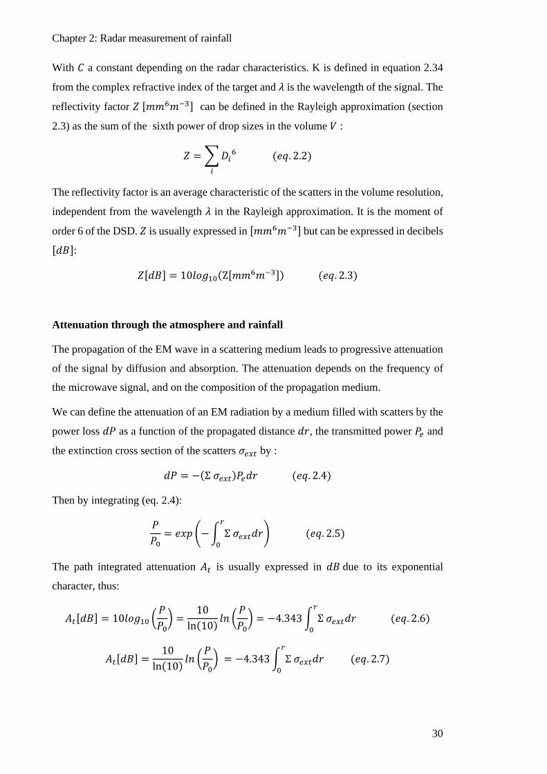
FIGURE 2-1: EXAMPLE OF RAW POLARIMETRIC OBSERVABLES ......................................... 34
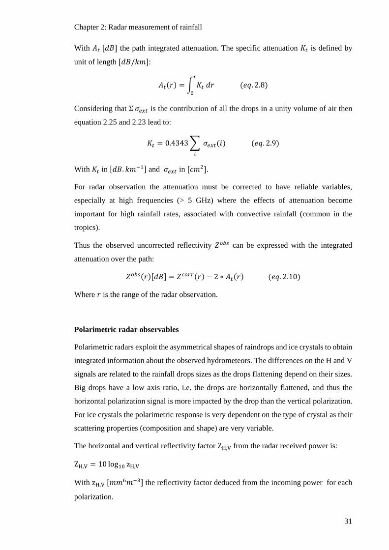
FIGURE 2-2: EXAMPLE OF RAW POLARIMETRIC OBSERVABLES ......................................... 34
FIGURE 2-3: EXAMPLE OF RAIN DROP PHOTOS .................................................................. 40
FIGURE 2-4: DIFFERENT RATIO SHAPE LAWS USED IN THIS WORK. .................................... 40
FIGURE 2-5: EXTINCTION CROSS SECTIONS FOR DIFFERENT FREQUENCIES BY DROP
DIAMETER FOR MIE AND RAYLEIGH MODELS. .......................................................... 45
FIGURE 2-6: MIE EXTINCTION CROSS SECTIONS FOR DIFFERENT FREQUENCIES AND
TEMPERATURES BY DROP DIAMETER. ....................................................................... 45
FIGURE 4-1: ONE DROP T-MATRIX OUTPUT ...................................................................... 74
FIGURE 4-2: T-MATRIX SIMULATED RADAR VARIABLES ................................................... 76
FIGURE 4-3: EXAMPLE OF THE OBSERVED, A PRIORI AND RETRIEVED ATTENUATED POLAR
VARIABLES AND DSD PARAMETERS FOR A GIVEN RADIAL ....................................... 83
FIGURE 4-4: RETRIEVED (TOP) AND A PRIORI (BOTTOM) MAPS OF DSD PARAMETERS F ... 85
FIGURE 4-5: RETRIEVED FIELDS OF ATTENUATED RADAR OBSERVABLES. ........................ 86
FIGURE 4-6: TIME EVOLUTION OF DM (TOP) AND LO 10[N0*] (BOTTOM) . ....................... 88
FIGURE 4-7: SENSITIVITY OF THE RETRIEVED DM (TOP) AND LO 10[N0*] (BOTTOM) ...... 90
FIGURE 4-8: : CONTOUR PLOT ON N0*-DM SPACE OF DISTRIBUTIONS OF DISDROMETER DSD
AND RADAR RETRIEVED DSD. ................................................................................. 91
FIGURE 4-9: SCATTERPLOT OF THE RADAR RETRIEVED DSD PARAMETERS ...................... 92
FIGURE 5-1: SCHEMATIC REPRESENTATION OF A LINE-OF-SIGHT MICROWAVE LINK ....... 104
FIGURE 5-2: K-R LAWS RETRIEVED FROM DSD OBSERVATIONS. ................................... 107
FIGURE 5-3: COEFFICIENTS OF THE K-R LAW FITTED ..................................................... 108
FIGURE 5-4: RECORDS OF THE BANIZOUMBOU STATION ................................................ 116
FIGURE 5-5: : RELATIVE DIFFERENCES IN RAINFALL ESTIMATION WITH K-R .................. 119
FIGURE 5-6: K-R LAWS CONSIDERING DIFFERENT POLARIZATIONS. ............................... 120
FIGURE 5-7: RELATIVE DIFFERENCE ON RAINFALL DUE TO DIFFERENT POLARIZATION ... 121

x
FIGURE 5-8: RELATIVE DIFFERENCE ON RAINFALL DUE TO DIFFERENT POLARIZATION ... 121
FIGURE 5-9: RESIDUALS BETWEEN OBSERVED DSD RAINFALL AND FITTED A-R LAW ... 123
FIGURE 5-10: MINIMAL DETECTABLE RAIN 1DB ............................................................ 126
FIGURE 5-11: MINIMAL DETECTABLE RAIN 0.1DB. ........................................................ 127
FIGURE 5-12: RELATIVE UNCERTAINTY DUE TO QUANTIZATION STEP ............................ 128
FIGURE 5-13: RELATIVE ERROR DUE TO A 3DB WET ANTENNA ATTENUATION ............... 130
FIGURE 6-1: CML ORANGE NETWORK IN NIAMEY ......................................................... 138
FIGURE 6-2: AVAILABLE CML DATA PER DAY FOR 2016-2017 SEASONS IN NIAMEY AND
HISTOGRAM OF CML LENGTHS IN THE NIAMEY ORANGE NETWORK. .................... 139
FIGURE 6-3: NUMBER OF COLLOCATED SAMPLES IN THE DATA ...................................... 139
FIGURE 6-4: : EXAMPLE OF RAW ATTENUATION AND BASELINE DETECTION ................... 141
FIGURE 6-5: EXAMPLE ATTENUATION MINIMIZATION FOR CALIBRATION 1 .................... 145
FIGURE 6-6: AVERAGE BIAS BY CALIBRATION DEPICTED BY RAINFALL RATE AND CML
LENGTH CLASS. ...................................................................................................... 148
FIGURE 6-7: RELAITVE BIAS BY CALIBRATION DEPICTED BY RAINFALL RATE AND CML
LENGTH CLASS. ...................................................................................................... 149
FIGURE 6-8: BIAS DECOMPOSITION BY CALIBRATION DEPICTED BY RAINFALL RATE. ..... 149
FIGURE 6-9: BOOTSTRAPPING OF CALIBRATION 1 .......................................................... 150
FIGURE 6-10: BOOTSTRAPPING OF CALIBRATION 1 (FILTERED) ...................................... 151
FIGURE 6-11: BOOTSTRAPPING OF CALIBRATION 2 ........................................................ 152
FIGURE 6-12: BOOTSTRAPPING OF CALIBRATION 2 (FILTERED) ...................................... 152
FIGURE 6-13: BOOTSTRAPPING OF CALIBRATION 3 ........................................................ 153
FIGURE 6-14: BOOTSTRAPPING OF CALIBRATION 3 (FILTERED). ..................................... 154
FIGURE 6-15: RELATIVE BIAS OF RAINFALL FOR CALIBRATION 3. .................................. 156
FIGURE 6-16: RELATIVE BIAS OF RAINFALL FOR CALIBRATION 3 ................................... 157
FIGURE 6-17: : COMPARISON OF THE DIFFERENT CALIBRATIONS OF WET ANTENNA
ATTENUATION (FOR BOTH ANTENNAS) ................................................................... 158
xi
FIGURE 6-18: SCATTERPLOTS OF SPECIFIC ATTENUATION K OF CML AFTER WET ANTENNA
CORRECTION VERSUS RAIN GAGE RAINFALL FOR CALIBRATION 2 ........................... 160
FIGURE 6-19: SCATTERPLOTS OF RETRIEVED CML RAINFALL VERSUS RAIN GAGE RAINFALL
FOR CALIBRATION 1 (FILTERED) ............................................................................. 161
FIGURE 6-20: : SCATTERPLOTS OF RETRIEVED CML RAINFALL VERSUS RAIN GAGE
RAINFALL FOR CALIBRATION 2 (FILTERED) ............................................................. 162
FIGURE 6-21: SCATTERPLOTS OF RETRIEVED CML RAINFALL VERSUS RAIN GAGE RAINFALL
FOR CALIBRATION 3 (FILTERED) WITH G=0.65.. ...................................................... 163
FIGURE 6-22: DAILY RAINFALL TIME SERIES FOR RAIN GAGE AND CML BY LENGTH CLASS
FOR CALIBRATION 1 ............................................................................................... 165
FIGURE 6-23: DAILY RAINFALL TIME SERIES FOR RAIN GAGE AND CML BY LENGTH CLASS
FOR CALIBRATION 2. .............................................................................................. 165
FIGURE 6-24: DAILY RAINFALL TIME SERIES FOR RAIN GAGE AND CML BY LENGTH CLASS
FOR CALIBRATION 3. .............................................................................................. 167
FIGURE 6-25: DAILY RAINFALL TIME SERIES FOR RAIN GAGE AND CML BY LENGTH CLASS
FOR CALIBRATION 3 BIS. ......................................................................................... 167
FIGURE 6-26: : RELATIVE BIAS DECOMPOSITION FOR CALIBRATION 1 ............................ 168
FIGURE 6-27: RELATIVE BIAS DECOMPOSITION FOR CALIBRATION 2 .............................. 169
FIGURE 6-28: RELATIVE BIAS DECOMPOSITION FOR CALIBRATION 3 .............................. 169
FIGURE 6-29: RELATIVE BIAS DECOMPOSITION FOR CALIBRATION 3 BIS ........................ 170
FIGURE 7-1: ZOOM ON THE NIAMEY CML NETWORK. ................................................... 178
FIGURE 7-2: EMPIRICAL VARIOGRAM AND FITTED MODEL. ............................................ 180
FIGURE 7-3: EXAMPLE OF A CML OVER A REGULAR GRID. ............................................ 182
FIGURE 7-4: ARCHITECTURE OF THE NN USED IN THIS STUDY ....................................... 184
FIGURE 7-5: EXAMPLE OF A 15MIN RADAR FIELD. .......................................................... 188
FIGURE 7-6: EXAMPLE OF MAPPINGS FOR THE THREE METHODS. .................................... 190
FIGURE 7-7: R2 MAPS OF THE THREE MAPPING METHODS COMPARED TO THE REFERENCE
RADAR RAIN FIELD ................................................................................................. 193

xii
FIGURE 7-8: BIAS MAPS OF THE THREE MAPPING METHODS COMPARED TO THE REFERENCE
RADAR RAIN FIELD ................................................................................................. 194
FIGURE 7-9: TAYLOR’S DIAGRAMS OF THE THREE METHODS FOR EACH DIFFERENT
NETWORK. .............................................................................................................. 196
FIGURE 7-10: TAYLOR DIAGRAM OF THE THREE METHODS OF INTERPOLATION APPLIED TO
REAL DATA FOR NIAMEY ........................................................................................ 200
FIGURE A 1: CORRELOGRAMS FOR 16 CML IN NIAMEY. ............................................... 217
FIGURE A 2: EXAMPLE OF ATTENUATION MINIMIZATION FOR MODEL 1 ......................... 218
FIGURE A 3: EXAMPLE OF ATTENUATION MINIMIZATION FOR MODEL 1 (FILTERED) ...... 219
FIGURE A 4: EXAMPLE ATTENUATION MINIMIZATION FOR MODEL 1 18GHZ. ................. 219
FIGURE A 5: EXAMPLE ATTENUATION MINIMIZATION FOR MODEL 1 ( FILTERED) 18GHZ
............................................................................................................................... 220
FIGURE A 6: EXAMPLE ATTENUATION MINIMIZATION FOR MODEL 2 ............................. 220
FIGURE A 7: EXAMPLE ATTENUATION MINIMIZATION FOR MODEL 2 ( FILTERED) .......... 221
FIGURE A 8: EXAMPLE ATTENUATION MINIMIZATION FOR MODEL 2 18GHZ ................ 221
FIGURE A 9: EXAMPLE ATTENUATION MINIMIZATION FOR MODEL 2 (FILTERED) 18GHZ 222
FIGURE A 10: RADAR FIELD OF RETRIEVED EQUIVOLUMETRIC MEDIAN DIAMETER DM .. 225
FIGURE A 11: SCATTERPLOTS OF SIMULATED CML SAMPLING VERSUS RAINGAGE
SAMPLING WITH RADAR DSD FIELDS ..................................................................... 229
FIGURE A 12: ADDITIONAL EXAMPLES OF MAPPING TECHNIQUES. ................................. 231
FIGURE A 13:ADDITIONAL EXAMPLES OF MAPPING TECHNIQUES ................................... 232
FIGURE A 14: ADDITIONAL EXAMPLES OF MAPPING TECHNIQUES. ................................. 233
FIGURE A 15: ADDITIONAL EXAMPLES OF MAPPING TECHNIQUES. ................................. 234
FIGURE A 16: BIAS MAPS BY METHOD AND ATTENUATION QUANTIFICATION FOR DOUALA
CML NETWORK. .................................................................................................... 235
FIGURE A 17: BIAS MAPS BY METHOD AND ATTENUATION QUANTIFICATION FOR NIAMEY
CML NETWORK. .................................................................................................... 235

xiii
FIGURE A 18: R2 MAPS BY METHOD AND ATTENUATION QUANTIFICATION FOR DOUALA
CML NETWORK. .................................................................................................... 236
FIGURE A 19: R2 MAPS BY METHOD AND ATTENUATION QUANTIFICATION FOR DOUALA
CML NETWORK. .................................................................................................... 236
FIGURE A 20: R2 MAPS BY METHOD AND ATTENUATION QUANTIFICATION FOR DOUALA
CML NETWORK. .................................................................................................... 237

xiv
LIST OF ABBREVIATIONS AND ACRONYMS ANDS99: Andsanger et al. 1999 aspect ratio law
AMMA-CATCH : Analyse Multidisciplinaire de la Mousson Africaine – Couplage de
l’Atmosphère Tropicale et du Cycle Hydrologique
CML: Commercial Microwave Link
DBS: Dual Beam Spectropluviometer
DSD: Drop Size Distribution
EM: Electro-Magnetic waves
GPCC: Global Precipitation Climatology Center
ILLI02: Illingworth et al. 2002 aspect ratio law
IR: Infrared radiation
IRD : Institut de Recherche pour le Développement (French research institution)
LIN1: Aspect ratio law from Gorgucci et al. 2000 with βe = 0.052
LIN5: Aspect ratio law from Gorgucci et al. 2000 with βe = 0.072
LWC: Liquid Water Content
MCS : Mesoscale Convective Systems
MT : Megha-Tropiques satellite
MP: Marshall-Palmer parameterization of the DSD
MW : Microwaves
PPI : Plan Position Indicator
QPE : Quantitative Precipitation Estimate
RAINCELL: for Rain Measurement from Cellular network ; Name of the Scientific
program initiated in Africa by IRD to monitor rainfall with CML
UV: Ultraviolet radiation
WMO: World Meteorological Organization
X-PORT: Name of the X-band doppler dual polarization radar developed by IRD/IGE (F.
Cazenave and M. Gosset) that operated in West-Africa
Introduction
1
INTRODUCTION
Rainfall is a major variable in the water cycle. Because it is the main entry for fresh water
to continental surfaces, it has a great impact on human societies. Hence, it is a key
parameter for hydrological forecast, crop modelling and hazard management. The
precipitating systems plays a major role in the energy budget of the planet. Due to its
spatial and temporal variability and its intermittency, the measurement of rainfall is a
challenge. The uncertainties associated with the quantitative estimation of rainfall need
to be understood and quantified for several applications.
The West African monsoon season, which lasts from May to October, provides the yearly
rainfall accumulation in this region. It is mainly driven by large organized convective
storms associated with intense rainfall rates that can lead to flood events. As elsewhere
in the tropics, rainfall in West Africa is poorly monitored due to the scarcity of the
operational meteorological networks.
Rainfall measurement can be ground or satellite based. Ground based measurements are
made with rain gages, disdrometers, radars or commercial microwave links which sample
the hydrometeors or the rainfall accumulations from ground level. They can be direct
measurements or based on remote sensing. Satellite measurements are based on remote
sensing techniques which use the interaction between hydrometeors and electromagnetic
radiation to retrieve information about the hydrometeors in the sampled volume.
Microwave remote sensing of precipitation can be used to infer the spatial distribution

Introduction
2
and physical properties of hydrometeors in horizontal and vertical scales. When they
grow, the frozen hydrometeors start falling and melting, producing precipitations.
Rain gages are the historical mean to measure rainfall. They are often considered as the
ground truth because their measurement principle is simple and quite direct. Rain gauges,
however, sample only an area of a few hundred of 𝑐𝑐𝑐𝑐2 and the spatial representativity of
their measurement is therefore limited.
Meteorological radars, developed in the second half of the 20𝑡𝑡ℎ century, are the main
instrument for ground-based active remote sensing of rainfall. An important asset of
radars is their resolution which offer a fine horizontal and vertical sampling of
precipitating systems. They provide an indirect measurement of precipitation: the main
variable measured by a radar is the back-scattered power due to the scattering of
microwaves by hydrometeors. The back-scattering is very sensitive to the phase of the
hydrometeors: water drops are much more sensitive to microwaves than frozen
hydrometeors. Some radar systems can use polarized emitted signals adding a layer of
information: they use the differential response in vertical and horizontal polarizations to
better characterize the precipitation. Empirical relationships are often used to convert the
radar observables into physical quantities leading to estimation uncertainties. Radars are
the major instrument for rainfall monitoring, but they are expensive instruments
affordable only in rich countries.
In the past ten years, an innovative technique to measure rainfall has emerged based on
commercial microwave links (hereafter CML). The method is based on the rainfall
induced attenuation of the EM signal between a pair of antennas. The attenuation levels
of the CML are monitored by the telecom companies to survey their network. Telecom
companies ensure the installation and maintenance costs. They are an alternative to radars
and rain gauges in ill-equipped regions but they are unequally distributed over territories
with dense networks in highly populated areas.
Satellites provide a global coverage of rainfall but the measurements are indirect.
Different types of instruments exist based on infra-red or microwave observations. The
microwave-based instruments can be passive or active sensors. Active sensors are radars,
based on the same principle as ground based radars. Passive sensors measure the
brightness temperature in different wavelengths at the top of the clouds. The retrieval of
physical characteristics of rainfall with passive satellites depends on the modeling of the
characteristics of the hydrometeors in the atmospheric column. Rainfall estimation with
Introduction
3
satellites is still subjected to important uncertainties (Gosset et al. 2013; Gosset et al.
2018; Kirstetter, Viltard, and Gosset 2013) and coarse resolutions (~25km for 3h
(Guilloteau, Roca, and Gosset 2016)) which are inappropriate for small scale studies
(such as flash floods in small catchments).
This thesis is the result of several years of work developed as an engineer. My first
mission consisted in the validation of Megha-Tropiques satellite products with ground
reference rainfall data. The Megha-Tropiques (𝑀𝑀𝑀𝑀) satellite mission (Roca et al. 2015) is
dedicated to monitor the water and energy cycle in the tropical atmosphere with passive
microwave radiometry. The original feature of the satellite is its tropical orbit (a low
inclination orbit), which decrease the revisiting time span in the tropics, increasing the
daily microwave (MW) observations and improving the gridded accumulated rainfall
products. The Megha-Tropiques Ground Validation campaign (MTGV) gathered
different types of observations of mesoscale convective systems in West Africa. The main
goal of the campaign was to evaluate the performance of the satellite rainfall products. It
also became an opportunity to combine different types of observations of precipitating
systems as airborne observations were supplemented with a ground based dual-
polarization radar (X-port). In addition to my duties I was able to carry out research on
dual-polarization radar to improve the characterization of the sampled hydrometeors. The
first part of this thesis deals with the development of two techniques using meteorological
radar data to extract information on hydrometeors.
The first original technique developed consist in the retrieval of the density of the icy
hydrometeors above the 0°C isotherm with the modeling of the observation of the melting
layer by the radar. The density retrievals were validated with the in-situ airborne
observations. The density of icy hydrometeors impacts the passive microwave
observation from satellites as the hydrometeors have different scattering properties
depending on their density. Obtaining information regarding the density of hydrometeors
above the melting layer could improve rainfall retrieval from satellites.
The second original technique presented in this thesis is the retrieval of the drop size
distribution (DSD) by inversion of polarimetric radar data. The drop size distribution
variability is one of the main sources of uncertainty in radar and microwave link rainfall
retrievals, as the relations linking radar observables and drops are not constant. Radar
polarimetry facilitates accessing information about the differential response of the
hydrometeors as seen by the horizontal and vertical channels of the radar. That differential
Introduction
4
response is linked to the drop size distribution. X-band radars are strongly affected by
attenuation. Usually, in literature, a two-step procedure is used to retrieve drop size
distributions from polarimetric radar: first an attenuation correction is obtained and later,
a retrieval of the DSD with empirical relations. In the proposed inversion of the DSD in
this thesis, the retrieval is performed on the uncorrected radar variables, thus avoiding the
empirical approximation of the attenuation. The retrieval is not based on empirical
relations but in a physical model of scattering.
Both techniques developed have a similar approach: first a model is used to simulate the
observations and then an original inversion technique is applied to retrieve the physical
characteristics of the hydrometeors in the sampled volume.
My second mission as an engineer was the data processing of commercial microwave
links in West-African countries. The RAIN CELL project began as a solution to increase
the ground based data for the validation of MEGHA-TROPIQUES satellite products.
Beginning in 2012, it was developed in the framework of a collaboration between IRD
(Institut de Recherche pour le Développement) and the telecom company Orange.
Later, the objective of the project was to show the potential use of CML to monitor rainfall
on real time in small scales (i.e. cities) so that an urban hydrological model could be fed
in order to forecast flood episodes. First the validation of the measurement of rainfall with
CML needed to be addressed. Two seasons of data (2016-2017) were provided for the
CML network in the city of Niamey, Niger from Orange-Niger. The second part of this
thesis starts with an introductory chapter on the principle of rainfall measurement with
CML followed by the quantitative evaluation of the data set in Niger.
The final objective was to combine CML observations to produce rainfall maps to feed
hydrological models. The last chapter of this thesis introduce a prospective method to
combine heterogeneous information from dense CML networks to retrieve rainfall maps
on a city-scale.
The thesis is organized in two parts introduced by a general chapter (Chap. 1). The first
part is dedicated to the retrieval of the physical characteristics of precipitation with
polarimetric radar. It is composed by three chapters. Chapter 2 describes the physics of
the radar measurement. Chapter 3 describes the ice particles density retrieval by inverting
the melting layer observation. Chapter 4 describes the inversion of polarimetric radar
variables at attenuating frequencies to retrieve the drop size distribution.

Introduction
5
The second part of the thesis introduces the commercial microwave links for rainfall
monitoring. The first chapter (Chap 5) describes how CML rainfall measurement
operates, considering its uncertainties. Chapter 6 describes the assessment of the CML
Niamey measurements and analyzes the CML-gage comparison. The concluding chapter
7 introduces an original method to retrieve rainfall maps from a network of CML based
on machine learning of radar rainfall maps.

Chapter 0: Introduction
6
Chapter 1: Rainfall characteristics and measurement in West Africa
7
1 RAINFALL CHARACTERISTICS AND MEASUREMENT IN WEST AFRICA
As in most of the tropics, rainfall in West Africa is driven by convection leading to intense
precipitation. The Sahel climate is characterized by a wet season which runs from May to
October and a dry season from November to April with almost no rainfall accumulation.
During the wet season in the Sahel a small number of strong events account for most of
the annual precipitation. Rainfall in such events is characterized by strong horizontal
variability and a particular vertical structure.
In the first part of this chapter we describe the organization, structure and composition of
rainfall systems in the study region. Later we describe the different ground-based
instruments to measure rainfall and their particular benefits. A section is dedicated to raise
explicitly the scientific questions addressed in this work. Finally, we describe the context
and the data sets used.
1.1 The organization and structure of rainfall systems in the study region
Mesoscale convective systems
Mesoscale convective systems (MCS) accounts for the majority of the rainfall in the
tropics and on Earth (Roca et al. 2014).They have a strong impact in water resources in
tropical regions and they can also generate floods due the associated violent rainfall rates.
Chapter 1: Rainfall characteristics and measurement in West Africa
8
A precipitating system is considered a MCS when it produces a contiguous precipitation
area of 100km or more in at least one direction. They are formed by a convective front
area of buoyant moist air creating strong precipitation rates and by a stratiform cloud area
associated with light and medium rain rates.
In this region the climatic conditions lead to rapidly moving squall lines (~60 km/hr) and
a seasonal dependence of precipitations. In the Sahel region 80% of the precipitation
comes from convective rainfall cells, in the front of the squall line (Houze 2004).
Microphysics in MCS
Hydrometeors are atmospheric particles formed by water molecules in ice or liquid phase.
The condensation of water vapor requires condensation nuclei (aerosols) to start the phase
transition. Hydrometeors can be in liquid or ice phase, depending on the temperature of
the atmospheric layer and the generation process. Two principal growth mechanisms can
initiate the precipitation of hydrometeors: condensation/riming and coalescence with
other hydrometeors. By growing, the hydrometeors become heavier and start falling.
Above the freezing level of the atmosphere (0°C isotherm) the hydrometeors are usually
in the form of ice particles. The microphysical processes involved in the formation and
evolution of the particles are numerous and complex. The dynamical growing processes
(aggregation, riming) adds complexity on the resulting geometries and densities of the
particles leading to a large fauna of ice crystals. Some atmospheric situation can lead to
water drops in super-cooled state (liquid phase with a temperature below freezing point)
and the production of graupel.
Under the freezing layer of the atmosphere, precipitating ice particles begin to melt,
increasing their density and accelerating their fall, as they become raindrops. The
complexity of physical processes involved in hydrometeors generation and evolution in
MCS leads to a high spatial variability of the particles quantity and sizes. As we describe
later, the particle size distribution (PSD) above the melting layer and the drop size
distribution (DSD) of rainfall play an important role in precipitation remote sensing with
microwaves.
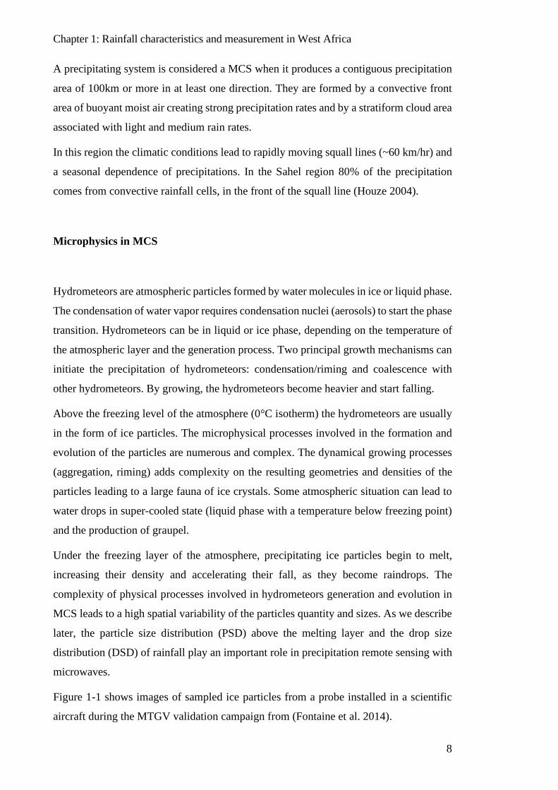
Figure 1-1 shows images of sampled ice particles from a probe installed in a scientific
aircraft during the MTGV validation campaign from (Fontaine et al. 2014).
Chapter 1: Rainfall characteristics and measurement in West Africa
9
Figure 1-1: Example of 2-D images recorded by the precipitation imaging probe
PIP for Megha-Tropiques validation campaigns. Images of hydrometeors presented
as a function of temperature. From [Fontaine et al. 2014]
Chapter 1: Rainfall characteristics and measurement in West Africa
10
1.2 Ground based measurement of rainfall
In the following section we describe the instruments used to measure rainfall, their assets
and limitations are discussed.
1.2.1 Rain gages
Point rain gage measurement
The oldest, simplest and direct method to measure rainfall accumulations is the rain gage.
The tipping-bucket gauge is composed by a bucket which swing for a certain volume of
water. Each tip time of the bucket is then recorded into an electronic system (or a rolling
chart for the old school instruments).
The measurement of rainfall by a rain gage is subjected to different sources of errors.
Some common sources of error are the evaporative loss, the instrument calibration, the
outsplash of the drops, the levelling of the gage, the instrument sitting and the wind
effects. The wind effects are the most important source of error and the more difficult to
correct.
(Ciach 2003) used an empirical method using 15 collocated rain gages to derive the errors
of local random differences and the effect of bucket sampling when calculating rain rates
at different time scales and rain rates: the relative error increase with low rain rates, and
increase with shorter time scales. They stated the errors to be 2% for high rain rates
(>20mm/h) in 1 hour sampling, 3% for 15 minutes sampling and 6% for 5 minutes
sampling.
Rain gages are considered the reference rainfall measurement, but their measurements are
associated with a significant uncertainty. The rainfall measurement uncertainty of a
raingage should be considered when using it as a reference.
Chapter 1: Rainfall characteristics and measurement in West Africa
11
Representativity and interpolation
For many applications there is a need of spatial averages of rainfall instead of local
measures as rain gage do. As we pointed out, rainfall is extremely variable and
intermittent in space and time. Using a reduced number of rain gages over an area can
lead to wrong estimations of the mean areal rainfall. The concept of ‘representativity’ of
a rain gage measurement arises: to which extent can a single (or multiple rain gages)
account for the mean areal surface rain in a certain spatio-temporal scale?
An example is the impact of the rainfall variability in a hydrology model: the output water
flow (for floods or outflow prediction) can be impacted by a wrong estimation of rainfall,
leading to a wrong calibration or initialization of the hydrological model (Arnaud et al.
2011; Balme et al. 2006).
Scarcity of measurements
Rain gauges are relatively cheap but dense networks are needed to account for rain
variability as discussed. Dense networks require recurrent maintenance to provide reliable
data, which represent a cost in human resources. The national meteorological agencies
manage synoptic networks of rain gages of variable densities depending on the country
wealth. There is a strong inequality on instrument coverage between countries, and
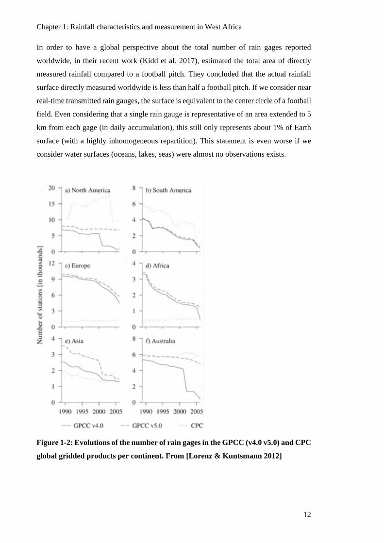
regions inside of them. In their work, (Lorenz and Kunstmann 2012) analyze three global
atmospheric reanalysis models in terms of precipitation and temperature estimates with
independent observations worldwide between 1989 and 2006. They pointed out that the
major source of uncertainty in the analysis is the density evolution of the observations
through time and space. Figure 1-2 shows decreasing number of rain gauges through
1989-2006 in the global gridded ground rainfall products GPCC (v4.0 v5.0) and CPC
(v5.0). The figure shows the small number of reported rain gauges in Africa. Some
reasons of the loss reported could be the decrease of investments in meteorology to
support the human resources necessary and the instruments substitution, the lack of
reliable data filtered by the quality controls procedures or the lack of reporting of the data
by the national responsible institutions.
Chapter 1: Rainfall characteristics and measurement in West Africa
12
In order to have a global perspective about the total number of rain gages reported
worldwide, in their recent work (Kidd et al. 2017), estimated the total area of directly
measured rainfall compared to a football pitch. They concluded that the actual rainfall
surface directly measured worldwide is less than half a football pitch. If we consider near
real-time transmitted rain gauges, the surface is equivalent to the center circle of a football
field. Even considering that a single rain gauge is representative of an area extended to 5
km from each gage (in daily accumulation), this still only represents about 1% of Earth
surface (with a highly inhomogeneous repartition). This statement is even worse if we
consider water surfaces (oceans, lakes, seas) were almost no observations exists.
Figure 1-2: Evolutions of the number of rain gages in the GPCC (v4.0 v5.0) and CPC
global gridded products per continent. From [Lorenz & Kuntsmann 2012]
Chapter 1: Rainfall characteristics and measurement in West Africa
13
1.2.2 Disdrometer
Disdrometers are instruments designed to measure the drop sizes of rainfall. They sample
the individual drops deriving into drop size distributions over a time period (ie. the
number of drop in several classes of diameter). Disdrometers uses different principles to
sample the number of drops and their sizes. Here we describe the Dual Beam
Spectropluviometer (DBS) (Delahaye et al. 2006) installed near Djougou, Benin, in 2006
and used in Chapter 4 for validation of the retrieved DSD from polarimetric radar.
The DBS instrument is composed by a double infrared beam and a system of lens which
project the IR beam. The sensor measures a signal depending on the quantity of energy
received. The amplitude and duration of the signal due to a raindrop transit are a function
of the vertical section of the drop and the crossing time in the volume. A correct
processing of the signal allows to retrieve the equivalent diameter of the raindrop. The
raindrop falling speed is deduced with the crossing time through the IR beam.
Disdrometers have also their sources of errors. Small drops, with diameters smaller than
the resolution limit, are not measured. Also the biggest drops, having a strong impact on
microwave observation of rainfall, can be under represented for small sampling times.
The wind and two simultaneous drops can also be sources of errors.
1.2.3 Meteorological radar
Principle
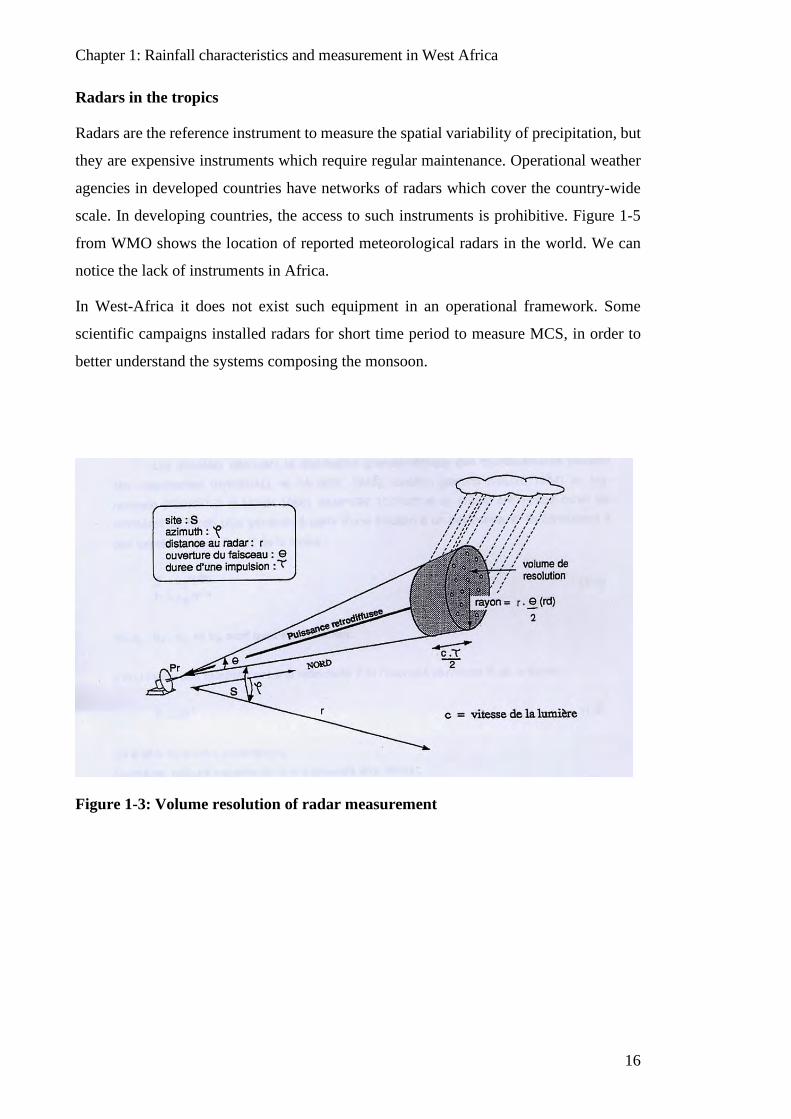
Radars (for RAdio Detection And Ranging) are composed by a microwave emitter and
an antenna which detects the reflected power over time. The localization of the target is
based on the antenna direction and the time measurement between the emission and the
reception signal, converted into distance with the speed of light in the atmosphere. The
maximum available range is limited by the time span between two pulses and by the
emission power and the attenuation (which depends on the wavelength). Due to the beam
opening angle (given by the antenna characteristics, diagram on figure 1-3) and the pulse
duration, the radar resolution volume is a quasi-cone section (neglecting the second lobes
Chapter 1: Rainfall characteristics and measurement in West Africa
14
of the antenna emission diagram). The volume resolution size become bigger for
increasing ranges.
Hydrometeors reflect the MW radiation: the total reflected power depends on the amount,
sizes and phase of the hydrometeors. The frequency of the MW signal has an impact on
the amount of reflected energy and the attenuation of the signal along its propagation.
The operational radars for weather monitoring are C or S band as the maximal range is
high and the attenuation by water drops is low. But higher wavelength (lower frequency)
involves big antennas and leads to expensive radars for maintenance and operation.
Research radars are often X-band (~10 GHz) as they offer an easier mobility and cost.
Quantitative Precipitation Estimate
The principal objective of operational radars is the quantitative precipitation estimation
(QPE). Traditional radars measure the received power converted into reflectivity, a
property of the hydrometeors present in the resolution volume. Reflectivity factor is
closely linked to the drop size distribution (DSD) of the hydrometeors. The link between
reflectivity and rainfall rate is not straightforward: both are moments of different order of
the DSD. The precipitation (R) estimation through reflectivity factor (Z) is usually done
through Z-R power laws which contains implicit assumptions on the DSD. Z-R laws are
empirically calibrated with collocated measures of rain gage and radars, or with
disdrometer measurements. Such laws are very noisy due to the DSD variability. The
reflectivity is quantitatively more impacted by large drops than the rainfall rate. The
variability of the DSD is the main source of uncertainty in the precipitation estimation
through radar.
3D scanning geometry
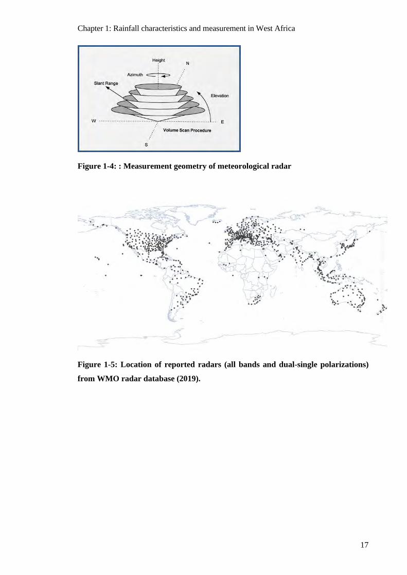
Radars emits a pulse in a certain azimuth and elevation and moves to sample the desired
zone. The azimuth 𝜑𝜑 ∈ [0,360] is the angle with the north direction (clock wise) and the
elevation 𝜃𝜃 ∈ [0,90] is the angle with the horizontal. Usually, meteorological radars for
rainfall monitoring visit all the azimuths (with a certain angular resolution) and after
changes the elevation to revisit the azimuths for different heights over the ranges. A visit
over all azimuth for a certain elevation is called PPI (Plan Position Indicator). Figure 1-4
shows the 3D geometry of the radar measurement for 5 PPI at different elevations.
Chapter 1: Rainfall characteristics and measurement in West Africa
15
With this particular scanning geometry, radars sample the horizontal spatial variability of
precipitation inside the systems. The vertical evolution of precipitation is also observed;
radars access the layers of the atmosphere where the frozen hydrometeors are generated.
The melting layer of hydrometeors, located at the 0°C isotherm has a particular signature
when observed by radars. An artifact of the observation creates a peak of reflectivity on
the melting layer (bright band) due to the high reflectivity of melting hydrometeors. Most
studies concerning the bright band focus on its correction for QPE, which can create
errors. While the bright band artifact depends on the properties of hydrometeors melting,
we can use the bright band observation to infer hydrometeors properties.
Polarimetry, adding information
Polarimetric radars emit pulses at horizontal and vertical polarizations (H and V channels)
adding information with the differences in the returned echoes. The differences of H and
V channels comes from the hydrometeor’s anisotropy: horizontal polarization echoes in
rainfall are more intense due the oblateness of large raindrops (Chapter 2). Polarimetric
radars measure the received power at H and V polarizations, but also the phase shift of
the EM wave between the two channels. The differential phase of H and V channels is
impacted during the propagation in an anisotropic scattering medium (Bringi and
Chandrasekar 2001).
The QPE estimation with polarimetric radar benefits from additional information
improving the estimations. For X-band radars the attenuation correction is a crucial step,
as the attenuation is high. With polarimetry we can estimate the attenuation with the phase
shift propagative variable. The phase shift between H and V channels is also closely
linked to rainfall rate. Rainfall estimation with the phase shift usually performs better than
the above mentioned Z-R relations based only on reflectivity factor. Though, the phase
shift-rainfall relations are also power laws empirically established.
The additional information provided by polarimetry can improve the characterization of
the average properties of the hydrometeors in the resolution volume. Polarimetric
information can be used to constrain the modelling of the interaction between MW and
hydrometeors.
Chapter 1: Rainfall characteristics and measurement in West Africa
16
Radars in the tropics
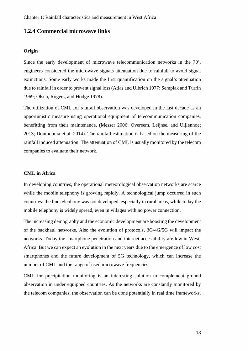
Radars are the reference instrument to measure the spatial variability of precipitation, but
they are expensive instruments which require regular maintenance. Operational weather
agencies in developed countries have networks of radars which cover the country-wide
scale. In developing countries, the access to such instruments is prohibitive. Figure 1-5
from WMO shows the location of reported meteorological radars in the world. We can
notice the lack of instruments in Africa.
In West-Africa it does not exist such equipment in an operational framework. Some
scientific campaigns installed radars for short time period to measure MCS, in order to
better understand the systems composing the monsoon.
Figure 1-3: Volume resolution of radar measurement
Chapter 1: Rainfall characteristics and measurement in West Africa
17
Figure 1-4: : Measurement geometry of meteorological radar
Figure 1-5: Location of reported radars (all bands and dual-single polarizations)
from WMO radar database (2019).
Chapter 1: Rainfall characteristics and measurement in West Africa
18
1.2.4 Commercial microwave links
Origin
Since the early development of microwave telecommunication networks in the 70’,
engineers considered the microwave signals attenuation due to rainfall to avoid signal
extinctions. Some early works made the first quantification on the signal’s attenuation
due to rainfall in order to prevent signal loss (Atlas and Ulbrich 1977; Semplak and Turrin
1969; Olsen, Rogers, and Hodge 1978).
The utilization of CML for rainfall observation was developed in the last decade as an
opportunistic measure using operational equipment of telecommunication companies,
benefitting from their maintenance. (Messer 2006; Overeem, Leijnse, and Uijlenhoet
2013; Doumounia et al. 2014). The rainfall estimation is based on the measuring of the
rainfall induced attenuation. The attenuation of CML is usually monitored by the telecom
companies to evaluate their network.
CML in Africa
In developing countries, the operational meteorological observation networks are scarce
while the mobile telephony is growing rapidly. A technological jump occurred in such
countries: the line telephony was not developed, especially in rural areas, while today the
mobile telephony is widely spread, even in villages with no power connection.
The increasing demography and the economic development are boosting the development
of the backhaul networks. Also the evolution of protocols, 3G/4G/5G will impact the
networks. Today the smartphone penetration and internet accessibility are low in West-
Africa. But we can expect an evolution in the next years due to the emergence of low cost
smartphones and the future development of 5G technology, which can increase the
number of CML and the range of used microwave frequencies.
CML for precipitation monitoring is an interesting solution to complement ground
observation in under equipped countries. As the networks are constantly monitored by
the telecom companies, the observation can be done potentially in real time frameworks.
Chapter 1: Rainfall characteristics and measurement in West Africa
19
Geographical distribution
Telecommunication companies use the backhaul microwave network of antennas to
transmit their information in a country wide scale. The density of CML is closely related
to the population density. In cities, dense networks are used to collect signals from all the
neighborhoods. The number of CML in a city exceed several hundreds of CML. For
example, the city of Bamako, Mali has 700 CML, Yaounde in Cameroon around 200
CML, Douala, Cameroon, 300 and Niamey 100 for the Orange network. Such density of
ground measurement of rainfall is unique, even for developed countries. Outside cities,
longer CML interconnects villages with central nodes of the telecom company. The
country wide coverage of CML and the high densities in cities offers new perspectives
on rainfall monitoring. The combination of such rich densities of heterogeneous
measurements and the merging with classical observation are open questions.
Indirect measurement
However, the rainfall observation with commercial microwave links is not
straightforward. CML are not optimized for rainfall measuring. The sampling is
controlled by the equipment of the telecom company. As we use information of a private
company, we do not have access to the instrument setup. Sometimes the collected
information is not the optimal information which we would collect in a scientific
dedicated experiment.
Integrated measurement
The CML attenuation due to rainfall is linked to the average rainfall rate in the CML path.
It is a ‘lineal’ integrated measurement. Integrated measurements are interesting for
hydrology due to the poor spatial representativity of a raingage as discussed. Usually
hydrological models need the integrated rainfall over an area (watershed) instead of
ponctual measurements.
The attenuation-rainfall relation is almost linear (depending on the signal frequency)
which reduces the impact of the rainfall variability inside the CML. The microwave
attenuation is closer to the rainfall rate than the radar reflectivity factor (Z). The rainfall
estimation by attenuation measurement is an effective technique as we will see in part 2
of this thesis.

Chapter 1: Rainfall characteristics and measurement in West Africa
20
1.3 Main scientific questions
This section points out the main scientific questions that we will try to develop in this
work.
Radar to characterize precipitation
The first part of this thesis concerns the retrieval of the precipitation characteristics with
polarimetric radar.
• Can a radar observational artifact be used to characterize physical properties of
the scatters?
• At which level can a simple modelization of the melting layer observation bring
information?
• Can we derive drop size distribution constraining an observational model with
polarimetric information?
• Can we avoid using empirical relations, using a physical model of the observation
to derive DSD parameters?
Commercial Microwave Links to measure precipitation
The second part of the thesis concerns the use of CML to measure precipitation
• Can we evaluate the uncertainties related to precipitation monitoring with CML?
• How can we calibrate CML observation with a reference observation?
• How can we combine dense network of CML to produce rainfall maps?
1.4 Data used in the present work
In this section we present the different datasets used to address the presented scientific
questions. We present the X-port polarimetric radar and their different locations in West-
Africa. Later we present the CML dataset provided by Orange in Niamey, and the rain
gages used to evaluate the rainfall retrieval with CML.

Chapter 1: Rainfall characteristics and measurement in West Africa
21
1.4.1 X-Port radar
Figure 1-6: X-port radar location in Ouagadougou, Burkina-Faso in 2012 with a
squall line front and the associated dust cloud due to high speed winds.
X-port is an X-band Doppler polarimetric research radar developed by the IRD (Institut
de Recherche pour le Développement) to increase the observations in the tropics. X-port
was located in 2006 and 2007 in Djougou, Benin, in the framework of the AMMA-
CATCH project. AMMA-CATCH is a long term observatory which aims to document
the climatic, hydrological and ecological evolutions in West-Africa in a changing climate
and increasing demographic pressure.
X-port was moved to Niamey, Niger, in 2010 in the framework of MEGHA-TROPIQUES
ground validation campaign. MEGHA-TROPIQUES, a French-Indian satellite mission,
was designed to sample the rainfall in the tropics with a frequent revisit. X-port was
planned as the ground reference to validate the rainfall satellite products of MEGHA-
TROPIQUES. The security situation in Niamey deteriorated in 2011, and the radar was
moved to Ouagadougou, Burkina-Faso, for the years 2012-2013 to continue the validation
campaign. Figure 1-6 shows X-port radar at its location in Ouagadougou during the rainy
season of 2012, in the background we observe the approximation of the convective front
of an MCS. Figure 1-7 shows the different location of X-port and the years of the data
used in this work.

Chapter 1: Rainfall characteristics and measurement in West Africa
22
Figure 1-7: Different locations of X-port radar.
1.4.2 Microwave links
During the MEGHA-TROPIQUES ground validation campaign emerged the idea of
complementing the X-port and gauges observation with CML data for the validation of
satellite rainfall products due to the lack of measures in the tropics, and the Sahel in
particular. Contacts with local and international telecom companies began in order to
access the data. Telecel-Faso, a Burkina-Faso telecom company acceded to share data
from some long CML in the field of view of X-port radar in 2012. The result of the rainfall
retrieval was published in (Doumounia et al. 2014). This was a premiere for rainfall
observation in Africa with CML.
Later Orange provided two complete rainy seasons (MJJASO) of CML data in Niger for
the years 2016 and 2017. The CML are situated in the four mains cities of the country:
Niamey, Maradi, Tahoua and Agadez. The total number of links provided by Orange for
the best day is 494 (some of them doubled) for the whole country. The number of link’s
Chapter 1: Rainfall characteristics and measurement in West Africa
23
data provided vary for each day due to problems in the operational network and
transmission of the data.
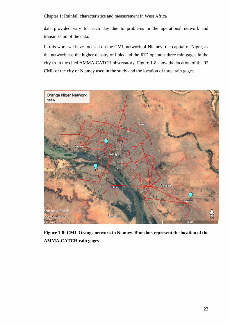
In this work we have focused on the CML network of Niamey, the capital of Niger, as
the network has the higher density of links and the IRD operates three rain gages in the
city from the cited AMMA-CATCH observatory. Figure 1-8 show the location of the 92
CML of the city of Niamey used in the study and the location of three rain gages.
Figure 1-8: CML Orange network in Niamey. Blue dots represent the location of the
AMMA-CATCH rain gages
Chapter 1: Rainfall characteristics and measurement in West Africa
24
1.4.3 AMMA-CATCH network in Niamey
The AMMA-CATCH observatory presented in the previous section has a long term
component in Niger. The Niger rain gage network is composed of 40 to 50 tipping bucket
rain gages (depending on the year) in an area of 100x100 𝑘𝑘𝑐𝑐2. The network was installed
in the late 90’ and is operational since then. Figure 1-8 shows the location of the gages in
the area of Niamey (blue points).
The gages are equipped with 0.5 mm tipping buckets and a collection surface of 400 𝑐𝑐𝑐𝑐2.
The maintenance protocol of the instruments includes a GPS time pick up by the
technicians at each visit to correct from possible temporal drift of the electronic device.
A rainfall accumulator is buried next to each raingage in order to correct the tipping
bucket calibration errors. The technicians revisit period is two weeks during the rainy
season to ensure the quality of the raingage data.

Chapter 1: Rainfall characteristics and measurement in West Africa
25
Meteorological radars are a powerful instrument to study hydrometeors. By their
particular configuration they can access the lower and upper layers of the precipitating
systems, where direct measurements are expensive (flights), difficult to do and risky.
Polarimetric radar measures magnitudes (power and differential phase) which are linked
to the average characteristics of the hydrometeors in the sampled resolution volume. The
sizes, phase and types of the hydrometeors impacts the polarimetric radar measurements.
Compared to conventional radars, polarimetric radar adds information which can improve
the quantitative precipitation estimate at ground level. But also, they can be used to
identify the frozen hydrometeors above the freezing level to understand the microphysical
processes forming such particles.
The hydrometeors classification by type, by their characteristics (density, shape), and by
their variability inside a system are essential elements to improve the radiative transfer
models in the atmospheric column, which are the basis of passive microwave satellite
rainfall retrieval algorithms. Passive microwave sensors in satellites measures brightness
temperatures at the top of the clouds which are the result of the radiative processes along
the atmosphere. Ice crystals variability have a strong impact on the observed brightness
temperatures (Kummerow, Olson, and Giglio 1996; Bennartz and Petty 2001).
PART 1 RETRIEVALS OF PHYSICAL
CHARACTERISTICS OF PRECIPITATIONS WITH A POLARIMETRIC RADAR
Chapter 1: Rainfall characteristics and measurement in West Africa
26
Different methods are found in the literature to classify hydrometeors with polarimetric
radar measurements. One method is based on fuzzy logic algorithms (Liu and
Chandrasekar 2000; Cazenave et al. 2016). In chapter 3 we present a published paper
describing an original method to infer the density of the hydrometeors above the bright
band of reflectivity (related to the melting layer of frozen particles). The idea is to exploit
the shape and size of the bright band to retrieve a density law of the frozen hydrometeors.
Previous studies showed the link between the properties of the bright band and
microphysical processes aloft (Uijlenhoet, Steiner, and Smith 2003; Fabry and Szyrmer
1999). In this study we present a simple model describing the melting layer: the model
do not describe the thermodynamics of the melting layer unlike (Fabry and Zawadzki
1995). The idea is to reproduce the main characteristics of the melting layer, to derive the
density of crystals above with an inversion method.
Melted ice crystals become water drops. Their sizes depend on the particle size
distribution above the melting layer, and the break-up and coalescence mechanisms
during the fall. The first objective of drop size distribution (DSD) retrieval with
polarimetric radar is to improve the quantitative precipitation estimates at the ground
level, as the DSD is the main source or uncertainty in rainfall retrievals.
DSD retrievals in the literature are often based on empirical relations linking polarimetric
radar observables and the DSD parameters. The 𝛽𝛽-method by (Gorgucci et al. 2002) is
based on the derivation of a 𝛽𝛽 parameter of the drop shape law (from radar observables)
to later express the parameters of the DSD by 𝛽𝛽 and the observables. Another example is
the constrained gamma-method which uses empirical relation between the slope and
shape of the DSD from which are derived the relation expressing DSD parameters to radar
polarimetric variables.
The majority of the studies are made with C-band radars, associated with a low
attenuation of the MW signal by the rainfall. The studies with X-band radar (high MW
signal attenuation by rainfall) correct first the attenuation empirically to later derive DSD
parameters. (Yoshikawa, Chandrasekar, and Ushio 2014) notice that the 2-step empirical
procedure (correction and DSD parameter retrieval) can lead to errors. In the third chapter
we present a submitted article describing an inversion method of DSD parameters. The
inversion is done on the uncorrected polarimetric variables in a context of high
attenuation. The inversion of the whole radar tilt using all the polarimetric information

Chapter 1: Rainfall characteristics and measurement in West Africa
27
brings coherence to the solution and avoid the 2-steps procedure and the use of empirical
relationships.
The two algorithms presented in this section aims to retrieve characteristics of the
precipitation with the inversion of radar observations.

Chapter 1: Rainfall characteristics and measurement in West Africa
28
Chapter 2: Radar measurement of rainfall
29
2 RADAR MEASUREMENT OF RAINFALL
This chapter introduces the principle of meteorological radar observation. First the radar
observables are described. Then the main hydrometeors characteristics impacting the
microwave radiation emitted by radars are detailed in order to introduce the techniques
developed in chapters 3 and 4. It starts with a description of the usual parameterizations
used to describe the water drops and ice hydrometeors. The models to represent the
interaction between hydrometeors and microwaves are described at the end.
2.1 Principle of radar measurement
Radars are composed by an active emitter and an antenna emitting pulses of microwaves
and measuring the received power back-scattered by the targets. The precipitating
systems are scanned in 3 dimensions with the particular geometry of radar measurements
(chapter 1). Conventional radars measure the backscattered power. Polarimetric radars
emit pulses in horizontal and vertical polarizations. They measure received power from
the back-scattered microwave radiation and have also access to the phase of the horizontal
and vertical polarizations. The anisotropy of rain drops create different signal in
horizontal and vertical polarizations in terms of back-scattered power and phase shift.
The Radar equation
The radar equation links the received power 𝑃𝑃𝑟𝑟 [𝑊𝑊] to the emitted power 𝑃𝑃𝑃𝑃 [𝑊𝑊] with
the reflectivity factor 𝑍𝑍 of the hydrometeors in a volume 𝑉𝑉 at a distance 𝑟𝑟 by:
𝑃𝑃𝑟𝑟 = 𝑃𝑃𝑃𝑃 C𝜋𝜋5
𝜆𝜆4|𝐾𝐾|2
𝑍𝑍𝑟𝑟2
(𝑃𝑃𝑒𝑒. 2.1)
Chapter 2: Radar measurement of rainfall
30
With 𝐶𝐶 a constant depending on the radar characteristics. K is defined in equation 2.34
from the complex refractive index of the target and 𝜆𝜆 is the wavelength of the signal. The
reflectivity factor 𝑍𝑍 [𝑐𝑐𝑐𝑐6𝑐𝑐−3] can be defined in the Rayleigh approximation (section
2.3) as the sum of the sixth power of drop sizes in the volume 𝑉𝑉 :
𝑍𝑍 = �𝐷𝐷𝑖𝑖6
𝑖𝑖
(𝑃𝑃𝑒𝑒. 2.2)
The reflectivity factor is an average characteristic of the scatters in the volume resolution,
independent from the wavelength 𝜆𝜆 in the Rayleigh approximation. It is the moment of
order 6 of the DSD. 𝑍𝑍 is usually expressed in [𝑐𝑐𝑐𝑐6𝑐𝑐−3] but can be expressed in decibels
[𝑑𝑑𝑑𝑑]:
𝑍𝑍[𝑑𝑑𝑑𝑑] = 10𝑙𝑙𝑙𝑙𝑙𝑙10(Z[𝑐𝑐𝑐𝑐6𝑐𝑐−3]) (𝑃𝑃𝑒𝑒. 2.3)
Attenuation through the atmosphere and rainfall
The propagation of the EM wave in a scattering medium leads to progressive attenuation
of the signal by diffusion and absorption. The attenuation depends on the frequency of
the microwave signal, and on the composition of the propagation medium.
We can define the attenuation of an EM radiation by a medium filled with scatters by the
power loss 𝑑𝑑𝑃𝑃 as a function of the propagated distance 𝑑𝑑𝑟𝑟, the transmitted power 𝑃𝑃𝑒𝑒 and
the extinction cross section of the scatters 𝜎𝜎𝑒𝑒𝑒𝑒𝑡𝑡 by :
𝑑𝑑𝑃𝑃 = −(Σ 𝜎𝜎𝑒𝑒𝑒𝑒𝑡𝑡)𝑃𝑃𝑒𝑒𝑑𝑑𝑟𝑟 (𝑃𝑃𝑒𝑒. 2.4)
Then by integrating (eq. 2.4):
𝑃𝑃𝑃𝑃0
= 𝑃𝑃𝑒𝑒𝑒𝑒 �−� Σ 𝜎𝜎𝑒𝑒𝑒𝑒𝑡𝑡𝑑𝑑𝑟𝑟𝑟𝑟
0� (𝑃𝑃𝑒𝑒. 2.5)
The path integrated attenuation 𝐴𝐴𝑡𝑡 is usually expressed in 𝑑𝑑𝑑𝑑 due to its exponential
character, thus:
𝐴𝐴𝑡𝑡[𝑑𝑑𝑑𝑑] = 10𝑙𝑙𝑙𝑙𝑙𝑙10 �𝑃𝑃𝑃𝑃0� =
10ln(10) 𝑙𝑙𝑙𝑙 �
𝑃𝑃𝑃𝑃0� = −4.343� Σ 𝜎𝜎𝑒𝑒𝑒𝑒𝑡𝑡𝑑𝑑𝑟𝑟 (𝑃𝑃𝑒𝑒. 2.6)
𝑟𝑟
0
𝐴𝐴𝑡𝑡[𝑑𝑑𝑑𝑑] =10
ln(10) 𝑙𝑙𝑙𝑙 �𝑃𝑃𝑃𝑃0� = −4.343� Σ 𝜎𝜎𝑒𝑒𝑒𝑒𝑡𝑡𝑑𝑑𝑟𝑟
𝑟𝑟
0 (𝑃𝑃𝑒𝑒. 2.7)
Chapter 2: Radar measurement of rainfall
31
With 𝐴𝐴𝑡𝑡 [𝑑𝑑𝑑𝑑] the path integrated attenuation. The specific attenuation 𝐾𝐾𝑡𝑡 is defined by
unit of length [𝑑𝑑𝑑𝑑/𝑘𝑘𝑐𝑐]:
𝐴𝐴𝑡𝑡(𝑟𝑟) = � 𝐾𝐾𝑡𝑡 𝑑𝑑𝑟𝑟𝑟𝑟
0 (𝑃𝑃𝑒𝑒. 2.8)
Considering that Σ 𝜎𝜎𝑒𝑒𝑒𝑒𝑡𝑡 is the contribution of all the drops in a unity volume of air then
equation 2.25 and 2.23 lead to:
𝐾𝐾𝑡𝑡 = 0.4343� 𝜎𝜎𝑒𝑒𝑒𝑒𝑡𝑡(𝑖𝑖)𝑖𝑖
(𝑃𝑃𝑒𝑒. 2.9)
With 𝐾𝐾𝑡𝑡 in [𝑑𝑑𝑑𝑑.𝑘𝑘𝑐𝑐−1] and 𝜎𝜎𝑒𝑒𝑒𝑒𝑡𝑡 in [𝑐𝑐𝑐𝑐2].
For radar observation the attenuation must be corrected to have reliable variables,
especially at high frequencies (> 5 GHz) where the effects of attenuation become
important for high rainfall rates, associated with convective rainfall (common in the
tropics).
Thus the observed uncorrected reflectivity 𝑍𝑍𝑜𝑜𝑜𝑜𝑜𝑜 can be expressed with the integrated
attenuation over the path:
𝑍𝑍𝑜𝑜𝑜𝑜𝑜𝑜(𝑟𝑟)[𝑑𝑑𝑑𝑑] = 𝑍𝑍𝑐𝑐𝑜𝑜𝑟𝑟𝑟𝑟(𝑟𝑟) − 2 ∗ 𝐴𝐴𝑡𝑡(𝑟𝑟) (𝑃𝑃𝑒𝑒. 2.10)
Where 𝑟𝑟 is the range of the radar observation.
Polarimetric radar observables
Polarimetric radars exploit the asymmetrical shapes of raindrops and ice crystals to obtain
integrated information about the observed hydrometeors. The differences on the H and V
signals are related to the rainfall drops sizes as the drops flattening depend on their sizes.
Big drops have a low axis ratio, i.e. the drops are horizontally flattened, and thus the
horizontal polarization signal is more impacted by the drop than the vertical polarization.
For ice crystals the polarimetric response is very dependent on the type of crystal as their
scattering properties (composition and shape) are very variable.
The horizontal and vertical reflectivity factor ZH,V from the radar received power is:
ZH,V = 10 log10 zH,V
With zH,V [𝑐𝑐𝑐𝑐6𝑐𝑐−3] the reflectivity factor deduced from the incoming power for each
polarization.

Chapter 2: Radar measurement of rainfall
32
The differential reflectivity factor 𝑍𝑍𝐷𝐷𝐷𝐷 (dB) is defined as:
ZDR = ZH − ZV = 10𝑙𝑙𝑙𝑙𝑙𝑙 �𝑧𝑧𝐻𝐻𝑧𝑧𝑉𝑉� (𝑃𝑃𝑒𝑒. 2.11)
𝑍𝑍𝐷𝐷𝐷𝐷 is stronger for bigger drops, as the flattening is higher. For water rain drops 𝑍𝑍𝐷𝐷𝐷𝐷 > 0,
as the drops are larger in the horizontal direction and ZH > ZV. In some systems needle-
shaped crystals can become vertical orientated in the presence of a strong vertical
electrostatic field (before a lighting) resulting in a 𝑍𝑍𝐷𝐷𝐷𝐷 < 0.
The 𝑍𝑍𝐷𝐷𝐷𝐷 variable is function of:
• the incidence angle of the incoming EM field (elevation)
• the particle orientation angles
• dielectric constant (or relative permittivity) of the particle
• Aspect ratio of the particle.
The particle orientation and the elevation of the radar (incidence angle) have a strong
impact on ZDR measurement. As the water drops have a symmetrical revolution axis
vertically oriented (on average), i.e. horizontal flattening, the greater the elevation, the
lower ZDR for the same ensemble of drops. For a 90° elevation the drops look symmetrical
(circles) and 𝑍𝑍𝐷𝐷𝐷𝐷 = 0 . This property is used to calibrate the 𝑍𝑍𝐷𝐷𝐷𝐷 variable on polarimetric
radars by observing clouds or light rain at vertical incidence .
The resulting 𝑍𝑍𝐷𝐷𝐷𝐷 is weighted by the dielectric constant of hydrometeors 𝜀𝜀 (see section
2.3). For low density snow (dry snowflakes) 𝜀𝜀 is low and 𝑍𝑍𝐷𝐷𝐷𝐷 → 1 even for strongly
flattened particles.
The propagation of the MW signal in a scatter medium has two consequences:
1/ The attenuation of the signal
2/ The progressive phase shift between H and V channels.
The phase shift between H and V channels is due to the propagation of the MW in
different volumes of scatters. H polarization crosses more water in his path compare to V
polarization
The propagative variables in radar polarimetry are AH,V, ADP, KDP namely, specific
attenuation, differential attenuation and specific differential phase shift respectively.
Chapter 2: Radar measurement of rainfall
33
The specific attenuation (detailed in the previous section) is the basis of rainfall estimation
using CML. For radar observation, the polarimetric variables must be corrected from
attenuation, especially at X-band frequencies and high rainfall rates when the effects are
stronger.
Thus the observed uncorrected variables can be expressed with the integrated attenuation
𝐴𝐴𝐻𝐻𝑡𝑡𝑜𝑜𝑡𝑡 over the path:
𝑍𝑍𝐻𝐻𝑜𝑜𝑜𝑜𝑜𝑜(𝑟𝑟) = 𝑍𝑍ℎ(𝑟𝑟) − 2𝐴𝐴𝐻𝐻𝑡𝑡𝑜𝑜𝑡𝑡(𝑟𝑟) (𝑃𝑃𝑒𝑒. 2.12)
𝑍𝑍𝐷𝐷𝐷𝐷𝑜𝑜𝑜𝑜𝑜𝑜(𝑟𝑟) = 𝑍𝑍𝐷𝐷𝐷𝐷𝑐𝑐𝑜𝑜𝑟𝑟𝑟𝑟(𝑟𝑟) − 2𝐴𝐴𝐷𝐷𝐷𝐷(𝑟𝑟) (𝑃𝑃𝑒𝑒. 2.13)
With 𝐴𝐴𝐻𝐻𝑡𝑡𝑜𝑜𝑡𝑡 being the integrative of specific attenuation 𝐾𝐾𝐻𝐻
𝐴𝐴𝐻𝐻𝑡𝑡𝑜𝑜𝑡𝑡 = 2�𝐾𝐾𝐻𝐻𝑑𝑑𝑟𝑟 (𝑃𝑃𝑒𝑒. 2.14)
And 𝐴𝐴𝐷𝐷𝐷𝐷 = 𝐾𝐾𝐻𝐻 − 𝐾𝐾𝑉𝑉.
The radar can measure the differential phase shift 𝜙𝜙𝐷𝐷𝐷𝐷 between H and V channels, which
is a cyclic variable and varies in the [0,2𝜋𝜋] interval. Considering that the phase shifts in
a continuous way during the propagation, the signal is unwrapped to follow a continuous
variation. Then we can express the measured phase shift 𝜙𝜙𝐷𝐷𝐷𝐷 with KDP and 𝛿𝛿𝐻𝐻𝑉𝑉, the back
scatter differential phase:
𝜙𝜙𝐷𝐷𝐷𝐷(𝑖𝑖) = 2�KDP𝑑𝑑𝑟𝑟𝑖𝑖
0
+ 𝛿𝛿𝐻𝐻𝑉𝑉(𝑖𝑖) (𝑃𝑃𝑒𝑒. 2.15)
In Rayleigh regime 𝛿𝛿𝐻𝐻𝑉𝑉 ≈ 0° while non zero values of 𝛿𝛿𝐻𝐻𝑉𝑉 are indicative of Mie
scattering effects [Hubbert and Bringi 1994]. If we consider small or constant 𝛿𝛿𝐻𝐻𝑉𝑉, 𝜙𝜙𝐷𝐷𝐷𝐷
become the simple integral KDP. Thus we can estimate KDP by filtering 𝜙𝜙𝐷𝐷𝐷𝐷 (as it is a
very noisy variable) and deriving it for each range interval (see chapter 4).
Figures 2-1 and 2-2 shows two examples of radar observables PPI for an MCS system
(Chapter 1) from the polarimetric radar X-port installed in north Benin in 2008. The MCS
is moving westwards. In the first image at 06h30 UTC the convective front is clearly
visible in the horizontal reflectivity peaks of about 60 dBZ related to strong showers. 𝜙𝜙𝐷𝐷𝐷𝐷
shows also high values in the convective zone. Uncorrected 𝑍𝑍𝐷𝐷𝐷𝐷 shows values around
~3𝑑𝑑𝑑𝑑 associated with big flattened drops. Behind the convective front the signal is loss
due to extinction: the power is absorbed and scattered and the incoming signal is only
Chapter 2: Radar measurement of rainfall
34
noise. The second image at 07h37, once the MCS passed over the radar (at the center)
shows the stratiform part of the system hidden in the previous image. The convective
front is no longer distinguishable with ZH due to strong attenuation, but the strong signal
in 𝜙𝜙𝐷𝐷𝐷𝐷 suggests the convective front.
Figure 2-1: Example of raw polarimetric observables (not corrected from
attenuation) for the 28/07/2006 06h30 UTC in north Benin with the X-port X-band
radar (9.4 GHz). Worth noting the extinction of the signal due to strong attenuation
in the convective front.
Figure 2-2: Example of raw polarimetric observables (not corrected from
attenuation) for the 28/07/2006 07h37 UTC in north Benin. Note the difference of
values in the front compared to figure 2-4 due to the attenuation of the signal.
Chapter 2: Radar measurement of rainfall
35
2.2 Hydrometeors characteristics impacting microwave remote sensing
This section details the common parameterizations used to describe the hydrometeors
properties.
Fall speed of rain drops
The terminal fall speed 𝑉𝑉 of rain drops subjected to gravity is reached soon as they start
falling caused by the air friction. The terminal speed increases with the particle diameter
and decreases as the drops falls and encounter denser air. Atlas and Ulbrich with
laboratory measurements stablish an empirical power law between the terminal velocity
𝑉𝑉(𝐷𝐷) at ground level depending on the drop diameter 𝐷𝐷 which is widely used in the
literature (Atlas and Ulbrich 1977) :
𝑉𝑉(𝐷𝐷) = 3.78𝐷𝐷0.67 (𝑃𝑃𝑒𝑒. 2.16)
With V in [𝑐𝑐. 𝑠𝑠−1] and D in [𝑐𝑐𝑐𝑐]. This power law is widely used due to its simple
expression, but other laws exists.
DSD definition and moments
The size distribution of raindrops is the result of the condensation, growth, break-up and
coalescence processes during the fall. After reaching a certain size, drops become
unstable and break-up into smaller drops during the fall. Drop Size Distribution (DSD)
and its variability are key factors in rainfall observation: in remote sensing we do not have
direct access to the amount of rainfall but to information related to the drop size
distribution. Due to non-linear laws in the absorption and diffusion of microwaves by
water droplets, the DSD assumptions impacts the retrieval of rainfall from radar, satellite
or microwave links.
The drop size distribution 𝑁𝑁(𝐷𝐷) in [𝑐𝑐−3𝑐𝑐𝑐𝑐−1] is defined as the number of rain drops
by volume unit and by diameter 𝐷𝐷.
The rainfall rate 𝑅𝑅 In [𝑐𝑐𝑐𝑐. ℎ−1] can be defined as the volume of water crossing a surface
in a unit of time, we can write it in function of the DSD 𝑁𝑁(𝐷𝐷):
Chapter 2: Radar measurement of rainfall
36
𝑅𝑅 = ∫𝐶𝐶𝑁𝑁(𝐷𝐷)𝑉𝑉(𝐷𝐷)D3 𝜋𝜋6𝑑𝑑𝐷𝐷 (𝑃𝑃𝑒𝑒. 2.17)
Where C is the scale factor to convert units, 𝑁𝑁(𝐷𝐷) in [𝑐𝑐−3𝑐𝑐𝑐𝑐−1] is the number of rain
drops per volume unit by diameter, 𝑉𝑉(𝐷𝐷) in [𝑐𝑐𝑠𝑠−1] the fall speed of drops at 𝑖𝑖𝑡𝑡ℎ bin, and
𝐷𝐷3 𝜋𝜋6 the volume of the drop with diameter 𝐷𝐷 in [mm]. Considering the fall speed in
equation 2.16, then:
𝑅𝑅 = 𝐶𝐶 �𝑉𝑉(𝐷𝐷)𝐷𝐷3𝑁𝑁(𝐷𝐷)𝑑𝑑𝐷𝐷 = 𝐶𝐶𝐷𝐷𝑀𝑀3.67 (𝑃𝑃𝑒𝑒. 2.18)
Where 𝐶𝐶𝐷𝐷 = 22.68𝜋𝜋10−4 and 𝑀𝑀3.67 is the moment of order 3.67 of the drop size
distribution 𝑁𝑁(𝐷𝐷).
A moment of order 𝑙𝑙 of a distribution 𝑁𝑁(𝐷𝐷) can be defined as:
𝑀𝑀𝑛𝑛 = � 𝐷𝐷𝑛𝑛𝑁𝑁(𝐷𝐷)𝑑𝑑𝐷𝐷∞
0 (𝑃𝑃𝑒𝑒. 2.19)
The rainfall is proportional to the 3.67 moment of the DSD (using eq. 2.16 and eq. 2.18).
The characterization of the DSD with its moments is a useful tool as the usual information
that we get when doing remote sensing are integrated variables depending on the DSD
moments. The radar reflectivity factor 𝑍𝑍 [𝑑𝑑𝑑𝑑𝑍𝑍] is proportional to the 6𝑡𝑡ℎ moment of the
DSD in Rayleigh approximation (when the droplet radius are much smaller than the radar
wavelength).
𝑍𝑍 ∝ 𝑀𝑀6 (𝑃𝑃𝑒𝑒. 2.20)
The other polarimetric radar variables are linked to integrated moments of the DSD.
DSD double moment normalization M3, M4
In this work we adopted the (Testud et al. 2001) DSD parameterization. The authors have
a physical approach considering that the goal of a DSD parameterization is to derive the
rain intensity (or liquid water content LWC). The scaling parameters of the DSD are
defined with the moments of the DSD. Thus, they are related to the bulk polarimetric
variables. The intrinsic normalized shape function of the DSD is independent from the
scaling parameters.
For its normalization the authors chose two scaling parameters [𝑁𝑁0∗;𝐷𝐷𝑚𝑚] and is as follows:
𝑁𝑁(𝐷𝐷) = 𝑁𝑁0∗𝐹𝐹(𝐷𝐷/𝐷𝐷𝑚𝑚) (𝑃𝑃𝑒𝑒. 2.21)
Chapter 2: Radar measurement of rainfall
37
Where 𝐹𝐹(𝑋𝑋) is the normalized shape of the DSD. The normalization diameter is the
equivolumetric median volume 𝐷𝐷𝑚𝑚, defined as:
𝐷𝐷𝑚𝑚 =∫ 𝐷𝐷4𝑁𝑁(𝐷𝐷)𝑑𝑑𝐷𝐷∞0
∫ 𝐷𝐷3𝑁𝑁(𝐷𝐷)𝑑𝑑𝐷𝐷∞0
=𝑀𝑀4
𝑀𝑀3 (𝑃𝑃𝑒𝑒. 2.22)
The liquid water content (𝐿𝐿𝑊𝑊𝐶𝐶) in a volume of air can be written with the third moment
of the DSD:
𝐿𝐿𝑊𝑊𝐶𝐶 =𝜋𝜋𝜌𝜌𝑤𝑤
6𝑀𝑀3 (𝑃𝑃𝑒𝑒. 2.23)
With 𝜌𝜌𝑤𝑤 the density of water and 𝑀𝑀3 the third moment of the DSD.
It follows from the definition of 𝐿𝐿𝑊𝑊𝐶𝐶 and eq. 2.21, that:
𝐿𝐿𝑊𝑊𝐶𝐶 =𝜋𝜋𝜌𝜌𝑤𝑤
6� 𝑁𝑁0∗𝐹𝐹(𝐷𝐷/𝐷𝐷𝑚𝑚)𝐷𝐷3𝑑𝑑𝐷𝐷∞
0=𝐷𝐷𝑚𝑚4 𝑁𝑁0∗𝜋𝜋𝜌𝜌𝑤𝑤
6� 𝐹𝐹(𝑋𝑋)𝑋𝑋3𝑑𝑑𝑋𝑋∞
0 (𝑃𝑃𝑒𝑒. 2.24)
For the normalized function 𝐹𝐹(𝑋𝑋) to be independent of 𝐿𝐿𝑊𝑊𝐶𝐶 and 𝐷𝐷𝑚𝑚 it is required that :
� 𝐹𝐹(𝑋𝑋)𝑋𝑋3𝑑𝑑𝑋𝑋∞
0= 𝐶𝐶0 (𝑃𝑃𝑒𝑒. 2.25)
Where 𝐶𝐶0 is a constant, thus:
𝑁𝑁0∗ =6
𝐶𝐶0𝜋𝜋𝜌𝜌𝑤𝑤𝐿𝐿𝑊𝑊𝐶𝐶𝐷𝐷𝑚𝑚4
(𝑃𝑃𝑒𝑒. 2.26)
The second scaling parameter 𝑁𝑁0∗ is proportional to 𝑀𝑀35 and 𝑀𝑀4
−4. If we choose the 𝐶𝐶0
constant to be 𝐶𝐶0 = Γ(4)/44, the 𝑁𝑁0∗ parameter can be interpreted as the intercept
parameter of the exponential DSD with an equivalent 𝐿𝐿𝑊𝑊𝐶𝐶 and 𝐷𝐷𝑚𝑚.
In their work, they applied the new parametrization to airborne microphysical
observations of DSD and conclude that the average normalized shape is remarkably stable
for all rain categories and independent of the parameters (they chose a normalized gamma
distribution for 𝐹𝐹(𝑋𝑋)).
The DSD, as rainfall, has important spatial and temporal variability. The different physics
of precipitation impacts the resulting DSD. The convective front in a MCS has different
DSD characteristics compared to the stratiform region in the resulting DSD fields
retrieved in chapter 4. The DSD can also vary from climatic regions, over the sea versus
land and for different seasons. A usual solution is to parameterize the DSD parameters
([𝑁𝑁0∗;𝐷𝐷𝑚𝑚] in the Testud et al 2001 work) with one moment of the DSD, rainfall being a
Chapter 2: Radar measurement of rainfall
38
common choice. (Moumouni, Gosset, and Houngninou 2008) after extensive analysis of
Benin disdrometer data (2006-2007) parameterized the DSD for MCS in West-Africa. In
the submitted paper presented in chapter 4 we present an inversion of the polarimetric
radar variables to retrieve the parameters of the Testud DSD parametrization. In chapter
5 we quantify the uncertainty related to different parameterization of the DSD in the
retrieval of rainfall rates with microwave links.
Water drop shapes
When raindrops fall they are subjected to the air resistance increasing with speed. The air
drag force modifies the shape of the water drops by flattening it. The resulting shape of
the drops are an equilibrium between drag forces which depends on terminal velocity
(thus diameter) and drop surface tension resulting in a obloid. In figure 2-3 from
(Pruppacher and Beard 1970) we show an image of falling drops for different diameters.
The turbulent air flow around the drop leads to its oscillation which can be described
theoretically by spherical harmonics oscillation modes, or in a pragmatic way, by a mean
canting angle.
The flattening of the drops depending on its sizes is the cause of differential signals of
horizontal and vertical polarimetric signals. The flattening parameterization is a strong
assumption in remote sensing retrievals with polarimetry. Many studies focus on the rain
drop shape laws, their variability, and the canting angle of drops in natural conditions
with two different group of methods: experimental and theoretical. Three recent reviews
summarize the literature on rain drop shapes (Beard, Bringi, and Thurai 2010; Szakáll et
al. 2010; Gorgucci, Baldini, and Chandrasekar 2006). The experimental methods involve
imaging techniques as high-speed video cameras (Thurai et al. 2009) or two dimensional
video disdrometers (2DVD) for in-situ measurements (Tokay and Beard 1996). Other
technique aiming the simulation of real conditions (like drop terminal velocity), is to use
a long shaft (Andsager, Beard, and Laird 1999) or wind tunnels (Pruppacher and Beard
1970) to control the observation setup.
There is a large spectrum of laws describing the falling drop shapes depending on the
conditions of the experiment or assumptions. In addition, the presence of a canting angle
of the droplet main axis due to particle oscillation (apparently due to resonance with eddy
shedding (Beard, Bringi, and Thurai 2010)) can lead to a high variability of ratio laws for
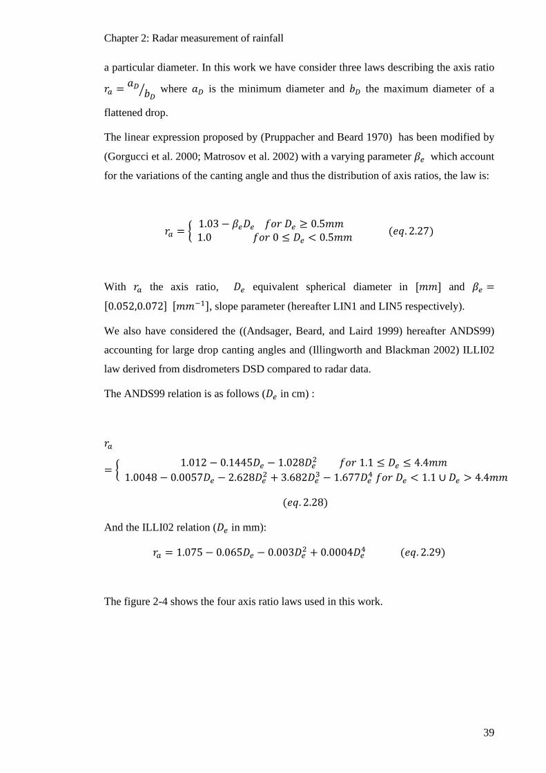
Chapter 2: Radar measurement of rainfall
39
a particular diameter. In this work we have consider three laws describing the axis ratio
𝑟𝑟𝑎𝑎 = 𝑎𝑎𝐷𝐷𝑏𝑏𝐷𝐷� where 𝑎𝑎𝐷𝐷 is the minimum diameter and 𝑏𝑏𝐷𝐷 the maximum diameter of a
flattened drop.
The linear expression proposed by (Pruppacher and Beard 1970) has been modified by
(Gorgucci et al. 2000; Matrosov et al. 2002) with a varying parameter 𝛽𝛽𝑒𝑒 which account
for the variations of the canting angle and thus the distribution of axis ratios, the law is:
𝑟𝑟𝑎𝑎 = � 1.03 − 𝛽𝛽𝑒𝑒𝐷𝐷𝑒𝑒 𝑓𝑓𝑙𝑙𝑟𝑟 𝐷𝐷𝑒𝑒 ≥ 0.5𝑐𝑐𝑐𝑐 1.0 𝑓𝑓𝑙𝑙𝑟𝑟 0 ≤ 𝐷𝐷𝑒𝑒 < 0.5𝑐𝑐𝑐𝑐 (𝑃𝑃𝑒𝑒. 2.27)
With 𝑟𝑟𝑎𝑎 the axis ratio, 𝐷𝐷𝑒𝑒 equivalent spherical diameter in [𝑐𝑐𝑐𝑐] and 𝛽𝛽𝑒𝑒 =
[0.052,0.072] [𝑐𝑐𝑐𝑐−1], slope parameter (hereafter LIN1 and LIN5 respectively).
We also have considered the ((Andsager, Beard, and Laird 1999) hereafter ANDS99)
accounting for large drop canting angles and (Illingworth and Blackman 2002) ILLI02
law derived from disdrometers DSD compared to radar data.
The ANDS99 relation is as follows (𝐷𝐷𝑒𝑒 in cm) :
𝑟𝑟𝑎𝑎
= � 1.012 − 0.1445𝐷𝐷𝑒𝑒 − 1.028𝐷𝐷𝑒𝑒2 𝑓𝑓𝑙𝑙𝑟𝑟 1.1 ≤ 𝐷𝐷𝑒𝑒 ≤ 4.4𝑐𝑐𝑐𝑐 1.0048 − 0.0057𝐷𝐷𝑒𝑒 − 2.628𝐷𝐷𝑒𝑒2 + 3.682𝐷𝐷𝑒𝑒3 − 1.677𝐷𝐷𝑒𝑒4 𝑓𝑓𝑙𝑙𝑟𝑟 𝐷𝐷𝑒𝑒 < 1.1 ∪ 𝐷𝐷𝑒𝑒 > 4.4𝑐𝑐𝑐𝑐
(𝑃𝑃𝑒𝑒. 2.28)
And the ILLI02 relation (𝐷𝐷𝑒𝑒 in mm):
𝑟𝑟𝑎𝑎 = 1.075 − 0.065𝐷𝐷𝑒𝑒 − 0.003𝐷𝐷𝑒𝑒2 + 0.0004𝐷𝐷𝑒𝑒4 (𝑃𝑃𝑒𝑒. 2.29)
The figure 2-4 shows the four axis ratio laws used in this work.

Chapter 2: Radar measurement of rainfall
40
Figure 2-3: Example of rain drop photos having spherical equivalent diameters of
𝑫𝑫𝒆𝒆=[8.00,7.35,5.80,5.30,3.45,2.70 mm] by Pruppacher and Beard (1970)
Figure 2-4: Different ratio shape laws used in this work.

Chapter 2: Radar measurement of rainfall
41
Ice particles parameterization
The average properties of icy hydrometeors are often parameterized by power laws
derived from observed data (Fontaine et al. 2014). The diameter of an icy hydrometeor is
ill defined, usually the maximum diameter of the particle is used, 𝐷𝐷𝑚𝑚𝑎𝑎𝑒𝑒, or the melted
equivalent spherical diameter 𝐷𝐷𝑒𝑒𝑒𝑒,𝑤𝑤. Related to the hydrometeor density, the mass can be
parameterized by a power law:
𝑐𝑐ℎ = 𝛼𝛼𝑚𝑚𝐷𝐷𝑚𝑚𝑎𝑎𝑒𝑒𝛽𝛽𝑚𝑚 (𝑃𝑃𝑒𝑒. 2.30)
With 𝛼𝛼𝑚𝑚 and 𝛽𝛽𝑚𝑚 the mass-diameter law coefficients.
Similarly, another usual parameterization is the density-diameter relationship:
𝜌𝜌ℎ = 𝛼𝛼𝑑𝑑𝐷𝐷𝑒𝑒𝑒𝑒,𝑤𝑤𝛽𝛽𝑑𝑑 (𝑃𝑃𝑒𝑒. 2.31)
Where 𝜌𝜌ℎ is the density.
Many other parameterizations exist to describe the fauna of icy crystals. The radiative
properties of crystals can be extremely different depending on their shapes. This variety
on the response of crystals to the IR and MW radiation has an incidence on the remote
sensing by radar and satellite (reflectivity and polar. variables for radar, brightness
temperatures for passive satellites). Ice crystals add a layer of uncertainty, compared to
melted rainfall, when modelling the interaction between EM waves and hydrometeors.
2.3 Models representing hydrometeors and EM interaction
In this section we describe the main dielectric properties of hydrometeors used to describe
their interaction with EM radiation. Then we describe the usual theories for hydrometeors
microwave scattering calculation.
Dielectric properties of hydrometeors
The dielectric constant 𝜀𝜀 of the hydrometeors varies with the wavelength of the EM field
𝜆𝜆, the temperature and the phase of the scatter (ice, water or mix).
The complex refractive index 𝑐𝑐 is defined with the dielectric constant 𝜀𝜀:
Chapter 2: Radar measurement of rainfall
42
𝑐𝑐 = √𝜀𝜀 = 𝑙𝑙 − 𝑖𝑖𝑘𝑘𝑎𝑎 (𝑃𝑃𝑒𝑒. 2.32)
With 𝑙𝑙 the ordinary refractive index and 𝑘𝑘𝑎𝑎 the absorption coefficient of the scatter
material.
The refraction index impacts the scattering properties of the hydrometeors and thus the
received signal on the radars. The model of (Liebe, Hufford, and Manabe 1991) is
commonly used to calculate the refraction index of water at microwave frequencies.
For solid and melting hydrometeors the refraction index depends on the relative fraction
of the different phases constituting the particle: during melting the particles are
constituted of a mix of air, ice and water. The solid hydrometeors are constituted by ice
or ice and air. Different models exist to calculate the refractive index of a melting particle.
In chapter 3 we detail the models and use the radar observation of the melting layer to
derive their density using such models.
Two simplifying theories: Rayleigh and Mie scattering
The theory of scattering of EM waves by particles was developed in the 19th and early
20th century. A general solution was given by Mie (Mie 1908). It is based on the
application of the Maxwell’s equations in the scatter and the propagation medium and
applying the limit conditions at the border of the scatter by considering the continuity of
the tangential component of the electromagnetic field.
The resulting scattered field depends on the following basic parameters:
• The scattering direction
• the dielectric constant 𝜀𝜀 of the scatter which varies with the wavelength of the
EM field 𝜆𝜆 and the temperature 𝑀𝑀. The complex refractive index 𝑐𝑐 defined by
𝑐𝑐=√𝜀𝜀 = 𝑙𝑙 − 𝑖𝑖𝑘𝑘𝑎𝑎 with 𝑙𝑙 the ordinary refractive index and 𝑘𝑘𝑎𝑎 the absorption
coefficient of the scatter material
• The size parameter 𝛼𝛼 = 𝜋𝜋𝐷𝐷/𝜆𝜆 with 𝐷𝐷 the diameter of the scatter and 𝜆𝜆 the
wavelength of the EM field.
Chapter 2: Radar measurement of rainfall
43
When the size parameter 𝛼𝛼 ≪ 1, the scatter size is small with respect to the wavelength,
the approximation of Rayleigh is satisfied.
The scattering cross section multiplied by the power density of the incident wave is
equivalent to the total amount of energy removed from the electromagnetic wave due to
scattering in all directions. A certain amount of energy is absorbed by heating by the
particle: this amount is equal to the absorption cross section multiplied by the power
density of the incident wave. The backscattering cross section is related to the quantity of
power scattered by the particle in the same direction than the incident wave.
The backscattering cross section, absorption cross section and the scattering cross section
can be expressed with the diameter 𝐷𝐷 and by 𝐾𝐾 being:
𝐾𝐾 =𝑐𝑐2 − 1m2 + 2
(𝑃𝑃𝑒𝑒. 2.33)
In Rayleigh approximation we can express 𝜎𝜎𝑜𝑜𝑜𝑜 the backscattering cross-section, 𝜎𝜎𝑎𝑎 the
absorption cross section of the scatter, 𝜎𝜎𝑜𝑜 the scattering cross section, and 𝜎𝜎𝑒𝑒𝑒𝑒𝑡𝑡 the
extinction cross section:
𝜎𝜎𝑜𝑜𝑜𝑜 =𝜋𝜋5
𝜆𝜆4𝐷𝐷6|𝐾𝐾|2 (𝑃𝑃𝑒𝑒. 2.34)
𝜎𝜎𝑎𝑎 =𝜋𝜋2
𝜆𝜆𝐷𝐷3𝐼𝐼𝑐𝑐(−𝐾𝐾) (𝑃𝑃𝑒𝑒. 2.35)
𝜎𝜎𝑜𝑜 =2𝜋𝜋5
3λ4𝐷𝐷6|𝐾𝐾|2 (𝑃𝑃𝑒𝑒. 2.36)
𝜎𝜎𝑒𝑒𝑒𝑒𝑡𝑡 = 𝜎𝜎𝑎𝑎 + 𝜎𝜎𝑜𝑜 (𝑃𝑃𝑒𝑒. 2.37)
If the MW signal is at 3 GHz (𝜆𝜆~10𝑐𝑐𝑐𝑐) all rain drop sizes verify the Rayleigh
approximation.
For higher frequencies the Rayleigh approximation is no longer valid and we shall use
the Mie’s theory.
Then if the size parameter 𝛼𝛼~1, the Mie’s theory shows that the scattering and total
absorption cross sections are given by:
𝜎𝜎𝑜𝑜𝑜𝑜 =𝜆𝜆2
4𝜋𝜋��(2𝑙𝑙 + 1)(−1)𝑛𝑛(|𝑎𝑎𝑛𝑛|2 +∞
𝑛𝑛=1
|𝑏𝑏𝑛𝑛|2)�2
(𝑃𝑃𝑒𝑒. 2.38)

Chapter 2: Radar measurement of rainfall
44
𝜎𝜎𝑜𝑜 =𝜆𝜆2
2𝜋𝜋�(2𝑙𝑙 + 1)(|𝑎𝑎𝑛𝑛|2 +∞
𝑛𝑛=1
|𝑏𝑏𝑛𝑛|2) (𝑃𝑃𝑒𝑒. 2.39)
𝜎𝜎𝑒𝑒𝑒𝑒𝑡𝑡 =−𝜆𝜆2
2𝜋𝜋𝑅𝑅𝑃𝑃𝑎𝑎𝑙𝑙 ��(2𝑙𝑙 + 1)(|𝑎𝑎𝑛𝑛|2 +
∞
𝑛𝑛=1
|𝑏𝑏𝑛𝑛|2)� (𝑃𝑃𝑒𝑒. 2.40)
Where 𝑎𝑎𝑛𝑛 and 𝑏𝑏𝑛𝑛 are the spherical Bessel functions of order 𝑙𝑙 with arguments 𝛼𝛼 and 𝑐𝑐
Figures 2-5 and 2-6 shows the Rayleigh and Mie scattering cross sections for different
frequencies, at different temperatures for the typical range of water drops. There is a high
sensitivity on the frequency with different impacts at different drop sizes. Worth noting
the Mie oscillation at 5mm diameter at 7 GHz. The Mie and Rayleigh calculations of the
scattering cross sections converge at a certain diameter depending on the frequency. For
low frequencies (ie. 7 GHz in the figure), the Mie and Rayleigh cross sections converges
at 3.5 mm. For higher frequencies, we move away from Rayleigh regime and the meeting
of both curves occur for lower diameters. The dependency on temperature is lower, as we
see in figure 2-6. This dependency comes from the evolution of the complex refractive
index of water with temperature.
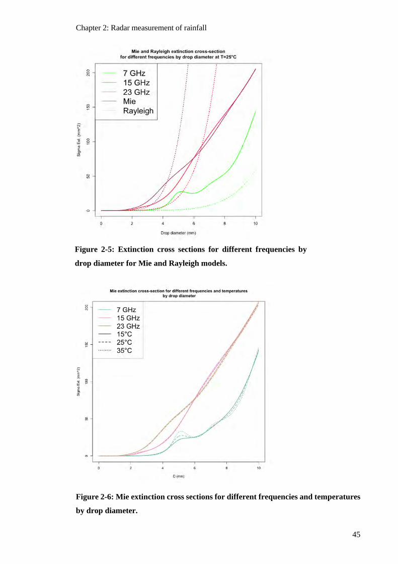
Chapter 2: Radar measurement of rainfall
45
Figure 2-6: Mie extinction cross sections for different frequencies and temperatures
by drop diameter.
Figure 2-5: Extinction cross sections for different frequencies by
drop diameter for Mie and Rayleigh models.
Chapter 2: Radar measurement of rainfall
46
T-matrix model
The T-matrix approach (Mishchenko, Travis, and Mackowski 1996) was developed to
calculate scattering of non-spherical icy and liquid hydrometeors (Barber and Yeh 1975;
Vivekanandan, Adams, and Bringi 1991). The scattering calculations for an irregular
scatter are made by solving the Maxwell's equations explicitly (more details in the cited
articles).
The T-matrix method for EM scattering by non-spherical particles is a reference in
weather radar polarimetry and an open source code has generalized its use. The method
calculates the propagative and scattering properties of populations of spheroid drops
defined by their aspect ratio, their orientation compared to the incident electromagnetic
field, their size relative to the wavelength, and their refractive index. In order to account
for drop oscillation, a distribution of canting angles can be provided.
The T-matrix solves the scattered electromagnetic field by estimating the scattering
matrix components 𝑆𝑆𝑖𝑖𝑖𝑖, which is the operator between the incident EM field decomposed
into the vertical and horizontal polarizations and the scattered field by a conjunction of
asymmetrical spheroids:
�𝐸𝐸𝐻𝐻𝑆𝑆
𝐸𝐸𝑉𝑉𝑆𝑆� =
𝑃𝑃−𝑖𝑖𝑘𝑘0𝑟𝑟
𝑟𝑟�𝑆𝑆𝐻𝐻𝐻𝐻 𝑆𝑆𝐻𝐻𝑉𝑉𝑆𝑆𝑉𝑉𝐻𝐻 𝑆𝑆𝑉𝑉𝑉𝑉
� �𝐸𝐸𝐻𝐻𝑖𝑖
𝐸𝐸𝑉𝑉𝑖𝑖� (𝑃𝑃𝑒𝑒. 2.41)
With 𝑘𝑘0 the wave number, 𝐸𝐸𝐻𝐻,𝑉𝑉𝑆𝑆 the components of the scattered field, and 𝐸𝐸𝐻𝐻,𝑉𝑉
𝑖𝑖 the
components of the incident field.
We can define the horizontal and vertical reflectivity factors with the coefficients 𝑆𝑆𝑖𝑖𝑖𝑖 by:
zH,V = 4 λ4
π5 |K|2 ∫ �sHH,VV(D)�
2(D)N(D)dDDmaxDmin
(𝑃𝑃𝑒𝑒. 2.42)
The differential reflectivity factor 𝑍𝑍𝐷𝐷𝐷𝐷 (dB) is defined as:
ZDR = ZH − ZV = 10𝑙𝑙𝑙𝑙𝑙𝑙 �𝑧𝑧𝐻𝐻𝑧𝑧𝑉𝑉� = 10𝑙𝑙𝑙𝑙𝑙𝑙 �
|𝑆𝑆𝐻𝐻𝐻𝐻|2
|𝑆𝑆𝑉𝑉𝑉𝑉|2� (𝑃𝑃𝑒𝑒. 2.43)
The T-matrix approach estimates the fH,V forward and sHH,VV backward scattering
amplitudes (m) at horizontal (H) or vertical (V) polarization respectively, which can be
used to derive the propagative variables:
Chapter 2: Radar measurement of rainfall
47
kH,V = 8.68 λ ∫ Im�fH,V(D)� N(D)dDDmaxDmin
(𝑃𝑃𝑒𝑒. 2.44)
KDP = 180 πλ
∫ Re[fH(D) − fV(D)] N(D) dD [°/km]DmaxDmin
(𝑃𝑃𝑒𝑒. 2.45)
With 𝜆𝜆 wavelength (m), Re and Im denoting their real and imaginary parts.
In chapter 4 we use T-matrix calculations for different aspect ratio laws as a forward
model to estimate polarimetric variables from the characteristics of the hydrometeors.
The model is then inverted to retrieve the characteristics of the hydrometeors from
polarimetric radar measurements.

Chapter 2: Radar measurement of rainfall
48

Chapter 3: A simple bright band method to infer the density of hydrometeors
49
3 A SIMPLE BRIGHT BAND METHOD TO INFER THE DENSITY OF HYDROMETEORS
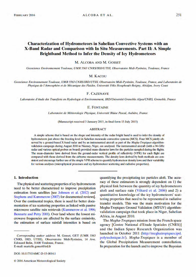
Chapter 3: A simple bright band method to infer the density of hydrometeors
50
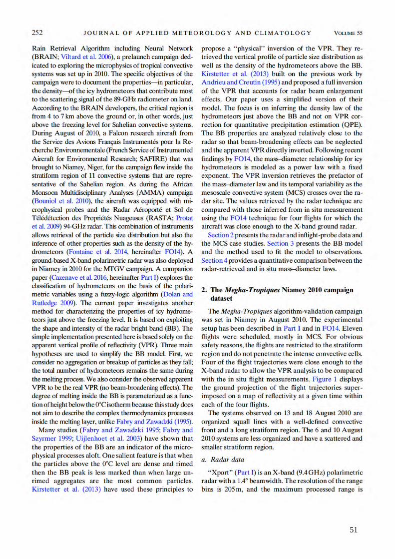
Chapter 3: A simple bright band method to infer the density of hydrometeors
51
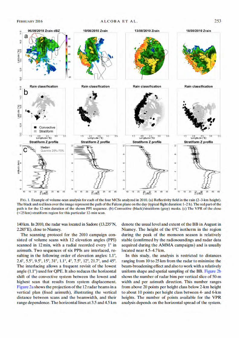
Chapter 3: A simple bright band method to infer the density of hydrometeors
52

Chapter 3: A simple bright band method to infer the density of hydrometeors
53

Chapter 3: A simple bright band method to infer the density of hydrometeors
54

Chapter 3: A simple bright band method to infer the density of hydrometeors
55
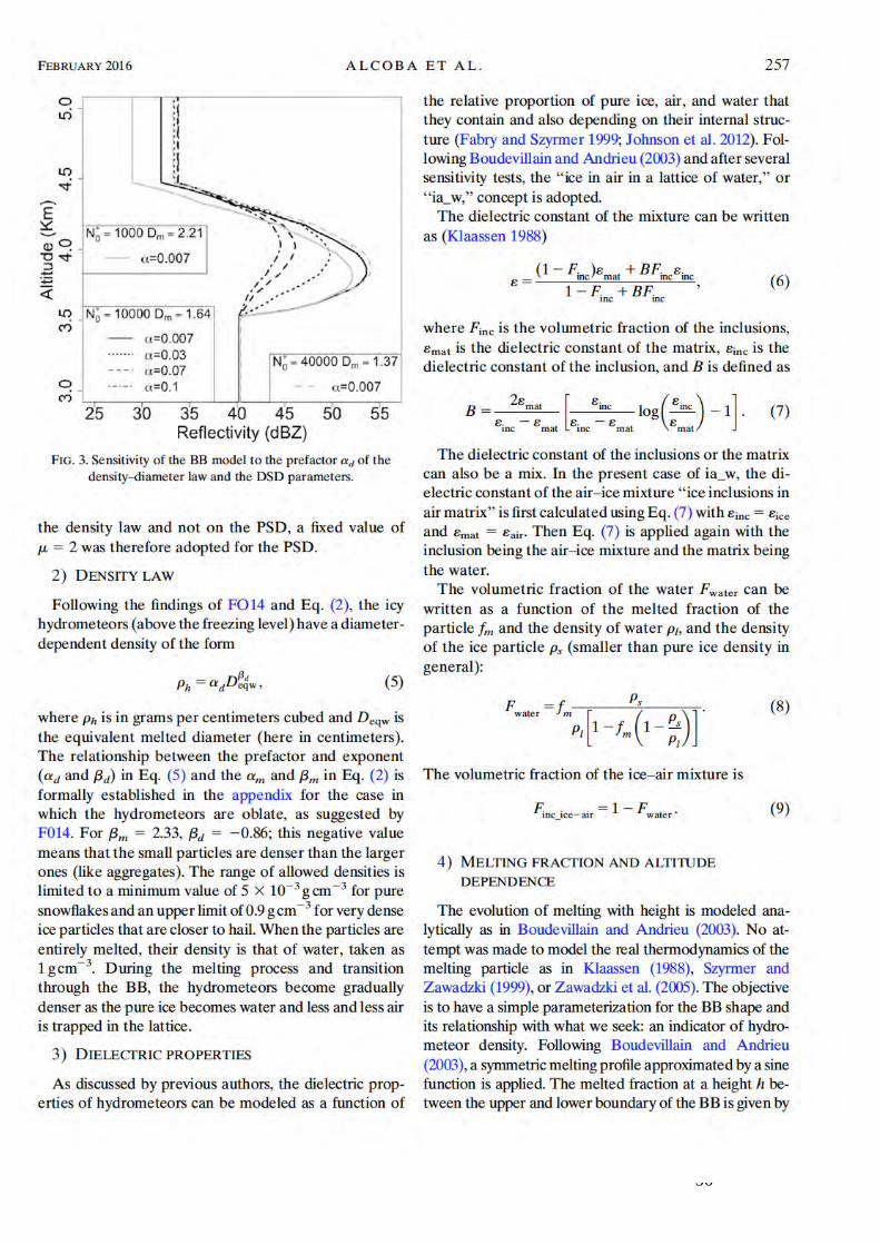
Chapter 3: A simple bright band method to infer the density of hydrometeors
56
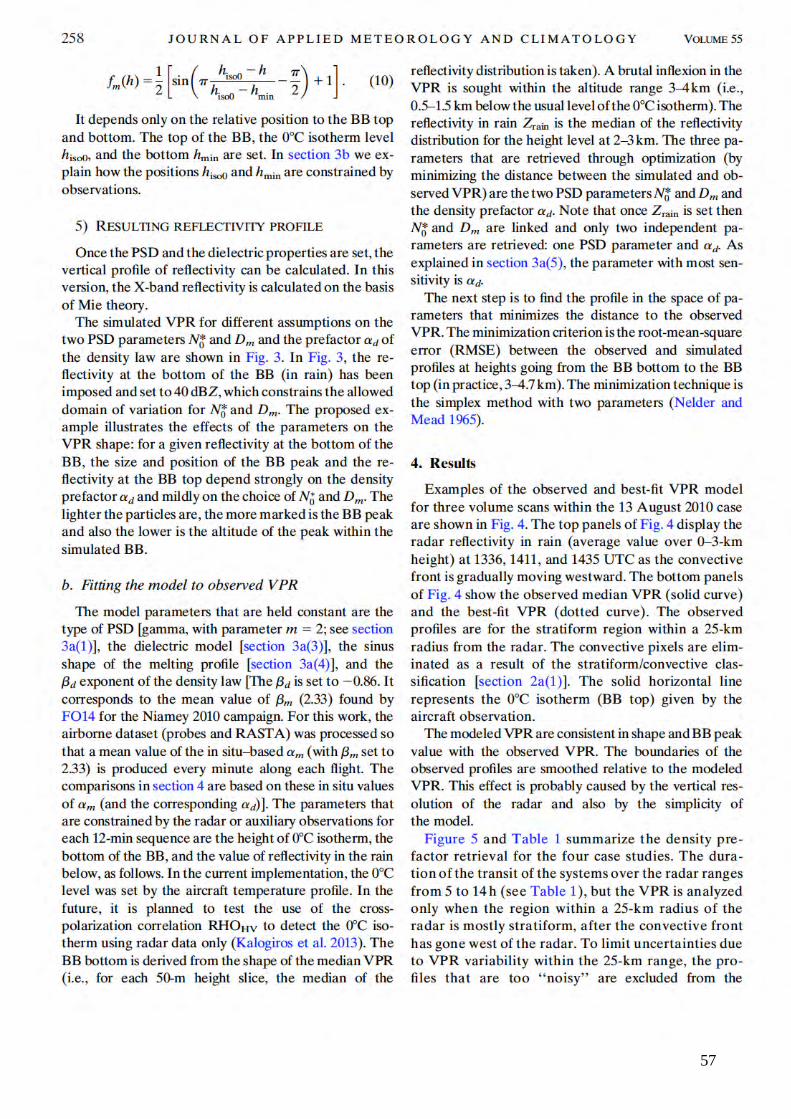
Chapter 3: A simple bright band method to infer the density of hydrometeors
57
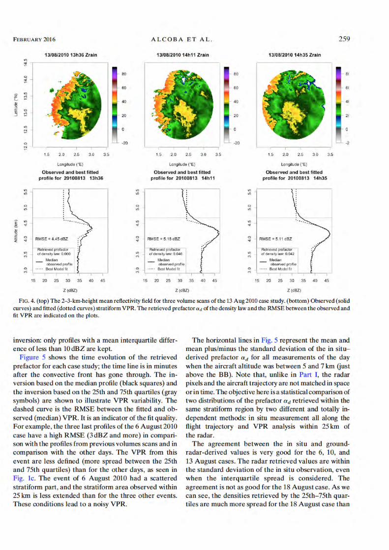
Chapter 3: A simple bright band method to infer the density of hydrometeors
58
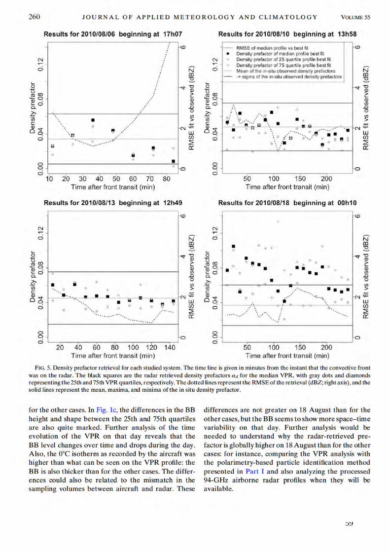
Chapter 3: A simple bright band method to infer the density of hydrometeors
59
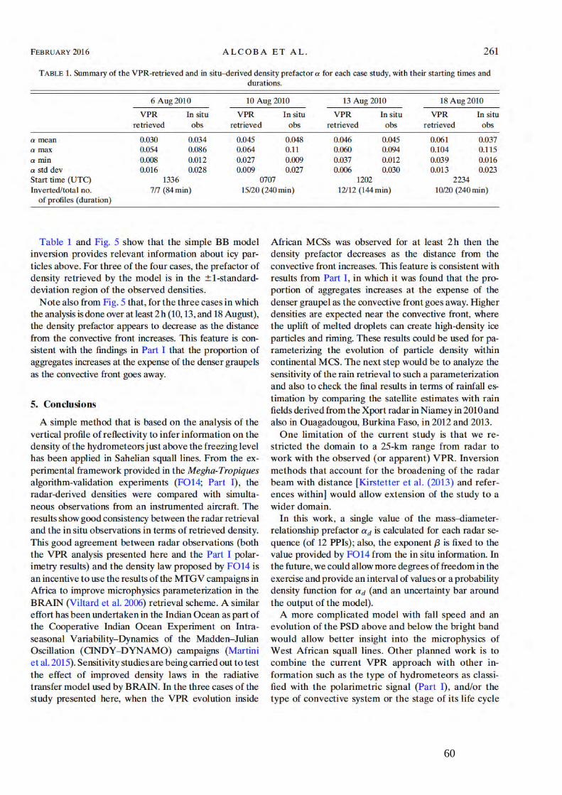
Chapter 3: A simple bright band method to infer the density of hydrometeors
60
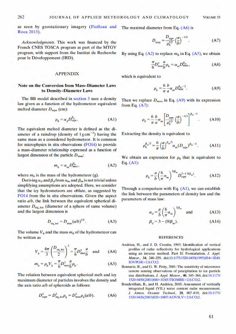
Chapter 3: A simple bright band method to infer the density of hydrometeors
61
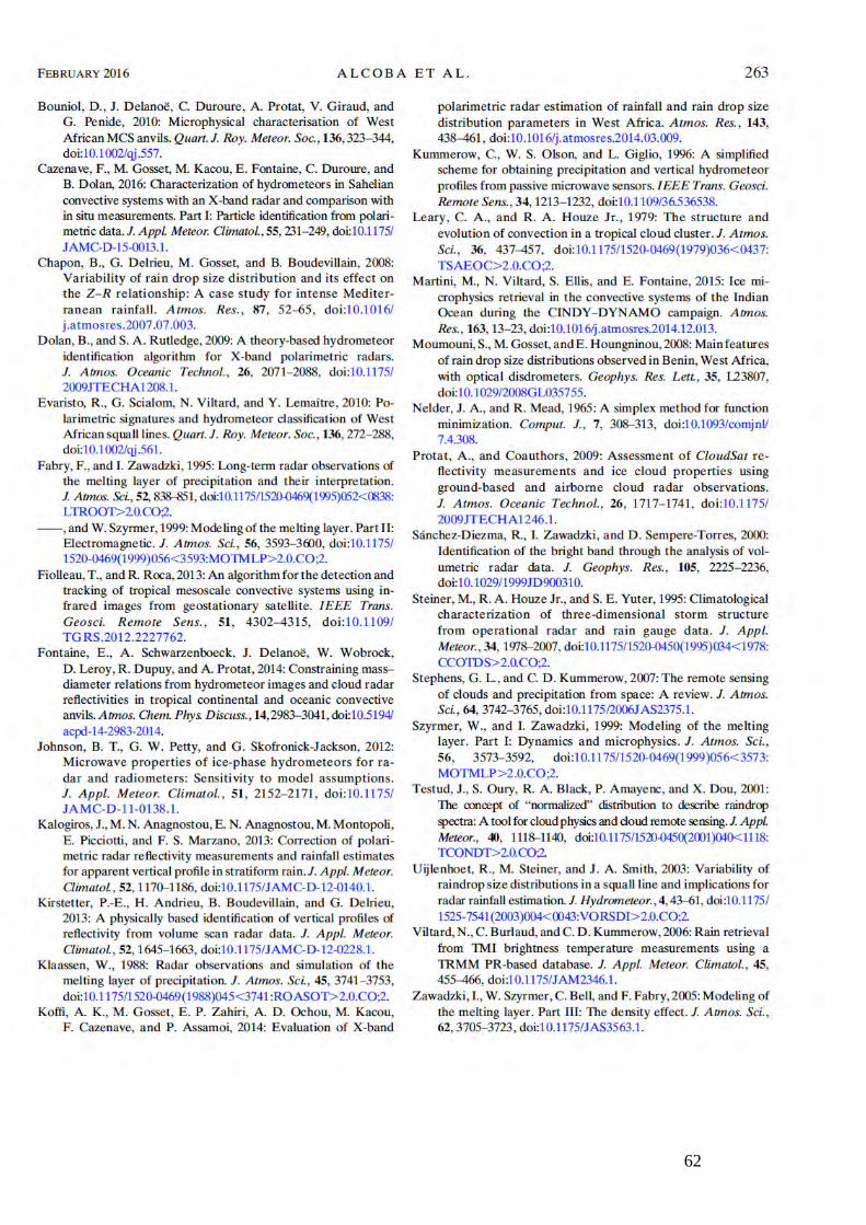
Chapter 3: A simple bright band method to infer the density of hydrometeors
62
Chapter 4: An inverse method for drop size distribution retrieval
63
4 AN INVERSE METHOD FOR DROP SIZE DISTRIBUTION RETRIEVAL
Article submitted to MDPI ‘Remote Sensing’
An inverse method for Drop Size Distribution retrieval
from polarimetric radar at attenuating frequency
Matias Alcoba1, Hervé Andrieu2 and Marielle Gosset1,*
1 Géoscience Environnement Toulouse, GET (CNRS-IRD-Université de Toulouse III-CNES) 2 Laboratoire Eau et Environnement, IFSTTAR
* Correspondance : [email protected]; Tel: +33(0)637502211
Abstract: A method which formulates the retrieval of Drop Size Distribution (DSD)
parameters from polarimetric radar variables at attenuating frequency as the solution of
an inverse problem is presented. The proposed method leads to a solution that best
reconstitutes the polarimetric radar observables along the bins of radar radials. DSDs are
represented by normalized Gamma distributions defined by three parameters
(Dm, N0∗ , μ). The direct problem that describes polarimetric radar observables, including
attenuation and their dependency on DSD parameters is analyzed based on T-matrix
scattering simulations. The principle of the inverse algorithm and the crucial importance
of the information a priori are discussed. The inverse algorithm and its application to the
DSD retrieval are then presented. The inverse method is applied to an African Monsoon
Multidisciplinary Analysis (AMMA) field campaign that deployed an X-band dual-
polarization Doppler radar and optical disdrometers in Benin, West Africa in 2006 and
2007. The dataset is composed of X-band polarimetric radar PPIs and disdrometer data
of 15 organized convective systems observed in 2006. The a priori information on DSD
parameters is derived from the polarimetric radar observables, by means of relationships
suited to these type of rain events. The proposed retrieval method of DSD parameters
Chapter 4: An inverse method for drop size distribution retrieval
64
leads to the following results: i) the obtained DSD fields show a better spatial
consistency than the a priori DSD fields, ii) the polarimetric radar observables are better
reproduced from the obtained DSD parameters than from the a priori ones, iii) the
comparison with time series of DSD parameters derived from disdrometer data confirms
that the inverse method results in an improved estimation of DSD parameters compared
to a priori ones. These promising results indicate that DSD retrieval based on the inverse
theory framework and considering the whole radial improves the coherence of DSD
estimates at radar image scale, compared to retrieval obtained from polarimetric radar
observables processed gate by gate. A more comprehensive evaluation in different
climatological contexts would be required to confirm these first results.
Keywords: Radar polarimetry; Drop size distribution retrieval; inverse problem;
attenuation correction; X-band radar; tropical rainfall
4.1 Introduction Rainfall is usually defined as a flux of water, which monitoring is very important at
all scales (local to global) in many applications, from climate research to flash flood
prediction. Rainfall estimation has greatly benefitted from the progress of weather radar
and the development of dual-polarization methods. In addition to quantitative rainfall
estimation, radar techniques have provided some insight in the microphysics and the
dynamics of storms, enabling a 3D analysis of winds and hydrometeor type and density
within clouds and precipitation ((Fabry 2015) for a recent review). A whole branch of
weather radar research has been devoted to rain or cloud Drop Size Distributions (DSD),
with two purposes: i) characterizing DSD and its variability as a source of uncertainty in
radar estimation of rainfall ((Atlas et al. 1999; Lee and Zawadzki 2005; Lee et al. 2004;
Steiner, Smith, and Uijlenhoet 2004; Uijlenhoet, Steiner, and Smith 2003; Cao et al.
2008)) and ii) deriving information on the DSD from the radar measurements itself
((Vivekanandan, Zhang, and Brandes 2004; Koffi et al. 2014; Bringi et al. 2002)). The
determination of the DSD over various spatial and temporal scales is interesting for a
range of scientific applications. With a better knowledge of the DSD, accurate and
physically based characterization of rain can be obtained and used for many
meteorological and hydrological applications: rain rate estimation, rain erosivity, satellite
and radar remote sensing studies, rain microphysics, cloud modeling, among others. Most
Chapter 4: An inverse method for drop size distribution retrieval
65
of the early work on the DSD was based on disdrometers and mainly focused on
investigating if some standard form of DSD could be defined ((Torres, Porrà, and Creutin
1994)). Based on these studies, on observations and on theoretical considerations on
cloud/rain microphysics, it is commonly accepted that rainfall DSD can be represented
by a Gamma law governed by three parameters characterizing: the number of drops, the
characteristic diameter, the shape ((Testud et al. 2001)). The exponential DSD initially
proposed by Marshall and Palmer (Marshall and Palmer 1948) is a particular case of
gamma DSD; other laws like lognormal or 4 parameters extended gamma have also been
proposed, but are less commonly used. Many studies have been devoted to analyzing how
the DSD parameters vary with rain bulk variables (rain rate, radar reflectivity factor,
liquid water content, median-volume diameter) and to find expressions for the DSD
function and parameters, that reduce the variability ((Testud et al. 2001; Lee et al. 2009)).
A well adopted solution consists in normalizing the DSD and the drop diameters by one
or two integral moments of the DSD ((Torres, Porrà, and Creutin 1994; Testud et al. 2001)
among others).
Another topic of research is the time-space variability of the DSD parameters and its
relation with the physical processes inside the clouds and precipitation. (Moumouni,
Gosset, and Houngninou 2008) highlighted the variability between and within West
African squall lines, with a marked partition between convective and stratiform DSDs.
This is consistent with several authors (Uijlenhoet, Steiner, and Smith 2003; Testud et al.
2001; Tokay and Short 1996) who also reported a marked jump in the DSD characteristic
number (‘𝑁𝑁0 jump’) between convective cells and the stratiform trail. (Hachani et al.
2017) based on a five-year DSD climatology across the Mediterranean Cevennes–
Vivarais region showed the influence on the DSD of the orographic environment, season,
weather patterns and rainfall types. (Steiner, Smith, and Uijlenhoet 2004) demonstrated
that different rainfall generation processes lead to different types of DSD and different
relationships between the characteristic number and diameter.
Disdrometers provide only punctual information on the DSD and no information on
its spatial variability unless an extensive (hence expensive) network of disdrometers is
used. Polarimetric weather radar, on the other hand, can provide spatially distributed
information on rain microphysics. Radar polarimetry has lead to significant progress in
rainfall characterization. In addition to the reflectivity factor (ZH, expressed in dBZ), a
polarimetric radar provides the differential reflectivity (𝑍𝑍DR = ZH − ZV, expressed in dB,
with H and V denoting horizontal and vertical components of the polarized wave

Chapter 4: An inverse method for drop size distribution retrieval
66
respectively), the cross-correlation coefficient (ρHV) and the differential phase shift (𝜙𝜙𝐷𝐷𝐷𝐷
expressed in degrees). The range derivative, called the specific differential phase shift
(𝐾𝐾𝐷𝐷𝐷𝐷) can be estimated from 𝜙𝜙𝐷𝐷𝐷𝐷. Because of the drop oblateness increases with their
diameter ((Bringi and Chandrasekar 2001)), 𝑍𝑍𝐷𝐷𝑅𝑅 is well related to the mean drop diameter
of the DSD. 𝜙𝜙𝐷𝐷𝐷𝐷, is influenced by the amount of water along the path and by the
oblateness of the drops – it is closely related to the attenuation along the path and can be
used to correct it ((Gourley, Tabary, and Parent du Chatelet 2007; Gosset, Zahiri, and
Moumouni 2010a; Carey et al. 2000; Bringi, Keenan, and Chandrasekar 2001; Matrosov
et al. 2005)). 𝐾𝐾𝐷𝐷𝐷𝐷 can be used to estimate the rainfall rate (R in mm/h), 𝜌𝜌𝐻𝐻𝑉𝑉 helps
distinguishing melting hydrometeors, and altogether the polarimetric variables can help
determining the dominant type of hydrometeors and non-meteorological echoes. First
radar polarimetry was investigated for rainfall estimation. Different methods have been
proposed and compared ((Tabary et al. 2011), (Chen, Chandrasekar, and Bechini 2017)).
The retrieval of DSDs was first proposed as a mean to improve rainfall estimation from
polarimetric variables ((Gorgucci et al. 2001a)). (Gorgucci et al. 2001b; Gorgucci et al.
2002) proposed the β-method, improved in (Gorgucci, Chandrasekar, and Baldini 2009),
to retrieve the parameters of a DSD gamma distribution. This method introduces the
additional parameter β,slope of the empirical equation expressing the drop ratio axis in
function of the drop diameter. The authors first express 𝛽𝛽 from polarimetric variables and
derive the DSD parameters from polarimetric variables (𝑍𝑍𝐻𝐻,𝑍𝑍𝐷𝐷𝐷𝐷 ,𝐾𝐾𝐷𝐷𝐷𝐷) by means of
power laws whose coefficients depend on β. The constrained gamma method ((Zhang,
Vivekanandan, and Brandes n.d.; Brandes, Zhang, and Vivekanandan 2004)) is based on
an empirical relation between the slope (λ) and the shape (µ) parameters of the DSD,
from which are derived the relations expressing the DSD parameters as functions of 𝑍𝑍𝐻𝐻
and 𝑍𝑍𝐷𝐷𝐷𝐷. According to (Kim, Maki, and Lee 2010; Anagnostou et al. 2008), the
constrained gamma method performs better than the β-method. (Raupach and Berne
2017) developed a method applicable to a double-moment normalized DSD, defined by
two parameters. (Koffi et al. 2014) tested in Africa DSD retrievals based on empirical
relationships. All these studies rely on empirical (mostly power law) relationships
between the DSD parameters and the radar variables. Other studies proposed statistical
frameworks to account for the stochastic nature of the DSD. (Islam, Rico-Ramirez, and
Han 2012) used a tree-based genetic program to retrieve the parameters of a gamma DSD
from 𝑍𝑍𝐻𝐻 and 𝑍𝑍𝐷𝐷𝐷𝐷. (Cao et al. 2010) proposed a Bayesian approach with DSD parameters
as state variables to estimate rainfall rate from S-band polarimetric radar. (Wen et al.
Chapter 4: An inverse method for drop size distribution retrieval
67
2018) formulated the retrieval of DSD parameters from S-band polarimetric radar
variables as an inverse problem.
The studies above do not explicitly account for radar attenuation by rain, either
because they are based on S-band radar or because the radar reflectivities were corrected
for attenuation before DSD retrieval. For X-band radars, the variables (𝑍𝑍𝐻𝐻,𝑍𝑍𝐷𝐷𝐷𝐷) must be
corrected for attenuation to avoid underestimation of the DSD parameters. (Kim, Maki,
and Lee 2008; Park et al. 2005; Shi et al. 2017) adapted the self-consistent method
proposed by (Bringi, Keenan, and Chandrasekar 2001) for attenuation correction of X-
band data. (Gorgucci, Chandrasekar, and Baldini 2009) also used a self-consistency
method. (Raupach and Berne 2017) proposed a variation on the ZPHI algorithm ((Testud
et al. 2000)). In most studies a relationship between the path integrated attenuation and
the differential phase shift is used as in (Matrosov et al. 2002), (Testud et al. 2000) and
(Bringi, Keenan, and Chandrasekar 2001). (Kalogiros et al. 2014) presented the self-
consistent with optimal parameterization (SCOP) algorithm to correct X-band radar for
attenuation. (Gou, Chen, and Zheng 2019) proposed an improved version of the
attenuation correction for C-Band. (Koffi et al. 2014; Gosset, Zahiri, and Moumouni
2010a) followed (Matrosov et al. 2005) and found that a simple attenuation correction
based on a linear relationship between attenuation and 𝜙𝜙𝐷𝐷𝐷𝐷 gave robust results; in these
papers the linear coefficient is derived on the radar data itself using (Carey et al. 2000).
(Chang, Vivekanandan, and Chen Wang 2014) formulated the attenuation estimation of
X-band polarimetric radar by means of a variational algorithm. (Yoshikawa,
Chandrasekar, and Ushio 2014) noticed that the two-step procedure that applies
sequentially attenuation correction and then DSD retrieval may result in errors and
inconsistency in the retrieved DSD. They proposed a three step procedure, based on a
cost function minimization, to retrieve the DSD along all the gates of a radar radial. In
(Yoshikawa, Chandrasekar, and Ushio 2014) the first step is an iterative method based on
a simultaneous calculation of the forward and backscattering effects of DSD in order to
insure consistency in the assumptions used for all radar variables.
The present study builds upon these papers and formulates the retrieval of a radial
profile of DSD parameters from X-band polarimetric radar in the framework of inverse
theory ((Tarantola 2005; Menke 2018)). The objective is to retrieve the parameters of
DSD distributions (here, gamma) that best reconstitute the measured polarimetric radar
observables along a radial. The proposed model expresses the radar observable as a
function of DSD parameters along the radial, explicitly accounting for the attenuation.
Chapter 4: An inverse method for drop size distribution retrieval
68
The retrieval method presented in this study can be viewed as an evolution of the method
proposed by (Yoshikawa, Chandrasekar, and Ushio 2014). Its originality lies in the
following points: i) an extension to X-band polarimetric data affected by attenuation of
the statistical approach proposed by (Cao et al. 2010) and applied to S-band radar data,
ii) a solution of the inverse problem by an algorithm different from that used by (Wen et
al. 2018) that did not account for attenuation and from (Yoshikawa, Chandrasekar, and
Ushio 2014) who do not explicitly account for a priori information, iii) a special attention
given to the a priori information, a key point in inverse methods in presence of non-linear
models or for solving underdetermined problems, v) a test of the method with X-band
radar data in West Africa, on case studies with intense rainfall and heavy attenuation –
challenging conditions for DSD retrieval.
Section 2 introduces the radar and disdrometer dataset gathered in West Africa, and
the typology of the studied convective rainfall systems. Section 3 provides a detailed
description of the forward problem relating polarimetric radar variables at attenuating
frequency and the DSD along the radar beam. Section 4 introduces the inverse model
framework and its advantages for DSD retrieval. The practical implementation and
sensitivity to model parameters and to the a priori information is discussed. Section 5
provides the quantitative results and statistics when the radar retrieved DSD is compared
with disdrometer data. The conclusions and perspective of this work are proposed in
section 6.
4.2 Study area and dataset This work was initiated as part of the African Monsoon Multi-disciplinary Analysis
(AMMA) program ((Lebel et al. 2010)). One of many AMMA objectives was a better
characterization of the meso-scale convective systems (MCS) which bring most of the
rainfall during the West African Monsoon ((Depraetere et al. 2009)). For this purpose,
several super sites were equipped during AMMA, including one in Northern Benin near
the town of Djougou situated in the upper basin of the Oueme river. This area has been
equipped as a hydro-meteorological observatory since the late 90s, with a dense network
of rain and stream gauges, as part of the AMMA-CATCH observing system ((Galle et al.
2018)). During the AMMA intensive observation period, from 2005 to 2007, a X-band
polarimetric radar was installed in Djougou. Several disdrometers ((Moumouni, Gosset,
and Houngninou 2008)) complemented the experiment during this period. The dataset
and some results that are a starting point for the present study are summarized below.

Chapter 4: An inverse method for drop size distribution retrieval
69
4.2.1 X-band polarimetric Radar data The X-port X-band polarimetric radar was developed by the Institut de Recherche
pour le Developpement (IRD) as a transportable unit to study rainfall associated with
tropical convection ((Cazenave et al. 2016)). The radar operates at 9.4 GHz with
simultaneous transmission and reception of horizontal (H) and vertical (V) signals thanks
to an orthomode feed. The peak transmitted power in each polarization is 50 kW, and the
1.4 m antenna provides a 1.4° radar beam. For the present dataset, the radar pulse length
is set to 1𝜇𝜇𝑠𝑠 and the radar pulse repetition frequency is 1 kHz. The raw data from 128
instant pulses are processed in order to provide the radar variables every range gate (150
m length) along a given azimuth. The stored radar variables are: radar reflectivity in
horizontal and vertical polarization (𝑍𝑍𝐻𝐻 and 𝑍𝑍𝑉𝑉), differential phase shift (𝜙𝜙𝐷𝐷𝐷𝐷), cross
polarization correlation coefficient (𝜌𝜌𝐻𝐻𝑉𝑉), and Doppler radial velocity calculated for each
polarization (𝑉𝑉𝐻𝐻 and 𝑉𝑉𝑉𝑉). In this work, the radial velocity is used only to detect and
remove ground clutters. During AMMA the radar was located in Djougou (9.66°N,
1.69E°) and operated with a ‘volumetric’ protocol composed of 12 successive Plan
Position Indicator scans (PPI) in a sequence of 5 or 10 min. In the present work only the
PPI with elevation 2.8° is used; it is low enough to avoid the melting layer (which is quite
high and stable at 3.5 to 4 km height in this region) and better than the lowest elevation
angles (0.9°-1.8°) in terms of ground clutter contamination.
To derive KDP from the measured ΦDP , two sliding window filters are applied, first
a median filter length of 25 gates and then a convolution with a Gaussian filter of length
10 gates and standard deviation of 5 gates length. The median filter first eliminates the
main noise variability of about 5-10°. Then the Gaussian convolution smoothes the gate
to gate gaps generated by the local median filter. The filtering reduces the noise in the
derived KDP and limits the effect of the differential scattering phase shift. We find that
this simple filtering compares well with the filtering technique proposed by (Hubbert and
Bringi 1995) that was implemented on the same dataset in (Koffi et al. 2014).
In the results presented in section 4, the other observed variables have also been
smoothed in order to minimize the influence of the noise in the DSD retrieval.
4.2.2 Optical disdrometer data Optical disdrometers were installed in three locations in the AMMA Benin super-
site: Copargo (1.53°E; 9.83°N) situated 18 km from the radar, Nangatchiori (about 10 km
from the radar) and Djougou at the radar site. As described in (Moumouni, Gosset, and
Chapter 4: An inverse method for drop size distribution retrieval
70
Houngninou 2008), the instruments are based on an optical principle. A near-IR
rectangular single or double-beam of light is attenuated by the falling rain drops. A
dedicated processing transforms this raw information into the diameter and fall velocity
of the drops. For the present dataset the rain drop spectra are acquired every minute with
22 diameter classes from 0.06 mm to 6.5 mm. The whole data base (described in
(Moumouni, Gosset, and Houngninou 2008)) is composed of 11.640 spectra, belonging
to 93 different storms and a total of 1220 mm rainfall acquired in 2005 (Nangatchori,
Djougou), 2006 (Copargo, Djougou) and 2007 (Djougou) by one (or two) of the
disdrometers. The quality of the dataset was verified by comparing the rain rates
distributions and daily total collected by each disdrometer with the closest rain gauge
((Moumouni, Gosset, and Houngninou 2008)).
In the present work, radar retrieval of the DSD is compared solely with the dual beam
disdrometer (Delahaye et al. 2006) that operated in Copargo during the peak of rainy
season (June-September) 2006, for two reasons: i) this disdrometer is the most distant
from the radar and best suited to analyze the effect of attenuation on the radar signal, and
ii) dual beam disdrometers provide a more precise estimation of the DSD because the
drops fall through two successive beams, which reduces the uncertainty on drop velocity
estimation and detection of multiple drops (Delahaye et al. 2006)
4.2.3 Previous findings from this dataset (Moumouni, Gosset, and Houngninou 2008) and (Moumouni 2009) provide an
extensive analysis of the AMMA DSD dataset. They investigated which form of DSD
and normalization best fitted the observed spectra. They also analyzed the variability of
the DSD characteristics and its relation to bulk variables like the rain rate or water content,
and the type of rainfall (convective or stratiform; organized squall lines versus local
convection). Their main conclusion is that the double moment normalization of the DSD
introduced by (Testud et al. 2001) provides a good framework to represent the shape, fit
the parameters and explain the variability of the observed DSDs. The DSD is therefore
expressed:
𝑁𝑁𝐺𝐺(𝐷𝐷𝑚𝑚,𝑁𝑁0∗, 𝜇𝜇;𝐷𝐷) = 𝑁𝑁0∗ 𝐹𝐹 �𝐷𝐷𝐷𝐷𝑚𝑚
, 𝜇𝜇� (𝑃𝑃𝑒𝑒. 4.1)
where the three parameters of the normalized DSD distribution are the volume
weighted mean diameter 𝐷𝐷𝑚𝑚, the scaling parameter of concentration 𝑁𝑁0∗, and the shape
parameter 𝜇𝜇. 𝐷𝐷𝑚𝑚 and 𝑁𝑁0∗ are defined by :
Chapter 4: An inverse method for drop size distribution retrieval
71
𝐷𝐷𝑚𝑚 = 𝑀𝑀4𝑀𝑀3
𝑤𝑤𝑖𝑖𝑤𝑤ℎ 𝑀𝑀𝑛𝑛 = ∫ 𝑁𝑁(𝐷𝐷)𝐷𝐷𝑛𝑛𝑑𝑑𝐷𝐷∞0 (𝑃𝑃𝑒𝑒. 4.2)
𝑁𝑁0∗ = 44
𝜋𝜋𝜌𝜌𝑤𝑤
𝐿𝐿𝐿𝐿𝐿𝐿𝐷𝐷𝑚𝑚4
𝑤𝑤𝑖𝑖𝑤𝑤ℎ 𝐿𝐿𝑊𝑊𝐶𝐶 = 𝜋𝜋𝜌𝜌𝑤𝑤6𝑀𝑀3 (𝑃𝑃𝑒𝑒. 4.3)
where 𝑀𝑀𝑛𝑛 is the moment of order n of the DSD distribution, 𝜌𝜌𝑤𝑤 is the density of
water, and LWC is the total liquid water content.
𝐹𝐹(𝑋𝑋, 𝜇𝜇) represents the shape of the normalized distribution, in our case the gamma
function well fitted on the observed DSD. As discussed by (Testud et al. 2001), this choice
insures the independence between 𝐷𝐷𝑚𝑚, 𝑁𝑁0∗ on one side, and 𝜇𝜇, the shape parameter of the
gamma law :
𝐹𝐹(𝑋𝑋, 𝜇𝜇) = Γ(4)(𝜇𝜇+4)𝜇𝜇+4
44Γ(𝜇𝜇+4) 𝑋𝑋𝜇𝜇exp[−(𝜇𝜇 + 4)𝑋𝑋] (𝑃𝑃𝑒𝑒. 4.4)
(Moumouni, Gosset, and Houngninou 2008) confirmed on the African DSD the
findings of (Testud et al. 2001): the normalized DSD function 𝐹𝐹 is remarkably stable and
independent of the rain type. The variability of the DSD within and between systems is
well explained by the variability of the parameters 𝑁𝑁0∗ and 𝐷𝐷𝑚𝑚. Another finding from
(Moumouni, Gosset, and Houngninou 2008) consistent with (Testud et al. 2001) and
(Tokay and Short 1996) is the existence of a ‘𝑁𝑁0 jump’ or clear distinction in the DSD
characteristics between the convective and stratiform rain. For a given rain rate, 𝑁𝑁0∗ tends
to be higher, and corollary 𝐷𝐷𝑚𝑚 smaller in convective rain; this existence of relative large
drops for low or moderate rain rates in the stratiform part can be explained by the melting
of large aggregates in this part of the squall lines ((Alcoba et al. 2016)(Cazenave et al.
2016)). The characterization of the shape parameter μ from disdrometer spectra is more
delicate. (Moumouni, Gosset, and Houngninou 2008) showed that very different values
of μ are obtained if the moment method is used or if μ is fitted directly on the shape of
the DSD. No clear variability of μ as a function of the other DSD parameters or bulk
variables was found.
The combined radar/disdrometer dataset, together with the AMMA-CATCH rain
gauges has been used in (Gosset, Zahiri, and Moumouni 2010b) and (Koffi et al. 2014)
to study the influence of DSD variability on the polarimetric variables and to test various
attenuation correction, rain rate and DSD estimation algorithms.
(Koffi et al. 2014) used reflectivity (𝑍𝑍𝐻𝐻𝑐𝑐𝑜𝑜𝑟𝑟𝑟𝑟), differential reflectivity (𝑍𝑍𝐷𝐷𝐷𝐷𝑐𝑐𝑜𝑜𝑟𝑟𝑟𝑟), both
corrected for attenuation and (𝐾𝐾𝐷𝐷𝐷𝐷) to test various expressions of DSD parameters 𝑁𝑁0∗ and
𝐷𝐷𝑚𝑚. The best estimation of these two parameters was evaluated on four rain events by

Chapter 4: An inverse method for drop size distribution retrieval
72
comparison with the Copargo disdrometer. The comparison between radar and
disdrometer derived DSDs proved satisfactory, with a correlation coefficient above 0.6
for 𝑁𝑁0∗ and 0.5 for 𝐷𝐷𝑚𝑚 and low relative biases in both cases (less than 3 % for 𝑁𝑁0∗ and 1%
for 𝐷𝐷𝑚𝑚 respectively). The proposed power-law expressions are:
𝑙𝑙𝑙𝑙𝑙𝑙10 (𝑁𝑁0∗) = 𝑎𝑎 + 𝑏𝑏 𝑍𝑍𝐻𝐻𝑐𝑐𝑜𝑜𝑟𝑟𝑟𝑟 + 𝑐𝑐 𝑙𝑙𝑙𝑙𝑙𝑙10 (𝐾𝐾𝐷𝐷𝐷𝐷) + 𝑑𝑑 𝑙𝑙𝑙𝑙𝑙𝑙10 (𝑍𝑍𝐷𝐷𝐷𝐷𝑐𝑐𝑜𝑜𝑟𝑟𝑟𝑟) (𝑃𝑃𝑒𝑒. 4.5)
𝐷𝐷𝑚𝑚 = 𝑃𝑃 𝑍𝑍𝐷𝐷𝐷𝐷𝑐𝑐𝑜𝑜𝑟𝑟𝑟𝑟𝑓𝑓 (𝑃𝑃𝑒𝑒. 4.6)
with 𝑎𝑎 = 2.16, 𝑏𝑏 = 0.039, 𝑐𝑐 = 0.41, 𝑑𝑑 = −2.04, 𝑃𝑃 = 1.699, 𝑓𝑓 = 0.353.𝐾𝐾𝐷𝐷𝐷𝐷 in
[°𝑘𝑘𝑐𝑐−1] ,𝑍𝑍𝐻𝐻𝑐𝑐𝑜𝑜𝑟𝑟𝑟𝑟and 𝑍𝑍𝐷𝐷𝐷𝐷𝑐𝑐𝑜𝑜𝑟𝑟𝑟𝑟 (in dB), 𝐷𝐷𝑚𝑚 in [𝑐𝑐𝑐𝑐] and 𝑁𝑁0∗ in [𝑐𝑐−3𝑐𝑐𝑐𝑐−1].
As detailed in section 4, the fields of 𝑁𝑁0∗ and 𝐷𝐷𝑚𝑚 derived from above will be used as
a priori solution for the new DSD retrieval scheme presented in the next sections.
4.3 Forward modelling of polarimetric radar observables
4.3.1 Measured radar variables at X-band At attenuated frequencies like X-band (and to a lesser extend C-band), radar
measurement is strongly influenced by the effect of the atmosphere and especially the
precipitation, encountered along the path. This is reminded in the equations below for the
three variables of interest which are actually measured by the radar, the reflectivities and
the differential phase shift:
𝑍𝑍𝐻𝐻,𝑉𝑉𝑎𝑎𝑡𝑡𝑡𝑡(𝑟𝑟) = 𝑍𝑍𝐻𝐻,𝑉𝑉(𝑟𝑟) + 10∫ −0.1∗𝐾𝐾𝐻𝐻,𝑉𝑉(𝑜𝑜)𝑑𝑑𝑜𝑜𝑟𝑟
0 (𝑃𝑃𝑒𝑒. 4.7)
where H and V denote polarization, 𝑍𝑍𝐻𝐻,𝑉𝑉𝑎𝑎𝑡𝑡𝑡𝑡 is the attenuated reflectivity measured at
range r, 𝑍𝑍𝐻𝐻,𝑉𝑉 is the intrinsic reflectivity of the volume of precipitation at range r, and 𝐾𝐾𝐻𝐻,𝑉𝑉
is the specific attenuation (in dB/km) along the radial.
The differential reflectivity is derived as the ratio (or difference when the
reflectivities are in dBZ) between 𝑍𝑍𝐻𝐻 and 𝑍𝑍𝑉𝑉 . Its measured value 𝑍𝑍𝐷𝐷𝐷𝐷𝑎𝑎𝑡𝑡𝑡𝑡 at range r is
expressed:
𝑍𝑍𝐷𝐷𝐷𝐷𝑎𝑎𝑡𝑡𝑡𝑡(𝑟𝑟) = 𝑍𝑍𝐷𝐷𝐷𝐷(𝑟𝑟) + 10∫ −0.1∗(𝐾𝐾𝐻𝐻(𝑜𝑜)−𝐾𝐾𝑉𝑉(𝑜𝑜))𝑑𝑑𝑜𝑜𝑟𝑟0 (𝑃𝑃𝑒𝑒. 4.8)
where the differential attenuation 𝐴𝐴𝐷𝐷𝐷𝐷 = 𝐾𝐾𝐻𝐻−𝐾𝐾𝑉𝑉 is introduced. Similarly the
differential phase shift measured at range r, is the sum of the cumulative effect of the
specific differential phase shift 𝐾𝐾𝐷𝐷𝐷𝐷 and the backscattering phase shift 𝛿𝛿𝐷𝐷𝐷𝐷 at range r.
Chapter 4: An inverse method for drop size distribution retrieval
73
Φ𝐷𝐷𝐷𝐷(𝑟𝑟) = 𝛿𝛿𝐷𝐷𝐷𝐷(𝑟𝑟) + ∫ 𝐾𝐾𝐷𝐷𝐷𝐷(𝑠𝑠) 𝑑𝑑𝑠𝑠𝑟𝑟0 (𝑃𝑃𝑒𝑒. 4.9)
4.3.2 Polarimetric radar observables/variables All polarimetric radar variables introduced in the right hand side of Eq (4.7 to 4.9) :
𝑍𝑍𝐻𝐻,𝑉𝑉,𝑍𝑍𝐷𝐷𝐷𝐷 ,𝐾𝐾𝐷𝐷𝐷𝐷, 𝐾𝐾𝐻𝐻,𝑉𝑉,,𝐴𝐴𝐷𝐷𝐷𝐷 characterize the interactions between radar waves and
precipitation ((Bringi and Chandrasekar 2001)). They depend on the number, size and
shape of the raindrops inside the radar beam and also on their phase if other types of
hydrometeors than raindrop were considered. A commonly adopted assumption is to
consider drops as ellipsoids with a revolution symmetry along their vertical axis (b), and
an oblate shape, the horizontal axis (a) being the largest. The shape and deformation of
drops as they grow and fall, and the expression of the aspect ratio (ra = ab� ) has been the
subject of many studies, based on direct or indirect observations. Three recent reviews
summarize the literature on rain drop shapes ((Beard, Bringi, and Thurai 2010; Szakáll et
al. 2010; Gorgucci, Baldini, and Chandrasekar 2006)). Figure 4-1 illustrates the
sensitivity of polarimetric radar variables to the aspect ratio law. In this work, the law
proposed by (Andsager, Beard, and Laird 1999):
𝑟𝑟𝑎𝑎 =
�1.012 − 0.1445𝐷𝐷𝑒𝑒 − 1.028𝐷𝐷𝑒𝑒2 𝑓𝑓𝑙𝑙𝑟𝑟 1.1 ≤ 𝐷𝐷𝑒𝑒 ≤ 4.4𝑐𝑐𝑐𝑐
1.0048 − 0.0057𝐷𝐷𝑒𝑒 − 2.628𝐷𝐷𝑒𝑒2 + 3.682𝐷𝐷𝑒𝑒3 − 1.677𝐷𝐷𝑒𝑒4 𝑓𝑓𝑙𝑙𝑟𝑟 𝐷𝐷𝑒𝑒 < 1.1 ∪ 𝐷𝐷𝑒𝑒 > 4.4𝑐𝑐𝑐𝑐,
(𝑃𝑃𝑒𝑒. 4.10)
with 𝐷𝐷𝑒𝑒 the equivalent spherical diameter of the drop in mm, is adopted - unless
otherwise stated.
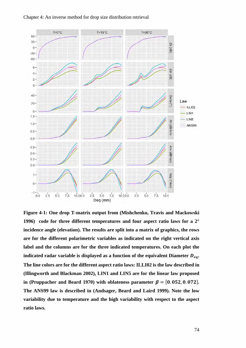
Chapter 4: An inverse method for drop size distribution retrieval
74
Figure 4-1: One drop T-matrix output from (Mishchenko, Travis and Mackowski
1996) code for three different temperatures and four aspect ratio laws for a 2°
incidence angle (elevation). The results are split into a matrix of graphics, the rows
are for the different polarimetric variables as indicated on the right vertical axis
label and the columns are for the three indicated temperatures. On each plot the
indicated radar variable is displayed as a function of the equivalent Diameter 𝑫𝑫𝒆𝒆𝒆𝒆.
The line colors are for the different aspect ratio laws: ILLI02 is the law described in
(Illingworth and Blackman 2002), LIN1 and LIN5 are for the linear law proposed
in (Pruppacher and Beard 1970) with oblateness parameter 𝜷𝜷 = [𝟎𝟎.𝟎𝟎𝟎𝟎𝟎𝟎,𝟎𝟎.𝟎𝟎𝟎𝟎𝟎𝟎].
The ANS99 law is described in (Andsager, Beard and Laird 1999). Note the low
variability due to temperature and the high variability with respect to the aspect
ratio laws.
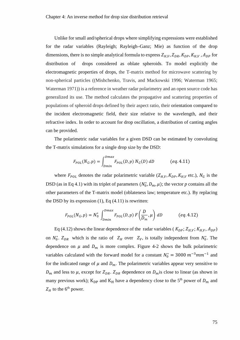
Chapter 4: An inverse method for drop size distribution retrieval
75
Unlike for small and/spherical drops where simplifying expressions were established
for the radar variables (Rayleigh; Rayleigh–Ganz; Mie) as function of the drop
dimensions, there is no simple analytical formula to express 𝑍𝑍𝐻𝐻,𝑉𝑉,𝑍𝑍𝐷𝐷𝐷𝐷 ,𝐾𝐾𝐷𝐷𝐷𝐷 ,𝐾𝐾𝐻𝐻,𝑉𝑉 ,𝐴𝐴𝐷𝐷𝐷𝐷 for
distribution of drops considered as oblate spheroids. To model explicitly the
electromagnetic properties of drops, the T-matrix method for microwave scattering by
non-spherical particles ((Mishchenko, Travis, and Mackowski 1996; Waterman 1965;
Waterman 1971)) is a reference in weather radar polarimetry and an open source code has
generalized its use. The method calculates the propagative and scattering properties of
populations of spheroid drops defined by their aspect ratio, their orientation compared to
the incident electromagnetic field, their size relative to the wavelength, and their
refractive index. In order to account for drop oscillation, a distribution of canting angles
can be provided.
The polarimetric radar variables for a given DSD can be estimated by convoluting
the T-matrix simulations for a single drop size by the DSD:
𝐹𝐹𝐷𝐷𝑃𝑃𝐿𝐿(𝑁𝑁𝐺𝐺,𝑒𝑒) = � 𝐹𝐹𝐷𝐷𝑃𝑃𝐿𝐿(𝐷𝐷,𝑒𝑒) 𝑁𝑁𝐺𝐺(𝐷𝐷) 𝑑𝑑𝐷𝐷𝐷𝐷𝑚𝑚𝑎𝑎𝑒𝑒
𝐷𝐷𝑚𝑚𝑖𝑖𝑛𝑛 (𝑃𝑃𝑒𝑒. 4.11)
where 𝐹𝐹𝐷𝐷𝑃𝑃𝐿𝐿 denotes the radar polarimetric variable (𝑍𝑍𝐻𝐻,𝑉𝑉,𝐾𝐾𝐷𝐷𝐷𝐷,𝐾𝐾𝐻𝐻,𝑉𝑉 etc.), 𝑁𝑁𝐺𝐺 is the
DSD (as in Eq 4.1) with its triplet of parameters (𝑁𝑁0∗,𝐷𝐷𝑚𝑚, 𝜇𝜇); the vector p contains all the
other parameters of the T-matrix model (oblateness law; temperature etc.). By replacing
the DSD by its expression (1), Eq (4.11) is rewritten:
𝐹𝐹𝐷𝐷𝑃𝑃𝐿𝐿(𝑁𝑁𝐺𝐺,𝑒𝑒) = 𝑁𝑁0∗ � 𝐹𝐹𝐷𝐷𝑃𝑃𝐿𝐿(𝐷𝐷,𝑒𝑒) 𝐹𝐹�
𝐷𝐷𝐷𝐷𝑐𝑐
,𝜇𝜇� 𝑑𝑑𝐷𝐷𝐷𝐷𝑚𝑚𝑎𝑎𝑒𝑒
𝐷𝐷𝑚𝑚𝑖𝑖𝑛𝑛 (𝑃𝑃𝑒𝑒. 4.12)
Eq (4.12) shows the linear dependence of the radar variables ( 𝐾𝐾𝐷𝐷𝐷𝐷; 𝑍𝑍𝐻𝐻,𝑉𝑉; 𝐾𝐾𝐻𝐻,𝑉𝑉, 𝐴𝐴𝐷𝐷𝐷𝐷)
on 𝑁𝑁0∗. 𝑍𝑍𝐷𝐷𝐷𝐷 which is the ratio of 𝑍𝑍𝐻𝐻 over 𝑍𝑍𝑉𝑉, is totally independent from 𝑁𝑁0∗. The
dependence on 𝜇𝜇 and 𝐷𝐷𝑚𝑚 is more complex. Figure 4-2 shows the bulk polarimetric
variables calculated with the forward model for a constant 𝑁𝑁0∗ = 3000 𝑐𝑐−3𝑐𝑐𝑐𝑐−1 and
for the indicated range of 𝜇𝜇 and 𝐷𝐷𝑚𝑚. The polarimetric variables appear very sensitive to
𝐷𝐷𝑚𝑚 and less to 𝜇𝜇, except for 𝑍𝑍𝐷𝐷𝐷𝐷. 𝑍𝑍𝐷𝐷𝐷𝐷 dependence on 𝐷𝐷𝑚𝑚is close to linear (as shown in
many previous work); KDP and KH have a dependency close to the 5th power of 𝐷𝐷𝑚𝑚 and
𝑍𝑍𝐻𝐻 to the 6th power.
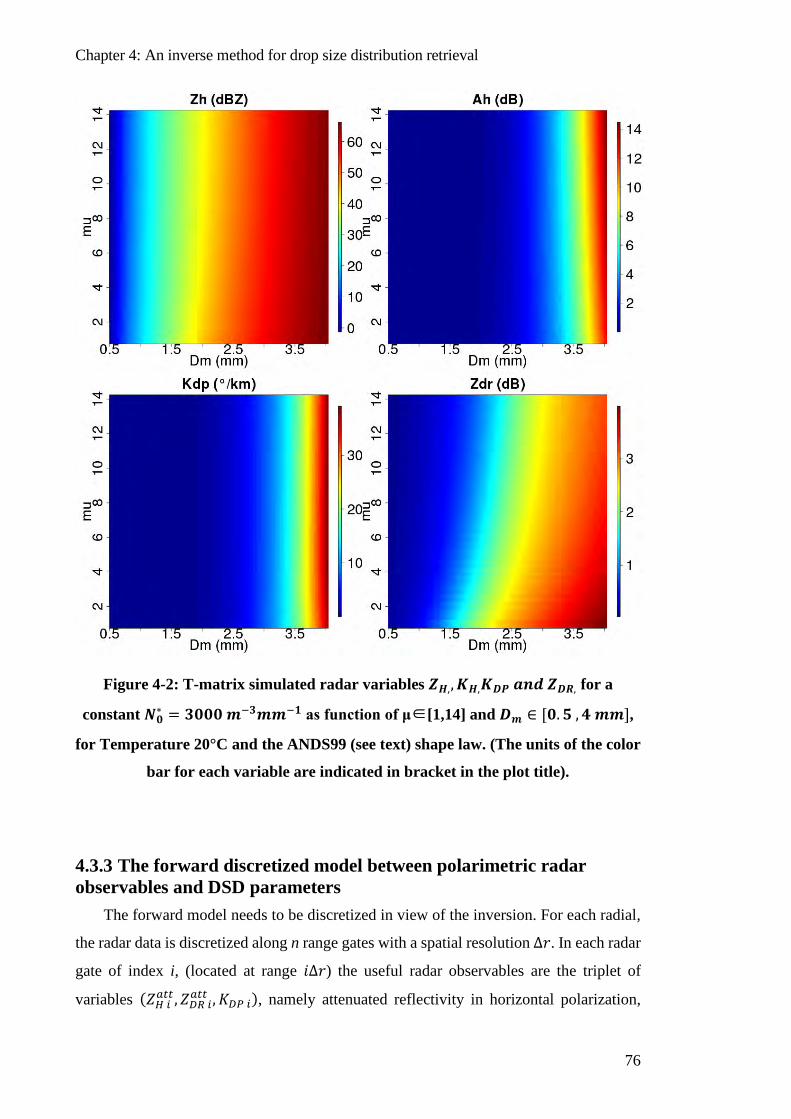
Chapter 4: An inverse method for drop size distribution retrieval
76
Figure 4-2: T-matrix simulated radar variables 𝒁𝒁𝑯𝑯,,𝑲𝑲𝑯𝑯,𝑲𝑲𝑫𝑫𝑫𝑫 𝒂𝒂𝒂𝒂𝒂𝒂 𝒁𝒁𝑫𝑫𝑫𝑫, for a
constant 𝑵𝑵𝟎𝟎∗ = 𝟑𝟑𝟎𝟎𝟎𝟎𝟎𝟎 𝒎𝒎−𝟑𝟑𝒎𝒎𝒎𝒎−𝟏𝟏 as function of μ∈[1,14] and 𝑫𝑫𝒎𝒎 ∈ [𝟎𝟎.𝟎𝟎 ,𝟒𝟒 𝒎𝒎𝒎𝒎],
for Temperature 20°C and the ANDS99 (see text) shape law. (The units of the color
bar for each variable are indicated in bracket in the plot title).
4.3.3 The forward discretized model between polarimetric radar observables and DSD parameters
The forward model needs to be discretized in view of the inversion. For each radial,
the radar data is discretized along n range gates with a spatial resolution Δ𝑟𝑟. In each radar
gate of index i, (located at range 𝑖𝑖Δ𝑟𝑟) the useful radar observables are the triplet of
variables (𝑍𝑍𝐻𝐻 𝑖𝑖𝑎𝑎𝑡𝑡𝑡𝑡 ,𝑍𝑍𝐷𝐷𝐷𝐷 𝑖𝑖
𝑎𝑎𝑡𝑡𝑡𝑡 ,𝐾𝐾𝐷𝐷𝐷𝐷 𝑖𝑖), namely attenuated reflectivity in horizontal polarization,
Chapter 4: An inverse method for drop size distribution retrieval
77
attenuated differential reflectivity, and specific differential phase. In addition, the phase
shift Φ𝐷𝐷𝐷𝐷 𝑛𝑛 at the last gate of the radar radial is also taken as an additional constraint to
identify the DSD parameters along the radial. The rain DSD in each radar gate is defined
by a triplet of parameters 𝑋𝑋𝐺𝐺𝑖𝑖 = (𝑁𝑁0 𝑖𝑖∗ ,𝐷𝐷𝑚𝑚 𝑖𝑖, 𝜇𝜇𝑖𝑖). The objective of the inversion in section
4 is to retrieve these 𝑋𝑋𝐺𝐺𝑖𝑖 .
Following Eq (4.11), the system of equations at each gate can be written:
𝑍𝑍𝐻𝐻 𝑖𝑖𝑎𝑎𝑡𝑡𝑡𝑡 = 𝑍𝑍 (𝑁𝑁𝐺𝐺 𝑖𝑖) − 2 Δ𝑟𝑟 ∑ 𝐾𝐾𝐻𝐻 (𝑁𝑁𝐺𝐺 𝑘𝑘) 𝑘𝑘=𝑖𝑖
𝑘𝑘=1 (𝑃𝑃𝑒𝑒. 4.13)
𝑍𝑍𝐷𝐷𝐷𝐷 𝑖𝑖𝑎𝑎𝑡𝑡𝑡𝑡 = 𝑍𝑍𝐷𝐷𝐷𝐷 (𝑁𝑁𝐺𝐺 𝑖𝑖) − 2 Δ𝑟𝑟 ∑ 𝐴𝐴𝐷𝐷𝐷𝐷(𝑁𝑁𝐺𝐺 𝑘𝑘) 𝑘𝑘=𝑖𝑖
𝑘𝑘=1 (𝑃𝑃𝑒𝑒. 4.14)
𝐾𝐾𝐷𝐷𝐷𝐷 𝑖𝑖 = 𝐾𝐾𝐷𝐷𝐷𝐷(𝑁𝑁𝐺𝐺 𝑖𝑖) (𝑃𝑃𝑒𝑒. 4.15)
And in addition for 𝑖𝑖 = 𝑙𝑙
Φ𝐷𝐷𝐷𝐷 𝑛𝑛 = 2 Δ𝑟𝑟 �∑ 𝐾𝐾𝐷𝐷𝐷𝐷 𝑘𝑘𝑘𝑘=𝑛𝑛𝑘𝑘=1 − Φ𝐷𝐷𝐷𝐷 1� (𝑃𝑃𝑒𝑒. 4.16)
Equations (4.13) and (4.14) are expressed in dBZ. Note that Eq (4.16) is an
approximation and does not account for the backscattering phase 𝛿𝛿𝐷𝐷𝐷𝐷 at gate 1 and n;
however the Φ𝐷𝐷𝐷𝐷 filtering (see section 2) reduces the impact of 𝛿𝛿𝐷𝐷𝐷𝐷 and our previous
work ((Koffi et al. 2014; Gosset, Zahiri, and Moumouni 2010b)) showed that the actual
effect of 𝛿𝛿𝐷𝐷𝐷𝐷 is low.
The vector regrouping the attenuated reflectivity, attenuated differential reflectivity,
specific differential phase in the n successive gates and the total differential phase shift at
gate n, for a radar radial is denoted 𝒀𝒀 = �Zh att, Zdr
att, Kdp ,ΦDP n�. The vector regrouping
the parameters of the gamma DSD in the n successive gates of the same radar radial is
denoted 𝑿𝑿 = [𝑵𝑵𝟎𝟎 ∗ ,𝑫𝑫𝒎𝒎 ,𝝁𝝁] , 𝑵𝑵𝟎𝟎
∗ ,𝑫𝑫𝒎𝒎 ,𝝁𝝁 being the vectors regrouping each parameter in
the n successive gates of this radial. The vector 𝒀𝒀 has a length of [3𝑙𝑙 + 1] and the vector
𝑿𝑿 has a length of [3𝑙𝑙].
The relationships between polarimetric radar observables and DSD parameters along
a radar radial are regrouped in the non-linear model m based on Equations 4.11 to 4.16:
𝒀𝒀 = 𝒎𝒎(𝑿𝑿) (𝑃𝑃𝑒𝑒. 4.17)
The objective of the inversion is to retrieve the vector 𝑿𝑿 that best explains the radar
observables 𝒀𝒀 measured along each radar radial. The next section explains the method
used to reach this objective.

Chapter 4: An inverse method for drop size distribution retrieval
78
4.4 The inverse problem to retrieve DSD from observations
4.4.1 Inverse modeling framework The retrieval of the DSD triplets all along the radial based on the system of equations
(4.17) is a typical inverse problem. The proposed approach is to solve this problem within
the framework of inverse theory, as detailed in (Menke 2018) and (Tarantola 2005), with
the algorithm proposed by (Tarantola and Valette 1982). Let us notice that inverse and
variational approaches are close and use similar algorithms. The difference between the
two approaches might be found in the initialization of the parameters to retrieve, called
“a priori information” in the inverse theory.
In the problem to solve (Eq 4.17), the input data are the variables measured by a
polarimetric weather radar regrouped in a vector denoted 𝒀𝒀0. The parameters to retrieve
are the three parameters of the Gamma DSD distributions along a radar radial,
components of the vector 𝑿𝑿𝑮𝑮. The solution minimizes the following expression:
Φ(𝒀𝒀,𝑿𝑿) = [𝒎𝒎(𝑿𝑿) − 𝒀𝒀0]𝑡𝑡 𝑪𝑪𝑌𝑌−1 [𝒎𝒎(𝑿𝑿) − 𝒀𝒀0]
+ �𝑿𝑿 − 𝑿𝑿𝑝𝑝𝑟𝑟𝑖𝑖𝑜𝑜𝑟𝑟�𝑡𝑡 𝑪𝑪𝑋𝑋−1 �𝑿𝑿 − 𝑿𝑿𝑝𝑝𝑟𝑟𝑖𝑖𝑜𝑜𝑟𝑟� (𝑃𝑃𝑒𝑒. 4.18)
Where Φ is the likelihood function, t signifies transpose, 𝒀𝒀0 is the vector of observed
(attenuated) radar data, 𝑿𝑿𝑝𝑝𝑟𝑟𝑖𝑖𝑜𝑜𝑟𝑟is the vector of a priori DSD parameters,𝑪𝑪𝑿𝑿 is the
covariance matrices of residuals between true and a priori values of 𝑿𝑿 and 𝑪𝑪𝒀𝒀 the
covariance matrix of measurement errors.
The statistical distributions of both [𝒀𝒀 − 𝒀𝒀0] and �𝑿𝑿 − 𝑿𝑿𝒑𝒑𝑟𝑟𝑖𝑖𝑜𝑜𝑟𝑟� are assumed to be
unbiased and Gaussian. (Menke 2018) showed that the solution vector 𝑿𝑿′ satisfies:
𝑿𝑿′ = 𝑿𝑿𝒑𝒑𝑟𝑟𝑖𝑖𝑜𝑜𝑟𝑟 + 𝑪𝑪𝑋𝑋 𝑱𝑱𝑡𝑡 [𝑱𝑱𝑡𝑡𝑪𝑪𝑋𝑋𝑱𝑱 + 𝑪𝑪𝑌𝑌]−1�𝒀𝒀0 −𝑐𝑐(𝑿𝑿′) + 𝑱𝑱(𝑿𝑿′ − 𝑿𝑿𝒑𝒑𝑟𝑟𝑖𝑖𝑜𝑜𝑟𝑟)� (𝑃𝑃𝑒𝑒. 4.19)
Where J is the matrix of (first-order) partial derivatives of the model m. If the model
m is nonlinear, (Tarantola 2005) demonstrates that the solution can be obtained by an
algorithm which can be written:
𝑿𝑿𝑘𝑘+1 ≈ 𝑿𝑿𝑘𝑘 + 𝛼𝛼[ 𝑱𝑱𝑘𝑘𝑡𝑡 𝑪𝑪𝑌𝑌−1 𝑱𝑱𝒌𝒌 + 𝑪𝑪𝑋𝑋−1]−1 � 𝑱𝑱𝑘𝑘𝑡𝑡 𝑪𝑪𝑌𝑌−1 ⟨ 𝒀𝒀𝟎𝟎 −𝒎𝒎(𝑿𝑿𝑘𝑘) ⟩
+ 𝑪𝑪𝑋𝑋−1 ⟨𝑿𝑿𝑘𝑘 − 𝑿𝑿𝑝𝑝𝑟𝑟𝑖𝑖𝑜𝑜𝑟𝑟⟩ � (𝑃𝑃𝑒𝑒. 4.20)
In which 𝑿𝑿𝑘𝑘 constitutes the result of the kth iteration, 𝑱𝑱𝒌𝒌 = 𝝏𝝏 𝒎𝒎(𝑿𝑿𝑘𝑘)𝝏𝝏(𝑿𝑿𝑘𝑘) is the Jacobian
matrix of (first order) partial derivatives of the model at point 𝑿𝑿𝑘𝑘. Further information
about the stability, convergence and uniqueness of the solution of such nonlinear
problems can be found in Chapter 9 of (Menke 2018) and in (Tarantola and Valette 1982).
Chapter 4: An inverse method for drop size distribution retrieval
79
The general case of inverse problems involving non-Gaussian statistics has been
addressed by (Tarantola 2005). Additional terms could be added to Φ(𝒀𝒀,𝑿𝑿) in order to
take into account some additional constraints on the parameters. The 𝛼𝛼 parameter in Eq
(4.20) is used to control the convergence of the gradient descend algorithm: for highly
nonlinear problems a low value for 𝛼𝛼 helps avoiding brutal jumps on the descent and
divergence.
According to Eq (4.18), the solution provided by the inverse algorithm results from
a compromise between two extreme states: i) a solution that perfectly fits the observed
data through the theoretical model and ii) a solution remaining very close to the a priori
information on the parameters. This compromise solution depends on the a priori
confidence put on the various terms of the system. If the confidence in the observed data
(as defined by the covariance matrix 𝑪𝑪𝑌𝑌) is weak, the problem is underdetermined and
the a priori information takes a dominant role. If the problem is overdetermined (very
good quality data in sufficient number, or weakly informative a priori values of the
parameters as defined by the covariance matrix 𝑪𝑪𝑋𝑋) then the a priori information plays a
minor role.
The next sections present and discuss the implementation of this inverse algorithm
to retrieve DSD parameters from polarimetric weather radar observables on radar radials.
The principle of the proposed method is: i) start with an a priori DSD based on the
empirical power laws suited to the local climatology (equations 4.5 and 4.6); the DSDs
are retrieved gate by gate, based on attenuation corrected data, and ii) rely on the inverse
method to improve this initial solution and provide a distribution of DSDs along the entire
range which is consistent with the observed radar variables.
The implementation of the inverse algorithm requires the definition of : i) the
vector Y0 of radar data and its covariance matrix CY which characterizes the level of
confidence in the data, ii) the vector Xprior of a priori values of DSD parameters and its
covariance matrix CX which contain the initial guess of the parameters and the error
covariance assumption, iii) the applications conditions of the algorithm.
4.4.2 The vector 𝒀𝒀𝟎𝟎 of radar data and its covariance matrix 𝑪𝑪𝒀𝒀 The covariance matrix of measurement errors 𝑪𝑪𝒀𝒀 is assumed fully diagonal, which
means that the measurement error of each radar observable is independent from the
measurement error of the same variable measured at a different radar bin, and independent
from the other radar observables, including at the same location. The diagonal of the
Chapter 4: An inverse method for drop size distribution retrieval
80
matrix CY can be written 𝑑𝑑𝑖𝑖𝑎𝑎𝑙𝑙 𝑪𝑪𝒀𝒀 = �𝝈𝝈𝑍𝑍𝐻𝐻2 ,𝝈𝝈𝑍𝑍𝐷𝐷𝐷𝐷2 ,𝝈𝝈𝐾𝐾𝐷𝐷𝐷𝐷2 ,𝜎𝜎Φdpn2 �. Where 𝝈𝝈𝒁𝒁𝑯𝑯𝟎𝟎 ,𝝈𝝈𝑍𝑍𝐷𝐷𝐷𝐷2 ,𝝈𝝈𝐾𝐾𝐷𝐷𝐷𝐷2
are vectors, and their components are the variances of measurement error of the
(attenuated) reflectivity 𝑍𝑍𝐻𝐻𝑎𝑎𝑡𝑡𝑡𝑡, the (attenuated) differential reflectivity 𝑍𝑍𝐷𝐷𝐷𝐷𝑎𝑎𝑡𝑡𝑡𝑡and the
differential phase shift 𝐾𝐾𝐷𝐷𝐷𝐷. 𝜎𝜎Φdpn2 is the variance of measurement error of the phase shift
at gate 𝑙𝑙.
The variance of measurement errors associated with 𝑍𝑍𝐻𝐻𝑎𝑎𝑡𝑡𝑡𝑡and 𝑍𝑍𝐷𝐷𝐷𝐷𝑎𝑎𝑡𝑡𝑡𝑡 can be estimated
on the base of the fluctuations of the measured reflectivities. The error on 𝐾𝐾𝐷𝐷𝐷𝐷 is quite
high due to the noisy nature of 𝛷𝛷𝐷𝐷𝐷𝐷 and its derivative. After some sensitivity analysis we
have adopted the following constant values (for all radar gates) : 𝜎𝜎 𝑍𝑍𝐻𝐻 = 3 𝑑𝑑𝑑𝑑𝑍𝑍, 𝜎𝜎 𝑍𝑍𝐷𝐷𝐷𝐷 =
0.5 𝑑𝑑𝑑𝑑, 𝜎𝜎K𝐷𝐷𝐷𝐷 = 1 𝑑𝑑𝑃𝑃𝑙𝑙/𝑘𝑘𝑐𝑐 and 𝜎𝜎Φ𝐷𝐷𝐷𝐷 𝑛𝑛 = 2 𝑑𝑑𝑃𝑃𝑙𝑙.
4.4.3 A priori information: DSD parameters and associated covariance matrix
The a priori value of the parameters 𝑿𝑿𝑝𝑝𝑟𝑟𝑖𝑖𝑜𝑜𝑟𝑟 is derived from the polarimetric radar
observables, thanks to the relationships proposed by (Koffi et al. 2014) and detailed in
Section 2.3 (Eq. 4.5 and 4.6). The radar measurement of reflectivity and differential
reflectivity which are used for that purpose must first be corrected from attenuation. The
self-consistency correction method proposed by (Bringi, Keenan, and Chandrasekar
2001) is used to estimate the attenuation at any gate of the radar radial and to correct
observed values of 𝑍𝑍𝐻𝐻 and 𝑍𝑍𝐷𝐷𝐷𝐷 for attenuation. Then the a priori values of 𝑵𝑵𝟎𝟎 ∗ and 𝑫𝑫𝒎𝒎 are
provided by the Eq (4.5) and (4.6). The attenuation correction is only used to derive the
a priori vector. Then the inversion is applied on 𝑍𝑍𝐻𝐻𝑎𝑎𝑡𝑡𝑡𝑡and 𝑍𝑍𝐷𝐷𝐷𝐷𝑎𝑎𝑡𝑡𝑡𝑡 , and accounts for the
attenuation explicitly (see the Jacobian calculation in Appendix A).
The a priori value of 𝜇𝜇 is more difficult to set as the bulk radar variables do not carry
any information about the shape of the DSD. The choice of the a priori value of 𝜇𝜇 is based
on (Moumouni, Gosset, and Houngninou 2008) who showed by fitting gamma laws on
observed DSD of the same dataset, that convective precipitation tends to have higher
values of 𝜇𝜇 than stratiform precipitation. They showed that the values of 𝜇𝜇 fall in the
interval 𝜇𝜇 ∈ [0.5,12]. We choose to set a constant a priori value of 𝜇𝜇 = 2 for all the radar
gates as the stratiform rainfall is more frequent in the radar PPIs.
𝜇𝜇𝑖𝑖𝑝𝑝𝑟𝑟𝑖𝑖𝑜𝑜𝑟𝑟 = 2.0 (𝑃𝑃𝑒𝑒. 4.21)
The covariance matrix of parameters stands for the errors between the a priori values
of parameters and the true values. We assume that the covariance between the variables
Chapter 4: An inverse method for drop size distribution retrieval
81
𝑁𝑁0 ∗ ,𝐷𝐷𝑚𝑚 , 𝜇𝜇 is equal to 0.0, which is consistent with previous findings on the property of
normalized DSD. We also decided not to impose any covariance between these variables
to avoid over-constraining the algorithm.
For each radial the matrix 𝑪𝑪𝑋𝑋 is then a “block-diagonal” matrix of size [3𝑙𝑙 × 3𝑙𝑙]
composed by three sub-matrixes:
𝑪𝑪𝑋𝑋 = �𝛽𝛽𝑵𝑵𝟎𝟎
∗
𝛽𝛽𝑫𝑫𝒎𝒎
𝛽𝛽𝝁𝝁� 𝑤𝑤𝑖𝑖𝑤𝑤ℎ 𝛽𝛽𝑝𝑝𝑎𝑎𝑟𝑟
𝑖𝑖𝑖𝑖 = 𝜎𝜎𝑝𝑝𝑎𝑎𝑟𝑟2 𝑃𝑃𝑒𝑒𝑒𝑒�−𝑑𝑑𝑖𝑖𝑖𝑖𝑑𝑑𝑐𝑐𝑜𝑜𝑟𝑟𝑟𝑟
� (𝑃𝑃𝑒𝑒. 4.22)
Where 𝜎𝜎𝑝𝑝𝑎𝑎𝑟𝑟2 is the estimated a priori variance of the parameter par, that is 𝑁𝑁0 ∗ ,𝐷𝐷𝑚𝑚 , 𝜇𝜇
and 𝑑𝑑𝑖𝑖𝑖𝑖the distance between the gates i and j of a radial. For this work, 𝑑𝑑𝑐𝑐𝑜𝑜𝑟𝑟𝑟𝑟 = 3 𝑘𝑘𝑐𝑐 has
been adopted which is consistent with the spatial correlation of the DSD parameters in
the study region.
The standard-deviation on parameters is defined as a fraction of its a priori value and
expressed:
𝜎𝜎𝑫𝑫𝒎𝒎 = 𝜀𝜀 𝐷𝐷𝑚𝑚𝑝𝑝𝑟𝑟𝑖𝑖𝑜𝑜𝑟𝑟, 𝜎𝜎𝑵𝑵𝟎𝟎
∗ = 𝜀𝜀 𝑁𝑁0∗𝑝𝑝𝑟𝑟𝑖𝑖𝑜𝑜𝑟𝑟 and 𝜎𝜎𝝁𝝁 = 𝜀𝜀 𝜇𝜇𝑝𝑝𝑟𝑟𝑖𝑖𝑜𝑜𝑟𝑟 (𝑃𝑃𝑒𝑒. 4.23)
We set the value of the coefficient 𝜀𝜀 = 0.5 - or in other words, a relative uncertainty
of 50% for all three parameters- by testing the convergence speed of the algorithm.
4.4.4 Application conditions The calculation of the Jacobian matrix of the partial derivatives of the radar
observables 𝑌𝑌 with respect to the parameters on vector 𝑋𝑋 is detailed in the Appendix A.
As in Figure 1 and 2, the calculation of the radar variables as a function of raindrop size
and shapes is based on T-matrix modeling with the (Andsager, Beard, and Laird 1999)
ratio law (Eq 4.10), and a temperature equal to 20°C (compatible with observations in
Africa). The convergence parameter α in the algorithm (Eq (4.20)) is set to α =0.1, in
order to insure a careful convergence of the algorithm. At each iteration of the algorithm
described in Equation (4.23), the convergence is evaluated through the normalized root
mean square error (𝑁𝑁𝑅𝑅𝑀𝑀𝑆𝑆𝐸𝐸) between the retrieved (𝑌𝑌𝑛𝑛) and observed ( 𝒀𝒀0) attenuated
polarimetric variables [𝑍𝑍𝐷𝐷𝐷𝐷; 𝑍𝑍𝐻𝐻; 𝐾𝐾𝐷𝐷𝐷𝐷]. This variable is written: 𝑁𝑁𝑅𝑅𝑀𝑀𝑆𝑆𝐸𝐸 =
𝑁𝑁𝑅𝑅𝑀𝑀𝑆𝑆𝐸𝐸𝑍𝑍𝐷𝐷𝐷𝐷 + 𝑁𝑁𝑅𝑅𝑀𝑀𝑆𝑆𝐸𝐸𝑍𝑍𝐻𝐻 + 𝑁𝑁𝑅𝑅𝑀𝑀𝑆𝑆𝐸𝐸K𝐷𝐷𝐷𝐷. The condition fixed to stop the algorithm is
𝑁𝑁𝑅𝑅𝑀𝑀𝑆𝑆𝐸𝐸 < 0.25. A value of NRMSE of 0.25 is equivalent to a mean residual variance of
8% between each retrieved and observed polar variables. Typically, a stable solution is
reached after 4-5 iterations, the maximum number of iterations we experienced being 20.

Chapter 4: An inverse method for drop size distribution retrieval
82
4.5 Results
4.5.1 Retrieved DSD, sensitivity to model parameters and gain from the a priori solution
Figure 4-3 illustrates the retrieval along a given radial, extracted from the 2006 July
28th case study (Azimuth 251°; 7h58 UTC; 2.8° elevation PPI). The observed system is
typical of African squall lines and 𝐾𝐾𝐷𝐷𝐷𝐷 shows two peaks of convective rainfall at 42km
and 53km range, and stratiform rainfall at 30-40 km, while the system is moving away
from the radar (Westwards). The left column shows 4 radar variables along the radial: the
attenuated 𝑍𝑍𝐻𝐻, the attenuated 𝑍𝑍𝐷𝐷𝐷𝐷, the differential phase shift 𝛷𝛷𝐷𝐷𝐷𝐷 and the specific
differential phase shift 𝐾𝐾𝐷𝐷𝐷𝐷. On each plot the observed variables (in black) are displayed
together with the radar variables simulated (attenuation included) from the a priori DSD
(blue) and from the inverse model framework (red). On the right column the 3 retrieved
DSD parameters 𝑁𝑁0 ∗ ,𝐷𝐷𝑚𝑚 , 𝜇𝜇 (red) are compared with the a priori solution (blue).
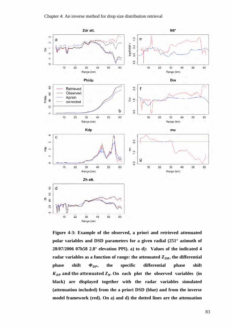
Chapter 4: An inverse method for drop size distribution retrieval
83
Figure 4-3: Example of the observed, a priori and retrieved attenuated
polar variables and DSD parameters for a given radial (251° azimuth of
28/07/2006 07h58 2.8° elevation PPI). a) to d): Values of the indicated 4
radar variables as a function of range: the attenuated 𝒁𝒁𝑫𝑫𝑫𝑫, the differential
phase shift 𝜱𝜱𝑫𝑫𝑫𝑫, the specific differential phase shift
𝑲𝑲𝑫𝑫𝑫𝑫 𝐚𝐚𝐚𝐚𝐚𝐚 𝐭𝐭𝐭𝐭𝐭𝐭 𝐚𝐚𝐭𝐭𝐭𝐭𝐭𝐭𝐚𝐚𝐚𝐚𝐚𝐚𝐭𝐭𝐭𝐭𝐚𝐚 𝒁𝒁𝑯𝑯. On each plot the observed variables (in
black) are displayed together with the radar variables simulated
(attenuation included) from the a priori DSD (blue) and from the inverse
model framework (red). On a) and d) the dotted lines are the attenuation
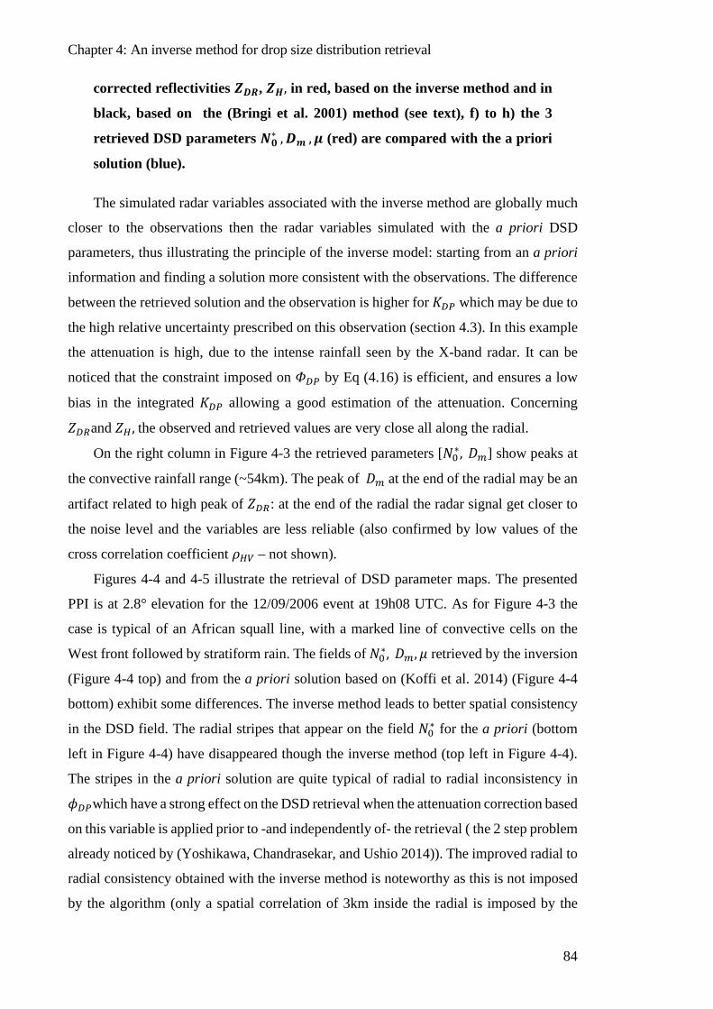
Chapter 4: An inverse method for drop size distribution retrieval
84
corrected reflectivities 𝒁𝒁𝑫𝑫𝑫𝑫, 𝒁𝒁𝑯𝑯, in red, based on the inverse method and in
black, based on the (Bringi et al. 2001) method (see text), f) to h) the 3
retrieved DSD parameters 𝑵𝑵𝟎𝟎 ∗ ,𝑫𝑫𝒎𝒎 ,𝝁𝝁 (red) are compared with the a priori
solution (blue).
The simulated radar variables associated with the inverse method are globally much
closer to the observations then the radar variables simulated with the a priori DSD
parameters, thus illustrating the principle of the inverse model: starting from an a priori
information and finding a solution more consistent with the observations. The difference
between the retrieved solution and the observation is higher for 𝐾𝐾𝐷𝐷𝐷𝐷 which may be due to
the high relative uncertainty prescribed on this observation (section 4.3). In this example
the attenuation is high, due to the intense rainfall seen by the X-band radar. It can be
noticed that the constraint imposed on 𝛷𝛷𝐷𝐷𝐷𝐷 by Eq (4.16) is efficient, and ensures a low
bias in the integrated 𝐾𝐾𝐷𝐷𝐷𝐷 allowing a good estimation of the attenuation. Concerning
𝑍𝑍𝐷𝐷𝐷𝐷and 𝑍𝑍𝐻𝐻 , the observed and retrieved values are very close all along the radial.
On the right column in Figure 4-3 the retrieved parameters [𝑁𝑁0∗, 𝐷𝐷𝑚𝑚] show peaks at
the convective rainfall range (~54km). The peak of 𝐷𝐷𝑚𝑚 at the end of the radial may be an
artifact related to high peak of 𝑍𝑍𝐷𝐷𝐷𝐷: at the end of the radial the radar signal get closer to
the noise level and the variables are less reliable (also confirmed by low values of the
cross correlation coefficient 𝜌𝜌𝐻𝐻𝑉𝑉 – not shown).
Figures 4-4 and 4-5 illustrate the retrieval of DSD parameter maps. The presented
PPI is at 2.8° elevation for the 12/09/2006 event at 19h08 UTC. As for Figure 4-3 the
case is typical of an African squall line, with a marked line of convective cells on the
West front followed by stratiform rain. The fields of 𝑁𝑁0∗, 𝐷𝐷𝑚𝑚, 𝜇𝜇 retrieved by the inversion
(Figure 4-4 top) and from the a priori solution based on (Koffi et al. 2014) (Figure 4-4
bottom) exhibit some differences. The inverse method leads to better spatial consistency
in the DSD field. The radial stripes that appear on the field 𝑁𝑁0∗ for the a priori (bottom
left in Figure 4-4) have disappeared though the inverse method (top left in Figure 4-4).
The stripes in the a priori solution are quite typical of radial to radial inconsistency in
𝜙𝜙𝐷𝐷𝐷𝐷which have a strong effect on the DSD retrieval when the attenuation correction based
on this variable is applied prior to -and independently of- the retrieval ( the 2 step problem
already noticed by (Yoshikawa, Chandrasekar, and Ushio 2014)). The improved radial to
radial consistency obtained with the inverse method is noteworthy as this is not imposed
by the algorithm (only a spatial correlation of 3km inside the radial is imposed by the
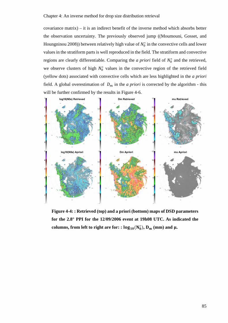
Chapter 4: An inverse method for drop size distribution retrieval
85
covariance matrix) – it is an indirect benefit of the inverse method which absorbs better
the observation uncertainty. The previously observed jump ((Moumouni, Gosset, and
Houngninou 2008)) between relatively high value of 𝑁𝑁0∗ in the convective cells and lower
values in the stratiform parts is well reproduced in the field. The stratiform and convective
regions are clearly differentiable. Comparing the a priori field of 𝑁𝑁0∗ and the retrieved,
we observe clusters of high 𝑁𝑁0∗ values in the convective region of the retrieved field
(yellow dots) associated with convective cells which are less highlighted in the a priori
field. A global overestimation of 𝐷𝐷𝑚𝑚 in the a priori is corrected by the algorithm - this
will be further confirmed by the results in Figure 4-6.
Figure 4-4: : Retrieved (top) and a priori (bottom) maps of DSD parameters
for the 2.8° PPI for the 12/09/2006 event at 19h08 UTC. As indicated the
columns, from left to right are for: : 𝐥𝐥𝐥𝐥𝐥𝐥𝟏𝟏𝟎𝟎(𝐍𝐍𝟎𝟎∗), 𝐃𝐃𝐦𝐦 (mm) and 𝛍𝛍.
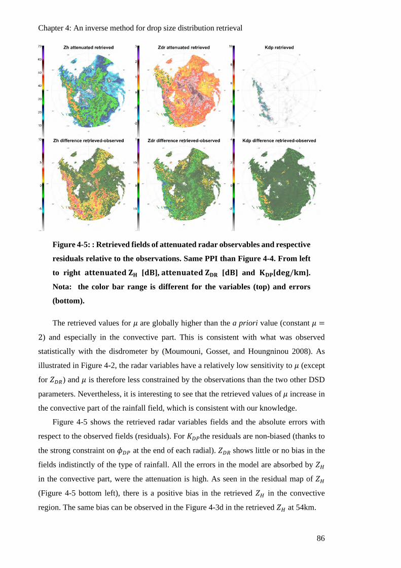
Chapter 4: An inverse method for drop size distribution retrieval
86
Figure 4-5: : Retrieved fields of attenuated radar observables and respective
residuals relative to the observations. Same PPI than Figure 4-4. From left
to right 𝐚𝐚𝐭𝐭𝐭𝐭𝐭𝐭𝐚𝐚𝐚𝐚𝐚𝐚𝐭𝐭𝐭𝐭𝐚𝐚 𝐙𝐙𝐇𝐇 [𝐚𝐚𝐝𝐝], 𝐚𝐚𝐭𝐭𝐭𝐭𝐭𝐭𝐚𝐚𝐚𝐚𝐚𝐚𝐭𝐭𝐭𝐭𝐚𝐚 𝐙𝐙𝐃𝐃𝐃𝐃 [𝐚𝐚𝐝𝐝] and 𝐊𝐊𝐃𝐃𝐃𝐃[𝐚𝐚𝐭𝐭𝐥𝐥/𝐤𝐤𝐦𝐦].
Nota: the color bar range is different for the variables (top) and errors
(bottom).
The retrieved values for 𝜇𝜇 are globally higher than the a priori value (constant 𝜇𝜇 =
2) and especially in the convective part. This is consistent with what was observed
statistically with the disdrometer by (Moumouni, Gosset, and Houngninou 2008). As
illustrated in Figure 4-2, the radar variables have a relatively low sensitivity to 𝜇𝜇 (except
for 𝑍𝑍𝐷𝐷𝐷𝐷) and 𝜇𝜇 is therefore less constrained by the observations than the two other DSD
parameters. Nevertheless, it is interesting to see that the retrieved values of 𝜇𝜇 increase in
the convective part of the rainfall field, which is consistent with our knowledge.
Figure 4-5 shows the retrieved radar variables fields and the absolute errors with
respect to the observed fields (residuals). For 𝐾𝐾𝐷𝐷𝐷𝐷the residuals are non-biased (thanks to
the strong constraint on 𝜙𝜙𝐷𝐷𝐷𝐷 at the end of each radial). 𝑍𝑍𝐷𝐷𝐷𝐷 shows little or no bias in the
fields indistinctly of the type of rainfall. All the errors in the model are absorbed by 𝑍𝑍𝐻𝐻
in the convective part, were the attenuation is high. As seen in the residual map of 𝑍𝑍𝐻𝐻
(Figure 4-5 bottom left), there is a positive bias in the retrieved 𝑍𝑍𝐻𝐻 in the convective
region. The same bias can be observed in the Figure 4-3d in the retrieved 𝑍𝑍𝐻𝐻 at 54km.
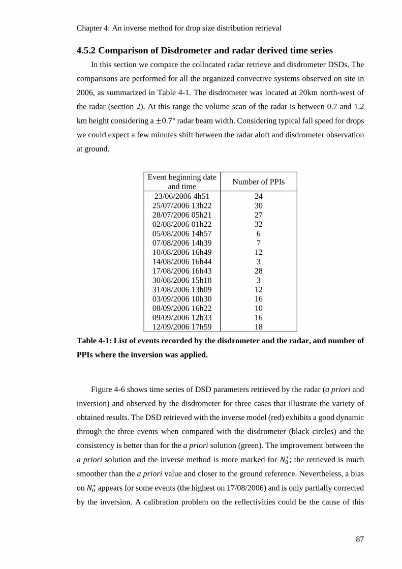
Chapter 4: An inverse method for drop size distribution retrieval
87
4.5.2 Comparison of Disdrometer and radar derived time series In this section we compare the collocated radar retrieve and disdrometer DSDs. The
comparisons are performed for all the organized convective systems observed on site in
2006, as summarized in Table 4-1. The disdrometer was located at 20km north-west of
the radar (section 2). At this range the volume scan of the radar is between 0.7 and 1.2
km height considering a ±0.7° radar beam width. Considering typical fall speed for drops
we could expect a few minutes shift between the radar aloft and disdrometer observation
at ground.
Event beginning date and time Number of PPIs
23/06/2006 4h51 25/07/2006 13h22 28/07/2006 05h21 02/08/2006 01h22 05/08/2006 14h57 07/08/2006 14h39 10/08/2006 16h49 14/08/2006 16h44 17/08/2006 16h43 30/08/2006 15h18 31/08/2006 13h09 03/09/2006 10h30 08/09/2006 16h22 09/09/2006 12h33 12/09/2006 17h59
24 30 27 32 6 7 12 3 28 3 12 16 10 16 18
Table 4-1: List of events recorded by the disdrometer and the radar, and number of
PPIs where the inversion was applied.
Figure 4-6 shows time series of DSD parameters retrieved by the radar (a priori and
inversion) and observed by the disdrometer for three cases that illustrate the variety of
obtained results. The DSD retrieved with the inverse model (red) exhibits a good dynamic
through the three events when compared with the disdrometer (black circles) and the
consistency is better than for the a priori solution (green). The improvement between the
a priori solution and the inverse method is more marked for 𝑁𝑁0∗; the retrieved is much
smoother than the a priori value and closer to the ground reference. Nevertheless, a bias
on 𝑁𝑁0∗ appears for some events (the highest on 17/08/2006) and is only partially corrected
by the inversion. A calibration problem on the reflectivities could be the cause of this
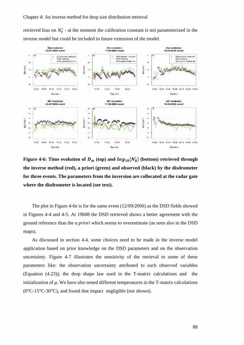
Chapter 4: An inverse method for drop size distribution retrieval
88
retrieved bias on 𝑁𝑁0∗ - at the moment the calibration constant is not parameterized in the
inverse model but could be included in future extension of the model.
Figure 4-6: Time evolution of 𝑫𝑫𝒎𝒎 (top) and 𝒍𝒍𝒍𝒍𝒍𝒍𝟏𝟏𝟎𝟎[𝑵𝑵𝟎𝟎∗ ] (bottom) retrieved through
the inverse method (red), a priori (green) and observed (black) by the disdrometer
for three events. The parameters from the inversion are collocated at the radar gate
where the disdrometer is located (see text).
The plot in Figure 4-6e is for the same event (12/09/2006) as the DSD fields showed
in Figures 4-4 and 4-5. At 19h08 the DSD retrieved shows a better agreement with the
ground reference than the a priori which seems to overestimate (as seen also in the DSD
maps).
As discussed in section 4.4, some choices need to be made in the inverse model
application based on prior knowledge on the DSD parameters and on the observation
uncertainty. Figure 4-7 illustrates the sensitivity of the retrieval to some of these
parameters like: the observation uncertainty attributed to each observed variables
(Equation (4.23)); the drop shape law used in the T-matrix calculations and the
initialization of 𝜇𝜇. We have also tested different temperatures in the T-matrix calculations
(0°C-15°C-30°C), and found that impact negligible (not shown).
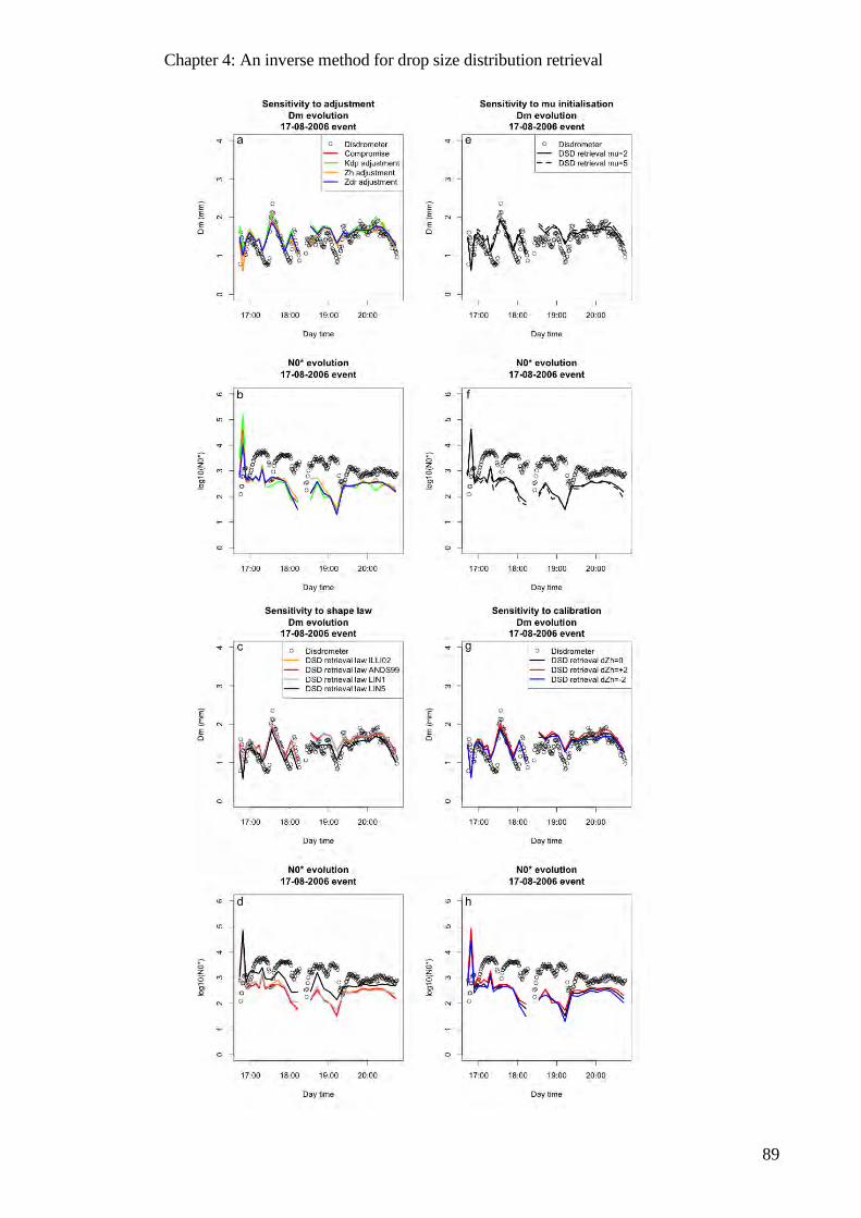
Chapter 4: An inverse method for drop size distribution retrieval
89

Chapter 4: An inverse method for drop size distribution retrieval
90
Figure 4-7: Sensitivity of the retrieved 𝐃𝐃𝐦𝐦 (top) and 𝐥𝐥𝐥𝐥𝐥𝐥𝟏𝟏𝟎𝟎[𝐍𝐍𝟎𝟎∗] (bottom) on the 17-
08-2006 event to several parameters of the inverse model :a-b) sensitivity to the
relative observation errors : red, the default parameters as in section 4.2; green,
reduced error and therefore more weight on KDP; orange, more weight on ZH; blue,
more weight on ZDR. c-d) sensitivity to the aspect ratio law (as indicated on color
legend). e-f) sensitivity to 𝛍𝛍 initial value. g-h) sensitivity to a calibration of error of
+/- 2dBZ on ZH. As in Figure 6 the retrieval is compared with the disdrometer data
(black circles).
Modifying the uncertainty associated with an observed variable (Eq (4.23)), thus
increasing or decreasing the relative confidence in this variable, is equivalent to changing
its weight in the retrieval. The Figure 4-7a-b show the results on the time series retrieval
of the 17/08/2006 event. The red curve shows the default compromise solution (as in
Figure 4-6b and e ) 𝜎𝜎 𝑍𝑍𝐷𝐷𝐷𝐷 = 0.5 𝑑𝑑𝑑𝑑 𝜎𝜎 K𝑫𝑫𝑫𝑫 = 1°/𝑘𝑘𝑐𝑐 𝜎𝜎 𝑍𝑍ℎ = 3 𝑑𝑑𝑑𝑑𝑍𝑍, the green curve is for
an increased confidence in 𝐾𝐾𝐷𝐷𝐷𝐷 with 𝜎𝜎 𝐊𝐊𝑫𝑫𝑫𝑫 = 0.1°/𝑘𝑘𝑐𝑐, the orange curve for an increased
confidence in 𝑍𝑍𝐻𝐻, with a value 𝜎𝜎 𝑍𝑍𝐻𝐻 = 0.1 𝑑𝑑𝑑𝑑𝑍𝑍 and the blue curve for an increased
confidence in 𝑍𝑍𝐷𝐷𝐷𝐷, with 𝜎𝜎 𝑍𝑍𝐷𝐷𝐷𝐷 = 0.01 𝑑𝑑𝑑𝑑. The ‘orange’ solution which relies more on 𝑍𝑍𝐻𝐻
leads to some outliers, but also some points show a better comparison to the ground
reference, for example the 𝐷𝐷𝑚𝑚 drop at 19h10 UTC. The adjustment with more weight for
𝐾𝐾𝐷𝐷𝐷𝐷 and 𝑍𝑍𝐷𝐷𝐷𝐷 are very close to the compromise solution.
The sensitivity to the drop shape law is larger, as the T-matrix coefficients are
impacted (Figure 4-1). In Figures 4-7c and 4-7d we show the retrievals for four drop
shape law (ILLI02, ANDS99, LIN1 and LIN5 see Figure 4-1). For the law with the
highest aspect ratio (LIN5) the retrieved 𝐷𝐷𝑚𝑚 decreases as only relatively small diameters
are needed to fit the observed 𝑍𝑍𝐷𝐷𝐷𝐷. Conversely 𝑁𝑁0∗ increases to compensate 𝐷𝐷𝑚𝑚 decrease
while keeping the same constraint on 𝑍𝑍𝐻𝐻 and 𝐾𝐾𝐷𝐷𝐷𝐷. For this drop shape assumption (LIN5)
the bias observed on 𝑁𝑁0∗ in Figure 4-7 decreases; this could mean that the drops are indeed
more oblate for this event or that more extreme drops are present, or that a given
parameter (here the oblateness) may compensate some other source of uncertainty (as an
unaccounted miss-calibration). Various model parameters can compensate each other as
the problem is globally under –constrained. The sensitivity to the initialization of 𝜇𝜇 is
illustrated Figure 4-7e,f: for a higher initial 𝜇𝜇 (thus a narrower DSD) the retrieval leads
to a higher 𝐷𝐷𝑚𝑚 (thus lower 𝑁𝑁0∗). In the natural range of variation of 𝜇𝜇 [2-5] the sensitivity
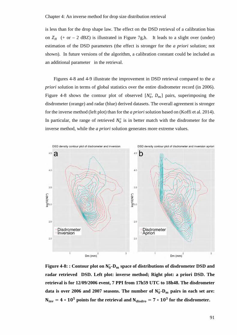
Chapter 4: An inverse method for drop size distribution retrieval
91
is less than for the drop shape law. The effect on the DSD retrieval of a calibration bias
on 𝑍𝑍𝐻𝐻 (+ or – 2 dBZ) is illustrated in Figure 7g,h. It leads to a slight over (under)
estimation of the DSD parameters (the effect is stronger for the a priori solution; not
shown). In future versions of the algorithm, a calibration constant could be included as
an additional parameter in the retrieval.
Figures 4-8 and 4-9 illustrate the improvement in DSD retrieval compared to the a
priori solution in terms of global statistics over the entire disdrometer record (in 2006).
Figure 4-8 shows the contour plot of observed [𝑁𝑁0∗, 𝐷𝐷𝑚𝑚] pairs, superimposing the
disdrometer (orange) and radar (blue) derived datasets. The overall agreement is stronger
for the inverse method (left plot) than for the a priori solution based on (Koffi et al. 2014).
In particular, the range of retrieved 𝑁𝑁0∗ is in better match with the disdrometer for the
inverse method, while the a priori solution generates more extreme values.
Figure 4-8: : Contour plot on 𝐍𝐍𝟎𝟎∗-𝐃𝐃𝐦𝐦 space of distributions of disdrometer DSD and
radar retrieved DSD. Left plot: inverse method; Right plot: a priori DSD. The
retrieval is for 12/09/2006 event, 7 PPI from 17h59 UTC to 18h48. The disdrometer
data is over 2006 and 2007 seasons. The number of 𝐍𝐍𝟎𝟎∗-𝐃𝐃𝐦𝐦 pairs in each set are:
𝐍𝐍𝐢𝐢𝐚𝐚𝐢𝐢 = 𝟒𝟒 ∗ 𝟏𝟏𝟎𝟎𝟎𝟎 points for the retrieval and 𝐍𝐍𝐚𝐚𝐢𝐢𝐝𝐝𝐚𝐚𝐝𝐝𝐥𝐥 = 𝟎𝟎 ∗ 𝟏𝟏𝟎𝟎𝟑𝟑 for the disdrometer.
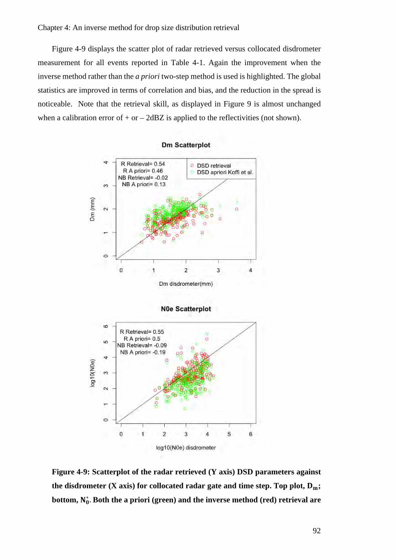
Chapter 4: An inverse method for drop size distribution retrieval
92
Figure 4-9 displays the scatter plot of radar retrieved versus collocated disdrometer
measurement for all events reported in Table 4-1. Again the improvement when the
inverse method rather than the a priori two-step method is used is highlighted. The global
statistics are improved in terms of correlation and bias, and the reduction in the spread is
noticeable. Note that the retrieval skill, as displayed in Figure 9 is almost unchanged
when a calibration error of + or – 2dBZ is applied to the reflectivities (not shown).
Figure 4-9: Scatterplot of the radar retrieved (Y axis) DSD parameters against
the disdrometer (X axis) for collocated radar gate and time step. Top plot, 𝐃𝐃𝐦𝐦;
bottom, 𝐍𝐍𝟎𝟎∗ . Both the a priori (green) and the inverse method (red) retrieval are
Chapter 4: An inverse method for drop size distribution retrieval
93
shown. The correlation (R) and normalized bias (NB) compared to the
disdrometer for both retrieval are indicated on the plots. 18 rainy systems for a
total of 𝐍𝐍 = 𝟎𝟎𝟒𝟒𝟒𝟒 collocated points are displayed.
Figures 4-8 and 4-9 indicate an improvement in DSD retrieval from the a priori to
the final solution. However some differences remain between the disdrometer and radar
retrieved DSDs. The distribution of median diameter Dm is narrower on radar than on the
disdrometer dataset (Figure 8). Some of these differences are unavoidable given the
different nature of the two datasets. The radar samples a larger volume of atmosphere and
higher above ground than the disdrometer.
4.6 Conclusion A method based on an inverse model to retrieve DSD parameters from radar
polarimetric observations at attenuated frequency is presented and tested on X-band data
in Africa. Three parameters of a gamma DSD (the volume weighted mean diameter 𝐷𝐷𝑚𝑚,
the scaling parameter of concentration 𝑁𝑁0∗ and a shape parameter, 𝜇𝜇) are retrieved at each
range gate along a radial. The DSD range profile for the entire radial is found at once, as
the solution which best matches the radar observations. The procedure does not need a
previous attenuation correction because the forward and inverse model account explicitly
for the path integrated attenuation in the measured reflectivities. In line with the approach
developed by (Yoshikawa, Chandrasekar, and Ushio 2014), this framework ensures a
global consistency between the retrieved DSD and all radar variables. It reduces the errors
brought by the uncertainty in the attenuation correction procedure. The inversion
procedure is an iterative algorithm which finds the solution for the entire radar radial; it
can make use of a strong constraint –like the differential phase shift at the last gate – to
insure robustness.
The forward model needed for the inversion relates the observed radar variables to
the DSD along the radial. This model is based on explicit calculations of radar variables
(reflectivities in horizontal and vertical polarization; specific differential phase shift;
specific attenuation coefficient for each polarization) as a function of drop sizes and
shapes. T-matrix calculations for drops considered as oblate spheroids were used for this
purpose. By convoluting the T-matrix output and the DSD, the radar variables were pre-
calculated for gamma DSD over a range of values of the 3 parameters of interest 𝐷𝐷𝑚𝑚, 𝑁𝑁0∗
Chapter 4: An inverse method for drop size distribution retrieval
94
and 𝜇𝜇. Based on these calculations the partial derivative of the radar variables (the
Jacobian), needed in the inversion procedure, are computed. These calculations were
made for several assumptions concerning the aspect ratio of drops and the sensitivity to
the prescribed temperature also analyzed (and found to be small). In addition to i) the
observed radar variables, and ii) the radial profile of the 3 DSD parameters to be retrieved,
many other parameters and a priori information need to be prescribed to the inverse
model
The results of the inversion were evaluated through direct comparisons with
disdrometer data and also by analyzing the global consistency of the solution compared
to the ‘2 step’ empirical method from (Koffi et al. 2014). 15 rainfall events, for a total of
244 PPI were used for direct comparison between the disdrometer and the radar DSD
retrieved at the closest pixel. The correlations between the time series, for 𝐷𝐷𝑚𝑚 and for 𝑁𝑁0∗
are about 0.55, and improved compared to the a priori solution. These numbers are similar
to the scores obtained when radar retrieved DSD is compared with disdrometer data in
other studies (Raupach and Berne 2017) at non attenuating frequencies. This is quite
remarkable given the intense attenuation encountered in the study region in West Africa.
Compared to empirical methods, the proposed inverse model, by providing an overall
retrieval of the range profile of DSD, leads to a solution which is more consistent with all
observed radar variables, and shows a better spatial consistency. This is apparent on the
retrieved DSD maps based on any given PPI; the spurious radials that tend to appear with
the 2 steps method because of errors brought by the attenuation correction are more
consistent with the inverse method. This improved consistency in the retrieval is also
shown when the frequency distribution and co-distributions of 𝑁𝑁0∗ and 𝐷𝐷𝑚𝑚 are analyzed.
The distributions retrieved with the inverse model are closer to the disdrometer derived
ones, and show less spread than those from the empirical method.
These results appear promising, but a more comprehensive assessment of the
proposed method is required. For that purpose, various datasets representative of different
climatological contexts are needed. In addition, it would be interesting to compare it with
the method proposed by [47], in order to assess their respective advantages and
drawbacks. If these methods were to be used with operational radars and in real time, the
optimization of the processing time compared to retrieval accuracy should be analyzed.
Some improvement and new implementations could be added to the inverse model. In the
current version the calibration of reflectivities is assumed to be correct, but a calibration
Chapter 4: An inverse method for drop size distribution retrieval
95
(slowly varying) constant could be added in the model and retrieved as a parameter. We
showed for one case study (Figure 4-5) that one extreme shape law best fits the
observations, and discussed that this could be a compensation for a calibration error rather
than a real rainfall microphysics feature. If we consider a linear axis ratio law with a
parameter 𝛽𝛽 (Eq 4.10) we can consider a new inversion with the parameter 𝛽𝛽 as a variable
in the parameters space as we can calculate the partial derivates of [𝑍𝑍𝐷𝐷𝐷𝐷, 𝑍𝑍𝐻𝐻, 𝐾𝐾𝐷𝐷𝐷𝐷] with
respect to 𝛽𝛽 (Jacobian). Also the calibration coefficients, Δ𝑍𝑍𝐻𝐻 and Δ𝑍𝑍𝑉𝑉 could be added to
the parameters space as its Jacobian can be computed.
The retrieval a posteriori error covariance is a by-product of the inverse model which
is currently not used; in the future it could be used to generate ensembles instead of using
a single retrieved DSD field for each PPI.
Author Contributions: The work presented was carried out in collaboration with all authors. All authors contributed
to the writing of the manuscript, and conceived and designed the content of this paper, M.G. coordinated the deployment
of the disdrometer and weather radar in Africa, H.A contributed to the formalization of the inverse problem and M.A
performed the calculations and figures.
Funding: This research was partially funded by the French Centre National d’Etudes Spatiales (CNES) under the
TOSCA program in link with the Megha-Tropiques satellite mission. The deployment of the radar and disdrometer in
Africa was funded by Institut de Recherche pour le Développement (IRD) as part of the Anayse Multi-disciplinaire de
la Mousson Africaine (AMMA) program.
Conflicts of Interest: The authors declare no conflict of interest.
Appendix: Jacobian matrix of partial derivatives
The Jacobian matrix is the derivative of the polarimetric radar observables with
respect to the DSD parameters.
The radar observables are regrouped in the vector [𝒁𝒁𝑯𝑯 𝒂𝒂𝒂𝒂𝒂𝒂,𝒁𝒁𝑫𝑫𝑫𝑫
𝒂𝒂𝒂𝒂𝒂𝒂 ,𝑲𝑲𝑫𝑫𝑫𝑫 ,𝜱𝜱𝑫𝑫𝑫𝑫 𝒂𝒂] which
has (3𝑙𝑙 + 1) components, 𝑙𝑙 being the number of gates of a radar radial. The number of
parameters is 3𝑙𝑙, (𝑁𝑁0 ∗ ,𝐷𝐷𝑚𝑚 , 𝜇𝜇) at each of the 𝑙𝑙 radar gates. The Jacobian 𝑱𝑱 is composed
of 12 sub-matrices
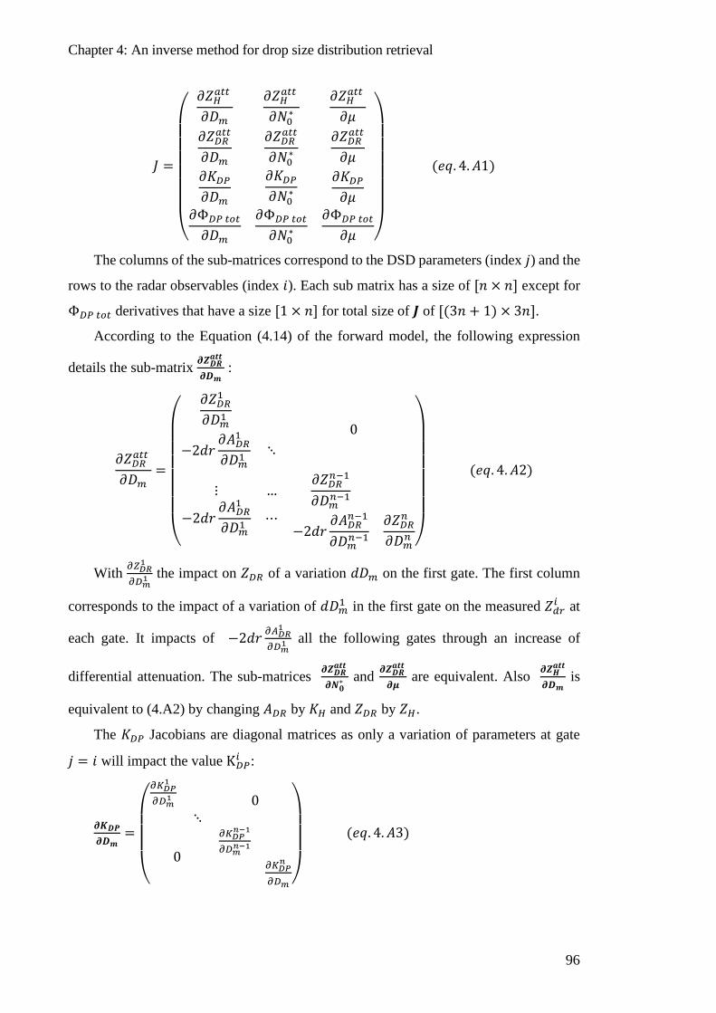
Chapter 4: An inverse method for drop size distribution retrieval
96
𝐽𝐽 =
⎝
⎜⎜⎜⎜⎜⎜⎛
𝜕𝜕𝑍𝑍𝐻𝐻𝑎𝑎𝑡𝑡𝑡𝑡
𝜕𝜕𝐷𝐷𝑚𝑚𝜕𝜕𝑍𝑍𝐻𝐻𝑎𝑎𝑡𝑡𝑡𝑡
𝜕𝜕𝑁𝑁0∗𝜕𝜕𝑍𝑍𝐻𝐻𝑎𝑎𝑡𝑡𝑡𝑡
𝜕𝜕𝜇𝜇𝜕𝜕𝑍𝑍𝐷𝐷𝐷𝐷𝑎𝑎𝑡𝑡𝑡𝑡
𝜕𝜕𝐷𝐷𝑚𝑚𝜕𝜕𝑍𝑍𝐷𝐷𝐷𝐷𝑎𝑎𝑡𝑡𝑡𝑡
𝜕𝜕𝑁𝑁0∗𝜕𝜕𝑍𝑍𝐷𝐷𝐷𝐷𝑎𝑎𝑡𝑡𝑡𝑡
𝜕𝜕𝜇𝜇𝜕𝜕𝐾𝐾𝐷𝐷𝐷𝐷𝜕𝜕𝐷𝐷𝑚𝑚
𝜕𝜕Φ𝐷𝐷𝐷𝐷 𝑡𝑡𝑜𝑜𝑡𝑡
𝜕𝜕𝐷𝐷𝑚𝑚
𝜕𝜕𝐾𝐾𝐷𝐷𝐷𝐷𝜕𝜕𝑁𝑁0∗
𝜕𝜕Φ𝐷𝐷𝐷𝐷 𝑡𝑡𝑜𝑜𝑡𝑡
𝜕𝜕𝑁𝑁0∗
𝜕𝜕𝐾𝐾𝐷𝐷𝐷𝐷𝜕𝜕𝜇𝜇
𝜕𝜕Φ𝐷𝐷𝐷𝐷 𝑡𝑡𝑜𝑜𝑡𝑡
𝜕𝜕𝜇𝜇 ⎠
⎟⎟⎟⎟⎟⎟⎞
(𝑃𝑃𝑒𝑒. 4.𝐴𝐴1)
The columns of the sub-matrices correspond to the DSD parameters (index 𝑗𝑗) and the
rows to the radar observables (index 𝑖𝑖). Each sub matrix has a size of [𝑙𝑙 × 𝑙𝑙] except for
Φ𝐷𝐷𝐷𝐷 𝑡𝑡𝑜𝑜𝑡𝑡 derivatives that have a size [1 × 𝑙𝑙] for total size of 𝑱𝑱 of [(3𝑙𝑙 + 1) × 3𝑙𝑙].
According to the Equation (4.14) of the forward model, the following expression
details the sub-matrix 𝝏𝝏𝒁𝒁𝑫𝑫𝑫𝑫𝒂𝒂𝒂𝒂𝒂𝒂
𝝏𝝏𝑫𝑫𝒎𝒎 :
𝜕𝜕𝑍𝑍𝐷𝐷𝐷𝐷𝑎𝑎𝑡𝑡𝑡𝑡
𝜕𝜕𝐷𝐷𝑚𝑚=
⎝
⎜⎜⎜⎜⎜⎜⎛
𝜕𝜕𝑍𝑍𝐷𝐷𝐷𝐷1
𝜕𝜕𝐷𝐷𝑚𝑚1
−2𝑑𝑑𝑟𝑟𝜕𝜕𝐴𝐴𝐷𝐷𝐷𝐷1
𝜕𝜕𝐷𝐷𝑚𝑚1⋱
0
⋮ …
−2𝑑𝑑𝑟𝑟𝜕𝜕𝐴𝐴𝐷𝐷𝐷𝐷1
𝜕𝜕𝐷𝐷𝑚𝑚1⋯
𝜕𝜕𝑍𝑍𝐷𝐷𝐷𝐷𝑛𝑛−1
𝜕𝜕𝐷𝐷𝑚𝑚𝑛𝑛−1
−2𝑑𝑑𝑟𝑟𝜕𝜕𝐴𝐴𝐷𝐷𝐷𝐷𝑛𝑛−1
𝜕𝜕𝐷𝐷𝑚𝑚𝑛𝑛−1𝜕𝜕𝑍𝑍𝐷𝐷𝐷𝐷𝑛𝑛
𝜕𝜕𝐷𝐷𝑚𝑚𝑛𝑛 ⎠
⎟⎟⎟⎟⎟⎟⎞
(𝑃𝑃𝑒𝑒. 4.𝐴𝐴2)
With 𝜕𝜕𝑍𝑍𝐷𝐷𝐷𝐷1
𝜕𝜕𝐷𝐷𝑚𝑚1 the impact on 𝑍𝑍𝐷𝐷𝐷𝐷 of a variation 𝑑𝑑𝐷𝐷𝑚𝑚 on the first gate. The first column
corresponds to the impact of a variation of 𝑑𝑑𝐷𝐷𝑚𝑚1 in the first gate on the measured 𝑍𝑍𝑑𝑑𝑟𝑟𝑖𝑖 at
each gate. It impacts of −2𝑑𝑑𝑟𝑟 𝜕𝜕𝐴𝐴𝐷𝐷𝐷𝐷1
𝜕𝜕𝐷𝐷𝑚𝑚1 all the following gates through an increase of
differential attenuation. The sub-matrices 𝝏𝝏𝒁𝒁𝑫𝑫𝑫𝑫𝒂𝒂𝒂𝒂𝒂𝒂
𝝏𝝏𝑵𝑵𝟎𝟎∗ and 𝝏𝝏𝒁𝒁𝑫𝑫𝑫𝑫
𝒂𝒂𝒂𝒂𝒂𝒂
𝝏𝝏𝝁𝝁 are equivalent. Also 𝝏𝝏𝒁𝒁𝑯𝑯
𝒂𝒂𝒂𝒂𝒂𝒂
𝝏𝝏𝑫𝑫𝒎𝒎 is
equivalent to (4.A2) by changing 𝐴𝐴𝐷𝐷𝐷𝐷 by 𝐾𝐾𝐻𝐻 and 𝑍𝑍𝐷𝐷𝐷𝐷 by 𝑍𝑍𝐻𝐻.
The 𝐾𝐾𝐷𝐷𝐷𝐷 Jacobians are diagonal matrices as only a variation of parameters at gate
𝑗𝑗 = 𝑖𝑖 will impact the value K𝐷𝐷𝐷𝐷𝑖𝑖 :
𝝏𝝏𝑲𝑲𝑫𝑫𝑫𝑫𝝏𝝏𝑫𝑫𝒎𝒎
=
⎝
⎜⎜⎜⎛
𝜕𝜕𝐾𝐾𝐷𝐷𝐷𝐷1
𝜕𝜕𝐷𝐷𝑚𝑚1
⋱0
0
𝜕𝜕𝐾𝐾𝐷𝐷𝐷𝐷𝑛𝑛−1
𝜕𝜕𝐷𝐷𝑚𝑚𝑛𝑛−1
𝜕𝜕𝐾𝐾𝐷𝐷𝐷𝐷𝑛𝑛
𝜕𝜕𝐷𝐷𝑚𝑚⎠
⎟⎟⎟⎞
(𝑃𝑃𝑒𝑒. 4.𝐴𝐴3)
Chapter 4: An inverse method for drop size distribution retrieval
97
The matrix 𝝏𝝏𝚽𝚽𝑫𝑫𝑫𝑫 𝒂𝒂𝒍𝒍𝒂𝒂𝝏𝝏𝑫𝑫𝒎𝒎
involves only the value of Φ𝐷𝐷𝐷𝐷 at the end of the radial, thus the
matrix is dimension [1 × 𝑙𝑙]. As Φ𝐷𝐷𝐷𝐷 is a cumulative variable, then, matrix is:
𝝏𝝏𝚽𝚽𝑫𝑫𝑫𝑫 𝒂𝒂𝒍𝒍𝒂𝒂𝝏𝝏𝑫𝑫𝒎𝒎
= �𝜕𝜕Φ𝐷𝐷𝐷𝐷 𝑡𝑡𝑡𝑡𝑡𝑡𝜕𝜕𝐷𝐷𝑚𝑚1
… 𝜕𝜕Φ𝐷𝐷𝐷𝐷 𝑡𝑡𝑡𝑡𝑡𝑡𝜕𝜕𝐷𝐷𝑚𝑚𝑛𝑛−1
𝜕𝜕Φ𝐷𝐷𝐷𝐷 𝑡𝑡𝑡𝑡𝑡𝑡𝜕𝜕𝐷𝐷𝑚𝑚𝑛𝑛
� (𝑃𝑃𝑒𝑒. 4.𝐴𝐴4)
A variation of 𝑑𝑑𝐷𝐷𝑚𝑚 at the first gate will add 𝜕𝜕Φ𝐷𝐷𝐷𝐷1
𝜕𝜕𝐷𝐷𝑚𝑚1 to all the following radar gates.
The sub matrixes are estimated using finite difference method with pre-calculated
tables of variation of the polarimetric variables for a range of DSD parameters. We have
pre calculated tables for the different radar observables for a range of N0 ∗ ∈ [500; 105]
by steps of 500 𝑐𝑐−3𝑐𝑐𝑐𝑐−1 for 𝐷𝐷𝑚𝑚 ∈ [0.05,7] by 0.02 𝑐𝑐𝑐𝑐 and for 𝜇𝜇 ∈ [1,14] by steps
of 0.5. The matrix J is calculated at the initial iteration (a priori vector 𝑿𝑿𝑝𝑝𝑟𝑟𝑖𝑖𝑜𝑜𝑟𝑟) and then
update at each iteration 𝑿𝑿𝑘𝑘.
© 2019 by the authors. Submitted for possible open access
publication under the terms and conditions of the Creative
Commons Attribution (CC BY) license
(http://creativecommons.org/licenses/by/4.0/).
Chapter 4: An inverse method for drop size distribution retrieval
98
PART 1 CONCLUSIONS
In the first part of the thesis we have presented two applications of inverse methods to
retrieve information on the characteristics of precipitation. In both applications, the
method is based on a forward model that links radar observables to a simplified model of
rainfall microphysics.
The first application, a simplified Bright Band model is inverted to retrieve the parameters
of the PSD: 𝑁𝑁0∗,𝐷𝐷𝑚𝑚 and the pre-factor of the density law 𝛼𝛼𝑑𝑑 of frozen particles. The
solution is the PSD that best fits to the observed shape of the bright band. As only three
parameters are retrieved per VPR, the inversion technique used is the ‘simplex’ algorithm.
The retrieved values of the pre-factor of the density law are compatible with the in situ
density law observed by the airborne probe. A simple model of melting snow is enough
to retrieve realistic values of the density above the isotherm 0°C.
The model has however three simplifying assumptions: 1/ No aggregation or break-up
was considered during the melting. 2/ We considered the observed VPR as the real VPR,
neglecting the beam broadening effect, and 3/ The degree of melting inside the BB was
parameterized as a simplified function of height. We also considered a fixed exponent 𝛽𝛽𝑑𝑑
in the density law.
The second assumption has a low impact as the profile was constructed with radar
observations within 25 km range. The broadening of the radar beam at this distance has
little effect (no smoothing of the BB peak). The third assumption concerning the degree
of melting of the hydrometeors can impact the shape of the simulated BB. The used model
of melted fraction of a particle depends only on the height of 0°C isotherms and the bright
band bottom. We can imagine that the melted fraction of a particle with height depends
on the particle diameter: big particles could melt slower than little particles. Also the
differential falling velocities of particles were not considered. This can change BB shapes
and thus the retrieved parameters. Another limitation of the study is the constant exponent
𝛽𝛽𝑑𝑑, which was set through the airborne observations. Though, the inversion of both
parameters [𝛽𝛽𝑑𝑑,𝛼𝛼𝑑𝑑] is difficult because their effects on 𝑍𝑍𝐻𝐻 compensate.
The first assumption, concerning the break-up and aggregation could be studied by
combining the two methods presented in this part. For future work we can compare the
airborne observed PSD with the below retrieved DSD of chapter 4 method, under the
trace of the airplane. The DSD retrieval could also be done at different heights using
Chapter 4: An inverse method for drop size distribution retrieval
99
different PPI to evaluate the evolution of the DSD due to break-up, coalescence and
evaporation.
For the bright band inversion only the reflectivity profile was used. For future work the
polarimetric information could also be modelled and used to increase the information
allowing a more complex model of the melting layer.
The second inversion technique presented is a DSD parameters retrieval in all bins of a
radial. The inversion is performed on the attenuated measured variables. With the T-
matrix model of scattering by oblate drops, we found the parameters of the DSD best
describing the polarimetric attenuated variables. The solution is a compromise between
the different observed variables, bringing global coherence to the radial. Due to the high
dimension of the problem and the high nonlinearities, the inversion is sensitive to the a
priori value. The main assumption of the inversion is the ratio shape law of the drops. In
a future version of the inversion algorithm we can try to find an optimal parameter linked
to the ratio shape law, in a similar way than the 𝛽𝛽-method by [Gorgucci et al 2002]. Also
the calibration of the reflectivity could be added into the inversion procedure. A main
objective for this method for future developments is to retrieve ensembles of DSD fields
instead of a single field. In the framework of the inversion theory we can compute the
solution uncertainty with the error covariance matrix, permitting the production of
ensembles. The method is slow compared to power law relations, making it difficult to
apply in a real time framework.
The technique was validated with one rainy season in West Africa. Validation in other
climatic regions could be interesting to test the performance of the algorithm. The
validation disdrometer in the study was at 20km from the radar. A farthest disdrometer or
the comparison with rain gages could show an eventual benefit of the method in terms of
attenuation, compared to a two-steps procedure.

Chapter 4: An inverse method for drop size distribution retrieval
100

Chapter 4: An inverse method for drop size distribution retrieval
101
This part the manuscript is dedicated to rainfall retrieval using commercial microwave
links (CML) from telecommunication companies. In the first part we showed the value
of radars observation to retrieve precipitation characteristics, but radars are expensive and
have a poor implantation in tropical countries.
The attenuating effect of rainfall on CML has been known for several decades. The first
work quantifying the attenuation induced from rainfall are from the late 60’ and 70’ (Atlas
and Ulbrich 1977; Semplak 1970; Olsen, Rogers, and Hodge 1978). In the last decade,
researchers proposed using the measured attenuation levels in CML to derive
precipitation measurements as a new opportunistic technique, especially useful where no
other source of data is available (Messer 2006; Overeem, Leijnse, and Uijlenhoet 2011;
Doumounia et al. 2014). The CML networks are maintained by the telecom operators and
their density covers large parts of the globe, especially densely populated regions.
To monitor rainfall through CML we first must separate the rainfall induced attenuation
from the other sources of attenuation. As we have seen in chapter 2 and chapter 4, the
attenuation by rain drops depends on the drop size distribution over the path of the EM
wave. The specific attenuation can be linked to the rainfall by a power law relation which
depends on the assumptions made on the DSD. The algorithms used to classify rainy
periods from raw attenuation time series can lead to false alarms and non-detection. The
PART 2 COMMERCIAL MICROWAVE LINKS FOR
RAINFALL MONITORING

Chapter 4: An inverse method for drop size distribution retrieval
102
following chapter is focused on the quantitative estimation of precipitation using CMLs
and the different sources of the uncertainty and bias.
Chapter 6 addresses the evaluation and algorithm calibration of a CML dataset from
Niamey, Niger, using 3 rain gauges. We also analyze the sampling differences between a
link and a rain gauge and the possible impact on the link-gauge rainfall time series
comparison. This analysis is based on simulation using the DSD maps derived from
polarimetric radar in Chapter 4.
CML networks are not optimized for rainfall measurement but for telecommunication
purposes. The CML in the network operate at various frequencies, with a distribution of
length, position and orientation, designed by the telecommunication operator. This leads
to heterogeneous measurements in terms of spatial sampling and rainfall measurement
accuracy. The problem of combining CML observations to produce regularly gridded rain
maps is addressed in chapter 7. A prospective method based on neural network is tested.
Chapter 5: Rainfall measurement from microwave links: principle and sources of uncertainty
103
5 RAINFALL MEASUREMENT FROM MICROWAVE LINKS: PRINCIPLE AND SOURCES OF UNCERTAINTY
Mobile telecommunication companies use radio-frequencies to transmit some of their
signal through the network. The commercial micro-wave links (CML) are composed of a
transmitter and a receiver, communicating thanks to antennas located on towers, one at
each end of the link. The microwave signal at the receiver fluctuates because of
attenuation by rainfall along the path; this is the basis for CML based rainfall estimation,
as illustrated in Figure 5-1.
This chapter describes the principle rainfall measurement from CMLs. First the various
terms of a CML attenuation budget are presented and the methods used to isolate rain-
induced attenuation. Then the relationship between specific attenuation (K) and rainfall
rate (R) is discussed.
In the second part of this chapter we detail the various sources of uncertainty in rainfall
measurement from microwave links. We discuss their dependencies on the microwave
link characteristics and their relative strength.
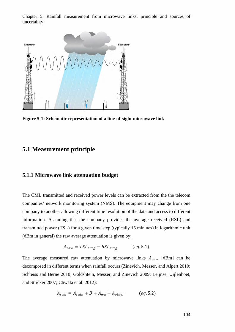
Chapter 5: Rainfall measurement from microwave links: principle and sources of uncertainty
104
Figure 5-1: Schematic representation of a line-of-sight microwave link
5.1 Measurement principle
5.1.1 Microwave link attenuation budget
The CML transmitted and received power levels can be extracted from the the telecom
companies’ network monitoring system (NMS). The equipment may change from one
company to another allowing different time resolution of the data and access to different
information. Assuming that the company provides the average received (RSL) and
transmitted power (TSL) for a given time step (typically 15 minutes) in logarithmic unit
(dBm in general) the raw average attenuation is given by:
𝐴𝐴𝑟𝑟𝑎𝑎𝑤𝑤 = 𝑀𝑀𝑆𝑆𝐿𝐿𝑎𝑎𝑎𝑎𝑟𝑟𝑎𝑎 − 𝑅𝑅𝑆𝑆𝐿𝐿𝑎𝑎𝑎𝑎𝑟𝑟𝑎𝑎 (𝑃𝑃𝑒𝑒. 5.1)
The average measured raw attenuation by microwave links 𝐴𝐴𝑟𝑟𝑎𝑎𝑤𝑤 [dBm] can be
decomposed in different terms when rainfall occurs (Zinevich, Messer, and Alpert 2010;
Schleiss and Berne 2010; Goldshtein, Messer, and Zinevich 2009; Leijnse, Uijlenhoet,
and Stricker 2007; Chwala et al. 2012):
𝐴𝐴𝑟𝑟𝑎𝑎𝑤𝑤 = 𝐴𝐴𝑟𝑟𝑎𝑎𝑖𝑖𝑛𝑛 + 𝑑𝑑 + 𝐴𝐴𝑤𝑤𝑎𝑎 + 𝐴𝐴𝑜𝑜𝑡𝑡ℎ𝑒𝑒𝑟𝑟 (𝑃𝑃𝑒𝑒. 5.2)
Chapter 5: Rainfall measurement from microwave links: principle and sources of uncertainty
105
𝐴𝐴𝑟𝑟𝑎𝑎𝑖𝑖𝑛𝑛 denotes the integrated path attenuation due to rain in [dB], 𝐴𝐴𝑤𝑤𝑎𝑎 denotes the
attenuation due to wet antenna [dB]. The baseline signal, ie. the attenuation level before
rainfall occurs, is noted 𝑑𝑑. 𝐴𝐴𝑜𝑜𝑡𝑡ℎ𝑒𝑒𝑟𝑟 includes all other sources of apparent attenuation (for
instance misalignment of antennas due to wind burst during the storm etc) not included
in the baseline 𝑑𝑑. The baseline level of attenuation 𝑑𝑑 includes all sources of attenuation
during dry periods: the free-space propagative loss, the antennas gain and the electronic
losses.
In the following sections we detail the different terms of the above equation.
5.1.2 Attenuation-Rainfall relation
The specific attenuation 𝐾𝐾𝑡𝑡 [𝑑𝑑𝑑𝑑/𝑘𝑘𝑐𝑐] is defined as the total attenuation 𝐴𝐴𝑟𝑟𝑎𝑎𝑖𝑖𝑛𝑛[𝑑𝑑𝑑𝑑] in a
path, divided by the CML path length 𝐿𝐿. 𝐾𝐾𝑡𝑡, is closely related to the third moment of the
DSD, and thus to the rainfall rate. Assuming that the total extinction cross section 𝜎𝜎𝑒𝑒𝑒𝑒𝑡𝑡
can be expressed by a power law of the particle diameter 𝐷𝐷: 𝜎𝜎𝑒𝑒𝑒𝑒𝑡𝑡~𝐶𝐶𝐷𝐷𝑛𝑛 with 𝑙𝑙 and 𝐶𝐶
unknown constant values at a given frequency and temperature (Atlas and Ulbrich 1977),
then the specific attenuation become a n-order moment of the DSD. Two different
moment of the DSD can be related by a power law (Torres, Porrà, and Creutin 1994; Lee
et al. 2004). 𝐾𝐾𝑡𝑡 and 𝑅𝑅 being moments of the DSD we can relate them by a power law:
𝐴𝐴𝑟𝑟𝑎𝑎𝑖𝑖𝑛𝑛𝐿𝐿
= 𝐾𝐾𝑡𝑡[𝑑𝑑𝑑𝑑/𝑘𝑘𝑐𝑐] = 𝑎𝑎𝑅𝑅𝑜𝑜 (𝑃𝑃𝑒𝑒. 5.3)
Many authors considered the attenuation-rainfall power law relation to convert rainfall
attenuations to rainfall rate. Two types of approaches exist:
• the first are theoretical calculations of 𝐾𝐾𝑡𝑡 with Mie scattering (or T-matrix for polarimetry) considering either observed or parameterized DSD.
• The second are empirical procedures comparing observed 𝐾𝐾𝑡𝑡 and R and fitting linear relations in the log-log space.
The works from (Semplak and Turrin 1969; Atlas and Ulbrich 1977; Olsen, Rogers, and
Hodge 1978) gave the firsts systematic estimation of coefficients [𝑎𝑎, 𝑏𝑏] of the power law
relationship depending on the DSD parameterization, temperature and frequency, and
showed the strong empirical evidence of the power law relation approximation with little
Chapter 5: Rainfall measurement from microwave links: principle and sources of uncertainty
106
deviation for strong rain rates. (Atlas and Ulbrich 1977) showed that the above
relationship becomes linear (𝑏𝑏 = 1) at 𝜆𝜆 = 0.9 𝑐𝑐𝑐𝑐 (ie. 𝑓𝑓 = 33 𝐺𝐺𝐻𝐻𝑧𝑧).
The 𝑏𝑏 coefficient in eq. 5.3 is close to 1 for many of the frequencies used on CMLs. This
is an asset. The quasi-linearity between the path integrated attenuation (PIA) and specific
attenuations along the path: 𝐴𝐴𝑟𝑟𝑎𝑎𝑖𝑖𝑛𝑛 = ∫ 𝐾𝐾𝑡𝑡(𝑟𝑟)𝑑𝑑𝑟𝑟𝑟𝑟0 means that the PIA is a good estimator
of the path average rain rate.
In order to establish attenuation-rainfall relationship (usually called K-R relationship) for
West-African convective systems we have used the DSD data from disdrometers
observation is Benin presented in Chapter 4. To compute the complex refractive index 𝑐𝑐
of the liquid water at microwave frequencies for a range of temperatures [1-40°] we have
used the model from (Ray 1972). Then the attenuation cross section 𝜎𝜎𝑒𝑒𝑒𝑒𝑡𝑡 in Mie regime
was calculated with the method of (Bohren and Huffman 2004). The attenuation cross
sections 𝜎𝜎𝑒𝑒𝑒𝑒𝑡𝑡 are shown in figures 2-5 and 2-6 depending on temperature and wavelength.
For a given observed DSD 𝑁𝑁𝑜𝑜𝑜𝑜𝑜𝑜(𝐷𝐷) we can compute the observed rainfall rate 𝑅𝑅 and the
corresponding attenuation considering the extinction cross section 𝜎𝜎𝑒𝑒𝑒𝑒𝑡𝑡. K-R relationship
are stablished by fitting a linear law of observed 𝑅𝑅 and 𝐾𝐾 in the log-log space. Figure 5-
2 shows the K-R relations at 18 and 23 GHz (frequencies of Niamey CML network
presented in chapter 5). The black dots show each observed DSD for the year 2006 with
the 2D disdrometer (list of MCs systems sampled on table 4-1). The black line is the fitted
K-R law from the DSD observations. The results are then compared with one moment
(rainfall) DSD parameterization (Moumouni 2009) and the classical Marshall-Palmer
parameterization. For Moumouni’s parameterization of DSD using one moment (rainfall
𝑅𝑅 in [𝑐𝑐𝑐𝑐/ℎ𝑟𝑟]) we have:
𝑁𝑁0∗ = 775𝑅𝑅0.42 [𝑐𝑐−4] (𝑃𝑃𝑒𝑒. 5.4)
𝐷𝐷𝑚𝑚 = 1.55𝑅𝑅0.13 [𝑐𝑐𝑐𝑐] (𝑃𝑃𝑒𝑒. 5.5)
𝜇𝜇 = 5.27 (𝑃𝑃𝑒𝑒. 5.6)
For Marshall-Palmer parameterization with rainfall:
𝑁𝑁(𝐷𝐷) = 𝑁𝑁0𝑃𝑃−Λ𝐷𝐷 (𝑃𝑃𝑒𝑒. 5.7)
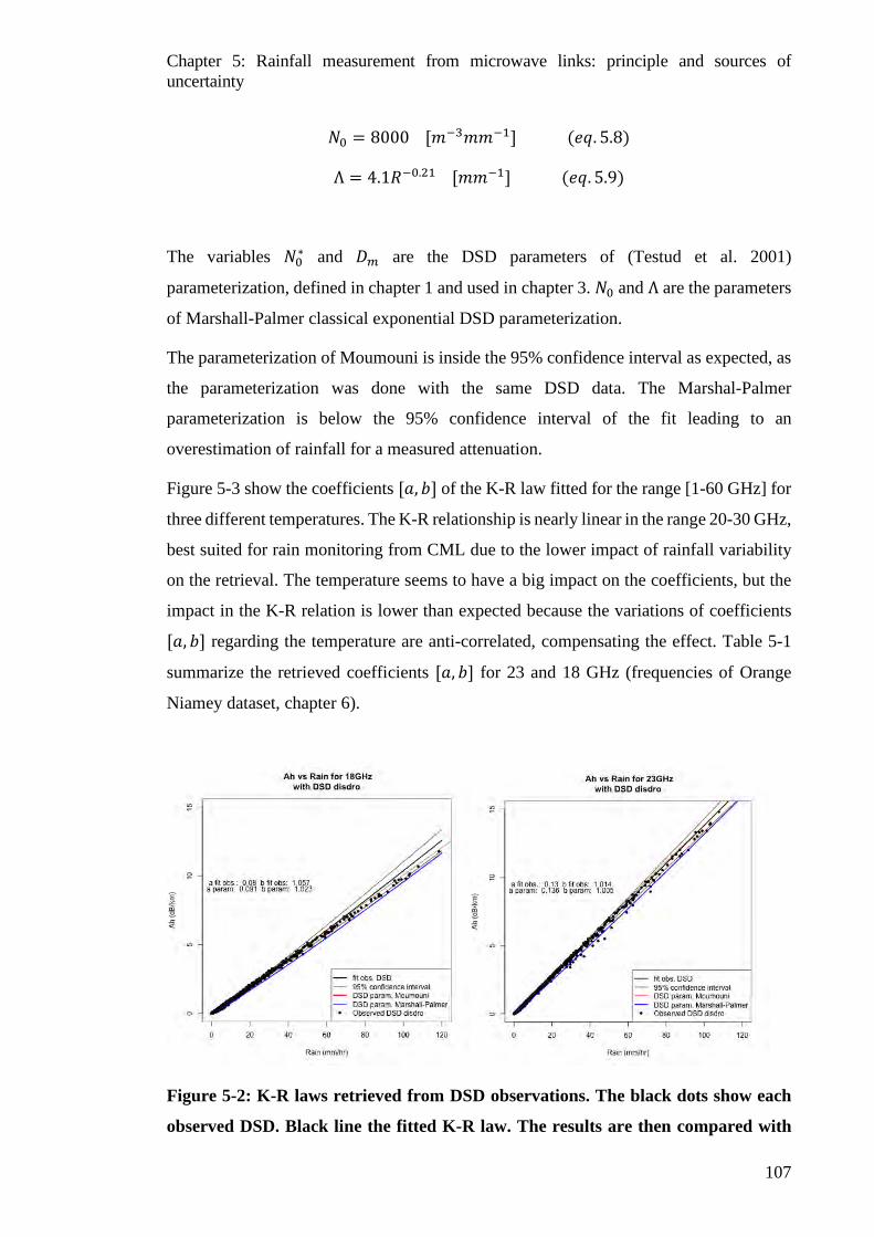
Chapter 5: Rainfall measurement from microwave links: principle and sources of uncertainty
107
𝑁𝑁0 = 8000 [𝑐𝑐−3𝑐𝑐𝑐𝑐−1] (𝑃𝑃𝑒𝑒. 5.8)
Λ = 4.1𝑅𝑅−0.21 [𝑐𝑐𝑐𝑐−1] (𝑃𝑃𝑒𝑒. 5.9)
The variables 𝑁𝑁0∗ and 𝐷𝐷𝑚𝑚 are the DSD parameters of (Testud et al. 2001)
parameterization, defined in chapter 1 and used in chapter 3. 𝑁𝑁0 and Λ are the parameters
of Marshall-Palmer classical exponential DSD parameterization.
The parameterization of Moumouni is inside the 95% confidence interval as expected, as
the parameterization was done with the same DSD data. The Marshal-Palmer
parameterization is below the 95% confidence interval of the fit leading to an
overestimation of rainfall for a measured attenuation.
Figure 5-3 show the coefficients [𝑎𝑎, 𝑏𝑏] of the K-R law fitted for the range [1-60 GHz] for
three different temperatures. The K-R relationship is nearly linear in the range 20-30 GHz,
best suited for rain monitoring from CML due to the lower impact of rainfall variability
on the retrieval. The temperature seems to have a big impact on the coefficients, but the
impact in the K-R relation is lower than expected because the variations of coefficients
[𝑎𝑎, 𝑏𝑏] regarding the temperature are anti-correlated, compensating the effect. Table 5-1
summarize the retrieved coefficients [𝑎𝑎, 𝑏𝑏] for 23 and 18 GHz (frequencies of Orange
Niamey dataset, chapter 6).
Figure 5-2: K-R laws retrieved from DSD observations. The black dots show each
observed DSD. Black line the fitted K-R law. The results are then compared with
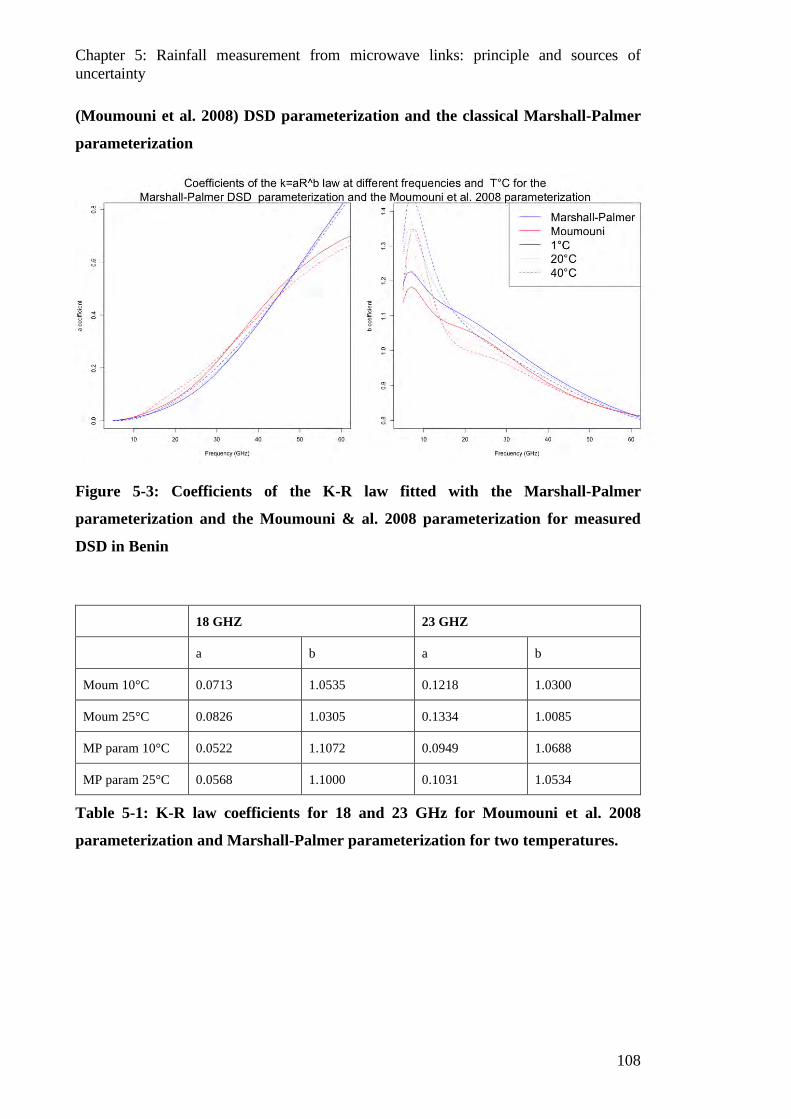
Chapter 5: Rainfall measurement from microwave links: principle and sources of uncertainty
108
(Moumouni et al. 2008) DSD parameterization and the classical Marshall-Palmer
parameterization
Figure 5-3: Coefficients of the K-R law fitted with the Marshall-Palmer
parameterization and the Moumouni & al. 2008 parameterization for measured
DSD in Benin
18 GHZ 23 GHZ
a b a b
Moum 10°C 0.0713 1.0535 0.1218 1.0300
Moum 25°C 0.0826 1.0305 0.1334 1.0085
MP param 10°C 0.0522 1.1072 0.0949 1.0688
MP param 25°C 0.0568 1.1000 0.1031 1.0534
Table 5-1: K-R law coefficients for 18 and 23 GHz for Moumouni et al. 2008
parameterization and Marshall-Palmer parameterization for two temperatures.
Chapter 5: Rainfall measurement from microwave links: principle and sources of uncertainty
109
5.1.3 Baseline and wet-dry period detection
The baseline level of attenuation is defined as the attenuation level in a CML without
rainfall. The wet-dry classification is based on the measured attenuation. The baseline
level can be subjected to significant variations over time. Many factors can impact the
level of the baseline:
• Atmospheric conditions (humidity, temperature) • Variation on the electronic response of the equipment • Changes in wave propagation conditions (misalignment of the antenna) • Type of signal provided by operator and the sampling
Several algorithms have been proposed to establish decision rules to determine wet/dry
periods (Leijnse, Uijlenhoet, and Stricker 2007; Schleiss and Berne 2010; Wang et al.
2012). The stationarity or not of the baseline signal is an important feature as the baseline
detection algorithms for non-stationary signals need to account for the temporal variation.
In stationary baseline signals two main decision rule algorithms are usually applied. The
first is the simple threshold method where the decision rule is based on a fixed attenuation
threshold (Leijnse, Uijlenhoet, and Stricker 2007):
�𝑟𝑟𝑎𝑎𝑖𝑖𝑙𝑙 𝑖𝑖𝑓𝑓 𝐴𝐴𝑟𝑟𝑎𝑎𝑤𝑤 > 𝑎𝑎0𝑑𝑑𝑟𝑟𝑑𝑑 𝑖𝑖𝑓𝑓 𝐴𝐴𝑟𝑟𝑎𝑎𝑤𝑤 ≤ 𝑎𝑎0
(𝑃𝑃𝑒𝑒. 5.10)
Where 𝐴𝐴𝑟𝑟𝑎𝑎𝑤𝑤 is the raw attenuation and 𝑎𝑎0 is the chosen threshold, which may vary
depending on the noise levels of the raw attenuation, the equipment, the link length, and
the weather conditions. The optimal choice of 𝑎𝑎0 is made by minimizing the non-
detections (too restrictive) and rain false alarms (too permissive).
The second algorithm used in stationary signals is based on the temporal variability of the
attenuation (Schleiss and Berne 2010). Choosing a sliding window on length 𝑙𝑙
representing a duration 𝑤𝑤𝑛𝑛, the decision rule is based on a threshold on the local variability
𝜎𝜎𝑡𝑡𝑛𝑛 of the measured attenuation, as attenuation during rainfall events exhibits a higher
variability than during dry periods:
�𝑟𝑟𝑎𝑎𝑖𝑖𝑙𝑙 𝑖𝑖𝑓𝑓 𝜎𝜎𝑡𝑡𝑛𝑛 > 𝜎𝜎0𝑑𝑑𝑟𝑟𝑑𝑑 𝑖𝑖𝑓𝑓 𝜎𝜎𝑡𝑡𝑛𝑛 ≤ 𝜎𝜎0
(𝑃𝑃𝑒𝑒. 5.11)
Chapter 5: Rainfall measurement from microwave links: principle and sources of uncertainty
110
The choice of the number of time steps 𝑙𝑙, to calculate local attenuation variabilities is
delicate. It depends on the climatic rainfall variability and also on the time step resolution
and type of data provided by the operator (nature and precision of the signal). (Schleiss
and Berne 2010) choose 𝑤𝑤𝑛𝑛 = 25 𝑐𝑐𝑖𝑖𝑙𝑙 sliding window for 30s resolution data.
More complex situations can be found if we observe strong temporal drifts in the
attenuation for dry periods. The drifts may occur due to variations in the atmosphere due
to temperature, pressure and humidity (changing the refraction index and thus the
propagation of the MW signals). Also the atmospheric effects result in hardware
instabilities leading to temporal drifts. To take into account the temporal variation of the
baseline, more complex methods have been proposed: the factor graph which assumes
the baseline to vary linearly over time with parameters who can vary (slowly) over time
(Reller, Loeliger, and Diaz 2011). Another method is based on a Markov switching
algorithm which is not based on an empirically estimated threshold parameter and shows
better results than threshold-type classifications (Wang et al. 2012). Finally, (Chwala et
al. 2012) developed a spectral method adapted to their large set of data: the classification
is made by comparing the local normalized Fourier Transforms (FT) of the attenuation
signals to a set of reference dry/wet FT signals (valuable for signals with a good temporal
resolution). The work of (Cherkassky, Ostrometzky, and Messer 2014) uses the min/max
raw attenuations to classify the periods into three types of precipitation: snow, sleet,
rainfall, based on the kernel Fisher discriminant analysis. Other methods can use external
information to classify wet/dry periods, for example IR information from geostationary
satellites in (van het Schip et al. 2017).
5.1.4 Wet antenna
The wetting of the antenna during rainfall events creates a layer of water on the shield of
the antenna. That water layer is an extra attenuation source to the total measured
attenuation which should be removed to avoid biases on the rainfall rate estimation.
There is not a clear consensus in the CML rainfall estimation community on the method
to adopt for quantifying the wet antenna attenuation. In a first approach, the attenuation

Chapter 5: Rainfall measurement from microwave links: principle and sources of uncertainty
111
caused by wet antennas expressed by (Kharadly and Ross 2001) and extended by (Minda
and Nakamura 2005) states that the wet antenna attenuation depends on the rainfall rates
and thus on the rainfall attenuation 𝐴𝐴𝑟𝑟𝑎𝑎𝑖𝑖𝑛𝑛 with the following characteristics:
• An exponential increase of 𝐴𝐴𝑤𝑤𝑎𝑎 for increasing values of 𝐾𝐾𝑡𝑡[𝑑𝑑𝑑𝑑/𝑘𝑘𝑐𝑐], bounded with a maximum value.
• An exponential decrease with time after the rainfall event (due to antenna progressive drying)
The exponential laws can be fitted with simultaneous data of rain gages (or disdrometers)
and CML. The various coefficients of the exponential laws retrieved can vary depending
on the CML frequency, antenna type, antenna shield or even temperature or wind
direction. The exposition to wind or heat of the antenna can lead to a faster drying or to a
thinner water layer in the shield.
(Leijnse, Uijlenhoet, and Stricker 2008) adopted a more physical approach by expressing
the thickness of the water layer in the antenna 𝑙𝑙 by a power law of the rainfall rate 𝑅𝑅. The
principal features of Leijnse approach are:
• 𝑙𝑙 = 𝛾𝛾𝑅𝑅𝛿𝛿 law • Increasing 𝐴𝐴𝑤𝑤𝑎𝑎 for increasing 𝑅𝑅 without a bounded 𝐴𝐴𝑤𝑤𝑎𝑎. • 𝐴𝐴𝑤𝑤𝑎𝑎(𝑅𝑅) frequency dependency.
The coefficients 𝛾𝛾, 𝛿𝛿 were fitted to observed data by converting the estimated empirical
antenna attenuation to a water layer thickness 𝑙𝑙 by calculating the theoretical attenuation
caused by a flat layer of water in an antenna at a certain frequency. Then a set of 𝐴𝐴𝑤𝑤𝑎𝑎(𝑅𝑅)
laws for different frequencies were derived. The exponent coefficient found 𝛿𝛿 = 0.24
leads to an increasing value of a 𝐴𝐴𝑤𝑤𝑎𝑎 with the rainfall rate 𝑅𝑅. However, the 𝑙𝑙(𝑅𝑅) law can
be dependent on the antenna type and shield as well as the weather conditions: wind,
antenna location, temperature.
The quality of the fitting was poor due to few gauges present on the link path and distant
from several hundred meters from as well as using a long CML (4.89km) which can lead
to errors due to the spatial variability, even for a close to linear 𝐾𝐾 − 𝑅𝑅 relation at 27 GHz.
A dedicated experiment to estimate the wet antenna effect is described in (Schleiss,
Rieckermann, and Berne 2013). They used four disdrometers disposed along a CML of
38 GHz and length 1.85 km to estimate the specific attenuation (with T-matrix model).

Chapter 5: Rainfall measurement from microwave links: principle and sources of uncertainty
112
Then they build a model of the wet antenna dynamics by removing to the CML signal the
rainfall component. The main features of its wet antenna model are:
• Wet antenna attenuation bounded at 2.3 GHz maxima • Exponential increase with time toward 2.3 dB (firsts 5-10 min of rainfall) • Exponential decrease with time when rain stops (drying time between 2h and
30min) • Non dependent on rainfall rate attenuation (rainfall rate)
The study (Schleiss, Rieckermann, and Berne 2013) shows evidence that the wet antenna
attenuation does not depend on the rainfall rate for rainfall rates below 8 mm/hr. He
describes the wetting of the antenna as a collection of droplets stuck in the antenna rather
than a thin layer of water as modeled by (Leijnse, Uijlenhoet, and Stricker 2008). But
this study (and others from (Chwala et al. 2012) or (Rayitsfeld et al. 2012)) were made in
mid latitudes regions (Switzerland, Nederland, Germany and Israel) where the rainfall
rates involved are low compared to tropical MCS. The wet antenna attenuation should be
quantified and studied in more detail in tropical regions for strong rainfall rates related to
convective precipitation which can be greater than 100 mm/hr.
5.1.5 Other sources of atmospheric attenuation
This section describes other atmospheric sources of attenuation of MW. The main
absorbers in atmosphere in MW frequencies are oxygen and water vapor. Non-
precipitating suspended droplets (clouds, haze) and suspended dust particles can also
cause attenuation. This section only provides an overview of these sources of attenuation
and does not get into the detailed models. Table 5-1 summarizes the magnitude of specific
attenuation by different atmospheric phenomena.
If we consider no variation of these elements during rainfall events, their contribution to
the total path integrated attenuation between a pair of antennas is included in the baseline
and thus removed. However, at high frequency and in tropical region, these factors may
vary during the storm itself. Further analysis would be needed to asses this problem.
Chapter 5: Rainfall measurement from microwave links: principle and sources of uncertainty
113
Oxygen
Oxygen is the main absorber of MW frequencies in a dry atmosphere. The amount of
energy absorbed by oxygen depend on the frequency of the MW signal and on the quantity
of oxygen (depending mainly on the atmospheric pressure and temperature).
The absorption spectra of MW by oxygen is composed 44 absorption lines in the [1-
1000GHz] range of frequencies. The absorption spectrum between the lines (peaks) is
composed by a continuum which increase with frequency. For frequencies below
100GHz, the continuum contribution is low (attenuation < 0.01 𝑑𝑑𝑑𝑑/𝑘𝑘𝑐𝑐).
There is, however an absorption peak centered at 60 GHz. The work (Liebe, Hufford, and
Cotton 1993) show laboratory measurements of the absorption peak around the 60 GHz
for different pressures. At 6°C and 1013 mbar, in the peak center (60 GHz) the attenuation
due to oxygen absorption is up to 15 𝑑𝑑𝑑𝑑/𝑘𝑘𝑐𝑐. It exists other absorption lines of the
oxygen above 350 GHz, which is beyond the frequencies used commonly by
telecommunication operators.
Humidity
In a wet atmosphere, water vapor is an important absorber of MW radiation. As for
oxygen, the amount of absorbed energy depend on the density of 𝐻𝐻20 molecules in the
atmosphere.
The absorption spectrum of water vapor is composed by a continuum increasing with
frequency and a series of absorption peaks. The main absorption peaks below 100 GHz
are at 22.2 GHz and 67.8 GHz frequencies.
(Liebe, Hufford, and Cotton 1993) modeled the absorption by 𝐻𝐻20. Below 100 GHz, at
sea level normal conditions, 1013 mbar, 20°C and 40% of relative humidy (RH) the
continuum contribution to water vapor absorption is below 0.2 𝑑𝑑𝑑𝑑/𝑘𝑘𝑐𝑐.
However, the contribution of the 22.2 GHz peak is high. At 0°C, RH=100%, P=1013
mbar, the attenuation is 0.1 𝑑𝑑𝑑𝑑/𝑘𝑘𝑐𝑐. For 20°C is 0.5 𝑑𝑑𝑑𝑑/𝑘𝑘𝑐𝑐 and for 30°C 0.9 𝑑𝑑𝑑𝑑/𝑘𝑘𝑐𝑐.
West African mesoscale convective systems are huge perturbation of the atmosphere. As
we described briefly in chapter 1, the convective front updraft of moist air is followed by
a downdraft of cold dry air from upper layers of the atmosphere leading to a drop of the
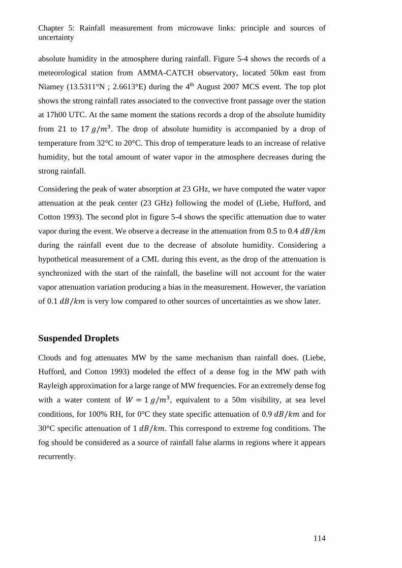
Chapter 5: Rainfall measurement from microwave links: principle and sources of uncertainty
114
absolute humidity in the atmosphere during rainfall. Figure 5-4 shows the records of a
meteorological station from AMMA-CATCH observatory, located 50km east from
Niamey (13.5311°N ; 2.6613°E) during the 4th August 2007 MCS event. The top plot
shows the strong rainfall rates associated to the convective front passage over the station
at 17h00 UTC. At the same moment the stations records a drop of the absolute humidity
from 21 to 17 𝑙𝑙/𝑐𝑐3. The drop of absolute humidity is accompanied by a drop of
temperature from 32°C to 20°C. This drop of temperature leads to an increase of relative
humidity, but the total amount of water vapor in the atmosphere decreases during the
strong rainfall.
Considering the peak of water absorption at 23 GHz, we have computed the water vapor
attenuation at the peak center (23 GHz) following the model of (Liebe, Hufford, and
Cotton 1993). The second plot in figure 5-4 shows the specific attenuation due to water
vapor during the event. We observe a decrease in the attenuation from 0.5 to 0.4 𝑑𝑑𝑑𝑑/𝑘𝑘𝑐𝑐
during the rainfall event due to the decrease of absolute humidity. Considering a
hypothetical measurement of a CML during this event, as the drop of the attenuation is
synchronized with the start of the rainfall, the baseline will not account for the water
vapor attenuation variation producing a bias in the measurement. However, the variation
of 0.1 𝑑𝑑𝑑𝑑/𝑘𝑘𝑐𝑐 is very low compared to other sources of uncertainties as we show later.
Suspended Droplets
Clouds and fog attenuates MW by the same mechanism than rainfall does. (Liebe,
Hufford, and Cotton 1993) modeled the effect of a dense fog in the MW path with
Rayleigh approximation for a large range of MW frequencies. For an extremely dense fog
with a water content of 𝑊𝑊 = 1 𝑙𝑙/𝑐𝑐3, equivalent to a 50m visibility, at sea level
conditions, for 100% RH, for 0°C they state specific attenuation of 0.9 𝑑𝑑𝑑𝑑/𝑘𝑘𝑐𝑐 and for
30°C specific attenuation of 1 𝑑𝑑𝑑𝑑/𝑘𝑘𝑐𝑐. This correspond to extreme fog conditions. The
fog should be considered as a source of rainfall false alarms in regions where it appears
recurrently.
Chapter 5: Rainfall measurement from microwave links: principle and sources of uncertainty
115
Dust
As suspended droplets and rainfall does, the presence of dust particles in the atmosphere
can cause scattering and absorption of the MW signal. During a sandstorm in Khartoum-
Sudan, (Elshaikh et al. 2009) measured specific attenuations of 0.67 𝑑𝑑𝑑𝑑/𝑘𝑘𝑐𝑐 on a 15 km
CML at 13 GHz. In their study they modeled the dust attenuation depending on the
visibility (in km). The model predicts specific attenuations of 1 𝑑𝑑𝑑𝑑/𝑘𝑘𝑐𝑐 at K-band (18-
26 GHz) for a 50m visibility dust storm, which is a rare event.
(Xiao-Ying Dong, Hsing-Yi Chen, and Dong-Hui Guo 2011) stated that attenuation
decreases sharply as the visibility increases from 1m to 1 km. Thus the attenuation due to
sand and dust storms is not serious except for storms with visibilities less than a few
meters and frequencies higher than 30 GHz.
Insects and other animals
Flying animals can be a potential source of attenuation: birds, bats and insects can cause
attenuations on commercial CML. Telecommunication companies informed us about the
occasional presence of wasp nests in the antennas.
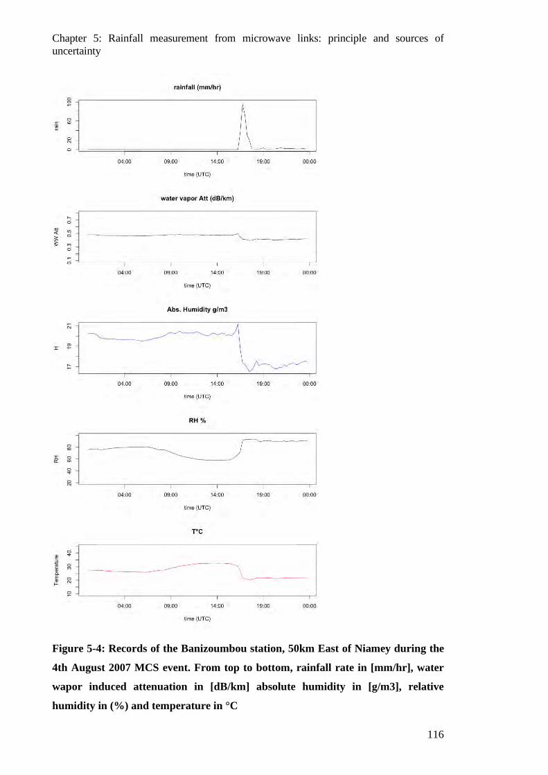
Chapter 5: Rainfall measurement from microwave links: principle and sources of uncertainty
116
Figure 5-4: Records of the Banizoumbou station, 50km East of Niamey during the
4th August 2007 MCS event. From top to bottom, rainfall rate in [mm/hr], water
wapor induced attenuation in [dB/km] absolute humidity in [g/m3], relative
humidity in (%) and temperature in °C
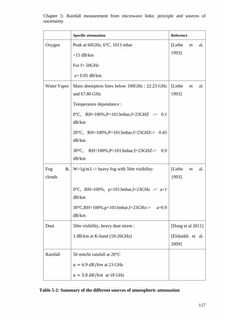
Chapter 5: Rainfall measurement from microwave links: principle and sources of uncertainty
117
Specific attenuation Reference
Oxygen Peak at 60GHz, 6°C, 1013 mbar
~15 dB/km
For f< 50GHz
a< 0.05 dB/km
[Liebe et al.
1993]
Water Vapor Main absorption lines below 100GHz : 22.23 GHz
and 67.80 GHz
Temperature dependance :
0°C, RH=100%,P=1013mbar,f=23GHZ -> 0.1
dB/km
20°C, RH=100%,P=1013mbar,f=23GHZ-> 0.45
dB/km
30°C, RH=100%,P=1013mbar,f=23GHZ-> 0.9
dB/km
[Liebe et al.
1993]
Fog &
clouds
W=1g/m3 -> heavy fog with 50m visibility:
0°C, RH=100%, p=1013mbar,f=23GHz -> a=1
dB/km
30°C,RH=100%,p=1013mbar,f=23GHz-> a=0.9
dB/km
[Liebe et al.
1993]
Dust 50m visibility, heavy dust storm :
1 dB/km at K-band (18-26GHz)
[Dong et al 2011]
[Elshaikh et al.
2009]
Rainfall 50 mm/hr rainfall at 20°C
𝑎𝑎 = 6.9 𝑑𝑑𝑑𝑑/𝑘𝑘𝑐𝑐 at 23 GHz
𝑎𝑎 = 5.0 𝑑𝑑𝑑𝑑/𝑘𝑘𝑐𝑐 at 18 GHz
Table 5-2: Summary of the different sources of atmospheric attenuation
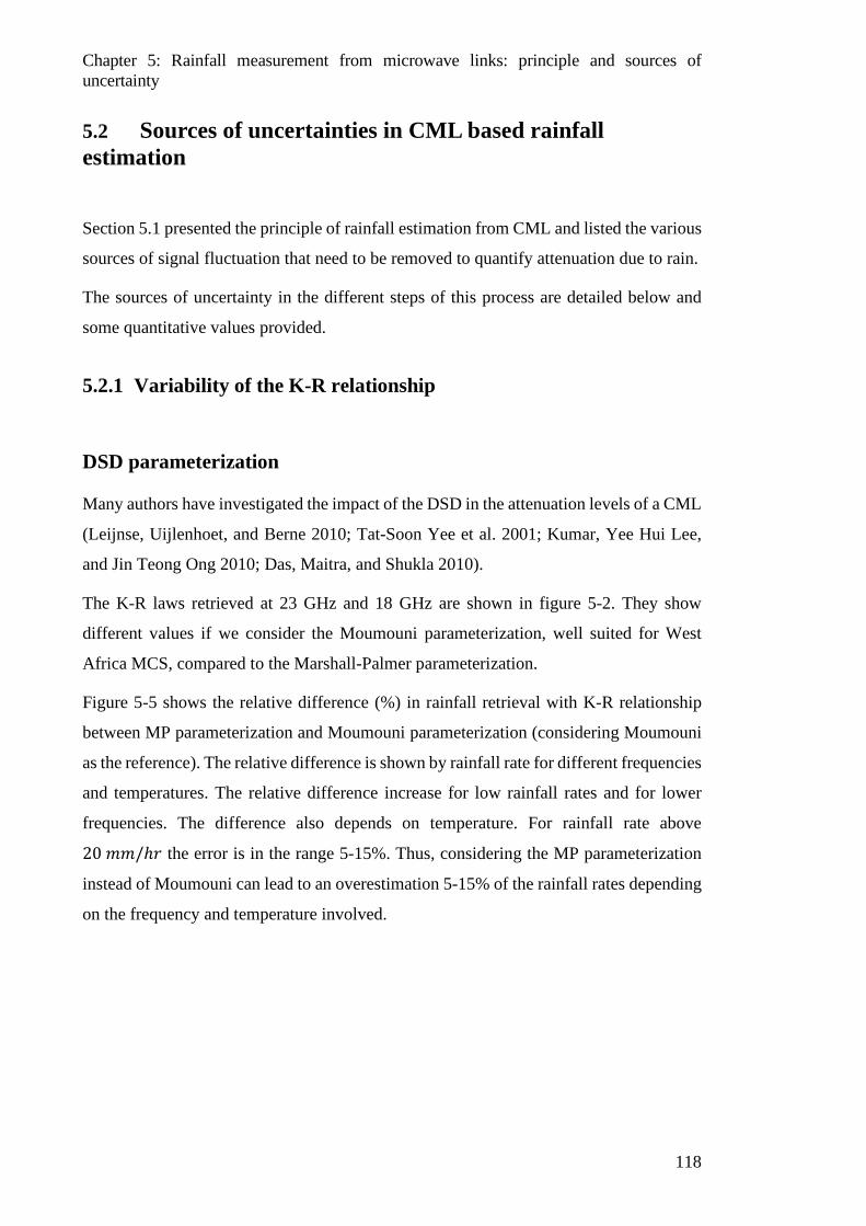
Chapter 5: Rainfall measurement from microwave links: principle and sources of uncertainty
118
5.2 Sources of uncertainties in CML based rainfall estimation
Section 5.1 presented the principle of rainfall estimation from CML and listed the various
sources of signal fluctuation that need to be removed to quantify attenuation due to rain.
The sources of uncertainty in the different steps of this process are detailed below and
some quantitative values provided.
5.2.1 Variability of the K-R relationship
DSD parameterization
Many authors have investigated the impact of the DSD in the attenuation levels of a CML
(Leijnse, Uijlenhoet, and Berne 2010; Tat-Soon Yee et al. 2001; Kumar, Yee Hui Lee,
and Jin Teong Ong 2010; Das, Maitra, and Shukla 2010).
The K-R laws retrieved at 23 GHz and 18 GHz are shown in figure 5-2. They show
different values if we consider the Moumouni parameterization, well suited for West
Africa MCS, compared to the Marshall-Palmer parameterization.
Figure 5-5 shows the relative difference (%) in rainfall retrieval with K-R relationship
between MP parameterization and Moumouni parameterization (considering Moumouni
as the reference). The relative difference is shown by rainfall rate for different frequencies
and temperatures. The relative difference increase for low rainfall rates and for lower
frequencies. The difference also depends on temperature. For rainfall rate above
20 𝑐𝑐𝑐𝑐/ℎ𝑟𝑟 the error is in the range 5-15%. Thus, considering the MP parameterization
instead of Moumouni can lead to an overestimation 5-15% of the rainfall rates depending
on the frequency and temperature involved.
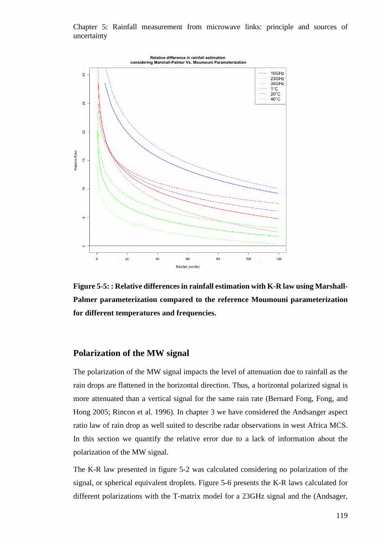
Chapter 5: Rainfall measurement from microwave links: principle and sources of uncertainty
119
Figure 5-5: : Relative differences in rainfall estimation with K-R law using Marshall-
Palmer parameterization compared to the reference Moumouni parameterization
for different temperatures and frequencies.
Polarization of the MW signal
The polarization of the MW signal impacts the level of attenuation due to rainfall as the
rain drops are flattened in the horizontal direction. Thus, a horizontal polarized signal is
more attenuated than a vertical signal for the same rain rate (Bernard Fong, Fong, and
Hong 2005; Rincon et al. 1996). In chapter 3 we have considered the Andsanger aspect
ratio law of rain drop as well suited to describe radar observations in west Africa MCS.
In this section we quantify the relative error due to a lack of information about the
polarization of the MW signal.
The K-R law presented in figure 5-2 was calculated considering no polarization of the
signal, or spherical equivalent droplets. Figure 5-6 presents the K-R laws calculated for
different polarizations with the T-matrix model for a 23GHz signal and the (Andsager,
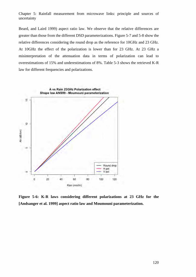
Chapter 5: Rainfall measurement from microwave links: principle and sources of uncertainty
120
Beard, and Laird 1999) aspect ratio law. We observe that the relative differences are
greater than those from the different DSD parameterizations. Figure 5-7 and 5-8 show the
relative differences considering the round drop as the reference for 10GHz and 23 GHz.
At 10GHz the effect of the polarization is lower than for 23 GHz. At 23 GHz a
misinterpretation of the attenuation data in terms of polarization can lead to
overestimations of 15% and underestimations of 8%. Table 5-3 shows the retrieved K-R
law for different frequencies and polarizations.
Figure 5-6: K-R laws considering different polarizations at 23 GHz for the
[Andsanger et al. 1999] aspect ratio law and Moumouni parameterization.
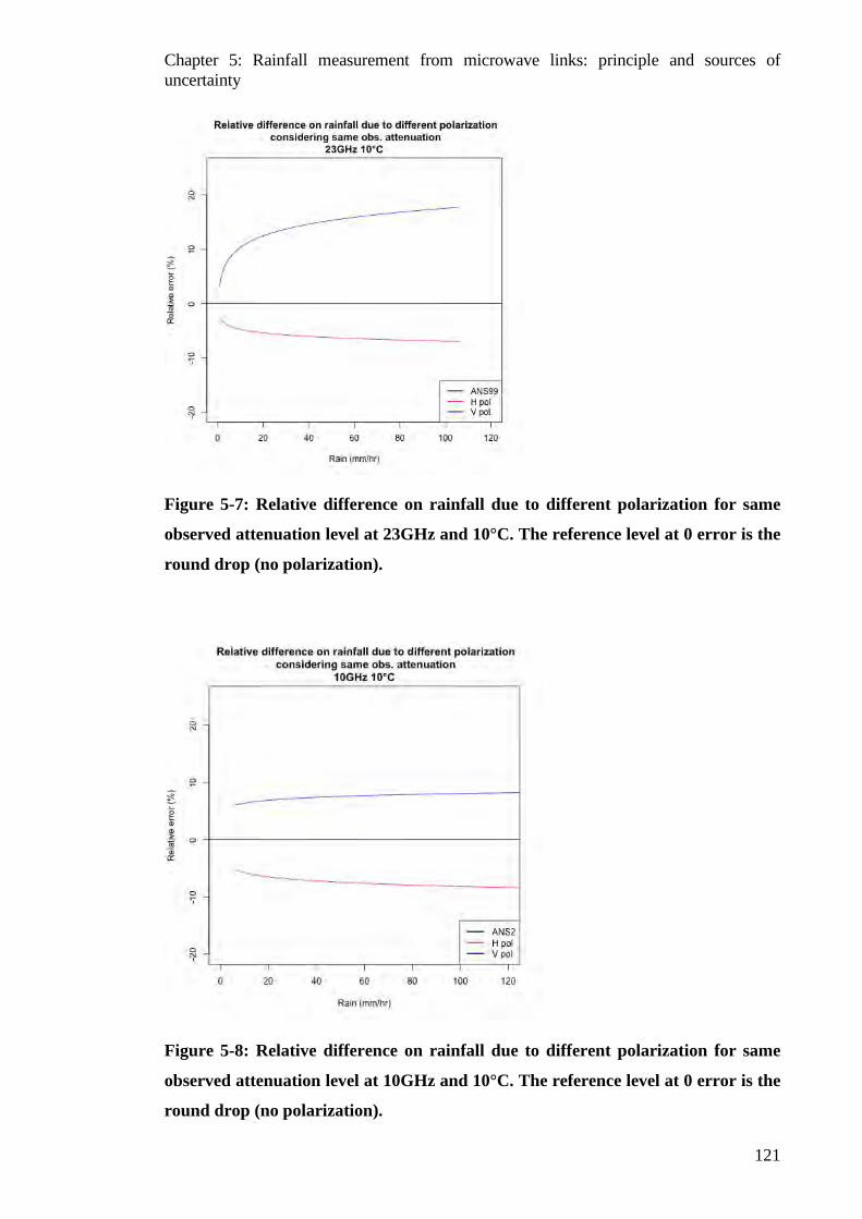
Chapter 5: Rainfall measurement from microwave links: principle and sources of uncertainty
121
Figure 5-7: Relative difference on rainfall due to different polarization for same
observed attenuation level at 23GHz and 10°C. The reference level at 0 error is the
round drop (no polarization).
Figure 5-8: Relative difference on rainfall due to different polarization for same
observed attenuation level at 10GHz and 10°C. The reference level at 0 error is the
round drop (no polarization).
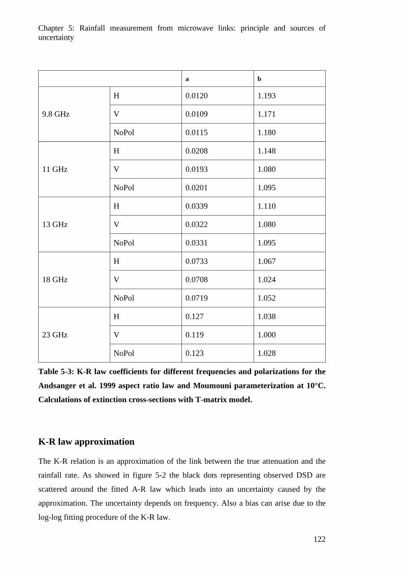
Chapter 5: Rainfall measurement from microwave links: principle and sources of uncertainty
122
a b
9.8 GHz
H 0.0120 1.193
V 0.0109 1.171
NoPol 0.0115 1.180
11 GHz
H 0.0208 1.148
V 0.0193 1.080
NoPol 0.0201 1.095
13 GHz
H 0.0339 1.110
V 0.0322 1.080
NoPol 0.0331 1.095
18 GHz
H 0.0733 1.067
V 0.0708 1.024
NoPol 0.0719 1.052
23 GHz
H 0.127 1.038
V 0.119 1.000
NoPol 0.123 1.028
Table 5-3: K-R law coefficients for different frequencies and polarizations for the
Andsanger et al. 1999 aspect ratio law and Moumouni parameterization at 10°C.
Calculations of extinction cross-sections with T-matrix model.
K-R law approximation
The K-R relation is an approximation of the link between the true attenuation and the
rainfall rate. As showed in figure 5-2 the black dots representing observed DSD are
scattered around the fitted A-R law which leads into an uncertainty caused by the
approximation. The uncertainty depends on frequency. Also a bias can arise due to the
log-log fitting procedure of the K-R law.

Chapter 5: Rainfall measurement from microwave links: principle and sources of uncertainty
123
Figure 5-9 show the relative error on rainfall between each 1-min observed DSD in Benin
and the retrieved K-R law. The uncertainty grows as the frequency lowers. Also, the
residual bias lower with higher frequency. The remaining average bias for rain rates >
50 𝑐𝑐𝑐𝑐/ℎ𝑟𝑟 are -9.5 % for 9 GHz, -8% for 13 GHz, -2.4% for 18 GHz and -2.8% for 23
GHz.
The relative errors here were calculated for point scale measured DSD. As the CML
measures path integrated attenuations, the uncertainty decrease with longer links and for
longer integration sampling time.
Figure 5-9: Residuals between observed DSD rainfall and fitted A-R law. The
uncertainty lower as the frequency increase. The remaining average bias for rain
rates >50 mm/hr are -9.5 % for 9 GHz, -8% for 13 GHz, -2.4% for 18 GHz and -
2.8% for 23 GHz
Chapter 5: Rainfall measurement from microwave links: principle and sources of uncertainty
124
Spatial variability of rainfall
The K-R relation is quasi lineal as the 𝑏𝑏 coefficient in equation 5.3 is near 1. In Figure 5-
3 presenting the retrieved 𝑏𝑏 coefficient against frequency, we can see that the relation
becomes lineal for the Moumouni parameterization of DSD around 28 GHz at 20°C. For
frequencies below 10 GHz the relation moves away from linearity as 𝑏𝑏 > 1.2, specially
for higher temperatures, and also, for frequencies above 40 GHz, as 𝑏𝑏 < 0.9.
In that situations the spatial variability of DSD can lead into errors as the path average
rainfall is not equal to the retrieved rainfall, and the rainfall 𝑅𝑅(𝑠𝑠) is highly variable along
the path 𝑠𝑠:
� 𝑎𝑎𝑅𝑅(𝑠𝑠)𝑜𝑜𝑑𝑑𝑠𝑠𝐿𝐿
0≠ 𝑎𝑎 �� 𝑅𝑅(𝑠𝑠)𝑑𝑑𝑠𝑠
𝐿𝐿
0�𝑜𝑜
=𝐴𝐴𝑟𝑟𝑎𝑎𝑖𝑖𝑛𝑛𝐿𝐿
𝑖𝑖𝑓𝑓 𝑏𝑏 ≠ 1 (𝑃𝑃𝑒𝑒. 5.12)
In they work (Berne and Uijlenhoet 2007) the authors have estimated the impact of the
DSD variability along CML of different lengths and frequencies with a stochastic
generator of DSD profiles of different lengths. They computed the expected attenuation
𝐾𝐾, the real rainfall, the relative error and the uncertainty due to the path averaged rainfall
using fitted K-R laws. The found the following characteristics:
• A mean relative bias of -2% for a 4 km link due to the K-R fitting • An uncertainty range due to DSD variability between 15-10% for 23GHz [0-
5km] CML. • A bias due to a wrong DSD parameterization between [0; -20%] (using
climatological DSD parameterization) Our results are in agreement with their findings. They have retrieved a mean relative bias
of -2% for short links due to the K-R fitting. We found in the last section -3%.
Considering that we have calculated at the point scale and they have considered spatial
variability of DSD.
We also have a similar magnitude in the error due to a wrong DSD parameterization. By
considering Marshal-Palmer parameterization, we found biases at the point scale arround
[5; 20%].
Chapter 5: Rainfall measurement from microwave links: principle and sources of uncertainty
125
5.2.2 Quantization step
In the work (Zinevich, Messer, and Alpert 2010) the authors build a complete error
model of the CML rainfall measurement including the quantization step.
The systems monitoring the CML in Telecom companies usually stores the Tx and Rx
data signals for a quantized level of attenuation. Our datasets are quantized at 0.1 dB or
1 dB (depending on the zone). As mentioned above, a rough quantization step can absorb
the baseline variations due to noise.
A rough quantization step leads to a minimal detectable rainfall 𝑅𝑅𝑚𝑚𝑖𝑖𝑛𝑛 which depends on
the frequency 𝑓𝑓, the link length 𝐿𝐿 and the quantization step Δ𝑎𝑎 of the attenuation provided
by the telecom company. The 𝐾𝐾 − 𝑅𝑅 relation being a power law (eq 5.3), it follows that
the minimal detectable rain is:
Rmin = �Δa
2aL�1/b
(𝑃𝑃𝑒𝑒. 5.13)
Where 𝐿𝐿 is the link length and [𝑎𝑎, 𝑏𝑏] are the 𝐾𝐾 − 𝑅𝑅 law parameters at a certain frequency.
Figure 5-10 and figure 5-11 shows the minimal detectable as a function of the link length
for different frequencies at Δa =1 dB and Δ𝑎𝑎 =0.1 dB quantization steps. As we can see
the lower the frequency and the shorter the link length the minimal detectable rain get
high values corresponding to convective rainfall. Follows that short links and rough
quantization step can lead to systematic non-detections of rainfall.
Considering the maximum span of attenuation ±Δ𝑎𝑎/2. Figure 5-12 represent the
maximum relative uncertainty due to 1 dB quantization step for different rainfall rates
and link lengths a 23 GHz link.

Chapter 5: Rainfall measurement from microwave links: principle and sources of uncertainty
126
Figure 5-10: Minimal detectable rain in function of link length and frequency at a 1
dB quantification step of the attenuation. For low frequency and short links the link
sensitivity is very high.
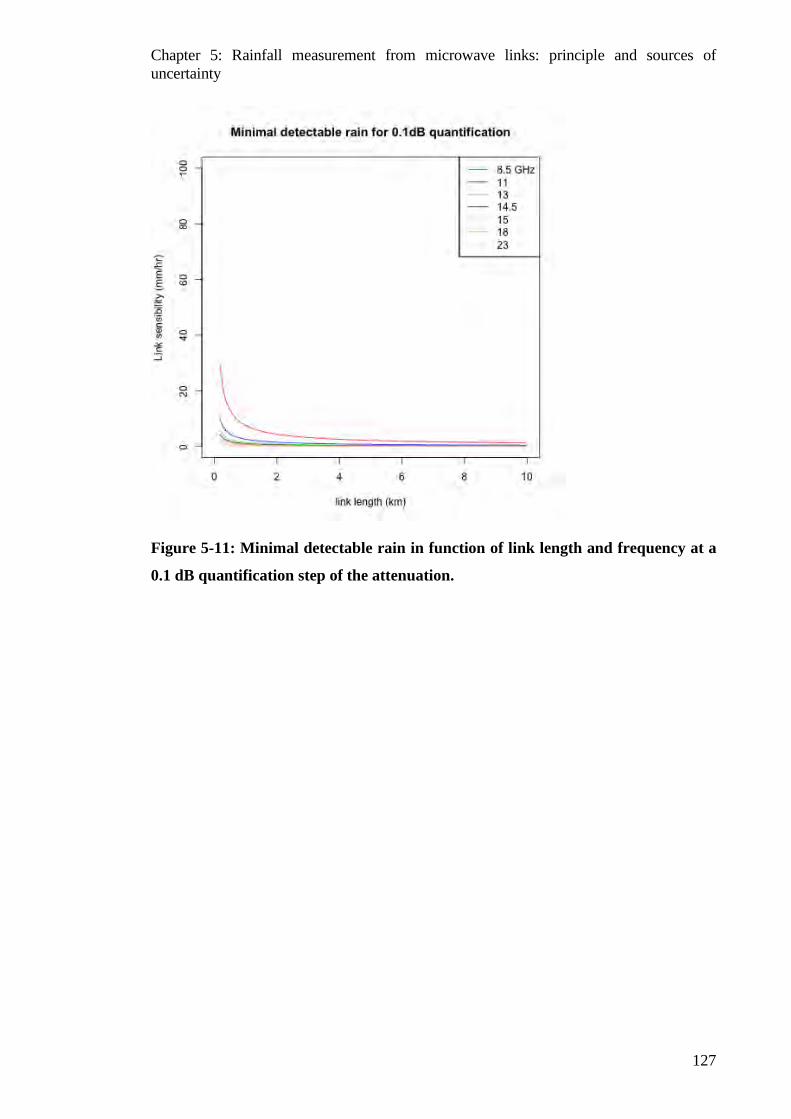
Chapter 5: Rainfall measurement from microwave links: principle and sources of uncertainty
127
Figure 5-11: Minimal detectable rain in function of link length and frequency at a
0.1 dB quantification step of the attenuation.
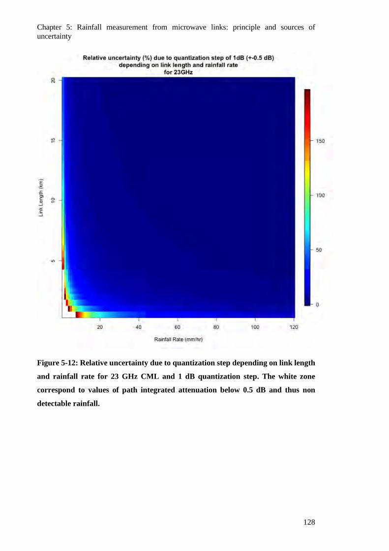
Chapter 5: Rainfall measurement from microwave links: principle and sources of uncertainty
128
Figure 5-12: Relative uncertainty due to quantization step depending on link length
and rainfall rate for 23 GHz CML and 1 dB quantization step. The white zone
correspond to values of path integrated attenuation below 0.5 dB and thus non
detectable rainfall.
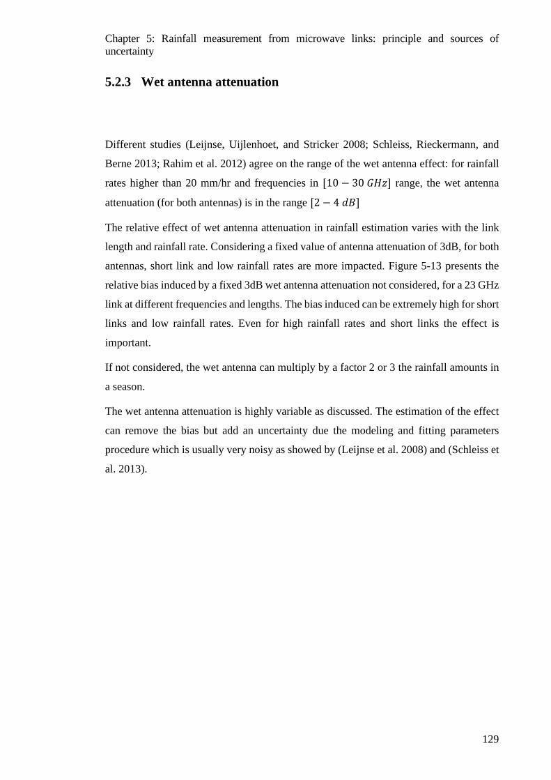
Chapter 5: Rainfall measurement from microwave links: principle and sources of uncertainty
129
5.2.3 Wet antenna attenuation
Different studies (Leijnse, Uijlenhoet, and Stricker 2008; Schleiss, Rieckermann, and
Berne 2013; Rahim et al. 2012) agree on the range of the wet antenna effect: for rainfall
rates higher than 20 mm/hr and frequencies in [10 − 30 𝐺𝐺𝐻𝐻𝑧𝑧] range, the wet antenna
attenuation (for both antennas) is in the range [2 − 4 𝑑𝑑𝑑𝑑]
The relative effect of wet antenna attenuation in rainfall estimation varies with the link
length and rainfall rate. Considering a fixed value of antenna attenuation of 3dB, for both
antennas, short link and low rainfall rates are more impacted. Figure 5-13 presents the
relative bias induced by a fixed 3dB wet antenna attenuation not considered, for a 23 GHz
link at different frequencies and lengths. The bias induced can be extremely high for short
links and low rainfall rates. Even for high rainfall rates and short links the effect is
important.
If not considered, the wet antenna can multiply by a factor 2 or 3 the rainfall amounts in
a season.
The wet antenna attenuation is highly variable as discussed. The estimation of the effect
can remove the bias but add an uncertainty due the modeling and fitting parameters
procedure which is usually very noisy as showed by (Leijnse et al. 2008) and (Schleiss et
al. 2013).
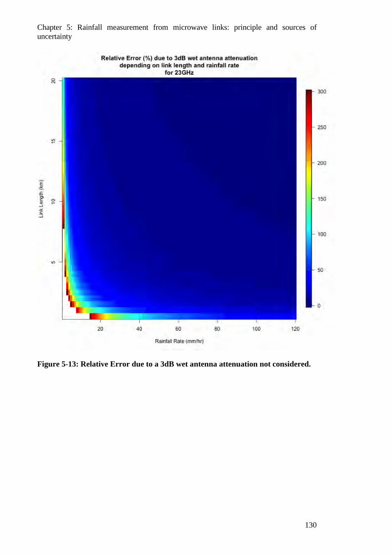
Chapter 5: Rainfall measurement from microwave links: principle and sources of uncertainty
130
Figure 5-13: Relative Error due to a 3dB wet antenna attenuation not considered.

Chapter 5: Rainfall measurement from microwave links: principle and sources of uncertainty
131
5.2.4 Quality of raw information
Temporal Sampling
Telephone companies provide data with different temporal resolutions depending
on the storage constrains of their servers. We can find in the literature datasets at high
temporal resolution (some seconds) usually for one-off studies for a short time period and
a limited number of microwave links. In operational frameworks, high temporal
resolution data is not stored due to the high volumes of the data. Usually the provided
data stored by the monitoring systems of the companies are in a coarser temporal
resolution (several minutes).
With high temporal resolution data we can quantify the short time variations of
the baseline and the rainfall short time scale variability. Also, the assessment of the wet
antenna attenuation with high temporal resolution data allow to monitor the dynamical
evolution of the antenna wetting (if a validation dataset is available). Another asset of
high temporal resolution data is to quantify the losses due to a coarser temporal resolution
in data or a particular sampling strategy (discussed in the section below).
Equation 5.12 presented in section 5.2.2 showing the impact of the non-linear K-
R relation on the spatial variability of rainfall has a similar effect on the temporal
evolution of rainfall rates (by changing the integral over time). As rainfall is highly
variable in space and time, the temporal averaging of attenuations in time deviate from
the temporal averaging of rainfall over time when applying the K-R law if 𝑏𝑏 ≠ 1. The
effect of the non-linear time averaging is less dramatic if the time resolution is below the
time decorrelation scale, which depends on the climatic regimes.
Sampling Strategy
For coarse time resolution scales (~15 minutes is often found in the literature)
different sampling strategies can be found constrained by the software of the telecom
companies’ servers. The data can be averaged over the 15 minutes or sampled every 15
Chapter 5: Rainfall measurement from microwave links: principle and sources of uncertainty
132
minutes. The resulting uncertainty in the rainfall retrievals are different: the averaged
attenuation over 15 minutes compensates the noise of the baseline at short time scales due
to atmospheric scintillation of the atmosphere. For an intermittent sampling every 15
minutes the noise of the high resolution scale is not compensated leading to an uncertainty
on the baseline detection equivalent to the value of the noise at short scales. Of course an
averaged attenuation value is preferred to smooth the noise of the baseline and to account
for the actual average rainfall over the 15 minutes instead of the point measurement
rainfall, which may be far from the average due to high temporal variability.
Unfortunately, is hard to access the information in the codes sampling the
attenuation in the antennas to know the number of samples of attenuation used during the
15 minutes interval to calculate the averaged attenuation values. The expected variance
on the measured average compared to the true average is greater if the number of samples
during the 15 minutes is 𝑁𝑁 = 15 (1 per minute) or 𝑁𝑁 = 900 (1 per second). The resulting
uncertainty depends on the number of samples 𝑁𝑁 used to average the attenuation and also
on the short scale variability.
In the study (Leijnse et al. 2008) the authors estimates the effect of the sampling
strategy errors and uncertainties depending on the link frequency and link length, and
compared it to the effect of a rough quantization step. Concerning the errors (bias) due to
the sampling stategy they found:
• A growing relative error due to sampling when K-R relation deviates from linearity due to increasing non lineal effects. The relative error due to sampling increase for longer links as the variability of rainfall increases. For high resolution sampling the relative error bias are in [-8;8%] interval for [5-50GHz] and length [1-10 km]. For averaged attenuation over 15 minutes [10 ; -10%] bias, and for intermittent 15 minutes sampling the bias is [8;-8%].
• When introducing a rough quantization step (1dB) the resulting biases are absorbed by the rounding effect and the differences of the biases for the different sampling strategies vanishes. The resulting biases are in [-5; -5%] interval.
Concerning the relative uncertainty due to the sampling strategy they highlight that:
• A higher RMSE (uncertainty) in the intermittent sampling strategy in the interval [60-100%] compared to the averaged and continuous strategy in the interval [0-100%]
• The effect of the sampling in the intermittent strategy in the uncertainty remains for a rough quantization step.
Chapter 5: Rainfall measurement from microwave links: principle and sources of uncertainty
133
In conclusion, the intermittent sampling strategy adds an important uncertainty in the
data. The bias induced by the different strategies due to nonlinear effect on K-R relation
are similar. That bias is masked by the bias induced by the quantization effect.
Attenuation value sampled
The min/max values of the attenuation give a proxy of the variability of the baseline and
the rainfall over time which can be used as a proxy of the uncertainty due to temporal
rainfall variability.
When the average rainfall over time is no available and only min/max values are, the
estimation of average rainfall rates can be estimated with the extreme values using
extreme value theory as showed in (Ostrometzky and Messer 2014; Ostrometzky and
Messer 2018).
5.2.5 Other sources of errors
Temperature effect on electronics
The temperature variation can affect the electronics systems on the antennas recording
the transmitted and received powers. The temperature effect on electronics is not well
known and poorly described in the literature.
Considering mesoscale convective systems in West-Africa, the temperature drop when
rainfall starts can be very fast and intense. The typical drop of temperature during a MCs
can be [-10 ; -15 °C] in less than 15 minutes as shown in the example of figure 5-4. Such
fast and extreme temperature drops can affect the signal in an unknown manner.
Chapter 5: Rainfall measurement from microwave links: principle and sources of uncertainty
134
Antenna misalignment (wind)
The strong winds during intense rainfall events can impact the alignment of the radio link
by moving the cellphone towers or the antennas. The expected effect of the wind in the
attenuation is an increase of the noise in the baseline or a bias in the baseline if the
misalignment of the antennas remains.
Multiple path
Another source of bias is the multiple path propagation of the MW signal. Multipath
propagation can occur for different reasons.
For long CML anisotropic propagation of MW in the atmosphere due for example to a
change in the gradient of the refraction index of the atmosphere with the altitude can cause
a misalignment of the peak of the radiated power and thus a produce loss in the receiver.
The EM power is radiated from the antenna in many directions. The amount of power by
direction is determined by the radiation pattern depending on the antenna type. The EM
power radiated upper the CML can be redirected to the receiver antenna due to anisotropic
propagation from higher layers of the atmosphere. In that case the received power
increase reducing the attenuation. The power radiated below the CML line of sight can
be reflected by the ground, especially in water or wet surfaces (for MW). In that case the
reflected power can reach the receiver antenna increasing the received power and
lowering the attenuation.
5.2.6 Conclusions
In this section we have reviewed the different sources of errors and uncertainties in the
CML rainfall estimation. Table 5-3 summarizes the main characteristics and magnitudes
of the different causes. The DSD parameterization chosen for the K-R law calculation can
impact the rainfall retrieval by a 5-15% positive bias if we choose a climatological
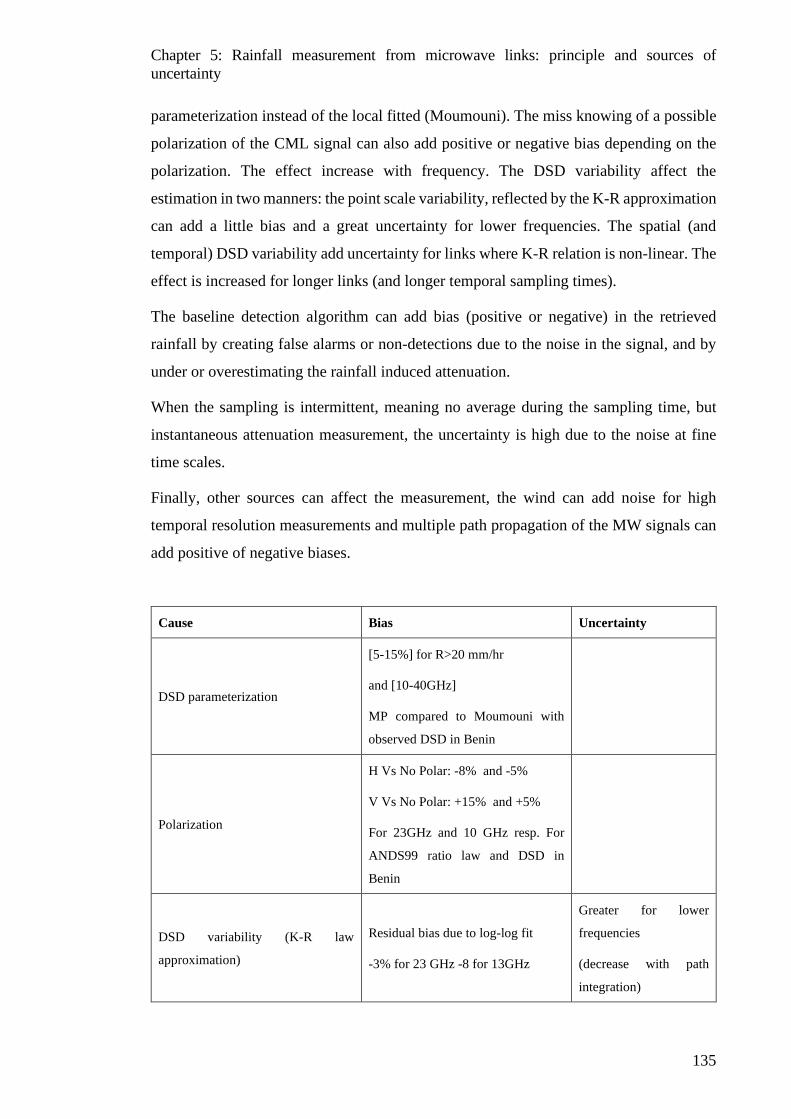
Chapter 5: Rainfall measurement from microwave links: principle and sources of uncertainty
135
parameterization instead of the local fitted (Moumouni). The miss knowing of a possible
polarization of the CML signal can also add positive or negative bias depending on the
polarization. The effect increase with frequency. The DSD variability affect the
estimation in two manners: the point scale variability, reflected by the K-R approximation
can add a little bias and a great uncertainty for lower frequencies. The spatial (and
temporal) DSD variability add uncertainty for links where K-R relation is non-linear. The
effect is increased for longer links (and longer temporal sampling times).
The baseline detection algorithm can add bias (positive or negative) in the retrieved
rainfall by creating false alarms or non-detections due to the noise in the signal, and by
under or overestimating the rainfall induced attenuation.
When the sampling is intermittent, meaning no average during the sampling time, but
instantaneous attenuation measurement, the uncertainty is high due to the noise at fine
time scales.
Finally, other sources can affect the measurement, the wind can add noise for high
temporal resolution measurements and multiple path propagation of the MW signals can
add positive of negative biases.
Cause Bias Uncertainty
DSD parameterization
[5-15%] for R>20 mm/hr
and [10-40GHz]
MP compared to Moumouni with
observed DSD in Benin
Polarization
H Vs No Polar: -8% and -5%
V Vs No Polar: +15% and +5%
For 23GHz and 10 GHz resp. For
ANDS99 ratio law and DSD in
Benin
DSD variability (K-R law
approximation)
Residual bias due to log-log fit
-3% for 23 GHz -8 for 13GHz
Greater for lower
frequencies
(decrease with path
integration)
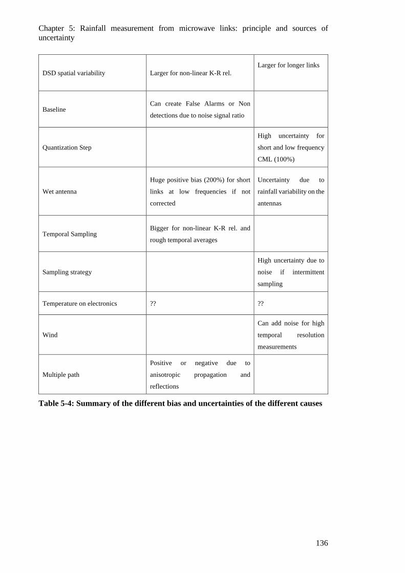
Chapter 5: Rainfall measurement from microwave links: principle and sources of uncertainty
136
DSD spatial variability Larger for non-linear K-R rel. Larger for longer links
Baseline Can create False Alarms or Non
detections due to noise signal ratio
Quantization Step
High uncertainty for
short and low frequency
CML (100%)
Wet antenna
Huge positive bias (200%) for short
links at low frequencies if not
corrected
Uncertainty due to
rainfall variability on the
antennas
Temporal Sampling Bigger for non-linear K-R rel. and
rough temporal averages
Sampling strategy
High uncertainty due to
noise if intermittent
sampling
Temperature on electronics ?? ??
Wind
Can add noise for high
temporal resolution
measurements
Multiple path
Positive or negative due to
anisotropic propagation and
reflections
Table 5-4: Summary of the different bias and uncertainties of the different causes

Chapter 6: Evaluation of CML rainfall measurements in Niamey
137
6 EVALUATION OF CML RAINFALL MEASUREMENTS IN NIAMEY
In the last chapter we have introduced the principle of rainfall measurement with CML
and we have listed and quantified the possible sources of errors and uncertainties
associated. In this chapter we address the evaluation of a CML dataset in Niamey for the
2016-2017 rainy seasons, to retrieve rainfall from attenuation measurements and quantify
the remaining biases depending on the links characteristics. We evaluate three
calibrations with a validation dataset composed by three rain gages.
6.1 Data
Orange has provided two complete rainy seasons (MJJASO) of CML data in Niger for
the years 2016 and 2017. Figure 6-1 show the location of the 92 CML of the city of
Niamey used in the study and the location of three rain gages. Figures 6-2 shows the
availability of CML data per day in Niamey. Some days are missing in the dataset. For
2016, in a two-month period (July-August) only 10-20% of the CML were available.
The frequency of the CML in Niamey are 23 GHz and 18GHz (respectively 85 and 7
links). The distribution of the link lengths in the network is represented in Figure 6-2. The
shortest link measuring 245m and the largest 5.44 km.
The data provided was the average, minimal and maximal transmitted power (Tx) and
received power (Rx) at the time step of 15 minutes. The quantization step is 1dB.
We made a first data quality control based on the correlation of the time series of each
CML with their neighbors (developed in the appendix 3).
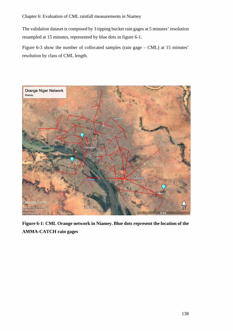
Chapter 6: Evaluation of CML rainfall measurements in Niamey
138
The validation dataset is composed by 3 tipping bucket rain gages at 5 minutes’ resolution
resampled at 15 minutes, represented by blue dots in figure 6-1.
Figure 6-3 show the number of collocated samples (rain gage – CML) at 15 minutes’
resolution by class of CML length.
Figure 6-1: CML Orange network in Niamey. Blue dots represent the location of the
AMMA-CATCH rain gages
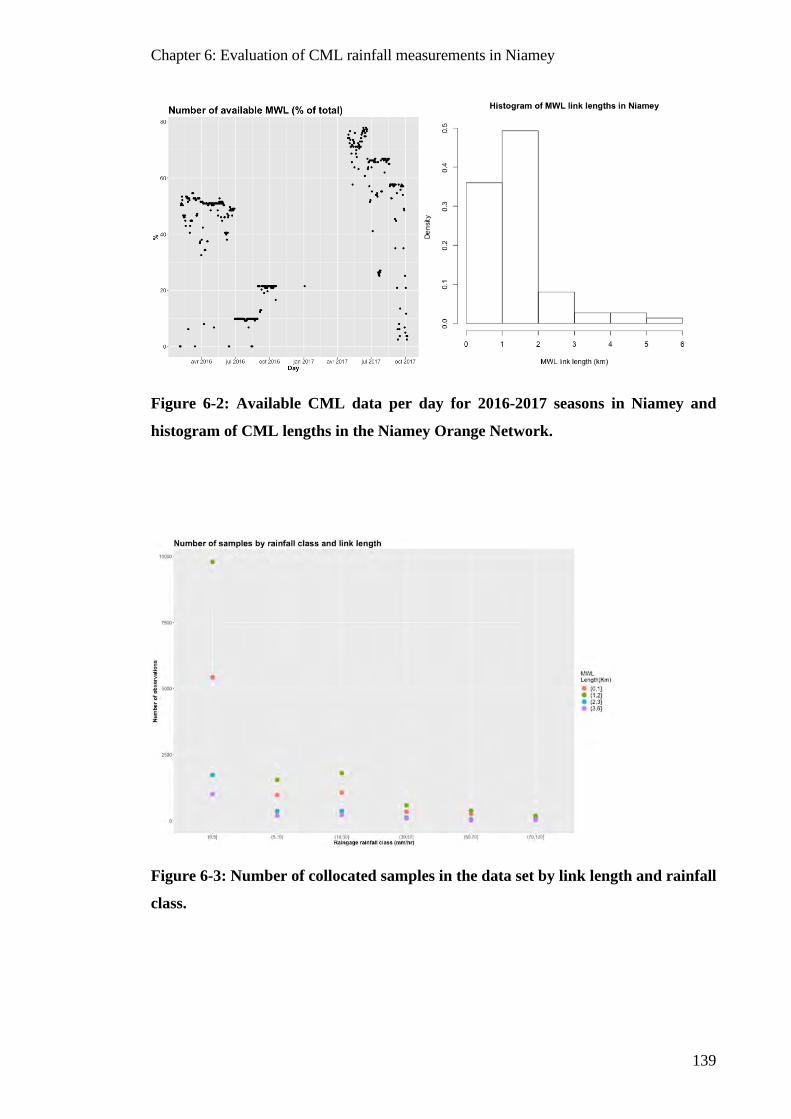
Chapter 6: Evaluation of CML rainfall measurements in Niamey
139
Figure 6-2: Available CML data per day for 2016-2017 seasons in Niamey and
histogram of CML lengths in the Niamey Orange Network.
Figure 6-3: Number of collocated samples in the data set by link length and rainfall
class.
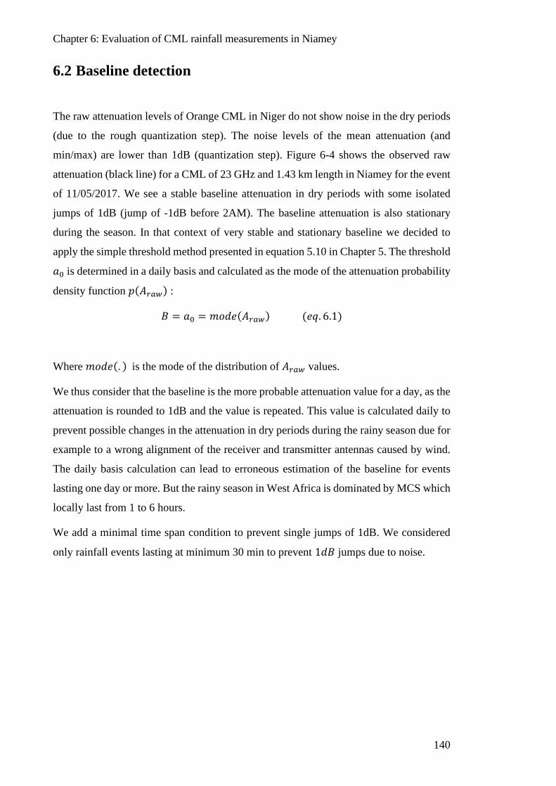
Chapter 6: Evaluation of CML rainfall measurements in Niamey
140
6.2 Baseline detection
The raw attenuation levels of Orange CML in Niger do not show noise in the dry periods
(due to the rough quantization step). The noise levels of the mean attenuation (and
min/max) are lower than 1dB (quantization step). Figure 6-4 shows the observed raw
attenuation (black line) for a CML of 23 GHz and 1.43 km length in Niamey for the event
of 11/05/2017. We see a stable baseline attenuation in dry periods with some isolated
jumps of 1dB (jump of -1dB before 2AM). The baseline attenuation is also stationary
during the season. In that context of very stable and stationary baseline we decided to
apply the simple threshold method presented in equation 5.10 in Chapter 5. The threshold
𝑎𝑎0 is determined in a daily basis and calculated as the mode of the attenuation probability
density function 𝑒𝑒(𝐴𝐴𝑟𝑟𝑎𝑎𝑤𝑤) :
𝑑𝑑 = 𝑎𝑎0 = 𝑐𝑐𝑙𝑙𝑑𝑑𝑃𝑃(𝐴𝐴𝑟𝑟𝑎𝑎𝑤𝑤) (𝑃𝑃𝑒𝑒. 6.1)
Where 𝑐𝑐𝑙𝑙𝑑𝑑𝑃𝑃(. ) is the mode of the distribution of 𝐴𝐴𝑟𝑟𝑎𝑎𝑤𝑤 values.
We thus consider that the baseline is the more probable attenuation value for a day, as the
attenuation is rounded to 1dB and the value is repeated. This value is calculated daily to
prevent possible changes in the attenuation in dry periods during the rainy season due for
example to a wrong alignment of the receiver and transmitter antennas caused by wind.
The daily basis calculation can lead to erroneous estimation of the baseline for events
lasting one day or more. But the rainy season in West Africa is dominated by MCS which
locally last from 1 to 6 hours.
We add a minimal time span condition to prevent single jumps of 1dB. We considered
only rainfall events lasting at minimum 30 min to prevent 1𝑑𝑑𝑑𝑑 jumps due to noise.
Chapter 6: Evaluation of CML rainfall measurements in Niamey
141
Figure 6-4: : Example of raw attenuation and baseline detection for 11/05/2017 event
in Niamey for one CML. The link length is 1.43 km and frequency 23 GHz. The
dotted red line shows the baseline detection for the day. The right Y axis represent
the rainfall rate in [mm/hr]. The max and min attenuation are also show in light
grey. The hyetogram of rainfall at 15 min in the CML has the classical signature of
a convective front (peak at 70 mm/hr) followed by a stratiform trail.
6.3 Rainfall retrieval algorithm, calibration with evaluation against gauges
The objective of this section is to describe the calibration procedure of the CML to
retrieve reliable rainfall accumulations and to quantify the remaining residual biases
depending on the links characteristics. The calibration was done with the comparison of
collocated CML and rain gages data at 15 minutes’ time steps. Three different calibration
where considered, described in the first section. The minimization procedure to retrieve
the model parameters is described in section 6.3.1. Then are showed the residual biases
depending on the links characteristics, followed by the robustness tests of the different
calibrations.
Finally, we show the resulting scatterplots of the retrieved rainfall and the resulting daily
accumulation biases for the 2016 and 2017 seasons in Niamey.
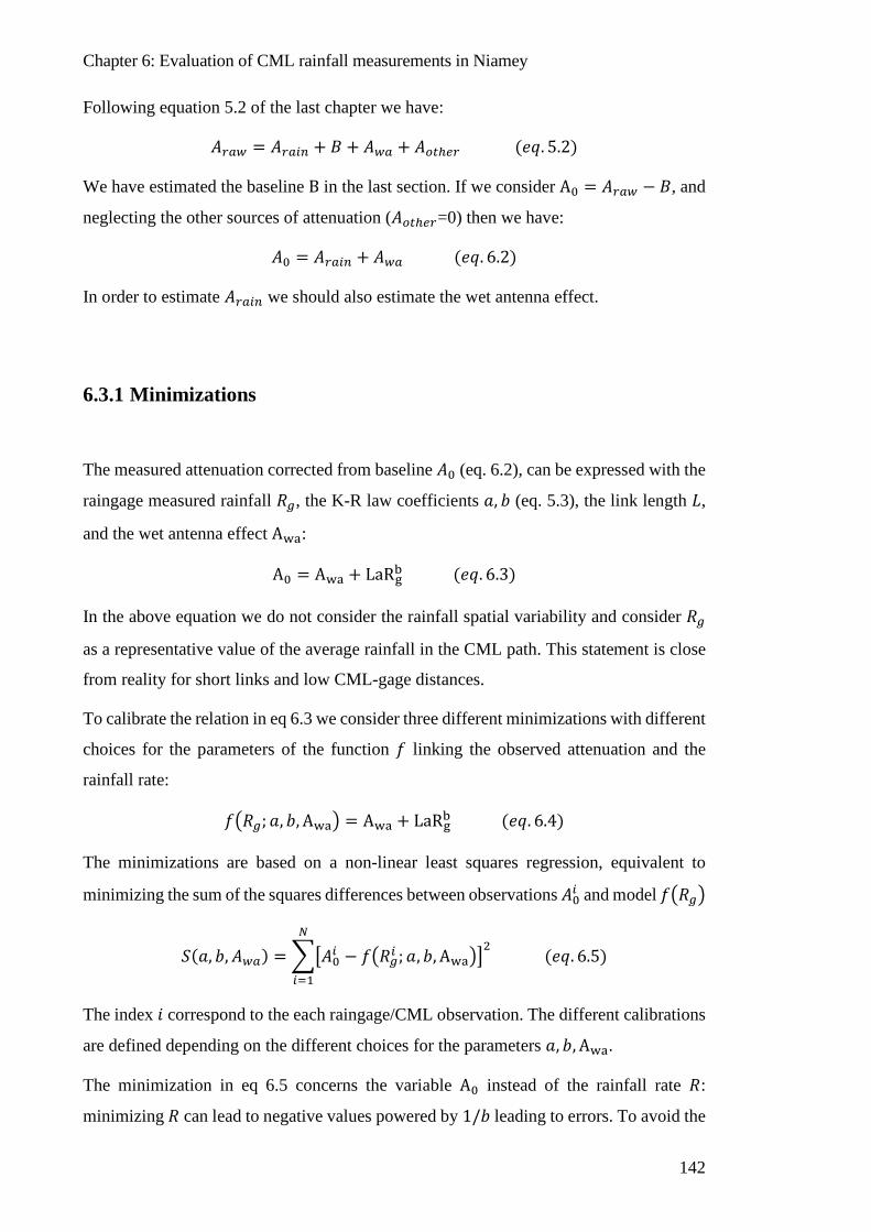
Chapter 6: Evaluation of CML rainfall measurements in Niamey
142
Following equation 5.2 of the last chapter we have:
𝐴𝐴𝑟𝑟𝑎𝑎𝑤𝑤 = 𝐴𝐴𝑟𝑟𝑎𝑎𝑖𝑖𝑛𝑛 + 𝑑𝑑 + 𝐴𝐴𝑤𝑤𝑎𝑎 + 𝐴𝐴𝑜𝑜𝑡𝑡ℎ𝑒𝑒𝑟𝑟 (𝑃𝑃𝑒𝑒. 5.2)
We have estimated the baseline B in the last section. If we consider A0 = 𝐴𝐴𝑟𝑟𝑎𝑎𝑤𝑤 − 𝑑𝑑, and
neglecting the other sources of attenuation (𝐴𝐴𝑜𝑜𝑡𝑡ℎ𝑒𝑒𝑟𝑟=0) then we have:
𝐴𝐴0 = 𝐴𝐴𝑟𝑟𝑎𝑎𝑖𝑖𝑛𝑛 + 𝐴𝐴𝑤𝑤𝑎𝑎 (𝑃𝑃𝑒𝑒. 6.2)
In order to estimate 𝐴𝐴𝑟𝑟𝑎𝑎𝑖𝑖𝑛𝑛 we should also estimate the wet antenna effect.
6.3.1 Minimizations
The measured attenuation corrected from baseline 𝐴𝐴0 (eq. 6.2), can be expressed with the
raingage measured rainfall 𝑅𝑅𝑎𝑎, the K-R law coefficients 𝑎𝑎, 𝑏𝑏 (eq. 5.3), the link length 𝐿𝐿,
and the wet antenna effect Awa:
A0 = Awa + LaRgb (𝑃𝑃𝑒𝑒. 6.3)
In the above equation we do not consider the rainfall spatial variability and consider 𝑅𝑅𝑎𝑎
as a representative value of the average rainfall in the CML path. This statement is close
from reality for short links and low CML-gage distances.
To calibrate the relation in eq 6.3 we consider three different minimizations with different
choices for the parameters of the function 𝑓𝑓 linking the observed attenuation and the
rainfall rate:
𝑓𝑓�𝑅𝑅𝑎𝑎;𝑎𝑎, 𝑏𝑏, Awa� = Awa + LaRgb (𝑃𝑃𝑒𝑒. 6.4)
The minimizations are based on a non-linear least squares regression, equivalent to
minimizing the sum of the squares differences between observations 𝐴𝐴0𝑖𝑖 and model 𝑓𝑓�𝑅𝑅𝑎𝑎�
𝑆𝑆(𝑎𝑎, 𝑏𝑏,𝐴𝐴𝑤𝑤𝑎𝑎) = ��𝐴𝐴0𝑖𝑖 − 𝑓𝑓�𝑅𝑅𝑎𝑎𝑖𝑖 ;𝑎𝑎, 𝑏𝑏, Awa��2
𝑁𝑁
𝑖𝑖=1
(𝑃𝑃𝑒𝑒. 6.5)
The index 𝑖𝑖 correspond to the each raingage/CML observation. The different calibrations
are defined depending on the different choices for the parameters 𝑎𝑎, 𝑏𝑏, Awa.
The minimization in eq 6.5 concerns the variable A0 instead of the rainfall rate 𝑅𝑅:
minimizing 𝑅𝑅 can lead to negative values powered by 1/𝑏𝑏 leading to errors. To avoid the

Chapter 6: Evaluation of CML rainfall measurements in Niamey
143
errors we can filter the dataset for each value of explored Awa resulting in a different
dataset for each calculation of 𝑆𝑆(𝑎𝑎, 𝑏𝑏,𝐴𝐴𝑤𝑤𝑎𝑎). This lead to a non-continuous resulting
function 𝑆𝑆(𝑎𝑎, 𝑏𝑏,𝐴𝐴𝑤𝑤𝑎𝑎). To avoid the issue we decided to minimize the attenuation as 𝑅𝑅𝑎𝑎 >
0, the quantity Rgb can be always calculated.
Calibration 1
In the first calibration we seek the optimal 𝑎𝑎, 𝑏𝑏 coefficients of the K-R law and a constant
value of wet antenna attenuation 𝐴𝐴𝑤𝑤𝑎𝑎 = 𝐶𝐶𝑤𝑤𝑃𝑃 which best explain the observed data. We
aim to find the minima RMSE in a three parameters space [𝑎𝑎, 𝑏𝑏,𝐴𝐴𝑤𝑤𝑎𝑎]. The solution
�𝑎𝑎𝑓𝑓𝑖𝑖𝑡𝑡,𝑏𝑏𝑓𝑓𝑖𝑖𝑡𝑡,𝐴𝐴𝑤𝑤𝑎𝑎𝑓𝑓𝑖𝑖𝑡𝑡� verify:
𝑆𝑆�𝑎𝑎𝑓𝑓𝑖𝑖𝑡𝑡,𝑏𝑏𝑓𝑓𝑖𝑖𝑡𝑡,𝐴𝐴𝑤𝑤𝑎𝑎𝑓𝑓𝑖𝑖𝑡𝑡� = min[𝑆𝑆(𝑎𝑎, 𝑏𝑏,𝐴𝐴𝑤𝑤𝑎𝑎)] (𝑃𝑃𝑒𝑒. 6.6)
Calibration 2:
In the second calibration we consider only a two parameter regression, the constant wet
antenna attenuation: 𝐴𝐴𝑤𝑤𝑎𝑎 = 𝐶𝐶𝑤𝑤𝑃𝑃 and the 𝑎𝑎 parameter of the K-R law. We consider a fixed
𝑏𝑏𝑡𝑡ℎ coefficients of the K-R law corresponding to the obtained from the T-matrix
calculation with the observed DSD in Benin presented in chapter 5.
𝑆𝑆�𝑎𝑎𝑓𝑓𝑖𝑖𝑡𝑡2,𝐴𝐴𝑤𝑤𝑎𝑎𝑓𝑓𝑖𝑖𝑡𝑡2� = ��𝐴𝐴0𝑖𝑖 − 𝑓𝑓�𝑅𝑅𝑎𝑎𝑖𝑖 ;𝑎𝑎𝑓𝑓𝑖𝑖𝑡𝑡2, 𝑏𝑏𝑡𝑡ℎ,𝐴𝐴𝑤𝑤𝑎𝑎
𝑓𝑓𝑖𝑖𝑡𝑡2��2
𝑁𝑁
𝑖𝑖=1
(𝑃𝑃𝑒𝑒. 6.7)
Calibration 3:
In the third calibration we consider a wet antenna attenuation depending on the rainfall
rate (Chap 5, section 4.1.5). We used the parameterization of the water layer covering the
antenna developed by (Leijnse, Uijlenhoet, and Stricker 2008) considering the proposed
parameters and a temperature of 20°C for the calculation of the refractive index of water.
Chapter 6: Evaluation of CML rainfall measurements in Niamey
144
By addition we consider a possible proportional variation of this parameterization due to
the possible different characteristic on the antenna. We considered:
𝐴𝐴𝑤𝑤𝑎𝑎�𝑅𝑅𝑎𝑎� = 𝑙𝑙 ∗ 𝐴𝐴𝑤𝑤𝑎𝑎𝐿𝐿 �𝑅𝑅𝑎𝑎� (𝑃𝑃𝑒𝑒. 6.8)
Where 𝐴𝐴𝑤𝑤𝑎𝑎𝐿𝐿 is the wet antenna model developed in (Leijnse, Uijlenhoet, and Stricker
2008) and a parameter 𝑙𝑙 to fit to the data. We consider the theoretical [𝑎𝑎𝑡𝑡ℎ, 𝑏𝑏𝑡𝑡ℎ] found
with the observed DSD in Benin and T-matrix calculation. Calibration 3 is a one
parameter minimization (parameter 𝑙𝑙 in eq. 6.9) :
𝑆𝑆(𝑙𝑙) = ��𝐴𝐴0𝑖𝑖 − 𝑓𝑓�𝑅𝑅𝑎𝑎;𝑎𝑎𝑡𝑡ℎ , 𝑏𝑏𝑡𝑡ℎ,𝑙𝑙 ∗ 𝐴𝐴𝑤𝑤𝑎𝑎𝐿𝐿 ��2
𝑁𝑁
𝑖𝑖=1
(𝑃𝑃𝑒𝑒. 6.9)
Calib 3bis:
The calibration 3 is a one parameter minimization. The parameter 𝑙𝑙 to fit to the data, is a
multiplicative parameter of the wet antenna model 𝐴𝐴𝑤𝑤𝑎𝑎𝐿𝐿 , of [Leijnse et al. 2008]. As the
wet antenna attenuation 𝐴𝐴𝑤𝑤𝑎𝑎𝐿𝐿 (𝑅𝑅) depends on the rainfall rate, we need 𝑅𝑅 to calculate it.
In calib. 3 we use the raingage rainfall to estimate 𝐴𝐴𝑤𝑤𝑎𝑎𝐿𝐿 �𝑅𝑅𝑎𝑎�. In calibration 3bis we do not
use the raingage rainfall. For each time step we solve the equation presented in (eq. 6.10).
6.3.2 Minimization procedure
The non-linear least squares minimization was done with a build-in function in R using
the Gauss-Newton algorithm. The different parameters were estimated for both 18GHz
and 23GHz datasets. Figure 6-5 shows the optimum parameters (green dot) found in the
parameters space for the calibration 1 at 23 GHz. The RMSE (minimization criteria) and
the global bias are shown. The black crosses in the figure show the location in the
parameters space where no bias is found (bias<0.1 mm/hr). The retrieved values are
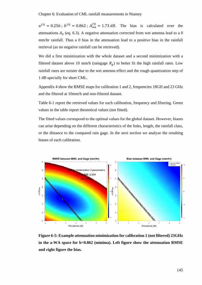
Chapter 6: Evaluation of CML rainfall measurements in Niamey
145
𝑎𝑎𝑓𝑓𝑖𝑖𝑡𝑡 = 0.256 ; 𝑏𝑏𝑓𝑓𝑖𝑖𝑡𝑡 = 0.862 ; 𝐴𝐴𝑤𝑤𝑎𝑎𝑓𝑓𝑖𝑖𝑡𝑡 = 1.73 𝑑𝑑𝑑𝑑. The bias is calculated over the
attenuations 𝐴𝐴0 (eq. 6.3). A negative attenuation corrected from wet antenna lead to a 0
mm/hr rainfall. Thus a 0 bias in the attenuation lead to a positive bias in the rainfall
retrieval (as no negative rainfall can be retrieved).
We did a first minimization with the whole dataset and a second minimization with a
filtered dataset above 10 mm/h (raingage 𝑅𝑅𝑎𝑎) to better fit the high rainfall rates. Low
rainfall rates are noisier due to the wet antenna effect and the rough quantization step of
1 dB specially for short CML.
Appendix 4 show the RMSE maps for calibration 1 and 2, frequencies 18GH and 23 GHz
and the filtered at 10mm/h and non-filtered dataset.
Table 6-1 report the retrieved values for each calibration, frequency and filtering. Green
values in the table report theoretical values (not fitted).
The fitted values correspond to the optimal values for the global dataset. However, biases
can arise depending on the different characteristics of the links, length, the rainfall class,
or the distance to the compared rain gage. In the next section we analyze the resulting
biases of each calibration.
Figure 6-5: Example attenuation minimization for calibration 1 (not filtered) 23GHz
in the a-WA space for b=0.862 (minima). Left figure show the attenuation RMSE
and right figure the bias.

Chapter 6: Evaluation of CML rainfall measurements in Niamey
146
Cal 1 Cal 2 Cal 3 Cal. 1
>10mm/h
Cal 2
>10mm/h
Cal. 3
>10mm/h
a-
23GHz 0.256 0.128 0.123 0.056 0.109 0.123
b-
23GHz 0.862 1.028 1.028 1.178 1.028 1.028
Wet Ant.
23 GHz
(dB)
1.73 2.05 0.36*𝐴𝐴𝑤𝑤𝑎𝑎𝐿𝐿 3.92 3.40 0.32*𝐴𝐴𝑤𝑤𝑎𝑎𝐿𝐿
RMSE
(dB)
23GHz
2.594 2.613 2.577 4.273 4.283 4.331
Nobs
23GHz 23318 23318 23318 4962 4962 4962
a-
18GHz 0.052 0.064 0.072 0.005 0.056 0.072
b-
18GHz 1.103 1.052 1.052 1.581 1.052 1.052
Wet Ant.
18 GHz
(dB)
2.03 1.94 0.31*𝐴𝐴𝑤𝑤𝑎𝑎𝐿𝐿 5.17 3.39 0.21*𝐴𝐴𝑤𝑤𝑎𝑎𝐿𝐿
RMSE
(dB)
18GHz
3.059 3.061 3.129 5.401 5.580 5.786
Nobs
18GHz 3372 3372 3372 721 721 721
Table 6-1:Parameters fitted to the observed attenuation for the three calibrations,
filtered above 10mm/hr and not filtered. The minimal RMSE on attenuation and the
Chapter 6: Evaluation of CML rainfall measurements in Niamey
147
number of observations are reported. The green values correspond to theoretical a
prior values (not fitted).
6.3.3 Residual bias of the calibrations
A global minimum RMSE and zero bias in the fitted optimal attenuations of the three
calibrations leads to non-zero bias in the retrieved rainfall due to the positive condition
of the retrieved rainfall. Also compensations can occur between the different CML
lengths and rainfall rates. Figures 6-6 show the average bias by calibration depicted by
the raingage rainfall class and CML length. The three bottom figures correspond to the
three calibrations with a fitting dataset filtered above 10 mm/h (to best fit high rain rates).
The biases are calculated for the entire dataset including R<10 mm/h. The horizontal
black line represents the global bias.
We observe that the average biases are high for short links and increase with rainfall rate
class. The calibration 3 (considering a wet antenna depending on the rainfall rate) correct
some of the bias of short links compromising long links (underestimation). The fitted
calibrations filtering the small rainfalls decrease the biases in high rainfall but also
globally in small rainfall rates. That is due to higher values of retrieved wet antenna
attenuation for filtered datasets: the higher values of retrieved wet antenna attenuation
(table 6-1) lead to lower bias on small rainfall due to the increasing cases where the
corrected attenuation become negative and thus a zero rainfall is retrieved. The squeeze
of the small rainfall lead to a global bias closer to zero, as the relative weight in the dataset
of small rainfalls is higher.
Figure 6-7 present the relative biases in % of the raingage rainfall rate average (per rainfall
class). The horizontal black lines show the remaining relative global bias. For calibration
3 the relative bias of small rainfall is high compared to the other calibrations.
Figure 6-8 present the bias decomposition in non-detection bias and hit bias per rainfall
class. In the original dataset only hits are used. Due to the wet antenna correction some
attenuations become negative leading to zero rainfall introducing non-detection biases.
As said before, the retrieved wet antenna attenuation for filtered dataset are greater,
increasing the non-detection bias for calibrations 1 and 2. The calibration 3 considering a
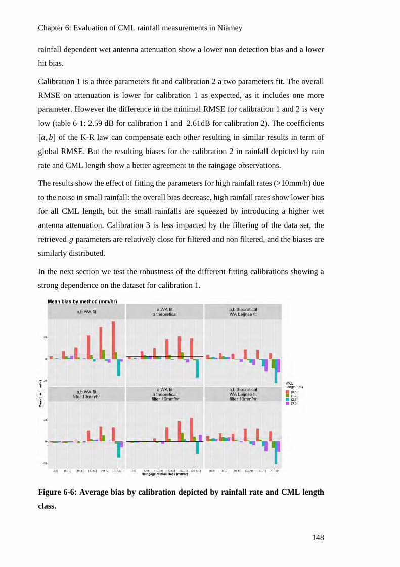
Chapter 6: Evaluation of CML rainfall measurements in Niamey
148
rainfall dependent wet antenna attenuation show a lower non detection bias and a lower
hit bias.
Calibration 1 is a three parameters fit and calibration 2 a two parameters fit. The overall
RMSE on attenuation is lower for calibration 1 as expected, as it includes one more
parameter. However the difference in the minimal RMSE for calibration 1 and 2 is very
low (table 6-1: 2.59 dB for calibration 1 and 2.61dB for calibration 2). The coefficients
[𝑎𝑎, 𝑏𝑏] of the K-R law can compensate each other resulting in similar results in term of
global RMSE. But the resulting biases for the calibration 2 in rainfall depicted by rain
rate and CML length show a better agreement to the raingage observations.
The results show the effect of fitting the parameters for high rainfall rates (>10mm/h) due
to the noise in small rainfall: the overall bias decrease, high rainfall rates show lower bias
for all CML length, but the small rainfalls are squeezed by introducing a higher wet
antenna attenuation. Calibration 3 is less impacted by the filtering of the data set, the
retrieved 𝑙𝑙 parameters are relatively close for filtered and non filtered, and the biases are
similarly distributed.
In the next section we test the robustness of the different fitting calibrations showing a
strong dependence on the dataset for calibration 1.
Figure 6-6: Average bias by calibration depicted by rainfall rate and CML length
class.
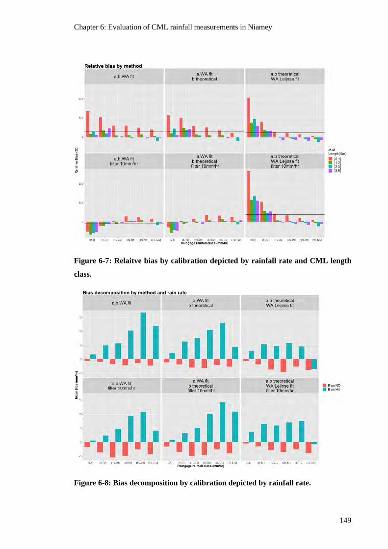
Chapter 6: Evaluation of CML rainfall measurements in Niamey
149
Figure 6-7: Relaitve bias by calibration depicted by rainfall rate and CML length
class.
Figure 6-8: Bias decomposition by calibration depicted by rainfall rate.
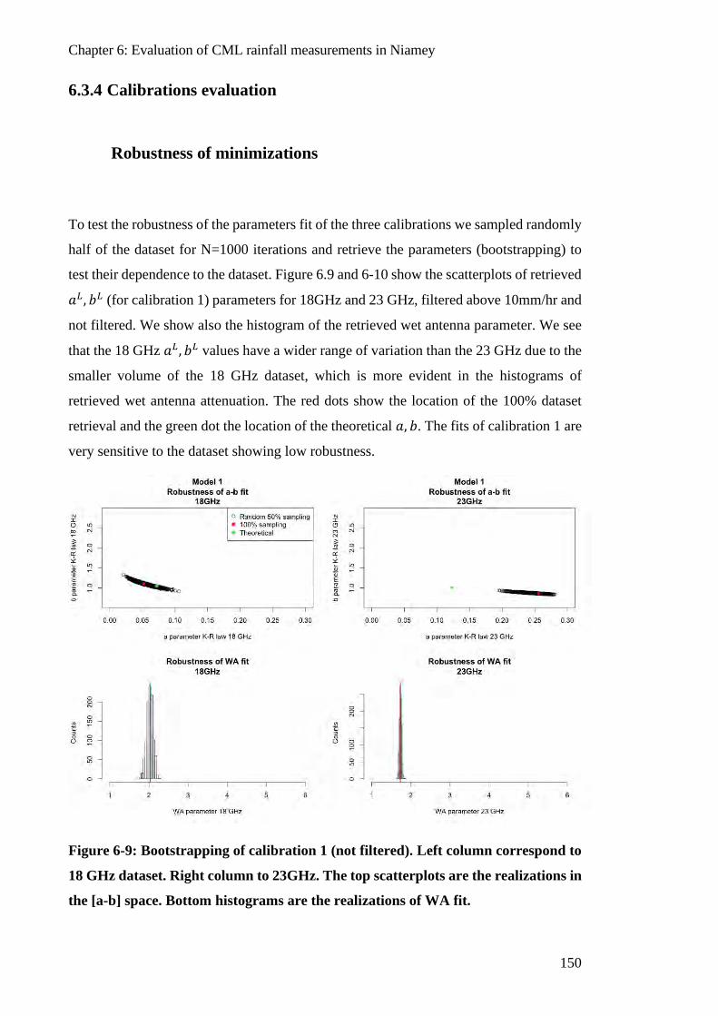
Chapter 6: Evaluation of CML rainfall measurements in Niamey
150
6.3.4 Calibrations evaluation
Robustness of minimizations
To test the robustness of the parameters fit of the three calibrations we sampled randomly
half of the dataset for N=1000 iterations and retrieve the parameters (bootstrapping) to
test their dependence to the dataset. Figure 6.9 and 6-10 show the scatterplots of retrieved
𝑎𝑎𝐿𝐿 , 𝑏𝑏𝐿𝐿 (for calibration 1) parameters for 18GHz and 23 GHz, filtered above 10mm/hr and
not filtered. We show also the histogram of the retrieved wet antenna parameter. We see
that the 18 GHz 𝑎𝑎𝐿𝐿 , 𝑏𝑏𝐿𝐿 values have a wider range of variation than the 23 GHz due to the
smaller volume of the 18 GHz dataset, which is more evident in the histograms of
retrieved wet antenna attenuation. The red dots show the location of the 100% dataset
retrieval and the green dot the location of the theoretical 𝑎𝑎, 𝑏𝑏. The fits of calibration 1 are
very sensitive to the dataset showing low robustness.
Figure 6-9: Bootstrapping of calibration 1 (not filtered). Left column correspond to
18 GHz dataset. Right column to 23GHz. The top scatterplots are the realizations in
the [a-b] space. Bottom histograms are the realizations of WA fit.

Chapter 6: Evaluation of CML rainfall measurements in Niamey
151
Figure 6-10: Bootstrapping of calibration 1 (R>10mm/h). Left column correspond
to 18 GHz dataset. Right column to 23GHz. The top scatterplots are the realizations
in the [a-b] space. Bottom histograms are the realizations of WA fit.
Figure 6-11 and 6-12 show the same fitting procedure for 1000 resampling of the dataset
for the calibration 2. Black dots on the scatterplot represent each iteration of the
minimization in the wet antenna and 𝑎𝑎 coefficient parameter space. We observe a lesser
spread of 𝑎𝑎 parameter in calibration 2 compared to calibration 1 due to the fixed value of
𝑏𝑏: in calibration 1 the compensation of 𝑎𝑎 and 𝑏𝑏 made the fit more sensitive to the dataset,
as a range of values become equivalent in terms of minimal RMSE. Also the wet antenna
attenuation has a narrower spread. The difference in spread between 18 GHz and 23GHz
are due to the lesser number of observations for 18GHz (as seen for calibration 1). The
vertical green line shows the theoretical 𝑎𝑎𝑡𝑡ℎ which falls into the dots cloud.
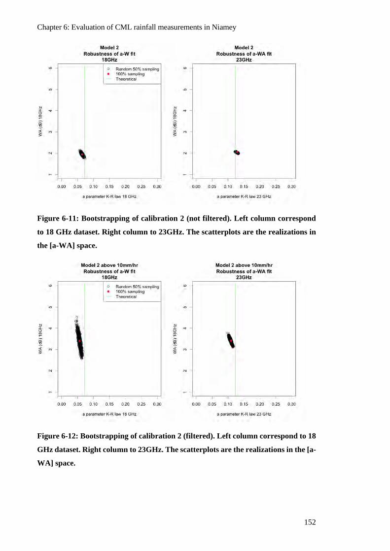
Chapter 6: Evaluation of CML rainfall measurements in Niamey
152
Figure 6-11: Bootstrapping of calibration 2 (not filtered). Left column correspond
to 18 GHz dataset. Right column to 23GHz. The scatterplots are the realizations in
the [a-WA] space.
Figure 6-12: Bootstrapping of calibration 2 (filtered). Left column correspond to 18
GHz dataset. Right column to 23GHz. The scatterplots are the realizations in the [a-
WA] space.
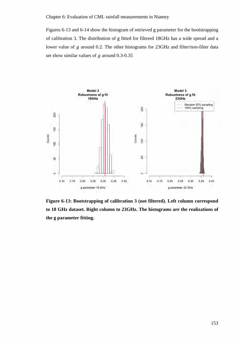
Chapter 6: Evaluation of CML rainfall measurements in Niamey
153
Figures 6-13 and 6-14 show the histogram of retrieved g parameter for the bootstrapping
of calibration 3. The distribution of g fitted for filtered 18GHz has a wide spread and a
lower value of 𝑙𝑙 around 0.2. The other histograms for 23GHz and filter/non-filter data
set show similar values of 𝑙𝑙 around 0.3-0.35
Figure 6-13: Bootstrapping of calibration 3 (not filtered). Left column correspond
to 18 GHz dataset. Right column to 23GHz. The histograms are the realizations of
the g parameter fitting.
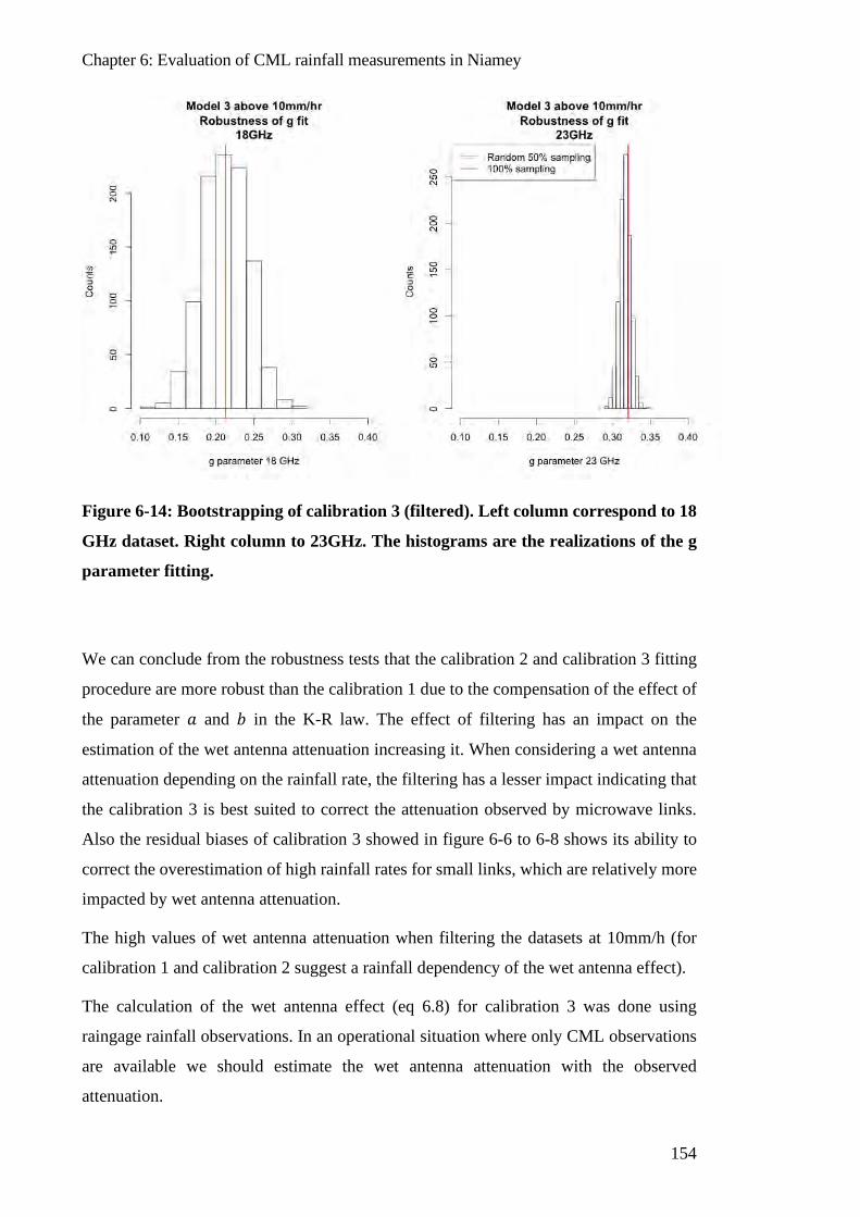
Chapter 6: Evaluation of CML rainfall measurements in Niamey
154
Figure 6-14: Bootstrapping of calibration 3 (filtered). Left column correspond to 18
GHz dataset. Right column to 23GHz. The histograms are the realizations of the g
parameter fitting.
We can conclude from the robustness tests that the calibration 2 and calibration 3 fitting
procedure are more robust than the calibration 1 due to the compensation of the effect of
the parameter 𝑎𝑎 and 𝑏𝑏 in the K-R law. The effect of filtering has an impact on the
estimation of the wet antenna attenuation increasing it. When considering a wet antenna
attenuation depending on the rainfall rate, the filtering has a lesser impact indicating that
the calibration 3 is best suited to correct the attenuation observed by microwave links.
Also the residual biases of calibration 3 showed in figure 6-6 to 6-8 shows its ability to
correct the overestimation of high rainfall rates for small links, which are relatively more
impacted by wet antenna attenuation.
The high values of wet antenna attenuation when filtering the datasets at 10mm/h (for
calibration 1 and calibration 2 suggest a rainfall dependency of the wet antenna effect).
The calculation of the wet antenna effect (eq 6.8) for calibration 3 was done using
raingage rainfall observations. In an operational situation where only CML observations
are available we should estimate the wet antenna attenuation with the observed
attenuation.

Chapter 6: Evaluation of CML rainfall measurements in Niamey
155
In the next section we address the impact of using calibration 3 with only the available
attenuation (not the observed rainfall by the raingage).
Calibration 3bis calculation of wet antenna with observed
attenuation
Considering no rain gage observation of rainfall, the rainfall retrieval from observed CML
attenuation needs to solve in 𝑅𝑅 the following equation for each observation:
A0 − 2𝑙𝑙𝐴𝐴𝑤𝑤𝑎𝑎𝐿𝐿 (𝑅𝑅) − La𝑡𝑡ℎ𝑅𝑅𝑜𝑜𝑡𝑡ℎ = 0 (𝑃𝑃𝑒𝑒. 6.10)
Where A0 is the observed attenuation, 𝐴𝐴𝑤𝑤𝑎𝑎𝐿𝐿 is the wet antenna effect depending on rainfall
as described in (Leijnse et al 2008), 𝐿𝐿 the link length, 𝑙𝑙 the retrieved parameter and
[a𝑡𝑡ℎ, 𝑏𝑏𝑡𝑡ℎ] the theoretical parameters of K-R law. The equation 6.10 does not have an
analytical solution. The solution is found by finding the zero of the left hand side of the
6.10 equation in a given interval (the numerical solution is found using a common R
function at a precision of 10−4 ).
Figure 6-15 show the relative biases of calibration 3 rainfall retrieval solving equation
6.10 (fitted with filtered rainfall) for each couple observation. The retrieved rainfall
without using the raingage rainfall show higher biases than those retrieved using raingage
observations. Using only the observed attenuation add a bias on the results compared to
the wet antenna attenuation estimated with the ground rainfall. The black line in figure 6-
15 showing the global bias is higher than 50%. That indicates an underestimation of the
𝑙𝑙 parameter.
To better estimate a correct value of 𝑙𝑙 we calculated the global bias of the resulting
rainfall solving equation 6.10 for each observation for different 𝑙𝑙 in the range [0.3,1] by
steps of 0.05.
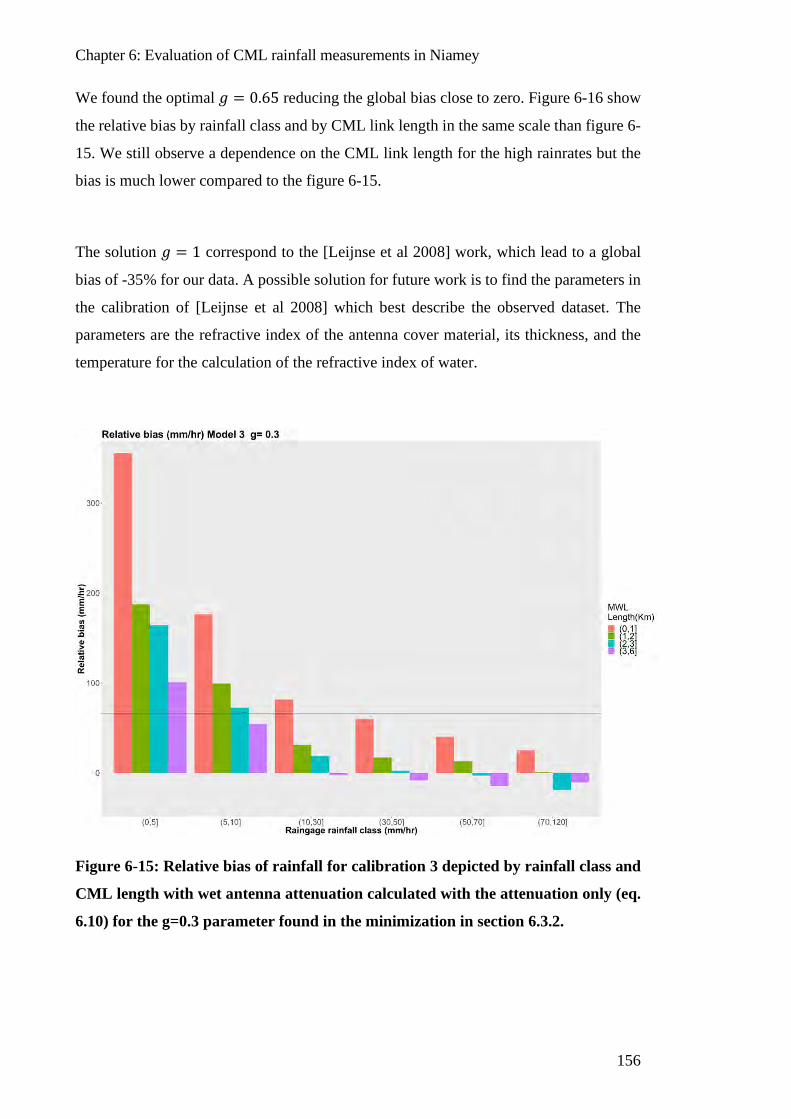
Chapter 6: Evaluation of CML rainfall measurements in Niamey
156
We found the optimal 𝑙𝑙 = 0.65 reducing the global bias close to zero. Figure 6-16 show
the relative bias by rainfall class and by CML link length in the same scale than figure 6-
15. We still observe a dependence on the CML link length for the high rainrates but the
bias is much lower compared to the figure 6-15.
The solution 𝑙𝑙 = 1 correspond to the [Leijnse et al 2008] work, which lead to a global
bias of -35% for our data. A possible solution for future work is to find the parameters in
the calibration of [Leijnse et al 2008] which best describe the observed dataset. The
parameters are the refractive index of the antenna cover material, its thickness, and the
temperature for the calculation of the refractive index of water.
Figure 6-15: Relative bias of rainfall for calibration 3 depicted by rainfall class and
CML length with wet antenna attenuation calculated with the attenuation only (eq.
6.10) for the g=0.3 parameter found in the minimization in section 6.3.2.
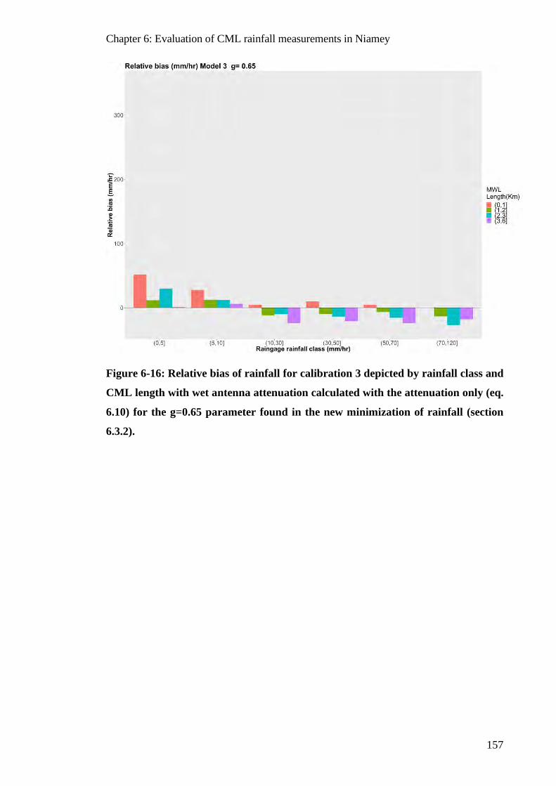
Chapter 6: Evaluation of CML rainfall measurements in Niamey
157
Figure 6-16: Relative bias of rainfall for calibration 3 depicted by rainfall class and
CML length with wet antenna attenuation calculated with the attenuation only (eq.
6.10) for the g=0.65 parameter found in the new minimization of rainfall (section
6.3.2).

Chapter 6: Evaluation of CML rainfall measurements in Niamey
158
Figure 6-17: : Comparison of the different calibrations of wet antenna attenuation
(for both antennas)
Figure 6-17 show the resulting wet antenna attenuation calibrations fitted to the data in
the calibration. The red lines shows the constant value for calibration 1, the blue line the
constant value for calibration 2. Dashed lines show the fitted values for the filtered
datasets. Green line is the wet antenna calculated using the calibration in [Leijnse et al.
2008] and the black line the retrieved calibration (g = 0.65). The filtered dataset shows
higher values of the wet antenna suggesting the dependency to rainfall of the wet antenna
attenuation. We observe also that the original wet antenna calibration of [Leijnse et al.
2008] does not falls into the optimal parameters found.
In the next section we show the resulting scatterplot at 15 minutes colocalisations.
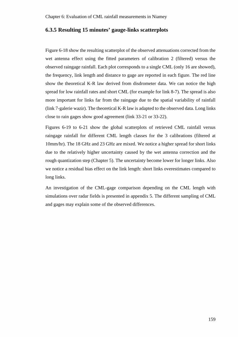
Chapter 6: Evaluation of CML rainfall measurements in Niamey
159
6.3.5 Resulting 15 minutes’ gauge-links scatterplots
Figure 6-18 show the resulting scatterplot of the observed attenuations corrected from the
wet antenna effect using the fitted parameters of calibration 2 (filtered) versus the
observed raingage rainfall. Each plot corresponds to a single CML (only 16 are showed),
the frequency, link length and distance to gage are reported in each figure. The red line
show the theoretical K-R law derived from disdrometer data. We can notice the high
spread for low rainfall rates and short CML (for example for link 8-7). The spread is also
more important for links far from the raingage due to the spatial variability of rainfall
(link 7-galerie wazir). The theoretical K-R law is adapted to the observed data. Long links
close to rain gages show good agreement (link 33-21 or 33-22).
Figures 6-19 to 6-21 show the global scatterplots of retrieved CML rainfall versus
raingage rainfall for different CML length classes for the 3 calibrations (filtered at
10mm/hr). The 18 GHz and 23 GHz are mixed. We notice a higher spread for short links
due to the relatively higher uncertainty caused by the wet antenna correction and the
rough quantization step (Chapter 5). The uncertainty become lower for longer links. Also
we notice a residual bias effect on the link length: short links overestimates compared to
long links.
An investigation of the CML-gage comparison depending on the CML length with
simulations over radar fields is presented in appendix 5. The different sampling of CML
and gages may explain some of the observed differences.
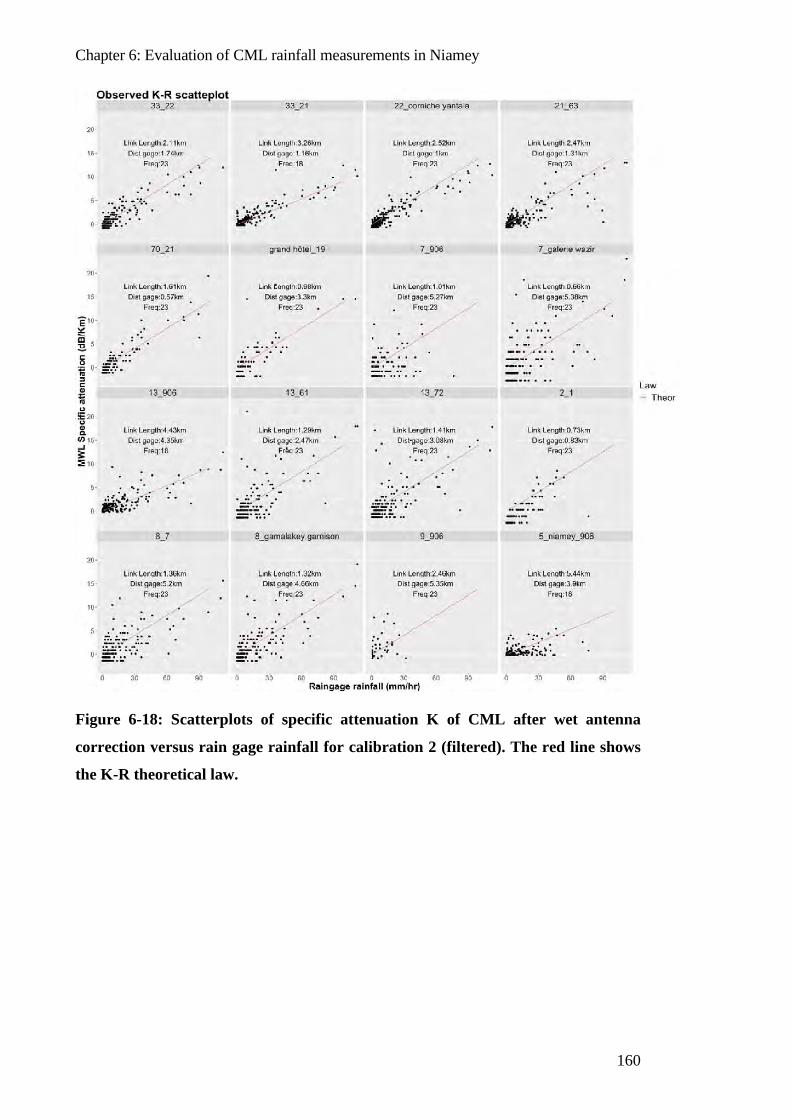
Chapter 6: Evaluation of CML rainfall measurements in Niamey
160
Figure 6-18: Scatterplots of specific attenuation K of CML after wet antenna
correction versus rain gage rainfall for calibration 2 (filtered). The red line shows
the K-R theoretical law.
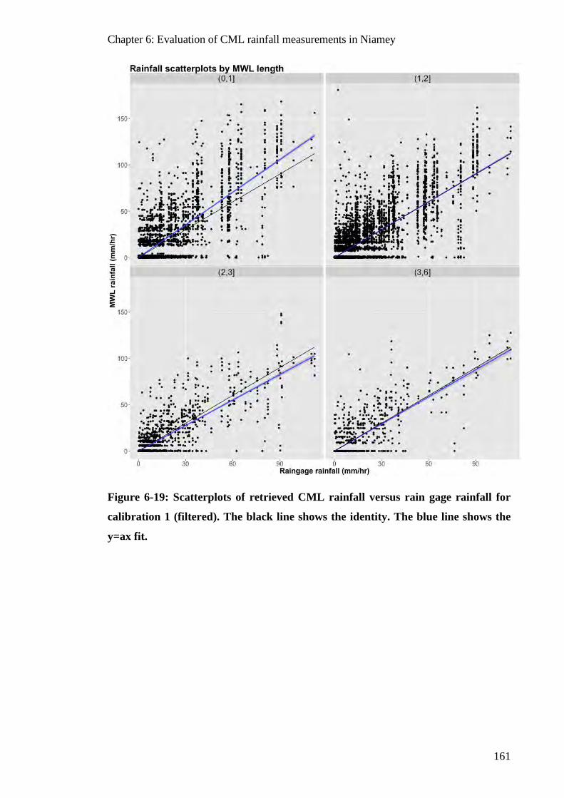
Chapter 6: Evaluation of CML rainfall measurements in Niamey
161
Figure 6-19: Scatterplots of retrieved CML rainfall versus rain gage rainfall for
calibration 1 (filtered). The black line shows the identity. The blue line shows the
y=ax fit.
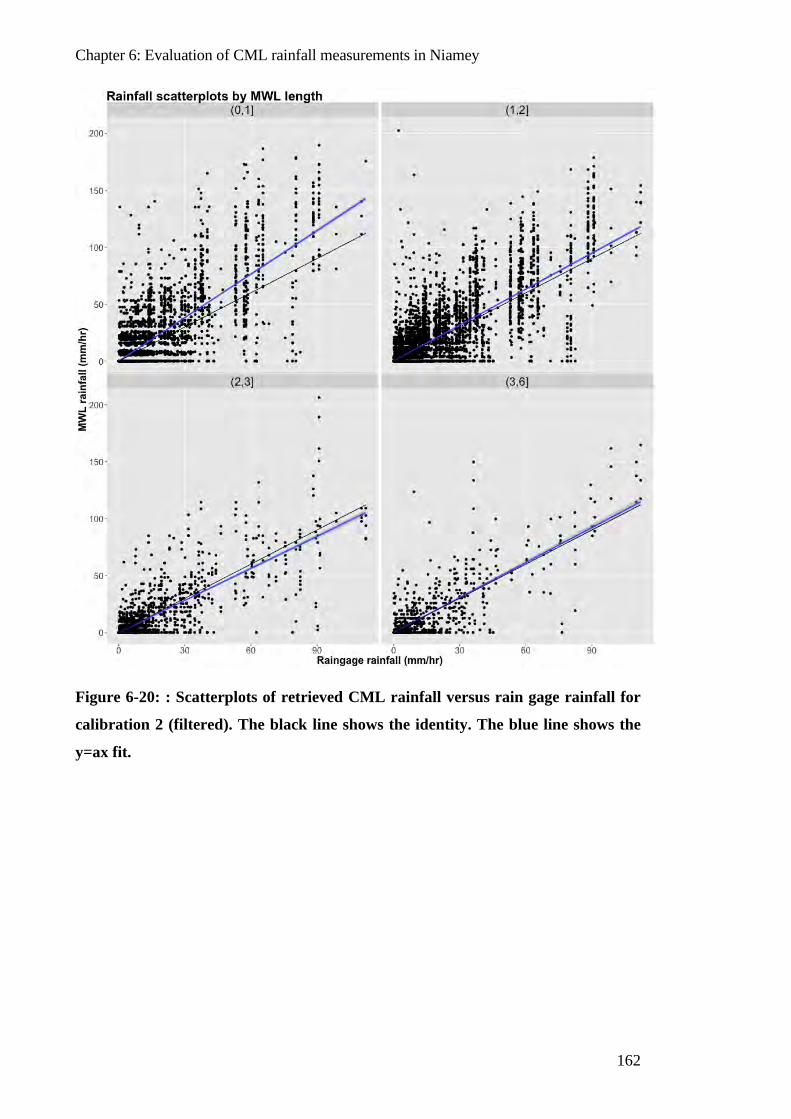
Chapter 6: Evaluation of CML rainfall measurements in Niamey
162
Figure 6-20: : Scatterplots of retrieved CML rainfall versus rain gage rainfall for
calibration 2 (filtered). The black line shows the identity. The blue line shows the
y=ax fit.
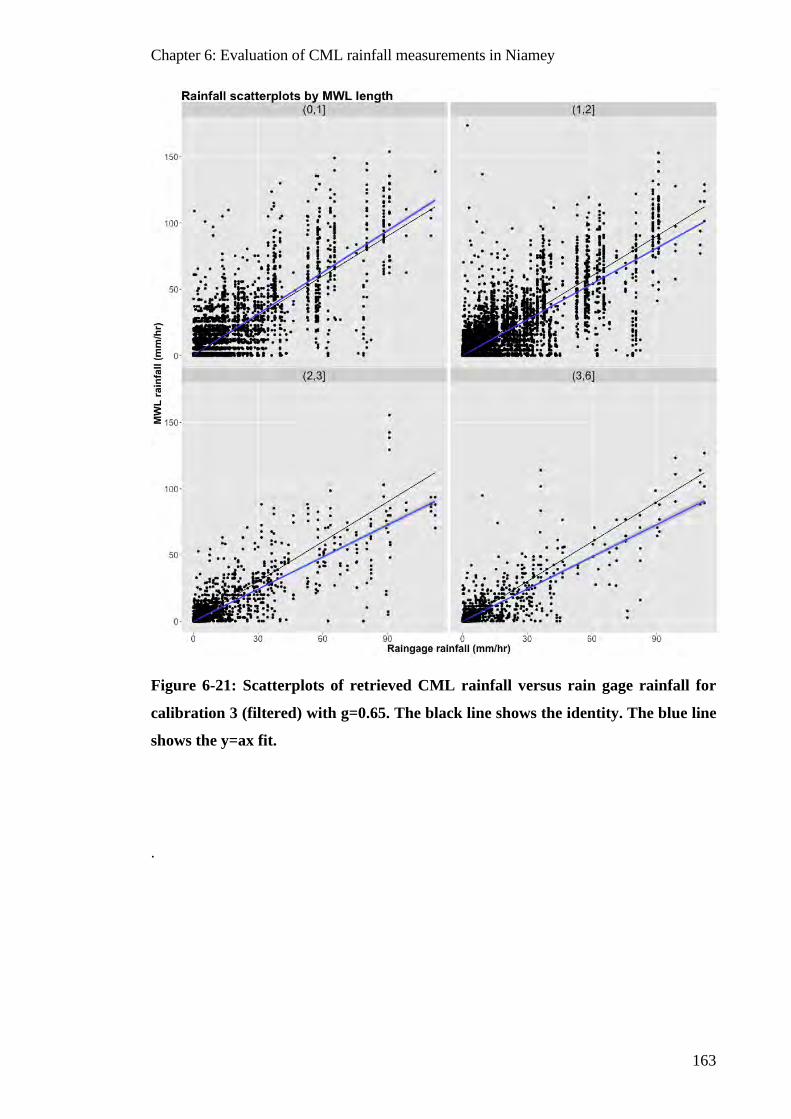
Chapter 6: Evaluation of CML rainfall measurements in Niamey
163
Figure 6-21: Scatterplots of retrieved CML rainfall versus rain gage rainfall for
calibration 3 (filtered) with g=0.65. The black line shows the identity. The blue line
shows the y=ax fit.
.
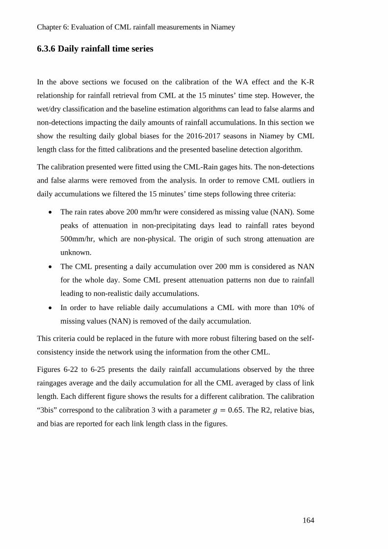
Chapter 6: Evaluation of CML rainfall measurements in Niamey
164
6.3.6 Daily rainfall time series
In the above sections we focused on the calibration of the WA effect and the K-R
relationship for rainfall retrieval from CML at the 15 minutes’ time step. However, the
wet/dry classification and the baseline estimation algorithms can lead to false alarms and
non-detections impacting the daily amounts of rainfall accumulations. In this section we
show the resulting daily global biases for the 2016-2017 seasons in Niamey by CML
length class for the fitted calibrations and the presented baseline detection algorithm.
The calibration presented were fitted using the CML-Rain gages hits. The non-detections
and false alarms were removed from the analysis. In order to remove CML outliers in
daily accumulations we filtered the 15 minutes’ time steps following three criteria:
• The rain rates above 200 mm/hr were considered as missing value (NAN). Some
peaks of attenuation in non-precipitating days lead to rainfall rates beyond
500mm/hr, which are non-physical. The origin of such strong attenuation are
unknown.
• The CML presenting a daily accumulation over 200 mm is considered as NAN
for the whole day. Some CML present attenuation patterns non due to rainfall
leading to non-realistic daily accumulations.
• In order to have reliable daily accumulations a CML with more than 10% of
missing values (NAN) is removed of the daily accumulation.
This criteria could be replaced in the future with more robust filtering based on the self-
consistency inside the network using the information from the other CML.
Figures 6-22 to 6-25 presents the daily rainfall accumulations observed by the three
raingages average and the daily accumulation for all the CML averaged by class of link
length. Each different figure shows the results for a different calibration. The calibration
“3bis” correspond to the calibration 3 with a parameter 𝑙𝑙 = 0.65. The R2, relative bias,
and bias are reported for each link length class in the figures.
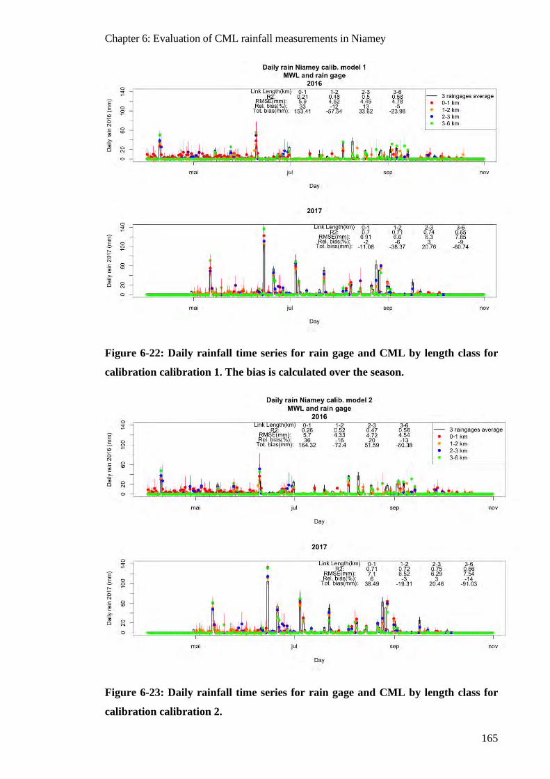
Chapter 6: Evaluation of CML rainfall measurements in Niamey
165
Figure 6-22: Daily rainfall time series for rain gage and CML by length class for
calibration calibration 1. The bias is calculated over the season.
Figure 6-23: Daily rainfall time series for rain gage and CML by length class for
calibration calibration 2.

Chapter 6: Evaluation of CML rainfall measurements in Niamey
166
The daily accumulations were calculated by applying the baseline detection described in
section 6.2 to the whole CML network and by applying the different calibration
calibrations described with the fitted parameter in table 6-1 (for the filtered dataset).
Some links presents anomalous attenuation patterns not explained by rainfall leading to
strong values of retrieved rainfall. We remove the values of retrieved rainfall at 15 min
higher than 200 mm/hr. No additional criteria were used to improve the retrieved rainfall
in Niamey: the internal coherence of the dataset can be used to improve the detection of
rainfall events by considering the detection of neighbor CML to remove false alarms.
We can see in figure 6-24 in the begging of season 2016 many false alarms for the [0-
1km] CML degrading the scores for short links. Those false alarms are generated by few
links detecting huge rainfall rate (higher than 100mm/hr) and can be removed using the
information on the other CML of the network. For the three methods the scores are better
for the 2017 season as more data were available and the presence well detected strong
rainfall events improve the scores.
For calibration calibration 1 and 2 (figure 6-22 and 6-23) the relative biases are low and
around zero specially for the year 2017 in which the relative bias is between [-14%,6%]
with respect the yearly amount. For the strong events the uncertainty bars linked to the
variability of the rainfall in the zone usually overlaps.
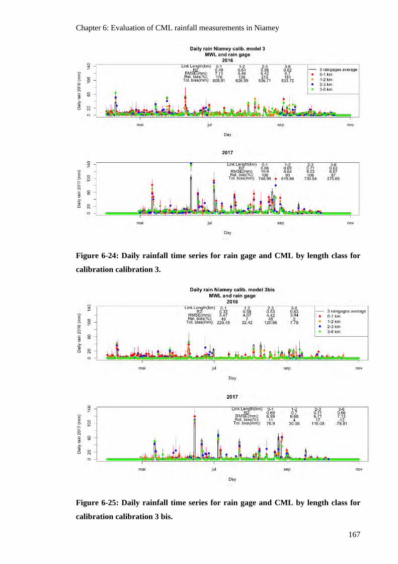
Chapter 6: Evaluation of CML rainfall measurements in Niamey
167
Figure 6-24: Daily rainfall time series for rain gage and CML by length class for
calibration calibration 3.
Figure 6-25: Daily rainfall time series for rain gage and CML by length class for
calibration calibration 3 bis.
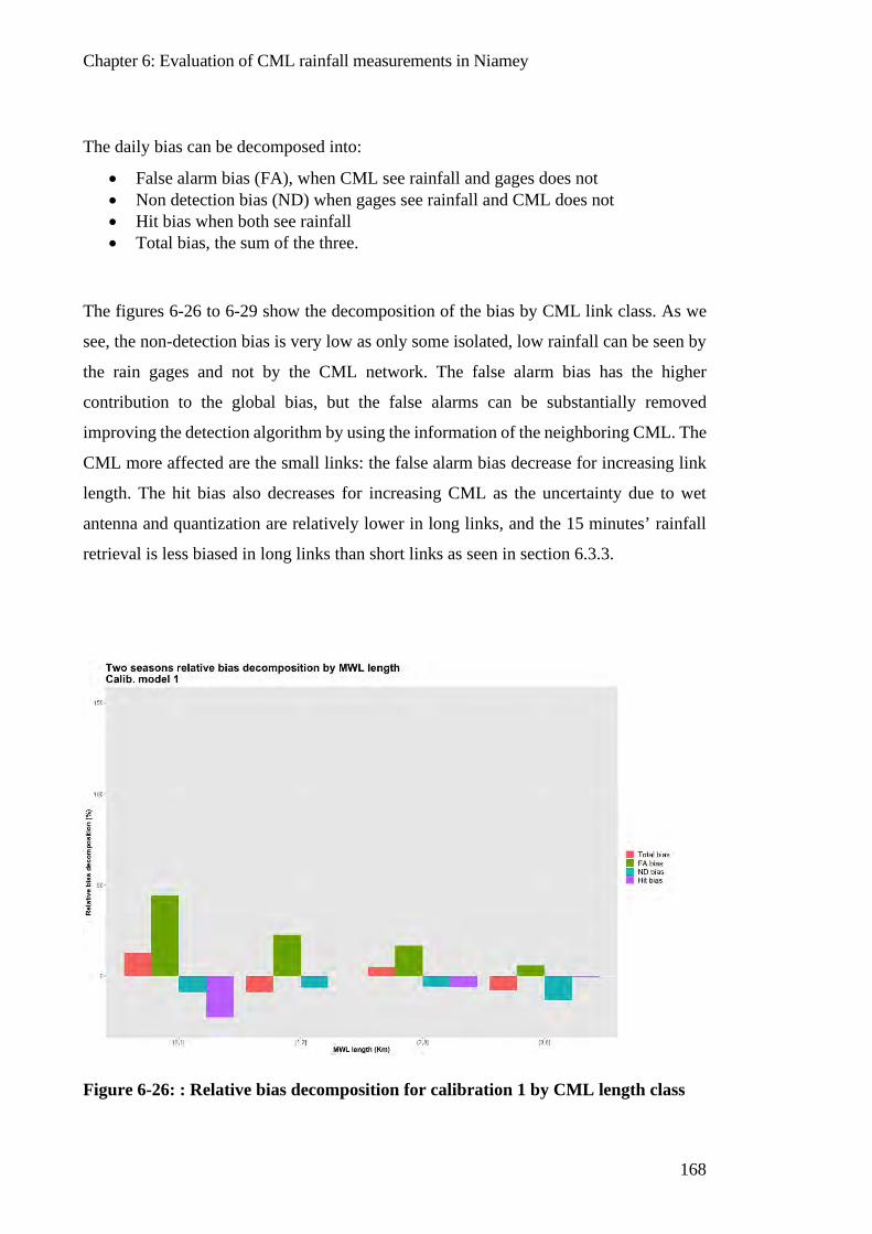
Chapter 6: Evaluation of CML rainfall measurements in Niamey
168
The daily bias can be decomposed into:
• False alarm bias (FA), when CML see rainfall and gages does not • Non detection bias (ND) when gages see rainfall and CML does not • Hit bias when both see rainfall • Total bias, the sum of the three.
The figures 6-26 to 6-29 show the decomposition of the bias by CML link class. As we
see, the non-detection bias is very low as only some isolated, low rainfall can be seen by
the rain gages and not by the CML network. The false alarm bias has the higher
contribution to the global bias, but the false alarms can be substantially removed
improving the detection algorithm by using the information of the neighboring CML. The
CML more affected are the small links: the false alarm bias decrease for increasing link
length. The hit bias also decreases for increasing CML as the uncertainty due to wet
antenna and quantization are relatively lower in long links, and the 15 minutes’ rainfall
retrieval is less biased in long links than short links as seen in section 6.3.3.
Figure 6-26: : Relative bias decomposition for calibration 1 by CML length class
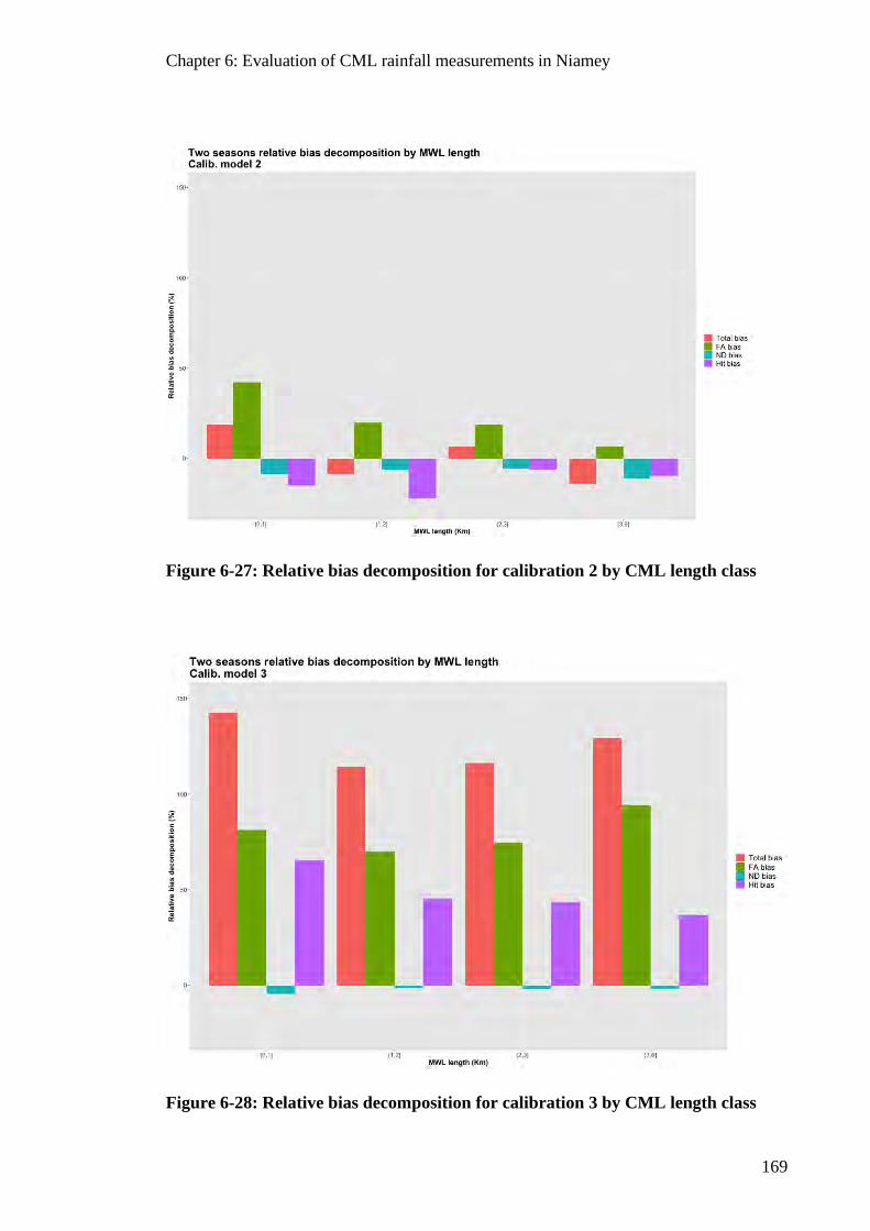
Chapter 6: Evaluation of CML rainfall measurements in Niamey
169
Figure 6-27: Relative bias decomposition for calibration 2 by CML length class
Figure 6-28: Relative bias decomposition for calibration 3 by CML length class
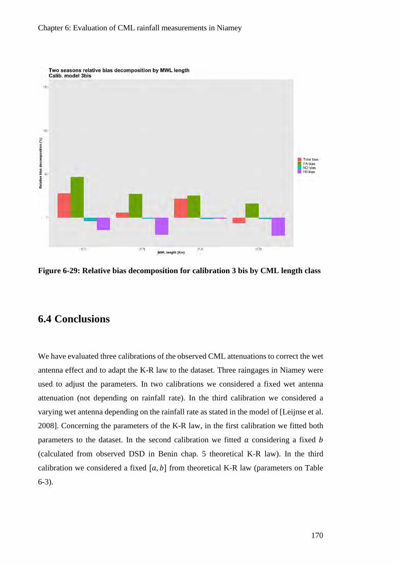
Chapter 6: Evaluation of CML rainfall measurements in Niamey
170
Figure 6-29: Relative bias decomposition for calibration 3 bis by CML length class
6.4 Conclusions
We have evaluated three calibrations of the observed CML attenuations to correct the wet
antenna effect and to adapt the K-R law to the dataset. Three raingages in Niamey were
used to adjust the parameters. In two calibrations we considered a fixed wet antenna
attenuation (not depending on rainfall rate). In the third calibration we considered a
varying wet antenna depending on the rainfall rate as stated in the model of [Leijnse et al.
2008]. Concerning the parameters of the K-R law, in the first calibration we fitted both
parameters to the dataset. In the second calibration we fitted 𝑎𝑎 considering a fixed 𝑏𝑏
(calculated from observed DSD in Benin chap. 5 theoretical K-R law). In the third
calibration we considered a fixed [𝑎𝑎, 𝑏𝑏] from theoretical K-R law (parameters on Table
6-3).
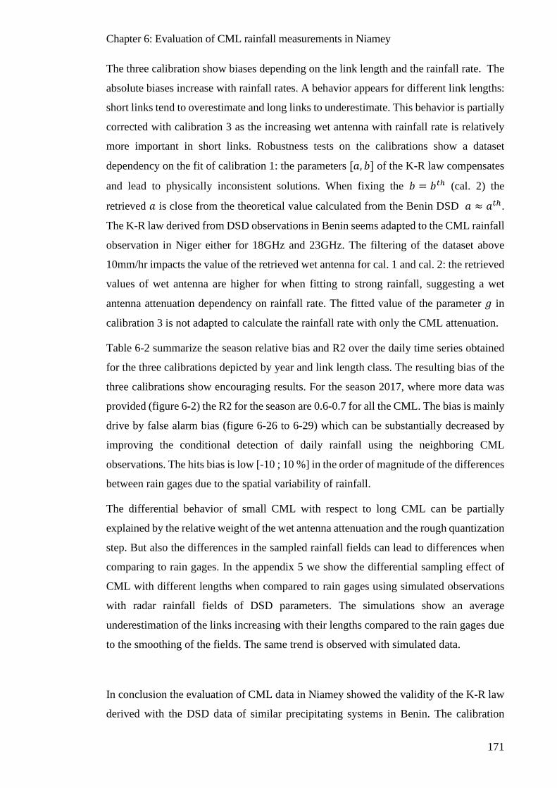
Chapter 6: Evaluation of CML rainfall measurements in Niamey
171
The three calibration show biases depending on the link length and the rainfall rate. The
absolute biases increase with rainfall rates. A behavior appears for different link lengths:
short links tend to overestimate and long links to underestimate. This behavior is partially
corrected with calibration 3 as the increasing wet antenna with rainfall rate is relatively
more important in short links. Robustness tests on the calibrations show a dataset
dependency on the fit of calibration 1: the parameters [𝑎𝑎, 𝑏𝑏] of the K-R law compensates
and lead to physically inconsistent solutions. When fixing the 𝑏𝑏 = 𝑏𝑏𝑡𝑡ℎ (cal. 2) the
retrieved 𝑎𝑎 is close from the theoretical value calculated from the Benin DSD 𝑎𝑎 ≈ 𝑎𝑎𝑡𝑡ℎ.
The K-R law derived from DSD observations in Benin seems adapted to the CML rainfall
observation in Niger either for 18GHz and 23GHz. The filtering of the dataset above
10mm/hr impacts the value of the retrieved wet antenna for cal. 1 and cal. 2: the retrieved
values of wet antenna are higher for when fitting to strong rainfall, suggesting a wet
antenna attenuation dependency on rainfall rate. The fitted value of the parameter 𝑙𝑙 in
calibration 3 is not adapted to calculate the rainfall rate with only the CML attenuation.
Table 6-2 summarize the season relative bias and R2 over the daily time series obtained
for the three calibrations depicted by year and link length class. The resulting bias of the
three calibrations show encouraging results. For the season 2017, where more data was
provided (figure 6-2) the R2 for the season are 0.6-0.7 for all the CML. The bias is mainly
drive by false alarm bias (figure 6-26 to 6-29) which can be substantially decreased by
improving the conditional detection of daily rainfall using the neighboring CML
observations. The hits bias is low [-10 ; 10 %] in the order of magnitude of the differences
between rain gages due to the spatial variability of rainfall.
The differential behavior of small CML with respect to long CML can be partially
explained by the relative weight of the wet antenna attenuation and the rough quantization
step. But also the differences in the sampled rainfall fields can lead to differences when
comparing to rain gages. In the appendix 5 we show the differential sampling effect of
CML with different lengths when compared to rain gages using simulated observations
with radar rainfall fields of DSD parameters. The simulations show an average
underestimation of the links increasing with their lengths compared to the rain gages due
to the smoothing of the fields. The same trend is observed with simulated data.
In conclusion the evaluation of CML data in Niamey showed the validity of the K-R law
derived with the DSD data of similar precipitating systems in Benin. The calibration
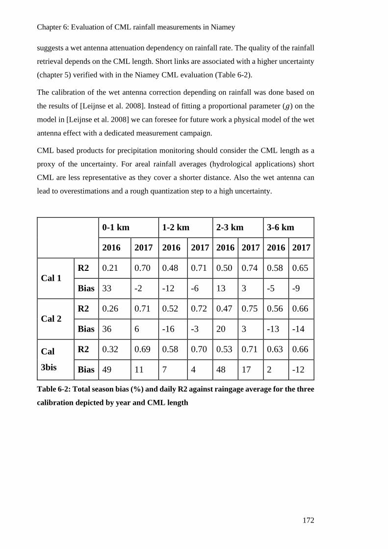
Chapter 6: Evaluation of CML rainfall measurements in Niamey
172
suggests a wet antenna attenuation dependency on rainfall rate. The quality of the rainfall
retrieval depends on the CML length. Short links are associated with a higher uncertainty
(chapter 5) verified with in the Niamey CML evaluation (Table 6-2).
The calibration of the wet antenna correction depending on rainfall was done based on
the results of [Leijnse et al. 2008]. Instead of fitting a proportional parameter (𝑙𝑙) on the
model in [Leijnse et al. 2008] we can foresee for future work a physical model of the wet
antenna effect with a dedicated measurement campaign.
CML based products for precipitation monitoring should consider the CML length as a
proxy of the uncertainty. For areal rainfall averages (hydrological applications) short
CML are less representative as they cover a shorter distance. Also the wet antenna can
lead to overestimations and a rough quantization step to a high uncertainty.
0-1 km 1-2 km 2-3 km 3-6 km
2016 2017 2016 2017 2016 2017 2016 2017
Cal 1 R2 0.21 0.70 0.48 0.71 0.50 0.74 0.58 0.65
Bias 33 -2 -12 -6 13 3 -5 -9
Cal 2 R2 0.26 0.71 0.52 0.72 0.47 0.75 0.56 0.66
Bias 36 6 -16 -3 20 3 -13 -14
Cal
3bis
R2 0.32 0.69 0.58 0.70 0.53 0.71 0.63 0.66
Bias 49 11 7 4 48 17 2 -12
Table 6-2: Total season bias (%) and daily R2 against raingage average for the three
calibration depicted by year and CML length
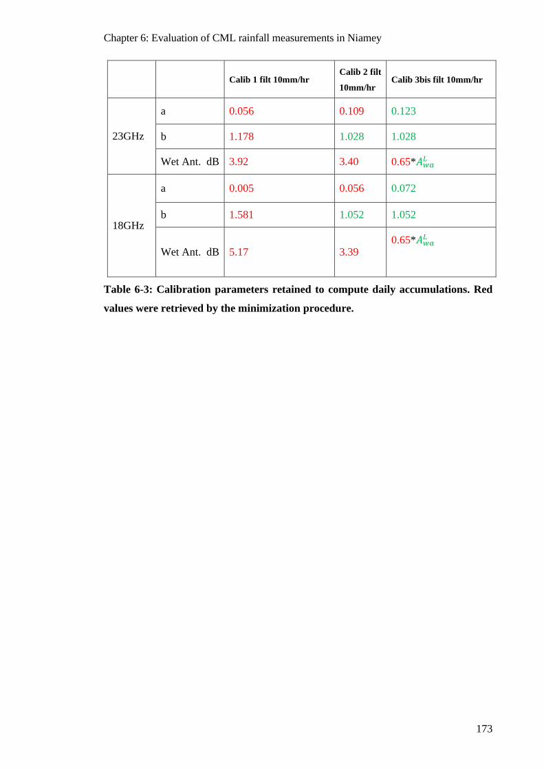
Chapter 6: Evaluation of CML rainfall measurements in Niamey
173
Calib 1 filt 10mm/hr Calib 2 filt
10mm/hr Calib 3bis filt 10mm/hr
23GHz
a 0.056 0.109 0.123
b 1.178 1.028 1.028
Wet Ant. dB 3.92 3.40 0.65*𝐴𝐴𝑤𝑤𝑎𝑎𝐿𝐿
18GHz
a 0.005 0.056 0.072
b 1.581 1.052 1.052
Wet Ant. dB 5.17 3.39 0.65*𝐴𝐴𝑤𝑤𝑎𝑎𝐿𝐿
Table 6-3: Calibration parameters retained to compute daily accumulations. Red
values were retrieved by the minimization procedure.

Chapter 6: Evaluation of CML rainfall measurements in Niamey
174
Chapter 7: Rain maps from CML estimations: comparison of methods including a neural network approach
175
7 RAIN MAPS FROM CML ESTIMATIONS: COMPARISON OF METHODS INCLUDING A NEURAL NETWORK APPROACH
In the last chapter we have adjusted the estimation algorithm and evaluated the rain rate
retrieval based on the CMLs from the dense network available in Niamey. For many
applications we needed rain maps rather than the retrieval at individual links.
The objective of this prospective chapter is to compare some of the existing mapping
techniques commonly used for CML interpolation and a new method based on a neural
network (NN). Given the limited CML data set available, the radar rain fields (presented
in part 1 of this manuscript) are used as a proxy to simulate synthetic CML data used for
training the NN and evaluate the results. This simulation work is complemented with
some (limited) evaluation with CML data and rain gauge.
7.1 Introduction
Different techniques have been proposed for mapping (or interpolating) rainfall fields
from CML data. A simple solution is to consider the rainfall seen by the CML as a rain
gauge in its path center (Overeem, Leijnse, and Uijlenhoet 2011; Overeem, Leijnse, and
Uijlenhoet 2016; Rios Gaona et al. 2015) and to interpolate rainfall as is usually done for
rain gages (for example kriging or inverse distance interpolation). For sparse networks in
Chapter 7: Rain maps from CML estimations: comparison of methods including a neural network approach
176
large scales this can be a simple solution if the links information is not redundant (link
path lengths lower than distance between links or link lengths small compared to the
domain).
In urban contexts the CML density is usually high, offering a rich sampling of rainfall.
Microwave links represent a very interesting solution to rainfall monitoring at city scale
as pointed out by (Upton et al. 2005). In such scale other techniques are needed to extract
the full information from the network. If we consider CML as rain gages in its center, two
CML with the same path center and different length can have different values of detected
rainfall leading to contradictory information at the same point. More complex algorithms
have been applied to extract the spatial information provided by CML networks: the
combined localization of the different CML paths gives us information about the spatial
distribution of rainfall. In the works (Zohidov et al. 2014; D’Amico, Manzoni, and Solazzi
2016; Roy, Gishkori, and Leus 2014) the authors use the framework of inversion theory
to retrieve rain fields. Another technique developed in (Zinevich, Alpert, and Messer
2008) is based on a tomography with a variable grid size. In the cited work the solution
is constrained by the CML observed rain and an imposed spatial correlation of the
solution. Both techniques show a reliable pattern detection of the rainfall when compared
to a reference field. But both techniques have an ill definition of the observation scale as
they project the CML network (with variables path lengths) into a grid of variable size.
That leads to rainfall fields with a non-realistic distribution of rainfall rates. Another
limitation of this techniques is the unrealistic patterns of rain at the boundaries of the
mapping zone were less information is provided.
Rainfall has a strong spatial and temporal variability and the probability density function
of rainfall rates depends on the observation scale. By construction CML networks have
various links lengths and geometries depending on the local constrains and network
optimization from the telecom company. Combining observations from links of different
length implies combining different observation scales of rainfall, as discussed in chapter
6.
Rainfall from CML has a minimal detectable rainfall Rmin which depends on the
frequency f, the link length L and the quantization step Δa of the attenuation provided by
the telecom company, as discussed in chapter 5. The minimal detectable rainfall Rmin for
a quantization step of attenuation Δa was defined in chapter 5 as:
Chapter 7: Rain maps from CML estimations: comparison of methods including a neural network approach
177
Rmin = �Δa
2aL�1/b
(𝑃𝑃𝑒𝑒. 7.1)
Figure 5-11 of chapter 5 shows the minimal detectable rain as a function of the link length
for different frequencies at Δa =1 dB quantization step. Short links and a rough
quantization step lead to non-detections of rainfall.
Figure 7-1 shows an example of the “Gruyere” effect in observation of rainfall from CML
in Niamey, Niger: the sinks of rainfall rate come from non-detections of short links due
to a rough quantization step (grey lines). The CML network detect rainfall at some links
located very close (~100m) to the CML who does not detect rainfall.
A possible solution to this inhomogeneity in the sensitivity of the observations can be
filtering links depending on its frequency and length to ensure a threshold of a common
Rmin. But this solution leads to a loss of valuable local information brought by short links.
In addition, short links are more probable to detect high rain rates related to local
convective cells.
To retrieve a reasonable value of Rlink we could use the information of the surrounding
links as the rainfall is spatially correlated.
In this chapter we propose an alternative method using a multi-layer neural network
(hereafter NN) trained with radar data to retrieve maps from CML information. Multilayer
feedforward neural networks are universal approximators and an efficient method to find
a function linking a set of input data to an output set of variables (Haykin 1994). They are
particularly good estimating non-linear and non-continuous functions.
The idea is to retrieve the spatial properties of rainfall (as seen by a radar) in a context of
limited (and uncertain) spatial information. The simulated CML training dataset is
constructed with radar rain fields in order to simulate real observations of attenuation with
a quantization step. The radar fields are then used as the reference field to feed the
backpropagation algorithm for the NN learning.
In section 7.2 we describe the three methods of mapping compared in this work: the NN,
the kriging interpolation ant the tomography. In section 7.3 we describe the radar dataset
and the construction of the virtual CML observations to train the NN. In section 7.4 we
show the validation of the three methods compared to the reference simulated data. In

Chapter 7: Rain maps from CML estimations: comparison of methods including a neural network approach
178
section 7.5 we show a cross-validation study in Niamey with the 2016-2017 Orange data
calibrated in chapter 6. Finally, in section 7.6 we discuss the results and conclude.
Figure 7-1: Zoom on the Niamey CML network. The bars represent the location of
the CML and their color the Rainfall estimation (without wet antenna correction)
for the 25/05/2016 event at 11h30 UTM. Some CML are black as they do not detect
a jump in attenuation greater than 1dB. The window size is 3x3 Km.
7.2 Rain mapping from links: common methods
7.2.1 Simple kriging interpolation
Simple kriging is a geostatistical interpolation technique to estimate fields of a random
function (spatially correlated) from a limited sample of point measurements in space. The
difference with other simpler techniques (inverse distance interpolation, or Thiessen
polygons) is that the weights ωi of the lineal combination of the input values Vi are given
by an estimated space covariance. The estimated value V�j at point uj is:
V�j�uj� = �ωiVi(ui) with �ωi = 1i
(𝑃𝑃𝑒𝑒. 7.3)i
Chapter 7: Rain maps from CML estimations: comparison of methods including a neural network approach
179
Where , V�j is a linear combination of the sample of observations Vi at locations ui. The
weights ωi depends on a space covariance model which can be estimated with the data.
An experimental semivariogram γ�(d) is usually estimated with the sampled data:
γ�(d) =1
2N(d) �[Vi(ui) − Vi(ui + d)]2
N(d)
i=1
(𝑃𝑃𝑒𝑒. 7.4)
Where N(d) is the number of pairs of data locations at a distance d. The semivariogram
is a function of the distance d. It can also be a function of the direction if we consider
anisotropic fields. When considering rainfall accumulations, the variogram varies for
different aggregation periods: for longer periods the correlation distance increase. The
empirical semivariogram is usually fitted to a model.
Kriging estimation is unbiased, and is the best linear estimator of a field if the assumptions
holds: it implies that the variogram (or spatial covariance) is well estimated, and the field
has stationary properties.
In our study the stationary assumption is not well satisfied as the squall line rainfall has
two distinct zones of convective heavy rainfall with different spatial properties compared
to the stratiform tail. Figure 7-2 shows the empirical variogram calculated from 40 PPI
(1° elevation) of X-port radar rain fields for the squall line event of 03/07/2012. We see
two distinct behaviors corresponding to the convective scale (~10km) and the stratiform
scale (~50km). More sophisticated kriging techniques exist to take into account different
rainfall regimes. In this prospective study we limit to simple kriging with a unique
variogram modeled as a double exponential (red curve in figure 7-2). We fitted the
empirical variogram with a double exponential: a first exponential with correlation
distance of 4 km and a second exponential with a 42km correlation distance.
To apply the simple kriging to the CML network we consider the average rainfall rate
through the link path as a punctual rainfall rate at its path center. This assumption implies
that we lose the information of path length and direction. The benefits of the method are
a small computing time and straightforward implementation.
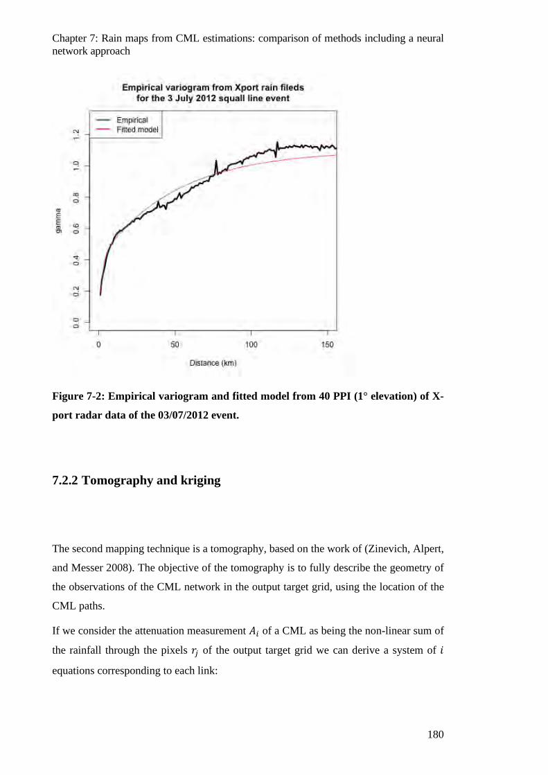
Chapter 7: Rain maps from CML estimations: comparison of methods including a neural network approach
180
Figure 7-2: Empirical variogram and fitted model from 40 PPI (1° elevation) of X-
port radar data of the 03/07/2012 event.
7.2.2 Tomography and kriging
The second mapping technique is a tomography, based on the work of (Zinevich, Alpert,
and Messer 2008). The objective of the tomography is to fully describe the geometry of
the observations of the CML network in the output target grid, using the location of the
CML paths.
If we consider the attenuation measurement 𝐴𝐴𝑖𝑖 of a CML as being the non-linear sum of
the rainfall through the pixels 𝑟𝑟𝑖𝑖 of the output target grid we can derive a system of 𝑖𝑖
equations corresponding to each link:
Chapter 7: Rain maps from CML estimations: comparison of methods including a neural network approach
181
𝐴𝐴𝑖𝑖 = 𝑎𝑎𝑖𝑖𝑅𝑅𝑖𝑖𝑜𝑜𝑖𝑖𝐿𝐿𝑖𝑖 ≅ 𝑎𝑎i�𝑙𝑙𝑖𝑖𝑖𝑖 𝑟𝑟𝑖𝑖
𝑜𝑜𝑖𝑖n
j=1
(𝑃𝑃𝑒𝑒. 7.5)
Where 𝑙𝑙 is the number of pixels crossed by the link path, 𝑙𝑙𝑖𝑖𝑖𝑖 the length of the part of the
𝑖𝑖𝑡𝑡ℎ link passing through the 𝑗𝑗𝑡𝑡ℎ pixel, [𝑎𝑎𝑖𝑖, 𝑏𝑏𝑖𝑖] the coefficients of the K-R relation and 𝑅𝑅𝑖𝑖
the average rainfall rate in the link path (deduced from the measure 𝐴𝐴𝑖𝑖).
The algorithm consists in finding the values of the rain rate 𝑟𝑟𝑖𝑖 in the pixels, that minimize
the functions 𝑓𝑓𝑖𝑖:
𝑓𝑓𝑖𝑖(r) = �𝑙𝑙𝑖𝑖𝑖𝑖𝑟𝑟𝑖𝑖𝑜𝑜𝑖𝑖 −
n
j=1
𝑅𝑅𝑖𝑖𝑜𝑜𝑖𝑖 = 0, i = 1, … , m (𝑃𝑃𝑒𝑒. 7.6)
Figure 7-3 from (Zinevich, Alpert, and Messer 2008) shows the geometry of a CML over
the spatial grid on which we aim to retrieve the values of rainfall 𝑟𝑟𝑖𝑖.
Usually the number of pixels 𝑙𝑙 is greater than the number of links 𝑐𝑐 and thus the inverse
problem is underdetermined and need regularization to find a possible solution among the
infinite possible combinations. The choice of (Zinevich, Alpert, and Messer 2008) was to
set a spatial correlation among pixels in function of their distance to constrain the solution.
That is equivalent to introduce ∑ jnj=1 equations per link and thus the problem become
overdetermined. The introduction of a spatial correlation constraint the solution with a
priori information extracted from previous observation of radar rain fields (variogram).
The tomography can only estimate rain rates in pixels with information, ie. pixels crossed
by a CML. The pixels without information are filled with another interpolation technique
(kriging in our study).
If the network is dense the tomography bring coherence in the retrieved field by finding
a solution which is spatially correlated and which verify the observations of the CML.
But remains the problem of the ill definition of the resolution of the retrieved field (as
well for the kriging). As the rainfall distribution in the output target grid is not realistic
when compared to real rainfall fields (radar). The spatial correlation imposed in the
solution tend to smooth rainfall fields and this can have consequences in hydrology
modeling.
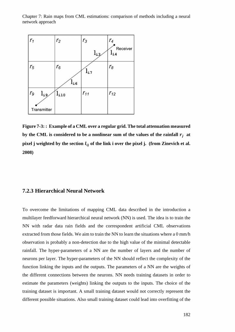
Chapter 7: Rain maps from CML estimations: comparison of methods including a neural network approach
182
Figure 7-3: : Example of a CML over a regular grid. The total attenuation measured
by the CML is considered to be a nonlinear sum of the values of the rainfall 𝒓𝒓𝒋𝒋 at
pixel j weighted by the section 𝒍𝒍𝒊𝒊𝒋𝒋 of the link i over the pixel j. (from Zinevich et al.
2008)
7.2.3 Hierarchical Neural Network
To overcome the limitations of mapping CML data described in the introduction a
multilayer feedforward hierarchical neural network (NN) is used. The idea is to train the
NN with radar data rain fields and the correspondent artificial CML observations
extracted from those fields. We aim to train the NN to learn the situations where a 0 mm/h
observation is probably a non-detection due to the high value of the minimal detectable
rainfall. The hyper-parameters of a NN are the number of layers and the number of
neurons per layer. The hyper-parameters of the NN should reflect the complexity of the
function linking the inputs and the outputs. The parameters of a NN are the weights of
the different connections between the neurons. NN needs training datasets in order to
estimate the parameters (weights) linking the outputs to the inputs. The choice of the
training dataset is important. A small training dataset would not correctly represent the
different possible situations. Also small training dataset could lead into overfitting of the
Chapter 7: Rain maps from CML estimations: comparison of methods including a neural network approach
183
training data by the NN. Overfitting avoid the generalization of the function linking the
input to the outputs.
The NN architecture developed for this application is showed in figure 7-4. The input
layer is a vector composed of 7 characteristics of the 5 closest links relative to the pixel
on which we estimate the rainfall (35 inputs), the rainfall at the target pixel is the single
output of the NN. To map the rainfall with a trained NN, we execute the trained NN for
each pixel in the zone.
The input parameters for each of the CML are the relative distance (in km) from the two
antennas to the target pixel [dX1, dY1, dX2, dY2], the rainfall rate measured by the CML
at the current time step Pt, the rainfall rate measured at the previous time step Pt−1 and
the threshold of minimal detectable rain Pmin which depends on the path length and the
frequency of the CML (see figure 5-11). The input vector I is:
I = [IL1, IL2, IL3, IL4, IL5] (𝑃𝑃𝑒𝑒. 7.7)
A combination of the information from the 5 closest links ILx:
ILx = [dX1, dY1, dX2, dY2, Pt, Pt−1, Pmin]Lx (𝑃𝑃𝑒𝑒. 7.8)
A benefit of the NN is the possibility to add ancillary variables to improve the regression.
The NN has two hidden layers, the first layer is partially connected: there is no causal
relation between the coordinates of different links, or the minimal detectable rainfall. The
second layer is a fully connected (dense) layer which derive into a single output, the
rainfall estimation.
The tests concerning the hyper-parameters of the NN were made with a one-day subset
of the data. The metrics used to validate the output was the root mean square (RMS). The
objective is to find a compromise between a large number of parameters which can lead
to overfitting and a small number which cannot reproduce the complexity of the function
linking the input and output. We found that a third hidden layer did not improve the
results increasing the computing time. The optimal choice for the first layer is two neurons
per input link, one neuron leading to worse results and more neurons not contributing to
better results. A similar approach for the second layer derived into N2=15 neurons as the
optimal choice.

Chapter 7: Rain maps from CML estimations: comparison of methods including a neural network approach
184
In section 7.2.3 we describe the training dataset of the NN and in section 7.3 we show the
results compared to the other mapping techniques.
Figure 7-4: Architecture of the NN used in this study
Chapter 7: Rain maps from CML estimations: comparison of methods including a neural network approach
185
7.3 Synthetic data
In the following section we describe the radar data set used as a reference rainfall field to
test the performance of the mapping algorithms. Then we describe the generation of
artificial CML and the training dataset.
7.3.1 Radar data and African context
For this study we projected the X-port radar data into a 1 km regular grid by simply
averaging the rain rates falling into the regular grid pixels. The CML data provided by
telecom companies is at a 15 minutes’ time resolution (see Chapter 6). To be consistent
with the real CML data we average the instant 1-minute radar rain fields into 15-minutes
fields to have proxy fields of a real 15 minutes’ spatial variability of rainfall in the West-
African monsoon context.
In this study we focus on the retrieval of rainfall from CML networks on a city-scale. We
extract three zones of 40km x 40km in the radar maps showed in figure 7-5. The zones
were chosen in the western and upper part of the radar fields to avoid extinction cases.
The three zones were located far enough from the radar to avoid the central parts affected
by ground cluttering.
We used the whole 2013 monsoon season from May to October. We used only 15-min
averaged PPI covered at least by 75% of data (less than 25% of missing values) to filter
rain fields with poor spatial coverage.
7.3.2 Generation of artificial links from radar data
We have used three different real CML networks of African cities to avoid a network
topology dependence in the NN training. The CML configurations are from the cities of
Niamey (Niger), Yaoundé and Douala (Cameroun) provided by the telecom operator
Orange. The CML networks are shown in black lines (at different scales) on figure 7-6.
We can see that the coverage surface of the network varies from each city depending on
Chapter 7: Rain maps from CML estimations: comparison of methods including a neural network approach
186
its size. Also the number of CML and the frequencies are different for each network.
Table A-1 in appendix 6 summarize the characteristics of the three CML networks.
We have considered the real signal frequency of the CML networks which varies from
8.5 GHZ to 23GHZ. The synthetic CML observation were calculated considering both
quantization step of the attenuation, 0.1 dB and 1 dB.
The simulated CML observations Rlınk� are computed with the radar pixels Rradi :
Rlınk� = �1 a� � ∗ �round �∑ LiaRrad
i bi ,∆dB� − 0.5
L�
1b
(𝑃𝑃𝑒𝑒. 7.9)
To simulate the CML observations Rlınk� we extract the observed rainfall in the link’s path
from the radar field. We convert each pixel value of rain Rradi into attenuation following
the K − R relationship weighted by the path length in each pixel Li. We round the value
considering the quantization step ∆dB. The term −0.5 dB in equation 7.9 correspond to
an artificial addition of an observation bias to evaluate the capability of the NN to correct
possible biases in the observed data (due to a wet antenna for example).
In this study we focus on the uncertainty in the mapped rain field induced by the
quantization step and the minimal detectable rain of the links. We also consider a possible
bias in the CML observation dataset. We test the ability of the NN to correct the bias
introduced artificially in eq. 7.9.
We centered the CML networks in the three zones (figure 7-6). For each zone and for
each CML network Rlınk� was calculated using the two considered quantization steps
∆dB= [0.1; 1 dB].
7.3.3 Training data set
To train the NN we used as input the computed values of artificial CML observation Rlınk�
and the values of the radar pixels as output. As mentioned above the radar field was
divided in three zones of 40km x 40km (see figure 7-5): two zones were used for training
keeping the third zone for validation. The different combination of two zones for training
and one for validation leads to three different trained NN.
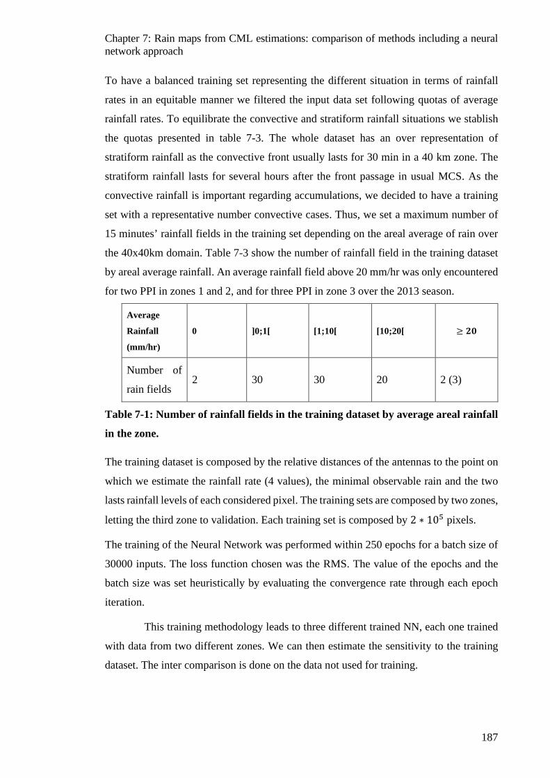
Chapter 7: Rain maps from CML estimations: comparison of methods including a neural network approach
187
To have a balanced training set representing the different situation in terms of rainfall
rates in an equitable manner we filtered the input data set following quotas of average
rainfall rates. To equilibrate the convective and stratiform rainfall situations we stablish
the quotas presented in table 7-3. The whole dataset has an over representation of
stratiform rainfall as the convective front usually lasts for 30 min in a 40 km zone. The
stratiform rainfall lasts for several hours after the front passage in usual MCS. As the
convective rainfall is important regarding accumulations, we decided to have a training
set with a representative number convective cases. Thus, we set a maximum number of
15 minutes’ rainfall fields in the training set depending on the areal average of rain over
the 40x40km domain. Table 7-3 show the number of rainfall field in the training dataset
by areal average rainfall. An average rainfall field above 20 mm/hr was only encountered
for two PPI in zones 1 and 2, and for three PPI in zone 3 over the 2013 season.
Average
Rainfall
(mm/hr)
0 ]0;1[ [1;10[ [10;20[ ≥ 𝟎𝟎𝟎𝟎
Number of
rain fields 2 30 30 20 2 (3)
Table 7-1: Number of rainfall fields in the training dataset by average areal rainfall
in the zone.
The training dataset is composed by the relative distances of the antennas to the point on
which we estimate the rainfall rate (4 values), the minimal observable rain and the two
lasts rainfall levels of each considered pixel. The training sets are composed by two zones,
letting the third zone to validation. Each training set is composed by 2 ∗ 105 pixels.
The training of the Neural Network was performed within 250 epochs for a batch size of
30000 inputs. The loss function chosen was the RMS. The value of the epochs and the
batch size was set heuristically by evaluating the convergence rate through each epoch
iteration.
This training methodology leads to three different trained NN, each one trained
with data from two different zones. We can then estimate the sensitivity to the training
dataset. The inter comparison is done on the data not used for training.
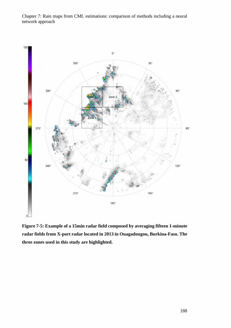
Chapter 7: Rain maps from CML estimations: comparison of methods including a neural network approach
188
Figure 7-5: Example of a 15min radar field composed by averaging fifteen 1-minute
radar fields from X-port radar located in 2013 in Ouagadougou, Burkina-Faso. The
three zones used in this study are highlighted.
Chapter 7: Rain maps from CML estimations: comparison of methods including a neural network approach
189
7.4 Results on synthetic data
This section compares the three mapping methods of artificial CML data to the original
radar rainfall fields. In the first section we define the metric for the validation of the maps.
Later we assess the efficiency of the different mapping methods and then we inter-
compare it globally.
An example of rainfall map for each method is presented in figure 7-6 for a 1dB
quantization step. The reference rainfall field is in the left column. The second column
shows the maps from the NN method, the third and fourth column the tomography and
kriging methods. Each row presents the results for a different real CML network (Niamey,
Douala and Yaounde). The reference rainfall field is the same but the size of the mapping
zone is different due to the different size of the cities. An interesting asset of the NN
technique is the retrieval of rainfall at the limits of the zone where no information is
available. In figure 7-6 for the Yaounde mapping we can see a blue zone (~10mm/hr) in
the north west of the city. The other techniques tend to the average the observed rainfall
at the edges (where there is no spatial correlation with the observed data). The neural
network is able to learn from previous rainfall events patterns of spatial distribution from
limited information. More examples of fields are included in Appendix 6. Figure A12 of
the appendix 6 show a case where the comparison of the NN output to the reference rain
field is not as good as in figure 7-6.
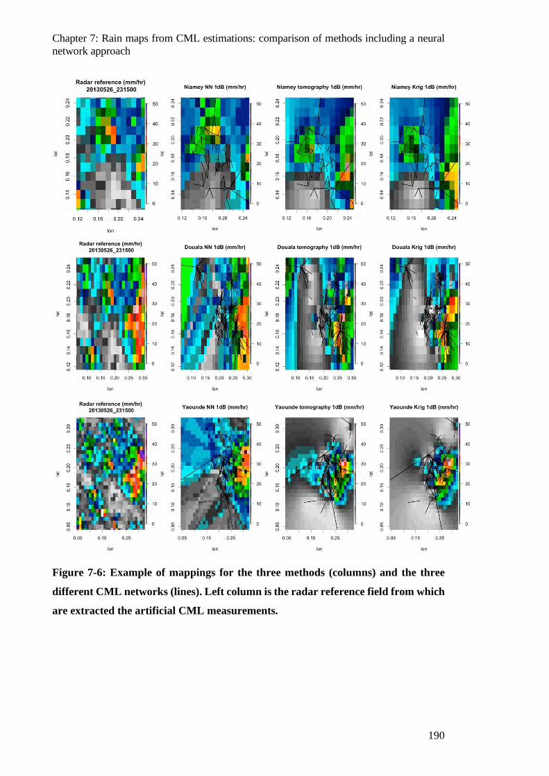
Chapter 7: Rain maps from CML estimations: comparison of methods including a neural network approach
190
Figure 7-6: Example of mappings for the three methods (columns) and the three
different CML networks (lines). Left column is the radar reference field from which
are extracted the artificial CML measurements.
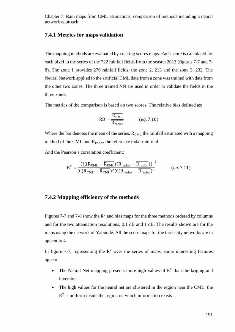
Chapter 7: Rain maps from CML estimations: comparison of methods including a neural network approach
191
7.4.1 Metrics for maps validation
The mapping methods are evaluated by creating scores maps. Each score is calculated for
each pixel in the series of the 722 rainfall fields from the season 2013 (figures 7-7 and 7-
8). The zone 1 provides 276 rainfall fields, the zone 2, 213 and the zone 3, 232. The
Neural Network applied to the artificial CML data from a zone was trained with data from
the other two zones. The three trained NN are used in order to validate the fields in the
three zones.
The metrics of the comparison is based on two scores. The relative bias defined as:
RB =RCML�������Rradar�������� (𝑃𝑃𝑒𝑒. 7.10)
Where the bar denotes the mean of the series. RCML the rainfall estimated with a mapping
method of the CML and Rradar the reference radar rainfield.
And the Pearson’s correlation coefficient:
R2 =(∑(RCML − RCML�������)(Rradar − Rradar��������))∑(RCML − RCML�������)2 ∑(Rradar − Rradar��������)2
2
(𝑃𝑃𝑒𝑒. 7.11)
7.4.2 Mapping efficiency of the methods
Figures 7-7 and 7-8 show the R2 and bias maps for the three methods ordered by columns
and for the two attenuation resolutions, 0.1 dB and 1 dB. The results shown are for the
maps using the network of Yaoundé. All the score maps for the three city networks are in
appendix 4.
In figure 7-7, representing the R2 over the series of maps, some interesting features
appear:
• The Neural Net mapping presents more high values of R2 than the kriging and
inversion.
• The high values for the neural net are clustered in the region near the CML: the
R2 is uniform inside the region on which information exists

Chapter 7: Rain maps from CML estimations: comparison of methods including a neural network approach
192
• The peaks of R2 appear on the nodes of the CML network for the NN technique,
where redundant information exists. Not true for the kriging and inversion, were
the nodes can carry controversial information.
• The three techniques exhibit similar performances outside the CML dense zone,
where no information exist.
• As expected the R2 is impacted by the 1 dB sensibility compared to the 0.1 dB.
However, the NN still perform better than the kriging and inversion.
• The inversion technique shows better results along the isolated links
• Inversion and kriging are more network-dependent as they do not handle the
sampling limitations.
Figure 7-8 presents the absolute bias maps for the series of events. The maps show the
following features:
• There is a global bias (yellow field) on the inversion and kriging coming from the
artificial bias addition of -0.5dB in equation 7.9. The NN can partially correct it.
• It exists a strong east-west bias gradient caused by the MCS movement which is
less exaggerated in the NN.
• The bias addition on the attenuation values in eq. 7.9 was set to test the ability of
the NN to correct a global bias. In real cases global biases can occur such as wet
antenna attenuation. If collocated CML and radar data is available, the neural
network can be trained with biased data to have correct outputs.
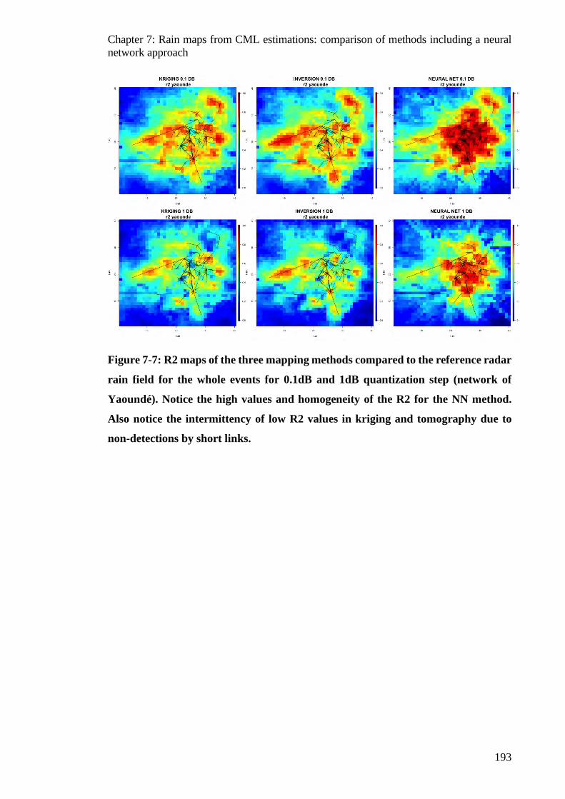
Chapter 7: Rain maps from CML estimations: comparison of methods including a neural network approach
193
Figure 7-7: R2 maps of the three mapping methods compared to the reference radar
rain field for the whole events for 0.1dB and 1dB quantization step (network of
Yaoundé). Notice the high values and homogeneity of the R2 for the NN method.
Also notice the intermittency of low R2 values in kriging and tomography due to
non-detections by short links.
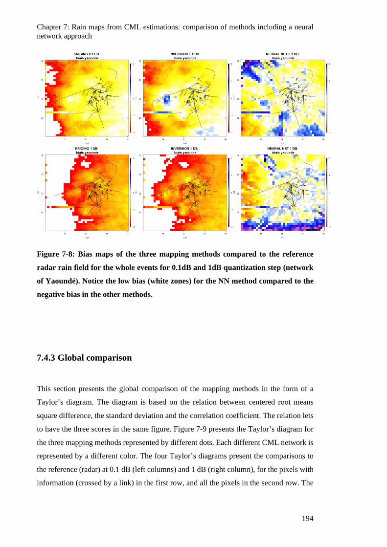
Chapter 7: Rain maps from CML estimations: comparison of methods including a neural network approach
194
Figure 7-8: Bias maps of the three mapping methods compared to the reference
radar rain field for the whole events for 0.1dB and 1dB quantization step (network
of Yaoundé). Notice the low bias (white zones) for the NN method compared to the
negative bias in the other methods.
7.4.3 Global comparison
This section presents the global comparison of the mapping methods in the form of a
Taylor’s diagram. The diagram is based on the relation between centered root means
square difference, the standard deviation and the correlation coefficient. The relation lets
to have the three scores in the same figure. Figure 7-9 presents the Taylor’s diagram for
the three mapping methods represented by different dots. Each different CML network is
represented by a different color. The four Taylor’s diagrams present the comparisons to
the reference (radar) at 0.1 dB (left columns) and 1 dB (right column), for the pixels with
information (crossed by a link) in the first row, and all the pixels in the second row. The
Chapter 7: Rain maps from CML estimations: comparison of methods including a neural network approach
195
tomography technique is performed on the pixels with information (crossed by a link).
The other pixels are filled by kriging.
In the Taylor’s diagram the reference (radar) is situated at coordinate [1,0] in green. The
closer the point, the better the comparison. We can compare the different points in terms
of correlation, represented by the angle from the X –axis. The standard deviation
compared to the reference is represented by the range distance of the points and the RMS
difference represented by the distance to the reference (point [1,0]).
We can see that at 0.1 dB sensibility, for the pixels with information there is a significant
contribution of the NN in terms of correlation, RMS and standard deviation. The result
holds for a 1 dB sensibility if we compare the methods by CML network (colors).
However, the NN method does not improve the results when comparing all the pixels in
terms of R and RMS. While the distributions remain closer (standard deviation).
The NN bring coherence to the pixels with information as shown in the scores maps of
figures 7-7 and 7-8. The rainfall is better estimate with the NN in zones with high density
of CML.
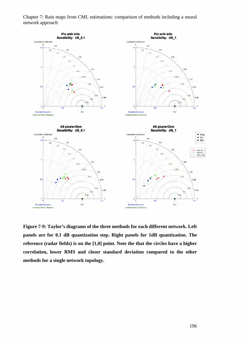
Chapter 7: Rain maps from CML estimations: comparison of methods including a neural network approach
196
Figure 7-9: Taylor’s diagrams of the three methods for each different network. Left
panels are for 0.1 dB quantization step. Right panels for 1dB quantization. The
reference (radar fields) is on the [1,0] point. Note the that the circles have a higher
correlation, lower RMS and closer standard deviation compared to the other
methods for a single network topology.
Chapter 7: Rain maps from CML estimations: comparison of methods including a neural network approach
197
7.5 Results on real data
In this section we show the application of the mapping methods to real CML data using
the three NN trained with the artificial CML data generated with radar fields. To validate
the maps, we adopt a cross-validation methodology, which consists in removing a CML,
make the mapping without it and comparing the retrieved rainfall to the removed CML
observed rainfall.
7.5.1 Data Niamey
We have used the CML data of Orange Niger presented in chapter 6. The attenuation
from the wet antenna effect is presented in chapter 6, we used the calibration model 3bis
(considering a wet antenna depending on rainfall).
We computed the maps for the 2016 and 2017 rainy seasons using the three NN trained
with the artificial CML extracted from radar rain fields presented in section 7.2. The NN
used in this section were trained with a dataset of artificial CML where no bias was added:
equivalent of removing the factor -0.5 dB of equation 7.9.
We applied the three mapping methods for the events of 2016/2017 season with daily
rainfall accumulation greater than 10mm/hr representing a total of 21 events and 253 15-
minutes time steps. The average number of 15 minutes steps by event is 12 (3h rainfall
duration) with a maxima of 28 time steps for the 14 June 2017 event.
7.5.2 Cross-validation methodology
The cross-validation method consists in mapping the rainfall while removing one CML.
Then we compare the retrieved rainfall in the path to the removed CML. Due to the high
uncertainty of short CML (Chapter 5 and 6) we used only the CML longer than 2 km for
the cross-validation.

Chapter 7: Rain maps from CML estimations: comparison of methods including a neural network approach
198
The total number of CML with L > 2km in Niamey is 12. For each 15-minutes time step
we apply the algorithms 12 times, each time removing one CML. We obtain a cross-
validation dataset of 2300 couples of values (for each trained NN).
7.5.3 Results
Figure 7-10 presents the global results in a Taylor’s diagram equivalent to figure 7-9. The
reference corresponds to the rainfall seen by the CML removed from the analysis. For the
cross-validation with real data the three methods show similar results in terms of
correlation coefficient and RMS compared to the results using the artificial dataset in
section 7.3.3. The three different NN show a variability in terms of standard deviation
from the reference, specially NN2.
Table 7-4 show the false alarm rate (FAR), the non-detection rate (NDR), the hits and the
zeros for each method. The FAR, TND, hits and zeros are defined against the total number
of couples. The four values are calculated with a threshold of 1mm/hr. The NN show a
lower TND and a bigger TFA compared to tomography and kriging.
Table 7-5 show the scores of the different methods for the series of cross-validation
couples. The correlation coefficient is slightly higher for the tomography and kriging and
the RMSE slightly lower. The bias is lower for two of the three NN.
When using real data from CML the benefits of the NN shown in the simulation in section
7.3 are no longer present. Some elements can explain the different results with real CML
observed data:
• The modelization of the CML observations in equation 7.9 used to create artificial
dataset is incomplete: the modelization of the uncertainty should be addressed to
better characterize the measure of a CML.
• If the uncertainty is addressed, the Neural Network could be trained with the link
length as an input as the uncertainty is higher for smaller links (scatterplot of
chapter 6 figure 6-19). Training such NN could potentially decrease the relative
weight of small CML when mapping rainfall for real data. In the NN presented in
this section the small CML where considered as “perfect”, only the minimal
detectable rainfall was considered.
Chapter 7: Rain maps from CML estimations: comparison of methods including a neural network approach
199
• The wet antenna effect as showed in chapter 6 is high. To correct the wet antenna
attenuation, we considered both antennas wetted. We stablish different calibration
models: one for a constant wet antenna attenuation, another with a rainfall
dependent wet antenna. The CML network carries information about the spatial
distribution of the rainfall. Thus we could consider training a NN from artificial
measurements of attenuation calculating a wet antenna attenuation for each
antenna considering the rainfall rate at the antenna location and the corrected
model from (Leijnse et al. 2008).
• In this study we focused on the sampling problem of CML concerning minimal
detectable rainfall. In real observations the non-detections due to the correction of
the wet antenna are more significant than the non-detections due to the minimal
detectable rainfall.
• Finally, the cross-validation is limited by the inherent noise of the validation data.
To fully train and validate the NN, collocated observations from radar and CML
should be used. Using collocated observations could remove biases on the CML
(if we consider no biased radar reference data) and learn the patterns of the rainfall
for a location and season.
• The NN showed a significant contribution in pixels with information (figure 7-9)
in the simulations. The cross-validation was made mainly on pixels without
information as the CML was removed from the analysis.
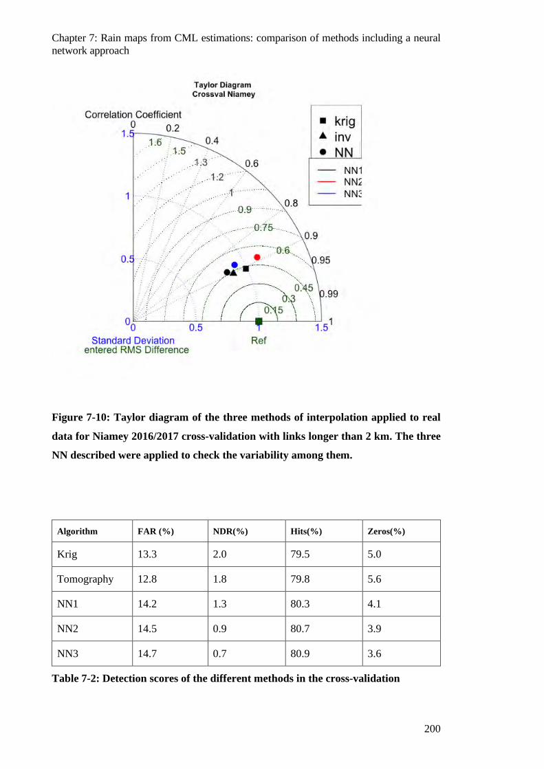
Chapter 7: Rain maps from CML estimations: comparison of methods including a neural network approach
200
Figure 7-10: Taylor diagram of the three methods of interpolation applied to real
data for Niamey 2016/2017 cross-validation with links longer than 2 km. The three
NN described were applied to check the variability among them.
Algorithm FAR (%) NDR(%) Hits(%) Zeros(%)
Krig 13.3 2.0 79.5 5.0
Tomography 12.8 1.8 79.8 5.6
NN1 14.2 1.3 80.3 4.1
NN2 14.5 0.9 80.7 3.9
NN3 14.7 0.7 80.9 3.6
Table 7-2: Detection scores of the different methods in the cross-validation
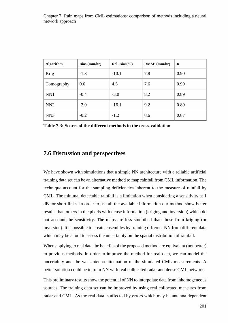
Chapter 7: Rain maps from CML estimations: comparison of methods including a neural network approach
201
Algorithm Bias (mm/hr) Rel. Bias(%) RMSE (mm/hr) R
Krig -1.3 -10.1 7.8 0.90
Tomography 0.6 4.5 7.6 0.90
NN1 -0.4 -3.0 8.2 0.89
NN2 -2.0 -16.1 9.2 0.89
NN3 -0.2 -1.2 8.6 0.87
Table 7-3: Scores of the different methods in the cross-validation
7.6 Discussion and perspectives
We have shown with simulations that a simple NN architecture with a reliable artificial
training data set can be an alternative method to map rainfall from CML information. The
technique account for the sampling deficiencies inherent to the measure of rainfall by
CML. The minimal detectable rainfall is a limitation when considering a sensitivity at 1
dB for short links. In order to use all the available information our method show better
results than others in the pixels with dense information (kriging and inversion) which do
not account the sensitivity. The maps are less smoothed than those from kriging (or
inversion). It is possible to create ensembles by training different NN from different data
which may be a tool to assess the uncertainty on the spatial distribution of rainfall.
When applying to real data the benefits of the proposed method are equivalent (not better)
to previous methods. In order to improve the method for real data, we can model the
uncertainty and the wet antenna attenuation of the simulated CML measurements. A
better solution could be to train NN with real collocated radar and dense CML network.
This preliminary results show the potential of NN to interpolate data from inhomogeneous
sources. The training data set can be improved by using real collocated measures from
radar and CML. As the real data is affected by errors which may be antenna dependent

Chapter 7: Rain maps from CML estimations: comparison of methods including a neural network approach
202
(wet antenna depending on the equipment) or by different atmospheric situations (relative
humidity increase during rainfall) the training of a NN with real data and a reference
rainfall field could improve the results. In this situation, a NN could absorb the bias of
the CML measured rainfall.
Another interesting feature of NN is that secondary information such as temperature or
humidity can be added to the input data set of the NN to improve the regression of rainfall.
In other climatic regimes, where there is seasonal variability in the precipitation systems,
the season, or month can be added as an input variable. We can also consider the
topography of a region affecting the rainfall rates by adding it to the input, similar to a
co-kriging method.
We have seen in the results section that the density of the network is a key factor regarding
the comparison with other methods. As the network density decreases, the tomography
method show better results. The tomography shows better results with isolated CML. On
bigger scales with lower network density we can investigate the combination of CML
with satellite data from either microwave low orbit satellite or IR geostationary data to
retrieve combined CML-satellite rainfall products from machine learning algorithms.
The training dataset for this study was limited to one season of radar data in the Sahel.
The MCS are organized systems which represent large areas of rainfall. Such technique
for different climatic zones, with sparse rainfall could not be an efficient solution.
Conclusions and perspectives
203
CONCLUSIONS AND PERSPECTIVES
FIRST PART
In the first part of this manuscript we have introduced the precipitation observation with
polarimetric weather radars. We have then presented two original techniques to retrieve
information on the hydrometeors characteristics with the modeling of the remote sensing
observation.
The first inversion is based on a simple model of the hydrometeors melting layer as seen
by radars. The bright band is a peak of reflectivity seen by radars caused by the bigger
size of melting hydrometeors compared to raindrops due to the lower density of ice crystal
and the presence of water is those melting crystals. The shape of the bright band is drived
by different processes: fall speed, temperature gradient, break-up, aggregation of particles
and the density of the falling particles. As different studies already shown the properties
of the BB depend on the particles density and type. In the showed study we demonstrate
that the BB shape could be used to infer the particles’ density law above the bright band.
By simplifying the model considering a fixed melted fraction depending on the height,
we can derive shapes of bright band depending only on the particle size distribution and
the pre-factor of the density law. With a simple three parameters inversion for each
vertical profile of reflectivity we found pre-factors of the density law close to that
observed in-situ by the on flight probe (Fontaine et al. 2014). We also found denser
particles when approaching the convective front, in agreement with the hydrometeor
Conclusions and perspectives
204
classification retrieved by fuzzy logic with polarimetric radar observation, presented in
the companion paper (Cazenave et al. 2014). Three important simplifying assumptions
where:
• No aggregation or break-up of particles during the fall
• Observed VPR considered as the real VPR
• Fixed degree of melting during the fall depending only on height
The aggregation and break-up of the particles during the fall lead to changes in the DSD
and thus can generate errors in the density estimation as the shape of the BB is sensitive
to the DSD. The DSD (or PSD) evolution during the fall could be assessed with the DSD
inversion presented in chapter 4, at least on the rainfall layer. By inverting polarimetric
radar variables at different radar PPI elevations and studying the vertical evolution of the
DSD, we could evaluate break-up and aggregation rates during fall.
The second assumption of the BB inversion rely on considering the observed VPR as the
real VPR. As the scanning volume resolution of the radar echoes increase with the range,
the apparent VPR is smoothed for high ranges, because of the rougher vertical resolution.
This effect is attenuated by selecting the radar pixels within 25 km radius to construct the
VPR. If this method should be implied for higher radar ranges a VPR correction need to
be addressed as (Kirstetter et al. 2013).
The third assumption follow (Boudevillain and Andrieu 2003) by considering a fixed
symmetric vertical profile of melting fraction of the hydrometeors. A more complete
description on the real thermodynamics of the melting particle was made by (Klaassen
1988; Zawadzki et al. 2005). Such description could improve the physics description of
the BB. But a great number of unknown parameters should be addressed. We could make
the BB model more complex by increasing the observations constraining it. The other
polarimetric variables could be inserted in the inversion. Then the type of the
hydrometeors should be represented in the T-matrix simulations.
The second inversion of polarimetric radar data presented in chapter 4 aims to retrieve
the DSD parameters of each pixel of a radar PPI. With radar polarimetry we measure
three independent variables linked to the drops characteristics in the sampling volume:
[𝑍𝑍𝐻𝐻 ,𝑍𝑍𝐷𝐷𝐷𝐷 ,𝜙𝜙𝐷𝐷𝐷𝐷]. In the literature we can found different techniques to retrieve DSD
parameters (Gorgucci et al. 2001a; Koffi et al. 2014; Raupach and Berne 2017). All these
Conclusions and perspectives
205
studies rely on empirical relationships between DSD parameters and radar variables. Also
the proposed studies did not account explicitly for radar attenuation in the DSD retrieval.
In the West-African context of strong convective rainfall rates, and X-band radar
observation, the attenuation correction is a crucial step for QPE or DSD retrieval (Kacou
2014). In the proposed inversion method, we account explicitly for attenuation as we use
as input variables the non-corrected from attenuation radar variables. Three parameters
of a gamma DSD [𝐷𝐷𝑚𝑚, 𝑁𝑁0∗ ,𝜇𝜇] are retrieved at each range gate along a radial. The
procedure avoids using the common two steps procedure (attenuation correction and DSD
parameters retrieval) which can lead into errors. The direct model to calculate
polarimetric observables from oblate drops is based on the T-matrix model (Mishchenko,
Travis, and Mackowski 1996).
The presented framework ensures a global consistency between the retrieved DSD and
all the radar variables. The inversion it is make at once for each radial in an iterative
procedure. This radial-based inversion can make use of strong constrains, as the total
differential phase shift at the last gate, insuring coherence and robustness. As a priori
guess (algorithm initialization) we used the empirical DSD parameter retrieval from
polarimetric variables found by (Koffi et al. 2004).
The inversion output was compared to in-situ DSD data recorded by a disdrometer
located at 20 Km from the radar showing good consistency between observed and
retrieved DSD. Some events present although bias on the retrieved 𝑁𝑁0∗.
The major assumption of the inversion is the drop shape law. The sensitivity tests on the
drop shape laws showed the high dependency of the results to that assumption. The future
version of the algorithm could include an additional parameter linked to the aspect ratio
law similar to the 𝛽𝛽-method by (Gorgucci et al. 2002). The 𝛽𝛽 parameters is the linear
coefficient of the oblateness-diameter shape law. Also we can include a 𝑍𝑍𝐻𝐻 or 𝑍𝑍𝐷𝐷𝐷𝐷
calibration to correct from possible wrong calibration of the polarimetric variables.
The presented study was validated with one disdrometer at 20 km from the radar. A future
validation with more disdrometers, located farther of the radar, could test the ability of
the method to estimate the attenuation.
The high dimension of the problem (650*3 x 650*3 matrices) and the high non-linearity
(exponential decrease of 𝑍𝑍𝐻𝐻 due to attenuation) make the iterative algorithm slow for real
time applications. Also, the high non-linearity makes it sensitive to the a priori initial
state.
Conclusions and perspectives
206
However, the method combine all the available polarimetric information using a physical
model of the observation to retrieve DSD fields consistent with the observations. With
the proposed methodology we can impose global physical constraints either in integrated
quantities (imposed total differential phase shift) or on the solution (correlation between
radial gates, or correlation between retrieved variables).
SECOND PART
The second part of the thesis address the rainfall observation using microwave links. In
the initial chapter we described the principle of rainfall rate estimation from raw
attenuation data of a microwave link telecommunication companies. First the raw
attenuation can be easily calculated from the raw transmitted and received power of the
microwave link. An important step follows to estimate the rainfall induced attenuation.
For that purpose, the wet and dry period detection and the baseline level detection
(attenuation level without rainfall) algorithms are applied. The wet/dry and baseline
detection algorithms depend on the fluctuations and temporal drift of the attenuation
signal. In the simple case of low noise signals without temporal drift, the usual algorithms
used in the literature are based on thresholds of the attenuation (thresholds on the
attenuation variability or on the attenuation values). Then a K-R power law is used to
convert the estimated rain induced attenuation into rainfall rate. The K-R law can be
estimated using DSD parameterizations or DSD measurements from disdrometers.
Other sources of attenuation can bias the raw attenuation signal. Among them, the more
important is the wet antenna attenuation caused by the presence of a water film over the
antennas of the link during rainfall. Other sources of attenuation can cause errors in the
rainfall estimation: humidity variation, fog or dust are some of them.
The rainfall spatial variability in the CML is a source of uncertainty specially for non-
lineal K-R laws. The K-R law can also be a source of error if a wrong parameterization
of the DSD is used. The baseline detection algorithm can lead to wrong detections and
false alarms leading to an error in the rainfall accumulations. The quantization step of
attenuation, if it is rough, it adds uncertainty on the rainfall retrievals, specially for small
CML. Also the sensitivity of the CML to rainfall is affected by a rough quantization step.
The type of variable sampled the telecom companies and the sampling is also a source of
Conclusions and perspectives
207
uncertainties. Some companies provide only maximum attenuation values. Then a
correction must be done.
Chapter 6 of the thesis was focused on a real dataset of attenuation of CML from Orange
company in Niamey, Niger. The data from 92 CML during two seasons was provided at
15 minutes’ time step. Three typing bucket raingage at 5 minutes where used to calibrate
the rainfall retrievals. First a data quality control is used to filter CML with suspicious
data. The quality control is based on the correlation of each CML with the other
depending on the distance. As the rainfall fields are spatially correlated, the pattern of the
correlograms are a proxy of the quality of the data. Some CML where removed from the
analysis with this argument.
Later we used all the gage/CML collocations to test three calibration models. The
objective of the calibration is to find the best [𝑎𝑎, 𝑏𝑏] parameters from the K-R law and the
best wet antenna attenuation which fits the rain gage data. The different models consider
one, two or three varying parameters, as we have a theoretical K-R law calculated from
observed DSD in the zone. In the third model we have considered a rainfall dependent
wet antenna attenuation.
We evaluate the robustness of the models by a bootstrapping test. The bootstrapping
showed that the fitted parameters of model (model 1) are less robust than the other
models. Model 1 seems to over fit the data, and the retrieved [𝑎𝑎, 𝑏𝑏] are not physically
coherent. The retrieved 𝑎𝑎 of the K-R law from Model 2 has low variability in the
bootstrapping, showing robustness. Also the retrieved 𝑎𝑎𝑓𝑓𝑖𝑖𝑡𝑡 is close to the theoretical 𝑎𝑎𝑡𝑡ℎ
from K-R relation calculated with observed DSD. Model 3 has also a low variability of
the retrieved parameter, the scaling parameter of the wet antenna model of [Leijnse et al
2008.].
Model 3 needs the solution of an equation for each collocation as the wet antenna
attenuation depends on rainfall, which is unknown. When using only the attenuation (not
ancillary information from rain gages) and optimizing the scaling parameter, model 3 give
the best results in terms of bias. The remaining bias show low dependency on the CML
length and rainfall rate compared to model 1 and model 2. Considering a rainfall
independent wet antenna attenuation (model 1 and model 2) induce a bias which depend
on the rainfall rate and CML length.
The resulting daily time series, when filtering well enough the outliers CML show a very
good consistency with rain gages, with R2 in the order of 0.7 and bias around [-10 ; 10%].
Conclusions and perspectives
208
However, there is a remaining effect on the link length. Long links underestimate
compared to short links which seems to overestimate. We show an effect of the different
sampling on the CML and the raingage. The different sampling is drived by the link
length. Using the retrieved DSD fields of chapter 4, we simulated CML and raingage
sampling to show the effect. However, the retrieved number are difficult to compare due
to the limited number of CML observations.
Instead of estimating the wet antenna effect by minimizing the observed attenuation with
raingage observations we could made a dedicated experiment in the zone to estimate the
wet antenna effect. By installing several disdrometer (or rain gages) in a CML path we
could deduce the wet antenna effect for different rainfall rates.
The final chapter is about combining the information from a spatial network of CML to
create rainfall maps in a regular grid. We presented an original, potential technique, based
on machine learning to map rainfall from limited spatial information.
We find in the literature different techniques to interpolate rainfall from linear averages
from dense CML networks. Two common techniques are based on simple kriging from
Geostatistics theory, and tomography, from inversion theory. For the simple kriging we
consider the CML as a punctual rainfall measurement. It is enough for low density CML
measurement, but for dense measurement we lose the spatial information provided by the
link path location. The tomography uses the location of the link’s path to find a possible
solution, constrained by a spatial covariance imposed. Both techniques cannot include the
sampling uncertainty caused by the attenuation quantization step of the attenuation.
In order to train a neural network we create a synthetic dataset of CML observation from
rainfall radar fields. In the synthetic data we have simulated the quantification step of the
attenuation. The neural network was trained with the reference radar field as output and
the simulated CML observations as input.
The resulting rainfall fields from the NN present variability of rainfall at the edges of the
zone. A common issue with interpolation techniques is in the edges, where the
interpolated value tends to the average of the observations. The NN can predict values
other than the average. When comparing the R2 maps, and bias maps of the three
techniques, the NN can bring coherence in the zones where the information is denser (ie.
the nodes of the CML). The introduced bias on the artificial data is corrected by the NN.

Conclusions and perspectives
209
When using real data the benefits of the technique are more difficult to show in that
configuration. The noise of real data can hide the benefits. Using a cross-validation
approach, the noise of the “validating” link can hide the improvement. Also we showed
that the major contribution of the technique, at this stage, is in the pixels with information.
In the cross-validation we validate by definition in the pixels without information, as the
link is removed from the analysis. An future validation of the technique should be done
using either collocated radar maps and MSL data or several rain gages in 1km pixels.
Also the wet antenna attenuation correction could be learned by the NN in future versions,
if collocated radar data and CML data is used to train the NN. This prospective chapter
showed the potential use of machine learning to map rainfall from heterogeneous sources
of information, using a reference rainfall field.
GLOBAL PERSPECTIVES
The CML networks are constantly evolving. In West-Africa the population growth and
wide use of mobile telephones is increasing the number of CML in populated areas. In
Europe the long CML interconnecting villages, and cities are being replaced by optic
fiber, but the future 5G technology will need the installation of CML at higher
frequencies. Also the MW bands used for telecommunication are increasing the frequency
due to the high demand and overbooking of traditional frequencies.
High frequencies are more sensitive to rainfall. Even frozen particles can attenuate signals
at 80GHz or more, being potentially a source for snow rate estimation. In this thesis we
showed the CML rainfall estimation without polarization. A double polarization
attenuation measurement can improve the rainfall estimation. In part 1 of the thesis we
show a DSD retrieval using polarimetric information. Using double polarization CML we
can expect retrieving DSD instead of rainfall rates. Also double frequency CML can lead
to similar approaches.
In developed countries the precipitation observation is done by networks of radars
covering the countries. But still some regions are uncovered, mostly mountainous regions
where radar beams are blocked by the orography. CML can be a solution to complete the
precipitation observation in mountainous valleys. Then arise the question about the CML-
radar merging, which opens a new field.
Conclusions and perspectives
210
In a large scale, we can track precipitating systems with CML networks potentially in real
time. The temporal sampling of microwave precipitation satellites is poor and depend on
the orbit and the location. The IR geostationary satellite can track precipitating systems
at high resolution, but their quantitative estimate of rainfall has huge errors. Combination
of IR geostationary tracking and CML rainfall estimation could improve the
characterization and now-casting of precipitating systems.
Opportunity measures are an interesting source of data which can increase the
observations in poorly equipped regions. Then come the question about how to combine
heterogeneous measurements with traditional measures.
Appendix 1: Quasi-Newton algorithm demonstration
211
APPENDIX 1: QUASI-NEWTON ALGORITHM DEMONSTRATION In the theory of inverse problems one often considers a non-linear model 𝑀𝑀(𝑋𝑋)
describing the link between physical parameters 𝑋𝑋 and observations 𝑌𝑌𝑜𝑜𝑜𝑜𝑜𝑜 which are
vectors in the parameters and observations spaces (respectively 𝔐𝔐 and 𝔇𝔇 spaces). The
minimization techniques (considering observations and their uncertainties, physical
parameters with the desired shape and a theoretical model) rely on the minimization of
the misfit function 𝑆𝑆 (or cost function) which can be written as:
2𝑆𝑆 = ‖𝑀𝑀(𝑋𝑋) − 𝑌𝑌𝑜𝑜𝑜𝑜𝑜𝑜‖𝔇𝔇 + �𝑋𝑋 − 𝑋𝑋𝑝𝑝𝑟𝑟𝑖𝑖𝑜𝑜𝑟𝑟�𝔐𝔐 (𝑃𝑃𝑒𝑒.𝐴𝐴1.1)
The misfit function can be seen as the sum of the distances separating the model with its
parameters 𝑀𝑀(𝑋𝑋) to the observation 𝑌𝑌𝑜𝑜𝑜𝑜𝑜𝑜 set plus the distance separating the parameters
X to the a priori value of the parameters 𝑋𝑋𝑝𝑝𝑟𝑟𝑖𝑖𝑜𝑜𝑟𝑟. The distance is computed in two different
spaces 𝔐𝔐 and 𝔇𝔇 with their own metrics. The metric of the observation space 𝔇𝔇 is defined
by the uncertainties related to the observations and their correlations. Although the metric
of the parameters space 𝔐𝔐 is related to the variability of the parameters and their
covariances. In the simplified situation of independent covariance in 𝑋𝑋 and 𝑌𝑌 one can
write the relation in 𝐴𝐴1.1 as:
2𝑆𝑆 = �|𝑀𝑀(𝑋𝑋) − 𝑌𝑌𝑜𝑜𝑜𝑜𝑜𝑜|
𝜎𝜎𝐷𝐷+ �
�𝑋𝑋 − 𝑋𝑋𝑝𝑝𝑟𝑟𝑖𝑖𝑜𝑜𝑟𝑟�𝜎𝜎𝑀𝑀
(𝑃𝑃𝑒𝑒.𝐴𝐴1.2)
Where 𝜎𝜎𝐷𝐷 is the uncertainty related to the observation, and 𝜎𝜎𝑀𝑀 is the variability of the
solution. The solution of an inverse problem should be interpreted as a distribution of
probabilities as the observation and also the 𝑋𝑋𝑝𝑝𝑟𝑟𝑖𝑖𝑜𝑜𝑟𝑟 are interpreted as a PDF. The resulting
PDF can be seen as a Gaussian for linear problems, and getting away from Gaussian as
the problem is getting away from linear. The expression in 1 can be write in matricial
notation as:
2𝑆𝑆 = (𝑀𝑀(𝑋𝑋) − 𝑌𝑌𝑜𝑜𝑜𝑜𝑜𝑜)𝑡𝑡𝑅𝑅−1(𝑀𝑀(𝑋𝑋) − 𝑌𝑌𝑜𝑜𝑜𝑜𝑜𝑜)
+ �𝑋𝑋 − 𝑋𝑋𝑝𝑝𝑟𝑟𝑖𝑖𝑜𝑜𝑟𝑟�𝑡𝑡𝑑𝑑−1�𝑋𝑋 − 𝑋𝑋𝑝𝑝𝑟𝑟𝑖𝑖𝑜𝑜𝑟𝑟� (𝑃𝑃𝑒𝑒.𝐴𝐴1.3)
Where 𝑅𝑅 and 𝑑𝑑 are the covariance matrix of observations and a priori respectively.
Minimizing A1.3 means to find a compromise between observation, its errors and the a
priori knowledge on the solution. Many minimization methods rely on the gradient 𝛾𝛾 of
model 𝑆𝑆, to find the “descent path” to the solution. That methods are very efficient in
Appendix 1: Quasi-Newton algorithm demonstration
212
problems which are not too far from linear. For strongly nonlinear problems one can
converge to local minima and other techniques are suitable. The gradient of the misfit
function at the point 𝑋𝑋0: 𝛾𝛾0 = 𝜕𝜕𝑆𝑆𝜕𝜕𝑋𝑋
from equation 𝐴𝐴. 1.3:
𝛾𝛾0 = 𝐽𝐽0𝑡𝑡𝑅𝑅−1(𝑀𝑀(𝑋𝑋) − 𝑌𝑌𝑜𝑜𝑜𝑜𝑜𝑜) + 𝑑𝑑−1�𝑋𝑋 − 𝑋𝑋𝑝𝑝𝑟𝑟𝑖𝑖𝑜𝑜𝑟𝑟� (𝑃𝑃𝑒𝑒.𝐴𝐴1.4)
Where 𝐽𝐽0 = 𝜕𝜕𝑀𝑀𝜕𝜕𝑋𝑋
is the gradient of the model 𝑀𝑀 at point 𝑋𝑋0 (the Jacobian matrix). The
Jacobian matrix can be sometimes determined explicitly. Many problems use indeed
numerical methods such finite differences (as we use in our problem).
The Hessian matrix 𝜀𝜀 of the misfit function (second derivatives of 𝐽𝐽) can now be write
from 𝐴𝐴. 1.4:
𝜀𝜀0 =𝜕𝜕𝛾𝛾0𝜕𝜕𝑋𝑋
= 𝐽𝐽0𝑡𝑡𝑅𝑅−1𝐽𝐽0 + 𝑑𝑑−1 +𝜕𝜕𝐽𝐽0𝜕𝜕𝑋𝑋
𝑅𝑅−1(𝑀𝑀(𝑋𝑋) − 𝑌𝑌𝑜𝑜𝑜𝑜𝑜𝑜)
𝜀𝜀0 ≈ 𝐽𝐽0𝑡𝑡𝑅𝑅−1𝐽𝐽0 + 𝑑𝑑−1 (𝑃𝑃𝑒𝑒.𝐴𝐴1.5)
Considering only the first terms of the derivative.
Now if we consider the series development of gradient of the misfit at first order around
𝑋𝑋0 we have:
𝛾𝛾(𝑋𝑋) ≈ 𝛾𝛾0 + 𝜀𝜀0(𝑋𝑋 − 𝑋𝑋0) (𝑃𝑃𝑒𝑒.𝐴𝐴1.6)
Make the steepest descent is equivalent to set:
𝛾𝛾(𝑋𝑋) = 0 (𝑃𝑃𝑒𝑒.𝐴𝐴1.7)
𝐴𝐴. 1.6 and 𝐴𝐴. 1.7 lead to:
𝑋𝑋 ≈ 𝑋𝑋0 − 𝜀𝜀0−1𝛾𝛾0
⇒ 𝑋𝑋𝑛𝑛+1 ≈ 𝑋𝑋𝑛𝑛 − 𝜀𝜀𝑛𝑛−1𝛾𝛾𝑛𝑛 (𝑃𝑃𝑒𝑒.𝐴𝐴1.8)
Equation 𝐴𝐴1.8 is known as Newton algorithm. Replacing 𝐴𝐴. 1.4 and the approximation
𝐴𝐴1.5 in 𝐴𝐴1.8 is known as the quasi-Newton algorithm (due to the Hessian approximation)
which is:
𝑋𝑋𝑛𝑛+1 ≈ 𝑋𝑋𝑛𝑛 + [𝐽𝐽𝑛𝑛𝑡𝑡𝑅𝑅−1𝐽𝐽𝑛𝑛 + 𝑑𝑑−1]−1�𝐽𝐽𝑛𝑛𝑡𝑡𝑅𝑅−1(𝑀𝑀(𝑋𝑋) − 𝑌𝑌𝑜𝑜𝑜𝑜𝑜𝑜) + 𝑑𝑑−1�𝑋𝑋 − 𝑋𝑋𝑝𝑝𝑟𝑟𝑖𝑖𝑜𝑜𝑟𝑟��
𝑿𝑿𝒂𝒂+𝟏𝟏 ≈ 𝑿𝑿𝒂𝒂 + [𝑱𝑱𝒂𝒂𝒂𝒂 𝑫𝑫−𝟏𝟏𝑱𝑱𝒂𝒂 + 𝑩𝑩−𝟏𝟏]−𝟏𝟏[𝑱𝑱𝒂𝒂𝒂𝒂 𝑫𝑫−𝟏𝟏𝜹𝜹𝜹𝜹 + 𝑩𝑩−𝟏𝟏𝒙𝒙] (𝑃𝑃𝑒𝑒.𝐴𝐴1.9)
Appendix 2: Self-consistency correction
213
APPENDIX 2: SELF-CONSISTENCY CORRECTION In chapter 3 we used the self-consistency method developed by (Bringi, Keenan, and
Chandrasekar 2001) as a first guess of attenuation along the radial. Then, during the
inversion procedure we modify the Ah iteratively retrieved. The method is an estimation
of the attenuation Ah and differential attenuation Adp by constraining the cumulative
attenuation in the radial by the change on the differential phase Δ𝜙𝜙𝐷𝐷𝐷𝐷 = 𝜙𝜙𝐷𝐷𝐷𝐷(𝑟𝑟1) −
𝜙𝜙𝐷𝐷𝐷𝐷(𝑟𝑟0) were 𝑟𝑟1 and 𝑟𝑟0 are the ending and starting range of coherent signal. Under this
constraint we have (Bringi et al. 2001 for details):
𝐴𝐴ℎ(𝑟𝑟) =𝑍𝑍ℎ𝑜𝑜𝑜𝑜𝑜𝑜(𝑟𝑟)𝑜𝑜�100.1𝑜𝑜𝑏𝑏Δ𝜙𝜙𝐷𝐷𝐷𝐷 − 1�
𝐼𝐼(𝑟𝑟1, 𝑟𝑟0) + (100.1𝑜𝑜𝑏𝑏Δ𝜙𝜙𝐷𝐷𝐷𝐷 − 1)𝐼𝐼(𝑟𝑟, 𝑟𝑟0) (𝑃𝑃𝑒𝑒 𝐴𝐴2.1)
Where
𝐼𝐼(𝑟𝑟, 𝑟𝑟0) = 0.46𝑏𝑏� 𝑍𝑍ℎ𝑜𝑜𝑜𝑜𝑜𝑜(𝑟𝑟)𝑜𝑜𝑑𝑑𝑠𝑠𝑟𝑟0
𝑟𝑟 (𝑃𝑃𝑒𝑒 𝐴𝐴2.2)
The coefficients 𝛼𝛼 and 𝑏𝑏 can be found from the following empirical relations:
𝐴𝐴ℎ = 𝑎𝑎𝑍𝑍ℎ𝑜𝑜 (𝑃𝑃𝑒𝑒 𝐴𝐴2.3)
𝐴𝐴ℎ = 𝑎𝑎𝐾𝐾𝑑𝑑𝑝𝑝𝑐𝑐 (𝑃𝑃𝑒𝑒 𝐴𝐴2.4)
𝑍𝑍ℎ here represents the corrected reflectivity in 𝑐𝑐𝑐𝑐−6𝑐𝑐−3, 𝐴𝐴ℎ is in 𝑑𝑑𝑑𝑑/𝑘𝑘𝑐𝑐, 𝐾𝐾𝑑𝑑𝑝𝑝 in °/𝑘𝑘𝑐𝑐.
The 𝛼𝛼 and 𝑏𝑏 coefficient in the power law relations are sensitive to the temperature and
drop shape laws. 𝛼𝛼 is much more sensitive than 𝑏𝑏 as 𝐾𝐾𝑑𝑑𝑝𝑝 is much more sensitive to drop
shape. The coefficient 𝑏𝑏 varies in the range [0.76 ; 0.84] (Delrieu, Caoudal, and Creutin
1997) at X band and 𝛼𝛼 varies from 0.05 to 0.11 𝑑𝑑𝑑𝑑/°.
For that reason, the self-consistency correction method does not fix the 𝛼𝛼 coefficient. The
optimal 𝛼𝛼 is chosen by comparing the calculated 𝜙𝜙𝐷𝐷𝐷𝐷𝑐𝑐𝑎𝑎𝑐𝑐 (from 𝐴𝐴ℎestimation in 𝑃𝑃𝑒𝑒 𝐴𝐴. 2.1)
and the observed 𝜙𝜙𝐷𝐷𝐷𝐷 considering eq 𝐴𝐴. 2.4 as linear:
𝜙𝜙𝐷𝐷𝐷𝐷𝑐𝑐𝑎𝑎𝑐𝑐(𝑟𝑟,𝛼𝛼) = 2�𝐴𝐴ℎ(𝑠𝑠,𝛼𝛼)
𝛼𝛼
𝑟𝑟
𝑟𝑟0𝑑𝑑𝑠𝑠 (𝑃𝑃𝑒𝑒.𝐴𝐴2.5)
The 𝛼𝛼 value is chosen by minimizing the error 𝐸𝐸𝜙𝜙:
Appendix 2: Self-consistency correction
214
𝐸𝐸𝜙𝜙 = ��𝜙𝜙𝐷𝐷𝐷𝐷𝑐𝑐𝑎𝑎𝑐𝑐(𝑟𝑟𝑖𝑖,𝛼𝛼) − 𝜙𝜙𝐷𝐷𝐷𝐷(𝑟𝑟𝑖𝑖)�𝑁𝑁
𝑖𝑖=1
(𝑃𝑃𝑒𝑒.𝐴𝐴2.6)
Similar to the 𝑍𝑍ℎ correction, in the self-consistency method 𝑍𝑍𝐷𝐷𝐷𝐷 is corrected by an
estimation of 𝐴𝐴𝐷𝐷𝐷𝐷:
𝐴𝐴𝐷𝐷𝐷𝐷(𝑟𝑟) = 𝛾𝛾𝐴𝐴ℎ𝑑𝑑(𝑟𝑟) (𝑃𝑃𝑒𝑒.𝐴𝐴2.7)
Where 𝑑𝑑~1 in X-band frequencies. The optimal value 𝛾𝛾 of is chosen by a similar method
constraining the 𝑍𝑍𝐷𝐷𝐷𝐷 in the last gate of the radial 𝑟𝑟0 with the corrected 𝑍𝑍ℎ (Bringi et al
2001):
𝑍𝑍𝐷𝐷𝐷𝐷(𝑟𝑟0) = 𝑒𝑒10𝑙𝑙𝑙𝑙𝑙𝑙10�𝑍𝑍ℎ(𝑟𝑟0)� − 𝑒𝑒 (𝑃𝑃𝑒𝑒.𝐴𝐴2.8)
Where 𝑒𝑒 and 𝑒𝑒 are the coefficients of empiric 𝑍𝑍𝐷𝐷𝐷𝐷-𝑍𝑍ℎ law which is very noisy.
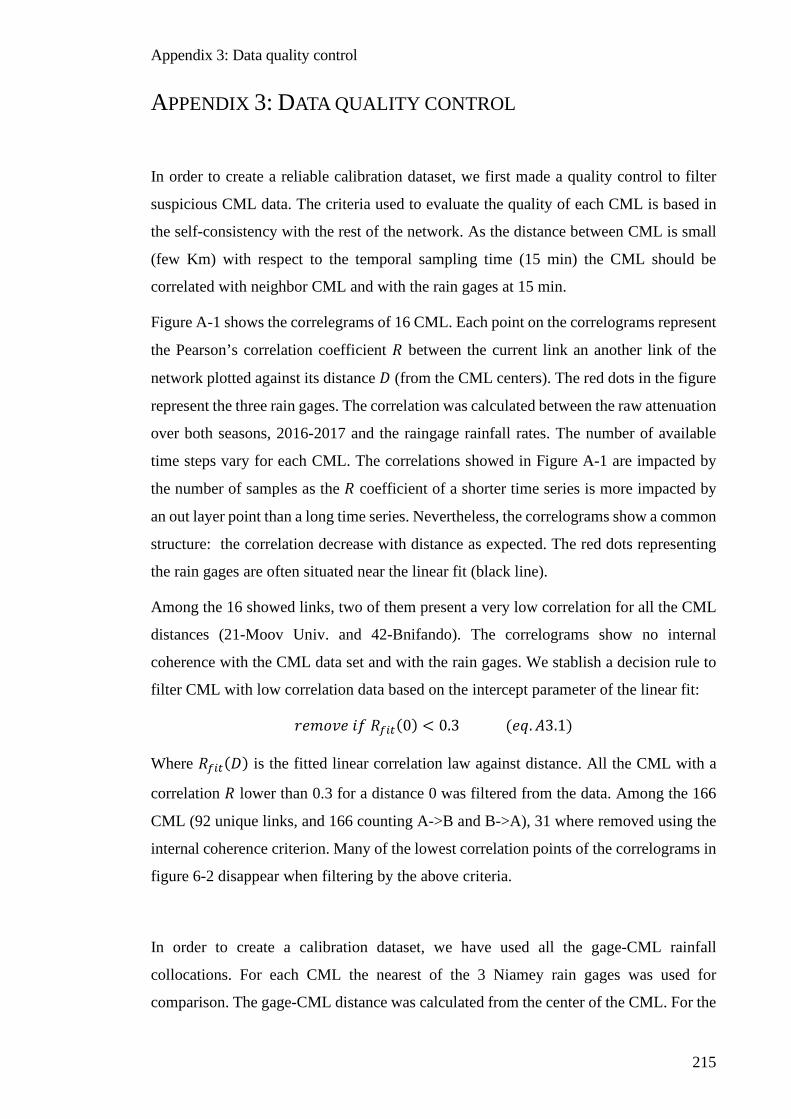
Appendix 3: Data quality control
215
APPENDIX 3: DATA QUALITY CONTROL
In order to create a reliable calibration dataset, we first made a quality control to filter
suspicious CML data. The criteria used to evaluate the quality of each CML is based in
the self-consistency with the rest of the network. As the distance between CML is small
(few Km) with respect to the temporal sampling time (15 min) the CML should be
correlated with neighbor CML and with the rain gages at 15 min.
Figure A-1 shows the correlegrams of 16 CML. Each point on the correlograms represent
the Pearson’s correlation coefficient 𝑅𝑅 between the current link an another link of the
network plotted against its distance 𝐷𝐷 (from the CML centers). The red dots in the figure
represent the three rain gages. The correlation was calculated between the raw attenuation
over both seasons, 2016-2017 and the raingage rainfall rates. The number of available
time steps vary for each CML. The correlations showed in Figure A-1 are impacted by
the number of samples as the 𝑅𝑅 coefficient of a shorter time series is more impacted by
an out layer point than a long time series. Nevertheless, the correlograms show a common
structure: the correlation decrease with distance as expected. The red dots representing
the rain gages are often situated near the linear fit (black line).
Among the 16 showed links, two of them present a very low correlation for all the CML
distances (21-Moov Univ. and 42-Bnifando). The correlograms show no internal
coherence with the CML data set and with the rain gages. We stablish a decision rule to
filter CML with low correlation data based on the intercept parameter of the linear fit:
𝑟𝑟𝑃𝑃𝑐𝑐𝑙𝑙𝑟𝑟𝑃𝑃 𝑖𝑖𝑓𝑓 𝑅𝑅𝑓𝑓𝑖𝑖𝑡𝑡(0) < 0.3 (𝑃𝑃𝑒𝑒.𝐴𝐴3.1)
Where 𝑅𝑅𝑓𝑓𝑖𝑖𝑡𝑡(𝐷𝐷) is the fitted linear correlation law against distance. All the CML with a
correlation 𝑅𝑅 lower than 0.3 for a distance 0 was filtered from the data. Among the 166
CML (92 unique links, and 166 counting A->B and B->A), 31 where removed using the
internal coherence criterion. Many of the lowest correlation points of the correlograms in
figure 6-2 disappear when filtering by the above criteria.
In order to create a calibration dataset, we have used all the gage-CML rainfall
collocations. For each CML the nearest of the 3 Niamey rain gages was used for
comparison. The gage-CML distance was calculated from the center of the CML. For the

Appendix 3: Data quality control
216
2016-2017 the total number of 15’ rainy time steps is 816 for 77 different days, 43 days
in 2016 and 34 days in 2017. The non-detections and false alarms from the CML were
filtered: only the hits were used in the comparison to avoid the effects of rain/ no-rain
detection algorithm and focus on the wet antenna effect and the K-R law. The total
number of CML-gage couples of observations is 26690. Figure 6-3 show the number of
samples by raingage rainfall class and by CML length. The CML length class (1,2] km is
overrepresented and the more intense rainfall the lower number of samples.
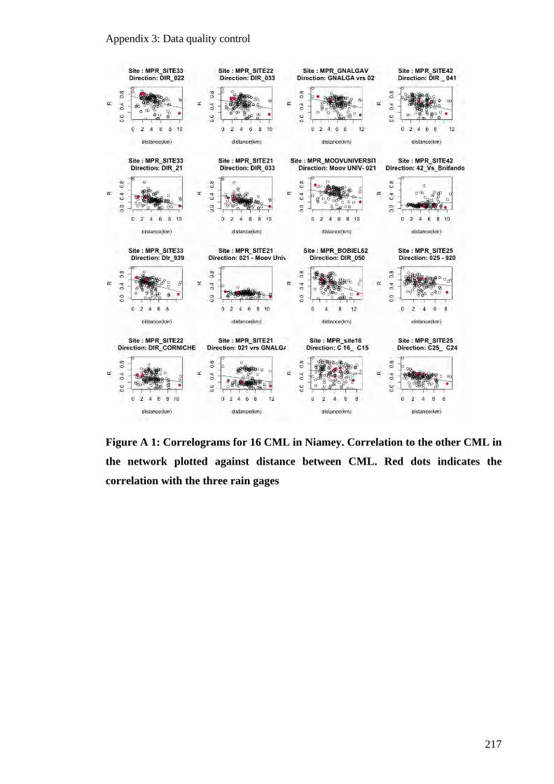
Appendix 3: Data quality control
217
Figure A 1: Correlograms for 16 CML in Niamey. Correlation to the other CML in
the network plotted against distance between CML. Red dots indicates the
correlation with the three rain gages
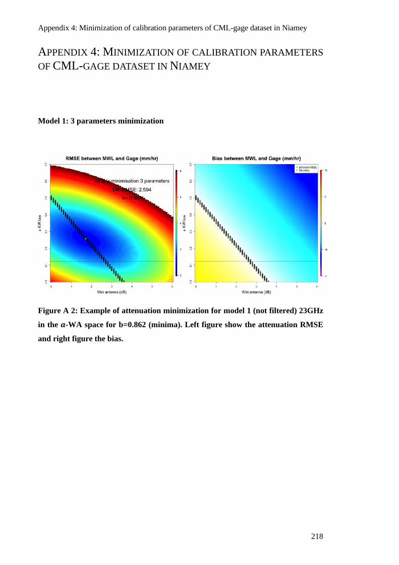
Appendix 4: Minimization of calibration parameters of CML-gage dataset in Niamey
218
APPENDIX 4: MINIMIZATION OF CALIBRATION PARAMETERS OF CML-GAGE DATASET IN NIAMEY
Model 1: 3 parameters minimization
Figure A 2: Example of attenuation minimization for model 1 (not filtered) 23GHz
in the 𝒂𝒂-WA space for b=0.862 (minima). Left figure show the attenuation RMSE
and right figure the bias.
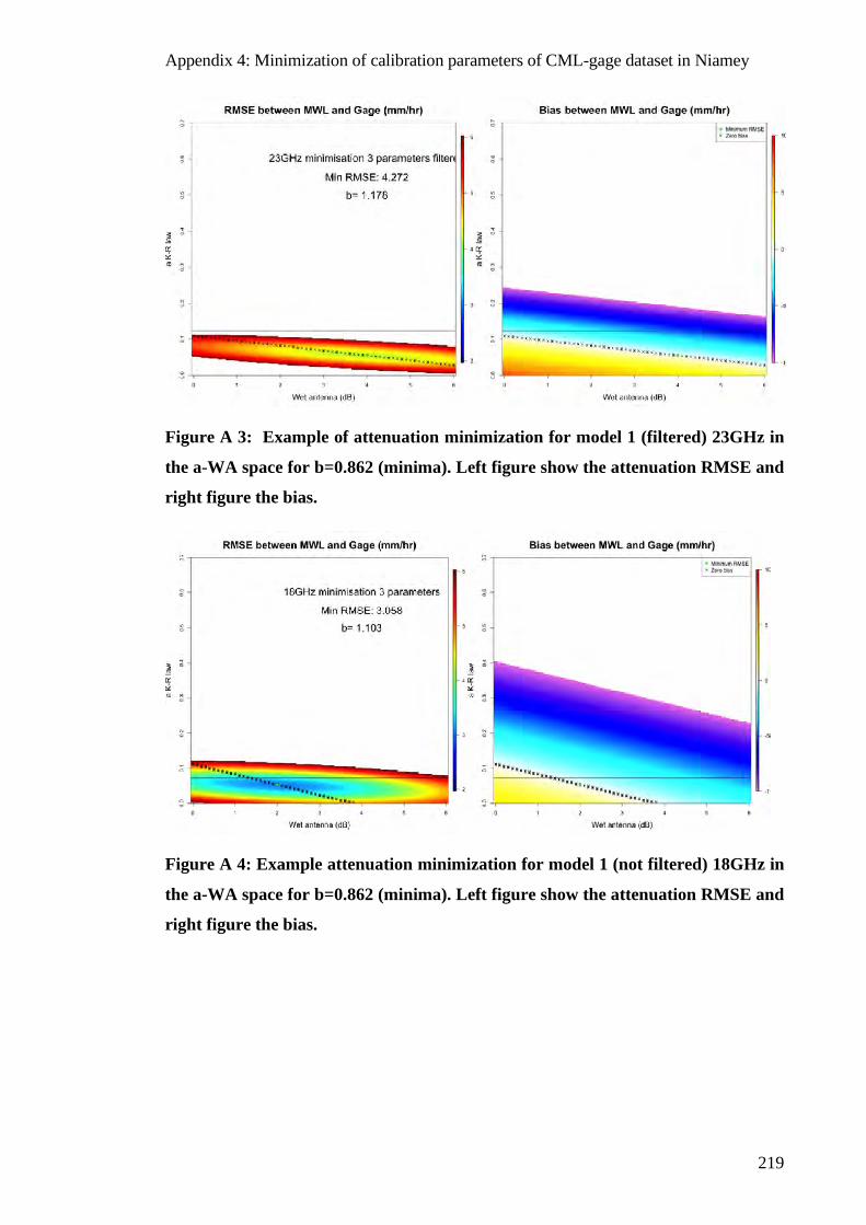
Appendix 4: Minimization of calibration parameters of CML-gage dataset in Niamey
219
Figure A 3: Example of attenuation minimization for model 1 (filtered) 23GHz in
the a-WA space for b=0.862 (minima). Left figure show the attenuation RMSE and
right figure the bias.
Figure A 4: Example attenuation minimization for model 1 (not filtered) 18GHz in
the a-WA space for b=0.862 (minima). Left figure show the attenuation RMSE and
right figure the bias.
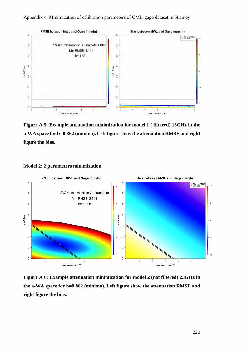
Appendix 4: Minimization of calibration parameters of CML-gage dataset in Niamey
220
Figure A 5: Example attenuation minimization for model 1 ( filtered) 18GHz in the
a-WA space for b=0.862 (minima). Left figure show the attenuation RMSE and right
figure the bias.
Model 2: 2 parameters minimization
Figure A 6: Example attenuation minimization for model 2 (not filtered) 23GHz in
the a-WA space for b=0.862 (minima). Left figure show the attenuation RMSE and
right figure the bias.
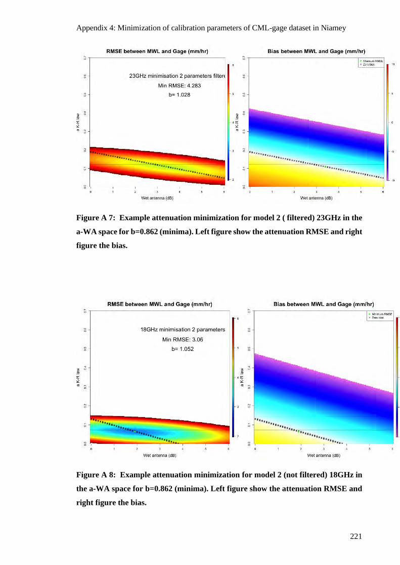
Appendix 4: Minimization of calibration parameters of CML-gage dataset in Niamey
221
Figure A 7: Example attenuation minimization for model 2 ( filtered) 23GHz in the
a-WA space for b=0.862 (minima). Left figure show the attenuation RMSE and right
figure the bias.
Figure A 8: Example attenuation minimization for model 2 (not filtered) 18GHz in
the a-WA space for b=0.862 (minima). Left figure show the attenuation RMSE and
right figure the bias.
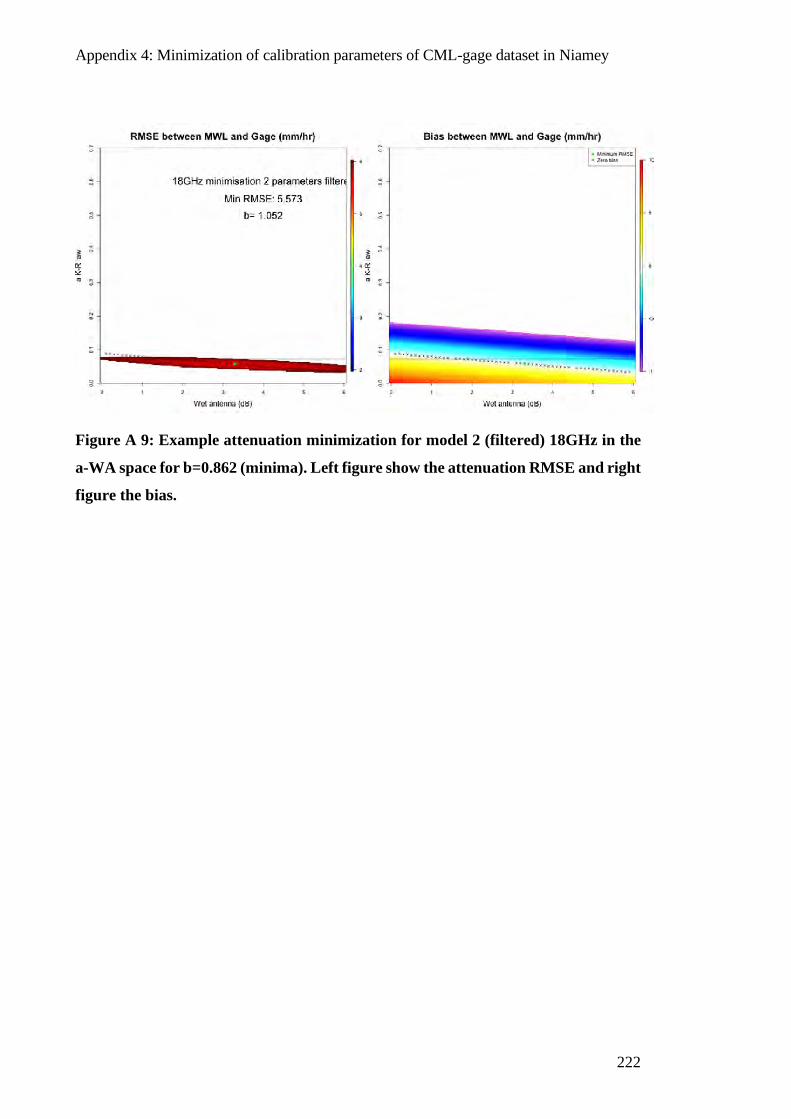
Appendix 4: Minimization of calibration parameters of CML-gage dataset in Niamey
222
Figure A 9: Example attenuation minimization for model 2 (filtered) 18GHz in the
a-WA space for b=0.862 (minima). Left figure show the attenuation RMSE and right
figure the bias.
Appendix 5: Investigation of the bias dependency on links’ length using simulations
223
APPENDIX 5: INVESTIGATION OF THE BIAS DEPENDENCY ON LINKS’ LENGTH USING SIMULATIONS
The scatterplots in figures 6-19 to 6-21 show a differential behavior of short and long
links compared to the rain gage after the wet antenna correction. In this section we assess
the differential behavior of path averaged rainfall rates at 15 minutes for different spatial
scales when compared to point scale observations with simulations of the spatial sampling
of links and rain gages.
The statistical properties of the rainfall fields depend on the scale of observation. (Guillot
and Lebel 1999) fit a geostatistical model to their observations to reproduce random fields
with similar characteristics than the observed depending on the scale. Another study in
the region (Panthou, Vischel, and Lebel 2014) fit the probability density function of
rainfall rates (PDF) describing the annual maxima of rainfall depending on time and space
scales to evaluate the annual probability of extreme events.
Concerning the gage-CML comparison we compare point scale to lineal averages. It is
not the aim of this section to fit a theoretical model to the data, as the cited studies. Though
it should be interesting for future work. In this section we try to reproduce the observed
CML/gage differences with an empirical method.
We simulate the space-time sampling of rainfall by CML and rain gages with radar DSD
fields. The objective is to reproduce the scatter plots showed in figure 6-19 to 6-21 with
realistic DSD parameters fields. We use the DSD retrieved with the inversion method
showed in the chapter 4 of this PhD. The DSD fields were retrieved from X-port X-band
polarimetric radar located in Benin in 2006. The DSD used correspond to squall lines
MCS, which are the characteristic rainfall systems of Niger.
In the first section we show the methodology to simulate the CML and gage observation
at 15 minutes sampling from DSD fields. In the following section we show the simulated
CML at different lengths compared to the simulated raingage to show the effect of
different samplings in the comparisons.

Appendix 5: Investigation of the bias dependency on links’ length using simulations
224
A5.1 Time-space effect on the PIA-rainfall relationship: simulation study based on the DSD fields
The sampling of rainfall by a microwave link 𝑅𝑅𝐿𝐿 of length 𝐿𝐿 for a duration Δ𝑤𝑤, can be
defined with the spatio-temporal field of rainfall r(x, y; t) :
𝑅𝑅𝐿𝐿(𝐿𝐿,Δ𝑤𝑤) = � � r(x, y; t)𝑑𝑑𝑠𝑠𝑑𝑑𝑤𝑤Δ𝑡𝑡
0
𝐿𝐿
0 (𝑃𝑃𝑒𝑒.𝐴𝐴5.1)
Where 𝑠𝑠 is the segment of the CML in the XY space. The rain gage sampling 𝑅𝑅𝐿𝐿=0 can
be defined as an integration of the point (𝑒𝑒0,𝑑𝑑0) over the time scale:
𝑅𝑅𝐿𝐿=0(𝑒𝑒0,𝑑𝑑0,Δ𝑤𝑤) = � r(𝑒𝑒0,𝑑𝑑0; t)𝑑𝑑𝑤𝑤Δ𝑡𝑡
0 (𝑃𝑃𝑒𝑒.𝐴𝐴5.2)
In this section we simulate a realistic set of estimated 𝑅𝑅�𝐿𝐿 with radar rainfall fields. The
accentuation in 𝑅𝑅�𝐿𝐿 denotes an estimation and the 𝐿𝐿 denotes the link length. When 𝐿𝐿 = 0
is considered to be the rain gage. The objective is to compare 𝑅𝑅�𝐿𝐿 for different lengths 𝐿𝐿
to 𝑅𝑅�0.
As a proxy of real rainfall fields 𝑟𝑟(𝑒𝑒, 𝑑𝑑; 𝑤𝑤), we used high resolution DSD parameters fields
retrieved from Xband radar data. For more details about the DSD fields, the inversion
algorithm and the DSD parameters the reader can consult the chapter 3 of this work.
The aim of using radar fields is to access the finest spatial variability of rainfall. However,
the temporal variability of rainfall is not well resolved by the radar as two consecutive
PPIs (same elevation) have a time lag of 10 minutes.
X-port radar measures instantaneous rainfall in two dimensions (range, azimuth) at a
resolution of 150m in range and 1° in azimuth. To overcome the time resolution
limitation, we consider one space dimension as the time dimension. In this region the
squall lines move usually westwards with a mean speed of 50 km/hr [Vischel et al 2011].
If we consider a theoretical CML situated along south-north direction, we can consider
the east-west direction as the time dimension of the rainfall. That is equivalent to consider
a translation of the field over the CML (and gage). The sampling of the CML can thus be
represented by a rectangle over the PPI and the raingage by a line.
Figure A-10 represents a possible sampling of a CML (black rectangle) and a gage located
in its center (white line). In this example the CML is 10 𝑘𝑘𝑐𝑐 long and the time distance
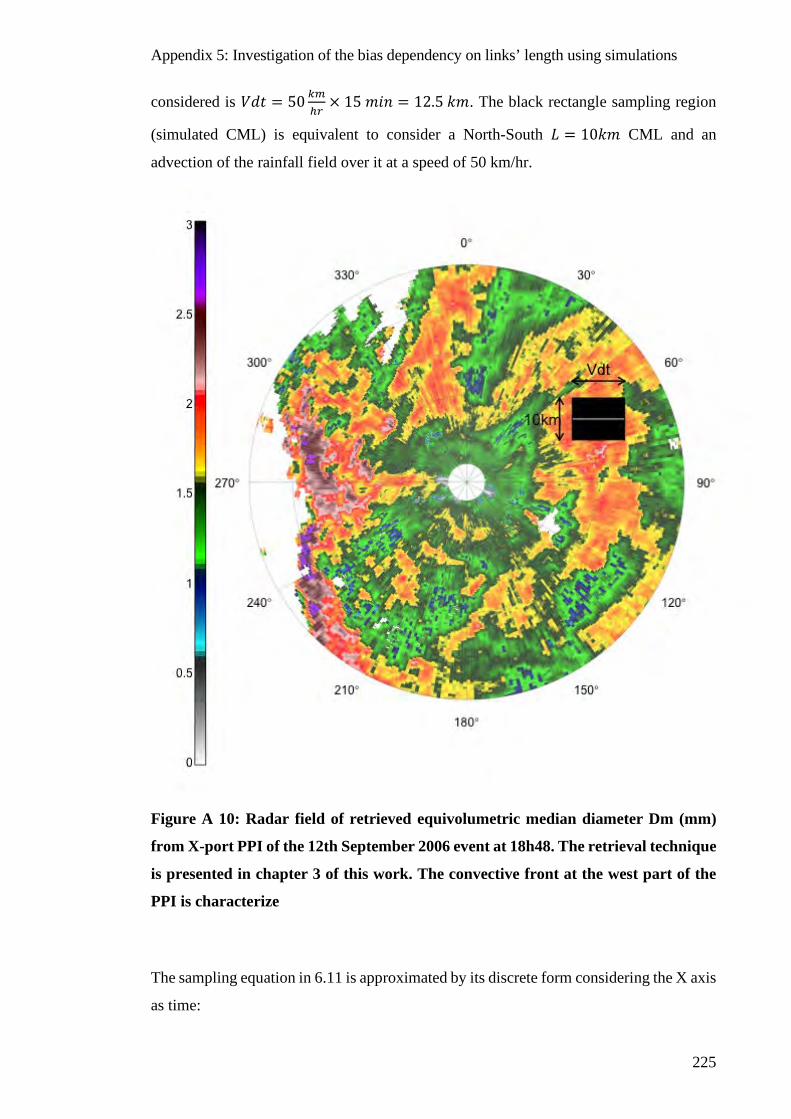
Appendix 5: Investigation of the bias dependency on links’ length using simulations
225
considered is 𝑉𝑉𝑑𝑑𝑤𝑤 = 50 𝑘𝑘𝑚𝑚ℎ𝑟𝑟
× 15 𝑐𝑐𝑖𝑖𝑙𝑙 = 12.5 𝑘𝑘𝑐𝑐. The black rectangle sampling region
(simulated CML) is equivalent to consider a North-South 𝐿𝐿 = 10𝑘𝑘𝑐𝑐 CML and an
advection of the rainfall field over it at a speed of 50 km/hr.
Figure A 10: Radar field of retrieved equivolumetric median diameter Dm (mm)
from X-port PPI of the 12th September 2006 event at 18h48. The retrieval technique
is presented in chapter 3 of this work. The convective front at the west part of the
PPI is characterize
The sampling equation in 6.11 is approximated by its discrete form considering the X axis
as time:

Appendix 5: Investigation of the bias dependency on links’ length using simulations
226
𝑅𝑅𝐿𝐿� =1𝑙𝑙𝑝𝑝𝑖𝑖𝑒𝑒
�� r𝑟𝑟𝑎𝑎𝑑𝑑𝑎𝑎𝑟𝑟(x, y)𝑑𝑑𝑒𝑒𝑑𝑑𝑑𝑑𝑋𝑋1
𝑋𝑋1
𝑌𝑌2
𝑌𝑌1
(𝑃𝑃𝑒𝑒.𝐴𝐴5.3)
Where r𝑟𝑟𝑎𝑎𝑑𝑑𝑎𝑎𝑟𝑟(x, y) is the radar rainfall field (PPI), and 𝑙𝑙𝑝𝑝𝑖𝑖𝑒𝑒 the number of pixels falling
un the zone . The length [𝑌𝑌1,𝑌𝑌2] is the link length 𝐿𝐿 and the length [𝑋𝑋1,𝑋𝑋2] the considered
temporal drift 𝑉𝑉𝑑𝑑𝑤𝑤.
In practice, as the radar geometry is range-azimuth (𝜌𝜌,𝜑𝜑 ) instead of 𝑋𝑋,𝑌𝑌 we compute the
simulated rainfall as:
𝑅𝑅𝐿𝐿� =1𝑙𝑙𝑝𝑝𝑖𝑖𝑒𝑒
� 𝑟𝑟𝑟𝑟𝑎𝑎𝑑𝑑𝑎𝑎𝑟𝑟𝜌𝜌,𝜑𝜑 ∈ 𝒟𝒟𝐿𝐿
(𝜌𝜌,𝜑𝜑) (𝑃𝑃𝑒𝑒.𝐴𝐴5.4)
Where 𝑟𝑟𝑟𝑟𝑎𝑎𝑑𝑑𝑎𝑎𝑟𝑟(𝜌𝜌,𝜑𝜑) is the rainfall rate of a pixel in the domain 𝒟𝒟𝐿𝐿 defined by a rectangle
of sizes 𝐿𝐿𝑐𝑐𝑖𝑖𝑛𝑛𝑘𝑘 × 𝑉𝑉𝑑𝑑𝑤𝑤 and 𝑙𝑙𝑝𝑝𝑖𝑖𝑒𝑒 the total number of pixels in the domain 𝒟𝒟𝐿𝐿.
As we have the DSD parameters for each pixel, we can compute also the expected
measured specific attenuation 𝐾𝐾𝐿𝐿� for each sample (equation 2.23):
𝐾𝐾𝐿𝐿� =0.4343𝑙𝑙𝑝𝑝𝑖𝑖𝑒𝑒
� � 𝑁𝑁𝑝𝑝𝑖𝑖𝑒𝑒(𝐷𝐷)𝐷𝐷𝑚𝑚𝑚𝑚𝑚𝑚
𝐷𝐷𝑚𝑚𝑖𝑖𝑛𝑛
𝜎𝜎𝑒𝑒𝑒𝑒𝑡𝑡(𝐷𝐷)𝑑𝑑𝐷𝐷𝑝𝑝𝑖𝑖𝑒𝑒 ∈ 𝒟𝒟𝐿𝐿
(𝑃𝑃𝑒𝑒.𝐴𝐴5.5)
With 𝑁𝑁𝑝𝑝𝑖𝑖𝑒𝑒(𝐷𝐷) the DSD in the pixel in [m−3] and 𝜎𝜎𝑒𝑒𝑒𝑒𝑡𝑡 the extinction cross section in [cm2]
from Mie scattering. We then can convert the expected measured attenuation 𝐾𝐾𝐿𝐿� into the
expected measured rainfall with the K-R law to evaluate the impact of the non-linear sum:
R�LNL = aKL�b (𝑃𝑃𝑒𝑒.𝐴𝐴5.6)
Where 𝑎𝑎, 𝑏𝑏 are the coefficients of the K-R law.
The comparison of 𝑅𝑅𝐿𝐿� and 𝑅𝑅0� is a proxy of the effect of the different scale sampling
between CML and rain gage. . The comparison of R�LNL and 𝑅𝑅0� adds the effect of the non-
linear K-R relation to the spatial sampling effect.
The sampling of the CML is simulated by averaging the rainfall rates of pixels included
in the zone. The sampling of raingage is simulated by a 1D line representing the time
dimension (white line in figure A-10). More precisely we considered the gage sampling
zone as a flat rectangle with a vertical extension of 500m to have enough pixels falling
inside. As the minimal size of the radar pixel in the fields are 87m x 120m (range 5km)
and a maximal size of 870m x 120m (range 50km), in practice the 500m scale is the so
called the “point scale”.
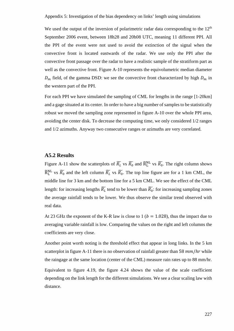
Appendix 5: Investigation of the bias dependency on links’ length using simulations
227
We used the output of the inversion of polarimetric radar data corresponding to the 12th
September 2006 event, between 18h28 and 20h08 UTC, meaning 11 different PPI. All
the PPI of the event were not used to avoid the extinction of the signal when the
convective front is located eastwards of the radar. We use only the PPI after the
convective front passage over the radar to have a realistic sample of the stratiform part as
well as the convective front. Figure A-10 represents the equivolumetric median diameter
𝐷𝐷𝑚𝑚 field, of the gamma DSD: we see the convective front characterized by high 𝐷𝐷𝑚𝑚 in
the western part of the PPI.
For each PPI we have simulated the sampling of CML for lengths in the range [1-20km]
and a gage situated at its center. In order to have a big number of samples to be statistically
robust we moved the sampling zone represented in figure A-10 over the whole PPI area,
avoiding the center disk. To decrease the computing time, we only considered 1/2 ranges
and 1/2 azimuths. Anyway two consecutive ranges or azimuths are very correlated.
A5.2 Results Figure A-11 show the scatterplots of 𝑅𝑅𝐿𝐿� vs 𝑅𝑅0� and R�LNL vs 𝑅𝑅0�. The right column shows
R�LNL vs 𝑅𝑅0� and the left column 𝑅𝑅𝐿𝐿� vs 𝑅𝑅0�. The top line figure are for a 1 km CML, the
middle line for 3 km and the bottom line for a 5 km CML. We see the effect of the CML
length: for increasing lengths 𝑅𝑅𝐿𝐿� tend to be lower than 𝑅𝑅0�: for increasing sampling zones
the average rainfall tends to be lower. We thus observe the similar trend observed with
real data.
At 23 GHz the exponent of the K-R law is close to 1 (𝑏𝑏 = 1.028), thus the impact due to
averaging variable rainfall is low. Comparing the values on the right and left columns the
coefficients are very close.
Another point worth noting is the threshold effect that appear in long links. In the 5 km
scatterplot in figure A-11 there is no observation of rainfall greater than 58 𝑐𝑐𝑐𝑐/ℎ𝑟𝑟 while
the raingage at the same location (center of the CML) measure rain rates up to 88 mm/hr.
Equivalent to figure 4.19, the figure 4.24 shows the value of the scale coefficient
depending on the link length for the different simulations. We see a clear scaling law with
distance.
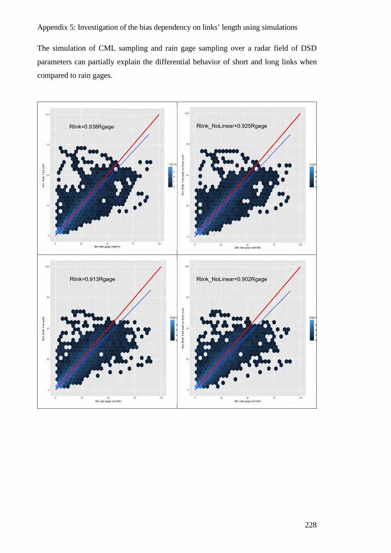
Appendix 5: Investigation of the bias dependency on links’ length using simulations
228
The simulation of CML sampling and rain gage sampling over a radar field of DSD
parameters can partially explain the differential behavior of short and long links when
compared to rain gages.
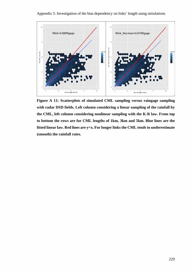
Appendix 5: Investigation of the bias dependency on links’ length using simulations
229
Figure A 11: Scatterplots of simulated CML sampling versus raingage sampling
with radar DSD fields. Left column considering a linear sampling of the rainfall by
the CML, left column considering nonlinear sampling with the K-R law. From top
to bottom the rows are for CML lengths of 1km, 3km and 5km. Blue lines are the
fitted linear law. Red lines are y=x. For longer links the CML tends to underestimate
(smooth) the rainfall rates.

Appendix 6 : Additional figures of chapter 7
230
APPENDIX 6 : ADDITIONAL FIGURES OF CHAPTER 7
Nlinks Frequencies (GHz)
Mean
Length
(Km)
Min
Length
(Km)
Max
Length
(Km)
Density
(Km/Km2)
Niamey 85 freq 18 23
Nlinks 7 78
1.37 0.51 5.44 0.49
Douala 209 8.5 11.5 14.5 15
20 1 137 51
1.62 0.12 6.59 0.82
Yaounde 168 8.5 11 13 14.5 15
24 1 1 89 53
2.11 0.17 19.16 0.36
Table A 1: Characteristics of the CML networks used for the rainfall mapping
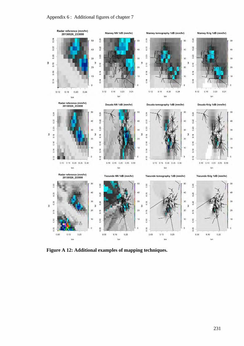
Appendix 6 : Additional figures of chapter 7
231
Figure A 12: Additional examples of mapping techniques.
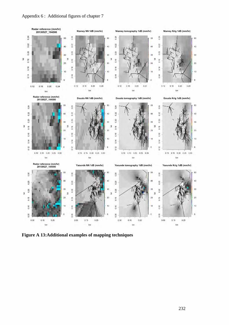
Appendix 6 : Additional figures of chapter 7
232
Figure A 13:Additional examples of mapping techniques
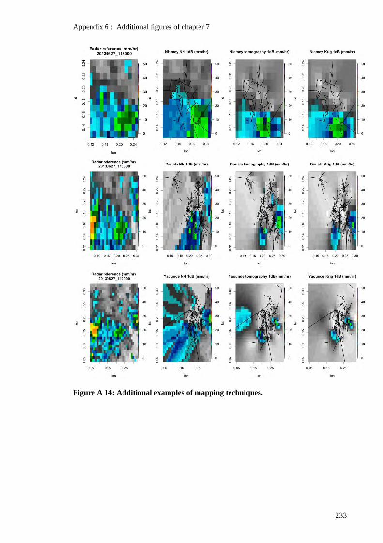
Appendix 6 : Additional figures of chapter 7
233
Figure A 14: Additional examples of mapping techniques.
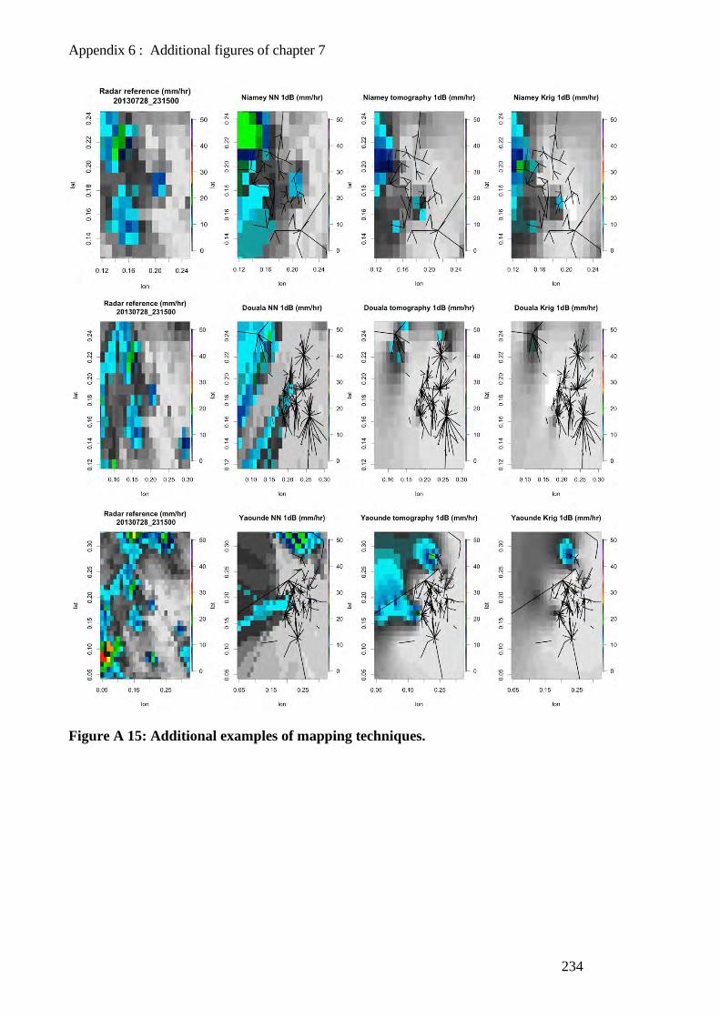
Appendix 6 : Additional figures of chapter 7
234
Figure A 15: Additional examples of mapping techniques.
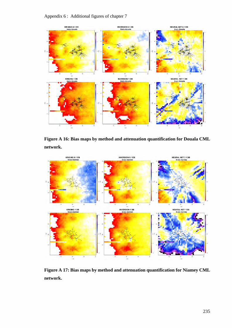
Appendix 6 : Additional figures of chapter 7
235
Figure A 16: Bias maps by method and attenuation quantification for Douala CML
network.
Figure A 17: Bias maps by method and attenuation quantification for Niamey CML
network.
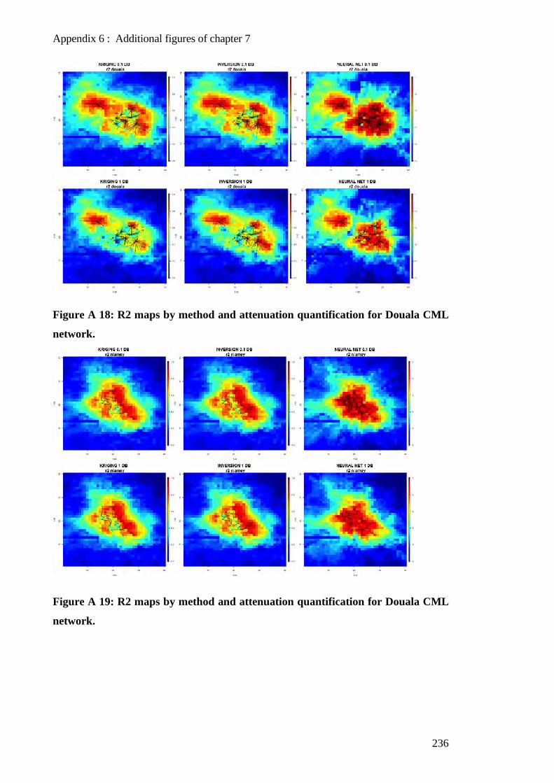
Appendix 6 : Additional figures of chapter 7
236
Figure A 18: R2 maps by method and attenuation quantification for Douala CML
network.
Figure A 19: R2 maps by method and attenuation quantification for Douala CML
network.
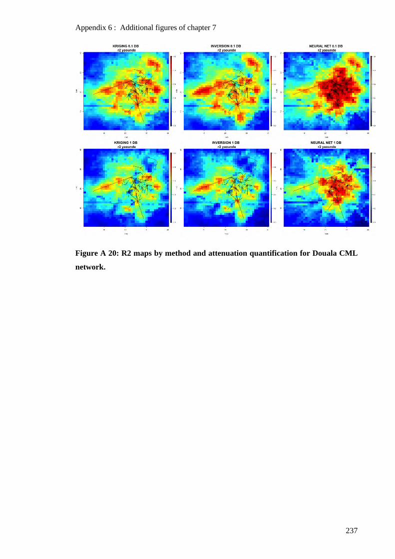
Appendix 6 : Additional figures of chapter 7
237
Figure A 20: R2 maps by method and attenuation quantification for Douala CML
network.

Appendix 6 : Additional figures of chapter 7
238

Bibliography
239
BIBLIOGRAPHY
Alcoba, M., Marielle Gosset, M. Kacou, Frédéric Cazenave, and E. Fontaine
2016 Characterization of Hydrometeors in Sahelian Convective Systems with an X-Band Radar and Comparison
with in Situ Measurements. Part II: A Simple Brightband Method to Infer the Density of Icy Hydrometeors. Journal of
Applied Meteorology and Climatology 55(2): 251–263.
Anagnostou, Marios N., Emmanouil N. Anagnostou, Gianfranco Vulpiani, et al.
2008 Evaluation of X-Band Polarimetric-Radar Estimates of Drop-Size Distributions From Coincident S-Band
Polarimetric Estimates and Measured Raindrop Spectra. IEEE Transactions on Geoscience and Remote Sensing 46(10):
3067–3075.
Andsager, Karen, Kenneth V. Beard, and Neil F. Laird
1999 Laboratory Measurements of Axis Ratios for Large Raindrops. Journal of the Atmospheric Sciences 56(15):
2673–2683.
Arnaud, Patrick, Jacques Lavabre, Catherine Fouchier, Stéphanie Diss, and Pierre Javelle
2011 Sensitivity of Hydrological Models to Uncertainty in Rainfall Input. Hydrological Sciences Journal 56(3):
397–410.
Atlas, David, and Carlton W. Ulbrich
1977 Path- and Area-Integrated Rainfall Measurement by Microwave Attenuation in the 1–3 Cm Band. Journal
of Applied Meteorology 16(12): 1322–1331.
Atlas, David, Carlton W. Ulbrich, Frank D. Marks, Eyal Amitai, and Christopher R. Williams
1999 Systematic Variation of Drop Size and Radar-Rainfall Relations. Journal of Geophysical Research:
Atmospheres 104(D6): 6155–6169.
Balme, Maud, Théo Vischel, Thierry Lebel, Christophe Peugeot, and Sylvie Galle
2006 Assessing the Water Balance in the Sahel: Impact of Small Scale Rainfall Variability on Runoff. Journal
of Hydrology 331(1–2): 336–348.
Bibliography
240
Barber, P., and C. Yeh
1975 Scattering of Electromagnetic Waves by Arbitrarily Shaped Dielectric Bodies. Applied Optics 14(12):
2864.
Beard, Kenneth V., V.N. Bringi, and M. Thurai
2010 A New Understanding of Raindrop Shape. Atmospheric Research 97(4): 396–415.
Bennartz, Ralf, and Grant W. Petty
2001 The Sensitivity of Microwave Remote Sensing Observations of Precipitation to Ice Particle Size
Distributions. Journal of Applied Meteorology 40(3): 345–364.
Bernard Fong, A.C.M. Fong, and G.Y. Hong
2005 On the Performance of Telemedicine System Using 17-GHz Orthogonally Polarized Microwave Links
under the Influence of Heavy Rainfall. IEEE Transactions on Information Technology in Biomedicine 9(3): 424–429.
Berne, A., and R. Uijlenhoet
2007 Path-Averaged Rainfall Estimation Using Microwave Links: Uncertainty Due to Spatial Rainfall
Variability. Geophysical Research Letters 34(7). http://doi.wiley.com/10.1029/2007GL029409, accessed July 9, 2019.
Bohren, Craig F., and Donald R. Huffman
2004 Absorption and Scattering of Light by Small Particles. Weinheim: Wiley-VCH.
Boudevillain, Brice, and Hervé Andrieu
2003 Assessment of Vertically Integrated Liquid (VIL) Water Content Radar Measurement. Journal of
Atmospheric and Oceanic Technology 20(6): 807–819.
Brandes, Edward A., Guifu Zhang, and J. Vivekanandan
2004 Drop Size Distribution Retrieval with Polarimetric Radar: Model and Application. Journal of Applied
Meteorology 43(3): 461–475.
Bringi, V. N., Gwo-Jong Huang, V. Chandrasekar, and E. Gorgucci
2002 A Methodology for Estimating the Parameters of a Gamma Raindrop Size Distribution Model from
Polarimetric Radar Data: Application to a Squall-Line Event from the TRMM/Brazil Campaign. Journal of
Atmospheric and Oceanic Technology 19(5): 633–645.
Bringi, V. Nꎬ, and V. Chandrasekar
2001 Polarimetric Doppler Weather Radar: Principles and Applications. Cambridge university press.

Bibliography
241
Bringi, V.N., T.D. Keenan, and V. Chandrasekar
2001 Correcting C-Band Radar Reflectivity and Differential Reflectivity Data for Rain Attenuation: A Self-
Consistent Method with Constraints. IEEE Transactions on Geoscience and Remote Sensing 39(9): 1906–1915.
Cao, Qing, Guifu Zhang, Edward Brandes, et al.
2008 Analysis of Video Disdrometer and Polarimetric Radar Data to Characterize Rain Microphysics in
Oklahoma. Journal of Applied Meteorology and Climatology 47(8): 2238–2255.
Cao, Qing, Guifu Zhang, Edward A. Brandes, and Terry J. Schuur
2010 Polarimetric Radar Rain Estimation through Retrieval of Drop Size Distribution Using a Bayesian
Approach. Journal of Applied Meteorology and Climatology 49(5): 973–990.
Carey, Lawrence D., Steven A. Rutledge, David A. Ahijevych, and Tom D. Keenan
2000 Correcting Propagation Effects in C-Band Polarimetric Radar Observations of Tropical Convection Using
Differential Propagation Phase. Journal of Applied Meteorology 39(9): 1405–1433.
Cazenave, Frédéric, Marielle Gosset, M Kacou, et al.
2016 Characterization of Hydrometeors in Sahelian Convective Systems with an X-Band Radar and Comparison
with in Situ Measurements. Part I: Sensitivity of Polarimetric Radar Particle Identification Retrieval and Case Study
Evaluation. Journal of Applied Meteorology and Climatology 55(2): 231–249.
Chang, Wei-Yu, Jothiram Vivekanandan, and Tai-Chi Chen Wang
2014 Estimation of X-Band Polarimetric Radar Attenuation and Measurement Uncertainty Using a Variational
Method. Journal of Applied Meteorology and Climatology 53(4): 1099–1119.
Chen, Haonan, V. Chandrasekar, and Renzo Bechini
2017 An Improved Dual-Polarization Radar Rainfall Algorithm (DROPS2.0): Application in NASA IFloodS
Field Campaign. Journal of Hydrometeorology 18(4): 917–937.
Cherkassky, Dani, Jonatan Ostrometzky, and Hagit Messer
2014 Precipitation Classification Using Measurements From Commercial Microwave Links. IEEE Transactions
on Geoscience and Remote Sensing 52(5): 2350–2356.
Chwala, C., A. Gmeiner, W. Qiu, et al.
2012 Precipitation Observation Using Microwave Backhaul Links in the Alpine and Pre-Alpine Region of
Southern Germany. Hydrology and Earth System Sciences 16(8): 2647–2661.

Bibliography
242
Ciach, Grzegorz J.
2003 Local Random Errors in Tipping-Bucket Rain Gauge Measurements. Journal of Atmospheric and Oceanic
Technology 20(5): 752–759.
D’Amico, Michele, Andrea Manzoni, and Gian Leonardo Solazzi
2016 Use of Operational Microwave Link Measurements for the Tomographic Reconstruction of 2-D Maps of
Accumulated Rainfall. IEEE Geoscience and Remote Sensing Letters 13(12): 1827–1831.
Das, Saurabh, Animesh Maitra, and Ashish K. Shukla
2010 RAIN ATTENUATION MODELING IN THE 10-100 GHz FREQUENCY USING DROP SIZE
DISTRIBUTIONS FOR DIFFERENT CLIMATIC ZONES IN TROPICAL INDIA. Progress In Electromagnetics
Research B 25: 211–224.
Delahaye, J.-Y., L. Barthès, P. Golé, J. Lavergnat, and J.P. Vinson
2006 A Dual-Beam Spectropluviometer Concept. Journal of Hydrology 328(1–2): 110–120.
Delrieu, G., S. Caoudal, and J. D. Creutin
1997 Feasibility of Using Mountain Return for the Correction of Ground-Based X-Band Weather Radar Data.
Journal of Atmospheric and Oceanic Technology 14(3): 368–385.
Depraetere, Christian, Marielle Gosset, Stéphane Ploix, and Henri Laurent
2009 The Organization and Kinematics of Tropical Rainfall Systems Ground Tracked at Mesoscale with Gages:
First Results from the Campaigns 1999–2006 on the Upper Ouémé Valley (Benin). Journal of Hydrology 375(1–2):
143–160.
Doumounia, Ali, Marielle Gosset, Frederic Cazenave, Modeste Kacou, and François Zougmore
2014 Rainfall Monitoring Based on Microwave Links from Cellular Telecommunication Networks: First Results
from a West African Test Bed: WIRELESS NETWORKS FOR RAINFALL IN AFRICA. Geophysical Research
Letters 41(16): 6016–6022.
Elshaikh, Zain Elabdin Omer, Md. Rafiqul Islam, Othman O. Khalifa, and Hany Essam Abd-El-Raouf
2009 MATHEMATICAL MODEL FOR THE PREDICTION OF MICROWAVE SIGNAL ATTENUATION
DUE TO DUSTSTORM. Progress In Electromagnetics Research M 6: 139–153.
Fabry, Frédéric
2015 Radar Meteorology: Principles and Practice. Cambridge, United Kingdom: Cambridge University Press.
Fabry, Frédéric, and Wanda Szyrmer
Bibliography
243
1999 Modeling of the Melting Layer. Part II: Electromagnetic. Journal of the Atmospheric Sciences 56(20):
3593–3600.
Fabry, Frederic, and Isztar Zawadzki
1995 Long-Term Radar Observations of the Melting Layer of Precipitation and Their Interpretation. Journal of
the Atmospheric Sciences 52(7): 838–851.
Fontaine, E., A. Schwarzenboeck, J. Delanoë, et al.
2014 Constraining Mass–Diameter Relations from Hydrometeor Images and Cloud Radar Reflectivities in
Tropical Continental and Oceanic Convective Anvils. Atmospheric Chemistry and Physics 14(20): 11367–11392.
Galle, S., M. Grippa, C. Peugeot, et al.
2018 AMMA-CATCH, a Critical Zone Observatory in West Africa Monitoring a Region in Transition. Vadose
Zone Journal 17(1): 0.
Goldshtein, O., H. Messer, and A. Zinevich
2009 Rain Rate Estimation Using Measurements From Commercial Telecommunications Links. IEEE
Transactions on Signal Processing 57(4): 1616–1625.
Gorgucci, Eugenio, Luca Baldini, and V. Chandrasekar
2006 What Is the Shape of a Raindrop? An Answer from Radar Measurements. Journal of the Atmospheric
Sciences 63(11): 3033–3044.
Gorgucci, Eugenio, V. Chandrasekar, and Luca Baldini
2009 Can a Unique Model Describe the Raindrop Shape–Size Relation? A Clue from Polarimetric Radar
Measurements. Journal of Atmospheric and Oceanic Technology 26(9): 1829–1842.
Gorgucci, Eugenio, V. Chandrasekar, V. N. Bringi, and Gianfranco Scarchilli
2002 Estimation of Raindrop Size Distribution Parameters from Polarimetric Radar Measurements. Journal of
the Atmospheric Sciences 59(15): 2373–2384.
Gorgucci, Eugenio, Gianfranco Scarchilli, V. Chandrasekar, and V. N. Bringi
2000 Measurement of Mean Raindrop Shape from Polarimetric Radar Observations. Journal of the Atmospheric
Sciences 57(20): 3406–3413.
2001a Rainfall Estimation from Polarimetric Radar Measurements: Composite Algorithms Immune to Variability
in Raindrop Shape–Size Relation. Journal of Atmospheric and Oceanic Technology 18(11): 1773–1786.
2001b Rainfall Estimation from Polarimetric Radar Measurements: Composite Algorithms Immune to Variability

Bibliography
244
in Raindrop Shape–Size Relation. Journal of Atmospheric and Oceanic Technology 18(11): 1773–1786.
Gosset, Marielle, Matias Alcoba, Remy Roca, Sophie Cloché, and Guillaume Urbani
2018 Evaluation of TAPEER Daily Estimates and Other GPM Era Products against Dense Gauge Networks in
West Africa, Analyzing Ground Reference Uncertainty. Quarterly Journal of the Royal Meteorological Society.
Gosset, Marielle, Julien Viarre, Guillaume Quantin, and Matias Alcoba
2013 Evaluation of Several Rainfall Products Used for Hydrological Applications over West Africa Using Two
High-Resolution Gauge Networks. Quarterly Journal of the Royal Meteorological Society 139(673): 923–940.
Gosset, Marielle, Eric-Pascal Zahiri, and Sounmaila Moumouni
2010a Rain Drop Size Distribution Variability and Impact on X-Band Polarimetric Radar Retrieval: Results from
the AMMA Campaign in Benin. Quarterly Journal of the Royal Meteorological Society 136(S1): 243–256.
2010b Rain Drop Size Distribution Variability and Impact on X-Band Polarimetric Radar Retrieval: Results from
the AMMA Campaign in Benin. Quarterly Journal of the Royal Meteorological Society 136(S1): 243–256.
Gou, Yabin, Haonan Chen, and Jiafeng Zheng
2019 An Improved Self-Consistent Approach to Attenuation Correction for C-Band Polarimetric Radar
Measurements and Its Impact on Quantitative Precipitation Estimation. Atmospheric Research 226: 32–48.
Gourley, Jonathan J., Pierre Tabary, and Jacques Parent du Chatelet
2007 Empirical Estimation of Attenuation from Differential Propagation Phase Measurements at C Band. Journal
of Applied Meteorology and Climatology 46(3): 306–317.
Guillot, Gilles, and Thierry Lebel
1999 Disaggregation of Sahelian Mesoscale Convective System Rain Fields: Further Developments and
Validation. Journal of Geophysical Research: Atmospheres 104(D24): 31533–31551.
Guilloteau, Clément, Rémy Roca, and Marielle Gosset
2016 A Multiscale Evaluation of the Detection Capabilities of High-Resolution Satellite Precipitation Products
in West Africa. Journal of Hydrometeorology 17(7): 2041–2059.
Hachani, Sahar, Brice Boudevillain, Guy Delrieu, and Zoubeida Bargaoui
2017 Drop Size Distribution Climatology in Cévennes-Vivarais Region, France. Atmosphere 8(12): 233.
Haykin, Simon S.
1994 Neural Networks: A Comprehensive Foundation. New York : Toronto : New York: Macmillan ; Maxwell
Bibliography
245
Macmillan Canada ; Maxwell Macmillan International.
Houze, Robert A.
2004 Mesoscale Convective Systems. Reviews of Geophysics 42(4).
http://doi.wiley.com/10.1029/2004RG000150, accessed July 4, 2019.
Hubbert, J., and V. N. Bringi
1995 An Iterative Filtering Technique for the Analysis of Copolar Differential Phase and Dual-Frequency Radar
Measurements. Journal of Atmospheric and Oceanic Technology 12(3): 643–648.
Illingworth, Anthony J., and T. Mark Blackman
2002 The Need to Represent Raindrop Size Spectra as Normalized Gamma Distributions for the Interpretation
of Polarization Radar Observations. Journal of Applied Meteorology 41(3): 286–297.
Islam, Tanvir, Miguel A. Rico-Ramirez, and Dawei Han
2012 Tree-Based Genetic Programming Approach to Infer Microphysical Parameters of the DSDs from the
Polarization Diversity Measurements. Computers & Geosciences 48: 20–30.
Kacou, Modeste Huberson Ahiba
2014 Analyse Des Précipitations En Zone Sahélienne à Partir d’un Radar Bande X Polarimétrique. PhD Thesis,
Université de Toulouse, Université Toulouse III-Paul Sabatier; Université ….
Kalogiros, John, Marios N. Anagnostou, Emmanouil N. Anagnostou, et al.
2014 Evaluation of a New Polarimetric Algorithm for Rain-Path Attenuation Correction of X-Band Radar
Observations Against Disdrometer. IEEE Transactions on Geoscience and Remote Sensing 52(2): 1369–1380.
Kharadly, M.M.Z., and R. Ross
2001 Effect of Wet Antenna Attenuation on Propagation Data Statistics. IEEE Transactions on Antennas and
Propagation 49(8): 1183–1191.
Kidd, Chris, Andreas Becker, George J. Huffman, et al.
2017 So, How Much of the Earth’s Surface Is Covered by Rain Gauges? Bulletin of the American Meteorological
Society 98(1): 69–78.
Kim, Dong-Soon, Masayuki Maki, and Dong-In Lee
2008 Correction of X-Band Radar Reflectivity and Differential Reflectivity for Rain Attenuation Using
Differential Phase. Atmospheric Research 90(1): 1–9.
Bibliography
246
Kim, D-S., M. Maki, and D-I. Lee
2010 Retrieval of Three-Dimensional Raindrop Size Distribution Using X-Band Polarimetric Radar Data.
Journal of Atmospheric and Oceanic Technology 27(8): 1265–1285.
Kirstetter, Pierre-Emmanuel, Hervé Andrieu, Brice Boudevillain, and Guy Delrieu
2013 A Physically Based Identification of Vertical Profiles of Reflectivity from Volume Scan Radar Data.
Journal of Applied Meteorology and Climatology 52(7): 1645–1663.
Kirstetter, Pierre-Emmanuel, Nicolas Viltard, and Marielle Gosset
2013 An Error Model for Instantaneous Satellite Rainfall Estimates: Evaluation of BRAIN-TMI over West
Africa. Quarterly Journal of the Royal Meteorological Society 139(673): 894–911.
Klaassen, Wim
1988 Radar Observations and Simulation of the Melting Layer of Precipitation. Journal of the Atmospheric
Sciences 45(24): 3741–3753.
Koffi, A.K., M. Gosset, E.-P. Zahiri, et al.
2014 Evaluation of X-Band Polarimetric Radar Estimation of Rainfall and Rain Drop Size Distribution
Parameters in West Africa. Atmospheric Research 143: 438–461.
Kumar, Lakshmi Sutha, Yee Hui Lee, and Jin Teong Ong
2010 Truncated Gamma Drop Size Distribution Models for Rain Attenuation in Singapore. IEEE Transactions
on Antennas and Propagation 58(4): 1325–1335.
Kummerow, C., W.S. Olson, and L. Giglio
1996 A Simplified Scheme for Obtaining Precipitation and Vertical Hydrometeor Profiles from Passive
Microwave Sensors. IEEE Transactions on Geoscience and Remote Sensing 34(5): 1213–1232.
Lebel, T., D. J. Parker, C. Flamant, et al.
2010 The AMMA Field Campaigns: Multiscale and Multidisciplinary Observations in the West African Region.
Quarterly Journal of the Royal Meteorological Society 136(S1): 8–33.
Lee, Choong Ke, Gyu Won Lee, Isztar Zawadzki, and Kyung-Eak Kim
2009 A Preliminary Analysis of Spatial Variability of Raindrop Size Distributions during Stratiform Rain Events.
Journal of Applied Meteorology and Climatology 48(2): 270–283.
Lee, Gyu Won, and Isztar Zawadzki
Bibliography
247
2005 Variability of Drop Size Distributions: Time-Scale Dependence of the Variability and Its Effects on Rain
Estimation. Journal of Applied Meteorology 44(2): 241–255.
Lee, Gyu Won, Isztar Zawadzki, Wanda Szyrmer, Daniel Sempere-Torres, and Remko Uijlenhoet
2004 A General Approach to Double-Moment Normalization of Drop Size Distributions. Journal of Applied
Meteorology 43(2): 264–281.
Leijnse, H., R. Uijlenhoet, and J. N. M. Stricker
2007 Rainfall Measurement Using Radio Links from Cellular Communication Networks: RAPID
COMMUNICATION. Water Resources Research 43(3). http://doi.wiley.com/10.1029/2006WR005631, accessed July
4, 2019.
Leijnse, H., R. Uijlenhoet, and J.N.M. Stricker
2008 Microwave Link Rainfall Estimation: Effects of Link Length and Frequency, Temporal Sampling, Power
Resolution, and Wet Antenna Attenuation. Advances in Water Resources 31(11): 1481–1493.
Leijnse, Hidde, Remko Uijlenhoet, and Alexis Berne
2010 Errors and Uncertainties in Microwave Link Rainfall Estimation Explored Using Drop Size Measurements
and High-Resolution Radar Data. Journal of Hydrometeorology 11(6): 1330–1344.
Liebe, Hans J., George A. Hufford, and Takeshi Manabe
1991 A Model for the Complex Permittivity of Water at Frequencies below 1 THz. International Journal of
Infrared and Millimeter Waves 12(7): 659–675.
Liebe, HJ, GA Hufford, and MG Cotton
1993 Propagation Modeling of Moist Air and Suspended Water/Ice Particles at Frequencies below 1000 GHz. In
In AGARD, Atmospheric Propagation Effects Through Natural and Man-Made Obscurants for Visible to MM-Wave
Radiation 11 p (SEE N94-30495 08-32).
Liu, Hongping, and V. Chandrasekar
2000 Classification of Hydrometeors Based on Polarimetric Radar Measurements: Development of Fuzzy Logic
and Neuro-Fuzzy Systems, and In Situ Verification. Journal of Atmospheric and Oceanic Technology 17(2): 140–164.
Lorenz, Christof, and Harald Kunstmann
2012 The Hydrological Cycle in Three State-of-the-Art Reanalyses: Intercomparison and Performance Analysis.
Journal of Hydrometeorology 13(5): 1397–1420.
Marshall, J. S., and W. Mc K. Palmer
Bibliography
248
1948 THE DISTRIBUTION OF RAINDROPS WITH SIZE. Journal of Meteorology 5(4): 165–166.
Matrosov, Sergey Y., Kurt A. Clark, Brooks E. Martner, and Ali Tokay
2002 X-Band Polarimetric Radar Measurements of Rainfall. Journal of Applied Meteorology 41(9): 941–952.
Matrosov, Sergey Y., David E. Kingsmill, Brooks E. Martner, and F. Martin Ralph
2005 The Utility of X-Band Polarimetric Radar for Quantitative Estimates of Rainfall Parameters. Journal of
Hydrometeorology 6(3): 248–262.
Menke, William
2018 Geophysical Data Analysis: Discrete Inverse Theory. Fourth edition. Amsterdam London Cambridge, MA:
Elsevier/Academic Press.
Messer, H.
2006 Environmental Monitoring by Wireless Communication Networks. Science 312(5774): 713–713.
Mie, Gustav
1908 Beiträge zur Optik trüber Medien, speziell kolloidaler Metallösungen. Annalen der Physik 330(3): 377–
445.
Minda, Haruya, and Kenji Nakamura
2005 High Temporal Resolution Path-Average Rain Gauge with 50-GHz Band Microwave. Journal of
Atmospheric and Oceanic Technology 22(2): 165–179.
Mishchenko, Michael I., Larry D. Travis, and Daniel W. Mackowski
1996 T-Matrix Computations of Light Scattering by Nonspherical Particles: A Review. Journal of Quantitative
Spectroscopy and Radiative Transfer 55(5): 535–575.
Moumouni, Sounmaïla
2009 Analyse Des Distributions Granulométriques Des Pluies Au Bénin : Caractéristiques Globales, Variabilité
et Application à La Mesure Radar.
Moumouni, Sounmaila, Marielle Gosset, and Etienne Houngninou
2008 Main Features of Rain Drop Size Distributions Observed in Benin, West Africa, with Optical Disdrometers.
Geophysical Research Letters 35(23). http://doi.wiley.com/10.1029/2008GL035755, accessed May 16, 2018.
Olsen, R., D. Rogers, and D. Hodge
Bibliography
249
1978 The AR<Sup>B</Sup>Relation in the Calculation of Rain Attenuation. IEEE Transactions on
Antennas and Propagation 26(2): 318–329.
Ostrometzky, Jonatan, and Hagit Messer
2014 Accumulated Rainfall Estimation Using Maximum Attenuation of Microwave Radio Signal. In 2014 IEEE
8th Sensor Array and Multichannel Signal Processing Workshop (SAM) Pp. 193–196. A Coruna, Spain: IEEE.
http://ieeexplore.ieee.org/document/6882373/, accessed July 4, 2019.
2018 On the Information in Extreme Measurements for Parameter Estimation. ArXiv:1809.08662 [Cs, Eess,
Math]. http://arxiv.org/abs/1809.08662, accessed July 4, 2019.
Overeem, A., H. Leijnse, and R. Uijlenhoet
2011 Measuring Urban Rainfall Using Microwave Links from Commercial Cellular Communication Networks:
MEASURING URBAN RAINFALL USING MICROWAVE LINKS. Water Resources Research 47(12).
http://doi.wiley.com/10.1029/2010WR010350, accessed September 10, 2018.
Overeem, Aart, Hidde Leijnse, and Remko Uijlenhoet
2013 Country-Wide Rainfall Maps from Cellular Communication Networks. Proceedings of the National
Academy of Sciences 110(8): 2741–2745.
Panthou, G., T. Vischel, and T. Lebel
2014 Recent Trends in the Regime of Extreme Rainfall in the Central Sahel: RECENT TRENDS OF EXTREME
RAINFALL IN THE WEST AFRICAN SAHEL. International Journal of Climatology 34(15): 3998–4006.
Park, S. G., Masayuki Maki, K. Iwanami, V. N. Bringi, and V. Chandrasekar
2005 Correction of Radar Reflectivity and Differential Reflectivity for Rain Attenuation at X Band. Part II:
Evaluation and Application. Journal of Atmospheric and Oceanic Technology 22(11): 1633–1655.
Pruppacher, H. R., and K. V. Beard
1970 A Wind Tunnel Investigation of the Internal Circulation and Shape of Water Drops Falling at Terminal
Velocity in Air. Quarterly Journal of the Royal Meteorological Society 96(408): 247–256.
Rahim, S. K. A., A. Y. Abdulrahman, T. A. Rahman, and M. R. Ul Islam
2012 Measurement of Wet Antenna Losses on 26 GHz Terrestrial Microwave Link in Malaysia. Wireless
Personal Communications 64(2): 225–231.
Raupach, Timothy H., and Alexis Berne
2017 Retrieval of the Raindrop Size Distribution from Polarimetric Radar Data Using Double-Moment
Normalisation. Atmospheric Measurement Techniques 10(7): 2573–2594.
Bibliography
250
Ray, Peter S.
1972 Broadband Complex Refractive Indices of Ice and Water. Applied Optics 11(8): 1836.
Rayitsfeld, Asaf, Rana Samuels, Artem Zinevich, Uri Hadar, and Pinhas Alpert
2012 Comparison of Two Methodologies for Long Term Rainfall Monitoring Using a Commercial Microwave
Communication System. Atmospheric Research 104–105: 119–127.
Reller, Christoph, Hans-Andrea Loeliger, and Juan Pablo Marᅢᆳn Dᅢᆳaz
N.d. A Model for Quasi-Periodic Signals with Application to Rain Estimation From Microwave Link Gain: 5.
Rincon, R.F., S.W. Bidwell, A.R. Jameson, and O.W. Thiele
1996 A Multi-Frequency, Dual-Polarization, Microwave Link for Rainfall Estimation. In IGARSS ’96. 1996
International Geoscience and Remote Sensing Symposium Pp. 402–404. Lincoln, NE, USA: IEEE.
http://ieeexplore.ieee.org/document/516354/, accessed July 9, 2019.
Roca, R., J. Aublanc, P. Chambon, T. Fiolleau, and N. Viltard
2014 Robust Observational Quantification of the Contribution of Mesoscale Convective Systems to Rainfall in
the Tropics. Journal of Climate 27(13): 4952–4958.
Roca, Rémy, Hélène Brogniez, Philippe Chambon, et al.
2015 The Megha-Tropiques Mission: A Review after Three Years in Orbit. Frontiers in Earth Science 3.
http://www.frontiersin.org/Atmospheric_Science/10.3389/feart.2015.00017/abstract, accessed July 4, 2019.
Roy, Venkat, Shahzad Gishkori, and Geert Leus
2014 Spatial Rainfall Mapping from Path-Averaged Rainfall Measurements Exploiting Sparsity. In Signal and
Information Processing (GlobalSIP), 2014 IEEE Global Conference On Pp. 321–325. IEEE.
van het Schip, T. I., A. Overeem, H. Leijnse, et al.
2017 Rainfall Measurement Using Cell Phone Links: Classification of Wet and Dry Periods Using Geostationary
Satellites. Hydrological Sciences Journal 62(9): 1343–1353.
Schleiss, Marc, and Alexis Berne
2010 Identification of Dry and Rainy Periods Using Telecommunication Microwave Links. IEEE Geoscience
and Remote Sensing Letters 7(3): 611–615.
Schleiss, Marc, Jörg Rieckermann, and Alexis Berne

Bibliography
251
2013 Quantification and Modeling of Wet-Antenna Attenuation for Commercial Microwave Links. IEEE
Geoscience and Remote Sensing Letters 10(5): 1195–1199.
Semplak, R.
1970 The Influence of Heavy Rainfall on Attenuation at 18.5 and 30.9 GHz. IEEE Transactions on Antennas and
Propagation 18(4): 507–511.
Semplak, R. A., and R. H. Turrin
1969 Some Measurements of Attenuation by Rainfall at 18.5 GHz*. Bell System Technical Journal 48(6): 1767–
1787.
Shi, Zhao, Haonan Chen, Venkatachalam Chandrasekar, and Jianxin He
2017 Deployment and Performance of an X-Band Dual-Polarization Radar during the Southern China Monsoon
Rainfall Experiment. Atmosphere 9(1): 4.
Steiner, Matthias, James A. Smith, and Remko Uijlenhoet
2004 A Microphysical Interpretation of Radar Reflectivity–Rain Rate Relationships. Journal of the Atmospheric
Sciences 61(10): 1114–1131.
Szakáll, Miklós, Subir K. Mitra, Karoline Diehl, and Stephan Borrmann
2010 Shapes and Oscillations of Falling Raindrops — A Review. Atmospheric Research 97(4): 416–425.
Tabary, Pierre, Abdel-Amin Boumahmoud, Hervé Andrieu, et al.
2011 Evaluation of Two “Integrated” Polarimetric Quantitative Precipitation Estimation (QPE) Algorithms at C-
Band. Journal of Hydrology 405(3–4): 248–260.
Tarantola, Albert
2005 Inverse Problem Theory and Methods for Model Parameter Estimation, vol.89. siam.
Tarantola, Albert, and Bernard Valette
1982 Generalized Nonlinear Inverse Problems Solved Using the Least Squares Criterion. Reviews of Geophysics
20(2): 219.
Tat-Soon Yee, Pang-Shyan Kooi, Mook-Seng Leong, and Le-Wei Li
2001 Tropical Raindrop Size Distribution for the Prediction of Rain Attenuation of Microwaves in the 10-40
GHz Band. IEEE Transactions on Antennas and Propagation 49(1): 80–83.

Bibliography
252
Testud, Jacques, Erwan Le Bouar, Estelle Obligis, and Mustapha Ali-Mehenni
2000 The Rain Profiling Algorithm Applied to Polarimetric Weather Radar. Journal of Atmospheric and Oceanic
Technology 17(3): 332–356.
Testud, Jacques, Stéphane Oury, Robert A. Black, Paul Amayenc, and Xiankang Dou
2001 The Concept of “Normalized” Distribution to Describe Raindrop Spectra: A Tool for Cloud Physics and
Cloud Remote Sensing. Journal of Applied Meteorology 40(6): 1118–1140.
Thurai, M., V. N. Bringi, M. Szakáll, et al.
2009 Drop Shapes and Axis Ratio Distributions: Comparison between 2D Video Disdrometer and Wind-Tunnel
Measurements. Journal of Atmospheric and Oceanic Technology 26(7): 1427–1432.
Tokay, Ali, and Kenneth V. Beard
1996 A Field Study of Raindrop Oscillations. Part I: Observation of Size Spectra and Evaluation of Oscillation
Causes. Journal of Applied Meteorology 35(10): 1671–1687.
Tokay, Ali, and David A. Short
1996 Evidence from Tropical Raindrop Spectra of the Origin of Rain from Stratiform versus Convective Clouds.
Journal of Applied Meteorology 35(3): 355–371.
Torres, Daniel Sempere, Josep M. Porrà, and Jean-Dominique Creutin
1994 A General Formulation for Raindrop Size Distribution. Journal of Applied Meteorology 33(12): 1494–
1502.
Uijlenhoet, Remko, Matthias Steiner, and James A. Smith
2003 Variability of Raindrop Size Distributions in a Squall Line and Implications for Radar Rainfall Estimation.
Journal of Hydrometeorology 4(1): 43–61.
Upton, G.J.G., A.R. Holt, R.J. Cummings, A.R. Rahimi, and J.W.F. Goddard
2005 Microwave Links: The Future for Urban Rainfall Measurement? Atmospheric Research 77(1–4): 300–312.
Vivekanandan, J., W. M. Adams, and V. N. Bringi
1991 Rigorous Approach to Polarimetric Radar Modeling of Hydrometeor Orientation Distributions. Journal of
Applied Meteorology 30(8): 1053–1063.
Vivekanandan, J., Guifu Zhang, and Edward Brandes
2004 Polarimetric Radar Estimators Based on a Constrained Gamma Drop Size Distribution Model. Journal of
Applied Meteorology 43(2): 217–230.
Bibliography
253
Waldvogel, A.
1974 The N 0 Jump of Raindrop Spectra. Journal of the Atmospheric Sciences 31(4): 1067–1078.
Wang, Z., Marc Schleiss, J. Jaffrain, A. Berne, and J. Rieckermann
2012 Using Markov Switching Models to Infer Dry and Rainy Periods from Telecommunication Microwave
Link Signals. Atmospheric Measurement Techniques 5(7): 1847–1859.
Waterman, P. C.
1971 Symmetry, Unitarity, and Geometry in Electromagnetic Scattering. Physical Review D 3(4): 825–839.
Waterman, P.C.
1965 Matrix Formulation of Electromagnetic Scattering. Proceedings of the IEEE 53(8): 805–812.
Wen, Guang, Haonan Chen, Guifu Zhang, and Jiming Sun
2018 An Inverse Model for Raindrop Size Distribution Retrieval with Polarimetric Variables. Remote Sensing
10(8): 1179.
Xiao-Ying Dong, Hsing-Yi Chen, and Dong-Hui Guo
2011 Microwave and Millimeter-Wave Attenuation in Sand and Dust Storms. IEEE Antennas and Wireless
Propagation Letters 10: 469–471.
Yoshikawa, Eiichi, V. Chandrasekar, and Tomoo Ushio
2014 Raindrop Size Distribution (DSD) Retrieval for X-Band Dual-Polarization Radar. Journal of Atmospheric
and Oceanic Technology 31(2): 387–403.
Zawadzki, I., W. Szyrmer, C. Bell, and F. Fabry
2005 Modeling of the Melting Layer. Part III: The Density Effect. Journal of the Atmospheric Sciences 62(10):
3705–3723.
Zhang, Guifu, J Vivekanandan, and Edward Brandes
N.d. A Method For Estimating Rain Rate And Drop Size Distribution From Polarimetric Radar Measurements:
4.
Zinevich, A., H. Messer, and P. Alpert
2010 Prediction of Rainfall Intensity Measurement Errors Using Commercial Microwave Communication Links.
Atmospheric Measurement Techniques 3(5): 1385–1402.

Bibliography
254
Zinevich, Artem, Pinhas Alpert, and Hagit Messer
2008 Estimation of Rainfall Fields Using Commercial Microwave Communication Networks of Variable
Density. Advances in Water Resources 31(11): 1470–1480.
Zohidov, Bahtiyor, Hervé Andrieu, Myriam Servières, and Nicolas Normand
2014 Rainfall Retrieval in Urban Areas Using Commercial Microwave Links from Mobile Networks: A
Modelling Feasibility Study. In EGU General Assembly Conference Abstracts.