
Impacts of model improvements on general circulation model sensitivity to sea-surface temperature...
26
INTERNATIONAL JOURNAL OF CLIMATOLOGY, VOL. 15, 1061-1086 (1995) IMPACTS OF MODEL IMPROVEMENTS ON GENERAL CIRCULATION MODEL SENSITIVITY TO SEA-SURFACE TEMPERATURE FORCING LEONARD M. DRUYAN AND KATHRYN l? SHAH Center for Climate Systems Research. Columbia Universiw, New York, W USA KWOK-WAI K. LO Science Systems and Applications, Inc. JOSE A. MARENGO Cenm de Previsao de Tempo e Estudos Climaticos, CPTEC, Sao Paulo, B a i l AND GARY RUSSELL NASAIGoddard Institute for Space Studies, 2880 Broadway. New York, NY 10025, USA Received 26 June 1994 Accepted 8 February I995 ABSTRACT The sensitivity of the 4" x 5" resolution general circulation model of the Goddard Institute for Space Studies to some basic changes in model formulation was studied by comparing parallel simulations forced by global sea-surface temperature of June- August 1987 and 1988. The new modelling schemes were substituted for the control model's parameterizations of moist convection, planetary boundary layer, ground hydrology, and cloud optical thickness in a series of sensitivity experiments. In addition, linear and quadratic upstream schemes for advecting tracers were tried in place of second-order differencing. Elimination of the vertical mixing of horizontal momentum by moist convection was also tested. Impacts of the new modelling schemes on simulated circulation, temperature, and precipitation rates were inferred from pairs of simulations made by model versions that differed with respect to a single change. No discernible positive impacts were found for the new ground hydrology scheme or for changes in the determination of cloud optical thickness. Profiles of zonal wind speeds and lower tropospheric circulation patterns, both in the tropics, were more realistic when the vertical mixing of horizontal momentum was included. Major improvements in modelling the, interannual variability of the planetary circulation, mid-tropospheric temperature, and precipitation can be attributed to the salutory effects of the new moist convection, new planetary boundary layer, and the quadratic upstream scheme for advecting tracers. KEY WORDS: global circulation model (GISS); sea-surface temperature forcing; summer seasons 1987 and 1988; model validation 1. INTRODUCTION Projections of global warming have been based on extended integrations of the general circulation model (GCM) developed at the NASNGoddard Institute for Space Studies (GISS). Hansen et al. (1988) describe the results of an equilibrium double COz experiment as well as transient runs for which COZ. concentrations were prescribed to increase according to several alternative time trends. The GCM version used in those experiments (Model 11) had a rather coarse horizontal grid, 8" latitude by 10" longitude, and model physics that were developed more than 10 years ago. Although many of the conclusions appear reasonable and consistent with similar parallel studies using other models, we recognize that the validity of the results from such investigations of climatic change and climate sensitivity is limited by the skill of the simulations. Traditionally, multiyear means of modelled climates, which use seasonally varying climatological mean sea- surface temperatures (SST) as part of the lower boundary condition, are compared with observed climatological mean fields in order to assess model skill (Hansen et al., 1983; Druyan and Rind, 1989; Marengo and Druyan, CCC 0899-8418/95/101061-26 0 1995 by the Royal Meteorological Society
Transcript of Impacts of model improvements on general circulation model sensitivity to sea-surface temperature...
INTERNATIONAL JOURNAL OF CLIMATOLOGY, VOL. 15, 1061-1086 (1995)
IMPACTS OF MODEL IMPROVEMENTS ON GENERAL CIRCULATION MODEL SENSITIVITY TO SEA-SURFACE TEMPERATURE FORCING
LEONARD M. DRUYAN AND KATHRYN l? SHAH Center for Climate Systems Research. Columbia Universiw, New York, W USA
KWOK-WAI K. LO Science Systems and Applications, Inc.
JOSE A. MARENGO Cenm de Previsao de Tempo e Estudos Climaticos, CPTEC, Sao Paulo, B a i l
AND
GARY RUSSELL NASAIGoddard Institute for Space Studies, 2880 Broadway. New York, NY 10025, USA
Received 26 June 1994 Accepted 8 February I995
ABSTRACT The sensitivity of the 4" x 5" resolution general circulation model of the Goddard Institute for Space Studies to some basic changes in model formulation was studied by comparing parallel simulations forced by global sea-surface temperature of June- August 1987 and 1988. The new modelling schemes were substituted for the control model's parameterizations of moist convection, planetary boundary layer, ground hydrology, and cloud optical thickness in a series of sensitivity experiments. In addition, linear and quadratic upstream schemes for advecting tracers were tried in place of second-order differencing. Elimination of the vertical mixing of horizontal momentum by moist convection was also tested. Impacts of the new modelling schemes on simulated circulation, temperature, and precipitation rates were inferred from pairs of simulations made by model versions that differed with respect to a single change. No discernible positive impacts were found for the new ground hydrology scheme or for changes in the determination of cloud optical thickness. Profiles of zonal wind speeds and lower tropospheric circulation patterns, both in the tropics, were more realistic when the vertical mixing of horizontal momentum was included. Major improvements in modelling the, interannual variability of the planetary circulation, mid-tropospheric temperature, and precipitation can be attributed to the salutory effects of the new moist convection, new planetary boundary layer, and the quadratic upstream scheme for advecting tracers.
KEY WORDS: global circulation model (GISS); sea-surface temperature forcing; summer seasons 1987 and 1988; model validation
1. INTRODUCTION
Projections of global warming have been based on extended integrations of the general circulation model (GCM) developed at the NASNGoddard Institute for Space Studies (GISS). Hansen et al. (1988) describe the results of an equilibrium double COz experiment as well as transient runs for which COZ. concentrations were prescribed to increase according to several alternative time trends. The GCM version used in those experiments (Model 11) had a rather coarse horizontal grid, 8" latitude by 10" longitude, and model physics that were developed more than 10 years ago. Although many of the conclusions appear reasonable and consistent with similar parallel studies using other models, we recognize that the validity of the results from such investigations of climatic change and climate sensitivity is limited by the skill of the simulations.
Traditionally, multiyear means of modelled climates, which use seasonally varying climatological mean sea- surface temperatures (SST) as part of the lower boundary condition, are compared with observed climatological mean fields in order to assess model skill (Hansen et al., 1983; Druyan and Rind, 1989; Marengo and Druyan,
CCC 0899-8418/95/101061-26 0 1995 by the Royal Meteorological Society
1062 L. M. DRUYAN ET AL.
1994). Some measure of internannual variability is registered by such simulations, but they do not offer an opportunity to examine the model response to the most important forcing of short-term interannual variability in the actual climate, namely, SST. Sensitivity to SST variability is a requirement for climate change experiments although it does not guarantee realistic GCM responses to changes in greenhouse gas concentrations.
The SST-forced climate in GCMs has been studied by many different modelling groups. Results from some 10 models were presented at a workshop of the Working Group on Numerical Experimentation (WGNE), held at the European Centre for Medium Range Weather Forecasting (ECMWF), during May 1988. The workshop summary states that the GCMs ‘ . . . all demonstrated that regional-scale tropical SST anomalies of sufficient magnitude have a large (and usually beneficial) impact on (simulated) time-averaged atmospheric circulation and precipitation in the tropics . . .’, although mid-latitude responses are more ambiguous (WMO, 1988, p. viii).
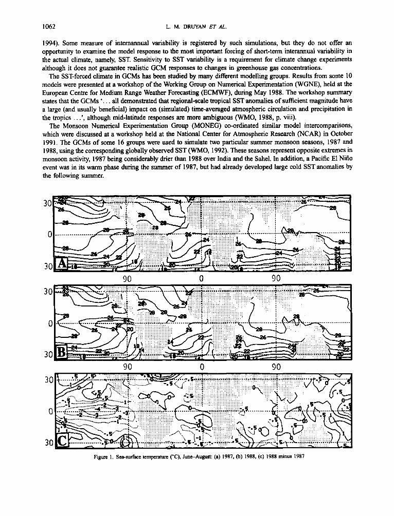
The Monsoon Numerical Experimentation Group (MONEG) co-ordinated similar model intercomparisons, which were discussed at a workshop held at the National Center for Atmospheric Research (NCAR) in October 199 1. The GCMs of some 16 groups were used to simulate two particular summer monsoon seasons, 1987 and 1988, using the corresponding globally observed SST (WMO, 1992). These seasons represent opposite extremes in monsoon activity, 1987 being considerably drier than 1988 over India and the Sahel. In addition, a Pacific El NGo event was in its warm phase during the summer of 1987, but had already developed large cold SST anomalies by the following summer.
90 0 90
90 0 90
Figure 1. Sea-surface temperature (“C), June-August: (a) 1987, @) 1988, (c) 1988 minus 1987
GCM SENSITIVITY TO SSTS 1063
Many of the large-scale 1988 minus 1987 circulation differences were captured by a number of the models participating in the 1991 MONEG workshop (WMO, 1992). However, a wide range of skill was evident, presumably reflecting the relative merits of each GCM. For example, the ECMWF T42L19 (cycle 34) model made very skilful simulations of the 1988 minus 1987 differences in 200 hPa velocity potential and gave a good indication of the positive 1988 minus 1987 rainfall differences over the Sahel, and to a lesser extent over India (Palmer et al., 1992). On the other hand, the 200 hPa velocity potential generated by the NMC T80 model of 1990 was not sensitive enough to the interannual SST differences to alter the position of the velocity potential minimum over the western Pacific (Mo, 1992).
Druyan and Hastenrath (1994) describe results obtained with the GISS Model I1 GCM (4" by 5" horizontal resolution), which was run with observed SST (Reynolds, 1988) from June to August 1987 and 1988, each year from three different initial atmospheric conditions. Although the simulations captured some of the observed 1988 minus 1987 differences in circulation and precipitation, model biases obscured some of the other important characteristics of these interannual variations.
The present study examines the sensitivity of the 4" x 5" GISS GCM to some basic changes in model structure by comparing parallel simulations forced by observed SST of the June-August 1987 and 1988 monsoon seasons (Figure 1). Inclusion of each modelling change, in effect, defines a different 'version' of the GCM. Their success in reproducing some of the basic features of the climate anomalies of each season, as well as the 1988 minus 1987 seasonal differences, is interpreted as a validation of their relative skill. Positive impacts in these experiments then justify the evaluation of an improved version of the GCM that combines several or all of the model changes. Because of the non-linear nature of the GCM, however, the interpretation of model impacts from a single change or combined changes is not at all straightforward. Nevertheless, by comparing pairs of runs that differ by a single change one can often gauge the impact of that change, especially if the impact has a plausible physical rationale. Basic model structure is discussed in section 2, followed by brief descriptions of each of the new parameterizations. Sections 3-7 validate the models' performance in simulating circulation, thermal structure, and precipitation rates.
2. THE MODELS
NMC initial atmospheric conditions at 00 GMT on 1,2, and 3 June 1987 and 1988 were interpolated to the three- dimensional GISS grid in order to initialize six 3-month simulations using each of the model versions described below. The validation of each model version therefore uses two ensembles of three runs forced by the corresponding monthly mean SST (PCMDI, 1993) interpolated to daily values for each of the two seasons.
Table 1. Versions of the GISS GCM validated by comparing simulations forced by June-August 1987 and 1988 SST. See text for more complete explanations of the differences between the model versions. Parameterizations: PBL, planetary boundary layer; MC, moist convection; GH, ground hydrology; MM, vertical mixing of horizontal momentum; CWB, cloud water budget; QUS (LUS), quadratic (linear) upstream scheme for advection of tracers. Asterisks denote
different version of new scheme adapted for C-grid runs (see text)
New PBL New MC New GH MM CWB QUS - - - - - X
X X
B1 B2 B3 X X
B4 X X
B5 X X X
B6 X X X X
B7 X X X
B8 X X X X B9 X X X X X X
X - LUS c1 X - LUS c2 X*
c3 X* - - X X* LUS
- - - X - - - -
- - - - - - -
- - X X
- - -
- - - - -
1064 L. M. DRUYAN ET AL.
Table I summarizes the modelling experiments, which test some 12 versions of the GISS GCM. All versions used in the present study share a basic structure. Computations using the primitive equations for dynamics are made at a horizontal resolution of 4" latitude by 5" longitude at nine vertical sigma levels. Each 4" by 5" grid element is divided into land and ocean fractions, where the surface-atmosphere energy exchanges are calculated separately. Physical processes that are parameterized include solar and terrestrial radiation transfer and their interaction with computed clouds. Vertical transport of moisture, heat and momentum is accomplished by convection. See Hansen er al. (1983) for a complete description of Model 11, which is the basic or control version to which all of the changes described below have been added. The impacts of these model changes, which were developed by the assiduous research of the GISS modelling group, are often but not always beneficial when judged from the perspectives presented in our analysis.
Model I1 utilizes a simple mass flux cumulus parameterization which is described fully by Del Genio and Yao (1 993). In this scheme, moist convection is diagnosed to occur whenever a parcel of air lifted adiabatically from some level is buoyant with respect to the environment at the next higher level, the parcel rising to the highest consecutive level at which the buoyancy criterion is satisfied. A fixed 50 per cent of the mass of the cloud base layer rises in each event, without any additional entrainment into the rising plume. This probably overestimates the magnitude of convective transports and cloud feedbacks (Del Genio and Yao, 1988). Moreover, the heating and drying of the lower troposphere that results from compensating subsidence has been found to be excessive in the tropics (Del Genio and Yao, 1993). The control run with this version is designated as B 1.
2.1. Changes in moist convection (MC)
A new scheme for moist convection, based on sensitivity tests conducted by Del Genio and Yao (1988) and Yao and Del Genio (1989), has the potential for improving the verification of modelled precipitation and the many characteristics of the circulation sensitive to moist processes. Cumulus mass fluxes are made proportional to the instability. The required flux is calculated iteratively by relaxing the atmosphere to a neutrally stable state at the cloud base in a model physics time step. The result of using this closure is that the model passes through a series of quasi-equilibrium states, as observed, with realistic variability of lapse rate and boundary layer humidity. However, the parameterization does not assume quasi-equilibrium or any fixed vertical cloud-work function distribution as an input, as is done for example by Arakawa and Schubert (1974). This flexibility, combined with the scheme's relative simplicity, makes it suitable for long-term climate model integrations that strive to predict small climatic shifts in thermodynamics structure. Also included is an innovative parameterization of convective-scale downdrafts, whose effect is to prevent excessive drying of the boundary layer by compensating subsidence. The downdraft mass is one-third the updraft mass and it evaporates as much falling rain from lower layers as necessary to remain saturated. Improvements in upper tropospheric humidity and the cumulus heating profile were achieved by partitioning the convective plume into two parts, entraining and non-entraining, for each convective event. Run B2 tests the impact of this scheme on the control (Bl).
2.2. improvement of planetary boundary layer (PBL)
This part of the model determines the surface wind speed and the vertical fluxes of heat, moisture, and momentum. Model 11's dependence on the Ekman length was inappropriate near the equator, where l/sin (Lat) becomes very large, making the upper boundary condition for the wind profile impossible to satisfy. The new approach determines a velocity profile within the PBL by solution of the equations of motion with realistic upper and lower boundary conditions on the domain bounded by the surface and the top of the boundary layer. This parameterization now correctly gives purely pressure-gradient-driven flow at the equator and well behaved wind profiles (and surface wind) without introducing any ad hoc empirical adjustments. Vertical heat, momentum, and moisture flux were computed via a cmde bulk formula in Model 11, using the same transport coefficients for all of them. The new scheme is based on similarity theory, which determines three distinct transfer coefficients. Roughness lengths over the oceans are specified as hct ions of momentum fluxes and the specified roughness over land and water is used to compute the neutral drag coefficient and transfer coefficients for heat, moisture and momentum. Better estimates of these transfer coefficients in turn give better estimates of the vertical fluxes of heat,
GCM SENSITIVITY TO SSTS 1065
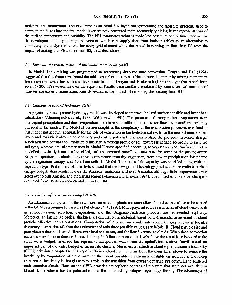
moisture, and momentum. The PBL remains an equal flux layer, but temperature and moisture gradients used to compute the fluxes into the first model layer are now computed more accurately, yielding better representations of the surface temperature and humidity. The PBL parameterization is made less computationally time intensive by the development of a pre-computed version, which can supply data from look-up tables as an alternative to computing the analytic solutions for every grid element while the model is running on-line. Run B3 tests the impact of adding this PBL to version B2, described above.
2.3. Removal of vertical mixing of horizontal momentum (MM)
In Model I1 this mixing was programmed to accompany deep moisture convection. Druyan and Hall (1 994) suggested that this feature weakened the mid-tropospheric jet over Africa in boreal summer by mixing momentum from monsoon westerlies with mid-level easterlies, and Druyan and Hastenrath (1 994) thought that model level seven ( ~ 2 0 0 hPa) westerlies over the equatorial Pacific were similarly weakened by excess vertical transport of near-surface easterly momentum. Run B4 evaluates the impact of removing this mixing from B3.
2.4. Changes in ground hydmlogy (GH)
A physically based ground hydrology model was developed to improve the land surface sensible and latent heat calculations (Abramopoulos et al., 1988; Webb et al., 1991). The processes of transpiration, evaporation from intercepted precipitation and dew, evaporation from bare soil, infiltration, soil-water flow, and runoff are explicitly included in the model. The Model I1 version simplifies the complexity of the evaporation processes over land in that it does not account adequately for the role of vegetation in the hydrological cycle. In the new scheme, six soil layers and realistic hydraulic conductivity and matric potential hc t ions replace the previous two-layer design, which assumed constant soil moisture difisivity. A vertical profile of soil textures is defined according to assigned soil type, whereas soil characteristics in Model I1 were specified according to vegetation type. Surface runoff is modelled physically instead of specified, and underground runoff is a new sink for some of the ground-water. Evapotranspiration is calculated as three components: from dry vegetation, from dew or precipitation intercepted by the vegetation canopy, and from bare soils. In Model I1 the soil’s field capacity was specified along with the vegetation type. Preliminary off-line tests showed that the new ground hydrology produced more realistic surface energy budgets than Model I1 over the Amazon rainforests and over Australia, although little improvement was noted over North America and the Sahara region (Marengo and Druyan, 1994). The impact of this model change is evaluated from B5 as an incremental impact on B4.
2.5. Inclusion of cloud water budget (CWB)
An additional component of the new treatment of atmospheric moisture allows liquid water and ice to be carried in the GCM as a prognostic variable (Del Genio et al., 1993). Microphysical sources and sinks of cloud water, such as autoconversion, accretion, evaporation, and the Bergeron-Findeisen process, are represented explicitly. Moreover, an interactive optical thickness (t) calculation is included, based on a diagnostic assessment of cloud particle effective radius variations. Computation of t based on condensate concentrations allows a broader frequency distribution of t than the assignment of only three possible values, as in Model 11. Cloud particle size and precipitation thresholds are different over land and ocean, and for liquid versus ice clouds. When deep convection occurs, some of the condensate formed in the updraft four or more cloud levels above the cloud base is added to the cloud-water budget. In effect, this represents transport of water from the updraft into a cirrus ‘anvil’ cloud, an important part of the water budget of mesoscale clusters. Moreover, a restrictive cloud-top entrainment instability (CTEI) criterion prompts the mixing of sufficient cloudy air with air from the clear layer above to remove the instability by evaporation of cloud water to the extent possible in extremely unstable environments. Cloud-top entrainment instability is thought to play a role in the transition from extensive marine stratocumulus to scattered trade cumulus clouds. Because the CWB provides atmospheric sources of moisture that were not available in Model 11, the scheme has the potential to alter the modelled hydrological cycle significantly. The advantages of
1066 L. M. DRUYAN ET AL.
including the CWB are analysed by the differences between B6 or B9 (with CWB) versus B3 or B8 (without CWB).
2.6. Inclusion of quadratic upstream scheme (QUS)
This is a second-order version of the ‘linear upstream scheme’ described by Russell and Lerner (1981) for the advection of the tracers water vapour and potential enthalpy (Russell, pers. comm.). It is more realistic in computing advection of tracers than the scheme used in Model I1 because the latter tends to produce very noisy tracer concentration fields (Russell and Lerner, 198 1). Potential advantages of this change will have to be weighed against an unfortunate disadvantage: the QUS adds significantly to the required computing time. The contributions of the QUS are determined from comparisons of B7 (with QUS) with B4.
2.7. Numerics
2.7.1. C-grid with linear upstream scheme (Cl). The versions of the model described above in 2.1-2.6 use Arakawa’s (1972) B-grid scheme for which pressure and temperature are computed at the centre of each grid-box while the orthogonal components of winds are carried at the comers. We are also testing several versions which use Arakawa and Lamb’s (1977) C-grid scheme, for which the wind components are carried perpendicularly at the sides of the grid-boxes. Arakawa and Lamb (1977) showed that C-grid schemes perform geostrophic adjustment better than B-grid schemes. Additionally, these numerics improve the distribution of modelled sea-level pressure and the magnitude of cross-equatorial transports in the GCM. One of their disadvantages, however, concerns excessive high wavenumber noise in modelled winds, which is suppressed efficiently with a partial strength eighth- order Shapiro (1970) filter. Version C 1 uses the ‘linear upstream scheme’ (LUS) (Russell and Lerner, 198 1) for the advection of the tracers water vapour and potential enthalpy. Within each grid-box, the mean value of the tracer as well as the east-west, the north-south, and vertical gradients are all prognostic variables, which are used to compute the advection sequentially in each of the three directions. This scheme is more accurate in computing advection of tracers than the second-order scheme used in Model I1 because the latter tends to produce very noisy tracer concentration fields (Russell and Lerner, 1981). In Model 11, convection, radiative forcing, and diffusion eliminate much of the noise, but such smoothing does not restore realistic distributions to the tracer concentrations. Validation of the C-grid versions of the GISS GCM has taken on additional significance recently in light of its use in a newly developed coupled atmosphere-ocean model by Russell et al. (1995).
2.7.2. C-grid with simplified PBL (C2). In addition to C1, two additional versions were also tried. In consideration of the limitations of the Model I1 PBL (see above), a simplified representation of the wind profile above the surface and alternative parameterizations for boundary layer vertical fluxes of heat, moisture, and momentum, were substituted by Russell et al. (1 995) for the Model I1 scheme used in C 1. Here the surface wind speed is specified as a fixed 75 per cent of the layer-one wind speed, and the surface wind direction is determined by computing cross-isobar angles that depend on stability and wind speed. Surface air temperature and surface humidity are derived by downward extrapolation from layer-one values, using the prognostic vertical gradients within the lowest computational layer. The transfer coefficients for heat, moisture, and momentum are identical in this formulation and depend on the Richardson number computed from the vertical gradient between the surface air temperature and the ground or sea-surface temperature.
2.7.3. C-grid with modification of radiation transfer (C3). The third version tests the incremental impact on C2 of two changes to the computations of radiation transfer. Spatial averaging of the radiative forcing is eliminated by making all appropriate radiation computations at every grid-box instead of at alternating boxes, as in Model 11. In addition, cloud optical depths are given a wider variability than before by making them dependent on temperature and the square root of condensate concentrations (liquid water or ice). The temperature dependence is linear between 0°C and - 30°C, but constant values are specified outside these limits. Warm : cold ratios of cloud optical depths at the extremes of this temperature range are 3 : 1 for convective clouds and 30: 1 for large-scale
GCM SENSITIVITY TO SSTS 1067
supersaturation. Preliminary testing has shown that this modification of cloud properties yields planetary albedos and radiances that are in closer agreement with satellite measurements over areas of heavy rainfall than Model I1 values (Russell, pers. corn.) . Version C3 also uses the PBL described above for C2.
Table I lists the different model versions that have been validated in the present study. The observed June- August 1988 means and/or 1988 minus 1987 differences are discussed and compared with corresponding simulations in the following sections: Section 3, 200 hPa velocity potential; section 4, 200 hPa streamfunction; section 5 , lower tropospheric circulation; section 6, tropospheric thermal structure; and section 7, precipitation rates.
3. COMPARISON OF 200 HPA VELOCITY POTENTIAL
The global distributions of 200 hPa velocity potential ( x 2 ) and streamfunction (Y2), two mutually exclusive components of the upper tropospheric planetary circulation, are diagnostic fields that exhibit identifiable interannual variability. The broad scale of spatial variability of both the June-August mean distribution of x2 and Y2 and the June-August 1988 minus 1987 differences (Ax2 and AY2) suggests that realistic modelling of these fields constitutes an appropriate minimum standard for evaluating GCM performance.
90 90
45 4 5
0 0
-45 -45
-90 -90
-180 -90 0 90 180 -180 -90 0 90 180 90
4 5
0
-45
-90
-1 80 -90 0 90 180 -180 -90 0 90 180
90 90
45 45
0 0
-45 -45
-90 -90 - 1 80 -90 0 90 180 -180 -90 0 90 180
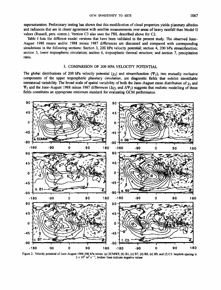
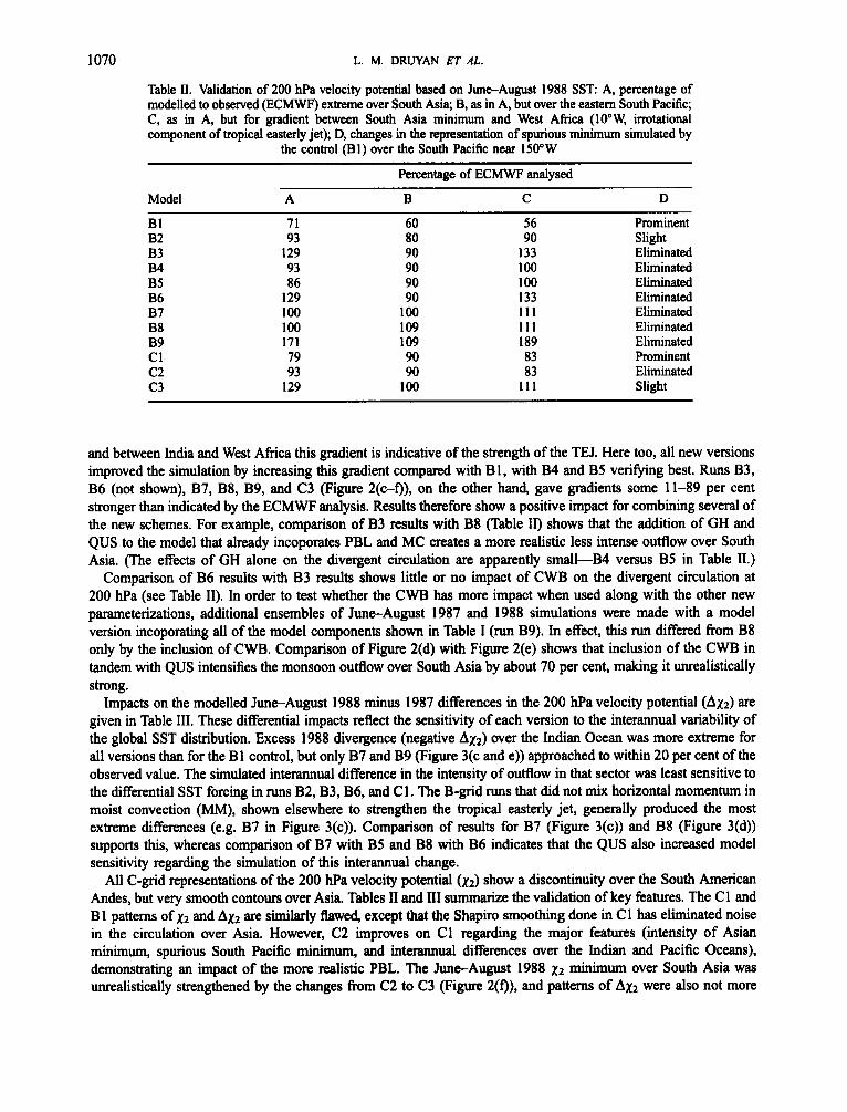
Figure 2. Velocity potential of June-August 1988 200 hPa winds: (a) ECMWF, (b) BI, (c) B7, (d) B8, (e) B9, and (f) C3. Isopleth spacing is 2 x lo6 m2 s- '; broken lines indicate negative values
1068 L. M. DRUYAN E T A L .
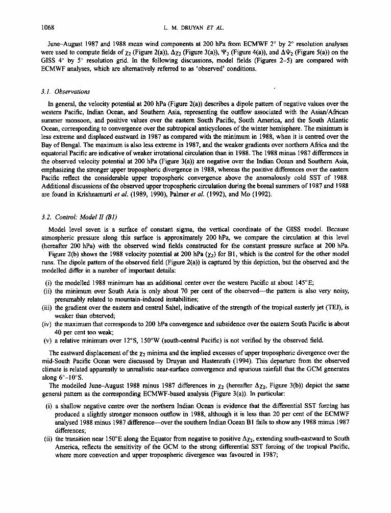
June-August 1987 and 1988 mean wind components at 200 hPa from ECMWF 2" by 2" resolution analyses were used to compute fields of ~2 (Figure 2(a)), Ax2 (Figure 3(a)), "2 (Figure 4(a)), and AQ2 (Figure 5(a)) on the GISS 4" by 5" resolution grid. In the following discussions, model fields (Figures 2-5) are compared with ECMWF analyses, which are alternatively referred to as 'observed' conditions.
3.1. Observations
In general, the velocity potential at 200 hPa (Figure 2(a)) describes a dipole pattern of negative values over the western Pacific, Indian Ocean, and Southern Asia, representing the outflow associated with the AsidAfrican summer monsoon, and positive values over the eastern South Pacific, South America, and the South Atlantic Ocean, corresponding to convergence over the subtropical anticyclones of the winter hemisphere. The minimum is less extreme and displaced eastward in 1987 as compared with the minimum in 1988, when it is centred over the Bay of Bengal. The maximum is also less extreme in 1987, and the weaker gradients over northern Africa and the equatorial Pacific are indicative of weaker irrotational circulation than in 1988. The 1988 minus 1987 differences in the observed velocity potential at 200 hPa (Figure 3(a)) are negative over the Indian Ocean and Southern Asia, emphasizing the stronger upper tropospheric divergence in 1988, whereas the positive differences over the eastern Pacific reflect the considerable upper tropospheric convergence above the anomalously cold SST of 1988. Additional discussions of the observed upper tropospheric circulation during the boreal summers of 1987 and 1988 are found in Krishnamurti et al. (1989, 1990), Palmer er al. (1992), and Mo (1992).
3.2. Control: Model II (Bl)
Model level seven is a surface of constant sigma, the vertical coordinate of the GISS model. Because atmospheric pressure along this surface is approximately 200 hPa, we compare the circulation at this level (hereafter 200 hPa) with the observed wind fields constructed for the constant pressure surface at 200 hPa.
Figure 2(b) shows the 1988 velocity potential at 200 hPa (x2) for B1, which is the control for the other model runs. The dipole pattern of the observed field (Figure 2(a)) is captured by this depiction, but the observed and the modelled differ in a number of important details:
(i) the modelled 1988 minimum has an additional center over the western Pacific at about 145"E; (ii) the minimum over South Asia is only about 70 per cent of the observed-the pattern is also very noisy,
(iii) the gradient over the eastern and central Sahel, indicative of the strength of the tropical easterly jet (TEJ), is
(iv) the maximum that corresponds to 200 hPa convergence and subsidence over the eastern South Pacific is about
(v) a relative minimum over 12"S, 150"W (south-central Pacific) is not verified by the observed field.
The eastward displacement of the x2 minima and the implied excesses of upper tropospheric divergence over the mid-South Pacific Ocean were discussed by Druyan and Hastenrath (1994). This departure from the observed climate is related apparently to unrealistic near-surface convergence and spurious rainfall that the GCM generates along 6"-10"S.
The modelled June-August 1988 minus 1987 differences in x2 (hereafter Ax2, Figure 3(b)) depict the same general pattern as the corresponding ECMWF-based analysis (Figure 3(a)). In particular:
(i) a shallow negative centre over the northern Indian Ocean is evidence that the differential SST forcing has produced a slightly stronger monsoon outflow in 1988, although it is less than 20 per cent of the ECMWF analysed 1988 minus 1987 difference-over the southern Indian Ocean B1 fails to show any 1988 minus 1987 differences;
(ii) the transition near 150"E along the Equator from negative to positive Ax2, extending south-eastward to South America, reflects the sensitivity of the GCM to the strong differential SST forcing of the tropical Pacific, where more convection and upper tropospheric divergence was favoured in 1987;
presumably related to mountain-induced instabilities;
weaker than observed;
40 per cent too weak;
GCM SENSITIVITY TO SSTS 1069
90
4 5
0
-45
-90 -180 -90 0 90 180 -180 -90 0 90 180
90 90
4 5 4 5
0 0
-45
-90 -90 -180 -90 0 90 180 -180 -90 0 90 180
90 90
45 4 s
0 0
-45 -45
-90 -90 -180 -9 0 0 BO 180 -180 -90 0 90 180
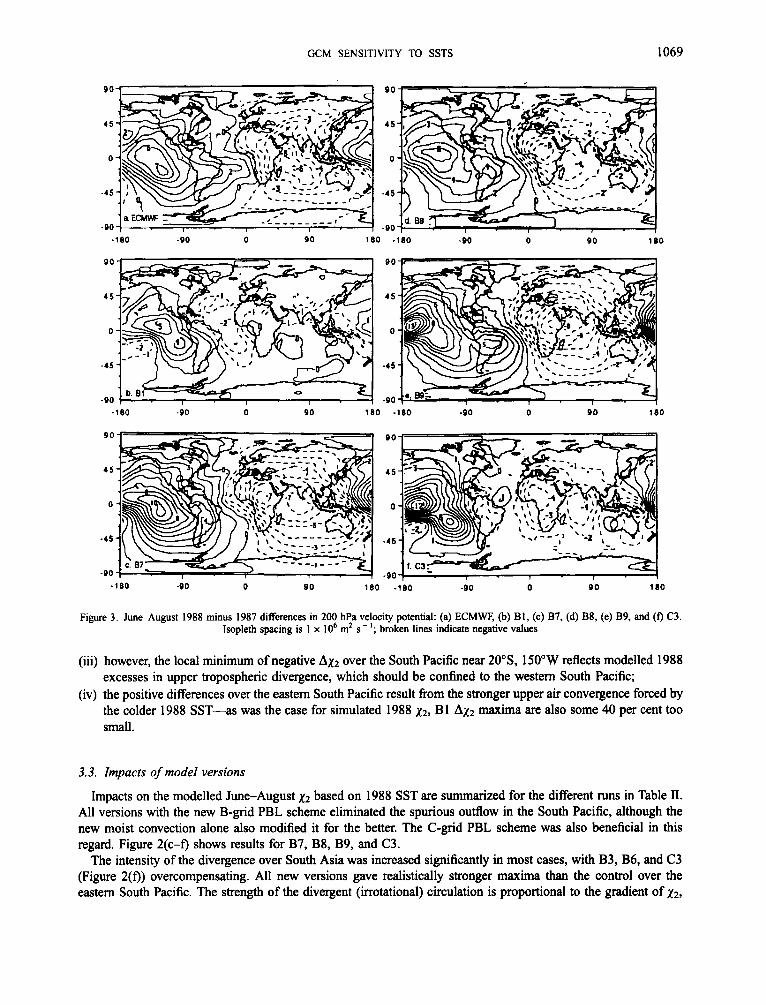
Figure 3. June-August 1988 minus 1987 differences in 200 hPa velocity potential: (a) ECMWF, (b) B1, (c) B7, (d) B8, (e) B9, and (0 C3. lsopleth spacing is 1 x lo6 m2 s - I ; broken lines indicate negative values
(iii) however, the local minimum of negative Ax2 over the South Pacific near 20°S, 150" W reflects modelled 1988 excesses in upper tropospheric divergence, which should be confined to the western South Pacific;
(iv) the positive differences over the eastern South Pacific result from the stronger upper air convergence forced by the colder 1988 SST-as was the case for simulated 1988 x2, Bl Ax2 maxima are also some 40 per cent too small.
3.3. Impacts of model versions
Impacts on the modelled June-August x2 based on 1988 SST are summarized for the different runs in Table 11. All versions with the new B-grid PBL scheme eliminated the spurious outflow in the South Pacific, although the new moist convection alone also modified it for the better. The C-grid PBL scheme was also beneficial in this regard. Figure 2(c-f) shows results for B7, B8, B9, and C3.
The intensity of the divergence over South Asia was increased significantly in most cases, with B3, B6, and C3 (Figure 2(f)) overcompensating. All new versions gave realistically stronger maxima than the control over the eastern South Pacific. The strength of the divergent (irrotational) circulation is proportional to the gradient of x2,
1070 L. M. DRUYAN E T A L .
Table II. Validation of 200 hPa velocity potential based on June-August 1988 SST A, percentage of modelled to observed (ECMWF) extreme over South Asia; B, as in A, but over the eastern South Pacific; C, as in A, but for gradient between South Asia minimum and West Africa (lOOW, irrotational component of tropical easterly jet); D, changes in the representation of spurious minimum simulated by
the control (B1) over the South Pacific near 150°W
Model
B1 B2 B3 B4 B5 B6 B7 B8 B9 c 1 c 2 c 3
Percentage of ECMWF analysed
A B C D
71 93
129 93 86
129 100 100 171 79 93
129
60 80 90 90 90 90
100 109 109 90 90
100
56 90
133 100 100 133 111 111 189 83 83
111
Prominent Slight Eliminated Eliminated Eliminated Eliminated Eliminated Eliminated Eliminated Prominent Eliminated Slight
and between India and West Africa this gradient is indicative of the strength of the TEJ. Here too, all new versions improved the simulation by increasing this gradient compared with B1, with B4 and B5 verifying best. Runs B3, B6 (not shown), B7, B8, B9, and C3 (Figure 2(c-f)), on the other hand, gave gradients some 11-89 per cent stronger than indicated by the ECMWF analysis. Results therefore show a positive impact for combining several of the new schemes. For example, comparison of B3 results with B8 (Table 11) shows that the addition of GH and QUS to the model that already incoporates PBL and MC creates a more realistic less intense outflow over South Asia. (The effects of GH alone on the divergent circulation are apparently small-B4 versus B5 in Table 11.)
Comparison of B6 results with B3 results shows little or no impact of CWB on the divergent circulation at 200 hPa (see Table 11). In order to test whether the CWB has more impact when used along with the other new parameterizations, additional ensembles of June-August 1987 and 1988 simulations were made with a model version incoporating all of the model components shown in Table I (run B9). In effect, this run differed from B8 only by the inclusion of CWB. Comparison of Figure 2(d) with Figure 2(e) shows that inclusion of the CWB in tandem with QUS intensifies the monsoon outflow over South Asia by about 70 per cent, making it unrealistically strong.
Impacts on the modelled June-August 1988 minus 1987 differences in the 200 hPa velocity potential (Ax2) are given in Table 111. These differential impacts reflect the sensitivity of each version to the interannual variability of the global SST distribution. Excess 1988 divergence (negative Axz) Over the Indian Ocean was more extreme for all versions than for the B 1 control, but only B7 and B9 (Figure 3(c and e)) approached to within 20 per cent of the observed value. The simulated interannual difference in the intensity of outflow in that sector was least sensitive to the differential SST forcing in runs B2, B3, B6, and C1. The B-grid runs that did not mix horizontal momentum in moist convection (MM), shown elsewhere to strengthen the tropical easterly jet, generally produced the most extreme differences (e.g. B7 in Figure 3(c)). Comparison of results for B7 (Figure 3(c)) and B8 (Figure 3(d)) supports this, whereas comparison of B7 with B5 and B8 with B6 indicates that the QUS also increased model sensitivity regarding the simulation of this interannual change.
All C-grid representations of the 200 hPa velocity potential (x2) show a discontinuity over the South American Andes, but very smooth contours over Asia. Tables I1 and 111 summarize the validation of key features. The C1 and B1 patterns of x2 and Ax2 are similarly flawed, except that the Shapiro smoothing done in C1 has eliminated noise in the circulation over Asia. However, C2 improves on C1 regarding the major features (intensity of Asian minimum, spurious South Pacific minimum, and interannual differences Over the Indian and Pacific Oceans), demonstrating an impact of the more realistic PBL. The JuneAugust 1988 x2 minimum over South Asia was unrealistically strengthened by the changes from C2 to C3 (Figure 2(f)), and patterns of Ax2 were also not more
GCM SENSITIVITY TO SSTS 1071
Table 111. Validation of simulated 1988 minus 1987 differences in 200 hPa velocity potential: A, percentage of modelled to observed (ECMWF) extreme difference over the northern Indian Ocean; B, as for A, but over the southern Indian Ocean; C, as for A, but over eastern South Pacific; D, as for A, but
for gradient of differences between the northern Indian Ocean and the equatorial Pacific at 180"
Percentage of ECMWF analysed
Model A B C D
B1 B2 B3 B4 B5 B6 B7 B8 c1 c 2 c 3
17 33 33 50 68 33
117 67 33 50 67
0 18 45 64 64 27
100 67 45 36 55
57 71 43 79
114 57
143 71 86
100 100
30 25 60 40 85 60
140 60 10 90
125
realistic for C3 (Figure 3(9) than C2 over the western and central Pacific, although there was an improvement over the Indian Ocean.
4. COMPARISONS OF 200 HPA STREAMFUNCTION
4.1. Observations
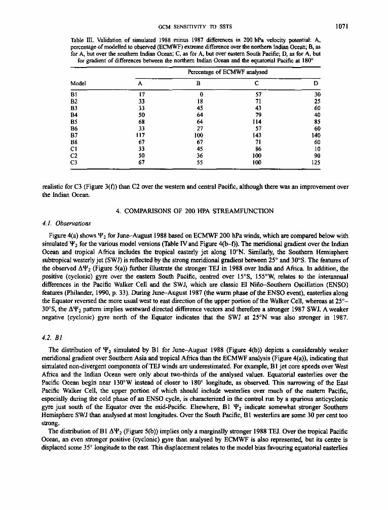
Figure 4(a) shows Y 2 for June-August 1988 based on ECMWF 200 hPa winds, which are compared below with simulated Y for the various model versions (Table IV and Figure 4 0 ) . The meridional gradient over the Indian Ocean and tropical Africa includes the tropical easterly jet along 10"N. Similarly, the Southern Hemisphere subtropical westerly jet (SWJ) is reflected by the strong meridional gradient between 25" and 30"s. The features of the observed AY2 (Figure 5(a)) further illustrate the stronger TEJ in 1988 over India and Africa. In addition, the positive (cyclonic) gyre over the eastern South Pacific, centred over 15"S, ISSOW, relates to the interannual differences in the Pacific Walker Cell and the SWJ, which are classic El Niiio-Southern Oscillation (ENSO) features (Philander, 1990, p. 33). During June-August 1987 (the warm phase of the ENSO event), easterlies along the Equator reversed the more usual west to east direction of the upper portion of the Walker Cell, whereas at 25"- 30"S, the AY2 pattern implies westward directed difference vectors and therefore a stronger 1987 SWJ. A weaker negative (cyclonic) gyre north of the Equator indicates that the SWJ at 25"N was also stronger in 1987.
4.2. B l
The distribution of Y2 simulated by B1 for JuneAugust 1988 (Figure 4(b)) depicts a considerably weaker meridional gradient over Southem Asia and tropical Africa than the ECMWF analysis (Figure 4(a)), indicating that simulated non-divergent components of TEJ winds are underestimated. For example, B 1 jet core speeds over West Africa and the Indian Ocean were only about two-thirds of the analysed values. Equatorial easterlies over the Pacific Ocean begin near 130"W instead of closer to 180" longitude, as observed. This narrowing of the East Pacific Walker Cell, the upper portion of which should include westerlies over much of the eastern Pacific, especially during the cold phase of an ENSO cycle, is characterized in the control run by a spurious anticyclonic gyre just south of the Equator over the mid-Pacific. Elsewhere, B1 Y2 indicate somewhat stronger Southern Hemisphere SWJ than analysed at most longitudes. Over the South Pacific, B1 westerlies are some 30 per cent too strong.
The distribution of B1 AY2 (Figure 5(b)) implies only a marginally stronger 1988 TEJ. Over the tropical Pacific Ocean, an even stronger positive (cyclonic) gyre than analysed by ECMWF is also represented, but its centre is displaced some 35" longitude to the east. This displacement relates to the model bias favouring equatorial easterlies
1072 L. M. DRUYAN ET A L .
90
4 5
0
-45
-90 -100 -90 0 90 180 ,180 -90 0 90 180
90
4 5
0
- 4 5
-90
90 -90 0 90 180 180 .90 0
.eo 90 -180 -DO 0 80 180 - i n 0 -90 0 90 1 no
Figure 4. Streamfunction of June-August 1988 200 hPa winds: (a) ECMWF, (b) B1, (c) B7, (d) B8, (e) B9, and (f) C3. lsopleth spacing is 10 x 1 O6 mz s - ’; broken lines indicate negative values
east of 180°, as described above for the 1988 simulation. The B1 modelled negative gyre just north of the Equator is also stronger than observed.
4.3. Impacts of model versions
Table IV summarizes some of the impacts of the different modelling schemes on the simulated 1988 Yz. Among the model versions evaluated, the relative gradients in columns A and B are inversely proportional, with stronger Indian Ocean easterlies concurrent with weaker North Pacific westerlies. Model versions that cooled temperatures in the tropics (relative to the control run) strengthened the meridional gradient over the monsoon region while weakening it over the Pacific. For example, the control simulated only 53 per cent of the ECMWF-analysed gradient between South Asia and the southern Indian Ocean, but achieved 73 per cent of the analysed North Pacific gradient (see also Figure 4(b)). Gradients of easterlies over the Indian Ocean were strengthened by all versions (see also Figures 4(c-f)). Inclusion of MC and PBL notably cooled the equatorial mid-troposphere, wheres the C-grid models (e.g. C3 in Figure 4(f)) experienced more slight improvements in the Indian monsoon gradients. The
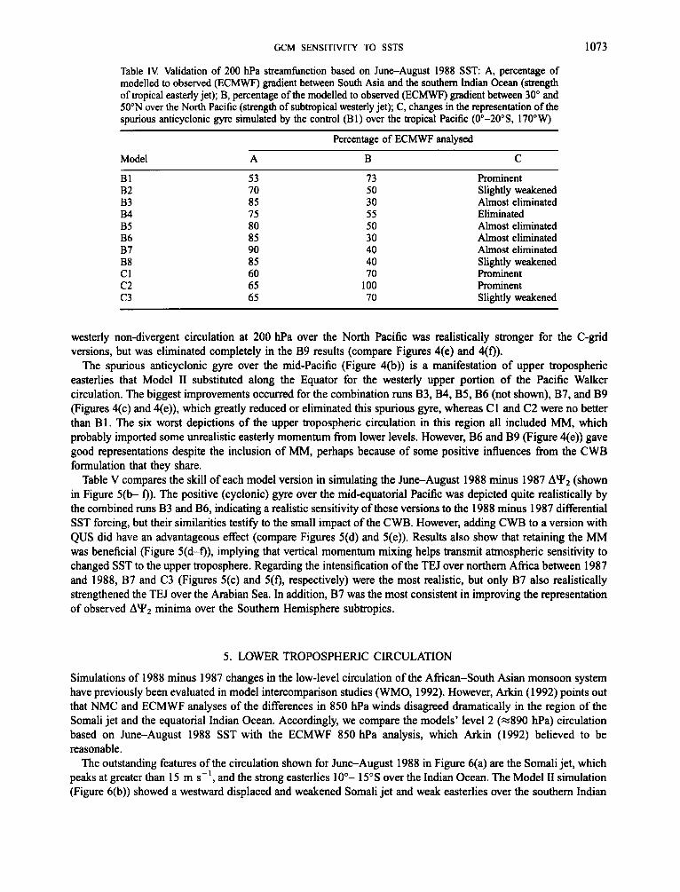
GCM SENSITIVITY TO SSTS 1073
Table I\! Validation of 200 hPa streamhction based on June-August 1988 SST: A, percentage of modelled to observed (ECMWF) gradient between South Asia and the southern Indian Ocean (strength of tropical easterly jet); B, percentage of the modelled to observed (ECMWF) gradient between 30" and 50"N over the North Pacific (strength of subtropical westerly jet); C, changes in the representation of the spurious anticyclonic gyre simulated by the control (BI) over the tropical Pacific (0"-20"S, 170"W)
Percentage of ECMWF analysed
Model A B
B1 B2 B3 B4 B5 B6 B7 B8 c1 c 2 c 3
53 70 85 75 80 85 90 85 60 65 65
73 50 30 55 50 30 40 40 70
100 70
C
Prominent Slightly weakened Almost eliminated Eliminated Almost eliminated Almost eliminated Almost eliminated Slightly weakened Prominent Prominent Slightly weakened
westerly non-divergent circulation at 200 hPa over the North Pacific was realistically stronger for the C-grid versions, but was eliminated completely in the B9 results (compare Figures 4(e) and 4(f)).
The spurious anticyclonic gyre over the mid-Pacific (Figure 4(b)) is a manifestation of upper tropospheric easterlies that Model I1 substituted along the Equator for the westerly upper portion of the Pacific Walker circulation. The biggest improvements occurred for the combination runs B3, B4, B5, B6 (not shown), B7, and B9 (Figures 4(c) and 4(e)), which greatly reduced or eliminated this spurious gyre, whereas C 1 and C2 were no better than B1. The six worst depictions of the upper tropospheric circulation in this region all included MM, which probably imported some unrealistic easterly momentum from lower levels. However, B6 and B9 (Figure 4(e)) gave good representations despite the inclusion of MM, perhaps because of some positive influences from the CWB formulation that they share.
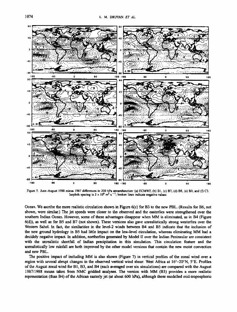
Table V compares the skill of each model version in simulating the June-August 1988 minus 1987 AY2 (shown in Figure 5 ( b f)). The positive (cyclonic) gyre over the mid-equatorial Pacific was depicted quite realistically by the combined runs B3 and B6, indicating a realistic sensitivity of these versions to the 1988 minus 1987 differential SST forcing, but their similarities testify to the small impact of the CWB. However, adding CWB to a version with QUS did have an advantageous effect (compare Figures 5(d) and 5(e)). Results also show that retaining the MM was beneficial (Figure 5(d-f)), implying that vertical momentum mixing helps transmit atmospheric sensitivity to changed SST to the upper troposphere. Regarding the intensification of the TEJ over northern Africa between 1987 and 1988, B7 and C3 (Figures 5(c) and 5(f), respectively) were the most realistic, but only B7 also realistically strengthened the TEJ over the Arabian Sea. In addition, B7 was the most consistent in improving the representation of observed AY2 minima over the Southern Hemisphere subtropics.
5 . LOWER TROPOSPHERIC CIRCULATION
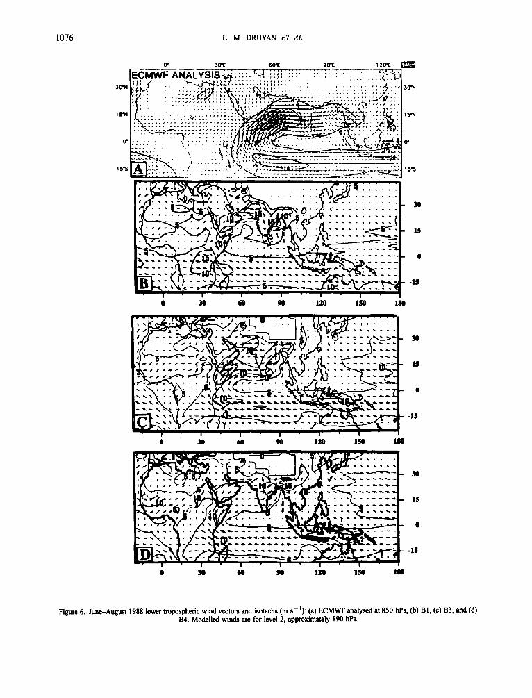
Simulations of 1988 minus 1987 changes in the low-level circulation of the African-South Asian monsoon system have previously been evaluated in model intercomparison studies (WMO, 1992). However, Arkin (1992) points out that NMC and ECMWF analyses of the differences in 850 hPa winds disagreed dramatically in the region of the Somali jet and the equatorial Indian Ocean. Accordingly, we compare the models' level 2 ( ~ 8 9 0 hPa) circulation based on June-August 1988 SST with the ECMWF 850 hPa analysis, which Arkin (1992) believed to be reasonable.
The outstanding features of the circulation shown for JuneAugust 1988 in Figure 6(a) are the Somali jet, which peaks at greater than 15 m s-', and the strong easterlies 10"- 15"s over the Indian Ocean. The Model I1 simulation (Figure 6(b)) showed a westward displaced and weakened Somali jet and weak easterlies over the southern Indian
1074 L. M. DRUYAN ET AL.
-180 -90 0 90 180 ,180 -80 n on
4 5
0
-45
-90
I
4 5
0
-45
-90 90 180 -180 -90 0 90 180 -180 -90 0
90
45
0
-45
-90
-180 -90 0 90 180 -160 -90 0 90 180
Figure 5. June-August 1988 minus 1987 differences in 200 hPa sbwnfunction: (a) ECMWF, (b) BI, (c) B7, (d) B8. (e) B9, and (4 C3. Isopleth spacing is 2 x Id m2 s - I ; broken lines indicate negative values
Ocean. We ascribe the more realistic circulation shown in Figure 6(c) for B3 to the new PBL. (Results for B6, not shown, were similar.) The jet speeds were closer to the observed and the easterlies were strengthened over the southern Indian Ocean. However, some of these advantages disappear when MM is eliminated, as in B4 (Figure 6(d)), as well as for B5 and B7 (not shown). These versions also gave unrealistically strong westerlies over the Western Sahel. In fact, the similarities in the level-2 winds between B4 and B5 indicate that the inclusion of the new ground hydrology in B5 had little impact on the low-level circulation, whereas eliminating MM had a decidely negative impact. In addition, northerlies generated by Model I1 over the Indian Peninsular are consistent with the unrealistic shortfall of Indian precipitation in this simulation. This circulation feature and the unrealistically low rainfall are both improved by the other model versions that contain the new moist convection and new PBL.
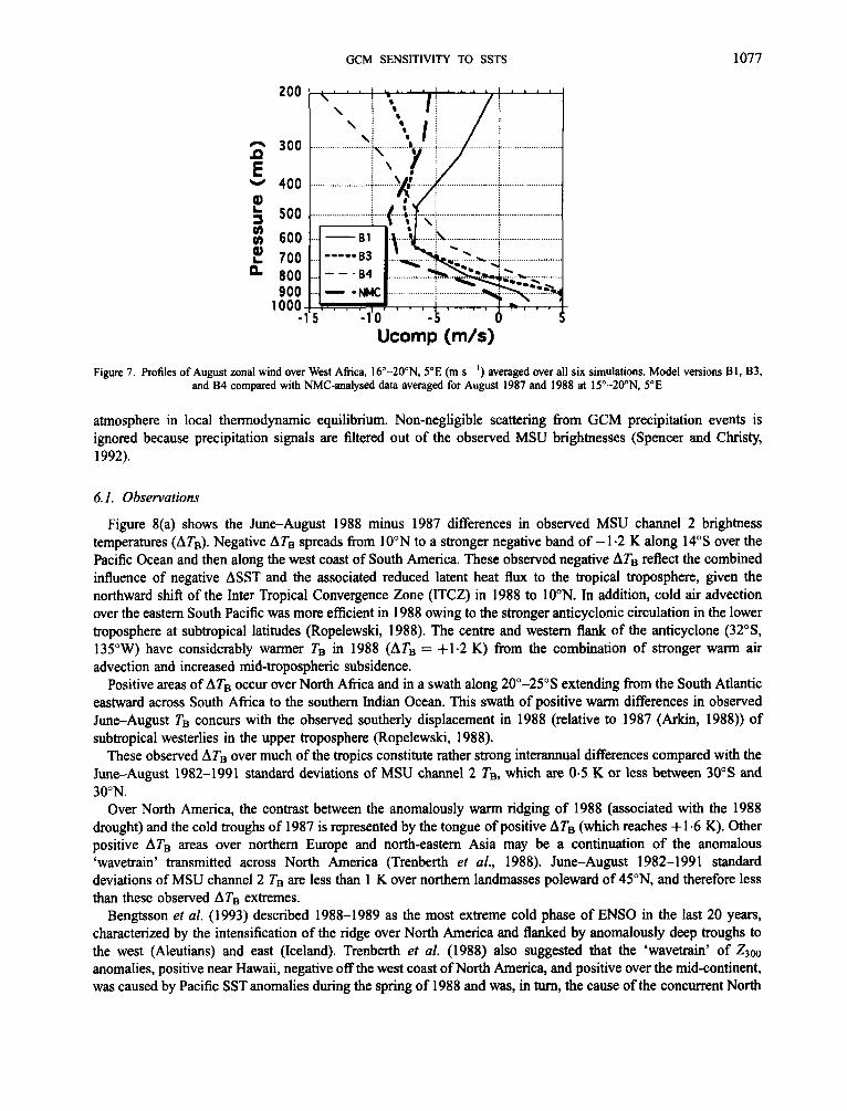
The positive impact of including MM is also shown (Figure 7) in vertical profiles of the zonal wind over a region with several abrupt changes in the observed vertical wind shear: West Africa at 16"-20"N, 5"E. Profiles of the August zonal wind for B 1, B3, and B4 (each averaged over six simulations) are compared with the August 1987/1988 means taken from NMC gridded analyses. The version with MM (B3) provides a more realistic representation (than B4) of the African easterly jet (at about 600 hPa), although these modelled mid-tropospheric
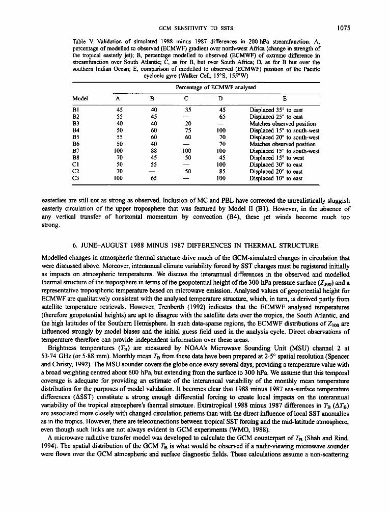
GCM SENSITIVITY TO SSTS 1075
Table V. Validation of simulated 1988 minus 1987 differences in 200 hPa streamfunction: A, percentage of modelled to observed (ECMWF) gradient over north-west Africa (change in strength of the tropical easterly jet); B, percentage modelled to observed (ECMWF) of extreme difference in streamfunction over South Atlantic; C, as for B, but over South Africa; D, as for B but over the southern Indian Ocean; E, comparison of modelled to observed (ECMWF) position of the Pacific
cyclonic gyre (Walker Cell, 15"S, I S S O W )
Model
B1 B2 B3 B4 B5 B6 B7 B8 C1 c 2 c3
Percentage of ECMWF analysed
A B 45 55 40 50 55 50
100 70 50 70
100
40 45 40 60 60 40 88 45 55
65 -
C
35
20 75 60
100 50
50
-
-
-
D
45 65
100 70 70
100 45
100 85
100
-
E
Displaced 35" to east Displaced 25" to east Matches observed position Displaced 15" to south-west Displaced 20" to south-west Matches observed position Displaced 15" to south-west Displaced 15" to west Displaced 30" to east Displaced 20" to east Displaced 10" to east
easterlies are still not as strong as observed. Inclusion of MC and PBL have corrected the unrealistically sluggish easterly circulation of the upper troposphere that was featured by Model I1 (Bl). However, in the absence of any vertical transfer of horizontal momentum by convection (B4), these jet winds become much too strong.
6. JUNE-AUGUST 1988 MINUS 1987 DIFFERENCES IN THERMAL STRUCTURE
Modelled changes in atmospheric thermal structure drive much of the GCM-simulated changes in circulation that were discussed above. Moreover, interannual climate variability forced by SST changes must be registered initially as impacts on atmospheric temperatures. We discuss the interannual differences in the observed and modelled thermal structure of the troposphere in terms of the geopotential height of the 300 hPa pressure surface (Z3w) and a representative tropospheric temperature based on microwave emission. Analysed values of geopotential height for ECMWF are qualitatively consistent with the analysed temperature structure, which, in tum, is derived partly from satellite temperature retrievals. However, Trenberth (1992) indicates that the ECMWF analysed temperatures (therefore geopotential heights) are apt to disagree with the satellite data over the tropics, the South Atlantic, and the high latitudes of the Southern Hemisphere. In such data-sparse regions, the ECMWF distributions of Z300 are influenced strongly by model biases and the initial guess field used in the analysis cycle. Direct observations of temperature therefore can provide independent information over these areas.
Brightness temperatures (TB) are measured by NOAA's Microwave Sounding Unit (MSU) channel 2 at 53.74 GHz (or 5.88 mm). Monthly mean TB from these data have been prepared at 2.5" spatial resolution (Spencer and Christy, 1992). The MSU sounder covers the globe once every several days, providing a temperature value with a broad weighting centred about 600 Ma, but extending from the surface to 300 hPa. We assume that this temporal coverage is adequate for providing an estimate of the interannual variability of the monthly mean temperature distribution for the purposes of model validation. It becomes clear that 1988 minus 1987 sea-surface temperature differences (ASST) constitute a strong enough differential forcing to create local impacts on the interannual variability of the tropical atmosphere's thermal structure. Extratropical 1988 minus 1987 differences in TB (ATB) are associated more closely with changed circulation patterns than with the direct influence of local SST anomalies as in the tropics. However, there are teleconnections between tropical SST forcing and the mid-latitude atmosphere, even though such links are not always evident in GCM experiments (WMO, 1988).
A microwave radiative transfer model was developed to calculate the GCM counterpart of TB (Shah and Rind, 1994). The spatial distribution of the GCM TB is what would be observed if a nadir-viewing microwave sounder were flown over the GCM atmospheric and surface diagnostic fields. These calculations assume a non-scattering
1076 L. M. DRUYAN ET AL.
. , ' . . . ' ..,..-. 30
15
0
-1s
Figure 6. June-August 1988 lower tropospheric wind vectors and isotachs (m 8 - I ) : (a) ECMWF analysed at 850 hPa, @) B1, (c) B3, and (d) B4. Modelled winds are for level 2, approximately 890 hPa
GCM SENSITIVITY TO SSTS 1077
Ucomp (m/s)
Figure 7. Profiles of August zonal wind over West Africa, 16"-20"N, 5"E (m s - ') averaged over all six simulations. Model versions 61, B3, and B4 compared with NMC-analysed data averaged for August 1987 and 1988 at 15"-20"N, 5"E
atmosphere in local thermodynamic equilibrium. Non-negligible scattering from GCM precipitation events is ignored because precipitation signals are filtered out of the observed MSU brightnesses (Spencer and Christy, 1992).
6.1. Observations
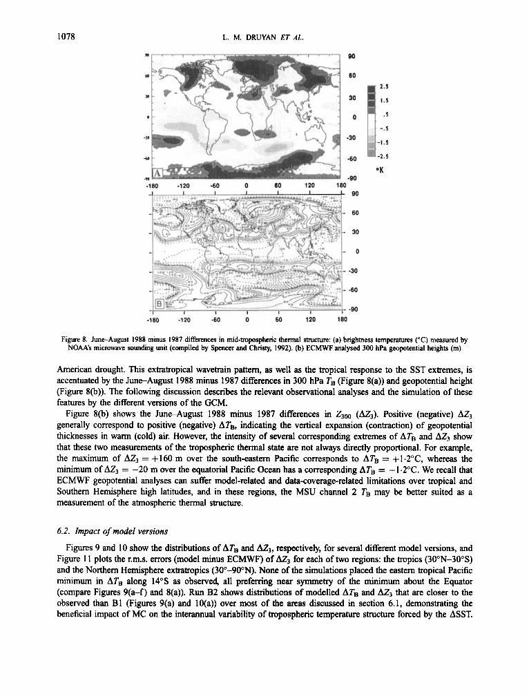
Figure 8(a) shows the June-August 1988 minus 1987 differences in observed MSU channel 2 brightness temperatures (ATB). Negative ATB spreads from 10"N to a stronger negative band of - 1.2 K along 14"s over the Pacific Ocean and then along the west coast of South America. These observed negative ATB reflect the combined influence of negative ASST and the associated reduced latent heat flux to the tropical troposphere, given the northward shift of the Inter Tropical Convergence Zone (ITCZ) in 1988 to 10"N. In addition, cold air advection over the eastern South Pacific was more efficient in 1988 owing to the stronger anticyclonic circulation in the lower troposphere at subtropical latitudes (Ropelewski, 1988). The centre and western flank of the anticyclone (3223, 135"W) have considerably warmer TB in 1988 (ATB = +1.2 K) from the combination of stronger warm air advection and increased mid-tropospheric subsidence.
Positive areas of ATB occur over North Africa and in a swath along 2Oo-25"S extending from the South Atlantic eastward across South Africa to the southern Indian Ocean. This swath of positive warm differences in observed June-August TB concurs with the observed southerly displacement in 1988 (relative to 1987 (Arkin, 1988)) of subtropical westerlies in the upper troposphere (Ropelewski, 1 988).
These observed ATB over much of the tropics constitute rather strong interannual differences compared with the June-August 1982-1991 standard deviations of MSU channel 2 TB, which are 0.5 K or less between 30"s and 30"N.
Over North America, the contrast between the anomalously warm ridging of 1988 (associated with the 1988 drought) and the cold troughs of 1987 is represented by the tongue of positive ATB (which reaches + 1.6 K). Other positive ATB areas over northern Europe and north-eastern Asia may be a continuation of the anomalous 'wavetrain' transmitted across North America (Trenberth et al., 1988). June-August 1982-1 99 1 standard deviations of MSU channel 2 TB are less than 1 K over northern landmasses poleward of 45"N, and therefore less than these observed ATB extremes.
Bengtsson et al. (1993) described 1988-1989 as the most extreme cold phase of ENS0 in the last 20 years, characterized by the intensification of the ridge over North America and flanked by anomalously deep troughs to the west (Aleutians) and east (Iceland). Trenberth et al. (1988) also suggested that the 'wavetrain' of 23, anomalies, positive near Hawaii, negative off the west coast of North America, and positive over the mid-continent, was caused by Pacific SST anomalies during the spring of 1988 and was, in turn, the cause of the concurrent North
1078 L. M. DRUYAN ET AL.
90
60
O K .m --
-180 -120 -60 0 60 120 180
-180 -120 -60 0 60 120 180
Figure 8. June-August 1988 minus 1987 differences in mid-tropospheric thermal structure: (a) brightness temperatures ("C) measured by NOAA's microwave sounding unit (compiled by Spencer and Christy, 1992). (b) ECMWF analysed 300 hPa geopotential heights (m)
American drought. This extratropical wavetrain pattern, as well as the tropical response to the SST extremes, is accentuated by the JuneAugust 1988 minus 1987 differences in 300 hPa TB (Figure 8(a)) and geopotential height (Figure 8(b)). The following discussion describes the relevant observational analyses and the simulation of these features by the different versions of the GCM.
Figure 8(b) shows the JuneAugust 1988 minus 1987 differences in Z3, (AZ3). Positive (negative) AZ3 generally correspond to positive (negative) AT,, indicating the vertical expansion (contraction) of geopotential thicknesses in warm (cold) air. However, the intensity of several corresponding extremes of ATB and AZ3 show that these two measurements of the tropospheric thermal state are not always directly proportional. For example, the maximum of AZ3 = +160 m over the south-eastern Pacific corresponds to ATB = +1.2"C, whereas the minimum of AZ3 = -20 m over the equatorial Pacific Ocean has a corresponding ATB = - 1.2"C. We recall that ECMWF geopotential analyses can suffer model-related and data-coverage-related limitations over tropical and Southern Hemisphere high latitudes, and in these regions, the MSU channel 2 TB may be better suited as a measurement of the atmospheric thermal structure.
6.2. Impact of model versions
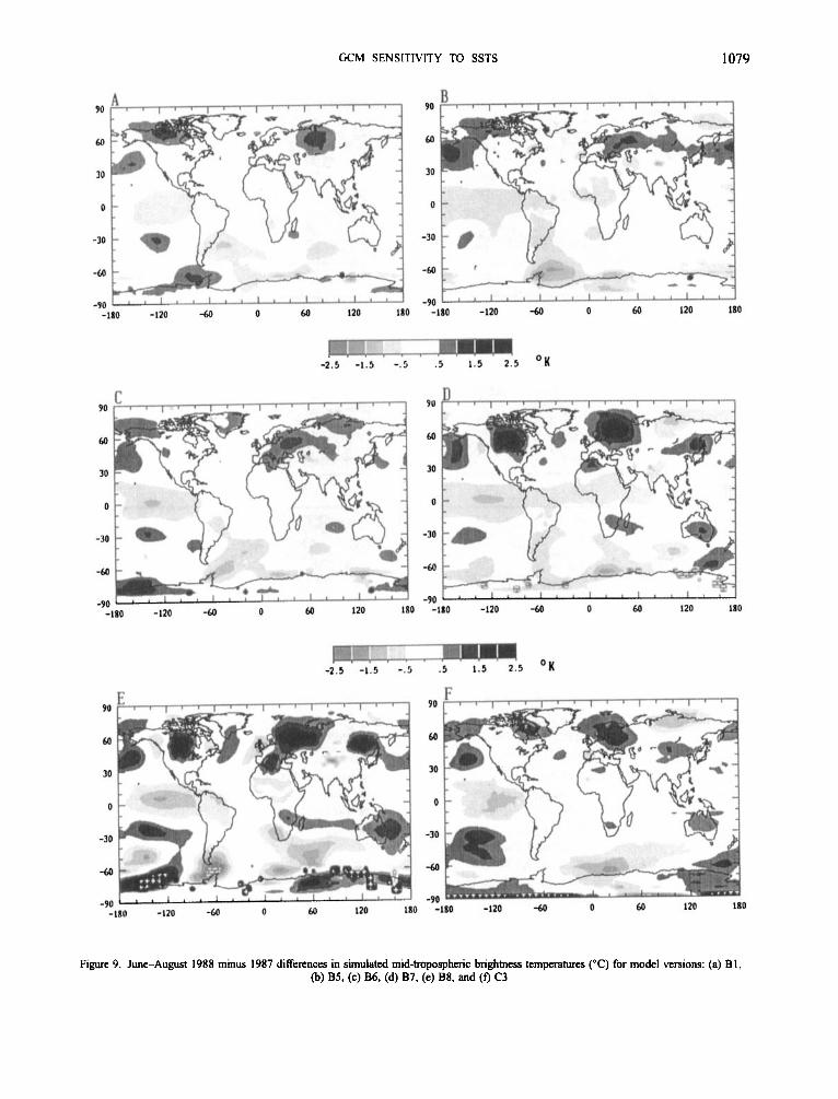
Figures 9 and 10 show the distributions of ATB and A&, respectively, for several different model versions, and Figure 11 plots the r.m.s. errors (model minus ECMWF) of A& for each of two regions: the tropics (3O0N-30"S) and the Northern Hemisphere extratropics (3O"-9O0N). None of the simulations placed the eastem tropical Pacific minimum in AT, along 14"s as observed, all preferring near symmetry of the minimum about the Equator (compare Figures 9(a-f) and 8(a)). Run B2 shows distributions of modelled ATB and A Z 3 that are closer to the observed than B1 (Figures 9(a) and lO(a)) over most of the areas discussed in section 6.1, demonstrating the beneficial impact of MC on the interannual variability of tropospheric temperature structure forced by the ASST.
GCM SENSITIVITY TO SSTS 1079
90
M)
30
0
-30
-180 -120 -60 0 120 180 -180 -120 -60 0 60 120 180
. . . . . -2.5 -1.5 - .5
. . . . 5 1 .5 2.5 O K
90 D
-60
-qn _ - -180 -120 -60 0 120 180
-60
-w ,- -180 -120 -60 0 60 120 180
-2.5 -1.5 - .5
90
60
30
0
-30
-60
-90 -180 -120 -60 0 60 120 180
.5 1.5 2.5 ‘K
-180 -120 -60 0 60 120 180
Figure 9. June-August 1988 minus 1987 differences in simulated mid-tropospheric brightness temperatures (“C) for model versions: (a) BI, (a) B5, (4 B6, (4 B7, (e) B8, and (f) C3
1080 L. M. DRUYAN ET AL.
-1iO .lio do 0 W llo 180
0 110 1W -1m -110 do 0 120
I I 110 im - 1 ~ -110 do 60 120 1m -180 -110 40 0 60
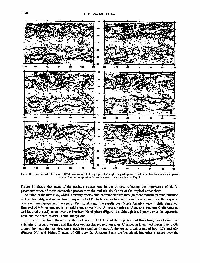
Figure 10. June-August 1988 minus 1987 differences in 300 hPa geopotential height. Isopleth spacing is 20 m; broken lines indicate negative values. Panels correspond to the same model versions as those in Fig. 9
Figure 11 shows that most of the positive impact was in the tropics, reflecting the importance of skilful parameterization of moist convective processes to the realistic simulation of the tropical atmosphere.
Addition of the new PBL, which indirectly affects ambient temperatures through more realistic parameterization of heat, humidity, and momentum transport out of the turbulent surface and Ekman layers, improved the response over northern Europe and the central Pacific, although the results over North America were slightly degraded. Removal of MM restored realistic model signals over North America, north-east Asia, and southern South America and lowered the AZ3 errors over the Northern Hemisphere (Figure 1 l), although it did poorly over the equatorial zone and the south-eastern Pacific anticyclone.
Run B5 differs from B4 only by the inclusion of GH. One of the objectives of this change was to improve estimates of ground wetness and therefore continental evaporation rates. Changes in latent heat fluxes due to GH altered the mean thermal structure enough to significantly modify the spatial distributions of both ATB and AZ3 (Figures 9(b) and lo@)). Impacts of GH over the Amazon Basin are beneficial, but other changes over the
1081
n E
c
E
Y
L
L al u)
80
70
60
50
40
30
20
10
0
model version
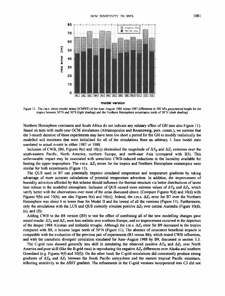
Figure 1 1. The r.m.s. errors (model minus ECMWF) of the June-August 1988 minus 1987 differences in 00 ->Pa geopotential height for tropics between 30"N and 30"s (light shading) and the Northern Hemisphere extratropics north of 30"N (dark shading)
ie
Northern Hemisphere continents and South Africa do not indicate any salutary effect of GH (see also Figure 11). Based on tests with multi-year GCM simulations (Abramopoulos and Rosenzweig, pers. comm.), we surmise that the 3-month duration of these experiments may have been too short a period for the GH to modify realistically the modelled soil moistures that were initialized for all of the simulations from an arbitrary 1 June model state unrelated to actual events in either 1987 or 1988.
Inclusion of CWB, (B6, Figures 9(c) and lO(c)) diminished the magnitude of ATB and AZ3 extremes over the south-eastern Pacific, North America, northern Europe, and north-east Asia (compared with B3). This unfavourable impact may be associated with unrealistic CWB-induced reductions in the humidity available for heating the upper troposphere. The r.m.s. AZ3 errors for the tropics and Northern Hemisphere extratropics were similar for both experiments (Figure 11).
The QUS used in B7 can potentially improve simulated temperature and temperature gradients by taking advantage of more accurate calculations of potential temperature advection. In addition, the improvement of humidity advection afforded by this scheme should influence the thermal structure via better distributions of latent heat release in the modelled atmosphere. Inclusion of QUS caused more extreme values of ATB and AZ3, which verify better with the observations over most of the areas discussed above. (Compare Figures 9(d) and 10(d) with Figures 9(b) and lO(b); see also Figures 9(e) and 10(e)). Indeed, the r.m.s. AZ3 error for B7 over the Northern Hemisphere was about 6 m lower than for Model I1 and the lowest of all the versions (Figure 11). Furthermore, only the simulations with the LUS and QUS correctly simulate positive AZ3 over central Australia (Figure lO(d),
Adding CWB to the B8 version (B9) to test the effect of combining all of the new modelling changes gave mixed results: AT* and A Z 3 were less realistic over northern Europe, and no improvement occurred in the depiction of the deeper 1988 Aleutian and Icelandic troughs. Although the r.m.s. AZ3 error for B9 decreased in the tropics compared with B8, it became larger north of 30"N (Figure 11). The absence of consistent beneficial impacts is compatible with the evaluation of the previous pair of experiments (B3 versus B6), which tested CWB influences, and with the unrealistic divergent circulation simulated for JuneAugust 1988 by B9, discussed in section 3.3.
The C-grid runs showed generally less skill in simulating the observed positive ATB and AZ3 over North America and poor skill (like the B-grid runs) in reproducing the negative AZ3 differences over Alaska and southern Greenland (e.g. Figures 9(f) and lO(f)). On the other hand, the C-grid simulations did consistently produce strong gradients of ATB and A Z 3 between the South Pacific anticyclone and the eastern tropical Pacific minimum, reflecting sensitivity to the ASST w e n t . The refinements in the C-grid versions incorporated into C3 did not
(el, and (0).
1082 L. M. DRUYAN ET AL.
improve the performance over the western USA, although more realistic positive ATB and AZ3 over northern Europe and north-east Asia did result. The changes to the PBL and cloud properties incorporated into C2 and C3 broadened the cold differences over the eastern tropical Pacific and improved their longitudinal positioning. Figure 11 shows that the r.m.s. AZ3 errors of C1 were comparable with those of B1 north of 30"N, and that the model refinements on the C-grid did not reduce the tropical or extratropical r.m.s. errors.
7. JUNE-AUGUST 1988 MINUS 1987 DIFFERENCES IN PRECIPITATION RATES
The strong 1988 minus 1987 differences in SST in the tropical Pacific Ocean (Figure 1) were responsible for significant 1988 minus 1987 local differences in June-August precipitation rates there. Outgoing longwave radiation (OLR) and highly reflective cloudiness (HRC) evidence of convective activity (Druyan and Hastenrath, 1994; see also Janowiak and Arkin (1991) for satellite-based precipitation estimates) show that the 1988 ITCZ in the eastern Pacific was displaced to about 12"N, some 5" latitude northward of its 1987 position. Extremes of HRC and OLR June-August 1988 minus 1987 differences indicate that the greatest 1988 cloudiness deficits were along the Equator, latitudinally broadest near 160"W, whereas the 1988 excesses were centred 10"-15"N. Over the extreme eastern Tropical Pacific, however, June-August 1988 cloudiness deficits were confined to north of the Equator.
We examined the June-August 1988 minus 1987 modelled precipitation differences (APr) normalized by standard deviations of the monthly mean precipitation rate (a) from a 10-year control run based on climatological SST. According to a two-tailed t-test, APr 2 2a are different significantly from the model's natural variability with 96 per cent confidence. The pattern of the contours of normalized June-August 1988 minus 1987 precipitation differences (NPD = APro-') over the tropical Eastern Pacific for B1 shows some parallels to the HRC and OLR evidence. Large 1988 deficits along the Equator where there is less 1988 cloudiness also correspond to the large negative SST differences seen in Figure 1. The warmer ocean surface of 1987 was more conducive to convective precipitation than the cooler conditions of the following year. Positive differences in the modelled rainfall rate along 6"N are, however, probably too close to the Equator according to the HRC and OLR 1988 minus 1987 difference distributions. The various model versions show a number of contrasts in their depictions of the NPD. In summary, the spatial configuration of NPD is improved by the combination of MC and PBL and by adding QUS. It is insensitive to the addition of CWB and is somewhat degraded by removing MM.
Mo (1992), Palmer et al. (1992), and Landsea et al. (1993) show that June-August 1988 was considerably rainier in Africa's Sahel (approximately 10"-20"N) than the previous summer, Other studies have suggested that the Sahel's interannual rainfall variability is related to the interannual variability of the global SST (Folland et al., 1986; Rowel1 et al., 1992). None of the simulations indicate positive and significant NPD over the western Sahel. However, all of the new versions that do not include MM (€34, B5, and B7) produce NPD > 2 imbedded within swaths of positive NPD over comparable areas of northern Africa. This may be related to the stronger near-surface westerlies over the Sahel produced by removal of MM (section 5). The C-grid runs showed insignificantly small positive differences over the entire Sahel.
June-August 1988 was also rainier over much of India than the previous summer (Mo, 1992), with differences reaching 3 4 mm day-' over the north-west and north-central parts. Model I1 and B2 (with MC) both indicate negative NPD over India, but the addition of the PBL (B3) succeeds in mitigating this discrepancy. Although there is no evidence that the GH by itself produces an improvement (B5), the combination of GH and QUS (B7 and B8) does lead to weak positive NPD over central India. Run C2 also achieves small 1988 precipitation excesses over central and western India.
Large June-August 1988 minus 1987 precipitation differences also occurred over large areas of the USA ( N O M S D A , 1987, 1988). Drought conditions prevailed in 1988 over parts of the Mid-west, Great Plains, and the Northern Rockies, in contrast to relatively wet conditions in these places in 1987. The largest 1988 relative deficits, between -2.5 to - 4 mm day-', oc, urred southwest of the Great Lakes.
Atlas et al. (1993) investigated the impact ofthe lower boundary conditions on GCM-simulated May-July 1988 precipitation over the USA using the Goddard Laboratory for Atmospheres 17-layer model at 4" x 5" horizontal resolution. Simulations with globally specified May-July 1988 SST distribution achieved about a 0.8 mm day-' reduction in the precipitation rate over the Great Plains compared with controls that used climatological SST. A
GCM SENSITIVITY TO SSTS 1083
larger reduction in rainfall.(-l.4 mm day-’) resulted from specifying soil moistures based on observed monthly mean surface temperature and precipitation data. Their study shows that skilful simulations of the 1988 drought in the Great Plains, USA, require realistically depleted soil moisture as a lower boundary condition. In their study soil moisture was prescribed, but a sophisticated ground hydrology component to the GCM could serve the same purpose.
The GH did not make the modelled NDP over the USA drought area more realistic (B5 compared with B4), although the GH and the QUS together (B7) did give small negative differences over eastern USA, overlapping some of the 1988 drought region. The relative dryness of June-August 1988 was similarly modelled by B8, for which MM was restored to the version with MC, PBL, GH, and QUS.
8. CONCLUSION
We have analysed the impact of several modelling changes by evaluating simulations of the June-August 1987 and 1988 global climates. Although the study does not provide an exhaustive validation of all the important conceivable features of the modelled climate, it does focus on two characteristics that are crucially important for GCMs involved in climate change studies: model sensitivity to SST forcing and the skill of the simulated interannual variability.
In order to filter some of the models’ inherent variability, most comparisons were made from ensembles of three runs, each from different initial atmospheric conditions, but sharing identical SST forcing. (Wind profiles over northern Africa were based on the average of six runs.) By comparing pairs of model ensemble simulations that differed by a single modelling change we have been able to attribute some of the simulation impacts to the incorporation of new parameterizations: moist convection, planetary boundary layer physics, upstream advection, and cloud optical thickness. In addition, impacts also have been evaluated for on-off switching of vertical mixing of horizontal momentum, inclusion of cloud liquid waterlice budgeting, and replacement of B-grid numerics with the C-grid formulation. The following conclusions emerge as reasonable interpretations of the results.
(i) The new moist convection, new planetary boundary layer and quadratic upstream schemes had discernible positive impacts on major features of the planetary circulation.
(ii) The new ground hydrology and the cloud waterlice budget (CWB) had strong impacts on the upper tropospheric planetary circulation only when combined with the quadratic upstream scheme (QUS) for advecting water vapour and enthalpy. There was evidence that inclusion of the CWB in tandem with the QUS invigorated monsoon convection over South Asia, although in our examples by too much. A similar enhancement of monsoon convection also resulted from a second scheme that increased the variability of cloud optical thickness (in this case combined with a linear upstream advection scheme).
(iii) Lower tropospheric circulation and vertical wind shears in the tropics were more realistic with the new PBL - - and with the inclusion of the vertical mixing of horizontal momentum in moist convection. The new moist convection scheme dramatically improved the simulation of the JuneAugust 1988 minus 1987 differences in mean tropospheric temperature, presumably because the spatial distribution of latent heat release and vertical transport of heat was more realistic. The new PBL improved some of the GCM’s tropospheric response to differential SST forcing. However, neither the inclusion of the new ground hydrology nor the inclusion of the cloud liquid waterhe budget gave evidence of any similar incremental improvement in the simulation of tropospheric temperatures. We conclude that, at least for these runs, impacts on the evolution of soil moistures, continental evaporation rates, or tropospheric temperatures by the new ground hydrology were not beneficial to model simulations. Similarly, changes in local radiation budgets that used the more variable optical thicknesses of the cloud waterhce budgets did not have an advantageous impact on simulated temperature distributions and therefore also on circulations, although selective benefits from the application of variable cloud optical thicknesses in the C-grid runs could be discerned. Simulations of the interannual temperaturelgeopotential height differences also improved when the LUS and QUS were used to provide more realistic thermal advections, and consequently more accurate computations of temperature variability. The SST-forced interannual differences in precipitation rate were improved by the combined new moist
1084 L. M. DRUYAN E T A L .
90
60
30
0
-30
-60
-90 -180 -120 -60 0 60 120 180 -180 -120 -60 0 60 120 180
90 90
60 60
30 30
0 0
-30 -30
-60 -60
-90 -90 -180 -120 -60 0 60 120 180 -180 -120 -60 0 60 120 180
2.5 90
1.5 60
.5 30
-.5 0
-30
-60
-90
-1.5
-2.5
O K
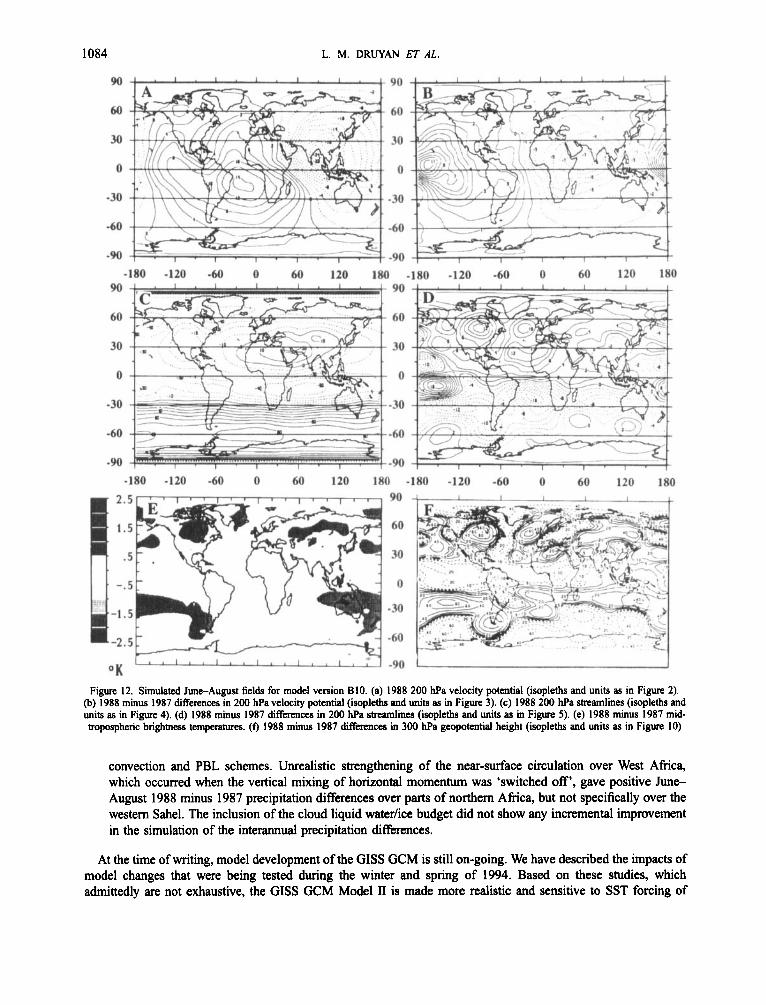
Figure 12. Simulated June-August fields for model version BIO. (a) 1988 200 hPa velocity potential (isopleths and units as in Figure 2). @) 1988 minus 1987 differences in 200 hPa velocity potential (isopleths and units as in Figure 3). (c) 1988 200 hPa streamlines (isopleths and units as in Figure 4). (d) 1988 minus 1987 differences in 200 hPa streamlines (isopleths and units as in Figure 5). (e) 1988 minus 1987 mid- tropospheric brightness temperatures. (0 1988 minus 1987 differences in 300 hPa geopotential height (isopleths and units as in Figure 10)
convection and PBL schemes. Unrealistic strengthening of the near-surface circulation over West Africa, which occurred when the vertical mixing of horizontal momentum was 'switched off', gave positive June- August 1988 minus 1987 precipitation differences over parts of northern Africa, but not specifically over the western Sahel. The inclusion of the cloud liquid waterhce budget did not show any incremental improvement in the simulation of the interannual precipitation differences.
At the time of writing, model development of the GISS GCM is still on-going. We have described the impacts of model changes that were being tested during the winter and spring of 1994. Based on these studies, which admittedly are not exhaustive, the GISS GCM Model I1 is made more realistic and sensitive to SST forcing of
GCM SENSITIVITY TO SSTS 1085
interannual variability by new parameterizations of moist convection, planetary boundary layer physics, and first- and second-order upstream schemes for advecting moisture and potential temperature.
8. I . Postscript
Subsequent to the foregoing analysis, the GISS model development group introduced additional modelling changes to the GCM, settling on an interim version for several GCM application projects and submission to AMP. Some of the more important changes to B9 in this version (B10) include the introduction of fourth-order differencing, semi-random cloud overlap, and increased differentiation of land-surface characteristics based on vegetatiodcrop types. Using B10, we repeated the simulations with JuneAugust 1987 and 1988 SST forcing as before. Some of the results are shown in Figure 12 and can be compared with Figures 2-5 and 8-10. Gross overestimates of Bay of Bengal precipitation lead to the exaggerated JuneAugust 1988 x2 minimum and excessive gradients (Figure 12(a)), slightly improving on B9, but inferior to B7 and B8. The distribution of Ax2 (Figure 12(b)) is one of the best depictions despite too high values over the mid-Pacific. The simulated JuneAugust 1988 Y2 (Figure 12(c)) are most realistic south of 30”N and the AY2 field (Figure 12(d)) is superior over the tropical and South Pacific, but not over North Africa and South Asia, where B7 and B8 are more realistic. The ATB (Figure 12(e)) extremes are lower in amplitude than for B7, B8, and B9 and the positive signals observed over northern Europe and north-eastem Asia are lacking, although the general pattern of alternating positive and negative differences in the Pacific and North America is in evidence. The B10 simulation of AZ3 (Figure 12(f)) offers one of the better representations of 1988 ridging over North America, improving on B8 and B9, and elsewhere it is comparable to several other versions. The r.m.s. errors in AZ3 were among the lowest of all versions (see Figure 11) in the tropics, but not in other regions that were monitored. Overall, the performance of the B10 simulations forced by June-August 1987 and 1988 SST was realistic in many respects, although several detracting features that surfaced in other versions were not cleared up by the added sophistication of the model design.
ACKNOWLEDGEMENTS
This research was supported by DOE grant DE-FG02-92ER61477 (LD), NSF grant ATM-9407018 (LD), NASA Climate and Earth Observing System Programs, the NASA Subsonic Assessment Program (KS) and NASA grants NAGW-3101 and NAG5-1587 (Jh4).
REFERENCES
Abramopoulos, F., Rosennveig, C. and Choudhwy, B. 1988. ‘Improved ground hydrology calculations for global climate models (GCMs): soil
Arakawa, A. 1972. Design ofthe UCLA GCM, Technical Report No. 7, Department of Meteorology, University of California, Los Angeles,
Arakawa, A. and Lamb, V 1977. ‘Computational design of the basic dynamical processes of the UCLA GCM’, Methods in Computational
Arakawa, A. and Schubert, W. 1974. ‘Interaction of a cumulus cloud ensemble with the large-scale environment, Part 1’, 1 Atmos. Sci., 31,674-
Arkin, F! A. 1988. ‘The global climate for JuneAugust 1987’. J: Climate, 1, 306-324. Arkin, I? A. 1992. ‘Circulation and precipitation during the 1987 and 1988 monsoons’, Simulation of Intemnnual and Intmseasonal Monsoon
Kwiabiliy, World Meteorological Organization, Geneva, TD No. 470, 2.1- 2.6. Atlas, R., Wolfson, N. and Terry, J. 1993. ‘The effect of SST and soil moisture anomalies on GLA model simulations of the 1988 US summer
drought’, 1 Climate, 6, 2034-2048. Bengtsson, L., Schlese, U., Roeckner, E., Latif, M., Bamett, T. and Graham, N. 1993. ‘A two-tiered approach to long-range climate forecasting’,
Science, 261, 1026-1029. Del Genio, A. and Yao, M.-S. 1988. ‘Sensitivity of a global climate model to the specification of convective updraft and downdraft mass fluxes’, 1 Atmos. Sci., 45, 3641-3667.
Del Genio, A. and Yao, M . 4 . 1993. ‘Efficient cumulus parameterization for long-term climate studies. The GISS scheme’, in Emanuel, K. and Raymond, D. (eds), Cumulus Parameterization, American Meteorological Society, Monograph Series, Vol. 24, Boston, MA,
Del Genio, A,, Yao, M.-S. and Wendell, C. 1993. ‘GCM feedback sensitivity to interactive cloud water budget parameterization’, Fourth
Druyan, L. and Hall, T. 1994. ‘Studies of African wave disturbances with the GISS GCM’, 1 Climate, 7 , 261-276. Druyan, L. and Hastenrath, S. 1994. ‘Tropical impacts of SST forcing. A case study for 1987 versus 1988’. 1 Climate, 7, 1316-1323.
water movement and evapotranspiration’, 1 Climate, 1, 92 1-94 I .
116 pp.
Physics, Vol. 17, Academic Press, New York, 337 pp.
701.
181-184 pp.
Symposium on Global Change Studies, American Meteorological Society, Boston, MA.
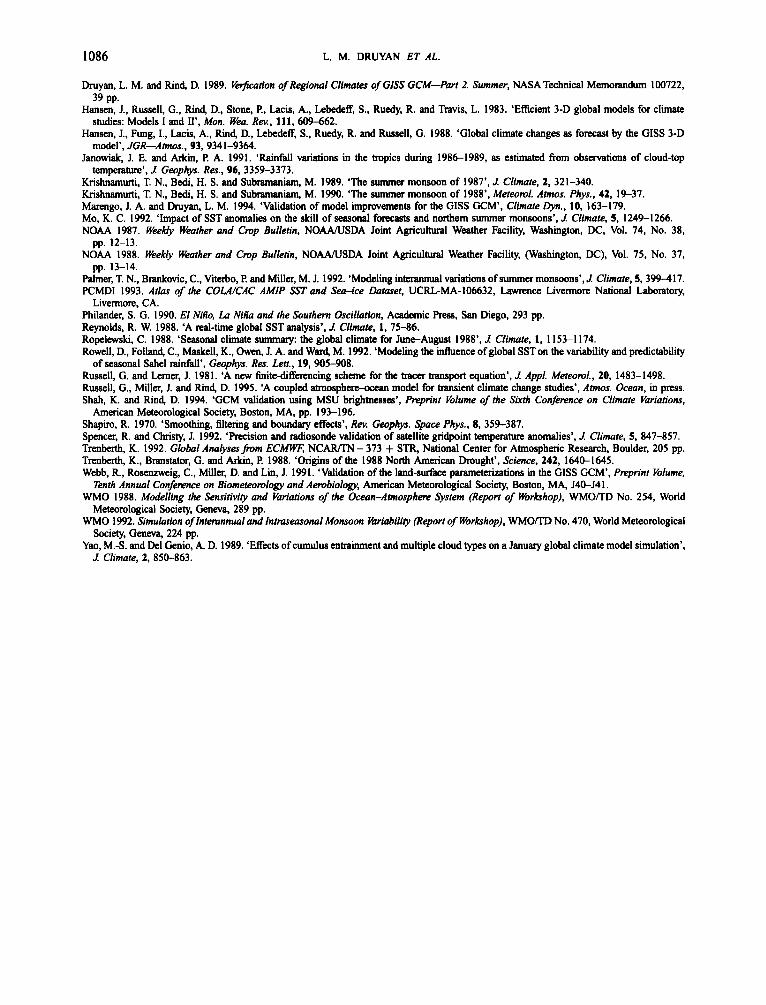
1086 L. M. DRUYAN ET AL.
Druyan, L. M. and Rind, D. 1989. Vbfication of Regionul Climates of GISS GCM-Part 2. Summer, NASA Technical Memomdum 100722,
Hansen, J., Russell, G., Rind, D., Stone, P., Lacis, A., Lebedeff, S., Ruedy, R. and Travis, L. 1983. ‘Efficient 3-D global models for climate
Hansen, J., Fung, I., Lacis, A., Rind, D., Lebedeff, S., Ruedy, R. and Russell, G. 1988. ‘Global climate changes as forecast by the GISS 3-D
Janowiak, J. E. and Arkin, P. A. 1991. ‘Rainfall variations in the tropics during 1986-1989, as estimated from observations of cloud-top
Krishnamurti, T. N., Bedi, H. S. and Subramaniam, M. 1989. ‘The summer monsoon of 1987’, 1 Climate, 2, 321-340. Krishnamurti, T. N., Bedi, H. S. and Subramaniam, M. 1990. ‘The summer monsoon of 1988’, Meteoml. Atmos. Phys., 42, 19-37. Marengo, J. A. and Druyan, L. M. 1994. ‘Validation of model impmvemcnts for the GISS GCM’, Climate Dyn., 10, 163-179. Mo, K. C. 1992. ‘Impact of SST anomalies on the skill of seasonal foncasts and northern summer monsoons’, 1 Climate, 5, 1249-1266. NOAA 1987. Weekly Weather and Cmp Bulletin, NOAAAJSDA Joint Agricultural Weather Facility, Washington, DC, Vol. 74, No. 38,
NOAA 1988. Weekly Weather and Cmp Bulletin, N O M S D A Joint Agricultural Weather Facility, (Washington, DC), Vol. 75, No. 37,
Palmer, T. N., Brankovic, C., Viterbo, P. and Miller, M. J. 1992. ‘Modeling interannual variations of summer monsoons’, 1 Climate, 5,399417. PCMDI 1993. A t h of the COWCAC AMlP SST and Sea-ice hfase t , UCRL-MA-106632, Lawrence. Livermore National Laboratory,
Philander, S. G. 1990. El Niiio, La Niria and the Southern Oscillation, Academic Press, San Diego, 293 pp. Reynolds, R. W. 1988. ‘A real-time global SST analysis’, 1 Climate, 1, 75-86. Ropelewski, C. 1988. ‘Seasonal climate summary: the global climate for June-August 1988’, 1 Climare, 1, 1 153-1 174. Rowell, D., Folland, C., Maskell, K., Owen, J. A. and Ward, M. 1992. ‘Modeling the influence of global SSTon the variability and predictability
Russell, G. and Lerner, J. 1981. ‘A new finitedifferencing scheme for the tracer bansport equation’, 1 Appl. Meteoml., 20, 1483-1498. Russell, G., Miller, J. and Rind, D. 1995. ‘A coupled atmospherwxean model for transient climate change studies’, Atmos. Ocean, in press. Shah, K. and Rind, D. 1994. ‘GCM validation using MSU brightnesses’, Preprinr Volume of the Skth Conference on Climate Variations,
Shapiro, R. 1970. ‘Smoothing, filtering and boundary effects’, Rev. Geophys. S’ce Phys., 8, 359-387. Spencer, R. and Christy, J. 1992. ‘Precision and radiosonde validation of satellite gridpoint temperature anomalies’, 1 Climate, 5, 847-857. Tmberth, K. 1992. Global Analysesfiom E C m NCAWTN - 373 + STR, National Center for Atmospheric Research, Boulder, 205 pp. Tmberth, K., Branstator, G. and Arkin, P. 1988. ‘Origins of the 1988 North American Drought’, Science, 242, 1640-1645. Webb, R., Rosenzweig, C., Miller, D. and Lin, J. 1991. ‘Validation of the land-surface p a r a m e t a t i o n s in the GISS GCM’. freprinr Yolume,
Tenth Annual Conference on Biometeomlogy and Aembiology, American Meteorological Society, Boston, MA, J40-J4 1 . WMO 1988. Modelling the Sensitiviry and kriations of the Ocean-Ahnmphere System (Report of Workshop), WMOITD No. 254, World
Meteorological Society, Geneva. 289 pp. WMO 1992. Simulation of htemnnual and Inhaseasonal Monsoon Wriabiliry (Report of firctshop), WMOITD No. 470, World Meteorological
Society, Geneva, 224 pp. Yao, M A . and Del Genio, A. D. 1989. ‘Effects of cumulus entrainment and multiple cloud types on a January global climate model simulation’, 1 Climate, 2, 850-863.
39 PP.
studies: Models I and 11’, Mon. Wea. Rev., 111, 609-662.
model’, JGR-Afmos., 93,9341-9364.
temperature’, 1 Geophys. Res., 96,3359-3373.
pp. 12-13.
pp. 13-14.
Livermore. CA.
of seasonal Sahel rainfall’, Geophys. Res. Lon., 19, 905-908.
American Meteorological Society, Boston, MA, pp. 193-196.