Sensitivity of a Greenland ice sheet model to atmospheric forcing fields

The Cryosphere, 6, 999–1018, 2012www.the-cryosphere.net/6/999/2012/doi:10.5194/tc-6-999-2012© Author(s) 2012. CC Attribution 3.0 License.

The Cryosphere

Sensitivity of a Greenland ice sheet model to atmosphericforcing fields

A. Quiquet1, H. J. Punge2,*, C. Ritz1, X. Fettweis3, H. Gallee1, M. Kageyama2, G. Krinner 1, D. Salas y Melia4, andJ. Sjolte5,**

1UJF – Grenoble 1/CNRS, Laboratoire de Glaciologie et Geophysique de l’Environnement (LGGE) UMR 5183,Grenoble, 38041, France2Laboratoire des Sciences du Climat et de l’Environnement (LSCE)/IPSL, CEA-CNRS-UVSQ, UMR 8212,91191 Gif-sur-Yvette, France3Departement de Geographie, Universite de Liege, Liege, Belgium4CNRM-GAME, URA CNRS-Meteo-France 1357, Toulouse, France5Center for Ice and Climate, Niels Bohr Institute, Copenhagen, Denmark* now at: Institute for Meteorology and Climate Research, Karlsruhe Institute of Technology, Karlsruhe, Germany** now at: GeoBiosphere Science Centre, Quaternary Sciences, Lund University, Solvegatan 12, 223 62 Lund, Sweden

Correspondence to:A. Quiquet ([email protected])

Received: 13 February 2012 – Published in The Cryosphere Discuss.: 15 March 2012Revised: 19 July 2012 – Accepted: 1 August 2012 – Published: 18 September 2012

Abstract. Predicting the climate for the future and how itwill impact ice sheet evolution requires coupling ice sheetmodels with climate models. However, before we attempt todevelop a realistic coupled setup, we propose, in this study,to first analyse the impact of a model simulated climate on anice sheet. We undertake this exercise for a set of regional andglobal climate models. Modelled near surface air temperatureand precipitation are provided as upper boundary conditionsto the GRISLI (GRenoble Ice Shelf and Land Ice model) hy-brid ice sheet model (ISM) in its Greenland configuration.

After 20 kyrs of simulation, the resulting ice sheets high-light the differences between the climate models. Whilemodelled ice sheet sizes are generally comparable to the ob-served one, there are considerable deviations among the icesheets on regional scales. These deviations can be explainedby biases in temperature and precipitation near the coast.This is especially true in the case of global models. But thedeviations between the climate models are also due to the dif-ferences in the atmospheric general circulation. To accountfor these differences in the context of coupling ice sheet mod-els with climate models, we conclude that appropriate down-scaling methods will be needed. In some cases, systematiccorrections of the climatic variables at the interface may berequired to obtain realistic results for the Greenland ice sheet(GIS).

1 Introduction

Recent growing awareness of the possible consequences ofglobal warming on ice sheets (4th assessment report ofthe Intergovernmental Panel on climate change, IPCC-AR4,Meehl et al., 2007) has led to the developing of numericalmodels aiming to predict their future evolution. While esti-mates of surface mass balance (SMB) from climate modelsgive insights into the response of the ice sheet surface to cli-mate warming (e.g.,Yoshimori and Abe-Ouchi, 2012), icesheet models (ISMs) must also be used to simulate the long-term evolution of ice sheets (e.g.,Robinson et al., 2010). Atthe same time, awareness of the importance of feedback fromother components of the Earth system has risen and sev-eral attempts have been undertaken to integrate ISMs intoclimate models in order to include and evaluate these feed-back mechanisms for the upcoming centuries (Ridley et al.,2005; Vizcaıno et al., 2008, 2010). These feedbacks include,for example, water fluxes to the ocean (Swingedouw et al.,2008), orography variations (Kageyama and Valdes, 2000)and albedo changes (Kageyama et al., 2004).

However, when model results are compared with actualobservations, major uncertainties remain due to shortcom-ings in both climate models and ISMs. Because of the longtime scales involved in ice sheet development, synchronous

Published by Copernicus Publications on behalf of the European Geosciences Union.

1000 A. Quiquet et al.: Sensitivity of a Greenland ice sheet model

coupling is feasible only with low resolution and physi-cally simplified earth system models (e.g.,Fyke et al., 2011;Driesschaert et al., 2007). Direct synchronous coupling witha fine resolution using a physically sophisticated atmosphericgeneral circulation model (GCM) is still a challenge (Pol-lard, 2010). Recent approaches try to avoid this problem byimplementing asynchronous coupling of the climate modelsand ISMs (Ridley et al., 2010; Helsen et al., 2012).

The recent observations of fast processes at work in theGreenland and West Antarctic ice sheets (e.g.,Joughin et al.,2010) show the need for synchronous coupling between theISMs that represent these processes and coupled atmosphere-ocean GCMs (AOGCMs) if we want to predict the state ofthe ice sheets in the near future, i.e., the coming century.The ISMs should include fast processes such as fast flow-ing ice streams and grounding line migration. These ISMsare becoming available (Ritz et al., 2001; Bueler and Brown,2009) and the first step towards their coupling to GCMs isto examine how they perform when forced by the GCM out-puts. Until recently, the major concern of ISM developerswas to improve the representation of physical processes oc-curring inside or at the boundaries of the ice sheet (e.g.,Ritzet al., 1997; Tarasov and Peltier, 2002; Stone et al., 2010),primarily in order to better simulate past ice sheet evolu-tion. In reconstructions of the paleo-climate, ISMs are oftenforced by ice core-derived proxy records, with spatial reso-lution of atmospheric conditions stemming from reanalysis(e.g.,Bintanja et al., 2002), or from climate model snapshots(Letreguilly et al., 1991; Greve, 1997; Tarasov and Peltier,2002; Charbit et al., 2007; Graversen et al., 2010). But for re-liable projections of the future ice sheet state the explicit useof climate model scenarios is necessary. More specifically,the first test is to evaluate how a Greenland ISM respondswhen forced by output from different GCMs. Consideringthat the extent of the ablation zone is often less than 100 km(van den Broeke et al., 2008), the GCMs generally have acoarse resolution compared with the typical ISMs. We con-sequently need to assess the gain provided by higher resolu-tion models, such as regional climate models (RCMs), evenif the trade off is a more limited scope.

To date, few studies have tested the sensitivity of an ISMto atmospheric forcing fields explicitly.Charbit et al.(2007)showed that an ISM forced by six GCMs simulations fromthe Paleo Climate Intercomparison Project (PMIP) was un-able to reproduce the last deglaciation of the Northern Hemi-sphere. They showed great discrepancies between the sixsimulated ice volume evolutions. The fast processes men-tioned earlier were not included in this study because theISM they used does not include ice streams representation.Graversen et al.(2010) simulated the total sea level in-crease over the next century using the GCMs from the Cou-pled Model Intercomparison Project phase 3 (CMIP-3). Hereagain, the ISM they used does not take into account the icestreams. Although different climate model outputs were usedas forcing fields, neither the studies mentioned above, nor the

parameter-based approaches (e.g.,Hebeler et al., 2008; Stoneet al., 2010), illustrate directly the links between climate forc-ing and simulated ice sheet behaviour. That is the main goalof the present study.

We present and discuss some of the difficulties arisingwhen combining ice sheet and climate models. We restrictour study to the case of Greenland and choose an uncoupledapproach: to examine the sensitivity of a single state-of-the-art Greenland ice sheet (GIS) model to atmospheric inputfields stemming from a number of selected climate models.Then, for comparison and in the tradition of previous ISMstudies, we examine a reference case derived from meteoro-logical observations.

In Sect.2, we first present our state-of-the-art ISM and itsspecifications. We then explain how we selected the climatemodels with different degrees of resolution and comprehen-siveness. The downscaling of atmospheric variables and theSMB computation is then described. Finally, we discuss howwe calibrated the ISM and set it up for the sensitivity ex-periments. The results of the ISM simulations are shownin Sect.3. The links between the climate model biases andhorizontal resolution on the one hand, and simulated devi-ations in ice sheet size and shape on the other hand are dis-cussed. Our conclusions and suggestions for future directionsto explore in climate-ice sheet model studies are presented inSect. 4.

2 Tools and methodology

2.1 The GRISLI ice sheet model

The model used here is a three-dimensional thermo-mechanically coupled ISM called GRISLI. With respect toice flow dynamics, it belongs to the hybrid model type: itincludes both the shallow ice approximation (SIA,Hutter,1983) and the shallow shelf approximation (SSA,MacAyeal,1989) to solve the Navier-Stokes equations. This model hasbeen validated on the Antarctic ice sheet (Ritz et al., 2001;Philippon et al., 2006; Alvarez-Solas et al., 2011a) and hasbeen successfully applied on the northern hemisphere icesheets for paleo-climate experiments (Peyaud et al., 2007;Alvarez-Solas et al., 2011b). In the more recent version usedhere, the combination of SIA and SSA is the following:

1. A map of “allowed” ice streams is determined on thebasis of basal topography. More specifically, we as-sume that ice streams are located in the bedrock val-leys (Stokes and Clark, 1999). These valleys are derivedfrom the difference between bedrock elevation at anygiven grid point and bedrock elevation smoothed overa 200-km radius around this point. Additionally, icestreams are allowed where observed present-day veloc-ities (Joughin et al., 2010) are greater than 100 m yr−1

even if the bedrock criterion is not fulfilled.

The Cryosphere, 6, 999–1018, 2012 www.the-cryosphere.net/6/999/2012/

A. Quiquet et al.: Sensitivity of a Greenland ice sheet model 1001

2. Ice streams are activated only if the temperature at theice-bedrock interface reaches the melting point. In thiscase, the SSA is used as a sliding law (Bueler andBrown, 2009). As in MacAyeal(1989), basal drag is as-sumed to be proportional to basal velocity; this relation-ship corresponds to a linear viscous sediment type. Inthe experiments presented here, the proportionality co-efficient,β, assumed to be the same for all ice streams,is one of the parameters of the model that will be cal-ibrated by comparison with observed velocities (seeSect.2.4.1).

3. Where ice streams are not allowed or not activated, thegrounded ice flow is computed using the SIA only. Iceshelves are processed with SSA only.

Calving is parameterised with a simple cut-off based ona threshold on the ice thickness. This threshold is spatiallyuniform but time-dependent. Its value varies with the surfacetemperature anomaly used in the spin-up experiment pre-sented in Sect.2.4.1. For the present climate, the thresholdis 250 m.

One of the features of the GRISLI model is a polynomialconstitutive equation, that combines the strain rate compo-nents from Glen and Newtonian flow laws. This kind of law,already used inRitz et al.(1983), accounts for the fact thatthe exponent of the flow law depends on the stress range(Lliboutry and Duval, 1985). Additionally, as in most largescale ISMs, we use enhancement factors that are multipli-cation coefficients supposed to represent the impact of iceanisotropy on deformation. According toMa et al. (2010),enhancement factors are different for SIA and SSA becausethe impact on the rate of deformation of the fabric, typi-cally with a vertically oriented C-axis, depends on the stressregime. We, thus, have four different enhancement factors,one for each component of the flow law (Newtonian or Glen)and for SIA and SSA (here calledESIA

1 andESIA3 for SIA

Newtonian and Glen, respectively, andESSA1 andESSA

3 forSSA Newtonian and Glen, respectively). These factors arenot completely independent because the stronger a factor isfor SIA, the smaller it is for SSA. These four enhancementfactors are tuned during the dynamic calibration procedure(see Sect.2.4.1below and Table1 for the values).

The model is run on a 15-km Cartesian grid resultingfrom the stereographic projection with the standard parallelat 71 ◦ N and the central meridian at 39◦ W. The bedrockelevation map comes from the ETOPO1 dataset, which it-self combines other maps (Amante and Eakins, 2009). Theice sheet thickness map is derived from the work ofBamberet al.(2001). The surface elevation is the sum of the bedrockelevation and ice thickness. Figure1 presents the initial to-pography, which is also referred to as the observed topog-raphy. Note that under this construction there are no floatingpoints at the time of initialisation. We use the geothermal heatflux distribution proposed byShapiro and Ritzwoller(2004).

Fig. 1. Present day topography of the GIS, used to initialise the ISM. Selected weather stations arerepresented.figure

39

Fig. 1.Present day topography of the GIS, used to initialise the ISM.Selected weather stations are represented.

The procedure to initialise the thermal state of the ice sheetis described in Sect.2.4.

2.2 Atmospheric model forcing fields

The ISM requires the climatological monthly mean valuesfor the near surface air temperature and precipitation as wellas the surface topography for the corresponding atmosphericforcings. These are derived from a common 20-year refer-ence period, 1980–1999. The length of 20 years is a com-promise between the need for meaningful climatology on theone hand and the consistency of boundary conditions usedfor driving the regional models and reanalysis on the otherhand.

Among the CMIP-3 coupled atmosphere-ocean GCMsused for the IPCC-AR4, there are significant discrepanciesregarding the Greenland climate (Franco et al., 2011; Yoshi-mori and Abe-Ouchi, 2012). We selected two models withreasonable agreement to reanalysis (Franco et al., 2011), butdiverging mass balance projections, as discussed inYoshi-mori and Abe-Ouchi(2012):

– The coupled atmosphere-ocean GCM CNRM-CM3(Salas-Melia et al., 2005).

www.the-cryosphere.net/6/999/2012/ The Cryosphere, 6, 999–1018, 2012


Table 1.Model parameters used in the GRISLI model for this study.

Variable Identifier name Value

Basal drag coefficient β 1500 myrPa−1

SIA enhancement factor, Glen ESIA3 3

SIA enhancement factor, linear ESIA1 1

SSA enhancement factor, Glen ESSA3 0.8

SSA enhancement factor, linear ESSA1 1

Transition temperature of deformation, Glen T trans3 −6.5◦C

Activation energy below transition, Glen Qcold3 7.820× 104Jmol−1

Activation energy above transition, Glen Qwarm3 9.545× 104Jmol−1

Transition temperature of deformation, linearT trans1 −10◦C

Activation energy below transition, linear Qcold1 4.0× 104Jmol−1

Activation energy above transition, linear Qwarm1 6.0× 104Jmol−1

Topographic lapse rate, July lrJuly 5.426◦Ckm−1

Topographic lapse rate, annual lrann 6.309◦Ckm−1

Precipitation ratio parameter γ 0.07◦C−1

PDD standard deviation of daily temperatureσ 5.0◦CPDD ice ablation coefficient Cice 8.0 mmday−1◦C−1

PDD snow ablation coefficient Csnow 5.0 mmday−1◦C−1

– The coupled atmosphere-ocean GCM IPSL-CM4(Marti et al., 2010).

Surface climate fields were extracted from the CMIP-3 20thcentury transient simulations for years 1980 to 1999.

In addition, as an example of an atmosphere-only modelwith GCM resolution, we included the atmospheric compo-nent of the IPSL model, but in a version with an improvedphysical ice sheet surface scheme, as follows:

– The global atmosphere-only GCM, LMDZ, with an ex-plicit snow model adapted from the SISVAT model, asused in the regional model MAR (Brun et al., 1992;Gallee et al., 2001), termed LMDZSV. Here and for thefollowing climate models, we imposed SST and sea iceboundary conditions for the years 1980–1999. The in-troduction of a more realistic snow scheme on ice sheetsmakes this version of LMDZ very different from thestandard one in terms of surface climate (Punge et al.,2011).

This climate forcing is meant to identify the impact of an im-proved representation of surface climate processes in a GCMon ice sheet evolution.

To study the impact of resolution in a GCM, we also con-sidered:

– The global atmosphere-only GCM LMDZ4 with an im-proved resolution on Greenland (Krinner and Genthon,1998; Hourdin et al., 2006), termed LMDZZ (for zoom).

The much higher resolution over Greenland compared withIPSL-CM4 induces scaling effects of the parameterisations

which leads to very different surface climates. In particular,the impact of orography near the coast is much better repre-sented in the zoomed model, and it can influence moisturetransport and temperature over the entire ice sheet.

Regional climate models achieve much higher spatial res-olution than GCMs, but require lateral boundary conditions.We selected:

– The regional climate model MAR (Fettweis, 2007;Lefebre et al., 2002). The model output we used stemsfrom the 1958–2009 simulation (Fettweis et al., 2011),forced by ERA40 as boundary conditions. We use thenear surface air temperatures at 3 m provided by theMAR output, instead of 2 m temperatures used in allother cases, but this is not likely to affect our analysissignificantly.

– The regional climate model REMO (Sturm et al., 2005;Jacob and Podzun, 1997), as used in a recent isotopestudy on Greenland precipitation (Sjolte et al., 2011),forced by ECHAM4 as lateral boundary conditions andnudged to the upper level wind field. The ECHAM4simulation is itself nudged towards the ERA40 wind andtemperature fields every six hours. For a complete de-scription of the nudging procedure, seevon Storch et al.(2000).

As for the GCMs, this selection is in no way meant to becomplete. It was guided in part by the availability of themodel output at the beginning of the study, but still repre-sents the state-of-the-art climate representation.



(a) (b)

Fig. 2. Greenland (land points) mean seasonal cycle of near surface air temperature (in ◦ C, left panel)and precipitation (in millimeters of water equivalent per month, right panel) for the 8 atmospheric forcingfields used in this study (colored lines). For FE09, temperature is representative for the 1996-2006 period(Fausto et al., 2009) and precipitation for the 1958-2009 period (Ettema et al., 2009). For the other forcingfields, climatological means are evaluated on the 1980-1999 period. Annual mean values are representedby triangles on the right. The grey, shaded area is the spread of 12 CMIP-3 models. Light grey and blacklines respectively represent individual models and their means.

40

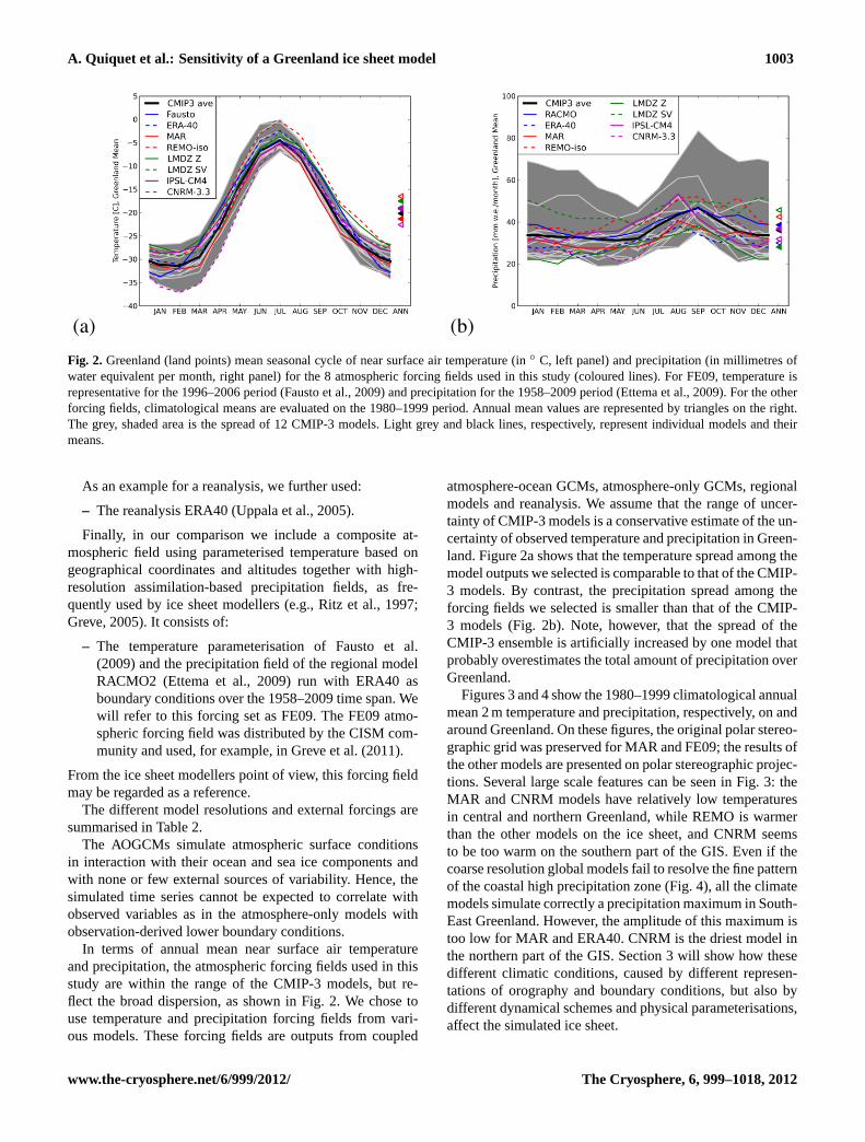
Fig. 2. Greenland (land points) mean seasonal cycle of near surface air temperature (in◦ C, left panel) and precipitation (in millimetres ofwater equivalent per month, right panel) for the 8 atmospheric forcing fields used in this study (coloured lines). For FE09, temperature isrepresentative for the 1996–2006 period (Fausto et al., 2009) and precipitation for the 1958–2009 period (Ettema et al., 2009). For the otherforcing fields, climatological means are evaluated on the 1980–1999 period. Annual mean values are represented by triangles on the right.The grey, shaded area is the spread of 12 CMIP-3 models. Light grey and black lines, respectively, represent individual models and theirmeans.

As an example for a reanalysis, we further used:

– The reanalysis ERA40 (Uppala et al., 2005).

Finally, in our comparison we include a composite at-mospheric field using parameterised temperature based ongeographical coordinates and altitudes together with high-resolution assimilation-based precipitation fields, as fre-quently used by ice sheet modellers (e.g.,Ritz et al., 1997;Greve, 2005). It consists of:

– The temperature parameterisation ofFausto et al.(2009) and the precipitation field of the regional modelRACMO2 (Ettema et al., 2009) run with ERA40 asboundary conditions over the 1958–2009 time span. Wewill refer to this forcing set as FE09. The FE09 atmo-spheric forcing field was distributed by the CISM com-munity and used, for example, inGreve et al.(2011).

From the ice sheet modellers point of view, this forcing fieldmay be regarded as a reference.

The different model resolutions and external forcings aresummarised in Table2.

The AOGCMs simulate atmospheric surface conditionsin interaction with their ocean and sea ice components andwith none or few external sources of variability. Hence, thesimulated time series cannot be expected to correlate withobserved variables as in the atmosphere-only models withobservation-derived lower boundary conditions.

In terms of annual mean near surface air temperatureand precipitation, the atmospheric forcing fields used in thisstudy are within the range of the CMIP-3 models, but re-flect the broad dispersion, as shown in Fig.2. We chose touse temperature and precipitation forcing fields from vari-ous models. These forcing fields are outputs from coupled

atmosphere-ocean GCMs, atmosphere-only GCMs, regionalmodels and reanalysis. We assume that the range of uncer-tainty of CMIP-3 models is a conservative estimate of the un-certainty of observed temperature and precipitation in Green-land. Figure2a shows that the temperature spread among themodel outputs we selected is comparable to that of the CMIP-3 models. By contrast, the precipitation spread among theforcing fields we selected is smaller than that of the CMIP-3 models (Fig.2b). Note, however, that the spread of theCMIP-3 ensemble is artificially increased by one model thatprobably overestimates the total amount of precipitation overGreenland.

Figures3and4show the 1980–1999 climatological annualmean 2 m temperature and precipitation, respectively, on andaround Greenland. On these figures, the original polar stereo-graphic grid was preserved for MAR and FE09; the results ofthe other models are presented on polar stereographic projec-tions. Several large scale features can be seen in Fig.3: theMAR and CNRM models have relatively low temperaturesin central and northern Greenland, while REMO is warmerthan the other models on the ice sheet, and CNRM seemsto be too warm on the southern part of the GIS. Even if thecoarse resolution global models fail to resolve the fine patternof the coastal high precipitation zone (Fig.4), all the climatemodels simulate correctly a precipitation maximum in South-East Greenland. However, the amplitude of this maximum istoo low for MAR and ERA40. CNRM is the driest model inthe northern part of the GIS. Section3 will show how thesedifferent climatic conditions, caused by different represen-tations of orography and boundary conditions, but also bydifferent dynamical schemes and physical parameterisations,affect the simulated ice sheet.



Table 2.Main characteristics of atmospheric forcing fields used for this study.

Dataset Atmosphere Lateral Ocean bound. Referenceresolution bounds conditions

Fausto/Ettema Fausto (t2m), ERA40∗ obs. derived Fausto et al.(2009)FE09 RACMO2/GR (precip.), ERA40∗ Ettema et al.(2009)

0.29◦× 0.29◦, L40∗

ERA-40 ERA40, – obs. derived Uppala et al.(2005)1.125◦ × 1.125◦, T159 L60 HadISST/NCEP

MAR MAR, ERA40 obs. derived Fettweis(2007)0.66◦

× 0.66◦ ERA40

REMO REMO, ECHAM4 obs. derived Sturm et al.(2005)0.5◦

× 0.5◦, L19 ERA40

LMDZ-zoom LMDZ4, – obs. derived Krinner and Genthon(1998)1.2−3.6◦

× 0.5−5.5◦, L19 AMIP2

LMDZ-SISVAT LMDZ4, – obs. derived Punge et al.(2011)3.75◦

× 2.5◦, L19 AMIP2

IPSL-CM4 LMDZ4, – coupled Marti et al.(2010)3.75◦

× 2.5◦, L19 ORCA model

CNRM-CM3.3 ARPEGE-Climat 3 – coupled Salas-Melia et al.(2005)1,9◦

× 1.9◦, T63 L45 OPA 8 model

Resolutions in◦ approximated. *: for RACMO2/GR

2.3 SMB computation

The ISM is forced by the atmospheric fields described inSect.2.2. To compute the SMB, we use monthly means oftemperature and precipitation for present day climate. Evenif the SMB is an output of the atmospheric models, we can-not use it directly for the ISM because of the large differ-ence in resolution between the two grids. Innovative tech-niques using SMB gradients exist (Helsen et al., 2012), butare strictly limited to high resolution climate models with so-phisticated snow schemes and consequently exclude GCMs.The downscaling of near surface air temperature and precip-itation is physically based, as detailed below, contrary to theSMB downscaling, which is not. Thus, we compute the SMBfrom downscaled temperature and precipitation means.

Ablation is computed with the widely-used Positive De-gree Days (PDD) method (Reeh, 1991). Even if this methodis a very schematic representation of surface melt (van denBroeke et al., 2010), it can be tuned to simulate the observedSMB and its variability (Tarasov and Peltier, 2002; Faustoet al., 2009b), consequently it is still commonly used amongthe glaciologist community (e.g.,Peyaud et al., 2007; Greveet al., 2011; Kirchner et al., 2011; Graversen et al., 2010).We also chose this method because it requires a limited num-ber of atmospheric fields, which are easy to obtain from thedifferent models. We compute the number of PDD, repre-senting melt capacity, numerically at each grid point, basedon the downscaled monthly mean near-surface temperature.Following Reeh(1991), a statistical temperature variation isconsidered, allowing melt even in months with mean temper-

ature below the freezing point. The melt capacity computedwith the PDD method is first used to melt the snow layer. Afraction of the melted snow is allowed to percolate into thesnowcover and refreeze, generating superimposed ice. Meltwater runoff is allowed if the amount of superimposed icereaches the limit of 60 % of the snowcover (Reeh, 1991). Therefreezing is responsible for firn warming, as described inReeh(1991). The remaining PDD are used to melt possiblesuperimposed ice from refreezing and then old ice.

The PDD integration constants and the melt rates of snowand ice are listed in Table1. We choseCsnow to be substan-tially higher than inReeh(1991). But the melting rate co-efficients are poorly constrained and a wide range of valuescan be found in the literature (van den Broeke et al., 2010).This choice was motivated by the better agreement of ab-lation with the one simulated in regional models (Fettweiset al., 2011; Ettema et al., 2009).

The ISM distinguishes between rainfall and snowfall. Liq-uid precipitation does not contribute to the surface mass bal-ance and is assumed to run off instantaneously. This proce-dure is a drastic simplification, but still commonly employed(Charbit et al., 2007; Peyaud et al., 2007; Hubbard et al.,2009; Kirchner et al., 2011). An explicit refreezing model(Janssens and Huybrechts, 2000) was tested, but producedonly slight differences (not shown). The monthly solid pre-cipitation,Psm, is calculated based on total monthly precipi-tationPm and monthly near surface air temperatureTm, fol-lowing Marsiat(1994):



Fig. 3. Climatological (1980-1999) June-July-August mean 2 m temperature in the eight different climatemodels (in ◦C).

41

Fig. 3.Climatological (1980–1999) June–July–August mean 2 m temperature in the eight different climate models (in◦C).

Fig. 4. Climatological (1980-1999) annual mean precipitation (solid + liquid) in the eight different cli-mate models (in metres of ice equivalent).

42

Fig. 4. Climatological (1980–1999) annual mean precipitation (solid + liquid) in the eight different climate models (in metres of ice equiva-lent).

Psm

Pm=

0, Tm ≥ 7◦C

(7◦C− Tm)/17◦C, −10◦C ≥ Tm ≥ 7◦C

1, Tm ≤ −10◦C

(1)

As the ice sheet topography changes during the simula-tion, and can hence differ strongly from the one prescribedin the atmospheric models, the near surface air tempera-ture has to be adapted. For this correction, we use a verti-cal temperature gradient, referred to hereafter as topographiclapse rate, which does not vary spatially, but is different frommonth to month. The monthly values follow an annual si-nusoidal cycle with a minimum in July at 5.426◦C km−1 andan annual mean of 6.309◦C km−1. They are derived from the

Greenland surface temperature parameterisation proposed byFausto et al.(2009). The adaptation method is, thus, consis-tent with the FE09 reference experiment. The gradients ob-tained in this way are derived from spatial variations of nearsurface air temperature and not from the actual temperatureresponse to surface elevation changes at each grid point. Thisinformation could be obtained only by repeated atmosphericmodel simulations with different topographies, as performedby Krinner and Genthon(1999), who found values that areclose to the ones we use here. The hypothesis that the sensi-tivity of the results to topographic lapse rate is of secondaryorder compared to the different forcing fields is tested inSect.3.5.



The temperature field from the low resolution topographyof the climate model (T0) is downscaled to the high resolutionrequired for the ISM (Tref) using the topographic lapse ratecorrection as described above. For the downscaling of theprecipitation rate, we used an empirical law that links tem-perature differences to accumulation ratio (Ritz et al., 1997):

Pref

P0= exp(−γ × (Tref − T0)), (2)

in which the ratio of precipitation change with temperaturechange,γ , is poorly constrained (Charbit et al., 2002). Weuse a value ofγ = 0.07, which corresponds to a 7.3 % changeof precipitation for every 1◦C of temperature change (Huy-brechts, 2002).

We chose to use the same parameters for SMB calculationsfor all atmospheric forcings, because our goal is to comparethe sensitivity of the ISM to the forcing, not to determinethe parameters which yield the most realistic GIS for eachforcing.

2.4 Experimental setup of the ice sheet model

2.4.1 Spin-up and dynamic calibration

The calibration/initialisation of an ISM is a difficult prob-lem that would require assimilation methods to be accuratelysolved (Arthern and Gudmundsson, 2010). In the experi-ments presented here we wanted to start from fields as closeas possible to the present state. The prognostic variables ofISMs are ice thickness, bedrock topography and ice tempera-ture. The first two of them are the reasonably well-known 2-D horizontal fields (Bamber et al., 2001; Layberry and Bam-ber, 2001; Amante and Eakins, 2009). The 3-D temperaturefield is much more difficult to estimate, but is also crucialbecause it is strongly linked to the velocity distribution. Thetemperature distribution within the ice depends on the pastevolution of the ice sheet, in particular on past boundary con-ditions including surface mass balance and near surface airtemperature. The typical time scale of thermal processes isup to 20 kyrs (Huybrechts, 1994), so today’s ice temperatureis still affected by the temperature increase during the lastdeglaciation.

To account for this past evolution, we run a long glacial-interglacial spin-up simulation to obtain a realistic presenttemperature field. To do so, we use present day climatic con-ditions and apply perturbations deduced from proxy data.The present day atmospheric fields of temperature and pre-cipitation are the same as in the FE09 experiment.

The temperature perturbations with respect to the presentday were reconstructed followingHuybrechts(2002) basedon the GRIP isotopic record (Dansgaard et al., 1993; Johnsenet al., 1997), using a constant slope of 0.42 ‰◦ C−1. Thesetime-dependent and spatially uniform perturbations are usedas deviations from present day conditions to force the ISM.

The resulting precipitation perturbations are assumed to fol-low the temperature evolution as in Eq.2.

However, the 3-D temperature field obtained after thisspin-up procedure corresponds to a topography that is differ-ent from the observed one. Consequently, for the sensitivityexperiments, we stretch the temperature field to the observedtopography in order to obtain the initial state.

Once the 3-D temperature field has been obtained, we tunethe various parameters that govern the velocity field by per-forming dynamic calibration.

These are the four enhancement factors and theβ coeffi-cient of the basal drag presented in Sect.2.1. Assuming thatafter the spin-up procedure the temperature field is realistic,the velocity field will depend on these parameters only. Ourtarget is the surface velocity field measured by radar interfer-ometry (Joughin et al., 2010).

We must stress that for ice streams, it is almost impossi-ble to tune the coefficientβ of basal drag and the enhance-ment factorsESSA

1 and ESSA3 separately. As explained in

Sect.2.1, the SIA and SSA enhancement factors are not in-dependent and we added a constraint on the relationship be-tween SIA and SSA. This is because the enhancement fac-tors are both equal to 1.0 in the case of isotropic ice, and thestronger the ice anisotropy, the higher the SIA enhancementfactors and the lower the SSA enhancement factors (Ma et al.,2010). We choseESSA

= 0.9 for ESIA= 2.0, ESSA

= 0.8for ESIA

= 3.0, andESSA= 0.63 for ESIA

= 5.0. The pro-cedure consists in running short (100 years) simulations ina constant present day climate. We ran a matrix of sim-ulations by varying simultaneously and independently thefive parameters already mentioned: the enhancement fac-tors ESSA

1 , ESSA3 , ESIA

1 andESIA3 , and theβ coefficient of

basal drag. The range tested for the SIA enhancement fac-tors was 1.0 < ESIA < 5.0, corresponding to SSA factors of1.0 > ESSA > 0.63. The range tested for theβ coefficientwas 500 to 1500 Pa.yr/m.

For each set of parameters, we computed mean squarederror and standard deviation, in terms of difference betweenobserved and simulated velocities as well as in terms of therespective flux of ice (being the velocity multiplied by the icedepth). The best set of parameters corresponds to the mini-mum values of mean squared error and standard deviation.Considering that a different set of parameters can give ap-proximately the same statistical scores, we also examined thecorresponding mapped velocity amplitudes and distributionhistogram and compared then with the observed velocity.

This best set obtained was with:

– Glen cubic law:ESIA3 = 3.0 andESSA

3 = 0.8.

– Newtonian finite viscosity:ESIA1 = 1.0 andESSA

1 = 1.0.

– Coefficient of basal drag:β = 1500 Pa yr m−1.

These values are consistent with the findings ofMa et al.(2010), and with the range 3.0–5.0 generally used in the SIA



Fig. 5. Simulated ice sheet topography at the end of the 20-kyr constant climate forcing model run.

43

Fig. 5.Simulated ice sheet topography at the end of the 20-kyr constant climate forcing model run.

and Glen flow law case. We used this set of parameters in allfurther experiments.

This solution is not unique, because we can obtain thesame velocity field with more viscous ice streams (lowerSSA enhancement factor) and weaker basal drag. It is worthnoting that our dynamical calibration is almost independentof the atmospheric forcing fields used. Ice velocity is indeeda diagnostic variable which depends on surface and bedrocktopography, 3-D temperature field, basal drag and ice defor-mation properties, but it does not depend directly on surfacemass balance.

Our calibration is, however, impacted by the initial tem-perature field. Temperature is a prognostic variable and, thus,depends on the past ice sheet evolution, past surface tem-perature and poorly constrained distribution of geothermalheat flux (Greve, 2005). However, we estimate that this ef-fect is secondary when compared with the impact of the at-mospheric field.

Nonetheless, our sensitivity studies indicate that the modelresults are much more sensitive to surface mass balance thanto dynamic parameters: with the FE09 forcing, a doublingof sliding (β/2) induces a 0.1 % reduction in total volume,whereas changing the FE09 forcing for the MAR forcing in-duces a 9.0 % increase in total volume.

2.4.2 Sensitivity test procedure

Having calibrated the dynamical parameters, we compare theresponses with the various climate model forcings. We keepthe same set of dynamic and mass balance downscaling pa-rameters in all the experiments and change only the atmo-spheric fields of total precipitation and near surface air tem-perature provided by the atmospheric models. We then run20 kyr-long experiments to allow for the ice sheet to sta-bilise, while keeping the climate constant over time (“glacio-logical steady state”). Nevertheless, during these simula-tions, temperature and consequently precipitation, is likelyto change, in relation with the elevation changes as describedin Sect.2.3. We do not expect, in this kind of experiment, toreproduce a realistic present day ice sheet because the presentday GIS is the result of complex changes of temperature andprecipitation during the last thousand years. We do not expecteither to provide realistic projections of the future GIS statebecause we do not perturb the present day climate to takeinto account the rate of change of temperature and precipita-tion consequent to changes in concentrations of greenhousegases. The idea here is to present an idealised configurationdepending on a minimal number of parameters. The focus ofour analysis in Sect.3 will, thus, be on the range of relativedeviation, from the present reference state obtained with thedifferent atmospheric forcing fields.



(a) (b)

(c) (d)

Fig. 6. a: North Greenland (latitudes greater than 75 ◦N) simulated ice volume evolution for the steadystate model runs shown in Fig. 5. The regional initial volume corresponds to the observed one. b: Re-gional (land mask with latitudes greater than 75 ◦N) monthly mean precipitation for each individualatmospheric forcing, with annual mean values (triangles). c, d: Station climatology for, respectively,Humboldt and Tunu-N (Steffen et al., 1996), and closest grid point near surface air temperature for eachindividual atmospheric forcing, with July temperature (left hand triangles) and annual mean temperature(right hand triangles). The black markers stand for the observations (initial regional ice volume and t2mstations measurement). Vertical bars are standard deviations from the monthly mean in the observationsdata sets. Time periods vary, depending on availability.

44

Fig. 6. (a): North Greenland (latitudes greater than 75◦N) simulated ice volume evolution for the steady state model runs shown in Fig.5.The regional initial volume corresponds to the observed one.(b): Regional (land mask with latitudes greater than 75◦N) monthly meanprecipitation for each individual atmospheric forcing, with annual mean values (triangles).(c, d): Station climatology for, respectively,Humboldt and Tunu-N (Steffen et al., 1996), and closest grid point near surface air temperature for each individual atmospheric forcing,with July temperature (left hand triangles) and annual mean temperature (right hand triangles). The black markers stand for the observations(initial regional ice volume and t2m stations measurement). Vertical bars are standard deviations from the monthly mean in the observationsdatasets. Time periods vary, depending on availability.

3 Results

3.1 20 kyr equilibrium simulated topographies

Figure 5 presents the impact of inter-model climate differ-ences in terms of simulated topography at the end of the run.Differences between simulated topographies and observedtopography is available in the Supplement accompanying thispaper. A remarkable diversity of simulated topographies isobserved. At first sight, the simulated southern part of the icesheet is more similar than the simulated northern part. In theNorth, at the end of the simulation, with two models (REMOand ERA40) presenting almost no ice, and at least three mod-els (CNRM, MAR, IPSL) presenting a fully covered area, therange is very broad. The surface height is also very differ-ent among the models with an approximate 7 % thickeningfor MAR in the interior and 8 % thinning with IPSL. In allthe simulations, the ice sheet is spreading towards the SouthWest. This common characteristic is due to the ISM’s inabil-

ity to reproduce fine scale features. The south of Greenlandis indeed a very mountainous area characterised by high oro-graphic precipitation and strong slope effects, even in the iceflow dynamics. The 15-km grid is too coarse to reproducesuch local effects and specific parameterisations would beneeded (Marshall and Clarke, 1999).

To distinguish between the different regional behaviours,we consider three regions: a southern region with latitudeslower than 68◦N, a northern one with latitudes greater than75 ◦N, and a central region in between. Specific differencesoccur mainly in the north and in the south. The central regionpresents a more complex response and we were not able toidentify well-defined specificities. Hence, we discuss mainlythe results for the South and North regions. The evolutionof the simulated volume for the northern and southern re-gions is presented in Figs.6a and7a, respectively. Exceptfor MAR and CNRM experiments, all models simulate a de-crease of ice volume in the north. If we put aside REMO and



(a) (b)

(c) (d)

Fig. 7. a: South Greenland (latitudes lower than 68 ◦N) simulated ice volume evolution for the steadystate model runs shown in Fig. 5. The regional initial volume corresponds to the observed one. b: Re-gional (land mask with latitudes lower than 68 ◦N) monthly mean precipitation for each individual at-mospheric forcing, with annual mean values (triangles). c, d: Station climatology for, respectively, Nuuk(DMI) and South Dome (Steffen et al., 1996), and closest grid point near surface air temperature for eachindividual atmospheric forcing, with July temperature (left-sided triangles) and annual mean temperature(right-sided triangles). The black markers stand for the observations (initial regional ice volume and t2mstations measurement). Vertical bars are standard deviations from the monthly mean in the observationsdata sets. Time periods vary, depending on availability.

45

Fig. 7. (a): South Greenland (latitudes lower than 68◦N) simulated ice volume evolution for the steady state model runs shown in Fig.5.The regional initial volume corresponds to the observed one.(b): Regional (land mask with latitudes lower than 68◦N) monthly meanprecipitation for each individual atmospheric forcing, with annual mean values (triangles).(c, d): Station climatology for, respectively, Nuuk(DMI) and South Dome (Steffen et al., 1996), and closest grid point near surface air temperature for each individual atmospheric forcing,with July temperature (left-sided triangles) and annual mean temperature (right-sided triangles). The black markers stand for the observations(initial regional ice volume and t2m stations measurement). Vertical bars are standard deviations from the monthly mean in the observationsdatasets. Time periods vary, depending on availability.

ERA40, which simulate nearly no ice in this region, the vol-ume variation ranges from –0.1 to +0.16 106 km3 in 20 kyrs.REMO and ERA40 present the same pattern of retreat proba-bly due to the nudging procedure (von Storch et al., 2000) ofthe REMO model towards the ERA40 reanalysis. The south-ern region systematically gains ice volume (Fig.7a), and theresponse of the ISM is almost instantaneous, compared totypical evolution time scales, given that 50 % of the final vol-ume variation is generally achieved within a thousand years.The volume simulated by all models reaches a maximum be-fore decreasing slightly due to the precipitation correction.The final volume deviation in this region ranges from 0.05 to0.15 106 km3 in 20 kyrs.

3.2 Comparison of the atmospheric model results withobservations and with the ISM response

The simulated topographies presented in Fig.5 and the simu-lated regional volume evolutions presented in Figs.6a and7a

highlight the spread of results due to different atmosphericinputs. In this section, we study the simulated volume de-viation, by comparing the atmospheric forcing fields on lo-cal and regional scales. We take advantage of the presenceof weather stations in Greenland to validate the atmosphericnear surface temperature fields in the forcing fields at se-lected points.

Near surface air temperatures for each atmospheric modeland for observations are plotted in Figs.6 and7 (c, d). Station2 m temperature data is evaluated for the automated weatherstations (AWS) Humboldt, TUNU-N and South Dome lo-cated on the GIS (Steffen et al., 1996) and for the coastalDMI station in Nuuk (Cappelen et al., 2011). Regional meanprecipitation is compared in Figs.6 and7(b).

The location of the stations is indicated in Fig.1. At theHumboldt AWS in the northwest of the ice sheet (Fig.6c),it is apparent that temperatures simulated by ERA40 andREMO are around 5◦C too high compared to climatologicalmean observations in July. This is certainly the main reason



for the rapid ice retreat in this region for those models. TheIPSL and LMDZZ models are also slightly warmer than ob-servations in summer, while their seasonal cycle appears tobe delayed by a few weeks. MAR is colder than observa-tions throughout the year. There is a spread among models inthe boreal winter and the assumption of sinusoidal seasonalvariation in FE09 does not give realistic results for the win-ter. These deficiencies, however, are not relevant for melt andhave a lesser impact on the ice mass balance than the sum-mer. At the same time, the IPSL model is too warm in par-ticular during the boreal winter, but also on average, whichfavours more rapid ice movements and, hence, a rather thinice sheet in the region despite displaying the highest precipi-tation of all models.

At the more eastern TUNU-N station, the warm bias ofREMO and ERA40 is confirmed. Precipitation is relativelylow for the LMDZZ, LMDZSV and CNRM models, but forthe latter this bias has no impact on the ice sheet thickness be-cause a strong cold bias from November through July even-tually reduces the summer melt.

At Summit (not shown), the spread of model temperaturesin the summer has certainly less of an impact due to the ab-sence of melting. LMDZZ and IPSL have the lowest pre-cipitation, resulting in a relatively thinner ice sheet. In con-trast, the high precipitation models CNRM and, in particular,MAR have a thicker ice sheet.

At South Dome, the IPSL and CNRM models show strongwarm biases, with temperatures 15◦C higher than other mod-els, and an amplitude of the annual cycle that is too small.At the same time, they have much higher precipitation thanthe other models. This can be explained by the very coarseresolution of these GCMs that do not capture the high to-pography of the dome in a satisfactory way. The IPSL modelalso presents storm-tracks that are slightly shifted southward(Marti et al., 2010), resulting in a wet bias in the south anda dry bias in the north. The rather low ice sheet thicknesswith LMDZZ can be explained by the low precipitation inthe south region in this model. LMDZZ is drier at high eleva-tion than the IPSL probably due to resolution effects (Krin-ner and Genthon, 1998). However, the local comparison ofatmospheric variables is not sufficient to explain the ISM re-sponse. The ISM is also influenced by ice flow dynamics,which means that local atmospheric differences at locationsother than the three stations considered above may have aregional impact. The following section discusses this issue.

3.3 Sensitivity to temperature and precipitation

In the following, we consider the FE09 forcing field as a ref-erence. Given that the FE09 precipitation field byEttemaet al. (2009) is the output from an atmospheric model, wedo not claim here that the FE09 is the best atmospheric forc-ing field and that it is free of biases. The accumulation fieldcomputed by the ISM from each atmospheric forcing afterdownscaling to the ISM grid was compared with the accu-

mulation map based on ice/firn cores and coastal precipita-tion record ofBurgess et al.(2010) andvan der Veen et al.(2001). The FE09 experiment presents a better agreementthan the other forcing fields (see Fig.8). At this point, itshould be noted that the accumulation fields ofBurgess et al.(2010) (for ice covered areas) andvan der Veen et al.(2001)(for ice free areas) are not suitable for an ISM forcing forpaleo experiments and for mid/long-term future projections.The first reason is that atmospheric models generally do notprovide accumulation rate as output. A second reason is thatalthough we have some confidence in temperature anoma-lies (e.g., isotopic content), accumulation is less constrained,being a joint result of both near surface air temperature andprecipitation. Differences between each atmospheric forcingfield and the FE09 forcing in terms of July temperature andannual mean precipitation on the ISM grid are available inthe Supplement.

Considering that ISM dynamical parameters and basalconditions are identical in all simulations, the spread of re-sulting topographies only results from differences in nearsurface air temperature and precipitation. In order to distin-guish the effects of the two fields, we repeated the previousstandard experiments (Table2), but replaced the precipitationfields by the reference ofEttema et al.(2009). Thus, in thefollowing, the terms “too cold / too warm / too dry / too wet”express anomalies relative to this reference simulation (FE09forcing).

This approach is different from the simple comparison forall atmospheric models as performed in the previous sectionbecause it enables us to compare the atmospheric differencesin terms of ice sheet response. For example, a warm bias atan ice stream terminus is likely to have a higher impact thanthe same bias in a slowly moving area, because of a possi-ble larger ablation zone due to a spreading of the ice. Thus,this section first aims at assessing the impact of the regionaldifferences of climate models from a glaciological point ofview. We also aim at determining the key variable (tempera-ture or precipitation) explaining the spread of ISM simulatedvolumes amongst the atmospheric models. Let us notedV0,the volume difference (simulated minus present day obser-vations) at the end of the 20-kyr FE09 simulation. For eachatmospheric modeli of Table2, let us notedVi , the volumedifference of the standard ISM experiment anddV ′

i , the vol-ume difference for the simulation where precipitation fieldswere replaced by the one ofEttema et al.(2009).

Given these anomalies of volume, six cases are possible.The first family of results corresponds to a standard simu-lated volume anomaly lower than the reference,dVi < dV0.This negative anomaly can be due to conditions which aretoo dry or/and too warm. Three sub-cases can be identified:

– dVi < dV ′

i < dV0: the use of theEttema et al.(2009)precipitation map increases the simulated volume,which, however, stays below the reference one. The



Fig. 8. Difference in annual accumulation between ISM evaluation (after downscaling, snow and rainpartitioning and refreezing) and observation based map (Burgess et al., 2010; van der Veen et al., 2001)for each individual atmospheric forcing.

46

Fig. 8. Difference in annual accumulation between ISM evaluation (after downscaling, snow and rain partitioning and refreezing) andobservation based map (Burgess et al., 2010; van der Veen et al., 2001) for each individual atmospheric forcing.

Table 3.Large scale biases of atmospheric forcing fields with respect to FE09 and key variable explaining the deviation of volume (bold).

Atmospheric forcing Anomaly in temperature and Anomaly in temperaturefield precipitation South and precipitation North

ERA40 Warm WarmMAR Warm anddry Cold and wetREMO Warm and wet Warm and wetLMDZZ Dry WarmLMDZSV Warm and wet Warm and wetIPSL Cold anddry Cold and dryCNRM Very warm and wet Very cold and dry

considered forcing field is consequently too dry (dV ′

i >

dVi) but also too warm (dV0 > dV ′

i ).

– dVi < dV0 < dV ′

i : as for the previous case, the use oftheEttema et al.(2009) precipitation map increases thesimulated volume, but here the final volume anomaly isgreater than the reference one. The considered forcingfield is consequently too dry (dV ′

i > dVi) and too cold(dV ′

i > dV0).

– dV ′

i < dVi < dV0: the simulated volume is even lowerwith the use of theEttema et al.(2009) precipitation

map. The considered forcing field set is consequentlytoo wet (dVi > dV ′

i ) and too warm (dV0 > dV ′

i ). Thiscase indicates a much warmer atmospheric model, be-cause even if it is wetter, the ISM simulated volume isstill below the reference volume.

The second family of results corresponds to a simulatedvolume anomaly greater than the reference,dVi > dV0. Thispositive anomaly can be due to too wet conditions or/and totoo cold conditions. Again three sub-cases can be identified:



(a) (b)

(c) (d)

Fig. 9. Regional volume difference (simulated volume minus initial volume, being 1.10 and 0.46 106 km3

for North and South respectively) for each model run. Empty bars correspond to the standard volumedifference (dVi) and hatched bars correspond to the volume difference computed with the precipitationin each model replaced by the Ettema et al. (2009) precipitation map (dV ′i ). The first solid bar is thesimulated reference volume difference (dV0, FE09). The upper panel corresponds to the South region(latitudes lower than 68 ◦N) at 0.5 kyr (a) and 20 kyrs (b), and the lower panel corresponds to the Northregion (latitudes greater than 75 ◦N) at 0.5 kyr (c) and 20 kyrs (d).

47

Fig. 9. Regional volume difference (simulated volume minus initial volume, being 1.10 and 0.46 106 km3 for north and south, respectively)for each model run. Empty bars correspond to the standard volume difference (dVi ) and hatched bars correspond to the volume differencecomputed with the precipitation in each model replaced by theEttema et al.(2009) precipitation map (dV ′

i). The first solid bar is the simulated

reference volume difference (dV0, FE09). The upper panel corresponds to the south region (latitudes lower than 68◦N) at 0.5 kyr (a) and20 kyrs (b), and the lower panel corresponds to the north region (latitudes greater than 75◦N) at 0.5 kyr (c) and 20 kyrs (d).

– dV ′

i > dVi > dV0: the use of theEttema et al.(2009)precipitation map increases the simulated volume, aug-menting the positive volume anomaly. The consideredforcing field is consequently too dry (dV ′

i > dVi) andtoo cold (dV ′

i > dV0). Note that this case suggests thatthe atmospheric model is strongly cold biased, becauseeven if it is drier, the ISM simulated volume is largerthan the reference volume.

– dVi > dV ′

i > dV0: in this case, the use of theEttemaet al. (2009) precipitation map decreases the simulatedvolume, which still stays above the reference volumeanomaly. The considered forcing field is consequentlytoo wet (dVi > dV ′

i ) and too cold (dV ′

i > dV0).

– dVi > dV0 > dV ′

i : as for the previous case, the use oftheEttema et al.(2009) precipitation map decreases thesimulated volume, which becomes lower than the refer-ence one. The considered forcing field is consequentlytoo wet (dVi > dV ′

i ) and too warm (dV0 > dV ′

i ).

The relative importance of temperature and precipitation onthe simulated ice sheet state can be evaluated considering theamplitude of the deviation of the simulated volumes com-pared with the reference volume. When the value ofdV ′

i isclose todV0, it means that precipitation is the key factorexplaining simulated volume anomaly differences. Temper-ature in this case is secondary. On the other hand, whendV ′

i

anddVi are similar, temperature differences have to be con-sidered as the key factor.

Following this classification and with the simulated vol-ume differences plotted in Fig.9, we can identify the mainbias of the atmospheric models in terms of glaciological re-sponse and the key variable for the north and south regions(see Table3).

The warm models generally retreat in the north, even ifthey often present a relatively high precipitation anomaly.For instance, the two models presenting a collapse of thenorthern part, ERA40 and REMO, present a warm bias andthe deviation of volume is attributable to temperature only. It



(a) (b)

Fig. 10. Volume loss (down-pointing triangle) and gain (up-pointing triangle) as a function of Julymean temperature. The tendency lines are also plotted (we omitted the two warmest models, ERA40and REMO, for the tendency calculation of the North volume loss on the long-term response). The lost(resp. gained) volume is defined as the sum of the negative (resp. positive) thickness variation multipliedby the ISM grid cell area. On the left (a), the volume deviations after a 500-yr simulation and, on theright (b), after a 20-kyr simulation. Each pair of traingles (down and up-pointing) represent a particularatmospheric model.

48

Fig. 10.Volume loss (down-pointing triangle) and gain (up-pointing triangle) as a function of July mean temperature. The tendency lines arealso plotted (we omitted the two warmest models, ERA40 and REMO, for the tendency calculation of the north volume loss on the long-termresponse). The lost (resp. gained) volume is defined as the sum of the negative (resp. positive) thickness variation multiplied by the ISMgrid cell area. On the left (a), the volume deviations after a 500-yr simulation and, on the right (b), after a 20-kyr simulation. Each pair oftraingles (down and up-pointing) represent a particular atmospheric model.

appears that the range of the simulated volume is mainly at-tributable to air temperature differences between the forcingsin the north (3 out of 8 cases for near surface temperature, 0out of 8 for precipitation) and precipitation differences in thesouth (3 out of 8 for precipitation, 1 out of 8 for near surfacetemperature).

Hence, the northern region appears to be highly sensi-tive to air temperature and is more prone to larger volumechanges than the southern region. We, therefore, investigatein the next section whether a given warm/cold bias has thesame impact on ice volume in the North and in the South.

3.4 Sensitivity of the ISM to the July temperature

Figure10 presents the anomalies of gained and lost volumefor the various regions against the mean July temperature inthe corresponding region for each of the eight atmosphericforcing fields. We distinguish short-term (500 yrs) and long-term (20 kyrs) responses in volume anomaly. Each point onthe temperature axis corresponds to a specific forcing field.There is a wide spread in the north region temperature amongthe models: the range of the simulated temperatures overthe northern region is 10◦C, while it is less than 5◦C forthe southern region. In the south for both short-term andlong-term response, the volume loss, which is close to 0 inmost cases, is insensitive to an increase in temperature. Thevolume gain in this region, however, increases with risingtemperatures in the short-term, but decreases slightly withincreasing temperatures in the long-term. This means thatthe south region gains mass with a temperature increase, atgreater rates for the short-term response than for the long-term response.

In the north, for both the short-term and long-term re-sponses, an increase in the mean July temperature results ina decrease of volume gain and increase of volume loss. Inthe long-term response, we can observe a threshold for theJuly temperature around –2◦C, above which the volume lossincreases drastically. The medium region is intermediate, re-sponding more like the north in the short term and more likethe south for the volume loss in the long term.

3.5 Importance of surface elevation change feedback

Sea level rise projections generally use complex climatemodels with fine resolution and/or sophisticated physics.ISMs are not yet included in these models and in this sectionwe want to assess the importance of including the elevationchange feedback for the ISM computation of SMB.

For this, the ISM is forced with the 8 atmospheric fieldsagain (Table2), but without the topographic lapse rate cor-rection. In these conditions, temperature and precipitation re-main constant during all of the simulation.

The evolution of the difference of ice volume in the ex-periment where the elevation change feedback is switchedoff with respect to the standard correction experiment for thesouth and north regions is presented in Fig.11. The two re-gions show a completely different response.

In the south, all the runs result in a volume closer to obser-vations when we do not take into account the surface eleva-tion change feedback. Considering that the volume anomalyis systematically positive in this region (see Fig.7a), the ex-periment without the correction of temperature and precipi-tation due to surface elevation change presents a better agree-ment with the initial state. As we already mentioned, due toits resolution, the ISM is not adapted to reproducing steep



(a) (b)

Fig. 11. Evolution of the difference between the experiment in which the surface elevation change feed-back on temperature and precipitation is not taken into account, minus the standard correction experi-ment. On the left (a), the South region (latitudes lower than 68 ◦N) and on the right (b), the North region(latitudes greater than 75 ◦N).

49

Fig. 11.Evolution of the difference between the experiment in which the surface elevation change feedback on temperature and precipitationis not taken into account, minus the standard correction experiment. On the left (a), the south region (latitudes lower than 68◦N) and on theright (b), the north region (latitudes greater than 75◦N).

slopes such as those observed in the south. The resultingspread leads to an increase of the elevation in the peripheralarea, initially in the ablation zone, but with a high value ofprecipitation. With the topographic lapse rate correction, theISM turns this warm and very high precipitation zone intoa mild/cold high precipitation zone. The resulting displace-ment of the equilibrium line is, hence, a direct consequenceof the downscaling method and of the resolution of the ISM.

In the north, all the simulations present a bigger ice sheetwhen the surface elevation change feedback on temperatureand precipitation is not taken into account. The only excep-tion is IPSL, i.e., the only model that retreats and has a coldand dry bias. For this model, the dry anomaly causes a gen-eral thinning of the ice sheet. A warming and a consequentincrease of precipitation is observed when the surface eleva-tion change feedback is taken into account. Two model runs(REMO and ERA40) present a huge difference whether thesurface elevation change feedback is taken into account ornot. Those two models present a collapse of the north of theGIS (see Fig.6a) in the standard experiment, but when thesurface elevation change feedback is switched off, the icesheet stabilises and is still present at the end of the run. Thesurface elevation change feedback on temperature and pre-cipitation accelerates and, thus, accentuates the retreat.

The forcing fields that show a volume increase in the North(MAR and CNRM) produce a slightly bigger volume whenthe feedback is switched off. This is mainly due to the al-ready cold bias in those forcings (see Sect.3.3), resulting inan advance of ice over an area which normally is tundra zone.

We can conclude that the surface elevation change feed-back on temperature and precipitation is an important driverfor the forcing fields with temperature as a predominant vari-able, accentuating the biases (north case). However, whenprecipitation is the driver, this feedback tends to reduce the

deviation (south case). It also appears that we cannot discardthis feedback for simulations lasting more than a thousandyears.

4 Conclusions

In the face of uncertainties on future climate, we need to de-velop tools to predict the coupled climate-ice sheet evolu-tion for the coming centuries. The first step in this develop-ment should be to validate the uncoupled approach and todo so, we have performed here a sensitivity study of an icesheet model (ISM) to atmospheric forcing fields. We have ap-plied several atmospheric forcing fields to an ISM in climaticsteady state experiments. We have shown major discrepan-cies in the simulated ice sheets resulting from the differentatmospheric forcing fields due to the tendency of the ISM tointegrate the biases in the atmospheric forcings. Apart fromthe numerical and physical differences among the climatemodels, the model resolution also plays a role in explain-ing the range of model results. Using the same interpolationmethod for all forcing fields, we do not find a systematic dif-ference between regional climate models and global GCMs.Nonetheless, some of the models seem to be inappropriatefor absolute forcing. For these models, we suggest the use ofan anomaly method, in which the ISM is forced with the bestavailable present day climatology plus anomalies computedby the climate model as a perturbation, instead.

Although July temperature seems to be important for theISM behaviour, in particular in the northern part of the GIS,precipitation may also play an important role, particularly inthe south. We have shown that the north of Greenland is moresensitive to temperature anomalies than the south and we sus-pect that major changes are likely to occur there in a warmerclimate. The south seems to be relatively stable and almost



insensitive to July temperature, as in the works ofStone et al.(2010); Greve et al.(2011); Born and Nisancioglu(2011);Fyke et al.(2011). This southern stability is not reflected,however, in the works ofCuffey and Marshall(2000); Otto-Bliesner et al.(2006); Robinson et al.(2010). The precise ge-ographical definition of these regions characterised by differ-ent sensitivities to climate may vary depending on the SMBcalculation used. In particular, the PDD method may increasethe changes in a warmer climate compared with more physi-cally based calculation (van de Wal, 1996). The bedrock mapused can also greatly affect the results (Stone et al., 2010).

The surface elevation change feedback on temperature andprecipitation can play an important role in long simulationsover several thousand years, even though it is of secondaryorder compared with atmospheric model biases. While themost common way to downscale surface temperature forcingfields from climate model to ISM is using a relatively uncon-strained topographic lapse rate, specific experiments have tobe performed.

The current ISM is unable to accurately reproduce thesouthern ice sheet topography because it does not take intoaccount the very fine scale processes taking place in this re-gion. To improve on this, in addition to a finer ISM grid, veryfine resolution atmospheric forcing fields and better down-scaling techniques are required, such as those proposed byGallee et al.(2011).

Supplementary material related to this article isavailable online at:http://www.the-cryosphere.net/6/999/2012/tc-6-999-2012-supplement.pdf.

Acknowledgements.We thank CISM for providing the datasetsof Shapiro and Ritzwoller(2004); Joughin et al.(2010); Burgesset al. (2010); van der Veen et al.(2001). Janneke Ettema, Jan vanAngelen and Michiel van den Broeke (IMAU, Utrecht University)are thanked for providing RACMO2 climate fields. We thankKonrad Steffen and the DMI for providing temperature data forthe Greenland weather stations. Aurelien Quiquet is supported bythe ANR project NEEM-France. NEEM is directed and organizedby the Center of Ice and Climate at the Niels Bohr Instituteand US NSF, Office of Polar Programmes. It is supported byfunding agencies and institutions in Belgium (FNRS-CFB andFWO), Canada (NRCan/GSC), China (CAS), Denmark (FIST),France (IPEV, CNRS/INSU, CEA and ANR), Germany (AWI),Iceland (RannIs), Japan (NIPR), Korea (KOPRI), The Netherlands(NWO/ALW), Sweden (VR), Switzerland (SNF), UK (NERC) andthe USA (US NSF, Office of Polar Programs). Heinz-Jurgen Pungeis supported by the European Commission FP7 project 226520COMBINE and the ANR project NEEM-France. This work wassupported by funding from the ice2sea programme from the Eu-ropean Union 7th Framework Programme, grant number 226375.Ice2sea contribution number ice2sea066. All (or most of) thecomputations presented in this paper were performed using the

CIMENT infrastructure (https://ciment.ujf-grenoble.fr), which issupported by the Rhone-Alpes region (GRANT CPER0713 CIRA:http://www.ci-ra.org).

Edited by: M. van den Broeke

The publication of this article is financed by CNRS-INSU.

References

Alvarez-Solas, J., Charbit, S., Ramstein, G., Paillard, D., Du-mas, C., Ritz, C., and Roche, D. M.: Millennial-scale os-cillations in the Southern Ocean in response to atmo-spheric CO2 increase, Global Planet. Change, 76, 128–136,doi:10.1016/j.gloplacha.2010.12.004, 2011.

Alvarez-Solas, J., Montoya, M., Ritz, C., Ramstein, G., Charbit, S.,Dumas, C., Nisancioglu, K., Dokken, T., and Ganopolski, A.:Heinrich event 1: an example of dynamical ice-sheet reactionto oceanic changes, Clim. Past, 7, 1297–1306,doi:10.5194/cp-7-1297-2011, 2011.

Amante, C. and Eakins, B.: ETOPO1 1 Arc-Minute Global ReliefModel: Procedures, Data Sources and Analysis, NOAA Techni-cal Memorandum NESDIS NGDC-24, p. 19, 2009.

Arthern, R. J. and Gudmundsson, G. H.: Initialization of ice-sheetforecasts viewed as an inverse Robin problem, J. Glaciol., 56,527—533,doi:10.3189/002214310792447699, 2010.

Bamber, J. L., Layberry, R. L., and Gogineni, S. P.: A new ice thick-ness and bed data set for the Greenland ice sheet 1. Measurement,data reduction, and errors, J. Geophys. Res., 106, 33773–33780,doi:10.1029/2001JD900054, 2001.

Bintanja, R., van de Wal, R. S. W. and Oerlemans, J.: Globalice volume variations through the last glacial cycle simulatedby a 3-D ice-dynamical model, Quatern. Int., 95–96, 11–23,doi:10.1016/S1040-6182(02)00023-X, 2002.

Born, A. and Nisancioglu, K. H.: Melting of Northern Greenlandduring the last interglacial, The Cryosphere Discuss., 5, 3517–3539,doi:10.5194/tcd-5-3517-2011, 2011.

Brun, E., David, P., Sudul, M., and Brunot, G.: A numerical modelto simulate snow-cover stratigraphy for opera tional avalancheforecasting, J. Glaciol., 38, 13–22, 1992.

Bueler, E. and Brown, J.: Shallow shelf approximation as a “slidinglaw” in a thermomechanically coupled ice sheet model, J. Geo-phys. Res., 114, F03008,doi:10.1029/2008JF001179, 2009.

Burgess, E. W., Forster, R. R., Box, J. E., Mosley-Thompson, E.,Bromwich, D. H., Bales, R. C., and Smith, L. C.: A spatiallycalibrated model of annual accumulation rate on the GreenlandIce Sheet (1958–2007), J. Geophys. Res.-Earth, 115, F02004,doi:10.1029/2009JF001293, 2010.


http://www.the-cryosphere.net/6/999/2012/tc-6-999-2012-supplement.pdf

http://www.the-cryosphere.net/6/999/2012/tc-6-999-2012-supplement.pdf

http://www.ci-ra.org

http://dx.doi.org/10.1016/j.gloplacha.2010.12.004

http://dx.doi.org/10.5194/cp-7-1297-2011

http://dx.doi.org/10.5194/cp-7-1297-2011

http://dx.doi.org/10.3189/002214310792447699

http://dx.doi.org/10.1029/2001JD900054

http://dx.doi.org/10.1016/S1040-6182(02)00023-X

http://dx.doi.org/10.5194/tcd-5-3517-2011

http://dx.doi.org/10.1029/2008JF001179

http://dx.doi.org/10.1029/2009JF001293


Cappelen, J., Laursen, E. V., Jørgensen, P. V., and Kern-Hansen, C.:DMI Monthly Climate Data Collection 1768–2009, Denmark,The FaroeIslands and Greenland, DMI Technical Report, 10–05,2011.

Charbit, S., Ritz, C., and Ramstein, G.: Simulations of NorthernHemisphere ice-sheet retreat: sensitivity to physical mechanismsinvolved during the Last Deglaciation, Quatern. Sci. Rev., 21,243–265,doi:10.1016/S0277-3791(01)00093-2, 2002.

Charbit, S., Ritz, C., Philippon, G., Peyaud, V., and Kageyama,M.: Numerical reconstructions of the Northern Hemisphere icesheets through the last glacial-interglacial cycle, Clim. Past, 3,15–37,doi:10.5194/cp-3-15-2007, 2007.

Cuffey, K. M. and Marshall, S. J.: Substantial contribution to sea-level rise during the last interglacial from the Greenland ice sheet,Nature, 404, 591–594, 2000.

Dansgaard, W., Johnsen, S. J., Clausen, H. B., Dahl-Jensen, D.,Gundestrup, N. S., Hammer, C. U., Hvidberg, C. S., Stef-fensen, J. P., Sveinbjornsdottir, A. E., and Jouzel, J.: Evidencefor general instability of past climate from a 250-kyr ice-corerecord, Nature, 364, 218–220, 1993.

Driesschaert, E., Fichefet, T., Goosse, H., Huybrechts, P.,Janssens, I., Mouchet, A., Munhoven, G., Brovkin, V., andWeber, S. L.: Modeling the influence of Greenland ice sheetmelting on the Atlantic meridional overturning circulation dur-ing the next millennia, Geophys. Res. Lett., 34, L10707,doi:10.1029/2007GL029516, 2007.

Ettema, J., van den Broeke, M. R., van Meijgaard, E., van deBerg, W. J., Bamber, J. L., Box, J. E., and Bales, R. C.: Highersurface mass balance of the Greenland ice sheet revealed by high-resolution climate modeling, Geophys. Res. Lett., 36, L12501,doi:10.1029/2009GL038110, 2009.

Fausto, R. S., Ahlstrøm, A. P., van As, D., Bøggild, C. E.,and Johnsen, S. J.: A new present-day temperature pa-rameterization for Greenland, J. Glaciol., 55, 95–105,doi:10.3189/002214309788608985, 2009.

Fausto, R. S., Ahlstrøm, A. P., van As, D., Johnsen, S. J., Langen, P.L., and Steffen, K.: Improving surface boundary conditions withfocus on coupling snow densification and meltwater retention inlarge-scale ice-sheet models of Greenland, J. Glaciol., 55, 869–878,doi:10.3189/002214309790152537, 2009.

Fettweis, X.: Reconstruction of the 1979–2006 Greenland ice sheetsurface mass balance using the regional climate model MAR,The Cryosphere, 1, 21–40,doi:10.5194/tc-1-21-2007, 2007.

Fettweis, X., Tedesco, M., van den Broeke, M., and Ettema, J.:Melting trends over the Greenland ice sheet (1958–2009) fromspaceborne microwave data and regional climate models, TheCryosphere, 5, 359–375,doi:10.5194/tc-5-359-2011, 2011.

Franco, B., Fettweis, X., Erpicum, M., and Nicolay, S.: Presentand future climates of the Greenland ice sheet accordingto the IPCC AR4 models, Clim. Dynam., 36, 1897–1918,doi:10.1007/s00382-010-0779-1, 2011.

Fyke, J. G., Weaver, A. J., Pollard, D., Eby, M., Carter, L., andMackintosh, A.: A new coupled ice sheet/climate model: de-scription and sensitivity to model physics under Eemian, LastGlacial Maximum, late Holocene and modern climate condi-tions, Geosci. Model Dev., 4, 117–136,doi:10.5194/gmd-4-117-2011, 2011.

Gallee, H., Guyomarc’h, G., and Brun, E.: Impact of snow drift onthe Antarctic ice sheet surface mass balance: possible sensitiv-ity to snow-surface properties, Bound.-Lay. Meteorol., 99, 1–19,2001.

Gallee, H., Agosta, C., Gential, L., Favier, V., and Krin-ner, G.: A downscaling approach toward high-resolution sur-face mass balance over Antarctica, Surv. Geophys., 32, 507–518,doi:10.1007/s10712-011-9125-3, 2011.

Graversen, R. G., Drijfhout, S., Hazeleger, W., van de Wal, R., Bin-tanja, R., and Helsen, M.: Greenland’s contribution to global sea-level rise by the end of the 21st century, Clim. Dynam., 37, 1427–1442, 2010.

Greve, R.: Application of a polythermal three-dimensional icesheet model to the Greenland ice sheet: Response to steady-state and transient climate scenarios, J. Climate, 10, 901–918,doi:10.1175/1520-0442(1997)010<0901:AOAPTD>2.0.CO;2,1997.

Greve, R.: Relation of measured basal temperatures and the spa-tial distribution of the geothermal heat flux for the Greenland icesheet, Ann. Glaciol., 42, 424–432, 2005.

Greve, R., Saito, F., and Abe-Ouchi, A.: Initial results of theSeaRISE numerical experiments with the models SICOPOLISand IcIES for the Greenland ice sheet, Ann. Glaciol., 52, 23–30,2011.

Hebeler, F., Purves, R. S., and Jamieson, S. S. R.: The impact ofparametric uncertainty and topographic error in ice-sheet mod-elling, J. Glaciol., 54, 899–919, 2008.

Helsen, M. M., van de Wal, R. S. W., van den Broeke, M. R., vande Berg, W. J., and Oerlemans, J.: Coupling of climate modelsand ice sheet models by surface mass balance gradients: appli-cation to the Greenland Ice Sheet, The Cryosphere, 6, 255–272,doi:10.5194/tc-6-255-2012, 2012.

Hourdin, F., Musat, I., Bony, S., Braconnot, P., Codron, F.,Dufresne, J., Fairhead, L., Filiberti, M., Friedlingstein, P., Grand-peix, J., Krinner, G., Levan, P., Li, Z., and Lott, F.: The LMDZ4general circulation model: climate performance and sensitivityto parametrized physics with emphasis on tropical convection,Clim. Dynam., 27, 787–813,doi:10.1007/s00382-006-0158-0,2006.

Hubbard, A., Bradwell, T., Golledge, N., Hall, A., Patton, H., Sug-den, D., Cooper, R., and Stoker, M.: Dynamic cycles, ice streamsand their impact on the extent, chronology and deglaciation of theBritish-Irish ice sheet, Quaternary Sci. Rev., 28, 758–776, 2009.

Hutter, K.: Theoretical glaciology: material science of ice and themechanics of glaciers and ice sheets, Springer, Reidel PublishingCompany, Dordrecht, The Netherlands, 1983.

Huybrechts, P.: The present evolution of the Greenland ice sheet:an assessment by modelling, Global Planet. Change, 9, 39–51,doi:10.1016/0921-8181(94)90006-X, 1994.

Huybrechts, P.: Sea-level changes at the LGM from ice-dynamicreconstructions of the Greenland and Antarctic ice sheetsduring the glacial cycles, Quatern. Sci. Rev., 21, 203–231,doi:10.1016/S0277-3791(01)00082-8, 2002.

Jacob, D. and Podzun, R.: Sensitivity studies with the regionalclimate model REMO, Meteorol. Atmos. Phys., 63, 119–129,doi:10.1007/BF01025368, 1997.


http://dx.doi.org/10.1016/S0277-3791(01)00093-2

http://dx.doi.org/10.5194/cp-3-15-2007

http://dx.doi.org/10.1029/2007GL029516

http://dx.doi.org/10.1029/2009GL038110

http://dx.doi.org/10.3189/002214309788608985

http://dx.doi.org/10.3189/002214309790152537

http://dx.doi.org/10.5194/tc-1-21-2007

http://dx.doi.org/10.5194/tc-5-359-2011

http://dx.doi.org/10.1007/s00382-010-0779-1

http://dx.doi.org/10.5194/gmd-4-117-2011

http://dx.doi.org/10.5194/gmd-4-117-2011

http://dx.doi.org/10.1007/s10712-011-9125-3

http://dx.doi.org/10.1175/1520-0442(1997)010<0901:AOAPTD>2.0.CO;2

http://dx.doi.org/10.5194/tc-6-255-2012

http://dx.doi.org/10.1007/s00382-006-0158-0

http://dx.doi.org/10.1016/0921-8181(94)90006-X

http://dx.doi.org/10.1016/S0277-3791(01)00082-8

http://dx.doi.org/10.1007/BF01025368


Janssens, I. and Huybrechts, P.: The treatment of meltwater retar-dation in mass-balance paramete rizations of the Greenland icesheet, Ann. Glaciol., 31, 133–140, 2000.

Johnsen, S. J., Clausen, H. B., Dansgaard, W., Gundestrup, N. S.,Hammer, C. U., Andersen, U., Andersen, K. K., Hvidberg, C. S.,Dahl-Jensen, D., Steffensen, J. P., Shoji, H., Sveinbjornsdottir,A. E., White, J., Jouzel, J., and Fishe, D.: Theδ18O record alongthe Greenland Ice Core Project deep ice core and the problemof possible Eemian climatic instability, J. Geophys. Res., 102,26397–26410,doi:10.1029/97JC00167, 1997.

Joughin, I., Smith, B. E., Howat, I. M., Scambos, T.,and Moon, T.: Greenland flow variability from ice-sheet-wide velocity mapping, J. Glaciol., 56, 415–430,doi:10.3189/002214310792447734, 2010.

Kageyama, M. and Valdes, P. J.: Impact of the North Amer-ican ice-sheet orography on the Last Glacial Maximum ed-dies and snowfall, Geophys. Res. Lett., 27, 1515–1518,doi:10.1029/1999GL011274, 2000.

Kageyama, M., Charbit, S., Ritz, C., Khodri, M., and Ramstein, G.:Quantifying ice-sheet feedbacks during the last glacial inception,Geophys. Res. Lett., 31, 24203, 2004.

Kirchner, N., Greve, R., Stroeven, A. P., and Heyman, J.: Pale-oglaciological reconstructions for the Tibetan Plateau during thelast glacial cycle: evaluating numerical ice sheet simulationsdriven by GCM-ensembles, Quaternary Sci. Rev., 30, 248–267,2011.

Krinner, G. and Genthon, C.: GCM simulations of the Last GlacialMaximum surface climate of Greenland and Antarctica, Clim.Dynam., 14, 741–758,doi:10.1007/s003820050252, 1998.

Krinner, G. and Genthon, C.: Altitude dependence of the icesheet surface climate, Geophys. Res. Lett., 26, 2227–2230,doi:10.1029/1999GL900536, 1999.

Layberry, R. L. and Bamber, J. L.: A new ice thickness and bed dataset for the Greenland ice sheet 2. Relationship between dynam-ics and basal topography, J. Geophys. Res., 106, 33781–33788,doi:10.1029/2001JD900053, 2001.

Lefebre, F., Gallee, H., van Ypersele, J., and Huybrechts, P.:Modelling of large-scale melt parameters with a regional cli-mate model in south Greenland during the 1991 melt season,Ann. Glaciol., 35, 391–397,doi:10.3189/172756402781816889,2002.

Letreguilly, A., Reeh, N., and Huybrechts, P.: The Greenland icesheet through the last glacial-interglacial cycle, Global Planet.Change, 4, 385–394,doi:10.1016/0921-8181(91)90004-G, 1991.

Lliboutry, L. and Duval, P.: Various isotropic and anisotropic icesfound in glaciers and polar ice caps and their corresponding rhe-ologies, Ann. Geophys., 3, 207–224, 1985,http://www.ann-geophys.net/3/207/1985/.

Ma, Y., Gagliardini, O., Ritz, C., Gillet-Chauvet, F., Durand, G., andMontagnat, M.: Enhancement factors for grounded ice and iceshelves inferred from an anisotropic ice-flow model, J. Glaciol.,56, 805–812, 2010.

MacAyeal, D. R.: Large-scale ice flow over a viscous basal sed-iment: theory and application to ice stream B, Antarctica, J.Geophys. Res., 94, 4071–4087,doi:10.1029/JB094iB04p04071,1989.

Marshall, S. J. and Clarke, G. K. C.: Ice sheet incep-tion: subgrid hypsometric parameterization of mass bal-ance in an ice sheet model, Clim. Dynam., 15, 533–550,

doi:10.1007/s003820050298, 1999.Marsiat, I.: Simulation of the Northern Hemisphere continental ice

sheets over the last glacial-interglacial cycle: experiments witha latitude-longitude vertically integrated ice sheet model cou-pled to zonally averaged climate model, Paleoclimates, 1, 59–98,1994.

Marti, O., Braconnot, P., Dufresne, J., Bellier, J., Benshila, R.,Bony, S., Brockmann, P., Cadule, P., Caubel, A., Codron, F.,Noblet, N., Denvil, S., Fairhead, L., Fichefet, T., Foujols, M.,Friedlingstein, P., Goosse, H., Grandpeix, J., Guilyardi, E., Hour-din, F., Idelkadi, A., Kageyama, M., Krinner, G., LAvy, C.,Madec, G., Mignot, J., Musat, I., Swingedouw, D., and Ta-landier, C.: Key features of the IPSL ocean atmosphere modeland its sensitivity to atmospheric resolution, Clim. Dynam., 34,1–26,doi:10.1007/s00382-009-0640-6, 2010.

Meehl, G. A., Stocker, T. F., Collins, W. D., Friedlingstein, P.,Gaye, A. T., Gregory, J. M., Kitoh, A., Knutti, R., Murphy, J. M.,Noda, A., Raper, S. C. B., Watterson, I. G., Weaver, A. J., andZhao, Z.-C.: Global climate projections, in: Climate Change2007: The Physical Science Basis. Contribution of WorkingGroup I to the Fourth Assessment Report of the Intergovernmen-tal Panel on Climate Change, (edited by: Solomon, S., Qin, D.,Manning, M., Chen, Z., Marquis, M., Averyt, K. B., Tignor, M.,and Miller, H. L.), Cambridge Univ. Press, 2007.

Otto-Bliesner, B. L., Marshall, S. J., Overpeck, J. T., Miller, G. H.,and Hu, A.: Simulating Arctic climate warmth and icefield retreatin the last interglaciation, Science, 311, 1751–1753, 2006.

Peyaud, V., Ritz, C., and Krinner, G.: Modelling the Early We-ichselian Eurasian Ice Sheets: role of ice shelves and influenceof ice-dammed lakes, Clim. Past, 3, 375–386,doi:10.5194/cp-3-375-2007, 2007.

Philippon, G., Ramstein, G., Charbit, S., Kageyama, M., Ritz, C.,and Dumas, C.: Evolution of the Antarctic ice sheet throughoutthe last deglaciation: a study with a new coupled climate – northand south hemisphere ice sheet model, Earth Planet. Sci. Lett.,248, 750–758,doi:10.1016/j.epsl.2006.06.017, 2006.

Pollard, D.: A retrospective look at coupled ice sheet-climate mod-eling, Clim. Change, 100, 173–194,doi:10.1007/s10584-010-9830-9, 2010.

Punge, H. J., Gallee, H., Kageyama, M., and Krinner, G.: Modellingsnow accumulation on Greenland in Eemian, glacial inceptionand modern climates in a GCM, Clim. Past Discuss., 8, 1523–1565,doi:10.5194/cpd-8-1523-2012, 2012.

Reeh, N.: Parameterization of melt rate and surface temperature onthe Greenland Ice Sheet, Polarforschung, 59, 113–128, 1991.

Ridley, J., Gregory, J., Huybrechts, P., and Lowe, J.: Thresholds forirreversible decline of the Greenland ice sheet, Clim. Dynam.,35, 1049–1057,doi:10.1007/s00382-009-0646-0, 2010.

Ridley, J. K., Huybrechts, P., Gregory, J. M., and Lowe, J. A.: Elim-ination of the Greenland Ice Sheet in a high CO2 climate, J. Cli-mate, 18, 3409–3427,doi:10.1175/JCLI3482.1, 2005.

Ritz, C., Lliboutry, L., and Rado, C.: Analysis of a 870 m deep tem-perature profile at Dome C, Ann. Glaciol., 3, 284–289, 1983.

Ritz, C., Fabre, A., and Letreguilly, A.: Sensitivity of a Green-land ice sheet model to ice flow and ablation parameters: con-sequences for the evolution through the last climatic cycle, Clim.Dynam., 13, 11–23,doi:10.1007/s003820050149, 1997.

Ritz, C., Rommelaere, V., and Dumas, C.: Modeling the evolutionof Antarctic ice sheet over the last 420,000 years: Implications


http://dx.doi.org/10.1029/97JC00167

http://dx.doi.org/10.3189/002214310792447734

http://dx.doi.org/10.1029/1999GL011274

http://dx.doi.org/10.1007/s003820050252

http://dx.doi.org/10.1029/1999GL900536

http://dx.doi.org/10.1029/2001JD900053

http://dx.doi.org/10.3189/172756402781816889

http://dx.doi.org/10.1016/0921-8181(91)90004-G

http://www.ann-geophys.net/3/207/1985/

http://dx.doi.org/10.1029/JB094iB04p04071

http://dx.doi.org/10.1007/s003820050298

http://dx.doi.org/10.1007/s00382-009-0640-6

http://dx.doi.org/10.5194/cp-3-375-2007

http://dx.doi.org/10.5194/cp-3-375-2007

http://dx.doi.org/10.1016/j.epsl.2006.06.017

http://dx.doi.org/10.1007/s10584-010-9830-9

http://dx.doi.org/10.1007/s10584-010-9830-9

http://dx.doi.org/10.5194/cpd-8-1523-2012

http://dx.doi.org/10.1007/s00382-009-0646-0

http://dx.doi.org/10.1175/JCLI3482.1

http://dx.doi.org/10.1007/s003820050149


for altitude changes in the Vostok region, J. Geophys. Res., 106,31943–31964, 2001.

Robinson, A., Calov, R., and Ganopolski, A.: Greenland ice sheetmodel parameters constrained using simulations of the EemianInterglacial, Clim. Past, 7, 381–396,doi:10.5194/cp-7-381-2011,2011.

Salas-Melia, D., Chauvin, F., Deque, M., Douville, H.,Gueremy, J. F., Marquet, P., Planton, S., Royer, J. F., andTyteca, S.: Description and validation of the CNRM-CM3 globalcoupled model, CNRM working note, 103, 36 pp., 2005.

Shapiro, N. M. and Ritzwoller, M. H.: Inferring surface heat fluxdistributions guided by a global seismic model: particular ap-plication to Antarctica, Earth Planet. Sci. Lett., 223, 213–224,doi:10.1016/j.epsl.2004.04.011, 2004.

Sjolte, J., Hoffmann, G., Johnsen, S., Vinther, B., Masson-Delmotte, V., and Sturm, C.: Modeling the water iso-topes in Greenland precipitation 1959–2001 with the meso-scale model REMO-iso, J. Geophys. Res., 116, D18105,doi:10.1029/2010JD015287, 2011.

Solgaard, A. M. and Langen, P. L.: Multistability of the Greenlandice sheet and the effects of an adaptive mass balance formulation,Clim. Dynam.,doi:10.1007/s00382-012-1305-4, in press, 2012.

Steffen, K., Box, J., and Abdalati, W.: Greenland Climate Network:GC-Net, Special report on glaciers, ice sheets and volcanoes,(edited by: Colbeck, W. C.), Report 96-27103, 98–103, 1996.

Stokes, C. R. and Clark, C. D.: Geomorphological criteria for iden-tifying Pleistocene ice streams, Ann. Glaciol., 28, 67–74, 1999.

Stone, E. J., Lunt, D. J., Rutt, I. C., and Hanna, E.: Investigating thesensitivity of numerical model simulations of the modern state ofthe Greenland ice-sheet and its future response to climate change,The Cryosphere, 4, 397–417,doi:10.5194/tc-4-397-2010, 2010.

Sturm, K., Hoffmann, G., Langmann, B., and Stichler, W.:Simulation of δ18O in precipitation by the regional cir-culation model REMOiso, Hydrol. Proces., 19, 3425–3444,doi:10.1002/hyp.5979, 2005.

Swingedouw, D., Fichefet, T., Huybrechts, P., Goosse, H., Driess-chaert, E., and Loutre, M.: Antarctic ice-sheet melting providesnegative feedbacks on future climate warming, Geophys. Res.Lett., 35, L17705,doi:10.1029/2008GL034410, 2008.

Tarasov, L. and Peltier, W. R.: Greenland glacial history and lo-cal geodynamic consequences, Geophys. J. Int., 150, 198–229,doi:10.1046/j.1365-246X.2002.01702.x, 2002.

Uppala, S. M., Kallberg, P. W., Simmons, A. J., Andrae, U., Bech-told, V. D. C., Fiorino, M., Gibson, J. K., Haseler, J., Hernan-dez, A., Kelly, G. A., Li, X., Onogi, K., Saarinen, S., Sokka, N.,Allan, R. P., Andersson, E., Arpe, K., Balmaseda, M. A., Bel-jaars, A. C. M., Berg, L. V. D., Bidlot, J., Bormann, N.,Caires, S., Chevallier, F., Dethof, A., Dragosavac, M., Fisher, M.,Fuentes, M., Hagemann, S., Holm, E., Hoskins, B. J., Isaksen, L.,Janssen, P. A. E. M., Jenne, R., McNally, A. P., Mahfouf, J.-F., Morcrette, J.-J., Rayner, N. A., Saunders, R. W., Simon, P.,Sterl, A., Trenberth, K. E., Untch, A., Vasiljevic, D., Viterbo, P.,and Woollen, J.: The ERA-40 re-analysis, Q. J. Roy. Meteor.Soc., 131, 2961–3012,doi:10.1256/qj.04.176, 2005.

van den Broeke, M., Smeets, P., Ettema, J., and Munneke, P. K.:Surface radiation balance in the ablation zone of thewest Greenland ice sheet, J. Geophys. Res., 113, D13105,doi:10.1029/2007JD009283, 2008.

van den Broeke, M., Bus, C., Ettema, J., and Smeets, P.:Temperature thresholds for degree-day modelling of Green-land ice sheet melt rates, Geophys. Res. Lett., 37, L18501,doi:10.1029/2010GL044123, 2010.

van der Veen, C. J., Bromwich, D. H., Csatho, B. M., and Kim, C.:Trend surface analysis of Greenland accumulation, J. Geophys.Res., 106, 33909–33918,doi:10.1029/2001JD900156, 2001.

van de Wal, R. S. W.: Mass-balance modelling of the Greenland icesheet: a comparison of an energy-balance model and a degree-day model, Ann. Glaciol., 23, 36–45, 1996.

Vizcaıno, M., Mikolajewicz, U., Groger, M., Maier-Reimer, E.,Schurgers, G., and Winguth, A. M. E.: Long-term ice sheet-climate interactions under anthropogenic greenhouse forcingsimulated with a complex Earth System Model, Clim. Dynam.,31, 665–690,doi:10.1007/s00382-008-0369-7, 2008.

Vizcaıno, M., Mikolajewicz, U., Jungclaus, J., and Schurgers, G.:Climate modification by future ice sheet changes and conse-quences for ice sheet mass balance, Clim. Dynam., 34, 301–324,doi:10.1007/s00382-009-0591-y, 2010.

Von Storch, H., Langenberg, H., and Feser, F.: A spec-tral nudging technique for dynamical downscaling purposes,Month. Weather Rev., 128, 3664–3673,doi:10.1175/1520-0493(2000)128<3664:ASNTFD>2.0.CO;2, 2000.

Yoshimori, M. and Abe-Ouchi, A.: Sources of spread in multi-model projections of the Greenland ice-sheet surface mass bal-ance, J. Climate,doi:10.1175/2011JCLI4011.1, 2012.


http://dx.doi.org/10.5194/cp-7-381-2011

http://dx.doi.org/10.1016/j.epsl.2004.04.011

http://dx.doi.org/10.1029/2010JD015287

http://dx.doi.org/10.1007/s00382-012-1305-4

http://dx.doi.org/10.5194/tc-4-397-2010

http://dx.doi.org/10.1002/hyp.5979

http://dx.doi.org/10.1029/2008GL034410

http://dx.doi.org/10.1046/j.1365-246X.2002.01702.x

http://dx.doi.org/10.1256/qj.04.176

http://dx.doi.org/10.1029/2007JD009283

http://dx.doi.org/10.1029/2010GL044123

http://dx.doi.org/10.1029/2001JD900156

http://dx.doi.org/10.1007/s00382-008-0369-7

http://dx.doi.org/10.1007/s00382-009-0591-y

http://dx.doi.org/10.1175/1520-0493(2000)128<3664:ASNTFD>2.0.CO;2

http://dx.doi.org/10.1175/1520-0493(2000)128<3664:ASNTFD>2.0.CO;2

http://dx.doi.org/10.1175/2011JCLI4011.1

Sensitivity of a Greenland ice sheet model to atmospheric forcing fields

Documents

Transcript of Sensitivity of a Greenland ice sheet model to atmospheric forcing fields