Impact of hauler scale in mine planning - ERA

University of Alberta

Impact of hauler scale in mine planning

by

Dotto, Magreth Sungwa

A thesis submitted to the Faculty of Graduate Studies in Partial fulfillment of the

requirements for the degree of

Master of Science

in

Mining Engineering

Civil and Environmental Engineering

© Magreth Dotto

Spring 2014,

Edmonton, Alberta

Permission is hereby granted to the University of Alberta Libraries to reproduce single copies of this thesis

and to lend or sell such copies for private, scholarly or scientific research purposes only. Where the thesis is

converted to, or otherwise made available in digital form, the University of Alberta will advise potential users

of the thesis of these terms.

The author reserves all other publication and other rights in association with the copyright in the thesis and,

except as herein before provided, neither the thesis nor any substantial portion thereof may be printed or

otherwise reproduced in any material form whatsoever without the author's prior written permission.

Dedications

This thesis is dedicated to my husband Allen Matari and our son Nathan

Mellan Matari.

Thank you for the love, support, encouragement, patience and understanding

during the whole time of my studies.

ABSTRACT

Equipment selection is one of the most important decisions made in mine

planning. Size of equipment affects decisions from size of pit to total cost of

operation. There are some factors in equipment size selection which are currently

incorporated into mine planning process and others are not.

This study analyses hauler scale impacts on aspects not incorporated into

conventional mine planning including expansion of roads to accommodate larger

equipment, road layer thickness variation depending on hauler size, the rate of

increase of rolling resistance and fuel consumption and emissions. Results

obtained indicate a huge impact in cost and therefore their consideration in mine

planning is highly recommended.

Acknowledgement

I would like to express my deepest gratitude to Dr. Timothy Joseph, my research

supervisor for his patient guidance, enthusiastic encouragement and useful

critiques on this research work, without his support this would have not been

possible.

I would like to thank my friends; Niousha, Marjan, Enjia, Rahelleh, Sujith, Lin,

Enzu, Chaoshi and Ibrahim who encouraged me throughout my graduate studies.

The discussion we had were sources of useful information and directions which

made this possible.

Special thanks to my son, my husband and the whole family for the patience, love

and support throughout my studies.

I acknowledge the financial support from NSERC and University of Alberta. I am

grateful to the University of Alberta and the Department of Civil and

Environmental engineering for providing me with teaching assistant which

provided me with source of funds for my studies.

TABLE OF CONTENTS

ABSTRACT ............................................................................................................ ii

Acknowledgement ................................................................................................. iii

1 INTRODUCTION ........................................................................................... 1

1.1 Overview ........................................................................................................... 1

1.2 Research objective ............................................................................................ 2

1.3 Research approach ............................................................................................ 2

1.4 Research limitations ......................................................................................... 3

RESEARCH BACKGROUND .............................................................................. 4

2 MINE PLANNING .......................................................................................... 4

2.1 Introduction ....................................................................................................... 4

2.2 Mine planning process ..................................................................................... 5

2.3 Integrating fleet size to mine planning. ......................................................... 9

2.4 Equipment sizing .............................................................................................. 9

2.5 The evolution of equipment sizes................................................................. 11

2.5.1 Transition to bigger equipment ....................................................... 12

2.5.2 Equipment size advantages and challenges .................................... 13

2.6 Chapter conclusion ......................................................................................... 17

LITERATURE REVIEW ..................................................................................... 18

3 HAUL ROAD CONSTRUCTION ................................................................ 18

3.1 Haul road geometric design .......................................................................... 18

3.1.1 Impact of truck size to size of the road ........................................... 20

3.2 Mine haul road structural design .................................................................. 21

3.3 Functional design ........................................................................................... 31

3.4 Rolling resistance ........................................................................................... 34


4 FUEL CONSUMPTION AND EMISSIONS ................................................ 37

4.1 Fuel consumption ........................................................................................... 37

4.2 Diesel emissions ............................................................................................. 39

4.2.1 Diesel combustion ........................................................................... 39

4.2.2 Engine development ........................................................................ 40

4.2.3 Diesel emission improvement ......................................................... 40


5 ANALYSIS ................................................................................................... 42

5.1 Overview ......................................................................................................... 42

5.2 Haul road geometric design for different truck sizes ................................. 42

5.3 Haul road structural design ........................................................................... 45

5.4 Rolling resistance ........................................................................................... 54

5.5 Section conclusion .......................................................................................... 56

5.6 Fuel consumption and diesel emissions ...................................................... 57

5.6.1 Fuel consumption ............................................................................ 57

5.6.2 Diesel emissions .............................................................................. 60

5.7 Section conclusion .......................................................................................... 68

6 DISCUSSION ................................................................................................ 69

7 CONCLUSION AND RECOMMENDATIONS .......................................... 72

7.1 Summary of findings ...................................................................................... 72

7.2 Contribution to engineering research and mining industry....................... 73

7.3 Recommended future work ........................................................................... 73

8 REFERENCES .............................................................................................. 75

APPENDIX ........................................................................................................... 79

8.1 Appendix A ..................................................................................................... 79

8.2 Appendix B ..................................................................................................... 81

LIST OF TABLES

Table 2-1: Evolution on mine equipment in the past 40 years (Caterpillar, 2012

and Dietz, 2000) .................................................................................................... 12

Table 3-1: Parameters and variables for RR estimation ....................................... 35

Table 4-1: CAT haul trucks emission data (After Leslie, 2000) ........................... 41

Table 5-1: Trucks specifications (Caterpillar, 2012) ............................................ 43

Table 5-2: Switchback stripping requirement ....................................................... 44

Table 5-3: Truck size effects on overall pit slope and incremental stripping ........ 44

Table 5-4: Construction material properties ......................................................... 46

Table 5-5: Cycle time calculations........................................................................ 46

Table 5-6: Critical strain estimation. .................................................................... 47

Table 5-7: Contact stress estimation ..................................................................... 48

Table 5-8: Road layers thicknesses ....................................................................... 50

Table 5-9: Road layers thicknesses difference in metres ...................................... 50

Table 5-10: Percentage increase in layer thickness due to truck weight .............. 51

Table 5-11: Road distances on switchback for different truck sizes..................... 52

Table 5-12: Percentage increase in road construction material ............................ 53

Table 5-13: Traffic volume estimation ................................................................. 54

Table 5-14: rolling resistance estimation at day 1 ................................................ 55

Table 5-15: Fuel consumption and emissions data ............................................... 61

Table 5-16: NOx and CO emissions (After Rawlings and Unrau, 2008 ) ............ 63

LIST OF FIGURES

Figure 2-1: Simplified flowchart of strategic mine planning process (Nasab, 2011)

................................................................................................................................. 8

Figure 2-2: Comparative profiles of 400ton and 100ton capacity trucks (Cat,

1999) ..................................................................................................................... 12

Figure 2-3: Effects of larger equipment capacity on downtime costs (After Roman

and Daneshmand, 2000) ........................................................................................ 16

Figure 3-1: Effect of equipment size on pit slope (After Bozorgebrahimi 2004) . 20

Figure 3-2: Typical haul road cross-section (Tannant & Regensburg, 2001) ....... 22

Figure 3-3: CBR cover curves for 90-630 metric ton GVM haul trucks and

approximate bearing capacities of various soil types defined by UCS and

AASHTO systems (after Thompson 2010) ........................................................... 27

Figure 3-4: Typical haul road design categories and design data (after Thompson,

2011c ) .................................................................................................................. 29

Figure 3-5: Boussinesq ground stress bulb (after Perloff, 1975) .......................... 31

Figure 3-6: Haul road wearing course material selection (After Thompson and

Visser 2006) .......................................................................................................... 34

Figure 4-1: DDC Fuel consumption per ton of truck capacity (After Leslie, 2000)

............................................................................................................................... 38

Figure 5-1: Tire loads in field operation ............................................................... 47

Figure 5-2: Steps for haul road pavement design (Tannant & Regensburg, 2001)

............................................................................................................................... 49

Figure 5-3: Road layers thicknesses for trucks ..................................................... 51

file:///C:/Users/Magreth/Desktop/arranged%20version%20mod%201.docx%23_Toc375057037



Figure 5-4: Construction materials requirement ................................................... 53

Figure 5-5: Trucks rolling resistance progression in 12 days ............................... 55

Figure 5-6: Relationship between DDC engines fuel consumption per ton and

payload .................................................................................................................. 57

Figure 5-7: Relationship between DDC fuel consumption and payload .............. 58

Figure 5-8: Relationship between Liebherr engines fuel consumption per ton and

payload .................................................................................................................. 59

Figure 5-9: Relationship between Liebherr engines hourly fuel consumption and

payload .................................................................................................................. 59

Figure 5-10: Emission control in tier engines (after Caterpillar, 2008). ............... 60

Figure 5-11: Relationship between fuel consumption and NOx & HC emissions

............................................................................................................................... 61

Figure 5-12: Relationship between NOx and PM emissions ................................ 62

Figure 5-13: Relationship between NOx emissions and fuel consumption .......... 62

Figure 5-14: Relationship between NOx and CO emission and total resistance .. 64

Figure 5-15: Relationship between TR and fuel consumption per ton ................. 65

Figure 5-16: Relationship between TR and HC and NOx emissions for different

truck sizes .............................................................................................................. 66

Figure 5-17: Relationship between TR and CO emissions ................................... 67

Figure 5-18: Relationship between TR and PM emissions ................................... 68

Figure 6-1: Cost comparison for haulers............................................................... 71

SYMBOLS AND ABBREVIATIONS

# - Number

$ - Dollar

% - Percentage

∆ - Change

a - Acceleration

A - Area

AASHTO - Association of State Highway Transportation Official’s

System

b - Equivalent tire width

CAT - Caterpillar

CBR - California Bearing Ratio

D - Days

DDC - Detroit Diesel Corporation

ɛ - Strain

EBM - Economic block model

EBV - Economic block value

Er - Resilient modulus

EVW - Empty vehicle weight

F - Force

g - Gravity

GC - Grading coefficient

GR - Grade resistance

GVW - Gross vehicle weight

HC - Hydrocarbons

KPa - Kilo Pascal (N/m2)

KT - Kilo-tonnes

kW - Kilo-watt

kWh - Kilowatt-hour

m - Mass

MPa - Mega Pascal (N/m2)

NOx - Oxides of nitrogen

NPV - Net present value

OEM - Original equipment manufacturer

PI - Plasticity index

PM - Particulate matter

ROI - Return on investment

RR - Rolling resistance

SP - Shrinkage product

t - Tonne

ton - Short ton

TR - Total resistance

UCSC - Unified Soil Classification System

USBM - United State Bureau of Mines

V - Volume

V0 - Velocity

δ - Tire stain

ϕ - Tire diameter

σ - Tire stress

1

1 INTRODUCTION

1.1 Overview

The size of mining equipment especially trucks continues to increase. Under a

prevailing mentality that bigger is better, mine operations favour use of bigger

equipment. Mines are thinking of phasing out smaller equipment and replace by

bigger ones. Some improvements have been seen in reduction of cost per tonne

and increased productivity due to increased capacity. There are however

challenges associated with bigger size equipment affecting mine planning that

have not been addressed and which ultimately move economics adversely on

overall mine project.

Major challenges formally discussed around bigger equipment are associated with

selectivity and higher capital investment. There are more issues not yet analysed

by others and their effects yet to be quantified, which are equally important and

have huge impact in mine planning.

Size of haul roads impacts directly the size of the pit and waste stripping. Costs of

haul road design, construction and maintenance depend on size of roads which in

turn are influenced by truck size; bigger trucks cause these costs to go up.

Deterioration of quality of roads due to weight and motions imposed by the trucks

raise rolling resistance which affect performance, safety and operating costs of

trucks.

The costs associated with truck operations such as tires, maintenance and fuel

consumption are also influenced by size of truck. Diesel emissions are influenced

the amount of fuel consumed and engine efficiency. Better understanding of these

factors, quantifying their impacts and incorporating them into mine planning is

important to ensure improved planning practice.

2

1.2 Research objective

In the mine planning process; equipment size is traditionally considered as a tool

to meet the production rate anticipated. Selection of loading equipment is based

on production requirements and digging conditions. Also selection of haul trucks

depends on haul road alignment, distance between loading and dumping

destinations and should be matched to loading equipment within availability and

utilization restrictions. There are more areas affected by equipment selection,

particularly haulers, which are not currently incorporated in planning process or

other planning considerations.

The objective of this research is to determine the hauler scale impact in mine

planning touching some major areas which have been ignored. It focuses on

aspects such as road size (the increase in stripping ratio) and road construction

requirements as the function of hauler size, the estimate of rate of increase of

rolling resistance and the corresponding fuel consumption and diesel emissions as

the result of hauler size.

To quantify the impact of each aspect, the dollar value for each is attached

referencing 2012 operating costs in Alberta. These values used are at least relative

as it is hard to focus on a single dollar value. Emissions have a huge

environmental and health impact which is considered qualitative but in reference

to fuel use a cost may be applied.

1.3 Research approach

The approach used in this study was to review the literature on mine planning and

equipment selection; especially the advantages and challenges of hauler size in

mine operations.

The analysis of the impact of hauler scale was then evaluated for aspects of road

design, construction and deterioration of road quality (rolling resistance) affecting

fuel consumption and emissions. Already established approaches were reviewed

3

for road design, construction and analysis of rolling resistance increase. For fuel

consumption and emissions, information gathered from the literature and was

used to establish relationships to hauler size.

For comparison, three truck models of varying size from the same OEM were

used (CAT 785C, CAT 793F and CAT 797F). To ensure a reasonable

comparison, similar operating conditions and production requirements were

assumed.

This study was undertaken to help mine planners when deciding on equipment

size during the initial planning process, during mine operations and when the need

for equipment replacement or upgrade arises.

1.4 Research limitations

The study was conducted from data obtained from OEMs and previous

operational field data acquired from oil sand operations at an average ambient

temperature of 200C (spring through fall seasons).

For the design of road pavement thickness, static loads were used. Dynamic

evaluations would cyclically increase ground loading up to an additional 50%

with 1.5g events. For future work these variations should be considered.

Cost evaluations were performed using data from mine sites in Alberta. Snapshot

constant values were used ignoring interest rates and cost variation with time. As

this research work illustrates a methodology of considering the impact of

increasing hauler size, the economic comparison was taken as an example

"snapshot" only.

4

RESEARCH BACKGROUND

2 MINE PLANNING

2.1 Introduction

The prime objective of any mining operation is the extraction of a mineral deposit

at the lowest possible cost to maximize profit and net present value. Selection of

physical design parameters and scheduling of ore and waste extraction are

complex engineering decisions that have significant impact on economic viability

of any operation. Mine planning is therefore an economic exercise constrained by

geologic, technical and operational aspects to ensure the economic objective of a

mine operation is achieved (Nasab, 2011).

Mine planning objectives should ensure a realistic and actionable plan to extract

the mineral deposit profitably. To ensure that; a mine plan reflects the ultimate pit

limit within which the mineral can be extracted profitably as well as schedule the

sequence of ore mining and waste stripping over time to deplete the reserve to the

design pit limits defined by an ultimate stripping ratio. Decision on production

rate, size of equipment and fleet size is important, focusing on deposit

characteristics and mineral extraction method and capacity to ensure profitable

operation.

These decisions are made simultaneously and reflect a great uncertainty in

geotechnical conditions, geological composition, mining and processing

recoveries as well as market commodity price and the costs associated with

mining and processing (Whittle, 2011). Due to the uncertainties in input data,

mine planning tasks are done over and over again evaluating sensitivity,

redefining and confirming key assumptions and incorporating new available

information as it arises.

Equipment size has a major impact on mine planning. It is estimated that nearly

50% of mining cost comes from loading and hauling activities. Pit geometry and

stripping ratio, haul road sizes, dumping destination, crusher dumping points and

other infrastructure are all affected by the size of equipment used. Therefore

5

selection of equipment is a critical decision made during planning, as it impacts

greatly the economics of the project. The selection should not only be made to suit

the agreed on production rate but should also be focused on economic

implications of the selection. The geomechanical and environmental conditions

play a huge role in equipment performance affecting all other concerns.

Note: In the mining industry stripping ratio is the ratio of overburden (waste)

stripped to the ore mined. In considering road size, stripping was considered as

the additional waste required to be mined to accommodate an incremental

increase in the size of the road.

2.2 Mine planning process

The mine planning process is an engineering process of ensuring profitable

mining and processing of the mineral. The purpose of mine planning is to add

value to the resource taking into account the deposit and modifying factors. These

factors include market of the product, metallurgical processing and recoveries,

mine method, corporate objectives, environmental issues as well as political

constraints. The process can be done once or iteratively depending on availability

of new information about the deposit and operability factors, with potential

improvement in every iteration.

The outcomes of mine planning are decisions on pit design, mine sequencing,

production rate, mine equipment, ore selection and processing method. Generally,

the mine planning process includes;

i. Resource estimation

A resource estimate is based on prediction of the spatial characteristics of a

mineral deposit through collection of data, analysis of that data, and modeling the

size, shape, and grade of the deposit. Important spatial characteristics of the ore

body predicted include the size, shape, and continuity of ore zones, the

distribution of mineral grade, and spatial variability of mineral grade. These

6

spatial characteristics of the mineral deposit are never completely known but are

inferred from the drilled hole sample data (Noble, 1992)

ii. Ore body modelling

The model is formulated by dividing the ore body into fixed or variable size

blocks. The size of the blocks depends on physical characteristics of the mine

such as dip of the deposit, variability of ore grades, dependence on geotechnical

performance within rock structure, pit slopes and equipment used; therefore the

considerations of equipment size start early. The grade assignment depends on the

drill hole data analysis through geostatistics. Techniques such as distance

weighted interpolations, regression analysis, weighted moving averages and

Kriging are used for this purpose.

iii. Economic block model

An economic block model (EBM) is constructed by estimating the value for every

block in the model referred to as an economic block value (EBV). The value

depends on the metal content in the block, its location relative to the surface and

the cost associated with production, processing and refining. However it is rare to

have more than rough estimates of cost for a project at this stage. The net value

for each block is obtained by subtracting the costs from the revenue generated for

a particular block. Revenue is estimated from ore tonnage and grade from the

block model, mining and processing recoveries as well as product price. However,

market changes are difficult to predict and therefore add uncertainty to the

process. Cost is impacted by equipment size, therefore the idea of equipment size

is critical in formulating an EBM or at least understanding the impact of scale on

such associated costs.

CostvenueEBV Re (2-1)

7

iv. Ultimate pit limit

For any ore body there are many feasible outcomes. The optimal outline is

defined as one with the maximum dollar value at an acceptable pit slope i.e.

nothing can be increased without breaking the slope constraints or left without

reducing the pit value. The standard algorithm for finding an ultimate pit limit

used in the industry today is the Lerch- Grossman algorithm or the floating cone

method which is mathematically proven to generate an acceptable solution. Two

commercial software packages using this algorithm are Whittle and NPV

scheduler (Nasab, 2011). Locations and size of ramps and bench orientation

should be considered in any optimization to ensure minimum deviation in

designing the pit outline.

The outline generated is one of the tools used in deciding the mineral reserve at

least in a prefeasibility study. It is also used in evaluating economical potential of

the deposit, financing the business and taxation, short term and long term mine

plans and locating the boundaries beyond which other infrastructures can be

located. The input variables are estimated values and uncertain, so the optimal pit

outline may change at times depending on changes in input variables. These

variables include; overall pit slopes in different areas, mining and processing

costs, mining and processing recoveries, selling price etc.

v. Pushback planning

A pushback is a feasible increment of a pit over time. Push-backs are designed to

extend the limits of economic ore. An ore reserve is calculated with stripping

requirements for pushbacks to a final pit limit. These outlines may also change

depending on input parameters used for the optimization process and decision on

changing equipment size.

vi. Open pit scheduling

The mine scheduling process defines a mining sequence over the life of

the mine and stipulates the amount of ore, waste and specific blocks that will be

8

mined each year so that the highest economic return can be obtained under a

number of constraints. These constraints are:

Pit slope variations including stripping ratio (SR)

Volume of material extracted per period and "dropdown rate" (rate at

which a pit is mined out)

Size and quantity of equipment with their associated availabilities and

utilizations which will change with time

Mill throughput (mill feed and mill capacity) and

Blending constraints

The life of mine is determined as the time required to exhaust the whole reserve

within a defined schedule, which indicates equipment requirements throughout.

Equipment capacities and lifespan are important at this stage. When planning and

scheduling are completed, a range of viabilities for a project are determined.

Figure 2-1: Simplified flowchart of strategic mine planning process (after Nasab,

2011)

9

2.3 Integrating fleet size to mine planning.

Equipment selection affects mine planning, capital and production costs. Pit

optimization and production strategy depends on type and size of equipment used.

According to Bozorgebrahimi (2004) equipment optimization and pit optimization

are strongly linked. An optimum pit limit is assumed to be achieved whenever

some economic criteria, such as return on investment (ROI), is acceptable.

Improved equipment selection will lower mining costs and change the optimized

pit limits.

On the other hand, production strategy is one of the major decisions made in mine

planning after understanding deposit characteristics to ensure supply of ore and

required stripping depending on market conditions. This leads to decisions on;

Ore and waste production rates in conjunction with the available reserve

and market conditions

Selectivity, depending on the type of deposit and equipment used

Blending requirements and

Number of working places, which is the function of a market driven

production.

Type of material to be loaded, ground conditions and material destination all

influence the type, size and quantity of equipment required to profitably

accomplish production requirements. One of the major costs in an open pit mine

operation is associated with loading and hauling. Therefore cost comparisons by

type and equipment size alternatives need to be critically analyzed in selection of

these fleets.

2.4 Equipment sizing

Singhal (1986) suggests that size selection criteria for loading and haulage

machines are not the same. The mining selectivity, productivity, reliability and

flexibility are essential factors for loading machine selection. On the other hand

the size of the haulage equipment influences mine layout and design while being

10

also matched to loading equipment. Selection criteria for haulage equipment are

performance, flexibility, haul road conditions, distance travelled and haulage

capacity.

Loading equipment size is based on daily production and potential operating

conditions related to maintenance, utilization and mine layouts focused on

minimizing mining costs. According to Lizzote, (1988) the equipment selection

process consists of first choosing the type of the equipment, then sizing the

equipment and finally determining the number of units required to meet a selected

production rate permitting a match between loading and haulage equipment.

A common method used to size loading equipment is to compute dipper capacity.

According to Berkhimer (2011) production rates can be converted into loose

volume per hour units to allow the calculation of required bucket size.

AUBF

TPQ

3600 (2-2)

Where Q is the bucket (dipper) capacity, P is the required production (loose

volume per hour), T is the theoretical cycle time, BF is the bucket fill factor, U is

equipment utilization, and A mechanical availability expected over the period of

operation.

The performance of the entire hauling system is controlled by the availability and

utilization of the loading equipment. In all cases, shovels play a key role in a

performance decision. This is due to the simple fact that shovels are more

expensive with longer life, depending on size. The haulage equipment needs to be

matched with the loading machine. By "rule of thumb" the number of passes

required to fill a truck ranges from 3 to 5 passes, if ore selectivity is not an issue.

If selective high value ore deposits, like gold are being mined, the number of

passes can be as high as 20 passes per truck.

The dimensions of a machine and its production rate are important factors in

equipment sizing. Larger dimensions and increased productivity do not

necessarily go hand-in-hand. The speed of each component in a digging cycle and

11

dimensions such as dumping height influence loading machine productivity and

must also be taken in consideration.

The use of larger trucks in a fleet with smaller sized loading equipment would

increase loading time. The ability to reach into a truck box and create a good

balanced load distribution in the box could be a problem, resulting in detrimental

impacts on the truck body, suspension, tires frames and dynamic truck

performance; not to mention the operator’s health. On the other hand, if larger

loading machines are used with smaller capacity trucks; excess bucket loads will

have a damaging overload impact on the structure and suspension systems of

these trucks.

2.5 The evolution of equipment sizes

In the past 60 years mining equipment has increased in size and capacity,

particularly haul trucks under the assumption that “bigger is better”. For example,

the 400 ton trucks of today are more than 10 times the size of the 35ton trucks of

the 1950s. Experience has shown that larger equipment has reduced total overall

cost by improving productivity in some big mines, (Baumann, 1999). Decline in

commodity prices at the close of the 20th Century and sharp a rise in demand for

mineral commodities in recent years are two factors which perpetuate the use of

larger equipment to lower unit costs and get commodities out of the ground faster

(Gilewicz, 2001). Sometimes this theory does not match reality; only a few years

later, after ‘bigger is better’ adage popularity, a haulage forum rearranged the

words and asked, “Is bigger better?” The answer coming out of that conference

was: “It depends” (Berkhimer, 2011)

12

Table 2-1: Evolution on mine equipment in the past 40 years (Caterpillar, 2012

and Dietz, 2000)

Year

shovels

(yd3)

Trucks

payload

(tons)

1970

15

70

1985

46

150

2000

67

360

2012

88

400

Figure 2-2: Comparative profiles of 400ton and 100ton capacity trucks

(Caterpillar, 1999)

2.5.1 Transition to bigger equipment

Evolution of the mining industry to accommodate larger equipment is a

demanding process; some mines are unable to grow past a certain size for the

larger equipment to overcome the effects of expansion and be economical.

Boucom (2011) categorized mine site equipment evolution in 3 groups based on

the ability for a mine to accommodate larger equipment (trucks beyond the 240

ton class). He specified conditions which limit the application of such equipment

as mine design geometry, mining selectivity, pit layout, crusher dump widths and

infrastructure such as shop size and bay door widths. These groups are; (a) mines

13

with hard constraints, (b) mines with soft constraints and (c) Greenfield mines

with minimal constraints as they are at the beginning of a project.

Mines with hard constraints are the ones where it is cost prohibitive, geologically

and/or physically impossible to operate with larger trucks. Mine design, and

infrastructure act as hard capital constraints for mines to grow and accommodate

larger equipment.

Mines with soft constraints consist of mines that were initially designed to

accommodate medium sized trucks (240ton), for which the logical step is an

incremental increase in size. Estimates for infrastructure requirements are

typically conservative enough that this step is not impractical and would not

require significant capital investment to broaden application.

Greenfield mines are the mines that have not yet been developed. Greenfield

operations with high production potential may be able to accommodate ultra-class

trucks and rope shovels depending on ore body extent; as they can design their

pits and infrastructure to accommodate larger equipment allowing cost/t to

ultimately be lower although initial capital investment will be very high (Boucom,

2011). Therefore, transition from small to larger equipment size depends on

ability to extend the operating pit dimensions and other infrastructures without

affecting profitability, otherwise the adaptation may be extremely challenging.

2.5.2 Equipment size advantages and challenges

Transition to larger equipment has been believed to lower production cost and

increasing production capacity and many mines have transitioned to bigger

equipment while others are considering the option. On the other hand this has not

always been the case; there are more challenges in adopting bigger equipment,

whose impacts need to be considered in decision making.

14

i. Bigger equipment advantages

One of the biggest advantages of operating larger equipment is the reduction of

cost per tonne. This has been made possible through increased levels of

mechanization, automation and higher capacity. Cost reduction has been achieved

by reduction of the labor force required in operating and maintaining larger

equipment, increasing production capacity and maintenance efficiencies,

reduction of truck energy consumption per tonne and reduction of maintenance

costs per tonne.

Higher engine power which also results in higher power to weight ratios is

another advantage of larger equipment. In fact, the larger the haul truck, the faster

it can travel an identical distance (Boucom, 2011). The higher engine power

indicates that these trucks are able to travel much faster, particularly loaded uphill

than their smaller counterparts. This leads to a situation where in a mixed fleet of

trucks, bigger trucks are being slowed down on a ramp by smaller trucks.

ii. Bigger equipment Challenges

Apart from the compatibility to the size of the operation and the capital cost to

acquire, there are more challenges associated with bigger equipment. Increasing

levels of complexity with larger capacity equipment may result in increased

maintenance costs resulting in lower availability. Demand for skilled and

educated personnel together with special tools for maintenance of fewer more

complex and larger equipment increases maintenance cost.

Lack of redundancy through production losses incurred when bigger equipment

breakdowns are a challenge as discussed by Krause (2001) and Roman and

Daneshmand, (2000). When it comes to maintenance cost, (Roman and

Daneshmand, 2000) suggest that maintenance cost does not go down because

there are fewer trucks in the fleet to maintain. The cost of lost production due to

15

breakdown maintenance is higher with larger equipment and can potentially be

greater than the savings achieved from this fleet.

As illustrated in figure 2-3 downtime cost due to breakdowns consists of the

repair cost (including parts and labour) plus the cost of the lost production due to

failure. Plotting total downtime cost per truck as the sum of these two component

costs, we see that the total downtime cost per truck for the low capacity fleet of

smaller truck size is much lower than that associated with a high capacity fleet of

larger truck size.

The economics of open pit mines are sensitive to road width. Any change in the

road width directly influences the overall pit wall slope and the stripping ratio.

Bigger trucks need wider haul roads which means more stripping. This is quite an

issue with deep pits requiring advancing high-walls to accommodate haul roads

(Krause, 2001).

The quality of haul road running surfaces are a concern with increasing size and

weight of the trucks, as the roads get cyclically worked especially with soft

underfoot conditions such as exists in oil sand operations. With increasing rolling

resistance, the truck speed and productivity, truck maintenance, fuel consumption

and tire life are highly impacted.

16

Figure 2-3: Effects of larger equipment capacity on downtime costs (after Roman

& Daneshmand, 2000)

Other challenges include the increase in size of infrastructure such as the size of

maintenance facility, bay doors and crane heights, and supporting equipment such

as graders. Dumping points (hoppers) increase too. In terms of environmental

impacts, the use of larger equipment results in earlier production and processing

of extra waste. This makes waste management more costly and complicated due

to greater land requirements to accommodate early additional waste dumps and

tailing dams which transform into higher capital and operating costs.

For safe operation of equipment, pit benches and bottoms need to be wide enough

to accommodate the size of loading equipment via turning radii, truck dimensions,

safety berms and manoeuvring space for multiple units. Operating bigger

equipment necessitates bigger pit bottoms and therefore overall greater stripping

ratios are required.

17

2.6 Chapter conclusion

This chapter reviewed conventional mine planning process focusing on

consideration of equipment size. Mostly, equipment size is considered as a tool to

achieve production, taking into account deposit characteristics and mineral

extraction methods and capacity. The 'bigger is better' notion was discussed with

advantages and challenges of employing bigger equipment, as discussed by

different researchers active in the industry.

The effect of truck size on road size, road construction requirements, rolling

resistance increase and fuel consumption and emissions are not thought of in the

current conventional mine planning process. That is why this study was

undertaken to quantify their effects and see the importance of incorporating into

mine planning focusing on their subsequent impacts.

18

LITERATURE REVIEW

3 HAUL ROAD CONSTRUCTION

One of the major requirements for truck haulage are roads. Road construction can

be divided into four major categories. Geometric design deals with road layout

and alignment. Structural design deals with pavement construction and layer

thickness while functional design focuses on construction material selection. The

last category is maintenance design which focuses on maintenance management

to ensure overall lower costs for the road user i.e. balancing between maintenance

frequency and the impact on trucks due to increasing road deterioration (reflected

by an increase in rolling resistance).

3.1 Haul road geometric design

Geometric design is commonly the starting point for any haul road design. It

refers to the layout and alignment of the road, in the both horizontal and vertical

planes, stopping distances, sight distances, junction layouts, berm walls, provision

of shoulders and road width variation within the limits imposed by the mining

method. The ultimate aim is to produce an efficient and safe geometric design.

i. Road Widths

Road width is function of the size of truck used. In most cases, a straight stretch

of road will be 3 to 4 times the width of the widest heavy hauler with more width

on the corners to allow for vehicle overhang (car length extending beyond wheel

base). The minimum width of running surface for the straight sections of single

and multi-lane roads can be determined from the following expression according

to Tannant & Regensburg (2001);

XLW )5.05.1( (3-1)

Where;

W = width of running surface (m)

19

L = number of lanes

X = vehicle width (m).

For switchbacks and other sharp curves and/ or roads with high traffic volume or

limited visibility, a safe road width should be designed with an additional 0.5

times width of the vehicle (Thompson, 2011a).

XLW )15.1( (3-1a)

ii. Maximum and Sustained Grade

Grade of roads is a function of safety and economics. In most cases, grades will

vary between 0 and 8% on long hauls and may approach 12% on short hauls.

However, most of mine ramps will have a grade between 6% and 10%. With

ultra-class trucks the grade of less than 6% is more favourable especially for soft

underfoot conditions like oil sands (Tannant & Regensburg, 2001).

iii. Curves and Switchbacks

Curve and switchback design should take into account sight distance, minimum

vehicle turning radius and truck performance. It should be designed with the

maximum radius possible (generally >200m ideally) and be kept smooth and

consistent. According to Thompson (2011a), minimum curve radius (R (m)) can

be initially determined from;

e

eUvR

127

*min

2

0

(3-2)

Where;

e = super-elevation applied (m/m width of road)

Umin = coefficient of lateral friction tyre-road

vo = vehicle speed (km/h)

Umin, the coefficient of lateral tyre-road friction, is usually taken as zero for wet,

soft, muddy to 0.20 for dry, compacted gravel surface (Thompson, 2011a).

20

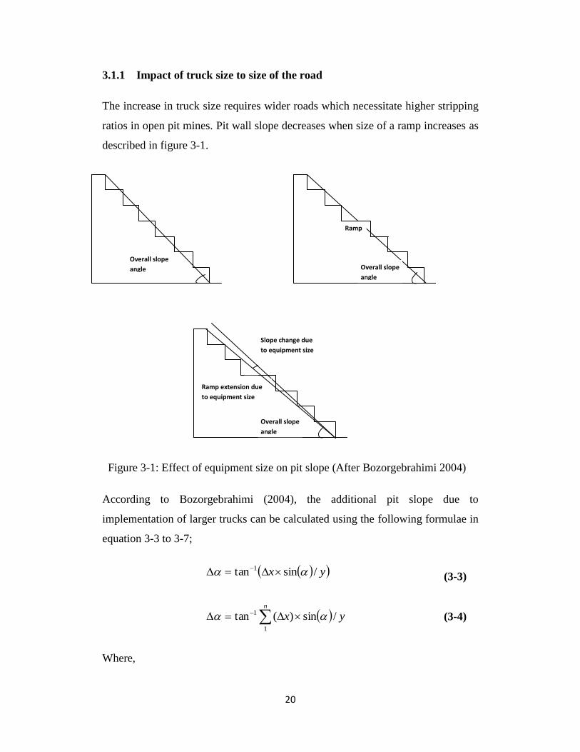
3.1.1 Impact of truck size to size of the road

The increase in truck size requires wider roads which necessitate higher stripping

ratios in open pit mines. Pit wall slope decreases when size of a ramp increases as

described in figure 3-1.

According to Bozorgebrahimi (2004), the additional pit slope due to

implementation of larger trucks can be calculated using the following formulae in

equation 3-3 to 3-7;

yx /sintan 1

(3-3)

yxn

/sin)(tan1

1

(3-4)

Where,

Overall slope

angle Overall slope

angle

Ramp

Overall slope

angle

Ramp extension due

to equipment size

Slope change due

to equipment size

Figure 3-1: Effect of equipment size on pit slope (After Bozorgebrahimi 2004)

21

LR

PDgINTn 1

(3-5)

where PD is the pit depth, LR is the length of pit wall the ramp occupies, Δx is the

road width increase required to use larger trucks (m), Δα is the overall pit slope

decrease from implementing larger trucks in degrees, α is the overall pit slope

before implementing larger trucks in degrees, n is the number of times that the

ramp cuts (crosses) the pit wall (determined from Eq 3-5), y is the pit depth (m),

and g ramp grade (%).

The weight, W of material to be mined due to ramp widening is given by the

following equation

dhdlxW

Yg

Y

00

5.0 (3-6)

Where γ is the average specific weight of the materials to be mined, Δx is the

width of the ramp widening, dh is an element of pit depth, dl is an element of the

length of the ramp, g is the ramp grade (%), and Y is the maximum depth of pit

which the ramp is to reach.

Solving Eq. 3-6 gives:

gYxW

2

)5.0( (3-7)

3.2 Mine haul road structural design

Haul road design, construction and maintenance management are critical to the

performance and life of roads. The difference in applied loads, truck dimensions,

traffic volumes, size of the tires used, construction material quality and

availability and climatic conditions, together impact design life and road user cost

considerations. These create differences for which designing and management of

roads can be highly variable.

22

In truck based hauling systems, the mine haul road networks are critical and vital

elements in the production process. Underperformance of roads impacts

productivity and cost; up to millions of dollars, can be spent maintaining roads,

repairing damaged truck frames and replacing tires. Productivity, equipment

longevity and operations safety are all dependent on well designed, constructed

and maintained roads (Thompson, 2011b).

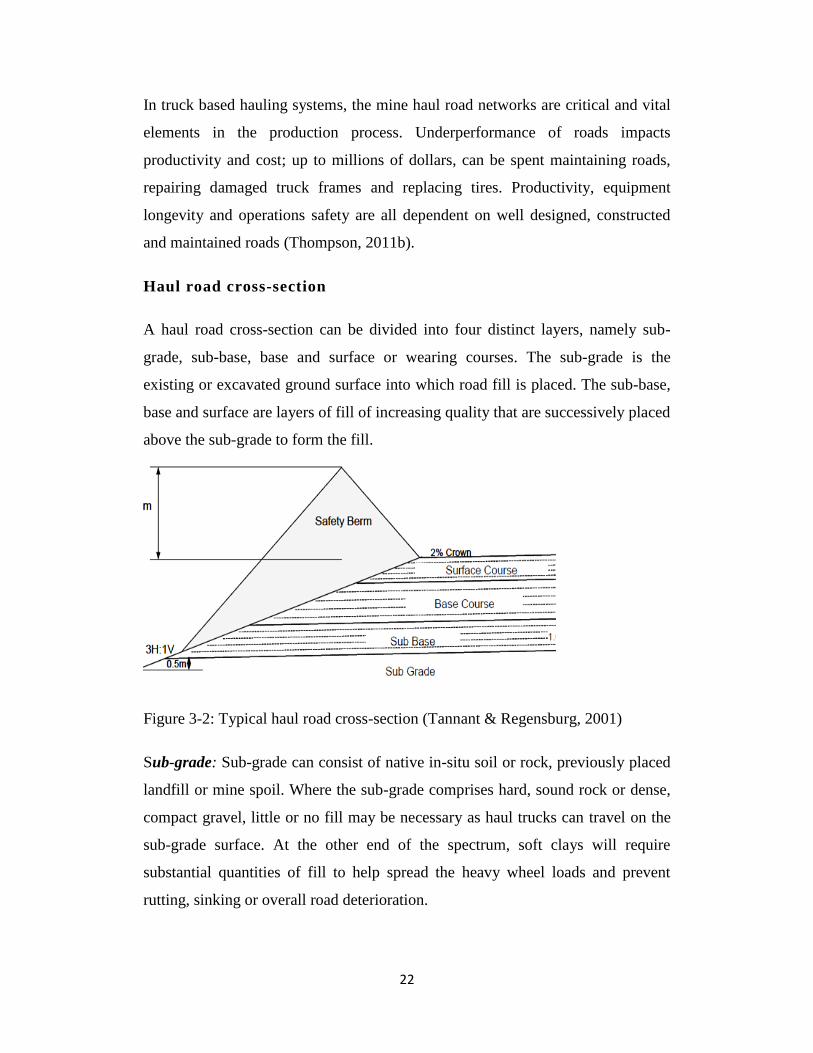
Haul road cross-section

A haul road cross-section can be divided into four distinct layers, namely sub-

grade, sub-base, base and surface or wearing courses. The sub-grade is the

existing or excavated ground surface into which road fill is placed. The sub-base,

base and surface are layers of fill of increasing quality that are successively placed

above the sub-grade to form the fill.

Figure 3-2: Typical haul road cross-section (Tannant & Regensburg, 2001)

Sub-grade: Sub-grade can consist of native in-situ soil or rock, previously placed

landfill or mine spoil. Where the sub-grade comprises hard, sound rock or dense,

compact gravel, little or no fill may be necessary as haul trucks can travel on the

sub-grade surface. At the other end of the spectrum, soft clays will require

substantial quantities of fill to help spread the heavy wheel loads and prevent

rutting, sinking or overall road deterioration.

23

Sub-base: Sub-base is the layer of a haul road between sub-grade and base of the

road. It usually consists of compacted granular material, either cemented or

untreated. Run of mine and coarse rocks are the general components of this layer.

Apart from providing structural strength to the road, it serves many other purposes

such as preventing intrusion of sub-grade soil into the base layer and vice-versa,

minimizing effects of frost, accumulation of water in the road structure, and

providing a working platform for construction equipment.

The sub-base distributes vehicle loads over an area large enough that the stresses

can be borne by the natural, sub-grade material. The lower the bearing capacity of

the ground, the thicker the sub-base must be.

Base: The layer of haul road directly beneath the surface layer of the road is

called the base. If there is no sub-base then the base is laid directly over the sub-

grade or roadbed. Usually higher quality treated or untreated material with

suitable particle size distribution is used for construction of this layer.

Specifications for base materials are generally considerably more stringent for

strength, plasticity, and gradation than those for the sub-grade. The base is the

main source of the structural strength of the road.

Surface (wearing course): The uppermost layer of the haul road that comes

directly in contact with tires is known as the surface (wearing) course or running

layer. A haul road surface is generally constructed with fine gravel with closely

controlled grading to avoid dust problems while maintaining proper binding

characteristic of the material. Apart from providing a smooth riding surface, it

also distributes the load over a larger area thus reducing stresses experienced by

the base (Tannant & Regensburg, 2001)

This is the alignment of a haul road layers. Next stage in road design is

determining thicknesses of these layers depending on sub-base strength, material

properties and traffic volume.

24

The structural design

The structural design provides haul road ‘strength’ to carry the imposed loads

over the design life without the need for excessive maintenance, necessitated by

deformation of one or more layers of the road most often caused by soft, weak or

wet in-situ materials below the road surface. Haul roads deteriorate with time due

to interactive efforts of traffic load and specific in-situ material strength. Two

approaches are commonly used for structural design. The California Bearing

Ratio (CBR) method (Kaufman & Ault, 1977) has been widely applied to design

mine haul roads in which untreated materials are used. When multilayer roads are

considered in conjunction with a base layer of selected rock, a Mechanistic

Approach is considered more appropriate (Thompson, 2011b). In both cases, an

understanding of haul truck tire interactions is necessary.

CBR cover curve

The California Bearing Ratio (CBR) cover curve design method was developed in

1942 and Kaufman and Ault (1977) were among the first to recommend the use of

the CBR method for the design of haul roads in surface mines. The approach

characterizes the bearing capacity of a given soil as a ratio to the bearing capacity

of a standard-crushed rock; the ratio of capacities being referred to as the CBR for

the given soil. Empirical curves, known as CBR curves, relate the required fill

thickness and applied wheel load to the CBR value. The technique is used for

successive layers with the requirement that each successive layer should be of

higher CBR than the preceding, and that the change in CBR should not be abrupt

since the preceding layer acts as a compaction cover to the subsequent layer

(Thompson, 2011b).

The United States Bureau of Mines (USBM, 1977) recommended accommodation

of wheel loads up to 55-mt (300mt GVW) truck size which was later extended to

accommodate ultra size trucks of up to 630mt GVW (Thompson, 2010). Figure 3-

3 shows an updated version of the USBM CBR design charts appropriate for ultra

25

class trucks, together with the approximate bearing capacities of various soil types

defined by The Unified Soil Classification (USC) and American Association of

State Highway Transportation Official's Systems (AASHTO).

Wheel loads for any haul truck can readily be computed from the manufacturer’s

specifications. It has been noted that haul trucks are frequently loaded above their

rated weight capacity which should be taken into consideration for road design.

By dividing the loaded vehicle weight over each axle by the number of tires on

that axle, the maximum load for any wheel of the vehicle may be established. In

every case, the highest wheel load should be used in design computations

(Thompson, 2011b). Furthermore in evaluating distribution of wheel loads for a

given time period of operation for a haul truck it is possible to evaluate a

neglected mean load which may also be argumentative.

The CBR method is particularly useful for estimating the total cover thickness

needed over the in-situ sub-grade material. A weaker sub-grade requires thicker

layers of road construction material. This moves the truck tires higher away from

the weak in-situ material, thus diminishing strains for a given material horizon to

a level that can be tolerated by the sub-grade and lower successive lower layers.

Shortcomings of CBR method

Morgan (1994) and Thompson & Visser (1997a) criticized the CBR method of

haul road design for the following considerations:

The CBR method is based on Boussinesq’s semi-infinite single layer

theory, which assumes a constant elastic modulus for different materials in

the pavement. Various layers of a mine haul road consist of different

materials each with its own specific elastic moduli and other properties

such as degree of compaction or moisture content

The CBR method does not take into account the properties of the surface

course material.

26

The CBR method was originally designed for paved roads and surfaces for

airfields. Therefore the method is less applicable for unpaved roads,

especially haul roads which experience very different wheel geometries,

poorer quality and construction materials (usually mine wastes).

CBR empirical design curves were not developed for the high axle loads

generated by large haul trucks as simple extrapolation of existing CBR

design curves can lead to errors of under, or even over design.

27

Figure 3-3: CBR cover curves for 90-630 metric ton GVM haul trucks and

approximate bearing capacities of various soil types defined by UCS and

AASHTO systems(after Thompson 2010)

28

Mechanistic design approach

A mechanistic approach supported by Thompson, (2011b) and others takes into

account the differing properties in each layer and predicts their behaviour under

applied load before construction by appropriate laboratory and in-situ testing. The

road cross section is treated as a composite beam in determining the reaction of

the structure to loading. A limit design criterion of vertical compressive strains of

sub-grade and cumulative sub-layer below any given higher horizon of materials

is used to assess the haul road under the specific load conditions, and hence

determine the adequacy of a given road structural design.

This value of limiting strain is associated with the category of the road to be

designed, truck size, traffic volume, performance required as a result of

maintenance requirement over the life of the road and road operating life. The

higher the wheel loads and traffic volumes together with longer required operating

life and associated performance, the lower the required critical value as shown in

figure 3-4. This data is used to calculate the thickness of the blasted rock to be

placed on top of in-situ or sub-grade such that the road perform satisfactorily over

its design life. Structural performance of the road is predominantly controlled by

applied load, subgrade strength and pavement structural thickness.

29

Figure 3-4: Typical haul road design categories and design data (after Thompson,

2011c )

Higher values of sub-grade critical strain cause permanent deformation to occur

over many load repetitions, where deformation accumulates to cause rutting, the

general shape of the road surface is lost. Riding quality deteriorates, serviceability

reduces and rolling resistance increases which have direct impact on hauler

availability, fuel consumption and emissions (Thompson, 2011c).

The mechanistic approach focuses on limiting load induced strain in progressively

thicker sub-grade below a target horizon to below a set critical value. Based on

field observations, the maximum vertical strain limits have been established to be

1500-2000 micro-strains for typical haul roads. Moreover, the stress level in any

layer of a haul road cross-section should not exceed the bearing capacity of the

material used in that layer. Values exceeding 2500 micro-strain are associated

with unacceptable structural performance, except for light traffic and short term

roads (Thompson & Visser, 1997b).

30

An empirical equation (3-8) for estimating the critical strain limit was developed

by Knapton, (1988). This equation was developed for the heavy loading

conditions found on docks at container ports. A modified version of the equation

for haul roads shows a similar functional relationship between the critical strain

limit and the design life of the road through traffic density:

27.0/000,80 NE (3-8)

Where:

E = critical strain limit (micro-strain) and

N = number of load repetitions.

The stresses in individual layers below the surface layer can be calculated using

stress models or the application of elastic theory. For example, the simplest

assumption is that a tire creates a uniform circular load over an isotropic,

homogeneous elastic half space as interpreted by Boussinesq. Although the

assumption of homogeneity of individual layers in the haul road cross-section

results in some error in estimation of the strain level in various layers, the

assumption simplifies the problem for preliminary examination. This approach is

still more acceptable than considering the entire haul road profile to be a singular

equivalent material as was the previous practice of CBR approach.

31

Figure 3-5: Boussinesq ground stress bulb ( after Perloff, 1975).

The strains induced in a pavement are a function of the effective elastic (resilient)

modulus values assigned to each layer in the structure. In order to facilitate a

mechanistic design, some indication of applicable modulus values is required.

Figure 3-3 gives recommended modulus value correlations USCS and AASHTO

classification system. Equation 3-9 can also be used in conjunction with layer

CBR values to determine modulus values (Eeff, MPa) (Thompson, 2011c)

46.063.17 CBREeff

(3-9)

3.3 Functional design

Functional design of the road is centered on the selection of a wearing course (or

surfacing) material where the most suitable choice and application is required to

minimize the rate of defect formation in road surface, which would otherwise

compromise road safety and performance.

32

Typically natural gravel or crushed stone and gravel mixtures commensurate with

safety, operational, environmental, and economic considerations are selected if

readily available. In addition to their low rolling resistance and high coefficient of

adhesion, their greatest advantage over other wearing course materials is that

roadway surfaces can be constructed rapidly and at relatively low cost (Tannant &

Regensburg, 2001). In the case of the Athabasca oil sand mines, gravel is at a

premium and not readily available and so alternative material such as limestone

crushed material or using chemical additions are currently being tested.

The defects most commonly associated with mine haul roads, in order of

decreasing impact on hauling operational performance, are typically as follows:

Skid resistance

Dustiness

Loose material

Corrugations

Stoniness—loose

Potholes

Rutting

Stoniness—fixed

Cracks—slip, longitudinal, and crocodile. “Crocodile cracks” are cracks in

a road caused by high plasticity/ high clay content material shrinking when

drying. This is a well-known phrase among the pavement design

fraternity.

By examining which wearing course material property parameters lead to these

defects, a specification has been developed for wearing-course materials selection.

The specifications are based on an assessment of wearing-course material

shrinkage product (Sp) and grading coefficient (Gc), defined in Equations 3-10

and 3-11, (Thompson & Visser, 2006).

33

425PLSSp (3-10)

100

4752265 PPPGc

(3-11)

Where;

LS = bar linear shrinkage

P425 = percent wearing course sample passing 0.425-mm sieve


P2 = percent wearing course sample passing 2-mm sieve


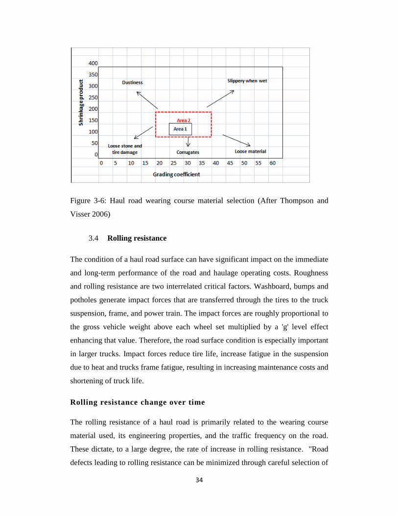
If the three most critical haul road defects are considered, it appears that mine

road user preference is for much reduced skid resistance and dust defects. This

defines the focus point of the specifications to an area bounded by a grading

coefficient of between 25 and 32 and a shrinkage product of between 95 and 130

in figure 3-6 where the overall and individual defects are minimized (Area 1).

Extending this region to encompass poorer (but nevertheless operable)

performance enables an additional area (Area 2) is defined (Thompson & Visser,

2006).

34

Figure 3-6: Haul road wearing course material selection (After Thompson and

Visser 2006)

3.4 Rolling resistance

The condition of a haul road surface can have significant impact on the immediate

and long-term performance of the road and haulage operating costs. Roughness

and rolling resistance are two interrelated critical factors. Washboard, bumps and

potholes generate impact forces that are transferred through the tires to the truck

suspension, frame, and power train. The impact forces are roughly proportional to

the gross vehicle weight above each wheel set multiplied by a 'g' level effect

enhancing that value. Therefore, the road surface condition is especially important

in larger trucks. Impact forces reduce tire life, increase fatigue in the suspension

due to heat and trucks frame fatigue, resulting in increasing maintenance costs and

shortening of truck life.

Rolling resistance change over time

The rolling resistance of a haul road is primarily related to the wearing course

material used, its engineering properties, and the traffic frequency on the road.

These dictate, to a large degree, the rate of increase in rolling resistance. "Road

defects leading to rolling resistance can be minimized through careful selection of

35

the wearing course, which will minimize, but not totally eliminate, rolling

resistance increase over time," Thompson, (2011c). Wearing course properties

and traffic volume are important parameters with regard to prediction of

deterioration progression.

To estimate rolling resistance (RR) at a given point in time Thompson & Visser ,

(2000) established the relationship in equation 3-12 which estimates roughness

defect score. It can be determined from an initial estimate of the minimum and

maximum roughness defect scores (RDSMIN, RDSMAX), together with the rate

of roughness defect score increase (RDSI). Rolling resistance at a point in time (D

days after road maintenance) is then estimated from a minimum value (RRMIN)

and the associated rate of increase.

The equations developed which are shown below may be used, together with the

parameters and variables defined in the table 3-1.

)(exp1 RDSI

RDSMINRDSMAXRDSMINRDS (3-12)

Where;

RDSMIN = 31,1919 - 0,05354.SP - 0,0152.CBR (3-12a)

RDSMAX = 7,6415 + 0,4214.KT + 0,3133.GC + 0,4952.RDSMIN (3-12b)

RDSI=1,768+0,001.D(2,69.KT-72,75.PI -2,59.CBR 9,35.GC+1,67.SP) (3-12c)

And

RR = RRMIN + RDS.exp(RRI )

(3-12d)

Where;

RRMIN=exp( -1,8166+0,0028.V )

(3-12 e)

RRI = -6,068 -0,00385.RDS +0,0061.V (3-12 f)

Table 3-1: Parameters and variables for RR estimation

Parameter Description

RDS Roughness defect score

RDSMIN Minimum roughness defect score immediately following last

maintenance cycle

36

RDSMAX Maximum roughness defect score

RDSI Rate of roughness defect score increase

RR Rolling resistance (N/kg)

RRMIN Minimum rolling resistance at (RDS) = 0

RRI Rate of increase in rolling resistance from RRMIN

Variable Description

Vo Vehicle speed (km/h)

D Days since last road maintenance

KT Average daily tonnage hauled (Kt)

PI Plasticity index

CBR 100% Mod. California Bearing Ratio of wearing course material


Road width depends on the width of a truck plus the extra width on a switchback;

this means with larger trucks wider roads are required. Road gradients vary from

0% to 8% and on short distances can be higher. On soft underfoot when using

larger trucks the grade of less than 6% is more favourable.

Haul road layer thicknesses are influenced by traffic loads, in-situ material

properties, performance requirements and road operating life. The higher the

wheel loads, traffic volume, higher performance requirement and longer operating

life, the lower the limiting strain which necessitates additional road layer

thickness.

Rate of rolling resistance increase is associated to wearing course material used

and traffic frequency. Weaker material and higher traffic volumes result into

faster rolling resistance deterioration rates.

37

4 FUEL CONSUMPTION AND EMISSIONS

Haul truck operations are a major contributor to overall surface mining equipment

operating costs. Most mines use trucks as the means of primary haulage in North

America (Kecojevic & Komljenovic, 2010). Among the primary costs associated

with the use of trucks, fuel consumption is in line with tire costs, haul road

construction and maintenance and equipment maintenance. A number of factors

contribute to fuel consumption, major ones being; truck load, speed, engine power

and road conditions.

4.1 Fuel consumption

The best way to determine fuel consumption is to obtain data from the actual mine

operation. In the absence or limited data availability such data maybe estimated

from equations and published data via the truck Original Equipment Manufacturer

(OEM) which may be used for estimation purposes.

According Runge, (1998) and (Filas, 2002) an hourly fuel consumption FC (l/h)

may be determined from equation 4-1:

LFPFC 3.0 (4-1)

Where P is engine power (kW), 0.3 is a unit conversion factor (l/kWh) and LF is

an engine load factor (the portion of full power required by the truck). Values for

the truck engine load factors range from 0.18 to 0.50 (Runge, 1998) while Filas,

(2002) states that engine load factors typically range between 0.25 and 0.75,

depending on the equipment type and use level; the latter being more reflective of

modern ultra-class haulers at the upper end of the scale.

A similar equation for fuel consumption was suggested by Hays, (1990):

FD

LFPCSFFC

(4-2)

Where, CSF is the engine specific fuel consumption at full power (0.21 – 0.27

kg/kWh) P is power (kW), LF is engine load factor and FD is the fuel density

(0.85 kg/l for diesel). Hays recommends the following values for engine load

38

factors: 25% (light: considerable idle, loaded hauls on favorable grades and good

haulage roads); 35% (average: normal idle, loaded hauls on adverse grades and

good haulage roads); and 50% (heavy: minimum idle, loaded hauls on steep

adverse grades).

Liebherr developed a method to determine the truck fuel consumption per hour.

According to this OEM, the fuel consumption rate is directly proportional to

delivered power on different truck sizes (Boucom, 2008). Assuming the load

factor of 100%, the relationship between fuel consumption and power was

obtained as;

602139.0%)100( PLFFC (4-3)

Caterpillar also provides data on fuel consumption for its trucks by load factors.

The load factors defined are categorised depending on gross vehicle weight,

payload and road conditions.

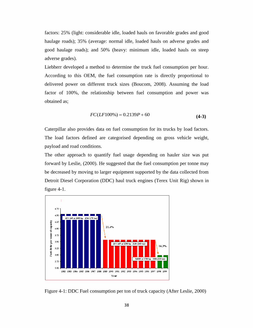
The other approach to quantify fuel usage depending on hauler size was put

forward by Leslie, (2000). He suggested that the fuel consumption per tonne may

be decreased by moving to larger equipment supported by the data collected from

Detroit Diesel Corporation (DDC) haul truck engines (Terex Unit Rig) shown in

figure 4-1.

Figure 4-1: DDC Fuel consumption per ton of truck capacity (After Leslie, 2000)

39

4.2 Diesel emissions

One of the disadvantages of truck and shovel mining systems is the increase in

diesel emissions. A large percentage of mining related emissions are attributed to

mine hauler fleets as the result of fuel combustion. In the oil sands region of

Northern Alberta a large percentage of regional NOx emissions is attributed to

mine fleets (Singh, Rawling, & Unrau, 2008). Other research conducted on a

surface coal mining operation in West Virginia show that a total of 966 tons of

NOx per year was emitted in the mine. In this case haul trucks and blasting

contributed to the total emission by 44.7% and 22.3%, respectively (Lashgari,

2013)

4.2.1 Diesel combustion

Diesel combustion consists of oxidizing hydrocarbon chains (CxHy) in an

explosive reaction to form carbon dioxide (CO2) and water (H2O) in which the

reaction is not 100% efficient and the constituents are not pure. The air used to

supply the oxygen (O2) contains about 80% nitrogen (N2) and the diesel fuel

contains a small percentage of sulphur (S). The result is that trace amounts of

other chemicals are formed in the reaction as described on the equation below

(After Leslie, 2000).

CxHy(Sz) + (O2 + N2) CO2 + H2O + (O2 + N2) + {NOx + HC + OOC + C +

CO+ SOx}

Combustion Reaction Major Constituents + {Trace Constituents}

Of the major constituents of the reaction, CO2 is a concern as a potential

"greenhouse" gas and a theoretical contributor to "global warming". Since it is an

integral part of the reaction, the way to reduce output is to increase the efficiency

of the engine and reduce fuel consumption. CO2 is produced at rate of

approximately 2.73 kg/litre of fuel (Jaques, 1992), The production of SOx is

directly related to the amount of sulphur in the diesel fuel. The other trace

constituents are the result of incomplete combustion. Unburned hydrocarbons are

40

the products of partial combustion account for the HC, OOC (oxidizable organic

carbon), and free carbon (C) components of the trace constituents. Additional

compounds of Nitrogen contribute to the formation of 'smog' after further

reactions in the presence of sunlight (hʋ), and can pose health risks as

concentrations rise.

The visible portion of PM, black smoke consists of is larger carbon particles that

are formed under acceleration and heavy loading due to insufficient air or low

combustion temperatures. Modern electronic engine controls can minimize the

formation of black smoke such that it is rarely visible (Leslie, 2000).

NOx is also produced in the high temperature, high-pressure diesel fuel

combustion chamber when there is excess oxygen available to combine with

nitrogen during the reaction. Oxides of nitrogen can react in the atmosphere to

form acidic compounds as well as promote low level ozone (O3), a major

component of smog. Ozone can be a lung irritant and can cause serious health

effects and breathing difficulty in higher concentrations.

4.2.2 Engine development

Engine manufacturers have been driven by the need to reduce the operating costs

of the engines they produce. This has been accomplished by designing engines

that require less maintenance and burn less fuel. Even without a focussed effort,

most emission component levels were in parallel reduced with this strategy. By

producing engines that are more efficient, the manufacturers reduced products of

incomplete combustion including CO, HC, and OOC, as well as CO2 since less

fuel was consumed. The only component of the emissions that did show any

potential for increase was NOx, since its formation primarily occurs as

temperatures rise in a combustion chamber (Leslie, 2000).

4.2.3 Diesel emission improvement

Over the years there has been improvement in engine efficiency. This evolution in

engine technologies made it possible for bigger trucks to use fuel more efficiently

and produce fewer emissions. Therefore the increase in size and engine efficiency

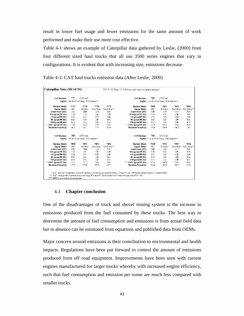
41

result in lower fuel usage and fewer emissions for the same amount of work

performed and make their use more cost effective.

Table 4-1 shows an example of Caterpillar data gathered by Leslie, (2000) from

four different sized haul trucks that all use 3500 series engines that vary in

configurations. It is evident that with increasing size, emissions decrease.

Table 4-1: CAT haul trucks emission data (After Leslie, 2000)


One of the disadvantages of truck and shovel mining system is the increase in

emissions produced from the fuel consumed by these trucks. The best way to

determine the amount of fuel consumption and emissions is from actual field data

but in absence can be estimated from equations and published data from OEMs.

Major concern around emissions is their contribution to environmental and health

impacts. Regulations have been put forward to control the amount of emissions

produced from off road equipment. Improvements have been seen with current

engines manufactured for larger trucks whereby with increased engine efficiency,

such that fuel consumption and emission per tonne are much less compared with

smaller trucks.

42

5 ANALYSIS

5.1 Overview

Over the past century, open pits have attempted to increase their production rates

and lower production costs by use of larger equipment. Pits and haul roads

designed to accommodate small equipment are now evaluated for the opportunity

to accommodate bigger ones. This has been possible to others and others not due

to operating conditions. Evaluation of aspects affected is important when making

decision to either purchase equipment for a new mine or transitioning to bigger

size equipment on an already operating mine.

This study is focused on evaluating the impacts of increasing size of haul trucks to

mine planning in term of road size and construction, rolling resistance increase,

fuel usage and diesel emissions. The costs and benefits are evaluated considering

the amount of material to be stripped off to accommodate the bigger size, road

pavement construction requirements for each truck size and increase in rolling

resistance as the function of traffic volume and material properties. Fuel

consumption and associated emissions are also evaluated subject to increasing in

truck size and total resistance (rolling + grade).

To accomplish the objective of the research, it is proposed to compare the three

different truck sizes from the same manufacturer (Caterpillar) and analyse their

application impacts. The trucks chosen are CAT 785C, CAT 793F and CAT 797F.

Similar operating conditions and production requirements are assumed for

comparison purposes.

5.2 Haul road geometric design for different truck sizes

The size of road varies depending on size of vehicle using that road. Changing in

road size impacts stripping cost and pit slope angle as well. As an illustration, to

evaluate the impact of changing hauler size to road width and stripping; an initial

pit is designed to accommodate the 136t trucks (CAT 785C). The pit slope is 70˚,

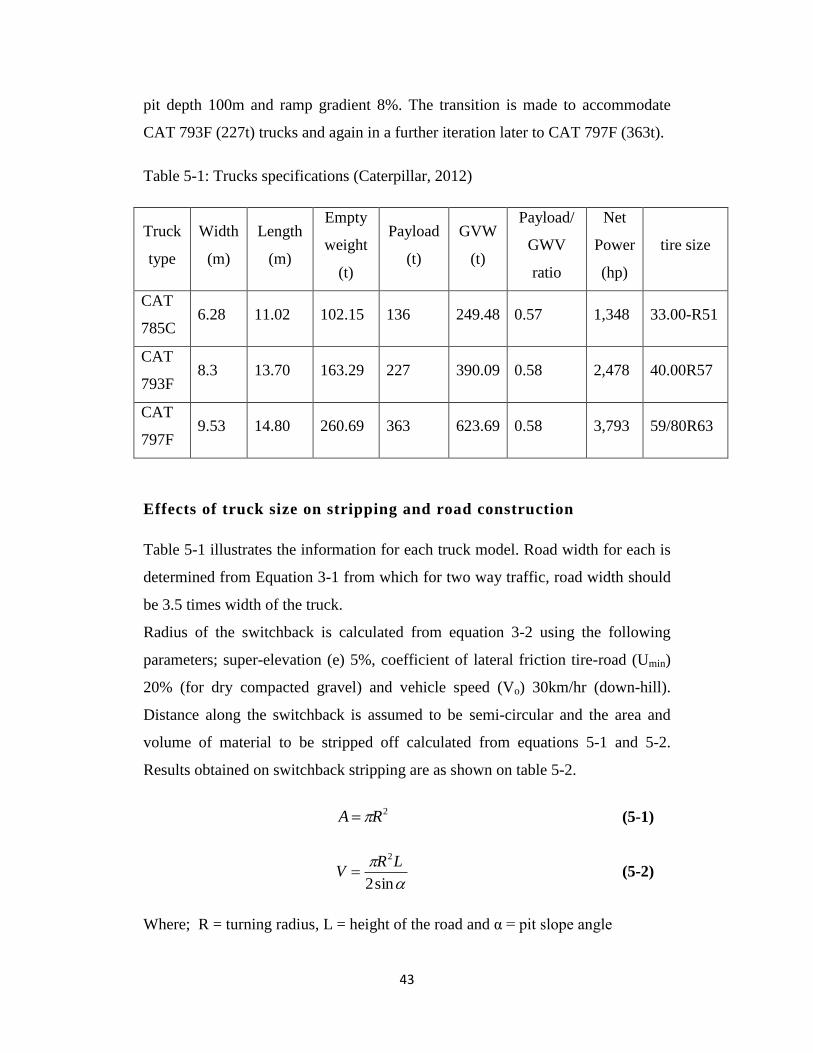
43

pit depth 100m and ramp gradient 8%. The transition is made to accommodate

CAT 793F (227t) trucks and again in a further iteration later to CAT 797F (363t).

Table 5-1: Trucks specifications (Caterpillar, 2012)

Truck

type

Width

(m)

Length

(m)

Empty

weight

(t)

Payload

(t)

GVW

(t)

Payload/

GWV

ratio

Net

Power

(hp)

tire size

CAT

785C 6.28 11.02 102.15 136 249.48 0.57 1,348 33.00-R51

CAT

793F 8.3 13.70 163.29 227 390.09 0.58 2,478 40.00R57

CAT

797F 9.53 14.80 260.69 363 623.69 0.58 3,793 59/80R63

Effects of truck size on stripping and road construction

Table 5-1 illustrates the information for each truck model. Road width for each is

determined from Equation 3-1 from which for two way traffic, road width should

be 3.5 times width of the truck.

Radius of the switchback is calculated from equation 3-2 using the following

parameters; super-elevation (e) 5%, coefficient of lateral friction tire-road (Umin)

20% (for dry compacted gravel) and vehicle speed (Vo) 30km/hr (down-hill).

Distance along the switchback is assumed to be semi-circular and the area and

volume of material to be stripped off calculated from equations 5-1 and 5-2.

Results obtained on switchback stripping are as shown on table 5-2.

2RA (5-1)

sin2

2LRV (5-2)

Where; R = turning radius, L = height of the road and α = pit slope angle

44

Table 5-2: Switchback stripping requirement

Truck

type

Road width on

switchback

(m)

Turning

Radius

(m)

Road

length

(m)

Incremental Stripping

on switchback (106

m3)

CAT 785C 29 150 471

CAT 793 38 159 500 0.365

CAT 797F 45 166 521 0.368

Using equations 3-4 to 3-7, pit specifications given above and truck specifications

in table 5-1, transitioning from one truck size to the other, the overall pit slope and

volume of waste stripping is calculated as shown in the table 5-3. The designed

widths are more than what is suggested in equation 3-1 and 3-1a due to an

additional width for angle of repose of construction material (38˚) added to all

truck sizes.

Table 5-3: Truck size effects on overall pit slope and incremental stripping

Truck

type

Approx

width

(m)

3.5×width

+ repose

(m)

Design

width

(m)

Increase

in road

width

(m)

Pit

slope

angle

(deg)

Incremental

stripping

ramp

(106

m3)

Incremental

stripping

switchback

(106 m

3)

Total

stripping

(106

m3)

CAT

785C 6.28 26.06 26 70

CAT

793 8.30 33.963 34 8 61.5 0.49 0.37 0.86

CAT

797F 9.75 39.965 40 6 55.5 0.38 0.37 0.74

This gives the rough idea of how much waste must be stripped off to extend the

road size with a change in equipment. When stripping cost per cubic metre is

known, it can be determined if it is economical to go for higher capacity trucks

45

including costs for other infrastructures such as crusher dump access, shop size,

bay doors etc. Apart from the increasing stripping due to increased road size, pit

bottoms need be big enough to allow safe operations of trucks and corresponding

loading equipment. For that reason the stripping ratio will practically be much

more than what is indicated above.

5.3 Haul road structural design

Haul road structural design is divided into two parts. The first part is

determination of layers thicknesses depending on truck weights and type of

construction material used. The second part is the final haul road design which

includes estimation of the total volume of material for road construction from pit

bottom to the exit.

Road layers design

To determine the effect of truck size on road layers design, the road was

constructed for each of the 3 truck types. For comparison, the road was designed

to haul same amount of material using each of the three truck options with the

same construction materials used. The effect of the size on road construction is

defined from the difference in pavement thickness for different trucks weights.

Material selection

The material selected for road construction are crushed rock for surface, pit-run

sand and gravel for base layer, till, mine spoil for sub grade and in-situ rock being

firm clay. The properties of selected materials are as shown in table 5-4 where, by

knowing the CBR value resilient modulus can be determined using figure 3-3, or

equation 3-9.

46

Table 5-4: Construction material properties

Layer Typical material CBR (%) Resilient modulus, MPa

Surface Crushed rock 95 330

Base Pitrun, sand & gravel 60 245

Sub-base Till, mine spoil 25 130

Sub-grade Firm clay 4 40

Critical strain

The roads were designed to haul 40Mt per year for five years using one truck

option from the three different truck sizes. The truck cycle time regardless the size

is set as 30mins and the trucks availability and utilization respectively 90%. Total

cycle times per year per truck and number of trucks needed to achieve production

were determined as follows;

Table 5-5: Cycle time calculations

production/day 109589.04t

production/year 40000000t

production in 5year 200000000t

cycle time 30mins

Availability 0.9

Utilization 0.9

cycles/year/truck 14191

Note:

yearperdaysof

yearperproductiontotaldayproduction

#/

timecycle

UAhourperutesdayperhoursyearperdaystruckyearcycles

min//

yeartimecyclepayloadtruck

yearperproductionunitsofnumber

/

Critical strains for trucks were calculated from equation 3-8

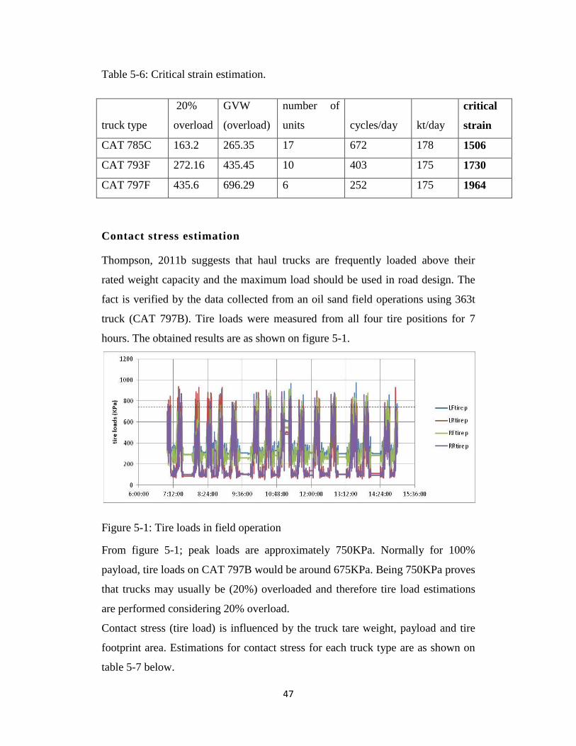
47

Table 5-6: Critical strain estimation.

truck type

20%

overload

GVW

(overload)

number of

units cycles/day kt/day

critical

strain

CAT 785C 163.2 265.35 17 672 178 1506

CAT 793F 272.16 435.45 10 403 175 1730

CAT 797F 435.6 696.29 6 252 175 1964

Contact stress estimation

Thompson, 2011b suggests that haul trucks are frequently loaded above their

rated weight capacity and the maximum load should be used in road design. The

fact is verified by the data collected from an oil sand field operations using 363t

truck (CAT 797B). Tire loads were measured from all four tire positions for 7

hours. The obtained results are as shown on figure 5-1.

Figure 5-1: Tire loads in field operation

From figure 5-1; peak loads are approximately 750KPa. Normally for 100%

payload, tire loads on CAT 797B would be around 675KPa. Being 750KPa proves

that trucks may usually be (20%) overloaded and therefore tire load estimations

are performed considering 20% overload.

Contact stress (tire load) is influenced by the truck tare weight, payload and tire

footprint area. Estimations for contact stress for each truck type are as shown on

table 5-7 below.

48

Table 5-7: Contact stress estimation

Truck type CAT 785C CAT 793F CAT 797F

Tare weight, t 102.15 163.29 260.69

Payload (120%), t 163.20 272.16 435.60

GVW(Tare +120%P), t 265.35 435.45 696.29

Tire size 33.00-R51 40.00R57 59/80R63

Total load per tire, t 44.23 72.58 116.05

Footprint area, A 0.83 1.14 1.51

Equivalent tire width (b) 0.91 1.07 1.23

Stress exerted, σ (MPa) 522.71 624.53 753.93

Note:

1. Tire strain, δ = 7% (0.07) under normal1g loading (Sharma, 2009).

2. Footprint area, A=1.35δϕ (experimental relation after Sharma, 2009)

3. Equivalent tire width, b=√A (Joseph, 2002)

4. Contact stress = Total load per tire / Footprint area

The weight used in this case, was based on a truck considered to be static.

However this might not be the case in dynamic conditions where operating force

(weight) is amplified during motion. The weight distribution in strut locations

differs.

For example; in static conditions (Vo=0) weight can be calculated by;

W=F=mg (i)

The mass m, contributing to each strut of the unit does not change and therefore

the change is caused by variation in acceleration (a), enhancing or reducing ‘g’ at

each strut location. Flexure in the frame give rise to the different values of ‘a’

which is in turn influenced by ground conditions (Joseph, 2003). This variation

‘a’ causes rack motion which varies weight at each tire set by F';

F’=m (g+a). (ii)

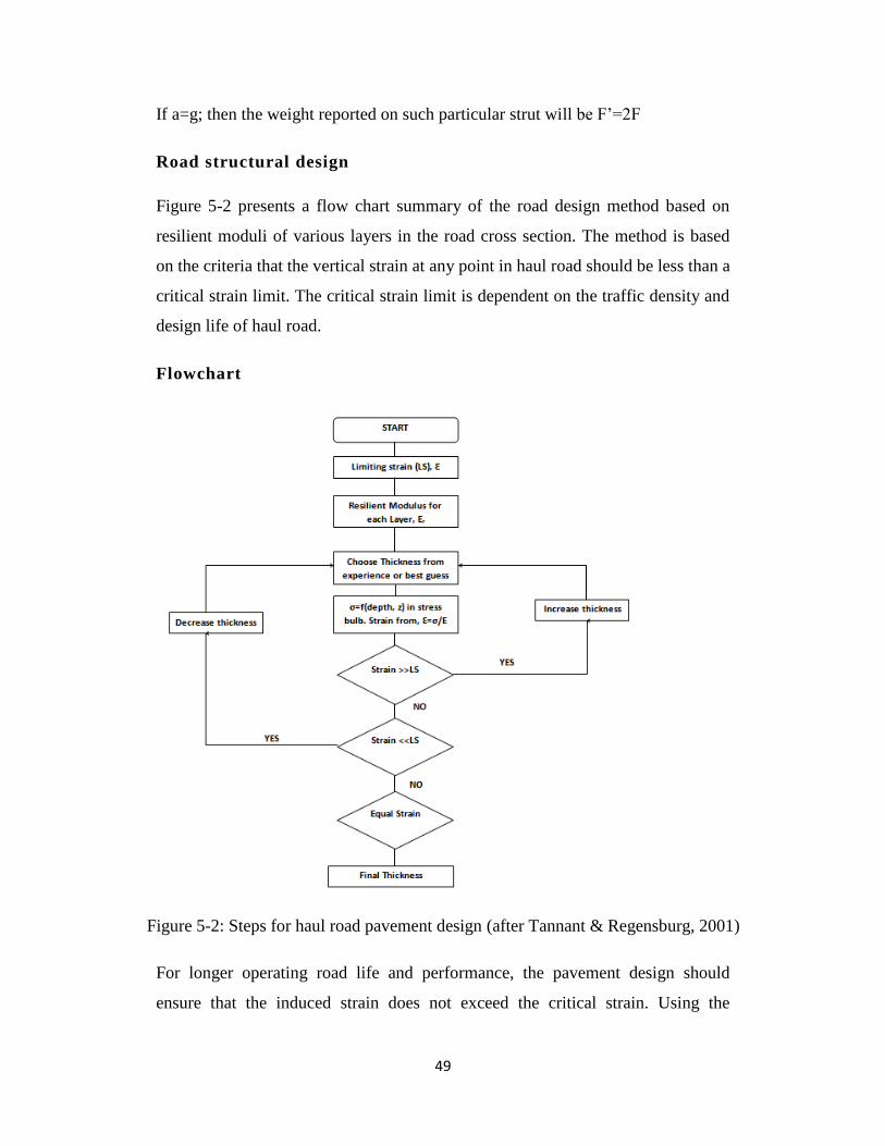
49

If a=g; then the weight reported on such particular strut will be F’=2F

Road structural design

Figure 5-2 presents a flow chart summary of the road design method based on

resilient moduli of various layers in the road cross section. The method is based

on the criteria that the vertical strain at any point in haul road should be less than a

critical strain limit. The critical strain limit is dependent on the traffic density and

design life of haul road.

Flowchart

For longer operating road life and performance, the pavement design should

ensure that the induced strain does not exceed the critical strain. Using the

Figure 5-2: Steps for haul road pavement design (after Tannant & Regensburg, 2001)

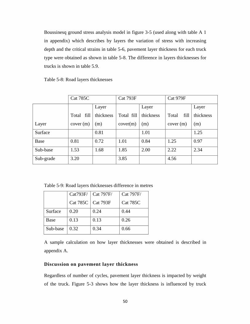
50

Boussinesq ground stress analysis model in figure 3-5 (used along with table A 1

in appendix) which describes by layers the variation of stress with increasing

depth and the critical strains in table 5-6, pavement layer thickness for each truck

type were obtained as shown in table 5-8. The difference in layers thicknesses for

trucks is shown in table 5.9.

Table 5-8: Road layers thicknesses

Table 5-9: Road layers thicknesses difference in metres

Cat793F/

Cat 785C

Cat 797F/

Cat 793F

Cat 797F/

Cat 785C

Surface 0.20 0.24 0.44

Base 0.13 0.13 0.26

Sub-base 0.32 0.34 0.66

A sample calculation on how layer thicknesses were obtained is described in

appendix A.

Discussion on pavement layer thickness

Regardless of number of cycles, pavement layer thickness is impacted by weight

of the truck. Figure 5-3 shows how the layer thickness is influenced by truck

Cat 785C Cat 793F Cat 979F

Layer

Total fill

cover (m)

Layer

thickness

(m)

Total fill

cover(m)

Layer

thickness

(m)

Total fill

cover (m)

Layer

thickness

(m)

Surface 0.81 1.01 1.25

Base 0.81 0.72 1.01 0.84 1.25 0.97

Sub-base 1.53 1.68 1.85 2.00 2.22 2.34

Sub-grade 3.20 3.85 4.56

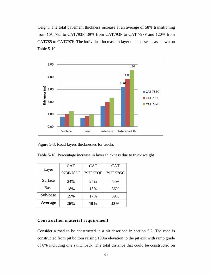
51

weight. The total pavement thickness increase at an average of 58% transitioning

from CAT785 to CAT793F, 39% from CAT793F to CAT 797F and 120% from

CAT785 to CAT797F. The individual increase in layer thicknesses is as shown on

Table 5-10.

Figure 5-3: Road layers thicknesses for trucks

Table 5-10: Percentage increase in layer thickness due to truck weight

Layer CAT

973F/785C

CAT

797F/793F

CAT

797F/785C

Surface 24% 24% 54%

Base 18% 15% 36%

Sub-base 19% 17% 39%

Average 20% 19% 43%

Construction material requirement

Consider a road to be constructed in a pit described in section 5.2. The road is

constructed from pit bottom raising 100m elevation to the pit exit with ramp grade

of 8% including one switchback. The total distance that could be constructed on

3.20

3.85

4.56

0.00

1.00

2.00

3.00

4.00

5.00

Surface Base Sub-base total road Th.

Thic

kne

ss (

m)

CAT 785C

CAT 793F

CAT 797F

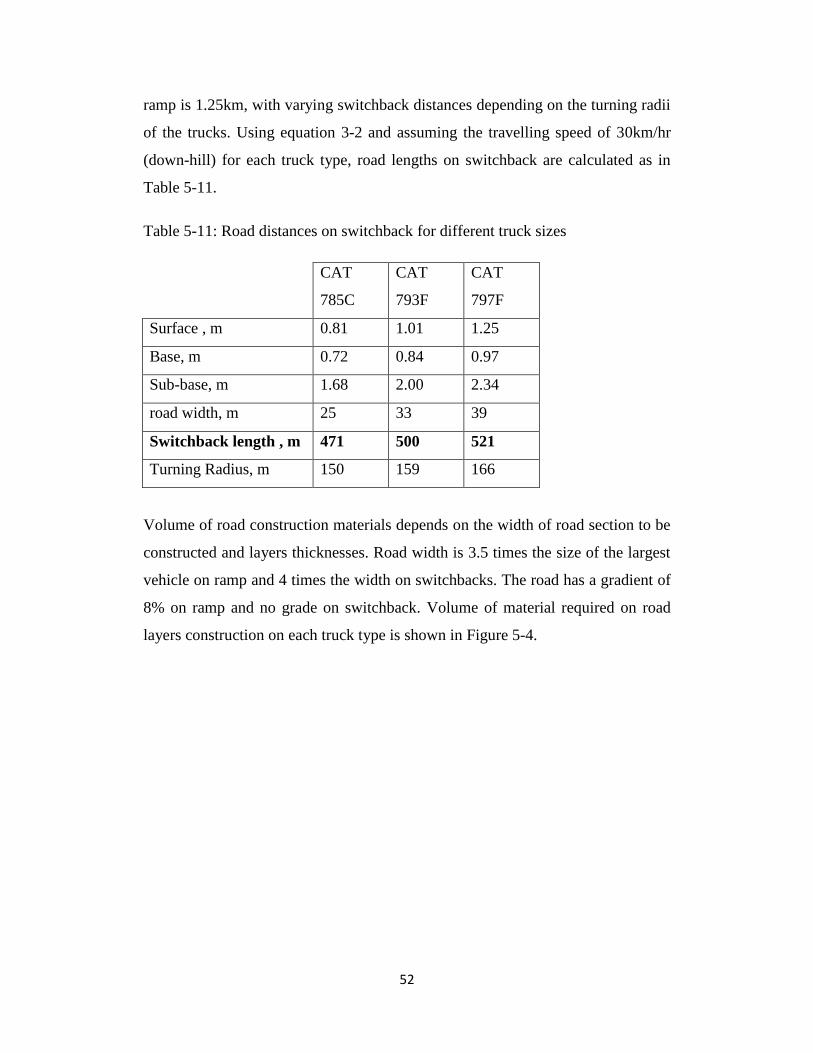
52

ramp is 1.25km, with varying switchback distances depending on the turning radii

of the trucks. Using equation 3-2 and assuming the travelling speed of 30km/hr

(down-hill) for each truck type, road lengths on switchback are calculated as in

Table 5-11.

Table 5-11: Road distances on switchback for different truck sizes

CAT

785C

CAT

793F

CAT

797F

Surface , m 0.81 1.01 1.25

Base, m 0.72 0.84 0.97

Sub-base, m 1.68 2.00 2.34

road width, m 25 33 39

Switchback length , m 471 500 521

Turning Radius, m 150 159 166

Volume of road construction materials depends on the width of road section to be

constructed and layers thicknesses. Road width is 3.5 times the size of the largest

vehicle on ramp and 4 times the width on switchbacks. The road has a gradient of

8% on ramp and no grade on switchback. Volume of material required on road

layers construction on each truck type is shown in Figure 5-4.

53

Figure 5-4: Construction materials requirement

Table 5-12: Percentage increase in road construction material

Layer

CAT

793F/785C

CAT

797F/793F

CAT

797F/785C

Surface 67% 48% 146%

Base 58% 37% 117%

Sub-base 58% 39% 121%

Average 61% 41% 128%

Indicated in Figure 5-4 above are the construction material requirements for an in-

pit haul road only. Extensions to waste dump and/or crusher/stockpiles as the

destinations for the mined rock need also to be constructed. The distance varies

depending on their location and therefore construction materials illustrated above

may likely go higher. The costs of construction materials may vary from one

operation to another depending on the possibility of preparing these materials on-

site. When deciding on truck size, considerations of road construction materials

need to be also done to account for the overall cost of increasing truck size in an

operation.

137

220

310

0

50

100

150

200

250

300

350

Surface Base Sub-base total material

Vo

lum

e o

f m

ate

rial

*1

00

0 m

3

CAT 785C

CAT 793F

CAT 797F

54

5.4 Rolling resistance

The rolling resistance is related to the wearing course material, material

engineering properties and the traffic frequency on the road which dictates the rate

of its increase. To estimate rolling resistance (RR) at a given point in time, the

approach suggested by Thompson & Visser (2000) of estimating the roughness

defect score (RDS) described in equation 3-12 was used. The parameters used for

estimation are;

Vo 20km/hr (uphill)

D 12 days

KT calculated for each truck type

PI 4.64 (for A-1-a in AASHTO in figure 3-3)

CBR 95% (for wearing course material)

SP 112.5 (for category 2 roads)

GC 28.5 (for category 2 roads)

Note: Category 2 roads are semi-permanent roads with medium to high traffic

volume. The elastic strain ranges from 1500 to 2000 micro-strain and traffic

volume less than 100Kt/day (Thompson, 2011c).

Rolling resistance estimation

Given that the cycles per year per truck is 14191 from table 5-5; the cycles per

day per truck is 39. For the three truck sizes, the traffic volume is estimated as

shown in table 5-13.

Table 5-13: Traffic volume estimation

CAT

797F

CAT

793F

CAT

785C

# units 6 10 17

Total trips/day 252 403 671

kt/day 58 58 59

55

Using the approach described in equation 3-12 rate of increase of rolling

resistance for three truck sizes may be estimated. Rolling resistance (%) estimates

for the first day of operation after maintenance is shown in table 5-14.

Table 5-14: rolling resistance estimation at day 1(after Thompson 2000)

CAT 797F CAT 793F CAT 785C

RDSMIN 23.72

RDSMAX 52.93 52.95 53.35

RDSI 1.26 1.26 1.27

RDS 30.16 30.17 30.24

RRMIN 0.17

RRI -6.06 -6.06 -6.06

RR(N/Kg) 0.24 0.24 0.24

RR % 2.38 2.38 2.38

The estimated rolling resistance increase rate for 12 days of operation are shown

in figure 5-5.

Figure 5-5: Trucks rolling resistance progression in 12 days

2.3

2.4

2.5

2.6

2.7

2.8

2.9

0 4 8 12 16

%R

R a

t 2

0km

/hr

days since last maintenance

CAT 797F

CAT 793F

CAT 785C

56

Rolling resistance discussion

The rate of increase in rolling resistance is basically the same regardless of truck

size. The average difference in rolling resistance between three truck sizes used

for 12 days is approximately 0.004% per day which is relatively small.

Estimations of rolling resistance increase per day for the three truck sizes are

shown on appendix B 2.

5.5 Section conclusion

The size of road varies with the size of trucks using the road. With larger trucks

wider roads are required, which necessitates more stripping. Pit slopes are

affected by the size of roads; with wider roads pit slopes decreases resulting in

laying back pit walls as pit size increases.

Road layer thickness is influenced by the construction materials used, applied

loads, performance level and required road life. If all other factors remain the

same, regardless of load repetitions, road layer thickness is most influenced by

truck load. The amount of road construction material required is a function of the

road layer thickness and road width. With larger trucks, construction material

requirements are much higher compared to smaller units.

When it comes to rolling resistance, the rate of increase is influenced by the

surface wearing course material used and traffic volume. Using crushed stone as a

wearing course material, the rate of increase in rolling resistance was observed to

be the same regardless of truck size. This is due to ground bearing pressure for the

tires being the same regardless of truck size. This in turn is an affect due to rubber

properties of the tire being the same for any truck size and so there is a constant

bearing pressure for a truck tire due to its material composition.

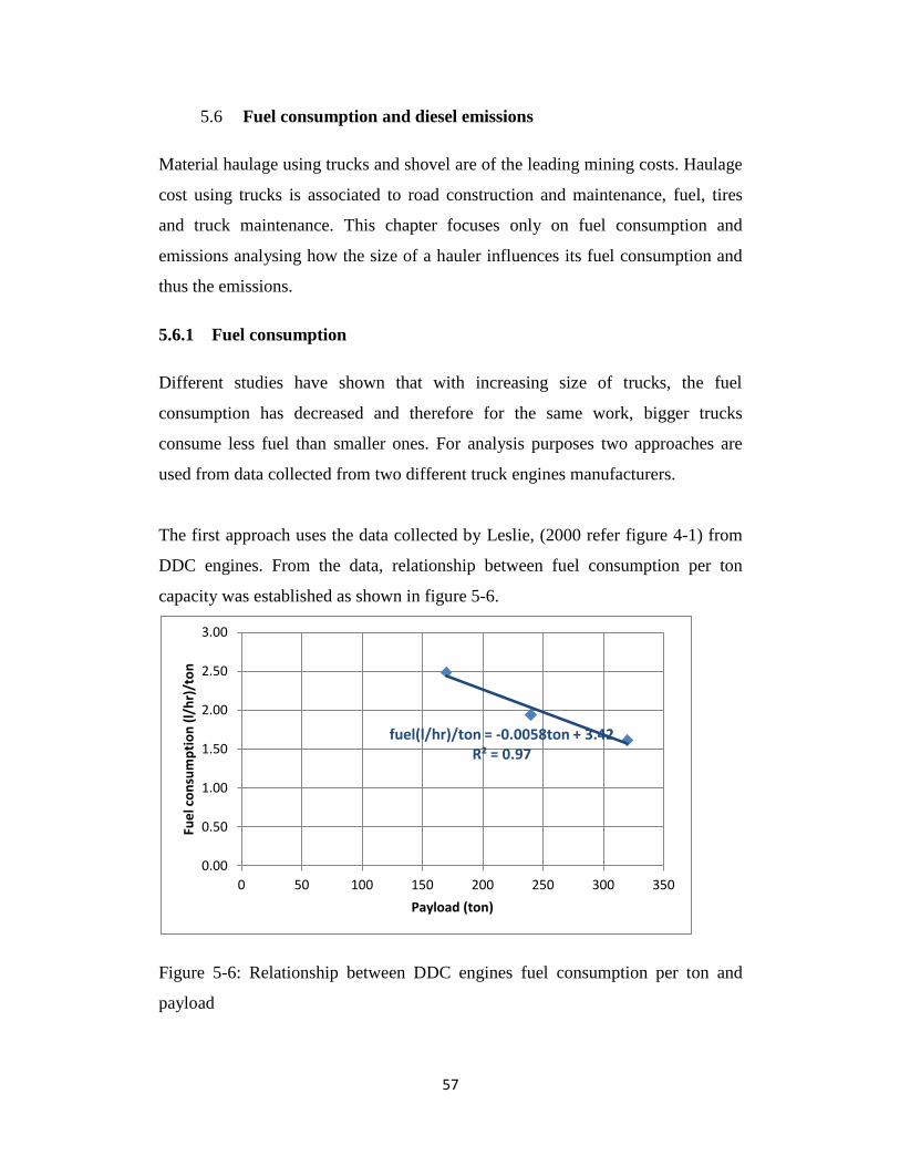
57

5.6 Fuel consumption and diesel emissions

Material haulage using trucks and shovel are of the leading mining costs. Haulage

cost using trucks is associated to road construction and maintenance, fuel, tires

and truck maintenance. This chapter focuses only on fuel consumption and

emissions analysing how the size of a hauler influences its fuel consumption and

thus the emissions.

5.6.1 Fuel consumption

Different studies have shown that with increasing size of trucks, the fuel

consumption has decreased and therefore for the same work, bigger trucks

consume less fuel than smaller ones. For analysis purposes two approaches are

used from data collected from two different truck engines manufacturers.

The first approach uses the data collected by Leslie, (2000 refer figure 4-1) from

DDC engines. From the data, relationship between fuel consumption per ton

capacity was established as shown in figure 5-6.

Figure 5-6: Relationship between DDC engines fuel consumption per ton and

payload

fuel(l/hr)/ton = -0.0058ton + 3.42 R² = 0.97

0.00

0.50

1.00

1.50

2.00

2.50

3.00

0 50 100 150 200 250 300 350

Fue

l co

nsu

mp

tio

n (

l/h

r)/t

on

Payload (ton)

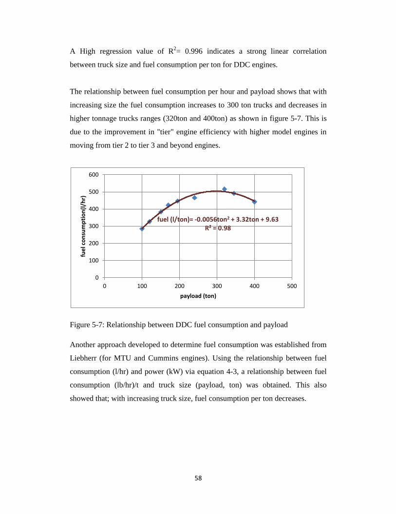
58

A High regression value of R2= 0.996 indicates a strong linear correlation

between truck size and fuel consumption per ton for DDC engines.

The relationship between fuel consumption per hour and payload shows that with

increasing size the fuel consumption increases to 300 ton trucks and decreases in

higher tonnage trucks ranges (320ton and 400ton) as shown in figure 5-7. This is

due to the improvement in "tier" engine efficiency with higher model engines in

moving from tier 2 to tier 3 and beyond engines.

Figure 5-7: Relationship between DDC fuel consumption and payload

Another approach developed to determine fuel consumption was established from

Liebherr (for MTU and Cummins engines). Using the relationship between fuel

consumption (l/hr) and power (kW) via equation 4-3, a relationship between fuel

consumption (lb/hr)/t and truck size (payload, ton) was obtained. This also

showed that; with increasing truck size, fuel consumption per ton decreases.

fuel (l/ton)= -0.0056ton2 + 3.32ton + 9.63 R² = 0.98

0

100

200

300

400

500

600

0 100 200 300 400 500

fue

l co

nsu

mp

tio

n(l

/hr)

payload (ton)

59

Figure 5-8: Relationship between Liebherr engines fuel consumption per ton and

payload

Comparing with the first approach, the Liebherr engines indicate that fuel

consumption per hour (lb/hr) increases with increasing truck capacity.

Figure 5-9: Relationship between Liebherr engines hourly Fuel consumption and

payload

Note: The decision to use payload instead on GVW is made based on the fact that

mine operators are more interested on how much fuel is used to move a certain

amount of material.

Fuel (l/hr)/t = -0.0018ton+ 2.30 R² = 0.97

1.5

1.6

1.7

1.8

1.9

2.0

0 100 200 300 400 500

fue

l co

nsu

mp

tio

n (

l/h

r)/t

Payload (ton)

Fuel (l/hr)= 0.0002ton2 + 1.022ton + 197.52 R² =1

400

450

500

550

600

650

700

200 250 300 350 400 450

Fue

l co

nsu

mp

tio

n (

l/h

r)

Payload (ton)

60

5.6.2 Diesel emissions

Diesel engines are one of the major sources of air pollution particularly emissions

of nitrogen oxides NOx, hydrocarbons (HC), Carbon monoxide (CO) and

particulate matter (PM). These are major targets for regulation for their

contribution to serious adverse health and environmental effects and they can be

controlled (EPA, 2005).

Emissions are a function of engine efficiency and fuel consumption. Engine

control strategies, including combustion optimization, better fuel control, exhaust

gas recirculation, improved charge air characteristics and after treatment devices

are used to control emissions. Diesel emissions have been improved this way to

correspond to tier regulations as shown in figure 5-10.

Figure 5-10: Emission control in tier engines (Caterpillar, 2008).

Using Leslie, (2000) data and some field data collected by Joseph (between 2000

and 2003 in oil sands operations) in table 5-15, some relationships between fuel

consumption and emissions were developed as shown in figure 5-11 to 5-13.

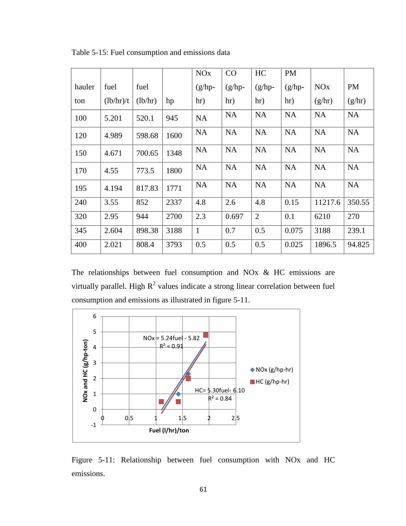
61

Table 5-15: Fuel consumption and emissions data

hauler

ton

fuel

(lb/hr)/t

fuel

(lb/hr) hp

NOx

(g/hp-

hr)

CO

(g/hp-

hr)

HC

(g/hp-

hr)

PM

(g/hp-

hr)

NOx

(g/hr)

PM

(g/hr)

100 5.201 520.1 945 NA NA NA NA NA NA

120 4.989 598.68 1600 NA NA NA NA NA NA

150 4.671 700.65 1348 NA NA NA NA NA NA

170 4.55 773.5 1800 NA NA NA NA NA NA

195 4.194 817.83 1771 NA NA NA NA NA NA

240 3.55 852 2337 4.8 2.6 4.8 0.15 11217.6 350.55

320 2.95 944 2700 2.3 0.697 2 0.1 6210 270

345 2.604 898.38 3188 1 0.7 0.5 0.075 3188 239.1

400 2.021 808.4 3793 0.5 0.5 0.5 0.025 1896.5 94.825

The relationships between fuel consumption and NOx & HC emissions are

virtually parallel. High R2 values indicate a strong linear correlation between fuel

consumption and emissions as illustrated in figure 5-11.

Figure 5-11: Relationship between fuel consumption with NOx and HC

emissions.

NOx = 5.24fuel - 5.82 R² = 0.91

HC= 5.30fuel- 6.10 R² = 0.84

-1

0

1

2

3

4

5

6

0 0.5 1 1.5 2 2.5

NO

x an

d H

C (

g/h

p-t

on

)

Fuel (l/hr)/ton

NOx (g/hp-hr)

HC (g/hp-hr)

62

Figure 5-12: Relationship between NOx and PM

Relationship between NOx emissions and fuel consumption is logarithmic with R2

= 0.93

Figure 5-13: Relationship between NOx emissions and fuel consumption

Some research has been conducted specifically to determine diesel emissions in

field operations. One report was generated by Golders Associates in the

Athabasca oil sands region assessing emissions for mobile equipment (Singh,

Rawling, & Unrau, 2008). The approach took into consideration equipment size,

actual operating conditions and operating modes. An emission model known as

GAME (Golder Associates Mining Emissions) was developed out of this work.

PM (g/hr) = 131.11ln(NOx (g/hr)) - 865.13 R² = 0.91

0

100

200

300

400

0 2000 4000 6000 8000 10000 12000

PM

(g/

hr)

NOx (g/hr)

fuel(l/hr)/ton= 61.31ln(NOx (g/hr) - 14.75 R² = 0.93

400

440

480

520

560

0 1000 2000 3000 4000 5000 6000 7000

Fue

l(l/

hr)

NOx(g/hr)

63

The 750 horsepower engine used was assumed to be used for an 80 ton capacity

truck. From the data obtained, the relationships in figure 5-14 were established;

Table 5-16: NOx and CO emissions (After Rawlings and Unrau, 2008 )

time

(hrs)

Grade

(%)

RR %

estimate TR%

NOx

(g) CO (g)

NOx

g/hr

CO

g/hr

0.2 0 12.6 12.6 97.68 24.64

0.08 0 12.6 12.6 102.34 62.00 1279.25 775.00

0.07 3 11.4 14.4 113.01 65.92 1614.43 941.71

0.32 0 6.5 6.5 279.10 169.10 872.19 528.44

0.05 5 8.8 13.8 103.91 61.48 2078.20 1229.60

0.1 0 4.5 4.5 40.18 24.56 401.80 245.60

0.07 0 9.5 9.5 32.75 8.06

0.2 0 9.5 9.5 194.35 101.52

Relationships between NOx and CO emissions to total (grade + rolling) resistance

were obtained with R2 values of 0.87, where the relationships were suggested to

be exponential.

64

Figure 5-14: Relationship between NOx and CO emission and total resistance

The effect of size and total resistance to fuel consumption and

emissions

From the NOx and CO relationships in figure 5-14 and the relationships obtained

in figures 5-7, 5-11, 5-12 and 5-13, the comparison between 3 trucks sizes with

capacities of 150 ton, 240 ton and 400 ton (assumed to be CAT785C, CAT793F

and CAT797F) on fuel consumption and diesel emissions were made. The aim

was to determine how fuel consumption and emissions vary with truck size

including the impact of increasing rolling and grade resistance on each.

The fuel consumption and total resistance relationship was deduced from the

relationships between fuel consumption and NOx emissions in figure 5-13 and

relationship between NOx emissions and total resistance in figure 5-14.

The increase in total resistance increases fuel consumption per ton of hauler

capacity. The effect was higher on smaller trucks compared to larger trucks.

Figure 5-15 shows the increase in fuel consumption was 0.09(l/hr)/ton for

NOx(g/hr) = 276.56e0.13TR% R² = 0.87

CO(g/hr) = 171.88e0.13TR% R² = 0.87

0

500

1000

1500

2000

2500

0 2 4 6 8 10 12 14 16

Emis

sio

ns

NO

x an

d C

O (

g/h

r)

TR% (GR+RR)

NOx g/hr

CO g/hr

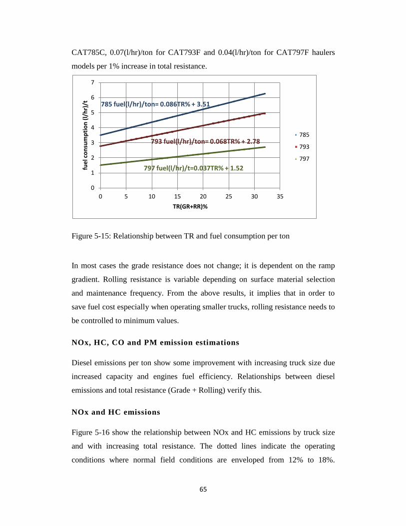
65

CAT785C, 0.07(l/hr)/ton for CAT793F and 0.04(l/hr)/ton for CAT797F haulers

models per 1% increase in total resistance.

Figure 5-15: Relationship between TR and fuel consumption per ton

In most cases the grade resistance does not change; it is dependent on the ramp

gradient. Rolling resistance is variable depending on surface material selection

and maintenance frequency. From the above results, it implies that in order to

save fuel cost especially when operating smaller trucks, rolling resistance needs to

be controlled to minimum values.

NOx, HC, CO and PM emission estimations

Diesel emissions per ton show some improvement with increasing truck size due

increased capacity and engines fuel efficiency. Relationships between diesel

emissions and total resistance (Grade + Rolling) verify this.

NOx and HC emissions

Figure 5-16 show the relationship between NOx and HC emissions by truck size

and with increasing total resistance. The dotted lines indicate the operating

conditions where normal field conditions are enveloped from 12% to 18%.

785 fuel(l/hr)/ton= 0.086TR% + 3.51

793 fuel(l/hr)/ton= 0.068TR% + 2.78

797 fuel(l/hr)/t=0.037TR% + 1.52

0

1

2

3

4

5

6

7

0 5 10 15 20 25 30 35

fue

l co

nsu

mp

tio

n (

l/h

r)/t

TR(GR+RR)%

785

793

797

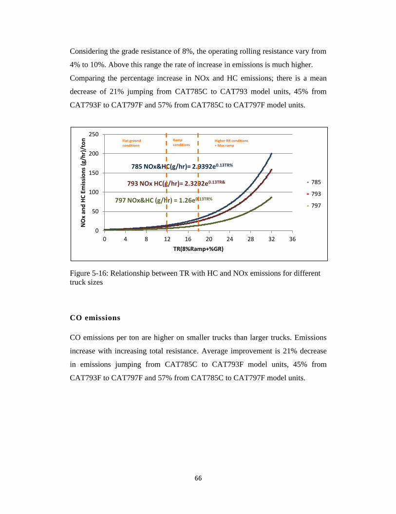
66

Considering the grade resistance of 8%, the operating rolling resistance vary from

4% to 10%. Above this range the rate of increase in emissions is much higher.

Comparing the percentage increase in NOx and HC emissions; there is a mean

decrease of 21% jumping from CAT785C to CAT793 model units, 45% from

CAT793F to CAT797F and 57% from CAT785C to CAT797F model units.

Figure 5-16: Relationship between TR with HC and NOx emissions for different

truck sizes

CO emissions

CO emissions per ton are higher on smaller trucks than larger trucks. Emissions

increase with increasing total resistance. Average improvement is 21% decrease

in emissions jumping from CAT785C to CAT793F model units, 45% from

CAT793F to CAT797F and 57% from CAT785C to CAT797F model units.

785 NOx&HC(g/hr)= 2.9392e0.13TR%

793 NOx HC(g/hr)= 2.3292e0.13TR&

797 NOx&HC (g/hr) = 1.26e0.13TR%

0

50

100

150

200

250

0 4 8 12 16 20 24 28 32 36

NO

x an

d H

C E

mis

sio

ns

(g/h

r)/t

on

TR(8%Ramp+%GR)

785

793

797

Flat ground conditions

Ramp conditions

Higher RR conditions + Max ramp

67

Figure 5-17: Relationship between TR and CO emissions

PM emissions

The PM emissions and total resistance relationship is similar to other emissions

for the fact that; emissions per ton capacity decrease with increasing truck size

and increase with increasing TR. The relationships are linear. Average percentage

decrease in PM emissions with increasing truck size is 24% from CAT785C to

CAT793F model units, 48% from CAT793F to CAT797F and 58% from

CAT785C to CAT797F model units.

785 CO(g/hr)/ton = 1.8267e0.13TR%

793 CO(g/hr)/ton= 1.4476e0.13TR%

797 CO(g/hr)/ton = 0.7927e0.13TR%

0

20

40

60

80

100

120

0 4 8 12 16 20 24 28 32 36

CO

(g/h

r)/t

on

TR(8%Ramp+%RR)

785

793

797

Flat ground conditions

Ramp conditions

Higher RR conditions +Max Ramp

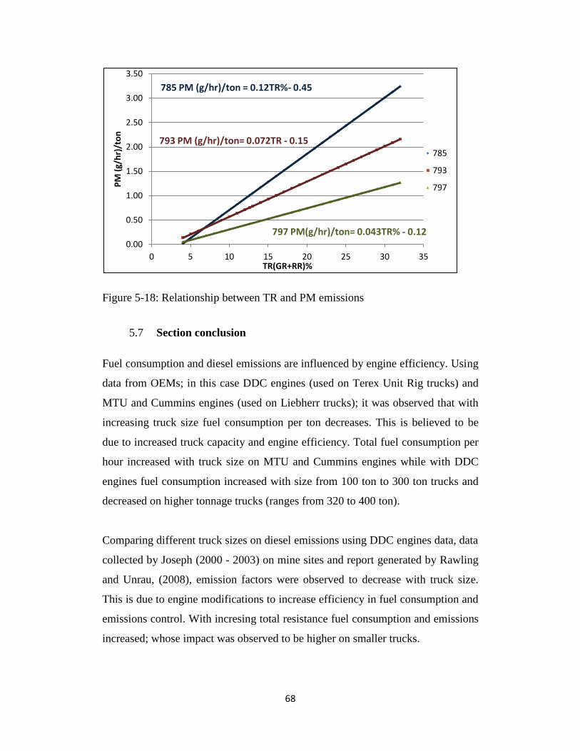
68

Figure 5-18: Relationship between TR and PM emissions

5.7 Section conclusion

Fuel consumption and diesel emissions are influenced by engine efficiency. Using

data from OEMs; in this case DDC engines (used on Terex Unit Rig trucks) and

MTU and Cummins engines (used on Liebherr trucks); it was observed that with

increasing truck size fuel consumption per ton decreases. This is believed to be

due to increased truck capacity and engine efficiency. Total fuel consumption per

hour increased with truck size on MTU and Cummins engines while with DDC

engines fuel consumption increased with size from 100 ton to 300 ton trucks and

decreased on higher tonnage trucks (ranges from 320 to 400 ton).

Comparing different truck sizes on diesel emissions using DDC engines data, data

collected by Joseph (2000 - 2003) on mine sites and report generated by Rawling

and Unrau, (2008), emission factors were observed to decrease with truck size.

This is due to engine modifications to increase efficiency in fuel consumption and

emissions control. With incresing total resistance fuel consumption and emissions

increased; whose impact was observed to be higher on smaller trucks.

785 PM (g/hr)/ton = 0.12TR%- 0.45

793 PM (g/hr)/ton= 0.072TR - 0.15

797 PM(g/hr)/ton= 0.043TR% - 0.12 0.00

0.50

1.00

1.50

2.00

2.50

3.00

3.50

0 5 10 15 20 25 30 35

PM

(g/

hr)

/to

n

TR(GR+RR)%

785

793

797

69

6 DISCUSSION

Summary

From the above analysis it was apparent that with increasing hauler size,

Width of haul roads and size of pit increases which necessitates more

waste stripping.

Haul road layer thickness increase with truck size where with wider roads

required for larger trucks, the amount of construction material, time and

construction resources increase.

The rate of increase of rolling resistance is the same regardless the size of

the hauler when crushed rock is used as wearing course material.

On fuel consumption and emission, great savings are evident when using

larger haulers.

Giving the dollar value to each of the component in additional to capital cost for

each truck, the general idea of hauler size cost is presented insisting on its impact

in mine planning.

Hauler costs estimations

The costs are estimates from field experience Joseph (2000-2012) has on different

mine sites. Constant values were used not taking into considerations interest rates

and costs variations with time.

Trucks cost

Truck cost is an estimate of purchasing cost per unit. It is assumed that the tires

are changed once a year and the estimation is done for 10 years which is the life

of trucks.

Truck 785 793 797

Capital cost $2.25M $3.8M 6M

Tire cost $50K/tire $80K/tire $130K/tire

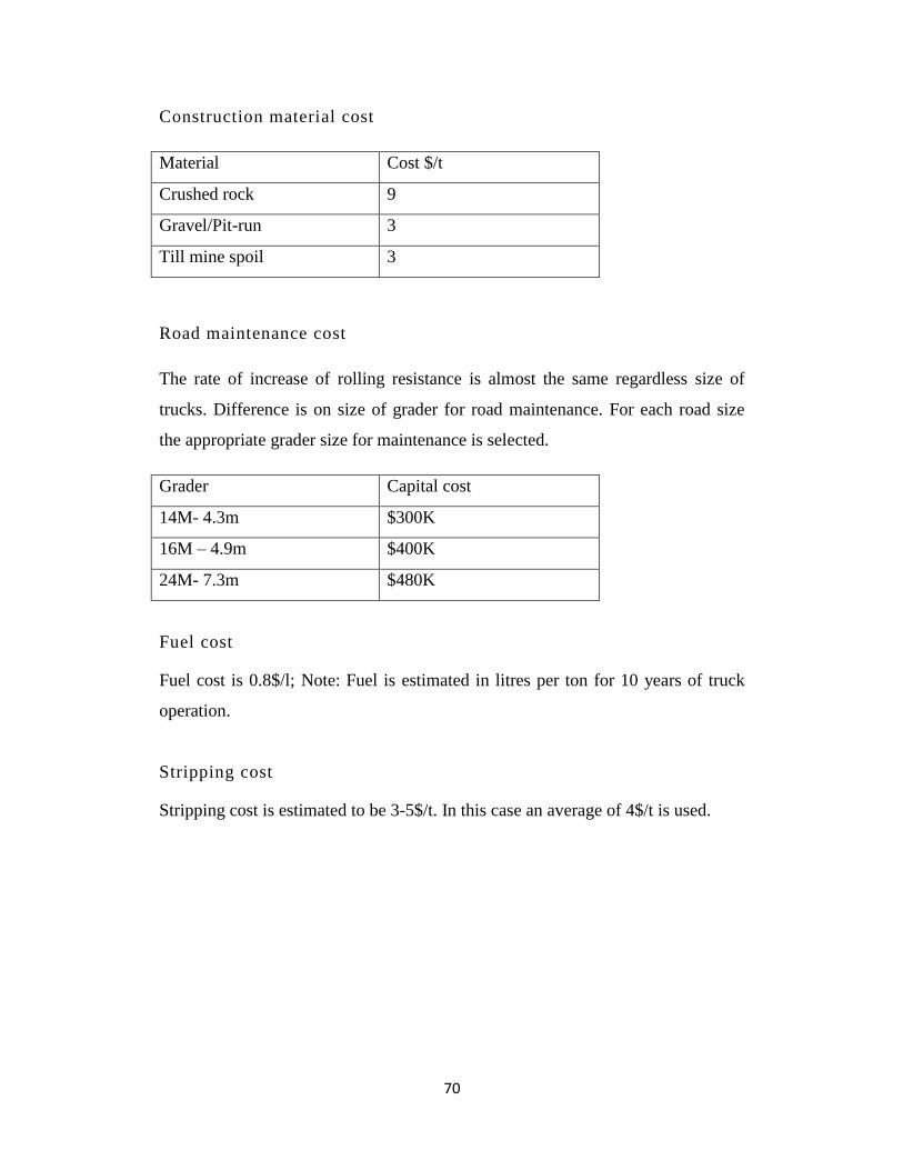
70

Construction material cost

Material Cost $/t

Crushed rock 9

Gravel/Pit-run 3

Till mine spoil 3

Road maintenance cost

The rate of increase of rolling resistance is almost the same regardless size of

trucks. Difference is on size of grader for road maintenance. For each road size

the appropriate grader size for maintenance is selected.

Grader Capital cost

14M- 4.3m $300K

16M – 4.9m $400K

24M- 7.3m $480K

Fuel cost

Fuel cost is 0.8$/l; Note: Fuel is estimated in litres per ton for 10 years of truck

operation.

Stripping cost

Stripping cost is estimated to be 3-5$/t. In this case an average of 4$/t is used.

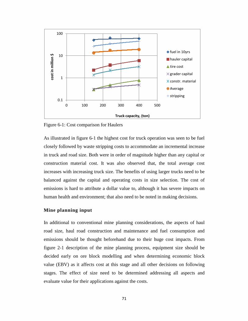
71

Figure 6-1: Cost comparison for Haulers

As illustrated in figure 6-1 the highest cost for truck operation was seen to be fuel

closely followed by waste stripping costs to accommodate an incremental increase

in truck and road size. Both were in order of magnitude higher than any capital or

construction material cost. It was also observed that, the total average cost

increases with increasing truck size. The benefits of using larger trucks need to be

balanced against the capital and operating costs in size selection. The cost of

emissions is hard to attribute a dollar value to, although it has severe impacts on

human health and environment; that also need to be noted in making decisions.

Mine planning input

In additional to conventional mine planning considerations, the aspects of haul

road size, haul road construction and maintenance and fuel consumption and

emissions should be thought beforehand due to their huge cost impacts. From

figure 2-1 description of the mine planning process, equipment size should be

decided early on ore block modelling and when determining economic block

value (EBV) as it affects cost at this stage and all other decisions on following

stages. The effect of size need to be determined addressing all aspects and

evaluate value for their applications against the costs.

0.1

1

10

100

0 100 200 300 400 500

cost

in m

illio

n $

Truck capacity, (ton)

fuel in 10yrs

hauler capital

tire cost

grader capital

constr. material

Average

stripping

72

7 CONCLUSION AND RECOMMENDATIONS

7.1 Summary of findings

The notion 'bigger is better' has been a focus for over a decade since 2000, and

mine operators are cognisant of opportunities to phase out smaller trucks and

employ bigger units with new and expanded projects. There are advantages

noticed with higher capacity equipment but there are challenges as well.

When making decision on equipment size there are many factors to consider. This

research was focused on road size, road construction requirements, rolling

resistance, fuel consumption and emissions. Overall results show an increase in

costs with increasing equipment size which should not be surprising. The increase

in cost was 33% from CAT 785 to CAT 793, 9% from CAT 793 to CAT 797 and

46% from CAT 785 to CAT 797.

Larger trucks require wider roads and therefore more stripping is required thus

impacting mining cost. Pit slopes are affected by the size of road; having wider

roads, pit slopes decrease which increase pit size.

Haul road construction is dependent on size and weight of trucks among other

factors. With larger trucks, thicker pavements and wider roads are required and

therefore more construction material, time and construction resources. Using

crushed rock as wearing course material, rolling resistance increase rates are the

same regardless of truck size. The difference in maintenance cost is therefore

dependent on grader size as a function of road size.

Regarding fuel consumption and diesel emissions per ton, there are huge

improvements observed in larger trucks. This is due to increased capacity,

reduced fuel consumption and improved engine efficiency as claimed by OEMs,

endorsing the notion “bigger is better”. Huge savings are evident on fuel

consumption when using larger trucks. On diesel emissions, the costs associated

73

with human health and environmental effects, although they cannot be given a

specific dollar value, have huge detrimental effects which are hard to undo and

therefore should be given enough weight in decision making.

7.2 Contribution to engineering research and mining industry

This study opens new thinking on equipment size implications on mine planning

by incorporating some aspects which are left out of the mine planning process and

have high cost impacts. The notion 'bigger is better' which is the current focus in

the industry is challenged with the results obtained which suggest that bigger is

not necessarily better as observed with respect to road size and road pavement

construction requirements. These and other challenges discussed in section 2.5.2

bring new opinion to equipment size. On the other side, this does not favour

smaller over bigger trucks due to higher operating costs witnessed in fuel

consumption and emissions. Balancing equipment size selection and qualitative

aspects with size of operation need to be considered in making a decision.

The results obtained can be used in a customized fashion depending on location

and stage of operation, whether it is the initial stages of mine planning or when

making the decision to employ a different equipment size. When this information

is improved to include different stages of mine planning and various operating

conditions can provide useful data for future modelling using software such as

'Symphony'.

7.3 Recommended future work

The results obtained in this study give a general picture on the costs associated

with hauler scale. The information used in this study is mainly from OEM and

pre-collected data sources. For this information to be useful the following is

recommended.

1. Applied loads used on road layer thickness calculations are estimated from

static loads. Load variations due to dynamic conditions which are caused

74

by truck motion are not accounted. Field data collection can help

determine the variations for different truck sizes to be used in layer

thickness calculations for more realistic results employing dynamic truck

data. These variations might increase loading up to an additional 50%

which is high to be neglected.

An interesting subject in road construction can also be balancing increase

in haul road grade, which means less stripping ratio and less haul road

construction material against operating costs and safety.

2. Rolling resistance estimation done in this study provides cumulative

efforts of load application for the surface course material used (crushed

stone). This might not be the case for shorter time periods and different

materials with the same loads applied. More tests are suggested on rolling

resistance estimation to determine the effects of individual loads and

different wearing course material types on haul road construction.

3. The data used for fuel consumption are fewer and mainly from equipment

manufacturers. However for the same truck capacity fuel consumption

might differ from one engine manufacturer to another. It is also believed

from a field experience that bigger trucks consume more fuel than stated

by OEMs. I would suggest as an extension of this study to determine the

actual values in field operations for different truck sizes and models.

4. Emissions can be more reflective of actual practice if measured from the

actual operation than estimated. There are more factors influencing

emissions which are not covered in this study such as age of the equipment

and others. More study on other factors affecting emissions need to be

done.

75

8 REFERENCES

1) Baumann, S. (1999). Review your assets to determine maximum fleet size. A

case study history of Glamis Gold's Operation, www.glamis.com.

2) Berkhimer, E. (2011). Selection and sizing of excavating, loading and

hauling equipment. In P. Darling, SME Mining engineering Handbook, 3rd

Ed (p. Chapter 10.4).

3) Boucom, J. (2011). The evolution pf Trucks is changing interactions and

pruductivity at minesites. Allen & Holt consulting company monthly articles,

110.

4) Boucom, J. W. (2008). Optimizing powered investment in sufrace coal

application. available at www.minexpo.com/Presenations/boucom.pdf.

5) Bozorgebrahimi, E. (2004). Evaluation of the haulage truck size effects on

open pit mining. PhD Thesis. University of British Columbia.

6) Caterpillar. (1998). Caterpillar Performance handbook. Edition 29. Peoria

IL, USA: Caterpillar Inc.

7) Caterpillar. (2008). Ultra class trucks, presentation to Univeristy of Alberta

MINe 420/620 class by Faher, D. and O'Neill, B. Edmonton, Albrta.

8) Caterpillar. (2012). Caterpillar performance handbook Ed 49. Peoria,

Illinois USA: Caterpillar Inc.

9) Dietz, M. (2000). Introduction. In W. A. Hustrulid, Slope stability for

surface mine (p. xv).

10) EPA. (2005). Emission reduction incentives for off-road diesel equipment

used in th port and construction sectors.

11) Filas, F. J. (2002). Excavation, loading and material transport. In R. L.

Lowrie, SME Mining Reference Handbook (pp. 215-241). Littleton, CO,

USA: Society of Mining, Metallurgy and Exploration Engineering.

76

12) Hays, M. R. (1990). Trucks. In B. A. Kennedy, Surface Mining Handbook

(pp. 672-691). Littleton, CO, USA: Society of Mining, Metallurgy and

Exploration Engineering.

13) Jaques, A. (1992). Canada's greenhouse gas emissions; Estimates for 1990.

Environmental Canada report EPS 5/AP/4.

14) Joseph, T. G. (2002). OsEIP: The oil sand - equipment interaction program.

CIM Bulletin, 95 (1064), (pp. 58-61).

15) Joseph, T. G. (2003). Large mobile mining equipment operating in soft

groud. Proceedings of International Mining Congress and Exhibition of

Turkey (IMCET), (pp. 143-147,588). Antalya, Turkey.

16) Kaufman , W. W., & Ault, J. C. (1977). The design of surface mine haul

roads. In A manual information circular 8758. Washington DC : US Bureau

of mines.

17) Kecojevic, V., & Komljenovic, D. (2010). Haul truck fuel consumption and

CO2 Emission under various engine loads conditions. In SME Mining

Engineering Journal, Vol 62 No 12 (pp. 47-52). Society of Mining,

Metallurgy and and Exploration.

18) Knapton, J. (1988). The structural design of heavy duty pavement for ports

and other industries. London, England: British Port Federation.

19) Krause, G. (2001). Large Heavy Hauler. Is bigger better? SMART Seminar

6. Edmonton, Alberta

20) Lashgari, A., Johnson, C., Kecojevic, V., Lusk , B., & Hoffman, J. M.

(2013). NOx emissions of equipment and blasting agents in surface mining.

In SME Mining Engineering Journal. Vol 65 (pp. 34-41). Society of Mining,

Metallurgy and Exlporation Engineering.

21) Leslie, D. R. (2000). Diesel emissions evaluation for the surface mining

industry. SMART conference.

77

22) Lizzote, Y. (1988). Economical and technical relations between open pit

design and equipment selection. In J. Singhal, Mine Planning and Equipment

Selection.

23) Morgan, J. R., Tucker, J. S., and McInnes, D. B. (1994). A mechanistic

design approach for unsealed mine haul roads. In Pavement design and

perfomance in road construction 1412 (pp. 68-81).

24) Nasab, H. A. (2011). Open pit long term planning stages. MinE 631 notes.

25) Noble, A. C. (1992). Ore reserve/resource estimation. In H. L. Hartman,

SME Mining Engineering Handbook 2nd Ed (pp. 334-359). Littleton,

Colorado.

26) P. Gilewicz: ‘Large truck report’, World Mining EquipmentMagazine,

July/Aug, 2001, <www.parkerbaymining.com>.

27) Perloff, W. H. (1975). Pressure distribution and settlement. In Foundation

Engineering Handbook (pp. 14-19).

28) Roman, P. A., and Daneshmand , L. (2000). Economics of scale in mining -

assesing upper bounds with simulation. The Engineering Economist, 45:4,

326-338.

29) Runge, I. (1998). Mining economics and strategy. Littleton, CO, USA:

Society of Mining, Metallurgy and Exploration Engineering.

30) Sharma, A. (2009). Scale tire - oil sand interaction, Master Thesis.

University of Alberta.

31) Singh, R. B., Rawling, M., and Unrau, G. (2008). Assesment of mobile

emissions in the Athabasca oil sand region - high resolution non-road

emission factor model. ACE conference paper 461.

32) Singhal , R. K., Fytas, K., and Collins, J. L. (1986). Optimization of loading

and hauling equipment productivity in surface mining. St. Louis: Society of

Mining, Metallurgy and Exploration Engineering.

78

33) Tannant , D., & Regensburg, B. (2001). Guidelines for mine haul road

design. Edmonton, Alberta: School of Mining and Petroleum Engineering,

University of Alberta.

34) Thompson , R. J., & Visser, A. T. (1997a). A mechanistic design procedure

for surface mine haul roads. In Int. Journal of Surface, Reclamation and

Environment, 11 (pp. 121-128).

35) Thompson, R. J. (2010). Mine haul road design and management best

practice for safe and cost effective effecient truck haulage. Society of

Mining, Metallurgy and Exploration Annual Meeting, (pp. 1-10). Phoenix,

Arizona.

36) Thompson, R. J. (2011a). Mine haul road design, constructionand

maintenance management.

37) Thompson, R. J. (2011b). Building better haul roads. Engineering and

Mining Journal, 49-53.

38) Thompson, R. J. (2011c). Design, construction and maintenance of haul

roads. In D. P, SME Mining Engineering Handbook, 3rd Ed (Chapter 10.4).

39) Thompson, R. J., & Visser , A. T. (2000). Selection parameters for mine haul

road wearing cousre material. International Journal of Surface Mining,

Reclamation and Environment, 1-17.

40) Thompson, R. J., & Visser, A. T. (1997b). An introduction to the integrated

design of surface mine haul roads. International Journal of Surface mining,

Reclamation and Environment. 11:3.

41) Thompson, R. J., & Visser, A. T. (2006). The impact of rolling resistance on

fuel, speed and costs. Continuous improvement case study.

42) Whittle, D. (2011). Open pit mine planning and design. In P. Darling, SME

Mining Engineeering Handbook, 3rd Ed ( Chapter 10.2).

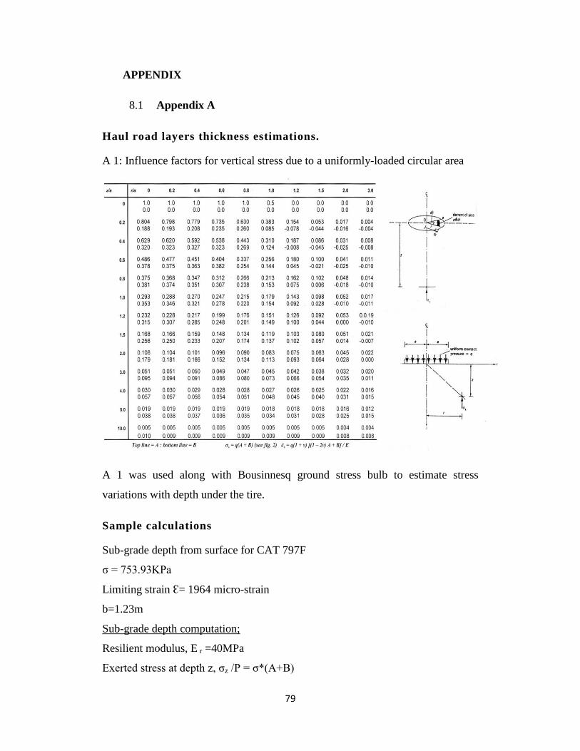
79

APPENDIX

8.1 Appendix A

Haul road layers thickness estimations.

A 1: Influence factors for vertical stress due to a uniformly-loaded circular area

A 1 was used along with Bousinnesq ground stress bulb to estimate stress

variations with depth under the tire.

Sample calculations

Sub-grade depth from surface for CAT 797F

σ = 753.93KPa

Limiting strain Ԑ= 1964 micro-strain

b=1.23m

Sub-grade depth computation;

Resilient modulus, E r =40MPa

Exerted stress at depth z, σz /P = σ*(A+B)

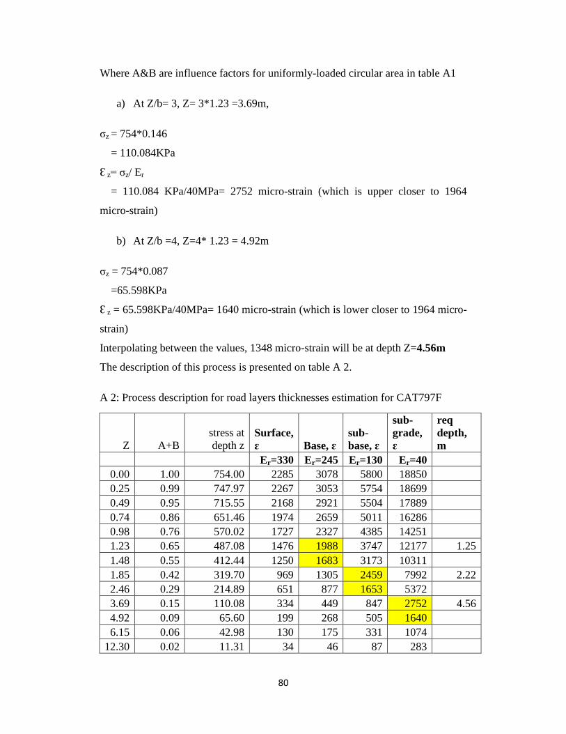
80

Where A&B are influence factors for uniformly-loaded circular area in table A1

a) At Z/b= 3, Z= 3*1.23 =3.69m,

σz = 754*0.146

= 110.084KPa

Ԑ z= σz/ Er

= 110.084 KPa/40MPa= 2752 micro-strain (which is upper closer to 1964

micro-strain)

b) At Z/b =4, Z=4* 1.23 = 4.92m

σz = 754*0.087

=65.598KPa

Ԑ z = 65.598KPa/40MPa= 1640 micro-strain (which is lower closer to 1964 micro-

strain)

Interpolating between the values, 1348 micro-strain will be at depth Z=4.56m

The description of this process is presented on table A 2.

A 2: Process description for road layers thicknesses estimation for CAT797F

Z A+B

stress at

depth z Surface,

ɛ Base, ɛ

sub-

base, ɛ

sub-

grade,

ɛ

req

depth,

m

Er=330 Er=245 Er=130 Er=40

0.00 1.00 754.00 2285 3078 5800 18850

0.25 0.99 747.97 2267 3053 5754 18699

0.49 0.95 715.55 2168 2921 5504 17889

0.74 0.86 651.46 1974 2659 5011 16286

0.98 0.76 570.02 1727 2327 4385 14251

1.23 0.65 487.08 1476 1988 3747 12177 1.25

1.48 0.55 412.44 1250 1683 3173 10311

1.85 0.42 319.70 969 1305 2459 7992 2.22

2.46 0.29 214.89 651 877 1653 5372

3.69 0.15 110.08 334 449 847 2752 4.56

4.92 0.09 65.60 199 268 505 1640

6.15 0.06 42.98 130 175 331 1074

12.30 0.02 11.31 34 46 87 283

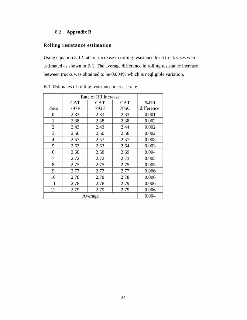
81

8.2 Appendix B

Rolling resistance estimation

Using equation 3-12 rate of increase in rolling resistance for 3 truck sizes were

estimated as shown in B 1. The average difference in rolling resistance increase

between trucks was obtained to be 0.004% which is negligible variation.

B 1: Estimates of rolling resistance increase rate

Rate of RR increase

days

CAT

797F

CAT

793F

CAT

785C

%RR

difference

0 2.33 2.33 2.33 0.001

1 2.38 2.38 2.38 0.002

2 2.43 2.43 2.44 0.002

3 2.50 2.50 2.50 0.002

4 2.57 2.57 2.57 0.003

5 2.63 2.63 2.64 0.003

6 2.68 2.68 2.69 0.004

7 2.72 2.72 2.73 0.005

8 2.75 2.75 2.75 0.005

9 2.77 2.77 2.77 0.006

10 2.78 2.78 2.78 0.006

11 2.78 2.78 2.79 0.006

12 2.79 2.79 2.79 0.006

Average 0.004

Impact of hauler scale in mine planning - ERA

Documents

Transcript of Impact of hauler scale in mine planning - ERA