MINT-709

Analysis of Network Protocols in an NS-3 Simulated Environment

Professor: Dr. Mike McGregor

Student Name: Aminul Haque Siddiqui

2

Table of Contents Introduction Project Scope Deliverables Preparation for the Test and Simulation Pre-requisite to install ns-3 in Ubuntu Pre-requisite to install ns-3 in Fedora Download and install ns-3 from the nsnam.org site Chapter 1: Simple Ethernet network: (Examples of Ethernet, ARP) 1.1 Introduction 1.2 Configuration & Experiment 1.3 Explanation 1.4 References Chapter 2: Network Layer Protocols 2.1 Introduction 2.2 Configuration & Experiment 2.3 Explanation 2.4 References Chapter 3: Examining a ping and traceroute: 3.1 Introduction 3.2 Configuration & Experiment: PING 3.3 Explanation: PING 3.4: Configuration & Experiment: TRACEROUTE 3.5 Explanation: TRACEROUTE Chapter 4: Transport Layer Protocol - UDP 4.1 Introduction 4.2 Configuration & Experiment 4.3 Explanation 4.3 References Chapter 5: Transport Layer Protocol - TCP 5.1 Introduction 5.2 Configuration & Experiment 5.3 Explanation 5.3 Explanation Conclusion

3

Introduction Wireshark (formerly known as Ethereal) is an open-source protocol analyzer used to analyze network protocols and troubleshoot network problems. Wireshark has a user-friendly GUI interface and can be run on many different platforms. ns-3 is a discrete-event network simulation tool used primarily in education and research. ns-3 is free software licensed under the link "http://www.gnu.org/copyleft/gpl.html" GNU GPLv2 license, and is publicly available for research, development, and use. Project Scope In this project, several network protocols will be examined in environments simulated using ns-3. Wireshark will be used as a protocol analyzer to dissect the traces gathered. Several test networks will be built up in ns-3 and traces gathered during their operation. The protocols of interest are Ethernet, IP, ARP, DHCP, ping, traceroute, TCP, UDP, HTTP, FTP, POP, SMTP, OSPF and BGP. For each protocol, one or more packet traces will be collected and analyzed. A variety of topologies will be built as the protocols need to be seen working in realistic settings. For example, a simple point-to-point connection with a serial link would suffice for Ethernet while two or three autonomous systems would be required for a reasonable BGP simulation. Deliverables The project report will include:

- one chapter for each of the protocols noted above - each chapter will contain a network diagram and a description of the addressing (L2 and L3) and routing configuration

- screen shots of the key parts of each trace as displayed in Wireshark - a text narrative describing in detail the contents of the traces captured for that

protocol The project will also include a CD containing the captured traces in tcpdump format.

4

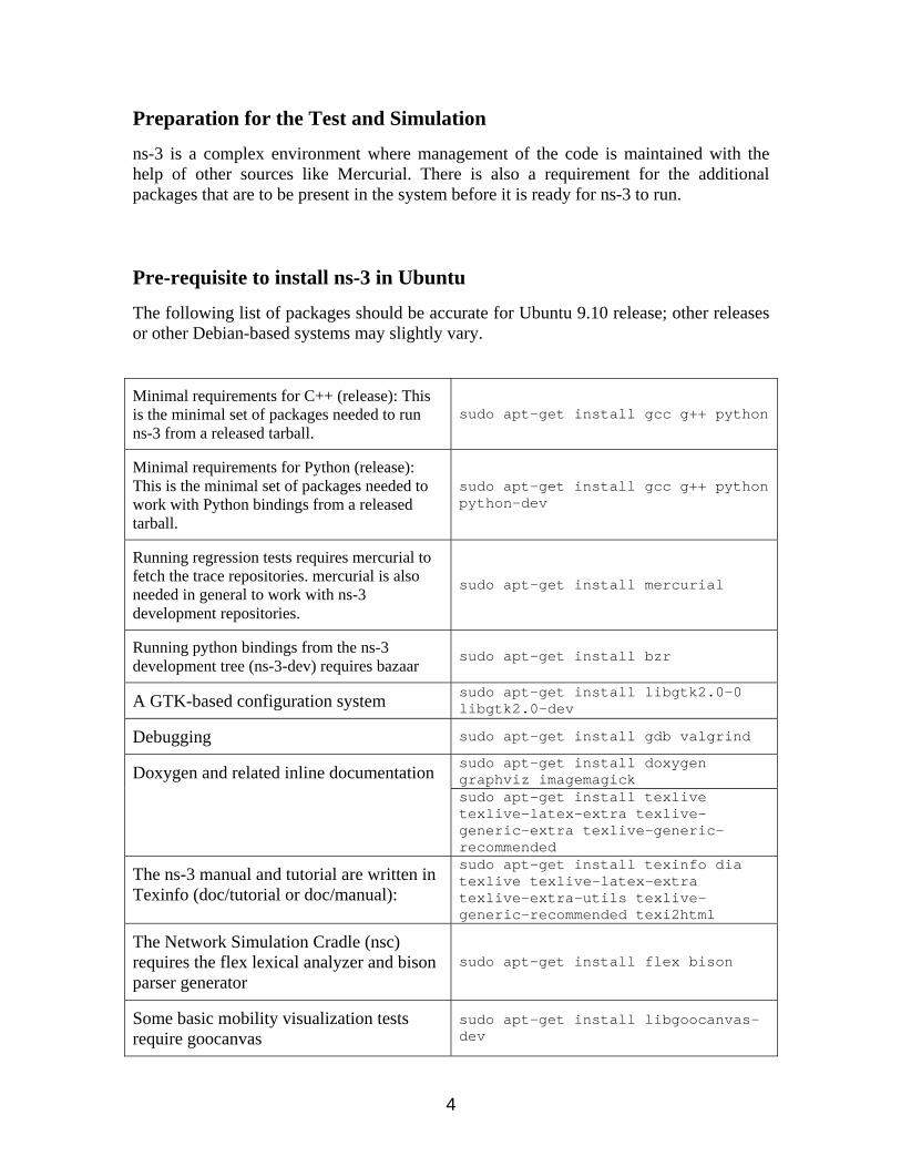
Preparation for the Test and Simulation

ns-3 is a complex environment where management of the code is maintained with the help of other sources like Mercurial. There is also a requirement for the additional packages that are to be present in the system before it is ready for ns-3 to run. Pre-requisite to install ns-3 in Ubuntu

The following list of packages should be accurate for Ubuntu 9.10 release; other releases or other Debian-based systems may slightly vary.

Minimal requirements for C++ (release): This is the minimal set of packages needed to run ns-3 from a released tarball.

sudo apt-get install gcc g++ python

Minimal requirements for Python (release): This is the minimal set of packages needed to work with Python bindings from a released tarball.

sudo apt-get install gcc g++ python python-dev

Running regression tests requires mercurial to fetch the trace repositories. mercurial is also needed in general to work with ns-3 development repositories.

sudo apt-get install mercurial

Running python bindings from the ns-3 development tree (ns-3-dev) requires bazaar

sudo apt-get install bzr

A GTK-based configuration system sudo apt-get install libgtk2.0-0 libgtk2.0-dev

Debugging sudo apt-get install gdb valgrind

sudo apt-get install doxygen graphviz imagemagick Doxygen and related inline documentation sudo apt-get install texlive texlive-latex-extra texlive-generic-extra texlive-generic-recommended

The ns-3 manual and tutorial are written in Texinfo (doc/tutorial or doc/manual):

sudo apt-get install texinfo dia texlive texlive-latex-extra texlive-extra-utils texlive-generic-recommended texi2html

The Network Simulation Cradle (nsc) requires the flex lexical analyzer and bison parser generator

sudo apt-get install flex bison

Some basic mobility visualization tests require goocanvas

sudo apt-get install libgoocanvas-dev

5

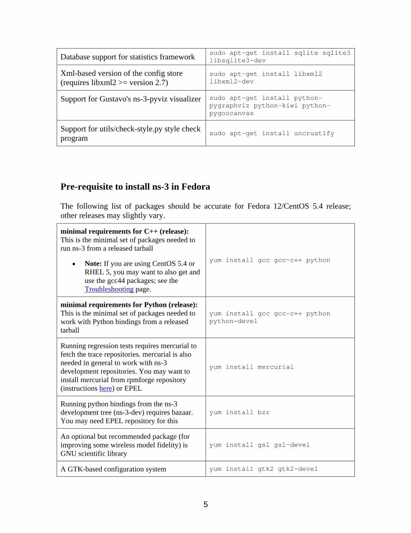
Database support for statistics framework sudo apt-get install sqlite sqlite3 libsqlite3-dev

Xml-based version of the config store (requires libxml2 >= version 2.7)

sudo apt-get install libxml2 libxml2-dev

Support for Gustavo's ns-3-pyviz visualizer sudo apt-get install python-pygraphviz python-kiwi python-pygoocanvas

Support for utils/check-style.py style check program

sudo apt-get install uncrustify

Pre-requisite to install ns-3 in Fedora

The following list of packages should be accurate for Fedora 12/CentOS 5.4 release; other releases may slightly vary.

minimal requirements for C++ (release): This is the minimal set of packages needed to run ns-3 from a released tarball

Note: If you are using CentOS 5.4 or RHEL 5, you may want to also get and use the gcc44 packages; see the Troubleshooting page.

yum install gcc gcc-c++ python

minimal requirements for Python (release): This is the minimal set of packages needed to work with Python bindings from a released tarball

yum install gcc gcc-c++ python python-devel

Running regression tests requires mercurial to fetch the trace repositories. mercurial is also needed in general to work with ns-3 development repositories. You may want to install mercurial from rpmforge repository (instructions here) or EPEL

yum install mercurial

Running python bindings from the ns-3 development tree (ns-3-dev) requires bazaar. You may need EPEL repository for this

yum install bzr

An optional but recommended package (for improving some wireless model fidelity) is GNU scientific library

yum install gsl gsl-devel

A GTK-based configuration system yum install gtk2 gtk2-devel

6

Debugging yum install gdb valgrind yum install doxygen graphviz ImageMagick Doxygen and related inline documentation

yum install texinfo texinfo-tex

The ns-3 manual and tutorial are written in Texinfo (doc/tutorial or doc/manual)

yum install texinfo dia texinfo-tex texi2html

The Network Simulation Cradle (nsc) requires the flex lexical analyzer and bison parser generator

yum install flex bison

To install gcc-3.4 for some Network Simulation Cradle (nsc) stacks

yum install compat-gcc-34

To read pcap packet traces yum install tcpdump

Database support for statistics framework yum install sqlite sqlite-devel

Xml-based version of the config store (requires libxml2 >= version 2.7) yum install libxml2 libxml2-devel

Support for utils/check-style.py style check program

yum install uncrustify

Download and install ns-3 from the nsnam.org site

wget http://www.nsnam.org/releases/ns-allinone-3.9.tar.bz2 tar xjf ns-allinone-3.9.tar.bz2 Building ns-3: Change into the directory where the ns-3 is installed and run the command ./build.py change the directory to the ns-3.8 and build the simulator in debug mode ./waf -d debug configure If the pybindgen is not found, change the name of the default directory to pybindgen (the default directory name that came with ns-3.9 is pybindgen-0.14.1 and waf can’t interpret it correctly) Run the above command again to check whether the location for pybindgen is found or not. In the same way, the nsc directory issue can be fixed. If the build shows that mpic++ is not found, the software can be installed from Ubuntu Software Center.

7

For any missing parameter, use the command to enable it, e.g. ./waf -d debug --enable-sudo –enable-mpi –enable-static configure Once the all missing and not-found parameters are fixed, we can build the simulator by the following command ./waf And this time the simulator will be built in debug mode as set by the command (./waf –d debug configure) above. If we need to build the simulator in optimized mode, we need to tell the simulator first with the following command ./waf –d optimize configure and then ./waf can be used to build the simulator to optimize mode.

8

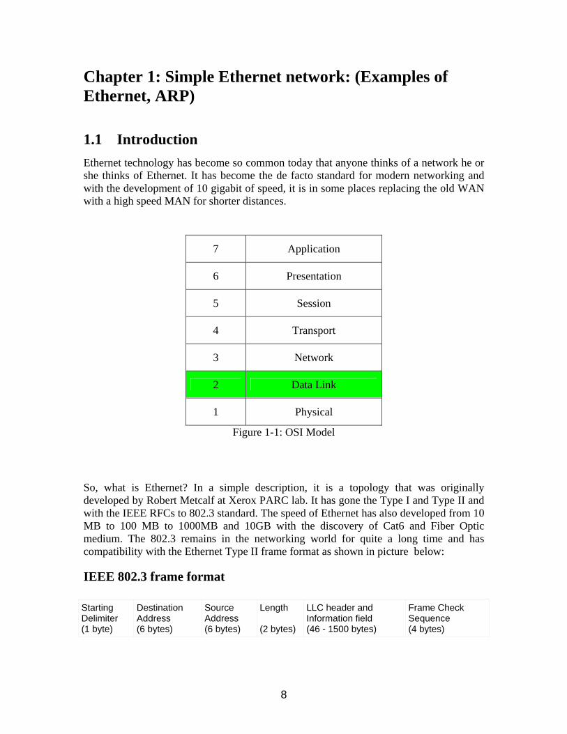
Chapter 1: Simple Ethernet network: (Examples of Ethernet, ARP)

1.1 Introduction

Ethernet technology has become so common today that anyone thinks of a network he or she thinks of Ethernet. It has become the de facto standard for modern networking and with the development of 10 gigabit of speed, it is in some places replacing the old WAN with a high speed MAN for shorter distances.

7 Application

6 Presentation

5 Session

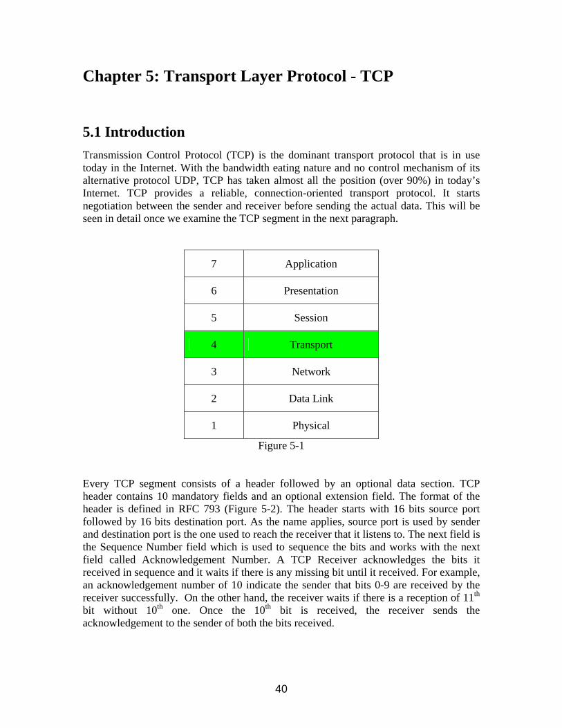
4 Transport

3 Network

2 Data Link

1 Physical

Figure 1-1: OSI Model

So, what is Ethernet? In a simple description, it is a topology that was originally developed by Robert Metcalf at Xerox PARC lab. It has gone the Type I and Type II and with the IEEE RFCs to 802.3 standard. The speed of Ethernet has also developed from 10 MB to 100 MB to 1000MB and 10GB with the discovery of Cat6 and Fiber Optic medium. The 802.3 remains in the networking world for quite a long time and has compatibility with the Ethernet Type II frame format as shown in picture below:

IEEE 802.3 frame format Starting Delimiter (1 byte)

Destination Address (6 bytes)

Source Address (6 bytes)

Length (2 bytes)

LLC header and Information field (46 - 1500 bytes)

Frame Check Sequence (4 bytes)

9

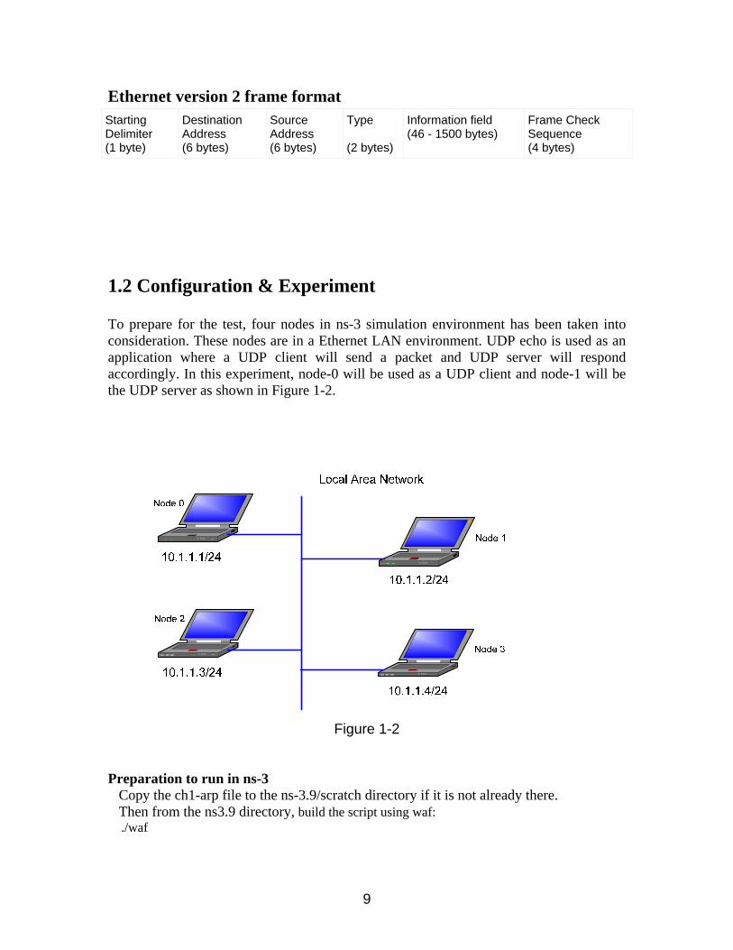
Ethernet version 2 frame format Starting Delimiter (1 byte)

Destination Address (6 bytes)

Source Address (6 bytes)

Type (2 bytes)

Information field (46 - 1500 bytes)

Frame Check Sequence (4 bytes)

1.2 Configuration & Experiment To prepare for the test, four nodes in ns-3 simulation environment has been taken into consideration. These nodes are in a Ethernet LAN environment. UDP echo is used as an application where a UDP client will send a packet and UDP server will respond accordingly. In this experiment, node-0 will be used as a UDP client and node-1 will be the UDP server as shown in Figure 1-2.

Figure 1-2

Preparation to run in ns-3

Copy the ch1-arp file to the ns-3.9/scratch directory if it is not already there. Then from the ns3.9 directory, build the script using waf:

./waf

10

If the build is successful, it will display a message showing the time it takes. Next, it is time to run it Run the executable from the main ns-3.9 directory ./waf –run scratch/ch1-arp it will create the pcap files for each node or as defined in the software to the main directory

1.3 Explanation

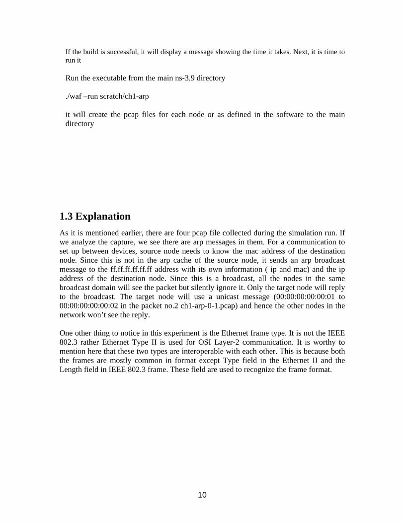
As it is mentioned earlier, there are four pcap file collected during the simulation run. If we analyze the capture, we see there are arp messages in them. For a communication to set up between devices, source node needs to know the mac address of the destination node. Since this is not in the arp cache of the source node, it sends an arp broadcast message to the ff.ff.ff.ff.ff.ff address with its own information ( ip and mac) and the ip address of the destination node. Since this is a broadcast, all the nodes in the same broadcast domain will see the packet but silently ignore it. Only the target node will reply to the broadcast. The target node will use a unicast message (00:00:00:00:00:01 to 00:00:00:00:00:02 in the packet no.2 ch1-arp-0-1.pcap) and hence the other nodes in the network won’t see the reply. One other thing to notice in this experiment is the Ethernet frame type. It is not the IEEE 802.3 rather Ethernet Type II is used for OSI Layer-2 communication. It is worthy to mention here that these two types are interoperable with each other. This is because both the frames are mostly common in format except Type field in the Ethernet II and the Length field in IEEE 802.3 frame. These field are used to recognize the frame format.

11

Screenshot of Capture:

Figure 1-3

1.4 References

http://www.computerhope.com/jargon/e/ethernet.htm http://www.dcs.gla.ac.uk/~lewis/networkpages/m04s03EthernetFrame.htm http://en.wikipedia.org/wiki/Ethernet http://en.wikipedia.org/wiki/MAC_address How to find your MAC address http://standards.ieee.org/regauth/oui/oui.txt Charles Spurgeon's Ethernet (IEEE 802.3) Web Site IANA - Ether Types http://www.nsnam.org http://code.google.com/p/waf http://www.selenic.com/mercurial/ http://en.wikipedia.org/wiki/GNU_toolchain http://www.cygwin.com/ http://cs.baylor.edu/~donahoo/practical/CSockets/ http://www.wireshark.org/

12

http://www.wand.net.nz/pubDetail.php?id=215 Wireshark - Wikipedia Wireshark and Ethereal network protocol analyzer toolkit SampleCaptures - The Wireshark Wiki

13

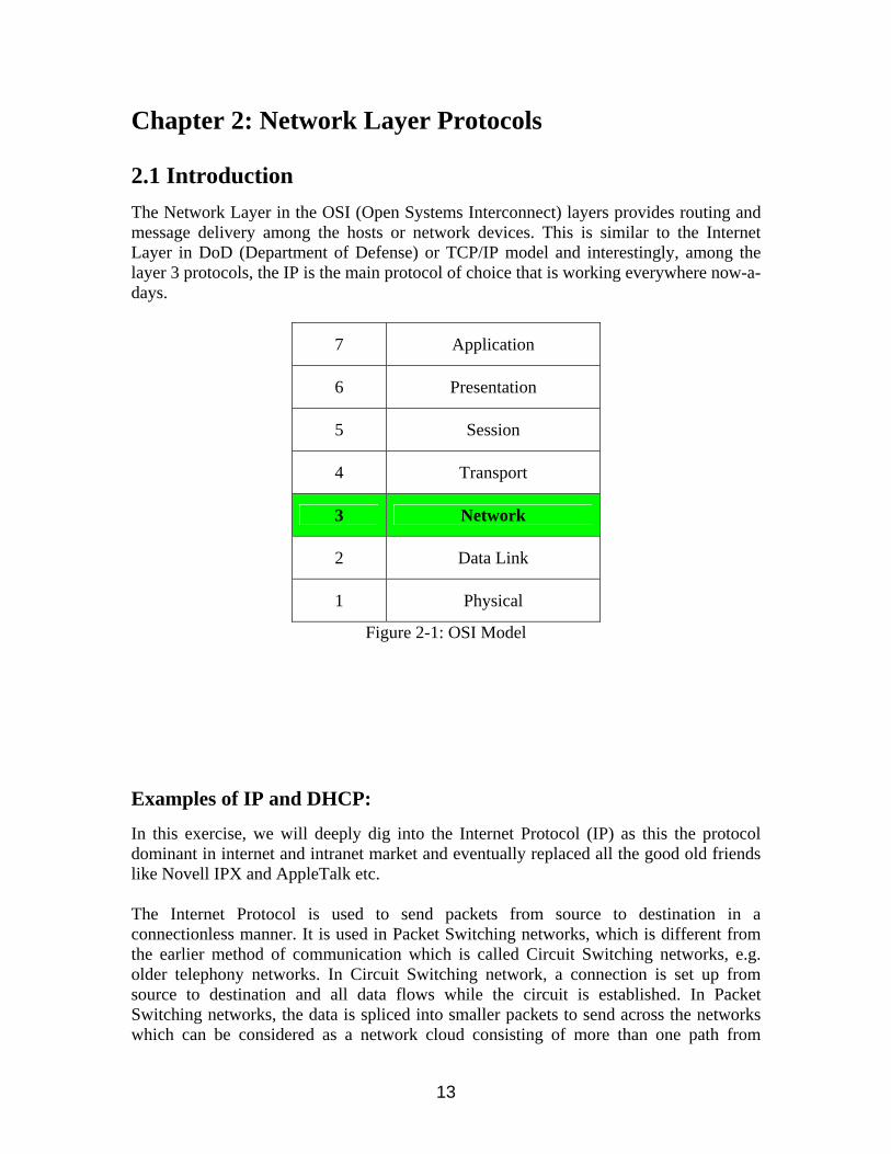
Chapter 2: Network Layer Protocols 2.1 Introduction

The Network Layer in the OSI (Open Systems Interconnect) layers provides routing and message delivery among the hosts or network devices. This is similar to the Internet Layer in DoD (Department of Defense) or TCP/IP model and interestingly, among the layer 3 protocols, the IP is the main protocol of choice that is working everywhere now-a-days.

7 Application

6 Presentation

5 Session

4 Transport

3 Network

2 Data Link

1 Physical

Figure 2-1: OSI Model

Examples of IP and DHCP:

In this exercise, we will deeply dig into the Internet Protocol (IP) as this the protocol dominant in internet and intranet market and eventually replaced all the good old friends like Novell IPX and AppleTalk etc. The Internet Protocol is used to send packets from source to destination in a connectionless manner. It is used in Packet Switching networks, which is different from the earlier method of communication which is called Circuit Switching networks, e.g. older telephony networks. In Circuit Switching network, a connection is set up from source to destination and all data flows while the circuit is established. In Packet Switching networks, the data is spliced into smaller packets to send across the networks which can be considered as a network cloud consisting of more than one path from

14

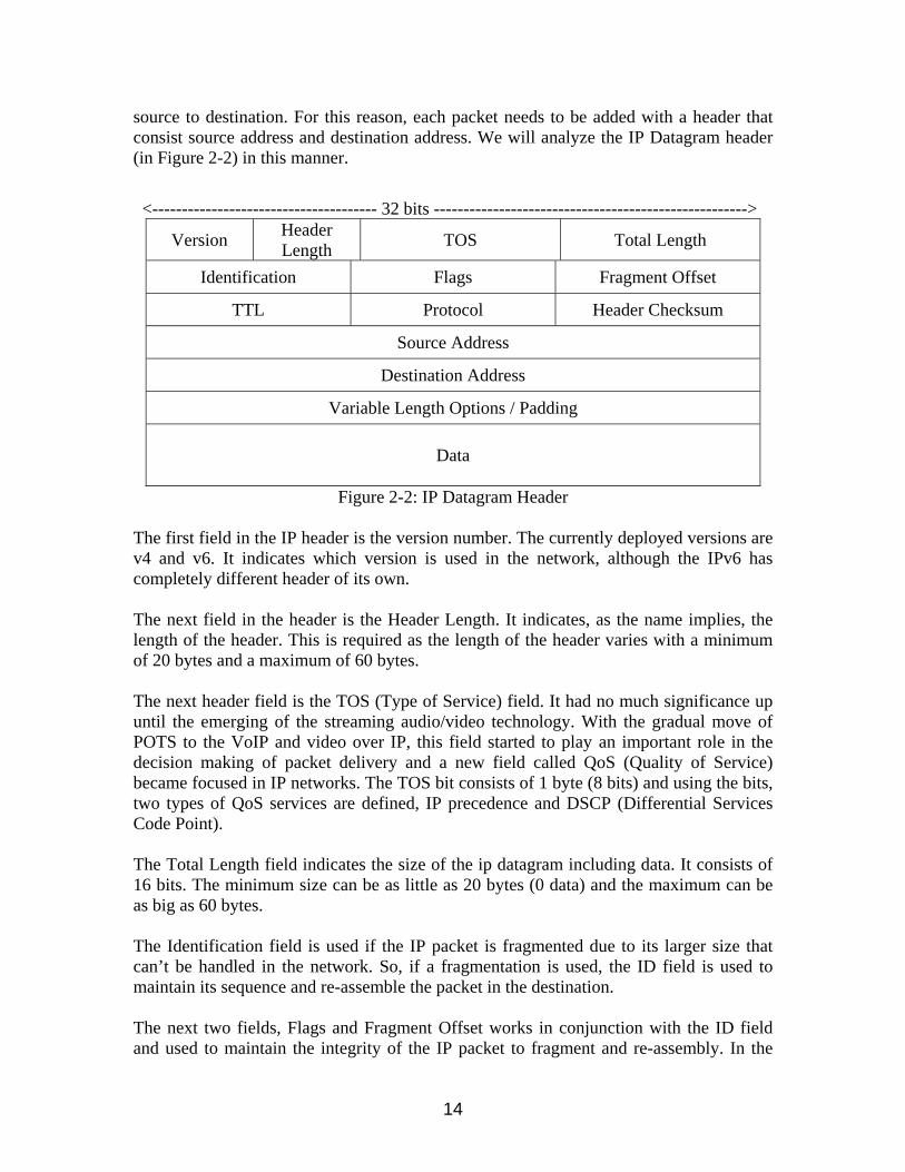
source to destination. For this reason, each packet needs to be added with a header that consist source address and destination address. We will analyze the IP Datagram header (in Figure 2-2) in this manner.

<-------------------------------------- 32 bits ----------------------------------------------------->

Version Header Length

TOS Total Length

Identification Flags Fragment Offset

TTL Protocol Header Checksum

Source Address

Destination Address

Variable Length Options / Padding

Data

Figure 2-2: IP Datagram Header

The first field in the IP header is the version number. The currently deployed versions are v4 and v6. It indicates which version is used in the network, although the IPv6 has completely different header of its own. The next field in the header is the Header Length. It indicates, as the name implies, the length of the header. This is required as the length of the header varies with a minimum of 20 bytes and a maximum of 60 bytes. The next header field is the TOS (Type of Service) field. It had no much significance up until the emerging of the streaming audio/video technology. With the gradual move of POTS to the VoIP and video over IP, this field started to play an important role in the decision making of packet delivery and a new field called QoS (Quality of Service) became focused in IP networks. The TOS bit consists of 1 byte (8 bits) and using the bits, two types of QoS services are defined, IP precedence and DSCP (Differential Services Code Point). The Total Length field indicates the size of the ip datagram including data. It consists of 16 bits. The minimum size can be as little as 20 bytes (0 data) and the maximum can be as big as 60 bytes. The Identification field is used if the IP packet is fragmented due to its larger size that can’t be handled in the network. So, if a fragmentation is used, the ID field is used to maintain its sequence and re-assemble the packet in the destination. The next two fields, Flags and Fragment Offset works in conjunction with the ID field and used to maintain the integrity of the IP packet to fragment and re-assembly. In the

15

Flags field, there are 3 bits and they are used as follows (from high order to low order): bit 0: always zero bit 1: Don’t Fragment (DF) bit 2: More Fragment (MF) So, if the DF is set, the packet is fragmented as per the fragment offset and each consequent (fragmented) packet contains the MF set except the last one. The Time-to-Live field was deployed to discard the packet if there is a loop in the path once its value reaches to zero. So, it helps in avoiding unwanted network bandwidth for unlimited time and increase productivity. In Latency, it is also used to count the hop and send back an ICMP message to the sender when the TTL=0. The Protocol field defines the protocol used in the data portion of the IP datagram. The Internet Assigned Numbers Authority maintains a list of IP protocol numbers which was originally defined in RFC 790. The checksum is created based on certain algorithm and it is maintained at each node to check whether the packet is corrupted in the medium. If the value doesn’t match the packet is discarded. The source and destination IP addresses are 32 bits and mentioned why they are required in packet switching networks. More of address allocation will be discussed later. The Option field is seldom used in networks. IPv4 Addressing: IP version four addressing scheme is based on 32bit in 4 octets. It is written in dotted decimal value, e.g. 10.0.0.1 to address a network device. The Internet Corporation for Assigned Name and Numbers (ICANN) maintains the highest level of ownership of the IP addresses and provide lower level ownership to the other parties, such as Regional Internet Registries or RIR. Registry like ARIN (American Registry for Internet Numbers) manages the IP addressing for the American continent. The IP addressing is classified in Classes based on the first octet as follows: Class A: 0-127 Class B: 128-191 Class C: 192-223 There are other classes for multicast and experimental uses. With the start of IPv4, it was assumed that 4 billions IP addresses would suffice for all but soon there was an indication of run-out of addressing. For this purpose, IANA re-addresses the issue reserving some

16

range of address for private use. One range was taken from each class to solve this issue as follows:

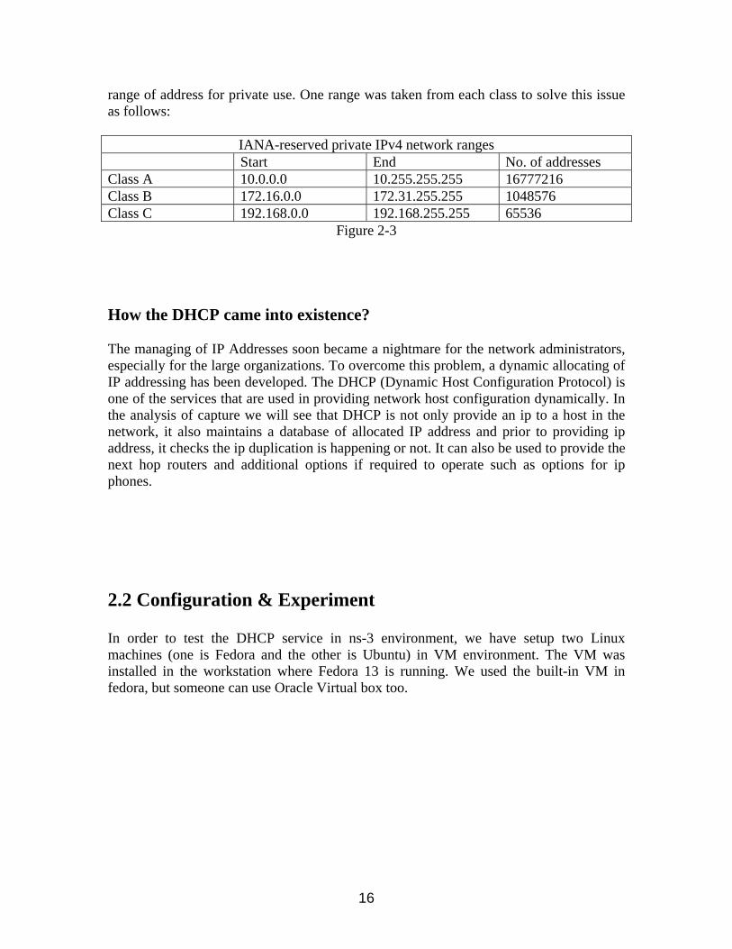
IANA-reserved private IPv4 network ranges Start End No. of addresses Class A 10.0.0.0 10.255.255.255 16777216 Class B 172.16.0.0 172.31.255.255 1048576 Class C 192.168.0.0 192.168.255.255 65536

Figure 2-3 How the DHCP came into existence? The managing of IP Addresses soon became a nightmare for the network administrators, especially for the large organizations. To overcome this problem, a dynamic allocating of IP addressing has been developed. The DHCP (Dynamic Host Configuration Protocol) is one of the services that are used in providing network host configuration dynamically. In the analysis of capture we will see that DHCP is not only provide an ip to a host in the network, it also maintains a database of allocated IP address and prior to providing ip address, it checks the ip duplication is happening or not. It can also be used to provide the next hop routers and additional options if required to operate such as options for ip phones.

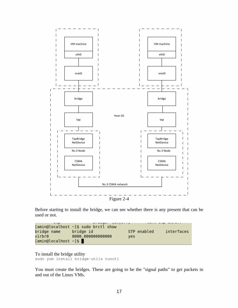
2.2 Configuration & Experiment In order to test the DHCP service in ns-3 environment, we have setup two Linux machines (one is Fedora and the other is Ubuntu) in VM environment. The VM was installed in the workstation where Fedora 13 is running. We used the built-in VM in fedora, but someone can use Oracle Virtual box too.

17

VM machine

eth0

vnet0

bridge

tap

TapBridgeNetDevice

CSMANetDevice

VM machine

eth0

vnet0

bridge

tap

TapBridgeNetDevice

CSMANetDevice

Host OS

Ns‐3 Node Ns‐3 Node

Ns‐3 CSMA network

Figure 2-4

Before starting to install the bridge, we can see whether there is any present that can be used or not.

To install the bridge utility sudo yum install bridge-utils tunctl

You must create the bridges. These are going to be the "signal paths" to get packets in and out of the Linux VMs.

18

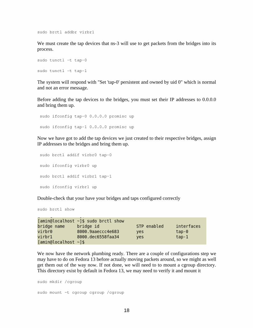
sudo brctl addbr virbr1

We must create the tap devices that ns-3 will use to get packets from the bridges into its process.

sudo tunctl -t tap-0

sudo tunctl -t tap-1

The system will respond with "Set 'tap-0' persistent and owned by uid 0" which is normal and not an error message.

Before adding the tap devices to the bridges, you must set their IP addresses to 0.0.0.0 and bring them up.

sudo ifconfig tap-0 0.0.0.0 promisc up

sudo ifconfig tap-1 0.0.0.0 promisc up

Now we have got to add the tap devices we just created to their respective bridges, assign IP addresses to the bridges and bring them up.

sudo brctl addif virbr0 tap-0

sudo ifconfig virbr0 up

sudo brctl addif virbr1 tap-1

sudo ifconfig virbr1 up

Double-check that your have your bridges and taps configured correctly

sudo brctl show

We now have the network plumbing ready. There are a couple of configurations step we may have to do on Fedora 13 before actually moving packets around, so we might as well get them out of the way now. If not done, we will need to to mount a cgroup directory. This directory exist by default in Fedora 13, we may need to verify it and mount it

sudo mkdir /cgroup

sudo mount -t cgroup cgroup /cgroup

19

We will also have to make sure that your kernel has ethernet filtering (ebtables, bridge-nf, arptables) disabled. If we do not do this, only STP and ARP traffic will be allowed to flow across our bridge and our whole scenario will not work.

pushd /proc/sys/net/bridge su for f in bridge-nf-*; do echo 0 > $f; done exit popd

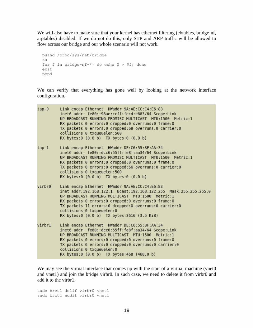
We can verify that everything has gone well by looking at the network interface configuration.

We may see the virtual interface that comes up with the start of a virtual machine (vnet0 and vnet1) and join the bridge virbr0. In such case, we need to delete it from virbr0 and add it to the virbr1. sudo brctl delif virbr0 vnet1 sudo brctl addif virbr0 vnet1

20

We need to verify the correct interface to the right bridge sudo brctl show

Running an ns-3 Simulated CSMA Network

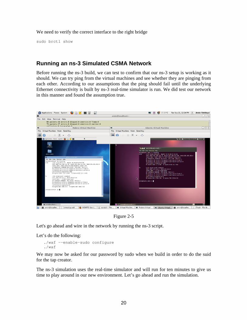
Before running the ns-3 build, we can test to confirm that our ns-3 setup is working as it should. We can try ping from the virtual machines and see whether they are pinging from each other. According to our assumptions that the ping should fail until the underlying Ethernet connectivity is built by ns-3 real-time simulator is run. We did test our network in this manner and found the assumption true.

Figure 2-5

Let's go ahead and wire in the network by running the ns-3 script.

Let’s do the following: ./waf --enable-sudo configure ./waf

We may now be asked for our password by sudo when we build in order to do the suid for the tap creator.

The ns-3 simulation uses the real-time simulator and will run for ten minutes to give us time to play around in our new environment. Let’s go ahead and run the simulation.

21

./waf --run tap-csma-virtual-machine Now, we need to shut the interfaces down and bring back up to see the DHCP operation. The virbr0 is configured for the DHCP server here.

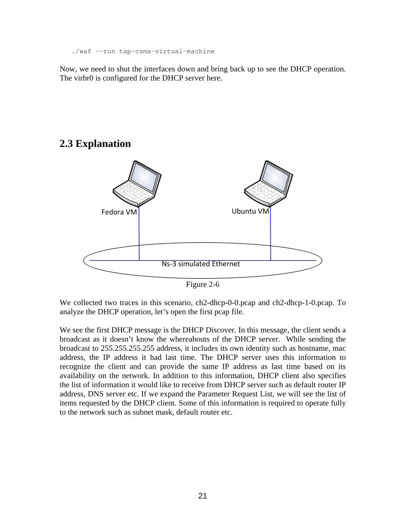
2.3 Explanation

Ns‐3 simulated Ethernet

Fedora VM Ubuntu VM

Figure 2-6

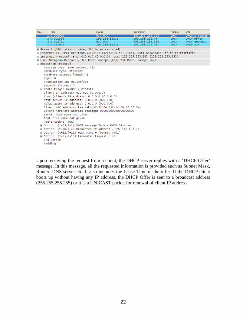
We collected two traces in this scenario, ch2-dhcp-0-0.pcap and ch2-dhcp-1-0.pcap. To analyze the DHCP operation, let’s open the first pcap file. We see the first DHCP message is the DHCP Discover. In this message, the client sends a broadcast as it doesn’t know the whereabouts of the DHCP server. While sending the broadcast to 255.255.255.255 address, it includes its own identity such as hostname, mac address, the IP address it had last time. The DHCP server uses this information to recognize the client and can provide the same IP address as last time based on its availability on the network. In addition to this information, DHCP client also specifies the list of information it would like to receive from DHCP server such as default router IP address, DNS server etc. If we expand the Parameter Request List, we will see the list of items requested by the DHCP client. Some of this information is required to operate fully to the network such as subnet mask, default router etc.

22

Upon receiving the request from a client, the DHCP server replies with a ‘DHCP Offer’ message. In this message, all the requested information is provided such as Subnet Mask, Router, DNS server etc. It also includes the Lease Time of the offer. If the DHCP client boots up without having any IP address, the DHCP Offer is sent to a broadcast address (255.255.255.255) or it is a UNICAST packet for renewal of client IP address.

23

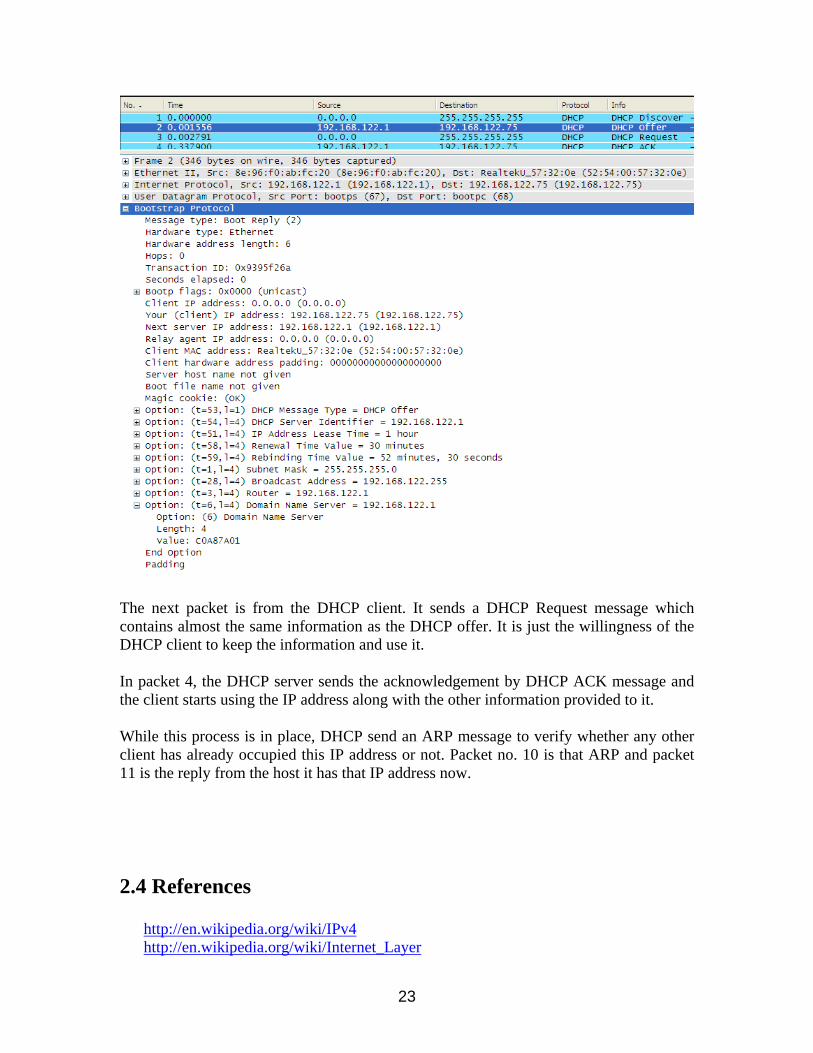
The next packet is from the DHCP client. It sends a DHCP Request message which contains almost the same information as the DHCP offer. It is just the willingness of the DHCP client to keep the information and use it. In packet 4, the DHCP server sends the acknowledgement by DHCP ACK message and the client starts using the IP address along with the other information provided to it. While this process is in place, DHCP send an ARP message to verify whether any other client has already occupied this IP address or not. Packet no. 10 is that ARP and packet 11 is the reply from the host it has that IP address now.

2.4 References

http://en.wikipedia.org/wiki/IPv4 http://en.wikipedia.org/wiki/Internet_Layer

24

ICANN - Internet Corporation for Assigned Names and Numbers American Registry for Internet Numbers (ARIN) http://en.wikipedia.org/wiki/Internet_Protocol http://www.nsnam.org http://code.google.com/p/waf http://www.selenic.com/mercurial/ http://en.wikipedia.org/wiki/GNU_toolchain http://www.cygwin.com/ http://cs.baylor.edu/~donahoo/practical/CSockets/ http://www.wireshark.org/ http://www.wand.net.nz/pubDetail.php?id=215 Wireshark - Wikipedia Wireshark and Ethereal network protocol analyzer toolkit SampleCaptures - The Wireshark Wiki

25

Chapter 3: Examining a ping and traceroute

3.1 Introduction

7 Application

6 Presentation

5 Session

4 Transport

3 Network

2 Data Link

1 Physical

Figure 3-1: OSI Model

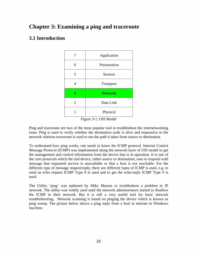
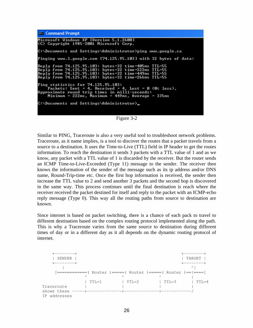
Ping and traceroute are two of the most popular tool to troubleshoot the internetworking issue. Ping is used to verify whether the destination node is alive and responsive to the network whereas traceroute is used to see the path it takes from source to destination. To understand how ping works, one needs to know the ICMP protocol. Internet Control Message Protocol (ICMP) was implemented along the network layer of OSI model to get the management and control information from the device that is in operation. It is one of the core protocols which the end device, either source or destination, uses to respond with message that requested service is unavailable or that a host is not reachable. For the different type of message request/reply, there are different types of ICMP is used, e.g. to send an echo request ICMP Type 8 is used and to get the echo-reply ICMP Type 0 is used. The Utility ‘ping’ was authored by Mike Muruss to troubleshoot a problem in IP network. The utility was widely used until the network administrators started to disallow the ICMP in their network. But it is still a very useful tool for basic network troubleshooting. Network scanning is based on pinging the device which is known as ping sweep. The picture below shows a ping reply from a host in internet in Windows machine.

26

Figure 3-2

Similar to PING, Traceroute is also a very useful tool to troubleshoot network problems. Traceroute, as it name implies, is a tool to discover the routes that a packet travels from a source to a destination. It uses the Time-to-Live (TTL) field in IP header to get the routes information. To reach the destination it sends 3 packets with a TTL value of 1 and as we know, any packet with a TTL value of 1 is discarded by the receiver. But the router sends an ICMP Time-to-Live-Exceeded (Type 11) message to the sender. The receiver then knows the information of the sender of the message such as its ip address and/or DNS name, Round-Trip-time etc. Once the first hop information is received, the sender then increase the TTL value to 2 and send another 3 packets and the second hop is discovered in the same way. This process continues until the final destination is reach where the receiver received the packet destined for itself and reply to the packet with an ICMP-echo reply message (Type 0). This way all the routing paths from source to destination are known. Since internet is based on packet switching, there is a chance of each pack to travel to different destination based on the complex routing protocol implemented along the path. This is why a Traceroute varies from the same source to destination during different times of day or in a different day as it all depends on the dynamic routing protocol of internet. +--------+ +--------+ | SENDER | | TARGET | +--------+ +--------+ | ^| [============( Router )=====( Router )=====( Router )==|====] ^ ^ ^ | | TTL=1 | TTL=2 | TTL=3 | TTL=4 Traceroute | | | | shows these -----+--------------+--------------+------------/ IP addresses

27

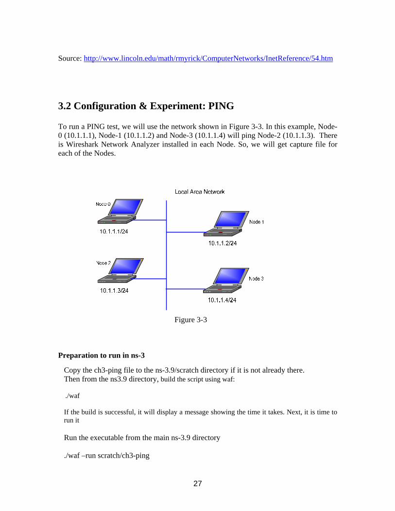
Source: http://www.lincoln.edu/math/rmyrick/ComputerNetworks/InetReference/54.htm 3.2 Configuration & Experiment: PING To run a PING test, we will use the network shown in Figure 3-3. In this example, Node-0 (10.1.1.1), Node-1 (10.1.1.2) and Node-3 (10.1.1.4) will ping Node-2 (10.1.1.3). There is Wireshark Network Analyzer installed in each Node. So, we will get capture file for each of the Nodes.

Figure 3-3 Preparation to run in ns-3

Copy the ch3-ping file to the ns-3.9/scratch directory if it is not already there. Then from the ns3.9 directory, build the script using waf:

./waf

If the build is successful, it will display a message showing the time it takes. Next, it is time to run it Run the executable from the main ns-3.9 directory ./waf –run scratch/ch3-ping

28

It will create the following pcap files for each node or as defined in the software to the main directory ch3-ping-0-1.pcap ch3-ping-1-1.pcap ch3-ping-2-1.pcap ch3-ping-3-1.pcap

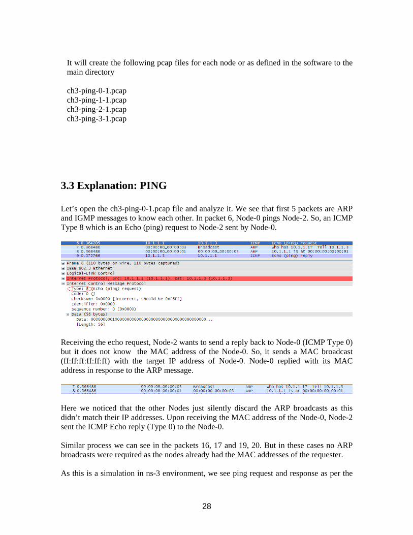
3.3 Explanation: PING Let’s open the ch3-ping-0-1.pcap file and analyze it. We see that first 5 packets are ARP and IGMP messages to know each other. In packet 6, Node-0 pings Node-2. So, an ICMP Type 8 which is an Echo (ping) request to Node-2 sent by Node-0.

Receiving the echo request, Node-2 wants to send a reply back to Node-0 (ICMP Type 0) but it does not know the MAC address of the Node-0. So, it sends a MAC broadcast (ff:ff:ff:ff:ff:ff) with the target IP address of Node-0. Node-0 replied with its MAC address in response to the ARP message.

Here we noticed that the other Nodes just silently discard the ARP broadcasts as this didn’t match their IP addresses. Upon receiving the MAC address of the Node-0, Node-2 sent the ICMP Echo reply (Type 0) to the Node-0. Similar process we can see in the packets 16, 17 and 19, 20. But in these cases no ARP broadcasts were required as the nodes already had the MAC addresses of the requester. As this is a simulation in ns-3 environment, we see ping request and response as per the

29

coding was done. Had we used a windows PC to send a ping, we would have seen 4 packets are sent to get response and Round-Trip-Time (RTT) and other parameters were measured (Figure 3-2).

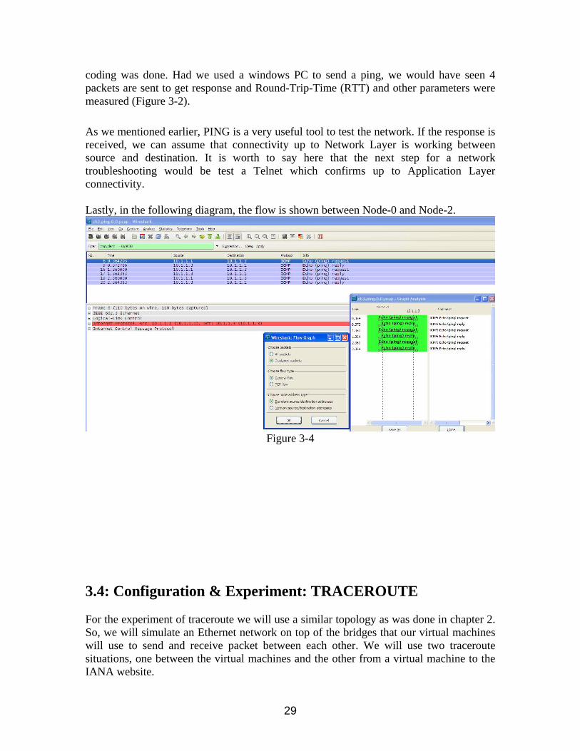
As we mentioned earlier, PING is a very useful tool to test the network. If the response is received, we can assume that connectivity up to Network Layer is working between source and destination. It is worth to say here that the next step for a network troubleshooting would be test a Telnet which confirms up to Application Layer connectivity. Lastly, in the following diagram, the flow is shown between Node-0 and Node-2.

Figure 3-4

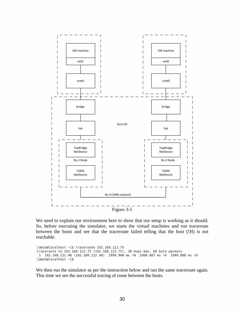
3.4: Configuration & Experiment: TRACEROUTE For the experiment of traceroute we will use a similar topology as was done in chapter 2. So, we will simulate an Ethernet network on top of the bridges that our virtual machines will use to send and receive packet between each other. We will use two traceroute situations, one between the virtual machines and the other from a virtual machine to the IANA website.

30

VM machine

eth0

vnet0

bridge

tap

TapBridgeNetDevice

CSMANetDevice

VM machine

eth0

vnet0

bridge

tap

TapBridgeNetDevice

CSMANetDevice

Host OS

Ns‐3 Node Ns‐3 Node

Ns‐3 CSMA network

Figure 3-5

We need to explain our environment here to show that our setup is working as it should. So, before executing the simulator, we starts the virtual machines and run traceroute between the hosts and see that the traceroute failed telling that the host (!H) is not reachable.

We then run the simulator as per the instruction below and run the same traceroute again. This time we see the successful tracing of route between the hosts.

31

Preparation to run in ns-3

Copy the ch3-traceroute.cc file to the ns-3.9/scratch directory if it is not already there. Then from the ns3.9 directory, build the script using waf: ./waf If the build is successful, it will display a message showing the time it takes. Next, it is time to run it Run the executable from the main ns-3.9 directory ./waf --run scratch/ch3-traceroute it will create the following pcap files for each node or as defined in the software to the main ns-3.9 directory ch3-traceroute-0-1.pcap ch3-traceroute-1-1.pcap

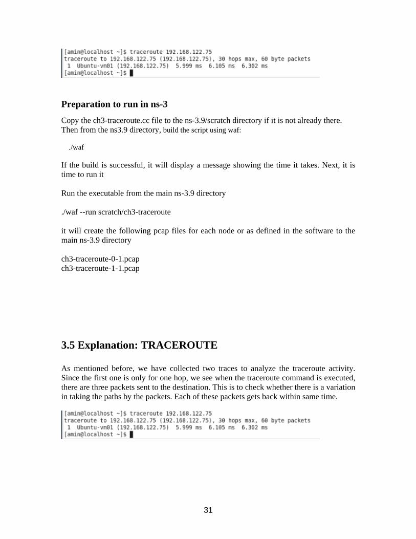
3.5 Explanation: TRACEROUTE As mentioned before, we have collected two traces to analyze the traceroute activity. Since the first one is only for one hop, we see when the traceroute command is executed, there are three packets sent to the destination. This is to check whether there is a variation in taking the paths by the packets. Each of these packets gets back within same time.

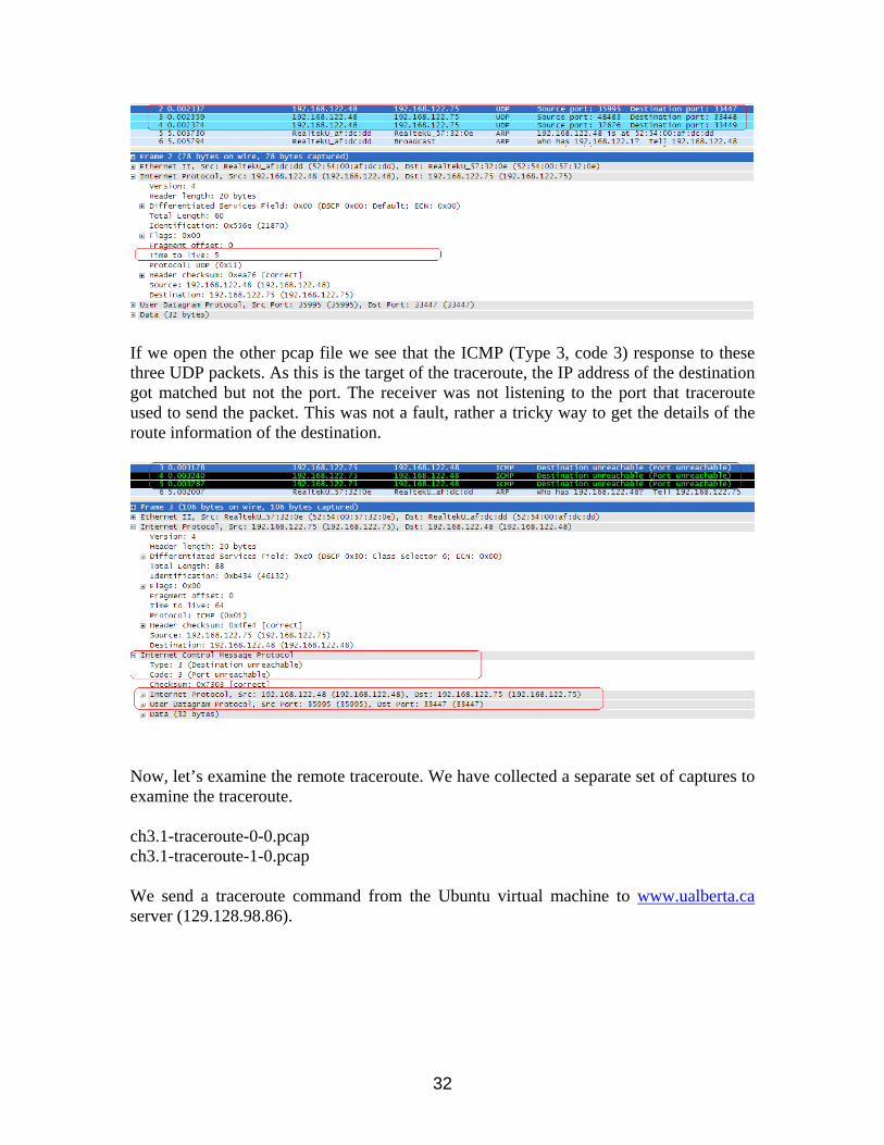
32

If we open the other pcap file we see that the ICMP (Type 3, code 3) response to these three UDP packets. As this is the target of the traceroute, the IP address of the destination got matched but not the port. The receiver was not listening to the port that traceroute used to send the packet. This was not a fault, rather a tricky way to get the details of the route information of the destination.

Now, let’s examine the remote traceroute. We have collected a separate set of captures to examine the traceroute. ch3.1-traceroute-0-0.pcap ch3.1-traceroute-1-0.pcap We send a traceroute command from the Ubuntu virtual machine to www.ualberta.ca server (129.128.98.86).

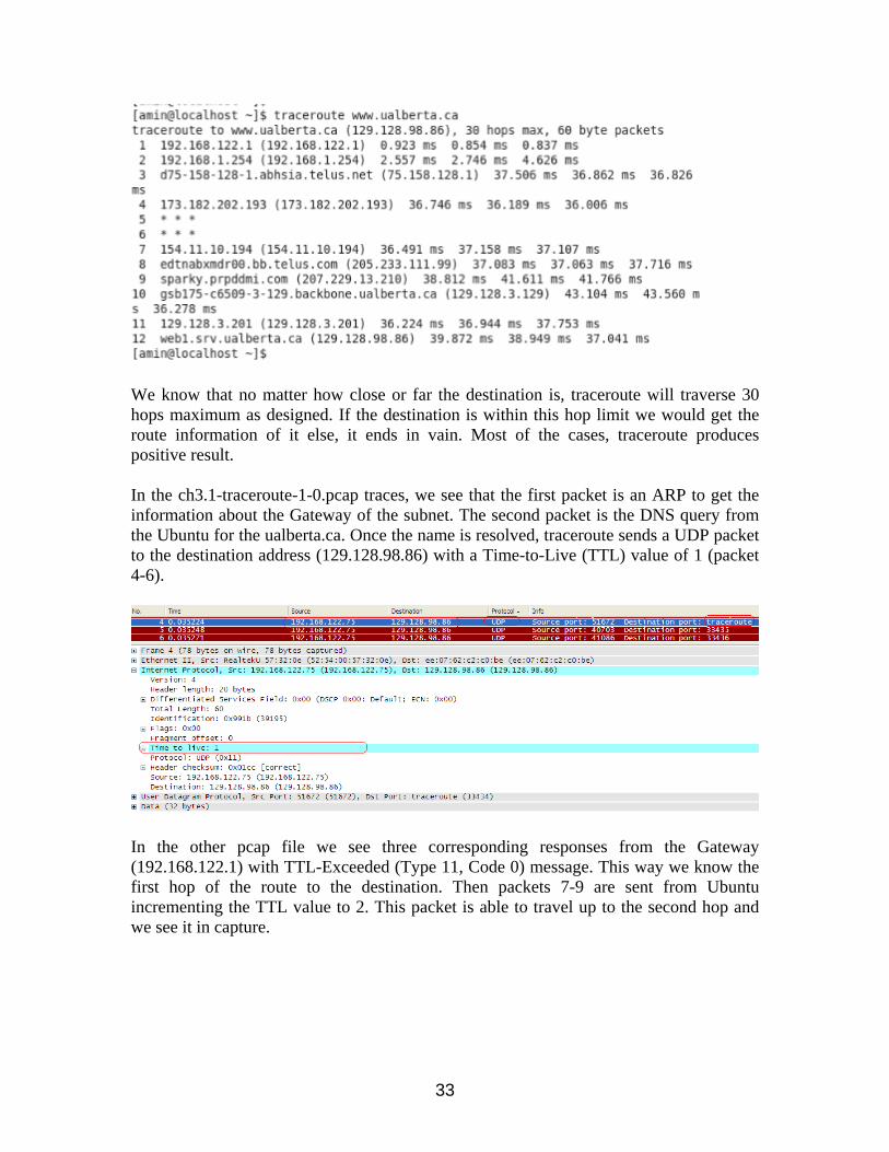
33

We know that no matter how close or far the destination is, traceroute will traverse 30 hops maximum as designed. If the destination is within this hop limit we would get the route information of it else, it ends in vain. Most of the cases, traceroute produces positive result. In the ch3.1-traceroute-1-0.pcap traces, we see that the first packet is an ARP to get the information about the Gateway of the subnet. The second packet is the DNS query from the Ubuntu for the ualberta.ca. Once the name is resolved, traceroute sends a UDP packet to the destination address (129.128.98.86) with a Time-to-Live (TTL) value of 1 (packet 4-6).

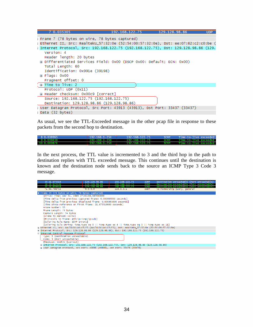
In the other pcap file we see three corresponding responses from the Gateway (192.168.122.1) with TTL-Exceeded (Type 11, Code 0) message. This way we know the first hop of the route to the destination. Then packets 7-9 are sent from Ubuntu incrementing the TTL value to 2. This packet is able to travel up to the second hop and we see it in capture.

34

As usual, we see the TTL-Exceeded message in the other pcap file in response to these packets from the second hop to destination.

In the next process, the TTL value is incremented to 3 and the third hop in the path to destination replies with TTL exceeded message. This continues until the destination is known and the destination node sends back to the source an ICMP Type 3 Code 3 message.

35

3.4 References

http://en.wikipedia.org/wiki/Traceroute http://www.lincoln.edu/math/rmyrick/ComputerNetworks/InetReference/54.htm http://help.expedient.com/general/ping_traceroute.shtml http://www.nsnam.org http://code.google.com/p/waf http://www.selenic.com/mercurial/ http://en.wikipedia.org/wiki/GNU_toolchain http://www.cygwin.com/ http://cs.baylor.edu/~donahoo/practical/CSockets/ http://www.wireshark.org/ http://www.wand.net.nz/pubDetail.php?id=215 Wireshark - Wikipedia Wireshark and Ethereal network protocol analyzer toolkit SampleCaptures - The Wireshark Wiki

36

Chapter 4: Transport Layer Protocol - UDP

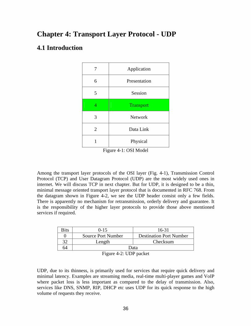
4.1 Introduction

7 Application

6 Presentation

5 Session

4 Transport

3 Network

2 Data Link

1 Physical

Figure 4-1: OSI Model

Among the transport layer protocols of the OSI layer (Fig. 4-1), Transmission Control Protocol (TCP) and User Datagram Protocol (UDP) are the most widely used ones in internet. We will discuss TCP in next chapter. But for UDP, it is designed to be a thin, minimal message oriented transport layer protocol that is documented in RFC 768. From the datagram shown in Figure 4-2, we see the UDP header consist only a few fields. There is apparently no mechanism for retransmission, orderly delivery and guarantee. It is the responsibility of the higher layer protocols to provide those above mentioned services if required.

Bits 0-15 16-31 0 Source Port Number Destination Port Number 32 Length Checksum 64 Data

Figure 4-2: UDP packet

UDP, due to its thinness, is primarily used for services that require quick delivery and minimal latency. Examples are streaming media, real-time multi-player games and VoIP where packet loss is less important as compared to the delay of transmission. Also, services like DNS, SNMP, RIP, DHCP etc uses UDP for its quick response to the high volume of requests they receive.

37

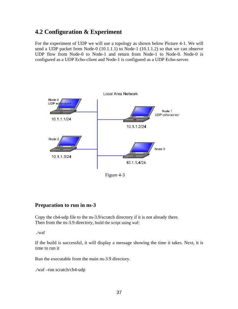
4.2 Configuration & Experiment For the experiment of UDP we will use a topology as shown below Picture 4-1. We will send a UDP packet from Node-0 (10.1.1.1) to Node-1 (10.1.1.2) so that we can observe UDP flow from Node-0 to Node-1 and return from Node-1 to Node-0. Node-0 is configured as a UDP Echo-client and Node-1 is configured as a UDP Echo-server.

Figure 4-3 Preparation to run in ns-3 Copy the ch4-udp file to the ns-3.9/scratch directory if it is not already there. Then from the ns-3.9 directory, build the script using waf: ./waf If the build is successful, it will display a message showing the time it takes. Next, it is time to run it Run the executable from the main ns-3.9 directory. ./waf –run scratch/ch4-udp

38

It will create the following pcap files for each node or as defined in the software to the main directory ch4-udp-0-1.pcap ch4-udp-1-1.pcap ch4-udp-2-1.pcap ch4-udp-3-1.pcap

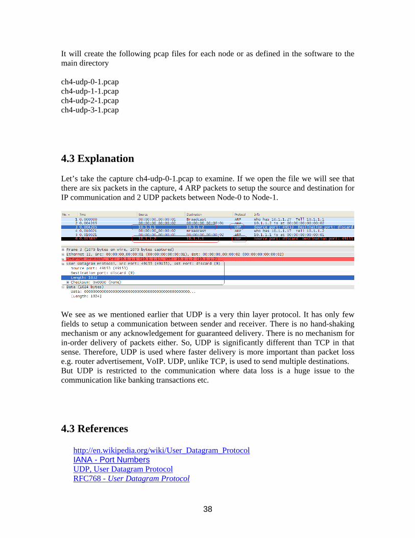
4.3 Explanation Let’s take the capture ch4-udp-0-1.pcap to examine. If we open the file we will see that there are six packets in the capture, 4 ARP packets to setup the source and destination for IP communication and 2 UDP packets between Node-0 to Node-1.

We see as we mentioned earlier that UDP is a very thin layer protocol. It has only few fields to setup a communication between sender and receiver. There is no hand-shaking mechanism or any acknowledgement for guaranteed delivery. There is no mechanism for in-order delivery of packets either. So, UDP is significantly different than TCP in that sense. Therefore, UDP is used where faster delivery is more important than packet loss e.g. router advertisement, VoIP. UDP, unlike TCP, is used to send multiple destinations. But UDP is restricted to the communication where data loss is a huge issue to the communication like banking transactions etc.

4.3 References

http://en.wikipedia.org/wiki/User_Datagram_Protocol IANA - Port Numbers UDP, User Datagram Protocol RFC768 - User Datagram Protocol

39

TCP - UDP Comparative analysis - Data Communications and Networks http://www.nsnam.org http://code.google.com/p/waf http://www.selenic.com/mercurial/ http://en.wikipedia.org/wiki/GNU_toolchain http://www.cygwin.com/ http://cs.baylor.edu/~donahoo/practical/CSockets/ http://www.wireshark.org/ Wireshark - Wikipedia Wireshark and Ethereal network protocol analyzer toolkit SampleCaptures - The Wireshark Wiki

40

Chapter 5: Transport Layer Protocol - TCP

5.1 Introduction

Transmission Control Protocol (TCP) is the dominant transport protocol that is in use today in the Internet. With the bandwidth eating nature and no control mechanism of its alternative protocol UDP, TCP has taken almost all the position (over 90%) in today’s Internet. TCP provides a reliable, connection-oriented transport protocol. It starts negotiation between the sender and receiver before sending the actual data. This will be seen in detail once we examine the TCP segment in the next paragraph.

7 Application

6 Presentation

5 Session

4 Transport

3 Network

2 Data Link

1 Physical

Figure 5-1

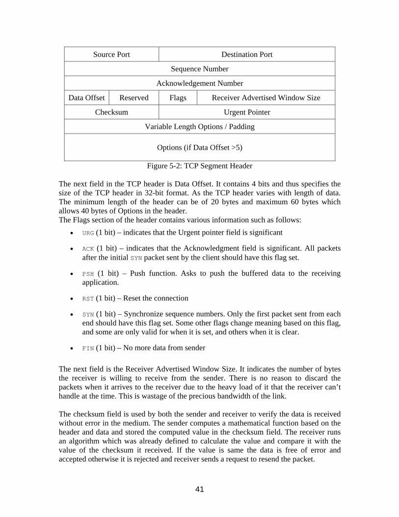
Every TCP segment consists of a header followed by an optional data section. TCP header contains 10 mandatory fields and an optional extension field. The format of the header is defined in RFC 793 (Figure 5-2). The header starts with 16 bits source port followed by 16 bits destination port. As the name applies, source port is used by sender and destination port is the one used to reach the receiver that it listens to. The next field is the Sequence Number field which is used to sequence the bits and works with the next field called Acknowledgement Number. A TCP Receiver acknowledges the bits it received in sequence and it waits if there is any missing bit until it received. For example, an acknowledgement number of 10 indicate the sender that bits 0-9 are received by the receiver successfully. On the other hand, the receiver waits if there is a reception of 11th bit without 10th one. Once the 10th bit is received, the receiver sends the acknowledgement to the sender of both the bits received.

41

Source Port Destination Port

Sequence Number

Acknowledgement Number

Data Offset Reserved Flags Receiver Advertised Window Size

Checksum Urgent Pointer

Variable Length Options / Padding

Options (if Data Offset >5)

Figure 5-2: TCP Segment Header

The next field in the TCP header is Data Offset. It contains 4 bits and thus specifies the size of the TCP header in 32-bit format. As the TCP header varies with length of data. The minimum length of the header can be of 20 bytes and maximum 60 bytes which allows 40 bytes of Options in the header. The Flags section of the header contains various information such as follows:

URG (1 bit) – indicates that the Urgent pointer field is significant

ACK (1 bit) – indicates that the Acknowledgment field is significant. All packets after the initial SYN packet sent by the client should have this flag set.

PSH (1 bit) – Push function. Asks to push the buffered data to the receiving application.

RST (1 bit) – Reset the connection

SYN (1 bit) – Synchronize sequence numbers. Only the first packet sent from each end should have this flag set. Some other flags change meaning based on this flag, and some are only valid for when it is set, and others when it is clear.

FIN (1 bit) – No more data from sender

The next field is the Receiver Advertised Window Size. It indicates the number of bytes the receiver is willing to receive from the sender. There is no reason to discard the packets when it arrives to the receiver due to the heavy load of it that the receiver can’t handle at the time. This is wastage of the precious bandwidth of the link. The checksum field is used by both the sender and receiver to verify the data is received without error in the medium. The sender computes a mathematical function based on the header and data and stored the computed value in the checksum field. The receiver runs an algorithm which was already defined to calculate the value and compare it with the value of the checksum it received. If the value is same the data is free of error and accepted otherwise it is rejected and receiver sends a request to resend the packet.

42

5.2 Configuration & Experiment As we will see the basic functionality of the TCP operation, we use a two-node P2P network type connection to analyze it. We have captured two .pcap files for this (ch5-tcp-0-1.pcap and ch5-tcp-1-1.pcap) 5.3 Explanation If we open any of the pcap files in Wireshark we will see the details the layered OSI communication. Let’s discuss with the ch5-tcp-0-1.pcap file. As we know that TCP starts communicating before actual data is sent, we see the first packet in the TCP header in Picture 5-3 contains a SYN message no data.

Figure 5-3

If we recall the discussion in the introduction that the Flag field contains 8 bits, 1 for each type of message, we can see that in the packet trace. The SYN packet in the handshake

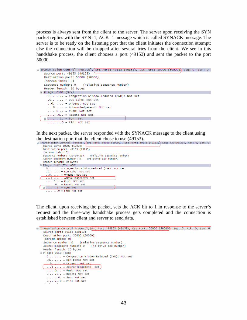
43

process is always sent from the client to the server. The server upon receiving the SYN packet replies with the SYN=1, ACK=1 message which is called SYNACK message. The server is to be ready on the listening port that the client initiates the connection attempt; else the connection will be dropped after several tries from the client. We see in this handshake process, the client chooses a port (49153) and sent the packet to the port 50000.

In the next packet, the server responded with the SYNACK message to the client using the destination port that the client chose to use (49153).

The client, upon receiving the packet, sets the ACK bit to 1 in response to the server’s request and the three-way handshake process gets completed and the connection is established between client and server to send data.

44

As we mentioned earlier that these three TCP segments do not contains any data (there is no data portion in capture, see Picture 5-1), the data starts flowing from the 4th segment

If we look at the sequence number in the TCP header, we see the first one is not zero (although Wireshark counts is as zero, it is a relative counting), TCP chooses a random number to avoid confusion from the old connection. The other point to note here is that the sequence number starts again with the actual data and independent of the handshaking process. The sequence number plays an important role in finding the missing segments in data flow as it is used to number the next flow as shown in Picture 5-2.

Here we see that the next sequence number is set to 250 as the data size is 250 bytes. The next packet (5th packet) shows the acknowledgement of the data and the indication that all the bytes are received.

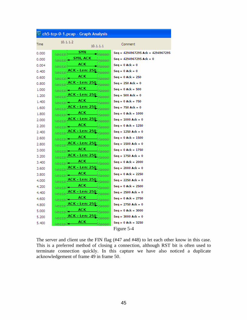
In the following captures, we see that the sequence number is an increment of 250 bytes that the client sent to server. We also see that both the client and server set the ACK bit to 1 during the data flow until all the data are sent. In the following picture, we see the three-way handshaking and ACK=1 in the subsequent flows. The relationship between sequence number and acknowledgement number is also noticeable what we discussed earlier.

45

Figure 5-4

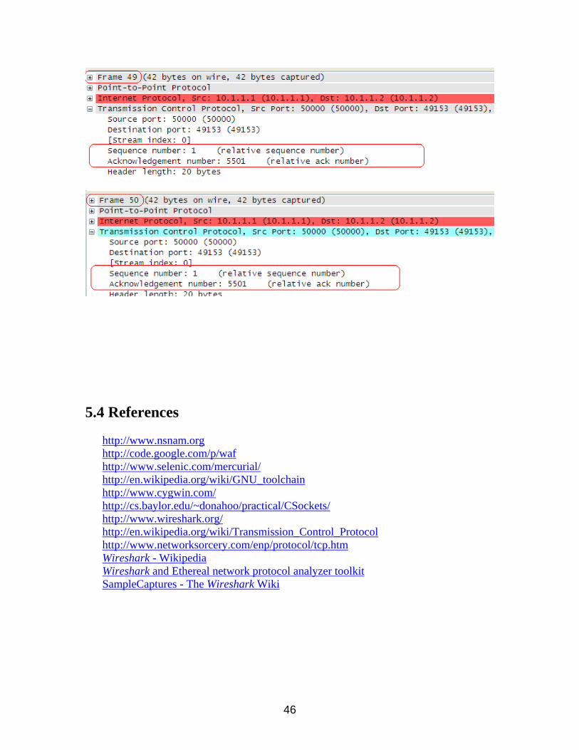
The server and client use the FIN flag (#47 and #48) to let each other know in this case. This is a preferred method of closing a connection, although RST bit is often used to terminate connection quickly. In this capture we have also noticed a duplicate acknowledgement of frame 49 in frame 50.

46

5.4 References

http://www.nsnam.org http://code.google.com/p/waf http://www.selenic.com/mercurial/ http://en.wikipedia.org/wiki/GNU_toolchain http://www.cygwin.com/ http://cs.baylor.edu/~donahoo/practical/CSockets/ http://www.wireshark.org/ http://en.wikipedia.org/wiki/Transmission_Control_Protocol http://www.networksorcery.com/enp/protocol/tcp.htm Wireshark - Wikipedia Wireshark and Ethereal network protocol analyzer toolkit SampleCaptures - The Wireshark Wiki

47

Conclusion

We have used ns-3 simulator in this project to run the network setup and gather the captures. ns-3 has its own limitation. The current version of stable release is ns-3.9. When we started the project ns-3.8 was the latest stable release and while developing the scenario, ns-3.9 came out, so we updated our test bed with ns-3.9. There are still lots of topology yet to be developed such as:

Dynamic Routing – right now only OLSR routing for wireless technology is supported. RIPv2, OSPF, BGP are not supported

Most of the Application Protocols (HTTP, FTP, POP, and SMTP) are yet to be supported. This may be overcome with the integration of real nodes with underlying simulation as communication medium