Incorporating Evapotranspiration of Plants in Thermal Modelling of Greenhouses in Cold

Regions

by

Anni Wei

A thesis submitted in partial fulfillment of the requirements for the degree of

Master of Science

in

CIVIL (CROSS-DISCIPLINARY)

Department of Civil and Environmental Engineering

University of Alberta

© Anni Wei, 2020

ii

Abstract

The energy consumption of greenhouse in cold regions, especially for the space heating, is still

large and needs to be diminished either by reducing heat loss or by increasing the percentage of

renewable energy usage. In order to predict the performance of different energy-saving designs,

a greenhouse model with better accuracy and reduced complexity is needed. The main objectives

of this paper are: 1. give a comprehensive review about the energy-saving design and operation

strategies of greenhouses from previous studies. 2. provide detailed descriptions about important

parameters of plants that should be used in greenhouse modelling. 3. develop a simplified

greenhouse modelling method. 4. test three advanced design concepts: insulated north wall,

cyclic lighting, transparent and vertical ceiling. The concepts and some other background

information of plants’ parameters are given, and the relationships between these parameters and

greenhouse modelling are explained. Before building the mathematical models, the thermal

networks were simplified by dividing a greenhouse into three kinds of areas: middle, edge, and

corner areas. The corner areas were not modelled because of their small proportion. When

compared to the conventional ways of doing greenhouse modelling, the difficulty of the new

modelling method is diminished by dividing a complex greenhouse thermal network into simpler

subnetworks, which can be combined to form a complete network. In addition, the accuracy of

new modelling method is also higher, since the interior air is modelled in more than one control

volumes in middle and edge areas within a greenhouse, and the air node is separated from the

plant node. The modelled results showed that the insulated north wall gave rise to a significant

increase in air temperature (around 3.5 ℃) and resulted in greatest thermal energy saving.

iii

Preface

After completing this research project, I could say that I had obtained deeper understanding in

this interdisciplinary area. I want to say thank you to my graduate supervisor, Dr. Yuxiang Chen.

He is an expert in building science. As a student who has a degree of Bachelor of Science in

Agriculture, I had gained sufficient knowledge of building science, thermodynamics, and

physics. He also spent lots of time to give me suggestions on how to build the greenhouse

mathematical models. During the three-year study, I learned knowledge of both engineering and

agriculture areas and became more comprehensive. In addition, I am grateful for the support

provided by Behrouz Nourozi who is a staff of KTH Royal Institute of Technology, Stockholm,

Sweden. I also would like to thank Sihan Liu, a computer science student of University of

Alberta who assisted in editing all matlab codes of cyclic lighting and basic designs.

iv

Table of contents

Chapter 1. Introduction ................................................................................................................... 1

Chapter 2. Literature review ........................................................................................................... 5

2.1 Lighting ................................................................................................................................. 9

2.1.1 Background scientific information ................................................................................ 9

2.1.2 Envelope design for natural lighting (transparent materials) ....................................... 10

Polyethylene (PE) ....................................................................................................... 10

Polycarbonate （PC） ............................................................................................... 11

Acrylic ........................................................................................................................ 12

Bubble wrap ................................................................................................................ 13

2.1.3 Artificial lighting and Lamp selection ......................................................................... 13

HPS ............................................................................................................................. 14

LED ............................................................................................................................ 15

Hybrid lighting ........................................................................................................... 16

2.1.4 Lighting operation ........................................................................................................ 20

Duration and intensity (W/m2) ................................................................................... 20

Interval and time: day extension (DE) or night interruption (NI), cyclic/intermittent or

continuous lighting............................................................................................................ 25

2.2 Air quality and temperature control .................................................................................... 27

2.3 Irrigation ............................................................................................................................. 29

2.4 Sustainable design options .................................................................................................. 31

2.4.1 Envelope design for natural lighting and thermal insulation ....................................... 33

General envelope insulation ....................................................................................... 33

Movable insulation/thermal screen/thermal curtain ................................................... 35

Hybridization of solar devices with greenhouses ....................................................... 36

Solar glass ................................................................................................................... 39

2.4.2 Energy storage ............................................................................................................. 39

Rock bed storage ........................................................................................................ 40

Phase change materials (PCMs) ................................................................................. 41

Soil .............................................................................................................................. 44

v

North wall ................................................................................................................... 45

2.4.3 Energy-efficient HVAC techniques ............................................................................. 46

Geothermal exchange: composite systems ................................................................. 46

Ground air collector .................................................................................................... 48

Ventilation Sustainable design ................................................................................... 49

2.5 Numerical Modeling ........................................................................................................... 51

2.5.1 Review and summaries of previous researches ........................................................... 52

2.5.2 Current development, potential problems, and possible solutions .............................. 55

2.6 Discussion and Conclusion ................................................................................................. 59

Chapter 3 Heat and moisture exchange between plants and air .................................................... 63

3.1 Leaf area index (LAI) and canopy cover (CC) ................................................................... 63

3.2 Transpiration and evapotranspiration ................................................................................. 65

3.3 Boundary layer resistance ................................................................................................... 69

3.4 Heat and moisture transfer of plants ................................................................................... 72

Chapter 4. Modeling：methods and materials ............................................................................. 75

4.1 General modeling approach ................................................................................................ 75

4.2 Thermal networks and equations for basic designs for the middle and edge areas ............ 76

4.2.1 Outdoor temperature (Text) ........................................................................................... 81

4.2.2 Solar radiation calculation (Isrd) ................................................................................... 82

4.2.3 Conduction and convention (Qcc) ................................................................................ 89

4.2.4 Lighting heat gain (Qsl) ................................................................................................ 91

4.2.5 Long wave radiation (Qr) ............................................................................................. 93

4.2.6 Heat loss caused by ventilation and in/exfiltration (Qv) .............................................. 96

4.3 Thermal equations for advanced designs ............................................................................ 96

4.3.1 Middle area with vertical skylight ............................................................................... 96

4.3.2 Edge area with insulated north wall ............................................................................. 99

4.3.3 Middle area with cyclic and night interruption (NI) lighting .................................... 100

Chapter 5 Results and discussion ................................................................................................ 102

5.1 Basic design ...................................................................................................................... 102

5.2 Middle area with vertical skylight .................................................................................... 104

5.3 Edge area with insulated north wall .................................................................................. 105

vi

5.4 Middle area with cyclic and night interruption (NI) lighting ........................................... 106

5.5 Comparison of magnitudes of plants’ heat exchange components ................................... 107

5.6 Comparison of energy consumption of advanced designs with the basic design ............. 110

5.7 Application of models in realistic conditions ................................................................... 114

5.7.1 Application of models in other plant species ............................................................. 114

5.7.2 Application of models in a whole greenhouse ........................................................... 116

Chapter 6 Conclusion .................................................................................................................. 118

References ................................................................................................................................... 121

Appendix ..................................................................................................................................... 143

vii

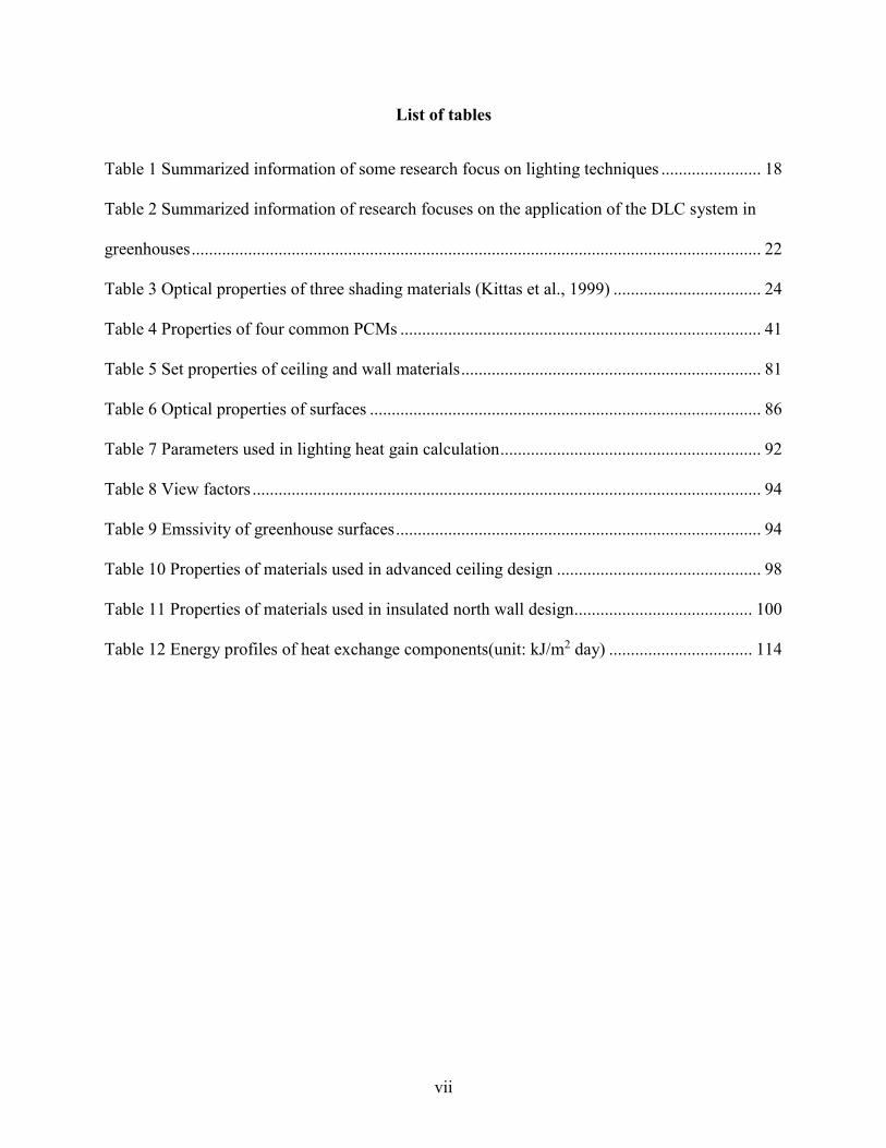
List of tables

Table 1 Summarized information of some research focus on lighting techniques ....................... 18

Table 2 Summarized information of research focuses on the application of the DLC system in

greenhouses ................................................................................................................................... 22

Table 3 Optical properties of three shading materials (Kittas et al., 1999) .................................. 24

Table 4 Properties of four common PCMs ................................................................................... 41

Table 5 Set properties of ceiling and wall materials ..................................................................... 81

Table 6 Optical properties of surfaces .......................................................................................... 86

Table 7 Parameters used in lighting heat gain calculation ............................................................ 92

Table 8 View factors ..................................................................................................................... 94

Table 9 Emssivity of greenhouse surfaces .................................................................................... 94

Table 10 Properties of materials used in advanced ceiling design ............................................... 98

Table 11 Properties of materials used in insulated north wall design ......................................... 100

Table 12 Energy profiles of heat exchange components(unit: kJ/m2 day) ................................. 114

viii

List of figures

Figure 1.Relationship between LAI and canopy cover ................................................................. 65

Figure 2 Relationship between indoor wind speed (m/s) and plant thermal conductance (W/m2 K)

....................................................................................................................................................... 71

Figure 3 Relationship characteristic leave length (m) and plant thermal conductance (W/m2 K) 71

Figure 4 Thermal network of a plant ............................................................................................ 72

Figure 5 The relationships between net radiation (W/m2), indoor air temperature (℃) and

evapotranspiration rate (W/m2) ..................................................................................................... 74

Figure 6 and Figure 7: Three kinds of unit areas in a greenhouse (front view and top view) ...... 76

Figure 8 Schematic of area M in the basic design ........................................................................ 77

Figure 9 Schematic of area E in the basic design ......................................................................... 78

Figure 10 Exterior temperature in January 1st, 2002 .................................................................... 82

Figure 11 Relationship between incidence angle (degree) and transmittance of transparent

material ......................................................................................................................................... 87

Figure 12 Solar radiation before transmission (basic design, insulated north wall design, cyclic

lighting design) ............................................................................................................................. 87

Figure 13 Solar radiation after transmission (basic design, insulated north wall design, cyclic

lighting design) ............................................................................................................................. 88

Figure 14 Solar radiation before transmission (advanced ceiling design) .................................... 88

Figure 15 Solar radiation after transmission (advanced ceiling design) ....................................... 89

Figure 16 Outdoor dew point temperature in January 1st, 2002................................................... 95

Figure 17 Emissivity of sky in January 1st, 2002 ......................................................................... 95

ix

Figure 18 Schematic of energy saving ceiling (surface 1: vertical and transparent ceiling to

increase solar heat gain; surface 2: insulated horizontal surface with white paint, can increase

solar heat gain and reduce heat loss; surface 3: insulated by lightweight; yellow arrows: solar

radiation) ....................................................................................................................................... 97

Figure 19 Schematic of the greenhouse design with insulated north wall .................................... 99

Figure 20 Lighting intensity within 24 hours in cyclic lighting design (area M) ....................... 101

Figure 21 Modelled values of temperatures of interior air (Ta.int), ceiling (Tcl.int), ground (Tg.ext),

and plant (Tp ) surfaces in basic design (area M) ........................................................................ 102

Figure 22 Modelled values of temperatures of interior air (Ta.int), ceiling (Tcl.int), ground (Tg.ext),

and plant (Tp ) surfaces in basic design (area E) ......................................................................... 103

Figure 23 Modelled values of temperatures of interior air (Ta.int), ceiling (Tcl.int), ground (Tg.ext),

and plant (Tp ) surfaces with vertical and transparent ceiling (area M) ...................................... 104

Figure 24 Modelled values of temperatures of interior air (Ta.int), ceiling (Tcl.int), north wall

(Tnw.int), ground (Tg.ext), and plant (Tp )surfaces with insulated north wall (area E) ................... 105

Figure 25 Modelled values of temperatures of interior air (Ta.int), ceiling (Tcl.int), ground (Tg.ext),

and plant (Tp )surfaces with cyclic lighting (area M) .................................................................. 106

Figure 26 Simulation results of plants' evapotranspiration and sensible heat exchange (basic

design) ......................................................................................................................................... 107

Figure 27 Simulation results of net radiation absorbed by plants (basic design) ....................... 108

Figure 28 Energy consumption of designs (from left to right, 1: basic design, area M; 2: basic

design, area E; 3: advanced ceiling; 4: insulated north wall; 5:cyclic and night interruption

lighting) ....................................................................................................................................... 110

Figure 29 Temperature profiles after adding the heating system (basic design, area M) ........... 111

x

Figure 30 Temperature profiles after adding the heating system (basic design, area E) ............ 112

Figure 31 Temperature profiles after adding the heating system (vertical skylight) .................. 112

Figure 32 Temperature profiles after adding the heating system (insulated north wall) ............ 113

Figure 33 Temperature profiles after adding the heating system (cyclic and night interruption

lighting) ....................................................................................................................................... 113

xi

Nomenclature

A surface area (m2)

T temperature (K)

C specific heat (J/kg K)

I solar radiation (W m-2)

F view factor (-)

LAI leaf area index (-)

Q heat load (W)

V volume (m3)

U thermal conductance (W/K)

CC canopy cover (-)

l thickness (m)

v wind speed (m/s)

d the characteristic length of tomato leaves (m)

ET evapotranspiration rate (kg/m2 s)

rb canopy boundary layer resistance (s/m)

ts sunset time (hour)

G soil heat flux density (W/m2)

k thermal conductivity(W/m K)

u thermal conductance (W/m2 K)

Es heat recovery efficiency

Q̇ air flow rate (L/s)

Rn net radiation at the plantsurface (W/m2)

ut total thermal conductance of the insulated north wall(concrete+rigid insulation+concrete)

Greek letters

ρ density (kg/m3)

α empirical coefficient (-)

∆ slope vapour pressure curve (Pa/K)

ϕ solar azimuth (°)

αs solar altitude

θ incidence angle (°)

µ solar radiation coefficient (-)

λ latent heat of evaporation (J/kg)

r reflectance (-)

τ transmittance (-)

a absorption (-)

ε emissivity (-)

γ psychrometric constant (Pa/K)

Subscripts

cl.ext transparent ceiling (horizontal), exterior side

xii

cl.int transparent ceiling (horizontal), interior side

cl transparent ceiling (horizontal)

mix combined ceiling surface in advanced ceiling design

mix.ext combined ceiling surface, exterior side

mix.mid combined ceiling surface, middle surface

mix.ext combined ceiling surface, interior side

nw insulated north wall

nw.ext insulated north wall, exterior side

nw.mid insulated north wall, middle surface

nw.int insulated north wall, interior side

g ground surface

g.ext ground surface, exterior surface

g.m05 ground surface at depth of 0.5m

g.m1 ground surface at depth of 1m

g.m15 ground surface at depth of 1.5m

g.m2 ground surface at depth of 2m

g.m25 ground surface at depth of 2.5m

p plant surface

sc thermal screen

w wall

w.ext wall, exterior surface

w.int wall, interior surface

a air

a.int air, interior side

a.ext air, exterior side

srd.g solar radiation absorbed by ground

srd.p solar radiation absorbed by plants

srd.w solar radiation absorbed by the wall surface

srd.nw solar radiation absorbed by the insulated north wall surface

b beam radiation

ds sky diffuse radiation

dn direct normal radiation

dg solar radiation reflected by ground

d diffused radiation

sl.g lighting heat absorbed by ground

sl.p lighting heat absorbed by plants

sl.w lighting heat absorbed by the wall surface

sl.nw lighting heat absorbed by insulated north wall

1

Chapter 1. Introduction

In cold regions, greenhouse is necessary for local agricultural and horticultural plants cultivation.

It serves as a functional building structure which provides desirable environment including

suitable air temperature, CO2 concentration, relative humidity, wind speed for plant growth. The

main problem for deploying more greenhouses in cold regions is the high heat and electricity

consumption due to the presence of extremely cold days with low solar radiation (Gao et al.,

2010). More energy is required to support different systems, especially the space heating and

lighting systems, compared to areas with temperate climate. The low temperature gives rise to

greater amount of heat loss from interior surfaces to the outdoor environment through the

envelope. In addition, longer operating hours of the supplemental lighting system are needed

when the solar radiation is too low to promote plant growth.

Currently, these energy-related problems have been diminished by developing and improving the

greenhouse designs. Some designs like the insulated north wall and ceiling, addition of thermal

screen and/or thermal blanket aim to decrease the heat loss from interior to exterior environment

(Shukla et al., 2006b). Some other designs like the transparent ceiling and south wall, solar PV

panels, composite systems, wind catchers have been developed in order to increase the

percentage of renewable energy in total energy consumption of greenhouses. These designs,

especially the ones which are related to renewable energy, are still in development. In 2006, the

main energy sources of conventional greenhouses are the electricity and thermal energy

generated from combustion of fossil fuels. For example, the fossil fuels still account for 88% of

the total energy input for greenhouse tomato production (Hatirli et al., 2006). According to

Council of Energy Ministers (2007), the renewable energy technology has the potential to reduce

the total energy demand of Canada by 16%-56% in 2025. In addition, the greenhouse designs

2

which aim to decrease heat loss also have the potential to be further improved by adjusting the

properties of used materials.

When scientists work on improving those designs, either the mathematical models or the

experiments are used to test the effects of their works. The experiments take advantage of high

accuracy and simple operation, however, it is time-consuming and not economic. Therefore, in

most cases, the performance of different greenhouse designs is assessed by the greenhouse

mathematical models. The models, as a result, play an important role in improving the designs,

reducing energy consumption, and increasing energy use efficiency of greenhouses in cold

regions. Whether the models are realistic directly influence the accuracy of modelled outcomes.

If the quality of models is good, considerable capitals and time could be saved for improving the

greenhouse designs.

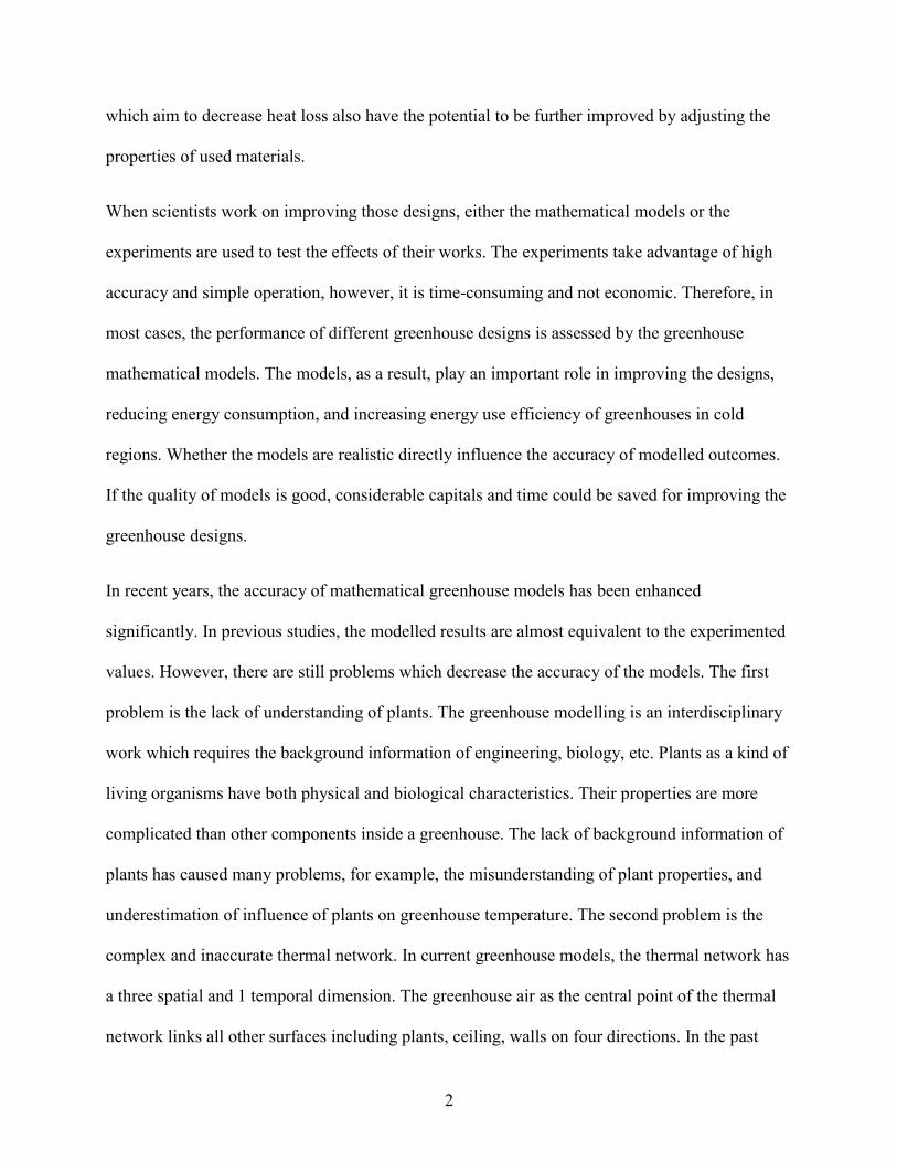
In recent years, the accuracy of mathematical greenhouse models has been enhanced

significantly. In previous studies, the modelled results are almost equivalent to the experimented

values. However, there are still problems which decrease the accuracy of the models. The first

problem is the lack of understanding of plants. The greenhouse modelling is an interdisciplinary

work which requires the background information of engineering, biology, etc. Plants as a kind of

living organisms have both physical and biological characteristics. Their properties are more

complicated than other components inside a greenhouse. The lack of background information of

plants has caused many problems, for example, the misunderstanding of plant properties, and

underestimation of influence of plants on greenhouse temperature. The second problem is the

complex and inaccurate thermal network. In current greenhouse models, the thermal network has

a three spatial and 1 temporal dimension. The greenhouse air as the central point of the thermal

network links all other surfaces including plants, ceiling, walls on four directions. In the past

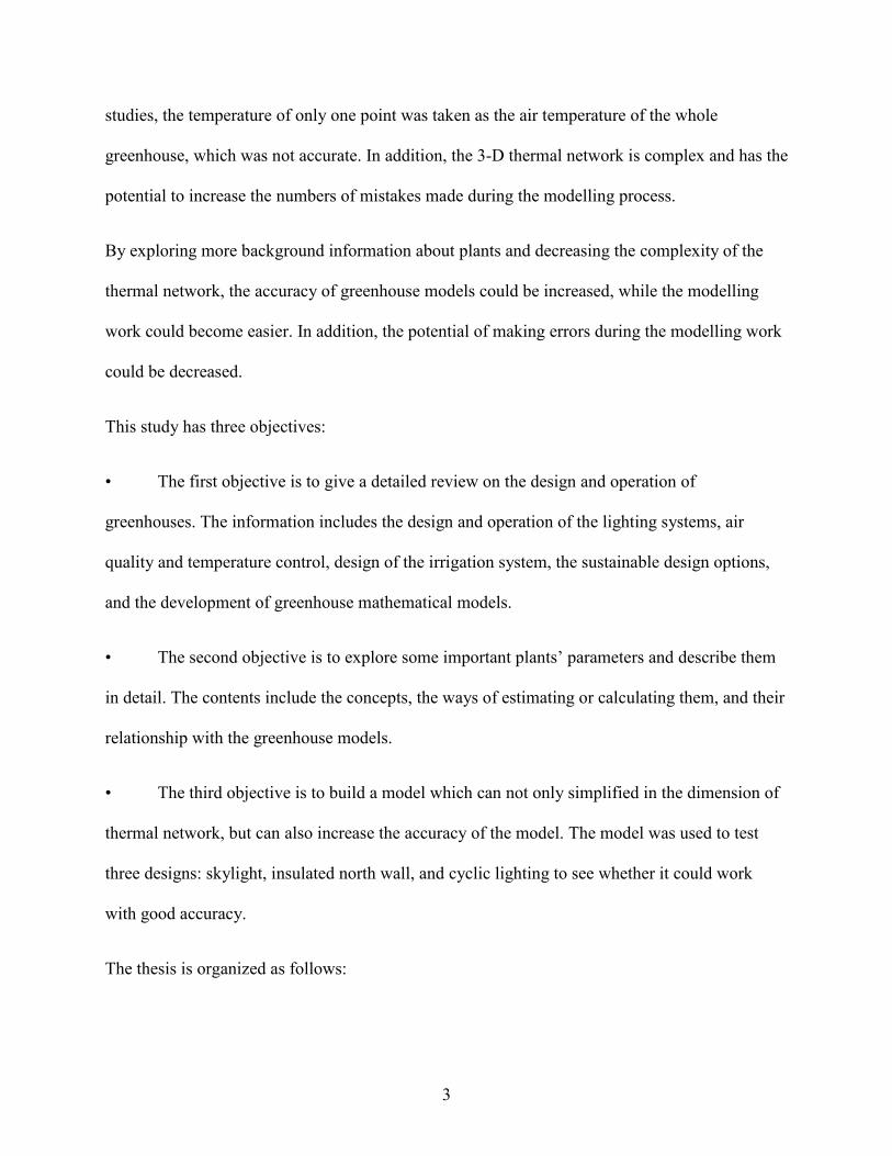
3

studies, the temperature of only one point was taken as the air temperature of the whole

greenhouse, which was not accurate. In addition, the 3-D thermal network is complex and has the

potential to increase the numbers of mistakes made during the modelling process.

By exploring more background information about plants and decreasing the complexity of the

thermal network, the accuracy of greenhouse models could be increased, while the modelling

work could become easier. In addition, the potential of making errors during the modelling work

could be decreased.

This study has three objectives:

• The first objective is to give a detailed review on the design and operation of

greenhouses. The information includes the design and operation of the lighting systems, air

quality and temperature control, design of the irrigation system, the sustainable design options,

and the development of greenhouse mathematical models.

• The second objective is to explore some important plants’ parameters and describe them

in detail. The contents include the concepts, the ways of estimating or calculating them, and their

relationship with the greenhouse models.

• The third objective is to build a model which can not only simplified in the dimension of

thermal network, but can also increase the accuracy of the model. The model was used to test

three designs: skylight, insulated north wall, and cyclic lighting to see whether it could work

with good accuracy.

The thesis is organized as follows:

4

The literature review was placed in chapter 2. In chapter 2, summarized information for all

aspects, including the design and operation of lighting, ventilation, irrigation systems. The

sustainable design options, which can decrease the demand for grid electricity and thermal

energy, are also introduced. In these parts, background information, the properties of materials,

and the performance of designs under different environmental conditions, could be found. In the

last part of chapter 2, the history of development of greenhouse models, the current situation, the

potential problems and potential solutions are all described. In chapter 3, the plants’ parameters

which are often used in greenhouse models are introduced in three parts separately. The

parameters are leaf area index (LAI) and canopy cover (CC), transpiration and

evapotranspiration, and boundary layer resistance. In the last part of chapter 3, heat and mass

transfer of plants are described by providing the thermal network and the heat balance equation

of a plant surface. The figures which plot the evapotranspiration rate against the indoor air

temperatures and the net radiation are displayed. The paper structure could be more

comprehensive because of the introduction of plants’ background. In chapter 4, the simplified

greenhouse model is given in the first part. In the next part, the equations and parameters used

for calculating all the heat transfer components in the model are provided. In the last part of

chapter 4, the model is applied in three advanced designs: transparent and vertical ceiling,

insulated north wall, cyclic lighting to test and compare their energy consumption. Finally, in

chapter 5, a conclusion will be given based on the outcomes in chapter 3 and 4. Chapter 2 had its

conclusion at its end.

5

Chapter 2. Literature review

Agriculture is an important and basic industry in the world (Howden et al., 2007). It has great

influences on the economy, social activities, environment, energy and land use. In 2018, it

accounted for approximately 30% of the total income in low GDP countries, and 33% of the ice-

free land usage over the world (Ramankutty et al., 2008). It supports the livelihoods of many

people in the world, while it provides considerable job opportunities (Sissoko et al., 2011). The

rapid increase in the world population gives rise to an increase in the percentage of land occupied

by intensive agricultural production. The intensive agriculture is defined as the farming practices

which aim to obtain maximum yield within a small area without considering the environmental

sustainability. Typical examples are heavy use of pesticides and chemical fertilizers, which can

cause a number of environmental impacts. The degradation of soil due to the intensive usage of

pesticides and fertilizer, loss in biodiversity, the discharge of harmful chemicals into aquatic

ecosystems, the release of greenhouse gases (GHGs) and other gaseous pollutants into the

atmosphere are typical examples of the negative impacts of intensive agriculture (Tsiafouli et al.,

2015). In addition, intensive agriculture has a higher demand for fossil energy due to excessive

input of mineralized N-fertilizer (Haas et al., 2011). The fossil fuels include coal, oil and natural

gas (Herzog& Golomb, 2004). In 2010, 87% of global energy was generated from using coal

(28%), oil (38%) and natural gas (21%) (Bose, 2010). These energy sources are non-renewable,

and energy production by using them can result in the release of pollutants which impose

negative impacts on both environment and living organisms.

To increase productivity and land-use efficiency, and reduce environmental impact during

agricultural production, the wide-range application of greenhouses is important. The widely

usage of greenhouses is a good alternative of open-area intensive agriculture, since

6

environmental parameters and energy sources of greenhouses could be adjusted and enhanced

based on specific plant requirements. By providing desired environmental conditions, a higher

yield per unit area could be obtained. In addition, the location of greenhouses can be everywhere,

ranging from rooftops to remote areas. The occupation of these areas to cultivate crops increases

both the biodiversity and land-use efficiency. Ultimately, some equipment like solar PV panels

and wind catchers can be hybridized with greenhouses to make use of clean and renewable

energy. Consequently, the environmental impact is diminished and energy use efficiency is

increased.

Greenhouses are especially important for cold regions. The application of greenhouses to support

crop growth is more necessary than that in temperate, subtropical and tropical zones. In cold

regions, the regular growing season is short, and the winter is cold, long, and snowy. The low

mean temperatures are not desirable to have high-yield and high-quality crops. To promote plant

growth, it is suitable to maintain a temperature above 12 ℃ continuously (Von Zabeltiz, 1992).

In order to extend such an environment condition beyond the regular growing season in cold

climates, the application of greenhouses is essential. Other than suitable indoor temperature,

greenhouses can also provide desirable relative humidity, and CO2 and O2 concentrations for

plants. Additionally, the usage of greenhouses can significantly reduce the number of fuels used

and decrease the costs of imported food, long-distance food transportation and food storage

(Golicic et al., 2011). In countries that have cold climates, the percentage of capital consumed in

food importation is larger than that in moderate and hot regions. For example, in Canada,

approximately 30% of the agricultural and food products were imported (Kissinger, 2012). If

more greenhouses could be constructed to produce food, the availability of local fresh food

products is expected to be higher. As a result, there will be lower demand for imported food.

7

The most significant problem of building greenhouses in cold regions is the greater energy

consumption which is mainly supported by fossil fuels. To maintain a desirable environment,

greenhouses consume both electrical and thermal energy. The main systems which are used for

maintaining the greenhouse environment are lighting, ventilation, heating and cooling systems.

In addition, an irrigation system is also considered as one of the main energy-consuming

components, especially for hydroponic systems. In cold regions, the great energy consumption of

the greenhouses, especially for space heating and lighting can impose economic burdens on

greenhouse owners and result in an increase in production costs. Based on Posterity Group

(2019), Ontario was the province which occupied 60% of the total greenhouse area in Canada. In

2018, 4x106 MWh of natural gas was used in space heating of greenhouses in Ontario, while 105

MWh of grid electricity supplied energy to greenhouse lighting systems. Around 73% and 18%

of energy were supported by natural gas and electricity, respectively. The main energy sources of

conventional greenhouses were the electricity and thermal energy generated from combustion of

fossil fuels, and the amount of energy consumed was not small.

To save energy and increase energy efficiency for the greenhouses in cold regions, innovative

greenhouse designs are necessary. The improvement in greenhouse designs can directly reduce

energy consumption and increase use of sustainable energy (e.g. solar heat gain). By increasing

the percentage of sustainable energy, the energy efficiency can also be increased (Lidula et al.,

2007).

Currently, there are review papers like Cuce et al. (2016) which summarized energy-saving

strategies for greenhouses. Yet, the general evaluation of each method or material, and operation

strategies are still not available. In addition, review with focus on cold regions is not available.

8

Therefore, a comprehensive review of energy-saving strategies of greenhouses in cold regions is

needed to find a way of reducing energy consumption in all related elements within greenhouses.

The objective of this project is to conduct a comprehensive review of the design and operation of

energy-efficient greenhouses in cold regions. Information from previous studies on main

greenhouse functions, lighting, ventilation, heating, and irrigation, are critically reviewed, and

energy-saving strategies are presented, as well as the numerical modelling. The evaluation

metrics of each approach and/or equipment are percentages or amount of total energy saving,

promotion in plant growth, initial costs and maintenance costs, etc.

In the following sections, research findings and technologies on lighting, ventilation, heating,

and irrigation functions will be presented. For each of these functions, the background plant

sciences will be provided. Different approaches to minimize energy consumptions and the

utilization of renewable energy will be presented. One section is devoted to the state of the art in

modelling since numerical modelling is an important approach for improving the energy design

and sizing energy systems. In the lighting system part, three popular light system designs will be

introduced based on their energy consumption energy efficiency, heat production and some other

energy related factors. The operation of lighting system will be analyzed in terms of availability

of natural light and requirement of different plant species. The “Air Quality and Temperature

Control” section provides information about the management of natural and forced ventilation

systems to maintain desired greenhouse air quality for plant growth. The irrigation system part

presents how to hybridize sustainable energy with the irrigation systems to save energy, and how

to adjust the water supply rate based on the evapotranspiration rate. In the sustainable design

part, solar energy, wind energy and geothermal energy are proposed as three sustainable energy

resources which have potential to be applied in greenhouses. Distinctive types of envelope,

9

energy storage, and HVAC system designs which aim to make use of renewable energy

resources are described. Ultimately, in the greenhouse model part, a review will be done on the

previous researches. The information includes the purposes of building models, potential

problems and expected solutions.

2.1 Lighting

2.1.1 Background scientific information

Lighting is an important component of the operation system of greenhouses. It influences the

yield and quality of crops. Crops can only complete their photosynthesis process and grow under

Photosynthetically Active Radiation (PAR), which has a wavelength spectrum from 400 to 700

nm (Prabhas et al., 2018)..

A greenhouse lighting system normally consists of two parts: daylighting and artificial lighting.

Daylighting is an important factor of energy consumption of greenhouses since it influences the

amount of artificial lighting and heating required. The solar radiation provides both heat and

light with different wavelengths including PAR, which are necessary to plant growth. In an

indoor environment like greenhouses, quality, duration, and intensity of artificial lighting can be

influencing factors of absorption of PAR by plants. Except for plants that do not prefer long-time

light exposure, plant growth is facilitated by the application of suitable supplemental lighting.

Adams et al. (2008) examined the response of petunias, impatiens, and tomato to 8-hour day

extension (DE) lighting (4pm-12am). The data showed that in all cases, the addition of artificial

lighting gave rise to the promotion of plant growth. The promotion of plant growth was observed

as increases in specific leaf area; increases in chlorophyll content; and changes in growth habit.

In Impatiens and tomato. All these outcomes resulted mainly from a positive effect of

supplemental lighting on photosynthesis. Ultimately, it was found that when the ambient light

10

levels were low (the estimated range was 0-24W/m2), a small increase in photosynthesis which

resulted from the addition of artificial lighting, could facilitate plant growth greatly.

2.1.2 Envelope design for natural lighting (transparent materials)

In order to increase the transmission of PAR and control the heat loss/gain from the exterior

environment, the envelope design is very important. For the lighting system, the proper envelope

design can increase the percentage of PAR transmitted, and avoid the problem of high-intensity

lighting during summer. In order to increase the transmissivity, transparent materials are

preferred to be selected for the main envelope, and shading or movable insulation can be used to

diminish the heat loss problem during winter and overheating during summer. In this section, a

technical and economic analysis is presented for some commonly used transparent materials in

greenhouse envelope.

Polyethylene (PE)

Polyethylene as one type of glazing products is widely used in greenhouse coverings for a long

time. It takes advantages of its low initial costs and high capability of diffusing light inside

greenhouses. A number of researches had investigated the spectral and thermal properties of

polyethylene. Kittas & Baille (1998) tested the spectral properties of three types of polyethylene:

low-density polyethylene film (LDPE), thermal polyethylene film (TPE), and bubbled

polyethylene plastic film (BPE). One of the tested spectral properties was the PAR transmission

(ƮPAR, 400-700nm). The results showed that both the LDPE and TPE showed 0.57 to 0.85 PAR

transmission which is higher than that of BPE. Zhang et al. (1996) conducted an energy

consumption assessment of four greenhouse covering materials: single glass and three kinds of

double polyethylene coverings. The results showed that the double PE which consisted of

standard PE and anti-fog thermal film was the most energy-efficient covering. It had an average

11

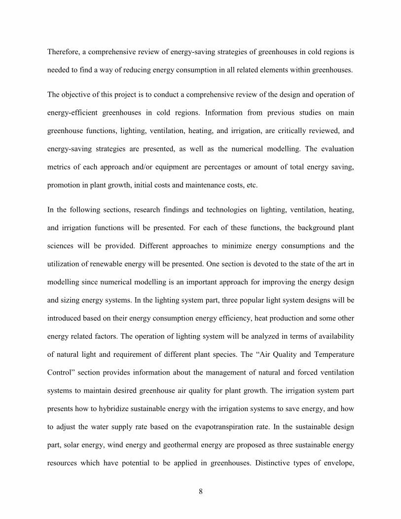
heat transfer coefficient (U value) of 2.9 W/m2. K, while for the other two kinds of double PE,

their average U value was 3.4 W/m2. K.

In most applications, PE is not used independently as a greenhouse covering material. It is often

hybridized with additives, other coverings or another layer of PE in order to enhance the

functionality in some desired aspects. Cemek & Demir (2005) tested the light transmissions by

using four greenhouse covering materials: UV stabilized polyethylene (UV+PE), IR absorber

polyethylene (IR+PE), polyethylene without additives (PE) and double layer PE films (D-Poly).

The thickness of four coverings was kept at 150μm. One more factor involved in the test was the

condensation state, which mean that the experiments were conducted under both the dry state (2

pm) and the wet state (7 am). The results indicated that from June to August, the highest

transmission loss was observed in the D-Poly treatment for both dry state (15.3%) and wet state

(17.4%).

Most polyethylene films have higher average light transmission percentages than other covering

films, however, the relationship between the transmission of PAR (or solar radiation) and yield

(or growth) of plants is complicated (Fabrizio, 2012). Both duration and intensity of solar

radiation are not proportional to the yield of plants. Depending on plant species, weather and

environment, the increase in transmittance of solar radiation into greenhouses can either promote

or inhibit plant growth. Therefore, detailed assessment and comparison which involve the

requirement of plants, local weather and environment need to be manipulated before making the

final decision

Polycarbonate （PC）

Polycarbonate is also used broadly in greenhouses as a cladding material. PC films have lower

light transmission than polyethylene films; however, it has been proven that they take advantage

12

of specific aspects. First, the polycarbonate sheets can give rise to thermal resistance without

reducing the amount of solar radiation transmitted. Fabrizio (2012) compare the energy

performance of the polycarbonate hollow sheets, traditional glass, and plastic films. The results

showed that the usage of PC sheets could result in a 30% energy saving without diminishing the

amount of light transmitted. Second, the PC materials have higher effective quantum

transmission - PAR transmission based on the number of incident photons and the relative

photosynthetic yield of each photon, than other covering materials including PE. Pearson et al.

(1995) evaluated the total percentage transmission and direct beam transmission of nine cladding

materials including polycarbonate. These two factors can be further divided into four sub-factors:

energy transmission (G), quantum transmission (Q), effective quantum transmission (E), solar

energy. The energy transmission calculated the transmission based on the amount of energy

received in a standard solar spectrum. The results showed that the polycarbonate led in all four

sub-factors in the direct beam transmission part. In the total percentage transmission part,

polycarbonate still performed well and obtained over 90% for all PAR related sub-factors.

The last advantage of PC is that it has high strength and long life expectancy, which means that

the potential maintenance and replacement costs are low.

Among the four transparent materials mentioned in this part, PC is the most comprehensive one

since it has a relatively low price, excellent light transmission, and high strength. For people who

consider more about long-term issues, factors like rates of annual reduction of light transmission,

life expectancy should be evaluated and compared with other available materials

Acrylic

Acrylic as a greenhouse cladding material is not as popular as PC and PE because of its high

initial costs and flammable property. However, based on Krywult et al. (2013), a single layer

13

acrylic plate has high transmittance (between 0.9 and 0.95) toward PAR. It is also very strong

and can tolerate strong wind and heavy snow, while it has a high life expectancy and can be used

for over 30 years (Berghage, 2017). In addition, it has a good capacity of reducing heat loss.

Short & Pang (1990) found that the installation of a 32-mm, double acrylic covering to a

greenhouse could result in 60-70% of heat loss reduction.

Acrylic costs more than PC and PE initially, but over a long-term period, it may cost lower

because of its long life expectancy and high strength. Therefore, it depends on how long do the

greenhouse owners want to replace their greenhouse coverings. If they want to replace the

coverings every 10 years, then acrylic is not a suitable choice. In addition, the flammable

property of this material needs to be considered, for the places which often have dry weather,

acrylic is also not a good choice.

Bubble wrap

Bubble wrap is seldom mentioned as a greenhouse covering material. It is often used for

packaging of products, and insulation for windows. It is made up of PE, so it has similar thermal

and optical properties with PE. Based on experimental results of Eggleston et al. (2013), the

thermal conductance of Mailer Type bubble wrap was 5.23 W/m2.K, while the thermal

conductance of single-layer large bubble wrap was 4.14 W/m2.K. If double-layer large bubble

wrap can be used, the thermal conductance could be further decreased, and the costs will not be

high.

2.1.3 Artificial lighting and Lamp selection

The design of the artificial lighting system is mainly the selection of lamp types, the ratio of

different pigments (e.g., blue and red) used. Among all types of lamps, the High-Pressure

Sodium (HPS) and Light Emitting Diode (LED) lamps are dominant because they have higher

14

efficiency than most types of traditional lamps, for example, the fluorescent and high-pressure

metal halide lamps (Moe & Gislerod, 2005). Therefore, in this part, the effectiveness of three

main lighting technologies: (1) High-Pressure Sodium (HPS) lamps (2) Light Emitting Diode

(LED) (3) Hybrid lamps (HPS+LED) in greenhouses will be reviewed, compared and discussed.

The LED will be discussed on the selection of pigments and the ratio of these pigments.

HPS

HPS lamps are often used to replenish lighting required for plant growth, especially during

winter. They were used in greenhouses earlier than LED lamps. It was found early that the

proper amount of light addition from HPS lamps could significantly increase the productivity of

plants. McAvoy & Janes (1988) conducted a research on the response of greenhouse tomatoes

under the natural light condition and the condition with the supplemental lighting from HPS

lamps over an 18-hour period for each day. For the seedling stage, the light intensity was 24

W/m2 (the original data was 50µmol m-2 s-1 for photosynthetic photon flux density (PPFD)),

while for the fruit production stage, the light intensity was 48 W/m2. Finally, the yield was

increased by 66% to 93%, showing that the HPS supplemental lighting treatment made

significant differences.

HPS as a lighting technique has a significant disadvantages: an excessive amount of heat

produced when compared to LED. The extra amount of heat production can give rise to great

energy loss. There were researchers as Gomez et al. (2013) found that under the conditions that

the increase in yield and quality were equivalent, the energy consumption of white HPS lamps

was significantly higher than LED lamps due to the lower energy efficiency. However, in cold

regions, the extra heat energy can be used to offset a part of demand for mechanical heating.

Based on different environmental conditions, whether the benefits generated from extra heat

15

production can cover the increase in electricity consumption need to be determined by doing

both energy and economic calculations.

In addition, there are sufficient evidences which show that the hybrid lighting (LED+HPS) works

better than LED alone, especially in cold regions. This will be described in detail in the hybrid

lighting part.

LED

LED is an advanced lighting technique that takes advantage of its low accumulative costs, high-

energy efficiency, specified wavelengths, and long life expectancy (Poulet et al., 2014). It is now

widely used for providing supplemental lighting for greenhouses. Its most significant advantage

is the increased energy efficiency and decreased energy consumption. Gómez et al. (2013) did a

detailed comparison between overhead HPS lamps and intracanopy LED towers in terms of

production and energy efficiency. The results showed that when HPS was replaced by LED, the

electrical conversion efficiency was increased by 75%, and the lighting cost per average fruit

grown was only 25% of the HPS treatment. Nevertheless, there was no significant difference

between productivity under these two supplemental lighting treatments.

For the most commonly used types of LED lamps, they are divided into three main groups based

on their pigments: blue or red light, blue and red lights, white light (Jen, 1974). For the growth of

plants, the red and blue lights are two basic supplemental light sources, since they cover the

entire range of PAR (Olle& Viršile, 2013). In most cases, the mature plants grown in sole red

light are larger and more vegetative, while the plants grown in sole blue light are smaller but

faster to flower and have seeds (Eskins, 1992). Therefore, for LED, utilization of the blue and

red lights can be cost-effective and energy-efficient ways of supporting plant growth. The

optimal ratio of red to blue lamps mainly depends on plant species, like for tomato, 5:1 was the

16

optimal ratio for higher fruit production (Deram et al., 2014). The white light, however, did not

show significant advantages when compared with the combination of red and blue light. This has

been proven by several researches, and there are two examples listed: Kim & You (2013) tested

the effect of red, blue, red and blue, red and blue and white, white and far-red light on growth of

Wasabia japonica. The results showed that the red and blue treatment showed significant

advantages when compared with other treatments. The dominant factors included the

aboveground biomass ,belowground biomass, and the total biomass. Sabzalian et al. (2014) did

experiments to test the effect of different kinds of lighting on the growth of Mentha species.

Based on the results, the plants grown under the red-blue LED treatment had the highest

photosynthesis rate, fresh and dry weight. For the white light treatment, however, there was no

significant difference between it and the sole-red treatment.

Hybrid lighting

The conventional lighting techniques like HPS are short in providing lights of certain

wavelengths like blue and far-red when compared to the solar PPF radiation (Ménard et al.,

2005). The photosynthetic photon flux (PPF) is a measure which values all photons within the

range of PAR (400-700nm). LED as an energy saving lighting strategy can provide almost all the

spectrum required by plants, however, in cold regions, the LED cannot provide extra heat as

HPS. Therefore, it is suitable to hybrid two or more techniques together in order to meet the

growth requirement of plants. Dueck et al. (2011) conducted a research on the effect of three

different lighting setups: HPS, LED, hybrid on the growth of tomato plants. The intensity of all

lamps was kept at 37W/m2, and the ratio of HPS to LED lamps in the hybrid treatment was

50/50. The results indicated that plants had higher photosynthesis capacity under LED and

hybrid lighting than under HPS. In addition, the least heating requirement was obtained in one of

17

hybrid treatments, which was the combination of top HPS lighting and LED inter-lighting.

Kumar et al. (2016) did a yield and cost comparison among three treatments: top HPS lighting

(control), HPS plus one row of LED inter-lighting, HPS plus two rows of LEDs lighting. The

productivity was increased by 22.3 and 30.8% respectively for additions of one row of LED and

two rows of LED treatments, while the corresponding costs (include electricity and capital costs)

were increased by 12.0% and 32% respectively.

The hybrid techniques are the most promising selection in terms of energy efficiency and product

quality, since the combination of two or more types of lamps can make the control of lighting

become more flexible. The main challenge for hybridization of techniques is the high complexity

of hybridization. For example, if LED and HPS lamps are used together in a greenhouse, it will

be hard to determine ratio of these two lamp types, and the way of arranging lamps is also a

difficult topic. The high capital cost is also a potential problem, but this is expected to be

diminished by the generated benefits over time.

Overall, the key points for selecting lamps are: 1. LEDs consume significantly less energy than

HPS lamps. Based on previous research, they have lowest yield potentials in most cases, but they

can satisfy the basic requirement of plant growth. 2. Hybrid lamps consume more energy than

LEDs but less than HPS lamps when the intensity or expected yield was equivalent. They give

rise to the highest yield and quality in most situations. 3. If the energy saving is considered more

for per unit yield, like energy saving per gram of fruit produced , then hybrid lamps are the most

promising choice. If the energy saving per unit area is considered more, then red and blue LED is

the best option. 4. The ratio of red to blue LED lamps depend on plant requirements. 5. After the

most suitable methods are picked up. Further analysis and comparison could be done among the

hybrid method (LED+HPS), HPS, and LED. The results are quite distinctive for different

18

climatic conditions (mainly the amount of available solar radiation), plant varieties, prices of

different lamps, current electricity rate, etc. In general situations, red and blue LED is the most

energy saving and economic option, but in cold regions, the hybrid lighting can work better.

A table which summarizes supplemental information for the three lighting techniques is attached

as follows. It further provides the evidence of summarized points above.

Table 1 Summarized information of some research focus on lighting techniques

Lighting conditions

Plants and growing conditions

Results

14-watt deep red

(DR)+white (W) +far-

red (FR) LED lamp

100 or 150 W

incandescent lamps

Two separate greenhouses at

Michigan State University (MSU)

Plant: day length-sensitive

bedding plants

An 150 W HPS lamp has a similar effect

on the flowering of bedding plants with a

14 W LED lamp

Annual energy consumption of two

lamps:

HPS: 876 kW h LED: 80.3 kW h

(Singh et al., 2015)

LED-LED: 128

W/m2(top light), 64

W/m2 (inter-light)

HPS – LED: 180

W/m2(top light), 64

W/m2 (inter-light)

HPS – HPS: 180

W/m2(top light), 56

W/m2 (inter-light)

Three separate 50m2 greenhouse

compartments in Natural

Resources Institute Finland

(60.39°N, 22.55°E).

Plant: Greenhouse

cucumber

LED-LED: highest light use efficiency,

but had lowest yield potential.

HPS – LED: highest fruit yield, but had

lower electrical use efficiency than LED-

LED. (Särkkä et al., 2015)

HPS (top light)

Wageningen UR greenhouses

LED: lower production

, highest energy saving per kilogram

19

LED (top light)

50/50 hybrid lamps:

HPS (top light) +LED

(inter-light)

Light intensity was

maintained at 170

µmol m-2 s-1

(~37W/m2)

Plant: Small Santa type tomato

plants

tomato

Hybrid: highest energy saving per

kilogram tomato (same as LED)

Small differences in fruit quality (Dueck

et al. ,2011)

1000 W overhead HPS

600 W overhead HPS

Intracanopy LED

towers (95% red + 5%

blue)

Greenhouses in in a northern

climate (40°N. latitude, West

Lafayette, IN, USA)

Plant: High-wire greenhouse

tomato

LED: 75% and 55% energy saving when

compared to 1000 W HPS and 600 W

HPS treatments, respectively.

No significant yield differences among

three treatments. (Gomez et al., 2013)

Target red + blue

LEDs

Full coverage red+

blue

Full coverage white

LEDs

16-day treatments

(Target: LEDs placed

only directly above

plants

Full coverage:

overhead)

Walk-in chamber of 9.29 m2 floor

area

Plant: Leaf lettuce

Target red + blue: lowest in total energy

consumption (9.6 kW h) and highest in

conversion efficiency (1.61 g/kW h)

Full coverage red + blue: highest in total

energy consumption (23.6 kW h) and

lowest in conversion efficiency

(0.86g/kW h) (Poulet et al., 2014)

HPS

100: 0 Red/Blue LEDs

85:15 Red/Blue LEDs

70:30 Red/Blue LEDs

Intensity: was

maintained at 70 µmol.

Plant: New Guinea

impatiens, geranium and petunia

(The greenhouse conditions were

not stated in detail)

Daily energy consumption:

HPS: 3.01 +1.49 kW h(fans used to do

the cooling)

100:0 R/B LEDs: 3.29 kWh

85: 15 R/B LEDs: 3.43 kWh

70: 30 R/B LEDs: 4.06 KWh

Blue LEDs consume more energy than

red ones (Currey & Lopez, 2014)

20

m–2.s–1

2.1.4 Lighting operation

The four main variables of lighting operation which will be discussed are duration, intensity,

interval and time. The duration is the total length of daytime and turn-on time. It is important

because it affects the all the growth stages of plants, especially the flowering stage (will be

discussed in detail in 2.2.1 section). The intensity is the density of light per unit area and/or per

unit time. It is indispensable because photosynthesis is a biochemical process which is light-

dependent. Within a suitable range, the photosynthesis rate increases as the intensity increases.

Hao & Papadopoulos (1999) conducted an experiment to test the growth, yield, and quality of

greenhouse cucumber with and without supplemental lighting. The supplemental lighting was

provided by 400W HPS lamps (54 W/m2 installed capacity) from 3 am to 7 pm, which was a

combination of day extension (DE) and night interruption (NI) lighting. The indoor temperatures

were kept at 21 ℃ in daytime and 17 ℃ at night, respectively. The results showed that the

marketable fruit numbers (yield) and grade #1 fruit numbers (quality) both increased after the

treatment of supplemental lighting. On the other hand, high intensity lighting can result in

negative responses from plants (Leyla et al., 2018). The interval is the way of distributing light

period and dark period within a day, continuous and intermittent lighting have different

performance in terms of promoting plant growth (discussed in 2.2.2). The time is the time points

which the lighting system starts and stops working. It also affects the performance of a lighting

system on facilitating plant growth.

Duration and intensity (W/m2)

The duration and intensity of lighting are not only necessary factors of energy consumption of

greenhouses. They are also strongly related to the flowering of plants. Plant species on the earth

21

are classified three groups: long-day plants, short-day plants and day-neutral plants. A long-day

plant only flowers when it is exposed to sunlight longer than a certain critical length. Potato,

lettuce, spinach are all long-day plants. Oppositely, a short day plant requires a longer dark

period to flower. Rice and onion are short-day plants. A day-neutral plant, however, the length of

daylight exposure does not affect the time it needs to flower. Typical examples of day-neutral

plants are tomato and cucumber. Depending on the cultivated plants, the critical day length

varies. The general range of the critical length which could let both short-day and long-day

plants flower is 12-14 hours. (Garner, 1933)

The intensity of greenhouse lighting depends on both the daylight (the solar radiation) and the

artificial light. The intensity of solar radiation is affected by factors like latitudes, seasons, and

percentages of cloud coverage of the day. It varies significantly even within a few hours.

Therefore, the management of artificial lighting is necessary to maintain a suitable environment

for plant growth. In a greenhouse with a conventional lighting system, in winter, the light turns

on partially during the daytime when the solar radiation is too weak to support plant growth, and

turn on entirely when there is no solar radiation, and plants need supplemental lighting to

continue growing. The control of light intensity is not accurate but acceptable to support plant

growth; however, a large amount of energy was wasted because of the inaccurate control. In

current years, some advanced systems can adjust the numbers of turn-on lights instantaneously

based on the changes in daylighting and the set threshold value. A typical example is the

dynamic lighting control (DLC) system. The application of it on lighting systems can avoid

unnecessary lighting supplements and save energy. Researches that focus on the application of

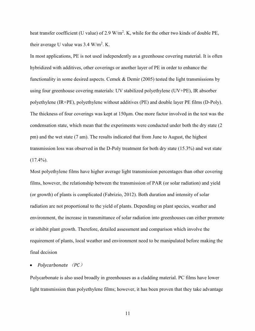
this system in greenhouses are summarized in the table as follows. All examples show that DLC

systems were energy saving when compared to the control (conventional) lighting systems.

22

Table 2 Summarized information of research focuses on the application of the DLC system in

greenhouses

Systems Greenhouse/plot and plant

conditions

Results

LED (36 warm white lamps, 13

W each)

LED-DLC (36 warm white

lamps, 13 W each)

HPS (2 lamps, 400 W each)

Photoperiod: 18-hours light (4am

to 10pm) and 6 hours dark (10pm

to 4am)

Greenhouses at Viikki, Finland

(60.228 N, 25.016 E)

Plant: Lettuce plants

LED-DLC: electricity consumption

reduce by 20% when compared to

the similar LED system. (Pinho et

al., 2013)

3 LED (54 W each, red: blue=

4:14) light bars

Threshold-based LED lighting

system: turning the all the lamps

on when the PPF was below a

specific threshold

LED-DLC: managing the duty

cycle of the lamps continuously

(every 5 minutes) based on PPF

values

Photoperiod: 14-hour light (6am

to 8pm)

A glass-covered greenhouse on the

Athens campus of the University of

Georgia

LED-DLC: energy consumption

save by 20% to 92%, depending on

the set PPF value and daily light

integral (DLI) from natural light

(Van & Gianino, 2017)

Greenhouse threshold control

strategy

DLC system

Plant: Tomato The application of DLC system

result in 12.3% increase in yield

and 30.1% decrease in energy

consumption. (Xu et al., 2020)

Threshold control (TSC): Top-

lighting LEDs and inter-

lighting LEDs were turned

off when outdoor global radiation

exceeded set boundary values.

A Venlo type greenhouse,

Shanghai, China (31°57’N,

121°70’E).

Plant: Tomato

The DOC system consumed

20.69% less electricity

than the TSC system. There was no

significant difference

between electricity consumption of

the DOC system and the DLC

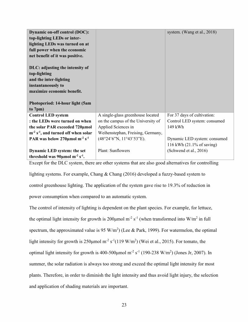
23

Dynamic on-off control (DOC):

top-lighting LEDs or inter-

lighting LEDs was turned on at

full power when the economic

net benefit of it was positive.

DLC: adjusting the intensity of

top-lighting

and the inter-lighting

instantaneously to

maximize economic benefit.

Photoperiod: 14-hour light (5am

to 7pm)

system. (Wang et al., 2018)

Control LED system

: the LEDs were turned on when

the solar PAR exceeded 720µmol

m-2 s-1, and turned off when solar

PAR was below 270µmol m-2 s-1

Dynamic LED system: the set

threshold was 90µmol m-2 s-1.

A single-glass greenhouse located

on the campus of the University of

Applied Sciences in

Weihenstephan, Freising, Germany,

(48°24’6”N, 11°43’53”E).

Plant: Sunflowers

For 37 days of cultivation:

Control LED system: consumed

149 kWh

Dynamic LED system: consumed

116 kWh (21.1% of saving)

(Schwend et al., 2016)

Except for the DLC system, there are other systems that are also good alternatives for controlling

lighting systems. For example, Chang & Chang (2016) developed a fuzzy-based system to

control greenhouse lighting. The application of the system gave rise to 19.3% of reduction in

power consumption when compared to an automatic system.

The control of intensity of lighting is dependent on the plant species. For example, for lettuce,

the optimal light intensity for growth is 200μmol m-2 s-1 (when transformed into W/m2 in full

spectrum, the approximated value is 95 W/m2) (Lee & Park, 1999). For watermelon, the optimal

light intensity for growth is 250μmol m-2 s-1(119 W/m2) (Wei et al., 2015). For tomato, the

optimal light intensity for growth is 400-500μmol m-2 s-1 (190-238 W/m2) (Jones Jr, 2007). In

summer, the solar radiation is always too strong and exceed the optimal light intensity for most

plants. Therefore, in order to diminish the light intensity and thus avoid light injury, the selection

and application of shading materials are important.

24

Theoretically, the shading materials can be any opaque materials, but the problem which is

needed to be considered is the absorption of solar radiation by materials. Black materials like

black mesh plastic can absorb solar radiation amply and heat the indoor environment, which is

not desired especially during summer. Examples of commonly used shading materials are

whitewash and aluminized shading screens (Kenig et al., 2005). The effectiveness of these

materials on reducing the transmission of lights with different wavelengths is summarized in the

following table.

Table 3 Optical properties of three shading materials (Kittas et al., 1999)

Treatments/Greenhouse

transmissions

(dimensionless)

Total(ƮT) PAR

(400-700nm)

(ƮP)

Near infrared

waveband (NIR)

(700nm-1100nm)

(ƮN)

Glasshouse 0.539 0.566 0.516

Glasshouse

with an aluminized

shade screen (70%

shading)

0.171 0.167 0.174

Glasshouse with an

external shade net

(30% shading)

0.401 0.421 0.384

Glasshouse with a

blanked (white-painted)

roof (35% shading)

0.349 0.378 0.324

The operation of a shading system is a part of the operation of the lighting system. When solar

radiation is strong and provides an excessive amount of heat and light, the percentage of shading

increases and protects plants from overheating and high-intensity lighting. When the solar

radiation is weak (e.g. nighttime and overcast days), the percentage of shading decreases based

on the set threshold. Typical examples of dynamic control systems are fuzzy systems that are

based on fuzzy set theory (FST) and fuzzy logic. Fuzzy set theory (FST) is a collection of

25

theories that were developed by Zadeh in 1965. The membership functions are built based on

linguistic terms which are described by subjective language. If the systems which are built based

on FST can be used to control the shading system, the percentage of covering can be adjusted

more accurately according to the availability of solar radiation. Azaza et al. (2016) designed a

fuzzy-logic based smart system to control greenhouse systems. For this shading system, there

were two input variables: solar radiation and outside temperature, the output variable was the

shading. There were three membership functions for the output: closed, half-open, open. The

results showed that the total energy saving (including shading and all other systems) of using the

proposed fuzzy system was 22% of the total energy consumption.

Interval and time: day extension (DE) or night interruption (NI), cyclic/intermittent or

continuous lighting

The management of time and interval of artificial lighting can be grouped into: day extension

(DE) and night interruption (NI) lighting, cyclic/intermittent and continuous lighting. There is no

evidence that the intermittent lighting works better than continuous lighting. A change in even

one of the factors such as plant species, light intensity, the light pigment can alter the final

outcomes. Oh et al. (2013) conducted experiments to determine the differences between the

treatments of cyclic/ intermittent lighting (CL) and continuous DE and NI. The experiments were

conducted in a 135 m2 plastic greenhouse which was divided into three identical rooms with the

area of 45 m2. The six treatments were: 9-hour (8 am-5 pm) exposure to natural sunlight (SD),

SD + 6-hour DE (5pm-11pm), SD + 2-hour (11pm-1am) NI , 4-hour NI (10 pm-2 am), 10% 4-

hour CL (6 min on and 54 min off for 4 hours), 20% 4-hour CL (6 min on and 24 min off). The

tested temperatures were 12 ℃, 16℃, 20℃. The results showed that the combination of 16℃

and 20% 4-hour CL was the optimal solution, which gave rise to an 83% reduction of cyclamen

26

production costs during winter when compared to the combination of 20 ℃ and 9-hour SD.

Sivakumar et al. (2006) compared the effect of continuous or intermittent radiation on sweet

potato plants. The six treatments were continuous and intermittent blue (B and IB), continuous

and intermittent red (R and IR), continuous and intermittent blue+ red (BR and IBR). The control

group was treated by cool-white fluorescent lamps (FL). The results showed that the growth of

sweet potato plants was better under the treatment of intermittent lighting than the continuous

lighting, and the IBR treatment enhanced the photosynthesis significantly when compared to all

other treatments.

The optimal interval of intermittent lighting is distinctive for different plant species. For Chinese

cabbage, 501 millisecond (µs) is the best duty cycle for Chinese cabbage under certain

conditions (Avercheva et al., 2016). For lettuce, two light/dark (L/D) cycles of 8 hour/4 hour

over a 24-hour period, and three L/D cycles of 6 hour/3 hour or 4 hour/2 hour could both

increase yield and quality of crop products (Chen & Yang, 2018). The one with three L/D cycles

consisted of two 6 hour/3 hour L/D intervals and one 4 hour/2 hour interval over a 24-hour

period. The exact optimal values of duration, intensity, and the ratio of pigments are also

dependent on plant requirements. In general, it is suitable to have less than 18-hour light period

for a day, since the dark period is necessary for all plant species, especially the short-day ones.

The short-day plants need day/dark cycles to complete their life cycles. If there is no dark period,

they will not flower. For the interval, the L/D cycles of 6 hour/3 hour could be a convenient and

general choice.

In general cases, night interruption is better than day extension lighting. In order to compare the

DE and NI comprehensively, Tewolde et al. (2016) did an experiment in the enhancement of

growth and yield of single-truss tomatoes by 12-hour DE lighting (4 am to 4 pm) and NI lighting

27

(10 am to 10 pm). The results indicated that when compared with DE lighting, the NI lighting

could promote plant growth effectively while consuming less energy in both summer and winter.

2.2 Air quality and temperature control

High-efficiency ventilation systems are indispensable for cold and humid areas (Flores-

Velazquez et al., 2014). In greenhouses, the air is often moist because of plant transpiration. If

the relative humidity is not controlled between 55% and 90% for a long time, the growth of most

plants will be limited (Grange & Hand, 1987). If the relative humidity often reaches 100%,

problems like condensation can occur. The ventilation systems are important because they take

responsibility of removing excessive humidity to prevent plants from crop mineral depletion and

fungal diseases (Mistriotis et al., 1997). They can also introduce fresh air that contains sufficient

CO2 and O2 to support photosynthetic and respiratory activities of plants. The optimal CO2

concentration for tomato plants was 600-800 ppm (Sionit et al., 1980; Zhang et al., 2018). For

most plants, 1000 ppm is verified as the boundary value of CO2 enrichment which can promote

plant growth, however, the global mean CO2 concentration in 2005 was 379 ppm (Mahesh et al.,

2014). Currently, the mean concentration rises to around 400ppm, however, it still do not reach

the optimal level for plant growth. Without the ventilation system, it is almost impossible to

reach CO2 concentration of above 600 ppm. Ultimately, the ventilation systems are also regarded

as a component of passive cooling systems, which can result in a great energy saving of

greenhouse cooling.

The natural ventilation is affected greatly by outdoor environment conditions. In winter, a forced

ventilation system can control the rate of air exchange properly to diminish the heat loss due to

the extreme indoor and outdoor temperature difference. In the meantime, the humidification

and/or dehumidification can be manipulated continuously to maintain RH between 55% and 90%

28

to support plant growth. In summer, natural ventilation is enough for greenhouses in cold regions

to release heat and enhance indoor air quality.

The proper application of both natural and forced ventilation systems in greenhouses can result

in great energy savings. Campen et al. (2003) calculated the energy savings of three forced

ventilation methods in greenhouses at northern latitudes when compared to the natural

ventilation method. All calculations were based on two Venlo-type greenhouses which had a

single and a two-layer glass covering respectively. The target species were tomato, sweet pepper,

rose, and cucumber. The energy savings were calculated for the whole cultivation period of all

tested plant species. Based on the calculation results, being condensation on a cold surface was

not an energy-efficient and cost-effective method, while the absorbing hygroscopic dehumidifier

had less suitability for practical usage. The most promising method was forced ventilation with

heat exchange. The energy cost savings of this method for tomato, sweet pepper, rose and

cucumber planted in single and double-layered greenhouses were $0.46/m2 and $0.66/m2,

$0.93/m2 and $1.39/m2, $0.73/m2 and $1.12/m2, $1.26/m2 and $1.99/m2, respectively. The

energy cost saving for tomato was less than the other three crops because of the lower air

temperature. Maslak & Nimmermark (2017) tested the performance of another widely-used

dehumidification method: air-to-air heat exchanger, and also did a comparison between this

method and the natural ventilation. The data used for simulations were collected from eight

10000m2 tomato greenhouses from April to September. For the leaf area index (LAI) of 3.5 m2

/m2, the total energy saving for these six months was 91 MJ/m2, which occupied 15% of the total

energy consumption. For LAI of 4 m2 /m2, the energy saving was 114 MJ/m2, which was 17 % of

the total use.

29

The proper integration of natural and forced ventilation systems could also result in great energy

saving while maintaining good indoor air quality. Coomans et al. (2013) did an energetic

performance assessment and comparison for two reference greenhouses and two ventilated

greenhouses, which were located in two facilities in Western Europe. The used systems were

semi-closed systems, which were a combination of forced and natural ventilation systems. The

results showed that the measured energy savings were 13% and 28% respectively for two tested

facilities.

In the areas where have extremely low temperatures during winter, the application of ventilation

can result in a small increase in energy consumption for heating, but it is necessary to maintain a

suitable indoor environment and cannot be saved. De Halleux & Gauthier (1998) did simulation

works in order to predict the performance of two kinds of ventilation systems. The results

indicated that the applications of on-off and proportional ventilation systems resulted in a 12.6%

and 18.4% increase in energy consumption of a greenhouse, respectively. Therefore, the

optimization of air exchange rates of ventilation systems is important for minimizing the energy

consumption of greenhouses in cold regions.

2.3 Irrigation

The irrigation system is also an important system, especially for hydroponic greenhouses. It

consumes a large amount of energy and water to operate. Globally, 70% of the demand for

freshwater comes from the irrigation system (Wada et al., 2013). For energy, it is difficult to

measure the energy consumption of an irrigation system as a single part; however, it is obvious

that it is a main energy-consuming part within a greenhouse. Based on the types of irrigation

systems, the amount of energy consumed could be significantly different. The drip irrigation

30

system is preferred in greenhouse cultivation because it can save a large amount of water and

energy.

The energy used for pressurizing water to the required rate could be fuels or electricity. The

overall efficiency of fuel-powered devices is often higher than the electricity-powered devices,

but the energy lost during the production and transportation process should be considered.

(Djevic & Dimitrijevic, 2004)

The energy consumption of irrigation systems can be reduced by making use of solar energy.

The related techniques are in development and have been used in greenhouses located in areas

where are remote and/or have dry weather. In these places, the imported electricity is not

sufficient to drive the whole irrigation system, and the applications of such techniques are

essential (Hassanien et al., 2016). The hybridized system is called the photovoltaic (PV) water

pumping system. Even though the direct hybridization of solar panels with a water pumping

system can result in low efficiency, the hybridized system is still a desirable alternative of the

conventional system which uses imported electricity. Energy consumption and environmental

impact can be reduced. In addition, the payback period of the hybridized is not long in most

cases, generally from 4-20 years, depending on the prices of agricultural products, interest rate,

electricity rate, etc. (Li et al., 2017). (Note that the optimization of PV sizes is also an energy-

saving strategy, but the size depends on not only the energy demand of the irrigation system.)

Another way of reducing the energy consumption of irrigation systems is to adjust the water flow

rate more accurately. The application of water to plants consume energy continuously, therefore,

the optimization of water flow rate should be implemented based on plant requirements. The

plant water demand could be estimated according to rates of crop evapotranspiration (ETc)

31

(Salokhe et al., 2005). For tomato, 75% of the ETc. is the recommended amount of water supply.

In general, 1.8L/plant/day is sufficient for tomato, and 75–80% of ETc is the recommended water

supply for crops inside greenhouses (Snyder, 1992).

Based on the equations, the evapotranspiration is affected greatly by two climate factors: solar or

extraterrestrial radiation and temperature (Hargreaves& Samani, 1985). These two factors vary

constantly, therefore, it is difficult to match the optimal value every time by using conventional

monitoring systems. In this case, dynamic systems like artificial neutral (ANN) systems can be

used to control the irrigation system. The ANN system can be trained by existing data, and then

predict the hourly water flow rate accurately by using measured hourly air temperature and solar

irradiation as inputs (Haddad et al., 2015). The increase in accuracy of water flow rate

adjustment can result in great energy savings and an increase in energy use efficiency.

2.4 Sustainable design options

Greenhouses consume both electricity and thermal energy to maintain a suitable indoor

environment. The electricity and thermal energy are mostly generated from the combustion of

fossil fuels, which lead to emissions of greenhouse gases and gaseous pollutants, releases of solid

hazards, and an extra amount of water usage (Cemek &Demir, 2005; Fabrizio, 2012; Pearson et

al., 1995; Martínez et al., 2016). The extra water usage is generated from the electricity

production process which uses fossil fuels as energy sources. The process requires both fuels and

water (Shaikh et al., 2017). In addition, the energy loss from the long-distance transmission and

multiple distributions of electricity occupy 8-15% of the total electricity production (Berghage,

2017). In order to reduce energy loss, mitigate environmental impact and increase energy

efficiency, the introduction of sustainable energy as alternative energy resources for greenhouses

becomes important. These energy resources take advantage of their sustainable and

32

environmentally friendly characteristics (Short & Pang, 1990). Among all sustainable energy,

solar energy and wind energy are the two most promising ones, since they have high availability

especially in remote and open spaces (Eggleston et al., 2013).

Solar energy as a kind of clean energy has been widely used in providing supplemental energy

for greenhouse heating system. It also has great potential to be used in greenhouse lighting. The

photovoltaic panels can be installed to support and adjust both daylighting and artificial lighting

(Xue, 2017). The transparent and semi-transparent PV panels can increase the amount of solar

radiation transmitted into greenhouses when compared to opaque envelope materials and

conventional PV panels (Yano et al., 2014). Even for the traditional PV panels, the extra

electricity provided by PV panels can offset the loss of solar energy caused by shading from PV

array (Cossu et al., 2014). As for the artificial lighting, LED can be supported easily by power

generated by PV systems (Wang et al., 2017). Consequently, by making use of PV techniques

properly, the energy consumption of lighting systems can be significantly compensated. If it is

economic, large-area PV panels can afford the energy consumption of the entire lighting system

and even the whole greenhouse, but the supply can be unstable and become extremely low

during winter and overcast days of other seasons (Trypanagnostopoulos et al., 2017).

When compared to solar energy, wind energy is limited more strictly by geographical locations.

Based on the literature reviews, the applications of wind energy can be divided into two parts:

first, to do the passive cooling, which can reduce the energy consumption for cooling and

ventilation; second, to use the wind turbine to generate electricity to offset the energy

consumption of greenhouses (Hirth & Müller, 2016). Wind energy is used for heating and

cooling systems, like the research conducted by Mahmoudi et al. (2015), while the usage of wind

energy to offset the energy consumption of lighting systems is not explored sufficiently.

33

In order to be economic and energy-efficient, the wind-driven equipment or components like

wind catcher and wind turbines are recommended to be applied in greenhouses in remote areas,

where the wind power is not diminished by crowded buildings. The historical weather data can

be collected to see whether the place is suitable to use wind power to offset energy consumption.

In general, wind speed between 0 to 8 m/s is regarded as low wind speed, and wind speed of 10-

15m/s can drive a small wind turbine to its peak power (Yusuf et al., 2018).

Except the solar and wind energy, geothermal energy can also be considered as a sustainable

energy (Kristmannsdóttir & Ármannsson, 2005). In this part, different types of greenhouse

designs which aim to make use of these sustainable energy resources will be discussed.

2.4.1 Envelope design for natural lighting and thermal insulation

General envelope insulation

The envelope design involves the ceiling, wall and the floor design. There is a trade-off between

heat loss and transmission of PAR. The transparent and semi-transparent materials often have

greater heat transfer coefficient (U values) than opaque materials, while the opaque materials can

decrease the transmission of natural light significantly. For example, polystyrene as a group of

opaque envelope materials is widely used in greenhouse covering. The application of it on

greenhouses can significantly reduce the energy consumption when compared to conventional

materials (Feuermann et al., 1998). The experimental results from Elwell et al. (1983) indicated

that the filling of a 5.6 m × 29.3 m greenhouse roof by a 100–150 mm polystyrene layer in 45

minutes (and kept emptied for 35 minutes) resulted in a 90% reduction in heat requirement

during nighttime. It works better as an insulation material than the energy curtain. For a 6 m × 12

m greenhouse, the estimated energy savings for the addition of curtain and polystyrene coverings

were 33% and 70%, respectively (Short & Shah, 1981). There are other commonly used opaque

34

materials like plywood, concrete, timber (hard and soft), and plasterboard and glass fiber.

Second, it is also recommended to find the envelope design which is the optimal solution to

balance the energy and economic benefit and loss. Whether the insulation is good depends on its

thermal properties and thickness. By having a material with high thermal resistance, or

increasing the thickness of a certain material, both two can decrease the heat loss significantly,

however, they can increase the initial cost for purchasing and installing the materials. In most

cases, researchers test several alternatives and chose the one which could obtain maximum net

benefit. Bambara and Athienitis published three papers from 2018 to 2019 to do energy and

economic analysis for some envelope design. In 2018, they tested three envelope designs in a

greenhouse located in Ottawa, Ontario, Canada. The three designs were single glazing, twin-wall

polycarbonate, and foil-faced rigid insulation (permanent or movable) plus the single glazing.

The results showed that any alternatives with the reflective opaque insulation on the north wall

gave rise to great reductions on electricity and heating energy consumption. In addition, the

maximum reduction in life cycle cost was achieved when the polycarbonate (on the west wall)

and the permanent insulation (on the north and east walls) were applied (Bambara & Athienitis,

2018a). In the same year, they also did the energy and economic assessment for two ground

insulation designs. One design was the combination of vertical insulation along the perimeter,

horizontal insulation beneath the greenhouse footprint, and a concrete slab over soil. In the

second design, the concrete slab was removed and the soil was unfinished. The results showed

the application of an insulation beneath the crop zone was not recommended because it increased

the life cycle cost. The highest energy saving was reached when insulation materials were

applied to both the perimeter and the surface beneath the floor zone (Bambara & Athienitis,

2018b). Near 2019, they started a research to test the performance of a semi-transparent

35

photovoltaic (STPV) cladding on the roof of a greenhouse. The results indicated that the design

was not economically attractive currently, but it will become a good alternative for enhancing

energy use efficiency and reducing energy costs of greenhouse operations (Bambara &

Athienitis, 2019).

Movable insulation/thermal screen/thermal curtain

One of the main problems of adding an extra layer of insulation material to the whole greenhouse

envelope is the reduction in transmission of effective solar radiation during the daytime. Instead

of this, the installation of movable insulation, or night thermal screen/curtain, is a

comprehensive, flexible and economic method of reducing heat loss during nighttime (Attar et

al., 2014). As a part of greenhouse insulation, it can be removed during the daytime to allow the

transmission of solar radiation, and it can be covered during nighttime to reduce heat loss.

Except for reducing energy loss, it can not only increase crop temperatures significantly during

nighttime but also reduce risks of condensation (Teitel et al., 2009). The materials which are

often used as thermal screen are single layers of polyethylene and aluminized polyester (Bailey,

1976). The costs of these materials are inexpensive when compared to concrete, block, and some

other envelope materials.

The thermal screens can be categorized into exterior and interior thermal screens. The interior

thermal curtain is preferred because the exterior curtain layer is more easily deteriorated by the

outside environment (Shukla et al., 2006b). The introduction of an internal screen alone can

result in a great energy saving of greenhouses. Based on the experimental results of previous

researches, around 30% of the total energy saving could be attained by using an internal screen

without considering other heating techniques (Huang & Hanan, 1976; Chandra & Albright,

1980). The exact percentages of energy savings depend on specific greenhouse conditions, local

36

weather, and local electricity rates, etc. By hybridizing the thermal screens with other heating

techniques or materials, for example, the rock bed storage system, significantly higher energy

saving (approximately 90% of the total energy consumption) can be reached (Albright et al.,

1978).

Hybridization of solar devices with greenhouses

Among three kinds of sustainable energy resources, the geothermal energy is the most stable

one; however, its application requires excavation work to install equipment (Templeton et al.,

2014). Wind energy is not stable and limited by geographical conditions. When compared to

these two sources, solar energy is more powerful, and it is easier to be used and managed. It

keeps changing, but the trend is regular based on seasons and latitudes. Even in winter days

when the solar radiation is weak, there are still around 6-hour daytime each day. The solar

devices is often installed directly on the greenhouse roofs, which is more convenient than the

installation of geothermal equipment. In addition, the integration of solar energy with

greenhouses can give rise to a reduction in both the demand for imported electricity and

emissions of greenhouse gases. Therefore, as a sustainable energy resource that has these

significant strengths, there are researches which focus on the hybridization of solar energy with

greenhouses. In this part, devices which are often used to hybridize solar energy with

greenhouses will be discussed.

Two main technologies that use solar energy to provide energy for heating greenhouses are solar

PV panels and solar thermal collectors. For the solar PV panels and solar thermal collectors,

there are diverse types of them, but in this part, the focus will be the concentrating types. The

reason is that the targets are residential greenhouses that have smaller areas. In order to reduce

the capital cost and increase the amount of energy generated, the concentrating devices are

37

recommended (Chemisana, 2011). For PV modules, the concentrating panels could be used

either independently to generate electricity (PV), or hybridized with solar thermal collectors to

produce both electricity and thermal energy (PV/T).

For both PV modules and solar thermal collectors, the most commonly used concentrators are

Fresnel lens, compound parabolic concentrators (CPC) and parabolic-trough concentrators (PTC)

(Segal, 2016; Joardder et al., 2017). Hussain et al. (2015) conducted a research to evaluate the

techno-economic performance of linear and spot Fresnel lens (LFL and SFL) solar collectors

used for greenhouses. The experimental greenhouses were tunnel type 2.21 m length × 1m

width× 0.8 height greenhouses. These two collectors had similar storage capacities and Fresnel

lens surface areas. The results showed that between 11 a.m. to 3 p.m., the period when the

energy demand of the greenhouse was low, the energy supplied by both LFL and SFL could

afford the load of greenhouses and had a surplus. From 7 to 9 a.m., when the building load

decreased from 569.4W/m2 to 491.7W/m2, the amount of energy supplied by LFL and SFL

increased from 451.4 W/m2 to 491.7 W/m2, and 491.7 W/m2 to 513.9 W/m2 respectively. In

conclusion, it was obvious that the systems in this study could not offset the energy demand

entirely in most times, but they made great contributions to the reduction in demand for imported

electricity.

Sonneveld et al. (2011) tested whether a photovoltaic/thermal (PV/T) module could cover the

energy consumption of well-isolated greenhouses in north European countries. The used

concentrators were linear Fresnel lenses. The results showed that the annual productivity of this

system was 29 kWh/m2 for electricity and 518 MJ/m2 for thermal energy, which was sufficient to

support normal operation of target greenhouses. Hussain et al. (2016) built models to calculate

the energy savings of concentrated photovoltaic thermal (CPVT) systems under three

38

assumptions. The assumptions were that the original heating sources of greenhouses were

electricity, kerosene, and diesel respectively. The results indicated that if a CPVT system was

installed to replace electricity, kerosene, and diesel, the life cycle savings (LCS) were estimated

to be $10201.34, $11554.58 and $15220.60, respectively.

For CPC, Feng et al. (2014) designed a kind of entity Compound Parabolic Concentrator (CPC)

as a greenhouse transparent covering material. The material was made up of many entity CPCs,

which mean that the material was plexiglass with high transparency. The bottom of these CPCs

was attached by compound parabolic cells which could generate electricity. The experimental

outputs showed that the lowest transmittance of 32% was obtained when there was strong

sunshine at noon. In the morning and afternoon, the transmittance was found to be 60%. In

addition, the power generated by using the surplus light was 6.2W/m2. Wang et al. (2015)

proposed a compound parabolic concentrator-photovoltaic / thermoelectric hybrid power

generation system (CPC-PV/TE), which was designed based on situations of greenhouses in

Northeast China. The system consisted of CPC, PV/TE system and flat heat pipe. It was

observed that the energy generation and efficiency of PV/TE system were increased after

hybridizing with CPC. The maximum power output obtained was 125.98 W, and the efficiency

was 20.06%.

For TPC, there are fewer researches focus on this concentrator when compared to CPC and

Fresnel lens. It has a higher heating capacity when compared to low temperature active solar

energy systems like flat plate solar collectors. The maximum value of its heating capacity is 250

℃. In addition, as a single-axis tracking concentrator, it is more flexible than stationary

concentrators like CPC. (de los Reyes et al., 2009)

39

There are other solar concentrators that have higher capacity and flexibility, for example, the

Parabolic dish reflector (PDR) and Heliostat field collector (HFC) (Tyagi et al., 2012). However,

they are not necessary for maintaining the desired indoor temperatures.

Solar glass

Solar glass is also called building-integrated photovoltaics (BIPV). It is defined as solar panels

which are designed to replace conventional covering materials (Peng et al., 2011). Currently, the

focus of most research is on the integration of solar glass with residential, commercial and

residential buildings to reduce energy consumption and greenhouse gas emissions (Pelland &

Poissant, 2006). The application of solar glass in greenhouses is still in development.

Based on “What is solar glass?” in 2016, there are two common kinds of solar glass: thin-film

solar glass and colorless PV glass. The colorless PV glass can work well in undesirable

conditions, but its initial cost is high and its transparency is limited. Thin-film solar glass is

designed to reduce heat gain, which can diminish the overheating problem during summer. In

addition, it can be designed into different forms, which can provide convenience and increase

aesthetics without significant heat gain loss. In addition, its initial cost is relatively low, which

ranges from $0.5 to $1.0 per watt (Barry, 2018).

2.4.2 Energy storage

In cold regions, the extremely low temperature or freezing is one of the environmental stress

which can injury organ, tissues of plants and even result in plant death (Levitt, 1980). In order to

maintain the environment consistency and avoid sporadic energy shortage, proper energy storage

technologies need to be applied. Depending on the types of stored energy, energy storage

materials can be grouped into materials which store latent heat (PCMs) and materials which store

40

sensible heat (e.g. soil). The sensible heat storage relies on the increase of the temperature of a

storage medium, while the latent heat storage is related to the transition of phases of materials

(Khan et al., 2016). In this part, phase change materials (PCMs) and other two commonly used

energy storage materials/techniques, will be reviewed, discussed and analyzed.

Rock bed storage

Rock bed storage is one of the most commonly used sensible heat storage techniques for

greenhouse heating. It has a high-energy storage capacity and low capital cost. The mechanism

of this technique is the combination of rock bed as the storage medium and the ventilators (Sethi,

& Sharma, 2008). The rock bed can be installed underground either inside or outside the

greenhouses. During the daytime, excessive heat is transferred to and retained by a rock bed with

the assistance of ventilators. During the nighttime, the stored heat can be used to warm up the

cold air inside greenhouses, and the direction of airflow. In order to diminish heat loss, extra

layers of insulation can be attached to the rock bed.

As a sensible heat storage method, rock bed storage does not have high-energy storage capacity

as PCMs when under normal conditions. However, it is powerful when compared to other

sensible heat storage techniques like soil heat storage. The experimental results of Bouhdjar et al.

(1996) showed that the introduction of a rock bed storage system to a 240m2 tunnel greenhouse

gave rise to a 7℃ elevation in greenhouse air temperature. The system which consisted of U-

shape pipes and nearly spherical gravels were buried at a depth of 60 cm under the greenhouse.

In general, the systems need to be buried at a depth between 40 to 50 cm (Sethi, & Sharma,

2008).

41

Phase change materials (PCMs)

PCMs as a large group of energy storage materials are widely used in greenhouse heating

because of their high capacity of storing latent heat. They have high-energy storage density and

can store latent heat of fusion without changing temperatures. A summarized table which shows

properties of some commonly used PCMs is attached as follows. Water, CaCl2.6H2O,

Na2SO4·10H2O and Na2HPO4·12H2O are all inorganic PCMs, and paraffin is an example of

organic PCMs. Capric acid-Palmitic acid is an example of eutectic PCMs. (Rathod & Banerjee,

2004). There are a large number of factors which can determine whether a PCM is good or not.

Three of the main key factors are melting point, latent heat of fusion per unit volume, density. A

suitable melting point, a high density and high latent heat of fusion per unit volume are all

necessary for a PCM to be considered as a good latent heat storage material (Nayak et al., 2011;

Alawadhi & Alqallaf, 2011). Other factors include limited or no supercooling during cold times,

low vapor pressure, etc. (Chaichan & Kazem, 2015).

Table 4 Properties of four common PCMs

Melting point, °C Heat of fusion, kJ/kg Density (solid), kg/m3

Calcium chloride

hexahydrate(CaCl2.6H2O)

(Alawadhi & Alqallaf,

2011)

30 170-192 1710

Disodium phosphate

dodecahydrate

(Na2HPO4·12H2O)

(Pielichowska &

Pielichowski, 2014)

35-45 279.6 1520

Paraffin (Buddhi et al.,

2003)

54 184 860

42

Capric acid-Palmitic acid

(Pielichowska &

Pielichowski, 2014)

22.5 173 870

Water can also be used as an energy storage medium. It has been widely used for storing thermal

heat for greenhouse heating. Its ability to store thermal energy is limited, however, it can still be

considered as an inorganic PCM. A typical example of the heating components which use water

to store energy is the solar water heater. Kalogirou (2009) studied the thermal and economic

performances of thermosiphon solar water heating systems. The results showed that when

compared to a conventional system, the new system could give rise to 70% of energy saving for

electricity or diesel backup. The payback periods for electricity and diesel backup were

calculated as 2.7 and 4.5 years respectively. Attar & Farhat (2015) developed a model to evaluate

the performance of a solar water system for greenhouse heating in Tunisia. The outputs of the

model showed that the system could independently meet the heating requirement of a 10m3

greenhouse. Even for a 1000m3 greenhouse, the energy cost was reduced by 51.8% on April after

the solar water system was applied.

Among all PCMs, CaCl2·6H2O and Na2SO4.10H2O are two main groups which are often used in

greenhouse heating. They take advantages of their high availability, low prices and relatively

high capacity of storing thermal energy. They are suitable to be used in small-scale greenhouses

and there are sufficient numbers of experimental outcomes can prove that. Benli & Durmuş

(2009) conducted a research to evaluate the effectiveness of an energy storage system on

reducing energy consumption of a greenhouse. In this energy storage system, the PCM

(CaCl2.6H2O) was integrated with ten pieced solar air collectors. The outputs showed that the

hybridized system saved 18%-23% of total thermal energy consumption when compared to the

conventional system. Nishina & Takakura (1983) did an experiment on the application of

43

Na2SO4.10H2O on a solar greenhouse in Japan. The total surface area of the greenhouse was

560m2. The greenhouse was large-scale, therefore, the amount of the PCM used was 2.5 tonnes

and the estimated value of stored energy was 105kcal. Finally, the target temperatures set for

different time periods were all reached without using supplemental heating, but the efficiency of

the PCM was not good (40–60%).

CaCl2·6H2O and Na2SO4.10H2O have significant strengths, but they are conventional PCMs

which still have potential problems like super cooling and phase separation. Therefore, they are

now often mixed with other PCMs with a suitable ratio in order to improve the properties of the

material. Hong-lia et al. (2008) selected Na2SO4.10H2O and Na2CO3·10H2O as base materials to

make new phase change material mixtures. In this research, five ratios (mass proportions) were

tested: 7∶3,6∶4,5∶5,4∶6 and 3∶7. The results showed that the only feasible group was 4∶6 since

both the transition temperature and latent heat of this mixture met the requirement of plants.

Jiang & Tie (2017) made three new PCMs by using industrial-grade Na2SO4.10H2O as the base

material in order to reach phase-change temperatures of 25°C, 15°C and 10°C respectively

(names of three treatments: PCM25, PCM15, PCM10). PCM25 was made by using 9.6 wt.%

Na2CO3·10H2O and 4 wt.% NaCl. PCM15 was prepared by adding 10 wt.% KCl and 10 wt.%

NaCl. PCM10 was produced by using 11 wt.% NH4Cl, 4 wt.% KCl and 2 wt.% K2SO4. The wt.

% here referred to weight percent, which was: the weight of solute/ weight of solvent×100. The

measured values showed that all three mixtures had suitable phase-change temperatures, high

latent heat, and thermal conductivity. For the latent heat, the values for PCM25, PCM15, PCM10

were 179.6, 129 and 116.2 J/g respectively. Zhang et al. (2010) did performance tests for two

PCMs mixtures: mixture 1 which was made up of Na2SO4.10H2O and Na2CO3·10H2O (mass

proportion: 46); mixture 2 which was composed of Na2SO4.10H2O and Na2HPO4·12H2O (mass

44

proportion: 1.97). The outcomes showed that for mixture 1, the super cooling and phase

separation phenomenon did not be eliminated. On the contrary, for mixture 2, the super cooling

and phase separation phenomenon could be diminished to an acceptable level, and the phase

transformation temperature was sufficiently stable.

Soil

Soil as an energy storage medium can store thermal energy as sensible heat. Like water, its

capacity of storing energy is not as high as PCMs, since the storage of thermal energy can give

rise to an increase in its temperatures. On the other hand, it is easier to be obtained and can be

used for both passive heating and cooling. Two of the most widely known applications of soil as

an energy storage medium are ground source heat pumps (GSHP), earth-to-air heat exchangers

(EAHE), the soil is used as a heat sink for these pumps and exchangers. Mongkon et al. (2013)

did an experiment to apply the horizontal earth tube system (HETS) to a 30m2 greenhouse. The

HETS was buried at the depth of 1m. The results indicated that used soil as a heat storage tank

could be used for passive cooling in tropical areas and the performance of HETS was acceptable.

The maximum coefficient of performance (COP) of sample summer days, monsoon days and

winter days were 3.56, 2.04 and 0.77 respectively. For summer days when HETS had the highest

COP value, the application of the system gave rise to a maximum energy saving of 74.84% of

the total energy consumption.

To study the performance of GSHP, Ozgener & Hepbasli (2005) did a techno-economic

comparison for a solar-assisted GSHP system for greenhouse heating. The experimental results

showed that if the ambient air temperature was not so low, the independent central heating

operation might met the total heating requirement of the greenhouse.

45

North wall

The installation of north walls can be a pathway of both reducing heat loss and storing extra heat

throughout an entire cycle with the effect of heat storage (Faraji, 2017). For east-west oriented

greenhouses located in the northern hemisphere, maximum solar radiation enters through south

walls and leaves through the north wall during winter times. If materials that have high thermal

mass, for example, brick and concrete, are applied on north walls, much more solar radiation can

be retained within greenhouses during daytime (Sethi & Sharma, 2008). During the nighttime,

the thermal energy stored on these walls is released and raise up the greenhouse air temperature.

The introduction of the north wall as an extra layer of materials can reduce the amount of energy

consumed by greenhouses significantly. Based on the experimental results of previous research,

the combination of the north storage wall and the buried pipe network, 30%-55% of the heat

demand of greenhouses could be offset (Santamouris et al., 1994). On the other hand, if the north

wall can be hybridized with energy storage systems or materials, a higher thermal storage

capacity can be reached. The most commonly used energy storage materials are the phase change

materials (PCMs). Berroug et al. (2011) hybridized CaCl2·6H2O with the north wall of a

greenhouse. They tested the thermal performance of an east–west oriented 24m2 greenhouse, the

north wall of which was made up of CaCl2·6H2O. The main input variables were all main

components of the greenhouse (plants, air, cover, PCM of the north wall), local weather (January

in Marrakesh) and the location of this greenhouse (31.62°N, 8.03°W). The results showed that

when the amount of PCM applied was equivalent to 32.4kg/ (m2 greenhouse ground area), the

night temperature increased between 6 and 12 °C. The mass of PCM applied in per square meter

of the north wall was 32.4 kg. The results also indicated that the application of this hybrid system

46

gave rise to a 6–12 °C increase and less fluctuation in nighttime temperatures during winter

times.

2.4.3 Energy-efficient HVAC techniques

Up to now, different kinds of heating and cooling systems are comprehensively developed and

can suit most conditions. For greenhouses, the most commonly used systems can be divided into

two categories: mechanical heating and/or cooling, passive heating/cooling. Mechanical heating

and cooling are often supported by HVAC systems, and the systems are often integrated with

energy storage and composite systems to save energy and diminish indoor temperature

fluctuations. In this part, composite systems that are based on geothermal exchange and other

kinds of heating systems will be discussed in terms of their principles and performance under

different conditions.

Geothermal exchange: composite systems

Currently, there are two commonly-used composite systems that can do both heating and cooling

will be discussed. They are the earth-to-air-heat exchanger system (EAHES) and the aquifer-

coupled cavity flow heat exchanger system (ACCFHES). These two systems work based on the

heat exchange between underground surfaces or underground water and outdoor air temperature.

The temperatures of underground layers are much more stable than the air temperature, in this

case, there is a concept named undisturbed ground temperature (UGT) (Gehlin & Nordell, 2003).

By exchanging heat with the underground layers, the outdoor air temperature which enters the

buried pipes could be warmed before entering the greenhouses. Since the UGT does not fluctuate

significantly for the whole year, the two systems could be used for both heating and cooling,

which makes them become two of the most commonly used systems in greenhouses.

47

According to the previous research, EAHES and ACCFHES have a similar capacity of

increasing and or decreasing temperatures. Ghosal & Tiwari (2006) did parametric modeling in

order to test the potential of an EAHES on maintaining the indoor temperature of a 24m2

greenhouse located in India. The outputs indicated that the introduction of EAHES to the

greenhouse could result in a 7–8 °C temperature increase in the winter and a 5–6 °C decrease in

the summer. For ACCFHES, the investigation results from Sethi & Sharma (2007a) showed that

the ACCFHES which had 0.47 kg/s air mass flow rate, and 12.63 m2 air and water contact area

could lower the temperature of a 24 m2 greenhouse by 6-7 K in extreme summer conditions and

increase the temperature by 7-8 K in extreme winter conditions. These two systems have

sufficient capacity to be integrated with the HVAC system to provide a more stable greenhouse

environment for plant growth. As supplemental systems for HVAC, they can offset the impact of

extreme conditions in which HVAC systems cannot respond in time without artificial

adjustment. Especially for places like Edmonton where has extreme weather, the hybridization of

these composite systems with the mechanical heating and/or cooling parts is good for saving

energy.

The composite systems are suitable to be used to save energy, in specific cases, if hybridized

with sustainable energy; they can even diminish the energy consumption to approximately zero

(Yildirim& Bilir, 2017). However, these systems require installation works and intensive

maintenance, which generate high initial and cumulative costs. In addition, in cold regions, the

pipes which are buried deep under the ground surface can be damaged by freezing. This makes

the repairing works more difficult. Therefore, it is recommended to do the economic and

technical assessment for installing composite systems for greenhouses. By evaluating the

48

payback period in the energetic cost aspect, it will be clear whether the benefits generated from

energy savings exceed the extra costs from complicated installation and maintenance works.

Ground air collector

The ground air collector (GAC) heats the greenhouses by making use of solar radiation. The

principle is that the pipes are embedded into the sand or concrete surface conduct heat to warm

up the cold air from the outside environment. The sand or concrete surface is heated up by

absorbing solar radiation. (Ghosal et al., 2005)

Like the two composite systems mentioned in the previous part, GAC can heat up the air and

raise the greenhouse temperature directly, and it can do the greenhouse heating constantly during

sunshine hours. Even during nighttime, the stored thermal energy can be used to support the

greenhouse heating. By doing the optimization based on local weather, the stored energy can

raise the greenhouse air temperature by 6–7 °C during nighttime in the winter season (Jain &

Tiwari, 2003). When compared to the composite systems, it takes advantage of the easiness to do

the installation, maintenance and inspection works, since the pipes do not need to be buried into

the depth of surfaces with UGT. However, the GAC requires extra installation of sand and

concrete surface, which increases the costs of installation and equipment purchases. In addition,

unlike the UGT which keeps constant for the whole year, the amount of solar radiation is

affected greatly by seasons, coverage of clouds, etc.

The heating capacity of GAC is higher than EAHES when the solar radiation is sufficient.

Ghosal et al. (2005) did performance assessments for both GAC and EAHEs for heating a

greenhouse located in Delhi, India. In order to do the comparison, the total lengths of pipes used

for the two systems were equal. When doing the experiments, the days were either clear or

49

sunny. Ultimately, the results showed that the greenhouse air temperatures with GAC were 2–3

°C higher than those with EAHEs. In addition, the stability of greenhouse air temperature with

GAC was also shown to be better than those with EAHEs. In general, GAC is a suitable heating

technique for greenhouses in cold regions, since it has a good heating capacity and it is energy-

efficient.

Ventilation Sustainable design

In cold regions, natural ventilation is sufficient for greenhouse cooling even during summer

times. It works based on the pressure difference between the greenhouse indoor environment and

outside. The management of natural ventilation is also a key factor in saving energy for

greenhouses in cold areas. The duration, interval, frequency, and rate of air exchange affect the

amount of heat loss significantly. As was stated by Sethi & Sharma (2007b), the factors which

influence the control of natural ventilation systems are sizes and locations of openings, the scale

of greenhouses, outdoor temperatures, wind speed, and wind direction. The interaction among

these factors makes the optimization of the air exchange rate become a complex issue. In

addition, the installation of insect-proof screens can also affect the management of natural

ventilation (Sethi & Sharma, 2007b). In order to diminish extra heating requirement due to

improper ventilation control, investigations that focus on the effect of these factors on managing

ventilation systems should be implemented. Ultimately, equipment like wind catchers can be

used to utilize wind power to do natural ventilation more effectively.

The natural ventilation can be manipulated by making use of sustainable energy like wind power.

The wind catcher makes use of wind power to do passive cooling, which can significantly reduce

energy consumption for cooling and ventilation, especially during peak hours in summer

(Saadatian et al., 2012). In addition, the usage of wind catchers can increase the efficiency and

50

stability of natural ventilation. Its operation principle is when the wind hits the wind catcher, the

wind catcher could create a positive pressure zone on the windward side and a negative pressure

zone on the leeward side. Because of the pressure difference and buoyancy effect, fresh air

moves in from the windward side, and the stale air moves out from the leeward side (Benkari et

al., 2017). Like the solar chimney, the operation of wind catcher does not require the support of a

mechanical system, which is both energy-saving and environmentally-friendly (Afshin et al.,

2016)

There are no sufficient researches focus on applications of wind catchers for greenhouse cooling

and ventilation, but there are evaluations that were carried out to test the performance of different

kinds of wind catchers in some buildings. In order to measure the feasibility of using wind

catcher for cooling, Mostafaeipour et al. (2014) did economic analysis for warehouses with

absorption chillers, underground warehouses, and underground warehouses with wind catchers.

As indicated by results, the construction of underground warehouses with wind catchers was the

most economic option, since the usage of wind catcher can save energy costs and reduce

environmental impact. Mahdavinejad & Javanroodi (2014) evaluated the performance of three

kinds of wind catchers: ARDAKANI wind catcher with one opening, KERMANI wind catcher

with two openings, YAZDI wind catcher with four openings. The results showed that the wind

catcher with one opening was not a good choice for natural ventilation. The wind catcher with

two openings was efficient enough to do natural ventilation for buildings, and it took advantage

of inducing air with different wind angles. The wind catcher with four openings was also an

efficient device, but its performance was better in hot regions.

Wind catchers have diverse designs and can function in different ways. For designs, there are

unidirectional, bidirectional, multidirectional and cylindrical wind catchers. Higher coverage of

51

different directions gives rise to better performance. For the ways of function, there are

downward airflow, upward airflow using wind and upward airflow. The downward airflow

works when a unidirectional wind catcher catches the wind and brings it down into the building

through a high, covered tower. For upward airflow using wind, the wind catcher is integrated

with an underground canal. The hot air is drawn down the tower into the canal and cooled by

ground or cool water, then the building will be cooled down by this air and the used air will be

drawn back up by the wind catcher. The principle of upward airflow is that the wind catcher is

used to allow hot air to escape from the building. (“Windcatcher”, 2020)

The solar energy can also be used in supporting ventilation systems. For fan-induced ventilation,

the fan can be hybridized with solar PV panels, which results in a reduction in demand for

imported electricity. In summer, high solar irradiance provides sufficient solar energy for PV

panels, and batteries and energy storage materials could be used to store surplus electricity. The

stored electricity could be used to drive fans, blowers, window window-opening motors over the

whole year. The heat extraction work is completed by water in winter (Rocamora &

Tripanagnostopoulos, 2006). Through the heat exchanger, some water is stored and circulated

during nighttime.

2.5 Numerical Modeling

When designing a greenhouse, modeling is an important pathway to predict the performance of

the design under different environmental conditions. In combination with specific experiments, it

can become a powerful and economic tool to optimize the design of every greenhouse

component and enhance the overall greenhouse design. Scientists initiated the greenhouse

modeling works for many purposes. In order to do the modeling work efficiently and accurately,

learning from previous research work is necessary. Collection, comparison and analysis of

52

previous modeling work are presented in this section in terms of their accuracy and the levels of

advancement. In addition, the potential problems of greenhouse model development and the

possible solutions are discussed.

2.5.1 Review and summaries of previous researches

Among all the greenhouse components, the heat exchange between the plant surface and other

surfaces is the most complex part for modeling. The different leaf ages and sizes, the distinctive

distance between leaf layers, spatial distributions of leaves, flowers, and fruits make the plant

layer become a porous and heterogeneous layer. In addition, even it is the same species, the plant

individuals in different growth stages have different shapes. All these factors give rise to an

increase in the complexity of predicting energy exchange between the plant layer and other

greenhouse components.

In order to explore the properties of plants, the experiments are necessary. The modeling work

for the whole greenhouse can only use the weather data as the input, since other parameters can

be estimated. For the plants, however, the experimental data is necessary for calculating some

parameters. The papers which focus on the detailed properties of the greenhouse plants can help

people from other areas know more about the plant science. The knowledge about how the

environmental variables affect the internal resistance and thus affect the thermal behavior of

plants is necessary while building a model for the whole greenhouse. By understanding this

knowledge, they can know whether their assumptions for the plant layer are reasonable and thus

build the model more accurately.

Papadakis et al. (1994) built a mathematical model in order to estimate the heat transfer between

a tomato plant and greenhouse environment. The heat storage of plants were divided into three

53

parts for calculation: the full spectrum net radiation, the transpiration and the sensible heat

transfer between the plant and the greenhouse air. In addition, the influence of four

environmental variables: the leaf temperature, the net radiation, the leaf water potential, and the

concentration of CO2 on the internal resistance of the tomato plant was determined. By

neglecting the influence of CO2 (taking the coefficient as constant and equal to 1) and using the

experimental data of rest three environmental variables, the function could be found out. As a

result, the relationship between the internal resistance and the environmental variables was

known. There were a large amount of experimental data input to calculate the internal resistance,

the full spectrum net radiation. The results which included the internal resistance, the full

spectrum net radiation, the leaf temperature, and the transpiration were validated by experimental

results and all showed high accuracy. In addition, the results also provided the curves which

showed that the plant and indoor air temperature was different in all times. The plant temperature

was always lower than the air temperature. In addition, the old leaves and young leaves had

different thermal behaviors. The old leaves had higher temperature than the indoor air during

mid-day, while the young leaves had lower temperature than the indoor air during the whole day.

In some cases, greenhouse models are developed to calculate the heat and mass transfer on the

system level. By predicting the total energy consumption, the performance of the greenhouse

design can be estimated. Since all the greenhouse components affect the heat and mass transfer

processes, every greenhouse elements needs to be considered during the modeling work.

Currently, researchers had built comprehensive models for greenhouses with different designs.

Based on different designs, they built heat balance equations for all major components inside the

greenhouses and set up the models. Taki. et al. (2016) developed a model for calculating the heat

transfer and energy consumption of a greenhouse. The greenhouse had an innovative (semi-

54

solar) structure. The energy balance equations for all the surfaces including the ceiling, the

thermal screen, the air below the screen, the air above the screen, the plants, the ground, were

built. All the calculations were based on the transient state, and the plants were considered for

both the sensible and latent heat transfer. The outputs were validated by experimental results and

showed high accuracy. Abdel-Ghany & Kozai (2006) built a model for calculating the heat and

mass transfer in a naturally ventilated, fog-cooled greenhouse. The greenhouse was a

conventional greenhouse with regular shape, and it did not have a thermal screen and any other

advanced design. Each heat transfer element like the convective heat transfer among surfaces

was defined, and the heat balance equations for the cover, the indoor air, the plants, and the floor

surface were built by using these elements. When compared with measured values, the results

including the indoor air temperature and the indoor relative humidity both showed high accuracy.

Consequently, the model performed well for the greenhouse design, and the assumptions were all

reasonable.

The greenhouse modeling works are also developed to test and/or optimize the functionality of

specific designs inside a greenhouse. The ventilation system, the heating system, the lighting

system, the greenhouse shape and orientation, are all examples of greenhouse design which can

be optimized based on the model outputs. Jain & Tiwari (2002) built a mathematical model in

order to optimize the design of the evaporative cooling system. The greenhouse was an even

span greenhouse with a brick north wall. The air was divided into zone 1 (from ceiling to the

upper edge of the cooling pad), zone (from the upper edge of the cooling pad to the floor). When

developing the model, heat balance equations were developed for walls and air in zone 1 and

zone 2, and the floor. Based on the outputs of the model, the parameters like length of

greenhouse, height of the cooling pad and mass flow rate were optimized in two zones. Sethi

55

(2009) built a thermal model for comparing the performance of greenhouses with different

shapes and orientations. The tested greenhouse types were single span, even span, uneven span,

vinery, modified arch and Quonset greenhouses. The length, width and height of these

greenhouses were kept equally. The heat balance equations were built for greenhouse plants,

floor and air. The results showed that the uneven-span greenhouse maintained the highest indoor

air temperature for the whole year, and the east west orientation was the best-suited orientation

for all latitudes to receive greater solar radiation during winter and less solar radiation during

summer.

2.5.2 Current development, potential problems, and possible solutions

The greenhouse modeling is an area which has been well developed. The equations for

calculating the heat transfer and/or mass transfer of every component were set up, even for some

components, there were different models which can be used to estimate the same subsection. For

example, for the evapotranspiration heat loss, it is a complex process which involves a great

number of biotic and abiotic factors. In previous years, a number of models were developed to

estimate the plant evapotranspiration rate. Among all models, there are four models which are

commonly used because of their high accuracy: Penman (1948), Monteith (1965), Stanghellini

(1987) and Fynn (1993) (Prenger et al., 2002). Stanghellini and Fynn models are more suitable to

be used in the greenhouse conditions when compared with other two models. The key factors

contained in equations of all these four models were vapor pressure deficit and the heat gain

from solar radiation. The vapor pressure deficit is the difference between the saturated vapor

pressure of air at current leave temperature and the actual vapor pressure. Without experiment, it

is difficult to obtain vapor pressure deficit at leaf temperature, since the data of the mean leaf

temperature is not available. Therefore, if one of these four models is used, it is better to have

56

experiments in order to have data of the input variable. If the people who do the estimation do

not intend to do any experiments, there are other formulas which only contain fewer variables as

the input. These formulas might not accurate as the four models stated above, but they could still

provide suitable outputs. De Graaf & Van den Ende (1981) collect formulas for calculating the

plant transpiration rates. These formulas have different variables, but the calculated results were

all located within the suitable range.

The diversity of models can help researchers find equations which are more suitable to be used

under different conditions. With different levels of data collection, and different environmental

conditions and designs, the optimal equations might be different. If the mathematical equations

for most components within a greenhouse can be selected based on the current environment, the

accuracy of the model is expected to be increased significantly.

On the other hand, the greenhouse modeling work still has potential problems which need to be

further diminished. The first problem is the feasibility of assumptions of models. Modeling work

is complex. It includes the calculation of many parameters. Some parameters are difficult to be

determined if every factor is considered, therefore, in order to simplify the models, the

researchers often made assumptions before setting up the heat balance equations. Some

assumptions are suitable and can increase the accuracy of the models, while some other

assumptions are not realistic and may cause a deviation of results from the true values. For

example, Ahamed et al. (2018) did the modeling work for a greenhouse. The calculations were

done based on the assumption that the greenhouse was located in a cold region. The ventilation

was assumed natural ventilation only, since the requirement for cooling was neglected. The

steady state was assumed for the calculation of the ground temperature. It is not correct, since the

greenhouse covering is transparent, and the transmitted solar radiation can affect the ground

57

temperature significantly. The solar radiation changes in a dynamic rate for a day, which cannot

be considered as the steady state. In addition, the longwave radiation heat transfer between the

plants and the ground, the ceiling and the ground, also affect the ground temperature and cannot

be ignored. The plant and the ceiling temperatures also kept changing dynamically for the whole

day. To solve the problems about the accuracy of the assumptions, researchers are recommended

to know more about the heat and mass transfer fundamentals and try to read more previous paper

to determine whether the assumptions are reasonable.

The second problem is the linkage of plants with other greenhouse components. Due to the inter-

disciplinary character of the modeling work, researchers who are not from the plant science or

related areas do not have deep understanding of plant behavior. In previous modeling papers, in

the conduction and convection part, the plants did not be mentioned. The convective sensible

heat transfer and the radiative heat transfer of plants were neglected, and the plants were not

considered as a part of thermal network. That is a common problem: only the heat consumption

of plant evapotranspiration is considered, which is not accurate. In other papers like Fitz- Fitz-

Rodríguez et al. (2010), the plants only occurred in the calculation of mass transfer part, and the

heat loss caused by the evapotranspiration process was neglected. Some papers like Najjar &

Hasan (2008) even assumed that the greenhouses were empty from the plants. These incorrect

assumptions had the potential to cause significant deviation from the measured (true) values,

since the plants played an important role in both mass and heat transfer. They should be

considered in both two plants and calculated carefully, because they involve abiotic and biotic

factors and are complicated.

In modelling the plants, most of the work has used simplified models. This is due to the

complicated characteristic of plants as a group of living organism. If everything is taken into

58

consideration, the modeling work can become complex, and the focus will not be the whole

greenhouse. In almost all cases, the plant layer needs to be assumed as a homogeneous layer with

uniform leaf and stem distribution. All plant individuals are assumed mature and there will be no

significant changes in their morphology. After that, the plant layer should be treated as other

surface and the heat balance equation could be built. For the heat exchange between the plant

layer and other surfaces, there were often two assumptions which made the calculations easier.

The first one is: the effect of CO2 concentrations on the evapotranspiration rate is negligible

(Taki. et al., 2016). The second one is that the evaporation from the floor (the soil) is combined

in the plant transpiration part and calculated as the evapotranspiration (the effect of evaporation

on indoor flow rate and other issues can be ignored) (Ahamed et al., 2018). Based on these

assumptions, the heat balance equation for the plant layer consists of four parts: the net radiation,

the plant transpiration, and the convective heat transfer between plants and greenhouse air, the

ground heat flux. All the plant calculations should be under the transient state rather the steady

state. The net radiation is the net heat gain of the plants from the solar radiation and longwave

radiation. The plant transpiration is the process through which the plants give off water through

stomata in all parts like leaves, flowers and stems. The latent heat loss is caused by the energy

consumption of the phase change of water. The convective heat exchange between the

greenhouse air and the plants was controlled by a special resistance: the boundary layer

resistance. It is defined as the convective heat transfer coefficient between the plant leaves and

the thin layer of calm air that surrounds these leaves (Ahmed et al., 2020). Its calculations is

always based on the characteristic length of leaves, and the indoor wind speed. The ground heat

flux was the conductive heat exchange between the ground surface and other surfaces. It is

affected greatly by moisture content of soil and percentage of canopy cover (Purdy et al., 2016).

59

The ground area with high soil moisture content and dense canopy cover always has negligible

ground heat flux.

In the future, the works which could be carried out to further improve the accuracy of the models

are the continuous improvement of the model toward the realistic situations. The realistic

situations are often more complicated. In order to reach this goal, more experiments should be

manipulated to investigate the properties of greenhouse components under different

environmental conditions. The plants, for example, their properties can be investigated by

changing variables like species, the growth stages, and the surrounding environment. By doing

experiments and collecting data, more specific formulas can be developed and thus improve the

accuracy of the model.

2.6 Discussion and Conclusion

Greenhouse is an important building type for cold regions because of the high growth

requirements of plants. There has been a large number of studies which focus on reducing the

energy consumption of greenhouses in cold regions, however, most of them are simply related to

the reduction in energy consumption of one or some components of greenhouses. The space

heating part is considered mostly, while the energy consumption of the rest of the greenhouse

systems, such as lighting, ventilation, and irrigation, is underestimated. To reduce the energy

consumption of these greenhouses effectively, the design of energy-saving techniques for these

greenhouses should be comprehensive, including energy, cost, and yield quality. In order to

reduce the energy consumption of greenhouses effectively, investigations on energy-saving

strategies for all necessary operation systems were implemented. These systems are lighting,

ventilation, heating, and cooling, and irrigation systems. The energy-saving strategies are

roughly grouped into energy conservation, an increase of energy efficiency and development of

60

sustainable energy. Based on the information obtained from technical surveys, the concluded key

points are:

· Lighting: Among LED, HPS, and hybridization of these two, the combination of the red and

blue LED, and the incorporation of LED and HPS are the two most promising options. The red

and blue LED is the most economical choice and can satisfy the growth requirement of plants,

while the combination of LED and HPS can optimize plant growth. The night interruption is

better than day extension lighting. Whether the intermittent/cyclic lighting is better than

continuous lighting depends on plant species. Tomato is sensitive to continuous lighting, so it

prefers cyclic lighting. The optimal interval of intermittent lighting is distinctive for different

plant species. The exact optimal values of duration, intensity, and the ratio of pigments are also

dependent on plant requirements. In addition, for the transmission of natural light, among all the

transparent materials, polycarbonate (PC) is the most comprehensive selection, since it has low

initial costs, good transmissivity, and high life expectancy. New and advanced materials like

solar glass have great potential to be a good greenhouse covering materials in the future. Shading

can be considered as a part of both lighting and envelope systems, the application of it during

summer times is necessary to maintain the desired indoor environment for plants (avoid

excessive lighting and heating).

· Ventilation: In many regions of Canada, the wind speed is high over a year. Therefore, the

usage of wind catcher and wind tower to do natural ventilation is a good way of saving energy.

Based on the wind speed and directions of different regions, the wind catcher could be selected

based on the coverage of different directions and the function ways. On the other hand, the

normal operation of forced ventilation is necessary to maintain the relative humidity, CO2 and O2

concentrations within suitable ranges.

61

Furthermore, it is energy-saving if wind power could be used properly to do ventilation, however,

the wind energy is affected greatly by geographical locations. Solar energy is also a good

alternative as an energy source substitute for fossil fuels and wind energy, but the costs of

installation and maintenance, and mismatch between supply and demand should be considered.

· Heating and cooling: the energy consumption of heating and cooling systems is considered

mostly by researchers, so there are different kinds of systems developed. In Canada, mechanical

heating systems are necessary since many regions have long, cold winter. Among all systems,

two composite systems: earth-to-air-heat exchanger system (EAHES) and aquifer-coupled cavity

flow heat exchanger system (ACCFHES) can do both heating and cooling. However, it is not

convenient and cost-effective to do the drilling works for small-scale greenhouses, and the

installation of pipes is expensive. Therefore, other heating and cooling systems like the

evaporative fan and movable insulation can be considered. Except for the passive heating and

cooling systems, energy storage materials can also be used to offset energy demand for heating

and cooling. The materials are divided into two groups: latent heat storage and sensible heat

storage. Phase change materials (PCMs) have higher thermal storage capacity than sensible heat

storage materials like soil, but they are not necessary to be used in small-scale greenhouses.

Instead, solar water heating systems are good choices to replace conventional systems, since they

have shorter payback periods, a smaller amount of greenhouse gas emissions and can result in

great energy savings.

· Irrigation: the energy consumption of irrigation systems mainly comes from the application of

water to crops. Therefore, the management of water flow rate based on plant requirements and

weather is important for saving energy. Generally, 75–80% of evapotranspiration rate (ETc) is

the estimated amount of water supply for crops inside greenhouses. ETc is affected significantly

62

by solar radiation and air temperature which kept changing, therefore, the application of dynamic

systems like ANN is recommended for controlling water flow rate.

· Modelling: There are three main purposes of doing the modeling work: to predict the

performance of a whole greenhouse or specific greenhouse designs under specific conditions; to

explore the properties of plants under indoor environment. For surfaces involved in greenhouse,

the heat balance equations need to be built to find the temperature changes. For plants, since they

are living organisms and have biological characteristics, the modeling work for them is more

complex than other greenhouse components. The plants release latent heat to the surrounding air

through the evapotranspiration process. It is difficult to calculate the evapotranspiration rate, so

assumptions need to be made to simplify the calculations. In addition, the convective heat

transfer coefficient between the plants and the greenhouse air has special properties when

compared with other heat transfer coefficient inside greenhouses. This difference is offset in the

final heat flux equation by the specific heat and density of air. There are potential problems of

current available greenhouse models. The three main problems are the high complexity of

thermal network, decreased accuracy due to unsuitable assumptions, and incorporation of plants

into the greenhouse models. These problems have the potential to be diminished by improving

greenhouse models toward the realistic situations continuously.

63

Chapter 3 Heat and moisture exchange between plants and air

In this chapter, the key variables defining the heat and moisture exchange between plants and

their environment are introduced. These variables are used in the mathematical models and will

be presented in the following chapter. The variables include leaf area index (LAI), canopy cover

(CC), boundary layer resistance, transpiration and evapotranspiration rate. LAI is used to

determine the total area of leaves, and CC is for calculating the percentage of ground covered by

plants in terms of LAI. The LAI is related to both sensible and latent heat (moisture) transfer

between plants and air. The canopy cover is related to the calculation of solar radiation and

absorbed by plants and ground and the longwave radiation absorbed and/or released by the plants

and ground. The boundary layer resistance is related to the sensible heat transfer between plants

and air. Transpiration and evapotranspiration rate indicate the amount of latent heat transfer from

plants to the air. The estimation or calculation of these variables are given. In addition, curves

which showed the relationship between LAI and CC, boundary layer resistance and its limiting

factors are also displayed.

3.1 Leaf area index (LAI) and canopy cover (CC)

The total area of leaves of one side (top or bottom) over unit ground area is defined as leaf area

index (LAI), which has a unit of m2/m2 (He et al., 2007). It is an important factor to estimate the

transpiration rate, the amount of light intercepted by plants, photosynthetic rate, and respiration

rate of plants (Bréda & Granier, 1996).

Both sides of the tomato leaves are effective for transpiration and sensible heat transfer.

Therefore, the effective leaf area of tomato plants is equal to the summed two-sided leaf area.

64

This means that in a 1m2 area, the total effective area of leaves is equal to twofold LAI. The

formula is shown as follows.

Ap=2LAI×Ag

Ap is the leaf area, and Ag is the ground area.

The value of LAI (for general plants) ranges from 0 to over 10, with 0 stands for bare ground,

and 10 stands for dense conifer forests (Iio et al., 2014). In most cases, the LAI value is smaller

than 3.5 (Pope & Treitz, 2013). In this study, 1.6 is taken as the LAI value, and canopy cover in

this case is estimated as 70%. The 70% ground coverage can provide sufficient growth space for

plants and avoid coverage of bottom leaves by top leaves. If the bottom leaves are shaded by top

leaves, they cannot receive sufficient light to grow well.

For calculating the transpiration rate during the lit period (natural or artificial lighting), the total

area of leaves (Ap) should be used because when the tomato plants are not shaded, the leaves are

amphistomatous (have a large number of stomata (pores) in both sides) (Gay & Hurd, 1975).

Water vapor comes out from two sides rather than one side. During the dark period when there

was no solar radiation and supplemental lighting, the stomata only dominate in back side of

leaves and thereby Ap/2 should be used.

When calculating the amount of light intercepted by tomato plants, the concept of canopy cover

(CC) should be used. The canopy cover is the the percentage of area which was covered by the

plants. The equation for calculating it is given by Katerji et al. (2013):

Canopy cover (CC)=1-exp(-0.75LAI)

65

Figure 1 shows the relationship between LAI and canopy cover. When LAI is larger than 10, the

canopy cover reaches 100%.

In this study, by calculating the value of CC, which is equivalent to the percentage of area

covered by the tomato plants, the percentage of uncovered area and the percentage of solar

radiation intercepted by plants could be known. The rest of the solar radiation is assumed to

arrive at the exposed ground and then is either absorbed or reflected.

Figure 1.Relationship between LAI and canopy cover

3.2 Transpiration and evapotranspiration

Water is important for plants to manage many biochemical pathways within their bodies. Roots

absorb a large amount of water from soil to support plants, however, only a small percentage

(0.5-3%) of water is used, and rest part is lost by transpiration and guttation (Sinha, 2004). The

guttation is the exudation of fluid droplets on the edges or tips of leaves (Singh, 2014). This

66

phenomenon occurs in vascular plants (e.g. corn) and some fungi species (Singh et al., 2009). In

this study, the tomato is selected as the plant species for modeling. It does not belong to vascular

plants; therefore, the effect of guttation is not considered. The transpiration involves latent heat

transfer; therefore, the transpiration rate can significantly influence the air and plant

temperatures. In this part, the definition and limiting factors of transpiration and

evapotranspiration are described.

On both sides of plant leaves, there are a large number of pores named stomata. The open-close

actions of stomata are controlled by guard cells and stomata complex (Bange, 1953). When the

stomata are open, water moves through plants and evaporate. In the meantime, the carbon

dioxide molecules in air can diffuse into plant leaves through stomata and be used in plant

photosynthesis (Taub, 2010).

When modeling a greenhouse, soil evaporation and plant transpiration are often combined

together for calculating latent heat transfer. The term for the combined water vapor transfer

process is evapotranspiration (Rothfuss et al., 2010).

The rate of evapotranspiration is influenced by several factors including wind speed, relative

humidity or water vapor pressure deficit, plant growth stage, net radiation, air temperature, the

percentage of soil covered by plants (Farg et al., 2012; Hatfield et al., 1983; Irmak et al., 2013).

These factors influence the evapotranspiration rate by affecting stomatal and aerodynamic

resistance. Stomatal resistance and aerodynamic resistance are used to determine the

evapotranspiration rate in many models. During the evapotranspiration process, water vapor is

diffused from plants to the air, in the meantime, the latent heat transfers from the plants to the

air. The rate of this process is limited by stomatal and aerodynamic resistance. The stomatal

67

resistance is limited by density, size, and opening percentage of stomata, while the aerodynamic

resistance is related to the wind speed and plant height (Martin et al., 1999; Allen et al., 1998).

In this study, the wind speed and the canopy cover are fixed, and the plant growth stage is

assumed mature to simplify the model, so they did not consider as independent variables when

calculating the evapotranspiration rate. The impact of the indoor relative humidity is also not

considered. In addition, the evapotranspiration model selected in this study does not have

stomatal and aerodynamic resistances as variables, so they will not be introduced. Only the

boundary layer resistance is introduced in detail in this chapter, because it is related to the

sensible heat transfer between plants and surrounding air. In this study, the evapotranspiration is

calculated by using Priestley & Taylor model (1972). Unlike the models provided by Penman

(1948), Monteith (1965), Stanghellini (1987) and other scientists, this model only needs the air

temperature, net radiation and ground heat flux to calculate the evapotranspiration rate. It does

not involve stomatal and aerodynamic resistances which are complex physical and biological

variables. The equation for calculating evapotranspiration is written as:

λ ET=α∆

∆+γ(Rn-G)

Where,

λ= latent heat of evaporation (J/kg)

ET= evapotranspiration rate (kg/m2 s)

α= empirical coefficient of 1.26 (Eichinger ey al., 1996)

∆= slope vapor pressure curve [Pa/K]

68

γ= psychometric constant (Pa/K)

Rn= net radiation at the plant surface (W/m2)

G= soil heat flux density (W/m2)

The formula is for the energy rate for mass rate, the heat conversion factor for the latent heat of

vaporization (λ) is placed on the left side in order to calculate the heat loss caused by water vapor

transfer directly from the evapotranspiration rate ET (water vapor diffusion rate).

The ground heat flux (G) contains the conductive heat transfer the between the ground surface

and other nearby surfaces. The conduction between the plant surface and the ground surface is

always neglected because the contact area between them is small. The ground heat flux is often

the smallest component of energy balance of soil surface. Whether the ground heat flux can be

ignored depends on percentage of surface cover, moisture content and availability of solar

radiation (Fuchs & Hadas, 1972). In general, the dry, bare soil during summer days has the

largest G value (around 300 W/m2) (Fuchs & Hadas, 1972). The soil which is moist and covered

by plants has significantly smaller G around 20W/m2 (Sauer & Horton, 2005). In our study, the

soil is assumed to be moist and covered by tomato plants. Consequently, the ground heat flux can

be neglected in energy balance equation for the plant surface and the evapotranspiration

calculation.

The slope vapor pressure curve (∆) can be calculated from the following relationship (Murray,

1967; Tetens, 1930):

∆=2.504.10

6exp (

17.27(Ta-273.15)T-273.15+237.15

)

(Ta-273.15+237.3)2

69

Where,

Ta= air temperature (K)

The psychometric constant (γ) can be expressed as (Brunt, 1952):

γ=0.665.10-3Pa

Where,

Pa= air pressure (Pa)

In Edmonton, the air pressure is usually around 93kPa; therefore, Pa in here is taken as 93000Pa.

3.3 Boundary layer resistance

When calculating heat and mass transfer of an object and its surrounding environment, the

resistance values need to be known. The plant resistances is complex and diverse because of the

biological characteristics. As it was mentioned in the previous part, aerodynamic and stomatal

resistances were often used to calculate mass transfer rate. In this study, the boundary layer

resistance which is needed to calculate the sensible heat exchange between plants and the air is

introduced. By knowing more about this resistance, a good understanding of convective heat

exchange between plants and air could be obtained.

The boundary layer resistance can be used for both sensible and latent transfer calculations

(Bonan, 2008). However, in many cases, it is only used to calculate the sensible heat transfer

between the air and plants. The boundary layer resistance controls the sensible heat exchange

because only the thin layer of air which surrounds the leaves exchange heat with plants (Martin

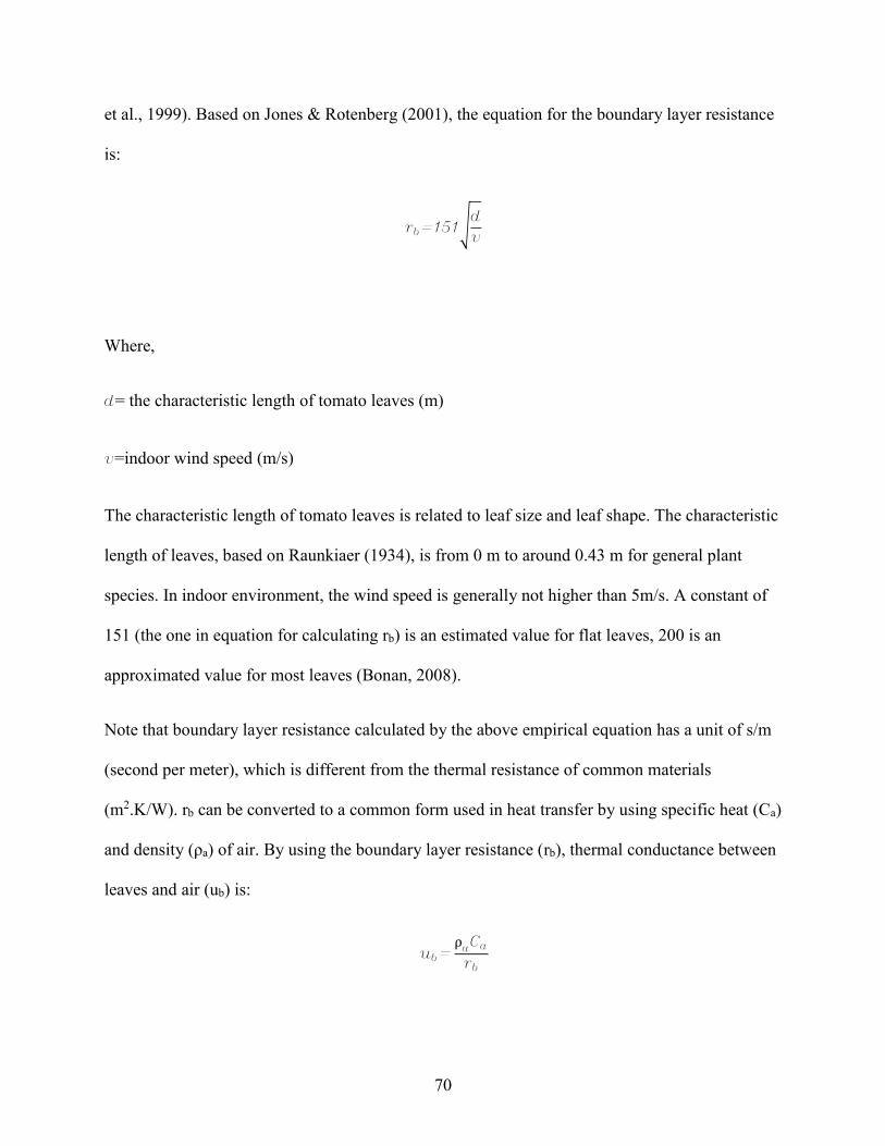
70

et al., 1999). Based on Jones & Rotenberg (2001), the equation for the boundary layer resistance

is:

rb=151√d

v

Where,

d= the characteristic length of tomato leaves (m)

v=indoor wind speed (m/s)

The characteristic length of tomato leaves is related to leaf size and leaf shape. The characteristic

length of leaves, based on Raunkiaer (1934), is from 0 m to around 0.43 m for general plant

species. In indoor environment, the wind speed is generally not higher than 5m/s. A constant of

151 (the one in equation for calculating rb) is an estimated value for flat leaves, 200 is an

approximated value for most leaves (Bonan, 2008).

Note that boundary layer resistance calculated by the above empirical equation has a unit of s/m

(second per meter), which is different from the thermal resistance of common materials

(m2.K/W). rb can be converted to a common form used in heat transfer by using specific heat (Ca)

and density (ρa) of air. By using the boundary layer resistance (rb), thermal conductance between

leaves and air (ub) is:

ub=ρaCa

rb

71

The relationship between characteristic dimension of leaves (wind speed is fixed at 0.5 m/s) and

thermal conductance of leaves, and the relationship between wind speed (characteristic length is

fixed at 0.04m) and thermal conductance of leaves, and are shown as follows.

Figure 2 Relationship between indoor wind speed (m/s) and plant thermal conductance (W/m2 K)

Figure 3 Relationship characteristic leave length (m) and plant thermal conductance (W/m2 K)

Based on the two figures, the plant thermal conductance is negligible when the wind speed is

high. In addition, when the leave size is small enough, the plant thermal conductance can

72

approach positive infinity (meaning the boundary layer resistance can be neglected). When the

leave size exceeds certain range, the plant thermal conductance is almost constant.

3.4 Heat and moisture transfer of plants

Under natural and indoor environmental conditions, the heat and mass exchange between plants

and the environment can be grouped into four parts: the evapotranspiration heat transfer (latent

heat transfer) from plants to the air (λ ET), the sensible heat transfer between leave surfaces and

the air (H), the net radiation (Rn), and the ground heat flux (G). The thermal network is provided

as follows, and the overall formula is given by Jaber et al. (2016):

Rn - G -λ ET – H = 0

Figure 4 Thermal network of a plant

For the convection process, the only resistance involved is the boundary layer resistance, which

is the thermal resistance of the exterior plant surface to the convective heat transfer. The formula

for estimating the convective sensible heat loss, based on Jones & Rotenberg (2001), can be

given as follows:

73

H=ρaCa(Tp-Ta)

rb

The calculations for rb and the ET have been presented in the previous subsection. The ground

heat flux has been described previously in transpiration and evapotranspiration part (section 3.2).

The net radiation (Rn) is the amount of radiation which is absorbed by the plant layer. The net

radiation is the net amount of shortwave (solar) radiation and longwave radiation absorbed by

plants. When under the indoor environment like a greenhouse, the components of net radiation is

more complicated than those under the natural and open environment. Within a greenhouse, the

plants receive not only the solar radiation, but also the radiation from the supplemental lighting.

In addition, the components of longwave radiation part increase, because in a greenhouse,

greenhouse components like the walls, the ceiling, the thermal screen, and some other objects

can have longwave radiation heat exchange with plants. The net radiation can be calculated as

follows.

Rn=Isrd.p+∑Qr(i→p)

n

i=1

Where,

i= surface index

Isrd.g=the amount of solar radiation absorbed by the plants (W)

∑ Qr(i→p)ni=1 = the amount of longwave radiation heat gain by plants from all other greenhouse

surfaces (W)

74

The relationships between net radiation, indoor air temperature as independent variables and

evapotranspiration rate as the dependent variable are shown by the curves as follows.

Figure 5 The relationships between net radiation (W/m2), indoor air temperature (℃) and

evapotranspiration rate (W/m2)

Stanghellini (1987) mentioned that the net radiation for calculating plant evapotranspiration

could be estimated as the sum of shortwave and longwave radiation absorbed by plants. The

spectrum of radiation does not matter, the solar radiation (shortwave) and longwave radiation can

be added directly. The plants omitted negligible amount of radiation outside the longwave range

in many cases. It can be seen obviously that within suitable ranges, the evapotranspiration rate

has a positive linear relationship with the amount of the net radiation, and the air temperature.

75

Chapter 4. Modeling：methods and materials

In this chapter, a modeling method which simplifies the structure of the thermal network is

introduced. A greenhouse is divided into three kinds of small areas based on their locations: the

middle areas located in the center of the greenhouse, the edge areas which attach to one wall of

the greenhouse, the areas located at four corners. The three kinds of areas correspond to three

kinds of mathematical models. For middle areas, the model is built based on a 1-D thermal

network, since heat exchange only occurred in vertical direction from the ceiling to the ground.

For edge areas, the model is created based on a 2-D thermal network, since the air had heat

exchange with the wall in horizontal direction. The areas located in four corners has a 3-D

thermal network because air had heat exchange with are not modelled because they only occupy

a small percentage of total area within the greenhouse, and plants are not expected to be

cultivated in these areas in most cases. The model for middle areas is tested by applying two

advanced designs: transparent and vertical ceiling, interruption (NI) and cyclic lighting in the

basic/reference greenhouse design. The model for edge areas is tested by applying insulated

north wall in the basic/reference greenhouse design.

4.1 General modeling approach

In this paper, the total area of a greenhouse is divided into three kinds of unit areas (Figure 6, 7)

for modelling. These unit areas have different thermal networks. For the unit areas which are

located in the middle of the greenhouse (area M), they have 1-D heat transfer mode in the

vertical direction, since they are not directly connected with and away from the vertical walls.

For the rest unit areas which attach to one of the boundaries (area E), since they have one vertical

surface attached to the outdoor, they have 2-D heat transfer mode. Only the areas which are

located in four corners (area C) have 3-D heat transfer mode. The simplified thermal network can

76

help reduce the amount of time used in editing the heat transfer equations and reduce the

potential of making mistakes. In addition, the accuracy of model is increased because more than

one air node are used in estimating air temperature.

Figure 6 and Figure 7: Three kinds of unit areas in a greenhouse (front view and top view)

In this study, the three kinds of unit areas are used to study the effect of different advanced

designs. The area of per unit area is determined as 4 m2 instead of 1 m2. The time step is set as

0.1 minutes (6s), and the total number of time step is 14400 for a day.

The accuracy of model is increased not only because there is more than one node for estimating

air temperature, but also the plant nodes are separated from the air nodes. In previous studies, the

air temperature was often assumed to be equivalent to the plant temperature. Based on Boulard

et al. (1991) and Papadakis et al. (1994), the plant temperature is lower than the air temperature

during the whole 24 hours. Therefore, by separating the air nodes and the plant nodes, the

accuracy of a model could be increased.

4.2 Thermal networks and equations for basic designs for the middle and edge

areas

Figure 8 and 9 show the schematics of center area type and edge area type of the conventional

design, respectively. The conceptual greenhouse is a conventional greenhouse with horizontal

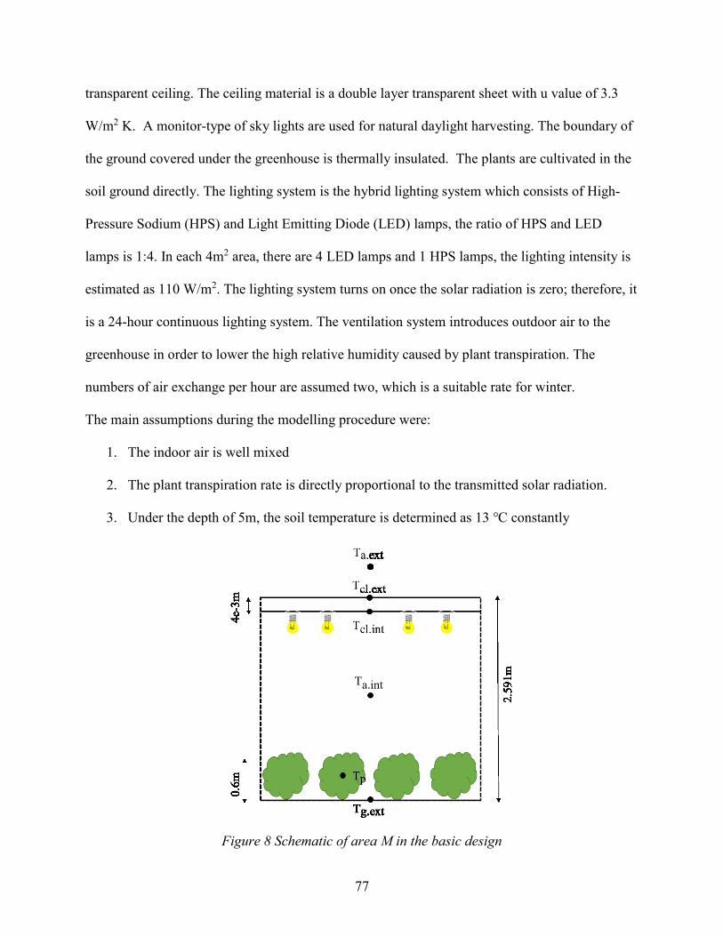
77

transparent ceiling. The ceiling material is a double layer transparent sheet with u value of 3.3

W/m2 K. A monitor-type of sky lights are used for natural daylight harvesting. The boundary of

the ground covered under the greenhouse is thermally insulated. The plants are cultivated in the

soil ground directly. The lighting system is the hybrid lighting system which consists of High-

Pressure Sodium (HPS) and Light Emitting Diode (LED) lamps, the ratio of HPS and LED

lamps is 1:4. In each 4m2 area, there are 4 LED lamps and 1 HPS lamps, the lighting intensity is

estimated as 110 W/m2. The lighting system turns on once the solar radiation is zero; therefore, it

is a 24-hour continuous lighting system. The ventilation system introduces outdoor air to the

greenhouse in order to lower the high relative humidity caused by plant transpiration. The

numbers of air exchange per hour are assumed two, which is a suitable rate for winter.

The main assumptions during the modelling procedure were:

1. The indoor air is well mixed

2. The plant transpiration rate is directly proportional to the transmitted solar radiation.

3. Under the depth of 5m, the soil temperature is determined as 13 ℃ constantly

Figure 8 Schematic of area M in the basic design

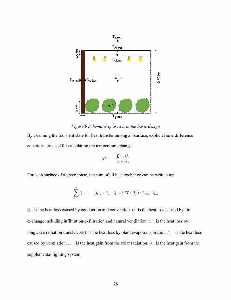
78

Figure 9 Schematic of area E in the basic design

By assuming the transient state for heat transfer among all surface, explicit finite difference

equations are used for calculating the temperature change.

∆T= ∑ Qini=1

ρi∙ci∙li

For each surface of a greenhouse, the sum of all heat exchange can be written as:

∑Qi

n

i=1

= -(Qcc+Qa+Qr+𝜆 𝐸𝑇+Qv)+Isrd+Qsl

Qcc is the heat loss caused by conduction and convection. Qa is the heat loss caused by air

exchange including infiltration/exfiltration and natural ventilation. Qr is the heat loss by

longwave radiation transfer. λET is the heat loss by plant evapotranspiration. Qv is the heat loss

caused by ventilation. Isrd is the heat gain from the solar radiation. Qsl is the heat gain from the

supplemental lighting system.

79

By expanding the formula, the equation for calculating the temperature change of different

surfaces is:

Tit+∆t

=∆T+Tit=(Qi)∆t

ρi∙ci∙li

+Tit

Where,

i= symbol of ‘i’ surface

Ti is the temperature of the target surface

Ti-1 and Ti+1 are temperatures of the surrounding surfaces

ρi, ci, li are the density, specific heat and characteristic length of ‘i’ surface, respectively

∆𝑡 is the time step

The heat balance equations for all surfaces in area M are:

∆Tcl.ext=Qr(cl.int→cl.ext)+Isrd.cl

-Qcc(cl.ext→a.ext)-Qr(a.ext→sky)

ρcl

∙ccl∙Vcl

(C1)

∆Tcl.int =Qcc(a.int→cl.int)-Qr(cl.int→cl.ext)+Qr(g.ext→cl.int)+Qr(p→cl.int)

ρcl

∙ccl∙Vcl

(C2)

∆Ta.int=Qcc(g.ext→a.int)-Qcc(a.int→p)-Qcc(a.int→cl.int)-Qv-λ ET

ρa

∙ca∙Va

(C3)

∆Tp=Qcc(a.int→p)-Qr(p→cl.int)+Qr(g.ext→p)-λ ET +Isrd.p + Qsl.p

ρp

∙cp∙Vp

(C4)

∆Tg.ext=Qcc(g.m05→g.ext)+Isrd.g-Qr(g→cl.int)- Qr(g→p)+Qsl.g-Qcc(g.ext→a.int)

ρg

∙cg∙Vg

(C5)

The heat balance equations for indoor ceiling, indoor air, plant and ground and wall surfaces in

edge area type (area E) are:

80

∆Tcl.ext=Qr(cl.int→cl.ext)+Isrd.cl

-Qcc(cl.ext→a.ext)-Qr(a.ext→sky)

ρcl

∙ccl∙Vcl

(E1)

∆Tcl.int=Qcc(a.int→cl.int)-Qr(cl.int→cl.ext)+Qr(g.ext→cl.int)+Qr(p→cl.int)+Qr(w.int→cl.int)

ρcl

∙ccl∙Vcl

(E2)

∆Ta.int=Qcc(g.ext→a.int)-Qcc(a.int→p)-Qcc(a.int→cl.int)-Qv-λ ET-Qcc(a.int→w.int)

ρa

∙ca∙Va

(E3)

∆Tp=Qcc(a.int→p)-Qr(p→cl.int)+Qr(g.ext→p)-λ ET +Isrd.p+Qsl.p-Qr(p→w.int)

ρp

∙cp∙Vp

(E4)

∆Tg.ext=Qcc(g.m05→g.ext)+Isrd.g-Qr(g→cl.int)- Qr(g.ext→p)+Qsl.g-Qcc(g→a.int)-Qr(g.ext→w.int)

ρg

∙cg∙Vg

(E5)

∆Tw.ext=Qcc(w.int→w.ext)+Isrd.w

-Qcc(w.ext→a.ext)-Qr(w.ext→sky)

ρw

∙cw∙Vw

(E6)

∆Tw.int=Qcc(a.int→w.int)-Qr(w.int→cl.int)+Qr(g.ext→w.int)+Qr(p→w.int)+Qsl.w+Qcc(w.ext→w.int)

ρw

∙cw∙Vw

(E7)

The assumed properties of ceiling and wall materials are listed in the table as follows.

81

Table 5 Set properties of ceiling and wall materials

Surface Symbols Materials Thermal

conductance

(W/m2 K)

Heat

capacity

(J/kg K)

Density

(kg/m3)

Thickness

(m)

Ceiling cl Double

layer

transparent

plastic

material

3.3 1250 1220 4.10-3

Wall w Foam

insulation

material

0.43 1500 40 0.075

Air a - 9 (indoor)

20 (outdoor)

1000 1.3 -

Plants p - 30.44 3253

(Chen et

al., 2012)

700

(Taki et

al.,

2017)

-

Ground g - 2.2

(Ekwue et

al., 2011)

850

(Song et

al., 2017)

2215

(Song et

al.,

2017)

0.5 (each

layer, five

layers in

total)

4.2.1 Outdoor temperature (Text)

The weather data used in the model is the exterior temperatures of a typical day of Edmonton,

Canada. The date was January 1st, 2002. This day is selected because it is a clear day, and it has

the extremely low temperature for the whole day. During a clear day, the effect of cloud cover

factor is negligible, and Hottel’s clear day model can be used to calculate the amount of solar

radiation (will be discussed in the solar radiation part).The mean temperature was -23℃ in that

day. Steady periodic weather conditions and lighting and ventilation operations are used for the

simulation. As is mentioned previously, the time step is set to be 0.01 min (6 seconds), so the

weather curve needs to have 14400 points. In order to use the hourly weather data, which is 24

discrete points in the loop, the interpolation is carried out to make the weather data become

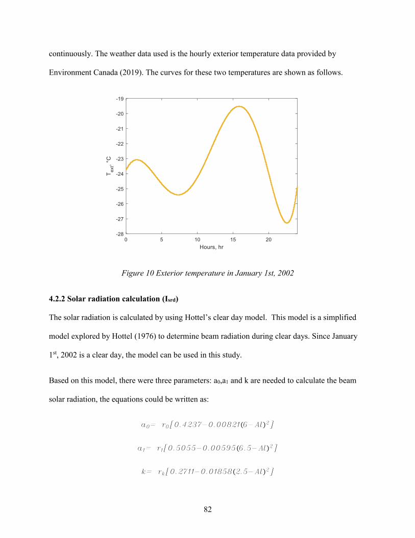
82

continuously. The weather data used is the hourly exterior temperature data provided by

Environment Canada (2019). The curves for these two temperatures are shown as follows.

Figure 10 Exterior temperature in January 1st, 2002

4.2.2 Solar radiation calculation (Isrd)

The solar radiation is calculated by using Hottel’s clear day model. This model is a simplified

model explored by Hottel (1976) to determine beam radiation during clear days. Since January

1st, 2002 is a clear day, the model can be used in this study.

Based on this model, there were three parameters: a0,a1 and k are needed to calculate the beam

solar radiation, the equations could be written as:

a0= r0[0.4237-0.00821(6-Al)2]

a1= r1[0.5055-0.00595(6.5-Al)2]

k= rk[0.2711-0.01858(2.5-Al)2]

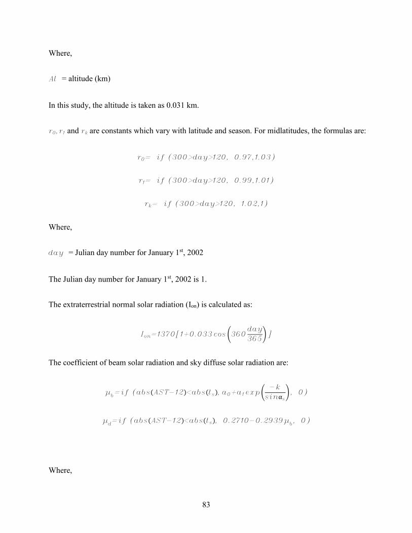
83

Where,

Al = altitude (km)

In this study, the altitude is taken as 0.031 km.

r0,r1 and rk are constants which vary with latitude and season. For midlatitudes, the formulas are:

r0= if (300>day>120, 0.97,1.03)

r1= if (300>day>120, 0.99,1.01)

rk= if (300>day>120, 1.02,1)

Where,

day = Julian day number for January 1st, 2002

The Julian day number for January 1st, 2002 is 1.

The extraterrestrial normal solar radiation (Ion) is calculated as:

Ion=1370[1+0.033cos(360day

365)]

The coefficient of beam solar radiation and sky diffuse solar radiation are:

μb=if (abs(AST-12)<abs(ts), a0+a1 exp (

-k

sinαs) , 0)

μd=if (abs(AST-12)<abs(ts), 0.2710-0.2939μ

b, 0)

Where,

84

AST = apparent solar time

ts = sunset time (hour)

αs = solar altitude

Without time adjustment, the apparent solar time (AST) is equal to the time on a watch.

The direct beam radiation and direct normal solar radiation can be given as follows.

Ib= if(θ<π

2,Ionμb

,0)

Idn= Ibcosθ

Where,

Ɵ= incidence angle (°)

Sky diffuse solar radiation (Ids) and solar radiation reflected by the ground (Idg) can be

expressed as follows.

Ids=[Ionsinα(μb+μ

d)]1+cosβ

2

Idg=[Ionsinα(μb+μ

d)]rg

1-cosβ

2

Where,

β = tilted angle of a surface (°)

rg = reflectance of ground

85

The day was extremely cold, the ground was covered by snow, therefore, the outdoor ground

reflectance can be assumed to be 0.3.

Finally, the total amount of solar radiation received by a surface is given as:

It = Idn+ Ids + Idg

Based on the ASHRAE (2013), the incidence angle in a surface calculated from the following

relationship:

cosθ= cosαcos(ϕ-ψ) sinβ+sinαcosβ

θ=if (abs(AST-12)<ts,acos(cosθ+abs(cosθ)

2 ,

π

2)

Where,

Φ = solar azimuth (°)

Ψ = surface azimuth (°)

The equations for calculating the amount of solar radiation absorbed by different surfaces are

given as follows.

Isrd.g=ItAgCCτclag

Isrd.p=ItApCCτclap

Isrd.cl=ItAclacl

Isrd.w=ItAwaw

86

Isrd.nw=ItAnwanw

Isrd.mix=ItAclamix

The optical parameters used in this part are all listed in the following table.

Table 6 Optical properties of surfaces

Parameters Surfaces

Ceiling (in

basic

design)

Ceiling

(in design

1)

Plants Wall (in

basic

design)

Insulated

north wall

Ground

Absorption (a) 0.17 0.6 0.8 0.7 0.9 0.8

Transmittance

(τ)

Change

with

incidence

angle

Change

with

incidence

angle

0 0 0 0

The transparent materials used in ceiling of basic design and advanced ceiling design are the

same double-glazing material. The transmittance of this material is plotted against the incidence

angle and given as follows. The data was provided by Dell’Isola et al. (2006).

87

Figure 11 Relationship between incidence angle (degree) and transmittance of transparent

material

For designs which model area M (the basic design, the insulated north wall, the cyclic lighting),

the amount of available solar radiation before and after transmission is given as follows.

Figure 12 Solar radiation before transmission (basic design, insulated north wall design, cyclic

lighting design)

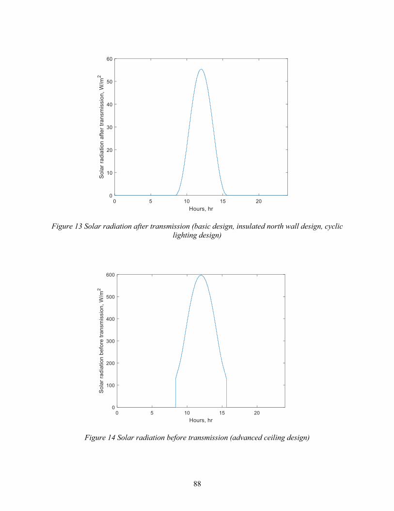
88

Figure 13 Solar radiation after transmission (basic design, insulated north wall design, cyclic

lighting design)

Figure 14 Solar radiation before transmission (advanced ceiling design)

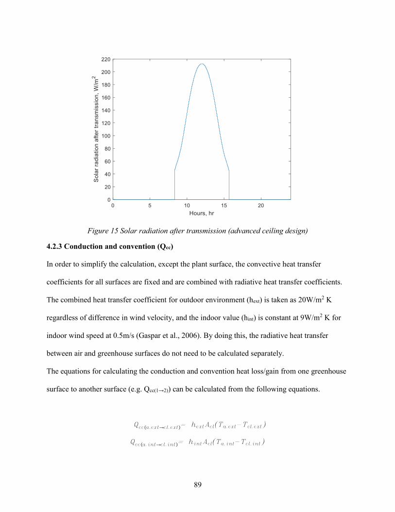
89

Figure 15 Solar radiation after transmission (advanced ceiling design)

4.2.3 Conduction and convention (Qcc)

In order to simplify the calculation, except the plant surface, the convective heat transfer

coefficients for all surfaces are fixed and are combined with radiative heat transfer coefficients.

The combined heat transfer coefficient for outdoor environment (hext) is taken as 20W/m2 K

regardless of difference in wind velocity, and the indoor value (hint) is constant at 9W/m2 K for

indoor wind speed at 0.5m/s (Gaspar et al., 2006). By doing this, the radiative heat transfer

between air and greenhouse surfaces do not need to be calculated separately.

The equations for calculating the conduction and convention heat loss/gain from one greenhouse

surface to another surface (e.g. Qcc(1→2)) can be calculated from the following equations.

Qcc(a.ext→cl.ext)= hextAcl(Ta.ext-Tcl.ext)

Qcc(a.int→cl.int)= hintAcl(Ta.int-Tcl.int)

90

Qcc(a.ext→mix.ext)= hextAmix(Ta.ext-Tmix.ext)

Qcc(a.int→mix.int)= hintAmix(Ta.int-Tmix.int)

Qcc(a.int-p)= ubAp(Ta.int-Tp)

Qcc(a.int→g.ext)= hintAg(Ta.int-Tg.ext)

Qcc(a.int→wall.int)= hintAw(Ta.int-Twall.int)

Qcc(asc→sc)= hintAsc(Tasc-Tsc)

Qcc(bsc→sc)= hintAsc(Tbsc-Tsc)

Qcc(a.ext→nw.ext)= hextAnw(Ta.ext-Tnw.ext)

Qcc(a.int→nw.int)= hextAnw(Ta.int-Tnw.int)

Qcc(w.int→w.ext)=kwAwlw

(Tw.int-Tw.ext)

Qcc(w.int→w.ext)=kwAwlw

(Tw.int-Tw.ext)

Qcc(nw.int→nw.ext)=utAnw(Tnw.mid-Tnw.ext)

Qcc(mix.int→mix.mid)=umixAmix(Tmix.int-Tmix.mid)

Qcc(mix.mid→mix.ext)=umixAmix(Tmix.mid-Tmix.ext)

When calculating the ground temperature, in order to increase accuracy, the soil with depth of

2.5m is divided into five layers for modelling. At the depth of 2.5m, the temperature is assumed

to be constant at 13 ℃ as undisturbed ground temperature (UGT).The UGT is not affected by

fluctuations of air temperatures from the ground surface (Kurevija et al., 2011).

91

Qcc(g.05→g.ext)=ksAg

h(Tg.05-Tg.ext

)

Qcc(g.1→g.05)=ksAg

h(Tg.1-Tg.05

)

Qcc(g.15→g.1)=ksAg

h(Tg.15-Tg.1

)

Qcc(g.2→g.15)=ksAg

h(Tg.2-Tg.15

)

Qcc(g.25→g.2)=ksAg

h(Tg.25-Tg.2

)

4.2.4 Lighting heat gain (Qsl)

The lighting system used in this model is the hybrid (LED+HPS) lighting system. Based on the

previous studies, hybrid system requires slightly more energy than the LED system, but they can

result in the highest yield and quality. This is caused by increased net heat gain and the extra

supplement of light with specific wavelengths (Dueck et al., 2011). The rise in net heat gain was

good for cold regions, since the requirement for heating can be satisfied partially by the extra

heat produced.

According to ASHRAE (2013), the heat supplied by the lighting system can be estimated as:

Qsl=WFhcFaAg

Where,

W=installed power of lamps (W/m2)

Fhc=heat conversion factor

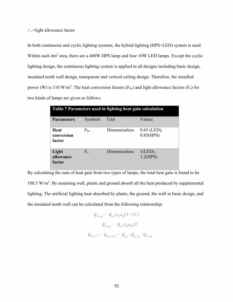
92

Fa=light allowance factor

In both continuous and cyclic lighting systems, the hybrid lighting (HPS+LED) system is used.

Within each 4m2 area, there are a 400W HPS lamp and four 10W LED lamps. Except the cyclic

lighting design, the continuous lighting system is applied in all designs including basic design,

insulated north wall design, transparent and vertical ceiling design. Therefore, the installed

power (W) is 110 W/m2. The heat conversion factors (Fhc) and light allowance factors (Fa) for

two kinds of lamps are given as follows.

Table 7 Parameters used in lighting heat gain calculation

Parameters Symbols Unit Values

Heat

conversion

factor

Fhc Dimensionless 0.65 (LED),

0.85(HPS)

Light

allowance

factor

Fa Dimensionless 1(LED),

1.2(HPS)

By calculating the sum of heat gain from two types of lamps, the total heat gain is found to be

108.5 W/m2. By assuming wall, plants and ground absorb all the heat produced by supplemental

lighting. The artificial lighting heat absorbed by plants, the ground, the wall in basic design, and

the insulated north wall can be calculated from the following relationship:

Qsl.g= QslAgag(1-CC)

Qsl.p= QslAgapCC

Qsl.w= Qsl.nw= Qsl-Qsl.g-Qsl.p

93

4.2.5 Long wave radiation (Qr)

The equations for calculating longwave radiation heat exchange among greenhouse surfaces are

written as follow. The emissivity (ε) of all greenhouse surfaces and the view factors (F) among

surfaces are given in the following two table.

Qr(cl.ext→sky)=σεclεskyFcl.ext→skyAg(Tcl.ext4-Tsky

4)

Qr(cl.int→cl.ext)=σ1

1

εcl+

1

εcl

Fcl.int→cl.extAcl(Tcl.int4-Tcl.ext

4)

Qr(p→cl.int)=σεpεclFp→cl.intAclLAI(Tp4-Tcl.int

4)

Qr(g.ext→cl.int)=σεgεclFg→cl.int(1-CC)Ag(Tg.ext4-Tcl.int

4)

Qr(g.ext→p)=σεgεpFg→pAg(Tg.ext4-Tp

4)

Qr(w.ext→sky)=σεwεskyFw.ext→skyAw(Tw4-Tsky

4)

Qr(p→w.int)=σεpεwFp→w.intAgLAI(Tp4-Tw.int

4)

Qr(g.ext→w.int)=σεgεwFg→w.int(1-CC)Ag(Tg4-Tw.int

4)

Qr(w.int→cl.int)=σεclεwFw.int→cl.intAw(Tw.int4-Tcl.int

4)

Qr(nw.ext→sky)=σεnwεskyFnw.ext→skyAnw(Tnw4-Tsky

4)

Qr(p→nw.int)=σεpεnwFp→nw.intAgLAI(Tp4-Tnw.int

4)

Qr(g→nw.int)=σεgεnwFg→nw.int.(1-CC)Ag(Tg.ext4-Tnw.int

4)

Qr(nw.int→cl.int)=σεclεnwFnw.int→cl.intAnw(Tnw.int4-Tcl.int

4

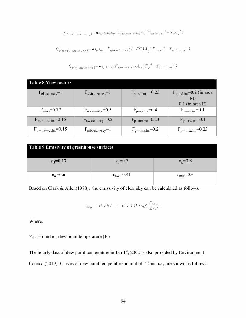
94

Qr(mix.ext→sky)=σεmixεskyFmix.ext→skyAg(Tmix.ext4-Tsky

4)

Qr(g.ext→mix.int)=σεgεmixFg→mix.int(1-CC)Ag(Tg.ext4-Tmix.int

4)

Qr(p→mix.int)=σεpεmixFp→mix.intAcl(Tp4-Tmix.int

4)

Table 8 View factors

Fcl.ext→sky=1 Fcl.int→cl.ext=1 Fp→cl.int =0.23 Fg→cl.int=0.2 (in area

M)

0.1 (in area E)

Fg→p=0.77 Fw.ext→sky=0.5 Fp→w.int=0.4 Fg→w.int=0.1

Fw.int→cl.int=0.15 Fnw.ext→sky=0.5 Fp→nw.int=0.23 Fg→nw.int=0.1

Fnw.int→cl.int=0.15 Fmix.ext→sky=1 Fg→mix.int=0.2 Fp→mix.int.=0.23

Table 9 Emssivity of greenhouse surfaces

εcl=0.17 εp=0.7 εg=0.8

εw=0.6 εnw=0.91 εmix=0.6

Based on Clark & Allen(1978), the emissivity of clear sky can be calculated as follows.

εsky= 0.787 + 0.7661.log(Tdew273

)

Where,

Tdew= outdoor dew point temperature (K)

The hourly data of dew point temperature in Jan 1st, 2002 is also provided by Environment

Canada (2019). Curves of dew point temperature in unit of ℃ and εsky are shown as follows.

95

Figure 16 Outdoor dew point temperature in January 1st, 2002

Figure 17 Emissivity of sky in January 1st, 2002

96

4.2.6 Heat loss caused by ventilation and in/exfiltration (Qv)

In this study, when the calculating the temperature change, only the sensible heat loss of

ventilation is considered. The sensible heat loss caused by ventilation and in/exfiltration can be

expressed as (ASHRAE , 2013):

Qv=(1-Es)Q̇ρaCa(Ta.int-Ta.ext)+Q̇

2ρaCa(Ta.int-Ta.ext)

Where,

Es= heat recovery efficiency

Q̇= number of air exchange caused by ventilation per second

In here, the heat recovery efficiency is taken as 0.65.The minimum requirement of ventilation for

greenhouse in winter is 2-3 air exchange per hour, and the in/exfiltration rate is around 50% of

the minimum requirement of ventilation rate during a heating season (Buffington et al., 2010;

Zhang& Barber, 1995). In order to minimize the heat loss caused by ventilation, the ventilation

rate in this study is taken as 2 air exchange per hour, and in/exfiltration rate is 0 air exchange per

hour in area M and 1 in area E.

4.3 Thermal equations for advanced designs

4.3.1 Middle area with vertical skylight

In this part, an advanced ceiling design which can increase both solar heat gain and decrease heat

loss is proposed. In each 4m2 area, there are three kinds of surfaces (figure 18). The vertical and

transparent surface (“1”) and the neighboring surface (“2”) with high reflectance can increase the

solar radiation transmitted into the greenhouse. The insulated tilt (“3”) and horizontal surface

(“2”) can decrease the heat loss significantly when compared to double layer plastic material.

97

Figure 18 Schematic of energy saving ceiling (surface 1: vertical and transparent ceiling to

increase solar heat gain; surface 2: insulated horizontal surface with white paint, can increase

solar heat gain and reduce heat loss; surface 3: insulated by lightweight; yellow arrows: solar

radiation)

The heat exchange can be calculated by combining thermal conductance of three surfaces into

one value. This is done for simplifying the calculation of heat transfer between ceiling and other

surfaces. The formula for combining thermal conductance is given as:

umix=u1A1

A1+A2+A3+u2

A2A1+A2+A3

+u3A3

A1+A2+A3

Where,

umix= combined thermal conductance of three surfaces (W/m2 K)

u1,u2,u3 = thermal conductance of surface 1, 2, 3 (W/m2 K)

A1,A2,A3= area of surface 1,2,3 (m2)

The combining thermal conductance is used in calculating conductive heat transfer among

different layers of ceiling. The equations have been given in section 4.2.3.

The calculation of denominator in heat balance equations only use the density and specific heat

of surface 2 and 3, which are insulated by the same lightweight insulation.

The heat balance equations for all temperature nodes with this advanced ceiling design are

written as:

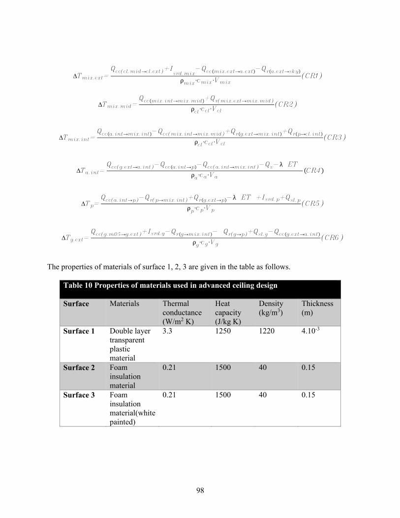
98

∆Tmix.ext=Qcc(cl.mid→cl.ext)+Isrd.mix

-Qcc(mix.ext→a.ext)-Qr(a.ext→sky)

ρmix

∙cmix∙Vmix

(CR1)

∆Tmix.mid=Qcc(mix.int→mix.mid)+Qr(mix.ext→mix.mid)

ρcl

∙ccl∙Vcl

(CR2)

∆Tmix.int=Qcc(a.int→mix.int)-Qcc(mix.int→mix.mid)+Qr(g.ext→mix.int)+Qr(p→cl.int)

ρcl

∙ccl∙Vcl

(CR3)

∆Ta.int=Qcc(g.ext→a.int)-Qcc(a.int→p)-Qcc(a.int→mix.int)-Qv-λ ET

ρa

∙ca∙Va

(CR4)

∆Tp=Qcc(a.int→p)-Qr(p→mix.int)+Qr(g.ext→p)-λ ET +Isrd.p+Qsl.p

ρp

∙cp∙Vp

(CR5)

∆Tg.ext=Qcc(g.m05→g.ext)+Isrd.g-Qr(g→mix.int)- Qr(g→p)+Qsl.g-Qcc(g.ext→a.int)

ρg

∙cg∙Vg

(CR6)

The properties of materials of surface 1, 2, 3 are given in the table as follows.

Table 10 Properties of materials used in advanced ceiling design

Surface Materials Thermal

conductance

(W/m2 K)

Heat

capacity

(J/kg K)

Density

(kg/m3)

Thickness

(m)

Surface 1 Double layer

transparent

plastic

material

3.3 1250 1220 4.10-3

Surface 2 Foam

insulation

material

0.21 1500 40 0.15

Surface 3 Foam

insulation

material(white

painted)

0.21 1500 40 0.15

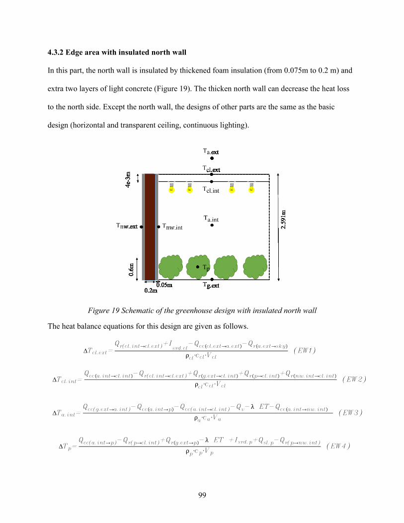
99

4.3.2 Edge area with insulated north wall

In this part, the north wall is insulated by thickened foam insulation (from 0.075m to 0.2 m) and

extra two layers of light concrete (Figure 19). The thicken north wall can decrease the heat loss

to the north side. Except the north wall, the designs of other parts are the same as the basic

design (horizontal and transparent ceiling, continuous lighting).

Figure 19 Schematic of the greenhouse design with insulated north wall

The heat balance equations for this design are given as follows.

∆Tcl.ext=Qr(cl.int→cl.ext)+Isrd.cl

-Qcc(cl.ext→a.ext)-Qr(a.ext→sky)

ρcl

∙ccl∙Vcl

(EW1)

∆Tcl.int=Qcc(a.int→cl.int)-Qr(cl.int→cl.ext)+Qr(g.ext→cl.int)+Qr(p→cl.int)+Qr(nw.int→cl.int)

ρcl

∙ccl∙Vcl

(EW2)

∆Ta.int=Qcc(g.ext→a.int)-Qcc(a.int→p)-Qcc(a.int→cl.int)-Qv-λ ET-Qcc(a.int→nw.int)

ρa

∙ca∙Va

(EW3)

∆Tp=Qcc(a.int→p)-Qr(p→cl.int)+Qr(g.ext→p)-λ ET +Isrd.p+Qsl.p-Qr(p→nw.int)

ρp

∙cp∙Vp

(EW4)

100

∆Tg.ext=Qcc(g.m05→g.ext)+Isrd.nw-Qr(g→cl.int)- Qr(g.ext→p)+Qsl.g-Qcc(g→a.int)-Qr(g.ext→nw.int)

ρg

∙cg∙Vg

(EW5)

∆Tnw.ext=Qcc(nw.int→nw.ext)+Isrd.nw

-Qcc(nw.ext→a.ext)-Qr(nw.ext→sky)

ρnw

∙cnw∙Vnw

(EW6)

∆Tnw.int=Qcc(a.int→nw.int)-Qr(nw.int→cl.int)+Qr(g.ext→nw.int)+Qr(p→nw.int)+Qsl.nw+Qcc(nw.ext→nw.int)

ρw

∙cw∙Vw (EW7)

The properties of materials used in insulating north wall are shown in the following table:

Table 11 Properties of materials used in insulated north wall design

Materials Thermal

conductance

(W/m2 K)

Heat capacity

(J/kg K)

Density (kg/m3) Thickness(m)

Rigid (foam)

Insulation

(middle layer)

0.16 1500 40 0.2

Lightweight

concrete

2.4 840 1200 0.05

4.3.3 Middle area with cyclic and night interruption (NI) lighting

Cyclic and night interruption (NI) lighting is an advanced design for supporting plant growth

rather than saving energy. As is mentioned previously in the literature review part, night

interruption (NI) is better than day-extension lighting in most cases, and whether cyclic lighting

is better than continuous lighting depends on plant species. Tomato is a plant species which is

sensitive to continuous lighting. It means that tomato plants give strong and negative response to

long-time and continuous lighting (Sysoeva, 2012). The all-day lighting in the basic design could

significantly decrease the energy demand for heating, but it can cause limitation in growth of

tomato plants. Therefore, in this part, the 24-hour lighting system is adjusted into 6-hour cyclic

and night interruption (NI) lighting. From 0am to 3am, and 9pm to 12am, within every hour, the

101

lights turn on for 54 minutes and turn off for the rest 6 minutes. The arrangement of lighting time

within the 24 hours is shown in the figure as follows.

Figure 20 Lighting intensity within 24 hours in cyclic lighting design (area M)

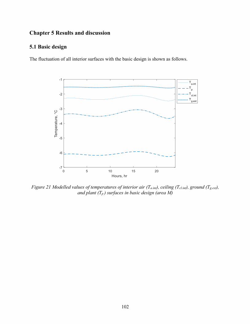
102

Chapter 5 Results and discussion

5.1 Basic design

The fluctuation of all interior surfaces with the basic design is shown as follows.

Figure 21 Modelled values of temperatures of interior air (Ta.int), ceiling (Tcl.int), ground (Tg.ext),

and plant (Tp ) surfaces in basic design (area M)

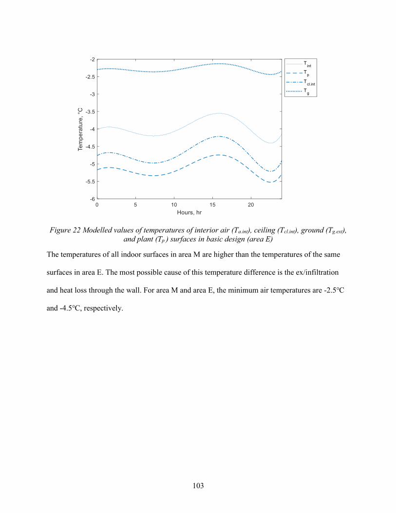
103

Figure 22 Modelled values of temperatures of interior air (Ta.int), ceiling (Tcl.int), ground (Tg.ext),

and plant (Tp ) surfaces in basic design (area E)

The temperatures of all indoor surfaces in area M are higher than the temperatures of the same

surfaces in area E. The most possible cause of this temperature difference is the ex/infiltration

and heat loss through the wall. For area M and area E, the minimum air temperatures are -2.5℃

and -4.5℃, respectively.

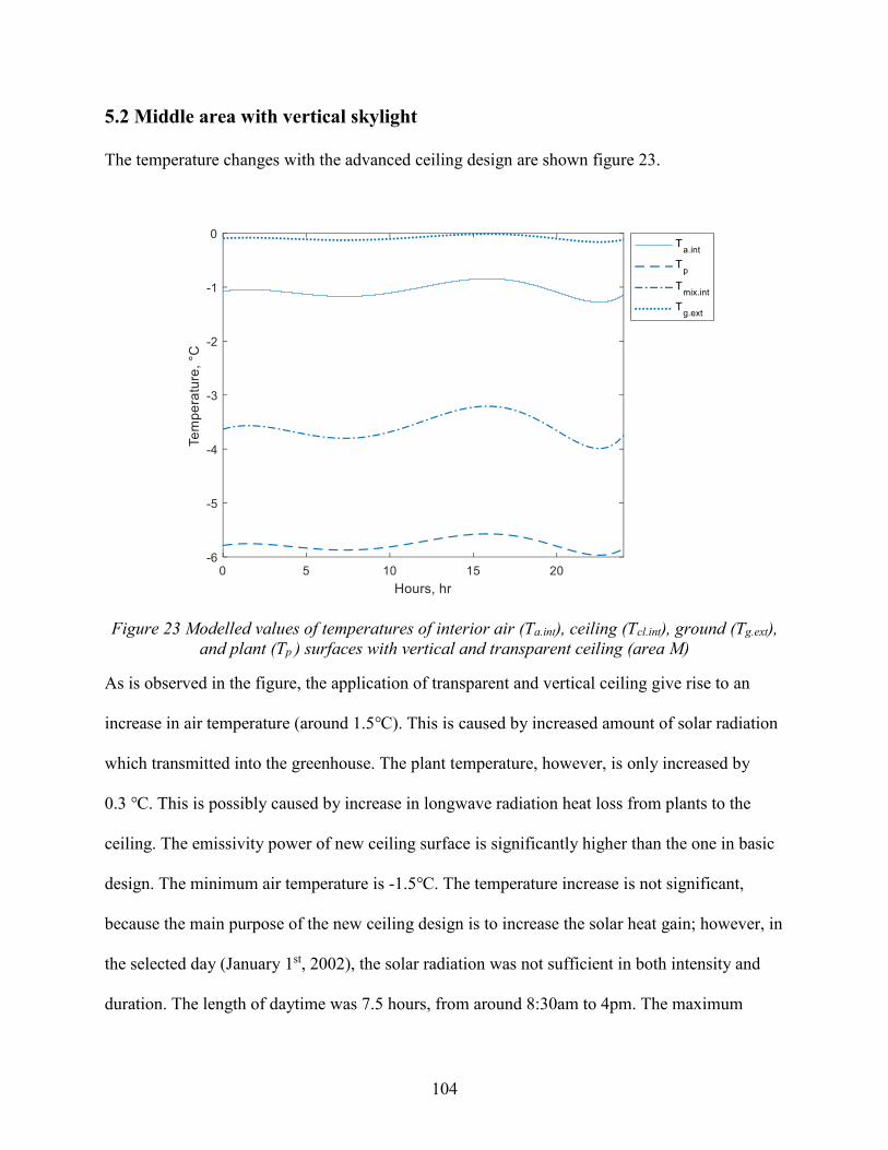
104

5.2 Middle area with vertical skylight

The temperature changes with the advanced ceiling design are shown figure 23.

Figure 23 Modelled values of temperatures of interior air (Ta.int), ceiling (Tcl.int), ground (Tg.ext),

and plant (Tp ) surfaces with vertical and transparent ceiling (area M)

As is observed in the figure, the application of transparent and vertical ceiling give rise to an

increase in air temperature (around 1.5℃). This is caused by increased amount of solar radiation

which transmitted into the greenhouse. The plant temperature, however, is only increased by

0.3 ℃. This is possibly caused by increase in longwave radiation heat loss from plants to the

ceiling. The emissivity power of new ceiling surface is significantly higher than the one in basic

design. The minimum air temperature is -1.5℃. The temperature increase is not significant,

because the main purpose of the new ceiling design is to increase the solar heat gain; however, in

the selected day (January 1st, 2002), the solar radiation was not sufficient in both intensity and

duration. The length of daytime was 7.5 hours, from around 8:30am to 4pm. The maximum

105

transmitted solar radiation was around 220W/m2, which was good for plant growth but not

enough to increase indoor surface temperatures significantly.

5.3 Edge area with insulated north wall

The figure below shows the variation of temperatures of all interior surfaces with insulated north

wall.

Figure 24 Modelled values of temperatures of interior air (Ta.int), ceiling (Tcl.int), north wall

(Tnw.int), ground (Tg.ext), and plant (Tp )surfaces with insulated north wall (area E)

The results show that the insulated north wall result in about 3℃ increase in air temperature. The

improvement is significant. The minimum air temperature is -1.7℃. Increased thermal resistance

of wall possibly causes the significant improvement. The increase in thickness of foam insulation

to 0.2 m (for basic design, it was 0.075m) and addition of extra two layers of lightweight

concrete increased the thermal conductance of wall from 0.43 W/m2 K to 0.14 W/m2 K. The

insulated north wall can decrease heat loss for the whole day and thus result in significant

106

increase in indoor surface temperatures. The two layers of lightweight concrete also works as a

medium of thermal energy storage because of the presence of concrete. During the nighttime, the

thermal energy stored on the wall can be released and give result in an increase in the greenhouse

air temperature.

5.4 Middle area with cyclic and night interruption (NI) lighting

Figure 25 Modelled values of temperatures of interior air (Ta.int), ceiling (Tcl.int), ground (Tg.ext),

and plant (Tp) surfaces with cyclic lighting (area M)

The application of cyclic lighting in the greenhouse model results in approximately 0.9℃

decrease in indoor air temperature. The temperature decrease result from the decrease in length

of lighting period. The turn-on time of the lighting system in basic design is around 16.5 hours,

since it is a continuous lighting system. The lamps turn on when the transmitted solar radiation is

zero. In this design, however, the lamps only work for 5.4 hours. When compared to the

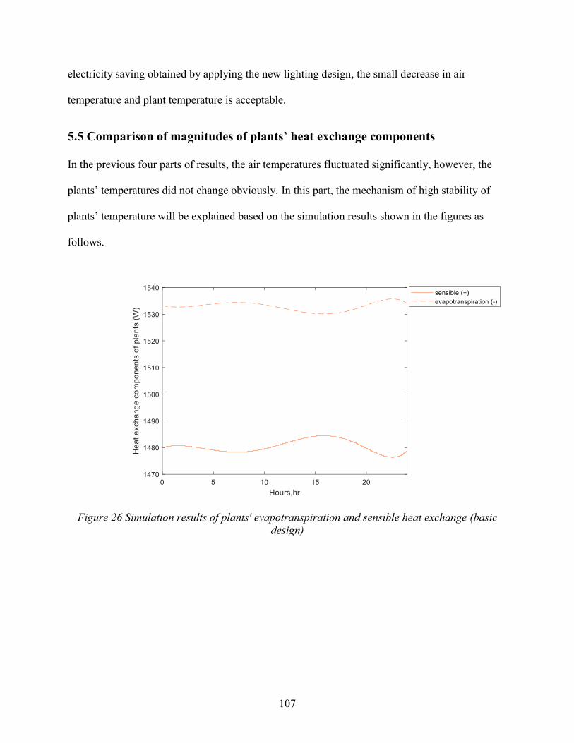
107

electricity saving obtained by applying the new lighting design, the small decrease in air

temperature and plant temperature is acceptable.

5.5 Comparison of magnitudes of plants’ heat exchange components

In the previous four parts of results, the air temperatures fluctuated significantly, however, the

plants’ temperatures did not change obviously. In this part, the mechanism of high stability of

plants’ temperature will be explained based on the simulation results shown in the figures as

follows.

Figure 26 Simulation results of plants' evapotranspiration and sensible heat exchange (basic

design)

108

Figure 27 Simulation results of net radiation absorbed by plants (basic design)

In here, the simulation results of the basic design is used as examples for explanation. In chapter

3, the heat and mass transfer of plants were described. The thermal network of plants consist of

four parts: the evapotranspiration heat transfer (latent heat transfer) from plants to the air (λ ET),

the sensible heat transfer between leave surfaces and the air (H), the net radiation (Rn), and the

ground heat flux (G). In this study, the ground heat flux was assumed negligible, so only three

components need to be analyzed. The two figures show the heat loss/gain of plants caused by

evapotranspiration, sensible heat exchange and net radiation. The unit is W instead of W/m2

because the three components were calculated by using different areas. The evapotranspiration

and sensible heat exchange were modelled by multiplying total leaf area (2LAI times ground

area). The net radiation was estimated by using both leaf area and areas of other surfaces,

depending on whether the plant surface absorbed or released thermal energy.

In figure 26, it can be seen that the sensible heat transfer is lower than the evapotranspiration

heat loss. The sensible heat transfer is bi-directional, and the direction depends on which surface

109

temperature is higher. Based on simulation results of this study, the plant temperature is lower

than the air temperature for a whole day, which suit the results from Boulard et al. (1991) and

Papadakis et al. (1994). Therefore, the plants obtain heat from the sensible heat exchange with

air. The difference between the heat gain (sensible heat transfer) and heat loss

(evapotranspiration) is around 50 W. In figure 27, it can be observed that the net radiation is not

high, since the weather of wintertime is used for modeling. The net radiation absorbed by plants

is mostly provided by artificial lighting. When the lights turn off, the net radiation drop

significantly from 250 W to approximately 50W to 150W.

The plant temperature is always lower than the air temperature and more difficult to be raised.

For this phenomenon, the mechanisms are the presence of evapotranspiration and high specific

heat of plants. The evapotranspiration is a process which let plants vaporize water through

stomata and cool themselves. The amount of heat loss during this process is high because of the

large leaf area. In chapter 3, the plots presented evapotranspiration heat loss in W/m2, which is

watts per leaf area. In per 1m2 ground area, the leaf area is often large than 1 and even reach 10.

In this study, the LAI value is taken as 1.6, which means that in per 1m2 ground area, the leaf

area is 1.6 m2. In addition, the tomato leaves have stomata on both sides; therefore, the leaf area

should be multiplied by 2 to calculate the evapotranspiration heat loss. The area in this study is

4m2, so the leaf area used for calculating evapotranspiration is 12.8 m2, which can give rise in

high total heat loss. The second reason is the high specific heat of plants. In 4.1, the specific heat

of tomato plants was mentioned. It is 3253 J/kg K. The density is also not low and taken as 700

kg/m3. The high specific heat and density result in high stability of plant temperature.

Consequently, the plant temperature is lower than air temperature for a whole day, and it is not

so easy to raise its temperature as raise air temperature.

110

In the design of vertical skylight, the increase in amount of effective solar radiation results in the

increase in net radiation, but the evapotranspiration rate also increases.

5.6 Comparison of energy consumption of advanced designs with the basic design

In this part, the energy consumption of all designs is calculated in order to compared the

advanced designs with the basic design. A space heating system with 200W/m2 release is

assumed to be applied in all designs. The heater will turn on if the indoor air temperature is

lower than the threshold value of current time step. For the whole day, 19 ℃ is set as the

threshold value. This temperature can allow the tomato plants grow well. The heater will turn on

if the air temperature of current time step is lower than the threshold value. In reality, there is

always a dead band which allows temperature to fluctuate within a suitable range, however, this

part is a theoretical estimation of energy consumption. Only one threshold value can simplify the

modeling work, while it will not result in significant deviation from the real outcomes.

The daily energy consumption of all designs is displayed by the figure as follows.

Figure 28 Energy consumption of designs (from left to right, 1: basic design, area M; 2: basic

design, area E; 3: advanced ceiling; 4: insulated north wall; 5:cyclic and night interruption

lighting)

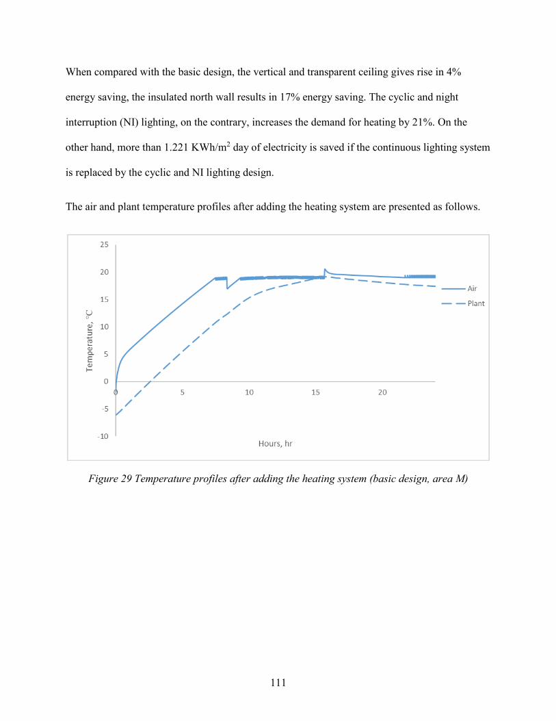
111

When compared with the basic design, the vertical and transparent ceiling gives rise in 4%

energy saving, the insulated north wall results in 17% energy saving. The cyclic and night

interruption (NI) lighting, on the contrary, increases the demand for heating by 21%. On the

other hand, more than 1.221 KWh/m2 day of electricity is saved if the continuous lighting system

is replaced by the cyclic and NI lighting design.

The air and plant temperature profiles after adding the heating system are presented as follows.

Figure 29 Temperature profiles after adding the heating system (basic design, area M)

112

Figure 30 Temperature profiles after adding the heating system (basic design, area E)

Figure 31 Temperature profiles after adding the heating system (vertical skylight)

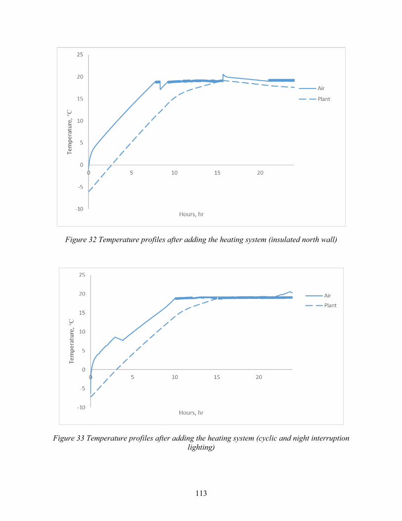
113

Figure 32 Temperature profiles after adding the heating system (insulated north wall)

Figure 33 Temperature profiles after adding the heating system (cyclic and night interruption

lighting)

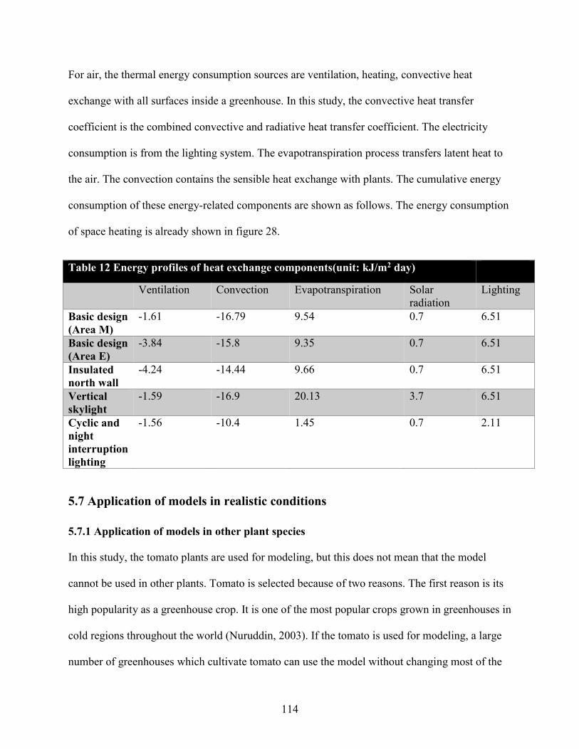
114

For air, the thermal energy consumption sources are ventilation, heating, convective heat

exchange with all surfaces inside a greenhouse. In this study, the convective heat transfer

coefficient is the combined convective and radiative heat transfer coefficient. The electricity

consumption is from the lighting system. The evapotranspiration process transfers latent heat to

the air. The convection contains the sensible heat exchange with plants. The cumulative energy

consumption of these energy-related components are shown as follows. The energy consumption

of space heating is already shown in figure 28.

Table 12 Energy profiles of heat exchange components(unit: kJ/m2 day)

Ventilation Convection Evapotranspiration Solar

radiation

Lighting

Basic design

(Area M)

-1.61 -16.79 9.54 0.7 6.51

Basic design

(Area E)

-3.84 -15.8 9.35 0.7 6.51

Insulated

north wall

-4.24 -14.44 9.66 0.7 6.51

Vertical

skylight

-1.59 -16.9 20.13 3.7 6.51

Cyclic and

night

interruption

lighting

-1.56 -10.4 1.45 0.7 2.11

5.7 Application of models in realistic conditions

5.7.1 Application of models in other plant species

In this study, the tomato plants are used for modeling, but this does not mean that the model

cannot be used in other plants. Tomato is selected because of two reasons. The first reason is its

high popularity as a greenhouse crop. It is one of the most popular crops grown in greenhouses in

cold regions throughout the world (Nuruddin, 2003). If the tomato is used for modeling, a large

number of greenhouses which cultivate tomato can use the model without changing most of the

115

plants’ parameters. The second reason is the availability of plants ’parameters. In chapter 3,

plants’ parameters including leaf area index (LAI), canopy cover (CC), boundary layer resistance,

evapotranspiration were described. In chapter 4, the specific heat and density of plants were

needed for modeling. The estimation or calculation methods of LAI, CC and evapotranspiration

can be used for all plant species; however, the boundary layer resistance, specific heat and

density are quite distinctive for different plant species. In this study, the modeling work is all

theoretical and has no experimental data. In order to get the parameters which cannot estimated

or calculated, information needs to be collected from previous researches. As a popular

greenhouse crop, tomato is used for greenhouse modeling frequently, and the data of its specific

heat and density can be found more easily than other greenhouse plant species.

On the other hand, the model can also be used for other plant species by changing values of some

parameters and adjusting systems based on plant requirements. The boundary layer resistance is

related to wind speed and characteristic length of leaves. In this study, these two values were

fixed at 0.5 and 0.04, respectively. The characteristic length of leaves is a measurement of leaf

size, so its value should be adjusted based on plant species. The specific heat and density of

leaves and stems are also diverse for different plant species. The values could be either found in

previous studies or determined by doing experiments. In addition, in evapotranspiration part in

chapter 3, the calculation of area of plants used for calculating evapotranspiration rate were

described. The tomato leaves are amphistomatous (have a large number of stomata (pores) in

both sides) (Gay & Hurd, 1975), so the area is 2LAI times ground area in daytime, however, not

all the plants are amphistomatous. Before calculating the evapotranspiration rate, whether the

plants are amphistomatous or hypostomatous (only have stomata on one side) should be

determined.

116

Ultimately, the lighting design and operation (including daylighting and artificial lighting)

should be adjusted based on requirement of different plant species. Whether the plants are long-

day, natural-day or short-day plants determine the duration and intensity of lighting. As for the

time and interval, night interruption lighting is better than day extension lighting in general cases.

In addition, whether the plants are sensitive to continuous lighting determine the interval

(continuous or cyclic) of lighting.

5.7.2 Application of models in a whole greenhouse

Based on the results for the basic design, the assumption that the indoor air is well mixed is not

accurate. There is always an approximately 2℃ difference between air temperatures of area M

and area E. Therefore, the greenhouse models which only use one node to estimate the air

temperature of a whole greenhouse are not realistic. When the new modeling method is used in

realistic situations, the heat exchange between air of area M and area E should be considered. As

a result, the thermal networks of area M and area E, and a whole greenhouse are all 2-D.

Consequently, the thermal network of a whole greenhouse is simplified from 3-D to 2-D

dimension, and the accuracy is increased because multiple nodes are used for estimating the air

temperature.

Except how to apply the model in a whole greenhouse, there are still two problems needed to be

discussed in this part. The first problem is how to deal with heat exchange among different M

areas. Some area M are located close to area E and have almost equivalent temperatures with

area E, while other area M are far away from area E and have temperature differences with area

E. The second problem is whether area E should be modelled separately. In most commercial

greenhouses, the plants are cultivated in area M, and area E is usually for people to walk. For

these two questions, the answers are both dependent on area of the greenhouse. If a greenhouse is

117

a residential greenhouse with small area, for example, a 22m2 shipping container, the percentage

of area M is small, and plants need to be cultivated in all areas. In this case, the heat exchange

between different area M can be neglected, and area E needs to be modelled. If a greenhouse is a

commercial greenhouse with large area, the situation is contrary, so the heat exchange between

different area M needs to be considered, and modeling of area E is not required.

118

Chapter 6 Conclusion

Greenhouse is an important building type for cold regions because of the high growth

requirements of plants. Until now, many researches have been conducted in order to reduce the

energy consumption of greenhouses in cold regions. The areas of both the design

improvement/optimization and development of mathematical models were explored deeply and

already had some good works. On the other hand, there still exists problems like

misunderstanding about plants and underestimation of plants, and the high complexity of

mathematical models used for greenhouse modeling. In this paper, detailed introduction to

related plant parameters was given, and plots which showed the relationship between these

parameters were also provided. Moreover, a model which decreased the dimension of thermal

networks and simplified heat balance equations was developed and used to predict the

performance of some commonly used energy-saving designs. The tested designs were

transparent and vertical ceiling with extra insulation, insulated north wall. In the meantime, a

night interruption and cyclic lighting system which could be more beneficial for growth of

tomato plants was also tested by the model.

Before the modeling work, a literature review was done to investigate the design and operation

of greenhouse systems which aim to decrease demand for exported energy.

The plant parameters which are important for incorporating plants into a greenhouse model are:

leaf area index (LAI), canopy cover (CC), boundary layer resistance, evapotranspiration. In this

study, the LAI was taken as 1.6 to avoid overlap of bottom leaves by top leaves and ensured

around 70% of ground coverage. The evapotranspiration process transfers latent heat from plants

to the air through diffusion of water vapor. It was calculated by using Priestley & Taylor model

(1972). The only variable which cannot be obtained easily in this case was the net radiation. The

119

net radiation was estimated as the sum of solar radiation and longwave radiation absorbed by

plants. The solar radiation and the longwave radiation can also be estimated by using other

models. By using this evapotranspiration model, it can be observed that the evapotranspiration

rate showed strong and positive relationship with air temperature and net radiation. The sensible

heat transfer between plants and air needs to be calculated by using the boundary layer

resistance. The boundary resistance is affected by leaf size and wind speed. The net radiation, the

sensible heat exchange, the latent heat exchange through evapotranspiration, and the ground heat

flux consist of the thermal network of a plant. The ground heat flux is negligible (smaller than

20W/m2) if the soil has high moisture content and covered by plants

By doing the modeling work, the key points which concluded from the modeling outputs were:

· The application of north wall resulted in significant increase (around 3℃) in interior air

temperature. The transparent and vertical ceiling gave rise to a suitable increase (1.5℃) in air

temperature. The possible reason why the insulated north wall worked better was that the

insulated north wall could store more heat and decrease heat loss for the whole day. In addition,

for the transparent and vertical ceiling, the selected day had short-time and low-intensity solar

radiation, and the transparent part increased the heat loss through ceiling for the whole day.

When compared with the basic design, there was an approximately 0.9 ℃ temperature decrease

in the cyclic and night interruption (NI) lighting design. On the other hand, it gave rise to energy

saving in electricity used for supporting lighting system.

-The smallest energy consumption was reached in the vertical and transparent ceiling design

(8.56 MJ/m2 day), but the greatest energy saving was obtained in insulated north wall (17%). The

120

cyclic and NI lighting design resulted in 21% increase in demand for thermal energy and 1.221

KWh/m2 day of electricity saving.

-When the new model is used for a whole greenhouse under realistic situations, the heat

exchange between air of area M and area E should be considered, and the thermal network of the

whole greenhouse should has a 2-D dimension.

121

References

Abdel-Ghany, A. M., & Kozai, T. (2006). Dynamic modeling of the environment in a naturally ventilated,

fog-cooled greenhouse. Renewable Energy, 31(10), 1521-1539.

Adams, S. R., Valdes, V. M., & Langton, F. A. (2008). Why does low intensity, long-day lighting

promote growth in Petunia, Impatiens, and tomato?. The Journal of Horticultural Science and

Biotechnology, 83(5), 609-615.

Afshin, M., Sohankar, A., Manshadi, M. D., & Esfeh, M. K. (2016). An experimental study on the

evaluation of natural ventilation performance of a two-sided wind-catcher for various wind

angles. Renewable Energy, 85, 1068-1078.

Ahamed, M. S., Guo, H., & Tanino, K. (2018). A quasi-steady state model for predicting the heating

requirements of conventional greenhouses in cold regions. Information processing in agriculture, 5(1),

33-46.

Ahmed, H. A., Yu-Xin, T., & Qi-Chang, Y. (2020). Lettuce plant growth and tipburn occurrence as

affected by airflow using a multi-fan system in a plant factory with artificial light. Journal of Thermal

Biology, 88, 102496.

Alawadhi, E. M., & Alqallaf, H. J. (2011). Building roof with conical holes containing PCM to reduce the

cooling load: Numerical study. Energy Conversion and Management, 52(8-9), 2958-2964.

Albright, L. D., Reines, R. G., Anderson, S. E., Chandra, P., Price, D. R., Langhans, R. W., & Cerilli, R.

V. (1978). Experimental results of solar heating on Brace Institute style greenhouse. Annual Progress

Report New York State Food and Energy Council.

Allen, R. G., Pereira, L. S., Raes, D., & Smith, M. (1998). Crop evapotranspiration-Guidelines for

computing crop water requirements-FAO Irrigation and drainage paper 56. Fao, Rome, 300(9),

D05109.

122

ASHRAE, A. H. (2013). Fundamentals, SI ed., American Society of Heating Refrigeration and Air-

conditioning Engineers. Inc., USA.

Attar, I., & Farhat, A. (2015). Efficiency evaluation of a solar water heating system applied to the

greenhouse climate. Solar Energy, 119, 212-224.

Attar, I., Naili, N., Khalifa, N., Hazami, M., Lazaar, M., & Farhat, A. (2014). Experimental study of an air

conditioning system to control a greenhouse microclimate. Energy conversion and management, 79,

543-553.

Avercheva, O. V., Berkovich, Y. A., Konovalova, I. O., Radchenko, S. G., Lapach, S. N., Bassarskaya, E.

M., ... & Tarakanov, I. G. (2016). Optimizing LED lighting for space plant growth unit: Joint effects

of photon flux density, red to white ratios and intermittent light pulses. Life sciences in space

research, 11, 29-42.

Azaza, M., Tanougast, C., Fabrizio, E., & Mami, A. (2016). Smart greenhouse fuzzy logic based control

system enhanced with wireless data monitoring. ISA transactions, 61, 297-307.

Bailey, B. J. (1976). Thermal screens for reducing heat losses from glasshouses. Technical and Physical

Aspects of Energy Saving in Greenhouses 70, 26-34.

Bambara, J., & Athienitis, A. K. (2018a). Energy and Economic Analysis for Greenhouse Envelope

Design. Transactions of the ASABE, 61(6), 1795-1810.

Bambara, J., & Athienitis, A. K. (2018b). Energy and Economic Analysis for Greenhouse Ground

Insulation Design. Energies, 11(11), 3218.

Bambara, J., & Athienitis, A. K. (2019). Energy and economic analysis for the design of greenhouses

with semi-transparent photovoltaic cladding. Renewable Energy, 131, 1274-1287.

Berghage, R. (2017). Plastics in Greenhouse Production. In A Guide to the Manufacture, Performance,

and Potential of Plastics in Agriculture (pp. 117-128). Elsevier.

123

Bange, G. G. J. (1953). On the quantitative explanation of stomatal transpiration. Acta Botanica

Neerlandica, 2(3), 255-297.

Barry, T. (2018). Solar panels that start out thin. Retrieved from https://www.sunpowersource.com/thin-

film-solar-panels/

Benkari, N., Fazil, I., & Husain, A. (2017). Design and performance comparison of two patterns of wind-

catcher for a semi-enclosed courtyard. International Journal of Mechanical Engineering and Robotics

Research, 6(5), 396-400.

Benli, H., & Durmuş, A. (2009). Performance analysis of a latent heat storage system with phase change

material for new designed solar collectors in greenhouse heating. Solar Energy, 83(12), 2109-2119.

Berroug, F., Lakhal, E. K., El Omari, M., Faraji, M., & El Qarnia, H. (2011). Thermal performance of a

greenhouse with a phase change material north wall. Energy and Buildings, 43(11), 3027-3035.

Bonan, G. (2008). Leaf energy fluxes. In Ecological Climatology: Concepts and Applications (pp. 229-

236). Cambridge: Cambridge University Press. doi:10.1017/CBO9780511805530.017

Bose, B. K. (2010). Global warming: Energy, environmental pollution, and the impact of power

electronics. IEEE Industrial Electronics Magazine, 4(1), 6-17.

Bouhdjar, A., Belhamel, M., Belkhiri, F. E., & Boulbina, A. (1996). Performance of sensible heat storage

in a rockbed used in a tunnel greenhouse. Renewable energy, 9(1-4), 724-728.

Boulard, T., Baille, A., Mermier, M., & Villette, F. (1991). Measurement of stomatal resistance and

transpiration in a greenhouse tomato coanopy. Comparison between a 1-layer and multi-layer

model. Agronomie (France).

Bréda, N., & Granier, A. (1996). Intra-and interannual variations of transpiration, leaf area index and

radial growth of a sessile oak stand (Quercus petraea). In Annales des sciences forestières (Vol. 53,

No. 2-3, pp. 521-536). EDP Sciences.

Brunt, D. (1952). Physical and Dynamical Meteorology, Cambridge, Univ.

124

Buddhi, D., Sharma, S. D., & Sharma, A. (2003). Thermal performance evaluation of a latent heat storage

unit for late evening cooking in a solar cooker having three reflectors. Energy conversion and

management, 44(6), 809-817.

Buffington D. E ., R. A., Bucklin R. W. Henley and D. B. McConnell, Greenhouse ventilation, AE-10,

Agricultural and Biological Engineering Department, University of Florida, IFAS Extension, 2010

Campen, J. B., Bot, G. P. A., & De Zwart, H. F. (2003). Dehumidification of greenhouses at northern

latitudes. Biosystems Engineering, 86(4), 487-493.

Cemek, B., & Demir, Y. (2005). Testing of the condensation characteristics and light transmissions of

different plastic film covering materials. Polymer testing, 24(3), 284-289.

Chaichan, M. T., & Kazem, H. A. (2015). Using aluminium powder with PCM (paraffin wax) to enhance

single slope solar water distillation productivity in Baghdad–Iraq winter weathers. International

Journal of Renewable Energy Research (IJRER), 5(1), 251-257.

Chandra, P., & Albright, L. D. (1980). Analytical determination of the effect on greenhouse heating

requirements of using night curtains. Transactions of the ASAE, 23(4), 994-1000.

Chang, C. L., & Chang, K. P. (2016). Design and implementation of a cloud-based LED lighting control

system for protected horticulture. Applied Engineering in Agriculture, 32(6), 697-706.

Chemisana, D. (2011). Building integrated concentrating photovoltaics: a review. Renewable and

Sustainable Energy Reviews, 15(1), 603-611.

Chen, J., Wang, Q., Zhu, X., Zhao, Y., Wu, M., Yang, X., & Zhang, J. (2012). Specific heat of tomato

leaf and fruit with heat balance method. Transactions of the Chinese Society of Agricultural

Engineering, 28(2), 279-283.

Chen, X. L., & Yang, Q. C. (2018). Effects of intermittent light exposure with red and blue light emitting

diodes on growth and carbohydrate accumulation of lettuce. Scientia Horticulturae, 234, 220-226.

125

Clark, G., & Allen, C. (1978, March). The estimation of atmospheric radiation for clear and cloudy skies.

In Proc. 2nd National Passive Solar Conference (AS/ISES) (pp. 675-678).

Coomans, M., Allaerts, K., Wittemans, L., & Pinxteren, D. (2013). Monitoring and energetic performance

of two similar semi-closed greenhouse ventilation systems. Energy Conversion and Management, 76,

128-136.

Cossu, M., Murgia, L., Ledda, L., Deligios, P. A., Sirigu, A., Chessa, F., & Pazzona, A. (2014). Solar

radiation distribution inside a greenhouse with south-oriented photovoltaic roofs and effects on crop

productivity. Applied Energy, 133, 89-100.

Council of Energy Ministers. (2007). Moving forward on energy efficiency in Canada: a foundation for

action. Natural Resources Canada.

Cuce, E., Harjunowibowo, D., & Cuce, P. M. (2016). Renewable and sustainable energy saving strategies

for greenhouse systems: A comprehensive review. Renewable and Sustainable Energy Reviews, 64,

34-59.

Currey, C. J., & Lopez, R. G. (2013). Comparing LED lighting to high-pressure sodium

lamps. Greenhouse Grower, 34-40.

de los Reyes, C. P., Soriano, A. P., & Martín, M. L. S. (2009). Use of flat plate solar collectors and

parabolic concentrators for greenhouse soil disinfestation. Spanish journal of agricultural research,

(2), 315-321.

De Halleux, D., & Gauthier, L. (1998). Energy consumption due to dehumidification of greenhouses

under northern latitudes. Journal of Agricultural Engineering Research, 69(1), 35-42.

De Graaf, R., & Van den Ende, J. (1981, March). Transpiration and evapotranspiration of the glasshouse

crops. In III International Symposium on Water supply and Irrigation in the open and under Protected

Cultivation 119 (pp. 147-158).

Dell’Isola, Marco & Fecondo, P. & Frattolillo, Andrea & Morganti, Renato. (2006). Building integration

technology of thermal solar energy systems.

126

Deram, P., Lefsrud, M. G., & Orsat, V. (2014). Supplemental lighting orientation and red-to-blue ratio of

light-emitting diodes for greenhouse tomato production. HortScience, 49(4), 448-452.

Djevic, M., & Dimitrijevic, A. (2004). Greenhouse energy consumption and energy efficiency. Balkan

Agricultural Engineering Review, 5, 1-9.

Dueck, T. A., Janse, J., Eveleens, B. A., Kempkes, F. L. K., & Marcelis, L. F. M. (2011, June). Growth of

tomatoes under hybrid LED and HPS lighting. In International Symposium on Advanced Technologies

and Management Towards Sustainable Greenhouse Ecosystems: Greensys2011 952 (pp. 335-342).

Eggleston, J., Martinez, R. J., Riley, S., Wander, J., Sparrow, E., Gorman, J., & Whitaker, M. (2013).

Thermal & Impact Barrier Packaging.

Eichinger, W. E., Parlange, M. B., & Stricker, H. (1996). On the concept of equilibrium evaporation and

the value of the Priestley‐Taylor coefficient. Water Resources Research, 32(1), 161-164.

Ekwue, E. I., Stone, R. J., & Bhagwat, D. (2011). Thermal conductivities of some common soils in

Trinidad. The West Indian Journal of Engineering, 33, 4-11.

Elwell, D. L., Short, T. H., & Fynn, R. P. (1983, August). A double-plastic greenhouse with a

polystyrene-pellet energy screen and floor heating for winter tomato production. In III International

Symposium on Energy in Protected Cultivation 148 (pp. 461-468).

Environment Canada. (2019). Hourly data report for Jan 1st , 2005. Retrieved from

https://climate.weather.gc.ca/historical_data/search_historic_data_e.html

Eskins, K. (1992). Light‐quality effects on Arabidopsis development. Red, blue and far‐red regulation of

flowering and morphology. Physiologia Plantarum, 86(3), 439-444.

Fabrizio, E. (2012). Energy reduction measures in agricultural greenhouses heating: Envelope, systems

and solar energy collection. Energy and Buildings, 53, 57-63.

Faraji, M. (2017). Numerical study of the thermal behavior of a novel Composite PCM/concrete

wall. Energy Procedia, 139, 105-110.

127

Farg, E., Arafat, S. M., Abd El-Wahed, M. S., & El-Gindy, A. M. (2012). Estimation of

evapotranspiration ETc and crop coefficient Kc of wheat, in south Nile Delta of Egypt using integrated

FAO-56 approach and remote sensing data. The Egyptian Journal of Remote Sensing and Space

Science, 15(1), 83-89.

Feng, C., Zheng, H., & Wang, R. (2014). Development of transparent greenhouse cover with function of

generating electricity by surplus light and photovoltaic. Transactions of the Chinese Society of

Agricultural Engineering, 30(8), 135-141.

Feuermann, D., Kopel, R., Zeroni, M., Levi, S., & Gale, J. (1998). Evaluation of a liquid radiation filter

greenhouse in a desert environment. Transactions of the ASAE, 41(6), 1781.

Fitz-Rodríguez, E., Kubota, C., Giacomelli, G. A., Tignor, M. E., Wilson, S. B., & McMahon, M. (2010).

Dynamic modeling and simulation of greenhouse environments under several scenarios: A web-based

application. Computers and electronics in agriculture, 70(1), 105-116.

Flores-Velazquez, J., Montero, J. I., Baeza, E. J., & Lopez, J. C. (2014). Mechanical and natural

ventilation systems in a greenhouse designed using computational fluid dynamics. International

Journal of Agricultural and Biological Engineering, 7(1), 1.

Fuchs, M., & Hadas, A. (1972). The heat flux density in a non-homogeneous bare loessial soil. Boundary-

layer meteorology, 3(2), 191-200.

Gao, Z., Guo, H., Brad, R., Waterer, D., & VanDuyvendyke, R. (2010). Greenhouse dehumidification in

cold regions. In 2010 Pittsburgh, Pennsylvania, June 20-June 23, 2010 (p. 1). American Society of

Agricultural and Biological Engineers.

Garner, W. W. (1933). Comparative responses of long-day and short-day plants to relative length of day

and night. Plant Physiology, 8(3), 347.

Gaspar, A. R., Oliveira, A. V., & Quintela, D. A. (2006, April). Effects of walking and air velocity on

convective heat transfer from a nude manikin. In Winsdor Conference: Comfort and Energy Use in

Buildings: Getting Them Right–International Conference, Windsor Great Park, UK (pp. 27-30).

128

Gay, A. P., & Hurd, R. G. (1975). The influence of light on stomatal density in the tomato. New

Phytologist, 75(1), 37-46.

Gehlin, S., & Nordell, B. (2003). Determining undisturbed ground temperature for thermal response test.

In ASHRAE Transactions (Vol. 109, No. 1, pp. 151-156).

Ghosal, M. K., Tiwari, G. N., Das, D. K., & Pandey, K. P. (2005). Modeling and comparative thermal

performance of ground air collector and earth air heat exchanger for heating of greenhouse. Energy

and buildings, 37(6), 613-621.

Golicic, S., Boerstler, C., & Ellram, L. (2010). 'Greening'the transportation in your supply chain. MIT

Sloan Management Review, 51(2), 47.

Gomez, C., Morrow, R. C., Bourget, C. M., Massa, G. D., & Mitchell, C. A. (2013). Comparison of

intracanopy light-emitting diode towers and overhead high-pressure sodium lamps for supplemental

lighting of greenhouse-grown tomatoes. HortTechnology, 23(1), 93-98.

Gomez, C., & Mitchell, C. A. (2013, October). Supplemental lighting for greenhouse-grown tomatoes:

intracanopy LED towers vs. overhead HPS lamps. In International Symposium on New Technologies

for Environment Control, Energy-Saving and Crop Production in Greenhouse and Plant 1037 (pp.

855-862).

Grange, R. I., & Hand, D. W. (1987). A review of the effects of atmospheric humidity on the growth of

horticultural crops. Journal of Horticultural Science, 62(2), 125-134.

Haas, G., Wetterich, F., & Köpke, U. (2001). Comparing intensive, extensified and organic grassland

farming in southern Germany by process life cycle assessment. Agriculture, ecosystems &

environment, 83(1-2), 43-53.

Haddad, S., Benghanem, M., Mellit, A., & Daffallah, K. O. (2015). ANNs-based modeling and prediction

of hourly flow rate of a photovoltaic water pumping system: Experimental validation. Renewable and

Sustainable Energy Reviews, 43, 635-643.

129

Hao, X., & Papadopoulos, A. P. (1999). Effects of supplemental lighting and cover materials on growth,

photosynthesis, biomass partitioning, early yield and quality of greenhouse cucumber. Scientia

Horticulturae, 80(1-2), 1-18.

Hargreaves, G. H., & Samani, Z. A. (1985). Reference crop evapotranspiration from temperature. Applied

engineering in agriculture, 1(2), 96-99.

Hassanien, R. H. E., Li, M., & Lin, W. D. (2016). Advanced applications of solar energy in agricultural

greenhouses. Renewable and Sustainable Energy Reviews, 54, 989-1001.

Hatfield, J. L., Perrier, A., & Jackson, R. D. (1983). Estimation of evapotranspiration at one time-of-day

using remotely sensed surface temperatures. In Developments in Agricultural and Managed Forest

Ecology (Vol. 12, pp. 341-350). Elsevier.

Hatirli, S. A., Ozkan, B., & Fert, C. (2006). Energy inputs and crop yield relationship in greenhouse

tomato production. Renewable Energy, 31(4), 427-438.

He, Y., Guo, X., & Wilmshurst, J. F. (2007). Comparison of different methods for measuring leaf area

index in a mixed grassland. Canadian Journal of Plant Science, 87(4), 803-813.

Herzog, H., & Golomb, D. (2004). Carbon capture and storage from fossil fuel use. Encyclopedia of

energy, 1(6562), 277-287.

Hirth, L., & Müller, S. (2016). System-friendly wind power: How advanced wind turbine design can

increase the economic value of electricity generated through wind power. Energy Economics, 56, 51-

63.

Hong-lia, W. A. N. G., Kaic, L. I., Jiana, W. A. N. G., & Li-mingb, Z. H. A. N. G. (2008). Thermal

properties testing of compound phase change material of inorganic salts suitable for

greenhouse. Journal of Northwest A & F University (Natural Science Edition), (3), 25.

Hottel, H. C. (1976). A simple model for estimating the transmittance of direct solar radiation through

clear atmospheres. Solar energy, 18(2), 129-134.

130

Howden, S. M., Soussana, J. F., Tubiello, F. N., Chhetri, N., Dunlop, M., & Meinke, H. (2007). Adapting

agriculture to climate change. Proceedings of the national academy of sciences, 104(50), 19691-

19696.

Huang, K. T., & Hanan, J. J. (1976). Theoretical analysis of internal and external covers for greenhouse

heat conservation. Hortscience.

Hussain, M. I., Ali, A., & Lee, G. H. (2015). Performance and economic analyses of linear and spot

Fresnel lens solar collectors used for greenhouse heating in South Korea. Energy, 90, 1522-1531.

Hussain, M. I., Ali, A., & Lee, G. H. (2016). Multi-module concentrated photovoltaic thermal system

feasibility for greenhouse heating: Model validation and techno-economic analysis. Solar Energy, 135,

719-730.

Iio, A., Hikosaka, K., Anten, N. P., Nakagawa, Y., & Ito, A. (2014). Global dependence of field‐observed

leaf area index in woody species on climate: a systematic review. Global Ecology and

Biogeography, 23(3), 274-285.

Irmak, S., Odhiambo, L. O., Specht, J. E., & Djaman, K. (2013). Hourly and daily single and basal

evapotranspiration crop coefficients as a function of growing degree days, days after emergence, leaf

area index, fractional green canopy cover, and plant phenology for soybean. Transactions of the

ASABE, 56(5), 1785-1803.

Jaber, H. S., Mansor, S., Pradhan, B., & Ahmad, N. (2016). Evaluation of SEBAL model for

Evapotranspiration mapping in Iraq using remote sensing and GIS. Int. J. Appl. Eng. Res, 11, 3950-

3955.

Jain, D., & Tiwari, G. N. (2002). Modeling and optimal design of evaporative cooling system in

controlled environment greenhouse. Energy Conversion and Management, 43(16), 2235-2250.

Jain, D., & Tiwari, G. N. (2003). Modeling and optimal design of ground air collector for heating in

controlled environment greenhouse. Energy conversion and management, 44(8), 1357-1372.

131

James, S. J., James, C., & Evans, J. A. (2006). Modelling of food transportation systems–a

review. International Journal of Refrigeration, 29(6), 947-957.

JEN, J. J. (1974). Influence of spectral quality of light on pigment systems of ripening tomatoes. Journal

of Food Science, 39(5), 907-910.

Jiang, Z., & Tie, S. (2017). Preparation and thermal properties of Glauber’s salt-based phase-change

materials for Qinghai–Tibet Plateau solar greenhouses. International Journal of Modern Physics

B, 31(16-19), 1744085.

Joardder, M. U. H., Halder, P. K., Rahim, M. A., & Masud, M. H. (2017). Solar pyrolysis: converting

waste into asset using solar energy. In Clean Energy for Sustainable Development (pp. 213-235).

Academic Press.

Jones Jr, J. B. (2007). Tomato Plant Culture: In the Field, Greenhouse, and Home Garden.

Jones, H. G., & Rotenberg, E. (2001). Energy, radiation and temperature regulation in plants. e LS.

Kalogirou, S. (2009). Thermal performance, economic and environmental life cycle analysis of

thermosiphon solar water heaters. Solar energy, 83(1), 39-48.

Katerji, N., Campi, P., & Mastrorilli, M. (2013). Productivity, evapotranspiration, and water use

efficiency of corn and tomato crops simulated by AquaCrop under contrasting water stress conditions

in the Mediterranean region. Agricultural Water Management, 130, 14-26.

Kenig, A., Camacho Ferre, F., Lao Arenas, M. T., Gomez, V. P., Jimínez, S., & Fernandez Rodriguez, E.

J. (2002, March). Effects of aluminized shading screens vs whitewash in a non heated greenhouse

temperature. In VI International Symposium on Protected Cultivation in Mild Winter Climate: Product

and Process Innovation 614 (pp. 427-432).

Khan, Z., Khan, Z., & Ghafoor, A. (2016). A review of performance enhancement of PCM based latent

heat storage system within the context of materials, thermal stability and compatibility. Energy

conversion and management, 115, 132-158.

132

Kim, H. R., & You, Y. H. (2013). Effects of red, blue, white, and far-red LED source on growth

responses of Wasabia japonica seedlings in plant factory. Horticultural Science & Technology, 31(4),

415-422.

Kissinger, M. (2012). International trade related food miles–The case of Canada. Food policy, 37(2), 171-

178.

Kittas, C., & Baille, A. (1998). Determination of the spectral properties of several greenhouse cover

materials and evaluation of specific parameters related to plant response. Journal of Agricultural

Engineering Research, 71(2), 193-202.

Kittas, C., Baille, A., & Giaglaras, P. (1999). Influence of covering material and shading on the spectral

distribution of light in greenhouses. Journal of Agricultural Engineering Research, 73(4), 341-351.

Kristmannsdóttir, H., & Ármannsson, H. (2003). Environmental aspects of geothermal energy

utilization. Geothermics, 32(4-6), 451-461.

Krywult, M., Smykla, J., & Wincenciak, A. (2013). The presence of nitrates and the impact of ultraviolet

radiation as factors that determine nitrate reductase activity and nitrogen concentrations in

Deschampsia antarctica Desv. around penguin rookeries on King George Island, Maritime

Antarctica. Water, Air, & Soil Pollution, 224(5), 1563.

Kumar, K. G. S., Hao, X., Khosla, S., Guo, X., & Bennett, N. (2016, May). Comparison of HPS lighting

and hybrid lighting with top HPS and intra-canopy LED lighting for high-wire mini-cucumber

production. In VIII International Symposium on Light in Horticulture 1134 (pp. 111-118).

Levitt, J. (1980). Responses of Plants to Environmental Stress, Volume 1: Chilling, Freezing, and High

Temperature Stresses. Academic Press..

Li, C., Wang, H., Miao, H., & Ye, B. (2017). The economic and social performance of integrated

photovoltaic and agricultural greenhouses systems: Case study in China. Applied Energy, 190, 204-

212.

133

Lin, K. H., Huang, M. Y., Huang, W. D., Hsu, M. H., Yang, Z. W., & Yang, C. M. (2013). The effects of

red, blue, and white light-emitting diodes on the growth, development, and edible quality of

hydroponically grown lettuce (Lactuca sativa L. var. capitata). Scientia Horticulturae, 150, 86-91.

Lee, Y. B., & Park, M. H. (1999, August). Effects of CO2 concentration, light intensity and nutrient level

on growth of leaf lettuce in a plant factory. In International Symposium on Growing Media and

Hydroponics 548 (pp. 377-384).

Leyla, B., Mostafa, A., Sasan, A., Mehdi, S., Tao, L., & Oksana, L. (2018). Effects of growth under

different light spectra on the subsequent high light tolerance in rose plantsm. AoB PLANTS.

Lidula, N. W. A., Mithulananthan, N., Ongsakul, W., Widjaya, C., & Henson, R. (2007). ASEAN

towards clean and sustainable energy: Potentials, utilization and barriers. Renewable Energy, 32(9),

1441-1452.

Mahdavinejad, M., & Javanroodi, K. (2014). Natural ventilation performance of ancient wind catchers, an

experimental and analytical study–case studies: one-sided, two-sided and four-sided wind

catchers. International journal of energy technology and policy, 10(1), 36-60.

Mahesh, P., Sharma, N., Dadhwal, V. K., Rao, P. V. N., Apparao, B. V., Ghosh, A. K., ... & Ali, M. M.

(2014). Impact of land-sea breeze and rainfall on CO2 variations at a coastal station. Journal of Earth

Science & Climatic Change, 5(6), 1.

Mahmoudi, H., Spahis, N., Goosen, M. F., Sablani, S., Abdul-wahab, S. A., Ghaffour, N., & Drouiche, N.

(2009). Assessment of wind energy to power solar brackish water greenhouse desalination units: A

case study from Algeria. Renewable and Sustainable Energy Reviews, 13(8), 2149-2155.

Martin, T. A., Hinckley, T. M., Meinzer, F. C., & Sprugel, D. G. (1999). Boundary layer conductance,

leaf temperature and transpiration of Abies amabilis branches. Tree Physiology, 19(7), 435-443.

Martínez, A. L. V., Ureña, L. J. B., Aiz, F. D. M., & Martínez, A. L. (2016). Greenhouse agriculture in

Almería: A comprehensive techno-economic analysis. Cajamar Caja Rural. Available online at:

http://citeseerx. ist. psu. edu/viewdoc/download.

134

Maslak, K., & Nimmermark, S. (2017). Thermal energy use for dehumidification of a tomato greenhouse

by natural ventilation and a system with an air-to-air heat exchanger. Agricultural and Food

Science, 26(1), 56-66.

McAvoy, R. J., & Janes, H. W. (1988). Alternative production strategies for greenhouse tomatoes using

supplemental lighting. Scientia horticulturae, 35(3-4), 161-166.

Ménard, C., Dorais, M., Hovi, T., & Gosselin, A. (2005, June). Developmental and physiological

responses of tomato and cucumber to additional blue light. In V International Symposium on Artificial

Lighting in Horticulture 711 (pp. 291-296).

Mistriotis, A., Bot, G. P. A., Picuno, P., & Scarascia-Mugnozza, G. (1997). Analysis of the efficiency of

greenhouse ventilation using computational fluid dynamics. Agricultural and Forest

Meteorology, 85(3-4), 217-228.

Moe, R., Grimstad, S. O., & Gislerod, H. R. (2005, June). The use of artificial light in year round

production of greenhouse crops in Norway. In V International Symposium on Artificial Lighting in

Horticulture 711 (pp. 35-42).

Mongkon, S., Thepa, S., Namprakai, P., & Pratinthong, N. (2013). Cooling performance and

condensation evaluation of horizontal earth tube system for the tropical greenhouse. Energy and

Buildings, 66, 104-111.

Mostafaeipour, A., Bardel, B., Mohammadi, K., Sedaghat, A., & Dinpashoh, Y. (2014). Economic

evaluation for cooling and ventilation of medicine storage warehouses utilizing wind

catchers. Renewable and sustainable energy reviews, 38, 12-19.

Murray, F. W. (1967). On the computation of saturation vapor pressure. J. Appl. Meteorol., 6, 203-204.

Najjar, A., & Hasan, A. (2008). Modeling of greenhouse with PCM energy storage. Energy Conversion

and Management, 49(11), 3338-3342. on. Computers and electronics in agriculture, 70(1), 105-116.

Nayak, A. O., Gowtham, M., Vinod, R., & Ramkumar, G. (2011). Analysis of PCM material in thermal

energy storage system. International Journal of Environmental Science and Development, 2(6), 437.

135

Nishina, H., & Takakura, T. (1983, August). Greenhouse heating by means of latent heat storage units.

In III International Symposium on Energy in Protected Cultivation 148 (pp. 751-754).

Nuruddin, M. M., Madramootoo, C. A., & Dodds, G. T. (2003). Effects of water stress at different growth

stages on greenhouse tomato yield and quality. HortScience, 38(7), 1389-1393.

Oh, W., Kang, K. J., Cho, K. J., Shin, J. H., & Kim, K. S. (2013). Temperature and long-day lighting

strategy affect flowering time and crop characteristics in Cyclamen persicum. Horticulture,

Environment, and Biotechnology, 54(6), 484-491.

Olle, M., & Viršile, A. (2013). The effects of light-emitting diode lighting on greenhouse plant growth

and quality. Agricultural and food science, 22(2), 223-234.

Ozgener, O., & Hepbasli, A. (2005). Performance analysis of a solar-assisted ground-source heat pump

system for greenhouse heating: an experimental study. Building and Environment, 40(8), 1040-1050.

Papadakis, G., Frangoudakis, A., & Kyritsis, S. (1994). Experimental investigation and modelling of heat

and mass transfer between a tomato crop and the greenhouse environment. Journal of agricultural

engineering research, 57(4), 217-227.

Pearson, S., Wheldon, A. E., & Hadley, P. (1995). Radiation transmission and fluorescence of nine

greenhouse cladding materials. Journal of Agricultural Engineering Research, 62(1), 61-69.

Pelland, S., & Poissant, Y. (2006, August). An evaluation of the potential of building integrated

photovoltaics in Canada. In Proceedings of the SESCI 2006 Conference, submitted.

Peng, C., Huang, Y., & Wu, Z. (2011). Building-integrated photovoltaics (BIPV) in architectural design

in China. Energy and buildings, 43(12), 3592-3598.

Pielichowska, K., & Pielichowski, K. (2014). Phase change materials for thermal energy

storage. Progress in materials science, 65, 67-123.

136

Pinho, P., Hytönen, T., Rantanen, M., Elomaa, P., & Halonen, L. (2013). Dynamic control of

supplemental lighting intensity in a greenhouse environment. Lighting Research & Technology, 45(3),

295-304.

Pope, G., & Treitz, P. (2013). Leaf area index (LAI) estimation in boreal mixedwood forest of Ontario,

Canada using light detection and ranging (LiDAR) and WorldView-2 imagery. Remote sensing, 5(10),

5040-5063.

Posterity Group. (2019). Greenhouse Energy Profile Study. http://www.ieso.ca/-

/media/Files/IESO/Document-Library/research/Greenhouse-Energy-Profile-Study.pdf.

Poulet, L., Massa, G. D., Morrow, R. C., Bourget, C. M., Wheeler, R. M., & Mitchell, C. A. (2014).

Significant reduction in energy for plant-growth lighting in space using targeted LED lighting and

spectral manipulation. Life Sciences in Space Research, 2, 43-53.

Prabhas, L., Agrawal, M., & Shukla, K. (2018). Hydroponics Emerging Technique of Plant Cultivation.

Prenger, J. J., Fynn, R. P., & Hansen, R. C. (2002). A comparison of four evapotranspiration models in a

greenhouse environment. Transactions of the ASAE, 45(6), 1779.

Priestley, C. H. B., & Taylor, R. J. (1972). On the assessment of surface heat flux and evaporation using

large-scale parameters. Monthly weather review, 100(2), 81-92.

Purdy, A. J., Fisher, J. B., Goulden, M. L., & Famiglietti, J. S. (2016). Ground heat flux: An analytical

review of 6 models evaluated at 88 sites and globally. Journal of Geophysical Research:

Biogeosciences, 121(12), 3045-3059.

Ramankutty, N., Evan, A. T., Monfreda, C., & Foley, J. A. (2008). Farming the planet: 1. Geographic

distribution of global agricultural lands in the year 2000. Global biogeochemical cycles, 22(1).

Rathod, M. K., & Banerjee, J. (2013). Thermal stability of phase change materials used in latent heat

energy storage systems: A review. Renewable and sustainable energy reviews, 18, 246-258.

137

Raunkiaer, C. (1934). The life forms of plants and statistical plant geography; being the collected papers

of C. Raunkiaer. The life forms of plants and statistical plant geography; being the collected papers of

C. Raunkiaer.

Rocamora, M. C., & Tripanagnostopoulos, Y. (2006, April). Aspects of PV/T solar system application for

ventilation needs in greenhouses. In International Symposium on Greenhouse Cooling 719 (pp. 239-

246).

Rothfuss, Y., Biron, P., Braud, I., Canale, L., Durand, J. L., Gaudet, J. P., & Bariac, T. (2010).

Partitioning evapotranspiration fluxes into soil evaporation and plant transpiration using water stable

isotopes under controlled conditions. Hydrological processes, 24(22), 3177-3194.

Saadatian, O., Haw, L. C., Sopian, K., & Sulaiman, M. Y. (2012). Review of windcatcher

technologies. Renewable and Sustainable Energy Reviews, 16(3), 1477-1495.

Sabzalian, M. R., Heydarizadeh, P., Zahedi, M., Boroomand, A., Agharokh, M., Sahba, M. R., & Schoefs,

B. (2014). High performance of vegetables, flowers, and medicinal plants in a red-blue LED incubator

for indoor plant production. Agronomy for sustainable development, 34(4), 879-886.

Salokhe, V. M., Babel, M. S., & Tantau, H. J. (2005). Water requirement of drip irrigated tomatoes grown

in greenhouse in tropical environment. Agricultural Water Management, 71(3), 225-242.

Santamouris, M., Balaras, C. A., Dascalaki, E., & Vallindras, M. (1994). Passive solar agricultural

greenhouses: a worldwide classification and evaluation of technologies and systems used for heating

purposes. Solar Energy, 53(5), 411-426.

Särkkä, L. E., Jokinen, K., Ottosen, C. O., & Kaukoranta, T. (2017). Effects of HPS and LED lighting on

cucumber leaf photosynthesis, light quality penetration and temperature in the canopy, plant

morphology and yield. Agricultural and food science, 26(2), 102-110.

Sauer, T. J., & Horton, R. (2005). Soil heat flux. Micrometeorology in agricultural systems, 47, 131-154.

138

Schwend, T., Beck, M., Prucker, D., Peisl, S., & Mempel, H. (2016). Test of a PAR sensor-based,

dynamic regulation of LED lighting in greenhouse cultivation of Helianthus annuus. Eur J Hortic

Sci, 81, 152-156.

Segal, A. (2016). Solar energy at high temperatures; researches at the Weizmann Institute of Science,

Israel; 25 years of success. Renewable Energy and Environmental Sustainability, 1, 1.

Sethi, V. P., & Sharma, S. K. (2007a). Thermal modeling of a greenhouse integrated to an aquifer coupled

cavity flow heat exchanger system. Solar energy, 81(6), 723-741.

Sethi, V. P., & Sharma, S. K. (2007b). Survey of cooling technologies for worldwide agricultural

greenhouse applications. Solar Energy, 81(12), 1447-1459.

Sethi, V. P., & Sharma, S. K. (2008). Survey and evaluation of heating technologies for worldwide

agricultural greenhouse applications. Solar energy, 82(9), 832-859.

Sethi, V. P. (2009). On the selection of shape and orientation of a greenhouse: Thermal modeling and

experimental validation. Solar Energy, 83(1), 21-38.

Shaikh, M. A., Kucukvar, M., Onat, N. C., & Kirkil, G. (2017). A framework for water and carbon

footprint analysis of national electricity production scenarios. Energy, 139, 406-421.

Short, T. H., & Pang, T. (1990). Heat transfer across a double acrylic greenhouse glazing. Paper-

American Society of Agricultural Engineers, (90-4534).

Short, T. H., & Shah, S. A. (1981). A portable polystyrene-pellet insulation system for

greenhouses. Transactions of the ASAE, 24(5), 1291-1295.

Shukla, A., Tiwari, G. N., & Sodha, M. S. (2006a). Energy conservation potential of inner thermal curtain

in an even span greenhouse. Trends Appl. Sci. Res, 1, 542-552.

Shukla, A., Tiwari, G. N., & Sodha, M. S. (2006b). Thermal modeling for greenhouse heating by using

thermal curtain and an earth–air heat exchanger. Building and Environment, 41(7), 843-850.

139

Singh, D., Basu, C., Meinhardt-Wollweber, M., & Roth, B. (2015). LEDs for energy efficient greenhouse

lighting. Renewable and Sustainable Energy Reviews, 49, 139-147.

Sinha, R. K. (2004). Modern plant physiology. CRC Press.

Singh, S. (2014). Guttation: new insights into agricultural implications. In Advances in agronomy (Vol.

128, pp. 97-135). Academic Press.

Singh, S., Singh, T. N., & Chauhan, J. S. (2009). Guttation in rice: occurrence, regulation, and

significance in varietal improvement. Journal of Crop Improvement, 23(4), 351-365.

Sionit, N., Hellmers, H., & Strain, B. (1980). Growth and Yield of Wheat under CO2 Enrichment and

Water Stress 1. Crop Science, 20(6), 687-690.

Sissoko, K., van Keulen, H., Verhagen, J., Tekken, V., & Battaglini, A. (2011). Agriculture, livelihoods

and climate change in the West African Sahel. Regional Environmental Change, 11(1), 119-125.

Sivakumar, G., Heo, J. W., Kozai, T., & Paek, K. Y. (2006). Effect of continuous or intermittent radiation

on sweet potato plantlets in vitro. The Journal of Horticultural Science and Biotechnology, 81(3), 546-

548.

Snyder, R. G. (1992). Greenhouse Tomato Handbook, Publication No. 1828. Mississippi State University,

Cooperative Extension Service, USA.

Song, W., Zhang, Y., Li, B., Xu, F., & Fu, Z. (2017). Macroscopic lattice Boltzmann model for heat and

moisture transfer process with phase transformation in unsaturated porous media during freezing

process. Open Physics, 15(1), 379-393.

Sonneveld, P. J., Swinkels, G. L. A. M., Van Tuijl, B. A. J., Janssen, H. J. J., Campen, J., & Bot, G. P. A.

(2011). Performance of a concentrated photovoltaic energy system with static linear Fresnel

lenses. Solar Energy, 85(3), 432-442.

Stanghellini, C. (1987). Transpiration of greenhouse crops: an aid to climate management (Doctoral

dissertation, IMAG).

140

Sysoeva, M. I., Shibaeva, T. G., Sherudilo, E. G., & Ikkonen, E. N. (2012, October). Control of

continuous irradiation injury on tomato plants with a temperature drop. In VII International

Symposium on Light in Horticultural Systems 956 (pp. 283-289).

Taki, M., Ajabshirchi, Y., Ranjbar, S. F., Rohani, A., & Matloobi, M. (2016). Modeling and experimental

validation of heat transfer and energy consumption in an innovative greenhouse structure. Information

Processing in Agriculture, 3(3), 157-174.

Taub, D. (2010). Effects of rising atmospheric concentrations of carbon dioxide on plants. Nature

Education Knowledge, 1.

Teitel, M., Barak, M., & Antler, A. (2009). Effect of cyclic heating and a thermal screen on the nocturnal

heat loss and microclimate of a greenhouse. Biosystems engineering, 102(2), 162-170.

Templeton, J. D., Ghoreishi-Madiseh, S. A., Hassani, F., & Al-Khawaja, M. J. (2014). Abandoned

petroleum wells as sustainable sources of geothermal energy. Energy, 70, 366-373.

Tetens, O. (1930). Uber einige meteorologische Begriffe. Z. geophys, 6, 297-309.

Tewolde, F. T., Lu, N., Shiina, K., Maruo, T., Takagaki, M., Kozai, T., & Yamori, W. (2016). Nighttime

supplemental LED inter-lighting improves growth and yield of single-truss tomatoes by enhancing

photosynthesis in both winter and summer. Frontiers in plant science, 7, 448.

Trypanagnostopoulos, G., Kavga, A., Souliotis, Μ., & Tripanagnostopoulos, Y. (2017). Greenhouse

performance results for roof installed photovoltaics. Renewable Energy, 111, 724-731.

Tsiafouli, M. A., Thébault, E., Sgardelis, S. P., De Ruiter, P. C., Van Der Putten, W. H., Birkhofer, K., ...

& Bjornlund, L. (2015). Intensive agriculture reduces soil biodiversity across Europe. Global change

biology, 21(2), 973-985.

Tyagi, V. V., Kaushik, S. C., & Tyagi, S. K. (2012). Advancement in solar photovoltaic/thermal (PV/T)

hybrid collector technology. Renewable and Sustainable Energy Reviews, 16(3), 1383-1398.

141

van Iersel, M. W., & Gianino, D. (2017). An adaptive control approach for light-emitting diode lights can

reduce the energy costs of supplemental lighting in greenhouses. HortScience, 52(1), 72-77.

Von Zabeltiz, C. (1992). Energy-efficient greenhouse designs for Mediterranean countries. Plasticulture

(France).

Wada, Y., Wisser, D., Eisner, S., Flörke, M., Gerten, D., Haddeland, I., ... & Tessler, Z. (2013).

Multimodel projections and uncertainties of irrigation water demand under climate

change. Geophysical research letters, 40(17), 4626-4632.

Wang, L., Li, L., Liang, Q., Ding, X., & Wang, B. (2015). Design and performance test of CPC-PV/TE

hybrid power generation system in greenhouse. Transactions of the Chinese Society of Agricultural

Engineering, 31(14), 8-15.

Wang, T., Wu, G., Chen, J., Cui, P., Chen, Z., Yan, Y., ... & Chen, H. (2017). Integration of solar

technology to modern greenhouse in China: Current status, challenges and prospect. Renewable and

Sustainable Energy Reviews, 70, 1178-1188.

Wang, Y., Xu, L., & Wei, R. (2018). Economic-based dynamic control of top-lighting and inter-lighting

for greenhouse. European Journal of Horticultural Science, 83(5), 329-333.

Wei, H., Ai, H. S., Fu, S. Y., Yuan, F. Z., Shan-Zhen, L., & Zhao, D. Z. (2015). Effects of sub-optimal

temperatures and low light intensity on growth and anti-oxidant enzyme activities in watermelon

(Citrullus lanatus) seedlings. The Journal of Horticultural Science and Biotechnology, 90(1), 92-98.

What is solar glass? (October 18th, 2016). Retrieved from https://www.thegreenage.co.uk/what-is-solar-

glass/

Windcatcher. (January 20th, 2020). Retrieved from https://www.designingbuildings.co.uk/wiki/Windcatch

er

Xu, L., Wei, R., & Xu, L. (2020). Optimal greenhouse lighting scheduling using canopy light distribution

model: A simulation study on tomatoes. Lighting Research & Technology, 52(2), 233-246.

142

Xue, J. (2017). Photovoltaic agriculture-New opportunity for photovoltaic applications in

China. Renewable and Sustainable Energy Reviews, 73, 1-9.

Yano, A., Onoe, M., & Nakata, J. (2014). Prototype semi-transparent photovoltaic modules for

greenhouse roof applications. Biosystems Engineering, 122, 62-73.

Yildirim, N., & Bilir, L. (2017). Evaluation of a hybrid system for a nearly zero energy

greenhouse. Energy Conversion and Management, 148, 1278-1290.

Yusuf, S. S., & Mustafi, N. N. (2018). Design and Simulation of an Optimal Mini-Grid Solar-Diesel

Hybrid Power Generation System in a Remote Bangladesh. International Journal of Smart Grids,

ijSmartGrid, 2(1), 27-33.

Zadeh, L. A. (1965). Fuzzy sets. Information and control, 8(3), 338-353.

Zhang, D., Jiao, X., Du, Q., Song, X., & Li, J. (2018). Reducing the excessive evaporative demand

improved photosynthesis capacity at low costs of irrigation via regulating water driving force and

moderating plant water stress of two tomato cultivars. Agricultural Water Management, 199, 22-33.

Zhang, Y., & Barber, E. M. (1995). Infiltration rates for a new swine building. ASHRAE Transactions,

(1), 413-422.

Zhang, Y., Zou, Z., Li, J., & Hu, X. (2010). Preparation of the small concrete hollow block with PCM and

its efficacy in greenhouses. Transactions of the Chinese Society of Agricultural Engineering, 26(2),

263-267.

Zhang, Y., Gauthier, L., De Halleux, D., Dansereau, B., & Gosselin, A. (1996). Effect of covering

materials on energy consumption and greenhouse microclimate. Agricultural and Forest Meteorology,

82(1-4), 227-244.

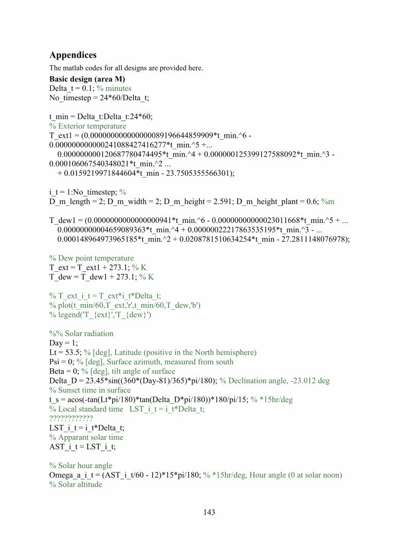
143

Appendices

The matlab codes for all designs are provided here.

Basic design (area M)

Delta_t = 0.1; % minutes

No_timestep = 24*60/Delta_t;

t_min = Delta_t:Delta_t:24*60;

% Exterior temperature

T_ext1 = (0.000000000000000089196644859909*t_min.^6 -

0.000000000000241088427416277*t_min.^5 +...

0.000000000120687780474495*t_min.^4 + 0.000000125399127588092*t_min.^3 -

0.000106067540348021*t_min.^2 ...

+ 0.0159219971844604*t_min - 23.7505355566301);

i_t = 1:No_timestep; %

D_m_length = 2; D_m_width = 2; D_m_height = 2.591; D_m_height_plant = 0.6; %m

T_dew1 = (0.0000000000000000941*t_min.^6 - 0.00000000000023011668*t_min.^5 + ...

0.00000000004659089363*t_min.^4 + 0.00000022217863535195*t_min.^3 - ...

0.000148964973965185*t_min.^2 + 0.0208781510634254*t_min - 27.2811148076978);

% Dew point temperature

T_ext = T_ext1 + 273.1; % K

T_dew = T_dew1 + 273.1; % K

% T_ext_i_t = T_ext*i_t*Delta_t;

% plot(t_min/60,T_ext,'r',t_min/60,T_dew,'b')

% legend('T_{ext}','T_{dew}')

%% Solar radiation

Day = 1;

Lt = 53.5; % [deg], Latitude (positive in the North hemisphere)

Psi = 0; % [deg], Surface azimuth, measured from south

Beta = 0; % [deg], tilt angle of surface

Delta_D = 23.45*sin((360*(Day-81)/365)*pi/180); % Declination angle, -23.012 deg

% Sunset time in surface

t_s = acos(-tan(Lt*pi/180)*tan(Delta_D*pi/180))*180/pi/15; % *15hr/deg

% Local standard time LST_i_t = i_t*Delta_t;

????????????

LST_i_t = i_t*Delta_t;

% Apparant solar time

AST_i_t = LST_i_t;

% Solar hour angle

Omega_a_i_t = (AST_i_t/60 - 12)*15*pi/180; % *15hr/deg, Hour angle (0 at solar noon)

% Solar altitude

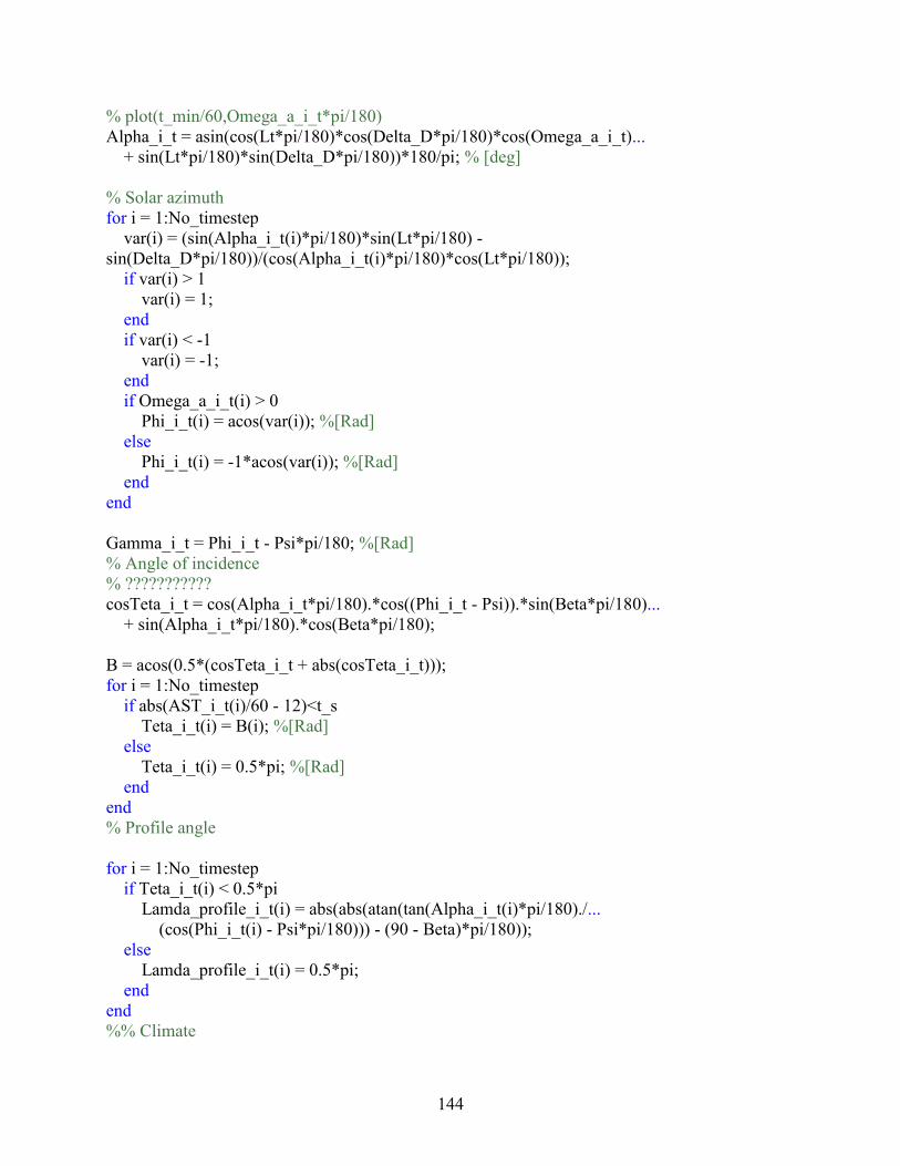
144

% plot(t_min/60,Omega_a_i_t*pi/180)

Alpha_i_t = asin(cos(Lt*pi/180)*cos(Delta_D*pi/180)*cos(Omega_a_i_t)...

+ sin(Lt*pi/180)*sin(Delta_D*pi/180))*180/pi; % [deg]

% Solar azimuth

for i = 1:No_timestep

var(i) = (sin(Alpha_i_t(i)*pi/180)*sin(Lt*pi/180) -

sin(Delta_D*pi/180))/(cos(Alpha_i_t(i)*pi/180)*cos(Lt*pi/180));

if var(i) > 1

var(i) = 1;

end

if var(i) < -1

var(i) = -1;

end

if Omega_a_i_t(i) > 0

Phi_i_t(i) = acos(var(i)); %[Rad]

else

Phi_i_t(i) = -1*acos(var(i)); %[Rad]

end

end

Gamma_i_t = Phi_i_t - Psi*pi/180; %[Rad]

% Angle of incidence

% ???????????

cosTeta_i_t = cos(Alpha_i_t*pi/180).*cos((Phi_i_t - Psi)).*sin(Beta*pi/180)...

+ sin(Alpha_i_t*pi/180).*cos(Beta*pi/180);

B = acos(0.5*(cosTeta_i_t + abs(cosTeta_i_t)));

for i = 1:No_timestep

if abs(AST_i_t(i)/60 - 12)<t_s

Teta_i_t(i) = B(i); %[Rad]

else

Teta_i_t(i) = 0.5*pi; %[Rad]

end

end

% Profile angle

for i = 1:No_timestep

if Teta_i_t(i) < 0.5*pi

Lamda_profile_i_t(i) = abs(abs(atan(tan(Alpha_i_t(i)*pi/180)./...

(cos(Phi_i_t(i) - Psi*pi/180))) - (90 - Beta)*pi/180));

else

Lamda_profile_i_t(i) = 0.5*pi;

end

end

%% Climate

145

Rho_g = 0.3;

if Day > 120 && Day < 300

r_o = 0.97; r_l = 0.99; r_k = 1.02;

else

r_o = 1.03; r_l = 1.01; r_k = 1;

end

Al = 0.031; % [km]

a_o = r_o*(0.4237 - 0.00821*(6 - Al)^2); %

a_l = r_l*(0.5055 + 0.00595*(6.5 - Al)^2); %

k = r_k*(0.2711 + 0.01858*(2.5 - Al)^2); %

% Extraterrestrial normal solar radiation

I_on = 1370*(1 + 0.033*cos(360*Day*pi/(365*180))); % [W/m^2]

% Determine beam solar radiation

for i = 1:No_timestep

if abs(AST_i_t(i)/60 - 12) < abs(t_s)

Tau_b_i_t(i) = a_o + a_l*exp(-k/(sin(Alpha_i_t(i)*pi/180)));

else

Tau_b_i_t(i) = 0; % when Sun sets, there's no beam radiation

end

end

% Incident beam radiation on surfaces

for i = 1:No_timestep

if Teta_i_t(i) < 0.5*pi

I_b_i_t(i) = I_on*Tau_b_i_t(i);

else

I_b_i_t(i) = 0; % when Sun goes behind the surface, there's no beam radiation

end

end

% Direct normal radiation

I_dn_i_t = I_b_i_t.*cos(Teta_i_t);

% Sky diffuse solar radiation

for i = 1:No_timestep

if abs(AST_i_t(i)/60 - 12) < abs(t_s)

Tau_d_i_t(i) = 0.271 - 0.2939*Tau_b_i_t(i);

else

Tau_d_i_t(i) = 0;

end

end

I_ds_i_t = I_on.*sin(Alpha_i_t.*pi/180).*Tau_d_i_t.*0.5.*(1 + cos(Beta.*pi/180));

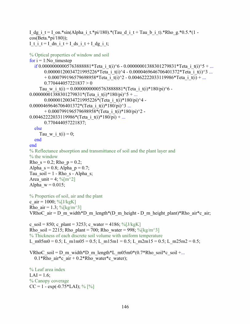
146

I_dg_i_t = I_on.*sin(Alpha_i_t.*pi/180).*(Tau_d_i_t + Tau_b_i_t).*Rho_g.*0.5.*(1 -

cos(Beta.*pi/180));

I_t_i_t = I_dn_i_t + I_ds_i_t + I_dg_i_t;

% Optical properties of window and soil

for i = 1:No_timestep

if 0.00000000005763888881*Teta_i_t(i)^6 - 0.00000001388301279831*Teta_i_t(i)^5 + ...

0.00000120034721995226*Teta_i_t(i)^4 - 0.0000469646706401372*Teta_i_t(i)^3 ...

+ 0.000799196579698958*Teta_i_t(i)^2 - 0.00462222033119986*Teta_i_t(i) + ...

0.770444057221837 > 0

Tau_w_i_t(i) = 0.00000000005763888881*(Teta_i_t(i)*180/pi)^6 -

0.00000001388301279831*(Teta_i_t(i)*180/pi)^5 + ...

0.00000120034721995226*(Teta_i_t(i)*180/pi)^4 -

0.0000469646706401372*(Teta_i_t(i)*180/pi)^3 ...

+ 0.000799196579698958*(Teta_i_t(i)*180/pi)^2 -

0.00462222033119986*(Teta_i_t(i)*180/pi) + ...

0.770444057221837;

else

Tau_w_i_t(i) = 0;

end

end

% Reflectance absorption and transmittance of soil and the plant layer and

% the window

Rho_s = 0.2; Rho_p = 0.2;

Alpha_s = 0.8; Alpha_p = 0.7;

Tau_soil = 1 - Rho_s - Alpha_s;

Area_unit = 4; %[m^2]

Alpha_w = 0.015;

% Properties of soil, air and the plant

c_air = 1000; %[J/kgK]

Rho_air = 1.3; %[kg/m^3]

VRhoC_air = D_m_width*D_m_length*(D_m_height - D_m_height_plant)*Rho_air*c_air;

c_soil = 850; c_plant = 3253; c_water = 4186; %[J/kgK]

Rho_soil = 2215; Rho_plant = 700; Rho_water = 998; %[kg/m^3]

% Thickness of each discrete soil volume with uniform temperature

L_m05m0 = 0.5; L_m1m05 = 0.5; L_m15m1 = 0.5; L_m2m15 = 0.5; L_m25m2 = 0.5;

VRhoC_soil = D_m_width*D_m_length*L_m05m0*(0.7*Rho_soil*c_soil +...

0.1*Rho_air*c_air + 0.2*Rho_water*c_water);

% Leaf area index

LAI = 1.6;

% Canopy coverage

CC = 1 - exp(-0.75*LAI); % [%]

147

L_cover = 4e-3; %[m]

L_air = 0.01; %[m]

c_cover = 1250; %[J/kgK]

Rho_cover = 1220; %[kg/m^3]

VRhoC_cover = D_m_width*D_m_length*L_cover*Rho_cover*c_cover;

VRhoC_plant = CC*D_m_width*D_m_length*D_m_height_plant*Rho_plant*c_plant + ...

(1 - CC)*D_m_width*D_m_length*D_m_height_plant*Rho_air*c_air;

I_transmittedwindow_i_t = I_t_i_t.*Tau_w_i_t.*Area_unit;

I_absorbwindow_i_t = I_t_i_t.*Alpha_w.*Area_unit;

I_absorbground_i_t = I_t_i_t.*(1 - CC).*Tau_w_i_t*Alpha_s*Area_unit;

I_absorbplant_i_t = I_t_i_t.*Tau_w_i_t.*Alpha_p*Area_unit*CC;

%% U-values

k_ground = 1.6; %[W/mK]

U_ground = k_ground*Area_unit/L_m05m0;

v_int = 0.5; % [m/s] indoor wind speed

d = 0.04; % [m] mean leaf width

R_b = 151*(d/v_int)^0.5; % [s/m] boundary layer resistance

u_b = Rho_air*c_air/R_b; % [W/m^2K]

U_b = u_b*Area_unit; % [W/K]

u_trans = 3.3; U_singlePC = 6.3; % [W/m2K]

U_trans = u_trans*Area_unit; %[W/K]

h_CHTC_int = 9; h_CHTC_ext = 20; % [W/m^2K]

H_int = h_CHTC_int*Area_unit; H_ext = h_CHTC_ext*Area_unit; %[W/K]

% Other factors

% Transmissivity factor of clear sky

Eps_clear_i_t = 0.787 + 0.7661* log(T_dew/273);

% Sky temperature

T_sky_i_t = T_ext.*Eps_clear_i_t.^0.25;

% Transpiration rate [mg/m^2s]

E_i_t = 0.232*I_transmittedwindow_i_t/(Area_unit) + 7.04;

% Mositure gain [kg/m^2s]

M_gain_i_t = E_i_t/1000000;

% Evapotranspiration heat loss [W]

Q_p_i_t = 2*LAI*Area_unit*M_gain_i_t*2450e3;

% Emissivity factors ????????????????????

Eps_plant = 0.7; Eps_air = 0.1; Eps_cover = 0.17; Eps_ground = 0.8;

Eps_plantcover = Eps_plant*Eps_cover; Eps_groundplant = Eps_plant*Eps_ground;

Eps_covercover = 1/(1/Eps_cover + 1/Eps_cover -1);

148

Eps_groundcover = Eps_cover*Eps_ground;

Eps_coversky_i_t = Eps_cover*Eps_clear_i_t;

Sigma = 5.56e-8; % [W/m^2K^4]

% Ventilation

u_vent = 0.465;

U_vent = u_vent*Area_unit;

% View factor

F_plantcover = 0.23; F_coverplant = 2*LAI*F_plantcover;

F_groundcover = 0.2; F_groundplant = 0.77;

F_coversky = 1; F_covercover = 1;

% Initial guess

T_int = 258.15; T_ground_ext = 273.15; T_plant_ext = 260.15; T_ground_m25 = 285.15;

T_ground_m2 = 283.15; T_ground_m15 = 281.15; T_ground_m1 = 279.15; T_ground_m05 =

276.15;

T_cell_ext = 253.15; T_cell_int = 253.15; Q_space = 40;

Timestep = Delta_t*60;

for i = 1:No_timestep

if I_transmittedwindow_i_t(i) == 0

Q_light_i_t(i) = 434;

else

Q_light_i_t(i) = 0;

end

if I_transmittedwindow_i_t(i) == 0 && Q_light_i_t(i) == 0

index_p_i_t (i) = LAI;

else

index_p_i_t (i) = 2*LAI;

end

Q_light_plant_i_t(i) = Q_light_i_t(i)*CC*Alpha_p;

Q_light_ground_i_t(i) = Q_light_i_t(i)*(1-CC)*Alpha_s;

T_ground_m2 = T_ground_m2 + ((T_ground_m25 - T_ground_m2)*U_ground...

+ (T_ground_m15 - T_ground_m2)*U_ground).*Timestep/(VRhoC_soil);

T_ground_m15 = T_ground_m15 + ((T_ground_m2 - T_ground_m15)*U_ground...

+ (T_ground_m1 - T_ground_m15)*U_ground).*Timestep/(VRhoC_soil);

149

T_ground_m1 = T_ground_m1 + ((T_ground_m15 - T_ground_m1)*U_ground...

+ (T_ground_m05 - T_ground_m1)*U_ground).*Timestep/(VRhoC_soil);

T_ground_m05 = T_ground_m05 + ((T_ground_m1 - T_ground_m05)*U_ground...

+ (T_ground_ext - T_ground_m05)*U_ground).*Timestep/(VRhoC_soil);

T_cell_ext = T_cell_ext + ((T_ext(i) - T_cell_ext).*H_ext + I_absorbwindow_i_t(i)...

+ Sigma.*Eps_covercover.*F_covercover.*Area_unit.*(T_cell_int.^4 - T_cell_ext.^4) -...

Sigma.*Eps_coversky_i_t(i).*Area_unit.*F_coversky.*(T_cell_ext.^4 -

T_sky_i_t(i).^4)).*Timestep./(VRhoC_cover);

T_cell_int = T_cell_int + ((T_int - T_cell_int).*H_int - ...

Sigma*Eps_covercover*Area_unit*F_covercover*(T_cell_int.^4 - T_cell_ext.^4) + ...

Sigma*Eps_groundcover*Area_unit*F_groundcover*(1 - CC)*(T_ground_ext.^4 -

T_cell_int.^4)...

+ Sigma*Eps_plantcover*Area_unit*LAI*(T_plant_ext.^4 -

T_cell_int.^4))*Timestep/(VRhoC_cover);

Slope_saturated = 4098*(0.6108*exp(17.27*(T_int - 273.15)/(T_int - 273.15 +

237.3)))./(T_int - 273.15 + 237.3).^2;

Q_e_i_t = Area_unit.*1.26.*index_p_i_t(i).*((1000*Slope_saturated/(1000*Slope_saturated +

61.845))*(Q_light_plant_i_t(i) + I_absorbplant_i_t(i)...

+ Sigma*Eps_groundplant*F_groundplant*Area_unit*(T_ground_ext.^4 -

T_plant_ext.^4)...

- Sigma*Eps_plantcover*F_plantcover*Area_unit*LAI*(T_plant_ext.^4 - T_cell_int.^4)));

T_int = T_int + ((((T_cell_int - T_int)*H_int + (T_ext - T_int)*U_vent + Q_e_i_t(i) +

(T_plant_ext - T_int)*2*LAI*U_b...

+ (T_ground_ext - T_int)*H_int)*Timestep)/(VRhoC_air));

T_plant_ext = T_plant_ext + ((T_int - T_plant_ext)*U_b*2*LAI + Q_light_plant_i_t(i) +

I_absorbplant_i_t(i)...

- Q_e_i_t(i) + Sigma*Eps_groundplant*F_groundplant*Area_unit*(T_ground_ext.^4 -

T_plant_ext.^4)...

- Sigma*Eps_plantcover*F_plantcover*Area_unit*LAI*(T_plant_ext.^4 -

T_cell_int.^4))*Timestep/(VRhoC_plant);

T_ground_ext = T_ground_ext + ((T_int - T_ground_ext)*H_int + ...

(T_ground_m05 - T_ground_ext)*U_ground + Q_light_ground_i_t(i) +

I_absorbground_i_t(i) ...

- Sigma*Eps_groundplant*F_groundplant*Area_unit*(T_ground_ext.^4 - T_plant_ext.^4)

...

150

- Sigma*Eps_groundcover*Area_unit*F_groundcover*(1 - CC)*(T_ground_ext.^4 -

T_cell_int.^4))*Timestep/(VRhoC_soil);

End

Basic design (area E)

Delta_t = 0.1; % minutes

%% Solar radiation

Day = 1;

Lt = 53.5; % [deg], Latitude (positive in the North hemisphere)

Psi = 0; % [deg], Surface azimuth, measured from south

Psi_1 = 180;

Beta = 0;% [deg], tilt angle of surface

Beta_1 = 90;

% Solar azimuth

for i = 1:No_timestep

var(i) = (sin(Alpha_i_t(i)*pi/180)*sin(Lt*pi/180) -

sin(Delta_D*pi/180))/(cos(Alpha_i_t(i)*pi/180)*cos(Lt*pi/180));

if var(i) > 1

var(i) = 1;

end

if var(i) < -1

var(i) = -1;

end

if Omega_a_i_t(i) > 0

Phi_i_t(i) = acos(var(i)); %[Rad]

else

Phi_i_t(i) = -1*acos(var(i)); %[Rad]

end

end

Gamma_i_t = Phi_i_t - Psi*pi/180; %[Rad]

Gamma_1_i_t = Phi_i_t - Psi_1*pi/180;

% Angle of incidence

cosTeta_i_t = cos(Alpha_i_t*pi/180).*cos((Phi_i_t - Psi)).*sin(Beta*pi/180)...

+ sin(Alpha_i_t*pi/180).*cos(Beta*pi/180);

cosTeta_1_i_t = cos(Alpha_i_t*pi/180).*cos((Phi_i_t - Psi)).*sin(Beta_1*pi/180)...

+ sin(Alpha_i_t*pi/180).*cos(Beta_1*pi/180);

B = acos(0.5*(cosTeta_i_t + abs(cosTeta_i_t)));

B_1 = acos(0.5*(cosTeta_1_i_t + abs(cosTeta_1_i_t)));

for i = 1:No_timestep

if abs(AST_i_t(i)/60 - 12)<t_s

151

Teta_i_t(i) = B(i); %[Rad]

else

Teta_i_t(i) = 0.5*pi; %[Rad]

end

end

for i = 1:No_timestep

if abs(AST_i_t(i)/60 - 12)<t_s

Teta_1_i_t(i) = B_1(i); %[Rad]

else

Teta_1_i_t(i) = 0.5*pi; %[Rad]

end

end

% Profile angle

for i = 1:No_timestep

if Teta_i_t(i) < 0.5*pi

Lamda_profile_i_t(i) = abs(abs(atan(tan(Alpha_i_t(i)*pi/180)./...

(cos(Phi_i_t(i) - Psi*pi/180))) - (90 - Beta)*pi/180));

else

Lamda_profile_i_t(i) = 0.5*pi;

end

end

for i = 1:No_timestep

if Teta_1_i_t(i) < 0.5*pi

Lamda_profile_i_t(i) = abs(abs(atan(tan(Alpha_i_t(i)*pi/180)./...

(cos(Phi_i_t(i) - Psi_1*pi/180))) - (90 - Beta_1)*pi/180));

else

Lamda_profile_i_t(i) = 0.5*pi;

end

end

% Direct normal radiation

I_dn_i_t = I_b_i_t.*cos(Teta_i_t);

I_dn_1_i_t = I_b_i_t.*cos(Teta_1_i_t);

% Sky diffuse solar radiation

for i = 1:No_timestep

if abs(AST_i_t(i)/60 - 12) < abs(t_s)

Tau_d_i_t(i) = 0.271 - 0.2939*Tau_b_i_t(i);

else

Tau_d_i_t(i) = 0;

end

end

152

I_ds_i_t = I_on*sin(Alpha_i_t*pi/180).*Tau_d_i_t*0.5*(1 + cos(Beta*pi/180));

I_dg_i_t = I_on*sin(Alpha_i_t*pi/180).*(Tau_d_i_t + Tau_b_i_t)*Rho_g*0.5*(1 -

cos(Beta*pi/180));

I_t_i_t = I_dn_i_t + I_ds_i_t + I_dg_i_t;

I_ds_1_i_t = I_on*sin(Alpha_i_t*pi/180).*Tau_d_i_t*0.5*(1 + cos(Beta_1*pi/180));

I_dg_1_i_t = I_on*sin(Alpha_i_t*pi/180).*(Tau_d_i_t + Tau_b_i_t)*Rho_g*0.5*(1 -

cos(Beta_1*pi/180));

I_t_1_i_t = I_dn_1_i_t + I_ds_1_i_t + I_dg_1_i_t;

% Reflectance absorption and transmittance of soil and the plant layer and

the window

Rho_s = 0.2; Rho_p = 0.2; Rho_wall = 0.8;

Alpha_s = 0.8; Alpha_p = 0.7;

Tau_soil = 1 - Rho_s - Alpha_s;

Area_unit = 4; %[m^2]

Alpha_w = 0.015;

% Wall insulation (xps)

Area_xps = D_m_height*D_m_width;

k_xps = 0.032;

L_xps = 75e-3;

u_xps = k_xps/L_xps;

c_xps = 1500; %[J/kgK]

Rho_cover_1 = 40; %[kg/m^3]

U_xps = u_xps*Area_xps;

VRhoC_xps = D_m_width*D_m_height*L_xps*Rho_cover_1*c_xps;

I_transmittedwindow_i_t = I_t_i_t.*Tau_w_i_t*Area_unit;

I_absorbwindow_i_t = I_t_i_t.*Alpha_w*Area_unit;

I_absorbground_i_t = I_t_i_t.*(1 - CC).*Tau_w_i_t*Alpha_s*Area_unit;

I_absorbplant_i_t = I_t_i_t.*Tau_w_i_t*Alpha_p*Area_unit*CC;

I_absorbwall_i_t = I_t_1_i_t.*Rho_wall*Area_xps;

% Other factors

% Transmissivity factor of clear sky

Eps_clear_i_t = 0.787 + 0.7661* log(T_dew/273);

% Sky temperature

T_sky_i_t = T_ext.*Eps_clear_i_t.^0.25;

% Transpiration rate [mg/m^2s]

E_i_t = 0.232*I_transmittedwindow_i_t/(Area_unit) + 7.04;

% Mositure gain [kg/m^2s]

M_gain_i_t = E_i_t/1000000;

% Evapotranspiration heat loss [W]

Q_p_i_t = 2*LAI*Area_unit*M_gain_i_t*2450e3;

153

% Emissivity factors

Eps_plant = 0.7; Eps_air = 0.1; Eps_cover = 0.17; Eps_ground = 0.8; Eps_wall = 0.8;

Eps_plantcover = Eps_plant*Eps_cover; Eps_groundplant = Eps_plant*Eps_ground;

Eps_covercover = 1/(1/Eps_cover + 1/Eps_cover -1);

Eps_groundcover = Eps_cover*Eps_ground;

Eps_coversky_i_t = Eps_cover*Eps_clear_i_t;

Eps_plantwall = Eps_plant*Eps_wall; Eps_groundwall = Eps_wall*Eps_ground;

Eps_wallsky_i_t = Eps_wall*Eps_clear_i_t;

Eps_wallcover = Eps_cover*Eps_wall;

Sigma = 5.56e-8; % [W/m^2K^4]

% Ventilation

u_vent = 1.13;

U_vent = u_vent*Area_unit;

% View factor

F_plantcover = 0.23; F_coverplant = 2*LAI*F_plantcover/2; F_plantwall = 1 - F_coverplant -

F_plantcover;

F_groundcover = 0.1; F_groundplant = 0.77; F_groundwall = 0.1;

F_coversky = 1; F_covercover = 0.85; F_coverwall = 0.15; F_wallcover = 0.15; F_wallsky =

0.5;

% Initial guess

T_int = 258.15; T_ground_ext = 273.15; T_plant_ext = 260.15; T_ground_m25 = 285.15;

T_ground_m2 = 283.15; T_ground_m15 = 281.15; T_ground_m1 = 279.15; T_ground_m05 =

276.15;

T_cell_ext = 253.15; T_cell_int = 253.15; T_wall_ext = 257.15; T_wall_int = 254.15;

Timestep = Delta_t*60; % 300 s

%%

for i = 1:No_timestep

if I_transmittedwindow_i_t(i) == 0

Q_light_i_t(i) = 434;

else

Q_light_i_t(i) = 0;

end

Q_light_plant_i_t(i) = Q_light_i_t(i)*CC*Alpha_s;

Q_light_ground_i_t(i) = Q_light_i_t(i)*(1-CC)*Alpha_p;

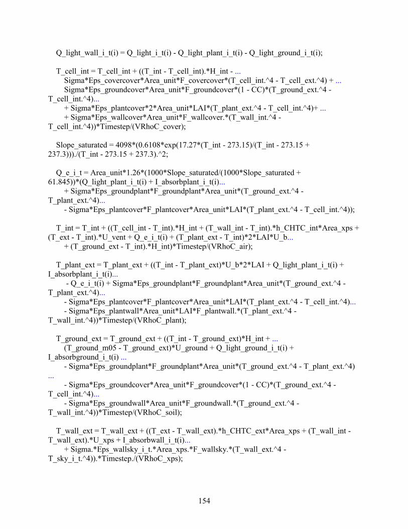
154

Q_light_wall_i_t(i) = Q_light_i_t(i) - Q_light_plant_i_t(i) - Q_light_ground_i_t(i);

T_cell_int = T_cell_int + ((T_int - T_cell_int).*H_int - ...

Sigma*Eps_covercover*Area_unit*F_covercover*(T_cell_int.^4 - T_cell_ext.^4) + ...

Sigma*Eps_groundcover*Area_unit*F_groundcover*(1 - CC)*(T_ground_ext.^4 -

T_cell_int.^4)...

+ Sigma*Eps_plantcover*2*Area_unit*LAI*(T_plant_ext.^4 - T_cell_int.^4)+ ...

+ Sigma*Eps_wallcover*Area_unit*F_wallcover.*(T_wall_int.^4 -

T_cell_int.^4))*Timestep/(VRhoC_cover);

Slope_saturated = 4098*(0.6108*exp(17.27*(T_int - 273.15)/(T_int - 273.15 +

237.3)))./(T_int - 273.15 + 237.3).^2;

Q_e_i_t = Area_unit*1.26*(1000*Slope_saturated/(1000*Slope_saturated +

61.845))*(Q_light_plant_i_t(i) + I_absorbplant_i_t(i)...

+ Sigma*Eps_groundplant*F_groundplant*Area_unit*(T_ground_ext.^4 -

T_plant_ext.^4)...

- Sigma*Eps_plantcover*F_plantcover*Area_unit*LAI*(T_plant_ext.^4 - T_cell_int.^4));

T_int = T_int + ((T_cell_int - T_int).*H_int + (T_wall_int - T_int).*h_CHTC_int*Area_xps +

(T_ext - T_int).*U_vent + Q_e_i_t(i) + (T_plant_ext - T_int)*2*LAI*U_b...

+ (T_ground_ext - T_int).*H_int)*Timestep/(VRhoC_air);

T_plant_ext = T_plant_ext + ((T_int - T_plant_ext)*U_b*2*LAI + Q_light_plant_i_t(i) +

I_absorbplant_i_t(i)...

- Q_e_i_t(i) + Sigma*Eps_groundplant*F_groundplant*Area_unit*(T_ground_ext.^4 -

T_plant_ext.^4)...

- Sigma*Eps_plantcover*F_plantcover*Area_unit*LAI*(T_plant_ext.^4 - T_cell_int.^4)...

- Sigma*Eps_plantwall*Area_unit*LAI*F_plantwall.*(T_plant_ext.^4 -

T_wall_int.^4))*Timestep/(VRhoC_plant);

T_ground_ext = T_ground_ext + ((T_int - T_ground_ext)*H_int + ...

(T_ground_m05 - T_ground_ext)*U_ground + Q_light_ground_i_t(i) +

I_absorbground_i_t(i) ...

- Sigma*Eps_groundplant*F_groundplant*Area_unit*(T_ground_ext.^4 - T_plant_ext.^4)

...

- Sigma*Eps_groundcover*Area_unit*F_groundcover*(1 - CC)*(T_ground_ext.^4 -

T_cell_int.^4)...

- Sigma*Eps_groundwall*Area_unit*F_groundwall.*(T_ground_ext.^4 -

T_wall_int.^4))*Timestep/(VRhoC_soil);

T_wall_ext = T_wall_ext + ((T_ext - T_wall_ext).*h_CHTC_ext*Area_xps + (T_wall_int -

T_wall_ext).*U_xps + I_absorbwall_i_t(i)...

+ Sigma.*Eps_wallsky_i_t.*Area_xps.*F_wallsky.*(T_wall_ext.^4 -

T_sky_i_t.^4)).*Timestep./(VRhoC_xps);

155

T_wall_int = T_wall_int + ((T_int - T_wall_int).*h_CHTC_int*Area_xps +

Q_light_ground_i_t(i) + (T_wall_ext - T_wall_int).*U_xps ...

- Sigma*Eps_groundwall*Area_unit*F_groundwall*(1 - CC)*(T_ground_ext.^4 -

T_wall_int.^4)...

+ Sigma*Eps_plantwall*Area_unit*LAI*(T_plant_ext.^4 - T_wall_int.^4)+ ...

- Sigma*Eps_wallcover*Area_xps*F_wallcover.*(T_wall_int.^4 -

T_cell_int.^4))*Timestep/(VRhoC_xps);

end

Vertical and transparent ceiling (skylight) (area M)

%% Solar radiation

Day = 1;

Lt = 53.5; % [deg], Latitude (positive in the North hemisphere)

Psi = 0; % [deg], Surface azimuth, measured from south

Beta = 90; % [deg], tilt angle of surface

Beta_1 = 0;

% Solar azimuth

for i = 1:No_timestep

var(i) = (sin(Alpha_i_t(i)*pi/180)*sin(Lt*pi/180) -

sin(Delta_D*pi/180))/(cos(Alpha_i_t(i)*pi/180)*cos(Lt*pi/180));

if var(i) > 1

var(i) = 1;

end

if var(i) < -1

var(i) = -1;

end

if var(i) > -1 && var(i) < 1

var(i) = var(i);

end

if Omega_a_i_t(i) > 0

Phi_i_t(i) = acos(var(i)); %[Rad]

else

Phi_i_t(i) = -1*acos(var(i)); %[Rad]

end

end

Gamma_i_t = Phi_i_t - Psi*pi/180; %[Rad]

% Angle of incidence

% ???????????

cosTeta_i_t = cos(Alpha_i_t*pi/180).*cos((Phi_i_t - Psi)).*sin(Beta*pi/180)...

+ sin(Alpha_i_t*pi/180).*cos(Beta*pi/180);

cosTeta_1_i_t = cos(Alpha_i_t*pi/180).*cos((Phi_i_t - Psi)).*sin(Beta_1*pi/180)...

156

+ sin(Alpha_i_t*pi/180).*cos(Beta_1*pi/180);

B = acos(0.5*(cosTeta_i_t + abs(cosTeta_i_t)));

B_1 = acos(0.5*(cosTeta_1_i_t + abs(cosTeta_1_i_t)));

for i = 1:No_timestep

if abs(AST_i_t(i)/60 - 12)<t_s

Teta_i_t(i) = B(i); %[Rad]

else

Teta_i_t(i) = 0.5*pi; %[Rad]

end

end

for i = 1:No_timestep

if abs(AST_i_t(i)/60 - 12)<t_s

Teta_1_i_t(i) = B_1(i); %[Rad]

else

Teta_1_i_t(i) = 0.5*pi; %[Rad]

end

end

% Profile angle

for i = 1:No_timestep

if Teta_i_t(i) < 0.5*pi

Lamda_profile_i_t(i) = abs(abs(atan(tan(Alpha_i_t(i)*pi/180)./...

(cos(Phi_i_t(i) - Psi*pi/180))) - (90 - Beta)*pi/180));

else

Lamda_profile_i_t(i) = 0.5*pi;

end

end

for i = 1:No_timestep

if Teta_1_i_t(i) < 0.5*pi

Lamda_profile_1_i_t(i) = abs(abs(atan(tan(Alpha_i_t(i)*pi/180)./...

(cos(Phi_i_t(i) - Psi*pi/180))) - (90 - Beta_1)*pi/180));

else

Lamda_profile_1_i_t(i) = 0.5*pi;

end

end

% Incident beam radiation on surfaces

for i = 1:No_timestep

if Teta_i_t(i) < 0.5*pi

I_b_i_t(i) = I_on*Tau_b_i_t(i);

else

I_b_i_t(i) = 0; % when Sun goes behind the surface, there's no beam radiation

end

end

157

for i = 1:No_timestep

if Teta_1_i_t(i) < 0.5*pi

I_b_1_i_t(i) = I_on*Tau_b_i_t(i);

else

I_b_1_i_t(i) = 0; % when Sun goes behind the surface, there's no beam radiation

end

end

% Direct normal radiation

I_dn_i_t = I_b_i_t.*cos(Teta_i_t);

I_dn_1_i_t = I_b_1_i_t.*cos(Teta_1_i_t);

% Sky diffuse solar radiation

for i = 1:No_timestep

if abs(AST_i_t(i)/60 - 12) < abs(t_s)

Tau_d_i_t(i) = 0.271 - 0.2939*Tau_b_i_t(i);

else

Tau_d_i_t(i) = 0;

end

end

I_ds_i_t = I_on*sin(Alpha_i_t*pi/180).*Tau_d_i_t*0.5*(1 + cos(Beta*pi/180));

I_dg_i_t = I_on*sin(Alpha_i_t*pi/180).*(Tau_d_i_t + Tau_b_i_t)*Rho_g*0.5*(1 -

cos(Beta*pi/180));

I_t_i_t = I_dn_i_t + I_ds_i_t + I_dg_i_t;

I_ds_1_i_t = I_on*sin(Alpha_i_t*pi/180).*Tau_d_i_t*0.5*(1 + cos(Beta_1*pi/180));

I_dg_1_i_t = I_on*sin(Alpha_i_t*pi/180).*(Tau_d_i_t + Tau_b_i_t)*Rho_g*0.5*(1 -

cos(Beta_1*pi/180));

I_t_1_i_t = I_dn_1_i_t + I_ds_1_i_t + I_dg_1_i_t;

% Leaf area index

LAI = 1.6;

% Canopy coverage

CC = 1 - exp(-0.75*LAI); % [%]

L_cover = 0.15; %[m]

L_air = 0.01; %[m]

c_cover = 1500; %[J/kgK]

Rho_cover = 400; %[kg/m^3]

VRhoC_cover = D_m_width*D_m_length*L_cover/2*Rho_cover*c_cover;

VRhoC_plant = CC*D_m_width*D_m_length*D_m_height_plant*Rho_plant*c_plant + ...

(1 - CC)*D_m_width*D_m_length*D_m_height_plant*Rho_air*c_air;

I_transmittedwindow_i_t = I_t_i_t.*Tau_w_i_t*Area_unit/2 +

I_t_1_i_t.*Tau_w_i_t*Rho_rf*Area_unit/2;

I_absorbwindow_i_t = I_t_i_t.*Alpha_w*Area_unit;

158

I_absorbground_i_t = I_transmittedwindow_i_t.*(1 - CC);

I_absorbplant_i_t = I_transmittedwindow_i_t.*CC;

%% U-values

u_trans = 1.4;

U_trans = u_trans*Area_unit; %[W/K]

% Emissivity factors

Eps_plant = 0.8; Eps_air = 0.1; Eps_cover = 0.6; Eps_ground = 0.8;

Eps_plantcover = Eps_plant*Eps_cover; Eps_groundplant = Eps_plant*Eps_ground;

Eps_groundcover = Eps_cover*Eps_ground;

Eps_coversky_i_t = Eps_cover*Eps_clear_i_t;

Sigma = 5.56e-8; % [W/m^2K^4]

% Ventilation

u_vent = 0.465;

U_vent = u_vent*Area_unit;

% View factor

F_plantcover = 0.23; F_coverplant = 2*LAI*F_plantcover;

F_groundcover = 0.2; F_groundplant = 0.77;

F_coversky = 1; F_covercover = 1;

% Initial guess

T_int = 258.15; T_ground_ext = 273.15; T_plant_ext = 260.15; T_ground_m25 = 285.15;

T_ground_m2 = 283.15; T_ground_m15 = 281.15; T_ground_m1 = 279.15; T_ground_m05 =

276.15;

T_cell_ext = 253.15; T_cell_int = 253.15; T_cell_mid = 253.15;

Timestep = Delta_t*60; % 300 s ?????????

%%

for i = 1:No_timestep

if I_transmittedwindow_i_t(i) == 0

Q_light_i_t(i) = 434;

else

Q_light_i_t(i) = 0;

end

if I_transmittedwindow_i_t(i) == 0 && Q_light_i_t(i) == 0

index_p_i_t (i) = LAI;

else

159

index_p_i_t (i) = 2*LAI;

end

Q_light_plant_i_t(i) = Q_light_i_t(i)*CC*Alpha_p;

Q_light_ground_i_t(i) = Q_light_i_t(i)*(1-CC)*Alpha_s;

T_cell_mid = T_cell_mid + ((T_cell_ext - T_cell_mid)*U_trans + (T_cell_int -

T_cell_mid)*U_trans).*Timestep./(VRhoC_cover);

T_cell_ext = T_cell_ext + ((T_ext - T_cell_ext).*H_ext + I_absorbwindow_i_t(i)...

+ (T_cell_mid - T_cell_ext)*U_trans -...

Sigma.*Eps_coversky_i_t.*Area_unit.*F_coversky.*(T_cell_ext.^4 -

T_sky_i_t.^4)).*Timestep./(VRhoC_cover);

T_cell_int = T_cell_int + ((T_int - T_cell_int).*H_int + ...

(T_cell_mid - T_cell_int)*U_trans + ...

Sigma*Eps_groundcover*Area_unit*F_groundcover*(1 - CC)*(T_ground_ext.^4 -

T_cell_int.^4)...

+ Sigma*Eps_plantcover*Area_unit*LAI*(T_plant_ext.^4 -

T_cell_int.^4))*Timestep/(VRhoC_cover);

Slope_saturated = 4098*(0.6108*exp(17.27*(T_int - 273.15)/(T_int - 273.15 +

237.3)))./(T_int - 273.15 + 237.3).^2;

Q_e_i_t = Area_unit.*1.26.*index_p_i_t(i)*((1000*Slope_saturated/(1000*Slope_saturated +

61.845))*(Q_light_plant_i_t(i)+ I_absorbplant_i_t(i)...

+ Sigma*Eps_groundplant*F_groundplant*Area_unit*(T_ground_ext.^4 -

T_plant_ext.^4)...

- Sigma*Eps_plantcover*F_plantcover*Area_unit*LAI*(T_plant_ext.^4 - T_cell_int.^4)));

T_int = T_int + ((T_cell_int - T_int).*H_int + (T_ext - T_int)*U_vent + Q_e_i_t(i) +

(T_plant_ext - T_int)*2*LAI*U_b...

+ (T_ground_ext - T_int).*H_int)*Timestep/(VRhoC_air);

T_plant_ext = T_plant_ext + ((T_int - T_plant_ext)*U_b*2*LAI + Q_light_plant_i_t(i) +

I_absorbplant_i_t(i)...

- Q_e_i_t(i) + Sigma*Eps_groundplant*F_groundplant*Area_unit*(T_ground_ext.^4 -

T_plant_ext.^4)...

- Sigma*Eps_plantcover*F_plantcover*Area_unit*LAI*(T_plant_ext.^4 -

T_cell_int.^4))*Timestep/(VRhoC_plant);

T_ground_ext = T_ground_ext + ((T_int - T_ground_ext)*H_int + ...

(T_ground_m05 - T_ground_ext)*U_ground + Q_light_ground_i_t(i)+

I_absorbground_i_t(i) ...

160

- Sigma*Eps_groundplant*F_groundplant*Area_unit*(T_ground_ext.^4 - T_plant_ext.^4)

...

- Sigma*Eps_groundcover*Area_unit*F_groundcover*(1 - CC)*(T_ground_ext.^4 -

T_cell_int.^4))*Timestep/(VRhoC_soil);

end

Insulated north wall design (Area E)

% Reflectance absorption and transmittance of soil and the plant layer and

% the window

Rho_s = 0.2; Rho_p = 0.2; Rho_wall = 0.8;

Alpha_s = 0.8; Alpha_p = 0.7;

Tau_soil = 1 - Rho_s - Alpha_s;

Area_unit = 4; %[m^2]

Alpha_w = 0.015;

% Wall insulation (xps)

Area_xps = D_m_height*D_m_width;

k_xps = 0.032;

L_xps = 0.2;

u_xps = k_xps/L_xps;

c_xps = 1500; %[J/kgK]

Rho_xps = 40; %[kg/m^3]

U_xps = u_xps*Area_xps;

Area_con = D_m_height*D_m_width;

k_con = 0.12;

L_con = 0.05;

u_con = k_con/L_con;

c_con = 840; %[J/kgK]

Rho_con = 1200; %[kg/m^3]

U_con = u_con*Area_xps;

U_total = 1/(1/u_xps+2*1/u_con)*Area_con;

u_total = U_total/Area_con;

VRhoC_xps = D_m_width*D_m_length*L_xps*Rho_xps*c_xps;

VRhoC_con = D_m_width*D_m_length*L_con*Rho_con*c_con;

I_transmittedwindow_i_t = I_t_i_t.*Tau_w_i_t*Area_unit;

I_absorbwindow_i_t = I_t_i_t.*Alpha_w*Area_unit;

I_absorbground_i_t = I_t_i_t.*(1 - CC).*Tau_w_i_t*Alpha_s*Area_unit;

I_absorbplant_i_t = I_t_i_t.*Tau_w_i_t*Alpha_p*Area_unit*CC;

I_absorbwall_i_t = I_t_1_i_t.*Rho_wall*Area_xps;

% Emissivity factors

161

Eps_plant = 0.7; Eps_air = 0.1; Eps_cover = 0.17; Eps_ground = 0.8; Eps_wall = 0.9;

Eps_plantcover = Eps_plant*Eps_cover; Eps_groundplant = Eps_plant*Eps_ground;

Eps_covercover = 1/(1/Eps_cover + 1/Eps_cover -1);

Eps_groundcover = Eps_cover*Eps_ground;

Eps_coversky_i_t = Eps_cover*Eps_clear_i_t;

Eps_plantwall = Eps_plant*Eps_wall; Eps_groundwall = Eps_wall*Eps_ground;

Eps_wallsky_i_t = Eps_wall*Eps_clear_i_t;

Eps_wallcover = Eps_cover*Eps_wall;

Sigma = 5.56e-8; % [W/m^2K^4]

% View factor

F_plantcover = 0.23; F_coverplant = 2*LAI*F_plantcover/2; F_plantwall = 1 - F_coverplant -

F_plantcover;

F_groundcover = 0.1; F_groundplant = 0.77; F_groundwall = 0.1;

F_coversky = 1; F_covercover = 0.85; F_coverwall = 0.15; F_wallcover = 0.15; F_wallsky =

0.5;

% Initial guess

T_int = 258.15; T_ground_ext = 273.15; T_plant_ext = 260.15; T_ground_m25 = 285.15;

T_ground_m2 = 283.15; T_ground_m15 = 281.15; T_ground_m1 = 279.15; T_ground_m05 =

276.15;

T_cell_ext = 253.15; T_cell_int = 253.15; T_wall_ext = 257.15; T_wall_int = 254.15;

Timestep = Delta_t*60; % 300 s ?????????

%%

for i_t = 1:No_timestep

if I_transmittedwindow_i_t(i) == 0

Q_light_i_t(i) = 434;

else

Q_light_i_t(i) = 0;

end

if I_transmittedwindow_i_t(i) == 0 && Q_light_i_t(i) == 0

index_p_i_t (i) = LAI;

else

index_p_i_t (i) = 2*LAI;

162

end

Q_light_plant_i_t(i) = Q_light_i_t(i)*CC*Alpha_p;

Q_light_ground_i_t(i) = Q_light_i_t(i)*(1-CC)*Alpha_s;

Q_light_wall_i_t(i) = Q_light_i_t(i) - Q_light_ground_i_t(i)- Q_light_plant_i_t(i);

T_cell_int = T_cell_int + ((T_int - T_cell_int).*H_int - ...

Sigma*Eps_covercover*Area_unit*F_covercover*(T_cell_int.^4 - T_cell_ext.^4) + ...

Sigma*Eps_groundcover*Area_unit*F_groundcover*(1 - CC)*(T_ground_ext.^4 -

T_cell_int.^4)...

+ Sigma*Eps_plantcover*Area_unit*LAI*(T_plant_ext.^4 - T_cell_int.^4)+ ...

+ Sigma*Eps_wallcover*Area_unit*F_wallcover.*(T_wall_int.^4 -

T_cell_int.^4))*Timestep/(VRhoC_cover);

Slope_saturated = 4098*(0.6108*exp(17.27*(T_int - 273.15)/(T_int - 273.15 +

237.3)))./(T_int - 273.15 + 237.3).^2;

Q_e_i_t = Area_unit*1.26*index_p_i_t(i)*((1000*Slope_saturated/(1000*Slope_saturated +

61.845))*(Q_light_plant_i_t(i) + I_absorbplant_i_t(i)...

+ Sigma*Eps_groundplant*F_groundplant*Area_unit*(T_ground_ext.^4 -

T_plant_ext.^4)...

- Sigma*Eps_plantcover*F_plantcover*Area_unit*LAI*(T_plant_ext.^4 - T_cell_int.^4)...

- Sigma*Eps_plantwall*Area_xps*LAI*F_plantwall.*(T_plant_ext.^4 - T_wall_int.^4)));

T_int = T_int + ((T_cell_int - T_int).*H_int + (T_wall_int - T_int).*h_CHTC_int*Area_xps +

(T_ext - T_int)*U_vent + Q_e_i_t(i) + (T_plant_ext - T_int)*2*LAI*U_b...

+ (T_ground_ext - T_int).*H_int)*Timestep/(VRhoC_air);

T_plant_ext = T_plant_ext + ((T_int - T_plant_ext)*U_b*2*LAI + Q_light_plant_i_t(i) +

I_absorbplant_i_t(i)...

- Q_e_i_t + Sigma*Eps_groundplant*F_groundplant*Area_unit*(T_ground_ext.^4 -

T_plant_ext.^4)...

- Sigma*Eps_plantcover*F_plantcover*Area_unit*LAI*(T_plant_ext.^4 - T_cell_int.^4)...

- Sigma*Eps_plantwall*Area_xps*LAI*F_plantwall.*(T_plant_ext.^4 -

T_wall_int.^4))*Timestep/(VRhoC_plant);

T_ground_ext = T_ground_ext + ((T_int - T_ground_ext)*H_int + ...

(T_ground_m05 - T_ground_ext)*U_ground + Q_light_ground_i_t(i) +

I_absorbground_i_t(i) ...

- Sigma*Eps_groundplant*F_groundplant*Area_unit*(T_ground_ext.^4 - T_plant_ext.^4)

...

- Sigma*Eps_groundcover*Area_unit*F_groundcover*(1 - CC)*(T_ground_ext.^4 -

T_cell_int.^4)...

- Sigma*Eps_groundwall*Area_unit*F_groundwall.*(T_ground_ext.^4 -

T_wall_int.^4))*Timestep/(VRhoC_soil);

163

T_wall_ext = T_wall_ext + ((T_ext - T_wall_ext).*h_CHTC_ext*Area_xps + (T_wall_int -

T_wall_ext).*U_total + I_absorbwall_i_t(i)...

+ Sigma.*Eps_wallsky_i_t.*Area_xps.*F_wallsky.*(T_wall_ext.^4 -

T_sky_i_t.^4)).*Timestep./(VRhoC_con);

T_wall_int = T_wall_int + ((T_int - T_wall_int).*h_CHTC_int*Area_xps +

Q_light_wall_i_t(i) + (T_wall_ext - T_wall_int).*U_total ...

- Sigma*Eps_groundwall*Area_unit*F_groundwall*(1 - CC)*(T_ground_ext.^4 -

T_wall_int.^4)...

+ Sigma*Eps_plantwall*Area_unit*LAI*(T_plant_ext.^4 - T_wall_int.^4)+ ...

- Sigma*Eps_wallcover*Area_xps*F_wallcover.*(T_wall_int.^4 -

T_cell_int.^4))*Timestep/(VRhoC_con);

end

Cyclic and night interruption lighting design (area M)

for i = 1:No_timestep

if i <= 540

Q_light_i_t(i) = 434;

elseif i > 540 && i <= 600

Q_light_i_t(i) = 0;

elseif i > 600 && i <= 1140

Q_light_i_t(i) = 434;

elseif i > 1140 && i <= 1200

Q_light_i_t(i) = 0;

elseif i > 1200 && i <= 1740

Q_light_i_t(i) = 434;

elseif i > 1740 && i <= 1800

Q_light_i_t(i) = 0;

elseif i > 12600 && i <= 13140

Q_light_i_t(i) = 434;

elseif i > 13140 && i <= 13200

Q_light_i_t(i) = 0;

elseif i > 13200 && i <= 13740

Q_light_i_t(i) = 434;

elseif i > 13740 && i <= 13800

Q_light_i_t(i) = 0;

elseif i > 13800 && i <= 14340

Q_light_i_t(i) = 434;

elseif i > 14340 && i <= 14400

Q_light_i_t(i) = 0;

else

164

Q_light_i_t(i) = 0;

end

if I_transmittedwindow_i_t(i) == 0 && Q_light_i_t(i) == 0

index_p_i_t (i) = LAI;

else

index_p_i_t (i) = 2*LAI;

end

Q_light_plant_i_t(i) = Q_light_i_t(i)*CC*Alpha_p;

Q_light_ground_i_t(i) = Q_light_i_t(i)*(1-CC)*Alpha_s;

T_ground_m2 = T_ground_m2 + ((T_ground_m25 - T_ground_m2)*U_ground...

+ (T_ground_m15 - T_ground_m2)*U_ground).*Timestep/(VRhoC_soil);

T_ground_m15 = T_ground_m15 + ((T_ground_m2 - T_ground_m15)*U_ground...

+ (T_ground_m1 - T_ground_m15)*U_ground).*Timestep/(VRhoC_soil);

T_ground_m1 = T_ground_m1 + ((T_ground_m15 - T_ground_m1)*U_ground...

+ (T_ground_m05 - T_ground_m1)*U_ground).*Timestep/(VRhoC_soil);

T_ground_m05 = T_ground_m05 + ((T_ground_m1 - T_ground_m05)*U_ground...

+ (T_ground_ext - T_ground_m05)*U_ground).*Timestep/(VRhoC_soil);

T_cell_ext = T_cell_ext + ((T_ext - T_cell_ext).*H_ext + I_absorbwindow_i_t(i)...

+ Sigma.*Eps_covercover.*F_covercover.*Area_unit.*(T_cell_int.^4 - T_cell_ext.^4) -...

Sigma.*Eps_coversky_i_t.*Area_unit.*F_coversky.*(T_cell_ext.^4 -

T_sky_i_t.^4)).*Timestep./(VRhoC_cover);

T_cell_int = T_cell_int + ((T_int - T_cell_int).*H_int - ...

Sigma*Eps_covercover*Area_unit*F_covercover*(T_cell_int.^4 - T_cell_ext.^4) + ...

Sigma*Eps_groundcover*Area_unit*F_groundcover*(1 - CC)*(T_ground_ext.^4 -

T_cell_int.^4)...

+ Sigma*Eps_plantcover*Area_unit*LAI*(T_plant_ext.^4 -

T_cell_int.^4))*Timestep/(VRhoC_cover);

Slope_saturated = 4098*(0.6108*exp(17.27*(T_int - 273.15)/(T_int - 273.15 +

237.3)))./(T_int - 273.15 + 237.3).^2;

Q_e_i_t = Area_unit.*1.26.*index_p_i_t(i).*((1000*Slope_saturated/(1000*Slope_saturated +

61.845))*(Q_light_plant_i_t(i) + I_absorbplant_i_t(i)...

+ Sigma*Eps_groundplant*F_groundplant*Area_unit*(T_ground_ext.^4 -

T_plant_ext.^4)...

- Sigma*Eps_plantcover*F_plantcover*Area_unit*LAI*(T_plant_ext.^4 - T_cell_int.^4)));

165

T_int = T_int + ((((T_cell_int - T_int)*H_int + (T_ext - T_int)*U_vent + Q_e_i_t(i) +

(T_plant_ext - T_int)*2*LAI*U_b...

+ (T_ground_ext - T_int)*H_int)*Timestep)/(VRhoC_air));

T_plant_ext = T_plant_ext + ((T_int - T_plant_ext)*U_b*2*LAI + Q_light_plant_i_t(i) +

I_absorbplant_i_t(i)...

- Q_e_i_t(i) + Sigma*Eps_groundplant*F_groundplant*Area_unit*(T_ground_ext.^4 -

T_plant_ext.^4)...

- Sigma*Eps_plantcover*F_plantcover*Area_unit*LAI*(T_plant_ext.^4 -

T_cell_int.^4))*Timestep/(VRhoC_plant);

T_ground_ext = T_ground_ext + ((T_int - T_ground_ext)*H_int + ...

(T_ground_m05 - T_ground_ext)*U_ground + Q_light_ground_i_t(i) +

I_absorbground_i_t(i) ...

- Sigma*Eps_groundplant*F_groundplant*Area_unit*(T_ground_ext.^4 - T_plant_ext.^4)

...

- Sigma*Eps_groundcover*Area_unit*F_groundcover*(1 - CC)*(T_ground_ext.^4 -

T_cell_int.^4))*Timestep/(VRhoC_soil);

end